FRANCIS B. HILDEBRAND
Associate Professor of Mathematics
Massachusetts Institute of Technology
Methods of
Applied Mathematics
SECOND EDITION
PRENTICE-HALL, INC.
ENGLEWOOD CLIFFS, NEW JERSEY

© 1952, 1965 by Prentice-Hall, Inc., Englewood Cliffs, N. J.
All Rights Reserved. No part of this book may be
reproduced in any form, by mimeograph or any other means,
without permission in writing from the publishers. Library
of Congress Catalog Card Number: 65-14941. Printed in
the United States of America. C-57920.
Prentice-Hall International, Inc., London
Prentice-Hall of Australia, Pty., Ltd., Sydney
Prentice-Hall of Canada, Ltd., Toronto
Prentice-Hall of India (Private) Ltd., New Delhi
Prentice-Hall of Japan, Inc., Tokyo

Preface
The principal aim of this volume is to place at the disposal of the engineer
or physicist the basis of an intelligent working knowledge of a number of
facts and techniques relevant to some fields of mathematics which often are
not treated in courses of the "Advanced Calculus" type, but which are
useful in varied fields of application.
Many students in the fields of application have neither the time nor the
inclination for the study of detailed treatments of each of these topics from
the classical point of view. However, efficient use of facts or techniques
depends strongly upon a substantial understanding of the basic underlying
principles. For this reason, care has been taken throughout the text either
to provide a rigorous proof, when the proof is believed to contribute to an
understanding of the desired result, or to state the result as precisely as
possible and indicate why it might have been formally anticipated.
In each chapter, the treatment consists of showing how typical problems
may arise, of establishing those parts of the relevant theory which are of
principal practical significance, and of developing techniques for analytical
and numerical analysis and problem solving.
Whereas experience gained from a course on the Advanced Calculus
level is presumed, the treatments are largely self-contained, so that the
nature of this preliminary course is not of great importance.
In order to increase the usefulness of the volume as a basic or
supplementary text, and as a reference volume, an attempt has been made to
organize the material so that there is little essential interdependence among
the chapters, and considerable flexibility exists with regard to the omission
of topics within chapters. In addition, a substantial amount of supplementary
material is included in annotated problems which complement numerous
exercises, of varying difficulty, arranged in correspondence with successive
v

VI
PREFACE
sections of the text at the end of the chapters. Answers to all problems are
either incorporated into their statement or listed at the end of the book.
The first chapter deals principally with linear algebraic equations,
quadratic and Hermitian forms, and operations with vectors and matrices, with
special emphasis on the concept of characteristic values. A brief summary
of corresponding results in function space is included for comparison, and
for convenient reference. Whereas a considerable amount of material is
presented, particular care was taken here to arrange the demonstrations in
such a way that maximum flexibility in selection of topics is present.
The first portion of the second chapter introduces the variational notation
and derives the Euler equations relevant to a large class of problems in the
calculus of variations. More than usual emphasis is placed on the significance
of natural boundary conditions. Generalized coordinates, Hamilton's
principle, and Lagrange's equations are treated and illustrated within the
framework of this theory. The chapter concludes with a discussion of
the formulation of minimal principles of more general type, and with the
application of direct and semidirect methods of the calculus of variations
to the exact and approximate solution of practical problems.
The concluding chapter deals with the formulation and theory of linear
integral equations, and with exact and approximate methods for obtaining
their solutions, particular emphasis being placed on the several equivalent
interpretations of the relevant Green's function. Considerable supplementary
material is provided here in annotated problems.
The present text is a revision of corresponding chapters of the first
edition, published in 1952. It incorporates a number of changes in method
of presentation and in notation, as well as some new material and additional
problems and exercises. A revised and expanded version of the earlier
material on difference equations and on finite difference methods is to
appear separately.
Many compromises between mathematical elegance and practical
significance were found to be necessary. However, it is hoped that the text
will serve to ease the way of the engineer or physicist into the more advanced
areas of applicable mathematics, for which his need continues to increase,
without obscuring from him the existence of certain difficulties, sometimes
implied by the phrase "It can be shown," and without failing to warn him
of certain dangers involved in formal application of techniques beyond the
limits inside which their validity has been well established.
The author is indebted to colleagues and students in various fields for
help in selecting and revising the content and presentation, and particularly
to Professor Albert A. Bennett for many valuable criticisms and suggestions.
Francis B. Hildebrand

Contents
CHAPTER ONE
Matrices and Linear Equations
Introduction
Linear equations. The Gauss-Jordan reduction
Matrices
Determinants. Cramer's rule
Special matrices
The inverse matrix
Rank of a matrix
Elementary operations
Solvability of sets of linear equations
Linear vector space
Linear equations and vector space
Characteristic-value problems
Orthogonalization of vector sets
Quadratic forms
A numerical example
Equivalent matrices and transformations
Hermitian matrices
Multiple characteristic numbers of symmetric
matrices
Definite forms
Discriminants and invariants
Coordinate transformations
Functions of symmetric matrices
Numerical solution of characteristic-value
problems
Additional techniques
vii

Vlll
CONTENTS
1.25. Generalized characteristic-value problems 69
1.26. Characteristic numbers of nonsymmetric matrices 75
1.27. A physical application 78
1.28. Function space 81
1.29. Sturm-Liouville problems 88
References 93
Problems 93
CHAPTER TWO
Calculus of Variations and Applications 119
2.1.
2.2.
2.3.
2.4.
2.5.
2.6.
2.7.
2.8.
2.9.
2.10.
2.11.
2.12.
2.13.
2.14.
2.15.
2.16.
2.17.
2.18.
2.19.
2.20.
Maxima and minima
The simplest case
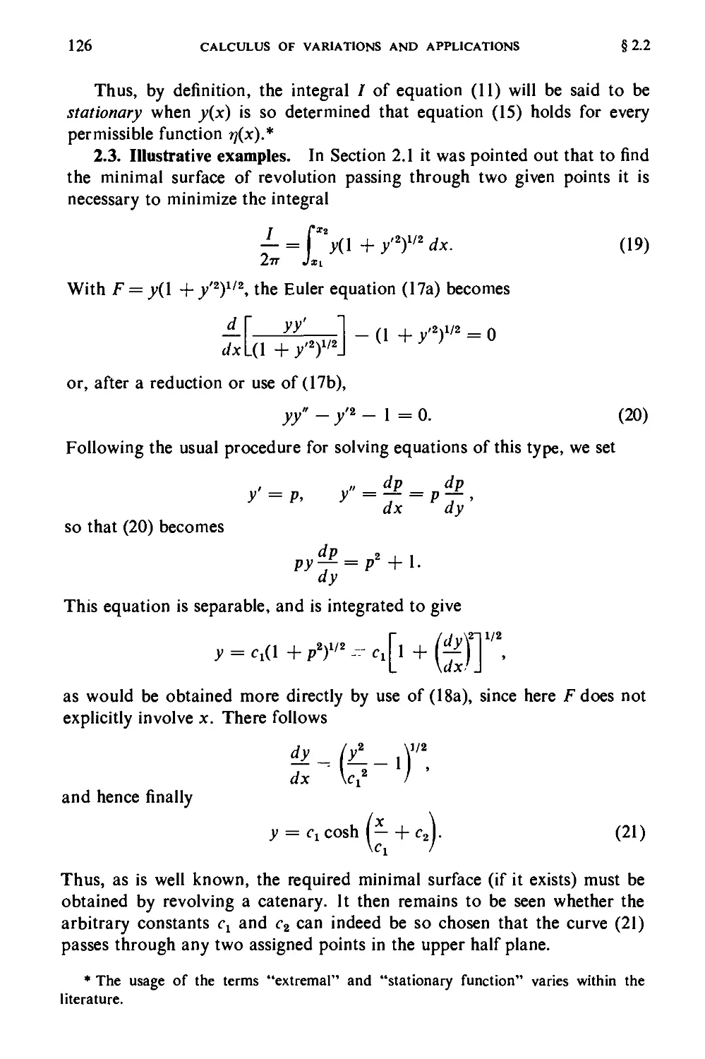
Illustrative examples
Natural boundary conditions and transition
conditions
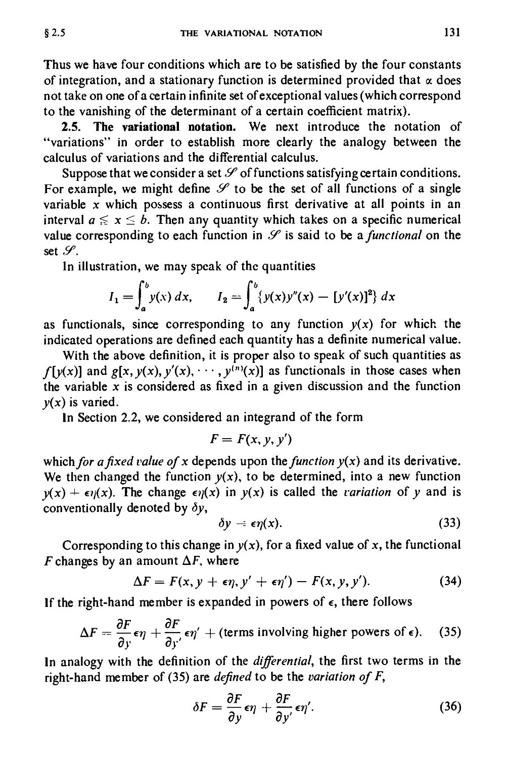
The variational notation
The more general case
Constraints and Lagrange multipliers
Variable end points
Sturm-Liouville problems
Hamilton's principle
Lagrange's equations
Generalized dynamical entities
Constraints in dynamical systems
Small vibrations about equilibrium. Normal
coordinates
Numerical example
Variational problems for deformable bodies
Useful transformations
The variational problem for the elastic plate
The Rayleigh-Ritz method
A semidirect method
References
Problems
119
123
126
128
131
135
139
144
145
148
151
155
160
165
170
172
178
179
181
190
192
193
CHAPTER THREE
Integral Equations 222
3.1. Introduction 222
3.2. Relations between differential and integral
equations 225

CONTENTS
IX
3.3.
3.4.
3.5.
3.6.
3.7.
3.8.
3.9.
3.10.
3.11.
3.12.
3.13.
3.14.
3.15.
3.16.
3.17.
3.18.
3.19.
3.20.
The Green's function
Alternative definition of the Green's function
Linear equations in cause and effect. The
influence function
Fredholm equations with separable kernels
Illustrative example
Hilbert-Schmidt theory
Iterative methods for solving equations of the
second kind
The Neumann series
Fredholm theory
Singular integral equations
Special devices
Iterative approximations to characteristic
functions
Approximation of Fredholm equations by sets of
algebraic equations
Approximate methods of undetermined
coefficients
The method of collocation
The method of weighting functions
The method of least squares
Approximation of the kernel
References
Problems
228
235
242
246
248
251
259
266
269
271
274
278
279
283
284
286
286
292
294
294
APPENDIX
The Crout Method for Solving Sets of
Linear Algebraic Equations 339
A. The procedure 339
B. A numerical example 342
C. Application to tridiagonal systems 344
Answers to Problems 347
Index 357

Methods of
Applied Mathematics

CHAPTER ONE
Matrices and
Linear Equations
1.1. Introduction. In many fields of analysis we find it necessary to deal
with an ordered set of elements, which may be numbers or functions. In
particular, we may deal with an ordinary sequence of the form
ax, Ojj, • • •, an
or with a two-dimensional array such as the rectangular arrangement
alV> fl12' ' ' ' » a\n
a21, fl22' ' ' ' > a2n
aml< am2-> ' ' ' ■> amni
consisting of m rows and n columns.
When suitable laws of equality, addition and subtraction, and
multiplication are associated with sets of such rectangular arrays, the arrays are called
matrices, and are then designated by a special symbolism. The laws of
combination are specified in such a way that the matrices so defined are of
frequent usefulness in both practical and theoretical considerations.
Since matrices are perhaps most intimately associated with sets of linear
algebraic equations, it is desirable to investigate the general nature of the
solutions of such sets of equations by elementary methods, and hence to
provide a basis for certain definitions and investigations which follow.
1.2. Linear equations. The Gauss-Jordan reduction. We deal first with
the problem of attempting to obtain solutions of a set of m linear equations
1

2
MATRICES AND LINEAR EQUATIONS
§1.2
in n unknown variables xx, x2, • • •, xn, of the form
«11*1 + «12*2 H \- «ln*n = Cl>
«21*1 + «22*2 H H «2n*n = C2,
«ml*l + «m2*2 + ' ' ' + "»A = cm
by direct calculation.
Under the assumption that (1) does indeed possess a solution, the Gauss-
Jordan reduction proceeds as follows:
First Step. Suppose that au ^ 0. (Otherwise, renumber the equations
or variables so that this is so.) Divide both sides of the first equation by an,
so that the resultant equivalent equation is of the form
*i + a'12x2 H \- a'lnxn = c'v (2)
Multiply both sides of (2) successively by a21, a31, • • •, aml, and subtract
the respective resultant equations from the second, third, • • •, /nth equations
of (1), to reduce (1) to the form
*i + a'12x2 + \- a'lnxn = c[,
«22*2 + ■ ■ ■ + «2n*„ = 4
«m2*2 + ' ' ' + amnXn = Cm
Second Step. Suppose that a22 ^ 0. (Otherwise, renumber the equations
or variables so that this is so.) Divide both sides of the second equation in
(3) by a22, so that this equation takes the form
*2 + «23*3 + ■ ■ ■ + «2n*n = 4'. (4)
and use this equation, as in the first step, to eliminate the coefficient of x2
in all other equations in (3), so that the set of equations becomes
*1 + «i'3*3 + ■ ■ ■ + «!„*„ = 4,\
*2 + «23*3 + ■ ' ' + a'i„x„ = c"2, I
«3'3*3 + • ■ ■ + «3„*„ = Cl } ■ (5)
«m3*3 + ' ' ' + amnxn — cm'
Remaining Steps. Continue the above process r times until it terminates,
that is, until r = m or until the coefficients of all x's are zero in all equations
following the rth equation. We shall speak of these m — r equations as the
residual equations, when m > r.
(1)
(3)

§ 1.2 LINEAR EQUATIONS. THE GAUSS-JORDAN REDUCTION 3
There then exist two alternatives. First, it may happen that, with m > r,
one or more of the residual equations has a nonzero right-hand member,
and hence is of the form 0 = ck{r) (where in fact ck(r) ^ 0). In this case, the
assumption that a solution of (1) exists leads to a contradiction, and hence
no solution exists. The set (1) is then said to be inconsistent or incompatible.
Otherwise, no contradiction exists, and the set (1) of m equations is
reduced to a set of r equations which, after a transposition, can be written
in the form
xx = yx + auxr+1 H [- a1-n_,jrn,
*2 = 72 + «2lXr+l H h a2.„-r*«.
Xr = Yt + «rl*rfl H H «r.n-r*«
where the y's and cc's are specific constants related to the coefficients in (1).
Since each of the steps in the reduction of the set (1) to the set (6) is reversible,
it follows that the two sets are equivalent, in the sense that each set implies
the other. Hence, in this case the most general solution of (1) expresses each
of the r variables xx, x2, ■ • •, xr as a specific constant plus a specific linear
combination of the remaining n — r variables, each of which can be assigned
arbitrarily.
If r = n, a unique solution is obtained. Otherwise, we say that an
(n — r)-parameter family of solutions exists. The number n — r = d may
be called the defect of the system (1). We notice that if the system (1) is
consistent and r is less than m, then m — r of the equations (namely, those
which correspond to the residual equations) are actually ignorable, and hence
must be implied by the remaining r equations.
The reduction may be illustrated by considering the four simultaneous
equations
xx + 2x2 — x, — 2x4 = — 1,
2xx + x2 + x, — x4 = 4,
Xj X2 + 2X3 -\- X4 = J,
Xj + 3x2 — 2x3 — 3x4 = —3
It is easily verified that after two steps in the reduction one obtains the
equivalent set
*i + *3 = 3.
x2 -½ xi = 2>
0 = 0,
0 = 0
(6)
(7)

4
MATRICES AND LINEAR EQUATIONS
§1-2
Hence the system is of defect two. If we write x3 = Q and x4 = C2, it
follows that the general solution can be expressed in the form
*i = 3 — Cv x2 = —2 + Q + C2, x3 = Cv x4 = C2, (8a)
where Cx and C2 are arbitrary constants. This two-parameter family of
solutions can also be written in the symbolic form
{xx, x2, x3, x4} = {3, -2, 0, 0} + Ci{-1, 1,1,0} + C2{0, 1, 0, 1}. (8b)
It follows also that the third and fourth equations of (7) must be
consequences of the first two equations. Indeed, the third equation is obtained
by subtracting the first from the second, and the fourth by subtracting one-
third of the second from five-thirds of the first.
The Gauss-Jordan reduction is useful in actually obtaining numerical
solutions of sets of linear equations,* and it has been presented here also
for the purpose of motivating certain definitions and terminologies which
follow.
1.3. Matrices. The set of equations (1) can be visualized as representing
a linear transformation in which the set of n numbers {x„ x2, • • •, x„} is
transformed into the set of m numbers {c1( c2, • • • , cm}.
The rectangular array of the coefficients a{j specifies the transformation.
Such an array is often enclosed in square brackets and denoted by a single
boldface capital letter,
-
«11
«21
_«ml
an •
«22 *
«m2 "
—
•• «ln
" ' «2n
"mn_
and is called an m X n matrix when certain laws of combination, yet to be
specified, are laid down. In the symbol atj, representing a typical element,
the first subscript (here /) denotes the row and the second subscript (herey)
the column occupied by the element.
* In place of eliminating xk from all equations except the kth, in the >tth step, one may
eliminate xk only in those equations following the k\\\ equation. When the process
terminates, after r steps, the rth unknown is given explicitly by the rth equation. The (r — l)th
unknown is then determined by substitution in the (r — l)th equation, and the solution is
completed by working back in this way to the first equation. The method just outlined is
associated with the name of Gauss. In order that the "round-off" errors be as small as
possible, it is usually desirable that the sequence of eliminations be ordered such that the
coefficient of xk in the equation used to eliminate xk is as large as possible in absolute value,
relative to the remaining coefficients in that equation.
A modification of this method, due to Crout (Reference 3), which is particularly well
adapted to the use of desk computing machines, is described in an appendix.

§1.3
MATRICES
5
The sets of quantities xt (/ = 1, 2. • • •, n) and c,- (/ = 1, 2, • • •, m) are
conventionally represented as matrices of one column each. In order to
emphasize the fact that a matrix consists of only one column, it is sometimes
convenient to denote it by a lower-case boldface letter and to enclose it in
braces, rather than brackets, and so to write
w
{'*>
(10a,b)
For convenience in writing, the elements of a one-column matrix are frequently
arranged horizontally,
the use of braces then being necessary to indicate the transposition.
Other symbols, such as parentheses or double vertical lines, are also
used to enclose matrix arrays.
If we interpret (1) as stating that the matrix A transforms the one-column
matrix x into the one-column matrix c, it is natural to write the
transformation in the form
Ax = c, (11)
where A = [aH], x = {xt}, and c = {c,}.
On the other hand, the set of equations (1) can be written in the form
1aikxk = Ci (/=l,2,---,/n), (12a)
which leads to the matrix equation
{j>,***} = fc}- (12b)
Hence, if (11) and (12b) are to be equivalent, we are led to the definition
A x = [aik]{xk} = J J><fcxJ. (13)
Formally, we merely replace the column subscript in the general term of the
first factor by a dummy index k, replace the row subscript in the general

6
MATRICES AND LINEAR EQUATIONS
§1.3
term of the second factor by the same dummy index, and sum over that
index.*
The definition clearly is applicable only when the number of columns in
the first factor is equal to the number of rows (elements) in the second factor.
Unless this condition is satisfied, the product is undefined.
We notice that aik is the element in the /th row and fcth column of A,
and that xk is the fcth element in the one-column matrix x. Since / ranges
from 1 to m in a(i, the definition (13) states that the product of an m x n
matrix into an n X 1 matrix is an m X 1 matrix (m elements in one column).
The /th element in the product is obtained from the /th row of the first
factor and the single column of the second factor, by multiplying together
the first elements, second elements, and so forth, and adding these products
together algebraically.
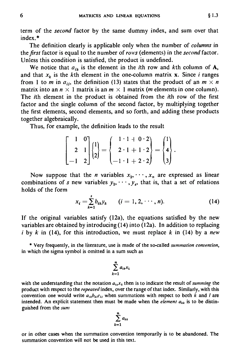
Thus, for example, the definition leads to the result
i!
Now suppose that the n variables xv • • •, x„ are expressed as linear
combinations of s new variables yv • • ■ ,ys, that is, that a set of relations
holds of the form
*i=?.bikyk (»' = 1,2,- ■-,«). (14)
k=l
If the original variables satisfy (12a), the equations satisfied by the new
variables are obtained by introducing (14) into (12a). In addition to replacing
/ by k in (14), for this introduction, we must replace k in (14) by a new
* Very frequently, in the literature, use is made of the so-called summation convention,
in which the sigma symbol is omitted in a sum such as
n
k=l
with the understanding that the notation aixxk then is to indicate the result of summing the
product with respect to the repeatedIndex, over the range of that index. Similarly, with this
convention one would write alkbklCa when summations with respect to both k and / are
intended. An explicit statement then must be made when the element akk is to be
distinguished from the sum
n
k=l
or in other cases when the summation convention temporarily is to be abandoned. The
summation convention will not be used in this text.
" 1 0"
2 1
.-1 2.
(l)
W

§1.3
MATRICES
7
dummy index, say /, to avoid ambiguity of notation. The result of the
substitution then takes the form
!<>Jibkly) = c, (/ = 1,2, •••,«), (15a)
or, since the order in which the finite sums are formed is immaterial,
2 fi%fcA, = c{ (/ = 1,2, •■•, IF!). (15b)
In matrix notation, the transformation (14) takes the form
x = By (16)
and, corresponding to (15a), the introduction of (16) into (11) gives
A(By) = c. (17)
But if we write
*,=!>*>« G:!;t*-;r) o»>
equation (15b) takes the form
s
I,Ptiyi = ct (/=1,2,...,//1),
1=1
and hence, in accordance with (12a) and (13), the matrix form of the
transformation (15b) is
Py = c, (19)
where P = [pa].
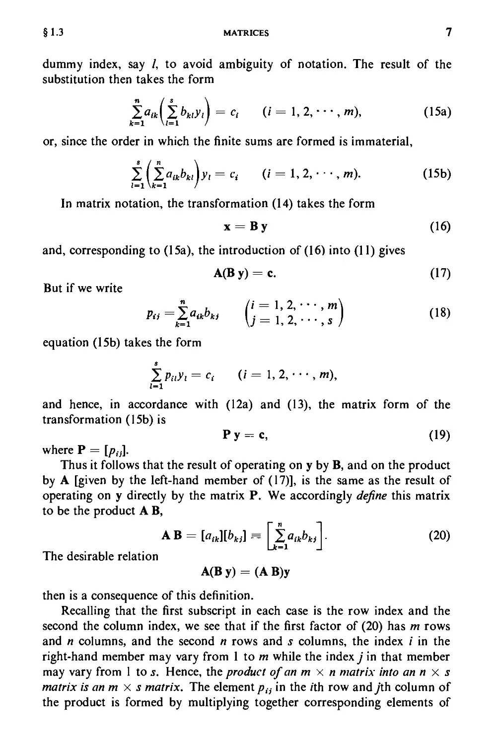
Thus it follows that the result of operating on y by B, and on the product
by A [given by the left-hand member of (17)], is the same as the result of
operating on y directly by the matrix P. We accordingly define this matrix
to be the product A B,
(20)
The desirable relation
A(By) = (AB)y
then is a consequence of this definition.
Recalling that the first subscript in each case is the row index and the
second the column index, we see that if the first factor of (20) has m rows
and n columns, and the second n rows and s columns, the index / in the
right-hand member may vary from 1 to m while the index j in that member
may vary from 1 to s. Hence, the product of an m x n matrix into an n x s
matrix is an m X s matrix. The element />,-,- in the /th row andy'th column of
the product is formed by multiplying together corresponding elements of
AB = wy-
2>«t*>,
_*=i
ikuki

8
MATRICES AND LINEAR EQUATIONS
§1.3
the /th row of the first factor and the jth column of the second factor, and
adding the results algebraically. In particular, the definition (20) properly
reduces to (13) when s = 1.
Thus, for example, we have
(1 • 1 + 0 • 1 + 1 • 2) (1
.(1-1-2-1 + 1-2)(1
"3 3 1
1"
1
"i 2 r
1 0 1
2 1 0_
2 + 0-0+1
2-2-0+1
DO
1)(1
1 +0-
1 -2-
l + i-o)-
1 + 1-0).
1
1
We notice that A B is defined only if the number of columns in A is equal
to the number of rows in B. In this case, the two matrices are said to be
conformable in the order stated.
If A is an m x n matrix and B an n x m matrix, then A and B are
conformable in either order, the product A B then being a square matrix of order
m and the product B A a square matrix of order n. Even in the case when A
and B are square matrices of the same order the products A B and B A are
not generally equal. For example, in the case of two square matrices of order
two we have
«11*11 + °lAl all*12 + «12*22
_a21*ll + °22*21 °21*12 + °22*22.
and also
°lAl + °21*12 «12*11 + a?2*12'
.°11*21 + °21*22 °12*21 + °22*22_
Thus, in multiplying B by A in such cases, we must carefully distinguish
/^multiplication (A B) from />as/multiplication (B A).
Two m X n matrices are said to be equal if and only if corresponding
elements in the two matrices are equal.
The sum of two m x n matrices [a^] and [b^] is defined to be the matrix
[a{j + btj]. Further, the product of a number k and a matrix [ait] is defined
to be the matrix [ka{)], in which each element of the original matrix is
multiplied by k.
From the preceding definitions, it is easily shown that, if A, B, and C
are each m x n matrices, addition is commutative and associative:
"«11
_°21
"*11
_*21
«12~
«22.
*12~
*22.
"*11
_*21
"«11
_°21
*12~
*22.
Ol2~
«22.
A + B = B + A, A + (B + C) = (A + B) + C.
(21)

§1.3
MATRICES
9
Also, if the relevant products are defined, multiplication of matrices is
associative,
A(B C) = (A B)C, (22)
and distributive,
A(B + C) = A B + A C, (B + C)A = B A + C A,
(23)
but, in general, not commutative.*
It is consistent with these definitions to divide a given matrix into smaller
submatrices, the process being known as the partitioning of a matrix. Thus,
for example, we may partition a square matrix A of order three symmetrically
as follows:
r?n «12
321 °22
_°31 fl32 ' °33_
where the elements of the partitioned form are the matrices
13
23
33.
"Bu
_B21
B]2
B22.
B,
'11 "12
L"21 "22.
B12 =
"23.
B21 = [°31 °32l >
Bo
Uha\-
If, for example, a second square matrix of order three is similarly partitioned,
the submatrices can be treated as single elements and the usual laws of matrix
multiplication and addition can be applied to the two matrices so partitioned,
as is easily verified.
More generally, if two conformable matrices in a product are partitioned,
necessary and sufficient conditions that this statement apply are that to
each vertical partition line separating columns r and r + 1 in the first factor
there correspond a horizontal partition line separating rows r and r + 1
in the second factor, and that no additional horizontal partition lines be
present in the second factor.
In particular, if we think of the matrices B and C in the relation A B = C
as being partitioned into columns, we rediscover the fact that each column
of C can be obtained by premultiplying the corresponding column of B by
the matrix A. Similarly, by thinking of A and C as being partitioned into
rows, we see that each row of C is the result of postmultiplying the
corresponding row of A by the matrix B.
* Except when otherwise noted, it will be supposed in this text that the scalars which
comprise the elements of matrices are real or complex numbers. However, many of the
results to be established are also valid (when suitably interpreted) for many other sets of
permissible elements.

10
MATRICES AND LINEAR EQUATIONS
§1.4
1.4. Determinants. Cramer's rule. In this section we review certain
properties of determinants. Associated with any square matrix [ait] of order
n we define the determinant |A| = \ai}\,
«11
a21
<*nl
a12 •
«22 •
<*n2 ■
" ' «1»
' <*2n
* «n„
as a number obtained as the sum of all possible products in each of which
there appears one and only one element from each row and each column,
each such product being prefixed by a plus or minus sign according to the
following rule: Let the elements involved in a given product be joined in pairs
by line segments. If the total number of such segments sloping upward to the
right is even, prefix a plus sign to the product. Otherwise, prefix a negative
sign*
From this definition, the following properties of determinants, which
greatly simplify their actual evaluation, are easily established:
1. If all elements of any row or column of a square matrix are zeros,
its determinant is zero.
2. The value of the determinant is unchanged if the rows and columns of
the matrix are interchanged.
3. If two rows (or two columns) of a square matrix are interchanged,
the sign of its determinant is changed.
4. If all elements of one row (or one column) of a square matrix are
multiplied by a number k, the determinant is multiplied by k.
5. If corresponding elements of two rows (or two columns) are equal or
in a constant ratio, then the determinant is zero.
6. If each element in one row (or one column) is expressed as the sum of
two terms, then the determinant is equal to the sum of two determinants, in
each of which one of the two terms is deleted in each element of that row
(or column).
7. If to the elements of any row (column) are added k times the
corresponding elements of any other row (column), the determinant is unchanged.!
* This statement of the rule of signs is equivalent to the statement which involves
inversions of subscripts. It possesses the advantage of being readily applicable in actual
cases when the elements are numbers (or functions) and are not provided with explicit
subscripts. Also, with this statement of the rule, the proofs of the properties which follow
are in general simplified.
t It can be shown that if we impose the condition that Properties 4 and 7 hold, and in
addition impose the requirement that the determinant be unity when the diagonal elements
are unity and all other elements are zero, then these conditions imply all other properties of
determinants, and may serve as the definition of a determinant.

§ 1.4
DETERMINANTS. CRAMER'S RULE
11
From these properties others may be deduced. For example, from
Property 7 it follows immediately that to any row (column) of a square
matrix may be added any linear combination of the other rows (columns)
without changing the determinant of the matrix. By combining this result
with Property 1, we deduce that if any row (column) of a square matrix is a
linear combination of the other rows (columns), then the determinant of that
matrix is zero.
If the row and column containing an element ai} in a square matrix A
are deleted, the determinant of the remaining square array is called the
minor of ati, and is denoted here by Miy The cofactor of ais, denoted here
by A,j, is then defined by the relation
Ait = (-l)«'Mii. (24)
Thus if the sum of the row and column indices of an element is even, the
cofactor and the minor of that element are identical; otherwise they differ
in sign.
It is a consequence of the definition of a determinant that the cofactor
of ait is the coefficient of ati in the expansion of |A|. This fact leads to the
important Laplace expansion formulas:
n n
|A|=2>,*i4tt and |A| = J,akiAki, (25a,b)
k=l k=l
for any relevant value of i otj. These formulas state that the determinant of a
square matrix is equal to the sum of the products of the elements of any single
row or column of that matrix by their cofactors.
If aik is replaced by ark in (25a), the result HLarkAik must accordingly be
the determinant of a new matrix in which the elements of the /th row are
replaced by the corresponding elements of the rth row, and hence must
vanish if r ^ i by virtue of Property 5. An analogous result follows if akj
is replaced by aks in (25b), when s ^ j. Thus, in addition to (25), we have the
relations
tarkAtk=0 (r^i), 2aksAki = 0 (s # j). (26a,b)
k=l t=l
These results lead directly to Cramer's rule for solving a set of n linear
equations in n unknown quantities, of the form
2aikxk = ci (/=1,2,---,//), (27)
*r=l
in the case when the determinant of the matrix of coefficients is not zero,
\a„\ ± 0. (28)
For if we assume the existence of a solution and multiply both sides of

12
MATRICES AND LINEAR EQUATIONS
§1.4
(27) by Air, where r is any integer between 1 and n, and then sum the results
with respect to /, there follows (after an interchange of order of summation)
-Ic,Atr (r = 1,2, ...,i!). (29)
By virtue of (25b) and (26b), the inner sum on the left in (29) vanishes unless
k = r and is equal to |A| in that case. Hence (29) takes the form
\A\xr=f,A^i (r =1,2,-..,/1). (30)
Thus, if the system (27) possesses a solution, then that solution also must
satisfy the equation set (30). When |A| ^ 0, the only possible solution of
(27) accordingly is given by
xr = -±-i^rc,. (r = 1,2, -.-,11). (31)
|A| .=i
To verify that (31) does in fact satisfy (27), we introduce (31) into (27),
first changing the dummy index / in (31) to another symbol, sayy, to avoid
ambiguity, after which the left-hand side of the /th equation of (27) becomes
inn i n / n \
777 2>«2AikCj = — I iMftki
|A| *=i i=i |A| >=i\*=i /
after an interchange of order of summation. The use of (26a) and (25a)
properly reduces this expression to
777(Z<Wl,*k = c{,
|A| U=i /
and hence establishes the validity of (31) when |A| ^ 0.
The expansion on the right in (30) differs from the right-hand member of
the expansion
n
|A| = 2 Atratr
«=i
only in the fact that the column {ct} replaces the column {air} of the
coefficients of xr in A. Thus we deduce Cramer's rule, which can be stated as
follows:
When the determinant |A| of the matrix of coefficients in a set of n linear
algebraic equations in n unknowns xx, ■ ■ •, xn is not zero, that set of equations
has a unique solution. The value of any xr can be expressed as the ratio of two
determinants, the denominator being the determinant of the matrix of
coefficients, and the numerator being the determinant of the matrix obtained by
replacing the column of the coefficients of xr in the coefficient matrix by the
column of the right-hand members.

§1.5
SPECIAL MATRICES
13
In the case when all right-hand members c{ are zero, the equations are
said to be homogeneous. In this case, one solution is clearly the trivial one
xi = x2 = ''' = xn = 0- The preceding result then states that this is the
only possible solution if |A| ^ 0, so that a set of n linear homogeneous
equations in n unknowns cannot possess a nontrivial solution unless the
determinant of the coefficient matrix vanishes.
We postpone the treatment of the case when |A| = 0, as well as the case
when the number of equations differs from the number of unknowns, to
Sections 1.9 and 1.11.
It can be shown that the determinant of the product of two square matrices
of the same order is equal to the product of the determinants:*
|AB| = |A||B|. (32)
A square matrix whose determinant vanishes is called a singular matrix;
a nonsingular matrix is a square matrix whose determinant is not zero.
From (32) it then follows that the product of two nonsingular matrices is also
nonsingular.
It is true also that if a square matrix M is of one of the special forms
"A
C
M
or
M
(33a)
where A and B are square submatrices and where 0 is a submatrix whose
elements are all zeros, then
|M| = |A| |B|. (33b)
Here the dimensions of A and B need not be equal and the zero submatrix
0 of M need not be square.
It follows from the definitions that the determinant of the negative of a
square matrix is not necessarily the negative of the determinant, but that one
has the relationship
|-A| = (-1)-|A|,
where n is the order of the matrix A.
1.5. Special matrices. In this section we define certain special matrices
which are of importance, and investigate some of their properties.
That matrix which is obtained from A = [atj] by interchanging rows
and columns is called the transpose of A, and is here indicated by Ar:
a21
\T =
«2n
* While this result is in no sense profound, the existent proofs of (32) are either lengthy
or indirect.

14
MATRICES AND LINEAR EQUATIONS
§1.5
Thus the transpose of an m x n matrix is an n x m matrix. If the element
in row r and column s of A is ars, where r may vary from 1 to m and s from
1 to n, then the element a'rs in row r and column 5 of Ar is given by a'rs = asr,
where now r may vary from 1 to n and s from 1 to m.
If A is an m x / matrix and B is an / x n matrix, then both the products
A B and BrAr exist, the former being anmxn matrix, and the latter an
n X m matrix. We show next that the latter matrix is the transpose of the
former. Since the element in row r and column s of the product A B = C
is given by
i
Z.ark"ks — crs>
*r=l
where r may vary from 1 to m and s from 1 to n, whereas the element c'rs in
row r and column s of the product Br Ar is given by
i i
crs =7 Z, "rkaks = Z, "krask = csr>
k=l k=l
where now r may vary from 1 to n and s from 1 to m, it follows that Br Ar is
indeed the transpose of A B.
Thus, we have shown that the transpose of the product A B is the product
of the transposes in reverse order:
(AB)r=BrAr. (34)
This result will be of frequent usefulness.
When A is a square matrix, the matrix obtained from A by replacing each
element by its cofactor and then interchanging rows and columns is called
the adjoint of A:
The adjoint of a product is found to be equal to the product of the adjoints
in the reverse order.
When the elements of a matrix A are complex, we denote by A the matrix
obtained by replacing each element of A by its complex conjugate, and call
the matrix A the conjugate of A.
The unit matrix I of order n is the square n x n matrix having ones in
its principal diagonal and zeros elsewhere,
"l 0 ••• 0"
T_ 0 1---0
AdjA
An A21
A12 A22
A„2
^ln ™2n
0 0---1

§15
SPECIAL MATRICES
15
while a zero matrix 0 has zeros for all its elements. When it is necessary to
indicate the dimensions of such matrices, the notation I„ may be used to
denote the n x n unit matrix and the notation 0mn to denote the m x n
zero matrix. It is readily verified that for any matrix A there follow
AI = A, IA = A (35a,b)
and
A 0 = 0, 0 A = 0. (36a,b)
Here, if A is an m x n matrix, the symbol I necessarily stands for I„ in
(35a) and for I„, in (35b), while 0 stands for 0„, on the left and 0m, on the
right in (36a), and for 0rm on the left and 0r „ on the right in (36b), where r
and s are any positive integers.
The notation of the so-called Kronecker delta,
= (0 when p^q,
" \l when p=q, Kil)
is frequently useful. With this notation, the general term of the unit matrix
is merely dtj; that is, we can write
i = [<y.
More generally, if all elements of a square matrix except those in the
principal diagonal are zeros, the matrix is said to be a diagonal matrix.
A diagonal matrix can thus be written in the form
D = [dAA = VM
where the diagonal elements, for which i = j, are dlt d2, • • •, dn. The
notation
D = diag(dvd2,- •-,</„) (38)
is also useful.
/Vemultiplication of a matrix A by D multiplies the rth row of A by d{;
/^/multiplication multiplies they'th column by </,-. These results follow from
the calculations
and
A D = [aik][dkdki]
I,dAkakj
L*=l
1iaa0Ai
Ut-i
[4fl«] (39)
[atidt] = [«/,«„]. (40)
A diagonal matrix whose diagonal elements are all equal is called a
scalar matrix. Thus, a scalar matrix must be of the form
S = k\ = [kdy].

16
MATRICES AND LINEAR EQUATIONS
§1.6
1.6. The inverse matrix. With the notation of (37), the two equations
(25a) and (26a) can be combined in the form
iaikAjk=\\\du, (41a)
while (25b) and (26b) lead to the relation
2akiAki=\A\8u. (41b)
If we write temporarily
m« = — . (42)
' |A|
under the assumption that |A| ^ 0, these equations become
n n
2aikmkj = da, J.mtkaki = dl}. (43a,b)
Hence, reviewing the definition (20) of the matrix product, we see that
these equations imply the matrix equations
[flttlNwl = I, [™{k][aki] = I. (44)
That is, the matrix M = [mtj] has the property that
A M = M A = I, (45)
where I is the unit matrix. It is natural to define a matrix satisfying (45)
to be an inverse or reciprocal of A, and to write M = A-1.
If A is not square, there is no matrix M for which both A M and M A are
unit matrices (see Problem 31), and hence A then cannot possess an inverse.
Further, a square matrix can have only one inverse. To prove this statement,
we suppose that M' is any matrix such that
AM' = I, (46)
where A is square. Then since accordingly |A| |M'| = 1, it follows that A
must be nonsingular, and hence the associated matrix M exists. If we pre-
multiply both sides of (46) by M and use (45) and (35), there follows
(M A)M' = MI or M' = M,
as was to be shown.
We conclude that if and only if the matrix A = [atj] is nonsingular, it
possesses an inverse A-1 such that
A-1 A = A A-1 = I, (47)
and that inverse is of the form
A"1 =[«„] where mu = ^f (48)
lAl

§1.6
THE INVERSE MATRIX
17
Thus, to obtain the inverse of a nonsingular square matrix [a{j] we may
first replace ati by its cofactor Ati = ( — \)i+iMijt then interchange rows and
columns and divide each element by the determinant \ai}\. In the terminology
of Section 1.5, the inverse of A is the adjoint of A divided by the determinant
of A:
A"1 = — Adj A.
|A|
This equation also implies the useful relations
A(Adj A) = |A| I, (Adj A)A = |A| I.
(49)
(50a,b)
It may be noticed that equations (50a,b) also follow directly from (4la,b)
and hence are valid even when |A| = 0.
To determine the inverse of a product of nonsingular square matrices,
we write
AB = C.
If we premultiply both sides of this equation successively by A-1 and B_1,
there follows
I = B-1 A"1 C
and hence, by postmultiplying both sides of this equation by C_1 and replacing
C by A B, we obtain the rule
(A B)-1 = B-1 A-1.
(51)
To illustrate the use of the inverse matrix, we again consider the problem
of solving the set of linear equations (27) under the assumption (28). In
matrix notation we have
Ax = c,
and hence, after premultiplying both sides by A-1, there follows
or
Xi\
Xi\
• \
• I
• '
1
~|A|
'An
A12
An
A2i ■
A22
A2„
■ An;
A„2
■ Ann.
Cl
1
V2
/•
1 •
/.
(52a)
(52b)
or
1
+ Anicn) (/ = 1,2,
in accordance with the expanded form of Cramer's rule.
Xt = — (AuC! + A2ic2 +
|A|
.«), (52c)

18
MATRICES AND LINEAR EQUATIONS
§1.7
1.7. Rank of a matrix. Before proceeding to the analytical treatment of
general sets of linear equations, to which Cramer's rule may not apply,
it is desirable to introduce an additional definition and to establish certain
preliminary basic results.
We define the rank of any matrix A as the order of the largest square
submatrix of A (formed by deleting certain rows and/or columns of A)
whose determinant does not vanish.
Suppose now that a certain matrix A is of rank r. We next show that if a
set of r rows of A containing a nonsingular r x r submatrix R is selected,
then any other row of A is a linear combination of those r rows.
To simplify the notation, we suppose that the square array R of order r
in the upper left corner of the matrix A has a nonvanishing determinant, and
consider the following submatrix of A:
M
'ii
AQl
UQl
(53)
where s > r and q > r. Then, since the matrix A is of rank r, the determinant
of this square submatrix must vanish for all such s and q.
Now it is possible to determine constants Xu A2, • • •, Ar such that the
equations
Xlan + A^ + • • • + k,arl = a^,)
kta12 + Ajja22 + • • • + A/jrf; = a„2,
(54)
ktalr + Xja2r + • • • + k,a„ = aq,
are satisfied, since the coefficient determinant |RT| = |R| assuredly does not
vanish and Cramer's rule applies. Hence, with these constants of
combination, we can determine a row of elements which is a linear combination of
the first r rows of M, and which will have its first r elements identical with
the first r elements of the last row. Let the last element of that combination
be denoted by a'Qs. In evaluating the determinant of M, we may subtract this
linear combination of the first r rows from the last row without changing the
value of the determinant, to obtain the result
|M|
an • • • «!
a,i • • • ar
0 aQS - a'QS
(55)

§1.8
ELEMENTARY OPERATIONS
19
But since |M| is equal, by the Laplace expansion, to the product of aQt — a'QS
and the determinant |R| which does not vanish, by hypothesis, and since
|M| = 0, it follows that a'QS = aQS. Hence we see that the last row ofM is a
linear combination of the first r rows. Since this is true for any q and s greater
than r, the result can be stated as follows:
If a matrix is of rank r, and a set of r rows containing a nonsingular
submatrix of order r is selected, then any other row in the matrix is a linear
combination of these r rows.
The same statement is easily seen to be true, by a similar argument, if
the word "row" is replaced by "column" throughout.
As a special case, we deduce that if a square matrix A is singular, then at
least one of the rows of A must be a linear combination of the others, and
the same statement applies to the columns. Since the converse has already
been established in Section 1.7, it follows that a square matrix is singular if
and only if one of its rows is a linear combination of the others. The same
statement applies to the columns.
It is obvious that the process of interchanging rows and columns does
not affect the rank of a matrix, so that the two matrices A and AT have the
same rank. The following section treats certain other operations on matrices
which also leave the rank invariant.
1.8. Elementary operations. Associated with a set of m linear equations
in n unknowns,
flu*i + "12*2 + V alnxn = cv
a2i*i + °22*2 H h a2nxn = c2,
amlxl + am2x2 + ' ' ' + amnXn = Cm
we consider two matrices: the m x n matrix of coefficients [atj], and the
m x (n + 1) matrix formed by joining to the columns of [atj] the column
of constants {ct}. We refer to the former matrix as the coefficient matrix
and to the second as the augmented matrix.
As was shown in Section 1.2, we may use the Gauss-Jordan reduction
(renumbering certain equations or variables, if necessary) to replace (56)
by an equivalent set of equations of the form
X2 <*21-*V+1 ' ' ' V-i.n-rXn = 72' J
Xr - <X.nXr+1 K^n-rXn = yr, \ , (57)
0 = Yr+U V
0 = ym j
(56)

20
MATRICES AND LINEAR EQUATIONS
§1.8
by a process which involves, in addition to possible renumbering, only the
multiplication of equal quantities by equal nonzero quantities and the
addition of equals to equals. Accordingly, the augmented matrix of (56) is
transformed to the augmented matrix of (57), which is of the form
1
0
0
0
0
0 •
1 •
0 •
0 •
0 •
• 0
• 0
• 1
• 0
• 0
-«11
— «21
-«rl
0
0
-«12 • •
— «22 ' '
-«r2 •
0
0
• -al.n-r Yl
' — ^2.n-r ?2
" -ar,n-r Yr
0 yr+1
0 ym
(58)
and, at the same time, the coefficient matrix of (56) transforms into the
result of deleting the last column of the matrix (58).
The steps in the reduction involve only the following so-called elementary
row and column operations:
1. The interchange of two rows (or of two columns).
2. The multiplication of the elements of a row (or column) by a number
other than zero.
3. The addition, to the elements of a row (column), of k times the
corresponding elements of another row (column).
It is clear that the transformed coefficient matrix in the above case is of
rank r, whereas if one or more of the numbers yr+1, yr+2, • • •, ym is not
zero, the rank of the transformed augmented matrix is r + 1. If yr+1 =
yr+2 = • • • = ym = 0, both transformed matrices are of rank r.
It is next shown that the ranks of the two matrices associated with (56)
are the same as the ranks of the corresponding transformed matrices, that is,
that the rank of a matrix is not changed by the elementary operations.
We need show only that a nonvanishing determinant of largest order r is
not reduced to zero, and that no nonvanishing determinant of higher order
is introduced, by any such operation.
Operation 1 is equivalent to renumbering rows or columns, and obviously
cannot affect over-all vanishing or nonvanishing of determinants.
Similarly, operation 2 can only multiply certain determinants by a nonzero
constant.
According to Property 7 of determinants (page 10), operation 3 does not
change the value of any determinant which involves either both or neither of
the two rows (or columns) concerned. To simplify the notation in the
remaining case, we again suppose that one nonsingular r x r submatrix R

§1.9
SOLVABILITY OF SETS OF LINEAR EQUATIONS
21
is in the upper left corner of A, and that k times the <yth row of A is to be
added to the /th row, with /' Si r <q. If we then consider the effect of this
row operation on the submatrix
'11
"rl
"«i
AlT
a„, • • • a„,
AQl
we may use the last result of Section 1.7 to deduce that the rank of A is not
reduced by row operation 3.
For either the last row of S is a linear combination of rows ofR excluding
the /th, in which case |R| is unchanged, or the r x r subarray of S which is
obtained by deleting the /th row (and which is unaffected by the operation)
is nonsingular. Thus there is at least one nonsingular r x r submatrix in S
after the operation is effected.
Conversely, this operation cannot increase the rank of a matrix, since
the reversed operation (which would be of the same type) then would reduce
the rank of the new matrix.
The same argument applies to operation 3 effected on columns. Hence
we conclude that the elementary operations, applied to rows or to columns, do
not change the rank of a matrix.
1.9. Solvability of sets of linear equations. If we notice that no column
operations are involved in the Gauss-Jordan reduction, except perhaps a
renumbering of certain columns of the coefficient matrix, we conclude both
that the augmented matrices of (56) and (57) are of equal rank, and also
that the same is true of the coefficient matrices.
If and only if one or more of the numbers yr+1, yr+2, • • •, ym in (57) is
not zero, the given set of equations possesses no solution. But if and only
if this is so, the rank of the augmented matrix is greater than the rank of the
coefficient matrix. Thus we deduce the following basic result:
A set of linear equations possesses a solution if and only if the rank of the
augmented matrix is equal to the rank of the coefficient matrix.
If the two ranks are both equal to r, and if we select a set of r equations
whose coefficient matrix contains a nonsingular submatrix of order r, then
we may disregard all other equations, since they are implied by the r basic
equations (that is, their coefficients are linear combinations of the
coefficients in the r basic equations). The n — r unknowns whose coefficients are
not involved in the nonsingular r x r submatrix can be assigned arbitrary

22
MATRICES AND LINEAR EQUATIONS
§1.9
values, after which the remaining r unknowns can be determined in terms of
them (by Cramer's rule or otherwise).*
In particular, if r = n the unknowns are determined uniquely. Otherwise,
if n — r = d > 0, the most general solution involves d independent
arbitrary parameters.
In the homogeneous case, when the right-hand members of (56) are all
zeros, the coefficient matrix and the augmented matrix are automatically of
equal rank, and a solution always exists. But this fact is obvious, since such a
system is always satisfied by the trivial solution xt = x2 = • • • = xn = 0.
If the rank r of the coefficient matrix is equal to the number n of unknowns,
then this is the only solution, in accordance with the special results of
Section 1.4. However, if r < n (in particular, if the number of equations
is less than the number of unknowns) infinitely many solutions exist, the
number of independent arbitrary parameters involved being given by the
difference n — r.
We notice that, in consequence of the linearity of the relevant equations,
the general solution of a nonhomogeneous set of equations is the sum of any
one particular solution of that set and the most general solution of the
associated homogeneous set.
A case of particular interest is that of a set of n homogeneous equations
in n unknowns, in which the coefficient matrix is of rank n — 1; that is, a
set of the form
laikxk = 0 (1=1,2,---,/1) (59)
where
K\ = 0 (60)
but where the determinant of at least one square submatrix of A of order
n — 1 does not vanish. In consequence of equations (41 a) and (60), these
equations are satisfied by the expressions
xt = CAsi (/=1,2, ••-,«) (61)
where C is an arbitrary constant and s may take on any value from 1 to n.
Since here d = n — r = 1, and since (61) contains one arbitrary parameter,
(61) must represent the most general solution of (59) unless, for the particular
value of s chosen, all cofactors A8i happen to vanish. (This exception cannot
exist for all values of s if the rank of A is n — 1.) With this reservation, the
result obtained is equivalent to the statement that, in the case under
consideration, the unknowns are proportional to the cofactors of their coefficients in
any row of the matrix [ati].
* In actual numerical cases, a procedure such as that of the Gauss or Gauss-Jordan
reduction avoids the necessity of perhaps evaluating a large number of determinants.
However, the results obtained here are of great importance in more general considerations.

§1.10
LINEAR VECTOR SPACE
23
1.10. Linear vector space. The preceding results have interesting and
instructive interpretations in terms of so-called "vector space," which is
briefly discussed in this section.
It is conventional to speak of a one-column matrix as a column vector
or, more briefly, as a vector. (Such an array is often called a numerical
vector, to distinguish it from a geometrical or physical vector quantity—such
as a force or an acceleration—which it may represent.) In accordance with
the notation introduced in Section 1.3, a lower-case boldface letter is used
in this text to specifically denote a vector, so that we write
x = \XU X2> ' ' ' ' xnf-
A one-row matrix [xv x2, ■ ■ •, jrj, which is the transpose of the vector x,
will be termed a row vector and will be denoted by xT when a special
symbolism is desirable.
In two-dimensional space, the elements of the vector {xv x2} can be
interpreted as the components of x in the directions of rectangular coordinate
(xt and x2) axes. The square of the length of this vector is then given by
/2 = x* + x2 = xT x.* Also, if u and v are two vectors in two-dimensional
space, the scalar product of u and v is defined to be utvx + u2v2 = uT v = vT u.
It is seen that the scalar product uT v here is the equivalent, in matrix
notation, of the "dot product" u • v in vector analysis. We recall that the
vectors u and v are orthogonal (perpendicular) if and only if this scalar
product vanishes. The vectors ix = {1, 0} and i2 = {0, 1} are the orthogonal
unit vectors ordinarily denoted by i and j, respectively, in vector analysis.
The above terminology is extended by analogy to the general case of n
dimensions. When n > 3, it is impossible to visualize the vectors
geometrically. However, we use the language associated with space of two or
three dimensions, and say that an H-dimensional rectangular coordinate
system comprises n mutually orthogonal axes, that a point has n
corresponding coordinates, and that a vector has n components along these axes.
The scalar product of two vectors u and v is defined to be
uT v = \T u = uxvx + u2v2-\ [- unvn (62)
and the square of the length of a vector u is defined to be
/2(u) = ur u = Wl2 + «22 + • • • + un\ (63)
It is sometimes convenient to denote the scalar product by the abbreviation
(u, v), so that
(u, v) = uT v = \T u = (v, u). (64)
* A product of the form \T\, which is truly a one-element matrix, is conventionally
treated as a scalar.

24 MATRICES AND LINEAR EQUATIONS § 1.10
The abbreviation
u2 = (u, u)
is frequently used in the special case when v = u.
Two vectors u and v are said to be orthogonal if their scalar product
vanishes, (u, v) = 0. A zero vector is thus orthogonal to all vectors of the
same dimension. A vector is said to be a unit vector if its length is unity, so
that(u, u) = 1.
When the components of u and v are real, it can be shown that
|(u, v)| ^ (u, uJ^V, v)1/2 (65)
(see Problem 43), that is, that the magnitude of the scalar product of u and
v is not larger than the product of the lengths of u and v. This important
result is known as the Schwarz inequality.
Hence the natural definition
cos e =;—wLv) w, (-ff <e^ *) (66)
(u, u)1/2(v, vy'2
makes |cos 0| ^ 1 and so yields a real interpretation for the "angle 0 between
the real vectors u and v" in the general n-dimensional case.
When the components of the vectors are complex numbers, the preceding
properties of length, angle, and orthogonality usually are of limited
significance and it is desirable to define more appropriate properties, which
reduce to the preceding ones in the real case.
For this purpose, the Hermitian scalar product of a vector u into a vector
v may be defined as
(u, v) = uTv = M^! + u2v2 + • • • + unvn = (v, u), (67)
and is complex and not, in general, equal to its conjugate (u, v). The square
of the Hermitian length (or absolute length) of a vector u with complex
components is then defined to be the nonnegative real quantity
V(«) = («. U) = «Tu = "l"l + «2"2 H + "n"n. (68)
and the Hermitian angle dH between u and v is a real quantity defined by the
relation
cosOH=^\+(:<% (-w«feS,r) (69)
2( u, u)' (v, v)
(see Problem 44). Two complex vectors u and v are then said to be orthogonal
in the Hermitian sense when (u, v) = 0, and hence also (v, u) = 0.
When the elements involved are real, they are equal to their complex
conjugates, and it is seen that (67), (68), and (69) reduce to (62), (63), and

§1.10
LINEAR VECTOR SPACE
25
(66). However, it should be noted, for example, that if v = {1,/}, where
/2 = -1, then there follows /(v) = 0 but lH(v) = V2.
A set of m vectors ux, u2, • • •, um is said to be linearly independent if
no set pf constants cv c2,..., cm, at least one of which is not zero, exists
such that
CjUj + c2u2 H \- cmum = 0. (70)
that
In two-dimensional space, the existence of cx and c2 (not both zero) such
CjUj + c2u2 = 0
would imply that one of the two-dimensional vectors ux and u2 is a scalar
multiple of the other. Hence any two vectors which are not multiples of the
same vector (parallel to a line) are linearly independent in two-dimensional
space. Further, geometrical considerations indicate that any three vectors
which are not parallel to a plane are linearly independent in three-dimensional
space.
To obtain an analytical criterion for linear dependence of a set of m
vectors with real components, we suppose that c's do exist, at least one of
which is not zero, such that (70) is satisfied. Then, by successively forming
the scalar products of ux, • • •, um into both sides of (70), we find that the
constants c, must also satisfy the equations
CiV + c2(ux, u2) + • • • + cm(uv uj = 0,
Ci(u2, ux) + c2u22 + • • • + cm(u2, u J = 0,
Ci(«m. ux) + c2(um, u2) + • • • + cmum2 = 0.
These conditions clearly require merely that the left-hand member of (70)
be simultaneously orthogonal to ux, u2, • • •, um. But, according to Cramer's
rule, this set of m equations in the m constants c, cannot possess a nontrivial
solution unless the determinant of the matrix of coefficients vanishes:
G =
(«i. «2)
("2. »l) »2:
("m.Ul) (Um.«2)
(«1» O
(»2, O
= 0.
(71)
This determinant is called the Gram determinant or Gramian of ux, • • •, um.
Thus, if the vectors are linearly dependent the Gramian must vanish. The
converse can also be shown to be true (see Problem 42). Hence it follows
that a set of real vectors is linearly dependent if and only if its Gramian vanishes.

26
MATRICES AND LINEAR EQUATIONS
§1.10
For vectors with complex components, this theorem is still true if all
scalar products in the definition of the Gramian are replaced by Hermitian
scalar products.
If ux, u2, • • •, um are n-dimensional vectors, then the set of all vectors
v which can be expressed in the form
v = quj + c2u2 H [- cmum (72)
is called the vector space generated or spanned by the vector set ux, • • •, um.
If r and only r of the u's are linearly independent, the space so generated is
said to be of dimension r. Thus the dimension of the generated space is also
the rank of a matrix which has the elements of the successive generating
vectors as its successive rows or columns.
When m > r, we see that m — r of the u's can be expressed as linear
combinations of the r independent u's, so that any vector v in the vector space
generated by the set of m vectors also can be generated by a subset of r
independent ones. Such a set of r linearly independent vectors is said to form a
basis for the r-dimensional vector space which it spans.
The space of all n-dimensional vectors, that is, the set of all vectors having
n elements, will be of principal importance in this work and will be referred
to, for brevity, as n-space. It is clear that n-space is spanned by any set of n
linearly independent n-dimensional vectors ult • • •, u„. For, if v is any
n-dimensional vector, then in the n equations which equate the n components
of the two members of the relation
v = c^ + c2u2 H [- c„u„, (73)
the matrix of coefficients of the c's has the property that no column is a linear
combination of the others, and hence the determinant of the coefficient
matrix cannot vanish. Thus c's can be determined so that (73) is true.
To determine the constants in (73) by an alternative method, we may
form the scalar product of each u into the equal members of (73). The
resultant set of n scalar equations always can be solved for the c's, when the
u's are linearly independent, since the determinant of the relevant coefficient
matrix is the Gramian of the u's, and hence does not vanish. In particular, it
follows that if the n-dimensional vector v is orthogonal to each of the n linearly
independent u's, then v must be the zero vector.*
A set of r linearly independent n-dimensional vectors is said to span an
r-dimensional subspace of the space of all n-dimensional vectors, when
r < n, and is said to be of defect (or nullity) d = n — r in n-space.
Clearly, any set of n nonzero mutually orthogonal n-dimensional vectors
is a basis in n-space, since its Gramian is the determinant of a diagonal
* In the complex case, the scalar products and the orthogonality are here to be defined
in the Hermitian sense.

§1.11
LINEAR EQUATIONS AND VECTOR SPACE
27
matrix with nonzero diagonal elements, and hence cannot vanish. An
especially convenient basis comprises the particular orthogonal unit vectors
^ = (1,0,0,---,0), i,= {0,1,0,---,0), ••-,
i„ = (0,0,0,---,1), (74)
and is sometimes called the standard basis of n-space.
1.11. Linear equations and vector space. We now indicate briefly the
interpretation of the basic results of Section 1.9, relevant to a set of m linear
algebraic equations in n unknowns, with reference to the terminology of
Section 1.10.
The set of equations
On*i + ^12*2 H V ai„x„ = cu~\
a2i*i + a22*2 H \- a2nxn = c2,'
(75)
ami*i + am2x2 H \- amnxn = c„
which corresponds to the vector equation
Ax = c,
can also be written in the form
(a,, x) = c( (/'= 1,2,-- -, m).
Here x is the //-dimensional vector {xlt • • •, x„) and
«< = {aa, ai2, • • •, ain) (i = 1, 2, • • •, m)
(76)
(77)
(78)
is the n-dimensional vector whose elements comprise the /th row of the
coefficient matrix A of (75) so that, schematically,
Kl =
Thus the equations in (75) can be interpreted as prescribing the scalar product
of the unknown vector x and the transpose of each of the m row vectors of A.
In particular, when the c's are all zeros the equations (75) become
homogeneous and require that x be orthogonal to each of the m vectors a^.
When the rank of A is equal to n, the results of Section 1.9 state that x = 0
is the only solution of the associated matrix equation
Ax = 0.
(79)

28
MATRICES AND LINEAR EQUATIONS
§1.11
This result is in accordance with the fact that in this case the m vectors a,
span all of n-space. However, when the rank of A is r, where r < n, Section
1.9 states that there is an (n — r)-fold infinity of vectors, each of which
satisfies (79) and hence is orthogonal to each of the m vectors a,-. This means
that when the vectors alt ■ • •, am span only a subspace of dimension r <n,
it is possible to find a set of d = n — r linearly independent nonzero vectors,
say Ul u2, • • •, ud, each of which is orthogonal to all the a's. Any vector x
which is a linear combination of these vectors,
x = Quj + C2u2 H h Cdud,
(80)
will satisfy the equation (79), and its components will satisfy (75) with ct = 0.
Here the solution space (80), which is generated by the basis Ui, • • •, u„_r,
and the complementary vector space, known as the row space of A, which is
generated by any r linearly independent vectors in the set ab • • •, am,
together comprise all of/i-space. For since the Gramian of the combination
of the two bases just considered is the product of the separate nonvanishing
Gramians [see equation (33)] it follows that their combination comprises
an n-member basis for the space of all //-dimensional vectors. Further, it is
easily seen that no vector other than the zero vector can be in both subspaces
(see Problem 48). Hence it may be deduced that a nonzero vector x satisfies
(79) if and only if it is not in the row space of A.
In order to display the general solution of (75) or, equivalently, (57) in
the form (80) when the right-hand members of (75) vanish, we may write
*r+l
— ^-1> xr+2 — ^-2>
X„ =
C„_r, where the C's are arbitrary. The
solution can then be written in the vector form
l
«21
'■l.n-r
•V+2
xr \ / arl \ / ar2 \ / ar n-r \
= C, < > + C, < rt\ + • • • + C„_r< "; ) . (80')
0
1
0
0
It is clear from the-form of the n — r solution vectors that these vectors are
indeed lmearly independent.

§ 1.11
LINEAR EQUATIONS AND VECTOR SPACE
29
In the more general case when equations (75) are nonhomogeneous, so
that the scalar products of x and the vectors ^, • • •, am are each to take on
prescribed values, the most general vector x having this property is expressible
as the sum of any particular vector having this property (if such exist) and an
arbitrary linear combination of all vectors which are orthogonal to all the
a's.
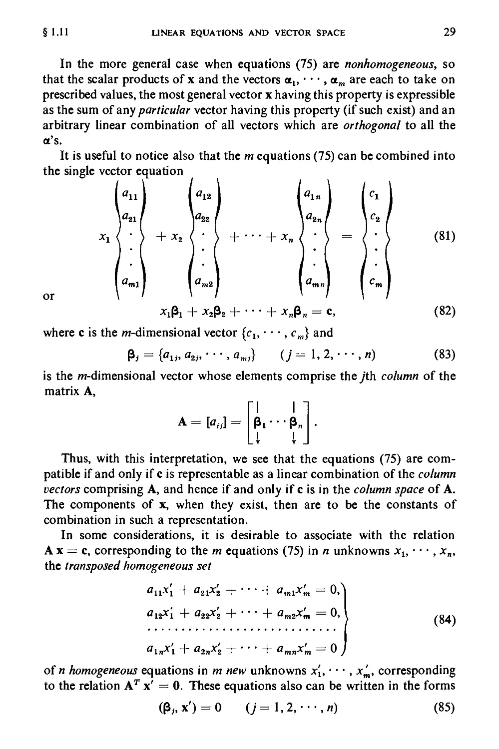
It is useful to notice also that the m equations (75) can be combined into
the single vector equation
-^12 I I "in
+ *i ( • > +••• + *„/ • \ = (• \ (81)
4m2
or
x£i + *2P2 + • • • + x&„ = c, (82)
where c is the /n-dimensional vector {cu • • •, c„,} and
& = {au, a2i, ■ ■ •, aml} (j - 1, 2, • • •, n) (83)
is the /n-dimensional vector whose elements comprise they'th column of the
matrix A,
"I I
A = [at)] = P! • • • P„
J 1
Thus, with this interpretation, we see that the equations (75) are
compatible if and only if c is representable as a linear combination of the column
vectors comprising A, and hence if and only if c is in the column space of A.
The components of x, when they exist, then are to be the constants of
combination in such a representation.
In some considerations, it is desirable to associate with the relation
A x = c, corresponding to the m equations (75) in n unknowns xu • • •, xn,
the transposed homogeneous set
anx[ -+ a21x'2 + 1 amlx'm = 0,\
°12*1 + fl22*2 + ' ' ' + am2X'm = U' I /g4\
«1^1 + a2nx'2 + • • • + amnx'm = 0 J
of n homogeneous equations in m new unknowns *[,•••, x^, corresponding
to the relation AT x' = 0. These equations also can be written in the forms
(P„x') = 0 0=1,2, ••-,/!) (85)

30
MATRICES AND LINEAR EQUATIONS
§1.11
and
m
2*;«, = o, (86)
«=i
with the notation of (78) and (83), in accordance with the fact that the row
and column vectors of A are the column and row vectors, respectively, of AT.
From the relations (82) and (85), we may deduce the following useful
result:
The nonhomogeneous equation A x = c possesses a vector solution x if
and only if the vector c is orthogonal to all vector solutions of the associated
homogeneous equation AT x' = 0.
In order to establish this result, we notice first that if A x = c has a
solution, then c is in the column space of A and hence in the row space of AT.
Hence c then is a linear combination of the vectors Pi, • • •, P„, each of which
is orthogonal to every x' which satisfies AT x' = 0, according to (85). Thus c
also is orthogonal to each x'. Conversely, if c is orthogonal to each solution
of AT x' = 0, then c is in the complement in //-space of the associated solution
space. Thus c is in the row space of AT and hence in the column space of A,
so that jfi, • • •, xn exist such that (82) is satisfied and accordingly A x = c
has a solution.
1.12. Characteristic-value problems. A frequently encountered problem
is that of determining those values of a constant A for which nontrivial
solutions exist to a homogeneous set of equations of the form
tfn*i + ^12*2 + • •' + ai„x„ = A*i,
^21-^1 ~\~ ^22*2 ~^~ ' ' ' ~^~ ^2nXn " A*2,
°nlXl + ^2^2 + " " ' + annXn — Ajf„
Such a problem is known as a characteristic-value problem; values of A for
which nontrivial solutions exist are called characteristic values (also eigenvalues
or latent roots) of the problem or of the matrix A, and corresponding vector
solutions are known as characteristic vectors (also eigenvectors) of the problem
or of the matrix A. A column made up of the elements of a characteristic
vector is often called a modal column.
In many practical considerations in which such problems arise, the matrix
A is real and symmetric, so that two elements which are symmetrically placed
with respect to the principal diagonal are equal:
a„ - a„. (88)
More generally, when the coefficients are complex the most important cases
are those in which symmetrically situated elements are complex conjugates:
(87)
aH = aiS.
(89)

§1.12
CHARACTERISTIC-VALUE PROBLEMS
31
Matrices having the symmetry property (89) are known as Hermitian matrices,
and are considered in Section 1.17.
The discussion of the present section is to be restricted to real symmetric
matrices, for which the symmetry property (88) applies. Whereas certain
of the results to be obtained hold also for symmetric matrices with imaginary
elements, such matrices are of limited importance in applications.
In matrix notation, equation (87) takes the form
A x = A x or (A - A I)x = 0, (90)
where I is the unit matrix of order n. This homogeneous problem possesses
nontrivial solutions if and only if the determinant of the coefficient matrix
A — A I vanishes:
«11-
«21
««1
A
«12
022 — A '
««2
«ln
«2„
• ann-X
This condition requires that A be a root of an algebraic equation of degree n,
known as the characteristic (or secular) equation. The n solutions ku A2, • • •,
A„, which need not all be distinct, are the characteristic numbers or latent
roots of the matrix A.
Corresponding to each such value kk, there exists at least one vector
solution (modal column) of (87) or (90), which is determined within an
arbitrary multiplicative constant.* Now let At and A2 be two distinct
characteristic numbers and denote corresponding characteristic vectors by
ut and u2, respectively, so that the equations
A ui = A^, A u2 = A2u2 (At ^ A2) (92a,b)
are satisfied. If we postmultiply the transpose of (92a) by u2 there follows
(A u0r u2 = A^/ u2
or, using (34),
U!T Ar u2 = Aiii,2* u2. (93a)
Also, by premultiplying (92b) by 11^, we obtain
u^ A u2 = k2ulT u2. (93b)
The result of subtracting (93a) from (93b), and noticing that for a symmetric
matrix AT = A, is then the relation
(A2 - AOK, u,) = 0, (93c)
* As was shown in Section 1.9, the components of this solution vector can be expressed
as arbitrary multiples of the cofactors of the elements in a row of the matrix A — Xk\
unless all those cofactors vanish.

32
MATRICES AND LINEAR EQUATIONS
§1.12
and, since we have assumed that At ^ A2, we thus have the following important
result:
Two characteristic vectors of a real symmetric matrix, corresponding to
different characteristic numbers, are orthogonal,
(Ui, u2) = 0. (94)
A second basic result is that the characteristic numbers of such a matrix
are always real. To establish this fact, we suppose that At = a + //3 is a
root of (91), where a and /3 are real.
Then if U! is a corresponding characteristic vector, so that
A U! = A^,
there follows also
A U! = Ijvti,
by virtue of the fact that the conjugate of a product is the product of the
conjugates, and of the fact that here A is real. Thus A2 = a — //3 = A\ must
also be a characteristic number with u2 = »i as an associated characteristic
vector. By premultiplying the first of the relations
A U! = A^, A ii! = %i ut (95a,b)
by 6^ and postmultiplying the transpose of the second by u^ we obtain the
relation
(At - X^uu Ul) = u/ A Ul - (A uO7 ut = 0. (96)
But now, since the product (ulf u0 is a positive quantity, it follows that
At — A\ = 2//3 must vanish, so that At must be real. Thus we conclude that
all characteristic numbers of a real symmetric matrix are real.
Accordingly, all_characteristic vectors also can be taken to be real, by
rejecting permissible imaginary multiplicative factors.
If a characteristic number, say Xx,of a symmetric matrix is a multiple root
of multiplicity s, that is, if the left-hand member of (91) possesses the factor
(A — kt)s, then to At there correspond s linearly independent characteristic
vectors, any nontrivial linear combinations of which accordingly also have
the same property. Proof of this important fact is postponed to Section 1.18.
The preceding statement is not necessarily true for nonsymmetric matrices,
as can be seen by considering the equations
*i + *2 = ^i» )
—X\ — jc2 = Ax2 J
for which

§1.12
CHARACTERISTIC-VALUE PROBLEMS
33
Here the characteristic equation is readily found to be merely A2 = 0, so
that A = 0 is a characteristic number of multiplicity two. However, when
A = 0, the only possible solution is given by x1 = Cu x2 = — Q and hence
x = Ci{\, —1}. Thus, here the double root A = 0 corresponds to only one
characteristic vector
As is shown in the following section, it is always possible to choose s
linearly independent vectors corresponding to a characteristic number of
multiplicity s in such a way that they are orthogonal to each other, in addition
to being (automatically) orthogonal to all other characteristic vectors.
Thus, if multiple roots of (91) are counted separately, we obtain always
exactly « characteristic numbers, and we can determine a corresponding
set of n mutually orthogonal characteristic vectors. By virtue of the results
of Section 1.10, this set of vectors comprises a basis in n-space; that is, any
vector in n-space can be expressed as some linear combination of these n
vectors.
In particular, if each of the n orthogonal characteristic vectors has been
divided by its length, and so is a unit vector, we say that the resultant set of
vectors is an orthonormal set. If these vectors are denoted by eu e2, • • •, e„,
so that there follows also
(e,. et) = dik, (97)
then the /th coefficient in the representation
» = 2>*e* (98)
of an arbitrary n-dimensional vector v is easily obtained by forming the
scalar product of e, with the equal members of (98), in the form
a, = (e„ v). (99)
Consider now the nonhomogeneous equation
Ax-Ax = c, (100)
where A is a real symmetric matrix. This equation reduces to (87) or (90)
when c = 0. If (100) has a solution, then that solution can be expressed as a
linear combination of the characteristic vectors of A. We suppose that «
orthogonal unit characteristic vectors eu e2, • • •, e„ are known, and notice
that they satisfy the respective equations
Ae1 = A1e1, •••, A e„ = A„e„. (101)
The solution of (100) then can be assumed in the form
*=2>*e*. (102)

34 MATRICES AND LINEAR EQUATIONS §1.12
where the constants <x.k are to be determined. The introduction of (102) into
(100), and the use of (101), then leads to the requirement
i(A*-AKet = c. (103)
By forming the scalar product of any e, with both sides of (103) we may
deduce that (102) satisfies (100) if and only if the /th coefficient a, satisfies
the equation
(A,. - A)at. = (e„ c) (/ = 1, 2, • • •, «). (104)
Hence, //A is not a characteristic number, the solution (102) is obtained in the
form
*=2^:et. (105)
Thus a unique solution of the nonhomogeneous problem is obtained
when A is not a characteristic number. Jfk = kP, no solution exists unless the
vector c is orthogonal to the characteristic vector (or vectors) corresponding
to AP. In case this condition is satisfied, equation (104) shows that the
corresponding coefficient (or coefficients) a.p may be chosen arbitrarily, so
that infinitely many solutions then exist.
In particular, if A = 0, equation (100) reduces to the equation
Ax = c,
which was studied previously. This equation thus has a unique solution
unless A = 0 is a characteristic number of A, that is, unless the equation
A x = 0 has nontrivial solutions. Tn this exceptional situation no solution
exists unless c is orthogonal to the vectors which satisfy A x = 0, in which
case infinitely many solutions exist. This result is in accordance with the
results of the preceding section, where it was shown that the requirement for
the existence of a solution in the exceptional case is that c be orthogonal to
the vectors which satisfy the equation Ar x = 0, since in the present case
we have considered only a symmetric matrix, for which Ar = A.
The existence criterion obtained here, in the more general case when
A = A,,, is also obtainable from the last result of the preceding section, by
replacing A by A — A„I in that result, and noticing that the latter matrix is
symmetric when A is symmetric.
1.13. Orthogonalization of vector sets. It is often desirable, as in the
preceding section, to form from a set of s linearly independent vectors
ub u2. • • •, u, an orthogonal set of s linear combinations of the original
vectors. It is also convenient to "normalize" the vectors in such a way that
each is a unit vector. The following procedure is a simple one, and it can be
extended by analogy to other similar problems.

§1.13
ORTHOGONALIZATION OF VECTOR SETS
35
We first select any one of the original vectors, say vt = ub and divide
it by its length. This is the first member of the desired set:
(106)
/(Ui)
We next choose a second vector, say u2, from the original set and write
v2 = u2 — c e^ The requirement that v2 be orthogonal to e! leads to the
determination
(ei, v2) = (el5 u2) - c(e!, e0 = 0
or c = (d, u^,
so that v2 = u2 — (ei, u2)ei. (107a)
Since e! is a unit vector, the familiar geometrical interpretation of the
scalar product in two or three dimensions leads us to say that (e^ u2) is
"the scalar component of u2 in the direction of e^" and hence that in (107a)
we have "subtracted off the e! component of u2."
The second member, e2, of the desired set of orthogonal unit vectors is
obtained by dividing v2 by its length:
e2 = -^-. (107b)
/(V2)
In the third step we write v3 = u3 — c^ — C2«2. The requirement that
v3 be simultaneously orthogonal to e! and e2 then determines values of c1
and c2 which are in accordance with the geometrical interpretation described
above, and there follows
V3 = "s — (ei. »s)ei — (¢2. »3)62. (108a)
so that the "e! and e2 components" of u3 are subtracted off. The third
required vector e3 is then given by
e3 = -p- . (108b)
A continuation of this process finally determines the sth member of the
required set in the form
es = -^- where vs = us - 2(et, u>t. (109)
/(vs) *=l
This method, which is often called the Gram-Schmidt orthogonalization
procedure, would fail if and only if at some stage vr = 0. But this would
mean that ur is a linear combination of eu e2, • • •, e^, and hence also a
linear combination of Ui, u2, • • •, ur_!, in contradiction with the hypothesis
that the set of u's is linearly independent.

36
MATRICES AND LINEAR EQUATIONS
§1.13
It is seen that this procedure permits the determination of an orthonormal
basis (that is, a basis comprising mutually orthogonal unit vectors) for a
vector space when any set of spanning vectors is known.
When the vectors Ui, • • •, u, are complex, the same procedure clearly
applies if Hermitian products and lengths are used throughout.
1.14. Quadratic forms. A homogeneous expression of second degree,
of the form
A = auxf + a22x22 + • • • + a„nxn2
+ 2^2^2 + 20^x^8 + • • • + 20,,.^,,.^,,, (110)
is called a quadratic form in xu jt2, • • •, x„. It will be supposed here that the
elements atj and the variables xt are real. In two-dimensional space the
equation A = constant represents a second-degree curve (conic) with center
at the origin, while in three-dimensional space the equation A = constant
represents a central quadric surface with center at the origin. Many problems
associated with such forms are intimately related to problems associated with
sets of linear equations.
We may notice first that if we write
1 dA /.,-, x
^( = -7- (/ = 1,2, ••-,«),
2 axt
we obtain the equations
fln-fi + ai2*2 + • • • + alnxn = ylt
«12*1 + «22*2 + * • • + «2n*„ = ^2.
«i„*i + «2„*2 H \- annx„ = y„
This set of equations can be written in the form
Ax = y, (112)
where A = [ait] is a symmetric matrix. That is, the elements satisfy the
symmetry condition
a« = a«- (113)
On the other hand, it is easily seen that (110) is equivalent to the relation
A = (x, y); that is, (110) can be written in the form
A=xT\x. (114)
In many cases it is desirable to express xu x2,---,x„ as linear
combinations of new real variables x[, x'2, • • •, x'n in such a way that A is reduced to
a linear combination of only squares of the new variables, the cross-product
terms being eliminated. A form of this type is said to be a canonical form.
(HI)

§1.14
QUADRATIC FORMS
37
Let the vector x be expressed in terms of x' by the equation
x = Qx', (115)
where Q is a square matrix of order n. The introduction of (115) into (114)
then gives
^ = (Qx')rAQx' = x':rQrAQx' (116)
or
^ = x'rA'x', (117)
where the new matrix A' is defined by the equation
A' = QrAQ. (118)
Thus we see that, if A is to involve only squares of the variables x't, the
matrix Q in (115) must be chosen so that Qr AQ is a diagonal matrix;
that is, so that all elements for which /' =£ j vanish.
We show next that if the characteristic numbers and corresponding
characteristic vectors of the real symmetric matrix A are known, a matrix Q
having this property can be very easily constructed. Suppose that the
characteristic numbers of A are Au A2, • • •, A„, repeated roots of the characteristic
equation being numbered separately, and denote the corresponding members
of the orthogonalized set of n characteristic unit vectors by eu e2, • • •, e„.
We then have the relations
Ae1 = A1e1, •••, Ae„ = A„e„. (119)
Let a matrix Q be constructed in such a way that the elements of the unit
vectors ei, e2, • • •, e„ are the elements of the successive columns of Q:
Q =
«11 «21
«12 «22
^n2
(120)
«ln «2n ' ' ' enn
Then, if use is made of (119), it is easily seen that
^1«11 ^2«21 - - - •*„«„!
AQ =
Ai«i2 A2e22
Ke.
nc7i2
Ai«i„ A2e2n
"A! 0
or
AQ = Q
0 A2
0 0
Kenn
(121a)
(121b)

38
MATRICES AND LINEAR EQUATIONS
§1.14
This relation follows directly from the fact that the product of A into the kth
column of Q is the kth column of the right-hand member of (121a). Since
the vectors e^ • • •, e„ are linearly independent, it follows that |Q| ^ 0.
Thus the inverse Q_1 exists, and by premultiplying the equal members of
(121b) by Q_1 we obtain the result
Q-'AQ=[W (122)
Hence, the matrix A is diagonalized by the indicated operations, the diagonal
elements being merely the characteristic numbers of A.
However, the tfes/ret/diagonalization (118) was to be of the form Qr A Q.
Thus, the matrix Q defined by (120) is not acceptable for present purposes
unless it can be shown that
Qr = Q-i or QT Q = I. (123)
But the typical term pu of the product Qr Q is of the form
n
Pij = 2. eikejk>
where t{ = {en, ei2, • • •, ein) ,
and since the e's are orthogonal the indicated sum vanishes unless /' =j, in
which case the sum is unity since the e's are unit vectors.
Hence there followspa = 6a; that is, Qr Q = [6tj] = I, as is required by
(123). Further, since |Q| = |Qr|, we may obtain from (123) the useful result
IQI2 = 1: IQI=±1. (124)
It follows that the matrix Q defined by (120) does indeed have the
property that the quadratic form
A = xTAx (125)
is reduced by the change in variables
x = Q x' (126)
to the form
A = x'T A' x' where A' = [Pitdu],
that is, to the form
A = A^l2 + A2x^2 + • • • + A„x;2, (127)
where the numbers Xt are the characteristic numbers of A.
A matrix whose columns comprise the elements of n linearly independent
characteristic vectors of a given matrix A, of order n, is called a modal matrix
of A. In particular, when those n vectors are mutually orthogonal and of
unit length, it is convenient to say that the modal matrix is orthonormal.
Thus the matrix Q is an orthonormal modal matrix of A.

§1.15
A NUMERICAL EXAMPLE
39
We notice that if A = 0 is an s-fold root of the characteristic equation
the form (127) has only n — j nonvanishing terms. It is shown in Section 1.18
that this situation arises if and only if the symmetric matrix A is of rank
r = n — s.
The new variables x't are related to the original ones, in accordance with
(115) and (123), by the equation
x' = Q1 x = QT x,
and hence are of the form
(128)
= ellxl + e12x2 + • • • + elnxn,
xn — £„1*1 ~r £»2*2 ~r " " " + snnxn
(129)
or
x; = (e<)X) (/=1,2,---,//). (129')
When all the characteristic numbers of A are distinct, the orthonormal
modal matrix Q is uniquely determined except for the ordering of the columns
and the arbitrary algebraic sign associated with each column. However, if a
root is of multiplicity s, the corresponding s orthogonalized unit vectors can
be chosen in infinitely many ways, as was shown in Section 1.13.
We remark that the modal matrix Q specified by (120) is not the only
matrix which can be used in (126) to reduce a quadratic form to a sum of
squares. However, it is the only such matrix which possesses the useful
property that
Q? = Q-i.
A matrix having this property is called an orthogonal matrix.
It is easily seen that a square matrix is an orthogonal matrix if and only
if its columns comprise the elements of real mutually orthogonal unit vectors.
1.15. A numerical example. To illustrate the preceding reduction in a
specific numerical case, we consider the quadratic form
A = 25x!2 + 34x22 + 41 x32 - 24x2x3.
The corresponding matrix A is then of the form
"25 0 01
A= 0 34-12
0 -12 41.
and the equations A x — A x = 0 become
(25 - A)xt = 0,
(34-A)x2 -12x3 = 0,
-12x2 + (41 -A)x3 = 0.

40
MATRICES AND LINEAR EQUATIONS
§1.15
The characteristic equation |A — A I| = 0 then takes the form
(25 - X)(X2 - 75A + 1250) = 0,
from which the characteristic numbers are determined:
Xl = X2 = 25, A3 = 50.
When X = Xx = X2= 25, the equations Ax — Ax = 0 become
0 = 0,
9x2 — 12x3 = 0,
-12x2+ 16x3 = 0,
with the general solution xt = C\, x2 = C2, x3 = |C2. In vector form we
may write x = CjUi + C2u2, where U! = {1, 0, 0} and u2 = {0, 1, |}. Since
it happens that U! and u2 are orthogonal, we need only divide them by their
lengths /t = 1 and /2 = f to obtain the two orthogonal unit characteristic
vectors
e1 = {1,0,0}, e,= {0,1,1}.
In a similar way, a unit characteristic vector corresponding to A = A3 = 50
is found to be
e3 = {0, |, -I}.
Hence the orthonormal modal matrix Q of equation (120) can be taken in
the form
"1 0 01
Q =
o 4- -3
3 4
S —S.
5 5
_0
and the new coordinates defined by (129) are then given by
xi = xi>
*3 = SX2 — "SX3-
With this choice of the new coordinates, (127) states that the quadratic
form under consideration takes the form
A = 25xi* + 25x22 + 50x32.
In particular, it follows that the quadric surface with the equation
25x!2 + 34x22 + 41 x32 - 24x2x3 = 25
takes the standard form
x[2 + x? + 2x32 = 1

§1.16
EQUIVALENT MATRICES AND TRANSFORMATIONS
41
with the introduction of the new coordinates. It is shown in Section 1.21
that the new x[-x'n coordinate system defined by (126) is also a rectangular
system when Q is an orthogonal matrix and that length and angle then are
preserved by the transformation. Hence the quadric surface just considered
is an oblaie spheroid with semiaxes of length 1, 1, V2/2.
In the present example it happens that the chosen matrix Q is symmetric,
and hence also is such that Q = Qr = Q_1.
It may be noticed that, by the usual method of "completing squares,"
we may, for example, also reduce the form A as follows:
A = 25xt2 + 34[x22 - ffx2x3 + (^)2½2] + (41 - \^W
= 25xt2 + 34(x2 - Ax3)2 + ^¾2.
Hence, if we introduce new variables by the relations
X2 = X2 17X3,
X3 == x3,
we can reduce A to the form
A = 25x;2 + 34x22 + Wxi1.
However, here the matrix Q for which x = Q x', and which takes the
triangular form
Q =
is not an orthogonal matrix. Consequently, as is shown in Section 1.21, the
new x[x2x3 coordinate system is not a rectangular system in this case; that is,
the new coordinate axes are not mutually perpendicular. Nevertheless, the
matrix Q does have the property that Qr A Q is a diagonal matrix.
1.16. Equivalent matrices and transformations. Two matrices A and B
which can be obtained from each other by a finite number of successive
applications of the elementary operations (Section 1.8) to rows and/or columns
are said to be equivalent (but not necessarily equal) matrices.
It can be shown that any such sequence of operations on the rows of A
can be effected by />remultiplying A by some nonsingular matrix P, while
corresponding operations on columns can always be effected by post-
multiplying A by a nonsingular matrix Q. This result is a consequence of the
easily established fact that an elementary operation on rows (columns) of
A may be accomplished by first performing that operation on the unit
"1
0
0
0
1
0
0"
4
1 7
1_

42
MATRICES AND LINEAR EQUATIONS
§1.16
matrix I of appropriate order, and then premultiplying (postmultiplying) A
by the resultant matrix (see Problems 32 and 33).
The converse of the preceding statement is also true (see Problem 34);
that is, the matrices A and B are equivalent if and only ifnonsingular matrices
P and Q exist such that B = P A Q.
Since the elementary operations do not change the rank of a matrix, it
follows that two equivalent matrices have the same rank.
Transformations of the form P A Q are classified according to restrictions
imposed on P and Q. Thus if P = Qr = Q"1, as in the reduction of Section
1.14, the transformation is called an orthogonal transformation. If only
P = Qr, as is required by equation (118), the resulting transformation
Qr A Q is called a congruence transformation, whereas a transformation of
the form Q_1 A Q, for which P = Q_1, is called a similarity transformation.
This terminology is motivated by certain geometrical considerations. We
notice that an orthogonal transformation is both a congruence and a similarity
transformation.
Conjunctive and unitary transformations, which are of importance in
dealing with matrices of complex elements, are defined in the following
section.
1.17. Hermitian matrices. We now consider a matrix with complex
elements which satisfy the relation
aSi = aiS. (130)
Such a matrix is hence of the special form
Oil «12 «13 - - - «ln
al2 #22 °23 " " " a2n
H= «13 «23 «33 ••• «3» ' (131)
J*u «2„ a3n ■■■ ann_
and is known as a Hermitian matrix. Thus a Hermitian matrix has the
property that two elements situated symmetrically with respect to the
principal diagonal are complex conjugates. In particular, (130) requires
that the elements in the principal diagonal (i =j) be real.
We see that the conjugate of the matrix H, obtained by replacing each
element by its complex conjugate, and denoted by H, is equal to the transpose
ofH:
Hr = H. (132)
The product
H = \TH\ (133)

§1.17
HERMITIAN MATRICES
43
is known as a Hermitian form. In two dimensions, the general Hermitian
form is thus given by
H =
[*i
xJl
~«11 «12"
_al2 a22_
*l'
*2.
= 011*1*1 + («12*1*2 + «12*2*l) + «22*2*2- (I34)
Although the elements au and variables x, may be complex, the values
assumed by a Hermitianform are always real. To establish this fact, we recall
first that the conjugate of a product of complex quantities is equal to the product
of the conjugates. Thus, if H were imaginary (nonreal), and given by (133),
then its conjugate H would be given by
R = \T H x = xT HT x = (H \)T x = xr (H x) = H. (135)
But H = H only if H is real, as was to be shown.
Also, we can show that the characteristic numbers of a Hermitian matrix
are real. For if U! is a characteristic vector corresponding to Xlt we must have
HUl = AlUl, (136)
and hence also, after premultiplying both sides by 0^,
6^ H Ul = X^T Ul. (137)
But since u^ H U! and u^ ut are both real, and u^ U! =£ 0, XY must also
be real.
Further, let u2 be a characteristic vector corresponding to a second
characteristic number A2 ^ Xu so that
Hu2 = A2u2. (138)
If the transposed conjugate of (136) is postmultiplied by u2, there follows
(H ut)T u2 = XfiJ u2,
while premultiplication of (138) by u^ leads to the relation
0^ H u2= A2U!r u2.
By subtracting these equations from each other, and using equations (34)
and (132), there follows
(A2 — X^ttj1, u2 = u^ H u2 — (H U!)T u2
= utT H u2 — utT Hr u2
= 0.

44
MATRICES AND LINEAR EQUATIONS
§1.17
Hence we conclude that two characteristic vectors of a Hermitian matrix,
corresponding to different characteristic numbers, are orthogonal in the
Hermitian sense:
(fii, u2) = u/ u2 = 0. (139)
The vectors u, then can be divided by their Hermitian lengths
/,,(10 = (0,,11^,
to give a set of orthogonal unit vectors et corresponding to successive non-
repeated roots of the characteristic equation. Corresponding to a root of
multiplicity s there exists a set of s linearly independent characteristic vectors
(see Section 1.18), which can be orthogonalized and reduced to absolute
length unity, by a procedure completely analogous to that given in Section
1.13. Thus we may again obtain a set of n mutually orthogonal unit
characteristic vectors e^ e2, • • •, e„, orthogonality and length being defined in the
Hermitian sense.
It then follows that any complex H-dimensional vector v can be expressed
in the form
v = !vt> (140)
where the kth coefficient is given by the formula
«* = (¼. »)■ (141)
In order to solve the equation
Hx-Ax = c, (142)
we may assume the expansion
n
x = 2¾¾. (143)
as in the real case, so that (142) takes the form
n
2(At-A)atet = c
and there follows
(A* - A)at = (ek, c).
Thus, if A is not a characteristic number, the solution becomes
x = %£*£ (144)
*=l Ak — A.
in analogy with (105). If A = Xv, no solution exists unless c is such that
(ep, c) = 0, in which case <x.P is arbitrary, and infinitely many solutions exist.
The reduction of a Hermitian form to a sum of the canonical form
H = k&x\ + A2x2x2 + • • • + A„xX (145)

§1.18 MULTIPLE CHARACTERISTIC NUMBERS OF SYMMETRIC MATRICES 45
may be accomplished by a method analogous to that of Section 1.14. Thus,
if we write
x = Ux', (146)
the form H of (133) becomes
H = (Ux')rHUx' = x'r(U2'HU)x'. (147)
This form will be identified with (145) if and only if U is such that
Ur H U = [A<<y. (148)
As in Section 1.13, a permissible choice of U consists of an orthonormal
modal matrix formed by arranging n orthogonal unit characteristic vectors
of H as its columns, in which case the scalars A, are the characteristic numbers
of H. For the matrix U it is found that
0r = IT1 or VT U = I.
(149)
A matrix U having the property (149) is called a unitary (or Hermitian
orthogonal) matrix, and the product Cr H U is then called a unitary
transformation of H. More generally, a transformation of the form tJT H U,
where U does not necessarily satisfy (149), is called a conjunctive transformation
ofH.
It is easily seen that a square matrix is unitary if and only if its columns
comprise the elements of mutually orthogonal unit vectors, length and
orthogonality being defined in the Hermitian sense.
1.18. Multiple characteristic numbers of symmetric matrices. We next
establish the assertion, made in Section 1.12, that a real symmetric matrix A
with a characteristic number Xx of multiplicity s has an j-parameter family of
characteristic vectors corresponding to At.
For this purpose, suppose first that A is a symmetric n x n matrix such
that the characteristic polynomial
F(A)=|A-AI|
has (A — AJ2 as a factor, and let e! be owe unit characteristic vector of A
corresponding to A^ Then, if Q is any n x n orthogonal matrix having e!
as its first column vector, there follows
QrAQ =
" e T f~
' e T f~
A
i
I
i :
{ :
•-
(150)
Since each vector whose elements comprise a row of Qr, except the first,
is orthogonal to the column A^, each element of the first column of the

46
MATRICES AND LINEAR EQUATIONS
§1.18
product except the leading element will vanish. Thus the result will be of
the form
At a12
QTAQ =
0 a„.
*2n
.0 a„
(151)
where the a's are certain constants, depending upon the remaining columns
of Q. But, since the symmetry of A implies the symmetry of Qr A Q, the
elements a12, • • •, aln also must vanish.
Hence, if Q is any orthogonal matrix having e! as its first column vector,
the product Qr A Q = Q"1 A Q is of the form
Q'AQ =
"A! 0
0 a22
0 '
a2n
0 a„
a„
and also there follows
Q1 A Q - AI
^ - A 0
0 a2o — A
0
«2n
0
'■in
«nn — A
Next we notice that, in consequence of the relation
Q-1 A Q - AI = QHA - A I)Q,
there follows also
IQ-1 A Q — AI| = |A-AI|
and hence (153) implies the relation
X^-X 0 • • • 0
I a AII = *22 '' ' a2n
0
= (h ~ A)
a2n
a22 — ^
an„-^
*2n
«2
a„„ — A
(152)
(153)
(154)
(155)
(156)
But since, by hypothesis, the left-hand member of (156) has (Xi — A)2 as a
factor, it follows that the coefficient of (Xi — A) in the right-hand member

§1.19
DEFINITE FORMS
47
has (At — A) as a factor, and hence vanishes when A = At. Thus the matrix
Q~1 A Q — AI in (153) w of rank n — 2 or less when A = At.
Finally, since (154) states that the matrix Q_1 AQ — AJ is similar to
the matrix A — XJ., we deduce that the rank of the matrix A — AJ « ho/
greater than n — 2 when At is a characteristic number of A of multiplicity
two or more, that is, that the matrix equation A x = A^ has at least a two-
parameter family of solutions in that case.
If the multiplicity of At is greater than two, then by taking Q to be any
orthogonal matrix having two orthogonal unit vectors e! and e2, both
corresponding to Alt as its first two column vectors, we deduce in a completely
analogous way that
Q1AQ-AI =
\
0
A,-A
0
0
0
«33 ~ A
0
0
«3n
0
0
a3n
(157)
and the same argument leads to the conclusion that the matrix A — AI
is of rank not greater than n — 3 when A = At, so that at least a three-
parameter family of corresponding characteristic vectors exists when the
multiplicity of At is at least three.
By inductive reasoning, we thus deduce that if At is a characteristic
number of a symmetric matrix A, of multiplicity s, then the rank of the
matrix A — AI is not greater than n — s when A = Au so that at least s
linearly independent characteristic vectors corresponding to At exist.
However, the rank also cannot be less than n — s, for if this were so, more
than s linearly independent characteristic vectors would correspond to Xu
in which case the total number of linearly independent characteristic vectors
corresponding to all characteristic numbers would exceed the dimension
of /i-space.
Thus we deduce the desired result:
If A^ is a characteristic number of multiplicity s,ofa real symmetric matrix
A of order n, then the rank of the matrix A — AI is exactly n — s when
A = At; that is, there exist exactly s linearly independent corresponding
characteristic vectors.
This statement does not apply in general to a nonsymmetric matrix, as
was shown by an example in Section 1.12. However, an argument analogous
to that given above shows that the same statement applies to Hermitian
matrices.
1.19. Definite forms. If the real quadratic form xrA x, associated with
a real symmetric matrix A, is nonnegative for all real values of the variables
x^, and is zero only if each of those n variables is zero, then that quadratic

48
MATRICES AND LINEAR EQUATIONS
§1.19
form is said to be positive definite. It is then conventional to say also that
the matrix A is positive definite.
Similarly, a Hermitian matrix H is said to be positive definite if the
associated Hermitian form xr H x is nonnegative for any real or complex
vector x, and vanishes only when x = 0.
If a real quadratic form A = \T A x is reducible by a transformation
of the form x = Q x', where Q is a nonsingular real matrix, to the sum of
squares of the n new variables, each with a positive coefficient, then it is clear
that A is a positive definite form relative to the real variables x[, ■ ■ •, x'n.
But from the relation x' = Q-1 x, which is a consequence of the assumed
nonvanishing of |Q|, we see that a real vector x then corresponds always to a
real vector x', and that the vectors x = 0 and x' = 0 then correspond
uniquely. Hence it follows in this case that A is also positive definite relative
to the original real variables x1( • • •, xn.
Similarly, if a Hermitian form is reducible by a nonsingular complex
transformation to the canonical form (145), wherein all coefficients are
positive, the form is then nonnegative for any complex values of the variables,
and is zero if and only if all the n variables vanish.
We notice that if the coefficients of the squares of any of the n variables
are zero, then the vanishing of the form does not imply the vanishing of
those variables, and hence the form is then not positive definite relative to
the entire set of n variables.
It then follows from the results of preceding sections [see equations (127)
and (145)] that a real quadratic (or Hermitian) form is positive definite if
and only if the characteristic numbers of the associated real symmetric (or
Hermitian) matrix are all positive.
A form is often said to be positive semidefinite when it takes on only
nonnegative values for all permissible values of the variables, but vanishes
for some nonzero values of the variables. The preceding argument leads
easily to the fact that a quadratic (or Hermitian) form is positive semidefinite
if and only if the associated symmetric (or Hermitian) matrix is singular and
possesses no negative characteristic numbers.
Positive definite forms are of particular importance in applications,
and are found to possess certain useful properties. In particular, we show
next that if at least one of the two real quadratic forms
A = \TA\, B = \TB\ (158a,b)
is positive definite, then it is always possible to reduce the two forms
simultaneously to linear combinations of only squares of new variables, that is, to
canonical forms, by a nonsingular real transformation. For this purpose,
suppose that the form B is positive definite. Then, by proceeding exactly
as in Section 1.14, we first set
x = Qy, (159)

§1.19
DEFINITE FORMS
49
where Q is an orthonormal modal matrix of B, defined in that section, and
so reduce B to the form
B = wf + p2y2* +■■■ + nnyn\ (160)
where here /i{ is written for the ith characteristic number of the symmetric
matrix B. Since B is positive definite, the ^'s are all positive. Hence we may
make the real substitution
Vi = ^l*iyt (1=1,2,---,/1), (161)
and thus reduce (160) to the form
B = vit + v»+---+Vn% = yirn- (162)
At the same time, the substitution (159) reduces A to the form
^ = (Qy)rAQy=yr(QrAQ)y (163)
and the subsequent substitution (161) reduces this form to the expression
A = riT(Q'TAQ')ri, (164)
where Q' is a matrix obtained from Q by dividing each element of the ith
column of Q by V/i(. Hence, if we write
G = Q'rAQ', (165)
equation (164) takes the form
A = y]r G v). (166)
Now G is a symmetric matrix, since
GT = (Q'r A Q')T = Q'r Ar Q' = Q'T A Q' = G. (167)
Hence we may reduce (166) to canonical form by setting
v) = Ra, (168)
where R is made up of the characteristic vectors of G just as Q is formed
from those of B, and (166) is reduced to the form
A = W + A2a22 + • • • + A„a„2 (169)
where A, is the ith characteristic number of the matrix G.
At the same time, the final substitution (168) reduces (162) to
B = t]Ty] = (Ra)T(Ra) = aTRTRoL. (170)
But since the matrix R is an orthogonal matrix, there follows Rr R = I,
and hence we have the result
B=.ara = a12+a22 + -- +a„2. (171)

50
MATRICES AND LINEAR EQUATIONS
§1.19
Thus, finally, with the substitution
x = Q y = Q' v) = Q' R «, (172)
the two forms (158a,b) are simultaneously reduced to the canonical forms
(169) and (171).
If we define the diagonal matrix
mi
0
0
0 •
m2 ■
0 •
• 0
• 0
' mn
it follows that
Q' = Q
and (172) becomes
x= QM
Since Q and R are orthogonal matrices, with determinants equal to unity
in absolute value [see equation (124)], and since clearly |M| ^ 0, it follows
that the transformation (172) is indeed nonsingular.
In certain applications to dynamical problems (see Section 2.14) the
positive definite form B {kinetic energy) involves the time derivative dxjdt
in place of x, whereas the form A (potential energy) involves only x itself.
The above reduction is still applicable, however, since x and dxjdt are
transformed in the same way at each step of the process.
Another method of accomplishing the same reduction, which is usually
more conveniently applied in practice, is presented in Section 1.25 [see
equations (265)-(267)].
1.20. Discriminants and invariants. It is frequently of importance to
determine whether a quadratic or Hermitian form which involves cross-
product terms is or is not a positive definite form, without reducing it to a
canonical form or determining the characteristic numbers of the associated
matrix. This problem is to be considered in the present section.
If we write the characteristic equation |A — AI| = 0 of a square matrix
A in the form
an —
«21
<*nl
A
«12
a22 — A •
«n2
«2„
• ann-h
= (-1)-[A" - /M"-1 + /M"-2 + (-1)"AJ = 0, (176)
, ittt
m,=
I
(173)
(174)
(175)

§1.20
DISCRIMINANTS AND INVARIANTS
51
and denote the n roots of this equation as Alt A2, • • • , A„, numbering multiple
roots separately, it follows that
A" - &A"-1 + &A"-2 + (-1)-0,,
= (A - Ai)(a - A2) • • • (A - A„). (177)
By comparing coefficients of A in the two sides of (177) it can be shown
that
Pi = K + K + ■ ■ ■ + K,
p3 = A^A^ + • • • + An_2An_iAn,
Pn — AiA2A3 • • • An
Now, for either a real symmetric or a Hermitian matrix, we have shown
that the roots of (176) are all real. Hence, by Descartes' rule of signs, we
see that in such cases the roots of the characteristic equation (176) are all
positive if and only if the quantities p\, 02,"'" > Pn are aM positive.
From (176) it follows that /3„ is the value of |A - AI| when A = 0;
that is, p„ is the value of the determinant of A:
Pn = K\. (179)
Further, it is easily seen that the coefficient of A"-1 in the expansion of the
determinant in (176) is merely
(-i)B+1(an + a22+ --- + 0;
that is, Pi is the sum of the diagonal elements of A:
A = flu + flu + ■ ■ ■ + ann = 2>w. (180)
*r=l
This sum is called the trace of A.
More generally, it can be shown that pt is the sum of all determinants
formed from square arrays of order i whose principal diagonals lie along the
principal diagonal of A. Such determinants are called the principal minors
of A.
Thus it follows that a real quadratic (or Hermitian) form is positive
definite if and only if the sums P{, relevant to the associated symmetric (or
Hermitian) matrix, are all positive.
In illustration, the real quadratic form
A = anXi2 + a^x22 + a33x32 + la^x^ + 2a23x2x3 + 2a13X!X3 (181)
(178)

52
MATRICES AND LINEAR EQUATIONS
§1.20
in three dimensions, which is associated with the real matrix
~an a12 a13~
A = a12 a22 «23 » (182)
_a13 a23 a33_
is positive definite if and only if the three conditions
"a + «22 + «33 > 0» (183a)
(ana22 — a122) + (a22as3 — a232) + (0^33 - a132) > 0, (183b)
Kl > 0, (183c)
are satisfied.
It is readily verified by direct expansion that the determinant of the
symmetric matrix (182) can be written in the form
,„ 1 («11^22 — Ql22)(Qll«33 — «132) ~ («11^23 ~ ^12^13^ nfi/1A
\aa\ — — , (184;
and also in two further equivalent forms obtained by cyclic permutation of
the subscripts.
Suppose that we require only that
on > 0, aua22 - a122 > 0, la^l > 0. (185a,b,c)
It then follows from (185a,b) that we must have a22 > 0, and also, by
referring to (184), we see that (185a,b,c) imply that aua& — al32 > 0.
This relation, together with (185a), in turn implies that 033 > 0. By
considering the permutation of the right-hand member of (184) in which 1 -+2,
2-+2>, 3-»-l, we then deduce similarly that (185a,b,c) also imply the
inequality a22a33 — a232 > 0- Thus it follows that the three conditions (185)
imply the three conditions (183).
By considering the conditions that (181) still be positive definite when,
first, only one variable differs from zero and when, second, only two variables
differ from zero, it is easily seen that each diagonal term ait must be positive
and also that each principal minor of second order must be positive. Hence
these conditions imply and must be implied by either the conditions (183)
or the more convenient conditions (185).
More generally, if for any real symmetric (or Hermitian) matrix A we
define the /nth discriminant Am to be the determinant of the submatrix Dm
obtained by deleting all elements which do not simultaneously lie in the
first m rows and columns of A, it can be shown that the real symmetric (or
Hermitian) matrix A, and the corresponding quadratic (or Hermitian) form,
is positive definite if and only if each of the n discriminants Am is positive.
If and only if this is so, all the principal minors of A are positive.

§1.20
DISCRIMINANTS AND INVARIANTS
53
To establish the sufficiency of this criterion, we need only prove that, if
Dm is positive definite and Am+1 = |Dm+1| is positive, then Dm+1 is also
positive definite. Suppose, on the contrary, that Dm+1 is not positive definite.
Then, since |Dm+1| is the product of the characteristic numbers of Dm+1, it
follows that an even number of these characteristic numbers must be negative.
Let yi and y2 be two such numbers, and denote by U! and u, corresponding
orthogonal unit characteristic vectors of DTO+1, length and orthogonality
being defined in the Hermitian sense. If we define the (m + l)-dimensional
vector
X* = CjUt + C2U2,
where at least one of the c's does not vanish, and notice that then we have
Dm+i U! = Yi»i and Dm+1 u2 = y2u2, there follows easily
x*r Dm+1 x* = cViyi + c2c2y2 < 0,
for any cx and c2. Thus the vector x* renders the Hermitian form associated
with Dm1.1 negative. Now let cl and c2 be related in such a way that the
component x*+1 vanishes. If we notice that the Hermitian form xr Dm+1 x
reduces to the form xr Dm x when xm+1 = 0, we conclude that the m-
dimensional vector made up of the first m components of the x* so determined
renders the Hermitian form associated with Dm negative. Since Dm is
positive definite, this situation is impossible, and the desired contradiction
is obtained.
The specialization of the preceding argument to the case of a real
symmetric matrix, and its associated real quadratic form, is obtained by
deleting the bars indicating complex conjugates. In this case, u! and u2 are
real, and the constants cl and c2 are also to be real.
Whereas the requirements that a form or matrix be positive definite
thus need not be stated in terms of the sums fi{, these sums nevertheless are
of considerable importance in themselves. We see from (178) that each /3,-
is a symmetric function, of degree /', of the characteristic numbers of A.
Also, it follows from (176) that for any two square matrices A and B such
that |A — AI| = |B—A I\for all values ofX, the n quantities fi{ are the same.
In order to determine conditions under which this situation exists, let
A and B be two equivalent matrices. This means that nonsingular matrices
P and Q exist such that B = P A Q. Hence we have, for any value of A,
B-AI = PAQ-AI
= P(A - A P-1 Q-^Q
and also |B - AI| = |P| |Q| |A - A P-1 Q-1!. (186)
Thus, if P and Q are such that P1 Q"1 = I or P = Q-1, so that
B = Q-i A Q,
(187)

54
MATRICES AND LINEAR EQUATIONS
§1.20
there follows P Q = I, and hence |P| |Q| = 1, and (186) takes the form
|B — A I| = |A — A I|, (188)
for all values of A.
A transformation of the form (187) has been defined as a similarity
transformation, and the matrices A and B are said to be similar. Since (188)
states that A and B have the same characteristic equation, it follows that the
quantities /3, are invariant under (unchanged by) any similarity transformation.
This result has important consequences in many physical considerations.
Since orthogonal and unitary transformations are special types of similarity
transformations, in which also Q_1 = Qr and Q_1 = Qr, respectively, the
preceding statement applies to them.
1.21. Coordinate transformations. The elements of an ^-dimensional
numerical vector x = {x^ x2, • • •, x„} may be interpreted as the components
of a certain geometrical vector 9C (such as a force or an acceleration or a
displacement from an origin to a point in a geometrical «-space) in the
directions of the n basic mutually orthogonal unit vectors
^ = (1,0,---,0), ••-, i„ = (0,0,---,1}
which lie along the axes of reference rectangular coordinates x^ x2, • • •, x„
in H-space. This interpretation corresponds to the relationship*
n
x = {xi,x2> •• -,x„} =2>A- (189)
*=i
Now let a new coordinate system in «-space be so chosen that the unit
vectors ii, i2, • ■ •, i'n in the directions of the axes of the new coordinates
x[, x2, • • •, x'n are linearly independent and are related to the original unit
vectors by the equations
U = <7nii + 92i«2 H V qniK^\
(190)
«n=4ln«l + ¢2^2 H V QnnO
or
K-IlrJr- (191)
The geometrical vector 9C then can be specified by its components
x[, x2, • • •, x'n along the new axes. If we denote the numerical vector
comprising this array of components by x', there follows
x' = xjii + x2i2 + • • • + x'ni'n = ixft. (192)
k=l
* In nongeometric terms, we can say that x is the numerical vector whose elements are
the constants of combination in the representation (189) of an abstract vector 3C in terms of
the standard basis \x, 12.' ' ', 'n-

§1.21
COORDINATE TRANSFORMATIONS
55
To determine the new components in terms of the original ones, we
transform the representation x' to the representation x by introducing (191) into
(192):
n n n I n \
X =2 J.x'kqrjr =1 2tfr**t Mr- (193)
Jt=lr=l r=l\Jt=l /
Then, since the vectors ir are mutually orthogonal, their respective
coefficients in (189) and (193) must be equal, so that
*r=2<7rX- (194)
Thus, if we write x' = {x[, x2, • • •, x^} for the numerical vector comprising
the components of 3C in the directions of the new coordinate axes specified
by (190), there follows
x = Qx', (195)
where Q is the transformation matrix
>11
?21
>1
?12 -
?22 •
<]n2 ■
• q\n
■ <}2n
• • qnn_
of which the coefficient matrix in (190) is the transpose. We notice that each
column of (196) contains the components of a new unit vector along the original
coordinate axes.
Here we interpret the matrix Q of (195) as relating the components of a
geometrical vector along the original coordinate axes to the components of
the same geometrical vector along the new coordinate axes. In other
considerations we may suppose that no change of axes is involved, and that
an equation of the form (195) merely transforms one numerical vector into
another one, both vectors then being referred to the same axes. Which
interpretation is to be attached to such an equation in practice clearly depends
upon the nature of the problem involved.*
In order that the new unit vectors be linearly independent, and hence
span H-space, the matrix Q must be nonsingular. Hence Q-1 then exists,
* In many other applications the two number sets {.*,, • • •, x„} and {x\, • • •, x'n} are
not inherently subject to any geometrical interpretations (for example, they could represent
the costs of n manufactured items under two different production schedules) and (195)
is merely a compact way of stating that the two sets of numbers are related by a certain set
of linear algebraic equations. In abstract terms, (195) relates the components of an abstract
vector <", relative to the standard basis i,, ■ ■ ■, i„, to the components of #", relative to a new
basis ij, ■ ■ •, i^, when the two bases are related by (191).

56
MATRICES AND LINEAR EQUATIONS
§1.21
and we have also, from (195),
x' = Q-1x. (197)
Suppose now that two numerical vectors x and y, representing 3C and
%/, respectively, are related by an equation of the form
y = Ax, (198)
when the components refer to the original coordinate frame, and that we
require the relationship between the two corresponding numerical vectors
x' and y' whose components are referred to a new coordinate frame (190).
(We may, for example, imagine that y and y' represent a force and that x and
x' represent an acceleration. In Newtonian mechanics, the matrix A then
would be a scalar matrix.) By replacing x by Q x' and y by Q y', we obtain
the relation
Qy' = AQx'
from (198) and hence, after premultiplying both sides by Q-1, we deduce
the desired result
y' = (Q1 A Q) x'. (199)
Thus we see that the matrix relating x' and y' is obtained from that
relating x and y by a similarity transformation. In particular, it follows that
the invariance properties discussed at the close of the preceding section
apply in the present case. That is, the quantities /3f of that section, pertaining
to the matrix A of (198), are invariant under a nonsingular coordinate
transformation. This result is of great importance in many applications.
If the new unit vectors are mutually orthogonal, we readily obtain from
(196) the result
QrQ = I or Qr = Q-1, (200)
so that Q then is an orthogonal matrix. Thus, a transformation from one set
of orthogonal axes to another is accomplished by an orthogonal transformation.
We may verify that in such a transformation the length of the vector
representation in the new system is the same as the length of the representation
in the original system (that is, there is no change in scale). For if x = Q x'
there follows
/2=xTx = (Q x')r Q x' = x'r Qr Q x' - x'r x' - I'2. (201)
Also, the magnitude of the scalar product of the numerical vectors
representing two quantities is the same in both systems (that is, the magnitude of an
"angle" is also preserved), since
(x, y) = xr y = x'r Qr Q y' = x'r y' = (x', y'). (202)

§1.22
FUNCTIONS OF SYMMETRIC MATRICES
57
As these results suggest, it can be shown that any orthogonal
transformation in /i-space can be interpreted as a combination of rotations and
reflections. *
In particular, reference to Section 1.14 shows that, when A is an n x n
real symmetric matrix, the real quadratic form
A = \T A x (203)
in the real variables xu ■ ■ •, xn can be reduced to the canonical form
X = A1x'12+-+Anx;2 (204)
by a real coordinate transformation, comprising only rotations and/or
reflections, in which the axes of the new coordinates x[, • ■ •, x'n are made to
coincide with the respective mutually orthogonal characteristic vectors of
the matrix A.
1.22. Functions of symmetric matrices. In this section, we again restrict
attention to real symmetric matrices, which are of principal interest in
applications. We notice first that, as is easily shown, the sum of two symmetric
matrices of the same order is also symmetric, while the product of two symmetric
matrices of the same order is symmetric if those matrices are commutative.
Positive integral powers of any square matrix A are defined by iteration:
A2=AA, A3 = AA2, •••, An+1 = AAB, •••. (205)
In consequence of this definition, there follows also
Ar As = As Ar = Ar+S, (206)
when r and s are positive integers. Negative integral powers are defined
only for nonsingular matrices, for which a unique inverse A-1 exists, and
are then defined by the relation
A-" = (A-1)". (207)
If we define also
A0 = I, (208)
then (206) applies to any nonsingular matrix, for any integers r and s. It is
clear that any integral power of a symmetric matrix is also symmetric.
Polynomial functions of A are then defined as linear combinations of a
finite number of nonnegative integral powers of A. Any polynomial in A
hence can be expressed as a symmetric matrix of the same order as A.
* When two real vectors x and y undergo the same real transformation, so that x -= Q x'
and y = Q y', the two sets of variables which comprise their components are said to be
cogredient. When the vectors are transformed separately, so that x — P x' and y — Q y',
in such a way that the condition (x, y) - (x', y') is satisfied, the two sets of variables are
said to be contragredient. Equation (202) states that when two vectors undergo the same
orthogonal transformation their components are both cogredient and contragredient.

58
MATRICES AND LINEAR EQUATIONS
§1.22
Suppose now that A is of order n, and let its characteristic numbers be
denoted by A^ A2, • • •, A„ (not necessarily distinct), with corresponding
orthogonalized characteristic vectors Ui, u2, • • •, u„, so that
Au, = A«u, (209)
for i = 1, 2, • • •, n. If we multiply both sides of (209) by A, and use (209)
to simplify the resulting right-hand member, there follows
A2 u, = XtA u, = A,2u<, (210)
and, by repeating this process, we deduce from (209) the relation
A'u, = Aru,. (211)
for any positive integer r. Similarly, if A is nonsingular, the result of
multiplying both sides of (209) by A-1 becomes
A-lut = Xi-\ (212)
and, by iteration, we find that (211) is then true for any integer r.
Thus we deduce that //A,- is a characteristic number of A, with a
corresponding characteristic vector ut, then A/ is a characteristic number of A.', with
the same characteristic vector u{. For a symmetric matrix of order n, there
are exactly n linearly independent characteristic vectors. Hence it follows
in this case that Ar cannot possess additional characteristic numbers or
linearly independent characteristic vectors.
It should be noticed, however, that Ar may have characteristic vectors
which are not possessed by A. As a simple example, it is seen that the matrix
A =
1 0"
0 -1
has the characteristic numbers At = 1 and A2 = — 1, and corresponding
characteristic vectors U! = {1,0} and u2 = {0, 1}. Here the matrix A2 = I
has the double characteristic number At2 = A22 = 1 and it is obvious that all
nonzero vectors in two-space are characteristic vectors of A2. Clearly, all
such vectors are indeed linear combinations of u! and u2.
Next, consider any polynomial in A, of degree m, of the form
P(A) - a0Am + o^A"'-1 + • ■ • + am_tA + a,„I. (213)
If we consider the product of the matrix P(A) with any characteristic vector
of A, and use (211), we obtain the relation
P(A) u, - aoVX + 0^,''-y. + • • • + am_1A,u,. + amu,.
or
P(A)ut = P(Xt)ui. (214)

§1.22
FUNCTIONS OF SYMMETRIC MATRICES
59
Hence it follows that the equation
[P(A) - (i I] x = 0 (215)
possesses a nontrivial solution when /j, = P(X{), and that a solution of (215)
in this case is an arbitrary multiple of u,-. But, as in the preceding argument,
no additional linearly independent solutions of (215) can exist. Thus we
find that if A is symmetric, then all characteristic vectors of A also belong to
P(A), and also, if the characteristic numbers of A are Xu ■ ■ •, Xn, then those
ofP(A)areP(X1),---,P(Xn).
Let the A-polynomial |A — AI|, the vanishing of which determines the
characteristic numbers of A, be denoted by F(X):
F(X) = |A — A I| = (— 1)"[A» - /M-i + ••• + (- 1)"/U. (216)
Then F(X) is a polynomial in A, of degree n, which vanishes when A = Xt,
F(X{) = 0 (/=1,2, •••,/!). (217)
If now we identify the polynomial function P with the function F,
equation (214) becomes
F(A)u, = 0 (i=l,2,---,/i). (218)
Thus if we write temporarily B = F(A), it follows that the equation B x = 0
possesses the n linearly independent solutions x = Ui, • ■ •, u„. But since B
is a square matrix of order n, the results of Section 1.9 show that B must be
of rank n — n = 0. Hence B = F(A) must be a zero matrix, and it follows
that*
F(A) = 0. (219)
That is, if the characteristic equation of a symmetric matrix A is F(X) = 0,
then the matrix A satisfies the equation F(A) = 0.
This curious and useful result is known as the Cayley-Hamilton theorem,
and is often stated briefly as follows: "A matrix satisfies its own characteristic
equation."
It is important to notice that in deducing (219) from (218) we have made
use of the fact that a symmetric matrix always has n linearly independent
characteristic vectors. Since this statement does not apply to nonsymmetric
matrices with repeated characteristic numbers, the preceding proof does
not apply in such cases. However, it can be proved by somewhat less direct
methods that the Cayley-Hamilton theorem is true for any square matrix.
* It should be noticed that F(M) is defined to be the matrix obtained by replacing X by
M in the polynomial F(X) = (— 1)"A" + • • • , with the understanding that X" is to be replaced
by I in the constant term. The interpretation F(M) = | A — M I| = |A — M| is not intended
and obviously would not lead to (219).

60
MATRICES AND LINEAR EQUATIONS
§1.22
If F(X) possesses a factor (A — Ar)s, where s > 1, so that Ar is of multiplicity
s, the same argument shows that the symmetric matrix A also satisfies the
reduced characteristic equation G(\) = 0, where G(A) = F(X)j(X — Ar)*-1.
(The matrix A considered in Section 1.15 may be used as an illustration.)
This statement is not necessarily true if A is nonsymmetric, as may be
illustrated by the matrix considered on page 32.
As a verification of the theorem, we notice that, for the matrix
A =
2 r
1 2
we have
F(A) =
2-A 1
1 2-A
= A2 - 4A + 3,
(220)
(221)
and the equation A2 — 4A + 31 = 0 becomes
"5 4"
4 5
"8 4"
4 8
+
"3 0
0 3
"0 0"
0 0
We notice that this theorem permits any positive integral power of a
matrix A, and hence any polynomial in A, to be expressed as a linear
combination of the matrices I, A, A2, • • •, A"-1, where n is the order of A.
Thus, for the matrix (220) considered above, we have the successive
results
A2 = 4A - 31,
A3 = 4A2 - 3A = 4(4A - 31) - 3A = 13A - 121, (222)
and so forth. In addition, we obtain the relation
Hence we deduce that
A - 41 + 3A-1 = 0.
A-1 = - JA + fl,
and obtain successive negative integral powers of A by successive
multiplications and simplifications.
A convenient determination of the constants of combination, in the
case of a general polynomial, is afforded by a result next to be obtained
under the assumption that all the characteristic numbers of A are distinct.
In place of directly determining the constants involved in the representation
P(A) = c^A"-1 + c2A"-2 + • ■ ■ + cnI, it is desirable for present purposes to
assume the equivalent form
P(\) = d[(A - A2I)(A - A3I) • • ■ (A - A„I)]
+ C,[(A - AtI)(A - A3I) • • • (A - A„I)] + • • •
+ C[(A - AtI)(A - kj) ■ ■ ■ (A - A^I)], (223)

§1.22
FUNCTIONS OF SYMMETRIC MATRICES
61
where each bracketed quantity, and hence also the complete right-hand side,
is clearly a polynomial of degree n — 1 in A. To determine the n C"s, we
postmultiply the equal members of (223) successively by each of the n
characteristic vectors ui, ■ • ■ , u„ of the matrix A.
If both members are postmultiplied by uk, and use is made of the relation
Aut = AfcUjt, it is found that the coefficients of all C's except Ck then contain
the factor (At — Xk), and hence vanish. Thus there follows, after a simple
calculation,
/>(A) ut = Ck[{Xk - AO • • • (A, - V0& - At+1) • • • (Ak - A„)K, (224)
for k = 1, 2, • • •, n. But reference to equation (214) then shows that the
coefficient of uk on the right must be equal to P(Xk). Thus if the characteristic
numbers of the matrix A are all distinct, we obtain the result
r W (fc = 1, 2, • • • , ri), (225)
r*k
where the notation JJ denotes the product of those factors for which r takes
on the values 1 through n, excluding k. If this result is introduced into (223),
the desired representation is obtained in the form
P(A) = |p(At)Zt(A), (226)
*r=l
with the convenient abbreviation
IKA-A^)
Zt(A) = ^| (k= 1,2, ••-,«). (227)
Cases in which certain characteristic numbers are repeated require special
treatment.*
To verify this result in the case of the matrix (220), we notice that At = 3
and A2 = 1. To evaluate P(A) = A3, we first calculate
Zl(A) ■= T=T = \(A "I}> Z2(A) = T^T = _ 2(A "3I)-
Hence, with P(3) = 27 and P(l) = 1, there follows
A3 = V(A - I) - i(A - 31) = 13A - 121,
in accordance with (222). The usefulness of (226) clearly would be better
illustrated in the calculation of A100.
* See Reference 7. It can be shown that this representation (with appropriate
modifications for repeated characteristic numbers) is valid for any square matrix A.

62
MATRICES AND LINEAR EQUATIONS
§1.22
It should be noticed that the matrices Zk(\) depend only on A, and are
not dependent upon the form of the polynomial P chosen. The result (226)
is known as Sylvester's formula.
Having defined polynomial functions, we may next define other functions
of A by infinite series such as
oo M
2«mAm=lim 2ccmA"\ (228)
m=0 M~* oo m=0
for those matrices for which the indicated limit exists. We omit discussion
of the convergence of such series. However, if A is of order n, it is clear
that the sum of M terms of the series can be expressed as a polynomial of
maximum degree n — 1 in A, regardless of the value of M, in consequence
of the preceding results. Thus we see that if the series converges, the function
represented by the series must also be so expressible, and hence must be
determinable from (226) if the characteristic numbers of A are distinct.
In particular, it can be shown that the series in the right-hand member of
the relation
oo im
e* = 2 — (229)
m=o m!
converges for any square matrix A, and hence may serve to define e*.
Suppose that A is a matrix of order two, with distinct characteristic numbers
A! and A2. Then (227) gives
Z,(A) = ^f , Z2(A) = ^A-1,
and from (226) we obtain the evaluation
eK = —~ [(«*• - e*)A - (V - V2)I]- (230)
Ai — A2
The corresponding evaluation when Aj = A2 can be obtained from this
result as the limiting form when ^-+ X^ (see Problem 86).
1.23. Numerical solution of characteristic-value problems. In the process
of dealing with a characteristic-value problem of the form
Ax = Ax, (231)
it is necessary first to determine roots of the characteristic equation
|A - A I| = 0, (232)
and then, for each such value of A, to obtain a nontrivial solution vector of
(231). If A is of order n, equation (232) is an algebraic equation of the same
degree in A, and the numerical determination of the characteristic numbers

§1.23 NUMERICAL SOLUTION OF CHARACTERISTIC-VALUE PROBLEMS 63
generally involves considerable labor when « > 2. Further, the actual
expansion of (232) may be tedious in such cases.
In this section we outline a numerical iterative method which avoids
these steps, and which is frequently useful in practice. This method is
analogous to a method, associated with the names of Vianello and Stodola,
which is applied to corresponding problems involving differential equations.*
Suppose first that the dominant characteristic number, that is, the
characteristic number with largest magnitude, is required. To start the
procedure, we choose an initial nonzero approximation to the corresponding
characteristic vector, say xa). In the absence of advance knowledge as to
the nature of this vector, we may, for example, start with the vector
{0,0, ■ ■ ■, 1} or {1, 1, ■ ■ ■, 1}. This initial approximation is then introduced
into the /e/?-hand member of (231). If we then set
yd) = A xa)f (233)
the requirement that (231) be approximately satisfied becomes
yi'i^h"1. (234)
If the respective components of xa) and y(1) are nearly in a constant ratio,
we may expect that the approximation xU) is good, and that this ratio is an
approximation to the true value of A.
It is rather conventional to choose xa) in such a way that one component
is unity, and to choose, as a first approximation to the dominant characteristic
value of A, the corresponding component of yU). A more efficient
determination is outlined in the following section [see equations (250a,b)].
A convenient multiple of ya) is then taken as the next approximation
x<2), and the process is repeated until satisfactory agreement between
successive approximations is obtained. As will be shown, in the case when
A is real and symmetric, this method will lead inevitably to the dominant
characteristic value of A and to the corresponding characteristic vector,
unless the vector xU) happens to be exactly orthogonal to that vector,
except in the unusual case when the negative of the dominant characteristic
number is also a characteristic number.
Analytically, if the rth approximation is denoted by x<r), the iteration
can be specified by the relations
y(r) = A x(r)^ x(r+l) = ^(r) (r={2,---), (235a,b)
where <xr is a conveniently chosen nonzero multiplicative constant, and the
assertion then is that, in general,
y(r> ~ A„x<r>, x<r> -ce„ (r — oo) (236a,b)
* See Reference 9.

64
MATRICES AND LINEAR EQUATIONS
§1.23
where A„ is the characteristic number of A which is of largest magnitude,
e„ is the corresponding unit characteristic vector, and c is a constant
depending upon the choice of the cc's. The introduction of the arbitrarily chosen <xr
in the rth cycle permits one to take the length of x<r+1) to be of the order of
unity, and so to prevent the lengths of successive approximation vectors
from growing unboundedly or tending to zero.
If the smallest characteristic value of A is required, we may first transform
(231) to the equation
x = A A"1 x.
With the notations
M = A"1, k = - (237a,b)
A
this equation takes the form
M x = k x. (238)
The largest characteristic value of k for this equation then can be determined
by the iterative method, and its reciprocal is the smallest characteristic value
of A for (231).*
Analytically, if the rth approximation is again denoted by x<r), and if
we now denote M x<r) = A-1 x<r) by y<r), it follows that also x<r) = A y<r),
so that we may specify this iteration by the relations
x(r) = A y(r)t x(r+l) = ^ylr) (,. = ^ 2, • • •) (239a,b)
and the assertion in this case is that, in general,
y<r)~ — x<r), x<r) —ce! (r—oo) (240a,b)
where Aj is the characteristic number of A of smallest magnitude and e! is
the corresponding unit characteristic vector. As before, we begin by choosing
the elements of the vector xU), but here we next determine the elements of
yU) in such a way that Ay<1) = x<1), whereas in approximating A„ we
determine yU) such that y<1) = Ax<1). Clearly, the computation of the
elements of the inverse matrix M = A-1 for the purpose of transforming
(231) to (238) may be avoided at the expense of solving the simultaneous
equations corresponding to (239a),
(239a')
<W!<r) + * • • + <Wn<r> = XnM I
by an appropriate numerical method in each cycle of the iteration.
* See also Problem 124.

§1.24
ADDITIONAL TECHNIQUES
65
This procedure clearly fails if A is singular, that is, if A = 0 is a
characteristic number of (231). A method which is useful in this case is presented
in the following section (page 68).
To illustrate the basic procedure, we seek the largest characteristic value
of A for the system
Xi + X2 ~T~ X3 = AXi,
X] ~\~ 2.X2 ~~y~ £X^ — AXn,
x1 + 2x2 + 3x3 = Ax3
With the initial approximation xU) = {1, 1, 1}, there follows
(241)
y<l) =
"1
1
_1
1
2
2
1"
2
3_
(242)
If we determine A such that the x3 components of A xU) and yU) are equal,
we have AU) = 6. Next, with x<2) = {£, f, 1}, there follows
y(2) =
"1
1
_1
1
2
2
1"
2
3_
/XA\
31
■■*!IV
(243)
1
The second approximation to the dominant characteristic number is then
A<2) = -¾1 — 5.17. The third step then gives
y(3, =
"1
1
.1
1
2
2
1"
2
3_
31
It
1
if
»12 6
31
142
31
'20 ■
157
112/ 124 \
31 \ 157
(244)
1
and also A<3) = *$■ = 5.06. The ratios ^:^:^3 according to the four
approximations are (1:1:1), (0.500:0.833:1), and (0.446:0.803:1). The next
cycle leads to the value A<4) = 5.05, and to the ratios 0.445:0.802:1, which
hence may be expected to be accurate to three significant figures.
1.24. Additional techniques. In order to improve and extend the
procedure just outlined, in the case when A is real and symmetric, it is desirable
to consider the analytical basis of the precedure in that case.* For this
purpose, we may suppose that els e2, • • •, e„ are the true orthogonalized
characteristic unit vectors of the problem (231), corresponding to the
characteristic numbers Al5 A2, • • •, A„, arranged in increasing order of
* Certain other cases are considered in Sections 1.25 and 1.26.

66
MATRICES AND LINEAR EQUATIONS
§1.24
magnitude. If the initial assumption xU) is imagined to be expressed in the
form
x(1)=2<V» (245a)
then the vector yU) = A xU) accordingly must be given by
y'^i^Ae^JvA- (245b)
*r=l k=l
Next, if a multiple of yU), say c^y'1', is taken to be x<2), there then follows
similarly
x<2> = ax 2 X«ckek, y<2) = ai 2 V%- (246a,b)
k=l k=l
More generally, after r steps we have
k=l t=l \Aj
or
x<" = cc^A -1[cne„ + (^)^^-^-1 + ' ' ' + iff1'1*] (247a)
where ¢¢^ = cc^ • • • a^, and, correspondingly,
y<" = *'r-iKr[cnen + (^=1^^ + ■■■ + (f)cx^. (247b)
Since A„ is the dominant characteristic number, the powers (XkjX^)r tend
to zero when k ^ n if |A„| > |A„ x| ^---, and the expressions tend to
multiples of e„ as r increases except in the very special case when the initial
assumption xa) happens to be exactly orthogonal to e„, so that cn = 0.
If An is a multiple root of the characteristic equation, it is easily seen that
the process will still lead to one corresponding characteristic vector. The
case when A„ and — A„ are both characteristic numbers requires special
treatment.* However, in most practical cases the characteristic numbers
are all nonnegative.
The rate of convergence of the method clearly depends upon the magnitude
of the ratio of the two largest characteristic numbers. In case this ratio is
near unity, and the convergence rate is slow, the matrix A may be first
raised to an integral power p. The characteristic numbers of the new
matrix A" are then A/, • • •, Xnv, and the ratio of the dominant and
subdominant numbers is increased.
* It is apparent from (247a) that if A„_, = — X„ the sequence x(1), x(ai, • ■ ■ converges to a
multiple of c„e„ + c„_ie„_,, whereas the sequence x(21, x|4), ■ ■ ■ converges to a multiple of
cnen — cn-ien-i (see Problem 96).

§1.24
ADDITIONAL TECHNIQUES
67
We may notice from (247a,b) that, if at any stage of the iteration the
true vector e„ were known, the condition
(e„, y<") = A(e„, x<->) (248)
would lead to the relation
<-xKrcn = K-iK'-'cn or X=Xn, (249)
and hence would determine A„ exactly. Clearly, any multiple of e„ would
serve the same purpose. Thus it may be expected that a reasonably good
approximation to An would be obtained by replacing e„ by a convenient
multiple of either the approximation x<r) or the better approximation y<r) in
(248). This procedure gives the alternative formulas
(x(r>, y<'>) ** A„(x<r>, x(r») (250a)
or
(y<", y<->) a, A„(x<", y<->), (250b)
of which the second is in general the more nearly accurate. It can be shown
that the approximation given by (250a) is always conservative in absolute
value (when A is real and symmetric). The same is true of that given by
(250b) if the matrix A is also positive definite (see Problem 119).
We list in the following table the results of applying (A) the method of
the preceding section, (B) the formula of (250a), and (C) the formula of
(250b), to the illustrative example:
r
1
2
3
4
(A)
6.000
5.167
5.065
5.051
(B)
4.667
5.043
5.049
5.049
(Q
5.000
5.048
5.049
5.049
It may be seen that if (250a) or (250b) is used, the successive approximations
to A„ converge more rapidly than do the approximations to e„. This
statement is generally true. Thus these formulas are useful in those cases when
an accurate value of the dominant characteristic number is required, but
comparable accuracy in the determination of the corresponding characteristic
vector is not needed.
To obtain the smallest characteristic number of (241), we may write
k = 1/A, resolve the equations in the form
zxj x2 = kX}, \
—*! + 2x2 — x3 = kx2, \ , (251)
— X2 + X3 = KX3 )

68
MATRICES AND LINEAR EQUATIONS
§1.24
and determine the largest characteristic value of k by the preceding methods,
or we may proceed equivalently by making use of (239) and (240).
Suppose now that one characteristic vector, say one which corresponds
to a dominant characteristic number, is known exactly. Then for a symmetric
matrix, all other characteristic vectors may be considered to be orthogonal
to en.* Hence, if we impose the constraint
(e„, x) = 0 (252)
on the problem (231), the resultant problem will possess those characteristic
numbers and corresponding characteristic vectors which are in addition to
A„ and en. But (252) permits one of the components, say xr, to be expressed
as a linear combination of the others. Hence we may eliminate xr from the
scalar equations corresponding to (231), disregard the rth resulting equation,
and obtain a set of n — 1 equations involving only n — 1 components.
The dominant characteristic number, and a corresponding characteristic
vector, are then obtained as before, the component xr being determined
finally from (252).
Whereas the coefficient matrix associated with the new set of n — 1
equations is generally nonsymmetric, the convergence of the iterative
method is assured in this case by results to be obtained in Section 1.26.
In particular, in the case when |A| = 0 so that A = 0 is a characteristic
number of A, we may replace e„ in (252) by the corresponding characteristic
vector. Unless A = 0 is of multiplicity greater than one, the corresponding
reduced set of equations can then be inverted for the purpose of determining
the smallest nonzero characteristic number. In the more general case, a
number of unknowns equal to the multiplicity of the number A = 0 must
be eliminated in this way.
The procedure may be repeated until the solution is concluded or until
only two components remain, at which stage the characteristic equation is
quadratic in A and the analysis can be conveniently completed without
matrix iteration. Thus, if A is of order three, only one iterative process is
needed. If A is of order four, we may conveniently determine the largest
and smallest characteristic numbers and their corresponding vectors. The
conditions (el5 x) = 0 and (e4, x) = 0 then permit the elimination of two
components, and the reduction of the problem to one involving only the
two remaining components.
In practice, the determination of the primary characteristic vector is
only approximately effected. It is found that the numerical determination
of a subdominant characteristic vector will often involve repeated subtraction
of nearly equal quantities, particularly if the two relevant characteristic
* If the characteristic numbers are distinct, this must be so; otherwise, we may impose
this condition without loss of generality.

§1.25
GENERALIZED CHARACTERISTIC-VALUE PROBLEMS
69
numbers are nearly equal. In such cases, it may be necessary to calculate
the components of the dominant characteristic vector to a degree of accuracy
much higher than that required for the subdominant characteristic vector.
To illustrate the reduction in the preceding example, we notice that the
dominant characteristic vector is given by {0.445, 0.802,1} to three significant
figures. Hence (252) here becomes
0.445*! + 0.802a:2 + x3 = 0. (253)
If we eliminate *3 between (253) and (241), and notice that the third equation
is then a consequence of the first two (to the three significant figures retained),
we obtain the reduced problem
0.555^ + 0.198*2= A*1( )
(254)
0.110^ + 0.396^ = A*a J
The dominant characteristic number of (254), and the two components of
the corresponding characteristic vector, can then be obtained by matrix
iteration, if this is desired, the component *3 being determined in terms of
them by (253). Otherwise, since the characteristic equation of (254) is
quadratic, that equation can be solved by the quadratic formula, and the
ratio of the xx and x2 components of the corresponding characteristic vectors
can be obtained directly.
V 1.25. Generalized characteristic-value problems. In some applications
we encounter characteristic-value problems of the more general form
A x = A B x, (255)
where A and B are real square matrices of order n. Such a problem reduces
to the type considered previously when B = I. The characteristic equation
corresponding to (255) is of the form
|A - A B| = 0. (256)
In the important practical cases in which both A and B are symmetric, so
that Ar = A and Br = B, we next establish a useful generalization of the
results of Section 1.12. If Aj and A2 are distinct characteristic numbers
corresponding, respectively, to the characteristic vectors Uj and u2, there
follows
A1»! = AjlB Ujl, A u2 = A2B u2
and hence also
(A 11^ u2 = A^B Uj)7 u2, u/ A u2 = Agii/ B u2,
or, making use of the symmetry in A and B,
UxT A u2 = A jUj7 B u2, VLiT A u2 = ^11^ B u2. (257)

70
MATRICES AND LINEAR EQUATIONS
§1.25
By subtracting the first equation from the second in (257), we then obtain
the relation
(A2 - AJu/ B u2 = 0. (258)
Thus, since Xx ^ A2 by assumption, we conclude that u^ B u2 = 0.
That is, if ux and u2 are characteristic vectors, corresponding to two distinct
characteristic numbers of the problem A x = A B x, where A and B are
symmetric, there follows
u/ B u2 = 0. (259)
It is convenient to speak of the left-hand member of (259) as the scalar
product ofiix and u2 relative to B, and to say that when (259) is satisfied the
vectors \ix and u2 are orthogonal relative to B. The ordinary type of
orthogonality is thus relative to the unit matrix I.
In consequence of (259) and (257), we deduce that the vectors ux and
u2 are also orthogonal relative to the matrix A.
The left-hand member of (259) is conveniently denoted by (u1( u2)B.
More generally, we write
(u, v)b = ur B v = vT B u (260)
for the scalar product of u and v relative to a symmetric matrix B. In
particular, when v = u we define the product
lB\u) = (u, u)b = ur B u (261)
to be the square of the generalized length of u, relative to B. In order that
this quantity be necessarily positive when u is real, except only when u is a
zero vector, the matrix B must be positive definite. This is the case which
most frequently arises in practice.*
In the remainder of this section, we assume that A is real and symmetric
and B real, symmetric, and positive definite. In particular, this implies that
B is nonsingular. The generalized length of a real vector, relative to B, is
then real and positive unless the vector is a zero vector, in which case its
generalized length is zero.
Further it is easily shown that when B is real and positive definite, any set
of nonzero real vectors which are mutually orthogonal relative to B Is a linearly
independent set (see Problem 103).
By a method analogous to that used in Section 1.12, it is then easily
shown that the characteristic numbers of (255) are real. Further, by an
argument similar to that used in Section 1.18, it can be shown that to a
characteristic number of multiplicity s there correspond s linearly independent
characteristic vectors. Then, by methods completely analogous to those of
* Usually at least one of the matrices Aand B is positive definite. If A is positive definite,
we may replace X by 1 \X and interchange the roles of A and B throughout this section.

§1.25
GENERALIZED CHARACTERISTIC-VALUE PROBLEMS
71
Section 1.13, this set can be orthogonalized relative to B, and normalized
in such a way that each vector possesses generalized length unity. It is seen
that the condition |B| ^ 0 guarantees that the characteristic equation (256) be
of degree n. Hence, in the case under consideration, we may always obtain
a set of n mutually orthogonal unit characteristic vectors els e2, • • •, en, such
that
(e,-, e,)B = ,5,.,. (262)
An orthonormal modal matrix M, associated with (255), may now be
defined as the matrix having the components of the fcth vector of the set
as the elements of its kth column. Then, in consequence of the relation
A e, = A,B e.
(/= 1,2,---,/1),
there follows
AM = BM
and also, by virtue of (262),
A 0
0 A2
0 0 ••• ;
MrBM = I.
BMD,
(See Problem 41.)
We may now verify the fact that, with the change of variables
x = M a,
the two quadratic forms
A = \T Ax, B = xT Bx
are reduced simultaneously to the canonical forms
A = aTDa = Aj0Ci2 + ^t + ...+ A„a„2,
B = aT a = ai2 + a22 +
+ CC2.
(263)
(264)
(265)
(266a,b)
(267a)
(267b)
For the substitution of (265) into (266b), and the use of (264), gives
immediately
B - <tT Mr B M a = ar a,
in accordance with (267b), whereas the substitution of (265) into (266a)
gives
A = aT MT A M a
and the use of (263) and (264) leads to the result
A = aT MT B M D a = aT D a,
in accordance with (267a).

72
MATRICES AND LINEAR EQUATIONS
§1.25
From (264) it follows that
IMI=±vk'
so that the transformation (265) is nonsingular. Further, since (264) leads to
the relation M_1 = Mr B, the inversion of (265) -may be conveniently
effected by use of the equation
a = Mr B x. (268)
Equations (267a,b) are identical with equations (169) and (171) of
Section 1.19. It is important to notice that the coefficients A,- in (267) are
the roots of the equation |A — A B| = 0, and hence are real, under the
present restrictions on A and B.
If the matrices A and B are both positive definite, the characteristic
numbers Xi are also necessarily positive. This result is established by noticing
that the relation
A e, = A,B et
implies the relation
e/Ae^A.e/Be,.
Since both e{T A e,- and e{T B e^ are positive when A and B are positive
definite (and et ^ 0), the same is true of A<.
The preceding results will be of importance in Section 2.14 of the
following chapter.
Since the vectors els e2, • • •, e„ are linearly independent (see Problem 103),
it follows that any vector v in /i-space can be expressed as a linear combination
of these vectors, of the form
n
v = a^! + a2e2 H + a„e„ = %a.kek. (269)
k=l
In order to evaluate any coefficient <xr, we merely form the generalized
scalar product of er into both sides of (269), and use (262) to obtain the result
ccr = (er, v)B = e/Bv (r = 1, 2, • • •, n). (270)
The case of most common
diagonal matrix G, say
G =
occurrence in practice is that in which B is a
\gx 0 •••
0 g2 ••
0"
0
(271)
0 0 ■■■ gn

§1.25
GENERALIZED CHARACTERISTIC-VALUE PROBLEMS
73
so that the equations A x = A G x take the special form
a11x1 + a12x2 + * * * + ainxn = Xgxxx, \
(272)
a„i*i + an2x2 H h annxn = Xgnxn J
where an = a{j.
The generalized scalar product (x, y)G then takes the form
(x, y)G = giXiyi + g2Xiy2 H \- gnx„y„, (273)
while the generalized length of x is given by
/G2(x) = (x, x)G = glXl* + g2x2* +■■■+ gnxn\ (274)
The condition that G be positive definite requires that the diagonal elements
be positive:
gi>0 (/=1,2,---,/1). (275)
It may be noticed that in certain cases a set of equations of the matrix
form A' x = A x, where A' is a nonsymmetric square matrix, can be reduced
to a set of the matrix form A x = A G x, where A is symmetric and G is a
diagonal matrix with positive diagonal elements, by multiplying the /th
equation of the original set by a suitably chosen positive constant gt. When
A' is of order two, this reduction is clearly always possible if a'12a'21 > 0; it is
possible in other cases only when the coefficients satisfy certain compatibility
conditions. If and only if such a reduction is possible, A' can be expressed
as a product D A, where D = G_1 is a diagonal matrix with positive diagonal
elements, and A is symmetric.
To conclude this section, we indicate the extension of the numerical
methods of the preceding sections to the treatment of a characteristic-value
problem of the form
A x = A B x, (276)
where again A is a symmetric matrix of order n, and B is a positive definite,
symmetric, matrix of the same order.
Since, by assumption, B is nonsingular, equation (276) can be reduced to
the form
B"1Ax = Ax, (277)
which is of the type considered previously. However, the matrix B_1 A will
now not be symmetric, in general. In the case of (272) the reduction to the
form (277) involves only division of both sides of the /th equation by gt.
Whether or not the transformation of (276) to (277) is effected, we may
define sequences of vectors x(1), x<2), • • • and y(1), y<2), ■ ■ • by the relations
A x<r> = B y<r>, x<r"> = ary(r> (r = 1, 2, • ■ •), (278a,b)

74
MATRICES AND LINEAR EQUATIONS
§1.25
where <xr is a conveniently chosen nonzero constant and where xU) is to be
chosen to start the iteration, in the hope that there will follow
y(r> ~ A„x(r>, x(r> ->cen (r ->■ co) (279a,b)
in general, where A„ is the relevant characteristic number of largest magnitude.
Here the vector y<r) is to be obtained from x<r), in accordance with (278a),
either by making use of the matrix B_1 or by a numerical solution of the
associated set of scalar equations in each iteration.
In order to investigate the convergence of the iterative procedure in this
case, let the normalized characteristic unit vectors be denoted by e^ e2, ■ ■ ■,
e„, corresponding, respectively, to Al5 A2, ■ • ■, A„, so that
A er = ArB er. (280)
The initial approximation x(1) can be imagined to be expressed as a linear
combination of these vectors, in the form
xU)=ickek. (281a)
k=l
There then follows
y'1' = B-'Ax111 = ickB-lAek=ickB-llkBek
k=l k-l
or
ya)^B-1Axa)=iAtcA. (281b)
By comparing (281 a,b) with (245a,b) of the preceding section, we see
that the arguments presented in that section again apply here, to show that
successive approximations will indeed converge to a multiple of the
dominant vector e„ when |AJ > |A„ x| ^ • • ■ , if c„ ^ 0.
In this case, however, it is seen that the requirement
(e», y<r% = A(e„, x<")B,
in place of (248), would give A = A„ exactly. Hence (250a,b) here should be
modified to the alternative conditions
(x<", y<")B ~ Ar((x<", x<")b (282a)
or, better,
(y<r), y<r% <* A„(x«r', y<r»)B- (282b)
Similarly, equation (252) must be replaced by the relation
(e,„ x)B = 0, (283)
which permits reduction of the order of the system when one characteristic
vector has been obtained.

§ 1.26 CHARACTERISTIC NUMBERS OF NONSYMMETRIC MATRICES 75
The same statements apply to the inversion of (277),
-x=A-'Bx,
A
which may be used in determining the smallest characteristic value of A when
A is nonsingular.* Here the relations (278) and (279) are to be replaced by
the relations
1, 2, ■ ■ ■) (284a,b)
oo), (285a,b)
where the iteration is to be initiated by choosing xn) and determining yU),
either by making use of A-1 or by a direct numerical method.
1.26. Characteristic numbers of nonsymmetric matrices. Whereas the
characteristic equation |A — A I| = 0 of a nonsymmetric square matrix A of
order n is of degree n, we have seen that when the roots of this equation are
not distinct the total number of linearly independent characteristic vectors
may be less than n. In the present section we exclude the exceptional cases,
which rarely occur in practice, and suppose that the n characteristic numbers
of A are real and distinct. The corresponding characteristic vectors are then
linearly independent.
In order to establish this fact, we assume the contrary and deduce a
contradiction. Suppose that the characteristic numbers Al5 • • •, A„ are all
distinct, and denote the corresponding characteristic vectors by uls • • •, u„.
We then have the relations A u{ = A^ for /= 1, 2, • • • , n. Assume that
the first r characteristic vectors are linearly independent, but that
r
k=\
where at least one ck is not zero since ur+1 ^ 0. By premultiplying the equal
members of this relation by A, there then follows
r
^r+l^+l = Z,ck^kUk>
k=l
and hence also, by comparing these relations,
r
I,Ck(K+i- **K = o.
k=l
But, since uls • • •, ur are linearly independent, the coefficient of each uk
must vanish. Since at least one ck is not zero, at least one At must equal
A^j, in contradiction with the hypothesis that the A's are distinct.
In correspondence with the characteristic-value problem
Ax = Ax, (286)
* See also Problem 125.
A y<r> = B x(r>, x(rJ-1» = ary(r> (r =
and
y<r,~-x<r>,
x<r) — ce!
(r

76
MATRICES AND LINEAR EQUATIONS
§1.26
we may consider the problem
Arx' = Ax', (287)
associated with the transpose of A. By virtue of the fact that the two matrices
A — AI and Ar — AI differ only in that rows and columns are interchanged,
their determinants possess the same expansion, so that (286) and(2%1)possess
the same characteristic numbers. Let Xx and A2 denote any two distinct
characteristic numbers, and let corresponding solutions of (286) and (287) be
denoted by uls u2 and u'v u2, respectively. We then have the relations
A Uj = AjUj, Ar u2 = A2u2,
from which there follows
(A2 - A^u/ u2 = 0. (288)
Hence we conclude that any characteristic vector of (286) is orthogonal to
any characteristic vector o/(287) which corresponds to a different characteristic
number:
(u,,u;.)=0 (A,.^A,). (289)
This property permits the generalization of the methods of Sections 1.23
and 1.24 to the more general case considered here. While the problems
considered in Section 1.25 are included in this generalization, the methods
given in that section are usually preferable when they are applicable.
In particular, it is seen that the coefficients in the representation
v=£atut (290a)
are determined by forming the scalar product of u^ with the two members of
this equation, in the form
4 «*K> K) = (t, <)■ (290b)
A development analogous to that of Section 1.24 then shows that the
matrix iteration procedure again converges in this case to the characteristic
vector corresponding to the dominant characteristic number of A. In fact,
such a development shows that the convergence of this procedure is insured
if the matrix A possesses n linearly independent characteristic vectors, and
only real characteristic numbers (which need not be distinct).* While
formulas analogous to (250a,b) can be devised for more accurate estimates
of A„, their use involves a considerable increase in calculation.
* By a somewhat more involved analysis, which may be based on the generalized
Sylvester formula mentioned in Section 1.22 (cf. Problem 89), it can be shown that the
iterative procedure converges to the dominant characteristic number of any real matrix
if that number is real, and if no unequal characteristic number has equal absolute value. If the
dominant number is repeated, however, the rate of convergence is not always exponential
and the procedure is often not practical unless the multiplicity of that number is somehow
known in advance. Modifications (similar to those of Problem 96) which are useful in this
special situation, as well as in the case when the dominant numbers are conjugate complex,
are given in Reference 7.

§ 1.26 CHARACTERISTIC NUMBERS OF NONSYMMETR1C MATRICES 77
The essential modification in procedure is involved in the calculation of
subdominant characteristic quantities. In the more general case considered
here, the constraint condition (252) must be replaced by the equation
«,x) = 0. (291)
Thus after the (approximate) determination of the dominant characteristic
number A„, and the corresponding vector solution u„, a vector u^ satisfying
the related equation AT x' = A„x' must be determined (see Problem 108).
The constraint (291), which corresponds to the fact that all other characteristic
vectors of A are orthogonal to u^, then permits the elimination of one of the
unknowns in the system of equations (and the neglect of one of the resulting
equations) so that the order of the system is reduced by unity.
It may be noticed that the relation
Ar < = AX
can also be written in the form
u^A = AXr (292)
Thus, if u^ is a characteristic vector of Ar, corresponding to Ar, then the row
vector u'rT is such that /?as/multiplication by the matrix A multiplies u'rr by
the scalar Ar, whereas the column vector ur is such that/^multiplication by A
multiplies ur by Ar.
If, for any n x n matrix A with n independent characteristic vectors, a
modal matrix M is formed, in such a way that the components of n successive
linearly independent characteristic vectors of A comprise successive columns
of M, the matrix A can be diagonalized by the similarity transformation
M_1 A M, the resultant diagonal elements being the characteristic numbers
of A (see Problem 109). However, in consequence of the fact that the n
characteristic vectors are generally not orthogonal, it follows that M_1 ^ Mr,
in general, so that the matrix M generally is not an orthogonal matrix.
If certain characteristic numbers of a nonsymmetric and non-Hermitian
matrix are repeated, there may be less than n linearly independent
characteristic vectors, so that complete diagonalization in this way is impossible.
In any case, it can be shown that any square matrix can be transformed by a
similarity transformation (which is not necessarily orthogonal) to a canonical
matrix with the following properties:
1. All elements below the principal diagonal are zero.
2. The diagonal elements are the characteristic numbers of the matrix.
3. All elements above the principal diagonal are zero except possibly
those elements which are adjacent to two equal diagonal elements.
4. The latter elements are each either zero or unity.
A matrix having these four properties is known as a Jordan canonical matrix.

78
MATRICES AND LINEAR EQUATIONS
§1.26
In illustration, for a matrix of order five for which Xx = A2 = A3 and
^4 = ^5) but Xx ^ A4, this canonical form would be
~XX olx 0 0 0"
0 Aj a2 0
0
f
£
0 0 A! 0 0
0 0 0 A4 a3
0 0 0 0 A4
where each of the elements als a2, and a3 is either unity or zero, according as
Xx corresponds to one, two, or three independent characteristic vectors, and
A4 to one or two independent characteristic vectors.
Reductions to certain other standard forms have
also been studied.*
To conclude this section, we repeat the
following comments made in Section 1.22:
The Cay ley-Hamilton theorem [see equation
(219)] is true for any square matrix A. Sylvester's
formula [see equations (226) and (227)] is valid for
any square matrix A with no repeated characteristic
numbers, and accordingly can be applied to the
evaluation of any function J"(A) which is represent-
able as a convergent series of powers of A..
1.27. A physical application. Several
applications of the preceding methods will be found in the
chapters which follow. In this section, we present
one such application to a mechanical problem.
We consider the problem of determining the natural modes of free
vibration of the mechanical system indicated in Figure 1.1, in which the
masses mu m2, and m3 are connected in series to a fixed support, by linear
springs with spring constants kx, k2, and k3. The effects of viscous damping
are neglected. If we denote the displacements of the respective masses from
their equilibrium positions by yx(t), y2(t), and y3(t), respectively, the
differential equations of motion are of the form
dt
«r3 |
Figure 1.1
™i "TT = ki.y2 - yi) - Kyi =
(ki + ka)y1 + k2y2,
m
<Cy,
2 -jr = ^3 - y2) - k2(y2 - yj = k2yx
dr
3d2y3
dt2
* See Reference 13.
(k2 + k3)y2 + k3y3.
= -k3(y3 - y*) = k3y2 - k3y3
■ (239)

§1.27
A PHYSICAL APPLICATION
79
The natural modes of vibration are those in which the masses oscillate
in phase with a common frequency, and hence the displacements are
specified by equations of the form
yi(t) = *i sin (cot + a), \
y2(t) = x2 sin (cot + a), , (294)
y3(0 = x3 sin (cot + a) J
where the amplitudes xx, x2, and x3 and the common circular frequency a>
are to be determined. By introducing (294) into (293), and canceling the
common resultant time factors, we obtain the equations
(ki + k2)xx — k2x2 = /HjO)2*!, \
— k2xx + (k2 + k3)x2 — k3x3 = m2co2x2, \ . (295)
—k3x2 + fc3x3 = m3co2x3 )
It should be noticed that the matrix of the coefficients in the left-hand
members is symmetric. Also it is found that the "discriminants" Am defined
in Section 1.20 are of the form
\l = kx + k2, \
A2=k1k2+k2k3 + k3kl, , (296)
A3 = kik2k3 )
so that the matrix of coefficients is also positive definite when the spring
constants are positive.
In the special case when ki = k2= k3 = k, and mx = m2= m3 = m,
these equations reduce to equations (251) of Section 1.24 if we set
« = U™»-. (297)
A k
Hence the characteristic values of A discussed in the example of that section
are inversely proportional to the squares of the natural frequencies of the
physical system under consideration, and the components of the characteristic
vectors are in the same ratio as the three amplitudes xx, x2, and x3 in a
corresponding mode of vibration.
In the fundamental mode, corresponding to the smallest natural frequency,
and hence to the dominant characteristic value of A as defined by (297), the
circular frequency is hence given by
^ = J_: Wl = 0.445 A
k 5.05 v m

80
MATRICES AND LINEAR EQUATIONS
§1.27
Here the three masses all move in the same direction, the respective
displacements from equilibrium at any instant being in the ratio 0.445:0.802:1.
By completing the analysis indicated in Section 1.24, we find that in the
second mode there follows
0,,= 1.2477-.
v m
In this mode the first two masses move in the same direction, whereas the
third mass moves in the opposite direction, the displacements being in the
ratio -1.247:-0.555:1. In the third mode there follows
o>3 = 1.8027-.
^ m
Here the first and third masses move in the same direction, and the second
mass in the opposite direction, the displacements being in the ratio
1.802:-2.247:1.
The most general motion of the system, possible in the absence of
externally applied forces, is then a superposition of the three modes just
described, in which the phase angle a of equation (294) may take on different
values in the individual modes.
If the three masses are unequal, equations (295) are of the form of
equations (272), with gt proportional to m{. To illustrate the treatment of
this case, we suppose that
^1 = ^2 = ^3 — £> ml = m2 — mi m3 = 2#h,
so that equations (295) become
<Xi X, =
Xj + zx2 x3 =
x2 ~T~ x3 =
mco2
mco2
; *2>
fc
mco2
2 , *3
In this case we may write
£i = l> $2=1» £s = 2.
In order to determine the fundamental mode directly, we may first invert
these equations in the form
xi + -^2 + 2x3 = AXX,
Xj + 2x2 + 4x3 = Ax2,
Xj + 2x2 + 6x3 = Ax3

§1.28
FUNCTION SPACE
81
where
ma>
Except for refihed successive estimates of A3 = kl(mco12), the calculation
proceeds exactly as before. The results of successive steps are tabulated
below to three significant figures:
*1
*2
*3
X(D y(l)
1 4
1 7
1 9
x(2)
0.444
0.777
1
y(2)
3.22
6.00
8.00
x(3)
0.402
0.750
1
y(3)
3.15
5.90
7.90
x<4) y(4)
0.399 3.15
0.747 5.89
1 7.89
x(5)
0.399
0.747
1
Thus, after four cycles, the modal column {0.399, 0.747, 1} is repeated.
The dominant characteristic value of A is seen to be 7.89, so that the
fundamental circular frequency of the physical system is
wj = 0.356
ill
If only this value were of interest, and accurate values of the corresponding
mode components were not required, the use of either (282a), in the form
A(Xj2 + x22 + 2x32) as (x^j + x2y2 + 2x3y3),
or (282b), in the form
A(x1^1 + x2y2 + 2x3y3) as {y^ + y22 + 2y32),
would yield the above result for the dominant value of A after only two
cycles.
If the remaining modes are required, the orthogonality relation (283)
becomes
0.399X! + 0.747x2 + 2.000x3 = 0,
and permits the reduction of the order of the system to two.
1.28. Function space. In this section, we develop certain analogies
between vector space and so-called "function space" and point out certain
essential difficulties involved in the treatment of the latter.
If, in three-dimensional space, we consider any two nonzero vectors u
and v which are not scalar multiples of each other, we see that the totality
of all vectors of the form CjU + c2v comprises a double infinity of vectors,
namely, all vectors in that space which are parallel to the plane of u and v.
If w is any third nonzero vector which is not parallel to the plane of u and v,
then all vectors in that space are comprised in the representation CjU +
W + c3w. More generally, in the language of linear vector spaces, we say
that "any n linearly independent vectors form a basis in H-dimensional space."

82
MATRICES AND LINEAR EQUATIONS
§1.28
Similarly, if we consider two functions f(x) and g(x), defined over an
interval (a, b) and not multiples of each other over that interval, those
functions which are of the form cxf(x) + c^(x) comprise a double infinity
of functions. The question then arises as to the possibility of choosing a
more comprehensive set of basic functions such that any function, satisfying
appropriate regularity conditions, can be expressed as a linear combination
of those functions over a certain given interval, that is, as to the possibility
of choosing a "basis" in a "function space" associated with that interval.
Certainly any such set of functions must have infinitely many members;
that is, such a "function space" comprises infinitely many dimensions.
Also, as in a vector space, we would expect the choice to be by no means a
unique one.
In a vector space of n dimensions, great advantage is attained by choosing
as a basis a set of n mutually orthogonal nonzero vectors, that is, a set of
nonzero vectors such that the scalar product of any two distinct vectors in
the set is zero. This fact suggests that we introduce an analogous definition
of the scalar product of two functions, relative to the interval under
consideration.
For real-valued functions, to which attention will be restricted here, it is
found that a particularly useful definition is of the form
(/, g) = [fg dx. (298)
This definition is a natural generalization of the vector definition
n
(u, \)=J.ukvk
*=i
when the dimension of the space and the number of components involved
become infinitely large.
Thus (assuming here and henceforth that the functions involved are
such that the integrals involved exist) we are led to say that two functions
f(x) and g(x) are orthogonal over an interval (a, b) if the integral I fg dx
vanishes. ,.„ Ja
In particular, when f= g we may think of the number /2 dx as the
J a
"square of the length" of f(x) in the function space associated with the
interval (a, b). It is more conventional to speak of this quantity as the square
of the norm off, and to write
norm/ = ||/|| = (f,ff<2 = (£/2 dxj\ (299)
A function whose norm is unity is said to be normalized, and is seen to be
analogous to a unit vector in vector space.*
* In some references, the norm of/ is defined as the quantity (/,/) itself.

§1.28
FUNCTION SPACE
83
We notice that if the norm of/is zero, then the integral of the non-
negative function f2 over the interval (a, b) must vanish. This means that
f(x) cannot differ from zero over any range of positive length in (a, b).
In particular, if/is continuous everywhere in (a, b), and has a zero norm
over that interval, then / must vanish everywhere in (a, b). However, it is
clear that if f(x) were zero everywhere except at a finite number of points
in (a, b), the integral of/2 over that interval would still vanish. It is
convenient to speak of a function/(x) for which /2 dx = 0 as a trivial function,
and to say that such a function vanishes "almost everywhere" in {a, b).*
A set of n functions may be said to be linearly independent in (a, b) if no
linear combination of those functions, with at least one nonvanishing
coefficient, is a trivial function over that interval. Given any such set of real
functions/^*), for each of which the integral fk2 dx exists and is nonzero,
Ja
we can determine a set of n new functions 4>k(x), each of which is a linear
combination of certain of the/'s, such that the <f>'s are mutually orthogonal
and normalized in (a, b). The procedure is completely analogous to the
Gram-Schmidt procedure of Section 1.13. We call such a set of functions an
orthonormal set. Any two functions of the set then have the property that
(4,,, 4>s) =jjih dx = 6{» (300)
where d(j is the Kronecker delta of equation (37).
Now for any (sufficiently regular) function /(x) defined in (a, b) we may
evaluate the scalar product of that function with each function <f>k:
ck = (/,&)=$Jfadx. (301)
The functions <f>k are analogous to a set of n mutually orthogonal unit vectors
in space, and we may think of the numbers cx, c2, • • •, cn as the scalar
components of/(x) relative to those functions. We refer to these numbers
as the Fourier constants of f(x) relative to the functions </>k(x) in (a, b).
There then exists an «-fold infinity of functions which can be generated
as linear combinations of the n </>'s. If for any such function F(x) we write
F(x)=ia*<Mx) (a<x<b), (302)
* For a more satisfactory definition of this term it is desirable to consider an extension
of the usual concepts of integration. The points at which a trivial function differs from zero
may be infinite in number, so long as they are not "densely" distributed.

84
MATRICES AND LINEAR EQUATIONS
§1.28
each coefficient ar can be determined by forming the scalar product of </>r
with both members of (302), and using (300) to obtain the result
ar = (F, <f>r). (303)
Thus the coefficient ak in (302) is the scalar component of F(x) relative to
<£*(*).
For a more general real function f(x), we may assume an approximation
of the form
f(x) «J a^x) (a < x < b), (304)
and determine the coefficients ak in such a way that the norm of the difference
between the two members of (304) over (a, b) is as small as possible, and
hence also such that
A.=
/(*) -ZakMx) \\ = f T/(x) -Iak<t>k(x)Ydx = min. (305)
*=1 II Ja L *=1
The approximation to be obtained, over the interval (a, b), is thus the best
possible in the "least squares" sense.
If we think of a function f(x) as a "vector" in function space, extending
from an origin O to a "point" P in that space (see Problems 126-131), we
can interpret (305) as choosing, from all points which can be attained by
n
vectors of the form 2 ak<t>k(x)> that point whose "distance" from P is as
small as possible.
Equation (305) is equivalent to the requirement that the expression
fb n fb pr n "12
AB = \ f*dx - l^aA ftkdx+\ IflA(x) dx
Ja k=l Ja Ja L*=l
take on a minimum value. But since the functions </>k are orthonormal it
follows that only squared terms in the last integrand have nonzero integrals.
Hence, with the notation of (301), we obtain the result
-I
/2 dx - 2fakck +iak\
which can be put in the more convenient form
-r
"f2dx-ick2+i(ck-ak)2. (306)
*=1 k=l
From this result it is clear that, since /and the c's are fixed, An takes a
minimum value when the coefficients ak are chosen such that
ak = ck. (307)

§1.28
FUNCTION SPACE
85
Thus it follows that the best approximation (304) in the least-squares sense
is obtained when ak is taken as the Fourier constant off(x) relative to <f>k(x)
over (a, b).
The squared norm of the deviation between f(x) and its best «-term
approximation of the form (304) is then obtained, by introducing (307)
into (306), in the form
f{x)-IckM*)
k=l
2 f(> n
min Ja 1=1
(308)
r
From the definition (305) it follows that (308) cannot be negative; that is,
we must have
"f2dx-lck2>0. (309)
a k=l
This relation is known as Bessel's inequality.
Suppose now that the dimension n of the orthonormal set fa, fa, • • •, </>„
is increased without limit. The positive series in (309) must increase with n
(unless the corresponding c's vanish) so that the norm of the error involved
decreases, but since the sum cannot become greater than the fixed number
r& °°
f2 dx, we conclude that the series 2 ck2 always converges to some positive
Ja p 1
number not greater than f2 dx. However, there is no assurance that the
Ja
limit to which this series converges will actually equal the value of this
integral, so that the right-hand member of (308) then will tend to zero as n
increases. That is, it is not sufficient merely to have a set of infinitely many
mutually orthogonal functions.
In illustration, we may recall that the functions cos (k^x/l) (k — 1,2,
3,---) constitute an orthogonal set of functions over the interval (0,/);
that is, we have the relation
1
rirx sttx , a / , \
cos — cos — dx = 0 (r ^ s).
II
The norm of each function over (0,1) is V//2, so that the functions
form an infinite orthonormal set over (0,1). However, for the simple function
f(x) = 1, the relevant Fourier constants are all zeros, since here
M>-
Ck=Jj\ l-COS^ydx^O (k= 1,2,---).
Hence, in this case the right-hand member of (308) is constantly equal to /,
regardless of the value of n.

86
MATRICES AND LINEAR EQUATIONS
§1.28
In a vector space of n dimensions, if we construct a set of n mutually
orthogonal unit vectors, then the possibility of expressing any other vector as a
linear combination of these vectors is a consequence of the fact that no other
vector can be linearly independent of them; that is, there exists no vector
in that space, other than the zero vector, which is simultaneously orthogonal
to these n vectors. However, in function space (of infinitely many
dimensions) the difficulty consists of the fact that a function may simultaneously
be orthogonal to an infinite number of mutually orthogonal functions. Thus,
in the above case, the function f(x) = 1 is orthogonal to all the functions in
the set (310) over the interval (0,/). However, it can be shown that any
function which has this property differs from a constant by a trivial function,
so that for the extended set
;1 /2 7tx 2 2nx 2 n-nx .....
-'V7cosT'V7cos —'••''Vy^5 —'"' (311>
there is no nontrivial function whose Fourier constants all vanish. Such a
set of orthogonal functions is said to be complete.
It is easily verified that the set (311) is also orthogonal (but not normalized)
over the larger interval (—/, I). However, it is obvious that any odd function
of x [for which/(—x) = —f(x)] will possess zero Fourier constants relative
to this set, over that interval. To complete the set, it is found to be sufficient
to add the functions
/2 . ttx 2 . 2ttx 2 . n-n-x ..,..
V 7 sin —. V 7sin "J"'"'' v 7sin "7"'"' ■ (312)
Either of the sets (311) and (312) is complete over (0,/), while the
combination of the two sets is complete over (-/,/) or, as a matter of fact,
over any interval of length 21. These results are consequences of the known
theory of Fourier series.
It can be shown that if the set of functions </>u <f>2, ■ • •, </>„, • • • is complete
in (a, b), then the right-hand member of (308) does indeed tend to zero for
any function f(x) which is of integrable square over that interval, so that
lch2=\bfdx (313)
in that case. The proof of this relation, known as Parseval's equality, is
involved. Furthermore, it is difficult in practice to establish the completeness
of a given infinite orthogonal set of functions. For this reason, no attempt
is made here to pursue the general theory.
However, it is important to realize that one further difficulty exists.
Even though we prove that the right-hand member of (308) tends to zero

§1.28
FUNCTION SPACE
87
as n increases, so that
dx = 0, (314)
we cannot then conclude that the integrand tends to zero everywhere in
{a, b). That is, there may be no specific value of x in (a, b) for which we are
then certain that the statement
n
f(x) =lim J,ck<j>k(x)
is true. We know only that the mean square error in (a, b) tends to zero,
and we say accordingly that if (314) is true then the series converges in the
mean tof(x).
In this case it is conventional to write
n
/(x) = l.i.m. J,cMx),
n — oo Jfc= 1
where "l.i.m." is to be read "limit in the mean" and is to be carefully
distinguished from the abbreviation "lim" which corresponds to the more
usual limiting process.
However, if f(x) is continuous throughout the interval (a, b), and if we
00
can prove that the series 2 C*<A*W also represents a continuous function
i
over that interval,* then the difference between these two functions is a
continuous function with zero norm, and hence is indeed zero everywhere in
(a, b), so that the series then converges to/(x) in the true sense at each point
of (a, b). Unfortunately, these conditions frequently are not fulfilled in
practical cases.
While the knowledge that a series represents a function which differs
from/(x) in (a, b) by a trivial function is often all that is required (for such
purposes as integration), it is nevertheless frequently desirable to determine
whether or not the series actually represents f(x) at a given point. The
treatment of problems of this type is again beyond the scope of the present
work.
The problems just discussed have been satisfactorily solved, in the
mathematical literature, for a very large class of sets of orthogonal functions
which frequently arise in practice. Certain known results are summarized,
for convenient reference, in the following section.
It should be pointed out first that, in analogy with the corresponding
situation in vector space, it is often desirable to modify somewhat the
definition of the norm of a function. In particular, if f(x) is a complex
* This will be the case, in particular, if the functions <f>k are continuous and if the series
converges uniformly in the interval {a, b).
lim f |/(x
)~1,ck<t>k(x)
*=1

88
MATRICES AND LINEAR EQUATIONS
§1.28
function of a real variable x, of the form u(x) + iv(x), the norm of/ is
usually defined to be the nonnegative real quantity
11/11» = (/./)1/2 = (j/fdxf*> (315)
where a bar indicates that the complex conjugate is to be taken. We speak
of (315) as the Hermitian norm of/. The Hermitian scalar product of two
complex functions/and g is then defined to be one of the two different
quantities (/, g) and (/, f), these two quantities being complex conjugates.
In particular, / and g are said to be orthogonal in the Hermitian sense if
(/, *) = (/0 = 0. (316)
In problems analogous to those discussed in Section 1.25, but involving
differential equations, sets of real functions are often generated for which the
members <£1( <f>2, • • • , <f>„, • • • are not orthogonal in the sense of (300), but
for which a relation holds of the form
Pr(x)<k(x)<^(x) dx = 0 (/ ^ j), (317)
Ja
where r(x) is real, nontrivial, and nonnegative in (a, b).
We may define the left-hand member of (317) to be the generalized or
weighted scalar product of <f>t and <f>t, relative to the weighting function r(x).
Finally, the norm of any function /relative to the function r is defined to be
ll/llr=(JV</x)1/2, (318)
and a function with unit norm, so defined, is said to be normalized relative
to r(x). The weighted scalar product of/and g is conveniently indicated by
the notation
ag)r=farfgdx. (319)
■^ 1.29. Sturm-LiouvHle problems. In this section we summarize briefly
certain known results concerning sets of orthogonal functions generated by
certain types of boundary-value problems involving linear ordinary
differential equations.
A problem which consists of a homogeneous linear differential equation
of the form
Mpd-A+qy + ^ry = Q> (320)
dx\ dx>
together with homogeneous boundary conditions of a rather general type,
prescribed at the end points of an interval {a, b), generally possesses a

§1.29
STURM-UOUV1LLE PROBLEMS
89
nontrivial solution only if the parameter A is assigned one of a certain set
of permissible values. For such a value of A, say A — At, the conditions of
the problem are satisfied by an expression of the form y = C</>k(x) where C
is an arbitrary constant. The permissible values of A are known as its
characteristic values (or "eigenvalues") and the corresponding functions
</>k(.<), which then satisfy the conditions of the problem when A = At, are
known as the characteristic functions (or "eigenfunctions").
In most cases occurring in practice, the functions p(x) and r(x) are
positive in the interval (a, b), except possibly at one or both of the end
points.
If we define a linear differential operator of second order by the formal
equation
*-£('£)+* (321>
the differential equation (320) takes the operational form
<£y + foy = 0, (322)
and is seen to be analogous to equation (255) of Section 1.25.
We show next that, when suitable homogeneous boundary conditions
are prescribed at the ends of an interval (a, b), the characteristic functions
of the resulting problem have properties analogous to those discussed in
Section 1.25. For this purpose, let <f>((x) and <j>j(x) be two characteristic
functions, satisfying the conditions of the problem in correspondence with
distinct characteristic numbers A, and Xf. We then have the relations
dxiP^t) Vq+i + X*r+*~- ° (323a)
and
t(p ^t) + **> + X>r*> = °" (323b)
dx \ ax /
If we multiply (323a) by <f>s and (323b) by <f>(, and subtract the resultant
equations from each other, there follows
and the result of integrating both members of (324) over the interval (a, b)
takes the form
(A, - kjj'rM, dx = \v[h ^ - * &)][. (325)

90
MATRICES AND LINEAR EQUATIONS
§1.29
Thus, since we have assumed that A, ^ A„ we conclude that if the specified
boundary conditions require the right-hand member of (325) to vanish, then
the characteristic functions <f>( and <f>s are orthogonal relative to the weighting
function r(x):
W(.^)r-|^* = 0 0,^ A,). (326)
Appropriate boundary conditions which may be seen to give rise to this
situation include the following:
1. At each end of the interval we may require that either y or dyjdx or a
linear combination ay + ft dyjdx vanish.
2. If it happens that p(x) vanishes at x = a or at x = b, we may require
instead merely that y and dyjdx remain finite at that point, and impose one of
the conditions 1 at the other point.
3. If it happens that p(b) = p(a), we may require merely that y(b) = y(a)
and y\b) = /(a).
In most practical cases [in particular, if p, q, and r are regular* and both
p and r positive throughout (a, b)], when the interval (a, b) is of finite length
it is found that in each of the listed cases there exists an infinite set of distinct
characteristic numbers Xu A2, • • •, A„, • ■ •. If also the function q(x) is
nonpositive in (a, b), and if
[Phtit ^ 0, (327)
the A's are all nonnegative. Furthermore, except in the case of the periodicity
condition 3, to each characteristic number there corresponds one and only
one characteristic function, an arbitrary multiple of which satisfies all the
specified conditions when A is assigned the appropriate characteristic value.
In case 3, two linearly independent characteristic functions generally
correspond to each characteristic number. Such pairs of functions then can be
orthogonalized, if this is desirable, by the Gram-Schmidt procedure.
A problem of the general type just considered is known as a Sturm-
Liouville problem.
The importance of such problems stems from the known fact that the
sets of orthogonal functions generated by these problems generally are
complete, in the sense of the preceding section, and further, that a positive
statement can be made in such cases concerning actual convergence of the
series representation of a sufficiently well-behaved function/(x) to the value
of the function at all points where f(x) is continuous.
In actual practice, it is often inconvenient to normalize the characteristic
functions (so that their norm relative to r is unity). In such cases, the
* A function/Or) is said to be regular at x = x„ if it can be represented by a convergent
power series over an interval including x„.

§1.29
STURM-LIOUVILLE PROBLEMS
91
coefficients in a series representation
f(x)=ICk<Mx) (a<x<b) (328)
are given, by the formula
C, \\tf dx = Crfh dx (329a)
Ja Ja
or, symbolically,
Qll<£,||r2 = (/,<£,)r. (329b)
This result is obtained formally by multiplying both sides of (328) by the
product r</>i, integrating the results term-by-term over (a, b), and taking into
account the orthogonality of the characteristic functions relative to the
weighting function r(x). We notice that (329b) reduces to the obvious
generalization of (301) when ||&||r = 1. The theorem to which reference was
made above can then be stated as follows:
Let the functions p(x), q(x), and r(x) in (320) be regular in the finite interval
(a, b), let p(x) and r(x) be positive in that interval, including the end points,
and let the homogeneous end conditions be such that (327) is satisfied. Then, if
f(x) is bounded and piecewise differentiable in (a, b), the series (328) converges
to f(x) at all points inside that interval where f(x) is continuous* and to the
mean value M/(x+) ~\-f(x—)] at any point where a finite jump occurs.
While the stated conclusions follow also under even milder restrictions
on/(x), the conditions given here are satisfied by most functions arising in
practice.
To illustrate this result, we may consider the differential equation
^2 + h = 0, (330)
dx2
which is the special case of (320) in which p(x) = r(x) = 1 and q(x) = 0.
If we consider the interval (0, /), and impose the boundary conditions
y(0) = 0, y(l) = 0, (331)
it is easily verified that the characteristic values of A, for which this problem
possesses a solution other than the trivial solution y(x) = 0, are of the form
Xk = k2TT2/l2, where k is any positive integer, and that the corresponding
* The convergence is absolute and uniform in any interior subinterval which does not
include a point of discontinuity as an interior or end point.

92
MATRICES AND LINEAR EQUATIONS
§1.29
characteristic functions are given by
<^(x) = sin-y^ (fc =1,2,---).
Thus wcobtain in this way a derivation of the Fourier sine-series representation
/(*) = 2 Ck sin £2 (0 < x < I), (332)
where, with r(x) = 1, equation (329) determines the coefficients in the form
C* = 7 f/(x)sin^c/x. (333)
/ •'o /
In a similar way, the conditions /(0) = /(0 = 0 associated with (330)
give rise to the Fourier cosine-series representation, while the periodicity
conditions y(—I) = y(l) and /(-1) =/(1), relevant to the interval (—1,1),
lead to the general Fourier series representation over that interval, involving
both sines and cosines of period 21.
By considering other appropriate special forms of (320), expansions in
terms of Bessel functions, Legendre polynomials, and so forth, may be
established. In certain of these cases the coefficient functions p, q, and r do
not satisfy the requirements specified in the preceding theorem, but it has
been found that the conclusions of the theorem are still valid.
Elementary discussions of such developments may be found in Reference
9 (Chapter 5). For more detailed treatments of these topics, References 2
and 12 are suggested.
In those cases when the interval (a, b) is of infinite length, or when other
conditions of the stated theorem are violated, it frequently happens that the
characteristic values of A are no longer discretely distributed, but that all
values of A in some continuous range are characteristic values. In such cases,
the superposition of characteristic functions is accomplished by integration,
rather than summation. In particular, for the problems discussed relative
to equation (330), it is found that all positive values of A are characteristic
values when the fundamental interval is of infinite length, and one is led to
the Fourier integral representations. In certain other exceptional cases the
characteristic values again may be discretely distributed, or there may be
both continuously distributed and discretely distributed characteristic values
of A.
Finally, we remark that the preceding discussion can be generalized to
apply to characteristic functions of boundary-value problems governed by
certain linear ordinary differential equations of higher order, as well as to
characteristic functions of two or more variables associated with certain
partial differential equations. Similar problems are related to linear integral
equations and to linear difference equations.

REFERENCES
93
REFERENCES
1. Birkhoff, G., and S. Maclane: A Survey oj Modern Algebra, The Macmillan
Company, New York, 1950.
2. Courant, R., and D. Hilbert: Methods of Mathematical Physics, Interscience
Publishers, Inc., New York, 1953.
3. Crout, P. D.: "A Short Method for Evaluating Determinants and Solving
Systems of Linear Equations with Real or Complex Coefficients," Trans.
AIEE, Vol. 60, pp. 1235-1241 (1941).
4. Dwyer, Paul S.: Linear Computations, John Wiley & Sons, Inc., New York,
1951.
5. Faddeeva, V. N. (Translated from Russian by Curtis D. Benster): Computational
Methods of Linear Algebra, Dover Publications, Inc., New York, 1959.
6. Forsythe, George E.: "Solving Linear Algebraic Equations Can Be Interesting,"
Bull. Amer. Math. Soc, Vol. 59, pp. 299-329 (1953).
7. Frazer, R. A., W. J. Duncan, and A. R. Collar: Elementary Matrices,
Cambridge University Press, London, 1960.
8. Halmos, P. R.: Finite Dimensional Vector Spaces, D. Van Nostrand Company,
Inc., Princeton, N.J., 1958.
9. Hildebrand, F. B.: Advanced Calculus for Applications, Prentice-Hall, Inc.,
Englewood Cliffs, N.J., 1962.
10. Hoffman, Kenneth, and Ray Kunze: Linear Algebra, Prentice-Hall, Inc.,
Englewood Cliffs, N.J., 1961.
11. Perlis, Sam: Theory of Matrices, Addison-Wesley Publishing Company, Inc.,
Reading, Mass., 1952.
12. Titchmarsh, E. C.: Eigenfunction Expansions, The Clarendon Press, Oxford,
1946.
13. Turnbull, H. W., and A. C. Aitken: An Introduction to the Theory of Canonical
Matrices, Blackie and Son, Ltd., London, 1932.
14. Zurmiihl, R.: Matrizen, Springer-Verlag, Berlin, 1950.
PROBLEMS
Sections 1.1, 1.2.
1. Illustrate the use of the Gauss-Jordan reduction in obtaining the general
solution of each of the following sets of equations:
(a) xt + 2x2 + 2jt3 = 1, (b) 2xl + x3 = 4,
J*Xi "T" Zx% ~T 3A*3 = 3, X^ 2*2 "i" 2a*3 = 7,
x1 — x2 + 3x3 — 5. 3x1 + 2x2 = 1.

94
MATRICES AND LINEAR EQUATIONS
(c) 2xl
-*, + 3*2
2*,
= 6,
= 1,
-2jt2 + 4jt3 - 3jt4 = -2,
— 3*3 + 5*4 = 1.
Section 1.3.
2. Evaluate the following matrix products:
1
1.
(a)
(c)
"1
.1
2"
-1.
"1
.1
0
-1
[fli a2
an]
(e)
.0 cj
3. If the product A(B C) is defined, show that it is of the form
[fl«rW*,JM)
and deduce that then A(B C)
2 2 atA
rs^sj
(A B)C.
4. If A B = C, show that the columns of C are linear combinations of the
columns of A and that the rows of C are linear combinations of the rows of B. [Show,
for example, that
(col. i of C) = bu(co\. 1 of A) + 62l(col. 2 of A) + • • •.]
5. If A and B are n x n matrices, when is it true that
(A + B)(A - B) = A2 - B2?
Give an example in which this relation does not hold.
6. Find the most general 2x2 matrix A such that A2 = 0.
7. Prove that, if two square matrices of order three are both symmetrically
partitioned as in the text on page 9, then these matrices may be correctly
multiplied by treating the submatrices as single elements.
8. It is required to determine values of the function
■£
«>(*) = K(x, i)fd) di,

PROBLEMS
95
at the n points xu x2> • • •, xn. Show that, if in each case the integral is
approximated by the use of Simpson's rule, as a linear combination of the ordinates at
N equally spaced points f 1 = a, f2, • • ■, fJV_1, (N = b, where N is odd, the
calculations can be arranged in the matrix form
^11 Kv.
#,
IN
v22
K,
K.
K,
nN.
/l
4/2
2/3
l/tfj
where «>< = «>(*<), Kti = K{xt, S,), and/, =/(£,).
9. Apply the procedure of Problem 8 to the approximate evaluation of the
integral
0>(*) = Vjr* + £2sin7r£<#,
for x = 0, J, J, f, and 1, with N = 5. Retain three significant figures in the
calculation.
Section 1.4.
10. Prove, by direct expansion or otherwise, that
IABI
IAI IBI
when A and B are square matrices of order two.
11. Determine those values A for which the following set of equations may
possess a nontrivial solution:
3x1 + x2 — Ax3 = 0,
4xt — 2jt2 ~ 3jc3 = 0,
2A*! + 4jt2 + ^3 = 0.
For each permissible value of A, determine the most general solution.
12. Show that the equation of the straight line ax + by + c = 0 which passes
through the points (jr1( yd and (x2, y2) can be written in the form
72 1
= 0.
13. Express the requirement, that four points (x0yf) (/ = 1, 2, 3, 4) lie
simultaneously on a conic of the form ax2 + bxy + cy2 + d = 0, in terms of the
vanishing of a determinant.

96
MATRICES AND LINEAR EQUATIONS
Section 1.5.
14. If A and B commute, prove that Ar and Br also commute.
15. A symmetric matrix A = [ati] is a square matrix for which aH = au.
(a) Show that Ar - A if and only if A is symmetric.
(b) Let A and B represent symmetric matrices of order n. Prove that A B
is also symmetric if and only if A and B are commutative.
16. Verify that, if A and B are square matrices of order two, there follows
Adj (A B) = (Adj B)(Adj A).
17. Let A and B represent diagonal matrices of order n.
(a) Prove that A B is also a diagonal matrix.
(b) Prove that B A = A B.
18. Evaluate each of the following sums:
(a) 2<5,A,-
n n
(c) J 2 dkSikSkldtj.
(b) 2X4A;>
Section 1.6.
19. (a) If A B = 0 and A is nonsingular, prove that B = 0.
(b) If A B = 0 and B is nonsingular, prove that A = 0.
20. If A B = A C, where A is a square matrix, when does it necessarily follow
that B = C? Give an example in which this conclusion does not follow.
21. Determine the elements of Ar, Adj A, and A-1 when
1 2 l"
2 1 0
-1 0 1
22. Determine the elements of the matrix M such that A M B = C when
"2
1
0
1
1
0
f
0
1
'3 1
1 1
C =
"l
2
1
f
2
1
23. If D - [d{da] is a nonsingular diagonal matrix, prove that its inverse is
given by
D-= ri
24. (a) Prove that A(Adj A) = 0 if A is singular, and illustrate by an example,
(b) Prove that |Adj A| = |A|n_1 (A of order//) and illustrate by an example.

PROBLEMS
97
25. If |A| -f- 0, prove that IA"1! = IAI"1.
26. If A and B commute and B is nonsingular, prove that A and B_1 also
commute.
27. For any matrix A, a matrix P is said to be a left inverse of A if P A = I and
a matrix Q is said to be a right inverse of A if A Q = I. Show that the matrix
"l
1
1
f
2
1
has a two-parameter set of left inverses but no right inverse, whereas Ar has a
two-parameter set of right inverses but no left inverse. [It is true (see Problem 31)
that A cannot have both right and left inverses unless A is nonsingular.]
Section 1.7.
28. If A is an m x n matrix and if rank A !£ m, prove that rank A = m.
29. Use the result of Problem 4 to prove that
rank (A B) ^ min (rank A, rank B).
30. (a) If aif — rtsp prove that A = [a0] is of rank one or zero.
(b) If A - [aa] is of rank one, prove that a{)- can be written as r,j?.. [Such
a matrix is called a dyad.]
31. Suppose that A is an m x n matrix. Prove that if A has a left inverse P
(see Problem 27) then the rank of A is n, and also that if A has a right inverse Q
then the rank of A is m. [Use the result of Problem 29, noticing that P and Q are
n x m.] Hence deduce thatif A has both a left inverse and a right inverse then A
must be nonsingular.
Section 1.8.
32. If A is an m x n matrix, show that each of the three elementary operations
on rows of A can be accomplished by ^'multiplying A by a matrix P, where P is
formed by performing that operation on corresponding rows of the unit matrix I
of order in. In each case, show also that P is nonsingular.
33. If A is an m x n matrix, show that each of the elementary operations on
columns of A can be accomplished by ^as/multiplying A by a matrix Q, where Q is
formed by performing that operation on corresponding columns of the unit matrix
I of order n. In each case, show also that Q is nonsingular.
34. Show that any nonsingular matrix can be reduced to the unit matrix of the
same order by use of only elementary row operations and also by use of only
elementary column operations. [Consider the process used in the Gauss-Jordan
reduction.] Thus deduce that //B = P A Q, where P and Q are nonsingular, then
B can be obtained from A by use of elementary row and column operations.

98
MATRICES AND LINEAR EQUATIONS
Section 1.9.
35. (a) By investigating ranks of relevant matrices, show that the following
set of equations possesses a one-parameter family of solutions:
X^ "T~ ZA*2 "T" A*g = Z,
4x1 — 7x2 — 5jt3 = 2.
(b) Determine the general solution.
36. (a) Show that the set
2X^ 2X% "■" "^3 ~ ™^1»
2.X i 3^*2 l 2.Xg — ^A*2)
— X\ T" 2.Xn == AX^
can possess a nontrivial solution only if X = 1 or A = — 3.
(b) Obtain the general solution in each case.
37. The matrix
"0 a 1 b
a 0 b 1
a a 2 2
is the augmented matrix of a system of linear algebraic equations. Determine for
what fixed values of a and b (if any) the system possesses the following:
(a) A unique solution.
(b) A one-parameter solution.
(c) A two-parameter solution.
(d) No solution.
Section 1.10.
38. Determine the dimension of the vector space generated by each of the
following sets of vectors:
(a) {1,1,0},{1,0, 1},{0,1,1}.
(b) (1,0,0),(0,1,0),(0,0,1),(1,1,1).
(c) (1,1,1),(1,0,1),(1,2,1).
39. Determine whether the vector (6, 1, —6, 2} is in the vector space generated
by the vectors (1, 1, -1, 1),(-1,0, 1,1), and (1, -1, -1,0).
40. (a) Determine the angle 6 between the vectors
u =(1, 1,1,1), v = (1,0,0,1).
(b) Determine the Hermitian angle 6H between the complex vectors
u = (0,;, 1), v = {;, 1 + ;, 1).

PROBLEMS
99
41. (a) If A is an m x n matrix and Q is an n x s matrix, and if the elements
of they'th column of Q are considered to comprise the elements of a vector vi( show
that they'th column of A Q is the vector A v,.
(b) If A is an m x n matrix and P is an r x m matrix, and if the elements
of the /th row of P are considered to comprise the elements of a transposed vector
u{T, show that the /th row of P A is the transposed vector u,r A.
(c) With the notation of parts (a) and (b), show that the typical element
bti of the product P A Q is the scalar u<r A v,-.
42. (a) Prove that if the Gramian of two real vectors u! and u2 vanishes, then
ut and u2 are linearly dependent. [Notice that, if G = 0, then the equations
c^!7, ut + c2uir "2 = 0 ar,d ^1¾7 "i + C2U2T U2 = 0
possess a nontrivial solution. Multiply the first equation by c1( the second by c2,
add, and interpret the result.]
(b) Generalize the result of part (a) to the case of n vectors.
43. If u and v are real vectors, use the fact that the quantity
(u + A v)r (u + A v) - (u, u) + 2A(u, v) + A2(v, v)
is nonnegative for all real values of A to deduce the Schwarz inequality:
|(U, T)| ^(11,11)^(^/2.
44. Deal as in Problem 43 with the nonnegative real quantity
(u + Av)r(u + Av),
where u and v are complex vectors and A is real, to deduce the generalized form of
the Schwarz inequality:
il(0,T)+(u,T)| ^(u.u^tf.v)1/2.
45. Establish the parallelogram law,
P(u + v) + ^(u - v) = 2/2(u) + 2lHy\
where u and v are real vectors, and interpret the result geometrically when u and v
are three-dimensional vectors. Also show that this result remains true when u and v
are complex if / is replaced by 1H.
Section 1.11.
46. Show that the set of equations
3*! + 3jt2 — 5¾ = 1
possesses a one-parameter family of solutions, and verify directly that the vector
c whose elements comprise the right-hand members is orthogonal to all vector
solutions of the transposed homogeneous set of equations.

100
MATRICES AND LINEAR EQUATIONS
47. (a) Prove that if the set A x = 0 possesses an /--parameter set of nontrivial
solutions, then the same is true of the transposed set A7" x' = 0, and conversely,
when A is square.
(b) Interpret the statement at the end of Section 1.10 in the case when the
transposed set Ar x' = 0 possesses no nontrivial solution.
48. Prove that no nonzero vector v can be in both the solution space of the
system A x = 0 and in the row space of A. [Assume that
v = ktat + • • • + krar = Qii! + ■ ■ ■ + C„_ru„_r,
with the notation of Section 1.11, and form the scalar product of each u{ into
the two equal right-hand members of this relation.]
Section 1.12.
49. Show that the problem
X^ ^--X*2 == ^*1»
Xi A*2 — ^A*2
does not possess real nontrivial solutions for any values of A.
50. (a) Determine the characteristic numbers (A1( ^) and corresponding unit
characteristic vectors (e^ e2) of the matrix
'5 2
.2 2
(b) Verify that et and e2 are orthogonal.
(c) If v ={1,1}, determine a.t and <x2 so that
v = a1e1 + <x2e2.
(d) Use the results of part (a), together with equation (105), to obtain the
solution of the following set of equations:
5x1 + 2x2 = Ajfj + 2,
2xt + 2jt2 = Ajr2 + 1.
Consider the exceptional cases separately.
51. (a) Suppose that the n characteristic vectors of the real symmetric matrix
A are not normalized (reduced to unit length). If they are denoted by ult u2, • • •, u„,
show that (105) must be replaced by the equation
*=2
("*, c)
*_! K - A (Uk, Uk) '
(b) Verify this result in the case of Problem 50(d).
52. Suppose that a sequence of approximations x(1), x(2), ■ ■ •, x(r), ■ ■ • to the
vector solution x of the equation
x = M x + c

PROBLEMS
101
is generated by the recurrence formula
x(r+i) =Mx(r> +c (r - 0,1,2,---),
where x(0) is an initial approximation, and assume that M is an n x n real,
symmetric matrix. Let the characteristic numbers of M be denoted by Xlt ■ • ■, A„, with
corresponding mutually orthogonal characteristic vectors ut, ■ • ■, u„.
(a) lf€(r» x - x(r», show that
e<r+i> =M£(r> (r -0,1,2,-).
(b) Noticing that the initial error vector €(0) can be expressed in the form
for some values of alt ■ ■ ■, a„, show that there follows
(c) Deduce that x(r) converges to x as r -► oo, regardless of the form of the
initial approximation x(0), if and only if |At| < 1 (k = 1, 2, • ■ ■, n). [This result
can also be established, by a less simple argument, when M is not necessarily
symmetric]
53. To illustrate the result of Problem 52, suppose that the system
— 00^ + x2 — «Jf3 = c2,
- ax2 + x, = c3
is solved iteratively by use of the relations
x^'+U = <xx2{r) + clt
X2<'+" - «(*!<'> + A-3(r») + C2,
A-a'^1' = aA-2(r» + c3.
Show that convergence is guaranteed if and only if |a| < ^2/2.
Section 1.13.
54. Construct a set of three mutually orthogonal unit vectors which are linear
combinations of the vectors {1, 0, 2, 2}, {1, 1, 0, 1}, and {1, 1, 0, 0}.
55. Prove that the vector v = {2, 1, 2, 0} is in the space generated by the three
vectors defined in Problem 54 and express v as a linear combination of the selected
vectors e1( e2, and e3.
Sections 1.14, 1.15.
56. If A is a (homogeneous) quadratic form in xu x2, • ■ ■, xn, prove that
1 » dA

102
MATRICES AND LINEAR EQUATIONS
57. Construct an orthonormal modal matrix Q corresponding to the matrix
1 0 0"
0 3-1
0 -1 3_
and verify that Qr A Q = [^fitj]. (Notice the footnote on page 31.)
58. Reduce the quadratic form A = xt2 + 3jt22 + 3*32 - 2¾¾ to a canonical
form by making an appropriate change in variables, x = Q x', where Q is an
orthogonal matrix.
59. Let M represent a modal matrix of a real symmetric matrix A, the modal
columns of which are orthogonal, but not necessarily reduced to unit length. If the
characteristic vectors whose elements comprise successive columns of M are
denoted by u1( u2, • • •, u„, show that
and
MrM
MrAM
U2 o ••
o /22 ••
0 0--
Vi2 o -
0 V22 •
0 0 ■
• 0
■ 0
■ /2
■n
• 0
•■ 0
•- Xni
2
n
where I2 = u{Tut. Hence deduce also that the form A = xT A x is reduced to the
form
A = Vi*i» + ^2¾2 + • • • + VX2
by the change in variables x = M x'. [Notice that this form reduces to the canonical
form (127) if the vectors ut are normalized, so that M is an orthogonal matrix.]
60. (a) Prove that the product of two orthogonal matrices is also an
orthogonal matrix.
(b) Prove that the inverse of an orthogonal matrix is also an orthogonal
matrix.
Section 1.16.
61. Let A
1 2 3
Determine nonsingular matrices P and Q such that
4 5 6J
P A Q = B, where B is obtained by interchanging the two rows of A and then
adding twice the first column to the third column. (See also Problems 32 and 33.)

PROBLEMS
103
Section 1.17.
62. (a) Determine the characteristic numbers (A1( Aj) and corresponding
Hermitian unit characteristic vectors (e^ e2) of the problem
9xt + (2 + 2/>2 = hcu
(2 - 2i)xt + 2x2 = te2,
where i2 = -1, and verify that e! and e2 are orthogonal in the Hermitian sense.
(b) If H is the coefficient matrix of the system of part (a) and U is the ortho-
normal modal matrix made up of et and e2, verify that
CrHU=[AAvl.
(c) If v = {1 + /, 1}, determine at and <x2 such that
v = a^ + 05*2,
where et and e2 are the vectors determined in part (a).
63. Describe the modification of the Gram-Schmidt orthogonalization
procedure of Section 1.13 which applies when orthogonality and unit length are
defined in the Hermitian sense.
64. Prove that an orthonormal modal matrix U of a Hermitian matrix H is a
unitary matrix [i.e., that equation (149) is satisfied].
65. Prove that (148) holds when H is Hermitian, U is a corresponding ortho-
normal modal matrix, and Xh is the Arth characteristic number of H.
66. (a) Show that, if a matrix is both unitary and Hermitian, it must satisfy
the equation U2 = I.
(b) Prove that any matrix of order two, of this type, is either the positive
or negative unit matrix, or else is of the form
U
a r e"
r e~ix -a
where a, r, and a are real and a2 + r2 = 1.
67. A matrix N is called a normal matrix if it commutes with its conjugate
transpose, so that
N Nr = Nr N.
(Notice that hence, in particular, any real matrix A for which Ar = ±A or any
complex matrix B for which Br = ±B is normal.)
(a) Prove that if N is normal, then ///(N v) = ///(NT v) and hence deduce
that ;/N is normal, then the relations
N v = 0, Nr v = 0
imply each other.
(b) Prove that N - AI is normal if N is normal.

104
MATRICES AND LINEAR EQUATIONS
(c) By replacing N by N - XkI and v by uk in the result of (a), prove that
Nut - Xkuk implies Nr uk = A.kuk, so that ifuk is a characteristic vector of a normal
matrix N, corresponding to Xk, then uk also is a characteristic vector of Nr,
corresponding to Xk.
(d) Prove that two characteristic vectors of a normal matrix N, corresponding
to distinct characteristic numbers, are orthogonal in the Hermitian sense. [Use the
relations N«,= A^ and Nr u2 = A^.]
68. Assuming that a normal matrix possesses j linearly independent
characteristic vectors in correspondence with a characteristic number of multiplicity j (see
Problem 71), prove that ;/"N is normal, then an associated orthonormal modal matrix
U is unitary and has the property that
where Aj is the ith characteristic number o/N.
Section 1.18.
69. Show that if the first two columns of an orthogonal matrix Q comprise the
elements of two unit characteristic vectors of a real symmetric matrix A, then
Q-1 A Q is of the form
'h
0
0
.0
0
h
0
0
0
0
«33
a3n
■■ 0 "
• 0
a3n
' ann.
where At and Aj are the characteristic numbers corresponding respectively to the
two characteristic vectors.
70. Modify the argument of Section 1.18 to deal with a Hermitian matrix H.
(Notice that Ur H U is also Hermitian.)
71. Modify the argument of Section 1.18 to deal with a general normal matrix
N (see Problems 67 and 68). [Use the fact that Nr e! - J1e1 to show that, when et
is the first column of U, both Ur N U and its conjugate transpose will have
zeros following the first element throughout the first column.]
Section 1.19.
72. Determine whether the real form
is positive definite, by examining the characteristic numbers of the associated
matrix.

PROBLEMS
105
2
1
-1
0
1
3
4
2
-1
4
1
2
0
2
2
1
73. Determine a real change in variables whicFT reduces the forms
A = 3*!2 - 2*^2 + 3x22, B = 2*!2 + 2*22
simultaneously to the canonical forms
A = Ajot!2 + A^2, i? = 042 + a22,
by using the methods of Section 1.19.
Section 1.20.
74. Find the ju/n and product of all characteristic numbers of the matrix
A =
75. Determine whether the matrix A of Problem 74 is positive definite.
76. A real symmetric matrix A is said to be negative definite if its associated
quadratic form xr A x is nonpositive for all real x, and is zero only when x = 0.
State conditions under which this situation exists, (a) in terms of the characteristic
numbers of A, and (b) in terms of the discriminants of A. (Notice that A is negative
definite if and only if -A is positive definite.)
77. Determine for what values of c, if any, it is true that
x2 + y2 + z2 S 2c(xy + yz + zx)
for all real values of x, y, and z, with equality holding only when x = y = z = 0.
78. Prove that if P is a nonsingular real matrix then A = Pr P is positive
definite.
79. Prove that if A is real, symmetric, and positive definite then there exists a
nonsingular real matrix P such that A = Pr P. [First show that A can be reduced
to a form Rr D R, where D = diag (At, ■ ■ ■, X„) and |R| ^ 0, and then show that D
can be rewritten appropriately as GT G.]
Section 1.21.
80. A geometrical vector sr is represented by the numerical vector x ={1,1,1}
in terms of components along unit vectors it, i2, and i3 coinciding with the axes
of a rectangular xtx^x3 coordinate system. If new axes are chosen in such a way
that the new unit vectors are related to the original ones by the equations
h " V2 ' 2 " V2 ' 3 3'
determine the representation x' of T in terms of components of 3C along the new
axes. Show also that the new coordinate system is also rectangular.

106
MATRICES AND LINEAR EQUATIONS
81. A numerical vector y, representing w, is related to the numerical vector x
of Problem 80 by the equation y = A x, where
"l
0
0
1
1
0
f
1
1
COS a
—sin a
sin al
COS a
Q<-> =
COS a
sin a
sin a
— COS a
Determine the components of the representation y' in the new system, first, by
determining the components of y and transforming them directly, and second, by
using equation (199) in connection with the result of Problem 80.
82. Prove that if the new unit vectors of (190) are mutually orthogonal, then
the matrix (196) is an orthogonal matrix.
83. (a) Show that an orthogonal matrix of order two is necessarily of one of the
following two types:
Q(+)
[Notice that |Q<+>| = +1, and |Q<->| = -1.]
(b) If x and x' are considered as two distinct vectors referred to the same
axes, and are related by the equation x = Q x', verify that x is rotated into x'
through the angle a by a positive (counterclockwise) rotation if Q = Q<+).
(c) If x and x' are considered as comprising the components of
representations of the same geometrical vector, referred to original and rotated axes,
respectively, verify that the coordinate transformation x = Q<+)x' corresponds to a
negative rotation of the original axes, through the angle a.
(d) If Q = Q<_) in parts (b) and (c), verify that the transformations then
each involve a reversed rotation combined with a suitable reflection.
Section 1.22.
84. If A is a symmetric n x n matrix with n distinct characteristic numbers Xt,
show that any polynomial P(\) can be expressed in the form
P(\) = qA"-1 + c2A"-2 + • • • + cn_!A + c„I
where the c's are determined by the n simultaneous linear equations
PVi)=ickkrh (1 = 1,2,---,11).
*=i
[In some cases this direct determination is more convenient than the use of
Sylvester's formula (226).]
85. Let A =
2 r
1 2
and B = A8 - 3A4 + 2A - I.

PROBLEMS
107
(a) Determine the characteristic numbers and corresponding characteristic
vectors of B.
(b) Determine whether B is positive definite.
(c) Determine the elements of A100.
86. Suppose that A is real and symmetric of order two, with a repeated
characteristic number At = ^.
(a) Obtain from (230) the evaluation
eA = ^i A - (X1 - l)^i I.
(b) Prove that A must in this case be a scalar matrix A = k I, and show that
the evaluation of part (a) reduces to
87. Suppose that the elements of a matrix A(/) = [%(/)] are differentiable
functions of a variable t.
(a) From the definition
d\(t) A(/ + A/) - A(/) AA
—— = lim -. s lim -— ,
* A«~0 A' A«~0 A'
prove that d\(t)/dt = [da^/df].
(b) Prove that
d d\ dB
-(AB)=-B + A-.
(c) Specialize the result of part (b) in the case when B = A, and give an
example to show that d\2/dt J= 2A dA/dt in general.
88. (a) If A is a real symmetric matrix, verify that the differential equation
dx
— = A x
dt
is satisfied by x = e(A c, where c is a constant vector.
(b) Use this result and an appropriate modification of equation (230) to
solve the system
dx1
—j- = Jfj + 2jr2,
dx2
— - 2x1 + x2,
subject to the initial conditions {x^O), x2(0)} = {q, c2}.
89. (a) Show that if A is a symmetric matrix of order n, with distinct
characteristic numbers, then
A^=Ja^Z,(A),
*=1
where Zk is defined by (227) and N is a positive integer.

108
MATRICES AND LINEAR EQUATIONS
(b) Let An be the dominant characteristic number (i.e., the characteristic
number with largest absolute value). Noticing that for sufficiently large N the nth
term in the preceding sum will then predominate, show that if x is an arbitrary
vector there follows
AA' x «> A„-v v, A^+1 x <* Xns+l v,
where v = [Zn(A)]x, when N is large, unless it happens that v = 0.
(c) Hence deduce that, in general, if an arbitrary vector x is premultiplied
repeatedly by a symmetric matrix A, the vector obtained after N + 1 such
multiplications is approximately An times that obtained after N multiplications, where
An is the dominant characteristic number of A, and hence also that the vectors
obtained after successive multiplications tend, in general, to become multiples of
the characteristic vector associated with An.
(d) Show that the exceptional case, in which the vector x is such that
[Zn(A)]x = 0, will occur if x happens to be a characteristic vector of A,
corresponding to a characteristic number Xh j= X„, or if x is a linear combination of such
vectors.
[A more complete treatment of this procedure, from a somewhat different point
of view, is given in Section 1.23.]
Section 1.23.
90. Determine the dominant characteristic number and the corresponding
characteristic vector for the system
*j "T~ A*2 "T" *3 ~ "*l»
xt + 3x2 + 3jt3 = Ax2,
x1 + 3*2 + 6jt3 = A*4.
(Retain slide-rule accuracy.)
91. Show that the iterative method does not converge to a characteristic vector
r j n
if A = , regardless of the initial approximation. Explain.
92. Investigate the application of the iterative method in the case of the matrix
1 1~|
A = . Explain.
-1
Section 1.24.
93. Determine the two largest characteristic numbers, and corresponding
characteristic vectors, of the system
*! + 2x2 + 2x3 + 2jt4 = A*2,
*! + 2*2 + 3*3 + 3*4 = A*3,
*! + 2*2 + 3*3 + 4*4 = Ax4.
(Retain slide-rule accuracy.)

PROBLEMS
109
94. Determine all characteristic numbers, and the corresponding characteristic
vectors, of the system
Xi — X2 = AXi,
—Xi+ 2x2 — x3 = Ax2,
—x2 + 2x3 — X4 = Ajr3,
"~ A*3 ~1 X^ = AX4.
(Retain slide-rule accuracy.)
95. Determine the smallest characteristic number for the system (241), without
using the inversion (251), by making use of the procedure described in connection
with (239) and (240). (Retain slide-rule accuracy.)
96. Suppose that the iterative method of Section 1.23 fails to converge for a real
symmetric matrix A, so that A„ and —An are both dominant characteristic numbers.
Take An > 0, and write A„_i = — X„.
Show that, if r is sufficiently large, the input in the rth cycle is given
approximately by
Ar)
<* Vn + V„_!,
where vn and vn_! are constant multiplies of the unit characteristic vectors relevant
to An and A„_j = — Xn, respectively, whereas the output is then given approximately
by
y<r) « XJyn - vn_!).
Show further that if this output is taken as the input for the next cycle, so that
x(r+l) _ y(r)(
there follows also
so that X„ can then be determined approximately by the relation
y(r+l) ^ An2X(r»,
after which approximations to vn and v,^! are given by
1
v«~2
x<r) + 7- y<r)
1
r<r) y(r)
when r is sufficiently large.
97. Illustrate the technique developed in Problem 96 in the case of the sym-
-4 3"
metric matrix A =
Section 1.25.
3 4
98. Prove that the characteristic numbers of the problem Ax = A B x are real
when A and B are real and symmetric, and either A or B is positive definite.

110
MATRICES AND LINEAR EQUATIONS
99. Determine the characteristic numbers and vectors of the problem
Ax = ABx, where
"l 0"
A =
5 2
2 3
B
0 2
and verify that the characteristic vectors are orthogonal relative to both A and B.
100. Construct an orthonormal modal matrix associated with Problem 99,
where the normalization is relative to B.
101. Use the results of Problems 99 and 100 to determine a change in variables
which reduces the quadratic forms
A = 5a-!2 + 4x^2 + 3x22, B = xf + 2x22
simultaneously to the canonical forms
A - V!2 + V22, B = at2 + a22.
102. Show that the condition (282a) is equivalent to the condition
(x<", x<")A * ^,(x<'>, x<")B
and that (282b) is equivalent to the condition
(y<r), y<r,)B * *n(x<r), x<r>)A.
103. Prove that any set of nonzero real vectors which are mutually orthogonal
relative to a real positive definite matrix B is a linearly independent set. [Assume
the contrary and deduce a contradiction.]
104. Consider the equation Ax = ABx, where
A -
(a) Determine the largest characteristic number A3 by an iterative process,
after rewriting the equation in the form B-1 Ax = Ax.
(b) Determine A3 by an iterative process without rewriting the equation in
the form suggested in part (a).
(Retain slide-rule accuracy.)
105. (a) Determine the smallest characteristic number At for the equation of
Problem 104 by an iterative process, after rewriting the equation in the form
A"1 B x = A-1 x.
(b) Determine Aj by an iterative process without rewriting the equation in
the form suggested in part (a).
(Retain slide-rule accuracy.)
2
-1
0
-1
2
-1
0
-1
2
B =
10
1
0
1
10
1
0
1
10
Section 1.26.
106. If A =
1
-1
, determine the characteristic vectors ut and u, of the

PROBLEMS
111
problem Ax = Xx, and the characteristic vectors u{ and u£ of the associated
problem Ar x' = A x', and verify the validity of equation (289).
107. (a) Suppose that A posesses n distinct characteristic numbers A1( • • •, X„,
with corresponding characteristic vectors u1( • • •, un, and denote corresponding
characteristic vectors of Ar by ui, • • •, u^. Obtain the solution of the problem
Ax — Xx = c in the form
^ = « (UJ, c) uk
*=i h ~ * ("*, "*)'
when X ^ Xlt ■ ■ ■, Xn. [Compare Problem 51.]
(b) Discuss the situation when X assumes a characteristic value Xp. (Notice
also that this case is described by the result of replacing A by A — Xpl in the
statement at the end of Section 1.11.)
108. With the terminology of Problem 107, use the result at the end of Section
1.9 to show that the elements of ur are proportional to the cofactors of respective
elements in any row of the matrix
«11 — K a12 ''' «ln
. , . «21 «22 — K ' ' ' a2n
«nl an2 ' ' ' «ntl _ K
whereas the elements of 11^ are proportional to the cofactors of respective elements
in any column of that matrix, if not all the relevant cofactors vanish. Verify this
conclusion in the example of Problem 106.
109. Let M represent a modal matrix of any square matrix A of order n with
n linearly independent characteristic vectors u1( • • •, un corresponding to the
respective characteristic numbers Xlt ■ ■ ■, Xn, where the u's which are used to
construct M need be neither orthogonal nor of unit length and the X's need be neither
real nor distinct.
(a) By appropriately modifying the argument of equations (119)-(122)
of Section 1.14, prove that
M-1 A M = D,
where D is the diagonal matrix
D = [AA,1,
so that A is thus diagonalized by a similarity transformation.
(b) Deduce that any such matrix A can be determined from its
characteristic numbers and vectors by use of the relation
A = M D M1
and show also that
A' = MD' M1
when r is any nonnegative integer.

112
MATRICES AND LINEAR EQUATIONS
110. Consider the nonsymmetric matrix
2 1"
-1 0
(a) Show that A has a double characteristic number Xl = ^ = 1,
corresponding to a single characteristic vector ut.
(b) Determine a matrix P such that P-1 A P is in the Jordan
canonical form,
"i r
P"'AP =
0 1
by taking the vector U! as the first column of P and determining the unknown
elements of the second column of P in such a way that the upper right element of
P_1 A P is unity. Notice that infinitely many such P's are obtained.
111. Prove the following theorem: If A is a real matrix with nonnegative elements
and if the sum of the elements in each column (or in each row) of A is less than one,
then the characteristic numbers of A are smaller than one in absolute value. [Let
u = {«!, • • •, u„} be a characteristic vector corresponding to A. Deduce from the
relation Xut = J ofkuk that |A| \uf\ £S J a>* !"*!> an<*sum over '• Note that A is also
k k
a characteristic number of Ar.]
Section 1.27.
Determine the natural frequencies and natural modes of vibration of the
mechanical system of Figure 1.1 in the following cases:
112. Assume kt = 2k, k2 = k3 = fc; m1 = m2 = m3 = m.
113. Assume kt = 2k, k2 = k3 = k; m1 = m2 = m, m3 = 2m.
114. Assume kt = 0, k2 = k3 = k; mt = m2 = m3 = m.
115. Assume kt = 0, k2 — k3 = k\ mt = m2 = m, m3 = 2m.
[In most physical problems of this type the fundamental mode (corresponding
to the smallest natural frequency) is such that the initial approximation {1, 1, 1,
• • •, 1} is a convenient one. In the highest natural mode, the successive masses
generally tend to oscillate with opposite phases, so that the initial approximation
{1, —1, 1, •••, +.1} usually leads to more rapid convergence. In Problems 114
and 115, the system of masses and springs is unattached to a support, and the
characteristic number associated with to = 0 corresponds to motion of the system
as a rigid body.]
Minimal Properties of Characteristic Numbers.
116. Let A denote a real symmetric matrix of order n, with characteristic
numbers Aj, • • •, Xn, arranged in increasing algebraic order (At ^ Ag ^ • • • ^ An), and
corresponding normalized and orthogonalized characteristic vectors e1( • • •, en.

PROBLEMS
113
(a) If x is an arbitrary real vector with n components, and hence expressible
in the form
n
x = ctet + c2e2 + • • • + cnen = £ c*e*>
establish the relations
xTx-Cl*+ct* + --- +cB2=Jct2,
n
A x = Vi«i + V2e2 + • • • + Kfirfin " 2 V*e»,
n
and xr A x = Xtct2 + V22 + • • • + X„c„2 = J **c*2-
(b) Deduce that
xrAx V12 + V22 + • • • + V„2
xr X
and hence also that
(c) Prove that
3 _
An
for any real vector x,
^ + ^ + --- + cB2 '
xrAx
xr X
^ KUx-
xT A x j"
xr X
n *
(d) If x is orthogonal to the characteristic vectors e^j, e,^
that
K-
xrAx ,
j
7x
c=1 ;> 0.
, en, show
(e) Show that, if x = e,-, there follows
xr A x e^ A e,-
—r— = —r = *,• (1 = 1, 2, • • •, n).
x1 x e,-' e,
117. Let A be a real symmetric matrix, with characteristic numbers X1 ^ ^ ^
■ ■ • ^ A„ and corresponding normalized and orthogonalized characteristic vectors
e1( e2, • • •, en. Deduce the following results from the results of Problem 116.
(a) The number An is the maximum value of (xr A x)/(xr x) for all real
vectors x, and this maximum value is taken on when x is identified with a
characteristic vector associated with Xn.
(b) The number Xr is the maximum value of (xr A x)/(xr x) for all real
vectors x which are simultaneously orthogonal to the characteristic vectors
associated with A^!, A^.2, • • •, Xn, and this maximum value is taken on when x is
identified with a characteristic vector associated with Ar.

114
MATRICES AND LINEAR EQUATIONS
(c) The number Xn is the maximum value of er A e for all real unit vectors
e, the number Xr is the maximum value for all unit vectors simultaneously orthogonal
to er+1, 6,+2.'' '» en» and these successive maxima are taken on when e is identified
with the relevant unit characteristic vector.
118. Suppose that Problems 116 and 117 are modified in such a way that
At = ^2 = • • • = X„ are the characteristic numbers of the problem Ax = X B x,
where A and B are real and symmetric, and also B is positive definite, and e1( e^ • • •,
en comprise an orthonormal set of corresponding characteristic vectors, the
orthogonality and normality being relative to the matrix B. Show that the results of those
Problems again apply if xr x is replaced by xr B x throughout, and if "unit vectors"
are of unit length relative to B.
119. Suppose that the characteristic numbers of a real symmetric matrix A are
arranged in order of increasing absolute value.
(a) Deduce from the result of Problem 116(b) that the use of equation
(250a), in connection with iterative approximation to characteristic quantities,
leads to approximations to X„ which are not greater than Xn in absolute value.
(b) Show that the use of equation (250b) amounts to approximating Xn
by a ratio of the form
Xfcf + Xfcf + - - - + Vcw2
Vi2 + Vt* + • • • + W '
and deduce that such an approximation is conservative if all characteristic numbers
A,- are positive.
120. (a) If A is a real symmetric matrix, all of whose elements are nonnegative
(a,7 ^ 0), deduce from preceding results that the characteristic number of largest
magnitude is positive (although its negative may then also be a characteristic
number), and that all components of the corresponding characteristic vector en are of
the same sign, and hence may be taken to be all nonnegative. [Consider the nature
of er A e.]
(b) Show that the result of part (a) is also true of the dominant
characteristic quantities for the problem Ax=ABxifBis real, symmetric, and positive
definite, A is real and symmetric, and ai} ^ 0.
[The result of part (a) is also true for any real square matrix A with nonnegative
elements.]
121. If A is a real symmetric matrix with characteristic numbers Xf and
corresponding characteristic vectors e,-, show that there follows
e<r(A x - X{x) = 0 (i = 1, 2, • • •, n),
for any real vector x. Hence, with the notation y = A x for the "transform" of x,
deduce that
eiT(y-X{x)=0 (i = l,2.---,«),
for any real vector x.
122. Suppose that A is a real symmetric matrix with no negative elements.

PROBLEMS
115
(a) Deduce from the results of Problems 120(a) and 121 that the
components of the vector y - A„x, where y Ax, then cannot all be of the same sign
(unless they all vanish, so that x is a multiple of e„).
(b) Deduce that, in this case, if the input x of the iterative method of
Section 1.23 posesses only nonegative elements, then the dominant characteristic
number Xn is not larger than the largest ratio yjxi of corresponding elements of the
output and input vectors, and not less than the smallest such ratio:
min -¾¾^ max — .
i Xj i Xj
[This result also holds for any real square matrix with no negative elements.']
123. Prove that the statement of Problem 122(b) is true also for the application
of the iterative method to the determination of the dominant characteristic number
of the problem Ax = A B x if B is real, symmetric, and positive definite whereas
A is real and symmetric and composed only of nonnegative elements, and if also
A and B are commutative. [Use Problem 120(b) and a generalization of Problem 121,
with y = B1 A x = A B"1 x.]
124. Suppose that A is a real, symmetric, positive definite matrix such that,
whereas all diagonal elements are positive, all elements off the diagonal are either
negative or zero. [See, for example, the matrix of coefficients in (295).]
(a) Show that, if a is any positive constant larger than the largest diagonal
element of A, then the matrix M a I — A is a symmetric matrix, all of whose
elements are nonnegative.
(b) Show that the characteristic numbers nt of M are given by /<,• =- a — A,-,
where A,- are the characteristic numbers of A, and that the characteristic vector of M
associated with //,- is that of A associated with A,-.
(c) Use the result of Problem 120(a) to show that the largest /<,- is positive.
Deduce that the dominant /<,• is /^ = a — Xt, where Aj is the smallest characteristic
number of A, and that all components of the corresponding characteristic vector have
the same sign. Hence show that the smallest characteristic number of a matrix A of
the type under consideration is not larger than the largest diagonal element of A, and
that all components of the associated characteristic vector may be taken as non-
negative. [Notice that the matrix M can be obtained more easily than the matrix
A-1, for the purpose of determining Aj and the corresponding characteristic vector
by matrix iteration.]
125. Generalize the results and procedures of Problem 124 to the case of the
problem Ax = ABx where A is a matrix of the type described in that problem,
and B is a positive definite matrix with no negative elements. [Here M = a B — A,
where a > (6,-,/fl„)m,lx-]
Section 1.28.
126. Prove that the relation
ii/w +si*n* = ii/wii*-tfl?wii

116
MATRICES AND LINEAR EQUATIONS
is true, over a prescribed interval (a, b), if and only if/
and* are orthogonal over (a, b). Notice that if we think
of 11/(.
f(x) + g(xY
g(x)
x)\\* .* j p
dx as the "square of the length of
/(jf)" in the function space relevant to (a, b), then this
result is analogous to the Pythagorean theorem (see
Figure 1.2).
127. By noticing that, if all integrals are evaluated
over an interval (a. b), the quantity
J[/(x) + **M]2 dx = $P dx + 2A $fg dx + V $g* dx
is necessarily nonnegative for any real value of A, deduce that
($fgdx)*<($pdx)($g2dx)
and hence
fix)
Figure 1.2
\Sfgdx\< (V]pdx)(VSg2dx).
This relation is known as the Schwarz inequality. Show also that equality holds
if and only if g(x) differs from a constant multiple
of f(x) by a trivial function.
Deduce that if we define the "angle between J(x)
and g(x)" in the function space relevant to (a, b) by
the equation
cos B[f,g] =
[fgdx
(/>*)
VlWf
g2dx
\f\\-Wg
f(x)-g(x)
then 8 is a real angle. Notice that this definition is
completely analogous to the geometrical definition of the angle between two
vectors (see Figure 1.3).
128. With the terminology of Problem 127, establish the "law of cosines,"
11/ -gII2 - ll/ll2 + \\gII2 - 2 11/11 • \\g\\ cos 8[f,g],
in function space.
129. Verify the truth of the identity
UVJpdx - VJflxf + 2[VJ7^ VJflx - Sfg dx]
S(f-g)*dx
UVSP dx + VJg^dxf - 2[V$P dx VJg^Jx + Sfg dx]
where each integral is evaluated over the interval (a, b). Use the Schwarz inequality
(Problem 127) to show that each quantity in square brackets is nonnegative, and
hence deduce the relation
-11*11 < \\f-g\\ < ll/ll + 11*11.

PROBLEMS
117
where neither equality can hold unless g(x) differs from a constant multiple off(x)
by a trivial function.
To what geometrical relation is this function-theoretical result analogous ?
130. As a special case of the Schwarz inequality (Problem 127), deduce that
[The left-hand member is the mean value of/(jf) over (a, b), the right-hand member
the so-called root mean square (rms) value.]
131. Establish the validity of the following statement: "The rms value of the
sum of two functions over a given interval is not greater than the sum of the separate
rms values, and not less than their difference."
132. Let/^jr), f2(x). • ■ ■ ,/„(*), • • • comprise an infinite set of functions defined
over (a, b). Describe a procedure for forming from this set a set of linear
combinations <f>i(x), <f>2(x), ■ ■ ■, <f>„(x), ■ ■ ■ which is orthonormal over (a, b). [See Section
1.13.]
133. Show that the functions f0(x) = x and fk(x) = sin /<** (k = 1, 2, • • •)
comprise an orthogonal set over (0,1) if the constants (tk are the positive roots of
the transcendental equation tan nk = fik.
134. Show that the complex functions fk(x) = e***, where k takes on all integral
values, comprise a set which is orthogonal in the Hermitian sense over any real
interval (a, a + 2w). Determine the normalizing factors.
Section 1.29.
135. Show that the functions defined in Problem 133 are the characteristic
functions of the following Sturm-Liouville problem:
J + fy = 0; jKO) = 0, jKD = /(1).
136. Determine the coefficients in the expansion
00
1 = A0x + 2 Ak sin /<,jc (0 < x < 1),
*=i
where tan /ik = /ik.
137. (a) If a function F(x) possesses the expansion
00
F(x) = AQx + J Ak sin //pc (0 < x < 1),
t=i
where tan /ik - /ik, obtain the solution of the problem
^ + Xy = F(x); y{0) = 0, y{\) = /(1),

118
MATRICES AND LINEAR EQUATIONS
in the form
A °° A
y(x) = -y x + J -,—*-s sin n^ (0 < x < 1),
A k=l A — [lk
when A j- 0, /u^, ,¾2.
(b) Use the result of Problem 136 to obtain this solution in the special
case when F(x) = 1.
138. Suppose that y is a nontrivial solution of the equation
S'y + Xry = 0 (a < x < b)
where & is defined by equation (321), with/>, q, and r real.
(a) By multiplying the equal members of this equation by the complex
conjugate function y, integrating the resultant relation over (a, b), and transforming
the result by integration by parts, show that
A ryydx = py'y' dx - qyy dx - \pyy%
Ja Ja Ja
(b) If p(x) and r(x) are positive and q(x) nonpositive over (a, b) and if y satisfies
the end conditions .
•Htyia) + fit/in) = 0, -*iy(.b) + ty{b) = 0,
show that A is real and positive when also al and Pt are of the same sign (or a^ = 0)
and <x2 and 02 are of opposite sign (or a^ = 0). [Thus, under these conditions, the
characteristic values of A are real and positive and the corresponding characteristic
functions can be taken to be real (by rejecting a permissible imaginary multiplicative
constant).]

CHAPTER TWO
Calculus of Variations and
Applications
2.1. Maxima and minima. Applications of the calculus ofvariations are
concerned chiefly with the determination of maxima and minima of certain
expressions involving unknown functions. Certain techniques involved are
analogous to procedures in the differential calculus, which are briefly
reviewed in this section.
An important problem in the differential calculus is that of determining
maximum and minimum values of a function y =/(x) for values of x in a
certain interval (a, b). If in that interval fix) has a continuous derivative,
it is recalled that a necessary condition for the existence of a maximum or
minimum at a point x0 inside {a, b) is that dyjdx = 0 at x0. A sufficient
condition that y be a maximum (or a minimum) at x0, relative to values at
neighboring points, is that, in addition, d2yjdx2 < 0 (or d2yjdx2 > 0) at
that point.
If z is a function of two independent variables, say z =f(x,y), in a region
Si, and if the partial derivatives dzjdx and dzjdy exist and are continuous
throughout 8$, then necessary conditions that z possess a relative maximum
or minimum at an interior point (x0, y0) of 8% are that dzjdx = 0 and
dzjdy = 0 simultaneously at (x0, y0). These two requirements are equivalent
to the single requirement that
dx dy
at a point (x0, y0), for arbitrary values of both dx and dy. Sufficient
conditions for either a maximum or a minimum involve certain inequalities
among the second partial derivatives (see Problem 1).
119

120
CALCULUS OF VARIATIONS AND APPLICATIONS
§2.1
More generally, a necessary condition that a continuously differentiable
function f(xu x2, • • •, x„) of n variables xu x2, • • •, xn have a relative
maximum or minimum value at an interior point of a region is that
df=^-dXl+^-dx, + ---+^-dxn = Q (1)
dXi ax2 axn
at that point, for all permissible values of the differentials dxt, • • •, dxn.
At a point satisfying (1) the function/is said to be stationary.
If the n variables are all independent, the n differentials can be assigned
arbitrarily, and it follows that (1) then is equivalent to the n conditions
df df df n
-^- = -^- = ••• = -^- = 0. (2)
dx1 dx2 dxn
Sufficient conditions that values of the variables satisfying (1) or (2) actually
determine maxima (or minima) involve certain inequalities among the higher
partial derivatives (see Problem 1).
Suppose, however, that the n variables are not independent, but are
related by, say, N conditions each of the form
<£*(*!, • • •, x„) = 0.
Then, at least theoretically, these N equations generally can be solved to
express N of the variables in terms of the n — N remaining variables, and
hence to express/and df in terms of n — N independent variables and their
differentials. Alternatively, N linear relations among the n differentials can
be obtained by differentiation. These conditions permit the expression of Nof
the differentials as linear combinations of the differentials of the n — N
independent variables. If (1) is expressed in terms of these differentials, their
coefficients must then vanish, giving n — N conditions for stationary values
of/which supplement the A' constraint conditions.
A procedure which is often still more convenient in this case consists of
the introduction of the so-called Lagrange multipliers. To illustrate their
use, we consider here the problem of obtaining stationary values of/(x, y, z),
df = f, dx +/, dy + fz dz = 0, (3)
subject to the two constraints
^(x,j,z) = 0, (4a)
fax,y,z) = 0. (4b)
Since the three variables x, y, z must satisfy the two auxiliary conditions
(4a,b), only one variable can be considered as independent. Equations
(4a,b) imply the differential relations
<f>lx dx + <£lv dy + <f>u dz = 0, (5a)
</>2x dx + <f>2v dy + </>2z dz = 0. (5b)

§2.1
MAXIMA AND MINIMA
121
The procedure outlined above would consist of first solving (5a,b) for,
say, dx and dy in terms of dz (if this is possible) and of introducing the results
into (3), to give a result of the form
df=(---)dz = 0.
Since dz can be assigned arbitrarily, the vanishing of the indicated expression
in parentheses in this form is the desired condition that/be stationary when
(4a,b) are satisfied.
As an alternative procedure, we first multiply (5a) and (5b) respectively
by the quantities At and A2, to be specified presently, and add the results to (3).
Since the right-hand members are all zeros, there follows
(fx + K4>ix + h<t>2x) dx + (fv + h<t>u + K<t>2V) dy
+ (/, + h<Pu + ^,) dz = 0, (6)
for arbitrary values of At and A2. Now let At and A2 be determined so that
two of the parentheses in (6) vanish.* Then the differential multiplying the
remaining parenthesis can be arbitrarily assigned, and hence that parenthesis
must also vanish. Thus we must have
r + *i 7^ + ^ = 0.
dx ox ox
^ + ^+^ = 0,). (7a,b,c)
oy oy oy
2 + ^ + ^ = 0
oz oz oz
Equations (7a,b,c) and (4a,b) comprise five equations determining x,y, z and
Xu Aj. The quantities At and A2 are known as Lagrange multipliers. Their
introduction frequently simplifies the relevant algebra in problems of the
type just considered. In many applications they are found to have physical
significance as well. We notice that the conditions (7) are the conditions that
f + A^! + A2<^2 be stationary when no constraints are present.
The procedure outlined is applicable without modification to the general
case of n variables and N < n constraints.
In illustration of the method, we attempt to determine the point on the
curve of intersection of the surfaces
z = xy + 5, x+y + z^\ (8a,b)
which is nearest the origin. Thus, we must minimize the quantity
f= x2 + y2 + z2
* It can be shown that if this were not possible, then the functions <f>i and <f>t would be
functionally dependent, so that the two constraints (4a) and (4b) would be either equivalent
or incompatible.

122
CALCULUS OF VARIATIONS AND APPLICATIONS
§2.1
subject to the two constraints (8a,b). With
4>i = z — xy — 5, <f>2 = x+y + z-\,
equations (7a,b,c) take the form
2x - Xy + A2 = 0, \
2y - Atx + K = 0, I • (9a,b,c)
2z + X1 + K = 0 J
The elimination of Aj and A2 from equations (9a,b,c) yields the two alternatives
x +y — z+ I =0 or x = y. (10a,b)
The simultaneous solution of (8a,b) and (10a) leads to the coordinates of the
two points (2, —2, 1) and (—2, 2, 1), which are each three units distant from
the origin, whereas the equations (8a,b) and (10b) have no real common
solution. Geometrical considerations indicate that there is indeed at least
one point nearest the origin; since the two points obtained are necessarily the
only possible ones, they must accordingly be the points required.
As an illustration closely related to certain topics in Chapter 1, we may
seek those points on a central quadric surface
<f> = anx2 + a^y2 + ^33^2 + 2ai2xy + 2^2¾)^ + 2al3xz = constant
for which distance from the origin is maximum or minimum relative to
neighboring points. We are thus to render the form
f=x2 + y2 + z2
stationary, subject to the constraint <f> = constant. Here, if we denote the
Lagrange multiplier by — 1/A, the requirement that <f> — A/ be stationary
leads to the conditions
anx + al2y + a13z = Ax, \
a12x + a22y + a^z = Xy, \ .
"is* + a^y + a^z = Xz )
This set of equations comprises a characteristic-value problem of the type
discussed in Section 1.12. Each "characteristic value" of A, for which a non-
trivial solution exists, leads to the three coordinates of one or more points
{x,y,z), determined within a common arbitrary multiplicative factor which
is available for the satisfaction of the equation of the surface. Section 1.21
shows that it is always possible to rotate the coordinate axes in such a way
that each new axis coincides with the direction from the origin to such a
point, and that the equation of the surface, referred to the new axes, then
involves only squares of the new coordinates. That is, the new axes (which

§2.2
THE SIMPLEST CASE
123
coincide with the "characteristic vectors" of the problem) are the principal
axes of the quadric surface. The characteristic values of A are inversely
proportional to the squares of the semiaxes. Repeated roots of the
characteristic equation correspond to surfaces of revolution, in which cases the new
axes can be so chosen in infinitely many ways, while zero roots correspond to
surfaces which extend infinitely far from the origin.
The basic problem in the calculus of variations is to determine & function
such that a certain definite integral involving that function and certain of its
derivatives takes on a maximum or minimum value. The elementary part of
the theory is concerned with a necessary condition (generally in the form of a
differential equation with boundary conditions) which the required function
must satisfy. To show mathematically that the function obtained actually
maximizes (or minimizes) the integral is much more difficult than in the
corresponding problems of differential calculus. Sufficient conditions are
developed in more advanced works. In physically motivated problems, such
additional considerations frequently may be avoided.
As an example of a problem of this sort, we notice that in order to
determine the surface of revolution, obtained by rotating about the x axis a
curve passing through two given points (x,,^) and (x2,y2), which has
minimum surface area, we must determine the function y(x) which specifies
the curve to be revolved, in such a way that the integral
I =2n]y(l + y'2)1/2dx
is a minimum, and also so that yix,) = yt and y(x2) = y2. Here it is assumed
that y1 and y2 are nonnegative.
In most cases it is to be required that the function and the derivatives
explicitly involved be continuous in the region of definition.
2.2. The simplest case. We now consider the problem of determining
a continuously differentiable function y(x) for which the integral
I=]F{x,y,y')dx (11)
takes on a maximum or minimum value,* and which satisfies the prescribed
end conditions
y(*i) = y» y(x2) = y*
To fix ideas, we may suppose that / is to be minimized.
Suppose that y(x) is the actual minimizing function, and choose any
continuously differentiable function rj(x) which vanishes at the end points
* We suppose that F has continuous second partial derivatives with respect to its three
arguments

124
CALCULUS OF VARIATIONS AND APPLICATIONS
§2.2
x = xt and x = x2. Then for any constant e the function y(x) + «?(*) will
satisfy the end conditions (Figure 2.1). The integral
m
r*2
= F(x,
y +«?, / +ei]')dx,
(12)
obtained by replacing y by y + «? in (11), is then a function of e, once y and
t] are assigned, which takes on its minimum value when e = 0. But this is
possible only if
dm
= 0 when e = 0. (13)
If we denote the integrand in (12) by
F,
F= F(x,y + «?,/ + «»?')»
and notice that
dF = d_F dF_ ,
di dy dy'
we obtain from (12) the result
de Jxi \dy ay' dxi
by differentiating under the integral sign. Finally, since F—of when e -»-0,
and the same is true of the partial derivatives, the necessary condition (13)
takes the form
Figure 2.1
JXl\dy' dy'dx!
(14)
The next step in the development consists of integrating the second term
by parts, to transform (14) to the condition
C*[dF d (dF\ '
dx +
BF
■dy
;V(x)
-0.
(15)
But since i](x) vanishes at the end points, by assumption, the integrated terms
vanish and (15) becomes
C*rdF _ d_(dF\
J., Ldy dx\dy')
t] dx — 0.
(16)
Finally, since rj(x) is arbitrary, we conclude that its coefficient in (16)
must vanish identically over (xlt x2). For if this were not so we could choose
a continuously differentiable function rj(x), which vanishes at the ends of the

§2.2
THE SIMPLEST CASE
125
interval, in such a way that the (continuous) integrand in (16) is positive
whenever it is not zero,* and a contradiction would be obtained.
The end result is that if y(x) minimizes (or maximizes) the integral (11),
it must satisfy the Euler equation
Here the partial derivatives dFjdy and dFjdy' have been formed by treating
x, y, and y' as independent variables. Since dFjdy' is, in general, a function
of x explicitly and also implicitly through y and y' = dyjdx, the first term
in (17a) can be written in the expanded form
dx\dy'l dyXdy'ldx dy'Xdy'J dx
Thus (17a) is equivalent to the equation
Fyy j* + FyvT + (Jv, - F,) = 0. (17b)
dx dx
This equation is of second order in y unless Fyly, = d2Fjdy'2 = 0, so that
in general two constants are available for the satisfaction of the end conditions.
It is useful to notice that (17b) is equivalent to the form
= 0, (17c)
y'ldx\ dy' dx! dx.
as can be verified by expansion (see also Problem 7). From this result it
follows that if F does not involve x explicitly a first integral of Euler's
equation is
F-y'dA = c if f^O, (18a)
dy dx
while (17a) shows that if F does not involve y explicitly a first integral is
f- = C if f£-0. (18b)
dy dy
Solutions of Euler's equation are known as extremals of the problem
considered. In general, they comprise a two-parameter family of functions
in the case just treated.
An extremal which satisfies the appropriate end conditions is often called
a stationary function of the variational problem, and is said to make the
relevant integral stationary, whether or not it also makes the integral maximum
or minimum, relative to all slightly varied admissible functions.
* This fact, which is intuitively plausible, can be proved analytically.

126
CALCULUS OF VARIATIONS AND APPLICATIONS
§2.2
Thus, by definition, the integral I of equation (11) will be said to be
stationary when y(x) is so determined that equation (15) holds for every
permissible function r](x).*
2.3. Illustrative examples. In Section 2.1 it was pointed out that to find
the minimal surface of revolution passing through two given points it is
necessary to minimize the integral
H"
y(l +y'T dx.
(19)
With F = y(\ +/2)1/2, the Euler equation (17a) becomes
d_
dx
yy
-(1+ y»f* = 0
L(l + /2)1/2J
or, after a reduction or use of (17b),
yy" — y'2 — 1 = 0.
Following the usual procedure for solving equations of this type, we set
dp
(20)
y = p>
dp
dx
so that (20) becomes
dy
dp 2,1
dy
This equation is separable, and is integrated to give
y = Cl(l + p')
,2\1/2
1 +
\dx).
1/2
as would be obtained more directly by use of (18a), since here F dots not
explicitly involve x. There follows
and hence finally
dy
dx
y = c! cosh
£+4
(21)
Thus, as is well known, the required minimal surface (if it exists) must be
obtained by revolving a catenary. It then remains to be seen whether the
arbitrary constants ct and c2 can indeed be so chosen that the curve (21)
passes through any two assigned points in the upper half plane.
* The usage of the terms "extremal" and "stationary function" varies within the
literature.

§2.3
ILLUSTRATIVE EXAMPLES
127
The determination of these constants is found to involve the solution of a
transcendental equation which possesses two, one, or no solutions, depending
upon the prescribed values yixj and y(x2). In particular, it is found that all
curves representing (21) and passing through one prescribed point Pi(xuy^)
are tangent to a certain curve ^ which passes through the point (xlt 0), and
that no such curve crosses ^. When the second prescribed point P2(x2,y2)
is separated from Pt by ^, there is accordingly no curve representing (21)
passing through both points, and hence no admissible minimal surface of
revolution. When Pt and P2 are on the same side of ^, there are two
"stationary curves," the shorter of which generates a minimal surface.
Finally, when P2 is on ^, there is one stationary curve but the surface of
revolution which it generates is not minimal.
The situations in which there is no admissible minimizing curve are those
in which smaller and smaller areas are generated by rotating curves which
more and more nearly approach a broken line consisting of segments from
(*i>yd to (xi> 0) to (x2, 0) to (x2, y2), and in which that unattainable limiting
area is smaller than the area generated by any admissible curve.
Physically, the problem can be interpreted as that of determining the
shape of a soap film connecting parallel circular wire hoops of radii y1 and y2,
perpendicular to the x axis, with centers at (x^ 0) and (x2, 0). The exceptional
cases arise when the separation x2 — xt is increased to or beyond the point
where the film no longer can join the hoops, but breaks into two parts, each
then spanning a hoop in its plane.
The classical "elementary" application of the calculus of variations
consists of proving mathematically that the shortest distance between two points
in a plane is a straight line. If the points, in the xy plane, are (xlt yt) and
(x2, y2) and if the equation of the minimizing curve is y = y(x), we are then
to minimize
/ = p(l +yytdx.
Jxi
Since here F = (1 + y'2)1/2 does not involve either x or y explicitly, either of
the forms (18a, b) can be used to give a first integral of Euler's equation
directly. However, here it is easier to use the form (17b) to deduce that
y" = 0 and consequently y = ctx + c2. From this result we can conclude
that if a minimizing curve exists and if it can be specified by an equation of the
form y = y(x), then that curve necessarily must be a straight line. It is clear
that the case in which x1 = x2 is exceptional, and must be treated separately.
In the preceding examples no proof was given that the stationary function
obtained actually possesses the required minimizing property. Such
considerations comprise most of the less elementary theory of the calculus of
variations. In a great number of physically motivated problems it is
intuitively clear that a minimizing function does indeed exist. Then if the

128
CALCULUS OF VARIATIONS AND APPLICATIONS
§2.3
present methods and their extensions show that only the particular function
obtained could possibly be the minimizing function, the problem can be
considered as solved for practical purposes. If several alternatives (stationary
functions) are determined, direct calculation will show which one actually
leads to the smaller value of the quantity to be minimized.
In many practical situations the stationary functions are of importance
whether or not they maximize or minimize the relevant integral. This fact is
illustrated, for example, in Section 2.9.
2.4. Natural boundary conditions and transition conditions. When the
value of the unknown function y(x) is not preassigned at one or both of the
end points x = x^ x2 the difference et](x) between the true function y(x) and
the varied function y(x) + et](x) need not vanish there. However, the left-
hand member of (15) must vanish when y(x) is identified with the minimizing
(or maximizing) function, for all permissible variations erj(x). Thus it must
vanish, in particular, for all variations which are zero at both ends. For all
such rfs the second term in (15) is zero and equation (16) again follows, and
yields the Euler equation (17) as before.
Hence the first term in (15) must be zero for all permissible rfs, since the
coefficient ofrj in the integrand must be zero. Thus it follows that the second
term in (15) must itself vanish,
_dy-'fl(X\
X=X2
for all permissible values of i](x2) and ??(xi)- If y(x) is not preassigned at
either end point, then ??(xi) and t](x2) are both completely arbitrary and we
conclude that their coefficients in (22) must each vanish, yielding the
conditions
[£L-°- H£L-° (23a-b>
which must be satisfied instead.
The requirements that (23a) hold when y(Xj) is not given, and that (23b)
hold when y(x2) is not given, are often called the natural boundary conditions
of the problem.* If, for example, j(xt) were preassigned as yt whereas y(x2)
were not given in advance, then the relevant end conditions would be
y(xi) = 7i and (dF/dy')x=X2 = 0, and (23a) would not apply.
In some situations the integrand F in (11) is such that one or both of the
terms dFjdy and d{dFjdy')jdx are discontinuous at one or more points inside
the interval (x^ x2), but the conditions assumed in the preceding section
are satisfied in the subintervals separated by these points. To illustrate the
treatment of such cases, we suppose here that there is only one point of
* In some references, only the conditions (23a,b) themselves are called the "natural
boundary conditions."

§2.4 NATURAL BOUNDARY CONDITIONS AND TRANSITION CONDITIONS 129
discontinuity, at x = c. Then the integral (11) must be expressed as the sum
of integrals over (x^ c—) and (c+, x2) before the steps leading to (15) are
taken, and equation (15) is replaced by the relation
L L~dy ~ Tx la/) Jv + L L dy dx by J
[dF t
+ lwv(x
rj dx
BF
Idy
-,y(x)
= o.
(24)
If we require that the minimizing (or maximizing) function y(x) be
continuous at x = c, and accordingly require that all admissible functions
y(x) + erj(x) have the same property, it follows that
v(c+) = y(c—) = v(c)<
so that (24) can be written in the form
J.i Idy dx\dy')y * 1+ [dy dx\dy').
%h{xd~
bf'
.3/.
t] dx +
"3F'
.3/.
bf'
V(x2)
V(c) =-- 0. (25)
Hence we may deduce that the Euler equation (17) must hold in each of
the subintervals (x^ c) and (c, x2), that dFjdy' must vanish at any end point
x = x1 or x = x2 where y is not prescribed, as before, and also that the
natural transition conditions
y(c+) = y(c-),
.. dF .. dF
lim — = lim —
x-c+ ay' x->c- ay'
(26a,b)
must be" satisfied at the point x = c. Whereas (26a) represents the requirement
that y itself be continuous at x = c, the condition (26b) may demand that the
derivative y' be discontinuous at that point.
To illustrate the preceding considerations, we consider the determination
of stationary functions associated with the integral
= f W2 -
Jo
pa>V) dx,
(27)
where T, p, and a> are given constants or functions of x. The Euler equation
is
AtTd_y\
dx\ dx)
+ pco2y = 0,
(28)
regardless of what (if anything) is prescribed in advance at the ends of the
interval.

130
CALCULUS OF VARIATIONS AND APPLICATIONS
§2.4
Thus, in particular, when T, p, and a> are positive constants, the extremals
are of the form
y = c1 cos ax + c2 sin ax I a2 =-—I, (29)
where c1 and c2 are constants. When the conditions
y(0) = 0, /1) = 1
are prescribed, there follows c1 = 0, c2 sin a = 1 and hence
sin ax , , * \ ,->n\
y = — (a 7^ ■", 2tt, • • •)• (30)
sin a
When the condition
y(0) = 1
is prescribed, but y(l) is not preassigned, the appropriate condition at x = 1
follows from (23b), with F = Ty'2 — pa>2y2, in the form
7>'(0) = 0
and hence
cos ax / , it 377 \ ,,,-,
y = a^-, —,•• . (31)
cos a \ 2 2 /
When neithery(0) nor y(l) is prescribed, the conditions (23a,b) require
7>'(0) =7/(1) = 0
and hence
^ =
• 0
c1 cos ax
(a ^ 7T, 2tt, •
(a = 77, 27T, •
••),
••),
(32)
where c1 is arbitrary. In the exceptional cases noted in (30) and (31), no
stationary function exists. The limiting cases in which a = 0 must be treated
separately, since (29) is incomplete in that case.
If T = Tx and p = pt when 0 ^ x < c whereas T = T2 and p = p2 when
c < x g; 1, where 7\, T2, p1, p2, and a> are positive constants, and if the
conditions
y(0) = 0, y(l)=l
are prescribed, there follows
Cj cos ajX + c2 sin ajX (0 g x < c),
dj cos a2x + d2 sin a2x (c < x ^ 1),
where <x.{2 = pto>2lT{. The natural transition conditions (26a,b) also give
lim y(x) = lim y(x), Tx lim y'(x) = T2 lim y'(x).
x-*c— x-*c+ x-*c— x-*c+
y =

§2.5
THE VARIATIONAL NOTATION
131
Thus we have four conditions which are to be satisfied by the four constants
of integration, and a stationary function is determined provided that a does
not take on one of a certain infinite set of exceptional values (which correspond
to the vanishing of the determinant of a certain coefficient matrix).
2.5. The variational notation. We next introduce the notation of
"variations" in order to establish more clearly the analogy between the
calculus of variations and the differential calculus.
Suppose that we consider a set «9" of functions satisfyingcertain conditions.
For example, we might define «9" to be the set of all functions of a single
variable x which possess a continuous first derivative at all points in an
interval a f> x < b. Then any quantity which takes on a specific numerical
value corresponding to each function in «9" is said to be afunctional on the
set«9".
In illustration, we may speak of the quantities
/i = )y(x) dx, /, - \b{y(x)y"(x) - [y'(x)f} dx
as functionals, since corresponding to any function y(x) for which the
indicated operations are defined each quantity has a definite numerical value.
With the above definition, it is proper also to speak of such quantities as
f[y(x)] and g[x,y(x),y'(x), ■ ■ ■, y{"\x)] as functionals in those cases when
the variable x is considered as fixed in a given discussion and the function
y(x) is varied.
In Section 2.2, we considered an integrand of the form
F=F(x,y,y')
which for a fixed value ofx depends upon the function y(x) and its derivative.
We then changed the function y(x), to be determined, into a new function
y(x) -+- €7j(x). The change €»;(x) in y(x) is called the variation of y and is
conventionally denoted by dy,
dy -- €V(x). (33)
Corresponding to this change in y(x), for a fixed value ofx, the functional
/"changes by an amount AF, where
AF = F(x, y + €V, / + «?')- F(x, y,y'). (34)
If the right-hand member is expanded in powers of €, there follows
AF = —ei] -\ erf + (terms involving higher powers of e). (35)
dy dy'
In analogy with the definition of the differential, the first two terms in the
right-hand member of (35) are defined to be the variation of F,
6F = ^eV+d£eV'. (36)
ay ay

132
CALCULUS OF VARIATIONS AND APPLICATIONS
§2.5
In the special case when F = y, this definition is properly consistent with
(33). Further, when F = y' it yields the additional relation
<5/ = €>?'> (37)
so that (36) can be rewritten in the form
dF dF
dF = °JLdy+°JL 8y>. (38)
dy dy
For a complete analogy with the definition of the differential, we would
perhaps have anticipated the definition
. dF dF dF
dF = — 8x + — dy + — dy'.
ox dy dy
But here x is not varied, so that we have
<5x = 0, (39)
and hence the analogy is indeed complete.
We notice that the differential of a function is a first-order approximation
to the change in that function along a particular curve, while the variation of
a functional is a first-order approximation to the change from curve to curve.
It is easily verified directly, from the definition, that the laws of variation
of sums, products, ratios, powers, and so forth, are completely analogous to
the corresponding laws of differentiation. Thus, for example, there follows
d(FiF,) = Ft 6F2 + F2 6Flt
F2 6Fl - Ft 8F2
'(£)-
and so forth.
Analogous definitions are introduced in the more general case. Thus, for
example, if x and y are independent variables, and u and v are dependent
variables, we may consider a functional
F = F(x, y, u, v, uz, u„, vx, vy).
We now vary both u and v, holding x and y fixed, into new functions u + «£
and v + «»?, and define the variations of u and v as follows:
du = e£(x, y), <5r == «?(x, y). (40)
The change in F is then found (by expansion in powers of e) to be
. BF BF ,dFtdFtdF dF
du dv dux duv dvx dvy
+ (terms involving higher powers of e). (41)

§2.5
THE VARIATIONAL NOTATION
133
The first-order terms are defined to comprise the variation of F. Hence,
using (40), we have the definition
*r BF A i dF a i dF a <dF a <dF a <dFA ,,-n
dF=—du+ — dv+ — dux+ — duv+ — dvx+ — dvy. (42)
au dv aux dUy ovx ovy
Since the independent variables x and y are held fixed, there follows also
dx = dy = 0. (43)
From (33) and (37) we obtain the result
dx dx dx
Hence, ifx is the independent variable (and, accordingly, dx = 0) the operators
8 and djd.x are commutative:
Similarly, from (40) and (42) we can deduce that if x andy are independent
variables (and hence dx = dy = 0) the operators 3 and d/dx or djdy are
commutative:
6 A AdU d A AdU ,.«
dxdU = 8dx' o-y8U=8d-y- (45)
That is, the derivative of the variation with respect to an independent variable
is the same as the variation of the derivative.
It should be noticed that this is not generally true unless the differentiation
is with respect to an independent variable. For ifx and y are both functions
of an independent variable t we may write
dy _ dyjdt _ /
dx dxjdt x'
where a prime now denotes t differentiation. Thus we then have
6*i = Jt) = *' w - y'8x'
dx 1x7 x'2
But now 6 and djdt are commutative, so that
dx d (a<,\ dy d ia \ d ia \ dyd ia \
*dy_= dt dt dt dt _ dt_ dt dt
dx (dx\2 dx dxdx
\dt / dt dt dt

134
CALCULUS OF VARIATIONS AND APPLICATIONS
§2.5
or, finally,
, dy d . dy d ,
o— = — 6y - — dx.
dx dx dx dx
(44')
If dx — 0, equation (44') reduces to (44).
The quantity 6F is sometimes called the first variation of F, the second
variation then being defined as the group of second-order terms in € in (35)
or (41). However, when the term "variation" is used alone the first variation
is generally implied.
For a functional expressed as a definite integral,
I = f *V(x, y, y') dx, (46a)
Jx,
where x is the independent variable in F, there follows from the definition
(5/ = <51 V dx = \dF dx, (46b)
Jx, Jx,
so that variation and integration between limits (which are not to be varied)
are commutative processes.
We now show that the integral
I = fV(x, y, y') dx
Jx,
is stationary if and only if its (first) variation vanishes,
61
fx;
Jx,
F(x, y, y')dx = 0,
(47)
(48)
for every permissible variation dy.
According to (46) and (38), equation (48) is equivalent to
61
■r
Jx,
rx2 r:
6F(x,y,y')dx=j^ ^-dy+^dy'
~BF
-dy'
dx = 0.
If we replace dy' by d(dy)/dx, in accordance with (44), and integrate by parts,
there follows
*2
L, Ldy dxXdy'J
dy dx -\-
dF A '
(49)
But the right-hand* member of (49) is proportional to the left-hand member
of (15), as was to be shown.
Thus a stationary function for an integral functional is one for which the
variation of that integral is zero, just as a stationary point of a function is one
at which the differential of the function is zero.

§2.6
THE MORE GENERAL CASE
135
The use of the variational notation leads to concise derivations and
computations. This notation will be used in the remainder of this chapter;
its justification in any particular case follows the lines of the preceding
argument.
2.6. The more general case. We next consider the case when the integral
to be maximized or minimized is of the form
=\l
F(x, y, u, v, ux, uv, vx, vv) dx dy. (50)
Here x andy are independent variables, u and v are continuously differentiable
functions of x and y to be determined, and the integration is carried out over
a simple two-dimensional region SI of the xy plane.
The condition
<5/=0 (51)
then becomes
«-mi»*t*-^
+
IdF . ,dF dF A V
\dv dv- ovy I.
dx dy = 0. (52)
Here the variations du and dv are to be continuously differentiable over ^
and are to vanish on the boundary <£ when u and v are prescribed on ^, but
are otherwise completely arbitrary.
In order to transform the terms involving variations of derivatives, we
make use of the formulas*
f f ^ dx dy = i d> cos v ds, f f ^ dx dy = <f d> sin v ds, (53a,b)
J M dx Jv J J* dy J*
in which v represents the angle between the positive x axis and the outward
normal at a point of the boundary ^ of ^ and s is arc length along #.
The general procedure may be illustrated by considering the treatment of
a typical term:
* These formulas are specializations of Green's theorem in the plane and are valid (in
particular) when <f>, d<f>/dx, and d<f>/dy are continuous inside and on *, and when * is a
piecewise smooth closed curve which does not cross itself.

136
CALCULUS OF VARIATIONS AND APPLICATIONS
§2.6
If the first of the last two integrals is transformed by use of (53a), there
follows (see Figure 2.2)
,dx dy
dF
cos v du ds
\\df5ux , a
JJ*dua Jvdu,
When the other terms in (52) are treated similarly, (52) takes the form
m©*** <*»
i, i \tdF >dF ■ \* , (dF ,dF ■ \ *"
SI = <P — cos v + — sin v) du + — cos v H sin v 5v
■>vL\dux Buy I \dvx dvv I .
JJ*IL3m 3x13«,./ 3>>\3mv/J
raf_ _a_/a_F\ _ _a_/3F\
Ldv dx\dvj dy\dvy/
ds
6v\ dx dy = 0. (55)
If the variations du and dv are independent of each other, that is, if u
and v can be varied independently,
then as in an earlier argument it
follows that the coefficients of du and
dv in the integrand of the double
integral must each vanish identically
in 01, giving the two Euler equations
dxXduJ dy\duj du
By
dx\dvj dy
d_(dF\ ,±(dF\
dF
dv
Figure 2.2
Furthermore, the natural boundary conditions require that
dF , dF ■ n a?
— cos v -\ sin v = 0 on *©
dux duv
when m is not prescribed on #, and that
dF , dF ■ n OO
— cos v + — sin v = 0 on V>
dvx dvv
= 0
(56a,b)
(57a)
(57b)
when v is not given on the boundary.
The conditions (56a,b) comprise two partial differential equations in u
and v and are, in general, linear or quasi-linear of second order in u and v,
as can be shown by expansion. We notice that in the differentiations with

§2.6
THE MORE GENERAL CASE
137
respect to u, v, ux, uv, vx, and vv all of the eight variables listed in (50) are
treated as though they were independent. Thus dF/dux is formed by holding
x, y, u, v, uv, vx, and vy constant in the expression for F. However, in the
differentiations with respect to x or y only these two variables are treated as
independent. Since, in general, dF/dux will involve x (and y) both explicitly
and implicitly, the first term in (56a) becomes, on expansion,
dx + ( u-)vdx + ( uJu'dx
(KX + (FuX — + (F»X — + (F«J«*
+ (F ) d-±l + <F ) —* + (F ) —»
or
F ?!+F J5L4-F L"x F *?
""" dx2 ^ """ dx dy ^ uu* dx ^ u*v* dx2
4- F -^-4- IT ^4- F
"""ax a>- "Uiax XUx'
Equations (56a,b) represent necessary conditions that I of equation (50)
take on a maximum or minimum value. They are subject, of course to the
appropriate boundary conditions along #. The formulation of sufficient
conditions again is extremely involved, and is omitted here.
Completely analogous conditions are obtained in the general case of m
dependent and n independent variables. Here m Euler equations analogous
to (56) are obtained, each having n + 1 terms. Still more generally, partial
derivatives of higher order than the first may be involved in the integral to be
made stationary. The extension of the present methods to such cases is
straightforward.
If the integrand F involves n independent variables x, y, • • •, and m
dependent variables u,v,---, together with partial derivatives, of various
orders, of u, v, • • • with respect to x, y, • • •, one obtains one Euler equation
for each of the m dependent variables. The equation corresponding to u is
then of the form
F /1F +AF +...\+(*-F 4-^-F 4--2-F 4---^
" \Bx "'^dy "'^ J^\dx2U"^dxdyu"^dy2U"^ )
-(£F-+ )+(£f«-+-)—-°-
(58)
As an application of the preceding results, we obtain the partial differential
equation satisfied by the equation of a minimal surface, that is, the surface
passing through a given simple closed curve # in space and having minimum
surface area bounded by #. If the equation of the surface is assumed to be

138
CALCULUS OF VARIATIONS AND APPLICATIONS
§2.6
expressible in the form z = z(x, y), the area to be minimized is then given by
the integral
S = j£(1 + z2 + z2f'2 dx dy,
(59)
where 3% is the region in the xy plane bounded by the projection #„ of #
onto the xy plane and where z is given along #„. With F = (1 + zx2 + z2)112,
the Euler equation is
JL(HL\ + A/^£\ -^ = 0
dx\dzj dy\dzv/ dz
or
dx
+1
L(i + zxz + z,yi
= o.
.(1 + z2 + z„y2J
After some reduction, this equation takes the form
(1 + z2)Zxx - 2¾¾¾ + (1+ z2)zvv = 0,
or, with the conventional abbreviations for the partial derivatives,
P = zx, q = zy, r = z^, s = zCT, t = zyy,
the differential equation of minimal surfaces becomes
(1 + q2)r -2pqs + {\ + p2)t = 0. (60)
As a second example, we seek the function <f>(x, y, z) for which the mean
square value of the magnitude of the gradient over a certain region 8$ of
space is minimum, when <f> is given on the boundary of 8$. This problem is
closely related to many physical considerations, as will be seen. A necessary
condition for the determination of <f> is then
<5 (<£/ + <£» + <£/) dx dy dz = 0. (61)
'«
With F = <f>x2 + <f>v2 + <f>z2, the Euler equation can be obtained by reference
to (58), in the form
dx\d<t>J dyXdfaJ dzXd+J
since F does not involve <f> explicitly. This equation reduces to
*«. + K + <£« = VV = 0, (62)
so that <f> must satisfy Laplace's equation.
Conversely, suppose that <f> satisfies (62) everywhere in a region 8$, and
takes on prescribed values on the boundary of that region. We may then
multiply both sides of (62) by any continuously differentiable variation d<f>

§2.7
CONSTRAINTS AND LAGRANGE MULTIPLIERS
139
which vanishes on the boundary of 8$, and integrate the results over 8# to
obtain
III'
. (<t>xx + <t>w + <t>zz) d<t> dx dy dz = 0.
If the first term is transformed by integration by parts, there follows
J7(f2<k*H dx)dy dz=//( [*x ^]?~C^ Hx Hdy dz
<f>x 6<f>x dx dy dz
--;•///<
</>x2 dx dy dz.
By treating the other terms similarly, we thus recover (61) from (62) when </>
is prescribed on the boundary of 8%. Thus, in this sense, the two problems
are equivalent.
Hence, the so-called Dirichlet problem, in which we seek a function which
satisfies Laplace's equation in a region 2% and which takes on prescribed
values along the boundary of St, can be expressed as a variational problem.
As will be shown, the variational problem (61) often can be treated
conveniently by approximate methods, to yield an approximate solution to the
corresponding Dirichlet problem.
2.7. Constraints and Lagrange multipliers. In certain cases in which
one or more functions are to be determined by a variational procedure, the
variations cannot all be arbitrarily assigned, but are governed by one or more
auxiliary conditions or constraints. Methods analogous to those described in
Section 2.1 are available for the treatment of such cases.
We illustrate the procedure first in the special case of two dependent
variables u and v, and one independent variable x,
f*2
(5 F(x, m, v, ux, vx) dx = 0, (63)
Jxi
in which the constraint is of the form
<£(«, v) = 0. (64)
We suppose that u and r are prescribed at the end points, in consistency
with (64). Then, by proceeding as in Section 2.6, we may transform (63) into
the condition
idv)] Hdx °' (65)
Since u and v must satisfy (64), the variations du and dv cannot both be
assigned arbitrarily inside (xu x2) so that their coefficients in (65) need not

140
CALCULUS OF VARIATIONS AND APPLICATIONS
§2.7
vanish separately. However, from (64) there follows 6<f> = 0, or
<f>u du + <f>v dv = 0.
(66)
If we multiply (66) by a quantity A (a Lagrange multiplier), which may be a
function of x, and integrate the result with respect to x over (xlt x2), there
follows
*2(A<£U du + kf>, dv) dx=0 (67)
f
dv) dx = 0,
for any A. The result of adding (65) and (67),
\n (td« dx^du) "^ ^"_ "^ .dv dx
(68)
must then also be true for any A. Let A be chosen so that, say, the coefficient
of du in (68) vanishes. Then, since the single variation dv can be arbitrarily
assigned inside (xlt x2), its coefficient must also vanish.* Thus we must have
d ldF\ _ d_F
dx\du
) - f- - hu = o, |
7 du
^x
(69a,b)
Equation (69a,b) and (64) comprise three equations in the three functions
m, v, and A.
If A is eliminated between (69a) and (69b), the result
¢,
d_(dF\ _ d£
dxxduj du.
-4>»
~d_(dF\ _ d£
_dx\dvj dv.
= 0,
(69c)
together with (64), gives two conditions governing u and v. It may be noticed
that this same relation would be obtained more directly by solving (66) for,
say, du as a multiple of dv, introducing the result into (65), and equating to
zero the resultant coefficient of dv in (65). In more involved cases, the use
of Lagrange multipliers is frequently more advantageous.
The extension to the more general case is perfectly straightforward.
In some cases the constraint condition is prescribed directly in the
variational form
fdu + gdv = 0,
rather than in the form of (64). Whether or not a function </> can be found
whose variation is given by the left-hand member, the preceding derivation
* If <f>„ vanishes identically, A is to be chosen such that the coefficient of 6v vanishes.
Clearly, <j>„ and <j>v cannot both vanish identically.

§2.7
CONSTRAINTS AND LAGRANGE MULTIPLIERS
141
shows that the required necessary conditions are given by replacing <f>u and <f>v
by/and g, respectively, in (69a,b) or (69c).
Also, a constraint condition may be expressed by the requirement that a
certain definite integral involving the unknown function or functions take on
a prescribed value. We illustrate a procedure which may be used in such
cases by supposing that y(x) is to be determined such that
(70)
rx2
I = F(x, y, y') dx = max or min,
Jx,
where y is prescribed at the end points,
y(xi)=yi, y(x2)=y2, (7ia,b)
and where y also is to satisfy the single constraint condition
J = [X*G(x, y, y') dx = k, (72)
Jx,
where k is a prescribed constant.
Here, in order to define an admissible set of varied functions which
satisfy (72) as well as (71), we express the variation of y in terms of two
parameters ej and e2,
dy(x) = etf^x) + e2%(x), (73)
where rj^x) and %(x) are continuously differentiable functions which each
vanish at both x = Xi and x = x2. Then, with the abbreviations
/(«1. «2) = F(x, y + e^! + e2%, y' + «iVi + e2r]'2) dx, I
tt . (74«.b)
J(eu e2) = 1 G(x, y + e1r]l + €2%, y' + e^ + e2r]'2)dx J
it must be true that I(elt e2) takes on a relative maximum or minimum value,
subject to the constraint J(elt e2) = k, when e1 = 0 and e2 = 0.
Hence, as was indicated in Section 2.1, we may introduce a Lagrange
multiplier A and write the relevant necessary conditions in the form
/■ [/(6l, €2) + U(€U €2)] = |- [/(6l, €2) + U(€U 62)] = 0
Oe1 Oe2
when €t = €2 = 0. (75)
When the indicated operations are effected, and the results are appropriately
integrated by parts, these conditions become
1, l\dxdy' dy) \dxdy' dy)
i]tdx = 0 (76a)

142
CALCULUS OF VARIATIONS AND APPLICATIONS
§2.7
and
far I a ac Pf\ I a dr. 3n\l
% dx = 0. (76b)
[X2\(d_ dF_ _ dF\ (±d£ _ dG\
LtlXdxdy' By) \dxdy' dy).
Now, unless G is such that the coefficient of Aj?2 in the integrand of (76b)
vanishes identically,* the function i]2(x) certainly can be so chosen that
[-Id BG BG\
■ dy' dy
in consequence of which the constant A then can be so determined that (76b)
is satisfied. Since %(x) then is arbitrary inside (Xj, x2), its coefficient in the
integrand of (76a) must vanish, giving the desired Euler equation
d_
dx
^-,(F + XG)
Idy'
|-(F + AG) = 0. (77)
dy
Thus the general solution of this equation will involve the constant parameter
A as well as the usual two constants of integration, in correspondence with
the presence of the three conditions (71a,b) and (72) which are to be satisfied
in this case.
The result established may be summarized as follows: In order to maximize
(or minimize) an integral I F dx subject to a constraint I G dx = k, first
Ja Ja T&
write H = F + AG, where Xisa constant, and maximize (or minimize) I H dx
Ja
subject to no constraint. Carry the Lagrange multiplier A through the
calculation, and determine it, together with the constants of integration arising in the
solution of Euler's equation, so that the constraint I G dx = k is satisfied,
Ja
and so that the end conditions are satisfied.
It may be seen that when one of the end conditions (71a,b) is not imposed,
the condition dHjdy' = 0 must be substituted for it at the end in question.
The same procedure is applicable in the more general case, in which two
or more independent and dependent variables are involved.
To illustrate the procedure, we determine the curve of length / which
passes through the points (0, 0) and (1,0) and for which the area I between
the curve and the x axis is a maximum. We are thus to maximize the integral
I - J y dx, (78a)
subject to the end conditions
y(0) =^(1) = 0 (78b)
* It can be shown that those cases in which this situation exists are trivial, and of no
interest.

§2.7
CONSTRAINTS AND LAGRANGE MULTIPLIERS
143
and to the constraint
J=j\l + y'2)112 dx = I, (78c)
where / is a prescribed constant greater than unity.
The Euler equation corresponding to the maximization of the integral of
H = y + A(l + /2)1/2 is then of the form
A^
dx
-1 = 0
L(1+/2)1/2J
or, after integration and simplification,
[A2 - (x - Cl)V2 = (* - c,f.
By solving fory' and integrating again, we find that the extremals are of the
form
j=±[A2-(x-Cl)2]1/2 + c2, (79)
and hence (as might have been expected) are arcs of the circles
(x - Clf + (y- c2f = A2. (80)
The three constants are to be determined so that the circle passes through
the end points, and so that the relevant arc length is /.
We may notice that if / > 77-/2, the "solution" defined by (80) will not
determiney as a single-valued function of x. In order to avoid such exceptional
situations, one may employ a parametric representation, expressing x and y
in terms of a parameter t, rather than assuming that one of the variables x
and y is a single-valued function of the other. Thus, in the present case, we
could reformulate the problem in the form*
1 f'2
1=-1 (xy — yx) dt = max (81a)
2 Jl!
where x(/x) = 0, x(/2) = 1, ^) = 0, y(t2) = 0 (81b)
and J = I V2 + ft12 dt = I. (81c)
Here a dot is used to denote t differentiation. With
H = ±{xy - yx) + X(x2 + y2)1'2,
* In transforming (78a), we make use of the fact that the element of area is correctly
given by dA = k(x dy — y dx), whether or not y is a single-valued function of x, whereas
the relation dA = y dx may not be valid in the general case.

144 CALCULUS OF VARIATIONS AND APPLICATIONS §2.7
the two relevant Euler equations take the forms
ly_l(_ly+ ^=)=0 (82a)
and - I x - MX- x + -JL=) = 0, (82b)
2 dt\2 y/x2 + y2'
and the relation (80) can be deduced without difficulty in this more general
case.
2.8. Variable end points. In some variational problems, the boundary
of the region of integration is not completely specified, but is to be determined
together with the unknown function or functions.
To illustrate such situations, we suppose that y(x) is to be determined
such that
61 = 6 \F(x, y, y') dx = 0 (83)
where Xj is fixed and the value of y(xt) is given,
yi*i)=yv (84)
but where the point (x2,y(x2)) is required only to lie on a certain curve
y = g(x), so that
X*J = 8(X*) (85)
where g(x) is a given function of x but x2 is not preassigned.
Since here x2 may be varied, the basic requirement (83) becomes*
or
^■^m:-C(i§-f)^^
or
BF
[F]X=X1 6x2 +
Idy'.
dy(x2)_n£f^m8ydx = 0. (86)
2 JXl \dxdy ay I
In order to relate <5x2 to <5y(x2), we must make use of the fact that the
varied end point is to remain on the curve y = g(x). Thus, if the true function
j(x) is changed to
y(x) + Ay(x) = y(x) + 6y(x) = y(x) + ejtfx),
* It is assumed here that the integrand F does not depend upon xt.

§ 2.9 STURM-LIOUVILLE PROBLEMS 145
and if x2 correspondingly changes by Ax2, the requirement that the new end
point lie on the curve y = g(x) is of the form
y(x2 + Ax2) + et](x2 + Ax2) = g(x2 + Ax2). (87)
When the equal members of (85) are subtracted from the corresponding
members of (87), there follows
y(x2 + Axa) - y(x2) + et](x2 + Ax2) = g(x2 + Ax2) - g(x2).
Thus
y'(x2) Ax2 + €j;(x2) = g'(x2) Ax2 + (higher-order terms in € and Ax2)
or Ax2 = 1- (higher-order terms in e),
g'(x2) - y'(x2)
and hence we deduce that
Sx2 = '**■> . (88)
g'(x2) - y'(x2) '
The result of introducing (88) into (86) then is the condition
\-^+df\ ,,(X2) r°(A|£_^w=0,
Lg'— y' oy'Jx-Xi JXl \dx dy' dy/
(89)
which yields the usual Euler equation, subject to the condition (84) and to
the condition
dF'
F + ig'-y')^-,
dy-
= 0. (90)
X=X2
This last condition is called a transversality condition.
In illustration, when F = (l + y'2)112 and g(x) = mx + b, where m
and b are prescribed constants, the transversality condition (90) becomes
y'(x2) = —\/m. This result clearly corresponds to the fact that the shortest
distance from the point (x^yj to the nearest point on the line y = mx + b
is measured in the direction perpendicular to that line.
2.9. Sturm-Liouville problems. To illustrate another important class
of problems, we consider next the determination of stationary values of the
quantity A defined by the ratio
\\Py'2-qy2)dx
A = J-^— ^ (91)
J ry2dx '2
where p, q, and r are given functions of the independent variable x. The

146 CALCULUS OF VARIATIONS AND APPLICATIONS § 2.9
variation of the ratio is of the form
where
/2 61\ - It 6I2 = l_
dX = >2»>i ''"'^-j-Vh-XdlJ (92)
<5/i
: \py' dy]" - 2 I \(py'Y + qy] Sy dx (93a)
Ja Ja
and Sl2 = 2 ry <5>> dx. (93b)
If (93a,b) are introduced into (92), there follows
py' dy~\- (\(py')' +qy + Xry\ dy dx
Ja Ja
<U = 2
ry2dx
(94)
Thus the condition <5A = 0 leads to the relevant Euler equation, in the form
and to the natural boundary conditions, which here require that py' vanish
at an end where y is not preassigned:
y(a)prescribed or [py']x=a= 0, y(b) prescribed or [py']x=b=0. (96)
In particular, when the boundary conditions are homogeneous, of the form
y(a) = 0 or /(a) = 0, y(b) = 0 or y'(b) = 0, (97)
the problem is one of characteristic values, and is a special case of the general
Sturm-Liouville problem (see Section 1.29). It follows that the problem of
determining characteristic functions of (95), subject to (97), is equivalent to
the problem of determining functions satisfying (97) which render (91)
stationary.
Stationary values of A then must be characteristic numbers of the problem.
To verify this fact directly, suppose that At and </>k(x) are corresponding
characteristic quantities, so that
(P&Y +q<k+^ = 0. (98)
Then if y is replaced by </>k in (91), A should reduce to Xk. Before making the
substitution, we transform /j by integrating the first term by parts, using (97),
to rewrite (91) in the form ,ft
[(py'Y+iy]ydx
A=-=^—p . (91')
ry2 dx

§2.9
STURM-LIOUVILLE PROBLEMS
147
Now, when y is replaced by <f>k, there follows
[\-(P<H)' - lM<k dx f W&1& dx
* = - p = ^J> =h, (99)
r+t'dx r<f>k2dx
Ja Ja
as was to be shown. The equality of the two square brackets in (99) follows
from (98).
If we arbitrarily impose the constraint
1
b
ry2dx=l, (100)
in the homogeneous case, it follows from (91) that the stationary condition
takes the form
«U = df\py'2 - qy2) dx = 0, (101)
where y is to satisfy (100) and the relevant end conditions. From (92) it
follows also that the condition
.5(^ - A/2) = 0, (102)
with the provision y ^ 0, is equivalent to either (92) or the combination of
(101) and (100). In this last form, the constant A plays the role of a Lagrange
multiplier, and is to be determined together with the function y so that
It — A/2 is stationary and y(x) ^ 0. The condition (100) is recognized as a
normalizing condition, the weighting function r(x) being that function with
respect to which pairs of characteristic functions of the problem are orthogonal
(see Section 1.29).
If the constraint (100) were suppressed, the problem (101) generally would
determine only one stationary function, y = 0. However, when the condition
(100) is added, the problem generally has an infinite set of stationary functions,
for each of which A is stationary for small variations in y.
For a physical interpretation of these results, we may recall that in the
case of small free vibrations of an elastic string of length / with fixed ends,
under tension F(x), the amplitude y(x) satisfies the equation
dLx{Ffx)+(°2py=0 (,03)
and the end conditions
y(0) = 0, y(l) = 0, (104a,b)
where p(x) is the linear mass density and a> the circular frequency. Equation
(103) is identified with (95) if we set
p = F, q = 0, r = p, A = o>\ (105)

148
CALCULUS OF VARIATIONS AND APPLICATIONS
§2.9
Hence the vibration modes are stationary curves of the problem
[lFy'2dx
do2 = 6^ = 0, (106)
jopy2dx
and stationary values of the ratio are squares of the natural circular
frequencies. Alternatively, from (102), the variational problem can be taken in the
form
<5 (Fy'2 - co2Py2) dx = 0. (107)
The statement of (106) is a special case of Rayleigh's principle which
applies to more general elastic systems (see Reference 8). It can be shown
that the smallest stationary value ofco2 is truly the minimum value of the ratio
in (106), for all continuously differentiable functions y(x) which vanish when
x = 0 and x = I (see Problem 55).
Equation (107) is closely connected with Hamilton's principle, which is
treated in the following section.
Methods for obtaining approximations to stationary functions of such
problems are to be considered in Sections 2.19 and 2.20.
- 2.10. Hamilton's principle. One of the most basic and important
principles of mathematical physics bears the name of Hamilton.* From it
can be deduced the fundamental equations governing a large number of
physical phenomena. It is formulated here in terms of the dynamics of a
system of particles, and is readily extended by analogy to other considerations.
We consider first a single particle of mass m, moving subject to a force
field. If the vector from a fixed origin to the particle at time t is denoted
by r, then, according to Newton's laws of motion, the actual path followed
is governed by the vector equation
dt2
where the vector f is the force acting on the particle. Now consider any
other path r + <5r. We require only that the true path and the varied path
coincide at two distinct instants t = t1 and t = t2, that is, that the variation
dr vanish at those two instants:
«5r|( = «5r|(2=0. (109)
At any intermediate time t we then have to consider the true path r and the
varied path r + <5r.
* Sir William Rowan Hamilton (1805-1865), an Irish mathematician, is also known for
his invention of quaternions.

§2.10
HAMILTON'S PRINCIPLE
149
The first step in the derivation consists of taking the scalar (dot) product
of the variation <5r into (108), and of integrating the result with respect to
time over (tlt t^), to obtain the relation
p(m—2'dr-f-dr\dt=0. (110)
If the first term is integrated by parts, it takes the form
ft'dh j[dr .1'« f'«</r Adr.\
m\ —-'drdt = m{ <5r — d — dt).
Jn dr (Ldt Jn Jh dt dt )
Since the variation <5r vanishes at the ends of the interval, the integrated
terms vanish. Also, we have the relation
*.,!<! = I,(*Y
dt dt 2 \dt)
Hence the first term in (110) is equivalent to
-d\}m(jT\=-dT- (u,)
where T is the kinetic energy (\mv2) of the particle, and (110) becomes
\dT+f-dr)dt=0. (112)
1
n
This is Hamilton's principle in its most general form, as applied to the
motion of a single particle. However, if the force field is conservative equation
(112) can be put in a more concise form.
To fix ideas, suppose that f is specified by its components X, Y, Z in the
directions of the rectangular xyz coordinates. We recall that a force field f
is conservative if and only if
f-A= Xdx+ Ydy + Zdz
is the differential d<b of a single-valued function 0. The force f is then the
gradient of O. The function O is called the force potential and its negative,
say V, is called the potential energy. Clearly, O and V each involve an
irrelevant arbitrary additive constant.
It follows that f is conservative if there exists a single-valued function O
such that
f.<5r = ,50. (113)
In terms of the xyz components of f, this means that
Xdx+ Ydy+ Zdz = dQ> (114)

150
CALCULUS OF VARIATIONS AND APPLICATIONS
§2.10
where
30 30 ^ 50
x = ™ y=™ z = £*. (115)
ox ay oz
Thus if O is the potential function, equation (112) becomes
6\\t + 0)^ = 0. (116)
In place of the potential function O, it is customary to use the potential energy
function V,
F=-0, (117)
so that Hamilton's principle takes the form
6\ (T- V)dt = 0 (118)
when a potential function exists, that is, when the forces acting are
conservative.
For such a problem Hamilton's principle states that the motion is such
that the integral of the difference between the kinetic and potential energies
is stationary for the true path. It can be shown further that actually this
integral is a minimum when compared with that corresponding to any
neighboring path having the same terminal configurations, at least over a
sufficiently short time interval. Thus we may say that "nature tends to
equalize the kinetic and potential energies over the motion."
The energy difference
L = T- V
is sometimes called the kinetic potential or the Lagrangian function. In terms
of this function, (118) becomes merely
6\Ldt = 0. (119)
If nonconservative forces are present, the potential energy function
generally does not exist, and recourse must be had to (112). We may notice,
however, that in any case f • <5r is the element of work done by the force f in
a small displacement dr. In particular, when the force is conservative this
element of work is equivalent to (50 = —6V.
The above derivation is extended to a system of N particles by summation,
and to a continuous system by integration. Thus if the kih particle is of mass
mk, is specified by the vector rk, and is subject to a force ft, the total kinetic
energy is given by
T = 2W^)2=2;;»W (120a)

§2.11
LAGRANGE'S EQUATIONS
151
while the total work done by the forces acting is given by
N
2 f* • <5«V
(120b)
Finally, the principle applies equally well to a general dynamical system
consisting of particles and rigid bodies subject to interconnections and
constraints. We notice that the derivation is independent of the coordinates
specifying the system.
2.11. Lagrange's equations. In a dynamical system with n degrees of
freedom it is usually possible to choose n independent geometrical quantities
which uniquely specify the position of all components of the system. These
quantities are known as generalized coordinates. For example, in the case of
Figure 2.3
Figure 2.4
a pendulum consisting of a point mass m suspended by an inextensible string
of length /, the position of the mass is completely determined by the angle 6
between the deflected and equilibrium positions of the string (Figure 2.3).
If xy coordinates were used, x and y would not be independent since the
constraint equation x2 + y2 = /2 would have to be imposed. Similarly,
the compound pendulum of Figure 2.4 has two degrees of freedom and the
indicated angles d1 and 02are suitable generalized coordinates. In rectangular
coordinates, if the quantities xu y^ and x2, y2 representing the positions of m1
and m2 were used, two equations of constraint would be needed.
In the general case, the total kinetic energy T may depend upon the
generalized coordinates, say qu q2, • • •, qn, as well as upon their time rates of
change or so-called generalized velocities qlt q2,''~, qn* F°r a conservative
system the total potential energy V is a function only of position and hence
does not depend upon the generalized velocities.
* Here and elsewhere, a dot indicates time differentiation.

152
CALCULUS OF VARIATIONS AND APPLICATIONS
§2.11
Also, the work done by the force system involved when the q's are given
small displacements is
-W= +<50 = Q, 8qt + Q2dq2+--- + Qn Sqn, (121)
where
a —I*-*, -. a. — ^-^- <■»>
oqi dql dqn dqn
The quantity Qt dq{ is the work done by the forces in a displacement 6qt.
Since the Q's may or may not have the dimension of true force they are
called generalized forces. Thus if qt is a linear displacement, then Q{ is truly
a force, while if q{ is an angular displacement, then Q{ is a torque. In other
applications the q's may represent electric charges, currents, areas, volumes,
and so forth, and the nature of the Q's is determined accordingly, in such a
way that Q dq has the dimensions of work.
In applications of Hamilton's principle,
S\\t- V)dt = 0, (123)
to conservative systems we may thus suppose that the total kinetic energy T
is expressed in terms of the n q's and the n q's, while the total potential
energy Fis expressed in terms of them's only. The associated Euler equations
then become
d
dt
d(T- V)'
- dq{ .
8(T- V)=0 (/=1,2,---,/1). (124a)
dq{
Since dVjdqt = 0, we may write each equation alternatively in the form
dt dq{ dq{ dq{
or, using (122), in the form
dt dq{ dqt
The three forms (124a,b,c) are completely equivalent for a conservative
system, and are usually called Lagrange's equations. One equation is obtained
for each independent q.
In illustration, for the simple pendulum of Figure 2.3 the kinetic energy
is given by
T=im(lO)2. (125a)
If damping is neglected, the work done by gravity in lifting the mass
from its equilibrium position to the position 6 is negative and is given by
—mgl{\ — cos 0), so that the potential energy is of the form
V= +mgl(\ — cos 6) + constant. (125b)

§2.11
LAGRANGE'S EQUATIONS
153
Thus, with qt = 0, equation (124b) becomes
- (/71/¾) - 0 + mgl sin 0 = 0
dt
or
0+^ sin 0 = 0. (126)
This is the well-known equation of motion for such a pendulum.
For the compound pendulum of Figure 2.4 we may proceed as follows.
If the rectangular coordinates of m1 and m2 are taken as (xu y^) and (x2, y%)
there follows , • „ D
x1 = /! sin 0U y1 = — /t cos 0t;
x2 = /1 sin 61 + /2 sin 02, y2 = —/1 cos 0t — /2 cos 02.
The total kinetic energy T is then
T = lmi(Xl* + h*) + im^x/ + y22).
Hence there follows, by substitution and simplification,
T= K/«i + /H2)/i20\2 + m2lJ26A cos (0t -02) + hm2l2%*. (127a)
The total potential energy is given by
y = "Wi + "»2^2 + constant
or
V = —(/«! + mdgU cos 0t — m^gl2 cos 02 + constant. (127b)
Use of equation (124b) then leads to the two equations of motion
(m1 + /M2)/i0i + /«2/2(62 cos a + 022 sin a) + (mt + m2)g sin 0! = 0 (128a)
an /A cos a + /202 - /A2 sin a + g sin 02 = 0, (128b)
where a = 0t - 02. (129)
We notice that it is not necessary to evaluate the constraints exerted by
tensions in the strings supporting the masses, since they do no work.
For a nonconservative force field, Lagrange's equations must be based on
the form (112), rather than (118). In this case it is still possible to express the
work done by the force system in small displacements dqu • • •, dqn, in the
form N
1 f* • 6rk = Q, dq, + Q2 dq2 + ■ ■ ■ + Qn dqn, (130)
*r=l
as in (121). However, the generalized forces Q{ are now in general not derivable
from a potential function as in (122). (In certain nonconservative systems
such a function may exist, depending upon time as well as position.) To
determine the Q's by physical considerations, we need only notice that, as

154
CALCULUS OF VARATIONS AND APPLICATIONS
§2.11
before, Qt dqt is the work done by the force system when qt is changed to
qt + dqt and the other q's are held fixed.
For an analytical determination, in the case of a system of N particles,
we may suppose that the components Xk, Yk, and Zk of the force fk acting on
the kth particle of the system are known in the directions of the x, y, and
z axes. Then (130) gives the relation
Qi <5<h + Qt dq2 + ■ ■ ■ + Qn dqn =J,(Xk dxk + Yk dyk + Zk dzk). (131)
k=l
Since xk, yk, and zk are functions of the coordinates qu q2,---, qm there
follows also
dxk
dxk = ^kdql + --- +
dql dqn
*1n
dyk = ^dq1 + ---+d^dqn,
dqi
dq„
bzv
Pdq1 + ---+^8qn
(132)
dqx dqn
Equation (131) must hold for arbitrary choices of the dq's. In particular, if
we require that all the dq\ except 8q( vanish, (132) then gives
6xk
and (131) becomes
dq<
dy,
dzk
^,-. $yk = -^ tq* dzk = r-* ^.-
dqf
dqt
jV
Qi 8q< = I(Xk 8xk + Yk 8yk + Zk dzk),
(133a)
(133b)
in this case. By introducing (133a) into (133b), we then obtain the desired
relation
Q<=i(xJf*+Yk&+zM. (134)
k-i\ oq{ aqi oqj
This result is clearly valid whether or not the system is conservative.
Hamilton's principle (112) then states that
d\tlTdt + \'\Qldql+Q2dq2
Jti Jti
+ ---+Qndqn)dt = 0.
By calculating the variation of the first integral in the usual way, we obtain
the condition
Jti ILdtfi dAdqJ
+
dr_
3qn dt\dqn-
da. dt\daJ
dqn\ dt = 0. (135)

§2.12
GENERALIZED DYNAMICAL ENTITIES
155
The vanishing of the coefficients of the independent variations leads again
to the equations (124c).
Thus the equations
d(dT\ _ dT
dt\dqj dq{
Q{ (/= 1,2,---,11) (136)
are valid whenever the variations of the n q's are independent. For a conservative
system the Q\ are derivable from a potential function and (124a) or (124b)
can be used alternatively.
2.12. Generalized dynamical entities. Before considering the definition
of additional generalized dynamical entities, it is desirable to emphasize the
fact that the so-called generalized velocity q{, associated with a generalized
coordinate qit is merely the time rate of change of that coordinate. Thus, for
example, in polar coordinates (r, 6) the generalized velocities associated with r
and 6 are merely r and 0, respectively. We notice that 6 is not the component
of the velocity vector in the circumferential direction (r6). Similarly, the
so-called generalized accelerations r and 6, associated with r and 6, are not
the respective components of the acceleration vector in the radial and
circumferential directions. It will be recalled that these latter quantities are
of the forms r — rO2 and rd + 2r6.
In the remainder of this section we deal always with generalized forces,
velocities, accelerations, and momenta. For brevity, the adjective
"generalized" frequently will be omitted.
In rectangular coordinates (x, y, z) the quantities
Px = mx, p, = my, p. = mi
are called the components of momentum. Since we have the relation
T = \m(x2 + y2 + i2),
it follows that
dT dT dT
ox ay az
In generalized coordinates, we call the quantity dT/dqt the generalized
momentum associated with qt, and write
Pt = % - (137)
dqt
The associated equation of motion (136) then becomes
dt dq{
Hence, the rate of change of the /th generalized momentum is equal to the sum

156
CALCULUS OF VARIATIONS AND APPLICATIONS
§2.12
of the /th generalized force Q{ and the quantity dTjdqt. In rectangular
coordinates the "corrective terms" dT/dq{ are absent.
In motion specified by plane polar coordinates (r, 6) we have
2 \dt! 2 '
and hence
Pr=mf, p9 = mr26; ?f = mr6\ |J = 0. (139)
or at)
The equations of motion (138) are then of the form
dt
dt *9
(140a)
(140b)
Here Qr is the impressed radial force, while the generalized 0 force Qe is a
torque. If a particle moves in such a way that the (generalized) momentum
associated with r is constant and hence, from (139), dr/dt is constant, (140a)
shows that a net force Qr = —mrO2 then must be exerted externally (e.g., by
a spring) in the r direction. More generally, in so far as change in the r
momentum is involved, the mass behaves as though a force -\-mrd2 = dTjdr
were acting in the r direction in addition to the actual external force Qr. The
fictitious force is recognized as the so-called centrifugal force.
Since such quantities are not true physical forces, they are often called
inertia forces. Their presence or absence depends, not upon the particular
problem at hand, but upon the coordinate system chosen.
In general, we see that if T involves the coordinate q< explicitly, the
quantity dT\dq( can be considered as an associated inertia force. Thus, if we
denote this quantity by Pt,
Pi = d-T< (141)
dqi
the /th equation of motion (138) becomes
dt
We shall refer to the quantity Pt as a momental inertia force.*
We may notice next that while the quantity dpjdt will in general contain
terms involving the generalized acceleration if,, its expansion may also involve
* Various terminologies, some of which are at variance with this one, are in use.

§2.12
GENERALIZED DYNAMICAL ENTITIES
157
nonaccelerational terms. Thus, if accelerations associated with generalized
coordinates are to be of prime interest (as is usually the case), these latter
terms may be conveniently transferred to the right in (142) and considered
as additional (generalized) inertia forces. Such inertia forces are often said
to be of the Coriolis type.
Thus a Coriolis inertia force is equivalent to an impressed force associated
with qt which tends to change the generalized velocity qt, but which does not
tend to change the generalized momentum, when actual external forces are
omitted. On the other hand, an inertia force of the "momental" type (e.g., a
centrifugal force) is equivalent to an impressed force which tends to change
both p( and qt in the absence of true external forces.
Since, from (139), we have dprjdt = mf, no such terms are present in
(140a) and we have
mf = Qr + mr&2. (143a)
However, since dp9jdt =^- mr26 + 2mrr6, the second term can be conveniently
transferred to the right in (140b) to give
mr26 = Qe - Imrfd. (143b)
The generalized " Coriolis force" in (143b) is clearly a torque.
We notice that the momental (centrifugal) term mrd2 is an inertia force
with regard to change in both r momentum and r velocity, while the Coriolis
term —2mrr0 is an inertia "force" (torque) only with regard to change in
0 velocity. That is, one may say that "a 0 velocity tends to change the r
velocity and the r momentum, whereas simultaneous r and 6 velocities tend
to change the 6 velocity, in the absence of actual impressed forces."
As a further example, we consider motion specified by spherical
coordinates (qlt qz, q3) — (/', 0, <f>) in space, where r is distance from the origin, 0 is
polar angle, and <f> is "cone angle" (Figure 2.5), so that
x = r cos 6 sin <f>, y = r sin 0 sin </>, z = r cos <f>.
Since the element of arc length is ds2 == dr2 + r2 sin2 <f> dO2 + r2 d<f>2, there
1 /dsY
follows from T = - m — the result
2 \dtj z
T = \m(j2 !- r262 sin2 <f> | r"-<j>2).
Thus, with the notation of (137) and (141), we
have
pr = mf, pe - nir20 sin2 </>, p^ mr2<f>
and (144a) X'
Pr -- mrO2 sin2 <f> + mr<j>2, * ^2 "" N
Pe =-- 0, P4, - mr20z sin </> cos <f>. (144b) Figure 2.5

158
CALCULUS OF VARIATIONS AND APPLICATIONS
§2.12
The equations of motion in the form (142) then become
dt
(mf) = Qr + mr&2 sin2 <f> + mr<j>2,
-=- (mr2d sin2 ¢)= Q»
at
dt
(mr2<f>) = Qj, + mr262 sin <f> cos <f>
(145a,b,c)
In particular, if a particle is constrained to move on the surface of a
sphere of radius a, there follows r = a, f = f = 0, and hence, from (145a),
the necessary physical constraint normal to the sphere surface is given by
Qr = -maO2 sin2 <f> - ma<j>2.
(146)
That is, the total centrifugal inertia force (Pr)r=a must be balanced by a
physical constraint equal to the negative of that quantity. Equations (145b,c)
then give the equations of motion
or
and
ma2 — (6 sin2 <f>) = Qe
dt
ma2 sin2 <f> 6 = Q9 — 2ma26(f> sin <f> cos <f>
ma2<$> = Q^ + ma262 sin <f> cos <f>.
(147a)
(147b)
The inertia force (torque) associated with 0 is of Coriolis type, while that
associated with <f> is of momental type.
Similarly, if the particle is constrained to move on the surface of the cone
<f> = a. the constraint is given by (145c) in the form
Q$ ■-= —mr202 sin a cos a,
and the equations of motion are
mf = Qr + mrO2 sin2 a
and
or
/jjsin'a— (r26) Qg,
dt
mr2 sin2 a 0 Qg
Imrfd sin2 a.
(148)
(149a)
(149b)
The inertia r force is momental, whereas the inertia 6 torque is of Coriolis
type.

§2.12
GENERALIZED DYNAMICAL ENTITIES
159
In illustration, suppose that a bead of mass m is sliding without friction
under gravity along a wire, inclined at an angle a to the vertical and rotating
with constant angular velocity co (Figure 2.6).
Then m must move on the surface of the cone
</> = a, in such a way that
6
cot.
(150)
I,
Figure 2.6
from which there follows
r = ct sinh (cot sin a) + c2 cosh (cot sin a)
if we measure t from a time when 0 = 0. Also
we have
Qr = mg cos a.
Hence, with 6 = co, equation (149a) is the
equation of motion determining the
coordinate r which, together with (150) and the
relation </> = a, specifies the position of m. This
equation takes the form
mf — mrco2 sin2 a = mg cos a, (151)
gcos a
co sin a
If the bead is released from rest at the origin at the instant t = 0, the
evaluation of the constants gives
g cos a
co2 sin2 a
[cosh (cot sin a) — 1].
(152)
With this expression for r, the generalized forces (torques) associated with <f>
and 6 are then found from (148) and (149b), in the form
Q<t>= — mr2co2 sin a. cos a.,
Imcorr sin2 a. (153a,b)
These results may be interpreted as follows: The forces acting on m in
the positive </> direction are the gravity component — mg sin a and the reaction
component R^ exerted by the wire. In a linear displacement ds+ = r 6<j>, in
which r and 6 are considered to be held fixed, the work done by these forces
would be (Rj, — mg sin <x)r 6<j>. By equating this work to Q^ d<f>, we obtain
the reaction R^ in the form
R* = mS s'n a — mrco2 sin a cos a.
Further, in a linear displacement 8s9 = r sin a 86, in which r and </> are
considered to be held fixed, the work done by the reaction component Rg

160
CALCULUS OF VARIATIONS AND APPLICATIONS
§2.12
would be Re r sin a 66. Since the force of gravity has no component in the
6 direction, there follows Re r sin a 66 = Q„ 66. Hence, the circumferential
force exerted by the wire is given by
Re — 2/nwrsina.
In this example </> is fixed and, if we think of 6 as prescribed, the system
actually has only one degree of freedom. The reactions R^ and R9 were
obtained by considering the system as a degenerate case of a system with three
degrees of freedom.
If the reactions were not required, we would write directly
x = r cos (ot sin a, y = r sin <ot sin a, z = r cos a,
and so obtain T immediately in terms of the one independent coordinate r,
in the form
T = bm(f2 + r2a>2 sin2 a).
Lagrange's equation for that coordinate would then be obtained as
— (mf) — mro>2 sin2 a — Qr = mg cos a,
dt
in accordance with (151).
2.13. Constraints in dynamical systems. In some cases it is inconvenient
or impossible to choose d independent generalized coordinates to specify the
configuration of a system having d degrees of freedom. Instead, if n
coordinates are used, we may have k independent auxiliary equations relating
these n coordinates. The system is then usually said to have n — k degrees of
freedom, and the k restrictive equations are known as the equations of
constraint. If these equations are of the form
<M?i> ?2> • • •. (In) = 0.
Mil* ?2> - - - . In) = 0»
<£*(?!> ?2> • • •. q») = o
then two possible procedures are available.
Clearly, if the k equations can be conveniently resolved to express k of
them's in terms of the n — k remaining^'s, then these lattery's are independent
and the governing differential equations are determined by the methods of
Section 2.11.
If this procedure is not convenient, the method of Lagrange multipliers,
as described in Section 2.7, is useful. The method consists of first forming
(154)

§2.13
CONSTRAINTS IN DYNAMICAL SYSTEMS
161
the variational conditions which follow from (154):
£>«..+■■
dql
dql
dq„
-+5^^- =
oqn
= 0
= 0
(155)
These equations are then multiplied respectively by functions Al7 • • •, Xk,
integrated over (/j, /2)» snd added to the equation of Hamilton's principle.
Then, as was indicated in Section 2.7, we obtain n equations, each of the
form
d_(dT\ _ dT
dAdqJ dq(
Qt + Atf^i + • • • + ^f& (J = 1, 2, • • •, w). (156)
dq{ dq{
These n equations, together with the k equations (154), then comprise n + k
equations in the n + k unknown quantities ol,---,qn and Al7 • • •, Xk. If the
A's are eliminated, the resultant n equations serve to determine the n q's.
In equation (156), Q{ is, as before, determined by the fact that Qt dqf is
the work done by the external forces when qt is varied by 6qt and the
remaining <7's are held fixed. However, here it is important to notice that such a
variation may violate the physical constraint conditions, which may require
that a displacement 6q{ actually be accompanied by changes in certain of the
other^'s. It is useful to notice that, for a conservative system, (156) is obtained
by replacing V by V — S Xr<f>r in (124b). This last quantity is sometimes
called the reduced potential energy.
From (156) it is apparent that a term Xk d<j>kjdqt is of the nature of a
generalized force, due to the fcth constraint and associated with the /th
coordinate. Each constraint thus may contribute an additional generalized
force to each of the equations of motion.
However, we notice that the work done in any set of displacements by
the force due to the fcth constraint is given by
^Sq1+Xk^dq2+---+^Sqn.
oqi oq2 dqn
Hence, by virtue of equations (155), the work done by the {fixed) constraint
vanishes if the displacements satisfy the constraint conditions. Displacements
which are compatible with the constraint conditions are often called virtual
displacements.
In certain cases, a constraint condition may not be expressible in the
form (154), but may be of the form
C1dql + --- + Cndqn = 0, (157)

162
CALCULUS OF VARIATIONS AND APPLICATIONS
§2.13
where the left-hand member is not proportional to the variation of any
function. In such a case the constraint is said to be nonhobnomic. If k non-
holonomic constraints are involved, it is not possible to eliminate certain of
the q's by solving equations similar to (154), so that n coordinates are still
needed to specify the configuration. Nevertheless, the system is usually said
to possess only n — k degrees of freedom.
////(,/////// jn anv case> jt js ciear that the method of Lagrange
multipliers (which involves only the variations of the
coordinates) is again directly applicable in that the functions
S<t>ildqu • • •, d^Jdqn are merely replaced by the functions
Cu ■ ■ ■, Cn. The general problem of the rolling of a disk
on a plane is found to be one involving nonholonomic
constraints, and is solvable by these methods.*
The basic ideas of this section may be illustrated by
two elementary examples. The simple pulley of Figure
2.7 possesses one degree of freedom, and qt is a suitable coordinate. The
kinetic energy of the system, neglecting the weight of the cord, is
T = \(mx + w2)?i2-
If qx is increased by dqly the work done by gravity is given by
>"ig <tyi - m^g dqx
and hence QY = (m^ — m2)g.
Thus the equation of motion is
(mt + m2)q\ = (m^ — m2)g, (158)
as is also obvious from other considerations.
Suppose, however, to illustrate the preceding developments in a simple case,
that the two coordinates qY and q2 of Figure 2.8 are
used. These two coordinates clearly are not
independent since, if the total length of the cord (assumed
to be inextensible) is /, the constraint
?i + ?i = / (159)
must be imposed. In terms of qY and q2, the kinetic
energy of the system is
T = \ntflf + \rn4S. (160)
If (fr is increased by dqx andq2 is held'fixed(violating the constraint condition),
the work done by gravity in the displacement dqx is mxg dqv Thus, we must
have ..
Qi = mYg
1
<72
r
■>
^
-4-4
/7?2
<7,
1
/n,0—*—
Fig
Ul
IE
2.8
* See, for example, Reference 10.

§2.13
CONSTRAINTS IN DYNAMICAL SYSTEMS
163
and, similarly,
From (159) we have also
Q2 = m^g.
(161)
This condition clearly requires that the displacements satisfy the constraint
condition, that is, that they be virtual displacements, so that the work done
by the constraining tension vanishes.
With the introduction of a Lagrange multiplier, the equations
corresponding to (156) become .. , 1 \
(162a,b)
m2q2 = m2g + A J
Equations (162a,b) and (159) are the desired three equations in qx, q2, and A.
The elimination of A between (162a,b) gives
mxq\ — /n2<jf2 = (mx — m2)g, (163)
and the elimination of q2 between (163) and (159) then leads to (158).
From (162) we see that A is the force exerted by the tension in the cord on
each of the masses. By eliminating qx between (158) and (162a), we find that
.1 m,m2 \
A = _2—*—a—)^.
\m1 + m2l
(164)
The negative sign corresponds to the fact that the tensile force acts in the
negative direction relative to qx and q2.
As a second example, involving two constraints, we consider the rolling
of a right circular cylinder of mass m
on another such cylinder, assuming the
axes of the cylinders to be parallel.
We choose the angles 0X and d2 of
Figure 2.9 and the distance r between
the centers as coordinates, noticing in
advance that so long as the cylinders
are in contact 0X and 62 are not
independent, and r is actually constrained
to remain constant. We notice that
the rolling cylinder rotates through an
angle 02 — 0t as the angle dx is
generated by the line of centers, and also
that the kinetic energy of the rolling
cylinder is composed of two parts: one
of the form \m(f2 + r2^2) due to translation of the center of gravity, and one
of the form b(hmR22)622 due to rotation about the center of gravity. Hence
WC h3Ve T= M'2 + r*6x* + \R2%2). (165)
Figure 2.9

164
CALCULUS OF VARIATIONS AND APPLICATIONS
§2.13
The potential energy clearly can be taken as
V = mgr cos 61 + constant. ('66)
The requirement of contact leads to the constraint equation
!■-(*! + R2) - 0, (167)
while, if pure rolling is present, the condition /^ = R2(62 — 6^ leads to the
frictional constraint equation
(R, + R^d, - R262 = 0. (168)
The variational forms of (167) and (168) are then
1 • dr + 0 • «50, + 0 • 662 = 0, )
(169a,b)
0 • dr + (Rt + R2) 6dl - R2 602 = 0 J
With the introduction of two Lagrange multipliers At and X2, the Lagrange
equations (156) take the form
mr = — mg cos d1 + mrO* + A^ \
4 (m^,) mgr sin 6, + k2(Rl + R2), } , (170a,b,c)
\mR2% = -X2R2 I
the coefficients {1, 0, 0} of At and {0, R1 + R2, —R2) of A2, in successive
equations, being read from (169a,b).
If r and 62 are eliminated by use of (167) and (168), equations (170a,c)
give
At =- mg cos 0t - m(Ri | K2)0\2> (171a)
A2 - -\mR262 = -MRi + R2)6i, (171b)
and the combination of (170b) and (171b) gives
m(Rl + R2Y'dl = mg{Rl -1 R2) sin 0l - \m(Rl -f R2y6t
or URi f R-z)0i ~ g sin 0t =-- 0. (172)
This is the required equation of motion, valid so long as contact persists.
From (170a) we see that At is the normal force (in the r direction) exerted
by the stationary cylinder on the rolling cylinder. Equation (171a) shows
that this force is positive only when
g cos 0l.>(Rl I R2)<)*,
after which contact ceases and the constraints are removed. Equations
(170a,b,c) then hold with Xx^ X2 -■ 0.

§2.14
SMALL VIBRATIONS ABOUT EQUILIBRIUM
165
From (170c) it follows that —A2 is the frictional force exerted on the
rolling cylinder (—X2R2 is the corresponding torque about its center). By
combining (171b) and (172), we obtain
—A2 = $mg sin 0V (173)
If the constraints were of no interest, we would more economically
introduce (167) and (168) directly into (165) and (166), to obtain
T=\m{Rl+R^l*
and V = mg(Rt + R2) cos dt + constant.
Since 61 is now an independent coordinate, equation (172) follows
immediately as the relevant Lagrange equation. It should be noticed that no
information as to the range of validity of (172) or as to the nature of the
subsequent motion would then be obtained.
While the examples just considered, in which the constraint equations
were of sufficiently simple form to permit direct elimination of superfluous
coordinates, do not illustrate the efficiency of the method of Lagrange
multipliers in more involved problems, they may serve to illustrate the
technique involved. Further, they indicate the fact that such multipliers are
very often capable of useful physical interpretation, and that their use in
connection with superfluous coordinates may lead to the determination of
unknown constraints when they are of interest.
At the same time, it should be noticed that the simplicity involved in the
use of Lagrange's equations stems from the fact that unknown constraints
generally can be omitted from consideration when they are not of interest.
2.14. Small vibrations about equilibrium. Normal coordinates. In many
problems in dynamics we deal with a system for which there exists a stable
equilibrium configuration in which the system can remain permanently at
rest, and such that motions with small displacements and velocities can
persist near the equilibrium state. If the system is specified by n generalized
coordinates qlt q2, • • •, q„, we can choose these coordinates in such a way
that they are all zero at an equilibrium position. For simplicity, we consider
here only the case when n = 2, so that the system possesses two degrees of
freedom and is completely specified by the coordinates q^ and q2. The
results to be obtained are readily generalized.
In the case of a conservative system with two degrees of freedom, there
exists a potential energy function V which depends only upon qx and q2, and
which generally can be expanded in a power series, near qY = q2 = 0, of the
form
K(^2) -- KU-i (¾ „, -, (£%

166
CALCULUS OF VARIATIONS AND APPLICATIONS
§2.14
where a zero subscript indicates evaluation at the equilibrium position
9\ = l2 = 0- But, since Fmust be stationary at equilibrium (see Problem 73),
the linear terms must vanish. The constant V0 is irrelevant, and it can be
taken to be zero. Hence, if the terms of order greater than two in the
expansion of V are neglected, we can write
V = \(a^q? + 2al2qiq2 + a22q2% (175)
where the a's are constants defined by comparison with (174), so that (to a
first approximation) V is a homogeneous quadratic function of qt and q2,
with constant coefficients.
The kinetic energy T is of the form
T = Ubnii2 + 2b12chq2 + b22q22), (176)
where the b's may depend upon qx and q2. For small departures from
equilibrium, and small velocities, these coefficients may be replaced by their
values when qx = q2 = 0. Hence, in such cases, (176) expresses T
approximately as a homogeneous quadratic function of qx and q2, with constant
coefficients.
With these approximations, Lagrange's equations in the form (124b)
become merely
or, with the notation of (175) and (176),
bnq\ + bl2q2 \ anqx \ al2q2 =- 0, )
(178a,b)
*i2?i 4 b22q2 + a,.,?! 4- a22q2 = 0 J
It is important to notice that these differential equations are linear, with
constant coefficients.
If the equilibrium state is to be stable, V must possess a relative minimum
at q1 — q2 — 0, so that the form (175) must be positiie unless qx -- q2 0.
Also, the kinetic energy T cannot be negative, and cannot vanish unless all the
velocities vanish. Quadratic forms having this property are said to be positiie
definite forms (see Section 1.19).
If we consider the coordinates qt and q2 as the components of a rector q,
equations (178a,b) can be combined into the matrix equation
Bq J- Aq 0. (179)
Following the usual procedure for solving such sets of equations, we seek
solutions of the form . , , /lon>
q x cos (ci/ y), (180)
where the elements of x are the amplitudes of the required solutions, and are
to be independent of t. Equation (179) then takes the form
Ax «!Bi. (181)

§2.14
SMALL VIBRATIONS ABOUT EQUILIBRIUM
167
In this way we are led to a characteristic-value problem of the type
considered in Section 1.25, with m2 identified with the parameter A of that
section. The characteristic values of w2 thus are the roots of the characteristic
equation
an — co2bn a12 — w2b12
|A - w2B\ =
w2b12 a22 — (o2b22
-0. (182)
Since A and B are symmetric and positive definite, the results of Section
1.25 show that the roots of this quadratic equation in (o2 are real and positive.
However, they need not be distinct. Corresponding to each distinct root, the
problem possesses a nontrivial vector solution. Furthermore, to a double
root there correspond two linearly independent solutions which can be
specified in infinitely many ways. Two solution vectors vt and \2 which
correspond to distinct characteristic values of w2 are orthogonal with respect
to both A and B; that is, we have the relations
v/Av2=0, v/Bv2 = 0 (183)
in this case. Furthermore, the two linearly independent solution vectors
corresponding to a repeated root of (182) can be so orthogonalized by the
generalized Gram-Schmidt procedure, if this is desirable.
Thus if V! = {vn, v12\ and v2 = {v21, v22\ are linearly independent
characteristic vectors corresponding to w,2 and cd22, respectively, where »! and a>2
need not be distinct, the solutions corresponding to the assumption (180) are
then given by the expressions
q1 = vt cos ((ott + yi), q2 = v2 cos (a>2t + y2) (184)
where y, and y2 are arbitrary constants. The most general solution is then
obtained by superposition, in the vector form
q = c^! cos (cV + y0 + c2v2 cos (co2t + y2), (185)
or in the expanded form
?i = ctvn cos («),/ + y0 + c2v2l cos («>2t + y2),
?2 = Cit>12 cos (rV + y0 + c2v22 cos (co2t + y2)
(186a,b)
where cx and c2 are also arbitrary constants.
It follows that the most general motion of the specified system is a
superposition of two simple-harmonic motions, the natural frequencies of which are
(oJItt. The fact that this statement is true even in the case when (182)
possesses repeated roots is of particular importance.

168
CALCULUS OF VARIATIONS AND APPLICATIONS
§2.14
The general solution (185) or (186a,b) can be written in the matrix form
or
*l=
w
~vn t'2r
.''12 v22_
q =
Ct COS (wj + yt)
c2 cos (u>2t + y2)
Mh,
(187a)
(187b)
where M is a modal matrix having the components of successive characteristic
vectors as the elements of its successive columns, and h denotes the vector
multiplied by M in (187a). If the equal members of (187b) are premultiplied
by M"1, there follows simply . ,,...
3 v 3 a. = h, (188)
where the vector a is defined by the relation
q = Ma, a = NT1q. (189a,b)
Thus the new coordinates at and <x2 so defined are such that the general
solution of (178a,b) or (179) can be expressed in the simple form
at — ct cos (cott + yO, a2 = c2 cos (w2t + y2), (190)
the two modes of vibration then being uncoupled. These new coordinates are
often called normal coordinates of the problem.
Since the characteristic vectors vt and v2 are each determined only within
a multiplicative arbitrary constant, the modal matrix M and the normal
coordinates al7 a2 are not uniquely defined. For some purposes it is
convenient to normalize the vectors relative to either A or B.* In particular, we
may determine multiples of V! and v2, say e! and e2, which are normalized
relative to B, so that
e,rBe, = 4, (191)
where dfi is the Kronecker delta. It then follows that the orthonormal modal
matrix M made up of these normalized characteristic vectors has the property
that it satisfies the equation
MrBM = I, (192)
where I is the unit matrix. By postmultiplying both members of (192) by
M_1, there then follows M-1 = MT B, so that (189) takes the more convenient
form
q = Ma, a = MTBq (193a,b)
in this case. Furthermore, it then follows (as in Section 1.25) that also
. 0
MrAM
0
(194)
* In some references, the coordinates a, and a2 are called natural coordinates, and are
said to be normal coordinates only when they are normalized in a certain way, as the
terminology suggests.

§2.14
SMALL VIBRATIONS ABOUT EQUILIBRIUM
169
Consequently, with the substitution (193), the potential and kinetic
energies then become
V = iqT A q = l<tT(MT A M)a = JKV + a>tV), ]
T= iqT B q = Jir(Mr B M)i = K*i2 + ^2) I'
The corresponding Lagrangian equations are then simply
&! + cofaLi = 0, a2 + w22a2 = 0, (196)
and equations (190) follow immediately.
More generally, if the columns of M are not necessarily normalized
relative to B, it is easily shown that the substitution q = M a reduces Fand T
to the forms
V = \{(otfW + oh%W), T = H/i2*!2 +f2W) (197a,b)
where „ „,
f* = rfTBrt. (198)
The corresponding Lagrangian equations,
/i2(«i + <«i) = 0, /22(a2 + co22cc2) = 0
are seen to be of the same form as (196), in accordance with the previously
established validity of (190). However, unless (192) is true the relation (193b)
is not a consequence of (193a), and (189b) must be used instead, for the
purpose of expressing at and <x2 explicitly in terms of q1 and q2- Unless it is
desirable to actually reduce the expressions for the potential and kinetic
energies to the standard forms (195a,b), it is clear that only this advantage
is gained by normalizing the characteristic vectors in the developments under
consideration.
In the more general case, the impressed force system may consist of a
conservative part, derivable from a potential energy V, and also of a dissipative
(nonconservative) part. In particular, there may exist resistive forces RY and
R2, associated with q1 and q2, which are proportional to the velocities, and
hence are expressible in the forms
*i = -0n?i + ^2), *2 = -0"2i?i + r22q2). (199)
These terms would then be added to the right-hand members of (178a,b),
thus introducing velocity terms into the linearized equations of motion. In
the special case when r2] = r12 (in particular, when these two coupling
coefficients are zero), if we define the function
F = K^n^i2 i 2r12^2 + r22qi), (200)
we see that
*«=-!? 0=1.2). (201)
dq(
The function Fis then known as Rayleigh1 s dissipation function.

170 CALCULUS OF VARIATIONS AND APPLICATIONS §2.14
If we denote any external forces associated with q^ and q2 which are
dissipative but not derivable from a dissipation function by Q[ and Q'2,
respectively, equation (177) must be modified to read
7(F)+r+r-« "-'•* <202>
dt\dqj dq{ dq,
to include both conservative and dissipative forces. With the notation of
(175), (176), and (200), this set of equations can be combined in the matrix
f°rm Bq + Rq + Aq = q' (203)
where B, R, and A are symmetric square matrices and q' is the column vector
{Qv e;}.
The coefficients bu in (176) are often known as the inertia coefficients
associated with q^ and q2, and the coefficients au in (175) as the stiffness
coefficients. The coefficients ri$ in (200), which govern deviations from simple-
harmonic motions when suitable dissipative forces are present, are often
called the associated resistance coefficients.
2.15. Numerical example. To illustrate the results of the preceding
section, we consider the determination of natural modes of small vibration of
the compound pendulum of Section 2.11. We obtain the form (175),
V = Kiii! + mJglA* + *»»i*W, (204)
by retaining leading terms in the expansion of (127b), and the form (176),
T = K™i + m2)lfd{ + mJjJA + W22022, (205)
by setting d1 = d2 = 0 in (127a). That 0t = 62 = 0 actually specifies an
equilibrium state (as is clear from physical considerations) follows
mathematically from the fact that dV/dd, = dVjdd2 = 0 when dl = d2 = 0.
The resultant equations of small oscillations,
(m, + m^l1261 + mJjJS, + (iff! + mJglA = 0 (206a)
and mJjA + m2l2*62 + m2gl262 = 0, (206b)
are equivalent to the results of linearizing (128a,b) in the displacements and
velocities.
We now consider explicitly the special case in which
m1 = m2 = /n, /j = /2 = /, (207)
so that, after removing a factor mP from the equal members of the governing
equations, there follows
^+0, + 2^ = 0,^
> . (208a,b)

§2.15
NUMERICAL EXAMPLE
171
Corresponding to the assumption
8 = x cos (cot + y),
the equation corresponding to (181) is obtained in the form
A x = d>2B x,
where
A =
2 0"
0 1
B =
2 1
1 1
and where o> is a dimenxionlexs parameter defined by the relation
I 2
- CO .
g
(209)
(210)
(211a,b)
(212)
The matrices A and B so defined differ from those defined in the preceding
section only in that their elements have been made dimensionless.
We have then to deal with the matrix
A - a>2B =
(213)
"2(1 - m2) -co2
— d>2 1 — d>2
the vanishing of the determinant of which leads to the characteristic equation
co* - 4<Z>2 + 2 = 0. (214)
Corresponding to the smaller root,
^ = 0.586, (215)
the matrix (213) takes the form
A - rVB =
• 0.828 -0.586"
-0.586 0.414
and the elements of the modal column are proportional to the cofactors of
the elements in either row of this matrix. By choosing the first row, we may
take V! in the form
(0.4141
vi= ■ (216)
(0.586J
Similarly, in correspondence with the other root of (214),
f7>22 = 3.414,
the modal column v2 may be taken in the form
'-2.414J
3.4141
v* =
(217)
(218)

172
CALCULUS OF VARIATIONS AND APPLICATIONS
§2.15
The general solution of (208a,b) then can be expressed by the relations
qx — 0.414^ cos (wt/ + yt) — 2.414c2 cos (o)2t + y2),
q2 = 0.586^ cos (w^t + yt) + 3.414c2 cos (o)2t + y2)
(219)
where
^ = 0.765^^,
co2= i.mj->
g
(220)
and where cu c2, yu and y2 are arbitrary constants.
The modal matrix made up of the elements of (216) and (218) is then of
the form
"0.414 -2.4141
M =
0.586
3.414
(221)
and the corresponding normal coordinates are defined by the matrix equation
" 1.207 0.854"
-0.207 0.146
a = M"1 q =
(222)
The modal columns (216) and (218) happen to be normalized in such a
way that the elements in each column add to unity. By multiplying each
column by a suitable constant, these columns can be normalized in other
ways, and multiples of the present at and <x2 (in terms of which the natural
modes are also uncoupled) are then obtained.
2.16. Variational problems for deformable bodies. General variational
principles have been established in connection with the theory of elasticity,*
as well as in many other fields. In this section no attempts are made to
establish such general theories. Instead, it is shown in what way a variational
problem can be derived/row a differential equation and the associated boundary
conditions, in certain illustrative cases. In later sections it is shown that such
formulations are readily adapted to approximate analysis.
We start with the problem of determining small deflections of a rotating
string of length I. The governing differential equation is then of the form
dx\ dxl
+ po>2y + p = 0,
(223)
where y(x) is the displacement of a point from the axis of rotation, F(x) is
the tension, p(x) the linear mass density, o> the angular velocity of rotation,
and p(x) is the intensity of a distributed radial load. Suitable end conditions
are also to be prescribed.
In order to formulate a corresponding variational problem, we first
multiply both sides of (223) by a variation by and integrate the result over
* See Reference 7.

§2.16 VARIATIONAL PROBLEMS FOR DEFORMABLE BODIES 173
(0, /) to obtain
f 4(F t) 8ydx + {'(""'y 8ydx + P
Jo ax\ dx/ Jo Jo
pdy dx = 0.
(224)
The second and third integrands are the variations of ipu>2y2 and py,
respectively. If the first integral is transformed by integration by parts, it takes the
form
■dy8yy_rFdy8dydXt
dx Jo Jo dx dx
and the integrand in this form is the variation of \F(dyjdx)2. Thus the left-
hand member of (224) can be transformed to the left-hand member of the
equation
•J"
J o
1 2 2 i
-pwy + py
2 W_
dx +
F^Sy
. dx .
= 0.
If we impose at each of the two ends one of the conditions
y = y0 or F-f-= 0
dx
(when x = 0, /)
(225)
(226)
where j0 is a prescribed constant, the integrated terms in (225) vanish and the
condition becomes
i
- po)2y2 + py
2 \dxL
dx = 0.
(227)
Conversely, (223) is the Euler equation [(17a)] corresponding to (227).
That is, if y renders the integral in (227) stationary it must satisfy (223), while
if y satisfies (223) and end conditions of the type required in (226), then y
renders the integral in (227) stationary.
The end conditions (226) or, equivalently,
F^dy
. dx .
= 0,
(228)
are the so-called natural boundary conditions of the variational problem (227).
If we recall that (in the linearized theory) the product F dy/dx is the component
of the tensile force normal to the axis of rotation, we see that (228) requires
that the end tensions do no work. This situation exists if no end motion is
permitted, so that by = 0, or if no end restraint (normal to the axis of rotation)
is present, so that F dy/dx = 0.
Thus, if the end tensions do no work, we conclude that ofallfunctions y(x)
which satisfy the relevant end conditions, that one which also satisfies the
relevant differential equation (223) renders the integral in (227) stationary.

174
CALCULUS OF VARIATIONS AND APPLICATIONS
§2.16
It is clear that the term \p(wy)2 in (227) represents the kinetic energy of
the string per unit length, since the speed of an element of the string is given
by coy. Also, since p dy dx is the element of work done by p on an element dx
in a displacement dy, the term — py is potential energy per unit length due to
the radial force distribution p{x). To identify the remaining term, we notice
that an element of original length dx stretches into an element of length
ds =
1 +
m
2T\ 1/2
dx.
The work per unit length done against the tensile force is then
„ds — dx „
F = F
dx
= F
1 +
2-| 1/2
- 1
+
-)
if]-
if higher powers of the slope dy/dx (assumed to be small) are neglected.
Thus this term represents potential energy per unit length due to the tension
in the string, to a first approximation.
Finally, (227) requires that the difference between the total kinetic and
total potential energies be stationary, in analogy with Hamilton's principle.*
In the case of a yielding support at the end x = 0, the end condition at
that point would be of the form
\ dx/x=o
k(y)x=0
(229)
where k is the modulus of the support. There would then follow
(F^dy) =(kydy)x=0=d(]-kf) .
\ dx /*=o \2 /*=o
Since this term would not vanish, (227) would be replaced by
*{f
-pcoy + py
j^'*-(HJ-* ™
the additional term corresponding to the potential energy stored in the
support.
* For a complete analogy, we should require that the lime integral of this difference
over (/,, it) be stationary. In the present case, however, the energy difference is independent
of time.

§2.16
VARIATIONAL PROBLEMS FOR DEFORMABLE BODIES
175
If the slope of the string at the end x = 0 were prescribed as
/(0) = a, (231)
where a is small, the deflection y(0) then being unknown, there would follow
U^dy) ^(F*dy)x=0,
\ dx /x^o
and (227) would be replaced by
ir
- pw2y2 + py
2 \dx).
dx - <x.F(0)y(0)\ = 0, (232)
the additional term corresponding to work done by the component of the
tension normal to the x axis (Fsin a «a Fa.) in the end displacement y(0).
In both (230) and (232), admissible functions must satisfy the single end
condition y(l) = 0.
As a second example, we consider the case of small deflections of a
rotating shaft of length I, subject to an axial end load P and to distributed
transverse loading of intensity p(x). The deflection y(x) is then governed by
the differential equation
where EI is the bending stiffness of the shaft. We first form the equation
| (Ely")" dy dx + P \ y" dy dx - \ (pco2y + p) dy dx = 0. (234)
Jo Jo Jo
If the first term is integrated twice by parts, it becomes
(Ely")' dy - Ely" dy'] + | Ely" dy" dx,
Jo Jo
and the new integrand is recognized as the variation of \EI(y")2. After one
integration by parts, the second term in (234) becomes
Py' dy
- P\ y' dy'
o Jo
dx
Py' dy
i ri ,
-«5 -P(y'fdx.
o Jo 2
Thus (234) implies the equation
«5 f[i EI(y"f - I P(y'f - i pa>Y - py
Jo 12 2 2
dx
+
{(Ely")' + Py'} dy - Ely" dy'
= 0.
Jo
(235)

176
CALCULUS OF VARIATIONS AND APPLICATIONS
§2.16
The value of [(Ely")' + Py'] dy at the end x = I can be interpreted as the
work done on the total transverse shear at that point in a displacement dy,
while the value of Ely" dy' is the work done by the end bending moment
Ely" in a rotation (change of slope) dy'. The total work done by end forces
and moments will vanish in case of satisfaction of the natural boundary
conditions
{(Ely")' + Py'} dy - Ely" dy'
or, explicitly,
y = y0 or (Ely")' + Py' = 0
(when x = 0,1). (236)
and y' = y'0 or Ely" = 0
In any case when such conditions are to be satisfied, the variational
problem (235) reduces to the form
i
= 0
_ o
Jo
J EI(y"f - i P(y'f - ± pcoY - py
dx = 0. (237)
Bx\ dx) By\ By) F™
Here \pco2y2 is the kinetic energy per unit length, and the remaining terms
\EI(y")2, — \P(y')2, and —py can be identified with potential energies per
unit length due to bending and to the end thrust and lateral loading,
respectively.
If end supports do work in bending the shaft, additional terms must be
added to the integral in (237) in analogy with (230) and (232).
As a third example, we consider small steady-state forced vibration of a
membrane. The basic equation is of the form
<fu
ByY By) ' ' ^dt2
where u is displacement, /"tension, p is surface mass density, and P(x, y, t) is the
impressed periodic normal force. If P is of the form P = p(x,y) sin (cut + a),
we may write the steady-state displacement u in the form
m = w(x, y) sin (cot + a),
where w is the amplitude of the oscillation. The amplitude w then must
satisfy the equation
(Fwx)x + (Fwv)v + pco2w +p = 0. (238)
After multiplying by the variation dw(x, y) and integrating over the
region 0t of the xy plane covered by the undeformed membrane, there
follows
(Pwx)x dwdx dy + \ (Fwv)v dw dx dy
+ d | | (- pco2w2 + pw\ dx dy = 0. (239)

§2.16
VARIATIONAL PROBLEMS FOR DEFORMABLE BODIES
177
The first integrand can be written as
(Fwx dw)x — Fwx dwx
after which, by use of (53a), the first integral can be transformed to the form
Fwx cos v ds — (5 - Fwx2dx dy,
v J Ml
where <€ is the boundary of S9. When the second integral is similarly
transformed, and use is made of the general relation
4- cos v + 4-sin v = ^r - (24°)
ox ay on
where d<f>jdn is the derivative of <£ in the direction of the outward normal to ^,
the result can be written in the form
F — ow ds
<e dn
'IL
- F{Vwf - - pco2w2 - pw
dA = 0, (241)
which is independent of the coordinate system.
The single integral in (241) represents the total work of the transverse
component of the edge tension, and vanishes if the membrane is fixed along "^
or, more generally, if the restraining transverse force Fdw/dn vanishes along
all parts of the boundary which are not fixed. In all such cases the relevant
variational problem becomes
•Ji
- F(Vw)2 pw2w2 — pw
dA = 0. (242)
The term \pw2w2 is the kinetic energy (per unit area) corresponding to
positions of maximum displacement, while the term \F(wx2 + wy2) represents
the potential energy stored in the membrane at such instants as a result of
the stretching, and — pw is the corresponding potential energy due to the
loading.
If, instead of prescribing w along part of the boundary ^, and requiring
that F dwjdn vanish along the remainder of the boundary, we require that
dwjdn = ip(s) along the portion r€' where w is not prescribed, equation (241)
shows that the term —b Fipw ds must be added to the left-hand member
of (242). J«"
When F = 1 and w — 0, equation (238) is Poisson's equation. When also
p = 0, this equation becomes Laplace's equation. The variational form of
the Dirichlet problem, where w = <f>(s) along ^, then takes the form
, \(Vw)2dA=0,
'« 2

178
CALCULUS OF VARIATIONS AND APPLICATIONS
§2.16
where the varied functions are to take on the prescribed values along #\ The
variational form of the Neumann problem, where dw/dn = f(s) along ^,
becomes
6{\l\^WfdA-^wds) = 0,
where the varied functions are unrestricted along #\
2.17. Useful transformations. Certain formulas of frequent use in
transformations of the type considered in the preceding section are collected
together in this section, for convenient reference.
The formula
j'\pf*)* ifdx = -f>J*2(\ Pfj) dx
+
pLV
2fxxvvdf =
established by integration by parts, implies the relation
(pfx)x df = -d(lpfS) + (pfx df)x. (243)
Here p is an explicit function of x, which is not to be varied. In a similar
way, the following relations can be established:
(*/«)» if = <W**2) + [(*/»)« if - '/« if,],- (244)
[(/>/»)* + (/>/*),] if = -bipffy) + (pfv if), + (pfx <5/),. (245)
V,v if = -<W„) + (A ¥), + if, Sf)v (246)
' <X/„2) + 2(/^ 40, + 2V„ <5/), - 2(/^, 6f)„ (247a)
. Hf~f„) + (f,w Sf-f„ Sfx)x + (/w «5/-/ra,5/,),. (247b)
The differentiations in (243) and (244) may be total or partial. In each case,
the truth of the relation can be verified directly by expanding both sides of
the equation.
In each of the preceding formulas, the left-hand member is expressed as
the sum of an exact variation and one or more derivatives. It is of interest to
notice that 2/^, df can be expressed thus in two different ways, according
to (247a,b). The two alternatives can be combined by expressing the left-hand
member as (1 — a) times (247a) plus a times (247b), where a is a completely
arbitrary constant. Thus we may write
Vxxvv if = <5[(1 - <*)fxv2 + <rfxxfw] + [(2 - a)/^, (5/- a/„ 6fx]x
+ [(2 - «)/**, if- a/ra 6fv]v - 2(1 - a)[/„ «5/U, (248)
where a is an arbitrary constant. This form reduces to (247a) when a = 0,
and to (247b) when a = 1.
If we take/> = 1 in (243), and add to this expression the result of replacing
x by y, we obtain the further useful result
Wfdf = -d[h(Vf)*] + (f, df)x + (/, ,5/),. (249)

§2.18 THE VARIATIONAL PROBLEM FOR THE ELASTIC PLATE 179
As a further example of the use of these formulas, we consider the product
V4/<5/ = (/**** + V**vv +fvvvv) df.
If use is made of (244) and (248), there follows
V4/<5/= SQ fj) + [f„, bf-f„ 5fx]x
+ W- «)f*v2 + <tfM + [(2 - a)/w df- <tf„ dfr]x
+ [(2 - «)/,„ <5/- a/„ «5/,], - 2(1 - «)[/„ «5/],,
or, after collecting terms,
V4/<5/:
^ (/,,* + /„*) + (1- «)/„* + «/**/„,
+
(1 -aVw V-(/,, + (^) 4/",}
+ (1 -ay.
dx dy
[2(1 -a)/„ (5/]. (250)
2.18. The variational problem for the elastic plate. As a final illustration
of the preceding methods, we consider the problem of determining the
amplitude w of small deflections of a thin, initially flat, elastic plate of
constant thickness. If the amplitude of the periodic impressed force is
denoted by p(x,y) and the circular frequency by w, it is known* that under
certain simplifying assumptions the governing differential equation is of the
form
D V4w - p<o2w - p = 0. (251)
Here D is a constant known as the bending stiffness of the plate.
We consider here only the special case of a rectangular plate (0 ^ x ^ a,
0 < y < b). Then, by multiplying both sides of (251) by a variation dw and
integrating the result over the area of the plate, there follows
ab ra rb
D V4w dw dxdy - d\
- pa> w + pw
dx dy = 0. (252)
* See Reference 9.

180
CALCULUS OF VARIATIONS AND APPLICATIONS
§2.18
If use is made of equation (250), this condition is transformed immediately
into the requirement that
l-D[wx
+ wv2 + 2<x.wxxwyy + 2(1 — cc)^2] pcoV — pw\ dx dy
+
+
dV2w
D^ + (l -*)Dw,
D
dx
By
+ (1 -ol)Dwx
dw — D(wxx + aw
dw — D(wyy + <*wx
,) fax) dy
1=0
1/=6
)dwy) dx
»=o
2D(1 -<x)wxvdw
1/=6
= 0.
(252')
1/=0
It is to be noticed that (252') and (252) are equivalent for any constant a.
In the physical problem under consideration, a is identifiable with the
physical constant known as Poisson's ratio. Its value is between zero and
one-half, and is dependent upon the plate material.
If the conditions of edge support are such that no deflection or rotation
of the edges is permitted, the plate is said to be clamped. In this case w is
prescribed as zero along the complete boundary, while dw/dx must be zero
on each boundary x = constant and dw/dy must vanish on the boundaries
y = 0 and y = b. In view of the fact that the corresponding variations are to
vanish when these quantities are prescribed, it follows that the partially
integrated terms in (252') vanish, and the variational problem takes the form
"'1
+ wvv2 + 2a.wxxwvv + 2(1 — a)wxy2]
— pw pw'w") dx dy
0. (253)
That part of the integrand which involves D is known as the strain energy
per unit area. The term — pw again represents additional potential energy
per unit area due to the transverse loading, and the term lpco2w2 represents
the kinetic energy per unit area, each of these quantities being evaluated at a
position of maximum deflection.
The natural boundary conditions of the problem are obtained by equating
to zero the integrands of the boundary integrals. Thus, at the boundaries
x = 0 and x — a, one must have either
w prescribed or D
BV2*
Bx
-I (1 -000^,,,, = 0
and
vx prescribed or D(wxx + ^wvy) = 0.
(254a)
(254b)
The natural boundary conditions at the boundaries y
obtained by interchanging x and y in (245a,b).
0 and y = b are

§2.19
THE RAYLE1GH-RITZ METHOD
181
In the theory of elasticity it is shown that the quantity D dV2w/dx is to be
interpreted as a transverse shearing force (Qx) at a boundary x = constant,
the quantity -(1 — u)Dwxy as corresponding twisting moment (M^), and the
quantity — D(wxx + <x.wyy) as corresponding bending moment (Mxx). From
(252') it follows that the effective transverse edge force associated with a
deflection dw along an edge x = constant must be of the form Rx= Qx— dMxJdy.
The discovery of this fact, by physical reasoning, constituted a significant
advance in the theory of small deflections of elastic plates. The presence of
the last expression in (252'), which involves values of Mxy at the four corners
of the plate, corresponds to the possible presence of concentrated reactions
at the corners.
The variations of appropriate boundary integrals, obtained by reference
to (252'), must be added to the left-hand member of (253) when edge
deflections and/or rotations are not prescribed, but edge forces and/or moments
are given.
It should be noticed that the case of static loading is contained in the
above discussion when a> = 0.
The present section is intended to illustrate two important facts. First, it
has been shown (in a fairly complicated physical problem) that mere
knowledge of the governing differential equation can lead to information as
to which mathematical quantities should be prescribed at the boundary, and
hence which mathematical quantities must be of principal physical interest.
Second, it is seen that, once the differential equation and the relevant
boundary conditions are known, the corresponding variational problem (if
one exists) can be obtained without specialized knowledge of the physical
details of the problem involved. On the other hand, a sufficiently general
knowledge of the physical background of the problem would permit one to
write down the variational problem and, if it were desirable, derive the relevant
differential equation from it.
In the remaining sections of this chapter, it is indicated that the variational
formulation of a problem is often particularly well adapted to numerical
procedures for obtaining an approximate solution.
2.19. The Rayleigh-Ritz method. The so-called Rayleigh-Ritz method
is a general procedure for obtaining approximate solutions of problems
expressed in variational form. In the case when a function y(x) is to be
determined, the procedure usually consists essentially of assuming that the
desired stationary function of a given problem can be approximated by a
linear combination of suitably chosen functions, of the form
y(x) as <j>0(x) + c^ix) + c2<f>2(x) H h c„c£„(x), (255)
where the n c's are constants to be determined. Usually the functions <j>k(x)
are to be so chosen that this expression satisfies the specified boundary
conditions for any choice of the c's.

182
CALCULUS OF VARIATIONS AND APPLICATIONS
§2.19
Thus, if y is to take on prescribed values at the ends of the interval under
consideration, we require that the function <j>0(x) take on the prescribed
values at the end points and that each of the remaining functions (f>i(x),
<f>2(x),"' ". <f>n(x) vanish at both end points of the interval.
Otherwise, the choice of the functions <f>k is to a large extent arbitrary.
In physically motivated problems, the general nature of the desired solution
is often known, and a set of (£'s is chosen in such a way that some linear
combination of them may be expected to satisfactorily approximate the
solution.
The relevant quantity / is then expressed as a function of the c's, and the
c's are so determined that the resultant expression is stationary. Thus, in
place of using the calculus of variations in attempting to determine that
function which renders / stationary with reference to all admissible slightly
varied functions, we consider only the family of all functions of type (255),
and use ordinary differential calculus to seek the member of that family for
which / is stationary with reference to slightly modified functions belonging
to the same family. It is clear that the efficiency of the procedure depends
upon the choice of appropriate approximating functions <f>k.
A more elaborate procedure consists of obtaining a sequence of
approximations, in which the first assumption is merely <f>0 + Cifa, the second
<f>o + c^ + c2(f>2, and so forth, the «th assumption being of the form (255).
The relevant c's are redetermined at each stage of the process by the method
outlined above. By comparing successive approximations, an estimate of the
degree of accuracy attained at any stage of the calculation can be obtained.
In order that this process converge as n -*■ oo, the functions <f>0, <fn, • • •, <f>n, • • •
should comprise an infinite set of functions such that the unknown function
y(x) can with certainty be approximated to any specified degree of accuracy by
some linear combination of the (£'s. Frequently it is useful to choose
polynomials of successively increasing degree, satisfying the specified end conditions.
In certain cases the use of special functions such as sine or cosine harmonics,
Bessel functions, and so forth, may afford computational advantages.
To illustrate such procedures in a simple case, we first consider the problem
of determining small static deflections of a string fixed at the points (0, 0)
and (/, h), and subject to a transverse loading (in the y direction) whose
intensity varies linearly, according to the lawp(x) = —qx/l. With u> = 0, the
corresponding variational problem (225) then becomes
dj^Fy'^qj^jdx^O, (256)
the integrated terms vanishing by virtue of the end conditions
y(0) = 0, y(l) - h, (257a,b)
which require that dy vanish at the end points.

§2.19
THE RAYLE1GH-RITZ METHOD
183
The function <f>0 in (255) then is to satisfy (257a,b), whereas the other
coordinate functions <f>u c£2, • • • are to vanish when x = 0 and when x = I.
If polynomials are to be used, for convenience, among the simplest choices
are the functions
<£0(x) = - x, <^(x) = x(x - /), Ux) = x2(x -/),•••, <j>n(x) = x"(x - /),
which correspond to an approximation of the form
y(x) ^jx + x(x- /)(Cl + c2x + • ■ • + c„x"-').
(258)
For simplicity, we consider here only the one-parameter approximation for
which n=l,
y(x) (¾ - x + c^(x - /),
(259)
in correspondence with which the result of replacing y(x) by its approximation
in (256) becomes
)ol2
- + Cl(2x - /)
. x
/L/
- x + Cl(x2 - /x)
\dx = 0. (260)
When the integration is carried out, this condition takes the form
^ + Iftl.)+,(iw_lCl,)]_0
and hence, since here only ct is varied,
- Fl3ct 5c, - — ql3 dct = - Fl3(cl - ^-) 6c, = 0.
3 12 3 \ 4F/
Thus, since dc1 is arbitrary, there must follow
-£•
so that the desired approximation (259) is obtained in the form
y(x) e* - x + 7- x(x - I).
I 4r
(261)
(262)
(263)
The exact solution of this particular problem is readily found by
elementary methods,
y(X) = jx + -2-x(x*-n
l 6FI
(264)

184
CALCULUS OF VARIATIONS AND APPLICATIONS
§2.19
and it happens to agree exactly with the approximation (263) at the midpoint
x = //2, as well as at the two ends of the interval (0, /). Further, it happens
that in this case a /wo-parameter approximation of form (258) would have
yielded the exact solution, with ct = /c2 = q/6F.
It is useful to notice not only that the Euler equation of (256) is the
governing differential equation
Fy" -q- = 0,
I
(265)
from which (264) was deduced, but also that ify satisfies conditions of type
(226) at the ends of the interval then (256) is, by virtue of the equivalence
of (224) and (225), equivalent to the equation
tf"-?)
dy dx = 0.
With the approximation of (259), this condition becomes simply
| \2ciF - q—\ x(x - I) dej, dx = 0
(266)
(267)
or
(- i c.Fl3 + ^¢/3) Sc, = 0,
and hence yields (262) somewhat more directly. This last procedure amounts
to calculating the variation of (259) before carrying out the integration, and
it frequently involves a reduced amount of calculation.
While the technique of forming (266) directly from (265) is a particularly
convenient one, and certainly is appropriate in this case, its use in other
situations may be less well motivated unless it is verified first that the
differential equation involved is indeed the Euler equation of some variational
problem, 61 = 0, whose natural boundary conditions include those which
govern the problem at hand.
For example, the equation
(x2y')' + xy = x (0 g x ^ /)
is readily transformed, by the methods of the preceding sections, to the
variational problem
fT-i
Jo L 2
Ay')2 + L2xf
xy
dx +
x2y' dy
= 0.
If the specified boundary conditions are such that
X2/ dy
= 0,

§2.19
THE RAYLE1GH-R1TZ METHOD
185
the variational problem thus can be taken as
- (51 [x2(y'f - xy2 + 2xy] dx = 0
2 Jo
or, after calculating the variation,
| [(*V)' + xy- x] dydx = 0.
Jo
The basic equation, when expanded, becomes
x2y" + 2xy' + xy = x.
While this equation is equivalent to the equation
xy" + 2/ + y= 1,
this last form cannot be transformed to a proper variational problem, 61 = 0,
merely by multiplication by dy and subsequent integration by parts. The
correct multiplicative factor is seen to be x dy. That is, the condition
f \xy" + 2/ + y - l)6ydx = 0
Jo
is not the consequence of a proper variational problem, whereas the result of
introducing the weighting function x into the integrand does have this
property.*
In the case of a differential equation of order greater than two, it may
happen that no such weighting function exists. However, it is readily verified
that the abbreviated procedure is valid (when appropriate boundary conditions
are prescribed) if the governing equation is of the so-called self-adjoint form
&y = (pyy+qy=f (268a)
or
Sey = (syT + (/>/)' + qy=f (268b)
where p, q, and s are functions of x or constants. That is, over an interval
(xu jc.j) such an equation is the Euler equation of a proper variational problem
Si = 0, which is equivalent to the condition
\X\sey - f) dy dx = 0 (269)
Jxi
* While it cannot be asserted that the omission of such a weighting function from the
appropriate integrand necessarily will lead to a less efficient approximation technique, the
motivations, interpretations, and existent literature associated with the application of
the Rayleigh-Ritz method to "proper" variational problems tend to suggest that such
formulations be preferred.

186
CALCULUS OF VARIATIONS AND APPLICATIONS
§2.19
when y(x) satisfies the appropriate natural boundary conditions. Any linear
second-order equation can be rewritten in the form (268a), by suitably
defining p(x) and q(x). While not all linear equations of fourth order can be
reduced to (268b), the reduction is possible in most cases which arise in
practice.
It may be noticed that, if the "unnatural" condition /(0) = a and the
natural condition y(l) = h were imposed on the solution of (265), the
variational problem (225) would take the form
^Fy'2 + q-iy}dx + F«y(0)
= 0,
in place of (256). By integrating by parts, we may transform this condition
into the problem
\h-4
dy dx + F[y'(0) - a] 6y(0) = 0,
in place of (266). Here the approximating series (255) should satisfy the
condition y(l) = h for all values of the c's, but it need not satisfy the
condition y'(0) = a identically. However, if it does not do so, care should be
taken that the latter condition can be satisfied for some choice of the c's.
As a second illustration of the Rayleigh-Ritz method, we consider the
solution of the boundary-value problem for which y(x) must satisfy the
differential equation
p- + xy = -x (270a)
dx2
and the homogeneous conditions
y(0) = 0, y(\) = 0. (270b)
Since (270a) is in the form of (268a), and the end conditions correspond to
the requirement that dy vanish at the end points, the variational problem
corresponding to (270a,b) can be expressed immediately in the reduced form
| (y"+xy + x)6ydx = 0. (271)
Jo
An appropriate assumption corresponding to (255) and satisfying (270b)
is of the form
y = x(l - x)(Cl + c2x + c3x2 + •••), (272)
according to which (271) takes the form
1
[(-2 + x2 - x3)Cl + (2 - 6x + x3 - x4)c2 + • ■ ■ + x]
• [dc^x - x2) + <5c2(x2 - x3) H ] dx = 0.

§2.19
THE RAYLEIGH-R1TZ METHOD
187
The result of carrying out the indicated integration is then of the form
(—6 0^1 — 7 0^2 + ' ' ' + 1-¾) "Cl
+ (-
If only a one-term a
we have c2 = c3 =
to the condition
llr — i-Stl-r 4-
70<-l 840c2 1
2'o) ^C2
pproximation is assumed,
yi) = Clx(\
= 0, and also dc2 ■■
-x),
= dc3= ■ ■ ■ ■■
: + •
= 0,
•=o.
and (273)
(273)
(274)
reduces
By virtue of the arbitrariness of dcl7 we then must have
r — 5
<-l — 19
and hence the "best" solution of form (274) is given by
Z1' = 0.263x(l - x). (275)
Similarly, for a two-term approximation of the form
y2» = Clx(l -x) + c2x2(l - x), (276)
the vanishing of the coefficients of the arbitrary variations dc1 and dc2 in (273)
leads to the simultaneous equations
0.317cl + 0.157c2 = 0.0833, )
(277)
0.157^ + 0.127^ = 0.0500 J
if only three significant figures are retained in the calculations. From these
equations we obtain the numerical results
ci = 0.177, c2= 0.173,
so that the "best" solution of form (276) is given by
y2» = (0.177* + 0.173x2)(l - x). (278)
An estimate of the accuracy of this solution is afforded by the fact that the
deviation between the two successive approximations (275) and (278) is found
to be smaller in magnitude than 0.009 over the interval (0, 1).
In dealing similarly with the characteristic-value problem consisting of
the equation
d2v
-f- + Xxy = 0, (279)
dx2

188
CALCULUS OF VARIATIONS AND APPLICATIONS
§2.19
in place of (270a), and the boundary conditions of (270b), the assumption
of (272) is found to lead to the equation
K-^M-;+
.)<
— )c2 +
105/
dc1
+
(l + ±)Cl + (l+±)C2 +
\ 6 105/ \ 15 168/
dc2 +
Corresponding to a one-term approximation (274), we obtain the condition
I 3 60/
since dcx is arbitrary, and hence obtain a nontrivial approximate solution
only if
A = Ai'1' = 20. (280)
The coefficient c1 is then arbitrary.
Corresponding to a two-term approximation (276), we obtain the two
conditions
(0.333 - 0.0167A)Cl + (0.167 - 0.00955A)c2 = 0, \
|. (281)
(0.167 - 0.00955A)Cl + (0.133 - 0.00595A)c2 = 0 J
Hence a nontrivial approximate solution can be obtained only if the
determinant of the coefficients of the c's vanishes. The expansion of this determinantal
equation takes the form
3A2 - 364A + 5880 = 0, (282)
with the two roots
A/2' = 19.2, V" - 1°2- (283)
Thus we obtain a second approximation to the smallest characteristic number
Al7 and a first approximation to the second characteristic number A2. For
each such value of A, the two equations of (281) become equivalent and
either can be used to express c2 as a multiple of cx (with ct arbitrary), thus
determining approximations to the corresponding characteristic functions.
In more involved cases, the iterative matrix methods of Sections 1.23 to 1.25
are useful.
The true characteristic functions of the problem are arbitrary multiples
of the functions
where A„ is the «th solution of the equation
JvziW12) = 0,
from which it is found that At = 18.9 and A2 = 81.8. As is indicated by this
example, the accurate calculation of the higher characteristic numbers by
iterative methods may involve considerable labor.

§2.19
THE RAYLE1GH-RITZ METHOD
189
As a third example, we consider the calculation of the smallest critical
frequency of a vibrating membrane in the form of an isosceles right triangle.
We choose dimensionless rectangular coordinates in such a way that the
vertices are at the origin and at the points (1, 0) and (0, 1) (Figure 2.10).
If it is assumed that the tension in the membrane is (approximately) uniform,
(238) gives the differential equation satisfied by
the amplitude function w in the form
Ww + Xw = 0, (284)
where, if the legs of the triangle are of length a,
(285)
x = e^-
If we require that the membrane be fixed along
its boundary, the boundary condition is
w = 0 on the boundary.
(286)
Figure 2.10
From the results of Section 2.16, the associated variational problem can
be expressed in the form
(51 | - [(V wf - kw2] dxdy = 0 (287a)
or, equivalently, in the reduced form
| | (V2w + kw) dw dx dy = 0. (287b)
Since the equation of the boundary can be written in the form
xy(x + y - 1) = 0,
appropriate approximating functions satisfying (286) are of the form
w = xy(x + y- l)(c! + c2x + c3y + c4x2 H ).
For simplicity we here consider only a one-term approximation:
wa) = ctxy(x + y — 1).
When w is replaced by w{1) in (287b), there follows
(288)
(289)
Jojo
[2(x + y) + k(x2y + xy2 - xy)]
(x2y + xy2 — xy) dx dy = 0.
Since 5c^ is arbitrary, and cx = 0 leads to a trivial solution, the value of the
double integral must vanish. The integrations are readily carried out, if use

190
CALCULUS OF VARIATIONS AND APPLICATIONS
§2.19
is made of the formula
m(\ „\n A*, —
(m + n+ 1)!'
I
1 , m\n\
/" ( 1 - y)n dy = ■ —- , (290)
and there follows
-- + - = 0 or A = 56. (291)
6! 7!
Thus a first approximation to the smallest characteristic value of A is
obtained. From (285), it follows that the smallest critical frequency is w^Itt^
where
ml & 7.48(-¾ *. (292)
The true value of the numerical factor in (292) is known to be n \/5 = 7.03.
2.20. A semidirect method. The procedures described in the preceding
section are often known as the direct methods in the calculus of variations.
The approximating functions are completely specified at the start, and only
the constants of combination are determined by variational methods. In the
present section a modified procedure of frequent usefulness is outlined.
To fix ideas, suppose that the function w to be determined in a variational
problem depends upon two independent variables x and y, and that the
region of determination is the rectangle (—a 1L x £ a, —b ^ y •'-_ b). In the
Rayleigh-Ritz method we would assume an approximation in the form
H- (¾ (f>0(x, y) + c^fay) H h c„<f>„(x,y) (293)
where the c£'s are completely specified functions, satisfying appropriate
boundary conditions, and the c's are to be determined by variational methods.
However, in many physical problems, while the general nature of the behavior
of w in, say, the x direction may be known, it may happen that the behavior
in the y direction is less predictable. In such cases, it is convenient to only
partially specify the approximating functions by writing instead
w % </>0(x, y) + yi(*)/iO0 + • • • + rpH(x)fn(y), (294)
where the y's are suitably chosen functions of x alone, satisfying appropriate
homogeneous conditions on the boundaries x = constant, and the/'s are
unspecified functions of y alone, to be determined by a variational method.
A procedure of this type, which may be called a semidirect method, then
leads to a set of ordinary differential equations involving the unknown /'s,
together with a proper number of corresponding end conditions.
To illustrate the procedure, we consider small deflections of a square
membrane (|jc| _< a, \y\ < a), fixed along the edges x --- \ a and along the
edge y = —a, but unrestrained along the edge y — a, and subject to a

§2.20
A SEM1DIRECT METHOD
191
distribution of static loading given by
p = -q(a2 - x2) (295)
where q is a constant. If the tension F in the membrane is again assumed to
be constant, the governing differential equation (238) is of the form
FV2w = q(a2- x2), (296)
and the associated variational problem (241) becomes
5 f° f° ["- F(V w)2 + q(a2 - x2)w\ dx dy
+
Fwx dw dy + Fwv dw
J —a L J x=—a J —a \_
V=a
dx = 0. (297)
V=-a
The vanishing of the first boundary integral is assured if w satisfies the
prescribed conditions
w(-a,y) = 0, w(a,y) = 0. (298)
In order that the second boundary integral vanish, we must have
w(x, -a) = 0, wy(x, a) = 0, (299)
the first condition being the prescribed one along the edge y = —a, and the
second representing that approximation to the requirement that no work be
done by constraints along the edge y = a which is in accordance with the
approximations upon which the present formulation is based. Having thus
formulated the boundary conditions appropriate to the variational problem,
we are at liberty to use either (297) or the more convenient reduced form
I" f ° [F V2w - q(a2 - x2)] dw dx dy = 0.
J—a J—a
(300)
In view of the nature of the loading (295), it may be suspected that the
deflection w(x, y) will be approximately parabolic in the x direction, with the
maximum deflection (along the x axis) varying as a function of y. Thus a
simple approximation of the form
w = (a2- x2)f(y) (301)
may be assumed. This approximation satisfies (298), regardless of the form
of/Xj); in order that it satisfy (299) for all values of x,f{y) must satisfy the
end conditions
f(-a) = 0, f\a) = 0. (302)
If w is replaced by its approximation, there follows
V2w = (a2 - x2)f(y) - 2/00
and dw = (a2 - x2) df(y),

192
CALCULUS OF VARIATIONS AND APPLICATIONS
§2.20
and hence (300) takes the form
/-« (j-a ^^2 ~ X2)f"(y) ~ 2Ff(y) ~ q(a2 ~ X2)](°2 ~ X2) ^ 6fiy) ^ = 0'
(303)
The integration with respect to x now can be carried out explicitly, to
express (303) in the form
J"« (FGs a&f"(y) ~ 3 a3f(y)] ~ 15 "M 6f(y) dy = °" (304)
From the arbitrariness of Sf(y) inside the interval (—a, a), it follows that the
quantity in braces must vanish, so that f(y) must satisfy the differential
equation
f"(y) - Af(y) = f • (305)
2a F
The solution of (305), satisfying (302), is found to be
(306)
5F
j coshK/lOq -yjd)
cosh ^16
and the introduction of (306) into (301) leads to the determination of the
desired one-term approximation to the deflection.
REFERENCES
1. Bliss, G. A.: Calculus of Variations, Mathematical Association of America,
The Open Court Publishing Company, La Salle, 111., 1925.
-: Lectures on the Calculus of Variations, University of Chicago
Press, Chicago, 1946.
3. Bolza, O.: Lectures on the Calculus of Variations, Stechert-Hafner, Inc., New
York, 1946.
4. Byerly, W. E.: Generalized Coordinates, Ginn & Company, Boston, 1916.
5. Courant, R., and D. Hilbert: Methods of Mathematical Physics, Interscience
Publishers, Inc., New York, 1953.
6. Fox, C.: An Introduction to the Calculus of Variations, Oxford University Press,
Inc., New York, 1950.
7. Sokolnikoff, I. S.: Mathematical Theory of Elasticity, McGraw-Hill Book
Company, New York, 1946 (Chapter 5).

PROBLEMS
193
8. Temple, G., and W. G. Bickley: Rayleigh's Principle, Dover Publications, Inc.,
New York, 1956.
9. Timoshenko, S.: Theory of Plates and Shells, McGraw-Hill Book Company,
New York, 1940.
10. Webster, A. G.: Dynamics, B. G. Teubner, Leipzig, 1925.
11. Weinstock, R.: Calculus of Variations with Applications to Physics and
Engineering, McGraw-Hill Book Company, New York, 1952.
PROBLEMS
Section 2.1.
1. Suppose that f(x,y) is stationary when x = a and y = b [so that df/dx =
df/dy = 0 at (a, b)], and that f(x, y) can be expanded in power series near (a, b).
(a) Show that the relevant power series then takes the form
f(x,y) -f(a, b) = H(x - a)2fxx(a, b)
+ 2(x - a)(y - b)f„fa, b) + (y - b)%v(a, b)] + ■ ■ ■,
where omitted terms are of degree greater than two in (x - a) and (y - b).
(b) Deduce that if 3f/dx = 3f/dy = 0 at (a, b), then/(x, y) possesses a relative
minimum at (a, b) if the matrix
Jxx Jxv
M =
Jxv Jvv_
is positive definite when x = a and y = b, and that it possesses a relative maximum
if M is negative definite at that point. [See Section 1.19.]
(c) Use the results of Section 1.20 to show that the stationary value is a
maximum if/^ < 0 andfxxfuv -fxy2 > 0 at (a, b), and is a minimum if /„» > 0
and/^/,, -/^2 > 0 at (a, b).
(d) Generalize the criterion of part (b) in the case of a function of n
independent variables xlt x2, • • •, x„.
2. Of all rectangular parallelepipeds which have sides parallel to the coordinate
planes, and which are inscribed in the ellipsoid
x2 y2 z2
— + — H = 1
a2+ b2 c2 '
determine the dimensions of that one which has the largest possible volume.
3. Determine the lengths of the principal semiaxes of the ellipse
Ax2 + 2Bxy + Cf = 1,

194
CALCULUS OF VARIATIONS AND APPLICATIONS
where AC > B2, and deduce also that the area of the ellipse is given by
n/VAC - B\
4. Of all parabolas which pass through the points (0,0) and (1,1), determine
that one which, when rotated about the x axis, generates a solid of revolution with
least possible volume between x = 0 and x = 1. [Notice that the equation may be
taken in the form y = x + cx(l — x), where c is to be determined.]
5. (a) If x = {xu x2, • • •, xn} is a real vector, and A is a real symmetric
square matrix of order n, show that the requirement that
F^xrAx — A xr x
be stationary, for a prescribed A, takes the form
Ax = A x.
Deduce that the requirement that the quadratic form A = xr A x be stationary,
subject to the constraint B = xT x = constant, leads to the requirement Ax = A x,
where A is a constant to be determined. [Notice that the same is true of the
requirement that B be stationary, subject to the constraint A = constant, with a suitable
redefinition of A.]
(b) Show that, if we write
_xrAx A
X=1FT ~B'
the requirement that A be stationary leads again to the matrix equation Ax = Ax.
[Notice that the requirement dk = 0 can be written as (B dA —A dB)/B2 = 0 or
(dA - XdB)jB = 0.] Deduce that stationary values of the ratio (xr Ax)/(xrx)
are characteristic numbers of the symmetric matrix A. (See also Problem 117 of
Chapter 1.)
Section 2.2.
6. Establish the equivalence of equations (17b) and (17c).
7. Derive equation (17b) by rewriting (11) in the form
and considering x as a function of the independent variable y. [Write
G(x,y, x') = x'F(x,y, \jx'),
notice that equation (17a) then takes the form
d^(3G\ dG
and express the left-hand side of this equation in terms of F.]

PROBLEMS
195
8. It is required to determine the continuously differentiable function y(x)
which minimizes the integral /=(1+ y'2) dx, and satisfies the end conditions
y(0) = 0,y{\) = 1.
(a) Obtain the relevant Euler equation, and show that the stationary function
is>> = x.
(b) With y(x) = x and the special choice nix) = x(\ — x), and with the
notation of equation (12), calculate /(e) and verify directly that dl(e)jde = 0 when
e =0.
(c) By writing y(x) = x + u(x), show that the problem becomes
Jo
/ = 2 + u'2dx = minimum,
Jo
where m(0) - //(1) = 0, and deduce that y(x) — x is indeed the required minimizing
function.
9. Obtain the Euler equation relevant to the determination of extremals of the
integral F(x,y,y') dx in the following cases:
Jo
(a) F - y'2 + y/ + y2. (b) F = xy'2 - yy' + y.
(c) F = y'2 + k2 cosy. (d) F = a(x)y'2 - b(x)y2.
10. By interchanging the order of integration, show that the extremals of the
integral
/= K(x,t)f(x,y,y')dxdt
J a J a
satisfy the equation
d_ /dF\ dF
dx \ dy'J dy
X) = J K(x, 1
where F(x, y, y') = i(x)f(x, y, y') and <f>(x) = | K(x, t) dt
Section 2.3.
A geodesic on a given surface is a curve, lying on that surface, along which
distance between two points is as small as possible. On a plane, a geodesic is a straight
line. Determine equations of geodesies on the following surfaces:
11. Right circular cylinder. [Take ds2 = a2 dO2 + dz2 and minimize
Va2 -r (dzjdO)2 dO or VaXdOjdzf + 1 dz.]
12. Right circular cone. [Use spherical coordinates (Figure 2.5) with
ds2 = dr2 + r2 sin2 a d62.]

196
CALCULUS OF VARIATIONS AND APPLICATIONS
13. Sphere. [Use spherical coordinates (Figure 2.5) with
ds2 = a2 sin2 <f> dd2 + a2 d<f>2.]
14. Surface of revolution. [Write* = rcos0,>> = r sin 0,z = /(r). Express the
desired relation between r and 6 in terms of an integral.]
15. The brachistochrone ("shortest time") problem, posed by Bernoulli in 1696,
states that a particle of mass m starts at a point Pi(xu j^) with speed V and moves
under gravity (acting in the negative y direction) along a curve y =f(x) to a point
P2(x2,y2), where yx > y2 and x2 > xt, and requires the curve along which the
elapsed time Tis minimum.
(a) Jf v is the speed and j the distance travelled at time t, use the relations
dt = dslv and \mv2 + mgy = constant to obtain the formulation
1 rwi + y'2 1 v2\
T = —= — dx = minimum <* = Vi + t-
V2gJXl Va-y \ n 2g)
where y(xY) = yx and y(x2) = y2.
(b) Deduce the relation
dx = - y dy,
VCl - (a - y)
where ct is a constant.
(c) By writing a — y = ct sin2 <f>/2, show that if a minimizing curve exists,
then it can be defined by parametric equations of the form
1 V2 1
x = 2 ci(<t> - S'n <t>) + c2, y = >>! + — - - c^l - cos <f>),
where ct and c2 are constants to be determined such that Px and P2 are on the curve.
[The extremals are cycloids. It is known that ct and c2 can be uniquely
determined so that /*! and P2 are on the same "arch" of one such cycloid and that the
corresponding arc P^ then truly minimizes T.]
Section 2.4.
16. Determine the stationary functions associated with the integral
I - I (/2 - 2*yy' - 2/?/) dx,
Jo
where a and /5 are constants, in each of the following situations:
(a) The end conditions >>(0) = 0 and _y(l) = 1 are preassigned.
(b) Only the end condition _y(0) = 0 is preassigned.
(c) Only the end condition y(l) = 1 is preassigned.
(d) No end conditions are preassigned.
Note any exceptional cases.
17. Determine the natural boundary conditions associated with the
determination of extremals in each of the cases considered in Problem 9.

PROBLEMS
197
18. Determine the stationary function associated with the integral
1= \ /2f(x)dx
Jo
when y(0) = 0 and y(\) = 1, where
/W
-1 (0 5j;c<£),
+ 1 (i<*^l).
Section 2.5.
19. If I(y) = V\ + /2 dx, calculate I(x) and /(cosh x).
Jo
20. If F = 1 + x + 7 + y2, calculate the following quantities for x = 0:
(a) rfF where y = sin x and rfx = e.
(b) 8F where y = sin x and (5y = e(x + 1).
21. If / = (^-/+ y'2) dx, calculate both A/ and 61 when y = x and
Jo
8y = ex2.
22. Let y = 1 + x2, where x and 7 are functions of an independent variable t.
dy d 1
Calculate <5 — and — <iy when x — -said ox = et2, and verify the validity of equation
(44') in this case.
23. Determine the stationary function y(x) for the problem
»[\ y'2dx + [y{\)A =0,
^(0)=1.
24. Obtain the Euler equation and the associated natural boundary conditions
for the problem
F(x,y,y'
-Ja
) dx - py(b) + ay(a)
0,
where a and /5 are given constants but y(a) and y(b) are not preassigned.
Section 2.6.
25. Determine the geodesies in the xy plane by writing
ds
W ($!**■
where t is a parameter, rather than by assuming that y is a single-valued function
of x on a geodesic. (Notice that the lines x = constant are not exceptional here.)

198
CALCULUS OF VARIATIONS AND APPLICATIONS
26. Derive the Euler equation of the problem
8 I F(x, v. v', y") dx = 0
in the form
F{x,y,y',
d2 /dF\ d/SF\ 3F _
dxAjy") ~ dx\dy~j + Ty = °'
and show that the associated natural boundary conditions are
~/d SF dF\ 1*2 VdF "|*»
\-r t~* ~ T~, )6y = ° end — <W = 0.
\dxdy" d/j y\xi id/ y\Xi
27. Specialize the results of Problem 26 in the case of the problem
8 [a(x)y"2 - b(x)y'2 + c(.x)f] dx = 0.
28. Derive the Euler equation of the problem
8 F(x, y, h, ux, uy) dxdy = 0
JJ9t
d /dF\ d /dF\ dF
dx\dux/ dy\duyj du
in the form
subject to the requirement that u(x, y) is prescribed along the closed boundary
% of the region a?.
29. Obtain the natural boundary condition relevant to Problem 28 in the form
I dF dF \
I -— cos v + -— sin r I f>u = 0 on '€
\ dux dny J
where v is the angle from the positive x axis to the outward normal at a point of ^.
30. Specialize the results of Problems 28 and 29 in the case of the problem
8 [a(x,y)ux2 + b(x,y)u2 - c(x, y)u2\dx dy = 0.
In particular, show that if b(x, y) = a(x, y) the natural boundary condition takes
the form
du
a — 8U - 0 on '€
on
where du/dn is the normal derivative of u on '<•.
31. Derive the Euler equation of the problem
r*2 /•»«
8 F(X, y, U, Uj-, Uy, llXX, llXy, llyy) rfjf <fy ~ = 0,
Jx1 Ju1

PROBLEMS
199
where x^ x2, yit and y2 are constants, in the form
d2 I dF\ d2 I dF \ d2 / dF\ d I dF\ d / dF\ dF
and show that the associated natural boundary conditions are then
and
/ d dF d dF dF\
( + ) <5n
\dx dllxx dy du^ duxJ
/ d dF d dF dF\
\dy duvy dx duxy duvJ
»2
0,
0,
8u.
dF
duL
dF
-1 fay
L3"VV .
0,
0.
»1
32. Specialize the results of Problem 31 in the case of the problem
Jx! Jvi !_*•
1
xx + 2 UVV + "-"xxUyv +(•- «)«*
dx dy = 0,
where a is a constant. [Show that the Euler equation is of the form V4« = 0,
regardless of the value of a, whereas the natural boundary conditions are dependent
upon a.]
33. Consider the problem of determining a stationary function associated with
the integral
-fo*
'■ dx dy,
where * is a simple region in the xy plane, bounded by a smooth curve #.
(a) Show that the condition 81 = 0 can be transformed to the requirement
uxx cos v 8ux ds w "xxx
(b) Obtain the relations
uxxx cos v du ds +
JJs* *
du du
du
du du
; du dx dy = 0.
du
— = — cos v — — sin v, — = — sin v + — cos v,
dx dn
ds
dn'
ds
where du/dn and du/ds are the derivatives of u normal to *f and along #, respectively,
and use the first relation to transform the first boundary integral in part (a) to the
form
I / 3« du \ £ du
<T> Uxx cos v 18 — cos v — 8 — sin v I ds = <X> uxx cos2 v8 — ds
— (uxx sin v cos v 8u) ds + <X> — (uxx sin v cos v) 8u ds.
(c) Noticing that the second integral on the right in the preceding relation
vanishes, deduce the Euler equation

200
CALCULUS OF VARIATIONS AND APPLICATIONS
and the associated natural boundary conditions
du = 0 on'
, du
uxx cos2 v 8 —
uxxx cos v - — (uxx sin v cos v)
OS
[Notice that this result agrees with the result of Problem 31 when F = uxx2 and
& is a rectangle with sides parallel to the axes. Similar procedures can be used to
obtain the natural boundary conditions associated with a more general integrand,
involving partial derivatives of order two or more, on the boundary of a region 3t.\
34. Make use of Green's theorem in the form
where & is the boundary of St and dr and da are elements of volume and surface
area, to establish the result
8 j jj \Vi,\2dT = -2 |j| (Wftdtdr + 2(D> j^tydo,
where \V<f>\2 = V<f> • V<j>.
Section 2.7.
35. Suppose that the constraint (64) is replaced by the more general condition
4>(x, u, v, ux, vx) = 0. (*)
Noticing that this condition implies the constraint
I
b
Kx)4>(x, u, v, ux, vx) dx = 0,
where A is any function of x, deduce that when (*) is imposed on (63) the two Euler
equations
d I dF d<f>\ dF d<f> d / dF d<f>\ dF S<f>
dx\dux dux/ du du ' dx\dvx dvx/ dv dv
must be satisfied by «he three unknown functions u, v, and A, in addition to the
original constraint condition (*).
36. A particle moves on the surface <f>(x, y, z) = 0 from the point (xl7 ylt ?t) to
the point (x2,y2, z2) in the time T. Show that if it moves in such a way that the
integral of its kinetic energy over that time is a minimum, its coordinates must also
CT\
satisfy the equations xj<j>x = yj^>v = z/<l>z. [Minimize - (x2 + y2 + z2) dt, sub-
Jo 2
ject to the constraint <j> = 0.]
37. Specialize Problem 36 in the case when the particle moves on the unit
sphere x2 + y2 + z2 - 1 = 0, from (0,0, 1) to (0,0, -1), in time T. [Show first

PROBLEMS
201
nirt
that the motion must be described by the equations r = ^x2 + y2 = sin —,
mrt y
z = cos —> 0 s tan-1 - = const., where n is an odd integer, so that motion is along
a great circle of the sphere. Then show that the integrated kinetic energy is least
when n = 1, and is then given by 7^/(27).]
38. Determine the equation of the shortest arc in the first quadrant, which
passes through the points (0, 0) and (1,0) and encloses a prescribed area A with
the x axis, where A ^ tt/8. [Reduce the problem of determining the arbitrary
constants to the solution of a transcendental equation.]
39. (a) Show that the extremals of the problem
«51 lp(x)y'2 - q(,x)f] dx = 0, \ r(x)f dx = 1,
where y(x{) and yix2) are prescribed, are solutions of the equation
where A is a constant.
(b) Show that the associated natural boundary conditions are of the form
pdx8y
= 0,
-1*1
so that the same result follows if py' is required to vanish at an end point where
y is not prescribed.
40. Specialize Problem 39 in the following special case:
d \ y'2 dx = 0, \ y2 dx = 1;
Jo Jo
/o Jo
y(0) = 0, y(n) = 0.
[Show that the stationary functions are of the form y = ^2Jtt sin nx, where n is
an integer other than zero.]
41. Show that, if the constraint y2 dx = 1 is omitted in Problem 40, the only
Jo
stationary function is the trivial one y = 0.
42. (a) Show that the extremals of the problem
8 I 2 [s(x)y"2 - p(x)y'2 + q(,x)f] dx = 0,
r{x):
c)y2 dx = 1,

202
CALCULUS OF VARIATIONS AND APPLICATIONS
where y(x{), y'(x{), y(x2), and y'(x2) are prescribed, are solutions of the equation
d2 I d2y\ d I dy\
5?('5?)+sM)+»-^-*
where A is a constant.
(b) By considering the associated natural boundary conditions, show that
the same result follows if (sy")' + py' is required to vanish at an end point where
y is not prescribed, and sy" is required to vanish at an end point where y' is not
prescribed.
43. Specialize Problem 42 in the following special case:
S \ y"2 dx = 0, \ f dx = 1;
Jo Jo
/0) = /(0) = 0, /») = /(„) = 0.
[Show that the end conditions are appropriate, and that the stationary functions are
of the form y = V2/V sin nx, where n is an integer other than zero.]
44. Show that, if the constraint y2 dx =■ 1 is omitted in Problem 43, the only
Jo
stationary function is the trivial one y = 0.
Section 2.8.
45. If F depends upon x2, show that the transversality condition (90) must be
replaced by the condition
dF'
F + (g' - /) -T-.
+
X — Xi
f*2 dF
Jr, d*2
dx =0.
46. Show that if (84) is replaced by the end condition y(x{) =f(x{), and if F
may depend upon xt, then the transversality condition at x = xt is
dF'
F+v-y>?p_
C^dF
-x, J*, 3*i
dx = 0.
47. If / is not preassigned, show that the stationary functions corresponding to
the problem
d\'y>2
Jo
dx -0,
/0) = 2, /0 = sin /
are of the form y = 2 + 2x cos /, where / satisfies the transcendental equation
2+2/ cos / — sin / = 0. Also verify that the smallest positive value of / is between
77-/2 and 3tt/4.

PROBLEMS
203
48. If / is not preassigned, show that the stationary functions corresponding to
the problem
«'f [y'2+4(y-l)]dx=0,
Jo
[y(0) = 2, yil) = /2
are of the form y = x2 — 20c//) + 2, where I is one of the two real roots of the
equation 2/4 - 2/3 - 1 = 0.
49. Show that if the brachistochrone problem (Problem 15) is modified in such
a way that the terminal point P2 is required only to lie on the curve y = g(x), then
the end condition at P2 is of the form y\x2)g\x2) =-1, and hence requires that the
cycloid intersect the curve y — g(x) orthogonally. [Notice that the treatment of
the case when Pl lies on a given curve is somewhat more complicated since then
the integrand involves j^.]
50. Use the calculus of variations to find the shortest distance between the line
y — x and the parabola y2 ^- x — 1.
Section 2.9.
51. Verify that the Euler equation relevant to the problem <5A = 0, where
fx2
f
Jit
(sy"2 - py'2 + qy2) dx
P"2
I ry2 dx
is of the form
d2 I d2y\ d I dy\
dx2{sd?)J-dx\f)Tx)+^-Xr)y-0'
and that the relevant natural boundary conditions at x = xt and x = x2 are the
following:
(sy")' -I py' =- 0 or y prescribed and sy" = 0 or y' prescribed.
[Compare Problem 42.]. Deduce, in particular, that when homogeneous natural
boundary conditions are prescribed, stationary values of the ratio A are
characteristic values of the associated boundary-value problem.
52. The deflection y of a beam executing small free vibrations of frequency m
satisfies the differential equation
d2 I d2y\
dx'^dx2)
pio2y = 0,
where £7 is the flexural rigidity and p the linear mass density. Deduce from Problem

204
CALCULUS OF VARIATIONS AND APPLICATIONS
51 that the deflection modes are stationary functions of the problem
Ely"2
Jo
r n
dx
8w2
UJ
py2 dx
0,
when appropriate homogeneous end conditions are prescribed, and where I is the
length of the beam, and that stationary values of the ratio are squares of the natural
frequencies. [The bending moment M is given (approximately) by M = Ely", and
the transverse shearing force S by S — M' = {Ely")'. Notice that the natural
boundary conditions are satisfied if either 5 = 0 or y is prescribed and either
M — 0 or y' is prescribed at each end of the beam. It can be shown that the smallest
stationary value of a>2 is truly the minimum value of the ratio.]
53. Suppose that the tension F and linear density p of a freely vibrating string
of length / are nearly uniform, and that the string is fixed at the ends x = 0 and x — I.
Recalling that the natural vibration modes for a uniform string are multiples of
the functions
(mrx\
— I (n = 1,2,---),
motivate the approximate formula
I
F cos2 (mrx/l) dx
(11 = 1,2,---),
p sin2 (mrx/l) dx
for the nth natural frequency, in the case under consideration. If the small deviations
in Fand p from uniformity are assumed to be linear, show also that the approximate
values of the natural frequencies take the form
nn IF
<"« * tJ- (« = 1, 2, ■ ■ ■),
1 \ p
where F and p are the mean values of F and p.
54. Obtain formulas analogous to those of Problem 53, in the case of the freely
vibrating beam of Problem 52, both ends of which are hinged in such a way that
both y and M vanish.
55. Let a>,2 represent the /th characteristic value of a>2 for the problem consisting
of the equation (Fy'Y + pw2y = 0 and of specific end conditions which require
that at each end of the interval (0, /) either y or Fy' vanishes, and denote the
corresponding characteristic function by fa(x). Suppose also that the ^"s are normalized
in such a way that
n
(441 dx = <\j
Jo

PROBLEMS
205
(see Section 1.29), and that the a>2's are arranged in increasing order of magnitude,
(a) Show that
F+?dx = - {F4>',)'+,dx
Jo Jo
(Of
(b) By making use of the fact that any continuously differentiable function
y(x) which satisfies the prescribed end conditions can be expressed in the form
00
yix) = 2 ckMx) (0 < x < I),
*=i
where the series converges uniformly, and by taking into account the orthogonality
of the <fs relative to p, show that the relation
i
■i
Fy'2 dx
py
Jo
dx
takes the form
o Jfc=l
ur = .
00
let
Jfc=l
(c) Show that a>2 — m? ^ 0, and that a>2 = u^2 when y(_x) = <f>i(x). Hence
deduce that the smallest characteristic value of to2 is the minimum value of the ratio
n (106) for all admissible functions.
(d) Show that, if ct = c2 = • • • =- cr_t = 0, there follows to2 — cor2 ^ 0,
and that to2 = a>r2 when y(x) = <l>r(x). Hence deduce that the rth characteristic
value of o}2 is the minimum value of the ratio in (106) for all admissible functions
which are orthogonal to the first r — 1 characteristic functions. (Compare Problem
117 of Chapter 1.)
Section 2.10.
56. A particle of mass m is falling vertically, under the action of gravity. If x
is distance measured downward, and no resistive forces are present, show that the
Lagrangian function is
L = 7 - V = m{\x2 + gx) + constant,
f'2
and verify that the Euler equation of the problem <51 L dt = 0 is the proper
equation of motion of the particle. ^1
57. A particle of mass m is moving vertically, under the action of gravity and a
resistive force numerically equal to k times the displacement x from an equilibrium

206
CALCULUS OF VARIATIONS AND APPLICATIONS
position. Show that the equation of Hamilton's principle is of the form
•re
i
) dt = 0,
mx2 + mgx — - kx2
and obtain the Euler equation.
58. A particle of mass m is falling vertically under the action of gravity, and its
motion is resisted by a force numerically equal to a constant c times its velocity x.
Show that the equation of Hamilton's
principle takes the form
h*i- h*2-" h*3—
Figure 2.11
(5 1 I - mx2 + mgx I dt — I cxSxdt — 0.
59. Three masses are connected in
series to a fixed support, by linear
springs. Assuming that only the spring
forces are present, and using the notation of Figure 2.11, show that the Lagrangian
function of the system is
L = ilm^^ + m^x2 + m^x32 - k^2 - k2(x2 - xt)2 - k3(x3 - x2f] + const.,
where the x{ represent displacements from equilibrium. [Notice that if the xt are
given increments 8xt the total work done by the springs is given by
«54» = -«5V - [k2(x2 - x0 ~ klXl\6Xl
+ [k3(x3 ~ x2) - k2(x2 - x^] dx2 + [-k3(x3 - x2)] dx3.]
Section 2.11.
60. Obtain the Lagrangian equations relevant to the mechanical system of
Problem 59.
61. A mass Am is attached to a string which passes over a smooth pulley. The
other end of the string is attached to a smooth pulley of
mass m, over which passes a second string attached to
masses m and 2m. If the system starts from rest,
determine the motion of the mass 4m, using the coordinates qt
and q2 indicated in Figure 2.12.
62. Obtain the Lagrangian equations for a triple
pendulum consisting of three weights of equal mass m,
connected in series to a fixed support by inextensible
strings of equal length a, taking as the coordinates the
angles 0^ 02, and 63 made with the vertical by the three
strings. Show also that, for small deviations from
equilibrium, and small velocities, the Lagrangian function
ttf/t/mutftttuH
Figure 2.12

PROBLEMS
207
takes the approximate form
- ~p W + 2922 + B2) + const.
63. Two particles of equal mass m are connected by an inextensible string which
passes through a hole in a smooth horizontal table, the first particle resting on the
table, and the second particle being suspended vertically. Initially, the first particle
is caused to describe a circular path about the hole, with an angular velocity
a> = ^g/a, where a is the radius of the path, so that the suspended mass is held at
equilibrium. At the instant t = 0, the suspended mass is pulled downward a short
distance and is released, while the first mass continues to rotate.
(a) If x represents the distance of the second mass below its equilibrium
position at time t, and 0 represents angular position of the first particle at time t,
show that the Lagrangian function is given by
L = m[x2 + \{a - x)262 + gx] + const.,
and obtain the equations of motion.
(b) Show that the first integral of the 0 equation is of the form
(a - x)26 = a V^,
and that the result of eliminating 6 between this equation and the x equation
becomes
1
2X +
(1 - x/a)3
1
g=0.
(c) In the case when the displacement of the suspended mass from
equilibrium is small, show that the suspended mass performs small vertical oscillations
of period 2rr V2a/3g.
Section 2.12.
64. (a) In terms of Lagrange's function L(qu • • •, qn; qt, • • •, q„), such that
L = T — V, show that the equations of motion become
d(3L\ dL
dt\3qj ~ Jqt
(i = 1,2,---,11).
(b) Show that the generalized momentum p( corresponding to the /th
coordinate qt is given by
_ dT _ dL

208
CALCULUS OF VARIATIONS AND APPLICATIONS
65. By noticing that Tis a homogeneous quadratic form in the nq's, establish
the identity
n
2 PtAk = 27".
*=1
[Compare Problem 56 of Chapter 1.]
66. The Hamiltonian function H, of a conservative system, is defined as the
sum of the kinetic and potential energies: H = T + V.
(a) By making use of the result of Problem 65, show that one may write
n
H = 2 PtAk ~ L-
*r=l
(b) Let the 3« variables plt • • •, pn, <\\, • • •, qn; ji • • •,qn be considered
independent. By using the result of Problem 64(b), show that
SH
¥. = 0'
so that H is a function only of the />'s andq's, and is independent of them's.
67. (a) By noticing that L is a function only of the ^'s and ^'s, use the result of
Problem 66(a) to show that
SH
T~ = qt (' = 1. 2, • • • , n).
°Pi
(b) By combining the results of Problem 66(a) and 64(a), show that the
equations of motion can be written in the form
SH
— ^-- -p( (i = 1, 2, • • • , n).
dqt
[The two sets of equations obtained in parts (a) and (b) are known as Hamilton's
canonical equations.]
(c) By multiplying the /th equation of part (a) by p(, the /th equation of
part (b) by q{, adding, and summing the results over ;', deduce the equation of
conservation of total energy, dH/dt = 0.
68. (a) For the simple pendulum of Figure 2.3, show that the Hamiltonian
function (expressed in terms of coordinates and momenta) is of the form
p2
H = -—^ - mgl cos 6 + const.,
2mP °
where p is the generalized momentum associated with the generalized
coordinate q = 6.
(b) Obtain Hamilton's canonical equations in the form
£p=6, mgl sin 0 = -p,
and show that they imply equation (126).

PROBLEMS
209
69. For a harmonic oscillator with one degree of freedom, show that the
Hamiltonian function is of the form
p2 kq2
H = im + T + const'
where k is the stiffness constant of the system. Show also that the canonical
equations take the form p = —kq and q — pjm.
70. A mass m moves in the xy plane, under the action of a central force directed
along the radius from the origin. If the position of the mass is specified by the
polar coordinates r and 0, and the potential energy function is denoted by V(r),
express the Hamiltonian function in terms of r, 0, pr, and pg, and obtain the four
relevant canonical equations.
Section 2.13.
71. Solve the problem of the simple pendulum by taking as two coordinates of
the mass m the distance r from the support to the mass and the angle 0 of Figure 2.3,
subject to the constraint r = I, and making use of a Lagrange multiplier. [Show
that the equations corresponding to (156) become
m(r — r62 — g cos 0) = A,
m(r2B + 2rr6 + gr sin 0) = 0.
By introducing the relation r = /, obtain equation (126) and deduce further that the
tension 5 in the string is given by 5 = —A = mg cos 0 + ml62.]
72. Suppose that the oscillations of a simple pendulum are not restricted to a
plane. By appropriately introducing the spherical coordinates of Figure 2.5, obtain
the equations of motion in the form
$ - 62 sin $ cos <f> + j sin <f> = 0, 6 sin2 <j> = C,
and show also that the tension in the string is given by
5 = mg cos <f> + ml(4>2 + 62 sin2 <f>).
Sections 2.14, 2.15.
73. Prove that the potential energy V must be stationary when the relevant
system is at equilibrium. [Notice that the kinetic energy T is a homogeneous
quadratic form in the ^'s, with coefficients depending upon the ^'s, and set each
q and q' equal to zero in Lagrange's equations.]
74. Potential energy of a linear spring. Suppose that the force exerted by a
spring is directed along the spring, and is proportional to its stretch e beyond its
"natural length" /0.
(a) Prove that the potential energy Vs stored in the spring is given by
k ,
Vs = - e2 + const.,

210
CALCULUS OF VARIATIONS AND APPLICATIONS
where k is the "spring constant" of proportionality. [Calculate the work done in
stretching the spring from the length /0 to the length /0 -t- e.]
(b) Suppose that an unstretched spring of length /0 coincides with the
vector at + b\ + ck, where a2 + b2 + c2 = /02, and that the subsequent
displacement of one end relative to the other is defined by the vector ui + v\ + wk. Show
that the potential energy is of the form
V, = - W(a + u)2 + {b + vf + (c + wf - l0]2 + const.
(c) Under the assumption of small displacements, obtain the expansion
ktau + bv + chA2
v' = i( T0 ) + •■■+«»*.
* -
= -z(lu + mv + nw)2 + • • • + const.,
where omitted terms involve powers of «, v, and w greater than two, and /, m, and n,
are the direction cosines of the line of action of the spring in its natural position,
so that the contents of the parentheses comprise the component of the relative
displacement vector in the direction of the natural position of the spring.
75. A mass m is elastically restrained in space by a number of springs with
spring constants k{, which are attached to the points Pt. The mass is at equilibrium
at the origin O, the springs then being of natural length (Figure 2.13). If the direction
cosines of the radii OP{ are denoted by (l{ m{, n{), and small displacements are
assumed, obtain the potential energy stored in the springs when the mass is
displaced to the position (x, y, z) in the form
^s=2^ (A* + mty + ntz)2.
i *•
[Use the result of Problem 74(c).] Also, obtain the equations of motion in the
absence of external forces.
Figure 2.13

PROBLEMS
211
76. Suppose that a pendulum, vibrating in a plane, consists of a mass m attached
to a fixed support by a linear spring with spring constant k (Figure 2.14).
(a) Show that the potential energy is given by
k ,
V = - e2 - mg(l0 + e) cos 0 + const.,
where /0 is the natural length of the spring and e is its stretch.
(b) Show that the position of equilibrium is specified by e — mgjk, 0^0.
With the introduction of the new coordinate s — e — mgjk, such that j is the
stretch beyond the length / = /0 + mgjk assumed by the loaded spring in
equilibrium under the action of gravity, obtain the relevant energy functions in the form
m
T = - [s2 + (/ + sfO\
klmg \2
I — + j I - mg(/ + s) cos 0 + const.,
2
and deduce the equations of motion in the form
ms + ks - m(l + s)62 + mg(\ - cos 6) = 0,
d
mj[(l + sfO] + mg(l + s) sin 0=0.
(c) Assuming small stretch and deflection, obtain the approximations
m k \
T = - (s2 + P6\ V:r~2s2 + 2mgl°2 + C°nSt"
and deduce that in the linear theory the extensional and deflectional vibration
modes are uncoupled, with frequencies ^kjm and ^gjl, respectively, so that j and 0
are normal coordinates.
77. In Problem 76, use as coordinates the components x and y of the
displacement of the mass m from equilibrium position, in the horizontal and vertical
directions, respectively. Show that there follows
m
T - - (x2 + ?),
k
V - - [Vx2 + (y - I)2 - /J2 + mgy + const.,
mg k mg
where /0 = / —; obtain the expansion V = -y* + — x2 + • • • + const.,
relevant to small oscillations; and compare the corresponding linearized equations
of motion with the results of Problem 76(c). [Notice that the results of Problem
74(c) are not applicable here, since x and y are not measured from a position
corresponding to zero stretch.]

212
CALCULUS OF VARIATIONS AND APPLICATIONS
78. The point of suspension of a simple pendulum is completely restrained from
vertical motion, and is partially restrained from horizontal motion by a spring
system which exerts a restoring force equal to — kx when the horizontal
displacement of that point is x (Figure 2.15). Obtain the equations of motion of
the suspended mass m, assuming the string to be inextensible and of length /. Show
that for small displacements there follows approximately
■?•
and
(' + *)
e+ge -o,
mg
so that the system is then equivalent to a simple pendulum of length / + — with
a fixed support.
VW—I—x
Figure 2.15
Figure 2.16
79. A mass m is attached to three symmetrically placed supports by linear
springs. With the notation of Figure 2.16, the mass is at equilibrium at the origin,
equidistant from the three supports (and in their plane), the springs then being
unstretched.
(a) Assuming small oscillations, show that the potential energy stored in the
springs, corresponding to a displacement (x, y) in the plane of the supports, is of
the form
Vs = mki r k2 + k3)x2 + 2Vl(k2 - k3)xy + 3(Ar2 + A:,)/],
and obtain the corresponding equations of motion of the mass.
(b) In the special case when k1 = 2k, k2 = (2 + Vj)k, and k3 = (2 - ^3)k,
determine the natural frequencies and the natural modes of small oscillations.
Show also that the coordinates aj = (x +y)/V5, a2 = (x -y)/V2 are then
normal coordinates, and express the kinetic and potential energies of the system
in terms of them.
80. A mass m under the action of gravity executes small oscillations near the
origin on a frictionless paraboloid
z = l(Ax2 + 2Bxy + Cf),
where B2 < AC, A > 0, and where the z axis is directed upward. Obtain the

PROBLEMS
213
characteristic equation determining the natural frequencies. [Use x and y as the
Lagrangian coordinates.]
81. A mass m under the action of gravity executes small oscillations near the
origin on a frictionless ellipsoid
x2 y2 (z - Cf
— + — + = 1
A2 B2 C2 '
where the z axis is directed upward. Show that the coordinates x and y are normal
coordinates, and that the natural frequencies are —— and . [Show that,
C/x2 y2\ A B
near the origin, there follows z = — I —^ + —51 + terms of higher order in x and y.]
82. From the analogy between coupled mechanical systems and coupled electric
networks, in which linear displacement x corresponds to charge Q = I I dt,
J to
where I is current, and where mass m corresponds to inductance L, spring constant
k to reciprocal capacity \jC, damping coefficient r to resistance R, and impressed
force F to impressed voltage E, deduce that to the potential energy V there must
correspond the "electromagnetic energy"
J n J J n i— 1 J n
V = z I F Q? + = I 2 -pr (Qt - Q})2 -2E(Qt,
z ,=1 w ^ ,-1 i=i w; (=1
where @, = I, is the current flowing in the /th circuit, C{ is the capacitance of that
circuit which is not in common with other circuits, Cis — Ci( is mutual capacitance
in common with the /th and /th circuits, and Ei is the impressed voltage (positive
in the positive direction of /,) in the /th circuit. Show also that to the kinetic energy
T there must correspond the "magnetic energy"
7 = = 2 L& + ^22 Lti(0< - &)2,
z ,=-1 z ,-1 i-1
where Lj and Ltj = LH are coefficients of self-inductance and mutual inductance,
respectively. Finally, show that to the Rayleigh dissipation function there must
correspond the "heat dissipation function"
^ = ^2 R& + \ 2 l*iAQi - Gi)\
z i=i z 1=1 ;=i
where /?, and Ru - Rit arc the resistances, after which the circuit equations are
obtained in the Lagrangian form
d ( BT\ dV dF

214
CALCULUS OF VARIATIONS AND APPLICATIONS
C±
/?12
—vw-
ic,
Cl2
-1(-
iLt
-©-
(b)
Figure 2.17
83. Derive the circuit equations relevant to the
two networks of Figure 2.17 by the Lagrangian
method of Problem 82, and verify the results by use
of Kirchhoff's laws. Also, investigate the natural
frequencies of small oscillating currents in each of
the two networks when the resistances are neglected.
[In the second case, merely express the characteristic
equation in terms of the vanishing of a
determinant.]
Section 2.16.
84. Suppose that y(x) satisfies the differential
equation
(sy")" + (py')' +qy ==/
everywhere in the interval (xt, x2) except at an
interior point f, and that one or more of the
functions s, p, q, and/ may be defined by different analytic expressions over the two
subintervals (xt, f) and (f, x2).
'I'V
(a) If y and y' are required to be continuous at x
dx +
f, obtain the relation
{(sy"Y + py'} Sy -(sy")<V
(sy")' + py'
(V
tyO;) +
sy
HyXS) = 0.
(b) Deduce the natural transition conditions
^ + )=^-), /(1 + )=/(1-),
[syl(+ -- [syl(-, [(sy"Y + py% ( -= l(sy")' + py%—
(c) Suppose that the conditions y — yt and y' — y[ are prescribed at
x — xi, and that the conditions (,sy"Y + py' — S2 and sy" -- M2 are prescribed
at x = x2. Further, suppose that it is required that (sy"Y + py' possess a jump of A,
and sy" a jump of B as the point x — f is crossed in the positive direction. Show
that the variational problem takes the form
[CG
s>' - ~2py
i 2
dx
+ SyixJ
M2/(X2) - Aytf) I ByW
= 0,
where admissible functions are to satisfy the conditions y(xi) - Vi and yXxJ - y[
and are to be continuously differentiate in (xL, x2).
85. Specialize the results of Problem 84 in the case of the equation
d?[EIdx-*) -v'-y-P'

PROBLEMS
215
which governs the steady-state amplitude of small forced vibration of a beam, and
interpret the conditions in physical terms. [See the note to Problem 52.]
86. (a) Modify the treatments of Problem 84 in the case of the second-order
equation
(py'Y +qy = f,
omitting the requirement that y' be continuous at x = S.
(b) Specialize the results of part (a) in the case of the equation
dx\ dx)
+ p<o2y + p = 0,
which governs the steady-state amplitude of small forced vibration of a string, and
interpret the conditions in physical terms.
87. Two unknown functions yt(x) and y2(x) are governed, over an interval
(a, b), by the simultaneous equations
(Piiy?' + (Pitf^ + rnyi + ri^2 =/i.
(Pity'i)' + (P^)' + ruyi + rztfz =/2.
whereptj, r{j, and/, are prescribed functions of x. By multiplying the first equation
by a variation dyly the second by dy2, adding, integrating over (a, b), and simplifying
the result, show that the corresponding variational problem is of the form
- 2r12yiy2 - r^A +/^ + fo2 dx = 0,
if the prescribed boundary conditions are compatible with the following ones:
(pny'i + Pitfd 8yi
0,
(/^1 + /W2) S)>2
0.
88. Show that the equations
xy'[ + 2y[ + xyi -- x2y2 == <t>t,
xyl + 4½ -yi + xyz = ¢2
are reducible to the standard form of Problem 87, and obtain the relevant variational
problem.
89. By starting with the known differential equation, or otherwise, deduce the
following variational problems in the cases noted. In each case, u represents
deflection at time t, and / represents the corresponding impressed force intensity.
(a) Transverse deformation of a string:
dxdt = 0,

216
CALCULUS OF VARIATIONS AND APPLICATIONS
(b) Transverse deformation of a beam:
pif' p (duf 1 IdW 1
'UL5'(»)--2D(5«M**-ft
(c) Transverse deformation of a membrane:
(d) Longitudinal deformation of a rod:
[£ is Young's modulus, /1 the cross-sectional area.]
Section 2.17.
90. Derive equations (244), (245), and (246) by considering the integral of each
left-hand member over an appropriate interval or region, and transforming the
integral by integration by parts.
91. Verify equation (248), by expanding the right-hand member or otherwise.
92. A linear partial differential equation of second order, of the form
F[w] = aw-cx + IbWzy + cwyy + dwx + ewv +fw + g = 0,
where the coefficients may be functions of x and y, is derivable from a variational
problem d\\ G dx dy = 0 if and only if the left-hand member can be reduced to
the left-hand member of a so-called "self-adjoint" form
S[w] = (pwx)x + (qwv)x + (qwx)v + (rwv)y + sw + t = 0,
by multiplication by a function A(x, y), which may be termed a "reducing factor."
(a) By requiring that S[w] be identical with /IFM, show that there must
follow
p -* Aa, q = Ab, r = Ac, s = Af, t = Ag,
and that the reducing factor A then must satisfy the simultaneous first-order partial
differential equations
dA dA
a— + b — = (d - ax - bv)A,
ox ay
dA dA
b— + c— =(e -bx- cv)A.
OX ay
Unless these equations possess a common solution, the equation F[w\ = 0 is not
derivable from a variational problem.
(b) Suppose that a reducing factor A exists. By multiplying the equation
F[w] = 0 by A dw dx dy, integrating the result over the relevant region af, and making

PROBLEMS
217
use of equations (243) and (245), show that the variational problem is of the form
<5 - (awx2 + 2bwxwv + cwv2 — fw2) - gw A dx dy = 0,
if appropriate boundary conditions are prescribed.
(c) Apply the preceding technique to the differential equation
X2WXX + lXWXy + X3Wyy + 3XW'„ + 2Wy + XW + g = 0.
[Show that the reducing factor must be a constant multiple of A = x.]
Section 2.18.
93. When the plate considered in Section 2.18 is also subjected to compressive
forces Nt and N2, parallel to its surface and in the x and y directions, respectively,
and to a shearing force 5 parallel to its surface, the approximate governing
differential equation differs from equation (251) in that the zero right-hand member is
replaced by -(Ni>vra + 2Swxy + N2wvv). Show that the integrand of (253) is then
to be modified by the addition of the expression
-K^ny* + 2Swxwv + N2wv2).
94. Suppose that a rectangular plate of uniform thickness is acted on only by
a uniform compressive force N in the x direction.
(a) Show that the variational problem derived in Problem 93 takes the form
D ["C"
S [WXX2 + Wyy2 + 2aWXXWyy + 2( 1 ~ «)WXy2] rfjf rfj
2 jo Jo
AL-'
dx dy = 0.
(b) Deduce that the critical buckling loads (for which the problem possesses
a nontrivial solution) are stationary values of the ratio
N
D [Wj* + Wyy2 + 2«0>XXWyy + 2( 1 ~ °0 W ^] (lX dy
Jo Jo
nwx2 dx dy
where w satisfies the appropriate support conditions along the boundary. [Compare
equation (94) and Problem 51. It can be shown that the smallest stationary value
of N is the minimum value of the ratio.]
Section 2.19.
95. Use the Rayleigh-Ritz method to obtain an approximate solution of the
problem
Tx(xdx)+y=x> j*>>=o, *d = '.
in the formy & x + x(\ — xXq + c^x).

218
CALCULUS OF VARIATIONS AND APPLICATIONS
96. Use the Rayleigh-Ritz method to find two successive approximations to the
smallest characteristic value of A in the problem
d
dx
dy
+ ly=0, y(0)=o, y(\) =0,
assuming first y(x) <** ¢^( 1 — x), and second y(x) <** (c1 + c2x)x(\ — x).
97. Suppose that a small mass m is attached at the point x = a to a vibrating
string of linear mass density p and length I. If the string is fixed at the ends x = 0
and x = I, show that the variational problem for small vibrations of frequency a>
is of the form
•IB
or, equivalently,
pary"
m
dx + S
1
; mo>2[y(a)]2
0
m
+ p<oy
dy dx + nvo2y(a) dy(a) = 0,
where F is the tension in the string. Assuming that F and p are constant, that
m <p/, and that the deflection modes differ slightly from those in which m is
absent, show that the /rth natural frequency is approximately given by
nit If I m ma\
°»~Tjp-y-pisin—)-
[Compare the use of the procedure of Problem 53.]
98. A uniform square plate of length a is subject to a uniformly distributed
compressive load N in the x direction, in the plane of the plate. The plate is clamped
along its complete boundary (x = 0, x = a, y = 0, y — a). Show that the
approximation
(2tt-;c\ I 2tt-v\
,-cos-)(,-cos^),
for the fundamental buckling mode, satisfies the relevant boundary conditions, and
determine a corresponding approximation to the critical buckling load Ncr. [Use
the result of Problem 94 or, equivalently, use the relation
D\ I V4»v 8w dx dy + Nt
Jo Jo
■ST
Jo Jo
The required approximation is given by Ncr «= 32^D/3d
rounded true value is known to be \03.5Dja2.]
wxx Sw dx dy = 0.
\Q5Dja2, whereas the
99. (a) Establish the relations
'■ dx
and
rx2 p2
py'2 dx = - (py'Yy dx +
Jxi Jxi
Jmx2 rx2
sy"2 dx = I (sy")"y dx
Xi Jxi
pyy
sy'y' - (sy")'y

PROBLEMS
219
(b) Use the results of part (a) to show that the expression
J* \2 Sy2 ~ 2 Py'2 + 2 qy2 ~fy) dx
can be written, not only in the form
[(*/)' + (py'Y + qy -/] fy dx + (sy") a/ - {(s/y + Py) 8y
Jxi L
but also in the form
1
1 (/>"'"
+ (py'Y + qy -2f]ydx +
(syly' - {(s/Y + Py'}y
100. Let Jt denote a region of the xy plane, with boundary V made up of one
or more nonintersecting closed curves, and suppose that w is to satisfy Laplace's
equation in ■#, that w is prescribed as <f>(s) along the portion «"' of %>, and that dwjdn
is prescribed as y(s) along the remainder of the boundary V", where j represents
distance along '<-. By calculating the variation, verify that the problem
8 2 II W^dxty ~\ (w ~ *> Y ds ~ Vw ds ^°
is equivalent to the problem
v2^ fiw dx dy + (w - ¢) 8 y ds - (y- - y)dw ds = °>
and hence deduce that the desired solution is a stationary function of either
formulation of this variational problem, where the admissible functions are unrestricted
along '<•. [Either '(>' or '6 " may, of course, be identified with the whole of '<>'. Notice
that, if use is made of the Rayleigh-Ritz method, the linear combination of
approximating functions need not identically satisfy the prescribed conditions along either
v,' or '(■". (In two-dimensional problems, it is often inconvenient to choose
approximating functions which have this property.) In particular, it is possible to choose,
as approximating functions, special solutions of Laplace's equation, so that the
double integral in the second form vanishes identically, and then to determine the
constants of combination in such a way that the sum of the boundary integrals vanishes.]
xl and y2 when x = x2- With
101. Let the symbol Y represent yi when x
this notation, verify that the problem
<\ . 1
iro
py
\iy
-*)
dx
p(y - Y)y'
x2
is equivalent to the problem
[(py'Y + qy
I
-f]*ydx +
p(y - Y)<y
x2
0.
Hence deduce that a stationary function of this problem, when the admissible
functions are unrestricted at x -=■ xt and x = x2, is the solution of the equation
(py'Y + qy =/ for which y(xi) - yi and y(x2) = y2.

220
CALCULUS OF VARIATIONS AND APPLICATIONS
dx = 0,
J»=o
Section 2.20.
102. The edges x — 0, x = a, and y = 0 of a vibrating square membrane are
fixed. Whereas the edge y = a is unrestrained, the thickness of the membrane is
abruptly increased at that edge. Suppose that the additional material may be
considered as concentrated along the edge, with linear mass density Apjh, where
A is the effective cross-sectional area and h is the uniform membrane thickness.
(a) Show that the relevant variational problem is of the form
8J J f5p<"2w2 ~~ 5 F(w*2 + Wy2) dx dy + J isT ^
and that this requirement is equivalent to the condition
I [FV2w + p<o2w] dwdxdy - I F -£■ - -£ m2w I 6w dx = 0,
where w is to vanish along the three fixed edges.
(b) Suppose that p, F, and h are considered to be constant, whereas A may
vary moderately along the edge y = a. By assuming approximate deflection modes
in the form
ntnx
w =fm(y) sin (m = 1, 2, • • •),
where/m(0) -= 0, show that/m(y) must satisfy the differential equation
(p<o2 m2t?\
(pm2 nr-rrx
and the homogeneous end conditions
/m(0) = 0, fl/» - «»ai»/M(a) = 0,
where
2p C" rmrx
form
Ca mil}
A(x) sin2
Jo a
(c) Deduce that corresponding critical frequencies are of the approximate
, ..,„,.... dx
v m tt + Kmn ,
where kmn is the «th solution of the equation
pa2 k
a,„ tan k
F k2 + tri'-n2"
[The approximation can be shown to be exact when A is constant.]
(d) Specialize this result in the two limiting cases in which the edge y = a
is unstiffened (<xm = 0) and in which it is fixed (<x„, — oo).

PROBLEMS
221
103. A uniform square plate is clamped along the edges x = Q,x = a,andy = 0,
and completely unrestrained along the edge y = a, and is subject to a uniform
loadings = — p0 normal to its surface. If an approximate deflection
w =x*(a-x?f(y)^<Kx)f(y)
is assumed, where f(y) satisfies the conditions /(0) = /'(0) = 0 along the edge
y = 0, use equation (252') to show that the relevant natural boundary conditions
along the edge y — a take the form
*!/"(«) + (2- a)Ar2/'(a) = 0,
Ar1/"(a) + aAr2/(a)=0,
where
105'
ra a» ra
and where a is Poisson's ratio for the plate material. Show also that the differential
equation governing/^) is obtained, from the condition
L [L{D v4w+p°] *dx]8fdy=°
for arbitrary Sf, in the form
»A) + W + k» fly) = -^¾0.
where kx and k2 are as defined above, and
ra 4as ra
-J wdx= — , Ar4--=l *
k, = \ Wdx=^-, k^\<j,dx^YQ.

CHAPTER THREE
Integral Equations
3.1. Introduction. An integral equation is an equation in which a function
to be determined appears under an integral sign. We consider here principally
linear equations, that is, equations in which no nonlinear functions of the
unknown function are involved.
Linear integral equations of most frequent occurrence in practice are
conventionally divided into two classifications. First, an equation of the form
a(x)>>(x) = F{x) + A \"k(x, f)j<f) d£, (1)
where a, F, and K are given functions and A, a, and b are constant, is known
as a Fredholm equation. The function y(x) is to be determined. The given
function K(x, f), which depends upon the current variable x as well as the
auxiliary variable f, is known as the kerne/ of the integral equation. If the
upper limit of the integral is not a constant, but is identified instead with
the current variable, the equation takes the form
a(x)>>(x) = F(x) + a['k(x, *)*(£) d£, (2)
and is known as a Volterra equation.
It is clear that the constant A could be incorporated into the kernel K(x, f)
in both (1) and (2). However, in many applications this constant represents a
significant parameter which may take on various values in a particular
discussion. Also, it will be seen that the introduction of this parameter is
advantageous in theoretical treatments.
When a ^ 0, the above equations involve the unknown function y both
inside and outside the integral. In the special Case when a = 0, the unknown
function appears only under the integral sign, and the equation is known as
222

§3.1
INTRODUCTION
223
an integral equation of the first kind, while in the case when a = 1 the equation
is said to be of the second kind.
In the more general Case when a is not a constant, but is a prescribed
function of x, the equation is sometimes called an integral equation of the
third kind. However, by suitably redefining the unknown function and/or the
kernel, it is always possible to rewrite such an equation in the form of an
equation of the second kind. In particular, when the function a(x) is positive
throughout the interval (a, b), equation (1) can be rewritten in an equivalent
symmetric form
^>™=M+ir.Mm^,mi <3>
and hence, in this form, Can be considered an integral equation of the second
kind in the unknown function Va(x)y(x), with a modified kernel. Whereas
other similar rearrangements are clearly possible, it frequently happens that
K(x, f) is a symmetric function of x and f; the modified kernel in (3) then
preserves this symmetry. As will be seen, symmetric kernels are of the same
importance in the theory of linear integral equations as are symmetric matrices
in the theory of sets of linear algebraic equations (Chapter 1).
Usually, in practice, the functions a(x), F(x), and K(x, f) are continuous
in (a, b), and it is to be required also that the solution y{x) be continuous in
that interval.
In the preceding equations the unknown function depends Only upon One
independent variable. If an unknown function w depends upon two current
variables x and y, the corresponding two-dimensional Fredholm equation is
of the form . .
a(x, y)w(x, y) = F(x, y) + A J | K(x, y; £, v)w(g, rj) dS drj. (4)
In general, an integral equation comprises the complete formulation of
the problem, in the sense that additional conditions need not and Cannot be
specified. That is, auxiliary conditions are, in a sense, already written into
the equation.
Certain integral equations can be deduced from or reduced to differential
equations. In order to accomplish the reduction, it is frequently necessary to
make use of the known formula,
d rBix)
SL.)F(x,f)df
= \B *H2J1 k + F[x, B(x)] *f - F[x, A(x)] £ , (5)
Ja ox dx dx
for differentiation of an integral involving a parameter.*
* The formula of equation (5) is valid if both Fand dF/dx are continuous functions of
both x and ( and if both A'(x) and B'(x) are continuous.

224
INTEGRAL EQUATIONS
§3.1
As a useful application of this formula, we consider the differentiation of
the function /„(x) defined by the equation
■J>
/n(x)=Ja(x-f)"-l/(f)df, (6)
where n is a positive integer and a is a constant. With
F{x, S) = (x - D-y«),
equation (5) gives the derivative of (6) in the form
T2 = (« - 1) f*(x - f)"-2/(f) « + [(x - f)"-V(f)]f.,.
ax Jo
Hence, if « > 1, there follows
^ = (/,-1)/^ (» >1), (7)
ax
while if n = 1, we have
T* =/(*)• (8)
ax
Repeated use of (7) leads to the general relation
TT = (» - W" -2)---(/1- *)/„_» (/i > k). (9)
ax*
In particular, we obtain the result
^¾ = (/i - 1)! /x(x), (9a)
ax
and hence by using (8), there follows
^= = („-1)!/(x). (9b)
ax"
If we notice that In{a) = 0 when //^ 1, we conclude from (9) and (9a) that
/n(x) and its first n — 1 derivatives all vanish when x = a.
Thus we may deduce that
hi*) = f/(*l) dxu /2(X) = \\(xj dx2 = f" P/(xx) OX! dX2,
and, in the general case,
■■■] /(*i) dxx dx2 ■ ■ ■ dxn_1 dxn,
[ Ja Ja

§3.2 RELATIONS BETWEEN DIFFERENTIAL AND INTEGRAL EQUATIONS 225
so that we have the result
' ' ' /(*i) dxx dx2 ■ ■ ■ dxn_x dxn
i Ja Ja
(« — 1)! Jo
This relation will be useful in the work that follows.
The left-hand member of (10) can be interpreted as the result of first
integrating/from a to x and then iterating this operation n — 1 additional
times, and is often represented symbolically in the form
n times n times
(■••■(Ve.
Ja Ja
) dx ■ ■ ■ dx.
3.2. Relations between differential and integral equations. We consider
first the initial-value problem consisting of the linear second-order differential
equation 2
±y + A(x)Y + B(x)y=f(x), (11)
dx2 dx
together with the prescribed initial conditions
yia) = y0> y'ifl) = y'o- (12)
If we solve (11) for y", replace x by x1( and integrate the result with respect
to xx over the interval (a, x), using (12), there follows
y'(x) - y'„ = - A(xx)y'(xx) dxx - E(xx)y{xx) dxx + f(xx) dxx
Ja Ja Ja
or, after integrating the first term on the right by parts,
y\x) = -A(x)y(x) -JWi) - A'(xx)]y(xx) dxx
+ Jj(xx) dxx + A(a)y0 + y'0.
A second integration then gives the relation
rx rx r*2
y(x) - y0 = - A(xx)y{xx) dxx - [B(xx) - A'(xx)\y(xx) dxx dx2
Ja Ja Ja
+ (X f/(*i) dxx dx2 + [A(a)y0 + y'0](x - a).
Ja Ja
If use is made of equation (10), this equation can be put in the form
y(*) = -JV(£) + (* - Wit) ~ ^'(SIW*) «
+1 \x - fl/(f) d£ + [A(a)y0 + y'0](x - a) + y0

226
INTEGRAL EQUATIONS
§3.2
or, equivalently,
/x) = J K(x, S)y(S) d£ + F(x), (13)
where we have written
K(x, £) = (£- x)[B(S) ~ A'(£)] - A(£) (14a)
and f.
F{x) = J^ (x - £)/(£) df + [A(a)y0 + y'0](x - a) + y0. (14b)
This equation is seen to be a Volterra equation of the second kind. We
may notice that the kernel K is a /wear function of the current variable x.
It must be assumed, of course, that the coefficients A and B and the function/
are such that the indicated integrals exist.*
In illustration, the problem
d2v
7^ + Ay=/(x),
dx2
/0)=1, /(0) = 0.
is transformed in this way to the integral equation
y(x) = A f "(£ - xMf) dS+l- f *(f - *)/(£) «•
Jo Jo
(15)
(16)
Conversely, the use of (5) permits the reduction of (13) to (11) by two
differentiations. The initial conditions (12) are recovered by setting x = a
in (13) and in the result of the first differentiation. Thus, differentiation
of (16) gives
^=-x('y(S)dS + ('f(S)dS, (17)
dx Jo Jo
and a second differentiation leads to the original differential equation. Since
the integrals vanish when the upper and lower limits coincide, equations (16)
and (17) supply the initial values y(0) = 1 and /(0) = 0.
To illustrate the corresponding procedure in the case of boundary-value
problems, we consider first a simple example. Starting with the problem
^ + Ay = 0,'
dx* *
(18)
/0) = 0, //) = 0/
we obtain after a first integration over (0, x) the relation
^=-Af/x1)dx1 + C) (19)
dx Jo
* An alternative procedure is suggested in Problem 7.

§ 3.2 RELATIONS BETWEEN DIFFERENTIAL AND INTEGRAL EQUATIONS 227
where C represents the unknown value of j'(0). A second integration over
(0, x) then leads to the relation
(x) = -A f*(x - £M£) dS + Cx.
y{x) = -A I (x - S)y(S) d£ + Cx. (20)
While the condition y(0) = 0 has been incorporated into this relation, it
remains to determine C so that the second end condition y(l) = 0 is satisfied.
When this condition is imposed on (20) there follows
*J>-
fMf) d£ = CI. (21)
If the value of C so determined is introduced into (20), this relation takes
the form
y(x) = -A P(x - £M£) dS + A 7 f'(/ - fMf) d£
Jo I Jo
or
y{x) = A P I (/ - xMf) d£ + A f' 7 (/ - S)y(S) df. (22)
Jo / Jx /
With the abbreviation
(/ — x) w/ie« f < x,
K(x, f) = ( (23)
equation (22) becomes
-(/-£) wAtr/i f > x,
>>(x) = A j\(x, £)>>(£) df. (24)
Thus, the integral equation corresponding to the boundary-value problem (18)
is a Fredholm equation of the second kind.
To recover (18) from (24), we differentiate the equal members of (22)
twice, making use of (5), as follows:
dy
dx
= - [-fjytf)d* + *(' - *m*> +£(' - fWf)« - x(/ - xMx)
=~i [~&m ds+£(/ ~ ^m d*\
and
3¾ = f [-***) - (/ -x)j<x)] = -A>>(x),
dx2 /
in accordance with (18). The boundary conditions y(0) = y(l) = 0 follow
directly from (22) by setting x = 0 and x = I.

228
INTEGRAL EQUATIONS
§3.2
We may notice that the kernel (23) has different analytic expressions in
the two regions f < x and f > x, but that the expressions are equivalent
when f = x. Thus, if we think of K as a function ofx, for a fixed value of f,
then K is continuous at x = f. However, the derivative dK/dx is given by
1 — f// when x < f and by — f// when x > f. Thus dK/dx is discontinuous
at x = f, and it has a finite jump of magnitude -1 asx increases through f.
Further, we notice that in each region K is a linear function ofx, that is, it
satisfies the differential equation d2Kjdx2 = 0, and K vanishes at the end
points x = 0 and x = /. Finally, it is seen that K(x, f) is unchanged if x
and f are interchanged; that is,
K(x, f) = K{£, x).
Kernels having this last property are said to be symmetric.
If analogous methods are used in the case of the more general second-
order equation
4ly + Aii + By=f>
dx2 dx
with associated end conditions, the kernel so obtained usually is discontinuous
at x = £ (see Problem 8). However, a kernel which is continuous can be
obtained, in general, by a different procedure which is presented in the
following section.
3.3. The Green's function. We consider first the problem consisting
of the differential equation
Sey + O(x) = 0, (25)
where J5f is the differential operator
2> = sLLA\+q = pf2+<LpA + q> (26)
dx \ dx/ dx2 dx dx
together with homogeneous boundary conditions, each of the form
.,+4=0
for some constant values of a and /3, which are imposed at the end points of
an interval dg x < b*
The function O may be a given direct function ofx, or it may also depend
upon x indirectly by also involving the unknown function y(x), and so being
expressible in the form
<t>(x) = <t>(x,y(x)).
* If p(x) — 0 at an end point, the corresponding appropriate end condition may require
merely that y(x) remain finite at that point.

§3.3
THE GREEN'S FUNCTION
229
In order to obtain a convenient reformulation of this problem, we first
attempt the determination of a Green's function G which, for a given number
f, is given by G^x) when x < f and by G2(x) when x > f, and which has
the four following properties:
1. The functions Gx and G2 satisfy the equation ££G = 0 in their intervals
of definition; that is, £CG1 = 0 when x < f, and <£G2 = 0 when x > f.
2. The function G satisfies the homogeneous conditions prescribed at the
end points x — a and x = b; that is, Gl satisfies the condition prescribed at
x = a, and G2 that corresponding to x = b.
3. The function G is continuous at x = f; that is, G1(f) = G2(g).
4. The derivative of G has a discontinuity of magnitude — 1//>(£) at the
point x = £; that is, Gjtf) - G;(£) = -1 //>(£).
It is assumed that the function p(x) is continuous and that it differs from
zero inside the interval (a, b), so that the discontinuity in the derivative of G
is of finite magnitude, and also that p'(x) and q(x) are continuous in (a, b).
We then show that, when the function G(x, f) exists, the original
formulation of the problem can be transformed to the relation
^(x)=J*G(x,f)4)(f)df, (27)
in the sense that then (27) defines the solution of the problem when O is a
given direct function of x, whereas (27) constitutes an equivalent integral-
equation formulation of the problem when O involves y.
For the purpose of determining G, let y = u(x) be a nontrivial solution
of the associated equation SCy = 0 which satisfies the prescribed homogeneous
condition at x = a, and let y = v(x) be a nontrivial solution of that equation
which satisfies the condition prescribed at x = b. Then conditions 1 and 2
are satisfied if we write Gt = ctu(x) and G2 = c2v(x), where cx and c2 are
constants, so that ,,^, *
I c,u(x) when x < f,
G = (28)
c2v(x) when x > f.
Conditions 3 and 4 then determine ct and c2 in terms of the value of f since
condition 3 requires that ,t. ,t. n ... .
n c2r(f) - f,M(f) = 0, (29a)
while condition 4 gives the requirement
c2vW - <-!«'(£) =-^-. (29b)
Equations (29a,b) possess a unique solution if the determinant
"(f) r(f)
h'(I) »'(«
»P[mf),r(f)]-
= H(£)r'(£) - !<£)«'(£) (30)

230
INTEGRAL EQUATIONS
§3.3
does not vanish. This quantity is called the Wronskian of the solutions u
and v of the equation £Cy = 0, and it cannot vanish unless the functions
u and v are linearly dependent. According to Abel's formula* this expression
has the value A/p(^), where A is a certain constant independent of f; that is,
we have
«(£)!>'(£) - KfK(f) = -j~. (31)
P(f)
With this relation, the solution of (29a,b) becomes
Ci= -
and hence (28) takes the form
Cl " " ^ ' C2 " " A
w(x)t>(f) when x < f,
G(x, f) = { t (32)
w(f)t>(x) w/ieH .x > f,
where /4 is a constant, independent of x and f, which is determined by (31).
This determination fails if and only if A vanishes, so that u and v are
linearly dependent, and hence are each multiples of a certain nontrivial
function U(x). In this case, the function U(x) satisfies the equation <£y = 0
and both end conditions. Thus, for example, since the function U(x) = 1
solves the problem d2y/dx2 = 0,y'(0) = y'(\) = 0, the Green's function does
not exist for the expression <£y — d2y/dx2, relevant to the end conditions
y'(0) =-- y\\) = 0. A generalized Green's function which is appropriate to
such exceptional situations is defined in Problem 19.
We now show that, with the definition of equation (32), the relation
y(x) = J*G(x, fWfl dS (33)
implies the differential equation
&y + O(x) = 0, (34)
together with the prescribed boundary conditions. For this purpose, we
write (33) in the explicit form
y(x) =--
A
fVx)M(f)0(f) # + f*«(xMfMf) d£
(35)
* Abel's formula may be derived as follows: The requirements that i<(x) and v(x)
satisfy^ - 0 are (pu'Y -I qu Oand(pv')' I qv 0 By multiplying the second equation
by u and the first by v, and subtracting the results, there follows
u(pv'Y -- lipu'Y [p(uv' — cu')]' 0.
Hence we have p(uv' — vu') A, where A is a constant, in accordance with (31).

§3.3
THE GREEN'S FUNCTION
231
Two differentiations, making use of (5), then lead to the relations
/« =-7
A
(*V(x)M(f)<i>(f) ds + i "uXxMtmt) dt
Ja Jx
and
y"{x) = - - [ f V(x)M(f)0>(f) dS + fV'WKf Wf) d£
A LJa Jx
(36)
- - [o'(x)«(x) - M'(x)Kx)]0(x). (37)
/1
If we form the combination
&y = />(*)/(*) + />'(*)/(*) + ?(x)jW
from these results, and make use of (31), there follows
&y(x) = - ^{JViWMfWf) dS +j\#u(xM£M£) d£
-- p(x)-^-<D(x)
/1 L p(x)
But since w(x) and u(x) satisfy £Cy = 0, the two integrands vanish identically,
and this relation becomes merely
<£y(x) = -O(x),
so that (33) implies (34). That is, a function y satisfying (33) satisfies the
differential equation (34). Also, since (35) and (36) give
y(a) =-- u(a) PitfWf) d£, (38a)
A Ja
/(a) = - - u\a) f V)0>(f) dS, (38b)
A Ja
it follows that a function y defined by (33) satisfies the same homogeneous
condition at x = a as the function u. But this condition was specified as that
which is imposed on the solution of (34) at x = a. A similar statement
applies to the satisfaction of the condition prescribed at x = b.
Conversely, the differential equation (34) together with the associated end
conditions can be shown to imply the relation (33) (see Problem 17), so that
the two formulations are entirely equivalent.
In particular, by identifying O(x) with Xr(x)y(x) — f(x) we may deduce
the equivalence of the differential equation
Sfy(x) + A/-(*M*) =/(x), (39)

232
INTEGRAL EQUATIONS
§3.3
with associated homogeneous conditions imposed at the ends of the interval
(a, b), and the Fredholm integral equation
y(x) = A f*G(x, f)r(fWO dS - f*G(x, £)/(£) d£, (40)
J a Ja
where G is the relevant Green's function.
We may notice that the kernel K(x, f) of (40) is actually the product
G(x, fMf). While the definition (32) shows that G(x, f) is symmetric, the
product K(x, f) is not symmetric unless r(x) is a constant. However, if we
write
VrWy(x) = Y(x), (41)
under the assumption that r(x) is nonnegative over (a, b), as is usually the
case in practice, equation (40) can be written in the form
Y(x) = A r*(x, f)y(f) dS - f A(x, f) -^ df, (42)
Ja Ja ^/rd)
where K is defined by the relation
R(x, S) = Vr(x)r(£) G(x, 0, (43)
and hence possesses the same symmetry as G. The importance of symmetry
will be seen in later considerations.
The Green's function G(x, f) defined by (32), or by the properties 1 to 4
(page 229), is often subject to a simple physical interpretation, as is illustrated
in Section 3.5.
In the special case when the operator £f and the associated end conditions
are such that r„ „ .... ,,. A ,..s
&y = y > y(°) = yif) = °. (44)
it is readily verified that the relevant Green's function G is identified with
the kernel K defined by (23),
( x
G(x, S) =
j(l-t) (x < f),
^(/-x) (x>£).
(45)
Thus, in particular, the solution of ihe problem
/=/(*), y(0)=y(l) = 0 (46)
y(x) = -J G(x, SV(S) d£, (47)
whereas the problem
y" + hry = f(x), y(0) = y{l) = 0 (48)

§3.3
THE GREEN'S FUNCTION
233
is equivalent to the integral equation
y(x) = A f G(x, S)KS)y(S) d£ - f G(x, £)/"(£) «• (49)
Jo Jo
When the prescribed end conditions are not homogeneous, a modified
procedure is needed. In this case, we denote by G(x, f) the Green's function
corresponding to the associated homogeneous end conditions, and attempt to
determine a function P(x) such that the relation
y(x) = P(x) + j*G(x, f)O(f) dS (50)
is equivalent to the differential equation
tfyix) + O(x) = 0, (51)
together with the prescribed nonhomogeneous end conditions. Since
JS?Tg(x, £)<!>(£) d£=-<I>(x),
the requirement that (50) imply (51) takes the form
£fP(x) = 0 (52)
and, since the second term in (50) satisfies the associated homogeneous end
conditions, it follows that the function P(x) in (50) must be the solution of'(52)
which satisfies the prescribed nonhomogeneous end conditions. The existence of
P(x) is insured when G(x, f) itself exists. The equivalence of the two
formulations follows from the previously established results when the new unknown
function w(x) = y(x) — P(x) is introduced.
In illustration, in order to transform the problem
y" + xy=l, y(0) = 0, y{l)=\ (53)
to an integral equation, we again use the Green's function (45), corresponding
to the associated homogeneous conditions y(0) = y(l) = 0, and determine
P(x) such that P"(x) = 0, P(0) = 0, P(l) = 1, and hence P(x) = x/l. With
O(x) = xy(x) — 1, equation (50) then becomes
j<x) = 7 + fc(x,f)[fj<f)-l]df
I Jo
and reduces to the form
y(x) = 1 (l + ^ + J'c(x, f)O(f) d£. (54)
As an explicit illustration of the use of (32), we consider the problem
^ + -^-^ = 0- ). <55,
y(0) = 0, y(l) = 0

234
INTEGRAL EQUATIONS
§3.3
(56)
The differential equation is first put into the form of (25),
&$ + (-;+»)>-*
from which there follows
v d l dy\ y 1
&y = — \x-f-)-*-, p = x, ¢ = --, r = x.
ax \ dxl x x
The general solution of the equation ¥y = 0 is found to be
y = Clx + c2x~x.
As a solution for which y(0) = 0 we may take y = w(x), where
«(x) = x, (57)
and as a solution for which y(\) = 0 we may takey = v(x), where
v(x) = - - x. (58)
x
The Wronskian of u and v is then given by
2 —2
u(x)v'(x) - v(x)u'(x) = = — ,
x p(x)
and hence, with the notation of (31), we have
A = -2. (59)
Thus (32) becomes
-(1- ?) when x < f,
G(x, f) = { (60)
— (1 — x2) when x > £.
2x
It follows from (40) that the problem (55) then corresponds to the integral
equation
y(x) = kj*G(x, S)Sy(S) d£. (61)
It is easily seen that the Bessel equation (55) has no solution other than
the trivial solution y = 0, satisfying the prescribed end conditions, unless A
satisfies the characteristic equation
JX(VX) = 0, (62)
in which case the solution is
y = cJ1(VTnx), (63)

§ 3.4 ALTERNATIVE DEFINITION OF THE GREEN'S FUNCTION 235
where c is arbitrary. The same statement must then apply to the integral
equation (61), with G given by (60).
If the condition y(\) = 0 were replaced by the condition y(\) = k in (55),
the function P(x) = kx would be added to the right-hand member of (61).
Because of the singular point of the differential equation at x = 0, a nonzero
value of y(0) could not be prescribed.
A completely analogous procedure can be used in transforming a
boundary-value problem consisting of a differential equation of order n, and
relevant homogeneous boundary conditions, to a Fredholm integral equation.
The Green's function corresponding to ¥y in the interval (a, b) then is to
possess the following properties:
1. G satisfies the equation &G = 0 when x < f and when x > f.
2. G satisfies the prescribed homogeneous boundary conditions.
3. G and its first n — 2 x-derivatives are continuous at x = f.
4. The (n — l)th x-derivative of G has a jump of magnitude — l/s(f) as x
increases through f, where s(x) is the coefficient of dnjdx" in £P.
With the function G so defined, the differential equation S£y + O(x) = 0,
subject to the relevant homogeneous end conditions, corresponds to the
relation
y(x) =J"g(x, SYHS) dS
and, in particular, the problem consisting of the equation ¥y + kry =/and
the prescribed homogeneous end conditions is equivalent to the Fredholm
equation
y(x) = A pG(x. £M£)j<£) d£ - ("g(x, £)/(£) d£.
Ja J a
In addition, for those fourth-order operators which are expressed in the
self-adjoint form
d
dx*
s(x) ■
+
dx2J dx
dx.
+ q(x), (64)
it will be found that the Green's function G(x, f) is symmetric. Most of the
linear fourth-order operators occurring in practice can be expressed in this
form.
3.4. Alternative definition of the Green's function. A useful interpretation
of the above definition of the Green's function may be obtained as follows.
We again consider the problem consisting of the differential equation
S£y + O(x) = 0, (65)
and suitably prescribed homogeneous boundary conditions at the ends of the
interval {a, b). Suppose first that O(x) is replaced by a function ht(x) which

236
INTEGRAL EQUATIONS
§3.4
is zero in (a, b) except over a small interval (f — e, f + e) about a temporarily
fixed point f, and is given by l/(2e) over that interval, so that
hc(x) dx = \, (66)
Js-c
and denote the solution of the resultant problem by G(. If the equal members
of the equation
&GC + hc(x) = 0
are integrated over (f — €, f + e), it follows that the solution of that equation
must be such that
£?Gcdx=-l. (67)
/:
For explicitness, suppose that
*-s('s)+«- <68)
where p(x) and q(x) are continuous and p(x) ^ 0 in the interval (a, b). In
this case, (67) takes the form
p2H.' + «G,</x = -l. (69)
dx k-c J$-c
We are concerned with the limiting form of this relation as € ->■ 0 and Gt
tends to a function G.
If we ask that Gt continue to satisfy the equation £CGt + ht = 0
throughout the interval (a, b) in the limit as e —>- 0, the derivative of p dG/dx must
exist at all points of that interval and hence, in particular, the quantities
p dGJdx and qGt must remain continuous at the point x — £ as € ->■ 0. Thus
the left-hand members of (69) then must tend to zero as € ->• 0, so that (69)
cannot be satisfied in the limit.
However, if we relax the requirement to the extent that, while G is to be
continuous throughout (a, b), a discontinuity in dG/dx is permitted at the
point x = £, it is seen that the limiting condition is satisfied if dG/dx has a
jump of magnitude —\/p(£) at x = £. Since we require further, in the limit,
that the differential equation £CG = 0 be satisfied on both sides of this point,
and that the prescribed end conditions be satisfied, we then have exactly the
conditions which define the Green's function of the preceding section.
The same conclusion is readily obtained in the more general case of a
linear operator SP of order n, if we require that all derivatives of order less
than n — 1 be continuous at x = f.
It is convenient (even though lacking in mathematical elegance) to say
that, as € ->• 0, the function /;£(x) "tends to the unit singularity function, with
singularity at x = f." This latter "function" is then considered to be zero

§ 3.4 ALTERNATIVE DEFINITION OF THE GREEN'S FUNCTION 237
throughout (a, b) except at the point x = f, and is imagined to be infinite at
that point in such a way that the integral of the "function" across its
singularity is unity. It is often known as the "unit impulse function" or as the
"Dirac delta function."
The convention is extended to two- or three-dimensional space in an
obvious way. Thus, in three dimensions, we start with a function which
vanishes except inside a small sphere S? of radius € surrounding a certain
point Q, and which is so defined inside that sphere that its integral over the
volume of the sphere is unity for all values of €. We then solve a problem,
the formulation of which involves that function, and consider the limit of
the solution as the sphere <£f enclosing the point Q shrinks to a point. It is
then convenient to say that the limit of the solution (if it exists) is the
"solution" corresponding to a "unit singularity function, with singularity
at 0."
If we agree to the meaning of this convention, we may say that the
Green's function, associated with a linear differential operator -S? and given
boundary conditions, is the "solution" of the equation ^y + bQ = 0, subject
to the same boundary conditions, where 6Q is the unit singularity function
(or "delta function"), with singularity at a point Q. The Green's function
thus involves the coordinates of Q, as well as the current variables representing
position in the space considered.
When only one independent variable is involved, the Green's function
can be obtained by the procedure outlined in the preceding section, and we
have seen that if it is of the form G(x, f) then the equation ¥y + O(x) = 0,
subject to the relevant homogeneous boundary conditions, is equivalent to
the relation
j<x) =^ G(x, £)<&(£)#.
In order to indicate the plausibility of the truth of an analogous statement
in the more general case, we consider the determination of a function w(x, y, z)
which satisfies a linear partial differential equation of the form
£fw + <J>(x,y, z) = 0 (70)
inside a three-dimensional region St, together with appropriate homogeneous
boundary conditions along the boundary of St. Let G((x,y, z;£,r\, £) be a
function which, for any relevant fixed values of f, t], and £, satisfies the
equation
M &GC + hc = 0
and the same boundary conditions, where ht, considered as a function of
(x, y, z), vanishes outside a sphere ^f with center at the point Q(!j, rj, £) and
radius €, and has the property that
1
hc dx dy dz = 1.

238
INTEGRAL EQUATIONS
§3.4
Then also hc, considered as a function of (f, i], £), vanishes outside a sphere «$f'
with center at the point P(x, y, z) and radius €, and has the property that
1
hcd^dt]dl= 1.
If we then define the function
w,{x, y, z) = Jj£ G.(x, y,z;£, r,, £)0(f, V, 0 d£ dV dl
and calculate 3Pwl by formally differentiating under the integral sign, there
follows
Xwt = - JJk 4>(f,17, 0 A, # dV dt,
= - |[[,,*(f. >?. 0 *c # ^ dt,,
where again «$f' is a sphere of radius € with center at the point P(x,y, z). If
the function O is continuous at P, its values in «$f' will approximate 0(x, j, z)
for small values of €, so that it may be expected that the approximation
&wl «s — <P(x, y, z) hc d£ dt] dt, = —<D(x, y, z)
will, in general, tend to an equality as € tends to zero. Hence, if we denote
the limits of Gt and wt by G and w, respectively, (and if £fwc tends to Jifw)
these formal arguments indicate that the relation
w(x, y, z) = Jj£ G(x, y, z; £, >?, £)<!>(£, >?. 0 # ^ <*£ (71)
implies the differential equation (70). The rigorous establishment of this
fact, and of the fact that the right-hand member of (71) also satisfies the
same homogeneous boundary conditions as does the Green's function G,
is complicated by the fact that G generally becomes infinite when the points
P(x, y, z) and Q(£, t], £) coincide, but is possible in most practical cases.
As this statement implies, the function G will not satisfy the differential
equation £P G = 0at the point Q where the unit singularity is located. In the
special case of the partial differential operator
associated with a three-dimensional region, it is found that G must behave
near the point Q(£,r], £) in such a way that the integral of the normal
derivative of G over the surface of the sphere «$f tends to — !//>(£, % £) as

§ 3.4 ALTERNATIVE DEFINITION OF THE GREEN'S FUNCTION 239
the radius € tends to zero:
lim <fl> ^ da = l—— . (73)
£-o JJsri dn p(f, rj, £)
Here dG/dn represents the derivative of G in the direction of the outward
normal at a point of the spherical boundary, and da is the element of surface
area.
This result can be obtained by noticingfirst that the equation <£Gt +h( = 0
can be written in terms of the vector differential operator V, in the form
V.(pVG£) + qG£= -hc.
If the equal members of this equation are integrated over the region 8%t
bounded by the sphere <£f with center at Q(!j, rj, £)> and the condition
1
hc dr = 1
is imposed, where dr is the element of volume, it follows that Gc must satisfy
the condition
The first volume integral on the left can be transformed to a surface integral,
by use of the divergence theorem, so that this condition takes the form
<fl> pd^da+(({ qGcdr=-\.
JJsrc on JJJ&c
It is clear that this condition cannot be satisfied in the limit as € ->■ 0
if G( and its first partial derivatives are required to remain finite at the point Q
in the limit. For small values of €, the first term on the left is approximated
by 4-ire2 times the mean value of p dGJdn on <£f, while the second term is
approximated by 47re3/3 times the mean value oiqGt in £#t. If we represent
radial distance from the point Q by the variable r, so that dGJdn — dGJdr
on <£f, the first term thus approaches a finite nonzero limit as € tends to
zero if and only if dGJdr becomes infinite like \jr2 on <£f as € -*■ 0. In this
case, Gt becomes infinite like 1//- and the second term is thus small of order e2
when € is small. Hence, as € —>• 0, we must require that the first term tend to
the value — 1. For small values of €, the function p may be evaluated at Q
and the condition (73) follows.
In the case of the special operator
'-s('s)+s('s)+'

240
INTEGRAL EQUATIONS
§3.4
associated with a /vw-dimensional problem, we consider a circle ^, of
radius €, surrounding the point Q(£, if). The condition corresponding to (73)
then requires that the integral of dG/dn around the perimeter of (€t tend to
— 1 //>(£, if) as € tends to zero:
Mm <f ^ ds = — . (75)
£-o Jve an p(f, if)
The condition (73) or (75), together with the requirements that G satisfy
the equation £CG = 0 except at the point Q, as well as the prescribed
boundary conditions, serves (in general) to determine the Green's function
relevant to the operator (72) or (74).
In the two-dimensional case, it is convenient to represent by r the distance
from the point @(f, if) to the point P(x,y),
lim '
r-»0 •'O
r = /•(/>, Q) = V(x - f)2 + (y - iff. (76)
On the circle c€l surrounding Q we may then write ds = r dO, where 0
represents angular position and r = e. Equation (75) then can be written in
the form
-22,,,. • (7y)
°r p(f, r})
This condition can be satisfied only lirdGjdr tends to the value — 1 j[2irp{^, if)]
as r tends to zero. Thus the function G must behave like —(log /-)/(2^(^, rfj\
when P(x, y) is in the neighborhood of the point Q(£, if). It is sometimes
convenient to indicate this fact symbolically in the form
G(P,0~-^P (P->6).
2ttP(Q)
In particular, when p = 1, the Green's function relevant to the operator
(74) must be of the form
G(x, r, f. V) = G(P, Q)=-^~ log V(x - f)2 + (y- iff + g(x, y; f, if)
= - ±- log r{P, Q) + g(P, Q), (77)
Lit
where g satisfies the equation
&g = V2g +qg = —q log r
2tt
in the given region, and is so determined that the right-hand member of (77)
satisfies the prescribed boundary conditions. When also q = 0 and O is
independent of w, the equation £Cw + O = 0 becomes Poisson's equation,
^ + ^ + 0 = 0. (78)

§ 3.4 ALTERNATIVE DEFINITION OF THE GREEN'S FUNCTION 241
If the Green's function (77) is known for a region St, with specified
homogeneous boundary conditions, then the solution of (78) in St which satisfies
those conditions is given by the integral *
■it
w(x, y) = 11 G(x, y; f, VMS, v) d£ dt]. (79)
Similar considerations lead to the fact that in the three-dimensional case
of (72) the Green's function must behave like r^jforpig, rj, £)] near the
point Q (f, t], £)> where here r represents the distance
r = r(P, Q) = V(x - f)2 + 0 - V)2 + (z - D2- (80)
In particular, when p = 1, the Green's function relevant to (72) must be of
the form
(Kx,y,ziS,i,,0 = G(P,Q)
1 1
W(x- $)2 + (y - V)2 + (z -01
1
= + g(x,y,z',$,ri,Q
477-KP, Q)
where g satisfies the equation
+ g(P, Q), (81)
V* +qg =--2-
Airr
everywhere in the given region and g + 1/(477/-) satisfies the prescribed
boundary conditions.
We may notice that whereas the Green's function relevant to the one-
dimensional operator (68) merely possesses a discontinuous derivative at Q,
that function relevant to (74) becomes logarithmically infinite at Q, while
that corresponding to (72) becomes infinite like 1 //-, where r represents distance
from Q.
In the case of the operator (68), which' is a one-dimensional specialization
of (74), the circle ^ is replaced by a line segment extending from the point
f — € to the point f + €. The outward derivative of G at the point x = £ + €
is given by the value of dG/dx at that point, whereas the outward derivative
at x = f — € is given by the negative of dG/dx at that point. The requirement
that the sum of these outward derivatives tend to — 1 /[/>(£)] as € tends to
zero,
dG
lim
£-•0
dG
dx
He dx
1_
l-J ~ P(f)
is seen to be analogous to (73) and (75), and identical with condition 4 of
page 229.
* See also Problem 27.

242
INTEGRAL EQUATIONS
§3.4
We have now seen that the Green's function can be defined, first, as the
limit of the solution of a certain problem in which a prescribed function
tends to a unit singularity function and, second, as a function satisfying a
differential equation (with boundary conditions) except at a certain point,
and having a certain prescribed behavior near that point. The two definitions
are equivalent, the second usually being more convenient than the first in
actual applications. In the following section a third alternative interpretation
of the Green's function is presented.
3.5. Linear equations in cause and effect. The influence function. Linear
integral equations arise most frequently in physical problems as a result of
the possibility of superimposing the effects due to several causes. To indicate
the general reasoning involved, we suppose that x and f are variables, each
of which may take on all values in a certain common interval or region St.
We may, for example, think of x and f as each representing position (in space
of one, two, or three dimensions) or time. We suppose further that a
distribution of causes is active over the region St, and that we are interested in
studying the resultant distribution of effects in St.
If the effect at x due to a unit cause concentrated at f is denoted by the
function G{x, f), then the differential effect at x due to a uniform distribution
of causes of intensity c(f) over an elementary region (f, f + d£) is given by
c(f)(/(x, f) df. Hence the effect e(x) at x, due to a distribution of causes c(f)
over the entire region St is given by the integral
e(x) = f G(x, f)c(f) d£ (82)
if superposition is valid, that is, if the effect due to the sum of two separate
causes is (exactly or approximately) the sum of the effects due to each of the
causes.
The function G(x, f), which represents the effect at x due to a unit
concentrated cause at f, is often known as the influence function of the problem.
As may be expected, this function is either identical with or proportional to
the Green's function defined in the preceding sections, when that definition
is applicable.
If the distribution of causes is prescribed, and if the influence function is
known, (82) permits the determination of the effect by direct integration.
However, if it is required to determine a distribution of causes which will
produce a known or desired effect distribution, (82) represents a Fredholm
integral equation of the first kind for the determination of c. The kernel is
then identified with the influence function of the problem.
If, instead, the physical problem prescribes neither the cause nor the
effect separately, but requires merely that they satisfy a certain linear relation
of the form
c(x) = <f>(x) + Xe{x), (83)

§ 3.5 LINEAR EQUATIONS IN CAUSE AND EFFECT. THE INFLUENCE FUNCTION 243
where <f> is a given function or zero and A is a constant, then the effect e can
be eliminated between (82) and (83), to give the relation
c(x) = <f>(x) + Af G(x, f)c(f) d£.
(84)
This relation is a Fredholm integral equation of the second kind, for the
determination of the cause distribution. Alternatively, if the cause c is
eliminated between (82) and (83), the equation
e(x) = f G(x, £)#£) d£ + A f G(x, £)«(£) dS (85)
serves to determine the effect distribution. Both cause and effect are
determined by solving either (84) or (85), and using (83).
As an explicit example of such derivations, we consider the study of
small deflections of a string fixed at
the points x = 0 and x = /, under a
loading distribution of intensity p(x).
We suppose that the string is initially
so tightly stretched that nonuniformity
of the tension, due to small deflections,
can be neglected. If a unit concentrated
load is applied in the y direction at an
arbitrary point f (Figure 3.1), the
string will then be deflected into two
linear parts with a corner at the point
x = f. If we denote the
(approximately) uniform tension by T, the requirement of force equilibrium in the y
direction leads to the condition
Figure 3.1
rsin0! + rsin02 = 1,
(86)
with the notation of Figure 3.1. For small deflections (and slopes) we have
the approximations
sin 0, & tan 0, = - ,
(87)
sin 0,
tan 0» =
where b is the maximum deflection of the string, at the loaded point f. The
introduction of these approximations into (86) leads to the relation

244
INTEGRAL EQUATIONS
§3.5
and hence determines the deflection d in the form
«5 = i- £(/ - f). (88)
The equation of the corresponding deflection curve is then readily obtained
in the form
( x
6 - when x < f,
1 l-x (89)
6 when x > f,
where 6 is given by (88), so that the influence function (for small deflections)
is given by the expression
— (/-£) when x < f,
G(x,£)=/ (90)
' — (/ — x) when x > f.
Tl
Hence, by superposition, the deflection y(x) due to a loading distribution
p(x) is given by
y(x) = Jo'c(x, f)p(f) dl (91)
If the deflection is prescribed, this relation constitutes an integral equation of
the first kind for the determination of the necessary loading distribution.
Suppose next that the string is rotating uniformly about the x axis, with
angular velocity u>, and that in addition a continuous distribution of loading
f(x) is imposed in the direction radially outward from the axis of revolution.
If the linear mass density of the string is denoted by p(x), the total effective
load intensity can be written in the form
p(x) = a>*p(x)y(x) +f(x), (92)
so that (91) takes the form
y(x) = w2 f'g(x, S)p(S)AS) d£ + f G(x, £)/(£) d£. (93)
Jo Jo
It may be noticed that the influence function (90) differs from the kernel
(23) of Section 3.2 only in a multiplicative factor \jT. By performing two
differentiations, as in the reduction of (24) to (18), it is easily shown that (93)
is equivalent to the more familiar formulation in terms of a differential

§ 3.5 LINEAR EQUATIONS IN CAUSE AND EFFECT. THE INFLUENCE FUNCTION 245
equation with boundary conditions,
dx ■ (94)
X0) = 0, y(l) = 0 J
If we write the differential equation in the form £Cy + O = 0, where
£C = Td2/dx2 and O = pw2y +/ we may recall that the Green's function of
the problem would then be that function which satisfies T d2yjdx2 = 0 except
at x = f, which vanishes when x = 0 and x = /, which is continuous at
x = f, and for which the radial force resultant T dyjdx decreases abruptly
by unity at x = f. These are precisely the conditions which determined the
influence function.
It is of interest to notice that if, in addition, a concentrated mass m0 were
attached to the rotating string at the point x = x0, the integral equation (93)
would be modified by merely adding the deflection m0(o2y(x0)G (x, x0) to the
right-hand member. The corresponding modification in the differential-
equation formulation would be somewhat more complicated.
In many physical problems, the Green's function is obtained empirically,
and is specified only by a table of numerical values. Thus, for example, in
studying small deflections of a beam of irregular cross section, subject to
certain physical end restraints, a number of points xu x2,---,xn may be
first selected along the axis of the beam. By applying loads successively at
the points f = xs and (in each case) measuring the deflections at each of the
points x = x„ a table of values of the influence function G(x, f) can be
obtained, giving deflections at points x = xt due to unit loads applied at
points f = Xj. If the beam extends from x = 0 to x = I, we thus obtain n2
entries, specifying G{x, f) = G(xt, xs) at symmetrically placed points of the
square (0gx</,0<fg/)ina fictitious x£ plane.
It is known that the deflection at a point x, due to a unit load at a point f,
is equal to the deflection at f, due to a unit load at x. The truth of this
reciprocity relation reduces the number of necessary measurements by a
factor of nearly two, and shows that the relevant Green's function is
symmetric; that is, G (x, f) = G (f, x). Accordingly, the matrix of entries G (x(, xj)
is symmetrical with respect to its principal diagonal.
The determination of small deflections of the same beam when it is
rotating and subject to a radial force distribution then can be based on the
solution of an integral equation of the same form as (93). Numerical methods
which are appropriate to the solution of such an equation, whether G(x, f)
is given analytically or by a table of values, are described in later sections
of this chapter.
It is important to notice that the influence function itself incorporates
the end conditions appropriate to the problem. Thus, as was mentioned

246
INTEGRAL EQUATIONS
§3.5
previously, the integral equation generally serves to specify the problem
completely.
Similar formulations of two- and three-dimensional problems are clearly
possible. However, for the purpose of simplicity, attention will be restricted
in most of what follows to problems involving only one independent variable.
We consider next certain analytical procedures which are available for the
exact solution of certain linear integral equations, after which we describe
numerical methods of obtaining approximate solutions.
3.6. Fredholm equations with separable kernels. We shall speak of a
kernel K(x, f) as separable if it can be expressed as the sum of a finite number
of terms, each of which is the product of a function of x alone and a function
of f alone. Such a kernel is thus expressible in the form
K(x, £) = 2 Ux)gn(£). (95)
n = l
There is no loss in generality if we assume that the N functions fn(x) are
linearly independent in the relevant interval.
Any polynomial in x and f is of this type. Further, we may notice, for
example, that the kernel sin (x + f) is separable in this sense, since we can
write ■ / , « vi ■ *
sin (* + £) = sin x cos f + cos x sin f.
Integral equations with separable kernels do not occur frequently in
practice. However, they are easily treated and, furthermore, the results of
their consideration lead to a better understanding of integral equations of
more general type. Also, it is often possible to apply the methods to be
developed in this section to the approximate solution of Fredholm equations
in which the kernel can be satisfactorily approximated by a polynomial in x
and f, or by a separable kernel of more general form.
A Fredholm equation of the second kind, with (95) as its kernel, can be
written in the form
y(x) = AJ\(x, £M£) d£ + F(x) (96)
or
y(x) = A IT 2 fn(x)gM)] j(f) dS + F{x,
or
n r r» "i
F(x). (97)
It is seen that the coefficients of/'1(v),/2( v), • • • ,/.\(x)in (97) are constants,
although their values are unknown. If we introduce the abbreviation
Ja
)y(x)dx (»= 1,2,-- -,N), (98)

§3.6
FREDHOLM EQUATIONS WITH SEPARABLE KERNELS
247
equation (97) takes the form
yix)=F(X) + X2Cnfn(x). (99)
n=l
This is thus the form of the required solution of the integral equation (96),
and it remains only to determine the N constants cv c2, • • •, cw.
For this purpose, we may obtain N equations involving only these N
constants and calculable quantities by multiplying both members of (99)
successively by gt(x), g2(x), ■ • •, g\(x), and integrating the results over the
interval (a, b). This procedure introduces calculable integrals which may be
denoted as follows:
r"gm(x)fn(x) dx, (100a)
= f
ran I t
Ja
Pm=)agJLx)Hx)dx. (100b)
With these abbreviations, the N equations so obtained can be written in the
form
(1 — Aau)c! — Aa12c2 — Aa13c3 + • • • — Aa1JVcjV = /3X,
-Aa21C! + (1- Aotj^Ca — Aa^c,, + • • • — Aa2A.ciV = /},
2»
• (101)
-*aMci — ^a,V2c2 — ^*vscs +••• + (!— Aajvjv)cA- = /?iV
This set of equations possesses a unique solution for the c's if and only if
the determinant A of the coefficients of the c's does not vanish. In the matrix
notation of Chapter 1, the set may be written in the abbreviated form
(I - A A)c = p, (102)
where I is the unit matrix of order N and A is the matrix [ct{i]. Thus the
results of Chapter 1, relevant to sets of linear equations, are immediately
applicable to the present discussion of solutions of the integral equation (96),
with a separable kernel.
If the function F(x) is identically zero in (96), the integral equation is
said to be homogeneous, and is obviously satisfied by the trivial solution
y(x) = 0, corresponding to the trivial solution cx = c2 = • • • = cN = 0
of (101) when the right-hand members vanish. Unless the determinant
A = 11 — A A| vanishes, this is the only solution. However, if A = 0, at least
one of the c's can be assigned arbitrarily, and the remaining c's can be
determined accordingly. Thus, in such cases, infinitely many solutions of the
integral equation (96) exist.
Those values of A for which A(A) = 0 are known as the characteristic
values (or eigenvalues), and any nontrivial solution of the homogeneous
integral equation (with a convenient choice of the arbitrary constant or

248
INTEGRAL EQUATIONS
§3.6
constants) is then called a corresponding characteristic function (eigenfunction)
of the integral equation. If fc of the constants cv c2, • • • , cN can be assigned
arbitrarily for a given characteristic value of A, then k linearly independent
corresponding characteristic functions are obtained.
If the function F(x) is not identically zero, but is orthogonal to all the
functions ^(x), g2(x), • • •, gN(x), equation (100b) shows that the right-hand
members of (101) again vanish. The preceding discussion again applies to
this case, except for the fact that here the solution (99) of the integral equation
involves also the function F(x). The trivial values ^ = ^=-- = ^ = 0
thus lead to the solution y = F(x). Solutions corresponding to characteristic
values of A are now expressed as the sum of F(x) and arbitrary multiples of
characteristic functions.
Finally, if at least one right-hand member of (101) does not vanish, a
unique nontrivial solution of (101) exists, leading to a unique nontrivial
solution of the integral equation (96), if the determinant A(A) does not vanish.
However, in this case, if A(A) does vanish equations (101) are either
incompatible, and no solution exists, or they are redundant, and infinitely many
solutions exist.
3.7. Illustrative example. The several possible cases just discussed may
be illustrated by a consideration of the integral equation
af(i-
Jo
y(x) = A (1 - 3xf)Xf) dt + F(x). (103)
Jo
This equation can be rewritten in the form
y(x) = A(Cl - 3c2x) + F(x), (104)
where
q = fxf) d£, c2 = CsyiS) dS. (105a,b)
Jo Jo
To determine cx and c2, we multiply both sides of (104) successively by 1
and x and integrate the results over (0, 1), to obtain the equations
or
cx = llci - - cA + I F(x) dx,
c2 = Al- cx — c2\ + xF(x) dx,
(\-X)c1 + lXc2=[1F(x)dx,
2 Jo
- \ Acx + (1 + X)c2 = CxF(x) dx
2 Jo
(106a,b)

§3.7
ILLUSTRATIVE EXAMPLE
249
The determinant of coefficients is given by
1 -A U
A(A) =
i(4 - A*). (107)
-\X 1 + A
It follows that a unique solution exists if and only if
A ^ ±2, (108)
and is obtained by solving (106a,b) for cl and c2, and introducing the results
into (104). In particular, if F(x) = 0 and A ^ ±2, the only solution is the
trivial one, y(x) = 0. The numbers A = ±2 are the characteristic numbers
of the problem.
If A = +2, equations (106a,b) take the form
— cx + 3c2= F(x)dx,
— cx + 3c2 = xF(x) dx
(109a,b)
(110a,b)
while if A = —2 equations (106a,b) become
cx - c2 = - I F(x) rfx,
cx — c2 = xF(x) dx
Equations (109a,b) are incompatible unless the prescribed function F(x)
satisfies the condition
I V(x) dx = I xF(x) dx or \\l - x)F(x) dx = 0, (111)
Jo Jo Jo
whereas (110a,b) are incompatible unless
- I V(x) dx = I xF(x) dx or I (1 - 3x)F(x) dx = 0, (112)
3 Jo Jo Jo
in which cases the corresponding equation pairs (109) or (110) are redundant.
We consider first the case when
/^)=0, (113)
so that (103) is homogeneous. Then, if A ^ ±2, the only solution is the trivial
oney(x) = 0, as was mentioned above. If A = 2 (and F = 0) equations (109)
are redundant, and either equation gives the single condition cx = 3c2. Thus
(104) then gives the solution
y(x) = A{\ - x) when A = 2, (114)

250
INTEGRAL EQUATIONS
§3.7
where A = 6c2 is an arbitrary constant. Thus the function 1 — x (or any
convenient nonzero multiple of that function) is the characteristic function
corresponding to the characteristic number A = +2. In a similar way, we find
the solution
y(x) = B{\ - 3jc) when A = -2, (115)
where B = —2cx = — 2c2 is an arbitrary constant, so that 1 — 3x is the
characteristic function corresponding to A = —2.
Equation (104) shows that any solution of (103) is expressible in the form
y(x) = F(x) + Ci(l -x) + Q(l - 3x), (116)
where we have written Cx = 3A(cx — c2)/2 and C2 = A(3c2 — cx)j2. Thus it
follows that any solution of (103) can be expressed as the sum of F(x) and
some linear combination of the characteristic functions. The fact that this
statement can be applied to a wide class of integral equations is of basic
importance, as will be seen.
In the nonhomogeneous case, F(x) ^ 0, a unique solution exists if A =^ ±2.
If A = 2, equation (111) shows that no solution exists unless F(x) is orthogonal
to 1 — x over the relevant interval (0, 1), that is, unless F(x) is orthogonal to
the characteristic function corresponding to A = 2. * If F satisfies this restriction
equations (109a,b) are again equivalent. Hence, if we use (109a), we may
obtain cx= 3c2 — F(x)dx, so that (104) gives the solution as follows:
Jo
A =2: y(x) = F(x)-2\ F(x)dx+A(l-x),
when
I \l - x)F(x) dx = 0. (117)
Here A = 6c2 is again an arbitrary constant. Thus, in this case, infinitely
many solutions exist, differing from each other by a multiple of the relevant
characteristic function.
Similarly, if A = —2 there is no solution unless F(x) is orthogonal to
1 — 3x over (0, 1), in which case infinitely many solutions exist as follows:
A = -2: y(x) = F(x) - - fV(x) dx + B(l - 3x),
3 Jo
when
f \l - 3x)F(x) dx = 0. (118)
Here B = —2c2 is an arbitrary constant.
* As will be seen in the following section, this situation is a consequence of the symmetry
of the kernel K(x, f) = 1 - 3x{ in (103).

§3.8
HILBERT-SCHMIDT THEORY
251
3.8. Hilbert-Schmidt theory. In those cases when the kernel K(x, f) of a
homogeneous Fredholm equation is not of the form (95), in particular, if
K(x, f) is given by different analytic expressions in the intervals for which
x < f and x > f, there are generally infinitely many characteristic numbers
A„ (« = 1, 2, 3, • • •), each corresponding to a characteristic function defined
within an arbitrary multiplicative constant. In exceptional cases, a given
characteristic number Xk may correspond to two or more independent
characteristic functions.* In this section we investigate certain properties of these
characteristic functions.
Let ym(x) and y„(x) be characteristic functions corresponding respectively
to two different characteristic numbers Am and A„ of the homogeneous
Fredholm equation
y(x) = AJ\(x, £Mf) dS, (119)
and suppose that the kernel K(x, f) is symmetric, so that
K{x, f) = *(£, x). (120)
As has been indicated in preceding sections, such kernels are of frequent
occurrence in the formulation of physically motivated problems. We may
notice that A = 0 cannot be a characteristic number since it leads necessarily
to the trivial solution y(x) = 0.
The functions ym and y„ accordingly must satisfy the equations
yJL*) = K \"k(x, s)yM) dS,)
t ■ 021a.b)
y„(x) = K]a K(x, e)y&) dZ J
If we multiply both members of (121a) by y„(x), and integrate the results
with respect to x over (a, b), there then follows
\"ymMyn(x) dx = Am r^„(x)f" fVx, £)yJL£) d£
J<i Jn L*/n
dx. (122)
If the order of integration is reversed in the right-hand member, equation
(122) becomes
ym(x)y„(x) dx = Xm\ yj£) K(x, £)y„(x) dx
dS. (123)
* It is known, however, that when K(x, () is continuous and (a, b) is finite the
characteristic numbers are of finite multiplicity and also are isolated, in the sense that they cannot
cluster about a finite "limit point." In particular, when there are infinitely many
characteristic numbers, successive magnitudes increase without limit.

252
INTEGRAL EQUATIONS
§3.8
We now make use of the assumed symmetry (120) to rewrite the inner integral
on the right in the form
Pk(£, x)yn(x) dx.
J a
But this integral differs from the coefficient of A„ in (121b) only in that x
and f are interchanged, and hence it is equivalent to
f >-„(£),
so that (123) becomes
f^mtonto dx = ^ ["yJ&yJM dl (124)
Ja An J a
Since the integrals in (124) are equivalent, (124) can be rewritten in the form
0» - K) \\jx)yn{x) dx = 0. (125)
Ja
Thus we conclude that ifym(x) and y„(x) are characteristic functions of (119)
corresponding to distinct characteristic numbers, then ym(x) and yn(x) are
orthogonal over the interval (a, b).
If two or more linearly independent characteristic functions correspond
to the same characteristic number, then an equal number of orthogonalized
linear combinations can be formed by the Gram-Schmidt procedure (Section
1.13). In the remainder of this chapter it will be assumed that this has been
done, when such exceptional cases arise.
It is important to notice that the preceding results apply only to a
symmetric kernel.
We show next that the characteristic numbers of a Fredholm equation
with a real symmetric kernel are all real* This result is established by
noticing that if Am were an imaginary characteristic number, corresponding
to a complex characteristic function ym(x), then the complex conjugate
number Am would necessarily also be a characteristic number, corresponding
to the characteristic function ym(x) which is the complex conjugate of ym(x).
Hence, by replacing A„ by Am and yn by ym in (125), it would follow that
(Am - Am) )yjx)ym(x) dx = 0. (126)
If we write Am = <xm + //3m and yjx) = fn(x) + /£m(x), this relation takes
the form
2//Smf(/m2 + £mVx = 0. (127)
Ja
* Proof that such an equation always possesses at least one characteristic number, when
K is continuous, is omitted.

§3.8
H1LBERT-SCHM1DT THEORY
253
But, since ym(x) ^ 0, the integral cannot vanish, and we conclude that the
imaginary part of Am must vanish, as was to be shown.
A Fredholm equation with a nonsymmetric kernel may possess
characteristic numbers which are not real.
In more advanced works* the following basic theorem is established:
Any function f{x) which can be generated from a continuous function O(x)
by the operation K(x, f)O(f) d£, where K(x, f) is continuous, real, and
Ja
symmetric, so that
/(x)=J\(*,fMf)#
for some continuous function O, can be represented over (a, b) by a linear
combination of the characteristic functions y1(x),y2(x), ■ ■ ■ , of the homogeneous
Fredholm integral equation (119) with K(x, £) as its kernel'.f
Because of the orthogonality, the coefficients in the representation
f(x) = lAnyn(x) (a£x<:_b) (128a)
n
are then determined by the familiar formula
An f\yn(x)T dx = f"f(x)yn(x) dx (n =1,2,-- •). (128b)
Ja Ja
In those cases when only a finite number of characteristic functions exist,
the functions generated by the operation
1
"k(x, f)0>(f) d£
form a very restricted class. For example, if K(x, f) = sin (x + f) and
(a, b) = (0, 2tt), there follows
)K(x, SMS) d£=\ '(sin x cos £ + cos x sin £)0(£) d£
Jo Jo
4>(f) cos f df sinx+ 4>(f) sin f df
Jo J LJo
cos x, (129)
and hence this operation can generate only functions of the form
fix) = Q sin x + C2 cos x, (130)
* See, for example, Reference 2.
t When the set of characteristic functions is infinite, the resultant infinite series
converges absolutely and uniformly in the interval (a, b). This theorem applies, more generally,
when K is any continuous complex kernel with the property that K((, x) = K(x, (), where
K(x, () is the complex conjugate of K(x, ().

254
INTEGRAL EQUATIONS
§3.8
regardless of the form of O. The characteristic functions of the associated
homogeneous Fredholm integral equation
y(x) = xj\\n (x + f) Xf) dS (131)
are readily found, by the methods of the preceding section, to be arbitrary
multiples of the functions yt(x) = sin x + cos x and y2(x) = sin x — cos x,
corresponding respectively to ^ = \jir and ^ = —1/77-. It is obvious that
J*2jt
sin (x + f) 0(f) d£, can
0
indeed be expressed as a linear combination of yt(x) and y2(x).
Even though the number of relevant independent characteristic functions
be infinite, it is not necessarily true that any continuous function/(x) defined
over (a, b) can be represented over that interval by a series of these functions;
that is, the set of characteristic functions, even though infinite in number,
may not comprise a complete set, in the sense defined in Section 1.28.
Suppose now that we have (in some manner) obtained all members of
the set of normalized characteristic functions yn(x), each corresponding to a
characteristic number A„ of the homogeneous equation
yix) = x(bK(x,S)y(S)dS, (132)
Ja
where K(x, f) is continuous, real, and symmetric. We next show that the
knowledge of these functions and constants permits a simple determination
of the continuous solution of the corresponding nonhomogeneous Fredholm
equation of the second kind,
y(x) = Fix) + *[*K(x, £M£) dS, (133)
where F(x) is a given continuous real function, when a continuous solution
exists.
We suppose that the characteristic numbers have been ordered (say, with
respect to magnitude), that characteristic numbers corresponding to k
independent characteristic functions have been counted k times, and that such
subsets of independent characteristic functions (corresponding to multiple
characteristic numbers) have been orthogonalized.
In order to simplify the relations which follow, we suppose also that the
arbitrary multiplicative constant associated with each characteristic function
yn is so chosen that the function is normalized over the relevant interval {a, b).
Thus we write
<t>n = Cnyn, (134)

§3.8
HILBERT-SCHM1DT THEORY
255
where the normalizing factor C„ is given by
, 1
J j\yn(x)f dx
C„ = ^==J_, (135)
so that there follows
r[<£n(x)]2rfx=l. (136)
Ja
The expansion (128) of a function/(x) in a series of the normalized
characteristic functions then takes the simpler form
m = I<>nMx) ^ere an=("f(x)4,n(x)dx. (137)
n Ja
Since the series (128) and (137) are identical, it follows that
aj„ = Anyn, An = anCn. (138a,b)
These relations permit transition from the expressions to be obtained to
corresponding expressions involving nonnormalized characteristic functions.
If the equation
y(x) = F{x) + A f "k(x, £)j<£) </£ (139)
J a
possesses a continuous solution y(x), then the function y(x) — F(x) is
generated by the operation K(x, f)[Ay(f)] d£, and hence it can be repre-
Ja
sented by a series (or linear combination) of the normalized characteristic
functions </>„(x) (« = 1, 2, • • ■), of the form
y(x) - F{x) = 2 anU*) ifl < x < b), (140)
fl„=£W)
where the coefficients an are given, by virtue of (137), by
0 - Hx)U„(x) dx. (141)
With the convenient abbreviations
cn = (by(x)Ux) dx, fn = \"f(x)Ux) dx, (142a,b)
Ja Ja
this relation takes the form
an = cn-fn. (143)
In order to obtain a relation which permits the elimination of the unknown
integral cn = y<f>n dx from (143), we multiply both members of (139) by
Ja

256
INTEGRAL EQUATIONS
§3.8
</>„(x) and integrate the results over (a, b), so that there follows
Cn = fn + ^ f VnW [ (^(X, f)Xf) #
Ja \Ja
dx, (144)
with the notation of (142). If the order of integration is reversed in the
coefficient of A, and use is made of the assumed symmetry in K(x, f), that
coefficient becomes
\"y(d Pk(£, x)M*) dx] dZ = J- P^f )*»(*) # = ^,
Ja \_Ja J A„ Ja A„
and hence (144) is equivalent to the relation
c„=f„ + ycn. (145)
The elimination of cn between (143) and (145) then gives
<>n = T^-Jn (146)
A„ — A
if A =fc A„. Hence the required solution (140) then takes the form
y(x) = F(x) + A 2 T^-r <£„(*) (A ^ A„) (147)
where, as previously defined,
/„ = |V(x)^„(x) dx (» = 1, 2, • • ). (148)
We may notice that the constants /„ would be the coefficients in the
expansion F(x) = ~Lfn<f>n(x) if F(x) were representable by such an expansion.
It is of some importance to notice that in the preceding derivation it was not
necessary to assume the validity of this representation.
The expansion (147) exists uniquely if and only if A does not take on a
characteristic value. Because of the presence of the termfk<f>k(x)l(Ak — A), we
see that if A = Xk, where Xk is the fcth characteristic number, the solution (147)
is nonexistent unless also fk = 0, that is, unless F(x) is orthogonal to the
corresponding characteristic function or functions. But if A = Xk and fk = 0
equation (145) reduces to the trivial identity when n = k, and hence imposes
no restriction on ck. From (143) it then follows that the coefficient of </>k(x)
in (147), which formally assumes the form 0/0, is truly arbitrary, so that in
this case (139) possesses infinitely many solutions, differing from each other
by arbitrary multiples of <f>k(x). If A assumes a characteristic value and F(x)
is not orthogonal to the corresponding characteristic function or functions,
no solution exists. These results are illustrated by the simple example of
Section 3.7, which involves the symmetric kernel K(x, £) = 1 — 3x£.

§3.8
hilbert-schmidt theory
257
By virtue of (138), the normalization of the characteristic functions is
unnecessary, in the sense that (147) can be replaced by the expression
y(x) = F(x) + A 2 -£a- yn(x) (A ^ A„), (147')
n A„ — A.
where
F
n fty-toP dx = fV(x)>>n(x) dx («=1,2,- •). (148')
Ja Ja
We consider next the Fredholm equation of the first kind,
F(x)=j*K(x,£)y(£)d£, (149)
with a continuous, real, and symmetric kernel, where F is a prescribed
continuous function and y is to be determined. It follows from the basic
expansion theorem (page 253) that (149) has no continuous solution unless
F(x) can be expressed as a linear combination of the characteristic functions
corresponding to the associated homogeneous equation of the second kind,
y(x) = xj*K(x,£)y(£)d£. (150)
For example, in the special case for which K(x, f) = sin (x + f) and
(a, b) = (0, 277-), equation (149) becomes
F(x) = £%(f) sin (x + £) dS (151a)
K*)= pXf) cos f dfl sin x + \'y(£)s\n£d£ cosx. (151b)
This relation can be satisfied only if F(x) is prescribed as a linear combination
of sin x and cos x or, equivalently, as a related linear combination of the
characteristic functions yx and y2 of the associated homogeneous equation
yx = sin x + cos x, j2 = s'n * — cos x, (152)
corresponding to Ax = 1/77- and Aj = —1/77-. If F(x) is prescribed as
F(x) = A sin x + B cos x, (153)
then (151b) is satisfied by any function y for which
P Xf) cos £d£ = A, fytf) sin £ d£ = B. (154)
Jo Jo
One such function is clearly
y(x) = - {A cos x + B sin x). (155)
7T
However, if we add to (155) any function which is orthogonal to both sin x
and cos x, and hence to the characteristic functions yx and y2, over (0, 27r),

258
INTEGRAL EQUATIONS
§3.8
the conditions (154) will still be satisfied, so that the solution is by no means
unique. Unless F(x) is prescribed in the form (153), no solution exists.
Suppose now that (149) does possess a continuous solution. Then F(x)
is generated from y(x) by the operation K(x, f)y(f) d£, and hence it can
be expanded in a series Ja
F(x) = If„</>„(*) (a^xfZb), (156)
n
where ,b
fn=jj(x)<f,n(x)dx, (157)
and where </>„ is the «th characteristic function of (150). The series may be
finite or infinite. But since </>„ satisfies the equation
M*) = *»[k(x, MM) d£, (158)
and since (149) must be satisfied, we may replace F(x) and <f>n(x) by the
right-hand members of (149) and (158), so that (156) takes the form
\"k(x, £)y(£) d£ = Z Kh \"k(x, £)<£„(£) d$
Ja n Ja
\"k(x, f) \y(£) - 2 XnfnUS)\ d£ = 0.* (159)
Ja L n J
This condition is satisfied if and only ify(x) is of the form
X*) = 2 A„/n<£n(x)+ 0(^), (160)
n
where O(x) is a solution of the equation
"k(x, f)0>(f) dS = 0. (161)
or
r
We conclude that if (149) possesses a continuous solution, then that solution
must be of the form (160), where O is any continuous function satisfying (161).
From the homogeneity of (161) it is clear that either (161) is satisfied only
by the trivial function O(x) = 0 or it possesses infinitely many solutions.
If we multiply both members of (161) by </>„(x), integrate the results over
(a, b) and make use of the assumed symmetry in K, we obtain the condition
[Ux)\ ("k(x, f)0(1) di\ dx = fW)[ fVf, *)<£„(x) dx
Ja \_Ja J Ja \_Ja
d£
<D(£M,(£) # = 0. (162)
* The validity of the interchange of order of integration and summation is a consequence
of the uniformity of the convergence of (156) (see footnote on page 253).

§ 3.9 ITERATIVE METHODS FOR SOLVING EQUATIONS OF THE SECOND KIND 259
Hence it follows that if (161) possesses a nontrivial solution, then that
solution must be orthogonal to all the characteristic functions </>„. If this
set of functions is finite, then infinitely many linearly independent functions
satisfying this condition exist. If the functions <f>„ comprise an infinite
complete set over (a, b), then no continuous nontrivial function can be
simultaneously orthogonal to all functions of the set, so that in this case the
function O in (160) must be identically zero.
In the preceding developments we made use of a known expansion
theorem to show that if a Fredholm equation with a continuous, real, and
symmetric kernel possesses a continuous solution, then that solution must be
of a certain form. In particular, if the nonhomogeneous equation (133), of
the second kind, possesses a continuous solution, then that solution is unique
unless A assumes a characteristic value, and is given by (147). If the equation
(149), of the first kind, possesses a continuous solution, then it is given by (160)
and it is or is not uniquely defined, according as (161) does not or does
possess nontrivial solutions.
In the case of equation (133), it is known (see Section 3.11) that a
continuous solution does in fact always exist when F{x) and K(x, f) are continuous
and A is noncharacteristic, so that the validity of (147) then is completely
established. However, as has been seen, no such assurance exists in the case
of a Fredholm equation of the first kind.*
In physically motivated problems, questions concerning existence and
uniqueness of a solution usually can be resolved by physical considerations.
Thus, for example, if the kernel in (161) is the Green's function (90) for a
loaded string, a nontrivial solution of (161) clearly cannot exist, since it
would represent a static loading which leads to no deflection at any point of
the string. From the mathematical point of view, however, such questions
are of considerable interest. Certain known results are included in the
following sections.
It should be remarked that before the theory of this section can be applied
it is necessary to determine the characteristic numbers and functions of the
homogeneous equation. Except in special cases this determination must
depend upon numerical (or graphical) procedures, certain of which are
discussed in Section 3.14.
3.9. Iterative methods for solving equations of the second kind. In certain
cases integral equations of the second kind can be solved by a method of
successive approximations. In this section we describe the method and
investigate its validity.
Suppose that in a Fredholm equation of the second kind,
y(x) = F(x) + a[*K(x, fMf) #, (163)
* It is possible to prove, by direct substitution, that (160) does indeed satisfy (149)
when the series involved converges uniformly {or terminates).

260
INTEGRAL EQUATIONS
§3.9
where F and K are continuous, we replace y under the integral sign by an
initial approximation y{0). Then (163) determines an approximation ya) in
the form
y»(x) = F(x) + xJ"k(x, £)>>«»(£) </£. (164)
By substituting this approximation into the right-hand member of (163), we
may then obtain the next approximation yi2), and continue the process in
such a way that successive approximations are determined by the formula
yin\x) = F(x) + iJ"k(x, £)^-^(0 </£. (165)
The same method is clearly applicable also when the upper limit b is replaced
by the current variable x, so that the equation is of the Volterra type. It
remains to determine under what conditions the successive approximations
actually tend toward a continuous solution of (163).
In order to examine this procedure more closely, we write out explicitly
the results of the indicated substitutions. Thus we first obtain the result of
replacing y in the right-hand member of (163) by ya), as given by (164). In
this substitution, we must replace the current variable x in (164) by the
dummy variable £ appearing in (163). To avoid ambiguity, we must then
replace £ in (164) by another dummy variable, say £x, so that (164) becomes
yll)($) = F(£) + *[**(£, £i)y{0)($i) #i.
The result of the substitution then takes the form
>><2,(x) = F{x) + A f K(x, £)|~F(£) + A f*K(£, £^(£0^] rf£
Ja L Ja
or
/M(x) = F(x) + A | K(x, £)F(£) d£
+ A2 pK(x, £) pK(£, £1)y<0,(£1) ^ #. (166)
Ja Ja
If we now replace x by £, £ by £x, and £x by £2, in (166), and substitute
once more in the right-hand member of (163), there follows
>><3,(x) = F(x) f A pK(x, £)F(£) d£
Ja
+ A2 p#C(x, £) pK(£, £1)F(£1) rf£x rf£
Ja Ja
+ A3 p#C(x, £) pK(£, £0 P#C(£lf £2)>-<0,(£2) ^£2 #1 #• (167)
Ja Ja Ja

§ 3.9 ITERATIVE METHODS FOR SOLVING EQUATIONS OF THE SECOND KIND 261
The analysis is abbreviated considerably if we introduce an integral
operator $f, defined by the equation
JT/(x) = J\(x, £)/(£) </£. (168)
The integral equation (163) then takes the symbolic form
y(x) = F(x) + Xjfy(x), (169)
while (165) becomes
/»>(*) = F(x) + A Jf><"-»(x). (170)
Further, equations (164), (166), and (167) take the forms
yu(jc) = F{x) + A Jf><°>(x), \
/»(x) = F{x) + A JTF(x) + A»jfy«(x), 1 . (171)
/»(x) = F(x) + A JTF(x) + A2JT2F(x) + A3jry°>(x) J
More generally, after the «th substitution we have
y»)(jc) = F(x) + A JfF{x) + A2JT2F(x) + )?jnF(x)
+ ■■■ + An-ijr»-iF(x) + *„(x), (172)
where Rn(x) is defined by
Rn(x) = Xnjry»(x). (173)
Hence, as n -»■ oo, we are led to the possibility that the desired solution
of (163) can be expressed as the infinite series
y(x) = F(x) + f A"JT »F(x), (174)
n=l
It remains to determine conditions under which the expression Rn(x) tends
to zero and under which the formal series (174) actually converges, and
represents a continuous solution of (163).
Since K(x, f) and F(x) are assumed to be continuous for all values of x
and f in (a, b), their magnitudes certainly are bounded in (a, b), so that there
exist positive constants M and m such that
\K(x, f)| < M, \F(x)\ ^ m (175a,b)
in (a, b). We suppose also that the magnitude of the initial approximation
yo)(x) is bounded in (a, b), so that
iyo,WI ^ C (176)
in that interval.
With the understanding that b > a, there then follows
"<0,(x)| = ("k(x, $)yl0)($) d$ < r
|Jf><0,(x)| = K(x, $)y{0)($) d£\<\ MCd£ = M(b - a)C.

262
INTEGRAL EQUATIONS
§3.9
More generally, we find by iteration that
I jry°>(x)| ^ M»(b - a)nC (177)
and, similarly,
| jTnF(x)\ :£ M"(b - a)nm. (178)
Hence, according to (173) and (177), there follows
\Rjx)\< \X\n M*(b - aye, (179)
and we may deduce that Rn(x) tends to zero with increasing n if
l*l< ' ,- (180)
M(b — a)
Further, from (178) it follows that the series
\F(x)\ + | |A|" |Jf"F(x)|
is dominated by the constant series
m 1 +f \X\nMn{b- a)"
n 1
Since this geometric series converges when A satisfies the inequality (180),
we may deduce that the series (174) converges absolutely and uniformly*
in (a, b) when (180) is satisfied.
It is then easily seen, by direct substitution and term-by-term integration,
that the series (174) actually satisfies the integral equation (163) and hence
represents the continuous solution of (163) when (180) is satisfied and K is
continuous.
The series (174) is a power series in A. If we recall that the solution to (163)
generally fails to exist when A takes on a characteristic value, we are led to
expect that the series solution (174) will cease to converge at least as soon
as |A| becomes equal to the absolute value of the smallest characteristic
number Ax. It can be shown that this is the case and, indeed, that the series
(174) converges when |A| < |A,|, and only then.
Since the condition (180) may be conservative, in the sense that the
series (174) may perhaps converge even though (180) is not satisfied, we thus
obtain as a by-product of this derivation the useful relation
|Ai|-777T—;- (181)
M(b — a)
* A series of functions of x which is dominated by a convergent series of positive
constants independent of x, for all values of x in an interval (a, b), is uniformly convergent
in (a, b). Such a series of continuous functions represents a continuous function, and it can
be integrated term by term in (a, b).

§ 3.9 ITERATIVE METHODS FOR SOLVING EQUATIONS OF THE SECOND KIND 263
which gives a lower bound for the magnitude of the smallest characteristic
number Ax. When K is real and symmetric, a somewhat more involved
analysis (see Problem 91) leads to the inequality
W s / .. .. 1 (182)
vrr<
which gives a sharper lower bound in that case.
It is of some interest to notice that the relation (174) can also be obtained
by writing (169) in the operational form
(S-XJT)y(x) = F(x), (183)
where f is the identity operator, deducing that
/x) = (y-AJO-iF(x), (184)
where (,/ — A Jt)"1 represents an operator inverse to f — A Jf", and
formally applying the binomial theorem to deduce that
{J - A JT)-1 = J + XjT + A2JT2 + • • •. (185)
Only when |A| < |AX| is this formal result valid.
In the case of the Volterra equation,
y(x) = F(x) + if'ttx, £M0 #, (186)
with a variable upper limit, we define J^ as the integral operator such that
'k(x,£ )f(£)d£, (187)
JTJix) =£"
and a procedure completely analogous to that used above leads to the formal
solution
y(x) = F(x) + I VX?Hx), (188)
n=l
if the expression
R„(x) = X»Jt?ym(x) (189)
tends to zero as n —»■ oo.
In this case, if we consider any interval (a, b), where b is any number
larger than a, and again assume the bounds (175) and (176) over (a, b), we
have
\X~J°Xx)\ = \XK(x, £)yi0\£) d£ <; MC f*</£ = MC(x - a),
I Ja Ja

264
INTEGRAL EQUATIONS
§3.9
when a ^ x ^ b, and hence also
iJr.W)! zJ'Mx, 01 MCQ - a) d£
:J>-:
Inductive reasoning then leads to the result
M'C I (£ - a) </£ = ^-^ 2l c.
2-1
I*„(*)! = iA-jr,-yo)(x)i ^ iai- M"(*; aT c
^|ArM^-fl>"c, "' (190)
«!
for a ^ jc ^ 6. In a similar way, it is found that
M"(h — a)"
\X"jr,nFix)\ < |A|" ^-^ 2L „ (191)
n\
for a ^ x ^ b. But the last member of (190) tends to zero as n -»■ oo, and
also the series whose «th term is given by the right-hand member of (191)
converges, for any finite value of A. Thus the method of successive
substitutions converges to the series (188) and that series converges absolutely and
uniformly, for any finite value of A, in any interval (a, b) for which b > a.
A similar result follows for any b < a. It then follows, by direct substitution,
that the series (188) converges to the unique continuous solution of the Volterra
equation (186) for all values ofX, in any interval (a, b) in which F(x) and K(x, f)
are continuous.
We may notice that, as was to be expected, the final solution in each case
is independent of the initial approximation y{0)(x). In practice, it is often
desirable to merely evaluate successive terms in the series (174) or (188) by
iteration, as is illustrated by an example which follows, rather than to actually
pursue the method of successive substitutions which motivated (174) and (188).
The latter method reduces to the former when the initial approximation
ym(x) = F(x)
is used. However, when advance information as to the nature of the required
solution is available, a better choice of y{0)(x) may suggest itself.
As a very simple illustration of these results, we consider the Fredholm
equation ~
y(x) = l + Aj (1 - 3xf)X0 dS, (192)
the solution of which can be obtained from the results of Section 3.7 in the
form
(x) = 4 + 2^2-3x) (A_^±2). (193)
4 — A2

§ 3.9 ITERATIVE METHODS FOR SOLVING EQUATIONS OF THE SECOND KIND 265
The operation $ff{x) is then of the form
jr/(x)=£(l-3x£)/-(£)</£.
To obtain the series solution (174), we make the calculations
jTF=[ (1 - 3jc£) </£ = 1 -- x,
Jo 2
^=£(1-3^(1-^)^ = 1,
jTF = f(l - 3xS)-dS = -(l--x),
Jo 4 4 \ 2 /
and so forth. From the form of these results the form of the general result is
obvious, and (174) becomes
Xx)-I + A(l-|x)+^ + i'(l-|x)
+ £ + £(l-|*) + ---- (194a)
16 16
This result can be expressed in the form
'w=K'+rl+-)[1 + '('-H
(194b)
The power series in (194b) is a geometric series, convergent when |A| < 2,
with the sum 1/(1 — A2/4). Hence (194) is the power series expansion, valid
when and only when |A| < 2, of the solution
1 + A(l ^fx)
iA2
^)=,^ » (195)
which is identical with (193), and which itself is valid for all values of X except
A= ±2.
We may notice that consequently the method of successive substitutions
would not converge, for example, if it were applied to the integral equation
y(x) = l +
4£(1 - 3x£M£) dS,
while it would converge if applied to the same equation with the factor 4
replaced by any number smaller than two in absolute value.
Obviously the method of Section 3.6 is generally to be preferred when the
kernel K(x, f) is separable, as in the preceding case. It is important to
notice that the methods of Section 3.6 express the solution as the ratio of a

266
INTEGRAL EQUATIONS
§3.9
function of x and A to a polynomial A(A), valid for all values of A except the
characteristic values for which A(A) = 0. The method of successive
substitutions, in such cases, leads to the power series expansion of this ratio, valid
only when |A| is smaller than the magnitude of the smallest characteristic
number.
In the more important cases when the kernel is not separable, there
exists a method, due to Fredholm, which generalizes the procedure of Section
3.6. This method is discussed in Section 3.11.
In the following section the preceding developments are considered from
a slightly different viewpoint.
3.10. The Neumann series. With the notation of equation (168),
Jf/to = \\{x, «/•(£) d£, (196)
Ja
there follows also
Jt*f(x)=j'K(x,SdJff(^dSi
Ja \_Ja
-i
" r r K(x, SdK(Si, f) dSi
dSi
f(S)d£. (197)
If we define the iterated kernel K2(x, f) by the relation
"k(x, SJKfo, £) dSi, (198)
K2(x, I) = f"
Ja
equation (197) takes the form
•aryW = j'Ktx, f)/(£) dl (199)
By repeating this process, it is easily seen that one can write
.r»f(x) = fV(*, £)/(£) d£, (200)
Ja
where Kn(x, f) is the «th iterated kernel, defined by the recurrence formula
K„(x, I) =j*K(x, SdK^iSi, 0 d£lt (201a)
for n = 2, 3, 4, • • • , and where we write
Kt(x, f) = K(x, |). (201b)
It is not difficult to establish the consequent validity of the relation
*„+,(*> f) = J\-(*. W^fi. » #i. (20¾

§3.10
THE NEUMANN SERIES
267
for any positive integers p and q. Further, if K(x, f) is bounded in (a, b),
in such a way that
\K(x, f)| < M (203)
in {a, b), then it follows easily that also
\K„(x. S)\ - M"(b - a)"-1 (204)
for values of x and f in (a, b).
With the notation of (200), the series (174), representing the solution of
the equation
y(x) = F(x) + A f*K(x, f)jr(f) </£ (205)
for sufficiently small values of |A|, takes the form
y(x) = F(x) + J A" l"V(*. f)f(f) #
= F(x) + A f* [ i A»K„+1(x, f)1 F(f) </£, (206)
assuming the legitimacy of interchange of summation and integration. If we
introduce the abbreviation
r(x, f; A) = iA'%1( ^,1)
= K(x, f) + AK2(x, f) + A2K3(.v, f) + • • • , (207)
equation (206) takes the form
y(x) = F(x) + / fr(.v, f; A)F(f) df. (208)
J a
The function T(.v, f; A) is known as the reciprocal or resolvent kernel
associated with the kernel K(x, £) in the interval (a, 6). Further, the series
(207) [or, in some references, the series (206)] is known as the Neumann series.
If use is made of (204), it is found that this series converges (absolutely and
uniformly) when |A| < \jM(b - a). A more precise analysis shows indeed
that the series converges when | A| < | AJ, where At is the smallest characteristic
number, as was the case in the analogous expansions of the preceding section.
In fact, equation (208) is merely an abbreviation for (206), which is equivalent
to (174) by virtue of (200).
In practice, unless the solution of (205) is required for several choices
of F( v), it may be more convenient to obtain leading terms of the series (206)
or (174) by the iterative methods of the preceding section, than actually to
evaluate terms of (207) and insert the result into (208); the net results are,
of course, the same. However, the Neumann series and the resolvent kernel
are of importance in theoretical developments. An interesting result in this

268
INTEGRAL EQUATIONS
§3.10
connection is obtained if we rewrite (207) in the form
T(x, f; A) = K(x, f) + a| A"K„+2(x, f)
il-0
= K(x, f) + /| A" fVv, £^,,+^, I) </&
and hence, again referring to (207), deduce the relation
T(x, £; A) = K(x, f) + A fV(x, ^)1½. f; A) </£lt
Ja
or, with a change in notation,
T(x, t;X)=- K(x, t) + A |\(x, f)I\f, /; A) d£. (209)
Ja
Thus it follows that the resolvent kernel F, considered as a function of the
two variables x and t and the parameter A, is the solution of equation (205)
when the prescribed function F is replaced by the kernel K, considered as a
function of x and t.
In order to illustrate the actual determination of the resolvent kernel in
a very simple case, we again consider equation (192). With
K(x, I) = 1 - 3x£,
there follows
K2(x, f) = f (1 - 3x10(1 - 3fif) dSi=l-\(x + S) + 3xf
Jo 2
and, similarly,
K3(x, f) = f K(x, fJKitfi. £) ,¾ = I (1 - 3xf).
Jo 4
Since, in this special case, we therefore have Kz = KJ4, it follows easily that
K„ -- K„_2/4 for n ^ 3, and hence we have
r = Ki + A/C2 + A2K3 + • • •
or
r(x, f; A) '
1 - A2/4
(1 + A) - - A(x + £) - 3(1 - A)xf
2
(|A|<2). (210)
The introduction of this function into (208), with F(x) = 1, leads again to
the solution (195).
It is important to notice that the result obtained is correct for all values
of A except A = ±2. That is, the resolvent kernel is correctly given by (210)

§3.11
FREDHOLM THEORY
269
for all such values of A. However, the series involved in the equation
preceding (210) converges only when |A| < 2. It happens that we are able to
sum that series explicitly in the present example, and that the resultant
function correctly represents the resolvent kernel for all values of A other
than characteristic values.
3.11. Fredholm theory. In the general case of a continuous kernel
K(x, f), which need not be real, it is possible to express the resolvent kernel
r(x, f; A) as the ratio of two infinite series of powers of A, in such a way that
both series converge for all values of X. The derivation of the basic equations,
due originally to Fredholm, involves considerable algebraic manipulation and
is not considered here.
If the resolvent kernel is expressed as the ratio
r(x, g; A) = D(x' ^ A), (211)
A(A)
where
D(x, f; A) = K(x, f) + \Dx(x, f) + PD2(x, !) + ••• (212)
and A(A) = 1 + AQ + X2C2 H , (213)
it is found that the coefficients C„ and the functions Dn(x, f) can be determined
successively by the following sequence of calculations:
d = f K(x, x) dx, Dt(x, f) = C,K{x, f) + [k(x, £jK(£lt f) d^;
Ja Ja
C2 = ("d^x, x) dx, D2(x, I) = C2K(x, f) + f K(x, f1)D1(f1, f) </&;
Ja Ja
Cn = ("d„^(x, x) dx, D„(x, f) = C„K(x, f) + pK(x, SdD^iSv f) <*&•
Ja Ja
(214)
The solution of the equation
>>(x) = F(x) + A f*K(x, f)Xf) # (215)
Ja
is then obtained by introducing (211) into (208), in the form
pD(x,f;A)F(f)^
Z Ja
y(x) = F(x) + a JJ> _ . (216)
A(A)
In those cases when K(x, f) is separable, this result is identical in form
with the solution obtained by the methods of Section 3.6. The series (212)
and (213) then each involve only a finite number of terms.

270
INTEGRAL EQUATIONS
§3.11
More generally, if the ratio of the two power series involved in (216) were
expressed as a single power series in A (by division or otherwise) the result
would reduce to the series (174). However, the result of this operation would
converge only for small values of |A| (when |A| < |AJ), whereas the separate
series expansions of the numerator and denominator in the last term of (216)
each converge for all values of A.
The denominator A(A) vanishes only when A takes on a characteristic
value, in which case either no solution or infinitely many solutions of (215)
exist, and (216) is no longer valid.
Despite the generality of the solution just described, the practical
usefulness of the result is limited by the fact that the relevant calculations usually
involve a prohibitive amount of labor unless K(x, f) is separable (and hence
the simpler methods of Section 3.6 are usually preferable). Nevertheless, the
rigorous development of the underlying theory has led to valuable information
concerning existence and uniqueness of solutions of (215). In the following
paragraph we summarize certain known facts which generalize results already
obtained in the special cases when the kernel is either separable or real and
symmetric (see Reference 2).
The equation
y(x) = F(x) + aJ\(x, £)y(£) d£, (217)
where (a, b) is a finite interval and where F(x) and K(x, f) are continuous in
(a, b), possesses one and only one continuous solution for any fixed value of A
which is not a characteristic value. If).c is a characteristic number oj multiplicity
r, that is, if the associated homogeneous equation
y(x) = Ar|V(x, £)>>(£) d$ (218)
possesses r linearly independent nontrivial solutions <^lt <f>2,--, <f>r, then r is
finite and the associated transposed homogeneous equation
z(x) = Acj\{£, x)z(f) d£ (219)
also possesses r linearly independent nontrivial solutions y)^ y)2, ■ ■ ■ , ipr. In
this exceptional case, (217) possesses no solution unless F(x) is orthogonal to
each of the characteristic junctions tplt y2< ' ' ' > W>
F(x)y>k(x) dx = 0 (k = 1, 2, • • •, r). (220)
Finally, ifA= Ac and (220) is satisfied, then the solution oj (217) is determinate
only within an additive linear combination c^ + c2</>2 + ' ' ' + cr<f>r, where
the r constants c„ are arbitrary. *
* See also Problem 67.

§3.12
SINGULAR INTEGRAL EQUATIONS
271
When K(x, f) is real and symmetric, equations (218) and (219) are
identical and the preceding results reduce to those given by the Hilbert-
Schmidt theory of Section 3.8.
It is useful to notice the complete analogy between the preceding results
and the corresponding results relevant to existence and uniqueness of
solutions of sets of n linear algebraic equations in n unknowns (see Section 1.11).
Indeed, the plausibility of these statements was first suggested by the
possibility of considering a Fredholm integral equation as the limit of such a set
of equations as the number n of equations and unknowns becomes infinite.
A Volterra integral equation, of the form
•f
y(x) = F(x) + AJ^ K(x, £)>>(£) dS, (221)
can be considered as a special form of a Fredholm equation, with a kernel
given by the expressions
{ 0 when x < f,
R(x, S) = (222)
[ K(x, D when x ^ f.
However, unless K(x, x) = 0, the modified kernel R(x, f) is discontinuous
when x = f. The results of Section 3.9 show that if F(x) and K(x, f) are
continuous the Volterra equation (221) possesses one and only one continuous
solution, and that solution is given by the series (188) for any value of A. In
particular, when F(x) = 0 the only possible continuous solution of (221) is
then the trivial solution y(x) = 0.
3.12. Singular integral equations. An integral equation in which the
range of integration is infinite, or in which the kernel K(x, f) is discontinuous,
is called a singular integral equation. Thus, in illustration, the equations
F(x) = f "sin (xf) y(i) d£, (223)
Jo
F(x) = f V**j<£) d£, (224)
Jo
rx y(£)
and F(x) - ,- d£ (225)
Jo Vx — f
are all singular integral equations of the first kind. As will be seen, such
equations may possess very unusual properties. The three preceding examples
were chosen here because of the fact that they have been studied rather
extensively.
The function F(x) defined by the right-hand member of (223) may be
recognized as the Fourier sine transform of y(x). If F(x) is piecewise differ-
/• 00
entiable when x > 0, and if |^(x)| dx exists, then it is known that

272
INTEGRAL EQUATIONS
§3.12
equation (223) can be inverted uniquely in the form
y(x) = - | sin (xf) F(f) d£ (x > 0). (226)
This result leads to an interesting property of the homogeneous integral
equation of the second kind,
r
= A sin (x
Jo
y(x) = X\ sin (xS) y($) d£, (227)
Jo
associated with (223) and obtained from (223) by replacing F(x) by j(x)/A,
since the corresponding inversion of (227) is then of the form
2 P .
= ^J Sln
y(x) = - sin(x£)y(S)d£. (228)
TTA JO
Unless y(x) = 0, equations (227) and (228) are compatible only if
A = ± J- ■ (229)
Thus we conclude that if (227) possesses characteristic numbers, those
numbers can only be A = Vljv and A = —Vljir.
That these values of A are actually characteristic values follows from the
verifiable relation
y 2 a + x y it Jo L^2 a
d£, (230)
when x > 0 and a > 0. This equation states that when A = VtJtt equation
(227) is satisfied by the function
*(*) = J Z, e~ax + -77—1 (x > °)« (231>
y 2 a + x
for any positive constant value of a, whereas when A = —a/2/tt the function
*(*) = J 7 e"ai - -rHi (x > °> (232>
y 2 a + x
is a solution for any positive value of a. Thus, the two characteristic values
of A here are of infinite multiplicity; that is, each value corresponds to infinitely
many independent characteristic functions. This situation is in contrast with
the fact that any characteristic number of a nonsingular Fredholm equation
corresponds only to a finite number of independent characteristic functions.
The function F(x) defined by the right-hand member of equation (224)
is the Laplace transform of the function y(x). It is known that, while not all

§3.12
SINGULAR INTEGRAL EQUATIONS
273
functions can be Laplace transforms of other functions, there cannot be two
distinct continuous functions with the same transform. Thus for a prescribed
function F(x), if (224) possesses a continuous solution then that solution is
unique, and it can be determined by known methods. In order to establish
an unusual property of the associated homogeneous equation of the second
kind,
y(x) = A f Y*j<£) dS (x > 0), (233)
Jo
we notice that, in accordance with the definition of the Gamma function, we
have the relation
r
e-X^a-l d£ = r(fl)x-a (fl > 0) (234)
,/0
The result of replacing a by 1 — a is then of the form
Y^fdf = T(l - ^x"-1 (a < 1). (235)
r
If (234) is divided by VT(a), and (235) is divided by Vr(l - a), and if the
resultant equations are added to each other, the truth of the equation
f Y* [Vr(l - a) I""1 + VlV) H d£
Jo
= VlWXl - a) [Vr(l - a) x"-1 + VlXo) x~a] (0 < a < 1) (236)
is established. This equation is identified with (233) by writing
A = l (0 < a < 1) (237)
VI»r(l - a)
and
y(x) = Vr(l -a) x"-1 + VT{a) x~a (x > 0). (238)
It thus follows that for any value of the parameter a such that 0 < a < 1
a value of A is determined by (237), corresponding to which (233) possesses a
nontrivial solution specified by (238). In consequence of the identity
I»r(l - a) = -^- (0 < a < 1), (239)
sin it a
equation (237) can be written in the form
(0 < a < 1), (240)
_ /sin -rra
from which it follows that all values of A in the interval 0 < A ^ 1 /Vn are
characteristic values for the singular integral equation (233).

274
INTEGRAL EQUATIONS
§3.12
This situation is in contrast with the fact that the characteristic values of A
for a nonsingular equation are discretely distributed, and cannot constitute a
continuous "spectrum."
It can be shown further that all values of A in the interval
-1/V^< A<0
are also characteristic values for equation (233).
Other singular Fredholm equations may possess only discretely distributed
characteristic numbers, or they may possess both a discrete and a continuous
spectrum of characteristic numbers.
Equation (225), in which the range of integration is finite but the kernel is
unbounded, is considered in the following section.
3.13. Special devices. In this section we present techniques which are
useful in dealing with certain special types of integral equations.
1. Transforms. If a relationship of the form
y(x) = P f V(x, WKfo, SMS) d£ dSi (241)
Ja Ja
is known to be valid (for a suitably restricted class of functions y) and if the
double integral can be evaluated as an iterated integral, then it follows that if
F(x) = f V(x, S)y{S) d£ (242)
Ja
we have also
= f V(x,
Ja
y(x) = T(x, f )F(|) dl (243)
Ja
Thus, if (242) is considered as an integral equation in y, a solution is given
by (243), whereas if (243) is considered as an integral equation in Fa solution
is given by (242). It is conventional to refer to one of the functions as the
transform of the second function, and to the second function as an inverse
transform of the first. The correspondence may or may not be unique. Thus,
for example, the Fourier sine-integral formula
y(x) = - f " f °°sin (xft) sin (&£) y(£) d£ d$t
■n Jo Jo
leads to the reciprocal relations (223) and (226).
2. The convolution. The function defined by the integral
Jo
u(x - £)»(£) dS (244)
is known as the convolution of w(x) and v(x). The known fact that the Laplace
transform of the convolution ofu and v is equal to the product of the transforms

§3.13
SPECIAL DEVICES
275
ofu and v permits the reduction of the problem of solving the special Volterra
equation
y(x) = F(x) + P*(x - $)y(£) dl; (245)
Jo
to the problem of determining an inverse Laplace transform. If we denote
the Laplace transform of a function f by if/, the result of taking the
transforms of the equal members of (245) takes the form
tfyix) = #>F(x) + ^K{x)iey{x\
and hence there follows
<ey&) = "^f(x) . (246)
1 - £>K{x)
The right-hand member of (246) is calculable, and it remains only to determine
(by use of tables or otherwise) its inverse transform. Equations of the form
(245) occur rather frequently in practice.
3. Volterra equations of the first kind. It is often possible to reduce an
integral equation of the form
F(x)=J\(x,£M£)</£ (247)
to an equation of the second kind. Such a reduction is desirable since the
method of successive substitutions is then applicable. Under the assumption
that the kernel is continuously differentiablc when f < x, two different
procedures are available. First, if F(x) is differentiate, we may obtain the
relation
F'(v)- K(x,x)y(x) | | dK[X' ^ y{£) d£
ox
r
Jo
by differentiating the equal members of (247). If K(x, x) is never zero, this
equation can be put in the form
y{x) = F(x) +!*£(*, fWf) ti, (248)
where
PM = vrh> *<*•»- - iff—^-^- (249>
K(x,x) K(x,x) ox
Alternatively, if we define the function
Y(x)--=('y{£)d£, (250)
Jo
equation (247) takes the form
F(x) =J"k(x, £)y'(£) d$

276
INTEGRAL EQUATIONS
§3.13
and an integration by parts leads to the relation
F(x) = K(x, x)Y(x) - | '^p Y(S) dl
Jo
If K(x, x) is never zero, we may rewrite this equation in the form
Y(x) = F(x) + f *K(x, £)Y(£) d£, (251)
Jo
where
Ax) = ^t. KM-w-^W1- (252)
K(x, x) K(x, x) of
The solution of (247) is then related to the solution of (251) by the equation
y(x) = Y'(x).
The preceding reductions are both unsatisfactory when K(x, x) is zero
for one or more isolated values of x in (a, b), since then F(x) and K(x, f)
generally will not remain finite. However, if K(x, x) is identically zero, so
that the new equation is still of the first kind, it may be possible to obtain a
nonsingular equation of the second kind by repeating the reduction process.
4. Abel's equation. The Volterra equation
F(x) = F-££Ld£ (253)
jo y/x — a
is known as Abel's integral equation. Because of the singularity in the kernel,
the preceding reductions cannot be used. However, the equation can be
solved, under appropriate restrictions on the prescribed function F, by an
indirect method in which we divide both sides of (253) by Vs — x, where s is
a parameter, and integrate the results with respect to x over (0, s). This
procedure leads to the equation
f-aa-.b-flf^*! * (254a,
JOyJS — X JO \J0 yJX — $ ) y/S — X
If the order of integration in the right-hand member is inverted, and the
limits of integration are modified accordingly, this equation becomes
/:
F{X) dx = CI f *-= d* \ >>(£) dS. (254b)
o Js — x Jo {.!( y/(x — £)(s — x)
The success of this special method depends upon the fact that the inner
integral on the right car. be evaluated by elementary methods* to give the
* With x --(s — $)t t I, this integral takes the form <///v /(1 - /).
Jo

§3.13
SPECIAL DEVICES
277
constant value
dx
/;
h V(x - f)(s - x)
Hence (254b) is equivalent to the relation
JO 77 JOJS — X
^) = ^(¾¾ (256)
tt dx Jo .
or, with a more convenient notation,
('y(S)dS = - (X^Ld$. (255)
JO 7T JO yJX — £
By differentiating this relation, we then obtain the desired solution
m
Unless F is prescribed in such a way that the right-hand member of (256)
exists and is continuous, the equation (253) does not possess a continuous
solution. A more direct derivation of (256) can be accomplished by the use
of Laplace transforms (see Problem 76).
It is of some interest to consider the mechanical problem which led Abel
to consider this equation. Suppose that a particle of mass m starts from rest
at the time t — 0, and slides to the ground along a smooth curve in a vertical
plane under the action of gravity. If the initial point is at height x above the
ground and if the height is f at time t, then the speed at time t is given by
V2g(x — f), regardless of the shape of the curve. However, the time of
descent will depend upon this shape. If distance along the curve from the
terminal point at time t is denoted by s(f), there follows
dt
and hence the time of descent is given by
'(f)
1_ C" s\
Jig Jo Jx
IT- I / *dS- (257)
For a specified curve, this relation permits the calculation of T as a function
of the initial height x. Abel considered the converse problem, in which the
time of descent is specified as a function of x, and the curve is to be determined.
Equation (257) reduces to (253) if we write F(x) = \2g 7"(x)andj(x) — s'(x).
The more general equation
FW = f, J(^L d* (0 < a < 1), (258)
Jo (x — f )*

278
INTEGRAL EQUATIONS
§3.13
which was also considered by Abel, can be solved in a similar way (see
Problem 74).
3.14. Iterative approximations to characteristic functions. Methods
analogous to those given in Section 1.23, for the approximate determination
of characteristic numbers and functions, can be applied to the homogeneous
equation
>>(x) = A (\(x, £)>>(£) rf£, (259)
Ja
where K(x, £) is continuous, real, and symmetric. If this equation is written
in the operational form y = \$fy, it appears that here the parameter A is
analogous to the inverse parameter 1/A in the matrix equation A x — Ax of
Section 1.23. Correspondingly, whereas the methods of that section tend to
determine the largest characteristic value of A, the analogous procedures in
the present case tend to determine the characteristic number with smallest
absolute value. Except in those cases when the kernel is separable, the
integral equation (259), with a real symmetric kernel, possesses an infinite set
of characteristic numbers (see Problem 49), and it is known that this set does
not possess a largest member, in terms of absolute value.
In order to approximate the fundamental characteristic function we choose
an initial approximation y>(x) and calculate a corresponding approximation
from the equation
y(x) = A [\(x, £)ym(£) d£ - A/<l,(x). (260)
A convenient multiple of/("(x) is then taken as a new approximationyi2)(x),
and the process is repeated until satisfactory convergence is indicated. In
those cases when the kernel K(x\ £) is continuous, real, and symmetric, it can
be shown that the successive approximationsy{ll)(x) tend to a characteristic
function yt(x) corresponding to the characteristic number A, with smallest
absolute value unless it happens that the initial approximation is orthogonal
to that function. Further, the ratio of the input y("](x) to the output / '"'(.v)
in the «th cycle tends to At as n increases. The proof is completely analogous
to that given in Section 1.24.
Estimates of the value of At in the «th cycle are afforded by use of any of
the following formulas (see Problem 95):
\yu'\x)dx [\y{n\x)fdx l" y{"](x)fM(x)dx
Ai ** TT, or -jr or f> •
| '/'"'(x) dx l" yin,(x)ftn}(x) dx I '[/'"'(x)]'- d.v
Ja Ja Ja
(261a,b,c)
The approximation given by the ratio (261b) is in general more nearly
accurate than that given by (261a), whereas (261c) is in general still more

§3.15
APPROXIMATION OF FREDHOLM EQUATIONS
279
efficient. It is easily shown that (when K is real and symmetric) the formula
(261b) always yields an approximation which is too large in absolute value,
and that the same is true of (261c) if the characteristic numbers are all
positive. [Compare equations (250a,b) of Section 1.24.]
If the characteristic function jx(x) were known exactly, and the next
higher characteristic quantities were required, a sequence of approximations
tending towardy2(x) would be obtained by starting with an initial
approximation which is orthogonal to yt(x) over (a, b). That is, we would choose a
convenient function F(x) and take
/»(x) = F(x) - cyi(x), (262)
where c is determined by the equation
c f W)l* dx = fbF(x)yi(x) dx, (263)
Ja J a
so that "the y1 component of F is subtracted from F." Since y^x) is not
known exactly, its approximation must be substituted for it in (262) and (263).
Convergence to X% and y2(x) will generally then obtain if before each cycle
the initial approximation is (approximately) "cleared" of y^x) before
substitution into (259). Once A.2 and y2(x) are satisfactorily approximated, the
successive initial approximations in the next stage must be cleared of both
yi(x) and y2(x), and the process may be continued indefinitely. However, it
is found that unless the fundamental characteristic functions are determined
to a high degree of accuracy, the accuracy and rate of convergence of
following calculations may be seriously impaired.
Modified procedures can be devised for the purpose of dealing with more
general classes of kernels, in analogy with the modifications of the
corresponding matrix method which are suggested in Sections 1.25 and 1.26. In
particular, in the case of the equation
y(x) = A f G(x, £M0J<£) dS, (264)
Ja
where G is continuous, real, and symmetric and r(x) is continuous, real, and
positive in (a, b), the basic theory differs from that associated with (259) only
in that the characteristic functions corresponding to distinct characteristic
numbers are orthogonal with respect to the weighting function r(x) (see
Problem 45). The iterative procedure accordingly is modified only to the
extent that the weighting function r is to be introduced into the integrands
appearing in equations (259), (260), (261), and (263). [Compare equations
(282a,b) of Section 1.25.]
3.15. Approximation of Fredholm equations by sets of algebraic equations.
It has already been pointed out that a Fredholm integral equation can be
considered as the limit of a set of n algebraic equations, as the number of

280
INTEGRAL EQUATIONS
§3.15
equations increases without limit. Use can be made of this fact to obtain
approximate solutions of such integral equations.
For this purpose, we recall first that a definite integral of the form
I - f/(1) dS (265)
Ja
is defined as a limit of the form
/=lim 2/(xt)(Ax)t, (266)
n-*oo k=l
where the interval {a, b) is divided into n subintervals of lengths (Ax)x, • • •,
(Ax)„, and xk is a point of the kth subinterval. An approximate evaluation
can be obtained by not proceeding to the limit, and hence by expressing I
approximately as the weighted sum of the ordinates f(xk) at n conveniently
chosen points x1; x2, • • •, x„ of the interval (a, b):
I^lDJ(xk), (267)
k=l
where Dk is the "weighting coefficient" associated with the point xk.
The coefficient Dk may be identified with the length (Ax)t of the sub-
interval associated with the point xk, as is suggested by (266). However,
when the points x1? x2, • • •, x„ are equally spaced, more nearly accurate
approximations are generally obtained by choosing these coefficients in
accordance with a formula such as the trapezoidal rule or Simpson's rule.
More elaborate formulas are also available in the literature. If the points xx
and xn are identified with the end points x — a and x = b, respectively, and
a uniform spacing h is chosen, so that
(n - \)h = b - a, (268)
we recall that the trapezoidal rule gives
{/>!, D2, D3, Z>4, • -,/),,-2, />„_!, />„} = h{\, 1,1,1,--,1,1,¾}. (269)
According to Simpson's rule, which is applicable only if n is odd, the weighting
coefficients are of the form
{©!, D2, D3, D4, • • • , D„_2, Dn_!, Dn} = - {1, 4, 2, 4, • • •, 2, 4, 1}, (270a)
when n = 5, 7, 9, • • •, and are of the form
{^,0,,0,)=^(1,4,1} (270b)
in the special case when n = 3.*
* It may be recalled that the trapezoidal rule results from approximating the integrand
by joining the ordinates at successive division points by straight lines; Simpson's rule
results from passing parabolas through successive sets of three ordinates, and is frequently
more nearly accurate.

§3.15
APPROXIMATION OF FREDHOLM EQUATIONS
281
In the same way, the integral equation
y(x) = F{x) + A (\(x, £)y(£) d£ (271)
can be approximated in the form
y(x) * F(x) + a£ DkK(x, xk)y{xk), (272)
where the points xk are n conveniently chosen points in the interval (a, b),
and the constants Dk are corresponding weighting coefficients. If we now
require that the two members of (272) be equal at each of the n chosen points,
we obtain the n linear equations
y(xt) = F(x,) + A J DkK(xt, xk)y{xk) (i = 1, 2, • • •, /i), (273)
in the « unknowns j^), • • •, y(xn) which specify approximate values of the
unknown function y(x) at the n points.
If we introduce the abbreviations
yt=y(xj, Ft = F(xd, Kt, = K(x»x,), (274)
where K(j is hence the value of K(x, f) when x = x( and f = xjy this set of
equations can be written in the form
yt=Ft + a| KtkDkyk (i = 1, 2, • • •, n). (275)
Thus, if we consider the numbers y{ and Ft as components of the vectors y
and f, and define the matrix K = [Ktj], the set of equations (273) can be
written concisely in the form
y = f + A K D y.
Here D = [D{dif] is a diagonal matrix, and the product K D is the matrix
obtained by multiplying successive columns of K by successive weighting
coefficients. Hence the required set of equations is of the form
(I - A K D)y = f (276)
where I is the unit matrix of order n.
To illustrate the use of this approximate procedure, we apply it to the
solution of the integral equation
y(x) = x + Ck(x, £)j<£) dS, (277)
Jo
where the kernel is of the form defined by (23),
x(l — f) when x < £,
K(x, S)
(278)
f(l — x) when x > £.

282
INTEGRAL EQUATIONS
§3.15
In this particular example, the integral equation can be reduced to the
differential equation d2y/dx2 + y = 0 with the end conditions y(0) = 0,
y(l) — 1, so that the exact solution is obtainable in the form
y(*) =
sin x
sin 1
For simplicity, we take n = 5 equally spaced points, so that
xx = 0, x2 = I, x3 = \, x4 = f, x5=l.
The corresponding matrix K is then easily determined in the form
"0 0 0 0 0"
0 h \ h 0
K= 0 \ i I 0
0 j». I h 0
0 0 0 0 0
(279)
(280)
(281)
If the weighting coefficients of the trapezoidal rule are used with h — \, the
matrix of coefficients of the linear equations corresponding to (276) with
A = 1 is then obtained, in the present special case, in the form I — JK. The
required equations then follow:
Hj2
h. y3 - Aj4 = h,
-3A2y2 + \ly3- A* = h\ ■ (282)
-64^2 — i*y* + Uy* = I,
The solution of this set of equations, when the results are rounded to four
decimal places, is obtained as follows:
^ = 0, y2 = 0.2943, y3 = 0.5702, yA = 0.8104, ^,= 1. (283)
These approximate values of the solution y(x) at the points x = 0, J, J, f,
and 1 may be compared with the rounded true values which are obtained
from (279) as follows:
yi = 0, y2 - 0.2940, ys = 0.5697, yt =-- 0.8100, ys = 1. (284)
In correspondence with the presence of a corner in the graph of the
integrand in (277), when x = f, it happens that in this case the use of
Simpson's rule is found to give less nearly accurate results.

§ 3.16 APPROXIMATE METHODS OF UNDETERMINED COEFFICIENTS 283
The preceding method clearly can be applied equally well to the
approximate solution of integral equations of the first kind, and to the treatment of
characteristic-value problems. In the latter case, a corresponding problem
of the type considered in Chapter 1 is obtained, and the iterative methods
developed in that chapter are applicable.
Once approximate values of the solution are determined at the n points
xt, • • •, x„, additional values may be obtained from them by interpolation.
Alternatively, the values of the n calculated approximate ordinates may be
introduced into the right-hand member of (272), which then may serve to
define an approximation to y(x) over all of (a, b).
It should be noticed that the present method is particularly useful when
the kernel K(x, f) is not given analytically, but is specified by empirical data.
In this case, the matrix K is immediately available as a table of values of the
empirical influence function.
3.16. Approximate methods of undetermined coefficients. Other numerical
methods for obtaining approximate solutions of integral equations also
generally consist of reducing the problem to the consideration of a finite set
of algebraic equations. In particular, the solution of the equation
y(x) = F(x) + A (\(x, S)y(S) dl; (285)
Ja
may be approximated by a linear combination of n suitably chosen functions
<£i» ^2''' '»<£«' °f the form
y(x)*>Ick<h{x), (286)
where the n constants of combination are to be determined in such a way
that (285) is satisfied as nearly as possible (in some sense) by (286) over the
interval (a, b).
The requirement that (286) approximately satisfy (285) takes the form
fcMx) * F(x) + lfck f K(x, £)&(£) dS (a^x< b). (287)
Jt=l t=l Ja
With the convenient abbreviation
<t>t(x) = !"k(x, £)<£*(£) </£, (288)
Ja
this condition becomes merely
IcMx) - A<t>t(x)] * F(x) (a^x< b). (289)
The coefficients clt • • •, c„ are then to be determined by a set of n
conditions which tends to reduce the two members of (289) to an equality over the
interval (a, b). Several procedures which lead to such sets of conditions are
outlined and illustrated in the sections which follow.

284
INTEGRAL EQUATIONS
§3.16
In practical cases, advance information concerning the nature of the
behavior of the unknown function y(x) is frequently at hand, and the choice of
the approximating functions is motivated by this knowledge. It is frequently
convenient to take the approximation in the form of a polynomial of degree n,
so that </>k(x) may be identified with xK. However, if it happens that one or
more of the end values y(a) and y(b) is known in advance (or obtainable by
inspection from the integral equation, as indeed was the case in the example
of the preceding section), it may be desirable to take the assumed
approximation in the form
J<x)*W*)+2^x). (290)
*r=l
where <f>0 is chosen in such a way that it assumes the known end values, and
the remaining <£'s are made to vanish at the corresponding end or ends of the
interval.
The dependability of the approximation obtained can be judged to some
extent by comparing the resultant left-hand member of (289) with the right-
hand member. It should be pointed out, however, that situations
unfortunately exist in which a large change in the function y(x) may correspond to a
small change in the function
y(x) - X \bK(x, £)j<£) d£.
Ja
In such cases, it may happen that the integral equation is very nearly satisfied
over the interval (a, b) by an "approximation" y(x), in the sense that the
difference between the two members of (289) then is everywhere small relative
to either of those members, but nevertheless y(x) may differ appreciably from
the exact solution y(x) over that interval.
A somewhat more satisfactory estimate of dependability is obtained by
comparing the result of an w-term approximation with the result of an
(« + l)-term approximation, where the constants of combination are
determined by the same technique in both cases.
3.17. The method of collocation. If we introduce the abbreviation
sk(x) = <Mx) - *Dt(x) - Mx) ~ * f*(*. S)<MS) dS, (291)
Ja
the requirement that (286) approximately satisfy (285) can be expressed in
the form
2c»st(x) « F(x) (a<x< b). (292)
*r=l
A set of n conditions for the determination of the n constants of combination
can be obtained most simply by requiring that (292) be an equality at n

§3.17
THE METHOD OF COLLOCATION
285
distinct points in the interval (a, b). If we denote these points by x,- (/ =1,2,
" ■ ,n), the resultant conditions are then of the form
2 cA(x,) = F(xt) (i = 1, 2, • • • , /i). (293)
k=l
The matrix of the coefficients of the c's in this set of equations is then given by
S = [sti] where Sij = ss(x{), (294)
that is, the set of equations can be expressed in the matrix form
S c = f (295)
where c = {cj and f = {F{}.
To illustrate the method, we again consider the integral equation (277),
where K{x, f) is defined by (278). For simplicity, we assume a three-term
approximation of the polynomial form
y(x) «s cx + c2x + c3x2. (296)
With <j>i= 1, <f>2 = x, and </>3 =■ x2, and with the notation of (288), there
follows by direct integration
Ox = Jjcfl - x), 02 = £x(l - x2), ¢3 = Ax(l - x3). (297)
Thus, with the notation of (291), equation (292) here takes the form
l-^(l-x)
+ c2
x - - (1 - x2)
6
+ c,
x2 - — (1 - x3)
12
(0 ^ x ^ 1). (298)
If we require that this relation be an equality at the three points x = 0, x = \,
and x = 1, we obtain the conditions
fa + Ac, + i\\c3 = J, I. (299)
Ci + c2 + cs = 1 J
The solution of this set of equations, with the results rounded to four decimal
places, is then given by
c1 = 0, c,= 1.2791, c3 = -0.2791, (300)
so that the desired approximate solution is of the form
y(x) * 1.2791x - 0.2791x2. (301)
A comparison with the exact solution is postponed until Section 3.19
(page 291).
In those cases where the integrals defining the O's in (288) are not readily
evaluated, or where K(x, f) is defined empirically, the integrals may be
evaluated approximately as weighted sums of ordinates (see Problem 106).

286
INTEGRAL EQUATIONS
§3.18
3.18 The method of weighting functions. A second method of obtaining
n conditions for the determination of the constants, which is often associated
with the name of Galerkin, consists of requiring that the difference between
the two members of (292) be orthogonal to n linearly independent functions
f{(x) (; = 1, 2, • • •, n) over the interval (a, b).
Thus, the conditions obtained in this way are of the form
n rb ra
2 ck y>{sk dx = ViF dx (/=1,2,--,n), (302)
k=l Ja Ja
or, equivalently,
M c = b where mti = y){Sj dx and b{ = iptF dx. (303)
J a Ja
The procedure can be interpreted as weighting the two members of (292)
by each of the functions ft(x), and requiring that the integrals of the weighted
members be equal. A particularly convenient choice of the n weighting
functions is the set 1, x, x2, • • •, x"~l. In this case the graphical
representations of the two members of (292) are required to determine areas with the
x axis which are equal, and whose first n — 1 moments are equal. It is
desirable to choose the functions ft as n members of a complete set of
functions (see Section 1.28), since then the relation (292) must tend to an
equality over (a, b) as n increases without limit. It is often convenient to
identify the weighting functions ft with the approximating functions </>{.
In illustration, the application of this procedure to the example considered
previously, with the weighting functions 1, x, and x2, leads to the conditions
1.1., 111, I 37 - 1 \
12'l T 24<"2 ~T 120<"3 — 2> I
2 4^1 + 45^2 I 7 2C3 = 3> } • (304)
32 . I 17. I 321 . 1 I
f20Cl + 72^2 + r680C3 — % )
These equations are obtained by multiplying the two members of (298)
successively by 1, x, and x2, and equating the integrals of the results over
(0, 1). The solution is found to be
ct = -0.0088, c2 = 1.2968, c3 = -0.2798, (305)
leading to the approximation
y(x) * -0.0088 + 1.2968x - 0.2798x2. (306)
A comparison with the exact solution, and with the approximation (301), is
presented in Section 3.19 (page 291).
3.19. The method of least squares. The accuracy obtained by the
procedures of the two preceding sections will in general depend upon the
choice of appropriate points of collocation or weighting functions. A method

§3.19
THE METHOD OF LEAST SQUARES
287
which avoids this dependence upon the judgment of the computer is next
presented.
In place of requiring that the integral equation be satisfied exactly at a
number of points equal to the number of undetermined coefficients (Section
3.17), we may require that the integral of the square of the difference between
the two members, over (a, b), be as small as possible. Thus the basic condition
is of the form
J a Uc=l
%(*) - F(x)
dx = minimum, (307)
with the notation of (291) and (292). In order that (307) be satisfied, the
derivative of the left-hand member with respect to each parameter c{ must
vanish, so that we must have
£S((x)L^a(x) ~ f(x)] dx=o (i=u 2>' ■ ■'n)- (3°8)
These conditions take the form
n p p
%ck SiSk dx = s{F dx (i = 1, 2, • • •, «), (309)
Ar=l Ja Ja
and hence are equivalent to the conditions (302) where the weighting functions
y>t(x) are identified with the functions st(x). Thus it follows that if the integral
equation is to be satisfied as well as possible over (a, b) in the least-squares
sense, the weighting functions of the preceding section must be identified with
the functions s{{x).
In many practical cases, the functions s,- are such that the integrations
involved in (309) are not feasible. Therefore, a modification which incorporates
most of the advantages of this method over the collocation procedure, with
only a small increase in the amount of calculation involved, is now formulated.
If the integrals in (307) and (308) are approximated by weighted sums of
the relevant ordinates at N conveniently chosen points, the resultant minimal
conditions (308) take the form
N
!DM*r)
r-1
ZCA(Xr) - F(xr)
= 0 (i=l,2,---,/i), (310)
where the numbers Dr (r = 1,2,-- -, N) a re appropriate weighting coefficients,
associated with the points xx, x2, • • •, xN involved in the approximate
integration. These conditions can also be expressed in the form
N
2 W'»W
,v
= 2 Dr5i(xr)F(xr) (i = 1, 2, • • •, «). (311)
r=l
In spite of the rather formidable appearance of this set of conditions, the
coefficients in the set of linear algebraic equations which it represents can be
obtained very simply by matrix multiplication, as is next shown.
Equation (311) can be written in the abbreviated form
n
ZC*P» =1i (i = 1, 2, • • •, «), (312)

288
INTEGRAL EQUATIONS
§3.19
where
and
and where we have written
N
Ptk = I,I>rSrisrk (313a)
r=l
N
^i=lDrSriFr, (313b)
r=l
*« = *,(Xi) (314)
in accordance with the notation of (294). With a change of indices, equation
(313a) can be written in the form
N
Pu=J.Hi^kSki (i,; = 1,2, •••,«), (315)
k=l
and hence can be expressed in the matrix form
P = SrDS (316)
where P = [pit], S = [stj] = [sf(Xf)], and D = [D,<50]. In the same way,
we obtain also
q = STDf (317)
where q = {q{} and f = {F,}. Further, since D is a diagonal matrix, there
follows also S'D = (DS)',
so that (316) and (317) become
P = (DSfS, q = (DS)rf. (318)
If we notice that S is the matrix of the coefficients of the c's in the
equations
£cA(x«) = F(x«) (i = 1,2,---, N), (319)
k=l
we see that the matrix of coefficients P in (311) can be obtained by pre-
multiplying the matrix of coefficients S in (318) by the transpose of the
matrix D S, and the column of right-hand members q in (311) can be obtained
similarly by premultiplying the corresponding column f in (319) by the same
matrix.
This result leads to the following procedure for determining the n linear
equations represented by (311):
1. Choose N points xx, x2, ■ ■ ■, xN in the interval (a, b) and write down
the N equations (319) which would require that the integral equation be
satisfied at those points when y(x) is replaced by the approximation (286).
2. Denote the N x n matrix of coefficients in this set of equations by S,
and form an associated "weighting matrix"
S* = DS
by multiplying the ith row of S by the weighting coefficient D{ associated
with the point x,- in an approximate integration scheme involving the Appoints.

§3.19
THE METHOD OF LEAST SQUARES
289
3. Premultiply the augmented matrix of (319) by the transpose of the
weighting matrix S*. The resultant matrix is the augmented matrix of the
required set of n linear equations which determines the constants cx, c2, • • •, cn.
We may notice that, since (311) is homogeneous in the D's, these weighting
coefficients may be multiplied by any convenient common factor in the
formation of S*. Thus if the formula of the trapezoidal rule is used, the
successive coefficients are conveniently taken to be merely J, 1, 1, • • •, 1, 1, \,
so that the elements of the first and last rows of S are divided by two and the
remaining entries are unchanged. Similarly, if Simpson's rule is used, the
coefficients can be taken as J, 2, 1,2, 1,---, 1, 2, \.
As may be expected, this method leads to a set of equations equivalent to
the original set when N = n, that is, when the number of chosen points x{ is
equal to the number of c's to be determined. However, when N > n, it
permits us to choose a number of points greater than n and to require that
the integral equation be satisfied as nearly as possible at those points, rather
than to require that it be satisfied exactly at n points. The weighting
coefficients Dt weight the squared errors committed in failing to satisfy the
equation at the respective points xt in proportion to the influence of the
ordinate at x{ in the integration of the squared error over (a, b). Whereas
the N equations (319) are in general incompatible, this procedure affords the
"best possible" solution in a least-squares sense.
It should be noticed that, by substitution of the calculated c's into the
left-hand members of the equations (319), the difference between the two
members of the integral equation can be readily calculated at the N chosen
points, to give an indication of the dependability of the solution. In physically
motivated problems, it is often clear from the nature of the relevant physical
phenomenon that small errors in the satisfaction of the integral equation
necessarily imply also small errors in the unknown function. However, as
was mentioned earlier, this situation does not always exist.
The present procedure differs from the collocation procedure of Section
3.17 in that, first, more than n equations are formed initially; second, a
weighting matrix must be determined; and, third, an additional matrix
multiplication is involved. Since additional equations would be needed in
any case for the purpose of investigating the degree of satisfaction of the
integral equation, this feature involves no additional calculation. As was
shown, the formation of the weighting matrix need involve only multiplication
or division of certain elements in the original coefficient matrix by a factor of
two if the formulas of the trapezoidal rule or of Simpson's rule are used. The
principal source of increased labor is involved in the matrix multiplication.
However, the relevant operations are particularly well adapted (for example)
to the use of automatic desk calculators, each element of the product matrix
being determined by a single continuous sequence of machine operations.

290
INTEGRAL EQUATIONS
§3.19
In those cases when N is large (so that the matrix S possesses a large
number of rows) it is often inconvenient to actually write the weighting
matrix S* in transposed form. In such cases it may be preferable to merely
write the matrix S* to the left of the original augmented matrix, without
transposing its rows and columns, and to determine the product by column-
into-column (rather than row-into-column) multiplication. The element in
the /th row andyth column of the product matrix is then formed from the /th
column of the first factor and they'th column of the second factor.
It is useful to notice that it follows from (315) that
Pa = Pu-
(320)
so that the coefficient matrix of the final set of equations is symmetric. This
means that all elements below the principal diagonal of P need not be
calculated directly, but may be written down by symmetry once the remaining
elements have been determined. The symmetry of the coefficient matrix also
permits an appreciable reduction of labor in the actual solution of the
corresponding set of equations (see Appendix, page 340).
To illustrate the procedure just considered, we again deal with the example
of the preceding sections. If we choose the five points x = 0, \, \, f, and 1
as the points xt, the five equations corresponding to (319) are obtained
by equating the two members of (298) for those five values of x, in the form
ct = 0,
3 2cl \ f2 8c2 T^ TT2 4<-3
C3 t>
IfCx + &V2 + 1W4C3 = I,
ci + C2 + C3 = 1
(321)
If five decimal places are retained in the calculations, the augmented matrix
of the required set of three equations is then obtained as follows:
0.50000 0 0
1.81250 0.42188 0.08398
0.87500 0.43750 0.21354
1.81250 1.39062 1.05274
.0.50000 0.50000 0.50000J
10 0 0-
0.90625 0.21094 0.04199 0.25000
0.87500 0.43750 0.21354 0.50000
0.90625 0.69531 0.52637 0.75000
.1111.
5.05078 2.52539 1.71700 2.75000
2.52539 1.74731 1.34312 1.86718
1.71700 1.34312 1.10326 1.41732
(322)

§3.19
THE METHOD OF LEAST SQUARES
291
The second factor in the product is merely the augmented matrix of (321).
In forming the weighting matrix which precedes it, we have used the weighting
coefficients J, 2, 1, 2, \ corresponding to the formula of Simpson's rule. The
corresponding set of equations,
5.05078^ + 2.52539c2 + 1.71700c3 = 2.75000, \
2.52539^ + 1.74731c2+ 1.34312c3= 1.86718, 1 , (323)
1.71700^ + 1.343l2c2+ 1.10326c3= 1.41732 j
then is found to possess the solution
cx =-0.0079, c2= 1.2939, c3 = -0.2783, (324)
leading to the approximation
y(x) «s -0.0079 + 1.2939x - 0.2783x2. (325)
In the following table we compare the results of (A) three-point collocation
[equation (301)], (B) use of weighting functions 1, x, and x2 [equation (306)],
and (C) five-point least squares with Simpson's rule [equation (325)], with
the exact solution given by equation (279):
X
0
0.1
02
0.3
0.4
05
0.6
0.7
08
0.9
10
X*)
0
0.1186
0.2361
0.3512
0.4628
0 5697
0.6710
0.7656
0.8526
0 9309
1.0000
Approximate Solutions
(A) (B) (C)
0 -0.0088 -0.0079
0 1251 0.1181 0 1187
0.2446 0.2394 0.2398
0.3586 0.3550 0.3552
0.4670 0.4651 0.4652
0.5698 0.5696 0 5695
0.6670 0.6685 0.6683
0.7586 0.7618 0 7615
0.8446 0 8495 0.8491
0 9251 0.9316 0 9312
1.0000 1.0081 1.0077
jJM
-0.0090
0.1180
0.2393
0.3550
0.4652
0.5697
0.6686
0.7619
0.8496
0.9316
1.0081
For the purpose of further comparison, there are included in the last
column of the table the values of the parabola y = cx-\- c2x + c3x2 which
gives the best least-squares approximation to the exact solution itself, over
the interval (0, 1). The coefficients were determined in such a way that the
integral
Pfsin x
Jo Lsin 1
(c1 + c2x + c3x2)
dx

292
INTEGRAL EQUATIONS
§3.19
takes on a minimum value, and are defined by the equation
y(x) = -0.0090 + 1.2976x - 0.2805x2. (326)
The example considered was chosen for the purpose of simplicity, and
also for the reason that the exact solution is known and can be reasonably
well approximated by a parabola over the relevant interval. It may be
noticed that approximation (B) agrees very closely with the "best possible"
parabolic approximation y, that it affords a better approximation to the
exact solution y than does the collocation approximation (A), and that the
five-point least-squares approximation (C) is only slightly less accurate
than (B).
Because of the simplicity of the coefficient functions st(x) appearing in
(298), in the present case, the formulation of equations (304) was very easily
accomplished. Indeed, the amount of relevant calculation was less than that
involved in the formation of the approximate least-squares equations (323).
In more involved problems, in which the integrals involved in (302) frequently
must be evaluated by approximate methods, the modified least-squares
procedure of the present section is usually preferable because of the fact that the
relevant numerical calculations are carried out in a systematic way.
In view of the fact that the integral equation specified by (277) and (278)
implies the obvious end conditions y(0) = 0, y(l) = 1, it is to be expected
that a three-parameter approximation of the form
y(x) «» x + x(l - x)(dx + d2x + d3x2)
would lead to much more nearly accurate results.
When polynomial approximation is used in connection with the method of
collocation, or the modified least-squares procedure, the calculations involved
can be further systematized if the approximating polynomial is expressed in
the so-called Lagrangian form. Details may be found in References 3 and 5.
Certain difficulties which arise when least-squares methods are applied to
characteristic-value problems, and methods of circumventing these difficulties,
are treated in Reference 4.
3.20. Approximation of the kernel. As was mentioned in Section 3.6,
it is sometimes convenient to approximate the kernel of a Fredholm integral
equation by a polynomial in x and f, or by a separable kernel of more general
form, and to solve the resultant approximate equation by the methods of that
section.
Thus, for example, the kernel (278) could be approximated by a three-
parameter polynomial, of the form At + A2x + A3x2 or of the mo"e
appropriate form x(l — x)(Bt + B2x + B3x2), where the -4's or B\ are determined
as functions of f by three-point collocation, the use of appropriate weighting
functions, or the use of least-square techniques.

§3.20
APPROXIMATION OF THE KERNEL
293
To illustrate the procedure, we assume a crude approximation of the
f°rm K(x, S) /w Bx(\ - x). (327)
Noticing that the approximation is exact at the end points x = 0 and x = 1,
we determine the coefficient B in such a way that the integral of the kernel
over (0, 1) is equal to the integral of its approximation over that interval:
| K(x, |) dx = B | x(l - x) dx. (328)
Jo Jo
Direct calculation then gives the determination
B = 3f(l - S), (329)
and the introduction of the corresponding approximate kernel into (277)
leads to the approximating integral equation
y(x) = x + 3x(l - x)J\l - i)y(i) dl (330)
Following the method of Section 3.6, we introduce the abbreviation
c = | x(l - x)y(x) dx, (331)
Jo
and rewrite (330) in the form
y(x) = x + 3cx(l - x). (332)
In order to determine c, we multiply the equal members of (332) by x(l — x)
and integrate the results over (0, 1), to obtain the condition
= | x2(l - x) dx + 3c | x2(l - x)2 dx,
Jo Jo
c = A- (333)
Hence the desired approximate solution (332) is obtained in the form
y(x) (¾ x + !58x(l - x) = 1.2778x - 0.2778x2. (334)
The approximation very nearly coincides with that of (301).
More generally, it is easily seen that a kernel approximation of the
special form
K(x, S) * xf(l - x)(l - f)(fll + a2x£ + a3x2S2 + • • •) (335)
would lead to an approximate solution of the form
y(x) «s x + x(l — x)(t'i + c2x -f c3x2 + • • 0 (336)
in the case of the present example.
Related procedures involving kernel approximation are outlined in
Problems 117 and 118.
c
and the evaluation

294 INTEGRAL EQUATIONS
REFERENCES
1. Biickner, H.: Die praktische Behandlung von Integralgleichungen, Ergebnisse
der angewandten Mathematik, Bd. 1, Springer-Verlag, Berlin, 1952.
2. Courant, R., and D. Hilbert: Methods of Mathematical Physics, Interscience
Publishers, Inc., New York, 1953.
3. Crout, P. D.: "An Application of Polynomial Approximation to the Solution
of Integral Equations Arising in Physical Problems," J. Math. Phys., Vol. 19,
No. 1 (1940).
4. Crout, P. D.: "A Least Square Procedure for Solving Homogeneous Integral
Equations," J. Math. Phys., Vol. 40, No. 2 (1961).
5. Crout, P. D., and F. B. Hildebrand: "A Least Square Procedure for Solving
Integral Equations by Polynomial Approximation," J. Math. Phys., Vol. 20,
No. 3 (1941).
6. Lovitt, W. V.: Linear Integral Equations, McGraw-Hill Book Company, New
York, 1924.
7. Mikhlin, S. G.: Integral Equations, Pergamon Press, London, 1957.
8. Smithies, F.: Integral Equations, Cambridge University Press, London, 1958.
9. Tricomi, F. G.: Integral Equations, Interscience Publishers, Inc., New York,
1957.
10. Whittaker, E. T., and G. N. Watson: Modern Analysis, Cambridge University
Press, New York, 1958.
PROBLEMS
Section 3.1.
1. (a) If y"(x) - F(x), and y satisfies the initial conditions y(0) =-- y0 and
/(0) = y'0, show that
yix) = | V - f)F(I) dS + y'0x + y0.
Jo
[Notice that /(*) = FixJ dxx + y'0, and use (10).]
Jo
(b) Verify that this expression satisfies the prescribed differential equation
and initial conditions.
2. (a) Hy"(x) = F(x), andy satisfies the end conditionsy(0) Oandj(l) = 0,
show that
yix) - \\x - S)FiS) dS - x\ (1 - f)F(f) d$.
Jo Jo
[Set y0 =- 0 in the result of Problem 1, and determine y'0 so that j(l) - 0.]

PROBLEMS
295
(b) Show that the result of part (a) can be written in the form
j(jr) = Ptf(A-(f)F(f)</f,
Jo
where K(x, I) is defined by the relations
K( t\ = \^x ~ ^ when S < x'
(Jf' ' \x($ - 1) when I > x.
(c) Verify directly that the expression obtained satisfies the prescribed
differential equation and end conditions.
Section 3.2.
3. (a) Show that, if y(x) satisfies the differential equation
d2y
and the conditions y(0) = /(0) = 0, then y also satisfies the Volterra equation
j«=ff(f-*)Hf)</f+ £*2.
Jo
(b) Prove that the converse of the preceding statement is also true.
4. Suppose that a sequence of approximate solutions is obtained for the integral
equation of Problem 3, the (n + l)th approximation y{n+1)(x) being defined by
substitution of the nth approximation into the right-hand member:
/«+!>(*) = Xf(f _ *)/«>(£) dS + ix\
Jo
(a) Taking /0)(jr) = 0, obtain the functions
ya)(x) = ix2 and /2)(x) = Jjr2 - &X6
as the two succeeding approximations.
(b) Obtain the first two nonvanishing terms in the power-series solution of
the problem considered in Problem 3(a), in the form
y(x) = a0 + ajjf + a2jf2 + ■ • •,
and compare the result with that of part (a). [Notice that we must have a0 = a1 = 0,
to satisfy the initial conditions, and determine the remaining a's by substitution in
the differential equation.]
5. (a) Show that, if y(x) satisfies the differential equation
d2y dy
xdS+Tx+x? = x
when* 5; 0, and ify,y', and y" are finite at x = 0, then there must follow j'(0) = 0.

296
INTEGRAL EQUATIONS
[This conclusion follows directly from the differential equation. Further, the most
general solution which is finite at x = 0 is found to be y(x) = 1 + cJ0(x), where
J0(x) is the Bessel function of first kind, of order zero. By virtue of the fact that
/0(0) = 1 and /0(0) = 0, the value of y(0) can be arbitrarily prescribed, whereas
y'(0) cannot be prescribed. This situation is a consequence of the fact that * = 0
is a singular point of the differential equation.]
(b) Show that the integral-equation formulation of equation (13) is not
applicable to the problem of part (a), if the initial conditions are prescribed at
point x = 0. [When the equation is written in the form of equation (11), the
function A(x) is not finite at x = 0, and hence the right-hand member of (14b) is
undefined. The integration by parts which led to (13) was not legitimate in this
case.]
6. By integrating the equal members of the differential equation of Problem 5(a)
twice over the interval (0, x), and simplifying the integrals f xy" dx and f xy' dx by
integration by parts in successive steps, show that y(x) must satisfy the integral
equation
xyix) = f[f(f -x) + l]jtf)dS + ix3,
Jo
of the "third kind" regardless of the prescribed initial condition. [Notice that this
equation hence must possess infinitely many solutions, each of the form y(x) =
1 + c y0(jf), where c is an arbitrary constant. This situation is a consequence of the
fact that, when this equation is written in the form (13), the kernel K(x, I) becomes
infinite when x = 0.]
7. Obtain an alternative integral-equation formulation of the problem described
by equations (11) and (12), by first setting y" = u, and showing that
y(x) = \\x - l)«(f)rfl +y0(x -a)+y0
Ja
where u(x) satisfies an integral equation of the form
«« = \HS - x)B(x) - A(x)]u(S) dS + F(x).
Ja
8. Show that the application of the method of Section 3.2 to the problem
y" + Ay' + By = 0, y(0) = y(\) = 0, where A and B are constants, leads to the
integral equation y(x) = K(x, f)y(f) dS, where
Jo
(BS(l - x) 4- Ax - A when I < x,
K(x, I) - |fljf(1 _ f) + Ax when ^ > x
[Notice that the kernel obtained in this way is nonsymmetric, and discontinuous at
I = x, unless A = 0.]

PROBLEMS
297
Section 3.3.
9. Transform the problem
g +xy = l, /0)-/1)-0
to the integral equation
y(x) = J G(x, $)Sy(S)di - ix(\ - x),
where G(x, £) = x(\ - I) when x < I and G(x, I) = 1(1 - x) when x > I.
10. Transform the problem
d^+y+<f=f{x), ,(0)=0, /1)=0
to a nonlinear Fredholm integral equation in each of the two following ways:
(a) Use the method of Section 3.3 with &y = y".
(b) Proceed as in part (a) with SCy = y" + y.
11. Transform the problem
g +y=x, ,(0)=0, /(1)=0
to a Fredholm integral equation.
12. Transform the problem
d2y
dxz
+ y=x, /0) = 1, /(1) =0
to a Fredholm integral equation.
13. (a) Determine p(x) and q(x) in such a way that the equation
d2y dy
d ( dy\
is equivalent to the equation — \p — I + £y = 0, thus showing that the equation
can be written in the "self-adjoint" form
d /I dy\ 2
dx\?dx} +xiy = °'
(b) Verify that u(x) = x and v(x) = xz are linearly independent solutions
of the equation of part (a), and verify Abel's formula in this case, showing that here
A = 1 in equation (31).
(c) Show that, if we take u(x) = ape + a2xz and v(x) = b^ + 62x2, there
follows A = a-jbz — flj&j. [Notice that hence -4^0 unless u and v are in a constant
ratio, and hence are not linearly independent.]

298
INTEGRAL EQUATIONS
14. (a) Show that the Green's function for the Bessel operator of order n,
y dx \ dx) x y'
relevant to the end conditions y(0) = y(l) = 0, is of the form
-^- (1 - I2") when x < I,
-y- (1 - x2n) when x > S,
when n ^ 0.
(b) Use the result of part (a) to reduce the problem
**§ +^ + (^-^=°. J(0) =^(1)=0
to an integral equation, when n -/-0.
15. Transform the problem
^ + 4>W = 0, j(0) = /(0) = y(\) = /(1) = 0
to the relation
y{x) = \ G(x, $)$(!) dS,
Jo
where
( £*2(1 - f)2(2*f + a- - 31) hVi<?/j a- < I,
G(x,S) =
[ |£2(1 - x)2(2xS + | - 3a-) HViert a- > I.
</ / <M
16. (a) If 5? is the self-adjoint operator & = — I p —- I + <?, show that
f /«[-^M]rf* = f ^Jr)[Jf/(jr)]rfx + \p(x){f(xY(x) -f'(x)g(x)}
Ja Ja L ->a
for any functions/(jr) and^(jr) which possess a continuous first derivative in (A, B).
rB rB
[Write the left-hand member in the form f(pg')'dx + fqg dx, and integrate
the first term by parts. Then integrate the resultant term again by parts, in an
appropriate way. This formula is known as Green's formula for the operator^.]
(b) If/00 and^(jf) satisfy identical homogeneous conditions at the ends
x = A and x = B of the interval, show that the integrated terms vanish, and there
follows
rB rB
f{xWg(x)]dx=\ g(x)l&f(x)]dx.
Ja Ja

PROBLEMS
299
[Notice that this situation exists if at each end we require the vanishing of each
function, or of the derivative of each function, or of a linear combination of each
function and its derivative. Further, if p(x) vanishes at an end, we may require
at that end only that each function and its derivative remain finite. Also, if p(B) =
p(A), we may require merely that each function and its derivative take on the same
values at x — B as at x — A.]
17. Prove by the following steps, that the differential equation (34), with
associated homogeneous conditions at the ends of the interval (a, b), implies the
relation (33).
(a) Assuming that y(x) satisfies (34), show that y also must satisfy the
equation
- G(x, I) fy(x) dx = G(x, £)«>(*) dx,
Ja J a
where G(x, I) - G(S, x) is the relevant Green's function.
(b) Divide the interval of integration in the left-hand member into the sub-
intervals (a, $) and (I, b) [so that Green's formula of Problem 16(a) applies over
each subinterval], and show that the resultant expression
Ja
-I
GjHx, $)&y{x) dx - G2(x, V&yix) dx,
can be written in the form
-/*«
C,(f, 1)/(1)
dx
y(S)
P(S)
c2(f, f)/(£)
3G2(x, I)
dx
x=l
J(f)
-y&-
(c) By appropriately changing variables, deduce that y(x) therefore must
satisfy (33).
18. Suppose that a function U(x) satisfies the equation ¥y = 0 in an interval
(a, b), where if is the self-adjoint operator defined in Problem 16, and also satisfies
certain homogeneous conditions at the ends of the interval. Prove that the equation
Ify ! ¢--0 cannot possess a solution, valid everywhere in (a, b) and satisfying
the same homogeneous conditions at the end points, unless <&(x) is "orthogonal"
to U(x), that is, unless the condition
f
Ja
U(x)<t>(x) dx = 0
is satisfied. [Assume that such a solution y(x) exists. Multiply the equal members
of the relation O -- l/'y by U(x), integrate the results over (a, b), and use Green's
formula of Problem 16(b).] Also, verify this result in the case of the problem
y" V ¢ -= 0, /(0) - /(1) - 0, with $ = 1 and with * = 2* - 1, noticing that
here £/(*) - constant.

300
INTEGRAL EQUATIONS
19. The generalized Green's function. Suppose that a problem, consisting of the
differential equation &y == (py'Y + qy = 0 and homogeneous conditions
prescribed at the ends of an interval (a, b), is satisfied by a nontrivial function y = U(x),
so that the Green's function defined by properties 1 to 4 of page 235 does not exist.
The generalized Green's function is then defined as a function H which, when
considered as a function of x for a fixed number I, posesses the following properties:
1. H satisfies the differential equation
seH = CU(x)U(S)
in the subintervals (a, I) and (?, b), where C is any nonzero constant.
2. H satisfies the prescribed end conditions.
3. H is continuous at x = I.
4. The x derivative of H possesses a jump of magnitude — l//?(f) as the point
x = I is crossed in the positive x direction.
5. H satisfies the condition
I
b
H(x,t)U(x)dx = 0.
Show, by the following steps, that (if such a function exists) the function H has the
property that, if $ is any function such that t/$ dx = 0, then the relation
Ja
y(x) = | H(x, f)4>(f) di + AU(x),
Ja
where A is any constant, implies the differential equation
<ey + 4> = 0,
together with the homogeneous end conditions associated with H.
(a) By writing H — H1 when x < I and H = //2 when x > I, show that
there follows
y(x) = \H2(x, S)Q(S)dS + \ H^x, f)<P(f) dS + AU(x),
Ja J x
y'(x) = \ y ¢(1)^1 + 1 j^4>(l)rfl I AU'(x),
and
[* d*H2(x, I) f" a2//^*, £) 1
y'W =ja 8> «>(f) <« + J gV2 *(f) <« - ^ *W + ^"M-
[Make use of properties 3 and 4.]
(b) Verify that
•*>« ™ \ VH^x. f)l*(f) «« + | * l^Hfr, «]*(« dS - 4>W
■/'
Ja
"b
= 1 [Cl/(jr) 1/(1)10(1)^ - <!>(*)
= -*(*).

PROBLEMS
301
[Make use of property 1 and the restriction on ¢. Notice that satisfaction of
property 5 is not necessary. (See, however, Problem 22.)]
20. Suppose that U(x) is a nontrivial solution of the equation Sfy = 0 in the
interval (a, b), and that U(x) satisfies certain prescribed homogeneous conditions
at the ends of that interval. Let u(x) denote a function such that S?u(x) = CU(x)
when a ^ x ^ I, and let v(x) denote a function such that sev{x) = CU(x) when
I ^ x ^ b. Finally, suppose that u(x) satisfies the prescribed condition at x = a,
whereas v(x) satisfies the prescribed condition at x = b.
(a) By setting/ = Uandg = u in Green's formula [Problem 16(a)], show
that ,.?
C [U{x)fdx = />(f)[£/(f)«'(f) - £/'(f)«(f)].
(b) In a similar way, show that
C\\u(x)fdx = -p(^[U(S)v'(S) - t/'(IMI)].
(c) Deduce that
/>(£){[«'(!) - f'(f)Mf) - [«(D - Kl)]t/'(f)} = c| [t/W]2rfA-.
21. With the terminology of Problems 19 and 20, verify that, if C and the
function U(x) are chosen in such a way that
Vdx = 1,
Ja
then the function
: I" W(x)f
Ja
v(S)U(x) + u(x)U(S) when x < I,
H(x, I) = a(f)l/(*) + ;
u(S)U(x) + v(x)U(S) when x > I
satisfies properties 1,2,3, and 4 of Problem 19, regardless of the form of the function
<x(f), so that the required generalized Green's function is obtained by determining
<x(f) by condition 5, in such a way that
I
b
H(x,$)U(x)dx =0.
[Use the result of Problem 20 in investigating the satisfaction of property 4.]
22. (a) By writing f(x) = H(x, r) and g(x) = H(x, s) in Green's formula
[Problem 16(a)], where H(x, I) is the generalized Green's function relevant to the
operator se in (a, b), show that
I
b
[H(x, r)^H(x, s) - H(x, s)^H(x, r)] dx =-- H(s, r) - H(r, s).
[Write --- + -I and recall that dH(x,r)jdx has a jump of magni-
Ja Ja Jr+ Js-f
tude - \/p(r) at x = r, whereas dH(x,s)/dx has a jump of magnitude —\/p(s)
at x = s.]

302
INTEGRAL EQUATIONS
(b) Show that the left-hand member of the preceding equation can be
written in the form
U(s) H{x, r)U(x) dx - U(r) H(x, s)U(x) dx,
Ja Ja
and hence vanishes in consequence of the satisfaction of Property 5. Thus deduce
that the generalized Green's function is symmetric:
H(x,S) =H(S,x).
[Notice that this proof applies also to the conventional Green's function(with t/^0),
although symmetry in this case is obvious from the explicit form (32).]
23. Prove (by methods similar to those used in Problem 17) that the differential
equation &y + $ = 0, with associated homogeneous conditions imposed at the
ends of the interval (a, b), implies the relation
y(x) = j H(x, l)4>(l)rf| + AU(x),
where H is the corresponding generalized Green's function, U is any nontrivial
function satisfying &U = 0 and the prescribed end conditions, and A is a constant.
Show also that
rb rb
rb rb
A U2dx = yUdx,
Ja Ja
so that A is determined when also the value of yU dx is known.
24. Determine the generalized Green's function, relevant to the end conditions
y'(0) = y'(\) ■=-- 0, for the expression
d2v
y dx2'
in the form
11 { £ when x < I,
H(x,S)=- + -(x* n?)
3 2
x when x > I.
[Use either the basic properties of Problem 19 or the formula of Problem 21, with
U(x) = 1.] Deduce that the problem
% *y=f, /(0) -/(D-o
is transformable to the integral equation
y(x) = X\ H(x, S)y(S) dS - H(x, f )/(1) dS - /1) dS.
Jo Jo Jo
Also, by integrating the equal members of the differential equation over(0, 1), show
that ,•! j »j

PROBLEMS
303
d
25. For the Legendre operator se = —
„ d~
(1 -x*)-
dx
there follows p(x) =
1 — x2, and hence/>(± 1) = 0, with the notation of equation (26). Here appropriate
end conditions for the expression Sfy in the interval (— 1, 1) consists of the
requirements that y{ — 1) and yl\) be finite. Noticing that the function U(x) = constant
satisfies the equation SCy = 0 and these finiteness conditions (so that the
conventional Green's function does not exist), obtain the generalized Green's function in
the form
1
-log [(1 + 1)(1 - x)] when x <(,
H(x,S) = \og2--
2 loS K' - *)(' + *)] when x > f-
Deduce that the problem
(1"x2)di ~lxd\+ Xy =/' yi±we
transforms into the integral equation
y(x) = Xf H(x, %(l) dS - f H(x, 1)/(1) dS + \ f J<f) dt
Also show that
£'*-!£'*■
Section 3.4.
26. Obtain an explicit solution of the problem y"(x) + Ae(jr) = 0, in the interval
(0, 1), where hc(x) vanishes outside the interval (f — e, f + e) and is given by
1/(2«) inside that interval, and wherey(0) = Oandj(l) = 0. [Determine the general
solution in each of the subintervals (0, f — «), (f — «, f + «), and (I + e, 1), and
determine the six constants of integration by satisfying the end conditions and
requiring that y and y' be continuous at the transition points.] Show that the
solution is of the form
x(\ - I) when 0 < x < I - e,
, x + I € (jr - I)2
yOd = { —= xS — : when I — e < jr < f + e,
■^ ' 2 4 4«
(1 - jr)f tvAew I + e < x < 1,
and notice that this form tends to the relevant Green's function of &y = d2y/dx2,
subject to the prescribed end conditions, as « ->■ 0.
27. Suppose that G(x, y; I, rj) is the Green's function for the Laplacian
expression V2»v in a simple region & of the xy plane, relevant to the requirement that
w vanish along the boundary #, so that the solution of Poisson's equation

304
INTEGRAL EQUATIONS
W + 4>(jr, y) = 0, subject to that boundary condition, is of the form
w(x, v) = H G(x, y;S,v) «>(f, n) dS dr,,
(A)
and the corresponding solution of the equation V2h» -f Xqw = 0 also satisfies the
integral equation
w(x, y) = A |J G(x, y; f, v) q(S, ijMf, v) dS dr,. (B)
It can be shown (by a method analogous to that used in Problem 22) that G is
symmetric in (x, y) and (I, rj), so that
G(x,y; 1,r,) = C(f, r,; x,y). Assuming
this fact, obtain a further useful property
of the Green's function, by the following
steps:
(a) By applying Green's theorem
of vector analysis, in the form
<x
(^V26>- ^^) dA
i(^-^h
to the region 9t' of the f?? plane in
Figure 3.2 Figure 3.2, with ^ = G(x,y\ I, rj) and
^2 - w(£, rj), where the interior of a
small circle ^ of radius « about the point P(x,y) is deleted from St, show that
£ (G VV - . W)**, = £(c£ - "^ * + $ (<?£ - *£) A.
a2 a2
+
2 i 2, and where the normal differentiation is with respect
where here V2
to the coordinates I and r,.
(b) Suppose that w satisfies Laplace's equation, V2w = 0, everywhere
inside St. Noticing that also V2C = 0 except at the point P, and that the normal
derivatives calculated along *? are along the inward normal relative to %, show that,
as « ->■ 0, there follows
f I dw dG\ f2'/ dw dG\
(DC- w — ids = lim \G - w —■ \ r dO,
JV\ dn dn) _0 J0 \ dr dr J
where r denotes radial distance outward from the point P (so that djdn = — dj dr on
^), and 6 denotes angular position along %. Show also that the limit on the right
is given formally by w(x,y), in consequence of the properties of the Green's
function. [See equation (75').] Deduce that, since G vanishes along the boundary
tf, there follows
Hx,y) = -
dG
w — ds,
' dn
(Q

PROBLEMS
305
where the normal differentiation is with respect to the coordinates I and ??, so that
the value of w at an interior point of St is thus expressed in terms of prescribed values
of w along the boundary %' with the help of the normal derivative of the Green's
function along #, and the solution of the
Dirichlet problem for the interior of the
region St is obtained.
(c) If instead, w satisfies the
equation V2h» + $ = 0 in St and is arbitrarily
prescribed along *", show that there then
follows
w(x,y)
= Jj <Xx,y,e,r,)W,v)dedr,
oG
w — ds.
an
(D)
[When w = 0 on «\ this relation
reduces to (A) if $ is a given function Figure 3.3
and to (B) if $ is replaced by Xqw.
When $ = 0, the relation (D) reduces to (C).]
28. Suppose that a function /(z) of the complex variable z = x + iy can be
found with the following properties (Figure 3.3):
1. /(z) is analytic everywhere inside a region St of the xy plane and on the
boundary #.
2. \f(z)\ = 1 at all points of «■ and |/(z)| < 1 inside*?.
3. /(z) possesses a simple zero at the point (I, ??), that is, at the complex point
«■ = t + it), and differs from zero elsewhere
in St and on #.
(a) Show that the function
1
G(x,y;t,rj)
2*
log |/(z)l
= -- Re [log/(z)]
J.TT
is the Green's function of the Laplacian
expression W relevant to the requirement that w
Figure 3.4 vanish along the boundary of St. [Recall that the
real and imaginary parts of/(z) satisfy Laplace's
equation at points where/(z) is analytic, and that log/(z) is analytic when /(z) is
analytic and /(z) ^ 0. Also notice that here we may write /(z) = (2 — «)^(z),
where ^(z) is analytic and nonzero everywhere in St and on #.]
(b) Show that the function/(z) defined in part (a) has the property that the
relation w =/(z) maps the interior of^ onto the interior of the unit circle M = 1 of
the w plane (Figure 3.4), with the point a = £ + it) being mapped into the origin.

306
INTEGRAL EQUATIONS
[Notice that the requirement that/(z) possess only a simple zero at z = a insures
that/'(z) ¥= 0, so that the mapping is indeed one to one.]
29. (a) Verify that the mapping
1
pia , _
5 z — 1/5'
where a = I + /'?? and a = |—/?? and a is any real constant, maps the boundary
and interior of the unit circle in the z
plane onto the boundary and interior of
the unit circle in the w plane if a is inside
the unit circle (that is, if |a| < 1), and that
the point a maps into the origin.
[Calculate ww, and show that ww = \w\2 is unity
when zz = |z|2 = 1. Also, show that the
point 1 /5 is the image of the point a in an
inversion relative to the unit circle (see
Figure 3.5) and hence deduce from the
second form of w that M < 1 when z
and a are inside the unit circle, recalling
that \z — <x| is the distance between the
points z and a.]
Figure 3.5 (b) Deduce that the Green's
function of W for the interior of the unit
circle, relevant to the requirement that w vanish along the boundary, is of the form
1
G(x,y\(, rj) = -y-log
1 - 5z
where a — I + it], 5 = I — it], and z = x + iy.
30. (a) With the introduction of the polar representations
z = P e{\
'e**,
so that x = p cos 6, y = p sin 8,1 = (icos<f>, and?? = /5 sin <f>, show that the Green's
function of Problem 29 takes the form
n fl.«^ 1 1 -2Pp cos (e-,a+/?y
(b) Deduce that the formal solution of the problem V2w + $ = 0 inside
the unit circle p = 1, where w(\, 0) = 0, is of the form
w(p, ff) = \ dp] *G(P, 0; ft #4>(ft *)d<f>,
Jo Jo
and that the formal solution of the Dirichlet problem W = 0 in the same region,

PROBLEMS
307
when »>(1, 0) is prescribed, is of the form
2" Jo
den
dPJfi=l
1 -P2
1 - 2P cos (0-^) + p1
w(\,<t>)d<t>.
[See Problem 27(b). The last result is the well-known Poisson integral formula,
relevant to the unit circle.]
31. Suppose that an analytic function F(z) maps the interior of a region St onto
the interior of the unit circle, but does not necessarily map the point z — a — I + /'??
into the origin. Use the result of Problem 29 to show that the Green's function
described in that problem is of the form
1
G(x,y;S, rj) = - — log
F(z) - F(a)
1 - F(a)F(z)
[Let the relation t = F(z) map St onto the interior of the unit circle of a t plane,
so that z = a maps into t = F(a), and map the t plane onto the w plane by the
mapping of Problem 29(a).]
32. (a) Verify that the function
Z — a.
f(z)=e*a z,
where a is a real constant, maps the upper half-plane (y > 0) onto the interior of the
unit circle when a is in the upper half-plane, and deduce from Problem 28 that
the Green's function for the upper half-plane is of the form
G(x,y\g, rj)
-^log
1 . {x
i;l0s;
i
tJ°z
(x - I) -I /Q - ??)
(x - I) + i(y + 7))
J? + (y +jjf
'(x -f)2 + (y
(b) Deduce that the formal solution of the problem V2»v + $ = 0 in the
upper half-plane, where w(x, 0) = 0, is of the form
w(x,y)
J-oc Jo
G(x,y,S,rj)<l>(.t,t))dn,
and that the formal solution of the problem V2h» = 0 in the same region, where
w(x, 0) = 0(jr), is of the form
f» r dG i
c La(--'/)J,=o
(f - x? 4 /
(j > 0).
[See Problem 27(b). Notice that the outward normal, relative to the upper half-plane,
is in the negative i\ direction.]

308
INTEGRAL EQUATIONS
33. Suppose that the analytic function F(z) maps the interior of a region 3t
onto the upper half-plane. Use the result of Problem 32(a) to show that the Green's
function for V2»v in the region St, relevant to the requirement that w vanish on the
boundary of 3t, is of the form
G(x,y;S,v) = - T~ log
F(z) - F(<x)
F(z) - FU)
whe o z = x + iy and a = f + irj. [When the boundary of & is polygonal, the
function F(z)can be determined by the Schwarz-Christoffel transformation.]
Section 3.5.
34. (a) In a certain linear system, the effect e at time t, due to a unit cause at a
time t, is a function only of the elapsed time t — t. If the system is inactive when
/ < 0, show that the cause-effect relation is a Volterra equation of the first kind, of
the form . (
e(t)= K(t - r)c(r)dr.
[Equations of this form are considered in Section 3.13.]
(b) Show that the equation of part (a) can also be written in the form
<K0
r
K(r)c(t - t) dr,
B'
\ *
by replacing t by t — t. [Notice that K(t) can be considered as the effect at time t
due to a unit cause at time t = 0.]
(c) Noticing that the corresponding homogeneous Volterra equation of the
second kind, »(
c(t) = A J K(t - t)c(t) dr,
expresses the requirement that the effect instantaneously reproduce the cause at all
times, within a constant multiplicative
factor, consider the possibility of
existence of continuous nontrivial solutions
of such an equation.
35. Figure 3.6 is a schematic
representation of an optical system in which
a distribution of illumination
emanating from a one-dimensional object along
the line AB passes through a refracting
lens and is projected into a
one-dimensional (reversed) image along the line
A'B'. With the notation of that figure,
the light intensity at a point x, due to a
unit source at I, is found to be a certain
symmetrical function of the difference x - I, with a maximum at the point x = I,
for a given lens.
\
\
»»/ii/»>>>>>/).
Lens
■777777777777777777

PROBLEMS
309
(a) Formulate the problem of determining the object illumination
distribution /0(|) over an interval a ^ I ^ b, corresponding to a prescribed image
distribution /,(x) over the interval a ^ x ^ b, as an integral equation.
(b) Formulate the problem of determining those object distributions over
a ^ I ^b which are magnified (and
reversed), but not distorted, when projected
on the line A'B'.
36. (a) If heat radiating from a unit
point source is constrained to flow in a
plane (as in a thin plate with insulated
faces), show that the temperature T at a
distance r from that point is given by
1
T = - ——- log r + constant,
ZttA
where K is the thermal conductivity of the
medium, in the absence of other sources Figure 3.7
or boundaries.
(b) Suppose that heat sources (and sinks) are continuously distributed along
the closed boundary '€ of a region 3t in the xy plane. Suppose also that the net heat
supplied per second along the entire boundary is zero, so that temperatures at
interior points of 3t do not change with time. Show that the steady-state temperature
T(x, y) at an interior point P(x, y) can be expressed in the form
T(x, y) = - — (J) q(o) log r(x, y; a) da + A,
where a represents distance along V, from a reference point O to a point Q, at which
point heat is being generated at the rate q{a) calories per second per unit length of
arc, where r{x,y; a) represents the distance from P to Q (Figure 3.7), and where
A is an undetermined constant. (Notice that the presence of A is in accordance with
the fact that a uniform temperature distribution in 3( can be maintained without
supplying heat along the boundary tf.)
(c) Suppose that q(a) is not prescribed, but that the temperature of each
boundary point Pb, at a distance 5 from O along "€, is prescribed as/(j). Denoting
by r(s; a) the length of the chord PbQ, show that q{a) must satisfy the integral
equation
/U) - - 2^ 4» #") loS r^; a) da + A,
where the constant A is to be determined in such a way that (p qda — 0.
37. (a) By appropriately specializing the results of Problem 36, show that
the steady-state temperature T(p, 0) at a point x = p cos 0, y -= p sin 0, inside the
boundary of a circular plate of radius a, with center at the origin (Figure 3.8), can

310
INTEGRAL EQUATIONS
be expressed in the form
1 n*
T(P, 6) = - — I q(4>) log VP2 - 2aP cos (0-4)+ a1 d<f, + A,
where, if the temperature along the boundary is prescribed as T(a, 0) = /(0), the
function q(<f>) satisfies the integral equation
/(0)
1 f2
"4^ J0
q(4>) log sin8
■d<t> + A,
in which A is to be determined in such a way that the condition
Jo
q(<f>)d<f>=0
is satisfied.
(b) By considering the result of integrating the equal members of the
integral equation over (0, 2n) with respect to 6 [and using symmetry to show that
the integral of the coefficient of q(<j>) is independent of <f>], show that A must then be
taken as the mean value of the prescribed function/(6) along the boundary,
r/"
f(6)de,
and verify further that A is also identified with the temperature T(0, 6) at the center
of the circle. [In the case of a circular boundary, the Dirichlet problem can also be
solved directly by use of the Poisson integral
formula (see Problem 30). However, in the
case of a general boundary, a formulation
analogous to the preceding one (based on
the results of Problem 36) is well adapted
to numerical calculation.]
38. (a) If a unit heat source is present at
a point Q, show that the rate of heat flow at
a point P, per unit length of arc, across a
curve '<! passing through P, is given by
a:
l a
■T„^r
1 cos (n, r)
Figure 3.8
where the differentiation is in the direction
of the normal to '<> at the point P, where
r denotes the distance from Q to P, and where (n, r) denotes the angle between QP
and the normal.
(b) In the formulation of Problem 36, deduce that the net rate of heat flow
into A across 'C at a boundary point Ph is given by
a:
dT
hi
1
;1&
l
cos [n(a\ r(s; a)]
•e r(s; n)

PROBLEMS
311
where the angle involved in the integrand is that between the vector from the point
Q to the point Pb and the outward normal at Pb. [The first term on the right
corresponds to the fact that only one half of the heat generated by the source at Pb enters
£; the second term subtracts the net rate of flow outward at Pb from the remaining
sources along V, Notice that, in this formulation, when K dTjdn is prescribed along
*?, the source distribution q is hence obtained as the solution of an integral equation
of the second kind. Notice also that the right-hand member of the preceding
equation is not the result of differentiating the right-hand member of the equation
of Problem 36 (b) under the integral sign, and evaluating the result at the boundary,
but that the additional term q{s)jl is present. Inside ^, however, the integrand does
not become infinite, and differentiation under the integral sign can then be justified,
in general.]
(c) In the case of a circular boundary (see Problem 37), verify that the
integral involved in part (b) vanishes,so that qi<t>)/K is identified with twice the boundary
value of dTjdn in this case, and the first equation of Problem 37 then gives the
solution of the Neumann problem for the circle explicitly, with A an arbitrary
constant. [Show that the coefficient of q(a) in the integral of part (b) is then given
by the value of
d ,
— log Vp2 - lap cos (6 - ¢) + a2
dp
when p = a, and that this expression has the constant value l/(2a).]
Sections 3.6, 3.7.
39. Express the solution of equation (105) in the form
y(x) = F{x) + A | T(x, I; A)F(f) dS
Jo
when A = ±2.
40. (a) Show that the characteristic values of A for the equation
/00 = A sin (jr + t)y($)dS
Jo
are Aj = 1/tt- and Aj = — 1/tt, with corresponding characteristic functions of the
form jj(jr) = sin x + cos x and y2(x) = sin x — cos x.
(b) Obtain the most general solution of the equation
y(x) = A sin (x + I) y{S) dS + F(x)
Jo
when F(x) = x and when F(x) = 1, under the assumption that A ^ ± 1/tt.
(c) Prove that the equation
1 C2'
y(x) = - sin (x + I) j(l) rff + F(x)
77 Jo
possesses no solution when F(x) = x, but that it possesses infinitely many solutions
when F(x) = 1. Determine all such solutions.

312
INTEGRAL EQUATIONS
(d) Determine the most general form of the prescribed function F(x), for
which the integral equation
I
Jo
2t
sin (a- + I);*!) rff = F(x),
Jo
of the first kind, possesses a solution.
41. Consider the equation
y(x) = F(x) + X I cos (x + £)y(£) dS.
Jo
(a) Determine the characteristic values of A and the corresponding
characteristic functions.
(b) Express the solution in the form
y(x) = F(x) +X\ *T(x, I; A)F(f)rff
Jo
when A is not characteristic.
(c) Obtain the general solution (when it exists) if F(x) = sin x, considering
all possible cases.
42. Solve the equation
y(x) = 1 + A «.«<■><*-?> j(|) dS,
considering separately all exceptional cases.
43. Obtain an approximate solution of the integral equation
Jo
y(x) = sin(jrf)_y(f)</f + x\
Jo
by replacing sin (xS) by the first two terms of its power-series development
(xS)3
sin Orf) = (*f) - — + • • •.
Section 3.8.
44. (a) Show that the kernel K(x, I) = 1 + 3jrf has a double characteristic
number associated with ( — 1, 1), with two independent characteristic functions.
(b) Show that the kernel K(x, I) = 1 + I + 3*1 has a double characteristic
number associated with ( —1, 1), with only one characteristic function.
(c) Show that the kernel K(x, I) = sin x cos § has no characteristic numbers
associated with (0, 2tt).
45. Suppose that the kernel K(x, I) of Section 3.8 is not necessarily symmetric,
but is expressible in the form
K(x, I) = r{S)G{x, I),

PROBLEMS
313
where r(f) is real and continuous in (a, b) and does not change sign in (a, b), and
where G(x, f) is real, continuous, and symmetric. By appropriately modifying the
treatments of that section, establish the following results:
(a) Two characteristic functions ym(x) and y„(x), corresponding to distinct
characteristic numbers Am and A„, are orthogonal over (a, b) with respect to the
weighting function r(x),
fb
r(x)ym(x)y„(x) dx = 0.
f
Ja
(b) The characteristic numbers of K(x, f) are all real.
(c) If equation (139) possesses a continuous solution, then that solution
is given by (147) or (147'), where the weighting function r(x) is to be inserted in the
integrands involved in (136) and in (148) or (148').
(d) If equation (149) possesses a continuous solution, then that solution is
given by (160), where the weighting function r(x) is to be inserted in the integrands
involved in (136) and (157).
46. A complex kernel K(x, f) [such as ei{x~()] which has the property
K((,x) = K(x,i),
where K(x, f) represents the complex conjugate of K(x, (), is called a Hermitian
kernel. Assuming that K(x, f) is continuous, and making use of the known fact
that the expansion theorem of page 253 applies also to Hermitian kernels, establish
the following results by appropriately modifying the treatments of Section 3.8:
(a) The characteristic numbers associated with a Hermitian kernel over
(a, b) are all real.
(b) Two characteristic functions ym(x) and y„(x), corresponding to distinct
characteristic numbers Am and A„, are orthogonal over (a, b) in the Hermitian
sense,
fb _
ym(x)y„(x) dx = 0.
f
Ja
(c) Let the characteristic functions be normalized in the Hermitian sense:
fb
r
Ja
MxHnW dx = 1.
Then, if equation (139) possesses a continuous solution, that solution is given by
(147), where (148) is replaced by the definition
/n = | Mx)F(x)dx,
Ja
or by (147'), where (148') is replaced by the definition
Fn yn(x)yn(x) dx = yn(x)F(x) dx.
Ja Ja

314
INTEGRAL EQUATIONS
(d) If (149) possesses a continuous solution, then that solution is given by
(160), where/„ is defined in part (c).
47. If u(x) is a characteristic function of a complex kernel K(x, f) (which need
not be Hermitian), corresponding to a characteristic number A over (a, b), and v(x)
is a characteristic function of the transposed complex conjugate kernel K((, x),
corresponding to a characteristic number //, show that
Ja
b
u(x)v(x) dx = 0,
if A =£ ft. [The kernel K({, x) is sometimes called the adjoint of K(x, £). Notice
that real symmetric kernels and Hermitian kernels are self-adjoint.]
48. When A is nearly equal to a characteristic number Am, to which there
corresponds only one characteristic function, show that the solution of the equation
y(x) = F(x) + X \bK(x, ()y({)d{,
Ja
where K(x, £) is real and symmetric, is given approximately by
y(x) (¾ F(x) + x _ x (J F<f>mdx\ <t>m(x),
where <f>m(x) is the corresponding normalized characteristic function.
49. Assume that a real symmetric kernel K(x, f) can itself be expanded in a series
of its orthogonalized and normalized characteristic functions,
00
K(x, {) = 2 anttHnix) (a<x^b,a^{ ^b),
n=l
where K is considered as a function of x for fixed values of {.
(a) Assuming also that term-by-term integration is permissible, show that
the coefficient function an(t) must be of the form
an(S) = T *„(«,
where Xn is the /rth characteristic number, and hence obtain the so-called bilinear
expansion of a real symmetric kernel:
K(x, £) = 2. 5 (a ^ x ^ b, a £ S ^ b).
n=l An
[Mercer's theorem states that this series converges (absolutely and uniformly) to
K(x, () for all x and ( in (a, b) if /l(jt, f) is continuous, real, and symmetric, and if
all except a finite number of its characteristic numbers are of the same sign. When
K is continuous and Hermitian (see Problem 46), the same conclusion follows if
<!>„($) is replaced by <f>„(i) in the expansion. In most physically motivated problems,

PROBLEMS
315
it is known in advance that all characteristic numbers are positive, so that the
expansion is then valid. The series defines such a kernel completely, in terms of its
characteristic functions and numbers, and is of basic importance in many
considerations. See also Problem 83.]
(b) Deduce that a real and continuous symmetric kernel which possesses
only a finite number of linearly independent characteristic functions must be a
separable kernel (in the sense of Section 3.6).
(c) Verify the result of part (a) in the case of the kernel involved in
equation (103).
Section 3.9.
50. Consider the integral equation
-iFxtyS)
/(*) = A xSy(S)dS 4 1.
(a) Make use of equation (182) to show in advance that the iterative
procedure of Section 3.9 will converge when |A| < 3.
(b) Show that the iterative procedure leads formally to the expression
(A A2 A3 \
2 + 6- + l8+---j
(c) Use the method of Section 3.6 to obtain the exact solution of the
problem in the form
**) = ,+2^T) (A*3)-
[Notice that the leading terms in the series expansion in powers of A are given
correctly by part (b), and that the estimate of part (a) happens to provide the actual
convergence limit on A.]
51. Deal with the integral equation
y{x) = A I (x + ()y(() d( + 1
Jo
as in Problem 50. Show also that the estimate afforded by (182) is slightly
conservative in this case.
52. Deal with the integral equation
y(x) = sin x + A cos (x + () y{() d(
Jo
as in Problem 50. [Compare with the result of Problem 41(c).]

316
INTEGRAL EQUATIONS
53. Show that, for sufficiently small values of | e|, an approximate solution of the
equation
y(x) = A e~\*-& y{IZ) dt + 1
Jo
is afforded by the expression
y(x) * I + <[2 - e~x - e-{"-x)].
54. (a) Apply the method of Section 3.9 to the equation
y(x) = f*(jr + ()y(() d( + 1,
Jo
taking y{0)(x) —- 1, and obtaining the results of three successive substitutions.
(b) Show that the problem considered is equivalent to that specified by the
differential equation y" — Ixy' — 3y = 0 and the initial conditions j(0) = 1,
/(0) = 0.
55. (a) If K(x, i) is real and symmetric, <f>„(x) is the normalized characteristic
function corresponding to Xn, and
(f,g) [ f(x)g{x)dx,
Ja
show that the expansion theorem of Section 3.8 implies the validity of the expansion
JTiiW = f {^-^ +nto (a^x< b),
n=l Ar>
with the notation of (168), when u(x) is continuous in (a, b).
(b) From the result of part (a), deduce Hilbert'sfortiiula:
(jTu, v) - 2 \ •
n=l An
Section 3.10.
56. Determine the resolvent kernel associated with K(x, f) = x£ in the interval
(0, 1) in the form of a power series in A, obtaining the first three terms.
57. Proceed as in Problem 56, for the kernel K(x, I) = x + I.
58. Determine the resolvent kernel associated with K(x, f) — cos (x -*- {) in
(0, 2n), in the form of a power series in A. [Compare with the result of Problem
41(b).]
59. Determine the iterated kernel K2(x, S) associated with K(x, £) = \x — f|
in (0, 1).
60. Determine the coefficient of X in the expansion of the resolvent kernel
associated with K(x, S) e~,x~a in the interval (0, a).

PROBLEMS
317
61. Show that the equation (147) can be written in the form
y(x) = F(x) + A 2 x - X ^ *
and deduce the validity of the expansion
tv * i\ V tSiC*)tSi(£) ,^ ,, , . ,, ,.
r(jr, ¢, A) = 2 —5 r~ (a =^ * s. ft, a < f < ft)
„=1 *„ - A
when /l(x, f) is continuous, real, and symmetric and A is not characteristic.
62. Suppose that the resolvent kernel in (208) is assumed, as the ratio of two
power series in A, in the form
2 Dn(x, {)*•
r(x, *; A) = =½ •
71=0
(a) By replacing j(jr) by F(x) + A r(jr, f; A)F($) d( in the basic equation
J a
(205), and clearing fractions, deduce formally that the relation
f A" f Dn(x, ()F(() d( - ( f C„A») P *(*, f)F(f) d(
n-0 Ja \n=0 / J a
-1 *n+i r r ^(jr, fi)^.«i,f)F(f) «1«=0
must be satisfied identically in A and F. [Assume that the order of integration and
summation can be interchanged.]
(b) Show that this requirement implies the relation
Dn(x, i) = CnK(x, {) + T K(x, *!)/>,,_,({,, f) 4/¾ (« = 1, 2, • • •),
together with the initial condition
D0(x, ¢) = C0tf(;r, 3.
(c) Verify that the preceding determination leads to the resolvent kernel
defined by equation (207) if we take C0 ■= 1 and Cn = 0 when « s? 1. [Whereas
this series converges only for |A| < IAJ, the constants C„ can be chosen that the
numerator and denominator series both converge for all values of A. This result,
which is discussed in Section 3.11, is of basic importance in the theory of linear
integral equations.]
Section 3.11.
63. Obtain the resolvent kernel associated with K(x, f) = x( in (0, 1), by the
method of Section 3.11.
64. Proceed as in Problem 63 for the kernel K(x, £) — x -| f in (0, 1).

318
INTEGRAL EQUATIONS
65. (a) Obtain the solution of the equation
y{x) = A J " K(x, S)y(S) d{ + F(x),
K(x, () = u(x)v((),
where
in the form
j* K{x, i)F(() d(,
y(x) = F(x) + X^ ^ ,
1 - A K(x, x) dx
by the methods of Section 3.6. [Write y(x) = Acu(x) + F(x), where
c = I " v(()y(() d(,
Ja
determine c, and identify the result with the form given.]
(b) Obtain the same result by the methods of Section 3.11.
P
[Notice that when I K(x, x) dx = 0 there is no characteristic number, whereas
Ja I [b
otherwise the single characteristic number is Aj = 1 / I K(x, x) dx.]
66. Show that A(A), in equation (211), is not changed when K(x, () is replaced
by K((, x) and deduce that K(x, () andK((, x) have the same characteristic numbers.
67. If K(x, {) is not real, show that the condition (220) may be interpreted either
as requiring that Fbe orthogonal to characteristic functions of the transposed kernel
K({, x) or, equivalently, as requiring that F be orthogonal in the Hermitian sense
(see Problem 46) to characteristic functions of the conjugate transposed kernel
Section 3.12.
68. If F(x) is the Fourier sine transform of /Or), show that
yi(x) - V^j2f(x) + F(x)
is a characteristic function of (227) corresponding to A --- V2/tt and that
y2(x) - V^J2f(x) - F(x)
is a characteristic function corresponding to A = — V2/tt. [Thus the functions
defined by (231) and (232) are by no means unique!]
69. Show formally that the Green's function G(x, () associated with the ex-
d2y
pression —^ y over the infinite interval (- oo, oo), subject to the requirement
that y be bounded finite as x -<■ ±oo, is of the form
G(x, () - J*-"-*'.

PROBLEMS
319
/"00
70. (a) If I(x) = «•-'*-'' «>(£)</£, verify that /*(*) = I(x) - 24>W for
J — 00
any continuous function <b(x) which is dominated by e1*1 as x ->■ ± oo.
(b) Use this result to show that any continuous solution of the integral
equation
y(x) - A I e"1*-*1 y($) di + F(x)
J — 00
must also satisfy the differential equation
y\x) -(1- 2X)y(x) = F"(x) - F(x).
71. Suppose that F(x) = 0 in Problem 70.
(a) In the case when 1 — 2A is positive, and hence we may write 1 — 2A = a2
or A = (1 — a2)/2, show that the general solution,
y(x) = c^fx + c2c_ax>
of the homogeneous differential equation, also satisfies the homogeneous integral
equation when and only when \a\ < 1. Deduce that any positive value of A of the
form A = (1 — <x2)/2 (and hence any A between 0 and ■£) is a characteristic number
of multiplicity two, with the characteristic functions e±ax.
(b) In the case when A = J, verify that the solutiony(x) = cx + c2x satisfies
the integral equation, so that A = \ is also a double characteristic number, with
characteristic functions 1 and x.
(c) In the case when 1 — 2A is negative, and hence we may then write
A = (1 + /?2)/2, show similarly that any such value of A (and hence any A > \) is
a double characteristic number, corresponding to y = cos Px and y = sin fix. Thus
deduce that all positive values of A, and only those values, are characteristic numbers.
(d) If only functions which are bounded as x ->■ ± oo are accepted as
characteristic functions, deduce that only those values of A for which A > \ are then
characteristic numbers, that the number A = \ is then of multiplicity one, and that
all values of A greater than J are of multiplicity two.
72. Suppose that F(x) = sin /tx in Problem 70.
(a) Show that the differential equation admits a bounded solution if and
only if A ^ (1 + n2)/2, where n > 0, and that this solution must be of the unique
form
-^)=,+,,2.2^1^
when X <\. Verify that this expression also satisfies the integral equation for all
values of A such that A ^ (1 + /;2)/2.
(b) Deduce that the integral equation
y{x)
= A e~]x-(] yd) di + sin/tx
J —00

320
INTEGRAL EQUATIONS
possesses a unique bounded continuous solution
**> = , + f(*-2X Sm "*
when A < J, a single infinity of such solutions,
1 + /*2
j(jt) = — sln ',jr + ci>
when A = ■£, and a double infinity of such solutions,
1 + H
2
fa) ~ 1 2 oT sm l*x + ci cos (^2A — 1 x) + c2 sin ( V2A — 1 jr),
when A > \ but A ^ (1 + ^)/2, and that it possesses no continuous solution
(bounded or otherwise) when A = (1 + /«2)/2. [Notice that, whereas all values of
A ^ \ are characteristic numbers, so that the homogeneous equation is then solvable,
the nonhomogeneous eq uation here is also solvable unless A coincides with a particular
characteristic number which depends upon the right-hand member, rather than on
the kernel itself. This is in contrast with the situation relevant to nonsingular
equations, where (for a symmetric kernel) solvability of the homogeneous equation
precludes solvability of the nonhomogeneous equation unless F(x) is orthogonal
to the corresponding homogeneous solutions.]
73. (a) Show that the equation
y(x) = X\ K(\x-{\)yi()d(,
J — 00
in which the kernel is a function only of |jr — £|, can be written in the form
y(x) = A I K(u)[y(x + u) + y(x - «)] du.
Jo
(b) Show that this equation is satisfied by
y(x) = c1 cos fix + c2 sin fix.
if A is of the form
1
A =
Jo
K(u) cos Pu du
Deduce that all values of /5 for which the integral involved exists give rise to
characteristic values of A, for which solutions exist which are bounded as x ->■ ±oo.
(c) In the special case K(\x — £\) = e~ix~^, considered in Problems 70 to
72, show that the preceding result is in accordance with the result of Problem 71(d).
Section 3.13.
74. Obtain the solution of the generalized Abel integral equation
Jo<-»
*"M = I 7Z^«dt (0<a<l)

PROBLEMS
321
sin <xn d [x F(() d(
in the form ^) = __ _ j^ _____ ,
by dividing both sides of the given equation by (s — jr)1-a and proceeding as in
Section 3.13. [Notice that
r«(l - /)--1 dt = T(l - a)r(a) = -r^—
Jo Sin an
when 0 < a < 1.]
75. Let the Laplace transform of a function/(jr) be considered as a function of a
new independent variable s, so that
sef(x) = F(s) = e-"f(x) dx.
Jo
(a) By making the substitution sx = h in the integral defining the transform,
show that
&x~« = T(l - a.)s'-\ s~« = —- yx*-1,
T(a)
when 0 < a < 1.
(b) Establish the property
76. By making use of the results of Problem 75, and of the convolution property
verify that the solution of Abel's integral equation,
F{x) = \\x-ir1,ly(,i)di
Jo
can be obtained by the following steps:
&F(x) = sex-** *y(x); Sfy(x) = — s1'* <?F(x);
(%(() _f = - f "(„ - 0"1'2 F(f) _f;
Jo " Jo
1 rf f * . „,
77. Obtain the solution of Problem 74 by the method of Problem 76.

322
INTEGRAL EQUATIONS
78. (a) If y satisfies the equation
F(x) = \H(x-$)y($)dS,
Jo
show that y also satisfies the equation
H(0)y(x) = F'(x) - \H'(x - ()y(() d(,
Jo
f*
and that Y(x) = I y{() d( satisfies the equation
Jo
//(0)Y(x) = F(x) - \*H'(x - ()Y(()d{.
Jo
(b) By formally integrating the equal members of the first equation of part
(a) over (0, co) with respect to x, and formally interchanging the order of integration
in the resultant right-hand member, obtain the relation
F(x)dx= H{u)du y({)d{.
Jo Jo Jo
79. If //(0) = 0 in Problem 78, show that y(x) also satisfies the equation
H'(0)y(x) = F"(x) - \ H"(x - S)y(S)di
Jo
and that Z(x) = I (x — $)y($) d( satisfies the equation
Jo
H'(0)Z(x) = F(x) - ]H"(x - ()Z(i) d{.
Jo
80. Suppose that y(x) satisfies the equation
y(x) = F(x) + X \bK(x, S)y(() d(,
Ja
where K(x, () is real and continuous, but not necessarily symmetric.
(a) By multiplying the equal members of this equation by K(x, t), and
integrating the results over (a, b) with respect to x, deduce that there follows also
0 = fff(f, x)y{{) dS - |tf (/, x)F(t) dt-Xl" ["Kit, x)K(t, ()y{() dt d(,
Ja Ja Ja Ja
after an appropriate relettering of variables.
(b) By multiplying the equal members of this equation by A, and adding the
results to the corresponding equal members of the original equation, show that any
solution of that equation also satisfies the equation
y(x) =/(*) + X \KS{X, S)y(() d(,
Ja
where f(x) = F(x) - X K(t,x)F(t)dt,
Ja

PROBLEMS
323
and where Ka(x, f) is the symmetric kernel
K,(x, i) = K(x, f) + K(S, x) - A J K(t, x)K(t, f) dt.
81. Suppose that y(x) satisfies the equation
F(x) = \bK(x,()y{()d(,
Ja
where K(x, £) is real, but not necessarily symmetric. By multiplying the equal
members by K(x, t), and integrating the results over (a, b) with respect to x, show that
y(x) also satisfies the equation
P(x) = (bK(x,S)y{S)d(,
Ja
where P(x) = K((,x)F(()d(
Ja
and where R(x, f) is the symmetric kernel
R(x,()=\K(t,x)K(t,()dt.
Ja
[Notice that the methods of Section 3.8 are applicable to the new equation.]
82. Let yn and un(x) denote corresponding characteristic quantities for the real
symmetric kernel
KI(x,{) = \K(x,t)K({,t)dt
Ja
Ja
over (a, b), so that
u„(x) = yn\ K,(x,i)uMdi.
(a) By replacing Kx by its definition, and interchanging the order of
integration in the resultant double integral, show that there follows
u„(x) = y„\ K(x,t)Vn(t)dt,
Ja
\K((, x)u„(
Ja
where V„{x) =- K(i, x)un($) di.
Ja
(b) By multiplying both members of the integral equation by un(x), and
integrating the results over (a, b), show that
\\un{x)f dx - yn\ \vn{x)fdx,
Jn J a
and hence deduce that the characteristic numbers yn of Kt(xy £) are positive.

324
INTEGRAL EQUATIONS
(c) By writing vn(x) = Vyn Vn(x), show that the equations of part (a) can
be expressed in the symmetrical form
«•(*)= ^7n\K(X,()vn^)d{,
Ja
»•(*) = Vyn\bK((,x)un(t)cli,
Ja
and that there then follows also
un2dx = \ v2dx.
Ja Ja
(d) Show that the result of introducing the first relation of part (c) into the
right-hand member of the second one is of the form
v„(x)=ynj Ku(x, S)vn(£)dS,
where Ku(x, {) = K(t, x)K(t, £) dt.
Ja
Hence deduce that the auxiliary kernels Kl and Ku, associated with a real non-
symmetric kernel K(x, (), possess the same characteristic numbers, that these numbers
are all positive, and that the respective characteristic functions un(x) and vn(x)
corresponding to yn satisfy the simultaneous equations of part (c). [Notice that the
two sets of characteristic functions thus associated with a real nonsymmetric kernel
are orthogonal sets, and that, by putting the equations of part (c) in a symmetrical
form, we have ensured the fact that one of the sets is normalized when the other set
has this property. Notice that the characteristic numbers yn are not, in general,
characteristic numbers of the kernel K(x, f) itself.]
83. With the notation of Problem 82, show formally that the assumption that
K(x, f) can be expanded in the form
K{x, S) =~ f un(x)an(S)
leads to the requirement that an(() = vn(i)lVyn when the functions u„(x) and
vn(x) are normalized,
u„2 dx = v„2
Ja Ja
'dx = 1,
Ja Ja
so that there must follow
K(x, {) = J - (a < x < b, a < f £ b).
n=l vyn
[This result is known to be valid for any continuous real kernel K(x, £), the series
converging uniformly, and it plays a role for such general kernels which is somewhat
analogous to that played by the expansion of Problem 49 for real symmetric (or
Hermitian) kernels (see Reference 8).]

PROBLEMS
325
84. The Cauchy principal value of an integral, <t /(x) dx, in which f(x) becomes
infinite at a point x = c inside the range of integration, is defined as the limit
±f(x)dx = lim f(x)dx+\ f{x)dx ,
Ja e-*0 LJa Je+f
when that limit exists. When the separate limits on the right exist, the integral is
convergent in the strict sense and the symbol <f may be replaced by the usual symbol J.
(a) Verify that
*2 dx
. t = 1°S2'
J-i x
£
P dx Cdx
but that — does not exist. [Recall that — = log \x\ + C]
f1 dx X1 dx
(b) Verify that neither I -j- nor (t —% exists.
85. The Hilbert integral representation of a suitably regular functiong(0), over
the interval 0 < 6 < -n, is of the form
g{0) = -2 {'i'K(8, fc)ff(*. fcfcW) «/fc </> + - \ga>) d<f,
n Jo Jo n Jo
sin 6
where tf(0, ^) = —— - .
cos <t> - cos 0
[The Cauchy principal values are necessary because of the strong singularity of
K(6, <j>) when <f> = 0.] Show that, if we write
/(*i)=-f'*(*,*!&<*)</*.
77 Jo
there follows
^(0) = - ±'k{8, ^)/(^) «/fc + - I VW) «**,
77 Jo n Jo
and hence deduce the validity of the simultaneous equations
1 £' sin 0
1 /T sin^ 1 [*
*(0) " ^ 1 /<« cos »- cos 0 d* + ; 1 *W *•
[The function/is often called the Hilbert transform ofg over (0, tt).]
86. (a) With the terminology of Problem 85, let a function^(0) be defined by the
Fourier cosine series
CO
g(0) = a0 + J o,i cos nO (0 < 0 < n).
n--i

326
INTEGRAL EQUATIONS
By making use of the known relation
f
cos n<j> sin nd
.^=_„ (,, = 0,1,2,---),
J0 cos 6 — cos <f> sin 0
and assuming the validity of a certain interchange of order of summation and
integration, deduce that the Hilbert transform of g(6) is of the form
/(0) = - J an sin nd (0 < 0 < rr).
n=i
[In particular, notice that the Hilbert transform of a constant is zero.]
(b) If /(0) is defined by the preceding equation, verify that g(6) is given
correctly by the last equation of Problem 85. [Express the product of two sines as
the difference between two cosines.]
87. (a) By making the change in variables
cos 6 = x, cos <f> = £,
and writing
/(cos"1 x) gjcos'1 x)
—, = F(x), —, = y(x),
in the relations of Problem 85, show that the solution of the singular integral
equation
1 X1 d(
F(x)=-t y{()- (-l<jr<l)
t J-i i - x
is defined by the relation
1 fi di 1 f1
Vl - x*y(x) = - <t Vl - f*F(£) ; + - y(i)d{.
it J-i X - £ -n J_!
[Notice that the solution is not unique, since the value of the integral I j(£) d{
may be prescribed.] ^-1
(b) If it is required that /( — 1) be finite, show that there must follow
di
1>* -L
V\ -£2F(£)-
1 +£'
and verify that the solution of part (a) can then be written in the form
di
1 /TT~x C1 /l - £
x-S
[These results are of importance, for example, in the aerodynamic theory of airfoils.]
Section 3.14.
88. Obtain two successive approximations to the smallest characteristic number
and the corresponding characteristic function of the problem
y(x)=x\ K(x,i)y{i)di where K(x, £) ' '
£, x > £,

PROBLEMS
327
starting with the initial approximation ya) = 1. [Show that /(1) = %(2x — x2),
and that equations (261 a,b,c) give the estimates V1' = 3. 3. a°d 2.5, respectively.
With /2> =2x - x2, show that there follows /<2) = ^(8* - Ax3 + x4), and that
(261a,b) give the respective estimates V2) = 2.5 and 2.471. (Equation (261c) gives
the estimate 2.4677.) By plotting the functions y{2\x) and V2)/<2)M> show also that
the difference between the input and output in the second cycle is less than about
3 percent of the maximum value.]
89. Show that the integral equation of Problem 88 is equivalent to the problem
y" + Xy = 0,/(0) =/'(') — 0, and deduce that the exact characteristic numbers are
of the form \(2n - \)2t2, with corresponding characteristic functions proportional
to sin \{2n - \)*x. [Notice that X1 = tt2/4 = 2.4674.]
90. Obtain an approximation to the second characteristic number and
corresponding characteristic function of Problem 88, assuming (for simplicity) that the
fundamental characteristic function is given with sufficient accuracy by yi(x) =
2x — x2, and taking F(x) = x in equation (262). [Show that, neglecting an arbitrary
multiplicative factor in ya), we may take ya) = 25a3 — 18*, and so obtain/(1) =
i\"(_8jf + 36.x3 - 25JT4). Show also that equation (261a) here fails to estimate
Aj'11, whereas (261b) gives Aj'11 =- 23.3. (Equation (261c) would give a more nearly
accurate result.) Notice that the true value is Aj = 9^/4 = 22.2, in accordance
with the result of Problem 89.]
91. Let A„ denote a characteristic number associated with a real symmetric
kernel K(x, () over (a, b), and denote by <j>„(x) a corresponding normalized
characteristic function, so that
<f>„(x) = X„\K(x,S)<l>n(S)de
Ja
and
\\<t>n(.x)? dx = 1.
Ja
(a) By multiplying both members of the first relation by <f>„(x), integrating
over (a, b), and using the normalizing condition, deduce that
1
K(x,e)<f>n(x)<t>n(e)dxd$
(b) By making use of the Schwarz inequality (Problem 127 of Chapter 1),
deduce that
so that |A„| ^ \jA. [This result establishes equation (182).]
92. If K(x, {) is a real symmetric kernel and Jf is the integral operator such that
XTf(x) -|' K(x, $)/($) dS,
Ja Jc

328
INTEGRAL EQUATIONS
the form
" y(x)JTy(x) dx ^ \ J "k(x, i)y(x)y(S) dx dS
Ay) = f"
Ja
is known as the quadratic integral form associated with the operator Jf. [Notice
that this definition is in complete analogy with the definition of the quadratic form
associated with a real symmetric matrix A, as the scalar product of a vector x and its
transform A x (see Section 1.14).]
(a) Verify that the variation of the functional J(y) can be expressed in the
form
SJ = 2 J T j" "k(x, ()y{() dS Sy(x) dx,
with the notation of Section 2.5.
(b) Deduce that the requirement that the expression
Ky) » A T f* K(x, ()y(x)y(()dxd( - f* [y(x)]2 dx + 2 l y(x)F(x)dx
Ja Ja Ja Ja
be stationary, for arbitrary small continuous variations in the function y(x), leads
to the requirement that y satisfy the integral equation
y(x) = A \"k(x, OyiS) d{ + F(x)
Ja
=- XXy(x) + F(x).
93. Deduce from Problem 92 that when K(x, £) is real and symmetric, the
characteristic numbers of the operator Jf are stationary values of the ratio
6
f [y(x)fdx I y2dx
Ja _ Ja
or of the ratio
f f K(x,
Ja Ja
()yix)y(S)dxd( V>
1 1
Ja Ja
K(x,$)<Kx)<KS)dxdS
where <f> is subject to the constraint (normalizing condition)
"6
Ja
'■dx = 1,
and that the stationary functions are the corresponding characteristic functions.
[Compare equation (94) of Chapter 2, and Problems 51 and 94 of that chapter. The
smallest stationary value can be shown to be a minimum (see Problem 94). Hence,
of all continuous functions <f> for which I <f>2dx = 1, that function ^ which
Ja

PROBLEMS
329
maximizes J(<f>) is the characteristic function corresponding to Xu where here
1/Aj 5 1/Aj ^ • • ■, and At ■= 1//(^). Of all the functions <f> which are
normalized and which are also orthogonal to ^, that function <f>2 which maximizes J(<j>) is
the second characteristic function, corresponding to A3 — 1/7(^), and so forth.
(Compare Problem 127 of Chapter 1, noticing that A here is analogous to 1/A in
Chapter 1.)]
94. (a) Use Hilberfs formula (Problem 54) to deduce the expansion
J(y)
co c 2 fb
n=l An Ja
when y is continuous in (a, b).
(b) If 1/A! ^ I/A3 ^ • • •, show that
U~JC22
and hence that
1 J(y)
3 00 00
1 Ic- !<„■
n=l n=l
h n=l
0,
(c) Use Bessel's inequality [equation (309) of Chapter 1] to deduce that
I
y2dx 1
and show that equality is obtained if and only if y is a characteristic function
corresponding to At. [Compare Problem 116 of Chapter 1.]
95. (a) Noticing that fM(x) = K(x, ()yM({) d{, verify that equation
Ja
(261 b) can be obtained by replacing y(x) in the ratio of Problem 93 by an
approximation yM(x) to a characteristic function.
(b) Recalling also that a constant multiple of the output f{n)(x) is taken as
the input yn+1)(jr) in the following cycle, verify that equation (261c) can be written
in the form
yn+U(x)yln)(.
x) dx
K(x,(yn+U(x)yM($)dxdS
Ja Ja
and so verify that the estimate afforded by (261c; corresponds to that obtained by
replacing j2 by y»y"+i> in the ratio of Problem 93. [Notice that the estimates of
(261 b,c) are obtained without the necessity of explicitly evaluating a double integral.

330
INTEGRAL EQUATIONS
A still better approximation (but one requiring such an evaluation) would be
obtained by replacing y by/<n) in the ratio of Problem 93, to give
^'wJy
(x)}2dx.]
96. An operator jf, associated with a real symmetric kernel K(x, f), whose
quadratic integral form
Ay) \ y(x).)fy(x) dx - \ \ K(x, £)y(x)y(() dx d(
Ja Ja Ja
is nonnegative for any real function y, is called a positive integral operator. If, in
addition, J(y) is zero only when y(x) is the zero function, then jf is said to be
positive definite.
(a) Use the result of Problem 93 (or of Problem 91) to show that the
characteristic numbers corresponding to a positive integral operator are positive.
(b) Show that the operators involving the kernels
Kj(x, ¢)=( K(x, t)K(S, t) dt, Kn(x, f) = \ K(t,x)K(t, {) dt,
Ja Ja
associated with a nonsymmetric kernel K(x, {), are positive operators. [In the case
of Ku show that J(y) = K(x, t)y(x) dx\ dt.]
97. A kernel which has the property
is called a skew-symmetric kernel.
(a) If K(x, f) is real and skew symmetric, show that the equation
y(x) = X \ K(x,S)y(S)d$
Ja
implies the equation
A2 I" Ku(x,
y(x)= -P | Ku(x, S)y($) dS,
with the notation of Problem 96(b).
(b) Use the result of Problem 96(b) to deduce that a real skew-symmetric
kernel possesses no real characteristic numbers. [Notice that a nonhomogeneous
equation with a real continuous skew-symmetric kernel (over a finite interval)
therefore possesses a solution for any continuous prescribed function F(x).]
(c) Verify this conclusion in the special case of the kernel K(x, f) = x — £,
associated with the interval (0, 1).

PROBLEMS
331
Section 3.15.
98. Obtain approximate values of the solution of the equation
1
2^
;U-^) = J K(x, ()y(() d(,
where K(x, £) is defined by equation (278), at the points x = 0,0.25, 0.5,0.75, and 1,
by the methods of Section 3.15. Use the weighting coefficients of the trapezoidal
rule.
99. With the notation of Section 3.15, show that approximate characteristic
numbers relevant to the problem
y(x) = X r K(x,S)y(S)dS
Ja
are afforded by reciprocals of the characteristic numbers relevant to the
corresponding matrix K D.
100. Determine approximately the smallest characteristic value of X for the
problem
y(x) = k\ e-*y(i)di,
Jo
by the method of Problem 99, using the ordinates at the points x = 0, 0.5, and 1,
and the weighting coefficients of Simpson's rule. Determine also the approximate
ratios of the ordinates of the corresponding characteristic function at those points.
[Write k = 6/A, and use the iterative methods of Chapter 1, retaining three
significant figures.]
Section 3.16.
101. (a) If K(x, () is of the form
(x when x < (,
£ when x > £,
show that the assumption y(x) «* ct 4 c2x + c3x* reduces the equation
y(x) - F(x) 4 A I K(x, £)y(£) d£ (0 < x < 1)
Jo
to the requirement
c,[l - X(x - .J*2)] | c2[x - \Kx - J*3)]
+ c3[x* -\Kx- ix*)] « F{x) (0 < x < 1).
(b) Show that the problem of part (a) can be reduced to the problem
/(*) + Xy(x) = F"(x), y(0) = F(0), /(1) = F'(l).
102. (a) Show that the assumption
y(°) *2ftsinke (0 < 0 < 71-)

332
INTEGRAL EQUATIONS
reduces the integro-differential equation
i
to the requirement
2 c.
y{e) = F(d) + xf(d) <t ^ ——^—- (0 < e < n)
J ' a<f> cos 0 — cos <$>
k
1 + l-nk 4^ sin kB * F(d) (0 < 0 < *).
sin 0
[The symbol <f denotes the Cauchy principal value. See Problems 84 and 86(a).
With a suitable interpretation of the symbols, this equation is one form of the basic
equation of the Prandtl lifting-line theory of aerodynamics.]
(b) In the special case when/(0) - sin 0, show that the formal solution of
the equation of part (a) is given by
00
y(0) = 2 , , *, , sin kB (0 < 0 < *),
where ak is the &th coefficient in the Fourier sine-series development of F(0) over
(0, -n). [Notice also that the numbers — 1/w, —1/2», -are hence characteristic
values of A when/(0) = sin 0.]
Section 3.17.
103. (a) Obtain an approximate solution of the special case of Problem 101(a)
in which F(x) = x and A = 1, using the method of collocation at the points x - 0,
0.5, and 1.
(b) Compare the approximate solution with the exact solution, obtained
from Problem 101(b), at the points x = 0, 0.25, 0.5, 0.75, and 1.
104. (a) Obtain an approximate solution of the equation
nx f1
siny = I K(x,S)y(S)d$,
where K(x, f) is defined in Problem 101(a), by assuming y{x) <«< Cj + c2x + c3x2,
and using the method of collocation at the points x = 0, 0.5, and 1.
(b) Compare the result with the exact solution \ir2 sin \-nx at the points
*= 0, 0.25, 0.5, 0.75, and 1.
105. Obtain an approximate solution of the special case of Problem 102(a) in
which/(0) - F(0) ^ 1 and A - 1/tt, assuming a three-term approximation of the
form
y{8) % Cj sin 0 - c3 sin 30 i- cb sin 50,
and collocating at 0 = 0, -njA, and 77-/2. [The exact solution is not known. Notice
that, if/(0) and F(0) are symmetric with respect to 0 =-- tt/2, only harmonics of odd
order need be considered, and recall that
.- sin£0
lim _ ^ i
«-o sin 0

PROBLEMS
333
106. (a) Suppose that the quantities
rb
«>/*,•) = J K(x{, OMOdS
(/= 1,2,-..,11)
cannot be conveniently evaluated by direct integration, but are to be determined
approximately, as weighted sums of the ordinates at a set of AT points Sl3 £%,-■■, fjy.
Show that the matrix *, for which
4>« = «>,•(*>) (' = 1, 2, ■ ■ ■, n;j = 1, 2,
can be obtained by matrix multiplication, in the form
* = KD<tȣ,
n)
where K is the n x N matrix
and <|>£ is the N x n matrix
*(*i, h)
L*(*„> f i)
+t
Mil)
LMSn)
tniiNU
and where D is the diagonal N x N matrix such that the diagonal element Dt = Dit
is the weighting coefficient associated with the point {,- in the numerical integrations.
[Notice that the matrix K D is hence obtained by multiplying all elements of they'th
column of K by D}.]
(b) Deduce that the matrix of coefficients of the c's in equation (293) can
be expressed in the form
S=*x - AKD4ȣ,
where, in addition to the matrices defined in part (a), the matrix 4>x is the square
n x n matrix
+*
>i(*i)
>l(*n)
•£n(*l)"
107. (a) Verify that the application of the procedure of Problem 106 to the
approximate solution of the equation
y(x) = x 4
\_ HsinH
x - S)
ry^)di,
S)2
with the assumption y(x) «* c1 + c^x, with approximate integration involving the
three ordinates f = 0, 0.5, and 1 according to Simpson's rule, and with collocation
at x = 0 and x = 1, leads to the equations specified by the matrix relation S c = f,

334
INTEGRAL EQUATIONS
where f = {0, 1}, and where S is evaluated as follows:
1 0"
1 1
1
24
1
0.919 0.708
0.708 0.919 1
"0.817 -0.106"
0.817 0.882
[l 0 o"
0 4 0
[o 0 1
"l o"
1 *
1 1
(b) Obtain the corresponding approximate solution.
Section 3.18.
108. (a) Obtain an approximate solution of the integral equation considered
in Problem 103(a), determining the parameters by use of the weighting functions
1, x, and x2.
(b) Compare the results so obtained with the data of Problem 103(b).
109. (a) Apply the method of weighting functions to the equation treated in
Problem 105, first multiplying both sides of the approximate relation by sin 0,
and then using the weighting functions sin 0, sin 30, and sin 50.
(b) Compare the results with those of Problem 105.
Section 3.19.
110. (a) Apply the modified method of least squares to the integral equation
treated in Problem 103(a), using the points x = 0, 0.25, 0.5, 0.75, and 1 as the
points xt, and using weighting coefficients corresponding to Simpson's rule.
(b) Compare the results with those of Problems 103(b) and 108.
111. (a) Proceed as in Problem 110 in dealing with Problem 105, introducing
the two additional points 0 = tt/8 and 3tt/8.
(b) Compare the results with those of Problems 105 and 109.
112. (a) Apply the modified method of least squares to the treatment of
Problem 107, introducing the one additional point x = 0.5. [First obtain the three
equations corresponding to (319) by the method of Problem 106, taking/; = N =3.]
(b) Compare the results with those of Problem 107.
Section 3.20.
113. (a) If K(x, {) = x when x < ( and K(x, ()
the coefficients in the approximation
K(x, f) * cx + c2x + c3x2
(0
f when x > f, determine
1),
as functions of f, in such a way that the two members are equal at x — 0, and at

PROBLEMS
335
x = 1, and that they possess equal integrals over (0, 1). [Thus obtain the
approximation K(x, () * 4x( - 3x(2 - 3x2( + 3x2(2.]
(b) Use this approximation to obtain an approximate solution of the
problem y(x) = x + K(x, ()y{() d(, and compare the result with the exact
Jo
solution. [See Problem 101(b).]
sin2(* - ()
114. By replacing K(x, f) ■-= — j-^- by the first two terms of its expansion
in powers of (x — f),
K(x, {) = l _ i(jr - ()2 + *(jr -()* + ■■-,
obtain an approximate solution of the problem
Jo
y{x)-x+- | K(x,()y(S)d(,
and compare the result with those of Problems 107 and 112.
115. (a) Determine the constants Cj and c2 in such a way that the integral of the
squared difference between the two members of the relation
sin2 u
g- KC-L+ c2u2 (0 ^ u ^ 1)
C1 sin2 u
is as small as possible. [Evaluate I —%— du numerically, by use of series or
otherwise.] ^° "
(b) Treat Problem 114 by replacing K(x, f) by the corresponding
approximation Cj + c2(x — f)2, and compare the result with the results of Problem 114.
116. Obtain an estimate of the smallest characteristic value of A for the problem
y(x) = A K(x, £)y(£) d£, where K(x, £) is defined in Problem 114.
Jo
117. Suppose that y(x) is the required solution of the integral equation
y(x) = FW + x\bK(x,()y{()d(,
Ja
and that y(x) is the solution of the equation obtained by approximating K(x, f)
by a separable kernel S(x, f). If the error y(x) — jf(x) in the solution is denoted by
e(jf), and the error K(x, f) — S(x, f) in the approximation to the kernel is denoted
by E(x, f), show that the true solution is of the form
y(x) = jf(x) + e(x),
where s(x) satisfies the equation
£(*) = «>(*) + A K(x, f)e(f) d(,
Ja

336
INTEGRAL EQUATIONS
in which
<&(*) = X I E(x, £)%£) d£.
X \E(x, £)y
Ja
[Notice that this equation is of the same form as the original equation, with the
prescribed fun:tion F(x) replaced by the calculable function 4>(jr). Thus, if K(x, £)
is again approximated by Six, £) in the integral equation for the correction six),
the linear algebraic equations which are then to be solved differ only in the right-
hand members from those already determined in obtaining the first approximation.
The function *(*), and the relevant integrals involving that function, may be
evaluated by numerical methods, extreme accuracy usually being unnecessary if
the kernel error E(x, £) is small over (a, b).]
118. Suppose that the kernel K(x, £) in the equation
yix) = F{x) + X \K(x, £)yi£) d£ (A)
Ja
is expressed as the sum of a separable kernel S(x, £) and a remainder E(x, £), so that
K(x, £) = S(x, £) + E(x, £),
in such a way that
1
max \E(x, £)\ <
0S1S6 ' (b - a) |A|'
(a) With the temporary abbreviation
<Kx) =F(x) + A J S(x, £)y(£)d£,
Ja
show that
yix) = 4>(x) + x\bE(x,£)y(£)d£.
Ja
(b) If y(x, £; X) is the resolvent kernel of E(x, £) over (a, b), show that there
follows
y(x) = <f>(x) + X [* y(x, £; X)^{£) d£,
Ja
and that this relation can be written in the form
y(x) =/(*) + X J * k(x, £; X)y(£) d£, (B)
Ja
where
fix) - Fix) + X J * yix, £; X)Fi£) d£
Ja
and where
kix, £; X) = Six, £) + Xl" yix, t; X)S(t, £) du
Ja

PROBLEMS
337
(c) If S(x, () is of the form
N
S(x, ¢) = 2 an(x)bn(S),
n=l
show that
N
n=l
where
An(x, X) = a„(x) + A y(x, t; X)an(t) dt,
"a
so that k(x, S; A) also is a separable kernel.
[This method can be used when | XK(x, {)| < 1 j{b — a) in (a, b), so that the
iterative method of Section 3.9 may not be applicable to the original equation (A).
Under the assumption \AE(x, f)| < 1/(6 — a) in (a, b), the Neumann series of
y(x, (; A) is convergent, and its first few terms may be used to supply an
approximation to y, after which corresponding approximations to f(x) and the separable
kernel k(x, (; X) are determined and the new integral equation (B) can be dealt with
by the algebraic methods of Section 3.6.]

APPENDIX
The Crout Method for
Solving Sets of Linear
Algebraic Equations
A. The procedure. The method of Crout, for solving a set of n linear algebraic
equations in n unknowns, is basically equivalent to the method of Gauss (see
footnote to page 4). However, the calculations are systematized in such a way that
they are conveniently carried out (for example) on a desk calculator, with a minimum
number of separate machine operations. Furthermore, a very considerable saving
of time and labor results from the fact that the recording of auxiliary data is
minimized and compactly arranged.
Only a description and illustration of the method is given here; an analytic
justification is included in the original paper.*
The calculation proceeds from the augmented matrix of the system,
M
vector c, to an auxiliary matrix
M'
* See Reference 3 to Chapter 1.
an a12 •• • aln
a21 a22 ' ' ' a2n
"nl <>n2 ' ' " «nn
partitioned into the c
trix
a'n a'12 - ' • a'ln
«21 «22 a2n
.anl an2 ' ' ' «nn
Cl
C2
C"_
oeffic
c[~
1
<?2
C'n_
[A ' c],
(1)
[A' i c'],
(2)
339

340 CROUT METHOD FOR SOLVING SETS OF LINEAR ALGEBRAIC EQUATIONS § A
of the same dimensions, and thence to the required solution vector
It is convenient to define the diagonal element of any element to the right of the
principal diagonal of a matrix as that element of the principal diagonal which lies
in the same row as the given element. The diagonal element of any element below
the principal diagonal is defined as that element of the principal diagonal which lies
in the same column as the given element.
With this definition, the procedure for obtaining the elements of M' from those
of the given matrix M may be described by the four rules which follow:
1. The elements of M' are determined in the following order: elements of the
first column, then elements of the first row to the right of the first column; elements
of the second column below the first row, then elements of the second row to the
right of the second column; and so on, until all elements are determined.
2. The first column of M' is identical with the first column of M. Each element
of the first row of M' except the first is obtained by dividing the corresponding
element of M by the leading element an.
3. Each element a'{j on or below the principal diagonal of M' is obtained by
subtracting from the corresponding element a,-,- of M the sum of the products of
elements in the /th row and corresponding elements in the /th column of M', all
uncalculated elements being imagined to be zeros. In symbols, we thus have
i-l
a'u = "a ~ J.a'iAi d 2? /')■ (4)
4. Each element a'^ to the right of the principal diagonal is calculated by the
procedure of Rule 3 followed by a division by the diagonal element a'u in M'. Thus
there follows
i-i
a'ti = ¥ (' <;>■ (5)
ii
In the important cases when the coefficient matrix A is symmetric (ai;- = aH),
it can be shown that any element a'{i to the right of the principal diagonal is equal
to the result of dividing the symmetrically placed element a'i{ (below the diagonal)
by its diagonal element a'u. This fact reduces the labor involved in the formation
of M', in such a case, by a factor of nearly two, since each element below the diagonal
may be recorded as a by-product of the calculation of the symmetrically placed
element, before the final division is effected.
The procedure for obtaining the final solution vector x from the matrix A' and
the vector c', into which M' is partitioned, may be described by the three rules which
follow:

§A
THE PROCEDURE
341
1. The elements of x are determined in the reverse order jrn, .r„_1, .r„_2, • • ■, xu
from the last element to the first.
2. The last element xn is identical with the last element c'n of c'.
3. Each remaining element xt of x is obtained by,subtracting from the
corresponding element c\ of c' the sum of the products of elements in the ;th row of A'
by corresponding elements of the column x, all uncalculated elements of x being
imagined to be zeros. Thus there follows
n
Xi =c'i - 2 a'ikxk. (6)
*r=t+l
The solution may, of course, be checked completely by substitution into the
n basic linear equations. However, if desired, a check column may be carried along
in the calculation to provide a continuous check on the work. Each element of the
initial check column, corresponding to the augmented matrix M, is the sum of the
elements of the corresponding row of M. If this column is recorded to the right of
the augmented matrix, and is treated in the same manner as the column c,
corresponding check columns are thus obtained for the auxiliary matrix M', and for the
solution vector x. Continuous checks on the calculation are then afforded by the
two rules which follow:
1. In the auxiliary matrix, any element of the check column should exceed by
unity the sum of the other elements in its row which lie to the right of the principal
diagonal.
2. Each element of the check column associated with the solution vector should
exceed by unity the corresponding element of the solution vector.
The preceding checks serve, not only to display numerical errors, but also to
give an estimate of the effect of round-off errors resulting from the retention of
insufficiently many significant figures.*
The simplicity and efficiency of this procedure can be appreciated only when it is
applied to specific sets of equations and compared with other procedures.
It is of some interest to notice that (as is shown in the reference cited) the set of
equations which would be obtained by the direct use of the Gauss reduction would
possess the augmented matrix
M
1 "n
0 1
0 0
[A.C], (7)
which differs from (2) only in the substitution of ones in the principal diagonal and
zeros below it. The transition from the set of equations represented by (7) to the
solution (6) is seen to correspond to the "back solution" of the Gauss procedure.
The compactness of the Crout procedure is achieved by recording auxiliary data in the
spaces of M which would otherwise be occupied by ones and zeros.
* Appreciable loss of accuracy may be encountered if a small diagonal element appears
in M' at an early stage of the calculation. Such a situation may often be remedied by
reordering the equations and/or unknowns.

342 CROUT METHOD FOR SOLVING SETS OF LINEAR ALGEBRAIC EQUATIONS § A
The /th diagonal element of A' happens to be the coefficient by which the /th
equation is divided, before that equation is used to eliminate the /th unknown from
succeeding equations in the Gauss reduction. Since all other steps in the reduction
do not affect the determinant of the coefficient matrix, it follows that the determinant
of A is equal to the product of the diagonal elements of A',
|A|
«11«»!
(8)
Thus the Crout procedure is useful also in evaluating determinants, the columns
c and c', as well as the final vector x, then being omitted.
Furthermore, it is found that the product a'na'22 ■ ■ ■ a'rr is the determinant Ar
of the r x r submatrix
arl ■■■ a
of A. The results of Section 1.20 thus state that when the coefficient matrix A is real
and symmetric, it is also positive definite if and only if all the diagonal elements
a'iv • • •, a'nn of K are positive.
In the reference cited, it is shown that the method can be extended to the
convenient treatment of equations with complex coefficients, and to the general case of
m equations in n unknowns.
B. A numerical example. In order to illustrate the procedure numerically,
we apply it to the system
554.11 *! - 281.91 *2 - 34.240X, = 273.02,
-281.91 x1 + 226.81 x2 + 38.100*3 = -63.965,
-34.240*! + 38.100*2 + 80.221*3 = 34.717,
with the augmented matrix (and associated check column)
M
The auxiliary matrix (and associated check column) are obtained in the form
Check
554.11
281.91
-34.240
-281.91
226.81
38.100
-34.240
38.100
80.221
273.02 "
-63.965
34.717.
Check
510.98
-80.965
118.80
554.11
281.91
-34.240
-0.50876
83.385
20.680
-0.061793
0.24801
72.976
0.49272"
0.89870
0.45224.
0.92216
2.14668
1.45228
M'
and the solution vector (and final check column) are found to be
Check
(0.92083] 1.92080
0.78654
lo.45224J
1.78650,
1.45228

§B
A NUMERICAL EXAMPLE
343
if all calculated values are rounded off to five significant figures throughout the
calculation. Thus there follows
x1 = 0.92083, x2 = 0.78654, *3 = 0.45224,
where reference to the final check column suggests the possible presence of round-off
errors of the order of four units in the last place retained. Such errors would be
decreased by retaining additional significant figures in the formation of M' and x.
The elements of the first column of M' are identical with the corresponding
elements of M; the elements of the first row of M' following the first element are
obtained by dividing the corresponding elements of M by 554.11. The remaining
elements of M' are determined as follows:
a'22 = 226.81 - (-281.91)(-0.50876) = 83.385.
a'S2 = 38.100 - (-0.50876)(-34.240) = 20.680.
38.100-(-0.061793)(-281.91) 20.680
83.385 83.385
-63.965 - (0.49272)(-281.91)
0.24801.
0.89870.
83.385
80.221 - (-0.061793)(-34.240) - (0.24801)(20.680) = 72.976.
34.717 -(0.49272)(-34.240) -(0.89870)(20.680)
72.976
0.45224.
The last element of x is identical with Cj. The remaining elements of x are
determined as follows:
x2 = 0.89870 - (0.24801)(0.45224) = 0.78654.
*! = 0.49272 -(-0.50876)(0.78654) - (-0.061793)(0.45224) = 0.92083.
It may be noticed that, because of the symmetry of the coefficient matrix, it is
not actually necessary to calculate a23 and a'32 independently. If a'^ is calculated, the
numerator (20.680) may be recorded as a'Z2 before the final division is effected.
The advantages of the procedure (and the additional simplifications introduced
by symmetry of the matrix A) increase with the number of equations involved.
It is particularly important to notice that the calculation of each element of
either M' or x involves only a single continuous machine operation (a sum of products,
with or without a final division), without the necessity of intermediate tabulation
or transfer of auxiliary data.
If the determinant of the coefficient matrix is required, it can be obtained as the
product of the diagonal elements of A':
|A| = (554.11)(83.385)(72.976) = 3.3718 x 10«.
Since the diagonal elements of A' are all positive, it follows also that A is positive
definite.

344 CROUT METHOD FOR SOLVING SETS OF LINEAR ALGEBRAIC EQUATIONS § C
C. Application to tridiagonal systems. Systems of equations of the special form
dlXl +/^2
e2x1 + d2x2 +/2*3
e3x2 + d3x3 +/3*4
c3,
(9)
^71-1-^71-2 + «n-l-*7i-l + fn-lxn ~ cn-
enxn—l "T" ®nxn = ^-n
are of frequent occurrence in practice and are often said to be tridiagonal, since
only the diagonal elements d{ and the adjacent elements et and f{ may differ from
zero in the coefficient matrix A associated with any such system. It can be seen that
the Crout reduction preserves this property, in the sense that the submatrix A' in the
auxiliary matrix M' of equation (2) then also is of tridiagonal form. Furthermore,
by virtue of the fact that the e's have no nonzero left neighbors and the /'s no
nonzero upper neighbors, it is easily verified that here the relationships between the
elements of M' and the corresponding elements of M take the simplified forms
<
*i.
e{ (1 = 2, 3,
= 4 ~ <fU
(/= 1.2,--
and
c.
<• = -f,'
c,
d'
(1 = 2, 3,
.«-1).
(' = 2, 3,
.«).
(10a)
(10b)
(10c)
.«).
Finally, the relations of equation (6) reduce to the forms
xn = c'n, Xi = c\ -f'txi+1 (/ = n - 1, n - 2,
1).
(11)
For the purpose of compactness, it is convenient to record the coefficients and
right-hand members of (9) in the array
(12)
so that the diagonal elements of A are in the second column, the subdiagonal
elements in the first column, and the superdiagonal elements in the third column.
If a corresponding array P', with primed elements, is defined in correspondence
<?2
en-i
en
di
d2
d„-i
d„
/1
h
fn-l
Cl
c2
cn-i
c„

§c
APPLICATION TO TRIDIAGONAL SYSTEMS
345
with the Crout auxiliary matrix, its elements may be determined by use of equations
(lOa-d), after which the elements of the solution vector x are obtained by use of (11).
For this purpose, we notice first that the first column of P' is identical with the
first column of P. To complete the first row of P', we next record the quantities
<
/i
/i
dV
<
Then, to complete the second row of P', we determine successively
d2 =d2~ e'if'v f'z
f±
dL
The third row is completed by use of the same formulas with all subscripts advanced
by unity and the remaining rows of P' are completed, in order, in the same way
(except that/n' is not needed in the last row).
The elements of x then are determined successively, from the last two columns
of P', in the reverse order
/n-
Xl
fW
It may be noticed that the complete process requires a maximum of 3« — 3
multiplications, In —1 divisions, and 3« —3 additions, when the system comprises
n equations, and it compares favorably with other procedures in this respect.
As a simple illustration, the system
corresponds to the array
'l ~~
x2
'l t 3*2
-2jc2
r
-1
-2
.-3
—
- 2x,
+ 4jt3 - 3jf4 =
— 3*3 + 5*4 =
2-1 6"
3 -2 1
4 -3 -2
5 1.
6,
1,
-2,
1
*
and it may be verified that the auxiliary array P' and the solution vector x are
obtained in the forms
P'
J2
5
i 31

346 CROUT METHOD FOR SOLVING SETS OF UNEAR ALGEBRAIC EQUATIONS § C
The check column can be used exactly as before, if so desired, when account is
taken of the fact that the second column of P (or of P) comprises the elements in the
principal diagonal of M (or M').
It follows from equation (8) that the determinant of the coefficient matrix
associated with (9) is the product of the elements in the second column of P'. In the
above example, this determinant thus has the value 15.
When the coefficient matrix associated with (9) is symmetric, it is also positive
definite if and only if all the elements in the second column of P' are positive, as is
true in the case of the example.

Answers to Problems
Chapter 1
1. (a) x1 = 1, x2 = -1, x, = 1.
(b) x1 = 2 - \C, x2 = -| + |C, x, = C.
(c) x1 = 5, Jf2 = 4, x, = 3, x4 = 2.
(b)
2. (a)
3-2 3
0 1 0
• (b)
r° °i
[p oj
(c) [aj&i + a^a + ■ ■ ■ + ajb„].
(d)
(0
6. A =
a-J?2 a262
Clflll Cjj012
.Clfl21 C2°22_
«n*2
(e)
Cl«ll C!fl12
/V21 C2°22.
where a and /5 are arbitrary complex numbers.
9. 0.319, 0.363, 0.462, 0.587, 0.724.
11. A = 1: x = C{\, -1, 2}; A = -9: x = C{3, 9, -2}.
xi xiyi y* 1
13.
x,2 Jfjjja j22 1
x32 x3y3 y32 1
V x*yi y* •
0.
347

348
ANSWERS TO PROBLEMS
CHAP. 1
18. (a) .5,.,..
(b) dAt.
20. |A| * 0.
21. \r -
"l 2 -f
2 1 0
1 0 1
(c) «W«
, Adj A -
1
-2
1
-2
2
-2
-f
2
-3
1
22. M
"o
0
0
-2
4
1
-J 1
1 -1
.-* >
35. (b) x = {|, I, 0} + C& -*, 1} = i{6 + C, 2 - 3C, 5C}.
36. (b) A = l;x =Ci{2, 1,0} + C2{-1,0, 1}; A = -3:x = C{1,2, -1}.
37. (a) a * 0, b * 1. (b) a * 0, 6 =- 1.
(c) a = 0,b = 1. (d) a = 0, b ¥- 1.
38. (a) r = 3. (b) r = 3. (c) r = 2.
39. Yes.
40. (a) 45°. (b) 45°.
47. (b) The set A x = c possesses a solution for any c.
50. (a) ^--=1:^- ±{1/V5, --2/V~5}; A2 = 6: e2 = ±{2/^5, 1/V5}._
(c) With upper signs in answer to part (a): aj = — 1/V5, a2 = 3/^5.
(d) x - {2/(6 - A), 1/(6 - A)} if A ^ 1 or 6. If A = 6, there is no solution.
If A = 1, x =- {f + C, \ - 2C}, where C is arbitrary.
54. If e1 is taken as a multiple of the first vector, and e2 a combination of the first
two, then
e! ~= ±-{1,0,2,2}, e2
V2
v/2
±—{2,3,-2,1}, e3=±—{2, 1,2,
-3}.
55. With upper signs in answer to Problem 54: v = 2e1 + (V2/2)e2 + (3 ^2/2)¾.
57. Q
(Columns may be interchanged. Also, the signs of all elements in any column
of Q may be changed.)
1 0
0 W2
0 2V2
0 "
4 vl
-£v'2_
, Q7'AQ =
"10 0
0 2 0
.° ° 4

CHAP. 1
ANSWERS TO PROBLEMS
349
58. With Q as in answer to Problem 57: A = x[2 + 2x'£ + 4x'32.
61. P =
0 1
1 0
, Q =
"l
0
0
0
1
0
2
0
1
\ 2 1
62. (a) ^ = 1: ei = ± -— {1 J- ;, -4}; A2 = 10: e2 = ± -z {2 + 2/, 1}.
o i
(c) With upper signs in answer to part (a); «i = — ^2/3, <x2 = 5/3.
72. A is not positive definite.
73. With jfj = i(aj + a2), x2 = J(aj - a2), there follows
A - aj2 + 2a22, B = aj2 + a22.
(Other sign combinations are possible in the definitions of x1 and x2.)
74. 7; 10.
75. A is not positive definite.
76. (a) All characteristic numbers must be negative.
(b) Discriminants with odd subscripts must be negative; those with even
subscripts must be positive.
'1 -I v/2
\ \ 0
0 0 1 .
85. (a) Characteristic numbers: —1 and 5; corresponding characteristic vectors :
multiples of {1, -1} and {1, 1}, respectively.
(b) B is not positive definite.
-3100 + , 3100 _ ,"
(c)
2 2
3100 _ , 3100 + !
88. (b) x
e3' + e~'
90. A3 = 8.12: multiple of {0.229, 0.631, 1.000}.

350
ANSWERS TO PROBLEMS
CHAP. 1
94,
91. The zero vector is inevitably obtained after two iterations. The only
characteristic number is A = 0.
92. Successive approximations oscillate. The characteristic numbers are complex.
93. A4 = 8.290: multiple of {0.347, 0.653, 0.879, 1.000};
A3 = 1: multiple of {1, 1,0, -1}.
X1 = 0: multiple of {1, 1, 1, 1};
A2 =0.586: multiple of {-1, -0.414,0.414, 1};
A3 = 2: multiple of {1, -1, -1, 1};
A4 = 3.414: multiple of {-1, 2.414, -2.414,1}.
Ai = 0.308.
Aj = 1: multiple of {1, -2}; A2 = ^: multiple of {4, 1}.
95
99
100. M
-f *^2
(Columns may be interchanged and the signs of all elements in any column
may be changed.)
101. With M as in answer to Problem 100, x = M 0 leads to desired forms with
ly = 1 and A2 = V".
104. A3 = 0.398.
105. Aj = 0.0513.
106. Aj = 0: Ui = Q0, -2}, u[
A2 = l:u2 = C2{1, -1}, u'2
q{i, i};
C2{2, 1}.
110. (b) P = k
1 a
1 p
where a 4-/3 = 1,^^0.
co2
to.
co2
to.
112. coj = 0.518 V^i-. x = d{0.268, 0.732, 1};
1.41 Vkfiii-.x = C2{1,1, -1};
1.93 VkTU: x = C3{3.73, -2.73, 1}.
113. coj - 0.404^4/^-. x = ^{0.238, 0.674, 1};
1.30Va>: x = C2{1.79, 2.36, -1};
-3 - 1.91 Vjfc/^: x = C3{9.53, -6.33, 1}.
114. coj = 0: x - QO, 1, 1};
co2 = 1.00V^:x = C2{1,0, -1};
co3 - \.73VkJ^r. x - C3{1, -2, 1}.
115. coj =- 0: x - Ci{l, 1, 1};
co2 - 0.85 V^: x - C2{1.56,0.44, -1};
co3 = 1.67V^: x = C3{2.56, -4.56, 1}.

CHAP. 2
ANSWERS TO PROBLEMS
351
3 2
136. A0 = -, Ak = —
2 fik(\ + COS/**)
. (This expression can also be written in various
other forms.)
137. (b) y(x) = -1 + J
2 sin /u*x
2A jfi i*£X - /"t2)d + cos /<*)
Chapter 2
(0 < x < 1).
2. Lengths aj v'S in the * direction, 6/^3 in the j direction, and c/^3 in the z
direction.
3. Squares of semiaxes are 2[(A + C) ± V(A - Cf + 4A2]-1.
4. y = l(5x2 - 3x).
8. (b) /(c) = 2 + i*2.
9. (a) y" -y = 0.
(c) 2y" + £2 sin 7=0.
11. Az + BB = C.
12. -4r = B sec (9 sin a + C).
13. /1 cot <f> = B cos 9 + Csin 0.
(b) 2(jr/)' = 1.
(d) (ay')' + by = 0.
14. /40 = B
'/:
Vi +/':
Vf
fl2
: rfr + C.
(b) y = M0 -«)(« *1).
16. (a) 7 = Jf.
(c) 7 = [1 -/» + (« + j8)jr]/(l + <x)(a * -1).
(d) _y = -PI<x (<x ^ 0),_y = /Jjr + constant (a = 0).
17. (a) T(2/ + j) <5y
(c) L' <5yl = 0.
18. y =
['
(b) (2*/ - 7) *y
0.
(d) lay'Sy
0.
-2a- (0 ^ x ^ J),
2* - 1 (JS^l).
19. I(x) = V2; /(cosh x) = sinh 1.
20. (a) 2(.
21. A/-l.-i- !»«»;«/^- »«.
23. y = 1 - Jjr.
(b) 3,.
d /dF\ dF raFl \~dF~]
U-Tx{ly-)-Yy-^ by-'Lr^ [wL= ^

352 ANSWERS TO PROBLEMS
25. x =■ Cj/ + c2, y = d-it + d2; +ax by = c.
27. Euler equation: {ay")" + {by')' + cy = 0.
Natural boundary conditions: {{ay")' + by'} dy\ = ay" Sy'
30. Euler equation: {aux)x + {buv\ + cu = 0.
Natural boundary condition:
1 du du \
I a — cos v + b — sin v I
\ Sx dy )
du = 0 on V.
32. Euler equation: u^a^ + lua^, + uvmv = V4« = 0.
Natural boundary conditions:
\{ty V*" + (1 ~ a)"Ktv| *" = ("vv + ""^ *"»
38. {x - \)2 + (y + Jfc)2 = £2 + J, where * satisfies the equation
{4k2 + 1) cor12k =4A +2k.
50. 3^2/8, along line_y = I - x.
= 0,
= 0.
P „ nwjr
E/sin2 —<£t
£0 '
I2 I P n^
V J/Sin2-
«0. /¾¾ = A:2(jf2 - ATj) - Arjjfj, wigXa = *j(jf8 - Jfg) - *a(jf8 - Xj),
61. Equation of motion is ^ = ^ g.
^ = 2^- + ^/) + ^). '=*•'
pr=Pe2lmi*- V'{r),pe=0.
75. (b) /w* + ^kiWtx + m,_y + w^z) = 0,
t
wj' + 2, ki™tikx + m{y + ntz) = 0,
i
rriz + 2, kifiMiX + m{y + w^z) = 0.
80. «>4 -^(/4 + C)a>2 + g\AC - B2) = 0.
/wr2

CHAP. 3
ANSWERS TO PROBLEMS
353
= 0.
83. (a) V = j£ - EQ, T = I L0.\ F = \ R&;
+ G 1
LQ + RO. + ^ - E = 0; <o = —=.
(b) K = 2Q + ^2^ " ElQl' T = KLlGl2 + LiCi%
f = ^12(61 - G*)2;
iiOi + 7T Gi + 77- (Gi - G*) + ^12(61 - G*) - E1 = 0,
L2Q.2 + 7T-(G2 - Gi) + ^issCGs - Gi) = 0;
L12
\ W Q2/ W2
Q2 \ Q2/
88. <S f H| (x^2 + x*y? - x*y? + 2**ytf, - x*y2*) + x^ + x3^^ dx = 0.
95. Cl = ff = 3.27, c2 = -ff = -2.69.
96. V1' = 15; V2) = 14.42, V11 = 63.6.
Chapter 3
7. F(x) ~f{x) - y'0A{x) - \y0 + y'0(x - a)]B(x).
10. (a) y(x) = - \G(x, f)/(f)«« + \G(xy S)[y(() + ./({)] d{
Jo Jo
x(\ - f) (Jf < ¢),
«1 - jr) (a- > ¢).
- \G(x, S)f(S) dS + *\ G(xy S)y\t) ,
Jo Jo
sin x sin (1 — ¢)
where G(x, ¢)
where G(x, ¢)
(b) y(x)
\di
sin 1
sin(l — x) sin ¢
sin 1
(* < 0.
U.;<jr) = g(*»-3jr) +
x (a- < ¢),
f (Jr > ¢).
12. ^) = - (x2 - 3* + 6) +
G(xy S)y(() di where C(x, ¢)
Jo
G(x, £)y(S) d{, where G is as in Problem 11
Jo

354
ANSWERS TO PROBLEMS
CHAP. 3
14. (b) y(x) = A G(x, {) Sy(£) d£, where G is defined in part (a).
Jo
39. T(x, (; A) = -^-^ |l + A - - X(x + f) - 3(1 - l)x$ (A * ±2).
2^A2 2ttA
40. (b) F(x) = x: y = ^ _ { sin x + ^ _ { cos x + x.
F(x) = \:y = 1.
(c) F(x) = 1: y = 1 + c(cos * + sin x).
(d) F(jt) = A cos jt + fi sin x.
1 1
41. (a) Aj = -, y^jr) = cos x; Aj = , y2(x) = sin jr.
n if
cos (jt + f) + wA cos (x - f) I 1 \
(b) ix*.**)-—i fr^ (^±;j-
sin jc 1 1 . 1
(c) y = if A ^ ± - ; y = - sin x + A cos x (A arbitrary) if A = - ;
1+wA rr 2 rr
1
no solution if A = — - .
rr
2A sin Ttoa 1
42. y = i+-—Tireiax a^T"'0""0)1
(1 — 2wA)a> 2w
2ttA 1 1
y = 1 H , eitttx (A ^ —, a> = 0); no solution if A = —— .
1 — 2wA 2rr 2rr
43. y sa 0.363* + x2 - 0.039*3.
„o ^ , i t ^3(1 -^3(1 -{) (1 - 3*)(1 - 31)
49. (c) 1 - 3x£ = 2 + T2 '
12Ax + 6A + A2 .-
5L^1+ 12-12A-A2 <**-«±*'3).
Estimated convergence limit: |A| < ^42/7 = 0.926.
True convergence limit: |A| < 4 V3 - 6 = 0.928.
sin* I \\
52. y=- A*±-.
y 1 + wA \ rrj
1
Estimated convergence limit: |A| <
1
True convergence limit: |A| < - .
V2
54. (a) /3\x) = 1 + \x* + fx4 + 2¾^6.
56. T(x, {; A) = x{(l + £A + £A2 + ■ ■ ■).

CHAP. 3 ANSWERS TO PROBLEMS 355
57. T(x, (; X) =(x + () + A[J + $(x + () + x(]
+ A2[i + i2(x + ()+x(] + --:
58. T(x, (; X) = [1 + t?X2 + JX* + ■ ■ ■] cos (x + ()
+ wX[\ + t?X2 + 7t*X* + ■■■] cos (x - ().
59. When* < (:
J«*. 0 = J V - ii)H - Si) Mi + J * (Si ~ *)(! ~ fi) dh
+ J' (h - *)(fi - S) ««i
= \ -\(* + () + *( +\(( ~xf.
[ (1 +(- x)e*->i - £[e-<*^> + e^^-2"] (x < f),
60. K£c, 0 =
[(1 + x - ()et-* - \[e-{x+^ + ^+^] (x > ().
3x(
63. T(x, (; X)
64. T(x, (;X)
3 - X
12(x + () + X[4 - 6(x + () + 12xf]
12 - 12A - X2
98. Exact solution is y(x) = 1.
100. X1 «* 1.24; y(i)ly(0) <* 0.801,^1)/^(0) *< 0.656.
105. yi&) «s 0.541 sin 6 + 0.031 sin 30 + 0.007 sin 50.
107. (b) y(x) «* 0.131 + 1.012a-.
116. Ai «s 1.06.

Index*
A
Abel's formula, 230
Abel's integral equation, 276, 320(74-77)
Absolute length of vector, 24
Abstract vector, 54
Adjoint kernel, 314(47)
Adjoint matrix, 14, 17
Angle:
between functions, 116(127)
between vectors, 24
Augmented matrix, 19
B
Basis, 26, 33
standard, 27, 54
Beam:
rotating, 175
vibrating, 203(52)
Bending moment, 176, 181
Bending stiffness, 175, 179
Bessel's inequality, 85
Biharmonic equation, 199(32)
Bilinear expansion of kernel, 314(49), 3:
(83)
Brachistochrone, 196(15), 203(49)
C
Calculus of variations, 119
direct methods of, 190
* Boldface figures in parentheses refer
Calculus of variations (Cont.):
semidirect methods of, 190
Canonical form, 36, 44, 48, 71, 169
Canonical matrix, 78
Catenary, 126
Cauchy principal value, 325(84)
Cayley-Hamilton theorem, 59, 78
Centrifugal force, 156
Characteristic equation, 31, 59
reduced, 60
Characteristic function, 89, 248, 278
expansions, 91, 253
orthogonality, 90, 252, 314(47)
Characteristic number, 30, 43, 75, 89, 92,
247
dominant, 63
minimal properties, 112(116-125), 194
(5), 204(55), 217(93),
328(93-95)
multiple, 32, 45, 70
Characteristic-value problem:
algebraic equations, 30, 69, 75, 122
numerical methods, 62, 65, 73, 76
differential equations, 89, 146, 187, 189
integral equations, 247, 251
numerical methods, 278
Characteristic vector, 30, 44, 69, 75
Coefficient matrix, 19
Cofactor, 11, 22
Cogredient variables, 57
Collocation, 281, 284
:> problem numbers.
357

358
INDEX
Column space, 29
Column vector, 23, 29
Completeness, 86, 254
Cone, motion on, 158
Conformal mapping, 305(28-33)
Congruence transformation, 42
Conjugate matrices, 14
Conjunctive transformation, 45
Conservation of energy, 208(67)
Conservative force, 149, 152, 165
Constraint, 120, 139, 160, 200(35)
nonholonomic, 162
Contragredient variables, 57
Convergence, in the mean, 87
Convolution, 274
Coordinate transformation, 54
Coriolis inertia force, 157
Cramer's rule, 11, 17
Crout reduction, 4, 339
Cycloid, 196(15)
D
Defect, 3, 26
Definite form, 47
Delta, Kronecker, 15
Delta function, 237
Determinant, 10
cofactor of, 11, 22
Laplace expansion of, 11
minor of, 11
of product, 13
Diagonal matrix, 15, 37, 45
Diagonalization of matrices, 37, 45, 48,
71
Differentiation, of integrals, 223
Dimension, of vector space, 26
Dirac delta function, 237
Dirichlet problem, 139, 177, 303(27),
309(36)
Discriminant of matrix, 50
Dissipative force, 169
Dyad, 97(30)
E
Eigenfunction, 89, 248
Eigenvalue, 30, 89, 247
Eigenvector, 30
Elementary operation, 19, 41
Equality of matrices, 8
Equivalence of matrices, 41
Euler equation, 125, 136, 137
Extremal, 125
F
Force potential, 149
Fourier constant, 83
Fourier series, 92
Fourier sine transform, 271, 318(68)
Fredholm integral equation, 222, 227,
232,246,251,259,269
Fredholm theory of integral equations,
269
Functional, 131
Function space, 81, 115(126-131)
linear dependence in, 83
norm in, 82, 88
Hermitian, 88
orthogonality in, 82, 88
scalar product in, 82, 88
G
Galerkin, method of, 286
Gauss-Jordan reduction, 1
Gauss reduction, 4
Generalized acceleration, 155
Generalized coordinate, 151
Generalized force, 152
Generalized momentum, 155
Generalized velocity, 151
Geodesic, 195(11-14)
Geometrical vector, 54
Gradient, minimization of, 138
Gramian, 25, 99(42)
Gram-Schmidt orthogonalization
procedure, 35
Green's formula, for self-adjoint
operator, 298(16)
Green's function, 228, 235, 242
construction, by conformal mapping,
305(28-33)
generalized, 230, 300(19-23)
Green's theorem, 200(34)
in plane, 135
H
Hamiltonian function, 208(66)
Hamilton's canonical equations, 208(67)

INDEX
359
Hamilton's principle, 148
Hermitian angle, 24
Hermitian form, 43, 48
Hermitian kernel, 313(46), 314(49)
Hermitian length, of vector, 24
Hermitian matrix, 31, 42, 47
Hermitian norm, 88
Hermitian orthogonality, 24, 88
Hermitian scalar product, 24, 88
Hilbert-Schmidt theory of integral
equations, 251
Hilberfs formula, 316(55)
Hilbert transform, 325(85)
Homogeneous linear equations, 13, 22
I
Inertia coefficient, 170
Inertia force, 156
Coriolis, 157
momental, 156
Influence function, 242
Integral equation, 222
approximate solution:
by iterative approximation, 259, 278
by kernel approximation, 292, 335
(117, 118)
as limit of set of algebraic equations,
281
by methods of undetermined
coefficients, 283
collocation, 284
least squares, 286
weighting functions, 286
of first kind, 223, 257, 275
Fredholm, 222, 227, 232, 246, 251, 259,
269
of lifting line, 331(102)
of second kind, 223
singular, 271
of third kind, 223
Volterra, 222, 226, 263, 275
Integral operator, 261, 263
positive, 330(96)
positive definite, 330(96)
Integro-differential equation, 331(102)
Invariant of matrix, 50
Inverse matrix, 16
left, 97(27)
right, 97(27)
Iterated kernel, 266
J
Jordan canonical matrix, 77
K
Kernel, 222
adjoint, 314(47)
auxiliary, 323(82)
bilinear expansion of, 314(49), 324(83)
Hermitian, 313(46)
iterated, 266
reciprocal, 267, 317(61)
resolvent, 267, 317(61)
self-adjoint, 314(47)
separable, 246
skew-symmetric, 330(97)
symmetric, 228, 251
Kinetic energy, 149, 150, 166
Kinetic potential, 150
Kronecker delta, 15
L
Lagrange multiplier, 120, 140, 160
Lagrange's equations, 151
for electrical network, 213(82)
Lagrangian function, 150
Laplace expansion of determinant, 11
Laplace's equation, 138, 177, 219(100),
303(27-33)
Laplace transform, 272, 274, 321(75)
Latent root, 30
Law of cosines, in function space, 116
(128)
Least-squares approximation, 84, 286
Left inverse of matrix, 97(27)
Length of vector, 23, 70
Lifting-line equation, 332(102)
Limit in the mean, 87
Linear algebraic equations, system of, 1
augmented matrix of, 19
characteristic-value problem, 30, 69, 75
numerical methods, 62, 65, 73, 76
coefficient matrix of, 19
Cramer's rule, 11, 17
Crout reduction, 4, 339
defect of, 3
Gauss-Jordan reduction, 1
Gauss reduction, 4
homogeneous, 13, 22

360
INDEX
Linear algebraic equations (Cont.):
homogeneous (Cont.):
transposed, 29
nullity of, 26
solvability of, 21, 30, 34, 44
tridiagonal, 344
trivial solution of, 13, 22
Linear dependence, 25, 83
Linear transformation, 4
M
Matrix, 4, 166, 285
addition, 8
adjoint, 14, 17
augmented, 19
canonical, 77
coefficient, 19
conformability, 8
conjugate, 14
diagonal, 15, 37,45,71
differentiation, 107(87)
discriminant of, 50
elementary operation on, 19, 41
equality, 8
equivalence, 41
function of, 57
Hermitian, 31, 42, 47
invariant of, 50
inverse, 16, 97(27)
latent root of, 30
modal, 38, 45, 71
orthonormal, 38, 45, 71
multiplication, 5, 7, 8
nonsingular, 13
normal, 103(67), 104(68, 71)
orthogonal, 39
partitioning, 9
positive definite, 48, 70
rank of, 18
scalar, 15
singular, 13
symmetric, 30
trace of, 51
transpose of, 13
triangular, 41
unit, 14
unitary, 45
zero, 15
Maxima and minima, 119, 193(1)
Membrane:
deflection of, 176, 190
vibration of, 176, 189
Mercer's theorem, 314(49)
Minimal properties of characteristic
numbers, 112(116-125), 194(5), 204
(55), 328(93-95)
Minimal surface, 126, 137
Minor, 11
principal, 51
Modal column, 30
Modal matrix, 38, 45, 71, 168
orthonormal, 38, 45, 71
Momental inertia force, 156
Momentum, 155
Multiple characteristic number, 45
N
Natural boundary condition, 128, 173,
176, 177, 180
Natural coordinates, 168
Natural transition condition, 129
Natural vibration mode, 79, 168
Negative definite matrix, 105(76)
Neumann problem, 178, 310(38)
Neumann series, 266
Nonconservative force, 153
Nonsingular matrix, 13
Norm, 82, 88
Hermitian, 88
Normal coordinates, 165
Normal matrix, 103(67), 104(68, 71)
Nullity, 26
Numerical vector, 23, 54
O
Orthogonality:
of functions, 82, 88, 252
of vectors, 24, 70
Orthogonalization, 34
Orthogonal matrix, 39
Orthogonal transformation, 42, 56
Orthonormal basis, 36
Orthonormal modal matrix, 38, 45, 71,
168
Orthonormal set:
of functions, 83
of vectors, 33

INDEX
361
P
Parallelogram law, 99(45)
Parametrization in calculus of variations,
143
Parseval's equality, 86
Partitioning of matrix, 9
Pendulum:
compound, 153, 170
simple, 152
Plate, deflection of, 179
Poisson's equation, 177, 240, 303(27)
Poisson's integral formula, 306(30)
Poisson's ratio, 180
Positive definite form, 48, 166
Positive definite integral operator, 330
(96)
Positive definite matrix, 48, 342
Positive semidefinite form, 48
Potential:
force, 149
kinetic, 150
Potential energy, 149, 165
of deformed beam, 175
of deformed membrane, 177
of deformed plate, 180
of deformed spring, 209(74)
reduced, 161
Principal axis, 123
Principal minor, 51
Principal value, of integral, 325(84)
Pulley, 162
Q
Quadratic form, 36, 166
canonical, 36, 48, 71, 169
discriminant of, 50
Hermitian, 43, 48
invariant of, 50
positive definite, 48, 166
positive semidefinite, 48
Quadratic integral form, 327(92)
Quadric surface, 36, 122
principal axis of, 123
R
Rank of matrix, 18
Rayleigh-Ritz method, 181
Rayleigh's dissipation function, 169
Rayleigh's principle, 148
Reciprocal kernel, 267, 317(61)
Reciprocity relation, 245
Reduced characteristic equation, 60
Reduced potential energy, 161
Reducing factor, 216(92)
Residual equations, 2
Resistance, 169
Resistance coefficient, 170
Resolvent kernel, 267, 317(61)
Right inverse of matrix, 97(27)
Root mean square value, 117(130)
Rotating shaft, 175
Rotating string, 172, 244
Row space, 28
Row vector, 23, 27
S
Scalar matrix, 15
Scalar product:
of functions, 82, 88
of vectors, 23, 70
Schwarz-Christoffel transformation, 308
(33)
Schwarz inequality, 24, 99(43, 44), 117
(127)
Secular equation, 31
Self-adjoint differential equation, 185,
216(92), 235
Self-adjoint kernel, 314(47)
Semidefinite form, 48
Separable kernel, 246, 335(117,118)
Shear, transverse, 176, 181
Similarity transformation, 42, 54, 56, 77,
111(109)
Simpson's rule, 94(8), 280
Singular integral equation, 271
Singularity function, 236
Singular matrix, 13
Solution space, 28
Spanning, of space, 26
Sphere, motion on, 158
Spherical coordinates, 157
Spring, potential energy of, 209(74)
Stable equilibrium, 165
Standard basis, 27, 54
Stationary function, 125
Stationary value, 120

362
INDEX
Stiffness coefficient, 170
Strain energy, of plate, 180
String:
deflection of, 172, 243
rotating, 172, 244
vibrating, 147, 204(53)
Sturm-Liouville problem, 88, 145
Subspace, 26
Summation convention, 6
Sylvester's formula, 62, 78
Symmetric kernel, 228, 251
Symmetric matrix, 30
T
Trace, of matrix, 51
Transform, 274
Transformation, 4, 42
congruence, 42
conjunctive, 45
coordinate, 54
orthogonal, 42, 56
similarity, 42, 54, 56, 77
unitary, 45
Transformation matrix, 55
Transpose of matrix, 13
Transversality condition, 145
Trapezoidal rule, 280
Triangular matrix, 41
Tridiagonal system, of linear equations,
344
Trivial function, 83
Trivial solution, 22
Twisting moment, 181
U
Unitary transformation, 45
Unit impulse function, 237
Unit matrix, 14
Unit singularity function, 237
Unit vector, 23, 71
V
Variation, 131
Vector, 23
abstract, 54
Hermitian product, 24
length of, 23
generalized, 70
linear dependence, 25
numerical, 23, 54
orthogonality, 24
generalized, 70
scalar product, 23
generalized, 70
unit, 23
generalized, 71
zero, 24
Vector space, 26
basis in, 26, 33
dimension of, 26
Vibration, small, 165
Virtual displacement, 161
Volterra integral equation, 222, 226, 263,
271, 275
W
Weighting matrix, 288
Wronskian, 230
Z
Uniform convergence, 91, 262 Zero matrix, 15
Unitary matrix, 45 Zero vector, 24