Eberhard Zeidler
>matical AppllGQ
Mathematical
sciences Functional
Analysis
Applications to
Mathematical Physics
Springer-Verlag

Eberhard Zeidler
Applied Functional Analysis
Applications to Mathematical Physics
With 56 Illustrations
Springer-Verlag
New York Berlin Heidelberg London Paris
Tokyo Hong Kong Barcelona Budapest

Eberhard Zeidler
Department of Mathematics
University of Leipzig
August usplatz 10
04109 Leipzig
Germany
Editors
J.E. Marsden L. Sirovich
Department of Division of
Mathematics Applied Mathematics
University of California Brown University
Berkeley, CA 94720 Providence, RI 02912
USA USA
Mathematics Subject Classification (1991): 34A12, 42A16, 35J05
Library of Congress Cataloging-in-Publication Data
Zeidler, Eberhard
Applied functional analysis : applications to mathematical physics
/ Eberhard Zeidler
p. cm. - (Applied mathematical sciences ; 108)
Includes bibliographical references and index.
ISBN 0-387-94442-7
1. Functional analysis. 2. Mathematical physics. I. Title.
II. Series: Applied mathematical sciences (Springer-Verlag New York
Inc.) ; v. 108.
QA1.A647 vol. 108
[QA320]
510 s—dc20 94-43219
[515'.7]
Printed on acid-free paper.
(c) 1995 Springer-Verlag New York, Inc.
All rights reserved. This work may not be translated or copied in whole or in part without
the written permission of the publisher (Springer-Verlag New York, Inc., 175 Fifth Avenue,
New York, NY 10010, USA), except for brief excerpts in connection with reviews or scholarly
analysis. Use in connection with any form of information storage and retrieval, electronic
adaptation, computer software, or by similar or dissimilar methodology now known or hereafter
developed is forbidden.
The use of general descriptive names, trade names, trademarks, etc., in this publication, even
if the former are not especially identified, is not to be taken as a sign that such names, as
understood by the Trade Marks and Merchandise Marks Act, may accordingly be used freely
by anyone.
Production managed by Laura Carlson; manufacturing supervised by Joe Quatela.
Photocomposed copy prepared from the author's lATgX files.
Printed and bound by R.R. Donnelley &; Sons, Harrisonburg, VA.
Printed in the United States of America.
987654321
ISBN 0-387-94442-7 Springer-Verlag New York Berlin H€$|&elbS*£

To My Students
Textbooks should be attractive by showing the beauty of the subject.
Johann Wolfgang von Goethe (1749-1832)
I am not able to learn any mathematics unless I can see some problem
I am going to solve with mathematics, and I don't understand how
anyone can teach mathematics without having a battery of problems
that the student is going to be inspired to want to solve and then
see that he or she can use the tools for solving them.
Steven Weinberg
(Winner of the Nobel Prize in physics in 1979)
The more I have learned about physics, the more convinced I am that
physics provides, in a sense, the deepest applications of mathematics.
The mathematical problems that have been solved, or techniques
that have arisen out of physics in the past, have been the lifeblood
of mathematics The really deep questions are still in the physical
sciences. For the health of mathematics at its research level, I think
it is very important to maintain that link as much as possible.
Sir Michael Atiyah
(Winner of the Fields Medal in 1966)

K
David Hilbert Stefan Banach
(1862-1943) (1892- 1945)
J
John von Neumann
(1903 1957)

Preface
A theory is the more impressive,
the simpler are its premises,
the more distinct are the things it connects,
and the broader is its range of applicability.
Albert Einstein
There are two different ways of teaching mathematics, namely,
(i) the systematic way, and
(ii) the application-oriented way.
More precisely, by (i), I mean a systematic presentation of the material
governed by the desire for mathematical perfection and completeness of
the results. In contrast to (i), approach (ii) starts out from the question
"What are the most important applications!" and then tries to answer this
question as quickly as possible. Here, one walks directly on the main road
and does not wander into all the nice and interesting side roads.
The present book is based on the second approach. It is addressed to
undergraduate and beginning graduate students of mathematics, physics,
and engineering who want to learn how functional analysis elegantly solves
mathematical problems that are related to our real world and that have
played an important role in the history of mathematics. The reader should
sense that the theory is being developed, not simply for its own sake, but
for the effective solution of concrete problems.

viii Preface
This introduction to functional analysis is divided into the following two
parts:
Part I: Applications to mathematical physics (the present AMS Vol. 108);
Part II: Main principles and their applications (AMS Vol. 109).
Our presentation of the material is self-contained. As prerequisites we
assume only that the reader is familiar with some basic facts from calculus.
One of the special features of our introduction to functional analysis is that
we try to combine the following topics on a fairly elementary level:
(a) linear functional analysis;
(b) nonlinear functional analysis;
(c) numerical functional analysis; and
(d) substantial applications related to the main stream of mathematics
and physics.
I think that time is ripe for such an approach. Prom a general point of view,
functional analysis is based on an assimilation of analysis, geometry,
algebra, and topology. The applications to be considered concern the following
topics:
ordinary differential equations (initial-value problems,
boundary-eigenvalue problems, and bifurcation);
linear and nonlinear integral equations;
variational problems, partial differential equations, and Sobolev spaces;
optimization (e.g., Cebysev approximation, control of rockets, game
theory, and dual problems);
Fourier series and generalized Fourier series;
the Fourier transformation;
generalized functions (distributions) and the role of the Green function;
partial differential equations of mathematical physics (e.g., the Laplace
equation, the heat equation, the wave equation, and the Schrodinger
equation);
time evolution and semigroups;
the iV-body problem in celestial mechanics;
capillary surfaces;
minimal surfaces and harmonic maps;
superfluids, superconductors, and phase transition (the Landau-Ginz-
burg model);
viscous fluids (the Navier-Stokes equations);

Preface ix
boundary-value problems and obstacle problems in nonlinear elasticity;
quantum mechanics (both the Schrodinger equation approach and the
Feynman path integral approach);
quantum statistics (both the Hilbert space approach and the C*-algebra
approach);
quantum field theory (the Fock space);
quarks in elementary particle physics;
gauge field theory (the Yang-Mills-Dirac equations);
string theory.
We also study the following fundamental approximation methods:
iteration method via fc-contractions;
iteration method via monotonicity in ordered Banach spaces;
the Ritz method and the method of finite elements;
the dual Ritz method (also called the TrefFtz method);
the Galerkin method; and
cubature formulas.
We shall make no attempt to present concepts in the most general way
but will rather try to expose their essential core without, on the other
hand, trivializing them. In the experience of the author, it is substantially
easier for the student to take a mathematical concept and extend it to
a more general situation than to struggle through a theorem formulated
in its broadest generality and burdened with numerous technicalities in
an attempt to divine the basic concept. Here it is the teacher's duty to
be helpful. To assist the reader in recognizing the central results, these
propositions are denoted as "theorems." A list of the theorems along with
a list of the most important definitions can be found at the end of this book.
Furthermore, a number of schematic overviews should help the reader to
understand the interrelations between the abstract principles and their
applications.
Functional analysis is a child of the twentieth century. It provides us
with a new language that allows us to formulate apparently different
topics in a unique way. It seems that functional analysis is deeply rooted
in our real world, since it is the appropriate tool for describing quantum
phenomena in terms of mathematics. For example, the famous Heisenberg
uncertainty principle on position and momentum of particles follows easily
from the Schwarz inequality, which represents the most important
inequality in Hilbert space theory. In the study of many problems, the following
steps are used:
(i) translating the given concrete problem into the language of functional
analysis;

x Preface
(ii) applying abstract functional analytic theorems;
(iii) verifying the assumptions in step (ii), which often requires applying
very specific analytical tools.
The basic idea of functional analysis is to formulate differential and
integral equations in terms of operator equations. For example, the operator
equation
Au = f, ueX, (E)
may represent a concise formulation of the following integral equation for
the unknown function u:
u(x) - / A(x,y)<p(u(y),y)dy = f(x), a<x<b, (Eint)
J a
provided we introduce the operator A through
(Au)(x) := u(x) — I A(x,y)(/)(u(y),y)dy for all x G [a, b]. (Op)
J a
From the abstract point of view, we assume that u is an element of the
"space" X, where X := C[a,b] denotes the set of all continuous functions
u: [a, b] -> R.
More precisely, the definition of the operator A is to be understood in the
following sense. To each function u £ X we assign a new function Au on
the interval [a, b) given by (Op). For example, iiu(x) = 1, then the function
Au is given by
fb '
(Au)(x) = 1 — / A(x,y)(j)(l,y)dy for all x G [a, b],
J a
The set X is also called a function space. Typically, functional analysis
employs the fact that the function spaces possess an additional structure.
For example, the space C[a, b] can be equipped with the norm
Nl := max \u(x)\.
a<x<b
We call \\u\\ the length of the vector (function) u. This way, C[a, b] becomes
a so-called Banach space. In the special case where </>(u, y) = u, the integral
equation (Eint) is said to be linear. Generally, the importance of nonlinear
problems stems from the fact that they describe processes in nature with
interactions.
In contrast to the integral equation (Eint), the operator equation (E) may
also correspond to the following boundary-value problem for a differential
equation:
u"{x) + c(x)u(x) = f(x), a < x <b,
(Ediff)
u(a) = u(b) = 0 (boundary condition),

Preface xi
provided we define the operator A through
(Au)(x) := u"(x) + c(x)u(x) for all x G [a, b].
Naturally enough, we now assume that u is an element of the space X,
where X denotes the set of all functions u: [a, b] —> R that are twice
continuously differentiable on the interval [a, b] and that satisfy the boundary
condition u(a) = u(b) = 0.
Finally, set u := (1/1,1/2), / := (fi, f2), where 1/1, u2, /1, and /2 are real
numbers, i.e., w,/El2. Then, the following system of real equations
Ai(ui,u2) = /i,
(Esys)
A2 (1/1,1/2) = h
corresponds to the original operator equation (E), too. Here we define the
operator A through
An := (Ai(ui,u2), A2(ui, u2)) for all u G X,
where we set X := R2. Obviously, u G X implies Au G X. Thus, the
operator A: X —> X maps the space X into itself.
Furthermore, for example, the abstract minimum problem
F(iz) = min!, u G X, (M)
corresponds to Euler's classical variational problem
I L(x,u(x),u/(x))dx = min!,
Ja (Mvar)
u(a) = u(b) = 0 (boundary condition),
provided we set
F(u) := / L(x,u(x),u'(x))dx for all u € X,
Ja
where X denotes an appropriate space of functions that satisfy the
boundary condition u(a) = u(b) = 0. Since F(u) is a real number for each function
u G X, the operator F: X —> R from the space X to the space R of real
numbers is called a functional In addition, many problems in optimization
and control theory can be formulated in terms of the abstract minimum
problem (M). Roughly speaking:
Functional analysis provides us with existence theorems for both the
operator equation (E) and the minimum problem (M) and with convergent
approximations methods for (E) and (M).

xii Preface
Typically, the spaces X are infinite-dimensional Prom the physical point
of view, such spaces describe physical systems with an infinite number of
degrees of freedom.
Problems of the type
minmaxL(u,p) = maxminL(u,p) = L(uo,po) (Minimax)
ueA peB peB ueA
and, more generally,
inf sup L(u,p) = sup inf L(u,p)
ueApeB PeBu^A
represent basic problems in game theory and duality theory. This will be
shown in Chapter 2 of AMS Vol. 109.
Functional analysis also establishes a calculus for linear operators. For
example, let us consider the abstract differential equation
u'{i) = Au(i), t > 0,
(D)
u(0) = uq (initial condition),
where A is a linear operator. Formally, the solution of (D) is given by
u(t) = etAu0.
It is the goal of the theory of semigroups to give the formal symbol etA a
rigorous meaning. Equation (D) describes many time-dependent processes
in nature. It turns out that if (D) corresponds to an irreversible process in
nature (e.g., diffusion or heat conduction), then the symbol etA only makes
sense for time t > 0.
Let us briefly discuss the contents of the present AMS Vol. 108 and of
AMS Vol. 109.
Chapter 1 concerns Banach spaces. For the convenience of the reader,
the most important notions of functional analysis are explained in terms of
the simple space C[a, b] of continuous functions without using the Lebesgue
integral. This way, the first chapter may serve as a quite elementary
introduction to functional analysis. The applications to be studied in Chapter
1 concern existence proofs for ordinary differential equations as well as for
linear and nonlinear integral equations. Here, we will use the two most
important fixed-point theorems due to Banach and Schauder. We also justify
the following fundamental principle in mathematics:
A priori estimates yield existence.
In an abstract functional analytic setting, this principle was established by
Leray and Schauder in 1934.
Riemann's famous Dirichlet principle stands at the beginning of Chapter
2, which is devoted to Hilbert space theory. We give an elegant functional

Preface xiii
analytic justification for the Dirichlet principle based on an existence
theorem for quadratic minimum problems in Hilbert spaces. In this connection,
the use of the Lebesgue integral is indispensible. Basic facts about this
integral are summarized in the appendix. Thus, the book is also accessible to
those readers who are not familiar with the Lebesgue integral. In fact, our
abstract setting for the Dirichlet principle represents one of several
equivalent formulations of the so-called linear orthogonality principle for Hilbert
spaces, which will be studied in Section 2.13. In terms of geometry, the
linear orthogonality principle tells us that:
In Hilbert spaces, there exists a perpendicular from any point to any
closed plane.
In other words, there exists an orthogonal projection onto closed linear
subspaces of Hilbert spaces. If one tries to generalize this fundamental
orthogonality principle to nonlinear operators, then one obtains an existence
theorem for so-called monotone operator equations.
Each Hilbert space is a Banach space. But Hilbert spaces possess a richer
structure than Banach spaces, since the concept of orthogonality is
available.
In Chapter 3 we shall show that complete orthonormal systems in Hilbert
spaces are the right tool for solving the convergence problem for Fourier
series and more general series expansions of functions. This convergence
problem was a famous open problem in the nineteenth century.
Hilbert discovered around 1900 that many eigenvalue problems of
classical analysis for differential and integral equations can be formulated in
terms of a general theory for compact symmetric operators in Hilbert
spaces. This approach, which is closely related to Chapter 3, will be
studied in Chapter 4. This way, it is possible to understand why the "Fourier
method" of physicists works. In terms of physics, this method represents
general states as superpositions of so-called eigenstates, which correspond
to eigenoscillations of the system under consideration. Functional analysis
rigorously establishes the old conjecture by Daniel Bernoulli (1700-1782)
that physical systems with an infinite number of degrees of freedom possess
an infinite number of eigenoscillations.
Around 1935 Friedrichs found out that the partial differential equations
of mathematical physics can be understood best by means of the Friedrichs
extension of symmetric operators. This extension procedure generates self-
adjoint operators, which von Neumann introduced in connection with his
mathematical foundations of quantum mechanics in 1932. From the
physical point of view, the Friedrichs approach is intimately related to the
concept of energy. This will be studied in Chapter 5, where we also show
that time-dependent processes in nature can be described mathematically
either by semigroups {irreversible processes) or by one-parameter groups
{reversible processes).
Near 1950 Kato proved that the Schrodinger equation for large classes of

xiv Preface
physical systems corresponds to a uniquely determined self-adjoint Hamil-
tonian. This way Kato showed that von Neumann's abstract setting for
quantum mechanics from 1932 represents the right tool for the
mathematical description of the behavior of atoms and molecules.
Chapter 5 represents the heart of the present book. It is devoted to the
close relations between functional analysis and both classical and modern
mathematical physics. For example, in Sections 5.21 through 5.24, which
discuss the Dirac calculus and the Feynman path integral in quantum
physics,
we try to build a bridge between the language and thoughts of physicists
and mathematicians.
The mathematician should have the following in mind. Until today, it has
not been possible to develop a mathematically rigorous quantum field
theory for describing the behavior of elementary particles. For about 40 years,
however, physicists have worked with dubious mathematical methods that
are in fantastic coincidence with experiment (e.g., in quantum
electrodynamics) .
As a typical example for the difference between the language of physicists
and mathematicians, let us consider the "delta function" <5, which the
famous physicist Paul Dirac introduced around 1930. In terms of physics, the
function 6 = 6(x) describes the mass density of a point of mass m = 1 at
x = 0 on the real line. This physical interpretation of 6 leads us immediately
to
c/ x /0 ifx^O m
^ = \+oo ifz = 0, W
as well as
/•OO
6(x)dx = total mass = 1 (II)
/
J — c
and
/oo
f(x)6(x)dx = /(0) • (mass at 0) = /(0). (Ill)
-OO
Using the substitution x := z — y and g(z) := f(z — y), we also get
/oo
g(z)6(z - y)dz = g(y) for all y e R. (IV)
-OO
Set u(x) := 8{x — y). Applying (IV) to the Fourier transformation
/oo
e~ikxu{x)dx for all k € R
-OO
and the inverse Fourier transformation
/oo
eikxv(k)dk for all xGR,
-OO

Preface xv
we formally obtain that
/oo
e~ikx6(x - y)dx for all k, y € R (V)
-OO
and
/oo
eiHx-y)dk for all x,yeR. (VI)
-oo
Prom a mathematical point of view, there is no classical function 8 that
satisfies (I) and (II). At a first glance, it seems that (I) along with (II) is
nonsense. In the introduction to his famous 1932 monograph Foundations
of Quantum Mechanics, John von Neumann points that the Dirac calculus
lacks a rigorous justification. Therefore, von Neumann did not use this
calculus. Around 1950 Laurent Schwartz created the theory of generalized
functions (distributions), which allows a rigorous definition of the delta
distribution related to Dirac's "delta function." As we will show in Chapters
2 and 3, the theory of generalized functions gives formulas (III) through
(VI) a precise meaning. However, physics textbooks do not use the rigorous
mathematical approach to generalized functions. Physicists prefer formulas
(I) through (VI) because of their mnemotechnical elegance. Experience
shows that, generally, the calculi used by physicists possess the advantage
of working on their own and leading very quickly to the desired results at
least on a heuristic level. Therefore, it is useful to learn both the language
of physicists and the language of mathematicians. The present book tries
to support this.
A mathematician who teaches mathematics to physics students should
try to help the students understand the differences and connections between
the two different languages of mathematics and physics. In order to avoid
confusion, we clearly distinguish between physical motivations and purely
mathematical results. The word "proof is always understood in the sense
of a rigorous mathematical proof.
Let us now briefly discuss the contents of AMS Vol. 109.
In Chapter 1 of AMS Vol. 109 we show that the Hahn-Banach theorem
allows us to solve interesting convex optimization problems. Here, in terms
of geometry, we use the separation of convex sets by hyperplanes.
Chapter 2 of AMS Vol. 109 is devoted to variational principles. In
particular, we generalize the classical Weierstrass existence theorem for minimum
problems via weak convergence. Furthermore, we consider the Ekeland
variational principle on the existence of quasi-minimal points. For example,
combining this principle with the Palais-Smale condition, we will get the
mountain pass theorem on saddle points. Functional analysis explains why
the nineteenth-century mathematicians encountered many difficulties in
establishing existence theorems for variational problems. The reason for this
is the following simple geometric fact:
The closed unit ball in an infinite-dimensional Banach space is not
compact.

xvi Preface
At the end of the 1920s, Banach proved a number of important theorems
on linear continuous operators in Banach spaces, which follow from the
Baire category theorem, which, in turn, is a consequence of a straightforward
generalization of Cantor's nested interval principle to Banach spaces. These
so-called principles of linear functional analysis are presented in Chapter 3
of AMS Vol. 109. Applications to linear and nonlinear operator equations
are studied in Chapters 4 and 5 in AMS Vol. 109. In particular, in Chapter 4
of AMS Vol. 109 we will use the implicit function theorem in order to study
the local behavior of nonlinear operators (diffeomorphisms, submersions,
immersions, and subimmersions). This is important for global analysis (i.e.,
the theory of finite-dimensional and infinite-dimensional manifolds).
Chapter 5 of AMS Vol. 109 is devoted to a study of linear and
nonlinear Fredholm operators along with bifurcation theory. Many differential
and integral operators correspond to Fredholm operators in appropriate
function spaces. The theory of Fredholm operators generalizes the classical
Fredholm alternative for integral equations formulated first by Fredholm
around 1900. In fact, the theory of linear and nonlinear Fredholm
operators represents the completely natural generalization of the classical theory
for finite systems of real equations to infinite dimensions. Bifurcation
theory mathematically models an essential change of the behavior of systems
in nature (e.g., the buckling of beams, ecological catastrophes, etc.). The
theory of nonlinear Fredholm operators dates back to a 1965 fundamental
paper by Smale.
The creation of functional analysis by Hilbert around 1900 was strongly
influenced by the theory of integral equations. Until the 1930s, partial
differential equations were treated by being reduced to integral equations.
The more successful modern functional analytic approach to partial
differential equations is based on an inspection of the operator equations that
correspond directly to the differential equations (cf. (E) and (Ediff)). This
approach dates back to von Neumann and Friedrichs in the 1930s. In fact,
this point of view works successfully in numerical analysis, too. Note that
all the basic equations of physical field theories (elasticity,
hydrodynamics, thermodynamics, gas dynamics, electrodynamics, quantum mechanics,
quantum field theory, general relativity, gauge field theory, etc.) are partial
differential equations. It seems fair to say that the theory of integral
equations has reached a certain final shape. In contrast, there are still many
deep open questions in the theory of those partial differential equations
related to physics.
At the end of each chapter, the reader will find problems. Most of them
are routine. I hope that such a carefully selected collection of fairly simple
problems will help the student to check her or his basic understanding of
the material. Some more advanced problems are marked with a star and
provided with hints for further reading. For an in-depth presentation of
nonlinear functional analysis and its many applications to the natural sciences,
the reader is referred to the five-volume treatise Nonlinear Functional Anal-

Preface xvii
ysis and Its Applications by the same author. In particular, Vols. 4 and 5
contain a detailed motivation of the basic equations in classical and modern
mathematical physics along with both abstract existence proofs and
interesting applications to concrete problems in physics, chemistry, biology, and
economics,.
The representation takes into account that in general no book is read
completely from beginning to end. We hope that even a quick skimming of
the text will suffice to grasp the essential contents. To this end, we
recommend reading the introductions to the individual chapters, the definitions,
the "theorems" (without proofs), and the examples (without proofs) as well
as the motivations and comments in the text, which point out the meaning
of the specific results. The proofs are worked out in great detail. Grasping
the individual steps in the proofs as well as their essential ideas is made
easier by the careful organization. It is a truism that only a precise study
of the proofs enables one to penetrate more deeply into a mathematical
theory.
Readers have the following two options:
(i) Those who want to become acquainted as quickly as possible with the
Hilbert space approach to mathematical physics and numerical
analysis can immediately begin with Chapter 2 after glancing at the last
section of Chapter 1, which summarizes important notions concerning
Banach spaces.
(ii) Those interested in the main principles of functional analysis and
their applications might skip to AMS Vol. 109 after reading
Chapter 1.
The book is based on lectures I have given for students of mathematics
and physics at Leipzig University. The manuscript has been finished during
a stay at the "Sonderforschungsbereich 256" of Bonn University and at
the Max Planck Institute for Mathematics in Bonn. I would like to thank
Professors Stefan Hildebrandt and Priedrich Hirzebruch for the invitations
and the kind hospitality. Finally, my special thanks are due to Springer-
Verlag for the harmonious collaboration.
I hope that the reader of this book enjoys getting a feel for the unity of
mathematics by discovering interrelations between apparently completely
different subjects.
Leipzig
Spring 1995
Eberhard Zeidler

Prologue
Each progress in mathematics is based on the discovery of stronger
tools and easier methods, which at the same time makes it easier
to understand earlier methods. By making these stronger tools and
easier methods his own, it is possible for the individual researcher to
orientate himself in the different branches of mathematics.
The organic unity of mathematics is inherent in the nature of this
science, for mathematics is the foundation of all exact knowledge of
natural phenomena.
David Hilbert, 1900
(Paris lecture)1
In order to understand the great achievement of Hilbert (1862-1943)
in the field of analysis, it is necessary to first comment on the state
of analysis at the end of the nineteenth century. After Weierstrass
(1815-1897) had made sure of the foundations of complex function
theory, and it has reached an impressive level, research switched
to boundary-value problems, which first arose in physics. The work
of Riemann (1826-1866) on complex function theory, however, had
shown that boundary-value problems have great importance for pure
mathematics as well. Two problems had to be solved:
xIn this fundamental lecture, Hilbert formulated his famous 23 open
problems, which strongly influenced the development of mathematics in the twentieth
century.

xx Prologue
(i) the problem of the existence of a potential function for given
boundary values; and
(ii) the problem of eigenoscillations of elastic bodies, for example,
string and membrane.
The state of the theory was bad at the end of the nineteenth
century. Riemann had believed that, by using the Dirichlet
principle, one could deal with these problems in a simple and uniform way.
After Weierstrass' substantial criticism of the Dirichlet principle in
1870, special methods had to be developed for these problems. These
methods, by C. Neumann, Schwarz, and Poincare, were very
elaborate and still have great aesthetic appeal today; but because of their
variety they were confusing, although at the end of the nineteenth
century, Poincare (1854-1912), in particular, endeavoured with great
astuteness to standardize the theory. There was, however, a lack of
"simple basic facts" from which one could easily get complete results
without sophisticated investigations of limiting processes.
Hilbert first looked for these "simple basic facts" in the calculus
of variations. He considered so-called regular variational problems
which satisfy the Legendre condition. In 1900 he had an immediate
and great success; he succeeded in justifying the Dirichlet principle.
While Hilbert used variational methods, the Swedish
mathematician Fredholm (1866-1927) approached the same goal by developing
Poincare's work by using linear integral equations. In the winter
semester 1900/01 Holmgren, who had come from Upsala (Sweden)
to study under Hilbert in Gottingen, held a lecture in Hilbert's
seminar on Predholm's work on linear integral equations which had been
published the previous year. This was a decisive day in Hilbert's life,
He took up Predholm's new discovering with great zeal, and
combined it with his variational methods. In this way he succeeded in
creating a uniform theory which solved problems (i) and (ii) above.
In 1904 Hilbert's first note on the "Foundations of a General
Theory of Linear Integral Equations" was published in the Gottinger
Nachrichten. These results were based on lectures which Hilbert held
from the summer of 1901 onwards. Fredholm had proved the
existence of solutions for linear integral equations of the second kind.
His result was sufficient to solve the boundary-value problems of
potential theory. But Predholm's theory did not include the
eigenoscillations and the expansions of arbitrary functions with respect to
eigenfunctions. Only Hilbert solved this problem by using finite-
dimensional approximations and a passage to the limit. In this way
he obtained a generalization of the classical principal-axis
transformation for symmetric matrices to infinite-dimensional matrices. The
symmetry of the matrices corresponds to the symmetry of the
kernels of integral equations, and it shows that the kernels appearing in
oscillation problems are indeed symmetrical.

Prologue xxi
Prom our point of view today, Hilbert's paper of 1904 appears
clumsy, compared to the elegance of Erhard Schmidt's method
published in 1907 which he developed in his dissertation written while a
student of Hilbert in Gottingen. But the first step had been made.
In the same year, 1904, Hilbert, in his second note, was able to apply
his theory to general Sturm-Liouville eigenvalue problems. His third
note in 1905 contained a very important result. Of the great
problems which had Riemann posed with the complex function theory,
there was still one left open; the proof of the existence of differential
equations with a prescribed monodromy group. Hilbert solved this
problem by reducing it to the determination of two functions which
are holomorphic in both the interior and the exterior of a closed
curve, and whose real and imaginary parts satisfy appropriate
linear combinations on the curve (the Riemann-Hilbert problem). The
solution to this problem is a classic example for the axiomatics of
limiting processes demanded by Hilbert. No concrete limiting processes
are used, but everything results from the existence of the Green
function for the interior and the exterior of the closed curve, and from the
Fredholm alternative which says that either the homogeneous
integral equation has a nontrivial solution or the inhomogeneous integral
equation has a solution.
Hilbert soon noticed that limits are set to the method of integral
equations. In order to overcome these limits he created, in his fourth
and fifth notes in 1906, the general theory of quadratic forms of an
infinite number of variables. Hilbert believed that with this theory he
had provided analysis with a great general basis which corresponds
to an axiomatics of limiting processses. The further development of
mathematics has proved him to be right.
Otto Blumenthal, 1932
The perfection of mathematical beauty is such that whatsoever is
most beautiful and regular is also found to be most useful and
excellent.
D'Arcy W. Thompson, 1917
On Growth and Form

Contents
Preface vii
Prologue xix
Contents of AMS Volume 109 xxvii
1 Banach Spaces and Fixed-Point Theorems 1
1.1 Linear Spaces and Dimension 2
1.2 Normed Spaces and Convergence 7
1.3 Banach Spaces and the Cauchy Convergence Criterion ... 10
1.4 Open and Closed Sets 15
1.5 Operators 16
1.6 The Banach Fixed-Point Theorem and the Iteration Method 18
1.7 Applications to Integral Equations 22
1.8 Applications to Ordinary Differential Equations 24
1.9 Continuity 26
1.10 Convexity 29
1.11 Compactness 33
1.12 Finite-Dimensional Banach Spaces and Equivalent Norms . 42
1.13 The Minkowski Functional and Homeomorphisms 45
1.14 The Brouwer Fixed-Point Theorem 53
1.15 The Schauder Fixed-Point Theorem 61
1.16 Applications to Integral Equations 62
1.17 Applications to Ordinary Differential Equations 63

xxiv Contents
1.18 The Leray-Schauder Principle and a priori Estimates .... 64
1.19 Sub- and Supersolutions, and the Iteration Method in
Ordered Banach Spaces 66
1.20 Linear Operators 70
1.21 The Dual Space 74
1.22 Infinite Series in Normed Spaces 76
1.23 Banach Algebras and Operator Functions 76
1.24 Applications to Linear Differential Equations in Banach
Spaces 80
1.25 Applications to the Spectrum 82
1.26 Density and Approximation 84
1.27 Summary of Important Notions 88
2 Hilbert Spaces, Orthogonality, and the Dirichlet ,
Principle 101
2.1 Hilbert Spaces 105
2.2 Standard Examples 109
2.3 Bilinear Forms 120
2.4 The Main Theorem on Quadratic Variational Problems . . 121
2.5 The Functional Analytic Justification of the Dirichlet
Principle 125
2.6 The Convergence of the Ritz Method for Quadratic
Variational Problems 140
2.7 Applications to Boundary-Value Problems, the Method of
Finite Elements, and Elasticity 145
2.8 Generalized Functions and Linear Functionals 156
2.9 Orthogonal Projection 165
2.10 Linear Functionals and the Riesz Theorem 167
2.11 The Duality Map 169
2.12 Duality for Quadratic Variational Problems 169
2.13 The Linear Orthogonality Principle 172
2.14 Nonlinear Monotone Operators 173
2.15 Applications to the Nonlinear Lax-Milgram Theorem and
the Nonlinear Orthogonality Principle 174
3 Hilbert Spaces and Generalized Fourier Series 195
3.1 Orthonormal Series 199
3.2 Applications to Classical Fourier Series 203
3.3 The Schmidt Orthogonalization Method 207
3.4 Applications to Polynomials / . . . 208
3.5 Unitary Operators 212
3.6 The Extension Principle 213
3.7 Applications to the Fourier Transformation 214
3.8 The Fourier Transform of Tempered Generalized Functions 219

Contents xxv
4 Eigenvalue Problems for Linear Compact Symmetric
Operators 229
4.1 Symmetric Operators 230
4.2 The^ilbert-Schmidt Theory 232
4.3 The Predholm Alternative 237
4.4 Applications to Integral Equations 240
4.5 Applications to Boundary-Eigenvalue Value Problems . . . 245
5 Self-Adjoint Operators, the Friedrichs Extension and
the Partial Differential Equations of Mathematical
Physics 253
5.1 Extensions and Embeddings 260
5.2 Self-Adjoint Operators 263
5.3 The Energetic Space 273
5.4 The Energetic Extension 279
5.5 The Friedrichs Extension of Symmetric Operators 280
5.6 Applications to Boundary-Eigenvalue Problems for the
Laplace Equation 285
5.7 The Poincare Inequality and Rellich's Compactness Theorem 287
5.8 Functions of Self-Adjoint Operators 293
5.9 Semigroups, One-Parameter Groups, and Their Physical
Relevance 298
5.10 Applications to the Heat Equation 305
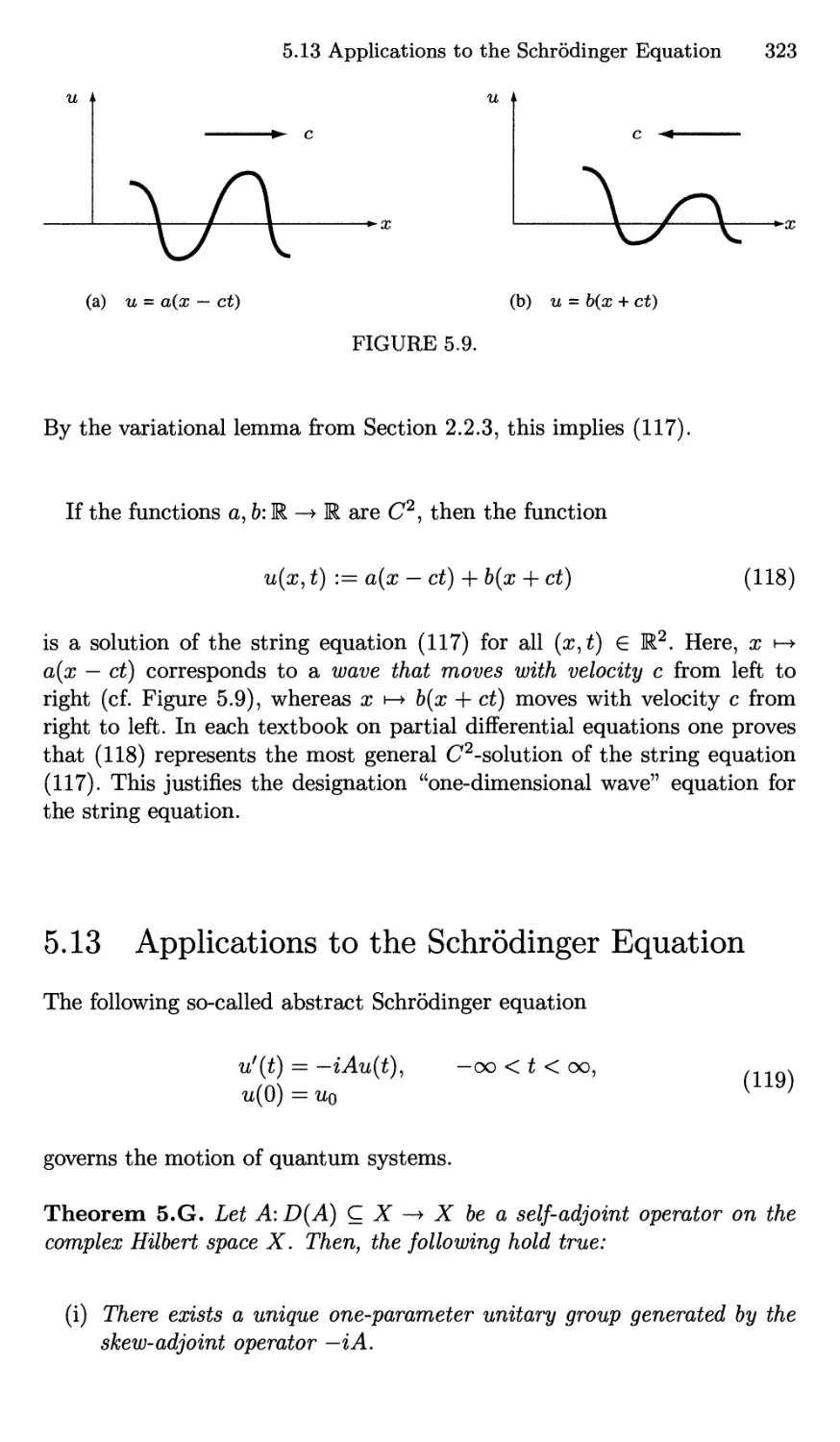
5.11 Applications to the Wave Equation 309
5.12 Applications to the Vibrating String and the Fourier Method 315
5.13 Applications to the Schrodinger Equation 323
5.14 Applications to Quantum Mechanics 327
5.15 Generalized Eigenfunctions 343
5.16 Trace Class Operators 347
5.17 Applications to Quantum Statistics 348
5.18 C*-Algebras and the Algebraic Approach to Quantum
Statistics 357
5.19 The Fock Space in Quantum Field Theory and the Pauli
Principle 363
5.20 A Look at Scattering Theory 368
5.21 The Language of Physicists in Quantum Physics and the
Justification of the Dirac Calculus 373
5.22 The Euclidean Strategy in Quantum Physics 379
5.23 Applications to Feynman's Path Integral 385
5.24 The Importance of the Propagator in Quantum Physics . . 394
5.25 A Look at Solitons and Inverse Scattering Theory 406
Epilogue 425
Appendix
429

xxvi Contents
References 443
Hints for Further Reading 455
List of Symbols 459
List of Theorems 465
List of the Most Important Definitions 467
Subject Index 471

Contents of AMS Volume 109
Preface
Contents of AMS Volume 108
1 The Hahn-Banach Theorem and Optimization
Problems
1.1 The Hahn-Banach Theorem
1.2 Applications to the Separation of Convex Sets
1.3 The Dual Space C[a, b]*
1.4 Applications to the Moment Problem
1.5 Minimum Norm Problems and Duality Theory
1.6 Applications to Cebysev Approximation
1.7 Applications to the Optimal Control of Rockets
2 Variational Principles and Weak Convergence
2.1 The nth Variation
2.2 Necessary and Sufficient Conditions for Local Extrema
and the Classical Calculus of Variations
2.3 The Lack of Compactness in Infinite-Dimensional Banach
Spaces
2.4 Weak Convergence
2.5 The Generalized Weierstrass Existence Theorem
2.6 Applications to the Calculus of Variations
2.7 Applications to Nonlinear Eigenvalue Problems

XXV111
Contents of AMS Volume 109
2.8 Reflexive Banach Spaces
2.9 Applications to Convex Minimum Problems and
Variational Inequalities
2.10 Applications to Obstacle Problems in Elasticity
2.11 Saddle Points
2.12 Applications to Duality Theory
2.13 The von Neumann Minimax Theorem on the Existence of
Saddle Points
2.14 Applications to Game Theory
2.15 The Ekeland Principle about Quasi-Minimal Points
2.16 Applications to a General Minimum Principle via the
Palais-Smale Condition
2.17 Applications to the Mountain Pass Theorem
2.18 The Galerkin Method and Nonlinear Monotone Operators
2.19 Symmetries and Conservative Laws (The Noether
Theorem)
2.20 The Basic Ideas of Gauge Field Theory
2.21 Representations of Lie Algebras
2.22 Applications to Elementary Particles
3 Principles of Linear Functional Analysis
3.1 The Baire Theorem
3.2 Application to the Existence of Nondifferentiable
Continuous Functions
3.3 The Uniform Boundedness Theorem
3.4 Applications to Cubature Formulas
3.5 The Open Mapping Theorem
3.6 Product Spaces
3.7 The Closed Graph Theorem
3.8 Applications to Factor Spaces
3.9 Applications to Direct Sums and Projections
3.10 Dual Operators
3.11 The Exactness of the Duality Functor
3.12 Applications to the Closed Range Theorem and to
Fredholm Alternatives
4 The Implicit Function Theorem
4.1 ra-Linear Bounded Operators
4.2 The Differential of Operators and the Frechet Derivative
4.3 Applications to Analytic Operators
4.4 Integration
4.5 Applications to the Taylor Theorem
4.6 Iterated Derivatives
4.7 The Chain Rule
4.8 The Implicit Function Theorem

Contents of AMS Volume 109 xxix
4.9 Applications to Differential Equations
4.10 Diffeomorphisms and the Local Inverse Mapping Theorem
4.11 Equivalent Maps and the Linearization Principle
4.12 The Local Normal Form for Nonlinear Double Splitting
Maps
4.13 The Surjective Implicit Function Theorem
4.14 Applications to the Lagrange Multiplier Rule
5 Fredholm Operators
5.1 Duality for Linear Compact Operators
5.2 The Riesz-Schauder Theory on Hilbert Spaces
5.3 Applications to Integral Equations
5.4 Linear Fredholm Operators
5.5 The Riesz-Schauder Theory on Banach Spaces
5.6 Applications to the Spectrum of Linear Compact
Operators
5.7 The Parametrix
5.8 Applications to the Perturbation of Predholm Operators
5.9 Applications to the Product Index Theorem
5.10 Fredholm Alternatives via Dual Pairs
5.11 Applications to Integral Equations and Boundary-Value
Problems
5.12 Bifurcation Theory
5.13 Applications to Nonlinear Integral Equations
5.14 Applications to Nonlinear Boundary-Value Problems
5.15 Nonlinear Fredholm Operators
5.16 Interpolation Inequalities
5.17 Applications to the Navier-Stokes Equations
References
Subject Index

1
Banach Spaces and Fixed-Point
Theorems
The role of functional analysis has been decisive exactly in
connection with classical problems. Almost all problems are on the
applications, where functional analysis enables one to focus on a specific
set of concrete analytical tasks and organize material in a clear and
transparent form so that you know what the difficulties are.
Concrete and functional analysis exist today in an inextricable
symbiosis* When someone writes down a system of axioms, no one is
going to take them seriously, unless they arise from some intuitive
body of concrete subject matter that you would really want to study,
and about which you really want to find out something.
Felix E. Browder, 1975
In a Banach space, the so-called norm
\\u\\ = nonnegative number
is assigned to each element u. This generalizes the absolute value \u\ of a
real number u. The norm can be used in order to define the convergence
lim un = u
n—*oo
by means of
lim \\un — u\\ = 0.
n—>oo

1. Banach Spaces and Fixed-Point Theorems
UN C[a, b]
\ /
I Banach space | —► Cauchy convergence criterion
normed space ,. , ,
. II .1 v —► convergence and boundedness
linear space ,.
„. .. J n n ► dimension and convexity
(linear combination au + pv) J
FIGURE 1.1.
As a standard example for a Banach space we will consider the space
C[a,b],
which consists of all continuous functions u: [a, b] —> R along with the norm
\\u\\ := max |^(x)|, where —oo<a<6<oo.
a<x<b
Figure 1.1 shows the relations between Banach spaces and other
important notions. For example, Figure 1.1 tells us that each Banach space is
also a normed space, etc. In this chapter we will prove the two fundamental
fixed-point theorems of Banach and Schauder
along with applications to integral equations and ordinary differential
equations (cf. Figures 1.2 and 1.3). We will show in Chapter 3 of AMS Vol. 109
that the fundamental implicit function theorem is a simple consequence of
the Banach fixed-point theorem.
The first chapter can be understood without any knowledge of the
Lebesgue integral.
1.1 Linear Spaces and Dimension
In the following let
K := R or K := C,
where R and C denote the set of real and complex numbers, respectively.
Roughly speaking, in a linear space X over K it is possible to form "linear
combinations"
au + Pv,
where u,v G X and a,/3 G K. In addition, the "usual rules" hold for
au + Pv.

1.1 Linear Spaces and Dimension 3
k— contraction A
(\\Au - Av\\ < k\\u - v\\, 0 < k < 1)
compact operator A
l
Banach fixed-point theorem
(Au = u)
Schauder fixed-point theorem
{Au = u)
I
Picard-Lindelof theorem for
the ordinary differential
equation y? = F(x, u)
Peano theorem for
the ordinary differential
equation y? = F(x, u)
FIGURE 1.2.
continuous operator convex set
#
Brower fixed-point theorem in EJ
+ compactness
Schauder fixed-point theorem in Banach spaces
\
the Leray-Schauder principle and a priori estimates
FIGURE 1.3.
Definition 1. A linear space X over K is a set X together with an addition
u + v, u, v G X
and a scalar multiplication
au, a G K, uEl,
where all the usual rules are satisfied.
More precisely, for all u, v G X and all a G K,
u + v and au

4 1. Banach Spaces and Fixed-Point Theorems
are defined elements of X such that, for all u,v,w G X and a,/3 G K, the
following are true:
u + v = v + u, (u + v) +w = u + (v + w),
(a + (3)u = au + f3u, a(u + v) = au + av,
a(j3u) = (a/3)u, au = u if a = 1.
Furthermore, there exists exactly one element 0 in X such that
u + 0 = u for all rz G X. (1)
Finally, for each given uEl, the equation
m + v = 6 (2)
has exactly one solution v G X.
X is called a real or complex linear space as K = R or K = C, respectively.
For simplifying notation, let us write
6 := 0 and v := —u
in (1) and (2), respectively. The following proposition shows that this
convention makes sense. We also write w — u instead of w + (—u).
Proposition 2. Let X be a linear space over K. Then:
(i) a6 = 6 for all a G K.
(ii) Ou = 0 for all ueX.
(iii) (—a)u = —(au) for all a G K and u G X.
Proof. Ad (i).1 It follows from
au = a(u + 6) = au + a9
and the unique solvability of the equation au = au + v that v — a6 = 6.
Ad (ii). Since
au = (a + 0)u = au + Ou,
we get Ou = 6.
Ad (iii). It follows from
9 = Ou = (a + (—a))u = au+ (—a)u
xThe Latin term "Ad (i)" stands for "proof of (i)."

1.1 Linear Spaces and Dimension 5
that -(aw) = {—a)u. □
Example 3. Let X := K. Then, X is a linear space over K, where
au + (3v with a,(3 G K and u,v E X
is to be understood in the classical sense.
Example 4. Let X := KN, where JV = 1,2,...; that is, the set X consists
of all the TV-tuples
x — (f i> • • • > £w) with ffeEK for all k.
Define
(£i, • • • ,6v) + fai,. • •, ^at) = (£1 + fr,... ,6v + m),
a(£i,...,6v) = (afi,...,a&\r), a G K.
Then, X becomes a linear space over K.
Obviously, 6 = (0,... ,0).
Example 5. Let C[a, b] denote the set of all continuous functions
u: [a, b] -> R,
where —oo < a < b < oo. For u,v e C[a, 6] and a G R, let
u + v and au
denote the corresponding functions, i.e.,
(u + v){x) — u{x) + v(x) and (au)(x) = au(x) for all x G [a, 6].
Since the sum and the product of two continuous functions are again
continuous, we get
u + v£ C[a, b] and au G C[a, 6].
Thus, C[a, b] becomes a real linear space.
Definition 6. Let X be a linear space over K. The elements ui,..., u^ of
X are called linearly independent iff
aiui -\ h a^UM = 0 with a/c G K for all k
always implies ai = • • • = a at = 0.
Let N = 1,2,.... We write
dim X = N

6 1. Banach Spaces and Fixed-Point Theorems
iff the maximal number of linearly independent elements in X is equal to
N. The number N is called the dimension of X.
We write
dim X — oo
iff, for each N = 1,2,..., there exist N linearly independent elements in
X. In this case, X is called an infinite-dimensional space.
For X = {0}, we set dim X = 0.
The space X is called finite-dimensional iff 0 < dim X < oo.
Example 7. Let X := K. Then dim X = 1.
Here, X is considered to be a linear space over K.
Proof. Let u G X with u ^ 0. Then
au = 0 implies a = 0.
Hence X contains at least one linearly independent element.
Let u and v be two linearly independent elements of X, i.e.,
au + j3v = 0 with a, /? G K implies a - /? = 0. (3)
Hence w^O and v ^ 0. Setting
a := — and p := —1,
u
we obtain a contradiction to (3). Thus, there are no two linearly
independent elements in X, i.e., dim X = 1. □
The following result is well known from the course on linear algebra.
Example 8. Let X := KN for fixed N = 1,2,..., where X is considered
to be a linear space over K.
Then, dim X = N.
Example 9. Let X := C[a,b]. Then, dim X = oo.
Proof. Set
Uk(x) := xk for all x G [a, b] and k = 0,1,... .
Let ao,..., aw G R. It follows from
aoUo + ai^i H h a^^N = 0 in C[a, 6]
that
a0 + aix + a2#2 H h olnxN = 0 for all x G [a, 6].

1.2 Normed Spaces and Convergence 7
Since a proper polynomial has only a finite number of zeros, we get a\ =
• • • = o/v = 0.
Consequently, for each N = 1,2,..., the elements uo,..., un in C[a, b]
are linearly independent, i.e., dim C[a, b] = oo. □
Definition 10. HA and B are subsets of a linear space over K, then we
set
A + B
olA
AxB
= {a + b: a G A and b G £},
= {aa:a e A}, a€
= {(a,b):aeA, b G B}.
1.2 Normed Spaces and Convergence
Recall that K := R or K := C.
Definition 1. Let X be a linear space over K.
Then, X is called a normed space over K iff there exists a norm || • || on
X, i.e., for all u, v £ X and a G K, the following are true:
(i)
(ii)
(iii)
(iv)
\u\\ > 0 (i.e., \\u\\ is a nonnegative real number).
HI =0iffrz = 0.
\au\\ = \a\\\u\\.
\u + v\\ < 11xx|| + |H| (triangle inequality).
A normed space over K = R or K = C is called a real or complex normed
space, respectively.
The number \\u — v\\ is called the distance between the two points u and
v. In particular,
|HI = distance between the point u and the origin v = 0.
Since — u — (—l)u, relation (iii) implies
|| - u\\ = \\u\\ for all u € X. (4)
It follows from (iv) that
\\(u + v)+ w\\ < \\u + v|| + \\w\\ < \\u\\ + ||v|| + \\w\\.
Analogously, by induction, we get
N
J2uj
3=1
N
— /J WujW ^or all ui,... ,^iv ^ -X', N = 1,2,... .

8 1. Banach Spaces and Fixed-Point Theorems
Example 2. Let X := R. We set
\\u\\ := \u\ for all uGR,
where \u\ denotes the absolute value of the real number u.
Then, X becomes a real normed space.
Example 3. Let X := C. We set
HI := \u\ for all u G C,
where \u\ denotes the absolute value of the complex number u.
Then, X becomes a complex normed space.
In these two examples, the triangle inequality (iv) from Definition 1
corresponds to the classical triangle inequality for real and complex numbers.
The norm generalizes the absolute value of numbers.
Further examples will be considered in the next section.
Proposition 4 (Generalized triangle inequality). Let X be a normed space.
Then, for all u, v G X,
|||«||-H|<||«±t;||<||«|H-|H|. (5)
Proof. By the triangle inequality,
||«±t;|| = ||« + (±i;)||<||«|| + ||±i;|| = ||u|| + |H|,
and
HI = \\(u - v) + v|| < \\u - v\\ + ||v||.
Hence
||u||-|M|<||«-i;||.
Analogously,
H-|M|<||«-u|| = ||«-t;||.
This implies
|HI-N|<II«-«||.
Replacing v with — v and observing that u—(—v) = u+v and ||— v\\ = \\v\\,
we also get
|H|-||v||| < \\u + v\\. D
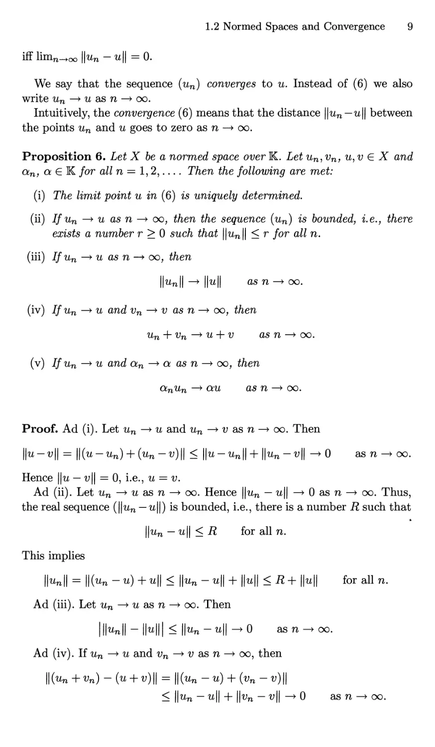
Definition 5. Let (un) be a sequence in the normed space X, i.e., un G X
for all n. We write
lim un = u (6)
n—>-oo

1.2 Normed Spaces and Convergence 9
iff limn_^oo ||rzn - u\\ = 0.
We say that the sequence (un) converges to u. Instead of (6) we also
write un —> u as n —> oo.
Intuitively, the convergence (6) means that the distance \\un—u\\ between
the points un and u goes to zero as n —> oo.
Proposition 6. Let X be a normed space over K. Let un,vn, u,v £ X and
an, a £ K /or all n = 1,2, T/ien £/ie following are met:
(i) T/ie /irm£ poin£ u in (6) 25 uniquely determined.
(ii) Jjf un —> u as n —> oo, £/ien £/ie sequence (un) is bounded, i.e., there
exists a number r > 0 si/c/i £/m£ ||un|| < r /or all n.
(iii) If un ^ u as n —> oo, £/ien
||un|| —> ||u|| as n —> oo.
(iv) If un —> u and vn ^ v as n —> oo, £/ien
^n + ^n —> ^ + v as n —> oo.
(v) Ifun^u and an —> a as n —> oo, £/ien
<^n^n -> cm as n —> oo.
Proof. Ad (i). Let un —> u and un —> v as n —> oo. Then
||w-v|| = ||(w-Wn)H-(^n-v)|| < ||u-un|| + ||un-v|| —> 0 as n —► oo.
Hence ||u — v|| = 0, i.e., u = v.
Ad (ii). Let un —> u as n —> oo. Hence ||un — u|| —> 0 as n —> oo. Thus,
the real sequence (\\un — u\\) is bounded, i.e., there is a number R such that
||^n — ^|| < -R for all n.
This implies
||^n|| = \\{un —u) + u\\ < \\un - u\\ + \\u\\ < R + ||it|| for all n.
Ad (iii). Let un —> u as n —> oo. Then
|||^n|| - HI| < ||^n - u\\ -> 0 as n -> oo.
Ad (iv). If un —> u and vn —> i? as n —> oo, then
|| (l/n+Vn) - (W + V)|| = ||(lZn ~ ^) + (vn ~ v)\\
< \\un — u\\ + ||vn — -L^H —^ 0 as n —> oo.

10 1. Banach Spaces and Fixed-Point Theorems
Ad (v). If un —> u and an —> a as n —> oo, then
||anun - aw|| = ||(an - a)un + a(un - u)\\
< ||(an - a)rzn|| + \\a(un - u)\\
< \an - a\ • ||itn|| + |a| • \\un - u\\
< \an — a\r + |a| • \\un — u\\ —> 0 as n —> oo. D
Definition 7. The sequence (un) in the normed space X is called a Cauchy
sequence iff, for each e > 0, there is a number no(e) such that
ll^n — ^m|| < £ fc>r all n,m> no(e).
Proposition 8. In a normed space, each convergent sequence is Cauchy.
Proof. Let un —> u as n —> oo. Hence ||un — u|| —> 0 as n —> oo, i.e., for
each e > 0, there is a number no(e) such that
\\un — u\\<- for all n > no(e).
This implies
||^n - Um\\ = \\(un -U) + (U- Um)\\
< \\un — u\\ + \\u — um\\ < £ for all n,ra > no(e). □
1.3 Banach Spaces and the Cauchy Convergence
Criterion
Definition 1. The normed space X is called a Banach space iff each Cauchy
sequence is convergent.
Therefore, from Proposition 8 in the preceding section, we get the
following so-called Cauchy convergence criterion:
In a Banach space, a sequence is convergent iff it is Cauchy.
Banach spaces are also called complete normed spaces.
Example 2. The space X := K is a Banach space over K with the norm
\\u\\ := \u\ for all uEK.

1.3 Banach Spaces and the Cauchy Convergence Criterion 11
This follows from the classical Cauchy convergence criterion.
Example 3. Let N = 1,2, The space X := KN is a Banach space over
K with the norm ||x|| := |x|oo? where
Moo := max Ifj|, x= (fi,...,fw).
l<j<iV
Let xn = (fin,..., fNn). Then
lim \xn - x|oo = 0 iff lim ffcn = ffe for all k = 1,..., N. (7)
n—►oo n—►oo
That is, the convergence xn —> x as n —> oo in X is equivalent to the
convergence of the corresponding components.
Proof. The inequality
If fen - ffc| < \xn - ^|oo = max |fjn - fj|
l<j<iV
implies statement (7). In fact, if \xn — x\oq —> 0 as n —> oo, then ffcn —> f^
as n —> oo for all fc, and the converse is also true.
Let us now prove that | • |oo 1S a norm. Obviously,
Moo = 0 ^ f j = 0 for aH j <^> x = 0,
and
|oMoo = max \a\ |f7| = |a| max |f7| = \a\ |x|oo-
Furthermore, the classical triangle inequality
|fi+%| < lfjl + 1%1 forfj,% GK
implies
\x + y\oo= max |f?+ry?|< max |f7|+ max \rjj\
1 ' i<j<NlJ Jl i<j<NlJl i<j<Nl Jl
= Moo + Moo-
Finally, we have to show that X is a Banach space with respect to the
norm | • l^. To this end, let (xn) be a Cauchy sequence. Then
Iffcn - f fern I < \xn ~ ^m|oo < £ for all 71, 771 > n0(s).
Thus, the sequence (ffcn) is also Cauchy. The classical Cauchy convergence
criterion implies the convergence
lim ffcn =ffe, k = l,...,iV.

12 1. Banach Spaces and Fixed-Point Theorems
By (7), xn —> x as n —> oo. D
Example 4. Let N = 1,2, The space X := R^ is a Banach space with
the Euclidean norm \\x\\ := |x|, where
Moreover,
lim |xn — x\ = 0 iff lim ^n = £& for all k = 1,..., N. (8)
n—>-oo n—>-oo
Convention 5. If we do not explicitly express the contrary, then the space
RN is equipped with the Euclidean norm | • |.
Proof. Statement (8) follows from (7) by using the following inequality:
|«^n «^|oo _ \^n «£| _ ■** \^n ^loo*
Next we want to prove that | • | is a norm. Obviously,
\x\ = 0 & £j = 0 for all j o x = 0,
and
|ax| = \a\ \x\ for all a G R, x G R^.
To prove the triangle inequality
\x + y\< \x\ + \y\ for all x, y G RN, (9)
we will use the classic Schwarz inequality
N \ N N
E^ ^E^E^ (10)
for all real numbers £j, 77^, jf = 1,..., N. Hence
N N
+ y\2 = E& + ^)2 = E 3 + 2^ + ^2
'7l
j=l j=l
2 / ^ \ 2
AT /AT \ I M \ N
= |x|2 + 2|x|M + M2 = (|x| + M)2.

1.3 Banach Spaces and the Cauchy Convergence Criterion 13
This implies (9).
It remains to prove (10). Prom 0 < (a ± b)2 = a2 ± 2ab + b2 we get
±2ab <a2 + b2 for all a, b G R.
Choosing a := £j/(X^i£|J2 and & := Wj/ \J2?=iWj) and summing
over j, it follows that
(Eli, <?) *&•)?)
This implies (10).
Finally, we have to show that RN is a Banach space with respect to the
Euclidean norm | • |. To this end, let (xn) be a Cauchy sequence with respect
to the norm | • |. It follows from
\xn — ^m|oo < \xn — xm\ < e for all n,m> no{e)
that (xn) is also a Cauchy sequence with respect to the norm | • l^. By
Example 3, we get the convergence
lim £kn = £fc for all fc,
n—>-oo
and hence (8) implies \xn — x| —> 0 as n —> oo. D
Standard Example 6. Let —oo < a < b < oo. Then, X := C[a,b] is a
real Banach space with the norm
HI := max \u(x)\.
a<x<b
The convergence wn-^win!asn^oo means
\\un — u\\ = max \un{x) — u{x)\ —> 0 as n —> oo,
a<x<b
i.e., the sequence (un) of continuous functions un:[a,b] —> R converges
uniformly on [a, 6] to the continuous function u: [a, 6] —> R.
Proof. We first prove that || • || is a norm. Obviously,
||cm|| = max \a\ \u(x)\ = \a\ max \u(x)\ = \a\ \\u\\,
a<x<b a<x<b
for all a € R, u G X, and
i<^ m
a<
& u{x) = 0 on [a, 6] «» rz = 0 in C[a, b].
\\u\\ = 0 <^> max |^(x)| = 0
a<#<&

14 1. Banach Spaces and Fixed-Point Theorems
Moreover, from \u(x) + v(x)\ < \u(x)\ + \v(x)\ we get the triangle inequality
\\u + v\\ < H| + ||v||.
Finally, we have to show that X = C[a,b] is a Banach space. Let (un)
be a Cauchy sequence in X, i.e.,
\\v>n — v>m\\ — max \un(x) — um(x)\ < e for all n, ra > no(e). (11)
a<x<b
This implies the pointwise convergence
un{x) —> uix) as n —> oo for each x £ [a, 6]. (12)
Letting m —> oo in (11), we obtain
max \un(x) — u(x)\ < e for all n > no(e).
a<x<b
Thus, the convergence in (12) is uniform on the interval [a, b]. By a classical
result, this implies the continuity of the limit function u: [a, b] —> R. Hence
u G X and
un —> u in X as n —> oo. D
Proposition 7. Le£ (wn) 6e a Cauchy sequence in the normed space X
overK, which has a convergent subsequence (unt), that is,
un> —> u in X as n —> oo.
TAen, £Ae entire sequence converges to u, i.e., un —> u in X as n —> oo.
Proof. Let £ > 0 be given. There is an no(e) such that
Wun — um\\ < £ for all n, ra > no(e).
Since (unf) converges to u, there exists some fixed index m such that
ll^m — ^|| < £> where ra > no(s).
By the triangle inequality,
ll^n — ^|| < ||^n — ^m|| + ll^m ~ ^|| < 2e for all n > no(e).
Hence un —> u as n —> oo. □
Corollary 8. Suppose that
oo
2lK-+i-«j|| <oo,

1.4 Open and Closed Sets 15
where (un) is a sequence in a normed space X over K. Then, (un) is a
Cauchy sequence in X.
Proof. By the triangle inequality, for all k = 1,2,..., we get
oo
\\un - un+k\\ < ^jT \\uj+i - Uj\\ -> 0 as n -> oo. D
j=n
1.4 Open and Closed Sets
Definition 1. Let X be a normed space. For fixed u0 G X and e > 0, the
set
U€{u0) := {u e X: \\u - u0\\ < e}
is called an e-neighborhood of the point u0.
The subset M of X is called open iff, for each point u0 G M, there is
some e-neighborhood Ue(u0) such that
Ue(uo) C M
(cf. Figure 1.4). The subset M of X is called closed iff the set X - M is
open.
Recall that X — M := {u £ X: u 0 M}. By an open neighborhood U(u)
of the point u, we understand an open subset of X containing u.
Proposition 2. Let M C X, where X is a normed space. Then, the
following are equivalent:
(i) M is closed.
(ii) It follows from un G M for all n and
un —> u as n —> oo
that ue M.
Proof, (i) => (ii). Let un —> u as n —> oo and un e M for all n. We have
to show that u 6 M. If this is not true, then u G X — M. Since the set
X — M is open, there is some ^-neighborhood Ue(u) such that
U£(u) CX-M.
From ||un — u\\ —> 0 as n —> oo we get ||um — u\\ < e for some index m, and
hence
um e U£(u),

16 1. Banach Spaces and Fixed-Point Theorems
\ v •no j
\ -^.— "
v.
(a) open set
■ U£(u0) \
J
/
/
(b) closed set
FIGURE 1.4.
i.e., um G X — M. This contradicts um € M.
(ii) => (i). Suppose that the set M is not closed, i.e., the set X — M is
not open. Then, there exists a point
ueX-M
such that no ^-neighborhood U£(u) is contained in the set X — M. Thus,
choosing e = ^, n = 1,2,..., we get a sequence (un) in X — M such that
un G CA (u) and un € M for all n.
Hence
■■ 1
Nn —v>\\< ► 0 as n —> oo.
n
By (ii), ue M. This contradicts ue X - M. D
Example 3 (Balls). Let X be a normed space. For fixed v e X and fixed
r > 0, define
B := {ue X: \\u - v\\ < r}.
Then, B is closed.
The set B is called a closed ball of radius r around the point v.
Proof. Let un e B for all n, i.e.,
\\v>n — v\\ < r for all n.
If un —> ia as n —> oo, then ||it — v|| < r, and hence ue B. □
1.5 Operators
Definition 1. Let M and Y be sets. An operator
A:M^Y

1.5 Operators 17
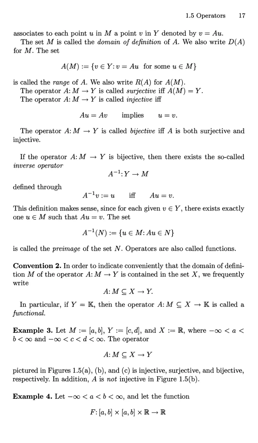
associates to each point winMa point v in Y denoted by v = Au.
The set M is called the domain of definition of A. We also write D(A)
for M. The set
A(M) := {v g7:d = Au for some u G M}
is called the range of A. We also write R(A) for A(M).
The operator A:M —> Y is called surjective iff A(M) = Y.
The operator A: M —> Y is called injective iff
^4ia = Ai? implies u = v.
The operator ^4: M —> y is called bijective iff ^4 is both surjective and
injective.
If the operator A: M —> Y is bijective, then there exists the so-called
inverse operator
A~X:Y ^M
defined through
A~xv := i£ iff ^4ia = v.
This definition makes sense, since for each given v G Y, there exists exactly
one u e M such that ^4ia = v. The set
^-!(Ar) :={ueM:AueN}
is called the preimage of the set AT. Operators are also called functions.
Convention 2. In order to indicate conveniently that the domain of
definition M of the operator A: M —> Y is contained in the set X, we frequently
write
A: M C X -► Y.
In particular, if Y = K, then the operator A: M C X —> K is called a
Example 3. Let M := [a, 6], Y := [c, d], and X := R, where —oo < a <
b < oo and —oo < c < d < oo. The operator
pictured in Figures 1.5(a), (b), and (c) is injective, surjective, and bijective,
respectively. In addition, A is not injective in Figure 1.5(b).
Example 4. Let —oo<a<6<oo, and let the function
F: [a, b] x [a, b] x R -> R

18 1. Banach Spaces and Fixed-Point Theorems
-H
-+-
a b
(a) injective
be continuous. We set
a/
(b) surjective
FIGURE 1.5.
(c) bijective
and
(Au)(x) := / F(x,y,u(y))dy for all x G [a, 6],
-/a
fb
(Bu)(x) := / F(x,y,u(y))dy for all x G [a, b],
J a
Then, we obtain the two operators
A: C[a, b] -► C[a, b] and B: C[a, b] -► C[a, b].
In fact, it is a well-known classical result that the continuity of the function
u: [a, b] -> R
implies the continuity of the two functions
Au: [a, 6] -> R and £u: [a, 6] -> R,
i.e., ia G C[a, 6] implies both ^4ia G (7[a, 6] and £??i G C[a, 6].
The operators A and £? are called integral operators.
1.6 The Banach Fixed-Point Theorem
and the Iteration Method
The Banach fixed-point theorem represents a fundamental
convergence theorem for a broad class of iteration methods.
We want to solve the operator equation
u = Au, ue M,
by means of the following iteration method:
un+i = Aun,
71 = 0,1, ....
(13)
(14)

1.6. The Banach Fixed-Point Theorem and the Iteration Method 19
where uq G M. Each solution of (13) is called a fixed point of the operator
A.
Theorem l.A (The fixed-point theorem of Banach). We assume that:
(a) M is a closed nonempty set in the Banach space X over K, and
(b) the operator A: M —> M is k-contractive, i.e., by definition,
\\Au - Av\\ < k\\u - v|| for all u,v e M, (15)
and fixed k, 0 < k < 1.
Then, the following hold true:
(i) Existence and uniqueness. The original equation (13) has exactly one
solution u, i.e., the operator A has exactly one fixed point u on the
set M.
(ii) Convergence of the iteration method. For each given Uq G M, the
sequence (un) constructed by (14) converges to the unique solution u
of equation (13).
(iii) Error estimates. For all n = 0,1,... we have the so-called a priori
error estimate
IK - ti|| < kn{\ - £0_1|K - "oil, (16)
and the so-called a posteriori error estimate
IK+i - u\\ < fc(l - fc)_1||tin+i - un\\. (17)
(iv) Rate of convergence. For all n = 0,1,... we have
IK+i -u\\ < k\\un-u\\.
This theorem was proved by Banach in 1920. The Banach fixed-point
theorem is also called the contraction principle.
The a priori estimate (16) makes it possible to use a knowledge of the
initial value Uq along with u\ = Auq to determine the maximal number of
steps of iteration required to attain a desired level of precision.
In contrast to this, the a posteriori estimate (17) allows the use of the
computed values un and Mn+i to determine the accuracy of the
approximation Mn+i.

20 1. Banach Spaces and Fixed-Point Theorems
Experience shows that, as a rule, a posteriori estimates are better than
a priori estimates.
Proof. Ad (i), (ii). Step 1: We show first that (un) is a Cauchy sequence.
Let n = 1,2, Using (15) we get
\\Un+l ~ Un\\ = \\AUn - AUn-l\\ < k\\Un - Un-l||
= k\\Aun-i - Aun-2\\ < k2\\un-i - un-2\\
<---<fcn||tii-tio||.
Now let n = 0,1,... and m = 1,2, The triangle inequality and the sum
formula for the geometric series yield
\\un - Un+m\\ = \\(un - Un+i) + (wn+l ~ ^n+2) H h (Mn+m-1 ~ ^n+m)||
< ||?in - tAn+l|| + ||^n+l - ^n+2|| H h ||^n+m-l ~ ^n+m||
< (fcn + fcn+1 + • • • + fcn+m_1)K - tio||
<fcn(l + fc + fc2 + -.-)IK-u0||
= fcn(l-fc)"1||w1 -Uq\\.
It follows from 0 < k < 1 that kn —> 0 as n —> oo. Hence the sequence (wn)
is Cauchy.
Since X is a Banach space, the Cauchy sequence (un) converges, i.e.,
un —> ia as n —> oo.
5£ep #: We show that the limit point u is a solution of the original
equation (13).
Prom uq G M and wi = Auq along with A(M) C M, we get wi G M.
Similarly, by induction,
un e M for all n = 0,1,... .
Since the set M is closed, we obtain
1*6 M,
and hence Au G M. By (15),
\\Aun — Au\\ < k\\un — u\\ —> 0 as n —> oo.
Letting n —> oo it follows from izn+i = A?in that
u = A?i.
5fep 5: We show the uniqueness of the solution w of (13). It follows from
Au = u and Av = v with u,v € M that
||u - v|| = 11 Aw - Av\\ < k\\u - v\\.

1.6. The Banach Fixed-Point Theorem and the Iteration Method 21
Since 0 < k < 1, this implies \\u — v\\ = 0, and hence u = v.
Ad (iii). Letting m —> oo it follows from
IK - un+m\\ < kn(\ - fc)-1!!^! - w01|
that
IK - u\\ < kn{\ - k)-1^ - uq\\ for all n = 0,1,... .
This is the error estimate (16).
Let n = 0,1,... and m = 1,2, To prove the error estimate (17),
observe that
IK+l - ^n+m+l|| < IK+1 ~ ^n+2|| + IK+2 ~ ^n+3||
H h ||^n+m
<(k + k2 + --- + km)\\un-un+1\\.
Letting m —> oo we get
||wn+l - u\\ < k{\ - fc)-1|K ~ ^n+l||-
Ad (iv). Observe that
|K+i - u\\ = \\Aun - Au\\ < k\\un - u\\. D
Example 1. Let —oo<a<6<oo. Suppose that we are given the
differentiable function
A: [a, b] —► [a, b]
such that
\A'(u)\ < k < 1 for all u G [a, b) and fixed k.
Then, Theorem l.A can be applied to the equation
u = An, u e [a, b] (18)
with M := [a, 6], X := R, and the norm \\u\\ := \u\.
In particular, equation (18) has a unique solution u. This solution
corresponds to the intersection point between the graph of A and the diagonal
in Figure 1.6.
Proof. The set M = [a, b] is closed in the real Banach space X = R.
By the classical mean value theorem, for each u, v G [a, 6], there exists a
point w G [a, b] such that
\Au - Av\ = \A'{w){u - v)\ < k\u - v\,
i.e., the function A: [a,b] —> [a, b] is fc-contractive.
Therefore, the assumptions of Theorem l.A are satisfied. □

22 1. Banach Spaces and Fixed-Point Theorems
FIGURE 1.6.
1.7 Applications to Integral Equations
We want to solve the integral equation
u(x) = \ f F(x, y, u{y))dy + /(x), a < x < 6, (19)
J a
along with the iteration method
un+i{x) = \l F{x,y,un{y))dy + f(x), a <x < 6, ra = 0,1,... , (19*)
-/a
where u0(x) = 0 and —oc < a < 6 < oo.
Proposition 1. Assume the following:
(a) TAe function f: [a, 6] —> R is continuous.
(b) TAe function F: [a, 6] x [a, b] x R —> R is continuous, and the partial
derivative
Fu:[a,b] x [a,6] xR^R
is also continuous.
(c) TAere is a number C such that
\Fu(x,y,u)\ < C for all x,y € [a, 6], wGR.
(d) Le£ £Ae reaZ number A 6e #wen si/cA that (b — a)|A|£ < 1.
(e) Set X := C[a,b] and \\u\\ := maxa<x<6 |w(x)|.
TAen, £Ae following hold true:
(i) TAe original problem (19) Aas a unique solution u 6 X.
(ii) TAe sequence (un) constructed by (19*) converges to u in X.

1.7 Applications to Integral Equations 23
(iii) For all n = 0,1,2,... we get the following error estimates:
IIUn-till^fc^l-fcr^ltiiH,
\\un+i — u\\ < fc(l — fc)-1||?in+i — Un\\, where k := (b — a)|A|£.
Proof. Define the operator
(Au)(x) := A / F{x,y,u{y))dy + /(#) for all x G [a, 6].
«/ a
Then, the original equation (19) corresponds to the fixed-point problem
u = An.
/\i u: [a, b] —> R is continuous, then so is the function Aw. [a, b] —> R. This
way we get the operator
AiX^X.
For each x, y G [a, 6] and w,^eR, there exists a w € R such that
\F(x,y,u) - F(x,y,v)\ < \Fu(x,y,w)\\u-v\ <C\u-v\,
by the classical mean value theorem. This implies
\\Au - Av\\ = max \(Au)(x) - (Av)(x)\
a<x<b
<\\\{b — a)C max \u{x) — v(x)\.
a<x<b
Hence
\\Au - Av\\ < k\\u - v\\ for all u, v € X.
Letting M := X, the assertions follow now from the Banach fixed-point
theorem (Theorem l.A in Section 1.6). □
Example 2 (Linear integral equation). Let
F(x,y,u):=K(x,y)u, (20)
and suppose that the function K : [a, b) x [a, 6] —> R is continuous.
Then, the assumptions of Proposition 1 are satisfied with
£= max \K(x,y)\.
Therefore, all the statements of Proposition 1 are true for the integral
equation (19) with (20).
In the special case (20), the original problem (19) is called a linear integral
equation.

24 1. Banach Spaces and Fixed-Point Theorems
FIGURE 1.7.
1.8 Applications to Ordinary Differential
Equations
We want to solve the following initial-value problem:
u' = F(x, u), x0 — ft < x < x0 + ft,
U(X0) = Uq,
where the point (xo, ^o) G R2 is given. More precisely, we are looking for a
solution u = u(x) of (21) such that
(21)
u: [x0 — ft, x0 + ft] —> R is differentiable, and
(x,u(x)) G S for all x G [xq — ft,Xq + ft],
(21*
with the square S := {(x, u) G R2: \x — Xo| < r and \u — u$\ < r} for fixed
r > 0 (see Figure 1.7). We set
X := C[xo — ft,Xo + ft] and M := {u G X: \\u — uq\\ < r}.
Recall that \\u\\ = maxa<a;<b |^(x)|.
Parallel to (21), (21*) let us consider the integral equation
u(x) = uq + / F(y, u(y))dy, Xo — ft < x < Xo + ft, u G M, (22)
Jxo
along with the iteration method
px
Wn+iW = uo+ F(y, un(y))dy, x0 - ft < x < x0 + ft, n = 0,1,...,
where uq(x) = uq.
(23)
Proposition 1 (The Picard-Lindelof theorem). Assume the following:
(a) The function F: S —> R 25 continuous and the partial derivative
FU:S ^R
25 a/50 continuous.

1.8 Applications to Ordinary Differential Equations 25
(b) We set
M := max \F(x,u)\ and £ := max |Fu(x,u)|,
(x,u)es (x,u)es
and we choose the real number h in such a way that
0 < h < r, hM < r, and hC < 1.
Then, the following hold true:
(i) The original problem (21) has a unique solution of the form (21*).
(ii) This is also the unique solution of the integral equation (22).
(iii) The sequence (un) constructed by (23) converges to u in the Banach
space X.
(iv) For n = 0,1,... we have the following error estimates:
\\u>n — V>\\ < kn(l — fc)_1||ui — M0||,
||un+i — u\\ < k(l — fc)_1||un+i — un\\, where k := h£.
Proof. Step 1: The integral equation. Define the operator A through
fx
(Au)(x) := uq + / JF(y, u{y))dy for all x G [xq — h, Xq + ft].
Jxq
Then, the integral equation (22) corresponds to the following fixed-point
problem:
u = Au, ueM. (22*)
If u G M, then the function u: [xq — ft, Xo + ft] —> R is continuous and
(x,u(x)) G S for all x G [xq — ft, Xo + ft]. Therefore, the function
x h-> F(x,u(x))
is also continuous on the interval [x0 — ft, Xo + ft]. This implies the continuity
of the function
Au: [xo — ft, x0 + ft] —> M.
This way we get the operator
A- M ^ X.
Let us prove that
(a) A{M) C M.

26 1. Banach Spaces and Fixed-Point Theorems
(b) \\Au - Av\\ < k\\u - v\\ for all u, v G M.
Ad (a). Let u G M. Then
I fx
\ F{y,u{y))dy
\Jxq
<|x —x0| max \F{y,u)\
(y,u)eS
< hM < r for all x G [x0 - ft,Xo + ft],
and hence
\\Au-uq\\= max / F(y,u(y))dy
xo-h<x<xo+h \JXQ
<r,
'Xq
i.e., Au e M.
Ad (b). By the classical mean value theorem,
\F(x,u) — F(x,v)\ = \Fu(x,w)\\u — v\ < C\u — v\
for all (x, u), (x, v) G S. Observe that w depends on u and v, where (x, w) G
S. Hence, for all u, v G M, we obtain
|| Au — Av\\ — max
xq— h<x<xo+h
f [F(y,u(y)) - F(y,v(y))\dy
Jxo
< hC max \u{y) — v(y)\ = k\\u — v\\,
xo—h<y<xo+h
where k := hC.
We now apply the Banach fixed-point theorem (Theorem l.A in Section
1.6) to equation (22*). This yields the statements concerning the integral
equation (22).
Step 2: Equivalence. Let u be a solution of the integral equation (22).
Differentiating (22), it follows that the function u is also a solution of the
original initial-value problem (21), (21*).
Conversely, let u be a solution of (21), (21*). Integration of (21) shows
that the function u is also a solution of the integral equation (22).
Therefore, the two problems (21), (21*) and (22) are equivalent. □
The following three sections serve as a preparation for the proof of the
fundamental Schauder fixed-point theorem, which allows a generalization of
the Picard-Lindelof theorem. The basic notions to be considered are:
continuity, convexity, and compactness.
1.9 Continuity
Definition 1. Let X and Y be normed spaces over K. The operator
A'.MCX^Y (24)

1.9 Continuity 27
is called sequentially continuous iff, for each sequence (un) in M,
lim un = u with u £ M implies lim Aun = Au.
n—►oo n—xx>
The operator ^4 in (24) is called continuous iff, for each point u e M and
each number e > 0, there is a number 6(e, u) > 0 such that
||v - rz|| < 6(e, u) and wgM imply \\Av - Au\\ < e. (25)
In addition, if it is possible to choose the number 6(e, u) > 0 in such a
way that it does not depend on the point u £ M, then the operator A in
(24) is called uniformly continuous.
Example 2. Let X and Y be normed spaces over K. The operator A: M C
X —> y is called Lipschitz continuous iff there is a number L > 0 such that
\\Av - Au\\ < L\\v - u\\ for all u, v £ M. (26)
Each Lipschitz continuous operator is uniformly continuous.
In fact, condition (26) implies (25) with 6(e) = f.
Proposition 3. We are given the operator A: M C X —> Y, where X
and Y are normed spaces over K. Then, the following two statements are
equivalent:
(i) A is continuous.
(ii) A is sequentially continuous.
Proof, (i) =4> (ii). Suppose that A is continuous. Let
un —> u as n —> oo, where un, u £ M for all n.
Then, for each e > 0, there is a number no such that
\\un — u\\ < 8(e, u) for all n > no,
where the number 8 corresponds to (25). It follows from (25) that \\Aun —
Au\\ < e for all n > no- Hence
Aun —> Au as n —> oo.
(ii) => (i). Suppose that the operator A is not continuous. Then, there
exists a number £o > 0 such that condition (25) is violated for each number
8 > 0. In particular, when 8 = ^ there is a point un £ M such that
\\un — u\\ < — and \\Aun — Au\\ > £q for all n = 1,2,... .

28 1. Banach Spaces and Fixed-Point Theorems
Hence un —> u as n —> oo. By (ii),
Aun —> ^4u as n —> oo.
This contradicts \\Aun — Au\\ > £q for all n. D
Proposition 4 (Composition of continuous operators). Let
A.MCX^Y and B:A(M) -► Z
be two continuous operators, where X, Y, and Z are normed spaces over
K. Set C := B o A, i.e.,
Cu := B(Aiz) /or a// u G M.
Then, the operator C:M ^> Z is continuous.
Proof. Let un, u G M for all n. Then, Aun, Au G A(M) for all n. It follows
from un —> u as n —> oo that
^4un —> ^4u as n —> oo,
and hence B{Aun) —> J3(Am) as n —> oo. D
Definition 5. Let M and Y be subsets of normed spaces over K. The
operator
A:M^Y
is called a homeomorphism iff it is continuous and bijective, and the inverse
operator A-1: Y —> M is also continuous.
The two sets M and Y are called homeomorphic iff there exists a
homeomorphism A: M —> Y.
Example 6. Let r, a, 6 > 0. The disk
D:={(£,77)GR2:£2+y <r2}
and the ellipse
£:={(£,,) €K2:g + g<l}
are homeomorphic. The homeomorphism A: D —> .E is given through
along with the inverse operator ^4_1(^,ry) = r(a~1£,b~1r)) (see Figure 1.8).
The intuitive meaning of a homeomorphism is a "rubber-sheet
transformation. "

1.10 Convexity 29
FIGURE 1.8.
l.lp Convexity
Definition 1. The set M in a linear space is called convex iff
u, v £ M and 0 < a < 1 imply au + (1 — a)v £ M.
The function /: M —► R is called convex iff M is convex and
/(au + (1 - a)v) < a/(u) + (1 - a)/(v),
for all u,v e M and all a, 0 < a < 1.
Intuitively, the convexity of the set M means that if the two points u
and v belong to M, then the segment joining them also belongs to M (see
Figure 1.9(a)).
The convexity of the real function /: [a, b] —> R means that the chords
always lie above the graph of / (see Figure 1.9(b)).
Example 2. Let X be a normed space, and let uq G X, r > 0 be given.
Then, the ball
B = {u e X: \\u — uo\\ < r}
is convex.
Proof. If u, v G B and 0 < a < 1, then
\\au -f- (1 - a)v - u0|| = \\a(u - u0) + (1 - a)(v - u0)||
<||a(M-wo)|| + ||(l-a)(t;-wo)||
= a||u — uo|| + (1 — a)\\v — uq\\ < ar + (1 — a)r = r.
Hence au + (1 — a)i? £ £?.
D
Example 3. Let X be a normed space with the norm || • ||. Set f(u) := \\u\\.
Then, the function /: X —> R is continuous and convex.
Proof. It follows from un —> u as n —> oo that ||un|| —> ||u||. Hence / is
continuous.

30 1. Banach Spaces and Fixed-Point Theorems
H h2 1 1 ►
a u v b
(a) convex sets (b) convex functions
FIGURE 1.9.
For u,v e X and 0 < a < 1,
||cm + (1 — a)v\\ < \\oiu\\ + ||(1 — a)v\\ = o^||ix|| + (1 — aO|M|.
This proves the convexity of /. D
Definition 4. A subset L of the linear space X over K is called a linear
subspace of X iff
u,v E 1/ and a, /3 E K imply au + (3v E L.
By a closed linear subspace L of the normed space X over K we mean a
linear subspace that is a closed set.
Obviously, each linear subspace is convex.
Example 5. Let X := C[a, 6], —oo < a < b < oo, and set
L := {wG X:rz(a) = 0}.
Then, L is a closed linear subspace of X.
Proof. If u, v E L and a, /3 E R, then
(aw 4- (3v)(a) — au(a) + /?v(a) = 0,
and hence au + (3v E L, i.e., L is a linear subspace of X.
If Un E L for all n and un —> u in X as n —> oo, then
^n(^) -*" u{a) as n —> oo,
and hence u(a) = 0, i.e., u E L. Thus, the set L is closed. □
Definition 6. Let M be a subset of the linear space X over K. Then:
span M := smallest linear subspace of X containing M;
co M := smallest convex set of X containing M.

1.10 Convexity 31
Let X be a normed space over K. Then:
M := smallest closed set of X containing M;
coM:= smallest closed convex set of X containing M;
int M := largest open set of X contained in M.
Here, we use the following terminology:
span M = linear hull of M;
M = closure of M;
co M = convex hull of M;
coM = closed convex hull of M;
int M = interior of M.
The set _
8M := Af - int M
is called the boundary of M.
Finally, the set ext M := int(X — M) is called the exterior of M.
The point u is called an interior point, boundary point, or exterior point
of M iff u e int M, ue dM, or u e ext M, respectively.
Proposition 7. Le£ M be a nonempty subset of the normed space X over
K. Tften, the following hold true:
(i) u € span M z/f, for some fixed n — 1,2,...,
^ = ai?ii H h an^n, (27)
w/iere ui,...,un € M and ai,..., an € K.
(ii) wGcoM ijff, /or some fixed n = 1,2,...,
ia = ai^i H h an?in, (28)
w/iere Mi,..., un € M and 0 < ai,..., an < 1 wi£/i ai H han = 1.
(iii) uEMiff, for some sequence (un) in M,
un —> u as n —> oo.
Proof. Ad (i). Let L be the set of all the linear combinations of the form
(27). Then
u,v G L and a,(3 € K imply au + (3v e L,

32 1. Banach Spaces and Fixed-Point Theorems
i.e., L is a linear subspace of X. In fact,
a{aiui + • • • + anun) + /3(/?iVi + • • • + Pmvm) = (aai)ui + • • • + {PPm)vm-
Conversely, let £ be a linear subspace of X such that M C £. Then, it
follows from wi,..., wn € M that u E C, where ia is given by (27). Hence
LCC.
Thus, L is the smallest linear subspace of X that contains the set M, i.e.,
L = span M.
Ad (ii). Use a similar argument as in the proof of (i). In this connection,
observe that it follows from
0 < ai,...,an, /3i,...,/3m < 1,
as well as ai H \- an = 1, fti H h /3m = 1, and a + /3 = 1, that
aai H h aan + /3/3i H h /3/3m = a + /3 = 1.
Ad (iii). Let C be the set of all the points u € X such that un —> u as
n —> ex) for some sequence (wn) in M, i.e.,
Il^n — u\\ —> 0 as n —> oo and un € M for all n. (29)
We want to show that the set C is closed. To this end, let (vn) be a sequence
in C such that
vn —> v as n —> oo.
By the definition of C, for each vn, there is a point wn € M such that
Ibn — wn\\ < — for all n = 1, 2,... .
n
By the triangle inequality,
\\wn ~ V\\ = \\{Wn - Vn) + (vn - v)\\
< \\wn - vn\\ + \\vn - v\\ -> 0 as n —► oo.
Hence v € C. Thus, the set C is closed.
Conversely, let C be a closed subset of X such that M CC. Then
CCC.
Therefore, C is the smallest closed subset that contains the set M, i.e.,
C = M. □

open set
closed set
bounded set
norm
i
1.1
[convergence
compact set
I
relatively compact set
FIGURE 1.10.
1 Compactness
compact operator
I
continuous operator
33
1.11 Compactness
We want to study both compact sets and compact operators. The notion
of a compact set generalizes the classical Bolzano-Weierstrass convergence
theorem.
Compact operators allow us to generalize classical results for
operator equations in finite-dimensional normed spaces to infinite-dimensional
normed spaces via approximation and a limiting process. For example, this
method will be used in the proof of the Schauder fixed-point theorem.
Compactness plays a key role in functional analysis.
Figure 1.10 tells us, for example, that each compact set is closed, and so
on.
1.11.1 Compact Sets
Definition 1. Let M be a set in a normed space.
M is called relatively sequentially compact iff each sequence (un) in M
has a convergent subsequence un> —> u as n' —> oo.
M is called sequentially compact iff each sequence (un) in M has a
convergent subsequence un> —> u as n' —* oo such that u G M.
M is called bounded iff there is a number r > 0 such that \\u\\ < r for all
ueM.
Convention 2. For brevity of terminology, we will use "relatively compact"
and "compact" instead of "relatively sequentially compact" and
"sequentially compact," respectively.
We will show in Problem 1.13 of AMS Vol. 109 that in normed spaces
this convention makes sense with respect to the corresponding definitions
in general topological spaces.
Proposition 3. The set M is compact iff it is relatively compact and closed.

34 1. Banach Spaces and Fixed-Point Theorems
Proof. Let M be compact. By definition, this implies that M is also
relatively compact. Furthermore, let
un —» v as n —> oo with un G M for all n.
Since M is compact, there is a subsequence un> —> u as n' -+ oo with
u e M. Obviously, u — v. Hence M is closed.
Conversely, let M be a relatively compact and closed set. Consider any
sequence (un) in M. Then, there is a subsequence such that un> —> u as
n' —> oo. Since M is closed, w€M. Thus, M is compact. □
Proposition 4. Eac/i relatively compact set is bounded.
Proof. Let the set M be relatively compact and suppose that M is not
bounded. Then, there exists a sequence (un) in M such that
||^n|| > n for all n. (30)
Since M is relatively compact, there exists a convergent subsequence (un').
Hence (un') is bounded. This contradicts (30). □
Example 5. Let M be a subset of R equipped with the usual norm \\u\\ :=
\u\.
Then, M is relatively compact iff it is bounded.
Proof. Let M be bounded, and let (un) be a sequence in M. By the classical
Bolzano- Weierstrass theorem, there exists a convergent subsequence un> —>
u as n' —> oo. Hence M is relatively compact.
Conversely, if the set M is relatively compact, then M is bounded, by
Proposition 4. □
Standard Example 6. Let M be a set in KN equipped with the norm
IMI •= Moo, where N = 1,2,
Then, M is relatively compact iff it is bounded.
Proof. By Proposition 4, it is sufficient to prove that each bounded set in
KN is relatively compact.
Step 1: K = R, N = 1. Observe that R1 = R and use Example 5.
Step 2: K = R, N = 2. Suppose that M is bounded. Let (wn) be a
sequence in M, i.e.,
Un '= (Clnj&n)-
Then, (wn) is bounded. Since
|£ln|, |&n| < |^n|oo for all 71, (31)

1.11 Compactness 35
the sequence (£in) is bounded in R. By Example 5, there is a convergent
subsequence
fin' -> f i as n' -> oo.
Similarly, by (31), the sequence (f2n') is bounded. Thus, there is a
convergent subsequence
£,2n" —> £2 as n" —> oo.
Setting ia := (^1,^2), we get wn// —> u as n" —> 00.
Step 3: K = R, AT > 3. Proceed similarly to Step 2.
Step ^: IK = C, iV = 1. Suppose that M is a bounded set in C. Consider
a sequence (vn) in M, i.e.,
Vn := fin + «f2n' fin, &n £ R.
Since M is bounded,
|fin|, |£2n| < |vn| < r for all n and fixed r > 0.
As in the proof of Step 2, we get subsequences
fin" —► fi and f2n" —> f 2 as n" —► 00.
Letting v := f 1 + ^2, this implies vn» -^vas n" —> 00.
Step 5: K = C, N > 2. Use the same argument as in Step 2 along with
Step 4. □
Standard Example 7 (The Arzela-Ascoli theorem). Let X := C[a,6]
with ||u|| := maxa<x<5 \u(x)\ and —00 < a < b < 00. Suppose that we are
given a set M in X such that
(i) M is bounded, i.e., ||w|| < r for all u G M and fixed r > 0.
(ii) M is equicontinuous, i.e., by definition, for each e > 0, there is a <5 > 0
such that
\x — y\<6 and ueM imply |^(#) — u(y)\ < e.
Then, M is a relatively compact subset of X.
Proof. Suppose that we are given a sequence (un) in M, i.e., the functions
un: [a, b] —> R, n = 1, 2,...
are continuous. Let Q denote the set of rational numbers contained in the
interval [a, 6]. This set is countable. Thus, we may write
Q = {ri:t = l,2,...}.

36 1. Banach Spaces and Fixed-Point Theorems
Step 1: Diagonal sequence. By assumption (i), the sequence (un(ri))
is bounded in R. Thus, there is a subsequence (u<h ) of (un) such that
(un (r±)) is convergent, i.e., there is a real number w\ such that
u£Hri) —> wi in R as n -> oo.
Again by (i), the sequence (uh, (r2)) is bounded in R. Hence there exists a
subsequence (uh,') of (un ) such that
u^\r2) —> w2 in R as n —> oo.
Continuing this construction, for each k — 1,2,..., we obtain a subsequence
(uh, ) of (un) such that, as n —> oo,
41}(ri)> 41}(ri)5 41)(ri),--- ^™i>
42)(r2), 42)(r2), 42)(r2),... ^™2,
43)(r3), 43)(r3), 43)(r3),-.. .->^3,
In addition, (un ^) is a subsequence of (uh, ') for all k.
We now consider the diagonal sequence
vn:=u£\ n = l,2,....
Then
vn(rj) —> Wj as n —> oo for all jf = 1,2,... . (32)
Step 2: Cauchy sequence in [a, 6]. Let £ > 0 be given. We choose the
number 6 > 0 as in (ii). Then, there exists a finite number of points
%i, • • •, xs G Q such that, for each x G [a, 6], there is some Xj such that
\x-Xj\<8. (33)
By (32), for each j = l,...,s, the sequence (vn(xj)) is convergent, and
hence it is a Cauchy sequence. Thus, there is a number n^e) such that
\vn(xj) — vm(xj)\ < £ for all n,m> n0(£), j — 1,... ,5.
Finally, for each x G [a, 6], it follows from assumption (ii) and (33) that
\vn(x) - Vm(x)\ < \vn(x) - Vn(Xj)\ + \vn(Xj) - Vm(Xj)\ + \vm(Xj) ~ Vm[x)\
<€ + € + £ for all n, m > no(e).

1.11 Compactness 37
This implies
\\vn — vm\\ = max \vn(x) — vm(x)\ < 3e for all n,m > no(e),
a<x<b
i.e., (vn) is a Cauchy subsequence of (un).
Since C[a, b] is a Banach space, (vn) represents a convergent subsequence
of (un) in C[a, 6]. D
Proposition 8 (The Weierstrass theorem). Let
f:M^R
be a continuous function on the compact nonempty subset M of a normed
space.
Then, f has a minimum and a maximum on M.
Proof. Set
a := inf f(u).
Then — oo < a < oo. Recall that if the set
M:={f(u):ueM}
is bounded below, then a is the largest lower bound of M, and hence
a > —oo. If M is not bounded below, then a := —oo.
By construction of a, there exists a sequence (un) in M such that
/(^n) -^ ol as n —> oo.
Since the set M is compact, there exists a convergent subsequence uni —> v
as n; —> oo. By the continuity of the function /,
f(un') -+ /(v) as n; -+ oo.
Hence a = f(v). Consequently, a > — oo and
f(v)= inf /(«).
That is, the function / has a minimum on the set M.
Replacing / with —/, we obtain the corresponding result for the
maximum of /. □
Proposition 9. Let X and Y be normed spaces over K, and let
A:MCX ^Y
be a continuous operator on the compact nonempty subset M of X.

38 1. Banach Spaces and Fixed-Point Theorems
Then, A is uniformly continuous on M.
Proof. Recall that the uniform continuity of A means that, for each e > 0,
there is a number 6(e) > 0 such that
\\u — v\\ < 6(e) and u,v G M imply ||Am-Av|| < e. (34)
Suppose that A is not uniformly continuous. Then, there exist a number,
e0 > 0 and two sequences (un) and (vn) in M such that
\\un — vn\\ < — and \\Aun — Avn\\ > eo for all n. (35)
n
Since M is compact, there exists a subsequence of (un), again denoted by
(un), such that
un —> u as n —> oo and ^ € M.
This implies \\vn — u\\ < \\vn — un\\ + ||wn — w|| —> 0 as n —> oo, and hence
vn —> ^ as n —> oo.
By the continuity of the operator A, Aun — Avn —> 0 as n —> oo. This
contradicts condition (35). □
Proposition 10 (Finite e-net). Le£ M be a nonempty set in the Banach
space X. Then, the following two statements are equivalent:
(i) M is relatively compact.
(ii) M has a finite e-net; that is, by definition, for each e > 0, there exists
a finite number of points v\,..., v j G M such that
min \\u — Vn II < e for all u G M.
Proof, (i) => (ii). Let M be relatively compact. Suppose that (ii) is not
true. Then, there is a number eo > 0 such that M has no finite £o-net.
Choose a fixed point u\ G M. Then, there exists a point U2 G M such that
11^2 — will > £o-
Furthermore, there exists a point U3 £ M such that
11^3 — U2W > £0 and \\us — ui\\ > eo-
Continuing this construction, we get a sequence (un) in M such that
\\v>n ~ v>m\\ > £0 for all n, m = 1,2,... with n ^ m.

1.11 Compactness 39
Consequently, each subsequence of (un) is not Cauchy, i.e., (un) does not
contain any convergent subsequence. This is a contradiction to the relative
compactness of M.
(ii) => (i). Suppose that condition (ii) is satisfied. Let (un) be a sequence
in M. Fix e — 1. By (ii), there is some Vj G M such that
\\un ~ vj\\ ^ 1 f°r infinitely many indices n.
Thus, there is a subsequence (uh ) of (un) such that
\\un^ — ^jll ^ 1 f°r a^ n-
Hence
ll^fc0 - um II ^ Il41} - VJII + IIVj - u$ || < 2 for all n, m.
Continuing this construction for e = ^, n = 2,3,..., we obtain the
sequences
(2) (2) (2)
with the following properties. For each k = 1,2,..., (i4 ) is a
subsequence of (un ^) and
Ik^-^ll^f for all n,m. (36)
Consider now the diagonal sequence
By (36),
2
Ikn — ^m < — for aU ^> ^ with m>n.
n
Therefore, (vn) is a Cauchy subsequence of (un). Since X is a Banach space,
the sequence (vn) is convergent. This proves the relative compactness of the
set M. □
1.11.2 Compact Operators
Definition 11. Let X and Y be normed spaces over K. The operator
A:MCX-*Y
is called compact iff

40 1. Banach Spaces and Fixed-Point Theorems
(i) A is continuous, and
(ii) A transforms bounded sets into relatively compact sets.
Obviously, property (ii) is equivalent to the following: If (un) is a bounded
sequence in M, then there exists a subsequence (unt) of (un) such that the
sequence (Aunf) is convergent in Y.
Standard Example 12. Let us consider the integral operator
(Au)(x) := / F(x,y,u(y))dy for all x G [a, 6],
J a
where — oo < a < b < oo. Set
Q := {(#, y, w) G R3: x, y G [a, 6] and |w| < r for fixed r > 0}.
Suppose that the function F: Q —> R is continuous. Set X := C[a, 6] and
M := {^GX:||^|| <r}.
Then, the operator A M —> X is compact.
Proof. By Proposition 9 in Section 1.11.1, the function F is uniformly
continuous on the compact set Q. This implies that, for each e > 0, there
is a number 6 > 0 such that
|F(x,y,ti)-F(z,y,v)|<6: (37)
for all (x, y, u), (z, y,v) £ Q with |x — z\ + |w — v\ < 6.
We first show that the operator A:M —> X is continuous. In fact, if
i£ G M, then the function ?x: [a, b] —> R is continuous, and |^(y)| < r for
all y G [a, 6]. Hence the function Au:[a, b] —> R is also continuous. Let
u,v G M. Then
||w — v|| = max \u(y) — v(y)\ < 6
a<x<b
implies
I fb
\\Au - Av\\ = max / [F(x, y, u{y)) - F(x, y, v(y))]dy
<(b- a)e, (38)
by (37). Hence A: M —> X is continuous.
We now show that A M —> X is compact Since the set M is bounded
it suffices to show that the set A(M) is relatively compact. By the Arzela-
Ascoli theorem (Standard Example 7 in Section 1.11.1), it remains to show
that

1.11 Compactness 41
(i) A(M) is bounded, and
(ii) A(M) is equicontinuous.
Ad (i). Set M := max^y^eQ |F(x,y,u)\. Then, for all u G M,
||Au|| = max / F(x,y,u(y))dy
a<x<b\Ja
<{b-a)M.
Ad (ii). Let \x — z\ < 6 and x,z e [a, 6]. Then, by (37),
\(Au)(x)-(Au)(z)\< f \F(x,y,u(y))-F(z]y,u(y))\dy
J a
<(b- a)e for all ueM. D
Proposition 13 (Approximation theorem for compact operators). Let
A:M CX ^Y
be a compact operator, where X and Y are Banach spaces over K, and M
is a bounded nonempty subset of X.
Then, for every n = 1,2,... there exists a continuous operator
An:M^Y
such that
sup \\Au — Anu\\ < — and dim (span^4n(M)) < oo,
as well as An{M) C co A{M).
Proof. The set A(M) is relatively compact in Y. Thus, for every n —
1,2,..., there exists a finite ^-net for A(M). That is, there are elements
Uj e A(M), j = 1,..., J, such that
1
\\Au-Un\\ <
1<3<J
min \\Au — Uj\\ < — for all u G M.
Define the Schauder operator
y\_i aAu)uj
Anu := J~X 3 3 for all u G M,
where
aj(u) := max{2n_1 — \\Au — Uj||, 0} for all u G M, j = 1,..., J.

42 1. Banach Spaces and Fixed-Point Theorems
The function u h-* \\Au — Uj\\ is continuous, by Proposition 6(iii) in Section
1.2. Thus, the function ay.M —> R is also continuous. Moreover, for each
i£ G M, the aj(^x) do not all vanish simultaneously. Hence the operator
An: M —> Y is continuous.
Finally, for each i£ G M,
||;4U - Ati|| = M^J ^ , <
\{u)n~
Ejaj(ti)
. Ejaj(ti)n l
<—4- —-—= n . D
1.12 Finite-Dimensional Banach Spaces
and Equivalent Norms
Definition 1. Let X be an iV-dimensional linear space over K, where
N = 1,2, By a 6aszs {ei,..., e^} of X we understand a set of elements
ei,..., ejsi oi X such that, for each u G X,
w = aiei H h a^eAr, (39)
where the numbers ai,..., a at G K are uniquely determined by u.
The numbers ai,..., a at are called the components of i£.
In particular, letting u = 0 in (39) it follows from the uniqueness of the
components that ai = • • • = a at = 0, i.e., the elements ei,..., ejv of a basis
are linearly independent.
Proposition 2. Le£ N = 1,2, In eac/i N-dimensional linear space X
over K there exists a basis {ei,..., e^}.
Proof. Since dim X = iV, there exist N linearly independent elements
ei,..., ejsi of X, and N + 1 elements of X are never linearly independent.
Thus, for given u G M, there are numbers /30, /?i,..., Pn such that
fau + /?iei + • • • + /?Are;v = 0,
where fa ^ 0 for some fc. Since fa = 0 implies /3i = • • • = (3n = 0, we get
fa 7^ 0. Letting olj; = — S2- we obtain (39).
Finally, it follows from (39) and u — ot!xe\-\ (- o!Ne^ that
(ai - aiJei H h (qat - oc'N)eN = 0,
and hence a^— a^ = 0 for all j. This yields the uniqueness of the components
aj. a
Definition 3. The two norms || • || and || • ||i on the normed space X are

1.12. Finite-Dimensional Banach Spaces and Equivalent Norms 43
called equivalent iff there are positive numbers a and /3 such that
a\\u\\ < \\u\\i < P\\u\\ for all ueX. (40)
Proposition 4. Two norms on a finite-dimensional linear space X over
K are always equivalent.
Proof. If dim X = 0, then X = {0}. In this case, the inequality (40) is
satisfied trivially. Let dim X = N for fixed N = 1,2, Suppose that || • ||
is a norm on X. By (39), two arbitrary elements u and v of X allow the
following representations:
N
N
u = Y^ OLdej and v = Y^ Pjej> where a? ,/3j G K for all j.
3=1 3=1
Set a = (ai,..., a at) and define
IMIoo := Moo :— max |a7-|.
1<3<N J
One checks easily that || • ||oo is a norm on X. We want to show that there
exist positive numbers a and b such that
a|M| < IMIoo < b\\u\\ for all u G X.
(41)
Observe first that
w-
1 N
EaH
l n
<SK-cjII
< &N|oo,
where 6 :^
AT
i=i
Since e^ ^ 0 for all j, we get b > 0.
Furthermore, set
M:={aGK*:|a|oo = l}.
Since | • |oo is a norm on KN, it follows from a^n^ —> a in KN as n —> oo
that
|« |c» —*• Moo as n —> oo.
Thus, the set M is closed and bounded in KN with respect to | • |oo, i.e.,
M is compact in KN. Define the function
/(ai,...,ajv) :=
N
3=1

44 1. Banach Spaces and Fixed-Point Theorems
Then, /: KN —> R is continuous. This follows from
\f(au...,aN) -/(/3i,...,0N)\
II N
\u2a3e3\
||i=i
-
1 N II
E^H
|i=i ||
<
N
i=i
AT
< la-^loo^He^l for all a,/? GK^.
By the Weierstrass theorem (Proposition 8 in Section 1.11.1), the
continuous function /: M —> R on the compact set M has a minimum. Denote the
minimal value of / by a. Then
/(/?) = \\v\\ > a for all v G X with |H|oo = 1,
where v := X)j=i /^jej- Note that |H|oo = 1 implies /3j ^ 0 for some j.
Hence a > 0. For given ^ ^ 0, set v := H^H^u. Hence
\\u\\ > a\\u\\
for all u £ X.
This proves inequality (41).
To finish our argument, let || • ||i be a second norm on X. Replacing
with || • ||i, from (41) we obtain
&ilMli < IMIoo < &1IMI1 f°r all ^ G X
(41*)
and fixed positive numbers a\ and b\. The desired inequality (40) follows
now from (41) and (41*). □
The following consequences of Proposition 4 show that
Finite-dimensional normed spaces possess a simple structure.
Proposition 5. Let (un) be a sequence in a finite-dimensional normed
space X with dim X > 0. Then
un —> u in X as n —> oo
(42)
iff the corresponding components with respect to any fixed basis converge to
each other.
Proof. Let {ei,..., ejv} be a fixed basis of X. Set
AT
AT
un = 2_]ajn^j and u = \_\ajeji where N = dim X.

1.13. The Minkowski Functional and Homeomorphisms 45
By (41),
a\\un — u\\ < max |a7-n — a A < b\\un — u\\.
1<3<N
Relation (42) means that \\un—u\\ —> 0 as n —> oo. In turn, this is equivalent
to
otjn —> olj as n —> oo for all j. (42*)
D
Corollary 6. .Eac/i finite-dimensional normed space is a Banach space.
Proof. Let dim X = 0. Then, X = {0}, and the statement is trivial.
Let dim X > 0. Suppose that (un) is a Cauchy sequence. Then
\anj — amj\ < b\\un — um\\ < e for all n,m > no(e) and all j.
Consequently, each sequence (anj) of the corresponding components is also
Cauchy. Hence we obtain (42*), which implies (42). □
Corollary 7. Each finite-dimensional linear subspace L of a normed space
is closed.
Proof. Let un —> u as n —> oo with un £ L for all n. Then, (un) is Cauchy,
and hence u £ L, by Corollary 6. □
Corollary 8. Let M be a subset of a finite-dimensional normed space X.
Then
(i) M is relatively compact iff it is bounded.
(ii) M is compact iff it is bounded and closed.
Proof. For dim X = 0, i.e., X = {0}, the statements are trivial.
Let N := dim X > 0. By Section 1.11.1, all the statements are true in
the special case of the space KN equipped with the norm | • |oo- Now use
Proposition 5 along with inequality (41). □
1.13 The Minkowski Functional
and Homeomorphisms
The following elementary geometrical considerations will be used in the
proof of the Brouwer fixed-point theorem in the next section.
Definition 1. Let N = 1,2, The points u0,..., u^ in the linear space
X over K are called to be in general position iff
Ui - U0, U2 - Uq, . . . ,UN - U0

46 1. Banach Spaces and Fixed-Point Theorems
are linearly independent.
This definition does not depend on the numbering of the points. For
example, if wq, ..., v>n are in general position, then so are ui, uo, U2,..., u^.
In fact, it follows from
^0(^0 — ^i) + 0^2(^2 — ui) -\ 1- &n(v>n — uo) = 0 with aj € K for all j
that
(a0 + ol2 H h aN){u0 - ^1) + ^2(^2 - uq) H h aN(uN - u0) = 0,
and hence ao + a2 H h a at = 0, a2 = • • • = a at = 0. This implies aj = 0
for all j.
Proposition 2. Le£ iV = 1,2, Suppose that the points uq,.,.,un are
in general position, and suppose that
u £ span{^o,..., v>n}, (43)
then the points uo,..., un, u are also in general position.
Proof. Let
ai(ui—uo)-\ haAr^Ar— Uo) + a(u —^0) = 0 with a^,a € Kfor all j.
By (43), a = 0. Hence ay = 0 for all j. D
Definition 3. Let TV = 1,2,..., and let X be a linear space over K. By an
N-simplex we understand the set
5:=co{^0,...,^at}, (44)
where the points Uo, •.., u^ G X are in general position.
By a 0-simplex <S, we understand a single point of X, i.e., S = {u0}.
Example 4. 1-simplices are segments, and 2-simplices are triangles (see
Figure 1.11).
Let N = 0,1, The points uo,...,un in (44) are called the vertices of
the simplex <S. Explicitly,
(n \
S = < Y^ajUj'.aj > 0 for all j and ao H h a at = 1 > . (44*)
(j=o J
Using a0 = 1 — (ai H 1- ajv), we also get
r at I
5 = < Uq + 2_, Q-j{uj —u0):aij > 0 for all j and ot\ + \- ojjv < 1 > .
(44**)

1.13. The Minkowski Functional and Homeomorphisms 47
,
So
. / .
# ' ' ' w
HO U\
(a) 1-simplex
K2
/^\ *
/ A /
/ \y
A A
/=: \
J= \
U0 ^1
(b) 2-simplex
FIGURE 1.11.
1
U0
A"2
/ \ §0
/ \ y
/ l \/
• 6 \
\
\
(c)
The point
N
'- N + l ^2Uj
is called the barycenter of S (see Figure 1.11(c)).
Let N = 1,2,.... The (iV - l)-simplices
<S0 :=co{ui,...,uat}, Si := co{u0,^2, • - ,^at}, . •.,
Sat := co{u0,... ,^at-i}
are called the (N — 1)-faces of 5 opposite to the points u0, • •., ^at,
respectively (see Figure 1.11(c)).
By a k-face of 5 we understand the convex hull of k + 1 distinct vertices
of <S, where fc = 0,1,..., N.
Definition 5. Let M be a nonempty set in a normed space X. Then, we
define the diameter of M through
The number
diam M := sup \\u — v\\.
u,v£M
dist(u, M) := inf \\u — w\\
is called the distance of the point u G X from the set M.
Instead of dist(u, M), we also write distx(^, M).
Standard Example 6 (iV-simplices). Let
S = co{u0,...,uN}
be an iV-simplex in the normed space X over K, where N = 1,2, Then,
the following are true:
(i) The set S is convex and compact.
(ii) SQL, where L := span{u0,..., ^at}-

48 1. Banach Spaces and Fixed-Point Theorems
(iii) The barycenter b is an interior point of S with respect to the linear
subspace L of X.
(iv) diam S < 2 max \\uj — u$\\.
V ' ~ l<j<N J
Proof. Ad (i). By (44), S is convex.
To show that S is compact, let (vn) be a sequence in S. Then
N
Vn = y ^QLjnUj,
3=0
where
0 < OL3n < 1 and a0n H V &Nn = 1 for all j, n.
By Standard Example 6 in Section 1.11.1, there exist convergent
subsequences
ajnf —> olj as n' —> oo for all j.
Hence
0 < c^ < 1 and ao H h a at = 1 for all j.
Letting v := ]T\. otjUj, we get v G S and ?v —> v as nf —> oo. Thus, S is
compact.
Ad (ii). This is obvious.
Ad (iii). Let || • || denote the norm on X. Then,
Y := span{^i — uo,..., u^ — v>o}
is an iV-dimensional linear subspace of X. We have u G Y iff
AT
u = S2Pj(uj — uo) with (3j G K for all j.
3 = 1
The norm
ll^lloo := max \BA for all u G Y"
i<j'<n
is equivalent to the norm || • || on F, by Proposition 4 in Section 1.12. Hence
\Pj\ < c\\u\\ for all u G Y, j = 1,..., N, and fixed c> 0. (45)
Let v G L and
||v — 6|| < r for fixed r > 0.
We have to show that this implies v G S provided r is sufficiently small. By
(44**), v — Uo£Y and b — u0 G Y. It follows from (45) that the coordinates

1.13. The Minkowski Functional and Homeomorphisms 49
(3j(v — Uq) and (3j(b — uo) of the points v — u$ and b — uo, respectively,
satisfy
\Pj(v - u0) - (3j(b - u0)\ < c\\(v - uo) - (b - u)\\ < cr, j = 1,..., N,
where /3j(b—Uo) = 7]v+T)' .7 = 1> • • •, -W. Consequently, for sufficiently small
r > 0, we get
(3j(v — uo) > 0 and (5\{u — v0) H h /3n(v> — v0)<1 for all j.
By (44**), this implies veS.
Ad(iv). Let u,veS. By (44**),
m — v =
AT
^(aiW ~ ai(v))K' - ^0)
j=i
AT
< max kx7 — Uo \\t^ \oLn(u) — a7-(v) < 2 max kx7 — uo . □
_ i<?'<w J "^' JV y JV y| ~~ i<j<at" 3 "
Definition 7. By a barycentric subdivision of the 1-simplex <S = co{^o, ^1},
we understand the collection of the following two 1-simplices:
<So -= co{6, uo} and <Si := co{6, ^1},
where b is the barycenter of S (see Figure 1.12(a)).
By induction, the barycentric subdivision of an iV-simplex S with bary-
center b is the collection of all the iV-simplices
co{Mi,...,vat_i},
where i>i,... ,1^-1 are vertices of any (N — l)-simplex obtained by a
barycentric subdivision of an (N - l)-face of S.
The barycentric subdivision of a 2-simplex is pictured in Figure 1.12(b).
Intuitively, a barycentric subdivision corresponds to a triangulation based
on barycentric centers.
Proposition 8. Let M be a closed, bounded, convex, nonempty subset of
a normed space X, where M has an interior point.
Then, M is homeomorphic to the closed ball B := {u £ X:\\u\\ <1}.
Proof. If X = {0}, then M = {0}, and the statement is trivial.
Now let X ^ {0}, and let uo £ M. Replacing u with u — uo, we may
assume that u0 = 0.

50 1. Banach Spaces and Fixed-Point Theorems
Uq
u\
So
U0
U2
Uq
U\
(a)
FIGURE 1.12.
(b)
A"1™
p(u) u
FIGURE 1.13.
Step 1: Minkowski functional. For each u G X, we define the Minkowski
functional of the set M through
p(u) := inf{A: A"1^ G M, A > 0}.
The intuitive meaning of p(u) is pictured in Figure 1.13, i.e., the ray through
the point u and the origin intersects the boundary dM of the set M at the
point p(u)~1u. We want to show that the following are true:
(i) a||tt|| < p(u) < b\\u\\ for all u G X and fixed a, b > 0.
(ii) p(au) = ap(u) for all a > 0.
(iii) p(u + v) < p(u) +p(v) for all u, v G X (triangle inequality),
(iv) p: X —> R is continuous.
(v) M = {ueX:p(u) < 1}.
Ad (i). Since 0 G int M, there is a number r > 0 such that
\\u\\ < r implies u G M.
Obviously, p(0) = 0. Now let u G X and ^ ^ 0. Then HA-1^!! = r for
A := r""1!!^!!. Hence A_1^x G M, i.e., the definition of p(u) makes sense, and
p(u) < r-1||^|| for all u G X.

1.13. The Minkowski Functional and Homeomorphisms 51
The set M is bounded, i.e.,
||u|| < R for all u G M and fixed R > 0.
Consequently, if X~xu G M, then HA"1^ < i?, i.e., A > ^2 x||tx||. This
implies
p(u) > R^WuW for all ueX.
Ad (ii). Let a > 0. Observe that X~xu G M with A > 0 iff (aX^au G M.
Ad (iii). Let u,v £ X. For fixed e > 0, choose numbers a and /3 such
that
p(u) < a < p(u) + e and p(v) < f3 < p(v) + £.
Then a~~ V /3_1i; G M. Let 7 := a + /?. Since 7~1a + 7_1/3 = 1 and the
set M is convex, the point
7_1(^ + v) = 7~1a(a~1^) + 7~1/3(/3~1^)
lives in M. By the definition of p,
p(u -\-v)<^ = a-\-/3< p(?x) + p(v) + 2e.
Letting e —> 0, we get (iii).
Ad (iv). It follows from (iii) that
p(?x) = p(v + (u — v)) < p(v) + p(u — v).
Replacing u with v and using (i), we obtain that
\p{u) —p(v)\ < max{p(u — v),p{v — u)}
< b\\u — v\\ for all u, v G X.
Thus, p is continuous on X.
Ad (v). Let u G M. Since 0 G M and the set M is convex, we get fin G M
for all //: 0 < fi < 1. Hence X~xu G M for all A > 1. This implies p(u) < 1.
Conversely, let p{u) < 1. If u = 0, then u£ M. Suppose now that ^ 7^ 0.
Then, p(u) > 0 by (i), and
X~*u G M for all A > p(u) + e.
Letting e —> 0, this implies p(^x)-1^ G M, since M is closed. Using 0 G M
and p(^)-"1 > 1, the convexity of M implies u G M.
Step 2: Homeomorphism A: X —> X. Set
I 0 if u = 0.
By (i),
||4u|| < b||u|| for all u€X. (46)

52 1. Banach Spaces and Fixed-Point Theorems
Thus, A: X —> X is continuous. In fact, let
Un —> u as n —> ex).
If ^ = 0, then Awn —> 0 as-n —> oo, by (46). Moreover, if w ^ 0 it follows
from the continuity of p and || • || along with \\u\\ ^ 0 and Proposition 6(v)
in Section 1.2 that Awn —> An as n —> oo.
The inverse operator A-1: A" —> X is given through
I 0 if v = 0.
This follows from v = p(^)||^|| ^ if ^ ^ 0. Again by (i), A 1: X —> X is
continuous. Thus, A X —> X is a homeomorphism.
Step 5: Obviously, A(M) C B and ^(B) C M, by (v) and (ii),
respectively. Hence A(M) — B. Consequently, the restriction A:M —> B
represents the desired homeomorphism. □
Proposition 9. Let M be a compact, convex, nonempty set in a finite-
dimensional normed space X.
Then, M is homeomorphic to some N-simplex S in X with N = 0,1, —
Proof. If M consists of a single point, then the statement is true for N = 0.
Suppose now that M contains at least two distinct points. Since dim
X < oo, the maximal number N of points in the set M being in general
position is finite. Let
u0,...,uN e M
be in general position. Set
L := span{i£0, •.., Ujy} and S := co{u0,..., u^}.
By Proposition 2 and the maximality of iV, we get
Ma,
and the convexity of M implies
S CM.
By Standard Example 6, the simplex <S has an interior point in the normed
space L, and hence M also has an interior point in L. By Proposition 8
applied to the space L, the set M is homeomorphic to the ball
B :={ueL:\\u\\ < 1}.
Again by Proposition 8, the compact convex set S is also homeomorphic
to the ball B.

1.14 The Brouwer Fixed-Point Theorem 53
Consequently, there exist homeomorphisms
A-.M-+B and C:S^B.
Then, the map
C~loA.M -^ B ^X S
is the desired homeomorphism from the given set M onto the simplex S.
□
1.14 The Brouwer Fixed-Point Theorem
Theorem l.B. The continuous operator
A:M^M
has a fixed point provided M is a compact, convex, nonempty set in a finite-
dimensional normed space over K.
A variant of this famous theorem was proved by Brouwer in 1912. The
Brouwer fixed-point theorem (Theorem l.B) represents one of the most
important existence principles in mathematics. It is equivalent to numerous,
apparently completely different, propositions. This can be found in Zeidler
(1986), Vol. 4, Chapter 77, along with interesting applications to game
theory, mathematical economics, and numerical mathematics. By the proof of
Example 2 ahead, the Brouwer fixed-point theorem generalizes the
classical intermediate-value theorem for continuous functions, which was proved
first by Bolzano in 1817.
Further important existence principles in mathematics are the following:
the Hahn-Banach theorem (Section 1.1 of AMS Vol. 109);
the Weierstrass existence theorem for minima (Section 2.5 of AMS Vol.
109);
the Baire category theorem (Section 3.1 of AMS Vol. 109).
The Brouwer fixed-point theorem implies the Schauder fixed-point theorem
(cf. Section 1.15). For example, we will prove in Section 1.18 that the
Schauder fixed-point theorem implies the Leray-Schauder principle: a priori
estimates yield existence.
Corollary 1. The continuous operator
B:K^K
has a fixed point provided K is a subset of a normed space that is homeo-
morphic to a set M as considered in Theorem l.B.

54
1. Banach Spaces and Fixed-Point Theorems
a u b
FIGURE 1.14.
The proof of Theorem l.B will be given in Section 1.14.4.
We first show that Corollary 1 is a simple consequence of Theorem l.B.
Proof of Corollary 1. Let C: M —> K be a homeomorphism. Then, the
operator
C~loBoC:M -£* K -^ K —
M
is continuous. By Theorem l.B, there exists a fixed point u of A := C l 6
BoC, i.e.,
C-1(B(Cu))=u, ueM.
Letting v = Cu, this implies Bv ^= v, v G K, i.e., B has a fixed point. D
Example 2. Let M = [a, 6], where — oo<a<6<oo. Then, each
continuous function
A: [a, b] —► [a, 6]
has a fixed point u (see Figure 1.14).
This is the simplest special case of the Brouwer fixed-point theorem
(Theorem l.B). Let us give a direct proof. To this end, we set
B{u) := A(u) — u for all u G [a, 6].
Since A(a), A(b) G [a, 6], we get A(a) > a and A(b) < b. Hence
B(a) > 0 and B(b) < 0.
By the intermediate-value theorem, the continuous real function B has a
zero u G [a, 6], i.e., B(u) = 0. Hence A(w) = u. D
1.14-1 Intuitive Proof of the Brouwer Fixed-Point Theorem
Let M be a closed disk in R2, and let A: M —> M be a continuous operator.
We want to use a simple intuitive argument in order to prove that A has a
fixed point.

1.14 The Brouwer Fixed-Point Theorem 55
FIGURE 1.15.
Suppose A: M —> M were a fixed-point free operator, i.e., Au ^ u for all
u £ M. Then, we can construct an operator
RiM^dM (47)
as follows. For each point u £ M follow the directed line segment from
the point Au through the point u to its intersection with the boundary
dM, and let the intersection point be Ru, as in Figure 1.15. Obviously, the
operator R in (47) is a so-called retraction, that is, R is continuous and
Ru = u for all u £ dM.
Intuitively, such a retraction does not exist. This is the desired
contradiction.
However, a rigorous proof for the nonexistence of a retraction of the form
(47) is highly nontrivial. Such a proof can be found in Zeidler (1986), Vol. 1,
p. 51, by means of the mapping degree, which represents an important tool
from topology.
At this place we want to give a completely different proof, one that uses
only elementary facts about simplices. This elegant proof was discovered
by Knaster, Kuratowski, and Mazurkiewicz in 1929.
Remark 3. Intuitively, all the closed sets M pictured in Figure 1.16 are
homeomorphic to a 2-simplex, and hence by Corollary 1 the Brouwer fixed-
point theorem applies to these sets.
Remark 4 (Counterexamples). We want to show through
counterexamples that each of the assumptions of the Brouwer fixed-point theorem is
essential.
(i) Let M := [0,1]. The function A; M -» M pictured in Figure 1.17(a)
has no fixed point. The set M is compact and convex, but A is not
continuous.

56 1. Banach Spaces and Fixed-Point Theorems
(a)
(b)
(c)
Homeomorphic sets
FIGURE 1.16.
A
- i
s
-+ y
/
/
y'y-
V.
1 ^
(a)
(b)
FIGURE 1.17.
(ii) Let M := R. The continuous function A: M —> M defined through
Au := u+1 has no fixed point. The set M is convex, but not compact.
(iii) Let M be a closed annulus as pictured in Figure 1.17(b). Then, a
proper rotation A: M —> M of the annulus around the center is fixed-
point free. Here, the operator A is continuous and M is compact, but
M is not convex.
For our proof of the Brouwer fixed-point theorem we need the
preparations that we consider in Sections 1.14.2 and 1.14.3.
1.14-2 The Sperner Lemma
Let
S = co{u0,...,uN}
be an iV-simplex with N > 1. By a triangulation of S we mean a finite
collection
<Si,...,Sj (48)

1.14 The Brouwer Fixed-Point Theorem 57
n0 ui / \
S3 S2
FIGURE 1.18.
of iV-simplices Sj such that
J
(a) S — I) Sj, and
i=i
(b) if j 7^ fc, then the intersection Sj D £& is either empty or a common
(N - l)-face (cf. Figure 1.18).
Lemma 5. Let one of the numbers 0,1,..., N be associated with each vertex
v of the simplices Sj in (48). Suppose that if
veco{uio,...,uik}, fc = 0,...,iV, (49)
then one of the numbers io,..., ik is associated with v.
By definition, Sj is called a Sperner simplex iff all of its vertices carry
different numbers, i.e., the vertices of S carry the numbers 0,1,...,N.
Then, the number of Sperner simplices is odd.
Condition (49) means the following. Each vertex u3 of the original
simplex S carries the number j. Moreover, let T be that lowest-dimensional
face of the original simplex S that contains the point v. Then, the number
associated with v is equal to one of the numbers of the vertices of T (cf.
Figure 1.19).
Proof. Step 1: Let N — 1 (Figure 1.19(a)). Then, each Sj is a 1-simplex
(segment). A 0-face (vertex) of Sj is called distinguished iff it carries the
number 0. We have exactly the following two possibilities:
(i) Sj has precisely one distinguished (N — l)-face (i.e., Sj is a Sperner
simplex);
(ii) Sj has precisely two or no distinguished (N — l)-faces (i.e., Sj is not
a Sperner simplex).
But since the distinguished 0-faces occur twice in the interior and once
on the boundary, the total number of distinguished 0-faces is odd. Hence
the number of Sperner simplices is odd.

58 1. Banach Spaces and Fixed-Point Theorems
no
(a)
Sperner
simplex
(b)
FIGURE 1.19.
Step 2: Let N = 2 (Figure 1.19(b)). Then, Sj is a 2-simplex. A 1-face
(segment) of Sj is called distinguished iff it carries the numbers 0,1. Then,
conditions (i) and (ii) above are satisfied for N — 2.
The distinguished 1-faces occur twice in the interior. By (49), the
distinguished 1-faces on the boundary are subsets of co{uo,ui}. It follows from
Step 1 that the number of distinguished 1-faces on co{uo,ui} is odd. Thus,
the total number of distinguished 1-faces is odd, and hence the number of
Sperner 1-simplices is also odd.
Step 3: Induction. Let N > 3. Suppose that the lemma is true for N — 1.
Then it is also true for N. This follows as in Step 2. In this connection, an
(N — l)-face of Sj is called distinguished iff its vertices carry the numbers
0,l,...,iV-l. □
1.14-3 The Lemma of Knaster, Kuratowski,
and Mazurkiewicz
Lemma 6. Let S — co{^o,..., u^} be an N-simplex in a finite-dimensional
normed space X, where N — 0,1, Suppose that we are given closed sets
Co,..., Cn in X such that
co{uio,...,uik} C (J d,
(50)
m=0
for all possible systems of indices {io,..., ik} and all k = 0,..., N.
Then, there exists a point v in S such that v G Cj for all j — 0,..., N.
Proof. For N — 0, S consists of a single point, and the statement is trivial.
Now let N>1.
Step 1: Consider a triangulation 5i,..., Sj of S. Let v be any vertex of
<Sj, j — 1,..., J, where
v e co{i^0,..., uik} for some k = 0,..., N.

1.14 The Brouwer Fixed-Point Theorem 59
By (50), there is a set Ck such that
veCk.
We associate the number k with the vertex k. It follows from the Sperner
lemma (Lemma 5) that there is a Sperner simplex Sj whose vertices carry
the numbers 0,..., N. Hence the vertices v$,..., vn of Sj satisfy the
condition
vk e Ck for all k = 0,..., N.
Step 2: We now consider a sequence of triangulations of the simplex S
such that the diameters of the simplices of the triangulation go to zero. For
example, one can choose a sequence of barycentric subdivisions of S.
By Step 1, there are points
4n) eft for all k = 0,..., N and n = 1,2,...
such that
lim diam co{vq ,..., v^} — 0. (51)
n—KX)
Since the simplex S is compact, there exists a subsequence, again denoted
by (vk), such that
Vi —> v as n —* oo and v E S.
By (51),
vk "^ v as n ~^ °° f°r aU k = 0,..., N.
Since the set Ck is closed, this implies
veCk for all k = 0,..., N. □
1.14-4 Proof of the Brouwer Fixed-Point Theorem
Step 1: Simplices. Let S be an iV-simplex in a finite-dimensional normed
space, and let the operator
A.S^S
be continuous, where N — 0,1, We want to show that A has a fixed
point.
For N = 0, the set S consists of a single point and the statement is
trivial. For N = 1, the proof has been given in Example 2.
Now let N — 2. Then, S = co{^o, wi, ^2}, i-e., S is a triangle. Each point
u in <S has the representation
i£ = a0(^)^o + oli(u)ui + 0:2(10^2,
where
0<a0,ai,a2<l and ao + ai+a^^l. (52)

60 1. Banach Spaces and Fixed-Point Theorems
With
u-u0 — ai(u)(ui - u0) + oi2{u)(u2 - u0)
and ao(u) = 1 — ai(u) — a2(w), it follows from the linear independency of
u\ — Wo, U2 — u$ that the barycentric coordinates ao(w), <^i(w), and 012(11)
of the points u are uniquely determined by u and depend continuously on
u, by Proposition 5 in Section 1.12.
We set
Cj := {ueSiaj(Au) < o^w)}, j = 0,1,2.
Since otj{-) and A are continuous on <S, the set Cj is closed.
Furthermore, the crucial condition (50) of the lemma of Knaster, Kuratowski, and
Mazurkiewicz is satisfied, i.e.,
k
co{uio,...,uik} C (J Cim, A; = 0,1,2.
m=0
In fact, if this is not true, then there exists a point u G co{uio,..., wifc}
such that u g Um=o C^-> i-e->
a^m (Aw) > airn (u) for all m — 0,..., k and some k = 0,1,2. (53)
This is a contradiction to (52). In fact, if we renumber the vertices, if
necessary, condition (53) means that
otj(Au) > otj(u) for all j — 0,..., k and some k — 0,1,2. (53*)
In addition, since u G S and Aw G <S, it follows from (52) that
a0(u) + ai(u) + a2(u) = 1 and a0(Aw) + ai(Aw)+ a2(Aw) = 1. (53**)
For k = 2, relation (53*) is impossible, by (53**). If fc = 1 or fc = 0, then
w G co{wo,wi} or u G co{wo}, and hence
a2(w) = 0 or ai(w) = a2(w) = 0,
respectively. Again, (53*) contradicts (53**).
The lemma of Knaster, Kuratowski, and Mazurkiewicz (Lemma 6) tells
us now that there is a point v G S such that
v G Cj for all j = 0,1,2.
This implies
olj(Av) < <Xj{v) for all j = 0,1,2.
According to (53**) with u — v, we get aj(Av) = aj(v) for j = 0,1,2, and
hence Av — v. Thus, v is the desired /iced pom£ of A in the case where
N = 2.

1.16. Applications to Integral Equations 61
If N > 3, then use the same argument as for N — 2 above.
Step 2: Let M be a compact, convex, nonempty subset of a
finite-dimensional normed space. By Proposition 9 in Section 1.13, the set M is
homeomorphic to some iV-simplex <S. Using Step 1, the same argument as
in the proof of Corollary 1 shows that each continuous operator A: M —> M
has a fixed point.
This finishes the proof of the Brouwer fixed-point theorem (Theorem
l.B). □
1.15 The Schauder Fixed-Point Theorem
Theorem l.C. The compact operator
A:M^M
has a fixed point provided M is a bounded, closed, convex, nonempty subset
of a Banach space X over K.
This theorem was proved by Schauder in 1930. If dim X < oo, then
Theorem l.C coincides with the Brouwer fixed-point theorem (Theorem
l.B in Section 1.14).
Proof. Let uq e M. Replacing u with u — ^o, if necessary, we may assume
that 0 e M.
It follows from the approximation theorem for compact operators
(Proposition 13 in Section 1.11) that, for every n = 1, 2,..., there exists a finite-
dimensional subspace Xn of X and a continuous operator
An:M -» Xn
such that
\\Au-Anu\\<- for all u e M. (54)
n
Define
Mn :- Xn n M.
Then, Mn is a bounded, closed, convex subset of Xn with 0 G Mn and
An{M) C co A(M) C M, since M is convex.
By the Brouwer fixed-point theorem (Theorem l.B in Section 1.14), the
operator An: Mn —> Mn has a fixed point un, i.e.,
Anun = un, un e Mn, for all n = 1,2,... . (55)
By (54),
\\Aun —un\\ < —, for all n — 1,2,... . (56)

62 1. Banach Spaces and Fixed-Point Theorems
Since Mn C M for all n, the sequence (un) is bounded. The compactness of
the operator A: M —> M implies that there is a subsequence, again denoted
by (un), such that
Aun —> v as n —> oo.
By (56), ||v — wn|| < ||v — A?xn|| + ||A?xn — wn|| —> 0 as n —> oo. Hence
i£n —> v as n —> oo.
Since Aun G M for all n and the set M is closed, we get v £ M. Finally,
since the operator A: M —> M is continuous, it follows that
Av = u, vGM. □
1.16 Applications to Integral Equations
We want to solve the integral equation
rb
u(x) — A / F(x,y,u(y))dy, a<x<b, (57)
J a
where "-oo < a < b < oo and A G R. Let
Q := {(#, y, w) G R3: x,t/E [a, 6], \u\ < r} for fixed r > 0.
Proposition 1. Assume the following:
(a) TAe function F:Q —► R is continuous.
(b) We de/me .M :— max^^^g |F(x, 2/,w)|. £e£ £Ae real number A 6e
#wen such that \X\M < r.
(c) We set X := C[o, 6] and M := {u G X: ||u|| < r}.
Then, the original integral equation (57) has a solution u G M.
This generalizes Proposition 1 in Section 1.7.
Proof. Define the operator
(Au)(x) := A / F(x, y, u(y))dy for all x G [a, 6].
./a
Then, the integral equation (57) corresponds to the following fixed-point
problem:
u = Au, ueM. (57*)

1.17 Applications to Ordinary Differential Equations 63
The operator A: M —> M is compact, by Standard Example 12 in Section
1.1L For each ueM,
/ F(x,y,u{y))dy
J a
\\Au\\ < |A| max
a<x<b
< \X\M < r.
Hence A(M) C M.
Thus, the Schauder fixed-point theorem (Theorem l.C in Section 1.15)
tells us that equation (57*) has a solution. □
1.17 Applications to Ordinary Differential
Equations
Let us consider the following initial-value problem:
v! = F(x, u), x0 — h < x < x0 + h,
(58)
u(x0) = u0,
where the point (#o, ^o) £ M2 is given. Set S := {(#, u) G M2: |x — #o| < ^»
|w — ^o| < ?"}•
Proposition 1 (The Peano theorem). Assume the following:
(a) T/ie function F: S —> M zs continuous.
(b) W^e se£ A4 := maxa<a;<6 |F(x, w)|, and we choose a number h in such
a way that 0 < h < r and hM < r.
Then, the original initial-value problem (58) has a solution.
This generalizes the Picard-Lindelof theorem from Section 1.8 based on
the Banach fixed-point theorem. We will now use the Schauder fixed-point
theorem.
Proof. Let us consider the integral equation
u(x) =:u0+ F(y, u(y))dy, x0 - h < x < x0 + h. (59)
JXq
Set X := C[a, b] and
M := {u e X: \\u - u0\\ < r}.

64 1. Banach Spaces and Fixed-Point Theorems
Define the operator
(Au)(x) :=u0 + / F(y,u(y))dy for all x G [x0 - h,x0 + h].
Then, the following are true:
(i) A: M —> X is continuous.
(ii) A(M) is equicontinuous.
(iii) A(M) C M, i.e., in particular, the set A(M) is bounded.
Ad (i), (ii). This follows as in the proof of Standard Example 12 in Section
1.11. In this connection, observe that
px pz II pz
I F(y,u(y))dy- F(y,u(y))dy\ = \ F(y,u(y))dy
J Xq J Xq I \J X
<\x — z\M,
for all x, z e [a, b] and ue M.
Ad (iii). If ueM, then
I fx
\\Au -uo\\= max / F{y,u{y))dy
< hM < r.
By the Arzela-Ascoli theorem (Standard Example 7 in Section 1.11), it
follows from (i), (ii) that the set A(M) is relatively compact in X. Since the
set M is bounded, this implies the compactness of the operator A: M -» M.
The Schauder fixed-point theorem (Theorem l.C in Section 1.15) tells us
that the operator equation
Au~u, ue M,
has a solution, i.e., the integral equation (59) has a solution u £ M.
Differentiating the integral equation (59) with respect to x, we see that
u is also a solution of the original problem (58). □
1.18 The Leray-Schauder Principle and a priori
Estimates
Let X be a Banach space. We want to solve the equation
u = An, ueX, (60)
by using properties of the parametrized equation
u = tAu, ueX, 0 < t < 1. (61)

1.18 The Leray-Schauder Principle and a priori Estimates 65
For t = 0, equation (61) has the trivial solution u = 0, whereas (61)
coincides with (60) if t — 1. The following condition is crucial:
(A) A priori estimate. There is a number r > 0 such that if u is a solution
of (61), then
IMI < r.
Observe that we do not assume that equation (61) has a solution.
Condition (A) is satisfied trivially if the set A{X) is bounded, i.e., there is a
number r > 0 such that \\Au\\ < r for all u £ X.
Theorem l.D. Suppose that the compact operator A:X —> X on the Ba-
nach space X over K satisfies condition (A).
Then, the original equation (60) has a solution.
This theorem was proved by Leray and Schauder in 1934. Roughly
speaking, Theorem l.C corresponds to the following important principle in
mathematics:
A priori estimates yield existence.
A typical application of this principle to the famous Navier-Stokes
equations for viscous fluids will be considered in Section 5.17 of AMS Vol. 109.
Further applications to a general class of quasilinear elliptic partial
differential equaitons can be found in Zeidler (1986), Vol. 1, Chapter 6.
Proof. Set M :~ {u G X: \\u\\ < 2r}. We define an operator
( An if \\Au\\
if \\Au\\ < 2r
> 2r.
Obviously, \\Bu\\ < 2r for all u 6 X, i.e., B(M) C M. We claim that
B:M —> M is compact. In fact, B is continuous. This follows from the
continuity of the operator A.X-+X and from
2rAu .„,,,,,
Au = Wh lf UA = 2r'
by using the (e — <5)-definition of continuity (Definition 1 in Section 1.9).
To establish compactness, let (un) be a sequence in the ball M. We
consider two cases, namely, there is a subsequence (vn) of (un) such that
(a) H^nll < 2r for all n;
(b) \\Avn\\ > 2r for all n.

66 1. Banach Spaces and Fixed-Point Theorems
In case (a), the boundedness of the set M and the compactness of the
operator A imply that there is a subsequence (wn) of (vn) such that Bwn —
Awn —> z as n —> oo.
In case (b), one can choose a subsequence (wn) of (vn) so that
i
a and Awn —> z as n —> oo
P^n|
for suitable a and z, since the sequence f ..^ ■■ j is bounded and the
operator A is compact. Hence
Bwn —> 2raz as n —> oo.
The Schauder fixed-point theorem (Theorem l.C in Section 1.15) applied
to the compact operator B:M —> M provides us with a point u G M such
that
u = Bw.
If \\Au\\ < 2r, then Bu = ^4w, and hence ^ = Aw, i.e., w is a solution of the
original problem (60).
The other case \\Au\\ > 2r is impossible by the a priori estimate (A). In
fact, let u~Bu with \\Au\\ > 2r. Then
2r
U = BU = tAu With t := -jr-r-rr < 1. (62)
||i4ii||
This forces ||w|| = |t| • \\Au\\ = 2r. On the other hand, equation (62) implies
IMI < ^, by (A), which is a contradiction. □
Applications can be found in Problems l.lo and l.lp.
1.19 Sub- and Supersolutions, and the Iteration
Method in Ordered Banach Spaces
The idea of ordered Banach spaces is to introduce a relation
u < v,
which generalizes the corresponding relation for real numbers.
Definition 1. A subset X+ of a normed space X is called an order cone
iff the following are true:
(i) X+ is closed, convex, and nonempty, and X+ ^ {0}.
(ii) If u e X+ and a > 0, then

1.19. Sub- and Supersolutions 67
(iii) If u G X+ and — u G -X+, then u = 0.
Let ^, i; G X. We define
^<v iff i; — u £ X+.
By an ordered normed space (resp., ordered Banach space) we understand
a normed space (resp., Banach space) together with an order cone.
We also define the order interval
[u, w] := {v G X: u < v < w}.
The order cone X+ is called normal iff there is a number c > 0 such that
0<u<v implies \\u\\ < c\\v\\.
Example 2. The Banach space X := R with the norm ||tt|| := |w| is an
ordered Banach space with the order cone X+ := R+ := {i£ G X: i£ > 0}.
Here, the order relation u < v in X coincides with the corresponding
classical relation. Since 0 < u < v implies \u\ < |v|, the order cone X+ is
normal.
Example 3. The Banach space X :~ RN, N = 1,2,..., with the Euclidean
norm | • | is an ordered Banach space with the order cone
X+ := R^ - {(ft, • • • ,&v) G R":& > 0 for all j}.
Here,
(fi, • • • ,€n) < (Vi> • • • > *7at) iff & < % for all j. (63)
By (63), 0 < x < y implies 0 < £? < rjj for all j, and hence \x\ < \y\.
Thus, the order cone X+ is normal. The order cone R+ in R2 is pictured
in Figure 1.20.
Standard Example 4. The Banach space X :~ C[a, 6], —oo < a < b < oo,
with the usual norm \\u\\ := maxa<a;<5 |m(#)|, is an ordered Banach space
with the normal order cone
X+ := C+[o, 6] = {u G C[o, b]:u(x) > 0 on [a, 6]}.
Here,
u <v on X iff ^x(x) < v(x) on [a, 6].
It follows from 0 < u < v in X that 0 < u(x) < v(x) on [a, 6], and hence
11ix11 < \\v\\. Thus, the order cone X+ is normal.

68
1. Banach Spaces and Fixed-Point Theorems
FIGURE 1.20.
The following proposition shows that the relation u < v has the usual
properties.
Proposition 5. Let u,v,w,un,vn G X+ for all n, where X+ is an order
cone in the Banach space X. Then:
(i) u < v and v < w imply u < w.
(ii) u < v and v < u imply u = v.
(iii) u < v implies u-\-w<v + w and au < av for all a > 0.
(iv) un < vn for all n and un —> u and vn —> v as n —> oo imply u < v.
(v) // the order cone X+ is normal, then u < v < w implies \\v — u\\ <
c\\w — u\\ and \\w — v\\ < c\\w — u\\.
Proof. Ad (i). v — u G X+ and w-i> G X+ imply 2~1(v-u) + 2~1(w-v) G
X+, since X+ is convex. Hence (v — u) + (w — v) G X+, i.e., w — u G A+.
Ad (ii). v — ix £ X+ and — (v — u) G X+ imply v — w = 0.
Ad (iii). v — u e X+ implies (v -\-w) — (u + w) G X+ and a(v — u)e X+
for all a > 0.
Ad (iv). If vn — un £ X+ for all n and un ^ u and vn -> v as n -> oo,
then v — w G -X"+, since X+ is closed.
Ad (v). Adding —1£ to i£ < v < w, we get 0<v — u<w — u, and hence
||^ — u\\ < c\\w — u\\.
Moreover, u < v < w implies v — u G X+ and (iu — u) — (w — v) G X+.
Hence 0 < iu — v <w — u. This yields ||w — v\\ < c\\w — u\\. □
We now want to solve the operator equation
u = Au, u0 < u < ^o, u G X, (64)
by means of the two iteration methods
un+1=Aun and vn+x = Avn, n = 0,1,..., (65)

1.20. Linear Operators 69
where uo,vo € X are given.
Theorem I.E. Suppose that the following are met:
(a) The operator A: [u0, v0] Q X —> X is compact, where X is an ordered
Banach space with normal order cone.
(b) The operator A is monotone increasing, i.e., u <v implies Au < Av.
(c) uo is a subsolution of (64), i.e., uo < Au$.
(d) ^o is a supersolution of (64), i.e., Avo < v0.
Then, the iterative sequences (un) and (vn) constructed in (65) converge
to a solution u andv of the original equation (64), respectively. In addition,
we have the error estimates
uo <u\ < " - <un <u <v <vn < vn-i < - - <vo for all n. (66)
This theorem corresponds to the following general existence principle in
mathematics:
The existence of both a subsolution and a supersolution yields the
existence of a solution.
Proof. We use the same arguments as in the classical case X = R.
Step 1: Monotonicity of (un) and (vn). For all n,
uo <ui <u2 < "• <un <vn < vn-i < • • • < vi < v0. (66*)
In fact, i£0 < Auo implies uo <U\. Since A is monotone increasing, u0 < U\
yields Auo < Au\, i.e., u\ <U2- Moreover, ^o < ^o implies Auo < Avo. By
hypothesis, Avo < vo- Hence u\ <v\ < vq. Relation (66*) follows now by
induction.
Step 2: Convergence of (un). By Proposition 5(v), it follows from (66*)
that
ll^o — un\\ < c\\vo — uo\\ for all n,
i.e., the sequence (un) is bounded. Since the operator A is compact, there
exists a subsequence (un>) such that
Aun> —> u as n' -^ cxd.
Let e > 0 be given. Since un+\ = Aun, there is a number no(e) such that
\\un0 -u\\ <e.
Letting n' —> oo in (66*), we get
Un0 <un<u for all n > no(e).

70 1. Banach Spaces and Fixed-Point Theorems
Hence \\u — un\\ < c\\u — uno\\ < e for all n > no(e), i.e.,
un—±u as n —> oo.
Since the operator A is continuous, letting n —> oo in i£n+i = Aun produces
u = An.
Step 3: Similarly, one proves that vn —> v as n —> oo and v = Av. Letting
n —> oo in (66*), we obtain (66).
An application to integral equations will be considered in Problem l.ln.
1.20 Linear Operators
Definition 1. Let X and Y be linear spaces over K. The operator A:L C
X —> Y is called linear iff L is a linear subspace of X and
A(cm + /3v) — a An + /3Av for all u,v £ L and a, /3 G K.
Recall that R(A) :— {v £Y:v = Au for some u G X}. We also introduce
the null space
N{A) :={ueX:Au = 0}.
The linear operator A:X —> Y is infective iff N(A) = {0}.
This follows from Au - Av = A(u - v). In fact, if N(A) = {0}, then
Au = Av implies u = v, i.e., ^4 is injective. Conversely, if A is injective,
then Aw = 0 implies u = 0, i.e., iV(A) = {0}.
Proposition 2. Le£ A: X —> Y 6e a Zmear operator, where X and Y are
normed spaces over K. Then the following two conditions are equivalent:
(i) A is continuous.
(ii) There is a number c > 0 such that \\Au\\ < c\\u\\ for all u G X.
For a linear continuous operator A: X —> Y, we define the operator norm
through
||4| := sup ||^||. (67)
IMI<i
By (ii), \\A\\ < oo. Prom (67) we get
||i4u|| < \\A\\ \\u\\ for all u € X, (67*)
by letting v := ||u||_1w for u ^ 0. In fact, then ||v|| = 1 and \\Av\\ =
||;4u|| IM!"1 < ||A||.

1.20 Linear Operators 71
Obviously, if X ^ {0}, then
\\A\\ = sup \\Av\\.
\\v\\ = l
Proof, (i) => (ii). Because of the linearity of A, condition (ii) is equivalent
to \\Av\\ < c for sllveX with ||v|| < 1.
Let A be continuous. If (ii) is not true, then there is a seoueiu i (vn) with
||^n|| < 1 and ||Ayn|| > n for all n = 1,2,... .
Setting wn := n~1vn, then wn —> 0 as n —> oo and
||Awn|| > 1 for all n. (68)
Since ^4 is linear, A(0) = 0. Moreover, since A is continuous, wn —> 0 as
n —> oo implies Awn —> 0 as n —> oo. This contradicts (68).
(ii) => (i). For given £ > 0 choose 6 = £C-1. Then
||w — v|| < 6 implies \\Au — Av\\ < e,
since
||A(u-v)|| < c||u-v|| < e. D
The following proposition tells us that linear continuous operators
between finite-dimensional normed spaces correspond to matrices. The two
basic formulas are given through
(N \ M
Y^Znen ) = ^ Vmfm, (69)
71=1 / 771=1
where
AT
r)m = Y^amn£>n, 771 = 1, . . . , Af. (69*)
71=1
Proposition 3. Let X and Y be finite-dimensional normed spaces over K
with dim X = N and dim Y = M, where N,M >1. Let {ei,..., e^} and
{/i> • • •, /m} be a basis in X and Y, respectively.
Then, the operator A:X —> Y is linear iff there is an (M x N)-matrix
(amn) with
amn € K for all n = 1,..., JV, m = 1,..., M
such that the formulas (69) and (69*) hold.
All these operators are continuous.

72 1. Banach Spaces and Fixed-Point Theorems
Proof. Suppose that A is linear. Then Aen G Y", and hence there
numbers amn in K such that
M
Aen = ]P amnfm for all n = 1,..., N.
m=l
Since A is linear,
/ n \ n
I / j snen J == / v sn^n-
are
\n=l / n=l
This yields (69) with (69*).
Conversely, define the operator A:X —> Y" through (69) and (69*). Then,
A is linear. Recall that |H|oo •= maxn |£n| for u = £iei H h £nen- Then
Halloo = niax|r7m| < w4.oo||^x||oo for all uGl,
m
where
AT
l<m<M ^—^
n=l
Hence
H-Alloo := sup ||i4ii||oo < ^oo. (70)
N|oo<l
Since each norm || • || on a finite-dimensional normed space is equivalent to
the norm || • ||oo, we get
\\Au\\ < C\\u\\ for all u G X and fixed C > 0,
by (40). Hence the operator A: X —> Y is continuous. □
Standard Example 4. Let X := C[a,b] with the norm
\\u\\ := max |ti(x)|,
a<x<b
where —oo<a<6<oo. Suppose that the function
K: [a, b] x [a, 6] -» R
is continuous. Define the integral operator
fb
(Au)(x) := / K(x,y)u(y)dy for all x G [a, 6].
./a
Then the operator A: X —> X is linear and continuous with
||A|| < max: |/f(»,|/)|(|r-a).

1.20 Linear Operators 73
In addition, it follows from Standard Example 12 in Section 1.11 that
A: X —> X is also compact.
Proof. Let u G X. It follows from
pb pb
\ K(x,y)u(y)dy\< max \K(x,y)\ / \u(y)\dy
\Ja a<x,y<b Ja
that
\\Au\\ = max
a<x<b
/ K(x,y)u(y)dy
J a
< max \K(x,y)\(b — a)\\u\\. D
Proposition 5. Let L(X, Y) denote the space of linear continuous
operators
A.X^Y,
where X is a normed space over K and Y is a Banach space over K.
Then L(X, Y) is a Banach space over K with respect to the operator
norm
Proof. Step 1: L(X,Y) is a linear space, where the linear combination
aA + (3B, A,BeL(X,Y), a,/?eK
is denned in the usual way through
(aA + 0B)u = aAu + (3Bu for all u G X, a, (3 e K.
Step 2: The operator norm represents a norm on L(X,Y). In fact, it
follows from (67) and (67*) that ||A|| = 0 iff A = 0.
Let a e K, and A,B e L(X, Y). Then
\\aA\\ = sup ||ai4ifc|| = |a| sup \\Au\\ = \a\ \\A\\.
M<i ||u||<i
Finally, the triangle inequality follows from
\\A + B\\ = sup \\Au + Bu\\ < sup(\\Au\\ + ||J5u||)
< sup \\Au\\ + sup ||J5ii|| = \\A\\ + ||JB||,
where the supremum is taken over all u G X with \\u\\ < 1.
Step 3: Cauchy sequences. Let (An) be a Cauchy sequence in L(X,Y),
i.e., \\An — Am\\ < e for all n,m > no(e). Hence
\\Anu — Amu\\ < \\An — Am\\ \\u\\ < e\\u\\ for all n,m > no(e). (71)

74 1. Banach Spaces and Fixed-Point Theorems
Thus, the sequence (Anu) is Cauchy. Since Y is a Banach space, (Anu) is
convergent. Define
Au := lim Anu for all u G X.
n—>-oo
Letting n —> oo, it follows from An(cm + /3v) = aAnM + (3Anv that
^.(a^x + /3v) = olAu + /L4v for all u,v e X, a, /3 G K,
i.e., the operator ^4 is linear. By (71),
||Anu|| < ||Anu - Anou|| + ||-Anou|| < e\\u\\ + ||Ai0^ll f°r all n > n0(e).
Letting n —> oo, this implies
pu|| < (e+||Ano||)|H| forall^GX,
i.e., A is continuous.
Finally, letting m —> oo in (71), we get
||^4nu — Au\\ < e\\u\\ for all n > no(e) and all u £ X.
Hence
||Ai — A\\ < e for all n > n0(e),
i.e., An —> ^4 in L(X, Y) as n —> oo.
This proves that each Cauchy sequence in L(X,Y) is convergent, i.e.,
L(X, Y) is a Banach space. □
Proposition 6. Let A:X —> Y and B:Y —> X be linear operators, where
X and Y are linear spaces over K. Suppose that
AB = I and BA = I.
Then A is bijective and A~x = B.
Proof. Since A(Bu) = u for all u G Y, the operator A is surjective.
Moreover, if Au = Av, then A(u — v) = 0. Hence u — v = BA(u — v) = 0,
i.e., A is injective. Consequently, A is bijective.
Applying A'1 to AB = /, we get A~XAB = A"1, i.e., £ = A"1. □
1.21 The Dual Space
Definition 1. Let X be a normed space over K. By a linear continuous
functional on X we understand a linear continuous operator
/:X-K.

1.21 The Dual Space 75
The set of all linear continuous functionals on X is called the dual space
X* of X.
Obviously, X* = L(X,K). We set
(/, u) :- /(«) for all u e X, / e X*.
Let / € X*. By (67), the norm of / is given through
ll/H := sup |/(„)|. (72)
Hl<i
Hence
|</,«>| = |/(«)| < ll/H ||u|| for all u 6 X, f 6 X*. (72*)
Proposition 2. Let X be a normed space over K. Then the dual space X*
is a Banach space over K with respect to the norm \\f\\.
This follows from Proposition 5 in Section 1.20.
Example 3. Let X := C[a, 6], — oo < a < b < oo, and let v G X. Define
fb
f(u) := / u{x)v{x)dx for all u e X.
J a
Then, feX*, and ||/|| < (b - a)\\v\\.
Proof. For all ueX,
\f{u)\<(b — a) max \u(x)\ max \v(x)\ = (b — a)\\u\\ \\v\\. D
a<x<b a<x<b
A complete description of the dual space C[a, 6]* will be given in Section
2.3 of AMS Vol. 109, along with applications to the famous classical moment
problem.
Proposition 4. Let X be a finite-dimensional normed space over K with
dim X > 1. Let {ei,..., e^} be a basis in X, and let
N
i=i
Then, f G X* iff there exisi numbers an G K, n = 1,..., N, such that
N
f(U) = 5Z an^n f°r aU UeX'
71=1

76 1. Banach Spaces and Fixed-Point Theorems
This is a special case of Proposition 3 in Section 1.20 with Y := K,
M = 1, and /i := 1.
Important properties of the dual space X* will be studied in Chapters 2
and 3 of AMS Vol. 109, namely, the Hahn-Banach extension theorem and
its consequences, the separation of convex sets, reflexive Banach spaces,
and variational principles.
1.22 Infinite Series in Normed Spaces
Definition 1. Let X be a normed space over K and let u3 G X for all j.
We set
oo n
j=0 3=0
provided this limit exists. This infinite series is called absolutely convergent
iff
OO
Proposition 2. Each absolutely convergent infinite series in a Banach
space is convergent.
Proof. Set sn := Y^=o ur ^v (73*), for each e > 0, there is an no(e) such
that
n+k
||sn+fc — sn\\ < ^ \\uj|| < e for all n > no(e) and all k = 1,2,... .
Hence the sequence (sn) is Cauchy, i.e., the limit (73) exists. □
1.23 Banach Algebras and Operator Functions
Definition 1. By a Banach algebra B over K we understand a Banach
space over K, where an additional multiplication "AB" is denned such
that
ABeB for all ,4,5 eS.
Moreover, for all A,B,CeB and a G K, the following are true:
(AB)C = A(BC), A(B + C) = AB + ,4C, (JB + C)A = RA + OA,
a(AB) = (aA)B = -A(aB), ||AB|| < ||;4|| ||B||.

1.23 Banach Algebras and Operator Functions 77
In addition, we postulate that there exists an E £ B such that
AE = EA for all,4e# and \\E\\ = 1.
Standard Example 2. Let X be a Banach space over K with X ^ {0}.
Then L(X, X) represents a Banach algebra, where AB corresponds to
the usual multiplication of operators denned through
(AB)u := A(Bu) for all ueX,
and E is equal to the identical operator, i.e., Eu := u for all u G X.
Proof. Observe that
||AB|| = sup ||i4(JBii)|| < sup P|| ||£u|| = \\A\ ||JB||,
H^ll = sup||^|| = 1,
where the supremum is taken over all u G X with ||m|| < 1. □
Proposition 3. Let B be a Banach algebra, and let A, B, An, Bn G B for
all n. Then:
(i) \\Ak\\ < \\A\\k for all fc = 0,1,2,..., where we set A0 := E.
(ii) If An —> A and Bn —> B in B as n —> oo, then AnBn —> AB in B as
n —> oo.
Proof. Ad (i). Use Pm+1|| = \\AmA\\ < Pm|| ||;4|| for m = 1,2,....
Ad (ii). Since the sequences (An) and (Bn) are bounded, we get
\\AnBn - AB\\ = \\{An - A)Bn - A(B - Bn)\\
< \\An - A\\ \\Bn\\ + \\A\\ \\B - Bn\\ -+ 0 as n -+ oo. D
Our next goal is the definition of operator functions through
oo
F(A) := Y, adAj, Aj G K for all j, (74)
j=o
where
oo
F(z) = ^a^', zGK, (75)
i=o
along with
oo
y^ |aj| |z|J < oo for all z G C with \z\ < r and fixed r > 0. (75*)
i=o

78 1. Banach Spaces and Fixed-Point Theorems
Recall that K = R or K = C.
Proposition 4. Let X be a Banach space over K. Suppose we are given
the function F as in (75) with (75*).
Then, for each A £ L(X, X) with
\\A\\<r,
formula (74) defines an operator F(A) £ L(X1X).
The following proof shows that this proposition remains valid if we
replace L(X,X) with a Banach algebra B. Then, F(A) £ B.
Proof. Let ||A|| < r. Then
oo oo
2>i^ll<5>i|||.A||''<oo.
Thus, the infinite series X]°l0a.7'A? from (74) is absolutely convergent and
hence convergent in L(X, X). D
Example 5 (The exponential function). Let X be a Banach space over K.
Then
(i) The infinite series
oo
= £>
7
converges absolutely for all ^4 £ L(X, X).
(ii) For each ,4 £ L(X, X) and all t, s £ K,
C*VA = e(t+s)A. (76)
Proof. Ad (i). Observe that YlTLo ^ < °° f°r a^ ^ £ C, by a well-known
property of the classical exponential function
oo ..
= ]T -,** for a11 zeC.
oo
J-0J
Ad (ii). As for the classical exponential function, we get
n .a n u n ,a v. n r .a t_a
j=0J' k=0 ' r=Oj+k=rJ' ' r-0 j=0 y Jr
r=0 j=0 ' XJ / r=0

1.23 Banach Algebras and Operator Functions 79
Letting n —> oo and using Proposition 3(ii), we obtain (76). □
Example 6 (The geometric series). Let X be a Banach space over K with
X ^ {0}. The classical geometric series
oo
i=o
converges absolutely for all z G C with \z\ < 1. By Proposition 4, for each
operator A G L(X,X) with \\A\\ < 1, the infinite series
oo
3=0
converges absolutely to an operator B G L(X,X). This series is called the
Neumann series. In addition,
B = (I-A)-\
Proof. Obviously,
(I - A)B = I and B(I - A) = I.
RenceB = (I-A)-1. □
Let X and Y be Banach spaces over K with X ^ {0} and Y =^ {0}.
Denote by Linv(X, Y) the set of all the operators A G L(X, Y) such that
the inverse operator A~l : Y —> X exists and ^4-1 G L(Y, X).
Proposition 7. If A G Linv(X, Y) and B G L(X, Y) iwtfi
ll^l^p-1!!"1,
then A + B e Liny(X,Y).
Corollary 8. The set Linv(X, Y) is open in L(X,Y).
Proof. Let A G Linv(X, Y). It follows from AA~l = I that A'1 ^ 0, and
hence H^"1!! ^ 0.
If A G Linv(X, Y) and C G Linv(X, X), then AC G Linv(^, ^) and
(ACy1 = C'lA'1. (77)
In fact, (C-1^-1)^^) = I = (ACJCC-M-1).
Since H-A-1^! < H-A"1!! ||jB|| < 1, it follows from Example 6 that
C:=(I + A-1B)eLinv(X,X).
By (77), AC = A + B G Linv(X, Y). □

80 1. Banach Spaces and Fixed-Point Theorems
1.24 Applications to Linear Differential Equations
in Banach Spaces
Definition 1. Let
u:U(t0) Cl^I
be a function where X is a normed space over K and U(to) is an open
neighborhood of the point to £ R- We define the derivative
u'(t0) := lim h~l(u(t0 + ft) - u(t0))
h—->0
provided this limit exists.
Proposition 2. // the derivative u'(to) exists, then the function u(-) is
continuous at the point to.
Proof. The identity
u(t0 + ft) = u(t0) + hih^iuito + ft) - u(t0)))
yields
u(t0 + h) —> ti(^o) as ft —► 0. D
Let us now consider the following initial-value problem:
u'{i) = A?x(£), — oo < £ < oo,
(78)
u(0) = u0,
where Uq € X is given.
Proposition 3. Let X be a Banach space over K, and let the operator
A e L(X, X) be given.
Then the initial-value problem (78) has a unique solution given by
u(t) = etAu0 for all t G R.
Example 4. Consider the special case where X := RN, N = 1, and A =
(djk) is a real (N x iV)-matrix. Then problem (78) corresponds to the
following system of linear differential equations:
N
€'W = 1JL,ajk€k(t), -oo < t < oo,
fc=i (78*)
6(o) = 6y, j = i,...,iv.

1.24 Applications to Linear Differential Equations in Banach Spaces 81
By Proposition 3, this system has a unique solution.
Proof of Proposition 3. Step 1: Existence. Let ft G R. It follows from
ft2
ehA = I + hA + -j- A2 +
that
A:=\\h-l(ehA-I)-A\\
t^
J=2
^ I^CMn— WAW3<const|ft|-^0 as ft-> 0.
—' 7
=9 J
Since
i=2
e(t+h)A = e*Ae/iA = e/iAetA
for all t, ft G R,
we get
llft"1^ + ft) - u(*)) - Au(t)\\ = \\(h-\ehA - I) - A)etAu0\
< A||c
tA\
\\uo\\
0 as ft ^ 0.
This implies u'(t) = A?x(£) for all t G R. In addition, u(t) = etAu0 = u0 for
t = 0.
Step 2: For the uniqueness proof, we need the following result, which will
be proved in Section 1.1 of AMS Vol. 109 as an easy consequence of the
Hahn-Banach theorem: For all v G X,
INI = sup ll/»|,
ll/ll<i
where / G X*.
Step 3: Let u = u(t) and v = v(£) be two solutions of the original problem
(78). Set
w(t) := u(*) - v(t) for all * G R.
Then
1t/(£) = Aw(t), — 00 < £ < 00,
w(0) = 0.
We have to show that (79) implies w(t) = 0 for all t eR.
Let w = w(*) be a solution of (79). Choose / G X*. By (79),
(/, u/(*)) = (/, j4w(*)> for all t G R.
Since /: X —> R is linear and continuous, we get
(79)
lim
/i->0
/i
= Km(f,h-1(w(t + h)-w(t)))
h—->0
= (f,w'(t)) for all* eR.

82 1. Banach Spaces and Fixed-Point Theorems
This implies
jt (/, w(t)) = (/, Aw(t)) for all * G R. (80)
By Proposition 2, the function t i-» w(t) is continuous on R. Hence, the
function t i-» (/, Aw(0)) is also continuous, since A and / are continuous.
Integrating (80) and observing that (/, w(0)) = 0, we obtain
(/, w(t)) = / (/, Aw(s))ds for all t G R.
By (72*), for all t with \t\ < ft, we get
l(j>(*)>l< I T11/11 Nl IkWHcfc
\Jo
<ft||/||||A||maK|KS)||.
\s\<h
It follows from Step 2 that
Hence
moil < hm max \\w(s)\\ for ai11: i*i < h>
\s\<h
max \\w(t)\\ < h\\A\\ max \\w(t)\\.
\t\<h \t\<h>
This yields w(t) = 0 for all * G R provided ,4 = 0.
If A ^ 0, then we choose the number ft := ^OTT- Hence
w(j) = 0 for all t: \t\ < ft.
Now applying the same argument to the initial-value problems
w'(t) = Aw(t), — oo < t < oo,
w(±ft) = 0,
we get w(t) = 0 for all t G [—2ft, 2ft]. Continuing this, we obtain w(t) = 0
for all teR. D
1.25 Applications to the Spectrum
Let us consider the equation
Au = \% ueX, Xe C. (81)
Definition 1. Let A G L(X, X), where X is a complex Banach space with
X ? {0}.

1.25 Applications to the Spectrum 83
The complex number A is called an eigenvalue of the operator A iff
equation (81) has a nontrivial solution u ^ 0.
The resolvent set p(A) of A is denned to be the set of all the complex
numbers A for which the inverse operator (A — A/)-1: X —> X exists and
{A-XI)~leL(X,X).
In this case, the operator (A — A/)-1 is called a resolvent of A.
The spectrum a(A) of A is defined through cr(A) := C — p(A).
Proposition 2. The spectrum cr(A) is a compact subset ofC and
|A| < \\A\\ forallXea(A).
Each eigenvalue X of A belongs to the spectrum of A.
The resolvent set p(A) is open in C.
Proof. Let A G p(A) and p G C. Hence A - XI G L-mv(X, X). Since
IK-A - AZ) - (-A - mZ)|| < |A - m|,
it follows from Example 6 in Section 1.23 that A—pi G Linv(X, X) provided
|A — >lx| is sufficiently small. Hence the set p(A) is open.
If |A| > ||A||, then A G p(A). In fact, since
IIa-^ii^ia-1!!^!^!,
Example 6 in Section 1.23 tells us that (A"1 A - I)'1 G L(X,X). Hence
(A - XI)-1 = X^iX^A - I)-1 G L(X, X).
Consequently, the spectrum cr(A) = C — p(A) is closed and bounded, i.e.,
a(A) is compact.
Finally, if A G p(A), then
(A - XI)u = 0 implies u = (A - A/)~1(0) = 0,
i.e., A is not an eigenvalue of A. □
The operator B: X —> X on the Banach space X is called semi-Fredholm
iff the range i?(B) is closed and the null space of B has a finite dimension,
i.e., 0 < dim $ < oo.
HIV)
Definition 3. Let the operator A G L(X,X) be given, where X is a
complex Banach space with X ^ {0}. The essential spectrum cre(A) of
A consists of all A G C such that the operator A — XI: X —> X is no£
semi-Fredholm.

84 1. Banach Spaces and Fixed-Point Theorems
Obviously, ae(A) C a (A). Moreover, ae(A) contains all the eigenvalues
A of A that have an infinite multiplicity, i.e., dim N(A — XI) = oo.
Example 4. If dim X < oo, then the essential spectrum of A is empty.
Proof. Observe that finite-dimensional linear subspaces of Banach spaces
are always closed. Hence R(A — XI) is closed for all A G C. □
Example 5. If the operator A is compact, then we shall show in Section
10.6 that the operator A — XI: X —> X is Fredholm (and hence also semi-
Fredholm) for all A G C with A ^ 0. Thus, either cre(A) is empty or cr^A) =
{0}.
The essential spectrum plays a fundamental role in quantum mechanics
with respect to scattering processes (cf. Section 5.20).
1.26 Density and Approximation
Classical approximation theorems can frequently be formulated in terms of
dense sets in normed spaces.
Definition 1. Let X be a normed space. A subset M of X is called dense
in X iff _
M = X,
i.e., for each u £ X and each e > 0, there is a v G M such that \\u — v\\ < e.
The space X is called separable iff there is an at most countable, subset
M of X. tk^VL
Recall that a set M is called countable iff there exists a bijective map
A: M —> N, where N denotes the set of natural numbers n = 1,2
The set M is called at most countable iff it is either finite or countable.
It is well-known that the set Q of rational numbers is countable.
Proposition 2. Let X := C[a, 6], where —oo < a < b < oo. Then the set
of all the polynomials
p(x) := a0 + a\x H h anxn,... , n = 0,1,... ,
with real coefficients ai is dense in X.
This is the classical Weierstrass approximation theorem. In fact,
Proposition 2 tells us that for each continuous function u: [a, b] —*■ R and each
e > 0, there is a polynomial p such that
||w — p|| := max \u(x) — p(x)\ < e.
a<x<b

1.26 Density and Approximation 85
Corollary 3. The space C[a, 6] is separable.
Proof of Corollary 3. For each real number aj and each e > 0, there is
(82)
a rational number r? such that
Letting
q(x) := r0 + T\x H h rnxn,
it follows from (82) that
||tx — #|| < ||w — p|| + ||p — q\ < e + \J |a? — r?| ( max |x| J < const • e.
j=0 \a<x<b J
Thus, the set M of all the polynomials q with rational coefficients is dense
in C[a, b]. But, the set M is countable, since the set of rational numbers is
countable, and the union of a countable number of countable sets is again
countable. □
Proof of Proposition 2. Let E := XX=o- ^e on^ consider the case where
a = 0 and 6=1. The general case can be reduced to this special case by
using the coordinate transformation x = a + (6 — a)y, which transforms
[0,1] into [a, 6].
Step 1: Two identities. For bk{x) :=, xk(l — x)n~k, we have
E6fc(x) = l, (83a)
and
E bk(x)(nx - k)2 = nx(l - x) for all x G R and n = 0,1,... . (83b)
To prove this, we begin with the binomial theorem
{x + y)n = Y,(fyxkyn-k.
{x + y)n = Tl['l)xkyn-k. (84)
Setting y = 1 — x, we get (83a).
Differentiation of (84) with respect to x and multiplication with x (resp.,
x2) yields
nx(x + y)n~l = E ^ } kxkyn~\
n(n - l)x2(x + y)n~2 = E ^ \ k(k - l)xfc2/n-fc.

86 1. Banach Spaces and Fixed-Point Theorems
Setting y = 1 — x, we obtain (83b) by summation. In fact,
E&fc(x)(n2x2 - 2nxk + k2) = n2x2 - 2n2x2 + [n(n - l)x2 + nx] = nx(l - x).
Step 2: The Bernstein polynomials Bn. Let u G C[0,1] and ||tt|| :=
maxo<a;<i |w(a:)|. We set
Bn{x) := Zu (^\ bk(x).
By (83a),
\u(x) -Bn(x)\ =
E f w(a;)-wf- J jbk(x]
\u(x) — ^
n
bk(x).
Let e > 0 be given. Since u is uniformly continuous on [0,1], there is a
8 > 0 such that
u(x) — u [ —
1 n
<e if
I k
\x
n
< 6 and x G [0,1].
k
x
n
Obviously,
kx)-ii^|<2|H|<2|H|rx-^ /62 if
Hence, by (83),
\u(x) - Bn(x)\ < E ( e + 2||ti|| (x - J J /<52 J bk(x)
>S.
This implies that
= £ + 2|M|x(l -x))/82n.
\\u — Bn\\ < 2e for all n > n0(e)
with suitable n0(e).
□
Exaraple 4. The set Q of rational numbers is dense in R.
In fact, for each real number x and each e > 0, there is a rational number
r such that |x — r\ < e.
Example 5. The set Q + iQ = {a + i/3: a, (3 G Q} is dense in C.
This follows from Example 4 and from the inequality
|a + 2/3-(7 + i6)| < |a-7| + |/3 - <5| for all a, /?,7,8 G R.

1.27. Summary of Important Notions 87
Since the set Q of rational numbers is countable, so is the set Q + iQ.
Consequently, R and C are separable.
Proposition 6. Each finite-dimensional normed space over K is separable.
Proof. Let X = {0}. Then the statement is trivial
Now let dim X = N with N > 1. Choose a fixed basis {ei,..., e^} of
X. Then, each u G X can be represented in the form
N
u = 2_\ €jeji where £j G K for all j.
j=i
Case 1:K = R. Let M be the set of all the u in X with Cj G Q for all j.
Let u G X. Then, for given e > 0, there is a w G M such that
AT
i=i
This follows from Example 4.
Thus, the set M is dense in X. Since the set Q is countable, so is the set
M. Hence X is separable.
Case 2: K = C. Let M be the set of all the u in X with ^ G Q + iQ for
all j. Then, the countable set M is dense in X, by the same argument as
in Case 1 along with Example 5. □
The following proposition is important for the construction of
approximation methods such as the Ritz and the Galerkin methods.
Proposition 7. Let X be a separable normed space over K. Then there
exists a sequence {Xn} of finite-dimensional linear subspaces Xn of X such
that
oo
XiCI2a3C...a and (J Xn = X.
71=1
Proof. First let X = {0}. Then, we set Xn := X for all n.
Now let 1 < dim X < oo. Since X is separable, there exists an at
most countable dense subset M of X. By the proof of Proposition 6, M is
countable, i.e.,
M = {ui,u2,...}.
Set Xn := span{^i,..., un} and K := U^Li Xn- Since M C K, it follows
from McZand¥ = I that if = X. □

88 1. Banach Spaces and Fixed-Point Theorems
1.27 Summary of Important Notions
We may distinguish between the ants, who read page n before page
(n+ 1), and the grasshoppers, who skim and skip until something of
interest appears and only then attempt to trace its logical ancestry
For the sake of the grasshoppers, herewith is a listing of certain
basics.
Dan Henry (1981)
Let us summarize a number of important notions that have been introduced
in this chapter. These notions will be used frequently throughout this book.
The most important notion is compactness (compact sets and compact
operators).
The symbol K stands for either M (the set of real numbers) or C (the set
of complex numbers).
1.27.1 Linear Spaces
By a linear space X over K we understand a set such that the linear
combinations
au + fiv
are denned for all u,v G X and a, (3 G K. In addition, we postulate that
the usual rules for classical vectors in the three-dimensional space of our
intuition remain valid. The precise definition can be found in Section 1.1.
The points ui,..., um in X are called linearly independent iff, for ai,...,
am G K,
aiUi H h amum = 0 implies ai = • • • = am = 0.
The maximal number of linearly independent points is called the dimension
dim X of X. In particular, we write dim X = oo iff there is no finite
maximal number of linearly independent points.
Let X, 7 be linear spaces over K. A subset M of X is called a linear
subspace of X iff
u,v G M implies au + (3v G M for all a, /3 G K.
The set M is called convex iff
u,v e M implies tu + (l- t)v G M for all t G [0,1].
An operator
A.MCX^Y

1.27 Summary of Important Notions 89
assigns to each point u G M precisely one point in Y, which is denoted by
Au. The set M is called the domain of definition of A. We sometimes write
D(A) instead of M. The set A(M) of all the image points of A is called
the range of A. We also write R(A) for A(M).
The operator A is called surjective (resp., injective) iff R(A) = Y (resp.,
Au = Av implies u = v). The operator A is called bijective iff it is both
injective and surjective.
The operator A: M C X —> Y is called linear iff M is a linear subspace
of X and
A(au + /3v) = aAu + /L4v for all u,v G M and a, /3 G K.
Operators of the form A: M C X —> K are also called functionals. The
functional i:MCI-^Ris called convex iff M is a convex set and
A(foz + (1 + t)v) < tAu + (1 - t)Av for all u,v e M, te [0,1].
1.27.2 Sets in Normed Spaces
It is typical for normed spaces that many notions from topology can be
characterized by means of sequences.
A linear space X over K is called a normed space over K iff to each u £ X
a real number \\u\\ > 0 is assigned such that, for all u, v G X and a G K,
the following hold:
(a) \\u\\ = 0 iff ^ = 0.
(b) ||mx|| = |a| \\u\\.
(c) ||m +v|| < \\u\\ + \\v\\.
The number \\u — v\\ is called the distance between the two points u and v.
A sequence (un) in the normed space X converges to the point u iff
\\un — 'ix|| —> 0 as n —> oo.
We briefly write ^xn —> ^ as n —> oo. The sequence (un) in X is called a
Cauchy sequence iff, for each £ > 0, there is a number Uq{e) such that
\\un — v>m\\ < ^ fc>r aU n,m> n0(e).
A normed space X over K is called a Banach space over K iff each Cauchy
sequence in X is convergent.
Let M be a subset of the normed space X. Then, M is called open iff,
for each point u G M, there is a number £ > 0 such that the set
{v G M: \\v -u\\ < e}

90 1. Banach Spaces and Fixed-Point Theorems
is contained in M. The set M is called closed iff the complement X — M
is open. This is equivalent to the fact that M is sequentially closed, i.e.,
un —> u as n —> oo and un G M for all n implies u G M.
By definition, the closure M of M is the smallest closed set that contains
M, and the interior int M of M is the largest open set contained in M.
The set M is called bounded iff there exists a number r > 0 such that
||tt|| < r for all u £ M.
The set M is called dense in X iff for each point u G X there exists a
sequence (un) in M such that un —> i£ as n —> oo.
The set M is called relatively sequentially compact iff each sequence (un)
in M has a convergent subsequence. If, in addition, the limits of these
convergent subsequences belong to M, then M is called sequentially compact.
The set M is called compact iff each family of open sets, that covers
M, possesses a finite subfamily that already covers M. The set M is called
relatively compact iff the closure M of M is compact. We have the following
equivalences:2
M is compact iff M is sequentially compact;
M is relatively compact iff M is relatively sequentially compact.
By an open neighborhood U(u0) of the point u0 G X, we understand an
open subset of X which contains the point Uq.
1.27.3 Operators in Normed Spaces
Let A: M C X —> Y be an operator, where X and Y are normed spaces
over K. Then, ^4 is called continuous at the point u G M iff, for each e > 0,
there is a (5(e) > 0 such that
\\v - u\\ < 6(e) and v G M imply ||Av - A?x|| < e.
This is equivalent to the fact that A is sequentially continuous at the point
u, i.e., for each sequence (un) in M,
i£n —> i£ as n —> oo implies ^4^n —> ^4^x as n —> oo.
2This will be proved in Problem 1.12 of AMS Vol. 109. In the following
chapters, we only need the concepts of relative sequential compactness and
sequential compactness. However, to simplify notation, we will use "compact" and
"relatively compact" instead of "sequentially compact" and "relatively
sequentially compact." By the equivalences above, this convention cannot cause any
misunderst andings.

Problems 91
The operator A: M C X —> Y is called continuous iff it is continuous at
each point u G M. If, in addition, A maps bounded sets onto relatively
compact sets, then the operator A is called compact.
The linear operator A: X —> Y is continuous iff it is bounded, i.e., there
exists a number d > 0 such that
Pu|| < d\\u\\ for all ugX.
The smallest of these numbers d is called the norm \\A\\ of the operator A,
\\A\\ := sup HAtill.
Nl<i
Hence, \\Au\\ < \\A\\ \\u\\ for all u£ X.
The space /: X —> K of all linear continuous junctionals on the normed
spaces X over K becomes a Banach space X* with respect to the norm
ll/H, i.e., we define the linear combination af + fig through
(a/ + fig){u) := af(u) + /fy(ti) for all u G X,
and we set ||/|| := sup||w||<:L |/(w)|. Here, X* is called the dual space to X.
Let X be a normed space over K and let Y be a Banach space over
K. Similarly to X*, the space L(X, Y) of all linear continuous operators
A\X —> Y becomes a Banach space over K equipped with the operator
norm ||A||. Obviously, X* = L(X,K).
Let A:X->Xbea linear operator, where X is a normed space over K.
The number A G K is called an eigenvalue of ^4 iff the equation
An = \u, u G X
has a nontrivial solution u ^ 0. Let K = C. The resolvent set p(A) of
A consists precisely of all those numbers A G C for which the continuous
inverse operator
(A-\I)-l:X^X
exists. This operator is called a resolvent of A.
The complement cr(A) := C — p(A) of p(A) is called the spectrum of
the operator A. Each eigenvalue of A is contained in the spectrum of A.
However, the spectrum may contain additional points.
Problems
1.1. Simple examples. Let X := C[a, 6], where -oo < a < 6 < oo and
\\u\\ := maxa<a;<6 |^(#)|- Show that
1.1a. {wGl:/>(^ = 0} is a closed linear subspace of X. This set
is not dense in X.

92 1. Banach Spaces and Fixed-Point Theorems
1.1b. {u G X:u(a)2 = u(b)} is a closed subset of X, but not a linear
subspace of X.
l.lc. {u G X: u(a) > 0} is an open, convex, dense subset of X.
l.ld. {u G X:u(a) = 1} is a closed, convex, dense subset of X.
l.le. {u G X: \\u\\ < 1} is not a compact subset of X.
Hint: Construct a sequence (un) of, say, piecewise linear continuous
functions such that un(x) —> 0 as n —> oo for all x G [a, 6], where this
convergence is not uniform on [a, 6].
l.lf. {u G X: w(:z) = 0 on [c, d]} is not dense in X provided a < c < d <
b.
l.lg. {w G -X": w(a) > 0} is the closure of the set {u G X:u(a) > 0} in
X.
l.lh. If we set 4>{u) := |w(a)|, then 0 is no£ a norm on X.
l.li. If we set
l^lli := / |w(x)|cte,
then || • ||i is a norm on X, but X is not a Banach space with respect to
Mli-
Hint: Define a discontinuous function w: [a, b] —> R, say,
/ N fl if a < x < c
w \ 0 if c < x < b.
<b
Construct a sequence (un) in X such that
\\un — w\\i —> 0 as n —> oo.
Show that (wn) is Cauchy with respect to || • ||i. Suppose that \\un— u\\i —> 0
as n —> oo, where u £ X. Then,
||w - w||i < \\u - Un\\i + \\un - w\\i —► 0 as n —► oo.
Hence w(x) = w(x) on [a, 6], contradicting the continuity of the function u.
l.lj. The operators A: X —> X and B:X ^> X denned through
(Aw)(a;) := w(a) and (Bu)(x) := / u(y)dy
J a
are linear and continuous with ||A|| = 1 and || JB|| = b — a.
1.1k. If we set
/(w) := / yu{y)dy for all w G X,

Problems 93
then /Gl* with Il/H = &£)!.
1.11. Let aGl with |a|(6 — a) < 1. For each given u0 £ X, the iteration
method
fb
un+i(x) = a \ sinun(x)dx + 1, n = 0,1,... , x £ [a, 6],
./a
converges uniformly on [a, 6] to the unique solution u £ X of the integral
equation
fb
u(x) = a smu(x)dx + 1, x £[a,b\.
J a
1.1m. Let a £ R with |a| < 1. For each given u0 £ R, the iteration
method
un+i = a sinun + 1, n = 0,1,...,
converges to the unique solution wGlof the equation u = a sinu + 1.
l.ln. Let K(x, y): [a, b] x [a, 6] —> R be continuous with 0 < K(x, y) <d
for all x,y £ [a, 6]. Let 2(6 — a)d < 1 along with u(x) = 0 and ^o(#) = 2.
Then, the two iteration methods
Un+i(x)= K(x,y)un(y)dy + l, n = 0,l,..., o?G[o,6],
./a
vn+i(x)= K(x,y)vn(y)dy + 1
J a
converge uniformly on [a, b] to the unique solution u £ X of the integral
equation
u(x)= K(x,y)u(y)dy + 1, x£[a,b],
J a
where i£o(#) <v>i(x) < --- < v\{x) < vq(x) for all x £ [a,6].
Hint: Use Theorem l.E on sub- and supersolutions and Example 2 in
Section 1.7.
l.lo. Let a £ R and / £ X be given. Then, the nonlinear integral
equation
u(x) = a sinu(x)dx + f(x)
J a
has a solution u £ X.
Hint: Use the Leray-Schauder principle from Section 1.18.
l.lp. Let /:R2 —> R be continuous. Then, the system
£ = 1027 + sin/(£,r?), rj = cos f&rj)

94 1. Banach Spaces and Fixed-Point Theorems
has a solution (£, rj) E M2.
Hint: Use the Leray-Schauder principle from Section 1.18.
1.2. Balls. Set B := {u E X: \\u\\ < r} and B0 := {u E X: \\u\\ < r} for
fixed r > 0, where X is a normed space over K. Show that
B = ~B=T30, ^£ = £0, 9B = {u E X: ||tx|| = r}.
1.3. 7%e spectrum. Let cr(^4) denote the spectrum of the linear operator
A: X -» X. Show that
1.3a. <x(A) = {2} provided X := C and Au = 2u.
1.3b. If X = CN, iV > 1, then the spectrum cr(^4) of the matrix operator
A X —> X given through
AT
Vj -^2^jk^ki j = 1,...,JV,
fc=l
consists precisely of a// £/ie eigenvalues A E C of the matrix (ajfc), i.e., A is
a solution of the characteristic equation
det(ajfc - X6jk) = 0,
where det(-) denotes the determinant of the corresponding (N x iV)-matrix.
1.3c. a(A) = {2^,-2^} and ||A|| = 2 provided
-A(f, V) :=(£ + */,£- V) for all (£, 77) E C2,
where X := C2 and ||(f,fj)|| := max{|£|, |ij|} on X.
1.3d. If X is a complex, finite-dimensional normed space, then the
spectrum cr(A) consists precisely of all the eigenvalues of the operator A.
Hint: Use Proposition 3 in Section 1.20.
1.4. The spectral radius. Let A: X —> X be a linear continuous operator on
the complex Banach space X. Define the spectral radius r(A) of A through
r(A) := sup |A|.
\ea(A)
Show that
1.4a. r(A) < \\A\\, by Proposition 2 in Section 1.25.
1.4b.*r(i4) = Umn-.ooPn||i.
Hint: Cf. Yosida (1980), Chapter 8, Section 2.

Problems 95
1.4c. Volterra integral operator. Let X := C[a, 6]c, where —oo < a <
b < oo (cf. Problem 1.6e). Define the operator A:X —> X through
(Au)(x) := / K{x,y)u{y)dy for all x G [a, 6],
./a
where K: [a, 6] x [a, 6] —> C is continuous. Then, r(A) = 0, and hence
a(A) = {0}.
Hint: Use Problem 1.4b. Cf. Zeidler (1986), Vol. 1, p. 38.
1.4d. Fredholm integral operator. Let X :— C[a, &]c- Define AX —> X
through
(Au)(x) := K(x1y)u(y)dy for all x G [a, 6],
«/a
where iiT is given as in Problem 1.4c. Show that
r(A)<(b-a) max \K(x,y)\.
x,ye[a,b]
Hint: Use Problem 1.4a.
1.5. The Banach space l^. Let K°° denote the space of all sequences
(un)n>i, where un G K for all n G N. Moreover, let /^ denote the set
of all (tin) G K°° such that
IIOOHoo :^SUp|^n| < OO.
n>l
Define
a(un) + P(vn) = (a^n + /3vn) for all a, /? G K.
Show that
1.5a. K°° is an infinite-dimensional linear space over K.
1.5b. l^ is an infinite-dimensional Banach space over K with respect to
the norm || • ||oo.
1.6. Classical function spaces on [a, 6]. Let —oo < a < b < oo. Show that
the following function spaces are Banach spaces.
Observe that Holder continuous functions play a fundamental role in
the theory of linear and nonlinear elliptic and parabolic partial differential
equations3 as well as in classical potential theory.4
3Cf. Zeidler (1986), Vol. 1, Chapter 6, and Gilbarg and Trudinger (1977).
4Cf. Kellogg, Foundations of Potential Theory, Springer-Verlag, 1929.

96 1. Banach Spaces and Fixed-Point Theorems
1.6a. Let B[a, b] denote the set of all bounded functions u: [a, b] —> R and
set
\\u\\ := sup |ti(x)|.
a<x<b
1.6b. For 0 < a < 1, let C°'a[a,6] denote the set of all the so-called
Holder continuous functions u: [a, b] —> R, i.e., by definition,
l^x(x) - w(y)| < const|x - y\a for all x,y G [a, 6]. (85)
Let
|u(a:)-u(2/)|
#a W := sup L-1r1 p-^-,
\x-y\a
where the supremum is taken over all x, y G [a, b] with x ^ y, i.e., the so-
called Holder constant Ha(u) of ^ is the smallest constant such that (85)
holds. In particular,
\u(x) — u(y)\ < Ha(u)\x — y\a for all x,y G [a, 6].
Set
||tt|| := max |w(a:)| + Ha(u).
a<x<b
1.6c. Let Ck[a,b] with fc = 1,2,... denote the set of all continuous
functions u: [a, b] —> R that have continuous derivatives on [a, 6] ttp £o order
fc. Set
M •= /^ max krJM#) ,
" " ^a<x<b] V '"
j=o - -
where u^ denotes the jth derivative.
1.6d. For 0 < a < 1 and k = 1,2,..., let Ck^[a, b] denote the set of all
functions u G Ck[a,b] with ^fc) G C°'a[a,6]. Set
k
\\u\\ :
= V max \uW(x)\ + Ha(uw).
(a<x<b
1.6e. Let C[a, 6]c denote the set of all complex continuous functions
u: [a, b] —> C. Define
||tt|| := max |m(#)|.
a<x<b
1.7. Compact embedding. Use the Arzela-Ascoli theorem from Section
1.11.1 in order to prove that the embedding
C°'a[a,b]CC[a,b], 0 < a < 1,

Problems 97
is compact, i.e., each bounded set in C°>a[a, b] is relatively compact in
C[a,b].
Show also that the embedding
C°'a[a,6] C C°^[a,6], 0 < 0 < a < 1,
is compact, again by the Arzela-Ascoli theorem.
Hint: Cf. Zeidler (1986), Vol. 2A, p. 283.
1.8. Classical function spaces on subsets ofSLN. Let us directly generalize
the function spaces from Problem 1.6. Let G be a nonempty bounded open
set in RN, N > 1. Show that the following function spaces are Banach
spaces. --
1.8a. Let B(M) denote the set of all bounded functions u: M —> R. Set
\\u\\ := sup |w(#)|,
x&M
where M is an arbitrary nonempty subset of RN.
1.8b. Let C(M) denote the set of all continuous functions u: M —> R.
Set
||tt|| := max|^(x)|,
11 " xgm ' v n
where M is a nonempty compact subset of R^ (e.g., M = G).
1.8c. For 0 < a < 1, let C0,a(G) denote the set of all Holder continuous
functions u: G —> R, i.e.,
I^x(x) — u(y)\ < const|x — y\a for all x,y £ G.
Set
||tt|| := max \u(x)\ + Ha(u),
where
Ha(u) := sup , _ ' •
x,yeG, x^y F 2/1
1.8d. For fc = 1,2,..., let Ck(G) denote the set of all functions u G C(G)
which have continuous partial derivatives on G up to order k. Moreover,
suppose that all these partial derivatives can be extended continuously to
the closure G. Set
IMI :== 7^ max|<9^i£(x)|,
i«<*xeQ
where we sum over the function and all their partial derivatives up to order
k.

98 1. Banach Spaces and Fixed-Point Theorems
1.8e. For 0 < aj^ 1 and k = 1,2,..., let Ck^(G) denote the set of all
functions u G Ck(G) such that all the partial derivatives of u of order k
belong to C°'a(G). We set
\\u\\ := J2 max|^ii(x)|+ ^ Ha(d^u).
\P\<k X&G |/?|=fc
1.9. Complexification. Let X be a rea/ linear space. Define
Xc := {(^,v):ti,i; G X}.
Show that
1.9a. Xc forms a complex linear space with respect to the following
operations:
(u, v) + (w, z) = (u + w,v + 2;), (86)
(a + z/?)(w, v) = (cm - /?v, av + /3u), a, /? G R. (87)
Instead of (u,v) we also write w + iv. Then, (87) corresponds to the
following formal multiplication rule:
(a + ip)(u + iv) = au — /3v + i(av + /3u).
1.9b. If X is a real normed space, then Xc becomes a complex normed
space equipped with the following norm:
||w + u?||:= max || (cos </>)w + (sin </>)?; ||.
0<(/><27T
1.9c. If X is a real Banach space, then Xc is a complex Banach space.
1.9d. Every linear continuous operator A: X —> X can be extended to a
linear continuous operator Ac'- Xc —> Xc by the quite natural definition
Ac(u + iv) := Aw + iAv.
Then, P||< Pc|| <2||A||.
1.9e. Show that if X := R, then Xc = C along with \\u + iv\\ -= |w + u?|
for all complex numbers w + u> with u,vGl.
1.10. Density. Let D bea dense subset of the normed space X over K.
Show that
(ti*, ti) = 0 for all u G D and fixed w* G X*
implies w* = 0.

Problems 99
Solution: Recall that u*(u) = (u*,u). Let v £ X be given. Since D is
dense in X, there exists a sequence (un) in D such that un —> v as n —> oo.
The functional i£* is continuous and ti*(tin) = 0 for all n. Hence
u*(v) = lim ^*(^n) = 0 for all v £ X.
n—>oo
Therefore, i£* = 0.
1.11. TAe importance of equivalent norms. Let || • || and || • ||i be two
equivalent norms on the linear space X over K, and let F be a normed
space over K.
1.11a. Show that the following notions are invariant under a passage
from the norm || • || to || • ||i: convergent sequence, open set, closed set,
bounded set, closure of a set, interior of a set, sequentially compact set,
relatively sequentially compact set, dense set in X, continuous (resp.)
compact operator A:X —> Y", and Cauchy sequence.
In particular, X is a Banach space with respect to || • || iff X is a Banach
space with respect to || • ||i.
1.11b. Use Banach's continuous inverse theorem from Section 3.5 of
AMS Vol. 109 in order to prove the following. Suppose that there is a
constant d > 0 such that
\\u\\ < d\\u\\i forall^eX, (88)
and suppose that X is a Banach space with respect to both the norms || • ||
and || • ||i. Then, || • || is equivalent to || • ||i on X.
Solution: Let X and Xi denote the linear space X equipped with the
norm || • || and || • ||i, respectively. Define the operator
A: Xi —> X through Au := u for all u £ Xi.
Obviously, A is bijective. By (88), A is continuous. Banach's continuous
inverse theorem tells us that the inverse operator A~x: X —> Xi is continuous,
too. Hence there is a constant c > 0 such that
\\Au\l! <c\\u\\ forallueXL. (89)
By (88) and (89), cT^Hi < ||u|| < d|M|i for all u£X.

Hilbert Spaces, Orthogonality, and
the Dirichlet Principle
When the answers to a mathematical problem cannot be found, then
the reason is frequently the fact that we have not recognized the
general idea, from which the given problem appears only as a single
link in a chain of related problems.
David Hilbert, 1900 (Paris lecture)
In a famous paper from 1857, Riemann used the Dirichlet principle for
the foundation of the theory of complex analytic functions. In 1870 Weier-
strass showed that there are variational problems that do not have any
solution.1 This way the justification of the Dirichlet principle became an
important open problem, which Hilbert solved in 1900.
In his Paris lecture, Hilbert formulated 23 open problems. In connection
with the twentieth problem, he said
The sophisticated methods of Schwarz, C. Neumann, and Poincare
essentially solved the boundary-value problems for the Laplace
equation. However, these methods cannot be directly extended to more
general cases... I am convinced that it will be possible to get these
existence proofs by a general basic idea, towards the Dirichlet
principle points. Perhaps it will then also be possible to answer the question
xThis classical counterexample will be considered in Problem 2.1. A detailed
historical discussion of the Dirichlet principle and its influence on modern analysis
can be found in Zeidler (1986), Vol. 2A, Sections 18.7 through 18.9.

102 2. Hilbert Spaces, Orthogonality, and the Dirichlet Principle
of whether or not. every regular variational problem possesses a
solution if, with regard to boundary conditions, certain assumptions are
fulfilled and if, when necessary, one sensibly generalizes the concept
of solution.
In this chapter we want to show that the Dirichlet principle can be
justified extremely elegantly by using elementary geometric arguments from
the theory of Hilbert spaces and by introducing Sobolev spaces based on
generalized derivatives. We will also study the convergence of the method
of finite elements, which represents one of the most important methods in
modern numerical analysis. A physical interpretation in terms of elasticity
can be found in Section 2.7.
In Hilbert spaces, an inner product (u \ v) is defined, allowing us to
introduce the fundamental notion of orthogonality.
Figure 2.1 shows the relationship between Hilbert spaces and Banach
spaces, and others, that is, each Hilbert space is a Banach space, and so
forth. With a view to applications, the most important Hilbert spaces are
the Lebesgue spaces L2(G), L%(G) and the related Sobolev spaces Wj (G)
o
and W\(G). Roughly speaking, the real Lebesgue space L,2(G) (resp., the
complex Lebesgue space L%{G)) consists of all functions
u:GC
J>N
(resp., u: G —> C) with
/ \u{x)\2dx < oo.
JG
jAT (rN
Lebesgue spaces
(L2(G), if (O)
Sobolev spaces
(W21(G),iy21(G»
■► Banach space
(the Cauchy criterion is valid)
pre-Hilbert space » normed space » linear space
(inner product (it | v)) (norm ||ti|| = (u | u) 2) (au + f3v)
FIGURE 2.1.

2. Hilbert Spaces, Orthogonality, and the Dirichlet Principle 103
real Lebesgue space Z/2(G)
Fourier series and
integral equations
(Sections 3.2 and 4.4)
partial differential
equations of mathematical
physics (Chapter 5)
i i
Sobolev spaces W2 (G) and W2 (G) ► Dirichlet principle and
calculus of variations
(Section 2.4)
complex Lebesgue space L% (RN) ► quantum mechanics
(Section 5.13)
Fourier transformation
(Section 3.7)
FIGURE 2.2.
The corresponding inner product2
(u | v) := / u{x)v{x)dx
JG
generalizes the classic Euclidean inner product
N
3 = 1
on RN and C^, where u = (t*i,..., un) and v — (vi,..., vn). Observe that
the integral JG ... is to be understood in the sense of Lebesgue.
The theory of Hilbert spaces forces the use of the Lebesgue integral.
The deeper reason for this is the fact that in the case of the classical
Riemann integral the limiting relation
lim / un{x)dx — / u{x)dx
n-*°° JG JG
2The bar denotes the conjugate complex number. In the case of the real space
Z/2(G), u(x) is real, and hence
u\ v) = / u(x)v(x)dx
JG

104 2. Hilbert Spaces, Orthogonality, and the Dirichlet Principle
is only valid under very restrictive assumptions, in contrast to the Lebesgue
integral. The Riemann integral leads only to pre-Hilbert spaces for which
the fundamental Cauchy criterion is not valid.
For the convenience of the reader, basic facts about the Lebesgue integral
are summarized in the appendix.
Figure 2.2 portrays some applications of Lebesgue spaces and Sobolev
spaces to important concrete problems. Moreover, Figure 2.3 displays the
logical structure of this chapter.
generalized functions
(distributions)
main theorem on quadratic
variational problems
existence of a perpendicular
orthogonal decomposition
generalized derivative
Sobolev spaces
justification of the
Dirichlet principle
Riesz theorem
A
convergence of the Ritz
approximation method
(finite elements)
-► nonlinear Lax-Milgram theorem
orthogonality principle
nonlinear Lipschitz continuous,
strongly monotone operators
Banach fixed-point theorem
FIGURE 2.3.

2.1 Hilbert Spaces 105
2.1 Hilbert Spaces
Recall that K = R or K = C.
Definition 1. Let X be a linear space over K. An inner product on X
assigns to each pair (u, v) with w,vGla number
(u\v)eK
such that the following hold for all u, v, w G X and a, (3 G K:
(i) (u | u) > 0 and (w | it) = 0 iff u = 0;
(ii) (u\av + /3w) = a(u \ v) + (3(u \ w)\
(iii) (u\v) = (y\u).
Here, the bar denotes the conjugate complex number.
A pre-Hilbert space over K is a linear space X over K together with an
inner product.
It follows from (ii) and (iii) that
(av + (3w | u) = a(v | u) + J3(w | u) for all u,v,w e X, a,/? G K. (1)
Let tt, ^ G X. Then, it is called orthogonal to ^ iff
(u\v) = 0. (2)
The following Schwarz inequality (3) is the most important inequality
in pre-Hilbert and Hilbert spaces. In Section 5.14, we shall show that the
famous Heisenberg uncertainty relation in quantum mechanics follows from
the Schwarz inequality.
Proposition 2. Let X be a pre-Hilbert space. Then
\(u | v)\ < (u I u)*(v I v)i for all u,v G X. (3)
Using the norm || • || introduced in Proposition 3 ahead, we can write the
Schwarz inequality in the following form:
\(u | v)\ < \\u\\ \\v\\ for all u,v G X. (3*)
Proof. Let v =^ 0. Then, we get (3) from
0 < (u — av | u — av) = (u | u) — a{u \ v) — a[(v \ u) — a(v \ v)]

106 2. Hilbert Spaces, Orthogonality, and the Dirichlet Principle
witha:=gg. D
Proposition 3. Each pre-Hilbert X space over K is also a normed space
over K with respect to the norm
\\u\\ := (u | u)* for all u G X. (4)
Proof. We have \\u\\ > 0 for all u G X, and \\u\\ = 0 iff it = 0. Furthermore,
||cm|| = (au | cm)2 = (aa)^(u \ u) = \a\ \\u\\ for all u G X, a G K.
Finally, the triangle inequality
\\v> + w|| < ||tt|| + H^ll for all u,v E X,
follows from the Schwarz inequality (3*). In fact, for all u, v G X,
||w + v\\2 = (u + v \u + v) = (u\u) + (u\v) + (u\v) + (v \v)
= ||it||2 + 2Re(it | v) + |H|2
< ||tt||2 + 2||u|| ||t;|| + |M|2 = (\\u\\ + |H|)2,
where Re z denotes the real part of the complex number z. □
From Proposition 3 we obtain the following:
All the notions and theorems for normed spaces3 remain valid for pre-
Hilbert spaces with respect to the norm \\u\\ from (4).
In particular, the convergence
un —> u as n —> oo
in the pre-Hilbert space X is to be understood in the following sense:
IWn — u\\ -+ 0 as n —> oo.
Proposition 4. Let X be a pre-Hilbert space. Then, the following hold
true:
(i) The inner product is continuous, that is,
un —> u and vn —> v as n —> oo
imply (un | vn) —> (u \ v) as n —> oo.
3The basic notions concerning normed spaces and Banach spaces are
summarized in Section 1.27.

2.1 Hilbert Spaces 107
(ii) Let M be a dense subset of X. If
(u | v) = 0 for fixed u £ X and all v £ M,
then u = 0.
Proof. Ad (i). Since (vn) is bounded, it follows from the Schwarz inequality
(3*) that
\{un | Vn) ~ {U | V)\ = \{un - u\vn) + (u\vn - v)\
< \{un - u I vn)\ + \{u I vn - v)\
< \\un — u\\ \\vn\\ + \\u\\ \\vn — v\\ —> 0 as n —> oo.
Ad (ii). Since M is dense in X, there is a sequence (vn) in M such that
vn —> tt in X as n —> oo. Letting n —> oo, it follows from ^
(u\vn) = 0 for all n 5j^" »
that (u\u) = 0. Hence tt = 0. □
Example 5 (The product rule). Let X be a pre-Hilbert space, and let
u,v: U(s) C R —> X be two functions defined on an open neighborhood of
s e R that are differentiable at the point s.
Then the function t h-> (it(£) | v(£)) is differentiable at s, where
^(«(t) | v(t))s = (u'(s) I t;(s)> (u(*) | «'(*)).
Proof. Set (j)(t) := (u(t) \ v(i)). Letting h —> 0, the assertion follows from
0(s + h) - <j)(s) fu(s + h) - u(s) \ / v(a + /i) - v(g)'
-' \v{s + h)) + [u{s) |
D
The following definition is basic.
Definition 6. By a Hilbert space we mean a pre-Hilbert space that is a
Banach space with respect to the norm \\u\\ from (4).
In other words, a linear space X over K is a Hilbert space iff the following
hold:
(i) there exists an inner product in X, and
(ii) each Cauchy sequence with respect to the norm \\u\\ from (4) is
convergent.

108 2. Hilbert Spaces, Orthogonality, and the Dirichlet Principle
If K = R or K = C, then X is called a real or complex Hilbert space,
respectively.
Example 7. Set X := R. Then, X is a real Hilbert space with the inner
product
(u | v) := uv for all u, v G R.
The corresponding norm \\u\\ = (u \ u)* equals \u\.
Example 8. Set X := C. Then, X is a complex Hilbert space with the
inner product
(u | v) := uv for all u, v G C,
and the norm \\u\\ = (u \ u)* = \u\.
Proposition 9. Each finite-dimensional pre-Hilbert space is a Hilbert
space.
This follows immediately from the fact that each finite-dimensional
normed space is a Banach space.
Proposition 10. Let X be a Hilbert space (resp., Banach space) over K,
and let L be a linear subspace of X.
Then, the closure L of L is also a Hilbert space (resp., Banach space)
with respect to the restriction of the inner product (resp., norm) on X to
L.
Proof. We first prove that L is a linear space over K. In fact, let u,v G L
and a, /? G K. Then, there are sequences (un) and (vn) in L such that
un —> u and vn —> v in X as n —> oo.
Letting n —> oo, it follows from
aun + (3vn G L for all n
that au + (3v G L.
Restrict the inner product (resp., norm) on X to the subset L of X.
Then, L is a pre-Hilbert space (resp., normed space).
Finally, let (un) be a Cauchy sequence in L. Then,
un —> u in X as n —> oo.
Since L is closed, u G Z. Hence
un -* u in Z as n —> oo. □

2.2 Standard Examples 109
2.2 Standard Examples
The reader who wants to pass to important applications of the Hilbert space
theory as quickly as possible should only read the examples and
propositions of this section without studying the corresponding proofs, which are
based on important properties of the Lebesgue integral.
Standard Example 1. The space X := KN, N = 1,2,..., is an N-
dimensional Hilbert space over K with the inner product
N
(x | y) := ]jP ZjTfj for all x, y G K,
i=i
where x = (£i, • •.,£jv) and ?/ = (771,..., tin). The corresponding norm is
given through
llxll = (x I a)* = [ ]£ |^|2 J for all x G K.
This is a real or complex Hilbert space if K = R or K = C, respectively.
For X = RN, the norm \\x\\ is identical to the Euclidean norm \x\.
Proof. One checks easily that (• | •) represents an inner product. Thus, X
is a finite-dimensional pre-Hilbert space, and hence it is a Hilbert space. □
The corresponding space in the case where N = 00 will be studied in
Problem 2.2.
Example 2. Let —00 < a < b < 00. For all u, v G C[a, &], we define
fb
(u I v) := / uvdx. ' (5)
J a
One checks easily that this is an inner product on C[a, b].
The corresponding pre-Hilbert space is denoted by C*[a,b\. Obviously,
the norm on C*[a, b], namely,
\\u\\ = (u I u)i = I / \u\2dx J for all u G C[a,b]
differs from the maximum norm maxa<x<b \u(x)\ introduced in Chapter 1.
We shall show in Example 9 that C* [a, b] is not a Hilbert space, but only
a dense subset of the Hilbert space L,2(a,b) whose definition is based on
the Lebesgue integral.
Convention 3. In the following, all integrals are to be understood in the
sense of Lebesgue.

110 2. Hilbert Spaces, Orthogonality, and the Dirichlet Principle
2.2.1 The Hilbert Space L2 (a, b)
Standard Example 4. Suppose that —oo < a < b < oo. Let L2(a,b)
denote the set of all measurable functions
u:]a,b[ ->R
such that
fb
/ |tt|2dx < oo.
J a
Then
(i) L2(a,b) is a real Hilbert space with respect to the following inner
product:
fb
(u\v):= / uvdx for all u, v € L2(a, b).
J a
(ii) dim L2(a, b) = oo.
More presicely, we use the following identification principle:
(I) Two functions u and v correspond to the same element in the Hilbert
space L2(a,b) iff
u{x) = v(x) for almost all x G ]a, b[.
Thus, the elements of L2(a,b) are classes of functions characterized by
(i).
Proof. In the following we will essentially make use of the Fatou lemma
for the Lebesgue integral (cf. the appendix).
Ad (i). Step 1: The classic Schwarz inequality. We want to show that if
u,v € L2(a,&), then the integral J uvdx exists and
/
J a
b
uvdx
<([ \u\2dx) I f \v\2dx) . (6)
To prove this, we start with the simple, classic inequality
N<2-1(|^|2 + H2) foraU^eC, (7)
which follows from 0 < (|£| - M)2 = |£|2 - 2|£| \v\ + \r)\2. Set
fb \ 2
ix)
f /»0
/ \u\2da
i J a

2.2 Standard Examples 111
First let ||u|| = 0 or ||t;|| = 0. Then
u(x) = 0 or v(x) = 0 for almost all x G ]a, &[,
respectively. Hence J uvdx — 0, i.e., (6) is true.
Suppose now that \\u\\ =^ 0 and \\v\\ =^ 0. Replacing u with -rAr and t>
with tAt, if necessary, we may assume that ||tt|| = 1 and ||^|| = 1. By (6),
\u{x)v{x)\ < 2~l{\u{x)\2 + |v(a;)|2) for all x G ]a, b[. (8)
Since the functions u and t> are measurable on ]a, &[, so is the product uv.
By (8), the existence of the integrals
"2dx
rO rO
I \u\2dx and / \v\
J a J a
b ,
implies the existence of the integral / |m;|d#, and hence the existence of
rb
Ja uv dx. Furthermore, it follows from (8) that
ft* \ rb I rb rb
\ uvdxl < / \uv\dx<2~1 I / \u\2dx + / |v|:
Ja Ja \Ja Ja
\2dx
Ja J
This is the desired inequality (6).
Step 2: We show that L2(a, b) is a linear space. In fact, for all a, (3 G R
and all x G ]a, b[,
\au(x) + pv(x)\2 < \a\2\u(x)\2 + |2a/?| |u(a?)v(a:)| + |/3|2|^(x)|2.
Let tt,^ G L2(a, &). Then, the integrals Ja |tt|2c?x and Ja |^|2dx exist. By
Step 1, this implies the existence of J \uv\dx. Hence the integral
rb
/ \au + (3v\2dx
J a
Step 3: We prove that (u \ v) := Ja uvdx is an inner product on L2(a, b).
exists, i.e., au + (3v G L2(a, b).
Step 3: We prove
We first show that
(u | u) = 0 iff w = 0.
In fact, let (it | u) = 0. Then
,6
/ |tt|2c?x = 0 implies u(x) = 0 for almost all x G ]a, &[.
J a

112 2. Hilbert Spaces, Orthogonality, and the Dirichlet Principle
By the identification principle (I) given earlier, we obtain that the function
u = u{x) corresponds to the zero element u = 0 in L2(a, b).
Conversely, let u = 0 be the zero element in L2(a, b). By (I), this element
corresponds to the class of all the functions u with u{x) = 0 for almost all
x G ]a, b[. Hence (u | u) = 0.
Furthermore, it follows from
u(x) = u\{x) and v(x) = v\(x) for almost all x G ]a, b[
that u(x)v(x) = ui(x)vi(x) for almost all x G ]a, &[, and
pb pb
I uvdx = uividx, i.e., (u\v) = {u\ \ v\).
J a J a
Consequently, the inner product respects the identification principle (I),
i.e., it depends only on the corresponding class of functions.
Finally, if u,v,w G Z^^ &), then (u | v) = (v \ u) and
pb pb pb
I u(av + (3w)dx = a uvdx + (3 I uwdx,
Ja Ja Ja
i.e., (u | av + (3w) = a(u \ v) + /3(u \ w).
Consequently, £,2(0,, b) is a pre-Hilbert space. Obviously, the Schwarz
inequality
\(u I v)\ < \\u\\ \\v\\ for all u,v G L2(a,b)
corresponds to the classic Schwarz inequality (6) from Step 1.
Step 4- Hilbert space. We want to show that L2(a, b) is a Hilbert space.
To this end, we have to show that each Cauchy sequence in L2(a,b) is
convergent. By Proposition 7 in Section 1.3, it is sufficient to prove that
each Cauchy sequence in L2(a,b) has a convergent subsequence.
Let (un) be a Cauchy sequence in L2(a,b), i.e.,
\Wn — Until < £ f°r aU n,m> no(e).
Choosing e = 2_fc, k = 1,2,..., there follows the existence of natural
numbers ri\ < n2 < ... such that
ll^njb+i ~ unk || < 2~fc for all k = 1,2,... .
We set Vk := unk and
771
sm(x) := ^ \vk+i(x) - Vk(x)\.
k=l
Since the sequence (sm(x)) is monotone increasing, the limit
S(x) := lim sm(x)2

2.2 Standard Examples 113
exists for all x G ]a, b[, where 0 < S(x) < oo. Since L2(a, b) is a pre-Hilbert
space, the triangle inequality holds. Hence
771
11^7711
< ]T \\vk+i ~ vk\\ < 2"1 + 2"2 + • • • < 1 for all m > 1.
This implies
/ sm(x)2dx < 1 for all m > 1.
J a
Thus, by the Fatou lemma, the function S is integrable over ]a, &[ with
pb pn pb
I S(x)dx = / lim sm(x)dx < lim / sm(x)dx < 1.
J a J a m^°° rn^ooJa
In particular, 5(x) is finite for almost all x G ]a, b[. In the remaining points
let us redefine 5 by setting S(x) := 0.
Letting s(x) := 5(x)2, we get
s(x) = lim sm(x) for almost all x G ]a, &[, (9)
m--*oo
^ 1, i.e., s G L
We now use the identity
and Ja s2dx < 1, i.e., s G 1^2(^5 &)•
7TI—1
vm(x) = ^i(x) + ^ ^+i(z) - ^fc(^)- (10)
By (9),
00
s(x) = 2_J \vk+i(x) — ^fc(#)| < 00 for almost all x G ]a, &[. (11)
Thus, the finite limit
v(x) := lim vm(x)
exists for almost all x G ]a, b[. In the remaining points x of the interval ]a, b[
we set ^(x) := 0. As the limit of measurable functions vm, the function v
is also measurable on the interval ]a, b[. According to (10) and (11),
\v(x)\ < \vi(x)\ + s(x) for almost all x G ]a, b[. (12)
Since ^1 G L2(a, &), we get |^i|, s G 1,2(0*, b), and hence |^i| + s G L,2(a,b),
by Step 2. It follows from (12) that
/»6 pb
/ MaO|2dx< / (Mx)|+s)2cte
J a J a
< OO,

114 2. Hilbert Spaces, Orthogonality, and the Dirichlet Principle
i.e., v G L2(a,b).
Finally, we want to show that
vn —> v in L2(a, b) as n —> oo. (13)
In fact, since (vn) is a Cauchy sequence, for each e > 0 there is an mo(e)
such that
II Il2
fb
/ |vn — ^m|2dx < e2 for all n, ra > mo(e).
♦/a
Letting ra —> oo, it follows from the Fatou lemma that
/•6
\\vn - v\\2 = / |un(aO ~ v(a;)|2da;
■/
b
lim |^n(x)-^m(x)|2dx
771—►OO
,6
< lim / \vn{x) — vm(x)\2dx < e2,
rn^°° Ja
for all n > m0(e). This is (13).
Ad (ii). Choose a fixed compact interval [c,d\ with [c,d] C ]a, 6[ and
c < d. Define
un(x):= {xU [ixe \CA
10 otherwise.
Then un G Z>2(a> &) for all n = 0,1,2,
It follows as in the proof of Example 9 in Section 1.1 that the functions
uo,... ,un are linearly independent for each n. Hence dim L2(a,b) = 00. □
2.2.2 The Lebesgue Spaces L2(G) and L$(G)
Proposition 5 (The space Lf(G)). Let G be a nonempty measurable subset
ofRN, N > 1 (e.g., G is open or closed), and let Lf(G) denote the set of
all measurable functions
u:G-*K
such that
\u\2dx < 00. (14)
L
IG
Then
(i) Lf(G) is a Hilbert space with respect to the following inner product:
(u \v):= / uvdx for all u, v G Lf(G). (15)
Jg
More precisely, two functions u and v correspond to the same element
of the Hilbert space Lf(G) iff u(x) = v(x) for almost all x G G.

2.2 Standard Examples 115
For K = R or K = C, Lf(G) is a real or complex Hilbert space,
respectively.
(ii) If G is open, then dim Lf(G) = oo.
In particular, the Schwarz inequality (3) applied to the Hilbert space
Lf(G) reads as follows:
/ uvdxl < / \uv\dx < f / H2cfo] f / |^|2dxj , (16)
for all u, v G Lf (G). For brevity of notation, we set
L2(G) := I*(G)
if K = R. Note also that L2(a, b) = L2(G) with G = ]a, 6[.
Proof. Ad (i). Use the same argument as in the proof of Standard Example
4, by replacing the interval ]a, b[ with the set G.
Ad (ii). Since G is open, there is a cuboid C := {(£i,... ,&v) G RN:
a <£j <b for all j} with C C M, where —oo < a < b < oo. Define
^(x):=\0 ifR"-C, (17)
where x = (^i,..., £N). Then, un G L^(G) for all n = 0,1,2,....
It follows as in the proof of Example 9 in Section 1.1 that the functions
tto, • •., un are linearly independent for all n. Hence dim Lf (G) = oo. □
2.2.3 The Space Cq°(G) and Density in the Hilbert Space
L2(G)
The space Cq?(G) plays a fundamental role in modern analysis.
Definition 6. Let G be a nonempty open set in RN, N > 1. Then
(a) Ck(G) is the set of all real functions
u: G -> R
that have continuous partial derivatives of orders4 m = 0,1,..., k.
4As usual, we understand the derivative of order m — 0 to be the function
itself.

116 2. Hilbert Spaces, Orthogonality, and the Dirichlet Principle
JG
(a) ueCg°(R)
(b)
FIGURE 2.4.
(b) Ck(G) is the set of all u G Ck(G) for which all partial derivatives of
order m = 0,..., k can be extended continuously to the closure G of
G.
(c) If u G Ck(G) (resp., u G Ck(G)) for all k = 0,1,2,..., then we write
u G C°°(G) (resp., u G C°°(G)).
(d) Cq°(G) is the set of all functions u G COQ{G) that vanish outside
a compact subset C of G that depends on G, i.e., tt(x) = 0 for all
x €G -C (see Figure 2.4). £*vApncf r a v , '* r
Instead of C°(G) (resp., G°(G)) we write briefly C{G) (resp., (7(G)).
That is, C(G) consists of all continuous functions u: G —> R, and G(G)
consists of all continuous functions u: G —> R.
The set Cq°(G)c consists of all functions tt:G —> C for which both the
real and the imaginary parts of u belong to Gq°(G). Similarly, we define
Gfc(G)c, and so on.
If u G Ck(G), then we say "u is Ck on G." In the one-dimensional special
case where G = ]a, ft[, we write briefly
Ck{a, ft) := Gfc(G) and Gfc[a, ft] := Ck{G),
and so forth.
Proposition 7. Le£ G be a nonempty open set in R^, AT > 1. T/ien, £/ie
following hold true:
(i) T/ie se£ G£°(G) zs dense in L2(G).
(ii) T/ie se£ C(G) is dense in L2(G).
(iii) The sets C^(G)C and C(G)C are dense in L$(G).
Corollary 8. The spaces L2(G) and L%{G) are separable.

2.2 Standard Examples 117
The proofs of Proposition 7 and Corollary 8 will be given in Problems
2.12ff by using an important smoothing technique.
Example 9. The pre-Hilbert space C*[a,b] is not a Hilbert space.
Proof. Let L := C*[a,b] and X := L2(a,b). By Proposition 7, the linear
subspace L is dense in X, i.e., L = X.
If L were be a Hilbert space, then L would be closed. Hence L = L = X.
But this is impossible, since there are functions with u G X and u $. L. For
example, this is true for
/ n f 1 if a < x < c for fixed c G ]a, b[ /-^
u\x) ,_ I o if c < x < &. ^ '
□
2.2.4 The Space Cq°(G) and £fte Variational Lemma
Variational Lemma 10. Let G be a nonempty open set in RN, N > 1.
Then, it follows from u G L,2(G) and
f uv dx = 0 for all v G C^{G) (19)
£/m£ u(x) = 0 /or almost all x G G.
//, m addition, u G C{G), then u{x) = 0 /or all x € G.
This lemma plays a fundamental role in the calculus of variations. We
shall use it in Section 2.5.
Proof. Let X := L2(G). By (19),
(u\v)=0 foralUGC0°°(G).
Since the set Cq°(G) is dense in X, it follows as in the proof of Proposition
4(ii) in Section 2.1 that
(u\u)= f \u\2dx = 0. (20)
Jg
Hence u{x) = 0 for almost all x G G.
If u is continuous on G, then (20) implies u(x) = 0 for all x G G. □
#.#.5 T/ie £pace Cq°(G) and Integration by Parts
The classic integration-by-parts formula reads as follows:
/ u'vdx = uv\a — / uv'dx, (21)

118 2. Hilbert Spaces, Orthogonality, and the Dirichlet Principle
with the "boundary integral" uv\ = u(b)v(b) — u(a)v(a). In particular, if
v(a) = v(b) = 0, then
nb nb
I u'vdx = - / uv'dx. (21*)
J a J a
Proposition 11. Let — oo < a < b < oo. Then, the following are met:
(i) The integration-by-parts formula (21) holds for all
u,v G C1^].
(ii) Formula (21*) Zio/ds /or a//
uGC^ajft) and veC%°(a,b).
Here, we set C^a.b] := C^G) and C1^) := C1^), where G = ]a,fc[,
and so on.
Proof. Ad (i). By the fundamental theorem of calculus,
I (u'v + uv')dx = / (uv)'dx = w|fl.
Ad (ii). Since the function ^ vanishes in a neighborhood of the two
boundary points x = a and x = b, we can choose a subinterval [c, d] of ]a, b[ such
that t> G Cq°(c, d). Furthermore, u G Cx(a, b) implies u G Cx[c, d]. Hence
/ (u'v + uv')dx = / (uv)'dx = uv\ = 0,
./a 7c
since v(c) = v(d) =0. D
The generalization of the integration-by-parts formula (21) to higher
dimensions reads as follows:
/ (dju)vdx= / uvrijdO — I udjvdx, j
Jg JdG Jg
1,...,N, (22)
where x = (£i,...,6v) and djU := du/d^j. In addition, the outer unit
normal vector to the boundary <9G is denoted by n = (ni,..., njq). In the
special two-dimensional case (N = 2), the surface integral J^ ... dO is to
be understood in the sense of JdG ... ds, where s denotes arclength, and
the boundary curve dG is oriented in such a way that the set G lies on the
left-hand side of dG (see Figure 2.5(a)).

2.2 Standard Examples 119
H
(a) (b) Q
FIGURE 2.5.
In the special case where v = 0 on <9G, formula (22) passes over to
/ (djUjv dx = — I udjV dx, j = 1,..., N.
Jg Jg
(22*)
Proposition 12 (Integration by parts). For N = 1,2, ..., the following
hold true:
(i) Formula (22) holds for all
u,veC\G),
provided G is a nonempty bounded open set in RN that has a
sufficiently smooth boundary.
(ii) Formula (22*) holds for all
u£C\G) and v€C^{G),
provided G is a nonempty open set in R^.
The integration-by-parts formula (22) is the key to the modern theory of
partial differential equations and to the modern calculus of variations.
In this book, we only need the special case (22*). Let us sketch the proof
of Proposition 12.
Ad (i). The generalization of the fundamental theorem of calculus
J a
w ax = w\
to higher dimensions is given by the famous Gauss theorem:
/ djwdx — I
JIg Jdc
IdG
wnjdO.

120 2. Hilbert Spaces, Orthogonality, and the Dirichlet Principle
Hence
/ ({dju)v + udjv)dx= I dj(uv)dx = / uvrijdO.
JG JG JdG
This is (22).
Ad (ii). Let v G Cq°(G). Then, the function v vanishes outside a compact
subset of G, i.e., v vanishes on a "boundary strip" ofdG. Thus, it is possible
to construct a nonempty bounded open subset H of G such that v = 0
outside H and the boundary dH is sufficiently smooth (see Figure 2.5(b)).
Hence
/ ((dju)v + udjv)dx = I dj(uv)dx
JG JG
= / dj(uv)dx = / uvrijdO = 0,
JH JdH
since v = 0 on dH.
2.3 Bilinear Forms
Definition 1. Let X be a normed space over K. By a bounded bilinear
form on X we understand a function
a:X xX -+K
that has the following properties:
(i) Bilinearity. For all u,v,w G X and a, /? G K,
a(au + (3v, w) — aa(u, w) + (3a(v, w)
and
a(w, au + (3v) = aa(w, u) + (3a(w, v).
(ii) Boundedness. There is a constant d > 0 such that
|a(^, v)\ < d\\u\\ \\v\\ for all u, v G X
In addition, a(-, •) is called symmetric iff
a(tt, t>) = a(v, u) for all u, v G X
Moreover, a(-, •) is called positive iff
0 < a(tt, it) for all u G X
Finally, a(-, •) is called strongly positive iff there is a constant c > 0 such
that
c|M|2 < a(tt, u) for all tt G X

2.4 The Main Theorem on Quadratic Variational Problems 121
Proposition 2. Let a: X x X —> R be a bounded bilinear form on the
normed space X over K. Then
un —> u and vn —> v as n —> oo
zmp/y a(un, vn) —> a(tt, ?;) as n —> oo.
Proof. Since the sequence (t>n) is bounded, we get
\a(un,vn) -a(u,v)\ = \a(un - u,vn) + a{u,vn - v)\
< d\\un — u\\ \\vn\\ + d\\u\\ \\vn — v|| —> 0 asn-> oo.D
2.4 The Main Theorem on Quadratic Variational
Problems
We consider the minimum problem
2~1a(u, u) - b{u) = min !, u G X. (23)
In the next section we shall show that the famous Dirichlet principle is a
special case of the following theorem.
Theorem 2.A (Main theorem on quadratic variational problems). Suppose
that
(a) a: X x X —> R is a symmetric, bounded, strongly positive, bilinear
form on the real Hilbert space X.
(b) b: X —► R is a linear continuous functional on X.
Then the following hold true:
(i) The variational problem (23) has a unique solution.
(ii) Problem (23) is equivalent to the following so-called variational
equation:
a(u, v) = b(v) for fixed u G X and all v G X. (23*)
Proof of Theorem 2.A. By hypothesis, there are constants c > 0 and
d > 0 such that
c|M|2 < a{u, u) < d\\u\\2 for all ueX. (24)
Step 1: Equivalent equation. We show that (23) is equivalent to (23*).
To this end, we set
F{u) := 2_1a(it, u) - b{u) for all u G X.

122 2. Hilbert Spaces, Orthogonality, and the Dirichlet Principle
Moreover, for fixed u, v G X, we set
<j)(t) := F[u + tv) for all t G R.
Using the symmetry condition a(u,v) = a(v,u), we obtain
(j)(t) = 2~~1t2a(v, v) + t[a(u, v) - b(v)} + 2_1a(it, it) - b(u).
Note that a(t>,t>) > c\\v\\2 > 0 for all v G X with v ^ 0. Thus, the original
problem (23),
F(u) = min !, tt G X,
has a solution u iff the real quadratic function <j> = </>(£) has a minimum at
the point £ = 0 for each fixed v G X, i.e.,
</>'(0) = 0. (25)
Equation (25) is identical to
a(u, v) — b(v) = 0 for all v £ X.
This is (23*).
Step 2: Uniqueness. Let u and w be solutions of the original problem
F(u) = min l,ueX. By Step 1,
iU'V\ = &\ for all veX,
Letting v := u — w, we get
c\\u — w\\2 < a(u — w, u — w) = 0.
Hence u = w, i.e., the original problem (23) has at most one solution.
Step 3: Existence proof. Set
a := inf F(u).
uex
Since
F(u) = 2_1a(u,u) - b(u) > 2_1c|M|2 - \\b\\ ||u||,
we obtain F(u) —> H-oo if ||tt|| —> +oo. Hence a > — oo.
By the definition of a, there is a sequence (un) such that
F(un) —> a as n —> oo.
Obviously, we have the following key identity:
1^{un,un) + 2a{um,um) = a{un-um,un-um) + a{un + um,un+um). (26)

2.4 The Main Theorem on Quadratic Variational Problems 123
Hence
F{un) + F{um) = 4_1o(«n ~ Um, Un - Um) + 2F
> 4_1c||ttn - um\\ +2a.
Since F{un) + F{um) —> 2a, it follows that (itn) is a Cauchy sequence.
Hence
un -* u as n —> oo.
Since F: X —> R is continuous,
F(un) —> F(it) as n —> oo.
This implies
F(it) = a,
i.e., u is a solution of the original problem F(u) = min !, u £ X. D
Proposition 1. LetX be apre-Hilbert space overK. Then, for allu, v G X,
we have the so-called parallelogram identity
2\\u\\2 + 2|H|2 = \\u + ^||2 + \\u - v\\2. (27)
Proof. From
(u±v \u±v) = (u\u) ±(u\ v) ± (v \u) + (v \v)
we get \\u ± v\\2 = ||tt||2 ±(u\v)±(v\u) + \\v\\2. D
Remark 2 (The geometrical meaning of the Dirichlet principle). Figure
2.6(a) shows the geometrical meaning of the parallelogram identity (26).
By Figure 2.6(b), it is obvious that (27) generalizes the classic Pythagorean
theorem.
The proof of Theorem 2.A has been based on the identity (26). If we
introduce the energetic inner product
(u | v)e := a>(u, v) for all u, v G X,
then (26) can be written in the following form:
211^111 + 2111^111 = \\un + Um\\2E + \\Un ~ ^m|||,
where \\u\\% = (u \ u)e- This is precisely the parallelogram identity with
respect to the energetic inner product.
In Section 2.13 we shall prove that Theorem 2.A is equivalent to the
perpendicular principle, which says the following:
V>n ~r V>r)

124 2. Hilbert Spaces, Orthogonality, and the Dirichlet Principle
v-u u + v v-u u + v
u u
(a) 2||u||2+2||^||2 = ||u + ^||2 + ||u-^||2 (b) ||u±*;||2 = |H2+H2
FIGURE 2.6.
m u
^— 1 L\
0
FIGURE 2.7.
In a Hilbert space, there exists a perpendicular from each point u to each
given closed linear subspace L.
This principle is pictured in Figure 2.7. Since the Dirichlet principle
follows from Theorem 2.A, we can say the following:
The functional analytic justification of the Dirichlet principle is based on
the idea of orthogonality.
There are ideas in mathematics that remain eternally young and that
lose nothing in their intellectual freshness, even after thousands of years.
Mathematicians of the Pythagorean school in ancient Greece attributed the
Pythagorean theorem to the master of their school, Pythagoras of Samos
(circa 560 B.C.-480 B.C.). It is said that Pythagoras sacrified one hundred
oxen to the gods in gratitude. In fact, this theorem was already known in
Babylon at the time of King Hammurabi (circa 1728 B.C.-1686 B.C.).
Presumably, however, it was a mathematician of the Pythagorean school who
first proved the Pythagorean theorem. This theorem appears as Proposition
47 in Book I of Euclid's Elements (300 B.C.).
The theory of Hilbert spaces is the abstract and very efficient formulation
of the idea of orthogonality.
It seems that this idea has deep roots in our real world, since the Hilbert
space theory is the right mathematical tool for describing quantum physics.
This will be discussed in Section 5.14.

2.5. The Functional Analytic Justification of the Dirichlet Principle 125
2.5 The Functional Analytic Justification
of the Dirichlet Principle
We want to study the following variational problem:
F(u) := 2"1 / J2(dju)2dx - [ fudx = min !, u = g on OG. (28)
Jg~[ jg
This problem is also called the Dirichlet problem. Here, we assume that
(H) G is a nonempty bounded open set in R^, N = 1, 2,
In addition, we set x = (£i,..., £;v) and djU := du/d£j.
The Dirichlet principle says_Jhat problem (28) has a solution u. After
the necessary preparations, the final existence theorem will be proved at
the end of this section.
2.5.1 The Classic Euler-Lagrange Equation
Along with (28) let us consider the following boundary-value problem for
the Poisson equation:
-Au = f on G
u = g on oG. v '
In addition, let us also study the so-called generalized problem to (28a):
/ J2 djudjVdx= f fv dx for all v e C^{G). (28b)
Jgj=1 Jg
Here, the Laplacian is defined through
If / = 0, then (28a) is called the first boundary-value problem for the
Laplace equation.
Proposition 1. Assume (H). Let the continuous functions g: dG —> R and
f: G —> R be given. Suppose that u G C2(G). Then, the following hold true:
(i) If the function u is a solution of the original variational problem (28),
i.e., more precisely, u is a solution of
F(w)=mm\, weC2(G),
(28*)
w = g on dG,
then u is a solution of the boundary-value problem (28a).

126 2. Hilbert Spaces, Orthogonality, and the Dirichlet Principle
(ii) The function u is a solution of the boundary-value problem (28a) iff
it is a solution of the generalized boundary-value problem (28b).
Equation (28a) is called the Euler-Lagrange equation to the variational
problem (28). The following arguments are typical for the calculus of
variations.
Proof. Ad (i). Step 1: Admissible functions. Let u be a solution of (28*).
Then, for each fixed v G Cq°(G) and <Gi, the function
w := u + tv
is admissible for the variational problem (28*), i.e.,
w = g ondG and w G C2(G).
Step 2: Reduction to a minimum problem for real functions. For fixed
v G C$>{G), we set
<j){t) := F(u + tv) for all t G R.
Explicitly,
(j)(t) = 2"1 / Y](djU + tdjvfdx - J f(u + tv)dx.
Jgj^[ Jg
Since u is a solution of (28*), the function 0: R —> R has a minimum at the
point t = 0. Hence
*'(0) = 0.
Explicitly,
r N
<£'(0)= / Y,dJudJvdx- / fvdx = 0 for all v € Cg°(G). (29a)
Thus, it is a solution of the generalized problem (28b).
Step 3: The variational lemma. Applying integration by parts to (29a),
we get
j
that is,
/ T^idjdjtfivdx - / fvdx = 0 for all v G Cg°(G), (29b)
Jg j=1 Jg
- [ (Au + f)vdx = 0 for all v G C%°(G).
Jg

By the variational lemma from Section 2.2.4, this implies
Au + / = 0 on G, (29c)
i.e., u is a solution to the boundary-value problem (28a).
Ad (iii). By Step 3, equation (29a) implies (29c). Conversely, integration
by parts tells us that (29c) implies (29a). □
Remark 2 (Lack of classic solutions). By Proposition 1, each sufficiently
smooth solution u to the Dirichlet problem (28) is also a solution to the
boundary-value problem (28a). However, the point is that
There exist reasonable situations where the Dirichlet problem (28) lacks
smooth solutions.
In order to understand this typical difficulty of the calculus of variations,
let us consider the following two simple minimum problems:
f(u) = mini, ue[a,b], (30)
and
f{u) = min !, ue [a, b] n Q, (30*)
where —oo < a < b < oo, and Q denotes the set of rational numbers.
Suppose that the function /: [a, b] —> R is continuous. Then
(a) problem (30) has always a solution, but
(b) there are reasonable functions / for which problem (30*) has no
solution.
In fact, statement (a) follows from the classical Weierstrass theorem.
Suppose now that all the solutions u of (30) are irrational numbers. Then,
problem (30*) has no solution. Consequently, mathematicians who do not
know irrational numbers cannot prove the Weierstrass existence theorem
for minimum problems.
A similar situation is encountered with respect to the Dirichlet problem.
Roughly speaking, the search for smooth solutions to the Dirichlet problem
(28) corresponds to problem (30*). In order to get a situation comparable
with the solvable problem (30), we have to add ideal elements to the class
of smooth solutions. These ideal elements correspond to functions
uew}{G)
in the Sobolev space WjJ (G), which will be introduced ahead. Such
functions only possess generalized derivatives of first order. Summarizing:
The introduction of Sobolev spaces corresponds to the introduction of
real numbers by completion of the set of rational numbers via irrational
numbers.
Our program is now the following:

128 2. Hilbert Spaces, Orthogonality, and the Dirichlet Principle
(i) We define generalized derivatives via integration by parts.
(ii) We define Sobolev spaces.
(iii) We prove the inequality of Poincare-Priedrichs.
(iv) We apply the main theorem on quadratic variational problems
(Theorem 2.A) to the Dirichlet problem (28) with respect to a suitable
o
linear closed subspace W\{G) of the Sobolev space W2 (G).
Here, the Poincare-Priedrichs inequality ensures the fundamental strong
positivity of the quadratic main part of the Dirichlet problem. This way
we obtain both generalized solutions of the Dirichlet problem (28) and
generalized solutions of the classical boundary-value problem (28a) for the
Poisson equation.
The modern theory of variational problems and partial differential
equations is governed by the notion of generalized solutions.
In this connection, one uses the following general strategy:
(a) One proves the existence of generalized solutions by using the
methods of functional analysis.
(/?) One uses sophisticated analytical methods in order to prove that
generalized solutions are also classic solutions, provided the situation
is sufficiently regular (e.g., the boundary dG and the functions / and
g in (28) are sufficiently smooth).
Step (/?) represents the subject of the so-called regularity theory. An
elementary introduction to regularity theory can be found in Zeidler (1986),
Vol. 2A.
2.5.2 Generalized Derivatives
The point of departure for the definition of generalized derivatives is the
classic integration-by-parts formula:
/ udjvdx = - [ {dju)vdx for all v G Cg°(G), (31)
Jg Jg
where u G C1(G). The simple trick is to set
w = djU.
This way we obtain the key formula
[ udjvdx = - [ wvdx for all v G Cg°(G). (31*)
Jg Jg

2.5. The Functional Analytic Justification of the Dirichlet Principle 129
£■
The point is that this formula remains valid for certain nonsmooth
functions u and w.
Definition 3. Let G be a nonempty open set in RN, N > 1. Let u,w G
L2(G), and suppose that (31*) holds. Then, the function w is called a
generalized derivative of the function u on the set G of type dj.
As in the classic case, we write w = djU.
Proposition 4. The generalized derivative w = djU is uniquely determined
up to the values of w on a set of N-dimensional measure zero.
Proof. Suppose that (31*) holds for w,w £ L2(G). This yields
(w - w)vdx = 0 for all v G C£°(G),
IG
and the variational lemma from Section 2.2.4 implies that
w(x) = w(x) for almost all x G G. □
Example 5. Consider the function u: ] — 1,1[ —> R with
u{x) := \x\ for all x G ] — 1,1[.
Set
r-1 if —1 < a; < 0
w(x) :— < c if x = 0
I 1 if 0 < x < 1,
where c is a fixed, but otherwise arbitrary, real number. Then, the function
w represents the generalized derivative of the function u on the interval
]-l,l[. We write
u' — w on ] — 1,1[.
Note that w is the classic derivative of u on both the subintervals ] — 1,0[
and ]0,1[, but the classic derivative of u does not exist at the point x — 0.
Proof. For all v G Cq°(—1,1), integration by parts yields
/l pO pi
uv'dx — I uv'dx + / uv'dx
-l J-i Jo
/o pi
u'vdx— / u'vdx+ uv\_l+uv\0
= — / wvdx— / wvdx + u(0)v(0) — u(—l)v(—1)
+ u(l)v(l)-u(0)v(0)
= — / wvdx,

130 2. Hilbert Spaces, Orthogonality, and the Dirichlet Principle
since v(±l) = 0. More precisely, for small e > 0, note that integration by
parts yields
/ uv'dx = — / u'vdx + uv\Jv
since u and v are C1 on ] — 1, — e[. Letting e —> +0, we get
uv'dx = / u'vdx + uv\_v
since uv is continuous on [—1,0].
Similarly, applying e —> +0 to J ..., we get the corresponding formula
/o1-• = ...• □
2.5.3 The Sobolev Space W$ (G)
Definition 6. Let G be a nonempty open set in R^, N > 1. The Sobolev
space W2 (G) consists precisely of all the functions
u € L2(G)
that have generalized derivatives
dju E L2{G) for all j = 1,..., N.
Furthermore, for all u,v £ W2(G), we set
r I \
(v> I ^)i,2 •= / j uv + jT^djudjV J dx,
uv ■
and ||w||i,2 •= (u | tt)i 2-
Proposition 7. T/ie space VK^G) together with the inner product (• |
•)i,2 becomes a real Hilbert space, provided we identify two functions whose
values differ only on a set of N-dimensional measure zero.
Proof. Let u G Wj (G). From (u | u)\^ = 0 we get JG u2dx = 0, and hence
u{x) = 0 for almost all x G G, i.e., it is the zero element. Hence (• | -)i?2 is
an inner product on Wj (G). Thus, WjJ (G) is a pre-Hilbert space.
In order to prove that Wj (G) is a Hilbert space, let (un) be a Cauchy
sequence in Wj(G), i.e.,
Il^n -^m||i,2 < ^ for all n,m> rio(e).
Hence (un) and (djUn) are Cauchy sequences in L2(G). Since Z/2(G) is a
Hilbert space, there are functions tt,^ G L2(G) such that, as n —> 00,
un -* u in L,2(G) and djU^ Wj in Z>2(G) for all j. (32)

2.5. The Functional Analytic Justification of the Dirichlet Principle 131
Letting n —> oo, from
/ undjvdx = — (djUn)vdx for all v G Cq°(G)
Jg Jg
IG
we obtain
// udjvdx = - / Wjvdx for all v € C£°(G), (33)
using the continuity of the inner product on the Hilbert space L2(G) (see
Proposition 4 in Section 2.1).
Equation (33) tells us that the function u has the generalized derivatives
Wj = djU on G for all j.
Since djU G L2(G) for all j, we get u G Wj(G).
Finally, it follows from (32) that
\Wn — ^||i,2 —► 0 as n —> oo,
i.e., un —► u in Wj(G) as n —> oo. Hence VK2X(G) is a Hilbert space. D
2.5.4 The Sobolev Space W\{G)
o
Definition 8. Let W2(G) denote the closure of the set Cq°(G) in the
Hilbert space W%(G).
o
We will later discuss that it makes sense to say that the functions u £W
1(G) satisfy the boundary condition
u = 0 on dG
in some generalized sense.
o
Proposition 9. The space W\{G) is a real Hilbert space.
Proof. Note that C™^) is a linear subspace of the Hilbert space W2{G).
Now use Proposition 10 from Section 2.1. □
In the special case where N = 1 and G = ]a, b[, let us briefly write
W%(a,b) and Wl2{a,b)
o
instead of W2{G) and W2(G), respectively. The following example shows
o
that the functions u €W2(a, b) possess a simple structure.
o
Example 10. Let —oo < a < b < oo. If u eW2(a,b), then there exists a
unique continuous function v: [a, b] —> R such that u{x) = v(x) for almost

132 2. Hilbert Spaces, Orthogonality, and the Dirichlet Principle
all x G ]a,b[ and
v(a) = v(b) = 0.
In addition, we have the estimate
max \v(x)\ < (6-a)M / u'2dx J < (b - a)i||u||lj2.
Recall that, by Section 2.5.3,
(u\v)ii2= / (uv + uv')dx and IM|i,2 = I / (u2 + u,2)dx\ ,
o
for all u, v GWj^a, &).
Proof. Uniqueness of v. If two continuous functions v, w: [a, b] —> R differ at
a single point, then they also differ on a small interval J with meas( J) > 0.
Hence
"v(x) = w(x) for almost all x G ]a, &[" implies t>(x) = w(x) on [a, &].
Existence of v. First let W G Co°(a, 6). Then
w(x) = / w'dy for all x G [a, &].
By the Schwarz inequality (6),
Kx)| < / 1 • I^ldy <([ dy\ If \w'\2dy)
< (b — a)2 ||k;||i52 for all x G [a, b],
o
Now let it ew\{a-> &)• Then, there exists a sequence (vn) in Co°(a, &) such
that
ll^n — wlli,2 ""^0 as n —> oo.
o
Since (vn) is a Cauchy sequence in W\{.ai &)> it follows from
max |vn(a:) - vm(a;)| < {b - a)*\\vn-vm\\i,2
a<x<b
that (vn) is also a Cauchy sequence in the Banach space C[a, b]. Thus, there
is a function v G C[a, b] such that
max \vn(x) — v(x)\ —> 0 as n —> oo.
a<x<b

2.5. The Functional Analytic Justification of the Dirichlet Principle 133
Since vn(a) = vn{b) = 0 for all n, this implies v(a) = v(b) = 0.
Finally, it follows from
pb pb
/ (v — u)2dx= lim / (vn — u)2dx < lim \\vn — u\\\ 2 = 0
J a n^°°Ja n^°°
that v{x) = u{x) for almost all x G ]a, b[. D
The following example will be used in Section 2.7.3 in order to prove the
convergence of the important method of finite elements.
Standard Example 11. Let —oo<a<&<oo, and let the function
u: [a, 6] -* R
be continuous and piecewise continuously differentiable. Denote by C the
set of points x where the classic derivative exists. Define the real function
\ arbitrary otherwise.
More precisely, we assume the following:
(a) The function u is continuous on [a, b).
(b) There exists a finite number of points aj with
a = ao < cl\ < - - - < an = b
such that, for all j, u is continuously differentiable on the open
subintervals ]aj,aj+i[ and the derivative v! can be extended continuously
to the closed subinterval [aj,aJ+i] (cf. Figure 2.8).
Then, the function u has the following properties:
(i) The function w is the generalized derivative of u on ]a, b[, i.e., w = v!
on ]a,6[.
(ii) ueW£(a,b).
(iii) u ew\(a, b) iff u{a) = u(b) = 0.
Proof. Ad (i). Divide the interval [a, b] into the subintervals [aj, aj+i] and
use integration by parts as in Example 5.
Ad (ii). Since u is continuous and w = vl is piecewise continuous and
bounded, we get
pb pb
/ u2dx < oo and / uf2dx < oo.
J a J a

134 2. Hilbert Spaces, Orthogonality, and the Dirichlet Principle
a\
Q>2
(a) ueW}(a,b)
(b) ueW\{a,b)
(c) veCl[a,b]
FIGURE 2.8.
Hence u G Wj (a,6).
o
Ad (iii). If u eW\(a, b), then u{a) = u(b) = 0, by Example 10.
Conversely, let u(a) = u(b) = 0. Choose a number 77 > 0. By smoothing
the function u at the corners, we obtain a function v G C1 [a, b] such that
v vanishes in a neighborhood of the two boundary points x — a and x = b
along with
<2= [ {(u-v)2 + (u'-v')2}dx<r,2.
J a
The idea of the construction of the function v related to u is pictured in
Figures 2.8(b) and (c).
Letting
ve(x) := / 0e(.
J a
x - y)v(y)dy,
it follows from the density proof in Problem 2.13a that v£ G C§°(a,b), for
sufficiently small e > 0, and
v£ —> v in L2(a, &) as e —> +0.
Differentiation and integration by parts yield
ve0*0 = / <^(X - y)v(y)dy = - / <M^ - yW(y)dy.
J a J a
Hence
This implies
—> i/ in L2(a, 6) as £ —> +0.
||ve — v||i,2 —> 0 as 5 —> +0.

2.5. The Functional Analytic Justification of the Dirichlet Principle 135
Summarizing, we get
\\u- ve||i,2 < \\u- v||i,2 + \\v - vc||i,2 < V, where v£ G Co°(a,6),
for sufficiently small £ > 0. Set un := vj,. Since 77 > 0 is arbitrary,
n
un -* u in Wj (a, &) as n —> 00,
o
where un G Co°(a, 6) for all n. Hence it GW2(a5 &)• ^
^.5.5 Generalized Boundary Values
Definition 12. Let G be a nonempty bounded open set in R^, N > 1. If
o
u G^fC), then we say that the functiou u satisfies the boundary condition
u = 0 on dG, (34)
in the generalized sense.
Remark 13 (Motivation of (34)). A very formal motivation is based on the
o
fact that the set Cq°(G) is dense in W\{G) and the functions u G Cq°(G)
vanish on a boundary strip of G, i.e., u satisfies condition (34) in the classic
sense. A more convincing motivation is obtained as follows:
(a) Let G C RN with N = 1 and G = ]a, b[. Then, Example 10 tells us
that (34) holds true in the "classic sense."
(b) Let G C R^ with N > 2, and suppose that the boundary dG of the
nonempty bounded open set G is sufficiently regular. Then it can be
proved that
f u2dO < const / I u2 + Ylidjuf I dx for all u G W%(G).
(B)
o
This implies the following: If u £Wl(G), then there exists a sequence (un)
in Cq°(G) such that un —> u in Wl{G) as n —> 00. By (B),
/ (it — un)2dO < const||w — un\\\ 2 —> 0 as n —> 00.
Since un = 0 on <9G, we get
tt2dO = 0,
JdG

136 2. Hilbert Spaces, Orthogonality, and the Dirichlet Principle
and hence
u(x) = 0 for almost all x G dG, (34*)
in the sense of the surface measure on dG.
The elementary proof of the boundary inequality (B) can be found in
Zeidler (1986), Vol. 2A, p. 247. This proof is based on the Schwarz
inequality.
2.5.6 The Poincare-Friedrichs Inequality
We want to prove the following Poincare-Friedrichs inequality:
r r N
C / u2dx < / y2(dju)2dx for all u ew\(G). (35)
Jg JGj^i
Proposition 14. Let G be a nonempty bounded open set in RN, N =
1,2, Then there exists a constant C > 0 such that inequality (35) holds.
Example 15. We consider first the special case where N = 1 and G = ]a,b[
with —oo < a < b < oo.
Step 1: Let u G C^{a, b). Then
rX
u{x) = / uf(y)dy for all x G [a, b].
J a
By the Schwarz inequality (6),
u{x)2 < ( / 1' \u'\dy\ < f dy f u'2dy,
and hence
po no
/ u2dx <(b- a)2 / u/2dx.
J a J a
Step 2: Let u G^^ b). Then, there is a sequence (un) in Co°(a, b) such
that \\u — iin|| 1,2 ->0asn->oo. Hence
un -+ u in L2(a, &) and u'n —> it7 in L2(a, &) as n —> oo.
By Step 1,
rb pb
I u2ndx <{b- a)2 I u,2dx for all n.
J a J a
Letting n —> oo, this implies the special Poincare-Friedrichs inequality,

2.5. The Functional Analytic Justification of the Dirichlet Principle 137
V
d
FIGURE 2.9.
rb
P f o
/ u2dx <{b- a)2 I u,2dx for all u ew\{a, b). (35*)
J a J a
□
Proof of Proposition 14. Let N = 2. The general case proceeds
analogously.
Step 1: Let u G Cq°(G). As in Figure 2.9 consider a rectangle ft :=
[a, b] x [c, d] with G C int TZ. Note that it vanishes outside G. Then
u(£ V)= u^fa y)dy for all fa rj) G ft.
The Schwarz inequality yields
l'Urjfay)dy) < dy uvfay)2dy
fd
<{d-c) uvfa y)2dy for all fa rj) G ft.
Integrating this over ft, we get
/ u2dx <{d — c)2 I u2dx.
Jn Jn
This is (35).
o
Step 2: Let u eWli^). Then there is a sequence (un) in Cq°(G) such
that
\\v>n — ^||i,2 --* 0 as n —> oo.
Hence
un-*u in L,2(G) and djUn-+djU in L,2{G) as n —> oo,
for all j. By Step 1,
C / u2ndx < I T,j(djUn)2dx for all n.
Jg Jg

138 2. Hilbert Spaces, Orthogonality, and the Dirichlet Principle
Letting n —> oo, we get the desired inequality (35). □
In 1890, inequalities of type (35) were considered by Poincare in a famous
paper on eigenvalue problems for the Laplace equation. In 1934, Priedrichs
recognized that such inequalities represent the key to the functional
analytic existence theory for linear elliptic differential equations.
2.5.7 The Existence Theorem for the Dirichlet Problem
That's what it was really all about.
Faust
Parallel to Section 2.5.1, let us consider the generalized Dirichlet problem
r N r
2_1 / Yl^u^dx - fudx = mml, u-g ew\{G), (36)
along with the generalized boundary-value problem
r N r
/ S^djudjvdx= \ fvdx for all v ew\{G), u-gew\{G). (37)
Jg j==1 Jg
o
As defined in (34), the condition "u — g EWliG)" corresponds to the
boundary condition
u — g = 0 on <9G,
in the generalized sense.
Theorem 2.B (The Dirichlet principle). Let G be a nonempty bounded
open set in RN, N = 1,2, We are given f e L2(G) and g e W$(G).
Then, the following hold true:
(i) The generalized Dirichlet problem (36) has a unique solution u G
(ii) This is also the unique solution u G W\ (G) of the generalized
boundary-value problem (37).
Proof. We set X :=W\{G) and
N
lG
a(u,v) := / 2_)djudjvdx, b\{v) := / fvdx,
Jgjt[ Jg

2.5. The Functional Analytic Justification of the Dirichlet Principle 139
for all u, v G Wl{G). Introducing w := u — g, the original problem (36) can
be written in the following form:
2~1a(w + g,u) + g) — b\{w + g) = min !, w G X.
If we use a(w + g,w + g) = a(w, w) + 2a(w, g) + a(g, g) and &i (w + g) =
bi(w) + &i(#), then this minimum problem is equivalent to
2~1a(w, w) - b(w) = min !, w G X, (36*)
where we set
b(w) := bi(w) — a(w,g) for all w G X.
Furthermore, the generalized boundary-value problem (37) is equivalent
to
a(w, v) = b(v) for fixed w G X and all v £ X. (37*)
We want to apply Theorem 2.A to problems (36*) and (37*).
Step 1: Properties oi a:X x X -*R. Set
H|2:=(/g,
% 2
2.
\Jg
and recall that
N
2
iMii,2= M"2+x>^)
„ ,2 j <&
3=1
represents the norm on X. By the Schwarz inequality (14), for all v, w € X,
we get
/• N
\a(v,w)\ <2_1 / V] |0jt/dju;|<*
< 2"1 J2 ll^lbll^Hk < 2-1Ar||^||lj2||^||l52, (38)
3=1
i.e., a(-,-) is bounded. Obviously, a(-,-) is bilinear, and
a(t>, k;) = a(w, t>) for all v, w G X,
i.e., a(-,-) is symmetric. Finally, the Poincare-Friedrichs inequality (35)
tells us that
C f I v2 + ^(d^)2 J dx < (1 + C) / ^{djvfdx for all uGl

140 2. Hilbert Spaces, Orthogonality, and the Dirichlet Principle
Hence
C(l + C)"1 |M|?|2 < a(v, v) for all v G X,
i.e., a(-, •) is strongly positive.
Step 2: The functional &: X —> R. By the Schwarz inequality,
\bi(v)\< [ |/^<||/||2H|2
Jg
< \\fh\\v\\i,2 for all VGA".
By (38),
\a(v,g)\ < 2-1Ar||^||l52||^||l52 for all v G X.
Hence
\b(v)\ < const||v||i>2 for all v G X. (39)
Obviously, &(•) is linear. By (39), b: X —> R is a linear continuous functional.
Thus, the assumptions of Theorem 2. A are satisfied. Consequently, using
Theorem 2.A, we obtain that problem (36*) has a unique solution w G X,
and w is also the unique solution of (37*).
Finally, set
u = g + w.
Then u G W^G), and u is the unique solution of both (36) and (37). □
2.6 The Convergence of the Ritz Method
for Quadratic Variational Problems
Let us again consider the variational problem
F[u) := 2~la{u, u) - b{u) = min !, u G X, (40)
along with the corresponding variational equation
a{u, v) = b(v) for fixed u G X and all v G X. (40*)
In order to construct the fundamental Ritz method for solving
approximately the problems (40) and (40*), let us consider the Ritz problem
2~1a(un, un) - b{un) = min !, un G Xn (41)
and the Ritz equation
a{un, vn) = b(vn) for fixed un G Xn and all vn G Xn, (41*)
where
Xn is a finite-dimensional subspace of the real Hilbert space X,

2.6. The Convergence of the Ritz Method 141
i.e., 0 < dim X < oo. Comparing (40) with (41), it turns out that the space
X of the original problem is replaced with Xn. Thus, the Ritz method is
based on a quite natural idea. Let {ein,..., e^n} be a basis of Xn. Then,
the elements un and vn of Xn allow the following simple representation:
N N
Un ~ / J QinCin and Vn = / j Pin^iw
z=l z=l
Choosing vn := ejn, we obtain that the Ritz equation (41*) is equivalent
to the following system of linear equations:
N
Y^ a™a{ein, ejn) = b(ejn), j = 1,..., N, (41**)
for the N unknown real numbers ain,..., olnw
We assume the following:
(HI) X is a real Hilbert space. There exists a sequence (Xn) of finite-
dimensional linear subspaces Xn of X such that
(J Xn = X,
n=l
i.e., the union |J^=i Xn is dense in X.
(H2) The bilinear form a:X xX -+ Ris bounded, symmetric, and strongly
positive, i.e., there exist positive constants c and d such that
|a(w,v)| < d\\u\\ \\v\\ and c\\u\\2 < a(u,u) for all u,v G X.
(H3) The functional b: X —> R is linear and continuous.
Theorem 2.C (The Ritz method). Assume (HI) through (H3). T/ien, t/ie
following hold true:
(i) Existence and uniqueness. T/ie original variational problem (40) /ms
a unique solution u. This is also the unique solution of the variational
equation (40*). We have the a priori estimate
NI<c_1IH|. (42)
(ii) The Ritz equation. For all n = 1,2,..., the Ritz problem (41) has
a unique solution un. This is also the unique solution of the Ritz
equation (41*).

142 2. Hilbert Spaces, Orthogonality, and the Dirichlet Principle
(iii) Convergence. The Ritz method converges, i.e., un -> u in X as n —>
oo.
(iv) Rate of convergence. For all n = 1,2,...,
\W~ un\\ < d~1c- distx(u,Xn). (43)
(v) Error estimates. Suppose that we know a lower bound /3 for the
minimal value of the original problem (40), i.e., F(u) > (3. Then,
2~1c\\u - un\\2 < F{un) - /? for all n = 1,2,... .
Remark 1 (Discussion of Theorem 2.C).
(a) Typical applications. For example, in elasticity we encounter the
following situation:
u = displacement of the elastic body (e.g., a beam or a plate);
2-1a(i£, u) = elastic potential energy of the body;
b(u) = work of the outer forces.
Furthermore:
minimum problem (40) = principle of minimal potential energy,
variational equation (40*) = principle of virtual power.
A simple example will be considered in Section 2.7 (the deformation of a
string). Applications of functional analysis to elasticity are studied in detail
in Zeidler (1986), Vol. 4.
In 1909, Ritz introduced his "Ritz method" in order to compute
approximately the deformation of plates under the action of forces.
(b) Lower bounds and error estimates via duality. In part (v) of Theorem
2.C we need a lower bound f3 for the minimal value F{u) in order to get error
estimates. Such lower bounds can be obtained by using duality theory. Here,
the basic idea is the following. Along with the original minimum problem
F{u) = min!, ueX, (V)
we also study a dual maximum problem
G(v) = max!, veY, (V*)
which has the crucial property that
minimal value of (V) = maximal value of (V*).

2.6. The Convergence of the Ritz Method 143
Therefore, if u is a solution of (V), then, for each v eY and each w e X,
we get
G(v) < F(u) < F(w),
i.e., G(v) is a lower bound and F(w) is an upper bound for the minimal
value of (V).
Such dual problems will be considered in Section 2.12.
(c) The golden rule for the rate of convergence. Using information from
approximation theory, it is possible to obtain estimates for the distance
distx(u,Xn),
which depend on the smoothness of the solution u in the case of boundary-
value problems for elliptic differential equations (e.g., the Poisson equation
or problems in elastostatics). Then, relation (43) yields information on the
rate of convergence of the Ritz method. This will be explained with a simple
example in the next section. Generally speaking, one has the following
golden rule of numerical analysis:
The smoother the solution u of the original problem and the smoother
the functions in Xn, the faster is the convergence of the Ritz method. Tka.
4wn$~4ftrX^-thc faster io the convergence of the Ritbt-'methodT*
A detailed discussion of this golden rule can be found in Zeidler (1986),
Vol. 2A.
(d) Finite elements. In engineering, the spaces Xn consist frequently of
so-called finite elements, which are piecewise smooth functions. A simple
example will be studied in the next section. More information can be found
in Zeidler (1986), Vol. 2.
The method of finite elements is one of the greatest achievements of
modern numerical analysis.
Proof of Theorem 2.C. Ad (i). This follows from Theorem 2.A.
In addition, if u is a solution of the variational equation (40*), then
a(u,u) ~ b(u).
Hence c\\u\\2 < a(u,u) = b(u) < \\b\\ \\u\\. This implies c\\u\\ < \\b\\.
Ad (ii). This follows from Theorem 2.A applied to the Hilbert space Xn.
Note that each finite-dimensional linear subspace of a Hilbert space is again
a Hilbert space. —? ^ hc\tui
Ad (iii), (iv). The key to the proof is relation (44). Subtracting the Ritz
equation (41*) from the variational equation (40*), we obtain the so-called
orthogonality relation
a(u — un, v) = 0 for all vGl,

144 2. Hilbert Spaces, Orthogonality, and the Dirichlet Principle
Letting v := un, we get a(u — un, un) = 0, and hence
a(u — un, u — un) = a(u — un, u — v) for all v £ Xn. (44)
This yields
c\\u — un\\2 < a(u — un,u — un)
= a(u — un,u — v) < d\\u — un\\ \\u — v\\ for all v £ Xn.
Hence
d_1c||tt — un\\ < inf \\u — v\\ = distx(^,Xn).
v£Xn
By (HI), distx(^, Xn) —> 0 as n —> oo. Hence un —> u as n —> oo.
Ad (v). For all v£X,
F(u + v) = 2~la{u -f v, u + v) — b(u + v)
= 2~1a(v, v) + (a(u, v) - b{v)) + 2~1a(u, u) - b{u).
By the variational equation (40*), a(u, v) — b(v) = 0. This implies
F(u + v) = 2~la{v, v) + F(u),
and hence
F{u + v) - F(u) > 2"1c||^||2 for all v £ X.
If we set w := u + v and if F(u) > /?, then
F(w)-0> 2-1c||it-^||2. D
Definition 2. We set
(u | v)e '•= o>(u, v) for all u, v £ X
and call (• | -)e the energetic inner product to a(-, •). The energetic norm
is defined through
i
\\u\\e •— (w | tt)|; for all u £ X.
The linear space X equipped with (• | -)e is called the energetic space
Xe to a(-, •).
A physical motivation for this terminology will be given in the next
section.
Corollary 3. Let X be a real Hilbert space, and assume that the bilinear
form a:X x X —> R satisfies assumption (H2) of Theorem 2.C.
Then, the following are met:

2.7. Applications to Boundary-Value Problems 145
(i) The energetic space Xe is a real Hilbert space.
(ii) The original norm || • || on X is equivalent to the energetic norm \\'\\e,
i.e.,
C\W\\2 < IMll < d\W\\2 for all ueX. (45)
(iii) A set is dense in the energetic space Xe iff it is dense in the original
Hilbert space X.
Proof. The inequality (45) follows from (H2).
Obviously, (• | •)# is an inner product on X, since a(-, •) is bilinear and
\\u\\e = 0 implies \\u\\ = 0, i.e., u = 0, by (45).
Let (un) be a Cauchy sequence in Xe- By (45), this is also a Cauchy
sequence in X, and hence it is convergent in X. Furthermore, (45) tells us
that (un) is also convergent in Xe- Thus, Xe is a Hilbert space.
Assertion (iii) follows immediately from (45). □
Corollary 4. Assume (HI) through (H3) of Theorem 2.C. Then, we get the
following crucial error relations for the Ritz method:
\\v> — UtiWe = distxE(u,Xn) for all n = 1,2,... .
Proof. Apply Theorem 2.C to the energetic space Xe- This situation
corresponds to c = d = 1. By Theorem 2.C(iv),
||w-Wn||js <distxE(u,Xn).
But since un G Xn, we can replace "<" with "=" by the definition of the
distance dist(-). □
2.7 Applications to Boundary-Value Problems,
the Method of Finite Elements, and Elasticity
We want to solve the following boundary-value problem:
-u"{x) = f(x), a < x < (3,
(46)
u(a) = u(0) = 0, ueC2[a,p],
where —oo<a</3<oo. According to Section 2.5.1, the corresponding
variational problem reads as follows:
F(u) := / (2"V2 - uf)dx = min !, (47)
Ja
u(a) =«(/?) = 0, u€C2[a,(3}.

146 2. Hilbert Spaces, Orthogonality, and the Dirichlet Principle
f(x0)
u = u(x)
a. xq j3 x
FIGURE 2.10.
This problem allows the following physical interpretation5 (cf. Figure 2.10):
u(x) = deflection of a string at the point x under
the vertical outer force density f (x) = f(x)e;
F(u) = total potential energy of the string;
(3
2 1uf2dx = elastic energy of the string;
a
(3
uf dx — work of the outer force density f with respect to the
l
I
vertical displacement u(x) — u(x)e of the string
= —(potential energy stored by the force density f).
Let us also consider the following generalized variational problem:
F{
u) := / (2~1u'2 - uf)dx = min !, u €W\{a, (3), (47*)
J a
where we replace the classical boundary condition "u(a) = u((3) = 0 and
o
u e C2[a,/?]" in (47) with the more general condition "u GW^(a,/?)."
Observe that the solutions u of (46) through (47**) are assumed to have
different smoothness properties.
From the physical point of view, problem (47*) is quite natural, namely:
o
The functions u £W\{a^) have a finite elastic energy, i.e.,
I
JOL
uf2dx < oo,
and u(a) — u{(3) = 0, in the sense of Example 10 in Section 2.5.
5That is, the force (J f(x)dx)e acts on the part of the string over the
interval [7,6].

2.7. Applications to Boundary-Value Problems 147
Furthermore, we set
r13 i
(u I v)e '.= / u'v'dx and \\u\\e •= (u \ u)^,
Ja
where (• | •)# and || • \\e are called the energetic inner product and the
energetic norm, respectively. Obviously,
2~x{u | u)e = 2_1||w|||; = elastic potential energy with
respect to the displacement u.
Finally, the variational equation reads as follows:
dF{u + tv) I
dt
t=o
I (u'v'-fv)dx = 0 for all v ew\(<x,0). (47**)
Ja
The variational equation (47**) represents the principle of virtual power.
To explain this, consider the motion t \-* u + tv of the string, where t
denotes time. Then, F(u + tv) is the total potential energy of the string at
time t, and relation (47**) tells us that the time derivative of the energy
at time t = 0 equals zero. In physics, the time derivative of energy is called
power.®
We will also need the integral formula
u(x)= / g(x,y)f(y)dy, (48)
Ja
G(x,y):=l 0-
where
(P-y)(x-a) [{ a<x<y<f3
<*-g£-«> Ha<y<x</3
is called the Green function to the original boundary-value problem (46).
Functions of this type were introduced by Green in 1828. The physical
meaning of the Green function will be discussed in Section 2.8.
2.7.1 Existence and Uniqueness
We set
w||i,2 := / [vr +uu)dx and ||u||2 :=
6For historical reasons, the principle of virtual power is frequently called the
principle of virtual work.

148 2. Hilbert Spaces, Orthogonality, and the Dirichlet Principle
Recall that
/ f(3 y
Proposition 1. Let the force density f G L2(a,/3) be given. Then, the
following hold true:
o
(i) The variational problem (47*) has a unique solution u eW^i0-^)-
This is also the unique solution of the variational equation (47**).
We obtain
Nli,2 < const||/||2 for all f G L2(a,/3). (49)
(ii) If f G C[a,(3], then the original boundary-value problem (46) has a
unique solution u G C2[a, /?], which is given by the integral formula
(48). This function u is identical to the unique solution of the two
variational problems (47) and (47*).
o
Corollary 2. Set X :=W2(aiP)- Let Xe denote the linear space X
equipped with the energetic inner product (• | •)#. Then, Xe is a real Hilbert
space.
By our physical motivation, it is quite natural to call Xe the energetic
space of the string.
The integral formula (48) explicitly relates the force density / to the
displacement u. By Proposition 1 (ii),
the integral operator from (48)
is the inverse operator to the
differential operator A from (46)
given by A: D(A) C C2[a, /?] -* C[a, 0] along with
An := -u" and D(A) := {u G C2[a,p]:u(a) = u(p) = 0}.
Roughly speaking:
Integral operators are frequently inverse operators to differential
operators.
In Section 4.5, we will use the integral formula (48) in order to reduce
boundary-eigenvalue problems to integral equations and to solve them. In
this connection, it is important that the Green function is symmetric, i.e.,
Q(x, y) = Q(y, x) for all x, y G [a, /?].

2.7. Applications to Boundary-Value Problems 149
It was one of the main goals of functional analysis in the twentieth
century to generalize the results above to more general elliptic partial
differential equations.
The Ritz method for solving numerically the original problem (46) will
be studied ahead.
o
Proof of Proposition 1. We set X :=w\{ai P) along with
a(u,v) := / u'v'dx and b(v) := / fvdx.
J a J a
The norm on X is given by || • ||ij2-
The variational problem (47*) is identical to
2~1a(it, u) - b(u) = min !, ueX, (V)
and the variational equation (47**) is identical to
a(u, v) — b(v) = 0 for fixed u G X and all v e X. (E)
Step 1: Uniqueness of the solution u of the original boundary-value
problem (46). Let ui and u^ be solutions of (46). Set w := u\ — U2- Then
w" = 0, a < x < /?,
w(a) = w(0) = O, weC2[a,l3}.
Integration by parts yields
0 = / wnwdx = ~ w'2dx,
J a J a
and hence w; = 0on [a, /?].
Step 2: Existence for (46). Let / G C[a, /?]. We want to show that the
function u from (48) represents a solution of (46). In fact, for all x G [a, /?],
(/? - a)u(x) = (/?-<*)/ Q(x, y)l(y)dy
= ((3-x) f (y-a)f(y)dy + (x-a) f (0-y)f{y)dy,
J a J x
and hence
(/? - a)u'(x) = - [ (y- a)f(y)dy + (/? - x)(x - a)f(x)
Ja
+ / ((3-y)f(y)dy-(0-x)(x-a)f(x),
Jx

150 2. Hilbert Spaces, Orthogonality, and the Dirichlet Principle
which yields
(/? - a)u"(x) = -(x - a) f{x) - (/? - x)f[x) = -(/? - a)f(x).
In addition, u(a) = u{f3) = 0.
Step 3: Existence and uniqueness for (V) and (E). By the Schwarz
inequality,
\b(v)\<U f2dx) Uv2dx) < H/yMli.2 for all v € X
Hence b: X —> R is a linear continuous functional with
11*11 < 11/112-
Again by the Schwarz inequality,
\a(u,v)\< I f u,2dx\ I f v,2dx\
< IMIi,2lMli,2 f°r aU u,v e x.
Furthermore, it follows from the Poincare-Friedrichs inequality (35*) that
/ u2dx <(0- a)2 / uf2dx for all ueX, (50)
J a J a
and hence
/ (u2 + u'2)dy < (09 - af + 1) / u'2dy,
i.e., there is a constant c > 0 such that
cIMIi,2 ^ a(u,u) for all u G X. (51)
By Theorem 2.C(i) in Section 2.6, problem (V) has a unique solution u,
which is also the unique solution of (E). Moreover,
IMIi,2 < const||6|| < const||/||2.
Step 4'> Regularity of the solution of the variational equation (E). For the
moment, let w denote the unique solution of the original boundary-value
problem (46). By Standard Example 11 in Section 2.5,
wex.
Integration by parts yields
fP
a(w, vn) - b(vn) = / {w'v'n - fvn)da
Ja

L
2.7. Applications to Boundary-Value Problems 151
{w" + f)vndx = 0 for all vn G C0°°(a, 0). (52)
For each given v G X, there is a sequence (vn) in Cq°((*,0) such that
vn —> v in X as n -^ oo. Letting n —> oo in (52) we obtain
a(w, v) — 6(v) = 0 for all v € X.
Since the solution of (E) is unique, we get w = u.
By Step 3, w is also the unique solution of the variational problem (V),
which corresponds to (47*).
Finally, since w satisfies the side conditions of the variational problem
(47) and w is a solution of the variational problem (47*), the function w is
also a solution of (47). □
Corollary 2 follows from Corollary 3 in Section 2.6.
2.7.2 Finite Elements and the Ritz Method
In order to solve approximately the given boundary-value problem
-u"(x) = /(#), a < x < /?,
(53)
u(a) = u(0) = 0, ueC2[oL,0],
by means of the so-called method of finite elements, let us divide the interval
[a,0] into n + 1 equal subintervals, i.e.,
a0 = a < ai < • • • < an < an+i = /?, (54)
where olj := ^+1 • ^ definition, a finite element
ein:[a,0] -* R, i = l,...,n,
is a piecewise linear function with
e»n(o») = 1 and Zin{a>j) = 0 for all j ^ i
(cf. Figure 2.11(a)). We also set
Xn := span{ein,..., enn}.
Then, itn G Xn iff
n
1in = ^ Oiin^in With Qin, . . . , Qnn G R.
2=1
The point is that

152 2. Hilbert Spaces, Orthogonality, and the Dirichlet Principle
62
a a\ a,2 j3
a a i a,2 (3
(a)
(b)
FIGURE 2.11.
Each basic function ein satisfies the boundary condition ein{a)
^in(P) = 0 of the original problem (53). Hence
un{a) = un(P) = 0 for all un G Xn.
(55)
The function un G Xn is piecewise linear and un{ai) = azn for all
i = l,...,n. Thus, the space Xn consists precisely of all piecewise
linear functions, with respect to the nod points a, ai,..., an, /?, which satisfy
the boundary condition (55) (Figure 2.11(b)).
Along with the original boundary-value problem we consider the
variational problem
F(u):= (2"V2 ~uf)dx = mini, uGW^(a,/?). (56)
J a
This induces the Ritz problem
F(un) = min !, un G Xn, (57)
which represents a minimum problem with respect to the real variables
&im • • • 5 OLnn. If un is a solution of (57), then
d
da
F{un) = 0, j = l,...,n.
jn
This yields the Ritz equation,
rP rP
/ u'ne'jndx= / ejnfdx,
Ja J a
un G Xn, j = l,...,n.
(58)
Explicitly, we get the linear system
'\ pp pp
X,a™ / e'ine'jndx = / ejnf dx, j = 1
,...,n,

2.7. Applications to Boundary-Value Problems 153
for the unknown real coefficients ain,..., ann of un.
Proposition 3 (The Ritz method via finite elements). Let f G C[a,/?].
Then, the Ritz method (58) converges to the unique solution u of the original
o
boundary-value problem (53), in the sense of the Sobolev space Wl(aiP)-
That is, for each n = 1,2,..., the Ritz equation (58) has the unique solution
un and
\\v>n — wlli,2 --* 0 as n —> oo.
More precisely, for all n = 1,2,..., we get the following error estimates:
(/3-a)~2 max \u(x) - un(x)\ < \\u - un\\E < hn\\f\\2, (59)
a<x</3
If \u(x)~un(x)\2dx\ =||u-un||2<^||/||2, (60)
where hn denotes the mesh size hn := fef •
The proof will be based on the following result.
Lemma 4.
(i) Xn C Xe for all n.
(ii) For all u G C2[a, (3] with u(a) = u((3) — 0 and all n = 1,2,...,
distxE(u,Xn) < ftnll^lb-
(iii) U^=i Xn is dense in Xe-
Proof. Ad (i). This follows from Standard Example 11 in Section 2.5.
Ad (ii). Set
n
^n(#) ."= yj^(aj)ejn(^) &nd v(x) := u(x) — vn(x).
i=i
Then the function vn is piecewise linear and v(aj) = 0 for all j = 0,..., n +
1. Consider a fixed subinterval [aj,aj+i], j = 0, ...,n. Since v(aj) =
v(aj+i) = 0, it follows from the mean value theorem of calculus that
v'(£) = 0 for some £ G [aj,aj+i].
Hence we get the key formula
v'{x) = I v"{y)dy for all x G [aj,aj+i].

154 2. Hilbert Spaces, Orthogonality, and the Dirichlet Principle
This implies
rdj + i
\v'(%)\ < / i • W'{y)\dy f°r aiix £ [aj>aj+i]-
By the Schwarz inequality,
raj+i raj+i
\v'(x)\2 < dy \v"\2dy
J a,j J a j
= hn / \v"\2dy.
Ja3
Hence
raj+i raj+i raj+i
/ \v'\2dx<h2n \v"\2dy = hl \u"\2dy,
Ja j Ja j J a j
since v!^ = 0 on [a^aj+i], by the linearity of vn on [aj,aj+i]. Summing
over j, we get
/ |</|2<te < /l2 / |</fdx.
J a J a
Recall that v — u — vn. Since vn G Xn, this implies
ft fP
[distxE(u,Xn)]2 < \\u - vn\\2E = / \v'\2dx <h2n I \u"\2dx.
J a J a
Ad (iii). The set Cg°(a,/3) is dense in X =w\{a,(3). By Corollary 3 in
Section 2.6, C§°(a,(3) is also dense in Xe- Thus, assertion (ii) implies (iii),
since hn —> 0 as n —> oo. D
o
Proof of Proposition 3. We set X :=W^2(aJ^) an(^
6(w) := / fudx.
Ja
It is convenient to use the energetic space Xe, which is equal to the linear
space X equipped with the energetic inner product
•P
(u | v)e '•— / u'v* dx.
Ja
Recall that \\u\\e = {u \ u)^. Along with the variational problem
2-1(u\u)E-b(u) = mml, u e XE, (V)
and the variational equation
(u | v)e - b(v) = 0 for fixed u e Xe and all v £ Xe, (E)

2.7. Applications to Boundary-Value Problems 155
we consider the Ritz problem
2~1(un | un)E - b(un) = min !, un G Xn, (Vn)
and the corresponding Ritz equation
{un I vn)E - b(vn) = 0 for fixed un G Xn and all vn G Xn. (En)
Problems (V), (Vn), and (En) correspond to (56), (57), and (58),
respectively. By (50),
Nh <(P~ <x)\\u\\e for all u G XE.
According to the Schwarz inequality along with (50),
\b(u)\ =
I
Ja
fudx
< H/II2NI2 <(P- <*)\\f\\2\\u\\E for all u G XE.
Kence \\b\\E < (p - a)\\f\\2.
Ad (59). Applying Theorem 2.C to (V) through (En), we obtain the
convergence of the Ritz method along with the following error estimates:
||w-'Un||js =distxE(u,Xn) < hn\\u"\\2, n = 1,2,... ,
by Lemma 4. It follows from Proposition 1 that the solution u of (V) is
also a solution of the original boundary-value problem (53), i.e., — u" = f
on [a,/?]. Hence
\\u-un\\E<hn\\f\\2. (61)
By Example 10 in Section 2.5,
max \u{x) -un{x)\ < (/? - a)^!^7 -i4||2 = (P ~ <x)*\\u -un\\E.
a<x<(3
Ad (60). Let us consider the following two functions:
w = solution of the original variational problem (V)
with f := u — un\
wn = solution of the Ritz equation (En) with f := u — un.
Replacing u, un, f with w, wn, u — un in (59), respectively, we get the key
estimate
||W ~ ^n||jS < hn\\u - Wn||2. (62)
Choosing v := u — un in the variational equation (E), we obtain
11^ "~ ^n||i — / (u ~ un)2dx — (w I u — un)E.
J a

156 2. Hilbert Spaces, Orthogonality, and the Dirichlet Principle
From (E) and (En) with v := wn and vn := wn we get
(u | wn)E - b(wn) = 0 and (un \ wn)E - b(wn) = 0,
respectively. This yields the decisive orthogonality relation
(un-u\ wn)E = 0.
Hence
\\U ~ Un\\l = {U-Un\w- Wn)E.
By the Schwarz inequality along with (61) and (62),
\\u - un\\l < \\u - un\\E\\w - wn\\E
< hl\\fh\\u - un\\2.
This implies (60). □
2.8 Generalized Functions and Linear Functionals
We want to discuss the physical meaning of the Green function Q from
Section 2.7 and its relation to the theory of generalized functions.
2.8.1 Special Force Densities
Let us consider the basic boundary-value problem (46) in the special case
where the force density fy^£(x)e is located around the given point
ye]a,0[.
That is, let us study the following boundary-value problem:
-u"{x) = fy,e(x), a<x<p,
u(a)=u(p) = 0, ueCPfap],
where /y?e: [a,/?] —> R is continuous with
f /^_/^° ifxe[y-e,y + e]
for sufficiently small e > 0, along with
(63)
I
(3
fVi£(x)dx = 1
(cf. Figure 2.12). By (48), the solution u = uy,£ of (63) is given through
hAx)= G(x,z)fyi£(z)dz. (64)

2.8 Generalized Functions and Linear Punctionals 157
CxL
I I' 1 *+
a y-s y y + s (3
FIGURE 2.12.
Jy,>
G(.,y)
a y-e y y + e j3
(a)
(b)
FIGURE 2.13.
In terms of physics, uy,e (x) represents the deflection of a string at the
point x under the vertical outer force density
*y,e\x) = Jy,e\x)®'>
with the unit vector e, i.e., the force
= Ij fyAx)dxJ
(65)
acts onto each subinterval [7, #] of [a,/3] (cf. Figure 2.13(a)).
Let us now consider any fixed sequence {fy,e)e>o, &nd let us study the
limiting process e —> +0 (cf. Figure 2.14).
Since the Green function Q: [a,/?] x [a,/?] —> R is continuous, the mean
value theorem along with (64) tells us that
uy,e(x) = g{x, y), where y-e<y<y + e.
This yields the classical key relation
G(x, y) = lim Uyi6(x) for all x, y G ]a, /?[.
(66)
-z—1—v 1—-
-<—e.
a y
6y
FIGURE 2.14.

158 2. Hilbert Spaces, Orthogonality, and the Dirichlet Principle
Along with (65) we get the following physical interpretation of the Green
function Q\
For fixed y G ]a, /3[, the function
#H-» Q(x,y)
describes the deflection of a string caused by the vertical unit force
F = e, (67)
which is concentrated at the point y (cf. Figure 2.13(b)).
2.8.2 Formal Approach of Physicists via the Dirac 6-Function
In order to describe formally the point force F from (67) by a "force density
6y" physicists introduce the Dirac 6y-function defined by
along with
jfW"{j Jj^ («,)
and they formally write
fy,e(%) -* 6y(x) as £ —► +0 for all x e [a,/?] (68c)
(cf. Figure 2.14). By (68b),
/6 p6
fVi£(x)dx= / Sv(x)dx,
for all subintervals [7,6] of [a,/?]. Finally, with e —> +0 it follows formally
from (63) and (66) that
-^|J^=W, «<*</?, (69)
for each y £ ]a,/?[.
Obviously, there is
g(a,y)=g(/3,y),
no classic function 6y
that satisfies relations (68a) and (68b). In the following we want to show
that 6y can be regarded as a generalized function.
The theory of generalized functions allows us to justify rigorously
equation (69).

2.8 Generalized Functions and Linear Functional 159
Let </>:[a,/?] —> R be continuous. Formally, we have "(cj)6y)(x) =
(j)(y)6y(x)" since "8y(x) = 0 for x =^ y." Hence
/•£ /•£
/ <t>{x)6y{x)dx = (j>(y) / 6y(x)dx = 0(2/). (70)
The rigorous definition of 6y will be based on this formal relation.
2.8.3 Rigorous Approach via Generalized Functions
In this section, G denotes a nonempty open set in R^, N > 1.
Definition 1. Let x = (£i,..., £;v) and cfy := d/d£j. By a multiindex a =
(ai,..., ajv)? we understand a tuple of nonnegative integers ai,..., a;v.
We set |a| := ai H + a^ and
dau:=d^'^d%Nu,
i.e.,
a u ■
For a = (0,..., 0), we set dau := it.
Proposition 2 (Integration by parts). For all u, v G Cq°(G) and all mul-
tiindices a,
/ udavdx = (-l)|a| / (fl^vdx. (71)
Jg Jg
Proof. Use repeatedly the classic formula
/ udjvdx = - / (dju)vdx for all u, v G Cq°(G).
Jg Jg
For example, if <9ai£ = didjU, then
/ (didju)vdx = — / djudivdx = / u(djdiv)dx,
Jg Jg Jg
for all «,«€ Cg°(G). This is (71). □
We set V{G) := C0°°(G). Let </>n, 0 G V{G) for all n. We write
<j)n -» 0 in ©(G) as n -► oo (72)
iff

160 2. Hilbert Spaces, Orthogonality, and the Dirichlet Principle
(i) there exists a compact subset K of the open set G such that
0n(x) = 0 for all x G G — K and all n, and
(ii) we have the uniform convergence
da(j)n z3 da(j) on K for all multiindices a,
i.e.,
max \da(j)n(x) — da(j)(x)\ —> 0 as n —> oo for all multiindices a.
x6KT
If G = ]a, /?[, then we set £>(a, /?) := V(G).
Fundamental Definition 3. By a generalized function U G V'(G), we
understand a linear, sequentially continuous functional
U:V(G)-*R,
with respect to the convergence (72), i.e.,
U{a4 + hj)) = aU((/)) + bUty) for all 0, i\) G ©(G), a, & G R,
and, as n —> oo,
0n -^ 0 in P(G) implies U((j)n) -> U(</>).
The theory of generalized functions (also called distributions) was created
by Laurent Schwartz around 1950.
We want to show first that a broad class of functions can be identified
with generalized functions. More precisely, we want to show that
L2(G) C V{G), (73)
i.e., the Hilbert space L,2(G) can be identified with a linear subspace of the
linear space W{G).
Standard Example 4. For u G L2(G), we define
U((j)) := f u(x)cj)(x)dx for all 0 G V{G). (74)
Jg
Then
(i) U is a generalized function, i.e., U G V'{G).
(ii) If u = v in the Hilbert space L2(G), then U = V in P7(G).

2.8 Generalized Functions and Linear Functional 161
(iii) The map u\-^U from L2{G) into W(G) is injective.
Proof. Ad (i). Obviously, the functional U:V(G) —> R is linear, and
(j)n —> <j> in V(G) as n -^ oo
implies (j)n —> 0 in L2(G), and hence U(4>n) —> ?/(</>) as n —> oo.
Ad (ii). It follows from tt(x) = ^(x) for almost all x G G that
/ u(x)(j)(x)dx = / ^(x)0(x)dx for all 0 G D(G).
Jg Jg
Ad (iii). Let it, v G L2(G), and suppose that
[/(</>) = / tt(x)0(x)dx = / v(x)(j)(x)dx for all <j> G £>(G).
This implies
/ (u(x) - v(x))(j)(x)dx = 0 for all <j> G £>(G).
Jg
By the variational lemma from Section 2.2.4, we get u = v in L2(G). □
Standard Example 5. Let y G G. We set
«y(0) := 0(2/) ^ all 0 G V(G). (75)
Obviously, this is a generalized function, which we call the Dirac
6y-distribution.
In the special case where G = ]a,/3[, definition (75) is motivated by the
formal relation (70) of physicists and by (74).
General Strategy 6. The basic definitions in the theory of generalized
functions are chosen in such a way that they are generalizations of the
corresponding definitions for functions via relation (74).
As a typical example, let us consider the derivative of a generalized
function.
Definition 7. For a generalized function U G W(G), the derivative daU
is defined through
(daU)((j>) := (~l)WU(da(j)) for all (j> G V(G), (76)
and for all multiindices a.

162 2. Hilbert Spaces, Orthogonality, and the Dirichlet Principle
In order to motivate this formula, assume that U corresponds to the
function u G V{G) and V corresponds to dau, in the sense of Standard
Example 4, i.e., for all </> G V(G),
U{(j)) = [ ucj)dx and V(</>) = [ (dau)<j)dx.
Jg Jg
Integration by parts yields
/ (dau)(j)dx = (-l)W / uda(j)dx.
Jg Jg
Hence V = dau.
Proposition S.IfUe V{G), then daU G V'{G) for all multiindices a.
Proof. The functional daU: V{G) -* R is linear. In fact, for all </>, i/j G V{G)
and all a, b G R,
(daU)(a$ + fa/0 = {~l)MU{ada(j) + bda^) = (-l)H (aU(da$) + bU(da^))
= a(daU)(<j>) + b(daU)(*/;).
Furthermore, as n —> oo, it follows from
K - 0 in ©(G)
that <9a0n -* <9a</> in D(G), and hence
f/(cP</>n) - u(da<i>),
i.e., (d"U){<l>n) - (^f/)(0). □
In contrast to classic functions, generalized functions possess derivatives
of arbitrary order.
Standard Example 9. For fixed y G R, define the function tt:R —> R
through
Then
£/'=«„ in£>'(R),
where U denotes that generalized function that corresponds to u.
Proof. For all </> G D(R),
/OO
tt(x)0(x)c?x.
-CXD

2.8 Generalized Functions and Linear Functionals 163
Hence
/•oo
U'{4>) = -U{4>') = - / 4>'{x)dx = 4>(V) = Sy(<f>),
since the function <j> vanishes outside some compact interval. □
Definition 10. Let Un, U G V'{G) for all n. We write
Un-+U as n -* oo in V'{G) (77)
iff f/n(0) -> U((j)) as n -> oo for all 0 G £>(G).
Proposition 11. If un, u G L2 (G) and all n and
un —> u in L,2(G) as n —> 00,
£/ien relation (77) fto/ds £n/e.
Proof. Observe that £>(G) C L2(G). Hence, for all 0 G £>(G),
/ un(j)dx —> /
./G ^G
tt(/)dx as n —> 00. □
G
Standard Example 12. Let —00 < a < (3 < 00 and 2/ G ]a, /3[. Suppose
that we are given a family (/y,e) of continuous functions /y?e: ]a, /?[—> R as
considered in Section 2.8.1. Then,
Fyi6 -* 8y as e —> +0 in D(a, /?),
where Fy?e denotes the generalized function that corresponds to /y?e. This
is a rigorous formulation of (68c).
Proof. Let <j> G T>(G). By the mean value theorem, there is a y G [2/—£, 2/+e]
such that
^/,e(</>) = / fyAx)^ix)dx = ( / /y,e(«)^J 0(2/) = 0(2/)-
This yields
hmoFv,£(cl>) = cj>(y). D
Applications to electrostatics can be found in Problem 2.9.

164 2. Hilbert Spaces, Orthogonality, and the Dirichlet Principle
2.8.4 Applications to the Green Function
Proposition 13. Let Q = Q(x,y) denote the Green function as defined in
(48). Then, for each y G ]a,/?[,
-U" =6y <mV(a,0),
where U denotes the generalized function that corresponds to the classic
function u(x) := G(x,y) for all x G [a, (3].
This result rigorously justifies equation (69).
Proof. For simplifying computations, we set a — 0 and (3 = 1. The general
case proceeds analogously. Let <f> G D(0,1). Then
Jo
Q(x,y)(j)(x)dx.
Jo
By (48),
U"(</>)= [ g(x,y)ci>"{x)dx
Jo
= [ (l-y)x(l)"(x)dx+ [ {l-x)y<l)"{x)dx.
JO Jy
With 0(0) = <j)'(0) = (f)(1) = <j)'(l) = 0, integration by parts yields
t/"W = (1 - v)v4>'(v) - /V - v)4>'{x)dx
Jo
- (1 - y)y<t>'{y) + / y<j)f(x)dx
Jy
= -(1 - y)(S>{y) - y(S>{y) = -<j>{y) = -«y(0). D
2.8.5 Generalized Derivatives
Recall that G denotes a nonempty open set in R^, N > 1.
Definition 14. Let u,w G L2(G), and let a denote any multiindex. We
write
w = dau (78)
iff this relation holds for the corresponding generalized functions, i.e., W =
DaU. Explicitly,
/ wcj)dx = (-I)'"' f uDacj)dx » for all </> G V(G). (79)
Jg Jg

2.9 Orthogonal Projection 165
If (78) holds true, then we call the function w a generalized derivative of
the function u of type da.
This generalizes Definition 3 in Section 2.5.2.
Proposition 15. The generalized derivative w from (78) is uniquely
determined up to the values of w on a set of N-dimensional measure zero.
Moreover, w is uniquely determined as an element of the Hilbert space
L2{G).
Proof. Let u,v,w G L2(G), and let
w = dau as well as v = dau.
By (79),
/ (v - w)</>dx = 0 for all 4> G £>(G),
Jg
and the variational lemma from Section 2.2.3 implies
w(x) = v(x) for almost all x G G.
Hence w = v in L2(G). D
2.9 Orthogonal Projection
We consider the minimum problem
||ifc-v|| =min!, v G M, (80)
and make the following assumptions:
(H) Let M be a closed linear subspace of the real or complex Hilbert
space X, and let u G X be given.
Figure 2.15 shows the geometrical meaning of (80), i.e., we seek the foot
v of a perpendicular from the point u to the plane M. Let M1- denote the
orthogonal complement to M, that is, by definition,
ML := {weX:(w\v) = 0 for all v G M}.
Theorem 2.D (The perpendicular principle). Assume (H). Then, the
minimum problem (80) has a unique solution v, and u — v G M1-.
Corollary 1 (Orthogonal decomposition). // (H) holds, then there exists
a unique decomposition of u of the form
u = v + V v G M, we ML.

166 2. Hilbert Spaces, Orthogonality, and the Dirichlet Principle
FIGURE 2.15.
Proof of Theorem 2.D. Since
\\u — v\\2 — (u — v I u — v) = (u I u) — (u I v) — (v I u) + (v I v),
problem (80) is equivalent to
2~1a(v, v) - b(v) = min !, v G M, (80*)
where
a(v,w) := Re(v \ w), b(v) := 2_1[(^ | v) + (v \ u)] — Re(u \ v).
Note that a{v,v) = (v \ v) for all v G X. By the Schwarz inequality,
|a(v,w)| < \\v\\ \\w\\, a(v,v) > \\v\\2, \HV)\ ^ ll^ll II^IIj
for all v,w G X.
First let X be a real Hilbert space; then M is also a real Hilbert space.
It follows from Theorem 2.A that problem (80*) has a unique solution v.
Hence the original problem (80) has also a unique solution v.
Now let X be a complex Hilbert space. Then, X becomes a real Hilbert
space with respect to the new inner product
(v | w)* := Re(v \ w) for all v, w G X.
Again by Theorem 2.A, problem (80*) has a unique solution v, and hence
(80) has a unique solution v.
Finally, let X be a Hilbert space over K. We want to show that u — ve
M1-. Since v is a solution of (80), we get
\\u - v\\2 < \\u - (v + Aw) ||2 for all w G M, AG K.
Hence
(u — v\u — v)<(u — v\u — v) — X(u — v\w) — X(w \u — v) + \X\2(w | w).

2.10 Linear Functional and the Riesz Theorem 167
Suppose that u — v ^ 0 and w ^ 0. Letting A := [M2 > we Set 0 <
— |(ia — v | tf)|2, and hence
(u — v \ w) — 0 for all w E M.
This remains true if ix — v = 0. □
Proof of Corollary 1. The existence of such a decomposition follows from
Theorem 2.D.
To prove the uniqueness of the decomposition, let
u = v\ + wi, v\ G M-1, w\ G M
be a second decomposition of u. Then
0 = (v — vi) + (w — wi), v — v\ e M, w — w\ e M1-.
Hence 0 = (v — v\ \w — w\) = —(v — v\ \v — vi), i.e., v = v\ and w = w\.
D
Corollary 2 (The Pythagorean theorem). If u is orthogonal to v, i.e.,
(u | v) = 0, then
\\u + v\\2 = \\u\\2 H- \\v\\2
(cf. Figure 2.6(b)).
Proof. \\u + v\\2 — (u + v | u + v) = (u \ u) + (u \ v) + (v \ u) + (v \ v) =
(u | u) -f (v | v). D
2.10 Linear Functional^ and the Riesz Theorem
Theorem 2.E (The Riesz theorem). Let X be a Hilbert space over K, and
let X* denote the dual space of X.
Then, f G X* iff there is a v G X such that
f(u) = (v\u) for all ueX. (81)
Here, the element v of X is uniquely determined by f.
In addition,
11/11 = HI- (82)
Proof. Step 1: Uniqueness of v. It follows from
(v | u) = (vi | u) for all u G X
that (v — v\ | u) = 0 for u = v — v\, and hence v = V\.

168 2. Hilbert Spaces, Orthogonality, and the Dirichlet Principle
Step 2: Existence of v. Let / G X* with / ^ 0. The null space
N(f):={ueX:f(u)=0}
is a closed linear subspace of X. In fact if f(un) = 0 for all n and un —> u as
n —» oo, then /(ix) = 0, by the continuity of /. According to the orthogonal
decomposition theorem (Corollary 1 in Section 2.9), there exists an element
uQ G N(f)-1 with uQ ^ 0.
Otherwise we would have N(f)± = {0}, and hence N(f) = X. But this is
impossible because of / ^ 0. Since u0 0 N(f), we get f(uo) ^ 0. Without
any loss of generality we may assume that f(uo) = 1. This implies
f(u — f(u)uo) = 0 for all u £ X,
i.e., u — f(u)uo G N(f). Hence we obtain the orthogonal decomposition
u = w + f(u)uo, w G N(f), u0 G Ntf^. (83)
Inner multiplication by Uq yields
(uq I u) = f(u)(uo I Uq) for all u £ X.
This implies (81) with v := j£fa.
If / = 0, then (81) holds with v = 0.
Step #: Conversely, if / is given through (81), then / G X*. In fact, / is
linear because
f(au + /?w) = (v \au + j3w) = a(v \ u) + j3{v \ w)
= af(u) + 0f(w) for all v,w e X, a, (3 G K.
Furthermore, the continuity of / follows from
\f(u)\ = \(v | u)\ < \\v\\ \\u\\ for all ueX. (84)
Step 4- By (84), ||/|| < \\v\\. Furthermore, f(v) = \\v\\ \\v\\. Hence
||/||= sup |/(u)| = |M|. □
lltill<l
Equation (83) tells us the following fundamental geometrical fact:
If f is a nonzero linear continuous functional on a Hilbert space, then
the null space N(f) of f is a closed plane and its orthogonal complement
N(f)± has dimension one, i.e..
dim N(f)-1 = 1.

2.12 Duality for Quadratic Variational Problems 169
2.11 The Duality Map
Definition 1. Let X be a Hilbert space over K. We define the duality map
J:X ->X*
of X through J(v) := /, where / is given by (81).
Using the notation (f,u) = f(u) for / G X* and u G X, this means
(J(v),u) := (v | u) for all u, v G X.
Proposition 2. The duality map J is bijective, continuous, and norm
preserving, i.e.,
\\J(u)\\ = \\u\\ for all u G X.
If X is a real Hilbert space, then J is linear.
If X is a complex Hilbert space, then J is antilinear, i.e.,
J(av + j3w) = aJu + J3 Jw for all a,/3eC, u,w G X.
Proof. This follows from Theorem 2.E. □
The duality map will be used critically in Section 5.4 in connection with
the energetic extension of symmetric operators. This allows important
applications to mathematical physics.
2.12 Duality for Quadratic Variational Problems
Along with the original minimum problem
F(u) := a(u, u) - 2b(u) = min !, ueX, (85)
let us consider the dual maximum problem
F*(v):=-a(v,v) = maxl, vev0 + Y, (85*)
where vq G Z is a fixed solution of the following equation:
a(vo, w) = b(w) for all w G X.
We make the following assumptions:
(HI) Let X be a linear closed subspace of the real Hilbert space Z.
(H2) Let a: Z x Z —» R be a bounded, symmetric, positive bilinear form.

170 2. Hilbert Spaces, Orthogonality, and the Dirichlet Principle
(H3) Let a:X x X —>Rbe strongly positive, i.e.,
cIMIz — a(^'u) ^or a^ u ^ ^ an<^ fixed c > 0.
(H4) The functional b: X —» R is linear and continuous.
Finally, we set
Y := {u G Z: a(u, w) = 0 for all w G X}.
Theorem 2.F (Duality). The original minimum problem (85) has a unique
solution Uq.
The element Uq is also the unique solution of the dual maximum problem
(85*), and the extremal values of (85) and (85*) are the same, i.e.,
F(0 = F*«).
Moreover, we have
a(u -v,u-v) = F(u) - F*(v) for allueX, vev0 + Y. (86)
Corollary 1 (Error estimates). For all u G X and v G vo + Y, we get
F*(v)<F(u0)<F(u) (87)
and
c\\uq - u\\2z < a(u0 - u,uq - u) < F(u) - F*(v). (88)
In numerical analysis, one computes u and v in Corollary 1 as solutions
of the Ritz method for (85) and (85*), respectively. The Ritz method for
the dual problem (85*) is also called the Trefftz method.
Proof. By Theorem 2.A in Section 2.4, problem (85) has a unique solution
uq that satisfies the variational equation
a(u, Uo) = b(u) for all u € X.
By construction of Y,
a(u, v — Vo) = 0 for all u G X, v Gvo + Y,
and the choice of ^o yields the key relation
a(u, v) = a(u, vq) = b(u) for all u G X, v Evq + Y.

2.12 Duality for Quadratic Variational Problems 171
Hence
0 < a(u — v1u — v) = a(u, u) — 2a(u, v) + a(v, v)
= a(u, u) — 2b(u) + a(v, v)
= F(u) - F*(v) for all u G X, v G v0 + Y. (89)
This implies
F*(v) < F{u0) for all vev0 + Y.
Furthermore, we shall show that uq G vq + Y and
F*(uo) = F(uo). (90)
Thus, Uq is a solution of the dual problem (85*).
To prove (90) observe that
a(uo,w) = b(w) and a(vo,w) = b(w) for all w G X.
Hence a(uo — Vq^w) = 0 for all w G X, i.e., uq — Vq G Y. Furthermore,
letting u = v = Uq in (89), we get (90).
Corollary 1 is an immediate consequence of Theorem 2.F. □
Example 2. Let X be a linear closed subspace of the real Hilbert space
Z. For given vq G Z, we consider the minimum problem
F(u) := ||v0 - ^ll2 ~ INH2 = min !, u e X, (91)
together with the dual maximum problem
F*(w) := -||v0 - ^||2 = max !, we X1-, (91*)
where || • || denotes the norm on Z.
Then, problem (91) has a unique solution uq, and vq — Uq is the unique
solution of (91*). Moreover,
F(uo) = F*(v0-uo). (92)
The geometrical meaning of the result is pictured in Figure 2.16. Relation
(92) is identical to the Pythagorean theorem
\\vo\\2 = \\Uq\\2 + ||v0 - ^o||2, ^0 G X, Vq - Uq G X1.
Proof. Use Theorem 2.F with
a(u,v) := (u | v)z and b(u) := (vq \ u)z>
Here, Y = X±. D

172 2. Hilbert Spaces, Orthogonality, and the Dirichlet Principle
^X
FIGURE 2.16.
2.13 The Linear Orthogonality Principle
The following three existence principles are mutually equivalent:
(i) the existence principle for quadratic minimum problems (Theorem
2.A);
(ii) the perpendicular principle (Theorem 2.D);
(iii) the Riesz theorem (Theorem 2.E).
These three principles represent variants of the linear orthogonality
principle in Hilbert spaces.
In the preceding sections we have already proved that
(i) =* (ii) =* (in).
It remains to show that (iii) => (i). To this end, we consider the minimum
problem
2~1a(u, u) - b(u) = min !, ueX, (93)
as in Section 2.4. Let us introduce the energetic inner product on X through
(u | v)e '= a(u, v) for all u, v G X.
By Definition 2 in Section 2.6, the energetic space Xe consists of the set
X equipped with (• | •)#, and Corollary 3 in Section 2.6 tells us that Xe is
a Hilbert space. Moreover, there are positive constants a and j3 such that
cHMU < \\u\\x < /3|MU for all u e X.
By assumption, the linear functional b: X —» R is continuous. Hence
|fc(t*)| < ll&ll Nix < /?||fc|| Nb for all ueX.
That is, b(-) also represents a linear continuous functional on Xe- By the
Riesz theorem, there is a v G Xe such that
b(u) = (v | u)e for all u G XE.

2.14 Nonlinear Monotone Operators 173
Consequently, problem (93) can be written in the following form:
2~1(u | u)e — (v | u)e = nrin !, u G Xe-
This is equivalent to the problem
(u — v\u — v)e = (u I u)e — 2{u | v)e + (v | v)e = niin !, u G XE,
which has the unique solution u = v.
2.14 Nonlinear Monotone Operators
We want to solve the nonlinear operator equation
Au = z, ueX. (94)
We make the following assumptions:
(HI) The operator A:X —» X is strongly monotone on the real Hilbert
space, i.e., by definition, there is a constant c > 0 such that
(Au — Av | u — v) > c\\u — v\\2 for all u, v G X.
(H2) The operator A is Lipschitz continuous, i.e., there is a constant L > 0
such that
\\Au - Av\\ < L\\u - v\\ for all u, v G X.
Theorem 2.G. For each given z G X, problem (94) has a unique solution
u.
This theorem was proved by Zarantonello in 1960. It marks the beginning
of the modern theory of monotone operators that allows many applications
to nonlinear mathematical physics. This can be found in Zeidler (1986),
Vols. 2, 4, and 5.
Proof. We will use the Banach fixed-point theorem. The idea of our proof is
to replace the original equation (94) by the equivalent fixed-point problem
u = Bu, ueX, (95)
where
Bu := u — t(Au — z) for fixed real t > 0.
If X = {0}, then the statement is trivial. Let X ^ {0}. For all u, v G X,
\\Bu-Bv\\2 = \\u-v\\2-2t(Au-Av \ u-v) + t2\\Au-Av\\2 < m||^-i;||2,
(96)

174 2. Hilbert Spaces, Orthogonality, and the Dirichlet Principle
where
ra=: l-2tc + t2L2.
By (96), m > 0. If t = 0 or t = |§, then m = 1. This implies
/c := v^- < 1 f°r all * £
Therefore,
\\Bu — Bv\\ < k\\u — v\\ for all u, v G X,
i.e., the operator 5 is ^-contractive for each t G ]0, ■£§[.
By the Banach fixed-point theorem in Section 1.6, problem (95) has a
unique solution u. □
In addition, it follows from the Banach fixed-point theorem that, for each
given uq G X and each fixed t G ]0, jrt[, the iteration method
un+i =un- t(Aun - z), n = 0,1,...
converges to the unique solution u of the original problem (94). Moreover,
we have the error estimates
||^ — un\\ < kn(l — fc)-1||^i — Uo\\ for n = 1,2,... .
2.15 Applications to the Nonlinear Lax-Milgram
Theorem and the Nonlinear Orthogonality
Principle
We want to solve the equation
a{u, v) = b(v) for fixed u G X and all v G X. (97)
We make the following assumptions:
(HI) Let b: X —» R be a linear continuous functional on the real Hilbert
space X.
(H2) Let a:IxI-4Rbea function such that, for each w G X,
v k+ a(w,v)
represents a linear continuous functional on X.
(H3) There are positive constants L and c such that, for all u, v, w G X,
c||ix — v||2 < a(ix, ia — v) — a(v, ix — v)
and
|a(w, w) — a(v, w)\ < L\\u — v\\ \\w\\.
„ 2c

Problems 175
Theorem 2.H (The nonlinear Lax-Milgram theorem). Problem (97) has
a unique solution.
Proof. By (H2) and the Riesz theorem in Section 2.10, for each w G X,
there is an element called Aw such that
a(w, u) = (Aw | u) for all u G X.
This way we get an operator A: X —» X. It follows from (H3) that
c\\u — v\\2 < (Au — Av | u — v) for all u,v E X,
i.e., A is strongly monotone. Furthermore,
\(Au — Av | w)\ < L\\u — v\\ \\w\\ for all u,v,w G X.
Hence
||Aia —Av|| = sup \(Au — Av | w)\ < L\\u — v\\ for all ix,v e X.
\\w\\<l
Again by the Riesz theorem, there is a z G X such that
b(u) = (z | u) for all uGX
Consequently, the original problem (97) is equivalent to the operator
equation
Au = z, ueX. (98)
It follows now from Theorem 2.G in the preceding section that equation
(98) has a unique solution u. □
In the special case where a: X xX —► R is bilinear, bounded, and strongly
positive, i.e.,
a(w,w) > c||w||2 for all w G X and fixed c > 0,
assumptions (H2) and (H3) are satisfied. Then, Theorem 2.H is called the
linear Lax-Milgram theorem. If, in addition, a(-, •) is symmetric, then
problem (97) is identical to the variational equation from Theorem 2.A. By
Section 2.13, it is motivated that
Theorem 2.H can be regarded as a nonlinear orthogonality principle on
Hilbert spaces.

176 2. Hilbert Spaces, Orthogonality, and the Dirichlet Principle
Problems
In Problems 2.9ff the importance of generalized functions for mathematical
physics will be studied on an elementary level. Moreover, in Problems 2.12ff
we will study in detail a smoothing technique that plays a fundamental role
in modern analysis (Friedrichs' mollification).
2.1. Weierstrass' classical counterexample from 1870. Consider the
minimum problem
F(u) := f {xu'{x)fdx = min !, u G C^-l, 1], u(-l) = 0, u(l) = 1.
(P)
Use the sequence
, x 11 arctan nx ^ n
un(x) := o + o 1 ' n = 1,2, ...,
2 2 arctan n
in order to show that this variational problem has no solution. Recall
that C1[—1,1] denotes the space of continuously differentiable functions
u:[-l,l] ->R.
Solution: Set M := {u G C^-l, l]:u(-l) = 0 and u(l) = 1}. Then,
problem (P) can be written in the following form:
F(u) = min !, ue M.
Since un(—1) = 0 and un(l) = 1, we get un G M for all n. Explicitly,
w< a - 1 f1 n2x*
*[Un) ~ 2n2 • arctan n J_x (1 + (nz)2)2
= * r y2 d < i r y2 d
2n2 - arctan n J_n (1 + y2)2 ~ 2n2 • arctan n J_00 (1 + y2)2
Hence F(un) —» 0 as n —» oo. Since F(ix) > 0 for all ix G M, this implies
inf F(u) = 0,
i.e., (ixn) is a minimal sequence for (P).
Suppose now that u is a solution of (P). Then,
F(u) = 0, weM,
and hence
xu'(x) = 0 for all EG [-1,1].
This implies v!(x) = 0 on [—1,1], i.e., ia(sc) = const. But, this contradicts
the side condition u(—l) = 0 and u(l) = 1.

Problems 177
This example was given by Weierstrass to show that a minimum problem
in the calculus of variations need not always have a solution, namely,
The infimum of the functional F on the set M is not attained at some
point u of M.
We shall discover in Chapter 2 of AMS Vol. 109 that the reason for this
bad structure of (P) is related to the fact that the Banach space C1[—1,1]
is^ not reflexive.
A detailed historical discussion can be found in Zeidler (1986), Vol. 2A,
Sections 18.7 through 18.9.
2.2. The classical Hilbert space if. By definition, the space if consists of
all the sequences (un)n>i with un G K for all n G N and
oo
Y^\Un\2 < OO.
n=l
The linear operations are defined as in Problem 1.5 for K°°. Show that
if is an infinite-dimensional Hilbert space over K equipped with the inner
product
oo
(u | v) := ^2,unvn,
n=l
where u := (un) and v := (vn). As usual, the bar denotes the conjugate
complex number.
Hint: Apply the limiting process N —» oo to the classical Schwarz
inequality
IN I / N \5 /JV \i
\^unvn\<l^2\un\2\ f^KI2] ,
|n=l I \n=l / \n=l /
which corresponds to the Hilbert space KN (cf. Standard Example 1 in
Section 2.2).
Hilbert introduced the space I2 in 1906. He used this space in order to
establish his general theory of integral equations (cf. Hilbert (1912)). The
notion of an abstract Hilbert space was introduced by von Neumann in
1929.
2.3. Simple identities. Let X be a pre-Hilbert space over K with the inner
product (• I •). Show that the following hold true:
(i) If K = R, then
4(u I v) = \\u + v\\2 - \\u - v\\2 for all u,v e X. (99a)

178 2. Hilbert Spaces, Orthogonality, and the Dirichlet Principle
(ii) If K = C, then
4(u | v) = \\u+v\\2-\\u-v\\2-i\\u+iv\\2+i\\u-iv\\2 for all u,v G X.
(99b)
(iii) Appolonius' identity. If K = R, C, then
\\w - u\\2 + \\w - v\\2 = 2~1\\u - v\\2 + 2\\w - 2~1(u + v)\\2 (99c)
for all u,v,w e X.
2.4. The Banach space C[a,b], Let —oo < a < b < oo. Show that the
Banach space C[a, b] equipped with the usual maximum norm
\\u\\ = maxa<x<6 \u(x)\ is not a Hilbert space.
Hint: Prove that the parallelogram identity is violated.
Use the same method in order to show that the Banach space C of
complex numbers equipped with the norm
(|x + iy\[= \x\ + \y\ for all x + iy e C
is not a Hilbert space.
2.5.* The role of the parallelogram identity. Let X be a normed space over
K. Show that X is a pre-Hilbert space iff the parallelogram identity holds,
i.e.,
2||ifc||2 + 2||v||2 = ||u-v||2 + ||^ + ^||2 for all %v G X.
Hint: Use (99a) and (99b). Cf. Jordan and v. Neumann, On inner
products in linear metric spaces, Annals of Math. (1935), 719-723.
2.6. Complexification of real Hilbert spaces. Let X be a real pre-Hilbert.
As in Problem 1.9, consider the complexification Xc of the space X, where
Xc consists of all the elements
u + iv with u, v G X.
Show that
(i) Xc becomes a complex pre-Hilbert space with the inner product
4-
(u + iv \w + iz) := (u\ w) — i(v \ w) + i(u \ z)(v \ z)
for all u + iv, w + iz G Xc.
(ii) If X is a real Hilbert space, then Xc is a complex Hilbert space.
2.7. Orthogonal complements. Let L be a linear subspace of the Hilbert
space X over K. Set LLL := (L1)1. Show that

Problems 179
(a) L = LLL.
(b) Lis closed iff L = LLL.
2.8. The Ritz method. By Section 2.7.1, the variational problem
(2"V2 - u cos x)dx = mini, ugC2[0,tt], u(0) = u(tt) = 0 (V)
is equivalent to the boundary-value problem
u"(x) + cosx = 0 on [0, tt], u(0) = u(tt) = 0, (B)
which has a unique solution u. Explicitly,
u(x) = cosx + 27r_1x — 1.
Use the Ritz method in order to compute an approximate solution U2n
of (V), by making the ansatz
2n
U2n{x) = ^2, Ck Sin kx'
fc=l
Determine the coefficients ci,..., c2n. Show that (^2n) converges uniformly
on [0,7r] to the solution u of (V).
Hint: Cf. Zeidler (1986), Vol. 2A, p. 94.
2.9. Applications of generalized functions to mathematical physics. In the
following, we set 6 := <S0, i.e., 6(</>) = <p{0) for all 0 G C^(RN). We want
to use very elementary arguments in order to explain the importance of
generalized functions for mathematical physics. In fact, the theory of
generalized functions allows us to justify many classical heuristic arguments
of physicists (for example, see Problems 2.9b and 2.9f on applications to
electrostatics).
2.9a. A special fundamental solution. Show that the equation
U{n) =« onl, n = l,2,... ,
has a solution U G £>'(R) that corresponds to the function
u{x) = [&y. ifa^°>
10 if x < 0.
Hint: Use a similar argument as in Standard Example 9 from Section
2.8.

180 2. Hilbert Spaces, Orthogonality, and the Dirichlet Principle
2.9b. The electric field of a charged point. Let us first consider the classic
basic equation of electrostatics in a vacuum:
-€QAu = p on R3. (100)
Here, p denotes the charge density and £o denotes the so-called dielectricity
constant in a vacuum. The function u is called the electrostatic potential
caused by the charge density p. If there is a particle P at the point x of
charge Q, then the force K acts on P, where
K = QE(x) with E(x) = -grad u(x).
Here, the vector E(x) is called the electric field at the point x.
Suppose now that p corresponds to a point of charge q at the origin
x = 0. Then, formally we get
P{X) too iix = 0
and JR3 p(x)dx = q. Thus, p corresponds to the Dirac distribution q6.
Consequently, let us replace the original equation (100) with the equation
-e0AU = q6 on R3, (101)
in the sense of generalized functions.
Show that equation (101) has a solution U G £>'(R3) that corresponds to
the function
«<*> = i^R • <102>
Moreover, show that —grad U corresponds to the classical vector field
This is the classic electric field caused by a charged point at the origin with
charge q. The corresponding force K = QE(x) is the Coulomb force.
Solution: Ad (101). To simplify notation, set q = 47T and £o = 1- Let
Ufa) = f &?. for all 4> e C0°°(R3).
./k3 \x\
By (101), we have to show that -(AC/)(0) = 4tt<S(0) for all <p G C£°(R3).
Since A = d\ + <9f + $35 the definition of derivatives of generalized functions
yields
-t/(A0) = 4tt<S(0) for all 0 G C^(R3).
Explicitly, this means that
^P^-dx = 4^(0) for all <f> € C%°(R3). (104)

Problems 181
To prove this, set G := {x G M3:0 < r < \x\ < R}. Choose R so large
2 '
that <j>(x) = 0 if \x\ > §. Using spherical coordinates, we get dx =
r2 sin d dr dd d<fi. Hence
f &pz)_dx= f f f ^rsmddrdddcj).
Jr3 \x\ Jo Jo Jr=o
Thus,
JR3 \X\ r-+OjG \x\
Integration by parts yields
Jg r Jg \mJ
JdG \\x\ dn 9n \\X\J J
where ^ denotes the derivative in the direction of the outer unit normal
vector, i.e., ^ = —^ for \x\ = r. Since Af-rM =0onG and 4> vanishes
in a neighborhood of the set {x: \x\ — R}, we get
By the mean value theorem, there are points y and z with \y\ = \z\ = r
such that
J = 4ir(-r</>r(y) - (f)(z)) —► -47T0(O) as r —► 0.
This is (104).
Ad (103). By the definition of the derivative of generalized functions, we
have to show that
/ E(x)(j)(x)dx = -(grad U)(4>) = C/(grad <j))
J®*
= / ?^(b forall0GCo-(R3),
JR3 Air€0\x\
where E(x) = ^^ui- However, this follows as above by using integration
by parts.
2.9c. Special fundamental solutions. Justify Table 2.1.

182 2. Hilbert Spaces, Orthogonality, and the Dirichlet Principle
Table 2.1
Differential equation Fundamental solution (a; G I3)
-AC/ = 6 on R3 u(x) = -Vr
47r|x|
(potential equation) (potential)
{—|x|^/4t
8(7Tt)3/2 if * > 0
0 if t < 0
(heat equation) (temperature)
Utt ~ AC/ = S on R4 U(<f>) = j- [ t'1 I [ <f>(x, t)dOx | dt.
47r Jo \J\x\=t J
(wave equation)
2.9d. Convolution of generalized functions. Let Li)o(Riv) denote the set
of all measurable (e.g., continuous) functions f:RN —> 1^ that vanish
outside some compact set and that are integrable, i.e., jRN \f(x)\dx < oo. Let
F denote the generalized function corresponding to /, i.e.,
F(<f>) = f f(x)(f)(x)dx for all <j) G C%
Jr"
oo/irpiV
)•
For all generalized functions Ug V'(Rn) and all / G Lit0(RN), we define
the convolution U * F through
(/
(U*F)((f)) = U( / f(x)(f)(x + y)dx) forall0GCooo(RiV).
Show that
(i) U*FeW(
(ii) 6*F = F.
(iii) Da{U*F) = (DaU)*F for all derivatives Da.
(iv) (/3iC/i + (32U2)*F = PxiUx+F) + P2(U2^F) for all /?i,/?2 G R.
Convince yourself that this follows simply from the corresponding
definitions.

Problems 183
2.9e. The importance of fundamental solutions. Let L denote any linear
differential operator of order m = 1,2,... with real coefficients, i.e.,
L:= J2 a<*D(*' (105)
\&\<m
where aa G R for all a. Suppose that U G V'(RN) is a fundamental solution
of L, i.e.,
LU = S on R*.
Let / G Li^R^)- Show that the convolution V = U * F is a solution of
the nonhomogeneous equation
£7 = F on R*.
Solution: By Problem 2.9d,
L(U*F) = (LU)*F = 6*F = F.
2.9f. Applications to electrostatics. We are given the charge density p G
Li)0(R3) H L2(R3) (e.g., p is continuous and vanishes outside some large
ball B). Let p G £>'(R3) denote the generalized function corresponding to
p. Show that the generalized function V G £>'(R3) corresponding to the
classic function
/* nlni\rlii
x G R3, (106)
v(x) = I
/R3 47re0|a-2/r
is a solution of the fundamental equation of electrostatics:
-e0AV -p on R3. (107)
The function v from (105) is called the classic volume potential. Recall
from classic analysis that v is a classic solution of (107) provided p is
sufficiently smooth (e.g., p G C^R3)).
Solution: Using spherical coordinates, it follows as in Problem 2.9b that
•It
dy
IggJb \x~y\2
SUp / -j rx < 00,
where B and G denote arbitrary balls in R3. By the Schwarz inequality,
|/f^|2</p(y)2%/r^<oo)
Ur3 \x-y\\ JB Jb F-2/12
provided p vanishes outside the ball B. Thus, the function v is well defined
on R3 and bounded on each ball. Let / := /R3. For all (j) G Cq°(R3), set
V{4>) := / v{x)4>{x)dx and p(</>) := / p(x)<p(x)dx.

184 2. Hilbert Spaces, Orthogonality, and the Dirichlet Principle
By Problem 2.9b, U is a fundamental solution of (106), i.e., — EqMJ = 8,
and Problem 2.9e tells us that the convolution W := U * p is a solution of
(106). Explicitly, for all <f> e C^°(R3),
W{<t>) = U (jp{x)<j>{x + y)dx\ = J ^-j-r (jp(x)<P(x + y)dx\dy
= l^\{lp{Z-V)<t>{z)dZ)dV-
By the Tonelli theorem (cf. the appendix) and by the substitution z := x—y,
we get
W((j)) = f (/^4 "ff^) <KZ)*Z = [ v(z)(/)(z)dz for all <j> G C0°°(R3).
Thus, W = V.
2.9g. Generalized plane waves. Let x := (^1,^2^3) £ R3, t G R, and
consider the wave operator
0:-££-<*-<*-*
Let n := (ni,712,^13), where n2 = n2 + n\ + n§ = 1. Let the function
ip:R —» R be given such that ij) G Lijioc(R) (e.g., ij) is continuous). Then,
the function
u(x, t) := i>{nx - ct), x G R3, t G R, (108)
is called a p/ane wawe, where nx := ni£i + 712^2 + ^3^3- Observe that the
function u is constant for nx — ct = const. That is, ij) is constant on planes
that move with the velocity c in the direction of n.
Show that the generalized function U corresponding to u is a solution of
the wave equation
DC/ = 0 on R4. (109)
Observe that u is a classic solution of (109) if i\) is sufficiently smooth (e.g.,
1> G C2(R)).
Hint: Approximate i\) by polynomials ij)n. Then, D^n = 0 in the classical
sense. Cf. Zeidler (1986), Vol. 2, p. 1050.
2.9h. A special tensor product. In classic analysis, the tensor product
<fi <8) ip of the two functions <fi = <fi{%) and ij) = ijj(y) is defined to be the
function
(<l>®il>)(x,y) :=(f)(x)^(y).
Let U G T>'(RN) and 6 G £>'(R). We define the tensor product U <g> «(n>
through
(CW(n))(x) = E/(*(n)(x)), n = 0,l,..., (110)

Problems 185
for all functions x = x(xi 0 with X £ Co°(Riv"fl). Here, 6 acts on the time
variable t.
To motivate this definition, let us formally consider the product
(u®8)(x,t) = u(x)6(t).
If U denotes the generalized function to u, then formally we get
(U®8)(x)= u(x)6(t)x(x,t)dtdx = f u(x)x(x,0)dx.
This is (110) for n = 0.
Show that the tensor product (110) yields a generalized function, i.e.,
U®6^ eVf(RN+1).
2.9i. The generalized initial-value problem for the wave equation in R3.
Using the notation from Problem 2.9g, the classic initial-value problem for
the wave equation reads as follows:
Du = f on R4,
(111)
u(x,0) = ^o(^) and ut{x,Qi) = u\{x) on R3.
For given functions uq (initial state) and U\ (initial velocity), we are looking
for a function u = u(x, t) such that (111) is satisfied.
Set R\ := {(x, t) eR4:t> 0}. We are given
feC(R\), uoeC^R3), Ul e C(R3).
Suppose that the function u G C2(int R%) n CX{R%) is a solution of (111).
Set u(x,t) = 0 and f{x,t) = 0 outside R\. Let U, C/o, C/i, F denote the
generalized functions corresponding tou,uo,ui,f, respectively. Show that
U is a solution to the following equation:
nU = F + U0®6' + U1®6 on R4, where supp U C R4.. (Ill*)
Here, supp U C R4. means that U(<f>) = 0 for all functions 4> G C£°(R4)
which vanish on an open neighborhood of R\. Problem (111*) is called the
generalized problem to (111).
In physics, the right-hand side / corresponds to some outer force. In
problem (111*), the initial conditions from (111) are replaced with additional
outer forces C/o (8) S' and U\ (8) <$, where the appearance of the ^-distribution
is responsible for the fact that these additional forces only act at the initial
time t = 0.
Hint: Use integration by parts. Cf. Zeidler (1986), Vol. 2, p. 1054.
2.10.* The general tensor product Let U G T>'(RN) arid V G V'(RM).
Then, there exists exactly one generalized function W G T)'(RN+M) such
that
W(<f>®t/>) = U(<l>)V(tl>) for all 0 G CHR^) and ^C0°°(RM),

186 2. Hilbert Spaces, Orthogonality, and the Dirichlet Principle
We call W := U (8) V the tensor product of U and V. Explicitly,
(U ® V)(X) = U(V(X(x, •)) for all X € C^°(RN+M),
where V acts on the function y h-> x(x, y).
Study the proof in Hormander (1983), Vol. 1, Section 5.1.
2.11.* The existence theorem for fundamental solutions. To each (nonzero)
linear differential operator L with constant coefficients (cf. (105)), there
exists a fundamental solution [/, i.e., the equation
LU = 6 on RN
has a solution U G V'(RN).
The proof of this famous Malgrange-Ehrenpreis theorem from 1955 can
be found in Yosida (1980), Chapter 6. This proof relies on properties of the
Fourier transform (the Pay ley-Wiener theorem).
2.12. Smoothing of functions by using mean values (Friedrichs'
mollification). The point of departure is the integral
u£(x):= 4>£(x-y)u(y)dy, (112)
where <j>e(x) := e~N4>(e~1x) along with
M \ - /ce-t1"!*!2)"1 if x G RN and \x\ < 1
0[X)' \0 ifxGR"and|x|>l.
Then
(i) j*eCf(RN).
(ii) 4> > 0 on R*.
(iii) JRN (j)(x)dx = 1 for a suitable choice of the constant c > 0.
Hence:
(i*) 4>E e C$°{RN) and <f>e(x) = 0 if \x\ > e for all s > 0.
(ii*) 4>£ > 0 on RN for all e > 0.
(iii*) jRN (f)£(x)dx = 1 (see Figure 2.17 for N = 1).
Let u G L2(G), where G is a nonempty open set in RN, N > 1. We set
w(rc) = 0 outside G. Show that
(a) u£ eC°°(RN) foralU>0.

Problems 187
FIGURE 2.17.
(/?) u£ G L2(G) for all s > 0.
(7) u£ —» u in L2{G) as £ —* +0.
Solution: Ad (a). Consider the ball
5:= {x GR^.'lx-xol < 1}
around the given point #o, and consider the set
B£:={yeG:dist(B,y)<e}.
Since 0e(x — y) = 0 for all points x,y G M^ with |x — y\ > e, from (112)
we get the key formula
u£{x) = I <fi£(x — y)u{y)dy for all x G B. (H3)
Jb£
By the Schwarz inequality (16), we obtain
\u(y)\dy= / 1- |w(2/)|d2/
< (J dyY (J \u(y)\2dyY < 00,
since JB dy = meas(i?e) < 00 and u G L2(Miv) implies ix G L2{B£). Thus,
the function y »-> |rx(2/)| is integrable over f?e.
First let iV = 1. For all x e B, y e B£, and fc = 0,1,2, ...,£> 0, we
obtain
|^*)(x-y)ti(y)| <const(fc,e)|ti(y)|, (114)
where <fi£ ' denotes the kth derivative. In this connection, note that the
function <jye ' is continuous on R, and hence it is bounded on compact sets
by the Weierstrass theorem (Proposition 8 in Section 1.11). In particular,
<jy£ ' is bounded on each ball.
Applying standard theorems on parameter integrals (see the appendix)
to (113), the majorant condition (114) tell us that the continuous derivative
u£ ' exists on 5, where
u£k\x) = f 4k)(x ~ V)<y)dy for all x G B, k = 0,1,... .
Jb£
Jbp

188 2. Hilbert Spaces, Orthogonality, and the Dirichlet Principle
Since the center xq of the ball B is arbitrary, this implies (a).
In the case where N = 2,3,..., we use the same argument with respect
to partial derivatives.
Ad (/?). Set / := JRN and / / := JrnxRn- Using the substitution z :=
e~1(x — y), it follows from (112) that
ue(x) = / <p{z)u{x — ez)dz. (115)
Observe now the identity <pu = <$*{<$* u). Thus, by the Schwarz inequality
(16), we get
\u£(x)\2 < J(f)(z)\u(x-ez)\2dz,
noting that / <p{z)dz = 1. Substituting y := x — ez, we obtain
J (J<f>(z)\u(x - ez)\2dx) dz = J(t>(z) (j \u(y)\2dy) dz
= / \u{y)\2dy < oo.
Therefore, it follows from the Fubini-Tonelli theorem (see the appendix)
that
/ \u£(x)\2dx < / ( / <P(z)\u(x - ez)\2dz j dx
= I [ I <fi(z)\u(x — ez)\2dx J dz < oo,
and hence u£ G L2(Miv).
Ad (7). Let B := {z e RN: \z\ < 1}. Recall that 4> = 0 outside and
fB <f>(z)dz = l. By (115),
u£{x) = / u(x — ez)(p(z)dz,
Jb
and hence
ue(x) — u(x) = / (u(x — ez) — u(x))<p(z)dz.
Jb
The Schwarz inequality (16) yields
\ue{x) — u(x)\2 < C / \u(x — ez) — u(x)\2dz,
Jb
where C is a positive constant. By the p-mean continuity of the Lebesgue
integral with p = 2 (see the appendix), for each rj there is an £q > 0 such
that
/ \u(x — ez) — u(x)\2dx < 77,
Jg

Problems 189
for all z G B and all s: 0 < e < Sq. Thus, it follows from the Fubini-Tonelli
theorem (see the appendix) that
/ \u£(x) — u(x)\2dx <C I I I \u(x — ez) — u(x)\2dz j dx
= C / ( / \u(x — ez) — u(x)\2dx 1 dz < Cmea,s(B) • 77,
for all e: 0 < e < £o- Hence
/ \u£(x) — u(x)\2dx —* 0 as e —» +0.
This is (7).
2.13. Density (Proof of Proposition 7 in Section 2.2). Let G be a nonempty
open set in R^, N > 1.
2.13a. Show that the set C°°(G) is dense in L2(G).
Solution: This follows immediately from Problem 2.12 (a)-(j).
2.13b. Show that C$°(G) is dense in L2(G).
Solution: Case A: The nonempty open set G is bounded. Let C be a
compact set7 with G C G, and let ix G L2{G). We set
/ n r u(x
) onG
on G - G.
Then
/ |w — i;|2dx = / |ix|2dx.
Jg Jg-c
By the absolute continuity of the integral (see the appendix), the right-
hand integral is arbitrarily small provided the measure of the set G — G is
sufficiently small. Thus, for each given 77, we can choose the set G in such
a way that
\\u — v\\=[j \u — v\2dx j < 77.
By Problem 2.12, there is a function ve G C°°(RN) such that
\\v — v£\\ <V for all e: 0 < e < £o-
Next let us show that ve G Gq°(G) for sufficiently small s. In fact, since
v = 0 outside G — G, it follows from (112) that
v£(x)= / <p£(x-y)v(y)dy.
Jc
7C C G means that C is a subset of G, and C C G means that C is a proper
subset of G, i.e., G C G and C ^ G.

190 2. Hilbert Spaces, Orthogonality, and the Dirichlet Principle
FIGURE 2.18.
Hence v£{x) = 0 for all x G G with dist(x, C) > e because of <j>e(x — y) = 0
for |x — y\ > e. Since C is a compact subset of the open set G, there is an
open set H such that
C CHCH CG
(see Figure 2.18).8 Consequently, if we choose the number e sufficiently
small, then dist(x, C) > e for all x G G — H, and hence
v£(x) =0 for all x G G - H,
i.e., v£ G Cq°(G). Summarizing,
\\U - Ve|| < \\U - V\\ + \\V - Ve\\ < 277,
i.e., Cg°(G) is dense in L2(G).
Case B: The open set G is unbounded. Then, for each r\ > 0, there is an
open ball B such that
/ |ix|2dx < t?2,
where H :—,GC\B and if ^ 0, by a well-known property of the Lebesgue
integral.
Applying Case A to the nonempty bounded open set H, there is a function
v£ G C$?(H), and hence v£ G C^°(G), such that
/■
u — ve\ dx < r\ .
Since ve = 0 on G — H, we get
||^-<ue||2= / \u\2dx+ / \u-v£\2dx < ry2,
./G-i/ ^if
8In fact, for each point x, there exists an open ball B around x such that
B C B C G. Since C is compact, a finite set of such balls already covers C. Call
the union of these balls H.

Problems 191
i.e., C%°(G) is dense in L2(G).
2.13c. Show that C(G) is dense in_L2(G).
Solution: Note that G£°(G) C C[G) and use Problem 2.13b.
2.14. Show that both C^°(G)C and C(G)C are dense in L2(G)C.
Hint: Use the same arguments as above.
2.15. Separability (Proof of Corollary 8 in Section 2.2).
2.15a. Let G = ]a, b[ be a bounded open interval in R. Show that L2(G)
is separable.
Solution: Let u G L2(G) and e > 0 be given. By Problem 2.13c, the set
C[a, b] is dense in L2(G), i.e., there is a function v G C[a, 6] such that
. i
2
— v\\ = I \u — v\2dx J < e.
By the Wezerstfrass approximation theorem (Proposition 2 in Section
1.25), the set of polynomials with real coefficients is dense in the Banach
space C[a, 6], i.e., there is a real polynomial p such that
\\v - p\\* := max \v(x) - p(x)\ < e.
a<x<b
Let us introduce
M := set of all polynomials with rational coefficients.
By the proof of Corollary 3 in Section 1.26, for each polynomial p, there is
a polynomial q G M such that
Ib-tfll* <s
Hence \\v - g||* < \\v - p||* + \\p - g||* < 2e. This implies
\\v -q\\ = I / \v -q\2dx j < (b-a)i\\v - q\\* < (b - a)*2e.
Summarizing, for each s > 0, there is a q G .M such that
lb - ?ll < lb - v\\ + lb - <l\\ <£ + {b- a)*2et
That is, the set M. is dense in L2(G). Since the set M is countable, the
space L2(G) is separable.
2.15b. Let G be an unbounded open interval in R, e.g., G = R. Show
that L2(G) is separable.

192 2. Hilbert Spaces, Orthogonality, and the Dirichlet Principle
Solution: There exists a sequence (Gn) of bounded open intervals G
such that Gi C G2 C • • • C G and
oo
G = (J Gn.
n=l
Define
<»(*):= {j;[
R — Gn,
and
A^oo := {XnT- q e M and n = 1,2,...}.
Let ix G L,2(G) and £ > 0 be given. There exists a bounded interval J
with J C.G and
/ |?x|2Gte < £2,
by a well-known property of the Lebesgue integral. Choose some interval
Gn such that J C Gn C G. Then
/c
|^|2dx < £2.
G—Gn
By Problem 2.15a, there is a polynomial q E M. such that
|ix- g|2dx < e2.
JG,
Hence
ll^-Xng||2= / \u\2dx+ / |^-g|2dx < 2e2.
JG-Gn JGn
Consequently, the countable set Moo is dense in L2(G), i.e., L2(G) is sep-
araWe.
2.16. Let G be an open interval in R. Show that L%(G) is separable.
Use an analogous argument as in Problem 2.15, based on polynomials
with complex coefficients.
2.17. Let G be a nonempty open set in R^, N >1. Show that L2(G) and
L^{G) are separable.
Hint: Use the same arguments as above. Replace the one-dimensional
Weierstrass approximation theorem with the iV-dimensional Weierstrass
approximation theorem (cf. Problem 6.19b).
2.18.* The Sobolev embedding theorems. An elementary approach to the
Sobolev embedding theorems can be found in Zeidler (1986), Vol. 2, Section
21.3. Study these proofs. The appendix to Zeidler (1986), Vol. 2, contains a

Problems 193
summary of important material related to the Sobolev embedding theorems
(relation to the theory of generalized functions, interpolation theory, etc.).
We also recommend Gilbarg and Trudinger (1983).
2.19. A formal relation for the 6-function. Let /:l->lbea (71-function
that has precisely the zeros x\,..., xn. In addition, assume that f'{xj) ^ 0
for all j. Use the formal definition of the <$-function to show that
N
6(f(x)) = J2S(X - xj)\f(xj)\~1 for a11 x £ R-
i=i
This relation is frequently used by physicists (cf. Standard Example 18 in
Section 5.24). For example, if a ^ 0, then
c/ 2 2\ $(x — o) + Six + a)
6(x2 - a2) = -± T-r-r-^ for all x G R.
2|o|
Solution: Let (j> G Co°_(R), and let gj be the inverse function to / in
a sufficiently small neighborhood of Xj such that f(gj(y)) = y> Then, for
sufficiently small e > 0,
= £/ %)^(5i(y))l5-(y)My
=E^(o))i^(o)i = E^)i//(^)r1-

Hilbert Spaces and Generalized
Fourier Series
The interplay between generality and individuality, deduction and
construction, logic and imagination—this is the profound essence of
live mathematics.
Any one or another of the aspects can be at the center of a
given achievement. In a far-reaching development all of them will be
involved. Generally speaking, such a development will start from the
"concrete ground," then discard ballast by abstraction and rise to
the lofty layers of thin air where navigations and observations are
easy; after this flight comes the crucial test of landing and reaching
specific goals in the newly surveyed low plains of individual "reality."
In brief, the flight into abstract generality must start from and
return to the concrete and the specific.
Richard Courant (1888-1972)
Let /:l->Rbea function of period 27T. Then, the corresponding
classical Fourier series reads as follows:
oc
f(x) = 2^"1ao + 2_2 ak cos ^x "*~ ^k sin kx, (1)
with the so-called Fourier coefficients
ak := 7T-1 / /(x) cos kxdx, k = 0,1, 2,... ,
J — 7T
bk:=7r'~1 / f(x)sinkxdx.
J — IT

196 3. Hilbert Spaces and Generalized Fourier Series
From the physical point of view, relation (1) tells us that the 27T-periodic
"oscillation" / can be represented as a superposition of simple "harmonic
oscillations"
h{x) := coskx, sinfcx, (2)
of period ^, where k = 1,2, The Fourier coefficients a& and bk
correspond to the amplitudes of the harmonic oscillations (2). For example,
if \dk\ is large for some fc, then the harmonic oscillation x h-> cosfcx
contributes strongly to the oscillation /. Therefore, physicists are interested
in such periods ^l for which |a&| or \bk\ are large with respect to the other
Fourier coefficients.
For example if /: R —» R has the period 2tt with
f(x) := \ (| - \x\) for - *" < x < n,
then
n/ x cos3x cos5x ^
f(x) = cos x H -^ \ T2 1 for all x G R.
Figure 3.1 represents schematically the corresponding superposition.
In the nineteenth century, many mathematicians studied in detail the
convergence of Fourier series. In 1876, du Bois-Reymond obtained the
surprising result that there are continuous functions / for which the Fourier
series / does not converge at each point x G R. This counterexample shows
that the classical convergence of infinite series is not the right concept for
solving the fundamental convergence problem for Fourier series.
In 1907, Fischer and Riesz proved independently that
A natural answer to the convergence problem for (1) can be given in
terms of the Hilbert space L2(—7T, 7r).
In this chapter we will show that this is a special case of an abstract
result on complete orthonormal systems in Hilbert spaces. In particular, it
turns out that, for each function
/ G L2(-7T,7r),
the Fourier series (1) converges in the Hilbert space L2(—7r,7r), i.e.,
lim ||/-sn|| =0,
n—>oc
where
n
sn(x) := 2_1ao + V^afcCOste + bksinkx,
k=l
and || • || denotes the norm on L2(—7r,7r). Explicitly,
lim / {f{x)-sn{x))2dx = 0.

3. Hilbert Spaces and Generalized Fourier Series 197
n/Ka, ,
— 7T 7T
(a)
cos 3 a:
AAAAA
(b)
(c)
FIGURE 3.1.
We shall also show that this corresponds to the convergence of the Gauss
method of least squares.
In the nineteenth century, mathematicians and physicists also used more
general series expansions than (1) of the following form:
f(x) = YlCkfk^'> x gG'
(3)
k=0
where G is a nonempty open set in R^, and the functions /o, /i,... satisfy
the so-called orthogonality relation
(//
'fe I fm) = / fk{x)fm{x)dx = Skm, k, m = 0,1,...
Jg
(4)
Here, 6 km =0iik ^ m and 6 km = 1 if fc = ra. Observe that (• | •) represents
the inner product in the Hilbert space L2(G).
Using (4), it is easy to compute the unknown coefficients c& formally.
Namely, multiplying (3) with /m(x) and integrating over G, it follows
formally from (4) that
Cm = (/ | fm) = / f(x)fm(x)d3L
Jg
m = 0,1,... .
Our abstract results will show that the infinite series (3) converges in the
Hilbert space L2(G) provided the set of all the real linear combinations
^2a^fki oto,...,aneR, n = 0,l,...
k=0

198 3. Hilbert Spaces and Generalized Fourier Series
is dense in L,2(G). This is a quite natural result.
In Chapters 4 and 5 we shall show that series expansions of the form (3)
are closely related to eigenvalue problems for integral equations and
differential equations where /o, /i, • • • are the corresponding eigenfunctions. In
terms of physics, for example, the infinite series (3) represents the
oscillations of an elastic body as a superposition of "eigenoscillations."
Moreover, in quantum mechanics the eigenfunctions fk from (3) correspond to
bounded states of atoms and molecules with a well-defined energy, whereas
(3) describes the superposition of a state / by means of the energy states
fk-
The continuous version of the Fourier series (1) is given through the
Fourier integral
/oo
a(k)eikxdk, -oo < x < oo, (5)
-OC
with
/OO
f(x)e-ikxdx, -oo<k<oo. (5*)
-OC
The function a(-) is called the Fourier transform of /(•).
From the physical point of view, formula (5) describes the superposition
of an arbitary, not necessarily periodic "oscillation" / by means of the
simple "harmonic oscillations"
e-ikx _ ^cog fcx _ i gin faj ^
of period ££ with real k, and {2n)~^a{k) is the amplitude of the harmonic
oscillation (6).
Differentiating formally equation (5), we get
df(x)
/OO
ika(k)eikxdx.
-OO
dx
Thus, the Fourier transform of the differential operator
is given through the multiplication operator
a(k) h-> ika(k).
This is the most important property of the Fourier transformation.
The Fourier transformation allows the reduction of differential equations
to purely algebraic problems.
For example, suppose we want to solve the differential equation
/'(*) = AC*), (7)

3.1 Orthonormal Series 199
where f\ is given. Applying formally the Fourier transformation to (7), we
get
ika(k) = ai(k),
where a and a\ denote the Fourier transform of / and /i, respectively.
Hence
and the solution / of (7) is obtained by the Fourier transiormation (5).
In classical mathematics, the crucial difficulty of this method was caused
by the lack of convergence for the Fourier integrals (5) and (5*). For
example, if f(x) = 1, then
/oo
e~ikxdx.
-OO
But this integral does not exist. In Section 3.7 we shall show that
The extension of the Fourier transformation to generalized functions of
the class S'{RN) overcomes the classical difficulties.
In order to describe this formally, choose
f(x) :=6y(x),
where 6y denotes the "Dirac function" from Section 2.8.2. By (5*),
/oo
Sy(x)e-ikxdx = (2ir)-ie-iky.
-OO
Thus, in the formal language of physicists, the "Dirac function" 6y has the
Fourier transform k h-> (2tt)~ * e~~lky. In particular, the "Dirac function" 60
has the constant Fourier transform
a(fc) = (27r)-i.
A rigorous approach will be considered in Section 3.7.
3.1 Orthonormal Series
In this section, we make the following assumption:
(H) Let X be a Hilbert space over K = R, C, and let {uq^ui, ...} be a
finite or countable orthonormal system in X, i.e., by definition,
(uk I um) = 8km for all k, m. (8)

200 3. Hilbert Spaces and Generalized Fourier Series
Our goal is to study the convergence of the so-called abstract Fourier
series
oc
U = ^T(un\ U)un. (9)
n=0
We also set
771
n=0
The numbers (un \ u) are called the Fourier coefficients of u.
Definition 1. Assume (H). The finite orthonormal system \uq, ..., u^} is
called complete in X iff
N
u = y^(^n I u)un for all u e X. (10)
71=0
The countable orthonormal system {uo,ui,...} is called complete in X
iff the infinite series (9) converges for all u e X, i.e.,
u = lim sm for all u E X.
m—>oo
Proposition 2. The finite orthonormal system {uq, ... ,un} is complete
in the Hilbert space X over K iff it is a basis of X.
Proof. Let {un} be a basis in X. Then,
N
u = \] cnun for all u e X, (10*)
n=0
where the coefficients Co,..., cm GK depend on u. Using (8), we get
N
(Uk | U) - Y Cn{Uk \Un)=Ck, fe = 0, 1, . . . , N.
n=0
This implies (10), i.e., {un} is complete.
Conversely, let {un} be a complete orthonormal system; then {un} is a
basis of X, by (10). In this connection, note that {uq, ... ,?xjv} is linearly
independent, since (10*) with u — 0 implies that c& = 0 for all fc. □
Corollary 3. Let {un} be a countable orthonormal system in the Hilbert
space over K. Assume that the infinite series
oc
u = 2^ cnun with cn e K for all n
n=0

3.1 Orthonormal Series 201
is convergent for some fixed u G X.
Then, cn — (un \ u) for all n.
Proof. Using (8) we get
/ 771 \ 771
(uk \u)= lim I uk | \l cnun = lim V" cn(uk \ un) = ck.
771—>00 V *—-^ / 771—>OQ *—-^
D
71=0
n=0
This motivates the ansatz (9). Let us give a second motivation for (9).
In order to get a good approximation of u by a linear combination cqUq +
hcmixm, we set
/(co,---,cm) :=
/ v CnUn
n=0
and we consider the following minimum problem:
/(co, • • •, Cm) = min !, c0,..., cm E :
according to the least-squares method of Gauss.
(ii)
Proposition 4. ylsswfte (H). Tften, £fte unique solution of (11) is given
through the Fourier coefficients cn = (un \ u), n = 0,..., m.
Proof. By (8),
(771 771 \
u ~ mCnUn \u~^2ckUk)
n=0 k=0 J
771 771 771
= {u\u)- Y^cn{un I w) - Y^ck{u I ixjfe) 4- Y^cncn.
Hence
71=0
fc=0
n=0
f(c) = \\uf - ]T \(un I u)|2 + ^ \(un | «) - cn|2. (12)
n=0 n=0
The smallest value of / is attained for cn = (un \ u), n = 0,..., m. D
In particular, it follows from (9*) that
\\u - sm\\2 < f(c) for all c G Km and all ra. (13)
By (12),
i 11 o ii n9
- Y2 \(Un i ^)i2 for a11 u e x and a11 m' (14)
n=0

202 3. Hilbert Spaces and Generalized Fourier Series
Hence we obtain the following Bessel inequality:
m
2_] \{un | u)\2 < \\u\\2 for all u G X and all ra. (15)
n=0
Proposition 5 (Convergence criterion). Let {un} be a countable
orthonormal system in the Hilbert space X over K. Then, the series
oo ,
22 cn^n-> cn eK for all n,
n=0
is convergent iff the series Yl™=o \cn\2 ^ convergent.
Proof. Let Sm := ^=0cnun. By (8),
H^ra+fc — ^n
m+k
/ j cn^"n
n=ra+l
m+k
n=ra+l
(16)
for all ra, k = 1, 2,
If ]T)n |cn|2 is convergent, then (5m) is a Cauchy sequence. Hence (Sm)
is convergent, i.e., ]Cnf^fLjs convergent.
Conversely, if ]T)n cnixn is convergent, then (5m) is a Cauchy sequence,
and hence ]T)n |cn|2 is convergent, by (16). D
It follows from Proposition 5 and the Bessel inequality (15) that for each
u e X the Fourier series is convergent, i.e., there is some v G X such that
oo
V = Yl(Un I U)Un'
71=0
However, it is possible that v ^ u. But if the orthonormal system {un} is
complete, then v = u for all u G X.
Theorem 3.A. Le£ {^n} &e a countable orthonormal system in the Hilbert
space X over K. Then, the following two conditions are equivalent:
(i) The system {un} is complete in X.
(ii) The linear hull of {un} is dense in X.
Proof, (i) => (ii). This is obvious, by Definition 1.
(ii) => (i). For given e > 0, there exist coefficients Co,... ,cm G K such
that
/(c)
/ j cn^"n
<€.
71=0

3.2 Applications to Classic Fourier Series 203
We also may assume that m is sufficiently large, by letting cn = 0 for large
n. Choosing s = £, r = 1,2,..., it follows from (13) that there exists a
subsequence (smr) such that
||t*-*mr|| < -, r = l,2,... . (17)
r
Since a Fourier series is always convergent, the sequence {sm} is
convergent, i.e., Sm —» v as m —» oo. Letting r —» oo, it follows from (17) that
v = u. □
Corollary 6. Let {un} be a countable complete orthonormal system in the
Hilbert space X over K. Then, the following hold true:
(i) For all u, v e X,
oc
(u | v) = Y^ cn(u) cn(v) (the Parseval equation), (18)
71=0
where cn(w) := (un \ w).
(ii) For all u G X, the Bessel inequality is replaced with the so-called
special Parseval equation
oo
112
= £|(«nl«)l2. (is*)
n=0
(iii) // (un | u) = 0 /or a// n and /wred uGX? then u = 0.
Proof. Ad (i). By (8) and (9),
(m m \ m
Y^cn(u)un | Y]ck(v)un I = lim Y]cn(^)cn(i;).
n=0 fc=0 / n=0
Ad (ii). This is a special case of (i).
Ad (iii). This follows from (9). □
3.2 Applications to Classic Fourier Series
Recall that the inner product in the Hilbert space L2(—7r,7r) is given
through
(u | v) = / u(x)v(x)dx.
J —TV

204 3. Hilbert Spaces and Generalized Fourier Series
For all x G [—7r,7r], we set uq{x) := (2tt)~^ and
^2m-i(#) •= ^~^ cosrax, U2m{%) •= ^~^ sin rax, m = 1,2,... .
Proposition 1. The set {uq, u\, ...} forms a complete orthonormal system
in the Hilbert space L2{—7T, 7r).
This proposition tells us that for each u G L2(—7r,7r) the Fourier series
oo
u=^T cnun, cn := (un I w), (19)
n=0
converges in L/2(—7T, 7r). This is identical to the classic Fourier series
oc
u(x) — 2_1ao + V^afcCoste + ^smfcx, (19*)
fc=i
where
bk
:= n * / ia(sc) cos fcx dx,
J— IT
:=7T~1 / ia(sc) sin kxdx, k = 0,1, 2,... .
In fact, (^2m I u)u2m{x) = 7T 1 [Jl^ u(x) sinmxdx J sin rax, m = 1,2,...,
and so on. Consequently, Proposition 1 implies the following corollary.
Corollary 2. For each u G L2(—tt, 7r), £/ie classic Fourier series converges
in L2(—7T, 7r), i.e.,
/.*■ / ™ \2
lim / j ti(x) — 2_1ao — ^Jafccoste + fefesin^x J dx = 0.
The proof of Proposition 1 will be based on the following classic
approximation theorem due to Weierstrass (see Lemma 3). Let T denote the set
of all trigonometric polynomials, i.e., p G T iff
771
p(x) := 22 an cos nx + f3n sin nx,
71=0
where m = 0,1,..., and all the coefficients an, j3n are real numbers. It
follows from the classical addition theorems for sin(-) and cos(-) that
p,q eT implies pq G T.

3.2 Applications to Classic Fourier Series 205
We also set
ll/llc[a,6] := max |/(x)
a<x<b
Lemma 3. For each function f G C[—7T, tt] with /(—tt) = f{it) and each
e > 0, there exists a function p &T such that
ll/-p||c[-7r,7r] <e.
Proof. Step 1: Let / be even, i.e., f(—x) = f(x) for all x G [—tt,tt]. The
function
<j>{x) := cosx
is strictly decreasing on [0, tt}. Since y h-> f{<p~1{y)) is continuous on [—1,1],
it follows from the Weierstrass approximation theorem (Proposition 2 in
Section 1.26) that there exists a polynomial p(y) = cq + c\y + • • • + cnyn
such that
max |/(^_1(y))-p(y)l <£
-1<2/<1
Letting y = cosx, this implies
max \f(x)-q(x)\ < e,
0<X<TT
where q(x) := p(cosx), and hence q G T. Since / and q are even, we also
get
max \f(x)-q(x)\ < e.
— TT<X<TT
Step 2: Let / be odd, i.e., f{—x) = —f(x) for all x G [—7r,7r], and let
/(0) = /(tt) = 0. Set
[0 if0<x<8 or tt -
— <S < £ < 7T.
Finally, let #(x) := —#(—£) if — tt < x < 0. Since / is uniformly continuous
on [—7r, 7r], we get
max \f(x)-g(x)\ < -
—7r<:r<7r Z
for sufficiently small <S > 0. Applying Step 1 to the even continuous function
x i-> Q^l on f—7T, 7rl, it follows that there exists a a G T such that
sin a; L 7 ■" *
max
-tt<x<tt
9(x) / \
V ' - q{x)
smx
<2-
Setting r(a;) := ?(a;) sin a;, we obtain that r £T and
max |0(a;)-r(aO| < t-
—7r<a;<7r Z

206 3. Hilbert Spaces and Generalized Fourier Series
By the triangle inequality,
max \f(x) — r(x)\ < e.
— TT<X<TT
Step 3: In the general case, we use the decomposition
/(*) = 2~\f{x) + f{-x)) + 2-\f{x) - f(-x)),
and we apply Steps 1 and 2 to the even part and odd part, respectively.
Observe that f(x) — f{—x) = 0 for x = 0, tt. D
Corollary 4. The set T of trigonometric polynomials is dense in
L2(-7r,7r).
Proof. Let u G L2(—7T, 7r), and let e > 0 be given. By Proposition 7 in
Section 2.2, the set C[—7r,7r] is dense in L2(—7T, tt). Thus, there exists a
continuous function /: [—7T, tt] —> R such that
\\u-f\\=y\u(x)-f(x))2dx^
2
< €.
Changing continuously the function / near the point x = 7T, we may assume
that /(—7r) = /(7r). By Lemma 3, there exists a function q E T such that
||/-g||<(27r)i max \f(x) - q(x)\ < e.
■~TT<X<7T
By the triangle inequality, \\u — q\\ < 2e. D
Proof of Proposition 1. We first show that {un} forms an orthonormal
system, i.e.,
(un | Uk) = / un(x)uk(x)dx = 8nk for n, k = 0,1,... .
J —TT
(20)
Using
e±mx _ ^cog nxJLj/ sm na.^
relation (20) follows from
„inx _i_ p—inx
n = l,2,...,
pina; „—inx
COo (Mb — T i Mil / t»«A/ — —— —•
2 ' 2%
and
/ Jrnxj _ ^ C
1 c CIX — ; ,
m = ±l,±2,...
zm
by a simple computation.
By Corollary 4, the set T = span{?xo,^i,...} is dense in L,2(—tt, 7r). It
follows from Theorem 3.A that the orthonormal system {un} is complete
in L2(—7T, 7r). □

3.3 The Schmidt Orthogonalization Method 207
3.3 The Schmidt Orthogonalization Method
Proposition 1. In each separable Hilbert space X over K with X ^ {0},
there exists a complete orthonormal system.
Proof. By assumption, there exists an at most countable set {vq,V\, ...}
that is dense in X. We may assume that ^T^O. Set
_ ^o
Uo - W
Suppose that we have already constructed uo,...,un such that {uq, ..., un}
forms an orthonormal system. Then, let
n
wn . _
k=0
If wn+i 7^ 0, then we set
Un+l := Vn+1 - Y^iUk I Vn+l)Uk' (21)
lFn+l||
Thus, (um I ifcn+i) = 0 for m = 0,..., n, and (ifcn+i I ^n+i) = 1-
If wn+i = 0, then we use ^n+2, and so forth. This way we obtain an
orthonormal system {um}.
By induction, it follows that all the vm are finite linear combinations of
the un. Hence the linear hull of {um} is dense in X. If {um} is countable,
then Theorem 3.A tells us that {um} is complete.
If {um} is finite, then span {um} = X, since each finite-dimensional
linear subspace of a Hilbert space is closed, by Corollary 7 in Section 1.12.
Thus, {un} is again complete. □
Method (21) for constructing the orthonormal system {un} is called the
Schmidt orthogonalization method. The following two results will be used
critically in the next section.
Proposition 2. We assume the following:
(i) Let {vo, vi,...} be a sequence in the Hilbert space X over K such that
^o> • • • 5 ^m are linearly independent for each m = 0,1,
(ii) Let the span {vo, ^i,...} be dense in X.
(iii) Let {uq,u\, ...} be a countable orthonormal system in X such that
u0 = a0v0, aQ > 0, (22)
and
n
Un+1 = Oin+l^n+l + ^ OLkVk, Q^n+l > °> (23)
k=0
for all n = 0,1,... and appropriate coefficients ^GK,fc = 0,...,n.

208 3. Hilbert Spaces and Generalized Fourier Series
Then, the following hold true:
(a) The system {un} is obtained from {vn} by means of the Schmidt
orthogonalization method.
(b) The system {un} is complete in X.
Proof. Ad (a). It follows from (22) that «o = Tnjnr, and hence
Foil
Let n > 1. By (23),
vk G span{^0,..., un} for k = 0,..., n. (23*)
Hence
n
m=0
where f3o,...,/3n G K are appropriate coefficients. Using (uk | ^n+i) = 0
for k = 0,..., n, we get 0k = -an+i(wjb I vn+i). By (21),
un+i = Tj n and wn+i ^ 0.
lFn+l||
Thus, according to (21*), ^n+i corresponds to the Schmidt
orthogonalization.
Ad (b). Since span {vn} is dense in X, it follows from (23*) that the set
span {un} is also dense in X. By Theorem 3.A, {un} is complete. □
Corollary 3. Let {vo, v\,...} be a sequence in the Hilbert space X over K.
Suppose that
(vn | u) = 0 for all n and fixed u G X implies u = 0. (24)
Then, the set span {vo, ^i, • • •} is dense in X.
Proof. Let S := span{v0, vi,...}. By (24), (S)-1 = {0}. Thus, Corollary 1
from Section 2.9 tells us that X = S. □
3.4 Applications to Polynomials
Standard Example 1 (Legendre polynomials). For n = 0,1,..., let
vn(x) := xn, -1 < x < 1.

3.4 Applications to Polynomials 209
Applying the Schmidt orthogonalization method to {vn}, we get the
complete orthonormal system {un} in the Hilbert space L2(—1,1). Explicitly,
-M-*^^-1'*- — ^ (25)
The polynomials
1 dn , 2
are called the Legendre polynomials.
Proof. Step 1: We show that the system {un} defined by (25) represents
an orthonormal system in L2(—1,1), i.e.,
(un | Um) = / un(x)um(x)dx = 6nm for n, m = 0,1,... .
To this end, we set
wn(x):=£^(x2-l)n, n = 0,l,....
Let n > m > 0. Then,
-^(x2-l)n = 0 forx = ±l and r = 0,1,... ,n - 1.
dxrK J ' ' '
Thus, integration by parts yields
^ wn(x)wm(x)dx = - jf_i ^^(x2 - i)n^r(*2 - i)mdx = ...
/I rfm+n
(x2 - l)n~—r~(x2 - l)mdx = 0,
_i ; dxm+nK J
since m + n > 2m. Similarly,
t«„(a;)t«m(i)<fc = (-1)™ / (i2 - 1)™^j(i2 " l)™<fc
Step #: The set span {i;n} is dense in L,2(—1,1). This follows from the
density of the set C[— 1,1] in L2(—1,1) and from the fact that span {vn}
is dense in the Banach space C[—1,1] by the Weierstrass approximation
theorem (cf. the proof of Corollary 4 in Section 3.2).

210 3. Hilbert Spaces and Generalized Fourier Series
Step 3: The assertion follows now from Proposition 2 in Section 3.3. In
fact, condition (23) is satisfied, since un is a polynomial of nth degree with
a positive coefficient at xn. □
Standard Example 2 (Hermitean functions). For n = 0,1,..., let
vn(x) := xne 2 5 —oo < x < oo.
Applying the Schmidt orthogonalization method to {^n}, we get the
complete orthonormal system {un} in the Hilbert spaces L2(—oo, oo) and
L§ (—00,00). Explicitly,
un(x) = ane 2 Hn(x), n = 0,1,... , (26)
with the Hermitean polynomials
Hn(x):=(-l)ne*2?^-, n = 0,l,...,
and an := 2~t (n!)~ 2 n~*.
The functions ixn are called Hermitean functions. These functions play
an important role in quantum mechanics (cf. Section 5.14.3).
Proof. Step 1: We show that the system {un} denned by (26) forms an
orthonormal system in Lf (—00, 00) with K = R or K = C, i.e.,
/oc
un(x)um(x)dx = 6nm for n, m = 0,1,... . (27)
-00
A simple computation shows that
u'n(x) + (2n+ 1 -x2)un(x) =0, -00 < x < 00, n = 0,1,... , (28)
um(x) + (2m + 1 - x2)um(x) = 0, -00 < x < 00, m = 0,1,... . (29)
Observe that, for all a > 0 and k = 0,1,...,
lim e~a*V = 0. (30)
£—»±OC
Consequently, integration by parts yields
/oo pN
u'n(x)urn{x)dx = lim / u'n{x)urn{x)dx
-00 N-*ooJ_N
\N fN
= lim ^n(x)^m(x) — lim / un(x)u'(x)dx
N-+oq \-N N-*ooJ_N
/oo
un(x)u'm(x)dx, n, m = 0,1,... .
■00

3.4 Applications to Polynomials 211
Similarly,
/oo /»oo
Un(x)um(x)dx = / un(x)u!^(x)dx, n, m = 0,1,... .
-oo J—oo
Thus, multiplying (28) and (29) by um and un, respectively, we get
/oo
un(x)um(x)dx = 0, n, m = 0,1,... .
-oo
This implies (27) for n^m.
Furthermore, if we use (30), then integration by parts yields
/.
oo
oo
/oo jnp-x~ poo Hn~l p~x
{-l)2nH^\x)e-x2dx
)
2nn\e-x2dx = 2nn\(7r)i.
This yields (27) for n = m.
Step 2: A classic lemma. Let the function /:R —» C be integrable, i.e.,
X^o \f{x)\dx <oo. Suppose that
J — c
f(x)e~lkxdx = 0 for all k G R.
Then, f(x) = 0 for almost all x e R.
The proof of this well-known uniqueness theorem for the Fourier
transformation can be found in Rudin (1966), p. 200.
Step 3: We want to show that span {vn} is dense in Lf (—oo, oo).
According to Corollary 3 in Section 3.3, we have to show that if u G Lf (—oo, oo)
and
/°° x2
xne~22~u(x)dx = 0 for all n = 0,1,... , (31)
-oo
then u = 0. To this end, let M := {k G C: |Im fe| < 1} and set
/OO 2
e~^~u(x)e~ikxdx for all k e M.
-oo
Formally,
/OO 2
e-^tx(x)Hx)ne-tocte for all k G M, n = 0,1, 2,... .
-oo
(32)

212 3. Hilbert Spaces and Generalized Fourier Series
For all x G R and k G M, we get
\e~^~u{x){^-ix)ne~ikx\ < e"^"|x|ne,:E,|^(x)|
I x2 I
< const(n) e~~^(x) , n = 0,1,... . (33)
2
Since xne'T and u are elements of Lf (—oo, oo),
J— c
e *4 ia(#)
dx < oo.
Thus, the majorant condition (33) justifies formula (32) (cf. Parameter
Integrals in the appendix). Consequently, the function g is analytic on the
strip M. By (31) and (32),
ff(»)(0) = 0 for all n = 0,1,... .
Hence g(k) = 0 for all k G M. By Step 2, u(x) = 0 for almost all x G R.
Step ^: The assertion follows now from Proposition 2 in Section 3.3. □
3.5 Unitary Operators
Definition 1. Let X and Y be Hilbert spaces over K. The operator U: X —»
Y is called unitary iff £/ is linear, surjective, and
(Uv | CM = (v I w) for all v, w G X (34)
Proposition 2. // £/ie operator U:X —» V as unitary, then U is bijective
and continuous, and
11^11 = 11^11 for all v eX. (35)
Moreover, there exists the inverse operator U^.Y —» X, which is also
unitary.
Proof. Equation (35) follows from (34) with v = w. By (35), C/ is
continuous.
If Uz = Uw, then U(z — w) = 0, and hence z — if — 0, by (35). That is,
U is bijective.
Finally, equation (34) implies (a \ b) = (U~1a | C/_16) for all a, 6 G Y,
i.e., C/_1 is unitary. □

3.6 The Extension Principle 213
3.6 The Extension Principle
Proposition 1. Suppose that
(a) X and Y are Banach spaces over K. The linear operator A: D C X —»
Y satisfies
\\Au\\ < C\\u\\ for all u G D, (36)
where C > 0 is a constant
(b) The set D is a linear dense subset of X.
Then, the following hold true:
(i) The operator A can be uniquely extended to a linear continuous
operator A: X —» Y such that (36) holds for all u G X.
(ii) //, in addition, A is compact on D, then so is the extended operator
A:X ->Y.
Proof. Ad (i).
Step 1: Existence. Let u G X — D. Since D is dense in X, there exists a
sequence (un) in D such that un —» u as n —» oo. In particular, (un) is a
Cauchy sequence. By (36),
\\Aun- Aum\\ <C\\u
Hence (Awn) is also a Cauchy sequence, i.e., (Aun) converges. We define
An := lim Aun. (37)
n—use
We have to show that this definition is independent of the choice of (un).
To this end, let (vn) be another sequence in D such that vn —» u as n —* oo.
Then
||Aifcn - Avn|| < C\\un - vn\\ -> 0 as n -> oo.
Hence Aun —* yhx as n —» oo.
A passage to the limit shows that (36) holds for all u G X and the
operator A is linear on X.
Step 2: Uniqueness. Each linear continuous extension A: X —» Y of the
operator A: D —* y satisfies (37). Hence the extension is unique.
Ad (ii). Let (un) be a bounded sequence in X. Since D is dense in X,
there exists a bounded sequence (vn) such that un — vn —»Oasn—»oo.
By assumption, the operator A: D —» y is compact. Thus, there exists a
convergent subsequence (Avn'). Since
A^n/ = A(un' - vn>) + Avn/,

214 3. Hilbert Spaces and Generalized Fourier Series
the sequence (Aun') is also convergent. □
Standard Example 2 (Unitary operators). Let A:D C X —» D be a
linear surjective operator such that
(Av | Aw) = (v\w) for all v,w e D, (38)
where D is a linear dense subspace of the Hilbert space X over K.
Then, this operator can be uniquely extended to a unitary operator
A.X-+X.
Proof. It follows as in the proof of Proposition 2 in Section 3.5 that A: D —»
D is bijective and
\\Au\\ = HA-^H = ||u|| for all u € D.
According to Proposition 1, the operators A:D —> D and A~X\D —» D
can be uniquely extended to linear continuous operators A:X —* X and
B:X —* X, respectively. Using (37), a passage to the limit shows that the
two relations (38) and
ABv = v for all v G D
remain true for all v,w £ X. Hence AB(X) = X, i.e., A is surjective. □
3.7 Applications to the Fourier Transformation
Definition 1. The space S consists precisely of all the C°°-functions
u: R -» C with
\\u\\Piq < oo for all p, # = 0,1,... , (39)
where
|HU:=sup(l + |xnV|^)(x)|. (40)
xeu n=Q
Let un, u e S for all n. We introduce the convergence
s
un —► u as n —» oo
by means of
ll^n — u\\p,q --* 0 as n —* oo for all p, # = 0,1,2,... .
The operator A: S --> 5 is called sequentially continuous iff, as n —* oo,
un —► ix implies Aun —> Au.

3.7 Applications to the Fourier Transformation 215
Obviously, u G S implies
\uW(x)\ < constjn^) on R for all n,p = 0,1,... . (41)
1 + \x\p
Therefore, the functions u from the linear space S are called rapidly
decreasing at infinity. In particular, if u,v G <S, then
/ u^n\x)dx\ < oo for all ra = 0,1,... ,
\J — oo I
and integration by parts yields
/oo .N pN
u'{x)v{x)dx = lim u(x)v(x)\ — / ^(^^(rcjcte
-oo iV-+±oc \-N J_N
u{x)v'{x)dx.
(42)
Obviously, formula (42) remains true if u G S and v G C1(R) along with
\v(x)\ + |v;(aO| < const on R.
Each || • \\Ptq represents a norm on S. In contrast to a linear normed space,
S is equipped with a countable set of norms.
Example 2. Set u{x) := e *2 . Obviously, u G 5. Moreover,
e 2
/ex
-c
e-%-e-ifcxda, for all A; €R.
(43)
In terms of the Fourier transformation introduced ahead, relation (43)
tells us that
u(k) = (Fu)(k) for all k G R,
i.e., u(-) is a fixed point of the Fourier transformation F:S -+ S.
Proof. Set
Formally,
J — C
e-^-e-ikxdx for all A; el.
(44)
/OC
-c
e-~e-lkx(~-ix)ndx for all k G R, n = 0,1,...
This can be justified rigorously because of the major ant condition
j — (
e-*re-lkx(ix)n
dx <
e 2 b|nefa; < oo

216 3. Hilbert Spaces and Generalized Fourier Series
for all k G R, n = 0,1,..., (cf. Parameter Integrals in the appendix).
Integration by parts yields
/»CXD
J — CXD
/»CXD
=_ye
«/ —CXD
Hence
By(44),/(0) = (27r)-4.
Let i
r g 2,"':r
x2
2 fce
fc2
= e 2
{—ix)dx
-ikxdx =
7(0)
-fc/(fc) for all k G
for all keR.
lis now study the so-called Fourier transformation
a(k) = (2tt)~
/»CXD
u(a;)e-ifexda; for all k G R,
D
(45)
along with the inverse Fourier transformation
/CXD
a(k)eikxdk for all ieR. (46)
-CXD
We set Fu := a.
Proposition 3. T/ie following hold true:
(i) Tfte Fourier transformation
F:S->S
is linear, bijective, and sequentially continuous.
(ii) The inverse transformation
F'^.S-^S
is also sequentially continuous. Explicitly, F~x is given through (46).
(iii) For all u,v e S,
/CXD /»CXD
u(x) v(x) dx = (Fu)(k) (Fv)(k) dk. (47)
-CXD J — CXD
(iv) For all u G S and all keR, we have
kpa(k) = (-i)p(Fu(p))(k) (48a)
and
aM(k) = (-i)qF[xqu(x)](k), (48b)
where p,q = 0,1,

3.7 Applications to the Fourier Transformation 217
Corollary 4. Let u G S. Then Fu = 0 implies u—0.
Proof. Step 1: We prove (48). Let u G S. Formal differentiation yields
/oc
u(x)(-ix)qe-ikxdx,
-OC
for all k G R, q = 0,1, This can be justified rigorously by using the
majorant condition
/oc poo
\u(x)(-ix)qe-ikx\dx < / \u(x)\\x\qdx < oo for all k € E
-oc J — oo
(cf. Parameter Integrals in the appendix).
Moreover, integration by parts yields
kpa{q\k) = (2tt)— / u(x)(-ix)q(-i)-p -- dx
J—oo dx*
= (27r)-*(-iy|~ { £!*(*)(-<*)*} {-i)-ve~ik*dx. (48*)
This implies (48).
Step 2: We want to show that F: S —> S is sequentially continuous. Let
9 < m. By (48*),
/oo P
(l + |xP)^|?/r)(x)|cte
-°° r=0
-oc 1 + N2 ^' ^ ^
f°° dx
< const / ||ifc||m+2>P i , I |2 ^ const||^||m+2,p.
J—oo *■ ' Pi
This implies
IMIp.g < const(p,g)||ifc||9+2>p.
Recall that a = Fu. Since F: S —* 5 is linear, we get
11Fix - Fun\\p,q < const(p, q)\\u - un\\q+2,P for all p, q = 0,1,... ,
and all u, un G 5. Consequently, as n —* oo,
ixn —► u implies Fun —> Fu.
Step 3: Let us prove the following key formula:
/oo poo
a(k)v(k)eikydk= / &(*)«(« +j/)dz, (49)
-oo J — oo

218 3. Hilbert Spaces and Generalized Fourier Series
provided a = Fu and b = Fv with u,v G S. In fact, by the Fubini theorem,
/oo /»oo / /»oo \
a{k)v{k)eikydk = (2ir)~ */ v{k)eiky I / e-ife:Eu(a:)<fc Idk
-oo J — oo \J — oo I* /
/oo / /»oo w
u(x)l / e-^^-^v^jda?
^oo x ^oo
= / u(x)b(x — y)df = / b(z)u(z + y)dz
J— oo J—oo
(cf. Iterated Integration in the appendix).
2 2
Step ^: Let £ > 0 and choose v(x) = e~§~2~~. Using the substitution
- fc2
z = ex, it follows from Example 2 and b = Fv that b(k) = £-1e 2^. By
(49),
Z400 e2fc2 r00 z2
/ a(fe)e ~^~el*ydk = e L / e *e*u(z + y)dz
J—00 «/ — 00
/OO 2
e-^u(et-\-y)dt. (50)
-00
-00
Observe that
roc ^ ^o<
/ e 2 |^(^ + 2/)|eft < const /
J— 00 J — c
e 2 d£ < 00,
for all y G R and £ > 0, since u G <S. Thus, letting £ —* +0 in (50), it follows
from the Lebesgue dominated convergence theorem (cf. the appendix) that
/OO /»00 2
a(k)eikydk = (2-K)~1u(y) / e-V<ft = u(p) for all y € R.
-OO J —OO
(51)
Instead of (51), let us write
Ga := u.
This way we obtain the linear sequentially continuous operator G:S —> S.
Observe that G is obtained from F by replacing e~lkx with ezfc:E, and use
the same argument as in Step 2.
Step 5: We want to prove that the linear operator F: S —» S is bijective.
By (51) with a = Fu, we get
GFu = u for all u G 5. (52)
Replacing e~2fc:E with elkx, the argument from Step 4 yields
FGu = u for all u e 5. (53)
By Proposition 6 in Section 1.20, F:«S —» 5 is bijective and F-1 = G.

3.8 The Fourier Transform of Tempered Generalized Functions 219
Similarly as in Step 2 it follows that F~X:S —» S is sequentially
continuous.
Step 6: Let us prove (47). By (49) with y = 0,
/OC />OC
(Fu^k^F^bX^dk = / u(z)b(z)dz for all u,beS.
-oc «/ — oc
Set 6 = it). Then
/oc
t»(*)e*teda; = (Fw)(k) for all A; € R.
-OC
Hence
/oo /»oo
{Fu){k){Fw){k) dk= u{z)w{z) dz for all u, w G 5.
-oc «/—oc
This is (47). □
Proposition 5. The Fourier transformation F:S —> S can be uniquely
extended to a unitary operator
F:L%(R)-*L%(R).
Proof. By the definition of <S,
CS°(R)cc$cl£(R).
Since the set C^°(R)C is dense in l£(R), so is the set S. By (47),
(F^ | Fv) = (u\v) for all u,v E S,
where (• | •) denotes the inner product in L^R). The assertion follows now
from Standard Example 2 in Section 3.6. 0 / □
3.8 The Fourier Transform of Tempered
Generalized Functions
Definition 1. The set Sf consists exactly of all the linear, sequentially
continuous mappings
T:S-+C,
i.e., we have T G Sf iff
T(au + /3v) = aTu + /3Ti; for all a, /? G C, u, v G 5,

220 3. Hilbert Spaces and Generalized Fourier Series
and, as n —* oo,
un —> u implies Tun —» Tu.
The elements T of S' are called tempered generalized functions (or
tempered distributions).
Definition 2* Let T G S'. The Fourier transform FT of T is denned by
(FT)(u) := T{Fu) for all u G S.
Proposition 3. The operator F:S' —> S' is linear and bijective.
s s
Proof. Let T G S'. If un —> u, then Fun —> Fu, as n —► oo. Hence
(FT)(un) = r(Fixn) -> T(Fix) = (FT)(u) as n -> oo.
Consequently, FT eS'.
Let S G 5'. Define
Tu = SiF^u) for all u G 5.
Then,
(<FT)(t4) = SiF^Fu) = S{u) for all u G 5.
Hence FT = 5, i.e., F: 5' —» 5' is surjective.
Moreover, let FT = 0. Then T(Fix) = 0 for all u G 5, and hence Tv = 0
for all v G 5, i.e., T = 0. Thus, F:«S' -+ 5' is bijective.
Let a, /? G C and T, 5 G 5'. Then
F(aT + /?S)(u) = (aT + 0S){Fu) = aT(Fu) + /?S(Fu)
- a(FT)(ti) + 0{FS){u) for all u G S.
Hence F(aT + /3S) = aFT + /3F5, i.e., F: S' -> 5' is linear. D
Standard Example 4. Let v: R —> C be a measurable bounded function
(e.g., v is continuous and bounded, i.e., \v(x)\ < const for all x G M). Define
/oo
v(rc)w(a;)da; for all u G 5.
-oo
Then, T € <S'.
Proof. Let un —> u as n —* oo. Then
An := sup(l + x2)\un(x) — u(x)\ —» 0 as n —* oo.
xeR

3.8 The Fourier Transform of Tempered Generalized Functions 221
Hence
\T{un - u)\ < f°° J^i (1 + x2)\un{x) - u{x)\dx
J — OO "*■ ' X
< const An —» 0 as n —» oo,
i.e., Tun —» Tu as n —» oo. D
Standard Example 5. Let ?/ G R. Define the tempered delta distribution
6y through
6y(u) :— u(y) for all u G S.
Then
(i)*y€S'.
(ii) F^ = (2tt)-4 "e-***."
(iii) «y = (27r)-*F-1 ("e"^").
Here, the tempered generalized function "e~lky" corresponds to the
classic function a(k) = e~lky for all k G R and fixed 7/ G R, in the sense of
Standard Example 4. That is,
/oo
e~ikvu{k)dk for all ue5.
-OO
o
Proof. Ad (i). Let un —► ix as n —* oo. Then
sup \un{x) — u{x)\ —» 0 as n —* oo.
:r£R
Hence
6y(un) —» <$2/(t0 as n —* oo.
Ad (ii). For all u G 5, y'/i
v~/>00
(F«„)(u) = «y(F«) = (Fu)(|/) = / u{k)e~ivkdk.
Ad (iii). Observe that F\Sf —» 5' is bijective. □
Remark 6 (The language of physicists). Instead of (ii) and (iii) from
Standard Example 5, physicists formally write
/oo
e~ikx6(x - y)dx for all k, y e R, (54)
-OO

222 3. Hilbert Spaces and Generalized Fourier Series
and
/oo
eik(x-y)dk for all Xj y € R> (55)
-OO
Formally, (54) follows from the "naive interpretation" J_ f(x)6(x —
y)dx = /(y) of the Dirac delta function 6. Moreover, (55) follows from (54)
by means of the inverse Fourier transformation if we regard 6 as a "classical
function."
Formulas (54) and (55) are frequently used in quantum physics. Applying
the Dirac calculus from Section 5.21, physicists "elegantly obtain" (55) in
the following way:
/°°
eik(*-y)dk = ^(x | fc)(fc | y) = (x | y) = 6(x - y).
-oo i_
Problems
3.1. Density. Let M be a subset of a Hilbert space X over K. Show that
the set span M is dense in X iff
(u | v) = 0 for all v € M implies ix = 0.
3.2. The Parseval equation. Let (un)n>i be an orthonormal system in the
separable Hilbert space X over K. Show that (un) is complete iff
]P \(un | u)|2 = |H|2 for all ue X.
n>l
3.3. A fundamental completeness theorem. Let —oo < a < b < oo. We are
given a measurable function /: ]a, b[—* K (e.g., / is continuous) such that
|/(a;)| < Ce-^ for all x G M and fixed a > 0 and C > 0.
Show that the linear hull of the system {#n/(x)}n=o,i,... is dense in the
Hilbert space Lf(a,b).
Hint: Use a similar argument as in the proof of Standard Example 2 in
Section 3.4. Cf. Kolmogorov and Fomin (1975), Section 8.4.3.
3.4. The completeness of the system of the Laguerre functions. Starting
from the system
xne"^, n = 0,l,... , £<EM,
the Schmidt orthogonalization method yields a system of functions
Ln(x)e~^, n = 0,l,..., x€R. (56)
Show that the following are true:

Problems 223
(i) System (54) forms a complete orthonormal system in Lf (0, oo).
(ii) Explicitly,
Ln(x) := ^—^- e-x — (e-xxn), n = 0,1,... , x G R.
Hint: Use a similar argument as in the proof of Standard Example 2 in
Section 3.4 and use Problem 3.3.
3.5.* Properties of the Fourier transform. Let /: R —» R be a measurable
function (e.g., / is continuous) such that JR \f(x)\dx < oo. Assume that
/ f(x)e~ixtdx = 0 for all t G M.
Then, f(x) = 0 for almost all x G R.
Study the proof in Rudin (1966), p. 200.
3.6. Applications to density. Problem 3.5 can be used in order to prove
the density of certain sets in X := L%(R) via the Fourier transformation
F: X —► X. Let D denote the set of all the Gaussian functions
uaAx) := e'^x~a)2 for all x G R, where a G R and /? > 0.
Show that D is dense in X.
Solution: Since F: X —» X is a unitary operator, it is sufficient to show
that F(D) is dense in X. Observe that, for all fcGl,
/oo
-OO
- (2b)^e~iakw(k), where w(fc) := e w .
To prove that span F(D) is dense in X, by Problem 3.1, we have to show
that
/oo
(Fua^){k)v(k)dk = 0 for all a G R, 0 > 0, (57)
-oo
implies v(k) = 0 for almost all k G R. In fact, from (57) we get
/oo
eiakw(k)v(k)dk = 0 for all a G R.
-OO
Since v, w G I^Wj we Set J^ |^(&)w(fc)M& < oo. Thus, Problem 3.5
implies that v(k)w(k) = 0 for almost all fcGl, and hence v(k) = 0 for
almost all fcGM.
3.7.* The fundamental Payley-Wiener theorem. Let us consider the Fourier
transform
/oo
-oo

224 3. Hilbert Spaces and Generalized Fourier Series
Then, for each fixed R > 0, the following two statements are equivalent:
(i) The function F: C —> C is holomorphic and, for each N = 1,2,...,
there is a constant Cn > 0 such that
\F(z)\ < CN(1 + \z\)-NeR\lm *l for all zeC.
(ii) The function / belongs to Cq°(R)c and vanishes outside the interval
Study the proof in Yosida (1980), Chapter 6.
3.8. The tensor product X ® Y. Let X and Y be linear spaces over K, and
let X* denote the space of all linear functional u*: X —» K. Define
(u®v)(u*,v*) :=u*(u)v*{v), (58)
for all u G X, v G Y, u* G X*, v* eY*. Obviously, u®v is a bilinear form
on X* x y*. Furthermore, let X (8) y denote the set of all possible finite
linear combinations
^2uj®vk, (59)
where Uj e X, Vk € Y. Thus, each element of X (g) Y is a bilinear form on
X* x y* given by (59), i.e.,
Y^uj ®vk> (u*,v*) = Y^(uj ®vk)(u*,v*),
j,k J j,k
for all u* e X*, v* e Y*. Naturally enough, if a, b G X (g) y, then we say
that a is identical to b iff the corresponding bilinear forms are identical,
i.e.,
a = b iff a(u*,v*) = b(u*,v*) for all u* G X*, v* G y*. (60)
Observe that different expressions (59) may correspond to identical bilinear
forms, i.e., the representation (59) is not unique for the elements of X®Y.
Show that
(i) X (g) y is a linear space, by means of the natural linear operations
for bilinear forms. More precisely, if a, b G X (8) Y and a, /? € K, then
aa + /36 is given by
(aa + 0b)(u*,v*) := aa(^*,t;*) + /36(^*,t;*) for all u* G X>* G y*.

Problems 225
(ii) The symbol "(8)" behaves like a product, i.e., for all u, v G X,w,z G Y,
and a, /? G K, we get the following distributive laws:
(ptu + /?v) (8) w — a(w ® w) + j3{v (8) if)
and
u (8) (aw + /?z) = a(u <g> w) + /?(m (8) z).
(iii) Let {i^i,..., u^} and {^i,..., vm} be a basis of the finite-dimensional
linear spaces X and Y. Then,
{(uj®vk):j = l,...,N, fc = l,...,M}
forms a basis of the tensor product X (8) Y.
(iv) Let X and F be Hilbert spaces. Set
(u®v \w®z) := (u\ w)(v | 2;),
and generalize this definition to linear combinations in a natural way
by letting
]P Uj (8) Vk \^Wr<g)Zs J := ]P Prs{Uj ®Vk\Wr® Zs)-
3>>k ri8 I 3,k,r,s
Then, we get an inner product on X (8) Y.
(v) Consider situation (iii). If X and Y are finite-dimensional Hilbert
spaces and {uj} and {vk} is an orthonormal basis of X and Y,
respectively, then {(uj (8) vjt)} is an orthonormal basis of the Hilbert
space X (8) Y\
Solution: Ad (i), (ii). Use elementary computations.
Ad (iii). Define
Ur ^2ajuj I := ar and V« ( Yl@kVk ) ''= @s'
By (ii), each a € X <g>Y can be represented as a linear combination of the
elements u3- ®Vfc. Moreover, it follows from
^ay*.^ ®vfc) = 0
3,k
that 0 = ]T]&jk(u<j (8) Vfc)(w*, v*) = ars for all r, s.

226 3. Hilbert Spaces and Generalized Fourier Series
Ad (iv). We first want to show that the definition of (• | •) is independent
of the choice of the representatives. For given w E X and z E Y, define
w* G X* and z* G Y* by
w*(u) := (w | u) and z*(v) :— (z \ v),
for all u G X and uGF, respectively. According to (58),
(u®v)(w*,z*) = w*(u)z*(v) = (w | ifc)(z \v) = (w ®z \u®v). (61)
Thus,
ix (8) v = 0 implies (iu ® 2 | ^ (8) v) = 0 for all w, z G X.
Now let a,b,cE X ®Y. Suppose that a = b. Then a — b = 0. Using linear
combinations, it follows from (61) that
(c\a-b) = 0.
Thus, a = b implies (c\ a) = (c\b).
Furthermore, one checks easily that
(aa + 0b\c) = a(a \ c) + 0(b | c), (a\b) = (b | a),
for all a, 6, c G X (g) y and a, /? E K. Finally, we have to show that
(a | a) > 0 and (a | a) = 0 implies a = 0. (62)
To this end, let a = ]T] ajk{uj®Vk)> Set L := span{iXj} and M := span^}.
Choose an orthonormal basis {e^} and {/&} of L and M, respectively. By
(ii),
Since (ej <g> A | er <g> /s) = (e,- | er)(A | /s) = £j A*>
(a\a) = Y^PjkPjk.
By (iii), a = 0 iff /3ifc = 0 for all j, k. This yields (62).
3.9. The tensor product X ® Y ® Z. Let X, Y, and Z be linear spaces over
K. Similarly to Problem 3.8, we set
(ia® v ®w)(u*,v*,w*) := u*(u)v*(v)w*(w)
for aHueX,v£Y,w€Z,u* eX*,v* e Y, w* E Z*. Thus, u <g> v<g> is a
trilinear form on X*xY*x Z*. By definition, the tensor product X®Y®Z
consists of all possible finite linear combinations
j,k,m
where Uj E X, Vk E y, wm E Z. Show that

Problems 227
(i) X (g) Y (g) Z is a linear space.
(ii) The symbol "(g)" behaves like a product. That is, for all u,v E X,
y G y, z e Z, and a, /? € K, we get
(aw H- /?v) (8) y ® z = a(w (8) y <8) z) + /?(v ®y®z), and so on.
(iii) If {uj}, {vk}, {vim} form a basis of the finite-dimensional linear spaces
X, y, Z, respectively, then {uj <g>Vk<8>wrn} forms a basis of the tensor
product X (8) y (8) Z.
(iv) Let X, y, Z be Hilbert spaces. Define
(u (8) v (8) w | a? <8) y <8> 2r) := (w | #)(v | y)(w \ z)
and extend this definition to linear combinations in a natural way.
Then, we get an inner product on X (8) Y (8) Z.
(v) If {v>j}, {vk}, {wm} form orthonormal bases of the finite-dimensional
Hilbert spaces X, Y, Z, respectively, then {uj (8) Vk (8) wm} forms an
orthonormal basis of the Hilbert space X ®Y (8) Z.
It will be shown in Section 2.22 of AMS Vol. 109 that
Tensor products describe composite states of elementary particles.

4
Eigenvalue Problems for Linear
Compact Symmetric Operators
The validity of theorems on eigenfunctions can be made plausible
by the following observation made by Daniel Bernoulli (1700-1782).
A mechanical system of n degrees of freedom possesses exactly n
eigensolutions. A membrane is, however, a system with an infinite
number of degrees of freedom. This system will, therefore, have an
infinite number of eigenoscillations.
Arnold Sommerfeld, 1900
In 1900 Fredholm had proved the existence of solutions for linear
integral equations of the second kind. His result was sufficient to
solve the boundary-value problems of potential theory. But Fred-
holm's theory did not include the eigenoscillations and the expansion
of arbitrary functions with respect to eigenfunctions. Only Hilbert
solved this problem by using finite-dimensional approximations and
a passage to the limit. In this way he obtained a generalization of
the classical principal-axis transformation for symmetric matrices to
infinite-dimensional matrices. The symmetry of the matrices
corresponds to the symmetry of the kernels of integral equations, and
it turns out that the kernels appearing in oscillation problems are
indeed symmetrical.
Otto Blumenthal, 1932
A great master of mathematics passed away when Hilbert died in
Gottingen on February 14, 1943, at the age of eighty-one. In
retrospect, it seems that the era of mathematics upon which he impressed

230 4. Eigenvalue Problems for Linear Compact Symmetric Operators
the seal of his spirit, and which is now sinking below the horizon,
achieved a more perfect balance than has prevailed before or since,
between the mastering of single concrete problems and the formation
of general abstract concepts.
Hermann Weyl, 1944
In this chapter we want to study the following eigenvalue problem:
An = \u, u G X, AeK, u ^ 0, (1)
on the Hilbert space X'over K, along with applications to integral equations
and boundary-value problems.
Each solution (u, A) of (1) is called an eigensolution of A, where u is called
an eigenvector and A is called an eigenvalue of A, respectively. Recall that
K = R or K = C.
The set of all the eigenvectors u that correspond to a fixed eigenvalue A
is called the eigenspace to u.
By definition, the eigenvalue A has finite multiplicity iff the corresponding
eigenspace has finite dimension.
In this chapter we will assume that A: X —> X is a linear compact
symmetric operator. We want to show that such operators possess a complete
orthonormal system of eigenvectors.
In the next chapter we will study problem (1) for more general
symmetric operators A: D(A) C X —> X, along with applications to the Laplace
and Poisson equations, the heat equation, the wave equation, and the
Schrodinger equation in quantum mechanics.
4.1 Symmetric Operators
Definition 1. The linear operator A: D(A) C X —> X on the Hilbert space
X over K is called symmetric iff the domain of definition D(A) is dense in
X and
(Au | v) = (u | Av) for all u, v G D(A).
Proposition 2. Let A: D(A) C X —> X be a linear symmetric operator on
the Hilbert space X over K. Then
(i) (Au | u) is real for all u G D(A).
(ii) All the eigenvalues of A are real
(iii) Two eigenvectors of A with different eigenvalues are orthogonal.
(iv) Let {ui,U2, • • •} be a finite or countable complete orthonormal system
of eigenvectors of A. Then the corresponding system {Ai, A2,...} of
eigenvalues contains all the eigenvalues of A.

4.1 Symmetric Operators 231
Proof. Ad (i). Let u G D(A). Then,
(Au | u) = (u | Au) = (Au | u).
Ad (ii). It follows from (1) that
\(u | u) = (u | Ait) = (Ait | u) = X(u | it)
with (u\u) =fi 0. Hence A = A.
Ad (iii). Prom Au = Xu and Av = \iv along with A, \i G R a id A ^ /jl it
follows that
(A - /x)(w | v) = (Au \v) - (u\ Av) = 0,
and hence (u \ v) = 0.
Ad (iv). Since {un} is complete, we have
N
u = y^(^n | u)un for all it G X, (2)
n=l
where iV is a natural number or "N — oo." Let Au = Xu with u =^ 0 and
A ^ An for all n. By (iii), (wn | u) = 0 for all n. Hence u = 0, by (2). This
contradicts w ^ 0. □
Proposition 3. Let A: X —> X be a linear continuous symmetric operator
on the Hilbert space X over K with X ^ {0}. Then
sup \{Au | «)| = \\A\\.
||u||=i
Proof. Set ol :— su.p|jlfc||==|_ \(Au \u)\. Since A is linear,
\(Av \v)\ < a\\v\\2 for all v G X.
By the Schwarz inequality,
\(Au | w)| < \\Au\\ \\u\\ < \\A\\ \\u\\2 for all ueX.
Hence a < \\A\\. To prove that ||A|| < a, we set
v± := Xu ± A_1Aw, A > 0.
It follows from (A2w | u) = (Aw | Au) and ||Aw||2 = (Aw | Au) that
||Am||2 = ^[(Av^ | v+) - (A<;_ | v-)}
^^VKf + llv-H2)
= 2-1^(A2||w||2 + A-2||Aw||2).
Assume first that Aw ^ 0. Letting A2 = \\Au\\ and \\u\\ = 1, we find that
||Aw||2 < a||Aw|| if Au ^ 0. Hence
\\Au\\ < a for all u £ X with ||w|| = 1.
This implies ||A|| < a. □

232 4. Eigenvalue Problems for Linear Compact Symmetric Operators
4.2 The Hilbert-Schmidt Theory
Theorem 4. A. Let A: X —> X be a linear compact symmetric operator on
the separable Hilbert space X over K with X ^ {0}. Then, the following
hold true:
(i) The operator A has a complete orthonormal system of eigenvectors.
(ii) All the eigenvalues of A are real, and each eigenvalue A ^ 0 of A has
finite multiplicity.
(iii) Two eigenvectors of A that correspond to different eigenvalues are
orthogonal. , />- /
(iv) If the operator A has a countable set of eigenvalues (e.g., X = 0 is
not an eigenvalue of A and dim X = oo), then the eigenvalues of A
form a sequence (An) such that
Xn —> 0 as n —> oo.
Proof of Theorem 4.A under the additional assumption (A).
Suppose that
(A) An = 0 implies u = 0 and let dim X = oo.
Since X ^ {0}, this implies A ^ 0 and hence ||A|| ^ 0.
Step 1 is decisive.
Step 1: Variational problem for constructing an eigensolution. We
consider the maximum problem
\(Au | u)\ = max !, ||u|| = 1. (3)
By Proposition 3 in Section 4.1, the maximal value is equal to ||A||. Thus,
there exists a sequence (vn) with ||i;n|| = 1 for all n such that
\(Avn | vn)\ -► ||A|| as n -► oo.
Set an := (Avn \ vn). Since the real sequence (an) is bounded, there exists
a convergent subsequence of (an). Consequently, there exist a subsequence,
again denoted by (vn), and a real number Ai such that
(Avn | vn) —> Ai as n —> oo.
Therefore,
|Ai| = ||A||>0.
This implies ||-A^n|| < \\A\\ \\vn\\ = |Ai|, and hence
0 < \\Avn - Ai?;n||2 = ||Avn||2 - 2X1(Avn | vn) + X\ ^ 0 as n ^ oo.

4.2 The Hilbert-Schmidt Theory 233
The operator A is compact. Thus, there exists a subsequence, again denoted
by (vn), such that (Avn) converges. Since
Avn — \\vn —> 0 as n —> oo,
and Ai ^ 0, the sequence (vn) also converges to a certain element m, i.e.,
Vn —> u\ asn-> oo.
This implies
Au\ — \\U\ =0, iti G X, ||wi || = 1,
i.e., (wi,Ai) is an eigensolution of A.
Step 2: Induction. Let
Y :={ueX:(u\u1) = 0}.
Then, Y is a closed linear subspace of X. The fcey to our induction argument
is the relation
A(Y) C F, (4)
i.e., the Hilbert space Y is invariant with respect to the operator A. In fact,
let u G Y. Then
(Au | u\) = (u | Aui) = Xi(u | ui) = 0,
and hence Au G Y\
Since dim X = oo, y ^ {0}. Furthermore, A ^ 0 on 7. Otherwise there
would exist an element u G y with u y^ 0 and Ait = 0, which contradicts
assumption (A).
Therefore, we may apply Step 1 to the restricted operator A:Y —> Y.
This way we obtain the eigensolution (u2, A2), i.e.,
Au2 = \2U2, w2e7, ||^2|| = 1.
According to Step 1, |A2| is equal to the norm of A: Y —> y. Hence
|A2| = sup ||Av||.
llv||=i,vGy
By Step 1,
|Ai| = ||i4||= sup \\Av\l
\\v\\=i,vex
and hence
|Ai| > |A2| >0.
We now set Z := {u G y: (it | it2) = 0} and continue this procedure.
This way we obtain a countable system {un, Xn} of eigensolutions, i.e.,
Aun = \nun, n = 1,2,... , |Ai| > |A2| > • • • > 0,

234 4. Eigenvalue Problems for Linear Compact Symmetric Operators
where {un} is an orthonormal system.
Step 3: We show that
An —> 0 as n —> oo.
Otherwise, |An| > const > 0 for all n, and hence the sequence (\~lun) is
bounded. The operator A is compact Since
A{\~1un) = un, n = 1,2,... ,
the sequence (un) contains a convergent subsequence. But this is
impossible, since (un \ Um) = 0 for n ^ m, and hence
\\un — ^m||2 = ||^n||2 + ||^m||2 = 2 for all n, m with n/m,
i.e., no subsequence of (un) is Cauchy.
Step 4: We show that
oo
An = yZ ^n{un | u)un for all it G X (5)
n=l
To this end, let
ra
Wm:=u- ^2(un I ^)wn> ra = 1,2,... .
n=l
Set V := {ue X: (u \ Uj) = 0, j = 1,..., m}. By Step 2, A(F) C V, and
|Am+i| equals the norm of A: V —> V, i.e.,
Il-A^ll < |Am+i| ||v|| for all v G V.
Obviously, Wm G V, and hence
P^m|| < |Am+i| ||wm||.
Since
ra
||wm||2 = IM|2 — /J |(^n | u)\2 < \\u\\2 for all m,
n=l
we get
||-A^m|| < |Am+i| H^ll —> 0 as m —> oo.
Hence
ra
-A^m = -A^ — Z^(Un I ^'Vi^n —► 0 as TTl —> OO.
n=l
This is (5).

4.2 The Hilbert-Schmidt Theory 235
Step 5: We show that
oo
U = Y^(Un I u)un- (6)
n=l
By Proposition 5 in Section 3.1, each Fourier series is convergent, i.e., there
is some v G X such that
v = Y2(Un I u>>Un'
n=l
Hence
Av = ^2(un | it)A^n = ^2(un | u)\nun = Au.
n=l n=l
By assumption (A), it follows from A(v — u) = 0 that v — u = 0.
Step 6: We show that each eigenvalue A ^ 0 of A has finite multiplicity.
Since {itn} forms a complete orthonormal system in X, A is identical to
some Am, by Proposition 2 in Section 4.1.
For simplifying notation, assume first that A = Ai. Since An ^ 0 and
An —> 0 as n —> oo, there exists a number N such that Ai = • • • = Ajv and
Xj ^ Ai for all j > N. Let
Au = Xu, u ^ 0.
By (5),
oo AT
Xu = ^2 ^n{un | U)un = Ai ^(^n | ^)ltn,
n=l n=l
since two eigenvectors of A with different eigenvalues are orthogonal, i.e.,
(un | u) = 0 for all n > N. Hence {^i,...,^n} forms a basis of the
eigenspace to A, i.e., A has the multiplicity N.
The same argument applies to the general case where A = Am.
The proof of Theorem 4.A is complete under the additional assumption
(A). □
Proof of Theorem 4. A under the additional assumption (B).
Suppose that
(B) Au = 0 implies u = 0 and let dim X = N, where N = 1,2,
In this case, it follows from Step 2 that there exist eigensolutions
Aun = Xnun, n = l,...,M,
where S := {u\,..., um} is an orthonormal system. Let M be the largest
possible number. The construction from Step 2 shows that M = N. Hence
the system S with M = N is complete.

236 4. Eigenvalue Problems for Linear Compact Symmetric Operators
This finishes the proof of Theorem 4.A under the additional assumption
(B). □
Proof of Theorem 4. A. Finally, let us consider the general case. We may
assume that A = 0 is an eigenvalue of A. Otherwise, we meet assumption
(A) or (B). Set
N(A) := {ue X:Au = 0}.
Then, N(A) ^ {0}. Since the operator A is continuous, N(A) is a closed
linear subspace of X. In fact, if Aun = 0 for all n and un —> u as n —> oo,
then An — 0.
By Proposition 1 in Section 3.3, there exists a complete orthonormal
system {wk} in N(A). Hence
Awk = 0 for all k.
Moreover, it follows from Corollary 1 in Section 2.9 that for each u G X
there exists the unique decomposition
u = w + z, weN(A), zeN(A)1-. (7)
Recall that
N(A)1- := {z € X: (z | w) = 0 for all w G N(A)}.
Thus, N(A)1- is a closed linear subspace of X. We have these conditions:
(a) The operator A maps N(A)1- into N(A)1-.
(b) If Az = 0 with z G N(A)1-, then z = 0.
Ad (a). Let z e N(A)1-. Then
(Az \w) = (z\ Aw) = 0 for all w G N(A),
and hence Az G N(A)1-.
Ad (b). If Az = 0 with z G N(A)1-, then z G N(A) n iV^)-1. By the
uniqueness of the decomposition (7), z = 0.
We now apply Theorem 4.A with the additional assumption (A) to the
restricted operator
AiNiA)1- ^N(A)1-.
This way we get a complete orthonormal system {un} of eigenvectors of
A on N(A)1-. Recall that {wk} forms a complete orthonormal system in
N(A).
By (7), for each u G X,
U = W + Z = Y2(Wk I W)Wk + Y2(Un I ^n'
fe n

4.3 The Predholm Alternative 237
Since w G N(A) and z G N(A)1-, we get (wk \ z) = 0 for all k and
(un | w) = 0 for all n. Hence
u = Y^(wk I u)wfc + Yl(Un I ^n*
fe n
Consequently, {^1,^1,^2,^2, • • •} represents a complete orthonormal
system of eigenvectors of A.
The proof of Theorem 4. A is complete. □
4.3 The Fredholm Alternative
Let us consider the equation
\u - An = 6, u G X, (8)
along with the homogeneous problem
f4v-> = 0, ve-Y. (8*)
Let us make the following assumption:
(H) The operator A:X —> X is linear, compact, and symmetric on the
separable Hilbert space X over K with X ^ {0}.
Theorem 4.B. Assume (H). We are given b G X and the number A G K
iwtfi A ^ 0.
Tften, tte original equation (8) ftas a solution iff
(b\v) =0 for all solutions v of (8*). (9)
Corollary 1. Assume (H). We are given b G X and A G K with A ^ 0.
Suppose that equation (8) ftas a£ mos£ one solution. Then, the following
hold true:
(i) There exists the linear continuous operator (XI — A)~l:X —> X.
(ii) Equation (8) ftas tte unique solution u = (XI — A)~1b.
This corollary tells us that the following important principle holds true
for the original problem (8):
Uniqueness implies existence.
Corollary 2. Assume (H) with K = C. Then, the following are met:

238 4. Eigenvalue Problems for Linear Compact Symmetric Operators
(i) If dim X < oo, then the spectrum a(A) of the operator A consists
precisely of all the eigenvalues of the operator A.
(ii) If dim X = oo, then the spectrum cr(A) consists of all the eigenvalues
of A together with the point A = 0.
Proof of Theorem 4.B. Suppose first that the operator A has a countable
system of nonzero eigenvalues.
By (5), there exists an orthonormal system {un} in X such that
oo
Au-^2, An(^n | U)un, (10)
n=l
along with Aun = \nun for all n. The system {An} contains all the nonzero
eigenvalues of A, and
An —> 0 as n —* oo. (11)
Furthermore,
(un | Au) = (Aun | u) = Xn(un I u) for all u G X and all n. (12)
Case 1: Suppose that A ^ An for all n, i.e., equation (8*) only has the
trivial solution v = 0. Then, equation (8) has at most one solution.
Let it be a solution of (8). Then,
u = A
_1 ^&+]PAnKi I u)un \ •
By (8) and (12),
(A — An)(^n I u) = (un I (XI — A)u) = (un | b) for all n. (13)
Hence
f 1 An
it = A 1 < b + 5^ an(?/n I 6)itn f , where an := -—^—.
I n=l J A"An
Conversely, it follows from the Bessel inequality
£|(Un|&)|2<||6||2
(14)
along with An —> 0 as n —> ooHhat |an| < const for all n, and hence
oo
X]KKI&)l2^constll&ll2-
n=l

4.3 The Predholm Alternative 239
By Proposition 5 in Section 3.1, the series (14) is convergent. It follows
from (10) with u = b and (14) that
{OO "j OO
Ab + ^2 anXn(un | b)un > = ^ A_1An(l + an)(un \ b)un
n=l J n=l
and
OO
\u = b + ]P an(un | b)un.
n=l
Hence ~
Am-Am = 6, rtf.i u^ ^ \ki I
i.e., u is a solution of (8). Since this solution is uniquef the inverse operator
(XI - A)"1: X —> X exists, In addition, (14) tells us that
OO
INI2 = |A-2| ll&H2 + £2qb|(«b I 6)|2 + a2 |(W„ | 6)|2
n=l
oo
<|A-2| ||6||2 + ^conSt|(Un|6)|2
n=l
< const ||6||2.
This implies
||u|| < const H&H for all b e X.
Hence the linear operator (XI — A)_1:X —> X is continuous.
Case 2: Suppose A is an eigenvalue of A, i.e., A = Am for some m. To
simplify notation, let us assume that A = Ai. Then Ai = A2 = • • • = A;v for
some natural number N and An ^ Ai for all n > N.
If u is a solution of (8), then it follows from (13) that
(un I b) = 0 for all n = 1,..., N. (15)
This is equivalent to condition (9). Hence
u = A"1 < b + J2 an(un I b)un > , an = n . (16)
I n=^+i J A"An
Conversely, let condition (15) be fulfilled. As in Case 1, one checks easily
that u from (16) satisfies Xu — An = 6, i.e., u is a solution of (8).
Finally, observe that if the operator A has only a finite number of nonzero
eigenvalues An, then the series from (14) and (16) reduce to finite sums
En ... . □
Proof of Corollary 1. If equation (8) has at most one solution, then
k -Xu — Au = Xv — Av implies u = v.

240 4. Eigenvalue Problems for Linear Compact Symmetric Operators
By the linearity of A, this is equivalent to the fact that Xw—Aw = 0 implies
w = 0. The assertion follows now from Case 1 in the preceding proof. D
Proof of Corollary 2. Let A ^ An for all n and A ^ 0. By Corollary l(i),
the point A G C belongs to the resolvent set of A.
Ad (i). Statement (i) follows from Problem 1.4. Let us give a different
proof. If A = 0 is an eigenvalue of A, then 0 G cr(A), by Section 1.25.
If A = 0 is not an eigenvalue of A, then Av = 0 implies v = 0. By
Theorem 4.A, the operator A has a complete orthonormal system {un} of
eigenvectors. Set
u-^Y^K1^ I b)un.
Then, Au = b and \\u\\ < const ||6|p Thus, the operator A~lm.X —> X is
continuous, i.e., A = 0 belongs to the resolvent set of A.
Ad (ii). Suppose first that the operator A has only a finite number of
nonzero eigenvalues. Since all these eigenvalues have finite multiplicity and
dim X = oo, it follows from Theorem 4.A that there is some v ^ 0 for
which Av = 0, i.e., A = 0 belongs to the spectrum &(A).
Suppose now that the operator A has a countable set {An} of nonzero
eigenvalues. Then, An —+ 0 as n —+ oo. Since the spectrum cr(A) is compact,
the limit point A = 0 belongs to cr(A). D
4.4 Applications to Integral Equations
We want to study the following integral equation:
A(x, y)u{y)dy = Xu(x), a < x <b. (17)
/
J a
Let —oo<a<6<oo. We are looking for eigensolutions X G R and
u G 1/2 (a, b) with u ^ 0. To this end, we assume the following: *t Cxc
(HI) The function A: [a, b] x [a, b] —> R is continuous.
(H2) The function A is symmetric, i.e.,
A(x, y) = A(y, x) for all x, y G [a, b].
We set X := L2(a, b) along with the inner product
fb
(u | v) := / it(x)^(x)dx.
We also define the integral operator
(Au)(jc) := / A{x,y)u(y)dy.
J a

4.4 Applications to Integral Equations 241
Then, the original equation (17) can be written in the following form:
Au = Xu, AgR, ueX, u^O. (17*)
Proposition 1 (Eigensolutions). Under assumptions (HI) and (H2), the
following hold true:
(i) The original integral equation (17) has a countable system of eigen-
functions {ui,v,2,...}, which forms a complete orthonormal system
in the Hilbert space L<i(a, b).
(ii) Two eigenfunctions u and v of (17) which correspond to different
eigenvalues are orthogonal in Z,2(a, 6), i.e., (u | v) = 0.
(iii) Each nonzero eigenvalue of (17) has finite multiplicity.
(iv) If the integral equation (17) has a countable number of eigenvalues
(e.g., X = 0 is not an eigenvalue of (17)), then all the nonzero
eigenvalues of (17) form a sequence (Xn) with Xn —> 0. ^ -» t^"**->t
(v) For eac/i eigenvalue X ^ 0 of (17), the eigenf unctions u are continuous
on [a, 6].
By (i), for each u G L<i(a, 6), the Fourier series
oo
^ = J^(^n | u)un (18)
n=l
converges in L<i(a, 6), i.e.,
,6 / m \ 2
lim / I u(x) — y^(iAn | u)un(x) I ate = 0.
ra—»oo / \ ^—' /
Ja \ n=l /
Corollary 2 (Classical convergence). Suppose that the function u allows
the following representation:
u(x) = / A(x,y)v(y)dy for all x G [a, 6],
./a
where v G L2(a,b). Tften, £/ie Fourier series
oo
^(x) = X^n I ^M^) (18*)
n=l
converges absolutely and uniformly on the interval [a, 6].

242 4. Eigenvalue Problems for Linear Compact Symmetric Operators
In addition, we have (un \ u) — 0 if the eigenvector un corresponds to
the eigenvalue A = 0.
Proposition 1 follows immediately from Theorem 4.A by using the
following result.
Lemma 3. Assume (HI) above and let X := Li{a, b). Then, the following
hold true:
(a) The operator A: X —+ X is linear and compact.
(b) IfueX, then An e C[a, b}.
(c) //, in addition, (H2) holds, then the operator A:X —> X is symmetric.
Proof. Ad (a), (b). Let u G X, and let \\u\\ denote the norm of u in X. By
the Schwarz inequality,
2 \\u\\.
j\-\u{y)\dy<(j\y\ [j['l«(»)N = (*-<*)*
Set v := An, i.e.,
v(x) = / A(x,y)u(y)dy for all x G [a, 6].
J a
Since the set [a, b] x [a, 6] is compact, the function A is uniformly continuous
on [a, b] x [a, 6]. Thus, for each e > 0, there is a (5 > 0 such that
x, z G [a,6] and \x — z\ < 6 implies a := max \A(x,y) — A(z,y)\ <e.
a<y<b
Hence
\v(x) - v(z)\ <a \u{y)\dy < e(b - a)* ||u||, (19)
J a
for all x, z G [a, 6] with |sc — z\ < 6. This proves the continuity of the
function v on [a, 6].
Moreover, we also get
fb
max |i;(sc)| < max |*4(#,y)| / \u(y)\dy < const \\u\\. (20)
This implies
||Aw|| = ( / |^(x)|2dxj < const |H|. (21)

4.4 Applications to Integral Equations 243
Obviously, the operator A:X —» X is linear. Consequently, relation (21)
tells us that A: X —> X is continuous.
Let M be a bounded set in X. Then, it follows from (19) and (20) along
with the Arzeld-Ascoli theorem (Example 7 in Section 1.11) that the set
A(M) is relatively compact in C[a,b].
Each relatively compact set in C[a, b] is also relatively compact in X =
1/2(a, b). In fact, if vn —> ^ in C[a, 6] as n —* oo, then
\\vn ~ v\\ = I / (vn(ic) ~ v{x))2dx I
< max \vn(x) — v(x)\(b — a)2 —> 0 as n —> 00.
a<#<6
Thus, the set A(M) is relatively compact in X, and hence A: X —> X is
compact
Ad (c). It follows from the Tonelli theorem1 (cf. Iterated Integration in
the appendix) that, for all u, v G X,
(Au I v) — / I / A{x, y)u(y)dy J v(a:)da:
= / ( / "4(^ y)v{x)dx J u(y)dy = (w | Av),
since ^4(x, y) = A(y, x) for all #, y G [a, 6]. □
Proof of Corollary 2. We are given u G £2 (a, b). Let An denote the
eigenvalue to the eigenvector un, i.e., Aun = \nun, Xn G R. Observe that
An = 0 is possible for some indices n. By (18),
00
Au = ^(tin I Aw)i^n. (22)
n=l
This series converges in I/2(a, 6). Observe that
(ttn I Alt) = (Attn I It) = Xn(un I W).
1 Observe that
pb pb
/ WaJ,y)I \u(y)\dy < const / \u(y)\dy
J a J a
(/V
2„
< const I / \u(y)\ dy ) < 00.

244 4. Eigenvalue Problems for Linear Compact Symmetric Operators
We now want to study the classical convergence of the series
oo
V\itn | Au)un(x) for all x G [a, 6].
n=l
Let k,m > 1. By the classic Schwarz inequality (10) from Chapter 1,
fc+ra k+m
]P |(wn | Aw)wn(a?)| = ]P \(Un I ^)An^n(^)|
n=k n=k
l l
(k+m \ 2 /fe+m \ 2
£lKM|2) (ElA-u"(x)l2) for all xe [a, 6]. (23)
n=fc / \n=k /
By the Bessel inequality (15) from Chapter 3, it follows that for all x G [a, 6]
and k,m > 1,
fc+ra fc+ra
A:=]T|AnUn(z)|2-£
n=fc n=fe
fc+ra
= Y,\(A(x,-)\un)\2<\\A(x,
n=k
/ A(x,y)un(y)dy
Ja
= / |^4(x,y)dy|2dy < (b - a) I sup |^4(x,y)| J < const.
Ja \a<x,y<b J
Since the Fourier series J2n(un \ u)un converges, it follows from Proposition
5 in Section 3.1 that the series
oo
Eikni2
n=l
is also convergent. Thus, for each e > 0, there exists a number no(e) such
that
k+m
2~J \(un | u)\2 < e for all k > no(e), m > 1.
n=k
By (23),
k+m
y^ |(^n I A^)^n(^)| < A • e < const • £,
n=fe
for all A; > no(e), m > 1, and x G [a, 6]. This proves the absolute and
uniform convergence of the series ^^=1(^n I Au)un{x) on [a, 6]. □
We now study the following nonhomogeneous integral equation:
rb
/ ^4(x,y)u{y)dy — \u{x) = h(x), a <x <b.
Ja
(24)

4.5 Applications to Boundary-Eigenvalue Problems 245
To this end, we need the corresponding homogeneous equation
b
A{x, y)v(y)dy - Xv(x) = 0, a < x < b. (24*)
Proposition 4 (The Predholm alternative). Assume (HI) and (H2). Let
the function h G L<i{a, b) and the real number X ^ 0 be given. Then, the
following hold true:
(i) If X is not an eigenvalue of the homogeneous integral equation (24*),
then the original equation (24) has a unique solution u G L<i{a, b).
(ii) If X is an eigenvalue of (24*), then (24) has a solution u G I/2(a, 6)
h(x)v(x)dx = 0,
for all the eigenfunctions v corresponding to X.
(iii) Ifhe C[a, b], then each solution u of (24) is continuous on [a, 6].
This follows from Theorem 4.B along with Lemma 3. Observe that
equation (24) can be written in the following form:
An - Xu = 6, u G X, A G R,
where X := L<i{a, b) and (h \ b) := Ja h(x)v(x)dx.
4.5 Applications to Boundary-Eigenvalue
Problems
Let us consider the following boundary-eigenvalue problem:
—U"{x) = IJLU(X), 0 < X < 7T,
u(0) = u(tt) = 0, u G C2[0,tt], fi G R.
This problem can be written in the following form:
Au = fiu, /i G R, ueD(A),
where An := — u" and
D(A) := {u G C2[0,tt]:u(0) = u(ir) = 0}.
/
/
(25)
(25*)

246 4. Eigenvalue Problems for Linear Compact Symmetric Operators
Let us also study the following integral equation:
u(x) = nf Q(x,y)u(y)dy, 0 < x < it, u G Z/2(0,7r), (26)
Jo
where
_/i^£ if0<s<y<7r
G(X>y)-\(!^)v ifo<y<x<n.
Observe the following:
The Green function Q is continuous and symmetric on [0, tt] x [0,7r].
We set X :=Z,2(0,7r) and
(u | v) := / u(x)v(x)dx for all u, v G X.
Jo
Lemma 1.
(i) The linear operator A: D(A) C X —> X is symmetric.
(ii) Two eigenf unctions u and v of (25) which correspond to different
eigenvalues are othogonal in X, i.e., (u \ v) = 0.
(iii) Each eigenvalue \x of (25) is positive.
(iv) The original boundary-eigenvalue problem (25) is equivalent to the
integral equation (26).
Proof. Ad (i). Integration by parts shows that, for all u, v 6 D(A),
/»7T /»7T
(Au \v) = I (~-u")vdx = — w'v|q + / ufvf dx
/»7T /»7T
= / wVda; = W|q — / uv" dx
= — J^ uv"dx = (u | Av),
(27)
since u and ?; vanish at the boundary points x = 0 and # = tt.
Ad (ii). This follows from Proposition 2 in Section 4.1.
Ad (iii). Let Au = /m, where \i G R, u G £>(.A), and it ^ 0. By (27),
/i(it | it) — (Au \u) = I u,2dx > 0.
Jo
Hence ji > 0.

4.5 Applications to Boundary-Eigenvalue Problems 247
Ad (iv). If it is a solution of (25), then u is also a solution of (26), by
Proposition l(ii) in Section 2.7.1. In this connection, set / := \iu.
Conversely, if it is a solution of (26), then it follows from Lemma 3(b)
in Section 4.4 that u G C[0,7r], and again Proposition l(ii) in Section 2.7.1
tells us that it is a solution of (25). □
Recall that eigenvalues of multiplicity one are called simple.
Proposition 2.
(i) The original problem (25) has precisely the eigenvalues
fin = n2, n= 1,2,... ,
which are simple.
(ii) The normalized eigenfunction un to nn with (un \ un) = 1 is given by
un{x) = 7r~2 sinnx, n = 1,2,... .
(iii) For each function u G D(A), the Fourier series
oo
u{x) = Y2(un I u)un(x) (28)
n=l
converges absolutely and uniformly on the interval [0,7r]. The same
is true for
u\x) = ][>„ I u)u'n{x). (28*)
n=l
For each function u G D(A) with u" G D(A), the series
oo
u"{x) = £>n | «)<(*) (28**)
n=l
converges absolutely and uniformly on the interval [0,7r].
(iv) For each function u G X, the Fourier series (28) converges in X :=
£2(0,7r), i.e., {ui,v,2,...} forms a complete orthonormal system in
X.
Applications of these results to the vibrating string can be found in
Section 5.12.
Proof. Ad (i), (ii). By Lemma 1, each eigenvalue \i of (25) is positive. The
general solution of the differential equation —u" = /j,u, /i > 0, is given
through
u(x) = Csin^x + jDcos/i2#,

248 4. Eigenvalue Problems for Linear Compact Symmetric Operators
where C and D are real constants. Prom u(0) = 0 we get D = 0. Moreover,
the second boundary condition u(n) = 0 along with u ^ 0 implies
//2 = ft, ?2 = 1,2, ... .
Ad (iii). Let u G jD(A). It follows from Proposition l(ii) in Section 2.7.1
with / := u" that
u(x) = - G(x,y)u"(y)dy.
Jo
Thus, the assertion for (28) follows from Corollary 2 in Section 4.4.
Let us prove (28*). Set
(Bf)(x) := / G(x,y)f(y)dx for all x G [0,tt].
Jo
It follows from (26) that
u'n(x)=fjbn / Gx(x,y)un(y)dy
Jo
since Gx is piecewise continuous and bounded on [0,7r] x [0,7r]. Prom the
symmetry condition G(x,y) = G(y,x) for all x,y G [0,7r], we get
(?/n | It) = (Un | -Bit") = (BlAn I -u") = -^{Un | u"),
because of un = —/j,nBun, by (26). Hence
OO OO I pn
^T \{un | u)u'n{x)\ = ^T Uun | u") I Gx(x,y)u>n(y)dy
n=l n=lI J°
The uniform convergence of this series on [0,7r] follows as in the proof
of (23), since Gx is bounded on [0,7r] x [0,7r]. This justifies the formal
differentiation of (28) in order to get (28*).
Finally, let us prove (28**). Observe that
(Un | -u") = (Un | Au) = (Aun | U) = fin(Un | U).
Since u" G D(A), relation (28) remains true if we replace u with u". Using
un = -VnUn, we get
OO OO
U"(X) = Yl(Un I u")un{x) = Y2(Un I U)Un(x)'
n=l n=l
Ad (iv). We have to prove that span {^i,^2?---} is dense in £2(0,71").
Then, the assertion follows from Theorem 3.A in Section 3.1.

4.5 Applications to Boundary-Eigenvalue Problems 249
The set Co°(0,7r) is dense in 1/2(0,tt). Let v G 1/2(0,7r), and let e > 0 be
given. Then, there is a function u G Co°(0, tt) such that
||i; — u\\ = I / (v(x) — u(x))2dx I < e.
Let us now study the following nonhomogeneous boundary-value
problem:
—u"{x) = jiu{x) -h /(#), 0 < X < 7T,
(29)
129
u(0) = u(tt) = 0, u<eC2[0,tt].
To this end, we need the corresponding homogeneous problem:
—u"(x) = fiu(x), 0 < X < 7T,
u(0) =u(tt) = 0, ugC2[0,tt].
Recall that (29*) has the following eigensolutions:
Hn = n2, un{x) = 7r~2 sinnx, n=l,2,....
Proposition 3 (The Predholm alternative). We are given the function
f G C[0,7r] and £fte rea/ number /j,. Then, the following hold true:
(i) J//i is not an eigenvalue of (29*), tten tte original equation (29) ftas
a unique solution u.
(ii) J//i is an eigenvalue of (29*), i.e., /i = /j,n for some n = 1,2,..., tten
equation (29) ftas a solution u iff the so-called resonance condition
\ f(x)un(x)dx = 0
./o
is satisfied.
Proof. It follows as in the proof of Lemma 1 that the boundary-value
problem (29) is equivalent to the integral equation
u(x)= [ G(x,y)(jjiu(y) + f(y))dy, 0 < x < tt, ugL2(0,tt). (30*)
Jo
This can be written as
u(x) = /i / g(x, y)u(y)dy + b(x), 0 < x < tt, u G L2(0, tt), (30)

250 4. Eigenvalue Problems for Linear Compact Symmetric Operators
where b(x) := Jq Q(x,y)f(y)dy.
The corresponding homogeneous integral equation
u(x) = n G(x, y)u(y)dy, 0 < x < it,
Jo
is equivalent to (29*). In particular, we get
un(x) = fin / g(x, y)un(y)dy, 0 < x < tt, n = 1,2,... . (31)
Jo
Finally, recall that the inner product on 1/2(0, tt) is given by
(/ I 9) := / f(x)g(x)dx.
Jo
Ad (i). This follows from Proposition 4(i) in Section 4.4.
Ad (ii). It follows from Proposition 4(ii) in Section 4.4 that (30) has a
solution iff
(b | un) = 0.
By (31),
{b\un) = I G{x,y)f{y)dy) un(x)dx
= / (/ G(x,y)un(x)dx) f{y)dy= fi-1un{y)f{y)dy
= /^n1(/ I Un),
since G(x,y) = G(y,x) for all #,y G [a, 6]. Therefore, (6 | itn) = 0 iff
(fK) = 0.
Observe that u G £>(.A). By (iii), there exists a function w £
span{iti, i*2, • • •} such that
Hence
A := max \u(x) — w(x)\ < e.
\u — w|| = I / (^(#) — w(#))2Gfo j <7r2A<7r2£.
This implies
\\V — W\\ < \\v — u\\ + ||w — W\\ < S + 7T2£.
Thus, the set span {iti, it2,. •.} is dense in 1/2(0,7r). D

Problems
Problems 251
Let —oo < a < b < oo.
4.1. Integral equations with degenerate kernels. Consider the integral
equation
rb
K(x,y)u(y)dy = Xu(x) for all x G [a, b]. (32)
/
J a
Suppose that
N
K(%, V) -= Yl fj(x)9j(y) for all x,y G [a, 6],
.7=1
where the nonzero functions fj,gji [a, 6] —» R are continuous for all j.
Compute the eigenvalues and eigenfunctions of (32). Consider first the
special case where N = 1.
4.2. The Green function. We want to study the following boundary-value
problem:
-(p(x)u'(x)Y + q(x)u(x) = f{x) on [a, 6], (33a)
along with the boundary conditions
au{a) + 0u'{f)=O, (33b)
7u(t»)+£?/(&) =0, (33c)
where a, /?, 7, and (5 are fixed real numbers with a2+/?2 ^ 0 and j2+82 ^ 0.
We are given the continuous functions p, q, f: [a, b] —> R such that
p(x) 7^0 on [a, 6].
Suppose that the homogeneous problem (33) with / = 0 has only the trivial
solution u = 0.
Let u\ and ui be a solution of (33a,b) and (33a,c) with / = 0,
respectively. Define
^^ Ha<x<y,
' y < x < b,
{Ul{x)u2{y) .f
t*2(aQm(y) -r,
p(*) ir -
where p(x) := p(x)(u2(x)u[(x) — ui(x)uf2(x)). Show that
(i) Q is the Green function to (33), i.e., if we set v(x) := G(x, y) for fixed
y G [a, 6], then i; is a solution of (33) with
in the sense of generalized functions.

252 4. Eigenvalue Problems for Linear Compact Symmetric Operators
(ii) Q is symmetric, i.e., G(x,y) = G(y,x) for all x,y G [a, 6].
(iii) Problem (33) has the solution
u(x) = / G{x,y)f{y)dy for all x G [a, 6].
(iv) Reduce the boundary-eigenvalue problem
—(p(x)uf(x))f + q(x)u(x) = Xu(x) on [a, 6]
along with the boundary conditions (33b,c) to an integral equation
and prove the results for (34), which are similar to Section 4.5.
4.3. A special problem. Compute the Green function to the following
boundary-value problem:
-u" = f on [0,1],
u(0) = u'(l) = 0.

5
Self-Adjoint Operators,
the Friedrichs Extension,
and the Partial Differential
Equations of Mathematical
Physics
In the fall of 1926, the young John von Neumann (1903-1957) arrived
at Gottingen to take up his duties as Hilbert's assistant. These were
the hectic years during which quantum mechanics was developing at
breakneck speed, with a new idea popping up every few weeks from
all over the horizon.
Jean Dieudonne
History of Functional Analysis, 1981
Stimulated by an interest in quantum mechanics, John von Neumann
(1903-1957) began the work in operator theory The result was
a paper von Neumann submitted for publication to the Mathemati-
sche Zeitschrift but later withdrew. The reason for this withdrawal
was that in 1928 Erhard Schmidt and myself, independently, saw
the role which could be played in the theory by the concept of the
adjoint operator, and the importance which should be attached to
self-adjoint operators. When von Neumann learned from Professor
Schmidt of this observation, he was able to rewrite his paper in a
much more satisfactory and complete form Incidentally, for
permission to withdraw the paper, the publisher exacted from Professor
von Neumann a promise to write a book on quantum mechanics.
The book soon appeared and has become one of the classics of
modern physics (Foundations of Quantum Mechanics, Springer-Verlag,
1932).
Marshall Harvey Stone, 1970

254 5. Self-Adjoint Operators, the Priedrichs Extension, etc.
At the very beginning the given elliptic differential operator is only
defined on a space of C2-functions. This operator is extended to an
abstractly defined operator by using a formal closure. The main task
is to show that the extended operator is self-adjoint. In this case it
is possible to apply the methods of John von Neumann.
Kurt Otto Priedrichs, 1934
The fundamental quality required of operators representing physical
quantities in quantum mechanics is that they be self-adjoint which
is equivalent to saying that the eigenvalue problem is completely
solvable for them, that is, there exists a complete set (discrete or
continuous) of eigenfunctions.
The problem has, of course, been solved in the case of operators
for which the eigenvalue problem is explicitly solved by separation
of variables or other methods, but it seems not have been settled in
the general case of many-particle systems.
The main purpose of the present paper is to show that the
Schrodinger Hamiltonian operator of every atom, molecule, or ion,
in short, of every system composed of a finite number of particles
interacting with each other through a potential energy, for instance,
of Coulomb type, is essentially self-adjoint (i.e., this operator
possesses a unique self-adjoint extension). Thus, our result serves as a
mathematical basis for all theoretical works concerning nonrelativis-
tic quantum mechanics.
Tosio Kato, 1951
The interaction between physics and mathematics has always played
an important role. The physicist who does not have the latest
mathematical knowledge available to him is at a distinct disadvantage.
The mathematician who shies away from physical applications will
most likely miss important insights and motivations.
Martin Schechter, 1981
In this chapter we want to study the following problems in a Hilbert
space X, where A: D(A) C X —* X is a linear symmetric operator that has
additional properties to be discussed ahead (cf. also Figure 5.1).
(i) Abstract boundary-value problem:
Au = f, u<E D(A). (1)
(ii) Abstract Dirichlet problem:
2~\Au \u)-(f\u) = min!, ue D(A), (1*)

5. Self-Adjoint Operators, the Priedrichs Extension, etc. 255
energetic space
(abstract Sobolev space)
I
abstract Dirichlet problem
I
elasticity
abstract wave equation
\
semigroup
\
irreversible process
in nature
quadratic variational
problem (Chapter 2)
orthogonal projection
Riesz theorem
l
duality map
I
energetic extension
I
self-adjoint
Priedrichs extension
functional calculus for
self-adjoint operators
abstract wave equation
\
one-parameter group
l
reversible process
in nature
FIGURE 5.1.
Hilbert-Schmidt theory
for symmetric compact
operators (Chapter 4)
eigenvalue problem
and Fredholm alternative
complete ortthonormal
system of eigenvectors
(abstract Fourier series)
abstract Schrodinger
equation
one-parameter
unitary group
quantum physics
which is equivalent to (1). This minimum problem is also equivalent to
2^{u | u)E - (/ | u) = min !, u G XE, (1**)
where Xe denotes the so-called energetic space of the operator A.
(iii) Abstract boundary-eigenvalue problem:
Au-fjLU-f, ue D(A), ii G R.
(iv) Abstract heat equation:
uf(t) + Au(t) = 0, t>0,
u(0) = uq,
with the solution
u{t) = e~Atu0 for all t > 0,
(2)
(3)

256 5. Self-Adjoint Operators, the Friedrichs Extension, etc.
which corresponds to the semigroup {e At}t>o-
(v) Abstract wave equation:
u"(t)+Au(t) = 0, teR,
(4)
u(0) = uo, uf(0) = ui,
with the solution
u(t) = (costA?)u0 + A~2(sintA1/2)ui.
(vi) Abstract Schrodinger equation:
iu(t) = Au(t), teR,
(5)
u(0) = uq,
with the solution
u(t) = e~iAtu0,
which corresponds to the one-parameter semigroup {e~tAt}teR.
Problems (i)-(vi) allow important applications to the partial differential
equations of mathematical physics.
For example, this concerns boundary-value problems and
boundary-eigenvalue problems for the Laplace equation or the Poission equation, the heat
equation, the wave equation, and the Schrodinger equation in quantum
mechanics. Such applications of the abstract theory will be considered in
this chapter. In particular, in applications to elasticity the "energetic space"
Xe corresponds to "states" u of the elastic body which have finite energy,
and
2~l{u | u)e = elastic energy in the state u,
(f \ u) = work of outer forces.
Thus, the variational problem (1**) corresponds to the principle of minimal
potential energy.
Observe that the "solutions" in (iv)-(vi) correspond to classic solutions
of ordinary differential equations if we assume that A is a real number and
u = u(t) is a real or complex function. The beauty of functional analysis
consists in the fact that
The classic formulas remain true for operator equations if we define
operator functions
A ^ F{A)
in an appropriate way.

5. Self-Adjoint Operators, the Friedrichs Extension, etc. 257
The simplest method for constructing such operator functions is the
following. Suppose that the operator A has a
complete orthonormal system {u\, U2,...}
of eigenvectors with the corresponding eigenvalues {Ai, A2,...}, i.e., Aun =
\nun for all n. Then
00
u = Vj(^n I u)un for all u e X.
n=l
This yields
00 00
An — 2_^{un I Au)un = 22, ^ri{un I u)un for all u e D(A), (6)
n=l n=l
since the symmetry of A implies
(un I Au) = (Aun I u) = An(un I it).
Formula (6) motivates the following definition:
00
F(A)u:=^2F(\n)(un\u)un. (7)
n=l
It is quite natural to define the domain of definition D(F(A)) of the
operator F(A) as follows:
it € jD(F(A)) iff the series (7) converges.
By the convergence criterion for abstract Fourier series (Proposition 5 in
Section 3.1), we get
00
u G D(F(A)) iff ]T \F(Xn)(un I n)\2 < 00.
n=l
If we apply this to (6), then we obtain
00
u £ D{A) iff £ |AnK I u)|2 < 00. (8)
n=l
It turns out that
7/ £fte linear operator A: D(A) C X -* X is self-adjoint, then condition
(8) is satisfied.
This way the functional calculus leads to self-adjoint operators in a natural
way.

258 5. Self-Adjoint Operators, the Friedrichs Extension, etc.
In applications to mathematical physics one encounters the following
situation. For example, the classic boundary-value problem for the Poisson
equation
~Au = / on G,
(9)
u = 0 on dG
can be written in the following form:
Bu = f, ueD(B), (9*)
where we set Bu := —Au and
D{B) := {u G C2(G): u = 0 on dG}.
Here, G is a nonempty bounded open set in R^. Letting X := L2(G), we
get the linear symmetric operator
B: D(B) C X -+ X
However, if iV > 2, then the operator B is not surjective. More precisely:
There are functions f G C(G) for which equation (9*) has no solution.
This is identical to the fact that problem (9) has not always a classic
solution if/ € C(<3).
The idea of Friedrichs was to extend the operator B to a self-adjoint
operator
A:D(A)CX^X,
i.e., we have
Bu = .Au for all w G D(B) and £>(£) C D(A).
The operator A is called the Friedrichs extension of the original operator
B. It turns out that the equation
Au = f, u£ D{A) (9**)
has a unique solution u for each given / G X. This solution u of (9**) can
be regarded as
a generalized solution to the classic problem (9).
In terms of the expansion (6), the situation is as follows. If G has a
sufficiently smooth boundary, then the symmetric operator B: D(B) CI-^I
has an orthonormal system {^i, U2,...} of classic eigenfunctions, which is
complete in the Hilbert space X = L,2(G). These eigenfunctions un
correspond to eigensolutions of the following classic eigenvalue problem:
-Aun = \nun on G,
un = 0 on dG.

5. Self-Adjoint Operators, the Priedrichs Extension, etc. 259
Using the same argument as for (6), we obtain that
oo
Bu = ^T \n(un I u)un for all u G D(B). (10)
n=l
However, this series also converges for points u G X that do not live in
D(B). Naturally enough, the Priedrichs extension A of the original operator
B is given through formulas (6) and (8), i.e.,
oo
Au = ]P \n(un I u)un for all u G D(A), (10*)
n=l
where
oo oo
u G D(A) «=> 22 ^n(Un I u)un is convergent «=> ^ \^n(un \ u)\2 < oo.
n=l n=l
The preceding considerations motivate the appearance of the Priedrichs
extension in a quite natural way. However, the general theory of the
Priedrichs extension is independent of Fourier series expansions. The basic idea is
the following. We are given a linear, symmetric, strongly monotone operator
B: D(B) C X —> X on the real Hilbert space X, i.e.,
(Bu | u) > c\\u\\2 for all u G D(B) and fixed c > 0.
We first construct the so-called energetic extension
Be-Xe —> Xg
of the operator B, where
D(B) QXEQXQX*E, (11)
and Be is the duality map of X#. Then, the Priedrichs extension
A:D(A)CX^X
of B is an appropriate restriction of £#, namely, we set
Au := £#?/ for all it G D(A),
where D(A) := {it G X#: £#?/ G X}. This construction guarantees
automatically that the Priedrichs extension A: D(A) C X —> X is bijective, since
the duality map Be is bijective. That is, the equation Au = /, u G jD(-A),
has a unique solution for each given / G X.
For brevity we write
BCACBe, (11*)

260 5. Self-Adjoint Operators, the Priedrichs Extension, etc.
i.e., A is an extension of B. In turn, Be is an extension of A.
In terms of Fourier series, the energetic space Xe of the symmetric
operator B: D(B) CI-^I from (10) is given through
XE = <u e X: ^ Xn\(un \ u)\2 \ < oc.
If the operator B corresponds to the classic boundary-value problem (9)
for the Poisson equation, i.e., B is given through (9*), then
XE =Wl(G),
i.e., the energetic space is a Sobolev space.
As we shall show in this chapter, the compactness of the embedding
W\{G) C L2(G)
plays a fundamental role. This is the famous Rellich compactness theorem.
In fact, this compact embedding guarantees that the Laplacian with zero
boundary conditions possesses a complete orthonormal system of eigen-
functions in the Hilbert space L,2(G), i.e., series (10) is convergent. This
result will be critically used in order to solve the heat and wave equations.
Our approach justifies the classic Fourier method of physicists.
The Friedrichs extension represents the functional analytic core of
mathematical physics.
This approach is closely related to the fundamental physical concept of
energy.
In quantum physics, physical states correspond to unit vectors in a
Hilbert space and the physical quantities (e.g., energy, momentum, and so
on) correspond to self-adjoint operators. This will be discussed in Section
5.14.
In Section 5.2 we shall show that
Self-adjoint operators are closely related to both orthogonality and
generalized derivatives.
5.1 Extensions and Embeddings
Definition 1. Let A: D(A) C X -+ Y and B: D(B) C X -+ Y be
operators, where X and Y are linear spaces over K. We write
BCA
iff
An = Bu for all u G D{B) and D(B) C D(A).

5.1 Extensions and Embeddings 261
A
B C A
FIGURE 5.2.
In this case, we say that the operator A is an extension of the operator B.
Obviously, A = B iff B C A and A C £.
Example 2. Set X = y := R and £>(B) = [0,1] as well as D(A) := [-1,1].
Moreover, let
Bu := u on D(B) and Ait := |w| on D(A).
Then, BCi (cf. Figure 5.2).
Definition 3. Let X and Y be normed spaces over K.
(i) We say that the embedding "X C y" is continuous iff there exists
an operator
j:X^F (12)
that is linear, continuous, and injective.
(ii) The embedding "X C y" is called compact iff the operator j from
(12) is linear, compact, and injective.
Let X be a subset of Y, i.e., X C.Y. Then we set j(^) :— u f°r all ^ £ -X"-
In terms of sequences, we have the following:
(a) The embedding XC7 is continuous iff, as n —> oo,
un^> u in X implies un^> u in y
(b) The embedding X C Y is compact iff it is continuous and each
bounded sequence (un) has a subsequence that converges in Y, i.e.,
as n —> oo,
wn/ —> i; in y

262 5. Self-Adjoint Operators, the Priedrichs Extension, etc.
In the general case of Definition 3, we may identify u with j(u). This
makes sense since j:X —+ Y is injective. In this sense, we may regard the
space X as a subset of Y, and we may write X C Y instead of "X C Y"
for brevity.
Standard Example 4. Let G be a nonempty bounded open set in RN,
N > 1. Then, the following hold true:
(i) The embedding C(G) C L2(G) is continuous.
o
(ii) The embedding W2(G) Q L2(G) is compact.
This is the prototype for embedding theorems, which play a fundamental
role in modern analysis.
Proof. Ad (i). We are given u G C(G). Let j(u) denote the element of
L2(G?) that corresponds to u. Then
\\3{u)\\l2{G) = ( / \u(x)\2dx) <( dx) max\u(x)\
< COIlSt\\u\\C(Qy
Thus, the operator j: C(G) —> L2(G) is linear and continuous.
Moreover, j is also injective. In fact, if j(u) = j(v) and u, v G C(G), then
u(x) = v(x) for almost all x G G.
Since u and ^ are continuous, this implies u(x) = v(x) for all x G G.
Ad (ii). This is the famous Rellich embedding theorem, which will be
proved in Section 5.7. □
Definition 5. Let X, Y, and Z be linear spaces over K, and let A: D(A) C
X —> y and J5: jD(B) C I -> 7 be linear operators. For each a G K, we
define the operators
(aA)it := olAu for all it G D(A),
and
(A + S)w := An + B^x for all u G D(A) H D(B),
i.e., jD(aA) := jD(A) and D(A + B) := D(A) D D(B).
Let C: D(C) C y —> Z be a linear operator. We set
{CA)u := C(Am) for all u G jD(A) with An G jD(C).
Obviously, the operators a A, A + B, and CA are also linear.

5.2 Self-Adjoint Operators 263
5.2 Self-Adjoint Operators
While working with operators A: D(A) C X —> X that are not
defined on the total space, observe carefully the specific form of the
domain of definition D(A) of A.
The following examples show that, roughly speaking, we have the
following situation:
(i) Linear integral operators correspond to linear operators A: X —> X
that are defined on the total space X.
(ii) Linear differential operators A: D(A) Cl->I correspond to linear
operators that are not defined on the total space X.
The definition of the adjoint operator A* is based on the following
formula:
(Au \v) = (u\ A*v) for all u G D(A), v G D(A*). (13)
Definition 1. Let A: D(A) C X —> X be a linear operator, where D(A) is
dense in the Hilbert space X over K. By definition,
v G D(A*)
iff there exists an element w G X such that
(Au \v) = (u\w) for all u G D(A). (14)
Furthermore, we set A*v := w. This way we obtain the adjoint operator
A*:D(A*)CX ^X.
We have to show that this definition makes sense. In fact, suppose that
relation (14) also holds if we replace w with w\. Then
(u | w - w\) = 0 for all u G D(A).
Since D(A) is dense in X, we get w = w\.
Proposition 2. Let A: D(A) C X -► X and B: D(B) C X ^ X be linear
operators, where D(A) and D(B) are dense in the Hilbert space X over K.
Then, the following hold true:
(i) The adjoint operator A*: D(A*) C X —* X is linear.
(ii) For each a G K,
(aA)* - aA\ (15)

264 5. Self-Adjoint Operators, the Priedrichs Extension, etc.
(iii) ACB implies B*U*.
Consequently, if D(A*) is dense in X, then the operator (A*)* exists. In
this case, we set
A** := (A*)*.
Proof. Ad (i). Let aua2 G K. If (Au \ Vj) = (u \ Wj) for all u G D(A),
j = 1,2, then
(Au | ol\Vi + 0:2^2) = ol\(Au I v\) + a2(Au \ v2)
= (u I aiWi + 0:2^2) for all it G jD(-A).
Thus, Vj G jD(A*) for j = 1,2 implies a\V\ + 0:2^2 £ £>(.A*) and
A*(ai^i + 0:2^2) = ai-A*^i + a2A*^2.
Ad (ii). If a ^ 0, then relation (15) follows from
(Au \v) = (u\w) <& (aAu \ v) = (u \ aw).
For a = 0, the assertion is trivial.
Ad (iii). Let A C B. It follows from
(Bu I v) = (u I B*t;) for all u G £>(£), v G £>(£*)
that (Ait I v) = (u I B*v) for all u G £>(-A), and hence A*v = B*v for all
veD(B*). This implies B*U*. □
Definition 3. Let A: D(A) C X —> X be a linear operator, where £>(.A) is
dense in the Hilbert space X over K.
(i) A is called symmetric iff A C A*, i.e., (Ait | v) = (u \ Av) for all
u,v £ i?(A).
(ii) A is called self-adjoint iff A = A*.
(iii) .A is called skew-symmetric iff A C —A*, i.e., (Ait | v) = — (u \ Av)
for all u,v G I>(A).
(iv) A is called skew-adjoint iff A= —A*.
Proposition 4. Let the operator A.X^X be linear and continuous on
the Hilbert space X over K. Then, the adjoint operator
A*:X^X

5.2 Self-Adjoint Operators 265
is also linear and continuous. In addition, \\A\\ = \\A*\\.
Moreover, A** = A.
Proof. Let v G X. Set
f(u) := (v | Au) for all u G X.
By the Schwarz inequality,
|/(t0| < \\Au\\ \\v\\ < \\A\\ \\u\\ \\v\\ for all ueX.
Hence the linear functional f:X —> K is continuous with ||/|| < \\A\\ \\v\\.
By the Riesz theorem from Section 2.10, there exists an element w G X
such that
/(it) = (w \u) for all it G X,
and ||i(;|| = ||/||. Hence {Au \v) = (u\w) for all u G X. This implies
and ||A*v|| < ||A|| ||v|| for all v G X. Therefore,
Ml < \\A\\. (16)
It follows from (Au \ v) = (u \ A*v) that
(A*v | u) == (v | Ait) for all it, ?; G X
Hence (A*)* = A. Replacing A with A* in (169), we get p|| = ||(A*)*|| <
P*||. This implies \\A\\ = \\A*\\. D
Standard Example 5 (Integral operators). Let A: [a, b] x [a, b] —> R be a
continuous function, where —oo<a<6<oo. Define
(Au)(x) := / A(x,y)u(y)dy for all x G [a, 6], (17)
J a
and set X := I/2(a, 6). Then, the following are met:
(i) The operator A: X —> X is linear and compact,
(ii) The adjoint operator A*:X —> X is given through
(A*u)(x)= A(y,x)u(y)dy for all x G [a, 6]. (17*)
J a
The operator .A*: X —> X is linear and compact.
(iii) If ^4 is symmetric, i.e., A(x, y) = A(y, x) for all x, y G [a, 6], then the
operator .A: X —> X is self-adjoint

266 5. Self-Adjoint Operators, the Priedrichs Extension, etc.
Proof. Ad (i). This follows from Lemma 3 in Section 4.4.
Ad (ii). We are given v e X. Set
w(x) := / A(y,x)v(y)dy for all x G [a, 6].
J a
As in the proof of Lemma 3(c) in Section 4.4, it follows from the Tonelli
theorem that
(Au | v) = / I / A(x,y)u(y)dy J v(x)dx
= I A(x,y)v(x)dx\u(y)dy
fb
— / w(y)u(y)dy = (u\w) for all u G X.
J a
Hence A*v = w. This yields (17*).
By (17*) and Lemma 3 in Section 4.4, the operator A*:X —> X is linear
and compact.
Ad (iii). If A is symmetric, then A = A*, by (17) and (17*). □
Proposition 6. Let A: D(A) C X —> X be a linear operator on the Hilbert
space X over K such that D(A) is dense in X. Then, the following hold
true:
(i) A is self-adjoint iff A is symmetric and
(Au | v) = (u | w) for all u G D(A) and fixed v, w G X (18)
implies that v G D(A) and w = Av.
(ii) A is skew-adjoint iff A is skew-symmetric and
(Au | v) = — (u | w) for all u G D(A) and fixed v, w G X (19)
implies v G D(A) and w = Av.
(iii) Let K = C and a G R with a ^ 0. Then,
A is skew-symmetric <& aiA is symmetric,
A is skew-adjoint <^ aiA is self-adjoint
Proof. Ad (i). Observe that A = A* iff A C A* and A* C A.
Ad (ii). Use A = -A* iff A C -A* and -A* C A.

5.2 Self-Adjoint Operators 267
Ad (iii). Since (aiA)* = —aiA*, we get
A C -A* & aiA C (criA)*
and
A = -A* &aiA = (aiA)*. D
Corollary 7.
(i) Each self-adjoint linear operator A: D(A) C X —> X on the Hilbert
space X overK is maximally symmetric, i.e., by definition, if we have
ACS
for any symmetric operator S: D(S) C X —> X, then A = S.
(ii) Each skew-adjoint linear operator A: D(A) C X —> X zs maximally
skew-symmetric.
Proof. Ad (i). It follows from iCS that 5* C A*. Since A = A* and
5 C 5*, we get S C A. Thus, 5 = A.
Ad (ii). If A C 5 with A = -A* and SC-S*, then 5* C A*, and hence
SCA Thus, A = 5. □
Standard Example 8 (Differential operator). Let X := L%(R). Define
(Au)(rc) := u'(rc) for all x G R,
where jD(A) := {it G X: t/ G X}. Here, the derivative v! is to be understood
in the generalized sense. Then, the following hold true:
(i) The operator A: D{A) C X —> X is skew-adjoint.
(ii) For each a G R, the operator aiA is self-adjoint.
Proof. Ad (i). We have u G D(A) iff it G X and there is a function w G X
such that
/ u(x)v'{x)dx = - J w(x)v(x)dx for all v G Cg°(R)c (20)
Jr Jr
If this holds true, then we get w = v! in the generalized sense.
Step 1: Approximation. Let v G D(A). We want to show that there exists
a sequence (vn) in Co°(R)c such that, as n —> oo,
vn -+ v in l£(R) and < -+ v' in l£(R).

268 5. Self-Adjoint Operators, the Friedrichs Extension, etc.
To prove this we will use the same arguments as in the proof of
Proposition 7 from Section 2.2. To this end, we set
vn(x) := / 0jl (x - y)v(y)dy, n = 1,2,...
Jr n
(see (15) in Chapter 2). Then, vn G Co°(R)c for all n, and we get vn —> v
in 1/2 (R) as n —> oo.
Since for fixed x G R, the function y h-> 0i(sc — y) belongs to the space
n
Cq° (R), it follows from the definition of the generalized derivative that
vn(x)= / -j-(t>±(x-y)v(y)dy = - / —cj)i{x-y)v{y)dy
Jr ax » JR dy »
= / (j)i{x-y)v'{y)dy.
Jr n
Hence v'n —> v' in L%(R) as n —> oo.
Since the function 0j, is real, we also get
vn -x v and «) -► (v;) in Lj(R) as n -► oo. (21)
5£ep #: We want to show that the operator A is skew-symmetric.
Replacing v with vn in (20) and letting n —> oo, we get
/ ujifjdx = - u'vdx for all u,v G £>(A). (22)
Ve Jr
Hence
(Av | w) = -(v | Ait) for all u, v G jD(A).
Step 5: We prove that the operator A is skew-adjoint In fact, it follows
from
(Av \u) = —(v \w) for all v G jD(A) and fixed u, w G X
that
/ (V)uGfo = - / vwdx for all v G C£°(R)C.
Jr Jr
Thus, we get v! = w in the generalized sense, i.e., w = Au. By Proposition
6, A is skew-adjoint.
Ad (ii). This follows from Proposition 6(iii). □
The following example shows that the notion of the generalized derivative
is quite natural from the operator theory viewpoint.
Example 9. Let X := L^(R). In contrast to the preceding Standard
Example 8, let us consider the classic differential operator
(Bu)(x) := u'{x) for all x G R,
where D(B) = X n C\R). Then

5.2 Self-Adjoint Operators 269
(i) The operator B: D(B) C X —> X is skew-symmetric but no£ skew-
adjoint.
(ii) For each a G R with a ^ 0, the operator m\B is symmetric but not
self-adjoint.
Proof. Ad (i). By Step 2 of the preceding proof, B is skew-symmetric. S'et
u(x) := \x\ and w(x) := ?/(#) if # ^ 0, w(0) := 0.
As in Example 5 from Section 2.5.2, we obtain that
w = uf in the generalized sense.
However, u $■ D(B), since u is not C1. By Standard Example 8,
An = w.
Hence the operator A is a proper skew-symmetric extension of B. Thus, B
is not skew-adjoint, by Corollary 7.
Ad (ii). This follows from (i) and Proposition 6(iii). D
Standard Example 10 (The multiplication operator). Let X := L%(R).
Define
(Mu)(x) := xu{x) for all x G R,
where D(M) := {u eI:MwG X}. Then, the operator M: £>(M) CI^
X is self-adjoint
The self-adjoint operators z.A and M from Standard Examples 8 and 10
correspond to momentum and position in quantum mechanics, respectively
(cf. Section 5.14).
Proof. For all u, v G D(M),
(Mu | v) = / (xu(x))v(x)dx = / u{x) (xv(x))dx = (u \ Mv).
Jr Jr
Hence M is symmetric.
Moreover, it follows from
(Mu | v) = (u | w) for all u G D(M) and fixed v, w G X
that
/ it(x)(x^(x))dx = / u(x)w(x)dx for all it G Cq
Jr Jr
°°^)c.

270 5. Self-Adjoint Operators, the Friedrichs Extension, etc.
u
M
0 Pu
FIGURE 5.3.
Hence w(x) = xv(x) for almost all x G R, i.e., w = Mu. Thus, M is
self-adjoint, by Proposition 6. □
Next we want to show that orthogonal projections are closely related to
a special class of self-adjoint operators. Let M be a closed linear subspace
of the Hilbert space X over K. By Section 2.9, for each u G X, there exists
the unique decomposition
u = v + w, where v G M and w G ML. (23)
Definition 11. The operator
Pu := v
is called the orthogonal projection from X onto M (cf. Figure 5.3).
Proposition 12. Let X be a Hilbert space over K. Then
(i) The orthogonal projection P:X —> M from X onto the closed linear
subspace M of X is linear, continuous, and self-adjoint and P2 = P.
IfM^{0}, then \\P\\ = 1.
(ii) Conversely, let P: X —» X be a linear continuous self-adjoint operator
with P2 = P. Then, P is the orthogonal projection from X onto the
closed linear subspace P(X).
Proof. Ad (i). By the Pythagorean theorem, it follows from (23) that
II 110 II II9 || || 9
INI = lrII + IMI •
Hence \\Pu\\ < \\u\\ for all u G X. Moreover, if u G M, then Pu = u. Hence
ll^ll = 1-
Let
Uj = Vj + Wj, where Vj G M and Wj G M-1, j = 1,2.
Then, (vj \ Wk) = 0 for j, k = 1,2. Hence
(vi I u2) = {ui | v2) = (vi | v2).

5.2 Self-Adjoint Operators 271
This implies
(Pui | U2) = (ui I PU2) for all u\,U2 E X.
Hence P = P*, i.e., P is self-adjoint.
UveM, then v = v + 0, where v G M, 0 G M-1. Hence Pv = v. By
(23),
P2u =^Pv = v = Pu for all w E X
Therefore, P2 = P.
Ad (ii). Set M := P(X). Since P is linear, M is a linear subspace of X.
It follows from P2 = P that M is closed. In fact, let (un) be a sequence
in M such that un —> it as n —> 00. Then, itn = Pvn for some vn and
Pitn = P2vn = Pvn = un. Hence
u = lim un = lim Pitn = Pit,
n—► oo n—>oo
i.e., u E M. Furthermore, since P is self-adjoint and P2 = P, we get
(Pu I (I - P)v) = (Pu I v) - (Pu I Pv)
= (Pit I v) - (P2it I v) = 0 for all u,v E M.
Hence (J - P)v E M"1 for all v E X. Thus, it follows from
w = Pu + (J - P)w, Pu eM, (I - P^u E M,
that P is the orthogonal projection from X onto M. □
Proposition 13. Le£ A: D(A) C X —> X fee a linear symmetric operator
on the Hilbert space X, where R(A) is dense in X. Then,
(A-1)* = (A*)-\
where all the appearing inverse and adjoint operators exist.
If, in addition, A is self-adjoint, then so is A"1.
Proof. The operator A is injective. In fact, An = 0 implies
(u I Av) = (Au I v) = 0 for all v E D(A).
Since R(A) is dense in X, u = 0.
The operator A* is also injective. In fact, if A*u = 0, then it follows from
(Av \u) = (v\ A*u) = 0 for all v E D(A)
that u = 0.
Consequently, the inverse operators A-1 and (A*)"1 exist. Since
D(A~1) = JR(A) and ii(A) is dense in X, the adjoint operator (A"1)*
exists.

272 5. Self-Adjoint Operators, the Priedrichs Extension, etc.
Set B := (A~l)\ We have
(u\v) = {A~lAu | v) = (Au | Bv) for all u G D{A), v G D{B), (24)
and
(z\w) = (AA~xz | w) = (A~lz | A*w) for all w G D{A% z G ^-A"1).
(25)
By (24), Bv G £>(A*), and
(u\v) = (u\ A*Bv) for all w G jD(A), v G £>(£).
Since D(A) is dense in X, this implies
i4*Bv = v for all v G D(B). (26)
Analogously, it follows from (25) that
BA*w = w, for all w G D(A*). (27)
Hence B = (A*)"1, by Proposition 6 in Section 1.20, i.e., (A-1)* = (A*)"1.
If A is self-adjoint, then A = A*, and hence (A"1)* = (A*)"1 = A"1,
i.e., A-1 is also self-adjoint. □
Proposition 14. Le£ A: D(A) C X ^> X be a linear operator where D(A)
is dense in the Hilbert space X over K. Suppose that there exists a sequence
(un) in D(A*) such that
un —> u and A*un —> v in X as n —> oo.
Then, u G D(A*) and A*u = v.
This implies that if A is self-adjoint or skew-adjoint, then
un —> u and Awn —> ?; in X as n —> oo
imply u G jD(-A) and Au = v.
Proof. Letting n —> oo, it follows from
(Aw | un) = (w I -A*un) for all w G D(A)
that (Ait; | u) = (w | v) for all w G D(A). Hence ,A*w = v. D
Proposition 15. For a linear operator U: X —> X on the Hilbert space X
over K, the following four conditions are mutually equivalent:
(i) U is unitary, i.e., U is surjective and (Uv | Uw) = (v \ w) for all
v,w G X.

5.3 The Energetic Space 273
(ii) UU* = U*U = L
(iii) U is bijective and U~1 = U*.
(iv) U is surjective and \\Uv\\ = \\v\\ for all v G X.
Proof, (i) => (ii). It follows from (Uv \ Uw) = (y \w) for all v, w G X that
U*(Uw)=w for all w e X,
i.e., U*U = I. Hence UU*UU~xw = w for all w G X, i.e., £/£/* = /.
(ii) <& (iii). This follows from Proposition 6 in Section 1.20.
(ii) => (i). Prom UU* = / it follows that /?(£/*) = X, and U*U = I
implies
(Uv | Uw) = (v | U*Uw) = (v | w) for all v, n; G X.
(i) <^> (iv). Observe that the inner product can be expressed by norms
(cf. Problem 2.2). For example, if X is a real Hilbert space, then
(u | v) =4~1(||it + ^||2 - ||ia-^||2) for all u,v G X.
Hence \\Uv\\ = \\v\\ for all v G X is equivalent to (Uv | Uw) = (v \ w) for
&Wv,weX. □
5.3 The Energetic Space
Definition 1. The linear operator B:D(B) CI-^I on the real Hilbert
space X is called strongly monotone iff
(Bu | it) > c|M|2 for all u G D(B) and fixed c> 0. (28)
We assume the following:
(H) The operator B: D(B) C X —> X is linear, symmetric, and strongly
monotone on the real Hilbert space X.
Let (• | •) and || • || denote the inner product and the norm on X,
respectively.
Let us also introduce the energetic inner product
(u | v)e := (Bu | v) for all u,v G D(B),
and the energetic norm
i
\\u\\e := (^ | w)Ji for all it G X.

274 5. Self-Adjoint Operators, the Priedrichs Extension, etc.
By (28), (u | u)e = 0 implies u = 0. The symmetry of B yields
(u | v)e = (v | u)e for all u, v G D(B).
Thus, (• | •)# represents an inner product on the linear space D(B).
Definition 2. Let the operator B be given as in (H). Then, the energetic
space Xe of the operator B consists precisely of all the u G X that have
the following two properties:
(i) There exists a sequence (un) in D{B) such that un —> u in X as
n —> oo.
(ii) The sequence (un) is Cauchy with respect to the energetic norm \\-\\e-
Each sequence (wn) having the properties (i) and (ii) is called an
admissible sequence for u G Xe-
For all u, v G Xe, we set
(it | v)E := lim (un | vn)tf,
n—>oo
where (wn) and (vn) are admissible for it and v, respectively. We shall show
below that this limit exists and is independent of the chosen admissible
sequences.
Proposition 3. Assume (H). Then, the following hold true:
(i) The energetic space Xe becomes a real Hilbert space with respect to
the energetic inner product (• | •)#. The set D(B) is dense in Xe-
(ii) The embedding Xe £ X is continuous, i.e.,
\\u\\ < c~2 \\u\\e foralluEXE-
(iii) There exists a continuous embedding "X C X^ " given by the operator
j\X —> Xe, where
j(f)(v) := (/ | v) for all v G Xe and each fixed f G X.
If we identify / with j{f), then X becomes a subset of X%, i.e.,
Xe £ X C JC_g,
and
(/, v)s = (/ | v) for all / G X, t; G X^, (29)

5.3 The Energetic Space 275
where we set
(g, v)e := g(v) for all g G XE, v G XE.
Proof. Ad (i), (ii). Step 1: Let (un) be an admissible sequence for u = 0.
We want to show that
lim H^nlU = 0.
n—»oo
In fact, since
| \\Un\\E - IkmlUI < \\un - Mm||tf (30)
and (un) is Cauchy with respect to || • \\E, the sequence (||^n|U) is also
Cauchy. Thus, the limit
A := lim \\un\\E
n—>oo
exists. Furthermore, observe that
\{un | U^e ~ (ur \ Ur)E\ = \{un - Ur | Wm)E + (ur \ U^ - Ur)E\
< \\un — Ur\\E\\Um\\E + H^rlUH^m ~ Ur\\E < £ (31)
for all n,m,r > no(e). Since un —> 0 in X, we get (un \ u^e = (un \
Bum) —> 0 as n —> oo. Letting n —> oo and r —> oo in (31) for fixed m, we
get | A21 < e for all e > 0. Hence A = 0.
Step 2: Let u G XE. Choose an admissible sequence (un) for u. By (30),
(H^nlU) is Cauchy. Define
\\u\\E := lim \\un\\E.
n—kx>
Let (^n) be another admissible sequence for it. We want to show that
\\u\\E = Hm ||vn|b.
n—>oo
In fact, since the sequence (itn — vn) is admissible for w = 0, we obtain that
I ||wn|b - ||Vn|bl < \\un ~ Vn\\E ~► 0 as 71 —► CO,
by Step 1.
Step #: For each un,vn G D(B), we have the identity
Ki | ^n)£ = 4"1 (||wn + Vn\\2E ~ \Wn ~ Vn\\%) .
Let (un) and (^n) be admissible for u G Xe and ?; G X^, respectively.
Then, the sequence (un ± t>n) is admissible for u± v. By Step 2, the limit
(it | v)E := Hm (un | vn)^ (32)
n—»oo
exists and is independent of the chosen admissible sequences.

276 5. Self-Adjoint Operators, the Priedrichs Extension, etc.
Step 4' Let (un) be an admissible sequence for u £ Xe> Then
lim \\u — un\\E = 0.
n—»oo
In fact, since (un) is Cauchy with respect to || • ||#,
\\un — u>m\\E < £ for all n,m > no(e).
For each fixed m, the sequence (un — Um) is admissible for u — Um. Letting
n —> oo, we get
\\u — um\\E < £ for all m > no(e),
by Step 2.
Step 5: Let (un) be admissible for it G X#. By (28),
ll^nlli? > cll^n||2 for all ra.
Letting n —> oo, this implies
hill > c||w||2 for all w G X^. (33)
5£ep #: XE is a pre-Hilbert space with respect to (• | •)#. In fact, (it |
u)e = 0 implies it = 0, by (33). Observe that (• | -)e is an inner product on
D(B). Using admissible sequences and the limiting relation (32), it follows
that (• | -)e is an inner product on the real linear space X#.
Step 7: The set D(B) is dense in Xe- In fact, let u G Xe- Then, there
exists a sequence (un) in D(B) that is admissible for u. By Step 4, for each
e > 0, there is a itn G D(B) such that ||w — un\\E < £•
Step 8: Xe is a Hilbert space. To prove this, let (un) be a Cauchy sequence
in Xe- We have to show that there exists a u G Xe such that
itn —> u in Xe; as n —> oo. (34)
In fact, since jD(B) is dense in Xe, there exists a sequence (vn) in £>(£)
such that
\Wn — vn\\E < n*1 for all n.
It follows from
\\vn - Vm\\E < \\vn ~ ^ti\\e + \\um - Vm\\E + \\un - Mm||£ < £,
for all n, m > no(e), that (^n) is Cauchy in Xe- By (33), (vn) is also Cauchy
in X. Thus,
^n —* it in X as n —> oo.
Hence the sequence (vn) is admissible for u. By Step 4,
Ikn ~ w||# —► 0 as n —> oo.

5.3 The Energetic Space 277
Therefore,
||«n - u\\e < \\un - vn\\E + \\vn - u\\E —>0 as n -> oo.
This is (34).
Ad (iii). Let feX. Set
j(f)(v) := (/ I v) for all v € XE.
By (33),
l(/ I v)\ < ll/H ||v|| < c-4 H/ll \\v\\E for all v e XB.
Hence j(/) e X'E and ||j(/)IU« < c-i||/||. Thus, the operator
j:X^X*E
is linear and continuous. In addition, if j(f) = .7(g), then
(/ - 0 M = 0 for all v G XE.
Since £>(£) C X# and D(B) is dense in X, / = #. Hence j is injective. D
Standard Example 4 (The Laplacian). Let G be a nonempty bounded
open set in RN, iV > 1. Set X := L2(G) and
Bu:=-Au, D{B):=C?(G).
Then, the following are met:
(i) The operator B: D(B) C X -> X is linear, symmetric, and strongly
monotone.
(ii) The corresponding energetic space is given through
XE =Wl(G),
i.e., Xe is a Sobolev space,
(iii) For all u, v G Xe,
f N
(u | v)e = / /_J ^ W ®3V ^x->
where the derivatives djU and djV are to be understood in the
generalized sense.
(iv) The embedding Xe C X is compact.

278 5. Self-Adjoint Operators, the Priedrichs Extension, etc.
Proof. Ad (i). Integration by parts yields
(Bu \v) = (-Au)vdx = / u(-Av)dx = (u | Bv) for all u,v G D(B).
JG JG
Hence B is symmetric.
For all u, v G D(B), integration by parts yields
(u | v)e ~ {u | Bv) = / (—Av)udx = / 2_\®Ju®ovdx- (^)
JG JGj^i
By the Poincare-Friedrichs inequality from Section 2.5.6, we get
c\\u\\2 < {Bu | u) for all w G £>(£),
i.e., B is strongly monotone.
Ad (ii). Let u G Xe. Then there exists an admissible sequence (un) for
u, i.e., wn G D(B) for all n,
ttn —> it in X as n —► oo, (36)
and (wn) is Cauchy in Xe- Hence (djUn) is Cauchy in X, since
AT
| ^n ^ra
by (35). Thus, for each j = 1,..., N, there exists a function Vj G X such
that
(?jWn —> Vj in X as n —> oo. (37)
Letting n —> oo, it follows from
/ undjwdx = — / (djUn)wdx for all w G C^(G)
Jg Jg
that
/ udjwdx = — / Vjwdx for all w G Cq°(G).
Jg Jg
Hence ^- = ^-w in the generalized sense. By (36) and (37), u EW^iG)-
o
Conversely, let u EWKG)- Then there exists a sequence (un) in D(B)
such that (36) and (37) hold true with Vj := djU. Thus, (un) is an admissible
sequence for it, and hence u G X#.
Ad (iii). Let u, v € X#, and let (wn) and (vn) be an admissible sequence
for u and v, respectively. Letting n —> oo, it follows from

5.4 The Energetic Extension 279
N
(un | vu)e = / 2_]^Un^Vn(^x ^or a^ n
Jg3 = 1
that
f N
(u | v)e = lim (un | vu)e = / /]djudjvdx.
n-*°° Jg j=1
Ad (iv). This will be proved in Section 5.7. D
5.4 The Energetic Extension
Definition 1. Let B: D(B) C X —> X be a linear, symmetric, strongly
monotone operator on the real Hilbert space X. Then, the duality map
Be'-Xe —> X^
of the energetic space Xe is called the energetic extension of the operator
B.
By Section 2.11, the operator Be is defined through
{BEu, v)e = {u | v)e for all it, i; G XE. (38)
Moreover, £#: X^ —> X|. is a linear homeomorphism with
||Beu||xs = \\u\\e for a11 w G ^-
Proposition 2. Tfte operator Be is an extension of B, i.e.,
Bu = BEu for all u G D(B).
Proof. Let u G D(B) be given. It follows from (29) and (38) that
(Beu,v)e = (u | v)e = {Bu | v) = (Bu,v)e for all u,v G D(B).
Since jD(B) is dense in Xe, this implies
(Beu,v)e = (Bu,v)e for all v G X^.
Hence Beu = Bu. O

280 5. Self-Adjoint Operators, the Priedrichs Extension, etc.
5.5 The Friedrichs Extension of Symmetric
Operators
We assume the following:
(H) B: D(B) C X —> X is a linear, symmetric, strongly monotone
operator on the real Hilbert space X, i.e.,
(Bu | u) > c\\u\\2 for all u G D(B) and fixed c > 0.
Definition 1. The Priedrichs extension A: D{A) CI-^I of the operator
B is defined through
An := Beu for all u G D(A),
where £>(A) := {u G X#: B^u G X}.
By Proposition 3(iii) in Section 5.3, we obtain that u G D(A) iff there
exists an / G X such that
(Beu, v)e = (f | v) for all v G X#.
Observe that £>(B) CI^CICI* and
bcacbe.
Theorem 5.A. Assume (H). The Priedrichs extension A possesses the
following properties:
(i) The operator A: D(A) C X —> X is self-adjoint and bijective, and
(Au | it) > c||u||2 /or a// u G I>(A).
(ii) Tfte inverse operator
A~l:X^X
is linear, continuous, and self-adjoint.
(iii) If, in addition, the embedding Xe Q X is compact, then A-1: X —> X
25 compact.
Proof. The operator A is a restriction of Be- Since Be'Xe —* X^ is
bijective, so is the operator A. For all u G D(A),
(Au | it) = (Au,u)e = (Beu,u)e = (u \ u)e > IM|2?

5.5 The Friedrichs Extension of Symmetric Operators 281
by (33).
The operator B^iX^ —> Xe is linear and continuous. Since the
embedding X C X^ is continuous, the restriction
BE : X —> Xe
is also continuous.1 This operator is identical to A~l. Hence the operator
A'^.X^Xe (39)
is linear and continuous. In turn, since the embedding Xe Q X is
continuous, the operator
A'hX^X (40)
is linear and continuous. Moreover, if the embedding Xe Q X is compact,
then it follows from (39) that the operator (40) is compact.
Let f,geX. By (29) and (38),
(A-1/ | A~1g)E = (BE(A-1f),A-1g)E = (/, A"1*)*
= (f\A-1g).
Since (A-1/ | A-1g)E = (A^g | A"1/)*, we get
(f\A-1g) = (A-1f\g) for all/, ^ e X.
Thus, the linear, continuous operator A~l:X —> X is symmetric, and hence
A~1 is self-adjoint (cf. Problem 5.1). Finally, by Proposition 13 in Section
5.2, the operator A is self-adjoint. □
5.5.1 Variational Problem
For given / G X, let us consider the following two variational problems:
2~1(u | u)E -{f\u)= min!, ue XE, (41)
and
2~1(Au \u)-(f\u)= min!, u G D(A). (41*)
Proposition 2. Let A be the Friedrichs extension of the operator B given
through (H). Then, the two variational problems (41) and (41*) have the
unique solution
no = A-1/.
1 Observe that, for all u G X,
WB^Ae < constHSj^uHx* < constWB^ul

282 5. Self-Adjoint Operators, the Priedrichs Extension, etc.
Proof. Ad (41). By (29) and (38), it follows that, for all u G XE,
(f \u) = (f,u)E = {Auq,u)e
— {Beuq,u)e = (uo I u)e-
Hence
2~x{u -u0\u- u0)E = 2~x{u | u)E - (/ | u) + 2~1{uq \ u0)e-
Thus, the minimum problem (41) is equivalent to
2~x{u — Uq I u — Uq)e = mini, u G Xe-
Obviously, this problem has the unique solution uq.
Ad (41*). Since (u0 \ Au) — (Au0 \ u) = (/ | u),
2~1(Au - Au0 | u - u0) = 2~1(Au \u)-(f\u) + 2~1(Au0 \ u0).
Therefore, problem (41*) is equivalent to
2~1(A(u- uo)\u — u0) = mini, u G D(A).
Because of (Av \ v) > c\\v\\2 for all v G D(A), this problem has the unique
solution u = uq. □
5.5.2 Operator Equation
Suppose we are given the operator equation
Bu = f, ueD(B), (42)
where the operator B satisfies condition (H). Let A be the Priedrichs
extension of B. Note that D(B) C D(A) C X and Bu = Au for all u G D(B).
Consequently, each solution of (42) is also a solution to the following
equation:
Au = f, ueD(A). (43)
Let us also consider the problem
(u | Bv) = {f\v) for fixed u e XE and all v G D(B), (43*)
along with the minimum problem
2~\u | u)E -{f\u)= mini, u G XE. (43**)
Theorem 5.B (The abstract Dirichlet problem). Assume (H). Let f € X.
Then, each of the three problems (43), (43*), and (43**) has the unique
solution uq = A~x f.

5.5 The Priedrichs Extension of Symmetric Operators 283
The solution uq is called a generalized solution to the original "classic
problem" (42). We will show in Section 5.6 that (43**) corresponds to the
Dirichlet problem and that the solution uq of (43*) is a solution to the
Poisson equation, in the sense of the theory of generalized functions.
Proof. By Theorem 5.A and Proposition 2, problems (43) and (43**) have
the unique solution uq.
Equation (43*) is identical to
(Av | u) = (/ | v) for fixed u G XE and all v G D(B).
Since (Av | u) = (Bev,u)e = (v \ u)e and (v | u)e = (u \ v)e for all
u G Xe and v G D(B), equation (43*) is equivalent to
(Beu,v)e = (f,v)E for fixed u G Xe and v G D(B).
Since D(B) is dense in Xe, this is equivalent to
Beu = /, u G XE
(cf. Problem 1.10). Finally, since / G X, this is equivalent to An = /,
u G D(A). D
5.5.3 Eigenvalue Problem
We now consider the operation equation
Bu = ^u + f, ueD(B), /iGR, u^O, (44)
along with the following two generalized problems:
Au = ti,u + f, ueD(A), /xGR, (44*)
and
(u | Bv) = fi(u | v)+(/ | v) for fixed u G X#, /x G R, and all v G jD(-B).
(44**)
It follows as in t\ie proof of Theorem 5.B that
Problem (44*) is equivalent to (44**).
We make the following assumptions:
(HI) Let X be a real separable Hilbert space with dim X = oo. We are
given the operator B: D(B) C X -* X as in (H), i.e., B is linear and
symmetric, along with (Bu \ u) > c\\u\\2 for all u € £>(B) and fixed
c> 0. Let
A:D(A) CX^X
be the Priedrichs extension of £?. In addition, we asume that the
embedding Xe Q X is compact.

284 5. Self-Adjoint Operators, the Priedrichs Extension, etc.
Theorem 5.C (Eigenvalue problem). Assume (HI) and set f = 0. Then,
the following hold true:
(i) The operator A has a countable system {un,/j,n} of eigensolutions
that contain all the eigensolutions of A.
(ii) The eigenvectors {un} form a complete orthonormal system in the
Hilbert space X. In addition, un G Xe for all n.
(iii) All the eigenvalues \in have finite multiplicity. Furthermore, we have
0 < c < \i\ < \ii < • - - and \in —» +oo as n —> oo.
Proof. According to Theorem 5.A, (Au | u) > c\\u\\2 for all u G D(A). If
it is a solution of (44*) with / = 0 and u ^ 0, then
/j,(u | u) = {Au | u) > c(u | u),
and hence \i > c > 0.
Again by Theorem 5.A, the operator A~X:X —> X is symmetric and
compact. Let A := /x_1. Then the eigenvalue problem (44**) with / = 0 is
equivalent to
A~xu = \u, ueX, A G R, u ^ 0. (45)
Observe that A = 0 is not an eigenvalue of A-1, since A~xu = 0 implies
u = 0. The assertion follows now from Theorem 4.A in Section 4.2 applied
to the inverse operator A-1. D
5.5.4 The Fredholm Alternative
Theorem 5.D. Assume (HI). We are given f G X and \i G R. Then, the
following hold true:
(i) // \i is not an eigenvalue of the operator A, then equation (44*) has
a unique solution u.
(ii) If 11 is an eigenvalue of A, then equation (44*) has a solution u iff
(f \v) = 0
for all eigenvectors v of A corresponding to fi.
Proof. By Theorem 5.A, the operator A~l:X —+ X is symmetric and
compact.
Case 1: Let \i ^ 0. Equation (44*) is equivalent to
\u-A-1u = \A~1f, ueX, (46)

5.6. Applications to Boundary-Eigenvalue Problems 285
where A := /i_1.
Ad (i). This follows from Theorem 4.B in Section 4.3 applied to A~1.
Ad (ii). By Theorem 4.B, equation (46) has a solution u iff
(XA-1/ \v) = 0 (47)
for all eigenvectors v of A~l corresponding to A. Observe that
{A'1! I v) = (f | A-\) = \{f | v).
Thus, condition (47) is equivalent to (/ | v) = 0 for all eigenvectors v of
A~1 corresponding to A. In turn, this is equivalent to assertion (ii).
Case 2: If \x = 0, then fi is not an eigenvalue of A. By Theorem 5.B,
equation (44*) has a unique solution u. □
5.6 Applications to Boundary-Eigenvalue
Problems for the Laplace Equation
Let us consider the following fundamental classical boundary-eigenvalue
problem for the Laplacian:
—Au — nu = f on G, /i E R,
(48)
u = 0 on dG.
Let G be a nonempty bounded open set in RN. For /x = 0, (48) is called
the Poisson equation.
Definition 1. The generalized problem to (48) reads as follows. We are
o
looking for a function u EWliG) sucn that
/ u(-Av)dx -\i [ uvdx= [ fvdx for all v E Cf?(G). (48*)
Jg Jg Jg
This means that equation (48) is satisfied in the sense of the theory of
generalized functions. Formally, we obtain (48*) by multiplying (48) with
v and subsequent integration by parts.
Proposition 2 (Eigenvalue problem). Let / = 0. Then, the following are
met:
(i) The generalized problem (48*) has a countable system {un,nn} of
eigensolutions that contain all the possible eigenvalues.

286 5. Self-Adjoint Operators, the Priedrichs Extension, etc.
(ii) The system {un} of eigenfunctions forms a complete orthonormal
o
system in the Hilbert space L,2(G). In addition, un €W\{G) for all n.
(iii) All the eigenvalues fin have finite multiplicity. Furthermore, we have
0 < /^i < /^2 < • • • and fjLn —> +oo as n —> oo.
Proof. We set X := L2(G) and
Bu := -Am, where I>(B) := C?(G).
By Standard Example 4 in Section 5.3, the operator B: D(B) C X —> X is
linear, symmetric, and strongly monotone. The corresponding energy space
is given through
XE =W\(G\
and the embedding Xe Q X is compact. Moreover,
f N
(u\v)e= I 2_^djudjvdx for all u,v G XE.
Let A be the Priedrichs extension oiB. Then, problem (48*) corresponds
to (44**). The assertion follows now from Theorem 5.C. □
Denote the energetic extension Be of B = — A by —A#. Then,
-AE:Wl(G) ^wl(G)*
is a linear homeomorphism, by Section 5.3. More precisely, the operator
o
—Ae is identical to the duality map of the Sobolev space W\{G)> Explicitly,
(—Aeu)(v) = (u | v)e for all u,v E Xe-
This means
r N
(-AE)(v)= / ^djudjvdx for all u,v ewl{G).
Jg j=i
Recall that the Priedrichs extension A of B = —A is given through
An = -AEu for all u E D(A),
o
where D(A) consists precisely of all those functions u EW\{G) for which
o
-AEu E L2(G). This means that u E D(A) iff u EW\(G) and that there
exists a function / G L2(G) such that
r N r
/ \^djudjvdx— I fvdx for all v EW\{G).
JgJ^[ jg

5.7. The Poincare Inequality 287
Proposition 3 (The Fredholm alternative). We are given f G L2(G) and
H G R. Then, the following hold true:
(i) If ii is not an eigenvalue, then problem (48*) has a unique solution.
(ii) If ji is an eigenvalue, then (48*) has a solution iff
L
fvdx = 0
for all eigenfunctions v £W\{G) corresponding to fi.
Proof. Problem (48*) corresponds to (44**), which is equivalent to (44*).
Thus, the assertion follows from Theorem 5.D. □
Proposition 4 (The variational problem). Let \i = 0, and let f £ I/2(G).
Then, the unique solution u of problem (48*) is equal to the unique solution
of the following minimum problem:
r N r
2~l / J2dJudJvdx~ / fudx = mm\, u£W\(G). (49)
Proof. Problems (48*) and (49) correspond to (43*) and (43**),
respectively. Thus, the assertion follows immediately from Theorem 5.B. □
Problem (49) is identical to the Dirichlet problem from Section 2.5.
5.7 The Poincare Inequality and Rellich's
Compactness Theorem
Proposition 1. Let G be a nonempty bounded open set in RN, N > 1.
Then, the embedding
W\(G) C L2(G)
is compact
This proposition was proved by Rellich in 1930. Our proof will be based
on the following special Poincare inequality:
fu2dx<2R2N fj2(dju)2dx + (2R)-N ( f udxj . (50)

288 5. Self-Adjoint Operators, the Priedrichs Extension, etc.
Lemma 2. Let C be a closed cube in RN, N > 1, with edge length 2R > 0.
Then, relation (50) holds for all u G Cl{C).
Proof. We will use the well-known inequality
(N \ 2 N
^anj <NY^al for allai,...,aiv GR, (51)
n=l / n=l
which follows from 2ab < a2 + b2 for all a, b G M.
Observe that (50) is invariant under a translation. Moreover, using the
transformation x i—► 2Rx, it is sufficient to prove (50) for R = |, i.e.,
^ == l~2' 2J X ' ' ' X L 2' 2J*
Step 1: Let JV = 1 and C = [-±, \). We are given w G C^C). Then,
it(y) — u{x) = / uf(t)dt for all x,y eC.
J x
By the Schwarz inequality,
(u(x) - u{y))2 = u{x)2 + it(y)2 - 2u{x)u{y)
< I l-\u\t)\db< J u'(t)2dt,
since Jc dt = 1. Applying the integral JCxC ... dxdy, we get
/ u{x)2dx + / u(y)2dy < / u'(t)2dt
JC JC JC
+ 21 / u(x)dx J ( / u(y)dy J .
Hence
2 / it(x)2dx < / u'{x)2dx + 2 ( / it(x)dx J .
This is (50) with R = |.
Step jg: Let AT = 2 and C = [-±, \] x [-|, ±]. We are given u G C1^).
Let x = (£, 77) and y = (a, /?). Then
uz(t,0)dt +
By (51), (a + 6)2 < A^a2 + Nb2 for all a, b G R. Hence
(u(rc) - u{y))2 = u{x)2 + u{y)2 - 2u{x)u{y)
u{x) — u{y) = / u$(t, (3)dt + / ^(^ t)dt for all x,y eC.
Jot JB
<
n(J ut(t,0)dt\ +N(J*uri&t)dt\ .

5.7. The Poincare Inequality 289
By the Schwarz inequality,
u{xf + u{yf <N [ut(t, /?)2 + Ur,(£, tf]dt + 2u{x)u{y).
Applying the integral JCxC •.. dxdy and observing that JCxC dxdy = 1, we
get
2 / u2dx <N I (u\ + ufydx + 2 ( / udx J .
This is (51).
5fep #: The proof proceeds analogously for RN with N > 3. D
Proof of Proposition 1. We set
j(u) := it.
Then, the linear operator
j:^(G)->L2(<?)
is continuous because
lb'Wlll2(G) =JGU2dx<jGL2 + f^(djU)2 I <fe = ||«||^(g)
Since the set Cq°(G) is dense in W\{G)i the compactness of j follows from
the compactness of the operator
j:C^(G)CW12(G)^L2(G), (52)
by the extension principle from Section 3.6.
Let B be an open ball in RN such that G C B. Since each function
u G Cq°(G) vanishes on a compact subset of (7, we get Cq°(G) C C§°(B),
and the compactness of the operator
j:C^(B)Cwl(B)^L2(B) (53)
implies the compactness of j from (52). Consequently, Proposition 1 follows
from Lemma 3, given next. □
Lemma 3. Let B be a closed ball in RN. Set j(u) := u. Then, the operator
j from (53) is compact
Proof of Lemma 3 for N = 1. Let B := ]a, 6[, where —oo < a < b < oo.
We are given it G Cg°(B). Then,
a(sc) = / uf{t)dt for all x G [a, 6].
♦/a

290 5. Self-Adjoint Operators, the Priedrichs Extension, etc.
By the Schwarz inequality,
i(x)\ < / 1 • \u'(t)\dt <( f dt) If u'(t)*\
< (6-a)*||M||if2, (54)
\u(x) - u(y)\ = \ u'(i)dt\
max \u[
a<x<b
and
< |a?-2/|*||w||ij2, (55)
where
i
2
/ {u2+u,2)dx
INIl,2 •= I / \U +U )CLX I .
o
Let M be a bounded set in Wl(B) H Cg°{B). By the Arzela-Ascoli
theorem from Section 1.11, it follows from (54) and (55) that the set j(M) is
relatively compact in C(B). Since
L J a
b
2
(vn(x) — v(x)) dx ] <(b — a)2 max \vn(x) — v(x)\,
J a<x<b
it follows from vn —> v in C(#) as n —> oo that
vn ^ v in L2OB) as n —> 00.
Consequently, the set j(M) is also relatively compact in Li2{B). D
Proof of Lemma 3 for N = 2. Let x = (£, 77) and set
1
2
Hli,2 •= f / (^2 + ^| + ^)dxj
Define
M:={ueCnS):IM|if2<l}.
We want to prove that
(A) The set j(M) is relatively compact in 1/2(0)-
Since the operator j is linear, j(aM) = aj(M) for each a > 0. Thus,
o
assertion (A) implies that j sends bounded sets from W\{&) ^ Cq°(B) to
relatively compact sets in L2(B). Consequently, (A) implies the assertion
of Lemma 3.
By Proposition 10 in Section 1.11, the set j(M) is relatively compact iff,
for each e > 0, the set j(M) has a finite e-net. Therefore, it remains to
prove the following:

5.7. The Poincare Inequality 291
C = 0(M)
(b)
FIGURE 5.4.
(B) For each e > 0, there exist functions u\,..., ur G M such that
miri \\j(u)-j(uk)\\2 = nun / (u - uk)2dx < e. (56)
Step 1: Boundary strip. We first prove the following: For each 6 > 0,
there exists an open subset H of the open ball B such that H C B and
/ u2dx < 6 (57)
JB-H
(cf. Figure 5.4(a)). To this end, we choose a local (/i, ^-coordinate system
as pictured in Figure 5.4(b). More precisely, we assume that the boundary
OB has a local representation of the form
C = g(v), /* e J,
where g: J —> R is a (^-function on the interval J :=] — a, a[ with a > 0.
For sufficiently small (3 > 0, the local boundary strip
Bp := {(/i, C): ^J, <?(/i) - 0 < C < g(li)}
is a subset of B. Let u G M. For all points (//, C) and (//, r) in S^,
K
U>(fJ»t)= U{([JL,t)dt + u(tl,,T).
From (a + 6)2 < 2a2 + 262 for all a, 6 G R and the Schwarz inequality, it
follows that
^(/i,C)2<2( / l.\uc(ii,t)\dt) +2^(/i,r)2
< 2/3 / wc(/x, *)2d* + 2w(/x,r)2.
Integration over r yields
gW-P
Pufa C)2 < / W2H(», t)2 + 2u(ji, t)2]dt,
Ja(u)-0

292 5. Self-Adjoint Operators, the Friedrichs Extension, etc.
and integration over B£ yields
(3 j u2dx <e I {2(32u2c + 2u2)dx
< e - const111*11f 2-
There exists a number n independent of e such that n local boundary
strips cover a boundary strip of the ball B. Thus, choosing the number e
sufficiently small, we obtain (57).
Step 2: The inequality of Poincare on H. We choose closed cubes Ci, ...,
Cs of edge length 2R that cover the set H such that Cj C B for all j. Let
V:=(jCd.
3 = 1
By the special Poincare inequality (50) with N = 2,
/ u2dx < I u2dx < 4R2 / (uj + u2)dx
Jn Jv Jv
+(2i?)-2E
3
We set
Jcn
udx
2
forallueCo°°(£). (58)
F(u) := (2/1,..., ys), where %• := / ucfo.
Relation (58) yields
/ u2dx < m2\\u\\\ 2 + (2R)-2\F(u)\2 for all u G C^B), (59)
where li7^)!2 = J2j \yj\2' By the Schwarz inequality,
\yj\2 < meas(Cj) / u2dx < meas(S) / u2dx,
JCj JB
for all j. Thus, the set F(M) is bounded in Rs and is hence relatively
compact Consequently, for each 77 > 0, the set F(M) has a finite 77-set, i.e.,
there exist functions ui,...,MrEM such that
min \F(u) - F(uk)\ < rj for all ue M.
l<k<r
Prom (57) and (59) along with (u — Uk)2 < 2u2 + 2u\, we get the key
formula
(u — Uk)2dx = (u — Uk)2dx + I (u — Uk)2dx
JB JB-H J?i
<46 + 4R2\\u - uk\\l2 + {2R)~2\F{u) - F(uk)\2
<46+WR2 + {2R)-2ri,

5.8 Functions of Self-Adjoint Operators 293
for all u G M and k = 1,..., r.
Finally, if we choose the positive numbers 6, i?, and rj sufficiently small,
then we get the desired estimate (56). □
For N > 3, the proof proceeds completely analogously.
5.8 Functions of Self-Adjoint Operators
Our objective is to construct a simple functional calculus for an important
class of self-adjoint operators. We make the following assumptions:
(H) The linear operator A: D(A) C X —> X is self-adjoint on the
separable Hilbert space over K, and A possesses a complete orthonormal
system {un} of eigenvectors in X, where Aun = Xnun for all n.
The system {un} is finite or countable if dim X < oo or dim X = oo,
respectively.
Proposition 1. Assume (H). Then
Au = 2_] Xn(un | u)un for all u G £2(.A). (60)
n
Furthermore, the following three conditions are mutually equivalent:
(i) u e D(A).
00 Hn^n{un | u)un is convergent
(iii) ]£n \K(v>n \u)\2 is convergent
Proof, (i) => (ii). Since {un} is complete,
v = 22(un I v)un for all v e X. (61)
n
If u e D(A), then (un \ Au) = (Aun \ u) = Xn(un \ u). Hence
Au = /_^(^n I Au)un = 2_] Xn(un | u)un for all u G ^(^4).
n n
(ii) <=> (iii). This equivalence represents the convergence criterion for
Fourier series (Proposition 5 in Section 3.1).
(ii) => (i). We construct the linear operator C: D(C) C X —> X through
Cu := YJ Xn(un | u)un for all ^ G D(C),

294 5. Self-Adjoint Operators, the Priedrichs Extension, etc.
where u G D(C) iff this series converges. It follows from
(Cu | v) = 2^ Xn(u | un)(un | v) = (u | Cv) for all u, v G D(C)
n
that C is symmetric. Obviously, C is an extension of A. Since .A is se//-
adjoint, there does not exist a proper symmetric extension of A (Corollary
7 in Section 5.2). Hence A = C. D
Let the functions F: E —> K be given. We define the operator
F(A):D(F(A))CX -> X
through the quite natural formula
F(A) := £ F(K)(un | u)un for all u G £>(F(A)), (62)
n
where u G D(F(.A)) iff X^n^(^)(^n I u)un is convergent. By Proposition
5 in Section 3.1 this means that u G D(F(A)) iff
^|F(An)K|^)|2<oo.
n
In particular, we obtain un G D(F(A)) and
F(A)iin = F(An)iin for all n.
Since {^n} is a complete orthonormal system in X, the set span {u\,U2,...}
is dense in X, and hence D(F(.A)) is dense in X. □
Proposition 2. Assume (H). T/ien, /or eac/i real function f:R-+R, the
operator F(A) is self-adjoint
Proof. Let C := F(A). As in the proof of Proposition 1, we obtain that C
is symmetric, i.e., C C C*.
In order to prove that C* C C, let u G C*. Since
(ixn | C*ix) = (Ci£n | u) = F{Xn)(un | u) for all n,
we obtain
C*u = Y^(un I C*u)un = ^2F(Xn)(un | u)un.
n n
Hence ugD(C). D
With a view to applications in the next section, we now consider functions
of the form
F(A,t)u = Y^F(\n,t)(un | u)un
n

5.8 Functions of Self-Adjoint Operators 295
depending on a real parameter t, which will play the role of time. Set
x(t) :=F(A,t)u
for fixed u G X. We expect that
x'{t) = Ft(A,t)u, (63)
where
Ft(A,t)u :=Y^Ft(K,t)(un | u)un.
n
In order to justify this we need the following two majorant conditions:
y2\cn(un | u)\2 < oo, wheie cn := sup |F(An,£)|, (64)
and
\2 \dn(un | u)\2 < oo, where dn := sup |Ft(An,t)|. (65)
Proposition 3. Suppose that (H) /io/ds. Le£ the function F:Rx J -+R be
given, where J is a real interval. Then, the following hold true:
(i) Assume (64) for ueX.Ift\-> F(\,t) is continuous on J for each
X eR, then t\->x(t) is continuous on J.
(ii) Assume (64) and (65) for fixed u e X. Ift\-+ F(\,t) is continuously
differentiate on J for each A G R, then t \-> x(t) is continuously
differentiable on J and relation (63) holds true for all t G J.
Proof. Ad (i). We set Fn(t) := F(\n,t) and an := (un \ u). Since |a + 6|2 <
2|a|2 + 2|6|2 for all a, b e K, we get
A := \\F(A,t)u - F(A,s)u\\2 = ]T \(Fn(t) - Fn{s))an\2
n
n<N n>N
Lets > 0 be given. By (64), there is a number TV such that 2^n>j/v lcn&n|2 <
e. Since Fn is continuous on J, this implies
A <e + e,
provided \t — s\ is sufficiently small.
Ad (ii). Use the mean value theorem
Fn{s)-fn{t) - <(*) = F'n{t + 4{8 -1)) - Kit), 0 < 4 < 1,
s — t

296 5. Self-Adjoint Operators, the Priedrichs Extension, etc.
and an analogous argument as in the proof of (i). □
Example 4 (Characterization of the energetic space Xe)> Let B:D(B) C
X —> X be a linear, symmetric, strongly monotone operator on the real
separable Hilbert space X. Suppose that the embedding
xEcx
is compact. Let A: D(A) C X -» X denote the Friedrichs extension of B.
Then
XE = D(A%), (66)
and
(u | v)e = (A^u | A%v) for all u,v G Xs. (67)
Proof. By Theorems 5.A and 5.C, the operator A satisfies condition (H),
where An > c > 0 for all n. Then
A^u = ^\l(un | u)un for all u G D(A%), (68)
n
where iz G J5(A2) iff
]PAn|(un | u)|2 < oo.
n
Observe that it G 2?(-A) iff $Zn ^nlfan I u)\2 < oo. Since 0 < An < const • A2
for all n,
D(A)CD(Ai).
In addition, note that D(B) C D(.A). Furthermore, it follows from (60) and
(68) that
(u | v)£? = (Bu | v) = (Au | v) = jP An(ii | ixn)(ix | v)
n
= (i4iw|i4*v) for all u,?;G £>(£). (69)
Moreover, by (68) we get
\\Aiu\\2 = £ An|K | u)\2 > c^ |K | u)|2
n n
= c||u||2 for allueD(Ai). (69*)
Step i: We set Y := D(A^) and
(u | v)y := (A5ix | A*v) for all w,-yG7.

5.8 Functions of Self-Adjoint Operators 297
By (69*),
\\u\\y > c\\u\\2 for all ueY. (70)
We want to show that Y becomes a real Hilbert space equipped with the
inner product (• | -)y.
In fact, if \\u\\y — 0, then u = 0, by (70). Now let (un) be a Cauchy
sequence in Y. Then, (A^un) is Cauchy in X. Hence
A*un-*v mX as n —► oo. (71)
It follows from (70) that (un) is also Cauchy in X, and hence
un -» u in X as n —> oo. (71*)
The operator A* is self-adjoint. According to Proposition 14 in Section 5.2,
it follows from (71) and (71*) that u G D(A%) and A%u = v, i.e., u eY.
Finally, by (71),
ll^n — u\\y = \\A*un — A*u\\ —> 0 as n —> oo.
In the following we want to show that Xe = Y.
Step 2: We prove that the set D(A) is dense in Y. In fact, if dim X < oo,
then D(A) —Y = X. Now let dim X = oo. Suppose we are given ix G D(A).
Hence u G D(i4i). Set
m
n=l
Then, iim G V for all m, and
\\Um - u\(y = \\A*Um - A*u\\2 = ^2 ^n|(^n | ^)|2 -» 0 as 771 -» 00,
n>ra
by (68).
Step 3: We prove that Xe Q Y. Let u G X#. Then there exists an
admissible sequence (un) for u. This means that un G £>(#) for all n as
well as
iin —> ii in X as n —> oo,
and (iin) is Cauchy with respect to || • \\e- By (69), (un) is Cauchy in Y.
Thus, Step 1 tells us that
un —> w in Y as n —* oo,
along with
c||ixn — w||2 < \\un — w\\y —» 0 as n —* oo.

298 5. Self-Adjoint Operators, the Priedrichs Extension, etc.
Hence u = w, i.e., u e Y.
Step 4: Let us prove (67), i.e.,
(u | v)e = (u | v)y for all u, v e XE. (72)
If u, v G Xe, then there exist admissible sequences (un) and (vn) for u and
v, respectively. Step 3 yields
un —> u and vn -+ v mY as n —> oo.
By (69), (i/n | vn)£; = (un | t>n)y for all n. Letting n -^ oo, we get (72).
Step 5: Since X# is a Hilbert space, X# is closed with respect to the
norm || • H^. By Step 4, \\u\\E = \\u\\y for all u e Xe- Thus, XE is a closed
linear subspace of Y. Since D(A) C X# C Y and D(.A) is dense in F, we
get Xs = Y. □
5.9 Semigroups, One-Parameter Groups,
and Their Physical Relevance
The notion of a semigroup is the most important notion for describing
time-dependent processes in nature in terms of functional analysis. The key
relations are
S(t + s) = S(t)S(s) for all M > 0, (73)
5(0) = /, (74)
and (75).
Definition 1. Let X be a Banach space over K. A semigroup {S(t)}t>o
on X consists of a family of operators S(t): X —> X for alH > 0 such that
(73) and (74) hold true.
The generator A:D(A) C X —> X of the semigroup {#(£)} is defined
through
Au:= Urn r1^) - J)ia, (75)
where ii G D(.A) iff this limit exists.
Let S+ = {S(t)} be a semigroup. Set
u(i) := S(t)u0 for all t > 0. (76)
Then
(i) S+ is called strongly continuous iff the function u: [0, oo[ —* K. is
continuous for each uq € X.

5.9. Semigroups, One-Parameter Groups, and Their Physical Relevance 299
(ii) <S+ is called nonexpansive iff<S+ is strongly continuous and S(t): X -»
X is nonexpansive for all t > 0, i.e.,
||5(0^o — 5(0^o|| < ||^o — vo\\ f°r all ^Cb^o £ X and each t>0.
(iii) <S+ is called linear iff S(t):X —> X is linear and continuous for all
Definition 2. A one-parameter group {5(0}teR on the Banach space X
consists of a family of operators S(t):X —> X for all £ G R such that
5(0) = I and
S(t + s) = S{t)S(s) for all t, s G R. (77)
The generator A: D(A) C I -^ I of the one-parameter group {5(0} is
defined through
Au :=\im t-\S(t)-I)u, (78)
where u G D(A) iff this limit exists.
Let S = {5(0} be a one-parameter group on X. Set
u(t) := S(t)uo for all t G R. (79)
Parallel to semigroups, we introduce the following terminology:
(i) S is called strongly continuous iff the function u: R -» R is continuous
for each i^o £ -X".
(ii) S is called linear iff S(t):X —> X is linear and continuous for all
(iii) S is called uniformly continuous iff <S is linear and the function 11—>
5(0 is continuous from R to L(X,X), i.e.,
||5(t +ft)-5(t)|| -+0 asft-+0,
for all t G R.
Each uniformly continuous one-parameter group {5(0} is strongly
continuous. This follows from
\\S(t + h)u0 - S{t)u0\\ < \\S(t + h)- 5(t)|| ||t£o|| -♦ 0 as h -+ 0,
for all uo G X.
Example 3. Let X be a Banach space over K, and let i:l -^ 1 bea
linear continuous operator. We set
5(t) := etA for all t G R.
Then

300 5. Self-Adjoint Operators, the Priedrichs Extension, etc.
(i) S = {S(t)} forms a linear one-parameter group on X with the
generator A.
(ii) S is uniformly continuous and hence strongly continuous.
(iii) Let u$ G X be given. If we set
u(t) := etAu0 for all tGK,
then u = u(t) is the unique solution to the following ordinary
differential equation:
u'(t) = Au(t), —oo < t < oo,
(80)
u(0) = u0.
This shows that there exists a close connection between one-parameter
groups and ordinary differential equations. We shall discuss later that one-
parameter groups describe reversible processes in nature. Therefore:
If the operator A: X —> X is linear and continuous, then the differential
equation (80) cannot describe an irreversible process in nature.
This explains why it is necessary to study the differential equation (80) in
the case where the linear operator
A:D(A)CX-*X
cannot be extended to a continuous operator on X. If D(A) is dense in X,
then this means that
sup H-^H = oo?
||u||<l,u€£>04)
by the extension principle from Section 3.6. Such linear operators are called
unbounded.
Proof. By Example 5 in Section 1.23,
e(t+s)A = etAesA fbralU,s€R.
This is the group property (77). Statement (iii) follows from Proposition 3
in Section 1.24. In particular, we get u'(0) = Au$ for each u0 G X, i.e., the
operator A is the generator of {£(£)}.
Furthermore,
h2 A2
ehA = I + hA+ _^ + ... for all ft € R.

5.9. Semigroups, One-Parameter Groups, and Their Physical Relevance 301
Hence \\ehA - I\\ < \\hA\\ + J^ll! + • ■ • < c»fcA» - 1. For each t e R, this
implies
\\S(t + h)- 5(t)|| = ||e(t+^A - etA\\ = \\etA(ehA - I)\\
< ||ctA||||c*iA_/|| _^0 as/i-^o,
i.e., {5(0} is uniformly continuous. D
Definition 4. Let X be a Hilbert space over K. By a one-parameter unitary
group we understand a strongly continuous, one-parameter group {5(0}
where each operator S(t):X —> X is unitary, i.e.,
\\S(t)u\\ = \\u\\ for all u e X, te R.
Example 5. Let A: X —> X be a linear continuous self-adjoint operator on
the complex Hilbert space X. Set
5(0 := eiAt for all t e R.
Then, {5(0} is a one-parameter unitary group with the generator zA
Proof. By Example 3, {5(0} is a uniformly continuous, one-parameter
group with the generator iA.
Since A is self-adjoint, we get
(A2u | v) = (Au | Av) = {u | .A2f) for all u,v e X,
i.e., A2 is also self-adjoint. Analogously, An is self-adjoint for n = 0,1,2,
— This implies
f E ^ i«) = («i E ^«) for a11«.«* *•
\n=0 ' / \ n=0 ' /
Letting m —> oo, we get
(e*Au | v) = (u | e~Mt>) for all v e X.
Thus, (e*tA)* = e~*tA, and hence
5(05(0* = 5(0*5(0 = J for all t G R.
By Proposition 15 in Section 5.2, 5(0 is unitary. □
Remark 6 (Physical interpretation). Let X be a Banach space. We regard
the elements u of X as "states" of a physical system. Furthermore, let
t = time.

302 5. Self-Adjoint Operators, the Priedrichs Extension, etc.
(i) One-parameter groups and reversible processes in nature. Let S =
{£(£)}teR be a one-parameter group. Each function u — u(t) given through
u(t) := S(t)u0 for silt G R and fixed u0 (81)
is called a possible process of the system. We say that the system is in the
state u(t) at time t. In particular, since 5(0) = /, the state u$ corresponds
to the "initial state" of the system at time t = 0.
It follows from the group property S(t + to) = S(t)S(to) for all t, to G R
that
u(t +10) = S(t)u(t0) for all* € R and fixed t0 G R. (82)
This allows the following interpretation:
(C) Strong causality. The state of the system u(to) at a fixed time to
determines uniquely all the states of the system in the future t > to
and in the past t < to-
(H) Homogeneity in time. Ift\-+ u(t) is a possible process of the physical
system, then the process t i-> u(t + to) is also possible for each fixed
to GR.
Observe that the transformation 11—> t + to corresponds to a translation of
time.
To explain this, consider two observers 0\ and 02. Suppose that 0\
and O2 perform two experiments that correspond to possible processes.
Furthermore, assume that 0\ measures the state uo at time t = 0, whereas
O2 measures the state uo at time t = to- Then, 0\ and O2 observe the
same process provided O2 changes his clock by replacing the initial time to
with the time t = 0.
In addition, the group property tells us that S(t)S(—t) = S(—t)S(t) =
5(0) = / for each t G R. Thus, we obtain that the operator S(t):X -» X
is bijective and
S(t)-X = S{-t) for all t G R.
Hence
u(-t) = S{t)-xuo. (83)
This allows the following interpretation:
(R) Reversibility. Ift\-+u(t) is a possible process of the system, then the
reverse process t \-> u(—t) is also possible.
Consequently, one-parameter groups describe reversible processes in nature,
e.g., wave processes without friction (energy dissipation). In fact, if u = u(t)
corresponds to such a wave process, then the reverse process u — u{—t) is
also possible (cf. Figure 5.5).
If the one-parameter group S is strongly continuous, then each possible
process u = u(t) depends continuously on time t for all teR.

5.9. Semigroups, One-Parameter Groups, and Their Physical Relevance 303
(a) (b)
FIGURE 5.5.
One-parameter groups are also called dynamical systems. For example,
many systems in mechanics are dynamical systems (e.g., the motion of
planets).
Suppose that the gravitational field of a star changes in time. Then the
motion of its planets is not homogeneous in time, i.e., this motion cannot
be described by a one-parameter group.
We will show in Sections 5.11 and 5.14 that
One-parameter unitary groups reflect energy conservation of wave
processes or probability conservation of quantum processes.
(ii) Semigroups and irreversible processes in nature. Let <S+ = {S(t)}t>o
be a semigroup. Each function u = u(t) defined through
u(t) := S(t)u0 for all* > 0 and fixed u0 e X (84)
is called a possible process of the physical system. In contrast to one-
parameter groups, such a process is only defined for time points t > 0,
and the reversibility condition (R) is not satisfied. Proper semigroups
describe irreversible processes. For example, the growth of a human being is
irreversible.
The semigroup property S(t + to) = S(t)S(t0) for all *, t0 > 0 yields
u(t +10) = S(t)u(t0) for all* > 0 and fixed t0 > 0. (85)
This allows the following interpretation:
(C) Causality. The state of the system at time to > 0 uniquely determines
all the states u(t) of the system in the future t > to.
(H) Homogeneity in time. If t \-> u(t) is a possible process for all t > 0,
then so is the process 11-> u(t +10) for allt>0 and fixed to > 0.
Example 7 (The harmonic oscillator). The motion x = x(*) of a mass
point of mass m > 0 on M1 is described by the basic equation of classic
mechanics, "force equals mass times acceleration," i.e.,
K = rax",
(86)

304 5. Self-Adjoint Operators, the Friedrichs Extension, etc.
x e
OK K
(a) (b)
FIGURE 5.6.
where x = ue and K = Ke. Here, e denotes a unit vector (cf. Figure 5.6).
For small \x\, the Taylor expansion yields
K(u) = K(0) + K'(0)u + --- .
We assume that K(0) = 0 and K'(0) < 0. From (86), we get
u"(t) + Au = 0, -oo < t < oo,
u(0) = u0, u'(0) = v0,
/^-... (87)
where .A = ^-^. For example, equation (87) describes the motion of a
spring (cf. Figure 5.6(b)). Introducing the new variable v := u', equation
(87) is equivalent to the following first-order system:
U' = V' (87*)
v' — -Au, u(0) = u0, v(0) =vo. y J
This can be written as
w' = Aw, w(0) = wo, (87**)
where we set w := (u,v) and .Aw := (v, —Au). The space X := M2 with
the inner product
(wi | w2) := AuiU2 + ^1^2
becomes a Hilbert space, and the operator A: X —> X is linear, continuous,
and skew-symmetric, i.e.,
(Ait; | 2) = —(w I Az) for all w,z e X.
According to Example 3, for each given wo e X, problem (87**) has the
unique solution
w(t) = etAw0 for all * e R, (88)
where {e**'4} represents a one-parameter group on X. On the other hand,
one checks easily that
u(t) = (costC)uo + C~1(sintC)vo1
v(t) = -C(sin£C>o + (cos*C)v0, C := A%,

5.10 Applications to the Heat Equation 305
is the solution of (87*). In matrix notation, this means that
fu(t)\ _ ( costC C^sintCN f u0\ _ tA (uo\
\v(t)J \-CsintC costC J\v0J 6 \v0 J '
The group property e^t+s^Auo = etAesAwo for all t,sGlis equivalent to
/ cos(* + s)C C^sin^ + ^CA
V-Csin(£ + s)C cos{t + s)C J
_( costC C-t-smtC^f cossC C^sinsCN
~ \-CsintC costC J \-CsinsC cossC /'
for all i,5Gl. In turn, this is equivalent to
cos(£ + s)C = (cos tC) cos sC — (sin tC) sin sC,
sin(t + s)C = (sin tC) cos sC + (cos tC) sin sC for all t,s6R,
which represents the addition theorems for the trigonometric functions. In
summary,
The addition theorems for the trigonometric functions are equivalent to
the fact that the harmonic oscillator corresponds to a dynamical system.
Finally, let us study the energy
E := 2~1mv2 + 2~1mAu2
of the harmonic oscillator. We want to show that
The energy E is constant along each possible motion of the harmonic
oscillator.
In fact, it follows from (87*) that
—r+ = mv(t)v'(t) + mAu(t)u'(t) = 0 for all t e R.
at
In Section 5.11 we shall show that the same argument applies to the wave
equation. Then, the original equation (87) represents the wave equation,
where the self-adjoint operator A is the Friedrichs extension of —A.
5.10 Applications to the Heat Equation
We consider the following initial-value problem:
u'{t) + Au(t) = 0, 0 < t < oo, (8Q,
We assume the following:

306 5. Self-Adjoint Operators, the Friedrichs Extension, etc.
(HI) The operator B: D(B) C X —> X is linear, symmetric, and strongly
monotone on the real separable Hilbert space X with dim X — oo.
(H2) A: D(A) C X —> X is the Friedrichs extension of I? with the energetic
space X#. Suppose that the embedding Xe £ X is compact
Theorem 5.E (The abstract heat equation). For each given initial value
uo G D(A), the original equation (89) has a unique C1-solution u: [0, oo[ —►
X. This solution is given by
u(t) = e~tAu0 for all t > 0. (90)
The operator —A is the generator of the linear, strongly continuous, non-
expansive semigroup {e~tA}.
We regard (89) as a generalized problem to the following classic problem:
u'(t) + Bu(t) =0, 0 < t < oo, ( .
The function u = ix(t) from (90) is defined for each uo e X. This function
is called a mi/d (generalized) solution of both (89) and (91).
Standard Example 1 (The classic heat equation). Let G be a nonempty
bounded open set in RN, N > 1. Set M+ =: [0, oo[. We consider the
following initial boundary-value problem for the heat equation:
ut-Au = 0 onGxl+,
u(x, t) = 0 on dG x M+ (boundary condition), (92)
u(x,t) = uo(x) on G (initial condition).
For example, this problem allows the following physical interpretation. Set
u(x,t) = temperature at the point x at time t.
Then equation (92) describes the distribution of temperature in the "body"
G without any outer heat sources.2 The given function u$ corresponds to
the initial temperature of the body at time t = 0.
We set X := L2(G) and
B := -A with D(B) := C?(G).
By Standard Example 4 in Section 5.3, conditions (HI) and (H2) are
satisfied with the energetic space
XE =Wl(G).
2 A detailed physical motivation can be found in Zeidler (1986), Vol. 4, Section
69.2.

5.10 Applications to the Heat Equation 307
Theorem 5.E tells us that for each given initial temperature u$ G £2 (GO the
original classic problem (92) has a uniquely determined mild (generalized)
solution in the sense of (90).
The semigroup property of {e~~tA} reflects the fact that
Heat conduction represents an irreversible process in nature.
Proof of Theorem 5.E. Uniqueness. Let i/,v:R+ —> X be two C1-
solutions of (89). Define w(t) := u(t) - v(t). Then, w(0) = 0. By the
product rule (Example 5 in Section 2.1), it follows from
4m*) I ™W) = 2(u/(t) I w(t)) = -2(Aw(t) I w(t)) < 0
at
for all t G R+ that (w(t) \w(t)) = 0 for all t G R+, and hence w(*) = 0 for
all t G R+.
T/ie semigroup. By Theorem 5.C, the operator .A has a complete or-
thonormal system {u}n>i of eigenvectors with
Aun = \nun and An > c> 0 for all n = 1,2,... .
We now use the functional calculus from Section 5.8. Then,
Au = ^Xn(un I u)un,
n
and u G D(-A) iff J2n \^n{un \ u)\2 < 00. By definition,
e~tAu := ^^ e~tAn (iin I ^)^n for each £ G R+,
n
where u G D(e~tA) iff £)n |e~*An(i/n I ^)|2 < °°.
Observe that An > 0. Thus, for all u G X and £ G R+,
||e-^||2 = Y, |e-tA"(«„ I u)\2 < Y IK I u)\2 = H|2.
n n
Hence D(e~tA) = X and ||e-*A|| < 1. From
e-(i+s)An = e-tAne-sAn
we get the semigroup property
e-{t+s)A = e-tAe-aA for aU ^ s e R+> (93)
In fact, let u G X and t,5G R+. Since the operator e~sA is self-adjoint,
(un I e~sAu) = (e'sAun I u) = e'sXn(un \ u).

308 5. Self-Adjoint Operators, the Friedrichs Extension, etc.
Hence
e-tA(e^sAu) = J2e~tXn(un I e~S^K
n
= £e-(t+s>A"K | u)un = e-^+^u.
n
We now set
u(t) := e~tAu0 for all t G R+.
For all i^o G X and teE+,we have the decisive majorant condition
]T \e-tXn(un I u0)|2 < 53 IK I u0)\2 < oo.
n n
Thus, by Proposition 3 in Section 5.8, the function 11~> u(t) is continuous
on R+, and ^(0) = u$.
Let i^o G D(A) and teR+. Then, we have the majorant condition
53 \Xne-tXn(un | u0)|2 < J] lAnK | ^o)|2 < oo.
n n
Again by Proposition 3 in Section 5.8, this implies that the derivative
n
exists for each teR+, and the function v! is continuous on R+.
Furthermore,
53 lAnKi | e~tAu0)\2 = 53 \Xne~tXn(un I u0)\2 < oo for all t G R+.
n n
Hence ?/(£) G D(A). In addition,
Au(£) = 53-Mw* I e~tAii0)^n = 5Z^ne_tAn^n I wo)^n = -w'C*)?
n n
for all teR+. Therefore, u = ?/(£) represents a solution of the original
problem (89).
Generator of the semigroup. Let us define the operator C: D(C) CI->
X through
Cw:= lim hT1 {eThA - I)w,
h-++0
where w G D(C) iff this limit exists. We want to show that C = —A. In
fact, differentiation of the relation
(e~tAu \v) = (u\ e~tAv) for all u,v G D(C) and all t € R+

5.11 Applications to the Wave Equation 309
with respect to t at t = 0 yields
(Cu | v) = (u | Cv) for all u, v e D(C),
i.e., C is symmetric. Let u(t) := e~tAuo for all t e R+. For each u0 € D(A),
u'(0) = — Auo. Hence —A C C. That is, the symmetric operator C is an
extension of the self-adjoint operator —A. By Corollary 7 in Section 5.2,
C = -A. □
5.11 Applications to the Wave Equation
We consider the initial-value problem
u"(t) + Au(t) = 0, -oo < t < oo,
u(0) = u0, u'(0) = v0,
and we make the following assumptions:
(94)
(HI) The linear operator B:D(B) C X —+ X is symmetric and strongly
monotone on the real separable Hilbert space with dim X = oo.
(H2) A: D(A) C X -» X is the Friedrichs extension of B with the energetic
space Xe> Suppose that the embedding Xe Q X is compact.
We also set C \— A*.
In the trivial case where X = R and A > 0, equation (94) describes the
motion of a harmonic oscillator with the classic solution
u(t) = (costC)uo + C~1(sintC)vo, /QC,x
u'(t) = -(smtC)Cuo + (costC)vo- [ '
Up to a constant, the energy of the harmonic oscillator at time t is given
through
E(t) = 2-\\u'(t)\2 + \Cu(t)\2) (96)
(cf. Example 7 in Section 5.9).
Definition 1. By a classic solution to the original problem (94), we
understand a C2-function u: E -» D(.A) such that (94) holds true and 11-> Cii(t)
is C1 from R into X.
By Example 4 in Section 5.8,
I>(i4) C D(C), Xs = D(C), and \\u\\E = \\Cu\\ for all ueX.
(97)
Generalizing the classic expression (96) for the energy of a harmonic
oscillator, we define the energy of a classic solution u = u(t) of (94) at time
t through
E(t):=2-1{\\u'(t)\\2 + \\Cu(t)f}.

310 5. Self-Adjoint Operators, the Friedrichs Extension, etc.
This is equal to
^(t) = 2-1{ll«,WII2 + ll«(t)lll}- (98)
Theorem 5,F (The abstract wave equation). Assume (HI) and (H2).
Then, for given initial values
u0 G D(A) and v0 e D(C),
the original problem (94) has a unique classic solution. This solution is
given by (95).
The energy E(t) is constant along this solution.
The proof will be given ahead.
We regard (94) as a generalized problem to the following classic problem:
u"(t) + Bu(t) = 0, -oo < t < oo, ( v
u(0)=u0, u'{<S)=v*. (yyj
Let us introduce the product space XE x X, which consists of all ordered
pairs3
w := (u,v), where u G Xe, v G X.
Then, Xe x X becomes a real Hilbert space equipped with the inner product
(wi I W2)xExx := (ui | u2)e + (vi | v2).
Let us define the operator
S(t)(«o,t;o) = Wt),«,(t)) (100)
through (95). If u0 G i?(i4) and v0 G D(C), then w = u(t) from (100) is
the classic solution to the original problem (94). Observe that the energy
at time t is given by
E(t) = 2-1\\S(t)(u0,v0)fXEXX.
This shows that the use of the space Xe x X is quite natural.
Energy conservation means that
\\S(t)(uo,v0)\\xBxx = \\(uo,v0)\\XbXx for all t G R. (100*)
However, we will show that the operator S(t) is still defined for all
u0 G XE and ^ G X, (100**)
3General product spaces will be studied in Section 3.6 of AMS Vol. 109.

5.11 Applications to the Wave Equation 311
and the relation (100*) remains valid.
Definition 2. Assume (100**). Then the function u = u(t) from (100) is
called a mild (generalized) solution of both (94) and (99).
Corollary 3 (One-parameter group). Assume (HI) and (H2). Then the
operator family {S(t)} defined in (100) represents a one-parameter unitary
group on the product space XE x X.
The proof will be given later. The original equation (94) describes wave
processes. Corollary 3 reflects the fact that these wave processes are
reversible.
Standard Example 4 (The classic wave equation). Let us consider the
following initial boundary-value problem for the wave equation:
utt- Au = 0 on G x R,
u(x, t) = 0 on dG x K. (boundary condition), . ,
u(x, 0) = uq(x) on G (initial position), ^ '
ut(x, 0) = vo(x) on G (initial velocity).
Here, G is assumed to be a nonempty bounded open set in RN, N > 1.
We set X := L2(G) and
Bu := -Au with D(B) := C%°(G).
By Standard Example 4 in Section 5.3, conditions (HI) and (H2) are
satisfied, where
XE =W\{G) and \\u\\E
Thus, we may apply the results to (101). In particular, for given initial
values
o
^o e^(G) and ^o g L2(G),
we get a uniquely determined mild (generalized) solution for (101). An
application to the vibrating string will be considered in the next section.
According to (98), the energy of the wave process at time t is given
through
N
E(t) = 2'1 [
JG
\ut{x,t)2 + ]T(d^(M))2
This is the well-known classic energy formula.
dx.
Proof of Theorem 5.F. We will use the functional calculus from Section
5.8. In fact, the assertions of Theorem 5.F follow by means of simple formal

312 5. Self-Adjoint Operators, the Priedrichs Extension, etc.
computations. The point is that we have to justify these formal
computations by respecting the domains of definition of the operators A, C, and
so forth, and by using majorant conditions in the sense of Proposition 3 in
Section 5.8.
By Theorem 5.C, the operator A has a complete orthonormal system
{un} of eigenvectors with
Aun = Xnun for all n = 1,2,... ,
where
0<c<Ai<...<An<...—>oo as n —> oo.
By Section 5.8, we get
Aau := ^2^n(.un I w)wn, a > 0,
n
where u G D(^a) iff £n lAnK I u)|2 < oo. Hence D(A) C D(C), where
C := A2. Moreover,
C(Cw) - An for all u G D(A).
i
In fact, since C is self-adjoint, we get (un \ Cu) — (Cun \ u) = \n{un \ u).
Hence, for all u G D(A),
C{Cu) = ^2^n (Un | Cu)un = ^2 ^n{un \ u)un = Au.
n n
This implies
{Cu | Cv) = {u | C(Cv)) = (u | Av) for all u, v G I>(j4).
Uniqueness via energy conservation. Let u = u(t) and v = v(£) be two
classic solutions to (94). Set w(t) := ii(t) — ?;(£). Then, w(-) is a classic
solution of (94) with w[o) = w'(0) = 0. Observe that
w(t) G D(A) for all t G R,
and hence w(t) G D(C) for all t G R. We shall show that
(Cw(t))' = Cw'(t) for all t G R. (102)
By the product rule (Example 5 in Section 2.1), differentiation of the energy
function
E(t) = 2-\w'{t) | w'(t)) + 2-\Cw{t) | Cw(t))
yields
E'(t) = (w"(t) | w'(t)) + [Cw\t) | Cti;(t))
== ~(Aw(t) | w'(t)) + (w'(t) | Aw(t)) = 0 for all t G R.

5.11 Applications to the Wave Equation 313
Since £"(0) = 0, this implies E(t) = 0. Therefore, w'(t) = 0, and hence
w(t) = 0.
Energy conservation. Similarly, we obtain that E'(t) = 0 along each
classic solution u = u(t) of (94).
Proof of (102). Let wh(t) := h'1{w{t + h) - w(t)). Then
Cwh(t) = h-\Cw{t + h)~ Cw(t)).
By Definition 1, the derivatives w'(t) and (Cw(t))' exist. Letting h -» 0,
we get
wh(t) -♦ w\t) and Cwh(t) -+ (Cw(t))'.
Since C is self-adjoint, this yields (Cw(t))' = Cw'(t), by Proposition 14 in
Section 5.2. This proves (102).
i
Let uo G D(A) and vo G D(C) be given. Set /xn := An- Then,
]T |/4 (un I ^o)|2 < oo and Y^ \^n{un I v0)\2 < oo. (103)
n n
For all t G R, define4
u(t) := (costC)iio + C~1(sintC)v0
sin/xn£
= ]PcOS/Xn£(un I li0)^n + J^ ~ (^n | V0)un. (104)
n ^n
Formal differentiation yields
u'(t) = ^2-/j,n sin/j,nt(un | u0)un + ^2 cos/jint(un \ Vo)un,
u"^) = -^^ncosM(^n I u0)un - ]P/xnsin/xn£(un I v0)un.
n n
For alH G R and all n = 1,2, ..., we get
in //.«.£ I
< const,
(105)
|cos/xn£|2, |sin/xn£|2,
, ,2
sin /xn£
Mn
and |/xn| < const |/xn|2. Thus, using (103), the necessary majorant conditions
from Proposition 3 in Section 5.8 are satisfied. This justifies the preceding
formal differentiation. Hence the function u:R -» X from (104) is C2 and
u(0) = u0, u'(0) = v0.
4For brevity of notation, we write cos ^nt{un \ uq) instead of (cos ^nt){un \ uq),
and so on.

314 5. Self-Adjoint Operators, the Friedrichs Extension, etc.
Similar arguments5 show that
Au(t) = ]P /4 COS fJLnt(un | U0)un + ]P fJLn sin /jLnt(un I Vo)ttn,
n n
and u(t) G D(A) for all t G R. Hence
u"(t) = -4u(t) for all t <E R.
In addition, we get
Cu(t) = ^2^n cosHnt{un \ u0)un + ^ sinnnt(un \ v0)un, (106)
n n
and u(t) G D(C) for all t G R, along with
(Cu(t))' = ]P -/4sin/xn£(un | u0)un + ^/xncos/xn£(un | v0)un,
n n
for all t G R, i.e., the function £ i-> Cit(t) is C1 on R. D
Proof of Corollary 3. Let u0 G D(C) and v0 G X. Then,
]P |/xn(^n I ^o)|2 < oo and ]P |(un | v0)\2 < oo.
n n
By the majorant criterion from Proposition 3 in Section 5.8, it follows from
(104) and (105) that u = u(t) is C1 on R.
Set
S(t)(uo,v0):=(u(t),u'(t)).
Since D(A) and D(C) are dense in X# and X, respectively, it follows from
the extension principle in Section 3.6 that relation (100*) remains valid for
all uo G Xe and vo G X, i.e.,
||S(t)(u0, vo)||xBxx = IK^o,vo)\\xExx for all (u0,vo) G XE x X
(107)
5For example, observe that
^(t) = y^anUn,
n
where
an := (un | it(t)) = (itn I uo) cos/int + («n | vo)^'1 sin/in£,
by (104). To prove that u(t) G D(-A), we need
2^|/i^an|2 < oo.
n
However, this follows from (103) along with \a + b\2 < \a\2 + |&|2 for all a, b G C.

5.12. Applications to the Vibrating String 315
Hence the operator S(t) is linear and continuous on Xe x X.
The group property
S(t + s) = S(t)S(s) for all t, s e R
follows as in Example 7 from Section 5.7 by using the addition theorems
for sin/xt and cos/xt along with the functional calculus. Thus, the operator
S(t) is bijective by Section 5.9. Finally, it follows from (107) that S(t) is
unitary for each t. □
5.12 Applications to the Vibrating String
and the Fourier Method
We will show that the motion of a vibrating string6 is governed by the
following equations:
Utt — Uxx =0, 0 < X < 7T, —00 < X < 00,
u(x, i) = 0, x = 0,7r, —oo < t < oo (boundary condition),
u(x, 0) =uo(x), 0 < x < n (initial position),
ut(x, 0) — vo(x) 0 < x < it (initial velocity).
(108)
Here, u(x, t) denotes the deflection of the string at the point x at time t
(cf. Figure 5.7). Set
un{x) := 7T~2 sinnx, An := n2, (u \ v) := / u{x)v{x)dx.
Jo
By a classic solution to (108), we understand a solution u such that
u,ux,uxx,uuutt e C([0,7r] x R).
Proposition 1. (i) Classic solution. We are given the functions
u0,vo€ ^[0,^]
with the boundary conditions u^ ' (0) = Uq ' (n) = Vq ' (0) = Vq \it) = 0 for
Jfc = 0,2.
Then, the original problem (108) has a unique classic solution u, where
oo
u{x,t) = /_^{(^n I ^o)cosnt+ (ixn I vo)^1 smnt}un(x). (109)
n=l
6For simplicity of notation we set c = 1, where c denotes the wave velocity
(cf. Remark 4 ahead). Moreover, we choose the string length £ = tc.

316 5. Self-Adjoint Operators, the Friedrichs Extension, etc.
,u = u(x, t)
FIGURE 5.7.
This series converges uniformly for all x G [0, it] and t G R.
(ii) Generalized solution. Suppose that the initial data satisfy the weaker
conditions
o
u0 €^2(0,71-) and v0 G L2(0,7r).
Then, for each t G R, series (109) converges in the sense of the Hilbert
space 1^(0,7r).
The proof ahead shows that, under the assumption (ii), series (109)
represents the mild (generalized) solution of the original problem (108), in the
sense of Theorem 5.F in Section 5.11.
Remark 2 (The classic Fourier method). Let us recall the famous classic
motivation of the ansatz (109). First we are looking for special solutions of
the string equation of the form
u(x,t) = <p(x)ip(t).
If u satisfies the equation utt — uxx = 0, then
(f){x)^"(t) - <i>"{x)il){t) = 0. (110)
Suppose that there exist points xo and to such that (j)(xo) ^ 0 and ^(to) ¥"
0. Then, the boundary condition "u(Q, t) = u(ix, t) = 0 for all times t G R"
implies 0(0) — 0(7r) = 0. Letting either t = to or x = xo in (110), we obtain
the following boundary-eigenvalue problem:
4f'{x) = -\4>{x),
0(0) = 0(tt) = 0,
along with the differential equation
</>"(*) = -A^(t),
0 < x < n, A G
-00 < t < 00,
(111)
(112)
where A = -^^ = ~^p Problem (111) has been studied in Section
4.5. The eigensolutions of (111) are
cj) = un, A = An = n, n=l,2,....

5.12. Applications to the Vibrating String 317
Moreover, each solution of (112) with A = An is a linear combination of the
two special solutions
i/>i(t) = cosnt and i/>2(t) = sinnt, n=l,2,....
The special solutions u(x,t) := un(x)ipi(t) and u(x,t) := un(x)ip2(t) of
^tt - wxx = 0, i.e.,
un(x) cosnt and un(x) sinnt, n = 1,2,... ,
are called the eigenosdilations of the string.
Now to the point of the classic Fourier method. We assume that
Each motion of the string is a superposition of eigenoscillations.
Therefore, we make the following ansatz:7
oo
u(x,t) = Y^(an cosnt + /?n sin nt)un(x). (113)
71=1
To determine the unknown coefficients an and /?n, we use the following
formal argument. Let t = 0. Then,
oo
U0(x) = u(x, 0) = ^2 <XnU>n(x)- (113*)
n=l
Observe the orthogonality relation
(wn I %) = / wn(a;)wm(a;)da; = 8nm for all n, m = 1,2,... .
Jo
Thus, multiplying equation (113*) by um(x) and integrating over the
interval [0,7r], we get
otm = Kn I uo), rn = 1,2,... .
Furthermore, formal differentiation of (113) yields
oo
v0(x) = ut(x, 0) = ]T n/3nun(x), (113**)
n=l
and hence
An = Kn | ^o)ra~\ m = 1, 2, . . . .
7This general superposition principle dates back to a famous paper by Daniel
Bernoulli in 1753. Interestingly enough, Euler did not believe that the ansatz
(113) describes the most general form of the string vibration. Obviously, the
time was not ripe for a general theory of Fourier series. A detailed discussion can
be found in Szabo (1987), Chapter 4.

318 5. Self-Adjoint Operators, the Priedrichs Extension, etc.
This way we obtain the expression (109).
In the following proof we have to justify these formal considerations.
Here, our earlier investigations about the boundary-eigenvalue problem
(111) will play a decisive role (cf. Section 4.5).
Proof. Ad (i). Uniqueness. Let u be a classic solution to (108). Then, for
each tGR,
u(>, t) e C2[0,tt] and u(0, t) = u(tt, t) = 0.
By Proposition 2(iii) in Section 4.5,
oo
u(x,t) = \] bn(t)un(x) for all x G [0,7r], teR,
n=l
where
M*) := (iin | u(-,t)) = / un(x)u(x,t)dx,
Jo
n=l,2,....
Hence
/»7T
&n(*) = / Un(x)ut(x,t)dx.
JO
to
Let n = 1,2, Integration by parts yields
pTT PIT
b'n(t)= I un(x)utt(x,t)dx = / un(x)uxx(x,t)dx
Jo Jo
= / Un(x)u(x,t)dx = -\nbn(t),
Jo
since u^ = —\nun. This implies the following initial-value problem
6n(*) = -An6(t), -oo < t < oo,
MO) = Ki | ^o), &n(°) = Ki I vo), n = 1,2,... ,
which has the following unique solution:
bn(t) = (un | u0)cosnt + (un | v^jn"1 smnt for all tGl.
Recall that An = n2. This way we obtain (109).
Existence. Formal differentiation of (109) yields the following formulas:
oo
Ut(x,t) = 2_]{~(Un I ^o)^sm^+ {un | Vo) COS Tlt}un(x),
n=l
oo
v>tt(x,t) = /_^{—(^n | uo)n2cosnt — (un \ vo)nsinnt}un(x),
n=l

5.12. Applications to the Vibrating String 319
ux(x,t) = 2j{(^n | uo)cosnt + (un | vq)™"1 sinnt}ufn(x),
oo
n=l
oo
uxx(x,t) = ^{(^n | ^o)cosnt + (un | v0)n 1sinnt}wJ((a;). (114)
71=1
To justify this, observe the following. By Proposition 2 in Section 4.5, each
of the series
oo
J2\{un\w)u^\x)l k = 0,1,2, ^ = ^o,^o (115)
71=1
converges uniformly on [0, n]. For alH e K. and n = 1,2, ...,
|cosn£|, |sinn£|<l and n<n2.
In addition, n2un = —u^. Therefore, each of the series from (114) can be
majorized by (115) and is hence uniformly convergent on [0, n] x R. This
justifies the formulas (114). In addition, we obtain that the functions u, ut,
v>tti Ux, uxx are continuous on [0, tt] x R.
One checks easily that the function u from (109) represents a solution of
the original problem (108). In fact, from
un(0) = un(7r) =0, n = 1,2,... ,
we obtain the boundary relation ^(0, t) = u(ir, t) = 0 for all tGR. Since
u„ = -n2un, n= 1,2,... ,
it follows from (114) that the differential equation
u>tt - uxx = 0
is satisfied on [0, tt] x R.
Finally, using Proposition 2 in Section 4.5, we obtain the following two
initial conditions:
u(z,o) = 5^Ki I ^o)Mz) = M^O,
71=1
oo
ut(x,0) = 5^(^71 I Vo)un(x) = v0(x) for all x e [0, tt],
71=1
Ad (ii). We set X := L2(0,tt) and
Bu:=-u" with £>(£):= C0°°(0,7r).

320 5. Self-Adjoint Operators, the Priedrichs Extension, etc.
Then, problem (108) is a special case of Standard Example 4 in Section 5.11.
Let A denote the Priedrichs extension of the operator B. The corresponding
energetic space is given through
Since un(0) = un(n) = 0, it follows from Standard Example 11 in Section
2.5 that
Un G Xe, n- 1,2,... .
Integration by parts yields
/ unv"dx = I u'^ydx = —\n I unvdx for all v G C£°(0,7r).
Jo Jo Jo
That is,
(un | Bv) = \n{un | v) for all v e D(B).
By (44**), this means that
Aun = Aniin, n = 1,2,... .
By Proposition 2 in Section 4.5, the orthonormal system {un} is complete in
£2(0,7r), by Section 4.1. Thus, the self-adjoint operator A has no
eigenvalues different from {An}. According to (104), the mild (generalized) solution
to the original problem (108) is given through
00
u^) = y%2i(Un I wo) cos/xnt + (iin I vq)^1 sinHnt}un,
71=1
I
where /xn := An = n. This is precisely the series from (109). □
Example 3 (Physical motivation of the string energy). Let p denote the
constant density of the string, where p > 0. Then, a small piece V of the
string has the mass
Am = pAs,
where As denotes the arclength of V (cf. Figure 5.7). Let x0 denote the
position of V. Then, the velocity v of V at time t is given through
v = ut(x0,t).
Thus, we obtain
£kin(P) = 2-\Am)v2 = 2-1p(As)ut(x0,t)2
for the kinetic energy of V. Finally, we assume that the potential energy
Epot(V) of V is proportional to the extension of V, i.e.,
Spot(V) = a(As — Ax), where a = const > 0.

5.12. Applications to the Vibrating String 321
Then, the total kinetic energy E^n and the total potential energy Epot of
the string are given by summing over all small pieces of the string, i.e.,
Ekin = J2 2-V(As)u? and Epot = ]T a(As - Ax),
v v
Observe that
As = ^l+ux(x,t)2Ax.
More precisely, the final definition of E^n and Epot at time t will be
based on the following integrals:
£kin(*):= / 2-1put{x,t)2dx,
Jo
Epot{t): = a {^l + ux{x,t)2-l)dx.
Jo
Suppose that the deflection of the string is small, i.e., \ux\ is small. By
Taylor series expansion,
y/l+U* = l + 2-1U2x + .-..
Hence the total energy E(t) of the string at time t is 5, given approximately
through
/»7T
E(t) = SkinW + EPot(t) = 2"V / (utfa *)2 + c2ux(x, t)2)dt,
Jo
where c := (-) .
Let (j>: K. -* K. be a C1-function. Then, / is said to be stationary at the
point x iff
/'(») = o,
i.e., the tangent line at the point x is horizontal (cf. Figure 5.8). Thus, / is
stationary at local minima, local maxima, and horizontal inflection points.
If f'(x) — 0, then we also say that x is a critical point of /, and f(x) is
called a critical value of /.
Remark 4 (Physical motivation of the string equation). The fundamental
principle of stationary action in mechanics says that
action A(u) := / (E^[n(t) — Epot(t))dt = stationary!.
J to
Here, we vary over those states of the system that are fixed at both the
initial time to and the terminal time t\ and those that satisfy the boundary

322 5. Self-Adjoint Operators, the Friedrichs Extension, etc.
I ^x
FIGURE 5.8.
conditions. For the string with fixed end points, this means the following
for the action A(u)\
A(u) := 2~1p / ( / (u2 — c2u2x)dx 1 dt = stationary!, (116a)
where
u(0,t) = u(n,t) = 0 for all t e [to,ti] (boundary condition),
u(x,to) = fixed for all x G [0, n] (initial condition),
u(x,ti) = fixed for all x e [0, it] (terminal condition).
(116b)
The meaning of "stationary!" will be explained in (117*). Define
n:=]0,7r[x]t0,ti[.
Let u = u(x,t) be a sufficiently smooth solution of (116). We set
w(x, t) := u(x, t) + tv(x, t),
where r is a real number. The sufficiently smooth function v is called
admissible iff
v = 0 on dW.
This guarantees that both w and u satisfy the same side conditions (116b).
Set
<t>v(r) := A(u + rv).
By definition, A is stationary at u iff
4>'v(0) = 0 for all admissible functions v. (117*)
We want to show that (117*) implies the string equation
utt(x, t) - c2uxx(x, t) = 0 on £L (117)
In fact, it follows from (117*) that
0^(0) = p I (utvt - c2uxvx)dx dt = 0 for all v e C^(n).
Integration by parts yields
/ {utt - c2uxx)v dxdt = 0 for all v e C^(n).
Jq

5.13 Applications to the Schrodinger Equation 323
c -m
(a) u = a(x — ct) (b) u = b(x + ct)
FIGURE 5.9.
By the variational lemma from Section 2.2.3, this implies (117).
If the functions a, b: R —> K. are C2, then the function
u(z, t) := a(x - ct) + b(x + ct) (118)
is a solution of the string equation (117) for all (x,t) G M2. Here, x i->
a(x — ct) corresponds to a wave that moves with velocity c from left to
right (cf. Figure 5.9), whereas x h-» b(x + ct) moves with velocity c from
right to left. In each textbook on partial differential equations one proves
that (118) represents the most general C2-solution of the string equation
(117). This justifies the designation "one-dimensional wave" equation for
the string equation.
5.13 Applications to the Schrodinger Equation
The following so-called abstract Schrodinger equation
u'(t) = -iAu(t), -oo < t < oo, ( v
u(0) = uo (119)
governs the motion of quantum systems.
Theorem 5.G. Let A: D(A) C X -» X be a self-adjoint operator on the
complex Hilbert space X. Then, the following hold true:
(i) There exists a unique one-parameter unitary group generated by the
skew-adjoint operator —iA.

324 5. Self-Adjoint Operators, the Priedrichs Extension, etc.
(ii) For each uo G D(A), the function
u(t) := S(t)u0 for allteR (120)
is the unique C1-solution to (119).
For each uo G X, the continuous function u: R —> X from (120) is called
a mild solution of (119).
Proof. Uniqueness. Let {S(t)} be a one-parameter unitary group generated
by the operator C := —iA. Then
S{t + h)- S(t) = S{t)(S(h) -I) = (S(h) - I)S(t). (121)
Let uo G D(A) be given. Then
~(S(t)u0) = lim S(t)h-\S(h) - I)u0 = S(t)Cu0,
dt h—>o
since {£(£)} is strongly continuous. On the other hand, it follows from (121)
that
lim h'^Sih) - I)S(t)u0 = S(t)Cu0.
h—>0
By the definition of the generator C in Section 5.9, this implies S(t)uo G
D(C) and
CS(t)u0 = S(t)Cu0 for all t G R.
Thus, the function u(t) := S(t)uo satisfies the initial-value problem
u'(t) = Cu(t), -oo < t < oo, ,122,
u(0) = u0. { }
Let v = v(t) be another solution of (122). We shall show below that
4~S(t - s)v{s) = -S(t - s)Cv(s) + S(t - s)v'(s)
ds (123)
= -S{t - s)Cv{s) + S(t - s)Cv{s) = 0
for all t,sGM. This implies that
S(t - s)v(s) = const(t) for all s G R,
and hence S(—s)v(s) = v(0) for all s G M. Applying S(s) to this equation,
we get
v(s) = S(s)uo = u(s) for all s G M.
This proves the uniqueness of the solution u = u(t) to (122).

5.13 Applications to the Schrodinger Equation 325
Let {T(t)} be another one-parameter unitary group generated by the
operator C. Then, the function
w(t) := T(t)uo for alU G R
is a solution of (122), and hence w(t) = u(t) for all tGl. This implies
(T(t) - S(t))uo = 0
for all uq from the dense subset D(A) of the Hilbert space X. By the
extension principle from Section 3.6,
T(t) = S(t) for all t e R.
This proves that the operator C cannot generate two different
one-parameter unitary groups.
Proof of (123). Since the derivative v'(s) exists, we get
v(s + ft) = v(s) + hv'(s) + he(h),
where £(ft)-»0asft-»0. Observe that
h'^Sit - s - h)v(s + h)- S(t - s)v{s)] = Ai + A2,
where
Ax := h-l[S(t-s-h)-S(t-s)]v(s), A2 := h-lS(t-s-h)(v(s+h)-v(s)).
Obviously,
Ax = S(t - s)h-\S(-h) - I)v(s) -+ -S(t - s)Cv(s) as h -♦ 0.
Moreover,
A2 = S(t-s- h)v'(s) + r(h), where r(h) := S(t - s - h)e(h).
Since ||5(t)|| < 1 for all t, we get ||r(ft)|| < ||e(ft)|| -* 0 as h -* 0, and hence
A2 -^ 5(t - s)t/(s) as ft -^ 0.
Existence. Case 1: We first make the following additional assumption.
(H) The self-adjoint operator A: D(A) C X -+ X possesses a finite or
countable complete orthonormal system {un} of eigenvectors with
the corresponding eigenvalues {An}, i.e.,
Aun = \nun for all n.

326 5. Self-Adjoint Operators, the Priedrichs Extension, etc.
We now use the functional calculus from Section 5.8. By definition,
e'itAu := ]T e'itx" (un \ u)un, (124)
n
where u e D(e~itA) iff £n \e~itXn{un | u)\2 < oo. Since \eiOL\ = 1 for all
real numbers a, we obtain D(e~ltA) = X. Moreover,
\\e-itAu\\2 = J2 \e~itXn(un I u)\2 = J2 IK I u)\2 = \\u\\2 for all ueX.
n n
(125)
As in the proof of Theorem 5.E, it follows from
e-itxe-isx = e-i(t+s)\ for all t)5?AeR
that
e-itAe-isA = e-i{t+s)A for aU ^ s e R>
That is, {e~ltA} represents a linear one-parameter group. Hence the
operator S(t): X -» X is bijective, by Section 5.9. Moreover, relation (125) tells
us that S(t) is unitary on X for each t.
Set
u(t) := e~itAu0 for all t e R.
First let ii0 G X. According to (124), it follows from the majorant criterion
(Proposition 3 in Section 5.8) that u = u(t) is continuous on R. Thus,
{e~~ltA} is strongly continuous. Summarizing, we obtain that {e~ltA} is a
one-parameter unitary group.
Now let uq G D(A). Formal differentiation of (124) with u = uq yields
U'$) = J2 e~iXnt(-iXn)(un I U0)un. (126)
71=1
Because of the majorant condition
oo oo
]T \e-iXnt\n{Un I W0)|2 < XI \Xn(un I U°)!2 < °°' (127)
n=l n=l
formula (126) holds true for all t G R, and i/ is continuous on R. By (124)
with u = u0 and (127), we get u(t) G D(A) for alU G R and
71=1
Hence
Au(t) = ^2 e iXntK(un | u0)un for all t G R.
71=1
u'(t) = -i;4u(t) for all t G R. (128)

5.14 Applications to Quantum Mechanics 327
Finally, we want to show that the operator — %A is the generator of
{e~itA}. Let C denote the generator of {e'itA}. By (124),
(e~iAtu \v) = (u\ eitAv) for all u, v e X.
Differentiating this with respect to t at t = 0, we obtain
(Cu \v) = (u | -Cv) for all u,v e D(C).
Thus, the operator C is skew-symmetric. By (128) with t — 0, C is an
expansion of the skew-adjoint operator — iA, and hence C = —%A by Corollary
7 in Section 5.2.
Case 2: In the general case where the operator A: D(A) C X -» X is
merely self-adjoint, one has to use the general functional calculus. Then,
we define
/oo
e-itXdExu for all u € X,
-OO
in the sense of Remark 4 in the upcoming Section 5.14, and the proof
proceeds analogously to Case 1. The details can be found in Zeidler (1986),
Vol. 2A, p. 186. □
Note that our applications of Theorem 5.G to the harmonic oscillator in
quantum mechanics correspond to Case 1, for which we have given a full
proof (cf. Section 5.14).
5.14 Applications to Quantum Mechanics
We want to show that the theory of Hilbert spaces represents a proper tool
for the mathematical description of quantum systems.
5.14.1 An Abstract Setting for Quantum Mechanics
A quantum system, e.g., an atom or a molecule, is described by a complex
Hilbert space X.
(i) Physical states. The unit vectors ip of X are called states, that is,
W> I VO = 1.
The two unit vectors ip and <\> are called equivalent iff ip = Xcj) for some
complex number A with |A| = 1.
Intuitively, each physical state of the quantum system corresponds to a
state. We assume that equivalent states represent the same physical state.8
8It was generally believed until 1952 that there exists a one-toone
correspondence between "states" and "physical states." However, in quantum field theory

328 5. Self-Adjoint Operators, the Priedrichs Extension, etc.
(ii) Physical quantities. The self-adjoint operators A: D(A) C X —> X on
the Hilbert space X are called observables.
Intuitively, each "physical quantity" of the quantum system corresponds
to an observable.
In particular, the energy of the quantum system corresponds to a self-
adjoint operator H:D(H) C X —> X, which is called the Hamiltonian of
the quantum system.
(iii) Measurements. Suppose that we measure the observable A in the
state ip. A fundamental feature of quantum physics is that, opposed to
classical physics, the prediction of a measurement's outcome is only
statistical. The numbers
A:=(il>\ Ail)), ^ € D(A),
and
(AA)2:=\\Ail>-A<l>\\2, iieD{A)
correspond to the mean value A and the dispersion (A.4)2 of the observable
A in the state ^, respectively.
Since the operator A is symmetric, the mean value A is real. Moreover,
AA = \\Ail> - Ail>\\ >0.9
(iv) Dynamics. The equation
i/>(t) = e-iJPil>o, t€R, (129)
describes the time-evolution of the quantum system, i.e., if ^o € X
corresponds to the state of the system at time t = 0, then i/;(t) corresponds to
the state of the system at time t.
Here, {e~V"} denotes the one-parametric unitary group generated by
the skew-adjoint operator — ^ (cf. Theorem 5.G in Section 5.13). Recall
that if ^o G D(H), then
itwp'{t) = Hi/>(t) for all t e R.
there exist so-called supers election rules, e.g., for charge and baryon number.
These superselection rules say that there exist "states" (resp., "observables")
that do not correspond to "physical states" (resp., "physical quantities"). For
example, suppose that the two states ipi and ip2 correspond to a charged
particle, with the charge e\ and e2, respectively, where e\ ^ e2> Then, the state
aiipi 4- ot2ip2 with a\ ^ 0 and ct2 ^ 0 does not correspond to a "physical state."
9To motivate the definition of A*4, assume that ip G D(A2), i.e., ip G D(A)
and A*l) € D(A). Then
(A.4)2 = ((A - AI)iP I (A - AI)iP) = (</> I (A - AI)2i/>)9
i.e., (A*4)2 is the mean value of the observable (A — AI)2. This coincides with
the definition of dispersion in probability theory.

5.14 Applications to Quantum Mechanics 329
This is the Schrodinger equation, where h := ^ and h denotes the Planck
quantum action. If we measure length, time, and mass in meter, second,
and kilogram, respectively, then
h = 6.625 -HT34kg—.
s
Since the operator U(t) :— e-1*- is unitary for each t G 1, we get
m) i w)) = (</>o i ^o) = i,
i.e., if ipo is a state, then so is ip(t) for each time t. Therefore, we obtain
the following crucial fact:
Time evolution of quantum systems preserves states.
5.14-2 Discussion of the Abstract Setting
Example 1 (Physical interpretation of eigenvalues). Suppose that a is an
eigenvalue of the observable A with the corresponding eigenstate ip, i.e.,
Aip = aip, (ip I ip) = 1.
Then
A = (ip | Alp) = a
and
AA = \\AiP - Aip\\ =0.
In this case we say that the observable A has the "sharp" value a in the
eigenstate ip.
Example 2 (Physical interpretation of Fourier coefficients and
probability). Suppose that {ipn} is an orthonormal system of eigenvectors of the
observable A, i.e.,
Aipn = anipn for all n.
Set Y := closure of span {ipn}- Then, {ipn} represents a complete
orthonormal system in Y. Thus, for each state ip G V, we get the Fourier expansion
^ = J^Wn I Wn- (130)
n
Since (ip | ip) = 1,
n
Therefore, the following physical interpretation of the Fourier coefficients
makes sense. Suppose that the system is in the state ip €Y. Then
\(ipn | ip)\2 = probability for the realization of the eigenstate ipn.

330 5. Self-Adjoint Operators, the Priedrichs Extension, etc.
Assume now that ip e Y and Aip e Y. Then
^l=(V;|^) = ^an|(^n|^)|2, (131)
n
and
(A^)2 = pv - ^vii2 = £k - A?\w« i ^)i2- (132)
n
Proof. Since Ai/> G V,
M> = ^2(^n | Al/J^n = ^T(All)n | ^)^n = ^M^n \ 1p)^n.
n n n
Hence
(l/) | i4^) = ^an(^n | ^)(^ | ^n).
n
This is (131). Moreover,
(A^)2 = {{A - AI)il) | {A - AI)*p)
= ( Xl(an " ^)(^ I W* I X](a™ " ^X^™ I W™ I '
\ n ra /
which implies (132). □
More generally, let the quantum system be in the state ip G X. Let <\> be
another state. Then, we define
|(-0 | 0)|2 = probability for realizing the state <\>.
This definition makes sense. In fact, by the Schwarz inequality, we have
l(^l^)l2<W2IHI2 = i.
If U: X —> X is a unitary operator, then {Uip \ U<p) = (ip | 0), and hence
|(I70 | Uip)\2 = |(</> | <t>)\2 for all ^Gl
Therefore, we obtain the following:
Unitary operators preserve probability.
In particular, since the time-evolution operator e-1*- is unitary, we obtain
that
Time evolution of quantum systems preserves probability.
Proposition 3 (The uncertainty inequality). Let A and B be two observ-
ables, and let ip be a state in the Hilbert space X such that
il> G D(A) n D(B), Aip G D{B), and Bip G D(A).

5.14 Applications to Quantum Mechanics 331
Then
AAAB > C, (133)
where A A and AB correspond to the state ip, and
C = 2-l((BA-AB)ip\ip).
Roughly speaking, relation (133) tells us that
// the two observables A and B do not commute, then it is impossible
to measure precisely the corresponding two physical quantities at the same
time.
In Section 5.14.5 we will show that (133) implies the classical Heisenberg
uncertainty principle:
It is impossible to measure precisely position and momentum of a
quantum particle at the same time.
The proof of the fundamental inequality (133) will be based on the
Schwarz inequality.
Proof. For all A,BeR,
{{BA- AB)ip\ip) = ({B -BI)(A- AI)ip\ip) - {{A- AI)(B -BI)ip\ip)
= {{B - BI){A - AI)ip | V) - (ip I (B - BI){A - AI)ip)
= 2i lm((B - BI)(A - A)ip \ ip).
With A:= (i/>\ Aip) and B =: (ip \ Bip), the Schwarz inequality yields
AAAB = \\(A - M)ip\\ ||(B - BI)ip\\ > \({A - AI)ip \ (B - BI)*P)\
> \lm((B - BI)(A - AI)ip | ip)\ > 2'1\((BA - AB)ip \ ip)\. D
5.14-3 A Look at the General Functional Calculus
Remark 4 (General functional calculus). In the general spectral theory
for self-adjoint operators, one shows that each self-adjoint operator
(observable) allows a representation of the following form:
/oo
XdEx.n
-oo
Explicitly, this means that
/oo
Xd(v | Exu) for all u € D(A), veX, (134)
-OO

332 5. Self-Adjoint Operators, the Priedrichs Extension, etc.
and
oo.
/oo
\X\2d(u | Exu) <
-OO
This way it is possible to define functions of the operator A through
/oo
F(\)dEx,»
-oo
for the given function F: K. —> C. Explicitly, this means that
/oo
F(X)d(v | £Au) for all u 6 I>(F(i4)), v G X,
-OO
where
/oo
|F(A)|2d(u | Exu) < oo.
-OO
In addition,
/oo
|F(A)|2d(u | Exu) for all u € D(F(A)).
-OO
Moreover, we get D(F(A)*) = D(F(A)), and
/oo
F(X)dEx,"
-OO
i.e.,
/oo
F(X) d{v | SAu) for all u G D(F(A)*), v € X.
-OO
The meaning of the Stieltjes integrals J... d(v | E'a'^) will be discussed
ahead.
This generalized functional calculus dates back to von Neumann (1932)
who generalized the spectral theory of Hilbert (1912) for bounded
symmetric operators to general self-adjoint operators.
In terms of quantum theory, the formula
/oo
d(tp | Exip)
-oo
allows the following interpretation: Let J be an interval. Suppose we
measure the observable A in the state ip. Let a be the measured value. Then
/ d(ip | E\i/>) = probability for a e J.

5.14 Applications to Quantum Mechanics 333
Using probability theory, the corresponding mean value A and the
dispersion (A.4)2 are given through
/oo
Ad(V | Ex1>\ tl> e D(A),
-oo
/oo
(\-A)*d{1>\Exil>), iJ€D(A2).
-OO
This implies A=(il>\ A*l>) and (A^)2 = (</> | (A-AI)2il>) = \\(A-AI)il>\\2,
which coincides with the definition given earlier.
This general spectral theory can be found in Riesz and Nagy (1955).
Applications to quantum theory are contained in Reed and Simon (1972),
Triebel (1972), and Prugovecki (1981).
Remark 5 (Spectral family and Stieltjes integral). More precisely, the
general functional calculus is to be understood as follows. For each self-
adjoint operator A: D(A) CI-^I, there exists a unique spectral family
{E\} having the following properties:
(i) For each X £R, the operator Ey.X —> X is linear, continuous, and
self-adjoint with E\ = Ex, i.e., Ex is an orthogonal projection.
(ii) For each u £ X, the function
A i-> (u | E\u)
is nondecreasing on R.
(iii) For each u £ X,
lim E\u = 0 and lim E\u = u.
A—> —oo A—>+oo
(iv) For each u £ X and each /jl £R,
lim E\u = Euu.
A->/z-0
(v) The operator A allows a representation of the form (134).
Since El = Ex and E$ = Ex,
(u | Exu) = \\Exu\\2 for all u £ X, \£ R.
Let u,v £ X and Ael. Then, for all u,v £ X,
4(v | Exu) = \\Ex(v + u)\\2 - \\Ex(v - u)\\2
+ a\\Ex(v + au)\\2 - a\\Ex(v - au)\\2, (135)

334 5. Self-Adjoint Operators, the Priedrichs Extension, etc.
where a — 0 or a = i if X is a real or complex Hilbert space, respectively.
Since the function Ah ||£\w||2 is nonincreasing for each w G X, it follows
from (135) that the function
A h-» (v | E\u)
is of bounded variation. That is, the integrals / ... d(v \ E\u) from Remark
4 are to be understood as Stieltjes integrals (see the appendix).
Standard Example 6. Let A: D(A) C X —> X be a self-adjoint operator
on the separable Hilbert space X, which possesses a complete orthonor-
mal system {u\, u2,...} of eigenvectors with the corresponding eigenvalues
{Ai,A2,...}, i.e.,
Aun = Xnun for all n.
Then,
where
E\u = ^2 eA(An)(^n I u)un for all u G X, X e R,
, v fO ifA</x
if /x < A.
Let the arbitrary function F:R —> C be given. Then, for all u G D(F(.A))
and v G X, we get
/oo
F(A)d(« | Saw) = J2F(Xn)(un | «)(« | «n).
Here, u € D(F(A)) iff
|F(A)|2d(u | Saw) - £ |F(An)|2|K | u)|2 < oo.
/
J — (
Thus, the functional calculus from Section 5.8 represents a special case of
the general functional calculus from Remark 4.
Example 7 (The multiplication operator). Let X := L2 (R). Define
(j4iO(sc) := setose) for all x G R, '
where i£ G D(-A) iff ^ G X and /^ |xii(x)|2dx < oo. By Example 10 in
Section 5.2, the operator A: D(A) C X -> J is self-adjoint.
(i) The spectral family {E\} of A is given through
(Exu)(x):={™
(x) if x < A
if x > A,
for all ii G X and each A G

5.14 Applications to Quantum Mechanics 335
(ii) For all ip G X and —oo < a < b < oo,
rb rb
f dty>|£^) = [ mx)\2dx. (136)
J a J a
Proof. Ad (i). For all u, v G X and A G R,
/•A
(v | £Au) = / v{x) u{x)dx = (JE7av | u). (137)
«/ — oo
In addition,
/A /»oo
|u(z)|2cte< / \u(x)\2dx = (u | u).
-oo «/—oo
Thus, the operator £"a:X —> X is linear, continuous, and self-adjoint.
Obviously, El = Ex for all A G R.
By (137), the function A i—> (?x | E\u) is nondecreasing on R. Let —oo <
A < /x < oo. Then, for each u G X,
/oo /./x
l(£Au)(z)-(£Mu)(z)l2dz = / |ix(x)| dx —> 0 as A —> /x — 0,
-oo «/A
-oo «/A
and hence
lim Exu = Euu,
\->fJL-0 *
Similarly, we get
lim En,u — 0 and lim Exu — u = 0 for all u G X.
At—>-oo A—>+oo
Let —oo<a<6<oo, and let F:R —► C be a measurable function. It
follows from (137) and from (5) in the appendix that
pb pb
/ F(X)d(v | Exu) = / F(A)v(A)u(A)dA, (138)
J a J a
provided u, v G X and the integral /^ F(X)v(X)u(X)dX exists.
For all u G D(A) and «gX,
/oo /»oo
u(A)Au(A)dA = / Xd(v \ Exu).
-oo J — oo
In this connection, observe that u G D(-A) iff J_oq X2\u(x)\2dx < oo. Thus,
the integral J v(X)Xu(X)dX exists, by the Schwarz inequality.
Ad (ii). Use (138) with F = l. □

336 5. Self-Adjoint Operators, the Friedrichs Extension, etc.
5,14-4 Quantization of Classical Mechanics
and the Schrodinger Equation
In classical mechanics, the motion x = x{t) of a particle of mass m in M3
is governed by the following classical Newtonian equation:
mx"(t) = K(x(*)). (139)
Here, x denotes the vector of position. Let us suppose that the force field
K = K(x) possesses a potential U, i.e.,
K(x) = -grad U(x).
Then, the total energy E of the particle is given though
E = ^ + U(x), (140)
where p(t) := mx'(t) denotes the momentum vector at time t. Recall that
|^ is called the kinetic energy and U is called the potential energy of the
particle.
If x = x(t) is a solution to (139), then
E = const along the motion x = x(t) (conservation of energy),
provided the potential U is C1 in a neighborhood of the trajectory. In fact,
E'{t) = mx'{t)x"{t) + x'{t) grad U(x{t)) = 0.
In quantum mechanics, the motion of a particle of mass m is described
by the following Schrodinger equation:
h2
ihil>t = -—A'<l> + Uil>, (141)
2m
which Schrodinger formulated in 1926. We are looking for solutions ip =
i/)(x,t) of (141) such that
/
Jr
\i/>(x, t)\2dx = 1 for all times t £ R. (142)
R3
The function ip describes the physical state of the particle. More precisely,
ip allows the following interpretation:
(i) Probability. Let G be a nonempty open set in M3. Then,
L
\ij)(x,t)^dx = probability of finding the particle in
G the set G at time t.

5.14 Applications to Quantum Mechanics 337
(ii) Stationary particle states of fixed energy E. Substituting the ansatz
ip(x,t) = 0(x)e-1^"
into the Schrodinger equation (141), we get the stationary Schro-
dinger equation
£0=-A-A0 + t/0, (143)
where the eigenvalue E corresponds to the energy of the particle in
the state (j). The normalization condition (142) is equivalent to
/ \(j){x)\2dx = l.
Formally, the Schrodinger equation (141) is obtained from the classic
energy relation (140) by using the following simple substitutions:
E => ih— and p => —ih grad.
ot
That is, when passing from classical mechanics to quantum mechanics,
classical physical quantities (e.g., energy and momentum) are replaced with
differential operators.10
In this connection, observe that in a Cartesian coordinate system we get
grad f = e1d1f + e2d2f + e3<93/,
where the basis vectors {ei,e2,es} form an orthonormal system. Hence
-p2 = ft2(grad)2 = h2(dl + d\ + d\) = h2A.
Remark 8 (Interpretation in terms of functional analysis). Let us introduce
the Hilbert space
X:=L%(R3).
Then, the normalization condition (142) reads as follows:
(i/)(t) | i/>(t)) = 1 for all t e R,
i.e., il)(t) is a unit vector in X for each t. The differential operator H:
D(H) CI->I given by D(H) := C$°(R3) and
h2
H<p:= ~—A(p + U(x)(p
A more detailed motivation can be found in Zeidler (1986), Vol. 4, p. 112.

338 5. Self-Adjoint Operators, the Priedrichs Extension, etc.
is called the formal Hamiltonian of the particle. Integration by parts yields
/ (A^dx = f ^(A^)dx for all <£,^ € £>(«),
and hence
(0 \Hil>)= [ 4>H^dx = f jHfijifjdx = (Ht | V) for all 0,</> € Z?(W),
provided the real function U = U(x) is sufficiently regular. Thus, the formal
Hamiltonian H is a linear symmetric operator on the Hilbert space X.
One of the main tasks of a rigorous mathematical approach to quantum
mechanics consists in extending the formal Hamiltonian H to a self-adjoint
operator H: D(H) CI->I, which is called the Hamiltonian of the
particle. Then, the spectrum of H corresponds to the possible energy values of
the particle. An important special case will be studied in the next section.
In Problem 5.10 we will show that for the electron of the hydrogen atom
the Hamiltonian H can be obtained as the Friedrichs extension of H.
5.14-5 Applications to the Harmonic Oscillator in Quantum
Mechanics
We want to explain how the abstract setting of quantum physics from
Section 5.14.1 can be realized in the special case of a harmonic oscillator.
In classical mechanics, a harmonic oscillator corresponds to a point of
mass m > 0, where the motion x = x(t) in K. is governed by the ordinary
differential equation
mx"(t) = -mw2x(t) (144)
for fixed u> > 0 (cf. Example 7 in Section 5.9). The total energy is given
through
9 9 9
pz muj^x*
where p(t) := mx'(t) denotes the momentum of the particle at time t. That
is,
. . p . . . momentum
velocity of the particle = .
mass
In quantum mechanics, the motion of the harmonic oscillator is described
by the Schrodinger equation
h2 , muj2x2 , . A.
ihtpt = -— Vz* + —o— ^' (145)
2ra 2
This is formally obtained from (144) by means of the substitutions
p=>-ifi— and E^ih — . (146)
CfX (jT

5.14 Applications to Quantum Mechanics 339
We are looking for solutions ip = ^{x,i) of (145) with
/oo
\ip(x,t)\2dx = 1 for all times t e R.
-oo
Using the ansatz
i/>(x,t) = (j)(x)e-"LTr,
from (145) we obtain the stationary Schrodinger equation
E0 = - — 0" 4- —— x20 on R. (147)
2m 2
Let us introduce the Hilbert space
X:=L%(R)
with the inner product
/oo _^
(/>(x)i/)(x)dx.
-oo
Each unit vector 0 G X is called a state of the particle (harmonic oscillator),
i.e.,
/oo
\4>{x)\2dx = 1.
-oo
Let —oo<a<6<oo. By definition,
/ \(j)(x)\2dx := probability of finding the particle (148)
^a in the interval [a, 6].
This will be motivated in Remark 16.
Definition 9. The formal Hamiltonian H: D(H) C I -> I of the
harmonic oscillator is given through
where D(H) := 5.
The space <S has been introduced in Section 3.7. Recall from Section 3.4
that the Hermitean functions un are defined through
un(x) := an(-l)ne^ -^-, n = 0,1,2,... , (149)
where
__ 1
2 2 7T4(n!)2

340 5. Self-Adjoint Operators, the Priedrichs Extension, etc.
Proposition 10.
(i) The operator H is symmetric.
(ii) For alln = 0,1,...,
UK = En(t>n, (150)
where <j>n{x) := un (j^j x~* wuh x0 := (~j)% and
En = hw(n+~Y n = 0,1,2,... . (150*)
(iii) T/ie eigenfunctions {(j)n} form a complete orthonormal system in X.
By (iii), all the eigenvalues of H are given through (150*). In terms of
physics, the numbers £"o, Ei,... are the only possible energy levels of the
harmonic oscillator in quantum mechanics. This tells us that
The energy of the simplest oscillating system is quantized.
Planck made this fundamental discovery in 1900. He formulated such a
quantum hypothesis in order to get the right radiation law.
This marked the beginning of quantum physics. Relation (150*) is closely
related to the following fundamental physical fact. In modern physics, one
assumes that light consists of particles called photons. The energy AE of
such a photon is given through
2ttc
AE = En+\ - En = Hu), where u = ——. (151)
A
Here, c = velocity of light in vacuum and A = wavelength of the specific
light. A derivation of Planck's radiation law from (151) and its applications
to the expansion of our universe and the vaporization of black holes can be
found in Zeidler (1986), Vol. 4.
Proof of Proposition 10. Ad (i). For all 0, ip € <S, integration by parts
yields
/oo \N /»oo
4>"^dx= lim 4>'{x)il){x)\ - / fii/i'dx
-oo iV->+oo \_N J_OQ
4>'ip'dx = / H"dx.
-oo J — oo
Hence
(0 | Hi\)) = {H<\> | V) for all 0, </> € D(H).
Ad (ii). By (149), un(x) = e xz x polynomial (x). Hence we obtain
(j)n G S. A fairly simple computation yields (150).

5.14 Applications to Quantum Mechanics 341
Ad (iii). This has been proved in Section 3.4. □
Definition 11. The operator H: D(H) C X -» X defined through
oo
H4>:=Y,En{(t>n\(t>)(t>n
71=0
is called the Hamiltonian of the harmonic oscillator. Here, <\> G D(H) iff
oo
J2\En(<t>n |0)0n)|2<OO.
71=0
Proposition 12.
(i) The Hamiltonian H: D(H) C X -* X is self-adjoint
(ii) The operator H is an extension of the formal Hamiltonian H.
Proof. Ad (i). This follows from Proposition 2 in Section 5.8.
Ad (ii). Let (j) G D(H), i.e., (j) G S. By the definition of the space S in
Section 3.7, H(j) G S. Since {(j)n} forms a complete orthonormal system in
x,
oo oo
H<P = Y^(<Pn | Hcj>)<t>n = J2 En^n I M»' (152)
71=0 71=0
by the symmetry of H along with (150). Hence the series (152) is
convergent, i.e., 0 e D(H). □
Since H C H, we get
#0n = En(j)n, n = 0,1,2,... .
According to Example 1, we say that the particle has the sharp energy En
in the state <j>n.
Suppose that the particle is in the state (j). By Example 2,
|(07i I 0)|2 — probability of having the sharp energy En.
Remark 13 (Dynamics of the harmonic oscillator). We are given
^o € X with (^0 | ^o) = 1.
Suppose that the harmonic oscillator is in the state ?/>o at time t = 0.
According to Section 5.14.1, the state ifj(t) of the harmonic oscillator at
time t is given through
il>(t) = e'^i/jo for all t e R.

342 5. Self-Adjoint Operators, the Priedrichs Extension, etc.
Explicitly,
oo
i/)(t) = ^2 e_li^L (^n | ^o)^ for all t eR.
n-0
This series converges in the Hilbert space X = L\ (R).
In addition, if ^0 £ <S, then it follows from Theorem 5.G in Section 5.13
that
ifhl>'(t) = Hi/)(t) for all t € R, ( .
The abstract Schrodinger equation generalizes the classical Schrodinger
equation (145).
Next we want to study both the momentum operator A and the position
operator B. Recall that X := l£(R).
Definition 14. The operator .A: D(A) C X -+ X with
(i40)(x) := -ih -r(t>(x) for all x e R
ax
is called the momentum operator. Here, Z?(.A) := {0 e X: (j)f e X}, where
the derivative is to be understood in the generalized sense.
The operator B: D(B) C X -+X with
{B(j))(x) := z0(z) for all x G R
is called the position operator. Here, D(B) := {(j) e X: B(j> e X}.
According to Standard Examples 8 and 10 in Section 5.2, the operators
A and B are self-adjoint. The definition of the momentum operator A
and the position operator B can be motivated by (146) and (154), (155),
respectively. A more detailed motivation can be found in Zeidler (1986),
Vol. 4, p. 112ff.
Remark 15 (Heisenberg's uncertainty principle). We are given the state
(j) G 5 with (0|0) = 1.
By Section 5.14.1, the mean position X and the corresponding dispersion
(AX)2 of the particle in the state (j) are given through
/oo
x\<t>(x)\2dx (154)
-oo
and
/oo
{x-X)2\4>{x)\2dx. (155)
-OO

5.15 Generalized Eigenfunctions 343
Furthermore, the mean momentum V and the corresponding dispersion
(AV)2 in the state (j) are equal to
V = {</>\ A<f)) and {AV)2 = \\A<f) - V(j)\\2.
Obviously,
AB<\> - BA<\> = ih{xct)f - {x<t>)') = -ihcj).
Thus, it follows from Proposition 3 that
APA* > ~. (156)
Heisenberg formulated this famous uncertainty principle in 1927. Relation
(156) tells us that it is impossible to measure exactly position and
momentum (i.e., the velocity) of the particle at the same time.
More precisely, we get the following:
(i) If we localize sharply the particle (i.e., AX is small), then the velocity
of the particle is highly uncertain (i.e., AV is large).
(ii) Conversely, if we determine sharply the velocity of the particle (i.e.,
AV is small), then the position of the particle is highly uncertain
(i.e., AX is small).
Remark 16 (Justification of (148)). Let {E\} be the spectral family of
the position operator B. We are given a state (j) of the particle, i.e., (j) G X
and (cj) | (j>) = 1. By Remark 4,
/
b
d((j) | E\4>) = probability of measuring the position x of
the particle in the interval [a, 6],
and Example 7 tells us that
f d(<l> | Ex4>) = [ \<l>(x)\2dx.
J a J a
This yields (148).
5.15 Generalized Eigenfunctions
In order to explain the basic idea in terms of physics, let us begin with the
following simple relation:
-ih — e^= pe1^ for all x G R (157)

344 5. Self-Adjoint Operators, the Priedrichs Extension, etc.
I Ye |2
y - e y y + e
(a) particle stream of (b) particle localized
velocity v in a neighborhood
of the point y
FIGURE 5.10.
and each fixed pel. That is, the function <j>p(x) := e1^ is an eigenfunc-
tion of the differential operator —ih-^ that corresponds to the momentum
operator A from Section 5.14.4. The point is that
The function <\>p does not live in the Hilbert space X = L% (R).
In fact,
/
J — c
\4>p(x)\2dx = oo.
Therefore, (j)p does not correspond to the state of a single particle. However,
physicists use the following interpretation. The function <pp corresponds to
a particle stream in R from left to right with the velocity
P
v= —,
m
where m > 0 denotes the particle mass (Figure 5.10(a)). In addition, the
density p of the particle stream is given through
p{x) := \(j)p{x)\2 for all x G R.
That is,
/
J a
b
p(x)dx — number of particles in the interval [a, b].
Definition 1. Set X := l£(R). Let A:D(A) C X -+ X be a symmetric
operator such that S C Z?(.A). Then the tempered distribution T E Sf
with T 7^ 0 is called a generalized eigenfunction of the operator A with the
eigenvalue A G R iff
T(^0) = AT(0) for all 0 G S.
The system {Ta}aG>/4 of generalized eigenfunctions of A is called complete
iff
Ta(0) = 0 for all a e A and fixed <\> e S

5.15 Generalized Eigenfunctions 345
implies 0 = 0.
Lemma 2. We set
/oo
i/>(x) </>(x)dx for all 0 G 5, (158)
-oo
i.e., T(0) = ('0|0) for all 0 G <S. T/ien, £/ie following are met:
(i) For each if; e X, T e S'.
(ii) T/ie corresponding map if; \-> T is linear and bijective from the space
X onto Sf.
Proof. Ad (i). Let 0n —► 0 as n —> oo. By the Schwarz inequality,
/oo /»oo
\i>(x)\2dx \<t>n{x)-<t>{x)\
OO J —OO
2(l + x2)2dx
{1 + x2)2
n2
< const sup(l + x2)|0n(x) — 0(x)
LsceR
0 as n —* oo.
Ad (ii). Let ^Gl,j = l,2. Since <S is dense in X, it follows from
7i(0) - T2(0) = (^i - ^2 | 0) = 0 for all 0 G 5
that ij)\ = '02- □
Proposition 3. Each eigenfunction if) G D(A) of the operator A from
Definition 1 is also a generalized eigenfunction in the sense of (158).
Proof. Let Ai\) = A-0 with -0 ^ 0 and A G M. For each 0 G <S, it follows
from the symmetry of A that
T(^0) = {$ | .A0) = (Aip | 0) = A(</> | 0) = AT(0). D
In the following let us consider an interpretation of equation (157) in
terms of generalized eigenfunctions.
Standard Example 4 (Momentum operator). Let p G R. We set
/oo
</>p(x) </>(x)dx for all 0 G <S, (159)
-oo
where <j>p(x) := e^. By Standard Example 4 in Section 3.8, Tp G Sf.

346 5. Self-Adjoint Operators, the Priedrichs Extension, etc.
Let A: D(A) C X —> X be the momentum operator from Definition 14
in Section 5.14. Then,
{<t>p}Pem
forms a complete system of generalized eigenfunctions for A, in the sense
of (159).
Proof. Recall that Aty ~ —ih^'. For each <\> G <S, integration by parts
yields
/oo /»oo
ih(j)fp(x) (j)(x)dx = / p(j)p(x) (j)(x)dx
-oo «/ —oo
In order to prove the completeness of {Tp}, suppose that
Tp(0) = 0 for all p G R and fixed 0 G <S.
This means
/•oo
e~ ^ 0(z)cfo = 0 for all peR.
I
J — c
Using the Fourier transformation F:S —> <S from Section 3.7, this implies
F0 = 0, and hence (j) = 0. □
Standard Example 5 (The position operator). Let B:D(B) C X -* X
be the position operator from Definition 14 in Section 5.14. Then,
{Sy}yeR
forms a complete system of generalized eigenfunctions for B. More precisely,
6y(B(/)) = y«„(<£) for all </> G 5, (160)
Proof. Recall that (Bc/>)(x) = xcj>{x) for all x G R. Hence
6y(B(t>) = (Bct>)(y) = #(</) = y«y(0) for all 0 G 5.
In order to prove the completeness of {6y}, let Sy((j)) = 0 for all y G R.
Then, 0(?/) = 0 for all y G R, and hence 0 = 0.
Because of (160), physicists regard the "Dirac delta function 6y" as a
"state" of the particle in which the particle is localized at the point y G R.
Such a "state" is approximated by a state i/;e G X, where ^ G Co°(R) and
^e(x) = 0 outside [y — e,y + e] for small e > 0, (161)
along with (^ | ^e) = J^ \i/>e(x)\2dx = 1. By (161), the probability of
finding the particle outside the interval [y — e, y + e] is equal to zero (Figure
5.10(b)). For the mean position Xe of the particle in the state i\)e, we get
/oo
x\^£(x)\2dx -* y as e —> +0.
-oo

5.16 Trace Class Operators 347
5.16 Trace Class Operators
Definition 1. Let X be a separable Hilbert space X over K.
(i) The linear operator A: X —> X is said to be of the trace class iff the
series
tr A := Y^(yn I Avn)
n
converges for each complete orthonormal system {vn} of X and the
value of the series is independent of {vn}. The number tr A is called
. the trace of A.
(ii) The linear continuous operator A: X —> X is called a Hilbert-Schmidt
operator iff .AM is of trace class.
Standard Example 2. Let A:X -+ X be & linear continuous symmetric
operator on the separable Hilbert space X over K. Suppose that A possesses
a complete orthonormal system {un} of eigenvectors with the corresponding
eigenvalues {An}, i.e.,
Aun = \nun for all n.
Then, the following hold true:
(i) If An > 0 for all n and J2n ^n < °°> then the operator A is of trace
class and
tr A = ]TAn.
n
(ii) If J2n ^n < °°> tnen A is a Hilbert-Schmidt operator.
Proof. Ad (i). Since the orthonormal system {un} is complete, the series
u = ^2(un\ u)un
n
converges for each u e X, and hence
2_] IC^n I ii)|2 < oo for all u € X.
n
Let a > 0. Since the sequence (An) is bounded,11 it follows that
J2 lAnK | u)\2 < oo for all ueX.
nBy Proposition 2 in Section 1.25, |An| < ||i4|| for all n.

348 5. Self-Adjoint Operators, the Priedrichs Extension, etc.
By the functional calculus from Section 5.8, we get D(Aa) = X and
Aau = V^ ^n(un | u)un for all u e X.
n
In particular, the operator A* :X -» X is self-adjoint and A^A* = A. Let
{vn} be an arbitrary complete orthonormal system in X. Then,
Y An = Y \\A^\\2 = YY \(v™ i A^u")\2
n n n m
n 77i
Since this is a convergent double series with nonnegative terms, the
summation can be interchanged. Hence
Y Xn = Y Y \(A*y™ I un)\2 = Y M*vm||2 = ^2(Ahm | Ahm)
n m n m m
= Y(v™ iAvm)-
m
Ad (ii). Obviously, A2un = A(Aun) — \^un for all n. Since {un} is
complete, all the eigenvalues of A2 are given through {A^}. Because of
A*A = A2, the assertion (ii) is a special case of (i). □
5.17 Applications to Quantum Statistics
The true logic in this world lies in probability theory.
James Clerk Maxwell (1831-1879)
Don't trust any statistics that you didn't falsify yourself.
Folklore
5.17.1 The Abstract Setting of Quantum Statistics
Let T be a quantum system (e.g., a gas). Assume that the "physical states"
of T correspond to states of the separable Hilbert space X. We want to
describe the physical behavior of T in terms of statistics.
(i) Statistical states. By a statistical state \P of the system T we
understand the tuple
* = Wi,pi;^2,P2;...), (162)
where {^m} forms a complete orthonormal system in X, and pi, p2? • • • are
real numbers with 0 < pm < 1 for all m and
YPm = L
771

5.17 Applications to Quantum Statistics 349
Intuitively, we say that pm is the probability of finding the system T in the
state ipm. In terms of statistics, roughly speaking, this means the following.
Let us consider C copies of the system T, where the number C is very large.
Then, pmC copies of the system T are in the state V™ •
The statistical state # is called a pure state iff pmo = 1 for some fixed
mo and pm = 0 for all m ^ mo. Otherwise, \£ is called a mixed state.
(ii) Measurements. Let A be an observable of the system T, i.e., the
operator A:D(A) C X -» X is self-adjoint. Suppose that we measure
the "physical quantity" corresponding to A in the statistical state \£ from
(162). Naturally enough, we assume that the outcome of this measurement
is statistical. More precisely, we assume that the mean value A and the
dispersion (A^l)2 of this measurement are given through12
771
and
(A„4)2 := J>m||M» - Mm\?-
771
(iii) Entropy. By definition, the entropy S of the statistical state \£ from
(162) is given through
S = -k^pnlnpn.
n
Here, k is the so-called Boltzmann constant, where k = 1.380 Joule/Kelvin.
(iv) Dynamics. Let H be the Hamiltonian of T, i.e., H: D(H) C X —> X
is a self-adjoint operator which corresponds to the energy of the system T.
Suppose that the system T is in the given statistical state
#o = (^io,pi;^2o,P2;...)
at time t = 0. Then, the system T is in the statistical state
*(t) = (^i(t),pi;^2W,P2;...)
at time tGl, where pm = const and
^m(t) = e~ ~^~ ifjmo for all times tGl and all m.
That is, the time evolution of the state ^mo is identical to the time evolution
of quantum states in Section 5.14.1.
12We assume tacitly that ^m £ D(A) for all m. Furthermore, note that (AA)2
is the mean value of (^4 — AI)2 provided ipm € D(A2) for all m. In fact,
\\All>m ~ All>m\\2 = (Alpm - A^m \ A^m ~ Alpm) = (lpm | (A - Alfl/jm).

350 5. Self-Adjoint Operators, the Priedrichs Extension, etc.
Let tGl. We have to show that &(t) represents a statistical state. In
fact, since the operator e~1^~ is unitary and the given orthonormal system
{V'rao} is complete in X, the set {^m{t)} also forms a complete orthonormal
system in X.
5.17.2 Discussion of the Abstract Setting
Definition 1. The operator p:X —> X is called a statistical operator iff
the following are met:
(a) p is linear, continuous, and self-adjoint.
(b) p possesses a complete orthonormal system {^m} of eigenvectors with
the corresponding eigenvalues {pm}, i.e.,
P^m = Pm^m for all m.
(C) YsmPrn = 1 and 0 < pm < 1 for all m.
Proposition 2. There exists a one-to-one correspondence between the
statistical states *& of the system T from (162) and the statistical operators p,
which is given through
9^ = ^Pmtym I ^rn for all ip e X. (163)
771
Proof. Let ^ be a statistical state. Since
IHII2 = £ \PmWm | VOI2 < E IW™ I ^l2 = H^ll2 fOT a11 ^ € X'
771 771
the operator p defined through (163) is a statistical operator, by Proposition
2 in Section 5.8.
Conversely, each statistical operator is of the form (163) and it
determines uniquely a statistical state of the form (162). □
If p is a statistical operator, then p is of trace class and
tr p = Y^Pm = 1-
771
In addition, by Section 5.8,
(plnp)^ = ^Vm lnpm(^m | V#m for all ipeX.
771

5.17 Applications to Quantum Statistics 351
Hence the entropy of the statistical state \£ corresponding to p is given
through
S = —k tr(plnp).
Let the operator A be given as in (ii) above. If pA is of trace class, then
the mean value A is equal to
A = tr(pA).
In fact,
tr(pA) = Y^i^rn | pAl/jm) = ^{p^m \ A<l/jm) = ^pm(^m | Al/)m).
m m m
Proposition 3. // the statistical state ty0 corresponds to the statistical
operator po, then the time evolution t h> ^(i) corresponds to t \-+ p(t) with
p{t) = U^poUit)-1 for all t e R, (164)
where U(t) := e-1^"'.
Equation (164) represents the basic equation of quantum statistics. A
formal differentiation of (164) yields
ihp'{t) - Hp(t) - p(t)H for all t e R.
Proof. It follows from (163) that for each ^ G X
m
Since tpm{t) = U(t)^mQ and hence (tpm(t) \ ij)) = (^m0 | U(t)*i/>), we get
p{t)ip = U(t)poU(t)*il> for all ip e X.
Noting that U(t) is unitary and hence U(t)* = U^)"1, we obtain (164). □
5.17.3 The Standard Model in Statistical Physics
The huge field of statistical physics can be understood best by studying
the following standard situation.
Let X be an M-dimensional complex Hilbert space with the orthonormal
basis
{^i,...,^m}-
We define the linear operators if, TV, p\ X -» X through
H^m = Emil)m, N^m = Nmil)m, and p^m = Pm^m,

352 5. Self-Adjoint Operators, the Friedrichs Extension, etc.
for m = 1,..., M, where
Pm'^-^M ~T—ZT77ZZ- (165)
^flNm-E^/kT
y-M efrNm-Em)/kT~
z_-/77i=l ^
Here, the positive numbers £"m and the nonnegative integers Nm are given.
A motivation for the choice of pm will be given in Remark 8.
Remark 4 (Physical interpretation). Let T be a physical system (e.g., a
gas). Then, ipm corresponds to a state of T, where
Em = energy of T in the state ipm, and
Nm = particle number of T in the state ij)m.
In addition,
Pm = probability of finding T in the state ipm.
Furthermore, the positive real parameter T and the real parameter /x
possess the following physical meanings:
T = absolute temperature of T;
\i = chemical potential of T.
By Section 5.17.1,
M
£ — mean value of energy of F = V^ Pm(n, T)Em,
771=1
M
M = mean value of the particle number of T = Y_] Pm(/^ T)Nm.
771=1
This relates T and /x to £ and A/". In this connection, note that
M M
£ = tr(pH) = ]T (l/jm | pHl/jm) = 5Z Prn#m
771=1 771=1
and
M
A/" = tr(pN) = ]T PmNm>
771=1
Since \\Hi/>m - £tym|| = \Em - £\ and \\N^m - AA/>m|| = \Nm - A/"m|, we
obtain that
M
(A£)2 = dispersion of the energy of r= yjpm(/x,T)|£'m — £|2;
771=1
M
(AAf)2 = dispersion of the particle number of r= /] Pm(^T)\Nm — A/]2
771=1

5.17 Applications to Quantum Statistics 353
Finally,
M
S = entropy of F = -k ^ pm(/x, T) lnpm(/x, T).
771=1
iti(
Dn 5. The function
ZfaT):
M
= L e kT
ra=l
is called the partition function of T, and
n(^,r):=-jfcrinz(^,r)
is called the statistical potential of T.
Obviously,
Z(/x,T) = tre"ncT-.
Proposition 6. j4ZZ important thermodynamical quantities of the system T
can be computed from the function £1. We have
dn Kr an n Kr ~ 8 fn
Proof. Use simple computations. For example,
M
UT = -k]nZ-l^ = -klnZ+~f2^Nm-Em)eB^
m=l
M
= kY^Pm lnpm = -5. □
m=l
Definition 7. Suppose that for each m the energy Em and the particle
number Nm depend on the volume V of the system T. Then, the pressure
V of T is defined through13
Remark 8 (Motivation of the fundamental formula (165) for the
probability Pm)> Let us use the principle of maximal entropy for fixed mean energy
13 A motivation of this definition in terms of phenomenological thermodynamics
can be found in Zeidler (1986), Vol. 4, pp. 387 and 400.

354 5. Self-Adjoint Operators, the Priedrichs Extension, etc.
and fixed mean particle number. That is, let us consider the following
maximum problem:
M
entropy S(p) := —k 2^. Pm lnpm = niax!, (166)
771=1
along with the side conditions
M
£(p) := ^2 p™e™ = const'
771=1
M
N(p) :=z Yl P™N™ = const, (167a)
771= 1
M
771=1
and
0<pm<l, m = l,...,M. (167b)
We are given the real numbers Em, Nm, m = 1,..., M, such that
(Ei E2 - - Em \
JVi iV2 • • • NM = 3. (168)
1 1 ... 1 /
We are also given the mean energy £ and the mean particle number J\f of
the system Y.
Suppose that p = (pi,... ,pm) is a solution of (166), (167) with 0 < pm <
1 for all m. By the Lagrange multiplier rule,14 there exist real parameters
a, /?, and 7 such that
^=0, m = l,...,M, (169)
OPm
where £ := S(p) + a£(p) + (3Af(p) + jW(p). It follows from (169) that
-k\npm - k + a^m + /?Nm +7 = 0-
14A rigorous justification of the general Lagrange multiplier rule can be found
in Section 4.14 of AMS Vol. 109. Observe that condition (168) implies that p is
a regular point of the side conditions (167a), i.e.,
T&nk(S'(p),Af'(p),W(p)) = maximal = 3.
Cf. also Zeidler (1986), Vol. 3, p. 293.

5.17 Applications to Quantum Statistics 355
Hence
aEm+(3Nm
pm = const e k
Using J2mPm = 1> we get (165) with
T = - and /x = -/?T.
a
Therefore, we obtain the surprising fact that from a purely mathematical
point of view temperature T and chemical potential \i are nothing more
than Lagrange multipliers.
5.17.4 Bose-Einstein Statistics and Fermi-Dirac Statistics
Suppose that the system T (e.g., a gas) consists of particles that may
assume one of the energy values £1,... ,£m- By definition, a state of T is
characterized through
£i,£2,...,£j, ni,n2,...,nj. (170)
This means that n^ particles of T have the energy £jr, 7 = 1,..., J. For each
such state ^, the particle number N and the energy E are given through
N = V^ rij and E = V^ n^-.
j=i i=i
Thus, the partition function Z and the statistical potential fi of T are equal
to
r j=i n3
and
J n
n(li,T) = -kT\nZ(fi,T) = Yl-kTlnJ2(e^) ° ' (171)
Standard Example 9 (Bose-Einstein statistics). Suppose that
Eac/i occupation number rij may assume the values 0,1,..., n.
Using the geometric series, it follows from (171) that
I _ e(n+l)(»-e3)/kT
-/e'i'ln
j=l n3=0 " " j=l
' » r HZU.^ A i_e(n+l)(p-e3)/k

356 5. Self-Adjoint Operators, the Priedrichs Extension, etc.
To simplify computations, suppose that the maximal occupation number
n is very large and /x — ej < 0 for all j. Letting n -» oo, we get
By Proposition 6, the mean particle number M and the mean energy £ of
the system T are given through Af — —ft^ and £ = /xA/" — T2 (p)T- Hence
j j
^=E^- f = E^*i' (172)
where
M := t wt^r. (173)
By (172), A/j is the mean occupation number of the energy level Sj.
At —£j
In the special case where e *t is very small (e.g., the energies £i,..., ej
are very large for fixed \i and T), we approximately obtain
tf. = €ri*L% (173*)
This corresponds to the classic Maxwell-Boltzmann statistics.
Standard Example 10 (Fermi-Dirac statistics). In contrast to Standard
Example 9, we now assume that
Each occupation number rij may only assume the values 0, 1.
This corresponds to the Pauli principle. By (171), we get
j
i=i
Hence the mean particle number M and the mean energy £ of the system
T are given through J\f = —fiM and £ = fjj\f - T2 (p)T, i.e.,
j j
i=i i=i
where
M =
' l + e(M-^)/feT*
If e kT is very small, then again the mean particle number A/}
corresponds approximately to the Maxwell-Boltzmann statistics from (173*).

5.18. C*-Algebras and the Algebraic Approach to Quantum Statistics 357
In physics, the Bose-Einstein statistics can be applied to particles with
integer spin (e.g., photons), whereas the Fermi-Dirac statistics can be
applied to particles with half-numberly spin (e.g., electrons, protons, neutrons,
etc.).
Interesting applications to cosmology (the Planck radiation law, the Big
Bang and the expansion of our universe, white dwarfs, etc.) can be found
in Zeidler (1986), Vol. 4.
5.18 C*-Algebras and the Algebraic Approach
to Quantum Statistics
Banach algebras have been defined in Section 1.23. Recall that we always
assume that such a Banach algebra contains a unit element E, which we
also denote by /. In the following, let us introduce special Banach algebras,
where we have the following implications:
von Neumann algebra => C*-algebra ■=> Banach algebra.
Definition 1. By a C*-algebra 21, we understand a Banach algebra over
C such that there exists a map A i—> A* from 21 to 21 having the following
properties for all A, B G 21, and all a, /? G C:
(i) (A*)*=A;
(ii) (a A + /3B)* = a A* + 0B*;
(iii) (AB)* = B*A*;
(iv) ||AM|| = P||2.
In addition, 21 is called commutative iff AB = BA for all A, B G 21. An
element A of 21 is called self-adjoint (resp., unitary or normal) iff A = A*
(resp., AA* = A"A = I or AA* = AM).
Standard Example 2. Let X be a complex Hilbert space. Then, the
Banach space L(X, X) of all linear continuous operators A: X —> X is a
C*-algebra if A* denotes the adjoint operator.
Proof. Properties (i)-(iii) follow easily from the definition of the adjoint
operator. Let us prove (iv). Assume that X ^ {0}. Since
(AM)* = AM** = A* A,

358 5. Self-Adjoint Operators, the Friedrichs Extension, etc.
the operator A* A is self-adjoint. By Proposition 3 in Section 4.1,
PM||= sup \(A*Au\u)\= sup \(Au \ Au)\
IMNi IMI=i
= sup ii^h2 = \\a\\2. n
IMI=i
Standard Example 3. Consider the Banach space C[a, b]c of all
continuous functions /: [a, b] —> C equipped with the norm ||/|| := maxa<x<t |/(#)|.
Letting
f*(x) ~f(x) for all x G [a, 6],
C[a, 6]c becomes a commutative C*-algebra.
Definition 4. Let 21 and 05 be two C*-algebras. By a *-homomorphism,
we understand a linear map (j>: 21 —> 05 such that, for all A, S G 21,
^(.AB) = 0(^)0(5) and 4>{A*) = <j>(A)*.
If, in addition, <\> is bijective, then </> is called a *-isomorphism between 21
and <B.
Each *-isomorphism (j>: 21 —> 21 is called a *-automorphism of 21.
The following notion is crucial for quantum statistics.
Definition 5. By a state a; of a C*-algebra 21, we understand a linear
continuous functional a;: 21 —> C such that u;(J) = 1 and
u(A*A) > 0 for all A G 21.
A state u; is called mixed iff there exist two different states u)\ and o;2 of
21 such that
a; = Xuji + (1 — X)uj2 for some A G ]0,1[.
Otherwise, the state w is called pure.
Standard Example 6. Let 21 := L(X,X), where X is a complex Hilbert
space, and X ^ {0}. For fixed u e X with ||^|| = 1, we set
u(A) := (u | Au) for all A G L(X, X).
Then, a; is a state of 21.
Proof. Obviously, uj(I) = 1 and
w(i4M) = (i4u | Au) > 0 for all A G L(X, X). D

5.18. C*-Algebras and the Algebraic Approach to Quantum Statistics 359
Let us now define von Neumann algebras based on the algebraic relation
05 = 05". (174)
Definition 7. Let X be a complex Hilbert space. A subset 05 of L(X, X)
is called a C*-subalgebra of L(X, X) iff 05 is a linear subspace of L(X, X)
and
A,B eB implies AB e*B and A* e 05.
The set 05' := {A e L(X,X): AB = BA for all B G »} is called the
commutant of 05. We also set 05" := (05')'-
By a von Neumann algebra, we understand a C*-subalgebra of L(X, X)
such that (174) holds.
Operator algebras represent an impoi ant tool of modern mathematical
physics. John von Neumann introduced von Neumann algebras in the 1930s.
The theory of C*-algebras was developed by Gelfand and Naimark in the
1940s. In particular, the famous Gelfand-Naimark theorem says that each
C*-algebra is *-isomorphic to a C*-subalgebra of L(X, X) for some complex
Hilbert space X (cf. Problem 1.20 of AMS Vol. 109).
5.18.1 The Algebraic Setting for Quantum Statistics
A physical system V (e.g., a gas) is described by a C*-algebra 21.
(i) The self-adjoint elements A of 21 are called observables. They
correspond to physical quantities like energy, particle number, and so
forth.
(ii) The states lj of 21 correspond to physical states of I\
(iii) We define
uj(A) :— expectation value A of the
observable A in the state uu;
lj((A - ou(A)I)2) := dispersion (AA)2 of the observable A
in the state uj.
(iv) Dynamics. We postulate that there exists a one-parameter family
{4>t}teM. of *-automorphisms <pt:21 —> 21 such that, for all t,seR,
(j)t+s = <j>t<j>8 and 0o = identity.
This allows the following physical interpretation. If the system Y is in
the state u at time t = 0, then it is in the state
ut := u o cj)t

360 5. Self-Adjoint Operators, the Friedrichs Extension, etc.
at time t. We have to show that ut is a state. In fact, for each A G 21, we get
<j)t(A*A) = B*B, where B := </>t(A), and hence vt(A*A) = uj(B*B) > 0.
Definition 8. Let (3 G R. A state u is called a (3-KMS-state iff
/ f{t)uo{A(j>t(B))dt = [ f(t + iPh)uo{(j>t{B)A)dt (175)
for all A, i? G 21 and for all continuous functions /: R —> R whose Fourier
transform belongs to Cq°(R).
In particular, condition (175) is satisfied if
uj{A(j>t{B)) = u;((j>t.m(B)A) for all t G R, (175*)
and these functions are continuous on R with respect to time t.
It was discovered around 1960 by the physicists Kubo, Martin, and
Schwinger that such states may describe thermodynamic equilibrium states.
From the mathematical point of view, we postulate that the KMS-states
correspond to thermodynamical equilibrium states of the system T. The
corresponding temperature T is given by
fc/T
where k denotes the Boltzmann constant. A motivation will be given ahead,
where we also introduce a more general concept of KMS-states that includes
systems with variable particle number (i.e., there is a nonvanishing chemical
potential fi). By (175) and (175*), we obtain the surprising fact that
The temperature T of thermodynamic equilibrium states is related to
imaginary time i(3h, where (3 = -^.
5.18.2 Applications to the Standard Model of Statistical
Physics
Let us reconsider the situation from Section 5.17.3. We are given a finite-
dimensional Hilbert space X with the orthonormal basis
{V>i,...,V>m}.
Let
Pm-^i 177Z ~> ra = l,...,M,
e/3(/iJVm-£m)
where (3 := ^. The operators H, N, p:X —> X are defined through
#Vm = Emi>m, Nl/j^ = Nm^m, and p^m = Pml/Jm

5.18. C*-Algebras and the Algebraic Approach to Quantum Statistics 361
for allra = 1,...,M.
Constant particle number. Let us first consider the case where \i = 0,
i.e., the particle numbers Nm are constant for each m.
(i) Algebra. Set 21 := L(X,X).
(ii) States. If we define
u(A) := tr(pA) for all A e 21, (176)
then a; is a state.
In fact, it follows from
M
UJ(A) = ]P PmiAljJm | VVi)
771=1
that
M
V(A*A) = ]T Pm(A*Atl>m | Vm)
m=l
M
= ^ Pm(A>ilJm \ A^m) > 0 for all A e 21
771=1
and u;(7) = 1.
The state lj from (176) is mixed provided we have pj > 0 and pk > 0 for
two different indices j and fc.
(iii) Dynamics. Define
4>t{A) := e^ Ae"^ for all A G 21 and all t e R. (177)
Then, 0t: 21 —> 21 is a *-automorphism for each time tel.
In fact, it follows from
(e nr) = e^ h
and (AB)* = B*A* that
&(AB) = MA)MB) and &(A)* = &(A*)
for all A,B G 21, and all * G R. Furthermore, </>t(A) = B implies A =
<i>-t{B), by (177). Hence ft1 = <j>-t.
To motivate (177), observe that
M
uj((j>t{A)) = ]P Pm{Am^m(t) \ ^m{t)), where i/>m(t) := e-^i/jrn.
771=1

362 5. Self-Adjoint Operators, the Friedrichs Extension, etc.
This coincides with the time evolution from Section 5.17.1.
From the physical point of view, the state u from (176) corresponds to a
physical state, where the total energy Em is realized with the probability
Pm. Intuitively, we expect that such a state corresponds to a thermodynamic
equilibrium. The following proposition justifies this in terms of the KMS-
condition.
Proposition 9. Each state uj from (176) is a (3-KMS-state with respect to
<t>t, i-e.,
uj(A<j>t{B)) = uo{(j>t-i(3h(B)A) for all A, B e 21 and all t e R. (178)
The temperature of this state is given by T = A.
Proof. For simplifying notation, let us use such units of time that ft = 1.
Observing that tr(C) := Ylm^i^m \ Cijjm) for all C G 21, we get
tr(OD) = tr(DC) for all C, D e 21 (179)
(cf. Problem 5.12). This implies (178). In fact, we have
u(C) = tr(pC) = Z'hrie-^C),
where Z := tr e~PH. By (179),
Zu(<Ih-0(B)A) = tr (e-Wei(t-imBe-i(t-iP)HA^
= ti(eitHBe-itHe-PHA)
= tr (e-PHA eitHB e~itH) = Zuo{A(j>t{B)). U
Variable particle number. Let us now consider the more general case
where j^^O. Here, the state u from (176) corresponds to a physical state
where the particle number Nm and the total energy Em are realized with
probability pm. We expect again that this represents a thermodynamic
equilibrium state. Introducing
^(A) := e~*Ae ^ for all A e 21,
where H{fi) := H — fj,N, we obtain the following generalization of
Proposition 9.
Proposition 10. The state uj from (176) is a /3-KMS-state with respect to
uj(A^(B)) = uj Ut-i(3h(B)A) f°r al1 A,B e$l andteR.
This equilibrium state corresponds to the temperature T = -K and to the
chemical potential \x.
Proof. Replace H with H{fi) and use the same argument as in the proof
of Proposition 9. □

5.19. The Fock Space in Quantum Field Theory 363
5.19 The Fock Space in Quantum Field Theory
and the Pauli Principle
In quantum mechanics the number of particles is fixed. Quantum field
theory describes the interaction between elementary particles where the
number of particles is not fixed. The Fock space allows us to describe such
a situation. Experience shows that there exist two completely different
kinds of elementary particles in nature, namely,
(i) bosons (i.e., particles with integer spin like photons) and
(ii) fermions (i.e., particles with half-numberly spin like electrons or
quarks).
The Pauli principle postulates the following:
It is impossible for two identical fermions to be in the same state.
Furthermore, we have the following principle of indistinguishability for both
bosons and fermions:
It is impossible to distinguish between n identical particles.
This means the following. For example, consider two electrons and let A
and B be two one-electron states. In classical physics, we can distinguish
between the following two-electron states:
AXA2, AXB2, A2BU BXB2.
Here, A\B2 means that electron 1 is in state A and electron 2 is in state
B. In quantum physics, only the following states exist:
AA, AB, BB,
where AA means that the two electrons are both in state A, and so on.
In quantum statistics, the number of different states is of fundamental
importance. A different counting of states yields completely different physical
results. In fact, the two preceding principles were discovered by physicists
via quantum statistics.
The completely elementary proofs of the following propositions are left
to the reader as exercises.
5.19.1 The Fock Space for Bosons
We start with the Hilbert space Xn := Z|(M3n), n = 1,2,..., with the
inner product
(/ I 9)n := / f(x)g(x)dx,
7R3n

364 5. Self-Adjoint Operators, the Priedrichs Extension, etc.
_ i
and we set X0 := C with (/ | g)0 - fg. As usual, let ||/||n := (/ | /)£.
Definition 1. The bosonic Fock space X consists of all the sequences
(/0n)n=O,l,.. SUCn tnat
oo
]£lhMn<00.
n=0
Here, we assume that each function ^n = ^n(^i»• • • > xn) is symmetric with
respect to all arguments x±,...,xn
We also set Vn := C§°(R3n), n > 1, and £>(X) := {(V>n) eI:iG Vn
for all n > 1}.
Proposition 2. T/ie bosonic Fock space X is a complex Hilbert space with
respect to the inner product
oo
C0 I 0) := X^n I 0n)n-
n=0
Definition 3. We set D(N) := {V> € X: £JJL0n2II^M2 < oo} and define
the particle number operator N: D(N) CI-^I through
N(il>n) = (nV>n).
Example 4. Let ^n £ -^n with ||^/;n|| = 1 for fixed n — 0,1, Set
^:=(0,...,0,^n,0,...),
where ij)n stands at the nth place. Then, ||^/;|| = 1 and
Ni/j — ni/j.
We say that the state tj) corresponds to n identical bosons (e.g., n photons).
The state
fi:= (1,0,0,...)
is called the vacuum (or the ground state). Obviously, NQ — 0.
Definition 5 (Creation operators 6+ and annihilation operators b). We are
given / G V\ and i\) G T>{X). Let us define the operators
b±{f):V{X)QX^V{X)
in the following way. For all xi,..., xn Gi3 and all n — 1,2,..., let
n
(M/MnOzi,... ,xn) := n"i ^/(arjj^n-i^i, • • •,^-1,^+1,... ,xn)

5.19. The Fock Space in Quantum Field Theory 365
and
(b-(f)ilj)n(xi,...,xn) := (ra + l)i / f(x)^njri(x,xi,... ,xn)dx.
Furthermore, for n — 0, we set (&±(/)V0o = 0.
Example 6. If /, g e Pi, then
M/)" = (0,/,0,...) and 6+(^)6+(/)fi = (0,0,/i,0,...),
where /i(xi,x2) := 2-s(#(xi)/(x2) + f(x1)g(x2)).
The following result is crucial.
Proposition 7 (The commutation relations). For all /, g G V\ and rf,<p e
V(X), we get
M/)Mff)V> - b+(g)b+(f)rl> = 0, (180)
b-(f)b-(g)rl> - b-(g)b-(f)rl> = 0, (181)
M/)MffW ' b+(g)b-V)1> = (/ I ff)i^ (182)
Furthermore,
(M/)lM 0 = (iH M/M-
Example 8. Let f,g € Vx with ||/||i = ||#||i = 1. Since M/)fi = °» ^
follows from (182) that
M/)M/)n = M/)M/)« + (/1 /)ifi = n
and
M/)M/)M/)n = i+(/)ft_(/)ft+(/)n + M/)n
= m/)M/)M/)« + 2ft+(/)n = 26+(/)n.
Moreover, from (180) we get
M/)M$)fl = b+(g)b+(f)n. (183)
Physical Interpretation 9. Let /,/i,...,/m E Pi with ||/||i = 1 and
||/j ||i = 1 for all j. Then, we regard /j as the state of one particle. Suppose
that V> ^ 0, where
^:=am6+(/i)6+(/2)---6+(/m)fi.
Choose am G C in such a way that ||V>|| = 1. Then, we regard i\) as a state
of m identical particles (bosons) in the states /i,..., /m. It follows as in

366 5. Self-Adjoint Operators, the Priedrichs Extension, etc.
(183) that ij) remains unchanged under a permutation of /i,..., fm. This
reflects the principle of indistinguishability of identical particles. Observe
that
Ni/j = mi/j.
We say that the operator &+(/) creates one particle in the state / from the
vacuum. Furthermore, by Example 8,
M/)M/)fi = a
Therefore, we say that &-(/) annihilates one particle in the state /.
5.19.2 The Fock Space for Fermions
In constrast to the bosonic Fock space, the functions i/jn are now
antisymmetric. As we will show, this forces the Pauli principle.
Definition 10. The fermionic Fock space Y consists of all the sequences
(/0n)n=O,l,... SUCn tnat
oo
5ZlhMn <00.
n=0
Here, we assume that each function ij)n = rfn(xi,..., xn) is antisymmetric
with respect to all arguments xi,..., xn e M3.
Then, Y is a complex Hilbert space with respect to the inner product
oo
n=0
Let V(Y) := {(V>n) e Y: ijjn e Vn for all n > 1}. The particle number
operator N: D(N) C Y —> Y is denned through
N(i/jn) = (ni/jn)
and D(N) := {^ € F: E^o^ll^ll2 < oo}.
Definition 11 (Creation operators a+ and annihilation operators a_). We
are given f £V\ and ^ 6 P(y). Let us define the operators
a±(f):V(Y)QY^V(Y)
in the following way. For all x\,..., xn G M3 and all n = 1,2,..., let
n
(a+(/)V0n(*i,..., *n) := n-i ^(-l)^1/^)
Xlpn—l(^lj • • • )Xj — i, Xj+i) . . . , XnJ

5.19. The Fock Space in Quantum Field Theory 367
and
(a-(f)il>)n(xi,...,xn) := (ra + 1)* / f(x)tl>n+i(x,xi,... ,xn)dx.
Furthermore, for n = 0, we set (a±(/)V>)o = 0.
Example 12. If / e £>i, then
a-(/)(0,/,0,0,...)-(/|/)iO.
Proposition 13 (The anticommutation relations). For all f,g € T>\ and
ip,4>€V(Y), we get
a+(f)a+(g)iP + a+(g)a+(f)i> = 0, (184)
a_ (/)a_ {g)i> + a_ (<?)a_ (/)V = 0, (185)
a-(f)a+(g)il> + a+(ff)a_(/)V> = (/ | g)nl>. (186)
Fwrt/ierTnore,
(a+(/)^|0) = (^|a_(/)0).
Example 14. Let f,g eT>x with ||/||i = ||#||i = 1. Since a_(/)ft = 0, it
follows from (186) that
o_(/)o+(/)n = -o+(/)a_(/)n + (/1 /)ifi = n
and
a_(/)a+(/)a+(/)fi = -o+(/)o_(/)o+(/)fi + a+(f)Q
= a+(f)a+(f)a-(f)tt + 2a+(f)fl = 2a+(f)fl.
From (184) we get
a+(/)a+(/)fl = -o+(/)a+(/)n = 0. (187)
Physical Interpretation 15. Let /i,..., fm G V\ with ||/j||i = 1 for all
j. Then, we regard fj as the state of one particle. Suppose that V ¥" 0>
where
V> := ama+(/i)a+(/2) • • • a+(/m)fi.
Choose am E C in such a way that ||V>|| = 1. Then, we regard ^asa state
of m identical particles (fermions) in the states /i,..., /m. It follows as in
(187) that i\) passes to i\) (resp., — V>) if we perform an even (resp., odd)

368 5. Self-Adjoint Operators, the Friedrichs Extension, etc.
permutation of /i,..., fm. This reflects the principle of indistinguishability
of identical particles. If f\ — $2 = * • * = /m? then it follows as in (187) that
a+(/)a+(/)-.-a+(/)fi = 0.
This is the Pauli principle.
Remark 16. Physicists use a heuristic machinery (e.g., the path integral)
in order to compute physical effects in particle accelerators with a high
accuracy. Unfortunately, there is no rigorous mathematical justification of
the arguments of physicists. It is one of the most important challenges of
mathematics to construct a rigorous quantum field theory which describes
realistic physical situations. Rigorous application of Fock spaces to
quantum statistics can be found in Bratteli and Robinson (1979), Vol. 2.
Mathematical models of quantum field theory are studied rigorously in Glimm
and Jaffe (1981), and in Grosse (1995).
5.20 A Look at Scattering Theory
Scattering theory studies the motion of particles that move like free
particles as time t goes to ±oo. By a free particle, we mean a particle that is
free of forces. In classical mechanics, free motion corresponds to a uniform
motion on straight lines. For example, in celestial mechanics the motion of
a comet with a hyperbolic trajectory is free as t —> ±oo (cf. Figure 5.11).
In particle accelerators, scattering experiments are performed in order to
study properties of elementary particles. In the following, let us study
scattering processes in quantum physics.
We are given a complex Hilbert space X along with the self-adjoint
operator H: D{H) CI->I such that
H = Hq + H\,
and the motion of a particle is given by
${t) := e-^i/j(0) for all t e R.
We assume that HjiD(Hj) C X —> X, j = 0,1, are self-adjoint. In terms
of physics, we regard the motion
<0O(£) := e-^Vo(O) for all* G R
as a free motion, whereas Hi corresponds to the action of forces.
Definition 1. The motion V> = i/j(t) is called asymptotically free as t —> +oo
(resp., t —> —oo) iff there exists a V'o(O) £ X such that
lim ||V(i)-Vo(i)ll=0
t—►-{-oo

5.20 A Look at Scattering Theory 369
FIGURE 5.11.
(resp., limt-.-oo \\^{t) - ^o(0ll = °)-
The motion ijj = i/;(t) is called asymptotically free (or a scattering
motion) iff there exists a ^(0) G I such that
lim ||^(0 —-0o(OII =0 and lim ||0(O-0o(OII = 0.
t—»+oo t—* — oo
Let us also define the wave operators W±:D(W±) C X —> X in the
following way. We set
W±tl>±(0) := lim e^e-^^MO), (188)
t—»-±oo
where V±(0) G D(W±) iff the limit (188) exists.
Proposition 2. Le£ ^i(O) 6 X. Then the motion
i/>(t) = e"^0(O) /or fll/tGl (189)
is asymptotically free as t —► +oo (resp., t —> —oo) ijf ^(0) G i2(VF+)
(reap., ^(0)6 £(1^-)).
More precisely, if i/)(Q) = W±i/j±, then
lim ||V(*)-Vo(*)|| = 0, (190)
t—*±oo
w/iere Vw) := e ~K^^±-
In particular, if D(W+) = X (resp., D(W_) = X), then for each free
motion V>o = V>o W> there exists a motion ^ = -0(0 under the action of the
"force £Ti" such that (190) holds as t —> +oo (resp., £ —> —oo).
Proof. Since the operator e^~: X —> X is unitary for each tGl,

370 5. Self-Adjoint Operators, the Friedrichs Extension, etc.
le-^V(O) - e-^Vo(0)|| - |V(0) - e^e-^^o(0)|l. (191)
□
At the same time, relation (191) tells us the following.
Corollary 3. Let i/j(0) G X. Then, the motion (189) is asymptotically free
iff*/j(o)eR(W+)nR(W-).
Example 4 (One-dimensional classical scattering motion). Let us first
consider the classical motion x = x(t) of a particle of mass m > 0 on the real
x-axis under the action of the force
K(x) :=-U'(x), xeR
in the direction of the positive x-axis. This motion is governed by the
Newtonian equation
mx"(t) = K(x(t)) for all teR, , .
x(0)=x0, x'{0) = x1. (iy^
We assume that
(A) The potential U: R —> R is C1 and vanishes outside some compact
interval.
Since K is bounded on R, the classical theory of ordinary differential
equations tells us that, for given real numbers xo and xi, problem (192)
has a solution for all times t. If x = x(t) is a solution of (192), then we get
i- (2~1mx\t)2 + U(x(t)) = [mx"(t) - K(x(t))]x'(t) = 0,
at
and hence
2~1mx,(t)2 + U(x(t)) = const = E for all times t, (193)
where E = energy. This means conservation of energy.
Case 1: Bound motion. Let E < 0 and let U be as given in Figure 5.12.
Then it follows from (193) that the motion is only possible in the region
{xeR:E- U{x) > 0}.
Case 2: Asymptotically free motion. Let E > 0 and let U be as given in
Figure 5.12. By (193), x'(t) ^ 0 for all times t e R. Thus, if xx > 0, then
x'(t) > (2f) * > 0 for all times t > 0, and hence
x(t) > f — J t + x0 for all* > 0.

5.20 A Look at Scattering Theory 371
particle
E
>x ►—-*5^- *—> ^~- >x
U U
(a) bound motion (E = energy) (b) asymptotically free motion
FIGURE 5.12.
Replacing t with —t, this implies
x(t) —> ±oo as t —> ±oo.
Recall that the classical momentum p is given by p = mx'(t). If U = 0,
then the force K vanishes and the energy E of the free motion x = x\t + xo
is equal to
* = t-
2m
Since each real value p is possible, we obtain the following:
The energy values E of classical free motion fill up the interval [0, oo[.
Standard Example 5 (One-dimensional scattering motion in quantum
mechanics). Parallel to the classical motion (192), let us now study the
corresponding motion in quantum mechanics described by the
one-dimensional Schrodinger equation
ihil>'(t)=Htl>(t), (192*)
where H = Hq + Hi with the free Hamiltonian,
the momentum operator pi\) := —ihijj', and H\ijj := Uijj. Let X := I^(R)
along with D(H) := {i/j e X: ijj', if," e X}. Assume (A). Then, the following
hold true:
(i) The Hamiltonian H: D(H) C X -> X is self-adjoint.
(ii) Let E(H) denote the linear hull of the eigenvectors of H. Then
D(W±) = X and R(W±) = E{H)L,
where E^)1- denotes the orthogonal complement to E{H).

372 5. Self-Adjoint Operators, the Friedrichs Extension, etc.
(iii) The spectrum <r(H) of H satisfies the relation
[0,oo[ Qor(H) CM,
where the essential spectrum of H is equal to [0, oo[.
If A is an eigenvalue of iJ, then A < 0 and A has finite multiplicity. Each
eigenvalue of H is isolated and the only possible limit points of the set of
eigenvalues of H are A = 0 and A = — oo.
(iv) If Jm U(x)dx < 0, then H has at least one eigenvalue.
(v) If U = 0, then H = Ho has no eigenvalues and the spectrum cr(Ho)
is equal to the essential spectrum [0, oo[.
Proof. The sophisticated proofs can be found in Schechter (1981). □
By (iii) and (v), the essential spectrum of the free Hamiltonian Hq is
stable under the perturbation Hi corresponding to the potential V.
Generally, it is a fundamental property of the essential spectrum that it is stable
under reasonable perturbations.
In terms of physics, the eigenvalues of H are the energy levels of bound
states of the particle. These energy levels do not belong to the essential
spectrum. From (ii) we get the following. Let ^(0) G X. Then, it follows
from R(W+) = R{WJ) = E(H)1- and Corollary 3 that
V>(0) is the initial state of an asymptotically free (scattering) motion iff
i/j(0) is orthogonal to all eigenvectors (bound states) of H.
In order to motivate the spectral property (r(H0) = [0, oo[, observe that
the function <pp(x) := e^ is an eigenfunction of Ho := — (^) ^ with
2
the eigenvalue ^, i.e.,
P2
Ho(t>P = 7T-(t>p for all p G R,
2m
but 4>p does not live in the Hilbert space X = L^ (M). However, for each
p G R, (j)p is a generalized eigenfunction of Ho in the sense of Section 5.15.
In fact, if we set
Tp((j)) := / (j)p(j)dx for all <\> G <S,
Jr
then Tp G S' for all p G R and integration by parts yields
p2
Tp(H0<p) = ^—Tp(4>) for all <£ 6 S and all p € E.

5.21. The Language of Physicists 373
5.21 The Language of Physicists in Quantum
Physics and the Justification of the Dirac
Calculus
If one does not sometimes think the illogical, one will never discover
new ideas in science.
Max Planck, 1945
"I think this is so," says Cicha, "in the fight for new insights, the
breaking brigades are marching in the front row. The vanguard that
does not look to left nor to right, but simply forges ahead—those
are the physicists. And behind them there are following the
various canteen men, all kinds of stretcher bearers, who clear the dead
bodies away or, simply put, get things in order. Well, those are the
mathematicians."
From the criminal novel Dead Loves Poetry of the
Czech physicist Jan Klima (born in 1938)
In this section, we try to build a bridge between the language of physicists
and mathematicians.
Let X be a separable Hilbert space over K with the inner product (u | u),
where u, v G X. Physicists write
\u) instead of u.
This forces
\au) = a\u) for all a G K and uGl.
They also use the symbol (v\ along with the formal multiplication
(v\ • \u) = (v I u) := (u | v) for all u,v e X.
This forces
(av\ = a (v\ for all a G K and u G X.
Furthermore, if A is an operator on X, then this formal multiplication
yields
(v\ • A\u) = (v\ A\u) = (v | Au).
Finally, the symbol
\u){v\
stands for the operator B: X —> X defined through
Bw := (v | w)u for all w G X.
In fact, formally we get \u)(v\ • \w) = \u) (v \w). As each perfect calculus,
The Dirac calculus works on its own.

374 5. Self-Adjoint Operators, the Friedrichs Extension, etc.
5.21.1 The Discrete Dirac Calculus for Complete
Orthonormal Systems
Let {uj} and {vj} be two complete orthonormal systems in X.
The Completeness and Orthogonality Relation 1. Physicists write
\uj)(uj\=I (completeness relation) (194)
3
and
(uj | Uk) = 6jk fc>r all j, k (orthogonality relation). (195)
Formal Consequences 2. Using the formal rules introduced previously,
we conveniently get the following relations from (194):
\u) = yz \uj)(uj iu) f°r a^u ^ ^ (196)
(v I u) = Y2(v | Uj)(uj | u) for all u,vGl. (197)
3
Along with V • |vj)(vj| = I and (194), we also obtain
2Z(V I uj)(u3 I vk)(vk \u) = (v \u) for all w, v G X (198)
3,k
Justification of the Dirac Calculus 3. Since {uj} is complete,
U = J2(U3 I U)U3 for a11 U e X- (196*)
3
This is (196). From (196*) we obtain
(v\u) = ]P(t; I Uj)(uj | u) for all u,v e X. (197*)
This is (197). Finally, since {vk} is complete, we have
Uj = ^(Vfc | Uj)Vife,
k
and from
we obtain
(v | u) = J^(t; | Uj)K' I Vfc)(vfc I w)» (198*)
noting that (aw | v) = a(w | v) for all aGK. This is (198).
E

5.21. The Language of Physicists 375
5.21.2 The Continuous Dirac Calculus, the Fourier
Transformation, and the Momentum Operator
Physicists also use formally the Dirac calculus in the case where a
continuum of indices appears. As an example, let us introduce the function
<j)k(x) := (27r)~ieikx for all x e R and each index k e R.
Physicists set
\k) := cj)k for all k e R
and
Recall also the formal use of the Dirac ^-function, namely,
Tf(k)6(k - k') = / f(k)S(k - k')dk = /(*').
k J^
This relation tells us the following:
The Dirac function 8(k — k') can be regarded as a continuous version of
the Kronecker symbol 8kk' •
The Completeness Relation and the Orthogonality Relation 4.
Physicists write
y^ \k)(k\ — I (completeness relation) (199)
k
and
(k' | k) = 6(k' - k) for all k\ k e R (orthogonality relation). (200)
Formal Consequences 5. Prom (199) we get
\u) = ]T |jfc>(jfc | u) for all u € X (201)
k
and
(v\u) = Y^(v \k)(k\ u) for all u,v e X. (202)
k
Furthermore, it follows from ^2k, \k')(k'\ — I that
(t;| = ]jT(t; | fc')(fc'| and \u) = ]T \k)(k I u)-

376 5. Self-Adjoint Operators, the Friedrichs Extension, etc.
Hence, by the orthogonality relation (200),
(v\u)= ]jT(t; I W \k)(k\u) = Y,(v I k')S(k' -k)(k\ u)
k
This coincides with (202). Thus, the orthogonality relation (200) guarantees
that the computation of (v | u) can be based on the multiplication of (v\
by \u).
Justification 6. Let X := l£(R). Then,
(u\v) = (u\v)= / u{x)v(x)dx for all u,vGX
jr
Now let u,v eS. Then
(k\u) = (</>k \u)= (j>k(x)u(x)dx = (27r)"~s / e~lkxu(x)dx.
JR JR
Consequently, the function k *-+ (k \ u) represents the Fourier transform of
u. Hence the inverse Fourier transformation yields
u(x) = (2tt)-* / eikx(k | u)dk for all xeR.
JR
This can be written as
u(x) = / (/>k(x)(k | u)dk,
JR
which is (201). Furthermore, since the Fourier transformation represents a
unitary operator on X, we get
(u | v) = / (k | u) (k | v)dk.
JR
Because of (k \ u) = (k \ u) = (u \ k) = (u \ fc), this is (202).
Example 7 (The momentum operator). As in Section 5.15, let us consider
the momentum operator
P — -' —
dx'
Here, we use such physical units that fi = 1. The equation
Peipx = peipx for all x e R and each p € R

5.21. The Language of Physicists 377
can be written as
P\p)=p\p) for all p e R.
Because of the completeness relation (199) and the orthogonality relation
(200), physicists say that {\p)} forms a "complete system" of eigenstates
of the momentum operator P.
Observe that \p) does not live in the Hilbert space X. But, recall from
Section 5.15 that, in terms of mathematics, the system {\p)} forms a
complete system of generalized eigenfunctions of P.
5.21.3 The Continuous Dirac Calculus and the Position
Operator
In order to deal with the position operator in a similar way, physicists
introduce the formal state \x) and they set
u(x) := (x | u) for all xGi.
The Formal Completeness and Orthogonality Relation 8.
Physicists write formally
y^ \x){x\ = I (completeness relation) (203)
X
and
(xf | x) = 8{x' — x) for all x',x eR (orthogonality relation). (204)
Moreover, they set ^2X • • • := JR • - • dx.
Formal Consequences 9. Prom (203) we get
(v | u) = ^2{v\x)(x\u). (205)
X
This is identical to the rigorous expression
(v | u) = (v I u) = / v(x) u(x)dx for all u, v € X,
Jr
where X := l£(R). From
(v\ = Yj(t> | x'){x'\ and \u) = Vj \x)(x \ u)
x' x

378 5. Self-Adjoint Operators, the Friedrichs Extension, etc.
along with the orthogonality relation (204), we obtain
(v | u) = y^(^ | x')(x' I x)(x I u) = 2Z(V I x')b(x' — x)(x,u)
x,x' x,x'
X
This coincides with (205). Formally,
u{x) = (x | u) = / u(y)6(y — x)dx.
JR
Therefore, physicists write
\x) = 6X,
where 6x(y) := 6(y — x) for all y G R.
Finally, we want to show that the Dirac calculus is so powerful that it
automatically leads to the right formula for the inverse Fourier
transformation. In fact, from
iu> = X>x*i«>
k
with \k) = (j>kt we obtain
(x | u) = ]T(x | jfc>(jfc | u) = ]T<^(:r)(fc I u). (206)
Furthermore, J2X \x)(x\ = I yields
(k\u) = ]T(fc | x)(x | u) = ^"(^P) <& I u) = Y^<t>k{x)u{x). (207)
CC X X
Letting a(k) := (fc | w) and recalling that <f>k{x) := (2tt)~*elkx, relation
(207) is identical to the Fourier transformation
a(k) = / </>k(x) u(x)dx for all k G R,
and (206) is identical to the inverse Fourier transformation
u(x) = / (j>k(x)a(k)dk for all x G R.
Jr
Example 10 (The position operator). Let Q be the position operator
defined by
W)(V)'.= Wl>(v) for all y G R.
Formally,
y*>x{y) = y$(y -x) = x6(y -x)= x6x(y) for all y€R,

5.22 The Euclidean Strategy in Quantum Physics 379
since "6(y - x) = 0 if y ^ x.n Hence
Q | x) = x | x) for all x G R.
Because of the completeness relation (203) and the orthogonality relation
(204), physicists say that {\x)} forms a "complete system" of eigenstates
of the position operator Q.
Observe that \x) does not live in the Hilbert space X. But recall from
Section 5.15 that, in terms of mathematics, the system {\x)} forms a
complete system of generalized eigenfunctions of Q.
Remark 11 (An artificial barrier between mathematics and physics). In
many math textbooks, the inner product on a complex Hilbert space X is
denned in such a way that
(au | v) = a{u | v) for all a G C and all u, v G X.
Hence {u \ av) = a(u \ v). However, the Dirac calculus used in all physics
textbooks forces the convention
(u \av) = a(u\ v) for all a G C and all u, v G X, (208)
which is used in the present book. In the future, mathematicians should
pass to the convention (208) in order to avoid an artificial barrier between
the language of physicists and mathematicians.
The beauty and elegance of the Dirac calculus will become clear in the
next section. The relation between the general Dirac calculus and rigorous
mathematics (namely, the general spectral theorem due to von Neumann),
is discussed in Zeidler (1986), Vol. 5, Chapter 89.
5.22 The Euclidean Strategy in Quantum Physics
5.22.1 Diffusion
Let us start out from the diffusion equation
ut = auxx for all x G M, t > 0,
(209)
u(x, 0) = uo(x) for all x G R (initial condition).
This equation describes the mass conservation of a diffusion process on the
real line, where
u(x, t) := mass density at the point x at time t.

380 5. Self-Adjoint Operators, the Friedrichs Extension, etc.
Hence
rd
i:
u(x, i)dx = mass on the interval [c, d] at time t.
The fixed positive number a is called the diffusion coefficient. A physical
motivation of (209) can be found in Zeidler (1986), Vol. 4, Section 69.1.
By a classical solution of (209), we understand a bounded continuous
function u:Rx [0,oo[ —> R which is C1 on Rx]0,oo[ and satisfies (209).
Proposition 1. Let the bounded continuous function uq:TSL —> R be given.
Then, the initial-value problem (209) has a unique classical solution given
by
{( — "i2
(Anat)-^ f^ e" *«« u0(y)dy if x e R, * > 0,
wo (a:) if are R, t = 0.
In addition, u is C°° on R x ]0, oo[.
The well-known classical proof of Proposition 1 can be found in John
(1982), Chapter 7.
Remark 2 (Probabilistic interpretation of the diffusion process via Brow-
nian motion). Suppose that the diffusion process (209) corresponds to the
motion of a large number of identical particles of mass m > 0. Define
fd _i (*-i/)2
(P) / (Airta) 2 e 4ta dx = probability of finding
c the particle in the interval [c, d\
at time t > 0 provided the particle is
at the point y at time t = 0.
Naturally enough, this corresponds to a Gauss distribution with the mean
value y and the dispersion a1 — 2ta. We want to show that (P) implies
Proposition 1. Let the mass density ^o be given at time t = 0.
For small Ay > 0, the number N of particles in the interval [y, y + h] at
time t = 0 is approximately equal to
N= Mv)&v
m
These N particles spread over the real line during the time interval [0,£].
Let M of them be in the small interval [x,x + Ax] at time t. By (P),
_ 1 (ar-y)2
M = (Anta) * e ^ Ax • N.
This corresponds to the partial mass density ^^ at the point x at time t.
The total mass in the interval [x,x + Ax] at time t is obtained by summing

5.22 The Euclidean Strategy in Quantum Physics 381
over all the contributions coming from all the possible intervals [y, y + Ay],
Letting Ax —> 0 and Ay —> 0, we get the formula from Proposition 1 for
the mass density u(x, t) at the point x at time t.
5.22.2 The Schrodinger Equation as a Diffusion Equation
in Imaginary Time
By (141), the Schrodinger equation for a free particle of mass m > 0 on
the real line reads as follows:
ipt = iai/jxx for all x € R, t> 0, (209*)
V>(x, 0) = rfo(x) f°r all x € R (initial condition), ^ '
where a := ~^. Recall that
\rf(x, t)\2dx = probability of finding the particle
in the interval [c, d).
Comparing (209*) with (209), we obtain the following fundamental result:
If we pass from the real time t to the imaginary time it, then the diffusion
equation passes to the Schrodinger equation.
This leads us immediately to the so-called Euclidean strategy of physicists:
In order to compute quantum processes in nature, consider first diffusion
processes and pass then to imaginary time.
The theory of diffusion processes on a microscopic level (the Brownian
motion) was created in rigorous mathematical terms by Norbert Wiener in
1923. Roughly speaking, we have the following:
Brownian motion in real time => the Wiener path integral
=^ diffusion process in nature.
Formally using the Euclidean strategy, we obtain the Feynman approach
to quantum processes discovered in the 1940s:
Brownian motion in imaginary time => the Feynman path integral
=> quantum process in nature.
Unfortunately, the latter approach frequently works only on a formal level.
However, from the physical point of view, the Feynman approach provides
us with deep insight concerning the relation between classical physics and
quantum physics.
Let us first use the Euclidean strategy in order to solve the Schrodinger
equation (209*) in terms of classical mathematics. The Feynman path
integral will be studied in the next section. Replacing t with it and letting

382 5. Self-Adjoint Operators, the Priedrichs Extension, etc.
a := ^, from Proposition 1 we obtain the following formal solution of
(209*):
/ TU \5 f°° m(-,)»
-OO
for all x € R and £ > 0. Here we choose i* := e™. To justify this, let us
write the Schrodinger equation (209*) in the usual operator form
ihip'(t) = H0ip(t) for all t e R,
(209**)
^(0) = V>o,
with the Hilbert space X :— L^M.) and the free Hamiltonian Hq: D(Hq) C
X ^ X denned through D(#0) := {V> € X: ?//,V" € X} and #0V> :=
~ (5m) ^", ^ Problem 5.7, Hq is self-adjoint. Thus, the quantum motion
corresponding to (209**) is given through
ip(t) := e-^Vo for all t e R.
Finally, let us introduce the Gauss function
UaAx) := e-^x~a)2 for all x € R
and define D := {ua^: a € R, /3 > 0}. It has been proved in Problem 3.6
that span D is dense in X. We shall show ahead that (Ai/jo)(x,t) can be
continued to all times t G R if V>o € span D.
By a classic solution of the Schrodinger equation (209*), we understand
a C°°-function V = ^(a;, *) on R2 that satisfies (209*).
Proposition 3. Let V>o £ span D be given. Then, the following hold true:
(i) A^o is a classical solution of the Schrodinger equation (209*).
(ii) Ai/jq coincides with the corresponding quantum dynamics, i.e.,
(Ai/jo) (t) = e~- ^ Vo for all t e R.
Proof. Ad (i). Let ua,p € D. For simplifying notation, set m = h = 1.
Computing the classical integral, we obtain
1 0(x-a)2
(Aua b)(x, t) = e w»* for all a; G R, t > 0.
V1 + Aijj
But the right-hand side also makes sense if t < 0. Therefore, we define
1 0(x-a)2
(Aua 0)(x, t) := „ e" *+4^ for all x € R, t< 0.

5.22 The Euclidean Strategy in Quantum Physics 383
More precisely, we have — f < arg(l + 4i/3) < ^ for alH G R, and we choose
that branch of the square root where
7T
-j < arg^l + 4ifit < - for all t G R.
To simplify notation, set B(x, t) := (Aua,p)(x, t). For all x, t G R,
27*/? flfcc-a)2
n ; (l + 4z^)Vl + 4i/?r V ' J
Computing the partial derivative Bxx the same way, we obtain
Bt(x, t) = iBxx(x, t) for all x, t G R.
Thus, B is a classic solution of the Schrodinger equation (209*).
Ad (ii). Since the operator Ho is linear, it is sufficient to prove the
statement for -00 £ D. Let i/jq :— ua^. Define
i/j(t) :=B(-,t) for alUGR,
i.e., ij)(t) represents the function x *-+ B(x, t) on R. Let us show the
following:
(a) i/j(t) G D(H0) for all t G R.
(b) The time derivative i/)'(t) exists in the Hilbert space X for all iGl.
Explicitly, i/j'(t) = Bt(;t) for all t G R.
(c) The function t »-> V'CO is continuous from R to X.
(d) i/j is a solution of the Schrodinger equation (209**).
This follows easily from the explicit expression for B(x,t) by using ma-
jorants for parameter integrals based on
J — c
e-P(x-oc)\kdx < ^ (M)
for all a € R, 0 > 0, and k = 0,1, ....
Proof of (a). By (M),
f00 (drB(x,
7-ocV dx-
t)\2
' dx < oo, r = 0,1,... ,
for all t € R. Thus, the functions B(-,t), Bx(-,t), and Bxx(-,t) belong to
X = Z|(R). Hence V £ £(#<))•

384 5. Self-Adjoint Operators, the Friedrichs Extension, etc.
Proof of (b). For all* G R,
,. f°° fB(x,t + h)-B(x,t) n, A2,
This follows by using a majorant of type (M) (cf. Parameter Integrals in
the appendix).
Proof of (c). Similarly, for all * G R,
/oo
(Bt(x, t + h)- Bt(x, t))2dx = 0.
-oo
Proof of (d). Observe that B is a classic solution of the Schrodinger
equation (209*).
In summary, i/j represents a C1 -solution of the Schrodinger equation
(209**). Therefore, assertion (ii) follows from Theorem 5.G in Section 5.13.
□
Remark 4 (The generalized quantum dynamics). Let the initial state V>o G
X be given. Then the corresponding quantum motion reads as follows:
ip(t) := U(t)ip0 for all * G R
with the unitary operator U(t) := e"1^*. Hence ||/7(*)|| = 1 for all * G R.
Since the set span D is dense in the Hilbert space X, there exists a
sequence (V>on) in span D such that Von —► V'o in X as n —> oo. This
implies
V>(*) = lim (A0on)(-? *) in X as n —> oo,
n—>oo
for all * G R. In fact,
l^(t) - (^0n)M)|| = \\U(t)(^0 ~ lfon)||
< II^OOII 11^0 ~ V^OnH = ||^0 ~ V^OnH ~> 0 as U -> OO.
The preceding considerations show that the formal integral expression
for (Ai/)q)(x, *) corresponds to the rigorous quantum dynamics provided we
use analytic continuation and the approximation argument from Remark
4.
It happens frequently that formal solutions lead to rigorous solutions
after discovering the proper mathematical interpretation of the formal
solution.

5.23 Applications to Feynman's Path Integral 385
5.23 Applications to Feynman's Path Integral
Dick Feynman (winner of the Nobel Prize in physics in 1965) was a
profoundly original scientist. He refused to take anybody's word for
anything. This meant that he was forced to rediscover or reinvent
for himself almost the whole of physics. It took him five years of
concentrated work to reinvent quantum mechanics. At the end, he
had a version of quantum mechanics that he could understand. The
calculations I did for Hans Bethe, using the orthodox theory (via the
Schrodinger equation), took me several months of work and several
hundred sheets of paper. Dick could get the same answer, calculating
on a blackboard, in half an hour.
In orthodox physics it can be said: Suppose an electron is in this
state at a certain time, then you calculate what it will do next by
solving a certain differential equation (the Schrodinger equation from
1926). Instead of this, Dick said simply: "The electron does whatever
it likes." A history of the electron is any possible path in space and
time. The behavior of the electron is just the result of adding together
all the histories according to some simple rules that Dick worked out.
I had the enormous luck to be at Cornell in 1948 when the idea was
newborn, and to be for a short time Dick's sounding board
Dick distrusted my mathematics and I distrusted his intuition.
Dick fought against my scepticism, arguing that Einstein had failed
because he stopped thinking in concrete physical images and became
a manipulator of equations. I had to admit that was true. The great
discoveries of Einstein's earlier years were all based on direct physical
intuition. Einstein's later unified theories failed because they were
only sets of equations without physical meaning
Nobody but Dick could use his theory. Without success I tried to
understand him For two weeks I had not thought about physics,
and then it came bursting into my consciousness like an explosion.
Feynman's pictures and Schwinger's equations began sorting
themselves out in my head with a clarity they had never had before. I
had no pencil or paper, but everything was so clear I did not need to
write it down. Feynman and Schwinger were just looking at the same
set of ideas from two different sides. Putting their methods together,
you would have a theory of quantum electrodynamics that combined
the mathematical precision of Schwinger with the practical flexibility
of Feynman.
Freeman J. Dyson in Disturbing the Universe
(Harper & Row, New York, 1979)
In this section, we only use purely formal arguments in the spirit of the
two great physicists Dirac and Feynman. We hope that our detailed pre-

386 5. Self-Adjoint Operators, the Friedrichs Extension, etc.
sentation helps mathematicians to understand the thoughts of physicists.
Our goal is to compute the Green function G = G(x, t; y, s).
If the Green function G is known, then the process u = u(x, t) is known
for each initial state u(x, s) = uq(x) at the initial time s, namely,
/oo
G(x, t\ y, s)u(y, s)dy for all x G R, t > s. (210)
-oo
This will be shown later. Therefore, the Green function plays a fundamental
role in physics. It is decisive that we will compute the Green function
without referring to the results from Section 5.22. To this end, we will use
the Dirac calculus and the Euclidean strategy. Recall from Section 5.21 that
\p) := (j)p and \x) := 6X for all x,p G R, (211)
where (j)p(x) := (27r)-£eipa: for all xei
5.23.1 Diffusion and the Wiener Path Integral
Let us first consider the following generalized diffusion equation:
Ut(x,t) = auxx(x,t) — U(x)u(x,t) for all x G M, t > s, , ,
u(x, s) = Uq(x) for all x G M, ^ '
and fixed initial time s. Here, u(x, i) denotes the mass density at the point
x at time £, and a > 0 is the so-called diffusion coefficient. Introducing the
operator
(Hv)(x) := -av"(x) + U(x)v(x) for all x G R,
equation (212) can be written as an operator equation of the following
form:
u'(t) = -Hu(t) for all t > s, _„.
u(s) = u0 ^ '
with the solution
u(t) = S(t, s)uo for all t > s,
where 5(^, s) := e~^~s^Huo- Here, u(t) stands for the function x i-> u(x,t)
onl.
Formal Definition 1. The function G defined through
G(x, t\ y, s) := (x | S(t, s) \ y) for all x, y G M, t > s

5.23 Applications to Feynman's Path Integral 387
is called the Green function (or the propagator) of the diffusion equation
(212).
Formal Proposition 2. For given u$, equation (210) yields the solution
u = u(x, t) of the initial-value problem (212) for the generalized diffusion
equation.
Formal Proof. By the Dirac calculus, J2y \y)(y\ — I- Hence
u(x,t) = (x | u) = (x | S(t,s) | u0) = Y2(x I S(t,s) \y)(y\ u0)
y
/oo
G(x,t\y,s)u0(y)dy. D
-oo
Formal Proposition 3. The Green function G satisfies the following
fundamental relation:
/oo
G(x,t;z,T)G(z,r;y,s)dz (213)
-OO
for all x, y G R and all times t >r > s.
Formal Proof. Observe that
e-(ts)H = e-(t-r)He-(r-s)H if t > T > S. (214)
Hence
(x | e-(t-s^ | y) = ]T(z | e-^-T^Hz)(z | e^T^Hy).
z
This is (213). D
The proof shows that (213) can be regarded as a localized version of the
semigroup property (214).
Formal Proposition 4. Let At > 0 be small. Then, for all x,y,t G R,
/oo
e-At(aP2+U(y))+i(x-y)pdp^ (215)
-oo
lip £o terras of order (At)2.
Formal Proof. Since e~tH = I - At • H + £M^! , we get
G(x, * + A*; y, t) = (x \ e~AtH \y) = (x\y)- At(x \ H \ y) + 0((At)2).

+ At^2{x\p')(p'\a1-^\p){p\y).
p,p'
388 5. Self-Adjoint Operators, the Priedrichs Extension, etc.
It follows from H = U-$ that
A:=(x\y)- At(x \H\y) = (x\y)- At(x \U\y)
ldx*
Observing \y) = 6yi we obtain (x \ U \ y) = U(y)(x \ y) and
V' ~h1 p) = (</>* IK) = -p2^p' I <t>p) = -p2(p' I p) = -*W - p).
as well as (x \ y) = J2p(x \p)(p\y). Hence
A = £> I p){p I y){\ - At(ap2 + U{y))
P
= E<x I P)<P I y)e-At^2+u^ + 0((Atf).
V
Thus, up to terms of order (A£)2,
/oo
0p(x)</»p(y)e-A*(^ +U^dp.
-OO
This is (215). □
Formal Proposition 5. // we set At := ^|, #n+i :— ^> ^0 :— V) and
n+l r / \ a
I / rp . rp ■ t \ _ I
(216)
s ■■= £ {* (^^zi) ^ -a^ - ^i-o} ha')>
then
/oo
ei,s(27r)"n"1dxi • • • dxndpi • • • dpn+1 (217)
-00
/or all x,|/Gl and £ > s.
Formal Proof. Let tk := fcA£. Then, s := to < t\ < • • • < tn+i := t. By
(213),
/OO
Gr^X; t\ Xn, tn)(jr{Xn, tn\ Xn—\, tn—\)
-00
- - G(xi,ti;y,s)dxn - -dxi.
Using (215) and letting A* -> 0, we obtain (217). D
Formal Example 6. If U = 0, then
G(ar, *; y, 5) = (47ra(£ - a))-*c"^^. (218)

5.23 Applications to Feynman's Path Integral 389
Formal Proof. By Example 2 in Section 3.7, the Fourier transformation
yields the following rigorous formula:
e-i0pe-<*p2dp= (47ra)-5e-fe
-OO
for all a > 0 and (3 € R. Furthermore, we will use the formal relation15
/oo
(2n)-1eix^k'-kUx = ]T<jfc I *><* I **> = «(* - *')•
By (216),
n n+1
z<S = ipn+ixn+i - ipix0 + i ]T] Xj(pj - pj+i) - ]P ap^At,
where (n + l)At = t — s. Hence
/oo
e^dxi • • • dxndpi • • • dpn+i
-oo
/oo ra+1 n
gtfon+lX-piy) JJ e-aPj2Atrfft. JJ e™APr-Pr+l)dXrt
■°° j=l r=l
Integrating first over eter, we get
/oo w+1 n
ci(p„+i*-piy) "Q e-ap23Atdpj JJ (5(pr+i _ ^
-°° j=l r=l
Observing that J^ 6(p-q)f(p)dp = /(<?), integration over pn+u pn,... ,p2
yields
/oo
eip1(x-y)e-ap5(n+l)Atdpi
-oo
_ i _ (g~y)
= (47ra(*-s)) 2e *«(*-•).
The assertion follows now from (217). □
Observe the following:
The Green function G from (218) coincides with the classical Green
function from Proposition 1 in Section 5.22.
Definition 7. We are given Ax > 0 and Ap > 0. By a discrete path, we
understand a curve
x = xn(r), p = pn(r), s<r<t,
15The rigorous version of this formula can be found in Standard Example 5 of
Secton 3.7.

390 5. Self-Adjoint Operators, the Friedrichs Extension, etc.
where xn,pn : [s,t] —> R are piecewise linear, continuous functions such
that
xn(tj) = integer • Ax, pn(tj) — integer • Ap for j = 1,..., n.
Furthermore, we postulate that xn{-) connects the fixed initial point y with
the fixed end point x, i.e., we set
%n(s) '= V, xn(t) := x, and pn(s) := 0, pn(t) := integer • Ap.
Let Vn denote the set of all these paths. According to (216), we define
S{xn,pn) := ^j^^-xnj-!)^ _ ap2^ _ y.(Xnj_i)| {_iAt)_
(219)
Here, xnj := arn(fy) and pnj- := pn(fy).
By an admissible path, we understand a curve
x = x(r), P = p(t), s<r<t,
which connects the fixed initial point y and the fixed end point x, i.e.,
x(s) :— y and x(t) := x. Furthermore, let p(s) := 0. In addition, we demand
that the integral
S(x(-),p(-)) ■= J {^(r)p(r) - ap{r)2 - U{x{r))}{-idt) (220)
exists. The set of all these admissible paths is denoted by V.
Observe that (220) is the limit of (219) as A* -> 0.
Formal Observation 8 (The path integral). Replace the integrals J ...dx
and J .. .dp with sums ^ • • • Ax and ^ • • • Ap> respectively. Then, the
integral from (217) has to be replaced by
'» £*•<***(£)
n+1
Here, the function <S has to be taken at all the possible node points, i.e.,
Xj := mAx, pr := fcAp, for all integers m, fc,
and j = 1,..., n, r = 1,..., n+1. Now to the point. A simple combinatorial
argument shows that
j=5>*<*»-*">(as)*(^Y

5.23 Applications to Feynman's Path Integral 391
where we sum over all discrete paths (xn,pn). Therefore, from (217) we get
the following fundamental formula:
G(x,t;y,8) = "lim"2e^n'Pn)(Ax)n (^V , (221)
where the symbol "lim" stands for the following formal limiting process:
n -> oo, A* -> 0, Ax -> 0, Ap -> 0.
Instead of (221), physicists write
G(x,t;y,s) = [ eiS{x^^VxVp. (221*)
Jv
Here, the "integral" has to be taken o\ t all paths (#(•),p(-)) G P and
VxVp denotes a "measure" on the path space V.
Remark 9 (Rigorous approach). The integral from (221*) can be given
a precise meaning by constructing a measure on V. This is the so-called
Wiener measure introduced by Norbert Wiener in 1923. In this paper,
Wiener created a mathematical theory for the Brownian motion. In terms
of physics, the Brownian motion was first studied by Einstein in 1905. A
rigorous justification of the so-called Feynman-Kac formula (221*) can be
found in Reed and Simon (1972), Vol. 2, Section X.ll. See also Albeve-
rio and Brezniak (1993) for a rigorous justification of the Feynman path
integral on the level of quantum mechanics.
5.23.2 Quantum Mechanics and the Feynman Path Integral
Parallel to the generalized diffusion equation (212), let us consider the
Schrodinger equation
—ihut(x,i) = auxx — U{x)u{x,t) for alHGi,t>s
u(x, s) = uq(x) for all xGl,
(222)
for the fixed initial time s. Here, a := ^. According to (141), this equation
describes the motion of a particle of mass m on the real line, under the
action of the force —U'(x) at the point x G R in direction of the positive
x-axis. Recall that
Jc \u(x, t)\2dx = probability of finding the particle (22^
in the interval [c, d],
provided j_Qo \u(x,t)\2dx = 1. The Hamiltonian (i.e., the energy operator)
is given by
p2

392 5. Self-Adjoint Operators, the Friedrichs Extension, etc.
where P := ihJ^ denotes the momentum operator. Hence
(Hv)(x) = -av"(x) + U(x)v(x),
i.e., the Hamiltonian coincides with the operator H introduced in Section
5.23.1 for the diffusion equation. Using the Hamiltonian, the solution of
(222) is given by
%{t-s)H
u(t) = e h uq for all teR.
First choose such physical units that ft = 1. Then, all the formulas from
Section 5.23.1 can be applied to (222) if we replace the real time t by the
imaginary time it.
In order to get formulas that display the role of Planck's quantum of
action ft, forget about the convention ft = 1. Then, the rescaling t => ^
and p => | yields the following basic formulas:
(i) The Green function G of the Schrodinger equation (222) is denned
through
G(x, t\ y, s) := (x \ S(t, s) \ y) for all x, y,t,se R, (224)
where S(t, s) \—e~ »
(ii) The solution of the initial-value problem (222) for the Schrodinger
equation is given by
/oo
G(x, t\ y, s)u0(y)dy for all x,teR. (225)
-oo
(iii) By definition, the set V of admissible paths is given by the curves
x = x{t), p = p(r), s<r<t, (226)
which connect the fixed initial point y and the fixed end point x, i.e.,
x(s) := y and x(t) := x. Furthermore, we postulate that p(s) = 0 and that
the integral
$(*(.),»(•)) := J (p(t)x'(t) - H{t))dt (227)
exists.
(iv) In terms of classical mechanics, the integral (227) represents the
action1^ of the admissible path (#(•),p(-)). Here, x{t) := position at time
16The physical meaning of action is discussed in great detail in Zeidler (1986),
Vol. 4, Sections 58.19fF. Observe the following peculiarity. If x = x(t) describes the
motion of a particle of mass m, then the momentum at time t is given by p(t) :=
mxf(t), where x'{t) equals the velocity of the particle at time t. However, we
also consider such paths (224) in the (cc,p)-phase spaces, where p(-) is completely
independent of x(-).

5.23 Applications to Feynman's Path Integral 393
£> pW •'— momentum at time £, and
H(t) := ^- + I7(a;(*)) = energy at time t.
(v) The Green function G can be expressed by the following Feynman
path integral:
G{x,t;y,s)= / e ** £>x£>p, (F)
where we "integrate" over all admissible paths (#(•),£>(•)).
The Feynman formula (F) is one of the most wonderful formulas of
physics.
In fact, (F) explains the relation between classical mechanics and
quantum mechanics. Namely, according to (223) and (i), the Green function G
describes
the propagation of probability
in quantum mechanics. This propagation is obtained in the following way.
Let the particle perform
all the admissible paths x = x(r), p = p(r) in the (x,p)-phase space.
Then, by (F), the Green function is
i , if i i tS(a:( ),p(Q)
the mean value over all the numbers e h ,
where S denotes the classical action along the admissible path x = x(r),
P — P(T) m tne (x,p)-phase space. This action is measured in units of ft,
which corresponds to
the quantization of action in quantum mechanics.
This approach goes back to Feynman's Princeton dissertation in 1942.
Feynman's universal method also works in quantum field theory. This can
be found in Kaku (1993), Sterman (1993), and in Zeidler (1986), Vol. 5,
Chapter 92.
Formal Example 10 (Free motion). Let U = 0. Then, the corresponding
Green function Go is given by
G0(x,t;y,8) = ( ^ LJ e ™(t-.) .
Formal Proof. This follows from Formal Example 5 by letting a := ^
and replacing t with ^ according to our general strategy. □

394 5. Self-Adjoint Operators, the Friedrichs Extension, etc.
5.24 The Importance of the Propagator
in Quantum Physics
In the following we want to show that
The propagator «S'(-,-) contains all the information about the quantum
system.
Namely, this information includes
(i) time evolution (the Dyson formula);
(ii) bound states of fixed energy E\ and
(iii) transition probabilities.
We will apply this to
(a) time-dependent scattering theory, the Feynman diagrams, and the
Heisenberg S-matrix; and
(b) time-independent scattering theory and the Lipman-Schwinger
integral equation.
Furthermore, observe that
The knowledge of the propagator S'(-, •) is equivalent to the knowledge of
the Green function G.
In fact, if the propagator S(t, s) is known, then by definition the Green
function G is given through
G(x,t',y,s) := (x | S(t,s) \y).
Conversely, let the Green function be given, and let {(j)a} be a complete
orthonormal system. Then
S(t,8)<l>:=^2Sa(t,8)(l>a,
Ot
where
/oo
(j>a(x)G(x,t;y,s)(l>(y)dy.
-oo
This follows from
sa(t,s) = ((t>a I s(t,s) | <t>) = J2(<t><* I x)(x I sfo*) I y)(v I <£>•
x
The following considerations possess a "universal" character. They can
be generalized directly to three-dimensional quantum mechanics. Moreover,
the same approach also applies to quantum field theory. This can be found
in Mandl and Shaw (1989), and in Zeidler (1986), Vol. 5, Chapters 89ff.
As in the preceding section, we restrict ourselves to purely formal
arguments.

5.24. The Importance of the Propagator in Quantum Physics 395
5.24-1 Time Evolution
Let us consider the Schrodinger equation
ihut = H(t)u for all x € R, t > s, (oo%\
u(x, s) = uq(x) for all x G R,
where
H(t):=H0 + U(-,t),
and Hq := — (~) ^. Observe that the potential U = U{x, i) may depend
on time t. Let u = u(t) be the solution of (228). Then, the propagator S(t, s)
is denned through
u(t) = S(t,s)u0. (229)
Formal Theorem 1. The propagator is given through the fundamental
Dyson formula:
5(4, s) = / + J2 T^y^j / TH{t{)H{t2) • • • ff(*n)d*i • • • d*n (230)
n=l ^ '- J s
for all t,sGl wz£/fc t > s.
Here, T denotes the chronological operator, i.e.,
More generally,
TH(h)H(t2) • • • ff(*n) := H(tv)H(t2') • • • J5T(*n0,
where ^/,..., tn/ denotes a permutation of £i,..., tn with ty > t2' > • • • >
tn/. Instead of (230), physicists formally write
S(t, s) = T exp (\- f H(r)drj . (230*)
Formal Proof. From (228) we get the integral equation
u(t) = u0 + (ih)-1 / H(r)u(r)dr.
Using the iteration method
un+i(t) = u0 + (ifi)"1 / H{r)un{r)dT, n = 0,1,... ,

396 5. Self-Adjoint Operators, the Friedrichs Extension, etc.
we obtain
u(t) = u0 + J2(ih)~n / #(*0 • • • H(tn)u0,
where / := f* dh J*1 d*2 • • • /^"_1 d*n. This yields (230). In fact, for
example, we get
J:= f dh f ' dt2H(h)H(t2) = l f H(t1)H(t2)e(t1-t2)dt1dt2,
J s J s Js J s
where 6(x) := 1 if x > 0 and 6(x) := 0 if x < 0. Using a permutation of
indices, we get
rt rt -,
tidt2
j = f f ^{Hit^H^e^-^ + Hi^H^e^-h^dh
= j j ^TH^H^dhdh. D
Formal Proposition 2. The evolution operator S(t, s) is unitary for all
times t and s.
Formal Proof. By (229),
jt{u{t)\u{t)) = {u\t)\u{t)) + {u{t)\u\t))
= {(ih)-lHu(t) | u(t)) + (u(t) | (ih)-lHu(t))
= -(ifi)-1^) | u(t)) + (tfi)-1^) | Hu(t)) = 0.
Hence (u(t) \ u(t)) = (u0 \ u0) for all t£R. □
5.i^.£ Sound States
Suppose that the potential U is independent of time t. Then, it follows
from (230) that
00 1
S(t, s)=I + Y jT^—.it - s)nHn
v J ^ (ih)nn\v ;
n=l v 7
i(t-s)H
Recall that by definition the state (j) is called a bound state of fixed energy
iff H(j) = E(j), i.e.,
ihSt(0,0)(j) = E(j). (231)
In terms of the Green function G(x, t; y, s), this means that
^£^<* I 5(t,0) | y)(y | ^)|t=0 = £<* | <t>),
y

5.24. The Importance of the Propagator in Quantum Physics 397
i.e., equation (231) is equivalent to
/oo
Gt(x, 0;y,0)(/>(y)dy = E</>(x) for all x e R.
-OO
5.24-3 Transition Amplitude and Transition Probabilities
Formal Definition 3. Let (j) and i\) be two states. Suppose that the
quantum system is in the state (j) at time s. Then
|(V> | S(t, s) | (j))\2 = probability of finding the system in foQo^i
the state ij) at time t. ^ '
Moreover, the complex number (i/j \ S(t, s) \ (j)) is called the transition
amplitude from the state (j) at time s to the state i\) at time t.
Definition (232) makes sense since S(t, s) is unitary. Hence \\S(t, s)</>\\ =
\\<p\\ = 1, i.e., S(t, s)(j) is a state.
Formal Proposition 4. We have
/oo /»oo
/ ip(x)G(x, t\ y, s)(j)(y)dxdy.
-OO J —OO
Formal Proof. By the Dirac calculus,
(V | S(t,s) | <j>) = £> | x)(x | S(t,s) | y)(y | </>). D
x,y
Formal Proposition 5 (The fundamental Feynman relation for transition
amplitudes). Let {(j>a} be a "complete orthonormal system" in the sense of
the Dirac calculus, i.e., J2a l^a) (<l>a\ = I- Then
(V | S(t,s) | </>) = £<V | S(t,a) | <f>a)(<f>a | S(<r,s) \ </>)
Ot
if s <a <t.
Formal Proof. By (228) and (229),
S(t,s)(j> = S(t,<j)[S(<j,s)(j)}.
Hence S(t, s) = S(t, ct)S((t, s). Now use the Dirac calculus. □
Formal Example 6 (Complete orthonormal systems). First let {4>a} be
a complete orthonormal system, i.e.,
{<j>ot I <f>p) = 8aj3-

398 5. Self-Adjoint Operators, the Friedrichs Extension, etc.
Set
WQ)/3 := transition probability from the state <\>$ at
time s to the state <j>a at time t.
Suppose that
((/)(3 | S(t,s) | </>a) =y}T/Q>j8j33a.
3
By (232),
W^ = {ifli|2 ITA for all,. <*»>
Now let {(/>a} be a "complete orthonormal system" in the sense of the
Dirac calculus, i.e.,
{(t>a | <j>p) =6(a-0),
and suppose that
{<i)p i s(t, s) i </>a) = Y^aJ6(f3j - «)•
3
Then, (j)a is a "generalized state" and physicists assume that (233) remains
valid. This is motivated by the philosophy that 6(a — /?) represents a
continuous version of the Kronecker symbol 6ap.
This argument will be used later in scattering theory (cf. Remark 10).
5.24-4 Applications to Time-Dependent Scattering Theory
and the Feynman Diagrams
Consider first a classical particle of mass m on the real line which moves
with the velocity v from left to right (Figure 5.13(a)). Such a particle has
the momentum p = mv and the energy
In terms of quantum mechanics such a particle is described by the
function
i/jp(x,t) :— ae K~~(j)p(x), where </>p(x) := (27rft)"~2e'* .
More precisely, ijjp represents a particle stream of velocity v = 2- and
particle density p(x,t) — \ij)p(x,t)\2, i.e.,
fb
/ p(x, t)dx = number of particles in the interval
J a
[a, b) at time t.

5.24. The Importance of the Propagator in Quantum Physics 399
U
• ► —^ ^ • ►
p q
(a) scattering process
Uih)
<t\<t
P
(b) <q\SX{t,s)\p>
mti) < u(t2)
-^* S < t\ < t2 < t
p Pi q
(c) <q\ S2(t, s)\p>
FIGURE 5.13.
In the following, we set a := 1 and fi := 1. We also write
Recall that {(j)p} forms a complete orthonormal system in the sense of the
Dirac calculus, i.e.,
/oo
dP\<l>p)(<l>p\ = I-
-OO
Furthermore, observe that
i/>p(t) = e-itHo(j>p.
Since the operator e~ltH° is unitary, {^p(t)} also forms a "complete
orthonormal system" for each time t.
We want to study the scattering of a particle stream on the real line under
the influence of a time-dependent potential U = U{x,t).
Formal Theorem 7. Let t > s. For the transition amplitude we get
oo
(g, t | S(t, s) | p, s) = S(q - p) + JjTfa | Sn(t, s)\p), (234)
n=l
where
(q | Sn(t,s) \p):= J ^T(q \ U{h) \ Pl){Pl \ U{t2) \ p2)

400 5. Self-Adjoint Operators, the Friedrichs Extension, etc.
---(Pn-l\U(tn)\P),
along with J := Js dt\ • • • dtn J^ dpi • • • dpn-\ and
/oo
4>q(x)U(x,t))4>p(x)dx.
-OO
The chronological operator T was introduced in Section 5.24.1. The
physical meaning of (g, t \ S(t, s) \ p, s) will be discussed in Remark 10.
Remark 8 (The Feynman diagrams). Explicitly, we get
(q\Si(t,8)\p) = -iJ dt1{q\U(t1)\p)
and
(q | S2(t, s)\p) = -\jr{q | U(h) | Pl)(Pl | U(t2) | p),
where J := Js dtxdt2 J^ dpi.
This is represented graphically in Figures 5.13(b) and (c) by means of
the so-called Feynman diagrams. Intuitively, these diagrams show that
A scattering process in quantum mechanics can be regarded as the
superposition of infinitely many micro scattering processes.
Observe the fundamental fact that the transition amplitude can be
completely computed if the first approximation (q \ U(t) \ p) is known. In the
language of Feynman diagrams, this means the following:
The Feynman diagrams of higher order are obtained from the first-order
Feynman diagrams (see Figure 5.13).
In fact, Feynman diagrams provide us with a deep insight into the structure
of scattering processes. Today they represent the most important tool in
quantum field theory (elementary particle physics).
In the quotation at the beginning of Section 5.23, Dyson pointed out that
Feynman was able to compute complex physical effects on the blackboard
in short time. The reason for this is the fact that the local language of
Feynman diagrams is much closer to the physical effects than the global
language of the Schrodinger equation.
Formal Proof of Theorem 7. Set u(t) := S(t,s)u. By (228),
iu'(t) = (H0 + U)u(t), u(s) = no.
To get a simpler differential equation we define
v(t):=eitHou{ty

5.24. The Importance of the Propagator in Quantum Physics 401
Then
v'(t) = eitH°iH0u(t) + eitH°u\t) = eitH°(-iU)u(t).
Hence
iv'(t) = Vv(t), v(s) = e*sif°u0, where V := eitH°Ue-itH°.
Letting wo := e~lsH°(j) and observing that v(s) = 0, it follows from the
Formal Theorem 1 that
v(t) = eitHoS(t,s)e-isH°(j)
oo - »t (235)
= </>+53 ^-t / ry(*i) • • • ^(*»)^*i • • • *»•
n=l * n- J»
Since ^>p = e~ltH°4>p, we obtain
<«,t | 5(t,s) \p,a) = (4>q | e^5(t,S)e-^° | <j>p)
= (<M <M + E ^ / r(<^ I ^(*i) • •' V(tn) | ^p>cfti • • • dtn.
n=l * n* Js
By the Dirac calculus, for example,
/oo
(</>, I V(t) I </>Pl)<0Pl I V(t) I 0p)dPl
-oo
= /<lMt) I C(*) I <M*)><lMr) | I7(r) | ^p(r))dpi.
Furthermore,
tyq{t) I ^W I ^pW> = cit(B(g)"£(p)) jdxJ^x)U(x,t)ct>p(x).
This yields (234). □
Formal Standard Example 9. Suppose that the potential U — U(x) is
independent of time t and vanishes outside a compact interval, say [c, d].
Let p > 0.
Then, as t —> -foo and s —> — oo, the first approximation of the transition
amplitude reads as follows:
(q\S\p) := lim (<?, £ | S(t, s) | p, s)
s—> —oo.c—»+oo
(236)
= %-p)a+(p)+%+p)a_(;p),
where
a+(p) := 1 - 27rmip~1/7F(0), a_(p) := 27rmip~1UF(-2p),

402 5. Self-Adjoint Operators, the Friedrichs Extension, etc.
and Uf denotes the Fourier transform of U. In particular, if U(x) ~ 0, then
a+{p) — 1 and a_(p) = 0.
Formal Proof. By Remark 8,
(q,t\S(t,s) \p,s) = 6(q-p) + (q\ Si(t,s) \ p) + • • • ,
where
/OO POO
dTeir(B(q)-B(p)) I <f,/x)U(X)4>p(x)dx
-oo J —oo
/OO
e-*(«-P)*J7(x)da;
-OO
= -2m6(E(q)-E(p))UF(q-p).
2
Since i?(p) = ^, it follows from Problem 2.19 that
S(E(q) - £(p)) = mp-1{6(q-p)+6(q + p)}. D
The operator
S<f>:= lim eitHoS(t,s)e-isHo<j>
s—*• — oo,t—>+oo
is called the Heisenberg S-operator. Since
(«,t | 5(«, a) | p, *> = <^g | eitH°S(t, s)e~isH° | </>„>,
it follows from (236) that
(q\S\p) = ((t>q\S\(t>p).
Heisenberg introduced the S-operator (or the ^-matrix) in 1942 as a
convenient way to describe scattering processes for elementary particles.
Explicitly, it follows from (235) that
S(j)
°° I /»00
= <t> + J2 —\ / TV^ ' ' ' VitnWh • • • dtn,
n=l % U' J~°°
where V(t) := eitH°Ue-itH°.
Remark 10 (Physical interpretation of (236) and the Born
approximation). Consider a potential U = U(x) as in the Formal Standard Example
9. Let p > 0. Define
Wq,p •= transition probability for a particle from
momentum p to momentum q.
Then, motivated by the Formal Example 6, it follows from (236) that

5.24. The Importance of the Propagator in Quantum Physics 403
u
p c
FIGURE 5.14.
(i) WfllP = 0ifg^±p.
(ii) W±P,P=\a±(p)\2.
In particular, if U{x) = 0, then WP)P = 1 and Wq,p = 0 for q ^ p, as
expected (no scattering).
In terms of the function i/j, this means the following. We are given a
stream of particles with mass m which moves from left to right with the
velocity Vin — ^ and the particle density
9%n = 1.
For large — t and —x, this stream is described by the function
il>in(x,t) = e-itEWei*x.
These particles either pass the potential barrier U or are reflected (cf.
Figure 5.14). More precisely, we get two different particle streams near
time t = +oo, namely:
(i) a particle stream from left to right of velocity v^ut = v-m with the
particle density
Pout = Wp.pPinj
(ii) and a reflected particle stream from right to left of velocity v~ut =
—V[n with the particle density
Pout = W_p)PPin.
For large t and x, the particle streams in (i) and (ii) are described by the
functions
^t{x,t)-=*±{p)e-UE{±p)e±ipx.
Observe that
Pout = lVdt|2 = |a±(p)|2-
As we shall show, this result is identical to the Born approximation that
follows from a completely different approach (the Lipman-Schwinger
integral equation).

404 5. Self-Adjoint Operators, the Friedrichs Extension, etc.
Naturally enough, (i) and (ii) above correspond to conservation of energy,
E = 2-1mv2 + U(x). (237)
In fact, since U(x) — 0 for large |x|, the incoming and outgoing particles
have the energy E-m — 2~1mvfn and Eout = 2~1mvlut, respectively. It
follows from E-m — Eout that vout — ±v-m.
Observe that the structure of quantum scattering processes differs
completely from the behavior of classical particles. For example, in classical
mechanics, it follows from (237) and U(x) = 0 for all x $. [c, d] that a
scattered particle V of initial velocity v-m has the energy E = 2~1mvfn. Thus,
by (237), the particle V cannot pass the potential barrier if U{x) > 0 for
some point x.
5.24-5 The Lipman-Schwinger Integral Equation
in Time-Independent Scattering Theory
The Lipman-Schwinger integral equation reads as follows:
/oo
eiplx-ylV(y)4>out(y)dy, (238)
-OO
where V(x) := imp~1U(x) and ft := 1. A physical interpretation of 0out
will be given ahead. Let us assume that the time-independent potential
U — U(x) vanishes outside the compact interval [c, d].
The integral equation (238) can be solved by using the following iteration
method:
/oo
e^x-yW{y)<j>ttl\y)dy, n=l,2,...,
-oo
where 0oUt(x) :~ eWX- This way we get the first approximation
/oo
eip\x-y\+ipyv{y)dyt (239)
-OO
which is called the Born approximation.
Formal Proposition 11 (Asymptotic behavior of (j>). If (j) is a solution of
(238), then
cj)out(x) = a+{p)eipx for all x > d
and
<l>out(x) = eipx + a.(p)e~ipx for all x < c,
where
/oo
e-^V(y)4>out(y)dy
-OO

5.24. The Importance of the Propagator in Quantum Physics 405
and
/oo
eipyV{y)^out{y)dy.
-OO
Formal Proof. By (238),
4>out{x) = tiv* - eip* f e-^Viy^oMdy
J —OO
/•OO
-e-H* e^Viy^Mdy.
J x
□
(240)
In particular, for the Born approximation (239) we get
/OO
e2ipyV{y)dy = -27rm*p-1l7j?(-2p),
-OO
/OO
V(y)dy = 1 - 2Trmip-1UF(0),
-OO
where Up denotes the Fourier transform of the potential U.
Formal Proposition 12 (Solution of the Schrodinger equation). Let </>out
be a solution of the Lipman-Schwinger equation (238). Then,
il>{x,t) := e-^Vout(z), x,t e R, (241)
2m*
zs a solution of the Schrodinger equation ii\)t = Hijj. Here, E(p) := ^—
Formal Proof. By Problem 5.1,
(£-2+p2yipW=2ip6(x).
Recall that H0 = ~^^i- Thus, it follows from (238) that
/OO
6(y-x)U(y)<fiout(y)dy
-OO
= -U(x)(j)out(x).
Hence H(j>out — E(p)^out. This implies ii/jt — H^. D
Remark 13 (Physical interpretation). The solution i/j from (241) has the
following asymptotic behavior:
ijj(x, t) = ij)-m(x, t) + ijj~nt(x, t) for all x < c,
V>(x, t) — ^oUt(x, *) f°r au x >d,

406 5. Self-Adjoint Operators, the Friedrichs Extension, etc.
where
1M*.t) := e^e^, V&tfot) := ^(pJe^We^,
for fixed p > 0. Here, V>in and ^J^. correspond to an incoming and outgoing
particle stream of velocity v := ^ from left to right and particle density
Pin = 1 and p+ut = |a+(p)|2, respectively. Furthermore, rf~ut corresponds
to a reflected particle stream from right to left of velocity v = — ^ and
particle density p~ut = |a_(p)|2 (cf. Figure 5.14).
If we use the Born approximation (240) for a±(p), then this result
coincides with Remark 10.
5.25 A Look at Solitons and Inverse Scattering
Theory
Waves are one of the most fundamental motions: waves on the water's
surface and of earthquakes, waves along springs, light waves, radio
waves, sound waves, waves of clouds, waves of crowds, brain waves,
and so forth.
Waves are recorded, and records are analyzed. In the case of
sound waves and light waves, it is customary to analyze a wave as the
sum of simple sinusoidal waves (Fourier series). This is the principle
of linear superposition.
However, when we observe water waves carefully, we see that the
linear superposition principle cannot be applied in general, except
for very small amplitudes. The study of water waves of finite
amplitude was one of the main topics in nineteenth-century physics. In
recent years, many nonlinear phenomena have become important.
For example, strong laser beams and waves in gas plasmas exhibit
nonlinear phenomena.
The increasing importance of such phenomena has given rise to
intensive study by means of high-speed computers, and it has been
revealed that in many nonlinear waves, stable pulses are to be
considered as fundamental entities. The stable pulses in nonlinear media
are called solitons. The discovery of solitons has led to new
developments in mathematics, which have made it possible to solve a variety
of nonlinear evolution equations in the last 30 years.
Morikazu Toda, 1989
5.25.1 Solitons
The Korteweg-de Vries equation (KdV equation) is given by
ut + 6uux + uxxx = 0, -oo < x, t < oo. (242)

5.25 A Look at Solitons and Inverse Scattering Theory 407
(a) soliton (solitary wave)
C2 C2
(b) collision between two solitons
FIGURE 5.15.
An explicit calculation shows that this equation has the following solution:17
u(x, t) = 2fc2 sech2fc(x -ct- x0), (243)
where c = 4fc2, k > 0, and xo £ R. This corresponds to a soliton (solitary
wave) that moves with the velocity c from left to right (cf. Figure 5.15(a)).
Proposition 1 (Two-soliton solutions). The KdV equation (242) has the
solution
d2
u(x,t)=2-^hi<p(x,t), (244)
where
<p(x,t) := 1 + Aie2m + A2e2ri2 + A3e2(?7l+772)
a/on# with
rjj := fcj(x - c^), Cj = 4fc2, j = 1,2,
and A3 := (%*+%}) A\A2. Here, the numbers fci,fc2 > 0 and Au A2 > 0
are given.
This follows from an explicit calculation. In particular, if A\ = 1, fci = fc,
A2 = 0, then (244) is identical to the soliton (243) with xo = 0.
Corollary 2. Let c\ < c2. Then as t —> ±oo, the solution (244) zs a
superposition of the following two solitons:
Uj(x, t) — 2fc2 sech2fcj(x - Cjt - xf0), j = 1,2. (245)
17Recall that sech x := ^^ = ^£=r.

408 5. Self-Adjoint Operators, the Friedrichs Extension, etc.
Here, A\ = exp(—kix^0) and
along with A2 = exp(-k2X20) and
Al(lrt) =exp(-fci^o)-
This shows that the solution (244) behaves like two solitons at time
t = —oo and time t = +oo (cf. Figure 5.15(b)). It is quite remarkable
that the two solitons are stable, i.e., they do not change their shape and
velocity after collision. There appears only a phase shift x^0. In summary,
we observe the following:
Solitons behave like particles under collisions.
This important fact was discovered by Kruskal and Zabusky via computer
experiments in 1963.
Proof. Let (x, t) G R2 be given such that
\x - c\t\ < a
for fixed a > 0. Then, as t —> +oo,
rj2 = k2(x - c2t) = k2[x - c\t - (c2 - c\)t) —> -oo,
since c2 > c\. Hence
<p(x,t) ^1 + Aie2771, t^+oo.
This yields (245) for j = 1. Now let (x,t) e M2 be given such that
\x — c2t\ < a.
Then, as t —> +oo,
rji = ki(x - c\t) = ki[x — c2t + (c2 - c\)t) —> +oo.
Hence
^(x,0 = ^ie277l+A3e2^1+?72)
= Aie2r» (l + ^-e2A , t - +oo.

5.25 A Look at Solitons and Inverse Scattering Theory 409
This implies
d2
u(x,t) = 2 g^2 WOM)
= 2-*
dx2
^fr)
which corresponds to (245) for j = 2.
Similarly, we obtain the asymptotic behavior as t —> — oo. D
5.25.2 Summary of Inverse Scattering Theory
and the Spectral Transform
We consider the stationary Schrodinger equation
-i>"(x) + u(x)ip(x) = k2i/j(x), -oo < x < oo. (246)
We assume that the real C°°-potential u vanishes sufficiently fast at infinity,
i.e.,
j — <
|w(a;)|(l + \x\)dx < oo.
We are looking for complex-valued eigenfunctions i\). The spectrum of (246)
has the following structure:
(i) Continuous spectrum. For each real k ^ 0, the number k2 is a double
eigenvalue of (246) with the two linearly independent eigenfunctions ^l and
V>2, which are uniquely characterized by the following asymptotic behavior:
il>\{x) = e~ikx + o(l), * r -^,
i/j2(x) = eikx + o(l), — lZ4°
Additionally, we obtain
^i(ar) = a(fc)e"to + 6(fc)_eto + o(l)
^(ar) = b(k) e~ikx + a(fc) eto + o(l),
X
X
0.
:i)
—►
~*
i
1,
-00,
-00.
X —>
X —J
+00,
► +oo.
(248)
(ii) Discrete spectrum. Equation (246) has either no negative eigenvalues
or a finite number of negative eigenvalues
-oo < k2 < kl < • • • < k% < 0.
All these eigenvalues are simple. Letting kj = iqj with qj > 0, the
corresponding eigenfunctions ifo\ j = 1,..., iV, are characterized by the
following asymptotic behavior:
t/>W(x) = eq>x + o(eq>% x -► -oo. (249)

410 5. Self-Adjoint Operators, the Friedrichs Extension, etc.
Additionally, we have
i/jW(x) = Cje-q>x + o(e~q>x), x -> +00,
where Cj is real.
The mapping
u V-+ (a(fc), 6(fc), ^-, Cj), (250)
with fc G R and j = 1,..., iV, is called the spectral transform.
In terms of quantum mechanics, (i) and (ii) correspond to scattered
particles and to bound states of particles, respectively.
Let all the scattering data a(fc), 6(fc), #j, and Cj be given. The main
task of inverse scattering theory consists in constructing the corresponding
potential u. To this end, we set
_, , ^c3e-*>x , 1 f°° b(k) ikxj1
F(x) := > • #/■ x + 7T~ / ~{elkxdk,
f^i «*'(*<&) 2tt 7.^ a(fc)
and we consider the Gelfand-Levitan-Marchenko integral equation
/>oo
K(x,y)+F(x + y)+ K(x,z)F(z + y)dz = 0. (251)
./CC
If we know a solution K of this linear integral equation, then we obtain the
unknown potential u by the relation
j
w(a;) = -2 —-K(x,x).
ax
5.25.3 Construction of Solutions of the Korteweg-de Vries
Equation via the Inverse Spectral Transform
We consider the initial-value problem for the nonlinear Korteweg-de Vries
equation18
ut — 6uux + uxxx = 0, —oo < x < oo, t > 0,
(252)
w(a;, 0) = uq
together with the linear Schrodinger equation
-i/j"(x)+u(x,t)ilj(x) = 0
for fixed, but otherwise arbitrary, time t. Then, we have the following
important result:
Replacing u with — u, we get (242).

5.25 A Look at Solitons and Inverse Scattering Theory 411
(R) Let u = u(x,t) be a solution of (252), which vanishes sufficiently fast
as \x\ —» oo. Then the spectral transform of u satisfies the following
simple linear equation:
d(fc, t) = 0, 6(fc, t) = 8ik3b(k, t), (2SS)
The dot denotes the ^-derivative.
According to (R), we can use the following elegant procedure in order to
solve the initial-value problem (252) for the Korteweg-de Vries equation:
(a) For given initial values u = uq(x), we compute the spectral transform
a(fc,0),6(fc,0),©(0),Ci(0).
(b) We solve equation (253). This yields
a(M)=a(fc,0), Qj(t)=Qj(0)> * > °>
b(k,t) = b(k,0)e8ik3t, Cj(t) = Cj(0)e8^3^.
(c) We obtain the solution of the original problem (252) by using the
inverse spectral transform
(a(k,t),b(k,t),qj(t),Cj(t)) *-+ u(x,t)
from Section 5.25.2.
Motivation of (R). In order to display the simple idea of proof as clearly
as possible, we restrict ourselves to formal considerations.
Step 1: The discrete spectrum. Let us introduce the following two
differential operators:
d2
L(t)ijj := -^2^(x) + u(x,^fa),
A{t)il) := 4—t/>(x) - 3u{x,t)—i/j(x) - —{u{x,t)i/j(x)),
where the fixed function u satisfies the KdV equation (252). From (252) we
obtain the key relation
Lt=LA- AL. (254)
Hence
L(t) = e-tAL(0)etA.
Consequently,
L(t)i/> = \il> iff L(0)(j> = \(j>, where (j> := etAi/j.

412 5. Self-Adjoint Operators, the Friedrichs Extension, etc.
Thus, the operator L{i) has the same eigenvalues as the operator 1/(0), i.e.,
we obtain the crucial relation
qj{t) = <7j(0) for all t,
and hence qj = 0. The pair {L, A} with (254) is called a Lax pair. Let
i/j — il)(x, t) and let
L(t)il> = -q2i/j (255)
for fixed £, where q = qj. By Section 5.25.2, for fixed t, the eigenfunction
i\) can be characterized by the following asymptotic behavior:
<ijj(x, t) = eqx + o(eqx), x -+ -oo. (256a)
In addition,
<ijj(x, t) = c(t)e~qx + o(e~qx), x -+ +oo. (256b)
Differentiation of (255) with respect to time t yields
Ltip + Lipt = ~q2^t'
Note that q is independent of*. By (254) and (255), (L-\-q2)(i/jt-\-A^) = 0.
Hence we obtain
L(t)(j> = -q2cj>,
where (j> := i\)t + Aijj. By (256a),
$ = Aq*eqx + o(eqx), x -> -oo.
Hence <\> = 4g3/0, i.e., we obtain the key equation
tl>t + Atl> = 4tfty- (257)
In this connection, note that u is rapidly vanishing as \x\ —> oo, i.e., we
may put A = 4^ as \x\ —> oo. Finally, it follows from (256b) and (257)
that
c(t) = Sq3c(t).
Step 3: Continuous spectrum. Let k > 0 be fixed, and let i/j denote the
eigenfunction of the equation
L(t)i/j = k2i/j (258)
for fixed £, where i/> = i/>(x,t) \s characterized by the following asymptotic
behavior:
il>(x, t) = e~ikx + o(l), x -► -oo. (259a)
In addition,
i/>(x, t) = a(fc, *)e"to + b(k, 0eifca! + o(l), ar -+ +oo. (259b)

Problems 413
As above, differentiation of (258) with respect to time t yields
L{t)(j) = k2(j), where (j> := ijjt + Ai/>.
By (259a),
cj) = 4ik3e'lkx + o(l), x -+ -oo.
Hence 0 = 4zfc3/0, i.e., we obtain the key equation
il>t + Ail) = Aik3^.
Using (259b), we get
ae~ikx + beikx = (-4-^g + 4ifc3 J (ae"ifca! + &eto) + o(l)
= 8zfc36eto+o(l), x^+oo.
Hence d = 0 and 6 = Sik3b. This finishes the motivation of (R).
Remark 3 (Nonlinear Fourier transformation). The method (a) through
(c) represents a nonlinear variant of the classical Fourier transformation.
To explain this, consider the linearized Korteweg-de Vries equation
ut + uxxx = 0.
Using the Fourier transformation
/oo
b(k,t)eikxdk,
-OO
we get
This implies
J —c
(6 - ik3b)eikxdk = 0.
b = ik\
which corresponds to (253).
A detailed discussion of this theory and its applications to the
computation of special solutions (iV-soliton solutions) can be found in Novikov
(1984) and Toda (1989).
Problems
5.1. A special fundamental solution. Let p G R. Show that
(t* + p2)eiPlxl = 2pisw for a11 x e R'

414 5. Self-Adjoint Operators, the Friedrichs Extension, etc.
in the sense of generalized functions.
Solution: Let
/oo
eiplx|4>(x)dx for all </> £ Cg°(R).
-OO
We have to show that
C/(0/,)+p2/7(0)=2p^(O).
In fact, using integration by parts, this follows from the decomposition
/»oo pO
U{(j>n) = / eipx<j>(x)dx + / e-ipx(j>(x)dx.
JO J -oo
5.2. The nonhomogeneous stationary Schrodinger equation. Let f:R —> C
be a continuous function that vanishes outside a compact interval. Set
/°° ieip\x-y\
Show that, for each p eR with p^O, the function v is a C2-solution of
-V -p2v^ f on R.
Hint: Use the decomposition v(x) = f£° H ^/^oo * * * and an analogous
argument as in the proof of Proposition 1 in Section 2.7.
5.3. Graph closed operators. Let A: D(A) C I -> I be a linear operator
on the Hilbert space X over K such that D(A) is dense in X. The set
G(A):={(u,Au):ueD(A)}
is called the graph of A. The operator A is called #rap/z. c/osed iff G(A) is
closed in X x X, i.e.,
un ^> u and A^n —> v in X as n —> oo
imply Au = v. The linear operator B: D(B) C X —> X is called the closure
of A iff A C 5 and19
G(A) = G(B).
We write A instead of B. Show the following:
(i) The adjoint operator A* is graph closed.
19Observe that (u,v) € G(A) iff there exists a sequence {(un,vn)} in G(A)
such that un —> u and vn —* v in X as n —* oo.

Problems 415
(ii) The closure A exists iff it follows from un G D(A) for all n along with
Aun —> v and un —> 0 as n —> oo
that v = 0.
(iii) If there exists a linear graph closed operator C: D(C) CI->I such
that ACC, then the closure A exists and
Acc.
Hence the closure A is the smallest graph closed extension of A. In
particular, A is uniquely determined by A.
(iv) If A is symmetric, then the closure A exists and is symmetric.
(v) If A exists, then (A)* = A*.
(vi) If A is self-adjoint, then A — A.
(vii) The operator A is graph closed iff D(A) is a Hilbert space over K
equipped with the inner product
{u | v)a := (u\v) + (u\ Av).
5.4. Symmetric operators. Let A: D(A) C X —> X be a linear symmetric
operator on the complex Hilbert space X. For all A G C and uGl, show
that
(i) ||Au-Au||>|ImA|||tt||;
(ii) (A -\I)*=A*- XI;
(iii) X = N(A* - XI) 0 R(A - XI) (orthogonal direct sum),
(iv) If A is graph closed, then
R(A - XI) = R(A - XI),
for all A 6 C with Im A ^ 0.
(v) A** = A.
Solution: Ad (i). By the Schwarz inequality and 2ab < a2 + b2,
2(Re X)(Au | u) < 2|Re A| ||Au|| ||u||
<||Att||2 + |ReA|2||«||2.

416 5. Self-Adjoint Operators, the Friedrichs Extension, etc.
Hence
\\Au - Xu\\2 = (Au - Xu | An - Xu)
= \\Au\\2 - (Au | Xu) - (Xu | Au) + |A|2|M|2
= \\Au\\2 - (2Re X)(Au | u) + |A|2|M|2
> |Re A|2|M|2 - |A|2|M|2 = |Im A|2|M|2.
Ad (ii). Use the definition of A*.
Ad (iii). Let v G N(A* - XI). Then
(Au -Xu\v) = (u\ A*v -Xv) = 0 for all u G D(A),
and hence v G R(A — XI) . Conversely, if v G R(A — XI) , then
(Au - Xu | v) = 0 for all u G D(A).
This implies_v € D((A - XI)*) and A*v - Xv = (A - XI)*v = 0, i.e.,
veN(A* -XI).
Ad (iv). Let vn :- (A - XI)u n —>• v as n —> oo. By Problem 5.4(i),
ll^n — ^m|| > |Im A| \\un — wm||, and hence (wn) is Cauchy, i.e.,
iin —> u as n —> oo.
Since A is graph closed, so is A — XL Hence (A — XI)u = v.
Ad (v). Cf. Riesz and Nagy (1955), Section 117.
5.5. Self-adjoint operators. Let A:D(A) C X —> X be a linear symmetric
operator on the complex Hilbert space X. Show the following:
(i) If R(A - XI) = R(A - XI) - X for some fixed A G C, then A is
self-adjoint.
(ii) If A is self-adjoint, then all the points A G C with Im A^O belong
to the resolvent set p(A) of A.
(iii) The operator A is self-adjoint iff R(A ± ii) = X.
(iv) The operator A is self-adjoint iff A is graph closed and
N(A*±iI) = {0}.
(v) A2 + I = (A-iI)(A + iI).
(vi) If A is self-adjoint, then so is A2.

Problems 417
Solution: Ad (i). Since A is symmetric, A C A*. Thus, we have to show
that A* C A. To this end, let v e D(A*). Since R(A - XI) = X, there is a
w e D(A) such that
Aw — Xw = A*v — Xv.
Thus, for all u e D(A),
(Au — Xu | v — w) = (u | A*v — Xv) — (u \ Aw — Xw) = 0.
Since R(A — XI) — X, this implies v = w, i.e., v G D{A).
Ad (ii). Let A G C be given with Im A ^ 0. We first show that
N{A - XI) = {0}. (260)
In fact, if Av — Xv = 0, then
(Im A)|M|2 = lm{X(v \ v)} = lm(v \ Xv)
= Im(t; | Av) = 0,
since (Av \ v) = (v \ Av) = (Av \ v). Thus, the operator A - XI: D(A) —► X
is injective. By Problem 5.4,
||(A - A/)"1™!! < |Im AI^MI f°r all w e R(A - A/),
and
R(A - XI) = X.
In this connection, observe that A = A*, and hence A is graph closed.
Thus, A e p(A).
Ad (iii). Use (i) and (ii).
Ad (iv). If A is self-adjoint, then A = A*. Hence A is graph closed and
N(A* ± ii) = R(A ± ii)1- = {0}.
Conversely, let A be graph closed and N(A* ± ii) = {0}. By Problem
5.4, R(A ± ii) = X. Hence A is self-adjoint, by (i).
Ad (v). Observe that D(A2 +1) = D(A2) and
D(A + iI) = D(A).
Hence D((A - U)(A + ii)) = D(A2).
Ad (vi). It follows from A2 + / = (A - U)(A + ii) and R(A ±%I) = X
that R(A2 +1) = X. By Problem 5.5(i), A2 is self-adjoint.
5.6. The Kato perturbation theorem. Let A: D(A) C X —> X be a linear
self-adjoint operator on the complex Hilbert space X, and let B: D(B) C
X —> X be a linear symmetric operator such that D(A) C D(B) and
||Bu|| < a||i4u|| + b\\u\\ for all u e D(A), (261)

418 5. Self-Adjoint Operators, the Friedrichs Extension, etc.
where a and b are fixed real numbers with 0 < a < 1 and b > 0.
Show that A + B is self-adjoint.
Solution: Let a G R with a ^ 0. Since ia G p(A), the operator (A -
ial)"1: X —> X is linear and continuous. We shall show ahead that
||£(j4 - iaiy1]] < 1 for all a G R: |a| > a0, (262)
provided qq is sufficiently large. Since
{A + B - iaI)(A - iaiy1 =I + B(A- ial)~\
it follows from (262) that
R(A + B - ial) = X for all a G R: |a| > a0
(cf. the Neumann series from Section 1.23). Thus, by Problem 5.5(i), A + B
is self-adjoint.
Proof of (262). By Problem 5.4(i),
\\(A - ial)~lu\\ < lal^H for all ueX.
Furthermore,
||yk>||2 + |a|2||v||2 = (Av — iav \ Av — iav)
= \\Av - iav\\2 for all v G D(A).
Letting v := (A ~ ial)~lu, this implies
||;4(j4 - ial^uf < \\u\\2 for all ueX.
Thus, it follows from (261) that
\\B(A - ial^uW < a\\A(A - ial)~lu\\ + b\\(A - ial)~lu\\
< (a + b^-^WuW for all u G X
This yields (262).
5.7. The Hamiltonian. Set X = l|(R). Let
H:=H0 + U,
where the continuous function U: R —> R vanishes outside a compact
interval. Let Hq := ^ be the free Hamiltonian, where P := 4 ^ with
D(P) :={ugX:u'gX}.
Show that H is self-adjoint.
Solution: Since P:D(P) C X —> X is self-adjoint, by Example 8 in
Section 5.2, so is P2. Moreover,
/oo /»oo
uU2udx < const / uudx < const |M|2.
-oo J —oo

Problems 419
The assertion follows now from Problem 5.6.
5.8. The Friedrichs extension in complex Hilbert spaces. Let A: D(A) C
X —> X be a symmetric operator on the complex Hilbert space X such
that
(Au | u) > c\\u\\2 for all u e D(A),
where c is a real constant. For fixed AgM with A + c > 0, define
(u | v)\ := (Au | v) + X(u \ v),
and
i
\\u\\\ := (u | u)l for all u, v e D(A).
Furthermore, let Xx be the set of all the points uGl such that there is
an admissible sequence (un) for u, i.e., by definition,
(a) un e D(A) for all n,
(b) un —> u in X as n —» oo, and
(c) (iin) is a Cauchy sequence with respect to || • ||a-
Show that, for A,juGl with A + c > 0 and \i + c > 0, the following hold
true:
(i) Xx is a complex Hilbert space equipped with the inner product
(u | v)x := lim (iin | vn)\ for all li, v G Xa, (263)
n—*oo
where (iin) and (vn) are admissible sequences for u and v, respectively.
The limit (263) is independent of the chosen admissible sequences.
(ii) Xx = XM;
(iii) || • ||a is equivalent to || • H^.
(iv) Set D(AF) := D(A*) D Xx and
Apu := A*ii for all u e D(AF).
Then, the operator Af- D(Ap) ^ X —> X is a self-adjoint extension of
A. In addition,
(AFu | u) > c|M|2 for all u e D(AF).
The operators Ap is called the Friedrichs extension.

420 5. Self-Adjoint Operators, the Priedrichs Extension, etc.
Hint: Use the same arguments as in Section 5.3ff.
5.9. A classical inequality. Show that, for all u G Co°(R3),
/ {u\ + ul + u2c)dx> [ ^dx, (264)
Jr3 7r3 4rz
where x = (£,77, C)-
Solution: Let u G C£°(R3). Set v = r%u. Then
u\ + u% + u\= r-l(v\ + v2 + v\) - r-2(v2)r + (4r3)~ V.
Observe that, for sufficiently large R,
/» /»7T /»27T /»/?
/ r-2(v2)rdx= / sin6d6dip (v2)rdr = 0,
Jr3 Jo Jo Jo
since v(x) = 0 for x = 0 and |x| = i?.
5.10. T/ie hydrogen atom and the Priedrichs extension. The Schrodinger
equation for the motion of the electron in the hydrogen atom is given
through
ihi/j = Hi/j,
where H := — ^A + U with the Coulomb potential for the electron
1 p1
Ulx) := — r-r on R3 - {0}.
Aneo \x\
Here m = mass of the electron, e = electric charge of the electron, and £o
= dielectricity constant. Let
D(W):=Cg°(R3)c.
Show that there is a real number c such that
(Hu | u) > c(u | u) for all u G D(H). (265)
Consequently, the self-adjoint Priedrichs extension H := Hf exists; H is
called the Hamiltonian of the hydrogen atom.
Solution: Let u G Co°(R). For each given a > 0, there is a b > 0 such
that
- < 4 + b for all r > 0. (266)
Hence
— / —dx > —a -wdx — b u2dx.
7r3 r JR3 rz JR3

Problems 421
Integration by parts yields
<*"'">-jU=;«+'*+'S>-s;t}*-
Using (264) this implies
(Hu | u) > - — / u2dx for all u e C£°(R3),
weo JR3
provided we choose the number a sufficiently small in (266). Finally, let
w G D(H). Then, w = u + iv, where % v G Cq°(R3). Since u and v are real
functions,
(Hw | w) = (Hu | u) - i(Hv | u) + i(u \ Hv) + (Hv \ v)
= (Hu | u) + (Hv | v)
> c(u I u) + c(v I v) = c(w I w;).
5.11**. The spectrum of the hydrogen atom. Show that the spectrum o-(H)
of the Hamiltonian H from Problem 5.10 consists of the eigenvalues
En:=-^ n = l,2,...,
2
where 7 := ^r^, and of the essential spectrum
aess(H) = [0,oo[.
Hint: Study the proof in Triebel (1972). In terms of a classical picture,
the eigenvalues En and E £ aess(H) correspond to the energy of bounded
orbits (Figure 5.16(a)) and unbounded orbits (Figure 5.16(b)), respectively.
5.12. Trace class operators. Let A, B:X —» X be linear operators on the
Hilbert space X over K with 0 < dim X < 00. Show the following:
(i) The operator A is of trace class,
(ii) tr(AB) = tr(BA).
(iii) tr A* = trA
(iv) tr(aA + 0B) = a tr A + /? tr B.
Solution: Ad (i). Let {uj} and {vj} be two complete orthonormal
systems in X. Then, by the Dirac calculus from Section 5.21,

422 5. Self-Adjoint Operators, the Friedrichs Extension, etc.
electron
(a) bound state
(b) scattering
FIGURE 5.16.
and hence
^2(um | Aum) = ^2(um\ Vk)(vk | Avr)(vr I Um)
m ra,/c,r
= ]P(v/fc I Avr) ^(Vr | Um){Um \ Vk)
k.r
= ^2(vk | Avr)(vr | vk) = ^2(vr | Avr).
k,r r
Ad (ii). Observe that
tr(AB) = ^2(uk | ABuk)
k
= Yl(Uk I Avm)(vm | Buk)
k,m
= Y2(vm | Buk)(uk | Ai;m)
/c,ra
= J^(t;m|5i4t;m>=tr(Bi4).
5.13. The extension of isometric operators. Let C:D(C) C I -^ I be a
linear isometric operator on the Hilbert space X over K, i.e.,
||Ct4|| = INI for all u € £>(C).
Suppose that £>(C) is a closed linear subspace of X. Let
dim £>(C)X < oo and dim jR(C)1- < oo,
where "±" denotes the orthogonal complement. Show that the following
two statements are equivalent:

Problems 423
(i) There exists a linear unitary operator U: X —» X with C C U.
(ii) dim D(C)L= dim R(C)L.
Hint: Let {ui,...,un} and {vi,...,vn} be an orthonormal basis of
0(C)1- and R(C)±, respectively. Set Uuj := Vj.
5.14. The Cayley transform. Let A: D(A) C I -> I be a linea^ symmetric
operator on the complex Hilbert space X. The operator
CA-iA-UHA + il)-1
is called the Cayley transform of A. Show that
(i) D{CA) = i?(A + iJ) and £(CU) - R(A - ii).
(ii) CU is graph closed iff A is graph closed,
(iii) Ca is isometric, i.e., ||Caiz|| = ||ti|| for all u G D{Ca)>
(iv) Ca is unitary iff A is self-adjoint.
(v) Let B: D{B) C. X -> X be linear and symmetric. Then,
ACB iff CUCCB.
(vi) If A is graph closed, then D(Ca) and R(Ca) are closed linear sub-
spaces of X.
Hint: Use Problems 5.3 through 5.5. Cf. Riesz and Nagy (1955), Section
123.
5.15. The extension of symmetric operators to self-adjoint operators. Let
A: D(A) C X —» X be a linear, symmetric, graph closed operator on the
complex Hilbert space X. The two numbers
n± := dim(A* ± ii)
are called the defect indices of A. By Problem 5.4,
n± := dim R(A±iI)±.
Suppose that n± < oo. Show that the following two statements are
equivalent:
(i) The operator A can be extended to a self-adjoint operator,
(ii) n+ = n_.

424 5. Self-Adjoint Operators, the Priedrichs Extension, etc.
In particular, A has no proper self-adjoint extension iff n+ =n- = 0.
Hint: By Problem 5.14, it is sufficient to study unitary extensions of
the Cayley transform Ca- Observe that n+ = dim D(Ca)± and n_ =
dim jR(CU)-1. Now use Problem 5.13.
5.16. Essentially self-adjoint operators. Let A: D(A) C X —» X be a
symmetric operator on the complex Hilbert space X. Show that the following
three statements are equivalent:
(i) A is essentially self-adjoint, i.e., by definition, the closure A is self-
adjoint.
(ii) A has exactly one self-adjoint extension.
(iii) N(A*±iI) = {0}.
Solution: (i) => (ii). Let B be a self-adjoint extension of A, i.e.,
ACB and £* = B.
Since B is graph closed and A = A**, by Problem 5.4(iv), we get
A** C B.
Hence B* C (A**)*. This implies
5 a**,
since A is self-adjoint. Thus, B = A** = A
(i) <^ (iity By Problem 5.5(iv), A is self-adjoint iff N((A)* ± iJ) = {0}.
Note that (A)* = A*.
(ii) & (iii). Cf. Problem 5.15.
5.17**. The Gelfand-Kostyuchenko theorem on generalized eigenvectors.
Set X := L£(R). Let
be a linear symmetric operator which can be extended to a self-adjoint
operator A: D{A) C X —» X. Then, A has a complete system T = {F} of
generalized eigenvectors, i.e., for all F £ T the following hold:20
(i) F £ S' and F ^ 0.
(ii) F(Au) = XF(u) for all ueS, where A € R.
(iii) F(u) = 0 for all F £ T implies u = 0.
This result is the special case of a famous general theorem. Study the
proof in Gelfand and Shilov (1964), Vol. 4, Chapter 1, §4. This proof is based
on the theory of nuclear spaces and deep results from spectral theory.
'The space S was introduced in Section 3.7.

Epilogue
If one does not sometimes think the illogical, one will never discover
new ideas in science.
Max Planck, 1945
Mathematics is not a deductive science—that's a cliche. When you
try to prove a theorem, you don't just list the hypotheses, and then
start to reason. What you do is trial-and-error, experimentation, and
guesswork.
Paul Halmos, 1985
The most vitally characteristic fact about mathematics, in my
opinion, is its quite peculiar felationship to the natural sciences, or more
generally, to any science which interprets experience on a higher more
than on a purely descriptive level
I think that this is a relatively good approximation to truth—
which is much too complicated to allow anything but
approximations —that mathematical ideas originate in empirics, although the
genealogy is sometimes long and obscure. But, once they are so
conceived, the subject begins to live a peculiar life of its own and is
better, compared to a creative one, governed by almost entirely
aesthetic motivations, than to anything else and, in particular, to an
empirical science
But there is a grave danger that the subject will develop along the
line of least resistance, that the stream, so far from its source, will

426 Epilogue
separate into a multitude of insignificant tributaries, and that the
discipline will become a disorganized mass of details and
complexities. In other words, at a great distance from its empirical sources, or
after much "abstract" inbreeding, a mathematical object is in danger
of degeneration. At the inception, the style is usually classical; when
it shows signs of becoming baroque, then the danger signal is up
Whenever this stage is reached, then the only remedy seems to be
a rejuvenating return to the source: the reinjection of more or less
directly empirical ideas. I am convinced that this was a necessary
condition to conserve the freshness and the vitality of the subject
and that this will remain equally true in the future.
John von Neumann, 1947
Mathematics is an ancient art, and from the outset it has been both
the most highly esoteric and the most intensely practical of human
endeavors. As long ago as 1800 B.C., the Babylonians investigated
the abstract properties of numbers; and in Athenian Greece,
geometry attained the highest intellectual status. Alongside this theoretical
understanding, mathematics blossomed as a day-to-day tool for
surveying lands, for navigation, and for the engineering of public works.
The practical problems and the theoretical pursuits stimulated one
another; it would be impossible to disentangle these two strands.
Much the same is true today. In the twentieth century,
mathematics has burgeoned in scope and in diversity and has been deepened
in its complexity and abstraction. So profound has this explosion
of research been that entire areas of mathematics may seem
unintelligible to laymen—and frequently to mathematicians working in
other subfields. Despite this trend towards—indeed because of it—
mathematics has become more concrete and vital than ever before.
In the past quarter of a century, mathematics and mathematical
techniques have become an integral, pervasive, and essential
component of science, technology, and business. In our technically oriented
society, "innumeracy" has replaced illiteracy as our principal
educational gap. One could compare the contributions of mathematics
to our society with the necessity of air and food for life. In fact, we
could say that we live in the age of mathematics—that our culture
has been "mathematized." No reflection of mathematics around us
is more striking than the omnipresent computer
There is an exciting development taking place right now,
reunification of mathematics with theoretical physics
In the last ten or fifteen years mathematicians and physicists
realized that modern geometry is in fact the natural framework for
gauge theory (cf. Sections 2.20ff in AMS Vol. 109). The gauge
potential or gauge theory is the connection of mathematics. The gauge

Epilogue 427
field is the mathematical curvature defined by the connection;
certain "charges" in physics are the topological invariants studied by
mathematicians. While the mathematicians and physicists worked
separately on similar ideas, they did not just duplicate each other's
efforts. The mathematicians produced general, far-reaching theories
and investigated their ramifications. Physicists worked out details
of certain examples which turned out to describe nature beautifully
and elegantly. When the two met again, the results are more powerful
than either anticipated
In mathematics we now have a new motivation to use specific
insights from the examples worked out by physicists. This signals
the return to an ancient tradition
Mathematical research should be as broad and as original as
possible, with very long-range goals. We expect history to repeat itself:
we expect that the most profound and useful future applications of
mathematics cannot be predicted today, since they will arise from
mathematics yet to be discovered.
Arthur M. Jaflfe, 1984
Mathematics is an organ of knowledge and an infinite refinement of
language. It grows from the usual language and world of intuition as
does a plant from the soil, and its roots are the numbers and simple
geometrical intuitions. We do not know which kind of content
mathematics (as the only adequate language) requires; we cannot imagine
into what depths and distances this spiritual eye (mathematics) will
lead us.
Erich Kahler, 1941

Appendix
Almost all concepts, which relate to the modern measure and
integration theory, go back to the works of Henri Lebesgue (1875-1941).
The introduction of these concepts was the turning point in the
transition from mathematics of the nineteenth century to mathematics
of the twentieth century.
Naum Jakovlevic Vilenkin, 1975
For the convenience of the reader we summarize a number of important
results about the following topics:
the Lebesgue measure;
the Lebesgue integral;
ordered sets and Zorn's lemma.
The Lebesgue Measure
Let us consider the space RN for fixed N = 1,2,
By an N-cuboid we understand the set
C :={&,...,£N) €RN:aj <£j <bj for j = 1,..., TV},
where aj and bj are fixed real numbers with aj < bj for all j. The volume
of C is defined through
N
vol(C) :=£[&■-«*)•

430 Appendix
The Lebesgue measure ji generalizes the classical volume of sufficiently
regular sets in RN to certain "irregular" sets.
More precisely, we have the following quite natural situation. There exists
a collection A of subsets of RN which has the following properties:
(i) Each open or closed subset of RN belongs to A.
(ii) If A, B G A, then
AUBgA, AdBgA, and A-BgA.
(iii) If An G A for all n = 1,2,..., then
oo oo
(J An G A and f] An g A.
n=l n=l
(iv) To each set A in A there is assigned a number /x(A), where
0 < fJ,(A) < op.
Here, ji{A) is called the (TV-dimensional) measure of A, and the sets A in
A are called measurable (in RN).
(v) If A, B G A and A n 5 - 0, then
/z(Au£)=/z(.A)+/z(£).
If yln € *4 for all n = 1,2,... and An n Am = 0 for all n, m with n ^ m,
then
(oo \ oo
n=l / n=l
Here, we use "oo -f- 0 = oo."
(vi) If C is an TV-cuboid, then C G A and
/x(C) = vol(C).
(vii) The subset A of RN has the TV-dimensional measure zero, i.e., AG A
and
p(A) = 0
iflF, for each e > 0, there is a countable number of TV-cuboids Ci, C2,
... such that
00 00
AQ[)Cj and ^(C^Ke.
j=i j=i

Appendix 431
(viii) If the set A has the TV-dimensional measure zero and B C A, then
the set B also has the TV-dimensional measure zero.
(ix) The collection A is minimal, i.e., if a collection Af satisfies conditions
(i) through (viii), then A C A!.
Then, the following hold true:
The measure ji is unique on A.
/j, is called the Lebesgue measure. As usual, we write "meas" instead of /z,
i.e.,
meas(.A) := fj,(A) for all A £ A.
Example. A finite or countable number of points in RN has the TV-
dimensional measure zero.
In particular, the set Q of rational numbers has the one-dimensional
measure zero in R, and the set
Q* = {(&,...,£*):& €Q for all j}
has the TV-dimensional measure4n RN.
Convention. By definition, a property P holds true "almost everywhere''''
iff P holds true for all points of RN with the exception of a set of TV-
dimensional measure zero.
One also uses "almost all." For example, almost all real numbers are
irrational. Let M C RN. We write
u(x) = lim un(x) for almost all x € M
n-+oo
iflF this limiting relation holds for all x € M — Z, where the set Z has the
TV-dimensional measure zero.
Approximation Property. The Lebesgue measure is regular, i.e., for each
measurable set M in RN, we have
meas(M) = inf meas(G),
where the infimum is taken over all the open subsets G of RN with M C G.
In particular,
meas(RiV) = +00 and meas(0) = 0.

432 Appendix
i
•—
1—
u
—c
1
».
a b
FIGURE A.l.
Step Functions
Recall that K = R or K = C. A function
u:MCRN ->K
is called a step function iff u is piecewise constant. To be precise, we suppose
that the set M is measurable and that there exists a finite number of
pairwise disjoint measurable subsets Mj of M such that meas(Mj) < oo
for all j and
, v _ (dj for x G Mj and all j
^ ' ~ \ 0 otherwise,
where a,j € K for all j.
The integral of a step function u is defined through
/ udx := yjmeas{M3)aj.
Jm i
Example. Let u: [a, 6] -> 1 be a step function as pictured in Figure A.l.
Then the integral of u defined above is equal to the classic integral.
Measurable Functions
The function
u:M CRN ->K
is called measurable iff the following hold:
(i) The domain of definition M is measurable.
(ii) There exists a sequence (un) of step functions un: M —» K such that
u(x) = lim un(x) for almost all x € M.

Appendix 433
Theorem of Luzin. Let M be a measurable subset of RN. Then, the
function
u:M ->K
is measurable iff it is continuous up to small sets, i.e., for each 6 > 0, there
is an open subset Ms of M such that the function
u:M-M6->K
is continuous and meas(Ms) < 6.
Standard Example. The function /: M C RN —» K is measurable if it is
almost everywhere continuous on the measurable set M (e.g., M is open
or closed).
Calculus. Linear combinations and limits of measurable functions are
again measurable.
More precisely, we set
F(x) := a{x)u{x) -f- b(x)v(x), G(x) := \u(x)\,
(L)
H(x) := lim un(x),
n—*oo
and we assume that the functions
a,b,u,v9Un:MCRN -> K
are measurable for all n and the limit (L) exists for all x € M. Then, the
functions
F,G,H:M CRN ->K
are also measurable.
Modification of Measurable Functions. If we change a measurable
function at the points of a set of measure zero, then the modified function
is again measurable.
For example, if the limit (L) exists only for almost all x G M, i.e., for all
x € M—Z with meas(Z) = 0, and if we set H(x) := 0 for all x € Z, then the
function H:M —> K is measurable provided all the functions un\M —» K
are measurable.
The Lebesgue Integral
The definition of the Lebesgue integral is based on the very natural formula
/ udx := lim / undx (A)
JM n-*°° Jm

434 Appendix
together with the following two formulas
u(x) = lim un(x) for almost all x £ M (B)
71—*00
and
/ \un(x) — um{x)\dx < e for all n, ra > no(e). (C)
Jm
Definition of the Lebesgue Integral. Let M be a nonempty measurable
set. The function u:M C RN —» K is called integrable (over M) iff the
following two conditions are satisfied:
(i) There is a sequence (un) of step functions un: M —» K such that (B)
holds.
(ii) For each e > 0, there is a number no(e) such that (C) holds.
If u is integrable, then we define the integral through (A).
This definition makes sense since the limit exists in (A), and this limit
is independent of the choice of the sequence (un).
Obviously, each integrable function is measurable.
For the empty set M = 0 we define f^udx = 0. We also use
synonymously the following terminology:
(a) fM u dx exists;
(b) u is integrable (over M);
(c) \!Mudx\ <OQ
Standard Example 1. Let M be a bounded open or compact subset of
R^, and suppose that the function
u: M -> K
is bounded and continuous almost everywhere, i.e., there is a set Z C M
with meas(Z) = 0 such that u is continuous on the set M — Z and
1^0*01 < const for all x G M.
Then, u is integrable over M.
Standard Example 2. Let the function u:M C RN —» K be almost
everywhere continuous on the measurable set M (e.g., M = RN). Suppose
that
const
|u(aE)| < 7-—rnr- for all x e M (G)

Appendix 435
and fixed a > N. Then, u is integrable over M.
Condition (G) controls the growth of the function u as \x\ —» oo.
Standard Example 3. Let the function f:M C RN —» R be almost
everywhere continuous on the bounded measurable set M (e.g., M is bounded
and open or M is compact). Suppose that there is a point xq in M such
that
const
M#)| ^ i ifl f°r all a; € M with x0 ^ x (H)
| re — rcor
and fixed (3:0 < (3 < N. Then, ia is integrable over M.
Condition (H) controls the growth of the function u as x —» x$.
Measure. Let M be a measurable subset of RN with meas(M) < oo. Then
dx = meas(M),
/
JM
IM
where we write JM dx instead of JM u dx with u = 1.
Linearity. Let the functions u, v:M —» K be integrable over M and let
a, P £ K. Then, the function an + (3v is also integrable over M and
/ (au -f- f3v)dx = a udx + (3 vdx.
JM JM JM
Absolute Integrability. Let u:M C RN —» K be a measurable function.
Then
/ w do; exists iff / |iz|drc exists.
JM JM
In addition, if one of these two integrals exists, then we have the
generalized triangle inequality
/ udx\ < I \u\dx.
JM JM
Transformation rule. Let the function u: M C RN —» R be integrable
over the nonempty open set M. Suppose that the function /: K —» M is a
C1-diffeomorphism21 from the open subset K of RN onto M. Then
/ u(x)dx= [ u(f(y))detf'(y)dy.
JM JK
That is, / is bijective and both / and / x are C1.

436 Appendix
Here, det f'(y) denotes the determinant of the first partial derivatives of
the function / at the point y.
Majorant Criterion. Let the function u: M C RN —» K be measurable,
and suppose that there exists a function g:M —> R that is integrable over
M such that
\u>(x)\ < g{x) for almost all x G M.
Then, the functions u and \u\ are also integrable over M and
/ udx < / \u\dx < gdx.
\Jm I Jm Jm
Vanishing Integrals. Let u:M C RN —» R be a measurable function such
that u{x) > 0 for all x e M. Then
/
udx = 0 iff u(x) = 0 for almost all x € M.
M
Let the function v:M —» K be integrable. Then, the integral JMvdx
remains unchanged if we change the function v at the points of a set of
iV-dimensional measure zero.
Additivity with respect to domains. Let M and K be two disjoint
measurable subsets of RN, and suppose that the function u:M U K —>K
is integrable over M and K. Then, u is also integrable over K U M, and
/ udx = I udx + I udx.
Jkum Jk Jm
Convergence with respect to domains. Let u: M C RN —» K be a
function. Suppose that
oo
Mi C M2 C ... and M = (J Mn.
n=l
Then, u is integrable over M iff u is integrable over all sets Mn and
supn JM \u\dx < oo. In this case,
/ udx = lim / udx.
Jm n-^°° JMn
Absolute Continuity. Let u: M C RN —> K be integrable. Then, for each
e > 0, there is a S > 0 such that
I f I
/ udx\ < e
\Ja I

Appendix 437
holds true for all subsets A of M with meas(A) < S.
Reduction to Bounded Sets. Let M be a nonempty unbounded
measurable subset of RN, N = 1,2,..., and let the function u: M —» K be
integrable.
Then, for each e > 0, there is an open ball B in M.N such that
/ udx\< I \u\d:
\jm-h I Jm-h
X < £,
where H := M DB. Hence
idx
\ I udx — ui
\Jm Jh
< e.
Observe that the set H is bounded.
p-Mean Continuity. Let u: M C RN —» K be a measurable function on
the nonempty bounded measurable set M. Suppose that
/ |w|pGte < oo
Jm
for fixed p > 1. Set u(x) := 0 outside M. Then, for each e > 0, there is a
6(e) > 0 such that
/
Jm
\u(x + h) - w(x)|pdo; < e for all h € RN with |h| < 5(e).
Limits of Functions and Integrals
Theorem on Dominated Convergence. We have
lim / undx = / lim un(x)dx,
n-^°° Jm Jm n-^°°
where all the integrals and limits exist, provided the following two conditions
are satisfied:
(i) The functions un:M C RN —» K are measurable for all n and the
limit
lim un(x) exists for almost all x € M.
n—>oo
(ii) There is an integrable function g:M —» R such that
\v>n(x)\ < g(x) for almost all x € M and all n.

438 Appendix
Theorem on Monotone Convergence. Let (un) be a sequence of
integrable functions un\ M C RN —» R such that
0 < ui(x) < u2(x) < ... for allx e M
and
/ undx < C for all n and fixed C > 0.
Jm
Then, there exists an integrable function u:M —» R such that
u{x) — lim un{x) for almost allx € M
n—»-oo
and
/ udx < C.
Jm
Lemma of Fatou. Le£ (wn) be a sequence of integrable functions un: M C
RN -> R. Suppose that
(a) wn(a:) > 0 /or all x £ M and all n.
(b) JM undx < C for all n.
Then
/ lim un(x)dx < lim / wnGte.
More precisely,
w(a:) := lim un(x) is finite for almost all x £ M.
n—»-oo
If we set u(x) := 0 for all the points x of M with limn_,00wn(o;) = oo, then
the function u: M —» R is integrable and
/ udx < lim / wnGfo < C.
Jm n->°° Jm
Iterated Integration
Our goal is the following fundamental formula:
/ u(x,y)dxdy= (/ u(x, y)dy ) dx
Jm Jrn \Jrl J
\ ( / u{x, y)dx ) dy.
Jrl \Jrn
(i)

Appendix 439
Here, we set u(x, y) = 0 outside M. Furthermore, let x £ RN, y GRL, and
M C RN+L.
Theorem of Fubini. Let u: M C RiV+L —» & 6e integrable. Then formula
(I) /io/ds £rwe.
2b be precise, the inner integrals exist for almost all x £ RN (resp., for
almost all y £ RL), and the outer integrals exist
Theorem of Tonelli. Let u: M C RiV+L -> K 6e measurable. Then the
following two conditions are equivalent:
(i) The function u is integrable over M.
(ii) There exists at least one of the iterated integrals from (I) if u is
replaced by \u\, i.e., J (J \u\dy)dx exists or J(J \u\dx)dy exists.
If condition (ii) is satisfied, then all the assertions of Fubini's theorem
are valid.
Special Case. Let M := {(x,y) £ R2:a < x < 6, c < y < d}, where
—oo < a < b < oo and —oo < c < d < oo.
Then, N = L = 1 and formula (I) reads as follows:
/ u(x,y)dxdy = / I / u(x, y)dy J dx = / I / u(x,y)dx\dy.
Parameter Integrals
We consider the function
F(p) := / f{x,p)dx,
JM
for all parameters p £ P. We are given the function
/: M x P -> K,
where M is a measurable subset of RN and P is a subset of RL or CL.
Continuity. The function F: P —» K is well-defined and continuous
provided the following three conditions are satisfied:
(i) The function x i—► f(x,p) is measurable on M for all parameters
(ii) There exists an integrable function g: M —» R such that
|/(£jP)| < ^(^) f°r all p € P and almost all x £ M.

440 Appendix
(iii) The function p \-> f(x,p) is continuous on P for almost all x G M.
Differentiability. Let P be a nonempty open subset of R or C. Then, the
function F: P —» K is differentiate and
F\p) = / fp(x,p)dx for all p £ P,
Jm
provided the following two conditions are satisfied:
(i) The integral JM f(x,p)dx exists for all parameters p G P.
(ii) There exists an integrable function g: M —» R such that
|/p(#?p)| < #0*0 f°r all p € P and almost all x £ M.
This condition tacitly includes the existence of the partial derivative
fv{x,p) for all p e P and almost all x G M.
Functions of Bounded Variation
Let —oo<a<6<oo. The function g: [a, b] —» C is called of bounded
variation iff
V(g) := inf £ |5(4»>) - 5(4"_\)| < oo, (1)
where the infimum is taken over all the possible finite decompositions V of
the interval [a, 6], i.e.,
a = 4n) < 4n) < * * * < 4n) = & with n = 1,2,... . (2)
The number V(g) is called the fofaZ variation of the function # on the
interval [a, 6].
Theorem of Jordan. The function g:[a,b] —» C zs 0/ bounded variation
iff there exist nondecreasing functions gy. [a, b] —» R, j = 1,2,3,4, 5^c/i £/ia£
#(z) = #i(a:) - g2(x) + z'(^(^) - #4(2)) for all x G [a, b]. (3)
77ie Classic Stieltjes Integral
We are given the continuous function /: [a, 6] —» C and the function g:
[a, 6] —» C of bounded variation, where —00 < a < b < 00. Then, there
exists the limit
f f(x)dg{x) := lim ^f^M^-g^)), (4)

Appendix 441
which is independent of the decomposition of the interval [a, b] from (2).
Hence
/ f(x)dg(x)\<( max \f(x)\)v(g).
Ja I \a<x<b J
If the function /:R —» C is continuous and the function g:R —► C is of
bounded variation on each compact interval, then we set
/oo pb
f{x)dg{x) := lim / f(x)dg(x),
-oo fc-^+oo Ja
a—► — oo
provided this limit exists.
The Lebesgue-Stieltjes Integral
If the function / is not continuous, then one introduces the so-called Lebes-
gues-Stieltjes integral which is identical to the Lebesgue integral in the
special case where g(x) := x for all x G R.
A summary of important properties of the Lebesgue-Stieltjes integral
including measure theory can be found in Zeidler (1986), Vol. 2B, Appendix.
Standard Example. Let — oo < a < b < oo. Then, the formula
/ f(x)dg(x) = f f(x)g'(x)dx (5)
J a J a
holds true provided the following assumptions are satisfied:
(i) The functions /, h: ]a, 6[—> C are measurable, and the functions h and
fh are integrable over ]a, 6[, in the sense of the Lebesgue integral.
(ii) For all x G ]a, 6[,
pX
g(x) := / h(y)dy.
Ja
More precisely, under the assumptions (i) and (ii), the left-hand integral
from (5) exists in the sense of a Lebesgue-Stieltjes integral, whereas the
right-hand integral from (5) exists in the sense of a Lebesgue integral with
g' = h.
If, in addition, / is continuous on the closure of ]a,b[, then the left-hand
integral from (5) exists in the sense of a classic Stieltjes integral.
Ordered Sets and Zorn's Lemma
The set C is called ordered iff there is a relation, written as
u <v,
among some pairs of elements of C such that the following hold:

442 Appendix
(i) u <u for all u £ C.
(ii) If u < v and v <w, then u <w.
(iii) If u < v and v < u, then u = v.
By a maximal element m of C we understand an element of C such that
m <u and uGC imply m = u.
A nonempty subset T of C is called totally ordered iflF, for all w,i; € T, we
have
w < w or v < u.
Zorn's Lemma. Let C be a nonempty ordered set which has the property
that each totally ordered subset TofC has an upper bound, i.e., there is an
element b of C such that
u <b for all u G T,
where b depends on T.
Then, there exists a maximal element in C.
Example 1. Let S be a set, and let C be the collection of all the subsets
of S. For u,v £C, we write
u < v iflF u Cv.
Then, C becomes an ordered set.
Example 2. The set E of real numbers is totally ordered, but R does not
have any maximal element.
Zorn's lemma can be used in mathematics if the usual induction
argument fails, since the set under consideration is not countable. In Section 1.1
of AMS Vol. 109 we use Zorn's lemma in order to prove the Hahn-Banach
theorem.

References
Abraham, R., Marsden, J., and Ratiu, T. (1983): Manifolds, Tensor
Analysis, and Applications. Addison-Wesley, Reading, MA.
Albers, D., Alexanderson, G., and Reid, C. (1987): International
Mathematical Congresses: An Illustrated History 1893-1986. Springer-Verlag,
New York.
Albeverio, S. and H0egh-Kron, R. (1975): Mathematical Theory of Feyn-
man Path Integrals. Lecture Notes in Mathematics, Vol. 523, Springer-
Verlag, Berlin.
Albeverio, S. and Brezniak, Z. (1993): Finite-Dimensional Approximation
Approach to Oscillatory Integrals and Stationary Phase in Infinite
Dimensions. J. Punct. Anal. 113, 177-244.
Allgower, E. and Georg, K. (1990): Numerical Continuation Methods.
Springer-Verlag, New York.
Alt, H. (1992): Lineare Funktionalanalysis: eine anwendungsorientierte
Einfuhrung. 2nd edition. Springer-Verlag, Berlin, Heidelberg.
Amann, H. (1990): Ordinary Differential Equations: An Introduction to
Nonlinear Analysis. De Gruyter, Berlin.
Amann, H. (1995): Linear and Quasilinear Parabolic Problems, Vol. 1.
Birkjiauser, Basel.
Ambrosetti, A. (1993): A Primer of Nonlinear Analysis. Cambridge
University Press, Cambridge, UK.
Ambrosetti, A. and Coti-Zelati, V. (1993): Periodic Solutions of Singular
Lagrangian Systems. Birkhauser, Basel.

444 References
Antman, S. (1995): Nonlinear Elasticity. Springer-Verlag, New York.
Appell, J. and Zabrejko, P. (1990): Nonlinear Superposition Operators.
Cambridge University Press, Cambridge, UK.
Aubin, J. (1977): Applied Functional Analysis. Wiley, New York.
Aubin, J. (1993): Optima and Equilibria: An Introduction to Nonlinear
Analysis. Springer-Verlag, Berlin, Heidelberg. (Translated from the
French.)
Aubin, J. and Ekeland, I. (1983): Applied Nonlinear Functional Analysis.
Wiley, New York.
Baggett, L. (1992): Functional Analysis: A Primer. Marcel Dekker, New
York.
Bakelman, I. (1994): Convex Analysis and Nonlinear Geometric Elliptic
Equations. Springer-Verlag, Berlin, Heidelberg.
Banach, S. (1932): Theorie des operations lineaires. Warszawa.
(English edition: Theory of Linear Operations. North-Holland, Amsterdam,
1987.)
Banks, R. (1994): Growth and Diffusion Phenomena. Springer-Verlag,
Berlin, Heidelberg.
Barton, G. (1989): Elements of Green's Functions and Propagation: Poten-
tials, Diffusion, and Waves. Clarendon Press, Oxford.
Bellissard, J. (1996): Applications of C*-Techniques to Modern Quantum
Physics. Springer-Verlag, Berlin, Heidelberg (to appear).
Berberian, S. (1974): Lectures in Functional Analysis and Operator Theory.
Springer-Verlag, New York.
Berezin, F. (1987): Introduction to Superanalysis. Reidel, Dordrecht.
Berezin, F. and Shubin, M. (1991): The Schrodinger Equation. Kluwer,
Dordrecht.
Berger, M. (1977): Nonlinearity and Functional Analysis. Academic Press,
New York.
Boccara, N. (1990): Functional Analysis. Academic Press, New York.
Booss, B. and Bleecker, D. (1985): Topology and Analysis. Springer-Verlag,
New York.
Bourguignon, J. (1995): Variational Calculus. Springer-Verlag, Berlin,
Heidelberg (to appear).
Bratteli, C. and Robinson, D. (1979): Operator Algebras and Quantum
Statistical Mechanics, Vols. 1,2. Springer-Verlag, New York.
Brezis, H. (1983): Analyse functionelle et applications. Masson, Paris.
Browder, F. (ed.) (1992): Nonlinear and Global Analysis. Reprints from the
Bulletin of the American Mathematical Society. Providence, RI.
Brown, R. (1993): A Topological Introduction to Nonlinear Analysis. Birk-
hauser, Basel.

References 445
Cascuberta, C. and Castellet, M. (1992): Mathematical Research Today
and Tomorrow: Viewpoints of Seven Fields Medalists. Springer-Verlag,
Berlin, Heidelberg.
Cercignani, C, Illner, R., and Pulvirenti, M. (1995): The Theory of Dilute
Gases. Springer-Verlag, Berlin, Heidelberg (to appear).
Chang, K. (1966): Critical Point Theory and Its Applications. Springer-
Verlag, Berlin, Heidelberg (to appear).
Choquet-Bruhat, Y., DeWitt-Morette, and Dillard-Bleick, M. (1988):
Analysis, Manifolds, and Physics. Vols. 1, 2. North-Holland, Amsterdam.
Ciarlet, P. (1977): Numerical Analysis of the Finite Element Method for
Elliptic Boundary- Value Problems. North-Holland, Amsterdam.
Ciarlet, P. (1983): Lectures on Three-Dimensional Elasticity.
Springer-Verlag, New York.
Colombeau, J. (1985): Elementary Introduction to New Generalized
Functions. North-Holland, New York.
Connes, A. (1994): Noncommutative Geometry. Academic Press, New York.
Conway, J. (1990): A Course in Functional Analysis. Springer-Verlag, New
York.
Cornwell, J. (1989): Group Theory in Physics. Vol. 1: Fundamental
Concepts; Vol. 2: Lie Groups and Their Applications; Vol. 3: Super
symmetries and Infinite-Dimensional Algebras. Academic Press, New York.
Courant, R. and Hilbert, D. (1937): Die Methoden der Mathematischen
Physik, Vols. 1,2. (English edition: Methods of Mathematical Physics,
Vols. 1,2, Wiley, New York, 1989.)
Courant, R. and John, F. (1988): Introduction to Calculus and Analysis,
Vols. 1, 2. 2nd edition. Springer-Verlag, New York.
Cycon, R., Proese, R., Kirsch, W., and Simon, B. (1986): Schrodinger
Operators. Springer-Verlag, New York.
Dautray, D. and Lions, J. (1990): Mathematical Analysis and Numerical
Methods for Science and Technology; Vol. 1: Physical Origins and
Classical Methods; Vol. 2: Functional and Variational Methods; Vol. 3:
Spectral Theory and Applications; Vol. 4: Integral Equations and Numerical
Methods; Vol. 5: Evolution Problems I; Vol. 6: Evolution Problems II
- the Navier-Stokes Equations, the Transport Equations, and
Numerical Methods. Springer-Verlag, Berlin, Heidelberg (Translated from the
French).
Davies, P. (ed.) (1989): The New Physics. Cambridge University Press,
Cambridge, UK.
Deimling, K. (1985): Nonlinear Functional Analysis. Springer-Verlag, New
York.
Deimling, K. (1992): Multivalued Differential Equations. De Gruyter,
Berlin.

446 References
Deuflhard, P. and Hohmann, A. (1993): Numerische Mathematik I. De
Gruyter, Berlin. (English edition: Numerical Analysis: A First Course
in Scientific Computation. De Gruyter, Berlin, 1994.)
Deuflhard, P. and Bornemann, F. (1994): Numerische Mathematikll.
Integration gewohnlicher Differentialgleichungen. De Gruyter, Berlin.
(English edition in preparation.)
DeVito, C. (1990): Functional Analysis and Linear Operator Theory.
Addison-Wesley, Reading, MA.
Dierkes, U., Hildebrandt, S., Kiister, A., and Wohlrab, O. (1992): Minimal
Surfaces, Vols. 1, 2. Springer-Verlag, Berlin, Heidelberg.
Dieudonne, J. (1969): Foundations of Modern Analysis. Academic Press,
New York.
Dieudonne, J. (1981): History of Functional Analysis. North-Holland,
Amsterdam.
Dieudonne, J. (1992): Mathematics—the Music of Reason. Springer-Verlag,
Berlin, Heidelberg.
Dittrich, W. and Reutter, M. (1994): Classical and Quantum Dynamics
from Classical Paths to Path Integrals. Springer-Verlag, Berlin,
Heidelberg.
Donoghue, J., Golowich, E., and Holstein, B. (1992): The Dynamics of the
Standard Model. Cambridge University Press, Cambridge, UK.
Dunham, W. (1991): Journey Through Genius: The Great Theorems of
Mathematics. Penguin Books, New York.
Dunford, N. and Schwartz, J. (1988): Linear Operators, Vols. 1-3. Wiley,
New York.
Dyson, F. (1979): Disturbing the Universe. Harper & Row, New York.
Economou, E. (1988): Green's Functions in Quantum Physics. Springer-
Verlag, New York.
Edwards, R. (1994): Functional Analysis. Dover, New York.
Ekeland, I. and Temam, R. (1974): Analyse convex et problemes
variationals. Dunod, Paris. (English edition: North-Holland, New York, 1976).
Ekeland, I. (1990): Convexity Methods in Hamiltonian Mechanics. Springer-
Verlag, New York.
Esposito, G. (1993): Quantum Gravity, Quantum Cosmology, and Lorent-
zian Geometries. Springer-Verlag, New York.
Evans, L. (1994): Partial Differential Equations. Berkeley Mathematics
Lecture Notes, Vols. 3A and 3B. University of Berkeley, CA.
Fenyo, S. and Stolle, H. (1982): Theorie und Praxis der linearen Integral-
gleichungen, Vols. 1-4. Deutscher Verlag der Wissenschaften, Berlin.
Feynman, R., Leighton, R., and Sands, M. (1963): The Feynman Lectures
in Physics. Addison-Wesley, Reading, MA.

References 447
Feynman, R. and Hibbs, A. (1965): Quantum Mechanics and Path Integrals.
McGraw-Hill, New York.
Finn, R. (1985): Equilibrium Capillary Surfaces. Springer-Verlag, Berlin,
Heidelberg.
Friedman, A. (1982): Variational Principles and Free Boundary-Value
Problems. Wiley, New York.
Friedman, A. (1989/94): Mathematics in Industrial Problems, Vols. 1-6.
Springer-Verlag, New York.
Gajewski, H., Groger, K., and Zacharias, K. (1974): Nichtlineare Operator-
gleichungen. Akademie-Verlag, Berlin.
Galdi, G. (1994): An Introduction to the Mathematical Theory of the
Navier-Stokes Equations, Vols. 1-4. Springer-Verlag, Berlin, Heidelberg
(Vols. 3 and 4 to appear).
Gelfand, I. and Shilov, E. (1964): Generalized Functions, Vols. 1-5.
Academic Press, New York. (Translated from the Russian.)
Gell-Mann, M. (1994): The Quark and the Jaguar: Adventures in the Simple
and the Complex. Freeman, San Francisco, CA.
Giaquinta, M. (1993): Introduction to Regularity Theory for Nonlinear
Elliptic Systems. Birkhauser, Basel.
Giaquinta, M. and Hildebrandt, S. (1995): Calculus of Variations, Vols. 1,
2. Springer-Verlag, New York.
Gilbarg, D. and Trudinger, N. (1994): Elliptic Partial Differential
Equations of Second Order. 2nd edition. Springer-Verlag, New York.
Gilkey, P. (1984): Invariance Theory, the Heat Equation, and the Atiyah-
Singer Index Theorem. Publish or Perish, Boston, MA.
Glimm, J. and Jaffe, A. (1981): Quantum Physics. Springer-Verlag, New
York.
Golub, G. and Ortega, J. (1993): Scientific Computing: An Introduction
with Parallel Computing. Academic Press, New York.
Green, M., Schwarz, J., and Witten, E. (1987): Superstrings, Vols. 1,2.
University Press, Cambridge, UK.
Greiner, W. (1994): Classical Physics, Vols. Iff. Springer-Verlag, New York.
Greiner, W. (1993/94): Theoretical Physics, Vols. 1-6. Cf. the following
titles.
Greiner, W. (1994): Quantum Mechanics: An Introduction. Springer-
Verlag, Berlin, Heidelberg.
Greiner, W. and Mtiller, B. (1994): Quantum Mechanics: Symmetries.
Springer-Verlag, Berlin, Heidelberg.
Greiner, W. (1993): Relativistic Quantum Mechanics. Springer-Verlag,
Berlin, Heidelberg.

448 References
Greiner, W. (1993): Gauge Theory of Weak Interactions. Springer-Verlag,
Berlin, Heidelberg.
Greiner, W. and Reinhardt, J. (1994): Quantum Electrodynamics. Springer-
Verlag, Berlin, Heidelberg.
Greiner, W. and Schafer, A. (1994): Quantum Chromodynamics. Springer-
Verlag, Berlin, Heidelberg.
Grosche, C. and Steiner, F. (1995): A Table of Feynman Path Integrals.
Springer-Verlag, Berlin, Heidelberg (to appear).
Grosche, G., Ziegler, D., Ziegler, V., and Zeidler, E. (eds.) (1995): Teubner
- Taschenbuch der Mathematik II. Teubner-Verlag, Stuttgart, Leipzig
(English edition in preparation).
Grosse, H. (1995): Models in Statistical Physics and Quantum Field Theory.
Springer-Verlag, Berlin, Heidelberg (to appear).
Gruber, P. and Wills, J. (1993): Handbook of Convex Geometry, Vols. 1, 2.
North-Holland, Amsterdam.
Guillemin, V. and Sternberg, S. (1990): Symplectic Techniques in Physics.
Cambridge University Press, Cambridge, UK.
Haag, R. (1993): Local Quantum Physics: Fields, Particles, Algebras.
Springer-Verlag, Berlin, Heidelberg.
Hale, J. and Kogak, H. (1991): Dynamics of Bifurcations. Springer-Verlag,
Berlin, Heidelberg (cf. also Kogak (1989)).
Hatfield, B. (1992): Quantum Field Theory of Point Particles and Strings.
Addison-Wesley, Redwood City, CA.
Heisenberg, W. (1989): Encounters with Einstein and Other Essays on
People, Places, and Particles. Princeton University Press, Princeton, NJ.
Henneaux, M. and Teitelboim, C. (1993): Quantization of Gauge Systems.
Princeton University Press, Princeton, NJ.
Henry, D. (1981): Geometric Theory of Semilinear Parabolic Equations.
Lecture Notes in Mathematics, Vol. 840. Springer-Verlag, New York.
Hermann, C. and Sapoval, B. (1994): Physics of Semiconductors. Springer-
Verlag, New York.
Heuser, H. (1975): Funktionalanalysis. Teubner-Verlag, Stuttgart. (English
edition: Functional Analysis, Wiley, New York, 1982.)
Hilbert, D. (1912): Grundzuge einer allgemeinen Theorie der Integralglei-
chungen. Teubner-Verlag, Leipzig.
Hilbert, D. (1932): Gesammelte Werke (Collected Works), Vols. 1-3.
Springer-Verlag, Berlin.
Hildebrandt, S. and Tromba, T. (1985): Mathematics and Optimal Form.
Scientific American Library, Freeman, New York.
Hiriart-Urruty, J. and Lemarchal, C. (1993): Convex Analysis and
Minimization Algorithms, Vols. 1, 2. Springer-Verlag, Berlin, Heidelberg.

References 449
Hirzebruch, F. and Scharlau, W. (1971): Einfilhrung in die Funktionalana-
lysis. Bibliographisches Institut, Mannheim.
Hofer, H. and Zehnder, E. (1994): Symplectic Invariants and Hamiltonian
Dynamics. Birkhauser, Basel.
Holmes, R. (1975): Geometrical Functional Analysis and Its Applications.
Springer-Verlag, New York.
Honerkamp, J. and Romer, H. (1993): Theoretical Physics: A Classical
Approach. Springer-Verlag, New York.
Hormander, L. (1983): The Analysis of Linear Partial Differential
Operators; Vol. 1: Distribution Theory and Fourier Analysis; Vol. 2:
Differential Operators with Constant Coefficients; Vol. 3: Pseudodifferen-
tial Operators; Vol. 4: Fourier Integral Operators. Springer-Verlag, New
York.
Huang, K. (1992): Quarks, Leptons, and Gauge Fields. 2nd edition. World
Scientific, Singapore.
Iagolnitzer, D. (1993): Scattering in Quantum Field Theory. Princeton
University Press, Princeton, NJ.
Isham, C. (1989): Modern Differential Geometry for Physicists. World
Scientific, Singapore.
John, F. (1982): Partial Differential Equations. Springer-Verlag, New York.
Jost, J. (1991): Two-Dimensional Geometric Variational Problems. Wiley,
New York.
Jost, J. (1994): Differentialgeometrie und Minimalflachen. Springer-Verlag,
Berlin, Heidelberg.
Jost, J. (1996): Postmodern Analysis. Springer-Verlag, Berlin, Heidelberg
(to appear).
Kac, M., Rota, G., and Schwartz, J. (1992): Discrete Thoughts: Essays on
Mathematics, Science, and Philosophy. Birkhauser, Basel.
Kadison, R. and Ringrose, J. (1983): Fundamentals of the Theory of
Operator Algebras, Vols. 1-4. Academic Press, New York.
Kaiser, G. (1994): A Friendly Guide to Wavelets. Birkhauser, Basel.
Kaku, M. (1987): Introduction to Superstring Theory. Springer-Verlag, New
York.
Kaku, M. and Trainer, J. (1987): Beyond Einstein: The Cosmic Quest for
the Theory of the Universe. Bantam Books, New York.
Kaku, M. (1991): Strings, Conformal Fields, and Topology. Springer-
Verlag, New York.
Kaku, M. (1993): Quantum Field Theory. Oxford University Press, Oxford.
Kantorovich, L. and Akilov, G. (1964): Functional Analysis in Normed
Spaces. Pergamon Press, Oxford. (Translated from the Russian.)

450 References
Kanwal, R. (1983): Generalized Functions. Academic Press, New York.
Kato, T. (1976): Perturbation Theory for Linear Operators. Springer-
Verlag, Berlin.
Kevasan, S. (1989): Topics in Functional Analysis and Applications. Wiley,
New York.
Kevorkian, J. and Cole, J. (1995): Multiple Scale and Singular Perturbation
Methods. Springer-Verlag, New York (to appear).
Kirillov, A. and Gvishiani, A. (1982): Theory and Problems in Functional
Analysis. Springer-Verlag, New York.
Kogak, H. (1989): Differential and Difference Equations Through Computer
Experiments. With Diskettes. Springer-Verlag, New York (cf. also Hale
and Kogak (1991)).
Kolmogorov, A., Fomin, S., and Silverman, R. (1975): Introductory Real
Analysis. Dover, New York. (Enlarged translation from the Russian.)
Kolmogorov, A. and Fomin, S. (1975): Reelle Funktionen und Funktional-
analysis. Deutscher Verlag der Wissenschaften, Berlin. (Translated from
the Russian.)
Krasnoselskii, M. and Zabreiko, P. (1984): Geometrical Methods in
Nonlinear Analysis. Springer-Verlag, New York. (Translated from the
Russian.)
Kress, R. (1989): Linear Integral Equations. Springer-Verlag, New York.
Kreyszig, E. (1989): Introductory Functional Analysis with Applications.
Wiley, New York.
Kufner, A., John, O., and Fucik, S. (1977): Function Spaces. Academia,
Prague.
Kufner, A. and Fucik, S. (1980): Nonlinear Differential Equations. Elsevier,
New York.
Landau, L. and Lifsic, E. (1982): Course of Theoretical Physics, Vols. 1-10.
Elsevier, New York.
Lang, S. (1993): Real Analysis. 3rd edition. Springer-Verlag, New York.
Lazutkin, V. (1993): KAM-Theory and Semiclassical Approximations to
Eigenfunctions. Springer-Verlag, Berlin, Heidelberg.
Leis, R. (1986): Initial-Boundary Value Problems in Mathematical Physics.
Wiley, New York.
Leung, A. (1989): Systems of Nonlinear Partial Differential Equations:
Applications to Biology and Engineering. Kluwer, Dordrecht.
LeVeque, R. (1990): Numerical Methods for Conservation Laws. Birk-
hauser, Basel.
Levitan, B. and Sargsjan, I. (1991): Sturm-Liouville and Dirac Operators.
Kluwer, Boston, MA. (Translated from the Russian.)

References 451
Lions, J. (1969): Quelques methodes de resolution des problemes aux limites
nonlineaires. Dunod, Paris.
Lions, J. (1971): Optimal Control of Systems Governed by Partial
Differential Equations. Springer-Verlag, Berlin. (Translated from the French.)
Lions, J. and Magenes, E. (1972): Inhomogeneous Boundary-Value
Problems, Vols. 1-3. Springer-Verlag, New York.
Louis, A. (1995): Inverse and Ill-Posed Problems. Springer-Verlag, New-
York (to appear).
Luenberger, D. (1969): Optimization by Vector Space Methods. Wiley, New
York.
Lust, D. and Theissen, S. (1989): Lectures on String Theory. Springer-
Verlag, Berlin, Heidelberg.
Lusztig, G. (1993): Introduction to Quantum Groups. Birkhauser, Boston,
MA.
Mackey, G. (1963): The Mathematical Foundations of Quantum Mechanics.
Benjamin, New York.
Mackey, G. (1992): The Scope and History of Commutative and Noncom-
mutative Harmonic Analysis. American Mathematical Society,
Providence, RI.
Mandl, F. and Shaw, G. (1989): Quantum Field Theory. Wiley, New York.
Marathe, K. and Martucci, G. (1992): The Mathematical Foundations of
Gauge Theory. North-Holland, Amsterdam.
Marchioro, C. and Pulvirenti, M. (1994): Mathematical Theory of Inviscid
Fluids. Springer-Verlag, New York.
Markowich, P. (1990): Semiconductor Equations. Springer-Verlag, Berlin,
Heidelberg.
Marsden, J. (1992): Lectures in Mechanics. Cambridge University Press,
Cambridge, UK.
Marsden, J. and Ratiu, T. (1994): Introduction to Mechanics and
Symmetry: A Basic Exposition of Classical Mechanical Systems. Springer-
Verlag, New York.
Matveev, V. (1994): Algebro - Geometrical Approach to Nonlinear
Evolution Equations. Springer-Verlag, New York.
Mawhin, J. and Willem, M. (1987): Critical Point Theory and Hamiltonian
Systems. Springer-Verlag, New York.
Maurin, K. (1972): Methods of Hilbert Spaces. Polish Scientific Publishers,
Warsaw.
Meyer, K. and Hall, G. (1992): Introduction to Hamiltonian Dynamical
Systems and the N-Body Problem. Springer-Verlag, New York.

452 References
Mielke, A. (1991): Hamiltonian and Lagrangian Flows on Center Manifolds
with Applications to Elliptic Variational Problems. Lecture Notes in
Mathematics, Vol. 1489. Springer-Verlag, Berlin, Heidelberg.
Monastirsky, M. (1993): Topology of Gauge Fields and Condensed Matter.
Plenum Press, New York.
Murray, J. (1989): Mathematical Biology. Springer-Verlag, Berlin,
Heidelberg.
Nakahara, M. (1990): Geometry, Topology, and Physics. Hilger, Bristol.
Necas, J. (1967): Les methodes directes en theorie des equations elliptiques.
Academia, Prague.
Neumann, J.v. (1932): Mathematische Grundlagen der Quantenmechanik.
Springer-Verlag, Berlin. (English edition: Mathematical Foundations of
Quantum Mechanics, Princeton University Press, Princeton, NJ, 1955.)
Newton, R. (1988): Scattering Theory of Waves and Particles. Springer-
Verlag, Berlin, Heidelberg.
Nikiforov, A. and Uvarov, V. (1987): Special Functions of Mathematical
Physics. Birkhauser, Boston, MA. (Translated from the Russian.)
Nishikawa, K. and Wakatani, M. (1993): Plasma Physics: Basic Theory
with Fusion Applications. Springer-Verlag, Berlin, Heidelberg.
Novikov, S. et al. (1984): Theory of Solitons. Plenum Press, New York.
(Translated from the Russian.)
Oberguggenberger, M. (1992): Multiplication of Distributions and
Applications to Partial Differential Equations. Harlow, Longman, UK.
Pazy, A. (1983): Semigroups of Linear Operators and Applications to
Partial Differential Equations. Springer-Verlag, New York.
Peebles, P. (1991): Quantum Mechanics. Princeton University Press,
Princeton, NJ.
Peebles, P. (1993): Principles of Physical Cosmology. Princeton University
Press, Princeton, NJ.
Penrose, R. (1992): The Emperor's New Mind Concerning Computers,
Minds, and the Laws of Physics. Oxford University Press, Oxford.
Penrose, R. (1994): Shadows of the Mind: The Search for the Missing
Science of Conciousness. Oxford University Press, Oxford.
Polyakov, A. (1987): Gauge Fields and Strings. Academic Publishers, Har-
wood, NJ.
Prugovecki, E. (1981): Quantum Mechanics in Hilbert Space. Academic
Press, New York.
Quarteroni, A. and Valli, A. (1994): Numerical Approximation of Partial
Differential Equations. Springer-Verlag, Berlin, Heidelberg.
Rabinowitz, P. (1986): Methods in Critical Point Theory with Applications.
Amer. Math. Soc, Providence, RI.

References 453
Racke, R. (1992): Lectures on Evolution Equations. Vieweg, Braunschweig.
Rauch, J. (1991). Partial Differential Equations. Springer-Verlag, New
York.
Reed, M. and Simon, B. (1972): Methods of Modern Mathematical Physics.
Vol. 1: Functional Analysis; Vol. 2: Fourier Analysis, Self-Adjointness;
Vol. 3: Scattering Theory; Vol. 4: Analysis of Operators. Academic Press,
New York.
Reid, C. (1970): Hilbert. Springer-Verlag, New York.
Reid, C. (1976): Courant in Gottingen and New York. Springer-Verlag, New
York.
Renardy, M. and Rogers, R. (1993): Introduction to Partial Differential
Equations. Springer-Verlag, New York.
Riesz, F. and Nagy, B. (1955): Legons d'analyse fonctionelle. (English
edition: Functional Analysis, Frederick Ungar, New York 1978.)
Rivers, R. (1990): Path Integral Methods in Quantum Field Theory.
University Press, Cambridge, UK.
Rolnick, W. (1994): Fundamental Particles and Their Interactions.
Addison-Wesley, Reading, MA.
Royden, H. (1988): Real Analysis. Macmillan, New York.
Rudin, W. (1966): Real and Complex Analysis. McGraw-Hill, New York.
Rudin, W. (1973): Functional Analysis. McGraw-Hill, New York.
Ruelle, D. (1993): Chance and Chaos. Princeton University Press,
Princeton, NJ.
Sakai, A. (1991): Operator Algebras. Cambridge University Press,
Cambridge, UK.
Sattinger, D. and Weaver, O. (1993): Lie Groups, Lie Algebras, and Their
Representations. Springer-Verlag, New York.
Schechter, M. (1971): Principles of Functional Analysis. Wiley, New York.
Schechter, M. (1982): Operator Methods in Quantum Mechanics. North-
Holland, Amsterdam.
Schechter, M. (1986): Spectra of Partial Differential Operators. North -
Holland, Amsterdam.
Schmutzer, E. (1989): Grundlagen der theoretischen Physik, Vols. 1, 2.
Deutscher Verlag der Wissenschaften, Berlin.
Scott, G. and Davidson, K. (1994): Wrinkles in Time. Morrow, New York.
Simon, B. (1993): The Statistical Mechanics of Lattice Gases. Princeton
University Press, Princeton, NJ.
Smoller, J. (1994): Shock Waves and Reaction-Diffusion Equations. 2nd
enlarged edition. Springer-Verlag, New York.
Spohn, H. (1991): Large Scale Dynamics of Interacting Particles. Springer-
Verlag, Berlin, Heidelberg.

454 References
Sterman, G. (1993): An Introduction to Quantum Field Theory. Cambridge
University Press, Cambridge, UK.
Strang, G. and Fix. G. (1973): An Analysis of the Finite Element Method.
Prentice-Hall, Englewood Cliffs, NJ.
Struwe, M. (1988): Plateau's Problem and the Calculus of Variations.
Princeton University Press, Princeton, NJ.
Struwe, M. (1990): Variational Methods. Springer-Verlag, New York.
Sunder, V. (1987): An Invitation to von Neumann Algebras. Springer-
Verlag, New York.
Szabo, I. (1987): Geschichte der mechanischen Prinzipien und ihrer wich-
tigsten Anwendungen. Birkhauser, Basel.
Temam, R. (1988): Infinite-Dimensional Dynamical Systems in Mechanics
and Physics. Springer-Verlag, New York.
Thaller, B. (1992): The Dirac Equation. Springer-Verlag, Berlin,
Heidelberg.
Thirring, W. (1991): A Course in Mathematical Physics. Vol. 1: Classical
Dynamical Systems; Vol. 2: Classical Field Theory; Vol. 3: Quantum
Mechanics of Atoms and Molecules; Vol. 4: Quantum Mechanics of Large
Systems. Springer-Verlag, New York.
Thorne, K. (1994): Black Holes and Time Warps: Einstein's Outrageous
Legacy.
Toda, M. (1989): Nonlinear Waves and Solitons. Kluwer, Dordrecht.
Triebel, H. (1972). Hohere Analysis. Verlag der Wissenschaften, Berlin.
Triebel, H. (1987): Analysis and Mathematical Physics. Kluwer, Dordrecht.
Triebel, H. (1992): Theory of Function Spaces II. Birkhauser, Basel.
Visintin, A. (1994): Differentiate Models of Hysteresis. Springer-Verlag,
Berlin, Heidelberg.
Weinberg, S. (1992): Dreams of a Final Theory. Pantheon Books, New
York.
Wendland, W. (1996): Integral Equation Methods for Boundary-Value
Problems. Springer-Verlag, Berlin, Heidelberg (to appear).
Wess, J. and Bagger, J. (1991): Supersymmetry and Supergravity. Second
edition revised and expanded. Princeton University Press, Princeton,
NJ.
Wiggins, S. (1990): Introduction to Applied Dynamical Systems and Chaos.
Springer-Verlag, New York.
Yosida, K. (1988): Functional Analysis. 5th edition. Springer-Verlag, New
York.
Yosida, K. (1991): Lectures on Differential and Integral Equations. Dover,
New York.

References 455
Zabczyk, J. (1992): Optimal Control Theory. Birkhauser, Basel.
Zeidler, E. (1986): Nonlinear Functional Analysis and Its Applications. Vol.
1: Fixed-Point Theorems', Vol. 2A: Linear Monotone Operators; Vol. 2B:
Nonlinear Monotone Operators; Vol. 3: Variational Methods and
Optimization; Vols. 4, 5: Applications to Mathematical Physics. Springer-
Verlag, New York. (Second enlarged edition of Vol. 1, 1992; second
enlarged edition of Vol. 4, 1995, Vol. 5 in preparation.)
Zuily, C. (1988): Problems in Distributions and Partial D<Jere, tial
Equations. North-Holland, Amsterdam.
Hints for Further Reading
Comprehensive collection of exercises: Kirillov and Gvishiani
(1982).
History of functional analysis: Dieudonne (1981), Mackey (1992)
(harmonic analysis).
International mathematical congresses: Albers, Alexanderson, and
Reid (1987).
Biographies of Hilbert and Courant: Reid (1970), (1976).
A summary of important material from linear functional
analysis: appendices to Zeidler (1986), Vols. 1, 2B, and 3.
Comprehensive bibliographies: Zeidler (1986), Vols. 1-5.
Classical textbooks on linear functional analysis: Riesz and Nagy
(1955), Schechter (1971), Rudin (1973), Kolmogorov and Fomin (1975),
Kato (1976), Dunford and Schwartz (1988), Yosida (1988).
Nonlinear functional analysis: Berger (1977), Aubin and Ekeland
(1983), Deimling (1985), Zeidler (1986ff), Vols. 1-5, Ambrosetti (1993).
Operator algebras: Kadison and Ringrose (1983), Vols. 1-4, Sunder
(1987), Sakai (1991), Bellissard (1996).
Generalized functions, pseudodifferential operators, and
Fourier integral operators: Hormander (1983), Vols. 1-4, Kanwal (1983).
Function spaces: Kufner, John, and Fucik (1980), Triebel (1992).
Applications to partial differential equations: Leis (1986),
Zeidler (1986), Vols. 1-5, Dautray and Lions (1990), Vols. 1-6, Alt (1992),
Racke (1992), Giaquinta (1993), Renardy and Rogers (1993), Evans (1994),
Smoller (1994), Amann (1995).
Applications to the calculus of variations: Friedman (1982), Rabi-
nowitz (1986), Zeidler (1986), Vol. 3, Mawhin and Willem (1987), Struwe
(1990), Jost (1991), (1994), Bourguignon (1995), Guiaquinta and Hilde-
brandt (1995), Chang (1996).

456 References
Minimal surfaces: Dierkes, Hildebrandt, Ktister, and Wohlrab (1992).
Applications to integral equations: Kress (1989), Dautray and Lions
(1990), Vol. 4.
Applications to optimization and mathematical economics: Lu-
enberger (1969), Zeidler (1986), Vol. 3, Aubin (1993), Zabczyk (1993).
Numerical functional analysis: Zeidler (1986), Vols. 2A, 2B, and 3,
Dautray and Lions (1990), Vols. 1-6, Louis (1995).
Scientific computing: Allgower and Georg (1990), LeVeque (1990),
Golub and Ortega (1993), Deuflhard and Hohmann (1993), Deuflhard and
Bornemann (1994), Quarteroni and Valli (1994).
Applications to industrial problems: Friedman (1989/94), Vols. 1-6.
Applications to the natural sciences: Zeidler (1986), Vols. 4 and 5,
Dautray and Lions (1990), Vols. 1-6, Grosche, Ziegler, and Zeidler (1995)
(handbook).
Applications to mechanics: Marsden (1992).
Applications to celestial mechanics: Meyer and Hall (1992), Am-
brosetti and Coti-Zelati (1993).
Applications to dynamical systems: Temam (1988), Amann (1990),
Wiggins (1990), Hale and Kogak (1991), Mielke (1991), Hofer and Zehnder
(1994), Marsden and Ratiu (1994).
Manifolds: Abraham, Marsden, and Ratiu (1983), Zeidler (1986), Vol.
4, Isham (1989).
Applications to mathematical biology: Murray (1989).
Applications to nonlinear elasticity: Ciarlet (1983), Zeidler (1986),
Vol. 4, Antman (1994).
Applications to fluid mechanics: Zeidler (1986), Vol. 4, Galdi (1994),
Marchioro and Pulvirenti (1994).
Solitons: Novikov (1984), Toda (1989), Matveev (1994).
Applications to capillarity: Finn (1985).
Large scale dynamics of multi-particle systems: Spohn (1991),
Cercigniani, Illner, and Pulvirenti (1995).
Hysteresis effects: Visentin (1994).
Semiconductors: Markowich (1990).
Plasma physics and fusion: Nishikawa and Wakatani (1993).
Symplectic techniques in physics: Guillemin and Sternberg (1990),
Hofer and Zehnder (1994).
Applications to quantum mechanics: Reed and Simon (1972), Vols.
1-4, Prugovecki (1981), Schechter (1982), Berezin and Shubin (1991).
Quantum statistics: Bratelli and Robinson (1979), Haag (1993), Simon
(1993), Grosse (1995), Bellissard (1996).

References 457
Quantum field theory: Glimm and Jaffe (1981), Reed and Simon
(1972), Vol. 2 (the Garding-Wightman axioms), Mandl and Shaw (1989),
Haag (1993), Kaku (1993), Schwarz (1993), Sterman (1993), Grosse (1995).
Scattering theory: Reed and Simon (1972), Vol. 3, Newton (1988),
Colton and Kress (1992), Iagolnitzer (1993).
Elementary particles: Rolnick (1994).
Standard model of elementary particles: Donoghue, Golowich, and
Holstein (1992), Kaku (1993).
Noncommutative geometry and the standard model of
elementary particles: Connes (1994).
The Feynman path integral: Albeverio (1975) as well as Albeverio
and Brezniak (1993) (rigorous theory), Dittrich and Reutter (1994), Rivers
(1990), Sterman (1994), Kaku (1993).
Cosmology: Zeidler (1986), Vol. 4, Peebles (1993).
Quantum cosmology: Esposito (1993).
Supersymmetry: Berezin (1987), Wess and Bagger (1991).
Superstring theory: Green, Schwartz, and Witten (1987), Kaku
(1987), Lust and Theissen (1989), Hatfield (1992).
Quantum groups: Lusztig (1993).
Conformal field theory: Kaku (1991).
Topology and physics: Nakahara (1990), Monastirsky (1993).
Topology, partial differential equations, pseudodifferential
operators, and the Atiyah-Singer index theorem: Gilkey (1984).
Textbooks in physics: Feynman, Leighton, and Sands (1963), Schmut-
zer (1989), Vols. 1, 2, Greiner (1993), Vols. 1-6, Honerkamp and Romer
(1993).
A survey on modern physics: Davies (1989).
Essays on modern physics: Kaku and Trainer (1987), Heisenberg
(1989), Weinberg (1992), Gell-Mann (1994), Scott and Davidson (1994),
Thome (1994).
Essays on modern mathematics: Cascuberta and Castellet (1992)
(viewpoints of seven Fields medalists), Penrose (1992), (1994), Kac, Rota,
and Schwartz (1994).

List of Symbols
What's in a name? That which we call a rose
By any other word would smell as sweet.
William Shakespeare (1564-1616)
Romeo and Juliet 2,2
General Notation
A=> B A implies B
iff if and only if
A & B AiftB (i.e., A =» B and B => A)
f(x):=2x f(x) = 2xby definition
x e S # is an element of the set 5
x # S £ is not an element of the set S
{x: ...} set of all elements x with the property ...
S CT the set S is contained in the set T
S CT S CT and S^T (the set S is properly contained in T
SuT the union of the sets S and T (the set of all
elements that live in S or T)
S C\T the intersection of the sets S and T (the set of
all elements that live in S and T)
S — T the difference set (the set of all elements that
live in S and not in T)
0 empty set
2^ set of all subsets of S (the power set of S)

460 List of Symbols
SxT
W
*•> ^) ^£5
piV
xiV
KN
Re z, Im z
z
\z\
[a,b]
]a,b[
]a,b]
[a,b[
sgn r
$jk
MS
sup S
min 5
max S
lim an
n—»oo
limn^ooan
product set {(x,y):x e S and y G T}
set of the single point p
set of the natural numbers 1,2,...
set of the real, complex, rational, integer numbers
lorC
set of all real iV-tupels x = (xi,..., xn)
(i.e., Xj G R for all j)
set of all complex 7V-tupels (rci,..., xn)
(i.e., Xj G C for all j)
RN or CN
real part of the complex number z = x -f- yi,
imaginary part
of z (i.e., Re z := #, Im z := ?/)
conjugate complex number z := x — yi,
absolute value of the complex number z,
\z\ := \/x2 + y2
closed interval (the set {x eR: a < x < b})
open interval (the set {x G R: a < x < b})
half-open interval (the set {x G R: a < x < b})
half-open interval (the set {x G R: a < x < b})
signum of the real number r
Kronecker symbol, 6jk := 1 if j = fc,
and 6jk := 0 if j'^ k
infimum of the set S of real numbers (the largest
lower bound of S)
supremum of the set S of real numbers (the
smallest upper bound of S)
the minimum of the set S of real numbers (the
smallest element of S)
the maximum of the set S of real numbers (the
largest element of S)
lower limit of the real sequence (an)
upper limit of the real sequence (an)
The Landau Symbols
f(x) = 0(g(x)), 1/0*01 < const|<7(rc)| for all o; in a neighborhood
x
► a
f{x) = o{g{x)), lim
of the point a
m
■a g(X)
0

11*11
lim xn =
n—kx)
(or xn -»
n —» oo)
OO
n=l
{x\v)
(x \y)
- X
x as
List of Symbols 461
Norms and Inner Products
norm of £ 7
the sequence (xn) converges to the point x 9
infinite series in a Banach space 76
inner product 105
N
Euclidean inner product, (x | y) := V^ xnyn 109
n=l
(yj conjugate complex number to yj)
(N Y
\x\ Euclidean norm, \x\ := (x \ x)* = I V^ \xn\2 J 109
\n=l /
|rc|oo special norm, |a;|oo := sup |o;n| 11
n
(ia | v)2 inner product on the Lebesgue spaces I/2(G) 114
and L%(G), (^ | v)2 := / u(x)v(x)dx
Jg
||w||2 norm on the Lebesgue spaces I/2(G) and I/JjT(G), 114
||^||2 := (^ | 1^)2 = ( / |^(o;)|2da; 1
(w | v)i,2 inner product on the Sobolev space W^G), , 120
(w | v)i,2 := / ( w +V]
djUdjV I do;
IM|i,2 norm on the Sobolev space W%{G),
N
2
||ti||i,2 := (ti I ^)i)2 = I / U2 + X](^)
dx
G v i=i
(• I -)e energetic inner product 273
|| • He energetic norm 273
Operators
A:S C X —>Y operator from the set S into 17
the set y, where S CY
D(A) (or dom A) domain of definition of the operator A 17
R(A) (or im A) range (or image) of the operator A 17
N(A) (or ker A) null space (or kernel) of the operator A, 70
N(A):={x:Ax = 0}
I (or id) identical operator, Ix := x for all x 76

462 List of Symbols
AB (or A o B)
ACB
A(S) image of the set S, A(S) := {Ax: x e S}
A_1(T) preimage of the set T, A~l(T) := {x: Ax e T} 17
A'1 inverse operator to A 17
G(A) graph of the operator A, 414
G(A):={(x,Ax):xeD(A)}
norm of the linear operator A 70
norm of the functional / 75
the product of the operators A and B, 28
(AB)(u) := A(5ti)
_ the operator B is an extension of 260
the operator A
A* adjoint operator adjoint operator to the linear operator A 263
AT dual operator dual operator to the linear operator A
(see Section 3.10 of AMS Vol. 109)
closure of the linear operator A 415
spectrum of the linear operator A 83
resolvent set of the linear operator A 83
spectral radius of the linear operator A 94
rank of the linear operator A,
rank A := dim R(A) (see Section 3.9
of AMS Vol. 109)
index of the linear operator A,
ind A := dim N(A) - codim R(A)
(see Section 5.4 of AMS Vol. 109)
determinant of the matrix A
trace of the (N x 7V)-matrix
A = (a/fem), tr A := an H f- o,nn
trace of the linear operator A 347
in a Hilbert space
A
a(A)
P{A)
r(A)
rank A
ind A
detA
tr A
tr
Special Sets
S
int S
extS
dS
Ue{p)
U(p)
dimX
Xc
X/L
codim L
closure of the set S 31
interior of the set S 31
exterior of the set S 31
boundary of the set S 31
^-neighborhood of the point p in a 15
normed space, U€(p) := {x € X: \\x — p\\ < s}
neighborhood of the point p 15
dimension of the linear space X 6
complexification of the linear space X 98
factor space (see Section 3.9 of AMS Vol. 109)
codimension of the linear subspace L,
codim L := dim(X/L) (see Section 3.9 of
AMS Vol. 109)

List of Symbols
463
V*
aS
S + T
M@L
X®Y
X*
Xe
span S
co 5
coS
dist(p, S)
diam S
meas S
S(x)
6
Derivatives
At)
djf
daf
\a\
d
dn
A/
SF{x\ h)
orthogonal complement to the linear
subspace L
the product aS := {ax:x e S}, a eR,C
the sum S+ T := {x + y:x e S and y eT}
orthogonal direct sum (M 0 L,
where L = ML),
tensor product
dual space
energetic space
linear hull of the set S
convex hull of the set S
closed convex hull of the set S
distance of the point p from the set S
diameter of the set S
measure of the set S
the Dirac delta function
the delta distribution
derivative of an operator function
u — u(t) at time t
partial derivative J^-
d^d^ • • • d%Nf, where a = (au ..., aN)
(the classical symbols are also used for the
derivatives of generalized functions)
the sum a\ H f- oln
derivative in the direction of
the exterior normal
N
Laplacian, A/ := V^djf
n=l
variation of the functional F at the
165
7
7
165
224
75
273
31
31
47
47
431
158
161
80
159
159
181
125
point x in direction of h (see
Section 2.1 of AMS Vol. 109)
SnF(x; h) nth variation of the functional F
at the point x in the direction of h
(see Section 2.1 of AMS Vol. 109)
A!{x) (or dA{x)) Prechet-derivative of the operator A
at the point x (see Section 4.2 of
AMS Vol. 109)
dnA(x)(hi,..., hn) nth Prechet-diflFerential of the operator A
at the point x in the directions of
hi,..., hn (see Section 4.2 of
AMS Vol. 109)

464 List of Symbols
Spaces of Continuous Functions
C[a,b],C(G) 14,116
L(X,Y), Lim(X,Y) 73,79
Spaces of Holder Continuous Functions
Ca[a,b], Ck'a[a,b], Ca(G), Ck<a{G) (Ca(G) = C°'a(G)) 95ff
Spaces of Smooth Functions
Ck[a, b], Ck(G), Ck(G), C°°(G), Ck(G)c (C°(G) := C(G)) 96, 116
C$°(G) (or V(G)), S 116, 214
Spaces of Integrable Functions (Lebesgue Spaces)
L2(a, b), L2{G), Lf(G) (L2(G) := Lf(G) if K = K) 130, 114
Sobolev Spaces
Wj(G), W\{G) 131, 132
Spaces of Sequences
K00, &, If (h := If if K = R) 95, 177
Spaces of Distributions
V'{G), S' 160, 219

List of Theorems
A good memory does not recall everything, but forgets the
unimportant.
Folklore
Theorem l.A (The Banach fixed-point theorem) 19
Theorem l.B (The Brouwer fixed-point theorem) 53
Theorem l.C (The Schauder fixed-point theorem) 61
Theorem l.D (The Leray-Schauder principle) 65
Theorem l.E (The method of sub- and supersolutions) 69
Theorem 2.A (Main theorem on quadratic minimum problems) 121
Theorem 2.B (The Dirichlet principle) 138
Theorem 2.C (The Ritz method) 141
Theorem 2.D (The perpendicular principle) 165
Theorem 2.E (The Riesz theorem) 167
Theorem 2.F (Dual quadratic variational problems) 170
Theorem 2.G (Nonlinear monotone operators) 173
Theorem 2.H (The nonlinear Lax-Milgram theorem) 175
Theorem 3.A (Complete orthonormal systems) 202
Theorem 4.A (Eigenvalues and eigenvectors of linear,
symmetric, compact operators) 232
Theorem 4.B (The Predholm alternative for linear, symmetric,
compact operators) 237
Theorem 5.A (The Priedrichs extension of symmetric operators) 280
Theorem 5.B (The abstract Dirichlet problem) 282

466 List of Theorems
Theorem 5.C (The eigenvalue problem) 284
Theorem 5.D (The Fredholm alternative) 306
Theorem 5.E (The abstract heat equation) 310
Theorem 5.F (The abstract wave equation) 310
Theorem 5.G (The abstract Schrodinger equation) 323

List of the Most Important
Definitions
Intelligence consists of this; that we recognize the similarity of
different things and the difference between similar ones.
Baron de la Brede et de Montesquieu (1689-1755)
Spaces
linear space 7
dimension 7
linear subspace 30
Banach space 10
norm 7
separable 84
reflexive (see Section 2.8 of AMS Vol. 109)
Hilbert space 107
inner product 105
orthogonal elements 105
orthogonal projection 165
complete orthonormal system 200
Fock space (bosons or fermions) 364
Lebesgue space 114
Sobolev space 273
energetic space 273
dual space 74

468 List of the Most Important Definitions
metric space and topological space (see Chapter 1 of AMS Vol. 109)
Convergence
norm convergence 8
Cauchy sequence 10
weak convergence (see Section 2.4 of AMS Vol. 109)
sequentially continuous 27
sequentially compact 33
relatively sequentially compact 33
Operators
domain of definition
range and preimage
injective
surjective
bijective
inverse operator
linear
symmetric
the Friedrichs extension
adjoint
dual (cf. Section 3.10 of AMS Vol. 109)
self-adjoint
Hamiltonian
orthogonal projection operator
skew-adjoint
unitary
Fourier transformation
trace class
statistical state
statistical operator
Hilbert-Schmidt operator
continuous
/^-contraction
Lipschitz continuous
Holder continuous
homeomorphism
diffeomorphism
compact
strongly monotone
monotone or coercive (see Section 2.18 of AMS Vol. 109)
semigroup
Green function (propagator)
17
17
17
17
17
17
70
264
280
263
264
328
270
264
212
216
347
348
350
347
26
19
27
97
28
436
39
273
298
386

List of the Most Important Definitions 469
one-parameter group 298
dynamics of a quantum system 328
Predholm alternative 237
linear Predholm operator and index
(see Section 5.4 of AMS Vol. 109)
nonlinear Predholm operator (see Section 5.15 of AMS Vol. 109)
m-linear bounded (see Section 4.1 of AMS Vol. 109)
Functional
nonlinear
linear
convex
bilinear form
bounded
symmetric
distribution (generalized function)
tempered distribution
Fourier transformation
generalized eigenfunction
Dirac delta distribution
Green function
fundamental solution
Palais-Smale condition (see Section 2.16 of AMS Vol. 109)
Embedding
continuous
compact
17
74
29
120
120
120
160
219
220
344
161
160
183
*
261
261
Spectrum
eigenvalue and eigenvector 83
generalized eigenvector 344
resolvent set 83
resolvent operator 83
essential spectrum 84
spectral family 333
measurements in quantum systems 343
Set
open 15
neighborhood 15
interior 30

470 List of the Most Important Definitions
closed 15
closure 30
boundary 31
compact or relatively compact 33
dense 83
convex 29
bounded 33
countable 84
Point
fixed point 18
critical point (see Section 2.1 of AMS Vol. 109)
saddle point (see Section 2.2 of AMS Vol. 109)
bifurcation point (see Section 5.12 of AMS Vol. 109)
Operator Algebras
Banach algebra 76
von Neumann algebra 359
C*-algebra 357
observable 359
state 358
pure 358
mixed 358
KMS-state (thermodynamic equilibrium) 360
*-automorphism 358
dynamics of a quantum system 359
Derivative
time derivative 80
generalized derivative of a function 129
derivative of a distribution 162
nth variation (see Section 2.1 of AMS Vol. 109)
Prechet derivative (see Section 4.2 of AMS Vol. 109)
Integral
Lebesgue integral 434
Lebesgue measure 429
integration by parts 118
Lebesgue-Stieltjes integral 441
Feynman path integral 385

Subject Index
a posteriori error estimate 19
a priori error estimate 19
a priori estimates 64
absolute continuity 437
absolute integrability 435
absolute temperature 352
absolutely convergent 76
abstract boundary-eigenvalue
problem 255
abstract boundary-value problem
254
abstract Dirichlet problem 282
abstract Fourier series 200
abstract heat equation 255, 306
abstract Schrodinger equation
256, 323
abstract setting for quantum
mechanics 327
abstract setting of quantum
statistics 348
abstract wave equation 256, 310
action 393
addition theorems 305
adjoint operator 263
admissible paths 392
admissible sequence 274
algebraic approach to quantum
statistics 357
almost all 431
almost everywhere 431
annihilation operator 366
anticommutation relations 367
antilinear 169
Appolonius' identity 178
Arzela-Ascoli theorem 35
asymptotically free 368
*-automorphism 358
balls 16, 94
Banach algebra 76
Banach fixed-point theorem 18
Banach space 10
barycenter 47
barycentric subdivision 49
basic equation of quantum
statistics 351
basis 42
Bernstein polynomials 86
Bessel inequality 202
beauty of functional analysis 256

472 Subject Index
Big Bang 357
bijective 17
bilinear form 120
black holes 340
Bolzano-Weierstrass theorem 34
Born approximation, 403, 404
Bose-Einstein statistics 355
bosonic Fock space 364
bosons 363
bound states 372, 394, 396
boundary 31
boundary point 31
boundary-eigenvalue problem
245, 285, 316
boundary-value problem 125
bounded 33
bounded bilinear form 120
bounded orbits 421
bounded sequence 9
Brouwer fixed-point theorem 53
Brownian motion 381
C*-algebra 357
calculus of variations 117, 126
Cauchy sequence 10
Cayley transform 423
characteristic equation 94
charge density 180
chemical potential 352
chronological operator 395
classical function spaces 95, 97
classical Schwarz inequality 12
closed 15
closed balls 16
closed linear subspace 30
closure 31
closure of an operator 414
closed convex hull 31
commutation relations 365
commutative C*-algebra 358
compact 90
compact embedding 96, 261
compact operator 39
compact set 33
compactness 33
complete 10
complete orthonormal system
200, 209, 210, 223, 232,
247, 374
complete system of generalized
eigenfunctions 346
completeness relation 374
completeness theorem 222
complex linear space 4
complex normed space 7
complexification 98
complexification of real Hilbert
spaces 178
composite states of elementary
particles 227
conservation of energy 336, 404
continuity 26
continuous 27
continuous Dirac calculus 375
continuous embedding 261
continuous spectrum 409
contraction principle 19
convergence 9
convex 29
convex hull 31
convexity 29
convolution 182
Coulomb force 180
Coulomb potential 420
countable 84
creation operators 364
critical point 321
defect indices 423
deflection of a string 157
degenerate kernels 251
degrees of freedom 229
dense 84
density 84, 189, 222
derivative 80
diagonal sequence 36
diameter 47
dielectricity constant 420
diffeomorphism 435
differential operator 267

Subject Index 473
diffusion 379, 386
diffusion equation 379
dimension 6
Dirac calculus 222, 373
Dirac ^-distribution 161
Dirac £-function 158, 346
Dirac function 375
Dirichlet principle 101, 123, 138
Dirichlet problem 125
discrete Dirac calculus 374
discrete spectrum 409
disk 28
dispersion 328
dispersion of the energy 352
dispersion of the particle number
352
distance 7, 47
distributions 160
domain of definition 17
dominated convergence 437
dual maximum problem 169
dual space 75
duality map 169, 279
duality of quadratic variational
problems 169
duality theory 142
dynamics 359
dynamical systems 303
dynamics of the harmonic
oscillator 341
dynamics of quantum systems
328
dynamics of statistical systems
349
Dyson formula 395
eigenfunction 247, 340
eigenoscillations 198
eigenoscillations of the string 317
eigensolution 230, 241
eigenspace 230
eigenstate 329
eigenvalue 83, 230
eigenvalue problem 283
eigenvector 230
elastic energy 256
elasticity 145
electric field 180
electric field of a charged point
180
electrostatics 183
electrostatic potential 180
embedding theorems 262
energetic extension 279
energetic inner product 123, 144,
273
energetic norm 144, 273
energetic space 144, 154, 273
energy 309
energy of the harmonic oscillator
309
energy conservation 303, 310,
313
entropy 349, 353
equicontinuous 35
equivalent norms 42, 99
error estimate 19, 142
error estimates via duality 142
essential spectrum 84, 372
Euclidean norm 12, 109
Euclidean strategy in quantum
physics 379
Euler-Lagrange equation 125
expansion of our universe 340,
357
exponential function 78
extension 261
extension principle 213
exterior 31
exterior point 31
Fatou lemma 110, 438
Fermi-Dirac statistics 356
fermions 363
fermionic Fock space 366
Feynman diagrams 400
Feynman formula 393
Feynman path integral 381, 385,
393

474 Subject Index
Feynman relation for transition
amplitudes 397
Feynman-Kac formula 391
finite-dimensional Banach spaces
42
finite-dimensional space 6
finite elements 151
finite £-net 38
finite multiplicity 230
fixed point 19
Fock space 363
force density 156
formal Hamiltonian 339
Fourier coefficients 195, 200
Fourier integral 198
Fourier method 315, 316
Fourier series 195, 203, 241, 247
Fourier transform 216, 376, 378,
413
Fourier transform of tempered
generalized functions
219
Fredholm alternative 237, 245,
249, 284, 287
Fredholm integral operator 95
free Hamiltonian 371
Friedrichs extension 258, 280
Friedrichs extension in complex
Hilbert spaces 419
Friedrichs' mollification 186
Fubini's theorem 439
function 17
functional calculus 293, 331
functions of bounded variation
440
functions of self-adjoint
operators 293
fundamental solution 179, 182,
183, 186, 413
fundamental theorem of calculus
119
Gauss method of least squares
197
Gauss theorem 119
Gaussian functions 223
Gelfand-Kostyuchenko theorem
424
Gelfand-Levitan-Marchenko
integral equation 410
general position 45
generalized boundary values 135,
138
generalized derivative 129
generalized diffusion equation
386
generalized Dirichlet problem
138
generalized eigenfunctions 343,
372, 377
generalized eigenvectors 424
generalized Fourier series 195
generalized functions 156, 160
generalized functions in
mathematical physics
179
generalized initial-value problem
185
generalized plane wave 184
generalized problem 285, 306,
310
generalized solution 258
generalized triangle inequality 8
generator 298
geometric series 79
golden rule for the rate of
convergence 143
golden rule of numerical analysis
143
graph 414
graph closed operators 414
Green function 147, 157, 164,
246, 251, 387, 392
group property 300
half-numberly spin 357
Hamiltonian 328, 371, 418
Hamiltonian of the harmonic
oscillator 341

Subject Index 475
Hamiltonian of the hydrogen
atom 420
harmonic oscillations 196, 303
harmonic oscillation in quantum
mechanics 338
heat equation 182
Heisenberg 5-operator 402
Heisenberg uncertainty principle
331, 342
Hermitean functions 210, 339
Hermitean polynomials 210
Hilbert space 107
Hilbert-Schmidt operator 347
Hilbert-Schmidt theory 232
Holder continuous functions 96,
97
homeomorphic 28
homeomorphism 28
homogeneity in time 302
*-homomorphjsm 358
hydrogen atom and the
Priedrichs extension 420
idea of orthogonality 124
ideal elements 127
identical operator 77
infinite series 76
infinite-dimensional space 6
initial-value problem 24
injective 17
inner product 105
integer spin 357
integrable 434
integration by parts 117, 119,
159
integral equations 22, 62, 240
integral operator 18, 40, 265
integral of a step function 432
iterated integration 438
interior 31
interior point 31
inverse Fourier transformation
216, 378
inverse operator 17
inverse scattering theory 406,
409
irreversible process in nature
300, 303
isometric operators 422
*-isomorphism 358
iteration method 18, 68, 395, 404
fc-contractive 19
Kato perturbation theorem 417
KdV equation 407
kinetic energy 321, 336
KMS-states 360
Knaster, Kuratowski, and
Mazur-
kiewicz lemma 58
Korteweg-de Vries equation 406
lack of classic solution 127
Lagrange multiplier rule 354
Laguerre functions 222
language of physicists 221, 373
Laplacian 125, 277, 285
Lax pair 412
Lax-Milgram theorem 174
least-squares method 201
Lebesgue integral 434
Lebesgue measure 429
Lebesgue spaces 114
Lebesgue-Stieltjes integral 441
Legendre polynomials 209
Leray-Schauder principle 64
linear combinations 2
linear continuous functional 74
linear hull 31
linear integral equation 23
linear Lax-Milgram theorem 175
linear operator 70
linear orthogonality principle 172
linear space 3
linear subspace 30
linearly independent 5
Lipman-Schwinger integral
equation 404
Lipschitz continuous 27

476 Subject Index
Luzin's theorem 432
major ant criterion 436
Malgrange-Ehrenpreis theorem
186
mapping degree 55
mass conservation 379
matrix 71
maximally skew-symmetric 267
maximally symmetric 267
maximum 37
Maxwell-Boltzmann statistics
356
mean continuity 437
measure 430
measurable functions 432
measurable set 430
measurements 328, 349
method of finite elements 145
microscattering processes 400
mild (generalized) solution 307,
311, 320, 324
minimal sequence 176
minimum 37
Minkowski functional 50
mixed state 358
models of quantum field theory
368
momentum operator 342, 345,
376
momentum vector 336
monotone convergence 437
monotone operators 173
multiindex 159
multiplication operator 269, 334
multiplicity 230
Navier-Stokes equations 65
neighborhood 15
Neumann series 79
Newtonian equation 336
nonexpansive semigroup 299
nonlinear Fourier transformation
413
nonlinear Lax-Milgram theorem
175
nonlinear mathematical physics
173
nonlinear orthogonality principle
174
norm 7
normal order cone 67
normed space 7
nuclear spaces 424
null space 70
observables 328, 359
one-dimensional wave 323
one-parameter group 299
one-parameter unitary group
301, 328
open 15
open neighborhood 15
operator 16
operator functions 76, 77, 257
operator norm 70
order cone 66
ordered Banach space 67
ordered normed space 67
ordered sets 441
ordinary differential equations
24,63
orthogonal 105
orthogonal complement 165, 178
orthogonal decomposition 165
orthogonal projection 165, 270
orthogonality 124
orthogonality principle 172, 175
orthonormal system 199
parallelogram identity 123, 178
parameter integrals 439
Parseval equation 203, 222
particle number 352
particle number operator 366
particle stream 344, 403
partial differential equations of
mathematical physics
256

Subject Index 477
partition function 353
path integral 390
Pauli principle 356, 363
Payley-Wiener theorem 186, 223
Peano theorem 63
perpendicular principle 123, 165
phase space 393
photon 340
physical interpretation of the
Green function 158
physical states 327
Picard-Lindelof theorem 24
Planck quantum action 329
Planck's radiation law 340, 357
plane wave 184
Poincare inequality 287
Poincare-Priedrichs inequality
136
Poisson equation 125, 258, 285
position operator 342, 346, 377
positive bilinear form 120
potential 182
potential barrier 403
potential energy 321, 336
potential equation 182
potential theory 95
pre-Hilbert space 105
preimage 17
principle of indistinguishability
363
principle of maximal entropy 353
principle of minimal potential
energy 256
principle of minimal potential
errors 142
principle of stationary action 321
principle of virtual power 142,
147
principle of virtual work 147
probability 336, 352
probability conservation of
quantum processes 303
probability of measuring the
position 343
product rule 107
propagation of probability 393
propagator 387
pure state 358
Pythagorean theorem 167
quadratic variational problems
121
quantization 336
quantization of action 393
quantum field theory 363
quantum hypothesis 340
quantum mechanics 327, 336
quantum statistics 348
quantum system 327
range 17
rate of convergence 19, 142
real normed space 7
real linear space 4
regularity theory 128
relatively compact 90
relatively sequentially compact
33
Rellich's compactness theorem
287
resolvent 83
resolvent set 83
resonance condition 249
restriction 259
retraction 55
reversibility 302
reversible processes in nature 302
Riesz theorem 167
Ritz equation 140, 152
Ritz method 140, 151, 179
S-matrix 402
scalar multiplication 3
scattering of a particle stream
399
scattering theory 368
Schauder fixed-point theorem 61
Schauder operator 41
Schmidt orthogonalization
method 207

478 Subject Index
Schrodinger equation 323, 336,
338, 381, 395
Schwarz inequality 105
self-adjoint operator 264, 416
semi-Predholm 83
semigroup 298
separable 84, 116
separability 191
sequentially compact 33
sequentially continuous 27
sharp energy 341
simple eigenvalue 247
simplex 46
skew-adjoint operator 264
skew-symmetric operator 264
smoothing of functions 186
smoothing technique 117
Sobolev embedding theorems 192
Sobolev space 130, 260. 277
solitons 406
spectral family 333
spectral radius 94
spectral transformation 410
spectrum 83, 94, 238
spectrum of the hydrogen atom
421
Sperner lemma 56
Sperner simplex 57
standard model in statistical
physics 351, 360
states 327, 359
stationary particle states 337
stationary Schrodinger equation
337
statistical operator 350
statistical potential 353
statistical states 348
step function 432
Stieltjes integral 333, 440
string 158, 315
string energy 320
string equation 321
strong causality 302
strongly continuous semigroup
298
strongly monotone operators
173, 259, 273
strongly positive bilinear form
120
subsolution 69
superselection rules 328
superposition 196
superposition of eigenoscillations
317
supersolution 69
surjective 17
symmetric bilinear form 120
symmetric operator 230, 264,
415
temperature
tempered delta distribution 221
tempered distributions 220
tensor product 224, 226
tensor product of functions 184
tensor product of generalized
functions 185
thermodynamic equilibrium 360
thermodynamical quantities 353
time evolution 329
time evolution of quantum
systems 330
time-dependent processes in
nature 298
time-dependent scattering theory
398
time-independent scattering
theory 404
Tonelli's theorem 439
total energy 321, 336
totally ordered 442
trace class operators 347, 421
transformation rule for integrals
435
transition amplitude 397
transition probabilities 397
Trefftz method 170
triangle inequality 7
triangulation 49

Subject Index 479
trigonometric polynomials 204,
206
two-soliton solutions 407
unbounded operator 300
unbounded orbits 421
uncertainty inequality 330
uncertainty principle 343
uniformly continuous 27
uniformly continuous
one-parameter group 299
uniqueness implies existence 237
unitary operator 212, 219, 272,
330
variational equation 140
variational lemma 117
variational problem 125, 140,
281, 287
vertices 46
vibrating string 315
Volterra integral operator 95
volume potential 183
von Neumann algebra 359
waves 406
wave equation 182, 185, 309
wave operators 369
Weierstrass approximation
theorem 84
Weierstrass classical
counterexample 176
Weierstrass theorem 37
white dwarfs 357
Wiener path integral 381, 386
Zorn's lemma 442

This is the first part of an elementary textbook which combines linear functional
analysis, nonlinear functional analysis, numerical functional analysis, and their
substantial applications with each other. The book addresses undergraduate
students and beginning graduate students of mathematics, physics, and
engineering who want to learn how functional analysis elegantly solves mathematical
problems which relate to our real world and which play an important role in the
history of mathematics. The book's approach begins with the question "what are
the most important applications" and proceeds to try to answer this question.
The applications concern ordinary and partial differential equations, the method
of finite elements, integral equations, special functions, both the Schrodinger
approach and the Feynman approach to quantum physics, and quantum
statistics. The presentation is self-contained. As for prerequisites, the reader should
be familiar with some basic facts of calculus.
The second part of this textbook has been published under the title Applied
Functional Analysis: Main Principles and Their Applications.
ISBN 0-387-94442-7
z
ISBN 0-387-94442-7
9 780387"944425 >