/


Text
Contents
1 Introduction 1
1.1 Basic Notation 1
1.2 Standard Problems of Numerical Linear Algebra 1
1.3 General Techniques 2
1.3.1 Matrix Factorizations 3
1.3.2 Perturbation Theory and Condition Numbers 4
1.3.3 Effects of Roundoff Error on Algorithms 4
1.3.4 Analyzing the Speed of Algorithms 5
1.3.5 Engineering Numerical Software 6
1.4 Example: Polynomial Evaluation 7
1.5 Floating Point Arithmetic 9
1.6 Polynomial Evaluation Revisited 15
1.7 Vector and Matrix Norms 19
1.8 References and Other Topics for Chapter 1 23
1.9 Questions for Chapter 1 24
2 Linear Equation Solving 31
2.1 Introduction 31
2.2 Perturbation Theory 32
2.2.1 Relative Perturbation Theory 35
2.3 Gaussian Elimination 38
2.4 Error Analysis 44
2.4.1 The Need for Pivoting 45
2.4.2 Formal Error Analysis of Gaussian Elimination 46
2.4.3 Estimating Condition Numbers 50
2.4.4 Practical Error Bounds 54
2.5 Improving the Accuracy of a Solution 60
2.5.1 Single Precision Iterative Refinement 61
2.5.2 Equilibration 62
2.6 Blocking Algorithms for Higher Performance 63
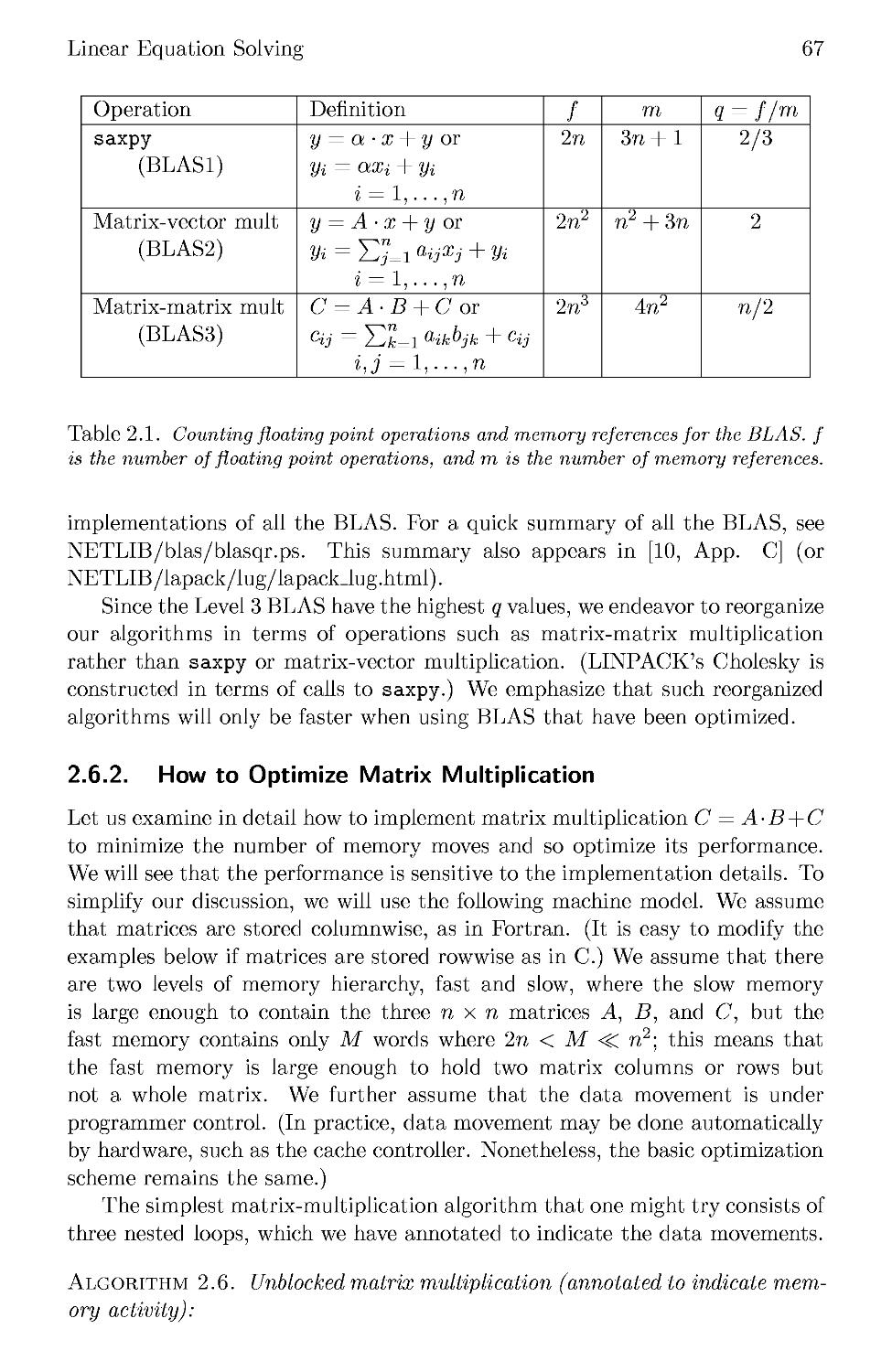
2.6.1 Basic Linear Algebra Subroutines (BLAS) 65
2.6.2 How to Optimize Matrix Multiplication 67
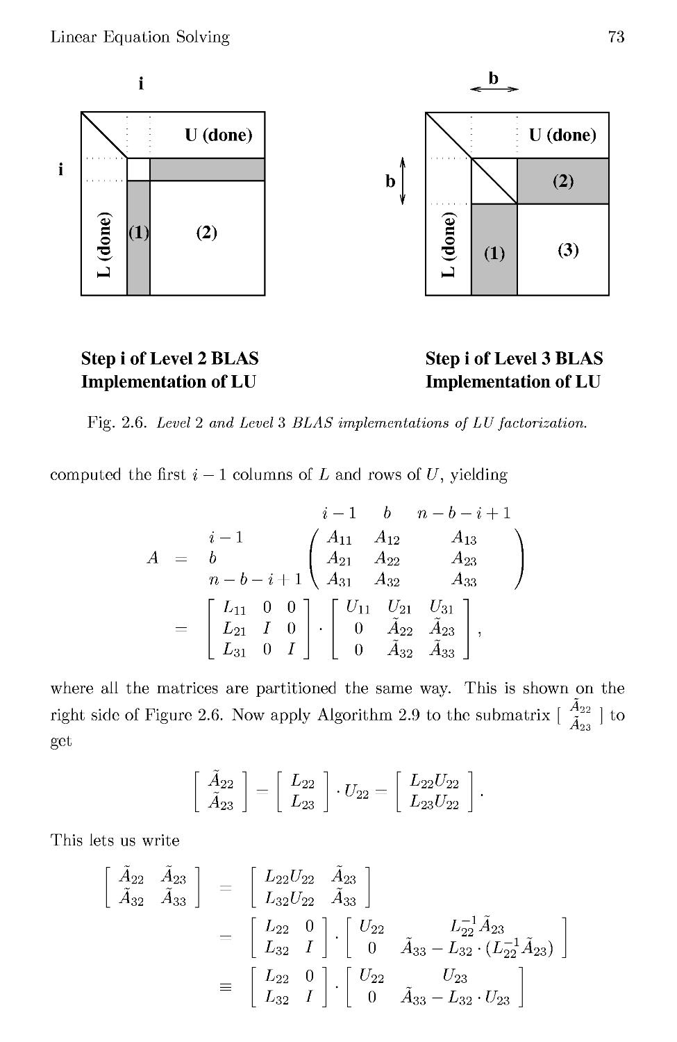
2.6.3 Reorganizing Gaussian Elimination to use Level 3 BLAS 72
2.6.4 More About Parallelism and Other Performance Issues . 75
2.7 Special Linear Systems 76
2.7.1 Real Symmetric Positive Definite Matrices 76
v
2.7.2 Symmetric Indefinite Matrices 79
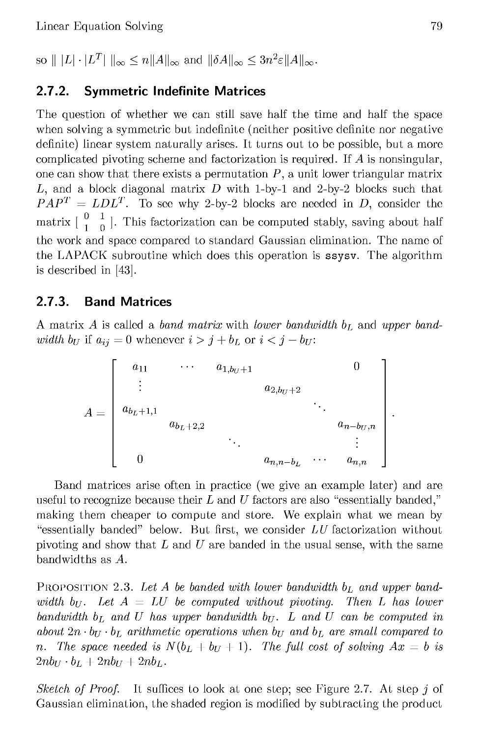
2.7.3 Band Matrices 79
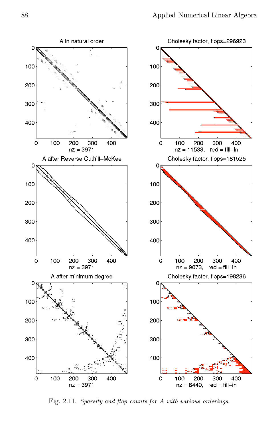
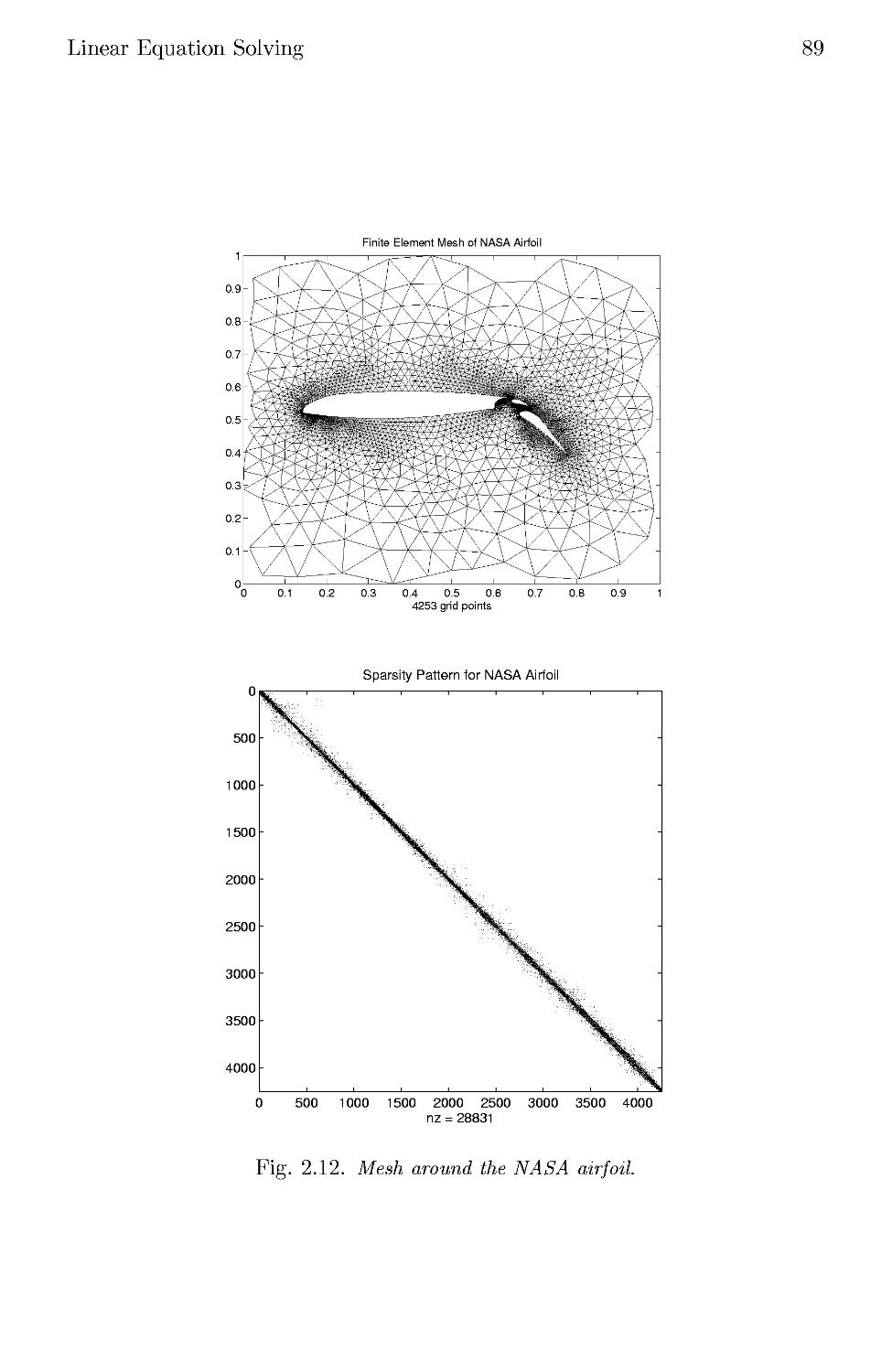
2.7.4 General Sparse Matrices 83
2.7.5 Dense Matrices Depending on Fewer Than 0(n2)
Parameters 90
2.8 References and Other Topics for Chapter 2 92
2.9 Questions for Chapter 2 93
3 Linear Least Squares Problems 101
3.1 Introduction 101
3.2 Matrix Factorizations That Solve the Linear Least Squares
Problem 105
3.2.1 Normal Equations 106
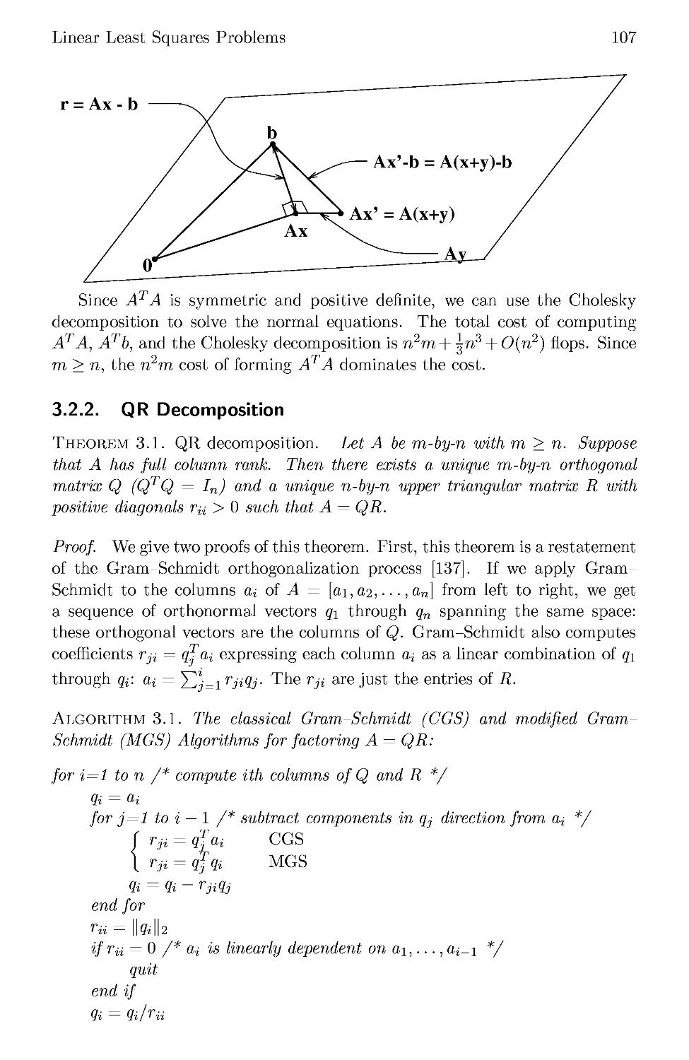
3.2.2 QR Decomposition 107
3.2.3 Singular Value Decomposition 109
3.3 Perturbation Theory for the Least Squares Problem 117
3.4 Orthogonal Matrices 118
3.4.1 Householder Transformations 119
3.4.2 Givens Rotations 121
3.4.3 Roundoff Error Analysis for Orthogonal Matrices .... 123
3.4.4 Why Orthogonal Matrices? 124
3.5 Rank-Deficient Least Squares Problems 125
3.5.1 Solving Rank-Deficient Least Squares Problems Using
the SVD 127
3.5.2 Solving Rank-Deficient Least Squares Problems Using
QR with Pivoting 130
3.6 Performance Comparison of Methods for Solving Least Squares
Problems 132
3.7 References and Other Topics for Chapter 3 134
3.8 Questions for Chapter 3 134
4 Nonsymmetric Eigenvalue Problems 139
4.1 Introduction 139
4.2 Canonical Forms 140
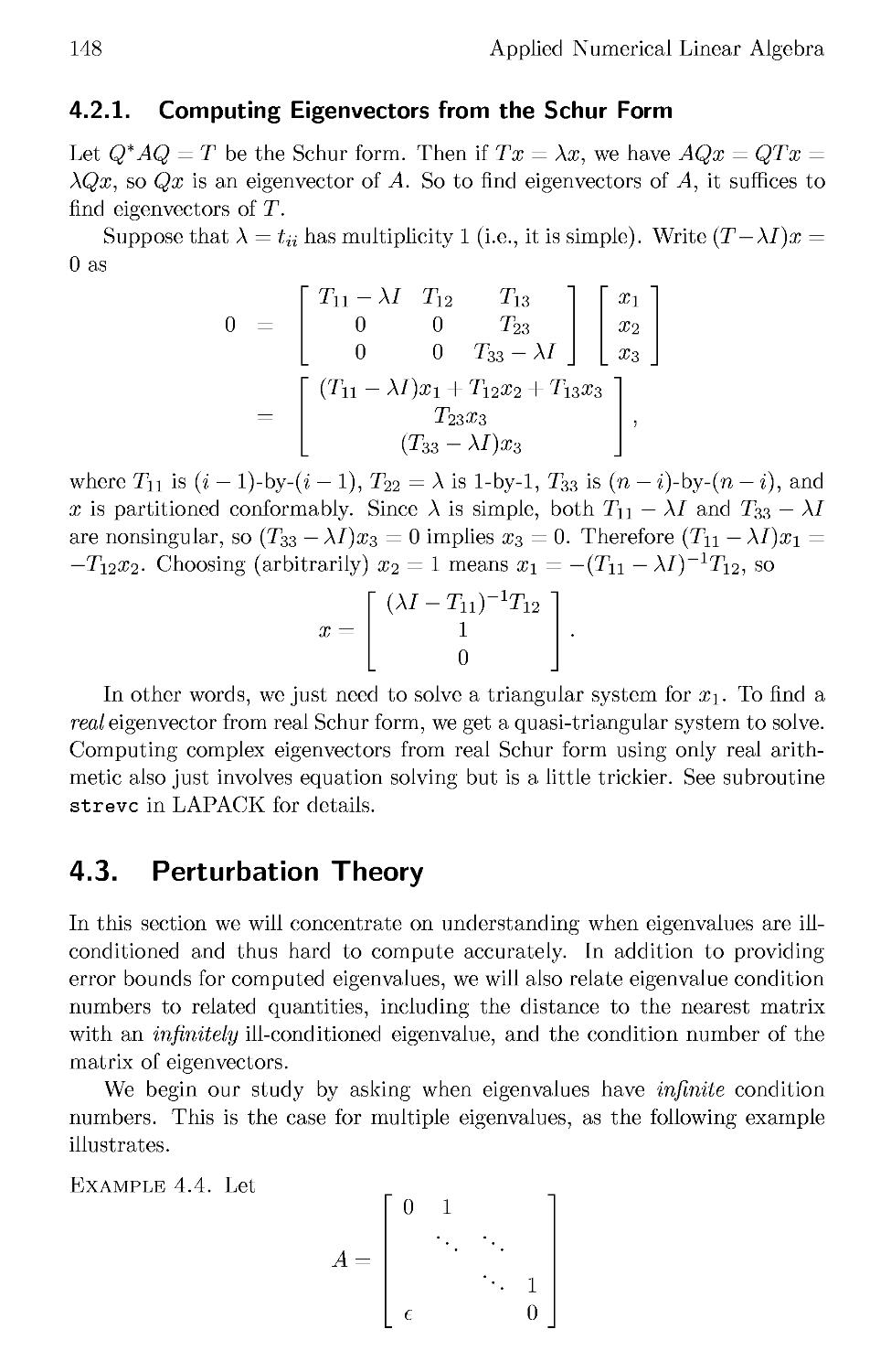
4.2.1 Computing Eigenvectors from the Schur Form 148
4.3 Perturbation Theory 148
4.4 Algorithms for the Nonsymmetric Eigenproblem 153
4.4.1 Power Method 154
4.4.2 Inverse Iteration 155
4.4.3 Orthogonal Iteration 156
4.4.4 QR Iteration 159
4.4.5 Making QR Iteration Practical 163
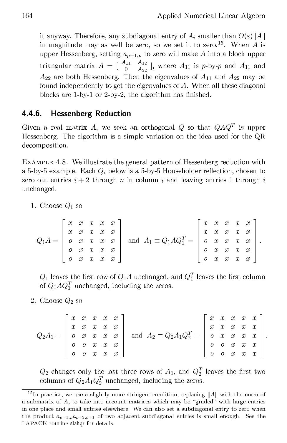
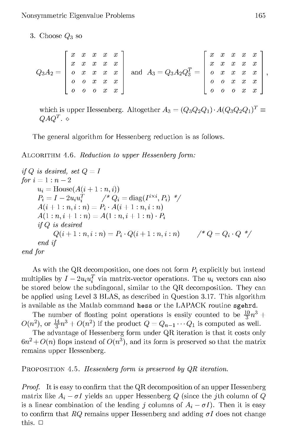
4.4.6 Hessenberg Reduction 164
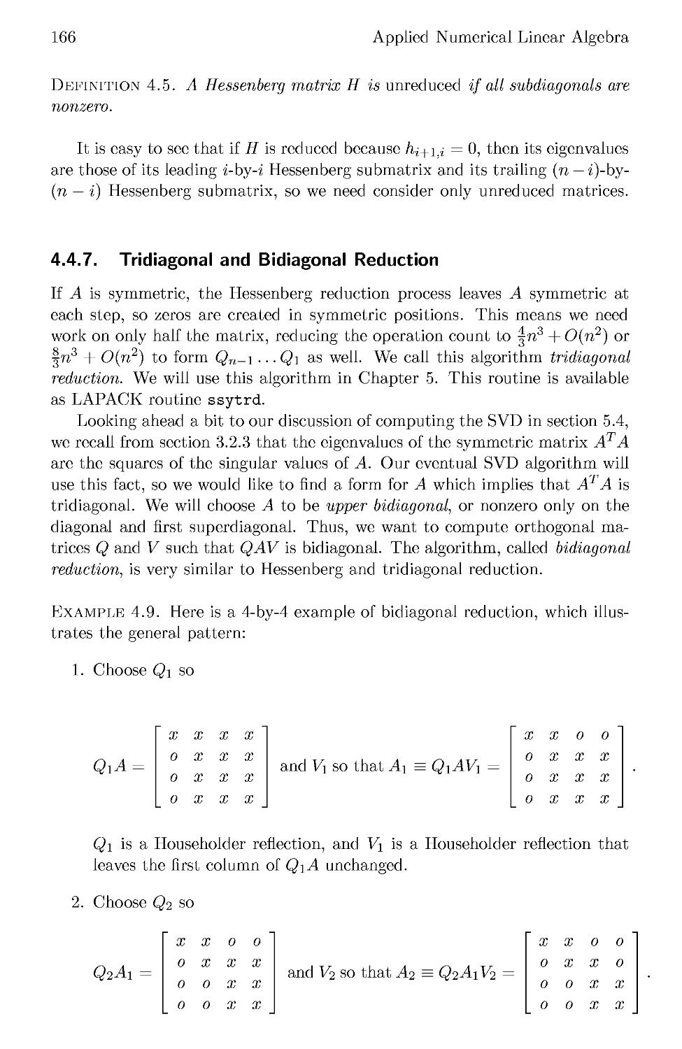
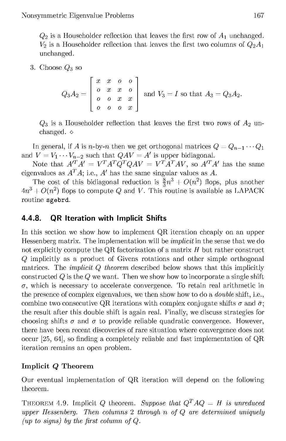
4.4.7 Tridiagonal and Bidiagonal Reduction 166
Vll
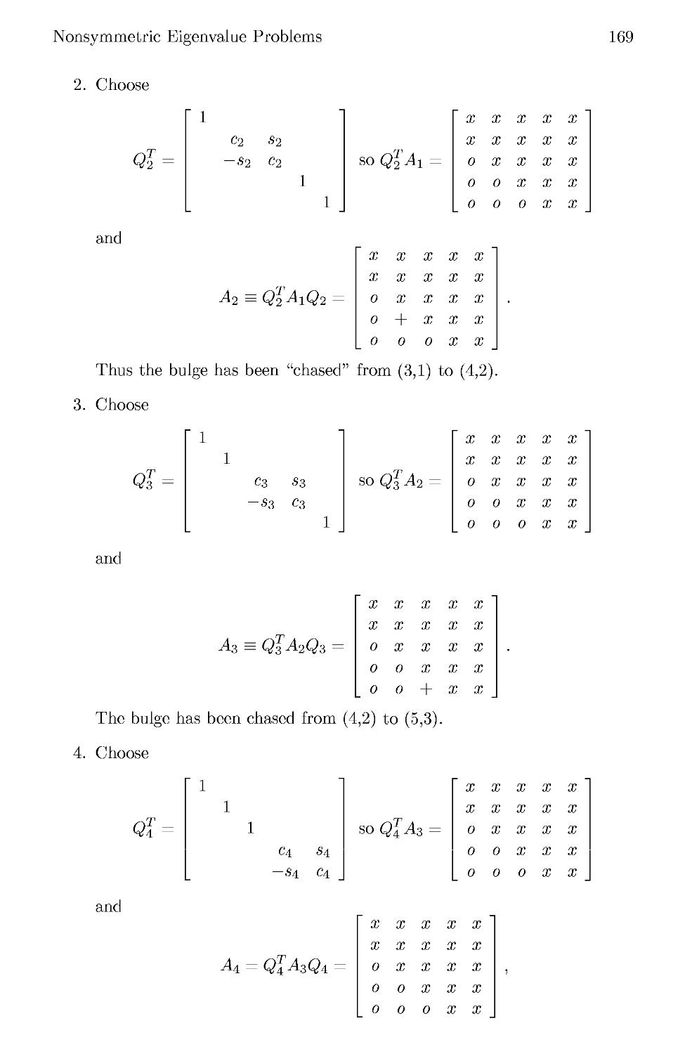
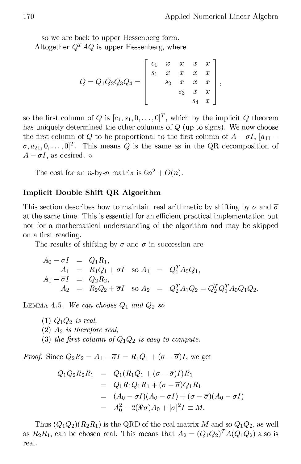
4.4.8 QR Iteration with Implicit Shifts 167
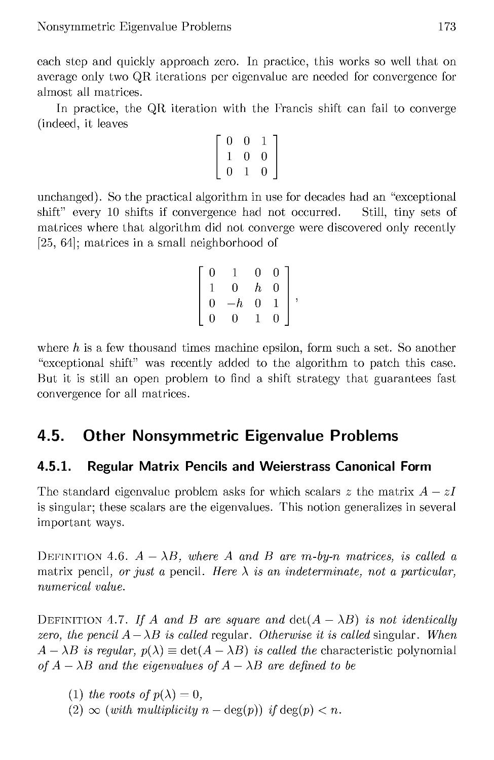
4.5 Other Nonsymmetric Eigenvalue Problems 173
4.5.1 Regular Matrix Pencils and Weierstrass Canonical Form 173
4.5.2 Singular Matrix Pencils and the Kronecker
Canonical Form 179
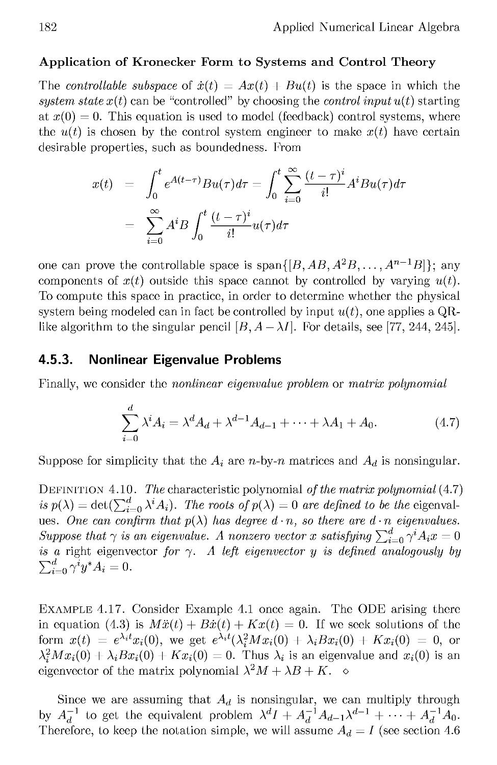
4.5.3 Nonlinear Eigenvalue Problems 182
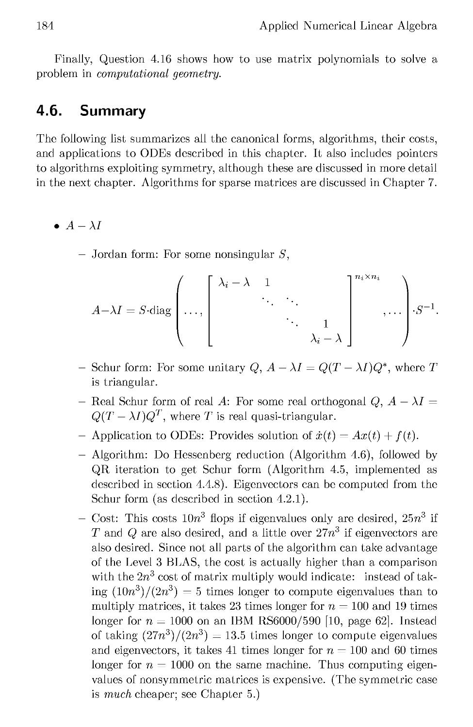
4.6 Summary 184
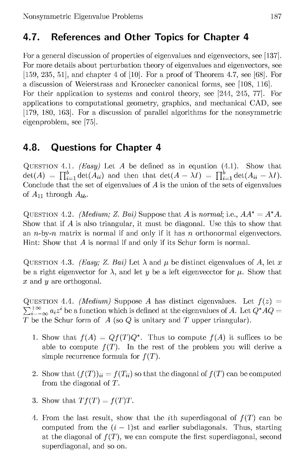
4.7 References and Other Topics for Chapter 4 187
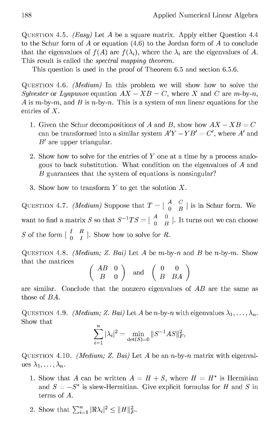
4.8 Questions for Chapter 4 187
5 The Symmetric Eigenproblem and Singular Value
Decomposition 195
5.1 Introduction 195
5.2 Perturbation Theory 197
5.2.1 Relative Perturbation Theory 207
5.3 Algorithms for the Symmetric Eigenproblem 210
5.3.1 Tridiagonal QR Iteration 212
5.3.2 Rayleigh Quotient Iteration 215
5.3.3 Divide-and-Conquer 217
5.3.4 Bisection and Inverse Iteration 228
5.3.5 Jacobi's Method 232
5.3.6 Performance Comparison 236
5.4 Algorithms for the Singular Value Decomposition 237
5.4.1 QR Iteration and Its Variations for the Bidiagonal SVD 242
5.4.2 Computing the Bidiagonal SVD to High Relative Accuracy 246
5.4.3 Jacobi's Method for the SVD 249
5.5 Differential Equations and Eigenvalue Problems 254
5.5.1 The Toda Lattice 255
5.5.2 The Connection to Partial Differential Equations .... 260
5.6 References and Other Topics for Chapter 5 260
5.7 Questions for Chapter 5 261
6 Iterative Methods for Linear Systems 265
6.1 Introduction 265
6.2 On-line Help for Iterative Methods 266
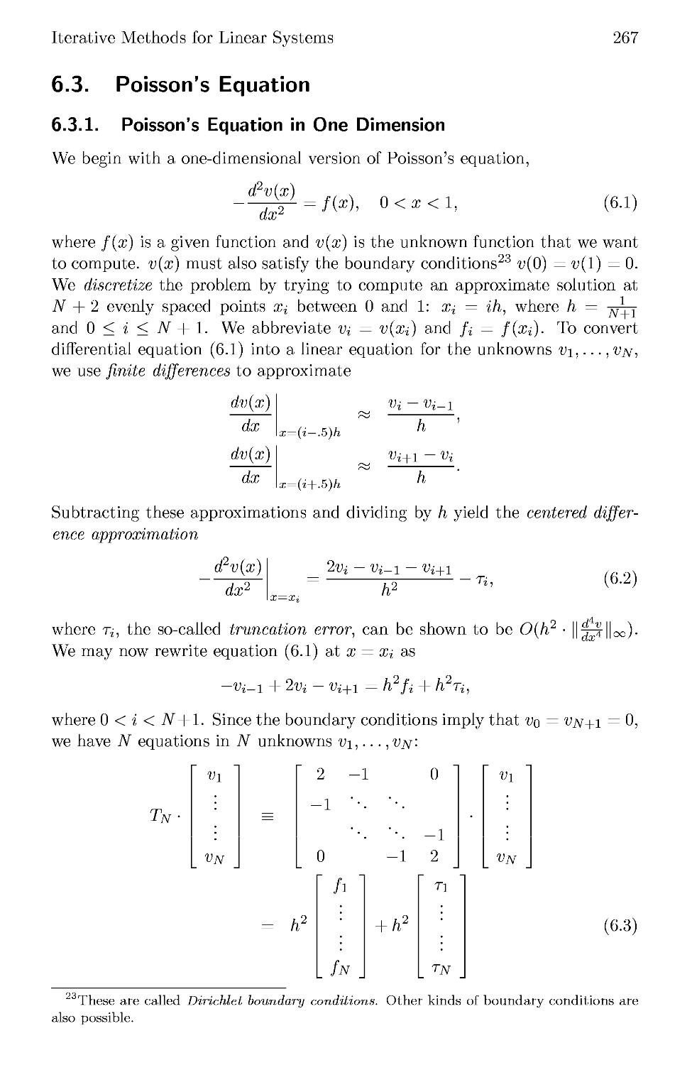
6.3 Poisson's Equation 267
6.3.1 Poisson's Equation in One Dimension 267
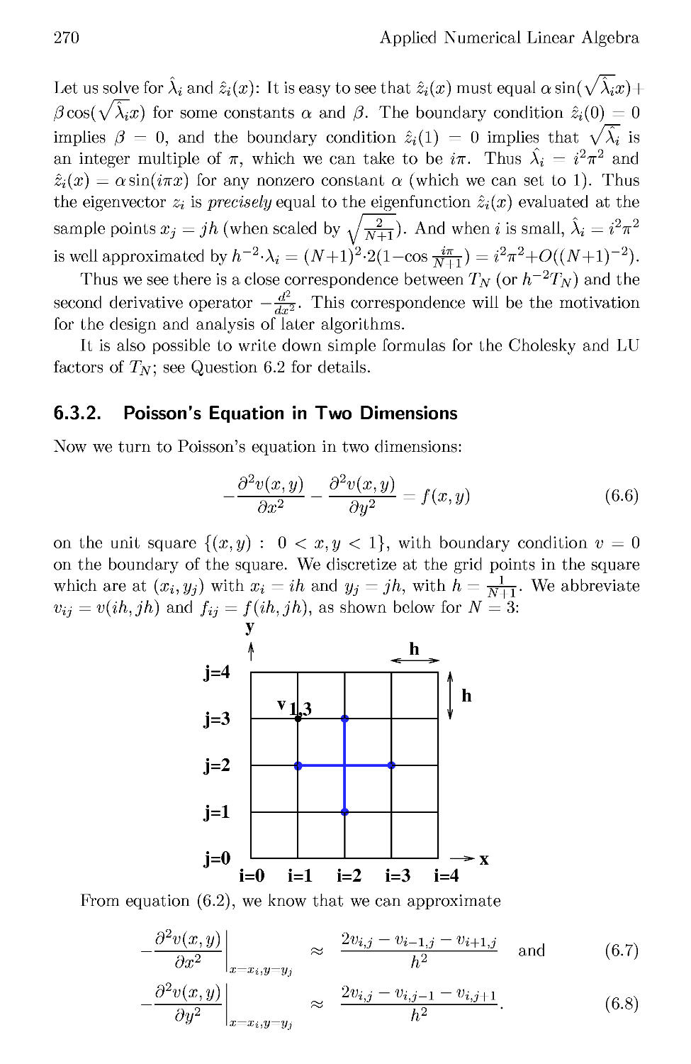
6.3.2 Poisson's Equation in Two Dimensions 270
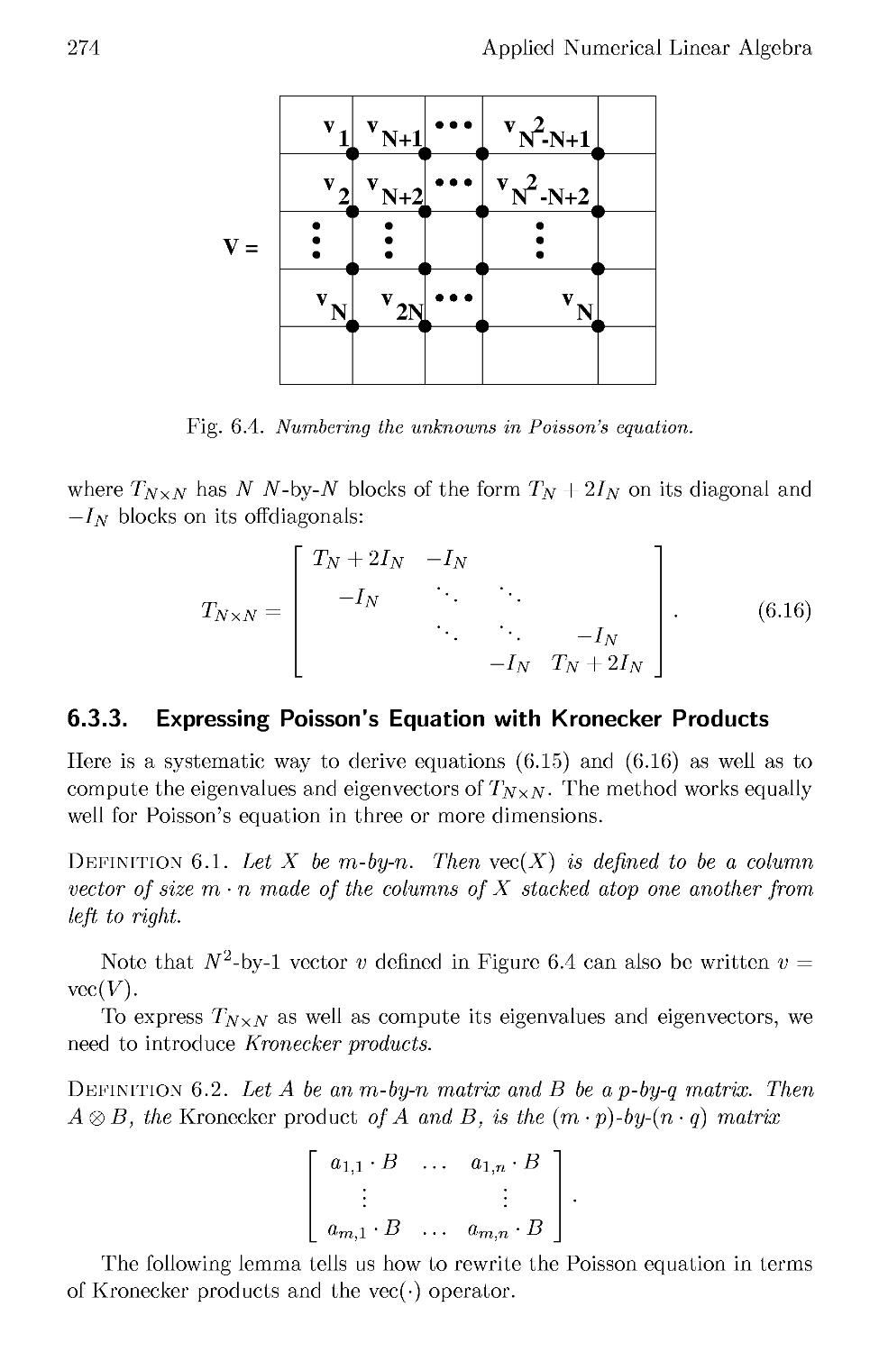
6.3.3 Expressing Poisson's Equation with Kronecker Products 274
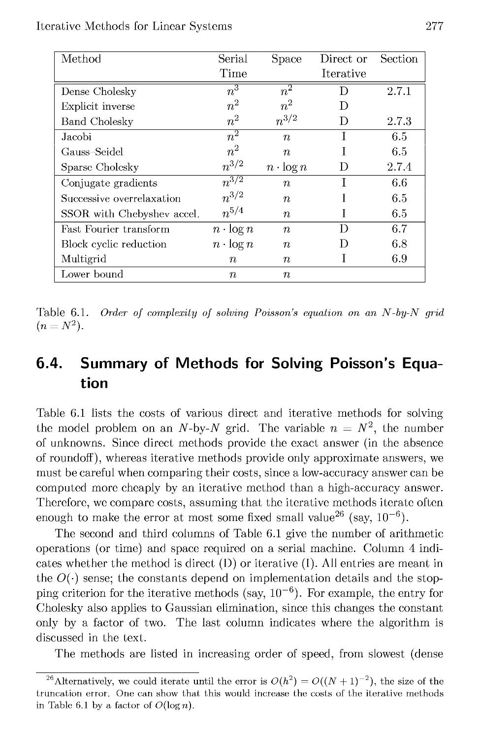
6.4 Summary of Methods for Solving Poisson's Equation 277
6.5 Basic Iterative Methods 279
6.5.1 Jacobi's Method 281
6.5.2 Gauss-Seidel Method 282
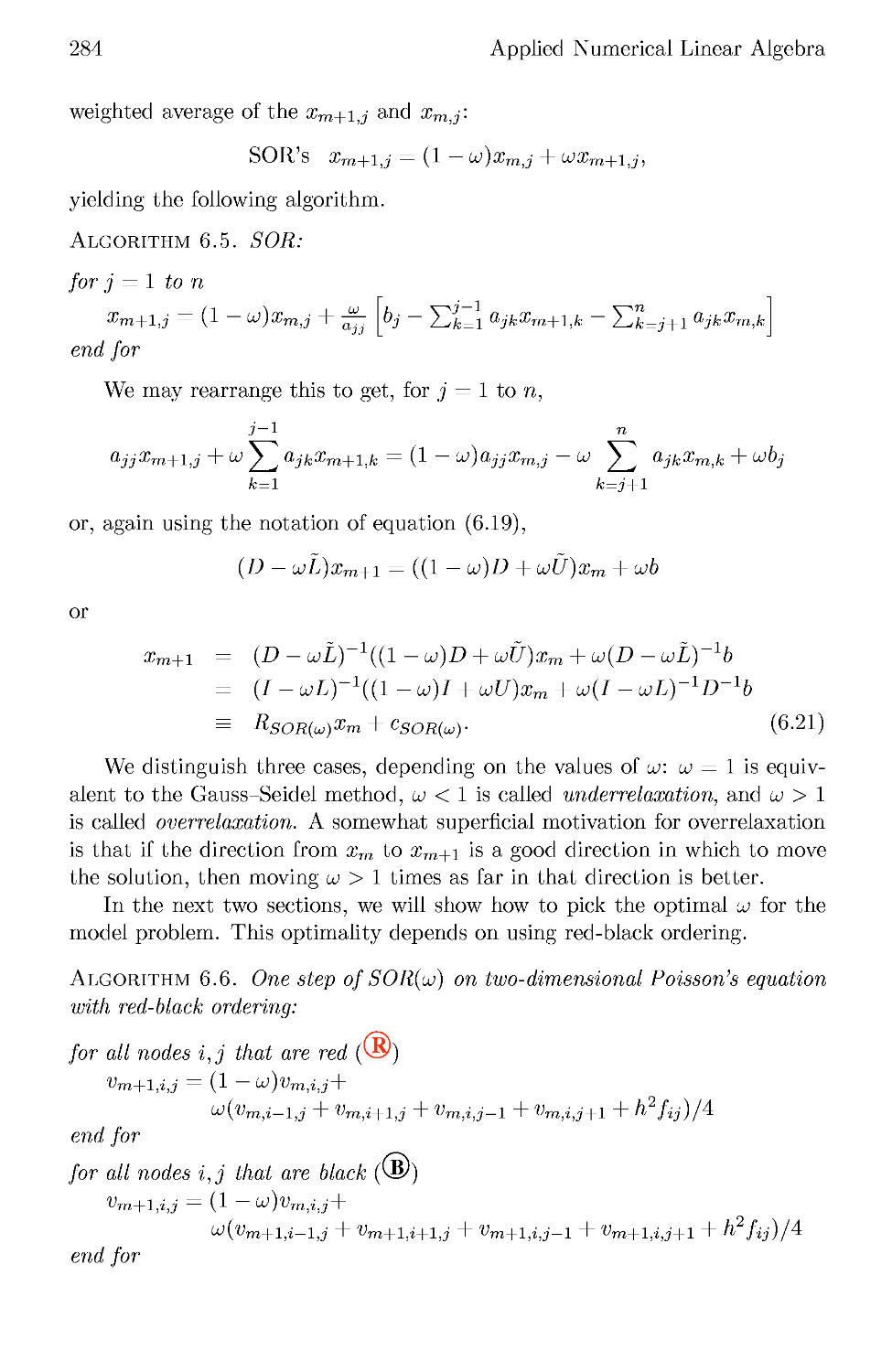
6.5.3 Successive Overrelaxation 283
Vlll
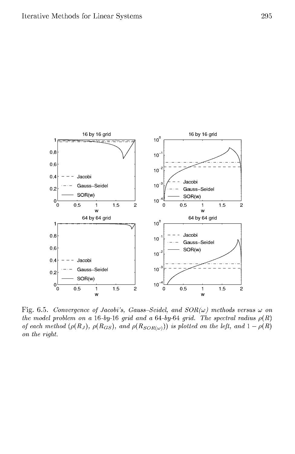
6.5.4 Convergence of Jacobi's, Gauss-Seidel, and
SOR(w) Methods on the Model Problem 285
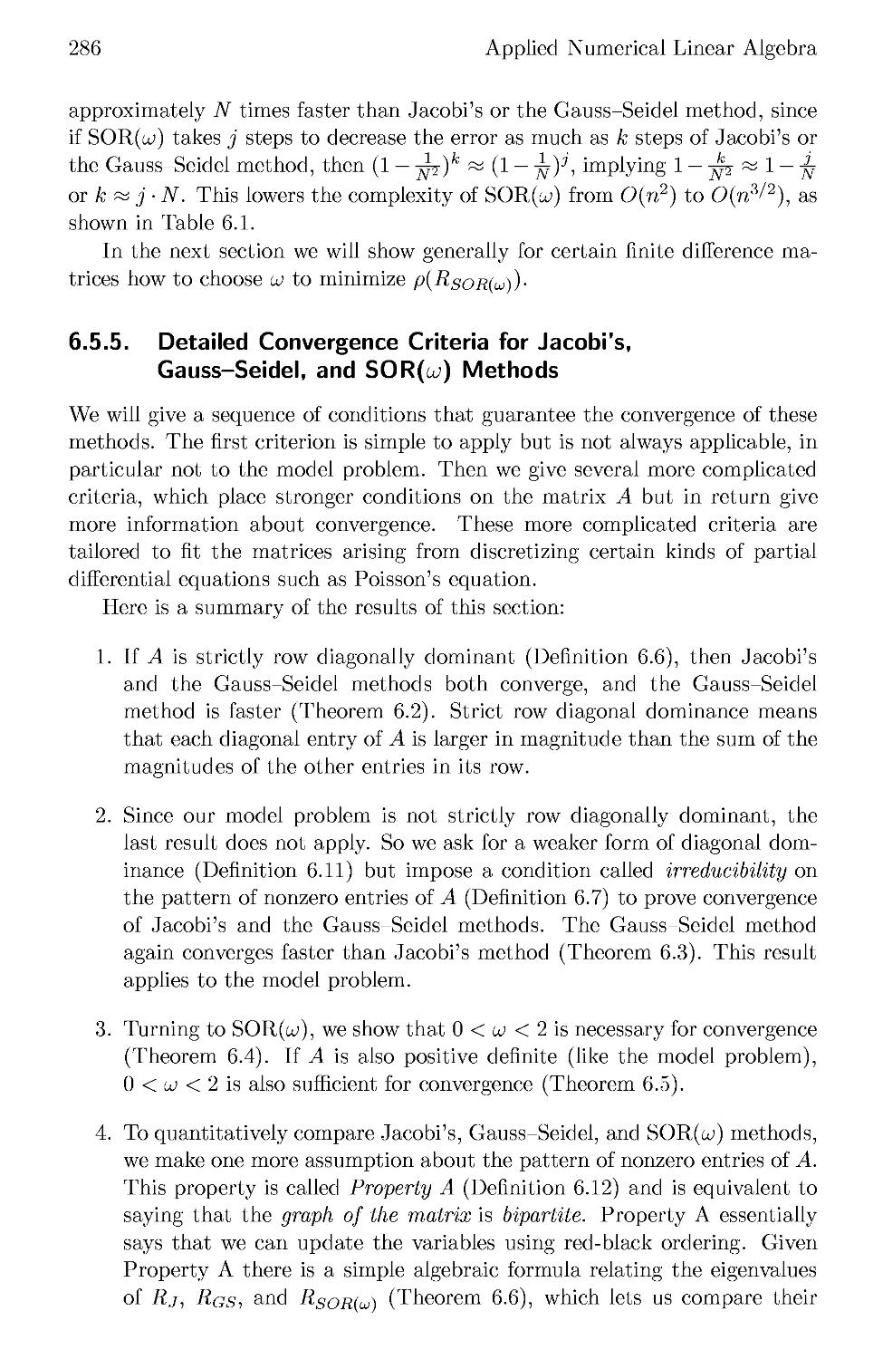
6.5.5 Detailed Convergence Criteria for Jacobi's,
Gauss-Seidel, and SOR(w) Methods 286
6.5.6 Chebyshev Acceleration and Symmetric SOR (SSOR) . 294
6.6 Krylov Subspace Methods 300
6.6.1 Extracting Information about A via Matrix-Vector
Multiplication 301
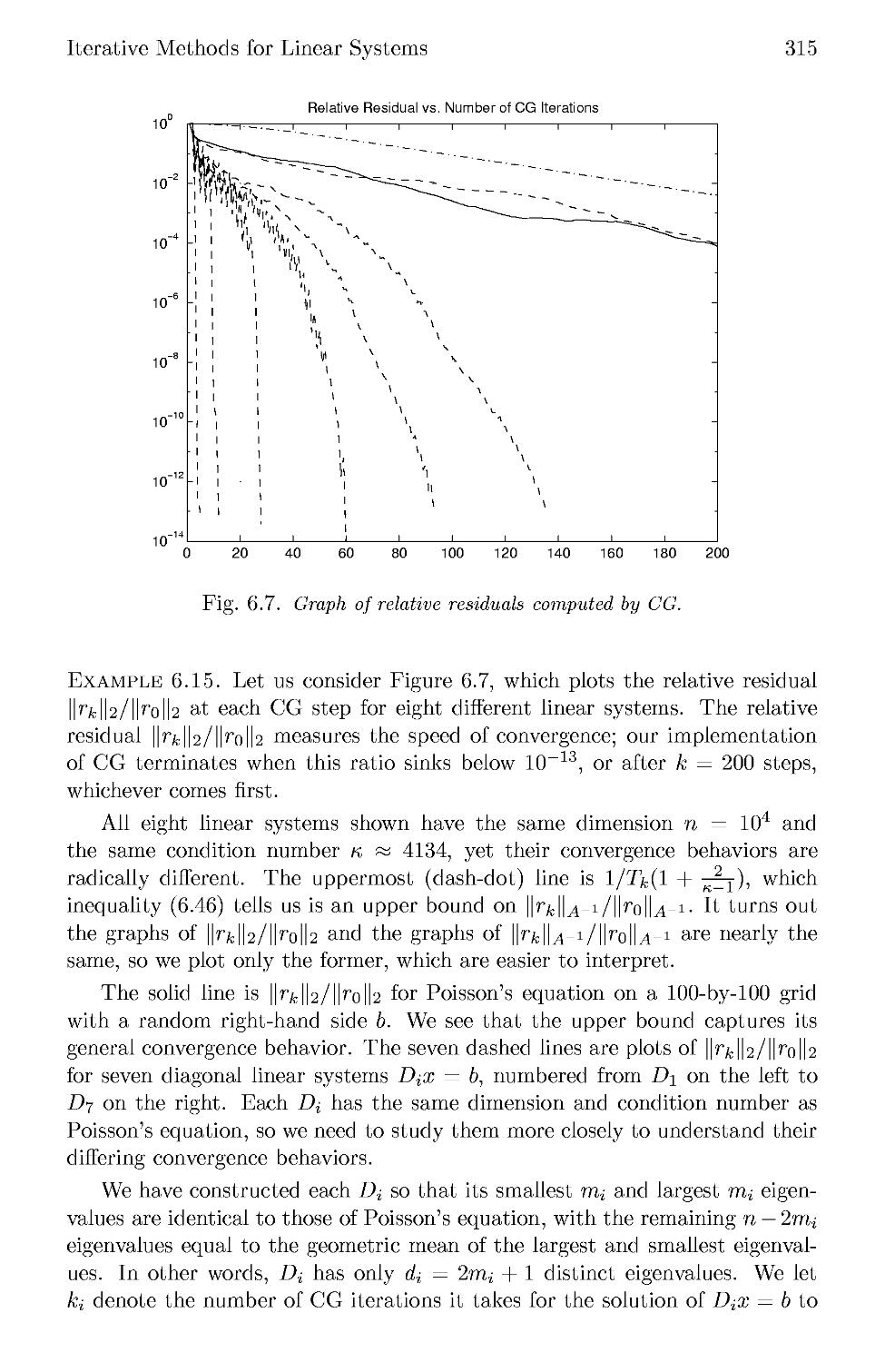
6.6.2 Solving Ax = b Using the Krylov Subspace 7C& 306
6.6.3 Conjugate Gradient Method 307
6.6.4 Convergence Analysis of the Conjugate Gradient Method 312
6.6.5 Preconditioning 317
6.6.6 Other Krylov Subspace Algorithms for Solving Ax = b 320
6.7 Fast Fourier Transform 321
6.7.1 The Discrete Fourier Transform 323
6.7.2 Solving the Continuous Model Problem Using Fourier
Series 324
6.7.3 Convolutions 326
6.7.4 Computing the Fast Fourier Transform 326
6.8 Block Cyclic Reduction 328
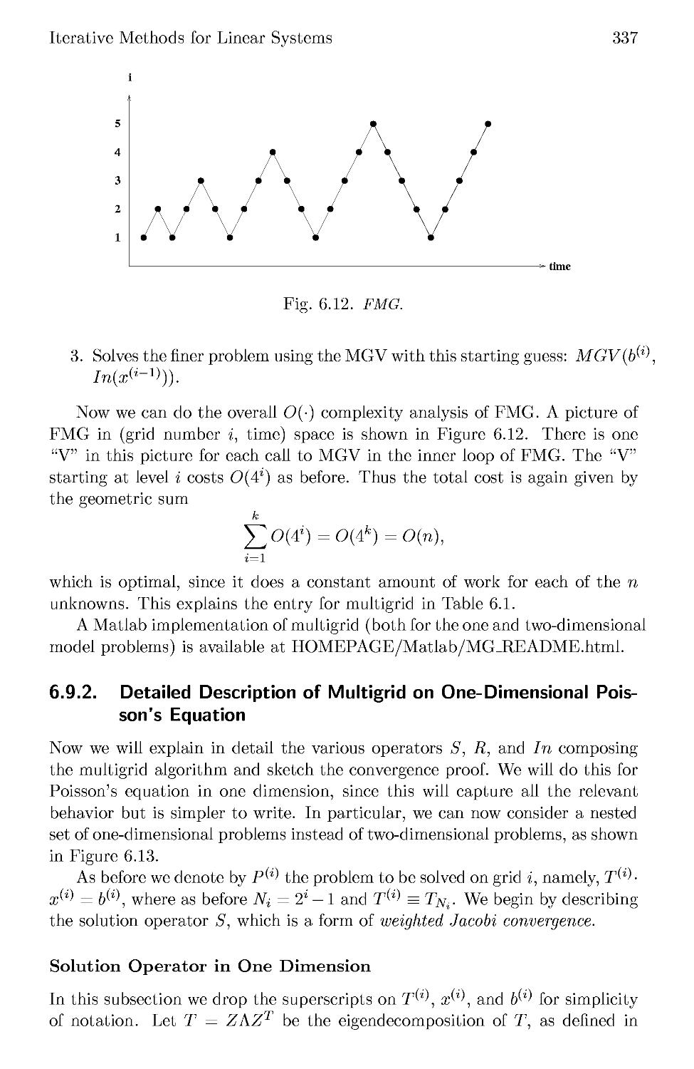
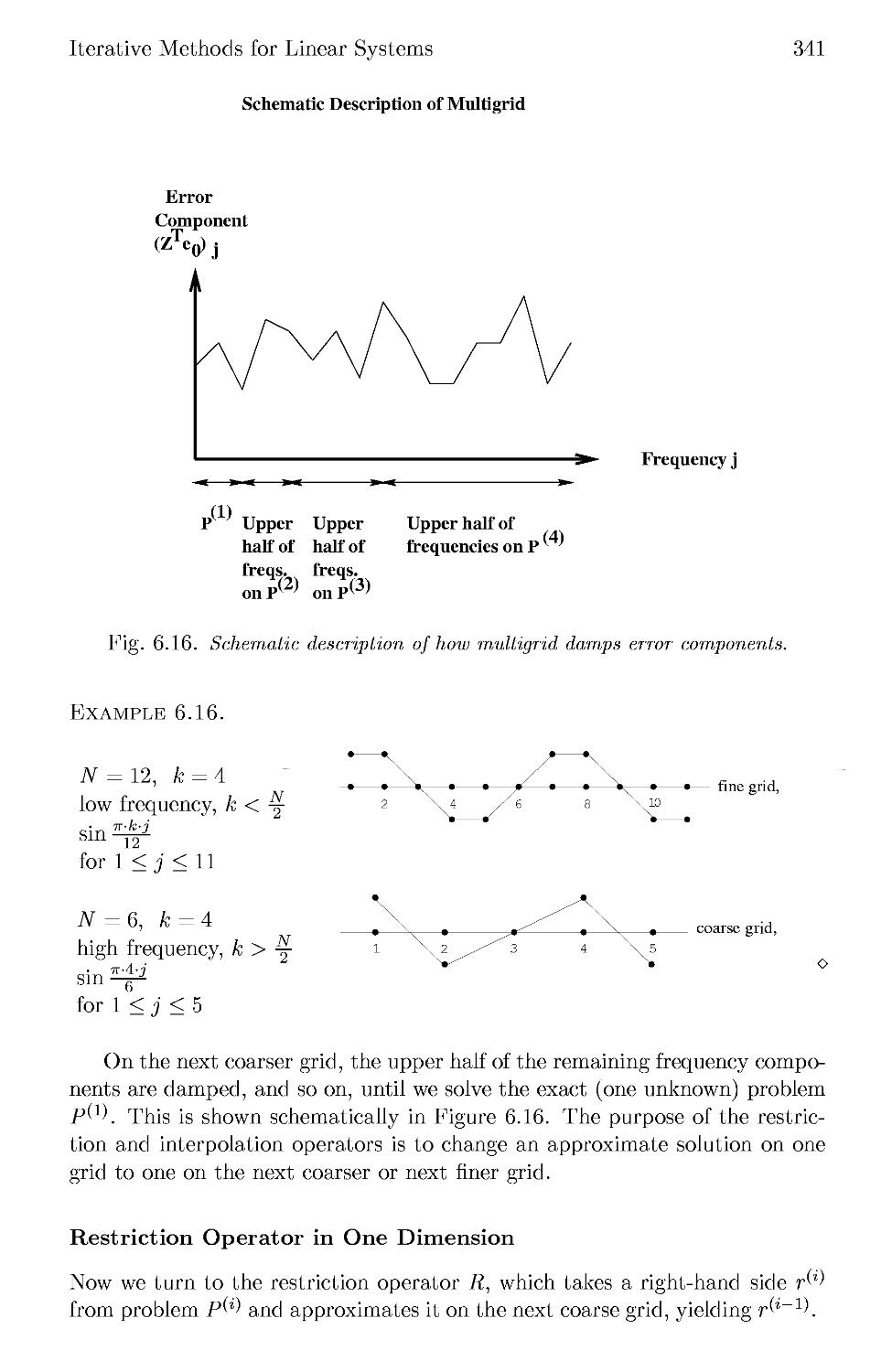
6.9 Multigrid 331
6.9.1 Overview of Multigrid on Two-Dimensional Poisson's
Equation 333
6.9.2 Detailed Description of Multigrid on One-Dimensional
Poisson's Equation 337
6.10 Domain Decomposition 348
6.10.1 Nonoverlapping Methods 349
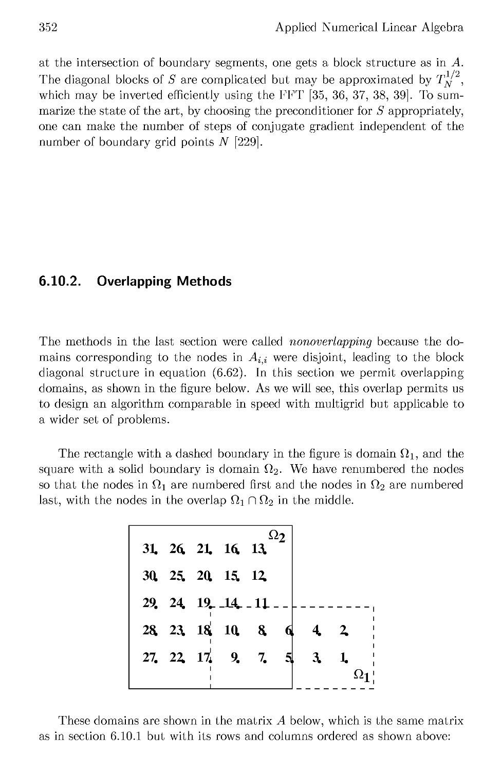
6.10.2 Overlapping Methods 352
6.11 References and Other Topics for Chapter 6 357
6.12 Questions for Chapter 6 357
7 Iterative Algorithms for Eigenvalue Problems 363
7.1 Introduction 363
7.2 The Rayleigh-Ritz Method 364
7.3 The Lanczos Algorithm in Exact Arithmetic 368
7.4 The Lanczos Algorithm in Floating Point Arithmetic 377
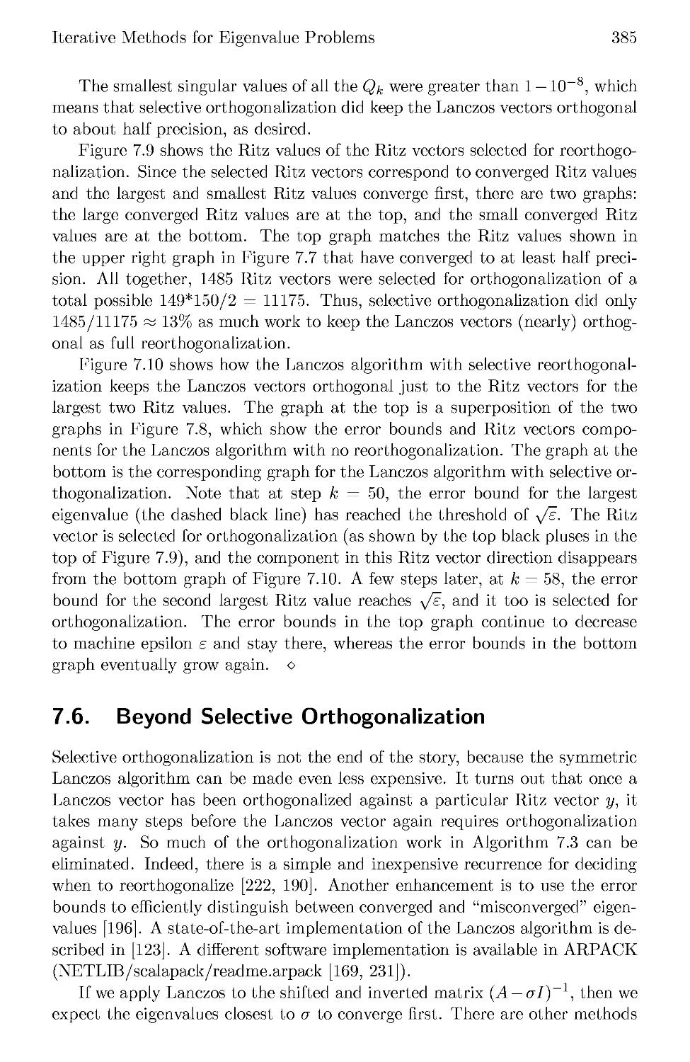
7.5 The Lanczos Algorithm with Selective Orthogonalization .... 382
7.6 Beyond Selective Orthogonalization 385
7.7 Iterative Algorithms for the Nonsymmetric Eigenproblem . . . 386
7.8 References and Other Topics for Chapter 7 388
7.9 Questions for Chapter 7 388
Bibliography 391
IX
Index 411
This page is intentionally left blank
Preface to the 1996 Edition
The following are natural goals for an aspiring textbook writer of a book like
this one:
1. It should be attractive to first year graduate students from a variety of
engineering and scientific disciplines.
2. The text should be self-contained, assuming only a good undergraduate
background in linear algebra.
3. The students should learn the mathematical basis of the field, as well as
how to build or find good numerical software.
4. Students should acquire practical knowledge for solving real problems
efficiently. In particular, they should know what the state-of-the-art
techniques are in each area, or when to look for them and where to find
them.
5. It should all fit in one semester, since that is what most students have
available for this subject.
The fifth goal is perhaps the hardest to manage. The first edition of these
notes was 215 pages, which did fit into one ambitious semester. This edition
has more than doubled in length, which is certainly too much material for
even a heroic semester. The new material reflects the growth in research in
the field in the last few years, including my own. It also reflects requests from
colleagues for sections on certain topics that were treated lightly or not at all
in the first edition. Notable additions include
• a class homepage with Matlab source code for examples and homework
problems in the text, and pointers to other on-line software and
textbooks;
• more pointers in the text to software for all problems, including a
summary of available software for solving sparse linear systems using direct
methods;
• a new chapter on Krylov subspace methods for eigenvalue problems;
• a section on domain decomposition, including both overlapping and nonover-
lapping methods;
XI
Xll
Preface
• sections on "relative perturbation theory" and corresponding high-accuracy
algorithms for eigenproblems, like Jacobi and qd;
• more detailed performance comparisons of competing least squares and
symmetric eigenvalue algorithms; and
• new homework problems, including many contributed by Zhaojun Bai.
A reasonable one-semester curriculum could consist of the following
chapters and sections:
• all of Chapter 1;
• Chapter 2, excluding sections 2.2.1, 2.4.3, 2.5, 2.6.3, and 2.6.4;
• Chapter 3, excluding section 3.5;
• Chapter 4, up to and including section 4.4.5;
• Chapter 5, excluding sections 5.2.1, 5.3.5, 5.4 and 5.5; and
• Chapter 6, excluding sections 6.3.3, 6.5.5, 6.5.6, 6.6.6, 6.7.2, 6.7.3, 6.7.4,
6.8, 6.9.2, and 6.10.
Homework problems are marked Easy, Medium or Hard, according to their
difficulty. Problems involving significant amounts of programming are marked
"programming".
Many people have helped contribute to this text, notably Zhaojun Bai,
Alan Edelman, Velvel Kahan, Richard Lehoucq, Beresford Parlett, and many
anonymous referees, all of whom made detailed comments on various parts of
the text. Table 2.2 is taken from the PhD thesis of my student Xiaoye Li. Alan
Edelman at MIT and Martin Gutknecht at ETH Zurich provided hospitable
surroundings at their institutions while this final edition was being prepared.
Many students at Courant, Berkeley, Kentucky and MIT have listened to and
helped debug this material over the years, and deserve thanks. Finally, Kathy
Yelick has contributed scientific comments, latex consulting, and moral support
over more years than either of us expected this project to take.
James Demmel
MIT
September, 1996
1
Introduction
1.1. Basic Notation
In this course we will refer frequently to matrices, vectors, and scalars. A
matrix will be denoted by an upper case letter such as A, and its (i,j)th
element will be denoted by a^-. If the matrix is given by an expression such
as A + B, we will write (A + B)ij. In detailed algorithmic descriptions we
will sometimes write A(i,j) or use the Matlab [182] notation A(i : j,k : /) to
denote the submatrix of A lying in rows i through j and columns k through
/. A lower-case letter like x will denote a vector, and its ith element will
be written x\. Vectors will almost always be column vectors, which are the
same as matrices with one column. Lower-case Greek letters (and occasionally
lower-case letters) will denote scalars. M will denote the set of real numbers;
W1, the set of n-dimensional real vectors; and WmXn, the set of m-by-n real
matrices. C, C™, and CrnXn denote complex numbers, vectors, and matrices,
respectively. Occasionally we will use the shorthand AmXn to indicate that A is
an m-by-n matrix. AT will denote the transpose of the matrix A: (AT)ij = a,ji.
For complex matrices we will also use the conjugate transpose A*: (A*)ij = a,ji.
5te and Qz will denote the real and imaginary parts of the complex number
z, respectively. If A is m-by-n, then \A\ is the m-by-n matrix of absolute
values of entries of A: (\A\)ij = \a,ij\. Inequalities like \A\ < \B\ are meant
componentwise: \a,ij\ < \bij\ for all i and j. We will also use this absolute value
notation for vectors: (\x\)i = \xi\. Ends of proofs will be marked by ?, and
ends of examples by o. Other notation will be introduced as needed.
1.2. Standard Problems of Numerical Linear Algebra
We will consider the following standard problems:
• Linear systems of equations: Solve Ax = b. Here A is a given n-by-n
nonsingular real or complex matrix, 6 is a given column vector with n
entries, and a; is a column vector with n entries that we wish to compute.
1
2
Applied Numerical Linear Algebra
• Least squares problems: Compute the x that minimizes \\Ax — 6||2- Here
A is m-by-n, b is m-by-1, x is n-by-1, and ||y||2 = y/Yl \Vi\2 ^s called
the two-norm of the vector y. If m > n so that we have more equations
than unknowns, the system is called overdetermined. In this case we
cannot generally solve Ax = b exactly. If m < n, the system is called
underdetermined, and we will have infinitely many solutions.
• Eigenvalue problems: Given an n-by-n matrix A, find an n-by-1 nonzero
vector x and a scalar A so that Ax = \x.
• Singular value problems: Given an m-by-n matrix A, find an n-by-1
nonzero vector x and scalar A so that ATAx = \x. We will see that this
special kind of eigenvalue problem is important enough to merit separate
consideration and algorithms.
We choose to emphasize these standard problems because they arise so
often in engineering and scientific practice. We will illustrate them throughout
the book with simple examples drawn from engineering, statistics, and other
fields. There are also many variations of these standard problems that we will
consider, such as generalized eigenvalue problems Ax = \Bx (section 4.5) and
"rank-deficient" least squares problems minx \\Ax — 6H2, whose solutions are
nonunique because the columns of A are linearly dependent (section 3.5).
We will learn the importance of exploiting any special structure our problem
may have. For example, solving an n-by-n linear system costs 2/3n3 floating
point operations if we use the most general form of Gaussian elimination. If we
add the information that the system is symmetric and positive definite, we can
save half the work by using another algorithm called Cholesky. If we further
know the matrix is banded with semibandwidth y/n (i.e., a^- = 0 if \i—j\ > \/n),
then we can reduce the cost further to 0{n2) by using band Cholesky. If we
say quite explicitly that we are trying to solve Poisson's equation on a square
using a 5-point difference approximation, which determines the matrix nearly
uniquely, then by using the multigrid algorithm we can reduce the cost to 0(n),
which is nearly as fast as possible, in the sense that we use just a constant
amount of work per solution component (section 6.4).
1.3. General Techniques
There are several general concepts and techniques that we will use repeatedly:
1. matrix factorizations;
2. perturbation theory and condition numbers;
3. effects of roundoff error on algorithms, including properties of floating
point arithmetic;
Introduction
3
4. analysis of the speed of an algorithm;
5. engineering numerical software.
We discuss each of these briefly below.
1.3.1. Matrix Factorizations
A factorization of the matrix A is a representation of A as a product of several
"simpler" matrices, which make the problem at hand easier to solve. We give
two examples.
Example 1.1. Suppose that we want to solve Ax = b. If A is a lower
triangular matrix,
«21 «22
®nl ®n2 • • • ®nn
is easy to solve using forward substitution:
for i = 1 to n
xi = (pi — 2_>fc=l aikxk)/aii
end for
An analogous idea, back substitution, works if A is upper triangular. To
use this to solve a general system Ax = b we need the following matrix
factorization, which is just a restatement of Gaussian elimination.
Theorem 1.1. If the n-by-n matrix A is nonsingular, there exists a
permutation matrix P (the identity matrix with its rows permuted), a nonsingular
lower triangular matrix L, and a nonsingular upper triangular matrix U such
that A = P ¦ L ¦ U. To solve Ax = b, we solve the equivalent system PLUx = b
as follows:
LUx = P_16 = PTb (permute entries of b),
Ux = L~1{PTb) (forward substitution),
x = U~1{L~1PTb) (back substitution).
We will prove this theorem in section 2.3. o
Example 1.2. The Jordan canonical factorization A = VJV-1 exhibits the
eigenvalues and eigenvectors of A. Here V is a nonsingular matrix, whose
columns include the eigenvectors, and J is the Jordan canonical form of A,
a special triangular matrix with the eigenvalues of A on its diagonal. We
will learn that it is numerically superior to compute the Schur factorization
A = UTU*, where U is a unitary matrix (i.e., J7's columns are orthonormal),
and T is upper triangular with A's eigenvalues on its diagonal. The Schur form
T can be computed faster and more accurately than the Jordan form J. We
discuss the Jordan and Schur factorizations in section 4.2. o
X\
X2
Xn
=
bi
b2
bn
4
Applied Numerical Linear Algebra
1.3.2. Perturbation Theory and Condition Numbers
The answers produced by numerical algorithms are seldom exactly correct.
There are two sources of error. First, there may be errors in the input data
to the algorithm, caused by prior calculations or perhaps measurement errors.
Second, there are errors caused by the algorithm itself, due to approximations
made within the algorithm. In order to estimate the errors in the computed
answers from both these sources, we need to understand how much the solution
of a problem is changed (or perturbed) if the input data is slightly perturbed.
Example 1.3. Let f(x) be a real-valued continuous function of a real variable
x. We want to compute f(x), but we do not know x exactly. Suppose instead
that we are given x + 5x and a bound on 5x. The best that we can do (without
more information) is to compute f(x + 5x) and to try to bound the absolute
error \f(x + 5x) —f(x)\. We may use a simple linear approximation to / to get
the error bound f(x + 5x) ~ f(x) + 5xf(x), and so the error is \f(x + 5x) —
f(x)\ ~ 15a;| • \f'(x)\. We call \f'(x)\ the absolute condition number of / at x.
If |/'(a;)| is large enough, then the error may be large even if 5x is small; in
this case we call / ill-conditioned at a;, o
We say absolute condition number because it provides a bound on the
absolute error \f(x + 5x) — f(x)\ given a bound on the absolute change \5x\ in
the input. We will also often use the following essentially equivalent expression
to bound the error:
\f(x + Sx)-f(x)\ _ \Sx\ \f'(x)\-\x\
\f(x)\ ~ \x\ \f(x)\ •
This expression bounds the relative error \f(x + 5x) — f(x)\/\f(x)\ as a
multiple of the relative change |&c|/|a;| in the input. The multiplier, \f'(x)\ ¦ \x\/\f(x)\
is called the relative condition number, or often just condition number for short.
The condition number is all that we need to understand how error in the
input data affects the computed answer: we simply multiply the condition
number by a bound on the input error to bound the error in the computed
solution.
For each problem we consider, we will derive its corresponding condition
number.
1.3.3. Effects of Roundoff Error on Algorithms
To continue our analysis of the error caused by the algorithm itself, we need
to study the effect of roundoff error in the arithmetic, or simply roundoff for
short. We will do so by using a property possessed by most good algorithms:
backward stability. We define it as follows.
If alg(a;) is our algorithm for f(x), including the effects of roundoff,
we call alg(a;) a backward stable algorithm for f(x) if for all x there
Introduction
5
is a "small" 5x such that alg(a;) = fix + 5x). 5x is called the
backward error. Informally, we say that we get the exact answer
(f(x + 8x)) for a slightly wrong problem (x + 5x).
This implies that we may bound the error as
error = |alg(ar) - f(x)\ = \f(x + Sx) - f(x)\ « \f(x)\ ¦ \6x\,
the product of the absolute condition number \f'(x)\ and the magnitude of
the backward error \5x\. Thus, if alg(-) is backward stable, \5x\ is always
small, so the error will be small unless the absolute condition number is large.
Thus, backward stability is a desirable property for an algorithm, and most
of the algorithms that we present will be backward stable. Combined with
the corresponding condition numbers, we will have error bounds for all our
computed solutions.
Proving that an algorithm is backward stable requires knowledge of the
roundoff error of the basic floating point operations of the machine and how
these errors propagate through an algorithm. This is discussed in section 1.5.
1.3.4. Analyzing the Speed of Algorithms
In choosing an algorithm to solve a problem, one must of course consider
its speed (which is also called performance) as well as its backward stability.
There are several ways to estimate speed. Given a particular problem instance,
a particular implementation of an algorithm, and a particular computer, one
can of course simply run the algorithm and see how long it takes. This may
be difficult or time consuming, so we often want simpler estimates. Indeed, we
typically want to estimate how long a particular algorithm would take before
implementing it.
The traditional way to estimate the time an algorithm takes is to count
the flops, or floating point operations, that it performs. We will do this for
all the algorithms we present. However, this is often a misleading time
estimate on modern computer architectures, because it can take significantly
more time to move the data inside the computer to the place where it is to
be multiplied, say, than it does to actually perform the multiplication. This
is especially true on parallel computers but also is true on conventional
machines such as workstations and PCs. For example, matrix multiplication on
the IBM RS6000/590 workstation can be sped up from 65 Mflops (millions of
floating point operations per second) to 240 Mflops, nearly four times faster,
by judiciously reordering the operations of the standard algorithm (and using
the correct compiler optimizations). We discuss this further in section 2.6.
If an algorithm is iterative, i.e., produces a series of approximations
converging to the answer rather than stopping after a fixed number of steps, then
we must ask how many steps are needed to decrease the error to a
tolerable level. To do this, we need to decide if the convergence is linear (i.e.,
6
Applied Numerical Linear Algebra
the error decreases by a constant factor 0 < c < 1 at each step so that
lerror^l < c- |errori_i|) or faster, such as quadratic (|errori| < c- |errori_i|2). If
two algorithms are both linear, we can ask which has the smaller constant c.
Iterative linear equation solvers and their convergence analysis are the subject
of Chapter 6.
1.3.5. Engineering Numerical Software
Three main issues in designing or choosing a piece of numerical software are
ease of use, reliability, and speed. Most of the algorithms covered in this course
have already been carefully programmed with these three issues in mind. If
some of this existing software can solve your problem, its ease of use may well
outweigh any other considerations such as speed. Indeed, if you need only to
solve your problem once or a few times, it is often easier to use general purpose
software written by experts than to write your own more specialized program.
There are three programming paradigms for exploiting other experts'
software. The first paradigm is the traditional software library, consisting of a
collection of subroutines for solving a fixed set of problems, such as solving
linear systems, finding eigenvalues, and so on. In particular, we will discuss
the LAPACK library [10], a state-of-the-art collection of routines available in
Fortran and C. This library, and many others like it, are freely available in
the public domain; see NETLIB on the World Wide Web.1 LAPACK provides
reliability and high speed (for example, making careful use of matrix
multiplication, as described above) but requires careful attention to data structures
and calling sequences on the part of the user. We will provide pointers to such
software throughout the text.
The second programming paradigm provides a much easier-to-use
environment than libraries like LAPACK, but at the cost of some performance. This
paradigm is provided by the commercial system Matlab [182], among others.
Matlab provides a simple interactive programming environment where all
variables represent matrices (scalars are just 1-by-l matrices), and most linear
algebra operations are available as built-in functions. For example, "C = A*B"
stores the product of matrices A and B in C, and UA = inv(-B)" stores the
inverse of matrix B in A. It is easy to quickly prototype algorithms in Matlab
and to see how they work. But since Matlab makes a number of
algorithmic decisions automatically for the user, it may perform more slowly than a
carefully chosen library routine.
The third programming paradigm is that of templates, or recipes for
assembling complicated algorithms out of simpler building blocks. Templates are
useful when there are a large number of ways to construct an algorithm but no
simple rule for choosing the best construction for a particular input problem;
therefore, much of the construction must be left to the user. An example of
this may be found in Templates for the Solution of Linear Systems: Building
1R,ecall that we abbreviate the URL prefix http://www.netlib.org to NETLIB in the text.
Introduction
7
Blocks for Iterative Methods [24]; a similar set of templates for eigenproblems
is currently under construction.
1.4. Example: Polynomial Evaluation
We illustrate the ideas of perturbation theory, condition numbers, backward
stability, and roundoff error analysis with the example of polynomial evaluation:
d
p(x) = y^aiX1.
i=0
Horner's rule for polynomial evaluation is
P = ad
for i = d — 1 down to 0
p = x * p + a,i
end for
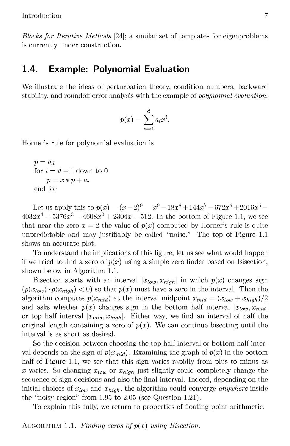
Let us apply this to p(x) = (x- 2)9 = x9 - 18a;8 + 144a;7 - 672a;6 + 2016a;5 -
4032a;4 + 5376a;3 - 4608a;2 + 2304a; - 512. In the bottom of Figure 1.1, we see
that near the zero x = 2 the value of p(x) computed by Horner's rule is quite
unpredictable and may justifiably be called "noise." The top of Figure 1.1
shows an accurate plot.
To understand the implications of this figure, let us see what would happen
if we tried to find a zero of p(x) using a simple zero finder based on Bisection,
shown below in Algorithm 1.1.
Bisection starts with an interval [a;;ou,, Xhigh] m which p(x) changes sign
(p(xiow) -pixhigh) < 0) so that p(x) must have a zero in the interval. Then the
algorithm computes p{xmid) at the interval midpoint xmid = (a;;ou, + Xhigh)/2
and asks whether p(x) changes sign in the bottom half interval [xiow, xmid]
or top half interval [xmid,Xhigh\- Either way, we find an interval of half the
original length containing a zero of p(x). We can continue bisecting until the
interval is as short as desired.
So the decision between choosing the top half interval or bottom half
interval depends on the sign of p(xmid)- Examining the graph oip(x) in the bottom
half of Figure 1.1, we see that this sign varies rapidly from plus to minus as
x varies. So changing xiow or xuigh just slightly could completely change the
sequence of sign decisions and also the final interval. Indeed, depending on the
initial choices of a;;ou, and Xhigh, the algorithm could converge anywhere inside
the "noisy region" from 1.95 to 2.05 (see Question 1.21).
To explain this fully, we return to properties of floating point arithmetic.
Algorithm 1.1. Finding zeros of p(x) using Bisection.
Applied Numerical Linear Algebra
xio-10
1.5
0.5
-0.5
-1.5
1.92 1.94 1.96 1.98 2 2.02 2.04 2.06 2.08
-0.5
-1.5
1.92
1.94
1.96
1.98
2.02
2.04
2.06
2.08
Fig. 1.1. Plot ofy=(x- 2)9 = x9 - 18a;8 + 144a;7 - 672a;6 + 2016a;5 - 4032a;4 +
5376a;3 — 4608a;2 + 2304a; — 512 evaluated at 8000 equispaced points, using y = (x — 2)9
(top) and using Horner's rule (bottom).
Introduction
9
proc bisect (p^Xi^^Xhigh^ol)
/* find a root of p{x) = 0 in [xiow,xhigh]
assuming pixi^) -p(xhigh) < 0 * /
/* stop if zero found to within ±tol * /
Plow OWJ
Phigh = PiXhigh)
while xhigh - xiow >2-tol
Xmid — \Xlow T Xhigh) I A
Pmid — P\Xmid)
if Plow -Pmid < 0 then /* there is a root in [xiow,xmid] */
<&high — <Emid
Phigh Pmid
else if pmid-Phigh < 0 then /* there is a root in [xmid,xhigh] */
Xlow Xrn-id
Plow — Pmid
else /* Xmid is a root */
Xlow — Xmid
Xhigh Xmid
end if
end while
root = (xiow + xhigh)/2
1.5. Floating Point Arithmetic
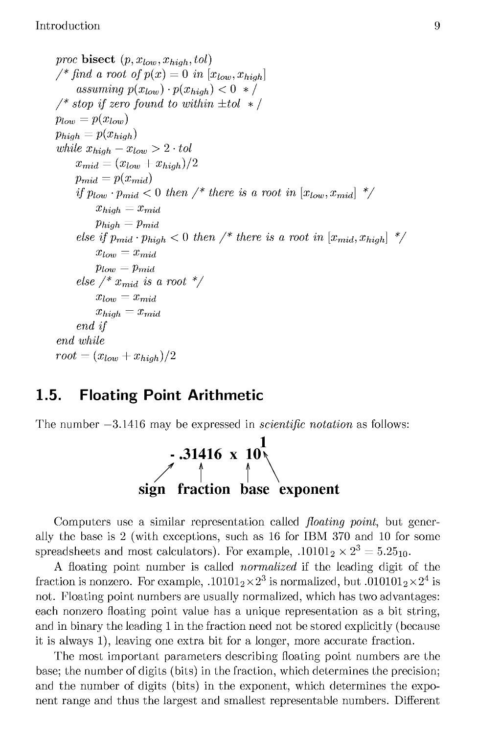
The number —3.1416 may be expressed in scientific notation as follows:
1
- .31416 x 10\
/ k t \
sign fraction base exponent
Computers use a similar representation called floating point, but
generally the base is 2 (with exceptions, such as 16 for IBM 370 and 10 for some
spreadsheets and most calculators). For example, .IOIOI2 x 23 = 5.25io-
A floating point number is called normalized if the leading digit of the
fraction is nonzero. For example, .IOIOI2 x23is normalized, but .OIOIOI2X24 is
not. Floating point numbers are usually normalized, which has two advantages:
each nonzero floating point value has a unique representation as a bit string,
and in binary the leading 1 in the fraction need not be stored explicitly (because
it is always 1), leaving one extra bit for a longer, more accurate fraction.
The most important parameters describing floating point numbers are the
base; the number of digits (bits) in the fraction, which determines the precision;
and the number of digits (bits) in the exponent, which determines the
exponent range and thus the largest and smallest representable numbers. Different
10
Applied Numerical Linear Algebra
floating point arithmetics also differ in how they round computed results, what
they do about numbers that are too near zero (underflow) or too big
(overflow), whether ±00 is allowed, and whether useful nonnumbers are provided
(sometimes called NaNs, indefinites, or reserved operands) are provided. We
discuss each of these below.
First we consider the precision with which numbers can be represented.
For example, .31416 x 101 has five decimal digits, so any information less than
.5 x 10~4 may have been lost. This means that if a; is a real number whose
best five-digit approximation is .31416 x 101, then the relative representation
error in .31416 x 101 is
lie - .31416 x 101! .5 x 10 _ __4
< T Ki .16 X 10 .
1
sign
8
exponent
23
1 fraction
.31416 x 101 - .31416 x 101
The maximum relative representation error in a normalized number occurs for
.10000 x 101, which is the most accurate five-digit approximation of all numbers
in the interval from .999995 to 1.00005. Its relative error is therefore bounded
by .5 • 10~4. More generally, the maximum relative representation error in a
floating point arithmetic with p digits and base C is .5 x /31_p. This is also half
the distance between 1 and the next larger floating point number, 1 + /31_p.
Computers have historically used many different choices of base, number
of digits, and range, but fortunately the IEEE standard for binary arithmetic
is now most common. It is used on SUN, DEC, HP, and IBM workstations
and all PCs. IEEE arithmetic includes two kinds of floating point numbers:
single precision C2 bits long) and double precision F4 bits long).
IEEE single precision
sign exponei
binary point
If s, e, and / < 1 are the 1-bit sign, 8-bit exponent, and 23-bit fraction in
the IEEE single precision format, respectively, then the number represented is
(—l)s • 2e_127 • A + /). The maximum relative representation error is 2-24 th
6 • 10~8, and the range of positive normalized numbers is from 2-126 (the
underflow threshold) to 2127 • B — 2-23) & 2128 (the overflow threshold), or
about 10~38 to 1038. The positions of these floating point numbers on the real
number line are shown in Figure 1.2 (where we use a 3-bit fraction for ease of
presentation).
IEEE double precision
sign exponei
binary point
If s, e, and / < 1 are the 1-bit sign, 11-bit exponent, and 52-bit fraction
in IEEE double precision format, respectively, then the number represented is
(—l)s • 2e_1023 • A + /). The maximum relative representation error is 2-53 ^
10~16, and the exponent range is 2-1022 (the underflow threshold) to 21023 •
1
sign
11
exponent
52
fraction
Introduction
11
128
-124
^-v
-126
-125
,-126
2
underflow
threshold
-0 and +0
-125
-124
,127,,, ,-23,
2 *B-2 )
overflow
threshold
,128
normalized
negative
numbers
subnormal
numbers
normalized
positive
numbers
Fig. 1.2. Real number line with floating point numbers indicated by solid tick marks.
The range shown is correct for IEEE single precision, but a 3-bit fraction is assumed
for ease of presentation so that there are only 23 — 1 = 7 floating point numbers
between consecutive powers of 2, not 223 — 1. The distance between consecutive tick
marks is constant between powers of 2 and doubles/halves across powers of 2 (among
the normalized floating point numbers). +2128 and — 2128, which are one unit in the
last place larger in magnitude than the overflow threshold (the largest finite floating
point number, 2127-B —2~23)), are shown as dotted tick marks. The figure is symmetric
about 0; +0 and —0 are distinct floating point bit strings but compare as numerically
equal. Division by zero is the only binary operation that gives different results, +oo
and — oo, for different signed zero arguments.
B
-52\
I024
(the overflow threshold), or about 10"
-308 tQ 10308_
When the true value of a computation a 0 b (where 0 is one of the four
binary operations +, —, *, and /) cannot be represented exactly as a
floatingpoint number, it must be approximated by a nearby floating point number
before it can be stored in memory or a register. We denote this approximation
by fl(a©6). The difference (a©6)—fl(a©6) is called the roundoff error. If fl(a©6)
is a nearest floating point number to a 0 6, we say that the arithmetic rounds
correctly (or just rounds). IEEE arithmetic has this attractive property. (IEEE
arithmetic breaks ties, when a 0 6 is exactly halfway between two adjacent
floating point numbers, by choosing fl(a 0 6) to have its least significant bit
zero; this is called rounding to nearest even.) When rounding correctly, if a ©6
is within the exponent range (otherwise we get overflow or underflow), then
we can write
fl(a©6) = (a©6)(l + 5), A.1)
where \5\ is bounded by s, which is called variously machine epsilon, machine
precision, or macheps. Since we are rounding as accurately as possible, e is
equal to the maximum relative representation error . 5 • /31_p. IEEE arithmetic
also guarantees that fl(y/a) = \fa(\ + 5), with \5\ < e. This is the most
common model for roundoff error analysis and the one we will use in this
book. A nearly identical formula applies to complex floating point arithmetic;
see Question 1.12. However, formula A.1) does ignore some interesting details.
IEEE arithmetic also includes subnormal numbers, i.e., unnormalized float-
12
Applied Numerical Linear Algebra
ing point numbers with the minimum possible exponent. These represent tiny
numbers between zero and the smallest normalized floating point number; see
Figure 1.2. Their presence means that a difference fl(a; — y) can never be zero
because of underflow, yielding the attractive property that the predicate x = y
is true if and only if fl(a; — y) = 0. To incorporate errors caused by underflow
into formula A.1) one would change it to
fl(a©6) = (aOb)(l + 5) + rj,
where \5\ < ? as before, and \rj\ is bounded by a tiny number equal to the
largest error caused by underflow B-150 ^ 10~45 in IEEE single precision and
2-1075 _ 10-324 in IEEE double precision).
IEEE arithmetic includes the symbols ±oo and NaN (Not a Number).±oo is
returned when an operation overflows, and behaves according to the following
arithmetic rules: a;/±oo = 0 for any finite floating point number x, x/0 = ±oo
for any nonzero floating point number x, +oo + oo = +oo, etc. An NaN is
returned by any operation with no well-defined finite or infinite result, such as
oo - oo, §§, §, v/^1, NaN 0 x, etc.
Whenever an arithmetic operation is invalid and so produces an NaN, or
overflows or divides by zero to produce ±oo, or underflows, an exception flag is
set and can later be tested by the user's program. These features permit one
to write both more reliable programs (because the program can detect and
correct its own exceptions, instead of simply aborting execution) and faster
programs (by avoiding "paranoid" programming with many tests and branches
to avoid possible but unlikely exceptions). For examples, see Question 1.19,
the comments following Lemma 5.3, and [80].
The most expensive error known to have been caused by an improperly
handled floating point exception is the crash of the Ariane 5 rocket of the
European Space Agency on June 4, 1996. See HOME/ariane5rep.html for
details.
Not all machines use IEEE arithmetic or round carefully, although nearly
all do. The most important modern exceptions are those machines produced
by Cray Research,2 although future generations of Cray machines may use
IEEE arithmetic.3 Since the difference between fl(a 0 6) computed on a Cray
and fl(a 0 6) computed on an IEEE machine usually lies in the 14th decimal
place or beyond, the reader may wonder whether the difference is important.
Indeed, most algorithms in numerical linear algebra are insensitive to details
in the way roundoff is handled. But it turns out that some algorithms are
easier to design, or more reliable, when rounding is done properly. Here are
two examples.
2We include machines such as the NEC SX-4, which has a "Cray mode" in which it
performs arithmetic the same way. We exclude the Cray T3D and T3E, which are
parallel computers built from DEC Alpha processors, which use IEEE arithmetic very nearly
(underflows are flushed to zero for speed's sake).
Cray Research was purchased by Silicon Graphics in 1996.
Introduction
13
When the Cray C90 subtracts 1 from the next smaller floating point
number, it gets —2-47, which is twice the correct answer, —2-48. Getting even
tiny differences to high relative accuracy is essential for the correctness of the
divide-and-conquer algorithm for finding eigenvalues and eigenvectors of
symmetric matrices, currently the fastest algorithm available for the problem. This
algorithm requires a rather nonintuitive modification to guarantee correctness
on Cray machines (see section 5.3.3).
The Cray may also yield an error when computing arccos (a;/\Jx2 + y2)
because excessive roundoff causes the argument of arccos to be larger than 1.
This cannot happen in IEEE arithmetic (see Question 1.17).
To accommodate error analysis on a Cray C90 or other Cray machines we
may instead use the model fl(a±6) = a(l+5i)±b(l+52), fl(a*6) = (a*b)(l+5s),
and fl(a/6) = (a/6)(l + 5s), with \5i\ < e, where e is a small multiple of the
maximum relative representation error.
Briefly, we can say that correct rounding and other features of IEEE
arithmetic are designed to preserve as many mathematical relationships used to
derive formulas as possible. It is easier to design algorithms knowing that
(barring over/underflow) fl(a — 6) is computed with a small relative error
(otherwise divide-and-conquer can fail), and that — 1 < c = ft(x/y/x2 + y2) < 1
(otherwise arccos(c) can fail). There are many other such mathematical
relationships that one relies on (often unwittingly) to design algorithms. For more
details about IEEE arithmetic and its relationship to numerical analysis, see
[157, 156, 80].
Given the variability in floating point across machines, how does one write
portable software that depends on the arithmetic? For example, iterative
algorithms that we will study in later chapters frequently have loops such as
repeat
update e
until "e is negligible compared to /,"
where e > 0 is some error measure, and / > 0 is some comparison value (see
section 4.4.5 for an example). By negligible we mean "is e < c • e • /?," where
c > 1 is some modest constant, chosen to trade off accuracy and speed of
convergence. Since this test requires the machine-dependent constant s, this test
has in the past often been replaced by the apparently machine-independent
test "is e + / = /?" The idea here is that adding e to / and rounding will
yield / again if e < sf or perhaps a little smaller. But this test can fail
(by requiring e to be much smaller than necessary, or than attainable),
depending on the machine and compiler used (see the next paragraph). So the
best test indeed uses e explicitly. It turns out that with sufficient care one
can compute e in a machine-independent way, and software for this is
available in the LAPACK subroutines slamch (for single precision) and dlamch
(for double precision). These routines also compute or estimate the overflow
14
Applied Numerical Linear Algebra
threshold (without overflowing!), the underflow threshold, and other
parameters. Another portable program that uses these explicit machine parameters
is discussed in Question 1.19.
Sometimes one needs higher precision than is available from IEEE single
or double precision. For example, higher precision is of use in algorithms such
as iterative refinement for improving the accuracy of a computed solution of
Ax = b (see section 2.5.1). So IEEE defines another, higher precision called
double extended. For example, all arithmetic operations on an Intel Pentium
(or its predecessors going back to the Intel 8086/8087) are performed in 80-bit
double extended registers, providing 64-bit fractions and 15-bit exponents.
Unfortunately, not all languages and compilers permit one to declare and compute
with double-extended precision variables.
Few machines offer anything beyond double-extended arithmetic in
hardware, but there are several ways in which more accurate arithmetic may be
simulated in software. Some compilers on DEC Vax and DEC Alpha, SUN
Sparc, and IBM RS6000 machines permit the user to declare quadruple
precision (or real*16 or double double precision) variables and to perform
computations with them. Since this arithmetic is simulated using shorter precision, it
may run several times slower than double. Cray's single precision is similar in
precision to IEEE double, and so Cray double precision is about twice IEEE
double; it too is simulated in software and runs relatively slowly. There are also
algorithms and packages available for simulating much higher precision
floating point arithmetic, using either integer arithmetic [20, 21] or the underlying
floating point (see Question 1.18) [202, 216].
Finally, we mention interval arithmetic, a style of computation that
automatically provides guaranteed error bounds. Each variable in an interval
computation is represented by a pair of floating point numbers, one a lower
bound and one an upper bound. Computation proceeds by rounding in such a
way that lower bounds and upper bounds are propagated in a guaranteed
fashion. For example, to add the intervals a = [ai,au] and b = [bi,bu], one rounds
ai + bi down to the nearest floating point number, a, and rounds au + bu
up to the nearest floating point number, cu. This guarantees that the
interval c = [q,cm] contains the sum of any pair of variables from a and from b.
Unfortunately, if one naively takes a program and converts all floating point
variables and operations to interval variables and operations, it is most likely
that the intervals computed by the program will quickly grow so wide (such as
[—oo, +oo]) that they provide no useful information at all. (A simple example
is to repeatedly compute when x is an interval; instead of getting
x = 0, the width xu — xi of x doubles at each subtraction.) It is possible to
modify old algorithms or design new ones that do provide useful guaranteed
error bounds [4, 138, 160, 188], but these are often several times as expensive
as the algorithms discussed in this book. The error bounds that we present
in this book are not guaranteed in the same mathematical sense that interval
bounds are, but they are reliable enough in almost all situations. (We discuss
Introduction
15
this in more detail later.) We will not discuss interval arithmetic further in
this book.
1.6. Polynomial Evaluation Revisited
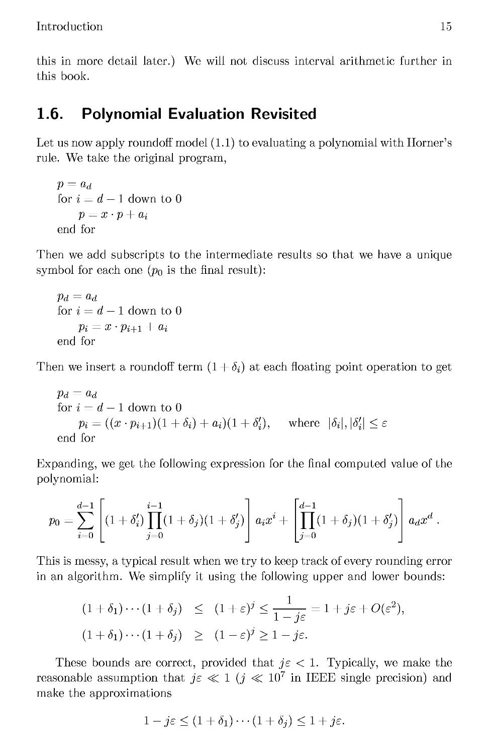
Let us now apply roundoff model A.1) to evaluating a polynomial with Horner's
rule. We take the original program,
for i = d — 1 down to 0
p = x ¦ p + a,i
end for
Then we add subscripts to the intermediate results so that we have a unique
symbol for each one (po is the final result):
Pd = ad
for i = d — 1 down to 0
Pi = x- pi+1 + a,i
end for
Then we insert a roundoff term A + Si) at each floating point operation to get
Pd = ad
for i = d — 1 down to 0
Pi = ((x -Pi+i){l + 6i) + ai)(l + 6'i), where |&|,|(^|<?
end for
Expanding, we get the following expression for the final computed value of the
polynomial:
d-i
Po = Y,
i=0
i-1
(i+$n(i+w+#
3=0
d-1
3=0
CLdXd .
This is messy, a typical result when we try to keep track of every rounding error
in an algorithm. We simplify it using the following upper and lower bounds:
A + <5i) • • • A + <*,-) < (l + ey<
1-je
l+je + 0(e2),
A + <5i) • • • A + <*,-) > (l-e)j>l-je.
These bounds are correct, provided that js < 1. Typically, we make the
reasonable assumption that js < 1 (j < 107 in IEEE single precision) and
make the approximations
I - je < (I + 5^ ¦ ¦ ¦ A + 53) <l + je.
16
Applied Numerical Linear Algebra
This lets us write
d
Po = /J(l + 5i)aiXl, where \5i\ < 2de
i=0
d
= y^jiiX1
i=0
So the computed value po of p(x) is the exact value of a slightly different
polynomial with coefficients Hi. This means that evaluating p{x) is "backward
stable," and the "backward error" is Ids measured as the maximum relation
change of any coefficient of p(x).
Using this backward error bound, we bound the error in the computed
polynomial:
\po-p(x)\ =
=
=
d d
^A + 5i)aiXl - y^aix
i=0 i=0
d
y^^jajX1
i=0
d
< J2e2d\
i=0
d
< :
lde)j \a,i
x%
i=0
Note that J2i \ai%l\ bounds the largest value that we could compute if there
were no cancellation from adding positive and negative numbers, and the error
bound is 2cfe times smaller. This is also the case for computing dot products
and many other polynomial-like expressions.
By choosing 5i = s ¦ sign(aiaf), we see that the error bound is attainable to
within the modest factor 2d. This means that we may use
l^j=Q l"»x I
I Vd nrl\
I Z^i=o "«x I
as the relative condition number for polynomial evaluation.
We can easily compute this error bound, at the cost of doubling the number
of operations:
p = ad, bp = \ad\
for i = d — 1 down to 0
p = x ¦ p + Cli
bp = \x\ ¦ bp+ \a,i\
end for
error bound = bp = 2d ¦ s ¦ bp
so the true value of the polynomial is in the interval [p — bp,p + bp], and the
number of guaranteed correct decimal digits is — log'i0(| — |). These bounds are
Introduction
17
plotted in the top ol Figure 1.3 for the polynomial discussed earlier, (x — 2)9.
(The reader may wonder whether roundoff errors could make this computed
error bound inaccurate. This turns out not to be a problem and is left to the
reader as an exercise.)
The graph of — log10 | — | in the bottom of Figure 1.3, a lower bound on
the number of correct decimal digits, indicates that we expect difficulty
computing p(x) to high relative accuracy when p(x) is near 0. What is special
about p(x) = 0? An arbitrarily small error e in computing p{x) = 0 causes
an infinite relative error -f^r = I. In other words, our relative error bound
p(x) 0 '
o K^l/I J2i=o ai-x%\ 1S infinite.
Definition 1.1. A problem whose condition number is infinite is called ill-
posed . Otherwise it is called well-posed .4
There is a simple geometric interpretation of the condition number: it tells
us how far p(x) is from a polynomial which is ill-posed.
Definition 1.2. Let p(z) = J2i=oaizt and q(z) = Z^=cA^- Define the
relative distance d(p,q) from p to q as the smallest value satisfying \ai — bi\ <
d(p,q) ¦ \a,i\ for 0 < i < d. (If all ai = 0, then we can more simply write
d(p,q) =max0<i<d\^^\.)
Note that if a\ = 0, then b\ must also be zero for d(p, q) to be finite.
Theorem 1.2. Suppose that p(z) = Y^i=o aizl ^s n°t identically zero.
Z-,i=0 aix I
mm{d(p, q) such that q(x) = 0}
Z-,i=0 \aixl
In other words, the distance from p to the nearest polynomial q whose condition
number at x is infinite is the reciprocal of the condition number of p(x).
Proof. Write q(z) = ^biZ1 = ^A + e^aiz1 so that d(p, q) = max^ \si\. Then
q(x) = 0 implies \p{x)\ = \q(x) - p{x)\ = \J2i=osiaixt\ < Yli=o\?iaixl\ <
maxi \si\ J2i \aixt\i which in turn implies d(p, q) = max \?i\ > \p(x)\/ J2i \aixl\-
To see that there is a q this close to p, choose
-p(x) . , ,-, ^
- — sign(aiX). ?
J2 \aixi
This definition is slightly nonstandard, because ill-posed problems include those whose
solutions are continuous as long as they are nondiflerentiable. Examples include multiple
roots of polynomials and multiple eigenvalues of matrices (section 4.3). Another way to
describe an ill-posed problem is one in which the number of correct digits in the solution is
not always within a constant of the number of digits used in the arithmetic in the solution.
For example, multiple roots of polynomials tend to lose half or more of the precision of the
arithmetic.
Applied Numerical Linear Algebra
xlO-1
1
0.8
0.6
0.4
0.2
0
-0.2
-0.4
-0.6
-0.8
-1—
1.85
upper bound
(x-2)A9
lower bound
1.9
1.95
2.05
2.1
2.15
16
Fig. 1.3. Plot of error bounds on the value of y = (x — 2)9 evaluated using Horner's
rule.
Introduction
19
This simple reciprocal relationship between condition number and distance
to the nearest ill-posed problem is very common in numerical analysis, and we
shall encounter it again later.
At the beginning of the introduction we said that we would use canonical
forms of matrices to help solve linear algebra problems. For example, knowing
the exact Jordan canonical form makes computing exact eigenvalues trivial.
There is an analogous canonical form for polynomials, which makes accurate
polynomial evaluation easy: p(x) = a,dYli=i(x ~ r*)- ^n other words, we
represent the polynomial by its leading coefficient ad and its roots r\,... rn. To
evaluate p(x) we use the obvious algorithm
P = a-d
for i = 1 to d
P = p ¦ (x — Ti)
end for
It is easy to show the computed p = p{x) ¦ A + 5), where \5\ < 2ds; i.e., we
always get p(x) with high relative accuracy. But we need the roots of the
polynomial to do this!
1.7. Vector and Matrix Norms
Norms are used to measure errors in matrix computations, so we need to
understand how to compute and manipulate them.
Missing proofs are left as problems at the end of the chapter.
Definition 1.3. Let B be a real (complex) linear space W1 (or C"). It is
normed if there is a function \\ ¦ \\ : B —>¦ R, which we call a norm, satisfying
all of the following :
1) ||a;|| > 0, and \\x\\ = 0 if and only ifx = 0 (positive defmiteness),
2) \\ax\\ = \a\ ¦ \\x\\ for any real (or complex) scalar a
(homogeneity),
3) ||a; + 2/|| < ||a;|| + \\y\\ (the triangle inequality).
Example 1.4. The most common norms are \\x\\p = (^ |a?i|pI/p for 1 < p <
oo, which we call p-norms, as well &S \\X oo — HISjX^ \Xi I, which we call the
co-norm or infinity-norm. Also, if ||a;|| is any norm and C is any nonsingular
matrix, then ||Ca;|| is also a norm, o
We see that there are many norms that we could use to measure errors; it
is important to choose an appropriate one. For example, let X\ = [1,2,3]T in
meters and X2 = [1-01, 2.01, 2.99]T in meters. Then X2 is a good approximation
to x\ because the relative error il"^00 ~ -0033, and X3 = [10,2.01,2.99]T is
a bad approximation because [ [["n = 3. But suppose the first component
20
Applied Numerical Linear Algebra
is measured in kilometers instead ol meters. Then in this norm x\ and 3K look
close:
" .001 "
2
3
, x3 =
.01
2.01
2.99
X\
To compare x\ and 3K, we should use
1000
Hail'
and
\X\ — Xz\
¦^1 ll°c
.0033 .
1
x
to make the units the same or so that equally important errors make the norm
equally large.
Now we define inner products, which are a generalization ol the standard
dot product J2i xiVii and arise frequently in linear algebra.
Definition 1.4. Let B be a real (complex) linear space. (•, ¦
is an inner product if all of the following apply :
B x B -»¦ R(C)
1) (x,y) = (y,x) (or (y,x)),
2) (x,y + z) = (x,y) + (x,z),
3) (ax,y) = a(x,y) for any real (or complex) scalar a,
4) (x, x) > 0, and (x, x) = 0 if and only ifx = 0.
Example 1.5. Over R, (x,y) = yTx = J2ixiyi> anc' over ^1 (x,y) = y*x =
J2ixiyi are inner products. (Recall that y* = yT is the conjugate transpose ol
V-) o
Definition 1.5. x and y are orthogonal if (x,y) = 0.
The most important property ol an inner product is that it satisfies the
Cauchy-Schwartz inequality. This can be used in turn to show that y/{x,x) is
a norm, one that we will frequently use.
Lemma 1.1. Cauchy-Schwartz inequality. \(x,y)\ < ^/(x,x) ¦ (y,y)-
Lemma 1.2. y/Jx~,
x) is a norm.
There is a one-to-one correspondence between inner-products and
symmetric (Hermitian) positive definite matrices, as defined below. These matrices
arise frequently in applications.
Definition 1.6. A real symmetric (complex Hermitian) matrix A is positive
definite if xTAx > 0 (x*Ax > 0) for all x = 0. We abbreviate symmetric
positive definite to s.p.d., and Hermitian positive to h.p.d..
Introduction
21
Lemma 1.3. Let B = Wl (or Cn) and (•,•) be an inner product. Then there
is an n-by-n s.p.d. (h.p.d.) matrix A such that (x,y) = yTAx (y*Ax).
Conversely, if A is s.p.d (h.p.d.), then yTAx (y*Ax) is an inner product.
The following two lemmas are useful in converting error bounds in terms
of one norm to error bounds in terms of another.
Lemma 1.4. Let || • \\a and \\ ¦ \\p be two norms on Rn (or Cn). There are
constants c±,C2 > 0 such that, for all x, ci\\x\\a < \\x\\p < C2\\x\\a. We also
say that norms \\ ¦ \\a and \\ ¦ \\p are equivalent with respect to constants c\ and
C2-
Lemma 1.5.
IMh < IMIi < v/^ll^lb,
IMIoo < ||a;||2 < v/nll^Hoo,
Halloo _ 11*^111 — /6||'^||00*
In addition to vector norms, we will also need matrix norms to measure
errors in matrices.
Definition 1.7. || • || is a matrix norm on m-by-n matrices if it is a vector
norm on m ¦ n dimensional space:
1) ||A|| > 0 and \\A\\ = 0 if and only ifA = 0,
2) ||aA|| = |a| • ||A||,
3) ||A + B|| < ||A|| + ||B||.
Example 1.6. max^- \a,ij\ is called the max norm, and (S Iftijl2I/2 = ||^4||f
is called the Frobenius norm, o
The following definition is useful for bounding the norm of a product of
matrices, something we often need to do when deriving error bounds.
Definition 1.8. Let \\ ¦ \\mxn be a matrix norm on m-by-n matrices, \\ ¦ ||„Xp
be a matrix norm on n-by-p matrices, and || • ||mXp be a matrix norm on m-
by-p matrices. These norms are called mutually consistent if \\A ¦ B\\mXp <
ll^llmxra • ||-B|UxP, where A is m-by-n and B is n-by-p.
Definition 1.9. Let A be m-by-n, \\ ¦ H^ be a vector norm on Rm, and \\ ¦ \\n
be a vector norm on Rn. Then
_ \\Ax\\™
Ut- Wmfi. = max - -
\\mn
* = ° \\X\
is called an operator norm or induced norm or subordinate matrix norm.
22
Applied Numerical Linear Algebra
The next lemma provides a large source of matrix norms, ones that we will
use for bounding errors.
Lemma 1.6. An operator norm is a matrix norm.
Orthogonal and unitary matrices, defined next, are essential ingredients of
nearly all our algorithms for least squares problems and eigenvalue problems.
Definition 1.10. A real square matrix Q is orthogonal if Q_1 = QT¦ A
complex square matrix is unitary if Q_1 = Q*.
All rows (or columns) of orthogonal (or unitary) matrices have unit 2-norms
and are orthogonal to one another, since QQT = QTQ = I (QQ* = Q*Q = I).
The next lemma summarizes the essential properties of the norms and
matrices we have introduced so far. We will use these properties later in the
book.
Lemma 1.7. 1. ||Ac|| < \\A\\ • ||a;|| for a vector norm and its corresponding
operator norm, or the vector two-norm and matrix Frobenius norm.
2. \\AB\\ < \\A\\ ¦ \\B\\ for any operator norm or for the Frobenius norm.
In other words, any operator norm (or the Frobenius norm) is mutually
consistent with itself.
3. The max norm and Frobenius norm are not operator norms.
4. HQAZH = \\A\\ if Q and Z are orthogonal or unitary for the Frobenius
norm and for the operator norm induced by \\ ¦ \\2- This is really just the
Pythagorean theorem.
5. Halloo = maxx=o M XJ = max^ Y] ¦ \aa\ = maximum absolute row sum.
1111 H^ll oo — J J
6. ||^4||i = maxx=o mJm = ||^4T||oo = maxj Y^/i \a\j\ = maximum absolute
column sum.
7. \\A\\2 = maxx=o mJi = \/^m~jA*AJ, where Amax denotes the largest
eigenvalue.
8. ||A||2 = ||AT||2.
9. \\A\\2 = maxi \Xi(A)\ if A is normal, i.e., AA* = A* A.
10. If A isn-by-n, then Ti_1/2||^4.||2 < Plli <n1/2PI|2-
11. If A isn-by-n, then n/2!^^ < PIU < n1/2||A||2.
12. If A isn-by-n, then n~1\\A\\00 < \\A\\i < n||^4||oo-
13. If A is n-by-n, then ||A||i < ||A||F < n^p^.
Introduction
23
Proof. We prove part 7 only and leave the rest to the reader.
Since A*A is Hermitian, there exists an eigendecomposition A* A = QAQ*,
with Q a unitary matrix (the columns are eigenvectors), and A = diag(Ai,...,
A„), a diagonal matrix containing the eigenvalues, which must all be real.
Note that all A^ > 0 since if one, say A, were negative, we would take q as
its eigenvector and get the contradiction 0 < ||^4#||| = qTATAq = qT\q =
\\\q\\l < 0. Therefore
\\Ax\\2 tx*A*AxI/2 (x*QAQ*xI/2
\\A h = max-11-—t^ = max ————=max- —-—-—
x=0 \\x\\2 x=0 \\x\\2 x=0 \\x\\2
((Q*xyAQ*xI/2 (y*AyI/2 Y,Wi
= max ——— = max —— = max '
x=o ||Q*a;)||2 y=o \\yh v=^ V ?j>.?
2
/ V^ 2
< max-y/AmaxW-^—|- = yf\r_
which is attainable by choosing y to be the appropriate column of the identity
matrix. ?
1.8. References and Other Topics for Chapter 1
At the end of each chapter we will list the references most relevant to that
chapter. They are also listed alphabetically in the bibliography at the end. In
addition we will give pointers to related topics not discussed in the main text.
The most modern comprehensive work in this area is by G. Golub and C.
Van Loan [119], which also has an extensive bibliography. A recent
undergraduate level or beginning graduate text in this material is by D. Watkins [250].
Another good graduate text is by L. Trefethen and D. Bau [241]. A classic
work that is somewhat dated but still an excellent reference is by J. Wilkinson
[260]. An older but still excellent book at the same level as Watkins is by G.
Stewart [233].
More detailed information on error analysis can be found in the recent book
by N. Higham [147]. Older but still good general references are by J. Wilkinson
[259] and W. Kahan [155].
"What every computer scientist should know about floating point
arithmetic" by D. Goldberg is a good recent survey [117]. IEEE arithmetic is
described formally in [11, 12, 157] as well as in the reference manuals published
by computer manufacturers. Discussion of error analysis with IEEE arithmetic
may be found in [53, 69, 157, 156] and the references cited therein.
A more general discussion of condition numbers and the distance to the
nearest ill-posed problem is given by the author in [70] as well as in a series
of papers by S. Smale and M. Shub [217, 218, 219, 220]. Vector and matrix
norms are discussed at length in [119, sects. 2.2, 2.3].
24
Applied Numerical Linear Algebra
1.9. Questions for Chapter 1
Question 1.1. (Easy; Z. Bai) Let A be an orthogonal matrix. Show that
det(A) = ±1. Show that if B also is orthogonal and det(A) = — det(B), then
A + B is singular.
Question 1.2. (Easy; Z. Bai) The ran& of a matrix is the dimension of the
space spanned by its columns. Show that A has rank one if and only if A = abT
for some column vectors a and b.
Question 1.3. (Easy; Z. Bai) Show that if a matrix is orthogonal and
triangular, then it is diagonal. What are its diagonal elements?
Question 1.4. (Easy; Z. Bai) A matrix is strictly upper triangular if it is
upper triangular with zero diagonal elements. Show that if A is strictly upper
triangular and n-by-n, then An = 0.
Question 1.5. (Easy; Z. Bai) Let || • || be a vector norm on W71 and assume
that C e RmXn. Show that if rank(A) = n, then \\x\\c = \\Cx\\ is a vector
norm.
Question 1.6. (Easy; Z. Bai) Show that if 0 = s G W1 and E e
l, then
El I
ss
STS
= \\E\
\Es\\^
STS
Question 1.7. (Easy; Z. Bai) Verify that H^y^Hi? = H^y^lb = IMI2IMI2 for
any x,y G C".
Question 1.8. (Medium) One can identify the degree d polynomials p(x) =
Y^i=o aixl with Md+1 via the vector of coefficients. Let x be fixed. Let Sx be
the set of polynomials with an infinite relative condition number with respect
to evaluating them at x (i.e., they are zero at x). In a few words, describe Sx
geometrically bset of Rd+1. Let Sx(k) be the set of polynomials whose
relative condition number is n or greater. Describe Sx(k) geometrically in a
few words. Describe how Sx(k) changes geometrically as k —>¦ 00.
Question 1.9. (Medium; from the 1995 final exam) Consider the figure
below. It plots the function y = log(l + x)/x computed in two different ways.
Mathematically, y is a smooth function of x near x = 0, equaling 1 at 0. But
if we compute y using this formula, we get the plots on the left (shown in the
ranges x e [—1,1] on the top left and x e [—10~15,10~15] on the bottom left).
This formula is clearly unstable near x = 0. On the other hand, if we use the
algorithm
Introduction
25
d = 1 + x
if d = 1 then
else
y = log(rf)/(rf - 1)
end if
we get the two plots on the right, which are correct near x = 0. Explain this
phenomenon, proving that the second algorithm must compute an accurate
answer in floating point arithmetic. Assume that the log function returns an
accurate answer for any argument. (This is true of any reasonable
implementation of logarithm.) Assume IEEE floating point arithmetic if that makes
your argument easier. (Both algorithms can malfunction on a Cray machine.)
y = logA+x)/x
y = logA+x)/[A+x)-1]
-0.8-0.6-0.4-0.2 0 0.2 0.4 0.6 0.8
x10
-1 -0.5 0 0.5 1
y = logA+x)/[A+x)-1]
-0.8-0.6-0.4-0.2 0 0.2 0.4 0.6 0.8
x 10
Question 1.10. (Medium) Show that, barring overflow or underflow,
HJ2i=i xiVi) = YA=ixiVi{^ + <y> where \6i\ < de. Use this to prove the
following fact. Let AmXn and BnXp be matrices, and compute their product
in the usual way. Barring overflow or underflow show that |fl(^4 • B) — A ¦ B\ <
n ¦ e ¦ \A\ ¦ \B\. Here the absolute value of a matrix |.A| means the matrix with
entries (|^4|)
i]
•njb
and the inequality is meant componentwise.
The result of this question will be used in section 2.4.2, where we analyze
the roundoff errors in Gaussian elimination.
26
Applied Numerical Linear Algebra
Question 1.11. (Medium) Let L be a lower triangular matrix and solve Lx =
b by forward substitution. Show that barring overflow or underflow, the
computed solution x satisfies (L + 8L)x = b, where \8kj\ < ns\kj\, where e is the
machine precision. This means that forward substitution is backward stable.
Argue that backward substitution for solving upper triangular systems satisfies
the same bound.
The result of this question will be used in section 2.4.2, where we analyze
the roundoff errors in Gaussian elimination.
Question 1.12. (Medium) In order to analyze the effects of rounding errors,
we have used the following model (see equation A.1)):
fl(aQb) = (aQb)(l + S),
where 0 is one of the four basic operations +, —, *, and /, and \5\ < s. To show
that our analyses also work for complex data, we need to prove an analogous
formula for the four basic complex operations. Now 5 will be a tiny complex
number bounded in absolute value by a small multiple of e. Prove that this
is true for complex addition, subtraction, multiplication, and division. Your
algorithm for complex division should successfully compute a/a & 1, where
\a\ is either very large (larger than the square root of the overflow threshold)
or very small (smaller than the square root of the underflow threshold). Is it
true that both the real and imaginary parts of the complex product are always
computed to high relative accuracy?
Question 1.13. (Medium) Prove Lemma 1.3.
Question 1.14. (Medium) Prove Lemma 1.5.
Question 1.15. (Medium) Prove Lemma 1.6.
Question 1.16. (Medium) Prove all parts except 7 of Lemma 1.7. Hint for
part 8: Use the fact that if X and Y are both n-by-n, then XY and YX have
the same eigenvalues. Hint for part 9: Use the fact that a matrix is normal if
and only if it has a complete set of orthonormal eigenvectors.
Question 1.17. (Hard; W. Kahan) We mentioned that on a Cray machine
the expression arccos(a;/Y/a;2 + y2) caused an error, because roundoff caused
(xj'\Jx2 + y2) to exceed 1. Show that this is impossible using IEEE arithmetic,
barring overflow or underflow. Hint: You will need to use more than the simple
model fl(a 0 6) = (a 0 6)A + 5) with \5\ small. Think about evaluating Vx2,
and show that, barring overflow or underflow, ^(Vx2) = x exactly; in numerical
experiments done by A. Liu, this failed about 5% of the time on a Cray YMP.
You might try some numerical experiments and explain them. Extra credit:
Prove the same result using correctly rounded decimal arithmetic. (The proof
is different.) This question is due to W. Kahan, who was inspired by a bug in
a Cray program of J. Sethian.
Introduction
27
Question 1.18. (Hard) Suppose a and b are normalized IEEE double
precision floating point numbers, and consider the following algorithm, running
with IEEE arithmetic:
if (\a\ < |6|), swap a and b
s\ = a + b
S2 = (a — si) + b
Prove the following facts:
1. Barring overflow or underflow, the only roundoff error committed in
running the algorithm is computing si = fl(a + 6). In other words, both
subtractions s\ — a and (s\ — a) — b are computed exactly.
2. S1 + S2 = a + b, exactly. This means that «2 is actually the roundoff error
committed when rounding the exact value of a + b to get s\.
Thus, this program in effect simulates quadruple precision arithmetic,
representing the true sum a + b as the higher-order bits (s\) and the lower-order
bits E2)-
Using this and similar tricks in a systematic way, it is possible to
efficiently simulate all four basic floating point operations in arbitrary precision
arithmetic, using only the underlying floating point instructions and no "bit-
fiddling" [202]. 128-bit arithmetic is implemented this way on the IBM RS6000
and Cray (but much less efficiently on the Cray, which does not have IEEE
arithmetic).
Question 1.19. (Hard; Programming) This question illustrates the challenges
in engineering highly reliable numerical software. Your job is to write a
program to compute the two-norm s = \\x\\2 = (YA=ix'iI^2 &ven X\,ldots,xn.
The most obvious (and inadequate) algorithm is
s = 0
for i = 1 to n
s = s + xf
endfor
s = sqrt(s)
This algorithm is inadequate because it does not have the following desirable
properties:
1. It must compute the answer accurately (i.e., nearly all the computed
digits must be correct) unless ||a;||2 is (nearly) outside the range of
normalized floating point numbers.
2. It must be nearly as fast as the obvious program above in most cases.
28
Applied Numerical Linear Algebra
3. It must work on any "reasonable" machine, possibly including ones not
running IEEE arithmetic. This means it may not cause an error
condition, unless ||a;||2 is (nearly) larger than the largest floating point number.
To illustrate the difficulties, note that the obvious algorithm fails when n = 1
and X\ is larger than the square root of the largest floating point number (in
which case x\ overflows, and the program returns +oo in IEEE arithmetic and
halts in most non-IEEE arithmetics) or when n = 1 and x\ is smaller than the
square root of the smallest normalized floating point number (in which case
x\ underflows, possibly to zero, and the algorithm may return zero). Scaling
the Xi by dividing them all by max^ \xi\ does not have property 2), because
division is usually many times more expensive than either multiplication or
addition. Multiplying by c = 1/maxj \xi\ risks overflow in computing c, even
when maxi \xi\ > 0.
This routine is important enough that it has been standardized as a Basic
Linear Algebra Subroutine, or BLAS, which should be available on all machines
[167]. We discuss the BLAS at length in section 2.6.1, and documentation
and sample implementations may be found at NETLIB/blas. In particular,
see NETLIB/cgi-bin/netlibget.pl/blas/snrm2.f for a sample implementation
that has properties 1) and 3) but not 2). These sample implementations are
intended to be starting points for implementations specialized to particular
architectures (an easier problem than producing a completely portable one, as
requested in this problem). Thus, when writing your own numerical software,
you should think of computing ||a;||2 as a building block that should be available
in a numerical library on each machine.
For another careful implementation of ||a;||2, see [34].
You can extract test code from NETLIB/blas/sblatl to see if your
implementation is correct; all implementations turned in must be thoroughly tested
as well as timed, with times compared to the obvious algorithm above on those
cases where both run. See how close to satisfying the three conditions you can
come; the frequent use of the word "nearly" in conditions A), B) and C)
shows where you may compromise in attaining one condition in order to more
nearly attain another. In particular, you might want to see how much easier
the problem is if you limit yourself to machines running IEEE arithmetic.
Hint: Assume that the values of the overflow and underflow thresholds are
available for your algorithm. Portable software for computing these values is
available (see NETLIB/cgi-bin/netlibget.pl/lapack/util/slamch.f).
Question 1.20. (Easy; Medium) We will use a Matlab program to illustrate
how sensitive the roots of polynomial can be to small perturbations in the
coefficients. The program is available5 at HOMEPAGE/Matlab/polyplot.m.
BRecall that we abbreviate the URL prefix of the class homepage to HOMEPAGE in the
text.
Introduction
29
Polyplot takes an input polynomial specified by its roots r and then adds
random perturbations to the polynomial coefficients, computes the perturbed
roots, and plots them. The inputs are
r = vector of roots of the polynomial,
e = maximum relative perturbation to make to each coefficient of
the polynomial,
m = number of random polynomials to generate, whose roots are
plotted.
1. (Easy) The first part of your assignment is to run this program for the
following inputs. In all cases choose m high enough that you get a fairly
dense plot but don't have to wait too long, m = a few hundred or perhaps
1000 is enough. You may want to change the axes of the plot if the graph
is too small or too large.
• r=(l:10); e = le-3, le-4, le-5, le-6, le-7, le-8,
• r=(l:20); e = le-9, le-11, le-13, le-15,
• r=[2,4,8,16,..., 1024]; e=le-l, le-2, le-3, le-4 (in this case, use
axis([.l,le4,-4,4]) and semilogx(real(rl),imag(rl),V) )
Also try your own example with complex conjugate roots. Which roots
are most sensitive?
2. (Medium) The second part of your assignment is to modify the program
to compute the condition number c(i) for each root. In other words, a
relative perturbation of e in each coefficient should change root r(i) by
at most about e*c(i). Modify the program to plot circles centered at r(i)
with radii e*c(i), and confirm that these circles enclose the perturbed
roots (at least when e is small enough that the linearization used to
derive the condition number is accurate). You should turn in a few plots
with circles and perturbed eigenvalues, and some explanation of what
you observe.
3. (Medium) In the last part, notice that your formula for c(i) "blows up" if
p'(r(i)) = 0. This condition means that r(i) is a multiple rootolp{x) = 0.
We can still expect some accuracy in the computed value of a multiple
root, however, and in this part of the question, we will ask how sensitive
a multiple root can be: First, write p{x) = q(x) ¦ (x — r(i))m, where
g(r(i)) = 0 and m is the multiplicity of the root r(i). Then compute the
m roots nearest r(i) of the slightly perturbed polynomial p(x) — q(x)e,
and show that they differ from r(i) by lei1/™. So that if m = 2, for
instance, the root r(i) is perturbed by e1/2, which is much larger than
e if |e| <C 1. Higher values of m yield even larger perturbations. If e is
around machine epsilon and represents rounding errors in computing the
root, this means an m-tuple root can lose all but 1/m-th of its significant
digits.
30
Applied Numerical Linear Algebra
Question 1.21. (Medium) Apply Algorithm 1.1, Bisection, to find the roots
of p(x) = (x — 2)9 = 0, where p(x) is evaluated using Horner's rule. Use the
Matlab implementation in HOMEPAGE/Matlab/bisect.m, or else write your
own. Confirm that changing the input interval slightly changes the computed
root drastically. Modify the algorithm to use the error bound discussed in the
text to stop bisecting when the roundoff error in the computed value of p(x)
gets so large that its sign cannot be determined.
2
Linear Equation Solving
2.1. Introduction
This chapter discusses perturbation theory, algorithms, and error analysis for
solving the linear equation Ax = b. The algorithms are all variations on
Gaussian elimination. They are called direct methods, because in the absence
of roundoff error they would give the exact solution of Ax = b after a finite
number of steps. In contrast, Chapter 6 discusses iterative methods, which
compute a sequence xo, xi, X2, ¦ ¦ • of ever better approximate solutions of Ax =
b; one stops iterating (computing the next Xi+\) when xi is accurate enough.
Depending on the matrix A and the speed with which x\ converges to x = A_1b,
a direct method or an iterative method may be faster or more accurate. We
will discuss the relative merits of direct and iterative methods at length in
Chapter 6. For now, we will just say that direct methods are the methods of
choice when the user has no special knowledge about the source6 of matrix A
or when a solution is required with guaranteed stability and in a guaranteed
amount of time.
The rest of this chapter is organized as follows. Section 2.2 discusses
perturbation theory for Ax = b; it forms the basis for the practical error bounds
in section 2.4. Section 2.3 derives the Gaussian elimination algorithm for dense
matrices. Section 2.4 analyzes the errors in Gaussian elimination and presents
practical error bounds. Section 2.5 shows how to improve the accuracy of a
solution computed by Gaussian elimination, using a simple and inexpensive
iterative method. To get high speed from Gaussian elimination and other
linear algebra algorithms on contemporary computers, care must be taken to
organize the computation to respect the computer memory organization; this
is discussed in section 2.6. Finally, section 2.7 discusses faster variations of
Gaussian elimination for matrices with special properties commonly arising in
practice, such as symmetry (A = AT) or sparsity (when many entries of A are
zero).
For example, in Chapter 6 we consider the case when A arises from approximating the
solution to a particular differential equation, Poisson's equation.
31
32
Applied Numerical Linear Algebra
Sections 2.2.1 and 2.5.1 discuss recent innovations upon which the software
in the LAPACK library depends.
There are a variety of open problems, which we shall mention as we go
along.
2.2. Perturbation Theory
Suppose Ax = b and (A + 5A)x = b + 5b; our goal is to bound the norm of
5x = x — x. We simply subtract these two equalities and solve for 5x: one way
to do this is to take
(A + 5A)(x + 5x) = b + 5b
_- [Ax = b]
5 Ax + (A + 5AMx = 5b
and rearrange to get
5x = A-\-5Ax + 5b). B.1)
Taking norms and using part 1 of Lemma 1.7 as well as the triangle inequality
for vector norms, we get
\\5x\\< WARSAW ¦ ||*ll+ l|fl>ID- B.2)
(We have assumed that the vector norm and matrix norm are consistent, as
defined in section 1.7. For example, any vector norm and its induced matrix
norm will do.) We can further rearrange this inequality to get
M<i^-.||.M|.(iM+jj«jj_y B.3)
The quantity k(A) = \\A 1|| • \\A\\ is the condition number7 of the matrix
A, because it measures the relative change -yP- in the answer as a multiple
of the relative change 4tJ in the data. (To be rigorous, we need to show
that inequality B.2) is an equality for some nonzero choice of 5A and 5b;
otherwise k(A) would only be an upper bound on the condition number. See
Question 2.3.) The quantity multiplying k(A) will be small if 5A and 5b are
small, yielding a small upper bound on the relative error Trfjf-
The upper bound depends on 5x (via x), which makes it seem hard to
interpret, but it is actually quite useful in practice, since we know the computed
solution x and so can straightforwardly evaluate the bound. We can also derive
a theoretically more attractive bound that does not depend on 5x as follows:
More pedantically, it is the condition number with respect to the problem of matrix
inversion. The problem of finding the eigenvalues of A, for example, has a different condition
number.
Linear Equation Solving
33
Lemma 2.1. Let \\ ¦ \\ satisfy \\AB\\ < \\A\\ ¦ \\B\\. Then \\X\\ < 1 implies that
I -X is invertible, (/-X) = E~0X\ and IKJ-X)!! < ^rpq-
Proof. The sum J2ilo X1 is said to converge if and only if it converges in
each component. We use the fact (from applying Lemma 1.4 to Example 1.6)
that for any norm, there is a constant c such that \xjk\ < c ¦ \\X\\. We then
get |(X*)jfc| < c- \\Xl\\ < c- ||X||l, so each component of ^Xl is dominated by
a convergent geometric series ^-A.JL— and must converge. Therefore Sn =
^"=0X* converges to some S as n —>¦ oo, and (/ — X)Sn = (I — X)(I +
X + X2 + h X") = I - Xn+1 -»¦ / as n -»¦ oo, since H^H < HX^ -»¦ 0.
Therefore (I-X)S = I and 5 = (/-X). The final bound is IKJ-X)!! =
II V^°° vi\\ <^ V^°° || "V"* II <^ V^°° || -vll* — 1 r-i
II Z^i=ox II < Z^i=o llA II < l^i=o \\x II - iqpq- D
Solving our first equation 5Ax + (^4 + 8A)8x = 8b for 8x yields
8x = (A + 6A)-\-6Ax + 6b)
= [Ail + A^SA^i-SAx + Sb)
= (I + A-18A)-1 A-1 (-8Ax + 5b).
Taking norms, dividing both sides by ||a;||, using part 1 of Lemma 1.7 and the
triangle inequality, and assuming that 8A is small enough so that ||^4_1(L4|| <
||^4_1|| • \\8A\\ < 1, we get the desired bound:
ff < \\(I + A-i8A)-^.\\A-^(\\8A\\ + ff)
ll^ll-PII f\\SA\\ , Httll
l-||A-i||.||A|||jj|l \\\A\\ \\A\\.\\x
K(A) f\\8A\\ \\8b\\\
~ i-K(A)^\\\A\\ + \\b\\) {ZA)
since ||6|| = ||Ac|| < \\A\\ ¦ \\x\\.
This bound expresses the relative error V^r in the solution as a multiple
of the relative errors '\m and '\j^- in the input. The multiplier, k(A)/A
k(A)
¦—-\ is close to the condition number k(A) if \\8A\\ is small enough.
The next theorem explains more about the assumption that ||^4_1|| • \\8A\\ =
k(A) ¦ T4I < 1: it guarantees that A + 8A is nonsingular, which we need for
8x to exist. It also establishes a geometric characterization of the condition
number.
Theorem 2.1. Let A be nonsingular. Then
mm \ M <n : A + 8A singular > = .. . _,..—
I Plb J A-1 2"
|A||2 «(A)
34
Applied Numerical Linear Algebra
Therefore, the distance to the nearest singular matrix (ill-posed problem) =
l
condition number '
Proof. It is enough to show min {||(L4||2 : A + 8 A singular} = n^iiM •
To show this minimum is at least n^iiM , note that if ||<L4||2 < im-im i
then 1 > \\5A\\2 ¦ ||^4_1||2 > ||A_1<L4||2, so Lemma 2.1 implies that I + A~15A
is invertible, and so A + 5A is invertible.
To show the minimum equals IIA-i„ , we construct a 5A of norm ,, ,ilM
\\A lb' ll-A 1||2
such that A + 5A is singular. Note that since ||^4_1||2 = maxx-0 ^ ,, /2.
II II -^
there exists an x such that ||a;||2 = 1 and ||^1_1||2 = ||^4_1a;||2 > 0. Now let
V = \\A-ix\\ = o^rr so \\y\\2 = 1. Let 5A = ^C.
Then
lie 4M IN^Ik |yT^| 1Mb 1
\\dA\\2 = max —r--— = max 1M = 1M ,
*=o HA-1!^ |M|2 ^=o 1Mb P_1||2 P_1l|2
where the maximum is attained when z is any nonzero multiple of y, and ^4+eL4
is singular because
(A + 8A)y = Ay-^f^ = —^-—^T- = 0. o
\ jy v WA-ty P_1||2 P_1||2
We have now seen that the distance to the nearest ill-posed problem equals
the reciprocal of the condition number for two problems: polynomial evaluation
and linear equation solving. This reciprocal relationship is quite common in
numerical analysis [70].
Here is a slightly different way to do perturbation theory for Ax = b; we
will need it to derive practical error bounds later in section 2.4.4. If x is any
vector, we can bound the difference 8x = x — x = x — A_1b as follows. We let
r = Ax — b be the residual of x; the residual r is zero if x = x. This lets us
write 5x = A_1r, yielding the bound
||fe|| = P_1r|| < ||A_1|| • ||r||. B.5)
This simple bound is attractive to use in practice, since r is easy to compute,
given an approximate solution x. Furthermore, there is no apparent need to
estimate 5A and 5b. In fact our two approaches are very closely related, as
shown by the next theorem.
Theorem 2.2. Let r = Ax — b. Then there exists a 5A such that \\8A\\ = M-
and (A + 8A)x = b. No 8A of smaller norm and satisfying {A + 8A)x = b
exists. Thus, 8A is the smallest possible backward error (measured in norm).
This is true for any vector norm and its induced norm (or || • H2 for vectors
and || • \\f for matrices).
Linear Equation Solving
35
Proof. (A + 5A)x = b if and only if 5A -x = b — Ax = — r, so ||r|| = ||(L4-ic|| <
\\8A\\ ¦ ||a;||, implying \\5A\\ > -Hi. We complete the proof only for the two-norm
and its induced matrix norm. Choose 8A = -jpp-. We can easily verify that
112
5A-x = -r and \\5A\\2 = -4f. ?
Thus, the smallest ||(L4
a: 2
that could yield an ? satisfying (A-\-5A)x = b and
r = Ax — b is given by Theorem 2.2. Applying error bound B.2) (with 5b = 0)
yields
||<te|| < HA!! dr-f-Plf) = P_1l
VIMI J
the same bound as B.5).
All our bounds depend on the ability to estimate the condition number
||^4|| • ||^4_1||. We return to this problem in section 2.4.3. Condition number
estimates are computed by LAPACK routines such as sgesvx.
2.2.1. Relative Perturbation Theory
In the last section we showed how to bound the norm of the error 5x = x — x
in the approximate solution x of Ax = b. Our bound on \\5x\\ was proportional
to the condition number k(A) = \\A\\ ¦ ||^4_1|| times the norms \\5A\\ and \\5b\\,
where x satisfies (A + 8A)x = 6 + 5b.
In many cases this bound is quite satisfactory, but not always. Our goal in
this section is to show when it is too pessimistic and to derive an alternative
perturbation theory that provides tighter bounds. We will use this
perturbation theory later in section 2.5.1 to justify the error bounds computed by the
LAPACK subroutines like sgesvx.
This section may be skipped on a first reading.
Here is an example where the error bound of the last section is much too
pessimistic.
Example 2.1. Let A = diagG,1) (a diagonal matrix with entries an = 7
and <222 = 1) and b = [7,1]T, where 7 > 1. Then x = A_1b = [1,1]T. Any
reasonable direct method will solve Ax = b very accurately (using two divisions
bi/an) to get x, yet the condition number k(A) = 7 may be arbitrarily large.
Therefore our error bound B.3) may be arbitrarily large.
The reason that the condition number k(A) leads us to overestimate the
error is that bound B.2), from which it comes, assumes that 5A is bounded
in norm, but is otherwise arbitrary; this is needed to prove that bound B.2)
is attainable in Question 2.3. In contrast, the 5A corresponding to the actual
rounding errors is not arbitrary but has a special structure not captured by
its norm alone. We can determine the smallest 5A corresponding to x for
our problem as follows: A simple rounding error analysis shows that Xi =
(bi/aa)/(l + Si), where \5i\ < e. Thus (an + 5iau)xi = b\. We may rewrite this
36
Applied Numerical Linear Algebra
as (A + 5A)x = 6, where 5A = diagEian, c^g^)- Then \\8A\\ can be as large
maxi \sau\ = sj. Applying error bound B.3) with 5b = 0 yields
?7
^ oo V 7
In contrast, the actual error satisfies
St —
|| UlLr || oo ~~
<
•b *b || oo
" Fi/on)/(l + *i
_ F2/a22)/(l + $2
' -tfi/a + tfi)
. -<V(i + s2)
?
Fi/an)
F2/«22)
1
or
<e/(l-e)
which is about 7 times smaller, o
For this example, we can describe the structure of the actual 5A as follows:
\Saij\ < e\aij\, where e is a tiny number. We write this more succinctly as
\5A\ < e|A|
B.6)
(see section 1.1 for notation). We also say that 5A is a small componentwise
relative perturbation in A. Since 5A can often be made to satisfy bound B.6) in
practice, along with \5b\ < e\b\ (see section 2.5.1), we will derive perturbation
theory using these bounds on 5A and 5b.
We begin with equation B.1):
5x = A'1 (-5 Ax + 5b).
Now take absolute values, and repeatedly use the triangle inequality to get
\5x\ = \A-\-5Ax + 5b)\
< lA-WSAl-lxl + lSbl)
< lA-^A] ¦ \x\ + e\b\)
= edA-^lAl-lxl + lbl)).
Now using any vector norm (like the infinity-, one-, or Frobenius norms), where
|| \z\ || = ||z||, we get the bound
\\5x\\ ^elHA-^GAHai
B.7)
Linear Equation Solving
37
Assuming for the moment that Sb = 0, we can weaken this bound to
\\Sx\\ < e|||^4_1| • \A\\\ • \\x\\
or
Jf^eiiiA-1!-!^!!!- B.6
This leads us to define kcr(A) = || |^4_1| • \A\ || as the componentwise relative
condition number of A, or just relative condition number for short. It is
sometimes also called the Bauer condition number [26] or Skeel condition number
[223, 224, 225]. For a proof that bounds B.7) and B.8) are attainable, see
Question 2.4.
Recall that Theorem 2.1 related the condition number k(A) to the distance
from A to the nearest singular matrix. For a similar interpretation of kcr(A),
see [71, 206].
Example 2.2. Consider our earlier example with A = diagG,1) and b =
[7,1]T. It is easy to confirm that kcr(A) = 1, since |^4_1| • \A\ = I. Indeed,
kcr(A) = 1 for any diagonal matrix A, capturing our intuition that a diagonal
system of equations should be solvable quite accurately, o
More generally, suppose D is any nonsingular diagonal matrix and B is an
arbitrary nonsingular matrix. Then
kcr(DB) = || KDB)-1] -\(DB)\ ||
= || IS!)-1! • \DB\ ||
= II l^! • \B\ ||
= kCr(B).
This means that if DB is badly scaled, i.e., B is well-conditioned but DB
is badly conditioned (because D has widely varying diagonal entries), then
we should hope to get an accurate solution of (DB)x = b despite DB's ill-
conditioning. This is discussed further in sections 2.4.4, 2.5.1, and 2.5.2.
Finally, as in the last section we provide an error bound using only the
residual r = Ax — b:
\\Sx\\ = ||A_1r|| < || |A_1| • \r\ ||, B.9)
where we have used the triangle inequality. In section 2.4.4 we will see that
this bound can sometimes be much smaller than the similar bound B.5), in
particular when A is badly scaled. There is also an analogue to Theorem 2.2
[191].
Theorem 2.3. The smallest e > 0 such that there exist \5A\ < e\A\ and \5b\ <
e\b\ satisfying (A+5A)x = b+5b is called the componentwise relative backward
error. It may be expressed in terms of the residual r = Ax — b as follows:
\r'
e = max
i (\A\-\x\ + \b\)t
38
Applied Numerical Linear Algebra
For a proof, see Question 2.5.
LAPACK routines like sgesvx compute the componentwise backward
relative error e (the LAPACK variable name for e is BERR).
2.3. Gaussian Elimination
The basic algorithm for solving Ax = 6 is Gaussian elimination. To state it,
we first need to define a permutation matrix.
Definition 2.1. A permutation matrix P is an identity matrix with permuted
rows.
The most important properties of a permutation matrix are given by the
following lemma.
Lemma 2.2. Let P, P\, and P2 be n-by-n permutation matrices and X be an
n-by-n matrix. Then
1. PX is the same as X with its rows permuted. XP is the same as X with
its columns permuted.
2. P = PT.
3. det(P) = ±1.
4. Pi • P2 is also a permutation matrix.
For a proof, see Question 2.6.
Now we can state our overall algorithm for solving Ax = b.
Algorithm 2.1. Solving Ax = b using Gaussian elimination:
1. Factorize A into A = PLU, where
P = permutation matrix,
L = unit lower triangular matrix (i.e., with ones on the diagonal),
U = nonsingular upper triangular matrix.
2. Solve PLUx = b for LUx by permuting the entries of b: LUx = P_16 =
PTb.
3. Solve LUx = P_16 for Ux by forward substitution: Ux = L~1(P~1b).
4. Solve Ux = L~1(P~1b) for x by back substitution: x = U~1(L~1P~1b).
We will derive the algorithm for factorizing A = PLU in several ways. We
begin by showing why the permutation matrix P is necessary.
Linear Equation Solving
39
Definition 2.2. The leading j-by-j principal submatrix of A is A(l : j, 1 : j).
Theorem 2.4. The following two statements are equivalent:
1. There exists a unique unit lower triangular L and nonsingular upper
triangular U such that A = LU.
2. All leading principal submatrices of A are nonsingular.
Proof. We first show A) implies B). A = LU may also be written
11 A12
21 A22
in 0
L21 L22
" tfn U12 '
0 U22 .
LnUn T\\U\2
L21U11 L
21
U\2 + L22U22
where An is a j-by-j leading principal submatrix, as are L\\ and U\\.
Therefore detain = det(Ln?/ii) = det L\\ det U\\ = 1 • rifc=i(^ii)fcfc = 0, since L is
unit triangular and U is triangular.
We prove that B) implies A) by induction on n. It is easy for 1-by-l
matrices: a = 1 • a. To prove it for n-by-n matrices A, we need to find unique
(n — l)-by-(n — 1) triangular matrices L and U, unique (n — l)-by-l vectors /
and u, and a unique nonzero scalar r\ such that
A =
~ A b~
cT 5
' L 0 "
JT 1 .
' U u~
0 V
LU Lu
lTU lTu +
V
By induction, unique L and U exist such that A = LU. Now let u = L_1b,
lT = cTU~1, and r\ = 5 — lTu, all of which are unique. The diagonal entries of
U are nonzero by induction, and r\ = 0 since 0 = det(A) = det(J7) • r\. ?
Thus LU factorization without pivoting can fail on (well-conditioned) non-
singular matrices such as the permutation matrix
P
0 1 0
0 0 1
1 0 0
the 1-by-l and 2-by-2 leading principal minors of P are singular. So we need
to introduce permutations into Gaussian elimination.
Theorem 2.5. If A is nonsingular, then there exist permutations P\ and P2,
a unit lower triangular matrix L, and a nonsingular upper triangular matrix
U such that P1AP2 = LU. Only one of P\ and P2 is necessary.
Note: P\A reorders the rows of A, AP2 reorders the columns, and P1AP2
reorders both.
40
Applied Numerical Linear Algebra
Proof. As with many matrix factorizations, it suffices to understand block
2-by-2 matrices. More formally, we use induction on the dimension n. It is
easy for I-by-I matrices: P\ = P2 = L = 1 and U = A. Assume that it is
true for dimension n — 1. If .A is nonsingular, then it has a nonzero entry;
choose permutations P[ and P2 so that the (I, I) entry of P[AP2 is nonzero.
(We need only one of P{ and P2 since nonsingularity implies that each row and
each column of A has a nonzero entry.)
Now we write the desired factorization and solve for the unknown
components:
P[AP'2
«11 M2
A2I A22
1 0
. L21 I.
Mil U12
L21UH L21U12 + A22
Uu
0
1
u12
A22
B.10)
where A22 and A22 are (n — l)-by-(n — 1).
Solving for the components of this 2-by-2 block factorization we get un =
an = 0, U12 = A12, and L21W11 = A21. Since un = an = 0, we can solve for
?21 = ^fp Finally, L21U12 + M2 = A22 implies A22 = A22 - L21U12.
We want to apply induction to A22, but to do so we need to check that
det A22 = 0: Since det P[AP2 = ± det A = 0 and also
det P[AP'2 = det
1
L21
0
I
•det
Un
0
U12
A22
1 • («n • det A22)
then det A22 must be nonzero.
Therefore, by induction there exist permutations Pi and P2 so that P1A22P2
= LU, with L unit lower triangular and U upper triangular and nonsingular.
Substituting this in the above 2-by-2 block factorization yields
P'iAP'2
0
I
0
PlL
Uu
0
1
0
0
PlL
1 0
L21 I
1
L21
1
L21
1 0
0 PT
so we get the desired factorization of A:
1 0
U12
PfLUPZ
Mil
0
1
P1L21
Un
0
U12P2
u
U12
up?
1
0
P1AP2
0 Pi
1
P1L21
P[)A P^
pT
Un
0
U12P2
u
Un
0
1 0
0 P2
U12P2
u
1
0
p?
?
Linear Equation Solving
41
The next two corollaries state simple ways to choose Pi and P2 to guarantee
that Gaussian elimination will succeed on a nonsingular matrix.
Corollary 2.1. We can choose P'2 = I and P[ so that an is the largest entry
in absolute value in its column, which implies L21 = -^2X has entries bounded by
1 in absolute value. More generally, at step i of Gaussian elimination, where
we are computing the ith column of L, we reorder the rows so that the largest
entry in the column is on the diagonal. This is called "Gaussian elimination
with partial pivoting," or GEPP for short. GEPP guarantees that all entries
of L are bounded by one in absolute value.
GEPP is the most common way to implement Gaussian elimination in
practice. We discuss its numerical stability in the next section. Another more
expensive way to choose Pi and P2 is given by the next corollary. It is almost
never used in practice, although there are rare examples where GEPP fails but
the next method succeeds in computing an accurate answer (see Question 2.14).
We discuss briefly it in the next section as well.
Corollary 2.2. We can choose P[ and P!2 so that a\\ is the largest entry
in absolute value in the whole matrix. More generally, at step % of Gaussian
elimination, where we are computing the ith column of L, we reorder the rows
and columns so that the largest entry in the matrix is on the diagonal. This is
called "Gaussian elimination with complete pivoting," or GECP for short.
The following algorithm embodies Theorem 2.5, performing permutations,
computing the first column of L and the first row of U, and updating A22 to get
A22 = A22 — L2iU\2- We write the algorithm first in conventional programming
language notation and then using Matlab notation.
Algorithm 2.2. LU factorization with pivoting
for i = 1 to n — 1
apply permutations so an = 0 (permute L and U too)
/* for example, for GEPP, swap rows j and i of A and of L
where I the largest entry in \A(i : n,i)\;
for GECP, swap rows j and i of A and of L,
and columns k and i of A and of U,
where \a,jk\ is the largest entry in \A(i :n,i: n)\ */
/* compute column i of L (L21 in B.10)) */
for j = i + 1 to n
ij-i — aj-if an
end for
/* compute row iofU {U12 in B.10)) */
for j = i to n
Uj-ij — a-ij
42
Applied Numerical Linear Algebra
end for
/* update A22 {to get A22 = A22 - L21U12 in B.10)) */
for j = i + 1 to n
for k = i + 1 to n
end for
end for
end for
Note that once column i of A is used to compute column i of L, it is never
used again. Similarly, row i of A is never used again after computing row i of
U. This lets us overwrite L and U on top of A as they are computed, so we
need no extra space to store them; L occupies the (strict) lower triangle of A
(the ones on the diagonal of L are not stored explicitly), and U occupies the
upper triangle of A. This simplifies the algorithm to
Algorithm 2.3. LU factorization with pivoting, overwriting L and U on A:
for i = 1 to n — 1
apply permutations (see Algorithm 2.2 for details)
for j = i + 1 to n
aji — aj-if an
end for
for j = i + 1 to n
for k = i + 1 to n
O'jk = O'jk Oiji * O'ik
end for
end for
end for
Using Matlab notation this further reduces to the following algorithm.
Algorithm 2.4. LU factorization with pivoting, overwriting L and U on A:
for i = 1 to n — 1
apply permutations (see Algorithm 2.2 for details)
A(i + 1 : n, i) = A(i + 1 : n, i)/A(i, i)
A(i + 1 : n, i + 1 : n) =
A(i + 1 : n, i + 1 : n) - A(i + 1 : n, i) * A(i, i + l:ri)
end for
In the last line of the algorithm, A(i + 1 : n, i)*A(i,i + l : n) is the product
of an (n — i)-by-l matrix (L2\) by a l-by-(n — i) matrix (C/12), which yields an
(n — i)-by-(n — i) matrix.
Linear Equation Solving
43
We now rederive this algorithm from scratch starting from perhaps the most
familiar description of Gaussian elimination: "Take each row and subtract
multiples of it from later rows to zero out the entries below the diagonal."
Translating this directly into an algorithm yields
for i = 1 to n — 1 /* for each row i */
for j = i + 1 to n /* subtract a multiple of
row i from row j ... */
for k = i to n /* ... in columns i through n ... */
ajk = ajk — ^aik /* ••• to zero out column i
below the diagonal */
end for
end for
end for
We will now make some improvements to this algorithm, modifying it until
it becomes identical to Algorithm 2.3 (except for pivoting, which we omit).
First, we recognize that we need not compute the zero entries below the
diagonal, because we know they are zero. This shortens the k loop to yield
for i = 1 to n —
1
for j = i + 1 to n
for k =
a>jk
end for
end for
end for
i + 1 to
= a>jk —
n
aji
a>ik
The next performance improvement is to compute — outside the inner
loop, since it is constant within the inner loop.
for i = 1 to n — 1
for j = i + 1 to n
1 aji
end for
for j = i + 1 to n
for k = i
O-jk -
end for
end for
end for
+ 1 to
= o-jk —
n
Iji
O-ik
Finally, we store the multipliers kj in the subdiagonal entries aij that we
originally zeroed out; they are not needed for anything else. This yields
Algorithm 2.3 (except for pivoting).
44
Applied Numerical Linear Algebra
The operation count of LU is done by replacing loops by summations over
the same range, and inner loops by their operation counts:
n — l I n n n
? ?i+? ?2
i=l \ j'=i+l j'=i+l k=i-\-l
n-1
= V((n -i) + 2(n - if) = -n3 + 0(n2).
i=\ 6
The forward and back substitutions with L and U to complete the solution
of Ax = b cost 0(n2), so overall solving Ax = b with Gaussian elimination
costs |n3 +0(n2) operations. Here we have used the fact that YllLi ^fc =
mk+1/(k + 1) + 0{mk). This formula is enough to get the high order term in
the operation count.
There is more to implementing Gaussian elimination than writing the
nested loops of Algorithm 2.2. Indeed, depending on the computer,
programming language, and matrix size, merely interchanging the last two loops on j
and k can change the execution time by orders of magnitude. We discuss this
at length in section 2.6.
2.4. Error Analysis
Recall our two-step paradigm for obtaining error bounds for the solution of
Ax = b:
1. Analyze roundoff errors to show that the result of solving Ax = b is the
exact solution x of the perturbed linear system (A+5A)x = b+5b, where
5A and 5b are small. This is an example of backward error analysis, and
5A and 5b are called the backward errors.
2. Apply the perturbation theory of section 2.2 to bound the error, for
example by using bound B.3) or B.5).
We have two goals in this section. The first is to show how to implement
Gaussian elimination in order to keep the backward errors 5A and 5b small.
In particular, we would like to keep \jw and 4nJ- as small as 0(e). This is as
small as we can expect to make them, since merely rounding the largest entries
of A (or 6) to fit into the floating point format can make JLJ (or ||L>?)- It
turns out that unless we are careful about pivoting, 5A and 5b need not be
small. We discuss this in the next section.
The second goal is to derive practical error bounds which are simultaneously
cheap to compute and "tight," i.e., close to the true errors. It turns out that
the best bounds for \\5A\\ that we can formally prove are generally much larger
than the errors encountered in practice. Therefore, our practical error bounds
(in section 2.4.4) will rely on the computed residual r = Ax—b and bound B.5),
Linear Equation Solving
45
instead of bound B.3). We also need to be able to estimate k(A) inexpensively;
this is discussed in section 2.4.3.
Unfortunately, we do not have error bounds that always satisfy our twin
goals of cheapness and tightness, i.e., that simultaneously
1. cost a negligible amount compared to solving Ax = 6 in the first place
(for example, that cost 0{n2) flops versus Gaussian elimination's 0(n3)
flops), and
2. provide an error bound that is always at least as large as the true error
and never more than a constant factor larger (fOO times larger, say).
The practical bounds in section 2.4.4 will cost 0(n2) but will on very rare
occasions provide error bounds that are much too small or much too large.
The probability of getting a bad error bound is so small that these bounds are
widely used in practice. The only truly guaranteed bounds use either interval
arithmetic, very high precision arithmetic, or both and are several times more
expensive than just solving Ax = b (see section f .5).
It has in fact been conjectured that no bound satisfying our twin goals of
cheapness and tightness exist, but this remains an open problem.
2.4.1. The Need for Pivoting
Let us apply LU factorization without pivoting to A = [ ' 1 ] in three
decimal-digit floating point arithmetic and see why we get the wrong answer.
Note that k(A) = ||^4||oo • ||^4_1||oo ~ 4, so A is well conditioned and thus we
should expect to be able to solve Ax = b accurately.
L =
U =
so LU =
but A =
I
0
I
fl(I/iO-4
10 I
fl(l - 104 • I)
, fl(l/10-4) rounds to I04,
, fl(l - I04 • I) rounds to - I04,
I 0
I04 I
10 I
I I
10"
1
-104
10 1
1 0
Note that the original 022 has been entirely "lost" from the computation by
subtracting 104 from it. We would have gotten the same LU factors whether
<222 had been 1, 0, —2, or any number such that fl(a22 — 104) = —104. Since
the algorithm proceeds to work only with L and U, it will get the same answer
for all these different 022, which correspond to completely different A and
so completely different x = ^4_16; there is no way to guarantee an accurate
answer. This is called numerical instability, since L and U are not the exact
46
Applied Numerical Linear Algebra
factors of a matrix close to A. (Another way to say this is that \\A — LU\\ is
about as large as ||^4||, rather than e||^4||.)
Let us see what happens when we go on to solve Ax = [1, 2]T for x using
this LU factorization. The correct answer is x & [1,1]T. Instead we get the
following. Solving Ly = [1, 2]T yields yx = fl(l/l) = 1 and y2 = flB - 104 • 1) =
—104; note that the value 2 has been "lost" by subtracting 104 from it. Solving
Ux = y yields x2 = fl((-104)/(-104)) = 1 and xx = fl((l - 1)/10) = 0, a
completely erroneous solution.
Another warning of the loss of accuracy comes from comparing the
condition number of A to the condition numbers of L and U. Recall that we
transform the problem of solving Ax = b into solving two other systems with
L and U, so we do not want the condition numbers of L or U to be much larger
than that of A. But here, the condition number of A is about 4, whereas the
condition numbers of L and U are about 108.
In the next section we will show that doing GEPP nearly always eliminates
the instability just illustrated. In the above example, GEPP would have
reversed the order of the two equations before proceeding. The reader is invited
to confirm that in this case we would get
and
L
U =
1 0
fl(.0001/l) 1
1 1
0 fl(l - .0001
1)
1
.0001
1
0
0
1
1
1
so
that LU approximates A quite accurately. Both L and U are quite well
conditioned, as is A. The computed solution vector is also quite accurate.
2.4.2. Formal Error Analysis of Gaussian Elimination
Here is the intuition behind our error analysis of LU decomposition. If
intermediate quantities arising in the product L ¦ U are very large compared to
||^4||, the information in entries of A will get "lost" when these large values
are subtracted from them. This is what happened to a22 in the example in
section 2.4.1. If the intermediate quantities in the product L ¦ U were instead
comparable to those of A, we would expect a tiny backward error A — LU in the
factorization. Therefore, we want to bound the largest intermediate quantities
in the product L ¦ U. We will do this by bounding the entries of the matrix
\L\ ¦ \U\ (see section 1.1 for notation).
Our analysis is analogous to the one we used for polynomial evaluation
in section 1.6. There we considered p = J2i ai%x anc' showed that if \p\ were
comparable to the sum of absolute values J2i \aixl\, then p would be computed
accurately.
After presenting a general analysis of Gaussian elimination, we will use
it to show that GEPP (or, more expensively, GECP) will keep the entries of
\L\ ¦ \U\ comparable to ||^4|| in almost all practical circumstances.
Linear Equation Solving
47
Unfortunately, the best bounds on \\6A\\ that we can prove in general are
still much larger than the errors encountered in practice. Therefore, the error
bounds that we use in practice will be based on the computed residual r and
bound B.5) (or bound B.9)) instead of the rigorous but pessimistic bound in
this section.
Now suppose that matrix A has already been pivoted, so the notation is
simpler. We simplify Algorithm 2.2 to two equations, one for ajk with j < k
and one for j > k. Let us first trace what Algorithm 2.2 does to ajk when
j < k: this element is repeatedly updated by subtracting IjiUik for i = 1 to
j — I and is finally assigned to Ujk so that
When j > k, ajk again has IjiUik subtracted for i = 1 to k — 1, and then the
resulting sum is divided by Ukk and assigned to Ijk-
, djk Z_^i=l IjiUik
vjk — •
Ukk
To do the roundoff error analysis of these two formulas, we use the result
from Question 1.10 that a dot product computed in floating point arithmetic
satisfies
/ d \ d
A ^2 xi1Ji = ^2 Xiyi(l + Si) with \5i\ < de.
\i=l I i=\
We apply this to the formula for Ujk, yielding8
Ujk = f ajk - ^j l3iUikiX + ?i) j A + 8')
with \5i\ < (j — l)e and \5'\ < e. Solving for ajk we get
aJk = Jjwujk ¦ Ijj + Yji=\ hiuik{1 + ^i) since Ijj = 1
with \5i\ < (j — l)e and 1 + 5j = j^p-
= Z_^i=l IjiUik i l-'jki
where we can bound Ejk by
\Ejk\ -
Y.h-u.k-S,
i=\
Strictly speaking, the next formula assumes we compute the sum first and then subtract
from ajk- But the final bound does not depend on the order of summation.
48
Applied Numerical Linear Algebra
, = A + 5ll) Ai + ^)(ffljfc-EttiOi«ifc(i + ^))'
Doing the same analysis for the formula for Ijk yields
Ukk
with \5i\ < (k — l)e, \5'\ < s, and \5"\ < e. We solve for ajk to get
fc-i
ajk = TTT^rn~X"\Ukkl/jk + ^ hWiU1 + s-<
with 1 + 8k =
A + S')A + S")"'
k
/ j vji^ik
i=\
k
/ ^ vji^ik
k
• + 2_^ h->
i=\
; + Ejk
kk^jk
iVjikO-i
1
(l + 5')(l + 5")
with \5i\ < ns, and so \Ejk\ < ns(\L\ ¦ \U\)jk as before.
Altogether, we can summarize this error analysis with the simple formula
A = LU + E where \E\ < ne\L\ -\U\. Taking norms we get \\E\\ < ns\\ \L\ \\ ¦
|| \U\ ||. If the norm does not depend on the signs of the matrix entries (true for
the Frobenius, infinity-, and one-norms but not the two-norm), we can simplify
this to ||?|| <n?\\L\\ ¦ \\U\\.
Now we consider solving the rest of the problem: LUx = b via Ly = b
and Ux = y. The result of Question 1.11 shows that solving Ly = b by
forward substitution yields a computed solution y satisfying (L+5L)y = b with
\5L\ <ns\L\. Similarly when solving Ux = y we get x satisfying (U+5U)x = y
with \5U\ <ne\U\.
Combining these yields
b = (L + SL)y
= (L + 5L)(U + 5U)x
= (LU + L5U + 5LU + 5L5U)x
= (A-E + L5U + 5LU + 5L5U)x
= (A + 5A)x where 5A = -E + L5U + 5LU + 5L5U
Now we combine our bounds on E, 5L, and 5U and use the triangle inequality
to bound 5A:
\5A\ = \-E + L5U + 5LU + 5L5U\
< \E\ + \L5U\ + \5LU\ + \5L5U\
< \E\ + \L\ ¦ \5U\ + \5L\ ¦ \U\ + \5L\ ¦ \5U\
< ne\L\ -\U\+ ne\L\ ¦ \U\ + ne\L\ -\U\+ n2e2\L\ ¦ \U\
« 3ne\L\-\U\.
Linear Equation Solving
49
Taking norms and assuming || \X\ \\ = \\X\\ (true as before for the Frobe-
nius, infinity-, and one-norms but not the two-norm) we get \\5A\\ < 3ne:||L|| •
ll^ll-
Thus, to see when Gaussian elimination is backward stable, we must ask
when 3ne:||L|| • ||J7|| = 0(e:)||^4||; then the 4oj in the perturbation theory
bounds will be 0(s) as we desire (note that 5b = 0).
The main empirical observation, justified by decades of experience, is that
GEPP almost always keeps ||L||-||J7|| & \\A\\. GEPP guarantees that each entry
of L is bounded by f in absolute value, so we need consider only ||J7||. We define
the pivot growth factor for GEPP9 as gFF = ||?/||max/||^4||max, where ||^4||max =
maxjj \aij\, so stability is equivalent to gFF being small or growing slowly as a
function of n. In practice, gFF is almost always n or less. The average behavior
seems to be n2/3 or perhaps even just n1/2 [240]. (See Figure 2.1.) This makes
GEPP the algorithm of choice for many problems. Unfortunately, there are
rare examples in which gFF can be as large as 2"_1.
Proposition 2.1. GEPP guarantees that gFF < 2n~1. This bound is
attainable.
Proof. The first step of GEPP updates djk = ajk — Iji ¦ Uik, where \lji\ < 1
and \uik\ = \dik\ < maxrs |ars|, so |ajfc| < 2 • maxrs |ars|. So each of the n — 1
major steps of GEPP can double the size of the remaining matrix entries, and
we get 2n~1 as the overall bound. See the example in Question 2.14 to see that
this is attainable. ?
Putting all these bounds together, we get
Halloo < 35ppn3?PHoo, B.11)
since ||L||oo < n and ||J7||oo < «5pp||^4||oo- The factor 3gPPn3 in the bound
causes it to almost always greatly overestimate the true \\5A\\, even if gFF = 1.
For example, if e = 10~7 and n = 150, a very modest sized matrix, then
3n3? > 1, meaning that all precision is potentially lost. Example 2.3 graphs
3gFFn3s along with the true backward error to show how it can be pessimistic;
\\5A\\ is usually 0(e:)||^4||, so we can say that GEPP is backward stable in
practice, even though we can construct examples where it fails. Section 2.4.4
presents practical error bounds for the computed solution of Ax = b that are
much smaller than what we get from using H^Hoo < S^ppn^H^llloo.
It can be shown that GECP is even more stable than GEPP, with its pivot
growth 5Gp satisfying the worst-case bound [260, p. 213]
max,;,- \u.
max.
^P4 < V/n-2-31/2.4i/3...ni/(«-i) « ni/2 + loge n/4.
This definition is slightly different from the usual one in the literature but essentially
equivalent [119, p. 115].
50
Applied Numerical Linear Algebra
This upper bound is also much too large in practice. The average behavior of
5gp is n1/2. It was an old open conjecture that gcv < n, but this was recently
disproved [97, 120]. It remains an open problem to find a good upper bound
for gCF (which is still widely suspected to be 0{n).)
The extra 0(n3) comparisons that GECP uses to find the pivots @(n2)
comparisons per step, versus 0{n) for GEPP) makes GECP significantly slower
than GEPP, especially on high-performance machines that perform floating
point operations about as fast as comparisons. Therefore, using GECP is
seldom warranted (but see sections 2.4.4, 2.5.1, and 5.4.3).
Example 2.3. Figures 2.1 and 2.2 illustrate these backward error bounds. For
both figures, five random matrices A of each dimension were generated, with
independent normally distributed entries, of mean 0 and standard deviation
1. (Testing such random matrices can sometimes be misleading about the
behavior on some real problems, but it is still informative.) For each matrix,
a similarly random vector b was generated. Both GEPP and GECP were used
to solve Ax = b. Figure 2.1 plots the pivot growth factors gFF and gGp- In both
cases they grow slowly with dimension, as expected. Figure 2.2 shows our two
upper bounds for the backward error, 3n3?gFF (or 3n3?gCi>) and Li •
It also shows the true backward error, computed as described in Theorem 2.2.
Machine epsilon is indicated by a solid horizontal line at e = 2-53 ^ 1.1 • 10~16.
Both bounds are indeed bounds on the true backward error but are too large
by several order of magnitude. For the Matlab program that produced these
plots, see HOMEPAGE/Matlab/pivot.m. o
2.4.3. Estimating Condition Numbers
To compute a practical error bound based on a bound like B.5), we need
to estimate ||^4_1||. This is also enough to estimate the condition number
k(A) = ||^4_1||-||^4||, since \\A\\ is easy to compute. One approach is to compute
A-1 explicitly and compute its norm. However, this would cost 2n3, more than
the original |n3 for Gaussian elimination. (Note that this implies that it is not
cheaper to solve Ax = b by computing A-1 and then multiplying it by b. This
is true even if one has many different b vectors. See Question 2.2.) It is a fact
that most users will not bother to compute error bounds if they are expensive.
So instead of computing A-1 we will devise a much cheaper algorithm to
estimate ||^4_1||. Such an algorithm is called a condition estimator and should
have the following properties:
1. Given the L and U factors of A, it should cost 0(n2), which for large
enough n is negligible compared to the |n3 cost of GEPP.
2. It should provide an estimate which is almost always within a factor of 10
of ||^4_1||. This is all one needs for an error bound which tells you about
Linear Equation Solving
51
Pivot Growth Factors, Partial = o, Complete = +
O 8 ° ° B o o
O a
O
o tb
¦o
« »
s 8 ° o
o g o 8 o
8 o
W + I"
* *
0 10 20 30 40 50 60 70 80 90 100
Matrix Dimension
Fig. 2.1. Pivot growth on random matrices, o = p,
pp? t — yep-
Backward error in Gaussian Elimination with Partial Pivoting
10
10
10
10
10
10
10"
10"
10"
10"
macheps = 2A(-53) = 1.1e-16
* *
M X
§88e
+ + + + +
8 8 8 8
* x x * N II
+ + + + +
8 8 0
10 20 30 40 50 60
Matrix dimension
70
80 90 100
Backward error in Gaussian Elimination with Complete Pivoting
macheps = 2A(-53) = 1.1 e-16
x X * *
ft *
N
: - t * * + * + +
O I I I I
X
+
ft
+
0
ft x
+ +
e »
*
8
X
+
y
+
X
+
i
X
+
s
X ft '!
+ + "
8 S &
i
10 20
30
40 50 60
Matrix dimension
70
80 90
100
Fig. 2.2. Backward error in Gaussian elimination on random matrices, x = 3n3eg,
+ = 3n|||L| • I^IHoo/PIU ° = \\Ax - felloo/dlAIUMU.
52
Applied Numerical Linear Algebra
how many decimal digits of accuracy that you have. (A factor-of-10 error
is one decimal digit.10)
There are a variety of such estimators available (see [144] for a survey).
We choose to present one that is widely applicable to problems besides solving
Ax = b, at the cost of being slightly slower than algorithms specialized for
Ax = b (but it is still reasonably fast). Our estimator, like most others, is
guaranteed to produce only a lower bound on ||^4_1||, not an upper bound.
Empirically, it is almost always within a factor of 10, and usually 2 to 3, of
||^4_1||. For the matrices in Figures 2.1 and 2.2, where the condition numbers
varied from 10 to 105, the estimator equaled the condition number to several
decimal places 83% of the time and was .43 times too small at worst. This is
more than accurate enough to estimate the number of correct decimal digits
in the final answer.
The algorithm estimates the one-norm ||-B||i of a matrix B, provided that
we can compute Bx and BTy for arbitrary x and y. We will apply the algorithm
to B = A-1, so we need to compute A~xx and A~Ty, i.e., solve linear systems.
This costs just 0(n2) given the LU factorization of A. The algorithm was
developed in [136, 144, 146], with the latest version in [145]. Recall that ||-B||i
is defined by
II D II n
II DM WBX * V^IJ. I
\\B i = max ——-— = max > 0j7-.
z=o \\x\\i j f-f
It is easy to show that the maximum over x = 0 is attained at x = eJ0 =
[0,..., 0,1, 0,..., 0]T (the single nonzero entry is component jo, where max.,- J2i \bi
occurs at j = jo).
Searching over all ej,j = 1,..., n means computing all columns of B =
A-1; this is too expensive. Instead, since ||-B||i = maxy^n^! ||-Ba;||i, we can
use hill climbing or gradient ascent on f(x) = ||-Ba;||i inside the set ||a;||i < 1.
IMIi < 1 is clearly a convex set of vectors, and f(x) is a convex function, since
0 < a < 1 implies f(ax + A — a)y) = \\aBx + A — a)By\\i < a||Sa;||i + A —
a)\\By\\1 = af{x) + {l-a)f{y).
Doing gradient ascent to maximize f(x) means moving x in the direction
of the gradient \/f(x) (if it exists) as long as f(x) increases. The convexity
of f(x) means f(y) > f(x) + \/f(x) ¦ (y — x) (if \/f(x) exists). To compute
V/ we assume all J2j bjXj = 0 in f(x) = J2i I J2j ^ijxj\ (this is almost always
true). Let d = sign (J2j kjXj), so & = ±1 and f(x) = J2iJ2jdbijXj. Then
§-k = EiCAfc and v/ = <TB = (BT()T.
In summary, to compute \/f(x) takes three steps: w = Bx, ( = sign (to),
and v/ = (TB.
As stated earlier, no one has ever found an estimator that approximates ||^4 || with some
guaranteed accuracy and is simultaneously significantly cheaper than explicitly computing
A~ . It has been been conjectured that no such estimator exists, but this has not been
proven.
Linear Equation Solving
53
Algorithm 2.5. Hager's condition estimator returns a lower bound \\w\\i on
\\B\\i:
choose any x such that \\x\\\ = 1 /* e.g. xi = \ */
repeat
w = Bx, ( = sign(io), z = BT( /* zT = y/ */
if IMIoo < zTx then
return \\w\\i
else
x = ej where \zj\ = ||z||oo
endif
end repeat
Theorem 2.6. 1. When \\w\\i is returned, \\w\\i = ||-Ba;||i is a local
maximum of ||Sa;||i.
2. Otherwise, ||-Bej|| (at end of loop) > \\Bx\\ (at start), so the algorithm
has made progress in maximizing f(x).
Proof.
1. In this case, ||z||oo < zTx. Near x, f(x) = ||-Ba;||i = J2iJ2jd^ijxj 1S
linear in x so f(y) = f(x) + \/f(x) ¦ (y — x) = f{x) + zT(y — x), where
zT = \/f(x). To show a; is a local maximum we want zT(y — x) < 0 when
\\y\\i = 1. We compute
zT(y-x) = zTy - zTx = ^2zi-yi- zTx <^2\zi\-\yi\- zTx
i i
^ IMIoo • \\y\\i — zTx = ||;z||oo — zTx < 0 as desired.
2. In this case ||z||oo > zTx. Choose x = ej ¦ sign(zj), where j is chosen so
that \zj\ — Halloo-
Then
f(x) > f(x) + y/ • (x - x) = f(x) + z1 (x - x)
= f(x) + zTx — zTx = f(x) + \Zj\ — zTx > f(x),
where the last inequality is true by construction. ?
Higham [145, 146] tested a slightly improved version of this algorithm
by trying many random matrices of sizes 10,25,50 and condition numbers
k = 10,103,106,109; in the worst case the computed k underestimated the
true k by a factor .44. The algorithm is available in LAPACK as subroutine
slacon. LAPACK routines like sgesvx call slacon internally and return the
estimated condition number. (They actually return the reciprocal of the
estimated condition number, to avoid overflow on exactly singular matrices.) A
different condition estimator is available in Matlab as rcond. The Matlab
routine cond computes the exact condition number ||^1_1||2||^4||2, using algorithms
discussed in section 5.4; it is much more expensive than rcond.
54
Applied Numerical Linear Algebra
Estimating the Relative Condition Number
We can also use the algorithm from the last section to estimate the relative
condition number kcr(A) = \\ \A_1\ ¦ \A\ W^ from bound B.8) or to evaluate
the bound || |^4_1| • \r\ ||oo from B.9). We can reduce both to the same problem,
that of estimating || |^4_1| -g ||oo, where g is a vector of nonnegative entries. To
see why, let e be the vector of all ones. From part 5 of Lemma 1.7, we see that
Halloo = H-X'eHoo if the matrix X has nonnegative entries. Then
lll^l! • |A| ||oo = lll^! • |A|e||oo = |||^_1| -fflloo, where g = \A\e.
Here is how we estimate || |^4_1| • g\\oc- Let G = diag(gi,... ,gn); then
g = Ge. Thus
|| IA-1! -^Hoo = |||A-1|-G'e||00 = |||A-1|-G'||00 = |||A-1G'|||00
= IIA-^Hoo. B.12)
The last equality is true because ||F||oo = || |^| ||oo for any matrix Y. Thus, it
suffices to estimate the infinity norm of the matrix A_1G. We can do this by
applying Hager's algorithm, Algorithm 2.5, to the matrix (A~1G)T = GA~T,
to estimate ||(^4_1G)T||i = ||^4—1C||00 (see part 6 of Lemma 1.7). This requires
us to multiply by the matrix GA~T and its transpose A_1G. Multiplying by
G is easy since it is diagonal, and we multiply by A-1 and A~T using the LU
factorization of A, as we did in the last section.
2.4.4. Practical Error Bounds
We present two practical error bounds for our approximate solution x of Ax =
b. For the first bound we use inequality B.5) to get
rp 1f*\\ 1"
error = —— < \\A ||oo • —-,—, B.13)
II Hoc Halloo
where r = Ax — 6 is the residual. We estimate ||^4_1||oo by applying
Algorithm 2.5 to B = A~T, estimating ||-B||i = ||^4~T||i = ||^4 x||cxd (see parts 5
and 6 of Lemma 1.7).
Our second error bound comes from the tighter inequality B.9):
rp nf*\\ ^4 .1"
error = ——— < — . (^-14)
II II oo II II oo
We estimate || |^4_1| • |r| ||oo using the algorithm based on equation B.12).
Error bound B.14) (modified as described below in the subsection "What can
go wrong") is computed by LAPACK routines like sgesvx. The LAPACK
variable name for the error bound is FERR, for Forward ERRor.
Linear Equation Solving
55
True Error vs. Error Bound, o = GEPP, + = GECP
True Error
Fig. 2.3. Error bound B.13) plotted versus true error, o = GEPP, + = GECP.
Example 2.4. We have computed the first error bound B.13) and the true
error for the same set of examples as in Figures 2.1 and 2.2, plotting the result
in Figure 2.3. For each problem Ax = b solved with GEPP we plot a o at
the point (true error, error bound), and for each problem Ax = b solved with
GECP we plot a + at the point (true error, error bound). If the error bound
were equal to the true error, the o or + would lie on the solid diagonal line.
Since the error bound always exceeds the true error, the os and +s lie above this
diagonal. When the error bound is less than 10 times larger than the true error,
the o or + appears between the solid diagonal line and the first superdiagonal
dashed line. When the error bound is between 10 and 100 times larger than
the true error, the o or + appears between the first two superdiagonal dashed
lines. Most error bounds are in this range, with a few error bounds as large
as 1000 times the true error. Thus, our computed error bound underestimates
the number of correct decimal digits in the answer by one or two and in rare
cases by as much as three. The Matlab code for producing these graphs is the
same as before, HOMEPAGE/Matlab/pivot.m. o
Example 2.5. We present an example chosen to illustrate the difference
between the two error bounds B.13) and B.14). This example will also show
56
Applied Numerical Linear Algebra
that GECP can sometimes be more accurate than GEPP. We choose a set of
badly scaled examples constructed as follows. Each test matrix is of the form
A = DB, with the dimension running from 5 to 100. B is equal to an
identity matrix plus very small random offdiagonal entries, around 10~7, so it is
very well-conditioned. D is a diagonal matrix with entries scaled geometrically
from 1 up to 1014. (In other words, rfi+i,i+i/rfi,i is the same for all i.) The
A matrices have condition numbers k(A) = WA-1]]^ ¦ ||^4||oo nearly equal to
1014, which is very ill-conditioned, although their relative condition numbers
kcr{A) = || |^4_1| • \A\ ||oo = II |-B_1| • \B\ ||oo are all nearly 1. As before,
machine precision is e = 2-53 ^ 10~16. The examples were computed using the
same Matlab code HOMEPAGE/Matlab/pivot.m.
The pivot growth factors gFF and gCF were never larger than about 1.33 for
any example, and the backward error from Theorem 2.2 never exceeded 10~15
in any case. Hager's estimator was very accurate in all cases, returning the
true condition number 1014 to many decimal places.
Figure 2.4 plots the error bounds B.13) and B.14) for these examples, along
with the componentwise relative backward error, as given by the formula in
Theorem 2.3. The cluster of plus signs in the upper left corner of the top
left graph shows that while GECP computes the answer with a tiny error
near 10~15, the error bound B.13) is usually closer to 10~2, which is very
pessimistic. This is because the condition number is 1014, and so unless the
backward error is much smaller than e ~ 10~16, which is unlikely, the error
bound will be close to 10_161014 = 10~2. The cluster of circles in the middle
top of the same graph shows that GEPP gets a larger error of about 10~8,
while the error bound B.13) is again usually near 10~2.
In contrast, the error bound B.14) is nearly perfectly accurate, as
illustrated by the pluses and circles on the diagonal in the top right graph of
Figure 2.4. This graph again illustrates that GECP is nearly perfectly
accurate, whereas GEPP loses about half the accuracy. This difference in accuracy
is explained by the bottom graph, which shows the componentwise relative
backward error for GEPP and GECP. This graph makes it clear that GECP
has nearly perfect backward error in the componentwise relative sense, so since
the corresponding componentwise relative condition number is 1, the accuracy
is perfect. GEPP on the other hand is not completely stable in this sense,
losing from 5 to 10 decimal digits.
In section 2.5 we show how to iteratively improve the computed solution x.
One step of this method will make the solution computed by GEPP as accurate
as the solution from GECP. Since GECP is significantly more expensive than
GEPP in practice, it is very rarely used, o
What Can Go Wrong
Unfortunately, as mentioned in the beginning of section 2.4, error bounds B.13)
and B.14) are not guaranteed to provide tight bounds in all cases when imple-
Linear Equation Solving
57
True Error vs. Error Bound B.13), o = GEPP, + = GECP
True Error
(a)
True Error vs. Error Bound B.14), o = GEPP, + = GECP
True Error
(b)
Fig. 2.4. (a) plots the error bound B.13) versus the true error, (b) plots the error
bound B.14) versus the true error.
58
Applied Numerical Linear Algebra
10
10
10
10
10"
10"
10"
10
Componentwise relative backward error, o = GEPP, + = GECP
o
g
o 8 °
o O o
o o o
o
j M *
o o
o
o §
********
o o
o
o
* * * I *
10
20
30
40 50 60
Matrix dimension
70
80
90
100
(c)
Fig. 2.4. Continued, (c) plots the componentwise relative backward error from
Theorem 2.3.
merited in practice. In this section we describe the (rare!) ways they can fail,
and the partial remedies used in practice.
First, as described in section 2.4.3, the estimate of ||^4_1|| from
Algorithm 2.5 (or similar algorithms) provides only a lower bound, although the
probability is very low that it is more than 10 times too small.
Second, there is a small but nonnegligible probability that roundoff in the
evaluation of r = Ax — b might make ||r|| artificially small, in fact zero, and
so also make our computed error bound too small. To take this possibility
into account, one can add a small quantity to \r\ to account for it: From
Question 1.10 we know that the roundoff in evaluating r is bounded by
\(Ax - b) - ft(Ax - b)\ < (n+l)e(\A\
\x\
\b\),
B.15)
so we can replace \r\ with \r\ + (n + 1)^(|^| • \x\ + |6|) in bound B.14) (this is
done in the LAPACK code sgesvx) or ||r|| with ||r|| + (n + l)e:(||^4|| • ||ic|| + ||6||)
in bound B.13). The factor n + 1 is usually much too large and can be omitted
if desired.
Third, roundoff in performing Gaussian elimination on very ill-conditioned
matrices can yield such inaccurate L and U that bound B.14) is much too low.
Example 2.6. We present an example, discovered by W. Kahan, that
illustrates the difficulties in getting truly guaranteed error bounds. In this example
Linear Equation Solving
59
the matrix A will be exactly singular. Therefore the computed error bound on
y~ll should be one or larger to indicate that no digits in the computed
solution are correct, since the true solution does not exist.
Roundoff error during Gaussian elimination will yield nonsingular but very
ill-conditioned factors L and U. With this example, computing using Matlab
with IEEE double precision arithmetic, the computed residual r turns out to
be exactly zero because of roundoff, so both error bounds B.13) and B.14)
return zero. If we repair bound B.13) by adding 4e:(||^4|| • ||ic|| + ||6||), it will be
larger than I as desired.
Unfortunately our second, "tighter" error bound B.14) is about 10~7,
erroneously indicating that seven digits of the computed solution are correct.
Here is how the example is constructed. Let x = 3/229, ? = 214,
A
x-C
C
. C -
" 9.1553
6.1035
6.1035
-c
C
-X-C1
10
10
10
C
0
r1.
-1.6384-104
6.1035 • 10
-3.410(
3 • 103
1.6384 • 1C
0
6.1035 • 10
and b = A ¦ [1,1 + e, l]T. A can be computed without any roundoff error,
but b has a bit of roundoff, which means that it is not exactly in the space
spanned by the columns of A, so Ax = b has no solution. Performing Gaussian
elimination, we get
1 0 0
L « .66666 1 0
.66666 1.0000 1
and
yielding
U
9.1553 • 10"
0
0
-1.6384
1.0923 •
0
•104
104
1.6384 •
-1.0923
104
•104
1.8190 • 10-
-12
A
computed value of
2.0480 • 103
-2.0480 • 103
-2.0480 • 103
5.4976 • 1011
-5.4976 • 1011
-5.4976 • 1011
-5.4976 • 10
5.4976 • 1011
5.4976 • 1011
ii l
This means the computed value of |^4_1| • |.A| has all entries approximately
equal to 6.7109-107, so kcr(A) is computed to be OA07). In other words, the
error bound indicates that about 16 — 7 = 9 digits of the computed solution
are accurate, whereas none are.
Barring large pivot growth, one can prove that bound B.13) (with ||r||
appropriately increased) cannot be made artificially small by the phenomenon
illustrated here.
Similarly, Kahan has found a family of n-by-n singular matrices, where
changing one tiny entry (about 2~n) to zero lowers kcr(A) to 0(n3). o
60
Applied Numerical Linear Algebra
2.5. Improving the Accuracy of a Solution
We have just seen that the error in solving Ax = b may be as large as k(A)s.
If this error is too large, what can we do? One possibility is to rerun the entire
computation in higher precision, but this may be quite expensive in time and
space. Fortunately, as long as k(A) is not too large, there are much cheaper
methods available for getting a more accurate solution.
To solve any equation f(x) = 0, we can try to use Newton's method to
improve an approximate solution x\ to get Xi+i = x\ — jf/fH. Applying this to
f(x) = Ax — b yields one step of iterative refinement:
r = Axi — b
solve Ad = r for d
If we could compute r = Ax\ — b exactly and solve Ad = r exactly, we
would be done in one step, which is what we expect from Newton applied to
a linear problem. Roundoff error prevents this immediate convergence. The
algorithm is interesting and of use precisely when A is so ill-conditioned that
solving Ad = r (and Axq = b) is rather inaccurate.
Theorem 2.7. Suppose that r is computed in double precision and k(A) -e <
c = 37131+1 < 1, where n is the dimension of A and g is the pivot growth factor.
Then repeated iterative refinement converges with
Wxi-A-^bW,
|A-ift||e
= o(?).
Note that the condition number does not appear in the final error bound.
This means that we compute the answer accurately independent of the
condition number, provided that k(A)s is sufficiently less than 1. (In practice, c is
too conservative an upper bound, and the algorithm often succeeds even when
k(A)s is greater than c.)
Sketch of Proof. In order to keep the proof transparent, we will take only
the most important rounding errors into account. For brevity, we abbreviate
II ' lloo by || • ||. Our goal is to show that
k(A)s .. _
By assumption, ? < 1, so this inequality implies that the error \\xi+\ — x\\
decreases monotonically to zero. (In practice it will not decrease all the way
to zero because of rounding error in the assignment Xi+\ = Xi — d, which we
are ignoring.)
We begin by estimating the error in the computed residual r. We get
r = &(Axi — b) = Axi — b + /, where by the result of Question 1.10 |/| <
Linear Equation Solving
61
ne:2(|^4| • \xi\ + |6|) + e\Axi — b\ ^ e\Axi — b\. The ?2 term comes from the
double precision computation of r, and the e term comes from rounding the
double precision result back to single precision. Since e2 <C s, we will neglect
the e2 term in the bound on |/|.
Next we get (A + 5A)d = r, where from bound B.11) we know that \\5A\\ <
7 • s ¦ \\A\\, where 7 = 3n3g, although this is usually much too large. As
mentioned earlier we simplify matters by assuming Xi+\ = Xi — d exactly.
Continuing to ignore all e2 terms, we get
d = {A + 5A)-1r = {I + A-15A)-1A-1r
= (I + A-15A)-1A-1(Axi-b + f)
= (I + A-15A)-1(xi-x + A-1f)
« (I-A-15A)(xi-x + A-1f)
Ri Xi- x - A~1SA(xi-x)+A~1f.
Therefore Xi+i — x = xi — d — x = A~15A(xi — x) — A_1f and so
\\xl+i-x\\ < HA-^Ate-aOII + HA-Vll
< P!! • \\6A\\ ¦ \\xi - x\\ + P!! • e ¦ \\Axi - b\\
< P_1|| • \\6A\\ ¦ \\xi - x\\ + P!! • e ¦ \\A(Xi - x)\\
< ||^4_1|| • j? ¦ \\A\\ ¦ \\xi — x\\
+ ||^4_1|| • ||A|| ¦?¦ \\Xi -x\\
= WA^W ¦ \\A\\ ¦ ? ¦ G + 1) ¦ \\Xl - x\\,
so if
C= ||A_1|| -||A|| -eG + l) = k(A)?/c< 1,
then we have convergence. ?
Iterative refinement (or other variations of Newton's method) can be used
to improve accuracy for many other problems of linear algebra as well.
2.5.1. Single Precision Iterative Refinement
This section may be skipped on a first reading.
Sometimes double precision is not available to run iterative refinement.
For example, if the input data is already in double precision, we would need to
compute the residual r in quadruple precision, which may not be available. On
some machines, like the Intel Pentium, double-extended precision is available,
which provides 11 more bits of fraction than double precision (see section 1.5).
This is not as accurate as quadruple precision (which would need at least
2 • 53 = 106 fraction bits) but still improves the accuracy noticeably.
But if none of these options are available, one could still run iterative
refinement while computing the residual r in single precision (i.e., the same
62
Applied Numerical Linear Algebra
precision as the input data). In this case, the Theorem 2.7 does not hold
any more. On the other hand, the following theorem shows that under certain
technical assumptions, one step of iterative refinement in single precision is still
worth doing because it reduces the componentwise relative backward error as
defined in Theorem 2.3 to 0(s). If the corresponding relative condition number
kcr(A) = || |^4_1| • \A\ ||oo from section 2.2.1 is significantly smaller than the
usual condition number k(A) = WA-1]]^ ¦ ||^4||oo, then the answer will also be
more accurate.
Theorem 2.8. Suppose that r is computed in single precision and
ll4-i|, I,.,, maxj(|A| • \x\)j
mini(|A| • \x\)i
Then one step of iterative refinement yields x\ such that {A+8A)x\ = b+5b
with \5aij\ = O(e)\o,ij\ and \5bi\ = 0(s)\bi\. In other words, the componentwise
relative backward error is as small as possible. For example, this means that
if A and b are sparse, then 5A and 5b have the same sparsity structures as A
and b, respectively.
For a proof, see [147] as well as [14, 223, 224, 225] for more details.
Single precision iterative refinement and the error bound B.14) are
implemented in LAPACK routines like sgesvx.
Example 2.7. We consider the same matrices as in Example 2.5 and
perform one step of iterative refinement in the same precision as the rest of the
computation (s ~ I0~16). For these examples, the usual condition number is
k(A) & I014, whereas kcr(A) ~ 1, so we expect a large accuracy improvement.
Indeed, the componentwise relative error for GEPP is driven below I0~15, and
the corresponding error from B.14) is driven below I0~15 as well. The Matlab
code for this example is HOMEPAGE/Matlab/pivot.m. o
2.5.2. Equilibration
There is one more common technique for improving the error in solving a linear
system: equilibration. This refers to choosing an appropriate diagonal matrix
D and solving DAx = Db instead of Ax = b. D is chosen to try to make the
condition number of DA smaller than that of A. In Example 2.7 for instance,
choosing da to be the reciprocal of the two-norm of row i of A would make DA
nearly equal to the identity matrix, reducing its condition number from I014
to 1. It is possible to show that choosing D this way reduces the condition
number of DA to within a factor of \fri of its smallest possible value for any
diagonal D [242]. In practice we may also choose two diagonal matrices Drow
and Dcoi and solve (D^AD^x = Drowb, x = D^x.
The techniques of iterative refinement and equilibration are implemented
in the LAPACK subroutines like sgerf s and sgeequ, respectively. These are
in turn used by driver routines like sgesvx.
Linear Equation Solving 63
2.6. Blocking Algorithms for Higher Performance
At the end of section 2.3, we said that changing the order of the three nested
loops in the implementation of Gaussian elimination in Algorithm 2.2 could
change the execution speed by orders of magnitude, depending on the computer
and the problem being solved. In this section we will explore why this is the
case and describe some carefully written linear algebra software which takes
these matters into account. These implementations use so-called block
algorithms, because they operate on square or rectangular subblocks of matrices in
their innermost loops rather than on entire rows or columns. These codes are
available in public-domain software libraries such as LAPACK (in Fortran, at
NETLIB/lapackI1 and ScaLAPACK (at NETLIB/scalapack). LAPACK (and
its versions in other languages) are suitable for PCs, workstations, vector
computers, and shared-memory parallel computers. These include the SUN
SPARCcenter 2000 [236], SGI Power Challenge [221], DEC AlphaServer 8400 [101],
and Cray C90/J90 [251, 252]. ScaLAPACK is suitable for distributed-memory
parallel computers, such as the IBM SP-2 [254], Intel Paragon [255], Cray T3
series [253], and networks of workstations [9]. These libraries are available on
NETLIB, including a comprehensive manual [10].
A more comprehensive discussion of algorithms for high performance
(especially parallel) machines may be found on the World Wide Web at PARAL-
LEL_HOMEPAGE.
LAPACK was originally motivated by the poor performance of its
predecessors LINPACK and EISPACK (also available on NETLIB) on some high-
performance machines. For example, consider the table below, which presents
the speed in Mflops of LINPACK's Cholesky routine spof a on a Cray YMP, a
supercomputer of the late 1980s. Cholesky is a variant of Gaussian elimination
suitable for symmetric positive definite matrices. It is discussed in depth in
section 2.7; here it suffices to know that it is very similar to Algorithm 2.2. The
table also includes the speed of several other linear algebra operations. The
Cray YMP is a parallel computer with up to 8 processors that can be used
simultaneously, so we include one column of data for 1 processor and another
column where all 8 processors are used.
11A C translation of LAPACK, called CLAPACK (at NETLIB/clapack), is also available.
LAPACK++ (at NETLIB/c++/lapack++)) and LAPACK90 (at NETLIB/lapack90)) are
C++ and Fortran 90 interfaces to LAPACK, respectively.
64
Applied Numerical Linear Algebra
Maximum speed
Matrix-matrix multiply (n = 500)
Matrix-vector multiply (n = 500)
Solve TX = B {n = 500)
Solve Tx = b{n = 500)
LINPACK (Cholesky, n = 500)
LAPACK (Cholesky, n = 500)
LAPACK (Cholesky, n = 1000)
1 Proc.
330
312
311
309
272
72
290
301
8 Procs.
2640
2425
2285
2398
584
72
1414
2115
The top line, the maximum speed of the machine, is an upper bound on
the numbers that follow. The basic linear algebra operations on the next four
lines have been measured using subroutines especially designed for high speed
on the Cray YMP. They all get reasonably close to the maximum possible
speed, except for solving Tx = 6, a single triangular system of linear equations,
which does not use 8 processors effectively. Solving TX = B refers to solving
triangular systems with many right-hand sides (B is a square matrix). These
numbers are for large matrices and vectors (n = 500).
The Cholesky routine from LINPACK in the sixth line of the table executes
significantly more slowly than these other operations, even though it is working
on as large a matrix as the previous operations and doing mathematically
similar operations. This poor performance leads us to try to reorganize Cholesky
and other linear algebra routines to go as fast as their simpler counterparts
like matrix-matrix multiplication. The speeds of these reorganized codes from
LAPACK are given in the last two lines of the table. It is apparent that the
LAPACK routines come much closer to the maximum speed of the machine.
We emphasize that the LAPACK and LINPACK Cholesky routines perform
the same floating operations, but in a different order.
To understand how these speedups were attained, we must understand how
the time is spent by the computer while executing. This in turn requires us to
understand how computer memories operate. It turns out that all computer
memories, from the cheapest personal computer to the biggest supercomputer,
are built as hierarchies, with a series of different kinds of memories ranging from
very fast, expensive, and therefore small memory at the top of the hierarchy
down to slow, cheap, and very large memory at the bottom.
Fast, small, expensive / \ Registers
/ \ Cache
/ \ Memory
/ \ Disk
Slow, large, cheap / \ Tape
Linear Equation Solving
65
For example, registers form the fastest memory, then cache, main memory,
disks, and finally tape as the slowest, largest, and cheapest. Useful arithmetic
and logical operations can be done only on data at the top of the hierarchy, in
the registers. Data at one level of the memory hierarchy can move to adjacent
levels—for example, moving between main memory and disk. The speed at
which data moves is high near the top of the hierarchy (between registers and
cache) and slow near the bottom (between and disk and main memory). In
particular, the speed at which arithmetic is done is much faster than the speed
at which data is transferred between lower levels in the memory hierarchy, by
factors of 10s or even 10000s, depending on the level. This means that an ill-
designed algorithm may spend most of its time moving data from the bottom
of the memory hierarchy to the registers in order to perform useful work rather
than actually doing the work.
Here is an example of a simple algorithm which unfortunately cannot avoid
spending most of its time moving data rather than doing useful arithmetic.
Suppose that we want to add two large n-by-n matrices, large enough so that
they fit only in a large, slow level of the memory hierarchy. To add them, they
must be be transferred a piece at a time up to the registers to do the additions,
and the sums are transferred back down. Thus, there are exactly 3 memory
transfers between fast and slow memory (reading 2 summands into fast memory
and writing 1 sum back to slow memory) for every addition performed. If the
time to do a floating point operation is iarfth seconds and the time to move a
word of data between memory levels is tmem seconds, where tmem 3> ?arith, then
the execution time of this algorithm is n2(taT\th + 3?mem), which is much larger
than than the time n2taT\th required for the arithmetic alone. This means that
matrix addition is doomed to run at the speed of the slowest level of memory
in which the matrices reside, rather than the much higher speed of addition.
In contrast, we will see later that other operations, such as matrix-matrix
multiplication, can be made to run at the speed of the fastest level of the
memory, even if the data are originally stored in the slowest.
LINPACK's Cholesky routine runs so slowly because it was not designed
to minimize memory movement on machines such as the Cray YMP.12 In
contrast, matrix-matrix multiplication and the three other basic linear algebra
algorithms measured in the table were specialized to minimize data movement
on a Cray YMP.
2.6.1. Basic Linear Algebra Subroutines (BLAS)
Since it is not cost-effective to write a special version of every routine like
Cholesky for every new computer, we need a more systematic approach. Since
operations like matrix-matrix multiplication are so common, computer
manufacturers have standardized them as the Basic Linear Algebra Subroutines, or
It was designed to reduce another kind of memory movement, page faults between main
memory and disk.
66
Applied Numerical Linear Algebra
BLAS [167, 87, 85], and optimized them for their machines. In other words,
a library of subroutines for matrix-matrix multiplication, matrix-vector
multiplication, and other similar operations is available with a standard Fortran or
C interface on high performance machines (and many others), but underneath
they have been optimized for each machine. Our goal is to take advantage of
these optimized BLAS by reorganizing algorithms like Cholesky so that they
call the BLAS to perform most of their work.
In this section we will discuss the BLAS in general. In section 2.6.2, we
will describe how to optimize matrix multiplication in particular. Finally, in
section 2.6.3, we show how to reorganize Gaussian elimination so that most of
its work is performed using matrix multiplication.
Let us examine the BLAS more carefully. Table 2.1 counts the number of
memory references and floating points operations performed by three related
BLAS. For example, the number of memory references needed to implement
the saxpy operation in line 1 of the table is 3n + 1, because we need to read
n values of Xi, n values of yi, and 1 value of a from slow memory to registers,
and then write n values of yi back to slow memory. The last column gives the
ratio q of flops to memory references (its highest-order term in n only).
The significance of q is that it tells us roughly how many flops that we can
perform per memory reference or how much useful work we can do compared to
the time moving data. This tells us how fast the algorithm can potentially run.
For example, suppose that an algorithm performs / floating points operations,
each of which takes iarfth seconds, and m memory references, each of which
takes tmem seconds. Then the total running time is as large as
/ • tarith + m ' *mem = / • *arith ' ( 1 + ~f . ) = / " ^arith • I 1 + ~ ,
V / tarith/ V (Jtarith/
assuming that the arithmetic and memory references are not performed in
parallel. Therefore, the larger the value of q, the closer the running time is to
the best possible running time / • ?arith, which is how long the algorithm would
take if all data were in registers. This means that algorithms with the larger
q values are better building blocks for other algorithms.
Table 2.1 reflects a hierarchy of operations: Operations such as saxpy
perform 0(n1) flops on vectors and offer the worst q values; these are called
Level 1 BLAS, or BLAS1 [167], and include inner products, multiplying a
scalar times a vector and other simple operations. Operations such as matrix-
vector multiplication perform 0(n2) flops on matrices and vectors and offer
slightly better q values; these are called Level 2 BLAS, or BLAS2 [87, 86],
and include solving triangular systems of equations and rank-1 updates of
matrices (A + xyT, x and y column vectors). Operations such as matrix-
matrix multiplication perform 0(n3) flops on pairs of matrices, and offer the
best q values; these are called Level 3 BLAS, or BLAS3 [85, 84], and include
solving triangular systems of equations with many right-hand sides.
The directory NETLIB/blas includes documentation and (unoptimized)
Linear Equation Solving
67
Operation
saxpy
(BLAS1)
Matrix-vector mult
(BLAS2)
Matrix-matrix mult
(BLAS3)
Definition
y = a ¦ x + y or
yi = axi + yi
% = 1,... ,n
y = A ¦ x + y or
i = 1,... ,n
C = A ¦ B + C or
i,j = l,...,n
f
2n
2n2
2n3
m
3n+l
n2 + 3n
An2
q = f/m
2/3
2
n/2
Table 2.1. Counting floating point operations and memory references for the BLAS. f
is the number of floating point operations, and m is the number of memory references.
implementations of all the BLAS. For a quick summary of all the BLAS, see
NETLIB/blas/blasqr.ps. This summary also appears in [10, App. C] (or
NETLIB/lapack/lug/lapack_lug.html).
Since the Level 3 BLAS have the highest q values, we endeavor to reorganize
our algorithms in terms of operations such as matrix-matrix multiplication
rather than saxpy or matrix-vector multiplication. (LINPACK's Cholesky is
constructed in terms of calls to saxpy.) We emphasize that such reorganized
algorithms will only be faster when using BLAS that have been optimized.
2.6.2. How to Optimize Matrix Multiplication
Let us examine in detail how to implement matrix multiplication C = A-B + C
to minimize the number of memory moves and so optimize its performance.
We will see that the performance is sensitive to the implementation details. To
simplify our discussion, we will use the following machine model. We assume
that matrices are stored columnwise, as in Fortran. (It is easy to modify the
examples below if matrices are stored rowwise as in C.) We assume that there
are two levels of memory hierarchy, fast and slow, where the slow memory
is large enough to contain the three n x n matrices A, B, and C, but the
fast memory contains only M words where In < M <C n2; this means that
the fast memory is large enough to hold two matrix columns or rows but
not a whole matrix. We further assume that the data movement is under
programmer control. (In practice, data movement may be done automatically
by hardware, such as the cache controller. Nonetheless, the basic optimization
scheme remains the same.)
The simplest matrix-multiplication algorithm that one might try consists of
three nested loops, which we have annotated to indicate the data movements.
Algorithm 2.6. Unblocked matrix multiplication (annotated to indicate
memory activity):
68
Applied Numerical Linear Algebra
for % = 1 to n
{ Read row i of A into fast memory }
for j = 1 to n
{ Read Cij into fast memory }
{ Read column j of B into fast memory }
for k = 1 to n
^ij = tvjj + Aik • B]-j
end for
{ Write C^ back to slow memory }
end for
end for
The innermost loop is doing a dot product of row i of A and column j of B to
compute Cij, as shown in the following figure:
C(ij)
One can also describe the two innermost loops (on j and k) as doing a
vector-matrix multiplication of the ith row of A times the matrix B to get the
ith row of C. This is a hint that we will not perform any better than these
BLAS1 and BLAS2 operations, since they are within the innermost loops.
Here is the detailed count of memory references: n3 for reading B n times
(once for each value of i); n2 for reading A one row at a time and keeping it in
fast memory until it is no longer needed; and 2n2 for reading one entry of C
at a time, keeping it in fast memory until it is completely computed, and then
moving it back to slow memory. This comes to n3 + 3n2 memory moves, or
q = 2n3/(n2 + 3n2) & 2, which is no better than the Level 2 BLAS and far from
the maximum possible n/2 (see Table 2.1). If M <C n, so that we cannot keep
a full row of A in fast memory, q further decreases to 1, since the algorithm
reduces to a sequence of inner products, which are Level 1 BLAS. For every
permutation of the three loops on i, j, and k, one gets another algorithm with
q about the same.
Our preferred algorithm uses blocking, where C is broken into an N x
N block matrix with n/N x n/N blocks ClJ, and A and B are similarly
B(:j)
Linear Equation Solving
69
partitioned, as shown below for N = 4. The algorithm becomes
ik
,kj
N
k=l
ik
,kj
Algorithm 2.7. Blocked matrix multiplication (annotated to indicate
memory activity):
for i = 1 to A"
for j = 1 to N
{ Read C1-7 into fast memory }
for k = l to N
{ Read Alk into fast memory }
{ Read Bki into fast memory }
end for
{ Write C1-7 back to slow memory }
end for
end for
Our memory reference count is as follows: In2 for reading and writing
each block of C once, Nn2 for reading A N times (reading each n/N-by-n/N
submatrix Alk N3 times), and Nn2 for reading B N times (reading each n/N-
by-n/N submatrix Bki N3 times), for a total of BN + 2)n2 & 2Nn2 memory
references. So we want to choose N as small as possible to minimize the
number of memory references. But N is subject to the constraint M > 3(n/NJ,
which means that one block each from A, B, and C must fit in fast memory
simultaneously. This yields N & n^S/M, and so q & Bn3)/BNn2) & y/M/3,
which is much better than the previous algorithm. In particular q grows
independently of n as M grows, which means that we expect the algorithm to
be fast for any matrix size n and to go faster if the fast memory size M is
increased. These are both attractive properties.
In fact, it can be shown that Algorithm 2.7 is asymptotically optimal [149].
In other words, no reorganization of matrix-matrix multiplication (that
performs the same In3 arithmetic operations) can have a q larger than 0(\/M).
On the other hand, this brief analysis ignores a number of practical issues:
1. A real code will have to deal with nonsquare matrices, for which the
optimal block sizes may not be square.
70 Applied Numerical Linear Algebra
RS2: Level 1, 2 and 3 BLAS
0 100 200 300 400 500 600
Order of vectors/matrices
Fig. 2.5. BLAS speed on the IBM RS 6000/590.
2. The cache and register structure of a machine will strongly affect the
best shapes of submatrices.
3. There may be special hardware instructions that perform both a multiply
and an addition in one cycle. It may also be possible to execute several
multiply-add operations simultaneously if they do not interfere.
For a detailed discussion of these issues for one high performance workstation,
the IBM RS6000/590, see [1], PARALLEL_HOMEPAGE, or ^ii^.^^.^,^,
Figure 2.6.2 shows the speeds of the three basic BLAS for this machine. The
horizontal axis is matrix size, and the vertical axis is speed in Mflops. The peak
machine speed is 266 Mflops. The top curve (peaking near 250 Mflops) is square
matrix-matrix multiplication. The middle curve (peaking near 100 Mflops) is
square matrix-vector multiplication, and the bottom curve (peaking near 75
Mflops) is saxpy. Note that the speed increases for larger matrices. This is a
common phenomenon and means that we will try to develop algorithms whose
internal matrix-multiplications use as large matrices as reasonable.
Both the above matrix-matrix multiplication algorithms perform 2n3
arithmetic operations. It turns out that there are other implementations of matrix-
matrix multiplication that use far fewer operations. Strassen's method [3] was
the first of these algorithms to be discovered and is the simplest to explain.
This algorithm multiplies matrices recursively by dividing them into 2x2 block
ouu
250
00
o
s150
tf>100
50
Linear Equation Solving
71
matrices and multiplying the subblocks using seven matrix multiplications
(recursively) and 18 matrix additions of half the size; this leads to an asymptotic
complexity of nlog2 7 & n2'81 instead of n
3
Algorithm 2.8. Strassen's matrix multiplication algorithm
C = Strassen(A,B ,n)
/* Return C = A* B, where A and B are n-by-n;
Assume n is a power of 2 */
if n = l
return C = A* B /* scalar multiplication
else
Partition A =
An A12
A21 A22
and B =
Bn B12
B21 B22
where the subblocks Aij and Bij are n/2-by-n/2
Pi = Strassen( A12 - A22, B21 + .622, n/2 )
P2 = Strassen( An + A22, Bn + ,622, n/2 )
P3 = Strassen( An - A21, Bn + B12, n/2 )
P4 = Strassen( An + A\2, B22, n/2 )
P5 = Strassen( An, ^12 - B22, n/2 )
P6 = Strassen( A22, B2\ - Bn, n/2 )
P7 = Strassen( A21 + A22, Bn, n/2 )
Cn =Pl + P2-Pl + P6
C12 = Pa + P5
C21 =P6 + P7
C22 = P2-P3 + P5-P7
Cn C12
C2\ C22
return C
end if
It is tedious but straightforward to confirm by induction that this algorithm
multiplies matrices correctly (see Question 2.21). To show that its complexity
is O(nlog27), we let T(ri) be the number of additions, subtractions, and
multiplies performed by the algorithm. Since the algorithm performs seven recursive
calls on matrices of size n/2, and 18 additions of n/2-by-n/2 matrices, we can
write down the recurrence T{n) = 7T(n/2) + 18(n/2J. Changing variables
from n to m = log2 n, we get a new recurrence T{m) = 7T(m — 1) + 18Bm_1J,
where T(m) = TBm). We can confirm that this linear recurrence for T has a
solution ?(m) = 0Gm) = O(nlog27).
The value of Strassen's algorithm is not just this asymptotic complexity
but its reduction of the problem to smaller subproblems which eventually fit
in fast memory; once the subproblems fit in fast memory, standard matrix
multiplication may be used. This approach has led to speedups on relatively
large matrices on some machines [22]. A drawback is the need for significant
workspace and somewhat lower numerical stability, although it is adequate for
72
Applied Numerical Linear Algebra
many purposes [76]. There are a number of other even faster matrix
multiplication algorithms; the current record is about 0(n2-376), due to Winograd and
Coppersmith [261]. But these algorithms only perform fewer operations than
Strassen for impractically large values of n. For a survey see [193].
2.6.3. Reorganizing Gaussian Elimination to use Level 3 BLAS
We will reorganize Gaussian elimination to use, first, the Level 2 BLAS and,
then, the Level 3 BLAS. For simplicity, we assume that no pivoting is necessary.
Indeed, Algorithm 2.4 is already a Level 2 BLAS algorithm, because most
of the work is done in the second line, A(i + 1 : n, i + 1 : n) = A(i + 1 :
n, i + 1 : n) — A(i + 1 : n, i) * A(i,i + 1 : n), which is a rank-1 update of
the submatrix A(i + 1 : n, i + 1 : n). The other arithmetic in the algorithm,
A(i + 1 : n, i) = A(i + 1 : n,i)/A(i,i), is actually done by multiplying the
vector A(i + 1 : n, i) by the scalar 1/A(i, i), since multiplication is much faster
than division; this is also a Level 1 BLAS operation. We need to modify
Algorithm 2.4 slightly because we will use it within the Level 3 version:
Algorithm 2.9. Level 2 BLAS implementation of LU factorization without
pivoting for an m-by-n matrix A, where m > n: Overwrite A by the m-by-n
matrix L and m-by-m matrix U. We have numbered the important lines for
later reference.
for i = 1 to min(m — 1, n)
A) A(i + 1 : m,i) = A(i + 1 : m,i)/A(i,i)
if i <n
B) A(i + 1 : m, i + 1 : n) = A(i + 1 : m, i + 1 : n)-
A(i + 1 : m, i) ¦ A(i, i + 1 : n)
end for
The left side of Figure 2.6 illustrates Algorithm 2.9 applied to a square
matrix. At step i of the algorithm, columns 1 to i — 1 of L and rows 1 to i — 1
of U are already done, column i of L and row i of U are to be computed, and
the trailing submatrix of A is to be updated by a rank-1 update. On the left
side of Figure 2.6, the submatrices are labeled by the lines of the algorithm
(A) or B)) that update them. The rank-1 update in line B) is to subtract the
product of the shaded column and the shaded row from the submatrix labeled
B).
The Level 3 BLAS algorithm will reorganize this computation by delaying
the update of submatrix B) for 6 steps, where 6 is a small integer called the
block size, and later applying 6 rank-1 updates all at once in a single matrix-
matrix multiplication. To see how to do this, suppose that we have already
Linear Equation Solving
73
\
s
o
3
-
U (done)
A)
B)
s
o
3
-
U(done)
A)
B)
C)
Step i of Level 2 BIAS
Implementation of LU
Step i of Level 3 BIAS
Implementation of LU
Fig. 2.6. Level 2 and Level 3 BLAS implementations of LU factorization.
computed the first i — \ columns of L and rows of U, yielding
A =
i-\
b
n — b —
" Ln 0 0
L2i I 0
L31 0 /
n
b-i
^23
-433
Un U21 U31
0 i22 ^23
0 i32 ^33
where all the matrices are partitioned the same way. This is shown on the
A22
right side of Figure 2.6. Now apply Algorithm 2.9 to the submatrix
get
A2
to
422
^23
-^22
-^23
U22 =
L22U22
L23U22
This lets us write
^22
^32
^23
^33
Co to
to to
to to
to to
22 0
32 I
22 0
32 I
A23
A33
' U22
0
" b
22
0
^33
^33
L22 A23
- L32 ¦ {L22 A23
U23
- L32 ¦ U23
74
Applied Numerical Linear Algebra
' L22 0 "
L32 I
U22 U23
0 I33
Altogether, we get an updated factorization with b more columns of L and
rows of U completed:
Un U21 U31 '
0 U22 U23 .
0 0 I33
This defines an algorithm with the following three steps, which are
illustrated on the right of Figure 2.6:
A) Use Algorithm 2.9 to factorize [ j22 } = [ LT22 } ¦ U22-
B) Form U2S = L^A23. This means solving a triangular linear
system with many right-hand sides (^23), a single Level 3 BLAS
operation.
C) Form A33 = A33 — L32 • U23, a matrix-matrix multiplication.
More formally, we have the following algorithms.
Algorithm 2.10. Level 3 BLAS implementation of LU factorization without
pivoting for an n-by-n matrix A. Overwrite L and U on A. The lines of
the algorithm are numbered as above and to correspond to the right part of
Figure 2.6.
for i = 1 to n — 1 step b
A) Use Algorithm 2.9 to factorize A(i : n, i : % + b — 1) = [ 22 ] U22
B) A(i : i + b - 1, i + b : n) = L^1 • A(i : i + b - 1, i + b : n)
/* form U23 */
C) A(i + 6 : n, i + 6 : n) = A(i + b : n, i + b : n)
-A(i + 6 : n, i : i + 6 - 1) • A(i : i + b - 1, i + 6 : n)
/* /orm A33 */
end for
We still need to choose the block size b in order to maximize the speed of
the algorithm. On the one hand, we would like to make b large because we
have seen that speed increases when multiplying larger matrices. On the other
hand, we can verify that the number of floating point operations performed
by the slower Level 2 and Level 1 BLAS in line A) of the algorithm is about
n2b/2 for small 6, which grows as b grows, so we do not want to pick b too
large. The optimal value of b is machine dependent and can be tuned for each
machine. Values of b = 32 or b = 64 are commonly used.
An A12 A13
A21 A22 A23
A31 A32 A33
Ln 0 0
L21 L22 0
L31 L23 I
Linear Equation Solving
75
To see detailed implementations of Algorithms 2.9 and 2.10, see
subroutines sgetf2 and sgetrf, respectively, in LAPACK (NETLIB/lapack). For
more information on block algorithms, including detailed performance
number on a variety of machines, see also [10] or the course notes at PARAL-
LEL_HOMEPAGE.
2.6.4. More About Parallelism and Other Performance Issues
In this section we briefly survey other issues involved in implementing Gaussian
elimination (and other linear algebra routines) as efficiently as possible.
A parallel computer contains p > 1 processors capable of simultaneously
working on the same problem. One may hope to solve any given problem
p times faster on such a machine than on a conventional uniprocessor. But
such "perfect efficiency" is rarely achieved, even if there are always at least
p independent tasks available to do, because of the overhead of coordinating
p processors and the cost of sending data from the processor that may store
it to the processor that needs it. This last problem is another example of
a memory hierarchy: from the point of view of processor i, its own memory
is fast, but getting data from the memory owned by processor j is slower,
sometimes thousands of times slower.
Gaussian elimination offers many opportunities for parallelism, since each
entry of the trailing submatrix may be updated independently and in parallel
at each step. But some care is needed to be as efficient as possible. Two
standard pieces of software are available. The LAPACK routine sgetrf described
in the last section [10] runs on shared-memory parallel machines, provided
that one has available implementations of the BLAS that run in parallel. A
related library called ScaLAPACK, for Scalable LAPACK [52], is designed for
distributed-memory parallel machines, i.e., those that require special operations
to move data between different processors. All software is available on NETLIB
in the LAPACK and ScaLAPACK subdirectories. ScaLAPACK is described in
more detail in the notes at PARALLEL_HOMEPAGE. Extensive performance
data for linear equation solvers are available as the LINPACK Benchmark [83],
with an up-to-date version available at NETLIB/benchmark/performance.ps,
or in the Performance Database Server.13 As of August 1996, the fastest that
any linear system had been solved using Gaussian elimination was one with
n = 128600 on an Intel Paragon XP/S MP with p = 6768 processors; the
problem ran at just over 281 Gflops (gigaflops), of a maximum 338 Gflops.
There are some matrices too large to fit in the main memory of any
available machine. These matrices are stored on disk and must be read into main
memory piece by piece in order to perform Gaussian elimination. The
organization of such routines is largely similar to the technique currently used in
ScaLAPACK, and they will soon be included in ScaLAPACK.
http://performance.netlib.org/performance/html/PDStop.htnil
76
Applied Numerical Linear Algebra
Finally, one might hope that compilers would become sufficiently clever to
take the simplest implementation of Gaussian elimination using three nested
loops and automatically "optimize" the code to look like the blocked algorithm
discussed in the last subsection. While there is much current research on this
topic (see the bibliography in the recent compiler textbook [262]), there is
still no reliably fast alternative to optimized libraries such as LAPACK and
ScaLAPACK.
2.7. Special Linear Systems
As mentioned in section 1.2, it is important to exploit any special structure
of the matrix to increase speed of solution and decrease storage. In practice,
of course, the cost of the extra programming effort required to exploit this
structure must be taken into account. For example, if our only goal is to
minimize the time to get the desired solution, and it takes an extra week of
programming effort to decrease the solution time from 10 seconds to 1 second,
it is worth doing only if we are going to use the routine more than A week *
7 days/week * 24 hours/day * 3600 seconds/hour) / A0 seconds — 1 second)
= 67200 times. Fortunately, there are some special structures that turn up
frequently enough that standard solutions exist, and we should certainly use
them. The ones we consider here are
1. symmetric positive definite matrices,
2. symmetric indefinite matrices,
3. band matrices,
4. general sparse matrices,
5. dense matrices depending on fewer than n2 independent parameters.
We will consider only real matrices; extensions to complex matrices are
straightforward .
2.7.1. Real Symmetric Positive Definite Matrices
Recall that a real matrix A is s.p.d. if and only if A = AT and xTAx > 0 for
all x = 0. In this section we will show how to solve Ax = b in half the time
and half the space of Gaussian elimination when A is s.p.d.
Proposition 2.2. 1. If X is nonsingular, then A is s.p.d. if and only if
is s.p.d.
2. If A is s.p.d. and H is any principal submatrix of A (H = A(j : k,j : k)
for some j < k), then H is s.p.d.
Linear Equation Solving
77
3. A is s.p.d. if and only if A = AT and all its eigenvalues are positive.
4. If A is s.p.d., then all an > 0, and maxjj \a,ij\ = max^ an > 0.
5. A is s.p.d. if and only if there is a unique lower triangular nonsingular
matrix L, with positive diagonal entries, such that A = LLT. A = LLT
is called the Cholesky factorization of A, and L is called the Cholesky
factor of A.
Proof.
1. X nonsingular implies Xx = 0 for all x = 0, so xTXTAXx > 0 for all
x = 0. So A s.p.d. implies XTAX is s.p.d. Use X-1 to deduce the other
implication.
2. Suppose first that H = A(l : m, 1 : m). Then given any m-vector y, the
n-vector x = [yT,0]T satisfies yTHy = xTAx. So if xTAx > 0 for all
nonzero x, then y1Hy > 0 for all nonzero y, and so H is s.p.d. If H does
not lie in the upper left corner of A, let P be a permutation so that H
does lie in the upper left corner of PTAP and apply Part 1.
3. Let X be the real, orthogonal eigenvector matrix of A so that XTAX = A
is the diagonal matrix of real eigenvalues Aj. Since xTAx = J2i^ixh A
is s.p.d if and only if each A^ > 0. Now apply Part 1.
4. Let ej be the ith column of the identity matrix. Then efAei = an > 0
for all i. If \a,ki\ =
Then xTAx = a^k
mi
but k = I, choose x = e^ — sign(a^)e;.
2|<2fcz| < 0, contradicting positive-definiteness.
T
5. Suppose A = LL with L nonsingular. Then x Ax = (x L)(L* x) =
\\LTx\\2 > 0 for all x = 0, so A is s.p.d. If A is s.p.d., we show that L
exists by induction on the dimension n. If we choose each la > 0, our
construction will determine L uniquely. If n = 1, choose In = ^/an,
which exists since an > 0. As with Gaussian elimination, it suffices to
understand the block 2-by-2 case. Write
A
AT
an
AT
A12
A22
0
I
A
22
1
0
0
^22
Al2
Af2A12
an
/an
0
/an
I
so the (n — l)-by-(n — 1) matrix A22 = A
22
an
is symmetric.
78
Applied Numerical Linear Algebra
By Part 1 above, [ „ r ] is s.p.d, so by Part 2 A22 is s.p.d.
Thus by induction there exists an L such that A22 = LLT and
A =
an 0
-^12
an
oil 0
L
A12
1 0
0 LLT
y/an -
0
/an
0
/ail
I
LL
T
a
We may rewrite this induction as the following algorithm.
Algorithm 2.11. Gholesky algorithm:
l^k=l ljk)
33
for j = 1 to n
hj = \a33 '
for i = j + 1 to n
end for
end for
If A is not positive definite, then (in exact arithmetic) this algorithm will
fail by attempting to compute the square root of a negative number or by
dividing by zero; this is the cheapest way to test if a symmetric matrix is
positive definite.
As with Gaussian elimination, L can overwrite the lower half of A. Only
the lower half of A is referred to by the algorithm, so in fact only n(n + l)/2
storage is needed instead of n2. The number of flops is
E ^ = ?
0(n2
or just half the flops of Gaussian elimination. Just as with Gaussian
elimination, Cholesky may be reorganized to perform most of its floating point
operations using Level 3 BLAS; see LAPACK routine spotrf.
Pivoting is not necessary for Cholesky to be numerically stable (equiva-
lently, we could also say any pivot order is numerically stable). We show this
as follows. The same analysis as for Gaussian elimination in section 2.4.2 shows
that the computed solution x satisfies (A + 5A)x = b with \5A\ < 3ns\L\ -\LT\.
But by the Cauchy-Schwartz inequality and Part 4 of Proposition 2.2
\L\ ¦ \L
T\
)%j
E
k
k
jk\
* VE'WE'
I2
ljk
— V Q>ii
< max I a.
ij
I ajj
33
%]\i
B.16)
Linear Equation Solving
79
so
\L\-\LT\ Hoo <n
and \\SA\loo < 3n2e
2.7.2. Symmetric Indefinite Matrices
The question of whether we can still save half the time and half the space
when solving a symmetric but indefinite (neither positive definite nor negative
definite) linear system naturally arises. It turns out to be possible, but a more
complicated pivoting scheme and factorization is required. If A is nonsingular,
one can show that there exists a permutation P, a unit lower triangular matrix
L, and a block diagonal matrix D with I-by-I and 2-by-2 blocks such that
PAPT = LDLT. To see why 2-by-2 blocks are needed in D, consider the
matrix
0 1
1 0
This factorization can be computed stably, saving about half
the work and space compared to standard Gaussian elimination. The name of
the LAPACK subroutine which does this operation is ssysv. The algorithm
is described in [43].
2.7.3. Band Matrices
A matrix A is called a band matrix with lower bandwidth bu and upper
bandwidth bu if a,ij = 0 whenever i > j + bu or i < j — bu-
A
«n
abL + l,l
0
al,fyy + l
a2,for/+2
abL+2,2
0
^n—bjj,Ti
Band matrices arise often in practice (we give an example later) and are
useful to recognize because their L and U factors are also "essentially banded,"
making them cheaper to compute and store. We explain what we mean by
"essentially banded" below. But first, we consider L U factorization without
pivoting and show that L and U are banded in the usual sense, with the same
band widths as A.
Proposition 2.3. Let A be banded with lower bandwidth bi, and upper
bandwidth bu- Let A = LU be computed without pivoting. Then L has lower
bandwidth b^ and U has upper bandwidth bu- L and U can be computed in
about 2n ¦ bu ¦ bu arithmetic operations when bu and bu are small compared to
n. The space needed is N(bu + bu + 1). The full cost of solving Ax = b is
2nbu ¦ bu + 2nbu + 2nbu ¦
Sketch of Proof. It suffices to look at one step; see Figure 2.7. At step j of
Gaussian elimination, the shaded region is modified by subtracting the product
80 Applied Numerical Linear Algebra
Fig. 2.7. Band LU factorization without pivoting.
of the first column and first row of the shaded region; note that this does not
enlarge the bandwidth. ?
Proposition 2.4. Let A be banded with lower bandwidth bi, and upper
bandwidth bu- Then after Gaussian elimination with partial pivoting, U is banded
with upper bandwidth at most bL + bu, and L is "essentially banded" with lower
bandwidth bi,. This means that L has at most 6^ + 1 nonzeros in each column
and so can be stored in the same space as a bandmatrix with lower bandwidth
bL-
Sketch of Proof. Again a picture of the region changed by one step of the
algorithm illustrates the proof. As illustrated in Figure 2.8, pivoting can
increase the upper bandwidth by at most 6^. Later permutations can reorder
the entries of earlier columns so that entries of L may lie below subdiagonal bi,
but no new nonzeros can be introduced, so the storage needed for L remains
6i per column. ?
Gaussian elimination and Cholesky for band matrices are available in LA-
PACK routines like ssbsv and sspsv.
Band matrices often arise from discretizing physical problems with nearest
neighbor interactions on a mesh (provided the unknowns are ordered rowwise
or columnwise; see also Example 2.9 and section 6.3).
Example 2.8. Consider the ordinary differential equation (ODE) y"(x) —
p(x)y'(x) — q(x)y(x) = r(x) on the interval [a, b] with boundary conditions
y(a) = a, y(b) = C. We also assume q(x) > q > 0. This equation may be used
to model the heat flow in a long, thin rod, for example. To solve the differential
Linear Equation Solving
bU + bL
>U
M
X \
\ X
\ X
\ X
\ X
\ X
X
\
x N.
X \
X. X X.
X X \
X. N X
X. N X
X. N X
X. N X
X. N
\^ X
\^ X
\^ X
\ X
\ X
\ \
Fig. 2.8. Band LU factorization with partial pivoting.
equation numerically, we discretize it by seeking its solution only at the evenly
spaced mesh points xi = a + ih, i = 0,..., N + 1, where h = F — a)/{N + 1) is
the mesh spacing. Define pi = p(xi), ri = r(xi), and qi = q(xi). We need to
derive equations to solve for our desired approximations yi ^ y(xi), where yo = a
and yN+i = P- To derive these equations, we approximate the derivative y'(xi)
by the following finite difference approximation:
Vi+i ~ Vi-i
y(xi
2h
(Note that as h gets smaller, the right-hand side approximates y'(xi) more and
more accurately.) We can similarly approximate the second derivative by
Vi+i ~ tyi + yi-i
y"(x%
h?
(See section 6.3.1 in Chapter 6 for a more detailed derivation.)
Inserting these approximations into the differential equation yields
Vi+i ~ tyi + Vi-i _ Vi+i ~ Vi-i
Pi
qiyi = n, l < i < N.
h2 " 2h
Rewriting this as a linear system we get Ay = 6, where
y =
Vi
yN
b =
ri
tn
0
. (I - jPn)P
82
Applied Numerical Linear Algebra
and
CL\
-b2
-ci
-bN
CN-l
a,N
a,i --
h =
Ci =
= 1 +
= *[1
= ^
2 "*
+ ?Pi
-\Vi
A =
Note that ai > 0, and also bi > 0 and a > 0 if h is small enough.
This is a nonsymmetric tridiagonal system to solve for y. We will show
how to change it to a symmetric positive definite tridiagonal system, so that
we may use band Cholesky to solve it.
Choose D
diag(l, ^Jll, ytlbt'---' y b2b3-bN
Ay = b to (DAD~1)(Dy) = Db or Ay = b, where
C1C2--CJV-1 '
Then we may change
A =
a\
-\/cib~2
-Vcib2
a2
-Verbis
-Verbis
-\/cN-ibN
-\/cN-lbN
It is easy to see that A is symmetric, and it has the same eigenvalues as
A because A and A = DAD-1 are similar. (See section 4.2 in Chapter 4 for
details.) We will use the next theorem to show it is also positive definite.
Theorem 2.9. Gershgorin. Let B be an arbitrary matrix. Then the
eigenvalues A of B are located in the union of the n disks
|A — bkk\ < 2_^ \bkj\-
j=k
Proof. Given A and x = 0 such that Bx = \x, let I = ||a;||oo = %k by
scaling x if necessary. Then ^ =1 bkjXj = Xxk = A, so A — bkk = Ei=1 bkjXj,
j=k
implying
|A-6fcfc| < ^2\bkjXj\ < ^2\bkj\ ?
j=k j=k
Now if h is so small that for all i, \^Pi\ < 1, then
\bi
a
1 / h
2 1+2^
1 / h
2 1_2K
1 < 1 + irQ < 1 + irQi
ai.
Therefore all eigenvalues of A lie inside the disks centered at 1 + h2qi/2 >
1 + h2q/2 with radius 1; in particular, they must all have positive real parts.
Since A is symmetric, its eigenvalues are real and hence positive, so A is positive
definite. Its smallest eigenvalue is bounded below by qh2/2. Thus, it can be
Linear Equation Solving
83
solved by Cholesky. The LAPACK subroutine for solving a symmetric positive
definite tridiagonal system is sptsv.
In section 4.3 we will again use Gershgorin's theorem to compute
perturbation bounds for eigenvalues of matrices, o
2.7A. General Sparse Matrices
A sparse matrix is defined to be a matrix with a large number of zero entries.
In practice, this means a matrix with enough zero entries that it is worth using
an algorithm that avoids storing or operating on the zero entries. Chapter 6
is devoted to methods for solving sparse linear systems other than Gaussian
elimination and its variants. There are a large number of sparse methods, and
choosing the best one often requires substantial knowledge about the matrix
[24]. In this section we will only sketch the basic issues in sparse Gaussian
elimination and give pointers to the literature and available software.
To give a very simple example, consider the following matrix, which is
ordered so that GEPP does not permute any rows:
A =
.1 .1
.1"
.1
.1
1 .1
1 .1 1
= LU
" 1 .1
1 .1
1 .1
1 .1
.96
.1 .1 .1 .1 1
A is called an arrow matrix because of the pattern of its nonzero entries. Note
that none of the zero entries of A were filled in by GEPP so that L and U
together can be stored in the same space as the nonzero entries of A. Also, if
we count the number of essential arithmetic operations, i.e., not multiplication
by zero or adding zero, there are only 12 of them D divisions to compute the
last row of L and 8 multiplications and additions to update the E,5) entry),
instead of |n3 & 83. More generally, if A were an n-by-n arrow matrix, it
would take only 3n — 2 locations to store it instead of n2, and 3n — 3
floatingpoint operations to perform Gaussian elimination instead of |n3. When n is
large, both the space and operation count become tiny compared to a dense
matrix.
Suppose that instead of A we were given A', which is A with the order
of its rows and columns reversed. This amounts to reversing the order of the
equations and of the unknowns in the linear system Ax = b. GEPP applied to
84
Applied Numerical Linear Algebra
A1 again permutes no rows, and to two decimal places we get
A' =
1
-.01
-.01
-.01
1
-.01
-.01
1 .1
1
.1 1
.1 1
.1
.1
1
.01 1 _
.1 .1"
1
1
" 1 .1
M
= L'U'
.1
) -.01
.99
.1
-.01
-.01
.99
.1
-.01
-.01
-.01
.99
Now we see that L' and U' have filled in completely and require n2 storage.
Indeed, after the first step of the algorithm all the nonzeros of A' have filled
in, so we must do the same work as dense Gaussian elimination, |n3.
This illustrates that the order of the rows and columns is extremely
important for saving storage and work. Even if we do not have to worry about
pivoting for numerical stability (such as in Cholesky), choosing the optimal
permutations of rows and columns to minimize storage or work is an extremely
hard problem. In fact, it is NP-complete [109], which means that all known
algorithms for finding the optimal permutation run in time which grows
exponentially with n, and so are vastly more expensive than even dense Gaussian
elimination for large n. Thus we must settle for using heuristics, of which there
are several successful candidates. We illustrate some of these below.
In addition to the complication of choosing a good row and column
permutation, there are other reasons sparse Gaussian elimination or Cholesky are
much more complicated than their dense counterparts. First, we need to design
a data structure that holds only the nonzero entries of A] there are several in
common use [91]. Next, we need a data structure to accommodate new entries
of L and U that fill in during elimination. This means that either the data
structure must grow dynamically during the algorithm or we must cheaply
precompute it without actually performing the elimination. Finally, we must
use the data structure to perform only the minimum number of floating point
operations and at most proportionately many integer and logical operations.
In other words, we cannot afford to do 0(n3) integer and logical operations to
discover the few floating point operations that we want to do. A more complete
discussion of these algorithms is beyond the scope of this book [112, 91], but
we will indicate available software.
Example 2.9. We illustrate sparse Cholesky on a more realistic example that
arises from modeling the displacement of a mechanical structure subject to
external forces. Figure 2.9 shows a simple mesh of a two-dimensional slice of
a mechanical structure with two internal cavities. The mathematical problem
Linear Equation Solving
85
Mechanical Structure with Mesh
21 1 1 1 1 1 1
Fig. 2.9. Mesh for a mechanical structure.
is to compute the displacements of all the grid points of the mesh (which
are internal to the structure) subject to some forces applied to the boundary
of the structure. The mesh points are numbered from 1 to n = 483; more
realistic problems would have much larger values of n. The equations relating
displacements to forces leads to a system of linear equations Ax = b, with
one row and column for each of the 483 mesh points and with a\j = 0 if and
only if mesh point i is connected by a line segment to mesh point j. This
means that A is a symmetric matrix; it also turns out to be positive definite,
so that we can use Cholesky to solve Ax = b. Note that A has only nz = 3971
nonzeros of a possible 4832 = 233289, so A is just 3519/233289 = 1.7% filled.
(See Examples 4.1 and 5.1 for similar mechanical modeling problems, where
the matrix A is derived in detail.)
Figure 2.10 shows the same mesh (above) along with the nonzero pattern
of the matrix A (below), where the 483 nodes are ordered in the "natural"
way, with the logically rectangular substructures numbered rowwise, one
substructure after the other. The edges in each such substructure have a common
color, and these colors match the colors of the nonzeros in the matrix. Each
substructure has a label "(i : j)" to indicate that it corresponds to rows and
columns i through j of A. The corresponding submatrix A(i : j,i : j) is a
narrow band matrix. (Example 2.8 and section 6.3 describe other situations
in which a mesh leads to a band matrix.) The edges connecting different
substructures are red and correspond to the red entries of A, which are farthest
from the diagonal of A.
86
Applied Numerical Linear Algebra
Mesh numbered in natural order
1.5
1
0.5
0
-0.5
-1
-1.5
-2
-2.5
50
100
150
200
250
300
350
400
450
B88:329)
C30:370) C71:406) D07:447)
E0:91) (92:133) A34:175)
-2-1 0 1 2
Matrix A, in natural order
D48:483)
'A76:217)
- r'r^ | \ri
" | | ^vf
100
200 300
nz = 256
400
Fig. 2.10. The edges in the mesh at the top are colored and numbered to match the
sparse matrix A at the bottom. For example the first 49 nodes of the mesh (the leftmost
green nodes) correspond to rows and columns 1 through 49 of A.
Linear Equation Solving
87
The top pair of plots in Figure 2.11 again shows the sparsity structure of
A in the natural order, along with the sparsity structure of its Cholesky factor
L. Nonzero entries of L corresponding to nonzero entries of A are black; new
nonzeros of L, called fill-in, are red. L has 11533 nonzero entries, over five
times as many as the lower triangle of A. Computing L by Cholesky costs just
296923 flops, just .8% of the |n3 = 3.76 • 107 flops that dense Cholesky would
have required.
The number of nonzeros in L and the number of flops required to compute
L can be changed significantly by reordering the rows and columns of A. The
middle pair of plots in Figure 2.11 show the results of one such popular
reordering, called reverse Guthill-McKee [112, 91], which is designed to make A
a narrow band matrix. As can be seen, it is quite successful at this, reducing
the fill-in of L 21% (from 11533 to 9073) and reducing the flop count almost
39% (from 296923 to 181525).
Another popular ordering algorithm is called minimum degree ordering
[112, 91] which is designed to create as little fill-in at each step of Cholesky as
possible. The results are shown in the bottom pair of plots in Figure 2.11: the
fill-in of L is reduced a further 7% (from 9073 to 8440) but the flop count is
increased 9% (from 181525 to 198236). o
Many sparse matrix examples are available as built-in demos in Matlab,
which also has many sparse matrix operations built into it (type "help sparfun"
in Matlab for a list). To see the examples, type demo in Matlab, then click
on "continue," then on "Matlab/Visit," and then on either "Matrices/Select
a demo/Sparse" or "Matrices/Select a demo/Cmd line demos." For example,
Figure 2.12 shows a Matlab example of a mesh around a wing, where the goal is
to compute the airflow around the wing at the mesh points. The corresponding
partial differential equations of airflow lead to a nonsymmetric linear system
whose sparsity pattern is also shown.
Sparse Matrix Software
Besides Matlab, there is a variety of public domain and commercial sparse
matrix software available in Fortran or C. Since this is still an active research
area (especially with regard to high-performance machines), it is impossible
to recommend a single best algorithm. Table 2.2 [175] gives a list of available
software, categorized in several ways. We restrict ourselves to supported codes
(either public or commercial) or else research codes when no other software is
available for that type of problem or machine. We refer to [175, 92] for more
complete lists and explanations of the algorithms below.
Table 2.2 is organized as follows. The top group of routines, labeled
serial algorithms, are designed for single-processor workstations and PCs. The
shared-memory algorithms are for symmetric multiprocessors, such as the SUN
SPARCcenter 2000 [236], SGI Power Challenge [221], DEC AlphaServer 8400 [101],
Applied Numerical Linear Algebra
A in natural order
Cholesky factor, flops=296923
100
200
300
400
0 100 200 300 400
nz = 3971
A after Reverse Cuthill-McKee
100
200
300
400
0 100 200 300 400
nz = 3971
0
100
200
300
400
A after minimum degree
\? ~r
' "ye* *'
zv_
v
¦v T-
=¦ :-
%
100
200
300
400
0 100 200 300 400
nz= 11533, red = fill-in
Cholesky factor, flops=181525
100
200
300
400
0 100 200 300 400
nz = 9073, red = fill-in
Cholesky factor, flops=198236
u
100
200
300
400
--,**.
y.::
IM"^-
¦=a-
*-3*W
¦\,
...-o'-'ffi'^k.
0 100 200 300 400
nz = 3971
100 200 300 400
nz = 8440, red = fill-in
Fig. 2.11. Sparsity and flop counts for A with various orderings.
Linear Equation Solving
Finite Element Mesh of NASA Airfoil
O.S
O.E
0.7h
0.6
0.5-
0.4 f
0.3;
0.2-
0.1 -
_b4rLr^s
p^u^p**5^
?)S
- V/V-^T^
|SS-5?S^^?|sS?|rE
\4/_\^x -
21i!lll§w\7Y/i
ywyn-
0.1 0.2 0.3 0.4 0.5 0.6
4253 grid points
0.7 0.8 0.9 1
Sparsity Pattern for NASA Airfoil
500
1000
1500
0 500 1000 1500 2000 2500 3000 3500 4000
nz = 28831
Fig. 2.12. Mesh around the NASA airfoil.
90
Applied Numerical Linear Algebra
and Cray C90/J90 [251, 252]. The distributed-memory algorithms are for
machines such as the IBM SP-2 [254], Intel Paragon [255], Cray T3 series [253],
and networks of workstations [9]. As you can see, most software has been
written for serial machines, some for shared-memory machines, and very little
(besides research software) for distributed memory.
The first column gives the matrix type. The possibilities include nonsym-
metric, symmetric pattern (i.e. either a\j = aji = 0, or both can be nonzero
and unequal), symmetric (and possibly indefinite), and symmetric positive
definite (s.p.d.). The second column gives the name of the routine or of the
authors.
The third column gives some detail on the algorithm, indeed more than
we have explained in detail in the text: LL (left looking), RL (right
looking), frontal, MF (multifrontal), and LDLT refer to different ways to organize
the three nested loops defining Gaussian elimination. Partial, Markowitz, and
threshold refer to different pivoting strategies. 2D-blocking refers to which
parallel processors are responsible for which parts of the matrix. CAPSS
assumes that the linear system is defined by a grid and requires the x, y, andz
coordinates of the grid points in order to distribute the matrix among the
processors.
The third column also describes the organization of the innermost loop,
which could be BLAS1, BLAS2, BLAS3, or scalar. SD refers to the algorithm
switching to dense Gaussian elimination after step k when the trailing (n — k-
by-(n — k) submatrix is dense enough.
The fifth column describes the status and availability of the software,
including whether it is public or commercial and how to get it.
2.7.5. Dense Matrices Depending on Fewer Than 0(n2)
Parameters
This is a catch-all heading, which includes a large variety of matrices that arise
in practice. We mention just a few cases.
Vandermonde matrices are of the form
V
1
xo
1
X\
1
jn— 1 rvtn—\
„n-l
a%xVi
T
Note that the matrix-vector multiplication
VT ¦ [oo, • • •, an]T = \^2 aix'o, ¦ ¦ ¦, J2,
is equivalent to polynomial evaluation; therefore, solving VTa = y is
polynomial interpolation. Using Newton interpolation we can solve VT a = y in |n2
Linear Equation Solving
91
Matrix
type
Name
Algorithm
Status/
source
Serial algorithms
nonsym.
nonsym.
nonsym.
nonsym.
sym- 1
pattern J
sym.
s.p.d.
Shared-m<
nonsym.
nonsym.
sym-
pattern
nonsym.
s.p.d.
s.p.d.
Distribute
sym.
sym-
pattern
s.p.d.
s.p.d.
s.p.d.
SuperLU
UMFPACK [61, 62]
MA38 (same as UMFPACK)
MA48 [94]
SPARSE [165]
f MUPS [5]
\ MA42 [96]
MA27 [95J/MA47 [93]
Ng & Peyton [189]
;mory algorithms
SuperLU
PARASPAR [268, 269]
MUPS [6]
George & Ng [113]
Gupta et al., [131]
SPLASH [153]
d-memory algorithms
van der Stappen [243]
Lucas et al. [178]
Rothberg & Schreiber [205]
Gupta & Kumar [130]
CAPSS [141]
LL, partial, BLAS-2.5
MF, Markowitz, BLAS-3
Anal: RL, Markowitz
Fact: LL, partial, BLAS-1, SD
RL, Markowitz, scalar
MF, threshold, BLAS-3
Frontal, BLAS-3
MF, LDLT, BLAS-1
LL, BLAS-3
LL, partial, BLAS-2.5
RL, Markowitz, BLAS-1, SD
MF, threshold, BLAS-3
RL, partial, BLAS-1
LL, BLAS-3
RL, 2-D block, BLAS-3
RL, Markowitz, scalar
MF, no pivoting, BLAS-1
RL, 2-D block, BLAS-3
MF, 2-D block, BLAS-3
MF, full parallel, BLAS-1
(require coordinates)
Pub/UCB
Pub/NETLIB
Com/HSL
Com/HSL
Pub/NETLIB
Com/HSL
Com/HSL
Com/HSL
Pub/Author
Pub/UCB
Res/Author
Res/Author
Res/Author
Com/SGI
Pub/Author
Pub/Stanford
Res/Author
Res/Author
Res/Author
Res/Author
Pub/NETLIB
Table 2.2. Software to solve sparse linear systems using direct methods.
Abbreviations used in the table:
nonsym. = nonsymmetric.
sym-pattern = symmetric nonzero structure, nonsymmetric values,
sym. = symmetric and may be indefinite,
s.p.d = symmetric and positive definite.
MF, LL, and RL = multifrontal, left-looking, and right-looking.
SD = switches to a dense code on a sufficiently dense trailing submatrix.
Pub = publicly available; authors may help use the code.
Res = published in literature but may not be available from the authors.
Com = commercial.
HSL = Harwell Subroutine Library:
http://www.rl.ac.uk/departments/ccd/numerical/hsl/hsl.html.
UCB = http://www.cs.berkeley.edu/^xiaoye/superlu.html.
Stanford = http://www-flash.stanford.edu/apps/SPLASH/.
92
Applied Numerical Linear Algebra
instead of |n3 flops. There is a similar trick to solve Va = y in |n2 flops too.
See [119, p. 178.].
Cauchy matrices C have entries
& - Vj
where a = [an,..., a„], 0 = [pi, ¦ ¦ ¦, Pn], Z = [?i, • • •. ?«], and V = [m, ¦ ¦ ¦. »7«]
are given vectors. The best-known example is the notoriously ill-conditioned
Hilbert matrix H, with hij = l/(i+j — 1). These matrices arise in interpolating
data by rational functions: Suppose that we want to find the coefficients Xj of
the rational function with fixed poles r\j
M = Z-
i=i
Vj
such that /(&) = yi for i = 1 to n. Taken together these n equations f(?i) = yi
form an n-by-n linear system with a coefficient matrix that is Cauchy. The
inverse of a Cauchy matrix turns out to be a Cauchy matrix, and there is a
closed form expression for C_1, based on its connection with interpolation:
(c-% = 0rW& - vi)PM)Qi(-i
¦3)i
where Pj(-) and Qi(-) are the Lagrange interpolation polynomials
PA*)=n
a
k=j
^ - Ci
and Qi(z) = \\ ¦
~Vk
k=i
-Vk + Vi
Toeplitz matrices look like
tto a\ a<2
a_i
a-2 '"•
a_2 «-i
a2
ai
i.e., they are constant along diagonals. They arise in problems of signal
processing. There are algorithms for solving such systems that take only 0(n2)
operations.
All these methods generalize to many other similar matrices depending on
only 0{n) parameters. See [119, p. 183] or [158] for a recent survey.
2.8. References and Other Topics for Chapter 2
Further details about linear equation solving in general may be found in
chapters 3 and 4 of [119]. The reciprocal relationship between condition numbers
Linear Equation Solving
93
and distance to the nearest ill-posed problem is further explored in [70]. An
average case analysis of pivot growth is described in [240], and an example of
bad pivot growth with complete pivoting is given in [120]. Condition
estimators are described in [136, 144, 146]. Single precision iterative refinement is
analyzed in [14, 223, 224]. A comprehensive discussion of error analysis for
linear equation solvers, which covers most of these topics, can be found in
[147].
For symmetric indefinite factorization, see [43]. Sparse matrix algorithms
are described in [112, 91] as well as the numerous references in Table 2.2.
Implementations of many of the algorithms for dense and band matrices
described in this chapter are available in LAPACK and CLAPACK [10], which
includes a discussion of block algorithms suitable for high-performance
computers. The BLAS are described in [85, 87, 167]. These and other routines are
available electronically in NETLIB. An analysis of blocking strategies for
matrix multiplication is given in [149]. Strassen's matrix multiplication algorithm
is presented in [3], its performance in practice is described in [22], and its
numerical stability is described in [76, 147]. A survey of parallel and other block
algorithms is given in [75]. For a recent survey of algorithms for structured
dense matrices depending only on 0{n) parameters, see [158].
2.9. Questions for Chapter 2
Question 2.1. (Easy) Using your favorite World Wide Web browser, go to
NETLIB (http://www.netlib.org), and answer the following questions.
1. You need a Fortran subroutine to compute the eigenvalues and
eigenvectors of real symmetric matrices in double precision. Find one using the
Attribute/Value database search on the NETLIB repository. Report the
name and URL of the subroutine as well as how you found it.
2. Using the Performance Database Server, find out the current world speed
record for solving 100-by-100 dense linear systems using Gaussian
elimination. What is the speed in Mflops, and which machine attained it? Do
the same for 1000-by-1000 dense linear systems and "big as you want"
dense linear systems. Using the same database, find out how fast your
workstation can solve 100-by-100 dense linear systems. Hint: Look at
the LINPACK benchmark.
Question 2.2. (Easy) Consider solving AX = B for X, where A is n-by-
n, and X and B are n-by-m. There are two obvious algorithms. The first
algorithm factorizes A = PLU using Gaussian elimination and then solves for
each column of X by forward and back substitution. The second algorithm
computes A-1 using Gaussian elimination and then multiplies X = A_1B.
Count the number of flops required by each algorithm, and show that the first
one requires fewer flops.
94
Applied Numerical Linear Algebra
Question 2.3. (Medium) Let || • || be the two-norm. Given a nonsingular
matrix A and a vector 6, show that for sufficiently small ||<L4||, there are nonzero
5A and 5b such that inequality B.2) is an equality. This justifies calling n(A) =
||^4_1|| • ||^4|| the condition number of A. Hint: Use the ideas in the proof of
Theorem 2.1.
Question 2.4. (Hard) Show that bounds B.7) and B.8) are attainable.
Question 2.5. (Medium) Prove Theorem 2.3. Given the residual r = Ax — 6,
use Theorem 2.3 to show that bound B.9) is no larger than bound B.7). This
explains why LAPACK computes a bound based on B.9), as described in
section 2.4.4.
Question 2.6. (Easy) Prove Lemma 2.2.
Question 2.7. (Easy; Z. Bai) If .A is a nonsingular symmetric matrix and
has the factorization A = LDMT, where L and M are unit lower triangular
matrices and D is a diagonal matrix, show that L = M.
Question 2.8. (Hard) Consider the following two ways of solving a 2-by-2
linear system of equations:
Ax = \ ai1 ai2 1 • [ Xl 1 = [ bl 1 = b
|_ «21 «22 J |_ X2 \ [ 62 J
Algorithm 1. Gaussian elimination with partial pivoting (GEPP).
Algorithm 2. Cramer's rule:
det = an * a22 - «i2 * «2i,
xi = (a22 * bi - ai2 * 62)/det,
x2 = (-021 *bi + an *62)/det.
Show by means of a numerical example that Cramer's rule is not backward
stable. Hint: Choose the matrix nearly singular and [61 62P ~ [012 a22]T-
What does backward stability imply about the size of the residual? Your
numerical example can be done by hand on paper (for example, with four-
decimal-digit floating point), on a computer, or a hand calculator.
Question 2.9. (Medium) Let B be an n-by-n upper bidiagonal matrix, i.e.,
nonzero only on the main diagonal and first superdiagonal. Derive an algorithm
for computing Koo(B) = ||-B||oo||-B_1||oo exactly (ignoring roundoff). In other
words, you should not use an iterative algorithm such as Hager's estimator.
Your algorithm should be as cheap as possible; it should be possible to do using
no more than 2n — 2 additions, n multiplications, n divisions, An — 2 absolute
values, and 2n — 2 comparisons. (Anything close to this is acceptable.)
Linear Equation Solving
95
Question 2.10. (Easy; Z. Bai) Let A be n-by-m with n > m. Show that
\\ATA\\2 = \\A\\22 and k2{At A) = k2{AJ.
Let M be n-by-n and positive definite and L be its Choiesky factor so that
M = LLT. Show that ||M||2 = ||L||| and n2(M) = n2(LJ.
Question 2.11. (Easy; Z. Bai) Let A be symmetric and positive definite.
Show that \a,ij\ < {auajjI/2.
Question 2.12. (Easy; Z. Bai) Show that if
where / is an n-by-n identity matrix, then kf(Y) = ||y||i?||y_1||i? = 2n +
\\7\\2
Question 2.13. (Medium; From the 1995 Final Examination) In this
question we will ask how to solve By = c given a fast way to solve Ax = b, where
A — B is "small" in some sense.
1. Prove the Sherman-Morrison formula: Let A be nonsingular, u and v
be column vectors, and A + uvT be nonsingular. Then (A + itvT)_1 =
A-1 - (A-1uvTA-1)/(l + vTA~1u).
More generally, prove the Sherman-Morrison-Woodbury formula: Let
U and V be n-by-A; rectangular matrices, where k < n and A is n-by-
n. Then T = I + VTA~XU is nonsingular if and only if A + UVT is
nonsingular, in which case (A + ?/VT)-1 = A'1 - A~XUT~XVTA~x.
2. If you have a fast algorithm to solve Ax = b, show how to build a fast
solver for By = c, where B = A + ifyT.
3. Suppose that \\A — B\\ is "small" and you have a fast algorithm for solving
Ax = b. Describe an iterative scheme for solving By = c. How fast do
you expect your algorithm to converge? Hint: Use iterative refinement.
Question 2.14. (Medium; Programming) Use Netlib to obtain a subroutine
to solve Ax = b using Gaussian elimination with partial pivoting. You should
get it from either LAPACK (in Fortran, NETLIB/lapack) or CLAPACK (in
C, NETLIB/clapack); sgesvx is the main routine in both cases. (There is also
a simpler routine sgesv that you might want to look at.) Modify sgesvx (and
possibly other subroutines that it calls) to perform complete pivoting instead
of partial pivoting; call this new routine gecp. It is probably simplest to
modify sgetf2 and use it in place of sgetrf. Test sgesvx and gecp on a
number of randomly generated matrices of various sizes up to 30 or so. By
choosing x and forming b = Ax, you can use examples for which you know the
right answer. Check the accuracy of the computed answer x as follows. First,
96
Applied Numerical Linear Algebra
examine the error bounds FERR ("Forward ERRor") and BERR ("Backward
ERRor") returned by the software; in your own words, say what these bounds
mean. Using your knowledge of the exact answer, verify that FERR is correct.
Second, compute the exact condition number by inverting the matrix explicitly,
and compare this to the estimate RCOND returned by the software. (Actually,
RCOND is an estimate of the reciprocal of the condition number.) Third, confirm
that |,Ty is bounded by a modest multiple of macheps/RCOND. Fourth, you
should verify that the (scaled) backward error R = \\Ax — b\\/((\\A\\ • ||a;|| +
||6||) • macheps) is of order unity in each case.
More specifically, your solution should consist of a well-documented
program listing of gecp, an explanation of which random matrices you generated
(see below), and a table with the following columns (or preferably graphs of
each column of data, plotted against the first column):
• test matrix number (to identify it in your explanation of how it
was generated);
• its dimension;
• from sgesvx:
—the pivot growth factor returned by the code
(this should ideally not be much larger than 1),
—its estimated condition number A/RCOND),
—the ratio of 1/RCOND to your explicitly computed condition
number (this should ideally be close to 1),
—the error bound FERR,
—the ratio of FERR to the true error
(this should ideally be at least 1 but not much larger
unless you are "lucky" and the true error is zero),
—the ratio of the true error to er/RCOND
(this should ideally be at most 1 or a little less,
unless you are "lucky" and the true error is zero),
—the scaled backward error R/s
(this should ideally be 0A) or perhaps 0(n)),
—the backward error BERR/e
(this should ideally be 0A) or perhaps 0(n)),
—the run time in seconds,
• the same data for gecp as for sgesvx.
You need to print the data to only one decimal place, since we care only about
approximate magnitudes. Do the error bounds really bound the errors? How
do the speeds of sgesvx and gecp compare?
It is difficult to obtain accurate timings on many systems, since many timers
have low resolution, so you should compute the run time as follows:
ii = time-so-far
for i = 1 to m
Linear Equation Solving
97
set up problem
solve the problem
endfor
?2 = time-so-far
for i = 1 to m
set up problem
endfor
?3 = time-so-far
t = {{t2-t1)-{U-t2))/m
m should be chosen large enough so that ?2 — ?1 is at least a few seconds. Then
? should be a reliable estimate of the time to solve the problem.
You should test some well-conditioned problems as well as some that are
ill-conditioned. To generate a well-conditioned matrix, let P be a
permutation matrix, and add a small random number to each entry. To generate an
ill-conditioned matrix, let L be a random lower triangular matrix with tiny
diagonal entries and moderate subdiagonal entries. Let U be a similar upper
triangular matrix, and let A = LU. (There is also an LAPACK subroutine
slatms for generating random matrices with a given condition number, which
you may use if you like.)
Also try both solvers on the following class of n-by-n matrices for n = 1
up to 30. (If you run in double precision, you may need to run up to n = 60.)
Shown here is just the case n = 5; the others are similar:
1
-1
-1
-1
-1
0
1
-1
-1
-1
0
0
1
-1
-1
0
0
0
1
-1
1
1
1
1
1
Explain the accuracy of the results in terms of the error analysis in section 2.4.
Your solution should not contain any tables of matrix entries or solution
components.
In addition to teaching about error bounds, one purpose of this question is
to show you what well-engineered numerical software looks like. In practice,
one will often use or modify existing software instead of writing one's own from
scratch.
Question 2.15. (Medium; Programming) This problem depends on
Question 2.14. Write another version of sgesvx called sgesvddouble that
computes the residual in double precision during iterative refinement. Modify the
error bound FERR in sgesvx to reflect this improved accuracy. Explain your
modification. (This may require you to explain how sgesvx computes its error
bound in the first place.) On the same set of examples as in the last question,
produce a similar table of data. When is sgesvxdouble more accurate than
sgesvx?
98
Applied Numerical Linear Algebra
Question 2.16. (Hard) Show how to reorganize the Cholesky algorithm
(Algorithm 2.11) to do most of its operations using Level 3 BLAS. Mimic
Algorithm 2.10.
Question 2.17. (Easy) Suppose that, in Matlab, you have an n-by-n matrix
A and an n-by-1 matrix b. What do A\b, b'/A, and A/b mean in Matlab? How
does A\b differ from inv(^4) * 6?
Question 2.18. (Medium) Let
A = \ An A12 '
[ A21 A22 J
where An is k-by-k and nonsingular. Then S = A22 — A2iAu1 Au is called the
Schur complement of An in A, or just Schur complement for short.
1. Show that after k steps of Gaussian elimination without pivoting, A22
has been overwritten by S.
2. Suppose A = AT, An is positive definite and A22 is negative definite
(—A22 is positive definite). Show that A is nonsingular, that Gaussian
elimination without pivoting will work in exact arithmetic, but (by means
of a 2-by-2 example) that Gaussian elimination without pivoting may be
numerically unstable.
Question 2.19. (Medium) Matrix A is called strictly column diagonally
dominant, or diagonally dominant for short, if
n
I I \^ I I
I ®ii I ^ / ^ I ®ji I •
i = l, j = i
• Show that A is nonsingular. Hint: Use Gershgorin's theorem.
• Show that Gaussian elimination with partial pivoting does not actually
permute any rows, i.e., that it is identical to Gaussian elimination without
pivoting. Hint: Show that after one step of Gaussian elimination, the
trailing (n — l)-by-(n — 1) submatrix, the Schur complement of an in A,
is still diagonally dominant. (See Question 2.18 for more discussion of
the Schur complement.)
Question 2.20. (Easy; Z. Bai) Given an n-by-n nonsingular matrix A, how
do you efficiently solve the following problems, using Gaussian elimination with
partial pivoting?
(a) Solve the linear system Akx = b, where A; is a positive integer.
(b) Compute a = cTA 1b.
Linear Equation Solving
99
(c) Solve the matrix equation AX = B, where B is n-by-m.
You should A) describe your algorithms, B) present them in pseudocode (using
a Matlab-like language; you should not write down the algorithm for GEPP),
and C) give the required flops.
Question 2.21. (Medium) Prove that Strassen's algorithm (Algorithm 2.8)
correctly multiplies n-by-n matrices, where n is a power of 2.
This page is intentionally left blank
3
Linear Least Squares Problems
3.1. Introduction
Given an m-by-n matrix A and an m-by-1 vector b, the linear least squares
problem is to find an n-by-1 vector x minimizing \\Ax — b\\2- li m = n and
A is nonsinguiar, the answer is simply x = A_1b. But if m > n so that we
have more equations than unknowns, the problem is called overdetermined,
and generally no x satisfies Ax = b exactly. One occasionally encounters the
underdetermined problem, where m < n, but we will concentrate on the more
common overdetermined case.
This chapter is organized as follows. The rest of this introduction describes
three applications of least squares problems, to curve fitting, to statistical
modeling of noisy data, and to geodetic modeling. Section 3.2 discusses three
standard ways to solve the least squares problem: the normal equations, the QR
decomposition, and the singular value decomposition (SVD). We will frequently
use the use SVD as a tool in later chapters, so we derive several of its properties
(although algorithms for the SVD are left to Chapter 5). Section 3.3 discusses
perturbation theory for least squares problems, and section 3.4 discusses the
implementation details and roundoff error analysis of our main method, QR
decomposition. The roundoff analysis applies to many algorithms using
orthogonal matrices, including many algorithms for eigenvalues and the SVD in
Chapters 4 and 5. Section 3.5 discusses the particularly ill-conditioned
situation of rank-deficient least squares problem and how to solve them accurately.
Section 3.7 and the questions at the end of the chapter give pointers to other
kinds of least squares problems and to software for sparse problems.
Example 3.1. A typical application of least squares is curve fitting. Suppose
that we have m pairs of numbers B/1,61), ..., (ym, bm) and that we want to find
the "best" cubic polynomial fit to b\ as a function of y\. This means finding
polynomial coefficients X\, ..., x± so that the polynomial p(y) = Ylj=i xjV^~1
minimizes the residual ri = p(yi) — h for i = 1 to m. We can also write this as
101
102
Applied Numerical Linear Algebra
minimizing
=
' p(vi)
P(.V2)
_ p{ym) _
-
' 61 "
62
1
yi vl vl
1 m vl yl
X\
X2
X3
?4
" 6l "
62
. bm _
x is 4-by-l. To minimize r,
or llrlb- The last one, which
1 ym yi I
= A- x — b,
where r and b are m-by-1, A is m-by-4, and
we could choose any norm, such
&s 11 f 11 00 5 I r 111:
corresponds to minimizing the sum of the squared residuals YliLi rh 1S a ^near
least squares problem.
Figure 3.1 shows an example, where we fit polynomials of increasing degree
to the smooth function b = sin(-7ry/5) +y/5 at the 23 points y = —5, —4.5, —4,
..., 5.5, 6. The left side of Figure 3.1 plots the data points as circles, and four
different approximating polynomials of degrees 1, 3, 6, and 19. The right side
of Figure 3.1 plots the residual norm ||r||2 versus degree for degrees from 1 to
20. Note that as the degree increases from 1 to 17, the residual norm decreases.
We expect this behavior, since increasing the polynomial degree should let us
fit the data better.
But when we reach degree 18, the residual norm suddenly increases
dramatically. We can see how erratic the plot of the degree 19 polynomial is on
the left (the blue line). This is due to ill-conditioning, as we will later see.
Typically, one does polynomial fitting only with relatively low degree
polynomials, avoiding ill-conditioning [60]. Polynomial fitting is available as the
function polyf it in Matlab.
Here is an alternative to polynomial fitting. More generally, one has a set
of independent functions fi(y),..., fn(y) from Rk to M and a set of points
B/1,61),..., (ym, bm) with yi e Rk and bi e M, and one wishes to find a best
fit to these points of the form b = Yl1j=ixjfj(y)- In other words one wants
to choose x = [x\,..., xn]T to minimize the residuals ri = Y^j=\ xjfj(yi) ~ bi
for 1 < i < m. Letting aij = fjiyi), we can write this as r = Ax — b, where
A is m-by-n, x is n-by-1, and b and r are m-by-1. A good choice of basis
functions fi(y) can lead to better fits and less ill-conditioned systems than
using polynomials [33, 82, 166]. o
Example 3.2. In statistical modeling, one often wishes to estimate certain
parameters Xj based on some observations, where the observations are
contaminated by noise. For example, suppose that one wishes to predict the
college grade point average (GPA) F) of freshman applicants based on their
Linear Least Squares Problems
103
Original data (o), and polynomial fits
Least squares residual norm
1
'
\
t
¦ /
/
—deg= 1
—deg= 3
deg= 6
—deg= 19
8%[
q I :
J
MiJl
1
/
'
1
/
- -
-10
10
0 5 10 15 20
Degree of fitted polynomial
Fig. 3.1. Polynomial fit to curve b = sinGn//5) + y/5, and residual norms.
high school GPA (a\) and two Scholastic Aptitude Test scores, verbal @2) and
quantitative (as), as part of the college admissions process. Based on past
data from admitted freshmen one can construct a linear model of the form
b = J2j=iajxj- The observations are an, a^, «i3,
the m students in the database. Thus, one wants to minimize
and bi, one set for each of
T2
an
«21
«12
«22
«13
«23
am\ am2 ams
X\
X2
. ^3 .
—
r 611
62
. bm _
A- x — b,
which we can do as a least squares problem.
Here is a statistical justification for least squares, which is called linear
regression by statisticians: assume that the a\ are known exactly so that only
b has noise in it, and that the noise in each bi is independent and normally
distributed with 0 mean and the same standard deviation a. Let x be the
solution of the least squares problem and xt be the true value of the parameters.
Then x is called a maximum-likelihood estimate of xt, and the error x — xt is
normally distributed, with zero mean in each component and covariance
matrix a (ATA)~1. We will see the matrix (ATA) 1 again below when we solve
the least squares problem using the normal equations. For more details on the
connection to statistics,14 see, for example, [33, 257]. o
The standard notation in statistics differs from linear algebra: statisticians write X/3 = y
instead of Ax = b.
104
Applied Numerical Linear Algebra
Example 3.3. The least squares problem was first posed and formulated by
Gauss to solve a practical problem for the German government. There are
important economic and legal reasons to know exactly where the boundaries
lie between plots of land owned by different people. Surveyors would go out and
try to establish these boundaries, measuring certain angles and distances and
then triangulating from known landmarks. As population density increased,
it became necessary to improve the accuracy to which the locations of the
landmarks were known. So the surveyors of the day went out and remeasured
many angles and distances between landmarks, and it fell to Gauss to figure
out how to take these more accurate measurements and update the government
database of locations. For this he invented least squares, as we will explain
shortly [33].
The problem that Gauss solved did not go away and must be periodically
revisited. In 1974 the US National Geodetic Survey undertook to update the
US geodetic database, which consisted of about 700,000 points. The
motivations had grown to include supplying accurate enough data for civil engineers
and regional planners to plan construction projects and for geophysicists to
study the motion of tectonic plates in the earth's crust (which can move up to
5 cm per year). The corresponding least squares problem was the largest ever
solved at the time: about 2.5 million equations in 400,000 unknowns. It was
also very sparse, which made it tractable on the computers available in 1978,
when the computation was done [162].
Now we briefly discuss the formulation of this problem. It is actually
nonlinear and solved by approximating it by a sequence of linear ones, each of
which is a linear least squares problem. The data base consists of a list of
points (landmarks), each labeled by location: latitude, longitude, and possibly
elevation. For simplicity of exposition, we assume that the earth is flat and
suppose that each point i is labeled by linear coordinates zi = (xi,yi)T. For
each point we wish to compute a correction bz\ = (bxi, byi)T so that the
corrected location z[ = {x'i,y'j)T = Zi + bzi more nearly matches the new, more
accurate measurements. These measurements include both distances between
selected pairs of points and angles between the line segment from point i to
j and i to k (see Figure 3.1). To see how to turn these new measurements
into constraints, consider the triangle in Figure 3.1. The corners are labeled
by their (corrected) locations, and the angles 9 and edge lengths L are also
shown. From this data, it is easy to write down constraints based on simple
trigonometric identities. For example, an accurate measurement of 8i leads to
the constraint
cos l V3-0TV3-0-{A-<)TiA-<Y
where we have expressed cos#i in terms of dot products of certain sides of
the triangle. If we assume that bzi is small compared to Zi, then we can
linearize this constraint as follows: multiply through by the denominator of
Linear Least Squares Problems 105
Fig. 3.2. Constraints in updating a geodetic database.
the fraction, multiply out all the terms to get a quartic polynomial in all the
-variables" (like 6xi), and throw away all terms containing more than one
5-variable as a factor. This yields an equation in which all 5-variables appear
linearly. If we collect all these linear constraints from all the new angle and
distance measurements together, we get an overdetermined linear system of
equations for all the ((-variables. We wish to find the smallest corrections, i.e.,
the smallest values of 5xi, etc., that most nearly satisfy these constraints. This
is a least squares problem, o
Later, after we introduce more machinery, we will also show how image
compression can be interpreted as a least squares problem (see Example 3.4).
3.2. Matrix Factorizations That Solve the Linear Least
Squares Problem
The linear least squares problem has several explicit solutions that we now
discuss:
1. normal equations,
2. QR decomposition,
3. SVD,
4. transformation to a linear system, (see Question 3.3).
The first method is the fastest but least accurate; it is adequate when the
condition number is small. The second method is the standard one and costs
up to twice as much as the first method. The third method is of most use on an
ill-conditioned problem, i.e., when A is not of full rank; it is several times more
106
Applied Numerical Linear Algebra
expensive again. The last method lets us do iterative refinement and improve
the solution when the problem is ill-conditioned. All methods but the third
can be adapted to deal efficiently with sparse matrices [33]. We will discuss
each solution in turn. We assume initially for methods 1 and 2 that A has full
column rank n.
3.2.1. Normal Equations
To derive the normal equations, we look for the x where the gradient of \\Ax ¦
6||| = {Ax — b)T{Ax — b) vanishes. So we want
(A(x + e) - b)T(A(x + e) - 6) - (Ax - b)T(Ax - b)
e^O ||e||2
, 2eT(ATAx - ATb) + eTATAe
= lim —-— .
e^O e 2
The second term |e ,,,,—— < M|e| '2 = ||^4|||||e||2 approaches 0 as e goes to
0, so the factor ATAx—ATb in the first term must also be zero, or ATAx = ATb.
This is a system of n linear equations in n unknowns, the normal equations.
Why is x = (ATA)~1ATb the minimizer of \\Ax — 6|||? We can note that
the Hessian ATA is positive definite, which means that the function is strictly
convex and any critical point is a global minimum. Or we can complete the
square by writing x' = y + x and simplifying
(Ax' - b)T(Ax' - b) = (Ay + Ax-bf(Ay + Ax-b)
= (Ayf(Ay) + (Ax - bf(Ax - b)
+2(Ay)T(Ax - b)
= \\Ay\\l + \\Ax - bf2 + 2yT(ATAx - ATb)
= ||Ai/||1 + ||Ae-6||1.
This is clearly minimized by y = 0. This is just the Pythagorean theorem, since
the residual r = Ax — b is orthogonal to the space spanned by the columns of
A, i.e., 0 = ATr = ATAx — ATb as illustrated below (the plane shown is the
span of the column vectors of A so that Ax, Ay, and Ax' = A(x + y) all lie in
the plane):
Linear Least Squares Problems
107
Since ATA is symmetric and positive definite, we can use the Cholesky
decomposition to solve the normal equations. The total cost of computing
ATA, ATb, and the Cholesky decomposition is n2m+|n3 + 0(n2) flops. Since
m>n, the n2m cost of forming ATA dominates the cost.
3.2.2. QR Decomposition
Theorem 3.1. QR decomposition. Let A be m-by-n with m > n. Suppose
that A has full column rank. Then there exists a unique m-by-n orthogonal
matrix Q (QTQ = In) and a unique n-by-n upper triangular matrix R with
positive diagonals r„ > 0 such that A = QR.
Proof. We give two proofs of this theorem. First, this theorem is a restatement
of the Gram-Schmidt orthogonalization process [137]. If we apply Gram-
Schmidt to the columns ai of A = [ai, 02, • • •, fln] from left to right, we get
a sequence of orthonormal vectors q\ through qn spanning the same space:
these orthogonal vectors are the columns of Q. Gram-Schmidt also computes
coefficients Vji = qjai expressing each column ai as a linear combination of q\
through q_i'- ai = S}=i rjiQj- The Vji are just the entries of R.
Algorithm 3.1. The classical Gram-Schmidt (CGS) and modified Gram-
Schmidt (MGS) Algorithms for factoring A = QR:
for i=l to n /* compute ith columns of Q and R */
Qi = ai
for j=l to % — 1 /* subtract components in qj direction from ai */
Vji = qjai CGS
rn = qjqi MGS
qi = qi- Tjiqj
end for
ru = II&H2
if Tu = 0 /* ai is linearly dependent on a\,..., a^_i */
quit
end if
qi = qi/ra
108
Applied Numerical Linear Algebra
end for
We leave it as an exercise to show that the two formulas for Vji in the
algorithm are mathematically equivalent (see Question 3.1). If A has full column
rank, m will not be zero. The following figure illustrates Gram-Schmidt when
A is 2-by-2:
M
q\
v^'
Tll- V \r22 ^ al
*r'
The second proof of this theorem will use Algorithm 3.2, which we present
in section 3.4.1. ?
Unfortunately, CGS is numerically unstable in floating point arithmetic
when the columns of A are nearly linearly dependent. MGS is more stable and
will be used in algorithms later in this book but may still result in Q being far
from orthogonal (\\QQT —1\\ being far larger than s) when A is ill-conditioned
[31, 32, 33, 147]. Algorithm 3.2 in section 3.4.1 is a stable alternative algorithm
for factoring A = QR. See Question 3.2.
We will derive the formula for the x that minimizes \\Ax — 6||2 using the
decomposition A = QR in three slightly different ways. First, we can always
choose m — n more orthonormal vectors Q so that [Q, Q] is a square orthogonal
matrix (for example, we can choose any m — n more independent vectors X
that we want and then apply Algorithm 3.1 to the n-by-n nonsingular matrix
[Q,X]). Then
\\Ax-b\\22
, Q] (Ax - b)\\2 by part 4 of Lemma 1.7
Q
Q
(QRx - b)
TnXn
/~)(m—n)xn
Rx - QTb
QTb
> \\QTb\\l
Rx
2
QTb
QTb
\Rx-QTb\\22+\\QTb\\22
Linear Least Squares Problems
109
We can solve Rx — QTb = 0 for x, since A and R have the same rank,
n, and so R is nonsingular. Then x = R~1QTb1 and the minimum value of
||^-6||2is||QT6||2.
Here is a second, slightly different derivation that does not use the matrix
Q. Rewrite Ax — 6 as
Ax-b = QRx - b = QRx - {QQT +1 - QQT)b
= Q(Rx-QTb) + (I-QQT)b.
Note that the vectors Q(Rx — QTb) and (/ — QQT)b are orthogonal,
because {Q{Rx - QTb))T{{I - QQT)b) = {Rx - QTb)T[QT{I - QQT)]b = {Rx -
QTb)T[0]b = 0. Therefore, by the Pytha gorean theorem,
\\Ax-bg = \\Q{Rx-QTb)\\l + \\{I-QQT)b\\l
= \\Rx-QTb\\l+\\{I-QQT)b\\l
where we have used part 4 of Lemma 1.7 in the form HQj/Hl = H^lll- This sum
of squares is minimized when the first term is zero, i.e., x = R_1QTb.
Finally, here is a third derivation that starts from the normal equations
solution:
x = {ATA)~1ATb
= {RTQTQR)-1RTQTb = {RTR)-1RTQTb
= R-1R-TRTQTb = R~1QTb.
Later we will show that the cost of this decomposition and subsequent least
squares solution is 2n2m — |n3, about twice the cost of the normal equations
if m>n and about the same if m = n.
3.2.3. Singular Value Decomposition
The SVD is a very important decomposition which is used for many purposes
other than solving least squares problems.
Theorem 3.2. SVD. Let A be an arbitrary m-by-n matrix with m>n. Then
we can write A = UT,VT, where U is m-by-n and satisfies UTU = I,V is n-by-
n and satisfies VTV = I, and E = diag(ai,..., an), where a\ > ¦ ¦ ¦ > an > 0.
The columns u\,..., un of U are called left singular vectors. The columns
v\,...,vn of V are called right singular vectors. The oi are called singular
values. (If m <n, the SVD is defined by considering AT'.)
A geometric restatement of this theorem is as follows. Given any m-by-n
matrix A, think of it as mapping a vector x ? M.n to a vector y = Ax ? W71.
Then we can choose one orthogonal coordinate system for W1 (where the unit
axes are the columns of V) and another orthogonal coordinate system for W™-
110
Applied Numerical Linear Algebra
(where the units axes are the columns of U) such that A is diagonal (E), i.e.,
maps a vector x = Y17=i ^iVi to y = Ax = Y17=i aiPiui- In other words,
any matrix is diagonal, provided we pick appropriate orthogonal coordinate
systems for its domain and range.
Proof of Theorem 3.2. We use induction on m and n: we assume that the
SVD exists for (m — l)-by-(n — 1) matrices and prove it for m-by-n. We assume
^4 = 0; otherwise we can take E = 0 and let U and V be arbitrary orthogonal
matrices.
The basic step occurs when n = 1 (since m > n). We write A = UT,VT
with U = A/||A||2, E = ||A||2, and V = 1.
For the induction step, choose v so \\v\\2 = 1 and \\A\\2 = \\Av\\2 > 0. Such
a v exists by the definition of \\A\\2 = max||^||2=i ll^lb- Let u = ..^j, , which
is a unit vector. Choose U and V to that U = [u, U] is an m-by-n orthogonal
matrix, and V = [v, V] is an n-by-n orthogonal matrix. Now write
UTAV
A- [ v V
uTAv uTAV
UTAv UTAV
Then
u Av
(AyI (Av
\\M\2
\\M\l
\\M\2
\\Avh
\A\
a
and UTAv = UTu\\Av||2 = 0. We claim uTAV = 0 too because otherwise
(j|itT^4y]||2 > a, a contra-
We may now apply the induction
1), Ei is
<r= \\a\\2 = Wu'Avhy \\[1,0, ¦ ¦ ¦ ,o]u2 AV\\2
diction. (We have used part 7 of Lemma 1.7.)
So UTAV = t o Av ] = t o I
hypothesis to A to get A = J/iSiV^, where U\ is (m — l)-by-(n
(n — l)-by-(n — 1), and V\ is (n — l)-by-(n — 1). So
UTAV
a
0
0 U^Vi
T
' 1 0
0 ?/i
a 0
0 Ei
' 1 0
0 Vi
T
or
A
II
r i o |
[ 0 Ui \
\
J
\ a 0 |
[ 0 Ei J
/,
V
V
r i o |
[ ° yi \
T
which is our desired decomposition. ?
The SVD has a large number of important algebraic and geometric
properties, the most important of which we state here.
Theorem 3.3. Let A = UY,VT be the SVD of the m-by-n matrix A, where
m>n. (There are analogous results for m < n.)
1. Suppose that A is symmetric, with eigenvalues \i and orthonormal
eigenvectors Ui. In other words A = UAUT is an eigendecomposition of A,
Linear Least Squares Problems
111
with A = diag(Ai,..., \n), U = [u\,..., un], and UUT = I. Then an
SVD of A is A = UT,VT, where oi = |Aj| and Vi = sign(Aj)Mj; where
sign(O) = 1.
2. The eigenvalues of the symmetric matrix AT A are of. The right singular
vectors Vi are corresponding orthonormal eigenvectors.
3. The eigenvalues of the symmetric matrix AAT are of and m — n zeroes.
The left singular vectors ui are corresponding orthonormal eigenvectors
for the eigenvalues of. One can take any m — n other orthogonal vectors
as eigenvectors for the eigenvalue 0.
4. Let H = [ . ] where A is square and A = UY>VT is the SVD of A.
Let E = diag(oi,... ,on), U = [u\,... ,un] and V = [v\,... ,vn]. Then
the 2n eigenvalues of H are ±ai, with corresponding unit eigenvectors
J_r Vi ,
V2L ±Ui J'
5. If A has full rank, the solution of minx \\Ax — b\\2 is x = VT,~1UTb.
6. 11^4112 = 0i- If A is also square and nonsingular, then H^l-1!!^1 = an and
\\A\\2.\\A-% = ^.
7. Suppose oi > • • • > or > or+i = ¦ ¦ ¦ = on = 0. Then the rank of A is r.
The null space of A, i.e., the subspace of vectors v such that Av = 0, is
the space spanned by columns r + 1 through n of V: span(iv+i, • • •, vn).
The range space of A, the subspace of vectors of the form Aw for all w,
is the space spanned by columns 1 through r ofU: span(«i,... ,ur).
8. Let S12'1 be the unit sphere in Rn: S12'1 = {x G R" : ||a;||2 = 1}.
Let A ¦ S1"-1 be the image of S1"-1 under A: A ¦ S1"-1 = {Ax : x G
W1 and ||a;||2 = 1}- Then A ¦ S1"-1 is an ellipsoid centered at the origin
ofRm, with principal axes oiui.
9. Write V = [v\,V2,... ,vn] and U = [u\,U2, ¦ ¦ ¦ ,un], so A = UT,VT =
Yli=i ViUivf (a sum of rank-1 matrices). Then a matrix of rank k < n
closest to A (measured with \\ ¦ H2) is A^ = Yli=i ViuivJ, and \\A — ^-fclb =
Cfc+i- We may also write A^ = UT,kVT, where E& = diag(oi,..., o&, 0,..., 0).
Proof.
1. This is true by the definition of the SVD.
2. ATA = VT,UTUT,VT = VT?VT. This is an eigendecomposition of ATA,
with the columns of V the eigenvectors and the diagonal entries of E2
the eigenvalues.
112
Applied Numerical Linear Algebra
3. Choose an m-by-(m—n) matrix U so that [U, U] is square and orthogonal.
Then write
AAT = UY>VTVYAJT = UT?UT
u,u
" E2 0 "
0 0
u,u
T
This is an eigendecomposition of AAT.
4. See Question 3.14.
5. \\Ax — 6||| = \\UT,VTx — 6|||. Since A has full rank, so does E, and thus
E is invertible. Now let [U, U] be square and orthogonal as above so
|[/EVTa;-6||! =
fjT
Y,VTx
T„
{UYV1 x-b)
UTb
\Y>VTx
-UTb
- uTb\\\
i2-nl^J6|l2-
This is minimized by making the first term zero, i.e., x = V'E~1UTb.
6. It is clear from its definition that the two-norm of a diagonal matrix is
the largest absolute entry on its diagonal. Thus, by part 3 of Lemma 1.7,
\A\
\UTAV\\2 = ||E||2 = <xi and HA^ = \\VTA~1U\
ov,
Again choose an m-by-(m — n) matrix U so that the m-by-m matrix
U = [U, U] is orthogonal. Since U and V are nonsingular, A and UTAV =
yinXn A
tfm-^xn = ? have the same rank—namely, r—by our assumption
about E. Also, v is in the null space of A if and only if VTv is in the null
space of UTAV = E, since Av = 0 if and only if UTAV(VTv) = 0. But
the null space of E is clearly spanned by columns r + 1 through n of the
n-by-n identity matrix /„, so the null space of A is spanned by V times
these columns, i.e., vr+\ through vn. A similar argument shows that the
range space of A is the same as U times the range space of UTAV = E,
i.e., U times the first r columns of Im, or u\ through ur.
We "build" the set A ¦ Sn 1 by multiplying by one factor of A
at a time. The figure below illustrates what happens when
XJYMT
A =
' 3
1
" 2"
2"
1 "
3
-1/2
-1/2
_2-i/2 "
2-l/2
0"
0 2
2_l/2 _2-l/2 iT
2-l/2 2-l/2
Linear Least Squares Problems
113
Assume for simplicity that A is square and nonsingular. Since V is
orthogonal and so maps unit vectors to other unit vectors, VT ¦ S1"-1 =
S1"-1. Next, since v e S1"-1 if and only if \\v\\2 = 1, w ? ES1™-1 if and
only if ||E_1io||2 = 1 or ^"=1(iCi/ciJ = 1. This defines an ellipsoid with
principal axes G\e^ where e\ is the ith column of the identity matrix.
Finally, multiplying each w = Ei> by U just rotates the ellipse so that
each e,-
becomes Ui, the ith column of U.
v*s
9. Ak has rank k by construction and
\A-A
fc 2
^2 (TiUivJ
i=k+l
u
0
<?k+l
V
T
Cfc+1-
It remains to show that there is no closer rank k matrix to A. Let B
be any rank k matrix, so its null space has dimension n — k. The space
spanned by {vi,..., ffc+i} has dimension k + 1. Since the sum of their
dimensions is (n — k) + (k + 1) > n, these two spaces must overlap. Let
h be a unit vector in their intersection. Then
\A-B\\l > ||(A-fl)/i||! = p/i||! =
\UZVTh\\l
|E(y^)||
> a
fc+i
'fc+i
11^
Ti
114
Applied Numerical Linear Algebra
Example 3.4. We illustrate the last part of Theorem 3.3 by using it for image
compression. In particular, we will illustrate it with low-rank approximations
of a clown. An m-by-n image is just an m-by-n matrix, where entry (i,j) is
interpreted as the brightness of pixel (i,j). In other words, matrix entries
ranging from 0 to 1 (say) are interpreted as pixels ranging from black (=0) through
various shades of gray to white (=1). (Colors also are possible.) Rather than
storing or transmitting all m ¦ n matrix entries to represent the image, we often
prefer to compress the image by storing many fewer numbers, from which we
can still approximately reconstruct the original image. We may use Part 9 of
Theorem 3.3 to do this, as we now illustrate.
Consider the image at the top left of Figure 3.3. This 320-by-200 pixel
image corresponds to a 320-by-200 matrix A. Let A = U"EVT be the SVD of
A. Part 9 of Theorem 3.3 tells us that Ak = Yli=i aiuivI 1S the best rank-A;
approximation of A, in the sense of minimizing ||^4 — ^4fc||2 = 0fc+i- Note that
it only takes m ¦ k + n ¦ k = (m + n) ¦ k words to store u\ through Uk and
G\V\ through (TkVk, from which we can reconstruct A^. In contrast, it takes
m ¦ n words to store A (or Ak explicitly), which is much larger when k is
small. So we will use A^ as our compressed image, stored using (m + n) ¦ k
words. The other images in Figure 3.3 show these approximations for various
values of k, along with the relative errors Ofc+i/cri and compression ratios
(m + ri)- k/(m ¦ n) = 520 • /c/64000 « k/123.
k
3
10
20
Relative error = ak+i/<?k
.155
.077
.040
Compression ratio =
.024
.081
.163
= 520/c/64000
These images were produced by the following commands (the clown and
other images are available in Matlab among the visualization demonstration
files; check your local installation for location):
load clown.mat; [U,S,V]=svd(X); colormap('gray');
image(U(:,1:k)*S(l:k,l:k)*V(:,1:k)')
There are also many other, cheaper image-compression techniques available
than the SVD [187, 150]. o
Later we will see that the cost of solving a least squares problem with the
SVD is about the same as with QR when m » n, and about An2m — |n3 +
0(n2) for smaller m. A precise comparison of the costs of QR and the SVD
also depends on the machine being used. See section 3.6 for details.
Definition 3.1. Suppose that A is m-by-n with m>n and has full rank, with
A = QR = UT,VT being A's QR decomposition and SVD, respectively. Then
A+ = (ATA)~1AT = R-iQ7' = VE^U7"
Linear Least Squares Problems
115
150 200 250 300
(a)
k =3, relative error =0.1554, compression =0.02442
50 100 150 200 250 300
(b)
Fig. 3.3. Image compression using the SVD. (a) Original image, (b) Rank k = 3
approximation.
Applied Numerical Linear Algebra
k=10, relative error =0.07662, compression =0.08141
50 100 150 200 250 300
(c)
k =20, relative error =0.04031, compression =0.1628
50 100 150 200 250 300
(d)
Fig. 3.3. Continued, (c) Rank k = 10 approximation, (d) Rank k = 20
approximation.
Linear Least Squares Problems
117
is called the (Moore-Penrose) pseudoinverse of A. If m < n, then A+ =
AT{AAT)-K
The pseudoinverse lets us write the solution of the full-rank, overdeter-
mined least squares problem as simply x = A+b. If A is square and full rank,
this formula reduces to x = A_1b as expected. The pseudoinverse of A is
computed as pinv(A) in Matlab. When A is not full rank, the Moore-Penrose
pseudoinverse is given by Definition 3.2 in section 3.5.
3.3. Perturbation Theory for the Least Squares Problem
When A is not square, we define its condition number with respect to the
2-norm to be K2(A) = crmax(^4)/(jmin(^4). This reduces to the usual condition
number when A is square. The next theorem justifies this definition.
Theorem 3.4. Suppose that A is m-by-n with m>n and has full rank.
Suppose thatx minimizes \\Ax—b\\2- Letr = b—Ax be the residual. Letx minimize
\\(A + 5A)x - (b + 5b)\\2. Assume e es max(^,ff) < ^ = ^f.
Then
\\X-X\\2 < f2-K2(A) +tang./t2(A)|+0(e2)_e./tLs + 0(e2))
\\%\\2 I cos
where s'mO = Kp. In other words, 9 is the angle between the vectors b and
Ax and measures whether the residual norm \\r\\2 is large (near \\b\\) or small
(near 0). kls is the condition number for the least squares problem.
Sketch of Proof. Expand x = ((A + 5A)T(A + 5A))_1 (A + 5A)T(b + 5b) in
powers of 5A and 5b, and throw away all but the linear terms in 5A and 5b. ?
We have assumed that e-K,2(A) < 1 for the same reason as in the derivation
of bound B.4) for the perturbed solution of the square linear system Ax = 6:
it guarantees that A + 5A has full rank so that x is uniquely determined.
We may interpret this bound as follows. If 6 is 0 or very small, then the
residual is small and the effective condition number is about 2^2(^4), much like
ordinary linear equation solving. If 9 is not small but not close to tt/2, the
residual is moderately large, and then the effective condition number can be
much larger: n\(A). If 9 is close to tt/2, so the true solution is nearly zero,
then the effective condition number becomes unbounded even if H2(A) is small.
These three cases are illustrated below. The rightmost picture makes it easy
to see why the condition number is infinite when 9 = tt/2: in this case the
solution x = 0, and almost any arbitrarily small change in A or b will yield a
nonzero solution x, an "infinitely" large relative change.
118
Applied Numerical Linear Algebra
Aw
k_LS = 2k(A) k_LS = 0(k(A) ) k_LS = infinity
An alternative form for the bound in Theorem 3.4 that eliminates the 0(e2)
term is as follows [256, 147] (here r is the perturbed residual r = F + 5b) -
(A + 5A)x):
\x
X\\2
\\x\\2
\r — r\\2
<
<
€K2(A)
r 2
1-
A
€K2{A)
-2e«2(A)).
2 + (k2(A) + 1I
\r\\2
A\
2 R 2
We will see that, properly implemented, both the QR decomposition and
SVD are numerically stable; i.e., they yield a solution x minimizing ||(-A +
5A)x -F + 5b) || 2 with
max
(\\sa\\ \m\
V \\M ' ||6|| J
O(e)
We may combine this with the above perturbation bounds to get error bounds
for the solution of the least squares problem, much as we did for linear equation
solving.
The normal equations are not as accurate. Since they involve solving
(ATA)x = ATb, the accuracy depends on the condition number K2(ATA) =
k\{A). Thus the error is always bounded by on k\{A)e, never just K2{A)e.
Therefore we expect that the normal equations can lose twice as many digits
of accuracy as methods based on the QR decomposition and SVD.
Furthermore, solving the normal equations is not necessarily stable; i.e.,
the computed solution x does not generally minimize ||(^4 + 5A)x — F + 5b)\\2
for small 5A and 5b. Still, when the condition number is small, we expect
the normal equations to be about as accurate as the QR decomposition or
SVD. Since the normal equations are the fastest way to solve the least squares
problem, they are the method of choice when the matrix is well-conditioned.
We return to the problem of solving very ill-conditioned least squares
problems in section 3.5.
3.4. Orthogonal Matrices
As we said in section 3.2.2, Gram-Schmidt orthogonalization (Algorithm 3.1)
may not compute an orthogonal matrix Q when the vectors being orthogonal-
Linear Least Squares Problems
119
ized are nearly linearly dependent, so we cannot use it to compute the QR
decomposition stably.
Instead, we base our algorithms on certain easily computable orthogonal
matrices called Householder reflections and Givens rotations, which we can
choose to introduce zeros into vectors that they multiply. Later we will show
that any algorithm that uses these orthogonal matrices to introduce zeros
is automatically stable. This error analysis will apply to our algorithms for
the QR decomposition as well as many SVD and eigenvalue algorithms in
Chapters 4 and 5.
Despite the possibility of nonorthogonal Q, the MGS algorithm has
important uses in numerical linear algebra. (There is little use for its less stable
version, CGS.) These uses include finding eigenvectors of symmetric tridiagonal
matrices using bisection and inverse iteration (section 5.3.4) and the Arnoldi
and Lanczos algorithms for reducing a matrix to certain "condensed" forms
(sections 6.6.1, 6.6.6, and 7.4). Arnoldi and Lanczos are used as the basis of
algorithms for solving sparse linear systems and finding eigenvalues of sparse
matrices. MGS can also be modified to solve the least squares problem stably,
but Q may still be far from orthogonal [33].
3.4.1. Householder Transformations
A Householder transformation (or reflection) is a matrix of the form P =
I — 2uuT where ||«||2 = 1. It is easy to see that P = PT and PPT = (I —
2uuT)(I — 2uuT) = I — 4uuT + 4uuTuuT = /, so P is a symmetric, orthogonal
matrix. It is called a reflection because Px is reflection of x in the plane
through 0 perpendicular to u.
Given a vector x, it is easy to find a Householder reflection P = I — 2uu
to zero out all but the first entry of x: Px = [c, 0,..., 0]T = c • e\. We do
this as follows. Write Px = x — 2u(uTx) = c • e\ so that u = 2<uTx) (x ~ cei)'
i.e., it is a linear combination of x and e\. Since ||a;||2 = H-P^lh = |c|, u must
be parallel to the vector u = x± ||a;||2ei, and so u = «/||«||2. One can verify
that either choice of sign yields a u satisfying Px = ce\, as long as u = 0. We
will use u = x + sign(a;i)ei, since this means that there is no cancellation in
120
Applied Numerical Linear Algebra
computing the first component of u. In summary, we get
xi + signal) • ||a;||2
u
signal)
x2
with u
u
\\u\\2
We write this as u = House(a;). (In practice, we can store u instead of u to save
the work of computing u, and use the formula P = I — B/||«||2)««T instead
of P = I - 2uuT.)
Example 3.5. We show how to compute the QR decomposition of a a 5-by-
4 matrix A using Householder transformations. This example will make the
pattern for general m-by-n matrices evident. In the matrices below, Pi is a
5-by-5 orthogonal matrix, x denotes a generic nonzero entry, and o denotes a
zero entry.
1. Choose Pi so
Ai
P^A
2. Choose P2 =
" 1
0
0
p'
so
A2 = P2AX =
3. Choose P3
P'
SO
A,
PrA
3^2
4. Choose P4 =
1
1
1
0
0
p'
so
AA
PaA, =
X
0
0
0
0
X
0
0
0
0
X
0
0
0
0
X
0
0
0
0
X
X
X
X
X
X
X
0
0
0
X
X
0
0
0
X
X
0
0
0
X
X
X
X
X
X
X
X
X
X
X
X
X
0
0
X
X
X
0
0
X
X
X
X
X
X
X
X
X
X
X
X
X
X
X
X
X
X
X
0
Here, we have chosen a Householder matrix P[ to zero out the subdiago-
nal entries in column i; this does not disturb the zeros already introduced in
previous columns.
Let us call the final 5-by-4 upper triangular matrix R = A±. Then A =
pTP2PIplR = QR, where Q is the first four columns of piP2PIpI =
P1P2P3P4 (since all Pi are symmetric) and R is the first four rows of R. o
Linear Least Squares Problems
121
Here is the general algorithm for QR decomposition using Householder
transformations.
Algorithm 3.2. QR factorization using Householder reflections:
for i = 1 to n
Ui = House(^4(i : m,i))
Pi = I- 2ulU[
A(i : m,i : n) = PiA(i :m,i:ri)
end for
Here are some more implementation details. We never need to form Pi
explicitly but just multiply
(/ — 2uiiif)A(i : m,i : n) = A(i : m,i : n) — 2iii(ujA(i : m,i : n)),
which costs less. To store Pi, we need only m, or u\ and ||«i||. These can
be stored in column i of A] in fact it need not be changed! Thus QR can be
"overwritten" on A, where Q is stored in factored form P\- ¦ ¦ Pn-\, and Pi is
stored as ui below the diagonal in column i of A. (We need an extra array of
length n for the top entry of Ui, since the diagonal entry is occupied by Ra.)
Recall that to solve the least squares problem min ||Ac —6||2 using A = QR,
we need to compute QTb. This is done as follows: QTb = PnPn-\ ¦ ¦ ¦ P\b, so
we need only keep multiplying 6 by Pi, P2,..., Pn ¦
for i = 1 to n
7 = -2 • ufb
b = b + 7«i
end for
The cost is n dot products 7 = —2 • ufb and n "saxpys" b + ym. The cost
of computing A = QR this way is 2n2m — |n3, and the subsequent cost of
solving the least squares problem given QR is just an additional 0{mn).
The LAPACK routine for solving the least squares problem using QR is
sgels. Just as Gaussian elimination can be reorganized to use matrix-matrix
multiplication and other Level 3 BLAS (see section 2.6), the same can be done
for the QR decomposition; see Question 3.17. In Matlab, if the m-by-n matrix
A has more rows than columns and b is m by 1, A\b solves the least squares
problem. The QR decomposition itself is also available via [Q,R]=qr(A).
3.4.2. Givens Rotations
cos 9 — sin 9 -, , , , ^ i™ 9
clockwise by 9:
A Givens rotation R(9) = \ . , , } rotates any vector i?R2 counter-
122
Applied Numerical Linear Algebra
RF)x
We also need to define the Givens rotation by 9 in coordinates i and j:
i 3
R(i,3,
1
1
cos 9
sm(
¦sine
cos l
1
Given x, i, and j, we can zero out Xj by choosing cos9 and s'm9 so that
x<i
H***
cos 9 — sin 9
sin 9 cos 9
v*?-
7
hx
Xj
2
3
=
0
or cos t
The Q-R algorithm using Givens rotations is analogous to using Householder
reflections, but when zeroing out column i, we zero it out one entry at a time
(bottom to top, say).
Example 3.6. We illustrate two intermediate steps in computing the QR
decomposition of a 5-by-4 matrix using Givens rotations. To progress from
we multiply
1
X
0
0
0
0
X
X
0
0
0
X
X
X
X
X
X
X
X
X
X
to
X
0
0
0
0
X
X
0
0
0
X
X
X
0
0
X
X
X
X
X
X
0
0
0
0
X
X
0
0
0
X
X
X
X
X
X
X
X
X
X
X
0
0
0
0
X
X
0
0
0
X
X
X
X
0
X
X
X
X
X
Linear Least Squares Problems
123
and
X
0
0
0
0
X
X
0
0
0
X
X
X
X
0
X
X
X
X
X
=
X
0
0
0
0
X
X
0
0
0
X
X
X
0
0
X
X
X
X
X
The cost of the QR decomposition using Givens rotations is twice the cost
of using Householder reflections. We will need Givens rotations for other
applications later.
Here are some implementation details. Just as we overwrote A with Q
and R when using Householder reflections, we can do the same with Givens
rotations. We use the same trick, storing the information describing the
transformation in the entries zeroed out. Since a Givens rotation zeros out just one
entry, we must store the information about the rotation there. We do this as
follows. Let s = sin# and c = cos 9. If |s| < |c|, store s ¦ sign(c) and
otherwise store ^iSEpi. To recover s and c from the stored value (call it p) we do
the following: if \p\ < 1, then s = p and c = \/l — s2; otherwise c = - and
s = \/l — c2. The reason we do not just store s and compute c = \/l — s2 is
that when s is close to 1, c would be inaccurately reconstructed. Note also
that we may recover either s and c or — s and —c; this is adequate in practice.
There is also a way to apply a sequence of Givens rotations while
performing fewer floating point operations than described above. These are called Fast
Givens rotations [7, 8, 33]. Since they are still slower than Householder
reflections for the purposes of computing the QR factorization, we will not consider
them further.
3.4.3. Roundoff Error Analysis for Orthogonal Matrices
This analysis proves backward stability for the QR decomposition and for many
of the algorithms for eigenvalues and singular values that we will discuss.
Lemma 3.1. Let P be an exact Householder (or Givens) transformation, and
P be its floating point approximation. Then
R(PA) = P(A + E) ||??||2=0(e)-||A||2
and
R(AP) = (A + F)P ||F||2 = 0(e)-Pll2
Sketch of Proof. Apply the usual formula fl(a 0 6) = (a 0 6)A + s) to the
formulas for computing and applying P. See Question 3.16. ?
In words, this says that applying a single orthogonal matrix is backward
stable.
124
Applied Numerical Linear Algebra
Theorem 3.5. Consider applying a sequence of orthogonal transformations
to Aq. Then the computed product is an exact orthogonal transformation of
Aq + 5A, where ||<L4||2 = 0(e:)||^4||2. In other words, the entire computation is
backward stable:
HPjPj-i ¦ ¦ ¦ PiAo&Qi ¦ ¦ ¦ Qj) = Pj... P^Ao + E)Q1 ¦¦¦QJ
with \\E\\2 = j ¦ 0(s) ¦ \\A\\2- Here, as in Lemma 3.1, Pi and Qi are floating
point orthogonal matrices and Pi and Qi are exact orthogonal matrices.
Proof. Let Pj = Pj ¦ ¦ ¦ P\ and Qj = Q\---Qj. We wish to show that
Aj = fl(P,-Aj_iQj) = Pj(A + Ej)Qj for some \\Ej\\2 = jO(e)||A||2. We use
Lemma 3.1 recursively. The result is vacuously true for j = 0. Now assume
that the result is true for j — I. Then we compute
B = fl(P,-A,-_i)
= PjiAj^ + E') by Lemma 3.1
= PjiPj-iiA + Ej-i)Qj-i + E') by induction
= P3{A + E3_x + PJ_XE'QT3_X)Q3_X
= PjiA + E'^Qj-!,
where
\\E ||2 = \\Ej-i + Pj_iEQj_1\\2<\\Ej-i\\2 + \\Pj_iEQj_1\\2
11 Z71 II I II Z71' 11
= ll-frj-ilb + \\e ||2
= JO(e)\\A\\2
since ||I?,-_i||2 = (j — 1H(?)\\A\\2 and \\E'\\2 = 0(V)||^4||2- Postmultiplication
by Qj is handled in the same way. ?
3.4.4. Why Orthogonal Matrices?
Let us consider how the error would grow if we were to multiply by a sequence of
nonorthogonal matrices in Theorem 3.5 instead of orthogonal matrices. Let X
be the exact nonorthogonal transformation and X be its floating point
approximation. Then the usual floating point error analysis of matrix multiplication
tells us that
&(XA) = XA + E = X(A + X^E) = X(A + F),
where ||??||2 < 0(?)\\X\\2 ¦ \\A\\2 and so ||F||2 < ||-X"_1||2 ¦ ll^lb < 0(e) ¦ k2(X) ¦
\\A\\2.
So the error ||i?||2 is magnified by the condition number K2(X) > 1. In a
larger product X^ ¦ ¦ ¦ X\AY\ ¦ ¦ ¦ Y& the error would be magnified by Yli «2pQ) ¦
K2(Xi)- This factor is minimized if and only if all X\ and Yi are orthogonal (or
scalar multiples of orthogonal matrices), in which case the factor is one.
Linear Least Squares Problems
125
3.5. Rank-Deficient Least Squares Problems
So far we have assumed that A has full rank when minimizing \\Ax — b\\2-
What happens when A is rank deficient or "close" to rank deficient? Such
problems arise in practice in many ways, such as extracting signals from noisy
data, solution of some integral equations, digital image restoration,
computing inverse Laplace transforms, and so on [139, 140]. These problems are
very ill-conditioned, so we will need to impose extra conditions on their
solutions to make them well-conditioned. Making an ill-conditioned problem
well-conditioned by imposing extra conditions on the solution is called regular-
ization and is also done in other fields of numerical analysis when ill-conditioned
problems arise.
For example, the next proposition shows that if A is exactly rank deficient,
then the least squares solution is not even unique.
Proposition 3.1. Let A be m-by-n with m > n and rank A = r < n. Then
there is an n — r dimensional set of vectors x that minimize \\Ax — b\\2-
Proof. Let Az = 0. Then if x minimizes \\Ax — b\\2, so does x + z. ?
Because of roundoff in the entries of A, or roundoff during the computation,
it is most often the case that A will have one or more very small computed
singular values, rather than some exactly zero singular values. The next
proposition shows that in this case, the unique solution is likely to be very large and is
certainly very sensitive to error in the right-hand side b (see also Theorem 3.4).
Proposition 3.2. Let am\n = am\n(A), the smallest singular value of A.
Assume (jmin > 0. Then
1. if x minimizes \\Ax — b\\2, then \\x\\2 > \u^b\/am\n, where un is the last
column ofUinA = UT,VT.
2. changing b to b + 5b can change x to x + 5x, where \\5x\\2 is as large as
\\Sb\\2/amin.
In other words, if A is nearly rank deficient (am\n is small), then the
solution x is ill-conditioned and possibly very large.
Proof. For part 1, x = A+b = yEt/T6, so ||a;||2 = HS^C^ftl^ >
|(E_1?/"T6)„| = \u^b\/am\n. For part 2, choose 5b parallel to un. ?
We begin our discussion of regularization by showing how to regularize
an exactly rank-deficient least squares problem: Suppose A is m-by-n with
rank r < n. Within the (n — r)-dimensional solution space, we will look for
the unique solution of smallest norm. This solution is characterized by the
following proposition.
126
Applied Numerical Linear Algebra
Proposition 3.3. When A is exactly singular, the x that minimize \\Ax — b\\2
can be characterized as follows. Let A = UT,VT have rank r < n, and write
the SVD of A as
A=[U!,U2]
Ei 0
0 0
[Vi,V2f = tfiEiVf',
C.1)
where Ei is r x r and nonsingular and U\ and V\ have r columns. Let a
cmm(Ei); the smallest nonzero singular value of A. Then
1. All solutions x can be written x = V\T,11Ufb-\-\/2Z, z an arbitrary vector.
2. The solution x has minimal norm \\x\\2 precisely when z = 0, in which
case x = ViE^U^b and \\x\\2 < H^lb/c-
3. Changing b to b + 5b can change the minimal norm solution x by at most
?bh/a.
In other words, the norm and condition number of the unique minimal norm
solution x depend on the smallest nonzero singular value of A.
Proof. Choose U so [U, U] = [Ui, U2,U] is an m x m orthogonal matrix. Then
\\Ax-b\\l
\\[U,UY(Ax-b)\\i
If
(t/iEiy/ x-b)
Tu 1
^Vfx - U(b
UTb
tTl\\2
= iieity x -utbwi + wu^bu
1. \\Ax — b\\2 is minimized when T,iV^x = Ufb, or x
since V^V2Z = 0 for all z.
\UTb\\l
= V1^1Ufb + V2z
2. Since the columns of V\ and V2 are mutually orthogonal, the Pythagorean
theorem implies that ||a;||2 = ll^i^1?/^!! + II^^Hl, and this is
minimized by z = 0.
3. Changing b by 5b changes x by at most 11ViS^ ^7^56112 < HE^I^Hc^lb =
\\Sb\\2/a. a
Proposition 3.3 tells us that the minimum norm solution x is unique and
may be well-conditioned if the smallest nonzero singular value is not too small.
This is key to a practical algorithm, discussed in the next section.
Linear Least Squares Problems
127
Example 3.7. Suppose that we are doing medical research on the effect of a
certain drug on blood sugar level. We collect data from each patient
(numbered from i = 1 to m) by recording his or her initial blood sugar level («i,i)
and final blood sugar level Fj), the amount of drug administered (a^), and
other medical quantities, including body weights on each day of a week-long
treatment (a^ through a^g). In total, there are n < m medical quantities
measured for each patient. Our goal is to predict b\ given a^i through a^,
and we formulate this as the least squares problem minx ||Ac — 6||2- We plan to
use x to predict the final blood sugar level bj of future patient j by computing
the dot product Ylk=i ajk%k-
Since people's weight generally does not change significantly from day to
day, it is likely that columns 3 through 9 of matrix A, which contain the
weights, are very similar. For the sake of argument, suppose that columns
3 and 4 are identical (which may be the case if the weights are rounded to
the nearest pound). This means that matrix A is rank deficient and that
xo = [0, 0,1, — 1, 0,..., 0]T is a right null vector of A. So if a; is a (minimum
norm) solution of the least squares problem minx \\Ax — b\\2, then x + fixo is
also a (nonminimum norm) solution for any scalar /3, including, say, /3 = 0 and
P = 106. Is there any reason to prefer one value of /3 over another? The value
106 is clearly not a good one, since future patient j, who gains one pound
between days 1 and 2, will have that difference of one pound multiplied by
106 in the predictor Ylk=i ajkxk of final blood sugar level. It is much more
reasonable to choose /3 = 0, corresponding to the minimum norm solution x.
o
For further justification of using the minimum norm solution for rank-
deficient problems, see [139, 140].
When A is square and nonsingular, the unique solution of Ax = 6 is of
course b = A~xx. If A has more rows than columns and is possibly rank-
deficient, the unique minimum-norm least squares solution may be similarly
written b = A+b, where the Moore-Penrose pseudoinverse A+ is defined as
follows:
Definition 3.2. (Moore-Penrose pseudoinverse A+ for possibly rank-deficient
A)
Let A = UYVT = C/iEiVf as in equation C.1). Then A+ = V^^Uf.
This is also written A+ = VTZ+U, where E+ = [ ^ °Q ]+ = [ ^ °Q }.
So the solution of the least squares problem is always x = A+b, and when
A is rank deficient, x has minimum norm.
3.5.1. Solving Rank-Deficient Least Squares Problems Using the
SVD
Our goal is to compute the minimum norm solution x, despite roundoff. In
the last section, we saw that the minimal norm solution was unique and had a
128
Applied Numerical Linear Algebra
condition number depending on the smallest nonzero singular value. Therefore,
computing the minimum norm solution requires knowing the smallest nonzero
singular value and hence also the rank of A. The main difficulty is that the
rank of a matrix changes discontinuously as a function of the matrix.
For example, the 2-by-2 matrix A = diag(l,0) is exactly singular, and its
smallest nonzero singular value is a = 1. As described in Proposition 3.3, the
minimum norm least squares solution to minx \\Ax — 6||2 with b = [1,1]T is
x = [1,0]T, with condition number 1/ct = 1. But if we make an arbitrarily
tiny perturbation to get A = diag(l,e), then a drops to e and x = [l,l/e]T
becomes enormous, as does its condition number 1/e. In general, roundoff will
make such tiny perturbations, of magnitude 0(e:)||^4||2. As we just saw, this
can increase the condition number from 1/ct to 1/e.
We deal with this discontinuity algorithmically as follows. In general each
computed singular value &i satisfies \&i—ai\ < 0(s)\\A\\2. This is a consequence
of backward stability: the computed SVD will be the exact SVD of a slightly
different matrix: A = U±VT = A + 5A, with \\5A\\ = 0(e) ¦ \\A\\. (This is
discussed in detail in Chapter 5.) This means that any &i < 0(s)\\A\\2 can
be treated as zero, because roundoff makes it indistinguishable from 0. In the
above 2-by-2 example, this means we would set the e in A to zero before solving
the least squares problem. This would raise the smallest nonzero singular value
from e to 1 and correspondingly decrease the condition number from 1/e to
1/a = 1.
More generally, let tol be a user-supplied measure of uncertainty in the data
A. Roundoff implies that tol > e ¦ \\A\\, but it may be larger, depending on the
source of the data in A. Now set ai = &i if ai > tol, and ai = 0 otherwise. Let
E = diag(<7i). We call U"EVT the truncated SVD of A, because we have set
singular values smaller than tol to zero. Now we solve the least squares problem
using the truncated SVD instead of the original SVD. This is justified since
\\UtVT - U±VT\\2 = \\U(t - S)yT||2 < tol, i.e., the change in A caused by
changing each &i to o\ is less than the user's inherent uncertainty in the data.
The motivation for using E instead of E is that of all matrices within distance
tol of E, E maximizes the smallest nonzero singular value a. In other words, it
minimizes both the norm of the minimum norm least squares solution x and its
condition number. The picture below illustrates the geometric relationships
among the input matrix A, A = U"EVT, and A = U"EVT, where we we think
of each matrix as a point in Euclidean space Wm"n. In this space, the rank-
deficient matrices form a surface, as shown below:
Linear Least Squares Problems
129
Rank-deficient matrices
Example 3.8. We illustrate the above procedure on two 20-by-10 rank-deficient
matrices A\ (of rank n = 5) and A2 (of rank V2 = 7). We write the SVDs of
either A\ or A2 as Ai = UiTjiV?, where the common dimension of Ui, E^, and
Vi is the rank ri of Af, this is the same notation as in Proposition 3.3. The ri
nonzero singular values of Ai (singular values of ?j) are shown as red pluses
in Figure 3.4 (for A\) and Figure 3.5 (for A2). Note that A\ in Figure 3.4 has
five large nonzero singular values (all slightly exceeding 1 and so plotted on
top of one another, on the right edge the graph), whereas the seven nonzero
singular values of A2 in Figure 3.5 range down to 1.2 • 10~9 & tol.
We then choose an rj-dimensional vector x\, and let Xi = Vix\ and bi =
AiXi = UiYjix'i, so Xi is the exact minimum norm solution minimizing \\AiXi —
bi\\2- Then we consider a sequence of perturbed problems Ai + 5A, where the
perturbation 5A is chosen randomly to have a range of norms, and solve the
least squares problems \\{Ai + 5A)yi — 6^2 using the truncated least squares
procedure with tol = 10~9. The blue lines in Figures 3.4 and 3.5 plot the
computed rank of Ai + 5A (number of computed singular values exceeding
tol = 10~9) versus ||<L4||2 (in the top graphs), and the error \\yi — a^l^/H^ilh
(in the bottom graphs). The Matlab code for producing these figures is in
HOMEPAGE/Matlab/RankDeficient.m.
The simplest case is in Figure 3.4, so we consider it first. A\ + 5A will
have five singular values near or slightly exceeding 1 and the other five equal
to ||(L4||2 or less. For ||(L4||2 < tol, the computed rank of A\ + 5A stays the
same as that of Ai, namely, 5. The error also increases slowly from near
machine epsilon (^ 10~16) to about 10~10 near ||(L4||2 = tol, and then both
the rank and the error jump, to 10 and 1, respectively, for larger ||(L4||2. This
is consistent with our analysis in Proposition 3.3, which says that the condition
number is the reciprocal of the smallest nonzero singular value, i.e., the smallest
singular value exceeding tol. For ||(L4||2 < tol, this smallest nonzero singular
value is near to, or slightly exceeds, 1. Therefore Proposition 3.3 predicts an
error of ||(L4||2/0A) = ||<L4||2. This well-conditioned situation is confirmed
by the small error plotted to the left of ||<L4||2 = tol in the bottom graph of
Figure 3.4. On the other hand, when ||(L4||2 > tol, then the smallest nonzero
130
Applied Numerical Linear Algebra
Rank of perturbed A, original s-values are plusses, tol=1 e-09
10 10
Norm of perturbation
Norm(solution-perturbed solution)/norm(solution)
10 10 "
Norm of perturbation
Fig. 3.4. Graph of truncated least squares solution of mmyi \\(Ai+6A)yi — &i II2? using
tol = 10~9. The singular values of A\ are shown as red pluses. The norm ||<L4||2 is
the horizontal axis. The top graph plots the rank of A\ + 5A, i.e., the numbers of
singular values exceeding tol. The bottom graph plots \\yi — a;i||i/||a;i||2> where x\ is
the solution with 5A = 0.
singular value is 0(||(L4||2), which is quite small, causing the error to jump to
||(L4||2/0(||(L4||2) = O(l), as shown to the right of \\5A\\2 = tol in the bottom
graph of Figure 3.4.
In Figure 3.5, the nonzero singular values of A2 are also shown as red pluses;
the smallest one, 1.2 • 10~9, is just larger than tol. So the predicted error when
\\5A\\2 < tol is ||(L4||2/10-9, which grows to O(l) when \\5A\\2 = tol. This is
confirmed by the bottom graph in Figure 3.5. o
3.5.2. Solving Rank-Deficient Least Squares Problems Using QR
with Pivoting
A cheaper but sometimes less accurate alternative to the SVD is QR with
pivoting. In exact arithmetic, if A had rank r < n and its first r columns were
independent, then its QR decomposition would look like
A = QR = Q
Rn
0
0
Rl2
0
0
where Rn is r-by-r and nonsingular and R\2 is r-by-(n — r)
we might hope to compute
R
With roundoff,
111
0
0
Rl2
R22
0
Linear Least Squares Problems
131
Rank of perturbed A, original s-values are plusses, tol=1e-09
10 10
Norm of perturbation
Norm(solution-perturbed solution)/norm(solution)
10 10 "
Norm of perturbation
Fig. 3.5. Graph of truncated least squares solution of mmy2 \\(A2 + 6A)y2 — &2II2; using
tol = 10~9. The singular values of A2 are shown as red pluses. The norm ||<L4||2 is
the horizontal axis. The top graph plots the rank of A2 + 5A, i.e., the numbers of
singular values exceeding tol. The bottom graph plots ||j/2 — a^lh/H^lh; where X2 is
the solution with 5A = 0.
with H-R22II2 very small, on the order of ?||^4||2- In this case we could just set
-R22 = 0 and minimize ||Ac —6H2 as follows: let [Q, Q] be square and orthogonal
so that
\\Ax-b\\l
QT
Rx - Qrbf2
(Ax - b)
2
,T(J|2
Rx - QTb
QTb
Ri
X2
that
\\Ax - b\\l = ||i?na;i + #12*2 - Qjb\\22 + \\Q^b\\22 + \\QTb\\22
is minimized by choosing x = [
Rll(QTb-Rl2X2)
Ri
Write Q = [Qi,Q2] and x = [ ^ ] conformally with R = [ ^ n'12
so
X2
for any x2- Note that the
choice x2 = 0 does not necessarily minimize ||a;||2, but it is a reasonable choice,
especially if Rn is well-conditioned and R^Rw is small.
Unfortunately, this method is not reliable since R may be nearly rank
deficient even if no -R22 is small. For example, the n-by-n bidiagonal matrix
A
132
Applied Numerical Linear Algebra
has amin(A) ^ 2~n, but A = Q ¦ R with Q = I and R = A, and no R22 is small.
To deal with this failure to recognize rank deficiency, we may do QR with
column pivoting. This means that we factorize AP = QR, P being a
permutation matrix. This idea is that at step i (which ranges from 1 to n, the number
of columns) we select from the unfinished part of A (columns i to n and rows
i to m) the column of largest norm and exchange it with the ith column. We
then proceed to compute the usual Householder transformation to zero out
column i in entries i + 1 to m. This pivoting strategy attempts to keep Rn as
well-conditioned as possible and R22 as small as possible.
Example 3.9. If we compute the QR decomposition with column pivoting
to the last example (.5 on the diagonal and 1 on the superdiagonal) with
n = 11, we get i?ii,ii = 4.23 • 10~4, a reasonable approximation to am\n(A) =
3.66-10~4. Note that Rnn > am\n(A) since am\n(A) is the norm of the smallest
perturbation that can lower the rank, and setting Rnn to 0 lowers rank, o
One only can show Rn?A\ ~ 2", but usually Rnn is a reasonable approx-
imation to crmin(^4). The worst case, however, is as bad as worst-case pivot
growth in GEPP.
More sophisticated pivoting schemes than QR with column pivoting, called
rank-revealing QR algorithms, have been a subject of much recent study. Rank-
revealing QR algorithms that detect rank more reliably and sometimes also
faster than QR with column pivoting have been developed [28, 30, 47, 49, 107,
124, 126, 148, 194, 234]. We discuss them further in the next section.
QRD with column pivoting is available as subroutine sgeqpf in LAPACK.
LAPACK also has several similar factorizations available: RQ (sgerqf), LQ
(sgelqf), and QL (sgeqlf). Future LAPACK releases will contain improved
versions of QR.
3.6. Performance Comparison of Methods for Solving
Least Squares Problems
What is the fastest algorithm for solving dense least squares problems? As
discussed in section 3.2, solving the normal equations is fastest, followed by
QR and the SVD. If A is quite well-conditioned, then the normal equations are
about as accurate as the other methods, even though they are not numerically
stable, and may be used as well. When A is not well-conditioned but far from
rank deficient, we should use QR.
Since the design of fast algorithms for rank-deficient least squares problems
is a current research area, it is difficult to recommend a single algorithm to use.
We summarize a recent study [204] that compared the performance of several
algorithms, comparing them to the fastest stable algorithm for the non-rank-
deficient case: QR without pivoting, implemented using Householder
transformations as described in section 3.4.1, with memory hierarchy optimizations
Linear Least Squares Problems
133
described in Question 3.17. These comparisons were made in double
precision arithmetic on an IBM RS6000/590. Included in the comparison were the
rank-revealing QR algorithms mentioned in section 3.5.2 and various
implementations of the SVD (see section 5.4). Matrices of various sizes and with
various singular value distributions were tested. We present results for two
singular value distributions:
Type 1: random matrices, where each entry is uniformly distributed from —1
to 1;
Type 2: matrices with singular values distributed geometrically from 1 to ?
(in other words, the ith singular value is 7*, where 7 is chosen so that
7" = e).
Type 1 matrices are generally well-conditioned, and Type 2 matrices are
rank-deficient. We tested small square matrices (n = m = 20) and large
square matrices (m = n = 1600). We tested square matrices because if m
is sufficiently greater than n in the m-by-n matrix A, it is cheaper to do a
QR decomposition as a "preprocessing step" and then perform rank-revealing
QR or the SVD on R. (This is done in LAPACK.) If m > n then the initial
QR decomposition dominates the the cost of the subsequent operations on the
n-by-n matrix R, and all the algorithms cost about the same.
The fastest version of rank-revealing QR was that of [30, 194]. On Type
1 matrices, this algorithm ranged from 3.2 times slower than QR without
pivoting for n = m = 20 to just 1.1 times slower for n = m = 1600. On Type 2
matrices, it ranged from 2.3 times slower (for n = m = 20) to 1.2 times slower
(for n = m = 1600). In contrast, the current LAPACK algorithm, dgeqpf,
was 2 times to 2.5 times slower for both matrix types.
The fastest version of the SVD was the one in [57], although one based on
divide-and-conquer (see section 5.3.3) was about equally fast for n = m = 1600.
(The one based on divide-and-conquer also used much less memory.) For Type
1 matrices, the SVD algorithm was 7.8 times slower (for n = m = 20) to 3.3
times slower (for n = m = 1600). For Type 2 matrices, the SVD algorithm was
3.5 times slower (for n = m = 20) to 3.0 times slower (for n = m = 1600). In
contrast, the current LAPACK algorithm, dgelss, ranged from 4 times slower
(for Type 2 matrices with n = m = 20) to 97 times slower (for Type 1 matrices
with n = m = 1600). This enormous slowdown is apparently due to memory
hierarchy effects.
Thus, we see that there is a tradeoff between reliability and speed in
solving rank-deficient least squares problems: QR without pivoting is fastest but
least reliable, the SVD is slowest but most reliable, and rank-revealing QR
is in-between. If m>n, all algorithms cost about the same. The choice of
algorithm depends on the relative importance of speed and reliability to the
user.
Future LAPACK releases will contain improved versions of both rank-
revealing QR and SVD algorithms for the least squares problem.
134
Applied Numerical Linear Algebra
3.7. References and Other Topics for Chapter 3
The best recent reference on least squares problems is [33], which also discusses
variations on the basic problem discussed here (such as constrained, weighted,
and updating least squares), different ways to regularize rank-deficient
problems, and software for sparse least squares problems. See also chapter 5 of
[119] and [166]. Perturbation theory and error bounds for the least squares
solution are discussed in detail in [147]. Rank-revealing QR decompositions
are discussed in [28, 30, 47, 49, 124, 148, 194, 204, 234]. In particular, these
papers examine the tradeoff between cost and accuracy in rank determination,
and in [204] there is a comprehensive performance comparison of the available
methods for rank-deficient least squares problems.
3.8. Questions for Chapter 3
Question 3.1. (Easy) Show that the two variations of Algorithm 3.1, CGS
and MGS, are mathematically equivalent by showing that the two formulas for
Vji yield the same results in exact arithmetic.
Question 3.2. (Easy) This question will illustrate the difference in
numerical stability among three algorithms for computing the QR
factorization of a matrix: Householder QR (Algorithm 3.2), CGS (Algorithm 3.1),
and MGS (Algorithm 3.1). Obtain the Matlab program QRStability.m from
HOMEPAGE/Matlab/QRStability.m. This program generates random
matrices with user-specified dimensions m and n and condition number end, computes
their QR decomposition using the three algorithms, and measures the accuracy
of the results. It does this with the residual \\A — Q- R\\/\\A\\, which should be
around machine epsilon e for a stable algorithm, and the orthogonality of Q
\\QT ¦ Q — I\\, which should also be around e. Run this program for small
matrix dimensions (such as m= 6 and n= 4), modest numbers of random matrices
(samples= 20), and condition numbers ranging from cnd= 1 up to cnd= 1015.
Describe what you see. Which algorithms are more stable than others? See
if you can describe how large ||QT • Q — I\\ can be as a function of choice of
algorithm, end and e.
Question 3.3. (Medium; Hard) Let A be m-by-n, m>n, and have full rank.
I A r b
1. (Medium) Show that [ .T 0 ] • [ ] = [ 0 ] has a solution where x
minimizes \\Ax — b\\2- One reason for this formulation is that we can
apply iterative refinement to this linear system if we want a more accurate
answer (see section 2.5).
2. (Medium) What is the condition number of the coefficient matrix, in
terms of the singular values of A? Hint: Use the SVD of A.
Linear Least Squares Problems
135
3. (Medium) Give an explicit expression for the inverse of the coefficient
matrix, as a block 2-by-2 matrix. Hint: Use 2-by-2 block Gaussian
elimination. Where have we previously seen the B,1) block entry?
4. (Hard) Show how to use the QR decomposition of A to implement an
iterative refinement algorithm to improve the accuracy of x.
Question 3.4. (Medium) Weighted least squares: If some components of Ax—
b are more important than others, we can weight them with a scale factor d\
and solve the weighted least squares problem min \\D(Ax — b)\\2 instead, where
D has diagonal entries rfj. More generally, recall that if C is symmetric positive
definite, then \\x\\c = (xTCxI'2 is a norm, and we can consider minimizing
11Ac — b\\c- Derive the normal equations for this problem, as well as the
formulation corresponding to the previous question.
Question 3.5. (Medium; Z. Bai) Let A e RnXn be positive definite. Two
vectors u\ and «2 are called Aorthogonal if ujAu2 = 0. If U G RnXr and
UTAU = /, then the columns of U are said to be Aorthonormal. Show that
every subspace has an A-orthonormal basis.
Question 3.6. (Easy; Z. Bai) Let A have the form
where R is n-by-n and upper triangular, and S is m-by-n and dense. Describe
an algorithm using Householder transformations for reducing A to upper
triangular form. Your algorithm should not "fill in" the zeros in R and thus require
fewer operations than would Algorithm 3.2 applied to A.
Question 3.7. (Medium; Z. Bai) If A = R + uvT, where R is an upper
triangular matrix, and u and v are column vectors, describe an efficient algorithm
to compute the QR decomposition of A. Hint: Using Givens rotations, your
algorithm should take 0{n2) operations. In contrast, Algorithm 3.2 would take
0(n3) operations.
Question 3.8. (Medium; Z. Bai) Let x G W1 and let P be a Householder
matrix such that Px = ±||a;||2ei. Let Gi,2, • • • ,Gn-iin be Givens rotations,
and let Q = G\p ¦ ¦ ¦ Gn-\tTl. Suppose Qx = ±||a;||2ei. Must P equal Q? (You
need to give a proof or a counterexample.)
Question 3.9. (Easy; Z. Bai) Let A be m-by-n, with SVD A = UT,VT.
Compute the SVDs of the following matrices in terms of U, S, and V:
1. (ATA)~\
2. (A2^)-1^,
136
Applied Numerical Linear Algebra
3. A{ATA)~\
4. A(ATA)-1AT.
Question 3.10. (Medium; R. Schreiber) Let A^ be a best rank-A;
approximation ol the matrix A, as defined in Part 9 ol Theorem 3.3. Let a be the ith
singular value of A. Show that Ak is unique if o^ > Cfc+i-
Question 3.11. (Easy; Z. Bai) Let A be m-by-n. Show that X = A+ (the
Moore-Penrose pseudoinverse) minimizes \\AX — I\\p over all n-by-m matrices
X. What is the value of this minimum?
Question 3.12. (Medium; Z. Bai) Let A, B, and C be matrices with
dimensions such that the product ATCBT is well defined. Let X be the set of
matrices X minimizing || AX\B — C\\f, and let Xq be the unique member of X
minimizing ||X||i?. Show that Xq = A+CB+. Hint: Use the SVDs of A and
B.
Question 3.13. (Medium; Z. Bai) Show that the Moore-Penrose
pseudoinverse of A satisfies the following identities:
AA+A = A,
A+AA+ = A+,
A+A = (A+A)T,
AA+ = {AA+)T.
Question 3.14. (Medium) Prove part 4 of Theorem 3.3: Let
0 AT
H = [ . ], where A is square and A = UT,VT is its SVD. Let E =
diag((Ji,..., G„), U = [m,..., u„], and V = [vi,..., vn]. Prove that the 2n
eigenvalues of H are ±Oi, with corresponding unit eigenvectors -4=[ * ]. Ex-
tend to the case of rectangular A.
Question 3.15. (Medium) Let A be m-by-n, m < n, and of full rank. Then
min \\Ax — b\\2 is called an underdetermined least squares problem. Show that
the solution is an (n — m)-dimensional set. Show how to compute the unique
minimum norm solution using appropriately modified normal equations, QR
decomposition, and SVD.
Question 3.16. (Medium) Prove Lemma 3.1.
Linear Least Squares Problems
137
Question 3.17. (Hard) In section 2.6.3, we showed how to reorganize
Gaussian elimination to perform Level 2 BLAS and Level 3 BLAS as each step in
order to exploit the higher speed of these operations. In this problem, we will
show how to apply a sequence of Householder transformations using Level 2
and Level 3 BLAS.
1. Let «i,..., Ub be a sequence of vectors of dimension n, where ||«i||2 = 1
and the first i — 1 components of ui are zero. Let P = Pb ¦ Pb-i • • • Pi,
where Pi = I — 2uiuf is a Householder transformation. Show that there
is a b-by-b lower triangular matrix T such that P = I — UTUT, where
U = [«i,... ,Ub\. In particular, provide an algorithm for computing the
entries of T. This identity shows that we can replace multiplication by b
Householder transformations Pi through Pb by three matrix
multiplications by U, T, and UT (plus the cost of computing T).
2. Let House(a;) be a function of the vector x which returns a unit vector u
such that (/ — 2uuT)x = ||a;||2ei; we showed how to implement House(a;)
in section 3.4. Then Algorithm 3.2 for computing the QR decomposition
of the m-by-n matrix A may be written as
for i = 1 : m
ui = House(^4(i : m,i))
Pi = I- 2muJ
A(i : m,i : n) = PiA(i : m,i : n)
end for
Show how to implement this in terms of the Level 2 BLAS in an efficient
way (in particular, matrix-vector multiplications and rank-1 updates).
What is the floating point operation count? (Just the high-order terms
in n and m are enough.) It is sufficient to write a short program in the
same notation as above (although trying it in Matlab and comparing
with Matlab's own QR factorization are a good way to make sure that
you are right!).
3. Using the results of step A), show how to implement QR decomposition
in terms of Level 3 BLAS. What is the operation count? This technique is
used to accelerate the QR decomposition, just as we accelerated Gaussian
elimination in section 2.6. It is used in the LAPACK routine sgeqrf.
Question 3.18. (Medium) It is often of interest to solve constrained least
squares problems, where the solution x must satisfy a linear or nonlinear
constraint in addition to minimizing \\Ax — 6||2- We consider one such problem
here. Suppose that we want to choose x to minimize \\Ax — 6||2 subject to
the linear constraint Cx = d. Suppose also that A is m-by-n, C is p-by-n,
and C has full rank. We also assume that p < n (so Cx = d is guaranteed to
138
Applied Numerical Linear Algebra
be consistent) and n < m + p (so the system is not underdetermined). Show
that there is a unique solution under the assumption that [ „ ] has full column
rank. Show how to compute x using two QR decompositions and some matrix-
vector multiplications and solving some triangular systems of equations. Hint:
Look at LAPACK routine sgglse and its description in the LAPACK manual
[10] (NETLIB/lapack/lug/lapack_lug.html).
Question 3.19. (Hard; Programming) Write a program (in Matlab or any
other language) to update a geodetic database using least squares, as described
in Example 3.3. Take as input a set of "landmarks," their approximate
coordinates (xi,yi), and a set of new angle measurements 9j and distance
measurements Lij. The output should be corrections Exi,5yi) for each landmark, an
error bound for the corrections, and a picture (triangulation) of the old and
new landmarks.
Question 3.20. (Hard) Prove Theorem 3.4.
Question 3.21. (Medium) Redo Example 3.1, using a rank-deficient least
squares technique from section 3.5.1. Does this improve the accuracy of the
high-degree approximating polynomials?
4
Nonsymmetric Eigenvalue Problems
4.1. Introduction
We discuss canonical forms (in section 4.2), perturbation theory (in section 4.3),
and algorithms for the eigenvalue problem for a single nonsymmetric matrix
A (in section 4.4). Chapter 5 is devoted to the special case of real
symmetric matrices A = AT (and the SVD). Section 4.5 discusses generalizations
to eigenvalue problems involving more than one matrix, including motivating
applications from the analysis of vibrating systems, the solution of linear
differential equations, and computational geometry. Finally, section 4.6 summarizes
all the canonical forms, algorithms, costs, applications, and available software
in a list.
One can roughly divide the algorithms for the eigenproblem into two groups:
direct methods and iterative methods. This chapter considers only direct
methods, which are intended to compute all of the eigenvalues, and (optionally)
eigenvectors. Direct methods are typically used on dense matrices and cost
0(n3) operations to compute all eigenvalues and eigenvectors; this cost is
relatively insensitive to the actual matrix entries.
The main direct method used in practice is QR iteration with implicit shifts
(see section 4.4.8). It is interesting that after more than 30 years of
dependable service, convergence failures of this algorithm have quite recently been
observed, analyzed, and patched [25, 64]. But there is still no global
convergence proof, even though the current algorithm is considered quite reliable. So
the problem of devising an algorithm that is numerically stable and globally
(and quickly!) convergent remains open.
Iterative methods, which are discussed in Chapter 7, are usually applied
to sparse matrices or matrices for which matrix-vector multiplication is the
only convenient operation to perform. Iterative methods typically provide
approximations only to a subset of the eigenvalues and eigenvectors and are
usually run only long enough to get a few adequately accurate eigenvalues
rather than a large number. Their convergence properties depend strongly on
the matrix entries.
139
140
Applied Numerical Linear Algebra
4.2. Canonical Forms
Definition 4.1. The polynomial p(X) = det(A — XI) is called the
characteristic polynomial of A. The roots ofp(X) = 0 are the eigenvalues of A.
Since the degree of the characteristic polynomial p(\) equals n, the
dimension of A, it has n roots, so A has n eigenvalues.
Definition 4.2. A nonzero vector x satisfying Ax = \x is a (right)
eigenvector for the eigenvalue X. A nonzero vector y such that y*A = \y* is a left
eigenvector. (Recall that y* = (y)T is the conjugate transpose of y.)
Most of our algorithms will involve transforming the matrix A into
simpler, or canonical forms, from which it is easy to compute its eigenvalues and
eigenvectors. These transformations are called similarity transformations (see
below). The two most common canonical forms are called the Jordan form
and Schur form. The Jordan form is useful theoretically but is very hard to
compute in a numerically stable fashion, which is why our algorithms will aim
to compute the Schur form instead.
To motivate Jordan and Schur forms, let us ask which matrices have the
property that their eigenvalues are easy to compute. The easiest case would be
a diagonal matrix, whose eigenvalues are simply its diagonal entries. Equally
easy would be a triangular matrix, whose eigenvalues are also its diagonal
entries. Below we will see that a matrix in Jordan or Schur form is triangular.
But recall that a real matrix can have complex eigenvalues, since the roots
of its characteristic polynomial may be real or complex. Therefore, there is
not always a real triangular matrix with the same eigenvalues as a real general
matrix, since a real triangular matrix can only have real eigenvalues. Therefore,
we must either use complex numbers or look beyond real triangular matrices
for our canonical forms for real matrices. It will turn out to be sufficient to
consider block triangular matrices, i.e. matrices of the form
" An A12 ¦¦¦ Alb '
Abb _
where each An is square and all entries below the An blocks are zero. One can
easily show that the characteristic polynomial det(A — XI) of A is the product
ni=idet(^4ii — XI) of the characteristic polynomials of the An and therefore
that the set X(A) of eigenvalues of A is the union L)^=1X(An) of the sets of
eigenvalues of the diagonal blocks An (see Question 4.1). The canonical forms
that we compute will be block triangular and will proceed computationally by
breaking up large diagonal blocks into smaller ones. If we start with a complex
matrix A, the final diagonal blocks will be 1-by-l, so the ultimate canonical
Nonsymmetric Eigenvalue Problems
141
form will be triangular. If we start with a real matrix A, the ultimate canonical
form will have 1-by-l diagonal blocks (corresponding to real eigenvalues) and 2-
by-2 diagonal blocks (corresponding to complex conjugate pairs of eigenvalues);
such a block triangular matrix is called quasi-triangular.
It is also easy to find the eigenvectors of a (block) triangular matrix; see
section 4.2.1.
Definition 4.3. Let S be any nonsingular matrix. Then A and B = S~1AS
are called similar matrices, and S is a similarity transformation.
Proposition 4.1. Let B = S^AS, so A and B are similar. Then A and B
have the same eigenvalues, and x (or y) is a right (or left) eigenvector of A if
and only if S_1x (or S*y) is a right (or left) eigenvector of B.
Proof. Using the fact that det(X-Y) = det(X) -det(F) for any square matrices
X and Y, we can write det(A - XI) = det(S'-1(A - XI)S) = det(B - XI), so
A and B have the same characteristic polynomials. Ax = Xx holds if and only
if S^ASS^x = XS^x or B^x) = X^x). Similarly, y*A = Xy* if and
only if y*SS~1AS = Xy*S or (S*y)*B = X(S*y)*. ?
Theorem 4.1. Jordan canonical form. Given A, there exists a nonsingular S
such that S~1AS = J, where J is in Jordan canonical form. This means that
J is block diagonal, with J = diag(J„1(Ai), Jn2(^2), ¦ ¦ ¦, Jnk{\)) and
Jrn \Xi
A,
1
0
1
A,;
niXrii
J is unique, up to permutations of its diagonal blocks.
For a proof of this theorem, see a book on linear algebra such as [108] or
[137].
Each Jm(A) is called a Jordan block with eigenvalue A of algebraic
multiplicity m. If some ni = 1, and A^ is an eigenvalue of only that one Jordan
block, then A^ is called a simple eigenvalue. If all ni = 1, so that J is diagonal,
A is called diagonalizable; otherwise it is called defective. An n-by-n defective
matrix does not have n eigenvectors, as described in more detail in the next
proposition. Although defective matrices are "rare" in a certain well-defined
sense, the fact that some matrices do not have n eigenvectors is a
fundamental fact confronting anyone designing algorithms to compute eigenvectors and
eigenvalues. In section 4.3, we will see some of the difficulties that such
matrices cause. Symmetric matrices, discussed in Chapter 5, are never defective.
142
Applied Numerical Linear Algebra
Ki+i
T=\
T=\
Xj = position of i-th mass @ = equilibrium)
m j = mass of i-th mass
kj = spring constant of i-th spring
b j = damping constant of i-th damper
Fig. 4.1. Damped, vibrating mass-spring system.
Proposition 4.2. A Jordan block has one right eigenvector, e\ = [1,0,..., 0]T;
and one left eigenvector, en = [0,..., 0,1]T. Therefore, a matrix has n
eigenvectors matching its n eigenvalues if and only if it is diagonalizable. In this
case, S~1AS = diag(Ai). This is equivalent to AS = S diag(Ai), so the ith
column of S is a right eigenvector for A^. It is also equivalent to S_1A =
diag^A^S1-1, so the conjugate transpose of the ith row of S_1 is a left
eigenvector for \i. If all n eigenvalues of a matrix A are distinct, then A is
diagonalizable.
Proof. Let J = Jm(A) for ease ol notation. It is easy to see Je\ = \e\ and
en J = \en, so ei and en are right and left eigenvectors of J, respectively. To
see that J has only one right eigenvector (up to scalar multiples), note that
any eigenvector x must satisfy (J — \I)x = 0 so x is in the null space of
J -\I =
0 1
1
0
But the null space of J — XI is clearly span(ei), so there is just one eigenvector.
If all eigenvalues of A are distinct, then all its Jordan blocks must be 1-by-l,
so J = diag(Ai,..., A„) is diagonal. ?
Example 4.1. We illustrate the concepts of eigenvalue and eigenvector with a
problem of mechanical vibrations. We will see a defective matrix arise in a
natural physical context. Consider the damped mass spring system in Figure 4.1,
which we will use to illustrate a variety of eigenvalue problems.
Newton's law F = ma applied to this system yields
miXi(t) = ki(xi-i(t) - Xi(t))
force on mass i from spring i
+ki+i{xi+1{t) - Xi{t)) D.2)
force on mass i from spring i-\-l
Nonsymmetric Eigenvalue Problems
143
-biXi(t)
force on mass i from damper i
or
Mx(t) = -Bx(t) - Kx(t),
D.3)
where M = diag(mi,..., mn), B = diagFi,..., bn), and
k\ + k2 -k2
-k2 k2 + k3
K =
^n-l
Kn—1 T Kn
Kn
We assume that all the masses mi are positive. M is called the mass matrix,
B is the damping matrix, and K is the stiffness matrix.
Electrical engineers analyzing linear circuits arrive at an analogous equation
by applying Kirchoff's and related laws instead of Newton's law. In this case x
represents branch currents, M represent inductances, B represents resistances,
and K represents admittances (reciprocal capacitances).
We will use a standard trick to change this second-order differential
equation to a first-order differential equation, changing variables to
This yields
m =
x(t) '
x(t)
y(t)
=
-M~XB
I
-M-
I
Jfl
=
' x(t) '
x(t)
" -M^Bxit) - M^Kxit) '
x(t)
-M~XK '
0
-A
0
• %
' x(t) '
x(t)
lit) = I
lj/(t).
D.4)
To solve y(t) = Ay(i), we assume that y@) is given (i.e., the initial positions
x@) and velocities a;@) are given).
One way to write down the solution of this differential equation is y(t) =
eAty@), where eAt is the matrix exponential. We will give another more
elementary solution in the special case where A is diagonalizable; this will be
true for almost all choices of rrii, hi, and 6j. We will return to consider other
situations later. (The general problem of computing matrix functions such as
eAt is discussed further in section 4.5.1 and Question 4.4.)
When A is diagonalizable, we can write A = SAS-1, where A = diag(Ai,...,
Then y(t) = Ay(t) is equivalent to y(t) = SAS^yit) or Sr_1^(t) = AS^yit)
144
Applied Numerical Linear Algebra
Fig. 4.2. Positions and velocities of a mass-spring system with four masses nil =
TO4 = 2 and m-2, = TO3 = 1. The spring constants are all fcj = 1. The damping
constants are all hi = .4. The initial displacements are xi@) = —.25, 0:2@) = ?3@) =
0, and ?4@) = .25. The initial velocities are «i@) = —1, ^2@) = ^3@) = 0, and
^4@) = 1. The equilibrium positions are 1, 2, 3, and 4. The software for solving and
plotting an arbitrary mass-spring system is HOMEPAGE/Matlab/massspring.m.
or z(t) = Az(t), where z(t) = S 1y(t). This diagonal system of
differential equations zi(t) = \iZi(t) has solutions zi(t)
o^it
Ait
Sdiagfe^
,e
\nt
Zi@), so y(t)
)S 1y@) = SeAtS 1y@). A sample numerical solution for
four masses and springs is shown in Figure 4.2.
To see the physical significance of the nondiagonalizability of A for a
mass-spring system, consider the case of a single mass, spring, and damper,
whose differential equation we can simplify to mx(t) = —bx(t) — kx(t), and so
A = [ ~b(m "fc0/m ]. The two eigenvalues of A are A± = ^(-^(l-^I/2).
When ^|p < 1, the system is overdamped, and there are two negative real
eigenvalues, whose mean value is — ^. In this case the solution eventually
decays monotonically to zero. When ^|p > 1, the system is underdamped,
and there are two complex conjugate eigenvalues with real part —^- In this
case the solution oscillates while decaying to zero. In both cases the system is
diagonalizable since the eigenvalues are distinct. When ^p2- = 1, the system
is critically damped, there are two real eigenvalues equal to — 2^7, and A has
a single 2-by-2 Jordan block with this eigenvalue. In other words, the non-
diagonalizable matrices form the "boundary" between two physical behaviors:
oscillation and monotonic decay.
When A is diagonalizable but S is an ill-conditioned matrix, so that S1-1 is
Nonsymmetric Eigenvalue Problems
145
difficult to evaluate accurately, the explicit solution y(t) = SeAtS~1y@) will be
quite inaccurate and useless numerically. We will use this mechanical system
as a running example because it illustrates so many eigenproblems. o
To continue our discussion of canonical forms, it is convenient to define the
following generalization of an eigenvector.
Definition 4.4. An invariant subspace of A is a subspace X ofW1, with the
property that x e X implies that Ax e X. We also write this as AX. C X.
The simplest, one-dimensional invariant subspace is the set span(a;) of all
scalar multiples of an eigenvector x. Here is the analogous way to build an
invariant subspace of larger dimension. Let X = [x\,..., xm], where xi,...,xm
are any set of independent eigenvectors with eigenvalues Ai,...,Am. Then
X = span(X) is an invariant subspace since x G X implies x = YliLi aixi f°r
some scalars aj, so Ax = YliLi aiAxi = YliLi ai^ixi ? X. ^4X will equal X
unless some eigenvalue \i equals zero. The next proposition generalizes this.
Proposition 4.3. Let A ben-by-n, letX = [xi,... ,xm] be any n-by-m matrix
with independent columns, and let X = span(X), the m-dimensional space
spanned by the columns of X. Then X is an invariant subspace if and only
if there is an m by m matrix B such that AX = XB. In this case the m
eigenvalues of B are also eigenvalues of A. (When m = 1, X = [x\] is an
eigenvector and B is an eigenvalue.)
Proof Assume first that X is invariant. Then each Ax\ is also in X, so each
Axi must be a linear combination of a basis of X, say, Axi = YlT=i xjbji- This
last equation is equivalent to AX = XB. Conversely, AX = XB means that
each Axi is a linear combination of columns of X, so X is invariant.
Now assume AX = BX. Choose any n-by-(n — m) matrix X such that
X = [X, X] is nonsingular. Then A and X_1AX are similar and so have
the same eigenvalues. Write X-1 = [ y(n-m)Xn ], so X~XX = I implies
YX = I and YX = 0. Then X^AX = [ \ } • [AX, AX] = [ V^ ?g ] =
[ - VT3 - . - ] = [ - . - ]. Thus by Question 4.1 the eigenvalues of A are
the union of the eigenvalues of B and the eigenvalues of YAX. ?
For example, write the Jordan canonical form S~1AS = J =
diag( Jni(Aj)) as AS = SJ, where S = [S\, S2, ¦ ¦ ¦, Sk] and Si has ni columns
(the same as Jni(Aj)). Then AS = SJ implies ASi = SiJni(\i), i.e., span(S'i)
is an invariant subspace.
The Jordan form tells everything that we might want to know about a
matrix and its eigenvalues, eigenvectors, and invariant subspaces. There are
also explicit formulas based on the Jordan form to compute eA or any other
146
Applied Numerical Linear Algebra
function of a matrix (see section 4.5.1). But it is bad to compute the Jordan
form for two numerical reasons:
First Reason: It is a discontinuous function of A, so any rounding error
can change it completely.
Example 4.2. Let
Jn@) =
0 1
1
0
which is in Jordan form. For arbitrarily small e, adding i ¦ e to the (i,i) entry
changes the eigenvalues to the n distinct values i ¦ e, and so the Jordan form
changes from J„@) to diag(e, 2e,..., ne). o
Second Reason: It cannot be computed stably in general. In other words,
when we have finished computing S and J, we cannot guarantee that S'_1(^4 +
5A)S = J for some small 5A.
Example 4.3. Suppose S~1AS = J exactly, where S is very ill-conditioned.
(k(S) = \\S\\ ¦ US'-11| is very large.) Suppose that we are extremely lucky and
manage to compute S exactly and J with just a tiny error 5J with ||5J|| =
0(e:)||^4||. How big is the backward error? In other words, how big must 5A
be so that 5_1(A + 6A)S = J + 5J? We get 5A = S5JS'1, and all that we
can conclude is that \\5A\\ < \\S\\ ¦ \\5J\\ ¦ WS^W = 0(e)«E)||A||. Thus \\5A\\
may be much larger than ?||-A||, which prevents backward stability, o
So instead of computing S~1AS = J, where S can be an arbitrarily ill-
conditioned matrix, we will restrict S to be orthogonal (so K2(S) = 1) to
guarantee stability. We cannot get a canonical form as simple as the Jordan
form any more, but we do get something almost as good.
Theorem 4.2. Schur canonical form. Given A, there exists a unitary matrix
Q and an upper triangular matrix T such that Q*AQ = T. The eigenvalues of
A are the diagonal entries ofT.
Proof. We use induction on n. It is obviously true if A is 1 by 1. Now let A
be any eigenvalue and u a corresponding eigenvector normalized so ||«||2 = 1.
Choose U so U = [u, U] is a square unitary matrix. (Note A and u may be
complex even if A is real.) Then
U* ¦ A ¦ U =
IT
U*
A ¦ [u, U] =
u*Au u*AU
U*Au U*AU
Nonsymmetric Eigenvalue Problems
147
Now as in the proof of Proposition 4.3, we can write u*Au = Xu*u
and U*Au = \U*u = 0 so U*AU = [ i T
P, so P*A22P = T is upper triangular. Then
A,
]. By induction, there is a unitary
U*AU =
A a\2
0 PTP*
so
1 0
0 P*
U*AU
1 0
0 P
1 0
0 P
A a12P
0 f
A ai2P
0 f
' 1 0
0 P*
= T
is upper triangular and Q = U[ „ „ ] is unitary as desired. ?
Notice that the Schur form is not unique, because the eigenvalues may
appear on the diagonal of T in any order.
This introduces complex numbers even when A is real. When A is real, we
prefer a canonical form that uses only real numbers, because it will be cheaper
to compute. As mentioned at the beginning of this section, this means that we
will have to sacrifice a triangular canonical form and settle for a block-triangular
canonical form.
Theorem 4.3. Real Schur canonical form. If A is real, there exists a real
orthogonal matrix V such that VTAV = T is quasi-upper triangular. This
means that T is block upper triangular with 1-by-l and 2-by-2 blocks on the
diagonal. Its eigenvalues are the eigenvalues of its diagonal blocks. The 1-
by-1 blocks correspond to real eigenvalues, and the 2-by-2 blocks to complex
conjugate pairs of eigenvalues.
Proof. We use induction as before. Let A be an eigenvalue. If A is real, it has
a real eigenvector u and we proceed as in the last theorem. If A is complex, let
it be a (necessarily) complex eigenvector, so Tu = \u. Since Tu = Tu = Am, A
and u are also an eigenvalue/eigenvector pair. Let ur = ^u+^u be the real part
of u and uj = 2lu~h7^ '3e ^ne imaginary part. Then span{uR, uj} = span-fit, u}
is a two-dimensional invariant subspace. Let U = [ur,uj] and U = QR be its
QRD.Thus span{Q} = span{uR, uj} is invariant. Choose Q so that U = [Q, Q]
is real and orthogonal, and compute
UT ¦ A ¦ U =
QT
QT
A-[Q,Q] =
QTAQ QTAQ
QTAQ QTAQ
Since Q spans an invariant subspace, there is a 2-by-2 matrix B such that
AQ = QB. Now as in the proof of Proposition 4.3, we can write QTAQ =
QTQB = B and QTAQ = QTQB = 0, so UTAU = [ BQ
induction to QTAQ. ?
]TAQ
)TAQ
Now apply
148
Applied Numerical Linear Algebra
4.2.1. Computing Eigenvectors from the Schur Form
Let Q*AQ = T be the Schur form. Then if Tx = \x, we have AQx = QTx =
\Qx, so Qx is an eigenvector of A. So to find eigenvectors of A, it suffices to
find eigenvectors of T.
Suppose that A = t„ has multiplicity 1 (i.e., it is simple). Write {T—\I)x =
0 as
" Tn - XI T12 T13 1 [ X! "
0 = 0 0 T23 x2
0 0 T33 - XI J [ x3
(Tu - XI)Xl + T12x2 + T13o:3
r23a;3
(T33 - Ai>3
where Tn is (i — l)-by-(i — 1), T22 = A is 1-by-l, T33 is (n — i)-by-(n — i), and
x is partitioned conformably. Since A is simple, both Tn — XI and T33 — XI
are nonsingular, so (T33 — XI)xs = 0 implies X3 = 0. Therefore (Tn — XI)x\ =
—TuX2- Choosing (arbitrarily) X2 = 1 means X\ = —(Tn — A/)_1Ti2, so
" (XI - Tn)-1^ "
a; = 1
0
In other words, we just need to solve a triangular system for x\. To find a
veal eigenvector from real Schur form, we get a quasi-triangular system to solve.
Computing complex eigenvectors from real Schur form using only real
arithmetic also just involves equation solving but is a little trickier. See subroutine
strevc in LAPACK for details.
4.3. Perturbation Theory
In this section we will concentrate on understanding when eigenvalues are ill-
conditioned and thus hard to compute accurately. In addition to providing
error bounds for computed eigenvalues, we will also relate eigenvalue condition
numbers to related quantities, including the distance to the nearest matrix
with an infinitely ill-conditioned eigenvalue, and the condition number of the
matrix of eigenvectors.
We begin our study by asking when eigenvalues have infinite condition
numbers. This is the case for multiple eigenvalues, as the following example
illustrates.
Example 4.4. Let
0 1
A =
1
0
Nonsymmetric Eigenvalue Problems
149
be an n-by-n matrix. Then A has characteristic polynomial A" — (—l)"e = 0
so A = \/±e (n possible values). The nth root of e grows much faster than
any multiple of e for small e. For example, take n = 16 and e = 10~16. Then
for each eigenvalue |A| = .1. More formally, the condition number is infinite
because 4^ = —— = oo at e = 0 for n > 2. o
ae n —
So we expect a large condition number if an eigenvalue is "close to
multiple", i.e., there is a small 5A such that A+5A has exactly a multiple eigenvalue.
Having an infinite condition number does not mean that they cannot be
computed with any correct digits, however.
Proposition 4.4. Eigenvalues of A are continuous functions of A, even if
they are not differentiable.
Proof. It suffices to prove the continuity of roots of polynomials, since the
coefficients of the characteristic polynomial are continuous (in fact polynomial)
functions of the matrix entries. We use the argument principle from complex
analysis [2]: the number of roots of a polynomial p inside a simple closed curve
7 is 2^ § (§\dz. If p is changed just a little, ^4^ is changed just a little,
so 2m § ^lljdz is changed just a little. But since it is an integer, it must be
constant, so the number of roots inside the curve 7 is constant. This means
that the roots cannot pass outside the curve 7 (no matter how small 7 is,
provided that we perturb p by little enough), so the roots must be continuous.
?
In what follows, we will concentrate on computing the condition number
of a simple eigenvalue. If A is a simple eigenvalue of A and 5A is small, then
we can identify an eigenvalue A + 5X of A + 5A "corresponding to" A: it is
the closest one to A. We can easily compute the condition number of a simple
eigenvalue.
Theorem 4.4. Let A be a simple eigenvalue of A with right eigenvector x and
left eigenvector y, normalized so that \\x\\2 = \\yW2 = 1- Let A + 5X be the
corresponding eigenvalue of A + 5A. Then
5X = y-^ + 0(\\5 AW^or
\SX\ < ^| + 0(||^||2) = sece(y,a;)||^||+0(||^||2),
where @(y,x) is the acute angle between y and x. In other words, sec @(y,x) =
l/\y*x\ is the condition number of the eigenvalue A.
Proof. Subtract Ax = \x from (^4 + 5A)(x + 8x) = (A + 8\){x + 8x) to get
A5x + 5 Ax + 5A5x = \5x + 5\x + 5\5x.
Ignore the second-order terms (those with two u5 terms" as factors: 5A5x and
SXSx) and multiply by y* to get y*ASx + y*SAx = y*XSx + y*SXx.
150
Applied Numerical Linear Algebra
Now y*A5x cancels y*\5x, so we can solve for 5\ = (y*5Ax)/(y*x) as
desired. ?
Note that a Jordan block has right and left eigenvectors e\ and en,
respectively, so the condition number of its eigenvalue is l/|e*ei| = 1/0 = oo, which
agrees with our earlier analysis.
At the other extreme, in the important special case of symmetric matrices,
the condition number is 1, so the eigenvalues are always accurately determined
by the data.
Corollary 4.1. Let A be symmetric (or normal: AA* = A*A). Then \5\\ <
\\5A\\ + 0(\\5Af).
Proof. If A is symmetric or normal, then its eigenvectors are all orthogonal,
i.e., Q*AQ = A with QQ* = I. So the right eigenvectors x (columns of Q) and
left eigenvectors y (conjugate transposes of the rows of Q*) are identical, and
l/\y*x\ = 1. ?
To see a variety of numerical examples, run the Matlab code referred to in
Question 4.14.
Later, in Theorem 5.1, we will prove that in fact \5\\ < \\5A\\2 if 5A = 5AT,
no matter how large ||(L4||2 is.
Theorem 4.4 is only useful for sufficiently small \\5A\\. We can remove the
0(||(L4||2) term and so get a simple theorem true for any size perturbation
||(L4||, at the cost of increasing the condition number by a factor of n.
Theorem 4.5. Bauer-Fike. Let A have all simple eigenvalues (i.e., be diago-
nalizable). Call them Aj, with right and left eigenvectors xi and yi, normalized
so \\xi\\2 = \\yiW2 = 1- Then the eigenvalues of A + 5A lie in disks Bi, where
Bi has center Xi and radius n « ,.
Our proof will use Gershgorin's theorem (Theorem 2.9), which we repeat
here.
Gershgorin's theorem. Let B be an arbitrary matrix. Then the
eigenvalues A of B are located in the union of the n disks defined by \ A — b„ \ <
Hj=i\bij\ fori = l ton.
We will also need two simple lemmas.
Lemma 4.1. Let S = [x\,... ,xn], the matrix of right eigenvectors. Then
' Vl/Vlxi '
VnlVnX'n
Nonsymmetric Eigenvalue Problems
151
Proof of Lemma. We know that AS = SA, where A = diag(Ai,..., A„), since
the columns xi of S are eigenvectors. This is equivalent to S_1A = AS1-1, so
the rows of S1-1 are conjugate transposes of the left eigenvectors y\. So
S~x =
yl-ci
for some constants Cj. But I = S 1S, so 1 = (S 1S)u = y*Xi ¦ Ci, and Cj = -^
as desired. ?
Lemma 4.2. If each column of S has two-norm equal to 1, \\S\\2 < \/n.
Similarly, if each row of a matrix has two-norm equal to 1, its two-norm is at most
fn.
Proof of Lemma. \\S\\2 = ll^lb = max||a;||2=1 ||S'Ta;||2. Each component
of STx is bounded by 1 by the Cauchy-Schwartz inequality, so ||S'Ta;||2 <
||[1,...,1]T||2 = ^. D
Proof of the Bauer-Fike theorem. We will apply Gershgorin's theorem to
S^iA + 5A)S = A + F, where A = S^AS = diag(Ai,..., A„) and F =
S~15AS. The idea is to show that the eigenvalues of A + 5A lie in balls
centered at the \i with the given radii. To do this, we take the disks containing
the eigenvalues of A + F that are defined by Gershgorin's theorem
ia-(a<+/«)i<x; i/,
3=1-
and enlarge them slightly to get the disks
|A-Ai| < ?IA
/*ji
I V2
< n1'2 ¦ J2 \fa\I/2 by Cauchy - -Schwartz
= nV2-\\F(i,:)\\2. D.5)
Now we need to bound the two-norm of the ith row F(i,:) of F = S~15AS:
\\F(i,:)\\2 = US-'SAS^-.m
< H(O(i.0ll2-|l^ll2-||5||2 by Lemma 1.7
nl/2
< r • ||5^4||2 by Lemmas 4.1 and 4.2.
\ytxi\
Combined with equation D.5), this proves the theorem. ?
152
Applied Numerical Linear Algebra
We do not want to leave the impression that multiple eigenvalues cannot
be computed with any accuracy at all just because they have infinite condition
numbers. Indeed, we expect to get a fraction of the digits correct rather than
lose a fixed number of digits. To illustrate, consider the 2-by-2 matrix with a
double eigenvalue at 1: A = [ „ 1 ]. If we perturb the B,1) entry (the most
sensitive) from 0 to machine epsilon s, the eigenvalues change from 1 to 1 ± y/s.
In other words the computed eigenvalues agree with the true eigenvalue to half
precision. More generally, with a triple root, we expect to get about one third
of the digits correct, and so on for higher multiplicities. See also Question 1.20.
We now turn to a geometric property of the condition number shared by
other problems. Recall the property of the condition number ||^4|| • ||^4_1||
for matrix inversion: its reciprocal measured the distance to nearest singular
matrix, i.e., matrix with an infinite condition number (see Theorem 2.1). An
analogous fact is true about eigenvalues. Since multiple eigenvalues have
infinite condition numbers, the set of matrices with multiple eigenvalues plays the
same role for computing eigenvalues as the singular matrices did for matrix
inversion, where being "close to singular" implied ill-conditioning.
Theorem 4.6. Let A be a simple eigenvalue of A, with unit right and left
eigenvectors x and y and condition number c = l/\y*x\. Then there is a 5A
such that A + 5A has a multiple eigenvalue at \, and
\\SAh < 1
||A||2 " \/^l'
When c> 1, i.e., the eigenvalue is ill-conditioned, then the upper bound on
the distance is l/\/c2 — 1 ^ 1/c, the reciprocal of the condition number.
Proof. First we show that we can assume without loss of generality that A is
upper triangular (in Schur form), with an = A. This is because putting A in
Schur form is equivalent to replacing A by T = Q*AQ, where Q is unitary. If
x and y are eigenvectors of A, then Q*x and Q*y are eigenvectors of T. Since
(Q*y)*(Q*x) = y*QQ*x = y*x, changing to Schur form does not change the
condition number of A. (Another way to say this is that the condition number
is the secant of the angle @(x,y) between x and y, and changing x to Q*x
and y to Q*y just rotates x and y the same way without changing the angle
between them.)
So without loss of generality we can assume that A = [ J 22l ]• Then
x = ei and y is parallel to y = [1, ^4i2(AJ — ^422)_1]*, or y = y/\\y\\2- Thus
1 llwlh .._..
\y x\ \y x\
\y\\2
A + \\A12(\I-A22)-1\\22I/2
or
Vc2-1 = Pi2(A/-A22)-1||2<Pi2||2-||(A/-A
||A||2
0"min(A7 ~ A22)'
22 J
<
Nonsymmetric Eigenvalue Problems
153
By definition of the smallest singular value, there is a 5A22 where 115^4.22112 =
Cmm(A/ — A22) such that A22 + SA22 — A/ is singular; i.e., A is an eigenvalue
of A22 + SA22- Thus [ „ . us. 1 has a double eigenvalue at A, where
U A22 + 0A22
\\A\\2
||^22||2 < (A/ - A22) < ~Jk=
Vr — 1
as desired. ?
Finally, we relate the condition numbers of the eigenvalues to the smallest
possible condition number H^H -US'-11| of any similarity S such that diagonalizes
A: S~1AS = A = diag(Ai,..., A„). The theorem says that if any eigenvalue
has a large condition number, then S has to have an approximately equally
large condition number. In other words, the condition numbers for finding the
(worst) eigenvalue and for reducing the matrix to diagonal form are nearly the
same.
Theorem 4.7. Let A be diagonalizable with eigenvalues \i and right and left
eigenvectors xi and yi, respectively, normalized so 11?c^112 = \y%\2 = 1-
Suppose that S satisfies S~1AS = A = diag(Ai,..., A„). Then \\S\\2 • H^-1^ >
maxi l/\y*Xi\. If we choose S = [x\,... ,xn], then ||<S'||2-||<S'_1||2 < n-max^ l/\y*Xi
i.e., the condition number of S is within a factor of n of its smallest value.
For a proof, see [68].
For an overview of condition numbers for the eigenproblem, including
eigenvectors, invariant subspaces, and the eigenvalues corresponding to an invariant
subspace, see chapter 4 of the LAPACK manual [10], as well as [159, 235].
Algorithms for computing these condition numbers are available in subroutines
strsna and strsen of LAPACK or by calling the driver routines sgeevx and
sgeesx.
4.4. Algorithms for the Nonsymmetric Eigenproblem
We will build up to our ultimate algorithm, the shifted Hessenberg QR
algorithm, by starting with simpler ones. For simplicity of exposition, we assume
A is real.
Our first and simplest algorithm is the power method (section 4.4.1), which
can find only the largest eigenvalue of A in absolute value and the
corresponding eigenvector. To find the other eigenvalues and eigenvectors, we apply the
power method to (A —a I)-1 for some shift a, an algorithm called inverse
iteration (section 4.4.2); note that the largest eigenvalue of (A — al)-1 is l/(Aj — a),
where A^ is the closest eigenvalue to a, so we can choose which eigenvalues to
find by choosing a. Our next improvement to the power method lets us
compute an entire invariant subspace at a time rather than just a single eigenvector;
154
Applied Numerical Linear Algebra
we call this orthogonal iteration (section 4.4.3). Finally, we reorganize
orthogonal iteration to make it convenient to apply to (A — a I)-1 instead of A; this
is called QR Iteration (section 4.4.4).
Mathematically speaking, QR iteration (with a shift a) is our ultimate
algorithm. But several problems remain to be solved to make it sufficiently
fast and reliable for practical use (section 4.4.5). Section 4.4.6 discusses the
first transformation designed to make QR iteration fast: reducing A from dense
to upper Hessenberg form (nonzero only on and above the first subdiagonal).
Subsequent sections describe how to implement QR iteration efficiently on
upper Hessenberg matrices. (Section 4.4.7 shows how upper Hessenberg form
simplifies in the cases of the symmetric eigenvalue problem and SVD.)
4.4.1. Power Method
Algorithm 4.1. Power method: Given xq, we iterate
% = 0
repeat
Vi+i
Xi+l
Xi+i
i = i
— AX\
= J/t+l/||j/t+l||2
= X^^AXi-^l
+ 1
until convergence
(approximate eigenvector)
(approximate eigenvalue)
Let us first apply this algorithm in the very simple case when A = diag(Ai,
..., A„), with |Ai| > | As | > ••• > |A„|. In this case the eigenvectors are
just the columns ej of the identity matrix. Note that xi can also be written
Xi = Atxo/\\Atxo\\2, since the factors 1 /112/i-i-i112 only scale Xi+\ to be a unit
vector and do not change its direction. Then we get
Alx0 = A1
a\
«2
. ari _
=
a\X\
OL2X\
Q-n'^ri
OL\X\
1
«2
Oil
ax
where we have assumed ot\ = 0. Since all the fractions Aj/Ai are less than 1
in absolute value, A1xq becomes more and more nearly parallel to e\, so xi =
A1xo/\\A1xq\\2 becomes closer and closer to ±ei, the eigenvector corresponding
to the largest eigenvalue Ai. The rate of convergence depends on how much
smaller than 1 the ratios | A2/A11 > • • • > |A„/Ai| are, the smaller the faster.
Since xi converges to ±ei, A^ = xfAxi converges to Ai, the largest eigenvalue.
In showing that the power method converges, we have made several
assumptions, most notably that A is diagonal. To analyze a more general case,
we now assume that A = SAS-1 is diagonalizable, with A = diag(Ai,..., A„)
Nonsymmetric Eigenvalue Problems
155
and the eigenvalues sorted so that |Ai| > |A21 > ••• > |A„|. Write S =
[si,...,sn], where the columns Si are the corresponding eigenvectors and also
satisfy ||si||2 = 1; in the last paragraph we had S = I. This lets us write
xq = S(S 1xq) = S([ai,
,a,
]T\
Also, since A = SAS 1, we can write
A1 = (SAS'1) ¦ ¦ ¦ (SAS'1) = StfS-1
i times
since all the S 1 ¦ S pairs cancel. This finally lets us write
Axq = (SA^-^S
«2
OLn
= S
012X2
Oi-n^ri
= ol\\\S
OL2 I ^2.
As before, the vector in brackets converges to ei, so Azxq gets closer and closer
to a multiple of S'ei = s\, the eigenvector corresponding to Ai. Therefore,
Ai = xjAxi converges to sjAsi = sJ\\Si = \\.
A minor drawback of this method is the assumption that ot\ = 0; this is true
with very high probability if Xq is chosen at random. A major drawback is that
it converges to the eigenvalue/eigenvector pair only for the eigenvalue of largest
absolute magnitude, and its convergence rate depends on |A2/A11, a quantity
which may be close to 1 and thus cause very slow convergence. Indeed, if A
is real and the largest eigenvalue is complex, there are two complex conjugate
eigenvalues of largest absolute value |Ai| = | A21, and so the above analysis
does not work at all. In the extreme case of an orthogonal matrix, all the
eigenvalues have the same absolute value, namely, 1.
4.4.2. Inverse Iteration
We will overcome the drawbacks of the power method just described by
applying the power method to (^4 — cr/)_1 instead of A, where a is called a shift.
This will let us converge to the eigenvalue closest to a, rather than just Ai.
This method is called inverse iteration or the inverse power method.
Algorithm 4.2. Inverse iteration: Given xq, we iterate
2 = 0
repeat
Vi+i = (A - a I) Yxi
xi+i = yi+i/\\yi+ih
X
¦i+l
X-
T
i+
\Ax^
(approximate eigenvector)
(approximate eigenvalue)
i = i + l
until convergence
156
Applied Numerical Linear Algebra
To analyze the convergence, note that A = SAS 1 implies A — a I = S(A —
(jJ)S'-1 and so (A - al)'1 = S(A - al^S'1. Thus (A - al)'1 has the same
eigenvectors si as A with corresponding eigenvalues ((A—al)'
)]j
(A,
-<x
The same analysis as before tells us to expect x\ to converge to the eigenvector
corresponding to the largest eigenvalue in absolute value. More specifically,
assume that |Afc — a\ is smaller than all the other |A» — a\ so that (A& — ct)_1
is the largest eigenvalue in absolute value. Also, write xq = S[a\,
before, and assume ak = 0. Then
,a.
]T
as
(A - a I) lx0
(S(A - aI)-*S-L)S
S
«i(Ai -a)
an(Xn -cr)
= ak(\k - a) lS
( Afc—o-
^k-
Ati"
where the 1 is in entry k. Since all the fractions (A& — a)/(\i — a) are less than
one in absolute value, the vector in brackets approaches e&, so (^4 — aI)~txo
gets closer and closer to a multiple of Sek = sk, the eigenvector corresponding
to Afc. As before, A^ = xfAxi also converges to A&.
The advantage of inverse iteration over the power method is the ability to
converge to any desired eigenvalue (the one nearest the shift a). By choosing a
very close to a desired eigenvalue, we can converge very quickly and not be as
limited by the proximity of nearby eigenvalues as is the original power method.
The method is particularly effective when we have a good approximation to
an eigenvalue and want only its corresponding eigenvector (for example, see
section 5.3.4). Later we will explain how to choose such a a without knowing
the eigenvalues, which is what we are trying to compute in the first place!
4.4.3. Orthogonal Iteration
Our next improvement will permit us to converge to a (p > 1)-dimensional
invariant subspace, rather than one eigenvector at a time. It is called orthogonal
iteration (and sometimes subspace iteration or Simultaneous Iteration).
Algorithm 4.3. Orthogonal iteration: Let Zq be annxp orthogonal matrix.
Then we iterate
2 = 0
repeat
Nonsymmetric Eigenvalue Problems
157
ii+i = AZi
Factor Yi+\
Zi+lRi+l
using Algorithm 3.2 (QR decomposition)
(Zi+i spans an approximate
invariant subspace)
i = i + l
until convergence
Here is an informal analysis of this method. Assume |AP| > |Ap+i|. Iip = 1,
this method and its analysis are identical to the power method. When p > 1, we
write span{Zi+i} = span{l^+i} = span{AZi}, so span{Zi} = span{AlZo} =
spanjS'A^S'-1^}. Note that
SA'S^Zo
= 5diag(Ai,...,
(Ai/AP)
K,)s zo
— A„o
Since | j^- \ > 1 if i < p, and | j^- \ < 1 if i > p, we get
(Ara/Ap
S^Zn.
(Ai/Ap
(Ara/Aj;
S^Zq
Y
V-PXP
(n—p)xp
where Yi approaches zero like (Ap+i/ApI, and Xi does not approach zero.
Indeed, if Xq has full rank (a generalization of the assumption in section 4.4.1
that ot.\ = 0), then X\ will have full rank too. Write the matrix of eigenvectors
S = [si,
ApD[ Y
¦ • , Sn\ — [Dp
= tfiSpXi -
•nXp Q,nx(n—p)]
3 n
, Dj
i.e.
Dp —
«1,
,sJ. Then SA^S^Zq =
Dpli)
Thus span(Zi) converges to
span(Zi) = span(S'AlS' 1Z0)
= span(S'p),
span(S'pXi
Dpli)
span(S'pXi
the invariant subspace spanned by the first p eigenvectors, as desired.
The use of the QR decomposition keeps the vectors spanning
span{AlZo} of full rank despite roundoff.
Note that if we follow only the first p < p columns of Z\ through the
iterations of the algorithm, they are identical to the columns that we would
compute if we had started with only the first p columns of Zq instead of p
columns. In other words, orthogonal iteration is effectively running the
algorithm for p = 1,2,... ,p all at the same time. So if all the eigenvalues have
158
Applied Numerical Linear Algebra
A, = ZTAZ; =
distinct absolute values, the same convergence analysis as before implies that
the first ft <p columns of Zi converge to spanjsi,..., sp} for any ft < p.
Thus, we can let p = n and Zq = I in the orthogonal iteration algorithm.
The next theorem shows that under certain assumption, we can use orthogonal
iteration to compute the Schur form of A.
Theorem 4.8. Consider running orthogonal iteration on matrix A withp = n
and Zq = I. If all the eigenvalues of A have distinct absolute values and if
all the principal submatrices S(l : j, 1 : j) have full rank, then Ai = ZjAZi
converges to the Schur form of A, i.e., an upper triangular matrix with the
eigenvalues on the diagonal. The eigenvalues will appear in decreasing order
of absolute value.
Sketch of Proof. The assumption about nonsingularity of S(l : j, 1 : j) for
all j implies that Xq is nonsingular, as required by the earlier analysis. First
note that Zi is a square orthogonal matrix, so A and Ai = Zf AZi are similar.
Write Zi = [Zu, Z2i], where Zu has p columns, so
ZuAZu ZuAZii
Z2iAZu Z^iAZ2i
Since span{Zii} converges to an invariant subspace of A, span-f^Z^} converges
to the same subspace, so Z^AZu converges to Z^Zu = 0. Since this is true
for all p < n, every subdiagonal entry of Ai converges to zero, so Ai converges
to upper triangular form, i.e., Schur form. ?
In fact, this proof shows that the submatrix Z^AZu = Ai{p + 1 : n, 1 : p)
should converge to zero like |Ap+i/Ap|*. Thus, \p should appear as the (p,p)
entry of A\ and converge like max(|Ap+i/Ap|l, |AP/Ap_i|l).
Example 4.5. The convergence behavior of orthogonal iteration is illustrated
by the following numerical experiment, where we took A = diag(l, 2, 6, 30) and
a random S (with condition number about 20), formed A = S ¦ A • S1-1, and
ran orthogonal iteration on A with p = 4 for 19 iterations. Figures 4.3 and
4.4 show the convergence of the algorithm. Figure 4.3 plots the actual errors
\Ai(p,p) — \p\ in the computed eigenvalues as solid lines and the approximations
max(|Ap+i/Ap|\ |AP/Ap_i|l) as dotted lines. Since the graphs are (essentially)
straight lines with the same slope on a semilog scale, this means that they are
both graphs of functions of the form y = c ¦ rl, where c and r are constants
and r (the slope) is the same for both, as we predicted above.
Similarly, Figure 4.4 plots the actual values ||^4j(p+ 1 : n, 1 : p)\\2 as solid
lines and the approximations |Ap+i/Ap|* as dotted lines; they also match well.
Here are Aq and Aig for comparison:
An =
3.5488 15.593 8.5775 -4.0123
2.3595 24.526 14.596 -5.8157
8.9953-lO 27.599 21.483 -5.8415
1.9227 55.667 39.717 -10.558
Nonsymmetric Eigenvalue Problems
159
Convergence of lambdaA)= 30
Convergence of lambdaB)= 6
0 5 10 15 20
Convergence of lambdaC)= 2
15 20
0 5 10 15 20
Convergence of lambdaD)= 1
Fig. 4.3. Convergence of diagonal entries during orthogonal iteration.
A19 =
30.000 -32.557 -70.844 14.984
6.7607-lO3 6.0000 1.8143 -.55754
1.5452 • 103 1.1086 • 10"9 2.0000 -.25894
7.3360 • 109 3.3769 • 105 4.9533 • 10"
1.0000
Example 4.6. To see why the assumption in Theorem 4.8 about nonsingular-
ity of S(l : j, 1 : j) is necessary, suppose that A is diagonal with the eigenvalues
not in decreasing order. Then orthogonal iteration yields Zi = diag(±l) (a
diagonal matrix with diagonal entries ±1) and Ai = A for all i, so the eigenvalues
do not move into decreasing order. To see why the assumption that the
eigenvalues have distinct absolute values is necessary, suppose that A is orthogonal,
so all its eigenvalues have absolute value 1. Again, the algorithm leaves Ai
essentially unchanged. (The rows and columns may be multiplied by —1.)
4.4.4. QR Iteration
Our next goal is to reorganize orthogonal iteration to incorporate shifting and
inverting, as in section 4.4.2. This will make it more efficient and eliminate
the assumption that eigenvalues differ in magnitude, which was needed in
Theorem 4.8 to prove convergence.
160
Applied Numerical Linear Algebra
Convergence of Schur formB:4 , 1:1)
10'
10°
10"
10"
10"
0 5 10 15 20
Convergence of Schur formD:4 , 1:3)
¦ ^^
\f—^"
10 15 20
10'
10C
10"
10"
10"
10"
10"
Convergence of Schur formC:4 , 1:2)
2
4
6
8
10
\
¦*s
V,
\\
^^
^s^.
^•^
10 15 20
Fig. 4.4. Convergence to Schur form during orthogonal iteration.
Algorithm 4.4. QR iteration: Given Aq, we iterate
i = 0
repeat
Factor Ai = QiRi
Ai-\-i = RiQi
i = i + l
until convergence
(the QR decomposition)
Since Ai+1 = RiQi = Qf(QiRi)Qi = QfAiQi, Ai+1 and Ai are
orthogonally similar.
We claim that the Ai computed by QR iteration is identical to the matrix
ZfAZi implicitly computed by orthogonal iteration.
Lemma 4.3. Ai = ZfAZi, where Zi is the matrix computed from orthogonal
iteration (Algorithm 4.3). Thus Ai converges to Schur form if all the
eigenvalues have different absolute values.
Proof. We use induction. Assume Ai = ZjAZi. From Algorithm 4.3,
we can write AZi = Zi+\Ri+i, where Zi+\ is orthogonal and Ri+i is upper
triangular. Then ZjAZi = Zf {Zi+\Ri+\) is the product of an orthogonal
matrix Q = Zf Zi+\ and an upper triangular matrix R = i^+i = Zf+1AZi]
this must be the QR decomposition Ai = QR, since the QR decomposition
Nonsymmetric Eigenvalue Problems
161
is unique (except for possibly multiplying each column of Q and row of R by
-1). Then
zT+1AZi+1 = (zT+1AZi)(zTzi+1) = Ri+i(zTzi+1) = RQ.
This is precisely how the QR iteration maps Ai to Aj+i, so Zf+1AZi+i = Ai+\
as desired. ?
To see a variety of numerical examples illustrating the convergence of QR
iteration, run the Matlab code referred to in Question 4.15.
From earlier analysis, we know that the convergence rate depends on the
ratios of eigenvalues. To speed convergence, we use shifting and inverting.
Algorithm 4.5. QR iteration with a shift: Given Aq, we iterate:
2 = 0
repeat
Choose a shift ai near an eigenvalue of A
Factor Ai — ail = QiRi (QR decomposition)
Ai-\-i = RiQi + a^
i = i + l
until convergence
Lemma 4.4. Ai and Ai+\ are orthogonally similar.
Proof Ai+1 = RiQi + aj = QfQiRiQi + <x;QfQi = Qf(QiRi + aiI)Qi =
QfAiQi. a
If Ri is nonsingular, we may also write
Ai+i = RiQi + Cil = RiQiRiR{ + aiRiRi = Ri{QiRi + aiI)R{
= RiAiRi .
If ai is an exact eigenvalue of Ai, then we claim that QR iteration converges
in one step: since ai is an eigenvalue, Ai — ail is singular, so Ri is singular, and
so some diagonal entry of Ri must be zero. Suppose Riinn = 0. This implies
that the last row of RiQi is 0, so the last row of Ai+\ = RiQi + arf equals <7ie^,
where en is the nth column of the n-by-n identity matrix. In other words, the
last row of Ai+\ is zero except for the eigenvalue ai appearing in the (n, n)
entry. This means that the algorithm has converged, because Ai+\ is block
upper triangular, with a trailing 1-by-l block af, the leading (n — l)-by-(n — 1)
block A' is a new, smaller eigenproblem to which QR iteration can be solved
without ever modifying ai again: Ai+\ = [ n ].
U (Ji
When (n is not an exact eigenvalue, then we will accept Ai+i(n, n) as having
converged when the lower left block Ai+i(n, 1 : n — 1) is small enough. Recall
from our earlier analysis that we expect Ai+i(n, 1 : n — 1) to shrink by a factor
IAfc — ai|/minJ=fc |Xj — ai\, where |A& — ai\ = min^ \Xj — ai\. So if ai is a very
good approximation to eigenvalue A&, we expect fast convergence.
162
Applied Numerical Linear Algebra
Here is another way to see why convergence should be fast, by recognizing
that QR iteration is implicitly doing inverse iteration. When ai is an exact
eigenvalue, the last column q. of Qi will be a left eigenvector of Ai for eigenvalue
ai, since q*Ai = q*(QiRi + ail) = e^R% + Oiq* = aiq*. When ai is close to an
eigenvalue, we expect q. to be close to an eigenvector for the following reason:
q. is parallel to ((Ai — ail)*)~1en (we explain why below). In other words q.
is the same as would be obtained from Inverse Iteration on (Ai — ail)* (and
so we expect it to be close to a left eigenvector).
Here is the proof that q. is parallel to ((Ai — ail)*)~1en. Ai — ail = QiRi
implies (Ai — a^Rj1 = Qi. Inverting and taking the conjugate transpose of
both sides leave the right-hand side Qi unchanged and change the left-hand side
to ((Ai - aiI)*)~1R*, whose last column is ((Ai - aj)*)'1 • [0,..., 0, Ri}nn]T,
which is proportional to the last column of ((Ai — ail)*)-1.
How do we choose ai to be an accurate approximate eigenvalue, when we
are trying to compute eigenvalues in the first place? We will say more about
this later, but for now note that near convergence to a real eigenvalue AitTm
is close to that eigenvalue, so ai = Ai}nn is a good choice of shift. In fact,
it yields local quadratic convergence, which means that the number of correct
digits doubles at every step. We explain why quadratic convergence occurs as
follows: Suppose at step i that ||^4j(n, 1 : n — 1)||/||^4|| = r\ <C 1. If we were
to set Ai(n,l : n — 1) to exactly 0, we would make Ai block upper triangular
and so perturb a true eigenvalue A& to make it equal to Ai(n,n). If this
eigenvalue is far from the other eigenvalues, it will not be ill-conditioned, so
this perturbation will be 0(rj). In other words, |Afc —Ai(n, n)\ = 0(r]\\A\\). On
the next iteration, if we choose ai = Ai(n, n), we expect Ai+i(n, 1 : n — 1) to
shrink by a factor |A& — ai\/miiij=fc |Aj —ai\ = 0(rj), implying that ||^4i+i(n, 1 :
n- 1)|| = 0(t72||A||), or ||Ai+i(n,l : n- 1)||/||A|| = 0(rf). Decreasing the
error this way from r\ to 0(r]2) is quadratic convergence.
Example 4.7. Here are some shifted QR iterations starting with the same
4-by-4 matrix Aq as in Example 4.5, with shift ai = AiD,4). The convergence
is a bit erratic at first but eventually becomes quadratic near the end, with
||^4jD,1 : 3)|| & \AiD,S)\ approximately squaring at each of the last three
steps. Also, the number of correct digits in AiD,4) doubles at the fourth
through second-to-last steps.
A>D,
AiD,
A2D,
4>D,
At D,
4s D,
As D,
AD,
As D,
A9D,
AioD
) = +1.9
) = -.85
) = +.35
)= -1.2-10
) = -1.5
) = -3.0
) = -1.4
) = -1.4
) = +2.8
) = -3.4
:) = +1.5
io-4
io-6
io-8
io-11
io-16
io-24
1Q-38
+56.
-4.9
+.86
-.17
-1.8-IO-2
-2.2
-6.3
-3.6
+4.2
-3.0
+7.4
io-3
io-B
io-7
io-11
io-18
1Q-32
+40.
+2.2-IO-2
+.30
-.70
-.38
-.50
-7.8-IO-2
-2.3-IO-3
+1.4-IO-6
-4.8-IO-13
+6.0-IO-26
-11.558
-6.6068
0.74894
1.4672
1.4045
1.1403
1.0272
0.99941
0.9999996468853453
0.9999999999998767
1.000000000000001
Nonsymmetric Eigenvalue Problems
163
30.000
6.1548
2.5531
1.4692
10~6
io-13
1Q-38
-32.557
6.0000
2.0120-lO
7.4289 • 10~32
-70.844
1.8143
2.0000
6.0040 • 10~26
14.985
-.55754
-.25894
1.0000
By the time we reach Aio, the rest of the matrix has made a lot of progress toward
convergence as well, so later eigenvalues will be computed very quickly, in one or two steps
each:
Ai
4.4.5. Making QR Iteration Practical
Here are some remaining problems we have to solve to make the algorithm
more practical:
1. The iteration is too expensive. The QR decomposition costs 0(n3) flops,
so if we were lucky enough to do only one iteration per eigenvalue, the
cost would be 0(n4). But we seek an algorithm with a total cost of only
<3(n3).
2. How shall we choose oi to accelerate convergence to a complex
eigenvalue? Choosing a complex means all arithmetic has to be complex,
increasing the cost by a factor of about 4 when A is real. We seek an
algorithm that uses all real arithmetic if A is real and converges to real
Schur form.
3. How do we recognize convergence?
The solutions to these problems, which we will describe in more detail later,
are as follows:
1. We will initially reduce the matrix to upper Hessenberg form; this means
that A is zero below the first subdiagonal (i.e., aij = 0 if i > j + 1) (see
section 4.4.6). Then we will apply a step of QR iteration implicitly, i.e.,
without computing Q or multiplying by it explicitly (see section 4.4.8).
This will reduce the cost of one QR iteration from 0(n3) to 0{n2) and
the overall cost from 0(n4) to 0(n3) as desired
When A is symmetric we will reduce it to tridiagonal form instead,
reducing the cost of a single QR iteration further to 0(n). This is discussed
in section 4.4.7 and Chapter 5.
2. Since complex eigenvalues of real matrices occur in complex conjugate
pairs, we can shift by oi and ctj simultaneously; it turns out that this
will permit us to maintain real arithmetic (see section 4.4.8). If A is
symmetric, all eigenvalues are real, and this is not an issue.
3. Convergence occurs when subdiagonal entries of Ai are "small enough."
To help choose a practical threshold, we use the notion of backward
stability: Since Ai is related to A by a similarity transformation by an
orthogonal matrix, we expect Ai to have roundoff errors of size 0(e:)||^4|| in
164
Applied Numerical Linear Algebra
it anyway. Therefore, any subdiagonal entry of A\ smaller than 0(V)||^4||
in magnitude may as well be zero, so we set it to zero.15. When A is
upper Hessenberg, setting ap+itP to zero will make A into a block upper
A. 11 A. i o
triangular matrix A = [ „ . ], where An is p-by-p and An and
A22 are both Hessenberg. Then the eigenvalues of An and A22 may be
found independently to get the eigenvalues of A. When all these diagonal
blocks are 1-by-l or 2-by-2, the algorithm has finished.
4.4.6. Hessenberg Reduction
Given a real matrix A, we seek an orthogonal Q so that QAQT
Hessenberg. The algorithm is
decomposition.
is upper
simple variation on the idea used for the QR
Example 4.8. We illustrate the general pattern of Hessenberg reduction with
a 5-by-5 example. Each Qi below is a 5-by-5 Householder reflection, chosen to
zero out entries i + 2 through n in column i and leaving entries 1 through i
unchanged.
1. Choose Q\ so
QiA
rp rp rp rp rp
tXj tXj tXj tXj tXj
rp rp rp rp rp
tXj tXj tXj tXj tXj
Orp rp rp rp
tXj tXj tXj tXj
Orp rp rp rp
tXj tXj tXj tXj
Orp rp rp rp
tXj tXj tXj tXj
and Ax = QiAQf
T
rp rp rp rp rp
tXj tXj tXj tXj tXj
rp rp rp rp rp
tXj tXj tXj tXj tXj
Orp rp rp rp
tXj tXj tXj tXj
Orp rp rp rp
tXj tXj tXj tXj
Orp rp rp rp
tXj tXj tXj tXj
Q\ leaves the first row of Q\A unchanged, and Qj leaves the first column
of Q\AQj unchanged, including the zeros.
2. Choose Q2 so
Q2^i
rp rp rp rp rp
tXj tXj tXj tXj tXj
rp rp rp rp rp
tXj tXj tXj tXj tXj
Orp rp rp rp
tXj tXj tXj tXj
0 0 X X X
0 0 X X X
T
and A2 = Q2A\Q\
rp rp rp rp rp
tXj tXj tXj tXj tXj
rp rp rp rp rp
tXj tXj tXj tXj tXj
Orp rp rp rp
tXj tXj tXj tXj
0 0 X X X
0 0 X X X
Q2 changes only the last three rows of A\, and Q\ leaves the first two
columns of Q2A\Q\ unchanged, including the zeros.
In practice, we use a slightly more stringent condition, replacing ||A|| with the norm of
a submatrix of A, to take into account matrices which may be "graded" with large entries
in one place and small entries elsewhere. We can also set a subdiagonal entry to zero when
the product ap+i,pap+2,p+i of two adjacent subdiagonal entries is small enough. See the
LAPACK routine slahqr for details.
Nonsymmetric Eigenvalue Problems
165
3. Choose Q3 so
Q3A2
rp rp rp rp rp
tXj tXj tXj tXj tXj
rp rp rp rp rp
tXj tXj tXj tXj tXj
Orp rp rp rp
tXj tXj tXj tXj
0 0 X X X
0 0 0 X X
and A3 = Q3A2Q3
rp rp rp rp rp
tXj tXj tXj tXj tXj
rp rp rp rp rp
tXj tXj tXj tXj tXj
Orp rp rp rp
tXj tXj tXj tXj
0 0 X X X
0 0 0 X X
which is upper Hessenberg. Altogether A3 = (Q3Q2Q1) • A(Q3Q2Qi
QAQT. o
The general algorithm for Hessenberg reduction is as follows.
\T
Algorithm 4.6. Reduction to upper Hessenberg form:
if Q is desired, set Q = I
for i = 1 : n — 2
Ui = House(^4(i + 1 : n, i))
Pi = I- 2Uiu[ /* Qi = diag(rxi, Pi) */
A(i + 1 : n, i : n) = Pi ¦ A(i + 1 : n, i : n)
A(l : n, % + 1 : n) = A(l : n,i + 1 : n) ¦ Pi
if Q is desired
Q(i + 1 : n,i : n) = Pi ¦ Q(i + 1 : n, i : n)
end if
end for
Q = Ql-Q
As with the QR decomposition, one does not form Pi explicitly but instead
multiplies by / — 2uiuf via matrix-vector operations. The Ui vectors can also
be stored below the subdiagonal, similar to the QR decomposition. They can
be applied using Level 3 BLAS, as described in Question 3.17. This algorithm
is available as the Matlab command hess or the LAPACK routine sgehrd.
The number of floating point operations is easily counted to be ^n3 +
0(n2), or ^n3 + 0(n2) if the product Q = Qn-i • • • Qi is computed as well.
The advantage of Hessenberg form under QR iteration is that it costs only
6n2 + 0{n) flops instead of 0(n3), and its form is preserved so that the matrix
remains upper Hessenberg.
Proposition 4.5. Hessenberg form is preserved by QR iteration.
Proof. It is easy to confirm that the QR decomposition of an upper Hessenberg
matrix like A\ — al yields an upper Hessenberg Q (since the jth column of Q
is a linear combination of the leading j columns of A\ — a I). Then it is easy
to confirm that RQ remains upper Hessenberg and adding al does not change
this. ?
166
Applied Numerical Linear Algebra
Definition 4.5. A Hessenberg matrix H is unreduced if all subdiagonals are
nonzero.
It is easy to see that if H is reduced because /ii+i,i = 0, then its eigenvalues
are those of its leading i-by-i Hessenberg submatrix and its trailing {n — i)-by-
(n — i) Hessenberg submatrix, so we need consider only unreduced matrices.
4.4.7. Tridiagonal and Bidiagonal Reduction
If A is symmetric, the Hessenberg reduction process leaves A symmetric at
each step, so zeros are created in symmetric positions. This means we need
work on only half the matrix, reducing the operation count to |n3 + 0(n2) or
|n3 + 0{n2) to form Qn-i ¦ ¦ ¦ Qi as well. We call this algorithm tridiagonal
reduction. We will use this algorithm in Chapter 5. This routine is available
as LAPACK routine ssytrd.
Looking ahead a bit to our discussion of computing the SVD in section 5.4,
we recall from section 3.2.3 that the eigenvalues of the symmetric matrix ATA
are the squares of the singular values of A. Our eventual SVD algorithm will
use this fact, so we would like to find a form for A which implies that ATA is
tridiagonal. We will choose A to be upper bidiagonal, or nonzero only on the
diagonal and first superdiagonal. Thus, we want to compute orthogonal
matrices Q and V such that QAV is bidiagonal. The algorithm, called bidiagonal
reduction, is very similar to Hessenberg and tridiagonal reduction.
Example 4.9. Here is a 4-by-4 example of bidiagonal reduction, which
illustrates the general pattern:
1. Choose Qi so
QiA
rp rp rp rp
tXj tXj tXj tXj
0 X X X
0 X X X
0 X X X
and V\ so that A\ = QiAVi
x x o o
o x x x
o x x x
o x x x
Qi is a Householder reflection, and V\ is a Householder reflection that
leaves the first column of Q\A unchanged.
2. Choose Q2 so
Q2A1 =
x x 0 0
0 X X X
0 0 X X
0 0 X X
and V2 so that A2 = Q2A1V2 =
x x 0 0
0 x x 0
0 0 x x
0 0 x x
Nonsymmetric Eigenvalue Problems
167
Q2 is a Householder reflection that leaves the first row of A\ unchanged.
V2 is a Householder reflection that leaves the first two columns of Q2A1
unchanged.
3. Choose Qs so
QsA2 =
X X 0 0
0 X X 0
0 0 X X
0 0 0 X
and V3 = / so that As = Q3A2.
Qs is a Householder reflection that leaves the first two rows of A2
unchanged, o
In general, if A is n-by-n then we get orthogonal matrices Q = Qn-i • • • Qi
and V = V\ ¦ ¦ ¦ Vn-2 such that QAV = A' is upper bidiagonal.
Note that A1?A' = VTATQTQAV = VTATAV, so A'TA' has the same
eigenvalues as ATA; i.e., A' has the same singular values as A.
The cost of this bidiagonal reduction is |n3 + 0{n2) flops, plus another
4n3 + 0(n2) flops to compute Q and V. This routine is available as LAPACK
routine sgebrd.
4.4.8. QR Iteration with Implicit Shifts
In this section we show how to implement QR iteration cheaply on an upper
Hessenberg matrix. The implementation will be implicit in the sense that we do
not explicitly compute the QR factorization of a matrix H but rather construct
Q implicitly as a product of Givens rotations and other simple orthogonal
matrices. The implicit Q theorem described below shows that this implicitly
constructed Q is the Q we want. Then we show how to incorporate a single shift
a, which is necessary to accelerate convergence. To retain real arithmetic in
the presence of complex eigenvalues, we then show how to do a double shift, i.e.,
combine two consecutive QR iterations with complex conjugate shifts a and a;
the result after this double shift is again real. Finally, we discuss strategies for
choosing shifts a and a to provide reliable quadratic convergence. However,
there have been recent discoveries of rare situation where convergence does not
occur [25, 64], so finding a completely reliable and fast implementation of QR
iteration remains an open problem.
Implicit Q Theorem
Our eventual implementation of QR iteration will depend on the following
theorem.
Theorem 4.9. Implicit Q theorem. Suppose that QTAQ = H is unreduced
upper Hessenberg. Then columns 2 through n of Q are determined uniquely
(up to signs) by the first column of Q.
168
Applied Numerical Linear Algebra
This theorem implies that to compute Ai+\ = QjAiQi from Ai in the QR
algorithm, we will need only to
1. compute the first column of Qi (which is parallel to the first column of
Ai — a^ and so can be gotten just by normalizing this column vector).
2. choose other columns of Qi so Qi is orthogonal and Ai+\ is unreduced
Hessenberg.
Then by the implicit Q theorem, we know that we will have computed
Ai+i correctly because Qi is unique up to signs, which do not matter. (Signs
do not matter because changing the signs of the columns of Qi is the same
as changing Ai — ail = QiRi to (QiSi)(SiRi), where Si = diag(±l,..., ±1).
Then Ai+\ = (SiRi)(QiSi) + ail = Si(RiQi + ail)Si, which is an orthogonal
similarity that just changes the signs of the columns and rows of Ai+\.)
Proof of the implicit Q theorem. Suppose that QTAQ = H and VTAV = G are
unreduced upper Hessenberg, Q and V are orthogonal, and the first columns
of Q and V are equal. Let (X)i denote the ith column of X. We wish to show
(Q)i = ±(V)i for all i > 1, or equivalently, that W = VTQ = diag(±l,..., ±1).
Since W = VTQ, we get GW = GVTQ = VTAQ = VTQH = WH.
Now GW = WH implies G{W)i = {GW)i = {WH)i = Y,f=i hji{W)j: so
hi+i,i(W)i+1 = G(W)i - ?}=i hji(W)j. Since {W^ = [1,0,..., 0]T and G is
upper Hessenberg, we can use induction on i to show that (W)i is nonzero in
entries 1 to i only; i.e., W is upper triangular. Since W is also orthogonal, W
is diagonal = diag(±l,..., ±1). ?
Implicit Single Shift QR Algorithm
To see how to use the implicit Q theorem to compute A\ from Aq = A, we use
a 5-by-5 example.
Example 4.10. 1. Choose
rp rp rp rp rp
tXj tXj tXj tXj tXj
rp rp rp rp rp
tXj tXj tXj tXj tXj
+ rp rp rp rp
tXj tXj tXj tXj •
0 0 X X X
0 0 0 X X
We discuss how to choose c\ and S\ below; for now they may be any
Givens rotation. The '+' in position C,1) is called a bulge and needs to
be gotten rid of to restore Hessenberg form.
\T
Ci Si
-Si Ci
Qi =
T
so Ai = Q{ AQx =
Nonsymmetric Eigenvalue Problems
169
2. Choose
Ql
C2 S2
S2 C2
so Q2 A\
rp rp rp rp rp
tXj tXj tXj tXj tXj
rp rp rp rp rp
tXj tXj tXj tXj tXj
Orp rp rp rp
tXj tXj tXj tXj
0 0 X X X
0 0 0 X X
and
A2 = QI2A1Q2
rp rp rp rp rp
**j tXj tXj tXj tXj
rp rp rp rp rp
**j tXj tXj tXj tXj
0 X X X X
0 + X X X
0 0 0 X X
Thus the bulge has been "chased" from C,1) to D,2).
3. Choose
Ql
and
1
C3 S3
S3 c3
->T
so Qi A2 =
rp rp rp rp rp
tXj tXj tXj tXj tXj
rp rp rp rp rp
tXj tXj tXj tXj tXj
Orp rp rp rp
tXj tXj tXj tXj
0 0 X X X
0 0 0 X X
\T
A3 = QiA2Q3 =
rp rp rp rp rp
**j tXj tXj tXj tXj
rp rp rp rp rp
**j tXj tXj tXj tXj
0 X X X X
0 0 X X X
0 0 + X X
The bulge has been chased from D,2) to E,3).
4. Choose
Ql
1
1
c4
Si
S4
c4 _
so Ql A3 =
rp rp rp rp rp
tXj tXj tXj tXj tXj
rp rp rp rp rp
tXj tXj tXj tXj tXj
Orp rp rp rp
tXj tXj tXj tXj
0 0 X X X
0 0 0 X X
and
At = QlAsQ^
rp rp rp rp rp
<-0 tXj tXj tXj tXj
rp rp rp rp rp
<-0 tXj tXj tXj tXj
0 X X X X
0 0 X X X
0 0 0 X X
170
Applied Numerical Linear Algebra
so we are back to upper Hessenberg form.
Altogether QTAQ is upper Hessenberg, where
Q — Q1Q2Q3Q4 —
Cl
Si
X
X
S2
X
X
X
S3
X
X
X
X
S4
X
X
X
X
X
so the first column of Q is [c\, S\, 0,..., 0]T, which by the implicit Q theorem
has uniquely determined the other columns of Q (up to signs). We now choose
the first column of Q to be proportional to the first column of A — al, [an —
a, 02i, 0,..., 0]T. This means Q is the same as in the QR decomposition of
A — al, as desired, o
The cost for an n-by-n matrix is 6n2 + 0(n).
Implicit Double Shift QR Algorithm
This section describes how to maintain real arithmetic by shifting by a and ct
at the same time. This is essential for an efficient practical implementation but
not for a mathematical understanding of the algorithm and may be skipped
on a first reading.
The results of shifting by a and a in succession are
Ao-al = Qiiii,
A1 = R1Q1 + aI so^i = QjAoQx,
Ai-Wl = Q2R2,
A2 = R2Q2 + VI soA2 = Q2MQ2 = QlQlAoQiQ2-
Lemma 4.5. We can choose Q\ and Q2 so
A) Q1Q2 is real,
B) A2 is therefore real,
C) the first column of Q1Q2 is easy to compute.
Proof. Since Q2R2 = Ai —al = R1Q1 + (a — a)I, we get
Q1Q2R2R1 = Qi(RiQi + (a-a)I)R!
= QiRiQiRi + (<t-W)QiRi
= (A0 - al) (A0 -al) + (a-a) (A0 - al)
Al - 2(^a)A0
\a\2I
M.
Thus (Q1Q2X-R2-R1) is the QRD of the real matrix M and so Q1Q2, as well
as R2R1, can be chosen real. This means that A2 = (QiQ2)TA(Q\Q2) also is
real.
Nonsymmetric Eigenvalue Problems
171
The first column of Q1Q2 is proportional to the first column of Aq—2di,aAo~
I a21, which is
r a\x + ai2(i2i - 2Cftcr)an + \a\2 n
«2l(«ll + «22 -2Cfcr))
a
tt21«32
0
0
The rest of the columns of Q1Q2 are computed implicitly using the implicit
Q theorem. The process is still called "bulge chasing," but now the bulge is
2-by-2 instead of 1-by-l.
Example 4.11. Here is a 6-by-6 example of bulge chasing.
1. Choose Qi = [ q1 r ], where the first column of Qj is given as above,
so
Q\A =
X
X
+
0
0
0
X
X
X
0
0
0
X
X
X
X
0
0
X
X
X
X
X
0
X
X
X
X
X
X
X
X
X
X
X
X
and Ai = Q{ AQi =
X
X
+
+
0
0
X
X
X
+
0
0
X
X
X
X
0
0
X
X
X
X
X
0
X
X
X
X
X
X
X
X
X
X
X
X
We see that there is a 2-by-2 bulge, indicted by plus signs.
2. Choose a Householder reflection Q\, which affects only rows 2, 3, and 4
of Q2A1, zeroing out entries C,1) and D,1) of A\ (this means that Q\
is the identity matrix outside rows and columns 2 through 4):
QlA1
X
X
0
0
0
0
X
X
X
+
0
0
X
X
X
X
0
0
X
X
X
X
X
0
X
X
X
X
X
X
X
X
X
X
X
X
and A2 = Q2MQ2
X
X
0
0
0
0
X
X
X
+
+
0
X
X
X
X
+
0
X
X
X
X
X
0
X
X
X
X
X
X
X
X
X
X
X
X
and the 2-by-2 bulge has been "chased" one column.
3. Choose a Householder reflection Q%, which affects only rows 3, 4, and 5
of Q3A2, zeroing out entries D, 2) and E,2) of A2 (this means that Qj
172
Applied Numerical Linear Algebra
is the identity outside rows and columns 3 through 5):
QiA2 =
X
X
0
0
0
0
X
X
X
0
0
0
X
X
X
X
+
0
X
X
X
X
X
0
X
X
X
X
X
X
X
X
X
X
X
X
and A3 = Qi A2QS =
X
X
0
0
0
0
X
X
X
0
0
0
X
X
X
X
+
+
X
X
X
X
X
+
X
X
X
X
X
X
X
X
X
X
X
X
4. Choose a Householder reflection Q\ which affects only rows 4, 5, and 6
of Q4A3, zeroing out entries E,3) and F,3) of As (this means that Q
is the identity matrix outside rows and columns 4 through 6):
T
AA
Q4A3Q4
X
X
0
0
0
0
X
X
X
0
0
0
X
X
X
X
0
0
X
X
X
X
X
+
X
X
X
X
X
X
X
X
X
X
X
X
5. Choose
->t
Qi =
c s
-s c
T
so A5 = Qi AAQ5 =
X
X
0
0
0
0
X
X
X
0
0
0
X
X
X
X
0
0
X
X
X
X
X
0
X
X
X
X
X
X
X
X
X
X
X
X
Choosing a Shift for the QR Algorithm
To completely specify one iteration of either single shift or double shift Hes-
senberg QR iteration, we need to choose the shift a (and a). Recall from the
end of section 4.4.4 that a reasonable choice of single shift, one that resulted
in asymptotic quadratic convergence to a real eigenvalue, was a = anjn, the
bottom right entry of Ai. The generalization for double shifting is to use the
Francis shift, which that means a and a are the eigenvalues of the bottom 2-by-
2 corner of Af. [ ™~1'ri~1 ™-i,™ j This will let us converge to either two real
eigenvalues in the bottom 2-by-2 corner or a single 2-by-2 block with complex
conjugate eigenvalues. When we are close to convergence, we expect an-ijn-2
(and possibly antTl-\) to be small so that the eigenvalues of this 2-by-2 matrix
are good approximations for eigenvalues of A. Indeed, one can show that this
choice leads to quadratic convergence asymptotically. This means that once
an-ijn-2 (and possibly ann-\) is small enough, its magnitude will square at
Nonsymmetric Eigenvalue Problems
173
each step and quickly approach zero. In practice, this works so well that on
average only two QR iterations per eigenvalue are needed for convergence for
almost all matrices.
In practice, the QR iteration with the Francis shift can fail to converge
(indeed, it leaves
01"
1 0 0
_ 0 1 0 _
unchanged). So the practical algorithm in use for decades had an "exceptional
shift" every 10 shifts if convergence had not occurred. Still, tiny sets of
matrices where that algorithm did not converge were discovered only recently
[25, 64]; matrices in a small neighborhood of
1 0 0"
1 0 h 0
0 -h 0 1 '
_ 0 0 1 0 _
where h is a few thousand times machine epsilon, form such a set. So another
"exceptional shift" was recently added to the algorithm to patch this case.
But it is still an open problem to find a shift strategy that guarantees fast
convergence for all matrices.
4.5. Other Nonsymmetric Eigenvalue Problems
4.5.1. Regular Matrix Pencils and Weierstrass Canonical Form
The standard eigenvalue problem asks for which scalars z the matrix A — zl
is singular; these scalars are the eigenvalues. This notion generalizes in several
important ways.
Definition 4.6. A — \B, where A and B are m-by-n matrices, is called a
matrix pencil, or just a pencil. Here A is an indeterminate, not a particular,
numerical value.
Definition 4.7. If A and B are square and det(A — \B) is not identically
zero, the pencil A — \B is called regular. Otherwise it is called singular. When
A — \B is regular, p{\) = det(A — \B) is called the characteristic polynomial
of A — \B and the eigenvalues of A — \B are defined to be
A) the roots of p{\) = 0,
B) oo {with multiplicity n — deg(p)) ifdeg(p) < n.
174
Applied Numerical Linear Algebra
Example 4.12. Let
" 1
1
0
-A
" 2
0
1
Then p(X) = det(A - XB) = A - 2A) • A - OA) • @ - A) = BA - 1)A, so the
eigenvalues are A = ^, 0 and oo. o
Matrix pencils arise naturally in many mathematical models of physical
systems; we give examples below. The next proposition relates the eigenvalues
of a regular pencil A — XB to the eigenvalues of a singular matrix.
Proposition 4.6. Let A — XB be regular. If B is nonsingular, all eigenvalues
of A — \B are finite and the same as the eigenvalues of AB_1 or B_1A. If B
is singular, A — \B has eigenvalue oo with multiplicity n — rank(_B). If A is
nonsingular, the eigenvalues of A — \B are the same as the reciprocals of the
eigenvalues of A_1B or BA~X, where a zero eigenvalue of A~XB corresponds
to an infinite eigenvalue of A — \B.
Proof. If B is nonsingular and A' is an eigenvalue, then 0 = o\et{A — X'B) =
det(AB_1 — \'I) = det(B_1A — A'/), so A' is also an eigenvalue of AB_1 and
B~XA. If B is singular, then take p(X) = det(A - XB), write the SVD of B as
B = UT,VT, and substitute to get
p(X) = det(A - Af/EVT) = det(U(UTAV - A?)VT) = ±det(UTAV - AE).
Since rank(_B) = rank(E), only rank(_B) A's appear in UTAV — AE, so the
degree of the polynomial det{UTAV — AE) is rank(_B).
If A is nonsingular, det{A — \B) = 0 if and only if det(J — \A_1B) = 0 or
det(J — XBA-1) = 0. This can happen only if A = 0 and 1/A is an eigenvalue
of A^B or BA-1. ?
Definition 4.8. Let X' be a finite eigenvalue of the regular pencil A — XB.
Thenx = 0 is aright eigenvector if {A—X'B)x = 0, or equivalently Ax = X'Bx.
If X' = oo is an eigenvalue and Bx = 0, then x is a right eigenvector. A left
eigenvector of A — XB is a right eigenvector of (A — XB)*.
Example 4.13. Consider the pencil A — XB in Example 4.12. Since A and B
are diagonal, the right and left eigenvectors are just the columns of the identity
matrix, o
Example 4.14. Consider the damped mass-spring system from Example 4.1.
There are two matrix pencils that arise naturally from this problem. First, we
can write the eigenvalue problem
Ax =
x = Xx
Nonsymmetric Eigenvalue Problems
175
as
' -B -K
I 0
x = A
"MO"
0 /
This may be a superior formulation if M is very ill-conditioned, so that MB
and M~XK are hard to compute accurately.
Second, it is common to consider the case B = 0 (no damping), so the
original differential equation is Mx(t) + Kx(t) = 0. Seeking solutions of the
form Xiit) = eXitXi@), we get \jeXitMxi@) + eXitKxi@) = 0, or \jMxi@) +
Kxi@) = 0. In other words, —A? is an eigenvalue and Xi@) is a right
eigenvector of the pencil K — AM. Since we are assuming that M is nonsingular,
these are also the eigenvalue and right eigenvector of M~1K. o
Infinite eigenvalues also arise naturally in practice. For example, later
in this section we will show how infinite eigenvalues correspond to impulse
response in a system described by ordinary differential equations with linear
constraints, or differential-algebraic equations [40]. See also Question 4.16,
for an application of matrix pencils to computational geometry and computer
graphics.
Recall that all of our theory and algorithms for the eigenvalue problem of a
single matrix A depended on finding a similarity transformation S~1AS of A
that is in "simpler" form than A. The next definition shows how to generalize
the notion of similarity to matrix pencils. Then we show how the Jordan form
and Schur form generalize to pencils.
Definition 4.9. Let Pl and Pr be nonsingular matrices. Then pencils A—\B
and PlAPr — XPlBPr are called equivalent.
Proposition 4.7. The equivalent regular pencils A-\B and PlAPr-\PLBPR
have the same eigenvalues. The vector x is a right eigenvector of A — \B if
and only if PrXx is a right eigenvector of PlAPr — XPlBPr. The vector y
is a left eigenvector of A — \B if and only if (Pl)~1y is a left eigenvector of
PLAPR - \PlBPr.
Proof.
det(A - \B) = 0 if and only if det(PL(A - \B)PR) = 0.
(A - \B)x = 0 if and only if PL(A - ^PrP^x = 0.
(A - \B)*y = 0 if and only if PR(A - XByP^PD^y = 0. ?
The following theorem generalizes the Jordan canonical form to regular
matrix pencils.
Theorem 4.10. Weierstrass canonical form. Let A — \B be regular. Then
there are nonsingular Pl and Pr such that
Pl(A- \B)Pr = diag(J„1(Ai) - \Ini,..., J„fc(A„J - \Ink,Nmi,... ,Nmr),
176
Applied Numerical Linear Algebra
where Jm(K) is an ni-by-ni Jordan block with eigenvalue \i,
\i 1
Jrii (Aj
1
and Nmi is a "Jordan block for A = oo with multiplicity ra\,"
1 A
1 '••
Nn
For a proof, see [108].
A
1
Im^-XJmM-
Application of Jordan and Weierstrass Forms to Differential
Equations
Consider the linear differential equation x(t) = Ax(t) + /(?), x@) = xq. An
explicit solution is given by x(t) = eMx0 + JqV^)f(r)dr. If we know
the Jordan form A = SJS-1, we may change variables in the differential
equation to y(i) = S~1x(t) to get y(t) = Jy(t) + S~1f(t), with solution y(t) =
eJtyo + Jo eJ(i_T)S'_1/(r)rfr. There is an explicit formula to compute eJt or
any other function f(J) of a matrix in Jordan form J. (We should not use this
formula numerically! For the basis of a better algorithm, see Question 4.4.)
Suppose that / is given by its Taylor series f(z) = Ylt^o —1\~ anc' J 1S a
single Jordan block J = XI + N, where N has ones on the first superdiagonal
and zeros elsewhere. Then
f(J) =
oo
E
i=0
oo
E
i=0
f^(o)(\i + Ny
/@@)
l\
i
E
3=0
oo oo
EE
j=0 i=j
n—1 oo
E^'E
j=0 i=j
7(l)(o)
A* 3 N3 by the binomial theorem
A* 3N3 reversing the order of summation
7(l)(o)
where in the last equality we reversed the order of summation and used that
fact that N3' = 0 for j > n — 1. Note that N3' has ones on the jth
superdiagonal and zeros elsewhere. Finally, note that Ylilj n ( %- )^~3 is the Taylor
Nonsymmetric Eigenvalue Problems
177
expansion for f^\\)/j\- Thus
f(J) = f
(
u
A 1
1
A
/(A) /'(A) ^
2!
^ATi/(i)@)
j=o
r-
)
("-1I
/"(A)
2!
/'(A)
/(A)
D.6)
so that /(J) is upper triangular with f^\0)/j\ on the jth superdiagonal.
To solve the more general problem Bx = Ax + f(t), A — XB regular, we use
the Weierstrass form: let Pl(A — \B)Pr be in Weierstrass form, and rewrite
the equation as PlBPrP^x = PlAPrP^x + PLf(t). Let PrXx = y and
PLf(t) = <?(*)• Now the problem has been decomposed into subproblems:
Jkx (Ai
*«*;
Jmi@)
Jnk(^k
lm\
Jm—ryJ)
y + 9-
Each subproblem y = Jni(\i)y + g(i) = Jy + y(t) is a standard linear ODE
as above with solution
y(t) = y@)eJt + f eJ^-^g{r)dT
Jo
The solution of Jm@)y = y + g(i) is gotten by back substitution starting
from the last equation: write Jm@)y = y + g(t) as
178
Applied Numerical Linear Algebra
0 1
1
0
Vi
Vm
Vl
Vm
+
01
9m
The mth (last) equation says 0 = ym + gm or y%
says yi+i = yi + #, so j/i = yi+i - # and thus
-gm. The ith equation
Vi
k=i
d
k—i
dtk-
-9k(t).
Therefore the solution depends on derivatives of g, not an integral of g as in
the usual ODE. Thus a continuous g which is not differentiable can cause a
discontinuity in the solution; this is sometimes called an impulse response, and
occurs only if there are infinite eigenvalues. Furthermore, to have a continuous
solution y must satisfy certain consistency conditions at t = 0:
w(o) = E -4^@).
k=r
dtk~
Numerical methods, based on time-stepping, for solving such differential
algebraic equations, or ODEs with algebraic constraints, are described in [40].
Generalized Schur Form for Regular Pencils
Just as we cannot compute the Jordanform stably, we cannot compute its
generalization by Weierstrass stably. Instead, we compute the generalized
Schur form.
Theorem 4.11. Generalized Schur form. Let A — \B be regular. Then there
exist unitary Ql and Qr so that QlAQr = Ta and QlBQr = Tb are both
upper triangular. The eigenvalues of A — \B are then Tau/Tbu, the ratios of
the diagonal entries of Ta and Tb ¦
Proof. The proof is very much like that for the usual Schur form. Let A' be
an eigenvalue and x a unit right eigenvector: ||a;||2 = 1. Since Ax — X'Bx = 0,
both Ax and Bx are multiples of the same unit vector y (even if one of Ax
or Bx is zero). Now let X = [x,X] and Y = [y,Y] be unitary matrices with
first columns x and y, respectively. Then Y*AX = [ " t12 ] and Y*BX =
[ n1 &2 ] by construction. Apply this process inductively to A22 — Ai?22- n
Nonsymmetric Eigenvalue Problems
179
If A and B are real, there is a generalized real Schur form too: real
orthogonal Ql and Qr, where QlAQr is quasi-upper triangular and QlBQr is
upper triangular.
The QR algorithm and all its refinements generalize to compute the
generalized (real) Schur form; it is called the QZ algorithm and available in LAPACK
subroutine sgges. In Matlab one uses the command eig(A.B).
Definite Pencils
A simpler special case that often arises in practice is the pencil A — \B, where
A = AT, B = BT, and B is positive definite. Such pencils are called definite
pencils.
Theorem 4.12. Let A = AT, and let B = BT be positive definite. Then
there is a real nonsingular matrix X so that X1AX = diag(ai,... ,an) and
XTBX = diag(/?i,... ,/?„). In particular, all the eigenvalues ai/Pi are real
and finite.
Proof. The proof that we give is actually the algorithm used to solve the
problem:
A) Let LLT = B be the Cholesky decomposition.
B) Let H = L~1AL~T; note that H is symmetric.
C) Let H = QTAQ, with Q orthogonal, A real and diagonal.
Then X = L~TQ satisfies XTAX = QTL-1AL~TQ = A and XTBX =
QTL-1BL~TQ = I. O
Note that the theorem is also true if aA + CB is positive definite for some
scalars a and C.
Software for this problem is available as LAPACK routine ssygv.
Example 4.15. Consider the pencil K — \M from Example 4.14. This is a
definite pencil since the stiffness matrix K is symmetric and the mass matrix
M is symmetric and positive definite. In fact, K is tridiagonal and M is
diagonal in this very simple example, so M's Cholesky factor L is also diagonal,
and H = L~1KL~T is also symmetric and tridiagonal. In Chapter 5 we will
consider a variety of algorithms for the symmetric tridiagonal eigenproblem.
o
4.5.2. Singular Matrix Pencils and the Kronecker
Canonical Form
Now we consider singular pencils A — \B. Recall that A — \B is singular if
either A and B are nonsquare or they are square and det(^4 — \B) = 0 for
all values of A. The next example shows that care is needed in extending the
definition of eigenvalues to this case.
180
Applied Numerical Linear Algebra
Example 4.16. Let A = [ „ „ ] and B = [ „ „ ]. Then by making
arbitrarily small changes to get A'
n1 1 and B' = \ *? 1, the eigenvalues
?2 0 ' l ?4 0 J' °
become 61/63 and 62/64, which can be arbitrary complex numbers. So the
eigenvalues are infinitely sensitive, o
Despite this extreme sensitivity, singular pencils are used in modeling
certain physical systems, as we describe below.
We continue by showing how to generalize the Jordan and Weierstrass forms
to singular pencils. In addition to Jordan and "infinite Jordan" blocks, we get
two new "singular blocks" in the canonical form.
Theorem 4.13. Kronecker canonical form. Let A and B be arbitrary
rectangular m-by-n matrices. Then there are square nonsingular matrices Pl and
Pr so that PlAPr — XP^BPr is block diagonal with four kinds of blocks:
Jm{\') - XI
Nn
Lr,
Ll =
A'-A 1
1 A
1 A
1
A "¦
1
A'-A
¦• A
1
1 A
1
A
m-by-m Jordan block;
m-by-m Jordan block
for A = 00;
m-by-(m + 1) right
singular block;
(m + l)-by-m left
singular block.
We call Lm a right singular block because it has a right null vector
for all A. L^ has an analogous left null vector. [Am, — Xm~ ,..., ±1]
For a proof, see [108].
Just as Schur form generalized to regular matrix pencils in the last section,
it can be generalized to arbitrary singular pencils as well. For the canonical
form, perturbation theory and software, see [27, 78, 244].
Singular pencils are used to model systems arising in systems and control.
We give two examples.
Nonsymmetric Eigenvalue Problems
181
Application of Kronecker Form to Differential Equations
Suppose that we want to solve Bx = Ax + /(?), where A — \B is a singular
pencil. Write PLBPRPi
R
xx
PlAPrP^ x + PLf(f) to decompose the
problem into independent blocks. There are four kinds, one for each kind in the
Kronecker form. We have already dealt with Jm(\') — XI and Nm blocks when
we considered regular pencils and Weierstrass form, so we have to consider
only Lm and L^ blocks. From the Lm blocks we get
0 1
0 1
Vi
Vm+l
1 0
1 0
or
fa
fa
= yi + gi
= V2 + 92
or
or
2/2(*) =
2/3 (*) --
= 2/2@)
= 2/3@)
2/1
2/m+l
9i
Io(vi(t) + 9l(T))dT,
/oBte(T)+S2(r))dr,
2/m+i = Vm + gm or j/m+i(t) = ym+i @) + /0*B/m(r) + gm{T))dT.
This means that we can choose j/i as an arbitrary integrable function and use
the above recurrence relations to get a solution. This is because we have one
more unknown than equation, so the the ODE is underdetermined. From the
L^ blocks we get
0
1
or
2/1
. 2/m .
" 1
o '••
'•• 1
0
0 = 2/1+Si
2/1
= 2/2+52
2/1
5i
<?m+l
Vm—l — 2/?tj ~r 5^ri5
2/m = <?m+l-
Starting with the first equation, we solve to get
2/1 =
2/2 =
-Si,
-52-Si,
rim — l
Vm =
"Sn
¦Sm-1
rfr
TSi
and the consistency condition gm-\-i = —gm — ¦¦¦ — JjsrSi- So unless the ^
satisfy this equation, there is no solution. Here we have one more equation
then variable, and the subproblem is overdetermined.
182
Applied Numerical Linear Algebra
Application of Kronecker Form to Systems and Control Theory
The controllable subspace of x(t) = Ax(t) + Bu(t) is the space in which the
system state x(t) can be "controlled" by choosing the control input u(t) starting
at a;@) = 0. This equation is used to model (feedback) control systems, where
the u(t) is chosen by the control system engineer to make x(t) have certain
desirable properties, such as boundedness. From
ft ft °° l+ \i
x{t) = / eA(t-T)Bu(T)dT= / V1 T) AlBu{T)dT
Jo Jo i=0 «!
one can prove the controllable space is span{[_B, AB, A2B,... ,An~1B]}; any
components of x(t) outside this space cannot by controlled by varying u(t).
To compute this space in practice, in order to determine whether the physical
system being modeled can in fact be controlled by input u(i), one applies a QR-
like algorithm to the singular pencil [B, A — XI]. For details, see [77, 244, 245].
4.5.3. Nonlinear Eigenvalue Problems
Finally, we consider the nonlinear eigenvalue problem or matrix polynomial
d
? AM, = XdAd + A^^.! + • • • + XA1 + A0. D.7)
i=0
Suppose for simplicity that the Ai are n-by-n matrices and Ad is nonsingular.
Definition 4.10. The characteristic polynomial of the matrix polynomial D.7)
is p(X) = det(^i=0 XlAi). The roots ofp(X) = 0 are defined to be the
eigenvalues. One can confirm thatp(X) has degree d-n, so there are d-n eigenvalues.
Suppose that 7 is an eigenvalue. A nonzero vector x satisfying Yli=o l%Mx = 0
is a right eigenvector for 7. A left eigenvector y is defined analogously by
Eto7V^ = 0.
Example 4.17. Consider Example 4.1 once again. The ODE arising there
in equation D.3) is Mx(t) + Bx(t) + Kx(t) = 0. If we seek solutions of the
form x(t) = eXitXi@), we get eXit(X2MXi@) + XiBxi@) + Kxi@) = 0, or
X2Mxi@) + XiBxi@) + Kxi@) = 0. Thus A^ is an eigenvalue and Xi@) is an
eigenvector of the matrix polynomial X2M + XB + K. o
Since we are assuming that A& is nonsingular, we can multiply through
by A^1 to get the equivalent problem XdI + A~21Ad_1Xd~1 + • • • + A^Aq.
Therefore, to keep the notation simple, we will assume A^ = I (see section 4.6
Nonsymmetric Eigenvalue Problems
183
for the general case). In the very simplest case where each Ai is 1-by-l, i.e., a
scalar, the original matrix polynomial is equal to the characteristic polynomial.
We can turn the problem of finding the eigenvalues of a matrix polynomial
into a standard eigenvalue problem by using a trick analogous to the one used
to change a high-order ODE into a first-order ODE. Consider first the simplest
case n = 1, where each Ai is a scalar. Suppose that 7 is a root. Then the
vector x' = [rfd~1,rfd~2,..., 7,1]T satisfies
Cx'
7
-Ad-! -Ad_2 ¦ ¦ ¦
1 0 •••
0 1 0
0
d-1
7
7
= 7a;
0 1
-A0
0
0
EtoV^
7'
d-i
7
7
Thus x' is an eigenvector and 7 is an eigenvalue of the matrix C, which is
called the companion matrix of the polynomial D.7).
(The Matlab routine roots for finding roots of a polynomial applies the
Hessenberg QR iteration of section 4.4.8 to the companion matrix C, since this
is currently one of the most reliable, if expensive, methods known [98, 115, 239].
Cheaper alternatives are under development.)
The same idea works when the Ai are matrices. C becomes an (n ¦ d)-by-
(n-d) block companion matrix, where the l's and O's below the top row become
n-by-n identity and zero matrices, respectively. Also, x' becomes
,4-
x =
7
7'
d-2
X
X
7a;
X
where a; is a right eigenvector of the matrix polynomial. It again turns out
that Cx' = jx'.
Example 4.18. Returning once again to \2M + \B + K, we first convert it
to A2 + \M~1B + M~XK and then to the companion matrix
C =
-M~XB
I
-M~XK
0
This is the same as the matrix A in equation 4.4 of Example 4.1. o
184
Applied Numerical Linear Algebra
Finally, Question 4.16 shows how to use matrix polynomials to solve a
problem in computational geometry.
4.6. Summary
The following list summarizes all the canonical forms, algorithms, their costs,
and applications to ODEs described in this chapter. It also includes pointers
to algorithms exploiting symmetry, although these are discussed in more detail
in the next chapter. Algorithms for sparse matrices are discussed in Chapter 7.
A-XI
Jordan form: For some nonsingular S,
A-XI = S-diag
/
V
A; - A 1
1
A,-A
¦S~
)
\I = Q(T- XI)Q\ where T
Schur form: For some unitary Q, A
is triangular.
Real Schur form of real A: For some real orthogonal Q, A — XI =
Q(T — XI)QT, where T is real quasi-triangular.
Application to ODEs: Provides solution of x(t) = Ax(t) + /(?).
Algorithm: Do Hessenberg reduction (Algorithm 4.6), followed by
QR iteration to get Schur form (Algorithm 4.5, implemented as
described in section 4.4.8). Eigenvectors can be computed from the
Schur form (as described in section 4.2.1).
Cost: This costs 10n3 flops if eigenvalues only are desired, 25n3 if
T and Q are also desired, and a little over 27n3 if eigenvectors are
also desired. Since not all parts of the algorithm can take advantage
of the Level 3 BLAS, the cost is actually higher than a comparison
with the 2n3 cost of matrix multiply would indicate: instead of
taking A0n3)/Bn3) = 5 times longer to compute eigenvalues than to
multiply matrices, it takes 23 times longer for n = 100 and 19 times
longer for n = 1000 on an IBM RS6000/590 [10, page 62]. Instead
of taking B7n3)/Bn3) = 13.5 times longer to compute eigenvalues
and eigenvectors, it takes 41 times longer for n = 100 and 60 times
longer for n = 1000 on the same machine. Thus computing
eigenvalues of nonsymmetric matrices is expensive. (The symmetric case
is much cheaper; see Chapter 5.)
Nonsymmetric Eigenvalue Problems
185
— LAPACK: sgees for Schur form or sgeev for eigenvalues and
eigenvectors; sgeesx or sgeevx for error bounds too.
— Matlab: schur for Schur form or eig for eigenvalues and
eigenvectors.
— Exploiting symmetry: When A = A*, better algorithms are
discussed in Chapter 5, especially section 5.3.
Regular A-XB (det(A - XB) ^ 0)
— Weierstrass form: For some nonsingular Pr and Pr,
(
A-XB = PL- diag
Jordan,
V
1 A
A
1
TiiXni\
P;
R ¦
J
Generalized Schur form: For some unitary Qr and Qr, A — XB =
Ql{Ta — XTr)Q*r, where Ta and Tr are triangular.
Generalized real Schur form of real A and B: For some real
orthogonal Ql and Qr, A — XB = Ql(Ta — \Tb)Q'r, where Ta is real
quasi-triangular and Tr is real triangular.
Application to ODEs: Provides solution of Bx(t) = Ax(t) + /(?),
where the solution is uniquely determined but may depend nons-
moothly on the data (impulse response).
Algorithm: Hessenberg/triangular reduction followed by QZ
iteration (QR applied implicitly to AB_1).
Cost: Computing Ta and Tr costs 30n3. Computing Qr and Qr in
addition costs 66n3. Computing eigenvectors as well costs a little
less than 69n3 in total. As before, Level 3 BLAS cannot be used in
all parts of the algorithm.
LAPACK: sgges for Schur form or sggev for eigenvalues; sggesx
or sggevx for error bounds too.
Matlab: eig for eigenvalues and eigenvectors.
Exploiting symmetry: When A = A*, B = B*, and B is positive
definite, one can convert the problem to finding the eigenvalues
of a single symmetric matrix using Theorem 4.12. This is done in
LAPACK routines ssygv, sspgv (for symmetric matrices in "packed
storage") , and ssbgv (for symmetric band matrices).
• Singular A — XB
186
Applied Numerical Linear Algebra
Kronecker form: For some nonsingular Pr and Pr,
A -\B = PL
(
diag
Weierstrass,
V
1 A
1 A
riiXrii
l
A '••
1
A
miXmi\
P;
R
J
- Generalized upper triangular form: For some unitary Qr and Qr,
A — \B = Ql{Ta — XTr)Q*r, where Ta and Tr are in generalized
upper triangular form, with diagonal blocks corresponding to
different parts of the Kronecker form. See [78, 244] for details of the
form and algorithms.
- Cost: The most general and reliable version of the algorithm can
cost as much as 0(n4), depending on the details of the Kronecker
Structure; this is much more than for regular A — \B. There is also
a slightly less reliable 0(n3) algorithm [27].
- Application to ODEs: Provides solution of Bx(t) = Ax(t) + /(?),
where the solution may be overdetermined or underdetermined.
- Software: NETLIB/linalg/guptri.
Matrix polynomials Yli=o X'Ai i116]
- If Ad = I (or Ad is square and well-conditioned enough to replace
each Ai by A^Ai), then linearize to get the standard problem
-Ad-
I
0
0
-Ad.
0
I
0
-A0
0
0
0
XL
If Ad is ill-conditioned or singular, linearize to get the pencil
'Ad
-A
id-l
I
0
-Ad-2
0
/
0 •••
••• -A0
0
0
Nonsymmetric Eigenvalue Problems
187
4.7. References and Other Topics for Chapter 4
For a general discussion of properties of eigenvalues and eigenvectors, see [137].
For more details about perturbation theory of eigenvalues and eigenvectors, see
[159, 235, 51], and chapter 4 of [10]. For a proof of Theorem 4.7, see [68]. For
a discussion of Weierstrass and Kronecker canonical forms, see [108, 116].
For their application to systems and control theory, see [244, 245, 77]. For
applications to computational geometry, graphics, and mechanical CAD, see
[179, 180, 163]. For a discussion of parallel algorithms for the nonsymmetric
eigenproblem, see [75].
4.8. Questions for Chapter 4
Question 4.1. (Easy) Let A be defined as in equation D.1). Show that
det(A) = rii=idet(^) and then that det(^ ~ A/) = rii=idet(^ ~ A/)-
Conclude that the set of eigenvalues of A is the union of the sets of eigenvalues
of An through A^.
Question 4.2. (Medium; Z. Bai) Suppose that A is normal; i.e., AA* = A*A.
Show that if A is also triangular, it must be diagonal. Use this to show that
an n-by-n matrix is normal if and only if it has n orthonormal eigenvectors.
Hint: Show that A is normal if and only if its Schur form is normal.
Question 4.3. (Easy; Z. Bai) Let A and /j, be distinct eigenvalues of A, let x
be a right eigenvector for A, and let y be a left eigenvecctor for /j,. Show that
x and y are orthogonal.
Question 4.4. (Medium) Suppose A has distinct eigenvalues. Let f(z) =
^2t°^oo aizl '3e a function which is defined at the eigenvalues of A. Let Q*AQ =
T be the Schur form of A (so Q is unitary and T upper triangular).
1. Show that f(A) = Qf(T)Q*. Thus to compute f(A) it suffices to be
able to compute f(T). In the rest of the problem you will derive a
simple recurrence formula for f(T).
2. Show that (f(T))u = f(Tu) so that the diagonal of f(T) can be computed
from the diagonal of T.
3. Show that Tf(T) = f(T)T.
4. From the last result, show that the ith superdiagonal of f(T) can be
computed from the (i — l)st and earlier subdiagonals. Thus, starting
at the diagonal of f(T), we can compute the first superdiagonal, second
superdiagonal, and so on.
188
Applied Numerical Linear Algebra
Question 4.5. (Easy) Let A be a square matrix. Apply either Question 4.4
to the Schur form of A or equation D.6) to the Jordan form of A to conclude
that the eigenvalues of f(A) are f(\i), where the Ai are the eigenvalues of A.
This result is called the spectral mapping theorem.
This question is used in the proof of Theorem 6.5 and section 6.5.6.
Question 4.6. (Medium) In this problem we will show how to solve the
Sylvester or Lyapunov equation AX — XB = C, where X and C are m-by-n,
A is m-by-m, and B is n-by-n. This is a system of mn linear equations for the
entries of X.
1. Given the Schur decompositions of A and B, show how AX — XB = C
can be transformed into a similar system A'Y — YB' = C", where A' and
B' are upper triangular.
2. Show how to solve for the entries of Y one at a time by a process
analogous to back substitution. What condition on the eigenvalues of A and
B guarantees that the system of equations is nonsingular?
3. Show how to transform Y to get the solution X.
A C
Question 4.7. (Medium) Suppose that T = [ Q B } is in Schur form. We
A 0
want to find a matrix S so that S~ TS = [ 0 B ]• It turns out we can choose
T D
S of the form [ „ ,' ]. Show how to solve for R.
Question 4.8. (Medium; Z. Bai) Let A be m-by-n and B be n-by-m. Show
that the matrices
AB 0 \ ( 0 0
B 0 J and \B BA
are similar. Conclude that the nonzero eigenvalues of AB are the same as
those of BA.
Question 4.9. (Medium; Z. Bai) Let A be n-by-n with eigenvalues Ai,..., \n.
Show that
n
V|Ai|2= min WS^ASfp,
f-' det(S)=0
^=l
Question 4.10. (Medium; Z. Bai) Let ^4 be an n-by-n matrix with
eigenvalues Ai,..., Xn.
1. Show that A can be written A = H + S1, where i? = iiT* is Hermitian
and S = — S* is skew-Hermitian. Give explicit formulas for H and S1 in
terms of A.
2 s IIH-II2
2. Show that Y2=\ 1^1 < II#IIf
Nonsymmetric Eigenvalue Problems
189
3. Show that ??=1 |SA;|2 < ||5|||,.
4. Show that A is normal (AA* = A*A) if and only if Ya=i I^P = II^IIf-
Question 4.11. (Easy) Let A be a simple eigenvalue, and let x and y be right
and left eigenvectors. We define the spectral projection P corresponding to A
as P = xy*/(y*x). Prove that P has the following properties.
1. P is uniquely defined, even though we could use any nonzero scalar
multiples of x and y in its definition.
2. P2 = P. (Any matrix satisfying P2 = P is called a projection matrix.)
3. AP = PA = \P. (These properties motivate the name spectral
projection, since P "contains" the left and right invariant subspaces of A.)
4. ||P||2 is the condition number of A.
Question 4.12. (Easy; Z. Bai) Let A = [ a ^}. Show that the condition
numbers of the eigenvalues of A are both equal to A + (-^j;JI^2- Thus, the
condition number is large if the difference a — b between the eigenvalues is small
compared to c, the offdiagonal part of the matrix.
Question 4.13. (Medium, Z. Bai) Let A be a matrix, s be a unit vector
(IMh = 1), A* be a scalar, and r = Ax — [ix. Show that there is a matrix E
with \\E\\p = \\r\\2 such that A + E has eigenvalue /j, and eigenvector x.
Question 4.14. (Medium; Programming) In this question we
will use a Matlab program to plot eigenvalues of a perturbed matrix and their
condition numbers. .(It is available at HOMEPAGE/Matlab/eigscat.m.) The
input is
a = input matrix,
err = size of perturbation,
m = number of perturbed matrices to compute.
The output consists of three plots in which each symbol is the location of an
eigenvalue of a perturbed matrix:
'o' marks the location of each unperturbed eigenvalue.
'x' marks the location of each perturbed eigenvalue, where a real
perturbation matrix of norm err is added to a.
'.' marks the location of each perturbed eigenvalue, where a
complex perturbation matrix of norm err is added to a.
A table of the eigenvalues of A and their condition numbers is also printed.
Here are some interesting examples to try (for as large an m as you want
to wait; the larger the m the better, and m equal to a few hundred is good).
190
Applied Numerical Linear Algebra
A) a = randnE) (if a does not have complex eigenvalues,
try again)
err=le-5, le-4, le-3, le-2, .1, .2
B) a = diag(onesD,1),1); err=le-12, le-10, le-8
C) a=[[l le6 0 0] ; ...
[0 2 le-3 0]; ...
[0 0 3 10]; . . .
[0 0-1 4]]
err=le-8, le-7, le-6, le-5, le-4, le-3
D) [q,r]=qr(randnD,4));a=q*diag(onesC,l),l)*q'
err=le-16, le-14, le-12, le-10, le-8
E) a = [[1 le3 le6]; [0 1 le3]; [0 0 1]],
err=le-7, le-6, 5e-6, 8e-6, le-5, 1.5e-5, 2e-5
F) a =
[[1
[0
[0
[0
[0
[0
0
2
0
0
0
0
0
1
2
0
0
0
0
0
0
3
0
0
0 0];
0 0];
0 0];
le2 le4];
3 le2];
0 3]]
err= le-10, le-8, le-6, le-4, le-3
Your assignment is to try these examples and compare the regions occupied
by the eigenvalues (the so-called pseudospectrum) with the bounds described
in section 4.3. What is the difference between real perturbations and complex
perturbations? What happens to the regions occupied by the eigenvalues as
the perturbation err goes to zero? What is limiting size of the regions as err
goes to zero (i.e., how many digits of the computed eigenvalues are correct)?
Question 4.15. (Medium; Programming) In this question we use a Matlab
program to plot the diagonal entries of a matrix undergoing unshifted QR
iteration. The values of each diagonal are plotted after each QR iteration, each
diagonal corresponding to one of the plotted curves. (The program is available
at HOMEPAGE/Matlab/qrplt.m and also shown below.) The inputs are
a = input matrix,
m = number of QR iterations,
and the output is a plot of the diagonals.
Examples to try this code on are as follows (choose m large enough so that
the curves either converge or go into cycles):
a = randnF);
Nonsymmetric Eigenvalue Problems
191
b = randnF); a = b*diag( [1,2,3,4,5,6])*inv(b);
a = [[1 10];[-1 1]]; m = 300
a = diag(A.5*ones(l,5)).\verb+~+@:4)) +
.01*(diag(onesD,l),l)+diag(onesD,l),-1)); m=30
What happens if there are complex eigenvalues?
In what order do the eigenvalues appear in the matrix after many
iterations?
Perform the following experiment: Suppose that a is n-by-n and symmetric.
In Matlab, let perm=(n:-l:l). This produces a list of the integers from n down
to 1. Run the iteration for m iterations. Let a=a(perm,perm); we call this
"flipping" a, because it reverses the order of the rows and columns of a. Run
the iteration again for m iterations, and again form a=a(perm,perm). How
does this value of a compare with the original value of a? You should not let
m be too large (try m = 5) or else roundoff will obscure the relationship you
should see. (See also Corollary 5.4 and Question 5.25.)
Change the code to compute the error in each diagonal from its final value
(do this just for matrices with all real eigenvalues). Plot the log of this error
versus the iteration number. What do you get asymptotically?
hold off
e=diag(a);
for i=l:m,
[q,r]=qr(a);dd=diag(sign(diag(r)));r=dd*r;q=q*dd;a=r*q; ...
e=[e,diag(a)];
end
clg
plot(e','w'),grid
Question 4.16. (Hard; Programming) This problem describes an application
of the nonlinear eigenproblem to computer graphics, computational geometry,
and mechanical CAD; see also [179, 180, 163].
Let F = [fij(xi,X2,Xs)] be a matrix whose entries are polynomials in the
three variables X{. Then det(F) = 0 will (generally) define a two-dimensional
surface S in 3-space. Let x\ = gi(t), X2 = 92(t), and xs = gs(t) define a (one-
dimensional) curve C parameterized by t, where the gi are also polynomials.
We want to find the intersection S n C. Show how to express this as an
eigenvalue problem (which can then be solved numerically). More generally,
explain how to find the intersection of a surface det(F(a;i,... ,xn)) = 0 and
curve {xi = gi(t), 1 < % < n}. At most how many discrete solutions can there
be, as a function of n, the dimension d of F, and the maximum of the degrees
of the polynomials fy and g^l
Write a Matlab program to solve this problem, for n = 3 variables, by
converting it to an eigenvalue problem. It should take as input a compact
description of the entries of each fij(xk) and <?»(?) and produce a list of the
intersection points. For instance, it could take the following inputs:
192
Applied Numerical Linear Algebra
• Array NumTerms (l:d,l:d), where NumTerms(ij) is the number of terms
in the polynomial fij(x\,X2,Xs).
• Array Sterms(l:4, l:TotalTerms), where TotalTerms is the sum of all the
entries in NumTerms(.,.). Each column of Sterms represents one term in
one polynomial: The first NumTerms A,1) columns of Sterms represent
the terms in /n, the second NumtermB,l) columns of Sterms represent
the terms in /21, and so on. The term represented by Sterms(l:4,k) is
StermD, k) ¦ xferrnA'k) ¦ xferrnB'k) . xf"™^.
• Array tC(l:3) contains the degrees of polynomials <?i, 92, and 93 in that
order.
• Array Curve(l: tC(l)+tCB)+tCC)+3) contains the coefficients of the
polynomials <?i, 52, and 53, one polynomial after the other, from the
constant term to the highest order coefficient of each.
Your program should also compute error bounds for the computed answers.
This will be possible only when the eigenproblem can be reduced to one for
which the error bounds in Theorems 4.4 or 4.5 apply. You do not have to
provide error bounds when the eigenproblem is a more general one. (For a
description of error bounds for more general eigenproblems, see [10, 235].
Write a second Matlab program that plots S and C for the case n = 3 and
marks the intersection points.
Are there any limitations on the input data for your codes to work? What
happens if S and C do not intersect? What happens if S lies in C?
Run your codes on at least the following examples. You should be able to
solve the first five by hand to check your code.
1- 5i =t,92 = 1+t, 53 = 2+t, F =
2+t3, F
X\
x2
0
X3
0
2- 91
3- 91
= t\ 92 =
= t2, 92 --
-- 1+*3, 53
= 1+t2, 53
2+?2, F
Xl
X\
X2
0
X2
0
X3
%X-2
7xz
0
10
3a; 1 + 5a;2 — 7xz + 10
x3 0
3xi + 5a;2 — 7x3 + 10
4- 9i =t2, g2 = 1 + t2, 93 = 2 + t2, F =
5- 5i = t2, 92 = 1+t2, 53 = 2+t2, F
Xl
1
0 3xi
X2
0
0
5a;2 — 7a;3 + 9
x3 0
3a; 1 + 5a;2 — 7a;3
6. 91 = t2, 92 = 1+t2, 93 = 2+t2, F = Xl + X2
X3
7. 9l = 7 - St + t5, g2 = 1 + t2 + t5, g3 = 2 + t2
x3
t\
3a;i
X\
5x2 — 7a;3
10
Nonsymmetric Eigenvalue Problems
193
F
X\X2 +?3
X2 — 7x\
2
6 x2
1 — x\ + X\X2X%
?>x\ + 5a;2 — 7a;3 +
a;i + X2 + ?3 + %\%2 + ^1^3 + ^2^3
3 + x\ + 3a;3 — 90:22:3
a;f — a;f + Ax\
You should turn in
• mathematical formulation of the solution in terms of an eigenproblem.
• the algorithm in at most two pages, including a road map to your code
(subroutine names for each high level operation). It should be easy to see how
the mathematical formulation leads to the algorithm and how the algorithm
matches the code.
— At most how many discrete solutions can there be?
— Do all compute eigenvalues represent actual intersections? Which ones
do?
— What limits does your code place on the input for it to work correctly?
— What happens if S and C do not intersect?
— What happens if S contains C?
• mathematical formulation of the error bounds.
• the algorithm for computing the error bounds in at most two pages,
including a road map to your code (subroutine names for each high-level
operation). It should be easy to see how the mathematical formulation leads to
the algorithm and how the algorithm matches the code.
• program listing.
For each of the seven examples, you should turn in
• the original statement of the problem.
• the resulting eigenproblem.
• the numerical solutions.
• plots of S and C; do your numerical solutions match the plots?
• the result of substituting the computed answers in the equations defining
S and C: are they satisfied (to within roundoff)?
This page is intentionally left blank
5
The Symmetric Eigenproblem and
Singular Value Decomposition
5.1. Introduction
We discuss perturbation theory (in section 5.2), algorithms (in sections 5.3
and 5.4), and applications (in section 5.5 and elsewhere) of the symmetric
eigenvalue problem. We also discuss its close relative, the SVD. Since the
0 AT
eigendecomposition of the symmetric matrix H = [ . ] and the SVD of A
are very simply related (see Theorem 3.3), most of the perturbation theorems
and algorithms for the symmetric eigenproblem extend to the SVD.
As discussed at the beginning of Chapter 4, one can roughly divide the
algorithms for the symmetric eigenproblem (and SVD) into two groups: direct
methods and iterative methods. This chapter considers only direct methods,
which are intended to compute all (or a selected subset) of the eigenvalues
and (optionally) eigenvectors, costing 0(n3) operations for dense matrices.
Iterative methods are discussed in Chapter 7.
Since there has been a great deal of recent progress in algorithms and
applications of symmetric eigenproblems, we will highlight three examples:
• A high-speed algorithm for the symmetric eigenproblem based on divide-
and-conquer is discussed in section 5.3.3. This is the fastest available
algorithm for finding all eigenvalues and all eigenvectors of a large dense
or banded symmetric matrix (or the SVD of a general matrix). It is
significantly faster than the previous "workhorse" algorithm, QR iteration.
16
• High-accuracy algorithms based on the dqds and Jacobi algorithms are
discussed in sections 5.2.1, 5.4.2, and 5.4.3. These algorithms can find
There is yet more recent work [199, 201] on an algorithm based on inverse iteration
(Algorithm 4.2), which may provide a still faster and more accurate algorithm. But as of
September 1996 the theory and software were still under development.
195
196
Applied Numerical Linear Algebra
tiny eigenvalues (or singular values) more accurately than alternative
algorithms like divide-and-conquer, although sometimes more slowly.
• Section 5.5 discusses a "nonlinear" vibrating system, described by a
differential equation called the Toda flow. Its continuous solution is closely
related to the intermediate steps of the QR algorithm for the symmetric
eigenproblem.
Following Chapter 4, we will continue to use a vibrating mass-spring system
as a running example to illustrate features of the symmetric eigenproblem.
Example 5.1. Symmetric eigenvalue problems often arise in analyzing
mechanical vibrations. Example 4.1 presented one such example in detail; we will
use notation from that example, so the reader is advised to review it now. To
make the problem in Example 4.1 symmetric, we need to assume that there is
no damping, so the differential equations of motion of the mass-spring system
become Mx(t) = —Kx(t), where M = diag(mi,..., mn) and
K
k\ + k2 -k2
-k2 k2 + &3
-k3
*n-l
kn—1 T kr,
Kr,
Since M is nonsingular, we can rewrite this as x(t) = —M~1Kx(t). If we seek
solutions of the form x(t) = e7*a;@), then we get eltrf2x@) = —M~1Keltx@),
or M~1Kx@) = —72a;@). In other words, —72 is an eigenvalue and x@) is
an eigenvector of M~1K. Now M~XK is not generally symmetric, but we
can make it symmetric as follows. Define M1/2 = diag(m
multiply M~xKx($)
1/2
1/2^
n , ...,rrin ), and
-72a;@) by M1/2 on both sides to get
M/2Ka;@) = M-1/2K(M/2M1/2)a;@) = -72M1/2a;@)
or Kx = -72?, where x = M1/2x@) and K = M~XI2KM~XI2. It is easy to
see that
K
fcl + ^2 — &2
mi y/m\m2
-fc2 k2 + k3
^/mim2
iri2
-fca
^/mimo,
fan —1\ fori
^mn-2mn-i rxin-i
fan
y'TOii-iniii
fan
y/mn-imn mn
is symmetric. Thus each eigenvalue —72 of K is real, and each eigenvector
x = M1/2x@) of K is orthogonal to the others.
The Symmetric Eigenproblem and SVD
197
In fact, K is a tridiagonal matrix, a special form to which any symmetric
matrix can be reduced, using Algorithm 4.6, specialized to symmetric matrices
as described in section 4.4.7. Most of the algorithms in section 5.3 for finding
the eigenvalues and eigenvectors of a symmetric matrix assume that the matrix
has initially been reduced to tridiagonal form.
There is another way to express the solution to this mechanical vibra-
1/2
tion problem, using the SVD. Define Kjj = diag(/ci,..., kn) and Kjj =
diag(/c1 ,..., kn ). Then K can be factored as K = BKr>BT, where
" 1 -1
B =
¦¦• -1
1
as can be confirmed by a small calculation. Thus
K = M-1/2KM~1/2
= M-1/2BKDBTM~1/2
= (M-^BKJi2) ¦ (K1J2BTM-1/2)
= (M-^BK1^2) ¦ (M-^BK^f
= GGT. E.1)
Therefore the singular values of G = M~1/2BK^) are the square roots of the
eigenvalues of K, and the left singular vectors of G are the eigenvectors of K,
as shown in Theorem 3.3. Note that G is nonzero only on the main diagonal
and on the first superdiagonal. Such matrices are called bidiagonal, and most
algorithms for the SVD begin by reducing the matrix to bidiagonal form, using
the algorithm in section 4.4.7.
Note that the factorization K = GGT implies that K is positive definite,
since G is nonsingular. Therefore the eigenvalues —72 of K are all positive.
Thus 7 is pure imaginary, and the solutions of the original differential equation
x(t) = e7*a;@) are oscillatory with frequency |7|.
For a Matlab solution of a vibrating mass-spring system, see
HOMEPAGE/Matlab/massspring.m. For a Matlab animation of the
vibrations of a similar physical system, see demo/continue/fun-extras/miscellaneous/
bending, o
5.2. Perturbation Theory
Suppose that A is symmetric, with eigenvalues ot\ > ¦ ¦ ¦ > otn and
corresponding unit eigenvectors qi,...,qn. Suppose E is also symmetric, and let
A = A + E have perturbed eigenvalues &i > ¦ ¦ ¦ > &n and corresponding
perturbed eigenvectors q\,..., qn. The major goal of this section is to bound the
198
Applied Numerical Linear Algebra
differences between the eigenvalues on and on, and between the eigenvectors qi
and q\ in terms of the "size" of E. Most of our bounds will use ||-E||2 as the size
of E, except for section 5.2.1, which discusses "relative" perturbation theory.
We already derived our first perturbation bound for eigenvalues in
Chapter 4, where we proved Corollary 4.1: Let A be symmetric with eigenvalues
«!>•••> an. Let A + E be symmetric with eigenvalues &i > ¦ ¦ ¦ > an. If on
is simple, then \on — dn\ < \\E\\2 + Odl-EHl).
This result is weak because it assumes oli has multiplicity one, and it is
useful only for sufficiently small ||?7||2- The next theorem eliminates both
weaknesses.
Theorem 5.1. Weyl. Let A and E be n-by-n symmetric matrices. Let ot\ >
¦ ¦ ¦ > ctn be the eigenvalues of A and &i > ¦ ¦ ¦ > an be the eigenvalues of
A = A + E. Then \oti - 6n\ < \\E\\2.
Corollary 5.1. Let G and F be arbitrary matrices (of the same size) where
ci > • • • > an are the singular values of G and a[ > ¦ ¦ ¦ > a'n are the singular
values ofG + F. Then \ai — c^| < ||-F||2-
We can use Weyl's theorem to get error bounds for the eigenvalues
computed by any backward stable algorithm, such as QR iteration: Such an
algorithm computes eigenvalues on that are the exact eigenvalues of A = A + E
where ||-E||2 = 0(e:)||^4||2. Therefore, their errors can be bounded by \ai — 6n\ <
\\E\\2 = 0(e:)||^4||2 = 0(s) maxj \otj\. This is a very satisfactory error bound,
especially for large eigenvalues (those oli near ||^4||2 in magnitude), since they will
be computed with most of their digits correct. Small eigenvalues (\on\ <C H^lb)
may have fewer correct digits (but see section 5.2.1).
We will prove Weyl's theorem using another useful classical result: the
Courant-Fischer minimax theorem. To state this theorem we need to
introduce the Rayleigh quotient, which will also play an important role in several
algorithms, such as Algorithm 5.1.
Definition 5.1. The Rayleigh quotient of a symmetric matrix A and nonzero
vector u is p(u,A) = (uTAu)/(uTu).
Here are some simple but important properties of p(u, A). First, p(ju, A) =
p(u,A) for any nonzero scalar 7. Second, if Aqi = onqi, then p(qi,A) = a^.
More generally, suppose QTAQ = A = diag(aj) is the eigendecomposition of
A, with Q = [qi,..., qn]. Expand u in the basis of eigenvectors qi as follows:
u = Q(QTu) = Q? = J2i Qi?i- Then we can write
,(, a) tTQTAQt en i>42
p{%Ji) eQTQt et e,42 '
In other words, p(u, A) is a weighted average of the eigenvalues of A. Its largest
value, maxu=op(u, A), occurs for u = q\ (? = ei) and equals p(q\,A) = a\.
The Symmetric Eigenproblem and SVD
199
Its smallest value, mmu=0 p(u, A), occurs for u = qn (? = en) and equals
p(qn,A) = an. Together, these facts imply
max \p(u, A)\ = max(|ai|, \an\) = \\A\\2- E.2)
u=0
Theorem 5.2. Courant-Fischer minimax theorem. Let a.\ > ¦ ¦ ¦ > an be
eigenvalues of the symmetric matrix A and q\,..., qn be the corresponding unit
eigenvectors.
max min p(r,A)=oij= min max p(s,A).
R^ 0=r?Ri sn~i+1 0=s?Sn-i+1
The maximum in the first expression for otj is over all j dimensional sub-
spaces RJ ofRn, and the subsequent minimum is over all nonzero vectors r in
the subspace. The maximum is attained for RJ = span(gi, q2,..., qj), and a
minimizing r is r = qj.
The minimum in the second expression for otj is over all (n — j + 1)-
dimensional subspaces S™--7^1 ofW1, and the subsequent maximum is over all
nonzero vectors s in the subspace. The minimum is attained for Sn~i+1 =
span(gj, (fr+i,..., qn), and a maximizing s is s = qj.
Example 5.2. Let j = 1, so ay is the largest eigenvalue. Given R1, p(r,A)
is the same for all nonzero r ? R1, since all such r are scalar multiples of one
another. Thus the first expression for a\ simplifies to ot\ = maxr=o p(r, A).
Similarly, since n — j + 1 = n, the only subspace S™--7^1 is Rn, the whole
space. Then the second expression for a\ also simplies to ot\ = maxs=o p(s, A).
One can similarly show that the theorem simplifies to the following
expression for the smallest eigenvalue: an = minr=0 p(r, A), o
Proof of the Courant-Fischer minimax theorem. Choose any subspaces RJ
and S"_J+1 of the indicated dimensions. Since the sum of their dimensions
j + (n — j + 1) = n + 1 exceeds n, there must be a nonzero vector x-rs ?
RinS«-i+i. Tnus
min p(r,A)<p(xns,A)< max p(s,A).
Now choose R7 to maximize the expression on the left, and choose S"_J+1 to
minimize the expression on the right. Then
max min p(r, A) = min p(r, A) E-3)
Ri 0=r?Ri 0=r?RJ
< p(xAs,A)
< max p(s,A)
= min max p(s,A).
sn~j+1 o=seSri-i+1
200
Applied Numerical Linear Algebra
To see that all these inequalities are actually equalities, we exhibit
particular RJ and S™--7^1 that make the lower bound equal the upper bound. First
choose R7 = span(gi,... ,qj), so that
max min p(r, A) > min p(r, A)
Ri 0=r?RJ 0=reRj
= min p(r, A)
°=r=J2i<j iili
= mm — ~..
some c.—11 x >-
^ Z_-ii<j >i
Next choose Sn~i+1 = span(gj,... ,qn) so that
min max p(s,A) < max p(s,A)
sn~j+1 o=ses™-i+1 o=sesri-^+1
= max p(s,A)
Ei>i 42«i
= max
some ii=0 Y.i>j 42
Thus, the lower and upper bounds are sandwiched between otj below and
otj above, so they must all equal otj as desired. ?
Example 5.3. Figure 5.1 illustrates this theorem graphically for 3-by-3
matrices. Since /9(«/||«||2,^4) = p(u,A), we can think of p(u,A) as a function on
the unit sphere ||«||2 = 1. Figure 5.1 shows a contour plot of this function on
the unit sphere for A = diag(l, .25, 0). For this simple matrix qi = a, the ith
column of the identity matrix. The figure is symmetric about the origin since
p(u,A) = p(—u,A). The small red circles near ±qi surround the global
maximum p(±qi,A) = 1, and the small green circles near ±^3 surround the global
minimum p(±qs,A) = 0. The two great circles are contours for p(u,A) = .25,
the second eigenvalue. Within the two narrow (green) "apple slices" defined
by the great circles, p(u, A) < .25, and within the wide (red) apple slices,
p(u,A) > .25.
Let us interpret the minimax theorem in terms of this figure. Choosing
a space R2 is equivalent to choosing a great circle C; every point on C lies
within R2, and R2 consists of all scalar multiplicatons of the vectors in C.
Thus min0=reR2 p(r,A) = minrec p(r, A). There are four cases to consider to
compute minrec p(r, A):
1. C does not go through the intersection points ±q2 of the two great circles
in Figure 5.1. Then C clearly must intersect both a narrow green apple
slice (as well as a wide red apple slice), so minrec p(r, A) < .25.
2. C does go through the two intersection points ±^2 and otherwise lies in
the narrow green apple slices. Then minrec p(r, A) < .25.
The Symmetric Eigenproblem and SVD
201
Transparent
Opaque
y = e_2
-1 -1
n
N
x = e 1
y = e_2
-1 -1
x = e 1
Fig. 5.1. Contour plot of the Rayleigh quotient on the unit sphere.
3. C does go through the two intersection points ±q2 and otherwise lies
in the wide red apple slices. Then minrec p(r, A) = .25, attained for
r = ±g2-
4. C coincides with one ol the two great circles. Then p(r, A) = .25 for all
reC.
The minimax theorem says that a^ = .25 is the maximum of minrec> p(r, A)
over all choices of great circle C. This maximum is attained in cases 3 and
4 above. In particular, for C bisecting the wide red apple slices (case 3),
R2 = span(gi,g2)-
Software to draw contour plots like those in Figure 5.1 for an
arbitrary 3-by-3 symmetric matrix may be found at
HOMEPAGE/Matlab/RayleighContour.m. o
Finally, we can present the proof of Weyl's theorem.
uT(A + E)u
oti = mm max
= mm max
< min max
s™-i+! o=-ues™-i+1
UTU
by the minimax theorem
uTAu uTEu
uTu
uTAu
uTu
\E\\
by equation E.2)
= OLi
\E\
by the minimax theorem again.
Reversing the roles of A and A + E, we also get a» < «» + ||-E||2- Together,
these two inequalities complete the proof of Weyl's theorem. ?
A theorem closely related to the Courant-Fischer minimax theorem, one
that we will need later to justify the Bisection algorithm in section 5.3.4, is
Sylvester's theorem of inertia.
202
Applied Numerical Linear Algebra
Definition 5.2. The inertia of a symmetric matrix A is the triple of integers
Inertia(A) = (uX,^), where v is the number of negative eigenvalues of A, ( is
the number of zero eigenvalues of A, andir is the number of positive eigenvalues
of A.
If X is orthogonal, then XTAX and A are similar and so have the same
eigenvalues. When X is only nonsingular, we say X1AX and A are congruent.
In this case X1AX will generally not have the same eigenvalues as A, but the
next theorem tells us that the two sets of eigenvalues will at least have the
same signs.
Theorem 5.3. (Sylvester's Inertia Theorem.) Let A be symmetric and
X be nonsingular. Then A and XTAX have the same inertia.
Proof. Let n be the dimension of A. Now suppose that A has v negative
eigenvalues but that X1AX has v! < v negative eigenvalues; we will find a
contradiction to prove that this cannot happen. Let N be the corresponding
v dimensional negative eigenspace of A; i.e., N is spanned by the eigenvectors
of the v negative eigenvalues of A. This means that for any nonzero x ? N,
xTAx < 0. Let P be the (n — u1)-dimensional nonnegative eigenspace of
XTAX; this means that for any nonzero x ? P, xTXTAXx > 0. Since X
is nonsingular, the space XP is also n — i/ dimensional. Since dim(N) +
dim(XP) = v + n — u! > n, the spaces N and XP must contain a nonzero
vector x in their intersection. But then 0 > xTAx since x ? N and 0 < xTAx
since x ? XP, which is a contradiction. Therefore, v = */; i.e., A and XTAX
have the same number of negative eigenvalues. An analogous argument shows
they have the same number of positive eigenvalues. Thus, they must also have
the same number of zero eigenvalues. ?
Now we consider how eigenvectors can change under perturbations of A+E
of A. To state our bound we need to define the gap in the spectrum.
Definition 5.3. Let A have eigenvalues ot\ > ¦ ¦ ¦ > an. Then the gap between
an eigenvalue ai and the rest of the spectrum is defined to be g&p(i,A) =
mmj=i \otj — oti\. We will also write gap(i) if A is understood from the context.
The basic result is that the sensitivity of an eigenvector depends on the gap
of its corresponding eigenvalue: a small gap implies a sensitive eigenvector.
Example 5.4. Let A = [ 1 + 9 : ] and A + E = [ 1+^9 ? ], where 0 < e < g.
Thus g&p(i,A) = g & g&p(i,A + E) for i = 1,2. The eigenvectors of A are
just q\ = e\ and q2 = &2- A small computation reveals that the eigenvectors
of A + E are
1+\
2e
9
Ri
" 1 "
e
- 9 -
The Symmetric Eigenproblem and SVD
203
h = P
2e
2^2
1
where f3 & 1/2 is a normalization lactor. We see that the angle between the
perturbed vectors & and unperturbed vectors qi equals e/g to first order in e.
So the angle is proportional to the reciprocal of the gap g. o
The general case is essentially the same as the 2-by-2 case just analyzed.
Theorem 5.4. Let A = QAQT = Qdiag(ai)QT be an eigendecomposition of
A. Let A + E = A = QAQT be the perturbed eigendecomposition. Write
Q = [q\,..., qn] and Q = [q\,..., qn], where qi and % are the unperturbed and
perturbed unit eigenvectors, respectively. Let 9 denote the acute angle between
qi and %. Then
1 \\E\\2
sin2# < provided that g&p(i,A) > 0.
2 gap(M):
Similarly
1 \\E\\2
- sin 26 < — —, provided that gap(i, A + E) > 0.
2 -gap(z,A + ?)'
Note that when 9 < 1, then 1/2sin29 & s'm9 & 9.
The attraction of stating the bound in terms of gap(i, A + E), as well as
gap(i, A), is that frequently we know only the eigenvalues of A + E, since they
are typically the output of the eigenvalue algorithm that we have used. In
this case it is straightforward to evaluate gap(i, A + E), whereas we can only
estimate g&p(i,A).
When the first upper bound exceeds 1/2, i.e., ||-E||2 > gap(^,^4)/2, the
bound reduces to sin 29 < 1, which provides no information about 9. Here
is why we cannot bound 9 in this situation: If E is this large, then A + ?"s
eigenvalue &i could be sufficiently far from ai for A + E to have a multiple
eigenvalue at on. For example, consider A = diagB,0) and A + E = I. But
such an A + E does not have a unique eigenvector %; indeed, A + E = I has
any vector as an eigenvector. Thus, it makes no sense to try to bound 9. The
same considerations apply when the second upper bound exceeds 1/2.
Proof. It suffices to prove the first upper bound, because the second one
follows by considering A + E as the unperturbed matrix and A = (A + E) — E
as the perturbed matrix.
Let qi + d be an eigenvector of A + E. To make d unique, we impose the
restriction that it be orthogonal to qi (written d ± qj) as shown below. Note
204
Applied Numerical Linear Algebra
that this means that qi + d is not a unit vector, so q\ = (% + rf)/||% + rf||2- Then
tan# = ||rf||2 and sec# = \\qi + d\\2-
Qi+d
Now write the ith column of (A + E)Q = QA as
(A + E)(qi + d) = di(ft + cO,
E.4)
where we have also multiplied each side by ||% + d\\2- Define r\ = dti — on.
Subtract Aqi = aiqi from both sides of E.4) and rearrange to get
(A-aiI)d=(r)I-E)(qi + d).
E.5)
Since q[(A — ail) = 0, both sides of E.5) are orthogonal to %. This lets us
write z = (rjl- E)(qi + d) = J2j=i CjQj ancl d = J2j=i folj- Since iA ~ ®il)<lj =
(otj — oti)qj, we can write
(A - Uil)d = J2(ai ~ aiMi(ii = Y 0«7 = (Vl ~ #)(» + d)
j=i
j=i
or
d = Y 5iqi = Y
j=i
ctj — a.,
¦Qj-
Thus
tan# =
<
E;
E
-&II2
OLj — OLi
1/2
1/2
gap(z, A)
gap(z, A)
Ec
j=»
since the qj are orthonormal
since gap(i, A) is the
smallest denominator
The Symmetric Eigenproblem and SVD
205
If we were to use Weyl's theorem and the triangle inequality to bound ||z||2 <
(ll-^lb + \v\) ' \\Qi + d\\2 < 2||?7||2sec6*, then we could conclude that s'm9 <
2||??||2/gap(z,A).
But we can do a little better than this by bounding ||z||2 = \\(rjl — E){qi +
d)\\2 more carefully: Multiply E.4) by q[ on both sides, cancel terms, and
rearrange to get r\ = q[E(qi + d). Thus
z = ($ + d)r) - Efa + d) = ($ + d)q[E(qi + d) - E(qi + d)
= ((qi + d)qf-I)E(qi + d),
and so ||z||2 < \\(qi + d)qf — I\\-\\E\\2-\\qi + d\\. We claim that \\(qi + d)qf — I\\2 =
\\qi + d\\2 (see Question 5.7). Thus ||z||2 < \\qi + rf||| • ll-^lb, so
+ a^ \\zh ^ \\Qi + d\\l\\E\\2 sec26»-||?;||2
tant^ < —— < —
or
gap(z, A) gap(z, A) gap(z, A)
\E\\2 . tan6» 1 .
> —7T- = sin c^ cos U = - sin 2#
gap(i, ^4) sec2 0 2
as desired. ?
An analogous theorem can be proven for singular vectors (see Question 5.8).
The Rayleigh quotient has other nice properties. The next theorem tells us
that the Rayleigh quotient is a "best approximation" to an eigenvalue in a
natural sense. This is the basis of the Rayleigh quotient iteration in section 5.3.2
and the iterative algorithms in Chapter 7. It may also be used to evaluate the
accuracy of an approximate eigenpair obtained in any way at all, not just by
the algorithms discussed here.
Theorem 5.5. Let A be symmetric, x be a unit vector, and P be a scalar.
Then A has an eigenpair Aqi = a^i satisfying \oti — C\ < \\Ax — /5a?112- Given
x, the choice C = p(x,A) minimizes \\Ax — /5a?112-
With a little more information about the spectrum of A, we can get tighter
bounds. Let r = Ax — p(x, A)x. Let ai be the eigenvalue of A closest to p(x, A).
Let gap' = minJ=i \aj — p(x,A)\; this is a variation on the gap defined earlier.
Let 9 be the acute angle between x and qi. Then
sin6><-^4 E-6)
gap'
and
II l|2
\ai-p(x,A)\<^. E.7)
gap
See Theorem 7.1 for a generalization of this result to a set of eigenvalues.
Notice that in equation E.7) the difference between the Rayleigh quotient
p(x, A) and an eigenvalue ai is proportional to the square of the residual norm
206
Applied Numerical Linear Algebra
||r||2. This high accuracy is the basis of the cubic convergence of the Rayleigh
quotient iteration algorithm of section 5.3.2.
Proof. We prove only the first result and leave the others for questions 5.9
and 5.10 at the end of the chapter.
If P is an eigenvalue of A, the result is immediate. So assume instead that
A — pi is nonsingular. Then x = (A — /3/)_1(yl — CI)x and
l = \\x\\2<\\(A-pI)-1\\2-\\(A-pI)x\\2.
Writing A's eigendecomposition as A = QAQT = Qdiag(ai,..., an)QT, we
get
||(A - pI)-% = \\Q(A - piy1QTh = ll(A - pI)-% = 1/min \at - p\,
i
so mini \oti — P\ < \\{A — pi)x\\2 as desired.
To show that P = p(x,A) minimizes \\Ax — Px\\2 we will show that x is
orthogonal to Ax — p(x, A)x so that applying the Pythagorean theorem to the
sum of orthogonal vectors
Ax — Px = [Ax — p(x, A)x\ + [(p(x, A) — C)x\
yields
||Ac-/?a;||| = \\Ax - p(x,A)x\\l +\\(p(x,A) - P)x\\l
|2
\2
> \\Ax - p(x,A)x\2
with equality only when /3 = p(x, A).
To confirm orthogonality of x and Ax — p(x, A)x we need to verify that
/ rp-*- A rp \ rp-*- rp
X [J\.X p[ X. x\\X\ — X \x\.X Tp X J — X x\.X X x\.X Tp — u
rpJ. rp rp-L rp
as desired. ?
Example 5.5. We illustrate Theorem 5.5 using a matrix from Example 5.4.
Let A = [ 1+^9 e ], where 0 < e < g. Let x = [1,0]T and P = p(x,A) = 1 + g.
Then r = Ax — /3a; = [0,e]T and ||r||2 = e. The eigenvalues of A are a± =
1 + | ± A + (—JI/2, and the eigenvectors are given in Example 5.4 (where
the matrix is called A + E instead of A).
Theorem 5.5 predicts that \\Ax—Px\\2 = \\r\\2 = e is a bound on the distance
from P = 1 + g to the nearest eigenvalue a+ of A; this is also predicted by
Weyl's theorem (Theorem '5.1). We will see below that this bound is much
looser than bound E.7).
When e is much smaller than g, there will be one eigenvalue near 1 + g
with its eigenvector near x and another eigenvalue near 1 with its eigenvector
near [0,1]T. This means gap' = |a_ - p(x,A)\ = §A + A + (—JI/2), and
The Symmetric Eigenproblem and SVD
207
so bound E.6) implies that the angle 9 between x and the true eigenvector is
bounded by
klb 2e/5
sin# <
gap' i + (i + (^J)i/2-
Comparing with the explicit eigenvectors in Example 5.4, we see that the upper
bound is actually equal to tan0, which is nearly the same as sin# for tiny 9.
So bound E.6) is quite accurate.
Now consider bound E.7) on the difference \C — a+\. It turns out that for
this 2-by-2 example both \C — a+\ and its bound are exactly equal to
IMIi 2e/5
gap' i + (i + (|J)i/2-
Let us evaluate these bounds in the special case where g = 10~2 and
e = 10~5. Then the eigenvalues of A are approximately a+ = 1.01000001 =
1.01 + 10"8 and a_ = .99999999 = 1 - 10"8. The first bound is \C - a+\ <
11r*112 = 10~5, which is 103 times larger than the actual error 10~8. In contrast,
bound E.7) is \C - a+\ < ||r|||/gap' = A0_5J/A.01 - a_) « 10"8, which is
tight. The actual angle 9 between x and the true eigenvector for a+ is about
10~3, as is the bound ||r||2/gap' = 10~5/A.01 - a J) & 10~3. o
Finally, we discuss what happens when one has a group of k tightly
clustered eigenvalues, and wants to compute their eigenvectors. By "tightly
clustered" we mean that the gap between any eigenvalue in the cluster and some
other eigenvalue in the cluster is small but that eigenvalues not in the
cluster are well separated. For example, one could have k = 20 eigenvalues in
the interval [.9999,1.0001], but all other eigenvalues might be greater than 2.
Then Theorems 5.4 and 5.5 indicate that we cannot hope to get the individual
eigenvectors accurately. However, it is possible to compute the /c-dimensional
invariant subspace spanned by these vectors quite accurately. See [195] for
details.
5.2.1. Relative Perturbation Theory
This section describes tighter bounds on eigenvalues and eigenvectors than in
the last section. These bounds are needed to justify the high-accuracy
algorithms for computing singular values and eigenvalues described in sections 5.4.2
and 5.4.3.
To contrast the bounds that we will present here to those in the previous
section, let us consider the 1-by-l case. Given a scalar a, a perturbed scalar
a = a + e and a bound |e| < e, we can obviously bound the absolute error in
a by |a — a\ < e. This was the approach taken in the last section. Consider
instead the perturbed scalar a = x2a and a bound \x2 — 1| < e. This lets us
208
Applied Numerical Linear Algebra
bound the relative error in a by
\a — a\
\a\
= \x2 — II < e.
We generalize this simple idea to matrices as follows. In the last section we
bounded the absolute difference in the eigenvalues ai of A and on of A = A + E
by \&i — on\ < \\E\\2- Here we will bound the relative difference between the
eigenvalues on of A and on of A = XTAX in terms of e = ||XTX — /||2-
Theorem 5.6. "Relative" Weyl. Let A have eigenvalues on and A = XTAX
have eigenvalues on. Let e = \\XTX — I\\2. Then \dn — on\ < \on\e. If on = 0,
then we can also write
ldi~ail < e. E.8)
\ai\
Proof. Since the ith eigenvalue of A — a\I is zero, Sylvester's theorem of
inertia tells us that the same is true of
XT(A - onI)X = (XTAX - onl) + oti(I - XTX) = H + F.
Weyl's theorem says that \\i(H) — 0\ < \\F\\2, or \dn — on\ < \on\ -\\XTX —1\\2 =
\oti\e. ?
Note that when X is orthogonal, e = ||XTX — /||2 = 0, so the theorem
confirms that X1AX and A have the same eigenvalues. If X is "nearly"
orthogonal, i.e., e is small, the theorem says the eigenvalue are nearly the
same, in the sense of relative error.
Corollary 5.2. Let G be an arbitrary matrix with singular values oi, and let
G = YTGX have singular values ctj. Let e = max(||XTX — I\\2, \\YTY — I\\2)-
Then \&i — oi\ <eoi. If oi = 0, then we can write
^^ < e. E.9)
We can similarly extend Theorem 5.4 to bound the difference between
eigenvectors % of A and eigenvectors q_i of A = X1AX. To do so, we need to
define the relative gap in the spectrum.
Definition 5.4. The relative gap between an eigenvalue oli of A and the rest
of the spectrum is defined to be rel_gap(i,^4) = minJ=i <~a ¦
Theorem 5.7. Suppose that A has eigenvalues on and corresponding unit
eigenvectors qi. Suppose A = XTAX has eigenvalues oli and corresponding unit
eigenvectors fa. Let 9 be the acute angle between qi and fa. Let e\ = \\I —
X~TX_1\\2 and €2 = \\X—I\\2. Then provided that e\ < 1 and reLgap(i, XTAX) >
1 „ d 1
- sin20 < : VT av\ + e2-
2 1 — ei rel_gap(«, X1 AX)
The Symmetric Eigenproblem and SVD
209
Proof. Let r\ = &i — oti, H = A — &il, and F = a>i{I — X TX 1). Note that
H + F = A - otiX^X'1 = X~T(XTAX - a^X'1.
Thus Hqi = —r\qi and (H + F){Xqi) = 0 so that Xqi is an eigenvector of
H + F with eigenvalue 0. Let 0\ be the acute angle between qi and Xqi. By
Theorem 5.4, we can bound
i3in2*^gJ,gW
E.10)
We have ||-F||2 = |ai|ei. Now gap(i,H + F) is the magnitude of the
smallest nonzero eigenvalue of H + F. Since XT(H + F)X = XTAX — ail has
eigenvalues a,j — 6ti, Theorem 5.6 tells us that the eigenvalues of H + F lie in
intervals from A — e\)(aj — a,i) to A + e\)(aj — a,i). Thus gap(i,H + F) >
A — ei)gap(i,XTAX), and so substituting into E.10) yields
1 . 9ff < eil^l ei
2 * " A - ei)gap(i,X^X) ~ A - ei)rel_gap(i,X^X)" [ }
Now let 02 be the acute angle between Xqi and q_i so that 9 < 9\ + 02-
Using trigonometry we can bound sin02 < \\(X — I)qi\\2 < ||X — 7||2 = ?2, and
so by the triangle inequality (see Question 5.11)
1
1
1
sin 20 < - sin 20i + - sin 26»2
<
<
sin 20i + sin 02
ei
(l-ei)rel_gap(i,XTAX)
?2
as desired. ?
An analogous theorem can be proven for singular vectors [99].
Example 5.6. We again consider the mass-spring system of Example 5.1 and
use it to show that bounds on eigenvalues provided by Weyl's theorem
(Theorem 5.1) can be much worse (looser) than the "relative" version of Weyl's
theorem (Theorem 5.6). We will also see that the eigenvector bound of
Theorem 5.7 can be much better (tighter) than the bound of Theorem 5.4.
Suppose that M = diag(l, 100,10000) and KD = diagA0000,100,1).
Following Example 5.1, we define K = BKr>BT and K = M~1/2KM~1/2, where
B =
210
Applied Numerical Linear Algebra
M-1/2KM~1/2 =
10100
-10
-10
1.01
-.001
-.001
.0001
and so
k
To five decimal places, the eigenvalues of K are 10100, 1.0001 and .00099.
Suppose we now perturb the masses (ma) and spring constants (ho,a) by at
most 1% each. How much can the eigenvalues change? The largest matrix
entry is Ku, and changing m\\ to .99 and kn,n to 10100 will change K\\
to about 10305, a change of 205 in norm. Thus, Weyl's theorem tells us
each eigenvalue could change by as much as ±205, which would change the
smaller two eigenvalues utterly. The eigenvector bound from Theorem 5.4 also
indicates that the corresponding eigenvectors could change completely.
Now let us apply Theorem 5.6 to K, or actually Corollary 5.2 to G =
M~1/2BKIi) , where K = GGT as defined in Example 5.1. Changing each
mass by at most 1% is equivalent to perturbing G to XG, where X is diagonal
with diagonal entries between l/\/799 & 1.005 and l/\/l.01 & .995. Then
Corollary 5.2 tells us that the singular values of G can change only by factors
within the interval [.995, 1.005], so the eigenvalues of M can change only by
1% too. In other words, the smallest eigenvalue can change only in its second
decimal place, just like the largest eigenvalue. Similarly, changing the spring-
constants by at most 1% is equivalent to changing G to GX, and again the
eigenvalues cannot change by more than 1%. If we perturb both M and Kjj at
the same time, the eigenvalues will move by about 2%. Since the eigenvalues
differ so much in magnitude, their relative gaps are all quite large, and so their
eigenvectors can rotate only by about 3% in angle too.
For a different approach to relative error analysis, more suitable for matrices
arising from differential ("unbounded") operators, see [159].
5.3. Algorithms for the Symmetric Eigenproblem
We discuss a variety of algorithms for the symmetric eigenproblem. As
mentioned in the introduction, we will discuss only direct methods, leaving iterative
methods for Chapter 7.
In Chapter 4 on the nonsymmetric eigenproblem, the only algorithm that
we discussed was QR iteration, which could find all the eigenvalues and
optionally all the eigenvectors. We have many more algorithms available for the
symmetric eigenproblem, which offer us more flexibility and efficiency. For
example, the Bisection algorithm described below can be used to find only the
eigenvalues in a user-specified interval [a, b] and can do so much faster than it
could find all the eigenvalues.
All the algorithms below, except Rayleigh quotient iteration and Jacobi's
method, assume that the matrix has first been reduced to tridiagonal form,
The Symmetric Eigenproblem and SVD
211
using the variation of Algorithm 4.6 in section 4.4.7. This is an initial cost of
|n3 flops, or |n3 flops if eigenvectors are also desired.
1. Tridiagonal QR iteration. This algorithm finds all the eigenvalues,
and optionally all the eigenvectors, of a symmetric tridiagonal matrix.
Implemented efficiently, it is currently the fastest practical method to
find all the eigenvalues of a symmetric tridiagonal matrix, taking 0(n2)
flops. Since reducing a dense matrix to tridiagonal form costs |n3 flops,
0(n2) is negligible for large enough n. But for finding all the eigenvectors
as well, QR iteration takes a little over 6n3 flops on average and is only
the fastest algorithm for small matrices, up to about n = 25. This is
the algorithm underlying the Matlab command eig17 and the LAPACK
routines ssyev (for dense matrices) and sstev (for tridiagonal matrices).
2. Rayleigh quotient iteration. This algorithm underlies QR iteration, but
we present it separately in order to more easily analyze its extremely
rapid convergence and because it may be used as an algorithm by itself.
In fact, it generally converges cubically (as does QR iteration), which
means that the number of correct digits asymptotically triples at each
step.
3. Divide-and-conquer. This is currently the fastest method to find all the
eigenvalues and eigenvectors of symmetric tridiagonal matrices larger
than n = 25. (The implementation in LAPACK, sstevd, defaults to
QR iteration for smaller matrices.)
In the worst case, divide-and-conquer requires 0(n3) flops, but in practice
the constant is quite small. Over a large set of random test cases, it
appears to take only 0(n2-3) flops on average, and as low as 0(n2) for
some eigenvalue distributions.
In theory, divide-and-conquer could be implemented to run in 0(n-logp n)
flops, where p is a small integer [129]. This super-fast implementation
uses the fast multipole method (FMM) [122], originally invented for the
completely different problem of computing the mutual forces on n
electrically charged particles. But the complexity of this super-fast
implementation means that QR iteration is currently the algorithm of choice
for finding all eigenvalues, and divide-and-conquer without the FMM is
the method of choice for finding all eigenvalues and all eigenvectors.
4. Bisection and inverse iteration. Bisection may be used to find just a
subset of the eigenvalues of a symmetric tridiagonal matrix, say, those in
an interval [a,b] or [ai,oti-j]. It needs only 0{nk) flops, where k is the
Matlab checks to see whether the argument of eig is symmetric or not and uses the
symmetric algorithm when appropriate.
212
Applied Numerical Linear Algebra
number of eigenvalues desired. Thus Bisection can be much faster than
QR iteration when fc«n, since QR iteration requires 0(n2) flops.
Inverse iteration (Algorithm 4.2) can then be used to find the corresponding
eigenvectors. In the best case, when the eigenvalues are "well separated"
(we explain this more fully later), inverse iteration also costs only 0{nk)
flops. This is much less than either QR or divide-and-conquer
(without the FMM), even when all eigenvalues and eigenvectors are desired
(k = n). But in the worst case, when many eigenvalues are clustered
close together, inverse iteration takes 0{nk2) flops and does not even
guarantee the accuracy of the computed eigenvectors (although in
practice it is almost always accurate). So divide-and-conquer and QR are
currently the algorithms of choice for finding all (or most) eigenvalues
and eigenvectors, especially when eigenvalues may be clustered.
Bisection and inverse iteration are available as options in the LAPACK routine
ssyevx.
There is current research on inverse iteration addressing the problem of
close eigenvalues, which may make it the fastest method to find all the
eigenvectors eigenvectors (besides, theoretically, divide-and-conquer with
the FMM) [103, 201, 199, 174, 171, 173, 267]. However, software
implementing this improved version of inverse iteration is not yet available.
5. Jacobi's method. This method is historically the oldest method for the
eigenproblem, dating to 1846. It is usually much slower than any of
the above methods, taking 0(n3) flops with a large constant. But the
method remains interesting, because it is sometimes much more accurate
than the above methods. This is because Jacobi's method is sometimes
capable of attaining the relative accuracy described in section 5.2.1 and
so can sometimes compute tiny eigenvalues much more accurately than
the previous methods [81]. We discuss the high-accuracy property of
Jacobi's method in section 5.4.3, where we show how to compute the
SVD.
Subsequent sections describe these algorithms in more detail. Section 5.3.6
presents comparative performance results.
5.3.1. Tridiagonal QR Iteration
Recall that the QR algorithm for the nonsymmetric eigenproblem had two
phases:
1. Given A, use Algorithm 4.6 to find an orthogonal Q so that QAQT = H
is upper Hessenberg.
The Symmetric Eigenproblem and SVD 213
2. Apply QR iteration to H (as described in section 4.4.8) to get a sequence
H = Hq , Hi, H2,... ol upper Hessenberg matrices converging to real
Schur form.
Our first algorithm for the symmetric eigenproblem is completely analogous
to this:
1. Given A = AT, use the variation of Algorithm 4.6 in section 4.4.7 to find
an orthogonal Q so that QAQT = T is tridiagonal.
2. Apply QR iteration to T to get a sequence T = To, Ti, T2,... of
tridiagonal matrices converging to diagonal form.
We can see that QR iteration keeps all the T tridiagonal by noting that
since QAQT is symmetric and upper Hessenberg, it must also be lower
Hessenberg, i.e., tridiagonal. This keeps each QR iteration very inexpensive. An
operation count reveals the following:
1. Reducing A to symmetric tridiagonal form T costs |n3 + 0(n2) flops, or
|n3 + 0(n2) flops if eigenvectors are also desired.
2. One tridiagonal QR iteration with a single shift ("bulge chasing") costs
6n flops.
3. Finding all eigenvalues of T takes only 2 QR steps per eigenvalue on
average, for a total of 6n2 flops.
4. Finding all eigenvalues and eigenvectors of T costs 6n3 + 0(n2) flops.
5. The total cost to find just the eigenvalues of A is |n3 + 0(n2) flops.
6. The total cost to find all the eigenvalues and eigenvectors of A is 8|n3 +
0{n2) flops.
We must still describe how the shifts are chosen to implement each QR
iteration. Denote the ith iterate by
T _ h '¦¦ '¦¦
bn-1
bn-i an
The simplest choice of shift would be oi = an; this is the single shift QR
iteration discussed in section 4.4.8. It turns out to be cubically convergent for
almost all matrices, as shown in the next section. Unfortunately, examples
exist where it does not converge [195, p. 76], so to get global convergence a
slightly more complicated shift strategy is needed: We let the shift oi be the
eigenvalue of [ ,™_1 ™_1 ] that is closest to an. This is called Wilkinson's
shift.
214
Applied Numerical Linear Algebra
Theorem 5.8. Wilkinson. QR iteration with Wilkinson's shift is globally, and
at least linearly, convergent. It is asymptotically cubically convergent for almost
all matrices.
A proof of this theorem can be found in [195]. In LAPACK this routine
is available as ssyev. The inner loop of the algorithm can be organized more
efficiently when eigenvalues only are desired (ssterf; see also [102, 198]) than
when eigenvectors are also computed (ssteqr).
Example 5.7. Here is an illustration of the convergence of tridiagonal QR
iteration, starting with the following tridiagonal matrix (diagonals only are
shown, in columns):
Tq = tridiag
1.263
-.82812
-3.1883
.24929
.96880
.48539
-.91563
1.263
-.82812
-3.1883
The following table shows the last offdiagonal entry of each Tj, the last diagonal
entry of each Tj, and the difference between the last diagonal entry and its
ultimate value (the eigenvalue a & —3.54627). The cubic convergence of the
error to zero in the last column is evident.
%
0
1
2
3
7iD,3)
-3.1883
-5.7-10
-2.5 • 10
-6.1 • 103
7iD,4)
-.91563
-3.5457
-3.5463
-3.5463
TiD,4)-a
2.6306
5.4-10
1.2-10-14
0
At this point
Ts = tridiag
.77513
-1.7207
-6.1 • 103
1.9871
1.7049
.64214
-3.5463
.77513
-1.7207
-6.1 • 103
and we set the very tiny D,3) and C,4) entries to 0. This is called deflation
and is stable, perturbing T3 by only 6.1 • 10 in norm. We now apply QR
iteration again to the leading 3-by-3 submatrix of T3, repeating the process to
get the other eigenvalues.
The Symmetric Eigenproblem and SVD
215
5.3.2. Rayleigh Quotient Iteration
Recall from our analysis of QR iteration in section 4.4 that we are implicitly
doing inverse iteration at every step. We explore this more carefully when the
shift we choose to use in the inverse iteration is the Rayleigh quotient.
Algorithm 5.1. Rayleigh quotient iteration: Given xq with ||a;o||2 = 1; and
a user-supplied stopping tolerance tol, we iterate
p0 = p(x0,A) = ^
2 = 0
repeat
yi = (A- pi-jy^Xi-i
Xi = yi/\\yi\\2
Pi = p(xi,A)
i = i + l
until convergence (\\Axi — pix^ < tol)
When the stopping criterion is satisfied, Theorem 5.5 tells us that pi is
within tol of an eigenvalue of A.
If one uses the shift oi = ann in QR iteration and starts Rayleigh quotient
iteration with xq = [0,..., 0,1]T, then the connection between QR and inverse
iteration discussed in section 4.4 can be used to show that the sequence of oi
and pi from the two algorithms are identical (see Question 5.13). In this case
we will prove that convergence is almost always cubic.
Theorem 5.9. Rayleigh quotient iteration is locally cubically convergent; i.e.,
the number of correct digits triples at each step once the error is small enough
and the eigenvalue is simple.
Proof. We claim that it is enough to analyze the case when A is diagonal. To
see why, write QTAQ = A, where Q is the orthogonal matrix whose columns are
eigenvectors, and A = diag(ai,..., an) is the diagonal matrix of eigenvalues.
Now change variables in Rayleigh quotient iteration to xi = QTXi and yi =
QTyi. Then
ty* l\ T* • sy*-*- ( }-*- ?\ ( inr* . /y*-*- A /y* .
dj^ -r±dyt dj^ Kerf IW^dj% dj^ iW/fc
iy*-*- iy* . If* I I-L I lit* • iy*-*- iy* .
n- - ntr- A) - l - l ^ ^ - l - ntr- \)
¦yt-L iy> . rpJ- I )± I )/y> . rpJ- n~
and Qyi = (A- pil) 1Qxi, so
yz = QT(A - plI)~1Qxl = (QTAQ - plI)~1xl = (A - plI)~1xl.
Therefore, running Rayleigh quotient iteration with A and Xq is equivalent
to running Rayleigh quotient iteration with A and xq. Thus we will assume
without loss of generality that A = A is already diagonal, so the eigenvectors
of A are ej, the columns of the identity matrix.
216
Applied Numerical Linear Algebra
Suppose without loss of generality that Xi is converging to e\, so we can
write Xi = e\ + di, where ||di||2 = e <C 1. To prove cubic convergence, we need
to show that Xi+i = e\ + di+i with ||di+i||2 = 0(e3).
We first note that
„t„
\Ti
„T ,
l = xfxi = (ei + diI (ei + di) = e{e\ + 2ejdi + dfdi = 1 + 2dn + e2
so that dn = — e2/2. Therefore
Pi = a;- Aa;i = (ei + diI A(ei + di) = e^ Aei + 2ejAdi + df Adi = ai - rj,
„T,
where ?y = — 2eJAdi — dj Adi = a\e2 — djAdi. We see that
\v\ <|ai|e2 + ||A||2||di||i<2||A||2e2,
E.12)
so pi = a.\ — r\ = a.\ + 0(e2) is a very good approximation to the eigenvalue
OL\.
Now we can write
yi+1 = (A - pj) 1xi
xn xi2
OL\ - Pi OL2 - Pi " "" Un ~ Pi
T
because (A — pil) 1 = diag ( )
1 + dn d.,
¦i2
di
ai - Pi''' a2 - Pi'' " '' &n - Pi
because x\ = ei + di
1 - e2/2 di2
T
di.
V
a2 - oti + V' " '' ®n - «i + r]
T
because Pi = oli — r\ and du = —e2/2
1 - e2/2 [i di2v
V
1 - e2/2
1,
(l-e2/2)(a2-ai+?7)''
dinH
(l-e2/2)(a„ -ai + 77)
T
¦ (ei + dj+i).
To bound ||di+i||2, we note that we can bound each denominator using
\aij — cki + 77I > gap(l, A) — \rj\, so using E.12) as well we get
l^i+llb <
\\dih\v\
<
2||A||2e3
(l-e2/2)(gap(l,A)-|??l) " A - e2/2)(gap(l, A) - 2||A||e2)
or IK+1II2 = 0(e3). Finally, since xi+i = ei + di+i = (ei + di+i)/||ei + di+i||2,
we see ||di+i||2 = 0(e3) as well. ?
The Symmetric Eigenproblem and SVD
217
5.3.3. Divide-and-Conquer
This method is the fastest now available if you want all eigenvalues and
eigenvectors of a tridiagonal matrix whose dimension is larger than about 25. (The
exact threshold depends on the computer.) It is quite subtle to implement in a
numerically stable way. Indeed, although this method was first introduced in
1981 [58], the "right" implementation was not discovered until 1992 [125, 129]).
This routine is available as LAPACK routines ssyevd for dense matrices and
sstevd for tridiagonal matrices. This routine uses divide-and-conquer for
matrices of dimension larger than 25 and automatically switches to QR iteration
for smaller matrices (or if eigenvalues only are desired).
We first discuss the overall structure of the algorithm, and leave numerical
details for later. Let
T =
on h
Q>m—\ Om — 1
Um — 1 &m
dm+1
bm+1
->m+l
Un-1
bn-1
a„.
bm-1
bm-1
777, ^77
flm+1 — bm bm-\-l
bm+1
'¦• bn-i
bn-l 0-n
218
Applied Numerical Linear Algebra
\n
0
0
T2 \
+ bm ¦
' 0 "
0
1
1
0
_ 0 _
[0,...,0,1,1,0,...,0]
[T1
0
0
T2 \
bmvv
T
Suppose that we have the eigendecompositions ol T\ and T2: Ti = QiAiQf.
These will be computed recursively by this same algorithm. We relate the
eigenvalues of T to those of Ti and T2 as follows.
T
Ti 0
0 T2
QiMqT
0
Qi o
o Q2
where
u =
T
Qi
o
+ bmvvT
Q2
](
0
Ql
0
MQl
1
V =
+
^2 .
bmvvT
+ bmuuT J
\Ql
0
last column of Qj
first column of Ql
0
Ql .
since v = [0,...,0,1,1,0,...,0]T. Therefore, the eigenvalues of T are the same
as those of the similar matrix D + puuT where D = [ * . ] is diagonal,
p = bm is a scalar, and it is a vector. Henceforth we will assume without loss
of generality that the diagonal d\,..., dn of D is sorted: dn < ¦ ¦ ¦ < d\.
To find the eigenvalues of D+puuT, assume first that D — XI is nonsingular,
and compute the characteristic polynomial as follows:
det(T> + puuT - XI) = det((T> - XI)(I + p(D - A)_1mT)). E.13)
Since D — XI is nonsingular, det(T + p(D — X)~1uuT) = 0 whenever A is an
eigenvalue. Note that I + p(D — X)~1uuT is the identity plus a rank-1 matrix;
the determinant of such a matrix is easy to compute:
Lemma 5.1. If x andy are vectors, det(I + xy
T\
T
y x.
The proof is left to Question 5.14.
Therefore
det{I+p{D-X)-1uuT) = l+puT{D-X)-1u = 1+pJ^
«?
i=l
di - X
/(A), E.14)
The Symmetric Eigenproblem and SVD
219
rf r ~ / 1 ~ -j i --^?^rz- _
Fig. 5.2. Graph of /(A) = 1 + ^- + ^- + ^- + ^-.
and the eigenvalues ol T are the roots ol the so-called secular equation f{\) = 0.
If all di are distinct and all m = 0 (the generic case), the function /(A) has
the graph shown in Figure 5.2 (for n = 4 and p > 0).
As we can see, the line y = 1 is a horizontal asymptote, and the lines
2
A = di are vertical asymptotes. Since /'(A) = pJ2i=i u^X)'1 > ^, ^ne function
is strictly increasing except at A = di. Thus the roots of /(A) are interlaced
by the di, and there is one more root to the right of d\ (d\ = 4 in Figure 5.2).
(If p < 0, then /(A) is decreasing and there is one more root to the left of dn.)
Since /(A) is monotonic and smooth on the intervals (di,di+\), it is possible
to find a version of Newton's method that converges fast and monotonically
to each root, given a starting point in (di,di+\). We discuss details later in
this section. All we need to know here is that in practice Newton converges
in a bounded number of steps per eigenvalue. Since evaluating /(A) and /'(A)
costs 0{n) flops, finding one eigenvalue costs 0{n) flops, and so finding all n
eigenvalues of D + pwuF costs 0{n2) flops.
It is also easy to derive an expression for the eigenvectors of D
uu
T
Lemma 5.2. If a is an eigenvalue of D + puuT, then (D — al) 1u is its
eigenvector. Since D — al is diagonal, this costs 0{n) flops to compute.
Proof.
(D + puuT)[{D - al^u]
= (D — al + al + puuT) (D — al) 1u
= u-\- a(D — al)~1u + u[puT(D — a/)_1it]
220
Applied Numerical Linear Algebra
= u
a(D — al)'
u
T i
since pu {D
u
-i„
¦aJ)_1u + l = f(a)
as desired. ?
Evaluating this formula for all n eigenvectors costs 0(n2) flops.
Unfortunately, this simple formula for the eigenvectors is not numerically stable,
because two very close values of ai can result in nonorthogonal computed
eigenvectors u\. Finding a stable alternative took over a decade from the
original formulation of this algorithm. We discuss details later in this section.
The overall algorithm is recursive.
Algorithm 5.2. Finding eigenvalues and eigenvectors of a symmetric tridi-
agonal matrix using divide-and-conquer:
proc dc-eig (T,Q,A) from input T compute
outputs Q and A where T = QAQT
if T is 1-by-l
return Q = 1, A = T
else
form I =
iVV
T
0 T2
call dc-eig (Ti,Qi,Ai)
call dc-eig G2,Q2,A2)
form D + puuT from Ai, A2, Qi, Q2
find eigenvalues A and eigenvectors Q' of D + puu
Qi 0
T
f0rmQ= 0 Q2
return Q and A
endif
Q' = eigenvectors of T
We analyze the complexity of Algorithm 5.2 as follows. Let t(ri) be the
number of flops to run dc_eig on an n-by-n matrix. Then
t{n)
2t{n/2)
+0{n2)
+0{n2)
+c-n3
for the 2 recursive calls to dc_eig(Ti,<3i, Aj
to find the eigenvalues of D + puuT
to find the eigenvectors of D + puuT
Qi 0
0 Q2
to multiply Q =
Q'.
If we treat Qi, Q2, and Q' as dense matrices and use the standard matrix
multiplication algorithm, the constant in the last line is c = 1. Thus we see
that the major cost in the algorithm is the matrix multiplication in the last
line. Ignoring the 0{n2) terms, we get t(ri) = 2t(n/2) + en3. This geometric
sum can be evaluated, yielding t(ri)
4 ?
(see Question 5.15). In practice, c
The Symmetric Eigenproblem and SVD
221
is usually much less than 1, because a phenomenon called deflation makes Q'
quite sparse.
After discussing deflation in the next section, we discuss details of
solving the secular equation, and computing the eigenvectors stably. Finally, we
discuss how to accelerate the method by exploiting FMM techniques used in
electrostatic particle simulation [122]. These sections may be skipped on a first
reading.
Deflation
So far in our presentation we have assumed that the di are distinct, and the
Ui nonzero. When this is not the case, the secular equation /(A) = 0 will
have k < n vertical asymptotes, and so k < n roots. But it turns out that
the remaining n — k eigenvalues are available very cheaply: If di = dj+i, or
if Ui = 0, one can easily show that di is also an eigenvalue of D + puuT (see
Question 5.16). This process is called deflation. In practice we use a threshold
and deflate di either if it is close enough to di+\ or if m is small enough.
In practice, deflation happens quite frequently: In experiments with
random dense matrices with uniformly distributed eigenvalues, over 15% of the
eigenvalues of the largest D + puuT deflated, and in experiments with random
dense matrices with eigenvalues approaching 0 geometrically, over 85%
deflated! It is essential to take advantage of this behavior to make the algorithm
fast [58, 208].
The payoff in deflation is not in making the solution of the secular equation
faster; this costs only 0(n2) anyway. The payoff is in making the matrix
multiplication in the last step of the algorithm fast. For if m = 0, then the
corresponding eigenvector is e^, the ith column of the identity matrix (see
Question 5.16). This means that the ith column of Q' is e^, so no work is
needed to compute the ith column of Q in the two multiplications by Q\ and
Q2- There is a similar simplification when di = dj+i. When many eigenvalues
deflate, much of the work in the matrix multiplication can be eliminated. This
is borne out in the numerical experiments presented in section 5.3.6.
Solving the Secular Equation
When some ui is small but too large to deflate, a problem arises when trying to
use Newton's method to solve the secular equation. Recall that the principle
of Newton's method for updating an approximate solution \j of /(A) = 0 is
1. to approximate the function /(A) near A = \j with a linear function /(A),
whose graph is a straight line tangent to the graph of /(A) at A = \j,
2. to let Aj+i be the zero of this linear approximation: /(Aj+i) = 0.
The graph in Figure 5.2 offers no apparent difficulties to Newton's method,
because the function /(A) appears to be reasonably well approximated by
222
Applied Numerical Linear Algebra
4
2
0
2
4
¦
¦
4
2
0
-2
-4
-6
1.99 1.995
2.005 2.01
Fig. 5.3. Graph of f(\)
io~J
1-A
10~J
2-A
10~J
3-A
10~J
4-A •
straight lines near each zero. But now consider the graph in Figure 5.3, which
differs from Figure 5.2 only by changing uf from .5 to .001, which is not
nearly small enough to deflate. The graph of /(A) in the left-hand figure is
visually indistinguishable from its vertical and horizontal asymptotes, so in the
right-hand figure we blow it up around one of the vertical asymptotes, A = 2.
We see that the graph of /(A) "turns the corner" very rapidly and is nearly
horizontal for most values of A. Thus, if we started Newton's method from
almost any Ao, the linear approximation /(A) would also be nearly horizontal
with a slightly positive slope, so Ai would be an enormous negative number, a
useless approximation to the true zero.
Newton's method can be modified to deal with this situation as follows.
Since /(A) is not well approximated by a straight line l(x), we approximate it
by another simple function h{x). There is nothing special about straight lines;
any approximation h{\) that is both easy to compute and has zeros that are
easy to compute can be used in place of l{x) in Newton's method. Since /(A)
has poles at dk and dj+i and these poles dominate the behavior of /(A) near
them, it is natural when seeking the root in (di,di+i) to choose h(X) to have
these poles as well, i.e.,
h(X)
Cl
C2
di — A d,
C3-
'i+1
There are several ways to choose the constants c\, C2, and cs so that h(X)
approximates /(A); we present a slightly simplified version of the one used
in the LAPACK routine slaed4 [170, 44]. Assuming for a moment that we
have chosen ci, C2, and C3, we can easily solve h(X) = 0 for A by solving the
equivalent quadratic equation
ci(di+i - A) + c2(di - A) + c3(di - X)(di+1 - A) = 0.
The Symmetric Eigenproblem and SVD
223
Given the approximate zero \j, here is how we compute ci, C2, and C3 so that
for A near A,-
a , c2
+ C3 = /l(A)^/(A) = l + p^
di — A di_|_i — A ^-^ dfc
Write
fc=l fc=i+l
For A e (d^ rfj+i), V'i(A) is a sum of negative terms and ^2 (A) is a sum of
positive terms. Thus both V'i(A) and ^2 (A) can be computed accurately, whereas
adding them together would likely result in cancellation and loss of relative
accuracy in the sum. We now choose c\ and c\ so that
h\{X) = c\ + satisfies
di — A
/ii(Aj) = Vi(Aj) and /ii(Aj) = Vi(Aj). E.15)
This means that the graph of h\{\) (a hyperbola) is tangent to the graph of
ipi (A) at A = \j. The two conditions in equation E.15) are the usual conditions
in Newton's method, except instead of using a straight line approximation, we
use a hyperbola. It is easy to verify that c\ = ip[(\j)(di — \jJ and c\ =
ipi(\j) — ^(Aj)(dj — \j). (See Question 5.17.)
Similarly, we choose C2 and C2 so that
Co
/12(A) = C2 + satisfies
di+i — A
/i2(A,-) = V2(Aj) and ^(A,) = ^(A,-). E.16)
Finally, we set
h(\) = 1 +/11(A) +/i2(A)
= A + Ci + C2
C3
di — X dj_|_i — A
Cl , c2
oL- — A di+i — A
Example 5.8. For example, in the example in Figure 5.3, if we start with
Ao = 2.5, then
1.1111-10-3 1.1111-10-3
*(A>= 2-A + 3-A +1"
and its graph is visually indistinguishable from the graph of /(A) in the right-
hand figure. Solving h(\\) = 0, we get Ai = 2.0011, which is accurate to 4
decimal digits. Continuing, A2 is accurate to 11 digits, and A3 is accurate to
all 16 digits, o
224
Applied Numerical Linear Algebra
The algorithm used in LAPACK routine slaed4 is a slight variation on
the one described here (the one here is called the Middle Way in [170]). The
LAPACK routine averages two to three iterations per eigenvalue to converge
to full machine precision, and never took more than seven steps in extensive
numerical tests.
Computing the Eigenvectors Stably
Once we have solved the secular equation to get the eigenvalues ai of D+puuT,
Lemma 5.2 provides a simple formula for the eigenvectors: (D — ail)~1u.
Unfortunately, the formula can be unstable [58, 88, 232], in particular when two
eigenvalues on and a^\ are very close together. Intuitively, the problem is that
(D — ail)~1u and (D — ai+\I)~1n are "very close" formulas yet are supposed
to yield orthogonal eigenvectors. More precisely, when on and a^\ are very
close, they must also be close to the di between them. Therefore, there is a
great deal of cancellation, either when evaluating dn — on and dn — a^+i or when
evaluating the secular equation during Newton iteration. Either way, di — oli
and di — an+i may contain large relative errors, so the computed eigenvectors
(D — ai)~1u and (D — ai+\)~1u are quite inaccurate and far from orthogonal.
Early attempts to address this problem [88, 232] used double precision
arithmetic (when the input data was single precision) to solve the secular
equation to high accuracy so that di — on and di — a^\ could be computed to
high accuracy. But when the input data is already in double precision, this
means quadruple precision would be needed, and this is not available in many
machines and languages, or at least not cheaply. As described in section 1.5,
it is possible to simulate quadruple precision using double precision [232, 202].
This can be done portably and relatively efficiently, as long as the underlying
floating point arithmetic rounds sufficiently accurately. In particular, these
simulations require that fl(a ±6) = (a ± 6)A + 8) with \5\ = 0(s), barring-
overflow or underflow (see section 1.5 and Question 1.18). Unfortunately, the
Cray 2, YMP, and C90 do not round accurately enough to use these efficient
algorithms.
Finally, an alternative formula was found that makes simulating high
precision arithmetic unnecessary. It is based on the following theorem of Lowner
[127, 177].
Theorem 5.10. Lowner. Let D = diag(di,... ,dn) be diagonal with dn <
¦¦¦ <d\. Let an < ¦ ¦ ¦ < ot\ be given, satisfying the interlacing property
dn < an < ¦ ¦ ¦ < di+i < aj+i < di < on < ¦ ¦ ¦ < d\ < ot\.
Then there is a vector u such that the oli are the exact eigenvalues of D =
The Symmetric Eigenproblem and SVD
225
D + uu . The entries of u are given by
\Ui\ =
1/2
Proof. The characteristic polynomial of D can be written both as det(Z)
XI) = YYj=i{aj ~ ^) and (using equations E.13) and E.14)) as
det(L> - XI)
n
lite -
3 = ±
n
lite -
_i=i
-A)
:
-A)
¦(i + ?
" ^2
n te-A)
i = i
i = *
• , dj -X
(>+ ?
it;
3 = 1
3 = i
dj-\
Setting X = di and equating both expressions for det(?> — XI) yield
Y\(aj -di
3 = 1
H (dj - di
3 = 1
3 = i
or
wf =
UU, Ud3 - di]
Using the interlacing property, we can show that the fraction on the right is
positive, so we can take its square root to get the desired expression for «j. ?
Here is the stable algorithm for computing the eigenvalues and eigenvectors
(where we assume for simplicity of presentation that p = 1).
Algorithm 5.3. Compute the eigenvalues and eigenvectors of D + uu
T
Solve the secular equation 1 + Yli=i j~=\ = 0 to get the eigenvalues
oti of D + uuT.
Use Lowner's theorem to compute u so that the a,i are "exact"
eigenvalues of D + uuT ¦
Use Lemma 5.2 to compute the eigenvectors of D + uuT.
226
Applied Numerical Linear Algebra
Here is a sketch of why this algorithm is numerically stable. By
analyzing the stopping criterion in the secular equation solver,18 one can show that
t „-„r,Tii2 < 0(?)(\\D\\2+\\uuT\\2); this means that D + uuT and D ' -"-"¦T
are so close together that the eigenvalues and eigenvectors of D + uu are
stable approximations of the eigenvalues and eigenvectors of D + uuT. Next
note that the formula for ui in Lowner's theorem requires only differences of
floating point numbers dj — di and otj — di, products and quotients of these
differences, and a square root. Provided that the floating point arithmetic is
accurate enough that fl(a 0 6) = (a 0 6)A + 5) for all 0 e {+, —, x, /} and
sqrt(a) = y/a ¦ A + 5) with \5\ = 0(s), this formula can be evaluated to high
relative accuracy. In particular, we can easily show that
n^ite-*) 1/2N
nLi,7=i(^--*
= A + (An - 2M)
n-=iK-^) 1/2
with \5\ = 0(s), barring overflow or underflow. Similarly, the formula in
Lemma 5.2 can also be evaluated to high relative accuracy, so we can compute
the eigenvectors of D + uuT to high relative accuracy. In particular, they are
very accurately orthogonal.
In summary, provided the floating point arithmetic is accurate enough,
Algorithm 5.3 computes very accurate eigenvalues and eigenvectors of a matrix
D+uuT that differs only slightly from the original matrix D+uuT. This means
that it is numerically stable.
The reader should note that our need for sufficiently accurate floating point
arithmetic is precisely what prevented the simulation of quadruple precision
proposed in [232, 202] from working on some Crays. So we have not yet
succeeded in providing an algorithm that works reliably on these machines.
One more trick is necessary: The only operations that fail to be accurate
enough on some Crays are addition and subtraction, because of the lack of a so-
called guard digit in the floating point hardware. This means that the
bottommost bit of an operand may be treated as 0 during addition or subtraction, even
if it is 1. If most higher-order bits cancel, this "lost bit" becomes significant.
For example, subtracting 1 from the next smaller floating point number, in
which case all leading bits cancel, results in a number twice too large on the
Cray C90 and in 0 on the Cray 2. But if the bottom bit is already 0, no
harm is done. So the trick is to deliberately set all the bottom bits of the di
to 0 before applying Lowner's theorem or Lemma 5.2 in Algorithm 5.3. This
modification causes only a small relative change in the di and aj, and so the
algorithm is still stable.19
In more detail, the secular equation solver must solve for ati — di or di+i — oti (whichever
is smaller), not oti, to attain this accuracy.
To set the bottom bit of a floating point number j3 to 0 on a Cray, one can show that it
is necessary only to set j3 := (/3-\-/3) — /3. This inexpensive computation does not change /3 at
all on a machine with accurate binary arithmetic (barring overflow, which is easily avoided).
The Symmetric Eigenproblem and SVD
227
This algorithm is described in more detail in [127, 129] and implemented
in LAPACK routine slaed3.
Accelerating Divide-and-Conquer using the FMM
The FMM [122] was originally invented for the completely different problem of
computing the mutual forces on n electrically charged particles or the mutual
gravitational forces on n masses. We only sketch how these problems are
related to finding eigenvalues and eigenvectors, leaving details to [129].
Let d\ through dn be the three-dimensional position vectors of n particles
with charges Zi-Ui. Let a\ through an be the position vectors of n other
particles with unit positive charges. Then the inverse-square law tells us that the
force on the particle at aj due to the particles at d\ through dn is proportional
to
A ZiUi(di - aj)
fi
^ II*""ill!
If we are modeling electrostatics in two dimensions instead of three, the force
law changes to the inverse-first-power law20
/; = ?
ZjUijdi - aj)
—i II*-Mi
Since di and aj are vectors in M2, we can also consider them to be complex
variables. In this case
n
Zi Hi
/; = ?
. , di- aj
where d\ and a,j are the complex conjugates of di and aj, respectively. If di
and aj happen to be real numbers, this simplifies further to
/; = ?
Zi Hi
. di- aj
Now consider performing a matrix-vector multiplication fT = zTQ', where
ij = UiSji
Q' is the eigenvector matrix of D+uuT. From Lemma 5.2, Q\- = UiSj/(di—a
But on a Cray it sets the bottom bit to 0. The reader familiar with Cray arithmetic is
invited to prove this. The only remaining difficulty is preventing an optimizing compiler
from removing this line of code entirely, which some overzealous optimizers might do; this is
accomplished (for the current generation of compilers) by computing (f3-\- f3) with a function
call to a function stored in a separate file from the main routine. We hope that by the time
compilers become clever enough to optimize even this situation, Cray arithmetic will have
died out.
Technically, this means the potential function satisfies Poisson's equation in two space
coordinates rather than three.
228
Applied Numerical Linear Algebra
where Sj is a scale factor chosen so that column j is a unit vector. Then the
jth entry of fT = zTQ' is
n n
fj = ^^3 = Sj^-^-,
i=\ i=\ 3
which is the same sum as for the electrostatic force, except for the scale
factor Sj. Thus, the most expensive part of the divide-and-conquer algorithm,
the matrix multiplication in the last line of Algorithm 5.2, is equivalent to
evaluating electrostatic forces.
Evaluating this sum for j = 1,... ,n appears to require 0(n2) flops. The
FMM and others like it [122, 23] can be used to approximately (but very
accurately) evaluate this sum in O(n-logn) time (or even 0{n)) time instead.
(See the lectures on "Fast Hierarchical Methods for the N-body Problem" at
PARALLEL_HOMEPAGE for details.)
But this idea alone is not enough to reduce the cost of divide-and-conquer
to 0(n ¦ logpn). After all, the output eigenvector matrix Q has n2 entries,
which appears to mean that the complexity should be at least n2. So we
must represent Q using fewer than n2 independent numbers. This is possible,
because an n-by-n tridiagonal matrix has only In — 1 "degrees of freedom"
(the diagonal and superdiagonal entries), of which n can be represented by the
eigenvalues, leaving n—1 for the orthogonal matrix Q. In other words, not every
orthogonal matrix can be the eigenvector matrix of a symmetric tridiagonal T;
only an (n — 1)-dimensional subset of the entire (n(n — l)/2)-dimensional set
of orthogonal matrices can be such eigenvector matrices.
We will represent Q using the divide-and-conquer tree computed by
Algorithm 5.2. Rather than accumulating Q = [ ^ ] ¦ Q', we will store all the
Q' matrices, one at each node in the tree. And we will not store Q' explicitly
but rather just store D, p, u, and the eigenvalues ai of D + puuT. We can do
this since this is all we need to use the FMM to multiply by Q'. This reduces
the storage needed for Q from n2 to 0(n ¦ logn). Thus, the output of the
algorithm is a "factored" form of Q consising of all the Q' factors at the nodes
of the tree. This is an adequate representation of Q, because we can use the
FMM to multiply any vector by Q in 0(n ¦ logpn) time.
5.3.4. Bisection and Inverse Iteration
The bisection algorithm exploits Sylvester's inertia theorem (Theorem 5.3)
to find only those k eigenvalues that one wants, at cost 0{nk). Recall that
Inertia(A) = (is,(,tt), where is, (, and ir are the number of negative, zero,
and positive eigenvalues of A, respectively. Suppose that X is nonsingular;
Sylvester's inertia theorem asserts that Inertia(-A) = Fnertia(XTyLY).
Now suppose that one uses Gaussian elimination to factorize A — zl =
LDLT, where L is nonsingular and D diagonal. Then Inertia(^4 — zl) =
The Symmetric Eigenproblem and SVD
229
Inertia(D). Since D is diagonal, its inertia is trivial to compute. (In what
follows, we use notation such as "# da < 0" to mean "the number of values of
da that are less than zero.")
Inertia(A - zl) = (# da < 0, # da = 0, # da > 0)
= (# negative eigenvalues of A — zl,
# zero eigenvalues of A — zl,
# positive eigenvalues of A — zl)
= (# eigenvalues of A < z,
# eigenvalues of A = z,
# eigenvalues of A > z).
Suppose zi < Z2 and we compute Inertia (^4 — zil) and Inertia (^4 — 2^-0 •
Then the number of eigenvalues in the interval [21,22) equals (# eigenvalues
of A < 22) - (# eigenvalues of A < zi).
To make this observation into an algorithm, define
Negcount(^4,2) = # eigenvalues of A < 2.
Algorithm 5.4. Bisection: Find all eigenvalues of A inside [a,b) to a given
error tolerance tol:
na = Negcount(A, a)
rib = Negcount(A, b)
if na = rib, Quit ... because there are no eigenvalues in [a,b)
put [a,na,b,rib\ onto Worklist
/* Worklist contains a list of intervals [a, b) containing
eigenvalues n — na + 1 through n — rib, which the algorithm
will repeatedly bisect until they are narrower than tol. */
while Worklist is not empty do
remove [low,niow,up,nup] from Worklist
if (up—low < tol,) then
print "there are nup — ri\ow eigenvalues in [low, up)"
else
mid = (low + up)/I
^mid = Negcount (A, mid)
*/^mid > ^low then ... there are eigenvalues in [low,mid)
put [low, niow, mid, ^mid] onto Worklist
end if
if nnp > nmid then ... there are eigenvalues in [mid, up)
put [mid,nmid,up, nup] onto Worklist
end if
end if
end while
If «i > • • • > an are eigenvalues, the same idea can be used to compute otj
for j = jo, jo + 1, • • • ,ji- This is because we know an-nup+i through an-niow
lie in the interval [low,up).
230
Applied Numerical Linear Algebra
If A were dense, we could implement Negcount(^4, z) by doing symmetric
Gaussian elimination with pivoting as described in section 2.7.2. But this
would cost 0(n3) flops per evaluation and so not be cost effective. On the other
hand, Negcount(^4, z) is quite simple to compute for tridiagonal A, provided
that we do not pivot:
A-zI
Cb\ — z
bl
61
a2 - z
K-
bn-l
1 O-n
1
h
n-1
I
d\
dr,
= LDLT
1 h
SO CLi
d\,d\l\ = 61 and thereafter /?_1di_i + di
ln-1
1
bi.
Substituting li = bi/di into l\_]di-\ + di
di = (ai
z yields the simple recurrence
b2
d
¦i-l
E.17)
Notice that we are not pivoting, so you might think that this is dangerously
unstable, especially when di-i is small. In fact, since it is tridiagonal, it can
be shown to be very stable [72, 73, 154].
Lemma 5.3. Thedi computed in floating point arithmetic, using equation E.17)
have the same signs (and so compute the same Inertia) as the di computed
exactly from A, where A is very close to A:
(A)a = di = ai and (A)iii+1 = k = 6;(I + e;), where |e;| < 2.5e: + 0(e2).
Proof. Let di denote the quantities computed using equation E.17) including
rounding errors:
K -*)(! + ?_,!,<) - b^{! + €^ . A + ?/ii)
di
d
¦i-l
A
e-,2,i
E.1?
where all the e's are bounded by machine roundoff e in magnitude, and their
subscripts indicate which floating point operation they come from (for example,
e_,2,i is from the second subtraction when computing di). Define the new
variables
di
'Ji-i
di
A +
bi-i
e-,i,i)(l + e-,2,i)
A + e*,i
E.19)
)A
s/,i)
A + e_ i,i)(l + e_,i,i_i)(l + e-t2,i-i)
1/2
'Ji-i
A
The Symmetric Eigenproblem and SVD
231
Note that d\ and di have the same signs, and |ej| < 2.5s + 0(s2). Substituting
E.19) into E.18) yields
&i — (Li Z ~ ,
di-i
completing the proof. ?
A complete analysis must take the possibility of overflow or underflow into
account. Indeed, using the exception handling facilities of IEEE arithmetic,
one can safely compute even when some di-\ is exactly zero! For in this case
di = — oo, di+i = di^i — z, and the computation continues unexceptionally
[72, 80].
The cost of a single call to Negcount on a tridiagonal matrix is An flops.
Therefore the overall cost to find k eigenvalues is 0{kn). This is implemented
in LAPACK routine sstebz.
Note that Bisection converges linearly, with one more bit of accuracy for
each bisection of an interval. There are many ways to accelerate convergence,
using algorithms like Newton's method and its relatives, to find zeros of the
characteristic polynomial (which may be computed by multiplying all the d^s
together) [171, 172, 173, 174, 176, 267].
To compute eigenvectors once we have computed (selected) eigenvalues, we
can use inverse iteration (Algorithm 4.2); this is available in LAPACK routine
sstein. Since we can use accurate eigenvalues as shifts, convergence usually
takes one or two iterations. In this case the cost is 0{n) flops per eigenvector,
since one step of inverse iteration requires us only to solve a tridiagonal system
of equations (see section 2.7.3). When several computed eigenvalues 6ti,..., a,j
are close together, their corresponding computed eigenvectors &,...,qj may
not be orthogonal. In this case the algorithm reorthogonalizes the computed
eigenvectors, computing the QR decomposition [qi,..., qj] = QR and replacing
each qk with the /cth column of Q; this guarantees that the qu are orthonormal.
This QR decomposition is usually computed using the MGS orthogonalization
process (Algorithm 3.1); i.e., each computed eigenvector has any components
in the directions of previously computed eigenvectors explicitly subtracted out.
When the cluster size k = j — i + 1 is small, the cost 0{k2n) of this reorthog-
onalization is small, so in principle all the eigenvalues and all the eigenvectors
could be computed by Bisection followed by inverse iteration in just 0{n2) flops
total. This is much faster than the 0(n3) cost of QR iteration or divide-and-
conquer (in the worst case). The obstacle to obtaining this speedup reliably
is that if the cluster size k = j — i + 1 is large, i.e., a sizable fraction of n,
then the total cost rises to 0(n3) again. Worse, there is no guarantee that the
computed eigenvectors are accurate or orthogonal. (The trouble is that after
reorthogonalizing a set of nearly dependent g&, cancellation may mean some
computed eigenvectors consist of little more than roundoff errors.)
There has been recent progress on this problem, however [103, 199, 201],
and it now appears possible that inverse iteration may be "repaired" to provide
232
Applied Numerical Linear Algebra
accurate, orthogonal eigenvectors without spending more than 0(ri) flops per
eigenvector to reorthogonalize. This would make Bisection and "repaired"
inverse iteration the algorithm of choice in all cases, no matter how many
eigenvalues and eigenvectors are desired. We look forward to describing this
algorithm in a future edition.
Note that Bisection and inverse iteration are "embarrassingly parallel,"
since each eigenvalue and later eigenvector may be found independently of
the others. (This presumes that inverse iteration has been repaired so that
reorthogonalization with many other eigenvectors is no longer necessary.) This
makes these algorithms very attractive for parallel computers [75].
5.3.5. Jacobi's Method
Jacobi's method does not start by reducing A to tridiagonal from as do the
previous methods but instead works on the original dense matrix. Jacobi's
method is usually much slower than the previous methods and remains of
interest only because it can sometimes compute tiny eigenvalues and their
eigenvectors with much higher accuracy than the previous methods and can be
easily parallelized. Here we describe only the basic implementation of Jacobi's
method, and defer the discussion of high accuracy to section 5.4.3.
Given a symmetric matrix A = Aq, Jacobi's method produces a sequence
Ai,A2,... of orthogonally similar matrices, which eventually converge to a
diagonal matrix with the eigenvalues on the diagonal. -Aj+i is obtained from
Ai by the formula Ai+\ = jj'AiJi, where Jj is an orthogonal matrix called a
Jacobi rotation. Thus
-^m. —
•Jm— 1 -^m—1 •Jm — 1
jT jT a j
um-l'Jm-2^irn-2'Jin-
Jm-i ¦ ¦ ¦ Jo AqJo ¦ ¦ ¦
JTAJ.
-2Jm-l
' •Jm—l
If we choose each Jj appropriately, Am approaches a diagonal matrix A for
large m. Thus we can write A ^ JTAJ or JAJT ^ A. Therefore, the columns
of J are approximate eigenvectors.
We will make JTAJ nearly diagonal by iteratively choosing Ji to make one
pair of offdiagonal entries of Ai+\ = jf AiJi zero at a time. We will do this by
The Symmetric Eigenprobiem and SVD
233
choosing Ji to be a Givens rotation,
Ji = R(j, k, i
cos 9
sm(
¦sint
cos I
1
where 9 is chosen to zero out the j, k and k,j entries of Ai+\. To determine 9
(or actually cos 9 and sin0), write
a
(i+i) (i+i)
jj jk
(i+1) (i+1)
=
cos 0 — sin 9
sin 0 cos 9
' Ai 0
0 A2
T
5
r w
Si
(i)
Vak3
(i) 1
(i)
akk .
cos(
sin(
— sin(
cos 9
where Ai and A2 are the eigenvalues of
Si a)l
(i) (i)
akj akk
It is easy to compute cos 9 and sin 9: Multiplying out the last expression, using
symmetry, abbreviating c = cos 9 and s = sin 9, and dropping the superscript
(i) for simplicity yield
Ai 0
0 A2
ajjc2 + akkS2 + 2s ca
jk
sc(akk - cijj) + ajk(c2 - s2)
sc(akk - a a) + a,jk(c2 - sz) cijjS2 + akkC - 2sca
jk
Setting the offdiagonals to 0 and solving for 9 we get 0 = sc(a,kk — a
a,jk{c
s2), or
jj)
-°j j
akk
la
jk
2sc
cos26>
sin 26*
= cot 19 = T.
We now let t = ^ = tan# and note that t2 + 2rt — 1 = 0 to get (via the
quadratic formula) t = ,slg"y-^--, c = J—% and s = t ¦ c. We summarize this
derivation in the following algorithm.
Algorithm 5.5. Compute and apply a Jacobi rotation to A in coordinates
234
Applied Numerical Linear Algebra
proc Jacobi-Rotation (A, j, k)
if \a,jk\ is not too small
T = (ajj ~ afcfc)/B • a-jk)
t = szpn(r)/(|r| + v/lT
r
2^
C= 1/Vl+t2
s = c-t
A = RT(j, k,9) ¦ A ¦ R(j, k,9) ... where c = cos9 and s = s'm9
if eigenvectors are desired
J = J-R(j,k,9)
end if
end if
The cost of applying R(j, k, 9) to A (or J) is only 0{n) flops, because only
rows and columns j and k of A (and columns j and k of J) are modified. The
overall Jacobi algorithm is then as follows.
Algorithm 5.6. Jacobi's method to find the eigenvalues of a symmetric
matrix:
repeat
choose a j, k pair
call Jacobi-Rotation(A, j, k)
until A is sufficiently diagonal
We still need to decide how to pick j, k pairs. There are several possibilities.
To measure progress to convergence and describe these possibilities, we define
off(A)
Thus off (A) is the root-sum-of-squares of the (upper) offdiagonal entries of
A, so A is diagonal if and only if off (A) = 0. Our goal is to make off (A)
approach 0 quickly. The next lemma tells us that off (.A) decreases monotonically
with every Jacobi rotation.
Lemma 5.4. Let A' be the matrix after calling Jacobi-Rotation(A, j, k) for any
j = k. Then off2(A') = off2(A) - a)k.
Proof Note that A' = A except in rows and columns j and k. Write
/ \
off2 (A) =
2^ aj>k>
. 1 < j' < y < n
\ j' = j or k' = k
ajk = S + CLjk
The Symmetric Eigenproblem and SVD
235
and similarly oS (A1) = S + a'jk = S , since a'-k = 0 after calling Jacobi-
Rotation(^l, j, k). Since \\X\\p = \\QX\\p and \\X\\f = II-^QHf f°r any X and
any orthogonal Q, we can show S2 = S'2. Thus off2(A') = off2 (A) - a2k as
desired. ?
The next algorithm was the original version of the algorithm (from Jacobi
in 1846), and it has an attractive analysis although it is too slow to use.
Algorithm 5.7. Classical Jacobi's algorithm:
while off (A) > tol (where tol is the stopping criterion set by user)
choose j and k so ajk is the largest offdiagonal entry in magnitude
call Jacobi-Rotation (A, j, k)
end while
Theorem 5.11. After one Jacobi rotation in the classical Jacobi's algorithm,
we have off (A') < wl-| off (A) where N = n^ = the number of su-
perdiagonal entries of A. After k Jacobi-Rotations off(-) is no more than
(l-i)fc/2off(A).
Proof. By Lemma 5.4, after one step, off2(A') = oS2(A) — a2k, where ajk is the
largest offdiagonal entry. Thus off2 (^4) < " 2~ aifc> or ajfc
so oS2(A) - a2k < (l - i) oS2(A) as desired. ?
So the classical Jacobi's algorithm converges at least linearly with the error
(measured by oS(A)) decreasing by a factor of at least wl — -^ at a time. In
fact, it eventually converges quadratically.
Theorem 5.12. Jacobi's method is locally quadratically convergent after N
steps (i.e., enough steps to choose each a^k once). This means that for i large
enough
off(^+7V) = 0(off2(^))-
In practice, we do not use the classical Jacobi's algorithm because searching
for the largest entry is too slow: We would need to search " ~" entries for every
Jacobi rotation, which costs only 0{n) flops to perform, and so for large n the
search time would dominate. Instead, we use the following simple method to
choose j and k.
Algorithm 5.8. Cyclic-by-row-Jacobi: Sweep through the offdiagonals of A
rowwise.
repeat
for j = 1 to n — 1
for k = j + 1 to n
236
Applied Numerical Linear Algebra
call Jacobi-Rotation(A, j, k)
end for
end for
until A is sufficiently diagonal
A no longer changes when Jacobi-Rotation(^4, j, k) chooses only c = 1 and
s = 0 for an entire pass through the inner loop. The cyclic Jacobi's
algorithm is also asymptotically quadratically convergent like the classical Jacobi's
algorithm [260, p. 270].
The cost of one Jacobi "sweep" (where each j, k pair is selected once) is
approximately half the cost of reduction to tridiagonal form and the
computation of eigenvalues and eigenvectors using QR iteration, and more than the
cost using divide-and-conquer. Since Jacobi's method often takes 5-10 sweeps
to converge, it is much slower than the competition.
5.3.6. Performance Comparison
In this section we analyze the performance of the three fastest algorithms
for the symmetric eigenproblem: QR iteration, Bisection with inverse
iteration, and divide-and-conquer. More details may be found in [10, chap. 3] or
NETLIB/lapack/lug/lapack_lug.html.
We begin by discussing the fastest algorithm and later compare the others.
We used the LAPACK routine ssyevd. The algorithm to find only
eigenvalues is reduction to tridiagonal form followed by QR iteration, for an operation
count of |n3 + 0(n2) flops. The algorithm to find eigenvalues and eigenvectors
is tridiagonal reduction followed by divide-and-conquer. We timed ssyevd on
an IBM RS6000/590, a workstation with a peak speed of 266 Mflops, although
optimized matrix-multiplication runs at only 233 Mflops for 100-by-100
matrices and 256 Mflops for 1000-by-1000 matrices. The actual performance is given
in the table below. The "Mflop rate" is the actual speed of the code in Mflops,
and "Time / Time(Matmul)" is the time to solve the eigenproblem divided by
the time to multiply two square matrices of the same size. We see that for large
enough matrices, matrix-multiplication and finding only the eigenvalues of a
symmetric matrix are about equally expensive. (In contrast, the nonsymmet-
ric eigenproblem is least 16 times more costly [10].) Finding the eigenvectors
as well is a little under three times as expensive as matrix-multiplication.
Dimension
100
1000
Eigenvalues only
Mflop rate
72
160
Time/
Time(Matmul)
3.1
1.1
Eigenvalues
and eigenvectors
Mflop rate
72
174
Time/
Time(Matmul)
9.3
2.8
Now we compare the relative performance of QR iteration, Bisection with
inverse iteration, and divide-and-conquer. In Figures 5.4 and 5.5 these are la-
The Symmetric Eigenproblem and SVD
237
beled QR, BZ (for the LAPACK routine sstebz, which implements Bisection),
and DC, respectively. The horizontal axis in these plots is matrix dimension,
and the vertical axis is time divided by the time for DC. Therefore, the DC
curve is a horizontal line at 1, and the other curves measure how many times
slower BZ and QR are than DC. Figure 5.4 shows only the time for the tridi-
agonal eigenproblem, whereas Figure 5.5 shows the entire time, starting from
a dense matrix.
In the top graph in Figure 5.5 the matrices tested were random symmetric
matrices; in Figure 5.4, the tridiagonal matrices were obtained by reducing
these dense matrices to tridiagonal form. Such random matrices have well-
separated eigenvalues on average, so inverse iteration requires little or no
expensive reorthogonalization. Therefore BZ was comparable in performance
to DC, although QR was significantly slower, up to 15 times slower in the
tridiagonal phase on large matrices.
In the bottom two graphs, the dense symmetric matrices had eigenvalues
1, .5, .25, ..., .5"_1. In other words, there were many eigenvalues clustered
near zero, so inverse iteration had a lot of reorthogonalization to do. Thus
the tridiagonal part of BZ was over 70 times slower than DC. QR was up to
54 times slower than DC, too, because DC actually speeds up when there is a
large cluster of eigenvalues; this is because of deflation.
The distinction in speeds among QR, BZ, and DC is less noticeable in
Figure 5.5 than in Figure 5.4, because Figure 5.5 includes the common 0(n3)
overhead of reduction to tridiagonal form and transforming the eigenvalues of
the tridiagonal matrix to eigenvalues of the original dense matrix; this common
overhead is labeled TRD. Since DC is so close to TRD in Figure 5.5, this means
that any further acceleration of DC will make little difference in the overall
speed of the dense algorithm.
5.4. Algorithms for the Singular Value Decomposition
In Theorem 3.3, we showed that the SVD of the general matrix G is closely
related to the eigendecompositions of the symmetric matrices GTG, GGT and
0 GT
[ c „ ]. Using these facts, the algorithms in the previous section can be
transformed into algorithms for the SVD. The transformations are not
straightforward, however, because the added structure of the SVD can often be
exploited to make the algorithms more efficient or more accurate [118, 79, 66].
All the algorithms for the eigendecomposition of a symmetric matrix A,
except Jacobi's method, have the following structure:
1. Reduce A to tridiagonal form T with an orthogonal matrix Q\\ A =
QiTQj.
2. Find the eigendecomposition of T: T = Q2AQ2, where A is the diagonal
matrix of eigenvalues and Q2 is the orthogonal matrix whose columns
238
Applied Numerical Linear Algebra
Random, reduced to tridiagonal matrices, time relative to DC = 1
16
14
12
10
~i r
i r
~i r
QR
BZ (Bisection + inverse iteration)
DC (divide and conquer) = 1
_l L_
_J L_
_l L_
QR
80
70
60
50
40
30
20
10
0 100 200 300 400 500 600 700 800 900 1000
matrix size
Geometrically dist., reduced to tridiagonal matrices, time relative to DC = 1
~i r
n r
~i r
QR
BZ (Bisection + inverse iteration)
DC (divide and conquer) = 1
i ~i~
i ~r-
i ~r-
BZ
QR
DC
0 100 200 300 400 500 600 700 800 900 1000
matrix size
Fig. 5.4. Speed of finding eigenvalue and eigenvectors of a symmetric tridiagonal
matrix, relative to divide-and-conquer.
The Symmetric Eigenproblem and SVD
239
Random Dense matrices, time relative to DC = 1
-QR
- BZ (Bisection + inverse iteration)
- DC (divide and conquer) = 1
TRD (lower bound: tridiagonal reduction + matmul)
QR
BZ
DC
TRD
100 200
300
400 500 600
matrix size
700
800
900 1000
Geometrically distributed matrices, time relative to DC = 1
QR
BZ (Bisection + inverse iteration)
DC (divide and conquer) = 1
TRD (lower bound: tridiagonal reduction + matmul)
BZ
QR
DC
TRD
0 100 200 300 400 500 600 700 800 900 1000
matrix size
Fig. 5.5. Speed of finding eigenvalue and eigenvectors of a symmetric dense matrix,
relative to divide-and-conquer.
240
Applied Numerical Linear Algebra
are eigenvectors.
3. Combine these decompositions to get A = (QiQ2)A(QiQ2)T- The columns
of Q = Q1Q2 are the eigenvectors of A.
All the algorithms for the SVD of a general matrix G, except Jacobi's method,
have an analogous structure:
1. Reduce G to bidiagonal form B with orthogonal matrices U\ and V\\
G = U\BV^. This means B is nonzero only on the main diagonal and
first superdiagonal.
2. Find the SVD of B: B = U2EV2 •> wriere ^ 1S the diagonal matrix of
singular values, and U2 and V2 are orthogonal matrices whose columns
are the left and right singular vectors, respectively.
3. Combine these decompositions to get G = (UiU2)'E(ViV2)T. The columns
of U = U1U2 and V = V1V2 are the left and right singular vectors of G,
respectively.
Reduction to bidiagonal form is accomplished by the algorithm in section 4.4.7.
Recall from the discussion there that it costs |n3 + 0(n2) flops to compute B;
this is all that is needed if only the singular values E are to be computed. It
costs another 4n3 + 0(n2) flops to compute U\ and V\, which are needed to
compute the singular vectors as well.
The following simple lemma shows how to convert the problem of finding
the SVD of the bidiagonal matrix B into the eigendecomposition of a symmetric
tridiagonal matrix T.
Lemma 5.5. Let B be an n-by-n bidiagonal matrix, with diagonal ai,...,an
and superdiagonal 61,..., bn-\. There are three ways to convert the problem of
finding the SVD ofB to finding the eigenvalues and eigenvectors of a symmetric
tridiagonal matrix.
1. Let A = [ ]. Let P be the permutation matrix P = [ei,e„+i,e2,
en+2, ¦ ¦ ¦ ,en,e2n], where ei is the ith column of the 2n-by-2n identity
matrix. Then Tps = PTAP is symmetric tridiagonal. The subscript
"ps" stands for perfect shuffle, because multiplying P times a vector x
"shuffles" the entries of x like a deck of cards. One can show that Tps
has all zeros on its main diagonal, and its superdiagonal and subdiagonal
is a\, 61, 02,62, • • •, bn-i, o>n- IfTpsXi = ctiXi is an eigenpair for Tps, with
xi a unit vector, then ai = ±ai, where oi is a singular value of B, and
Pxi = -4= [ , \ ], where Ui and Vi are left and right singular vectors of
B, respectively.
The Symmetric Eigenproblem and SVD
241
2. Let Tbbt = BBT. Then Tbbt is symmetric tridiagonal with diagonal
a\ + b\, a\ + 6|) • • • > an-i + ^-i> aL an<^ superdiagonal and subdiagonal
0261, B362, •••, o-nbn-i- The singular values of B are the square roots
of the eigenvalues of Tbbt , and the left singular vectors of B are the
eigenvectors of Tbbt . Tbbt contains no information about the right
singular vectors of B.
3. Let Tbtb = BTB. Then Tbtb is symmetric tridiagonal with
diagonal a\, a\ + bf, a§ + 63,..., a\ + b^l_1, and superdigonal and subdiagonal
a\b\, 0262, • • •, anibn-i- The singular values of B are the square roots of
the eigenvalues ofTBrB, and the right singular vectors of B are the
eigenvectors ofTBTB. Tbtb contains no information about the left singular
vectors of B.
For a proof, see Question 5.19.
Thus, we could in principle apply any of QR iteration, divide-and-conquer,
or Bisection with inverse iteration to one of the tridiagonal matrices from
Lemma 5.5 and then extract the singular and (perhaps only left or right)
singular vectors from the resulting eigendecomposition. However, this
simple approach would sacrifice both speed and accuracy by ignoring the special
properties of the underlying SVD problem. We give two illustrations of this.
First, it would be inefficient to run symmetric tridiagonal QR iteration or
divide-and-conquer on Tps. This is because these algorithms both compute all
the eigenvalues (and perhaps eigenvectors) of Tps, whereas Lemma 5.5 tells us
we only need the nonnegative eigenvalues (and perhaps eigenvectors). There
are some accuracy difficulties with singular vectors for tiny singular values too.
Second, explicitly forming either Tbbt or Tbtb is numerically unstable.
In fact one can lose half the accuracy in the small singular values of B. For
example, let r\ = e/2, so 1 + r\ rounds to 1 in floating point arithmetic. Let
B = [ „ _ ], which has singular values near \/2 and ^fr)J2. Then BTB =
[ 1 1 ] rounds to Tbtb = [ 1 1 ], an exactly singular matrix. Thus,
rounding 1 + r\ to 1 changes the smaller computed singular value from its true
value near yfr)/2 = y/s/2 to 0. In contrast, a backward stable algorithm should
change the singular values by no more than 0(e:)||-B||2 = 0(s). In IEEE double
precision floating point arithmetic, e ~ 10~16 and \fe/2 th 10~8, so the error
introduced by forming BTB is 108 times larger than roundoff, a much larger
change. The same loss of accuracy can occur by explicitly forming Tbbt .
Because of the instability caused by computing Tbbt or Tbtb, good SVD
algorithms work directly on B or possibly Tps.
In summary, we describe the practical algorithms used for computing the
SVD.
1. QR iteration and its variations. Properly implemented [102], this is the
fastest algorithm for finding all the singular values of a bidiagonal matrix.
242
Applied Numerical Linear Algebra
Furthermore, it finds all the singular values to high relative accuracy,
as discussed in section 5.2.1, This means that all the digits of all the
singular values are correct, even the tiniest ones. In contrast, symmetric
tridiagonal QR iteration may compute tiny eigenvalues with no relative
accuracy at all. A different variation of QR iteration [79] is used to
compute the singular vectors as well: by using QR iteration with a zero
shift to compute the smallest singular vectors, this variation computes
the singular values nearly as accurately, as well as getting singular vectors
as accurately as described in section 5.2.1. But this is only the fastest
algorithm for small matrices, up to about dimension n = 25. This routine
is available in LAPACK subroutine sbdsqr.
2. Divide-and-conquer. This is currently the fastest method to find all
singular values and singular vectors for matrices larger than n = 25. (The
implementation in LAPACK, sbdsdc, defaults to sbdsqr for small
matrices.) However, divide-and-conquer does not guarantee that the tiny
singular values are computed to high relative accuracy. Instead, it
guarantees only the same error bound as in the symmetric eigenproblem: the
error in singular value gj is at most O(e)o\ rather than 0(s)aj. This
sufficiently accurate for most applications.
3. Bisection and inverse iteration. One can apply Bisection and inverse
iteration to Tps of part 1 of Lemma 5.5, to find only the singular values in
a desired interval. This algorithm is guaranteed to find the singular values
to high relative accuracy, although the singular vectors may occasionally
suffer loss of orthogonality as described in section 5.3.4.
4. Jacobi's method. We may compute the SVD of a dense matrix G by
applying Jacobi's method of section 5.3.5 implicitly to GGT or GTG,
i.e., without explicitly forming either one and so possibly losing stability.
For some classes of G, i.e., those to which we can profitably apply the
relative perturbation theory of section 5.2.1, we can show that Jacobi's
method computes the singular values and singular vectors to high relative
accuracy, as described in section 5.2.1.
The following sections describe some of the above algorithms in more
detail, notably QR iteration and its variation dqds in section 5.4.1; the proof
of high accuracy of dqds and Bisection in section 5.4.2; and Jacobi's method
in section 5.4.3. We omit divide-and-conquer because of its overall similarity
to the algorithm discussed in section 5.3.3, and refer the reader to [128] for
details.
5.4.1. QR Iteration and Its Variations for the Bidiagonal SVD
There is a long history of variations on QR iteration for the SVD, designed
to be as efficient and accurate as possible; see [198] for a good survey. The
The Symmetric Eigenproblem and SVD
243
algorithm in the LAPACK routine sbdsqr was originally based on [79] and
later updated to use the algorithm in [102] in the case when singular values
only are desired. This latter algorithm, called dqds for historical reasons,21 is
elegant, fast, and accurate, so we will present it.
To derive dqds, we begin with an algorithm that predates QR iteration,
called LR iteration, specialized to symmetric positive definite matrices.
Algorithm 5.9. LR Iteration; Let Tq be any symmetric positive definite
matrix. The following algorithm produces a sequence of similar symmetric positive
definite matrices Ti:
2 = 0
repeat
Choose a shift rf smaller than the smallest eigenvalue ofTi.
Compute the Cholesky factorization Ti — rfl = BTBi
(Bi is an upper triangular matrix with positive diagonal.)
Tt+1=BtBf + r?I
i = i + l
until convergence
LR iteration is very similar in structure to QR iteration: We compute a
factorization, and multiply the factors in reverse order to get the next iterate
Tj_|_i. It is easy to see that Tj+i and Tj are similar: Tj+i = BiBT + rfl =
BrTBfBtBf + T?BrTBf = BrTTtBT'.
In fact, when the shift t? = 0, we can show that two steps of LR iteration
produce the same T2 as one step of QR iteration.
Lemma 5.6. LetT2 be the matrix produced by two steps of Algorithm 5.9 using
rf = 0, and let T' be the matrix produced by one step of QR iteration (QR = Tq,
T' = RQ). Then T2=T'.
Proof. Since To is symmetric, we can factorize Tq in two ways: First, Tq =
TqTq = (QR)TQR = RTR. We assume without loss of generality that R„ > 0.
This is a factorization of Tq into a lower triangular matrix RT times its
transpose; since the Cholesky factorization is unique, this must in fact be the
Cholesky factorization. The second factorization is Tq = BqBqBqBq. Now
by Algorithm 5.9, Ti = B0B% = BfB1, so we can rewrite T02 = B?B0B?B0 =
B^BJB^Bq = (B1B0)TB1B0. This is also a factorization of T02 into a
lower triangular matrix (BiBq)t times its transpose, so this must again be
the Cholesky factorization. By uniqueness of the Cholesky factorization, we
conclude R = B\Bq, thus relating two steps of LR iteration to one step of QR
iteration. We exploit this relationship as follows: To = QR implies
T' = RQ = RQiRR'1) = R(QR)R~1 = RTqR'1 because T0 = QR
21dqds is short for "differential quotient-difference algorithm with shifts" [207].
244
Applied Numerical Linear Algebra
= (B1B0)(B^B0)(B1B0)-1 because R = B±B0 and T0 = B%B0
= BiB0B0 B0Bq B^ = Bi(B0B0)B^
= Bi(flfBi)Bfx because B0B% = T1 = BjB1
= BXB\
= T2 as desired. ?
Neither Algorithm 5.9 nor Lemma 5.6 depends on To being tridiagonal,
just symmetric positive definite. Using the relationship between LR iteration
and QR iteration in Lemma 5.6, one can show that much of the convergence
analysis of QR iteration goes over to LR iteration; we will not explore this
here.
Our ultimate algorithm, dqds, is mathematically equivalent to LR iteration.
But it is not implemented as described in Algorithm 5.9, because this would
involve explicitly forming Tj+i = BiBf + rfl, which in section 5.4 we showed
could be numerically unstable. Instead, we will form Bi+\ directly from Bi,
without ever forming the intermediate matrix Tj+i.
To simplify notation, let Bi have diagonal a\,...,an and superdiagonal
61,..., bn-i, and Bi+\ have diagonal a\,... ,an and superdiagonal 61,..., bn-\.
We use the convention bo = bo = bn = bn = 0. We relate Bi to Bi+\ by
Bf+1Bl+1 + t?+1I = Tl+1 = BiBT + rfl. E.20)
Equating the j,j entries of the left and right sides of equation E.20) for j < n
yields
a^ + ^_1+r?+1 = a^ + 6^ + r? or a) = a) + b) - b)_x - 5, E.21)
where 5 = rf+1 — rf. Since rf must be chosen to approach the smallest
eigenvalue of T from below (to keep Ti positive definite and the algorithm well
defined), 5 > 0. Equating the squares of the j, j +1 entries of the left and right
sides of equation E.20) yields
a'jb'j = a2j+\b2j or bj = Oj+1bj/aj. E.22)
Combining equations E.21) and E.22) yields the not-yet-final algorithm
for j = 1 to n — 1
a) = a) + b)-b)_x-b
&? = &?¦ Dn/a?)
end for
This version of the algorithm has only five floating point operations in the
inner loop, which is quite inexpensive. It maps directly from the squares of the
entries of Bi to the squares of the entries of Bi+\. There is no reason to take
The Symmetric Eigenproblem and SVD
245
square roots until the very end of the algorithm. Indeed, square roots, along
with divisions, can take 10 to 30 times longer than additions, subtractions, or
multiplications on modern computers, so we should avoid as many of them as
possible. To emphasize that we are computing squares of entries, we change
variables to qj = a^ and ej = b?, yielding the penultimate algorithm qds (again,
the name is for historical reasons that do not concern us [207]).
Algorithm 5.10. One step of the qds algorithm:
for j = 1 to n — 1
Qj = qj + ej - e,j-i - 5
eJ =
end for
qn = qn
ej-
&n-
A+i/<
-i-5
h
The final algorithm, dqds, will do about the same amount of work as qds
but will be significantly more accurate, as will be shown in section 5.4.2. We
the subexpression qj -
ite it as follows:
dj =
=
=
=
=
- e.j-i — S from the first line of Algoi
Qj ~ gi-i - S
qj qiei~X 5 from E.22)
Qj-i
Qj-
Qj-
Qj
Qj-i-ej-i
. Qj-i .
-5
qj-! - ej-2 - 5
Qj-i
¦ ¦ dj-i — 5.
- 5 from E.21)
Qj-i
This lets us rewrite the inner loop of Algorithm 5.10 as
Qj = dj + ^
ej = ej ¦ (qj+i/qj)
dj+1 = dj ¦ (qj+i/qj) - 5
Finally, we note that dj+\ can overwrite dj and that t = qj+i/qj need be
computed only once to get the final dqds algorithm.
Algorithm 5.11. One step of the dqds algorithm:
d = q\ — 5
for j = 1 to n — 1
qj = d+ ej
t = (Qj+i/Qj)
ej = ei ' *
246
Applied Numerical Linear Algebra
d = d ¦ t — S
end for
qn = d
The dqds algorithm has the same number of floating point operations in its
inner loop as qds but trades a subtraction for a multiplication. This
modification pays off handsomely in guaranteed high relative accuracy, as described in
the next section.
There are two important issues we have not discussed: choosing a shift
5 = t?+1 —rf and detecting convergence. These are discussed in detail in [102].
5.4.2. Computing the Bidiagonal SVD to High Relative Accuracy
This section, which depends on section 5.2.1, may be skipped on a first reading.
Our ability to compute the SVD of a bidiagonal matrix B to high relative
accuracy (as defined in section 5.2.1) depends on Theorem 5.13 below, which
says that small relative changes in the entries of B cause only small relative
changes in the singular values.
Lemma 5.7. Let B be a bidiagonal matrix, with diagonal entries 0,1,..., an
and superdiagonal entries b\,... ,bn-\. Let B be another bidiagonal matrix
with diagonal entries di = aiXi and superdiagonal entries b\ = biQ. Then
B = D1BD2, where
tf^diagfxi,^1 X3X2X1 Xn'"Xl
C2C1 ' ' Cn-i • • • C
n ,. , , Cl C2C1 Cn-1 •••Cl
D2 = diag 1,—,
Xl X2X1 Xn-l-'-Xl
The proof of this lemma is a simple computation (see Question 5.20). We
can now apply Corollary 5.2 to conclude the following.
Theorem 5.13. Let B and B be defined as in Lemma 5.7. Suppose that there
is a t > 1 such that r_1 < x» < r and t_1 < d < t. In other words
e = t — 1 is a bound on the relative difference between each entry of B and the
corresponding entry of B. Let an < ¦ ¦ ¦ < a\ be the singular values of B and
an < ¦ ¦ ¦ < &i be the singular values of B. Then \&i — gi\ < ai(TAn~2 — 1). //
oi = 0 and T-l = e<l, then we can write
I Si -(Ti\ , 4„
Oi
<r4"-'-l = Dn-2)e + 0(e"
Thus, the relative change in the singular values \&i — 0i\J0i is bounded by
An—2 times the relative change e in the matrix entries. With a little more work,
The Symmetric Eigenproblem and SVD
247
the factor An — 2 can be improved to In — 1 (see Question 5.21). The singular
vectors can also be shown to be determined quite accurately, proportional to
the reciprocal of the relative gap, as defined in section 5.2.1.
We will show that both Bisection (Algorithm 5.4 applied to Tps from
Lemma 5.5) and dqds (Algorithm 5.11) can be used to find the singular values
of a bidiagonal matrix to high relative accuracy. First we consider Bisection.
Recall that the eigenvalues of the symmetric tridiagonal matrix Tps are the
singular values of B and their negatives. Lemma 5.3 implies that the inertia of
Tps — XI computed using equation E.17) is the exact inertia of some B, where
the relative difference of corresponding entries of B and B is at most about
2.5s. Therefore, by Theorem 5.13, the relative difference between the
computed singular values (the singular values of B) and the true singular values is
at most about (lOn — 5)s.
Now we consider Algorithm 5.11. We will use Theorem 5.13 to prove that
the singular values of B (the input to Algorithm 5.11) and the singular values
of B (the output from Algorithm 5.11) agree to high relative accuracy. This
fact implies that after many steps of dqds, when B is nearly diagonal with its
singular values on the diagonal, these singular values match the singular values
of the original input matrix to high relative accuracy.
The simplest situation to understand is when the shift 5 = 0. In this case,
the only operations in dqds are additions of positive numbers, multiplications,
and divisions; no cancellation occurs. Roughly speaking, any sequence of
expressions built of these basic operations is guaranteed to compute each output
to high relative accuracy. Therefore, B is computed to high relative accuracy,
and so by Theorem 5.13, the singular values of B and B agree to high relative
accuracy. The general case, where 5 > 0, is trickier [102].
Theorem 5.14. One step of Algorithm 5.11 in floating point arithmetic,
applied to B and yielding B, is equivalent to the following sequence of operations:
1. Make a small relative change (by at most 1.5s) in each entry of B, getting
B.
2. Apply one step of Algorithm 5.11 in exact arithmetic to B, getting B.
3. Make a small relative change (by at most s) in each entry of B, getting
B.
Steps 1 and 3 above make only small relative changes in the singular values
of the bidiagonal matrix, so by Theorem 5.13 the singular values of B and B
agree to high relative accuracy.
Proof. Let us write the inner loop of Algorithm 5.11 as follows, introducing
subscripts on the d and t variables to let us keep track of them in different
iterations and including subscripted 1 + e terms for the roundoff errors:
248
Applied Numerical Linear Algebra
Qj = (rfi + ei)A + ei,+)
h = (?j+i/?7)(l + ej,/)
ei = ei " *j(l + ei,*i)
*)A
Substituting the first line into the second line yields
Qi+i
U =
d-j
1 + €j,/
1 + ej,+'
Substituting this expression for tj into the last line of the algorithm and
dividing through by 1 + ej- yield
rfj+l rfj^i+i A + ei,/)A + ei,*2)
l + e7-
rfj + ej
1 + e
5.
i,+
E.23)
This tells us how to define B: Let
rf7+i
1 + e,V
Qj+i
1 + 6,-1,-'
(l + ej7)(l + eJ>2)
E.24)
«7 + l
1 + ej,+
so E.23) becomes
rf7+i
dj + e ,-
¦ <y.
Note from E.24) that B differs from B by a relative change of at most 1.5e in
each entry (from the three 1 + e factors in gJ+i = 6^+1 J+1).
Now we can define qj and e,- in B by
9j = dj + ej,
h = (Qj+i/Qj),
ej = ei 7i'
dj-\-\ = dj ¦ tj — o.
This is one step of the dqds algorithm applied exactly to B, getting B. To
finally show that B differs from B by a relative change of at most e in each
entry, note that
Qj = d3
d-;
1 + ej-i - 1 + ej-i
= (dj + ej)(l + ejl+)
1
1
A+ ej-,+)(l+ €,-_!,_)
«7
A + €,-, + )(! +€,-_!,_)
The Symmetric Eigenproblem and SVD
249
and
e,- =
ei ' ?j
1 + tj-i,
1 + ej-_i,
Qi+i
^J J \ ~^ ^J;*l
= e,-
1 + Cj,*2
1 + ?j,*i
1 + ej,*2
1 + ej,*i
D
5.4.3. Jacobi's Method for the SVD
In section 5.3.5 we discussed Jacobi's method for finding the eigenvalues and
eigenvectors of a dense symmetric matrix A, and said it was the slowest
available method for this problem. In this section we will show how to apply
Jacobi's method to find the SVD of a dense matrix G by implicitly applying
Algorithm 5.8 of section 5.3.5 to the symmetric matrix A = GTG. This implies
that the convergence properties of this method are nearly the same as those
of Algorithm 5.8, and in particular Jacobi's method is also the slowest method
available for the SVD.
Jacobi's method is still interesting, however, because for some kinds of
matrices G, it can compute the singular values and singular vectors much
more accurately than the other algorithms we have discussed. For these G,
Jacobi's method computes the singular values and singular vectors to high
relative accuracy, as described in section 5.2.1.
After describing the implicit Jacobi method for the SVD of G, we will
show that it computes the SVD to high relative accuracy when G can be
written in the form G = DX, where D is diagonal and X is well conditioned.
(This means that G is ill conditioned if and only if D has both large and small
diagonal entries.) More generally, we benefit as long as X is significantly better
conditioned than G. We will illustrate this with a matrix where any algorithm
involving reduction to bidiagonal form necessarily loses all significant digits in
all but the largest singular value, whereas Jacobi computes all singular values
to full machine precision. Then we survey other classes of matrices G for
which Jacobi's method is also significantly more accurate than methods using
bidiagonalization.
Note that if G is bidiagonal, then we showed in section 5.4.2 that we could
use either Bisection or the dqds algorithm (section 5.4.1) to compute its SVD
to high relative accuracy. The trouble is that reducing a matrix from dense
to bidiagonal form can introduce errors that are large enough to destroy high
relative accuracy, as our example will show. Since Jacobi's method operates on
250
Applied Numerical Linear Algebra
the original matrix without first reducing it to bidiagonal form, it can achieve
high relative accuracy in many more situations.
The implicit Jacobi method is mathematically equivalent to applying
Algorithm 5.8 to A = GTG. In other words, at each step we compute a Jacobi
rotation J and implicitly update GTG to JTGTGJ, where J is chosen so that
two offdiagonal entries of GTG are set to zero in JTGTGJ. But instead of
computing GTG or JTGTGJ explicitly, we instead only compute GJ. For this
reason, we call our algorithm one-sided Jacobi rotation.
Algorithm 5.12. Compute and apply a one-sided Jacobi rotation to G in
coordinates j,k:
proc One-Sided-Jacobi-Rotation (G, j, k)
Compute ajj = (GTG)jj, ajk = (GTG)jk, and akk = {GTG)kk
if \ajk\ is not too small
T = (ajj ~ «fcfc)/B ¦ ajk)
t = sign(r)/(|r| + Vl + r2)
c = 1/Vl + t2
s = c-t
G = G ¦ R(j, k,9) ... where c = cos 9 and s = s'm9
if right singular vectors are desired
J = J-R{j,k,9)
end if
end if
Note that the jj, jk, and kk entries of A = GTG are computed by
procedure One-Sided-Jacobi-Rotation, after which it computes the Jacobi rotation
R(j, k, 9) in the same way as procedure Jacobi-Rotation (Algorithm 5.5).
Algorithm 5.13. One-sided Jacobi: Assume that G is n-by-n. The outputs
are the singular values oi, the left singular vector matrix U, and the right
singular vector matrix V so that G = UT,VT, where E = diag((Ji).
repeat
for j = 1 to n — 1
for k = j + 1 to n
call One-Sided- Jacobi-Rotation(G, j, k)
end for
end for
until GTG is diagonal enough
Let oi = \\G(:,i)\\2 (the 2-norm of column i of G)
Let U = [«i,... ,un], where u\ = G(:,i)/ai
let V = J, the accumulated product of Jacobi rotations
The Symmetric Eigenproblem and SVD
251
Question 5.22 asks for a proof that the matrices E, U, and V computed by
one-sided Jacobi do indeed form the SVD of G.
The following theorem shows that one-sided Jacobi can compute the SVD to
high relative accuracy, despite roundoff, provided that we can write G = DX,
where D is diagonal and X is well conditioned.
Theorem 5.15. Let G = DX be an n-by-n matrix, where D is diagonal and
nonsingular, and X is nonsingular. Let G be the matrix after calling One-
Sided- Jacobi-Rotation(G, j, k) m times in floating point arithmetic. Let g\ >
¦ ¦ ¦ > o-n be the singular values of G, and let &i > ¦ ¦ ¦ > an be the singular
values ofG. Then
|(Ji ~ ^ < 0(me)K(X), E.25)
where k(X) = \\X\\ ¦ ||X_1|| is the condition number of X. In other words, the
relative error in the singular values is small if the condition number of X is
small.
Proof. We first consider m = 1; i.e., we apply only a single Jacobi rotation
and later generalize to larger m.
Examining One-Sided-Jacobi-Rotation(G, j, k), we see that G = &(G ¦ R),
where R is a floating point Givens rotation. By construction, R differs from
some exact Givens rotation R by 0(e) in norm. (It is not important or
necessarily true that R differs by 0(s) from the "true" Jacobi rotation, the one
that One-Sided-Jacobi-Rotation(G, j, k) would have computed in exact
arithmetic. It is necessary only that that it differs from some rotation by 0(s).
This requires only that c2 + s2 = 1 + 0(s), which is easy to verify.)
Our goal is to show that G = GR(I + E) for some E that is small in
norm: ||i?||2 = 0(s)k(X). If E were zero, then G and GR would have the
same singular values, since R is exactly orthogonal. When E is less than one
in norm, we can use Corollary 5.2 to bound the relative difference in singular
values by
^ ~ *" < \\(I + E)(I + E)T - I\\2 = \\E + ET + EET\\2 <3||?||2
= 0(e)n(X) E.26)
as desired.
Now we construct E. Since R multiplies G on the right, each row of G
depends only on the corresponding row of G; write this in Matlab notation as
G(i,:) = &(G(i,:) • R). Let F = G - GR. Then by Lemma 3.1 and the fact
that G = DX,
\\F(i, :)||2 = \\G(i,:) - G(i, :)R\\2 = 0(e)\\G(i, :)||2 = 0{e)\\duX{i, :)||2
and so \\d^F{i,-)\\2 = 0{e)\\X{i,-)h, or {{D^Fh = 0(e)\\X\\2. Therefore,
since R'1 = RT and G'1 = (DX)'1 = X^D'1,
G = GR + F = GR(I + RTG~1F) = GR(I + RTX-1D~1F) = GR(I + E)
252
Applied Numerical Linear Algebra
where
\E\\2 <
l^T||2||^"
|?>_1^||2 = O^llXHallX-1^ = 0{e)n{X)
as desired.
To extend this result to m > 1 rotations, note that in exact arithmetic
we would have G = GR = DXR = DX, with k(X) = k(X), so that the
bound E.26) would apply at each of the m steps, yielding bound E.25).
Because of roundoff, k(X) could grow by as much as n(I+E) < A+0(s)k(X)) at
each step, a factor very close to f, which we absorb into the 0(ms)
term. ?
To complete the algorithm, we need to be careful about the stopping
criterion, i.e. how to implement the statement "if |ajfc| is not too small" in
Algorithm 5.12, One-Sided-Jacobi-Rotation. The appropriate criterion
\o,jk\ > ?\/a±jOkk
is discussed further in Question 5.24.
Example 5.9. We consider an extreme example G = DX where Jacobi's
method computes all singular values to full machine precision; any method
relying on bidiagonalization computes only the largest one, y/S, to full machine
precision; and all the others with no accuracy at all (although it still computes
them with errors ±0(e) • y/S, as expected from a backward stable algorithm).
In this example e = 2-53 ^ 10~16 (IEEE double precision) and r\ = 10~20 (any
value of rj < ? will do). We define
G
77 1 1 1
rj rj 0 0
rj 0 rj 0
rj 0 0 rj
1
V
T) 1 1 1
110 0
10 10
10 0 1
D-X.
To at least 16 digits, the singular values of G are y/S, y/S ¦ r?, r?, and r\. To
see how accuracy is lost by reducing G to bidiagonal form, we consider just
the first step of the algorithm section 4.4.7: After step 1, premultiplication by
a Householder transformation to zero out GB : 4,1), G in exact arithmetic
would be
-.5
-.5
-2r?
0
0
0
-.5
-.5
-.5
-.5
n.
2
5?7
6
2
6
. R
6
R
2
2
6
-.5 + f
R
6
-.5
-.5
5-2
0 2
5-2
0 6
5-2
0 6
5t;
6
but since r? is so small, this rounds to
Gi =
-2r?
0
0
0
-.5
-.5
-.5
-.5
-.5
-.5
-.5
-.5
-.5
-.5
-.5
-.5
The Symmetric Eigenproblem and SVD
253
Note that all information about r\ has been "lost" from the last three columns
of G\. Since the last three columns of G\ are identical, G\ is exactly singular
and indeed of rank 2. Thus the two smallest singular values have been changed
from r\ to 0, a complete loss of relative accuracy. If we made no further rounding
errors, we would reduce G\ to the bidiagonal form
B =
-2rj
v/.75
1.5
with singular values \/3, \/3r), 0, and 0, the larger two of which are accurate
singular values of G. But as the algorithm proceeds to reduce G\ to bidiagonal
form, roundoff introduces nonzero quantities of O(er) into the zero entries of B,
making all three small singular values inaccurate. The two smallest nonzero
computed singular values are accidents of roundoff and proportional to e.
One-sided Jacobi's method has no difficult with this matrix, converging in
three sweeps to G = UT,VT, where to machine precision
U
0
l
±
±
n2
~V2
l
A
~V2
V
V2
1
R
3
V
3
V
3
0
-1
Ve
^
2
V6 .
, v =
0
JL JL. zJL
V2 Vz V&
V? ~7z VS
1 2
-1
131
V2 Vz V&
and E = diag(\/3?y, rj, y/S, rj). (Jacobi does not automatically sort the singular
values; this can be done as a postprocessing step.) o
Here are some other examples where versions of Jacobi's method can be
shown to guarantee high relative accuracy in the SVD (or symmetric eigen-
decomposition), whereas methods relying on bidiagonalization (or tridiago-
nalization) may lose all significant digits in the smallest singular value (or
eigenvalues). Many other examples appear in [74].
1.
If A = LLT is the Cholesky decomposition of a symmetric positive
definite matrix, then the SVD of L = UT>VT provides the eigendecompo-
sition of A = UT?UT. If L = DX, where X is well-conditioned and D
is diagonal, then Theorem 5.15 tells us that we can use Jacobi's method
to compute the singular values o\ of L to high relative accuracy, with
relative errors bounded by 0(s)k(X). But we also have to account for
the roundoff errors in computing the Cholesky factor L: using Cholesky's
backward error bound B.16) (along with Theorem 5.6) one can bound
the relative error in the singular values introduced by roundoff during
Cholesky by 0(?)n2(X). So if X is well-conditioned, all the eigenvalues
of A will be computed to high relative accuracy (see Question 5.23 and
[81, 90, 181]).
254
Applied Numerical Linear Algebra
Example 5.10. As in Example 5.9, we choose an extreme case where
any algorithm relying on initially reducing A to tridiagonal form is
guaranteed to lose all relative accuracy in the smallest eigenvalue, whereas
Cholesky followed by one-sided Jacobi's method on the Cholesky factor
computes all eigenvalues to nearly full machine precision. As in that
example, let r\ = 10~20 (any r\ < gr/120 will do), and let
A
1 y/V VV
y/rj 1 10?7
y/fj IO77 100?7
1 lO0 lO0
lO0 1 lO9
lO0 lO9 lO0
If we reduce A to tridiagonal form T exactly, then
T =
1 sfh)
rj .5 + 6O77 .5 - 50^7
.5 - 5O77 .5 + 40?7
but since r\ is so small, this rounds to
T =
1 sfh)
Ur\ .5 .5
.5 .5
which is not even positive definite, since the bottom right 2-by-2 sub-
matrix is exactly singular. Thus, the smallest eigenvalues of T is non-
positive, and so tridiagonal reduction has lost all relative accuracy in
the smallest eigenvalue. In contrast, one-sided Jacobi's method has no
trouble computing the correct square roots of eigenvalues of A, namely,
1 + \A? = 1 + 10U, 1-y/fj--
full machine precision, o
20
1 - 1CT1U, and .9977 = -99 • lCT^, to nearly
2. For extensions of the preceding result to indefinite symmetric eigenprob-
lems, see [226, 248].
3. For extensions to the generalized symmetric eigenproblem A — \B and
the generalized SVD, see [65, 90].
5.5. Differential Equations and Eigenvalue Problems
We seek our motivation for this section from conservation laws in physics. We
consider once again the mass-spring system introduced in Example 4.1 and
reexamined in Example 5.1. We start with the simplest case of one spring and
one mass, without friction:
The Symmetric Eigenproblem and SVD
255
k
OSLQSLQ-
m
I ^x
We let x denote horizontal displacement from equilibrium. Then Newton's
law F = ma becomes mx(t) + kx{t) = 0. Let E(i) = ^mx2(t) + ^kx2(t) =
"kinetic energy" + "potential energy." Conservation of energy tells us that
jjjE(t) should be zero. We can confirm this is true by computing ^E(t) =
mx(t)x(t) + kx(t)x(t) = x(t)(mx(t) + kx{t)) = 0 as desired.
More generally we have Mx(t)+Kx(t) = 0, where M is the mass matrix and
K is the stiffness matrix. The energy is defined to be E(t) = ^xT(t)Mx(t) +
7jXT(t)Kx(t). That this is the correct definition is confirmed by verifying that
it is conserved:
JtE{t) = ft^T(t)Mx(t) + \xT(t)Kx(t)
= -(xT(t)Mx(t) + xT(t)Mx(t) + xT(t)Kx(t) + xT(t)Kx(t))
= xT(t)Mx(t) + xT(t)Kx(t)
= xT(t)(Mx(t) + Kx{t)) = 0,
where we have used the symmetry of M and K.
The differential equations Mx(t) + Kx(t) = 0 are linear. It is a remarkable
fact that some nonlinear differential equations also conserve quantities such as
"energy."
5.5.1. The Toda Lattice
For ease of notation, we will write x instead of x(i) when the argument is clear
from context.
The Toda lattice is also a mass-spring system, but the force from the spring-
is an exponentially decaying function of its stretch, instead of a linear function:
x. = g-Oi-Zi-l) _ e-(xi+1-Xi) ^
We use the boundary conditions e-(xi-xo) = o (i.e., xq = —oo) and e~^Xn+1~Xn')
= 0 (i.e., xn+\ = +oo). More simply, these boundary conditions mean there
are no walls at the left or right (see Figure 4.1).
Now we change variables to 6^ = ^e{-Xk~Xk+1^2 and a^ = —\xk- This yields
the differential equations
h = -e(xk~Xk+l)/2 ¦ -(xk - xk+i) = bk(ak+1 - ak),
2 1 2 E.27)
dk = --xk = 2F^ - 6Li)
256
Applied Numerical Linear Algebra
with 60 = 0 and bn
a\ 61
T
0. Now define the two tridiagonal matrices
0 61
61
'' • bn-i
bn-l Q-n
and B
-h
bn-l
-bn-l 0
where B = —BT. Then one can easily confirm that equation E.27) is the same
as ^ = BT - TB. This is called the Toda flow.
Theorem 5.16. T(t) has the same eigenvalues as T@) for all t. In other
words, the eigenvalues, such as "energy," are conserved by the differential
equation.
Proof. Define ^U = BU, U@) = I. We claim that U(t) is orthogonal for all
t. To prove this, it suffices to show ^UTU = 0 since UTU@) = I:
-UTBU + UTBU = 0
—UTU = UTU + UTU = UTBTU + UTBU
at
since B is skew symmetric.
Now we claim that T(t) = U(t)T@)UT(t) satisfies the Toda flow ^ =
BT — TB, implying each T(i) is orthogonally similar to T@) and so has the
same eigenvalues:
1^'
= U(t)T@)UT(t) + U(t)T@)UT(t)
= B(t)U(t)T@)UT(t) + U(t)T@)UT(t)BT(t)
= B(t)T(t)-T(t)B(t)
as desired. ?
Note that the only property of B used was skew symmetry, so if ^T =
BT — TB and BT = —B, then T(t) has the same eigenvalues for all t.
Theorem 5.17. As t —>¦ +00 ort^ —oo; T(t) converges to a diagonal matrix
with the eigenvalues on the diagonal.
Proof. We want to show bi(i) —>¦ 0 as t —>¦ ±00. We begin by showing
I-oc Tii=i bf(t)dt < 00. We use induction to show /!^F|(t) + b2n_j(t))dt < 00
and then add these inequalities for all j. When j = 0, we get J^C&oC*) +
b^(t))dt, which is 0 by assumption.
Now let tp(t) = aj(t)-an-j+1(t). tp(t) is bounded by 2||T(t)||2 = 2||T@)||2
for all t. Then
(p(t)
dj(t) -an-j+1(t)
2{b%t)-b]_1{t))-
2(b2j(t) + bl_j(t))-
-2(fe2_j.+1(t)_fe2__.(t))
-2(b2j_1(t)-b2n_j+1(t))
The Symmetric Eigenproblem and SVD
257
and so
ip(r) - (p(-r)
= 2
(p(t)dt
(b27(t)
n-j
(t))dt
(^_l(t) + bl_J + 1{t))dt.
The last integral is bounded for all r by the induction hypothesis, and ip(r) —
(p(—r) is also bounded for all r, so JT^ibjit) + 6^ •(?))«/? must be bounded as
desired.
Let p(i) = Y17=i ^f(*)- We now know that f^pifydt < oo, and since
pit) > 0 we want to conclude that limi^±00p(t) = 0. But we need to exclude
the possibility that p(i) has narrow spikes as t —>¦ ±oo, in which case f^pitydt
could be finite without p(i) approaching 0. We show p(i) has no spikes by
showing its derivative is bounded:
\P(t)\
n-l
J]26i(tNi(t)
i=l
n-l
?
i=\
2^(t)(ai+1(t)-Oi(t))
<4(n
ITII1-
D
Thus, in principle, one could use an ODE solver on the Toda flow to solve
the eigenvalue problem, but this is no faster than other existing methods. The
interest in the Toda flow lies in its close relationship with with QR algorithm.
Definition 5.5. Let X_ denote the strictly lower triangle of X, and 7To(X) =
X.-XJ.
Note that 7To(X) is skew symmetric and that if X is already skew
symmetric, then 7To(X) = X. Thus ttq projects onto skew symmetric matrices.
Consider the differential equation
—T = BT - TB,
dt
E.2S
where B = — tto(F(T)) and F is any smooth function from the real numbers
to the real numbers. Since B = —BT, Theorem 5.f6 shows that T(t) has the
same eigenvalues for all t. Choosing F(x) = x corresponds to the Toda flow
that we just studied, since in this case
-7T0(F(T)) = -tto(T)
0 6i
-bi "••
bn-l
-bn-1 0
B.
The next theorem relates the QR decomposition to the solution of differential
equation E.28).
258
Applied Numerical Linear Algebra
Theorem 5.18. Let F(T@)) = F0. Let etFo = Q(t)R(t) be the QR
decomposition. Then T(t) = QT(t)T@)Q(t) solves equation E.28).
We delay the proof of the theorem until later. If we choose the function F
correctly, it turns out that the iterates computed by QR iteration (Algorithm 4.4)
are identical to the solutions of the differential equation.
Definition 5.6. Choosing F(x) = log a; in equation E.28) yields a differential
equation called the QR flow.
Corollary 5.3. Let F{x) = log a;. Suppose that T@) is positive definite, so
logT(O) is real. Let T0 = T@) = QR, Ti = RQ, etc. be the sequence of
matrices produced by the unshifted QR iteration. Then T{i) = Ti. Thus the
QR algorithm gives solutions to the QR flow at integer times t.22
Proof of Corollary. At t = 1, we get eilogT° = T0 = QA)RA), the QR
decomposition of T0, and T(l) = QT(l)T0Q(l) = R(l)Q(l) = Tx as desired.
Since the solution of the ODE is unique, this extends to show T(i) = Ti for
larger i. ?
The following figure illustrates this corollary graphically. The curve
represents the solution of the differential equation. The dots represent the solutions
T(i) at the integer times t = 0,1,2,..., and indicates that they are equal to
the QR iterates Ti.
T(l) = Tj TB) = T2
Proof of Theorem 5.18. Differentiate etF° = QR to get
F0etFo = QR + QR
orQ = Foe^R'1 -QRR-1
or QTQ = QTF0etFoR-1-RR-1
= QTF0(QR)R~1 - RR-1 because etFo = QR
= QTF(T@))Q-RR~1 because F0 = F(T@))
= F(QTT@)Q) - RR-1
= F(T) - RR'1.
Note that since the QR, decomposition is not completely unique (Q can be replaced by
QS and B. can be replaced by SB., where S is a diagonal matrix with diagonal entries ±1), Ti
and T(i) could actually differ by a similarity Ti = ST(i)S_1. For simplicity we will assume
here, and in Corollary 5.4, that S has been chosen so that T = T(i).
The Symmetric Eigenproblem and SVD
259
Now / = QTQ implies that 0 = ftQTQ = QTQ+QTQ = {QTQ)T+{QTQ).
This means QTQ is skew symmetric, and so ttq(QtQ) = QTQ = iro(F(T) —
RR-1). Since RR_1 is upper triangular, it doesn't affect ttq and so finally
QTQ = 7ro(F(T)). Now
?T(t) = iQT(t)T@)Q(t)
= QTT@)Q + QTT@)Q
= QT(QQT)T@)Q + QTT@)(QQT)Q
= QTQT{t)+T{t)QTQ
= -QTQT{t) + T{t)QTQ
= -MF(T(t)))T(t) + T(t)MF(T(t)))
as desired. ?
The next corollary explains the phenomenon observed in Question 4.15,
where QR could be made to "run backward" and return to its starting matrix.
See also Question 5.25.
Corollary 5.4. Suppose that we obtain T4 from the positive definite matrix
Tq by the following steps:
1. Bom steps of the unshifted QR algorithm on To to get T\.
2. Let T2 = "flipped T\" = JT\J, where J equals the identity matrix with
its columns in reverse order.
3. Do m steps of unshifted QR on T2 to get T3.
4. Let T4 = JT3J.
Then TA = T0.
Proof. If X = XT, it is easy to verify that iro(JXJ) = —Jiro(X)J so
Tj{t) = JT{t)J satisfies
%Tj(t) = J%T(t)J
= J[-iro(f(T))T + Tir0(F(T))}J
= -Jir0(F(T))J(JTJ) + (JTJ)Jir0(F(T))J since J2 = I
= ir0(JF(T)J)Tj-Tjir0(JF(T)J)
= ir0(F(JTJ))Tj-Tjir0(F(JTJ))
= Tro(F(Tj))Tj-Tjiro(F(Tj)).
This is nearly the same equation as T(t). In fact, it satisfies exactly the same
equation as T(—t):
jT{-t) = -jT\.t = -[iro{F{T))T + TKo{F{T))]_t.
So with the same initial conditions T2, Tj(i) and T(—i) must be equal.
Integrating for time m, T(—i) takes T2 = JT\J back to JToJ, the initial state, so
T3 = JT0J and T4 = JT3J = T0 as desired. ?
260
Applied Numerical Linear Algebra
5.5.2. The Connection to Partial Differential Equations
This section may be skipped on a first reading.
Let T(t) = -?¦ + q(x,t) and B(t) = -4^ + 3(q(x,t)? + ?q(x,t)).
Both T(t) and B(t) are linear operators on functions, i.e., generalizations of
matrices.
Substituting into ^ = BT -TB yields
qt = Gqqx - fc, E.29)
provided that we choose the correct boundary conditions for q. (B must be
skew symmetric and T symmetric.) Equation E.29) is called the Korteweg-
de Vries equation and describes water flow in a shallow channel. One can
rigorously show that E.29) preserves the eigenvalues of T{t) for all t in the
sense that the ODE
d2 \
--r-2 + q(x,t) J h(x) = \h(x)
has some infinite set of eigenvalues Ai, A2,... for all t. In other words, there
is an infinite sequence of energylike quantities conserved by the Korteweg-de
Vries equation. This is important for both theoretical and numerical reasons.
For more details on the Toda flow, see [142, 168, 66, 67, 237] and papers
by Kruskal [164], Flaschka [104], and Moser [185] in [186].
5.6. References and Other Topics for Chapter 5
An excellent general reference for the symmetric eigenproblem is [195]. The
material on relative perturbation theory can be found in [74, 81, 99];
section 5.2.1 was based on the latter of these references. Related work is found
in [65, 90, 226, 248] A classical text on perturbation theory for general linear
operators is [159]. For a survey of parallel algorithms for the symmetric
eigenproblem, see [75]. The QR algorithm for finding the SVD of bidiagonal matrices
is discussed in [79, 66, 118], and the dqds algorithm is in [102, 198, 207]. For
an error analysis of the Bisection algorithm, see [72, 73, 154], and for recent
attempts to accelerate Bisection see [103, 201, 199, 174, 171, 173, 267]. Current
work in improving inverse iteration appears in [103, 199, 201]. The divide-and-
conquer eigenroutine was introduced in [58] and further developed in [13, 88,
125, 129, 151, 170, 208, 232]. The possibility of high-accuracy eigenvalues
obtained from Jacobi is discussed in [65, 74, 81, 90, 181, 226]. The Toda flow and
related phenomena are discussed in [66, 67, 104, 142, 164, 168, 185, 186, 237].
The Symmetric Eigenproblem and SVD
261
5.7. Questions for Chapter 5
Question 5.1. (Easy; Z. Bai) Show that A = B + iC is Hermitian if and only
if
~ B -C
C B
M =
is symmetric. Express the eigenvalues and eigenvectors of M in terms of those
of A
Question 5.2. (Medium) Prove Corollary 5.1, using Weyl's theorem
(Theorem 5.1) and part 4 of Theorem 3.3.
Question 5.3. (Medium) Consider Figure 5.1. Consider the corresponding-
contour plot for an arbitrary 3-by-3 matrix A with eigenvalues 0:3 < ot2 < ot\.
Let C\ and C2 be the two great circles along which p(u,A) = «2- At what
angle do they intersect?
Question 5.4. (Hard) Use the Courant-Fischer minimax theorem (Theorem
5.2) to prove the Cauchy interlace theorem:
TT 1
• Suppose that A = [ , T ] is an n-by-n symmetric matrix and H is
(n — l)-by-(n — 1). Let an < ¦ ¦ ¦ < ot\ be the eigenvalues of A and
Qn-\ < • • • < 0i be the eigenvalues of H. Show that these two sets of
eigenvalues interlace:
Ctn < On-1 < ¦ ¦ ¦ < Oi < OLi < 9i-\ < «i_l < • • • < 9\ < «1.
FT R
• Let A = [ T ] be n-by-n and H be m-by-m, with eigenvalues 6m <
¦ ¦ ¦ < 0\. Show that the eigenvalues of A and H interlace in the sense
that aj+(n_m) < 6j < aj (or equivalently aj < %_(„_m) < ai_(„_m)).
Question 5.5. (Medium) Let A = AT with eigenvalues «i > • • • > an. Let
H = HT with eigenvalues 9\ > ¦ ¦ ¦ > 9n. Let A + H have eigenvalues Ai >
• • • > A„. Use the Courant-Fischer minimax theorem (Theorem 5.2) to show
that aj + 9n < \j < aj + 9\. If H is positive definite, conclude that Aj > aj.
In other words, adding a symmetric positive definite matrix H to another
symmetric matrix A can only increase its eigenvalues.
This result will be used in the proof of Theorem 7.1.
Question 5.6. (Medium) Let A = [A,^2] be n-by-n, where A\ is n-by-m
and A2 is n-by-(n — m). Let a\ > ¦ ¦ ¦ > an be the singular values of A
n > • • • > Tm be the singular values of A\. Use the Cauchy interlace theorem
from Question 5.4 and part 4 of Theorem 3.3 to prove that Oj > Tj > aj+n-m.
262
Applied Numerical Linear Algebra
Question 5.7. (Medium) Let q be a unit vector and d be any vector
orthogonal to q. Show that \\(q + d)qT — I\\2 = \\q + d||2- (This result is used in the
proof of Theorem 5.4.)
Question 5.8. (Hard) Formulate and prove a theorem for singular vectors
analogous to Theorem 5.4.
Question 5.9. (Hard) Prove bound E.6) from Theorem 5.5.
Question 5.10. (Harder) Prove bound E.7) from Theorem 5.5.
Question 5.11. (Easy) Suppose 9 = #i+#2, where all three angles lie between
0 and 7r/2. Prove that \ sin 29 < ^sm29\ + \ sin 2#2- This result is used in
the proof of Theorem 5.7.
Question 5.12. (Hard) Prove Corollary 5.2. Hint: Use part 4 of Theorem 3.3.
Question 5.13. (Medium) Let A be a symmetric matrix. Consider running
shifted QR iteration (Algorithm 4.5) with a Rayleigh quotient shift (ctj = ann)
at every iteration, yielding a sequence a\, 02,... of shifts. Also run Rayleigh
quotient iteration (Algorithm 5.1), starting with xq = [0,..., 0,1]T, yielding
a sequence of Rayleigh quotients pi,p2, Show that these sequences are
identical: o~i = pi for all i. This justifies the claim in section 5.3.2 that shifted
QR iteration enjoys local cubic convergence.
Question 5.14. (Easy) Prove Lemma 5.1.
Question 5.15. (Easy) Prove that if t(n) = 2t(n/2) + en3 + 0(n2), then
t{n) & c|n3. This justifies the complexity analysis of the divide-and-conquer
algorithm (Algorithm 5.2).
Question 5.16. (Easy) Let A = D + puuT, where D = diag(rfi, ...,dn) and
« = [«!,... ,un]T. Show that if ck = c^+i or m = 0, then di is an eigenvalue
of A. If m = 0, show that the eigenvector corresponding to di is e^, the
ith column of the identity matrix. Derive a similarly simple expression when
di = di+\. This shows how to handle deflation in the divide-and-conquer
algorithm, Algorithm 5.2.
Question 5.17. (Easy) Let ip and ip' be given scalars. Show how to compute
scalars c and c in the function definition h(X) = c + ^?^ so that at A = ?,
h(Q = V'i ancl ^'(?) = V''- This result is needed to derive the secular equation
solver in section 5.3.3.
Question 5.18. (Easy; Z. Bai) Use the SVD to show that if A is an
ruby-n real matrix with m > n, then there exists an m-by-n matrix Q with
orthonormal columns (QTQ = I) and an n-by-n positive semidefinite matrix P
such that A = QP. This decomposition is called the polar decomposition of A,
because it is analogous to the polar form of a complex number z = eiaTg(z> ¦ \z\.)
Show that if A is nonsingular, then the polar decomposition is unique.
The Symmetric Eigenproblem and SVD
263
Question 5.19. (Easy) Prove Lemma 5.5.
Question 5.20. (Easy) Prove Lemma 5.7.
Question 5.21. (Hard) Prove Theorem 5.13. Also, reduce the exponent An —
2 in Theorem 5.13 to In — 1. Hint: In Lemma 5.7, multiply D\ and divide Di
by an appropriately chosen constant.
Question 5.22. (Medium) Prove that Algorithm 5.13 computes the SVD of
G, assuming that GTG converges to a diagonal matrix.
Question 5.23. (Harder) Let A be an n-by-n symmetric positive definite
matrix with Cholesky decomposition A = LLT, and let L be the Cholesky
factor computed in floating point arithmetic. In this question we will bound
the relative error in the (squared) singular values of L as approximations
of the eigenvalues of A. Show that A can be written A = DAD, where
1 /2 1/2
D = diag(a1j ,..., a„n ) and an = 1 for all i. Write L = DX. Show that
n2(X) = k(A). Using bound B.16) for the backward error 5A of Cholesky
A+8A = LLT, show that one can write LTL = YTLTLY, where ||yTy-/||2 <
0(s)k(A). Use Theorem 5.6 to conclude that the eigenvalues of LTL and
of LTL differ relatively by at most 0(s)k(A). Then show that this is also
true of the eigenvalues of LLT and LLT. This means that the squares of
the singular values of L differ relatively from the eigenvalues of A by at most
0(e)k(A) = 0(s)k2(L).
Question 5.24. (Harder) This question justifies the stopping criterion for
one-sided Jacobi's method for the SVD (Algorithm 5.13). Let A = GTG,
where G and A are n-by-n. Suppose that |ajfc| < e^/ajjakk for all j = k. Let
an < ¦ ¦ ¦ < (Ji be the singular values of G, and a^ < ¦ ¦ ¦ < a\ be the sorted
diagonal entries of A. Prove that \ai — oti\ < ne\ai\ so that the ai equal the
singular values to high relative accuracy. Hint: Use Corollary 5.2.
Question 5.25. (Harder) In Question 4.15, you "noticed" that running QR
for m steps on a symmetric matrix, "flipping" the rows and columns, running
for another m steps, and flipping again got you back to the original matrix.
(Flipping X means replacing X by JXJ, where J is the identity matrix with
its row in reverse order.) In this exercise we will prove this for symmetric
positive definite matrices T using an approach different from Corollary 5.4.
Consider LR iteration (Algorithm 5.9) with a zero shift, applied to the
symmetric positive definite matrix T (which is not necessarily tridiagonal):
Let T = T0 = B^Bo be the Cholesky decomposition, Ti = B0B% = BfB1,
and more generally Ti = Bi_\Bj_x = BjBi. Let Ti denote the matrix obtained
from To after i steps of unshifted QR iteration; i.e., if Ti = QiRi is the QR
decomposition, then Ti+\ = RiQi. In Lemma 5.6 we showed that Ti = T2i;
i.e., one step of QR is the same as two steps of LR.
264
Applied Numerical Linear Algebra
1. Show that Ti = (Bi_iBi_2 • • • S0)-Tr0(Si_1Si_2 • • • B0)T.
2. Show that Ti = {Bi_xBi_2 ¦ ¦ ¦ S0)r0(Si_1Si_2 • • • B0)_1.
3. Show that T^ = (BiB^ ¦ ¦ ¦ 5o)TE;5;_i • • • B0) is the Cholesky
decomposition of Tq .
4. Show that Tq = (Qo • • • Qi-2Qi-i) • (Ri-iRi-2 • • • Ro) is the QR
decomposition Of Tq .
5. Show that T02i = (R2i-iR2i-2 • • • Ro)T(R2i-iR2i-2 • • • Ro) is the
Cholesky decomposition of Tq1.
6. Show the result after m steps of QR, flipping m steps of QR, and flipping,
is the same as the original matrix. Hint: Use the fact that the Cholesky
factorization is unique.
Question 5.26. (Hard; Z. Bai) Suppose that x is an n-vector. Define the
matrix C by Cij = |a;j| + |a;j| — \xi — Xj\. Show that C{x) is positive semidefmite.
Question 5.27. (Easy; Z. Bai) Let
A-( I B
A-\BH I
with ||-B||2 < 1. Show that
1 + llfll
UhWA-'l
2
1- LB
Question 5.28. (Medium; Z. Bai) A square matrix A is said to be skew
Hermitian if A* = —A. Prove that
1. the eigenvalues of a skew Hermitian are purely imaginary.
2. I — A is nonsingular.
3. C = (I — A)-1^ + A) is unitary. C is called the Cayley transform of A.
6
Iterative Methods for Linear Systems
6.1. Introduction
Iterative algorithms for solving Ax = b are used when methods such as
Gaussian elimination require too much time or too much space. Methods such
Gaussian elimination, which compute the exact answers after a finite number
of steps (in the absence of roundoff!), are called direct methods. In contrast to
direct methods, iterative methods generally do not produce the exact answer
after a finite number of steps but decrease the error by some fraction after
each step. Iteration ceases when the error is less than a user-supplied
threshold. The final error depends on how many iterations one does as well as on
properties of the method and the linear system. Our overall goal is to develop
methods which decrease the error by a large amount at each iteration and do
as little work per iteration as possible.
Much of the activity in this field involves exploiting the underlying
mathematical or physical problem that gives rise to the linear system in order to
design better iterative methods. The underlying problems are often finite
difference or finite element models of physical systems, usually involving a
differential equation. There are many kinds of physical systems, differential
equations, and finite difference and finite element models, and so many
methods. We cannot hope to cover all or even most interesting situations, so we
will limit ourselves to a model problem, the standard finite difference
approximation to Poisson's equation on a square. Poisson's equation and its close
relation, Laplace's equation, arise in many applications, including
electromagnetics, fluid mechanics, heat flow, diffusion, and quantum mechanics, to name
a few. In addition to describing how each method works on Poisson's equation,
we will indicate how generally applicable it is, and describe common variations.
The rest of this chapter is organized as follows. Section 6.2 describes on-line
help and software for iterative methods discussed in this chapter. Section 6.3
describes the formulation of the model problem in detail. Section 6.4
summarizes and compares the performance of (nearly) all the iterative methods in
this chapter for solving the model problem.
265
266
Applied Numerical Linear Algebra
The next five sections describe methods in roughly increasing order of their
effectiveness on the model problem. Section 6.5 describes the most basic
iterative methods: Jacobi, Gauss-Seidel, successive overrelaxation, and their
variations. Section 6.6 describes Krylov subspace methods, concentrating on
the conjugate gradient method. Section 6.7 describes the fast Fourier
transform and how to use it to solve the model problem. Section 6.8 describes block
cyclic reduction. Finally, section 6.9 discusses multigrid, our fastest algorithm
for the model problem. Multigrid requires only O(l) work per unknown, which
is optimal.
Section 6.10 describes domain decomposition, a family of techniques for
combining the simpler methods described in earlier sections to solve more
complicated problems than the model problem.
6.2. On-line Help for Iterative Methods
For Poisson's equation, there will be a short list of numerical methods that
are clearly superior to all the others we discuss. But for other linear systems
it is not always clear which method is best (which is why we talk about so
many!). To help users select the best method for solving their linear systems
among the many available, on-line help is available at NETLIB/templates.
This directory contains a short book [24] and software for most of the
iterative methods discussed in this chapter. The book is available in both
PostScript (NETLIB/templates/templates.ps) and Hypertext Markup
Language (NETLIB/templates/template.html). The software is available in Mat-
lab, Fortran, and C++.
The word template is used to describe this book and the software, because
the implementations separate the details of matrix representations from the
algorithm itself. In particular, the Krylov subspace methods (see section 6.6)
require only the ability to multiply the matrix A by an arbitrary vector z. The
best way to do this depends on how A is represented but does not otherwise
affect the organization of the algorithm. In other words, matrix-vector
multiplication is a "black-box" called by the template. It is the user's responsibility
to supply an implementation of this black-box.
An analogous templates project for eigenvalue problems is underway. Other
recent textbooks on iterative methods are [15, 134, 212].
For the most challenging practical problems arising from differential
equations more challenging than our model problem, the linear system Ax = b must
be "preconditioned," or replaced with the equivalent systems M~xAx = M~1b1
which is somehow easier to solve. This is discussed at length in sections 6.6.5
and 6.10. Implementations, including parallel ones, of many of these techniques
are available on-line in the package PETSc, or Portable Extensible Toolkit for
Scientific computing, at http://www.mcs.anl.gov/petsc/petsc.html [230].
Iterative Methods for Linear Systems
267
6.3. Poisson's Equation
6.3.1. Poisson's Equation in One Dimension
We begin with a one-dimensional version of Poisson's equation,
d2v (x)
dx2
f(x), 0 < x < 1,
F.1)
where f(x) is a given function and v (x) is the unknown function that we want
to compute, v(x) must also satisfy the boundary conditions23 v@) = vA) = 0.
We discretize the problem by trying to compute an approximate solution at
AT + 2 evenly spaced points xi between 0 and 1: xi = ih, where h = -^q-j-
and 0 < i < N + 1. We abbreviate vi = v(xi) and fi = f(xi). To convert
differential equation F.1) into a linear equation for the unknowns V\,.
we use finite differences to approximate
,vN,
dv(x)
dx
dv(x)
Vi
¦Vi-l
x=(i—.5)h
dx
h
Vi+1 - Vi
h
x=(i-\-.5)h
Subtracting these approximations and dividing by h yield the centered
ence approximation
er-
d2v(x)
dx2
IVj -Vj-\- vi+1
h2
F.2)
id4^ll \
where tj, the so-called truncation error, can be shown to be 0(h2
We may now rewrite equation F.1) at x = x\ as
-Vi-i + 2vi - vi+1 = h2fi + h2n,
where 0 < i < iV+1. Since the boundary conditions imply that vq = vn+\ = 0,
we have N equations in N unknowns v\,...,vn:
TN-
Vl
vn
-1
Vl
vn
= h2
' h '
Jn .
+ h2
Tl
. TN .
F.3)
These are called Dirichlet boundary conditions. Other kinds of boundary conditions are
also possible.
268
Applied Numerical Linear Algebra
0 2 4 6
10 12 14 16 18 20
Fig. 6.1. Eigenvalues of T^
21-
or
TNv = h2f + h2f.
F.4)
To solve this equation, we will ignore r, since it is small compared to /, to
get
TNv = h2f.
F.5)
(We bound the error v — v later.)
The coefficient matrix TV plays a central role in all that follows, so we will
examine it in some detail. First, we will compute its eigenvalues and
eigenvectors. One can easily use trigonometric identities to confirm the following
lemma (see Question 6.1).
Lemma 6.1. The eigenvalues ofTjq are \j = 2A —cos
7TJ
The eigenvectors
are Zj, where Zj(k) = Jj^i s'm(jkir/(N + 1)). Zj has unit two-norm. Let
Z = [z\,..., zn] be the orthogonal matrix whose columns are the eigenvectors,
and A = diag(Ai,..., \n), so we can write Tjq = ZkZ1'.
Figure 6.1 is a plot of the eigenvalues of Tjq for N = 21.
The largest eigenvalue is A^v = 2A — costt^ttt) ^ 4. The smallest
eigenvalue24 is Ai, where for small i
N+l-
\i
2 1 - cos ¦
17T
N+l
2 1
1
i2TT2
2(N + 1J
17T
N+l
Note that Ajv is the largest eigenvalue and Ai is the smallest eigenvalue, the opposite of
the convention of Chapter 5.
Iterative Methods for Linear Systems
269
0
-1
Eigenvector 1
5 10 15
Eigenvector 2
5 10 15
Eigenvector 3
20
Eigenvector 5
5 10 15 20
Eigenvector 11
5 10 15 20
Eigenvector 21
10 15 20
10 15 20
Fig. 6.2. Eigenvectors 0/T21.
Thus T/v is positive definite with condition number A^v/Ai & 4(iV+ lJ/^2 for
large N. The eigenvectors are sinusoids with lowest frequency at j = 1 and
highest at j = N, shown in Figure 6.2 for N = 21.
Now we know enough to bound the error, i.e., the difference between the
solution of Tjqv = h2 f and the true solution v of the differential equation:
Subtract equation F.5) from equation F.4) to get v — v
norms yields
WT^-f. Taking-
It) — V\\2
<h2\\Ti
N
2 T 2
h
2{N-
lf
IT*
|r||2 = 0(||r||2) = OU:
<Pv
cte4
so the error v — v goes to zero proportionally to h2, provided that the solution
is smooth enough. (||^|||oo is bounded.)
From now on we will not distinguish between v and its approximation v,
and so will simplify notation by letting Tjqv = h2f.
In addition to the solution of the linear system h~2Tjqv = f approximating
the solution of the differential equation F.1), it turns out that the eigenvalues
and eigenvectors of h~2Tjq also approximate the eigenvalues and eigenfunctions
of the differential equation: We say that \i is an eigenvalue and zi(x) is an
eigenfunction of the differential equation if
d2Zi(x)
dx2
= \iZi(x) with Zi@) = Zi(l) = 0 .
270
Applied Numerical Linear Algebra
Let us solve for Aj and Zi(x): It is easy to see that Zi(x) must equal a sin(v \ix)-{
/3cos(vAia;) for some constants a and C. The boundary condition Zi@) = 0
implies C = 0, and the boundary condition 2i(l) = 0 implies that vAi is
an integer multiple of ir, which we can take to be iir. Thus Aj = i2ir2 and
Zi(x) = as'm(iirx) for any nonzero constant a (which we can set to 1). Thus
the eigenvector zi is precisely equal to the eigenfunction Zi(x) evaluated at the
sample points Xj = jh (when scaled by \/jrrr)- And when i is small, Aj = i2ir2
is well approximated by h -Aj = (iV+1) -2A—cos ¦
iV-
N+lJ-> n rO((N+l)-2).
Thus we see there is a close correspondence between Tjq (or h~2Tjq) and the
second derivative operator —^2- This correspondence will be the motivation
for the design and analysis of later algorithms.
It is also possible to write down simple formulas for the Cholesky and LU
factors of TV; see Question 6.2 for details.
6.3.2. Poisson's Equation in Two Dimensions
Now we turn to Poisson's equation in two dimensions:
d2v(x,y) d2v(x,y)
dx2
dy2
f(x,y)
F.6)
on the unit square {(x,y) : 0 < x,y < 1}, with boundary condition v = 0
on the boundary of the square. We discretize at the grid points in the square
which are at (xi, yj) with xi = ih and yj = jh, with h =
Vij = v(ih,jh) and /,
l
7V+1
We abbreviate
i]
f(ih,jh), as shown below for N = 3:
y
I h
j=4 I 1 1 1 U
j=3
j=2
j=l
j=0
i=0 i=l i=2 i=3 i=4
From equation F.2), we know that we can approximate
vl 3
—ii "
1 p
d2v(x,y)
dx2
d2v(x,y)
dy2
In
1,3
Vi-1,
Vi+1,
x=Xi,y=yj
x=Xi,y=yj
h2
2vi,j ~ Vi,j-i ~ Vi,j+i
h2
and
F.7)
F.8)
Iterative Methods for Linear Systems
271
Adding these approximations lets us write
d2v(x,y) d2v(x,y)
9x2 Qy2 *=xi,v=vi
— ,2 Tzj, ^o.yj
where r^ is again a truncation error bounded by 0(h2). The heavy (blue)
cross in the middle of the above figure is called the E-point) stencil of this
equation, because it connects all E) values of v present in equation F.9).
From the boundary conditions we know vqj = vjq+i,j = ^,0 = ^i,JV+i = 0 so
that equation F.9) defines a set of n = N2 linear equations in the n unknowns
Vij for 1 < i, j < N:
4vij - Vi-ij - vi+ij - Vij-! - vijj+1 = h2fij. F.10)
There are two ways to rewrite the n equations represented by F.10) as a
single matrix equation, both of which we will use later.
The first way is to think of the unknowns v^ as occupying an N-by-N
matrix V with entries v^ and the right-hand sides h2fij as similarly occupying
an N-by-N matrix h2F. The trick is to write the matrix with i,j entry Avij —
Vi-l,j — vi+l,j ' ' ' "
note that
so adding these two equations yields
(TN ¦ V + V ¦ TN)ij = 4vij - Vi-ij - vi+ij - Vij-! - vijj+1 = h2fij = (h2F)
or
TN ¦ V + V ¦ TN = h2F. F.11)
This is a linear system of equations for the unknown entries of the matrix V,
even though it is not written in the usual "Ax = 6" format, with the unknowns
forming a vector x. (We will write the "Ax = 6" format below.) Still, it
is enough to tell us what the eigenvalues and eigenvectors of the underlying-
matrix A are, because uAx = \x" is the same as "T^V + VTjq = Ay." Now
suppose that TjqZi = \zi and TjqZj = XjZj are any two eigenpairs of T/v, and
let V = ZizJ. Then
vi,j
-1 —
2vij
2vij
Vi,j+1
~Vi-
~ vi,j-
m
L,J
-l
a simple
- vi+itj
~ Vi,j+1
way in 1
= (TN
= (v-
;erm
¦V)
TN)
1]
3
TNV + VTN = (TNZi)zJ + Zi(zjTN)
= (XiZi)zJ + Zi(zJ\j)
(Xi + Xj)zizJ
(Xi + Xj)V, F.12)
272
Applied Numerical Linear Algebra
so V = ZizJ is an "eigenvector" and A^ + \j is an eigenvalue. Since V has
N2 entries, we expect N2 eigenvalues and eigenvectors, one for each pair of
eigenvalues A^ and \j of Tjq. In particular, the smallest eigenvalue is 2Ai and
the largest eigenvalue is 2Atv, so the condition number is the same as in the
one-dimensional case. We rederive this result below using the "Ax = 6" format.
See Figure 6.3 for plots of some eigenvectors, represented as surfaces defined
by the matrix entries of ZizJ.
Just as the eigenvalues and eigenvectors of h~2Tjq were good
approximations to the eigenvalues and eigenfunctions of one-dimensional Poisson's
equation, the same is true of two-dimensional Poisson's equation, whose eigenvalues
and eigenfunctions are as follows (see Question 6.3):
d2 d2 \
= (i2ir2 + j27r2) sin(ma;) sm(jwy). F.13)
The second way to write the n equations represented by equation F.10)
as a single matrix equation is to write the unknowns Vij in a single long N2-
by-1 vector. This requires us to choose an order for them, and we (somewhat
arbitrarily) choose to number them as shown in Figure 6.4, columnwise from
the upper left to the lower right.
For example, when N = 3 one gets a column vector v = [v\,... ,Vg]T. If
we number / accordingly, we can transform equation F.10) to get
T3
x3 •
V2
vg
4 -1 -1
-1 4 -1 -1
-1 4 -1
-1 -1 4 -1 -1
-1 -1 4 -1
-1 -1 4 -1
-1 -1 4
V2
vg
h
h
F.14)
_ h
The —l's immediately next to the diagonal correspond to subtracting the
top and bottom neighbors —Vi-ij — i>i+i,j. The —l's farther away away from
the diagonal correspond to subtracting the left and right neighbors —Vij-i —
-i. For general N, we confirm in the next section that we get an N2-by-N2
ui,j-
linear system
TnxN ¦ v = h2f,
F.15)
Iterative Methods for Linear Systems
273
Eigenvector 1 , 1
Eigenvector 1 , 2
0 0
Eigenvector 1 , 1
2 4 6 8
Eigenvector 2 , 1
2 4 6 8
0 0
Eigenvector 1 , 2
2 4 6 8
Eigenvector 2 , 2
O) CO
S) (a
2 4 6 8
Fig. 6.3. Three-dimensional and contour plots of first four eigenvectors of the 10-by-10
Poisson equation.
274
Applied Numerical Linear Algebra
V =
vl
VN+1
• • •
VN2-N+1
v v • • • v 2
2 N+2 PT-N+2
• • •
• • •
• • •
\
v • • • v
Fig. 6.4. Numbering the unknowns in Poisson's equation.
where T^xN has N N-by-N blocks of the form Tjq + 2Ijq on its diagonal and
—In blocks on its offdiagonals:
T,
NxN
Tn + 2/jv
-In
-In
-In
—In Tn + 2In
F.16)
6.3.3. Expressing Poisson's Equation with Kronecker Products
Here is a systematic way to derive equations F.15) and F.16) as well as to
compute the eigenvalues and eigenvectors of T/vxTV- The method works equally
well for Poisson's equation in three or more dimensions.
Definition 6.1. Let X be m-by-n. Then vec(X) is defined to be a column
vector of size m ¦ n made of the columns of X stacked atop one another from
left to right.
Note that Af2-by-l vector v defined in Figure 6.4 can also be written v =
vec(V).
To express T^xN as well as compute its eigenvalues and eigenvectors, we
need to introduce Kronecker products.
Definition 6.2. Let A be an m-by-n matrix and B be ap-by-q matrix. Then
A® B, the Kronecker product of A and B, is the (m • p)-by-{n ¦ q) matrix
a\ i • B ... a\„ ¦ B
Si ' B • • • am,n ¦ B
The following lemma tells us how to rewrite the Poisson equation in terms
of Kronecker products and the vec(-) operator.
Iterative Methods for Linear Systems
275
Lemma 6.2. Let A be m-by-m, B be n-by-n, and X and C be m-by-n. Then
the following properties hold:
1. vec(AX) = (/„ <g> A) ¦ vec(X).
2. vec(XB) = (BT <g> Im) ¦ vec(X).
3. The Poisson equation TjqV + VTn = h?F is equivalent to
TNxN ¦ vec(V) = (IN ®TN + TN® IN) ¦ vec(V) = h2vec(F). F.17)
Proof. We prove only part 3, leaving the other parts to Question 6.4. We start
with the Poisson equation TjqV + VTjq = h?F as expressed in equation F.11),
which is clearly equivalent to
vec(TNV + VTN) = vec(!7W) + vec(VTN) = vec(h2F).
By part 1 of the lemma
vec(TNV) = (Jjv <g> TN)vec(V).
By part 2 of the lemma and the symmetry of T/v,
vec(VTN) = {T% (gi IN)vec(V) = (TN ® IN)vec(V).
Adding the last two expressions completes the proof of part 3. ?
The reader can confirm that the expression
TNxN = IN®TN + TN®IN
' TN
TN
from equation F.17) agrees with equation F.16).25
To compute the eigenvalues of matrices defined by Kronecker products, like
TnxN, we need the following lemma, whose proof is also part of Question 6.4.
Lemma 6.3. The following facts about Kronecker products hold:
1. Assume that the products A ¦ C and B ¦ D are well defined. Then (A <g)
B) ¦ {C ® D) = {A- C) ® {B ¦ D).
We can use this formula to compute Tnxn in two lines of Matlab:
TN = 2*eye(N) - diag(ones(N-l,l),l) - diag(ones(N-l,l),-l);
TNxN = kron(eye(N),TN) + kron(TN,eye(N));
117v —In
-In '•• '••
'•• '•• -In
—In IIn
276
Applied Numerical Linear Algebra
2. If A and B are invertible, then (A® B) 1 = A 1 ® B 1.
3. (A®B)T = AT ®BT.
Proposition 6.1. Let TN = ZAZT be the eigendecomposition ofTN, with
Z = [zi,... ,zn] the orthogonal matrix whose columns are eigenvectors, and
A = diag(Ai,..., A^v). Then the eigendecomposition ofTjqxN = I®Tn+Tn®I
is
I®TN + TN®I = (Z®Z)-(I®A + A®I)-(Z® Z)T. F.18)
I ®A + A®I is a diagonal matrix whose (iN + j)th diagonal entry, the (i,j)th
eigenvalue ofT^^N, is is an orthogonal matrix whose
(iN + j)th column, the corresponding eigenvector, is Zi®Zj.
Proof. From parts 1 and 3 of Lemma 6.3, it is easy to verify that Z ® Z is
orthogonal, since (Z®Z)(Z®Z)T = (Z®Z)(ZT®ZT) = (Z¦ ZT)®(Z¦ ZT) =
I ® I = I. We can now verify equation F.18):
(Z ® Z) ¦ (I ® A + A ® I) ¦ (Z ® Zf
= (Z ® Z) ¦ (I ® A + A ® I) ¦ (ZT ® ZT)
by part 3 of Lemma 6.3
= (Z ¦ I ¦ ZT) ® {Z ¦ A ¦ ZT) + (Z ¦ A ¦ ZT) ® {Z
by part 1 of Lemma 6.3
= (/) ® (TN) + (TN) ® (/)
= TjsfxN-
Also, it is easy to verify that /<g>A+A<g>/ is diagonal, with diagonal entry (iN+
j) given by \j + Aj, so that equation F.18) really is the eigendecomposition
of T/vxTV- Finally, from the definition of Kronecker product, one can see that
column iN + j of Z ® Z is Zi ® Zj. ?
The reader can confirm that the eigenvector zi ® Zj = vec(zjzf), thus
matching the expression for an eigenvector in equation F.12).
For a generalization of Proposition 6.1 to the matrix A ® I + BT ® I, which
arises when solving the Sylvester equation AX — XB = C, see Question 6.5
(and Question 4.6).
Similarly, Poisson's equation in three dimensions leads to
TNxN><N = TN ® IN ® IN + IN ®TN ® IN + IN ® IN ® TN,
with eigenvalues all possible triple sums of eigenvalues of T/v, and eigenvector
matrix Z ® Z ® Z. Poisson's equation in higher dimensions is represented
analogously.
¦I-ZT)
Iterative Methods for Linear Systems
277
Method
Dense Cholesky
Explicit inverse
Band Cholesky
Jacobi
Gauss-Seidel
Sparse Cholesky
Conjugate gradients
Successive overrelaxation
SSOR with Chebyshev accel.
Fast Fourier transform
Block cyclic reduction
Multigrid
Lower bound
Serial
Time
n3
n2
n2
n2
n2
n3/2
n3/2
n3/2
n5/4
n ¦ log n
n ¦ log n
n
n
Space
n2
n2
n3/2
n
n
n ¦ log n
n
n
n
n
n
n
n
Direct or
Iterative
D
D
D
I
I
D
I
I
I
D
D
I
Section
2.7.1
2.7.3
6.5
6.5
2.7.4
6.6
6.5
6.5
6.7
6.8
6.9
Table 6.1. Order of complexity of solving Poisson's equation on an N-by-N grid
(n = N2).
6.4. Summary of Methods for Solving Poisson's
Equation
Table 6.1 lists the costs of various direct and iterative methods for solving
the model problem on an N-by-N grid. The variable n = N2, the number
of unknowns. Since direct methods provide the exact answer (in the absence
of roundoff), whereas iterative methods provide only approximate answers, we
must be careful when comparing their costs, since a low-accuracy answer can be
computed more cheaply by an iterative method than a high-accuracy answer.
Therefore, we compare costs, assuming that the iterative methods iterate often
enough to make the error at most some fixed small value26 (say, 10~6).
The second and third columns of Table 6.1 give the number of arithmetic
operations (or time) and space required on a serial machine. Column 4
indicates whether the method is direct (D) or iterative (I). All entries are meant in
the O(-) sense; the constants depend on implementation details and the
stopping criterion for the iterative methods (say, 10~6). For example, the entry for
Cholesky also applies to Gaussian elimination, since this changes the constant
only by a factor of two. The last column indicates where the algorithm is
discussed in the text.
The methods are listed in increasing order of speed, from slowest (dense
Alternatively, we could iterate until the error is 0(h2) = 0((N + 1)-2), the size of the
truncation error. One can show that this would increase the costs of the iterative methods
in Table 6.1 by a factor of O(logn).
278
Applied Numerical Linear Algebra
Cholesky) to fastest (multigrid), ending with a lower bound applying to any
method. The lower bound is n because at least one operation is required per
solution component, since otherwise they could not all be different and also
depend on the input. The methods are also, roughly speaking, in order of
decreasing generality, with dense Cholesky applicable to any symmetric positive
definite matrix and later algorithms applicable (or at least provably
convergent) only for limited classes of matrices. In later sections we will describe the
applicability of various methods in more detail.
The "explicit inverse" algorithm refers to precomputing the explicit inverse
of TnxN, and computing v = T^Nf by a single matrix-vector multiplication
(and not counting the flops to precompute T^N). Along with dense Cholesky,
it uses n2 space, vastly more than the other methods. It is not a good method.
Band Cholesky was discussed in section 2.7.3; this is just Cholesky taking-
advantage of the fact that there are no entries to compute or store outside a
band of 2N + 1 diagonals.
Jacobi and Gauss-Seidel are classical iterative methods and not
particularly fast, but they form the basis for other faster methods: successive overre-
laxation, symmetric successive overrelaxation, and multigrid, our fastest
algorithm. So we will study them in some detail in section 6.5.
Sparse Cholesky refers to the algorithm discussed in section 2.7.4: it is
an implementation of Cholesky that avoids storing or operating on the zero
entries of TjvxJV or its Cholesky factor. Furthermore, we are assuming the
rows and columns of TjvxJV have been "optimally ordered" to minimize work
and storage (using nested dissection [110, 111]). While sparse Cholesky is
reasonably fast on Poisson's equation in two dimensions, it it significantly
worse in three dimensions (using 0(N6) = 0{n2) time and 0(N4) = 0(n4/3)
space), because there is more "fill-in" of zero entries during the algorithm.
Conjugate gradients, while not particularly fast on our model problem,
are a representative of a much larger class of methods, called Krylov subspace
methods, which are very widely applicable both for linear system solving and
finding eigenvalues of sparse matrices. We will discuss these methods in more
detail in section 6.6.
The fastest methods are block cyclic reduction, the fast Fourier transform
(FFT), and multigrid. In particular, multigrid does only O(l) operations per
solution component, which is asymptotically optimal.
A final warning is that this table does not give a complete picture, since
the constants are missing. For a particular size problem on a particular
machine, one cannot immediately deduce which method is fastest. Still, it is clear
that iterative methods such as Jacobi, Gauss-Seidel, conjugate gradients, and
successive overrelaxation are inferior to the FFT, block cyclic reduction, and
multigrid for large enough n. But they remain of interest because they are
building blocks for some of the faster methods, and because they apply to
larger classes of problems than the faster methods.
All of these algorithms can be implemented in parallel; see the lectures
Iterative Methods for Linear Systems
279
on PARALLEL_HOMEPAGE for details. It is interesting that, depending on
the parallel machine, multigrid may no longer be fastest. This is because on
a parallel machine the time required for separate processors to communicate
data to one another may be as costly as the floating point operations, and
other algorithms may communicate less than multigrid.
6.5. Basic Iterative Methods
In this section we will talk about the most basic iterative methods:
Jacobi's
Gauss-Seidel,
successive overrelaxation (SOR(w)),
Chebyshev acceleration with symmetric successive overrelaxation
(SSOR(w)).
These methods are also discussed and their implementations are provided at
NETLIB/ templates.
Given xo, these methods generate a sequence xm converging to the solution
A_1b of Ax = b, where xm+i is cheap to compute from xm.
Definition 6.3. A splitting of A is a decomposition A = M — K, with M
nonsingular.
A splitting yields an iterative method as follows: Ax = Mx — Kx = b
implies Mx = Kx + b or x = M~xKx + M~xb = Rx + c. So we can take
Xm+i = Rxm + c as our iterative method. Let us see when it converges.
Lemma 6.4. Le?||-|| be any operator norm (\\R\\ = maxx=o U). J/||i?|| < 1,
then xm+i = Rxm + c converges for any xq.
Proof. Subtract x = Rx+c from xm+i = Rxm+c to get xm+i— x = R(xm—x).
Thus II^Tn+i — x\\ < \\R\\ ¦ \\xm — x\\ < ||i?||m+1 • \\xq — x\\, which converges to
0 since \\R\\ < 1. ?
Our ultimate convergence criterion will depend on the following property
ofR.
Definition 6.4. The spectral radius of R is p(R) = max|A|; where the
maximum is taken over all eigenvalues A of R.
Lemma 6.5. For all operator norms p(R) < \\R\\. For all R and for all e > 0
there is an operator norm \\ ¦ ||* such that ||-R||* < p(R) +e. || • ||* depends on
both R and e.
280
Applied Numerical Linear Algebra
Proof. To show p(R) < \\R\\ for any operator norm, let x be an eigenvector for
A, where p(R) = |A| and so ||i?|| = maxy=
y=0'
\\Ry\\
>
\\Rx\\
II Axil
|A|.
To construct an operator norm ||-||* such that ||-R||* < p(R)+e, let S 1RS =
J be in Jordan form. Let De = diag(l, e, e2,..., e"_1). Then
(SDj^mSDe) = De~1JDe
Ai e
e
Ai
i.e., a "Jordan form" with e's above the diagonal. Now use the vector norm
\\(SD€
\R
to generate the operator norm
\\Rx\\+
max-
x=0 \\x\\*
{{(SDj-iRxl
max
=o \\(SDe
max
y=o
\\(SDe)-1R(SDe
\\y\\oo
= MSDj-iRiSDMc
= max I Ai I + e
= p(R) + e.
n
Theorem 6.1. The iteration xm+i = Rxm + c converges to the solution of
Ax = b for all starting vectors xq and for all b if and only if p{R) < 1.
Proof. If p(R) > 1, choose xq — x to be an eigenvector of R with eigenvalue
A where |A| = p(R). Then
(Xm+l - x) = R(xm - x) = ¦ ¦ ¦ = Rm+ (x0 - x) = \m+ (x0 - x)
will not approach 0. If p(R) < 1, use Lemma 6.5 to choose an operator norm so
||-R||* < 1 and then apply Lemma 6.4 to conclude that the method converges.
?
Definition 6.5. The rate of convergence of xm+i = Rxm + c is r{R) =
-iogw p(R).
Iterative Methods for Linear Systems
281
r(R) is the increase in the number of correct decimal places in the solution
per iteration, since log10 \\xm — x\\* — log10 ||a;m+i — a;||* > r(R) + O(e). The
smaller is p(R), the higher is the rate of convergence, i.e., the greater is the
number of correct decimal places computed per iteration.
Our goal is now to choose a splitting A = M — K so that both
A) Rx = M~xKx and c = M~xb are easy to evaluate,
B) p(R) is small.
We will need to balance these conflicting goals. For example, choosing M = I
is good for goal A) but may not make p(R) < 1. On the other hand, choosing
M = A and K = 0 is good for goal B) but probably bad for goal A).
The splittings for the methods discussed in this section all share the
following notation. When A has no zeros on its diagonal, we write
A = D-L-U = D(I-L-U), F.19)
where D is the diagonal of A, —L is the strictly lower triangular part of A,
DL = L, —U is the strictly upper triangular part of A, and DU = U.
6.5.1. Jacobi's Method
Jacobi's method can be described as repeatedly looping through the equations,
changing variable j so that equation j is satisfied exactly. Using the notation of
equation F.19), the splitting for Jacobi's method is A = D — (L+U); we denote
Rj = D_1(L + ?7) = L + U and cj = D~1b, so we can write one step of Jacobi's
method as xm+i = Rjxm + cj. To see that this formula corresponds to our first
description of Jacobi's method, note that it implies Dxm+i = (L + U)xm + 6,
Algorithm 6.1. One step of Jacobi's method:
for j = 1 to n
%m-\-l,j = ~^~j\yj ~ 2-^k=j ajk%m,k)
end for
In the special case of the model problem, the implementation of Jacobi's
algorithm simplifies as follows. Working directly from equation F.10) and
letting vm,i,j denote the mth value of the solution at grid point i,j, Jacobi's
method becomes the following.
Algorithm 6.2. One step of Jacobi's method for two-dimensional Poisson's
equation:
for i = 1 to N
for j = 1 to N
vm-\-l,i,j — \vm,i—l,j T ^m,i-\-l,j T ^m,i,j — l T ^m,i,j-\-l T il Jij)/^
282
Applied Numerical Linear Algebra
end for
end for
In other words, at each step the new value of Vij is obtained by "averaging"
its neighbors with h2fij. Note that all new values fm+i,i,j may be computed
independently of one another. Indeed, Algorithm 6.2 can be implemented in
one line of Matlab if the vm+i,i,j are stored in a square array V that includes
an extra first and last row of zeros and first and last column of zeros (see
Question 6.6).
6.5.2. Gauss-Seidel Method
The motivation for this method is that at the jth step of the loop for Jacobi's
method, we have improved values of the first j — 1 components of the solution,
so we should use them in the sum.
Algorithm 6.3. One step of the Gauss-Seidel method:
for j = 1 to n
(
i"m-\-l,j —
\
i-i
?¦
fc=i
-l,k / j ®jkXm,k
k=j+l
updated x s
end for
older
For the purpose of later analysis, we want to write this algorithm in the form
Xm+i = RcsXm + cgs- To this end, note that it can first be rewritten as
3
/ j U>jk3'm-\-l,k —
fc=l
n
-E
fc=j+i
ajkXm,k + bj.
F.20)
Then using the notation of equation F.19), we can rewrite equation F.20) as
(D - L)xm+1 = Uxm + 6 or
xm+1 = (D-L)-1Uxm + (D-L)-1b
= (I-L)-1Uxm + (I-L)-1D-1b
= RoSXm + CGS-
As with Jacobi's method, we consider how to implement the Gauss-Seidel
method for our model problem. In principle it is quite similar, except that we
have to keep track of which variables are new (numbered m + 1) and which
are old (numbered m). But depending on the order in which we loop through
the grid points i,j, we will get different (and valid) implementations of the
Iterative Methods for Linear Systems
283
Gauss-Seidei method. This is unlike Jacobi's method, in which the order in
which we update the variables is irrelevant. For example, if we update «TO;i,i
first (before any other fm,i,j), then all its neighboring values are necessarily
old. But if we update t>m,i,i last, then all its neighboring values are necessarily
new, so we get a different value for t>m,i,i- Indeed, there are as many possible
implementations of the Gauss-Seidel method as there are ways to order N2
variables (namely, iV2!). But of all these orderings, only two are of interest.
The first is the ordering shown in Figure 6.4; this is called the natural ordering.
The second ordering is called red-black ordering. It is important because
our best convergence results in sections 6.5.4 and 6.5.5 depend on it. To
explain red-black ordering, consider the chessboard-like coloring of the grid of
unknowns below; the ^S) nodes correspond to the black squares on a
chessboard, and the v!y nodes correspond to the red squares.
^HHN^
The red-black ordering is to order the red nodes before the black nodes.
Note that red nodes are adjacent to only black nodes. So if we update all the
red nodes first, they will use only old data from the black nodes. Then when
we update the black nodes, which are only adjacent to red nodes, they will use
only new data from the red nodes. Thus the algorithm becomes the following.
Algorithm 6.4. One step of the Gauss-Seidel method on two-dimensional
Poisson's equation with red-black ordering:
for all nodes i,j that are red (v?y)
m,i—l,j \ ^m,i-\-l,j \ ^m,i,j — l \ ^m,i,j-\-l
end for
for all nodes i,j that are black ( vJy)
Vm+l,i,j = (Vm+l,i-l,j + Vm+l,i+l,j + 1>m+l,i,j-l + 1>m+l,i,j+l + h fij)/^
end for
6.5.3. Successive Overrelaxation
We refer to this method as SOR(w), where to is the relaxation parameter.
The motivation is to improve the Gauss-Seidel loop by taking an appropriate
284
Applied Numerical Linear Algebra
weighted average of the ?m+i,j and xmj:
SOR's xm+1}j = A - uj)xmj + uxm+itj,
yielding the following algorithm.
Algorithm 6.5. SOR:
for j = 1 to n
Xm-\-l,j — \± LV)Xm,j T ~^~~ Oj Z_^fc=l ®'jkxm-\-l,k Z_^fc=j'+1 ^jkXm,k
end for
We may rearrange this to get, for j = 1 to n,
j-l n
CljjXm+lj + W 2_^ ajk%m+l,k = A — L0)ajjXm,j ~ W /_^ ajkxm,k + ^6j
fc=l fc=j+l
or, again using the notation of equation F.19),
(D - u)L)xm+i = (A - oj)D + u)U)xm + ub
or
a>m+i = (D -u)L)-1((l-u))D + u)U)xm + u)(D-u)L)-1b
= (/ - wL)((l - lu)I + w?7)a;m + u(I - coL^D^b
= RSOR(co)xm + CsOR(co)- F.21)
We distinguish three cases, depending on the values of to: to = 1 is
equivalent to the Gauss-Seidel method, to < 1 is called underrelaxation, and to > 1
is called overrelaxation. A somewhat superficial motivation for overrelaxation
is that if the direction from xm to xm+i is a good direction in which to move
the solution, then moving to > 1 times as far in that direction is better.
In the next two sections, we will show how to pick the optimal to for the
model problem. This optimality depends on using red-black ordering.
Algorithm 6.6. One step of SOR(uj) on two-dimensional Poisson's equation
with red-black ordering:
for all nodes i,j that are red (v?y)
Vm+l,i,j = A - U)vm,i,i +
^(Vm,i-l,j + Vm,i-\-l,j + Vm,i,j-1 + Vm,i,j+1 + h fij)/^
end for
for all nodes i,j that are black (\B/)
Vm+l,i,j = A - U)vm,i,j +
L0(vm-\-l,i-l,j + Vm+l,i+l,j + Vm+l,i,j-l + Vm+l,i,j+l + h fij)/^
end for
Iterative Methods for Linear Systems
285
6.5.4. Convergence of Jacobi's, Gauss-Seidel, and
SOR(u;) Methods on the Model Problem
It is easy to compute how fast Jacobi's method converges on the model problem,
since the corresponding splitting is TjvxJV = 4/ — D1 — TjvxJv), and so Rj =
DJ)_1DJ - TNxN) = I - T/vXjv/4. Thus the eigenvalues of Rj are 1 - A;j/4,
where the \ij are the eigenvalues of Tjvxjv:
. . . ,, / iri 7TJ
Ai 7- = Ai + A7- = 4 — 2 cos h cos
'J J V N + 1 N + 1
p(Rj) is the largest of |1 — \ij/4\, namely,
p(Rj) = |1 - Ai,i/4| = |1 - Ajv.jv/41 = cos
7T _ IT2
N+1 2(N+1)<
Note that as N grows and T becomes more ill-conditioned, the spectral
radius p(Rj) approaches 1. Since the error is multiplied by the spectral radius
at each step, convergence slows down. To estimate the speed of convergence
more precisely, let us compute the number m of Jacobi iterations required to
decrease the error by e_1 = exp(—1). Then m must satisfy (p(Rj))m = e_1,
A - 2(f+1y)m = e,ormK 2(NJ*1J = 0(N2) = 0(n). Thus the number of
iterations is proportional to the number of unknowns. Since one step of Jacobi
costs O(l) to update each solution component or 0(n) to update all of them,
it costs 0(n2) to decrease the error by e_1 (or by any constant factor less than
1). This explains the entry for Jacobi's method in Table 6.1.
This is a common phenomenon: the more ill-conditioned the original
problem, the more slowly most iterative methods converge. There are important
exceptions, such as multigrid and domain decomposition, which we discuss
later.
In the next section we will show, provided that the variables in Poisson's
equation are updated in red-black order (see Algorithm 6.4 and Corollary 6.1),
that p(Rgs) = p(RjJ = cos2 ]y+T- In other words, one Gauss-Seidel
step decreases the error as much as two Jacobi steps. This is a general
phenomenon for matrices arising from approximating differential equations with
certain finite difference approximations. This also explains the entry for the
Gauss-Seidel method in Table 6.1; since it is only twice as fast as Jacobi, it
still has the same complexity in the O(-) sense.
For the same red-black update order (see Algorithm 6.6 and Theorem 6.7),
we will also show that for the relaxation parameter 1 < uj = 2/(l+sin jjW) < 2
COS pj , -i 27T
PiRsoRi.)) = A + sin_^_J - !" FT! for iarge N-
This is in contrast to p(R) = 1 — O(^) for Rj and Rgs- This is the optimal
value for w; i.e., it minimizes Rsor(lo)- With this choice of lo, SOR(w) is
286
Applied Numerical Linear Algebra
approximately N times faster than Jacobi's or the Gauss-Seidel method, since
if SOR(w) takes j steps to decrease the error as much as k steps of Jacobi's or
the Gauss-Seidel method, then A — ;^)fc ~ A — ^)J, implying 1 — -^ ~ 1 — jj
or k ~ j ¦ N. This lowers the complexity of SOR(w) from 0(n2) to 0(n3/2), as
shown in Table 6.1.
In the next section we will show generally for certain finite difference
matrices how to choose uj to minimize p{Rsor(lo))-
6.5.5. Detailed Convergence Criteria for Jacobi's,
Gauss-Seidel, and SOR(u;) Methods
We will give a sequence of conditions that guarantee the convergence of these
methods. The first criterion is simple to apply but is not always applicable, in
particular not to the model problem. Then we give several more complicated
criteria, which place stronger conditions on the matrix A but in return give
more information about convergence. These more complicated criteria are
tailored to fit the matrices arising from discretizing certain kinds of partial
differential equations such as Poisson's equation.
Here is a summary of the results of this section:
1. If A is strictly row diagonally dominant (Definition 6.6), then Jacobi's
and the Gauss-Seidel methods both converge, and the Gauss-Seidel
method is faster (Theorem 6.2). Strict row diagonal dominance means
that each diagonal entry of A is larger in magnitude than the sum of the
magnitudes of the other entries in its row.
2. Since our model problem is not strictly row diagonally dominant, the
last result does not apply. So we ask for a weaker form of diagonal
dominance (Definition 6.11) but impose a condition called irreducibility on
the pattern of nonzero entries of A (Definition 6.7) to prove convergence
of Jacobi's and the Gauss-Seidel methods. The Gauss-Seidel method
again converges faster than Jacobi's method (Theorem 6.3). This result
applies to the model problem.
3. Turning to SOR(w), we show that 0 < uj < 2 is necessary for convergence
(Theorem 6.4). If A is also positive definite (like the model problem),
0 < uj < 2 is also sufficient for convergence (Theorem 6.5).
4. To quantitatively compare Jacobi's, Gauss-Seidel, and SOR(w) methods,
we make one more assumption about the pattern of nonzero entries of A.
This property is called Property A (Definition 6.12) and is equivalent to
saying that the graph of the matrix is bipartite. Property A essentially
says that we can update the variables using red-black ordering. Given
Property A there is a simple algebraic formula relating the eigenvalues
of Rj, Rgs, and Rsor(u) (Theorem 6.6), which lets us compare their
Iterative Methods for Linear Systems
287
rates of convergence. This formula also lets us compute the optimal uj
that makes SOR(w) converge as fast as possible (Theorem 6.7).
Definition 6.6. A is strictly row diagonally dominant if \a„\ > J2j=i\aij\
for all i.
Theorem 6.2. If A is strictly row diagonally dominant, Jacobi's and the
Gauss-Seidel methods both converge. In fact ||-Rgs||oo < ||-Rj||oo < 1-
The inequality ||-Rgs||oo < ||-Rj||oo implies that one step of the worst
problem for the Gauss-Seidel method converges at least as fast as one step of
the worst problem for Jacobi's method. It does not guarantee that for any
particular Ax = b, the Gauss-Seidel method will be faster than Jacobi's
method; Jacobi's method could "accidentally" have a smaller error at some
step. Proof. Again using the notation of equation F.19), we write Rj = L + U
and Rgs = (I — ?)_1?/". We want to prove
II-RgsIIoo = |||-RgsN|oo < |||-Rj|e||oo = ||-Rj||oo) F.22)
where e = [1,..., 1]T is the vector of all ones. Inequality F.22) will be true if
can prove the stronger componentwise inequality
|(J - L)^! • e = \RGS\ • e < \Rj\ ¦ e = (\L\ + \U\) ¦ e. F.23)
Since
|(/_L)-itf|.e <
<
inequality F.23) will be true if can prove the even stronger componentwise
inequality
(I - ILI)-1 ¦ \U\ ¦ e < (\L\ + \U\) ¦ e. F.24)
Since all entries of (I — |?|)_1 = Y17=o l-^T are nonnegative, inequality F.24)
will be true if we can prove
\U\-e<(I- \L\) ¦ (\L\ + \U\) ¦ e = (\L\ + \U\ - \L\2 - \L\ ¦ \U\) ¦ e
or
0 < (\L\ - \L\2 - \L\ ¦ \U\) ¦ e = \L\ ¦ (I - \L\ - \U\) ¦ e. F.25)
\(I - L)-1] ¦ \U\
n-l
i=0
n-l
\U\-e
E i^-i^i -e
by the triangle inequality
since Ln = 0
by the triangle inequality
i=0
G-|L|)_1-|i7|-e since \L\n = 0,
288
Applied Numerical Linear Algebra
Since all entries of \L\ are nonnegative, inequality F.25) will be true if we can
prove
0< (I-\L\ -\U\)-e or \Rj\ ¦ e = (\L\ + \U\)e < e. F.26)
Finally, inequality F.26) is true because by assumption HI-RjI-eHoo = ||-Rj||oo =
p< 1. ?
An analogous result holds when A is strictly column diagonally dominant
(i.e., AT is strictly row diagonally dominant).
The reader may easily confirm that this simple criterion does not apply to
the model problem, so we need to weaken the assumption of strict diagonal
dominance. Doing so requires looking at the graph properties of a matrix.
Definition 6.7. A is an irreducible matrix if there is no permutation matrix
P such that
\ Au
0
A12 '
A22 _
We connect this definition to graph theory as follows.
Definition 6.8. A directed graph is a finite collection of nodes connected by
a finite collection of directed edges, i.e., arrows from one node to another. A
path in a directed graph is a sequence of nodes n\,..., nm with an edge from
each Hi to nj+i. A self edge is an edge from a node to itself.
Definition 6.9. The directed graph of A, G{A), is a graph with nodes 1,2,..., n
and an edge from node i to node j if and only if aij = 0.
Example 6.1. The matrix
-1
-1 2
has the directed graph
o
Definition 6.10. A directed graph is called strongly connected if there exists
a path from every node i to every node j. A strongly connected component of
a directed graph is a subgraph (a subset of the nodes with all edges connecting
them) which is strongly connected and cannot be made larger yet still be strongly
connected.
Iterative Methods for Linear Systems
289
Example 6.2. The graph in Example 6.1 is strongly connected, o
Example 6.3. Let
1 1
1
A =
which has the directed graph
1 1
1
1
This graph is not strongly connected, since there is no path to node 1 from
anywhere else. Nodes 4, 5, and 6 form a strongly connected component, since
there is a path from any one of them to any other, o
Example 6.4. The graph of the model problem is strongly connected. The
graph is essentially
except that each edge in the grid represents two edges (one in each direction),
and the self edges are not shown, o
Lemma 6.6. A is irreducible if and only if G{A) is strongly connected.
A. 11 A. i o
Proof. If A = [ . ] is reducible, then there is clearly no way to get from
the nodes corresponding to A22 back to the ones corresponding to in; i.e.,
G{A) is not strongly connected. Similarly, if G{A) is not strongly connected,
renumber the rows (and columns) so that all the nodes in a particular strongly
connected component come first; then the matrix PAPT will be block upper
triangular. ?
Example 6.5. The matrix A in Example 6.3 is reducible.
Definition 6.11. A is weakly row diagonally dominant if for all i, \au\ >
J2k=i \aik\ w"tth strict inequality at least once.
Theorem 6.3. If A is irreducible and weakly row diagonally dominant, then
both Jacobi's and Gauss-Seidel methods converge, and p(Rgs) < p(Rj) < 1-
For a proof of this theorem, see [247].
290
Applied Numerical Linear Algebra
Example 6.6. The model problem is weakly diagonally dominant and
irreducible but not strongly diagonally dominant. (The diagonal is 4, and the
offdiagonal sums are either 2, 3, or 4.) So Jacobi's and Gauss-Seidel methods
converge on the model problem, o
Despite the above results showing that under certain conditions the Gauss-
Seidel method is faster than Jacobi's method, no such general result holds.
This is because there are nonsymmetric matrices for which Jacobi's method
converges and the Gauss-Seidel method diverges, as well as matrices for which
the Gauss-Seidel method converges and Jacobi's method diverges [247].
Now we consider the convergence of SOR(lo) [247]. Recall its definition:
Rsor^) = (/ - loL)-\A - UJ)I + UJU).
Theorem 6.4. p(Rsor(u>)) > lw — 1|- Therefore 0 < uj < 2 is required for
convergence.
Proof. Write the characteristic polynomial of Rsor(lu) as ?>(A) = det(AJ —
Rsor(lo)) = det((J - loL)(\I - RSor(lo))) = det((A + to - 1I - co\L - loU) so
that
n
(p@) =±l\ k(RsoR(co)) = ±det((w - 1)/) = ±(uj - 1)",
implying max; \\i(RsoR(u>))\ > |w - 1|. ?
Theorem 6.5. If A is symmetric positive definite, then p{Rsor(lo)) < 1 for
all 0 < uj < 2, so SOR(lo) converges for all 0 < uj < 2. Taking uj = 1, we see
that the Gauss-Seidel method also converges.
Proof. There are two steps. We abbreviate Rsor(lo) = R- Using the notation
of equation F.19), let M = ^{D - uL). Then we
A) define Q = A~1BM - A) and show KA;(Q) > 0 for all i,
B) show that R = (Q - I)(Q + J), implying \\i(R)\ < 1 for all i.
For A), note that Qx = \x implies BM - A)x = \Ax or x*BM - A)x =
\x*Ax. Add this last equation to its conjugate transpose to get x*(M + M* —
A)x = ($l\)(x*Ax). So KA = x*(M+M* -A)x/x*Ax = x*(%- l)Dx/x*Ax >
0 since A and (^ — 1)D are positive definite.
To prove B), note that (Q - I)(Q + J) = BA~1M - 2I){2A~1M)-1 =
1 — M~XA = R, so by the spectral mapping theorem (Question 4.5)
\X(R)\
X(Q) - 1
\(Q) + 1
(KA(Q) - lJ + CA(Q))S
(KA(Q) + lJ + CA(Q))S
2
< 1. ?
Together, Theorems 6.4 and 6.5 imply that if A is symmetric positive
definite, then SOR(w) converges if and only if 0 < uj < 2.
Iterative Methods for Linear Systems
291
Example 6.7. The model problem is symmetric positive definite, so SOR(w)
converges for 0 < uj < 2. o
For the final comparison of the costs of Jacobi's, Gauss-Seidel, and SOR(w)
methods on the model problem we impose another graph theoretic condition
on A that often arises from certain discretized partial differential equations,
such as Poisson's equation. This condition will let us compute p(Rgs) and
p(Rsor(lo)) explicitly in terms of p(Rj).
Definition 6.12. A matrix T has property A if there exists a permutation P
such that
PTPT =
\ Tn
[ T21
T121
T22
where Tn and T22 are diagonal. In other words in the graph G{A) the nodes
divide into two sets S\ U S2, where there are no edges between two nodes both
in S\ or both in S2 (ignoring self edges); such a graph is called bipartite.
Example 6.8. Red-black ordering for the model problem. This was introduced
in section 6.5.2, using the following chessboard-like depiction of the graph of
the model problem: The black \§) nodes are in S\, and the red v?> nodes are
in S2.
^NHNI
at
at
at
^NHNI
at
^NHNI
at
at
As described in section 6.5.2, each equation in the model problem relates
the value at a grid point to the values at its left, right, top, and bottom
neighbors, which are colored differently from the grid point in the middle. In
other words, there is no direct connection from an v> node to an v> node
or from a \&) node to a \&) node. So if we number the red nodes before the
black nodes, the matrix will be in the form demanded by Definition 6.12. For
292
Applied Numerical Linear Algebra
example, in the case of a 3-by-3 grid, we get the following:
P
- 4
-1
-1
-1
4
-1
-1
-1
4
-1
-1
4
-1
-1
-1
-1
4
-1
-1
-1
-1
4
-1
-1
4
-1
-1
-1
4
-1
-1
-1
4 .
p
,T
- 4
-1
-1
4
-1
-1
4
-1
-1
-1
-1
4
-1
-1
4
-1
-1
-1
-1
-1
4
-1
-1
-1
4
-1
-1
-1
4
-1
-1
-1
4
Now suppose that T has Property A, so we can write (where Di = Ta is
diagonal)
PTPT =
Dt T12
T2i D2
D1
D,
0 0
-T21 0
0 -T12
0 0
= D-L-U.
Definition 6.13. Let Rj(a) = aL + Ml. Then Rj(l) = Rj is the iteration
matrix for Jacobi's method.
Proposition 6.2. The eigenvalues of Rj(a) are independent of a.
Proof.
Rj(a) = -
has the same eigenvalues as the similar matrix
0 ^D^T12
aD^T21 0
/
al
Rj(a)
I
al
0
0
= Rj(l). ?
Definition 6.14. Let T be any matrix, with T = D - L - U and Rj(a) =
aD~1L + ^_D_1[/. // Rj(a)'s eigenvalues are independent of a, then T is
called consistently ordered.
Iterative Methods for Linear Systems
293
It is an easy fact that if T has Property A, such as the model problem,
then PTPT is consistently ordered for the permutation P that makes PTPT =
[ " J:2 } have diagonal Tn and T22. It is not true that consistent ordering
implies a matrix has property A.
Example 6.9. Any block tridiagonal matrix
B1 ••. ••.
Bn-l Dn
is consistently ordered when the Di are diagonal, o
Consistent ordering implies that there are simple formulas relating the
eigenvalues of Rj, Rgs, and Rsor(u) [247].
Theorem 6.6. If A is consistently ordered and uj = 0, then the following are
true:
1) The eigenvalues of Rj appear in ± pairs.
2) If [i is an eigenvalue of Rj and
(A + w-1J = AwV, F-27)
then A is an eigenvalue of Rsor(lu) ¦
3) Conversely, if A = 0 is an eigenvalue of Rsor(lo), then /j, in
equation F.27) is an eigenvalue of Rj.
Proof.
1) Consistent ordering implies that the eigenvalues of Rj(a) are
independent of a, so Rj = Rj(l) and Rj(—1) = —Rj(l) have same eigenvalues;
hence they appear in ± pairs.
2) If A = 0 and equation F.27) holds, then uj = 1 and 0 is indeed an
eigenvalue of Rsor(i) = Rgs = (I — I)~XU since Rgs is singular. Otherwise
0 = det(AJ - Rsor(lo))
= det((I - luL)(\I - RSOR(L0)))
= det((X + uj-l)I-ujXL-ujU)
'X + uj - Is
\jXu)
where the last equality is true because of Proposition 6.2. Therefore
X+^~1 = A*, an eigenvalue of L + U = Rj, and (A + uj — lJ = //2w2A.
detfr^-Ml-L-^W^)
294
Applied Numerical Linear Algebra
3) If A = 0, the last set of equalities works in the opposite direction. ?
Corollary 6.1. If A is consistently ordered, then p(Rgs) = (p(Rj)J- This
means that the Gauss-Seidel method is twice as fast as Jacobi's method.
Proof. The choice uj = 1 is equivalent to the Gauss-Seidel method, so
A2 = A//2 or A = p2 ?
To get the most benefit from overrelaxation, we would like to find wop?
minimizing p(RSoR(u>)) [247].
Theorem 6.7. Suppose that A is consistently ordered, Rj has real
eigenvalues, and p = p(Rj) < 1. Then
^opt —
1 + y/T-fi
2'
P(RsOR(coopt)) - ^opt - 1 - — , ,
f 0J - 1, LOopt < U < 2,
P{RS0R(U») = < l_u)+ 1 w2^2 + L _uj+ 1 w2//2) Q<w<Wopi.
Proof Solve (A + u - lJ = AwV for A. ?
Example 6.10. The model problem is an example: Rj is symmetric, so it has
real eigenvalues. Figure 6.5 shows a plot of p{Rsor(lo)) versus lo, along with
p(Rgs) and p(Rj), for the model problem on an N-by-N grid with N = 16
and N = 64. The plots on the left are of p(R), and the plots on the right
are semilogarithmic plots of 1 — p(R). The main conclusion that we can draw
is that the graph of p{Rsor(lo)) has a varv narrow minimum, so if uj is even
slightly different from wop?, the convergence will slow down significantly. The
second conclusion is that if you have to guess wop?, a large value (near 2) is a
better guess than a small value, o
6.5.6. Chebyshev Acceleration and Symmetric SOR (SSOR)
Of the methods we have discussed so far, Jacobi's and Gauss-Seidel methods
require no information about the matrix to execute them (although proving
that they converge requires some information). SOR(w) depends on a
parameter lo, which can be chosen depending on p{Rj) to accelerate convergence.
Chebyshev acceleration is useful when we know even more about the spectrum
of Rj than just p{Rj) and lets us further accelerate convergence.
Suppose that we convert Ax = 6 to the iteration Xi+\ = Rxi + c using some
method (Jacobi's, Gauss-Seidel, or SOR(w)). Then we get a sequence {xi}
where xi —>¦ x as i —>¦ oo if p(R) < 1.
Iterative Methods for Linear Systems
295
16 by 16 grid
16 by 16 grid
0.5 1 1.5
w
64 by 64 grid
0.5 1 1.5
w
64 by 64 grid
Fig. 6.5. Convergence of Jacobi's, Gauss-Seidel, and SOR(lo) methods versus lo on
the model problem on a IQ-by-lQ grid and a QA-by-QA grid. The spectral radius p(R)
of each method (p(Rj), p(Ras), ond p(Rsor<uj))) *s plotted on the left, and 1 — p(R)
on the right.
296
Applied Numerical Linear Algebra
Given all these approximations Xi, it is natural to ask whether some linear
combination of them, ym = YllLi 7mi%i, is an even better approximation of
the solution x. Note that the scalars 7mi must satisfy YliLolmi = 1, since if
xq = x\ = ¦ ¦ ¦ = x, we want ym = x, too. So we can write the error in ym as
m
Vm X — y ^ ]m%X% X
i=0
m
i=0
m
= ^ImiR'iXQ-x)
i=0
= pm(R)(x0-x), F.28)
where pm{R) = Yh=o ImiR1 is a polynomial of degree m withpm(l) = Yh=o 7mi
= 1.
Example 6.11. If we could choose pm to be the characteristic polynomial of
R, then pm(R) = 0 by the Cay ley-Hamilton theorem, and we would converge
in m steps. But this is not practical, because we seldom know the eigenvalues
of R and we want to converge much faster than in m = dim(i?) steps anyway.
o
Instead of seeking a polynomial such that pm (R) is zero, we will settle for
making the spectral radius of pm(R) as small as we can. Suppose that we knew
• the eigenvalues of R were real,
• the eigenvalues of R lay in an interval [—p,p] not containing 1.
Then we could try to choose a polynomial pm where
1) Pm{l) = 1,
2) max-p<x<p \pm(x)\ is as small as possible.
Since the eigenvalues of pm(R) are pm(\(R)) (see Problem 4.5), these
eigenvalues would be small and so the spectral radius (the largest eigenvalue in
absolute value) would be small.
Finding a polynomial pm to satisfy conditions 1) and 2) above is a
classical problem in approximation theory whose solution is based on Chebyshev
polynomials.
Definition 6.15. The mth Chebyshev polynomial is defined by the recurrence
Tm{x) = 2xTm_i(x) — Tm_2{x), where Tq(x) = 1 and T\(x) = x.
Iterative Methods for Linear Systems
297
Chebyshev polynomials have many interesting properties [238]. Here are
few, which are easy to prove from the definition (see Question 6.7).
Lemma 6.7. Chebyshev polynomials have the following properties:
• Tm(l) = 1.
• Tm{x) = 2m~1xm + 0(a;m).
cos(m • arccosa;) if \x\ < 1,
\ cosh(m • arccosha;) if \x\ > 1.
\Tm(x)\ <1 if\x\<l.
The zeros ofTm{x) are xi = cos(Bi — lOr/Bm)) for i = 1,,
, m.
• Tm(x) = \[(x + \/x2 - l)m + (x + \/x2 - l)~m] if \x\>l.
• Tm(l + e) > .5A + my/2e) ife>0.
Here is a table of values of Tm(l + e). Note how fast it grows as m grows,
even when e is tiny (see Figure 6.6).
m
10
100
200
1000
10
1.0
2.2
8.5
6.9 • 105
e
10
1.1
44
3.8 • 103
1.3 -1019
io-2
2.2
6.9 • 105
9.4-1011
1.2-1061
A polynomial with the properties we want is pm(x) = Tm{x/p)/Tm{l/p).
To see why, note that pm{l) = 1 and that if x ? [—p,p], then \pm(x)\ <
l/Tm{l/p). For example, if p = 1/A + e), then \pm{x)\ < 1/Tm(l + e). As we
have just seen, this bound is tiny for small e and modest m.
To implement this cheaply, we use the three-term recurrence Tm(x) =
2xTm-i{x) — Tm-2{x) used to define Chebyshev polynomials. This means
that we need only to save and combine three vectors ym, ym-i, and ym-2,
not all the previous xm. To see how this works, let pm = l/Tm(l/p), so
Pm{R) = PmTm{R/p) and — = —— ^— by the three-term recurrence in
Definition 6.15. Then
V*
Pm(R)(xo — x) by equation F.25
PmTm ( — )(X0-X)
Pr,
R fR\ ,
by Definition 6.15
x) -Tm_2 [ — ) (xo
x)
298
Applied Numerical Linear Algebra
T 3
T 4
T 5
4
2
0
-2
l\
l\
-1
200
100
0
100
200
\
\
0
T 10
/l
J \
1
/
10
5
0
-5
-10
1
0.5
0
-0.5
-1
x 10'
s T 20
Fig. 6.6.
\x\ <1.
Graph of Tm(x) versus x. The dotted lines indicate that \Tm{x)\ < 1 for
= Pn
Pn
R Pm-l(-)(X0 ~ X) pm-2(-)(X0 ~ X)
P Pm-1 Pm-2
R ym-i - x _ ym-2 - x
P Pm-1
Pm-2
by equation F.2?
or
where
?Pm tt Pm , ,
Vm = Vm-l Um-2 + 4
Pm-1 P Pm-2
_ 1pm fR\ ,_Pr_
= x
Pm-l \P J Pm-2
^Pm ( X C \ Pm
Pm-1 V P / Pm-2
1 2 1
-a; since x = Rx + c
= /^
. ^Pm
X -\ C
2//„
PPm-1
This yields the algorithm.
Pm PPm-1 Pm-2 J PPm-1
-c by the definition of pm.
Algorithm 6.7. Chebyshev acceleration of xi+\ = Rxi + c:
Iterative Methods for Linear Systems
299
A*o = i; Pi = p; yo = x0; yi = Rx0 + c
for m = 2,3,...
Pm = 1/
vPCra-l Cm-2;
?An — „., ttym — \ ., ?An—2 T C
f^m-l H'm — 2 L'H'm—l
end for
Note that each iteration takes just one application of i?, so if this is
significantly more expensive than the other scalar and vector operations, this
algorithm is no more expensive per step than the original iteration xm+i = Rxm+c.
Unfortunately, we cannot apply this directly to SOR(w) for solving Ax = b,
because Rsor(u) generally has complex eigenvalues, and Chebyshev
acceleration requires that R have real eigenvalues in the interval [—p,p\. But we can
fix this by using the following algorithm.
Algorithm 6.8. SSOR:
1. Take one step of SOR(uj) computing the components of x in the usual
increasing order: Xi,\,Xi$, • • •, x^n,
2. Take one step of SOR(uj) computing backwards: XiiTl, a^-i,..., x^\.
We will reexpress this algorithm as Xi+\ = E^xi + cw and show that E&
has real eigenvalues, so we can use Chebyschev acceleration.
Suppose A is symmetric as in the model problem and again write A =
D-L-U = D(I-L-U) as in equation F.19). Since A = AT, U = LT. Use
equation F.21) to rewrite the two steps of SSOR as
1. Xi+l = (/-WL)_1(A - LU)I + L0U)xi + C1/2 = LL0Xi + C1/2:
2. Xi = (I- wt/)_1((l - u))I + u)L)xi+i +ci = t/^a;i+i+ci.
Eliminating xi+i yields Xi+\ = E^xi + c, where
= I + (lu- 2J(J - luU)-1^ - luL)-1 + (w - 2)(J - loU)'1
+(lu - 2)(J - luU)-1^ - luL)-1^ - LOU).
We claim that E^ has real eigenvalues, since it has the same eigenvalues as the
similar matrix
(I - uU)Eu(I - uU)-1
= I + B - luJ(I - luL)-1^ - LOU)'1 + (to - 2) (J - LOU)'1
+(lu-2)(I-luL)-1
= I + B - luJ(I - luL)-1^ - uL?)-1 + (w - 2)(J - wLT)_1
+(lu-2)(I-luL)-\
which is clearly symmetric and so must have real eigenvalues.
300
Applied Numerical Linear Algebra
Example 6.12. Let us apply SSOR(w) with Chebyshev acceleration to the
model problem. We need to both choose uj and estimate the spectral radius p =
p{EL0). The optimal uj that minimizes p is not known but Young [265, 135] has
shown that the choice uj = , , 2, ,„1/2 is a good one, yielding p{EL0) & 1 —
2^. With Chebyshev acceleration the error is multiplied by pm & T ,* _s_, <
2/A + m^l) at step m. Therefore, to decrease the error by a fixed factor
< 1 requires m = 0(N1/2) = 0(n1/4) iterations. Since each iteration has the
same cost as an iteration of SOR(w), 0(n), the overall cost is 0(n5/4). This
explains the entry for SSOR with Chebyshev acceleration in Table 6.1.
In contrast, after m steps of SOR(wopi), the error would decrease only by
A — jj)m. For example, consider N = 1000. Then SOR(wopi) requires m =
220 iterations to cut the error in half, whereas SSOR(wopi) with Chebyshev
acceleration requires only m = 17 iterations, o
6.6. Krylov Subspace Methods
These methods are used both to solve Ax = b and to find eigenvalues of A.
They assume that A is accessible only via a "black-box" subroutine that
returns y = Az given any z (and perhaps y = ATz if A is nonsymmetric). In
other words, no direct access or manipulation of matrix entries is used. This
is a reasonable assumption for several reasons. First, the cheapest nontrivial
operation that one can perform on a (sparse) matrix is to multiply it by a
vector; if A has m nonzero entries, matrix-vector multiplication costs m
multiplications and (at most) m additions. Second, A may not be represented
explicitly as a matrix but may be available only broutine for computing
Ax.
Example 6.13. Suppose that we have a physical device whose behavior is
modeled by a program, which takes a vector x of input parameters and
produces a vector y of output parameters describing the device's behavior. The
output y may be an arbitrarily complicated function y = f(x), perhaps
requiring the solution of nonlinear differential equations. For example, x could
be parameters describing the shape of a wing and f(x) could be the drag on
the wing, computed by solving the Navier-Stokes equations for the airflow
over the wing. A common engineering design problem is to pick the input x
to optimize the device behavior f(x), where for concreteness we assume that
this means making f(x) as small as possible. Our problem is then to try to
solve f(x) = 0 as nearly as we can. Assume for illustration that x and y are
vectors of equal dimension. Then Newton's method is an obvious candidate,
yielding the iteration a;(m+1) = x^ - (Vj'{x^))'1 f\x^), where Vf{x^)
is the Jacobian of / at x^m'. We can rewrite this as solving the linear system
(Vf(x^))-5^ = f(x^) for 5^ and then computing a;(m+1) = x^-8^m\
Iterative Methods for Linear Systems
301
But how do we solve this linear system with coefficient matrix Vf(x^m^) when
computing f(x(m)) is already complicated? It turns out that we can compute
the matrix-vector product (V/(a;)) • z for an arbitrary vector z so that we can
use Krylov subspace methods to solve the linear system. One way to
compute (V/(a;)) • z is with divided differences or by using a Taylor expansion to
see that [f(x + hz) — f(x)]/h & (V/(a;)) • z. Thus, computing (V/(a;)) • z
requires two calls to the subroutine that computes /(•), once with argument
x and once with x + hz. However, sometimes it is difficult to choose h to
get an accurate approximation of the derivative (choosing h too small results
in a loss of accuracy due to roundoff). Another way to compute (V/(a;)) • z
is to actually differentiate the function /. If / is simple enough, this can be
done by hand. For complicated /, compiler tools can take a (nearly) arbitrary
subroutine for computing f(x) and automatically produce another subroutine
for computing (V/(a;)) • z [29]. This can also be done by using the operator
overloading facilities of C++ or Fortran 90, although this is less efficient, o
A variety of different Krylov subspace methods exist. Some are suitable for
nonsymmetric matrices, and others assume symmetry or positive definiteness.
Some methods for nonsymmetric matrices assume that ATz can be computed
as well as Az; depending on how A is represented, ATz may or may not be
available (see Example 6.13). The most efficient and best understood method,
the conjugate gradient method (CG), is suitable only for symmetric positive
definite matrices, including the model problem. We will concentrate on CG in
this chapter.
Given a matrix that is not symmetric positive definite, it can be difficult
to pick the best method from the many available. In section 6.6.6 we will
give a short summary of the other methods available, besides CG, along with
advice on which method to use in which situation. We also refer the reader to
the more comprehensive on-line help at NETLIB/templates, which includes a
book [24] and implementations in Matlab, Fortran, and C++. For a survey of
current research in Krylov subspace methods, see [15, 105, 134, 212].
In Chapter 7, we will also discuss Krylov subspace methods for finding-
eigenvalues.
6.6.1. Extracting Information about A via Matrix-Vector
Multiplication
Given a vector b and a subroutine for computing A ¦ x, what can we deduce
about A? The most obvious thing that we can do is compute the sequence of
matrix-vector products yi = b, y2 = Ay1: y3 = Ay2 = A2yx, ...,yn = Ayn_x =
An~1yi, where A is n-by-n. Let K = [yi, y2,,..., yn]- Then we can write
A-K = [Ay1,...,Ayn_1,Ayn} = [y2,... ,yn,Anyi}. F.29)
Note that the leading n — 1 columns of A ¦ K are the same as the trailing
n — 1 columns of K, shifted left by one. Assume for the moment that K is
302
Applied Numerical Linear Algebra
nonsingular, so we can compute c = —K 1Any\. Then
A ¦ K = K ¦ [e2, e3,..., en, -c] = K ¦ C,
where e» is the ith column of the identity matrix, or
K~XAK = C
0 0
1 0
0 1
: 0
0 -a
0 -c2
1 -c„
Note that C is upper Hessenberg. In fact, it is a companion matrix (see
section 4.5.3), which means that its characteristic polynomial is p(x) = xn +
Y^l=\cixX~X• Thus, just by matrix-vector multiplication, we have reduced A
to a very simple form, and in principle we could now find the eigenvalues of A
by finding the zeros of p(x).
However, this simple form is not useful in practice, for the following reasons:
1. Finding c requires n — 1 matrix-vector multiplications by A and then
solving a linear system with K. Even if A is sparse, K is likely to be
dense, so there is no reason to expect solving a linear system with K will
be any easier than solving the original problem Ax = b.
2. if is likely to be very ill-conditioned, so c would be very inaccurately
computed. This is because the algorithm is performing the power method
(Algorithm 4.1) to get the columns yi of K, so that yi is converging to
an eigenvector corresponding to the largest eigenvalue of A. Thus, the
columns of K tend to get more and more parallel.
We will overcome these problems as follows: We will replace K with an
orthogonal matrix Q such that for all k, the leading k columns of K and Q
span the same the same space. This space is called a Krylov subspace. In
contrast to K, Q is well conditioned and easy to invert. Furthermore, we will
compute only as many leading columns of Q as needed to get an accurate
solution (for Ax = b or Ax = \x). In practice we usually need very few
columns compared to the matrix dimension n.
We proceed by writing K = QR, the QR decomposition of K. Then
K~XAK = (R-iQ^AiQR) = C,
implying
->T
Q1 AQ = RCR'1 = H.
Iterative Methods for Linear Systems
303
Since R and R are both upper triangular and C is upper Hessenberg, it is
easy to confirm that H = RCR-1 is also upper Hessenberg (see Question 6.II).
In other words, we have reduced A to upper Hessenberg form by an orthogonal
transformation Q. (This is the first step of the algorithm for finding
eigenvalues of nonsymmetric matrices discussed in section 4.4.6.) Note that if A is
symmetric, so is QTAQ = H, and a symmetric matrix which is upper
Hessenberg must also be lower Hessenberg, i.e., tridiagonal. In this case we write
QTAQ = T.
We still need to show how to compute the columns of Q one at a time,
rather than all of them: Let Q = [q\,... ,qn]. Since QTAQ = H implies
AQ = QH, we can equate column j on both sides of AQ = QH, yielding
i+i
Since the qi are orthonormal, we can multiply both sides of this last equality
by qL to get
i+i
oLMj = Yl hijQmQi = hm,j for 1 < m < j
and so
j
hj+i,jQj+i = Aqj — 2_^hi,jQi-
This justifies the following algorithm.
Algorithm 6.9. The Arnoldi algorithm for (partial) reduction to Hessenberg
form:
Qi = b/\\bh
/* k is the number of columns of Q and H to compute */
for j = 1 to k
z = Aqj
for i = 1 to j
hij = q[z
Z — Z >H,jqi
end for
hi+i,i = 1Mb
if hj+ij = 0, quit
Qj+i = z/hj+i,j
end for
304
Applied Numerical Linear Algebra
The Qj computed by Arnoldi's algorithm are often called Arnoldi vectors.
The loop over i updating z can be also be described as applying the modified
Gram-Schmidt algorithm (Algorithm 3.1) to subtract the components in the
directions q\ through qj away from z, leaving z orthogonal to them. Computing
qi through qk costs k matrix-vector multiplications by A, plus 0{k2n) other
work. If we stop the algorithm here, what have we learned about A? Let us
write Q = [Qk, Qu], where Qk = [qi,---, Qk] and Qu = [qk+i, ¦¦¦,qn\- Note that
we have computed only Qk and qk-\-i', the other columns of Qu are unknown.
Then
H
T
QIAQ = [Qk,Qu]IA[Qk,Q.
Qk AQk Qk ^Qv
QTuAQk QTuAQv
k
n -
-k
k
( Hk
\Hku
n — k
Huk
Hu
F.30)
Note that Hk is upper Hessenberg, because H has the same property. For
the same reason, Hku has a single (possibly) nonzero entry in its upper right
corner, namely, /ifc+i,fc- Thus, Hu and Huk are unknown; we know only Hk
and Hku-
When A is symmetric, H = T is symmetric and tridiagonal, and the Arnoldi
algorithm simplifies considerably, because most of the hij are zero: Write
T
oti Pi
Pi "••
P
'n-l
Pn-1
OLn.
Equating column j on both sides of AQ = QT yields
Aqj = Pj-iqj-i + ajqj + /3jqj+i.
Since the columns of Q are orthonormal, multiplying both sides this equation
by qj yields qjAqj = otj. This justifies the following version of the Arnoldi
algorithm, called the Lanczos algorithm.
Algorithm 6.10. The Lanczos algorithm for (partial) reduction to symmetric
tridiagonal form.
qi=b/\\b\\2,p0 =
for j = 1 to k
z = Aqj
olj = qjz
z = z — ajqj
Pj = \\zh
-0,q0 = 0
- Pj-iqj-i
Iterative Methods for Linear Systems
305
if /3j = 0, quit
qj+1 = z/pj
end for
The qj computed by the Lanczos algorithm are often called Lanczos vectors.
After k steps of Lanczos, here is what we have learned about A
T =
QTAQ = [Qk,Qu]TA[Qk,Qu]T
Qk AQk Q^ AQU
QTuAQk QlAQv
k
n — k
Tk
-L ku
k
Tk
-L ku
TT
n — k
J-uk
T
F.31)
Tku has a
Note that
Because A is symmetric, we know Tk and Tku = T^k but not Tu.
single (possibly) nonzero entry in its upper right corner, namely, f3k
Pk is nonnegative, because it is computed as the norm of z.
We define some standard notation associated with the partial factorization
of A computed by the Arnoldi and Lanczos algorithms.
Definition 6.16. The Krylov subspace )Ck(A, b) is span[6, Ab, A2b,..., Ak~1b\.
We will write JCk instead of )Ck(A, b) if A and b are implicit from the context.
Provided that the algorithm does not quit because z = 0, the vectors Qk
computed by the Arnoldi or Lanczos algorithms form an orthonormal basis of
the Krylov subspace JCk. (One can show that JCk has dimension k if and only
if the Arnoldi or Lanczos algorithm can compute qk without quitting first; see
Question 6.12.) We also call Hk (or Tk) the projection of A onto the Krylov
subpace JCk.
Our goal is to design algorithms to solve Ax = b using only the information
computed by k steps of the Arnoldi or Lanczos algorithm. We hope that k can
be much smaller than n, so the algorithms are efficient.
(In Chapter 7 we will use this same information for find eigenvalues of A.
We can already sketch how we will do this: Note that if hk+\yk happens to be
zero, then H (or T) is block upper triangular and so all the eigenvalues of Hk
are also eigenvalues of H, and therefore also of A, since A and H are similar.
The (right) eigenvectors of Hk are eigenvectors of H, and if we multiply them
by Qk, we get eigenvectors of A. When hk+\yk is nonzero but small, we expect
the eigenvalues and eigenvectors of Hk to provide good approximations to the
eigenvalues and eigenvectors of A)
We finish this introduction by noting that roundoff error causes a
number of the algorithms that we discuss to behave entirely differently from how
they would in exact arithmetic. In particular, the vectors qi computed by
306
Applied Numerical Linear Algebra
the Lanczos algorithm can quickly lose orthogonality and in fact often
become linearly dependent. This apparently disastrous numerical instability led
researchers to abandon these algorithms for several years after their
discovery. But eventually researchers learned either how to stabilize the algorithms
or that convergence occurred despite instability! We return to these points
in section 6.6.4, where we analyze the convergence of the conjugate gradient
method for solving Ax = b (which is "unstable" but converges anyway), and in
Chapter 7, especially in sections 7.4 and 7.5, where we show how to compute
eigenvalues (and the basic algorithm is modified to ensure stability).
6.6.2. Solving Ax = b Using the Krylov Subspace Kk
How do we solve Ax = 6, given only the information available from k steps of
either the Arnoldi or the Lanczos algorithm?
Since the only vectors we know are the columns of Qk, the only place to
"look" for an approximate solution is in the Krylov subspace /Cfc spanned by
these vectors. In other words, we see the "best" approximate solution of the
form
fc
xk = ^2 Zkqk = Qk- z, where z = [zi,..., zk]T.
i=i
Now we have to define "best." There are several natural but different
definitions, leading to different algorithms. We let x = A_1b denote the true
solution and rk = b — Axk denote the residual.
1. The "best" Xk minimizes \\xk — x\\2- Unfortunately, we do not have
enough information in our Krylov subspace to compute this Xk-
2. The "best" Xk minimizes ||rfc||2- This is implementable, and the
corresponding algorithms are called MINRES (for minimum residual) when
A is symmetric [192] and GMRES (for generalized minimum residual)
when A is nonsymmetric [213].
3. The "best" Xk makes rk ± /Cfc, i.e., Q\rk = 0. This is sometimes called
the orthogonal residual property, or a Galerkin condition, by analogy to
a similar condition in the theory of finite elements. When A is
symmetric, the corresponding algorithm is called SYMMLQ [192]. When A is
nonsymmetric, a variation of GMRES works [209].
4. When A is symmetric and positive definite, it defines a norm ||r||J4_1 =
(r^-A-1/*I/2 (see Lemma 1.3). We say the "best" Xk minimizes HrfclU-i.
This norm is the same as \\xk —x\\a- The algorithm is called the conjugate
gradient algorithm [143].
When A is symmetric positive definite, the last two definitions of "best"
also turn out to be equivalent.
Iterative Methods for Linear Systems
307
Theorem 6.8. Let A be symmetric, Tk = Q^AQk, and rk = b — Axk, where
xk G /Cfc. IfTk is nonsingular andxk = QkTj^1ei\\b\\2, wheree^*1 = [1,0,... ,0]T;
then Q\rk = 0. If A is also positive definite, then Tk must be nonsingular, and
this choice of xk also minimizes Hr^H^-i over all xk G /Cfc. We also have that
rk = ±||rfc||2gfc+i.
Proof. We drop the subscripts k for ease of notation. Let x = QT_1ei||6||2
and r = b — Ax, and assume that T = QTAQ is nonsingular. We confirm that
QTr = 0 by computing
QTr = QT(b-Ax) = QTb-QTAx
= e1\\b\\2-QTA(QT-1e1\\b\\2)
because the first column of Q is 6/||6||2
and its other columns are orthogonal to b
= e1\\b\\2-(QTAQ)T-1e1\\b\\2
= eiHftlb-Cnr-^iHftlla because QTAQ = T
= 0.
Now assume that A is also positive definite. Then T must be positive
definite and thus nonsingular too (see Question 6.13). Let x = x + Qz be
another candidate solution in /C, and let f = b — Ax. We need to show that
H^IU-1 is minimized when z = 0. But
||r||^_i = f A~1f by definition
= (r-AQz)TA-\r-AQz)
since f = b — Ax = b — A(x + Qz) = r — AQz
= rTA-xrT - 2(AQz)TA~1r + (AQz)TA-\AQz)
= \\r\\2A-1-2zTQTr+\\AQz\\2A-1
since (AQzfA^r = zTQTAA~1r = zTQTr
= IkH^-1 + II^MIa-1 since QTr = 0)
so HrlU-1 is minimized if and only if AQz = 0. But AQz = 0 if and only if
z = 0 since A is nonsingular and Q has full column rank.
To show that rk = ±||rfc||2(Zfc+i, we reintroduce subscripts. Since xk G /Cfc,
we must have rk = b—Axk G /Cfc+i, so rk is a linear combination of the columns
of Qfc+i, since these columns span JCk+i. But since Q\rk = 0, the only column
of Qfc+i to which rk is not orthogonal is gfc+i. ?
6.6.3. Conjugate Gradient Method
The algorithm of choice for symmetric positive definite matrices is CG.
Theorem 6.8 characterizes the solution xk computed by CG. While MINRES might
seem more natural than CG because it minimizes ||rfc||2 instead of HrfcH^-i, it
308
Applied Numerical Linear Algebra
turns out that MINRES requires more work to implement, is more
susceptible to numerical instabilities, and thus often produces less accurate answers
than CG. We will see that CG has the particularly attractive property that
it can be implemented by keeping only four vectors in memory at one time,
and not k (q± through q^). Furthermore, the work in the inner loop, beyond
the matrix-vector product, is limited to two dot products, three "saxpy"
operations (adding a multiple of one vector to another), and a handful of scalar
operations. This is a very small amount of work and storage.
Now we derive CG. There are several ways to do this. We will start with
the Lanczos algorithm (Algorithm 6.10), which computes the columns of the
orthogonal matrix Qfc and the entries of the tridiagonal matrix Tk, along with
the formula xk = QkTk~1ei\\b\\2 from Theorem 6.8. We will show how to
compute Xk directly via recurrences for three sets of vectors. We will keep only
the most recent vector from each set in memory at one time, overwriting the
old ones. The first set of vectors are the approximate solutions Xk- The second
set of vectors are the residuals r^ = b — Axk, which Theorem 6.8 showed were
parallel to the Lanczos vectors qu+i- The third set of vectors are the conjugate
gradients pk- The pk are called gradients because a single step of CG can be
interpreted as choosing a scalar v so that the new solution Xk = Xk-i + vpk
minimizes the residual norm ||rfc|U-i = (rkA~1rkI^2- In other words, the Pk
are used as gradient search directions. The pk are called conjugate, or more
precisely A-conjugate, because p\Apj = 0 if j = k. In other words, the pk are
orthogonal with respect to the inner product defined by A (see Lemma 1.3).
Since A is symmetric positive definite, so is Tk = Q\"AQk (see
Question 6.13). This means we can perform Cholesky on Tk to get Tk = LkL^ =
LkDkL^, where L& is unit lower bidiagonal and Dk is diagonal. Then using
the formula for Xk from Theorem 6.8, we get
xk = QkT^Wbh
= QULfD-'L-^Wbh
= (QkL-kT)(D-k1L-k1e1\\b\\2)
= (Pk)(yk),
where Pk = QkLkT and yk = D^1 L'1 ei\\b\\2. Write Pk = \pi,...,pk\- The
conjugate gradients pi will turn out to be parallel to the columns pi of Pk- We
know enough to prove the following lemma.
Lemma 6.8. The columns pi of P& are A-conjugate. In other words, Pk APk
is diagonal.
Proof. We compute
PlAPk = (QkLkT)TA(QkL-T)=L-1(QlAQk)L-T = L-1(Tk)LkT
= L-\LkDkLl)LkT = Dk. ?
Iterative Methods for Linear Systems
309
Now we derive simple recurrences for the columns of j\ and entries of
yk- We will show that yk-i = [?7i, • • • ,%-i]T is identical to the leading k — 1
entries of yk = [r)\,..., Vk-i,Vk]T and that i\_i is identical to the leading k — 1
columns of j\. Therefore we can let
Xk
Pk-yk = [Pk-i,Pk]
Vk-i
Vk
Pk-Wk-i + PkVk = xk-i + PkVk F.32)
be our recurrence for Xk-
The recurrence for the r\k is derived as follows. Since Tk-\ is the leading
(k — l)-by-(/c — 1) submatrix of Tk, Lk-i and Dk-i are also the leading (k — 1)-
by-(k — 1) submatrices of Lk and Dk, respectively:
Tk =
ai Pi
Pi "••
LkDkLk
1
h '••
_
Lk-i
_ ^c-lC-l
Pk-
h-i
1
/5fc-i
1 OLk
1
• di
agC
rfi
<4-i
4 .
D
fc-i, <4) •
. 4-iC-i
l
'fc-l
T
where e^_1 = [0,..., 0,1] has dimension k — 1. Similarly, Z?^ and i^:^ are
also the leading (A; — l)-by-(/c — 1) submatrices of D^1 = diag(D^1, d^1) and
L~' =
L
k-i
¦k 1
respectively, where the details of the last row * do not concern us. This means
that yk-i = Z}fci1?jTj!;1ei||6||2, where ei has dimension k — 1, is identical to the
leading k — 1 components of
Vk = D^L^eil
Dz\Ll\ei
'k-i^k-i^
Vk
2 =
1II&II2 J
^
dk1 .
Vk-i
Vk
L
k-i
* 1
ei
Now we need a recurrence for the columns of Pk = [pi, ¦ ¦ ¦ ,pk\- Since L\_x
is upper triangular, so is L^v and it forms the leading (k — l)-by-(k — 1)
310
Applied Numerical Linear Algebra
submatrix of L, . Therefore Pk-i is identical to the leading k — 1 columns of
Pk = QkLk = [Qk-i, Qk]
L~k-i *
0 1
= [Qk-iLk_1,pk] = [Pk-i,pk]
-T TT„ „.„+- n tT
From Pk = QkLk we get PkL^ = Qk or, equating the kth column on both
sides, the recurrence
Pk = Qk -Ik-iPk-i- F.33)
Altogether, we have recursions for qk (from the Lanczos algorithm), for
pk (from equation F.33)), and for the approximate solution Xk (from
equation F.32)). All these recursions are short; i.e., they require only the previous
iterate or two to implement. Thus, they together provide the means to
compute Xk while storing a small number of vectors and doing a small number of
dot products, saxpys, and scalar work in the inner loop.
We still have to simplify these recursions slightly to get the ultimate CG
algorithm. Since Theorem 6.8 tells us that Vk and qk+i are parallel, we can
replace the Lanczos recurrence for qk+i with the recurrence r^ = 6 — Axk
or equivalently Vk = Tk-\ — VkAp~k (gotten from multiplying the recurrence
Xk = Xk-i + r\kPk by A and subtracting from 6 = 6). This yields the three
vector recurrences
vk = rk-i-r]kApk, F.34)
Xk = Xk-i + r]kPk from equation F.32), F.35)
Pk = Qk — h-iPk-i from equation F.33). F.36)
In order to eliminate qk, substitute qk = »™fc_i/11»™fc i 112 and Pk = Ikfc-ilb^fc
into the above recurrences to get
Vk „
rk = rk-i- j. n~APk
\\rk-ih
= rk-i - VkApk, F.37)
Vk
Xk = Xk-1 + T. T^Pk
\\rk-ih
= Xk-i + i^kPk, F.38)
Ikfc-ilb'fc-i
Pk = rk-\ n n Pk-l
\\rk-2h
= rk-i+Hk-Pk-i- F.39)
We still need formulas for the scalars Vk and [ik- As we will see, there are
several equivalent mathematical expression for them in terms of dot products
of vectors computed by the algorithm. Our ultimate formulas are chosen to
minimize the number of dot products needed and because they are more stable
than the alternatives.
Iterative Methods for Linear Systems
311
To get a formula for vk, first we multiply both sides of equation F.39) on
the left by p[A, and use the fact that pk and pk-\ are A-conjugate (Lemma 6.8)
to get
pTkApk = p\Ark_x + 0 = r\_xApk. F.40)
Then, multiply both sides of equation F.37) on the left by r\_x and use the
fact that r\_xrk = 0 (since the vi are parallel to the columns of the orthogonal
matrix Q) to get
"k
rk-irk-i
rl-iAPk
rk-irk-i
PlApk
by equation F.40). F.41)
(Equation F.41) can also be derived from a property of uk in Theorem 6.8,
namely, that it minimizes the residual norm
n n2 T a — 1
FfclU-i = rkA rk
= (rk-i - ukApk)TA^^k-x - UkApk) by equation F.37)
= rk-XA~xri_x - 1vkpTkrk-X + v2kpTkApk.
This expression is a quadratic function of uk, so it can be easily minimized by
setting its derivative with respect to vk to zero and solving for vk. This yields
i^k
VTkTk-\
VTkApk
(rfc_i+//fc-pfc_i)Trfc_i
plApk
by equation F.39)
VTkApk
where we have used the fact that p\_xTk-\ = 0, which holds since vk-\ is
orthogonal to all vectors in /Cfc_i, including pk-\.)
To get a formula for [ik, multiply both sides of equation F.39) on the left
by v\-\A and use the fact that pk and pk-\ are A-conjugate (Lemma 6.8) to
get
Pl-iArk-
Vk = ~ t A_ ¦ F-42)
The trouble with this formula for [ik is that it requires another dot product,
Pk-iArk-i, besides the two required for vk. So we will derive another formula
requiring no new dot products.
312
Applied Numerical Linear Algebra
We do this by deriving an alternate formula for v^\ Multiply both sides of
equation F.37) on the left by r\, again use the fact that v\_xVk = 0, and solve
for Uk to get
T
T T u
Vk = -^FT-- F-43)
Equating the two expressions F.41) and F.43) for u^-i (note that we
have subtracted 1 from the subscript), rearranging, and comparing to
equation F.42) yield our ultimate formula for //&:
pTk_xArk-\
rk-2rk-2
Combining recurrences F.37), F.38), and F.39) and formulas F.41) and
F.44) yields our final implementation of the conjugate gradient algorithm.
Algorithm 6.11. Conjugate gradient algorithm:
k = 0; x0 = 0; r0 = b; pi = b;
repeat
k = k + l
z = A-pk
Vk = (Hfelirfc-iVCpjCz)
Xk = Xk-1 + VkPk
rk = rk-\ - VkZ
Vk+i = {rlr^/irl^rk-i)
Pk+i = rk + Hk+iPk
until \\rk\\2 is small enough
The cost of the inner loop for CG is one matrix-vector product z = A ¦ pk,
two inner products (by saving the value of r^rk from one loop iteration to
the next), three saxpys, and a few scalar operations. The only vectors that
need to be stored are the current values of r, x, p, and z = Ap. For more
implementation details, including how to decide if "||rfc||2 is small enough," see
NETLIB/templates/templates.html.
6.6.4. Convergence Analysis of the Conjugate Gradient Method
We begin with a convergence analysis of CG that depends only on the condition
number of A. This analysis will show that the number of CG iterations needed
to reduce the error by a fixed factor less than 1 is proportional to the square
root of the condition number. This worst-case analysis is a good estimate for
the speed of convergence on our model problem, Poisson's equation. But it
Iterative Methods for Linear Systems
313
severely underestimates the speed of convergence in many other cases. After
presenting the bound based on the condition number, we describe when we
can expect faster convergence.
We start with the initial approximate solution xq = 0. Recall that xk
minimizes the A_1-norm of the residual rk = b — Axk over all possible solutions
Xk €E )Ck(A,b). This means Xk minimizes
||6 - Az\\2A-! = f(z) = (b- AzfA-^b - Az) = (x - zf A(x - z)
over all z e JCk = span[6, Ab, A2b,..., Ak~1b]. Any z e JCk(A, b) may be written
z = YljZl otjA3b = pk-i(A)b = pk-i(A)Ax, where Pk-i@ = Ej=o otji3 is a
polynomial of degree k — 1. Therefore,
f(z) = [(I-pk.1(A)A)x]TA[(I-pk.1(A)A)x]
= (qk(A)x)T A(qk(A)x)
= xTqk(A)Aqk(A)x,
where qk(?) = 1 — pk-i(?) • ? is a degree-A; polynomial with qk@) = 1. Note
that (qk(A))T = qk(A) because A = AT. Letting Qk be the set of all degree-A;
polynomials which take the value 1 at 0, this means
f(xk) = min f(z) = min xTqk(A)Aqk(A)x. F.45)
z&K.k qk&Qk
To simplify this expression, write the eigendecomposition A = QAQT and let
QTx = y so that
f(xk) = min f(z) = min x1 (q^QAQ1 ))(QAQJ )(%(QAQJ ))x
z€ICk Qk&Qk
= min xT(Qqk(A)QT)(QAQT)(Qqk(A)QT)x
Qk&Qk
min y qk(A)Aqk(A)y
qk&Qk
min yT ¦ diag(gfc(A;)A;gfc(A;)) • y
Qk&Qk
= min y^Vi2\i(qk(\i)J
qk&Qk z—:
< min ( max (qk(Xi)J ) ^y2\i
qk&Qk \\i&\{A) J f-^
= min ( max (gfe(Ai)J ) f(x0)
qk&Qk \\i&\(A) J
since xq = 0 implies /(so) = o:tAe = yTAy = Yli=i Vi2^i- Therefore,
< min max (qk(\i)J
\rk\\2A-i = f(xk)
ko 11 * -1 / (^o) ^ ^® A^e a(A)
314
Applied Numerical Linear Algebra
or
llntlU-i
< min max \qk(^i)\-
||r0|U-i qk&Q\i&\(A)
We have thus reduced the question of how fast CG converges to a question
about polynomials: How small can a degree-A; polynomial (&(?) be when ?
ranges over the eigenvalues of A, while simultaneously satisfying qk@) = 1?
Since A is positive definite, its eigenvalues lie in the interval [Amin, Amax], where
0 < Amin < Amax, so to get a simple upper bound we will instead seek a degree-
k polynomial qk{?,) that is small on the whole interval [Amm, Amax] and 1 at
0. A polynomial %(?) that has this property is easily constructed from the
Chebyshev polynomials Tfc(?) discussed in section 6.5.6. Recall that |7fc(?)| < 1
when |?| < 1 and increases rapidly when |?| > 1 (see Figure 6.6). Now let
^max Amin / / \ ^max ^min
It is easy to see that g@) = 1, and if ? E [Amin, Amax], then
^max ~r Amin ^s
A max ^n
<i,
so
\\rk HA-1 ^ I /\ M
-—- < mm max kfc(Ai)
IFoIU 1k?Q \i€\(A)
1 1 1 ,
< = = 6 46)
" rfc(fe±fe) Tk(&) W + ^Y
where k = Amax/Amm is the condition number of A.
If the condition number k is near 1, 1 + 2/(ac — 1) is large, 1/Tfc(l + -?-¦)
is small, and convergence is rapid. If k is large, convergence slows down, with
the convergence rate
1 2
<
Tfc(l + ^r)-l
2fc
/kPT
Example 6.14. For the N-by-N model problem, k = 0(N2), so after k steps
of CG the residual is multiplied by about A — 0(N~1))k, the same as SOR
with optimal overrelaxation parameter to. In other words, CG takes O(N) =
0(n1/2) iterations to converge. Since each iteration costs 0(n), the overall cost
is 0(n3'2). This explains the entry for CG in Table 6.1. o
This analysis using the condition number does not explain all the
important convergence behavior of CG. The next example shows that the entire
distribution of eigenvalues of A is important, not just the ratio of the largest
to the smallest one.
Iterative Methods for Linear Systems
315
Relative Residual vs. Number of CG Iterations
0 20 40 60 80 100 120 140 160 180 200
Fig. 6.7. Graph of relative residuals computed by CG.
Example 6.15. Let us consider Figure 6.7, which plots the relative residual
Ikfclb/lkolb at each CG step for eight different linear systems. The relative
residual 11 »~fc 112/11 »™o 112 measures the speed of convergence; our implementation
of CG terminates when this ratio sinks below 10~13, or after k = 200 steps,
whichever comes first.
All eight linear systems shown have the same dimension n = 104 and
the same condition number n ~ 4134, yet their convergence behaviors are
radically different. The uppermost (dash-dot) line is 1/Tfc(l + ^rr), which
inequality F.46) tells us is an upper bound on HrfcH^-i/HrolU-i. It turns out
the graphs of 11 »™fc 112 /11 »™o 112 and the graphs of HrfcH^-i/HrolU-i are nearly the
same, so we plot only the former, which are easier to interpret.
The solid line is 11 »~fc 112/11 »™o 112 for Poisson's equation on a 100-by-100 grid
with a random right-hand side 6. We see that the upper bound captures its
general convergence behavior. The seven dashed lines are plots of 11 »™fc 112 /11 »™o 112
for seven diagonal linear systems D\x = 6, numbered from D\ on the left to
D-j on the right. Each D\ has the same dimension and condition number as
Poisson's equation, so we need to study them more closely to understand their
differing convergence behaviors.
We have constructed each Di so that its smallest mi and largest mi
eigenvalues are identical to those of Poisson's equation, with the remaining n — Imi
eigenvalues equal to the geometric mean of the largest and smallest
eigenvalues. In other words, Di has only di = Imi + 1 distinct eigenvalues. We let
ki denote the number of CG iterations it takes for the solution of Dix = 6 to
316
Applied Numerical Linear Algebra
reach H^fcl^/H^o H2 < 10 13. The convergence properties are summarized in the
following table:
Example number
Number of distinct eigenvalues
Number of steps to converge
%
di
Ki
12 3 4 5 6 7
3 11 41 81 201 401 5000
3 11 27 59 94 134 > 200
We see that the number ki of steps required to converge grows with the number
di of distinct eigenvalues. D7 has the same spectrum as Poisson's equation,
and converges about as slowly.
In the absence of roundoff, we claim that CG would take exactly ki = di
steps to converge. The reason is that we can find a polynomial q^ (?) of degree
di that is zero at the eigenvalues otj of A, while ^@) = 1, namely,
Equation F.45) tells us that after di steps, CG minimizes ||j"dj|^_i = /(a;^)
over all possible degree-dj polynomials equaling 1 at 0. Since q^ is one of those
polynomials and qdi(A) = 0, we must have ||j"dj|^_i = 0, or r^ = 0. o
One lesson of Example 6.15 is that if the largest and smallest eigenvalues
of A are few in number (or clustered closely together), then CG will converge
much more quickly than an analysis based just on A's condition number would
indicate.
Another lesson is that the behavior of CG in floating point arithmetic can
differ significantly from its behavior in exact arithmetic. We saw this because
the number di of distinct eigenvalues frequently differed from the number ki
of steps required to converge, although in theory we showed that they should
be identical. Still, di and ki were of the same order of magnitude.
Indeed, if one were to perform CG in exact arithmetic and compare the
computed solutions and residuals with those computed in floating point
arithmetic, they would very probably diverge and soon be quite different. Still, as
long as A is not too ill-conditioned, the floating point result will eventually
converge to the desired solution of Ax = 6, and so CG is still very useful.
The fact that the exact and floating point results can differ dramatically is
interesting but does not prevent the practical use of CG.
When CG was discovered, it was proven that in exact arithmetic it would
provide the exact answer after n steps, since then rn+\ would be orthogonal
to n other orthogonal vectors r\ through rn, and so must be zero. In other
words, CG was thought of as a direct method rather than an iterative method.
When convergence after n steps did not occur in practice, CG was considered
unstable and then abandoned for many years. Eventually it was recognized as
a perfectly good iterative method, often providing quite accurate answers after
i<n steps.
Iterative Methods for Linear Systems
317
Recently, a subtle backward error analysis was devised to explain the
observed behavior of CG in floating point and explain how it can differ from
exact arithmetic [121]. This behavior can also include long "plateaus" in the
convergence, with ||rfc||2 decreasing little for many iterations, interspersed with
periods of rapid convergence. This behavior can be explained by showing that
CG applied to Ax = 6 in floating point arithmetic behaves exactly like CG
applied to Ax = b in exact arithmetic, where A is close to A in the following
sense: A has a much larger dimension than A, but Jl's eigenvalues all lie in
narrow clusters around the eigenvalues of A. Thus the plateaus in convergence
correspond to the polynomial q^ underlying CG developing more and more
zeros near the eigenvalues of A lying in a cluster.
6.6.5. Preconditioning
In the previous section we saw that the convergence rate of CG depended on
the condition number of A, or more generally the distribution of A's
eigenvalues. Other Krylov subspace methods have the same property. Preconditioning
means replacing the system Ax = b with the system M_1Ax = M~1b1 where
M is an approximation to A with the properties that
1. M is symmetric and positive definite,
2. M_1A is well conditioned or has few extreme eigenvalues,
3. Mx = b is easy to solve.
A careful, problem-dependent choice of M can often make the condition
number of M_1A much smaller than the condition number of A and thus accelerate
convergence dramatically. Indeed, a good preconditioner is often necessary for
an iterative method to converge at all, and much current research in iterative
methods is directed at finding better preconditioners (see also section 6.10).
We cannot apply CG directly to the system M~xAx = M~1b, because
M~XA is generally not symmetric. We derive the preconditioned conjugate
gradient method as follows. Let M = QAQT be the eigendecomposition of
M, and define M1/2 = QK1/2QT. Note that M1/2 is also symmetric positive
definite, and (M1/2J = M. Now multiply M~xAx = M~1b through by M1/2
to get the new symmetric positive definite system (M~1'2AM~1'2)(M1'2x) =
M~1'2b, or Ax = b. Note that A and M~XA have the same eigenvalues since
they are similar {M~XA = M~1/2AM1/2). We now apply CG implicitly to the
system Ax = b in such a way that avoids the need to multiply by M-1/2. This
yields the following algorithm.
Algorithm 6.12. Preconditioned CG algorithm:
k = 0; xo = 0; r0 = b; px = M~xb; y0 = M^
repeat
318
Applied Numerical Linear Algebra
k = k + l
z = A-pk
"k = (Vk-irk-i)/(pkZ)
xk = xk-i + VkVk
rk = rfc_i - ukz
yk = M-Vfc
»k+i = (Vkrk)/(Vk-irk-i)
Pk+i =Vk + Vk+iPk
until \\rk\\2 is small enough
Theorem 6.9. Let A and M be symmetric positive definite, A = M 1/2AM1/2,
and b = M~1/2b. The CG algorithm applied to Ax = b,
k = 0; ?0 = 0; r0 = b; pi = b;
repeat
k = k + l
z = A-pk
i>k = (fk-ifk-i)/(pkZ)
Xk = Xk-l + PkPk
ffc = fk-i - Okz
Afe+i = (^fe)/(^fe_i^-i)
Pk+i =rk + fik+iPk
until \\fkW2 is small enough
and Algorithm 6.12 are related as follows:
V-k --
h =
Z -
Xk =
Tk --
Pk --
- A*fc)
= ^fc,
= M~1/2z,
= M1'2xk)
= M~xl2rk
= Mxl2pk.
Therefore, xk converges to M 1I2 times the solution of Ax = b, i.e., to
M-xl2A~xb = A-Xb.
For a prool, see Question 6.14.
Now we describe some common preconditioners. Note that our twin goals ol
minimizing the condition number ol M~l A and keeping Mx = b easy to solve
are in conflict with one another: Choosing M = A minimizes the condition
number ol M~l A but leaves Mx = b as hard to solve as the original problem.
Choosing M = I makes solving Mx = b trivial but leaves the condition number
ol M~XA unchanged. Since we need to solve Mx = b in the inner loop ol the
algorithm, we restrict our discussion to those M for which solving Mx = b is
easy, and describe when they are likely to decrease the condition number ol
M~XA.
Iterative Methods for Linear Systems
319
If A has widely varying diagonal entries, we may use the simple diagonal
preconditioner M = diag( an, ..., ann ). One can show that among
all possible diagonal preconditioners, this choice reduces the condition
number of M_1A to within a factor of n of its minimum value [242].
This is also called Jacobi preconditioning.
As a generalization of the first preconditioner, let
"An • • • Alb "
A =
Abi ¦ ¦ ¦ Abb
be a block matrix, where the diagonal blocks An are square. Then among
all block diagonal preconditioners
M =
Mn
Mbb
where Ma and An have the same dimensions, the choice Ma = Aa
minimizes the condition number of M~1/2AM~1/2 to within a factor
of b [68]. This is also called block Jacobi preconditioning.
• Like Jacobi, SSOR can also be used to create a (block) preconditioner.
• An incomplete Cholesky factorization LLT of A is an approximation
A Ri LLT, where L is limited to a particular sparsity pattern, such as
the original pattern of A. In other words, no fill-in is allowed during
Cholesky. Then M = LLT is used. (For nonsymmetric problems, there
is a corresponding incomplete LUpreconditioner.)
• Domain decomposition is used when A represents an equation (such as
Poisson's equation) on a physical region O. So far, for Poisson's equation,
we have let tt be the unit square. More generally, the region tt may be
broken up into disjoint (or slightly overlapping) subregions Q, = Li j?lj,
and the equation may be solved on each subregion independently. For
example, if we are solving Poisson's equation and if the subregions are
squares or rectangles, these subproblems can be solved very quickly using
FFTs. Solving these subproblem corresponds to a block diagonal M (if
the subregions are disjoint) or a product of block diagonal M (if the
subregions overlap). This is discussed in more detail in section 6.10.
A number of these preconditioners have been implemented in the software
packages PETSc [230] and PARPRE (NETLIB/scalapack/parpre.tar.gz).
320
Applied Numerical Linear Algebra
6.6.6. Other Krylov Subspace Algorithms for Solving Ax = b
So far we have concentrated on the symmetric positive definite linear
systems and minimized the A~1-norra of the residual. In this section we describe
methods for other kinds of linear systems and offer advice on which method to
use, based on simple properties of the matrix. See Figure 6.8 for a summary,
[15, 105, 134, 212] and NETLIB/templates for details, and NETLIB/templates
in particular for more comprehensive advice on choosing a method, along with
software.
Any system Ax = b can be changed to a symmetric positive definite system
by solving the normal equations ATAx = ATb (or AATy = b, x = ATy).
This includes the least squares problem minx \\Ax — 6||2- This lets us use CG,
provided that we can multiply vectors both by A and AT. Since the condition
number of ATA or AAT is the square of the condition number of A, this
method can lead to slow convergence if A is ill conditioned but is fast if A is
well-conditioned (or ATA has a "good" distribution of eigenvalues, as discussed
in section 6.6.4).
We can minimize the two-norm of the residual instead of the A_1-norm
when A is symmetric positive definite. This is called the minimum residual
algorithm, or MINRES [192]. Since MINRES is more expensive than CG and is
often less accurate because of numerical instabilities, it is not used for positive
definite systems. But MINRES can be used when the matrix is symmetric
indefinite, whereas CG cannot. In this case, we can also use the SYMMLQ
algorithm of Paige and Saunders [192], which produces a residual rk -L )Ck(A, b)
at each step.
Unfortunately, there are few matrices other than symmetric matrices where
algorithms like CG exist that simultaneously
1. either minimize the residual ||rfc||2 or keep it orthogonal rk ± /Cfc,
2. require a fixed number of dot products and saxpy's in the inner loop,
independent of k.
Essentially, algorithms satisfying these two properties exist only for matrices
of the form eie(T + a I), where T = TT (or TH = (HT)T for some symmetric
positive definite H), 9 is real, and a is complex [100, 249]. For these symmetric
and special nonsymmetric A, it turns out we can find a short recurrence, as
in the Lanczos algorithm, for computing an orthogonal basis [qi,...,qk} of
/Cfc (A, b). The fact that there are just a few terms in the recurrence for updating
qk means that it can be computed very efficiently.
This existence of short recurrences no longer holds for general
nonsymmetric A. In this case, we can use Arnoldi's algorithm. So instead of the
tridiagonal matrix Tfc = Q^AQk, we get a fully upper Hessenberg matrix
Hk = Q^AQk- The GMRES algorithm (generalized minimum residual) uses
this decomposition to choose Xk = QkVk ? k-k{A, b) to minimize the residual
Vkh = \\b-Axk\\2
Iterative Methods for Linear Systems
321
= \\b-AQkyk\\2
= \\b - (QHQT)Qkyk\\2 by equation F.30)
= \\QTb —HQTQkyk\\2 since Q is orthogonal
ei||6||2-
Hk Huk
Vk 1
0 J
by equation F.30) and since the first column of
Q = [Qk,Qu] is 6/||6||2
ei||6||2-
Hk
Hku
Vk
Since only the first row of Hku is nonzero, this is a (k+l)-by-k upper Hessenberg
least squares problem for the entries ofyk. Since it is upper Hessenberg, the QR
decomposition needed to solve it can be accomplished with k Givens rotations,
at a cost of 0(k2) instead of 0(k3). Also, the storage required is O(kri), since
Qk must be stored. One way to limit the growth in cost and storage is to
restart GMRES, i.e., taking the answer xk computed after k steps, restarting
GMRES to solve the linear system Ad = rk = b — Axk, and updating the
solution to get xk + d; this is called GMRES(/c). Still, even GMRES(/c) is more
expensive than CG, where the cost of the inner loop does not depend on k at
all.
Another approach to nonsymmetric linear systems is to abandon
computing an orthonormal basis of JCk(A, b) and compute a nonorthonormal basis that
again reduces A to (nonsymmetric) tridiagonal form. This is called the non-
symmetric Lanczos method and requires matrix-vector multiplication by both
A and AT. This is important because ATz is sometimes harder (or impossible)
to compute (see Example 6.13). The advantage of tridiagonal form is that it is
much easier to solve with a tridiagonal matrix than a Hessenberg one. The
disadvantage is that the basis vectors may be very ill conditioned and may in fact
fail to exist at all, a phenomenon called breakdown. The potential efficiency
has led to a great deal of research on avoiding or alleviating this instability
(look-ahead Lanczos) and to competing methods, including biconjugate
gradients and quasi-minimum residuals. There are also some versions that do
not require multiplication by AT, including conjugate gradients squared, and
bi-conjugate gradient stabilized. No one method is best in all cases.
Figure 6.8 shows a decision tree giving simple advice on which method to
try first, assuming that we have no other deep knowledge of the matrix A (such
as that it arises from the Poisson equation).
6.7. Fast Fourier Transform
In this section i will always denote \^-T.
We begin by showing how to solve the two-dimensional Poisson's
equation in a way requiring multiplication by the matrix of eigenvectors of T/v-
322
Applied Numerical Linear Algebra
Is storage
expensive?
No
1
Try GMRES
Yes
T
A available?
^--^No
A symmetric?
No Yes
1
Try CGS or
Bi-CGStab or
GM
RES(k)
Is A well-
conditioned?
No
1
Try QMR
Yes
1
Try
normal
Yes~\_
Is A well-
conditioned?
Yes
1
CG on
equations
No
A
No
1
definite?
Try MINRES
Yes\
Largest and smallest
eigenvalues known?
No
1
Try CG
Yes
Try CG with
Chebyshev Accel.
Fig. 6.8. Decision tree for choosing an iterative algorithm for Ax = b. Bi-CGStab
bi-conjugate gradient stabilized. QMR = quasi-minimum residuals.
A straightforward implementation of this matrix-matrix multiplication would
cost 0(N3) = 0(n3/2) operations, which is expensive. Then we show how
this multiplication can be implemented using the FFT in only 0(N2 log N) =
O(nlogn) operations, which is within a factor of logn of optimal.
This solution is a discrete analogue of the Fourier series solution of the
original differential equation F.1) or F.6). Later we will make this analogy
more precise.
Let T/v = ZAZT be the eigendecomposition of T/v, as defined in Lemma 6.1.
We begin with the formulation of the two-dimensional Poisson's equation in
equation F.11):
TNV + VTN = h2F.
Substitute T/v = ZAZT and multiply by the ZT on the left and Z on the right
to get
ZT(ZAZT)VZ + ZTV{ZAZT)Z = ZT{h2F)Z
or
AV' + V'A = h2F',
where V = ZTVZ and F' = ZTFZ. The (j, k)th entry of this last equation is
(AV + V'A)]k = \3v' + v'Xk = h2f'
which can be solved for v'-k to get
vik =
h2f'
jk
\j + Afc
This yields the first version of our algorithm.
Algorithm 6.13. Solving the two-dimensional Poisson's equation using the
eigendecomposition Tjq = ZAZT:
Iterative Methods for Linear Systems
323
1) F' = ZTFZ
h2f
2) For all j and k, v'jk = j-^
3) V = ZV'ZT
The cost of step 2 is 3N2 = 3n operations, and the cost of steps 1 and 3
is 4 matrix-matrix multiplications by Z and ZT = Z, which is 8N3 = 8n3'2
operations using a conventional algorithm. In the next section we show how
multiplication by Z is essentially the same as computing a discrete Fourier
transform, which can be done in 0(N2 log N) = O(nlogn) operations using
the FFT.
(Using the language of Kronecker products introduced in section 6.3.3, and
in particular the eigendecomposition of TjvxJV from Proposition 6.1,
TNxN = I ®TN + TN <g> I = (Z <g> Z) ¦ (I <g> A + A <g> I) ¦ (Z <g> Z)T,
we can rewrite the formula justifying Algorithm 6.13 as follows:
vec(V) = (Tjvxjv) • vec(/i2F)
= ((Z <g> Z) ¦ (I <g> A + A <g> I) ¦ (Z (gi Z)T)_1 • vec(/i2F)
= (Z (g) Z)"T • (J <g> A + A (g. J) • (Z (gi Z) • vec(/i2F)
= (Z^Z)-(/^A + A^/)-1-(ZT^ZT)-vec(/i2F). F.47)
We claim that doing the indicated matrix-vector multiplications from right to
left is mathematically the same as Algorithm 6.13; see Question 6.9. This also
shows how to extend the algorithm to Poisson's equation in higher dimensions.)
6.7.1. The Discrete Fourier Transform
In this subsection, we will number the rows and columns of matrices from 0 to
N — 1 instead of from 1 to N.
Definition 6.17. The discrete Fourier transform (DFT) of an N-vector x
is the vector y = <&x, where $ is an N-by-N matrix defined as follows. Let
u) = e~^~ = cos ^r — i ¦ sin j^, a principal iVth root of unity. Then <f>jk = wjfc.
The inverse discrete Fourier transform (IDFT) of y is the vector x = $_1y.
Lemma 6.9. -7=$ is a symmetric unitary matrix, so $_1 = -^$* = -^$.
Proof. Clearly $ = $T, so $ = $*, and we need only show $ • $ = N ¦ I.
Compute ($$)y = T,k=o <t>ik4>kj = Y.k=o ^k3 = iS ^l~j\ since u> =
w_1. If / = j, this sum is clearly N. If / = j, it is a geometric sum with value
-, , -¦ = 0, since u) = 1. ?
Thus, both the DFT and IDFT are just matrix-vector multiplications and
can be straightforwardly implemented in 2A^2 flops. This operation is called
324
Applied Numerical Linear Algebra
a DFT because of its close mathematical relationship to two other kinds of
Fourier analyses:
the Fourier transform F(?) = f^° e 2ni<*xf(x)dx
and its inverse f(x) = J^ e+2wi^xF(()d(
the Fourier series Cj = J0 e~2nt:'xf(x)dx
where / is periodic on [0,1]
and its inverse f(x) = J2^L-od e+2n^xCj
the DFT Vi = {$x)j = J2k=o e~2wijk/Nxk
and its inverse xk = ($_1y)fc = jj Ylfjo1 e+2wijk/Nyj
We will make this close relationship more concrete in two ways. First, we
will show how to solve the model problem using the DFT and then the original
Poisson's equation F.1) using Fourier series. This example will motivate us to
find a fast way to multiply by $, because this will give us a fast way to solve
the model problem. This fast way is called the fast Fourier transform or FFT.
Instead of 2N2 flops, it will require only about |i\Tlog2 N flops, which is much
less. We will derive the FFT by stressing a second mathematical relationship
shared among the different kinds of Fourier analyses: reducing convolution to
multiplication.
In Algorithm 6.13 we showed that to solve the discrete Poisson equation
TjsfV + VTjsr = h2F for V required the ability to multiply by the N-by-N
matrix Z, where
7T(i + l)(/c+l)
(Recall that we number rows and columns from 0 to N — 1 in this section.)
Now consider the BN + 2)-by-BiV + 2) DFT matrix $, whose j, k entry is
2mjk\ f—mjk\ irjk . . irjk
exP 7T77 K = exP T? 7 = cos T? ~i l ' sm
2N + 2J ^ \N+lJ N+l N+l
Thus the N-by-N matrix Z consists of —yj^rj times the imaginary part of
the second through (N + l)st rows and columns of $. So if we can multiply
efficiently by $ using the FFT, then we can multiply efficiently by Z. (To
be most efficient, one modifies the FFT algorithm, which we describe below,
to multiply by Z directly; this is called the fast sine transform. But one
can also just use the FFT.) Thus, multiplying ZF quickly requires an FFT-
like operation on each column of F, and multiplying FZ requires the same
operation on each row. (In three dimensions, we would let V be an N-by-N-
by-N array of unknowns and apply the same operation to each of the 3A^2
sections parallel to the coordinate axes.)
6.7.2. Solving the Continuous Model Problem Using Fourier Series
We now return to numbering rows and columns of matrices from 1 to N.
Iterative Methods for Linear Systems
325
In this section we show how the algorithm for solving the discrete model
problem is a natural analogue of using Fourier series to solve the original
differential equation F.1). We will do this for the one-dimensional model
problem.
Recall that Poisson's equation on [0,1] is — ^r = f(x) with boundary
conditions v@) = v(l). To solve this, we will expand v(x) in a Fourier series:
v(x) = Yl<jLiajsmU7rx)- (The boundary condition v(l) = 0 tells us that no
cosine terms appear.) Plugging v(x) into Poisson's equation yields
oo
J2ajti27r2)sm(jirx) = f(x).
3 = 1
Multiply both sides by s'm(kirx), integrate from 0 to 1, and use the fact that
J0 s'm(jirx) s'm(kirx)dx = 0 if j = k and 1/2 if j = k to get
l
and finally
ak = , n n / sm(kirx)f(x)dx
kzirz Jo
v(x) = J2 1^2 / sin0'fJ/)/(j/)djH sin(j7ra;). F.48)
Now consider the discrete model problem Tjqv = h2f. Since Tjq = ZkZ1',
we can write v = TN1h2f = ZK~1ZTh2f,
N 2 TV
SO
« = Y.y^f), = g.n-^ g^,Z-/),) , <6.49)
where
iV+1
V JK V N + l^\ N + l \N + l)
1=1
N .,
El TTJl
ivTTsm(FTT)/z
i=i
« 2 / sin(ir jy)f(y)dy,
Jo
since the last sum is just a Riemann sum approximation of the integral.
Furthermore, for small j, recall that j- & ~4^i- So we see how the solution of the
discrete problem F.49) approximates the solution of the continuous problem
F.48), with multiplication by ZT corresponding to multiplication by sin(j7ra;)
and integration, and multiplication by Z corresponding to summing the
different Fourier components.
326
Applied Numerical Linear Algebra
6.7.3. Convolutions
The convolution is an important operation in Fourier analysis, whose definition
depends on whether we are doing Fourier transforms, Fourier series, or the
DFT:
Fourier transform
Fourier series
DFT
(/ * 9){x) = JZo f(x ~ v)9(y)dy
(f * g)(x) = Jo f(x - y)g{y)dy
If a = [ao, • • •, ajv-ij 0,..., 0]T and
b = [6o,..., 6jv-i) 0) • • •, 0]T are 2Af-vectors
then a * b = c = [cq, • • •, C2N-i]T, where
Cfc = 2-/7=0 ®3'"k—j
To illustrate the use of the discrete convolution, consider polynomial
multiplication. Let &(x) = Y^k=o akxk and b(«) = Ylk=o bkXk be degree-(AT — 1)
polynomials. Then their product c(x) = &(x) ¦ b(x) = Y^k=o ck%k, where the
coefficients cq, ..., C2N-1 are given by the discrete convolution.
One purpose of the Fourier transform, Fourier series, or DFT is to convert
convolution into multiplication. In the case of the Fourier transform, J7(f*g) =
T(f) ¦ F{g); i.e., the Fourier transform of the convolution is the product of the
Fourier transforms. In the case of Fourier series, Cj(f * g) = Cj(f) ¦ Cj(g);
i.e., the Fourier coefficients of the convolution are the product of the Fourier
coefficients. The same is true of the discrete convolution.
Theorem 6.10. Let a = [ao,..., ajv-i,0,... ,0]T andb = [bo,..., 6jv-i,0, ... ,0]T
be vectors of dimension 2N, and let c = a * b = [co,- ¦ ¦ ,C2N-i]T ¦ Then
($c)fe = ($a)fe • ($6)fe.
Proof. If a' = $a, then a'k = Ylj=o o>j^>kK the value of the polynomial
&(x) = Y^j=o ajx^ at a; = u)k. Similarly b' = $6 means b'k = Ylj=o bjU)k:> —
b(ujk) and c' = $c means c'k = Ylj=o CjU)k^ = c(ujk). Therefore
a'k ¦ K = a(wfc) • b(wfc) = c(wfc) = 4
as desired. ?
In other words, the DFT is polynomial evaluation at the points lo°, ..., w^-1,
and conversely the IDFT is polynomial interpolation, producing the coefficients
of a polynomial given its values at lo°, ..., w^-1.
6.7.4. Computing the Fast Fourier Transform
We will derive the FFT via its interpretation as polynomial evaluation just
discussed. The goal is to evaluate &(x) = Y^k=o akxk at x = uji for 0 < j <
N — 1. For simplicity we will assume N = 2m. Now write
&(x) = ao + a\x + a,2X2 + • • • + a^-ix1^-1
= (ao + a2X2 + a^x4 + •••) + x(a\ + 03a;2 + 05a;4 + • • •)
= &even\x ) T X &odd\x )¦
Iterative Methods for Linear Systems
327
Thus, we need to evaluate two polynomials aeven and aoc^ of degree y — 1
at (cujJ, 0<j<N-l. But this is really just f points cu2j iorO<j<f-l,
since w2-7 = uJ^+^\
Thus evaluating a polynomial of degree N — 1 = 2m — 1 at all N Nth roots
of unity is the same as evaluating two polynomials of degree ^ — 1 at all ^
^th roots of unity and then combining the results with N multiplications and
additions. This can be done recursively.
Algorithm 6.14. FFT (recursive version):
function FFT(a, N)
ifN=l
return a
else
a'even = FFT(aeven,N/2)
^odd = FFT(aodd,N/2)
uo = e~2m/N
w = [lu°,...,lun/2-1]
return a' = [a'even + w.* a'odd, a'even -w.* a'odd]
endif
Here .* means componentwise multiplication of arrays (as in Matlab), and we
have used the fact that uj^+n/2 = — loK
Let the cost of this algorithm be denoted C(N). Then we see that C(N)
satisfies the recurrence C(N) = 2C{N/2) + 3AT/2 (assuming that the powers
of u) are precomputed and stored in tables). To solve this recurrence write
C(N) . ,C(f)+f .4C(f)+2.f ^C(f)+3.f
= log2iV-—.
To compute the FFT of each column (or each row) of an N-by-N matrix
therefore costs log2 N ¦ ^-. This complexity analysis justifies the entry for the
FFT in Table 6.1.
In practice, implementations of the FFT use simple nested loops rather
than recursion in order to be as efficient as possible; see NETLIB/fftpack.
In addition, these implementations sometimes return the components in bit-
reversed order: This means that instead of returning yo, yi,..., yN-i, where
y = $?, the subscripts j are reordered so that the bit patterns are reversed.
For example, if N = 8, the subscripts run from 0 = OOO2 to 7 = III2. The
following table shows the normal order and the bit-reversed order:
328 Applied Numerical Linear Algebra
normal increasing order
0 = 0002
1 = 0012
2 = 0102
3 = 0112
4 = 1002
5 = 1012
6 = 1102
7 = 1112
bit-reversed order
0 = 0002
4 = 1002
2 = 0102
6 = 1102
1 = 0012
5 = 1012
3 = 0112
7 = 1112
The inverse FFT undoes this reordering and returns the results in their
original order. Therefore, these algorithms can be used for solving the model
problem, provided that we divide by the appropriate eigenvalues, whose
subscripts correspond to bit-reversed order. (Note that Matlab always returns
results in normal increasing order.)
6.8. Block Cyclic Reduction
Block cyclic reduction is another fast @(N2 log2 N)) method for the model
problem but is slightly more generally applicable than the FFT-based solution.
The fastest algorithms for the model problem on vector computers are often a
hybrid of block cyclic reduction and FFT.
First we describe a simple but numerically unstable version version of the
algorithm; then we say a little about how to stabilize it. Write the model
problem as
X\
_ XN _
=
' 61 "
where we assume that N, the dimension of A = T/v + 2In, is odd. Note also
that Xi and b\ are A-vectors.
We use block Gaussian elimination to combine three consecutive sets of
equations,
+ [ —Xj-2 +Axj-i -Xj = bj-i ],
+^4* [ ~xj-i +Axj —Xj+i = bj ],
+ [ -Xj +Axj+1 -xj+2 = bj+1 ],
thus eliminating Xj-\ and Xj+\:
-Xj-2 + (A2 - 2I)xj - Xj+2 = bj-i + Abj + 6J+i.
A -I
-I ¦¦. ¦¦.
'¦• '•• -I
-I A
Iterative Methods for Linear Systems
329
Doing this for every set of three consecutive equations yields two sets of
equations: one for the Xj with j even,
3
I
-I
B
-I
-I
-I
-I
B
X2
X4
_ XN-
61 + Ab2 + 63
63 + Ab4 + 65
bN-
Ab
W-l
bN
, F.50)
where B = 21 — A2, and one set of equations for the Xj with j odd, which we
can solve after solving equation F.50) for the odd xy.
A
A
A
X\
X3
xn
=
6l + X2
bz + X2 + ?4
bN + xn-i
Note that equation F.50) has the same form as the original problem, so
we may repeat this process recursively. For example, at the next step we get
and
where C = B2 - 2/,
c
-I
-I
c
-I
-I
-I
' B
-I
c
X4
x8
=
B
B
X2
xe
We repeat this until only one equation is left, which we solve another way.
We formalize this algorithm as follows: Assume N = Nq = 2fc+1 — 1, and
let iVr = 2k+1~r - 1. Let A<°) = A and ft/0) = b, for j = 1,..., N.
Algorithm 6.15. Block cyclic reduction:
1) Reduce:
for r = 0 to k — 1
A(r+1) = (A(r)J _ 2/
for j = 1 to Nr+1
bj{r+1) = 62j-i(r) + A^b23{r) + 62j+i(r)
end for
end for
330
Applied Numerical Linear Algebra
Comment: at the rth step the problem is reduced to
-I " ¦. " ¦.
•• -I
-I A^
X\
(r)
XN,
(r)
bNr(r)
2) A^x^ = b^ is solved another way.
3) Backsolve:
for r = k — 1,..., 0
for j = 1 to Nr+1
X2j(r) = ?j(r+1)
end for
for j = 1 to Nr step 2
solve A^xf) = b/r) + ?i-i(r) + ?j+i(r) for x(p
(r) (r)
(we take x0 = xN +1 = 0)
end for
end for
Finally, x = x^0) is the desired result.
This simple approach has two drawbacks:
1) It is numerically unstable because A^ grows quickly: \\A^\\ ~ ||^4_(^—1)||2 ,
42r, so in computing bfr+ \ the 62j±i are lost in roundoff.
2) A^r) has bandwidth 2r + 1 if A is tridiagonal, so it soon becomes dense
and thus expensive to multiply or solve.
Here is a fix for the second drawback. Note that A^> is a polynomial pr(A)
of degree 2r:
p0(A) = A and pr+i(A) = (pr(A)J - 21.
Lemma 6.10. Lett = 2cos0. Thenpr(t) = prBcos0) = 2cosBr6>).
Proof. This is a simple trigonometric identity. ?
Note that pr(t) = 2 cosBr arccos (|)) = 2T2r(|) where T2r(-) is a Chebyshev
polynomial (see section 6.5.6).
Lemma 6.11. pr(i) = YlJ=i(t - tj), where tj = 2cosGt^f^
Iterative Methods for Linear Systems
331
Proof. The zeros of the Chebyshev polynomials are given in Lemma 6.7. ?
Thus A(r) = Ylj=i(A — 2cosGr^7j^)), so solving A^z = c is equivalent
to solving 2r tridiagonal systems with tridiagonal coefficient matrices A +
2cosGr^|^), each of which costs O(N) via tridiagonal Gaussian elimination
or Cholesky.
More changes are needed to have a numerically stable algorithm. The final
algorithm is due to Buneman and described in [46, 45].
We analyze the cost of the simple algorithm as follows; the stable algorithm
is analogous. Multiplying by a tridiagonal matrix or solving a tridiagonal
system of size N costs O(N) flops. Therefore multiplying by A^ or solving a
system with A^ costs 0BrN) flops, since A^ is the product of 2r tridiagonal
matrices. The inner loop of step 1) of the algorithm therefore costs ^ttt •
0BriV) = 0(N2) flops to update the iVr+i « ^ vectors b^+1). A(r+V is not
computed explicitly. Since the loop in step 1) is executed k & log2 N times,
the total cost of step 1) is 0(N2log2N). For similar reasons, step 2) costs
0BkN) = 0(N2) flops, and step 3) costs 0(N2 log2 N) flops, for a total cost
of 0(N2 log2 N) flops. This justifies the entry for block cyclic reduction in
Table 6.1.
This algorithm generalizes to any block tridiagonal matrix with a
symmetric matrix A repeated along the diagonal and a symmetric matrix F that
commutes with A (FA = AF) repeated along the offdiagonals. See also
Question 6.10. This is a common situation when solving linear systems arising from
discretized differential equations such as Poisson's equation.
6.9. Multigrid
Multigrid methods were invented for partial differential equations such as
Poisson's equation, but they work on a wider class of problems too. In contrast to
other iterative schemes that we have discussed so far, multigrid's convergence
rate is independent of the problem size N, instead of slowing down for larger
problems. As a consequence, it can solve problems with n unknowns in 0(n)
time or for a constant amount of work per unknown. This is optimal, modulo
the (modest) constant hidden inside the O(-).
Here is why the other iterative algorithms that we have discussed cannot
be optimal for the model problem. In fact, this is true of any iterative
algorithm that computes approximation xm+i by averaging values of xm and
the right-hand side b from neighboring grid points. This includes Jacobi's,
Gauss-Seidel, SOR(w), SSOR with Chebyshev acceleration (the last three with
red-black ordering), and any Krylov subspace method based on matrix-vector
multiplication with the matrix T^xN', this is because multiplying a vector by
TnxN is also equivalent to averaging neighboring grid point values. Suppose
that we start with a right-hand side 6 on a 31-by-31 grid, with a single nonzero
entry, as shown in the upper left of Figure 6.9. The true solution x is shown
332
Applied Numerical Linear Algebra
Right Hand Side True Solution
11 11
5 steps of Jacobi Best 5 step solution
1 T 1 1
Fig. 6.9. Limits of averaging neighboring grid points.
in the upper right of the same figure; note that it is everywhere nonzero and
gets smaller as we get farther from the center. The bottom left plot in
Figure 6.9 shows the solution xj^ after 5 steps of Jacobi's method, starting with
an initial solution of all zeros. Note that the solution xj$ is zero more than
5 grid points away from the center, because averaging with neighboring grid
points can "propagate information" only one grid point per iteration, and the
only nonzero value is initially in the center of the grid. More generally, after k
iterations only grid points within k of the center can be nonzero. The bottom
right figure shows the best possible solution XBest,5 obtainable by any "nearest
neighbor" method after 5 steps: it agrees with x on grid points within 5 of
the center and is necessarily 0 farther away. We see graphically that the error
XBest,5 — x is equal to the size of x at the sixth grid point away from the center.
This is still a large error; by formalizing this argument, one can show that it
would take at least O(logn) steps on an n-by-n grid to decrease the error by
a constant factor less than 1, no matter what "nearest-neighbor" algorithm
is used. If we want to do better than O(logn) steps (and O(nlogn) cost),
we need to "propagate information" farther than one grid point per iteration.
Multigrid does this by communicating with nearest neighbors on coarser grids,
where a nearest neighbor on a coarse grid can be much farther away than a
nearest neighbor on a fine grid.
Multigrid uses coarse grids to do divide-and-conquer in two related senses.
Iterative Methods for Linear Systems
333
First, it obtains an initial solution for an N-by-N grid by using an (iV/2)-
by-(N/2) grid as an approximation, taking every other grid point from the
N-by-N grid. The coarser (N/2)-by-(N/2) grid is in turn approximated by an
(iV/4)-by-(iV/4) grid, and so on recursively. The second way multigrid uses
divide-and-conquer is in the frequency domain. This requires us to think of
the error as a sum of eigenvectors, or sine-curves of different frequencies. Then
the work that we do on a particular grid will eliminate the error in half of the
frequency components not eliminated on other grids. In particular, the work
performed on a particular grid—averaging the solution at each grid point with
its neighbors, a variation of Jacobi's method—makes the solution smoother,
which is equivalent to getting rid of the high-frequency error. We will illustrate
these notions further below.
6.9.1. Overview of Multigrid on Two-Dimensional Poisson's
Equation
We begin by stating the algorithm at a high level and then fill in details.
As with block cyclic reduction (section 6.8), it turns out to be convenient to
consider a Bk — l)-by-Bfc — 1) grid of unknowns rather than the 2fc-by-2fc grid
favored by the FFT (section 6.7). For understanding and implementation, it
is convenient to add the nodes at the boundary, which have the known value
0, to get a Bk + l)-by-Bfc + 1) grid, as shown in Figures 6.10 and 6.13. We
also let Nk = 2k - 1.
We will let P^ denote the problem of solving a discrete Poisson equation on
a B* + l)-by-B* + 1) grid with B* — lJ unknowns, or equivalently a (N + 2)-
by-(Ni + 2)) grid with Nf unknowns. The problem pM is specified by the
right-hand side 6^ and implicitly the grid size 2l — 1 and the coefficient matrix
pM = TjVjxJVj- An approximate solution of P^ will be denoted x^\ Thus, 6^
and x^ are B* — l)-by-B* — 1) arrays of values at each grid point. (The zero
boundary values are implicit.) We will generate a sequence of related problems
pW5 p(l_1M pi1--2) ^ ... 5 pi1) on increasingly coarse grids, where the solution
to pi1-1) is a good approximation to the error in the solution of Piz>.
To explain how multigrid works, we need some operators that take a
problem on one grid and either improve it or transform it to a related problem on
another grid:
• The solution operator S takes a problem pM and its approximate solution
x(l> and computes an improved x^1':
improved x(i) = S(b(i),x(i)). F.51)
The improvement is to damp the "high-frequency components" of the
error. We will explain what this means below. It is implemented by
averaging each grid point value with its nearest neighbors and is a variation
of Jacobi's method.
334
Applied Numerical Linear Algebra
•>,
»,
>,
>,
2
¦>,
>,
>,
>,
J
•>,
>,
»,
»,
J
•>,
»,
>,
>,
J
">
»,
'
'
2
T
1
T
1
P<3>:9by9grid of points
7 by 7 grid of unknowns
Points labeled 2 are
part of next coarser grid
P<2>: 5 by 5 grid of points
3 by 3 grid of unknowns
Points labeled 1 are
part of next coarser grid
P : 3 by 3 grid of points
1 by 1 grid of unknowns
Fig. 6.10. Sequence of grids used by two-dimensional multigrid.
The restriction operator R takes a right-hand side 6^ from problem pw
and maps it to 6^_1\ which is an approximation on the coarser grid:
ft**-1) = PF(i)).
F.52)
Its implementation also requires just a weighted average with nearest
neighbors on the grid.
The interpolation operator In takes an approximate solution x^~1'1 for
pi*-1) anc| converts it to an approximate solution x^1' for the problem
pW on the next finer grid:
x^ = In(x(i-^).
F.53)
Its implementation also requires just a weighted average with nearest
neighbors on the grid.
Since all three operators are implemented by replacing values at each grid
point by some weighted averages of nearest neighbors, each operation costs
just O(l) per unknown, or 0{n) for n unknowns. This is the key to the low
cost of the ultimate algorithm.
Multigrid V-Cycle
This is enough to state the basic algorithm, the multigrid V-cycle (MGV).
Algorithm 6.16. MGV (the lines are numbered for later reference):
function MGV{b^\x^) ... replace an approximate solution x^
... of pW with an improved one
ifi = l ... only one unknown
compute the exact solution x^ of P^
return x^
else
Iterative Methods for Linear Systems
335
1) a;W = S(b^l\x^) ... improve the solution
2) r^ = T^ ¦ a;W — fcM ... compute the residual
3) d(i) = 7n(MGyD • #(r^), 0)) ... so/we recursively
... on coarser grids
4) a;W = a;W — rfW ... correct fine grid solution
... improve the solution again
return x^
endif
In words, the algorithm does the following:
1. Starts with a problem on a fine grid F^, x^1').
2. Improves it by damping the high-frequency error: x^1' = S(b^1',x^1').
3. Computes the residual r^ of the approximate solution x^K
4. Approximates the fine grid residual r^ on the next coarser grid: R(r^).
5. Solves the coarser problem recursively, with a zero initial guess: MGVD-
R(rW),0). The factor 4 appears because of the h? factor in the right-
hand side of Poisson's equation, which changes by a factor of 4 from fine
grid to coarse grid.
6. Maps the coarse solution back to the fine grid:
<k = In(MGV(R(r®),G))
7. Subtracts the correction computed on the coarse grid from the fine grid
solution: x^ = x^ — d^\
8. Improves the solution some more: x^%> =
We justify the algorithm briefly as follows (we do the details later). Suppose
(by induction) that d^ is the exact solution to the equation
Rearranging, we get
T« • (z(i) - d{i)) = 6(i)
so that a;W — d^ is the desired solution.
The algorithm is called a V-cycle, because if we draw it schematically in
(grid number i, time) space, with a point for each recursive call to MGV, it
looks like Figure 6.11, starting with a call to MGV(ftE), x^) in the upper left
corner. This calls MGV on grid 4, then 3, and so on down to the coarsest grid
1 and then back up to grid 5 again.
Knowing only that the building blocks S, R, and In replace values at grid
points by certain weighted averages of their neighbors, we know enough to do
336
Applied Numerical Linear Algebra
5
4
3
2
1
Fig. 6.11. MGV.
a O(-) complexity analysis of MGV. Since each building block does a constant
amount of work per grid point, it does a total amount of work proportional to
the number of grid points. Thus, each point at grid level i on the "V" in the
V-cycle will cost 0(B* — lJ) = 0D*) operations. If the finest grid is at level k
with n = 0{Ak) unknowns, then the total cost will be given by the geometric
sum
k
^0D*) =0Dfc) =0(n).
Full Multigrid
The ultimate multigrid algorithm uses the MGV just described as a building-
block. It is called full multigrid (FMG):
Algorithm 6.17. FMG:
function FMG(b^k\x^) ... return an accurate solution x^ of P^
solve P^ exactly to get x^
for i = 2 to k
x® = MGV(b^,In(x^-^))
end for
In words, the algorithm does the following:
1. Solves the simplest problem P^1' exactly.
2. Given a solution x{k1~1> of the coarse problem P^ \ maps it to a starting
guess x^ for the next finer problem pM; In{x^l~1'1).
Iterative Methods for Linear Systems
337
- time
Fig. 6.12. FMG.
3. Solves the finer problem using the MGV with this starting guess:
Now we can do the overall O(-) complexity analysis of FMG. A picture of
FMG in (grid number i, time) space is shown in Figure 6.12. There is one
"V" in this picture for each call to MGV in the inner loop of FMG. The "V"
starting at level i costs 0D*) as before. Thus the total cost is again given by
the geometric sum
^0D*
i=\
0Dfc) = Q(n)
which is optimal, since it does a constant amount of work for each of the n
unknowns. This explains the entry for multigrid in Table 6.1.
A Matlab implementation of multigrid (both for the one and two-dimensional
model problems) is available at HOMEPAGE/Matlab/MG_README.html.
6.9.2. Detailed Description of Multigrid on One-Dimensional Pois-
son's Equation
Now we will explain in detail the various operators S, R, and In composing
the multigrid algorithm and sketch the convergence proof. We will do this for
Poisson's equation in one dimension, since this will capture all the relevant
behavior but is simpler to write. In particular, we can now consider a nested
set of one-dimensional problems instead of two-dimensional problems, as shown
in Figure 6.13.
As before we denote by pW the problem to be solved on grid i, namely, pM-
x(v = jj(v^ where as before iVj = T — 1 and T^1' = T^i. We begin by describing
the solution operator S, which is a form of weighted Jacobi convergence.
Solution Operator in One Dimension
In this subsection we drop the superscripts on T^\ x^\ and 6^ for simplicity
of notation. Let T = ZKZT be the eigendecomposition of T, as defined in
338
Applied Numerical Linear Algebra
P : ID grid of 9 points P : ID grid of 5 points P : ID grid of 3 points
7 unknowns 3 unknowns 1 unknown
Points labeled 2 are Points labeled 1 are
part of next coarser grid part of next coarser grid
Fig. 6.13. Sequence of grids used by one-dimensional multigrid.
Lemma 6.1. The standard Jacobi's method for solving Tx = 6 is xm+i = Rxm+
c, where R = I — T/2 and c = 6/2. We consider weighted Jacobi convergence
Xm+i = RwXm + cw, where Rw = I — wT/2 and Cw = wb/2; w = 1 corresponds
to the standard Jacobi's method. Note that Rw = Z(I — wA/2)ZT is the
eigendecomposition of Rw. The eigenvalues of Rw determine the convergence
of weighted Jacobi in the usual way: Let em = xm — x be the error at the mth
iteration of weighted Jacobi convergence so that
= R™eo
= (Z(I-wA/2)ZT)me0
= Z(I-wA/2)mZTe0
so
ZTem = (J - wA/2)mZTe0 or (ZTem)J = (I - wA/2)]}(ZTe0)r
We call (ZTem)j the jth frequency component of the error em, since em =
Z(ZTem) is a sum of columns of Z weighted by the (ZTem)j, i.e., a sum of
sinusoids of varying frequencies (see Figure 6.2). The eigenvalues \j(Rw) = 1 —
w\j/2 determine how fast each frequency component goes to zero. Figure 6.14
plots \j(Rw) for N = 99 and varying values of the weight w.
When w = | and j > ^, i.e., for the upper half of the frequencies Aj, we
have \\j(Rw)\ < |. This means that the upper half of the error components
(ZTem)j are multiplied by | or less at every iteration, independently of N.
Low-frequency error components are not decreased as much, as we will see in
Figure 6.15. So weighted Jacobi convergence with w = | is good at decreasing
the high-frequency error.
Thus, our solution operator S in equation F.51) consists of taking one step
of weighted Jacobi convergence with w = |:
S(b, x) = i?2/3 • x + 6/3. F.54)
When we want to indicate the grid i on which i?2/3 operates, we will instead
write #2/3 •
Figure 6.15 shows the effect of taking two steps of S for i = 6, where we
have 2l — 1 = 63 unknowns. There are three rows of pictures, the first row
Iterative Methods for Linear Systems
339
[i , , , , , , , , --—
0 10 20 30 40 50 60 70 80 90 100
Fig. 6.14. Graph of the spectrum of Rw for N = 99 and w = 1 (Jacobi's method),
w = 1/2 and w = 2/3.
showing the initial solution and error and the following two rows showing the
solution xm and error em after successive applications of S. The true solution
is a sine curve, shown as a dotted line in the leftmost plot in each row. The
approximate solution is shown as a solid line in the same plot. The middle
plot shows the error alone, including its two-norm in the label at the bottom.
The rightmost plot shows the frequency components of the error ZTem. One
can see in the rightmost plots that as S is applied, the right (upper) half of the
frequency components are damped out. This can also be seen in the middle and
left plots, because the approximate solution grows smoother. This is because
high-frequency error looks like "rough" error and low-frequency error looks like
"smooth" error. Initially, the norm of the vector decreases rapidly, from 1.65
to 1.055, but then decays more gradually, because there is little more error in
the high frequencies to damp. Thus, it only makes sense to do a few iterations
of S at a time.
Recursive Structure of Multigrid
Using this terminology, we can describe the recursive structure of multigrid as
follows. What multigrid does on the finest grid P^k\ is to damp the upper half
of the frequency components of the error in the solution. This is accomplished
by the solution operator S, as just described. On the next coarser grid, with
half as many points, multigrid damps the upper half of the remaining frequency
components in the error. This is because taking a coarser grid, with half as
many points, makes frequencies appear twice as high, as illustrated in the
example below.
340
Applied Numerical Linear Algebra
Solution after 0 steps
Error
Error in Frequency Coordinates
0.5 r
Solution after 1 steps
32
Norm = 1.65
Error
Error in Frequency Coordinates
0.5 r
32 64 0
Norm = 1.055
Solution after 2 steps
Error
Error in Frequency Coordinates
0.5 r
32 64
Norm = 0.9176
Fig. 6.15. Illustration of weighted Jacobi convergenc
Iterative Methods for Linear Systems
Schematic Description of Multigrid
341
Error
Component
(zTeo)j
Frequency j
-* »-* X
P Upper Upper Upper half of
half of half of frequencies onP( '
freqs. freqs.
onPB) onPC)
Fig. 6.16. Schematic description of how multigrid damps error components.
Example 6.16.
N = 12, k = 4
low frequency, k < y
sin
TT-k-j
12
for 1 < j < 11
N = 6, k = 4
high frequency, k > y
sin
TT-4-j
fine grid,
coarse grid,
for 1 < j < 5
On the next coarser grid, the upper half of the remaining frequency
components are damped, and so on, until we solve the exact (one unknown) problem
P^1'. This is shown schematically in Figure 6.16. The purpose of the
restriction and interpolation operators is to change an approximate solution on one
grid to one on the next coarser or next finer grid.
Restriction Operator in One Dimension
Now we turn to the restriction operator R, which takes a right-hand side r^1'
from problem P^ and approximates it on the next coarse grid, yielding r^~1\
342
Applied Numerical Linear Algebra
Restriction by Sampling
0.5
-0.5
6 8 10
Restriction by Smoothing
16
Fig. 6.17. Restriction from a grid with 24 — 1 = 15 points to a grid with 23 — 1 = 7
points. @ boundary values also shown.)
The simplest way to compute r^~1'1 would be to simply sample r^ at the
common grid points of the coarse and fine grids. But it is better to compute
r(l_1) at a coarse grid point by averaging values of r^ on neighboring fine grid
points: the value at a coarse grid point is .5 times the value at the corresponding-
fine grid point, plus .25 times each of the fine grid point neighbors. We call
this smoothing. Both methods are illustrated in Figure 6.17.
So altogether, we write the restriction operation as
r^-1) = R(r
(i)\
PI
.@
r 1
4
1
2
1
4
1
4
1
2
1
4
1
4
1
2
1
4
1
4
1
2
1
4
• r
@
F.55)
The subscript i and superscript i — 1 on the matrix P/_1 indicate that it maps
from the grid with 2* — 1 points to the grid with 2l_1 — 1 points.
In two dimensions, restriction involves averaging with the eight nearest
neighbors of each grid points: \ times the grid cell value itself, plus | times
the four neighbors to the left, right, top, and bottom, plus ^ times the four
remaining neighbors at the upper left, lower left, upper right, and lower right.
Iterative Methods for Linear Systems
343
Coarse Grid Function
0.5
-0.5
4 6 8 10 12
Interpolated Fine Grid Function
16
Fig. 6.18. Interpolation from a grid with 23 — 1 = 7 points to a grid with 24 — 1 = 15
points. @ boundary values also shown.)
Interpolation Operator in One Dimension
The interpolation operator In takes an approximate solution rf(l_1) on a coarse
grid and maps it to a function dSz> on the next finer grid. The solution S ^
is interpolated to the finer grid as shown in Figure 6.18: we do simple linear
interpolation to fill in the values on the fine grid (using the fact that the
boundary values are known to be zero). Mathematically, we write this as
l
2
1
1 l
2 2
rf(i) = In{d(i
-!h
p\_x ¦ rf(i} =
,(*-!)
F.56)
1 '• I
2 ' 2
'•• 1
1
2
The subscript i — \ and superscript i on the matrix P/_1 indicate that it maps
from the grid with 2l_1 — 1 points to the grid with T — 1 points.
Note that P?_1 = 2 • (P/_1)T. In other words, interpolation and smoothing
are essentially transposes of one another. This fact will be important in the
convergence analysis later.
In two dimensions, interpolation again involves averaging the values at
coarse nearest neighbors of a fine grid point (one neighbor if the fine grid point
344
Applied Numerical Linear Algebra
is also a coarse grid point; two neighbors if the fine grid point's nearest coarse
neighbors are to the left and right or top and bottom; and four neighbors
otherwise).
Putting It All Together
Now we run the algorithm just described for eight iterations on the problem
pictured in the top two plots of Figure 6.19; both the true solution x (on the
top left) and right-hand side b (on the top right) are shown. The number
of unknowns is 27 — 1 = 127. We show how multigrid converges in the
bottom three plots. The middle left plot shows the ratio of consecutive residuals
Ikm+ill/lkmll, where the subscript m is the number of iterations of multigrid
(i.e., calls to FMG, or Algorithm 6.17). These ratios are about .15, indicating
that the residual decreases by more than a factor of 6 with each multigrid
iteration. This quick convergence is indicated in the middle right plot, which
shows a semilogarithmic plot of ||rm|| versus m; it is a straight line with slope
log10(.15) as expected. Finally, the bottom plot plots all eight error vectors
xm — x. We see how they smooth out and become parallel on a semilogarithmic
plot, with a constant decrease between adjacent plots of log10(.15).
Figure 6.20 shows a similar example for a two-dimensional model problem.
Convergence Proof
Finally, we sketch a convergence proof that shows that the overall error in an
FMG "V"-cycle is decreased by a constant less than 1, independent of grid size
Nk = 2fc-l. This means that the number of FMG V-cycles needed to decrease
the error by any factor less than 1 is independent of k, and so the total work
is proportional to the cost of a single FMG V-cycle, i.e., proportional to the
number of unknowns n.
We will simplify the proof by looking at one V-cycle and assuming by
induction that the coarse grid problem is solved exactly [42]. In reality, the
coarse grid problem is not solved quite exactly, but this rough analysis suffices
to capture the spirit of the proof: that low-frequency error is eliminated on
the coarser grid and high-frequency error is eliminated on the fine grid.
Now let us write all the formulas defining a V-cycle and combine them all to
get a single formula of the form "new e^' = M-e^1'" where e^1' = x^1' —a; is the
error and M is a matrix whose eigenvalues determine the rate of convergence;
our goal is to show that they are bounded away from 1, independently of i.
The line numbers in the following table refer to Algorithm 6.16.
Iterative Methods for Linear Systems
345
True Solution
Right Hand Side
0 50 100
norm(res(m+1))/norm(res(m))
1
0.5
0
-0.5
-1
50 100
norm(res(m))
4 6
iteration number m
4 6
iteration number m
Error of each iteration
10u
10
10
10
10
10
10
10
/^^\/--v--^\
¦ I -"" ~r — ¦ —-^\ Ji
:/' .'¦ "J^ ~^K
H../C.. J'.r.r--r..\
!// ^'
1 ¦" ~~" n \
i ¦— - ^^ x *'
~ ~ - ^^\ N
"" ^ \ V
~~ ~~ ¦ N Y
' ^-" —-.^^^ x \
:,' / _s^^~ -v^^^ ^ ^
V''''*~""~~ ^^"^Y
' i i i i i i
20
40
60
80
100
120
Fig. 6.19. Multigrid solution of one-dimensional model problem.
346
Applied Numerical Linear Algebra
True Solution
Right Hand Side
0 0
norm(res(m+1 ))/norm(res(m))
5 10 15
iteration number m
n2
0°
o-2
o
o-6
o-8
c
0 0
norm(res(m))
\
^\
^\
^^^
) 5 10 15 2
iteration number m
Fig. 6.20. Multigrid solution of two-dimensional model proble
(a) zW
(b) r^
= S(b(i) ,x(i)) = R^x^ + 6@/3
by line 1) and equation F.54),
= T« • zW - 6(i)
by line 2),
= 7n(MGVD-fl(rW),0))
by line 3)
= Jn([T(i-1)]D-i?(r(i))))
by our assumption that the
coarse grid problem is solved exactly
= Jn([T(i-1)]D-P/-1r«))
by equation F.55)
= iti([r(i-1))]D-i?-1r»))
by equation F.56)
= x® - rf(i)
by line 4)
(e) x® = S(b(i), x(i)) = i^3a:(i) + 6(i)/3
by line 5).
In order to get equations updating the error e^\ we subtract the identity
x = R^Lx + b^/3 from lines (a) and (e) above, 0 = T^ -x — b^ from line (b),
(c)
(d) x®
Iterative Methods for Linear Systems
347
and x = x from line (d) to get
(a) e« = i4/3e(i),
(b) r-W = T® ¦ e{i\
(c) rf« =i^_1([r(i-1)]D-p;-1r«)),
(d) e« = e« - rf«,
(e) e« =^/3e(i)-
Substituting each of the above equations into the next yields the following-
formula, showing how the error is updated by a V-cycle:
new e
« = r\
@
'2/3
M -e(i).
P
i-l
j'C*-1) . D . p*-i j^h
^2/3 ' e
@
F.57)
Now we need to compute the eigenvalues of M. We first simplify
equation F.57), using the facts that P\_x = 2 • (P/_1)T and
rp(i-l) _ 4 . pi-lrp(i)pi = g . pi-lji(i) /pi-l\T
F.5?
(see Question 6.15). Substituting these into the expression for M in
equation F.57) yields
M = R\
@
'2/3
I~{Pl
,i-l\T
Pt1T{i\Pii-1)T] ¦ (P/-1^)) \ R,
?@
l2/3
or, dropping indices to simplify notation,
M = R2/3 11
,T1-1
PT • [PTPT] -PT\R
12/3-
F.59)
We continue, using the fact that all the matrices composing M (T, R2/3,
and P) can be (nearly) diagonalized by the eigenvector matrices Z = Z^> and
#(*-i) of T = T^ and T^~x\ respectively: Recall that Z = ZT = Z~X,T =
ZAZ, and P2/3 = Z{I — A/3)Z = ZARZ. We leave it to the reader to confirm
that Z^~1'>PZ^ = Ap, where Ap is almost diagonal (see Question 6.15):
Ap,7-fc
(+l + cosfj
(-1 + cosfj
0
if A = j,
if A: = 2* — j,
otherwise.
F.60)
This lets us write
ZMZ = (ZR2/3Z)
I - (ZPTZ^-^) ¦ \{Z^-^PZ){ZTZ){ZPTZ^-^)
¦(Z^PZ){ZTZ)X ¦ (ZR2/3Z)
T-l-l
= AR-\l-Aj> [ApAAp] ApA • A
LR-
348
Applied Numerical Linear Algebra
The matrix ZMZ is similar to M since Z = Z and so has the same
eigenvalues as M. Also, ZMZ is nearly diagonal: it has nonzeros only on its main
diagonal and "perdiagonal" (the diagonal from the lower left corner to the
upper right corner of the matrix). This lets us compute the eigenvalues of T
explicitly.
Theorem 6.11. The matrix M has eigenvalues 1/9 and 0, independent of
i. Therefore multigrid converges at a fixed rate independent of the number of
unknowns.
For a proof, see Question 6.15. For a more general analysis, see [266].
For an implementation of this algorithm, see Question 6.16. The Web site
[89] contains pointers to an extensive literature, software, and so on.
6.10. Domain Decomposition
Domain decomposition for solving sparse systems of linear equations is a topic
of current research. See [48, 114, 203] and especially [230] for recent surveys.
We will give only simple examples.
The need for methods beyond those we have discussed arises from of the
irregularity and size of real problems and also from the need for algorithms
for parallel computers. The fastest methods that we have discussed so far,
those based on block cyclic reduction, the FFT, and multigrid, work best
(or only) on particularly regular problems such as the model problem, i.e.,
Poisson's equation discretized with a uniform grid on a rectangle. But the
region of solution of a real problem may not be a rectangle but more irregular,
representing a physical object like a wing (see Figure 2.12). Figure 2.12 also
illustrates that there may be more grid points in regions where the solution is
expected to be less smooth than in regions with a smooth solution. Also, we
may have more complicated equations than Poisson's equation or even different
equations in different regions. Independent of whether the problem is regular,
it may be too large to fit in the computer memory and may have to be solved
"in pieces." Or we may want to break the problem into pieces that can be
solved in parallel on a parallel computer.
Domain decomposition addresses all these issues by showing how to
systematically create "hybrid" methods from the simpler methods discussed in
previous sections. These simpler methods are applied to smaller and more
regular subproblems of the overall problem, after which these partial solutions are
"pieced together" to get the overall solution. These subproblems can be solved
one at a time if the whole problem does not fit into memory, or in parallel on
a parallel computer. We give examples below. There are generally many ways
to break a large problem into pieces, many ways to solve the individual pieces,
and many ways to piece the solutions together. Domain decomposition theory
does not provide a magic way to choose the best way to do this in all cases
Iterative Methods for Linear Systems
349
but rather a set of reasonable possibilities to try. There are some cases (such
as problems sufficiently like Poisson's equation) where the theory does yield
"optimal methods" (costing O(l) work per unknown).
We divide our discussion into two parts, nonoverlapping methods and
overlapping methods.
6.10.1. Nonoverlapping Methods
This method is also called sub structuring or a Schur complement method in the
literature. It has been used for decades, especially in the structural analysis
community, to break large problems into smaller ones that fit into computer
memory.
For simplicity we will illustrate this method using the usual Poisson's
equation with Dirichlet boundary conditions discretized with a 5-point stencil but
on an L-shaped region rather than a square. This region may be decomposed
into two domains: a small square and a large square of twice the side length,
where the small square is connected to the bottom of the right side of a larger
square. We will design a solver that can exploit our ability to solve problems
quickly on squares.
In the figure below, the number of each grid point is shown for a coarse
discretization (the number is above and to the left of the corresponding grid
point; only grid points interior to the "L" are numbered).
is
24, 23, 22,, 21,
_L9
28^23
26_25>
18 17 1fr 15,
-20,
14, 13, 12 It
lQ^l
4 3.
U_§^fl, 2, 1,
Note that we have numbered first the grid points inside the two subdomains
A to 4 and 5 to 29) and then the grid points on the boundary C0 and 31).
The resulting matrix is
350
Applied Numerical Linear Algebra
4 -1
-1 4
-1
-1
-1
-1
-1
4 -1
-1 4
-1
4 -1
-1 4 -1
-1 4 -1
-1 4-1
-1 4
-1
-1
-1
-1
-1
-1
-1
-1
-1
-1
-1
4-1
-1 4 -1
-1 4-1
-1 4 -1
-1 4
-1
-1
-1
-1
-1
-1
-1
-1
-1
-1
-1
4 -1
-1 4 -1
-1 4-1
-1 4 -1
-1 4
-1
-1
-1
-1
-1
-1
-1
-1
-1
-1
4 -1
-1 4 -1
-1 4 -1
-1 4 -1
-1 4
-1
-1
-1
-1
-1
-1
-1
-1
-1
-1
4 -1
-1 4-1
-1 4 -1
-1 4 -1
-1 4
-1
-1
-1
-1
4 -1
-1 4
A
' An
0
AT
^13
0
A22
AT
^23
A13 '
A23
A33 _
Here, An = T2x2, ^22 = Tsxs, and A33 = T2xl = T2 + 2/2, where T^ is
defined in equation F.3) and T^xN is defined in equation F.14). One of the
most important properties of this matrix is that A\2 = 0, since there is no
direct coupling between the interior grid points of the two subdomains. The
only coupling is through the boundary, which is numbered last (grid points 30
and 31). Thus A\3 contains the coupling between the small square and the
boundary, and A23 contains the coupling between the large square and the
boundary.
To see how to take advantage of the special structure of A to solve Ax = b,
write the block LU decomposition of A as follows:
A
where
/
0
AT A'1
0
/
AT A'1
^23^22
0
0
/
7 0 0
0/0
0 0 5
S = A,, - A? ATM
An 0 A13
0 ^22 ^23
0 0/
13^11 ^13
A23A22 A23
F.61)
Iterative Methods for Linear Systems
351
is called the Schur complement of the leading principal submatrix containing
An and ^22- Therefore, we may write
A~* =
r a-1
0
0
0
A'1
^22
0
-A^A13 '
-A^A2s
I
' I 0
0 I
0 0
0
0
s-1
I
0
-AT A'1
0
I
-AT A'1
^23^22
0
0
I
Therefore, to multiply a vector by A-1 we need to multiply by the blocks in
the entries of this factored form of A-1, namely, A13 and A23 (and their
transposes), A^i anc' -^22-1 anc' S~X ¦ Multiplying by A\z and A23 is cheap because
they are very sparse. Multiplying by A^ and A^ is also cheap because we
chose these subdomains to be solvable by FFT, block cyclic reduction, multi-
grid, or some other fast method discussed so far. It remains to explain how to
multiply by S~x.
Since there are many fewer grid points on the boundary than in the
subdomains, A33 and S have a much smaller dimension than An and A22', this effect
grows for finer grid spacings. S is symmetric positive definite, as is A, and (in
this case) dense. To compute it explicitly one would need to solve with each
subdomain once per boundary grid point (from the A^Ais and A^Aiz terms
in F.61)). This can certainly be done, after which one could factor S using
dense Cholesky and proceed to solve the system. But this is expensive, much
more so than just multiplying a vector by S, which requires just one solve
per subdomain using equation F.61). This makes a Krylov subspace-based
iterative method such as CG look attractive (section 6.6), since these methods
require only multiplying a vector by S. The number of matrix-vector
multiplications CG requires depends on the condition number of S. What makes
domain decomposition so attractive is that S turns out to be much better
conditioned that the original matrix A (a condition number that grows like O(N)
instead of 0(N2)), and so convergence is fast [114, 203].
More generally, one has k > 2 subdomains, separated by boundaries (see
Figure 6.21, where the heavy lines separate subdomains). If we number the
nodes in each subdomain consecutively, followed by the boundary nodes, we
get the matrix
A
' ^1,1
0
AT
0
Ak,k
¦ ¦ AT
Ak,k+i
A\tk+i
Ak,k+i
Ak+i,k+i
F.62)
where again we can factor it by factoring each A^i independently and forming
the Schur complement S = Ak+i,k+i - Ya=i AI,k+iAi,iAi,k+i-
In this case, when there is more than one boundary segment, S has further
structure that can be exploited to precondition it. For example, by numbering
the grid points in the interior of each boundary segment before the grid points
352
Applied Numerical Linear Algebra
at the intersection of boundary segments, one gets a block structure as in A.
1/2
The diagonal blocks of S are complicated but may be approximated by T^ ,
which may be inverted efficiently using the FFT [35, 36, 37, 38, 39]. To
summarize the state of the art, by choosing the preconditioner for S appropriately,
one can make the number of steps of conjugate gradient independent of the
number of boundary grid points N [229].
6.10.2. Overlapping Methods
The methods in the last section were called nonoverlapping because the
domains corresponding to the nodes in A^i were disjoint, leading to the block
diagonal structure in equation F.62). In this section we permit overlapping
domains, as shown in the figure below. As we will see, this overlap permits us
to design an algorithm comparable in speed with multigrid but applicable to
a wider set of problems.
The rectangle with a dashed boundary in the figure is domain Oi, and the
square with a solid boundary is domain 0,2- We have renumbered the nodes
so that the nodes in Q,i are numbered first and the nodes in O2 are numbered
last, with the nodes in the overlap tti n O2 in the middle.
31.
3a
29.
2&
27.
26
25L
2\
23.
22.
21.
2a
1SU
1
1
17i
1
1
1
l<i
15.
-Lt
ia
9.
^2
13.
12.
_u__
8. <i
7. 5
4. 2.
3. 1.
Ql
These domains are shown in the matrix A below, which is the same matrix
as in section 6.10.1 but with its rows and columns ordered as shown above:
Iterative Methods for Linear Systems
353
4 -1 -1
-1 4 -1
-1 4-1-1
-1 -1 4 -1
-1 4-1
-1 -1 4
-1
-1
-1
-1
4-1 -1
-1 4 -1
-1 4-1
-1 -1 4
-1
-1
-1
-1
-1
-1
-1 -1
4 -1 -1
-1 4-1 -1
-1 4 -1
-1 4-1 -1
-1 -1 4 -1 -1
-1 -1 4 -1
4 -1 -1
-1 4 -1 -1
-1 -1 4-1 -1
-1 -1 4 -1 -1
-1 -1 4 -1
-1 4 -1 -1
-1 -1 4 -1 -1
-1 -1 4 -1 -1
-1 -1 4 -1 -1
-1 -1 4 -1
-1 4 -1
-1 -1 4-1
-1 -1 4 -1
-1 -1 4 -1
-1 -1 4
We have indicated the boundaries between domains in the way that we
have partitioned the matrix: The single lines divide the matrix into the nodes
associated with tti A through 10) and the rest O \ tti A1 through 31). The
double lines divide the matrix into the nodes associated with O2 G through
31) and the rest 0\^2 A through 6). The submatrices below are subscripted
accordingly:
A
Aalta!
Ac
A,
A,
fli,fl\fli
¦fi\fii, Q\Qi
We conformally partition vectors such as
Aq,\Q,2}Q,\Q,2 I) Aci\ci2jQ2
A,
x
xg\g2
ci2, ci\a2
x(l : 10)
M2
XQ.2
o;(ll :31)
x(l : 6)
xG: 31)
Now we have enough notation to state two basic overlapping domain
decomposition algorithms. The simplest one is called the additive Schwarz method for
historical reasons but could as well be called overlapping block Jacobi iteration
because of its similarity to (block) Jacobi iteration from sections 6.5 and 6.6.5.
354
Applied Numerical Linear Algebra
Algorithm 6.18. Additive Schwarz method for updating an approximate
solution Xi of Ax = b to get a better solution Xi+\ :
r = b — Axi /* compute the residual */
xi+i = 0
?i+i,fii =xija1+ ^i,fii ' r^i /* update the solution on Q,i */
Xi+i,a2 = Xi+i,a2 + Anl,n2 ' rn2 /* update the solution on tt2 */
This algorithm also be written in one line as
0
An2 , n2 ' ro,2
In words, the algorithm works as follows: The update A^1 a m1 corresponds
to solving Poisson's equation just on Oi, using boundary conditions at nodes
11, 14, 17, 18, and 19, which depend on the previous approximate solution x\.
The update A^1 a ra2 is analogous, using boundary conditions at nodes 5 and
6 depending on x\.
In our case the tti are rectangles, so any one of our earlier fast methods,
such as multigrid, could be used to solve A^1 fi.rsv Since the additive Schwarz
method is iterative, it is not necessary to solve the problems on fij exactly.
Indeed, the additive Schwarz method is typically used as a preconditioner
for a Krylov subspace method like conjugate gradients (see section 6.6.5). In
the notation of section 6.6.5, the preconditioner M is given by
0 || 0
n II 4_1 '
U || ^2,^2
If tti and O2 did not overlap, then M_1 would simplify to
0 An2,n2 _
and we would be doing block Jacobi iteration. But we know that Jacobi's
method does not converge particularly quickly, because "information" about
the solution from one domain can only move slowly to the other domain across
the boundary between them (see the discussion at the beginning of section 6.9).
But as long as the overlap is a large enough fraction of the two domains,
information will travel quickly enough to guarantee fast convergence. Of course we
do not want too large an overlap, because this increases the work significantly.
The goal in designing a good domain decomposition method is to choose the
domains and the overlaps so as to have fast convergence while doing as little
work as possible; we say more on how convergence depends on overlap below.
Xi-\-~L — Xi ~r
An1,n1 " r^i
M~
A'1
Oi, Oj
Iterative Methods for Linear Systems
355
From the discussion in section 6.5, we know that the Gauss-Seidel method
is likely to be more effective than Jacobi's method. This is the case here as
well, with the overlapping block Gauss-Seidel method (more commonly called
the multiplicative Schwarz method) often being twice as fast as additive block
Jacobi iteration (the additive Schwarz method).
Algorithm 6.19. Multiplicative Schwarz method for updating an
approximate solution Xi of Ax = b:
A) f^ = (b — Axi)^ /* compute residual of xi on tti */
B) xi+itQii =xija1+ ^i,ni ' r^i /* update solution on Q,i */
B') xi+^,n\n! =xi,n\cii
C) ra2 = (b — Axi+i)a2 /* compute residual of xi+i on O2 */
D) xi+1}a2 =xi+i^2 + An2^2 ¦ m2 /* update solution on tt2 */
D') a;i+i,n\n2 =a;t+i,n\n2
Note that lines B') and D') do not require any data movement, provided that
x-.i and Xi+i overwrite x\.
This algorithm first solves Poisson's equation on tti using boundary data
from Xi, just like Algorithm 6.18. It then solves Poisson's equation on O2, but
using boundary data that has just been updated. It may also be used as a
preconditioner for a Krylov subspace method.
In practice more domains than just two (tti and O2) are used. This is done
if the domain of solution is more complicated or if there are many independent
parallel processors available to solve independent problems A^1 a r^ or just
to keep the subproblems A^1 ^r^ small and inexpensive to solve.
Here is a summary of the theoretical convergence analysis of these methods
for the model problem and similar elliptic partial differential equations. Let h
be the mesh spacing. The theory predicts how many iterations are necessary to
converge as a function of h as h decreases to 0. With two domains, as long as
the overlap region Oin02 is a nonzero fraction of the total domain O1UO2, the
number of iterations required for convergence is independent of h as h goes to
zero. This is an attractive property and is reminiscent of multigrid, which also
converged at a rate independent of mesh size h. But the cost of an iteration
includes solving subproblems on Vt\ and O2 exactly, which may be comparable
in expense to the original problem. So unless the solutions on Vt\ and O2 are
very cheap (as with the L-shaped region above), the cost is still high.
Now suppose we have many domains fij, each of size H 3> h. In other
words, think of the Vti as the regions bounded by a coarse mesh with
spacing H, plus some cells beyond the boundary, as shown by the dashed line in
Figure 6.21.
Let 5 < H be the amount by which adjacent domains overlap. Now let H,
5, and h all go to zero such that the overlap fraction 5/H remains constant,
356
Applied Numerical Linear Algebra
ii}
IIIIIIIIIIIIIIIIIIIIHIIIIIIIIffl
Ml
t t H
Fig. 6.21. Coarse and fine discretizations of an L-shaped region.
and H 3> h. Then the number of iterations required for convergence grows
like 1/H, i.e., independently of the fine mesh spacing h. This is close to, but
still not as good as, multigrid, which does a constant number of iterations and
O(l) work per unknown.
Attaining the performance of multigrid requires one more idea, which,
perhaps not surprisingly, is similar to multigrid. We use an approximation Ah
of the problem on the coarse grid with spacing H to get a coarse grid precon-
ditioner in addition to the fine grid preconditioners A^1 n.. We need three
matrices to describe the algorithm. First, let Ajj be the matrix for the model
problem discretized with coarse mesh spacing H. Second, we need a restriction
operator R to take a residual on the fine mesh and restrict it to values on the
coarse mesh; this is essentially the same as in multigrid (see section 6.9.2).
Finally, we need an interpolation operator to take values on the coarse mesh
and interpolate them to the fine mesh; as in multigrid this also turns out to
beRT.
Algorithm 6.20. Two-level additive Schwarz method for updating an
approximate solution Xi of Ax = b to get a better solution Xi+\:
Xi-\-\ — X{
for i = 1 to the number of domains Vti
rnt =ib- Axi)^
endfor
Xi+i = xi+i + RTA^}Rr
As with Algorithm 6.18, this method is typically used as a preconditioner
for a Krylov subspace method.
Convergence theory for this algorithm, which is applicable to more general
problems than Poisson's equation, says that as H, 5, and h shrink to 0 with
Iterative Methods for Linear Systems
357
5/H staying fixed, the number of iterations required to converge is independent
of H, h or 5. This means that as long as the work to solve the subprobiems
A^1 a, and Ajj1 is proportional to the number of unknowns, the complexity is
as good as multigrid.
It is probably evident to the reader that implementing these methods in a
real world problem can be complicated. There is software available on-line that
implements many of the building blocks described here and also runs on parallel
machines. It is called PETSc, for Portable Extensible Toolkit for Scientific
computing. PETSc is available at http://www.mcs.anl.gov/petsc/petsc.html
and is described briefly in [230].
6.11. References and Other Topics for Chapter 6
Up-to-date surveys of modern iterative methods are given in [15, 105, 134, 212],
and their parallel implementations are also surveyed in [75]. Classical methods
such as Jacobi's, Gauss-Seidel, and SOR methods are discussed in detail in
[247, 135]. Multigrid methods are discussed in [42, 183, 184, 258, 266] and the
references therein; [89] is a Web site with pointers to an extensive bibliography,
software, and so on. Domain decomposition are discussed in [48, 114, 203, 230].
Chebyshev and other polynomials are discussed in [238]. The FFT is discussed
in any good textbook on computer science algorithms, such as [3] and [246].
A stabilized version of block cyclic reduction is found in [46, 45].
6.12. Questions for Chapter 6
Question 6.1. (Easy) Prove Lemma 6.1.
Question 6.2. (Easy) Prove the following formulas for triangular
factorizations of T/v-
1. The Cholesky factorization Tjq = B^Bjq has a upper bidiagonal Cholesky
factor Bjq with
i +1 i
B^{i,i) = \ —:— and B^{i,iJrl) =
2+1
2. The result of Gaussian elimination with partial pivoting on Tjq is Tjq
LnUn, where the triangular factors are bidiagonal:
Ljv(M) = 1 and Ljq{i + l^i)
i + V
i + 1
U]y(i,i) = —:— and J7zv(M + 1) = — 1.
358
Applied Numerical Linear Algebra
3. TN = DND%, where DN is the N-by-(N + 1) upper bidiagonal matrix
with 1 on the main diagonal and —1 on the superdiagonal.
Question 6.3. (Easy) Confirm equation F.13).
Question 6.4. (Easy)
1. Prove Lemma 6.2.
2. Prove Lemma 6.3.
3. Prove that the Sylvester equation AX — XB = C is equivalent to
(/„ <g> A - BT <g> Im)vec(X) = vec(C).
4. Prove that vec(AXB) = (BT <g> A) ¦ vec(X).
Question 6.5. (Medium) Suppose that AnXn is diagonalizable, so A has n
independent eigenvectors: Ax\ = aixi, or AX = XAa, where X = [xi,..., xn]
and Aa = diag(aj). Similarly, suppose that BmXm is diagonalizable, so b has m
independent eigenvectors: Byi = fayi, or BY = YAb, where Y = [yi,..., ym]
and Ab = diag(/3j). Prove the following results.
1. The mn eigenvalues of Im ® A + B ® In are \ij = ai + Pj, i.e., all possible
sums of pairs of eigenvalues of A and B. The corresponding eigenvectors
are Zij, where Zij = Xi&yj, whose (km + l)th entry is Xi(k)yj(l). Written
another way,
(Im (g) A + B (g) In)(Y ®X) = (Y®X)- (Im <g> AA + AB ® In). F.63)
2. The Sylvester equation AX + XBT = C is nonsingular (solvable for X,
given any C) if and only if the sum a\ + Cj =0 for all eigenvalues ai
of A and Cj of S. The same is true for the slightly different Sylvester
equation AX + XB = C (see also Question 4.6).
3. The mn eigenvalues of A ® B are \j = otifij, i.e., all possible products
of pairs of eigenvalues of A and B. The corresponding eigenvectors are
Zij, where z\j = x\ <g> yj, whose (km + /)th entry is Xi(k)yj(l). Written
another way,
(B®A)(Y®X) = (Y®X)-(AB®AA). F.64)
Question 6.6. (Easy; Programming) Write a one-line Matlab program to
implement Algorithm 6.2: one step of Jacobi's algorithm for Poisson's equation.
Test it by confirming that it converges as fast as predicted in section 6.5.4.
Question 6.7. (Hard) Prove Lemma 6.7.
Iterative Methods for Linear Systems
359
Question 6.8. (Medium; Programming) Write a Matiab program to solve the
discrete model problem on a square using FFTs. The inputs should be the
dimension N and a square N-by-N matrix of values of fy. The outputs should be
an N-by-N matrix of solution Vij and the residual \\Tnxnv — h2 f\\2/{\\Tjqxjq lb-
\\v\\). You should also produce three-dimensional plots of / and v. Use the fft
built in to Matiab. Your program should not have to be more than a few lines
long if you use all the features of Matiab that you can. Solve it for several
problems whose solutions you know and several you do not:
1. fjk = sm(jw/(N + 1)) • sm(kTr/(N + 1).
2. fjk = sm(jir/(N+l))-sm(kir/(N+l)+smCjir/(N+l))-smEkir/(N+l).
3. / has a few sharp spikes (both positive and negative) and is 0 elsewhere.
This approximates the electrostatic potential of charged particles located
at the spikes and with charges proportional to the heights (positive or
negative) of the spikes. If the spikes are all positive, this is also the
gravitational potential.
Question 6.9. (Medium) Confirm that evaluating the formula in F.47) by
performing the matrix-vector multiplications from right to left is
mathematically the same as Algorithm 6.13.
Question 6.10. (Medium; Hard)
1. (Hard) Let A and H be real symmetric n-by-n matrices that commute,
i.e., AH = HA. Show that there is an orthogonal matrix Q such that
QAQ = diag(ai,..., an) and QHQ = diag@i,... ,9n) are both
diagonal. In other words, A and H have the same eigenvectors. Hint: First
assume A has distinct eigenvalues, and then remove this assumption.
2. (Medium) Let
T
a 9
9 a
be a symmetric tridiagonal Toeplitz matrix, i.e., a symmetric tridiagonal
matrix with constant a along the diagonal and 9 along the offdiagonals.
Write down simple formulas for the eigenvalues and eigenvectors of T.
Hint: Use Lemma 6.1.
3. (Hard) Let
T =
A
H
H
H
H
A
360
Applied Numerical Linear Algebra
be an n2-by-n2 block tridiagonal matrix, with n copies of A along the
diagonal. Let QAQT = diag(ai,... ,an) be the eigendecomposition of
A, and let QHQT = diag(#i,..., 9n) be the eigendecomposition of H as
above. Write down simple formulas for the n2 eigenvalues and
eigenvectors of T in terms of the aj, 0j, and Q. Hint: Use Kronecker products.
4. (Medium) Show how to solve Tx = 6 in 0(n3) time. In contrast, how
much bigger are the running times of dense LU factorization and band
LU factorization?
5. (Medium) Suppose that A and H are (possibly different) symmetric
tridiagonal Toeplitz matrices, as defined above. Show how to use the FFT to
solve Tx = 6 in just 0(n2 log n) time.
Question 6.11. (Easy) Suppose that R is upper triangular and nonsingular
and that C is upper Hessenberg. Confirm that RCR-1 is upper Hessenberg.
Question 6.12. (Medium) Confirm that the Krylov subspace K,k(A,yi) has
dimension k if and only if the Arnoldi algorithm (Algorithm 6.9) or the Lanczos
algorithm (Algorithm 6.10) can compute qk without quitting first.
Question 6.13. (Medium) Confirm that when AnXn is symmetric positive
definite and Qnxk has full column rank, then T = QTAQ is also symmetric
positive definite. (For this question, Q need not be orthogonal.)
Question 6.14. (Medium) Prove Theorem 6.9.
Question 6.15. (Medium; Hard)
1. (Medium) Confirm equation F.58).
2. (Medium) Confirm equation F.60).
3. (Hard) Prove Theorem 6.11.
Question 6.16. (Medium; Programming) A Matlab program implementing
multigrid to solve the discrete model problem on a square is available on the
class homepage at HOMEPAGE/Matlab/MG_README.html. Start by
running the demonstration (type "makemgdemo" and then "testfmgv"). Then,
try running testfmg for different right-hand sides (input array b), different
numbers of weighted Jacobi convergence steps before and after each recursive
call to the multigrid solver (inputs jacl and jac2), and different numbers of
iterations (input iter). The software will plot the convergence rate (ratio of
consecutive residuals); does this depend on the size of b? the frequencies in b?
the values of jacl and jac2? For which values of jacl and jac2 is the solution
most efficient?
Iterative Methods for Linear Systems
361
Question 6.17. (Medium; Programming) Using a fast model problem solver
from either Question 6.8 or Question 6.16, use domain decomposition to build
a fast solver for Poisson's equation on an L-shaped region, as described in
section 6.10. The large square should be 1-by-l and the small square should
be .5-by-.5, attached at the bottom right of the large square. Compute the
residual in order to show that your answer is correct.
Question 6.18. (Hard) Fill in the entries of a table like Table 6.1, but for
solving Poisson's equation in three dimensions instead of two. Assume that
the grid of unknowns is N x N x N, with n = N3. Try to fill in as many entries
of columns 2 and 3 as you can.
This page is intentionally left blank
7
Iterative Algorithms for Eigenvalue
Problems
7.1. Introduction
In this chapter we discuss methods for finding eigenvalues of matrices that
are too large to use the "dense" algorithms of Chapters 4 and 5. In other
words, we seek algorithms that take far less than 0{n2) storage and 0(n3)
flops. Since the eigenvectors of most n-by-n matrices would take n2 storage to
represent, this means that we seek algorithms that compute just a few user-
selected eigenvalues and eigenvectors of a matrix.
We will depend on the material on Krylov subspace methods developed in
section 6.6, the material on symmetric eigenvalue problems in section 5.2, and
the material on the power method and inverse iteration in section 5.3. The
reader is advised to review these sections.
The simplest eigenvalue problem is to compute just the largest eigenvalue in
absolute value, along with its eigenvector. The power method (Algorithm 4.1)
is the simplest algorithm suitable for this task: Recall that its inner loop is
yi+1 = Axi,
xi+i = yi+i/\\yi+ih,
where x\ converges to the eigenvector corresponding to the desired eigenvector
(provided that there is only one eigenvalue of largest absolute value, and x\
is not orthogonal to its eigenvector). Note that the algorithm uses A only
to perform matrix-vector multiplication, so all that we need to run the
algorithm is a "black-box" that takes xi as input and returns Axi as output (see
Example 6.13).
A closely related problem is to find the eigenvalue closest to a user-supplied
value a, along with its eigenvector. This is precisely the situation inverse
iteration (Algorithm 4.2) was designed to handle. Recall that its inner loop is
yi+1 = (A-al^Xi,
xi+i = yi+i/\\yi+ih,
363
364
Applied Numerical Linear Algebra
i.e., solving a linear system of equations with coefficient matrix A—al. Again X{
converges to the desired eigenvector, provided that there is just one eigenvalue
closest to a (and x\ is not orthogonal to its eigenvector). Any of the sparse
matrix techniques in Chapter 6 or section 2.7.4 could be used to solve for
2/i+i, although this is usually much more expensive than simply multiplying
by A. When A is symmetric Rayleigh quotient iteration (Algorithm 5.1) can
also be used to accelerate convergence (although it is not always guaranteed
to converge to the eigenvalue of A closest to a).
Starting with a given x\, k — 1 iterations of either the power method or
inverse iteration produce a sequence of vectors x\, X2, ¦ ¦ •, Xk- These vectors
span a Krylov subspace, as defined in section 6.6.1. In the case of the power
method, this Krylov subspace is )Ck(xi,A) = span[a;i X\\,
and in the case of inverse iteration this Krylov subspace is JCk(x\, (A — ct/)-1).
Rather than taking Xk as our approximate eigenvector, it is natural to ask
for the "best" approximate eigenvector in /C&, i.e., the best linear combination
Yli=i aixi- We took the same approach for solving Ax = 6 in section 6.6.2,
where we asked for the best approximate solution to Ax = b from /C&. We
will see that the best eigenvector (and eigenvalue) approximations from /C& are
much better than Xk alone. Since /C& has dimension k (in general), we can
actually use it to compute k best approximate eigenvalues and eigenvectors.
These best approximations are called the Ritz values and Ritz vectors.
We will concentrate on the symmetric case A = AT. In the last section we
will briefly describe the nonsymmetric case.
The rest of this chapter is organized as follows. Section 7.2 discusses the
Rayleigh-Ritz method, our basic technique for extracting information about
eigenvalues and eigenvectors from a Krylov subspace. Section 7.3 discusses
our main algorithm, the Lanczos algorithm, in exact arithmetic. Section 7.4
analyzes the rather different behavior of the Lanczos algorithm in floating
point arithmetic, and sections 7.5 and 7.6 describe practical implementations
of Lanczos that compute reliable answers despite roundoff. Finally, section 7.7
briefly discusses algorithms for the nonsymmetric eigenproblem.
7.2. The Rayleigh-Ritz Method
Let Q = [Qk,Qu] be any n-by-n orthogonal matrix, where Qk is n-by-k and
Qu is n-by-(n — k). In practice the columns of Qk will be computed by the
Lanczos algorithm (Algorithm 6.10 or Algorithm 7.1 below) and span a Krylov
subspace /C&, and the subscript u indicates that Qu is (mostly) unknown. But
for now we do not care where we get Q.
We will use the following notation (which was also used in equation F.31):
T = QTAQ = [Qk,Qu}TA[Qk,Qu] =
Q{AQk Q{AQ.
QlAQk QlAQ.
Iterative Methods for Eigenvalue Problems
365
k
n — k
' Tk
-L ku
k
(Tk
\Tku
Jku
T
n — k
1 uk
T
G.1)
When k = l,Tk is just the Rayleigh quotient T\ = p(Qi, A) (see Definition 5.1).
So for k > 1, Tk is a natural generalization of the Rayleigh quotient.
Definition 7.1. The Rayleigh-Ritz procedure is to approximate the
eigenvalues of A by the eigenvalues of T^ = Q\TQk- These approximations are
called Ritz values. Let Tk = VAVT be the eigendecomposition ofTk- The
corresponding eigenvector approximations are the columns of QkV and are called
Ritz vectors.
The Ritz values and Ritz vectors are considered optimal approximations
to the eigenvalues and eigenvectors of A for several reasons. First, when Qk
and so Tk are known but Qu and so T\.u and Tu are unknown, the Ritz values
and vectors are the natural approximations from the known part of the matrix.
Second, they satisfy the following generalization of Theorem 5.5. (Theorem 5.5
showed that the Rayleigh quotient was a "best approximation" to a single
eigenvalue.) Recall that the columns of Qk span an invariant subspace of A if
and only if AQk = QkR for some matrix R.
Theorem 7.1. The minimum of \\AQk — QkR\\2 over all k-by-k symmetric
matrices R is attained by R = Tk, in which case \\AQk — QkR\\2 = \\Tku\\2- Let
Tk = VAVT be the eigendecomposition ofTk- The minimum of \\APk — PkD\\2
over all n-by-k orthogonal matrices Pk where span(P^) = span(Qfc) and D is
diagonal is also \\Tku\\2 and is attained by Pk = QkV and D = A.
In other words, the columns of QkV (the Ritz vectors) are the "best"
approximate eigenvectors and the diagonal entries of A (the Ritz values) are
the "best" approximate eigenvalues in the sense of minimizing the residual
\\APk - PkD\\2.
Proof. We temporarily drop the subscripts k on Tk and Qk to simplify
notation, so we can write the k-by-k matrix T = QTAQ. Let R = T + Z. We
want to show \\AQ — <5-R||l 1S minimized when Z = 0. We do this by using a
disguised form of the Pythagorean theorem:
\\AQ-QR\\l = \max[(AQ-QR)T(AQ-QR)]
by Part 7 of Lemma 1.7
= \max[(AQ-Q(T + Z))T(AQ-Q(T + Z))]
= Amax [{AQ - QT)T{AQ - QT) - {AQ - QT)T{QZ)
-{QZ)T{AQ - QT) + {QZ)T{QZ)]
366
Applied Numerical Linear Algebra
(QTAQ - T)Z
ZTZ]
>
Amax [(AQ - QT)T(AQ - QT)
-ZT(QTAQ -T) + ZTZ]
Amax [(AQ - QT)T{AQ - QT)
because Q1AQ = T
_ Amax [{AQ - QT)T{AQ - QT)]
by Question 5.5, since ZTZ is
symmetric positive semidefinite
= \\AQ - QT\\22 by Part 7 of Lemma 1.7.
Restoring subscripts, it is easy to compute the minimum value
\\AQk — QkTkh = \\(QkTk + QuTku) — {QkTk)\\2 = ||Q-u7fcM||2 = 11 Xfc-u 112 -
If we replace Qk by any product QkU where U is another orthogonal matrix,
then the columns of Qk and QkU span the same space, and
\\AQk - QkR\\2 = \\AQkU - QkRU\\2 = \\A{QkU) - {QkU){UTRU)\\2.
These quantities are still minimized when R = Tk, and by choosing U = V
so that UTTkU is diagonal, we solve the second minimization problem in the
statement of the theorem. ?
This theorem justifies using Ritz values as eigenvalue approximations. When
Qk is computed by the Lanczos algorithm, in which case (see equation F.31))
T
\ Tk
-L ku
Jku
T
u
OL\
Pi
Pi
Pk-l
Pk-l
OLk
Pk
Pk
Otk+1
Pk+1
Pk+1
Pn-1
Pn-1
OLn
then it is easy to compute all the quantities in Theorem 7.1. This is because
there are good algorithms for finding eigenvalues and eigenvectors of the
symmetric tridiagonal matrix Tk (see section 5.3) and because the residual norm is
simply 11 Tfc„ 112 = Pk- (From the Lanczos algorithm we know that pk is nonneg-
ative.) This simplifies the error bounds on the approximate eigenvalues and
eigenvectors in the following theorem.
Theorem 7.2. LetTk, Tku, andQk be as in equation G.1). IfQk is computed
by the Lanczos algorithm, let pk be the single (possibly) nonzero entry in the
upper right corner ofTku. Let Tk = VAVT be the eigendecomposition ojTk,
where V = [vi,..., vk] is orthogonal and A = diag(#i,..., 9k). Then
Iterative Methods for Eigenvalue Problems
367
1. There are k eigenvalues a.\,...,a.k of A (not necessarily the largest k)
such that \9i — oti\ < \\Tku\\2 for i = 1,..., k. If Qk is computed by the
Lanczos algorithm, then \9i — oti\ < \\Tku\\2 = Ac-
2. \\A(QkVi) — (QkViHi\\2 = \\TkuVi\\2- Thus, the difference between the Ritz
value 9i and some eigenvalue a of A is at most \\TkuVi\\2, which may be
much smaller than \\Tku\\2- If Qk is computed by the Lanczos algorithm,
then \\TkuVi\\2 = Pk\vi(k)\, where vi(k) is the kth (bottom) entry of vi.
This formula lets us compute the residual \\A(QkVi) — (QkVi)9i\\2 cheaply,
i.e., without multiplying any vector by Qk or by A.
3. Without any further information about the spectrum of Tu, we cannot
deduce any useful error bound on the Ritz vector QkVi- If we know that
the gap between 9i and any other eigenvalue of Tk or Tu is at least g,
then we can bound the angle 9 between QkVi and a true eigenvector of A
by
1
sin26> <
ll^k.
G.2)
2 g
If Qk is computed by the Lanczos algorithm, then the bound simplifies to
-sin20 < —.
2 - g
Proof.
n o
1. The eigenvalues of T = [ „ „ ] include 9\ through 9k- Since
U J-u
\T-Th =
0 Tl
Tku 0
= \\Ti
ku || 2 5
Weyl's theorem (Theorem 5.1) tells us that the eigenvalues of f and T
differ by at most HT^I^. But the eigenvalues of T and A are identical,
proving the result.
2. We compute
\\A{QkVi) - {QkVi)9%h = \\QTA{QkVi) - QT(Qkvt)9l\\2
\ Tkv% '
—
vi9i
0
2
0 1
-* kvVi
since TkVi = 9{V{
= ||2fcuVi||2.
Then by Theorem 5.5, A has some eigenvalue a satisfying \a — 9i\ <
\\TkuVi\\2- If Qk is computed by the Lanczos algorithm, then ||TfcM^||2 =
Pk\vi(k)\, because only the top right entry of Tku, namely, Pk, is nonzero.
368
Applied Numerical Linear Algebra
3. We reuse Example 5.4 to show that we cannot deduce a useful error bound
on the Ritz vector without further information about the spectrum of Tu:
T_ \ l + 9 e "
[ e 1 J '
where 0 < e < g. We let k = 1 and Qi = [ei]> so Ti = 1 + g and
the approximate eigenvector is simply e\. But as shown in Example 5.4,
the eigenvectors of T are close to [l,e/g]T and [—e/g, 1]T. So without
a lower bound on g, i.e., the gap between the eigenvalue of T^ and all
the other eigenvalues, including those of Tu, we cannot bound the error
in the computed eigenvector. If we do have such a lower bound, we can
apply the second bound of Theorem 5.4 to T and T + E = diag(Tfc, Tu)
to derive equation G.2). o
7.3. The Lanczos Algorithm in Exact Arithmetic
The Lanczos algorithm for finding eigenvalues of a symmetric matrix A
combines the Lanczos algorithm for building a Krylov subspace (Algorithm 6.10)
with the Rayleigh-Ritz procedure of the last section. In other words, it builds
an orthogonal matrix Qk = [Qi, ¦ ¦ ¦, Qk] of orthogonal Lanczos vectors and
approximates the eigenvalues of A by the Ritz values (the eigenvalues of the
symmetric tridiagonal matrix T^ = Q^AQ^), as in equation G.1).
Algorithm 7.1. Lanczos Algorithm in exact arithmetic for finding
eigenvalues and eigenvectors of A = AT :
qi = b/\\b\\2, Po = 0, qo = 0
for j = 1 to k
z = Aqj
olj = qjz
z = z- ajqj - Pj-iqj-i
Pj = \\zh
if Pj = 0, quit
qj+1 = z/pj
Compute eigenvalues, eigenvectors, and error bounds ofTk
end for
In this section we explore the convergence of the Lanczos algorithm by
describing a numerical example in some detail. This example has been chosen to
illustrate both typical convergence behavior, as well as some more problematic
behavior, which we call misconvergence. Misconvergence can occur because
the starting vector qi is nearly orthogonal to the eigenvector of the desired
eigenvalue or when there are multiple (or very close) eigenvalues.
Iterative Methods for Eigenvalue Problems
369
The title of this section indicates that we have (nearly) eliminated the
effects of roundoff error on our example. Of course, the Matlab code (HOME-
PAGE/Matlab/LanczosFullReorthog.m) used to produce the example below
ran in floating point arithmetic, but we implemented Lanczos (in particular
the inner loop of Algorithm 6.10) in a particularly careful and expensive way
in order to make it mimic the exact result as closely as possible. This careful
implementation is called Lanczos with full reorthogonalization, as indicated in
the titles of the figures below.
In the next section we will explore the same numerical example using the
original, inexpensive implementation of Algorithm 6.10, which we call
Lanczos with no reorthogonalization in order to contrast it with Lanczos with full
reorthogonalization. (We will also explain the difference in the two
implementations.) We will see that the original Lanczos algorithm can behave significantly
differently from the more expensive "exact" algorithm. Nevertheless, we will
show how to use the less expensive algorithm to compute eigenvalues reliably.
Example 7.1. We illustrate the Lanczos algorithm and its error bounds by
running a large example, a 1000-by-1000 diagonal matrix A, most of whose
eigenvalues were chosen randomly from a normal Gaussian distribution.
Figure 7.1 is a plot of the eigenvalues. To make later plots easy to understand,
we have also sorted the diagonal entries of A from largest to smallest, so
\i(A) = an, with corresponding eigenvector a, the ith column of the identity
matrix. There are a few extreme eigenvalues, and the rest cluster near the
center of the spectrum. The starting Lanczos vector qi has all equal entries,
except for one, as described below.
There is no loss in generality in experimenting with a diagonal matrix, since
running Lanczos on A with starting vector q\ is equivalent to running Lanczos
on QTAQ with starting vector QTqi (see Question 7.1).
To illustrate convergence, we will use several plots of the sort shown in
Figure 7.2. In this figure the eigenvalues of each Tk are shown plotted in
column k, for k = 1 to 9 on the top, and for k = 1 to 29 on the bottom, with
the eigenvalues of A plotted in an extra column at the right. Thus, column
k has k pluses, one marking each eigenvalue of Tk. We have also color-coded
the eigenvalues as follows: The largest and smallest eigenvalues of each Tk are
shown in black, the second largest and second smallest eigenvalues are red, the
third largest and third smallest eigenvalues are green, and the fourth largest
and fourth smallest eigenvalues are blue. Then these colors recycle into the
interior of the spectrum.
To understand convergence, consider the largest eigenvalue of each Tk; these
black pluses are on the top of each column. Note that they increase monoton-
ically as k increases; this is a consequence of the Cauchy interlace theorem,
since Tk is a submatrix of Tk+i (see Question 5.4). In fact, the Cauchy
interlace theorem tells us more, that the eigenvalues of Tk interlace those of Tk+i,
or that \i(Tk+1) > \i(Tk) > \i+i(Tk+1) > \i+1(Tk). In other words, A;(Tfc)
370
Applied Numerical Linear Algebra
4
3
2
0
-1
-2
-3
-4
I I
\
Eigenvalues of A
i i i i i
i i
-
-
"*"V.
»
0 100 200 300 400 500 600 700 800 900 1000
Fig. 7.1. Eigenvalues of the diagonal matrix A.
increases monotonically with k for any fixed i, not just i = \ (the largest
eigenvalue). This is illustrated by the colored sequences of pluses moving right and
up in the figure.
A completely analogous phenomenon occurs with the smallest eigenvalues:
The bottom black plus sign in each column of Figure 7.2 shows the smallest
eigenvalue of each 7^, and these are monotonically decreasing as k increases.
Similarly, the ith smallest eigenvalue is also monotonically decreasing. This is
also a simple consequence of the Cauchy interlace theorem.
Now we can ask to which eigenvalue of A the eigenvalue Aj(Tfc) can converge
as k increases. Clearly the largest eigenvalue of 7^, Ai(Tfc), ought to converge
to the largest eigenvalue of A, \i(A). Indeed, if Lanczos proceeds to step k = n
(without quitting early because some /?& = 0), then Tn and A are similar, and
so Ai(T„) = \\{A). Similarly, the ith largest eigenvalue Aj(Tfc) of Tk must
increase monotonically and converge to the ith largest eigenvalue \{A) of A
(provided that Lanczos does not quit early). And the ith smallest eigenvalue
Afc+i_i(Tfc) of Tfc must similarly decrease monotonically and converge to the
ith smallest eigenvalue \n+i-i{A) of A.
All these converging sequences are represented by sequences of pluses of a
common color in Figure 7.2 and other figures in this section. Consider the right
graph in Figure 7.2: For k larger than about 15, the topmost and bottom-most
black pluses form horizontal rows next to the extreme eigenvalues of A, which
are plotted in the rightmost column; this demonstrates convergence. Similarly,
the outermost sequences of red pluses form horizontal rows next to the second
Iterative Methods for Eigenvalue Problems
371
9 steps of Lanczos (full reorthogonalization) applied to A
Lanczos step
29 steps of Lanczos (full reorthogonalization) applied to A
0 5 10 15 20 25 30
Lanczos step
Fig. 7.2. The Lanczos algorithm applied to A. The first 9 steps are shown on the
top, and the first 29 steps are shown on the bottom. Column k shows the eigenvalues
ofTfr, except that the rightmost columns (column 10 on the left and column 30 on the
right) show all the eigenvalues of A.
largest and second smallest eigenvalues of A in the rightmost column; they
converge later than the outermost eigenvalues. A blow-up of this behavior for
more Lanczos steps is shown in the top two graphs of Figure 7.3.
To summarize the above discussion, extreme eigenvalues, i.e., the largest
and smallest ones, converge first, and the interior eigenvalues converge last.
Furthermore, convergence is monotonic, with the ith largest (smallest)
eigenvalue of Tk increasing (decreasing) to the ith largest (smallest) eigenvalue of
A, provided that Lanczos does not stop prematurely with some Pk = 0.
Now we examine the convergence behavior in more detail, compute the
actual errors in the Ritz values, and compare these errors with the error bounds
in part 2 of Theorem 7.2. We run Lanczos for 99 steps on the same matrix
pictured in Figure 7.2 and display the results in Figure 7.3. The top left graph
372
Applied Numerical Linear Algebra
in Figure 7.3 shows only the largest eigenvalues, and the top right graph shows
only the smallest eigenvalues.
The middle two graphs in Figure 7.3 show the errors in the four largest
computed eigenvalues (on the left) and the four smallest computed eigenvalues
(on the right). The colors in the middle graphs match the colors in the top
graphs. We measure and plot the errors in three ways:
• The global errors (the solid lines) are given by \\i(Tk) — \i(A)\/\\i(A)\.
We divide by |Aj(.A)| in order to normalize all the errors to lie between 1
(no accuracy) and about 10~16 (machine epsilon, or full accuracy). As k
increases, the global error decreases monotonically, and we expect it to
decrease to machine epsilon, unless Lanczos quits prematurely.
• The local errors (the dotted lines) are given by
minj |Aj(Tfc) — Aj(^4)|/|Aj(^4)|. The local error measures the smallest
distance between Aj(Tfc) and the nearest eigenvalue \j(A) of A, not just the
ultimate value \i(A). We plot this because sometimes the local error is
much smaller than the global error.
• The error bounds (the dashed lines) are the quantities
\PkVi(k)\/\\i(A)\ computed by the algorithm (except for the
normalization by |Ai(-A)|, which of course the algorithm does not know!).
The bottom two graphs in Figure 7.3 show the eigenvector components
of the Lanczos vectors ft for the four eigenvectors corresponding to the four
largest eigenvalues (on the left) and for the four eigenvectors corresponding
to the four smallest eigenvalues (on the right). In other words, they plot
q[ej = qk(j), where ej is the jth eigenvector of the diagonal matrix A, for
k = 1 to 99 and for j = 1 to 4 (on the left) and j = 997 to 1000 (on the
right). The components are plotted on a logarithmic scale, with "+" and "o"
to indicate whether the component is positive or negative, respectively. We
use these plots to help explain convergence below.
Now we use Figure 7.3 to examine convergence in more detail. The largest
eigenvalue of T^ (topmost black pluses in the top left graph of Figure 7.3)
begins converging to its final value (about 2.81) right away, is correct to six
decimal places after 25 Lanczos steps, and is correct to machine precision by
step 50. The global error is shown by the solid black line in the middle left
graph. The local error (the dotted black line) is the same as the global error
after not too many steps, although it can be "accidentally" much smaller if
an eigenvalue Aj(Tfc) happens to fall close to some other \j(A) on its way to
\i(A). The dashed black line in the same graph is the relative error bound
computed by the algorithm, which overestimates the true error up to about
step 75. Still, the relative error bound correctly indicates that the largest
eigenvalue is correct to several decimal digits.
The second through fourth largest eigenvalues (the topmost red, green and
blue pluses in the top left graph of Figure 7.3) converge in a similar fashion,
Iterative Methods for Eigenvalue Problems
373
3
2.9
2.8
2.7
2.5
99 steps of Lanczos (full reorthogonahzation) applied to A
+
+ .
+ .++-1-
+ /
- + + +/++ +
+ j-i 1111 11111111 111111111 111111111 111111111 111111111 i
2.3 -
2.2 -
2.1 -
+ ++ ,+++ ++HhW
+ + + . ++ +++^XV+++ J=^++^
-+J =t i i * I ?1 i i V i ++ i |±j ± l
10 20 30 40 50 60 70 80 90 100
Lanczos step
99 steps of Lanczos (full reorthogonahzation) applied to A
+-tu, , ,+L
^-k
"lH++Htt#
20 30 40 50 6C
Lanczos step
70 80 90 100
True errors and error bounds, in eigenvalues 997 to 1000
f
-top
f
Lanczos vector components to
eigenvectors 1 to 4
\
++ \ X
+++ °°o %
v ¦
\
Lanczos vector components for eigenvectors 997 to 1000
X
X
Fig. 7.3. 99 steps o/ Lanczos applied to A. The the largest eigenvalues are shown
on the left, and the smallest on the right. The top two graphs show the eigenvalues
themselves, the middle two graphs the errors (global = solid, local = dotted, bounds
= dashed), and the bottom two graphs show eigencomponents of Lanczos vectors. The
colors in a column of three graphs match.
374
Applied Numerical Linear Algebra
with eigenvalue i converging slightly faster than eigenvalue i + 1. This is typical
behavior of the Lanczos algorithm.
The bottom left graph of Figure 7.3 measures convergence in terms of
the eigenvector components q\ej. To explain this graph, consider what
happens to the Lanczos vectors qk as the first eigenvalue converges. Convergence
means that the corresponding eigenvector e\ nearly lies in the Krylov subspace
spanned by the Lanczos vectors. In particular, since the first eigenvalue has
converged after k = 50 Lanczos steps, this means that e\ must very nearly be
a linear combination of q\ though gso. Since the qk are mutually orthogonal,
this means qk must also be orthogonal to e\ for k > 50. This is borne out by
the black curve in the bottom left graph, which has decreased to less than 10~7
by step 50. The red curve is the component of e2 in q^, and this reaches 10~8
by step 60. The green curve (third eigencomponent) and blue curve (fourth
eigencomponent) get comparably small a few steps later.
Now we discuss the smallest four eigenvalues, whose behavior is described
by the three graphs on the right of Figure 7.3. We have chosen the matrix
A and starting vector qi to illustrate certain difficulties that can arise in the
convergence of the Lanczos algorithm to show that convergence is not always
as straightforward as in the case of the four eigenvalues just examined.
In particular, we have chosen 51 (999), the eigencomponent of q\ in the
direction of the second smallest eigenvalue (—2.81), to be about 10~7, which is
105 times smaller than all the other components of qi, which are equal. Also,
we have chosen the third and fourth smallest eigenvalues (numbers 998 and
997) to be nearly the same: -2.700001 and -2.7.
The convergence of the smallest eigenvalue of Tk to Aiooo(^4) ~ —3.03 is
uneventful, similar to the largest eigenvalues. It is correct to 16 digits by step
40.
The second smallest eigenvalue of Tk, shown in red, begins by misconverging
to the third smallest eigenvalue of A, near —2.7. Indeed, the dotted red line in
the middle right graph of Figure 7.3 shows that Aggg(Tfc) agrees with Xggg(A)
to six decimal places for Lanczos steps 40 < k < 50. The corresponding error
bound (the red dashed line) tells us that Aggg(T^) equals some eigenvalue of A
to three or four decimal places for the same values of k. The reason Aggg(T^)
misconverges is that the Krylov subspace starts with a very small component of
the corresponding Krylov subspace eggg, namely, 10~7. This can be seen by the
red curve in bottom right graph, which starts at 10~7 and takes until step 45
before a large component of eggg appears. Only at this point, when the Krylov
subspace contains a sufficiently large component of the eigenvector eggg, can
Aggg(Tfc) start converging again to its final value \ggg(A) & —2.81, as shown
in the top and middle right graphs. Once this convergence has set in again,
the component of eggg starts decreasing again and becomes very small once
Aggg(Tfc) has converged to \ggg(A) sufficiently accurately. (For a quantitative
relationship between the convergence rate and the eigencomponent qfeggg, see
the theorem of Kaniel and Saad discussed below.)
Iterative Methods for Eigenvalue Problems
375
-2.1 i
-2.2 - +
-2.3-
-2.4-
-2.5 - +
-2.6-
-2.7 - +
-2.8 -
-2.9-
-3-
-3.1
99 steps of Lanczos (full reorthogonalization) applied to A
T
+, + ++ +. + ++,
-¦¦:¦<:¦
-H*
+++W4W-
+++++++
10 20 30 40 50 60 70 80 90 100
Lanczos step
Fig. 7.4. Lanczos applied to A, where the starting vector qi is orthogonal to the
eigenvector corresponding to the second smallest eigenvalue —2.81. No approximation
to this eigenvalue is computed.
Indeed, if q\ were exactly orthogonal to eggg, so qjeggg = 0 rather than
just gfeggg = 10~7, then all later Lanczos vectors would also be orthogonal to
q±. This means Aggg(Tfc) would never converge to Aggg(A). (For a proof, see
Question 7.3.) We illustrate this in Figure 7.4, where we have modified q\ just
slightly so that qfeggg = 0. Note that no approximation to \ggg(A) & —2.81
ever appears.
Fortunately, if we choose q\ at random, it is extremely unlikely to be
orthogonal to an eigenvector. We can always rerun Lanczos with a different
random qi to provide more "statistical" evidence that we have not missed any
eigenvalues.
Another source of "misconvergence" are (nearly) multiple eigenvalues, such
as the the third smallest eigenvalue Aggs(^l) = —2.700001 and the fourth
smallest eigenvalue \gg7(A) = —2.7. By examining \ggg(Tk), the
bottommost green curve in the top right and middle right graphs of Figure 7.3, we
see that during Lanczos steps 50 < k < 75, \ggs(Tk) misconverges to about
—2.7000005, halfway between the two closest eigenvalues of A. This is not
visible at the resolution provided by the top right graph but is evident from
the horizontal segment of the solid green line in the middle right graph during
Lanczos steps 50 < k < 75. At step 76 rapid convergence to the final value
Xggs(A) = -2.700001 sets in again.
Meanwhile, the fourth smallest eigenvalue Agg7(T^), shown in blue, has
misconverged to a value near \ggs(A) & —2.64; the blue dotted line in the
middle right graph indicates that Agg7(T^) and \gge(A) agree to up to nine
decimal places near step k = 61. At step k = 65 rapid convergence sets in
again to the final value Agg7(^4) = —2.7. This can also be seen in the bottom
376
Applied Numerical Linear Algebra
-2.1 i
-2.2 - +
-2.3-
-2.4-
-2.5 - +
-2.6-
-2.7 - +
-2.8 -
-2.9-
-3-
-3.1
99 steps of Lanczos (full reorthogonalization) applied to A
^
+ + + + %, ++++ +
\V*wn
^^
tJftfl
X+++++*+
+++++-
-+-H+:
+++-H-H-^
40 50 60
Lanczos step
Fig. 7.5. Lanczos applied to A, where the third and fourth smallest eigenvalues are
equal. Only one approximation to this double eigenvalue is computed.
right graph, where the eigenvector components of egg7 and eggs grow again
during step 50 < k < 65, after which rapid convergence sets in and they again
decrease.
Indeed, if \gg7(A) were exactly a double eigenvalue, we claim that T^ would
never have two eigenvalues near that value but only one (in exact arithmetic).
(For a proof, see Question 7.3.) We illustrate this in Figure 7.5, where we have
modified A just slightly so that it has two eigenvalues exactly equal to —2.7.
Note that only one approximation to Aggs(^l) = \<j<jt{A) = —2.7 ever appears.
Fortunately, there are many applications were it is sufficient to find one
copy of each eigenvalue rather than all multiple copies. Also, it is possible to
use "block Lanczos" to recover multiple eigenvalues (see the algorithms cited
in section 7.6).
Examining other eigenvalues in the top right graph of Figure 7.3, we see
that misconvergence is quite common, as indicated by the frequent short
horizontal segments of like-colored pluses, which then drop off to the right to the
next smaller eigenvalue. For example, the seventh smallest eigenvalue is well-
approximated by the fifth (black), sixth (red), and seventh (green) smallest
eigenvalues of T^ at various Lanczos steps.
These misconvergence phenomena explain why the computable error bound
provided by part 2 of Theorem 7.2 is essential to monitor convergence. If the
error bound is small, the computed eigenvalue is indeed a good approximation
to some eigenvalue, even if one is "missing." o
There is another error bound, due to Kaniel and Saad, that sheds light on
why misconvergence occurs. This error bound depends on the angle between
the starting vector qi and the desired eigenvectors, the Ritz values, and the
Iterative Methods for Eigenvalue Problems
377
desired eigenvalues. In other words, it depends on quantities unknown during
the computation, so it is not of practical use. But it shows that if q\ is nearly
orthogonal to the desired eigenvector, or if the desired eigenvalue is nearly
multiple, then we can expect slow convergence. See [195, sect. 12-4] for details.
7.4. The Lanczos Algorithm in Floating Point
Arithmetic
The example in the last section described the behavior of the "ideal" Lanczos
algorithm, essentially without roundoff. We call the corresponding careful but
expensive implementation of Algorithm 6.10 Lanczos with full
reorthogonalization to contrast it with the original inexpensive implementation, which we call
Lanczos with no reorthogonalization (HOMEPAGE/Matlab/LanczosNoReorthog.m)
Both algorithms are shown below.
Algorithm 7.2. Lanczos algorithm with full or no reorthogonalization for
finding eigenvalues and eigenvectors of A = AT:
qi = b/\\b\\2, Po=0,qo = 0
for j = 1 to k
z = Aqj
OLj = qjz
z = z — YliZi (zTQi)Qi, z = z — YliZi (zTQi)Qi fuM reorthogonalization
z = z — otjqj — Cj-iqj-i no reorthogonalization
Pj = \\zh
if Pj = 0, quit
qJ+1 = z/Pj
Compute eigenvalues, eigenvectors, and error bounds ofTk
end for
Full reorthogonalization corresponds to applying the Gram-Schmidt or-
thogonalization process "z = z — YZ'iZi (zTqi)qi" twice in order to almost surely
make z orthogonal to q\ through qj-i- (See Algorithm 3.1 as well as [195, sect.
6-9] and [169, chap. 7] for discussions of when "twice is enough.") In exact
arithmetic, we showed in section 6.6.1 that z is orthogonal to q\ through qj_i
without reorthogonalization. Unfortunately, we will see that roundoff destroys
this orthogonality property, upon which all of our analysis has depended so
far.
This loss of orthogonality does not cause the algorithm to behave
completely unpredictably. Indeed, we will see that the price we pay is to get
multiple copies of converged Ritz values. In other words, instead of T^ having
one eigenvalue nearly equal to \{A) for k large, it may have many eigenvalues
nearly equal to \i{A). This is not a disaster if one is not concerned about
378
Applied Numerical Linear Algebra
computing multiplicities of eigenvalues and does not mind the resulting
delayed convergence of interior eigenvalues. See [56] for a detailed description of
a Lanczos implementation that operates in this fashion, and NETLIB/lanczos
for the software itself.
But if accurate multiplicities are important, then one needs to keep the
Lanczos vectors (nearly) orthogonal. So one could use the Lanczos algorithm
with full reorthogonalization, as we did in the last section. But one can easily
confirm that this costs 0{k2n) flops instead of 0{kn) flops for k steps, and
0{kn) space instead of 0{n) space, which may be too high a price to pay.
Fortunately, there is a middle ground between no reorthogonalization and
full reorthogonalization, which nearly gets the best of both worlds. It turns
out that the qk lose their orthogonality in a very systematic way by developing
large components in the directions of already converged Ritz vectors. (This is
what leads to multiple copies of converged Ritz values.) This systematic loss
of orthogonality is illustrated by the next example and explained by Paige's
theorem below. We will see that by monitoring the computed error bounds, we
can conservatively predict which qk will have large components of which Ritz
vectors. Then we can selectively orthogonalize qk against just those few prior
Ritz vectors, rather than against all the earlier qis at each step, as with full
reorthogonalization. This keeps the Lanczos vectors (nearly) orthogonal for
very little extra work. The next section discusses selective orthogonalization
in detail.
Example 7.2. Figure 7.7 shows the convergence behavior of 149 steps of
Lanczos on the matrix in Example 7.1. The graphs on the right are with full
reorthogonalization, and the graphs on the left are with no reorthogonalization.
These graphs are similar to those in Figure 7.3, except that the global error is
omitted, since this clutters the middle graphs.
Figure 7.6 plots the smallest singular value amm(Qk) versus Lanczos step
k. In exact arithmetic, Qk is orthogonal and so am\n(Qk) = 1- With roundoff,
Qk loses orthogonality starting at around step k = 70, and am\n(Qk) drops to
.01 by step k = 80, which is where the top two graphs in Figure 7.7 begin to
diverge visually.
In particular, starting at step k = 80 in the top left graph of Figure 7.7, the
second smallest (red) eigenvalue \2(Tk), which had converged to \2(A) & 2.7
to almost 16 digits, leaps up to \i(A) & 2.81 in just a few steps, yielding a
"second copy" of \i(A) along with Ai(Tfc) (in black). (This may be hard to see,
since the red pluses overwrite and so obscure the black pluses.) This transition
can be seen in the leap in the dashed red error bound in the middle left graph.
Also, this transition was "foreshadowed" by the increasing component of e\
in the bottom left graph, where the black curve starts rising again at step
k = 50 rather than continuing to decrease to machine epsilon, as it does with
full reorthogonalization in the bottom right graph. Both of these indicate
that the algorithm is diverging from its exact path (and that some selective
Iterative Methods for Eigenvalue Problems
379
Smallest singular value of first k Lanczos vectors
10°
Kf1 -
10"* -
10-10-
10 "-
20 40 60 80 100 120 140
Lanczos step
Fig. 7.6. Lanczos algorithm without reorthogonalization applied to A. The smallest
singular value <xmin(Q*:) of the Lanczos vector matrix Qk is shown for k = 1 to 149.
In the absence of roundoff, Qk is orthogonal, and so all singular values should be one.
With roundoff, Qk becomes rank deficient.
orthogonalization is called for). After the second copy of \i(A) has converged,
the component of e\ in the Lanczos vectors starts dropping again, starting a
little after step k = 80.
Similarly, starting at about step k = 95, a second copy of \2{A) appears
when the blue curve (A^T^)) in the upper left graph moves from about A3 (^4) &
2.6 to \2(A) & 2.7. At this point we have two copies of \i(A) & 2.81 and two
copies of \2(A). This is a bit hard to see on the graphs, since the pluses
of one color obscure the pluses of the other color (red overwrites black, and
blue overwrites green). This transition is indicated by the dashed blue error
bound for A^T^.) in the middle left graph rising sharply near k = 95 and is
foreshadowed by the rising red curve in the bottom left graph, which indicates
that the component of e2 in the Lanczos vectors is rising. This component
peaks near k = 95 and starts dropping again.
Finally, around step k = 145, a third copy of \i(A) appears, again indicated
and foreshadowed by changes in the two bottom left graphs. If we were to
continue the Lanczos process, we would periodically get additional copies of
many other converged Ritz values, o
The next theorem provides an explanation for the behavior seen in the
above example, and hints at a practical criterion for selectively orthogonalizing
Lanczos vectors. In order not to be overwhelmed by taking all possible roundoff
errors into account, we will draw on others' experience to identify those few
rounding errors that are important, and simply ignore the rest [195, sect. 13-
4]. This lets us summarize the Lanczos algorithm with no reorthogonalization
380
Applied Numerical Linear Algebra
149 steps of Lanczos (no reorthogonahzation) applied to A
149 steps of Lanczos (full reorthogonahzation) applied to A
-+ ^
-f
+ +
+ +
+ + + '
4
- J
4
"8 io""
True local error and error bounds, in eigenvalue;
2.9-
i| 2.8 - _^™
2.7- ++ ^>m
4) o, 2.6 - /
> 2.5 - +
22-
21 -
.f^ttt+ttt+tt
150 0
\ j V , I. ,, , _
"Si if
True local error and error bounds, in eigenvalue
150 0
Lanczos vector components for eigenvectors 1 to 4
A A : M
Lanczos vector components for eigenvectt
f\*.S
Fig. 7.7. 149 step of Lanczos applied to A. Column 150 (at the right of the top
graphs) shows the eigenvalues of A. In the left graphs, no reorthogonahzation is done.
In the right graphs, full reorthogonahzation is done.
Iterative Methods for Eigenvalue Problems
381
in one line:
PjQj+i + fj = Mi ~ otjQj ~ Pj-iQj-i- G-3)
In this equation the variables represent the values actually stored in the
machine, except for fj, which represents the roundoff error incurred by
evaluating the right-hand side and then computing Cj and qj+i- The norm ||/j||2 is
bounded by 0(e:||^4||), where e is machine epsilon, which is all we need to know
about fj. In addition, we will write Tk = VAVT exactly, since we know that
the roundoff errors occurring in this eigendecomposition are not important.
Thus, Qk is not necessarily an orthogonal matrix, but V is.
Theorem 7.3. Paige. We use the notation and assumptions of the last
paragraph. We also let Qk = [qi,---,qk], V = [vi,...,vk], and A = diag@i,..., 9k).
We continue to call the columns yk}i = Qk^i of QkV the Ritz vectors and the
9i the Ritz values. Then
Vk,iQk+l =
Q(e\\A\\)
Pk\vi(k)\
In other words the component ykiqk-\-i of the computed Lanczos vector
qk-\-i in the direction of the Ritz vector ykii = QkVi is proportional to the
reciprocal of f3k\Vi(k)\, which is the error bound on the corresponding Ritz
value Oi (see Part 2 of Theorem 7.2). Thus, when the Ritz value 0\ converges
and its error bound Pk\vi(k)\ goes to zero, the Lanczos vector g^+1 acquires a
large component in the direction of Ritz vector ykji- Thus, the Ritz vectors
become linearly dependent, as seen in Example 7.2. Indeed, Figure 7.8 plots
both the error bound \PkVi(k)\/\\i(A)\ & \pkVi(k)\/\\A\\ and the Ritz vector
component y^fik+i for the largest Ritz value (i = 1, the top graph) and for
the second largest Ritz value (i = 2, the bottom graph) of our 1000-by-1000
diagonal example. According to Paige's theorem, the product of these two
quantities should be 0(s). Indeed it is, as can be seen by the symmetry of the
curves about the middle line \fe of these semilogarithmic graphs.
Proof of Paige's theorem. We start with equation G.3) for j = 1 to j = k, and
write these k equations as the single equation
AQk = QkTk + [0,...,0,f3kqk+i]+Fk
= QkXk + Pkqk+i^k + Fk,
where e\ is the /c-dimensional row vector [0,..., 0,1] and Fk = [fi,..., fk] is
the matrix of roundoff errors. We simplify notation by dropping the subscript
k to get AQ = QT + CqeT + F. Multiply on the left by QT to get QTAQ =
QTQT + CQTqeT + QTF. Since QTAQ is symmetric, we get that QTQT +
PQTqeT + QTF equals its transpose or, rearranging this equality,
0 = (QTQT - TQTQ) + C(QTqeT - eqTQ) + (QTF - FTQ). G.4)
382
Applied Numerical Linear Algebra
If 9 and v are a Ritz value and Ritz vector, respectively, so that Tv = 9v, then
note that
vTp(eqTQ)v = [pv(k)} ¦ [qT{Qv)\ G.5)
is the product of error bound Cv(k) and the Ritz vector component qT(Qv) =
qTy, which Paige's theorem says should be 0(e:||^4||). Our goal is now to
manipulate equation G.4) to get an expression for eqTQ alone, and then use
equation G.5).
To this end, we now invoke more simplifying assumptions about roundoff:
Since each column of Q is gotten by dividing a vector z by its norm, the
diagonal of QTQ is equal to 1 to full machine precision; we will suppose that it
is exactly 1. Furthermore, the vector z' = z — otjqj = z — (qjz)qj computed by
the Lanczos algorithm is constructed to be orthogonal to qj, so it is also true
that qj+\ and qj are orthogonal to nearly full machine precision. Thus qj+iqj =
(QTQ)j+i,j = 0(s); we will simply assume (QTQ)j-\-i,j = 0. Now write QTQ =
I + C + CT, where C is lower triangular. Because of our assumptions about
roundoff, C is in fact nonzero only on the second subdiagonal and below. This
means
QTQT - TQTQ = {CT - TC) + (CTT - TCT),
where we can use the zero structures of C and T to easily show that CT — TC
is strictly lower triangular and CTT — TCT is strictly upper triangular. Also,
since e is nonzero only in its last entry, eqTQ is nonzero only in the last row.
Furthermore, the structure of QTQ just described implies that the last two
entries of the last row of eqTQ are zero. So in particular, eqTQ is also strictly
lower triangular and QTqeT is strictly upper triangular. Applying the fact that
eqTQ and CT — TC are both strictly lower triangular to equation G.4) yields
0 = (CT - TC) - peqTQ + L, G.6)
where L is the strict lower triangle of QTF — FTQ. Multiplying equation G.6)
on the left by vT and on the right by v, using equation G.5) and the fact that
vT{CT - TC)v = vTCvO - 0vTCv = 0, yields
vTp(eqTQ)v = \J3v(k)] ¦ [qT(Qv)\ = vTLv.
Since \vTLv\ < \\L\\ = 0(\\QTF - FTQ\\) = 0(\\F\\) = 0(e||A||), we get
[f3v(k)\ ¦ [qT(Qv)\ = 0(e\\A\\),
which is equivalent to Paige's theorem. ?
7.5. The Lanczos Algorithm with Selective Orthogonal-
ization
We discuss a variation of the Lanczos algorithm which has (nearly) the high
accuracy of the Lanczos algorithm with full reorthogonalization but (nearly) the
Iterative Methods for Eigenvalue Problems
383
Error Bounds and Lanczos vector componenis for Riiz vector 1
' A '
/ \
q-
P o
o ^
% f^
o%^
Error Bounds and Lanczos vector componenis for Riiz vecfor2
—F
S
^
4*$
Fig. 7.8. Lanczos with no reorthogonalization applied to A. The first 149 steps are
shown for the largest eigenvalue (in black, at top) and for the second largest eigenvalue
(in red, at bottom). The dashed lines are error bounds as before. The lines marked
by x's and o's show y^qk+ii the component of Lancos vector k + 1 in the direction of
the Ritz vector for the largest Ritz value (i = 1, at top) or for the second largest Ritz
value (i = 2, at bottom).
384
Applied Numerical Linear Algebra
low cost of the Lanczos algorithm with no reorthogonalization. This algorithm
is called the Lanczos algorithm with selective orthogonalization. As discussed
in the last section, our goal is to keep the computed Lanczos vectors qk as nearly
orthogonal as possible (for high accuracy) by orthogonalizing them against as
few other vectors as possible at each step (for low cost). Paige's theorem
(Theorem 7.3 in the last section) tells us that the qk lose orthogonality because they
acquire large components in the direction of Ritz vectors y^k = QkVi whose
Ritz values 0\ have converged, as measured by the error bound Pk\vi(k)\
becoming small. This phenomenon was illustrated in Example 7.2.
Thus, the simplest version of selective orthogonalization simply monitors
the error bound Pk\vi(k)\ at each step, and when it becomes small enough, the
vector z in the inner loop of the Lanczos algorithm is orthogonalized against
yitk- z = z — {yjkz)yitk- We consider Pk\vi(k)\ to be small when it is less than
Y^H^H, since Paige's theorem tells us that the vector component \yfkqk+i\ =
lyffc^/IMbl is then likely to exceed \fe. (In practice we may replace ||^4|| by
||Tfc||, since ||Tfc|| is known and ||^4|| may not be.) This leads to the following
algorithm
Algorithm 7.3. The Lanczos algorithm with selective orthogonalization for
finding eigenvalues and eigenvectors of A = AT.
q1 = b/\\b\\2,0o = O, g0 = 0
for j = 1 to k
z = Aqj
otj = qjz
z = z- ajqj - Pj-iqj-i
/* Selectively orthogonalize against converged Ritz vectors */
for alii < k such that Pk\vi(k)\ < y/s\\Tk\\
z = z- (yf}kz)yi,k
end for
Pj = \\zh
if Pj = 0, quit
Qi+i = ZIP]
Compute eigenvalues, eigenvectors, and error bounds ofTk
end for
The following example shows what will happen to our earlier 1000-by-
1000 diagonal matrix when this algorithm is used (HOMEPAGE/Matlab/
LanczosSelectiveOrthog.m).
Example 7.3. The behavior of the Lanczos algorithm with selective
orthogonalization is visually indistinguishable from the behavior of the Lanczos
algorithm with full orthogonalization shown in the three graphs on the right
of Figure 7.7. In other words, selective orthogonalization provided as much
accuracy as full orthogonalization.
Iterative Methods for Eigenvalue Problems
385
The smallest singular values of all the Qfc were greater than 1 —10 , which
means that selective orthogonalization did keep the Lanczos vectors orthogonal
to about half precision, as desired.
Figure 7.9 shows the Ritz values of the Ritz vectors selected for reorthogo-
nalization. Since the selected Ritz vectors correspond to converged Ritz values
and the largest and smallest Ritz values converge first, there are two graphs:
the large converged Ritz values are at the top, and the small converged Ritz
values are at the bottom. The top graph matches the Ritz values shown in
the upper right graph in Figure 7.7 that have converged to at least half
precision. All together, 1485 Ritz vectors were selected for orthogonalization of a
total possible 149*150/2 = 11175. Thus, selective orthogonalization did only
1485/11175 & 13% as much work to keep the Lanczos vectors (nearly)
orthogonal as full reorthogonalization.
Figure 7.10 shows how the Lanczos algorithm with selective
reorthogonalization keeps the Lanczos vectors orthogonal just to the Ritz vectors for the
largest two Ritz values. The graph at the top is a superposition of the two
graphs in Figure 7.8, which show the error bounds and Ritz vectors
components for the Lanczos algorithm with no reorthogonalization. The graph at the
bottom is the corresponding graph for the Lanczos algorithm with selective
orthogonalization. Note that at step k = 50, the error bound for the largest
eigenvalue (the dashed black line) has reached the threshold of \/e. The Ritz
vector is selected for orthogonalization (as shown by the top black pluses in the
top of Figure 7.9), and the component in this Ritz vector direction disappears
from the bottom graph of Figure 7.10. A few steps later, at k = 58, the error
bound for the second largest Ritz value reaches y/s, and it too is selected for
orthogonalization. The error bounds in the top graph continue to decrease
to machine epsilon e and stay there, whereas the error bounds in the bottom
graph eventually grow again, o
7.6. Beyond Selective Orthogonalization
Selective orthogonalization is not the end of the story, because the symmetric
Lanczos algorithm can be made even less expensive. It turns out that once a
Lanczos vector has been orthogonalized against a particular Ritz vector y, it
takes many steps before the Lanczos vector again requires orthogonalization
against y. So much of the orthogonalization work in Algorithm 7.3 can be
eliminated. Indeed, there is a simple and inexpensive recurrence for deciding
when to reorthogonalize [222, 190]. Another enhancement is to use the error
bounds to efficiently distinguish between converged and "misconverged"
eigenvalues [196]. A state-of-the-art implementation of the Lanczos algorithm is
described in [123]. A different software implementation is available in ARPACK
(NETLIB/scalapack/readme.arpack [169, 231]).
If we apply Lanczos to the shifted and inverted matrix (A — al)-1, then we
expect the eigenvalues closest to a to converge first. There are other methods
386
Applied Numerical Linear Algebra
Riiz values whose vectors are selected tor orthogonalizalion
2.8-
2.7-
2.6-
2.3 -
2.2-
2.1 -
50
100
Lanczos slep
Riiz values whose vectors are selecled tor orthogonalizalion
Fig. 7.9. The Lanczos algorithm with selective orthogonalization applied to A. The
Ritz values whose Ritz vectors are selected for orthogonalization are shown.
to "precondition" a matrix A to converge to certain eigenvalues more quickly.
For example, Davidson's method [59] is used in quantum chemistry problems,
where A is strongly diagonally dominant. It is also possible to combine
Davidson's method with Jacobi's method [227].
7.7. Iterative Algorithms for the Nonsymmetric Eigen-
problem
When A is nonsymmetric, the Lanczos algorithm described above is no longer
applicable. There are two alternatives.
The first alternative is to use the Arnoldi algorithm (Algorithm 6.9).
Recall that the Arnoldi algorithm computes an orthogonal basis Qfc of a Krylov
subspace )Ck(qi,A) such that Q^AQk = Hk is upper Hessenberg rather than
symmetric tridiagonal. The Rayleigh-Ritz procedure is again to approximate
Iterative Methods for Eigenvalue Problems
387
Error Bounds and Lanczos vector componenis for Riiz vectors 1 to 2
/ -!\
//.
Q I1 ^
\i
Lanczos step (no reorthogonahzalion)
Error Bounds and Lanczos vector componenis for Riiz vectors 1 to 2
//
|io-
few
Lanczos step (selective orihogonalizalion)
Fig. 7.10. The Lanczos algorithm with selective orthogonalization applied to A. The
top graph show the first 149 step of the Lanczos algorithm with no reorthogonalization,
and the bottom graph shows the Lanczos algorithm with selective orthogonalization.
The largest eigenvalue is shown in black, and the second largest eigenvalue is shown
in red. The dashed lines are error bounds as before. The lines marked by x's and o's
show ?/Jj<ft+i; the component of Lancos vector k + 1 in the direction of the Ritz vector
for the largest Ritz value (i = 1, in black) or for the second largest Ritz value (i = 2,
in red). Note that selective orthogonalization eliminates components these components
after the first selective orthogonalizations at steps 50 (i = 1) and 58 (i = 2).
388
Applied Numerical Linear Algebra
the eigenvalues of A by the eigenvalues of H^. Since A is nonsymmetric, its
eigenvalues may be complex and/or badly conditioned, so many of the
attractive error bounds and monotonic convergence properties enjoyed by the
Lanczos algorithm and described in section 7.3 no longer hold.
Nonetheless, effective algorithms and implementations exist. Good references include
[152, 169, 210, 214, 215, 231] and the book [211]. The latest software is
described in [169, 231] and may be found in NETLIB/scalapack/readme.arpack.
The Matlab command speig (for "sparse eigenvalues") uses this software.
A second alternative is to use the nonsymmetric Lanczos algorithm. This
algorithm attempts to reduce A to nonsymmetric tridiagonal form by a nonorthog-
onal similarity. The hope is that it will be easier to find the eigenvalues of a
(sparse!) nonsymmetric tridiagonal matrix than the Hessenberg matrix
produced by the Arnoldi algorithm. Unfortunately, the similarity transformations
can be quite ill-conditioned, which means that the eigenvalues of the
tridiagonal and of the original matrix may greatly differ. In fact, it is not always
possible to find an appropriate similarity because of a phenomenon known as
"breakdown" [41, 132, 133, 197]. Attempts to repair breakdown by by a
process called "lookahead" have been proposed, implemented, and analyzed in
[16, 18, 54, 55, 63, 106, 200, 263, 264].
Finally, it is possible to apply subspace iteration (Algorithm 4.3) [19],
Davidson's algorithm [214], or the Jacobi-D avid son algorithm [228] to the
sparse nonsymmetric eigenproblem.
7.8. References and Other Topics for Chapter 7
In addition to the references in sections 7.6 and 7.7, there are a number of good
surveys available on algorithms for sparse eigenvalues problems: see [17, 50,
123, 161, 195, 211, 260]. Parallel implementations are also discussed in [75].
In section 6.2 we discussed the existence of on-line help to choose from
among the variety of iterative methods available for solving Ax = b. A similar
project is underway for eigenproblems and will be incorporated in a future
edition of this book.
7.9. Questions for Chapter 7
Question 7.1. (Easy) Confirm that running the Arnoldi algorithm
(Algorithm 6.9) or the Lanczos algorithm (Algorithm 6.10) on A with starting vector
q yields the identical tridiagonal matrices T^ (or Hessenberg matrices H^) as
running on QTAQ with starting vector QTq.
Question 7.2. (Medium) Let \i be a simple eigenvalue of A. Confirm that
if q\ is orthogonal to the corresponding eigenvector of A, then the eigenvalues
of the tridiagonal matrices Tk computed by the Lanczos algorithm in exact
arithmetic cannot converge to \ in the sense that the largest Tk computed
Iterative Methods for Eigenvalue Problems
389
cannot have \ as an eigenvalue. Show by means of a 3-by-3 example, that an
eigenvalue of some other T^ can equal Aj "accidentally."
Question 7.3. (Medium) Confirm that no symmetric tridiagonal matrix Tk
computed by the Lanczos algorithm can have an exactly multiple eigenvalue.
Show that if A has a multiple eigenvalue, then Lanczos applied to A must
break down before the last step.
This page is intentionally left blank
Bibliography
[1] R. Agarwal, F. Gustavson, and M. Zubair. Exploiting functional
parallelism of POWER2 to design high performance numerical algorithms.
IBM J. Res. Development, 38:563-576, 1994.
[2] L. Ahlfors. Complex Analysis. McGraw-Hill, New York, 1966.
[3] A. Aho, J. Hopcroft, and J. Ullman. The Design and Analysis of
Computer Algorithms. Addison-Wesley, Reading, MA, 1974.
[4] G. Alefeld and J. Herzberger. Introduction to Interval Computations.
Academic Press, New York, 1983.
[5] P. R. Amestoy and I. S. Duff. Vectorization of a multiprocessor multi-
frontal code. International Journal of Supercomputer Applications, 3:41-
59, 1989.
[6] P. R. Amestoy. Factorization of large unsymmetric sparse matrices based
on a multifrontal approach in a multiprocessor environment.
Technical Report TH/PA/91/2, CERFACS, Toulouse, France, February 1991.
Ph.D. thesis.
[7] A. Anda and H. Park. Fast plane rotations with dynamic scaling. SIAM
J. Matrix Anal. Appl., 15:162-174, 1994.
[8] A. Anda and H. Park. Self scaling fast rotations for stiff least squares
problems. Linear Algebra Appl., 234:137-162, 1996.
[9] A. Anderson, D. Culler, D. Patterson, and the NOW Team. A case for
networks of workstations: NOW. IEEE Micro, 15A), February 1995.
[10] E. Anderson, Z. Bai, C. Bischof, J. Demmel, J. Dongarra, J. Du Croz,
A. Greenbaum, S. Hammarling, A. McKenney, S. Ostrouchov, and
D. Sorensen. LAPACK Users' Guide Bnd edition). SIAM,
Philadelphia, PA, 1995.
[11] ANSI/IEEE, New York. IEEE Standard for Binary Floating Point
Arithmetic, Std 754-1985 edition, 1985.
[12] ANSI/IEEE, New York. IEEE Standard for Radix Independent Floating
Point Arithmetic, Std 854-1987 edition, 1987.
391
392
Bibliography
[13] P. Arbenz and G. Goiub. On the spectral decomposition of Hermitian
matrices modified by row rank perturbations with applications. SIAM
J. Matrix Anal. AppL, 9:40-58, 1988.
[14] M. Arioli, J. Demmel, and I. S. Duff. Solving sparse linear systems with
sparse backward error. SIAM J. Matrix Anal. AppL, 10:165-190, 1989.
[15] O. Axelsson. Iterative Solution Methods. Cambridge University Press,
Cambridge, UK, 1994.
[16] Z. Bai. Error analysis of the Lanczos algorithm for the nonsymmetric
eigenvalue problem. Math. Comp., 62:209-226, 1994.
[17] Z. Bai. Progress in the numerical solution of the nonsymmetric eigenvalue
problem. J. Numer. Linear Algebra AppL, 2:219-234, 1995.
[18] Z. Bai, D. Day, and Q. Ye. ABLE: An adaptive block Lanczos method for
non-Hermitian eigenvalue problems. Mathematics Dept. Report 95-04,
University of Kentucky, May 1995. submitted to Math. Comp.
[19] Z. Bai and G. W. Stewart. SRRIT: A Fortran subroutine to calculate the
dominant invariant subspace of a nonsymmetric matrix. Computer
Science Dept. Report TR 2908, University of Maryland, April 1992.
Available as pub/reports for reports and pub/srrit for programs via
anonymous ftp from thales.cs.umd.edu.
[20] D. H. Bailey. Multiprecision translation and execution of Fortran
programs. ACM Trans. Math. Software, 19:288-319, 1993.
[21] D. H. Bailey. A Fortran-90 based multiprecision system. ACM Trans.
Math. Software, 21:379-387, 1995.
[22] D. H. Bailey, K. Lee, and H. D. Simon. Using Strassen's algorithm to
accelerate the solution of linear systems. J. Supercomputing, 4:97-371,
1991.
[23] J. Barnes and P. Hut. A hierarchical o(nlogn) force calculation
algorithm. Nature, 324:446-449, 1986.
[24] R. Barrett, M. Berry, T. Chan, J. Demmel, J. Donato, J. Dongarra,
V. Eijkhout, V. Pozo, C. Romine, and H. van der Vorst. Templates
for the Solution of Linear Systems: Building Blocks for Iterative
Methods. SIAM, Philadelphia, PA, 1994. also available electronically at
http: //www.netli b .org/templates.
[25] S. Batterson. Convergence of the shifted QR algorithm on 3 by 3 normal
matrices. Numer. Math., 58:341-352, 1990.
Bibliography
393
[26] F. L. Bauer. Genauigkeitsfragen bei der Losung iinearer Gleichungssys-
teme. Z. Angew. Math. Mech., 46:409-421, 1966.
[27] T. Beelen and P. Van Dooren. An improved algorithm for the
computation of Kronecker's canonical form of a singular pencil. Linear Algebra
AppL, 105:9-65, 1988.
[28] C. Bischof. Incremental condition estimation. SIAM J. Matrix Anal.
AppL, 11:312-322, 1990.
[29] C. Bischof, A. Carle, G. Corliss, A. Griewank, and P. Hov-
land. ADIFOR: Generating derivative codes from Fortran
programs. Scientific Programming, 1:11-29, 1992. Software available at
http://www.mcs.anl.gov/adifor/.
[30] C. Bischof and G. Quintana-Orti. Computing rank-revealing QR
factorizations of dense matrices. Argonne Preprint ANL-MCS-P559-0196,
Argonne National Laboratory, Argonne, IL, 1996.
[31] A. Bjorck. Solution of Equations in M.n, volume 1 of Handbook of
Numerical Analysis, chapter Least Squares Methods. Elsevier/North Holland,
Amsterdam, 1987.
[32] A. Bjorck. Least squares methods. Mathematics Department Report,
Linkoping University, 1991.
[33] A. Bjorck. Numerical Methods for Least Squares Problems. SIAM,
Philadelphia, PA, 1996.
[34] J. Blue. A portable FORTRAN program to find the Euclidean norm of
a vector. ACM Trans. Math. Software, 4:15-23, 1978.
[35] J. H. Bramble, J. E. Pasciak, and A. H. Schatz. The construction of
preconditioners for elliptic problems by substructuring, I. Math. Comp.,
47:103-134, 1986.
[36] J. H. Bramble, J. E. Pasciak, and A. H. Schatz. An iterative method
for elliptic problems on regions partitioned into substructures. Math.
Comp., 46:361-369, 1986.
[37] J. H. Bramble, J. E. Pasciak, and A. H. Schatz. The construction of
preconditioners for elliptic problems by substructuring, II. Math. Comp.,
49:1-16, 1987.
[38] J. H. Bramble, J. E. Pasciak, and A. H. Schatz. The construction of
preconditioners for elliptic problems by substructuring, III. Math. Comp.,
51:415-430, 1988.
394
Bibliography
[39] J. H. Bramble, J. E. Pasciak, and A. H. Schatz. The construction of
preconditioners for elliptic problems by substructuring, IV. Math. Comp.,
53:1-24, 1989.
[40] K. Brenan, S. Campbell, and L. Petzold. Numerical Solution of Initial-
Value Problems in Differential-Algebraic Equations. North Holland, New
York, 1989.
[41] C. Brezinski, M. Redivo Zaglia, and H. Sadok. Avoiding breakdown
and near-breakdown in Lanczos type algorithms. Numer. Algorithms,
1:261-284, 1991.
[42] W. Briggs. A Multigrid Tutorial. SIAM, Philadelphia, PA, 1987.
[43] J. Bunch and L. Kaufman. Some stable methods for calculating inertia
and solving symmetric linear systems. Math. Comp., 31:163-179, 1977.
[44] J. Bunch, P. Nielsen, and D. Sorensen. Rank-one modification of the
symmetric eigenproblem. Numer. Math., 31:31-48, 1978.
[45] B. Buzbee, F. Dorr, J. George, and G. Golub. The direct solution of the
discrete Poisson equation on irregular regions. SIAM J. Numer. Anal.,
8:722-736, 1971.
[46] B. Buzbee, G. Golub, and C. Nielsen. On direct methods for solving
Poisson's equation. SIAM J. Numer. Anal., 7:627-656, 1970.
[47] T. Chan. Rank revealing QR factorizations. Linear Algebra Appi,
88/89:67-82, 1987.
[48] T. Chan and T. Mathew. Domain decomposition algorithms. In A. Iser-
les, editor, Acta Numerica, Volume 3. Cambridge University Press, Cam-
bride, UK, 1994.
[49] S. Chandrasekaran and I. Ispen. On rank-revealing factorisations. SIAM
J. Matrix Anal. Appi, 15:592-622, 1994.
[50] F. Chatelin. Eigenvalues of Matrices. Wiley, Chichester, England, 1993.
English translation of the original 1988 French edition.
[51] F. Chatelin and V. Fraysse. Lectures on Finite Precision Computations.
SIAM, Philadelphia, PA, 1996.
[52] J. Choi, J. Demmel, I. Dhillon, J. Dongarra, S. Ostrouchov, A. Petitet,
K. Stanley, D. Walker, and R. C. Whaley. ScaLAPACK: A portable
linear algebra library for distributed memory computers—Design issues
and performance. Computer Science Dept. Technical Report CS-95-283,
University of Tennessee, Knoxville, TN, March 1995. (LAPACK Working-
Note 95.)
Bibliography
395
[53] J. Coonen. Underflow and the denormalized numbers. Computer, 14:75-
87, 1981.
[54] J. Cullum, W. Kerner, and R. Willoughby. A generalized nonsymmetric
Lanczos procedure. Comput. Phys. Comm., 53:19-48, 1989.
[55] J. Cullum and R. Willoughby. A practical procedure for computing-
eigenvalues of large sparse nonsymmetric matrices. In J. Cullum and
R. Willoughby, editors, Large Scale Eigenvalue Problems. North Holland,
Amsterdam, 1986. Mathematics Studies Series Vol. 127, Proceedings of
the IBM Institute Workshop on Large Scale Eigenvalue Problems, July
8-12, 1985, Oberlech, Austria.
[56] J. Cullum and R. A. Willoughby. Lanczos Algorithms for Large
Symmetric Eigenvalue Computations. Birkhauser, Basel, 1985. Vol. 1, Theory,
Vol. '2. Program.
[57] J. J. M. Cuppen. The singular value decomposition in product form.
SIAM J. Sci. Statist. Comput, 4:216-221, 1983.
[58] J. J. M. Cuppen. A divide and conquer method for the symmetric tridi-
agonal eigenproblem. Numer. Math., 36:177-195, 1981.
[59] E. Davidson. The iteration calculation of a few ofthe lowest
eigenvalues and corresponding eigenvectors of large real symmetric matrices. J.
Comp. Phys., 17:87-94, 1975.
[60] P. Davis. Interpolation and Approximation. Dover, New York, 1975.
[61] T. A. Davis and I. S. Duff. An unsymmetric-pattern multifrontal method
for sparse LU factorization. Technical Report RAL 93-036, Rutherford
Appleton Laboratory, Chilton, Didcot, Oxfordshire, UK, 1994.
[62] T. A. Davis and I. S. Duff. A combined unifrontal/multifrontal method
for unsymmetric sparse matrices. Technical Report TR-95-020,
Computer and Information Sciences Department, University of Florida, 1995.
[63] D. Day. Semi-duality in the two-sided Lanczos algorithm. Ph.D. thesis,
University of California, Berkeley, CA, 1993.
[64] D. Day. How the QR algorithm fails to converge and how to fix it.
Technical Report 96-0913J, Sandia National Laboratory, Albequerque,
NM, April 1996.
[65] A. Deichmoller. Uber die Berechnung verallgemeinerter singularer Werte
mittles Jacobi-ahnlicher Verfahren. Ph.D. thesis, Fernuniversitat-Hagen,
Hagen, Germany, 1991.
396
Bibliography
[66] P. Deift, J. Demmei, L.-C. Li, and C. Tomei. The bidiagonai singular
values decomposition and Hamiltonian mechanics. SIAM J. Num. Anal.,
28:1463-1516, 1991. (LAPACK Working Note 11.)
[67] P. Deift, T. Nanda, and C. Tomei. ODEs and the symmetric eigenvalue
problem. SIAM J. Numer. Anal., 20:1-22, 1983.
[68] J. Demmei. The condition number of equivalence transformations that
block diagonalize matrix pencils. SIAM J. Numer. Anal., 20:599-610,
1983.
[69] J. Demmei. Underflow and the reliability of numerical software. SIAM
J. Sci. Statist. Comput., 5:887-919, 1984.
[70] J. Demmei. On condition numbers and the distance to the nearest ill-
posed problem. Numer. Math., 51:251-289, 1987.
[71] J. Demmei. The componentwise distance to the nearest singular matrix.
SIAM J. Matrix Anal. Appl., 13:10-19, 1992.
[72] J. Demmei, I. Dhillon, and H. Ren. On the correctness of some
bisectionlike parallel eigenvalue algorithms in floating point arithmetic. Electronic
Trans. Numer. Anal., 3:116-140, Decemberl995. (LAPACK Working-
Note 70.)
[73] J. Demmei and W. Gragg. On computing accurate singular values and
eigenvalues of acyclic matrices. Linear Algebra Appl., 185:203-218, 1993.
[74] J. Demmei, M. Gu, S. Eisenstat, I. Slapnicar, K. Veselic, and Z. Drmac.
Computing the singular value decomposition with high relative accuracy,
in progress, 1996.
[75] J. Demmei, M. Heath, and H. van der Vorst. Parallel numerical linear
algebra. In A. Iserles, editor, Acta Numerica, Volume 2. Cambridge
University Press, Cambridge, UK, 1993.
[76] J. Demmei and N. J. Higham. Stability of block algorithms with fast
Level 3 BLAS. ACM Trans. Math. Software, 18:274-291, 1992.
[77] J. Demmei and B. Kagstrom. Accurate solutions of ill-posed problems
in control theory. SIAM J. Matrix Anal. Appl., 9:126-145, 1988.
[78] J. Demmei and B. Kagstrom. The generalized Schur decomposition of
an arbitrary pencil A — \B: Robust software with error bounds and
applications. Parts I and II. ACM Trans. Math. Software, 19B), June
1993.
[79] J. Demmei and W. Kahan. Accurate singular values of bidiagonai
matrices. SIAM J. Sci. Statist. Comput., 11:873-912, 1990.
Bibliography
397
[80] J. Demmei and X. Li. Faster numerical algorithms via exception
handling. IEEE Trans. Comput, 43:983-992, 1994. (LAPACK Working-
Note 59.)
[81] J. Demmei and K. Veselic. Jacobi's method is more accurate than QR.
SIAM J. Matrix Anal. AppL, 13:1204-1246, 1992. (LAPACK Working-
Note 15.)
[82] P. Dierckx. Curve and Surface Fitting with Splines. Oxford University
Press, Oxford, UK, 1993.
[83] J. Dongarra. Performance of various computers using standard linear
equations software. Computer Science Dept. Technical Report,
University of Tennessee, Knoxville, TN, April 1996. Up-to-date version available
at NETLIB/benchmark.
[84] J. Dongarra, J. Du Croz, I. Duff, and S. Hammarling. Algorithm 679:
A set of Level 3 Basic Linear Algebra Subprograms. ACM Trans. Math.
Software, 16:18-28, 1990.
[85] J. Dongarra, J. Du Croz, I. Duff, and S. Hammarling. A set of Level 3
Basic Linear Algebra Subprograms. ACM Trans. Math. Software, 16:1-
17, 1990.
[86] J. Dongarra, J. Du Croz, S. Hammarling, and R. J. Hanson. Algorithm
656: An extended set of FORTRAN Basic Linear Algebra Subroutines.
ACM Trans. Math. Software, 14:18-32, 1988.
[87] J. Dongarra, J. Du Croz, S. Hammarling, and R. J. Hanson. An extended
set of FORTRAN Basic Linear Algebra Subroutines. ACM Trans. Math.
Software, 14:1-17, 1988.
[88] J. Dongarra and D. Sorensen. A fully parallel algorithm for the
symmetric eigenproblem. SIAM J. Sci. Statist. Comput, 8:139-154, 1987.
[89] C. Douglas. MGNET: Multi-Grid net. http://NA.CS.Yale.EDU/mgnet/
www/mgnet .html.
[90] Z. Drmac. Computing the Singular and the Generalized Singular Values.
Ph.D. thesis, Fernuniversitat-Hagen, Hagen, Germany, 1994.
[91] I. S. Duff, A. M. Erisman, and J. K. Reid. Direct Methods for Sparse
Matrices. Oxford University Press, London, 1986.
[92] I. S. Duff. Sparse numerical linear algebra: Direct methods and
preconditioning. Technical Report RAL-TR-96-047, Rutherford Appleton
Laboratory, Chilton, Didcot, Oxfordshire, UK, 1996.
398
Bibliography
[93] I. S. Duff and J. K. Reid. MA47, a Fortran code for direct solution
of indefinite sparse symmetric linear systems. Technical Report RAL-
95-001, Rutherford Appleton Laboratory, Chilton, Didcot, Oxfordshire,
1995.
[94] I. S Duff and J. K. Reid. The design of MA48, a code for the direct
solution of sparse unsymmetric linear systems of equations. ACM Trans.
Math. Software, 22:187-226, 1996.
[95] I. S Duff and J. K. Reid. The multifrontal solution of indefinite sparse
symmetric linear equations. ACM Trans Math. Software, 9:302-325,
1983.
[96] I. S. Duff and J. A. Scott. The design of a new frontal code for solving
sparse unsymmetric systems. ACM Trans. Math. Software, 22:30-45,
1996.
[97] A. Edelman. The complete pivoting conjecture for Gaussian elimination
is false. The Mathematica Journal, 2:58-61, 1992.
[98] A. Edelman and H. Murakami. Polynomial roots from companion
matrices. Math. Comp., 64:763-776, 1995.
[99] S. Eisenstat and I. Ipsen. Relative perturbation techniques for singular
value problems. SIAM J. Numer. Anal., 32:1972-1988, 1995.
[100] V. Faber and T. Manteuffel. Necessary and sufficient conditions for
the existence of a conjugate gradient method. SIAM J. Numer. Anal.,
21:315-339, 1984.
[101] D. M. Fenwick, D. J. Foley, W. B. Gist, S. R. VanDoren, and D. Wissel.
The AlphaServer 8000 series: High-end server platform development.
Digital Technical Journal, 7:43-65, 1995.
[102] K. Fernando and B. Parlett. Accurate singular values and differential qd
algorithms. Numer. Math., 67:191-229, 1994.
[103] V. Fernando, B. Parlett, and I. Dhillon. A way to find the most redundant
equation in a tridiagonal system. Berkeley Mathematics Dept. Preprint,
1995.
[104] H. Flaschka. Dynamical Systems, Theory and Applications, volume 38
of Lecture Notes in Physics, chapter Discrete and periodic solutions of
some aspects of the inverse method. Springer-Verlag, New York, 1975.
[105] R. Freund, G. Golub, and N. Nachtigal. Iterative solution of linear
systems. In A. Iserles, editor, Acta Numerica 1992, pages 57-100. Cambridge
University Press, Cambridge, UK, 1992.
Bibliography
399
[106] R. Freund, M. Gutknecht, and N. Nachtigal. An implementation of the
look-ahead Lanczos algorithm for non-Hermitian matrices. SIAM J. Sci.
Comput, 14:137-158, 1993.
[107] X. Sun G. Quintana-Orti, and C. Bischof. A blas-3 version of the QR
factorization with column pivoting. Argonne Preprint MCS-P551-1295,
Argonne National Laboratory, Argonne, IL, 1995.
[108] F. Gantmacher. The Theory of Matrices, vol. II (translation). Chelsea,
New York, 1959.
[109] M. Garey and D. Johnson. Computers and Intractability. W. H. Freeman,
San Francisco, 1979.
[110] A. George. Nested dissection of a regular finite element mesh. SIAM J.
Numer. Anal., 10:345-363, 1973.
[Ill] A. George, M. Heath, J. Liu, and E. Ng. Solution of sparse positive
definite systems on a shared memory multiprocessor. Internat. J. Parallel
Programming, 15:309-325, 1986.
[112] A. George and J. Liu. Computer Solution of Large Sparse Positive
Definite Systems. Prentice-Hall, Englewood Cliffs, NJ, 1981.
[113] Alan George and Esmond Ng. Parallel sparse Gaussian elimination with
partial pivoting. Ann. Oper. Res., 22:219-240, 1990.
[114] R. Glowinski, G. Golub, G. Meurant, and J. Periaux, editors.
Domain Decomposition Methods for Partial Differential Equations, SIAM,
Philadelphia, PA, 1988. Proceedings of the First International
Symposium on Domain Decomposition Methods for Partial Differential
Equations, Paris, France, January 1987.
[115] S. Goedecker. Remark on algorithms to find roots of polynomials. SIAM
J. Sci. Statist. Comp., 15:1059-1063, 1994.
[116] I. Gohberg, P. Lancaster, and L. Rodman. Matrix Polynomials.
Academic Press, New York, 1982.
[117] D. Goldberg. What every computer scientist should know about
floatingpoint arithmetic. ACM Computing Surveys, 23A), 1991.
[118] G. Golub and W. Kahan. Calculating the singular values and pseudo-
inverse of a matrix. SIAM J. Numer. Anal. (Series B), 2:205-224, 1965.
[119] G. Golub and C. Van Loan. Matrix Computations. Johns Hopkins
University Press, Baltimore, MD, 3rd edition, 1996.
400
Bibliography
[120] N. Gould. On growth in Gaussian elimination with complete pivoting.
SIAM J. Mat. Anal. Appl., 12:354-361, 1991. see also editor's note it
SIAM J. Matrix Anal. Appl., 12C), 1991.
[121] A. Greenbaum and Z. Strakos. Predicting the behavior of finite precision
Lanczos and conjugate gradient computations. SIAM J. Matrix Anal.
Appl., 13:121-137, 1992.
[122] L. Greengard and V. Rokhlin. A fast algorithm for particle simulations.
J. Comput. Phys., 73:325-348, 1987.
[123] R. Grimes, J. Lewis, and H. Simon. A shifted block Lanczos algorithm
for solving sparse symmetric generalized eigenproblems. SIAM J. Matrix
Anal. Appl., 15:228-272, 1994.
[124] M. Gu. Studies in Numerical Linear Algebra. Ph.D. thesis, 1993.
[125] M. Gu and S. Eisenstat. A stable algorithm for the rank-1
modification of the symmetric eigenproblem. Computer Science Dept. Report
YALEU/DCS/RR-916, Yale University, September 1992.
[126] M. Gu and S. Eisenstat. An efficient algorithm for computing a
rank-revealing QR decomposition. Computer Science Dept. Report
YALEU/DCS/RR-967, Yale University, June 1993.
[127] M. Gu and S. C. Eisenstat. A stable and efficient algorithm for the rank-
1 modification of the symmetric eigenproblem. SIAM J. Matrix Anal.
Appl., 15:1266-1276, 1994. Yale Technical Report YALEU/DCS/RR-
916, September 1992.
[128] M. Gu and S. C. Eisenstat. A divide-and-conquer algorithm for the
bidiagonal SVD. SIAM J. Matrix Anal. Appl., 16:79-92, 1995.
[129] M. Gu and S. C. Eisenstat. A divide-and-conquer algorithm for the
symmetric tridiagonal eigenproblem. SIAM J. Matrix Anal. Appl., 16:172-
191, 1995.
[130] A. Gupta and V. Kumar. Optimally scalable parallel sparse Cholesky
factorization. In Proceedings of the Seventh SIAM Conference on Parallel
Proceesing for Scientific Computing, pages 442-447. SIAM, Philadelphia,
PA, 1995.
[131] A. Gupta, E. Rothberg, E. Ng, and B. W. Peyton. Parallel sparse
Cholesky factorization algorithms for shared-memory multiprocessor
systems. In R. Vichnevetsky, D. Knight, and G. Richter, editors, Advances
in Computer Methods for Partial Differential Equations—VII. IMACS,
1992.
Bibliography
401
[132] M. Gutknecht. A completed theory of the unsymmetric Lanczos process
and related algorithms, Part I. SI AM J. Matrix Anal. AppL, 13:594-639,
1992.
[133] M. Gutknecht. A completed theory of the unsymmetric Lanczos process
and related algorithms, Part II. SIAM J. Mat. Anal. AppL, 15:15-58,
1994.
[134] W. Hackbusch. Iterative Solution of Large Sparse Linear Systems of
Equations. Springer-Verlag, Berlin, 1994.
[135] L. A. Hageman and D. M. Young. Applied Iterative Methods. Academic
Press, New York, 1981.
[136] W. W. Hager. Condition estimators. SIAM J. Sci. Statist. Comput.,
5:311-316, 1984.
[137] P. Halmos. Finite Dimensional Vector Spaces. Van Nostrand, New York,
1958.
[138] E. R. Hansen. Global Optimization Using Interval Analysis. Marcel
Dekker, New York, 1992.
[139] P. C. Hansen. The truncated SVD as a method for regularization. BIT,
27:534-553, 1987.
[140] P. C. Hansen. Truncated singular value decomposition solutions to
discrete ill-posed problems ill-determined numerical rank. SIAM J. Sci.
Statist. Comp., 11:503-518, 1990.
[141] M. T. Heath and P. Raghavan. Performance of a fully parallel sparse
solver. In Proceedings of the Scalable High-Performance Computing
Conference, pages 334-341, IEEE, Los Alamitos, CA, 1994.
[142] M. Henon. Integrals of the Toda lattice. Phys. Rev. B, 9:1421-1423,
1974.
[143] M. R. Hestenes and E. Stiefel. Methods of conjugate gradients for solving
linear systems. J. Res. Natl. Bur. Stand., 49:409-436, 1954.
[144] N. J. Higham. A survey of condition number estimation for triangular
matrices. SIAM Rev., 29:575-596, 1987.
[145] N. J. Higham. FORTRAN codes for estimating the one-norm of a real or
complex matrix, with applications to condition estimation. ACM Trans.
Math. Software, 14:381-396, 1988.
[146] N. J. Higham. Experience with a matrix norm estimator. SIAM J. Sci.
Statist. Comput, 11:804-809, 1990.
402 Bibliography
[147] N. J. Higham. Accuracy and Stability of Numerical Algorithms. SIAM,
Philadelphia, PA, 1996.
[148] P. Hong and C. T. Pan. The rank revealing QR and SVD. Math. Comp.,
58:575-232, 1992.
[149] X. Hong and H. T. Kung. I/O complexity: The red blue pebble game. In
Proceedings of the 13th Symposium on the Theory of Computing, pages
326-334. ACM, New York, 1981.
[150] A. K. Jain. Fundamentals of Digital Image Processing. Prentice-Hall,
Englewood Cliffs, NJ, 1989.
[151] E. Jessup and D. Sorensen. A divide and conquer algorithm for
computing the singular value decomposition of a matrix. In Proceedings of the
Third SIAM Conference on Parallel Processing for Scientific Computing,
pages 61-66, SIAM, Philadelphia, PA, 1989.
[152] Z. Jia. Some Numerical Methods for Large Unsymmetric Eigenproblems.
Ph.D. thesis, Universitat Bielefeld, Bielefeld, Germany, 1994.
[153] W.-D. Webber J. P. Singh, and A. Gupta. Splash: Stanford parallel
applications for shared-memory. Computer Architecture News, 20:5-44,
1992.
[154] W. Kahan. Accurate eigenvalues of a symmetric tridiagonal matrix.
Computer Science Dept. Technical Report CS41, Stanford University,
Stanford, CA, July 1966 (revised June 1968).
[155] W. Kahan. A survey of error analysis. In Information Processing 71,
pages 1214-1239, North Holland, Amsterdam, 1972.
[156] W. Kahan. The baleful effect of computer benchmarks upon applied
mathematics, physics and chemistry. http://HTTP.CS.Berkeley.EDU/
~wkahan/ieee754status/baleful.ps, 1995.
[157] W. Kahan. Lecture notes on the status of IEEE standard 754
for binary floating point arithmetic. http://HTTP.CS.Berkeley.EDU/
^wkahan/ieee754status/ieee754.ps, 1995.
[158] T. Kailath and A. H. Sayed. Displacement structure: Theory and
applications. SIAM Rev., 37:297-386, 1995.
[159] T. Kato. Perturbation Theory for Linear Operators. Springer-Verlag,
Berlin, 2nd edition, 1980.
[160] R. B. Kearfott. Rigorous Global Search: Continuous
Problems. Kluwer, Dordrecht, the Netherlands, 1996. See also
http://interval.usl.edu/euromath.html.
Bibliography 403
[161] W. Kerner. Large-scale complex eigenvalue problems. J. Comput. Phys.,
85:1-85, 1989.
[162] G. Kolata. Geodesy: Dealing with an enormous computer task. Science,
200:421-422, 1978.
[163] S. Krishnan, A. Narkhede, and D. Manocha. BOOLE: A system to
compute Boolean combinations of sculptured solids. Computer Science
Dept. Technical Report TR95-008, University of North Carolina, Chapel
Hill, 1995. http://www.cs.unc.edu/~geom/geom.html.
[164] M. Kruskal. Dynamical Systems, Theory and Applications, volume 38 of
Lecture Notes in Physics, chapter Nonlinear Wave Equations. Springer-
Verlag, New York, 1975.
[165] K. Kundert. Sparse matrix techniques. In A. Ruehli, editor, Circuit
Analysis, Simulation and Design. North Holland, Amsterdam, 1986.
[166] C. Lawson and R. Hanson. Solving Least Squares Problems. Prentice-
Hall, Englewood Cliffs, NJ, 1974.
[167] C. Lawson, R. Hanson, D. Kincaid, and F. Krogh. Basic Linear Algebra
Subprograms for Fortran usage. ACM Trans. Math. Software, 5:308-323,
1979.
[168] P. Lax. Integrals of nonlinear equations of evolution and solitary waves.
Comm. Pure Appl. Math., 21:467-490, 1968.
[169] R. Lehoucq. Analysis and Implementation of an Implicitly Restarted
Arnoldi Iteration. Ph.D. thesis, Rice University, Houston, TX, 1995.
[170] R.-C. Li. Solving secular equations stably and efficiently. Computer
Science Dept. Technical Report CS-94-260, University of Tennessee,
Knoxville, TN, November 1994. (LAPACK Working Note 89.)
[171] T.-Y. Li and Z. Zeng. Homotopy-determinant algorithm for solving non-
symmetric eigenvalue problems. Math. Comp., 59:483-502, 1992.
[172] T.-Y. Li and Z. Zeng. Laguerre's iteration in solving the symmetric
tridiagonal eigenproblem—a revisit. Michigan State University Preprint,
1992.
[173] T.-Y. Li, Z. Zeng, and L. Cong. Solving eigenvalue problems of nonsym-
metric matrices with real homotopies. SIAM J. Numer. Anal., 29:229-
248, 1992.
[174] T.-Y. Li, H. Zhang, and X.-H. Sun. Parallel homotopy algorithm for
symmetric tridiagonal eigenvalue problem. SIAM J. Sci. Statist. Comput.,
12:469-487, 1991.
404
Bibliography
[175] X. Li. Sparse Gaussian Elimination on High Performance
Computers. Ph.D. thesis, Computer Science Division, Department of Electrical
Engineering and Computer Science, University of California, Berkeley,
September 1996.
[176] S.-S. Lo, B. Phillipe, and A. Sameh. A multiprocessor algorithm for
the symmetric eigenproblem. SIAM J. Sci. Statist. Comput., 8:155-165,
1987.
[177] K. Lowner. Uber monotone matrixfunctionen. Math. Z., 38:177-216,
1934.
[178] R. Lucas, W. Blank, and J. Tieman. A parallel solution method for
large sparse systems of equations. IEEE Trans. Computer Aided Design,
CAD-6:981-991, 1987.
[179] D. Manocha and J. Demmel. Algorithms for intersecting parametric and
algebraic curves i: simple intersections. ACM Transactions on Graphics,
13:73-100, 1994.
[180] D. Manocha and J. Demmel. Algorithms for intersecting parametric
and algebraic curves ii: Higher order intersections. Computer Vision,
Graphics and Image Processing: Graphical Models and Image Processing,
57:80-100, 1995.
[181] R. Mathias. Accurate eigensystem computations by Jacobi methods.
SIAM J. Matrix Anal. Appl., 16:977-1003, 1996.
[182] The MathWorks, Inc., Natick, MA. MATLAB Reference Guide, 1992.
[183] S. McCormick, editor. Multigrid Methods, volume 3 of SIAM Frontiers
in Applied Mathematics. SIAM, Philadelphia, PA, 1987.
[184] S. McCormick. Multilevel Adaptive Methods for Partial Differential
Equations, volume 6 of SIAM Frontiers in Applied Mathematics. SIAM,
Philadelphia, PA, 1989.
[185] J. Moser. Dynamical Systems, Theory and Applications, volume 38 of
Lecture Notes in Physics, chapter Finitely many mass points on the line
under the influence of an exponential potential—an integrable system.
Springer-Verlag, New York, 1975.
[186] J. Moser, editor. Dynamical Systems, Theory and Applications,
volume 38 of Lecture Notes in Physics. Springer-Verlag, New York, 1975.
[187] A. Netravali and B. Haskell. Digital Pictures. Plenum Press, New York,
1988.
Bibliography
405
[188] A. Neumaier. Interval Methods for Systems of Equations. Cambridge
University Press, Cambridge, UK, 1990.
[189] E. G. Ng and B. W. Peyton. Block sparse Cholesky algorithms on
advanced uniprocessor computers. SIAM J. Sci. Statist. Comp., 14:1034-
1056, 1993.
[190] B. Nour-Omid, B. Parlett, and A. Liu. How to maintain semi-
orthogonality among Lanczos vectors. CPAM Technical Report 420,
University of California, Berkeley, CA, 1988.
[191] W. Oettli and W. Prager. Compatibility of approximate solution of linear
equations with given error bounds for coefficients and right hand sides.
Numer. Math., 6:405-409, 1964.
[192] C. C. Paige and M. A. Saunders. Solution of sparse indefinite systems
of linear equations. SIAM J. Numer. Anal., 12:617-629, 1975.
[193] V. Pan. How can we speed up matrix multiplication. SIAM Rev., 26:393-
416, 1984.
[194] V. Pan and P. Tang. Bounds on singular values revealed by QR
factorization. Technical Report MCS-P332-1092, Mathematics and Computer
Science Division, Argonne National Laboratory, Argonne, IL, 1992.
[195] B. Parlett. The Symmetric Eigenvalue Problem. Prentice Hall, Engle-
wood Cliffs, NJ, 1980.
[196] B. Parlett. Misconvergence in the lanczos algorithm. In M. G. Cox
and S. Hammarling, editors, Reliable Numerical Computation, chapter 1.
Clarendon Press, Oxford, UK, 1990.
[197] B. Parlett. Reduction to tridiagonal form and minimal realizations.
SIAM J. Matrix Anal. Appl., 13:567-593, 1992.
[198] B. Parlett. Acta Numerica, chapter The new qd algorithms, pages 459-
491. Cambridge University Press, Cambridge, UK, 1995.
[199] B. Parlett. The construction of orthogonal eigenvectors for tight clusters
by use of submatrices. Center for Pure and Applied Mathematics PAM-
664, University of California, Berkeley, CA, January 1996. Submitted to
SIAM J. Matrix Anal. Appl.
[200] B. N. Parlett, D. R. Taylor, and Z. A. Liu. A look-ahead Lanczos
algorithm for unsymmetric matrices. Math. Comp., 44:105-124, 1985.
[201] B. N. Parlett and I. S. Dhillon. On Fernando's method to find the most
redundant equation in a tridiagonal system. Linear Algebra Appl., 1996.
to appear.
406
Bibliography
[202] D. Priest. Algorithms for arbitrary precision floating point arithmetic. In
P. Kornerup and D. Matula, editors, Proceedings of the 10th Symposium
on Computer Arithmetic, pages 132-145, Grenoble, France, June 26-28
1991. IEEE Computer Society Press, Los Alamitos, CA.
[203] A. Quarteroni, editor. Domain Decomposition Methods, AMS,
Providence, RI, 1993. Proceedings of the Sixth International Symposium on
Domain Decomposition Methods, Como, Italy, 1992.
[204] H. Ren. On Error Analysis and Implementation of Some Eigenvalue
and Singular Value Algorithms. Ph.D. thesis, University of California at
Berkeley, 1996.
[205] E. Rothberg and R. Schreiber. Improved load distribution in
parallel sparse Cholesky factorization. In Supercomputing, pages 783-792,
November 1994.
[206] S. Rump. Bounds for the componentwise distance to the nearest singular
matrix. SI AM J. Matrix Anal. Appi, 18:83-103, 1997.
[207] H. Rutishauser. Lectures on Numerical Mathematics. Birkhauser, Basel,
1990.
[208] J. Rutter. A serial implementation of Cuppen's divide and conquer
algorithm for the symmetric eigenvalue problem. Mathematics Dept.
Master's Thesis, University of California at Berkeley, 1994.
Available by anonymous ftp from tr-ftp.cs.berkeley.edu, directory pub/tech-
reports/csd/csd-94-799, file all.ps.
[209] Y. Saad. Krylov subspace methods for solving large unsymmetric linear
system. Math. Gomp., 37:105-126, 1981.
[210] Y. Saad. Numerical solution of large nonsymmetric eigenvalue problems.
Comput. Phys. Comm., 53:71-90, 1989.
[211] Y. Saad. Numerical Methods for Large Eigenvalue Problems. Manchester
University Press, Manchester, UK, 1992.
[212] Y. Saad. Iterative Methods for Sparse Linear Systems. PWS Publishing-
Co., Boston, 1996.
[213] Y. Saad and M. H. Schultz. GMRES: A generalized minimal residual
algorithm for solving nonsymmetric linear systems. SI AM J. Sci. Statist.
Comput, 7:856-869, 1986.
[214] M. Sadkane. Block-Arnoldi and Davidson methods for unsymmetric large
eigenvalue problems. Numer. Math., 64:195-211, 1993.
Bibliography
407
[215] M. Sadkane. A block Arnoldi-Chebyshev method for computing the
leading eigenpairs of large sparse unsymmetric matrices. Numer. Math.,
64:181-193, 1993.
[216] J. R. Shewchuk. Adaptive Precision Floating-Point Arithmetic and Fast
Robust Geometric Predicates. Technical Report CMU-CS-96-140, School
of Computer Science, Carnegie Mellon University, Pittsburgh, PA, May
1996. Submitted to Discrete and Comput. Geom.
[217] M. Shub and S. Smale. Complexity of Bezout's theorem I: Geometric
aspects. J. Amer. Math. Soc, 6:459-501, 1993.
[218] M. Shub and S. Smale. Complexity of Bezout's theorem II: Volumes
and probabilities. In F. Eyssette and A. Galligo, editors, Progress in
Mathematics, Vol. 109—Computational Algebraic Geometry. Birkhauser,
Basel, 1993.
[219] M. Shub and S. Smale. Complexity of Bezout's theorem III: Condition
number and packing. J. Complexity, 9:4-14, 1993.
[220] M. Shub and S. Smale. Complexity of Bezout's theorem IV: Probability
of success; extensions. Mathematics Dpartment Preprint, University of
California, 1993.
[221] SGI Power Challenge. Technical Report, Silicon Graphics, 1995.
[222] H. Simon. The Lanczos algorithm with partial reorthogonalization.
Math. Comp., 42:115-142, 1984.
[223] R. D. Skeel. Scaling for numerical stability in Gaussian elimination.
Journal of the ACM, 26:494-526, 1979.
[224] R. D. Skeel. Iterative refinement implies numerical stability for Gaussian
elimination. Math. Comp., 35:817-832, 1980.
[225] R. D. Skeel. Effect of equilibration on residual size for partial pivoting.
SIAM J. Numer. Anal., 18:449-454, 1981.
[226] I. Slapnicar. Accurate Symmetric Eigenreduction by a Jacobi Method.
PhD thesis, Fernuniversitat-Hagen, Hagen, Germany, 1992.
[227] G. Sleijpen and H. van der Vorst. A Jacobi-Davidson iteration method
for linear eigenavalue problems. Dept. of Mathematics Report 856,
University of Utrecht, 1994.
[228] S. Sleijpen, A. Booten, D. Fokkema, and H. van der Vorst. Jacobi-
Davidson type methods for generalized eigenproblems and polynomial
eigenproblems, Part I. Dept. of Mathematics Report 923, University of
Utrecht, 1995.
408
Bibliography
[229] B. Smith. Domain decomposition algorithms for partial differential
equations of linear elasticity. Technical Report 517, Department of Computer
Science, Courant Institute, September 1990. Ph.D. thesis.
[230] B. Smith, P. Bjorstad, and W. Gropp. Domain decomposition: Parallel
multilevel methods for elliptic partial differential equations. Cambridge
University Press, Cambridge, UK, 1996. Corresponding PETSc software
available at http://www.mcs.anl.gov/petsc/petsc.html.
[231] D. Sorensen. Implicit application of polynomial filters in a k-step Arnoldi
method. SIAM J. Matrix Anal. Appl., 13:357-385, 1992.
[232] D. Sorensen and P. Tang. On the orthogonality of eigenvectors computed
by divide-and-conquer techniques. SIAM J. Numer. Anal., 28:1752-1775,
1991.
[233] G. W. Stewart. Introduction to Matrix Computations. Academic Press,
New York, 1973.
[234] G. W. Stewart. Rank degeneracy. SIAM J. Sci. Statist. Gomput., 5:403-
413, 1984.
[235] G. W. Stewart and J.-G. Sun. Matrix Perturbation Theory. Academic
Press, New York, 1990.
[236] SPARCcenter 2000 architecture and implementation. SUN
Microsystems, Inc., November 1993. Technical White Paper.
[237] W. Symes. The QR algorithm for the finite nonperiodic Toda lattice.
Phys. D, 4:275-280, 1982.
[238] G. Szego. Orthogonal Polynomials. AMS, Providence, RI, 1967.
[239] K.-C. Toh and L. N. Trefethen. Pseudozeros of polynomials and pseu-
dospectra of companion matrices. Numer. Math., 68:403-425, 1994.
[240] L. Trefethen and R. Schreiber. Average case analysis of Gaussian
elimination. SIAM J. Matrix Anal. Appl., 11:335-360, 1990.
[241] L. N. Trefethen and D. Bau. Numerical Linear Algebra. SIAM,
Philadelphia, PA, 1997. http://www.cs.cornell.edu/Info/People/lnt/text.html.
[242] A. Van Der Sluis. Condition numbers and equilibration of matrices.
Numer. Math., 14:14-23, 1969.
[243] A. F. van der Stappen, R. H. Bisseling, and J. G. G. van der Vorst.
Parallel sparse LU decomposition on a mesh network of transputers.
SIAM J. Matrix Anal. Appl., 14:853-879, 1993.
Bibliography
409
[244] P. Van Dooren. The computation of Kronecker's canonical form of a
singular pencil. Linear Algebra AppL, 27:103-141, 1979.
[245] P. Van Dooren. The generalized eigenstructure problem in linear system
theory. IEEE Trans. Automat. Control, AC-26:111-128, 1981.
[246] C. V. Van Loan. Computational Frameworks for the Fast Fourier
Transform. SIAM, Philadelphia, 1992.
[247] R. S. Varga. Matrix Iterative Analysis. Prentice-Hall, Englewood Cliffs,
NJ, 1962.
[248] K. Veselic and I. Slapnicar. Floating point perturbations of Hermitian
matrices. Linear Algebra AppL, 195:81-116, 1993.
[249] V. Voevodin. The problem of non-self-adjoint generalization of the
conjugate gradient method is closed. Comput. Math. Math. Phys., 23:143-144,
1983.
[250] D. Watkins. Fundamentals of Matrix Computations. Wiley, Chichester,
UK, 1991.
[251] The Cray C90 series. http://www.cray.com/PUBLIC/product-
info/C90/. Cray Research, Inc.
[252] The Cray J90 series. http://www.cray.com/PUBLIC/product-info/J90/.
Cray Research, Inc.
[253] The Cray T3E series. http://www.cray.com/PUBLIC/product-info/
T3E/. Cray Research, Inc.
[254] The IBM SP-2. http://www.rs6000.ibm.com/software/sp_products/
sp2.html. IBM.
[255] The Intel Paragon, http://www.ssd.intel.com/homepage.html. Intel.
[256] P.-A. Wedin. Perturbation theory for pseudoinverses. BIT, 13:217-232,
1973.
[257] S. Weisberg. Applied Linear Regression. Wiley, Chichester, UK, 2nd
edition, 1985.
[258] P. Wesseling. An Introduction to Multigrid Methods. Wiley, Chichester,
UK, 1992.
[259] J. H. Wilkinson. Rounding Errors in Algebraic Processes. Prentice Hall,
Englewood Cliffs, NJ, 1963.
[260] J. H. Wilkinson. The Algebraic Eigenvalue Problem. Oxford University
Press, Oxford, UK, 1965.
410
Bibliography
[261] S. Winograd and D. Coppersmith. Matrix multiplication via arithmetic
progressions. In Proceedings of the Nineteenth Annual ACM Symposium
on the Theory of Computing, pages 1-6. ACM, New York, 1987.
[262] M. Wolle. High Performance Compilers for Parallel Computing.
Addison-Wesley, Reading, MA, 1996.
[263] Q. Ye. A convergence analysis for nonsymmetric Lanczos algorithms.
Math. Comp., 56:677-691, 1991.
[264] Q. Ye. A breakdown-lree variation ol the nonsymmetric Lanczos
algorithm. Math. Comp., 62:179-207, 1994.
[265] D. Young. Iterative Solution of Large Linear Systems. Academic Press,
New York, 1971.
[266] H. Yserentant. Old and new convergence prools for multigrid methods.
In A. Iserles, editor, Acta Numerica 1993, pages 285-326. Cambridge
University Press, Cambrigde, UK, 1993.
[267] Z. Zeng. Homotopy-Determinant Algorithm for Solving Matrix
Eigenvalue Problems and Its Parallelizations. Ph.D. thesis, Michigan State
University, East Lansing, MI, 1991.
[268] Z. Zlatev, J. Wasniewski, P. C. Hansen, and Tz. Ostromsky. PARAS-
PAR: a package for the solution ol large linear algebraic equations on
parallel computers with shared memory. Technical Report 95-10,
Technical University ol Denmark, Lyngby, September 1995.
[269] Z. Zlatev. Computational Methods for General Sparse Matrices. Kluwer
Academic, Dordrecht, Boston, 1991.
Index
Arnoldi's algorithm , 119 , 303 , 305 ,
320 , 360 , 388 , 389
ARPACK , 385
backward error , see backward
stability
backward stability , 4
bisection , 230 , 247
Cholesky , 76 , 80 , 253 , 263
convergence criterion , 164
direct versus iterative methods
for Ax = b , 31
eigenvalue problem , 123
Gaussian elimination , 41
GEPP , 41 , 46 , 49
Gram - Schmidt , 108 , 134
instability of Cramer's rule , 87
Jacobi's method for Ax = \x ,
242
Jacobi's method for the SVD ,
263
Jordan canonical form , 146
Lanczos algorithm , 306 , 321
linear equations , 44 , 49
normal equations , 118
orthogonal transformations , 124
polynomial evaluation , 16
QR decomposition , 118 , 119 , 123
secular equation , 224
single precision iterative
refinement , 60
Strassen's method , 69 , 86
substitution , 26
SVD , 118 , 119 , 123 , 128
band matrices
linear equations , 73 , 76 - 79 , 81 ,
82
symmetric eigenproblem , 185
Bauer - Fike theorem , 150
biconjugate gradients , 321
bidiagonal form , 131 , 240 , 308 , 357
condition number , 87
dqds algorithm , 242
LR iteration , 242
perturbation theory , 207 , 242 ,
245 , 246 , 263
qds algorithm , 242
QR iteration , 242
reduction , 166 , 240 , 253
SVD , 246 , 260
bisection
finding zeros of polynomials , 7 ,
30
SVD , 241 , 242 , 247 , 249
symmetric eigenproblem , 119 , 201 ,
210 , 211 , 228 , 236 , 241 , 260
BLAS (Basic Linear Algebra
Subroutines) , 28 , 64 - 72 , 83 , 86
in Cholesky , 76 , 91
in Hessenberg reduction , 165
in Householder transformations ,
137
in nonsymmetric eigenproblem ,
184 , 185
in QR decomposition , 121
in sparse Gaussian elimination ,
84
block algorithms
Cholesky , 64 , 76 , 91
Gaussian elimination , 70 - 72
Hessenberg reduction , 165
Householder reflection , 137
matrix multiplication , 66
nonsymmetric eigenproblem , 184 ,
185
QR decomposition , 121 , 137
sparse Gaussian elimination , 83
411
412
Index
block cyclic reduction , 266 , 328 - 331 ,
333 , 357
model problem , 277
boundary value problem
one - dimensional heat equation ,
77
Dirichlet , 267
eigenproblem , 270
L - shaped region , 349
Poisson's equation , 267 , 325 , 349
Toda lattice , 255
bulge chasing , 169 , 171 , 213
characteristic polynomial , 140 , 149 ,
296
companion matrix , 302
of A - \B , 173
of Rsor(») , 290
of a matrix polynomial , 182
secular equation , 218 , 225 , 231
Chebyshev acceleration , 279 , 294 -
300 , 331
model problem , 277
Chebyshev polynomial , 296 , 314 , 330 ,
357 , 358
Cholesky , 2 , 74 - 76 , 253
band , 2 , 77 , 78 , 277
block algorithm , 64 , 91
condition number , 88
conjugate gradients , 308
definite pencils , 179
incomplete (as preconditioner) ,
319
LINPACK , 62
LR iteration , 243 , 263
mass spring system , 179
model problem , 277
normal equations , 107
of TN , 270 , 357
on a Cray YMP , 62
sparse , 80 , 81 , 277
symmetric eigenproblem , 253 , 263
tridiagonal , 78 , 331
CLAPACK , 61 , 86 , 88
companion matrix , 183 , 302
block , 183
computational geometry , 139 , 175 ,
184 , 187 , 191
condition number , 2 , 4 , 5
convergence of iterative
methods , 285 , 312 , 314 , 317 , 320 ,
351
distance to ill - posedness , 17 , 19 ,
23 , 33 , 86 , 152
equilibration , 61
estimation , 50
infinite , 17 , 148
iterative refinement of linear
systems , 58
least squares , 101 , 102 , 106 , 108 ,
canonical form , 139 , 140 , 145
generalized Schur for real
regular pencils , 179 , 185
generalized Schur for regular
pencils , 178 , 180 , 185
generalized Schur for singular
pencils , 180 , 185
Jordan , 3 , 19 , 140 , 141 , 144 -
146 , 150 , 175 , 176 , 178 , 180 ,
184 , 185 , 188 , 280
Kronecker , iv , 179 - 182 , 185 , 187
polynomial , 19
real Schur , 147 , 163 , 184 , 213
Schur , 3 , 140 , 146 - 148 , 152 , 158 ,
160 , 163 , 175 , 178 , 180 , 184 ,
185 , 187 , 188
Weierstrass , iv , 173 , 175 , 176 ,
178 , 180 , 181 , 185 , 187
CAPSS , 84
Cauchy interlace theorem , 261 , 369
Cauchy matrices , 85
Cayley transform , 264
Cay ley - Hamilton theorem , 296
CG , see conjugate gradients 306
CGS , see Gram - Schmidt orthog -
onalization process
(classical); conjugate gradients squared
Index
413
117 , 125 , 126 , 128 , 129 , 134
linear equations , 32 - 38 , 46 , 50 ,
87 , 89 , 105 , 124 , 132 , 146
nonsymmetric eigenproblem , 32 ,
148 - 153 , 189
Poisson's equation , 269
polynomial evaluation , 15 - 17 , 24
polynomial roots , 28 , 29
preconditioning , 317
rank - deficient least squares , 101 ,
125 , 126 , 128 , 129
relative , for Ax = 6 , 35 , 54 , 60
symmetric eigenproblem , 197
conjugate gradients , 266 , 278 , 301 ,
306 - 319 , 351
convergence , 306 , 312 , 352
model problem , 277
preconditioning , 317 , 351 , 354
conjugate gradients squared , 321
conjugate gradients stabilized , 321
conjugate transpose , 1
conservation law , 255 , 256
consistent ordering , 293
controllable subspace , 182 , 187
convolution , 324 , 326
Courant - Fischer minimax theorem ,
198 , 199 , 201 , 261
Cray , 13 , 14
2 , 226
C90/J90 , 13 , 62 , 82 , 226
extended precision , 27
roundoff error , 12 , 25 , 26 , 224 ,
226
square root , 26
T3 series , 12 , 62 , 82
YMP , 62 , 64
DAEs , see differential algebraic
equations
DEC
symmetric multiprocessor , 62 ,
82
workstations , 10 , 12 , 14
defiation , 221
during QR iteration , 214
in secular equation , 221 , 237 ,
262
diagonal dominance , 91 , 388
convergence of Jacobi and Gauss -
Seidel , 286 - 294
weak , 289
differential algebraic equations , 175 ,
178 , 185
divide - and - conquer , 13 , 195 , 211 , 212 ,
217 - 228 , 231 , 236
SVD , 133 , 241 , 242
domain decomposition , 266 , 285 , 317 ,
319 , 348 - 357 , 361
dqds algorithm , 195 , 243
eigenvalue , 140
generalized nonsymmetric
eigenproblem , 173
algorithms , 173 - 184
nonsymmetric eigenproblem
algorithms , 153 - 173 , 184
perturbation theory , 148 - 153
symmetric eigenproblem
algorithms , 210 - 237
perturbation theory , 197 - 210
eigenvector , 140
generalized nonsymmetric
eigenproblem , 174
algorithms , 173 - 184
nonsymmetric eigenproblem
algorithms , 153 - 173 , 184
of Schur form , 148
symmetric eigenproblem
algorithms , 210 - 237
perturbation theory , 197 - 210
EISPACK , 62
equilibration , 37 , 61
equivalence transformation , 175
fast Fourier transform , 266 , 278 , 319 ,
321 - 328 , 333 , 348 , 351 , 352 ,
357 , 359 - 361
model problem , 277
FFT , see fast Fourier transform
414
Index
floating point arithmetic , 2 , 5 , 9 , 23
oo , 12 , 28 , 231
complex numbers , 11 , 26
cost of comparison , 50
cost of division , square root , 245
cost versus memory operations ,
63
Cray , 13 , 26 , 27 , 226
exception handling , 12 , 28 , 231
extended precision , 14 , 27 , 45 ,
60 , 224
IEEE standard , 10 , 241
interval arithmetic , 14 , 45
Lanczos algorithm , 377
machine epsilon , machine
precision , macheps , 11
NaN (Not a Number) , 12
normalized numbers , 9
overflow , 11
roundoff error , 11
subnormal numbers , 11
underflow , 11
flops , 5
Gauss - Seidel , 266 , 278 , 279 , 282 -
283 , 285 - 294 , 357
in domain decomposition , 355
model problem , 277
Gaussian elimination , 31 , 38 - 44
band matrices , 76 - 79
block algorithm , 31 , 61 - 73
error bounds , 31 , 44 - 58
GECP , 46 , 49 , 55 , 56 , 88
GEPP , 46 , 49 , 55 , 56 , 87 , 88 ,
132
iterative refinement , 31 , 58 - 61
pivoting , 45
sparse matrices , 79 - 83
symmetric matrices , 76
symmetric positive definite
matrices , 74 - 76
Gershgorin's theorem , 79 , 91 , 150
Givens rotation , 119 , 121 - 123
error analysis , 123
in GMRES , 321
in Jacobi's method , 233 , 251
in QR decomposition , 121 , 135
in QR iteration , 167 , 168
GMRES , 306 , 320
restarted , 321
Gram - Schmidt orthogonalization
process , 107 , 377
Arnoldi's algorithm , 304 , 320
classical , 107 , 119 , 134
modified , 107 , 119 , 134 , 231
QR decomposition , 107 , 119
stability , 108 , 118 , 134
graph
bipartite , 286 , 291
directed , 288
strongly connected , 289
guptri (generalized upper
triangular form) , 186
Hessenberg form , 163 , 184 , 213 , 302 ,
360
double shift QR iteration , 170 ,
172
implicit Q theorem , 167
in Arnoldi's algorithm , 303 , 304 ,
388 , 389
in GMRES , 320
QR iteration , 165 , 167 - 173 , 183
reduction , 164 - 166 , 212 , 303 , 389
single shift QR iteration , 168
unreduced , 166
Hilbert matrix , 85
Householder reflection , 119 - 123 , 135
block algorithm , 133 , 137 , 165
error analysis , 123
in bidiagonal reduction , 166 , 252
in double shift QR iteration , 170
in Hessenberg reduction , 212
in QR decomposition , 119 , 134 ,
135 , 157
in QR decomposition with
pivoting , 132
in tridiagonal reduction , 213
Index
415
HP workstations , 10
IBM
370 , 9
RS6000 , 5 , 14 , 27 , 68 , 95 , 133 ,
184 , 236
SP - 2 , 62 , 82
workstations , 10
ill - posedness , 17 , 23 , 33 , 34 , 86 , 148
implicit Q theorem , 167
impulse response , 178
incomplete Cholesky , 319
incomplete LU decomposition , 319
inertia , 202 , 208 , 228 , 247
Intel
8086/8087 , 14
Paragon , 62 , 73 , 82
Pentium , 14 , 60
invariant subspace , 145 , 147 , 153 ,
154 , 156 - 158 , 189 , 207
inverse iteration , 155 , 162
SVD , 242
symmetric eigenproblem , 119 , 211 ,
215 , 228 - 232 , 236 , 237 , 241 ,
260 , 363
inverse power method , see inverse
iteration
irreducibility , 286 , 288 - 290
iterative methods
for Ax = \x , 363 - 389
for Ax = 6 , 265 - 361
convergence rate , 281
splitting , 279
Jacobi's method (for Ax = \x) , 195 ,
210 , 212 , 232 - 237 , 260 , 263
Jacobi's method (for Ax = 6) , 278 ,
279 , 281 - 282 , 285 - 294 , 357
in domain decomposition , 355
model problem , 277
Jacobi's method (for the SVD) , 242 ,
249 - 254 , 263
Jordan canonical form , 3 , 19 , 140 ,
141 , 144 - 146 , 150 , 175 , 176 ,
178 , 180 , 184 , 185 , 188 , 280
instability , 146 , 178
solving differential equations , 176
Korteweg - de Vries equation , 260
Kronecker Canonical Form , iv , 182
Kronecker canonical form , 179 - 181 ,
185 , 187
solving differential equations , 181
Kronecker product , 274 , 358
Krylov subspace , 266 , 278 , 300 - 321 ,
351 , 354 , 360 , 363 - 389
Lanczos algorithm , 119 , 304 - 306 , 308 ,
310 , 320 , 360 , 364 - 389
nonsymmetric , 321 , 388
LAPACK , 6 , 61 , 62 , 86 , 87 , 153
dlamch , 13
sbdsdc , 242
sbdsqr , 242 , 243
sgebrd , 167
sgeequ , 61
sgees(x) , 153
sgeesx , 185
sgees , 185
sgeev(x) , 153
sgeevx , 185
sgeev , 185
sgehrd , 165
sgelqf , 132
sgelss , 133
sgels , 121
sgeqlf , 132
sgeqpf , 132 , 133
sgeqrf , 137
sgerfs , 61
sgerqf , 132
sgesvx , 35 , 53 , 54 , 57 , 61 , 88
sgesv , 88
sgetf2 , 72 , 88
sgetrf , 72 , 88
sggesx , 185
sgges , 179 , 185
sggevx , 185
sggev , 185
sgglse , 138
416
Index
slacon , 53
slaed3 , 227
slaed4 , 222 , 224
slahqr , 164
slamch , 13
slatms , 90
spotrf , 76
sptsv , 79
ssbsv , 77
sspsv , 77
sstebz , 231 , 237
sstein , 231
ssteqr , 214
ssterf , 214
sstevd , 211 , 217
sstev , 211
ssyevd , 217 , 236
ssyevx , 212
ssyev , 211 , 214
ssygv , 179 , 185
ssysv , 76
ssytrd , 166
strevc , 148
strsen , 153
strsna , 153
LAPACK++ , 61
LAPACK90 , 61
Laplace's equation , 265
least squares , 101 - 138
condition number , 117 - 118 , 125 ,
126 , 128 , 134
in GMRES , 321
normal equations , 105 - 107
overdetermined , 2 , 101
performance , 132 - 133
perturbation theory , 117 - 118
pseudoinverse , 127
QR decomposition , 105 , 107 - 109 ,
114 , 121
rank - deficient , 125 - 132
failure to recognize , 132
pseudoinverse , 127
roundoff error , 123 - 124
software , 121
SVD , 105 , 109 - 117
underdetermined , 2 , 101 , 136
weighted , 135
linear equations
Arnoldi's method , 320
band matrices , 73 , 76 - 79 , 81 ,
82
block algorithm , 61 - 73
block cyclic reduction , 328 - 331
Cauchy matrices , 85
Chebyshev acceleration , 279 , 294 -
300
Cholesky , 74 - 76 , 277
condition estimation , 50
condition number , 32 - 38
conjugate gradients , 307 - 321
direct methods , 31 - 92
distance to ill - posedness , 33
domain decomposition , 319 , 348 -
357
error bounds , 44 - 58
fast Fourier transform , 321 - 328
FFT , see fast Fourier
transform
Gauss - Seidel , 279 , 282 - 294
Gaussian elimination , 38 - 44
with complete pivoting (GECP) ,
41 , 50
with partial pivoting (GEPP) ,
41 , 49 , 87
iterative methods , 265 - 361
iterative refinement , 58 - 61
Jacobi's method (for Ax = b) ,
279 , 281 - 282 , 285 - 294
Krylov subspace methods , 300 -
321
LAPACK , 88
multigrid , 331 - 348
perturbation theory , 32 - 38
pivoting , 44
relative condition number , 35 -
38
relative perturbation theory , 35 -
38
Index
417
sparse Cholesky , 79 - 83
sparse Gaussian elimination , 79 -
83
sparse matrices , 79 - 83
SSOR , see symmetric
successive overrelaxation
successive overrelaxation , 279 ,
283 - 294
symmetric matrices , 76
symmetric positive definite , 74 -
76
symmetric successive
overrelaxation , 279 , 294 - 300
Toeplitz matrices , 85
Vandermonde matrices , 83
LINPACK , 62 , 64
spofa , 62
benchmark , 73 , 86
LR iteration , 243 , 263
Lyapunov equation , 188
machine epsilon , machine precision ,
macheps , 11
mass matrix , 143 , 179 , 255
mass - spring system , 142 , 174 , 179 ,
182 , 183 , 196 , 209 , 254
Matlab , 6 , 57
cond , 53
eig , 179 , 185 , 211
fft , 328
hess , 165
pinv , 117
polyfit , 102
rcond , 53
roots , 183
schur , 185
speig , 388
bisect.m , 30
clown , 114
eigscat.m , 150 , 189
FFT , 359
homework , 28 , 30 , 91 , 134 , 138 ,
189 - 191 , 358 - 360
iterative methods for Ax = b ,
266 , 301
Jacobi's method for Ax = b ,
282 , 358
Lanczos method for Ax = \x ,
369 , 377 , 384
least squares , 121 , 129
massspring.m , 144 , 197
multigrid , 337 , 360
notation , 1 , 41 , 42 , 91 , 92 , 251 ,
327
pivot.m , 50 , 55 , 56 , 61
Poisson's equation , 275 , 358 , 359
polyplot.m , 29
qrplt.m , 161 , 190
QRStability.m , 134
RankDeficient.m , 129
RayleighContour.m , 201
sparse matrices , 82
matrix pencils , 173
regular , 173
singular , 173
memory hierarchy , 63
MGS , see Gram - Schmidt orthog -
onalization process ,
modified
minimum residual algorithm , 320
MINRES , see minimum residual
algorithm
model problem , 265 - 276 , 285 - 286 ,
300 , 314 , 319 , 324 , 325 , 328 ,
331 , 348 , 360 , 361
diagonal dominance , 288 , 290
irreducibility , 290
red - black ordering , 291
strong connectivity , 289
summary of methods , 277 - 279
symmetric positive definite , 291
Moore - Penrose pseudoinverse , see pseu -
doinverse
multigrid , 331 - 348 , 357 , 360
model problem , 277
NETLIB , 86
418
Index
Newton's method , 58 , 219 , 221 , 231 ,
300
nonsymmetric eigenproblem , 139
algorithms , 153 - 173
condition number , 148
eigenvalue , 140
eigenvector , 140
equivalence transformation , 175
generalized , 173 - 184
algorithms , 184
ill - posedness , 148
invariant subspace , 145
inverse iteration , 155
inverse power method , see
inverse iteration
matrix pencils , 173
nonlinear , 182
orthogonal iteration , 156
perturbation theory , 148
power method , 154
QR iteration , 160
regular pencil , 173
Schur canonical form , 146
similarity transformation , 141
simultaneous iteration , see
orthogonal iteration
singular pencil , 173
software , 153
subspace iteration , see
orthogonal iteration
Weierstrass canonical form , 175
normal equations , 105 , 106 , 118 , 135 ,
136 , 320
backward stability , 118
norms , 19
notation , 1
null space , 111
ODEs , see ordinary differential
equations
ordinary differential equations , 175 ,
177 , 184 , 185
impulse response , 178
overdetermined , 181
underdetermined , 181
with algebraic constraints , 178
orthogonal iteration , 156
orthogonal matrices , 22 , 74 , 118 , 126 ,
131 , 160
backward stability , 124
error analysis , 123
Givens rotation , 119
Householder reflection , 119
implicit Q theorem , 168
in bidiagonal reduction , 167
in definite pencils , 179
in generalized real Schur form ,
179
in Hessenberg reduction , 164
in orthogonal iteration , 156
in Schur form , 147
in symmetric QR iteration , 213
in Toda flow , 256
Jacobi rotations , 232
PARPRE , 319
PCs , 10
pencils , see matrix pencils
perfect shuffle , 240 , 263
perturbation theory , 2 , 4 , 7 , 17
generalized nonsymmetric
eigenproblem , 180
least squares , 101 , 117 , 125
linear equations , 31 , 32 , 44 , 49
nonsymmetric eigenproblem , 79 ,
139 , 141 , 148 , 180 , 187 , 189
polynomial roots , 28
rank - deficient least squares , 125
relative , for Ax = \x , 195 , 198 ,
207 - 210 , 212 , 242 , 245 - 247 ,
249 , 260 , 263
relative , for Ax = b , 32 , 35 - 38 ,
60
relative , for SVD , 207 - 210 , 246 -
251
singular pencils , 180
symmetric eigenproblem , 195 , 197 ,
207 , 261 , 263 , 367
Index
419
pivoting , 41
average pivot growth , 86
band matrices , 77
by column in QR
decomposition , 130
Cholesky , 76
Gaussian elimination with
complete pivoting (GECP) , 49
Gaussian elimination with
partial pivoting (GEPP) , 49 ,
132
growth lactor , 49 , 59
Poisson's equation , 266 - 279
in one dimension , 267 - 270
in two dimensions , 270 - 279
see also model problem , 265
polynomial
characteristic , see
characteristic polynomial
convolution , 326
evaluation , 34 , 83
at roots of unity , 326
backward stability , 16
condition number , 15 , 16 , 24
roundoff error , 15 , 46
with Horner's rule , 7 , 15
fitting , 101 , 138
interpolation , 83
at roots of unity , 326
multiplication , 326
zero finding
bisection , 7
computational geometry , 191
condition number , 28
power method , 154
preconditioning , 317 , 352 - 356 , 388
projection , 189
pseudoinverse , 117 , 127 , 136
pseudospectrum , 190
qds algorithm , 243
QMR , see quasi - minimum
residuals
QR algorithm , see QR iteration
QR decomposition , 105 , 107 , 131 ,
147
backward stability , 118 , 119
block algorithm , 137
column pivoting , 130
in orthogonal iteration , 157
in QR flow , 258
in QR iteration , 163 , 170
rank - revealing , 132 , 134
underdetermined least squares ,
136
QR iteration , 160 , 190 , 210
backward stability , 119
bidiagonal , 242
convergence failure , 173
Hessenberg , 163 , 165 , 184 , 213
implicit shifts , 167 - 173
tridiagonal , 211 , 212 , 236
convergence , 214
QRD , see QR decomposition
quasi - minimum residuals , 321
quasi - triangular matrix , 147
range space , 111
Rayleigh quotient , 198 , 205
iteration , 211 , 215 , 262 , 364
Rayleigh - Ritz method , 205 , 261 , 364
red - black ordering , 283 , 291
relative perturbation theory
for Ax = \x , 207 - 210
for Ax = 6 , 35 - 38
for SVD , 207 - 210 , 246 - 249
roundoff error , 2 , 4 , 5 , 10 , 11 , 301
bisection , 30 , 230
block cyclic reduction , 330
conjugate gradients (CG) , 317
Cray , 13 , 26
dot product , 25
Gaussian elimination , 25 , 44 , 57
geometric modeling , 193
in logarithm , 25
inverse iteration , 231
iterative refinement , 58
420
Index
Jacobi's method for Ax = Xx ,
253
Jacobi's method for the SVD ,
251
Jordan canonical form , 146
Lanczos algorithm , 305 , 364 , 369 ,
377 , 378 , 381
matrix multiplication , 25
orthogonal iteration , 157
orthogonal transformations , 101 ,
123
polynomial evaluation , 15
polynomial root finding , 30
QR iteration , 164
rank - deficient least squares , 125 ,
127 , 128
rank - revealing QR
decomposition , 131
simulating quadruple precision ,
27
substitution , forward or back ,
26
SVD , 241 , 247
symmetric eigenproblem , 191
ScaLAPACK , 61 , 72
ARPACK , 385
PARPRE , 319
Schur canonical form , 3 , 140 , 146 -
148 , 152 , 158 , 160 , 163 , 175 ,
178 , 180 , 184 , 185
block diagonalization , 188
computing eigenvectors , 148
computing matrix functions , 187
for real matrices , 147 , 163 , 184 ,
213
generalized for real regular
pencils , 179 , 185
generalized for regular pencils ,
178 , 180 , 185
generalized for singular pencils ,
180 , 185
solving Sylvester or Lyapunov
equations , 188
Schur complement , 91 , 351
secular equation , 219
SGI symmetric multiprocessor , 62 ,
82 , 84
shifting , 155
convergence failure , 173
exceptional shift , 173
Francis shift , 172
in double shift Hessenberg QR
iteration , 163 , 170 , 172
in QR iteration , 161 , 172
in single shift Hessenberg QR
iteration , 168
in tridiagonal QR iteration , 213
Rayleigh quotient shift , 215
Wilkinson shift , 213
zero shift , 242
similarity transformation , 141
best conditioned , 153 , 187
simultaneous iteration , see
orthogonal iteration
singular value , 109
algorithms , 237 - 254
singular value decomposition , see SVD
singular vector , 109
algorithms , 237 - 254
SOR , see successive overrelaxation
sparse matrices
direct methods for Ax = b , 79 -
83
iterative methods for Ax = Xx ,
363 - 389
iterative methods for Ax = b ,
265 - 361
spectral projection , 189
splitting , 279
SSOR , see symmetric successive over -
relaxation
stiffness matrix , 143 , 179 , 255
Strassen's method , 68
strong connectivity , 289
subspace iteration , see orthogonal
iteration
Index
421
substitution (forward or backward) ,
3 , 38 , 44 , 48 , 86 , 177 , 188
error analysis , 26
successive overrelaxation , 279 , 283 -
294 , 357
model problem , 277
SUN
symmetric multiprocessor , 62 ,
82
workstations , 10 , 14
SVD , 105 , 109 - 117 , 134 , 136 , 174 ,
195
algorithms , 237 - 254 , 260
backward stability , 118 , 119 , 128
reduction to bidiagonal form , 166 ,
240
relative perturbation theory , 207 -
210
underdetermined least squares ,
136
Sylvester equation AX — XB = C ,
188 , 358
Sylvester's inertia theorem , 202
symmetric eigenproblem , 195
algorithms , 210
bisection , 211 , 260
condition numbers , 197 , 207
Courant - Fischer minimax
theorem , 199 , 261
definite pencil , 179
divide - and - conquer , 13 , 211 , 217 ,
260
inverse iteration , 211
Jacobi's method , 212 , 232 , 260
perturbation theory , 197
Rayleigh quotient , 198
Rayleigh quotient iteration , 211 ,
215
relative perturbation theory , 207
Sylvester's inertia theorem , 202
tridiagonal QR iteration , 211 ,
212
symmetric successive overrelaxation ,
279 , 294 - 300
model problem , 277
SYMMLQ , 320
templates for Ax = 6 , 266 , 279 , 301
Toda flow , 256 , 260
Toda lattice , 255
Toeplitz matrices , 85
transpose , 1
tridiagonal form , 119 , 166 , 179 , 232 ,
236 , 237 , 244 , 247 , 256 , 308 ,
330
bisection , 228 - 232
block , 293 , 359
divide - and - conquer , 217
in block cyclic reduction , 330 ,
331
in boundary value problems , 78
inverse iteration , 228 - 232
nonsymmetric , 321
QR iteration , 211 , 212
reduction , 163 , 166 , 197 , 213 ,
236 , 253
using Lanczos , 303 , 304 , 320 ,
321 , 366 , 389
relation to bidiagonal form , 240
unitary matrices , 22
Vandermonde matrices , 83
vec( - ) , 274
Weierstrass canonical form , 173 , 175 ,
176 , 178 , 180 , 181 , 185 , 187
solving differential equations , 176