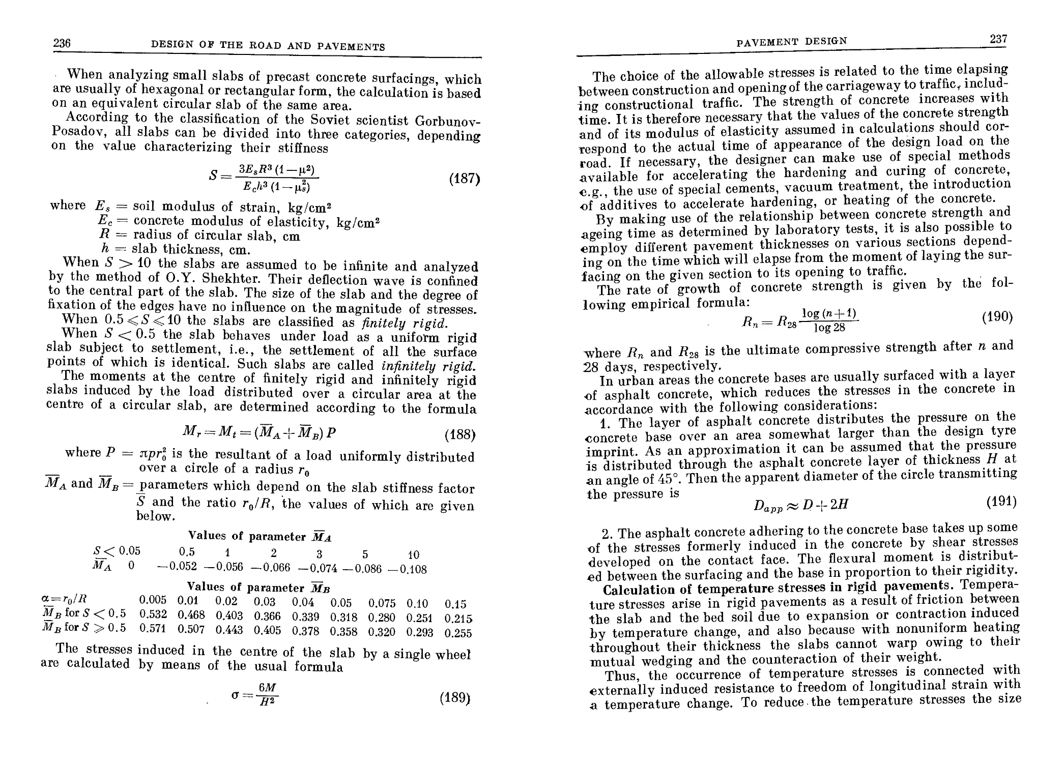
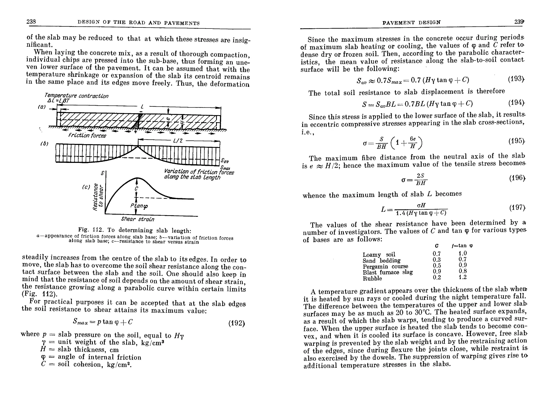
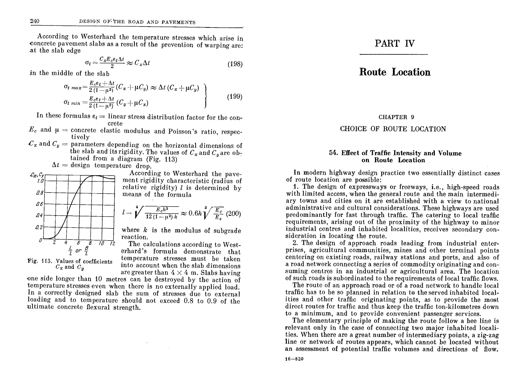
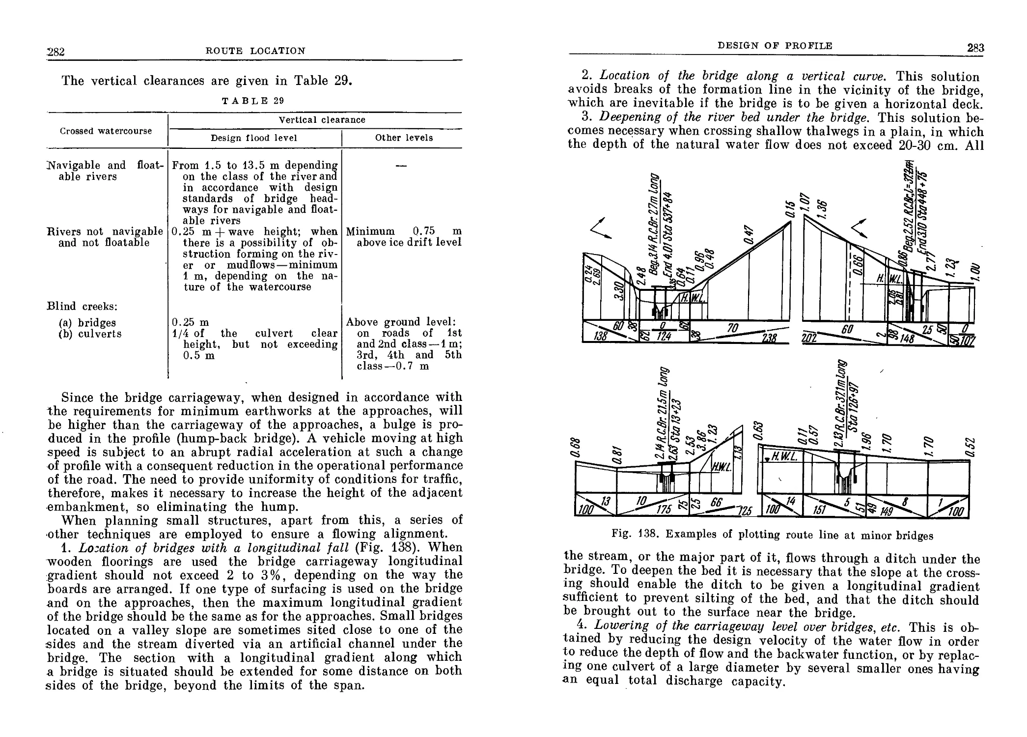
/

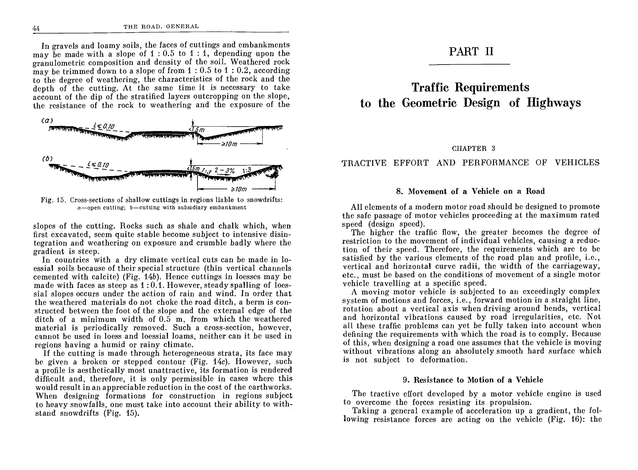


Text
Ml P PUBLISHERS • MOSCOW
В. Ф. БАБКОВ, М. С. ЗАМАХАЕВ
АВТОМОБИЛЬНЫЕ ДОРОГИ
ИЗДАТЕЛЬСТВО «ТРАНСПОРТ»
МОСКВА
V. BABKOV, M. ZAMAKHAYEV
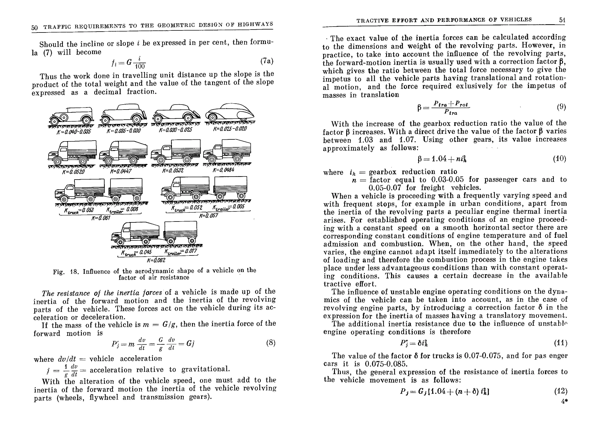
HIGHWAY
ENGINEERING
MIR PUBLISHERS
MOSCOW • 1967
UDC 625.8 (075.8) = 20
Translated from the Russian
Ла английском языке
Contents
1 (
I I . * I
Introduction . ..................... ... . .....................
Brief Survey of Road Engineering Development.................... 14
PART i
THE ROAD. GENERAL
Chapter 1. The Highway Network
1. Highways and the National Transport System................... 21
2. Highway Network Fundamentals............................... 22
3. Characteristics of Highway Traffic...................... . 22
4. National and Functional Classification of Highways .... 26
Chapter 2. Highway Design
5. The Road in Plan............................................. 30
6. Elements of Road Profile ............................, . 32
7. Right-of-way and Road Cross-section.......................... 34
PART II
TRAFFIC REQUIREMENTS TO THE GEOMETRIC DESIGN OF HIGHWAYS
Chapter 3. Tractive Effort and Performance of Vehicles
8. Movement of a Vehicle on a Road ............................. 45
9. Resistance to Motion of a Vehicle............................ 45
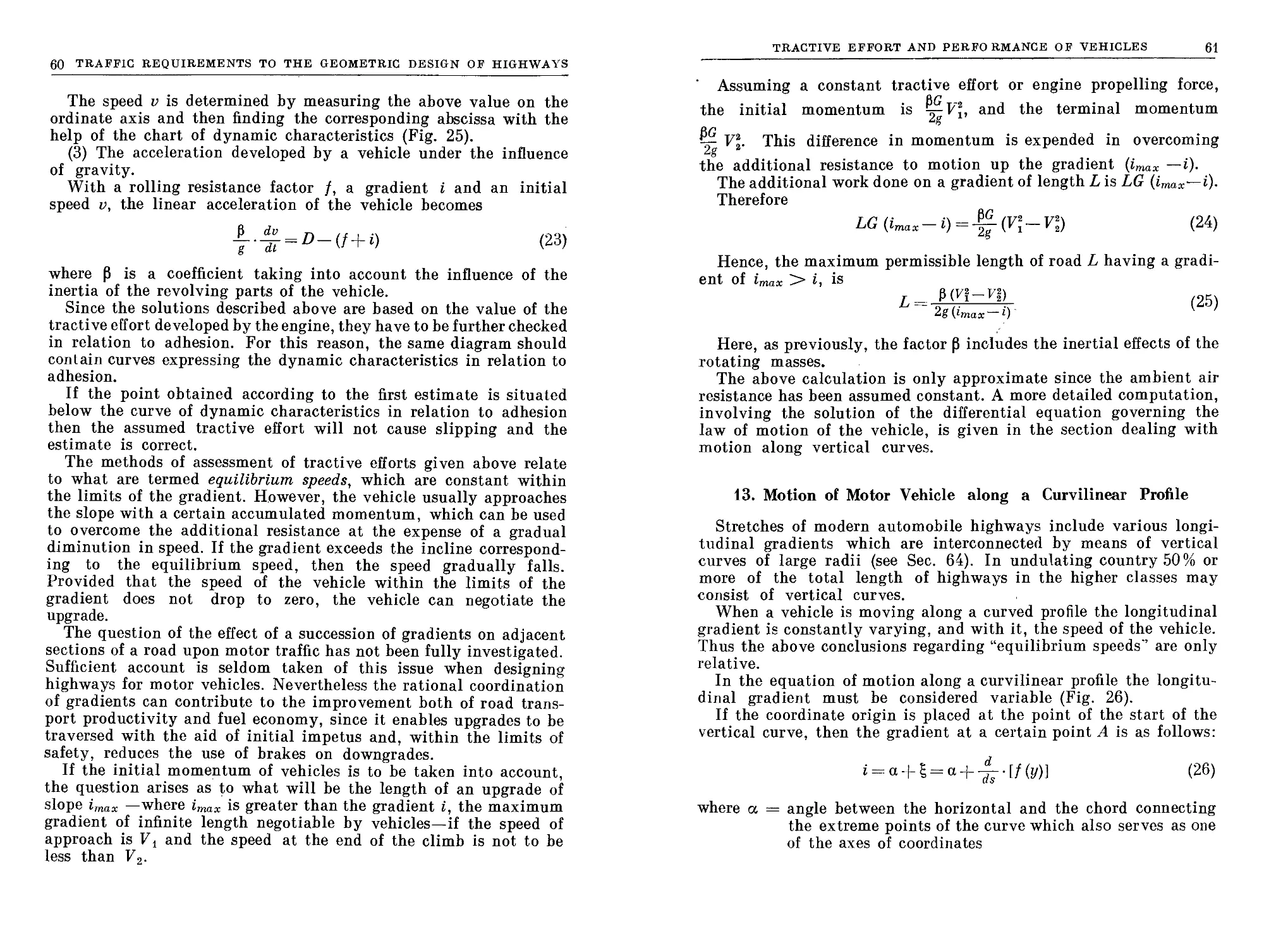
10. Dynamic Characteristics of a Vehicle........................ 52
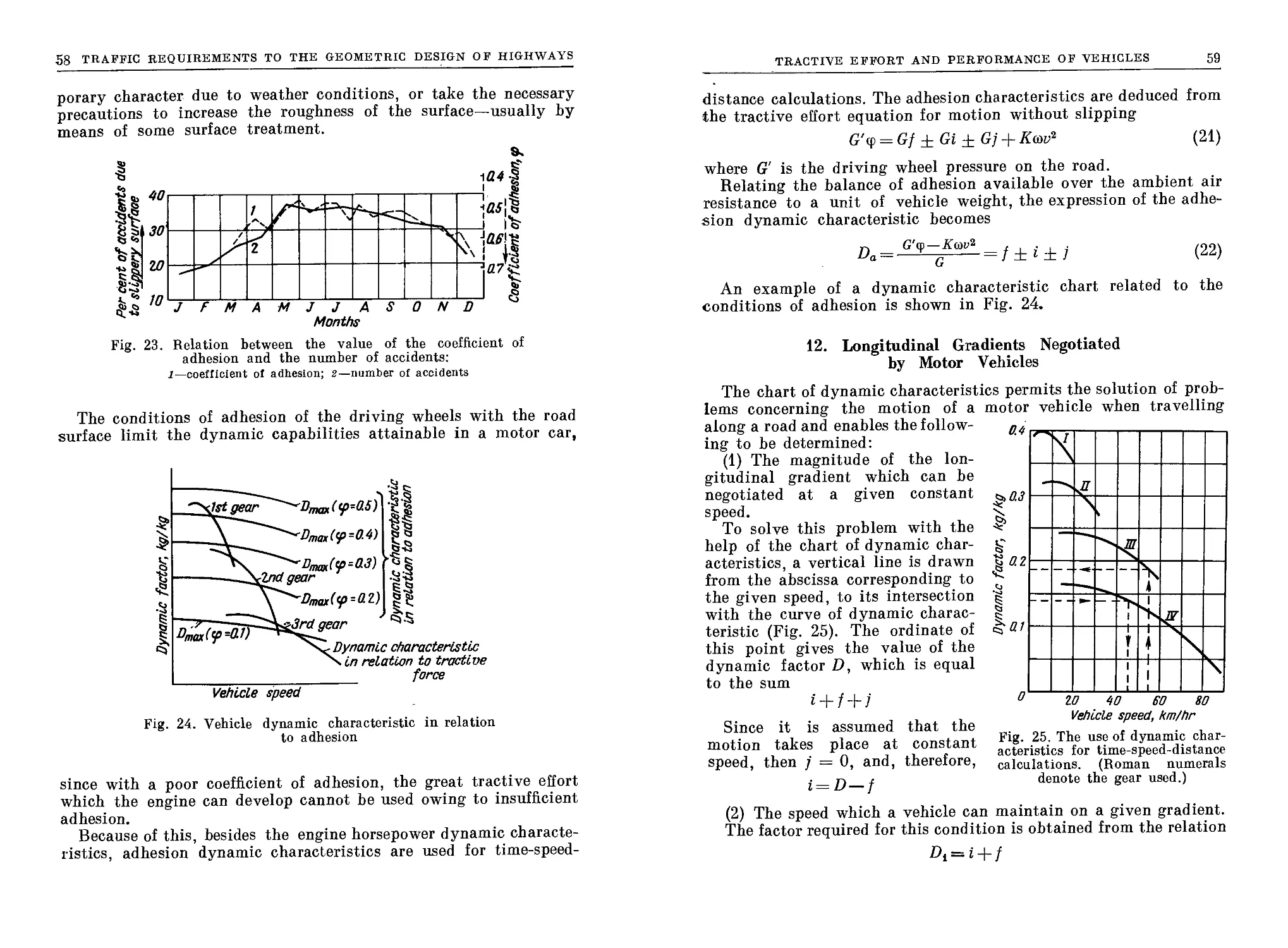
11. Adhesion of Pneumatic Tyres to the Road Surface............. 55
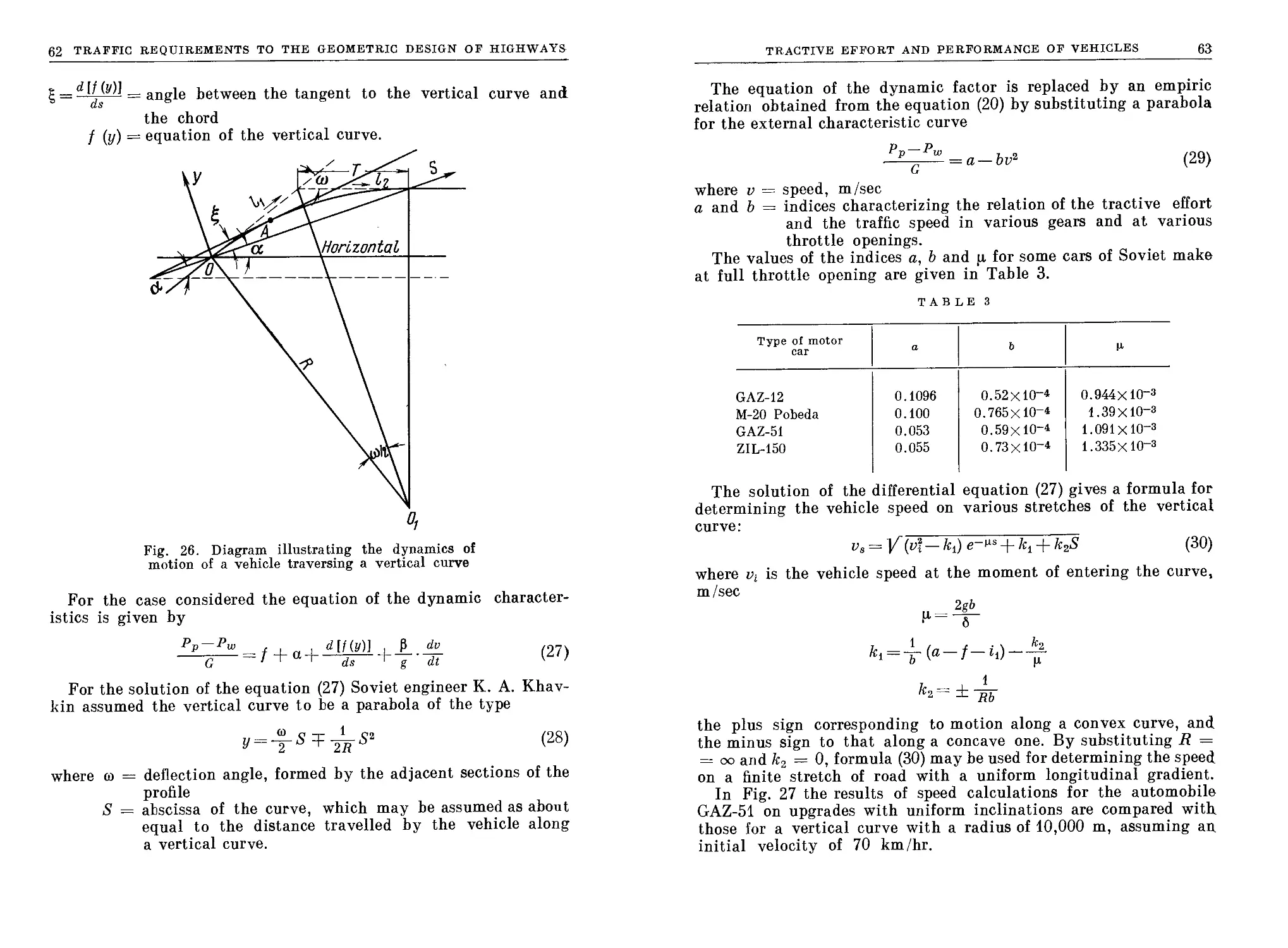
12. Longitudinal Gradients Negotiated by Motor Vehicles .... 59
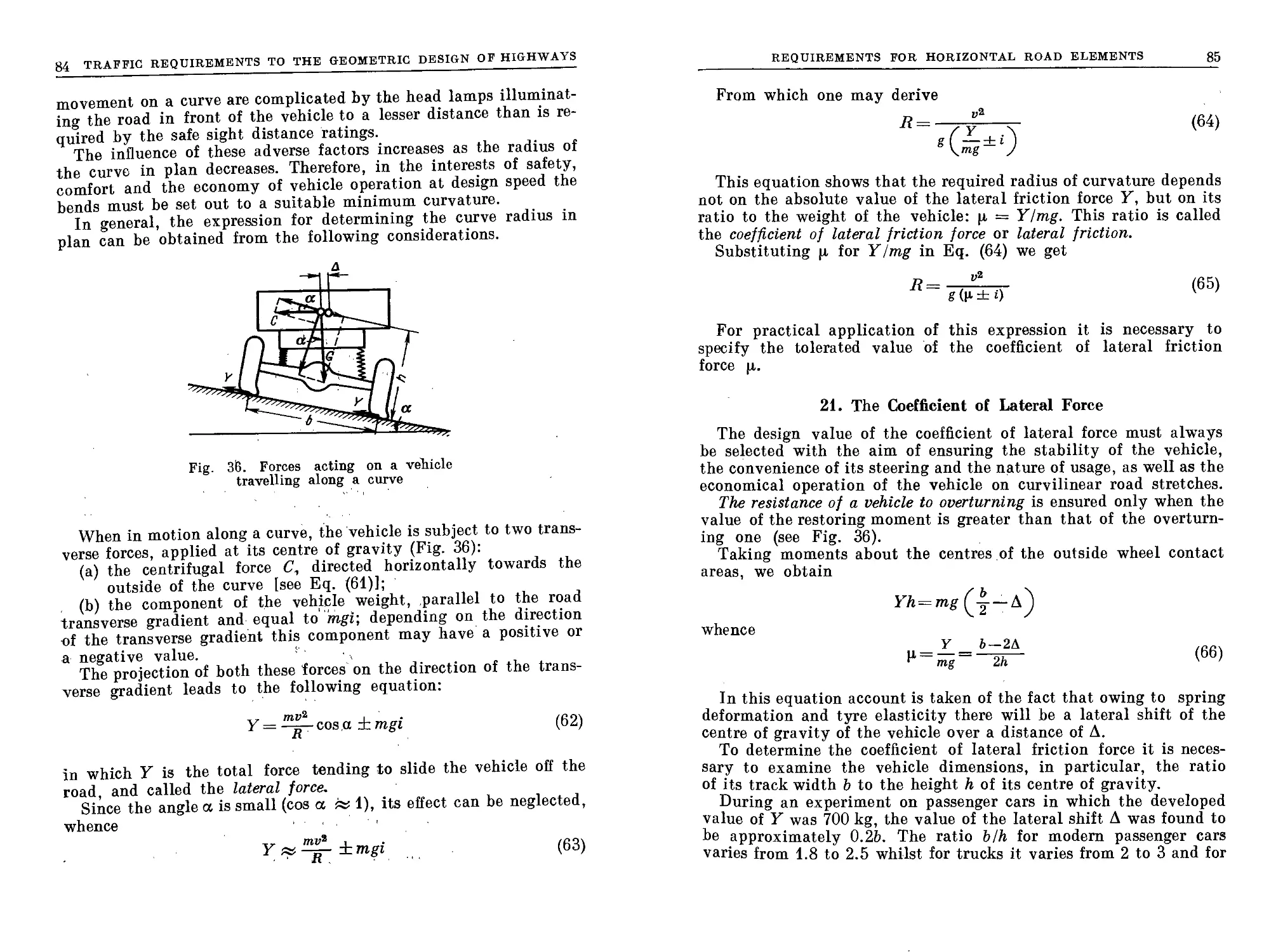
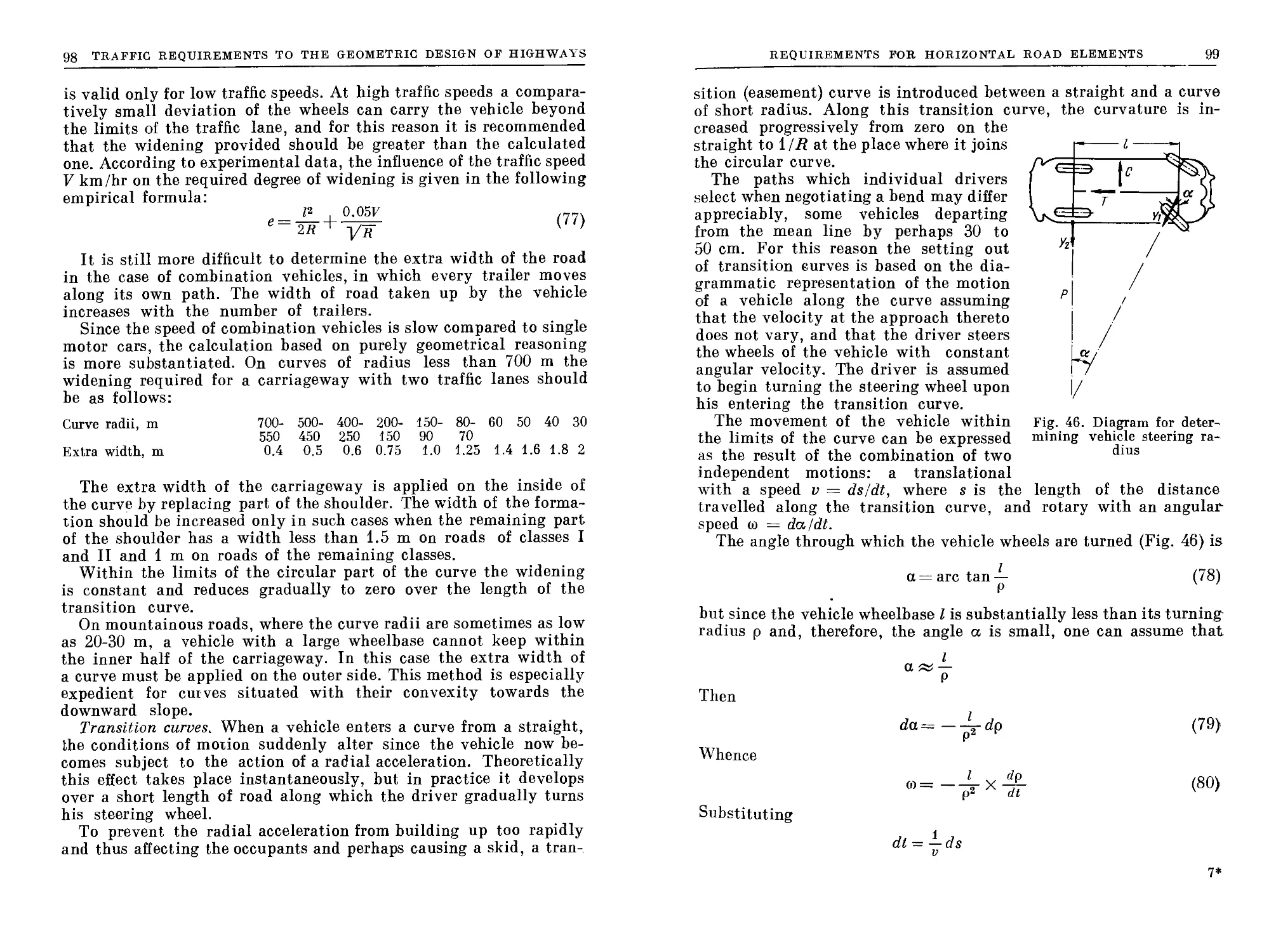
13. Motion of Motor Vehicle Along a Curvilinear Profile .... 61
14. Braking and the Characteristics of Vehicular Motion on Down-
grades ......................................................... 64
15. Standardization of Maximum Gradients on Highways .... 68
16. Characteristics of Combination Vehicles..................... 70
17. Fuel Consumption and Tyre Wjear in Relation to Road Condi-
tions ...................... '' . ............................ 72
6
CONTENTS
Chapter 4. Requirements for Horizontal Road Elements
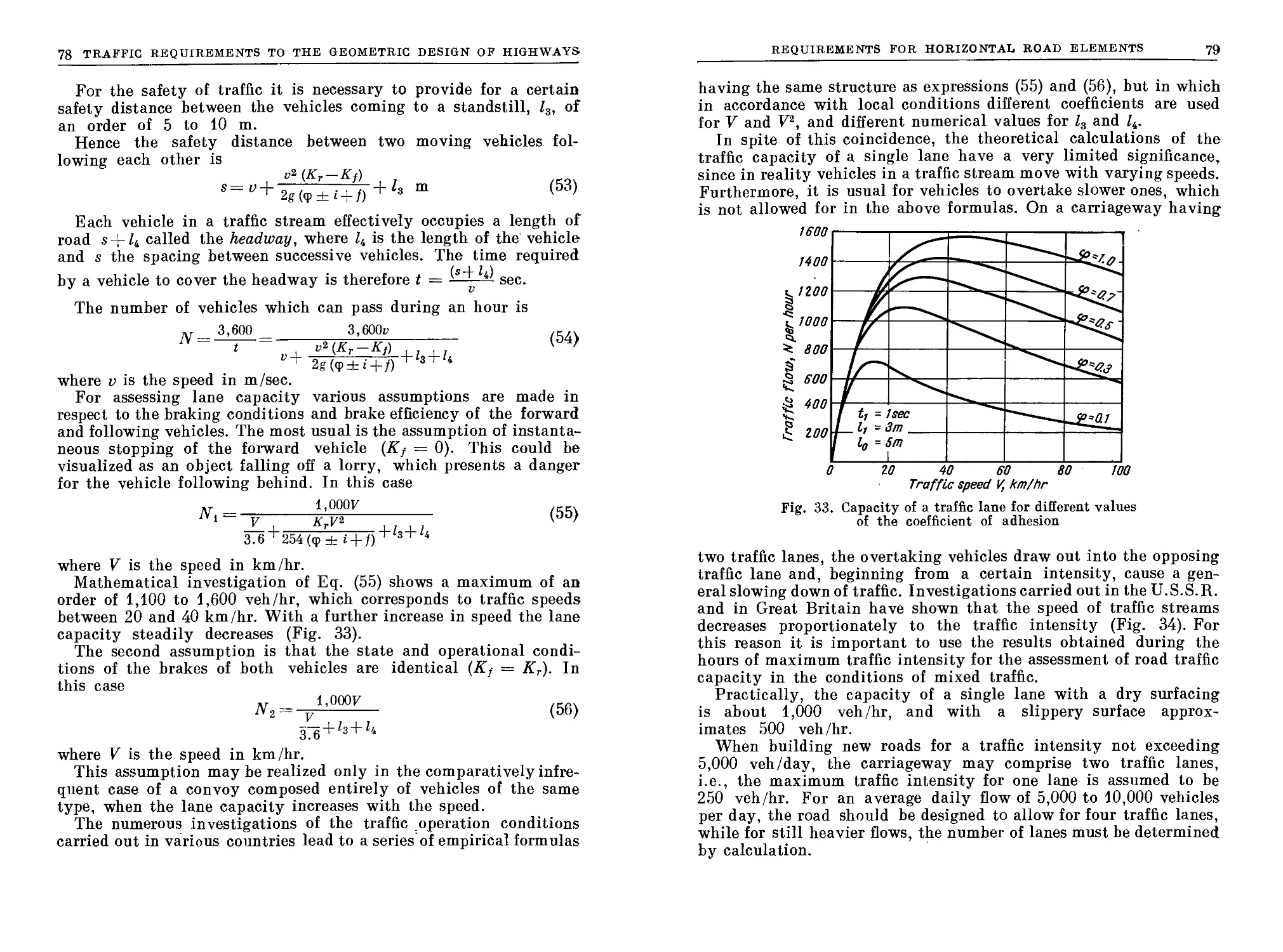
18. Traffic Capacity and the Required Number of Lanes .... 77
19. Width of Carriageways and Shoulders............................ 80
20. Problems of Traffic Motion on a Curve.......................... 83
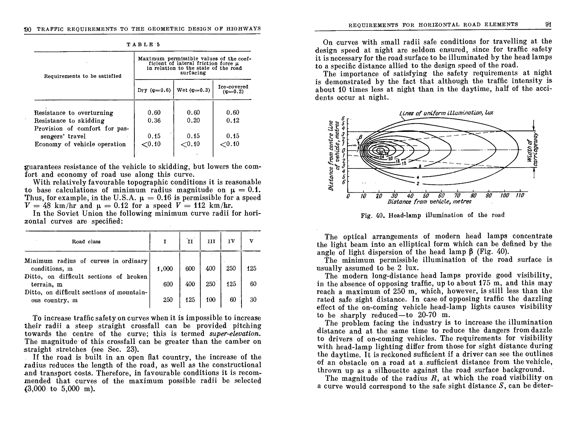
21. The Coefficient of Lateral Force............................ 85
22. Selection of Radii for Horizontal Curves....................... 89
23. Additional Elements on Curves of Small Radius.................. 92
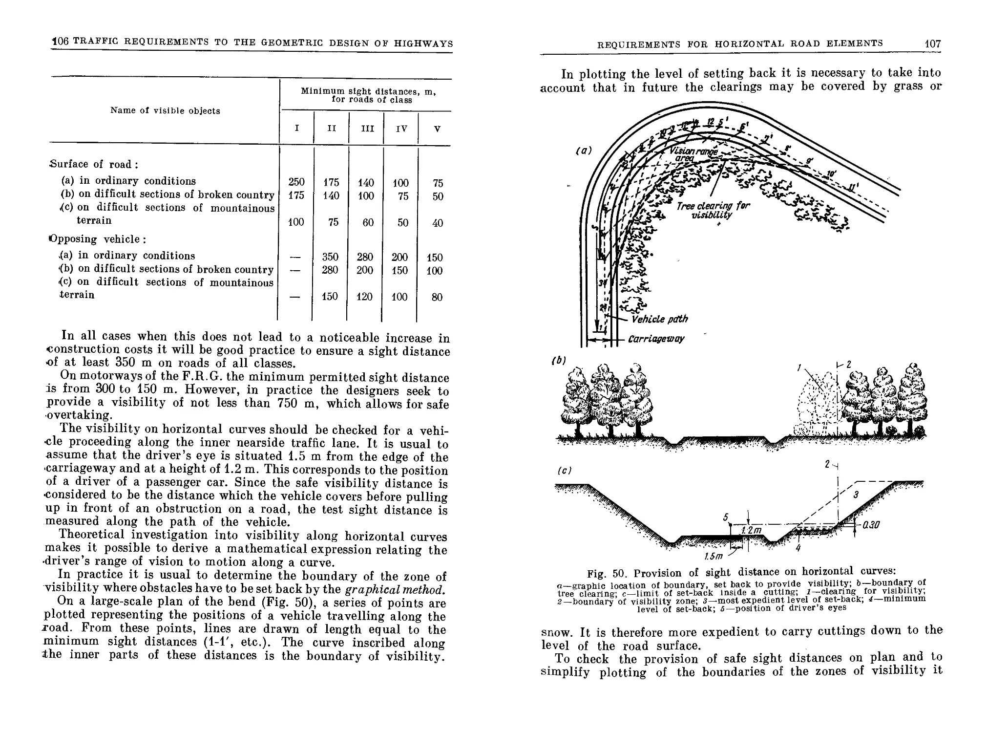
24. Provision of Visibility on Curves ........................... 103
25. Standard Conditions for Road Design........................... 109
PART Ш
DESIGN OF THE ROADBED AND PAVEMENTS
Chapter 5. Natural Factors Affecting Road Performance
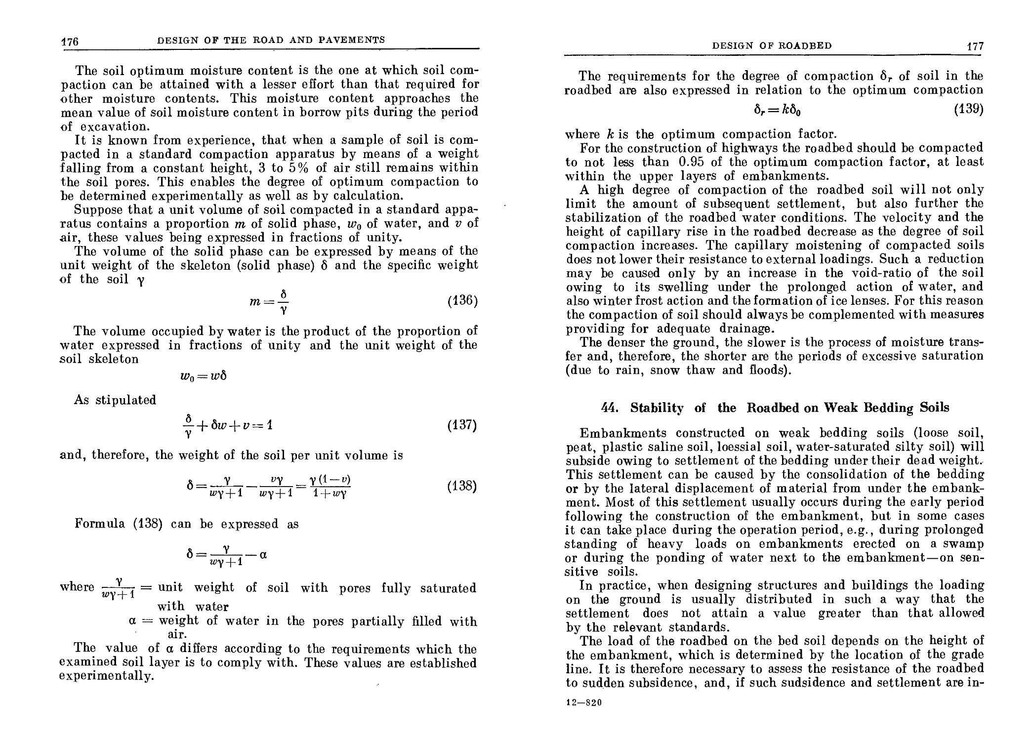
26. General ..................................................... Ill
27. Factors Causing Saturation of the Roadbed..................... 116
28. Water Conditions Under the Roadbed............................ 117
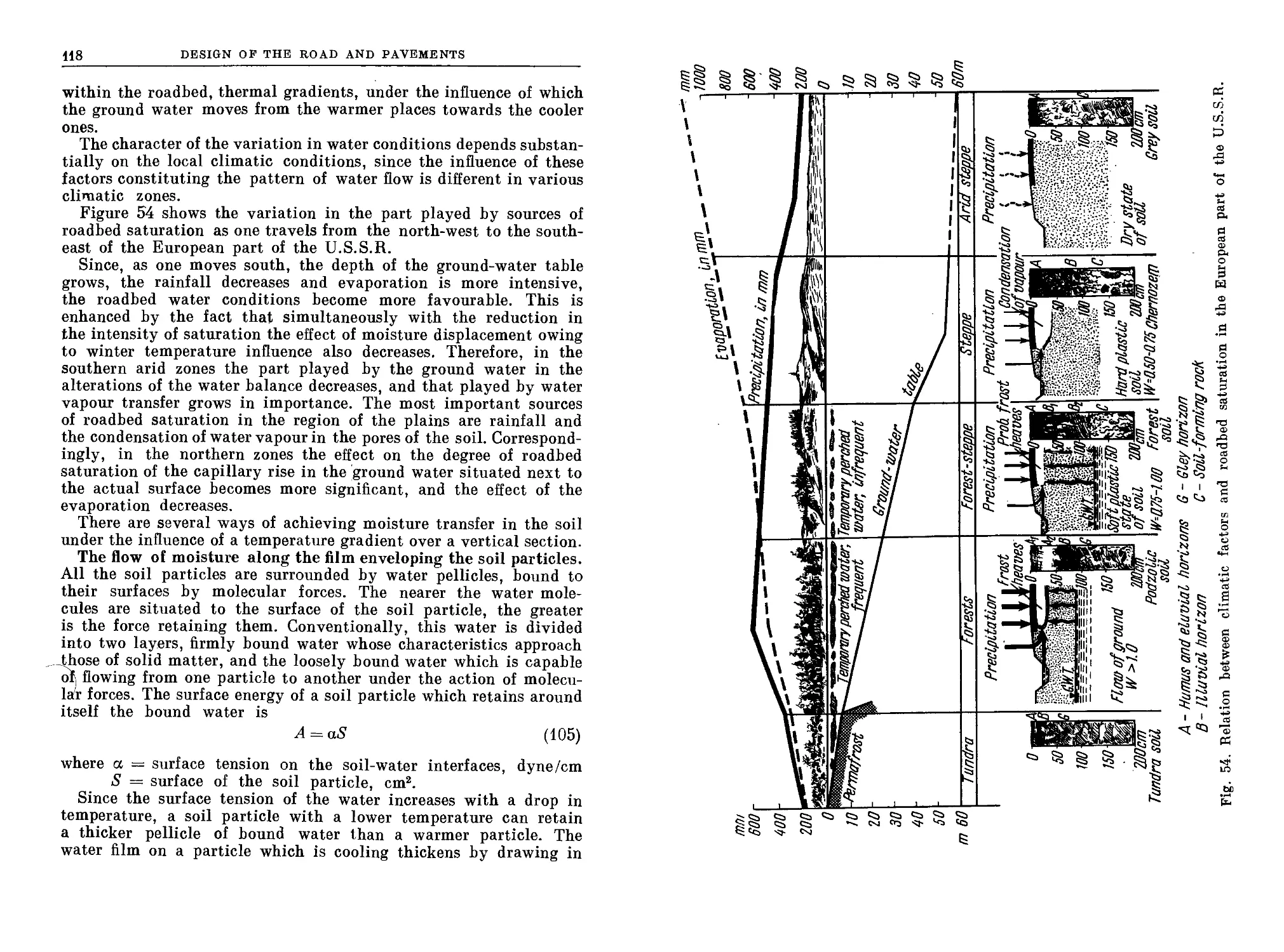
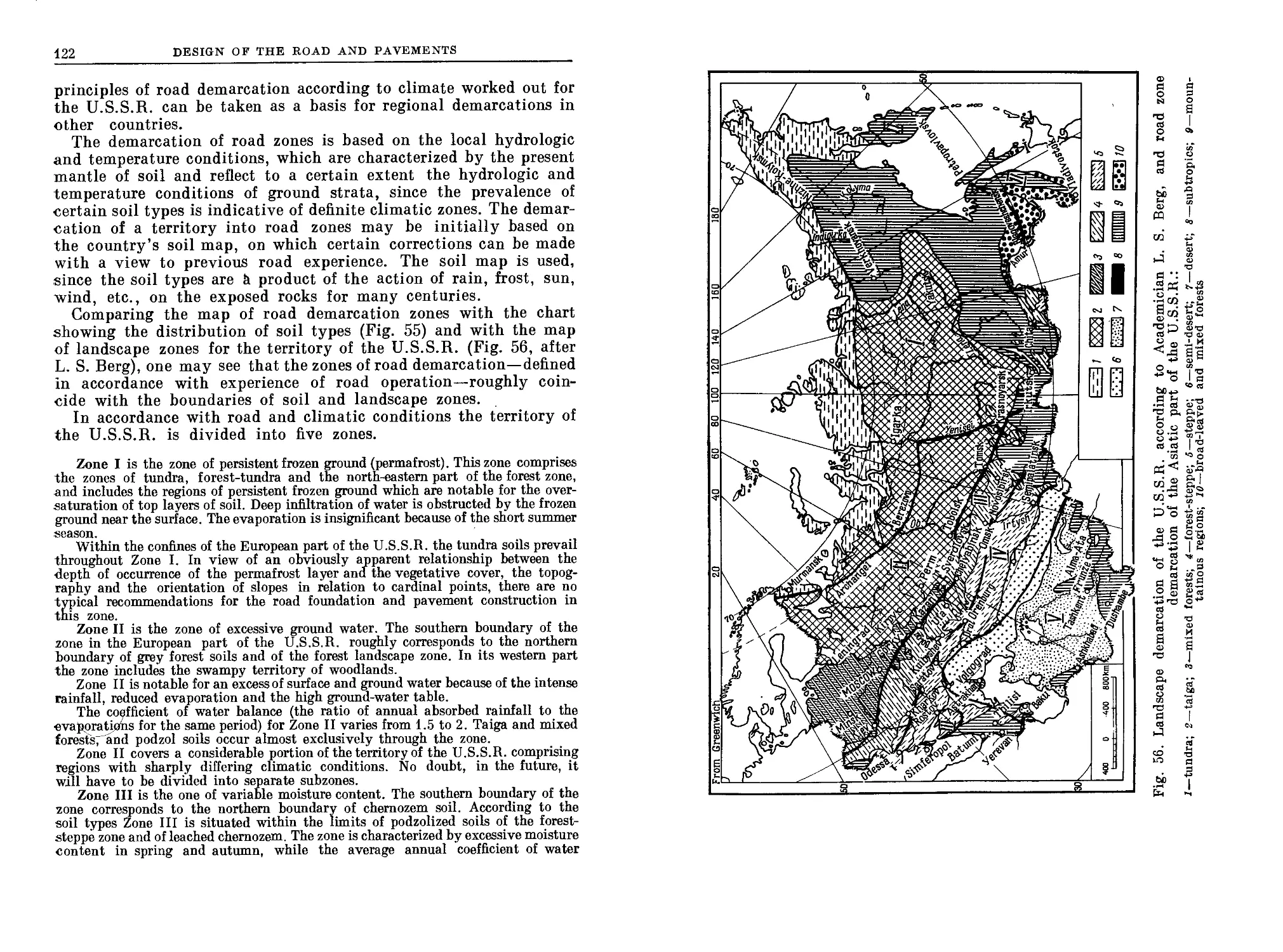
29. Demarcation of Road Zones..................................... 120
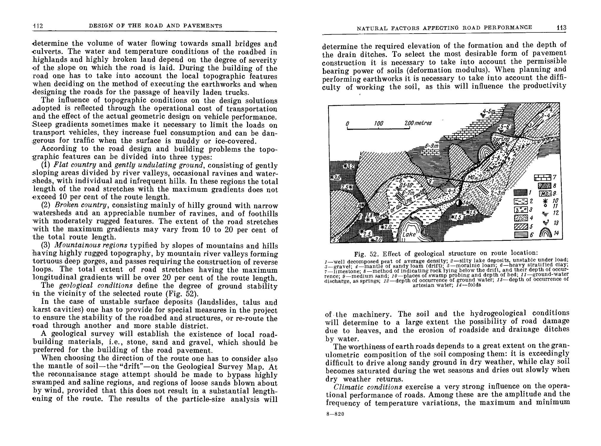
30. Estimation of Hydrologic and Hydrogeological Conditions 124
Chapter 6. Road Drainage
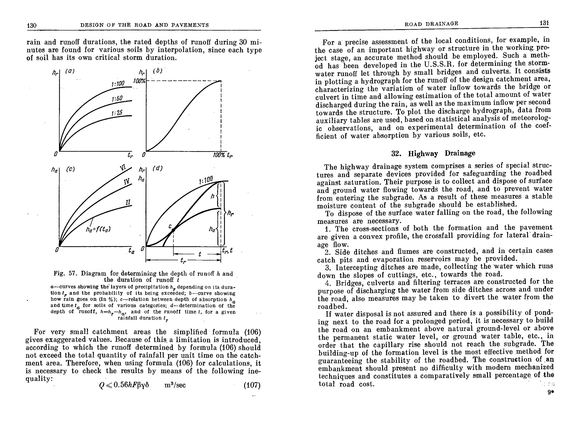
31. Determination of Water Inflow Towards the Highway from the
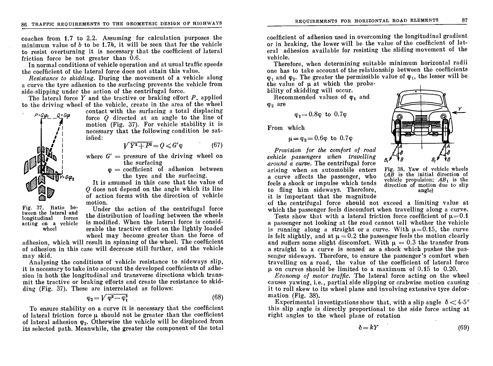
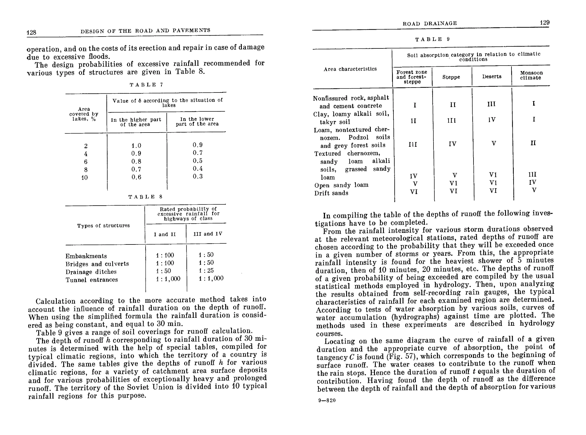
Surrounding Country........................................... 126
32. Highway Drainage. . .......................................... 131
33. Road Pavement Camber........................................ 134
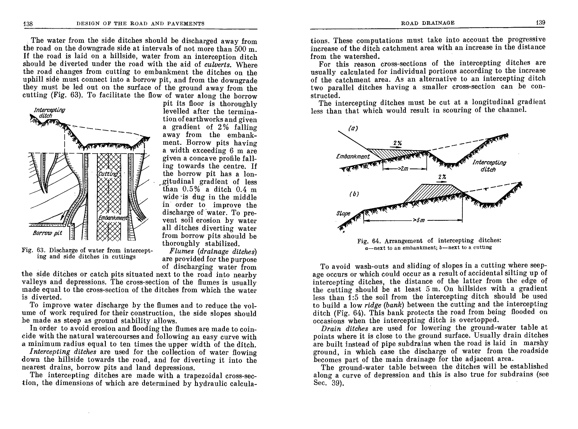
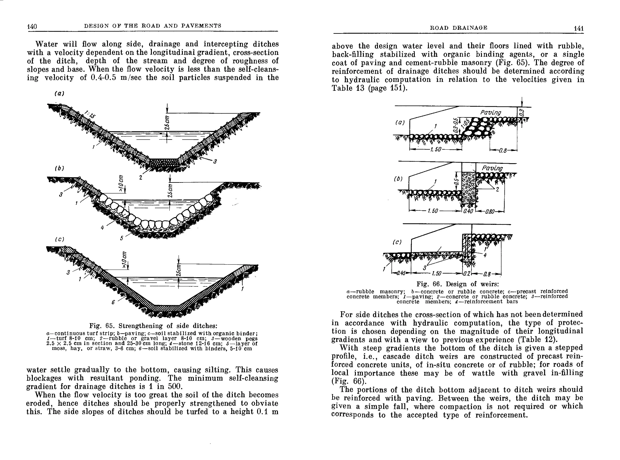
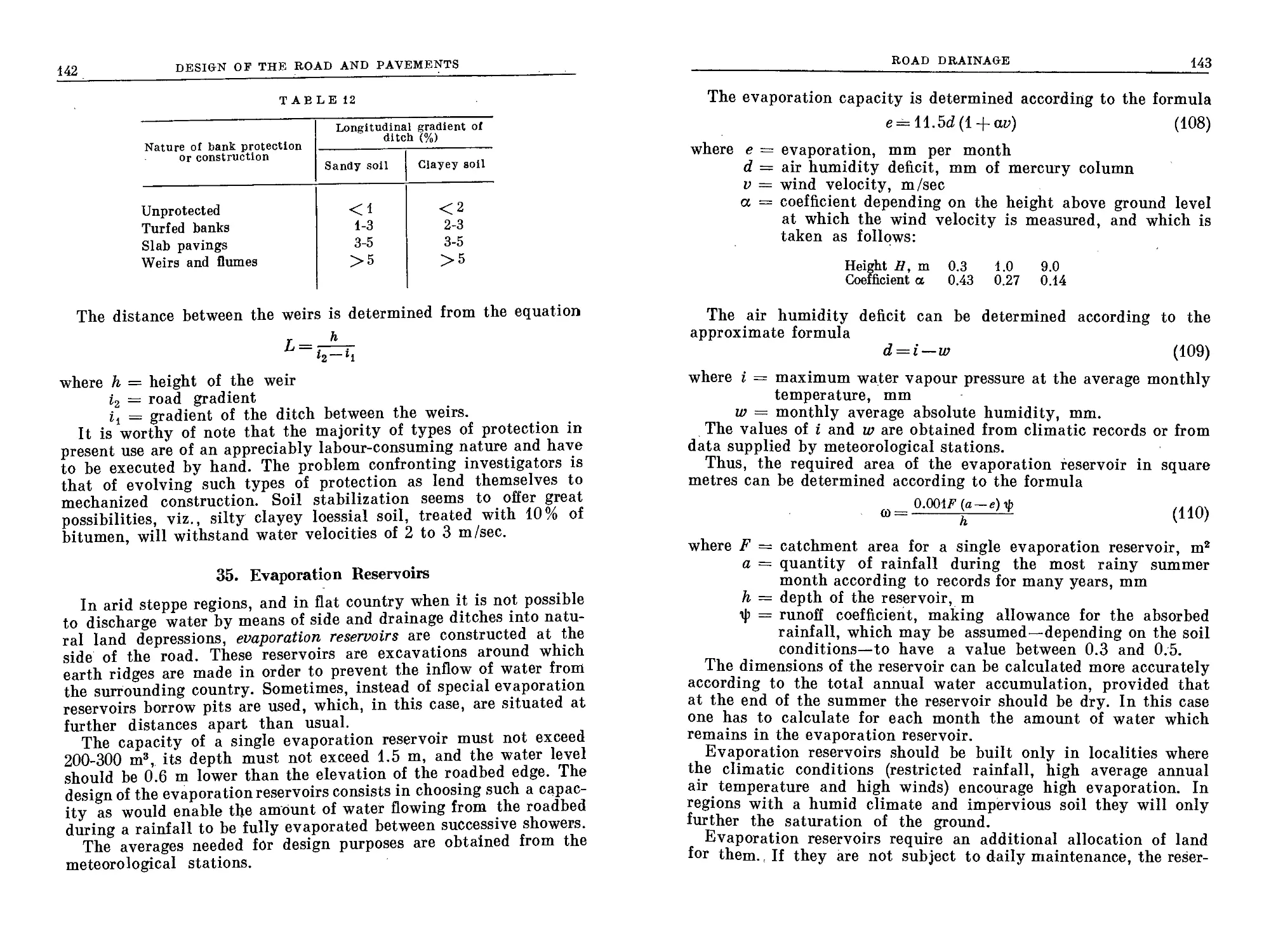
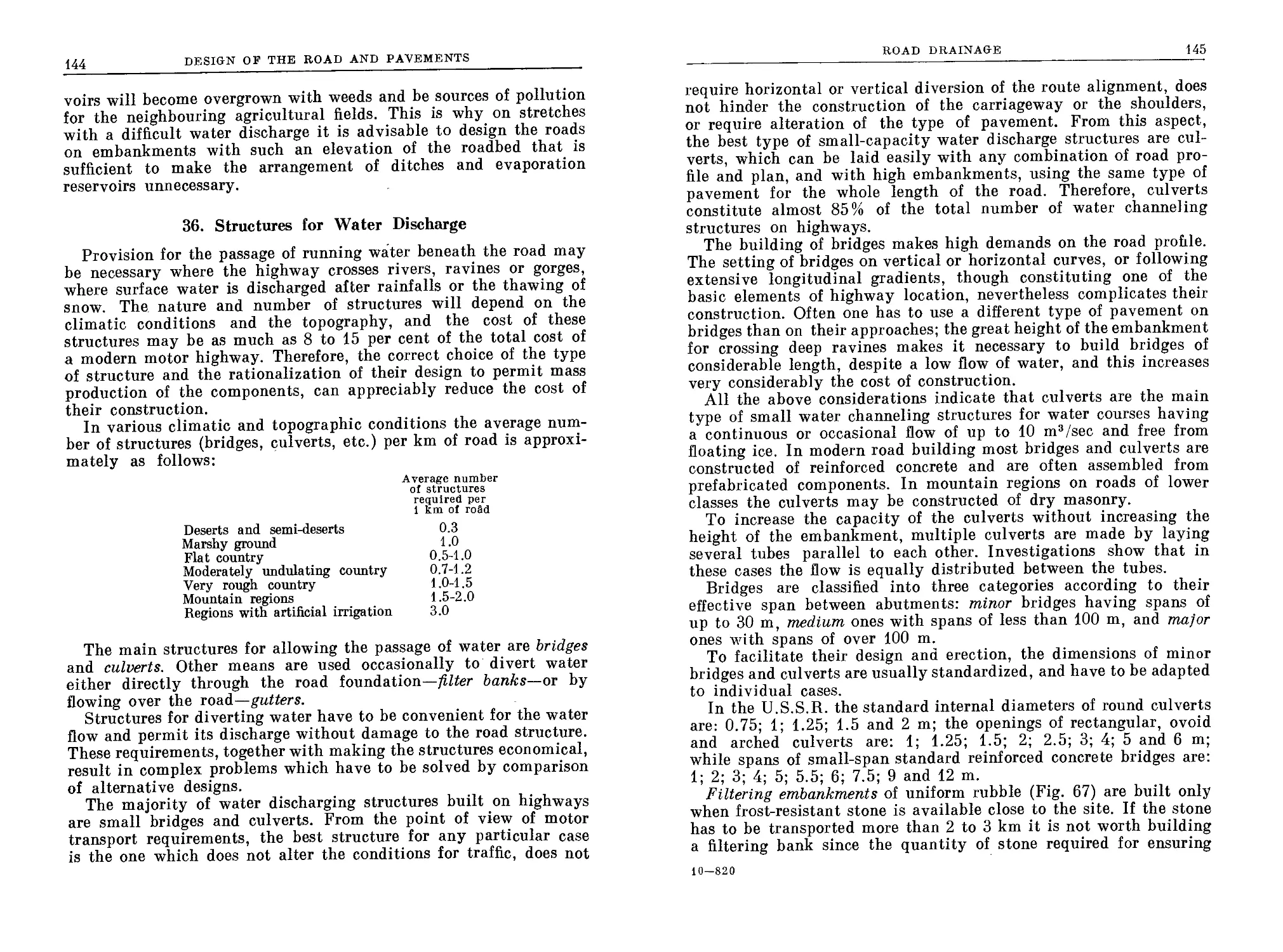
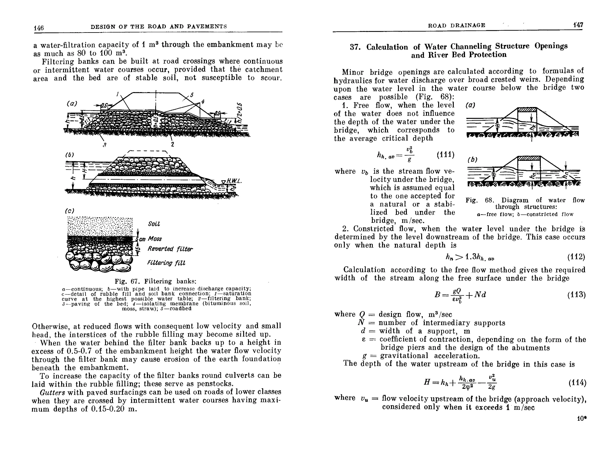
34. Ditches ..................................................... 136
35. Evaporation Reservoirs........................................ 142
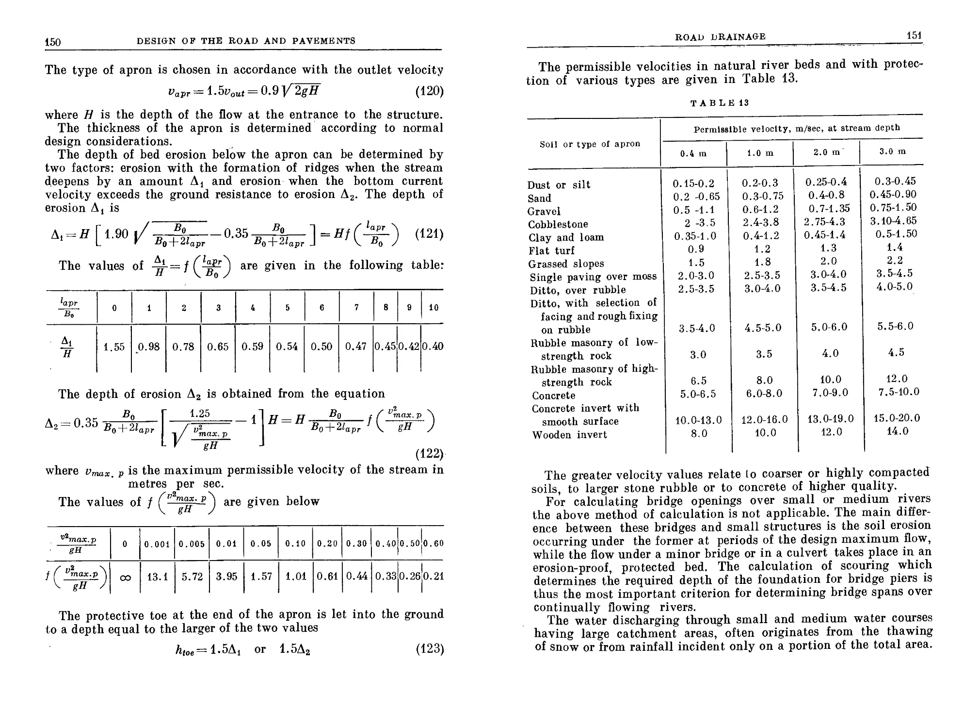
36. Structures for Water Discharge................................ 144
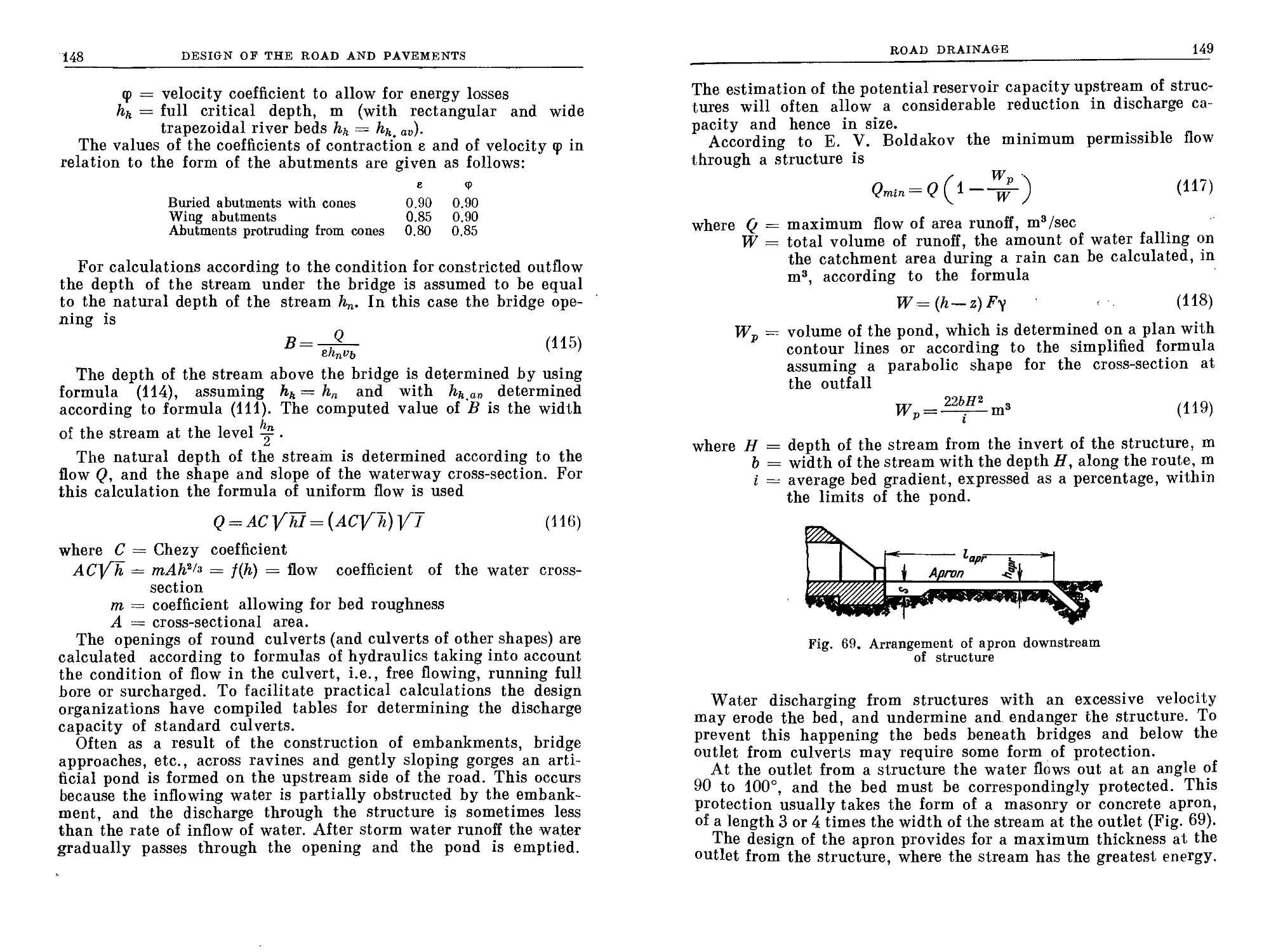
37. Calculation of Water Channeling Structure Openings and River
Bed Protection ................................................. 147
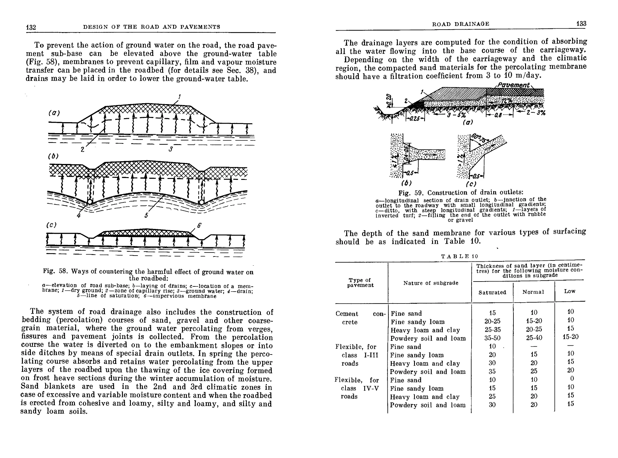
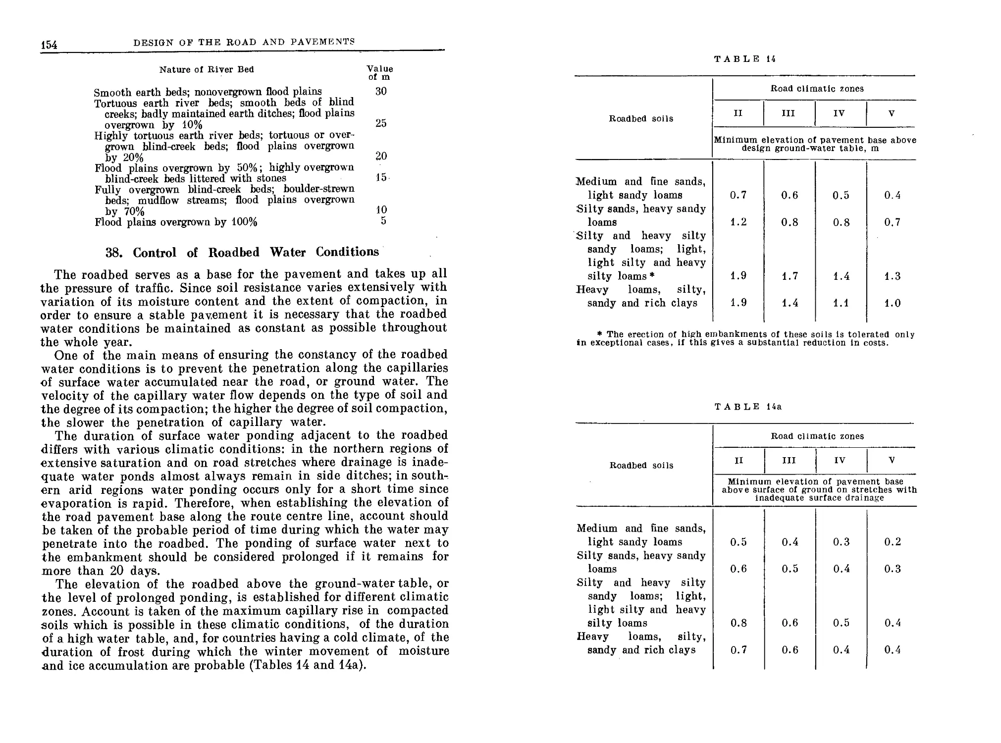
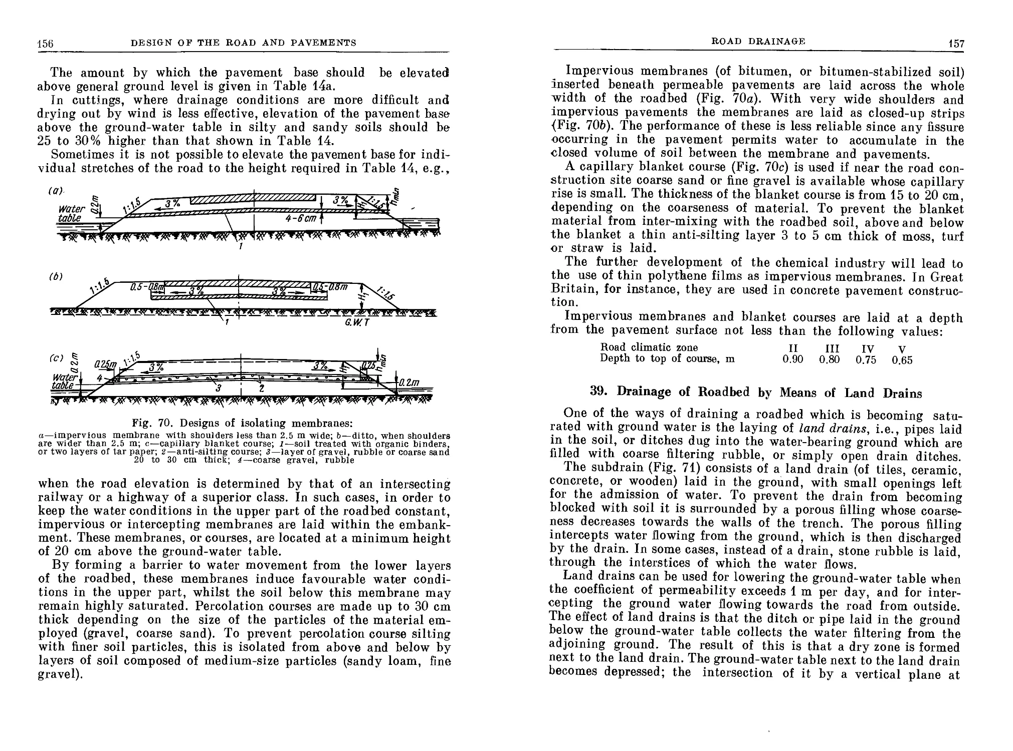
38. Control of Roadbed Water Conditions........................... 154
39. Drainage of Roadbed by Means of Land Drains................... 157
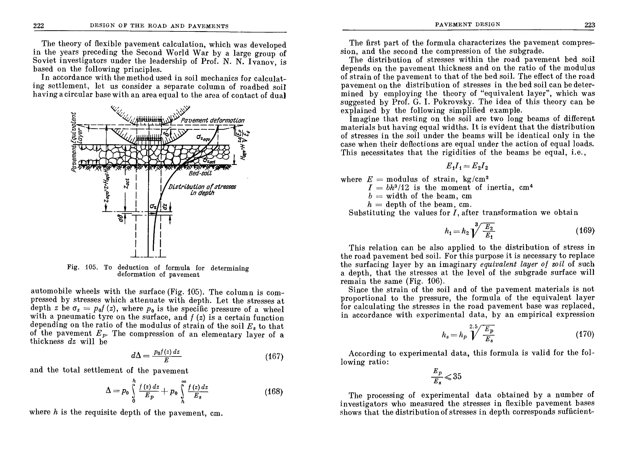
Chapter 7. Design of Roadbed
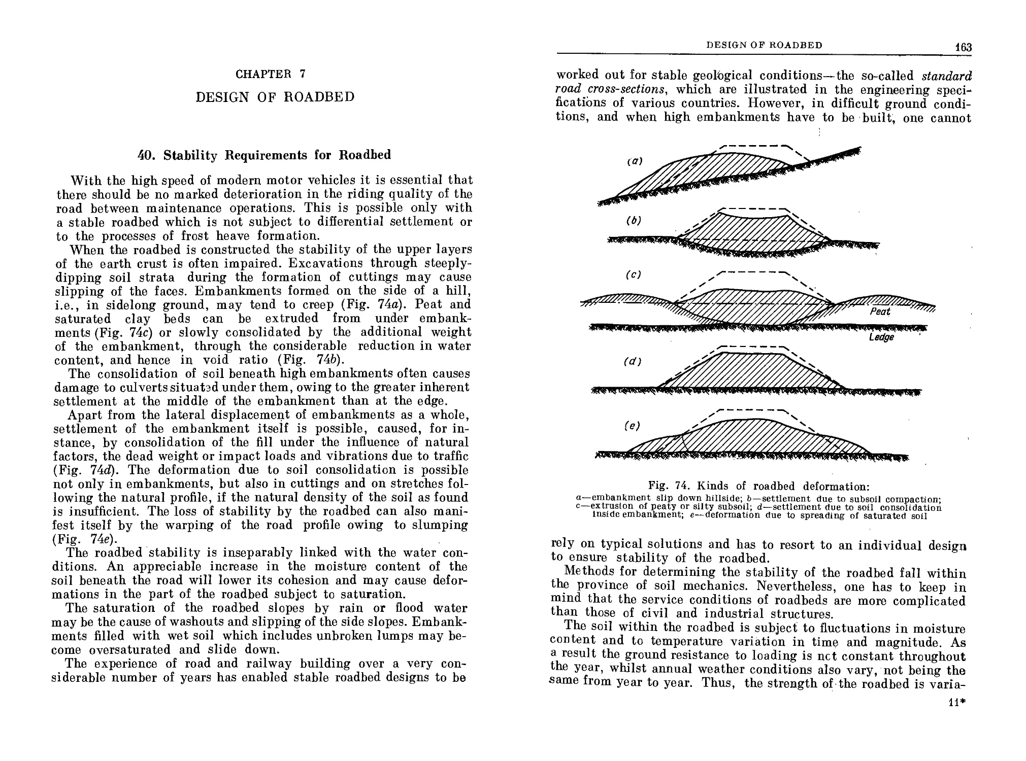
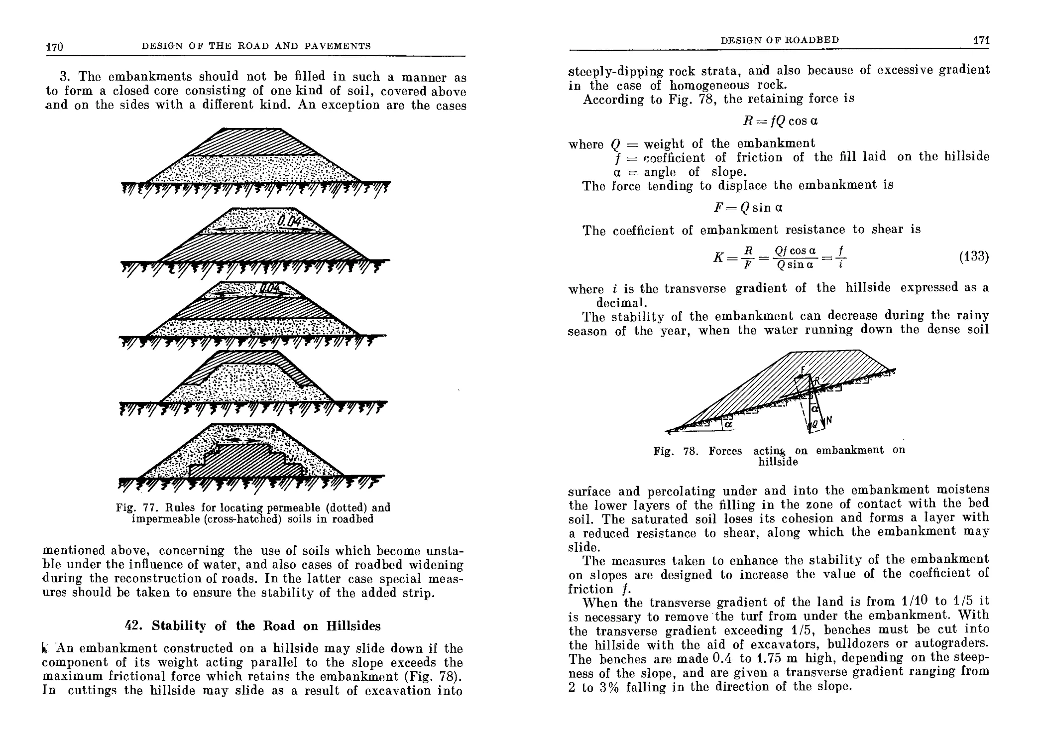
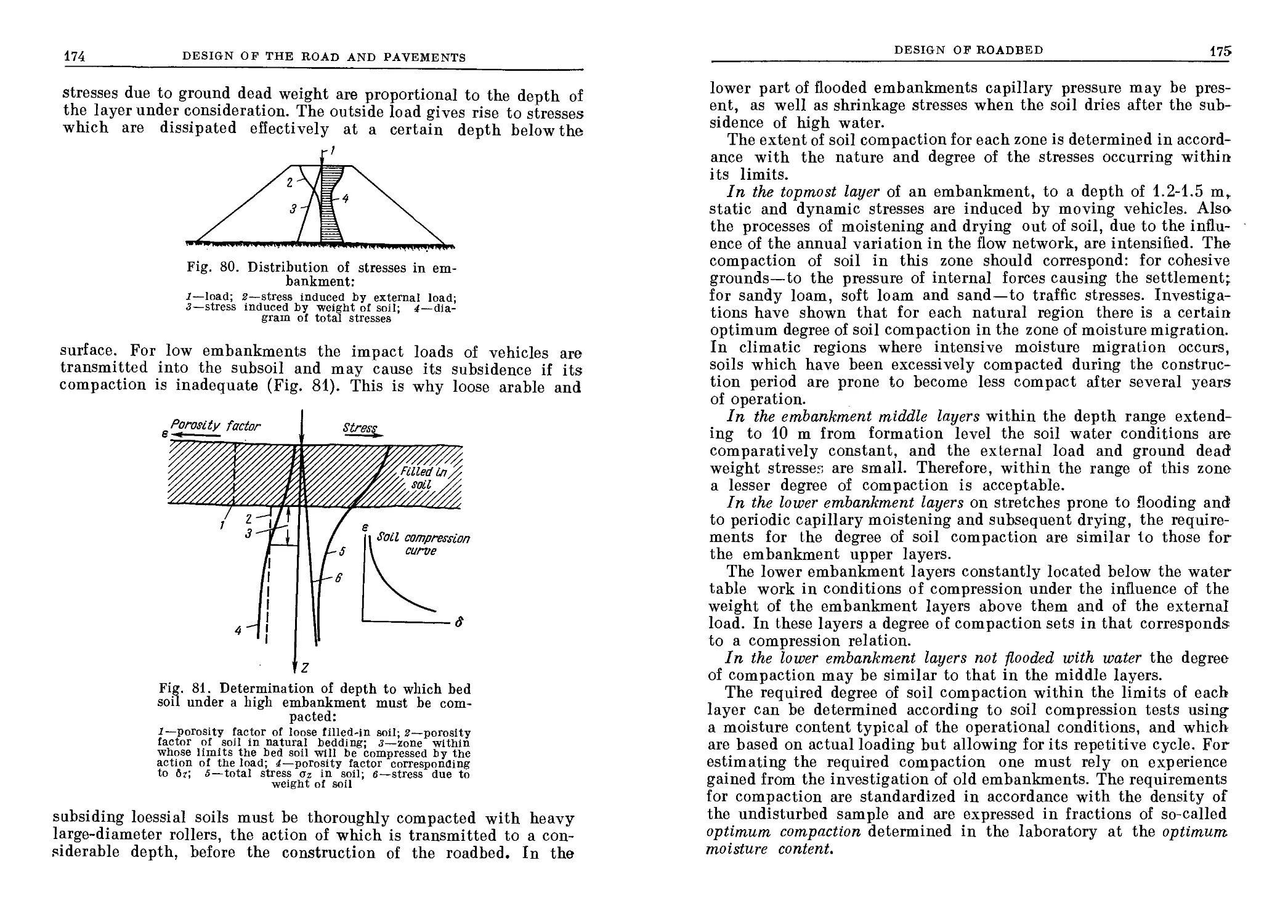
40. Stability Requirements for Roadbed............................ 162
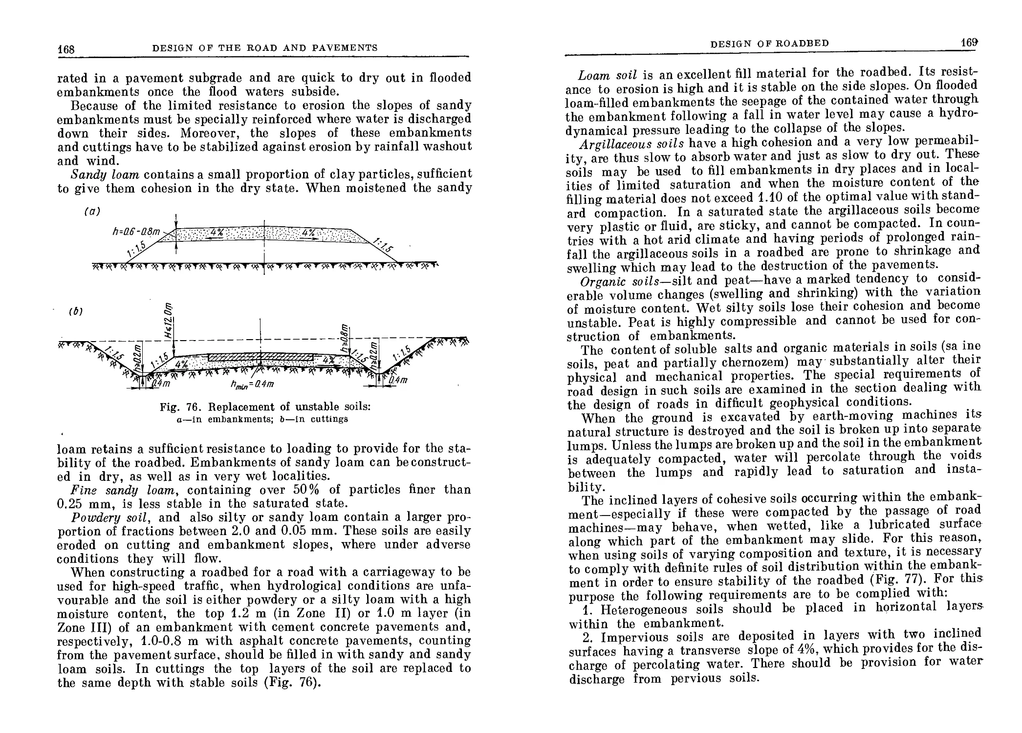
41. Disposition of Soils in a Roadbed............................. 167
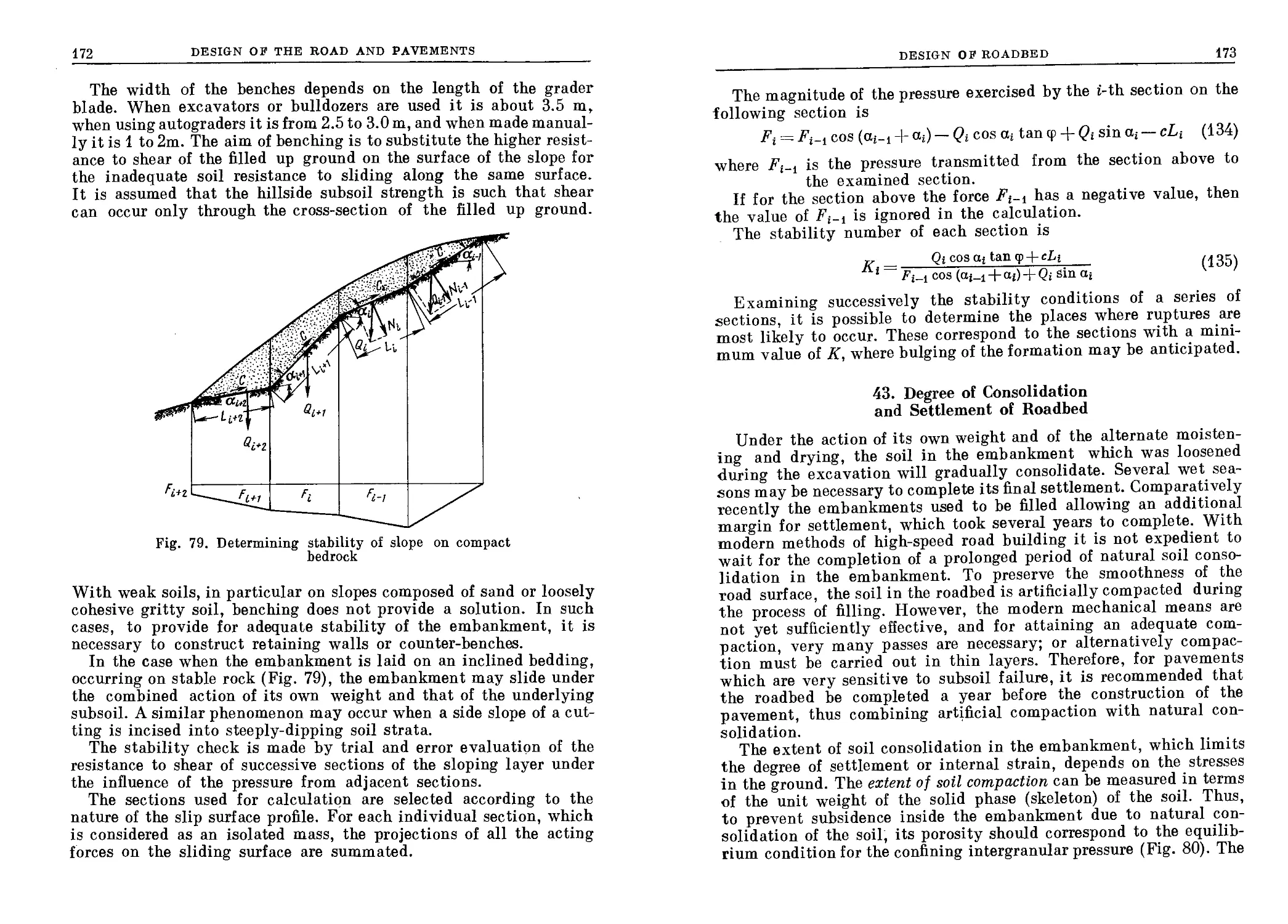
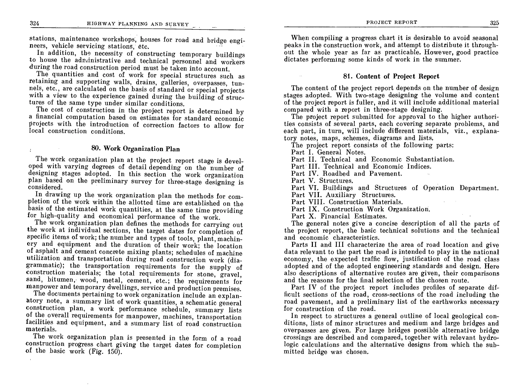
42. Stability of the Road on Hillside............................. 170
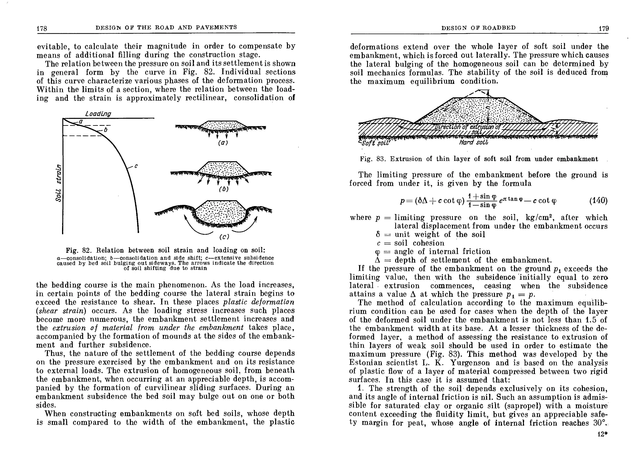
43. Degree of Consolidation and Settlement of Roadbed............. 173
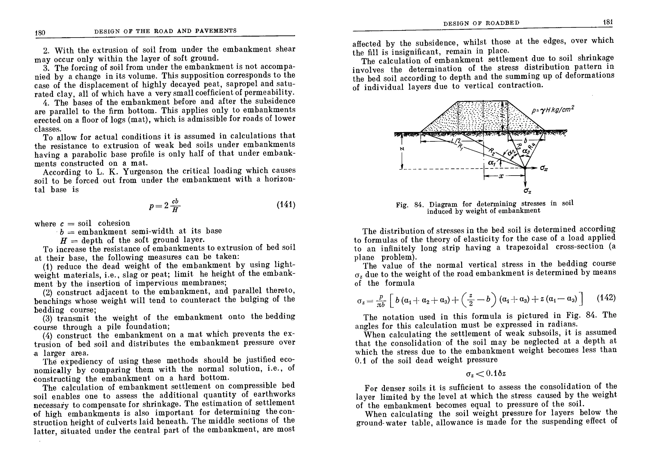
44. Stability of the Roadbed on Weak Bedding Soils ...... 177
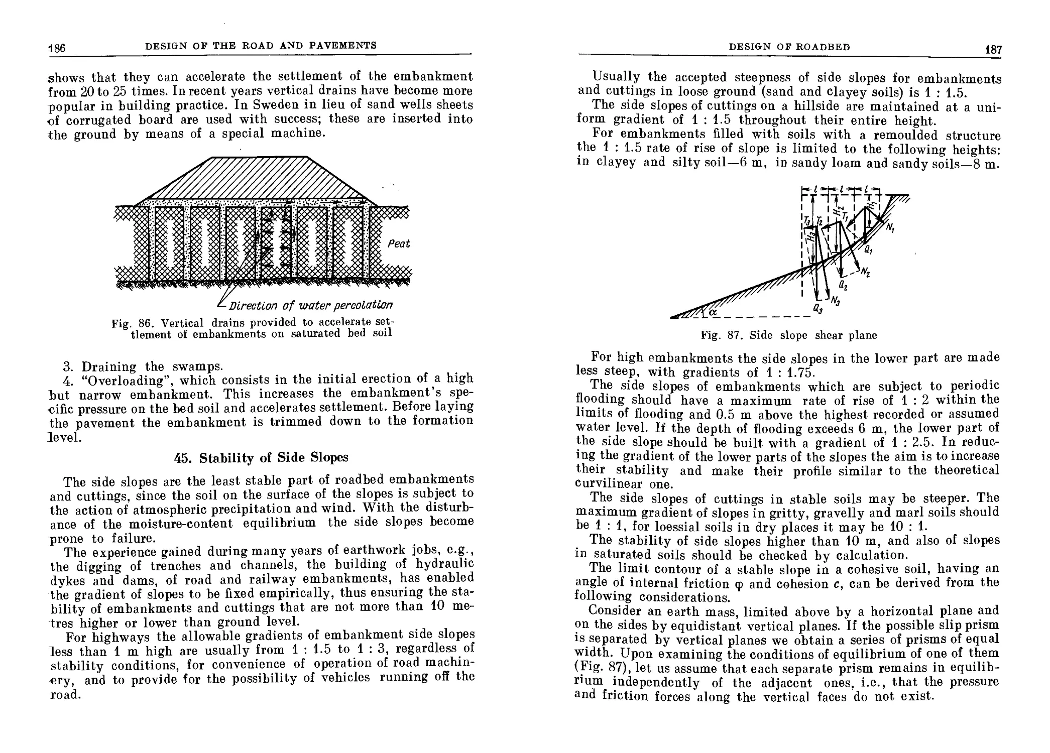
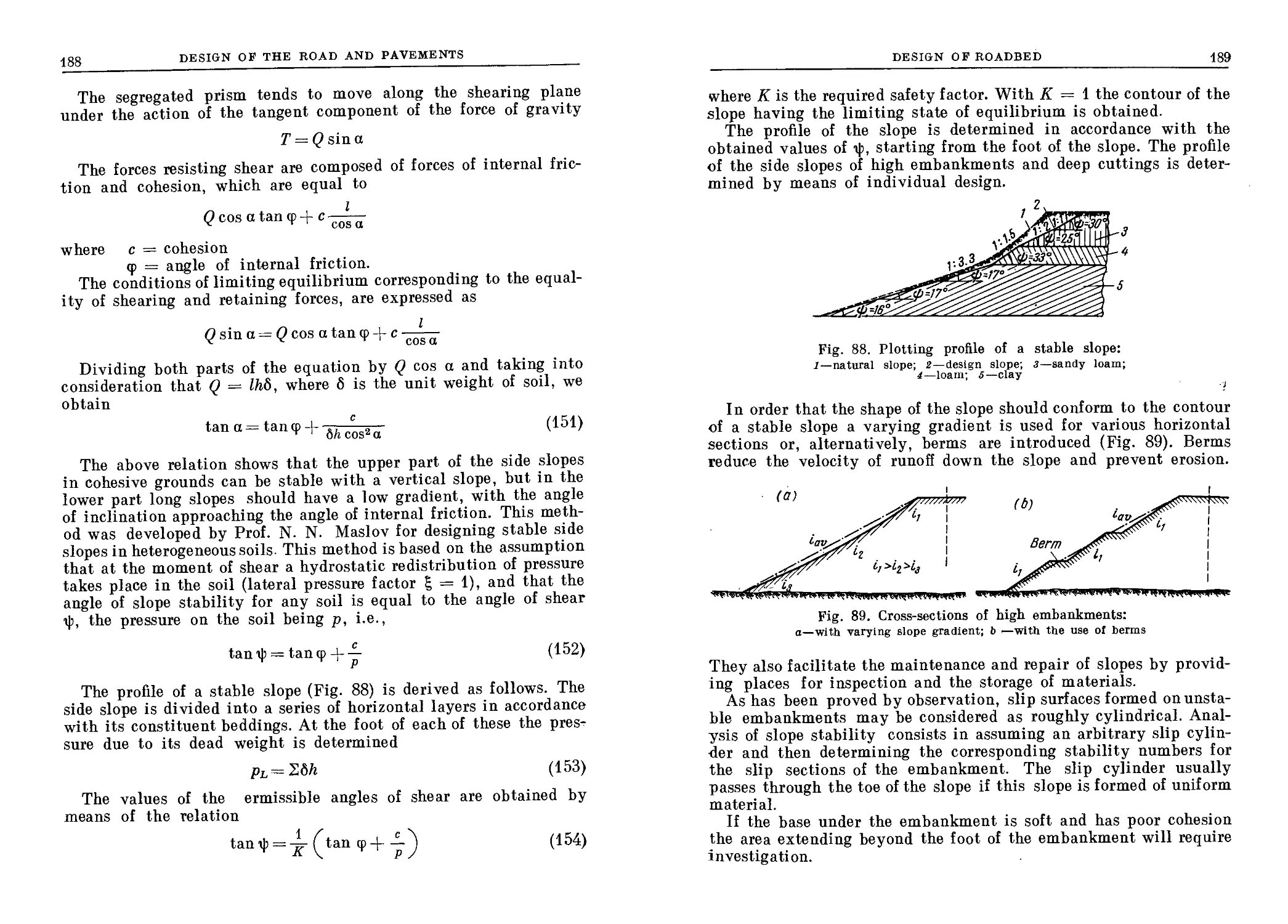
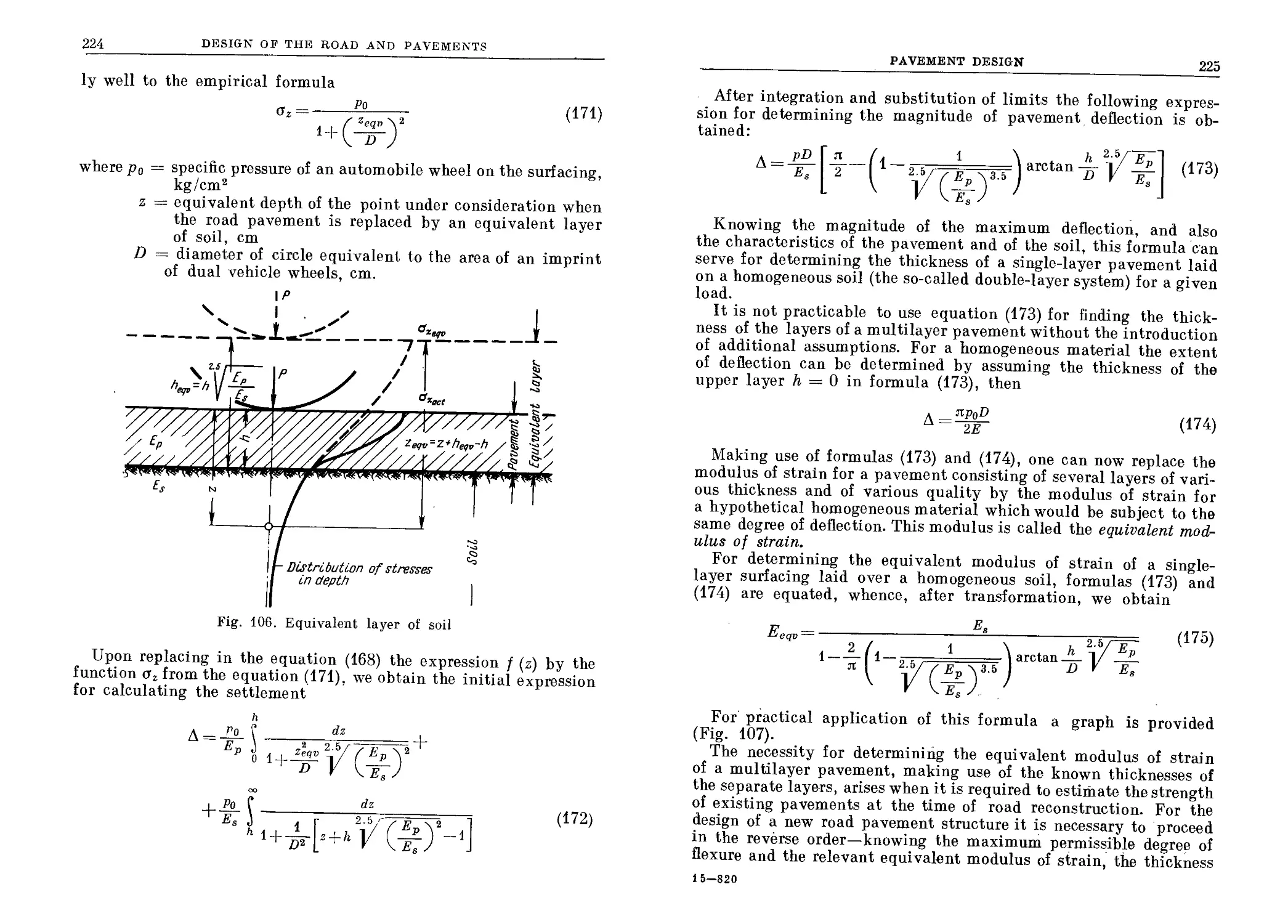
45. Stability of Side Slopes.............................. .... 186
CONTE TS
7
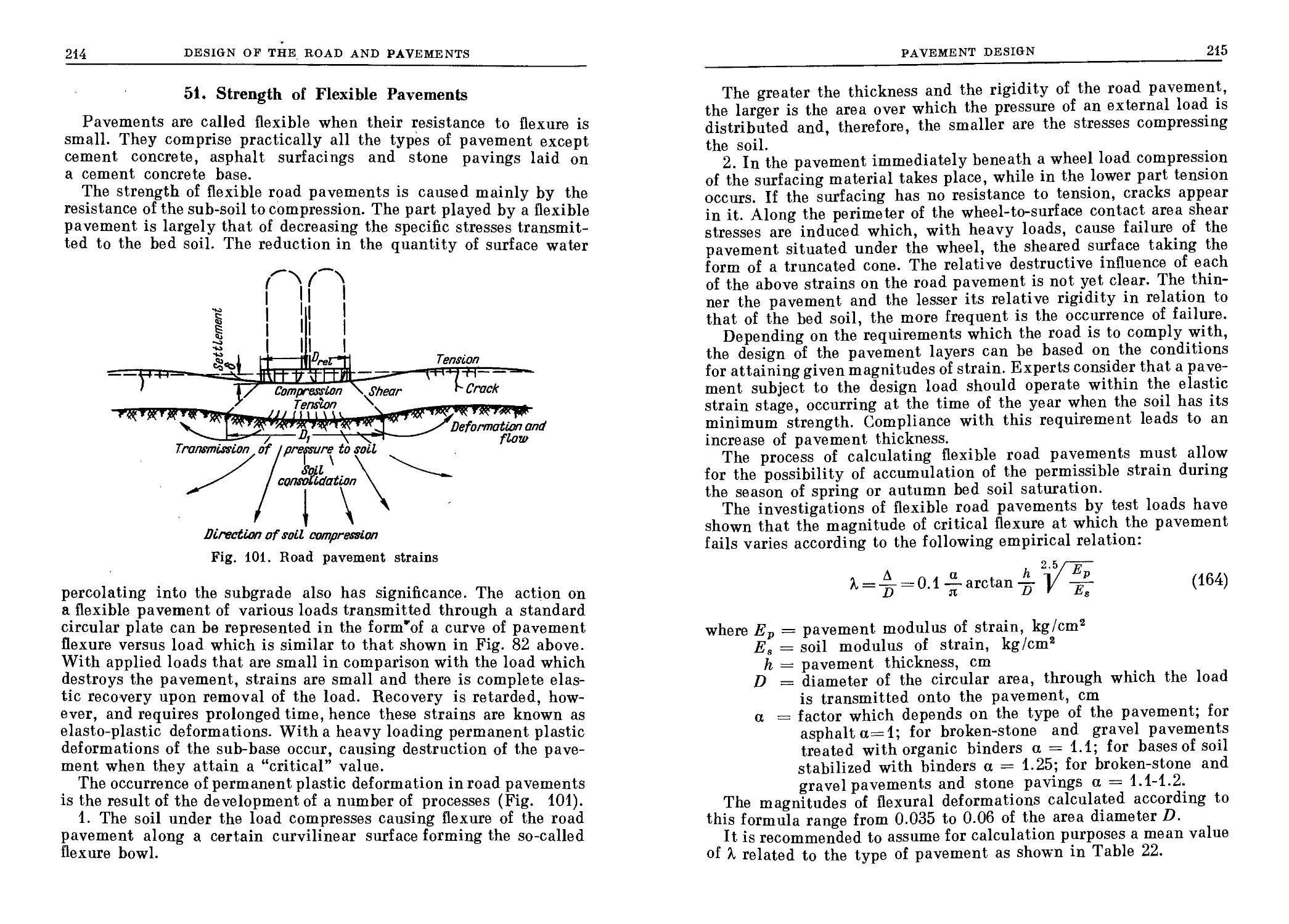
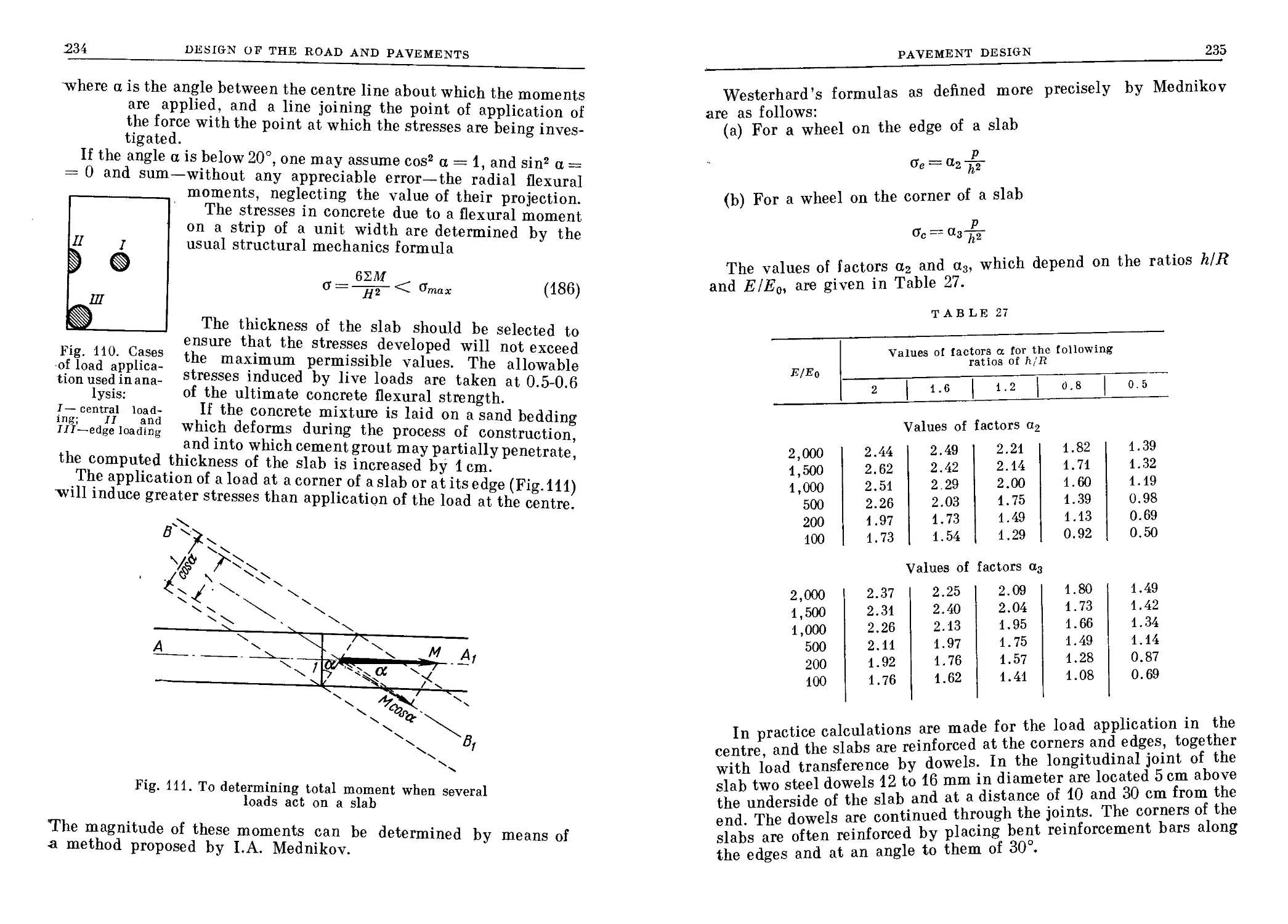
Chapter 8. Pavement Design
46. Pavement Structural Layers ................................. 198
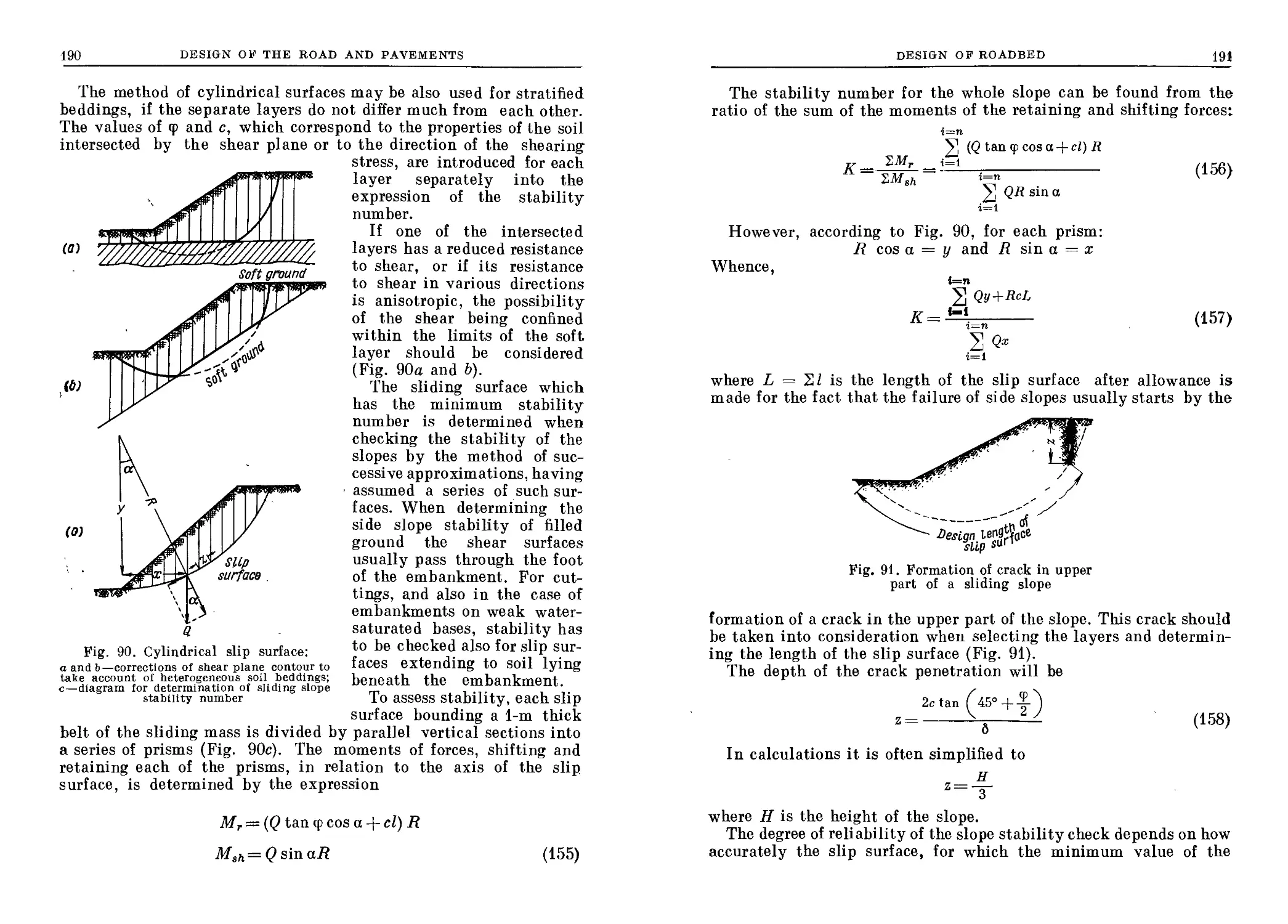
47. Main Types of Pavements . . . . . .......................... 200
48. Choice of Pavement Type ................. 205
49. General Principles of Pavement Analysis and Design.......... 208
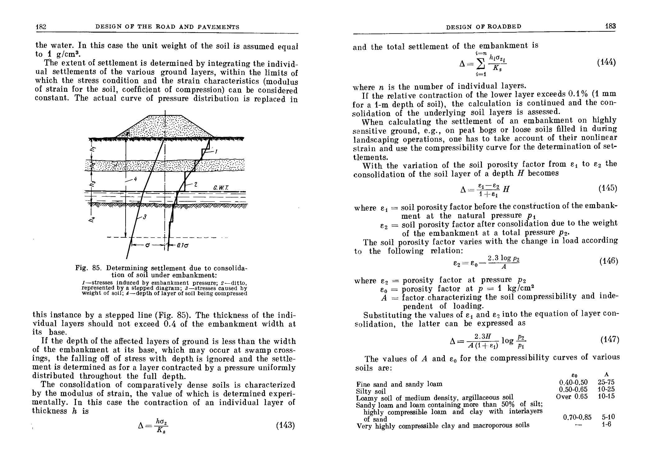
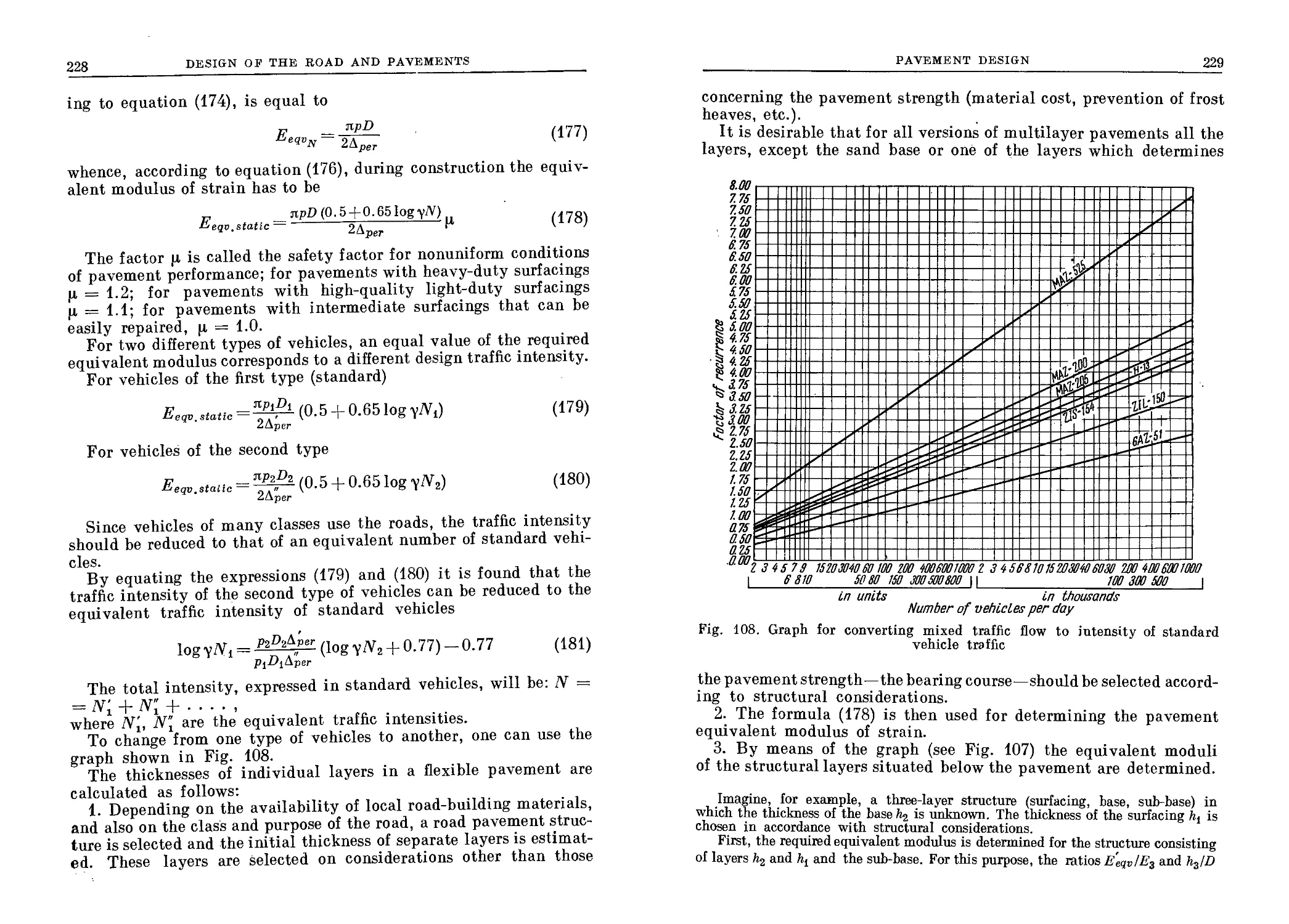
-50 . Pavement Loading......................................... 211
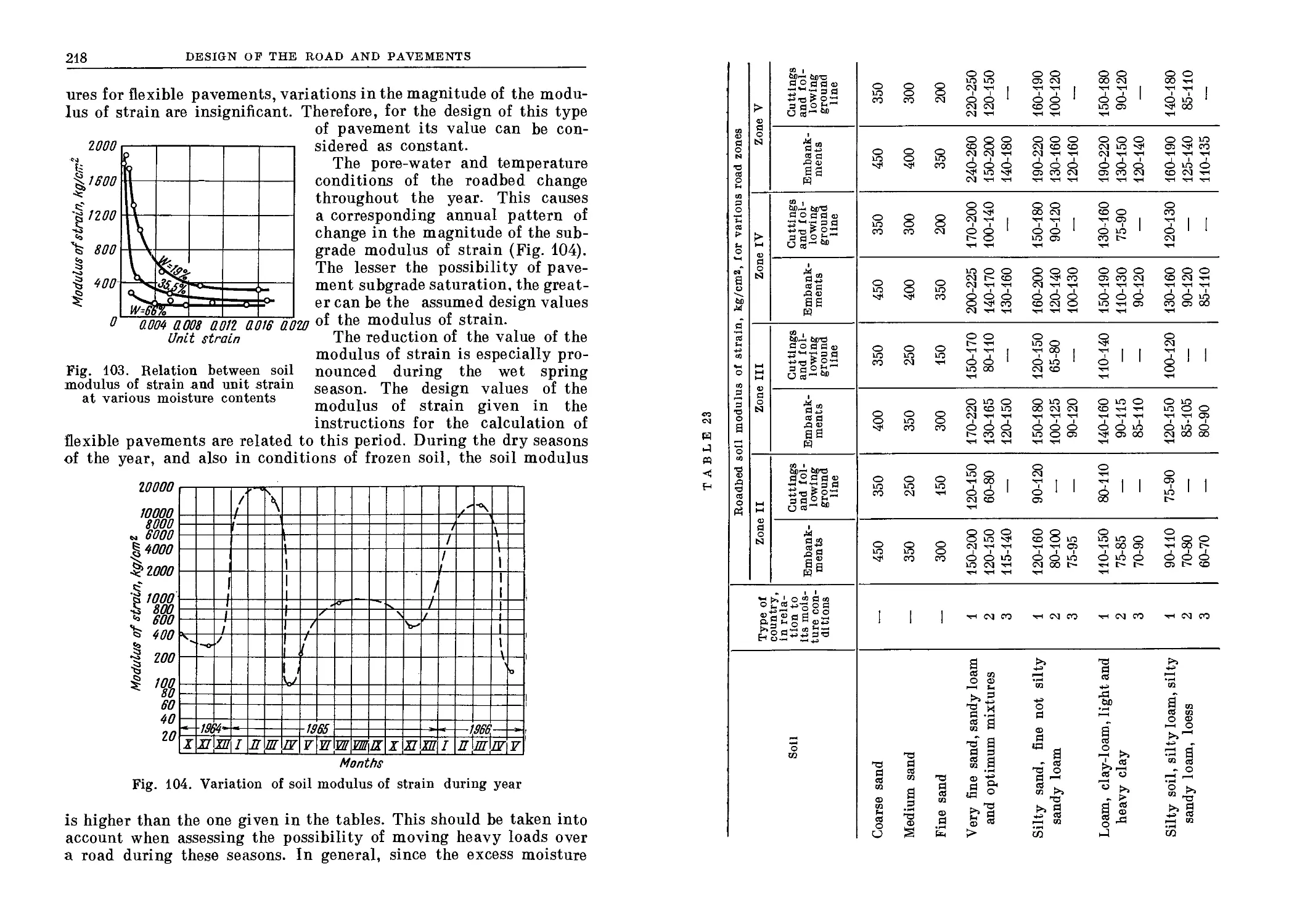
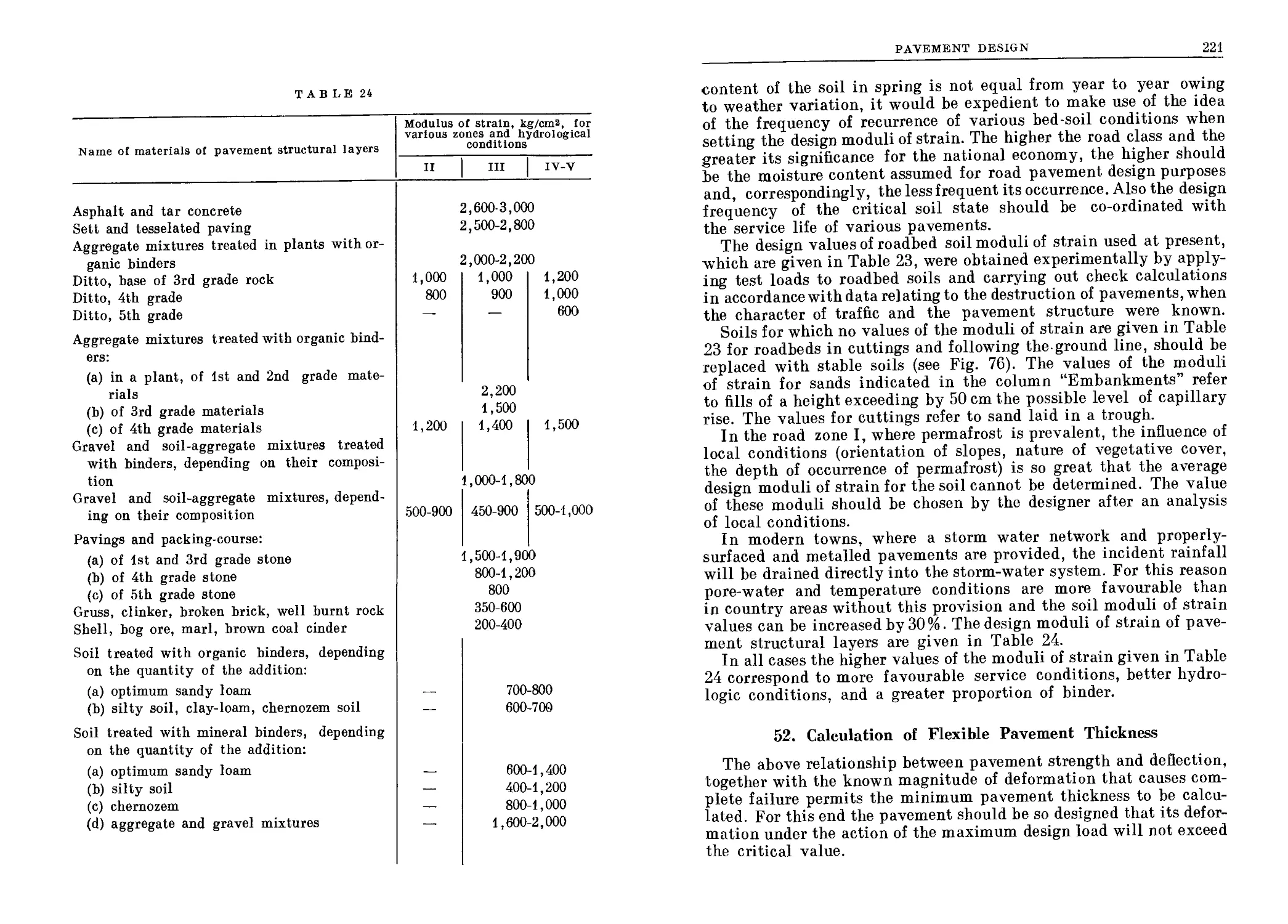
51. Strength of Flexible Pavements............................; 214
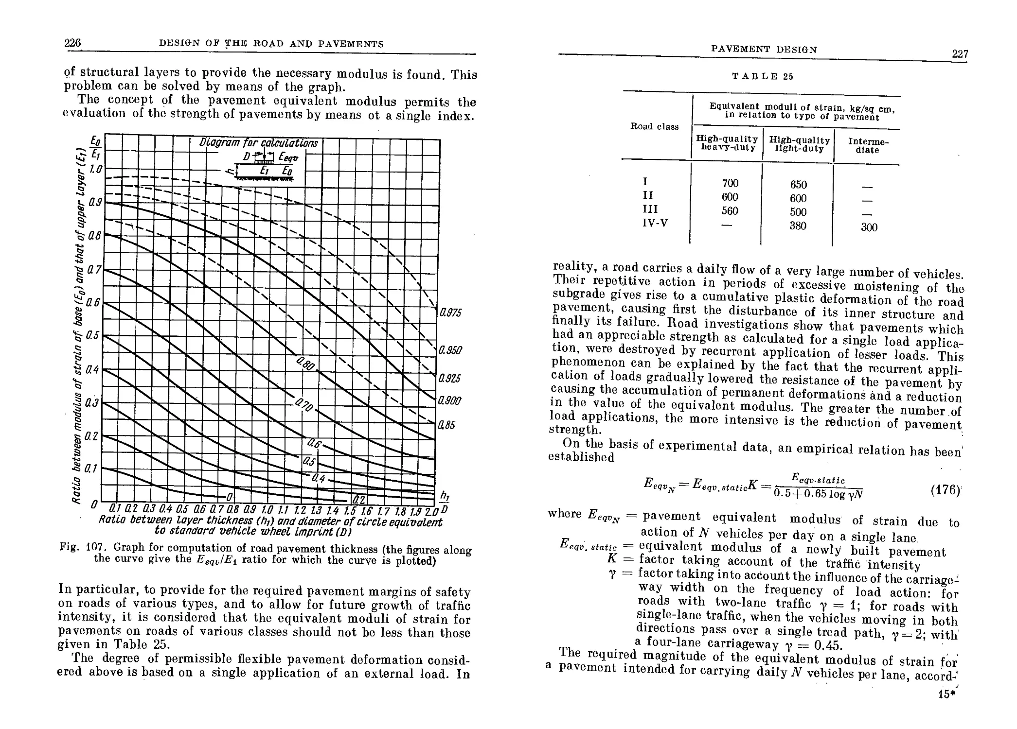
52. Calculation of Flexible Pavement Thickness.................. 221
53. Determination of Rigid Pavement Thickness................... 230
PART IV
ROUTE LOCATION
Chapter 9. Choice of Route Location
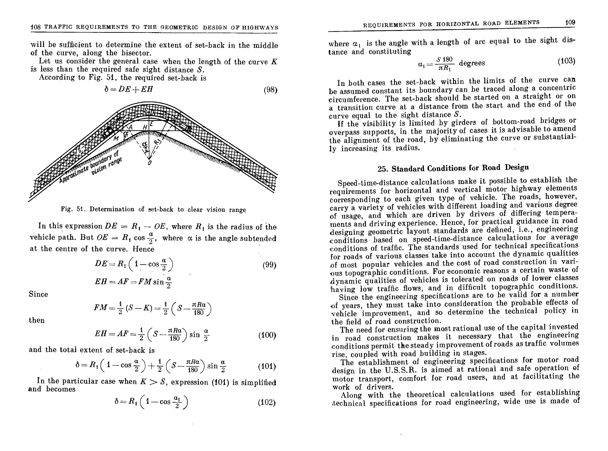
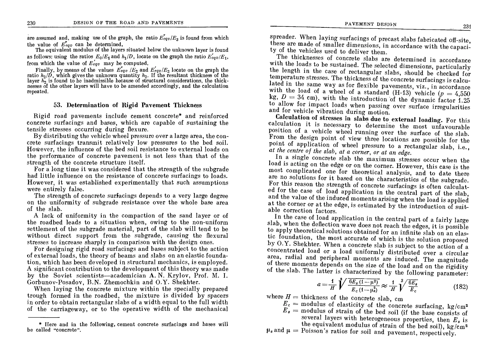
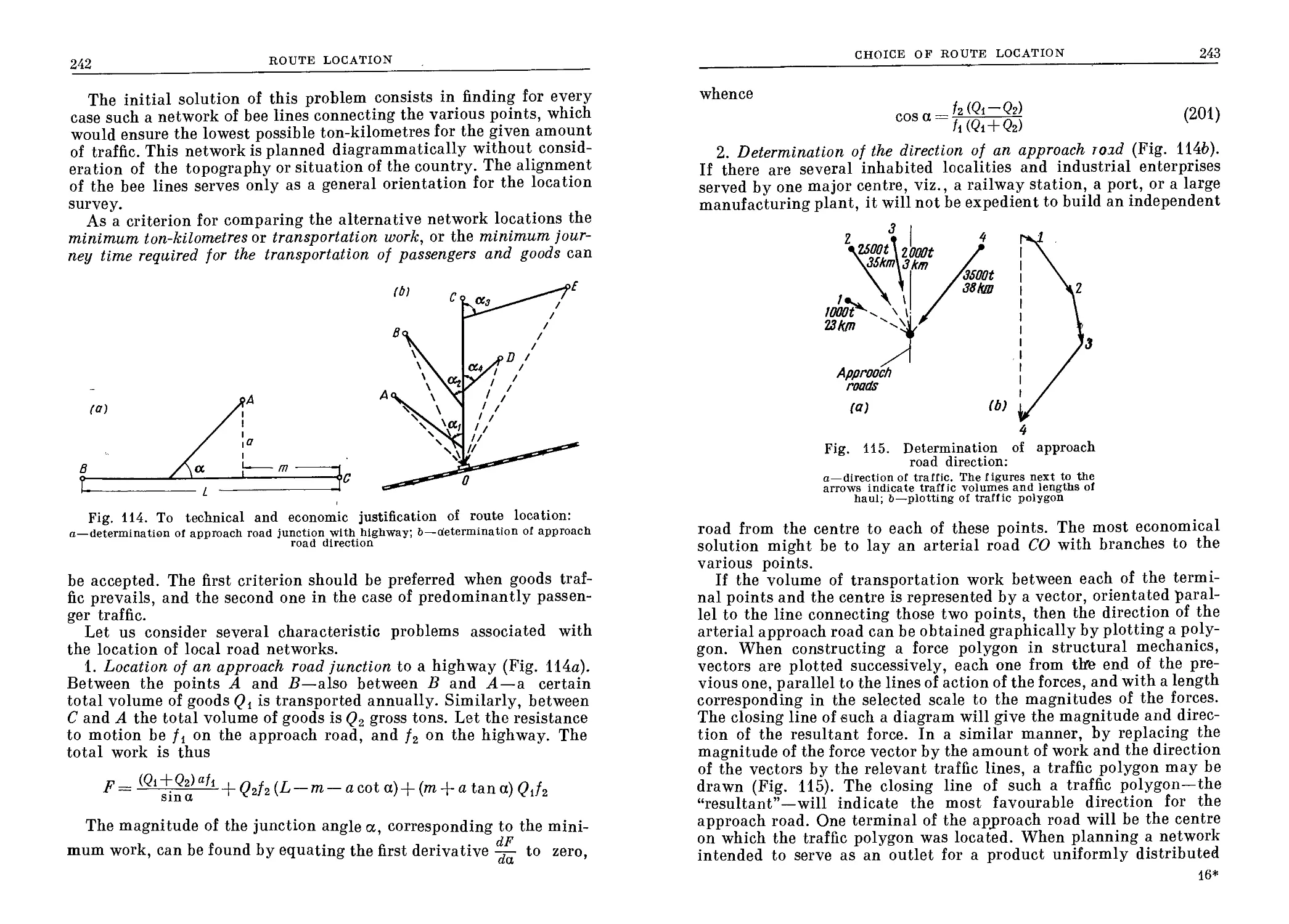
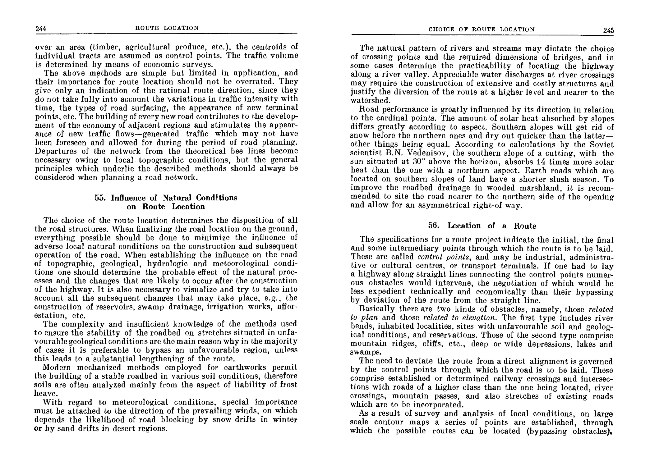
54. Effect of Traffic Intensity and Volume on Route Location . . 241
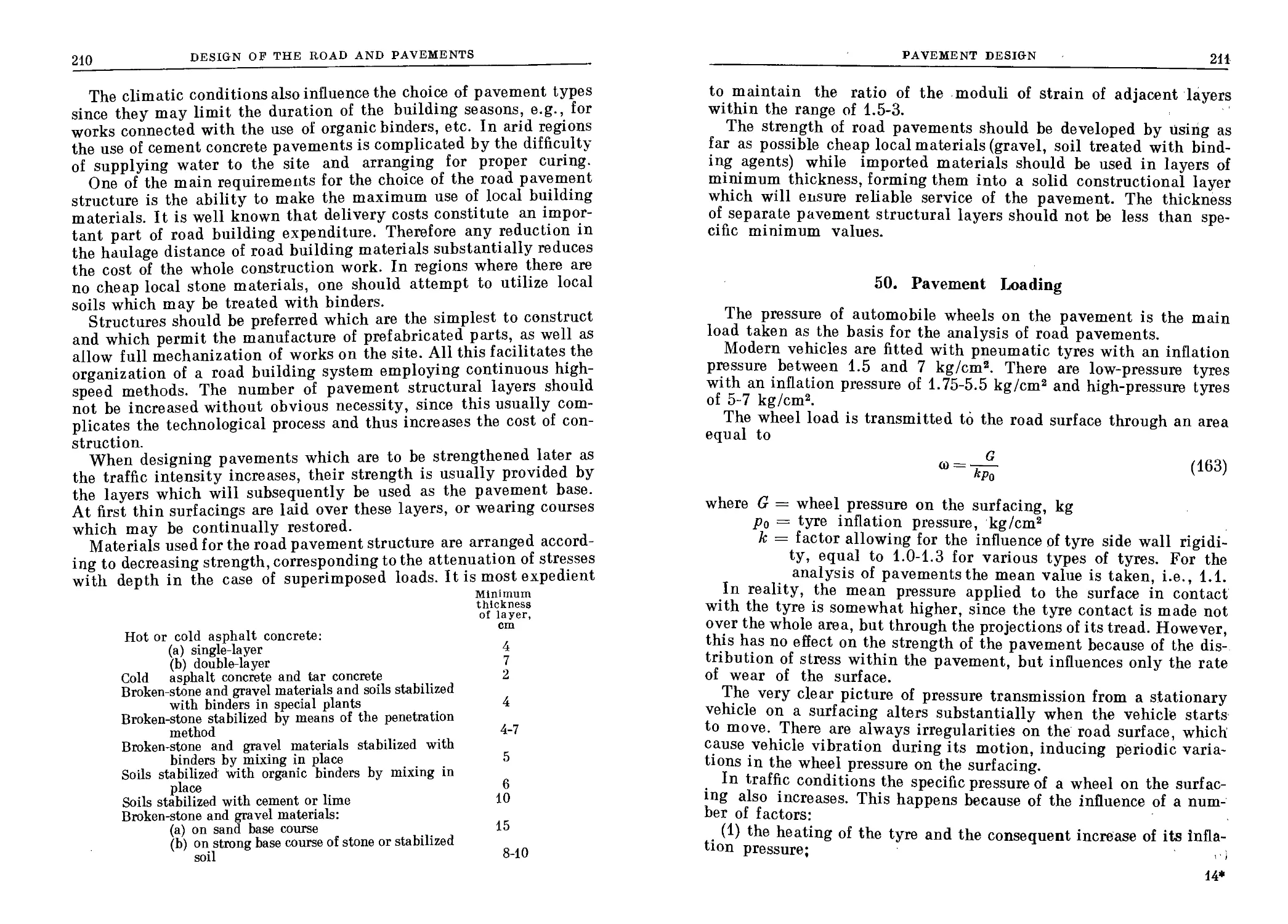
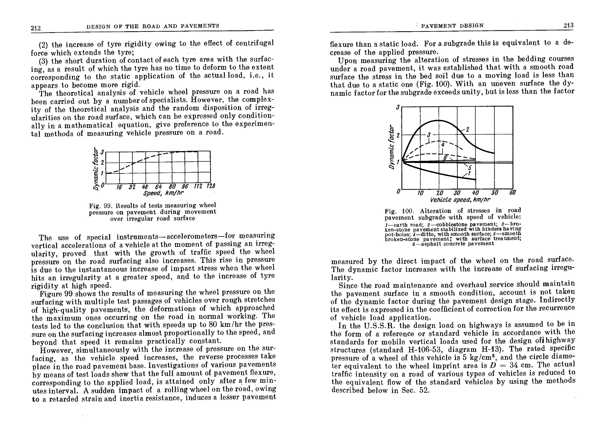
55. Influence of Natural Conditions on Route Location.......... 244
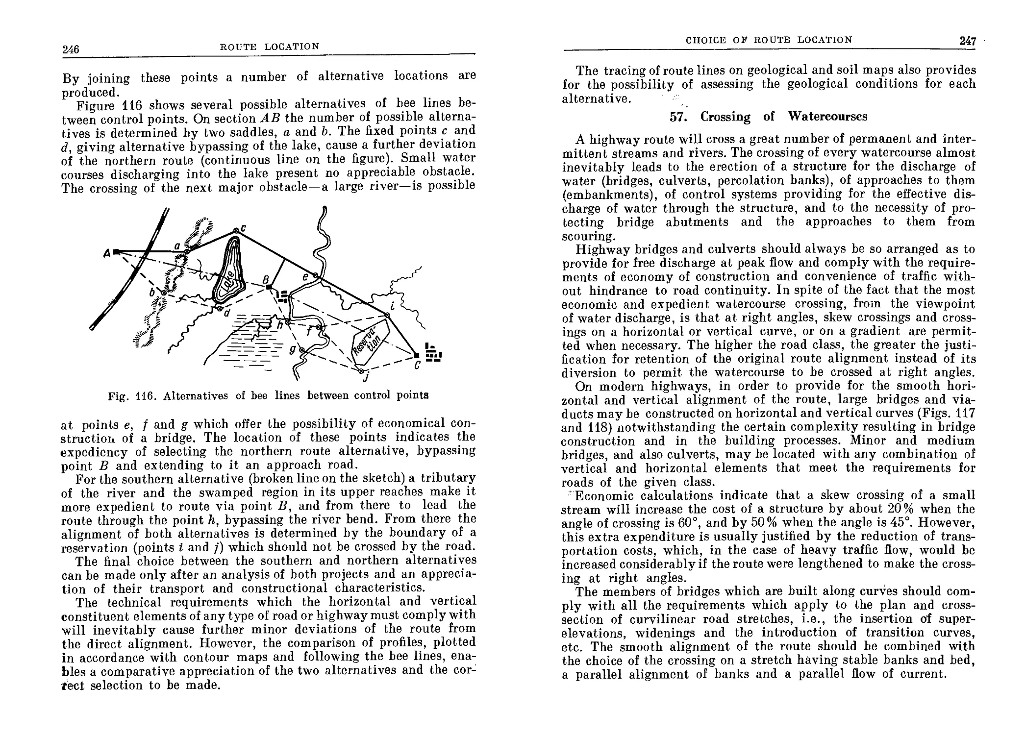
56. Location of a Route....................................... 245
57. Crossing of Watercourses . . . .......................... 247
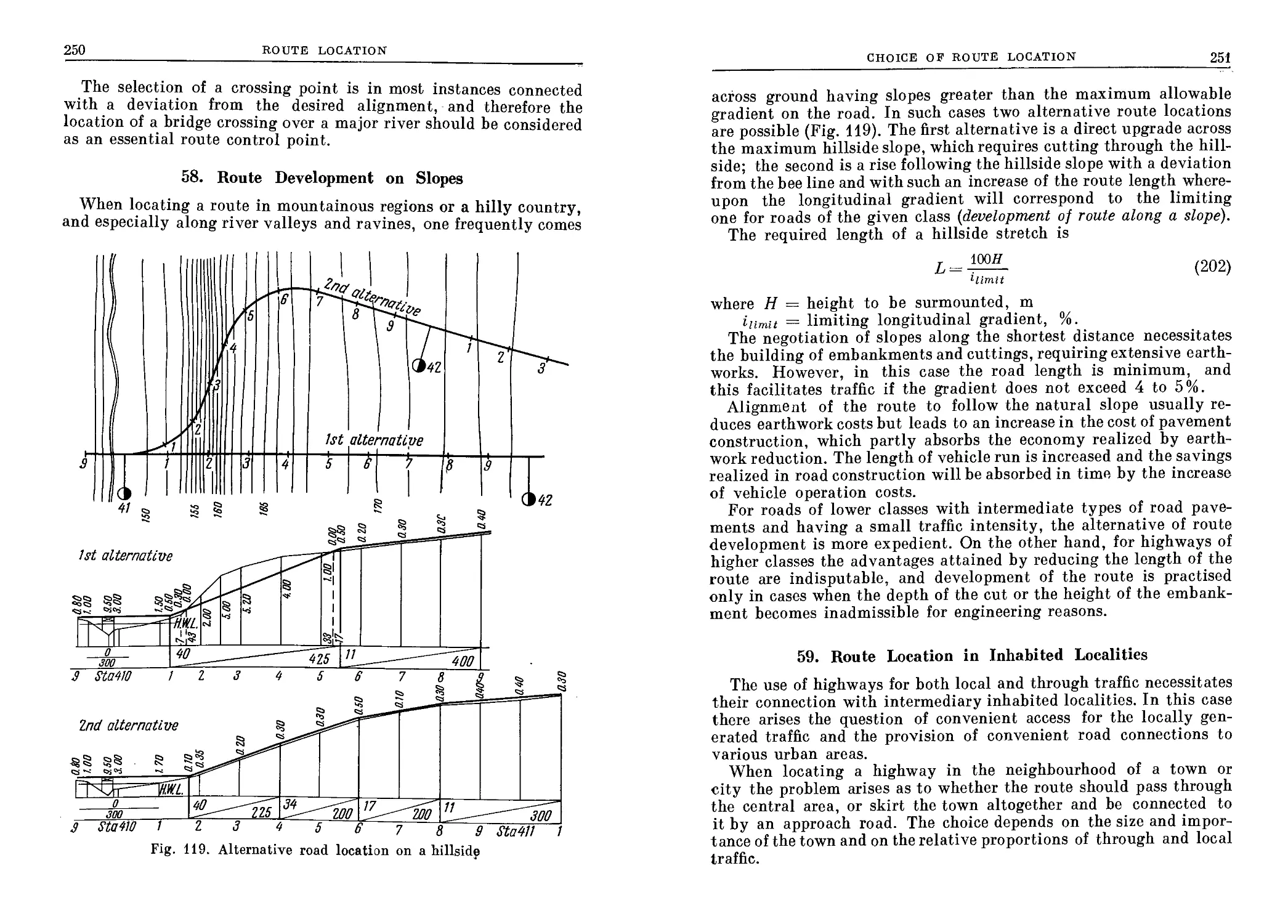
58. Route Development on Slopes.............................. . 250
59. Route Location in Inhabited Localities...................... 251
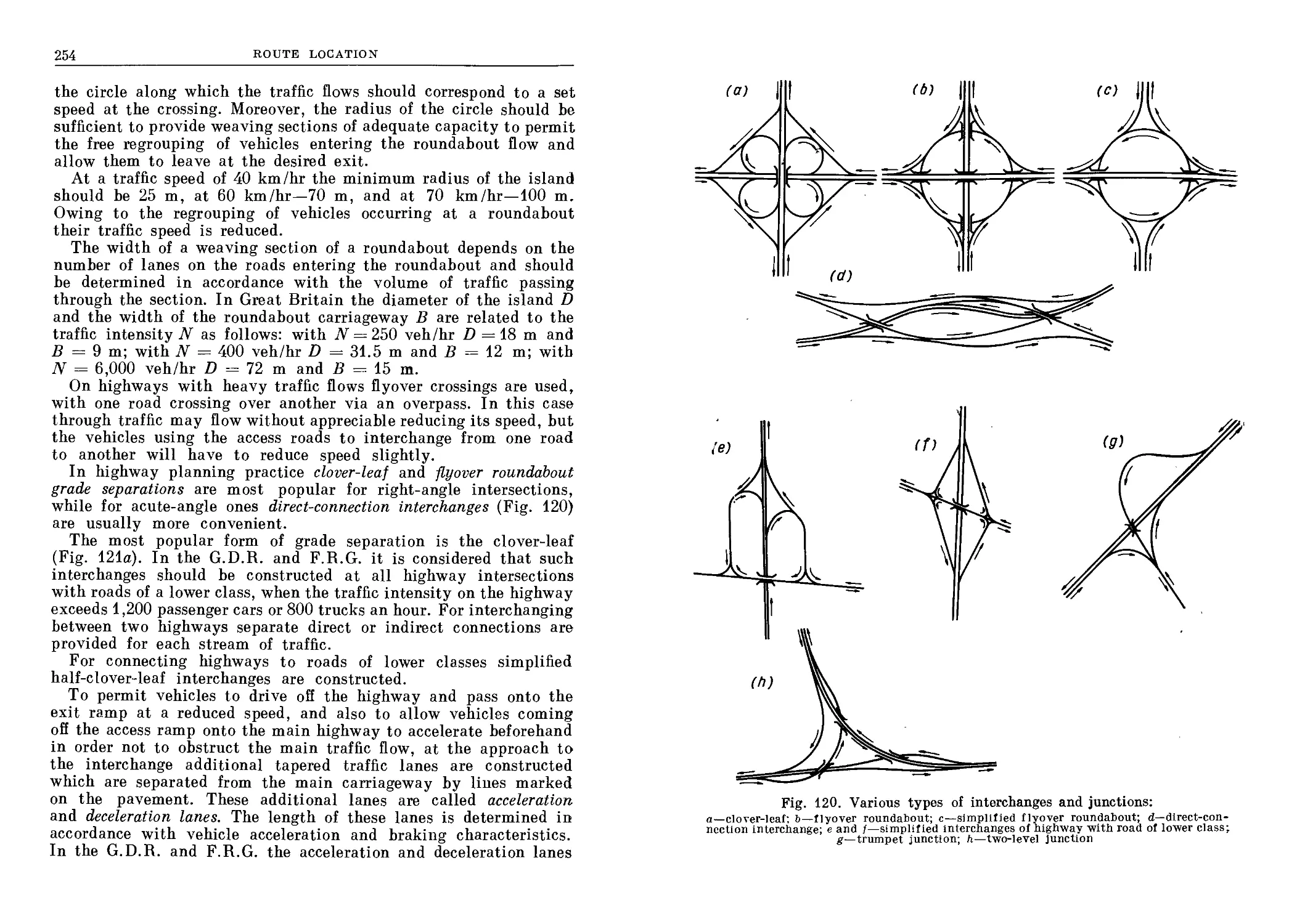
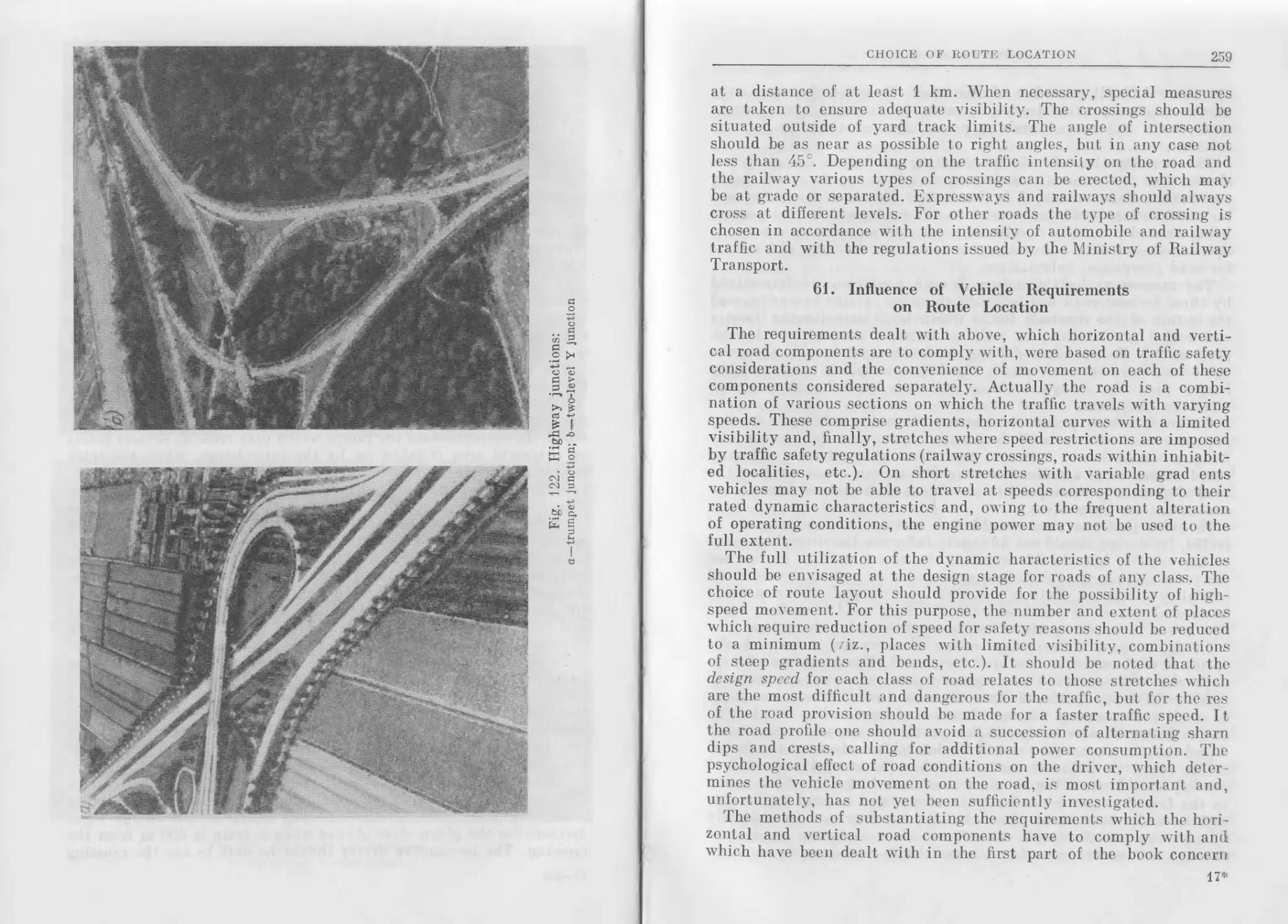
60. Highway Intersections . . .................................. 253
61. Influence of Vehicle Requirements on Route Location .... 259
62. Locating a Highway as an Integral Part of the General Land-
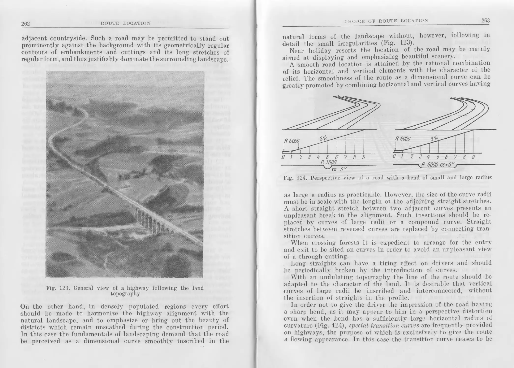
scape (Landscaping)............................................ 261
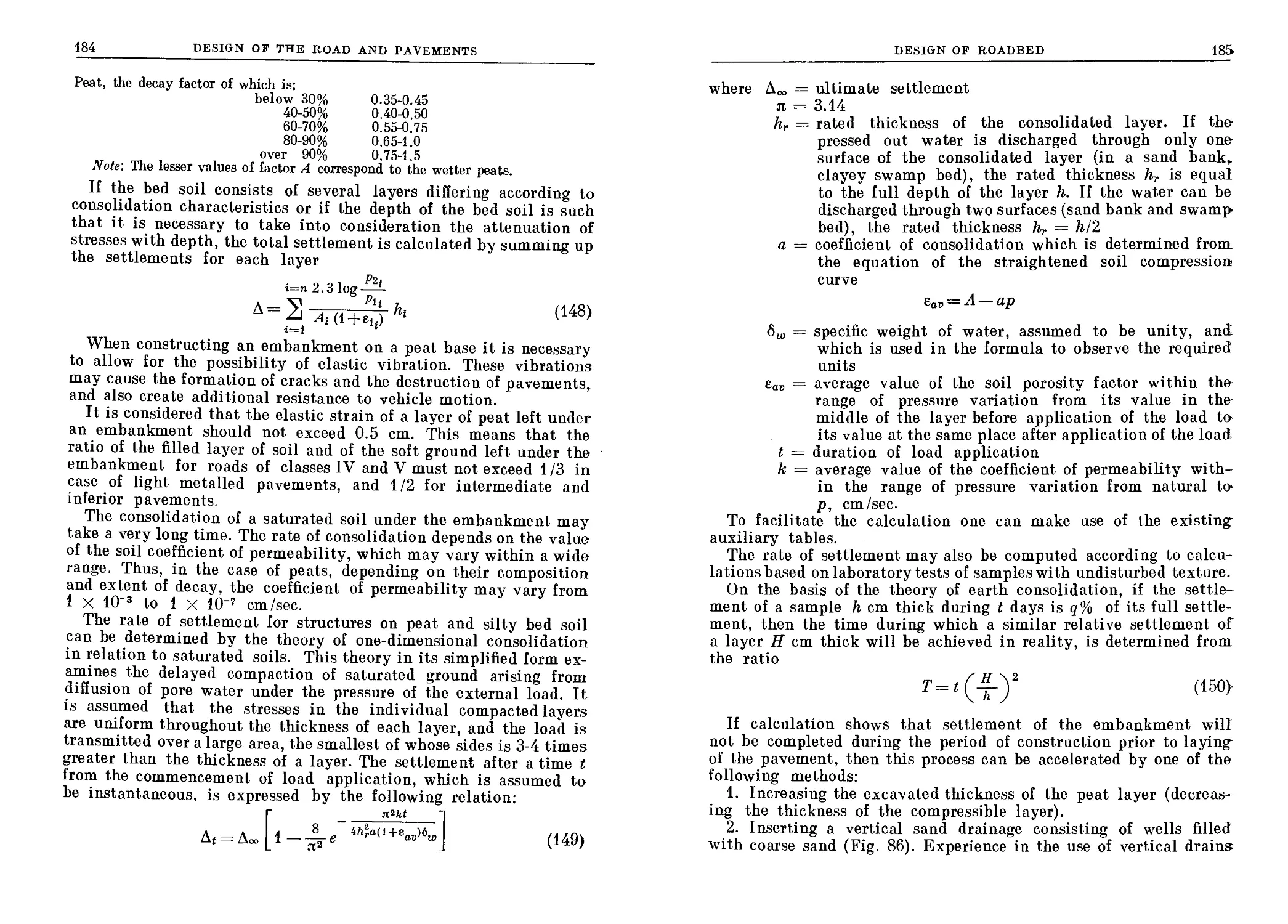
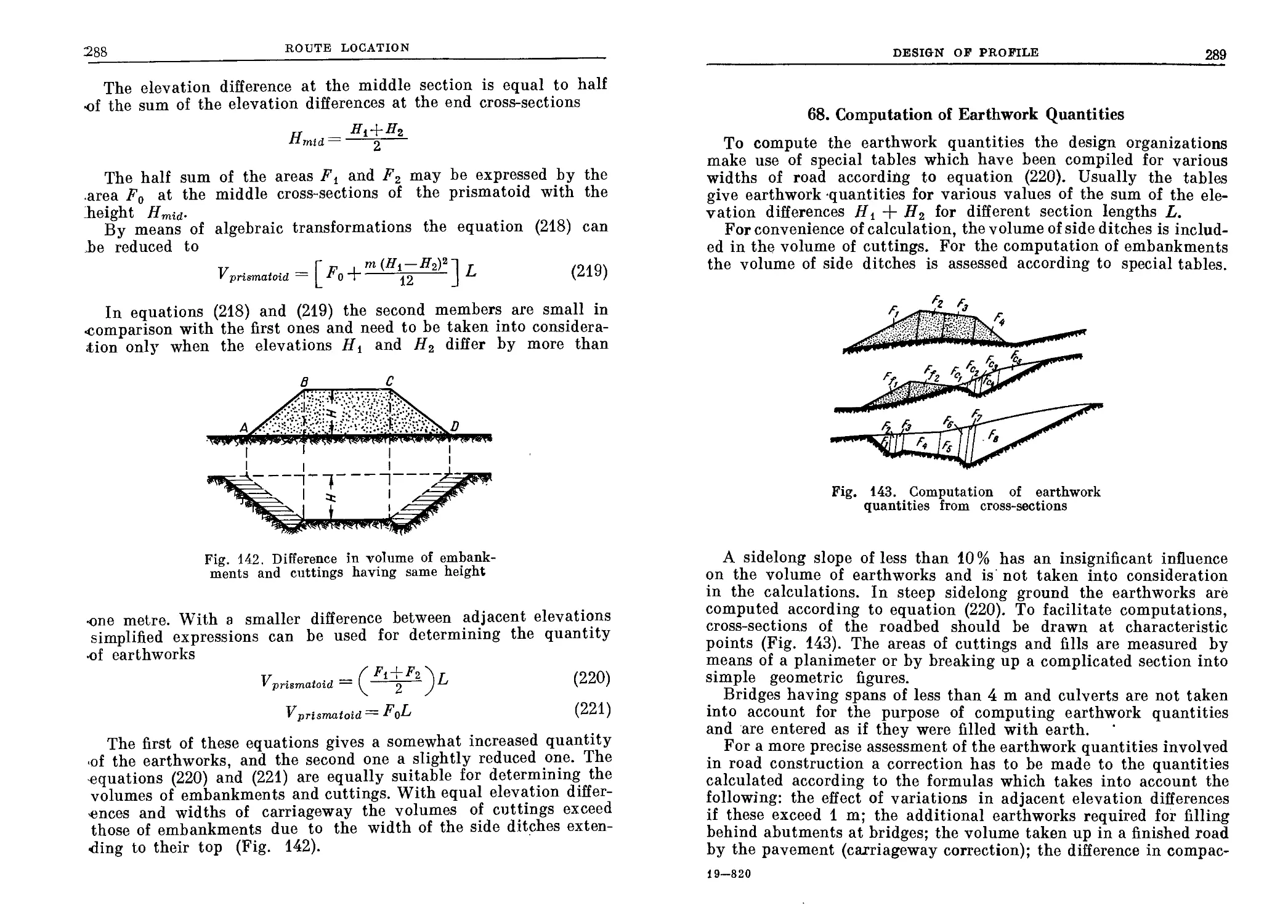
Chapter 10. Design of Profile
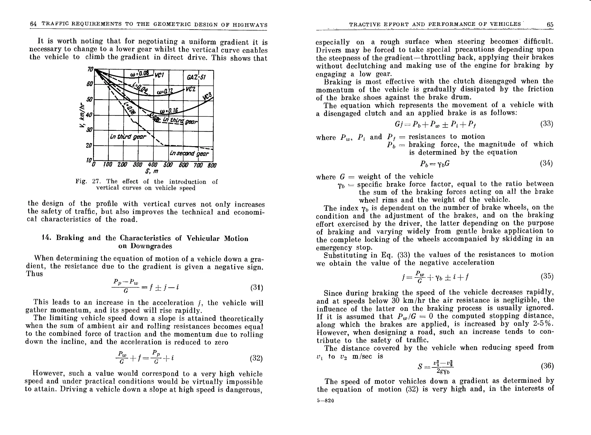
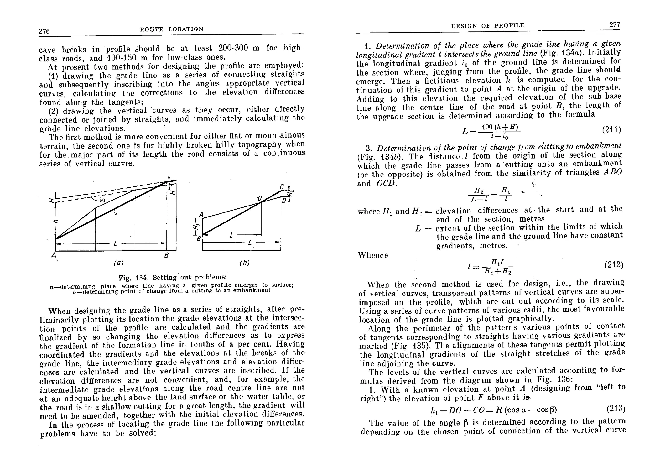
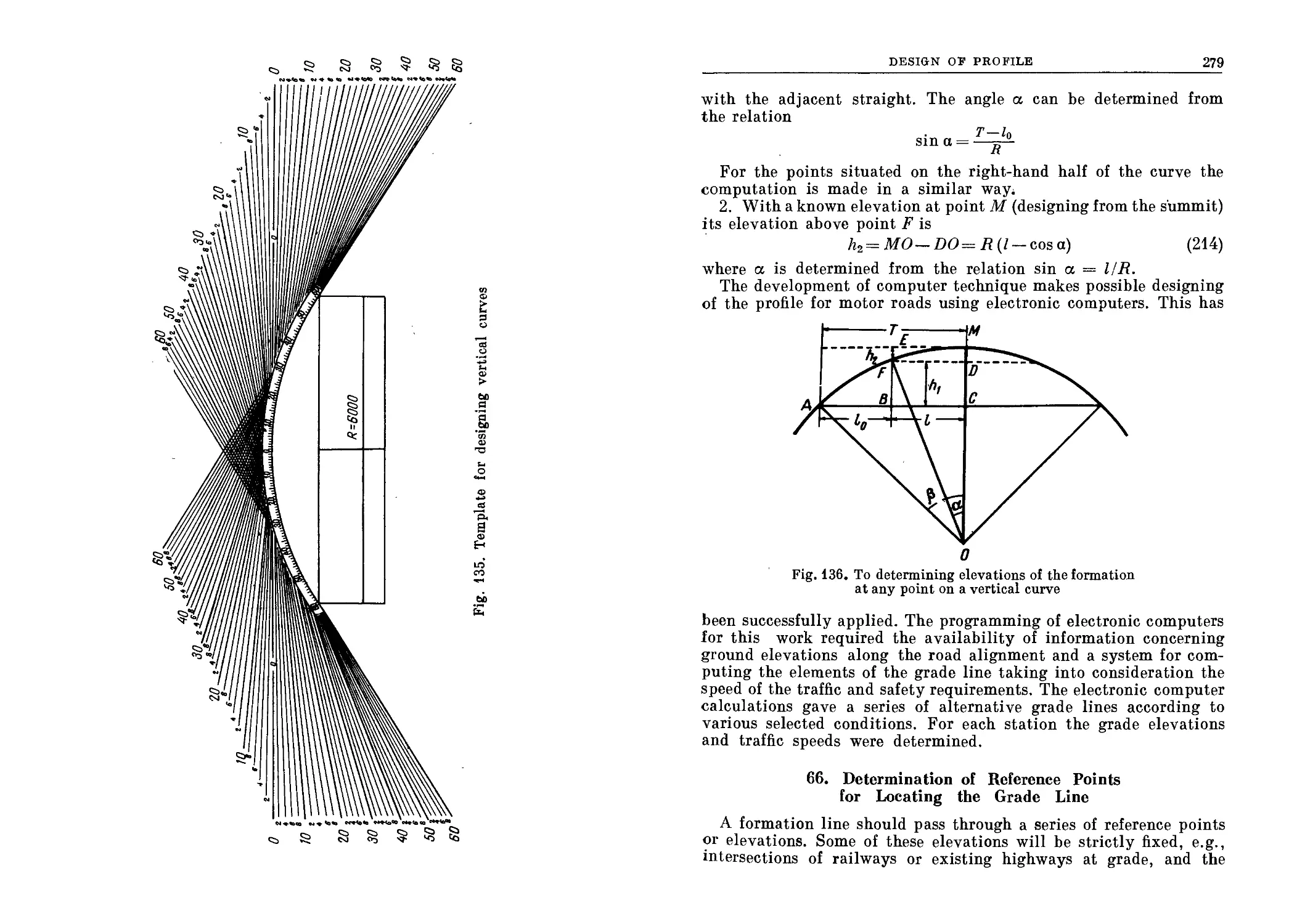
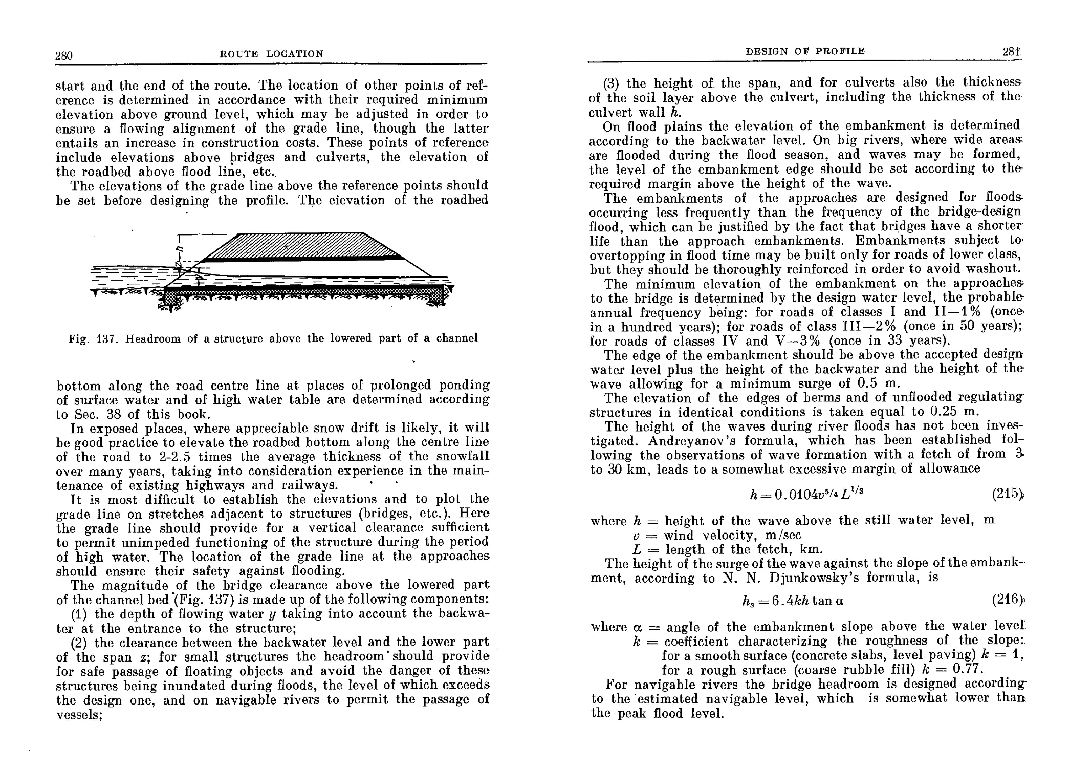
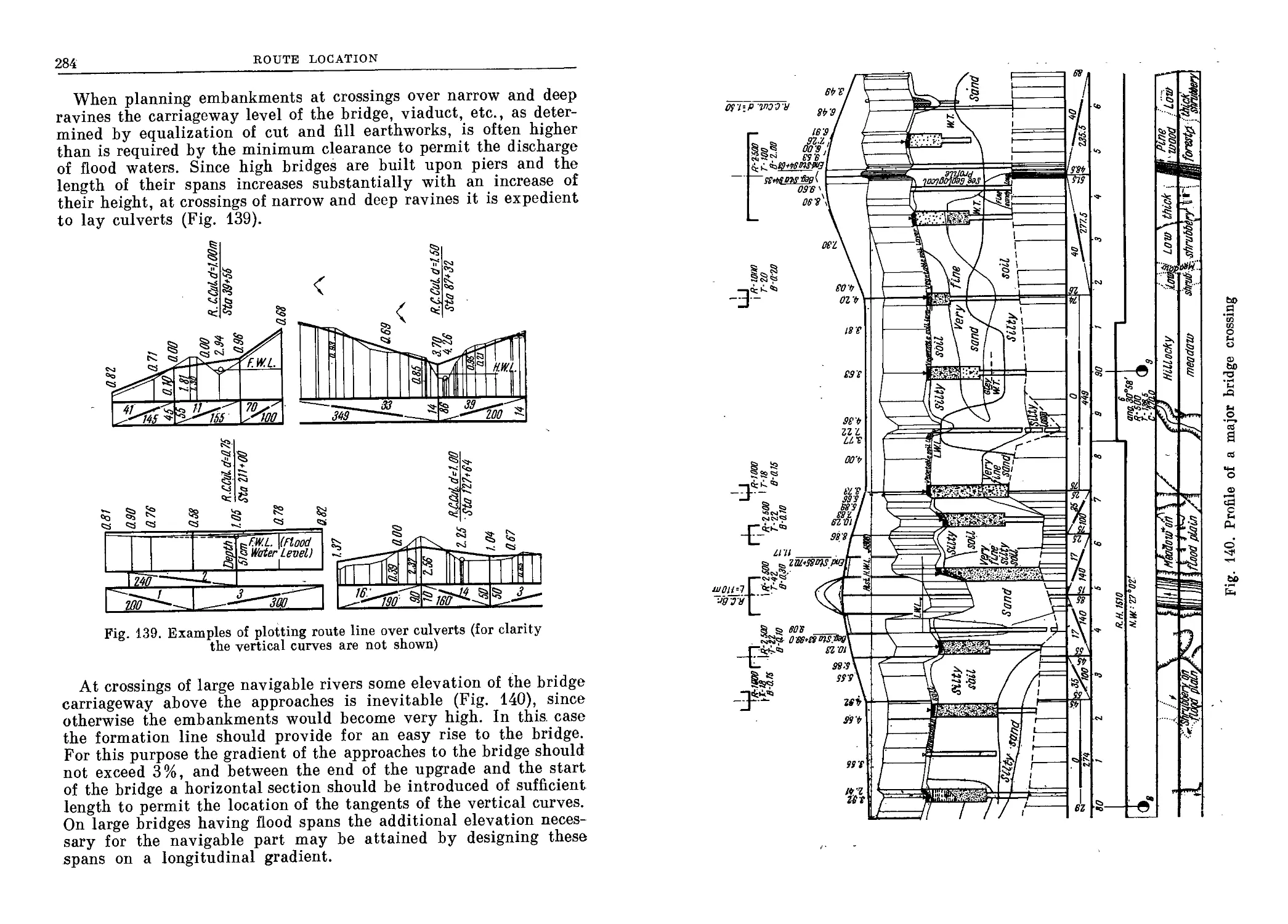
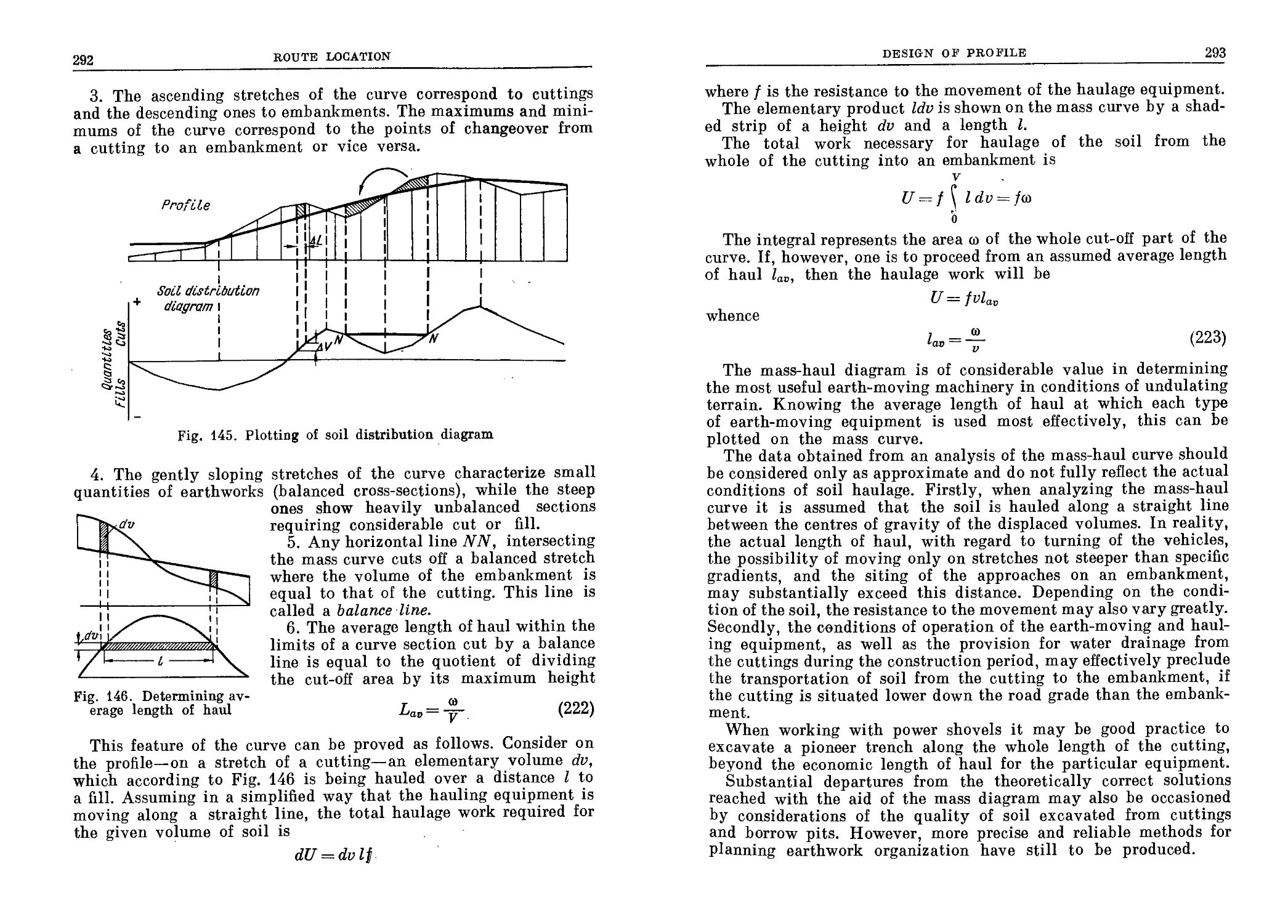
63. Location of the Grade’Line.................................. 268
64. Design of Vertical Curves................................... 269
65. Sequence of Designing the Profile........................... 275
66. Determination of Reference Points for Locating the Grade
Line ........................................................ 279
67. Volumes of Embankments and Cuttings......................... 286
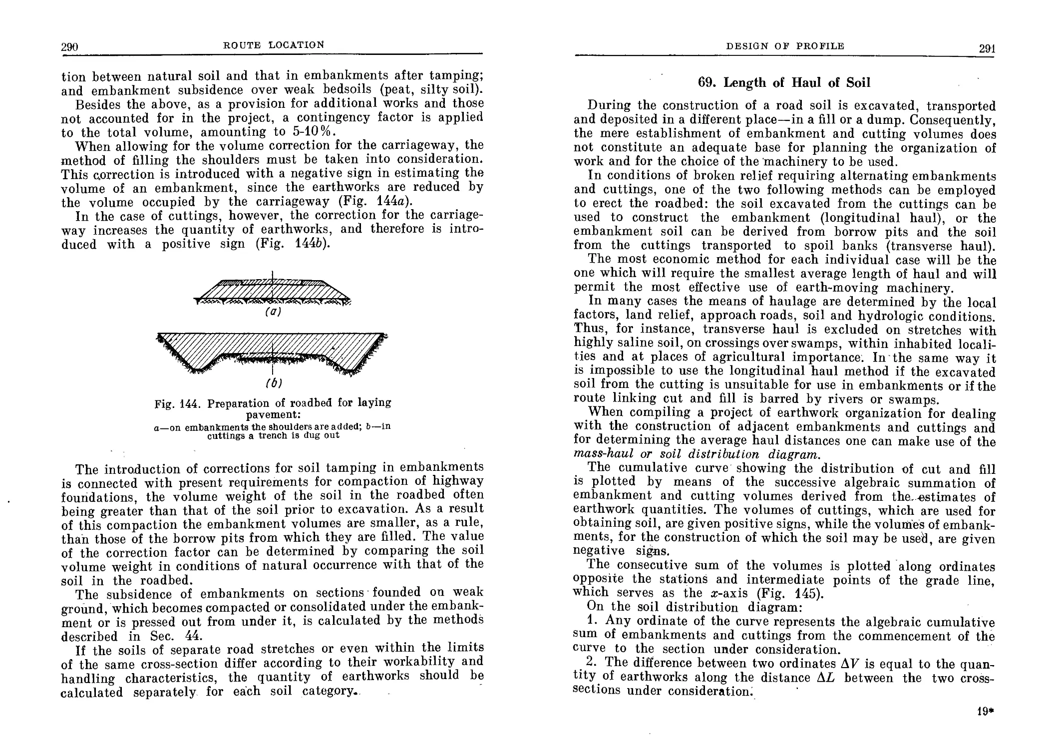
68. Computation of Earthwork Quantities......................... 289
69. Length 'of Haul of Soil.................................. 291
PART V
HIGHWAY, PLANNING AND SURVEY
Chapter 11. Stages of the Planning Process
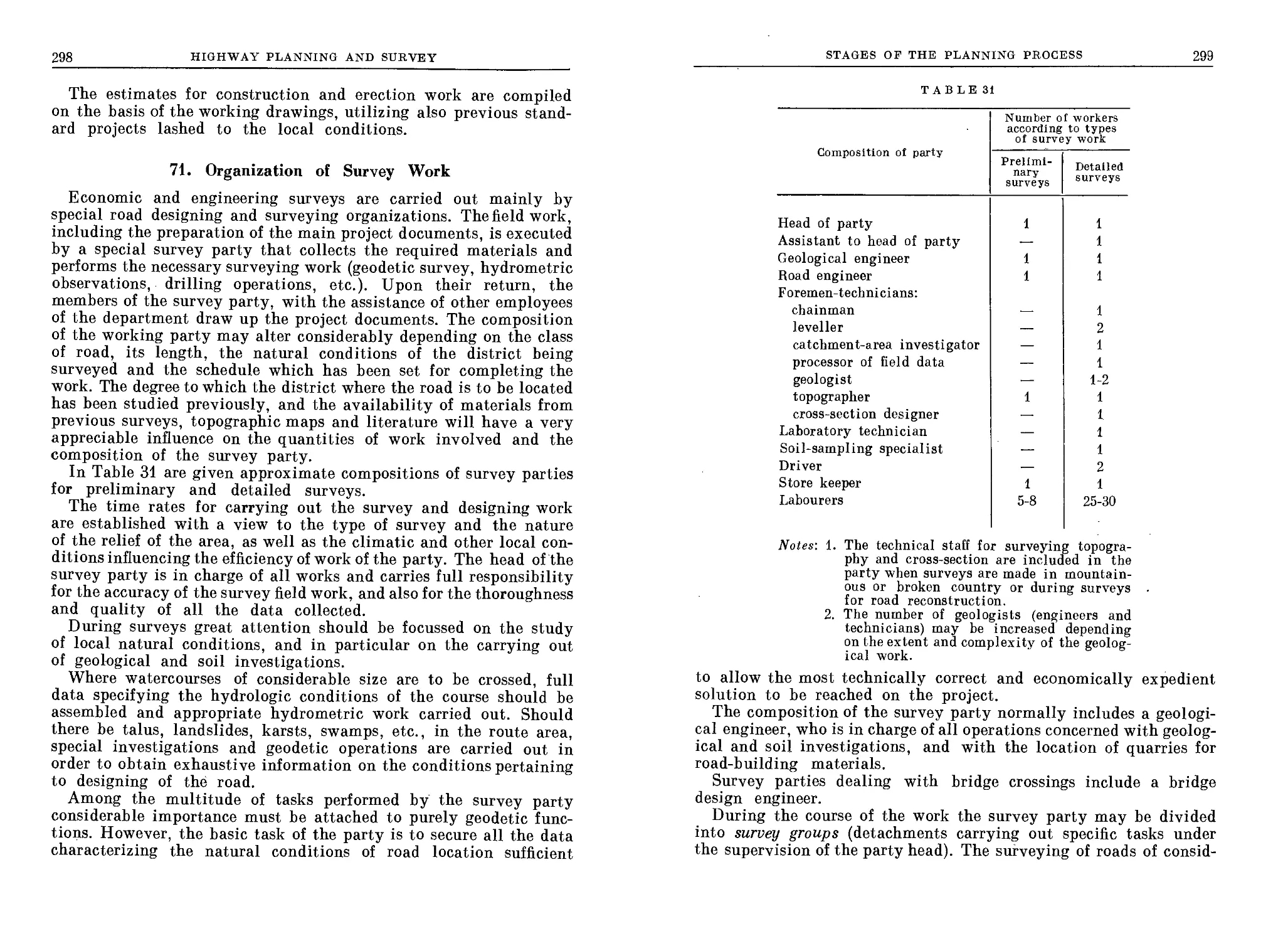
70. Types of Surveys and Their Purpose ......................... 294
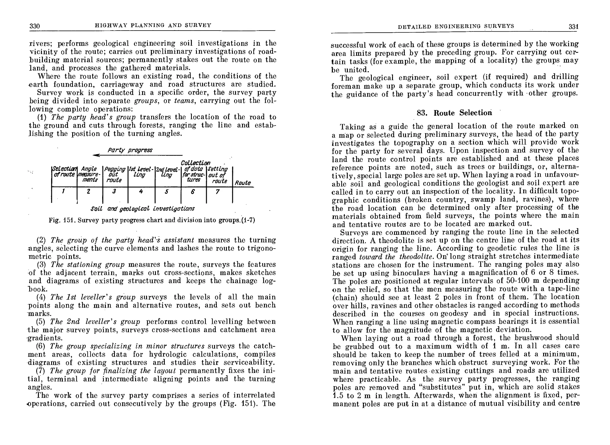
71. Organization of Зигуёу Work................................. 298
8
CONTENTS
Chapter 12. Preliminary Survey
72. Organization................................................... 302
73. Preparatory Work .................................... 302
74. Aerial Survey ................................................. 305
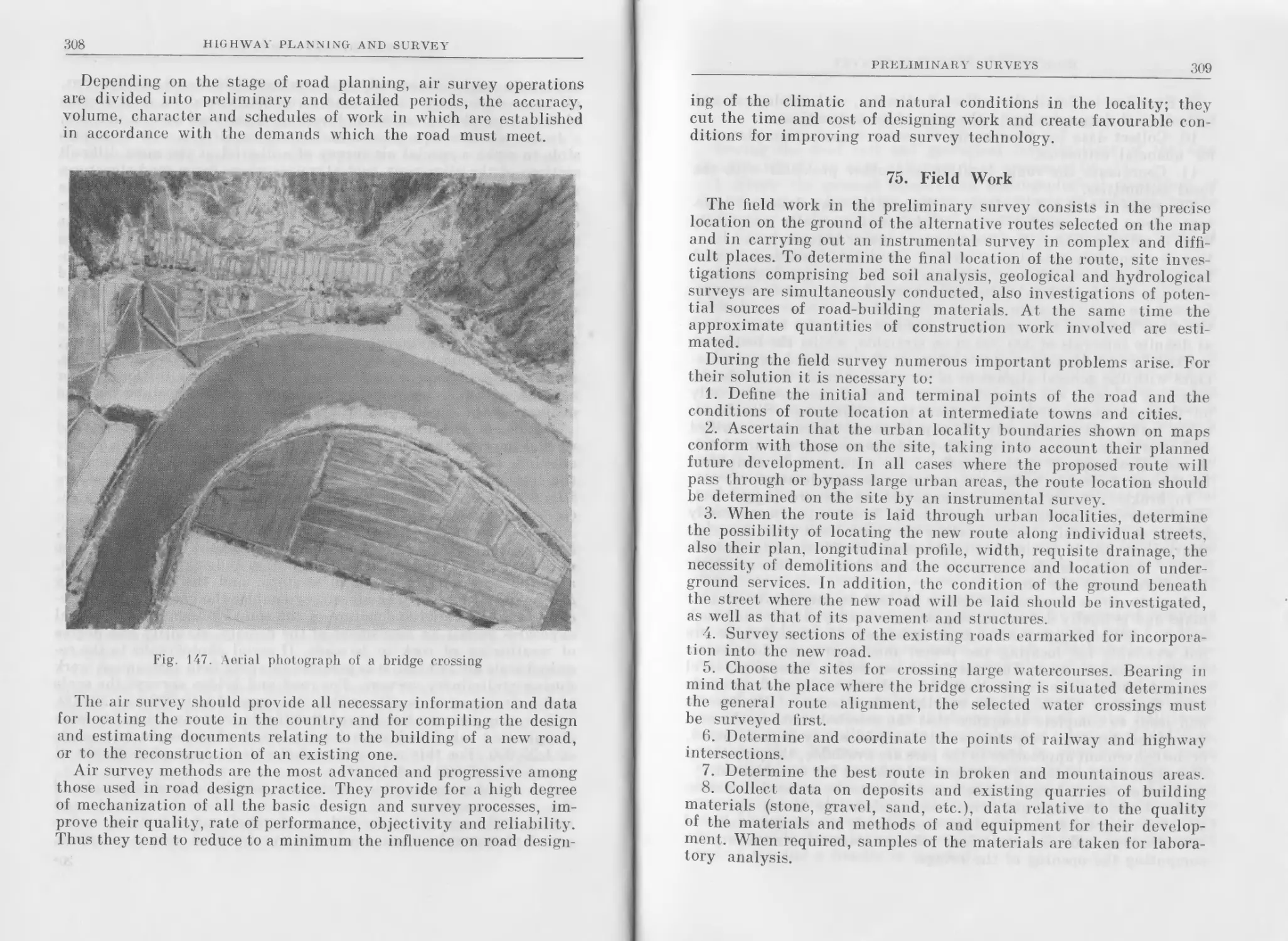
75. Field Work ................................................... 309
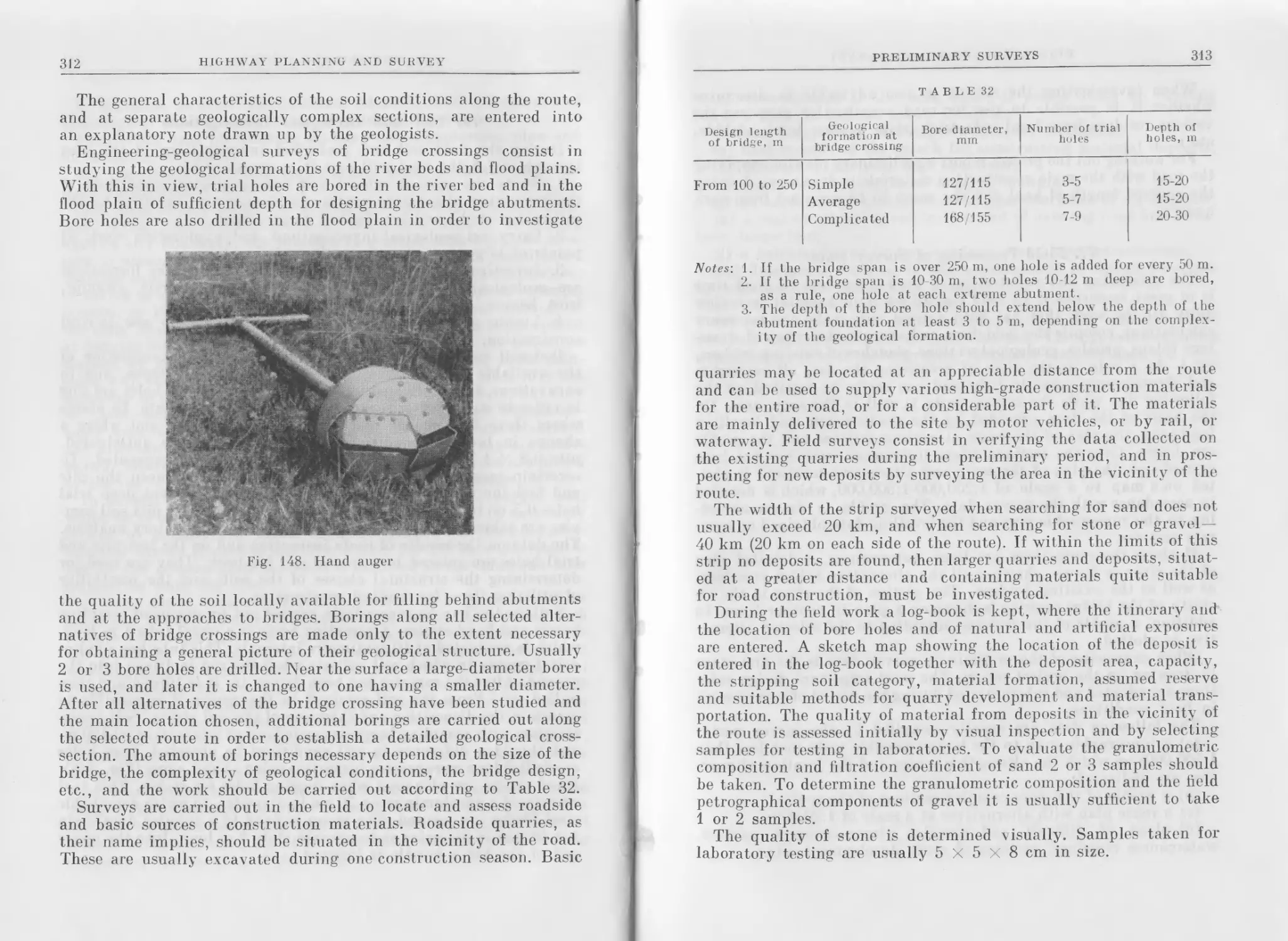
76. Soil and Geological Investigations............................ 311
77. Field Processing of Survey Data .............................. 314
Chapter 13. Project Report
78. Selection of Engineering Standards............................. 316
79. Estimate of Work Quantities and Cost........................... 318
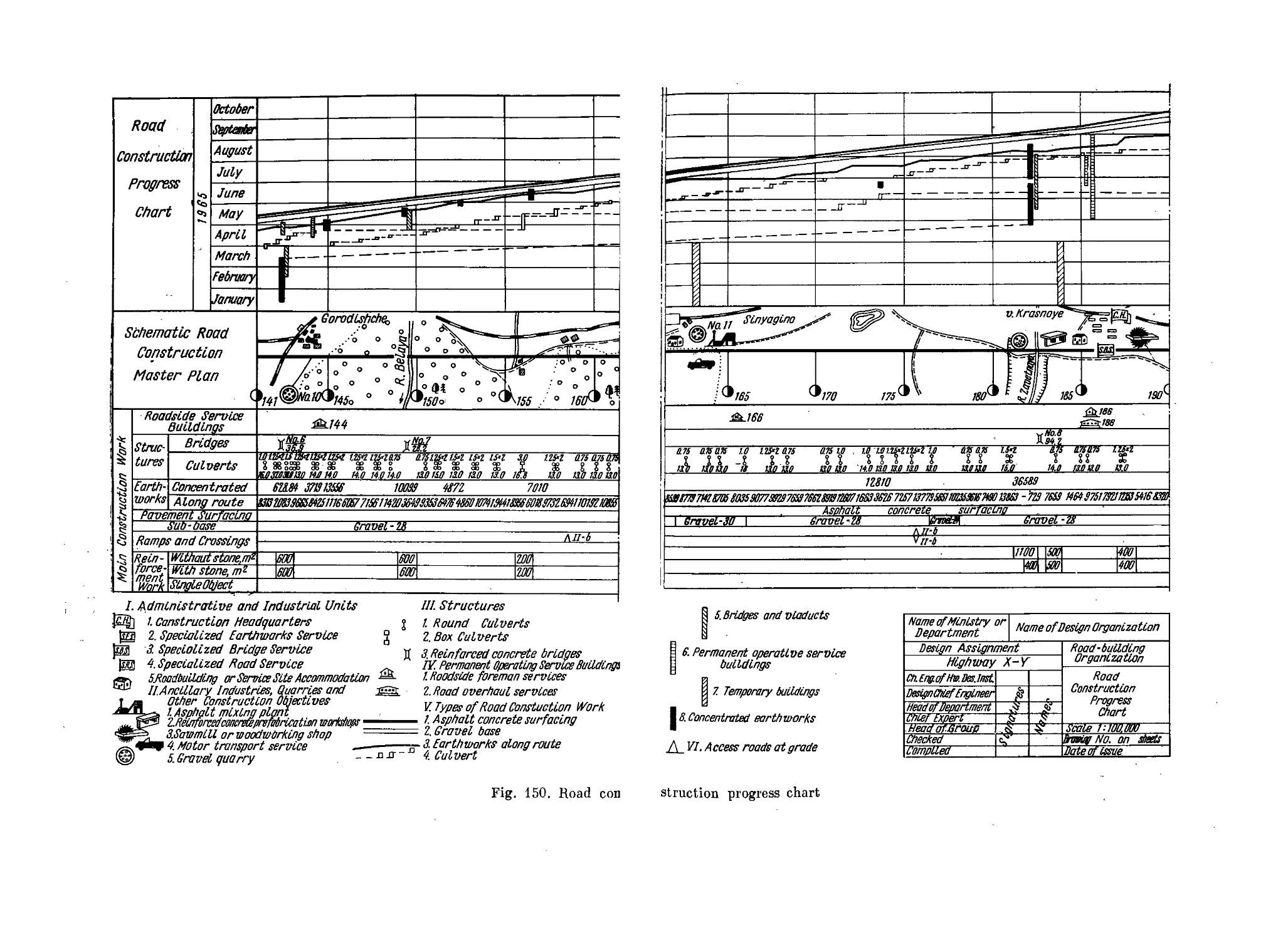
80. Work Organization Plan......................................... 324
81. Content of Project Report...................................... 325
Chapter 14. Detailed Engineering Surveys
82. Survey Procedure .............................................. 329
83. Route Selection............................................. 331
84. Measurement of Angles.......................................... 334
85. Marking Out the Stations.................... , .... 336
86. Route Levelling............................................... 340
87. Collection of Data for Structure and Drainage Design .... 342
88. Setting Out the Route.......................................... 346
89. Mapping Complicated Sites.................................. . 347
90. Soil Investigations............................................ 349
91. Basic Safety Rules for Highway Surveys......................... 354
92. Office Processing of Survey Materials.......................... 356
Chapter 15. The Highway Technical Project
93. Scope of Technical Project..................................... 358
94. Designing Road Plan, Profile and Cross-sections................ 358
95. Determination of Work Quantities............................... 360
96. Composition of the Technical Project........................... 362
Chapter 16. Surveying and Designing of Road Reconstruction
97. Road Reconstruction............................................ 363
98. Engineering Surveys for Road Reconstruction.................... 364
99. Field Work in Detailed Road Reconstruction Engineering Survey 365
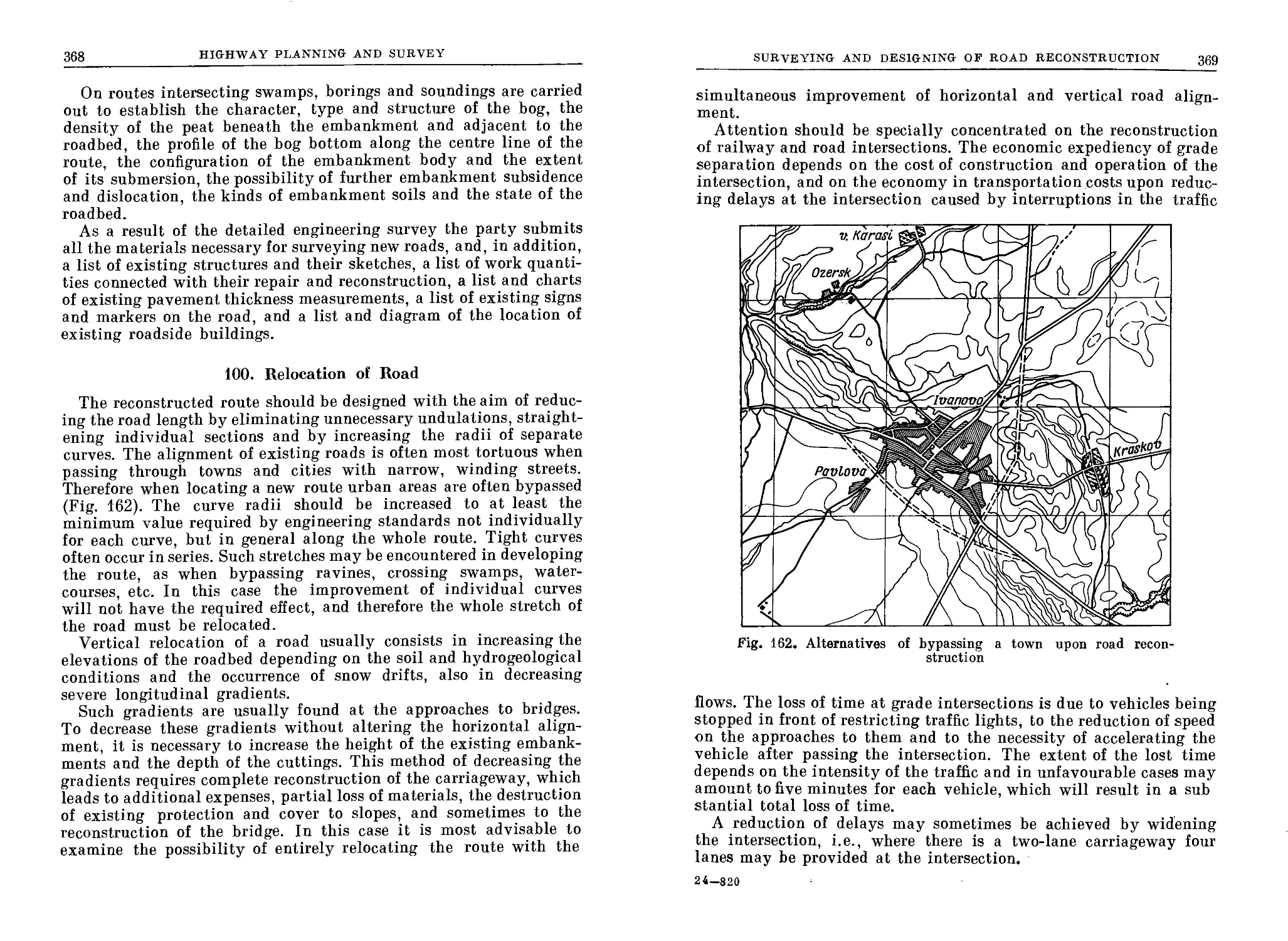
100. Relocation of Road........................................... 368
101. Reconstruction of Road Cross-section........................... 372
102. Reconstruction and Strengthening of the Pavement............... 374
103. Composition of Road Reconstruction Project................. . 376
Chapter 17. Comparison of Route Alternatives
104. Comparison of Alternatives According to Construction and
Operating Costs.............................................. 377
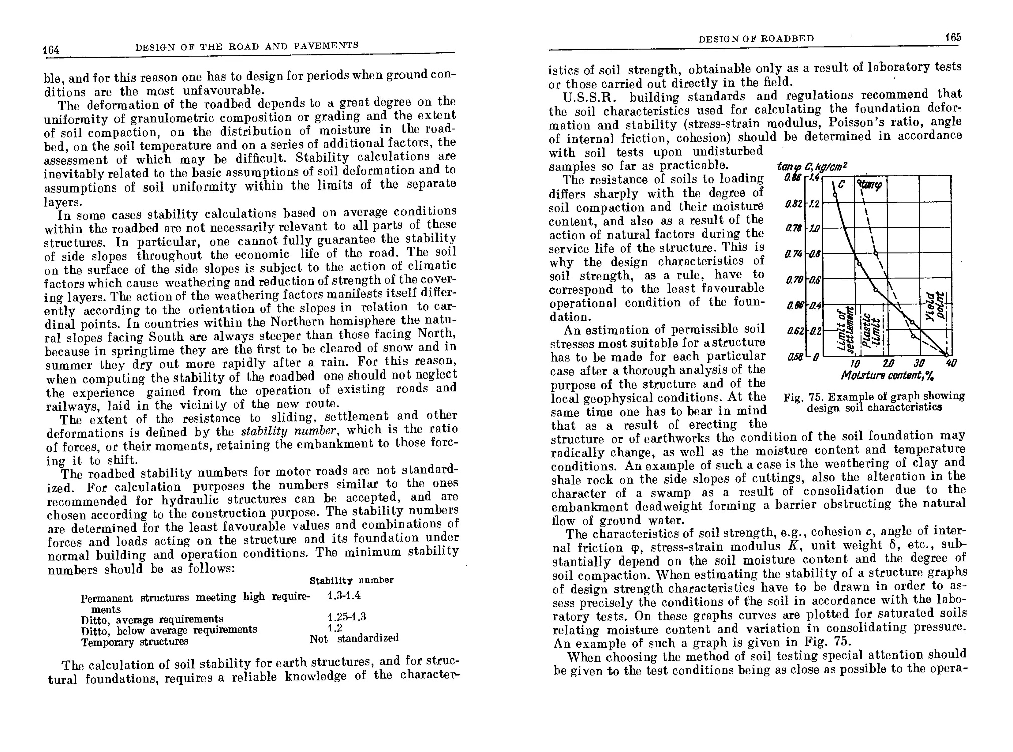
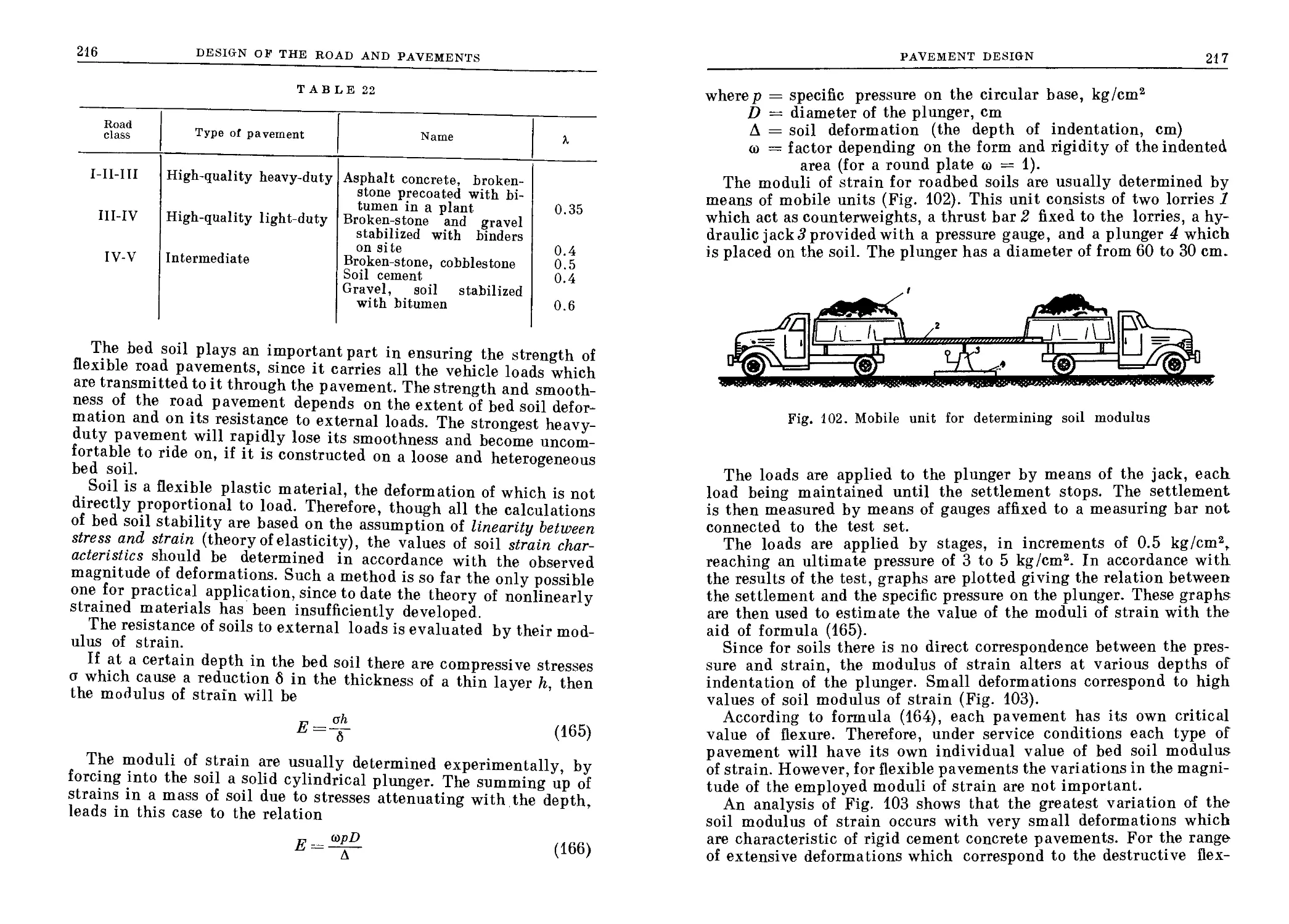
CONTENTS
9
PART VI
SPECIAL FEATURES OF ROAD DESIGN IN COMPLICATED
GEOPHYSICAL CONDITIONS
Chapter 18. Road Design in Swamped Regions
105. Origin, Characteristics and Types of Swamps................... . 381
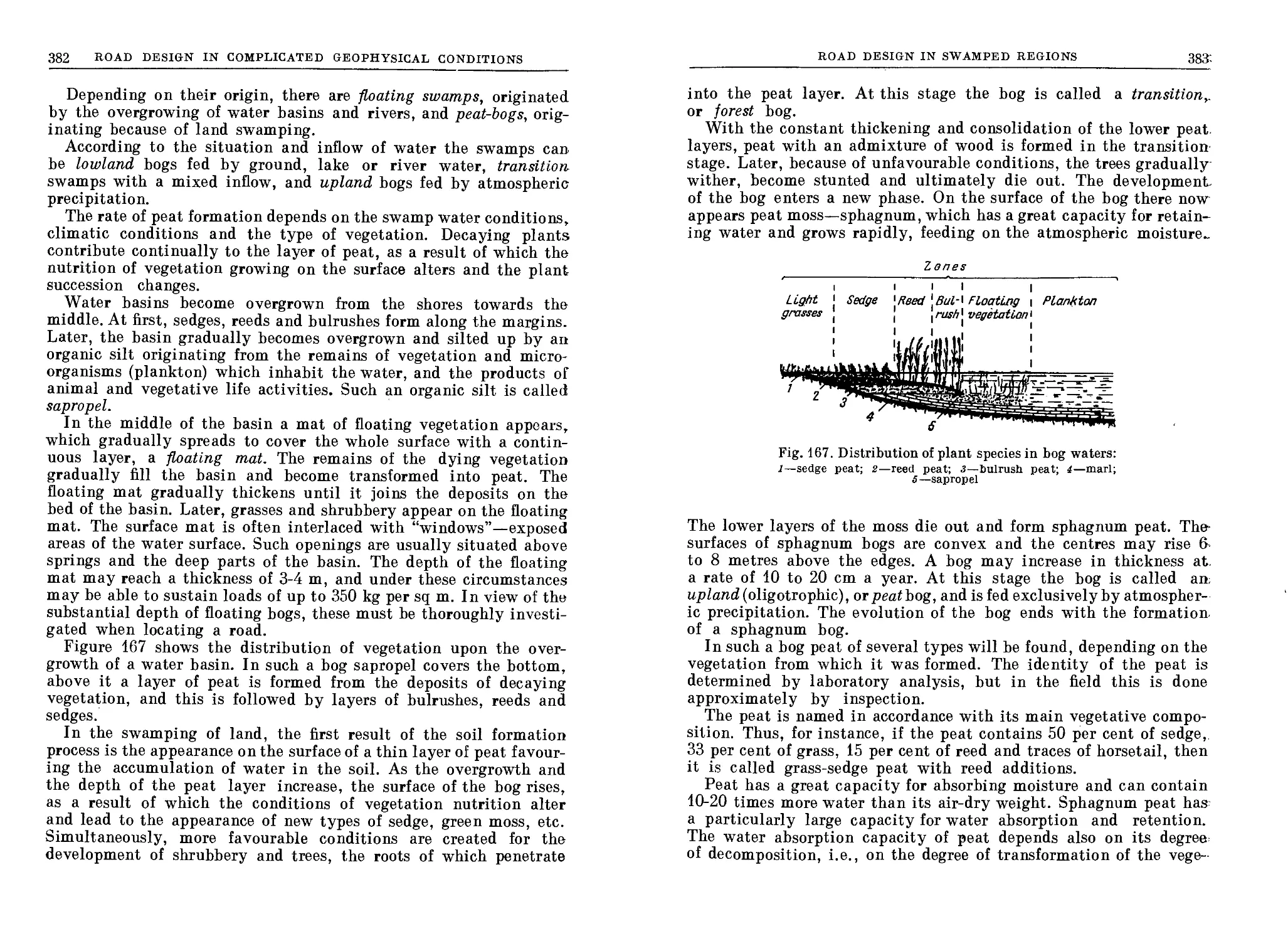
106. Location of a Road irv Swamped Regions........................ 385
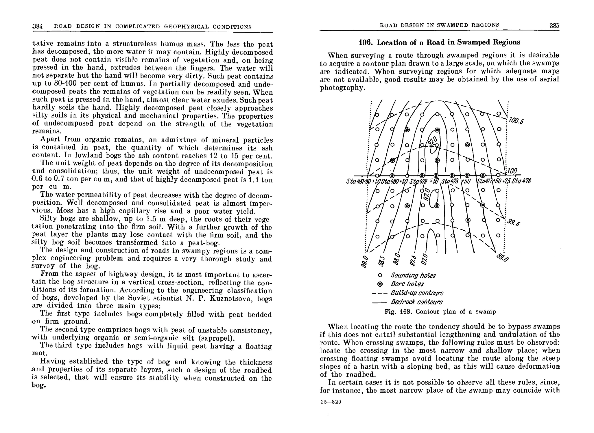
107. Investigation of Swamps During Route Survey................... 386-
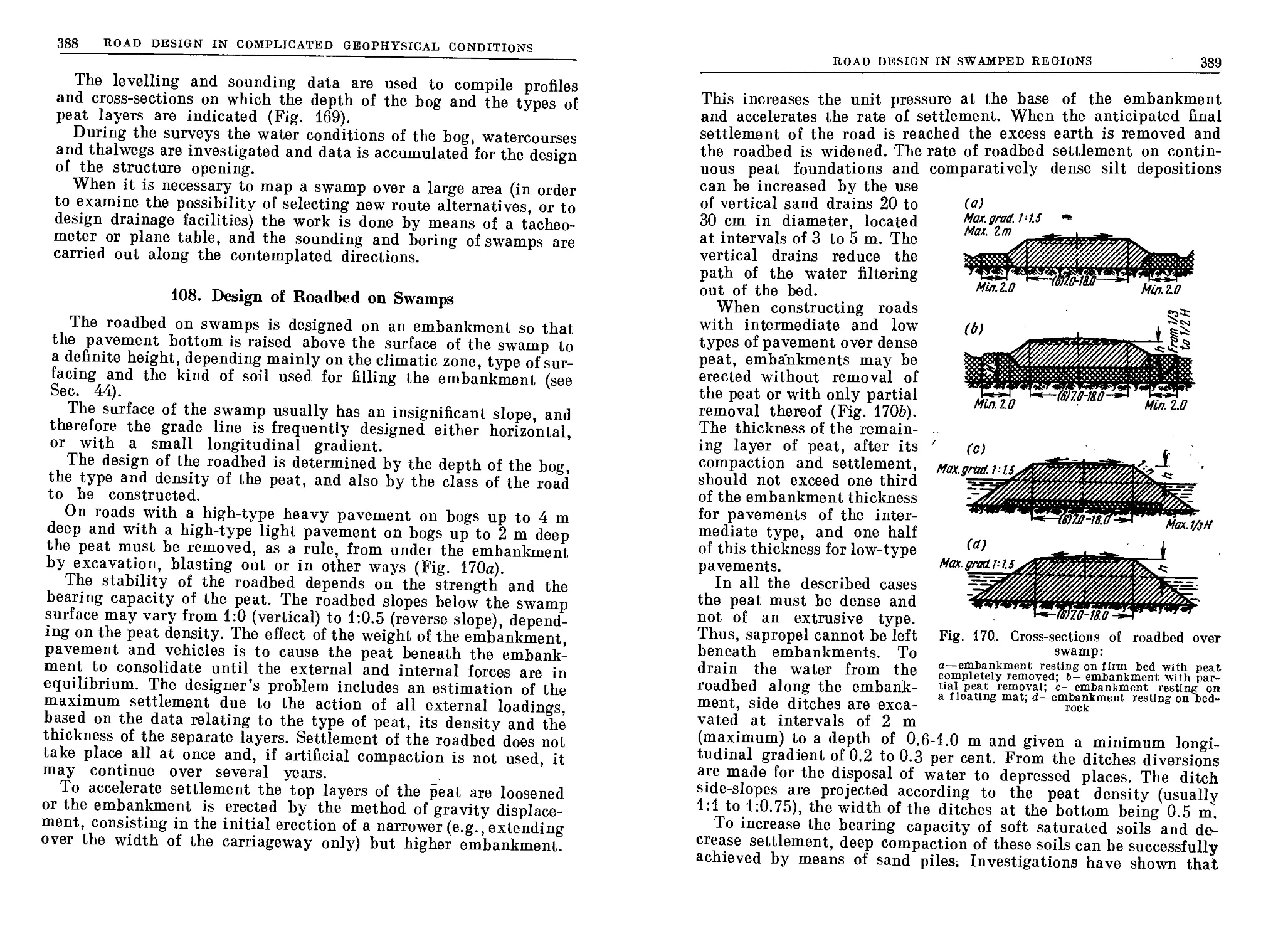
108. Design of Roadbed on Swamps............................... . 388*
109. Structure Design on Swamps................................. . 391
Chapter 19. Design of Roads in Regions Cut by Ravines
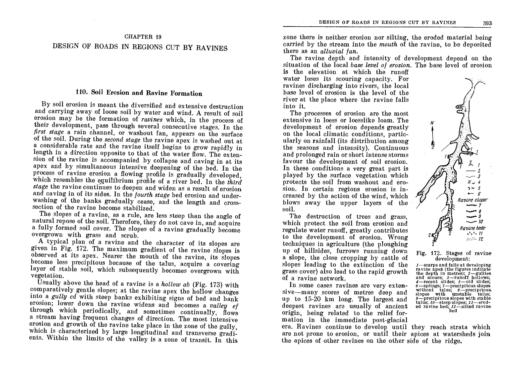
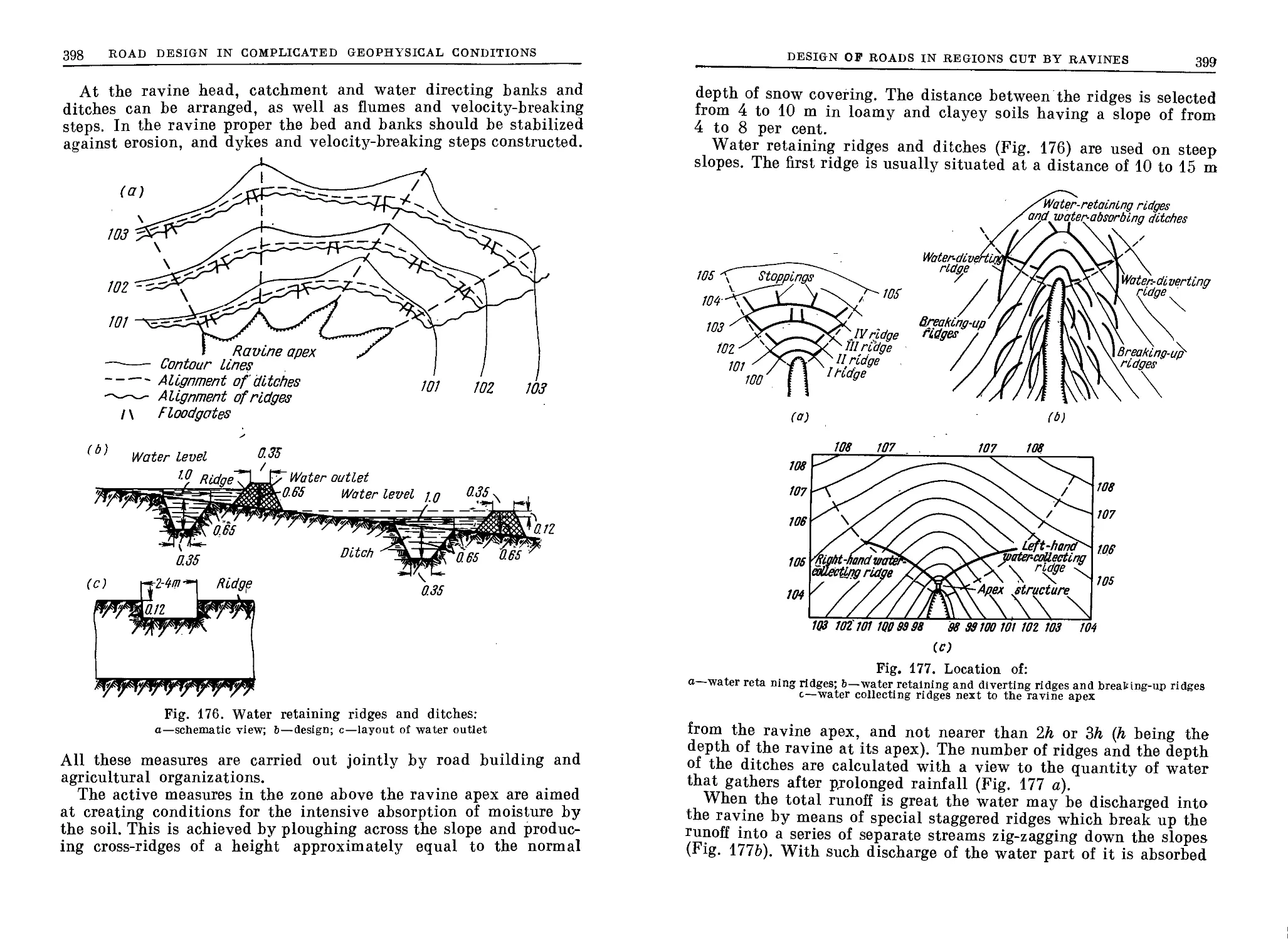
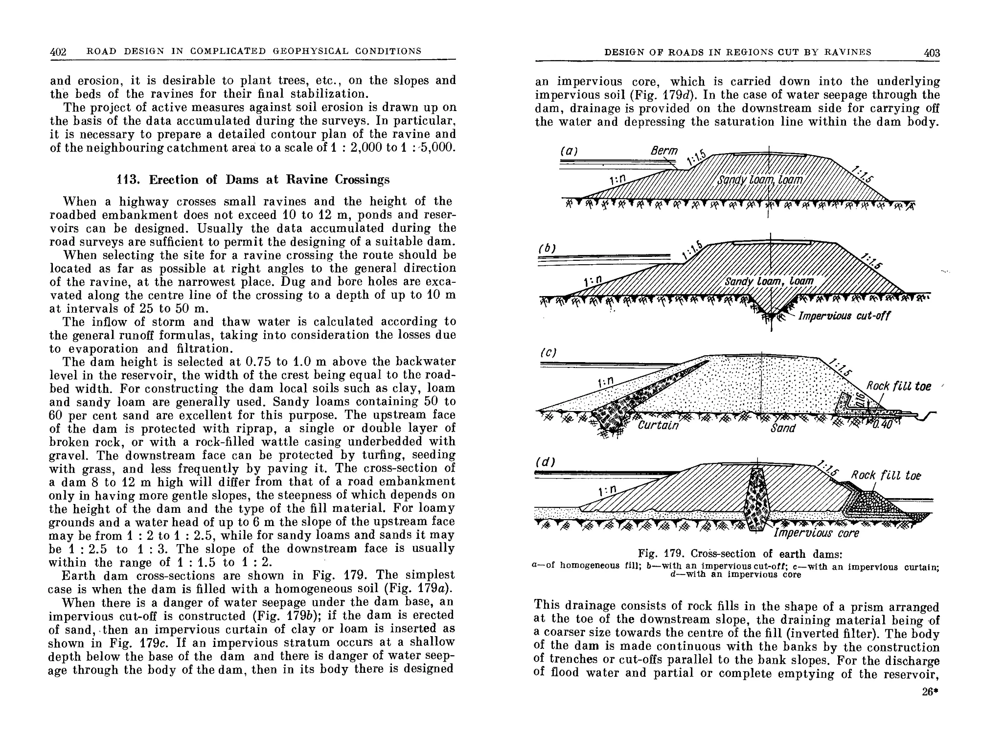
110. Soil Erosion and Ravine Formation................................. 392
111. Road Location in a Ravine Zone................................. 394
112. Ravine Stabilization........................................... 397
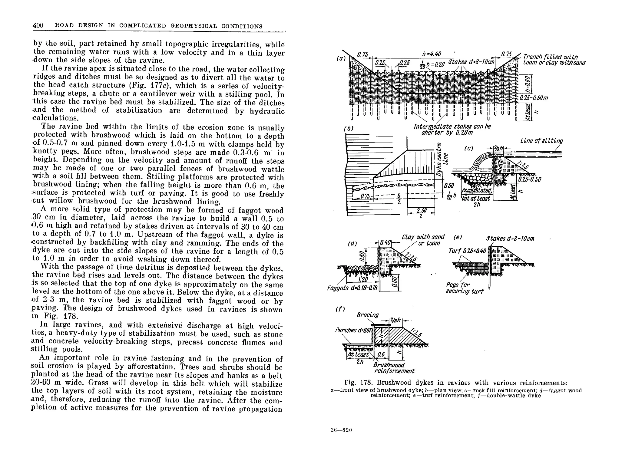
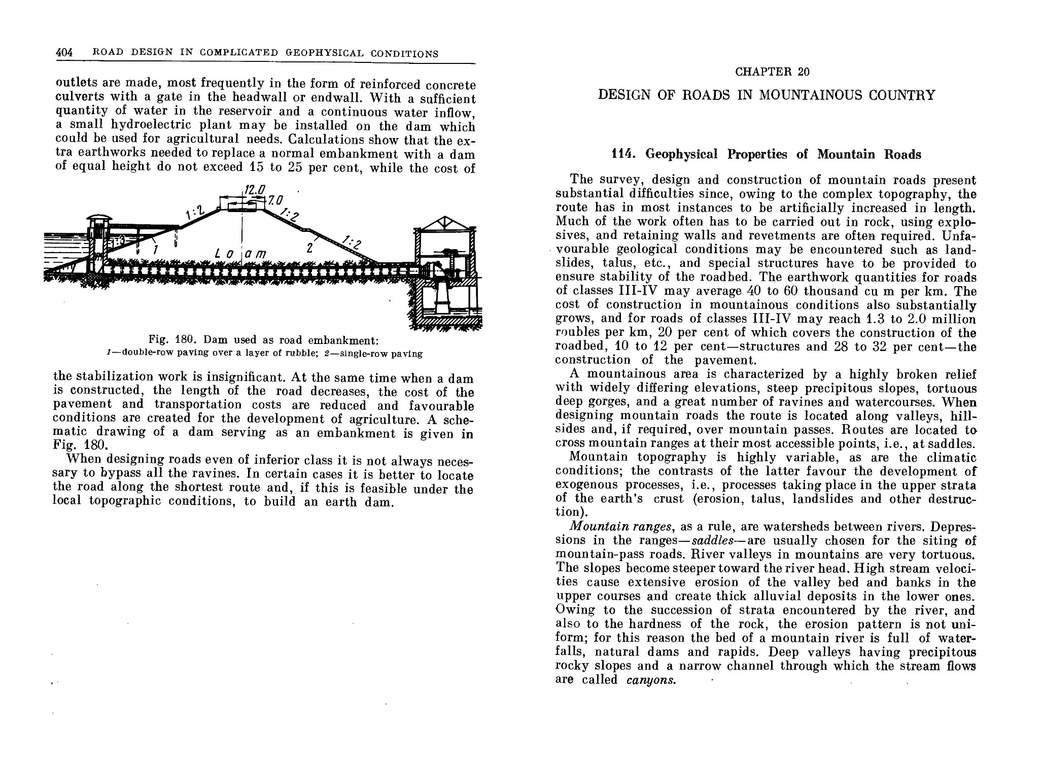
113. Erection of Dams at Rav ineCrossings........................... 402
Chapter 20. Design of Roads in Mountainous Country
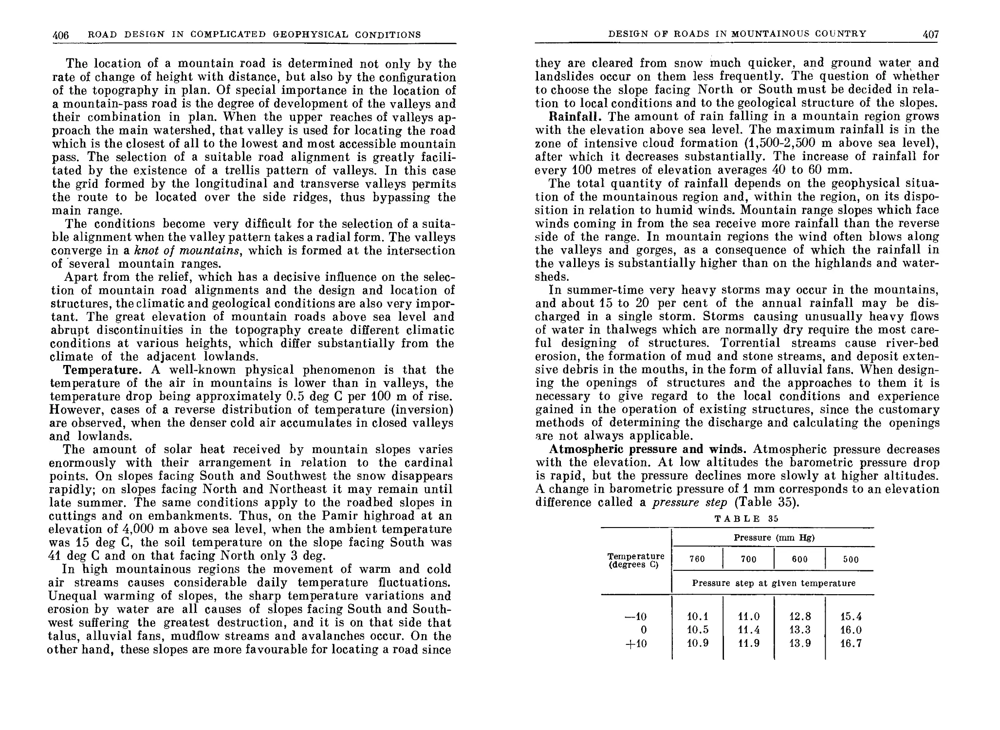
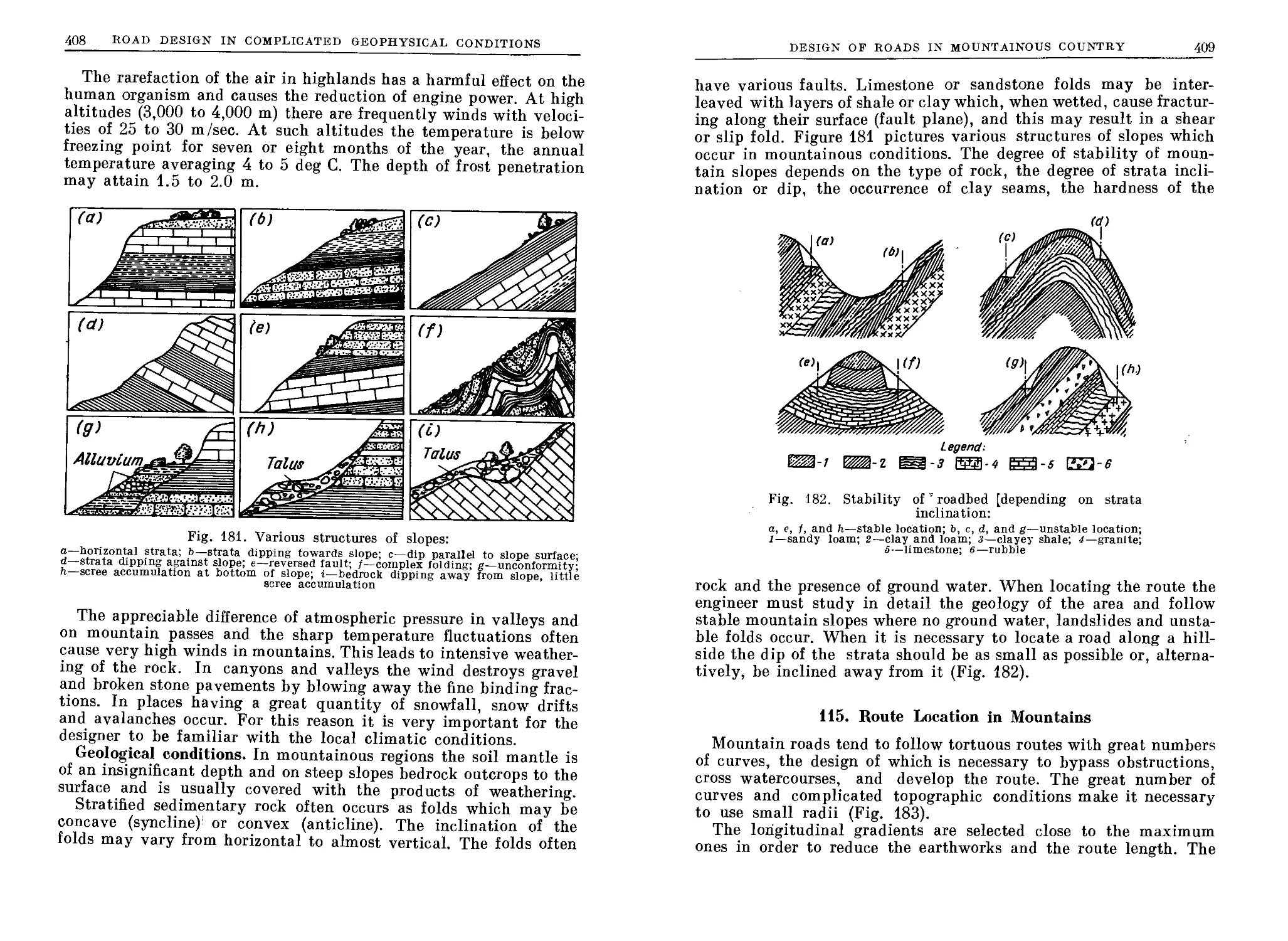
114. Geophysical Properties of Mountain Roads....................... 405
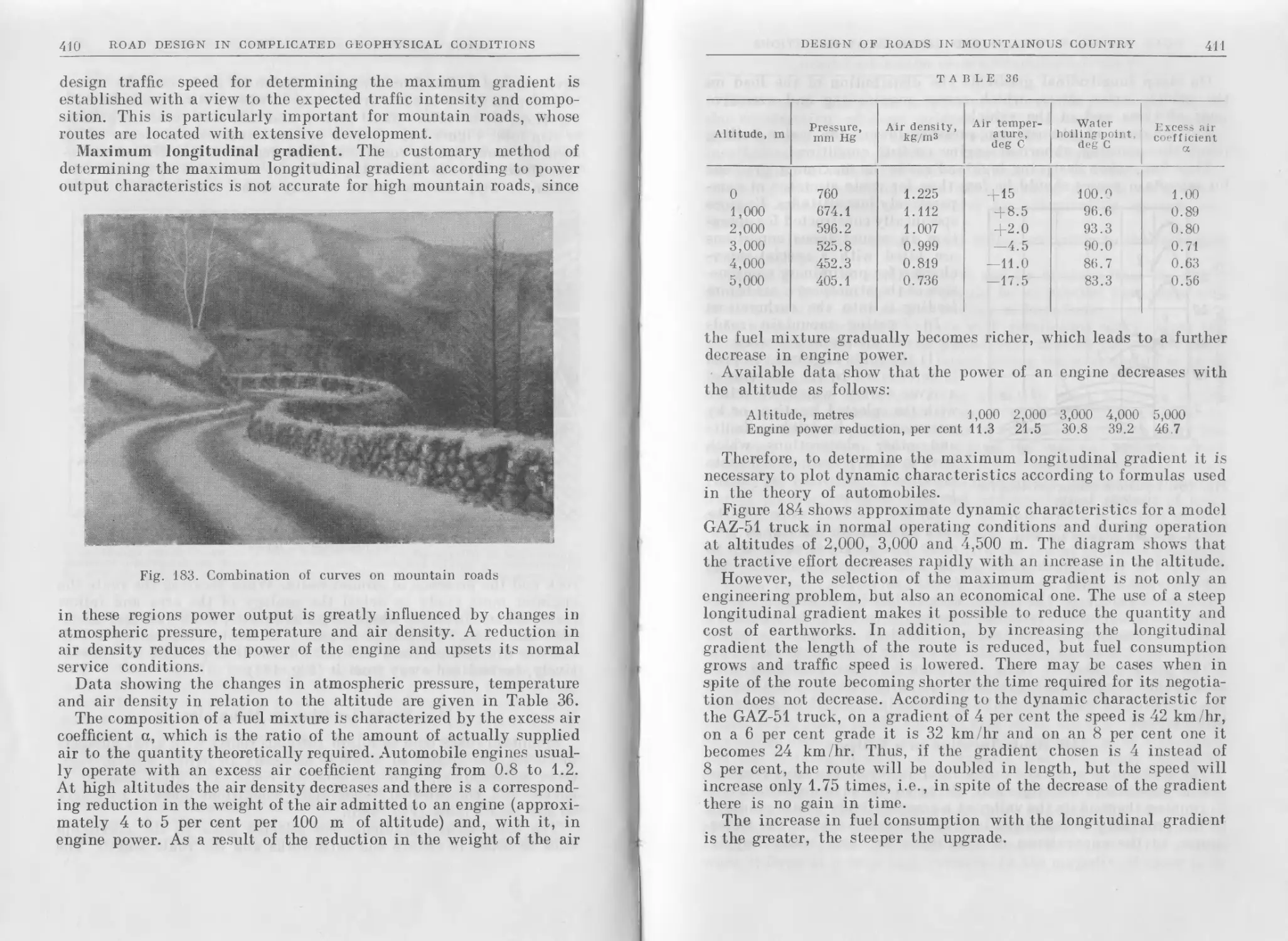
115. Route Location in Mountains.................................... 409
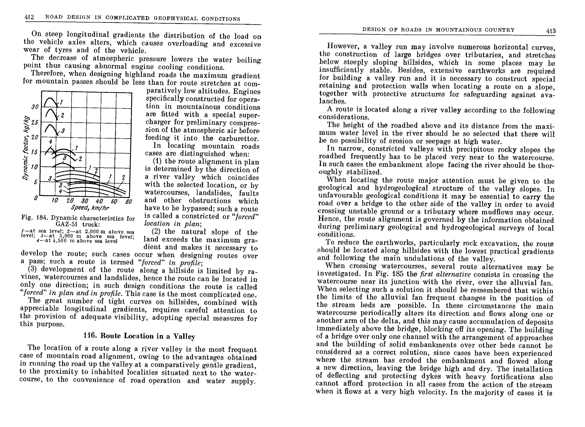
116. Route Location in a Valley..................................... 412
117. Roads Through Mountain Passes ................................. 417
118. Tunnels........................................................ 419
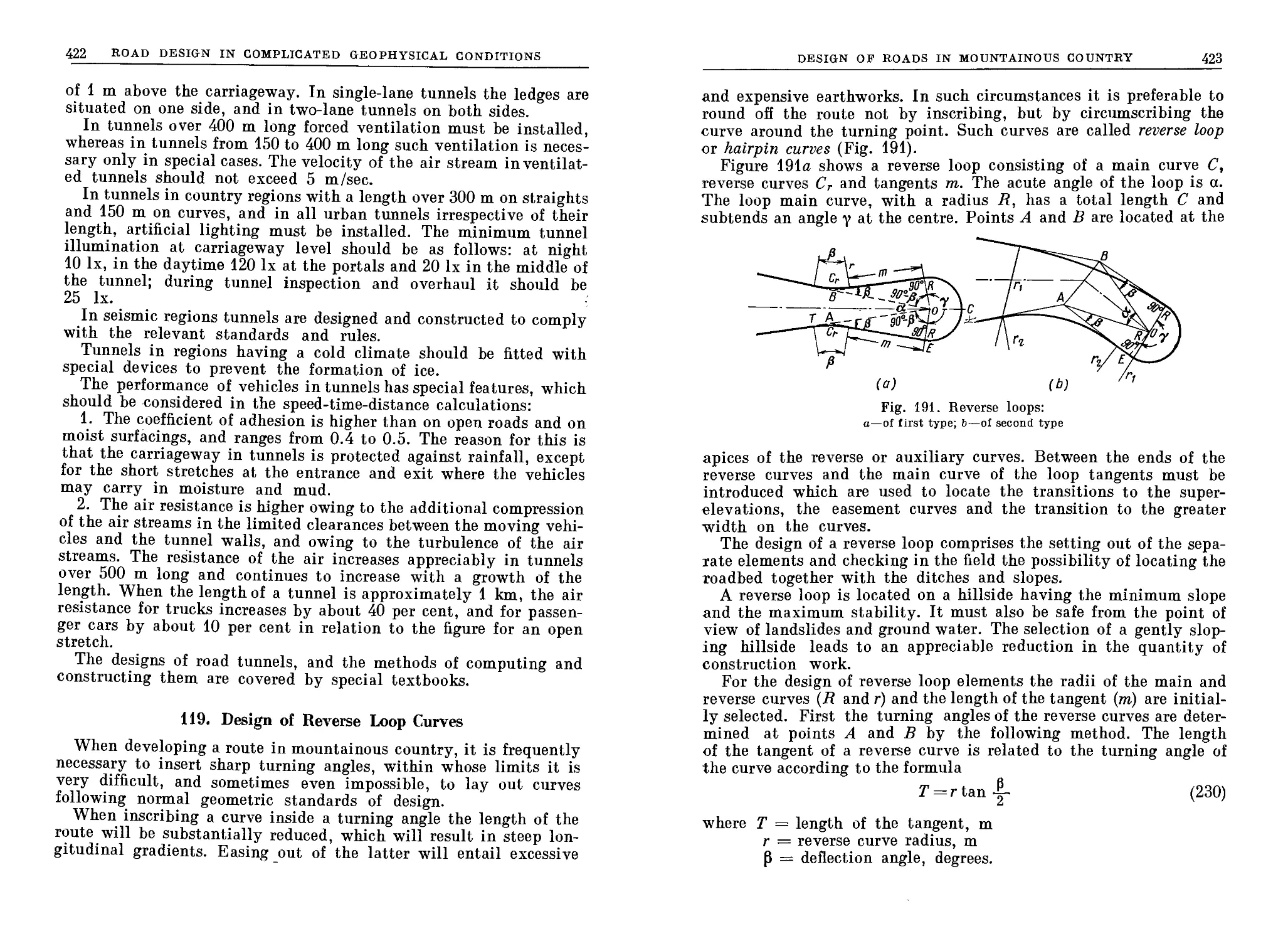
119. Design of Reserve Loop Curves ................................ 422
120. Mountain Road Cross-section.................................... 427
121. Mountain Road Profile.......................................... 435
122. Route, Location over Talus............................... ... 440
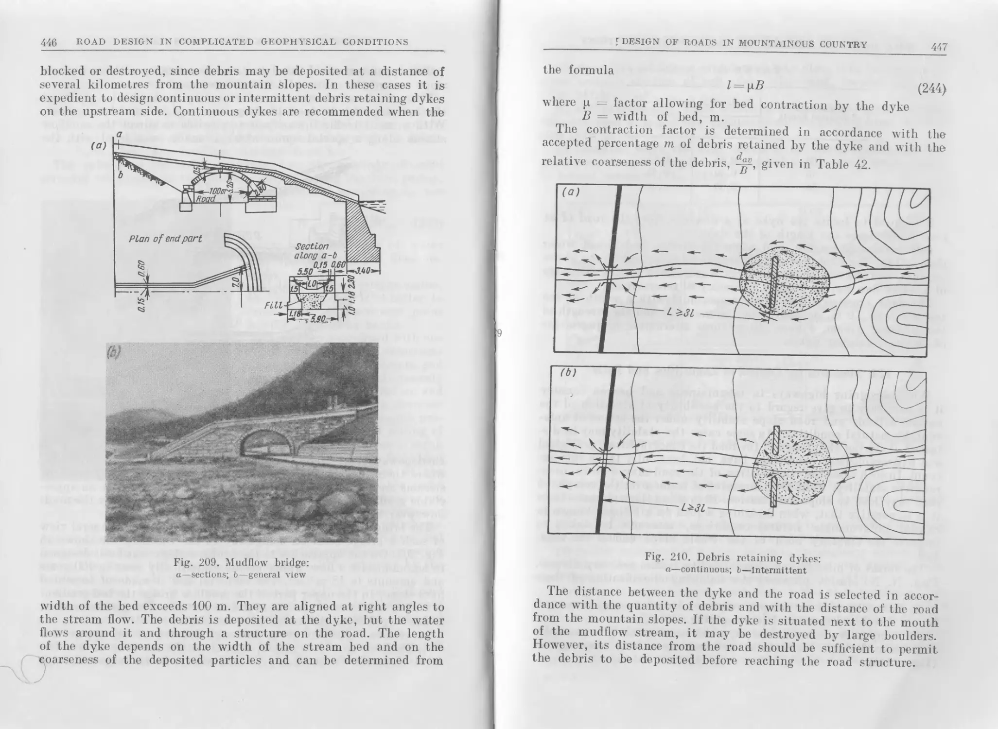
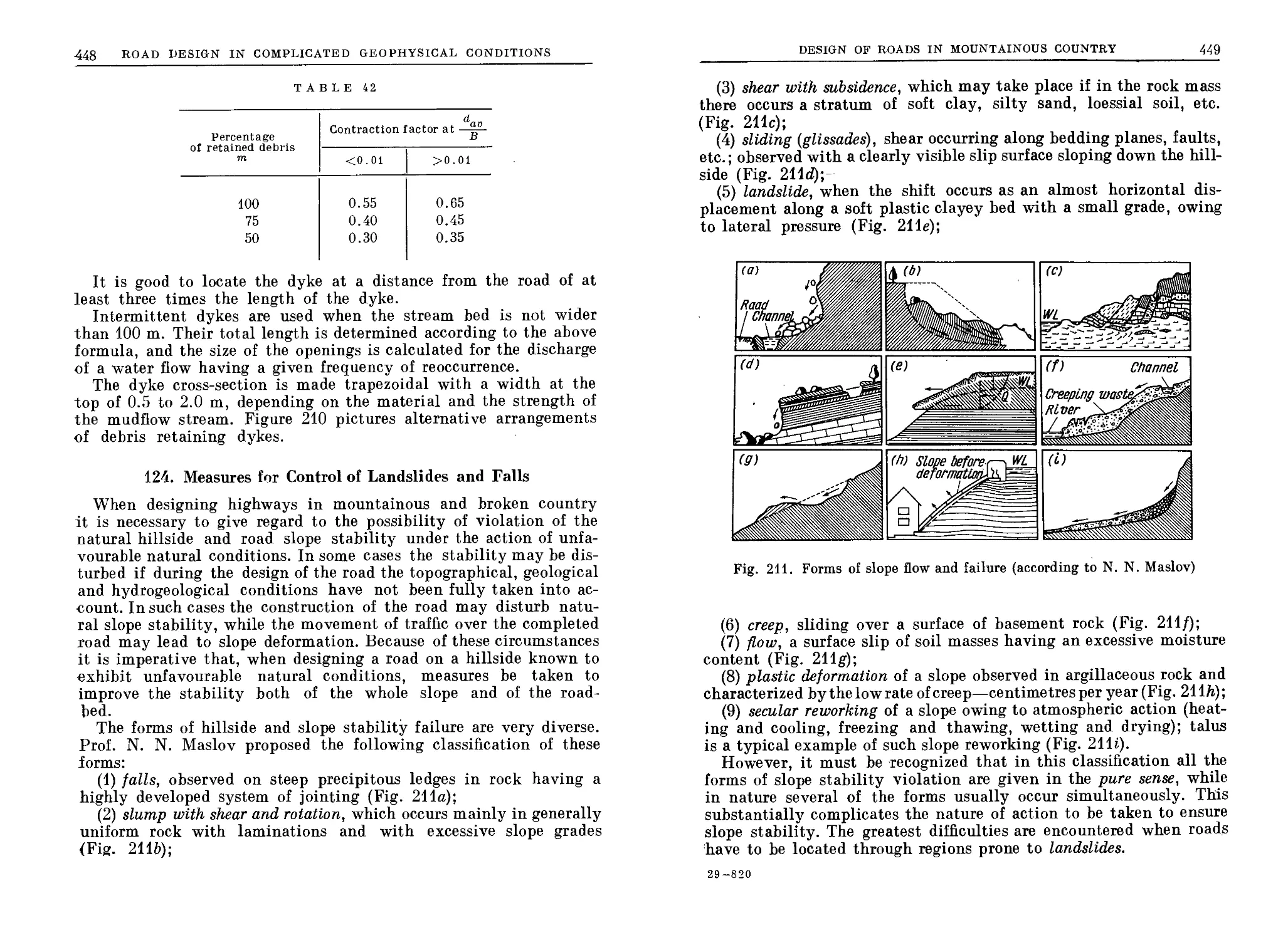
123. Route Location over Silt Washout Fans.......................... 442
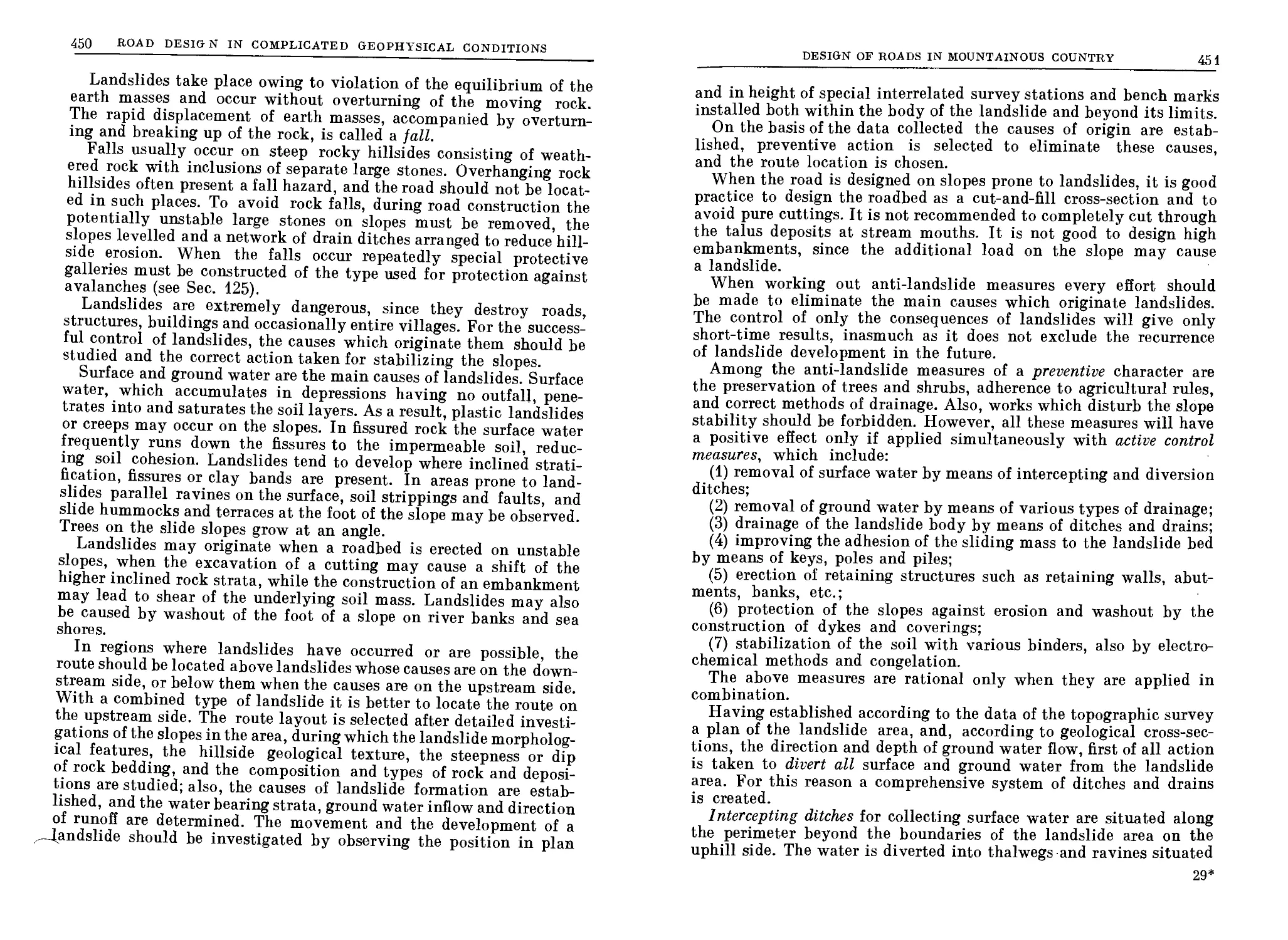
124. Measures for Control of Landslides and Falls ......... 448
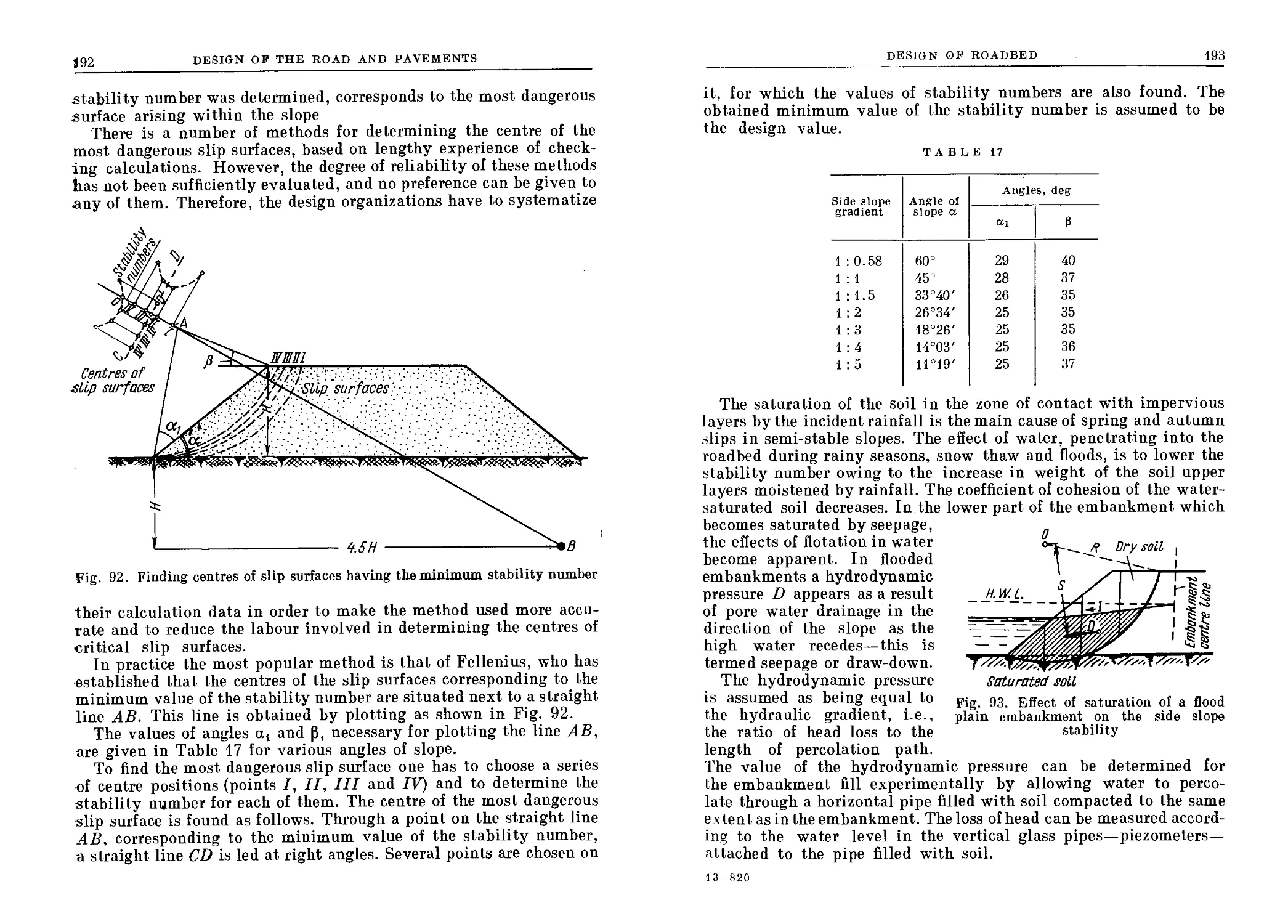
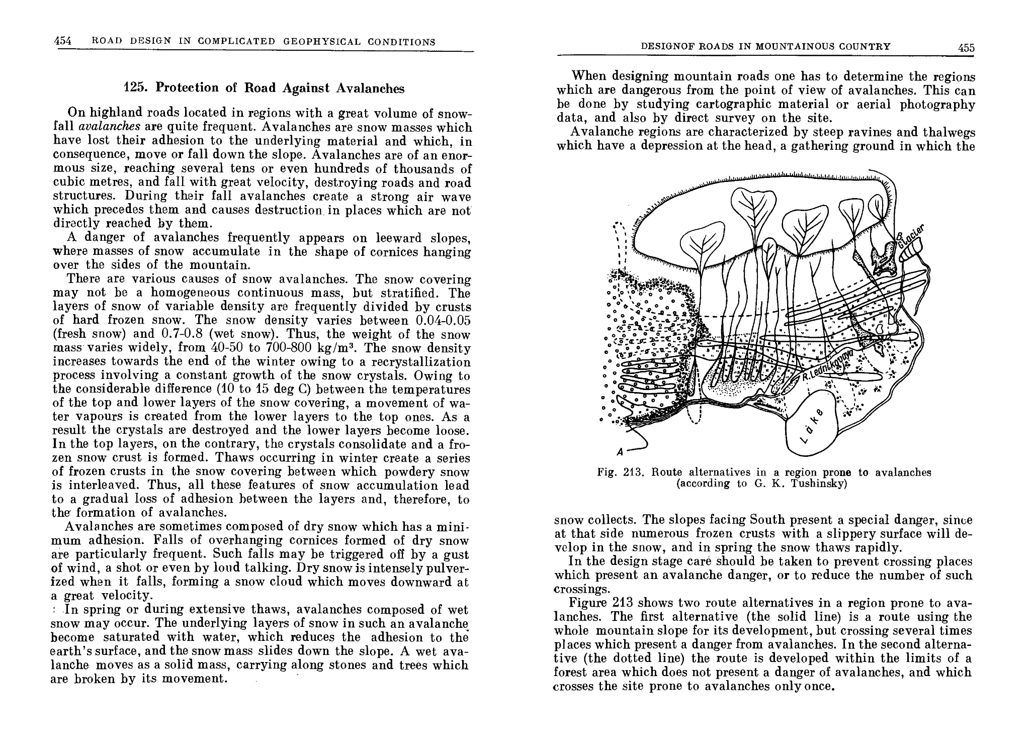
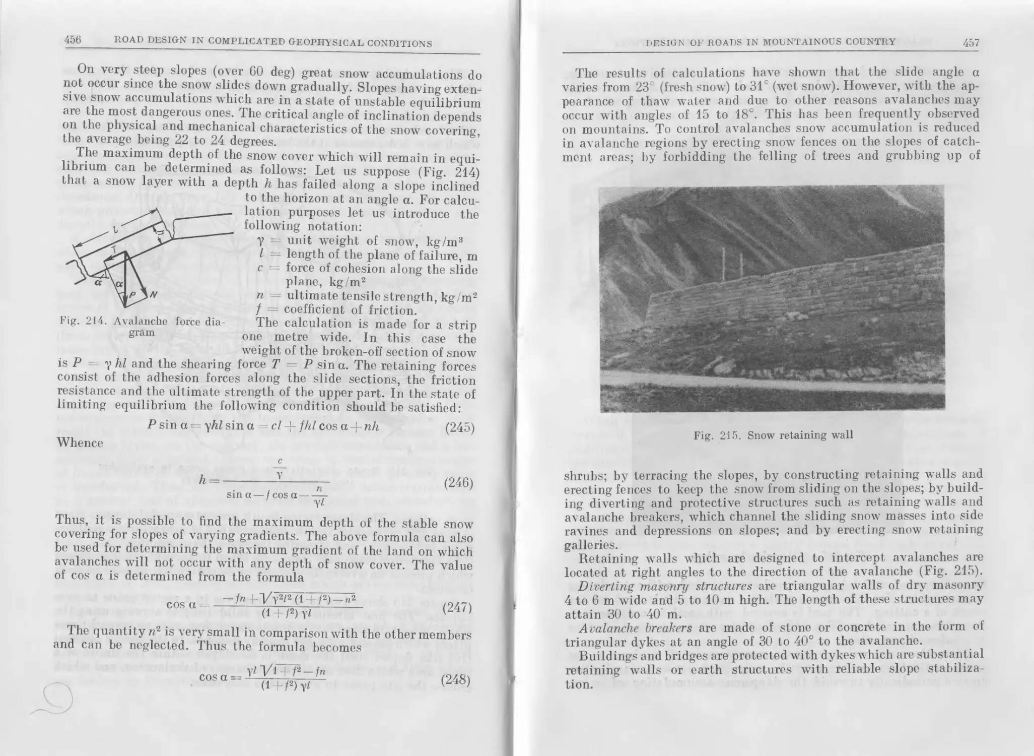
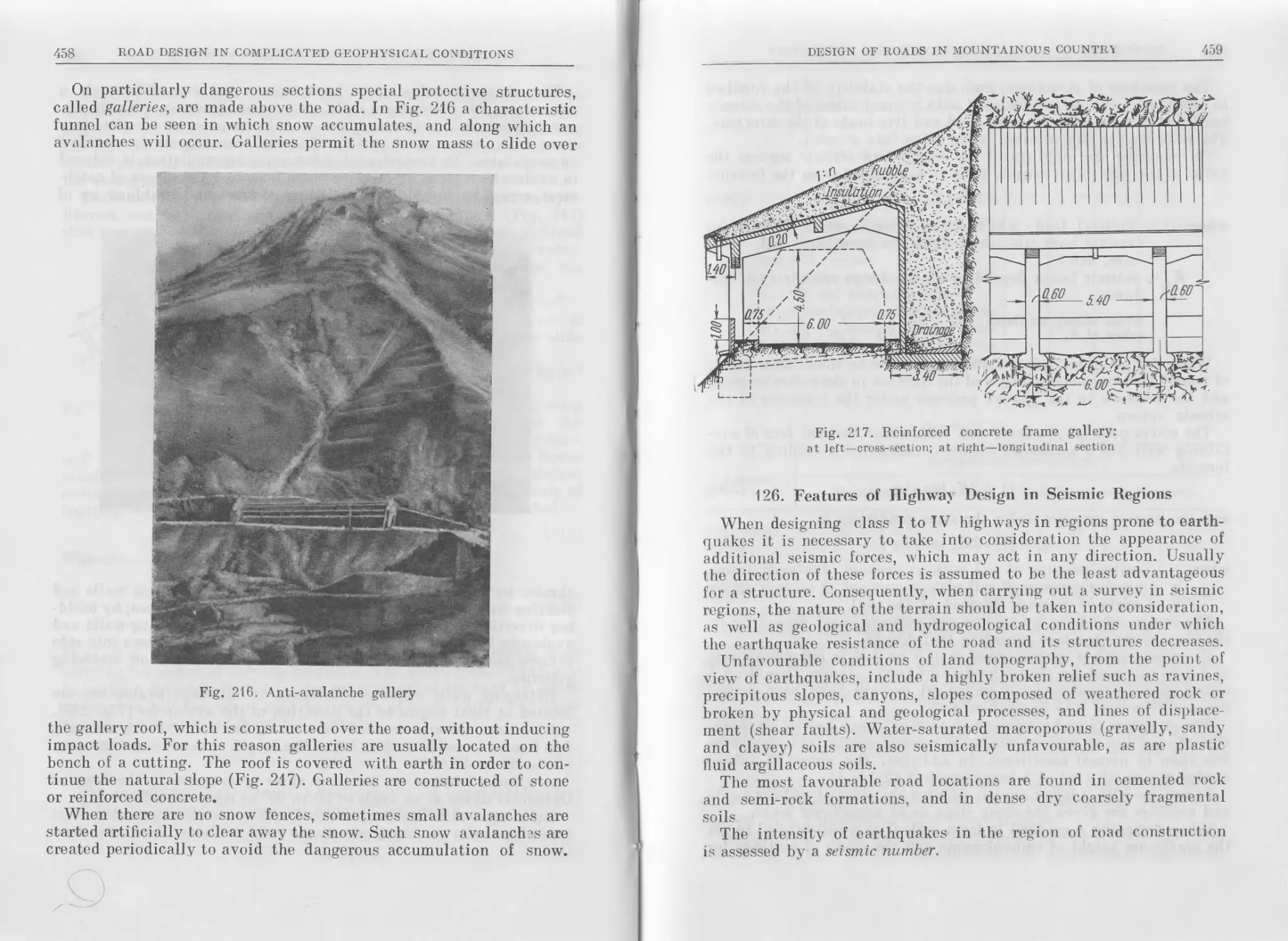
125. Protection of Road Against Avalanches.......................... 454
126. Features of Highway Design in Seismic Regions.................. 450
127. Minor Structures in Mountain Regions........................... 462
128. Design of Approach Channels to Structures ..................... 464
Chapter 21. Road Design in Karst Regions
129. Karst Processes................................................... 465
130. Design of Roads in Karst Regions............................... 467
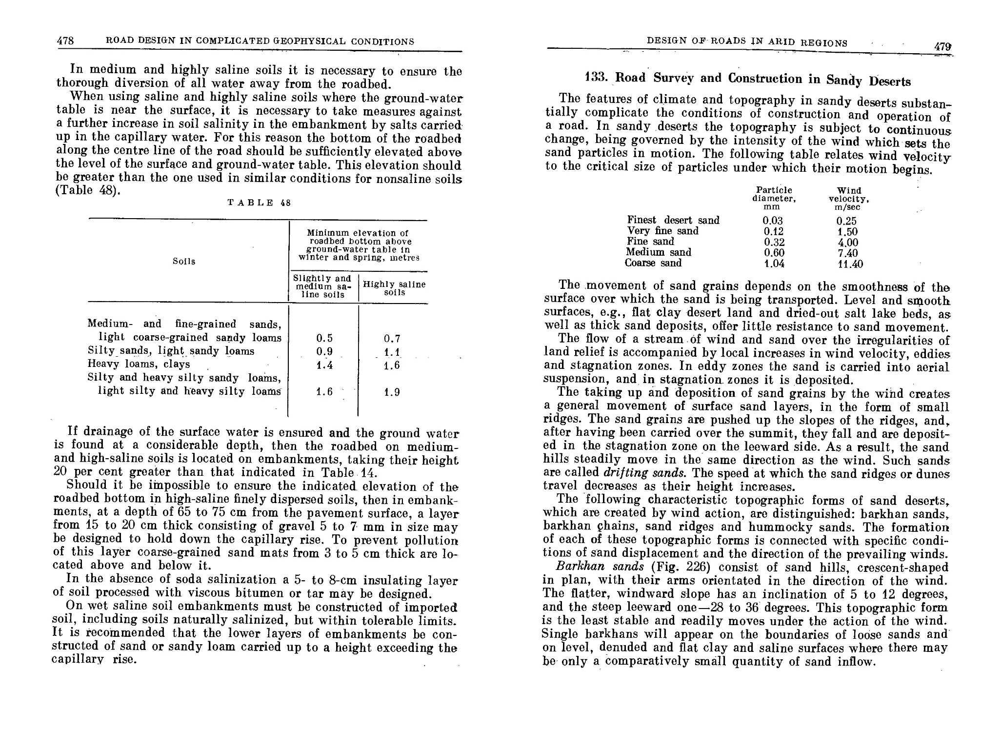
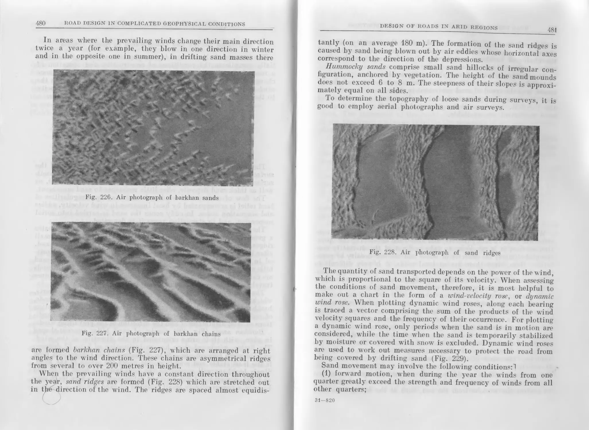
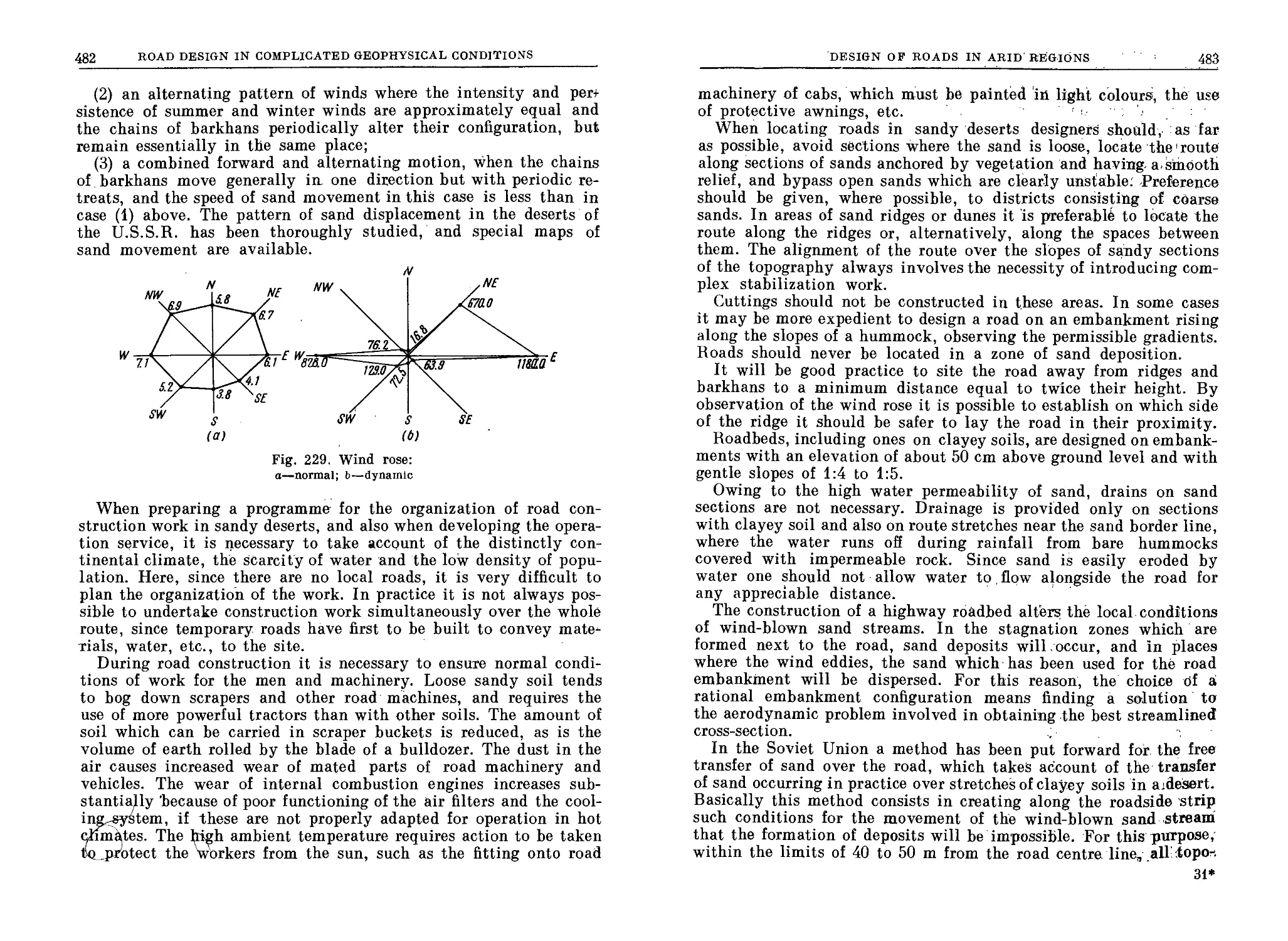
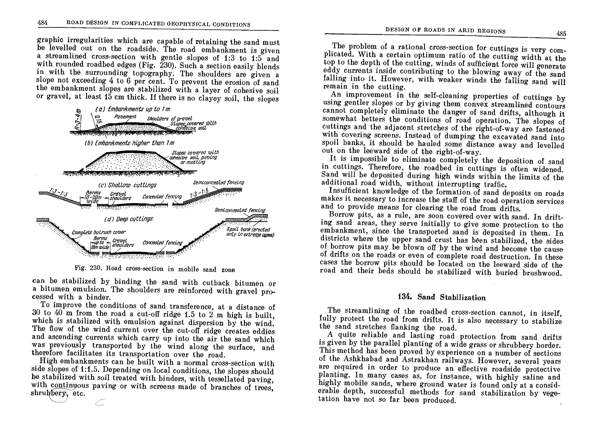
Chapter 22. Design of Roads in Arid Regions
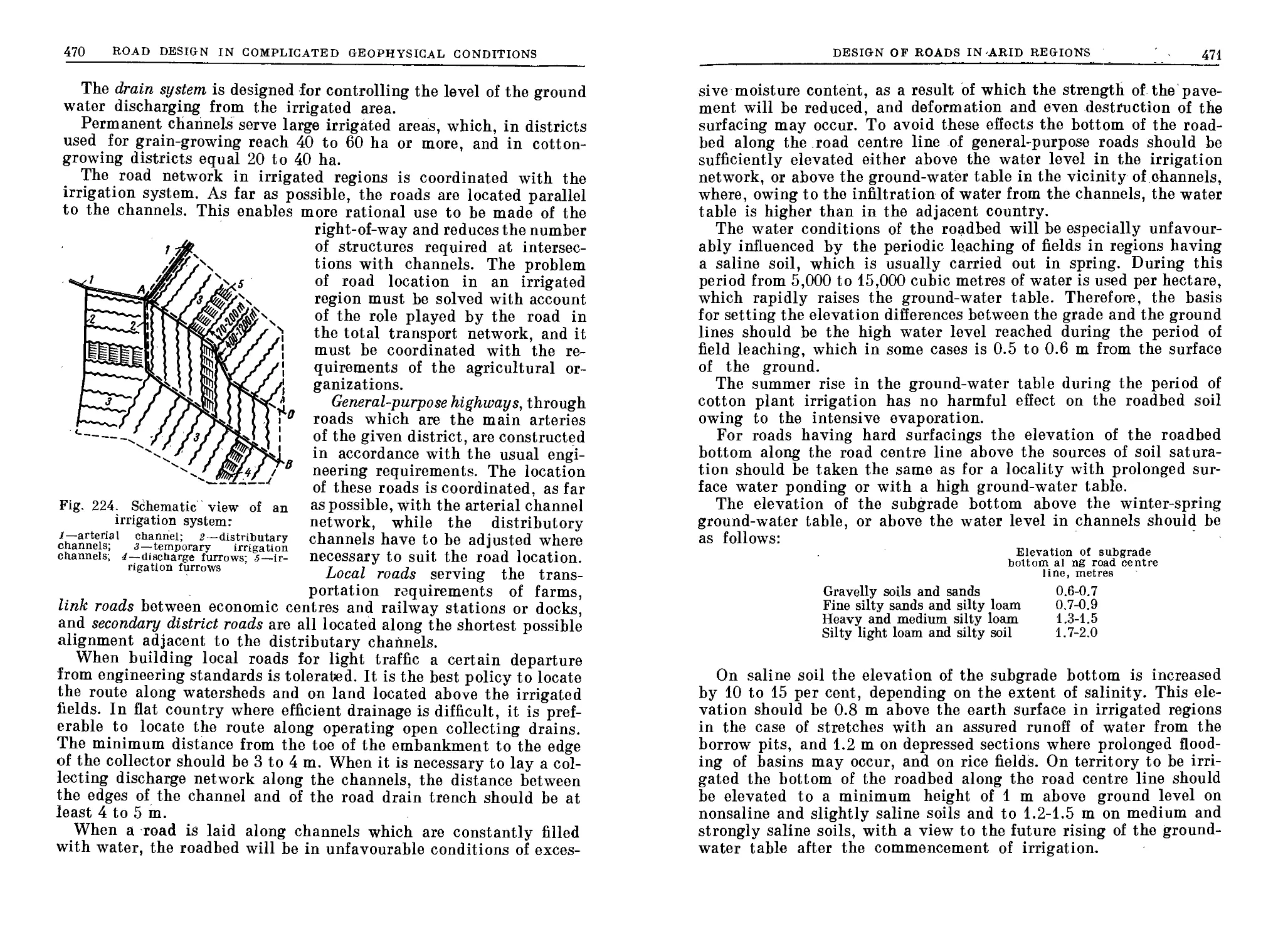
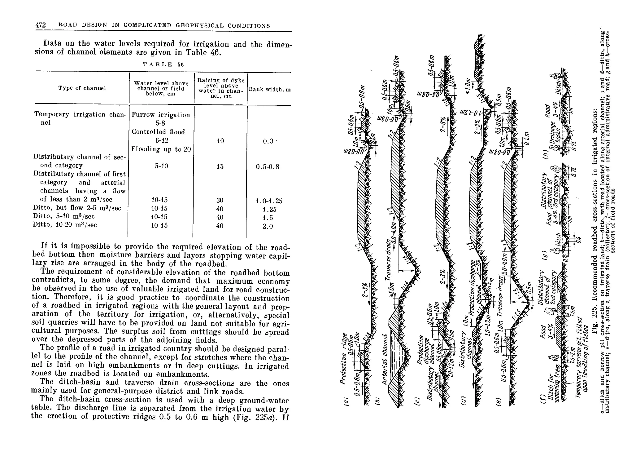
131. Design of Roads in Irrigated Regions........................... 469
132. Design of Roads in Saline Soils................................ 474
133. Road Survey and Construction in Sandy Deserts.................. 479
134. Sand Stabilization............................................ 485
10
CONTENTS
PART VII
URBAN STREETS AND ROADS
Chapter 23. Design of Urban Streets
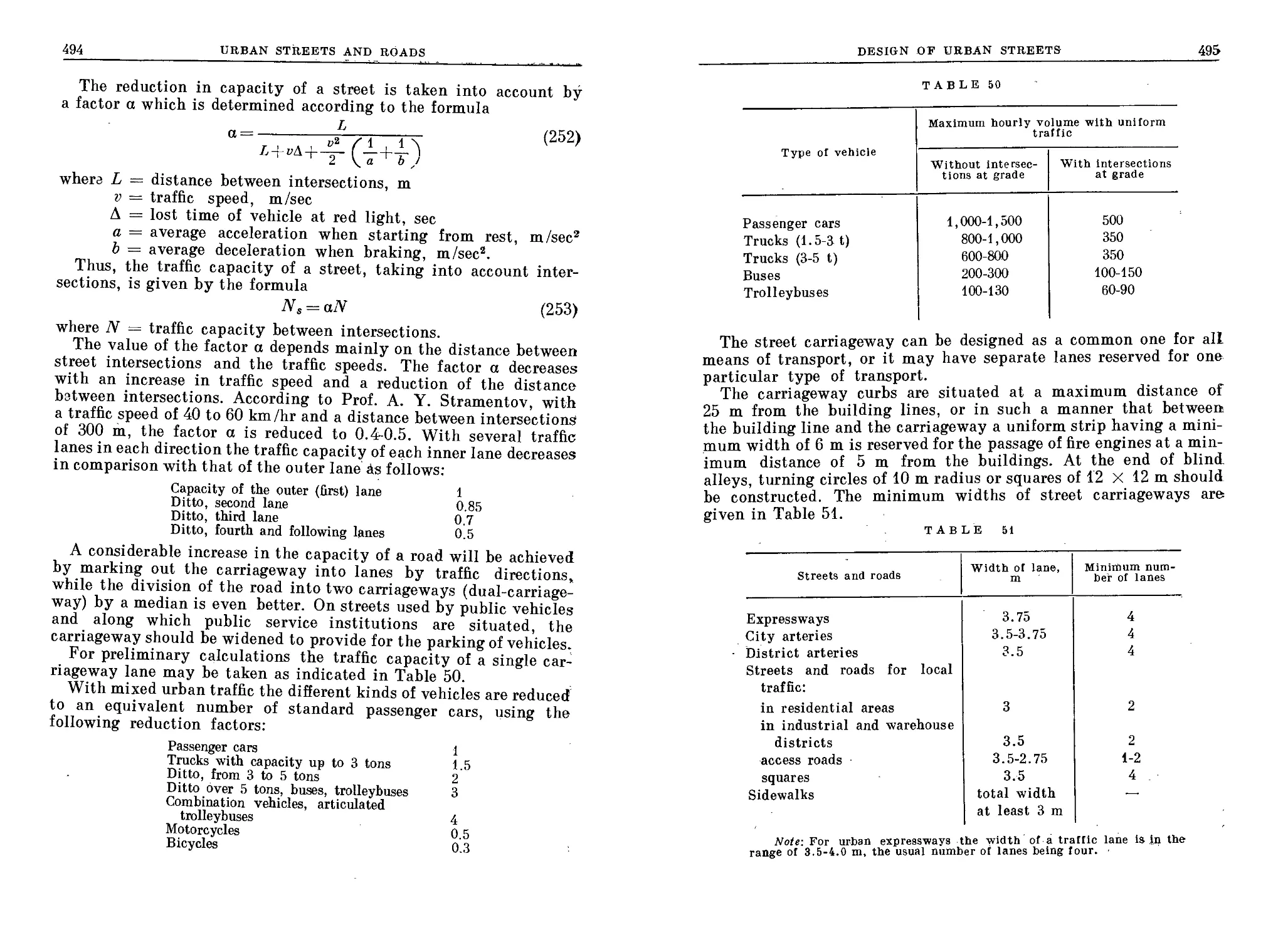
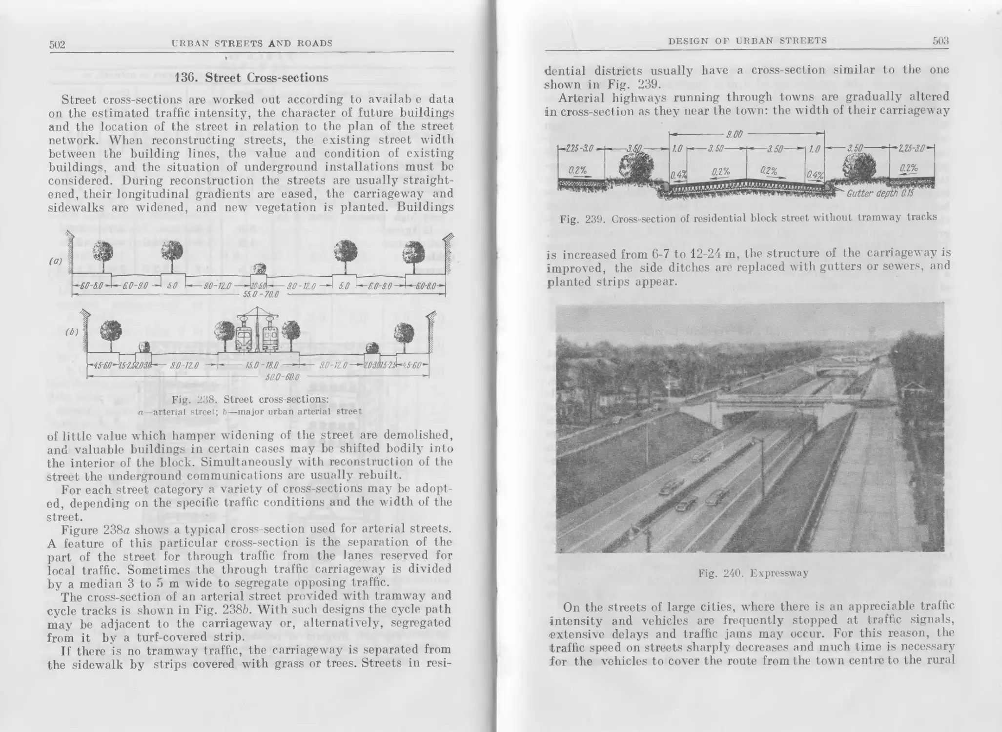
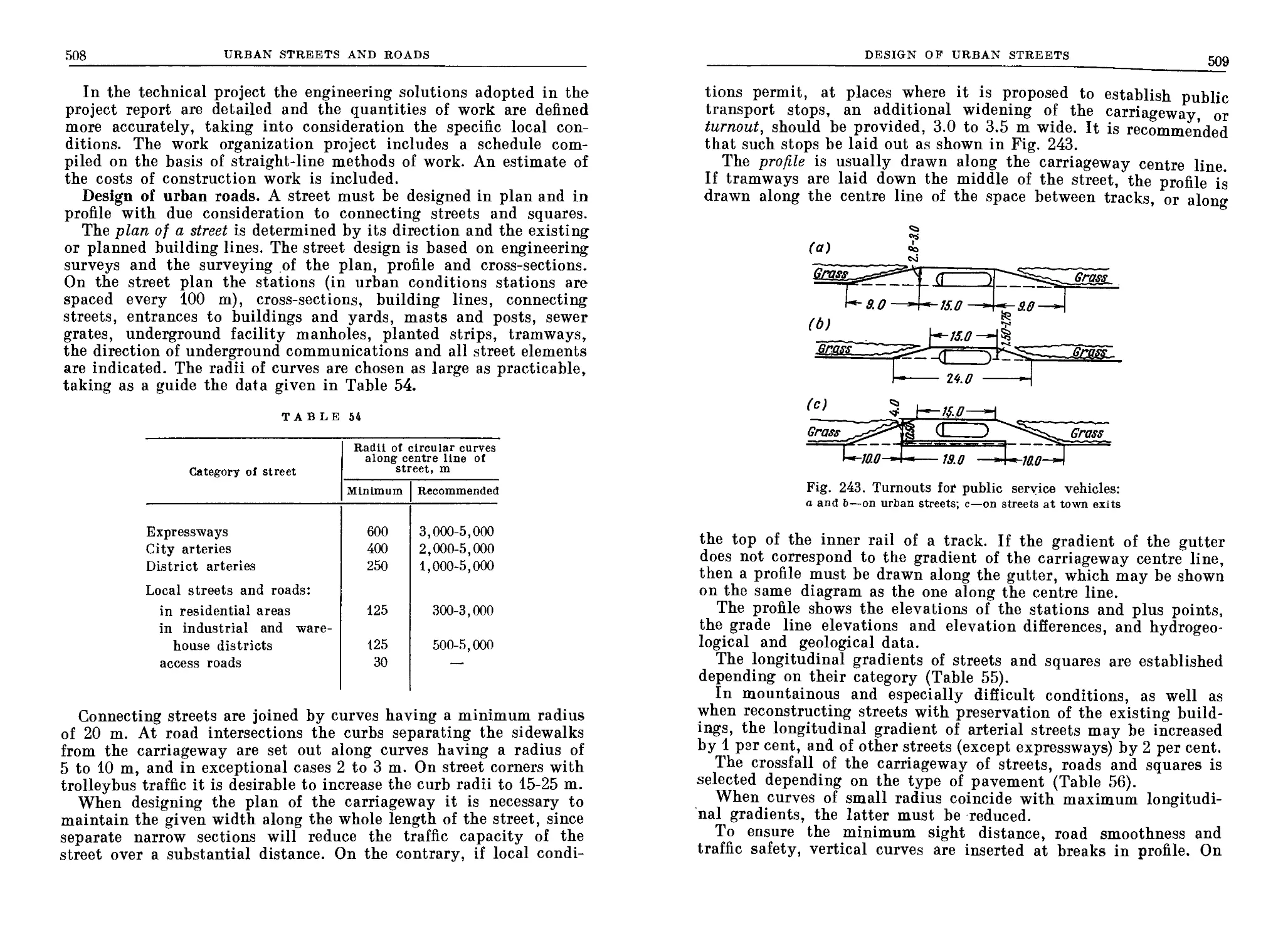
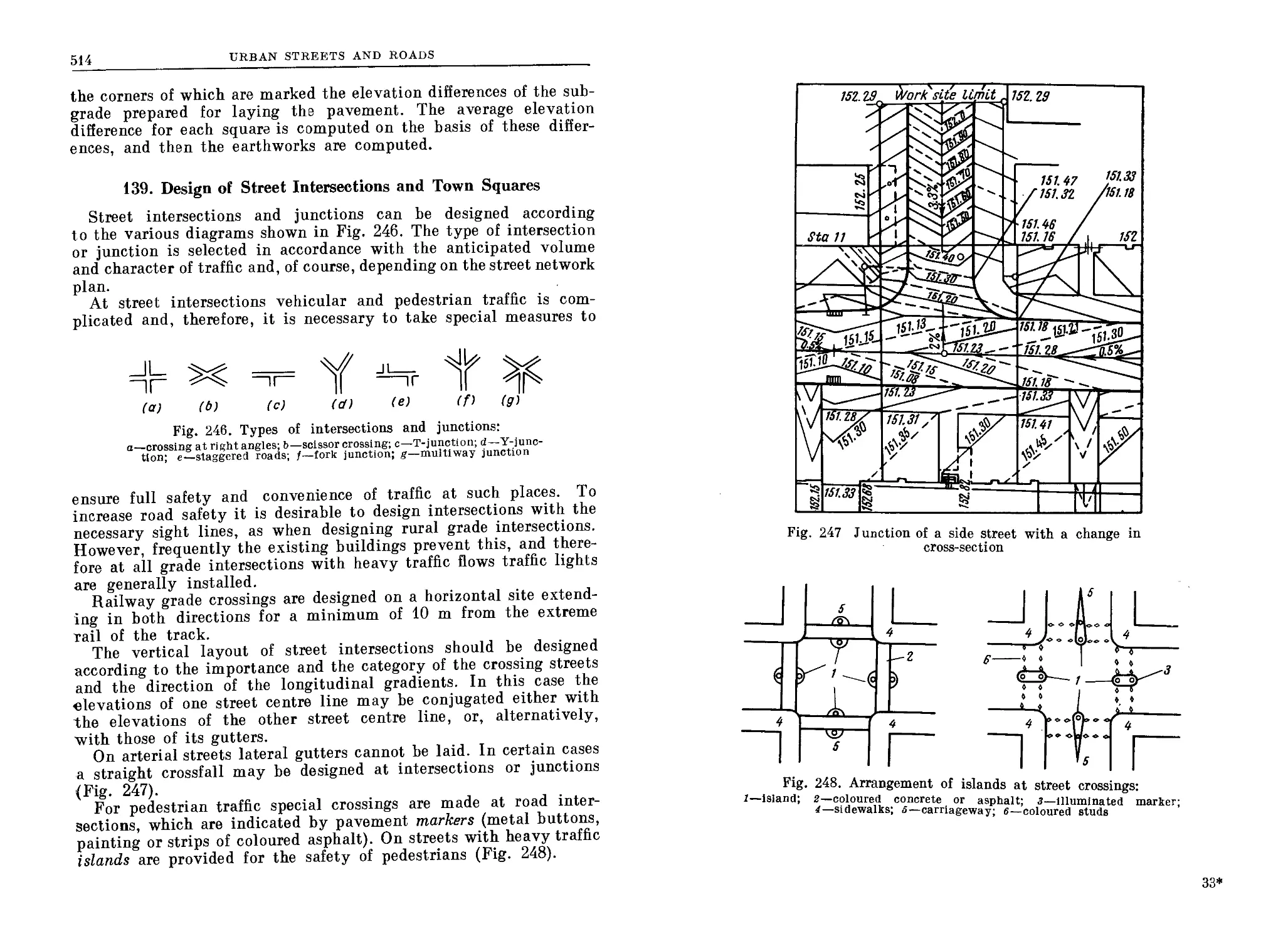
135. Street Layout and Elements.................................. 490
136. Street Cross-sections.................................... 502
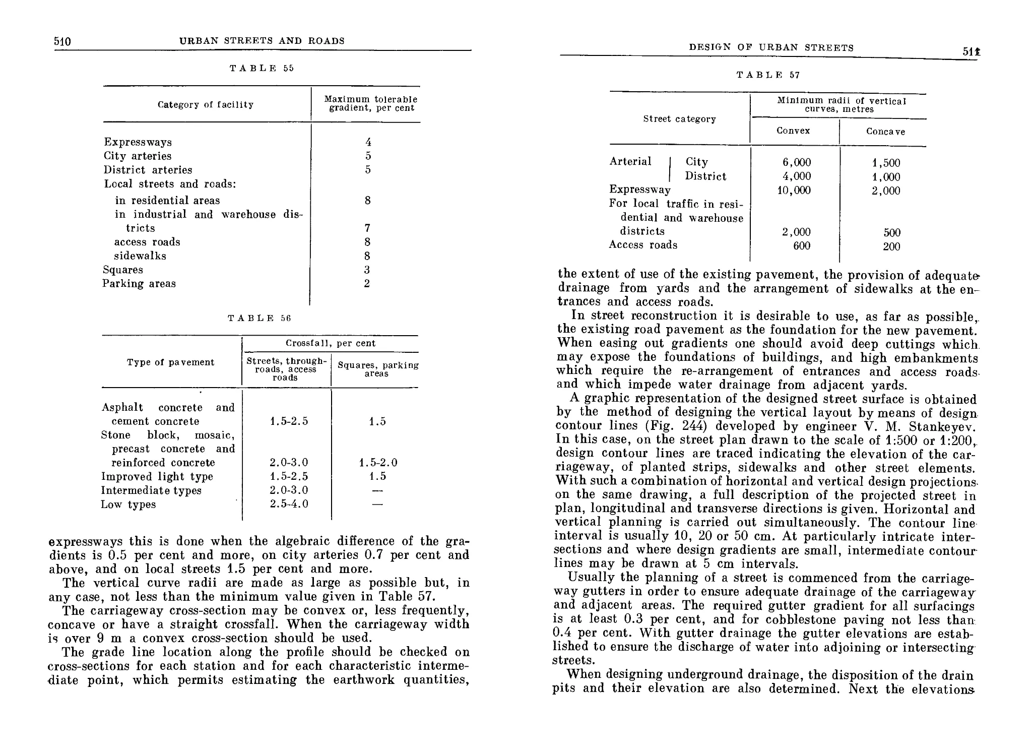
137. Horizontal and Vertical Layout.............................. 504
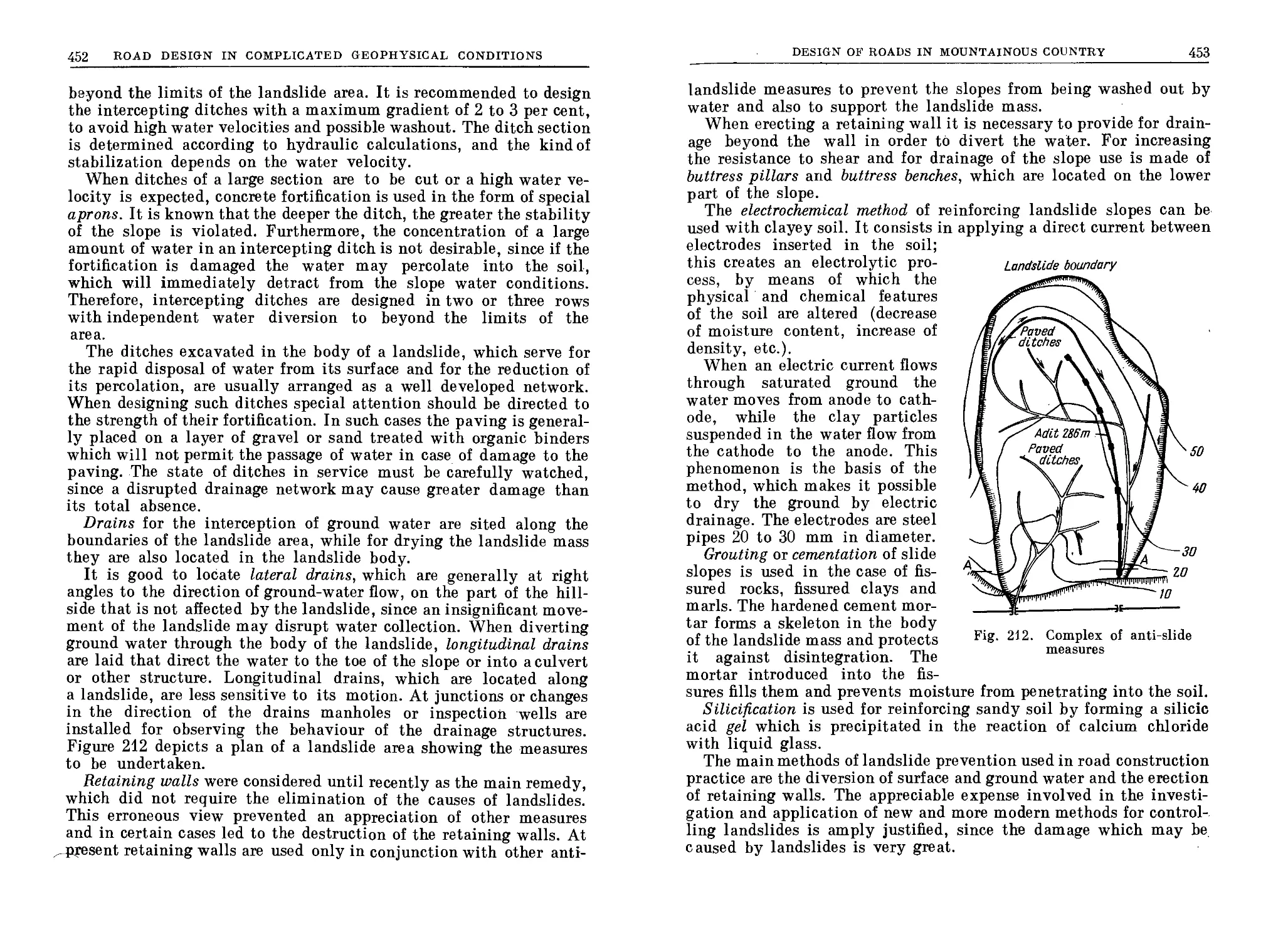
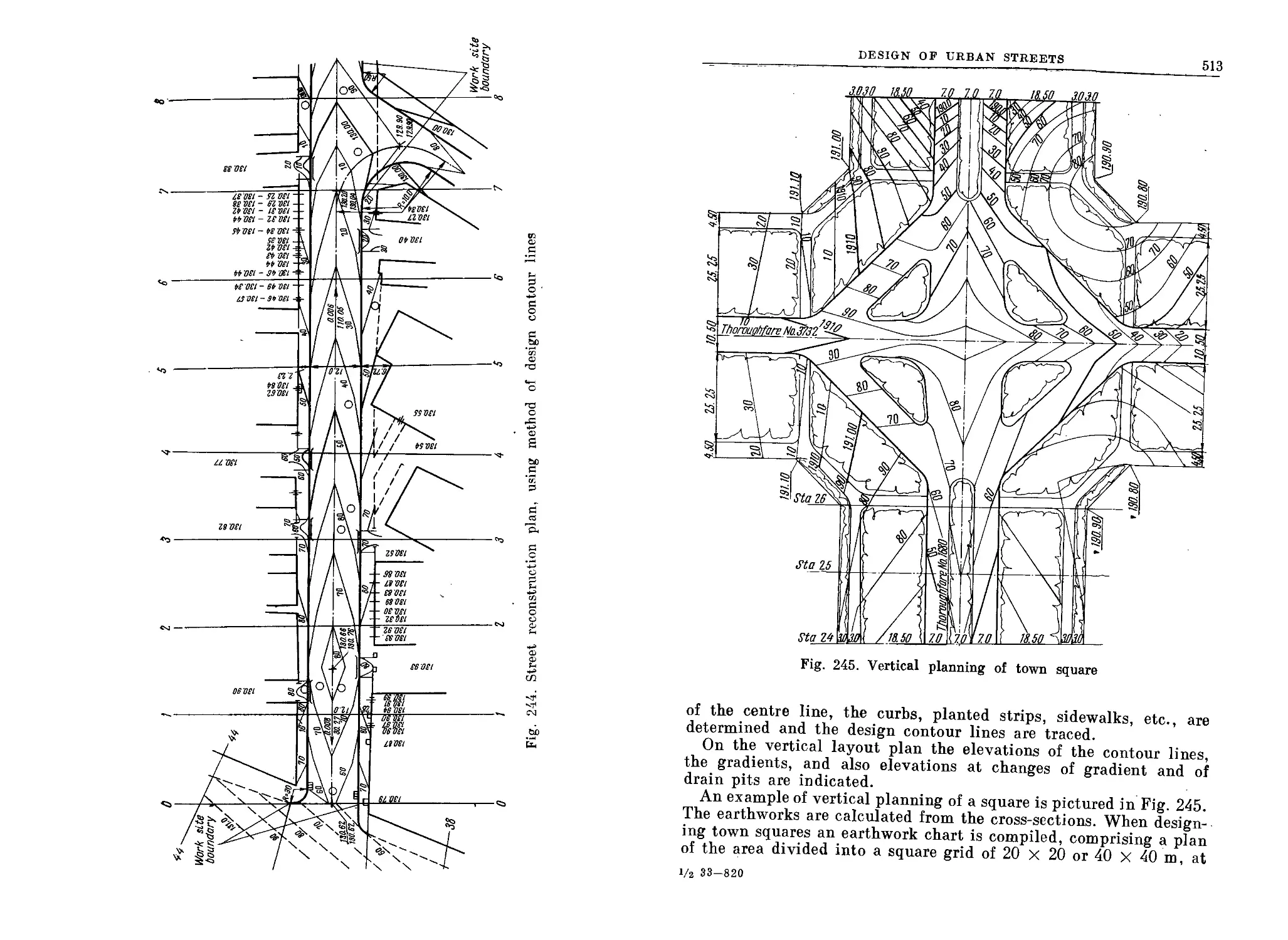
138. Urban Road Survey and Design in Plan and Profile............ 506
139. Design of Street Intersections and Town Squares............. 514
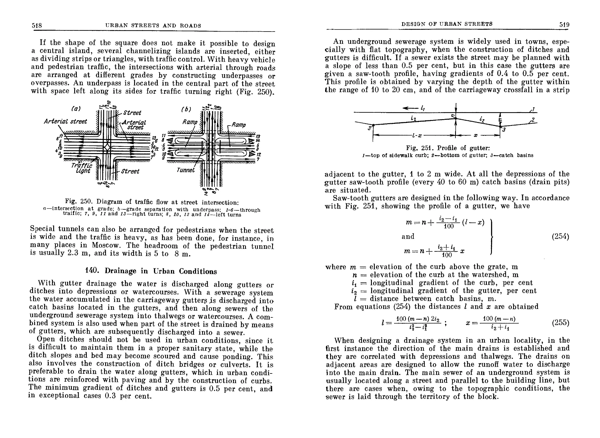
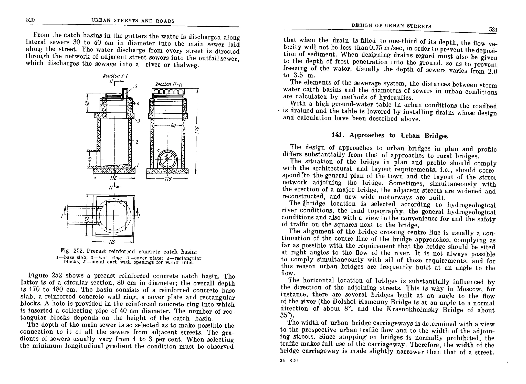
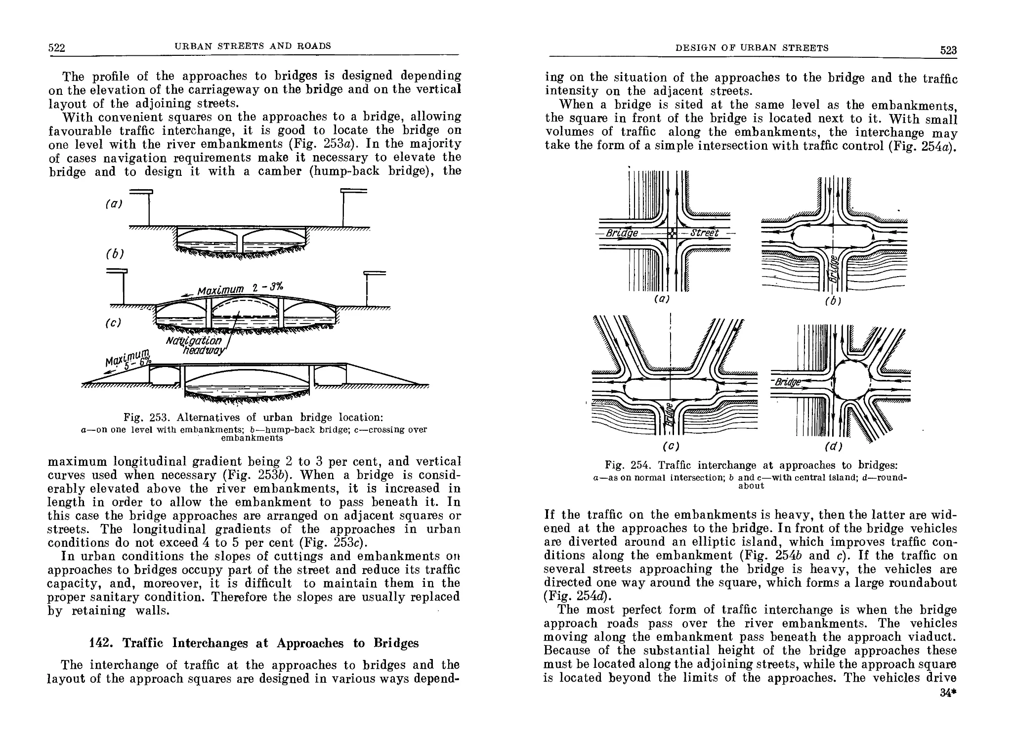
140. Drainage in Urban Conditions.......................... , . 518
141. Approaches to Urban Bridges................................. 521
142. Traffic Interchanges at Approaches to Bridges.............. 522
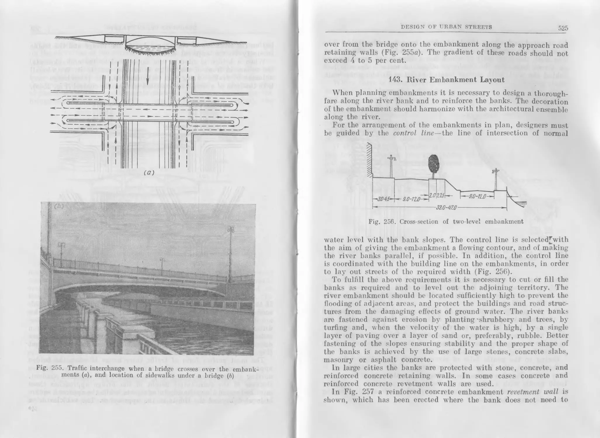
143. River Embankment Layout..................................... 525
Index......................................................... 528
Introduction
Modern highways are complex engineering structures; the calcu-
lations providing the basis for the design of individual road elements
are often just as complicated as the design calculations for machine
components, bridges and the structural details of public and in-
dustrial buildings.
Modern highways are intended for high-speed motor traffic.
Therefore, they must be designed and constructed in such a way
that the performance characteristics of vehicles may be effectively
realized under normal conditions of engine operation. Their design
should permit vehicles to negotiate bends and gradients without
the danger of skidding and overturning and without causing fatigue
and discomfort to passengers. The road pavement must continuously
provide good riding qualities and be capable of withstanding the
dynamic loads induced by the passage of vehicles.
Pavements and road subgrades are subject to the influence of
many natural factors, e.g., heating by the sun, freezing and thaw-
ing, moistening by rain, etc. In the annual cycle, complex physi-
cal processes develop in the subgrade occasioned by the variation
in moisture distribution and an increase in subsoil moisture content.
An excessive moisture content quickly causes the subsoil to lose
its strength and may lead to disintegration of the road foundation.
The many and varied factors of pavement performance have to be
taken into accoun£by the designer and constructor, who have to pro-
vide for the maximum stability of the subgrade and for the maximum
strength of the pavement to be laid thereon.
Roads are built in the most varied natural conditions—in the
broad plains and hills of the European part of the U.S.S.R., amidst the
lakes, marshes and rocks of Karelia, in the regions of Siberia covered
by taiga forests, on permafrost subsoils, in the sandy deserts and
irrigated cotton plantations of Central Asia, in the mountains of the
Caucasus and Pamir, in the fertile virgin lands of Siberia and Kazakh-
stan, and in the black earth steppes of the Ukraine and Kuban.
A similar diversity of terrain exists in all other countries having
a large territory.
In all these diverse and complex conditions the road engineer hds
to be able to find the correct engineering and economic solutions.
Because of this, when solving problems related to road construction,
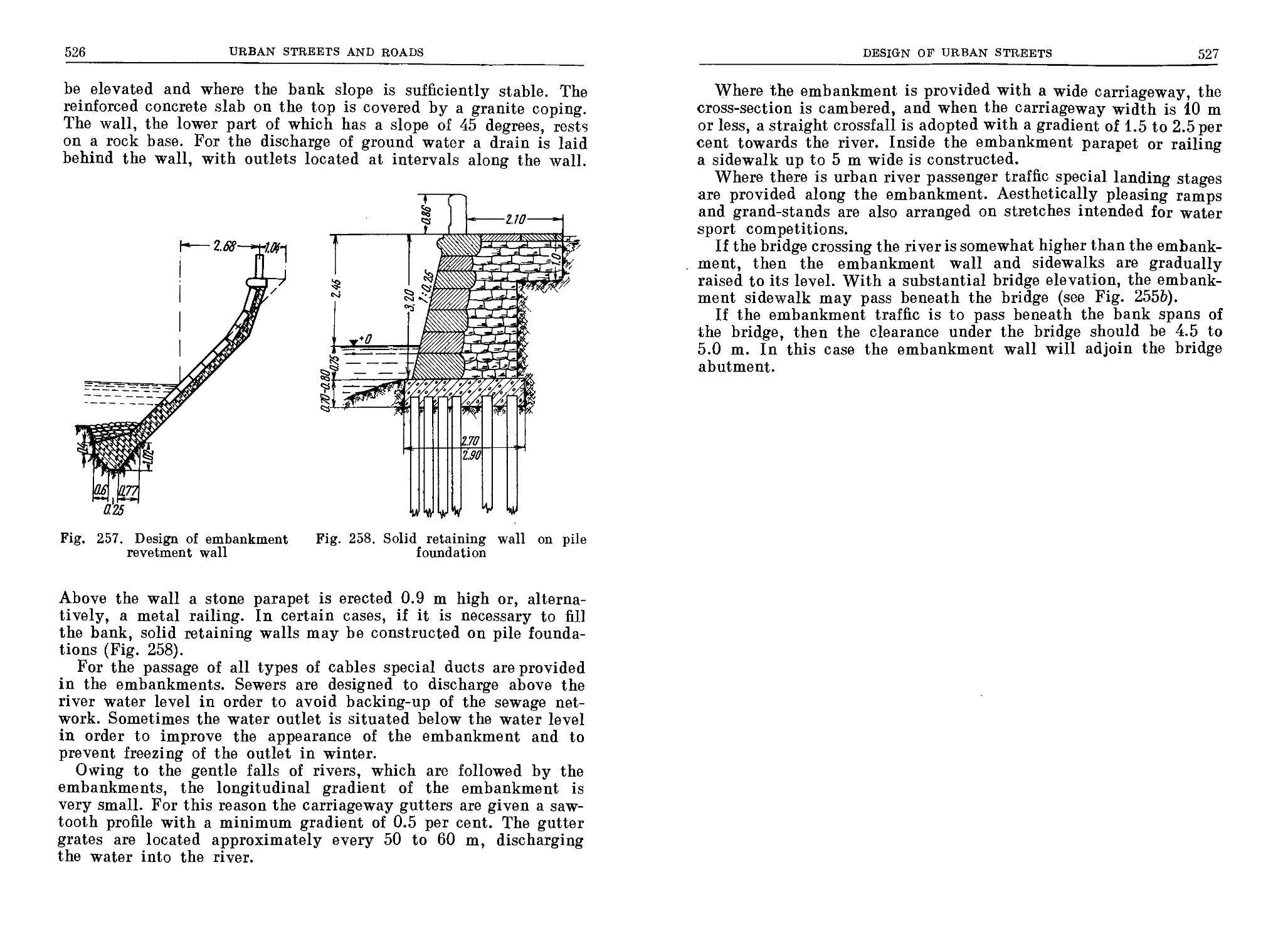
12
INTRODUCTION
he has to make use of natural and historical sciences, i.e., geology,
climatology, soil physics and mechanics, surveying, hydraulics,
hydrology, etc.
At present the requirements for an engineer engaged in the design
and construction of highways are very exacting. He must be fully
conversant with the methods of route selection and with the methods
used to obtain field data required for design purposes. He must be
able to design highways so as to ensure the comfort and safety of
transportation. At the same time he must take into account to
a maximum extent the local geophysical conditions which influence
the construction and maintenance of highways.
The maximum use should be made of modern machinery in the
best possible combination for roadbed and pavement construc-
tion.
Finally, when the highway is put into service, its maintenance and
the provision for uninterrupted traffic become of the utmost impor-
tance for the national economy. The engineer in charge of the high-
way operation must ensure the maintenance of the road quality
under all traffic and weather conditions. He must be familiar with the
methods of counteracting the natural agents which threaten the
road stability and which can interrupt the traffic (snow and sand
drifts, frost heave, washouts by rain, landslides, floods, etc.).
Road jobs are essentially labour-consuming, demanding the
extensive transportation of large quantities of materials. Thus, for
the construction of 1 km of a motor road with asphalt-macadam
surfacing on a gravel base, in flat country, it is necessary to trans-
port about 7,500 tons of sand and gravel and excavate up to
12,000 cum of soil, transporting it for a distance of perhaps several
hundred metres. Stone aggregates used in the road pavement often
have to be hauled from far afield.
The road-building operations become complicated because of the
extensive length of the construction site—often tens and hundreds
of kilometres. This requires the introduction of special techniques
and methods of work organization.
The task of the road engineer is to mechanize and technically
develop the road-building operations, and to provide for the most
efficient and complete mechanization of the entire construction
process.
As in other fields of construction, road building requires the
application of industrialization techniques on a wide scale—the
use of prefabricated reinforced concrete structures, light-weight
concrete constructions, factory-made large blocks and assemblies.
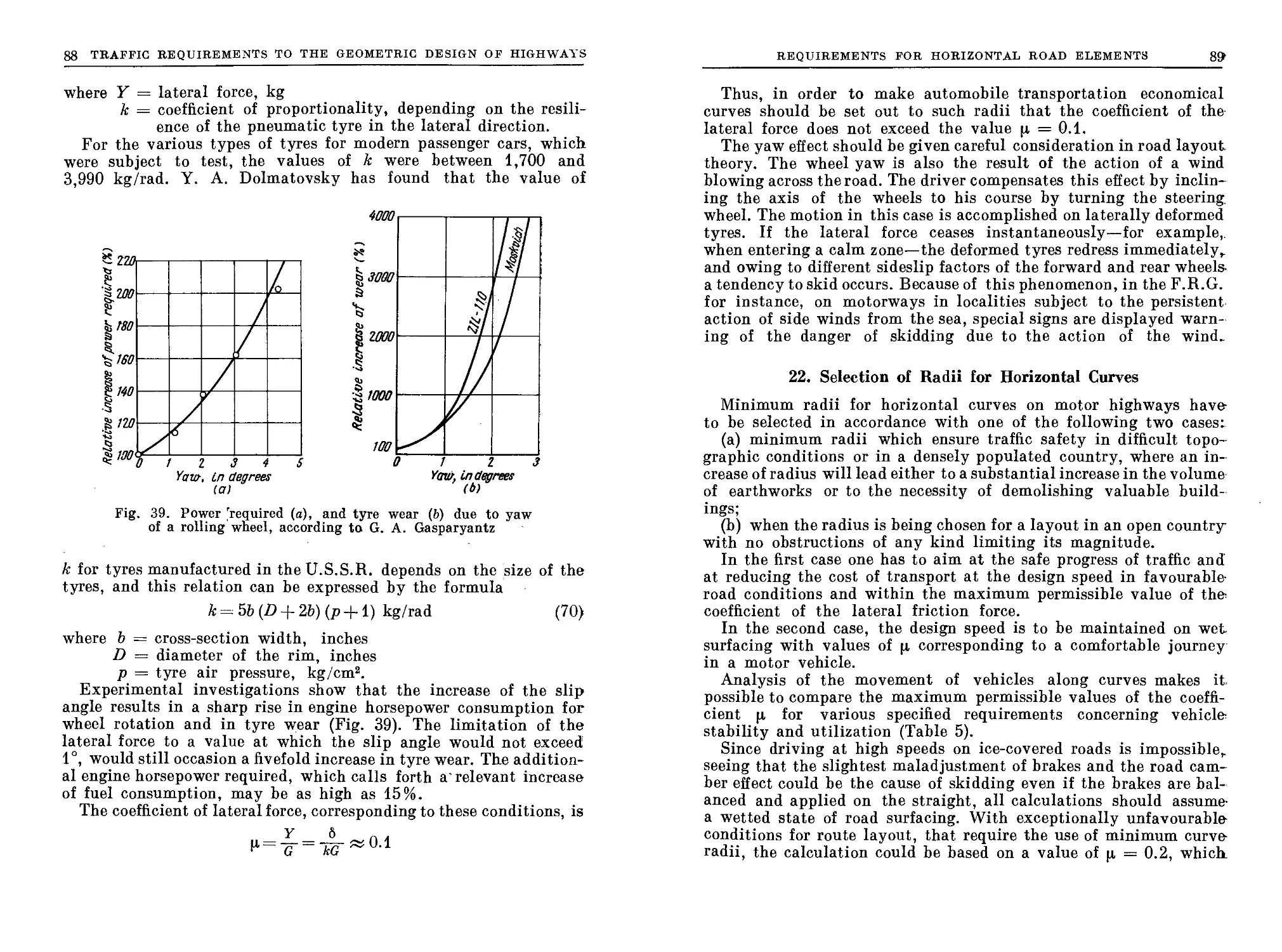
Because of this, road construction and the building of artificial
structures form complementary parts of the same constructional
programme.
INTRODUCTION
13
The mechanization of road construction has grown immensely
since the war. This is true of such operations as earthworks, sand
and gravel quarrying, stone crushing and the completion of asphalt
macadam and cement concrete surfacing.
The diversity of natural conditions in many countries—sharp
variation of climatic, ground, and hydrological conditions of various
regions—precludes the use of standardized design methods. Designers
must have a creative approach to their problems; they must thor-
oughly assess the influence on the constructed road of natural agents
and of the loads imposed by vehicular traffic.
The solutions of road construction problems are closely allied to
those of reduction of cost and the improvement of the quality of
the work. To ensure the most economical design of the road it is
necessary to assimilate the experience gained in the carrying out of
similar projects. It is very important that the latest techniques
developed in the fields of science and engineering be applied to the
construction and analysis of road and bridge projects.
When designing a highway one should reject over-large safety
factors, and limit the consumption of allocated and imported
materials. Extensive use should be made of local materials of limit-
ed strength, including local soils, by employing them in structures
where the stresses caused by traffic and natural agents will per-
mit their use. One must envisage the employment of chemical
and physical stabilization of soils when necessary in order to
increase their strength and stability.
It is imperative to extend the scientific basis of road building.
The construction of highways in complex natural conditions constant-
ly demands the continued scientific approach to new problems.
At present, the principles of road design and construction in
difficult conditions are not fully developed in all their details.
Great difficulties may be encountered in the use of local materials
of limited strength, which may result in frequent failures.
The science of road construction is on the threshold of new develop-
ments. Since it is an applied science, it depends on the achievements
of physical, mathematical and natural sciences. A wider applica-
tion of these sciences linked with the future important development
of the chemical industry opens up great possibilities for road engi-
neers to be able to alter the properties of local soils and stone
aggregates by means of physical and chemical treatment of their
active colloidal constituent parts.
The road engineer should be prepared for the possible alteration,
in the near future, of the character of vehicular traffic on roads.
Development in electric supply could permit the introduction of
trolleybus services on country roads, and the use of radar may give
rise to automatic traffic control. One possibility of a widespread
14
INTRODUCTION
development in the use of atomic energy would be that the road
engineer may have the opportunity of obtaining monolithic sur-
facing by the fusion of local soils.
With the growth of traffic density will come a demand for greater
amenities. It will be necessary to provide the national road system
with hotels and restaurants, service stations and repair shops, where
drivers and passengers may rest, and the vehicles be serviced and
overhauled. Attention should be given to such questions as fitting
roads into the landscape in plan and in profile, planting trees,
so as to improve their aesthetic value.
Brief Survey of Road Engineering Development
Road engineering is one of the earliest arts known to mankind-
The development of industry and the improvement of the means of
transport have led to the alteration and improvement of road build-
ing and of methods of road construction.
Roadmaking originated in the period of early human settlements.
People would choose the most convenient and the shortest ways of
approach to their hunting and fishing grounds, gradually making
footpaths. The earliest bridges were naturally fallen trees across
waterways; gradually, however, crossings were built of logs. With
the use of tamed animals for transport, the paths had to satisfy
higher standards since bridle paths for pack animals must be cleared
to a greater width and height.
The first artificially constructed tracks were made in mountainous
and forested country, where obstacles to movement were encount-
ered. It is likely that the first road surfacing was simply a layer of
logs and brushwood over marshland.
About four to five thousand years В. C. the introduction of the
wheel constituted a major technical achievement and greatly accel-
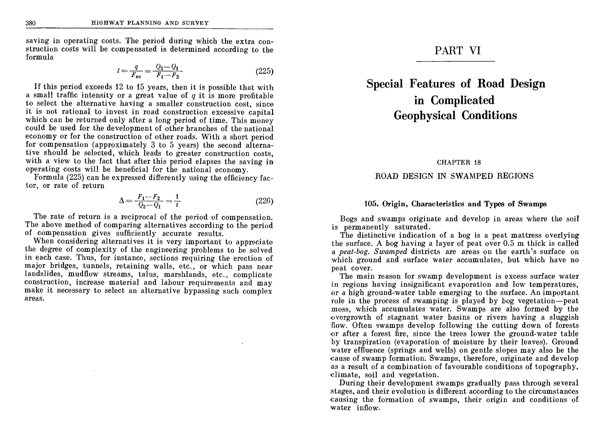
erated the development of road construction. The possibility of
carrying a greater load on wheels than could be moved by dragging
it, called for a corresponding improvement in carriageway and
bridge flooring and also created a demand for more convenient road
alignments and the bypassing of marshland and loose sands.
Road construction received a substantial impetus during the
slave-owning period of the ancient world—in Assyria, Babylon,
Persia and especially in the Roman'fempire. This road building was
maintained because of the continuous warfare with neighbouring
states, which required roads to link the centre of the country with
its borders. Thus, the transition from footpaths and bridle tracks to
comparatively well built roads was achieved largely through m litary
considerations.
INTRODUCTION
15
Commercial traffic at that time went mainly by sea and river.
These routes were cheaper than transport by land and were safer.
This situation was further accentuated by the territorial dissociation
of the various states and the absence of an interconnected system of
land communications. Therefore, during the whole of the slave-own-
ing period, and later of the feudal epoch, water transport developed
more quickly than overland transport. However, an appreciably
well developed road network was laid out in places where there
were no waterways.
The territory of the contemporary Uzbek and Turkmenian repub-
lics was crossed by great caravan routes which served for trade
between the people of Central Asia and China, Greece and Rome.
These routes consisted of wide tracts of free land, within the limits
of which there was grazing fodder for draught and pack animals.
The way was marked only by wells and inns, with fords and iso-
lated bridges at crossings of waterways.
The construction of the stone arch bridge originated during the
ancient Asiatic epoch. The earliest bridgeshad pointed arches, e.g.,
tjae ancient bridges of Persia, but later the Romans developed the
semi-circular arch which they used on bridges and viaducts.
In the ancient civilizations of the East artificially paved surfacings
were used mainly for town streets and approaches to temples. Baked
bricks were used extensively for paving in Assyria and Babylon,
as well as mastic asphalt—a mixture of natural bitumen, clay, sand
and gravel. Limestone slabs were also used for street pavement.
Road construction was extensively developed during the Roman
Empire, the strategic and commercial aims of which required the
creation of lines of communication cutting across Europe (Fig. 1).
The Roman historian Tacitus says that the roads of that time were
required by “the traders and the Roman army”, and the roads they
constructed were proof of the might of the Roman Empire. The
Roman highway network, built during seven centuries, extended over
a total length of 90,000 km, of which 14,000 km were situated
within present-day Italy. If one is to take into account secondary
earth and gravel roads, the total length of the Roman Empire road
network would attain 300 thousand kilometres.
The major Roman roads were of solid stone construction incorpo-
rating up to 10 to 15 thousand cubic metres of stone per kilometre.
This is from 4 to 6 times the amount used today in the construction
of modern motorways (Fig. 2).
Materials used in the construction of Roman roads were gravel,
cobblestone and hewn stone in the form of slabs. Lime burning was
known to the Romans, who used concrete extensively for construc-
tional purposes, employing as the matrix a mixture of lime, loose
volcanic rock (pozzuolana) and sand.
16
INTRODUCTION
The Romans were skilled in the art of bridge building as evidenced
by their roads which were endowed with innumerable stone arch
bridges whose remains can still be found in Italy, France and Spain.
As a rule, Roman roads were aligned to provide the most direct
route ignoring natural obstacles. This policy necessitated the con-
struction of numerous structures. For example, a depression 35 m
deep was filled in along the Appian Way near Terracina, whilst
near Naples the Romans drove a tunnel 1,300 m long, 10 m high,
Fig. 1. European major road network—2nd century A.D.
and 8 m wide. At intervals of 10 to 15 km along these roads, inns
were sited where about 40 horses were kept; by changing horses
messengers were able to cover up to 150 km per day.
The ruthless exploitation by the slave-owning states of conquered
provinces caused a gradual decline in their forces of production.
As F. Engels noted, this led to “universal impoverishment; decline
of commerce, handicrafts, the arts and of the population; decay of
towns; retrogression of agriculture to a lower stage”. The Roman
Empire, weakened by the slave revolts, was conquered at the end of
the fifth century by the Germanic barbarians, and in its place appea-
red dozens of small feudal states. Within the limits of the separate
states and domains the economies were of the subsistence type. The
European arterial roads, which now crossed several states, lost the
importance they once held during the Roman era, and were allowed
to fall into decay.
INTRODUCTION
17
The importance of land communications grew appreciably at the
end of the feudal period, when the process of uniting various sepa-
rate feudal domains into great states took place.
In the second half of the 18th century a period of intensive road
building began, the rate of building being dependent upon the rate
of development of industry and commerce in various states. The
construction of roads with uniform hard surface substantially
Gravel concrete
using time-
pozzuolana matrix
Gravel In
llme-pozzualana
matrix
Compacted loam
Broken stone
cemented with
martar
Limestone slabs
jointed with
mortar
Cement concrete
Sand layer
Fig. 2. Comparison of pavement struc-
tures of Roman roads and contemporary
highways. Above is the pavement of
a Praetorian road; below is a modern
cement concrete pavement for a traffic
flow of 5,000 vehicles per day
improved the conditions for the transportation of raw materials and
of finished products by reducing the tractive resistance and hence
allowing an increase in the load carried by individual vehicles.
At first, roads similar to the Roman roads were built. However,
owing to a scarcity of suitable material and the high cost of labour,
the amount of stone material used was progressively reduced and the
work was carried out less thoroughly. Research was undertaken
with a view to finding more rational methods of using stone for
pavement construction which would reduce both the amount of
labour and the cost.
Important stages in the development of road pavement construc-
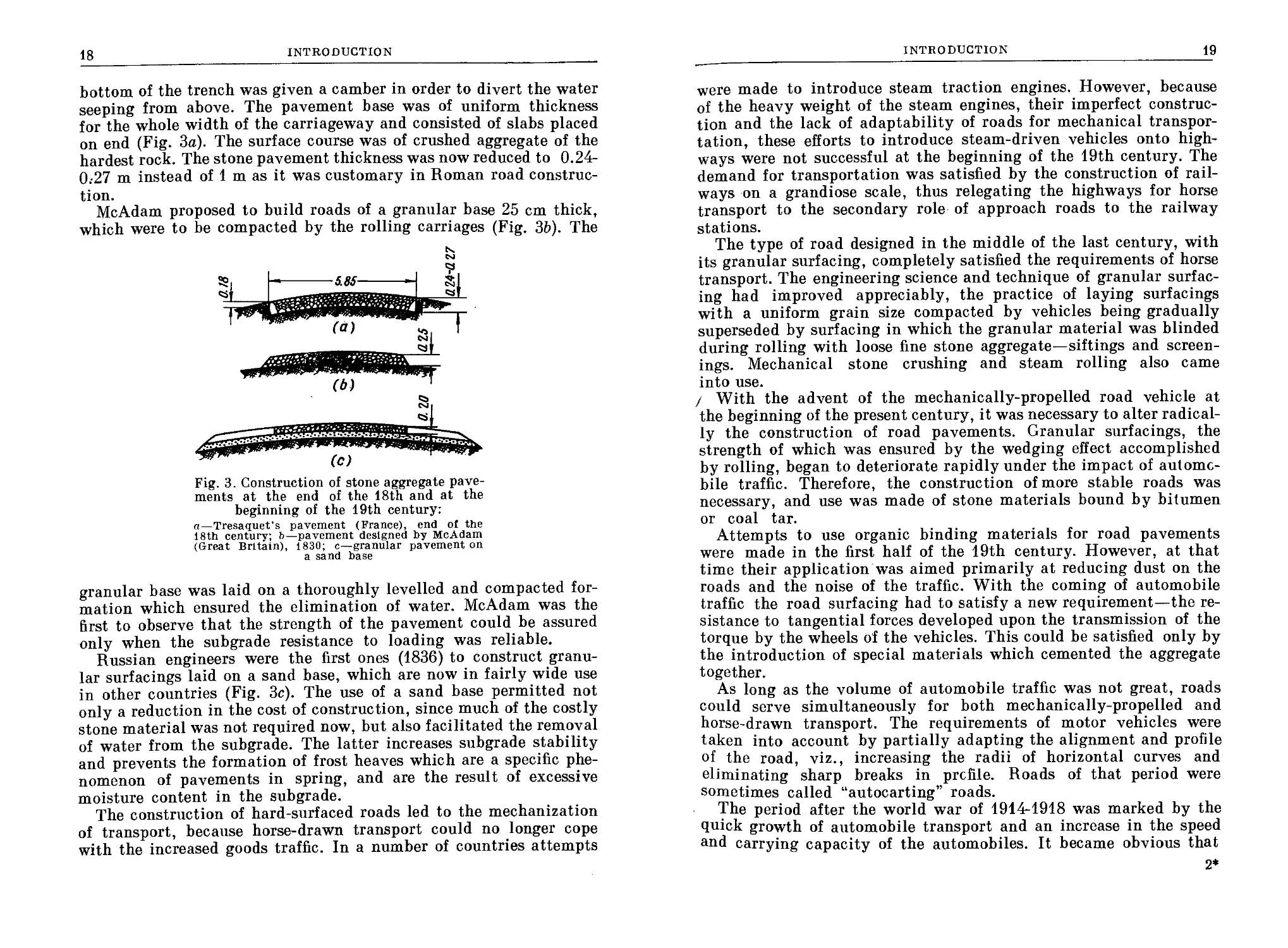
tion were marked by the introduction of two types of construction,
called by the names of their inventors—the Frenchman Tresaquet
and the Scot McAdam. Tresaquet’s system consisted in building the
road pavement in a wide trench dug out of the natural ground. The
2—820
18
INTRODUCTION
bottom of the trench was given a camber in order to divert the water
seeping from above. The pavement base was of uniform thickness
for the whole width of the carriageway and consisted of slabs placed
on end (Fig. 3a). The surface course was of crushed aggregate of the
hardest rock. The stone pavement thickness was now reduced to 0.24'
0.-27 m instead of 1 m as it was customary in Roman road construc-
tion.
McAdam proposed to build roads of a granular base 25 cm thick,
which were to be compacted by the rolling carriages (Fig. 3b). The
Fig. 3. Construction of stone aggregate pave-
ments at the end of the 18th and at the
beginning of the 19th century:
a—Tresaquet’s pavement (France), end of the
18th century; b—pavement designed by McAdam
(Great Britain), 1830; c—granular pavement on
a sand base
granular base was laid on a thoroughly levelled and compacted for-
mation which ensured the elimination of water. McAdam was the
first to observe that the strength of the pavement could be assured
only when the subgrade resistance to loading was reliable.
Russian engineers were the first ones (1836) to construct granu-
lar surfacings laid on a sand base, which are now in fairly wide use
in other countries (Fig. 3c). The use of a sand base permitted not
only a reduction in the cost of construction, since much of the costly
stone material was not required now, but also facilitated the removal
of water from the subgrade. The latter increases subgrade stability
and prevents the formation of frost heaves which are a specific phe-
nomenon of pavements in spring, and are the result of excessive
moisture content in the subgrade.
The construction of hard-surfaced roads led to the mechanization
of transport, because horse-drawn transport could no longer cope
with the increased goods traffic. In a number of countries attempts
INTRODUCTION
19
were made to introduce steam traction engines. However, because
of the heavy weight of the steam engines, their imperfect construc-
tion and the lack of adaptability of roads for mechanical transpor-
tation, these efforts to introduce steam-driven vehicles onto high-
ways were not successful at the beginning of the 19th century. The
demand for transportation was satisfied by the construction of rail-
ways on a grandiose scale, thus relegating the highways for horse
transport to the secondary role of approach roads to the railway
stations.
The type of road designed in the middle of the last century, with
its granular surfacing, completely satisfied the requirements of horse
transport. The engineering science and technique of granular surfac-
ing had improved appreciably, the practice of laying surfacings
with a uniform grain size compacted by vehicles being gradually
superseded by surfacing in which the granular material was blinded
during rolling with loose fine stone aggregate—siftings and screen-
ings. Mechanical stone crushing and steam rolling also came
into use.
/ With the advent of the mechanically-propelled road vehicle at
the beginning of the present century, it was necessary to alter radical-
ly the construction of road pavements. Granular surfacings, the
strength of which was ensured by the wedging effect accomplished
by rolling, began to deteriorate rapidly under the impact of automo-
bile traffic. Therefore, the construction of more stable roads was
necessary, and use was made of stone materials bound by bitumen
or coal tar.
Attempts to use organic binding materials for road pavements
were made in the first half of the 19th century. However, at that
time their application was aimed primarily at reducing dust on the
roads and the noise of the traffic. With the coming of automobile
traffic the road surfacing had to satisfy a new requirement—the re-
sistance to tangential forces developed upon the transmission of the
torque by the wheels of the vehicles. This could be satisfied only by
the introduction of special materials which cemented the aggregate
together.
As long as the volume of automobile traffic was not great, roads
could serve simultaneously for both mechanically-propelled and
horse-drawn transport. The requirements of motor vehicles were
taken into account by partially adapting the alignment and profile
of the road, viz., increasing the radii of horizontal curves and
eliminating sharp breaks in profile. Roads of that period were
sometimes called “autocarting” roads.
The period after the world war of 1914-1918 was marked by the
quick growth of automobile transport and an increase in the speed
and carrying capacity of the automobiles. It became obvious that
2*
20
INTRODUCTION
intensive automobile traffic and horse traffic could not be combined
on mixed-purpose roads. Therefore, parallel with the construction
of mixed-purpose roads on secondary routes, highways were construct-
ed which were intended exclusively for high-speed automobile
traffic on a large scale, i.e., motorways and expressways, all the
elements of which were designed for high-speed traffic.
Expressways are roads intended for the transportation of passengers
and goods over extended distances by motor vehicles, and which
permit such journeys to be accomplished without obstruction from
local traffic.
The expressways are provided with motels and service stations. On
the modern expressway the high speed of traffic makes it impera-
tive that the two opposing streams of vehicles should be physically
separated. Therefore, expressways are built with dual carriageways,
each of which should have a minimum width of two traffic lanes.
On an expressway there are no level crossings, no traffic lights and
no signals requiring the vehicles to stop. The entry to expressways
is possible only by special approach roads.
The economic committees of UNO have developed projects of
European and Asian International Highway Systems which include
the main expressways of individual countries.
PART I
The Road. General
CHAPTER 1
THE HIGHWAY NETWORK
1. Highways and the National Transport System
' The transportation of passengers and goods is accomplished, in
practice, by means of a communication network consisting of railways,
highways, aircraft routes, and river and sea routes. In countries
with a planned economy all means of transport form a single
transportation system and their operations are coordinated, thus
complementing each other’s services and providing an opportunity
to rationalize the use of each service.
The main volume of long-distance commercial and passenger traf-
fic is carried by rail transport. However, goods handled by rail are
received and delivered at special freight stations. Therefore, rail-
ways have to operate in conjunction with other forms of transport,
which function on the approach roads to the railway lines. Approach
roads are also required to service sea, river and canal transport and
airports, the role of approach roads being played by motor roads
and highways.
Goods may be loaded on to motor vehicles directly at the place
of their production, and these goods may then be carried without
transfer directly to their, respective destinations. Because of this,
motor transport is the most efficient form of transportation over
comparatively short distances. Depending on the nature of the
road network, the delivery of freight for a distance of 200 to 400 km
is accomplished more quickly by road than by rail.
The total volume of goods carried by motor transport is apprecia-
bly greater than that transported by all other means of transport.
Motor transport plays an important part in the development of
sparsely populated districts, providing for the transport of goods
while at the same time keeping the costs of road construction com-
22
THE ROAD. GENERAL
jaratively low. In recent years, with the construction of modern
lighway networks, motorized transport has also acquired impor-
tance as a means for the long-distance transportation of passengers
and freight.
2. Highway Network Fundamentals
Roads which interconnect inhabited localities and industrial and
agricultural centres, linking them to freight handling stations for
other means of transport, constitute the basic highway network.
Persons and goods requiring to be transported between specific ori-
gins and destinations, the amount of goods depending on the requi-
rements of the national economy and established trade relations,
make up traffic streams.
In planning an effective automobile highway network it is essen-
tial, in the first instance, to take into account the main freight and
passenger traffic streams in order to keep the costs down and to fa-
cilitate the delivery of goods. The framework of a highway network is
a system of trunk roads designed for long-distance high-speed pas-
senger and goods traffic, and connecting the main economic regions of
the country with its basic economic centres.
When laying out a highway network it is essential to maintain
administrative, cultural and economic communications between
various parts of the country.
The location of a highway network is a fundamental element of
road planning, and is determined by the distribution of the coun-
try’s productive forces, the further development of which it must
promote. However, the considerable amount of money already invest-
ed in road building compels the designer to make maximum use
of the existing metalled roads. In all projects concerned with the
development of highway networks, therefore, considerable atten-
tion must be given to the reconstruction of roads in order to render
them suitable for modern high-speed motor traffic.
^3. Characteristics of Highway Traffic
Vehicles travelling in the same direction constitute a traffic
stream. It is apparent that the greater the number of vehicles in
a stream, the more severe will be the requirements to be satisfied by
the road.
A traffic stream usually consists of many types of vehicles, trav-
elling at different speeds and carrying various loads. However, in
order to determine the layout of the road, e.g., the width of the
carriageways and the overall width of the road, the total number
of vehicles on the road at a given period is taken as the major design
criterion, and not the loads they may be carrying. The total number
THE HIGHWAY NETWORK
23
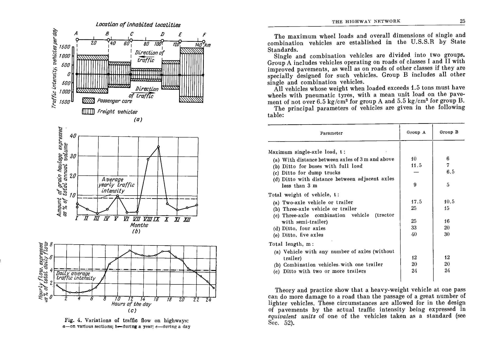
vehicles passing through any section of a road in unit time (day,
aour) is called the traffic intensity or flow and is the measure of
traffic usage for design purposes. Traffic flow varies along each indi-
vidual road section; it increases in the vicinity of towns, large inhab-
ited localities and railway stations, and is reduced along stretches
of road some considerable distance from large towns and cities
(Fig. 4a). The traffic flow on a road does not remain uniform through-
out the year. When seasonal agricultural activity is high, especial-
ly during the harvest, traffic intensity on country roads builds up
appreciably (Fig. 46). On the other hand, the volume of freight
traffic decreases during holiday periods. Nor does traffic flow remain
constant throughout the day, and it decreases sharply at nightfall
(Fig. 4c). As a result of the practical measurement of traffic, it is
customary to accept for calculation purposes that the total daily
volume of traffic passes during ten hours of daytime.
In the project stage of highway design, traffic is usually described
in terms of the “annual mean daily flow” (A.D.F.), i.e., the total
number of vehicles passing per year divided by 365. In some cases,
e.g., when planning a road for the transportation of agricultural
produce (grain, sugar beet, etc.), traffic flow at harvest time may be
appreciably in excess of the mean daily flow. In view of the nation-
al importance of this traffic, it would be desirable in this instance
to base the layout and geometric design of the road on flow during
the peak period.
The total traffic intensity in both directions during the peak hour
may also be taken for purposes of design.
Traffic flow is not the only basic traffic characteristic. One has to
bear in mind other factors when resolving certain design and opera-
tional problems of highways.
To determine the pavement thickness and to design different
structures one has to know not only the number of loads, but
also their weight. This makes it necessary to divide the total traffic
flow into separate streams according to the load-carrying capacity
of the vehicles.
For design purposes, motor vehicles in the U.S.S.R. are divided
into four basic categories:
Very small capacity —up to 1.0 ton
Small capacity —from 1 to 2 tons
Medium capacity—from 2 to 5 tons
Large capacity —from 5 tons to the limit permitted
by road vehicle regulations
Soviet trucks of very large capacity—MAZ-525 and MAZ-530 of
25 and 40 ton capacity—are intended for use at quarries and construc-
tion sites and can be seen on general purpose roads only on rare
occasions.
A
Location of Inhabited localities
§1500
•a 1000
SOO
I
g SOO
'2 1000
1500
10
40
\\\\\\\\\\v
^\\\\\\\\\\\\\
SS8S
80 10$
1 Direction of >
! traffic *—------
K\X№NSN
140
km
Direction
K\\\\\\\
Passenger cars
ill I III Freight vehicles
Fig. 4. Variations of traffic flow on highways:
a—on various sections; b^during a year; c—during a day
THE HIGHWAY NETWORK
25
The maximum wheel loads and overall dimensions of single and
combination vehicles are established in the U.S.S.R by State
Standards.
Single and combination vehicles are divided into two groups.
Group A includes vehicles operating on roads of classes I and II with
improved pavements, as well as on roads of other classes if they are
specially designed for such vehicles. Group В includes all other
single and combination vehicles.
All vehicles whose weight when loaded exceeds 1.5 tons must have
wheels with pneumatic tyres, with a mean unit load on the pave-
ment of not over 6.5 kg/cm2 for group A and 5.5 kg/cm2 for group B.
The principal parameters of vehicles are given in the following
table:
Parameter Group A Group В
Maximum single-axle load, t : (a) With distance between axles of 3 m and above 10 6
(b) Ditto for buses with full load 11.5 7
(c) Ditto for dump trucks 6.5
(d) Ditto with distance between adjacent axles less than 3 m 9 5
Total weight of vehicle, t: (a) Two-axle vehicle or trailer 17.5 10.5
(b) Three-axle vehicle or trailer 25 15
(c) Three-axle combination vehicle (tractor with semi-trailer) 25 16
(d) Ditto, four axles 33 20
(e) Ditto, five axles 40 30
Total length, m : (a) Vehicle with any number of axles (without trailer) 12 12
(b) Combination vehicles, with one trailer 20 20
(c) Ditto with two or more trailers 24 24
Theory and practice show that a heavy-weight vehicle at one pass
can do more damage to a road than the passage of a great number of
lighter vehicles. These circumstances are allowed for in the design
of pavements by the actual traffic intensity being expressed in
equivalent units of one of the vehicles taken as a standard (see
Sec. 52).
26
THE ROAD. GENERAL
The amount of attrition of the road surface is dependent upon the
total weight of vehicles which have passed since the road was last
repaired. Because of this, traffic flow is measured in terms of the
gross laden weight of vehicles traversing the road.
4. National and Functional Classification
of Highways
The importance of motor roads for the national economy is, in
the majority of cases, closely related to the intensity of traffic on
them, i.e., the higher the flow the better should be the standard of
design. Where flows are heavy, the expenditure necessary for the
construction of the road to follow the most direct route and with
shallow gradients will soon be compensated by the economy in
traffic operation. On the other hand, if in spite of a high traffic flow
the road is built with steep gradients and a narrow carriageway,
though its capital cost may be much lower it will not permit the
most effective performance of vehicles to be realized, in particular
the maintenance of high vehicle speeds. In the long run, the cost
of motor transport operation would become excessive.
The question of choice of the type of road, however, does not depend
exclusively on the cost of construction. A number of other major
factors must be taken into consideration, particularly the part played
by the specific highway in the transport system of the national econ-
omy. Therefore, it becomes necessary to have two road classifica-
tions: a national one in accordance with the specific importance
of the road for the national economy, with a view to both present
needs and future development, and a functional one based on the
traffic flow, which may not necessarily be coincident with the natio-
nal one.
An example of a national classification of motor roads is the one
applied in the Soviet Union, where the various roads are divided
into the following groups according to their importance for the na-
tional economy and cultural life of the country, as well as according
to administrative needs:
1. Arterial roads of all-Union importance, intended for long-dis-
tance motor communications between large centres and remote eco-
nomic regions.
2. Arterial roads of republican importance for long-distance motor
communications between remote regions of the Union republics.
3. Highways of regional importance, serving to connect districts
and large enterprises with regional centres, railway stations and
docks.
4. Roads serving district needs, connecting district centres with
other inhabited centres and large local industrial enterprises, with
THE HIGHWAY NETWORK
27
state farms, collective farms, railway stations and docks. The build-
ing and maintenance of these roads are carried out by the local
organizations.
In the U.S.S.R. the regional and district roads carry the bulk of
haulage, since their cumulative length forms 80% of the total road
network. In certain cases these are roads with a pavement of infe-
rior quality.
The reconstruction and building anew of the most important
parts of this road network, i.e., roads adjoining large towns and
industrial centres, approaches to railway stations and docks, should
receive priority in road construction plans for the near future.
5. Resort roads, mainly for passenger traffic within health resort
districts.
6. Approach roads to large towns and industrial centres, linking
them with neighbouring districts.
7. Town roads and roads in inhabited places (streets) which serve
the internal passenger and goods traffic. These roads are the respon-
sibility of the municipal services.
8. Roads used by separate economies and enterprises, and ap-
proach roads carrying internal traffic.
There is a number of roads which are built according to high techni-
cal standards in spite of their comparatively low traffic intensity,
e.g., roads within health resort areas which offer high-standard
amenities to holiday-makers and patients. These roads are always
of the highest technical standard.
The expected traffic intensity cannot be the only criterion when
designing roads for construction in new, sparsely populated regions.
In spite of the expected low traffic intensity for a number of years
to come, such roads will constitute the main artery for populating
these regions. Therefore, pioneer roads can be built with a view to
district development, according to technical standards correspond-
ing to a traffic intensity exceeding the present rate.
The motor roads of the U.S.S.R. are divided into five technical
classes. The class is determined according to the importance of the
road for the national economy. At the same time potential traffic
intensities are considered, as well as the construction difficulties
arising from the topographic features of the country in which the
road is to be located.
The elements of the plan, profile and cross-section are designed
with a view to the traffic intensities expected in 20 years, and the
road pavement—in 5 to 10 years, depending on its construction and
the possibility of gradually strengthening it.
Class I comprises roads having special economic, administrative
or cultural importance for the national economy of the U.S.S.R.
and having a high initial or potential traffic intensity; class II
28
THE ROAD. GENERAL
comprises similar roads with an appreciable potential traffic flow;
class III covers motor roads with a moderate traffic flow but having
a very great importance for the national economy of the Union
republics; class IV includes roads having local economic, admin-
istrative or cultural importance and a low traffic flow, and class V
covers motor roads with small initial and potential traffic
flow.
In the particularly difficult conditions of a mountainous region
it is permitted, provided one can justify this on economic grounds, to
lower the classification of a road at especially difficult sections by
one class. Table 1 gives the road classes in relation to potential
traffic flows.
TABLE i
Highway Classification System in the U.S.S.R.
Potential intensity of vehicular
traffic (annual mean daily
flow=A.D.F.)
More than 6,000 vehicles
From 3,000 to 6,000 vehicles
From 1,000 to 3,000 vehicles
From 200 to 1,000 vehicles
Less than 200 vehicles
Technical class
of road
I
II
III
IV
V
All road elements of each technical class are designed to ensure
the safe running of individual passenger cars under normal condi-
tions of cohesion between vehicle wheels and the carriageway surface
(a dry or comparatively clean wet pavement surface).
The geometric design of class I roads is based upon a design speed
of 150 km/hr. Glass II roads have a design speed of 120 km/hr,
class III roads—100 km/hr, class IV roads—80 km/hr and class V
roads—60 km/hr.
On difficult sections of rugged country the design speed is reduced
by 20 km/hr, while on difficult sections of mountainous terrain it
is halved (80 km/hr for roads of class I).
The design traffic speed for class I roads corresponds to the actual
speeds of modern motor cars, e.g., ZIL-110 and GAZ-12, and is
lower than the probable speeds of passenger cars to be produced
in the near future. Therefore, when laying out motorways intended
mainly for high-speed passenger traffic, the design speed may be
increased to 160-180 km/hr. When designing roads an attempt should
be made to allow a traffic speed exceeding the rated one, except
THE HIGHWAY NETWORK
29
when this entails substantial increases in constructional cost. This
is especially important in the case of class III or IV roads.:
In general the design speeds accepted in the U.S.S.R. correspond to
those used in other countries. For example, on expressways in
Western Germany the design speed in relation to topographic fea-
tures is 160 km/hr in flat country, 140 km/hr in hilly country and
120 km/hr in mountainous areas. In Great Britain the design speed
for motorways is taken as 130 km/hr, in the U.S.A, it is 112 km/hr.
The UNO Economic Commission for Europe recommended for the
International Highway System a design speed of 120 km/hr..
CHAPTER 2
HIGHWAY DESIGN
5. The Road in Plan
Highways are designed for the haulage of goods and passengers
with a minimum of effort and at low cost. These requirements would
be satisfied best if the road could be built along the shortest dis-
tance, i.e., a straight line between two given points. However, the
building of a road along the shortest distance is precluded by the
topography of the land (mountains, ravines, etc.), water obstacles
(marshes, lakes, rivers), as well as the necessity to lay the road
through certain intermediary points—places adjoining towns,
places conveniently located for crossing rivers, railways or other
highways.
As can be seen from Fig. 5, the necessity to locate the crossing
where the river is straight and affords a convenient approach with
shallow banks, the desirability of bypassing an inhabited locality
and the necessity to avoid the crossing of a ravine dictated the
location of the road along the broken line of the plan rather than
along the shortest and most direct (air line) route. For the conven-
ience of passage of motor vehicles, it is necessary to inscribe circular
arcs of adequate radius at changes in direction.
Such a line, marked on the land and located along the road centre
line, is called the route. The graphical representation of the line
of the route, projected on a horizontal plane and drawn to a given
scale, is called the plan of the route.
Any deviation of the direction of the route is determined by the
deflection angle, which is measured between the continued previous
line of the route and its new direction (Fig. 6). In practice, deflection
angles are given consecutive identifying labels. In order to transfer
the projected line of the route on to the ground, the bearings of the
individual straight sections of the route are carefully determined in
relation to the cardinal points. This facilitates the production of
a route plan which may be accurately oriented.
Conditions for the high-speed driving of vehicles tend to deterio-
rate on curved sections, especially on bends of small radius, since
steering becomes more involved. When moving along a curve, the
motor vehicle is subject to a centrifugal force, the effect of which
tends to displace it off the road, and to prejudice the car’s stability.
Also, the driver’s road visibility is impaired; in some cases, the
plantings at the side of the road have to be cleared, or the faces of
32
THE ROAD. GENERAL
a—deflection angle; В—apex
or intersection point; PC—point
of commencement; PT—point
of termination; R—radius;
C—curve; T—tangent
cuttings set back in order to provide safe visibility, and the traffic
speed is restricted.
However, excessively long straight stretches of road, through
monotonous surroundings, fatigue the driver and the passengers,
especially on long journeys. It is shown
by practice that the periodic insertion
of horizontal curves of modest curva-
ture improves drivers’ attention and
promotes the safety of traffic. For
locating the curve, the following geomet-
rical elements should be ascertained:
angle a, radius R, arc length C = AED,
tangent T, and bisector В = BE.
Since during the investigation period
the length of the route was measured
along the tangents, a cumulative error
arises in the overall measurement or
chainage since the broken line ABD is
longer than.the arc AED (Fig. 6). In
order to correct this error, one makes
use of a correction coefficient X for each
curve when the length of the road is
being measured.
The elements of the curve are interrelated by simple trigonometri-
cal equations, which can easily be obtained from Fig. 6
(1)
For the convenience of determining the length of curves and
laying them out on the ground special tables are provided.
6. Elements of Road Profile
The section of a road made by a vertical plane along its centre
line is termed a profile.
A profile shows the extent of longitudinal gradients of various road
sections, and the relation of the level of the carriageway to existing
ground level.
The rate of rise or fall of the longitudinal gradient is one of the
most important characteristics of a motor road. In dry weather light
passenger and freight vehicles, making use of their impetus, should
be able to negotiate short stretches of road having a comparatively
steep gradient (over 1 in 10).
HIGHWAY DESIGN
33
In the case of combination vehicles, or where the road surface is
dirty and slippery, the limiting negotiable gradient is appreciably
gentler.
The natural land slopes often exceed permissible gradients for
the effective use of motorized transport. In such cases the road gradi-
ent is made less steep than the slope of the ground by cutting into
the shoulder of the rise or, alternatively, by forming embankments
for the crossing of valleys or marshy ground.
Fig. 7. Location of a road on an embankment, in a cutting and following
the natural profile
When the road surface is situated below the land surface because
the ground has been excavated, the road is said to be in a cutting.
Places where the road is higher than the natural ground surface,
i.e., where an artificially filled bed has been produced, are termed
embankments. Because of the building of embankments and cuttings
the road levels do not correspond to the ground surface levels (Fig. 7).
The difference between the ground elevation and the grade elevation
or formation line, which determines the height of the embankment to
be filled in or the depth of the cutting to be excavated, is called the
working height or depth, or elevation difference (Fig. 8).
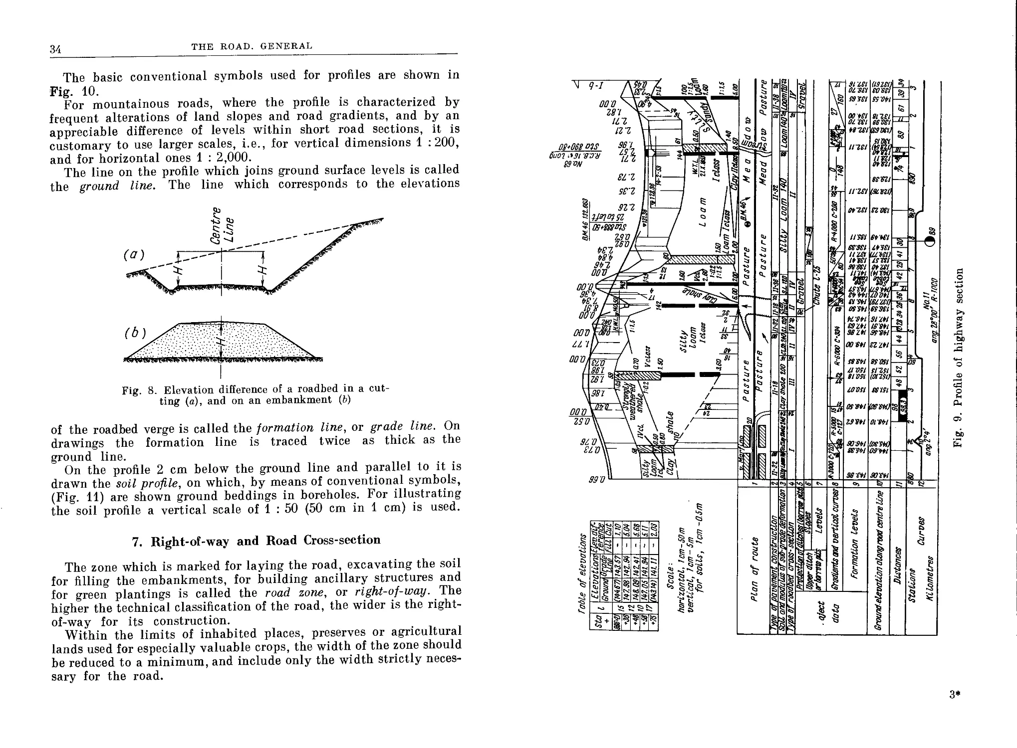
The graphical representation of the profile is one of the main work-
ing drawings, on which the construction of the road is based.
The drawing of the profile has to conform strictly with established
rules. Figure 9 shows an example of a drawing of a profile, as recom-
mended in the U.S.S.R.
In order to accentuate the profile visually, the vertical intervals
(levels) are drawn to a larger scale than the horizontal ones. For
roads laid in a flat country the accepted vertical scale is 1 : 500
(5 m in 1 cm) and the horizontal scale is 1 : 5,000 (50 m in 1 cm).
3-820
34
THE ROAD. GENERAL
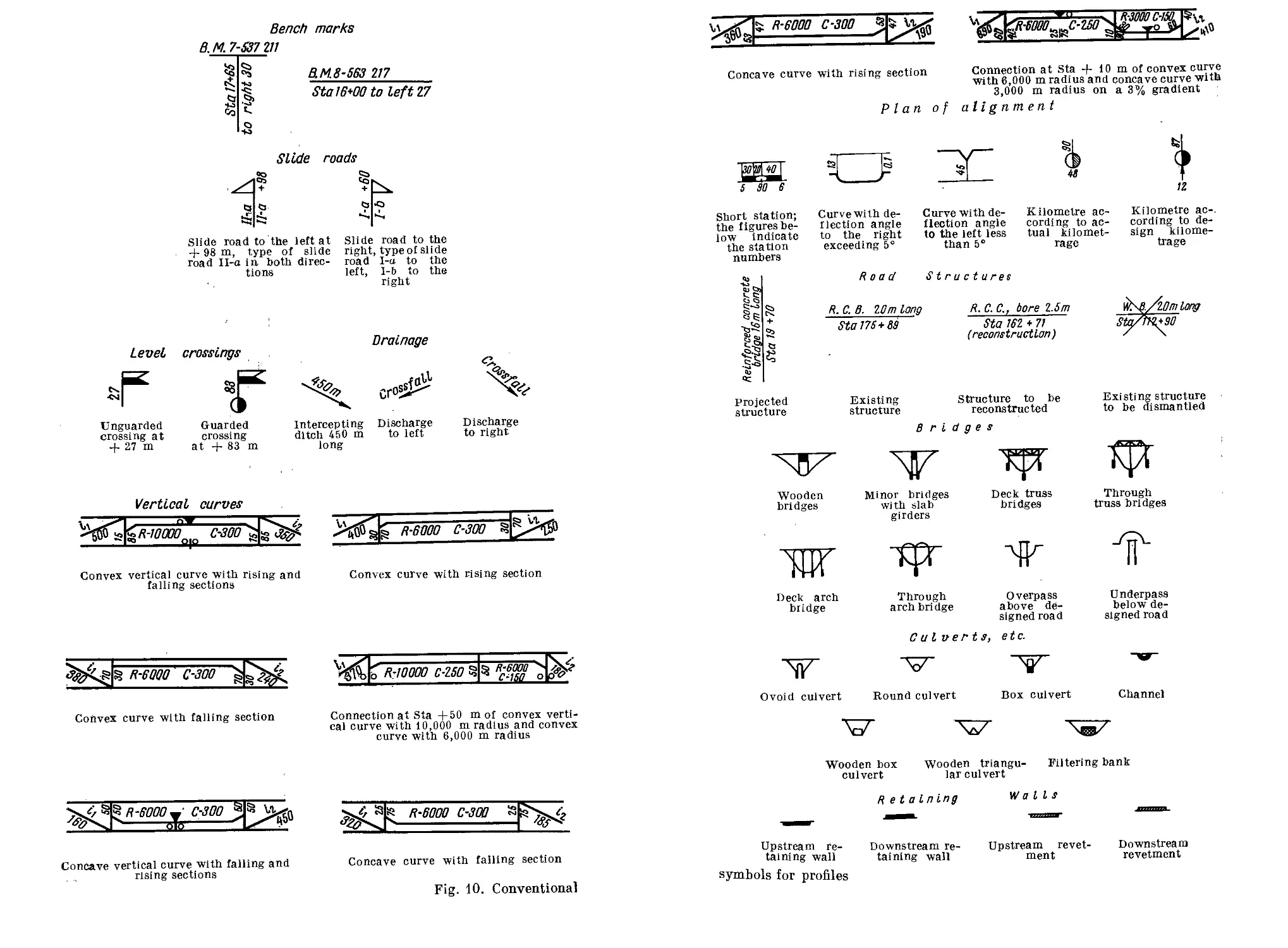
The basic conventional symbols used for profiles are shown in
Fig. 10.
For mountainous roads, where the profile is characterized by
frequent alterations of land slopes and road gradients, and by an
appreciable difference of levels within short road sections, it is
customary to use larger scales, i.e., for vertical dimensions 1 :200,
and for horizontal ones 1 : 2,000.
The line on the profile which joins ground surface levels is called
the ground line. The line which corresponds to the elevations
Fig. 8. Elevation difference of a roadbed in a cut-
ting (a), and on an embankment (6)
of the roadbed verge is called the formation line, or grade line. On
drawings the formation line is traced twice as thick as the
ground line.
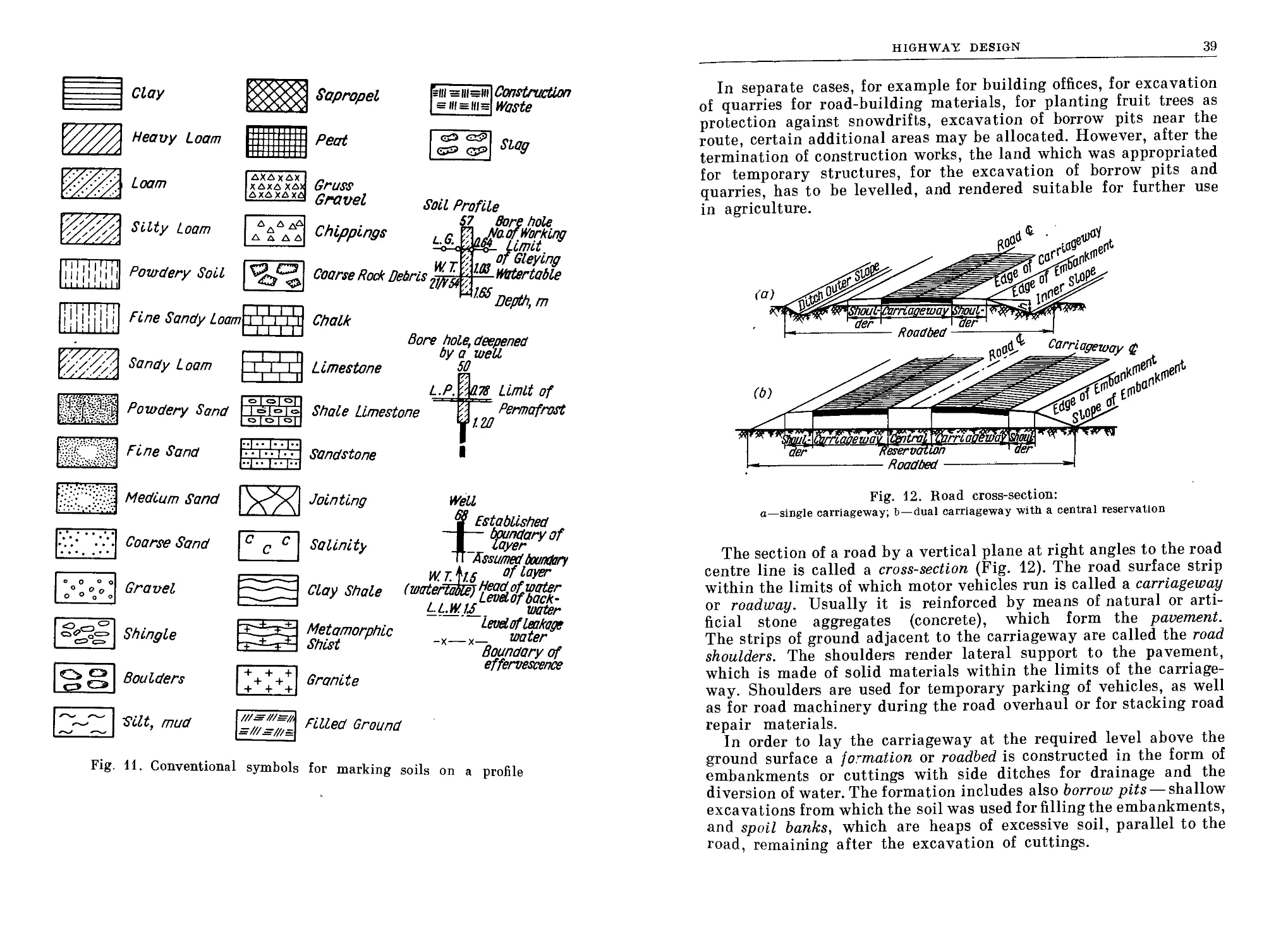
On the profile 2 cm below the ground line and parallel to it is
drawn the soil profile, on which, by means of conventional symbols,
(Fig. 11) are shown ground beddings in boreholes. For illustrating
the soil profile a vertical scale of 1 : 50 (50 cm in 1 cm) is used.
7. Right-of-way and Road Cross-section
The zone which is marked for laying the road, excavating the soil
for filling the embankments, for building ancillary structures and
for green plantings is called the road zone, or right-of-way. The
higher the technical classification of the road, the wider is the right-
of-way for its construction.
Within the limits of inhabited places, preserves or agricultural
lands used for especially valuable crops, the width of the zone should
be reduced to a minimum, and include only the width strictly neces-
sary for the road.
сл
~Si
я
jto
St
й
00'0
C)
£>
s>
g
s-j
I
В
ar
ZZ 7
CE
99'0
*5
qj
Si
Cj
S&
<3
Й
§
Z60
*81
*9*
9*1
000
00'0
98'*
*8Z
г/
08+068 KS
био? Л91 '92'9
99 ON
I LI
121
961
£TZ
9£’Z
9Z'Z
09+VWS
Ъ
сч
S3
ii_
tj
wo
ж 31
Z6‘l 41
3
Qj
00'0
ZS'Q
9t'0
£1'0
£ 1
%
««
St
81
51
Cj
~5i
в
i
Й
q>
rzr \§ t-A cm\ ffr ЗУ" В 1 т et 7w 1 Cj I Or 52r §& *•»> <fe Ci <?a 1 *; 31 ‘Ш 01 ’981 S3'SSI OOtfl 01 SSI W ISi H’ZSl irisi OTZSI ussi SS3SI itzsr itVSi 98881 inn tf-sw S^'^l SiSH OS'Sn К'ЗП S9in ЗВ1П 00 Mi S3 Ml U VS I 81’091 LOOS I OS Ml Z9WI 90MI SS'Ml 30 Mi (19Z81) £0 SSI SS'Oil 81281 86 OS I ^9VSl) siWt, m liSZi мои SS'OZl (SLSZO SZVSl orwi MSSl msi) SS-SSi OtZSi (UVH) № {OL'iSD 6S9SI 91 IS 8П 9SMI Gl'in SS'OSi srzsi (01291) SS'lSl (OSMi)\ 0Г9Ы (OSS^i) 09MI 90'Ml
co O1
Gradients and vertical curves Formation levels Ground elevation along rood centre line
5 §
•й:
S3
«о
TL
см
в
3
См
os
5oy
Fig. 9. Profile of highway section
г?
kj
<0
Et
Diet an Ci g
3*
Bench marks
В. M. 7-537 2//
В. М.8-563 217
Sta 16*00 to left 27
Slide roads
Slide road to the left at
+ 98 m, type of slide
road П-a in both direc-
tions
Slide road to the
right, type of slide
road I-a to the
left, I-b to the
right
Level crossings
Drainage
Unguarded
crossing at
4- 27 m
Guarded
crossing
at + 83 m
Intercepting Discharge
ditch 450 m to left
long
Discharge
to right
Vertical curves
, ,.о
R-10000 C-300
g|g
fa> R-6000 C-300
Convex vertical curve with rising and
falling sections
Convex curve with rising section
Convex curve with falling section
R40000 C-250 §
S R-6000
0-150 о
Connection at Sta +50 m of convex verti-
cal curve with 10,000 m radius and convex
curve with 6,000 m radius
R-6000** C-300
dTd1.......
R-6000 C-300
Concave vertical curve with falling and
rising sections
Concave curve with falling section
Fig. 10. Conventional
5: R-eOOO C-300
Concave curve with rising section
Plan of
Connection at Sta 4- 10 m of convex curve
with 6,000 m radius and concave curve with
3,000 m radius on a 3% gradient
alignment
5 SO 6
Short station;
the figures be'
low indicate
the station
numbers
Curve with de-
flection angle
to the right
exceeding 5°
Curve with de-
flection angle
to the left less
than 5°
Kilometre ac-
cording to ac-
tual kilomet-
rage
Kilometre ac-
cording to de-
sign kilome-
trage
Road Structures
/?. С. B. ZOm long В. C. C,f bore Z.5m
Sta 175+83 Sta 162 *71
(reconstruction)
WTB/20т long
Sta/frz*30
Projected
structure
Existing
structure
Structure to be
reconstructed
Existing structure
to be dismantled
Bridges
Wooden Minor bridges Deck truss
bridges with slab bridges
girders
Through
truss bridges
Deck arch
bridge
Through
arch bridge
Overpass
above de-
signed road
Underpass
below de-
signed road
w
Culverts, etc.
Ovoid culvert Round culvert Box culvert
Channel
Wooden box
culvert
Wooden triangu- Filtering bank
lar culvert
Retal nlng
Walls
Upstream re-
taining wall
symbols for profiles
Downstream re-
taining wall
Upstream revet-
ment
Downstream
revetment
Sapropel
Construction
Waste
Clay
Peat
Gruss
Chalk
hi =111=111
Stag
Gravel soil Profile
Chippings
Coarse Rock Debris
Silt, mud
Limestone
Shale Limestone
Sandstone
Jointing
Salinity
Clay Shale
Metamorphic
Shist
Granite
dore hole, deepened
by a well
50
Permafrost
Well
W,tAu of layer
(w^^^H&°ffWbKk-
water
level of leakage
_x________x_ water
Boundary of
effervescence
Pilled Ground
Fig. 11. Conventional symbols for marking soils on a profile
HIGHWAY DESIGN
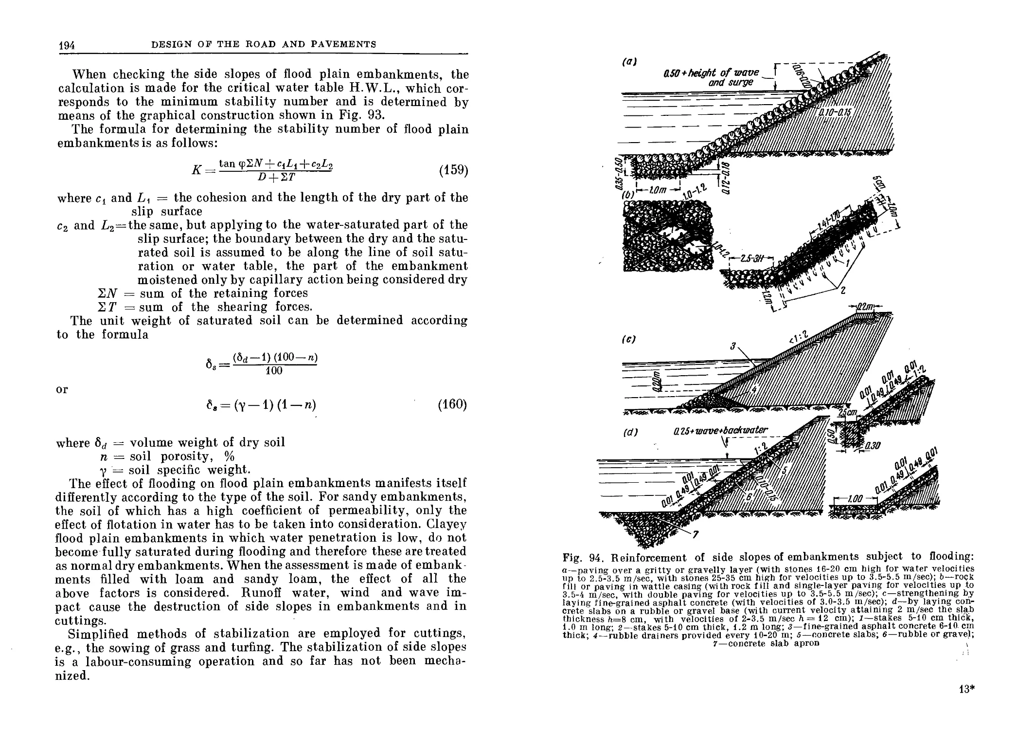
39
In separate cases, for example for building offices, for excavation
of quarries for road-building materials, for planting fruit trees as
protection against snowdrifts, excavation of borrow pits near the
route, certain additional areas may be allocated. However, after the
termination of construction works, the land which was appropriated
for temporary structures, for the excavation of borrow pits and
quarries, has to be levelled, and rendered suitable for further use
in agriculture.
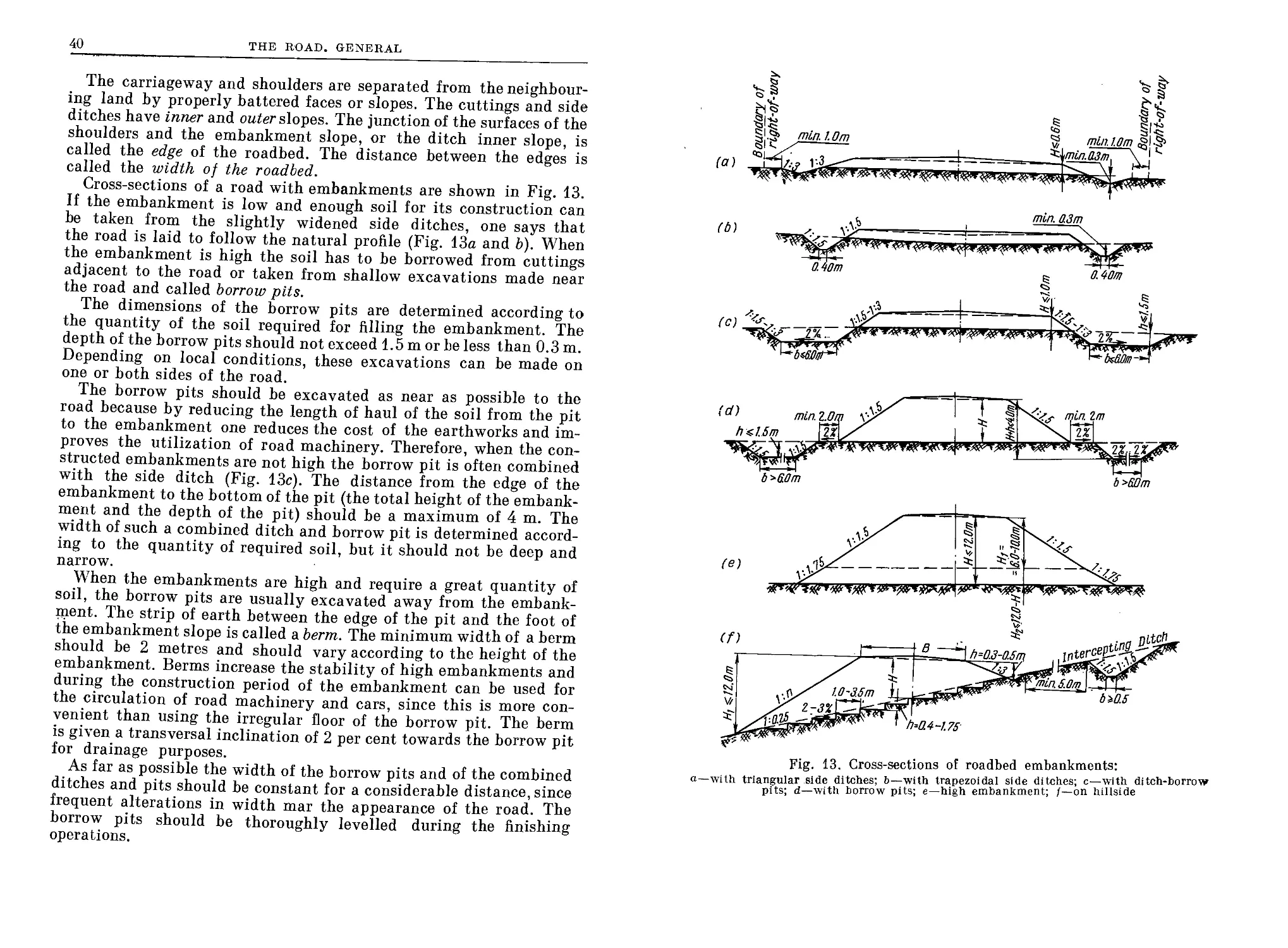
Fig. 12. Road cross-section:
a—single carriageway; b—dual carriageway with a central reservation
The section of a road by a vertical plane at right angles to the road
centre line is called a cross-section (Fig. 12). The road surface strip
within the limits of which motor vehicles run is called a carriageway
or roadway. Usually it is reinforced by means of natural or arti-
ficial stone aggregates (concrete), which form the pavement.
The strips of ground adjacent to the carriageway are called the road
shoulders. The shoulders render lateral support to the pavement,
which is made of solid materials within the limits of the carriage-
way. Shoulders are used for temporary parking of vehicles, as well
as for road machinery during the road overhaul or for stacking road
repair materials.
In order to lay the carriageway at the required level above the
ground surface a formation or roadbed is constructed in the form of
embankments or cuttings with side ditches for drainage and the
diversion of water. The formation includes also borrow pits — shallow
excavations from which the soil was used for filling the embankments,
and spoil banks, which are heaps of excessive soil, parallel to the
road, remaining after the excavation of cuttings.
40
THE ROAD. GENERAL
The carriageway and shoulders are separated from the neighbour-
ing land by properly battered faces or slopes. The cuttings and side
ditches have inner and outer slopes. The junction of the surfaces of the
shoulders and the embankment slope, or the ditch inner slope, is
called the edge of the roadbed. The distance between the edges is
called the width of the roadbed.
Cross-sections of a road with embankments are shown in Fig. 13.
If the embankment is low and enough soil for its construction can
be taken from the slightly widened side ditches, one says that
the road is laid to follow the natural profile (Fig. 13a and b). When
the embankment is high the soil has to be borrowed from cuttings
adjacent to the road or taken from shallow excavations made near
the road and called borrow pits.
The dimensions of the borrow pits are determined according to
the quantity of the soil required for filling the embankment. The
depth of the borrow pits should not exceed 1.5 m or be less than 0.3 m.
Depending on local conditions, these excavations can be made on
one or both sides of the road.
The borrow pits should be excavated as near as possible to the
road because by reducing the length of haul of the soil from the pit
to the embankment one reduces the cost of the earthworks and im-
proves the utilization of road machinery. Therefore, when the con-
structed embankments are not high the borrow pit is often combined
with the side ditch (Fig. 13c). The distance from the edge of the
embankment to the bottom of the pit (the total height of the embank-
ment and the depth of the pit) should be a maximum of 4 m. The
width of such a combined ditch and borrow pit is determined accord-
ing to the quantity of required soil, but it should not be deep and
narrow.
When the embankments are high and require a great quantity of
soil, the borrow pits are usually excavated away from the embank-
ment. The strip of earth between the edge of the pit and the foot of
the embankment slope is called a berm. The minimum width of a berm
should be 2 metres and should vary according to the height of the
embankment. Berms increase the stability of high embankments and
during the construction period of the embankment can be used for
the circulation of road machinery and cars, since this is more con-
venient than using the irregular floor of the borrow pit. The berm
is given a transversal inclination of 2 per cent towards the borrow pit
for drainage purposes.
As far as possible the width of the borrow pits and of the combined
ditches and pits should be constant for a considerable distance, since
frequent alterations in width mar the appearance of the road. The
borrow pits should be thoroughly levelled during the finishing
operations.
Fig. 13. Cross-sections of roadbed embankments:
a—with triangular side ditches; b—with trapezoidal side ditches; c—with ditch-borrow
pits; d—with borrow pits; e—high embankment; /—on hillside
42
THE ROAD. GENERAL
When planning the earthworks one should try to use earth exca-
vated from cuttings or from the levelling of ground irregularities
within land not being used for agriculture, rather than borrow soil
from pits. The sides of the embankments are battered to form regular
slopes. The slope gradient is specified by the slope ratio, i.e., by
the ratio of the height of the slope to its horizontal projection.
The slopes of small embankments, with maximum heights of 1 m,
are made with a ratio of 1 : 3* or less, in order to enable vehicles
to drive off the road in an emergency.
Embankments having a height of more than 1 m, and the embank-
ments at approaches to bridges, at fluvial plains, marshes and in
other places where there is no possibility of diversion off the road,
ure formed with steep side slopes, of 1 : 1.5. This applies to embank-
ments up to a maximum height of 6 m. Long experience proves that
such embankments are quite stable. Steeper slopes of high embank-
ments, however, may fail under the influence of their own weight, or
the weight of a vehicle stationed on the shoulder, when the soil
is saturated.
To ensure the stability of higher embankments the foot of the
slope is made less steep (1 : 1.75). The depth of the above section of
the embankment having the ratio of 1 : 1.5 is taken as 6 m in clay,
loamy and silty ground; 7 m in sandy loam and fine sand; 9 m in
medium and coarse sand; and 10 m in gravelly, gritty and soft, easi-
ly weathered rocky ground. The gradients of the inner slopes of the
borrow pits are made the same as those of the embankments for
which the borrowed material is being used.
The cross-section of a cutting in flat country is shown in Fig. 14a.
If the soil excavated from the cutting is not suitable as fill material
und if there is no practical reason to haul it to the nearby fills, then
it may be used primarily for filling depressions of the site, or for
•easing the embankment slopes. If no other use of the soil is practi-
cal, it may be heaped at the side of the road, parallel to the edge of
the cutting, into spoil banks which must be given a proper geomet-
rical shaping.
The maximum height of a spoil bank should be 3 m; and the
slopes facing the road should not exceed 1 : 1.5. The minimum dis-
tance of the spoil banks from the external edge of the slope of the cut-
ting must be 3 m. If the cutting is made in water-bearing soil and
spring water can seep from its slopes, the weight of the banked up
soil may cause slips to develop. To prevent this, in soft and wet
ground the spoil banks are placed at a minimum distance of H + 5 m
from the edge of the cutting, where H is the depth of the cutting
in metres.
* This denotes a slope of 1 vertical to 3 horizontal.—Tr.
HIGHWAY DESIGN
43
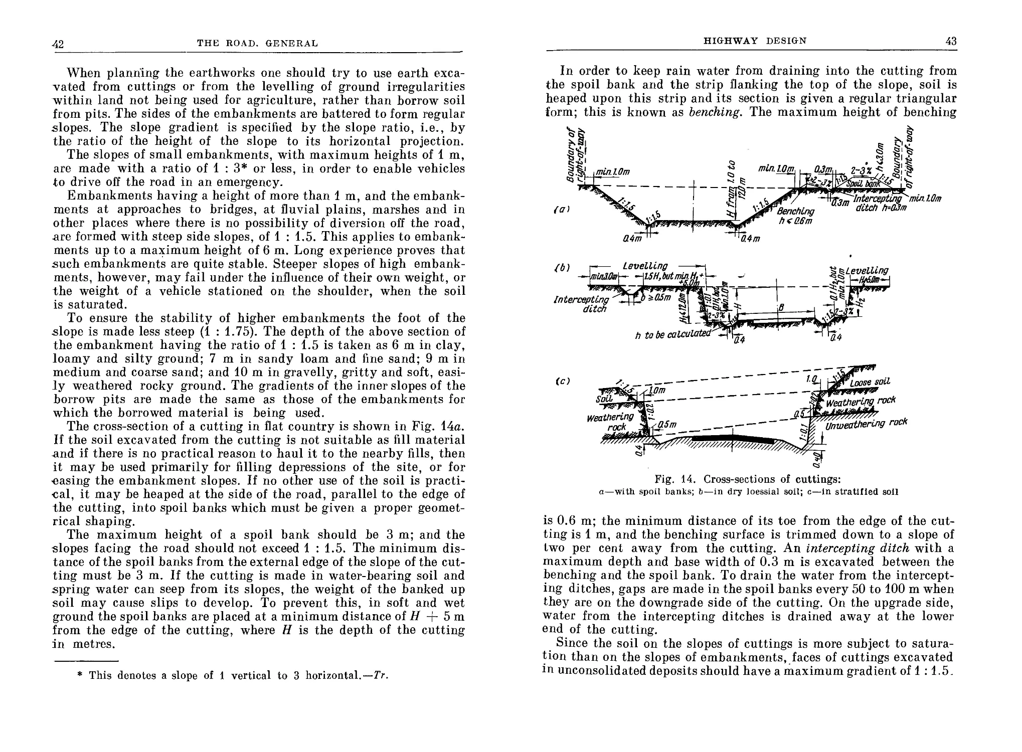
In order to keep rain water from draining into the cutting from
the spoil bank and the strip flanking the top of the slope, soil is
heaped upon this strip and its section is given a regular triangular
form; this is known as benching. The maximum height of benching
(c)
Fig. 14. Cross-sections of cuttings:
a—with spoil banks; b—in dry loessial soil; c—in stratified soil
is 0.6 m; the minimum distance of its toe from the edge of the cut-
ting is 1 m, and the benching surface is trimmed down to a slope of
two per cent away from the cutting. An intercepting ditch with a
maximum depth and base width of 0.3 m is excavated between the
benching and the spoil bank. To drain the water from the intercept-
ing ditches, gaps are made in the spoil banks every 50 to 100 m when
they are on the downgrade side of the cutting. On the upgrade side,
water from the intercepting ditches is drained away at the lower
end of the cutting.
Since the soil on the slopes of cuttings is more subject to satura-
tion than on the slopes of embankments, faces of cuttings excavated
in unconsolidated deposits should have a maximum gradient of 1 :1.5_
44
THE ROAD. GENERAL
In gravels and loamy soils, the faces of cuttings and embankments
may be made with a slope of 1 : 0.5 to 1 : 1, depending upon the
granulometric composition and density of the soil. Weathered rock
may be trimmed down to a slope of from 1 : 0.5 to 1 : 0.2, according
to the degree of weathering, the characteristics of the rock and the
depth of the cutting. At the same time it is necessary to take
account of the dip of the stratified layers outcropping on the slope,
the resistance of the rock to weathering and the exposure of the
Fig. 15. Cross-sections of shallow cuttings in regions liable to snowdrifts:
a—open cutting; b—cutting with subsidiary embankment
slopes of the cutting. Rocks such as shale and chalk which, when
first excavated, seem quite stable become subject to intensive disin-
tegration and weathering on exposure and crumble badly where the
gradient is steep.
In countries with a dry climate vertical cuts can be made in lo-
essial soils because of their special structure (thin vertical channels
cemented with calcite) (Fig. 145). Hence cuttings in loesses may be
made with faces as steep as 1 :0.1. However, steady spalling of loes-
sial slopes occurs under the action of rain and wind. In order that
the weathered materials do not choke the road ditch, a berm is con-
structed between the foot of the slope and the external edge of the
ditch of a minimum width of 0.5 m, from which the weathered
material is periodically removed. Such a cross-section, however,
cannot be used in loess and loessial loams, neither can it be used in
regions having a humid or rainy climate.
If the cutting is made through heterogeneous strata, its face may
be given a broken or stepped contour (Fig. 14c). However, such
a profile is aesthetically most unattractive, its formation is rendered
difficult and, therefore, it is only permissible in cases where this
would result in an appreciable reduction in the cost of the earthworks.
When designing formations for construction in regions subject
to heavy snowfalls, one must take into account their ability to with-
stand snowdrifts (Fig. 15).
PART II
Traffic Requirements
to the Geometric Design of Highways
CHAPTER 3
TRACTIVE EFFORT AND PERFORMANCE OF VEHICLES
8. Movement of a Vehicle on a Road
All elements of a modern motor road should be designed to promote
the safe passage of motor vehicles proceeding at the maximum rated
speed (design speed).
The higher the traffic flow, the greater becomes the degree of
restriction to the movement of individual vehicles, causing a reduc-
tion of their speed. Therefore, the requirements which are to be
satisfied by the various elements of the road plan and profile, i.e.,
vertical and horizontal curve radii, the width of the carriageway,
etc., must be based on the conditions of movement of a single motor
vehicle travelling at a specific speed.
A moving motor vehicle is subjected to an exceedingly complex
system of motions and forces, i.e., forward motion in a straight line,
rotation about a vertical axis when driving around bends, vertical
and horizontal vibrations caused by road irregularities, etc. Not
all these traffic problems can yet be fully taken into account when
defining the requirements with which the road is to comply. Because
of this, when designing a road one assumes that the vehicle is moving
without vibrations along an absolutely smooth hard surface which
is not subject to deformation.
9. Resistance to Motion of a Vehicle
The tractive effort developed by a motor vehicle engine is used
to overcome the forces resisting its propulsion.
Taking a general example of acceleration up a gradient, the fol-
lowing resistance forces are acting on the vehicle (Fig. 16): the
46 TRAFFIC REQUIREMENTS TO THE GEOMETRIC DESIGN OF HIGHWAYS
rolling resistance (rolling friction) Р/, the resistance to motion up
a gradient air resistance Pw, inertia forces Pj which occur when
the speed is altered.
The forces of rolling resistance and air resistance are always acting
on any vehicle in motion. Those of the resistance due to the gradient
and the forces of inertia depend on the character of the road profile
and on the vehicle operating conditions. These forces may he absent,
or even have a negative value assisting the movement (e.g., move-
ment downgrade).
Rolling resistance is caused by shocks and impacts when the
wheels of the vehicle run over the irregularities of the road surface,
Fig. 16. Forces acting on a vehicle
on an inclined plane
by the loss of power caused by the deformation of pneumatic tyres
and by plastic and elastic deformations of the road pavement.
When the movement takes place along metalled roads on which
no ruts are formed, the rolling resistance is directly proportional
to the rolling load
= Gdi (2)
where Gt = rolling load of individual wheels
ft = corresponding factor of rolling resistance.
When the movement causes the formation of ruts, a more compli-
cated relation occurs between the vehicle rolling resistance and
the wheel load
(3)
in which H = depth of the rut after passing of the wheel
D — wheel diameter
g = coefficient which varies from 0.6 to 1 depending on
the state of the ground.
Usually the factor of rolling resistance is assumed to be directly
related to the total weight of the motor vehicle, i.e., one assumes
TRACTIVE EFFORT AND PERFORMANCE OF VEHICLES
47
where 2^/ total rolling resistance of all the wheels of the vehicle
G = weight of the vehicle.
The factors of rolling resistance for wheels with pneumatic tyres
running on various surfacings have the following values:
Factor of rolling
resistance
Cement concrete and asphalt surfacing 0,01 to 0.02
Road with smooth chippings or gravel surface, treated
with bituminous binders 0.02 to 0.025
Chippings or gravel surfacings, not treated with
binder, having small pot-holes 0.03 to 0.04
Cobblestone pavement 0.04 to 0.05
Earth road, smooth, dry and compact 0.03 to 0.06
Ploughed field, saturated and swampy ground, loose sand 0.15 to 0.30 and over
The rolling resistance upon various surfaces is attributable to
different reasons. On smooth cement concrete and asphalt surfacings
the main cause of resistance to motion is the deformation of tyres.
On less smooth surfacings—chippings, gravel and cobblestone pave-
ments, additional rolling resistance is caused by the absorption of
power in deforming springs and shock absorbers when impacts and
jolts occur due to the surface irregularities. When traversing an
irregular and muddy road, additional resistance is created by the
compaction and extrusion of soil in the formation of ruts, the sticking
of soil to the wheels, the spinning of wheels, impacts and jolts due
to the vehicle swaying on bumps.
The rolling resistance depends on the speed of the vehicle and the
elasticity of the tyres. Each time a wheel runs over a road surface
irregularity a shock occurs which causes a loss of wheel velocity.
To propel the vehicle with constant speed on an irregular surface,
additional power is required. Since the magnitude of jolts in this
case is proportional to the square of the rolling velocity, the factor
of rolling resistance increases with the speed of the vehicle. When
the speed exceeds a certain critical value the tyres develop radial
vibrations, and the factor of rolling resistance increases sharply.
The lower the air pressure in the tyres, the less is the speed at which
this effect takes place. Nevertheless, one can assume that up to the
speeds of the order of 50 km/hr the value of the factor of rolling
resistance remains practically constant (Fig. 17).
When calculating tractive efforts corresponding to motor vehicles,
moving at a speed approaching the design speed of the road, i.e., in
the range of 50 to 150 km/hr, one should take account of the increase
of the factor of rolling resistance as expressed by the following
formula:
fv=~- /о [1 + 0.01 (7-50)1 (5)
where V is the speed in km/hr.
48 TRAFFIC REQUIREMENTS TO THE GEOMETRIC DESIGN OF HIGHWAYS
In calculations related to the traversing of a road by high-speed
motor cars, for instance racing cars, it is necessary to refer to the
values of this factor established by relevant experiments on high-
speed tracks.
Air resistance is caused by:
{!) reaction pressure of the air against the front of the vehicle;
{2) the friction of the air against the sides of the car body;
(3) power loss caused by eddying of the air stream behind the vehi-
cle, under the body and around the wheels.
Fig. 17. Relation between the factor of rolling
resistance and traffic speeds for various tyre
pressure (the figures next to the curves give the
tyre pressure in kg/cm2)
According to the laws of aerodynamics, the air resistance to auto-
mobile motion is expressed by the following relation:
D cpcoU2
Pw== 13
where c — factor of ambient air resistance (a dimensionless factor,
depending on the shape of the body moving in the air,
and also on the smoothness of its surface)
p = density of air, which at sea level is 0.125 kg-sec2/m4
a> = area in square metres of the projection of the vehicle on
a plane at right angles to the direction of its movement
(frontal projection); for modern vehicles it can be ob-
tained by the following formula: a> = 0.775 BH, where
В and H are overall width and height of the motor vehicles
V = motor vehicle.speed relative to the ambient air, km/hr;
with following wind V = (Vveh —Vwind);
with head wind V = (Vveh + Fwfnd).
TRACTIVE EFFORT AND PERFORMANCE OF VEHICLES
49
TABLE 2
Type of vehicle
Coefficient of air
resistance K,
kg - sec2/m4
Area of frontal
projection to, m2
Truck
Single-deck coach
Semi-streamlined passen-
ger car
Streamlined racing car
0.05 to 0.07
0.025 to 0.05
3 to 6
4 to 6.5
0.015 to 0.03
0.010 to 0.015
1.5 to 2.6
1.5 to 2.0
For automobile calculations the product ep is replaced by the
coefficient of air resistance K, which is determined experimentally
(Table 2).
Customarily, time-speed-distance calculations are made assuming
calm windless weather conditions.
Air resistance increases sharply with increase of traffic speed and
is the main type of resistance encountered by moving passenger
cars. Because of this, when designing motor cars, substantial con-
sideration is given to the possibility of reducing air resistance by
means of improving the streamlining of the body.
The contour of a vehicle has a great influence on the air resistance.
By means of comparatively simple alterations in the shape of truck
bodies one can reduce the value of the air resistance factor and, there-
fore, increase the economic and dynamic characteristics of the vehi-
cle (Fig. 18). It must be mentioned that arrangements which lower
the resistance to motion of a solo vehicle may adversely influence
the streamlining when the vehicle is used as the tractor of a combi-
nation vehicle.
The resistance to motion when driving a vehicle up an incline with
a slope i is increased as the result of the additional work done in
propelling the vehicle up the slope.
If the length of the slope is L and the height gained as the result
of travelling up the slope is /7, then the additional work needed for
propelling a vehicle of weight G up the slope can be expressed as
F = GH
Ignoring the difference between the actual length of the inclined
section and its horizontal projection, which will be negligible in the
case of longitudinal gradients on a motor road, the additional work
done in travelling a unit distance up the slope is
GH
4-820
50 TRAFFIC REQUIREMENTS TO THE GEOMETRIC DESIGN OF HIGHWAYS
Should the incline or slope i be expressed in per cent, then formu-
la (7) will become
Thus the work done in travelling* unit distance up the slope is the
product of the total weight and the value of the tangent of the slope
expressed as a decimal fraction.
К=0040-0035 K=0035-0030
K=0.OZ5-OO2j0
K=0030-0015
K=0.062
Fig. 18. Influence of the aerodynamic shape of a vehicle on the
factor of air resistance
(8)
The resistance of the inertia forces of a vehicle is made up of the
inertia of the forward motion and the inertia of the revolving
parts of the vehicle. These forces act on the vehicle during its ac-
celeration or deceleration.
If the mass of the vehicle is m — G/g, then the inertia force of the
forward motion is
du G du „.
=--------
J dt g dt
where dv/dt = vehicle acceleration
7 = acceleration relative to gravitational.
With the alteration of the vehicle speed, one must add to the
inertia of the forward motion the inertia of the vehicle revolving
parts (wheels, flywheel and transmission gears).
TRACTIVE EFFORT AND PERFORMANCE OF VEHICLES
51
• The exact value of the inertia forces can be calculated according
to the dimensions and weight of the revolving parts. However, in
practice, to take into account the influence of the revolving parts,
the forward-motion inertia is usually used with a correction factor 0,
which gives the ratio between the total force necessary to give the
impetus to all the vehicle parts having translational and rotation-
al motion, and the force required exlusively for the impetus of
masses in translation
(9)
With the increase of the gearbox reduction ratio the value of the
factor p increases. With a direct drive the value of the factor 0 varies
between 1.03 and 1.07. Using other gears, its value increases
approximately as follows:
p = 1.04 + ml (10)
where = gearbox reduction ratio
n = factor equal to 0.03-0.05 for passenger cars and to
0.05-0.07 for freight vehicles.
When a vehicle is proceeding with a frequently varying speed and
with frequent stops, for example in urban conditions, apart from
the inertia of the revolving parts a peculiar engine thermal inertia
arises. For established operating conditions of an engine proceed-
ing with a constant speed on a smooth horizontal sector there are
corresponding constant conditions of engine temperature and of fuel
admission and combustion. When, on the other hand, the speed
varies, the engine cannot adapt itself immediately to the alterations
of loading and therefore the combustion process in the engine takes
place under less advantageous conditions than with constant operat-
ing conditions. This causes a certain decrease in the available
tractive effort.
The influence of unstable engine operating conditions on the dyna-
mics of the vehicle can be taken into account, as in the case of
revolving engine parts, by introducing a correction factor 6 in the
expression for the inertia of masses having a translatory movement.
The additional inertia resistance due to the influence of unstable
engine operating conditions is therefore
(11)
The value of the factor 6 for trucks is 0.07-0.075, and for pas enger
cars it is 0.075-0.085.
Thus, the general expression of the resistance of inertia forces to
the vehicle movement is as follows:
Р> = СЯ1.04 + (п + б)Ш (12)
4*
52 TRAFFIC REQUIREMENTS TO THE GEOMETRIC DESIGN OF HIGHWAYS
10. Dynamic Characteristics of a Vehicle
The mechanical power generated by the vehicle engine is trans-
ferred by the transmission of the vehicle to its driving wheels.
At the area of contact of the wheel with the road the wheel
Fig. 19. Driving wheel
tractive effort
torque Mw induces a tractive force Pp
equal to
Pp = ^- (13)
r w
where rw = Xr0 is the radius of the wheel
rolling circle with account
taken of the tyre deforma-
tion (Fig. 19).
The tyre deformation factor к on a
hard surface will attain 0.945-0.950 for
high-pressure air tyres and 0.930-0.935
for low-pressure tyres.
The driving wheel torque Mw is the product of the engine torque
Mb, the gear ratios of the transmission and the mechanical efficiency
Mw = Mbigimv\
(14)
where ig = gearbox transmission ratio
im — main drive transmission ratio
q = mechanical efficiency of the vehicle transmission, which
takes account of the power loss due to overcoming the
resistance of all mechanisms between the engine and the
driving wheels.
The tractive effort Pp is therefore
MbigW]
„Р ~ Z
rU)
(15)
But the engine torque is proportional to the engine horsepower Nb
and inversely proportional to the number of revolutions of the crank-
shaft n, hence Mb = Nb/n, and formula (15) will transform into
the expression
Pp = 716.2^% (16)
nrw
where Nb is the engine brake horsepower.
The speed of the vehicle is related to the crankshaft speed, as
follows: .
' t 1 ,, 1 ’
; # -i m/sec
• ' 1 60igim
TRACTIVE EFFORT AND PERFORMANCE OF VEHICLES
53
or
7 = °'377Гц)- km/hr
(17)
where n ~ crankshaft speed, rpm
ig and im = transmission ratios of the gearbox and of the main
drive.
The maximum vehicle speed corresponds to the minimum trac-
tive effort. Therefore, when a vehicle is moving along a good road,
where the resistance to rolling is small,
be used — 1). When negotiating
a gradient or driving along a bad
road, one will need to change down
to a lower gear.
The horsepower produced depends
on the rotational speed of the engine.
This relation is usually determined
experimentally and represented dia- 4
grammatically by external power-
speed characteristics (Fig. 20).
The vehicle external power-
speed characteristics are usually
obtained by testing the vehicle at
full throttle for engines fitted with
carburettors or, in the case of fuel
injection, at maximum fuel
delivery. Therefore, these
specify the maximum power
the engine can develop.
Using this characteristic,
determine by calculation
speeds, assuming that it
to propulsion.
Equating external and
is obtained:
the direct drive will tend to
iso
140
iso
120
110
100
so
80
70
60
50
40
30
20
10
0
pump
curves
which
800 1600 2400 3200 4000
n, rpm
Fig. 20. External pover-speed
characteristics of engines
and formulas (6) and (16), one can
tractive effort Pp at various vehicle
the
is utilized in overcoming the resistance
internal forces, the following expression
Pp — Pf ± Pi + Pw i P j
(18)
where Pf — rolling resistance
Pi resistance to motion up ( + ) or down (—) a gradient i
Pw = air resistance to movement
Pj~ resistance of inertia forces, the ± sign indicating that,
depending on the correlation of the external resist-
ance forces, the vehicle may be either accelerating or
decelerating.
Transferring the air resistance, which depends on the speed of the
vehicle, to the left side of the equation and substituting the
ОАО
032
^0.24
о
ом
— Moskvich 407
— Zaporozhets
- М- 27 Volga
- М-20 Pobeda
- ZIL-ГЮ
го
40 60 80 WO 1Z0 140 160
Speed, km/hr
0.08
(b)
Fig. 21. Motor vehicle dynamic characteristics:
a—passenger cars; b—commercial vehicles
TRACTIVE EFFORT AND PERFORMANCE OF VEHICLES
55
values of the resistances as determined in Sec. 9, we obtain
Pp - Kav* ^Gf ±Gi± Gj (19)
The Soviet Academician E. A. Chudakov proposed to define the
tractive, or dynamic, characteristics of a motor vehicle by means of
a dynamic factor, which is the difference between the full tractive
effort on the driving wheels and the air resistance, per unit weight
of the vehicle
The dynamic factor gives the surplus of the tractive effort per unit
weight of a vehicle moving with a speed v, which can be used for
overcoming road resistance (/ ± 0 and for imparting to the vehicle
the acceleration /.
The tractive effort and the air resistance depend on the speed of
the vehicle. Therefore, the value of the dynamic factor does not
remain constant but is varied with change of speed. The diagram
showing the relation between the dynamic factor and the speed, known
as a dynamic characteristic (Fig. 21), is used in the Soviet Union
as a basic index of automobile traction performance and underlies
all motor road time-speed-distance calculations.
11. Adhesion of Pneumatic Tyres
to the Road Surface
The driving wheel tractive effort may be developed only if there is
sufficient adhesion between the driving wheels and the road. The
ratio of the tractive effort generated at the contact face Pp to the
vertical load on the wheel Gw at which the wheel starts slipping
(spinning), is called the coefficient of adhesion and is designated by
the symbol ip.
To improve the conditions of adhesion between the tyre and the
road surface and to expel water more effectively when running on
a wet road, the tyre contact surface is grooved creating a salient
pattern—a tread.
When determining the desirable characteristics of the road, two
separate coefficients of adhesion need to be taken into account:
1. The coefficient of adhesion corresponding to the commencement
of wheel spin without the development of any lateral force—this is
the coefficient of linear adhesion.
2. The coefficient of adhesion introduced when the wheel moves
at an angle to the plane of rotation, i.e., it is simultaneously spin-
ning and moving parallel to its axis—this is the coefficient of lat-
eral adhesion.
56 TRAFFIC REQUIREMENTS TO THE GEOMETRIC DESIGN OF HIGHWAYS
Since the tyre resilience is not the same in the plane of rotation as
in the lateral direction, the value of the coefficient of adhesion alters
with the tyre deformation in various directions.
However, for estimates relating to thr road design, it is usual
to assume that when a force acts on the wheel at an angle to the
direction of its rotation the absolute value of the coefficient of
adhesion is that of the coefficient of linear adhesion.
Numerous experimental investigations to determine the coeffi-
cient of adhesion have shown that its value is influenced more by the
condition of the road surface than by its type. This is because with
any surfacing, the protruding hard mineral parts press into the rub-
ber of the tread and, therefore, the wheel slips mainly owing to the
deformation of the rubber.
With continual wear and tear the roughness of the pavement de-
creases and with it there is a decrease in the adhesion properties
of the wheel.
In wet and muddy conditions the interstices in the pavement
surface become filled with dirt, dust, etc. A moist film acts as a lu-
bricant between the rough surfaces, wettening the area of contact
between the tyre and the tread, hence decreasing the value of the
coefficient of adhesion. At high traffic speeds the tyre is not given
sufficient time to deform fully and therefore the surface irregulari-
ties press into the tyre to a lesser depth causing a reduction in the
effective coefficient of adhesion. This effect is particularly apparent
on wet and dirty surfacings. On dry surfacings this reduction of the
coefficient of adhesion is less noticeable.
The relation of the safe, attainable coefficient of adhesion to the
forward speed on a wet cement concrete pavement as suggested by
the International Association of Civil Aviation for the design of
airfield runways, is shown in Fig. 22.
Since during the braking action the speed of the vehicle varies
over a wide range, calculations for the safe stopping distance are
based on the values of the coefficient of adhesion at speeds of the
order of 30 to 40 km/hr, which are the mean speeds for the
whole braking process. The values of the coefficient of linear adhesion
in relation to the state of the pavement are as follows:
Nature of road surface Coefficient of
linear adhesion
Dry, rough-surfaced (cement concrete) 1 to 0.7
Dry, smooth (bituminous surfacing) 0.5
Wet 0.4 to 0.3
Muddy 0.2
Ice covered 0.1
The conditions of pneumatic tyre adhesion to the road pavement
are related to the weather conditions, and the value of the coeffi-
cient of adhesion fluctuates greatly during the year.
TRACTIVE EFFORT AND PERFORMANCE OF VEHICLES
In summer it increases markedly. In winter, however, when ice
covers the road, the coefficient is much lower, and to increase adhesion
it is often necessary to fit antiskid chains to the wheels or spread
sand or grit over the road surface. Therefore, when estimating the
coefficient of adhesion for time-speed-distance calculations during
road design, one has to consider the climatic conditions of the re-
gion. Depending on the ratio of summer sunny and rainy days, the
length of the period of snow covering, and the frequency of occurrence
Fig. 22. Relation between the coefficient of adhesion
and aircraft speed over a wet cement concrete sur-
facing
of ice covering, a most typical condition of the pavement surface is
chosen, which is then used for time-speed-distance calculations. Also,
one has to consider the seasonal distribution of traffic, so that, in
the case of concentration at definite periods (e.g., seasonal agricultur-
al transportations), a maximum safety of traffic can be assured.
On the other hand, there is no necessity to base the design on the
pavement conditions at certain infrequent and short periods when
the weather conditions might deteriorate, since special precautions
can then be taken by the road service authorities with the introduc-
tion of temporary speed restrictions.
The coefficient of adhesion between the tyre and the surfacing is
one of the main traffic safety characteristics for a road, since, as it
is shown below, the extent of the stopping distance is inversely
proportional to the value of the coefficient of adhesion. The statis-
tics of accidents on roads show that the periods at which the value q>
decreases owing to weather conditions correspond to the increase
of the number of accidents (Fig. 23). In view of this, in a number of
countries the road maintenance organizations systematically check
the variation of the coefficient of adhesion, and when its value de-
creases below a certain minimum (usually <p = 0.4-0.5) have the duty
to display signs limiting the traffic speed, if this decrease has a tern-
58 TRAFFIC REQUIREMENTS TO THE GEOMETRIC DESIGN OF HIGHWAYS
porary character due to weather conditions, or take the necessary
precautions to increase the roughness of the surface—usually by
means of some surface treatment.
Fig. 23. Relation between the value of the coefficient of
adhesion and the number of accidents:
1—coefficient of adhesion; 2—number of accidents
The conditions of adhesion of the driving wheels with the road
surface limit the dynamic capabilities attainable in a motor car,
Vehicle speed
Fig. 24. Vehicle dynamic characteristic in relation
to adhesion
since with a poor coefficient of adhesion, the great tractive effort
which the engine can develop cannot be used owing to insufficient
adhesion.
Because of this, besides the engine horsepower dynamic characte-
ristics, adhesion dynamic characteristics are used for time-speed-
TRACTIVE EFFORT AND PERFORMANCE OF VEHICLES
59
distance calculations. The adhesion characteristics are deduced from
the tractive effort equation for motion without slipping*
G'cp - Gf ± Gi ± Gj + Kav* (21)
where G' is the driving* wheel pressure on the road.
Relating the balance of adhesion available over the ambient air
resistance to a unit of vehicle weight, the expression of the adhe-
sion dynamic characteristic becomes
G'cp —
G
(22)
An example of a dynamic characteristic chart related to the
conditions of adhesion is shown in Fig. 24.
12. Longitudinal Gradients Negotiated
by Motor Vehicles
The chart of dynamic characteristics permits the solution of prob-
lems concerning the motion of a
along a road and enables the follow-
ing to be determined:
(1) The magnitude of the lon-
gitudinal gradient which can be
negotiated at a given constant
speed.
To solve this problem with the
help of the chart of dynamic char-
acteristics, a vertical line is drawn
from the abscissa corresponding to
the given speed, to its intersection
with the curve of dynamic charac-
teristic (Fig. 25). The ordinate of
this point gives the value of the
dynamic factor D, which is equal
to the sum
г' + / + 7
Since it is assumed that the
motion takes place at constant
speed, then j = 0, and, therefore,
i = D—f
motor vehicle when travelling
Fig. 25. The use of dynamic char-
acteristics for time-speed-distance
calculations. (Roman numerals
denote the gear used.)
(2) The speed which a vehicle can maintain on a given gradient.
The factor required for this condition is obtained from the relation
Z>i =; i /
60 TRAFFIC REQUIREMENTS TO THE GEOMETRIC DESIGN OF HIGHWAYS
The speed v is determined by measuring the above value on the
ordinate axis and then finding the corresponding abscissa with the
help of the chart of dynamic characteristics (Fig. 25).
(3) The acceleration developed by a vehicle under the influence
of gravity.
With a rolling resistance factor /, a gradient i and an initial
speed v, the linear acceleration of the vehicle becomes
T-4r = 7>-tf+f) <23>
where f is a coefficient taking into account the influence of the
inertia of the revolving parts of the vehicle.
Since the solutions described above are based on the value of the
tractive effort developed by the engine, they have to be further checked
in relation to adhesion. For this reason, the same diagram should
contain curves expressing the dynamic characteristics in relation to
adhesion.
If the point obtained according to the first estimate is situated
below the curve of dynamic characteristics in relation to adhesion
then the assumed tractive effort will not cause slipping and the
estimate is correct.
The methods of assessment of tractive efforts given above relate
to what are termed equilibrium speeds, which are constant within
the limits of the gradient. However, the vehicle usually approaches
the slope with a certain accumulated momentum, which can be used
to overcome the additional resistance at the expense of a gradual
diminution in speed. If the gradient exceeds the incline correspond-
ing to the equilibrium speed, then the speed gradually falls.
Provided that the speed of the vehicle within the limits of the
gradient does not drop to zero, the vehicle can negotiate the
upgrade.
The question of the effect of a succession of gradients on adjacent
sections of a road upon motor traffic has not been fully investigated.
Sufficient account is seldom taken of this issue when designing
highways for motor vehicles. Nevertheless the rational coordination
of gradients can contribute to the improvement both of road trans-
port productivity and fuel economy, since it enables upgrades to be
traversed with the aid of initial impetus and, within the limits of
safety, reduces the use of brakes on downgrades.
If the initial momentum of vehicles is to be taken into account,
the question arises as to what will be the length of an upgrade of
slope imax —where imax is greater than the gradient i, the maximum
gradient of infinite length negotiable by vehicles—if the speed of
approach is and the speed at the end of the climb is not to be
less than V2.
TRACTIVE EFFORT AND PERFORMANCE OF VEHICLES
61
Assuming
the initial
VI. This
2g 2
a constant
momentum
tractive effort or engine propelling force,
is
and the terminal
momentum
difference in momentum is expended in overcoming
the additional resistance to motion up the gradient (imaX —i).
The additional work done on a gradient of length L is LG (iTnax—i).
Therefore
LG (V^-V*)
(24)
2g ki’
Hence, the maximum permissible length of road L having a gradi-
ent of imax L
T _ Р(Н-П) о,.
L 2s (imax-i) ( '
Here, as previously, the factor 0 includes the inertial effects of the
rotating masses.
The above calculation is only approximate since the ambient air
resistance has been assumed constant. A more detailed computation,
involving the solution of the differential equation governing the
law of motion of the vehicle, is given in the section dealing with
motion along vertical curves.
13. Motion of Motor Vehicle along a Curvilinear Profile
Stretches of modern automobile highways include various longi-
tudinal gradients which are interconnected by means of vertical
curves of large radii (see Sec. 64). In undulating country 50% or
more of the total length of highways in the higher classes may
consist of vertical curves.
When a vehicle is moving along a curved profile the longitudinal
gradient is constantly varying, and with it, the speed of the vehicle.
Thus the above conclusions regarding “equilibrium speeds’’ are only
relative.
In the equation of motion along a curvilinear profile the longitu-
dinal gradient must be considered variable (Fig. 26).
If the coordinate origin is placed at the point of the start of the
vertical curve, then the gradient at a certain point A is as follows:
* = а + £ = а + А.[/(г/)] (26)
where а — angle between the horizontal and the chord connecting
the extreme points of the curve which also serves as one
of the axes of coordinates
62 TRAFFIC REQUIREMENTS TO THE GEOMETRIC DESIGN OF HIGHWAYS
__ d If (y)] __ ang]e between the tangent to the vertical curve and
(Zu
the chord
/ (y) = equation of the vertical curve.
Fig. 26. Diagram illustrating the dynamics of
motion of a vehicle traversing a vertical curve
Horizontal
For the case considered the equation of the dynamic character-
istics is given by
Pp — Pw f , ₽ dv
--S-= 7 + “+ ds + ~~М
(27)
For the solution of the equation (27) Soviet engineer K. A. Khav-
kin assumed the vertical curve to be a parabola of the type
y=-Ts^S2
where co — deflection angle, formed by the adjacent sections of the
profile
S — abscissa of the curve, which may be assumed as about
equal to the distance travelled by the vehicle along
a vertical curve.
TRACTIVE EFFORT AND PERFORMANCE OF VEHICLES
63
The equation of the dynamic factor is replaced by an empiric
relation obtained from the equation (20) by substituting a parabola
for the external characteristic curve
P W 7 Q
—-------= a — bv2.
(29)
where v = speed, m/sec
a and b = indices characterizing the relation of the tractive effort
and the traffic speed in various gears and at various
throttle openings.
The values of the indices a, b and p for some cars of Soviet make
at full throttle opening are given in Table 3.
TABLE з
Type of motor car a b
GAZ-12 0.1096 0.52x10⁻⁴ 0.944x10⁻³
M-20 Pobeda 0.100 0.765x10⁻⁴ 1.39x10⁻³
GAZ-51 0.053 0.59x10⁻⁴ 1.091x10⁻³
ZIL-150 0.055 0.73X10’4 1.335x10⁻³
The solution of the differential equation (27) gives a formula for
determining the vehicle speed on various stretches of the vertical
curve:
vs = У (v- — kt) + kr + k2S (30)
where vt is the vehicle speed at the moment of entering the curve,
и— e
^i = y-(a-f~ii)—~
kz=±4b
the plus sign corresponding to motion along a convex curve, and
the minus sign to that along a concave one. By substituting R —
= oo and k2 — 0, formula (30) may be used for determining the speed
on a finite stretch of road with a uniform longitudinal gradient.
In Fig. 27 the results of speed calculations for the automobile
GAZ-51 on upgrades with uniform inclinations are compared with
those for a vertical curve with a radius of 10,000 m, assuming an
initial velocity of 70 km/hr.
64 TRAFFIC REQUIREMENTS TO THE GEOMETRIC DESIGN OF HIGHWAYS
It is worth noting that for negotiating a uniform gradient it is
necessary to change to a lower gear whilst the vertical curve enables
the vehicle to climb the gradient in direct drive. This shows that
Fig.
27. The effect of the introduction of
vertical curves on vehicle speed
the design of the profile with vertical curves not only increases
the safety of traffic, but also improves the technical and economi-
cal characteristics of the road.
14. Braking and the Characteristics of Vehicular Motion
on Downgrades
When determining the equation of motion of a vehicle down a gra-
dient, the resistance due to the gradient is given a negative sign.
Thus
p r w
(31)
This leads to an increase in the acceleration /, the vehicle will
gather momentum, and its speed will rise rapidly.
The limiting vehicle speed down a slope is attained theoretically
when the sum of ambient air and rolling resistances becomes equal
to the combined force of traction and the momentum due to rolling
down the incline, and the acceleration is reduced to zero
w
(32)
However, such a value would correspond to a very high vehicle
speed and under practical conditions would be virtually impossible
to attain. Driving a vehicle down a slope at high speed is dangerous,
TRACTIVE EFFORT AND PERFORMANCE OF VEHICLES 65
especially on a rough surface when steering becomes difficult.
Drivers may be forced to take special precautions depending upon
the steepness of the gradient—throttling back, applying their brakes
without declutching and making use of the engine for braking by
engaging a low gear.
Braking is most effective with the clutch disengaged when the
momentum of the vehicle is gradually dissipated by the friction
of the brake shoes against the brake drum.
The equation which represents the movement of a vehicle with
a disengaged clutch and an applied brake is as follows:
Gj^Pb + Pw± Pi + Pf (33)
where Pw, Pt and Pf = resistances to motion
Pb — braking force, the magnitude of which
is determined by the equation
Ръ = VbG (34)
where G = weight of the vehicle
yb = specific brake force factor, equal to the ratio between
the sum of the braking forces acting on all the brake
wheel rims and the weight of the vehicle.
The index yb is dependent on the number of brake wheels, on the
condition and the adjustment of the brakes, and on the braking
effort exercised by the driver, the latter depending on the purpose
of braking and varying widely from gentle brake application to
the complete locking of the wheels accompanied by skidding in an
emergency stop.
Substituting in Eq. (33) the values of the resistances to motion
we obtain the value of the negative acceleration
7 = Ф- + Уь ± i + f
О
(35)
Since during braking the speed of the vehicle decreases rapidly,
and at speeds below 30 km/hr the air resistance is negligible, the
influence of the latter on the braking process is usually ignored.
If it is assumed that PW!G = 0 the computed stopping distance,
along which the brakes are applied, is increased by only 2-5%.
However, when designing a road, such an increase tends to con-
tribute to the safety of traffic.
The distance covered by the vehicle when reducing speed from
to p2 m/sec is
The speed of motor vehicles down a gradient as determined by
the equation of motion (32) is very high and, in the interests of
5-820
66 TRAFFIC REQUIREMENTS TO THE GEOMETRIC DESIGN OF HIGHWAYS
Fig. 28. Diagram showing operation
of a motor vehicle brake:
1—brake shoe; 2—brake drum
safety, drivers cut down their speed. For time-speed-distance cal-
culations on motor roads it is usually recommended that the down-
grade speed assumed should correspond to the equilibrium speed
required to negotiate an upgrade of an identical gradient. This state-
ment concerns the case of passenger car motion, where there is
a comparatively large reserve of tractive force. An investigation of
the movement of heavy combination vehicles led to the conclusion
that the speed on downgrades having a gradient over 4 per cent is
about twice as high as the one
used on an equivalent upgrade.
This is caused by an insufficient
magnitude of the dynamic factor.
In the process of braking, the
driver, whose pressure on the
brake pedal is transmitted by the
brake linkage, creates a friction
force between the brake shoes
and the drum (Fig. 28).
If the engine is fully de-
clutched, normal service brake
application will correspond to
a partial locking of the wheels
which allows them to rotate with
a certain amount of slipping. The
braking force Ръ will be the
resistance created by the braking torque, and the resistance of
the tyre tread to slipping on the road Рф.
As the result of the braking effort the wheel rotates with a velocity
v which is lower than the speed of the vehicle v being equal to
y0X, and the slipping speed of the tyre at the point of contact with
the road is
Vslip = (v0 — v) = y0 (1 —- X)
If one assumes that the effect of the brake action is directly propor-
tional to the slip factor, then the total braking force is
P&-PtX + <pG(l~X) (37)
where Px = Мъ/г^ = resistance created by the braking torque
in the brake
Mb — braking torque
rft — radius of the rolling circle
ф = coefficient of adhesion of the tyre to the surfacing
when the wheels are completely locked.
With complete blocking of the wheels, X — 0, and the vehicle
will skid, i.e., Ръ = Gq>.
TRACTIVE EFFORT AND PERFORMANCE OF VEHICLES
67
In practice, because of the heating of the tyre, the coefficient of
adhesion is reduced and, as experiments have shown, the distance
covered during braking which enables the wheel to rotate just short
of slipping, is shorter than when skidding occurs.
The coefficient of specific braking force is
^X + <pG(l-X)
-------8------- (38)
The distance within which the driver can stop a vehicle from the
design speed is an important safety factor, playing a vital role in
determining the geometric standards for motor highways.
Equation (38), derived above, relates to a process of braking
already in operation. However, there is a time lag between the
moment when the driver sees the obstruction and the moment when
the full braking action takes place. Hence in determining the safe
stopping distance, it is necessary to consider the time required for
the driver’s reaction the delay in the operation of the brake drive
Az4 and the nonuniformity of the braking force building up during
the braking process t2~
The time lag in the operation of the braking system is 0.03 sec
for a hydraulic brake and 0.3 sec for an air-operated one. The period
of the building up of the braking effort is 0.2 sec for the hydraulic
gear and 0.4 to 1 sec for an air system.
The driver’s reaction time varies, depending on the traffic speed,
the driver’s age, experience, and his fatigue; on the average its
value varies from about 0.4 to 0.7 sec. When estimating the stopping
distance for designing the route in plan and profile, the driver’s
reaction time is usually taken as 1 sec since there may be some
novices amongst the drivers in a traffic stream.
Thus the rated time lag for the total reaction of the driver is t' =
— + Azt 4- Z2- At the instant when the full braking action occurs
will be 1.2 sec with a hydraulic brake, and 2 sec in the case of an
air brake system.
Neglecting the air resistance, 'the distance covered during the
period of full braking action may be determined according to the
formula of a uniformly decelerating movement
V = y^2aSb (39)
where v = speed at the start of braking action, m/sec
5ъ — stopping distance, m
a ~ absolute value of the negative acceleration during the
application of brakes. Substituting Pw = 0 and a = j
in Eq. (35), we get
a = (Yb + /±i)^ (40)
5*
68 TRAFFIC REQUIREM ENTS TO THE GEOMETRIC DESIGN OF HIGHWAY
Substituting the values of a and into Eq. (39), the expression
for the stopping distance becomes ,
p2
(41)
Because of the considerable effort required to stop a vehicle in
an emergency the drivers of trucks usually apply their brakes less
sharply, but over a longer distance.
The factor X is related to the braking effort Ръ and to the weight
of the vehicle G by the following equation
(42)
In calculations involving the determination of vertical and hori-
zontal geometrical road elements, emergency braking is consid-
ered with the complete locking of wheels. This corresponds to the
value of the factor X equal to 0. However, in actual conditions of
operation, owing to wear and dirt on the motor vehicle brakes,
inaccuracy of their adjustment and lack of uniformity in distribu-
tion of effort between the wheels in the process of braking, the full
theoretical value of the coefficient of adhesion is seldom realized.
This factor is taken into consideration by introducing into the
formula of the stopping distance a “coefficient of operational brak-
ing performance” Kop. After this, the computed stopping distance
becomes
v*KoP
2g (ф + i+f)
(43)
where v is the speed in m/sec.
According to practical measurements on vehicles equipped with
hydraulic or pneumatic brakes KoP = 1.4. However, in view of the
continual improvements in vehicle design and operation it is usual
to assume Kop = 1.2 when determining geometrical standards for
roads.
15. Standardization of Maximum Gradients
on Highways
The described methods of estimating the gradients negotiable by
motor cars give the means of determining the maximum upgrade
for a given type of vehicle under specified conditions of loading and
engine wear. Nevertheless, when performing the technical calcula-
tions for road design and the standardization of maximum longi-
tudinal gradients one has to take into account a variety of technical
and economic considerations.
TRACTIVE EFFORT AND PERFORMANCE OF VEHICLES
69
The chart of dynamic characteristics gives the maximum tractive
effort which a motor vehicle can develop at maximum power, i.e., at
full throttle in the case of carburettor-controlled engines and maxi-
mum fuel-pump delivery in fuel-injection engines. In reality, however,
engines are not called upon to operate at maximum power through-
out their journeys. Moveover, the condition and degree of wear of
each vehicle in any traffic stream are different. Thus the actual horse-
power developed by a vehicle engine which is in need of overhaul
can be 20% below that of a new engine recently run in, owing to
carbon deposits in the combustion chambers, deposits on the walls
of the inlet pipes, wear of parts and poor adjustments. Traffic
streams comprise a variety of types of vehicles carrying various
loadings. Because of this, the standardization of specifications
for longitudinal gradients, based on the dynamic characteristics
of one specific type of motor car, can be feasible only in a limited
number of cases, mainly for industrial transport, for quarries or
for building sites.
When determining the specifications for general-purpose motor
roads, one must attempt to reduce to a minimum the total cost
of these roads to the national exchequer, by assessing the effect of
the gradients on the cost of road building and on the automobile
transportation characteristics: traffic speed, fuel consumption and
load-carrying capacity. At the same time it should be noted that
stretches with steep longitudinal gradients form a comparatively
small percentage of the total extent of the road network.
If, for instance, steep gradients were to be accepted on a road in
undulating country, thereby reducing the extent of earthworks re-
quired and hence the constructional cost of the road, vehicles would
be compelled to proceed on these sections in low gear. On the other
hand, if traffic is to be permitted to traverse gradients at high speeds,
the roads will have to be built with gentle longitudinal gradients at
a considerably enhanced cost. Therefore, in determining the steepness
of gradients the capital cost of the road’s construction must be
weighed against the long-term effects of vehicle operational costs
along this road. Thus the establishment of longitudinal gradient
standards becomes a technical and economic problem.
In the U.S.S.R., according to the Building Standards and Regu-
lations, the maximum longitudinal gradients are taken in relation
to the design speed, as follows:
Design speed, km/hr 150 120 100 80 60 50 40 30
Gradient, per cent 3 4 56789 10
In all cases it will be good policy to design highways with longi-
tudinal grades not exceeding 3 per cent, unless this leads to a con-
siderable increase in the quantities and cost of the construction work.
70 TRAFFIC REQUIREMENTS TO THE GEOMETRIC DESIGN OF HIGHWAYS
The longitudinal gradient standards in force in the U.S.S.R.
differ little from those accepted in other countries. Thus, for instance,
in the Federal Republic of Germany the following maximum gra-
dients are in use for expressways: in flat country 4%, in hilly country
5%, in mountainous regions 6% and in highlands 6.5%. On roads
which are in the care of separate authorities and on rural roads the
maximum permissible gradients are from 3 to 7%, depending on the
country layout.
The UNO Committee in its 1950 specifications for interna-
tional motorways recommended longitudinal gradients of 5% for
roads in a flat country with a maximum of 6% for separate short
stretches, and for roads in mountainous regions, respectively, 8 and
10%.
16. Characteristics of Combination Vehicles
One of the ways of reducing the cost of transportation is by means
of articulated lorry and trailer units, generally referred to as combi-
nation vehicles. The use of combination vehicles, consisting of a lorry
and two standard trailers, enables the load-carrying capacity of the
vehicle to be increased from 2.5 to 3 times.
Analysis of vehicle service records proves that the productivity
of a combination vehicle increases by 40 to 60% as compared to
a single lorry, and at the same time the specific fuel consumption
drops by 20 to 35%, thus reducing the operating cost by 20 to 30%.
The roads on which combination vehicles run have to comply with
more stringent requirements than roads for single vehicles. This is
because the motive power remains the same as for a single lorry,
although the weight and the air and rolling resistances to motion
are greater.
The equation of the dynamic factor becomes for a combination
vehicle as follows:
where Pw = air resistance to the movement of the combina-
tion vehicle
Gi = weight of the lorry
Gtr — weight of the trailers
Д = rolling resistance factor for the vehicle.
The dynamic factor of a combination vehicle is less than that
of a single one, but the resistance of the vehicle is higher. Because
of the friction in the articulation couplings and in the slewing cir-
cle, and also owing to the pitching of the trailers in motion and to the
impacts (due to jolts, the rolling resistance of a combination vehicle
increases with the number of trailers attached. At the same time
TRACTIVE EFFORT AND PERFORMANCE OF VEHICLES
71
the air resistance increases because for each additional trailer there
is additional air friction on its sides with the formation of air eddies
behind it.
The values of combination vehicle rolling resistance on asphalt
concrete pavement and of air resistance are given in Table 4.
TABLE 4
Composition of combination vehicle Relative rolling resistance Relative air resistance
Single lorry 1.00 1.00
Ditto with one trailer 1.08 1.32
Ditto with two trailers 1.10 1.59
Ditto with three trailers 1.12 1.84
Additional resistance occurs when starting a combination vehicle,
and this should not be overlooked. To allow for this, the rolling
resistance factor should be increased 1.5-2.5 times for summer
conditions, and 2.5-5 times for winter conditions.
Still less favourable results are obtained for adhesion. The equa-
tion of combination vehicle propulsion is
4>Gad~ ?wcv > . . . . z/r4
C, <«)
Since the combination vehicles have relatively small speeds, the
air resistance Pw^ can be neglected in Eq. (45).
To increase the safety of traffic, modern trailers are fitted with
servo-brakes controlled from the lorry. Without servo-assistance
the braking of the unit presents appreciable difficulties, especially
on gradients.
In the above expression Pb is the load on the brake axles.
The distance covered by a combination vehicle during the braking
period is appreciably longer than that for a single vehicle. Moreover,
sharp application of brakes creates the danger of the trailers skid-
ding, jack-knifing or running into the lorry.
Consequently, when designing a road for the accommodation
of combination vehicles, the maximum longitudinal gradients should
72 TRAFFIC REQUIREMENTS TO THE GEOMETRIC DESIGN OF HIGHWAYS
be reduced. According to some authorities, if a road is to be used
by combination vehicles, the maximum gradients should be limited
to 4% irrespective of the category of the road.
17. Fuel Consumption and Tyre Wear
in Relation to Road Conditions
A substantial part of the cost of transportation is attributable
to the cost of fuel and lubricating oil required by the vehicle, the
amount of which depends on the road and traffic operating conditions.
Fig. 29. Diagram of economic characteristics
For estimating fuel consumption a diagram of the vehicle economic
characteristic is used, giving the curve of fuel consumption in
litres per 100 km for a variety of road conditions and for varying
speeds (Fig. 29). Since time-speed-distance calculations are based on
the condition that the throttle is fully open, the same conditions
are accepted for plotting the economic characteristic. For the per-
formance in each gear the economic characteristic is plotted as
a series of curves, each of which relates to a definite value of the
total road resistance, i.e., resistance to motion and the additional
resistance when travelling up a gradient.
TRACTIVE EFFORT AND PERFORMANCE OF VEHICLES
The automobile economic characteristics can be calculated or
obtained experimentally.
For a vehicle travelling with a speed V km/hr the engine has to
develop a brake horsepower equal to
V У P
where 2P — (Pw -|- Pf 4- + Pj) = sum of resistances encoun-
tered by the vehicle in motion (see Sec. 10)
T] = efficiency of the vehicle transmission system.
Upon substituting the values of the resistances, we obtain for
a uniform speed condition
Neng = 3.62 + Gty 270t) kP (48)
where ip — is the factor of road resistances.
Also, the specific fuel consumption per 1 hp in grams per hour
is given by
_ 632
96 ~ Hl4eng
where 632 = number of calories equivalent to a work of 1 hp done
during one hour
Hi == lower calorific value of the fuel, kcal/kg
— effective efficiency of the engine.
From this we obtain the fuel consumption
Q- - lil/hr <50>
where у is the specific weight of the fuel.
When plotting the diagram of economic characteristics it is cus-
tomary to express fuel consumption in terms of litres per 100 km
of travel. In this case, taking into consideration expressions (50)
and (48), the fuel consumption will be
100 0.233
<?ioo = Qs ~ -- Ht/100 km (51>
Figure 30 shows the economic characteristics of Soviet auto-
mobiles in direct drive on smooth horizontal stretches of road with
good surfacings.
The two diagrams — vehicle economic and dynamic characteris-
tics—provide a method of finding the running time for various
road stretches having diverse profiles and types of surfacing, and
of determining the overall fuel consumption.
74 TRAFFIC REQUIREMENTS TO THE GEOMETRIC DESIGN OF HIGHWAYS
The curves of economic characteristics show points of minimum
fuel consumption which correspond to speeds that are often called
economic speeds. This appellation is incorrect, since the economic
use of motor transport is determined from the transportation work it
performs. In the majority of cases, when speeds exceed the so-called
economic speeds, the extra consumption of fuel may be more than
Fig. 30. Diagrams of economic character-
istics of Soviet motor cars, using direct
drive, moving along high-quality road
surfacings:
I—ZIL-110; 2—GAZ-12; 3—Moskvich-402
compensated by a reduction in the cost of transportation, since
quicker turn-around permits a greater rate of handling passen-
gers and goods.
The fuel consumption of a vehicle moving on a given road stretch
can be determined by diagrams of the dynamic and economic char-
acteristics. At first the speeds of travel along separate stretches
must be determined. Corrections are then made to take account of
the actual traffic conditions: speed limits, movement down a gra-
dient while braking with the engine, etc. This allows the fuel con-
sumption to be determined for each stretch according to speeds and
the road resistances ip = /-Н- This estimate can be accomplished
conveniently by a graphical method, as shown in Fig. 31.
By analyzing the road profile, one determines the length of the
stretches from to ln with equal values of road resistances, which
can be travelled in one or other gear, and locates on the chart of
the dynamic characteristic the corresponding traffic speeds. If below
the speed coordinate of the dynamic characteristic the economic
characteristics are traced, then with the help of the latter it is pos-
sible to find the corresponding fuel consumption in lit/100 km.
Fig. 31. Graphical method of determining fuel con-
sumption
Fig. 32. Relation between tyre wear and vehicle
speed
76 TRAFFIC REQUIREMENTS TO THE GEOMETRIC DESIGN OF HIGHWAYS
This enables the consumption for each stretch q = QI/100 litres
to be determined. Corrections should be introduced in the calcula-
tion to take account of the actual traffic conditions, i.e., speed
limitations, bypasses, stops at cross-roads, descents while braking'
with the engine, etc.
The tyre wear also depends on the speed of the vehicle on the
various road stretches—high speeds increase tyre wear. This is
caused by an appreciable heating of tyres, also by an increase of the
magnitude of impacts against irregularities of the road pavement
(Fig. 32). The wear of the tyres also grows on curvilinear road
stretches (see Sec. 21).
CHAPTER 4
REQUIREMENTS FOR HORIZONTAL ROAD ELEMENTS
18. Traffic Capacity and the Required Number of Lanes
The carriageway of the road must be of a width sufficient to secure
the safe passage of vehicles travelling at the design speed and moving
either in a single stream, or in several streams depending on the
intensity of traffic.
The strip of carriageway conditionally occupied by a vehicle
travelling along the road is termed a traffic lane. Its width com-
prises the overall width of the vehicle and side strips necessary for
safe steering. The maximum number of vehicles which can pass
along a traffic lane in a unit of time is called the lane capacity.
The latter depends on the traffic speed and the state of the sur-
facing which is defined by its coefficient of adhesion.
There are several theoretical methods for calculating the ca-
pacity of a traffic lane, which are based on the consideration of a sin-
gle stream of vehicles following each other, ruling out the possibil-
ity of overtaking. The speed of all the vehicles is taken as con-
stant. The distance between vehicles in a traffic stream is a func-
tion of their speed. This distance must be sufficient to permit appli-
cation of the brakes and bringing the vehicle to a standstill with-
out end-on collision in case of an emergency stop.
There is a time lag between any vehicle commencing some con-
trol action—by braking sharply—and the following vehicle taking
similar action. This is termed the reaction time ix; the distance
travelled by the following vehicle in this time being li = txv.
It is usual to assume a reaction time of 1 second, from which
Zi -= v.
Since the braking efficiencies of the two vehicles may differ, the
stopping distance of the first may be shorter, and then the second
vehicle will approach it and reduce the distance between them by
(Kr — Kf)
l^Lr^Ll= (52)
where Lr and Lf = stopping distances of the rear or following and
the forward vehicles, respectively
Kr and Kf — coefficients of operational braking efficiency
of each vehicle.
78 TRAFFIC REQUIREMENTS TO THE GEOMETRIC DESIGN OF HIGHWAYS-
For the safety of traffic it is necessary to provide for a certain
safety distance between the vehicles coming to a standstill, Z3, of
an order of 5 to 10 m.
Hence the safety distance between two moving vehicles fol-
lowing each other is
v*(Kr-Kf)
s^v+~i^±i+f}+h m (53)
Each vehicle in a traffic stream effectively occupies a length of
road srZ4 called the headway, where Z4 is the length of the vehicle*
and s the spacing between successive vehicles. The time required
by a vehicle to cover the headway is therefore t = v 4/ sec.
The number of vehicles which can pass during an hour is
дт 3,600 3,600i? ? r / \
Z V^Kr~K^ -7 +1 1 ?
"+ Жф±Т+/)+'з+'4
where v is the speed in m/sec.
For assessing lane capacity various assumptions are made in
respect to the braking conditions and brake efficiency of the forward
and following vehicles. The most usual is the assumption of instanta-
neous stopping of the forward vehicle (Kf — 0). This could be
visualized as an object falling off a lorry, which presents a danger
for the vehicle following behind. In this case
--------- (55>
3.6"^254(<p ± « + /)+/з+/4
where V is the speed in km/hr.
Mathematical investigation of Eq. (55) shows a maximum of an
order of 1,100 to 1,600 veh/hr, which corresponds to traffic speeds
between 20 and 40 km/hr. With a further increase in speed the lane
capacity steadily decreases (Fig. 33).
The second assumption is that the state and operational condi-
tions of the brakes of both vehicles are identical (Kf ~ Kr). In
this case
A 2 = —-------- (56)
376+Zs+Z4
where V is the speed in km/hr.
This assumption may be realized only in the comparatively infre-
quent case of a convoy composed entirely of vehicles of the same
type, when the lane capacity increases with the speed.
The numerous investigations of the traffic operation conditions
carried out in various countries lead to a series of empirical formulas
REQUIREMENTS FOR HORIZONTAL ROAD ELEMENTS
79
having the same structure as expressions (55) and (56), but in which
in accordance with local conditions different coefficients are used
for V and V2, and different numerical values for Z3 and Z4.
In spite of this coincidence, the theoretical calculations of the
traffic capacity of a single lane have a very limited significance,
since in reality vehicles in a traffic stream move with varying speeds.
Furthermore, it is usual for vehicles to overtake slower ones, which
Traffic speed Vt km/hr
Fig. 33. Capacity of a traffic lane for different values
of the coefficient of adhesion
two traffic lanes, the overtaking vehicles draw out into the opposing
traffic lane and, beginning from a certain intensity, cause a gen-
eral slowing down of traffic. Investigations carried out in the U.S.S.R.
and in Great Britain have shown that the speed of traffic streams
decreases proportionately to the traffic intensity (Fig. 34). For
this reason it is important to use the results obtained during the
hours of maximum traffic intensity for the assessment of road traffic
capacity in the conditions of mixed traffic.
Practically, the capacity of a single lane with a dry surfacing
is about 1,000 veh/hr, and with a slippery surface approx-
imates 500 veh /hr.
When building new roads for a traffic intensity not exceeding
5,000 veh/day, the carriageway may comprise two traffic lanes,
i.e., the maximum traffic intensity for one lane is assumed to be
250 veh/hr. For an average daily flow of 5,000 to 10,000 vehicles
per day, the road should be designed to allow for four traffic lanes,
while for still heavier flows, the number of lanes must be determined
by calculation.
80 TRAFFIC REQUIREMENTS TO THE GEOMETRIC DESIGN OF HIGHWAYS
When travelling up steep inclines, laden trucks are compelled to
change down to low gear, and this causes an excessive slowing down
of the passenger car traffic. In order to avoid the consequent lower-
ing of traffic capacity, an additional traffic lane is often provided
for the up-grade traffic in Western Germany and in the U.S.A., spe-
cifically to accommodate heavy trucks and combination vehicles.
Three-lane carriageways are not built in the U.S.S.R., as it is
considered that there would be insufficient utilization of the
central lane, while there is a hazard of head-on collision between
Traffic Intensity, vehicles per hoar
Fig. 34. Mean traffic speed on roads versus
flow and lane width:
1—experimental values; 2—assumed values
vehicles when overtaking occurs in each direction. However, expe-
rience with three-lane carriageways shows that with suitable discip-
line of drivers, when vehicles draw out into the central lane only
in cases of strict necessity, the capacity of a three-lane carriageway
is much greater than that of a two-lane one.
19. Width of Carriageways and Shoulders
When a large number of vehicles traverse a single traffic lane,
their wheel tracks do not coincide exactly, but lie within a strip
50 to 60 cm wide, termed the tread path.
The higher the average speed of the traffic, the wider will be the
traffic lane required.
The width of the nearside traffic lane (Fig. 35) can be determined
by the following formula:
В ~ x ~г у (57)
&
REQUIREMENTS FOR HORIZONTAL ROAD ELEMENTS
81
where b — width of the vehicle body
c = automobile wheel track (distance between the wheel cen-
tre lines)
x = distance from the vehicle body to the adjacent traffic
lane
у = distance from the wheel track centre line to the edge
of the carriageway.
If the edge of the carriageway is defined by a raised kerb, the
distances у and x—determining the width of the traffic lane—are
measured from the edge of the vehicle body.
Fig. 35. Sketch for determining the width of a traffic lane
If the road has several traffic lanes, the width of the centre lane—
not next to the edge of the carriageway—is equal to
В = & + Xi + x2 (58)
where x{ and x2 are the distances from the vehicle body to the adja-
cent traffic lanes.
The values of x and у depend on the vehicle traffic speeds and
are standardized according to the investigations of traffic and its
safety conditions.
On the basis of measurements determined by the filming of actual
distances between vehicles when crossing and overtaking each other,
M. S. Zamakhayev proposed the following relation between the
distance x or у and the speed:
in the case of opposing traffic
x = у = 0.5 + 0.0057 (59)
and in the case of traffic in the same direction
Xi = x2 = 0.35 + 0.0057 (60)
where the speed of traffic 7 is expressed in km/hr, and the dis-
tances x and у in m.
6-820
82 TRAFFIC REQUIREMENTS TO THE GEOMETRIC DESIGN OF HIGHWAYS
When determining the design width of a traffic lane two separate
cases should he investigated. For this end we must consider:
(1) passenger cars, which have narrow bodies, but travel at high
speeds; -
(2) trucks, etc., which have wide bodies, but travel at lower speeds.
Determination of the carriageway width is both a technical and
an economic problem. On roads which are anticipated to carry only
modest flows, one may accept a lesser width of traffic lane in order
to keep down the capital cost of construction, it being understood
that this will entail a reduction in speed on the infrequent occasions
when overtaking is necessary.
Carriageway width is also related to driver discipline. Many driv-
ers persist in driving too far out from the edge of the carriageway,
and the unjustified increase of the distance у leads to the lowering
of the traffic speed and increases the danger of road accidents. One
of the measures for counteracting this undisciplined action is the
painting of white lines marking the lanes on the road, or their indi-
cation by means of reflecting studs.
The BS and R provide for the following lane widths, which in
general are quite satisfactory for the average modern conditions
of traffic over roads:
On roads of classes I and II 3.75 m
On roads of class III 3.5 m
On roads of class IV 3 m
On roads of class V the carriageway
may have a width of 4.5 m
On roads of classes I and II, and on roads of class III in espe-
cially unfavourable soil, hydrologic and climatic conditions,
edge strips, each 0.75 m wide, are constructed on the shoulders next
to the improved pavement. These strips are made from concrete
slabs, or from crushed stone and gravel materials processed with
various binders as well as from separate stones. An elevated curb
may be installed.
The edge strips must differ in colour from the main pavement to
ensure good vision of the latter at night.
The widths of the traffic lanes in other countries are similar to
those used in the U.S.S.R. The traffic lane width of 3.5 m is recom-
mended by the UNO Committee for the International Highway
Network. In the U.S.A., on heavily used roads, the lanes are made
3.65 m wide, and in the F.R.G. they are 3.75 m with complete lat-
eral separation of opposing traffic streams on autostradas and with
two lane traffic of heavy freight vehicles on local roads.
In rolling countryj motor roads consist of alternating upgrades
and downgrades. The vehicles travelling down a gradient gain an
REQUIREMENTS FOR HORIZONTAL ROAD ELEMENTS
83
impetus, and on the lower,part of the slope travel with greater speeds
than on its upper part.
Taking into account the relation established above between the
traffic lane Width and the traffic speed, the altering of the car-
riageway width according to speed is justified in conditions of varia-
ble-speed traffic.
This is taken into consideration by the recommendation of the
BS and R consisting in that in the lower part of concave vertical
curves with an algebraical difference between adjoining grades of
over 6 per cent, each lane of classes III and IV roads must be made
0.25 m wider over a distance of at least 100 m.
The construction of shoulders and verges on both sides of the car-
riageway provides firm edges on which vehicles may pull up. During
the renewal and repair of surfacing the materials and implements
may be stored on the shoulders and verges. It is desirable that the
width of the shoulders be such that the stationary vehicles do not
obtrude into the carriageway. For the majority of types of vehicles
a width of 2.5 to 3.0 m is sufficient.
On high-class roads and within populated areas the shoulders
are stabilized with gravel, by paving, or by treatment with bind-
ing agents. Without this the road would be soiled during the wet
season by the mud carried over onto the carriageway on the wheels
of the vehicles.
A cheaper method of stabilization is the building of a wide pave-
ment, forming a hard shoulder. The boundary of the carriageway is
marked by means of a coloured line.
20. Problems of Traffic Motion on a Curve
A vehicle moving with a constant speed v m/sec along a circular
curve of radius R is subject to the action of a centrifugal force
C = (61)
The centrifugal force, applied normal to the direction of vehicle
movement, has an appreciable influence on the stability and sub-
sequent motion of the vehicle. Apart from the overturning effect and
the sideways thrust, the centrifugal force leads to considerable
alteration in the distribution of loading between the nearside and
offside wheels. In this case it is more difficult for the driver to hold
the vehicle within the limits of the traffic lane.
The effect of the centrifugal force on the vehicle causes a trans-
verse deformation of the tyres, increases their wear, and also in-
creases fuel consumption. At night time the conditions of vehicle
6*
84 TRAFFIC REQUIREMENTS TO THE GEOMETRIC DESIGN OF HIGHWAYS
movement on a curve are complicated by the head lamps illuminat-
ing the road in front of the vehicle to a lesser distance than is re-
quired by the safe sight distance ratings.
The influence of these adverse factors increases as the radius of
the curve in plan decreases. Therefore, in the interests of safety,
comfort and the economy of vehicle operation at design speed the
bends must be set out to a suitable minimum curvature.
In general, the expression for determining the curve radius in
plan can be obtained from the following considerations.
Fig. 36. Forces acting on a vehicle
travelling along a curve
When in motion along a curve, the vehicle is subject to two trans-
verse forces, applied at its centre of gravity (Fig. 36):
(a) the centrifugal force C, directed horizontally towards the
outside of the curve [see Eq. (61)];
(b) the component of the vehicle weight, parallel to the road
transverse gradient and equal to mgi\ depending on the direction
of the transverse gradient this component may have a positive or
a negative value. ;
The projection of both these forces on the direction of the trans-
verse gradient leads to the following equation:
У = —и— cos,a ± mgi (62)
in which Y is the total force tending to slide the vehicle off the
road, and called the lateral force.
Since the angle a is small (cos <z 1), its effect can be neglected,
whence . (
Ytt-g~±mgl (63)
REQUIREMENTS FOR HORIZONTAL ROAD ELEMENTS
85
From which one may derive
(64)
This equation shows that the required radius of curvature depends
not on the absolute value of the lateral friction force Y, but on its
ratio to the weight of the vehicle: p = Y/mg. This ratio is called
the coefficient of lateral friction force or lateral friction.
Substituting p for Y/mg in Eq. (64) we get
i?2
g (P ± 0
(65)
For practical application of this expression it is necessary to
specify the tolerated value of the coefficient of lateral friction
force p.
21. The Coefficient of Lateral Force
The design value of the coefficient of lateral force must always
be selected with the aim of ensuring the stability of the vehicle,
the convenience of its steering and the nature of usage, as well as the
economical operation of the vehicle on curvilinear road stretches.
The resistance of a vehicle to overturning is ensured only when the
value of the restoring moment is greater than that of the overturn-
ing one (see Fig. 36).
Taking moments about the centres of the outside wheel contact
areas, we obtain
whence
Yh — mg (у — Д)
У Ь—2Д
mg 2h
(66)
In this equation account is taken of the fact that owing to spring
deformation and tyre elasticity there will be a lateral shift of the
centre of gravity of the vehicle over a distance of Д.
To determine the coefficient of lateral friction force it is neces-
sary to examine the vehicle dimensions, in particular, the ratio
of its track width b to the height h of its centre of gravity.
During an experiment on passenger cars in which the developed
value of Y was 700 kg, the value of the lateral shift A was found to
be approximately 0.2b. The ratio b/h for modern passenger cars
varies from 1.8 to 2.5 whilst for trucks it varies from 2 to 3 and for
86 TRAFFIC REQUIREMENTS TO THE GEOMETRIC DESIGN OF HIGHWAYS
coaches from 1.7 to 2.2. Assuming for calculation purposes the
minimum value of b to be 1.7Л, it will be seen that for the vehicle
to resist overturning it is necessary that the coefficient of lateral
friction force be not greater than 0.6.
In normal conditions of vehicle operation and at usual traffic speeds
the coefficient of the lateral force does not attain this value.
Resistance to skidding. During the movement of a vehicle along
a curve the tyre adhesion to the surfacing prevents the vehicle from
side-slipping under the action of the centrifugal force.
The lateral force Y and the tractive or braking effort P, applied
to the driving wheel of the vehicle, create in the area of the wheel
Fig. 37. Ratio be-
tween the lateral and
longitudinal forces
acting on a vehicle
wheel
contact with the surfacing a total displacing
force Q directed at an angle to the line of
motion (Fig. 37). For vehicle stability it is
necessary that the following condition be sat-
isfied:
КУ2 + Р2 = (2<С'(р " (67)
where Gf == pressure of the driving wheel on
the surfacing
ф — coefficient of adhesion between
the tyre and the surfacing.
It is assumed in this case that the value of
Q does not depend on the angle which its line
of action forms with the direction of vehicle
motion.
Under the action of the centrifugal force
the distribution of loading between the wheels
is modified. When the lateral force is consid-
erable the tractive effort on the lightly loaded
wheel may become greater than the force of
adhesion, which will result in spinning of the wheel. The coefficient
of adhesion in this case will decrease still further, and the vehicle
may skid.
Analysing the conditions of vehicle resistance to sideways slip,
it is necessary to take into account the developed coefficients of adhe-
sion in both the longitudinal and transverse directions which trans-
mit the tractive or braking efforts and create the resistance to skid-
ding (Fig. 37). These are interrelated as follows:
q>2=K<p2—<Pi
(68)
To ensure stability on a curve it is necessary that the coefficient
of lateral friction force p, should not be greater than the coefficient
of lateral adhesion <p2. Otherwise the vehicle will be displaced from
its selected path. Meanwhile, the greater the component of the total
REQUIREMENTS FOR HORIZONTAL ROAD ELEMENTS 87
coefficient of adhesion used in overcoming the longitudinal gradient
or in braking, the lower will be the value of the coefficient of lat-
eral adhesion available for resisting the sliding movement of the
vehicle.
Therefore, when determining suitable minimum horizontal radii
one has to take account of the relationship between the coefficients
<P! and ф2. The greater the permissible value of (p1? the lesser will be
the value of p, at which the proba-
bility of skidding will occur.
Recommended values of ф4 and
ф2 are
Ф1==0.8ф to 0.7ф
Fig.
(AB
vehicle propulsion; AB^ is the
direction of motion due to slip
angle)
IB Bj IB
38. Yaw of vehicle wheels
is the initial direction of
A
exceed a limiting value at
From which
ц— ф2= О.бф to 0.7<p
Provision for the comfort of road
vehicle passengers when travelling
around a curve. The centrifugal force
arising when an automobile enters
a curve affects the passenger, who
feels a shock or impulse which tends
to fling him sideways. Therefore,
it is important that the magnitude
of the centrifugal force should not
which the passenger feels discomfort when travelling along a curve.
Tests show that with a lateral friction force coefficient of p,=0.1
a passenger not looking at the road cannot tell whether the vehicle
is running along a straight or a curve. With p=0.15, the curve
is felt slightly, and at pi ==0.2 the passenger feels the motion clearly
and suffers some slight discomfort. With p, = 0.3 the transfer from
a straight to a curve is sensed as a shock which pushes the pas-
senger sideways. Therefore, to ensure the passenger’s comfort when
travelling on a road, the value of the coefficient of lateral force
p, on curves should be limited to a maximum of 0.15 to 0.20.
Economy of motor traffic. The lateral force acting on the wheel
causes yawing, i.e., partial side slipping or crabwise motion causing
it to roll skew to its wheel plane and involving extensive tyre defor-
mation (Fig. 38).
Experimental investigations show that, with a slip angle 6 <4-5°
this slip angle is directly proportional to the side force acting at
right angles to the wheel plane of rotation
6 = kY
(69)
88 TRAFFIC REQUIREMENTS TO THE GEOMETRIC DESIGN OF HIGHWAYS
where Y = lateral force, kg
к = coefficient of proportionality, depending on the resili-
ence of the pneumatic tyre in the lateral direction.
For the various types of tyres for modern passenger cars, which
were subject to test, the values of к were between 1,700 and
3,990 kg/rad. Y. A. Dolmatovsky has found that the value of
Fig. 39. Power 'required (a), and tyre wear (6) due to yaw
of a rolling wheel, according toi G. A. Gasparyantz
к for tyres manufactured in theU.S.S.R. depends on the size of the
tyres, and this relation can be expressed by the formula
к — 5b (Z) 4- 2b) (p 4-1) kg/rad (70)
where b = cross-section width, inches
D = diameter of the rim, inches
p = tyre air pressure, kg/cm2.
Experimental investigations show that the increase of the slip
angle results in a sharp rise in engine horsepower consumption for
wheel rotation and in tyre wear (Fig. 39). The limitation of the
lateral force to a value at which the slip angle would not exceed
1°, would still occasion a fivefold increase in tyre wear. The addition-
al engine horsepower required, which calls forth a’relevant increase
of fuel consumption, may be as high as 15%.
The coefficient of lateral force, corresponding to these conditions, is
REQUIREMENTS FOR HORIZONTAL ROAD ELEMENTS
89*
Thus, in order to make automobile transportation economical
curves should be set out to such radii that the coefficient of the
lateral force does not exceed the value p, = 0.1.
The yaw effect should be given careful consideration in road layout
theory. The wheel yaw is also the result of the action of a wind
blowing across the road. The driver compensates this effect by inclin-
ing the axis of the wheels to his course by turning the steering
wheel. The motion in this case is accomplished on laterally deformed
tyres. If the lateral force ceases instantaneously—for example,,
when entering a calm zone—the deformed tyres redress immediately^
and owing to different sideslip factors of the forward and rear wheels-
a tendency to skid occurs. Because of this phenomenon, in the F.R.G.
for instance, on motorways in localities subject to the persistent
action of side winds from the sea, special signs are displayed warn-
ing of the danger of skidding due to the action of the wind.
22. Selection of Radii for Horizontal Curves
Minimum radii for horizontal curves on motor highways havo
to be selected in accordance with one of the following two cases:
(a) minimum radii which ensure traffic safety in difficult topo-
graphic conditions or in a densely populated country, where an in-
crease of radius will lead either to a substantial increase in the volume
of earthworks or to the necessity of demolishing valuable build-
ings;
(b) when the radius is being chosen for a layout in an open country
with no obstructions of any kind limiting its magnitude.
In the first case one has to aim at the safe progress of traffic and
at reducing the cost of transport at the design speed in favourable-
road conditions and within the maximum permissible value of the-
coefficient of the lateral friction force.
In the second case, the design speed is to be maintained on wet
surfacing with values of p, corresponding to a comfortable journey
in a motor vehicle.
Analysis of the movement of vehicles along curves makes it
possible to compare the maximum permissible values of the coeffi-
cient p, for various specified requirements concerning vehicle?
stability and utilization (Table 5).
Since driving at high speeds on ice-covered roads is impossible^
seeing that the slightest maladjustment of brakes and the road cam-
ber effect could be the cause of skidding even if the brakes are bal-
anced and applied on the straight, all calculations should assume-
a wetted state of road surfacing. With exceptionally unfavourable-
conditions for route layout, that require the use of minimum curve-
radii, the calculation could be based on a value of p, = 0.2, which.
30 TRAFFIC REQUIREMENTS TO THE GEOMETRIC DESIGN OF HIGHWAYS
TABLE 5
Requirements to be satisfied Maximum permissible values of the coef- ficient of lateral friction force ц in relation to the state of the road surfacing
Dry (<p=0.6) Wet (<p=0.3) Ice-covered (<P=0.2)
Resistance to overturning 0.60 0.60 0.60
Resistance to skidding 0.36 0.20 0.12
Provision of comfort for pas-
sengers’ travel 0.15 0.15 0.15
Economy of vehicle operation <6.10 <0.10 <0.10
guarantees resistance of the vehicle to skidding, but lowers the com-
fort and economy of road use along this curve.
With relatively favourable topographic conditions it is reasonable
to base calculations of minimum radius magnitude on p, = 0.1.
Thus, for example, in the U.S.A, p, = 0.16 is permissible for a speed
V = 48 km/hr and p, = 0.12 for a speed V — 112 km/hr.
In the Soviet Union the following minimum curve radii for hori-
zontal curves are specified:
Road class I П ill IV V
Minimum radius of curves in ordinary
conditions, m 1,000 600 400 250 125
Ditto, on difficult sections of broken terrain, m Ditto, on difficult sections of mountain- 600 400 250 125 60
ous country, m 250 125 100 60 30
To increase traffic safety on curves when it is impossible to increase
their radii a steep straight crossfall can be provided pitching
towards the centre of the curve; this is termed super-elevation.
The magnitude of this crossfall can be greater than the camber on
straight stretches (see Sec. 23).
If the road is built in an open flat country, the increase of the
radius reduces the length of the road, as well as the constructional
.and transport costs. Therefore, in favourable conditions it is recom-
mended that curves of the maximum possible radii be selected
(3,000 to 5,000 m).
REQUIREMENTS FOR HORIZONTAL ROAD ELEMENTS
9’1
On curves with small radii safe conditions for travelling at the
design speed at night are seldom ensured, since for traffic safety
it is necessary for the road surface to be illuminated by the head lamps
to a specific distance allied to the design speed of the road.
The importance of satisfying the safety requirements at night
is demonstrated by the fact that although the traffic intensity is
about 10 times less at night than in the daytime, half of the acci-
dents occur at night.
0 10 20 30 40 50 60 70 80 90 WO 110
Distance from vehicle> metres
Fig. 40. Headdamp illumination of the road
The optical arrangements of modern head lamps concentrate
the light beam into an elliptical form which can be defined by the
angle of light dispersion of the head lamp £ (Fig. 40).
The minimum permissible illumination of the road surface is
usually assumed to be 2 lux.
The modern long-distance head lamps provide good visibility,
in the absence of opposing traffic, up to about 175 m, and this may
reach a maximum of 250 m, which, however, is still less than the
rated safe sight distance. In case of opposing traffic the dazzling
effect of the on-coming vehicle head-lamp lights causes visibility
to be sharply reduced—to 20-70 m.
The problem facing the industry is to increase the illumination
distance and at the same time to reduce the dangers from dazzle
to drivers of on-coming vehicles. The requirements for visibility
with head-lamp lighting differ from those for sight distance during
the daytime. It is reckoned sufficient if a driver can see the outlines
of an obstacle on a road at a sufficient distance from the vehicle,
thrown up as a silhouette against the road surface background.
The magnitude of the radius R, at which the road visibility on
a curve would correspond to the safe sight distance 5, can be deter-
92 TRAFFIC REQUIREMENTS TO THE GEOMETRIC DESIGN OF HIGHWAYS
mined from the following consideration (Fig. 41). The angle at the
centre P, subtended by an arc of a length (S + Z), where I is the
length of the vehicle, is given (in degrees) by
180 (S + Z)
nR
(71)
Fig. 41. Effect of head-lamp beam
on determination of curve radius
From Fig. 41 we can see that P —
2a. Equating a and the obtained
value of P, the magnitude of the
radius R is determined
д = 2 8.6(^ + /) (72>
Neglecting the length of the ve-
hicle Z, which is much less than
the safe sight distance 5, we obtain
the approximate expression for the
curve radius
д ~ (73)
The angle of light dispersion for
modern head lamps a is approxi-
mately 2°.
For the sight distances of 100 to 300 m specified for high-class,
roads, the curve radii at which the head lamps illuminate the
carriageway to these distances should be from 1,500 to 4,500 m.
23. Additional Elements
on Curves of Small Radius
To ensure traffic safety at the design speed on curves of small
radii, a number of additional provisions have been introduced into
the construction of roads, such as super-elevation, extension of the width
of the carriageway, and transition curves. For the improvement of
visibility along curves of small radii the toes of cuttings must be set
back on the inner side of the bend, etc.
Super-elevation. When rounding a curve, particularly adverse con-
ditions are created for vehicles moving on the outer edge of the
carriageway having a normal camber. In this case the stability of
the vehicle decreases sharply, and if high-speed traffic is to be main-
tained curves of large radius must be set out. However, local condi-
tions do not always permit this. To increase the stability of the
vehicle on curves of small radius adverse camber is eliminated by the
introduction of a straight crossfall—a super-elevation with the
gradient of the carriageway and shoulders falling towards the centre
REQUIREMENTS FOR HORIZONTAL ROAD ELEMENTS
93
of the curve. The amount of super-elevation is calculated to provide
for the vehicle’s resistance to side slipping.
The super-elevation required to maintain the traffic speed v m/sec
at a given radius is determined by transforming expression (65)
(74)
where (p2 is tbe coefficient of lateral adhesion between the wheel and
the road, because of all the criteria examined in Sec. 21, the criti-
cal value, in this case, is the resistance of the vehicle to skidding.
The amount of super-elevation theoretically required for high-
speed traffic may be considerable. Such super-elevations are applied,
for instance, on motor tracks intended for automobile racing.
On modern highways the super-elevation is usually limited to
about 6%. In regions where there is no prolonged snow or ice cover-
ing, an increase of the super-elevation up to 10% may be admissible.
However, such steep super-elevations are not convenient for trucks
travelling at a speed appreciably lower than the design speed.
In regions with frequent fogs and long periods of ice-covered pave-
ments, as well as on mountain roads where the pavements are fre-
quently covered with ice, the maximum super-elevation of the
roadway on curves is taken not over 4 per cent, correspondingly
increasing the radii of curves.
Experience of operating high-speed highways shows that super-
elevations affect the drivers psychologically in that the same traffic
speed is maintained on curves as on the adjacent straight stretches.
Without super-elevation the speed is unintentionally reduced. For
this reason, super-elevations are not regarded only as belonging to
curves of very small radii, and in the U.S.S.R. they are built on all
curves of radii smaller than 3,000 m on roads of class I and 2,000 m
on roads of other classes. In some other countries on roads with high
design speeds, super-elevations are also provided for curves of large
radii. For example, on the F.R.G. highways super-elevations are
provided on all curves without exception, maintaining the normal
crossfall of 1.5 % on curves of radius exceeding 5,000 m but increas-
ing it up to 6% for curves of a smaller radius.
Depending on the radius of the horizontal curve, the following
super-elevations are employed:
Radii of horizontal curves, 3,000 3,000 (2,000)- 1,000- 700- 650- Less
m 1,000 700 650 600 than
600
Super-elevation of curve, ridged 2-3 (2-3) 3-4 4-5 5-6 6
per cent section (3-4) (4) (4) (4)
Notes: 1, The smaller values of the banks on curves correspond to the larger
radii.
2. The figures in parentheses relate to regions where the pavements are
frequently covered with ica
94 TRAFFIC REQUIREMENTS TO THE GEOMETRIC DESIGN OF HIGHWAYS
II. Ill ! — I — I I !. I .1- , Pi . ! .„ ,|,| Г
The change of grade from straight crossfall to normal cross-section
camber is achieved within a short length of road known as the
transition (Fig. 42).
The transition from a cambered section to a uniform crossfall
is achieved by swinging the line of the outer part of the carriageway
Fig. 42. Diagram showing application of super-elevation to a cambered
carriageway
cross-section about the road centre line, until the cross-section,
becomes a straight fall and equal to the slope of the camber; there-
after the straight cross-section is rotated about the inner edge of the
carriageway until the required degree of super-elevation is at-
tained. . :
REQUIREMENTS FOR HORIZONTAL ROAD ELEMENTS
95
Figure 43 shows a layout for the super-elevation of a motorway
with carriageways having a straight crossfall. On a carriageway
which falls towards the centre of the curve, the super-elevation is
applied by increasing the transverse gradient. On the outer carriage-
way the adverse crossfall has to be eliminated by gradually revers-
ing the gradient. In both cases, super-elevation is applied by rota-
tion about the inner edge.
Transition curve
Fig. 43. Diagram showing application of super-elevation to straight
fall carriageways:
a—carriageway gradient coinciding with the inclination of the super-elevation;
b—carriageway gradient falls in the direction opposite to the super-elevation,
showing elimination of adverse crossfall
The super-elevation on roads with separate carriageways may
be applied as a common slope for both carriageways, as well as in
two separate parts for each carriageway (Fig. 44). The first method
provides an easier way to drain the water from the carriageways, but
requires an extensive volume of earthworks whilst the high embank-
ment produced is not pleasing. Because of this, the method most,
frequently used is to provide two separate carriageway super-eleva-
tions. In this case it is difficult to drain the water from the median and
it is necessary to provide underground culverts of the same type a&
in inhabited localities.
On horizontal curves the transverse gradient of the shoulders is-
made equal to the super-elevation of the main road carriageway.
The gradient of the shoulders and verges is altered 10 m before the?
start of the transition.
$6 TRAFFIC REQUIREMENTS TO THE GEOMETRIC DESIGN OF HIGHWAYS
The length of the transition to super-elevation should not be too
short, since in this case when the vehicle travels at a high speed over
-a changing transverse road profile the resultant side-sway is uncom-
fortable for the passengers. The minimum length of the vertical
Fig. 44. Application of super-elevation on motorways with separate
carriageways:
a—cross-section on a straight; b—independent super-elevation for each carriage-
way; c—common super-elevation for both carriageways; 1—median; 2—hard
strip; з—carriageway; 4—stabilized shoulder
transition is determined by the additional gradient appearing at
the outer edge of the carriageway in consequence of its elevation
when building the super-elevation.
If the gradient along the road centre line is i, then at the edge the
total gradient will be
• . . •
ledge = I + I add ~ 1 H-(75)
where В = width of the carriageway
L — length of the transition to super-elevation
it™ = transverse gradient of the surfacing.
REQUIREMENTS FOR HORIZONTAL ROAD ELEMENTS
97
If a curve is situated on a stretch of road with a steep gradient
the magnitude of the longitudinal gradient at the outer edge may
exceed the maximum permissible value for the given road. It is
imperative that the total gradient at the edge of the carriageway
should not be greater than the one permitted for this road in excep-
tional cases. The additional longitudinal gradient at the transition to
super-elevation for roads of classes I and II should have a maximum
Fig. 45. Diagram showing additional
width of traffic lane required on a sharp
curve
value of 0.5%, and for other roads a 1% maximum in flat and undu-
lating country, and a 2% maximum in mountainous areas.
Extra width of carriageway on curves. When rounding a bend each
wheel of an automobile is instantaneously moving along a separate
trajectory, as a result of which the width of the track occupied by
a vehicle on a road is increased (Fig. 45). To make the conditions
of motion along a curve similar to those along a straight stretch,
the carriageway along the curve should be widened. Assuming that
the path of motion of the vehicle within the curve is the arc of a cir-
cle, it is possible to obtain an approximate expression for the re- .
quired extra width of the curved traffic lane.
From the similarity of the triangles ABC and BCD we find that
= or ЛС(2Я-Л0 = /2
Neglecting the quantity AC within the parentheses, which is small
compared to 27?, we find that the required extra width e for a single
traffic lane is
(76)
e=AC=-^s
The deduced formula determining the extra width of the curved
path is based on purely geometrical considerations and, therefore,
7-820
98 TRAFFIC REQUIREMENTS TO THE GEOMETRIC DESIGN OF HIGHWAYS
is valid only for low traffic speeds. At high traffic speeds a compara-
tively small deviation of the wheels can carry the vehicle beyond
the limits of the traffic lane, and for this reason it is recommended
that the widening provided should be greater than the calculated
one. According to experimental data, the influence of the traffic speed
7 km/hr on the required degree of widening is given in the following
empirical formula:
/2 0.05У
‘=2i<+ yr
(77>
It is still more difficult to determine the extra width of the road
in the case of combination vehicles, in which every trailer moves
along its own path. The width of road taken up by the vehicle
increases with the number of trailers.
Since the speed of combination vehicles is slow compared to single
motor cars, the calculation based on purely geometrical reasoning
is more substantiated. On curves of radius less than 700 m the
widening required for a carriageway with two traffic lanes should
be as follows:
Curve radii, m 700- 500- 400- 200- 150- 80- 60 50 40 30
550 450 250 150 90 70
Extra width, m 0.4 0.5 0.6 0.75 1.0 1,25 1.4 1.6 1.8 2
The extra width of the carriageway is applied on the inside of
the curve by replacing part of the shoulder. The width of the forma-
tion should be increased only in such cases when the remaining part
of the shoulder has a width less than 1.5 m on roads of classes I
and II and 1 m on roads of the remaining classes.
Within the limits of the circular part of the curve the widening
is constant and reduces gradually to zero over the length of the
transition curve.
On mountainous roads, where the curve radii are sometimes as low
as 20-30 m, a vehicle with a large wheelbase cannot keep within
the inner half of the carriageway. In this case the extra width of
a curve must be applied on the outer side. This method is especially
expedient for curves situated with their convexity towards the
downward slope.
Transition curves. When a vehicle enters a curve from a straight,
the conditions of morion suddenly alter since the vehicle now be-
comes subject to the action of a radial acceleration. Theoretically
this effect takes place instantaneously, but in practice it develops
over a short length of road along which the driver gradually turns
his steering wheel.
To prevent the radial acceleration from building up too rapidly
and thus affecting the occupants and perhaps causing a skid, a tran-
REQUIREMENTS FOR HORIZONTAL ROAD ELEMENTS
99
sition (easement) curve is introduced between a straight and a curve
of short radius. Along this transition curve, the curvature is in-
creased progressively from zero on the
straight to 1/R at the place where it joins
the circular curve.
The paths which individual drivers
select when negotiating a bend may differ
appreciably, some vehicles departing
from the mean line by perhaps 30 to
50 cm. For this reason the setting out
of transition curves is based on the dia-
grammatic representation of the motion
of a vehicle along the curve assuming
that the velocity at the approach thereto
does not vary, and that the driver steers
the wheels of the vehicle with constant
angular velocity. The driver is assumed
to begin turning the steering wheel upon
his entering the transition curve.
The movement of the vehicle within
the limits of the curve can be expressed
as the result of the combination of two
Fig. 46. Diagram for deter-
mining vehicle steering ra-
dius
independent motions: a translational
with a speed v — ds/dt, where s is the length of the distance
travelled along the transition curve, and rotary with an angular
speed to = da/dt.
The angle through which the vehicle wheels are turned (Fig. 46) is
x I
a — arc tan —
P
(78)
but since the vehicle wheelbase I is substantially less than its turning
radius p and, therefore, the angle a is small, one can assume that
Then
Whence
Substituting
p2
I
(79)
(80)
dt — — ds
v
7*
100 TRAFFIC REQUIREMENTS TO THE GEOMETRIC DESIGN OF HIGHWAYS
we obtain
dp
p2 ds
or
*=-£x4
w p2
(81)
For solving the above differential equation of the vehicle transi-
tion trajectory it is assumed that the rate of application of angular
velocity to the front steering wheel is constant along the transition
curve, i.e.,
co = const = G)o
Integration of the differential equation gives the following expres-
sion:
S = JL._|_C’ (82)
<a0P '
The constant of integration C can be determined from the condi-
tion that at the point of origin of the transition curve s = 0
and p = oo.
Then
C = 0 and s=— (83)
(D0P V f
The obtained equation of the transition curve is an equation of
a radioidal spiral (clothoid).
If the constant factor lv/(oQ is expressed as a coefficient K, the
equation of the transition curve can be written as follows:
S = A (84)
i.e., the radius of curvature p at any point is inversely proportional
to the length of the curve s.
At the end of the transition curve s = L (the length of the transi-
tion curve), and p = R (the radius of the circular curve). Hence
К = LR, and therefore
LR
p =---
r s
(85)
The length of transition curves is chosen to permit the gradual build-
ing up of centrifugal force and obviating discomfort to vehicle
occupants.
The centrifugal acceleration transmitted to the vehicle during its
motion along a curve is I = y2/p. As the radius of curvature shortens
the value of the centrifugal acceleration I increases, and for this
reason the length of the transition curve is set out with the purpose
REQUIREMENTS FOR HORIZONTAL ROAD ELEMENTS
101
of creating conditions at which the rate of centrifugal acceleration
build-up will not exceed the value easily tolerated by the occupants.
Investigation shows that the majority of drivers do not exceed
a value of I = 0.8 m/sec2. This value is close to the value of I accept-
ed for calculations.
The time required for the centrifugal acceleration to build up
uniformly from zero to i>2/7?, is t — v2/RI.
Hence the required length of the transition curve becomes
7,3
L=vt = ^ (86)
or, expressing the speed V in km/hr
U3 1/3 л :
L = 3.63Я/ = 47Я/ (8P
Taking the design value of I = 0.5 m/sec2 ?
уз :
L = metres (88)
In the U.S.S.R. transition curves are designed on roads of all
classes for circular curves with radii less than 1,500 metres. Generally
the following lengths of transition curves are used:
Radii of circu-
lar curves, m 30 50 60 80 100 150 200 250 300 400 500 600-
Length of tran- 1,000
sition curves,
m 30 35 40 45 50 60 70 80 90 100 110 120
1,000-
2,000
100
Usually the transition curve is combined with the transition to
super-elevation. If according to the calculation the transition to
super-elevation would be longer than the length of the horizontal
transition curve, the latter should be increased.
When laying out highways designed for high-speed traffic the
transition curves become in themselves major horizontal and verti-
cal design elements of equal importance with straights and curves,
instead of being an auxiliary component for planning curves of
short radius. Long transition curves ensure the required smoothness
of the route, not only from the point of view of vehicle stability
and convenience for traffic, but also for the driver’s visual percep-
tion. This aspect is developed below in Sec. 62, which deals with
special aspects of highway landscape engineering.
Types of transition curves. The most rational contour of a transi-
tion curve is the radioidal spiral (radioid) or the clothoid, whose
radius of curvature at any point is inversely proportional to the
length of the curve from its origin.
In the practice of road building, a number of other curves addition-
al to the clothoid are in use (Fig. 47a):
102 TRAFFIC REQUIREMENTS TO THE GEOMETRIC DESIGN OF HIGHWAYS
(a) a cubic parabola, which is a curve having a radius of curvature
proportional to its abscissa;
(b) Bernoulli's lemniscate, which is a curve whose radius of cur-
vature is proportional to the length of its chord;
(c) a compound curve, which consists of separate segments of cir-
cular curves .(Fig. 47&).
Fig. 47. Transition curves:
a—lemniscate, spiral, cubic pa-
rabola; b—compound curve
When setting out a three-centered compound curve, the radius of
each offset is made twice the length of that of the following segment
of the curve.
The difference in ordinates of the transition curves set out accord-
ing to various formulas, is often well within the limits of accuracy of
possible motor vehicle deviations from the average path. For this
reason the equation of the transition curve is usually chosen with
the aim to facilitate its setting out. The method most commonly
used is the setting out of transition curves along a clothoid.
The equation of the latter in a system of rectangular coordinates
has the form
. S® /ОЛ\
3,456c*-’ • •
s3 s7 s11
& He ~ 336c® + 42,240c6
(90)
REQUIREMENTS FOR HORIZONTAL ROAD ELEMENTS
103
where c = RL, and s is the length of curve segment corresponding
to the coordinates x and y.
The series of x and у converge rapidly, and for compiling tables
usually only the first two members of equations (89) and (90) are used.
The introduction of the transition curves calls forth shifting
of the main circular curve towards the centre of the bend (Fig. 48).
This has to be taken into
account when setting out
the angles of turn and the
radii of curves, since the
length of the bisector is
increased by the extent of
the shift of the curve inside
the angle
p=y0 — R (1 — cos q>) (91)
where y0 = ordinate of the
transition curve
at the point of
its junction with
the circular arc
<p = L/2R, rad.
Fig. 48. Diagram for setting out transition
curves
Part of the circular curve has been replaced here by the transition
curve. According to Fig. 48, the setting out of the transition curve
is possible on condition that 2<p<a. If this condition is not satis-
fied, the length of the transition curve should be reduced or the
radius R increased.
24. Provision of Visibility on Curves
From safety considerations the driver should be able to see the
road in front of him for a distance sufficient to notice an obstruction,
realize its danger, and have time to avoid it or pull up.
When designing a road a safe vision distance has to be secured,
i.e., a distance in front of the vehicle at which the road should be
visible to the driver. This is known as the minimum sight distance.
Methods of determining the minimum sight distances have been
proposed, relating vehicle/driver conditions to vehicle spacings, as
well as to the location of obstructions on the road. All these schemes
can be divided into two groups differing according to their prin-
ciple:
(a) The application of brakes to bring the vehicle to a standstill
in front of the obstruction or an on-coming vehicle.
(b) The execution of vehicle manoeuvre, based on the expediency
of avoiding the obstruction by the vehicle, of overtaking a car moving
104 TRAFFIC REQUIREMENTS TO THE GEOMETRIC DESIGN OF HIGHWAYS
Fig. 49. Sight distance required for overtaking
in the same direction, or passing a vehicle proceeding in the opposite
direction after having drawn out into the opposing traffic lane.
These schemes are used mainly for estimating the minimum sight
distances on vertical curves.
In the first case—the one most commonly used and on which
recommendations for technical standards are usually based—the
same pattern of braking is envisaged as for calculating road lane
capacity. (Sec. 18)
_ TZ jri/2
5 = 3?6 + 254 (<p ± « + /) + l° metres (92>
where V is the speed in km/hr.
Depending on the initial assumptions, the stopping of the vehicle
in front of an obstruction, or the movement of two vehicles in oppo-
site directions on the same lane, can be analysed.
In the case of overtaking, the most desirable method for comput-
ing minimum sight distances is shown in Fig. 49. This presupposes
the following sequence of actions.
Overtaking commences when the overtaking vehicle 1 approaches
the front vehicle until the interval equals the difference of their
stopping distances — *S2). Before drawing out into the opposite
traffic lane a certain time elapses from the moment when the driv-
er makes the decision to overtake, which—similarly to the process
of braking examined previously—may be assumed equal to 1 sec.
During this time the vehicle would cover a distance m.
Therefore, overtaking starts at a distance from the slow-moving
vehicle of
= v, + (S, - S2) = Vt + (93)
where V2 = speed of the front vehicle, m/sec
Vi ~ speed of the overtaking vehicle, m/sec
<p = coefficient of adhesion
К = coefficient of operational efficiency of the brakes.
REQUIREMENTS FOR HORIZONTAL ROAD ELEMENTS
105.
The speed difference of the two vehicles being (Vi — k2), to close*
this gap the overtaking vehicle will travel a distance
= = П , КУ1(У1+У2)
1 (Vi-r2) 2g<p
(94)
Having drawn level with and passed the slow-moving vehicle,
the overtaking vehicle now has the opportunity to return to the-
nearside lane. In accordance with safety requirements the place of
return should be situated at a distance from the position of the-
overtaken vehicle equal to the latter’s stopping distance S2, in-
creased by a certain safety margin lQ = 5 to 10 m
I -Kv* + i
Hence the distance travelled by the vehicle 1 when drawing back
to the nearside traffic lane is
_ hVj KVI , 7 > v,
2 Vi-V2 < 2gq> Fi-Vz
(95>
The extreme case of the possibility of overtaking with the neces-
sity of drawing out into the opposing traffic lane corresponds to the-
return of the overtaking vehicle to its nearside lane at the moment
when it draws level with a vehicle travelling in the opposing direc-
tion. During the period of overtaking this vehicle will travel a dis-
tance
(96)-
, (М + ^гЖз
3~ ----та--
Hence the safe sight distance based on conditions of overtaking is*
(97)
There is a series of similar formulas, assuming certain simplifica-
tions or complications of the described overtaking process. All these^
are based on various assumptions concerning the relation between,
the relative speeds of two vehicles and their operating conditions.
The results of determining minimum sight distances according to-
these formulas differ appreciably from each other.
In practice, the majority of countries provide for a minimum safe-
sight distance of an order of 300 to 400 m, derived for the case of"
braking in front of an obstruction.
The minimum sight distances ensured on U.S.S.R. highways are.*
given below.
106 TRAFFIC REQUIREMENTS TO THE GEOMETRIC DESIGN OF HIGHWAYS
Name of visible objects Minimum sight distances, m, for roads of class
I II Ш IV V
Surface of road : (a) in ordinary conditions 250 175 140 100 75
(b) on difficult sections of broken country 175 140 100 75 50
<(c) on difficult sections of mountainous terrain 100 75 60 50 40
Opposing vehicle : >(a) in ordinary conditions 350 280 200 150
‘(b) on difficult sections of broken country — 280 200 150 100
<c) on difficult sections of mountainous terrain 150 120 100 80
In all cases when this does not lead to a noticeable increase in
construction costs it will be good practice to ensure a sight distance
of at least 350 m on roads of all classes.
On motorways of the F.R.G. the minimum permitted sight distance
is from 300 to 150 m. However, in practice the designers seek to
provide a visibility of not less than 750 m, which allows for safe
overtaking.
The visibility on horizontal curves should be checked for a vehi-
cle proceeding along the inner nearside traffic lane. It is usual to
assume that the driver’s eye is situated 1.5 m from the edge of the
carriageway and at a height of 1.2 m. This corresponds to the position
of a driver of a passenger car. Since the safe visibility distance is
considered to be the distance which the vehicle covers before pulling
up in front of an obstruction on a road, the test sight distance is
measured along the path of the vehicle.
Theoretical investigation into visibility along horizontal curves
makes it possible to derive a mathematical expression relating the
^driver’s range of vision to motion along a curve.
In practice it is usual to determine the boundary of the zone of
visibility where obstacles have to be set back by the graphical method.
On a large-scale plan of the bend (Fig. 50), a series of points are
plotted representing the positions of a vehicle travelling along the
road. From these points, lines are drawn of length equal to the
minimum sight distances (1-1', etc.). The curve inscribed along
the inner parts of these distances is the boundary of visibility.
REQUIREMENTS FOR HORIZONTAL ROAD ELEMENTS
107
In plotting the level of setting back it is necessary to take into
account that in future the clearings may be covered by grass or
Fig. 50. Provision of sight distance on horizontal curves:
a—graphic location of boundary, set back to provide visibility; b—boundary of
tree clearing; c—limit of set-back inside a cutting; 1— clearing for visibility;
2—boundary of visibility zone; <3—-most expedient level of set-back; 4—minimum
level of set-back; 5—position of driver’s eyes
snow. It is therefore more expedient to carry cuttings down to the
level of the road surface.
To check the provision of safe sight distances on plan and to
simplify plotting of the boundaries of the zones of visibility it
108 TRAFFIC REQUIREMENTS TO THE GEOMETRIC DESIGN OF HIGHWAYS
will be sufficient to determine the extent of set-back in the middle
of the curve, along the bisector.
Let us consider the general case when the length of the curve К
is less than the required safe sight distance S.
According to Fig. 51, the required set-back is
d=--DE + EH
(98)
Fig. 51. Determination
of set-back to clear vision rang^
In this expression DE ~ Rx — OE, where is the radius of the
•0
vehicle path. But OE — cos where a is the angle subtended
at the centre of the curve. Hence
DE — Ri fl — cosy') (99)
EH = AF = FMsin±
Since
then
<“»>
and the total extent of set-back is
в“я>(1-“8т) + тС'?-тяг)“п1 <101>
In the particular case when К > S, expression (101) is simplified
and becomes
6 = 7?! (1 —cos(102)
REQUIREMENTS FOR HORIZONTAL ROAD ELEMENTS
109
where is the angle with a length of arc equal to the sight dis-
tance and constituting
S’ 180 .
= de§rees
(103)
In both cases the set-back within the limits of the curve can
be assumed constant its boundary can be traced along a concentric
circumference. The set-back should be started on a straight or on
a transition curve at a distance from the start and the end of the
curve equal to the sight distance S.
If the visibility is limited by girders of bottom-road bridges or
overpass supports, in the majority of cases it is advisable to amend
the alignment of the road, by eliminating the curve or substantial-
ly increasing its radius.
25. Standard Conditions for Road Design
Speed-time-distance calculations make it possible to establish the
requirements for horizontal and vertical motor highway elements
corresponding to each given type of vehicle. The roads, however,
carry a variety of vehicles with different loading and various degree
of usage, and which are driven by drivers of differing tempera-
ments and driving experience. Hence, for practical guidance in road
designing geometric layout standards are defined, i.e., engineering
conditions based on speed-time-distance calculations for average
conditions of traffic. The standards used for technical specifications
for roads of various classes take into account the dynamic qualities
of most popular vehicles and the cost of road construction in vari-
ous topographic conditions. For economic reasons a certain waste of
dynamic qualities of vehicles is tolerated on roads of lower classes
having low traffic flows, and in difficult topographic conditions.
Since the engineering specifications are to be valid for a number
of years, they must take into consideration the probable effects of
vehicle improvement, and so determine the technical policy in
the field of road construction.
The need for ensuring the most rational use of the capital invested
in road construction makes it necessary that the engineering
•conditions permit the steady improvement of roads as traffic volumes
rise, coupled with road building in stages.
The establishment of engineering specifications for motor road
design in the U.S.S.R. is aimed at rational and safe operation of
motor transport, comfort for road users, and at facilitating the
work of drivers.
Along with the theoretical calculations used for establishing
technical specifications for road engineering, wide use is made of
110 TRAFFIC REQUIREMENTS TO THE GEOMETRIC DESIGN OF HIGHWAYS
the experience gained from earlier road constructions, since the
initial data, e.g., the design speed, the coefficient of adhesion, driv-
ers’ eye height and road hazards, are determined according to the
analysis of road operating conditions. Great importance is attached to-
the investigation of road accidents due to road conditions, particu-
larly through the unsuccessful combination of horizontal and verfical
road elements.
Specifications for design of road works have been repeatedly revised
as numbers and varieties of vehicles have increased, with standards
becoming more and more exacting.
However, one should not consider that the work of drawing up
standards is over. Natural conditions in various countries differ
widely. Therefore, the road operating conditions which are typical
of the north (excessive moistening of subgrade, marshy ground or like-
lihood of winter ice covering) are quite alien to southern regions.
On the other hand, in south-eastern regions whero there is an arid
climate, a highly saline soil or loose sands, etc., road engineering
has to satisfy specific requirements not concerning highways in the
n or them regions.
Therefore, for further refinement of road design standards, it is
necessary to establish quite independent specifications for road
layouts in typical areas, a common element for which should be
a constant design speed for roads of various classes which can be
maintained over sufficiently long periods of time during the course
of a year.
This requires a thorough study of natural and climatic conditions
in order to assess the rated value of the coefficient of adhesion between
tyres and road surfacing for the chosen road elements.
The values of the coefficient <p used should correspond to the most
typical unfavourable weather conditions for each natural region.
In some regions, when determining the width of the carriageway—
especially for roads of a lesser technical class—it is necessary to-
consider the movement of special types of agricultural and carrier
machines. For regions with a uniform and clearly seasonal distribu-
tion of traffic throughout the year, various methods for determining
rated traffic intensity will be applied. Details of water-temperature
conditions of subgrades and pavements make it possible to relate
specifications and constructional standards to specific natural regions.
In view of the high cost of road building in undulating country
and highlands the road designers should consider, along with the
achievements in the field of traffic and highway theory, design and
operation, the reverse problem, namely, the best possible adaptation
by manufacturers of vehicles to the typical conditions of natural
areas.
PART III
Design of the Roadbed
and Pavement
CHAPTER 5
NATURAL FACTORS AFFECTING ROAD PERFORMANCE
26. General
A highway is subject to the action of numerous natural geophysical
factors, the most important of which are the climate and hydrologi-
cal conditions, in addition to the soil texture and geological struc-
ture of the country, its topography and vegetation.
It is often difficult to segregate the influence of separate natural
factors on the road. Apart from their direct action on road construc-
tion or operational conditions, each of them is interlinked with the
others, weakening or intensifying their action. Thus, the topographic
features which determine to a large degree the longitudinal gradients,
the length of the road, and the volume of earthworks required for
road building, also influence the volume of water seepage towards the
road, the hydrogeological conditions of the country, the soil cover-
ing and the nature of the vegetation. Therefore, the natural condi-
tions for a region where the route is to be laid should be assessed as.
a composite unit, and applied to various landscape zones character-
ized by certain combinations of natural factors, and by the likeli-
hood that these may be altered radically as a result of human ac-
tivity. Thus, the clearing of forests leads to drying out of soil, and
perhaps to erosion on an extensive scale. Conversely, artificial
irrigation often elevates the water table and makes the climate
milder.
The regional topography influences the magnitude of longitudinal
gradients when determining the alignment of a route and the extent
of departures from the most direct route to overcome slopes and to-
bypass boggy or flooded districts. Thus the topographic features;
112
DESIGN OF THE ROAD AND PAVEMENTS
determine the volume of water flowing towards small bridges and
•culverts. The water and temperature conditions of the roadbed in
highlands and highly broken land depend on the degree of severity
•of the slope on which the road is laid. During the building of the
road one has to take into account the local topographic features
when deciding on the method of executing the earthworks and when
designing the roads for the passage of heavily laden trucks.
The influence of topographic conditions on the design solutions
adopted is reflected through the operational cost of transportation
and the effect of the actual geometric design on vehicle performance.
Steep gradients sometimes make it necessary to limit the loads on
transport vehicles, they increase fuel consumption and can be dan-
gerous for traffic when the surface is muddy or ice-covered.
According to the road design and building problems the topo-
graphic features can be divided into three types:
(1) Flat country and gently undulating ground, consisting of gently
sloping areas divided by river valleys, occasional ravines and water-
sheds, with individual and infrequent hills. In these regions the total
length of the road stretches with the maximum gradients does not
exceed 10 per cent of the route length.
(2) Broken country, consisting mainly of hilly ground with narrow
watersheds and an appreciable number of ravines, and of foothills
with moderately rugged features. The extent of the road stretches
with the maximum gradients may vary from 10 to 20 per cent of
the total route length.
(3) Mountainous regions typified by slopes of mountains and hills
having highly rugged topography, by mountain river valleys forming
tortuous deep gorges, and passes requiring the construction of reverse
loops. The total extent of road stretches having the maximum
longitudinal gradients will be over 20 per cent of the route length.
The geological conditions define the degree of ground stability
in the vicinity of the selected route (Fig. 52).
In the case of unstable surface deposits (landslides, talus and
karst cavities) one has to provide for special measures in the project
to ensure the stability of the roadbed and structures, or re-route the
road through another and more stable district.
A geological survey will establish the existence of local road-
building materials, i.e., stone, sand and gravel, which should be
preferred for the building of the road pavement.
When choosing the direction of the route one has to consider also
the mantle of soil—the “drift”—on the Geological Survey Map. At
the reconnaisance stage attempt should be made to bypass highly
swamped and saline regions, and regions of loose sands blown about
by wind, provided that this does not result in a substantial length-
ening of the route. The results of the particle-size analysis will
NATURAL FACTORS AFFECTING ROAD PERFORMANCE ЦЗ
determine the required elevation of the formation and the depth of
the drain ditches. To select the most desirable form of pavement
construction it is necessary to take into account the permissible
bearing power of soils (deformation modulus). When planning and
performing earthworks it is necessary to take into account the diffi-
culty of working the soil, as this will influence the productivity
Fig. 52. Effect of geological structure on route location:
1—well decomposed peat of average density; 2—silty lake deposits, unstable under load;
з—gravel; 4—mantle of sandy loam (drift); 5—morainic loam; 6—heavy stratified clay;
7—limestone; 5—method of indicating rock lying below the drift, and their depth of occur-
rence; P—medium sand; 10—places of swamp probing and depth of bed; 11—ground-water
discharge, as springs; 12—depth of occurrence of ground water; 13—depth of occurrence of
artesian water; 14—folds
of the machinery. The soil and the hydrogeological conditions
will determine to a large extent the possibility of road damage
due to heaves, and the erosion of roadside and drainage ditches
by water.
The worthiness of earth roads depends to a great extent on the gran-
ulometric composition of the soil composing them: it is exceedingly
difficult to drive along sandy ground in dry weather, while clay soil
becomes saturated during the wet seasons and dries out slowly when
dry weather returns.
Climatic conditions exercise a very strong influence on the opera-
tional performance of roads. Among these are the amplitude and the
frequency of temperature variations, the maximum and minimum
8—820
114
DESIGN OF THE ROAD AND PAVEMENTS
temperatures, precipitation and evaporation, wind direction and
strength, the depth of snow covering and the depth of frost pe-
netration.
These factors must all be taken into account when designing the
roadbed. Climatic conditions often limit the length of the construc-
tion season, or require the use of special techniques which complicate
the operations. Snowfalls and blizzards may interrupt road traffic.
An ice covering, by lowering the coefficient of adhesion between
the pneumatic tyre and the road, will enhance the possibility of
vehicle accidents. In hot climates, where there are periods of pro-
longed rainfall and drought seasons, the extreme variations in
moisture content of the subgrade may cause severe shrinkage and the
destruction of the road pavement.
To predict the influence of climatic conditions in the vicinity of
the road at various seasons, it is usual to produce a graph of climat-
ic conditions (Fig. 53), on which the yearly temperature variation,
the quantity of rainfall, the height of snow covering, etc., are plot-
ted. Figure 53 shows a graph for the European part of theU.S.S.R.
Knowing the temperatures at which various road works can be car-
ried out, one indicates on the diagram of climatic conditions, by
means of horizontal lines, the periods suitable for these works.
When determining these periods one should bear in mind that the
influence of climatic conditions decreases with the continued growth
of mechanization and adoption of industrial methods, as well as the
use of new road-building techniques and the improvement of road
technology. To plan the number of working shifts and to determine
the periods when artificial illumination of the works will be neces-
sary it is advisable to mark on the diagram the length of the daylight
period.
The hydrological and hydrogeological conditions are defined by
the quantity of rainfall, the conditions of runoff and evaporation of
water, the depth of occurrence of soil water, its movement and
retention, and the hydrological conditions of rivers and streams. All
these conditions must be taken into account when determining the
nature and amount of road drainage for deciding on the construc-
tion of the roadbed.
When appraising the influence of the natural factors on the motor
road operational conditions one should also consider the reverse
action, i.e., the alteration of natural conditions in the vicinity of
the road as a result of the road construction. Thus, the felling of
trees along the final route and the clearing of roadside vegetation
will contribute to partial dewatering of the site. On the other hand,
the crossing of a swamp by an embankment, which compresses the
peat, may prevent the seepage of soil water and so encourage bog
formation.
ш/а
4
--------7
--------g
---------9
________ ]Q
= = 11
----X----72
Fig. 53. Graph of physical and climatic conditions in the construc-
tion area:
f—rainfall; 2—snowfall; 3—earth roads impassable; 4—temperature;
<5—daylight duration; 6—thickness of snow cover; 7~earthworks and roadbed
construction; 8— construction of minor bridges and culverts; P—construction
of asphalt concrete pavements; io—construction of light-weight stabilized
pavements; 11—construction of cement concrete pavements; 12—-working of
quarries next to route
8*
116
DESIGrN OF THE ROAD AND PAVEMENTS
27. Factors Causing Saturation of the Roadbed
In dry summers earth roads have a solid, even surface which is
suitable for traversing by motor vehicles at high speeds. However,
after rain the soil will have absorbed the water and become soft;
in this state it is easily ploughed through by the wheels, forming
deep ruts. When this happens, wheel drag increases, the coefficient
of adhesion between the tyre and the ground surface decreases, and
often motor traffic becomes hopelessly bogged down until the road
dries out.
Roads which have metalled surfacing made from strong stone
materials—a pavementsxe also often destroyed by traffic if the
subgrade becomes saturated with water. Steep slopes of embankments
and cuttings may slide after becoming saturated with water. The
saturation of the roadbed with water is very dangerous because it
causes an appreciable reduction in the stability of the basic elements
of the roadbed. The prevention of subgrade saturation is complicated
by the fact that the water penetrates into it by two different ways,
i.e., by seepage down from the road surface and by elevation from
the water table.
Rain water partly runs off an earth surface and partly percolates
downwards, accumulating in the pores of the soil above the imper-
meable layers near the surface. The upper surface of the resultant
retained soil water which saturates the pores of the lower part of
the permeable layer is called the ground-water table.
The ground-water table tends, in general, to follow the smoothed
contours of the land. Usually it is elevated slightly under the hills
and is depressed under the valleys.
In places where the ground-water table intersects the surface,
springs and marshes may occur. In such places the water table is
depressed forming a curved surface, called a depression curve. The
less permeable the grotind, the steeper is the depression curve.
The interstices between the earth particles are very small and
form thin irregular, Tortuous and sensibly continuous channels—the
capillaries. The water moves along these capillaries both from the
ground-water table and from water remaining after rainfall on
the surface of the ground. In this way, above the water table and
in the upper soil layers there occur two zones of capillary water after
rainfall: one rising from the water table and another, the perched
water table, which is not related to ground water but is formed next
to the surface after rainfall.
The elevation attained by water rising owing to capillary forces
along the capillaries from the ground-water table is dependent on the
size of the soil particles and on the degree of the soil compaction.
In sands the height of the capillary rise is small (less than 30-50 cm),
NATURAL FACTORS AFFECTING ROAD PERFORMANCE
117
in loosely compacted powdery soil, however, it may attain several
metres.
The level of the capillary rise corresponds to the level of the
ground-water table. The layer of soil above the capillary rise contains
water in the form of very thin pellicles, which are measured by frac-
tions of a micron (bound water), and also as vapour contained in the
pores between the particles.
The separate kinds of ground water under the roadbed do not
remain in static equilibrium throughout the year. Under the influence
of water inflow, and also due to alteration of temperature and atmos-
pheric pressure, there will occur variations in the level of the ground-
water table, and in the height of the capillary rise, as well as
the transfer of water vapour and film moisture from places with
a higher temperature to places with a lower one.
Sources of roadbed saturation are rainfall, rain water flow from
the higher side in sloping ground, the capillary rise from the ground-
water table, the condensation of water vapour in the air and the
transfer of film moisture on the surface of soil particles.
Depending on the climatic and local conditions, and on the season
of the year, one or the other causes of roadbed saturation may
prevail.
28. Water Conditions under the Roadbed
The amount of water W in the roadbed does not remain constant
throughout the year and varies in a finite time period in accordance
with the pattern of water flow
+ B + + (104)
(water inflow) (water outflow
from the roadbed)
where A — rainfall over the roadbed
В = water inflow from the land adjacent to the road
C = water inflow from the ground-water table along the
capillaries, and also by the transfer of film and vapour-
ized moisture
D — water discharge from the roadbed
E — water evaporation from the surface of the soil
F = water seepage from the roadbed into the soil layers.
At different times of the year the correlation between the ele-
ments of the abovb equation alters.
Recent investigations have made it possible to elucidate the
movement of water and clarify the picture of moisture cyclic varia-
tion in various layers of the roadbed throughout the year.
Apart from rainfall, the water conditions are influenced extensive-
ly by the temperature variation throughout the year. This creates,
118
DESIGN OF THE ROAD AND PAVEMENTS
within the roadbed, thermal gradients, under the influence of which
the ground water moves from the warmer places towards the cooler
ones.
The character of the variation in water conditions depends substan-
tially on the local climatic conditions, since the influence of these
factors constituting the pattern of water flow is different in various
climatic zones.
Figure 54 shows the variation in the part played by sources of
roadbed saturation as one travels from the north-west to the south-
east of the European part of the U.S.S.R.
Since, as one moves south, the depth of the ground-water table
grows, the rainfall decreases and evaporation is more intensive,
the roadbed water conditions become more favourable. This is
enhanced by the fact that simultaneously with the reduction in
the intensity of saturation the effect of moisture displacement owing
to winter temperature influence also decreases. Therefore, in the
southern arid zones the part played by the ground water in the
alterations of the water balance decreases, and that played by water
vapour transfer grows in importance. The most important sources
of roadbed saturation in the region of the plains are rainfall and
the condensation of water vapour in the pores of the soil. Correspond-
ingly, in the northern zones the effect on the degree of roadbed
saturation of the capillary rise in the ground water situated next to
the actual surface becomes more significant, and the effect of the
evaporation decreases.
There are several ways of achieving moisture transfer in the soil
under the influence of a temperature gradient over a vertical section.
The flow of moisture along the film enveloping the soil particles.
All the soil particles are surrounded by water pellicles, bound to
their surfaces by molecular forces. The nearer the water mole-
cules are situated to the surface of the soil particle, the greater
is the force retaining them. Conventionally, this water is divided
into two layers, firmly bound water whose characteristics approach
jthose of solid matter, and the loosely bound water which is capable
ol\ flowing from one particle to another under the action of molecu-
lar forces. The surface energy of a soil particle which retains around
itself the bound water is
A = aS (105)
where a — surface tension on the soil-water interfaces, dyne/cm
S ~ surface of the soil particle, cm2.
Since the surface tension of the water increases with a drop in
temperature, a soil particle with a lower temperature can retain
a thicker pellicle of bound water than a warmer particle. The
water film on a particle which is cooling thickens by drawing in
120
DESIGN OF THE ROAD AND PAVEMENTS
water molecules from the lower warmer layers of soil owing to the
system of continually intercommunicating pellicles.
The transfer of moisture by means of water vapour condensation
on the surface of cooled soil particles. When a soil is only partially
saturated, the circulation of air and of water vapour within the
interstices of the soil can take place. During the cooling of the
ambient air warm air saturated with water vapour rises up from
the ground-water table. The amount of vapour in fully-saturated
air decreases with a drop in temperature. Therefore, as the rising
air cools off, the water vapour condenses on the surface of the soil
particles.
The flow of vaporized moisture decreases as the soil moisture
content grows, because the separate capillaries become sealed by
menisci rings. This stops circulation when the moisture content
reaches a value close to the capillary moisture capacity.
Flow of moisture along capillaries. The cooling of the soil
increases the water surface tension and, consequently, the lifting
force of the menisci. Because of this the height of capillary rise
in the cooling soil will increase somewhat.
The process of moisture flow and its accumulation occurs most
intensively in powdery soils where a large proportion of parti-
cles are within the 0.5 to 0.002 mm size. In these soils the surface of
soil grains is sufficiently developed to retain a thick water film;
simultaneously, a flow of vaporized moisture can take place through
the soil pores.
In grounds having a large clay content the water flows slowly v
since in very thin pores of argillaceous soil the viscosity of the
bound water is very high and the soil microstructure offers appre-
ciable resistance to water flow.
29. Demarcation of Road Zones
The conditions of water movement and retention in the roadbed
depend on the local climatic conditions in the vicinity of the
road itself. The variety of climatic, ground and hydrologic condi-
tions iu countries with a vast territory does not allow the road foun-
dations and pavements in their various geophysical zones to be
designed according to common rules.
A constructed highway, being exposed to the action of diverse
climatic factors, takes part in all the natural processes affecting the
upper layers of the earth crust. Though the influence of these natu-
ral factors is substantially reduced by such design measures as
the elevation of the sub-base, the building of waterproof surfac-
ing, etc., the intensity of their action does not differ from that of
the factors acting on the ground surface in this climatic region. The
Fig. 55. Comparison of road zones and soil formation of the European part
of the U.S.S.R.:
1—tundra soils; 2—podzol and swamped soils; 3—mountain and wood podzol soils;
4—fibrous humus-calcareous soils mixed with podzol ones; 5—grey forest soils and
other soils of forest-steppe; 6—chernozem soil; 7—chestnut and alkali soils; 8—brown
soils, alkali soils and occasional sands; 9—brown soils of southern deciduous forests of the
Crimea and Caucasus; 10—red soil, yellow soil and subtropical podzol soils
122
DESIGN OF THE ROAD AND PAVEMENTS
principles of road demarcation according to climate worked out for
the U.S.S.R. can be taken as a basis for regional demarcations in
other countries.
The demarcation of road zones is based on the local hydrologic
and temperature conditions, which are characterized by the present
mantle of soil and reflect to a certain extent the hydrologic and
temperature conditions of ground strata, since the prevalence of
certain soil types is indicative of definite climatic zones. The demar-
cation of a territory into road zones may be initially based on
the country’s soil map, on which certain corrections can be made
with a view to previous road experience. The soil map is used,
since the soil types are & product of the action of rain, frost, sun,
wind, etc., on the exposed rocks for many centuries.
Comparing the map of road demarcation zones with the chart
showing the distribution of soil types (Fig. 55) and with the map
of landscape zones for the territory of the U.S.S.R. (Fig. 56, after
L. S. Berg), one may see that the zones of road demarcation—defined
in accordance with experience of road operation—roughly coin-
cide with the boundaries of soil and landscape zones.
In accordance with road and climatic conditions the territory of
the U.S.S.R. is divided into five zones.
Zone I is the zone of persistent frozen pound (permafrost). This zone comprises
the zones of tundra, forest-tundra and the north-eastern part of the forest zone,
and includes the regions of persistent frozen ground which are notable for the over-
saturation of top layers of soil. Deep infiltration of water is obstructed by the frozen
ground near the surface. The evaporation is insignificant because of the short summer
season.
Within the confines of the European part of the U.S.S.R. the tundra soils prevail
throughout Zone I. In view of an obviously apparent relationship between the
depth of occurrence of the permafrost layer and the vegetative cover, the topog-
raphy and the orientation of slopes in relation to cardinal points, there are no
typical recommendations for the road foundation and pavement construction in
this zone.
Zone II is the zone of excessive ground water. The southern boundary of the
zone in the European part of the U.S.S.R. roughly corresponds to the northern
boundary of grey forest soils and of the forest landscape zone. In its western part
the zone includes the swampy territory of woodlands.
Zone II is notable for an excess of surface and ground water because of the intense
rainfall, reduced evaporation and the high ground-water table.
The coefficient of water balance (the ratio of annual absorbed rainfall to the
evaporations for the same period) for Zone II varies from 1.5 to 2. Taiga and mixed
forests;'and podzol soils occur almost exclusively through the zone.
Zone II covers a considerable portion of the territory of the U.S.S.R. comprising
regions with sharply differing climatic conditions. No doubt, in the future, it
will have to be divided into separate subzones.
Zone III is the one of variable moisture content. The southern boundary of the
zone corresponds to the northern boundary of chernozem soil. According to the
soil types Zone III is situated within the limits of podzolized soils of the forest-
steppe zone and of leached chernozem. The zone is characterized by excessive moisture
content in spring and autumn, while the average annual coefficient of water
rom Greenwich. 20 40 60 80 100 120 140
Fig. 56. Landscape demarcation of the U.S.S.R. according to Academician L. S. Berg, and road zone
demarcation of the Asiatic part of the U.S.S.R.:
1—tundra; 2—taiga; <3—mixed forests; 4—forest-steppe; 5—steppe; 6—semi-desert; 7—desert; 8—subtropics; 0—moun-
tainous regions; io—broad-leaved and mixed forests
124
DESIGN OF THE ROAD AND PAVEMENTS
balance is close to unity. In certain years the inflow of moisture may exceed
tfie outflow, and on other occasions the reverse may happen.
Zone IV is the zone of inadequate moisture content and comprises vast cher-
nozem territories. In its northern part the zone corresponds to that of forest-steppe,
on the right bank of the Dnieper River mixed forests occur and the southern part
of the left bank comprises the steppe. In this zone moderate moistening of the upper
layers of soil occurs because of an appreciable evaporation and a reduced rainfall,
qdie coefficient of water balance is 0.5-0.6. The ground water occurs only at a con-
sjderable depth.
Zone V is the arid zone. Within this zone the hydration of the soil is insignificant
on account of the high rate of evaporation. The boundary of Zone V is approximately
Go incident with the landscape zone of the dry steppe and of the semi-desert. Zone V
is characterized by the brown and chestnut soils partly including alkaline and saline
soils.
The conditions for freezing of the ground are more favourable in the western
part of the above climatic zones than in the east, where the climate is more conti-
nental, the rainfall is less and consequently, the speed of frost penetration is higher,
fhe boundary between the western and eastern parts of the zone is assumed to be
along the rivers Northern Dvina and Volga.
The highlands of the Caucasus and of Central Asia are not included within the
r^ad demarcation zones. The vertical zonality of soils in these regions, the rocky
ajid stony ground, as well as the pronounced dependence of moisture conditions on
the height above sea level and on the orientation of slopes in relation to cardinal
points, do not permit the soil classification of these regions for road engineering.
The same applies to the coastal areas where, independent of their geographical
position, the conditions of soil moistening will have to be determined for each spe-
cific case.
30. Estimation of Hydrologic
and Hydrogeological Conditions
For determining the elevation difference and the design thick-
ness of the road pavement it is vital that an assessment be made of
hydrologic and hydrogeological conditions prevailing, since these
conditions will influence the variation of moisture content of the
roadbed.
The road zone demarcation gives only the general characteristics
of the specific region. The location selected for the road may substan-
tially affect the soil characteristics of the road foundation. To take
care of this contingency there has been introduced the concept of
the hydrologic grouping of regions within the country.
By means of rational design it is always possible to minimize the
effect of unfavourable combinations of hydrologic and hydrogeolog-
ical factors on a road. However, this may entail an appreciable
increase in the construction cost and has to be justified by engi-
neering and economic reasons, which must be measured against the
possibility of bypassing the unfavourable districts.
The areas of route location may be divided into three types
according to the local inherent moisture content of the soil.
1. Dry places with moderate moisture content. These include
areas with assured surface runoff, without tendencies for bog for-
NATURAL FACTORS AFFECTING ROAD PERFORMANCE
125
mation and with the ground-water table at some considerable depth;
also regions with highly permeable outcrops of extensive thickness.
2. Damp places with excessive moisture content for some periods
of the year—places with restricted surface runoff, with excessive
moistening by surface water, with a deep ground-water table and an
extensive catchment, and where stagnant water collects in spring
and in autumn. Also regions with symptoms of bog formation and
regions where runoff is difficult owing to the soils having a low
permeability (sink holes and minor depressions on wide watershed
plateaux, lowlands, plains, trenches and the lower part of extensive
slopes covered with forests).
3. Wet places with excessive moisture content, ones that are
characterized by constant saturation of the upper soil strata with
ground water or with surface water standing for a long time (over
20 days), peat soils, gley soils with tendencies to bog formation,
saline soils and continuously irrigated areas of the arid zone.
Before relegating a route zone to one or other type according to
the hydrologic conditions one should examine the topographic
features of the location and its soil survey data.
The vegetation of a region often serves as a visual guide for the
preliminary appraisal of the soil and hydrologic conditions, since
certain groups of vegetative forms are encountered only in definite
combinations of soils and hydrologic conditions.
A sharp alteration of ecology is usually associated with variation
of soil particle size and of soil moisture content. The presence of
ground-water discharge is shown by the appearance of moisture-
loving vegetation among that preferring dry conditions, by the
freshness of vegetation, succulence of foliage and the thickness of
the turf covering.
In steppe and arid zones the vegetation gives a good indication
of the degree of soil salinity.
In determining an acceptable route for a road, the surveyor must
be fully aware of the relation between the types and manner of growth
of vegetation and the corresponding hydrogeological conditions.
CHAPTER 6
ROAD DRAINAGE
31. Determination of Water Inflow Towards
the Highway from the Surrounding Country
Water flows towards a road down the slopes from the surrounding
country when it is raining or the snow is thawing. The assessment
of the amount of water inflow is a complex problem, since the sur-
face runoff depends on the climatic conditions, the size of the catch-
ment area, the ground slopes, the vegetative cover, the soil condi-
tions and a number of other factors.
The study of the surface water runoff is an art of long standing.
Storm-water runoff from small drainage areas. The modern
method of estimating the runoff requires the handling of several
independent variables.
1. The determination of the amount of rainfall, or water from
thawing snow which is typical for a given climatic region. This is
based on data derived from meteorologic station investigations over
a number of years, enabling precipitation characteristics for various-
climatic regions to be deduced.
2. The estimation of runoff losses due to ground absorption,
evaporation, water retention by vegetation and the irregularities
of area surface.
3. The estimation of the influence of the magnitude, shape and
slope of the catchment area on the runoff of rain and thaw water.
In the first stage of highway design the storm-water runoff can be
calculated by using the simplified formula given by the Soviet
scientist E. V. Boldakov
Q = ip — 2)3/2 m3/sec (106)
where ip = physiographic coefficient which is related to the area
topography. In low-lying areas (swamps) ip = 0.04-0.05,
in flat country—0.06-0.08, in hilly areas—0.09-0.11, in
mountainous regions—0.12-0.14 and in highlands-
о. 15-0.16
h = “depth of runoff1’ which is the average thickness of
the rainfall layer over the whole catchment area during
the shower period, less the depth of the water absorbed
by the ground
z = depth of rainfall retained by the vegetation growing in
the area and by the irregularities of the ground surface.
In the northern and western regions of the U.S.S.R.
ROAD DRAINAGE
127
many catchment areas contain swamps and lakes which
retain the water and reduce the inflow towards the road.
The influence of swamping is taken into account by
adjusting the assumed value of the retained depth of
rainfall z. For dense grass and thin shrub its value is
taken equal to 5 mm; for forest of medium density and
brushwood—10 mm; for dense forest—15 mm; for taiga,
chocked forests and mossy bogs—20 to 40 mm
F ~ catchment area, km2
у = coefficient which takes account of the fact that the rain
belt may cover only part of the catchment area. The
greater the area, the greater is the likelihood of this
occurring. For very long catchment areas (>35 km) it is
usual to assume у = 0.8, for medium lengths (10 to
35 km) у = 0.9, for areas shorter than 10 km у — 1.
The simplified formula (106) has been obtained by taking into
consideration the relation between the water runoff towards the road
and the extent of the catchment area, its topography and retention
of rainfall in the soil and by the vegetation. The numerical values
of the coefficients and the exponent of F and (A — z) were obtained by
statistical analysis of data from an accurate investigation.
Since in large drainage areas the water inflow following
showers in remote catchment districts is retarded, a correction fac-
tor p was introduced into this formula, which takes account of the
delay of runoff after the shower. The values of 0 are given in Table 6.
TABLE 6
Catchment area Distance from structure to centroid of catchment area Lo> km
characteristics 1 2 3 4 5 6 7 10
Value of correction factor 3
Flat and hilly areas Mountainous areas 1 0.95 0.9 0.85 0.8 0.75 0.7 0.6
and highlands 1 1 1 0.95 0.9 0.85 0.8 0.7
The incidence of lakes is taken into account by the introduction
of the correction factor 6 for the computed flow given by Table 7.
The values of the total depth of runoff h take into consideration the
absorption of rainfall by the soil and correspond to the probable
frequency of a storm intensity exceeding a certain rated value. This
value is chosen according to engineering considerations depending on
the economic importance of a given structure for normal highway
128
DESIGN OF THE ROAD AND PAVEMENTS
operation, and on the costs of its erection and repair in case of damage
due to excessive floods.
The design probabilities of excessive rainfall recommended for
various types of structures are given in Table 8.
TABLE 7
Area covered by lakes, % Value of 6 according to the situation of lakes
In the higher part of the area In the lower part of the area
2 1.0 0.9
4 0.9 0.7
6 0.8 0.5
8 0.7 0.4
10 0.6 0.3
TABLE 8
Types of structures Rated probability of excessive rainfall for highways of class
I and II III and IV
Embankments 1 : 100 1 : 50
Bridges and culverts 1 :100 1 : 50
Drainage ditches 1 :50 1 : 25
Tunnel entrances 1 : 1,000 1 : 1,000
Calculation according to the more accurate method takes into
account the influence of rainfall duration on the depth of runoff.
When using the simplified formula the rainfall duration is consid-
ered as being constant, and equal to 30 min.
Table 9 gives a range of soil coverings for runoff calculation.
The depth of runoff h corresponding to rainfall duration of 30 mi-
nutes is determined with the help of special tables, compiled for
typical climatic regions, into which the territory of a country is
divided. The same tables give the depths of runoff h for various
climatic regions, for a variety of catchment area surface deposits
and for various probabilities of exceptionally heavy and prolonged
runoff. The territory of the Soviet Union is divided into 10 typical
rainfall regions for this purpose.
ROAD DRAINAGE
129
TABLE 9
Area characteristics Soil absorption category in relation to climatic conditions
Forest zone and forest- steppe Steppe Deserts Monsoon climate
Nonfissured rock, asphalt and cement concrete I II III I
Clay, loamy alkali soil, takyr soil II III IV I
Loam, nontextured cher- nozem. Podzol soils and grey forest soils III IV Д7 II
Textured chernozem, sandy loam alkali soils, grassed sandy loam IV VI III
Open sandy loam Д7 VI VI IV
Drift sands VI VI VI Д7
In compiling the table of the depths of runoff the following inves-
tigations have to be completed.
From the rainfall intensity for various storm durations observed
at the relevant meteorological stations, rated depths of runoff are
chosen according to the probability that they will be exceeded once
in a given number of storms or years. From this, the appropriate
rainfall intensity is found for the heaviest shower of 5 minutes
duration, then of 10 minutes, 20 minutes, etc. The depths of runoff
of a given probability of being exceeded are compiled by the usual
statistical methods employed in hydrology. Then, upon analyzing
the results obtained from self-recording rain gauges, the typical
characteristics of rainfall for each examined region are determined.
According to tests of water absorption by various soils, curves of
water accumulation (hydrographs) against time are plotted. The
methods used in these experiments are described in hydrology
courses.
Locating on the same diagram the curve of rainfall of a given
duration and the appropriate curve of absorption, the point of
tangency C is found (Fig. 57), which corresponds to the beginning of
surface runoff. The water ceases to contribute to the runoff when
the rain stops. Hence the duration of runoff t equals the duration of
contribution. Having found the depth of runoff as the difference
between the depth of rainfall and the depth of absorption for various
9—820
130
DESIGN OF THE ROAD AND PAVEMENTS
rain and runoff durations, the rated depths of runoff during 30 mi-
nutes are found for various soils by interpolation, since each type
of soil has its own critical storm duration.
Fig. 57. Diagram for determining the depth of runoff h and
the duration of runoff t
a—curves showing the layers of precipitation hr depending on its dura-
tion tr and the probability of its being exceeded; b—curve showing
. how rain goes on (in %); c—relation between depth of absorption
and time ta for soils of various categories; d—determination of the
depth of runoff, h=hr—ha, and of the runoff time i, for a given
rainfall duration t
r
For very small catchment areas the simplified formula (106)
gives exaggerated values. Because of this a limitation is introduced,
according to which the runoff determined by formula (106) should
not exceed the total quantity of rainfall per unit time on the catch-
ment area. Therefore, when using formula (106) for calculations, it
is necessary to check the results by means of the following ine-
quality:
<2<0.56AFpy6 m3/sec (107)
ROAD DRAINAGE
131
For a precise assessment of the local conditions, for example, in
the case of an important highway or structure in the working. pro>
ject stage, an accurate method should be employed. Such a meth-
od has been developed in the U.S.S.R. for determining the storm-
water runoff let through by small bridges and culverts. It consists
in plotting a hydrograph for the runoff of the design catchment area,
characterizing the variation of water inflow towards the bridge or
culvert in time and allowing estimation of the total amount of water
discharged during the rain, as well as the maximum inflow per second
towards the structure. To plot the discharge hydrograph, data from
auxiliary tables are used, based on statistical analysis of meteorolog-
ic observations, and on experimental determination of the coef-
ficient of water absorption by various soils, etc.
32. Highway Drainage
The highway drainage system comprises a series of special struc-
tures and separate devices provided for safeguarding the roadbed
against saturation. Their purpose is to collect and dispose of surface
and ground water flowing towards the road, and to prevent water
from entering the subgrade. As a result of these measures a stable
moisture content of the subgrade should be established.
To dispose of the surface water falling on the road, the following
measures are necessary.
1. The cross-sections of both the formation and the pavement
are given a convex profile, the crossfall providing for lateral drain-
age flow.
2. Side ditches and flumes are constructed, and in certain cases
catch pits and evaporation reservoirs may be provided.
3. Intercepting ditches are made, collecting the water which runs
down the slopes of cuttings, etc., towards the road.
4. Bridges, culverts and filtering terraces are constructed for the
purpose of discharging the water from side ditches across and under
the road, also measures may be taken to divert the water from the
roadbed.
If water disposal is not assured and there is a possibility of pond-
ing next to the road for a prolonged period, it is necessary to build
the road on an embankment above natural ground-level or above
the permanent static water level, or ground water table, etc., in
order that the capillary rise should not reach the subgrade. The
building-up of the formation level is the most effective method for
guaranteeing the stability of the roadbed. The construction of an
embankment should present no difficulty with modern mechanized
techniques and constitutes a comparatively small percentage of the
total road cost. ' >
9*
132
DESIGN OF THE ROAD AND PAVEMENTS
To prevent the action of ground water on the road, the road pave-
ment sub-base can be elevated above the ground-water table
(Fig. 58), membranes to prevent capillary, film and vapour moisture
transfer can be placed in the roadbed (for details see Sec. 38), and
drains may be laid in order to lower the ground-water table.
Fig. 58. Ways of countering the harmful effect of ground water on
the roadbed:
a—elevation of road sub-base; b—laying of drains; c—location of a mem-
brane; 1—dry ground; 2—zone of capillary rise; 3—ground water; 4—drain;
5—line of saturation; 6—impervious membrane
The system of road drainage also includes the construction of
bedding (percolation) courses of sand, gravel and other coarse-
grain material, where the ground water percolating from verges,
fissures and pavement joints is collected. From the percolation
course the water is diverted on to the embankment slopes or into
side ditches by means of special drain outlets. In spring the perco-
lating course absorbs and retains water percolating from the upper
layers of the roadbed upon the thawing of the ice covering formed
on frost heave sections during the winter accumulation of moisture.
Sand blankets are used in the 2nd and 3rd climatic zones in
case of excessive and variable moisture content and when the roadbed
is erected from cohesive and loamy, silty and loamy, and silty and
sandy loam soils.
ROAD DRAINAGE
133
The drainage layers are computed for the condition of absorbing
all the water flowing into the base course of the carriageway»
Depending on the width of the carriageway and the climatic
region, the compacted sand materials for the percolating membrane
should have a filtration coefficient from 3 to 10 m/day.
Fig. 59. Construction of drain outlets:
a—longitudinal section of drain outlet; b—junction of the
outlet to the roadway with small longitudinal gradients;
c—ditto, with steep longitudinal gradients; 1—layers of
inverted turf; 2—filling the end of the outlet with rubble
or gravel
The depth of the sand membrane for various types of surfacing
should be as indicated in Table 10.
TABLE 10
Type of pavement Nature of subgrade Thickness of sand layer (in centime- tres) for the following moisture con- ditions in subgrade
Saturated Normal Low
Cement con- Fine sand 15 10 10
Crete Fine sandy loam 20-25 15-20 10
Heavy loam and clay 25-35 20-25 15
Powdery soil and loam 35-50 25-40 15-20
Flexible, for Fine sand 10 . - —
class I-III Fine sandy loam 20 15 10
roads Heavy loam and clay 30 20 15
Powdery soil and loam 35 25 20
Flexible, for Fine sand 10 10 0
class IV-V Fine sandy loam 15 15 10
roads Heavy loam and clay 25 20 15
Powdery soil and loam 30 20 15
134
DESIGN OF THE ROAD AND PAVEMENTS
The drainage layers, as a rule, are designed over the whole width
of the roadbed. In some cases, however, they are designed over the
Width of the carriageway, and drains are provided for the removal
of water from these layers. The drains are filled with permeable
material—uniform rubble, pebbles of 40 to 60 mm size, etc.,
through which the water from the roadbed may percolate.
1
Fig. 60. Drains for draining a sand base:
a—longitudinal land drain: b—inlet of a spur drain;
c—plan view of pipe drain inlet; 1—shoulder;
2—pavement; 3—sand base; longitudinal drain
The drain outlets are of 0.4 X 0.2 m cross-section and are stag-
gered with a spacing of 4 to 6 m (Fig. 59).
The capacity of the individual drain outlet is not large, and there-
fore appreciable time is required for the disposal of water accumulat-
ed in the pores of the sand base. Because of this, in places with
unfavourable soil conditions the water from the bedding course
is discharged by means of lateral and longitudinal asbesto-cement
and ceramic drain pipes (Fig. 60).
33. Road Pavement Camber
To facilitate the disposal of water from the surface the carriage-
way is given a camber sloping away from its centre line and towards
its shoulders. The less the evenness of the surfacing, the greater
should be the lateral gradient, since the water may be retained in
the recesses which obstruct its flow and percolate inside the pave-
ment. However, to suit the traffic requirements the lateral gradi-
ent has to be reduced to the minimum necessary for the efficient
ROAD DRAINAGE
135
disposal of water. The necessity to reduce the lateral gradient is
demonstrated by the following considerations:
1. With considerable lateral gradients and with a slippery road
surface the vehicles may slide on the surfacing; this effect is espe-
cially noticeable on smooth cambered earth roads after a show-
er, when the road is covered by a thin layer of mud.
2. When vehicles having double wheels draw out into the middle
of the carriageway, their inner wheels are overloaded (Fig. 61)
causing excessive wear of tyres and of the surfacing.
Fig. 61. Overloading of inner wheels when
double-wheel vehicle draws over to the
middle of carriageway:
1—reduction of tyre compression compared with
running on a horizontal surface; 2—additional
compression of tyre due to overloading of the
inner wheel
3. The lateral gradient of the surfacing encourages tyre side
slip, rendering steering more difficult, and also rapidly wears out
the tyres.
The lateral gradients adopted in relation to the type of surfacing
are given in Table 11.
TABLE 11
Type of pavement Surfacing lateral gradient, per cent
Minimum Maximum
Asphalt concrete and cement concrete Gravel and crushed stone stabilized 15 20
with organic binders, mosaic, stone block and clinker pavements 20 25
Gravel and crushed stone Pavements of cobblestone or broken 25 30
stone, soil pavements stabilized with local materials 30 30
136
DESIGN OF THE ROAD AND PAVEMENTS
The shoulders receive a more pronounced slope than the main
carriageway, because their surfaces may become churned up by
vehicles which pull up there in unfavourable weather, whilst the
ponding of water on the ground usually causes saturation of the
road sub-base. Depending on the type of soil of the roadbed and
on the type of surfacing, the shoulders are given a crossfall 1 or
2% greater than that of the pavement.
The carriageway camber is usually parabolic, or consists of two
straight slopes joined at the centre by a circular strip 2 m wide.
With the parabolic camber the transverse gradient is specified as
the average between the most convex part of the profile and the
shoulders.
The shoulders of class I-III roads are levelled, compacted and
sown with short-stemmed grasses in order to create a turf covering.
Within populated areas, where frequent pulling up of vehicles on
the road shoulders is likely, the surface of the shoulders is stabilized
with gravel, chippings, slag, locally obtained rubble, or treated
with binding agents. If the shoulders are not stabilized and there
are no kerbs along the pavement edges, the latter may become rut-
ted and disintegrate. L
34. Ditches
For collection of water from the roadbed, side ditches, flumes,
interception ditches and drain channelling are used.
Side ditches in cuttings and next to embankments are excavated
to a depth of up to 0.6 m. These ditches are for the collection of
water flowing off the road surface and from the adjoining land during
rainfall or snow thawing. The side ditches contribute to the drainage
of the subgrade because of the evaporation of moisture from the
side ditch inner slopes. However, the major use of the side ditches
is to permit rapid discharge of water. When this water discharge
is not ensured and ponding occurs, the ditches become a source
from which water may penetrate back under the road, resulting
in saturation of the subgrade.
In the case of impermeable soils and in less favourable conditions
of runoff the side ditches are given a trapezoidal cross-section
(Fig. 62a) with a bottom width of 0.4 m and a depth of up to 0.7-
0.8 m from the edge of the embankment. The cuttings are battered
to a slope of 1:1.5, while for embankments the inner slope
is 1:3.
If the road is built in dry country with a rapid surface runoff, and
the occurrence of ground water is deep, the side ditches are given
the shape of triangular flumes of 0.3 m minimum depth (Fig. 62b).
The steepness of the flume slope is limited to 1:3 which permits
vehicles to draw off the road in an emergency.
ROAD DRAINAGE
137
In permeable sandy, gritty and gravelly soils, where the absorp-
tion of water is rapid at any time of the year, ditches are not
consid ered necessary.
In cuttings sited in gravelly, gritty, or in soft, easily weathered,
rocky grounds, trapezoidal ditches are built with a minimum depth
of 0.3 m, the slopes being battered at 1:1. In solid rocky ground
triangular ditches are made with a minimum depth of 0.3 m, the
inner slope being trimmed to a pitch of 1:3 and the outer one
of 1:1 to 1:0.5, depending on the type of ground.
Fig. 62. Cross-sections of roadside ditches:
a—trapezoidal; b—triangular
The depth of the ditches in flat country is determined according
to past operational experience within the above range, the capacity
of ditches being checked where necessary for runoff from adjoining
slopes by means of hydraulic computation. The probability of
flooding must be related to the class of road. The depth of the ditches
must be such that the discharge apron of the drain is at least 20 cm
above the ditch invert.
When designing the roadbed the following frequency of occurrence
for the maximum height of the ground-water table is taken:
Road class I II-III IV-V
Frequency in years 100 50 33
To discharge water rapidly, the side ditches are given a longitu-
dinal fall which should not be less than 0.5% in road zones I-III,
and 0.3% in zones IV and V. If these conditions cannot be satisfied,
the embankment elevation difference must be raised sufficiently
for the pavement sub-base to be above the level of permanent ground-
water saturation. Along stretches of road with steep longitudinal
gradients the side ditches are designed according to hydraulic
calculation from considerations of the amount of water flowing
into the separate ditch sections from the road and the adjacent land.
The calculation for each separate section must take into account
the accumulated increase of flow.
138
DESIGN OF THE ROAD AND PAVEMENTS
The water from the side ditches should be discharged away from
the road on the downgrade side at intervals of not more than 500 m.
If the road is laid on a hillside, water from an interception ditch
should be diverted under the road with the aid of culverts. Where
the road changes from cutting to embankment the ditches on the
uphill side must connect into a borrow pit, and from the downgrade
they must be led out on the surface of the ground away from the
cutting (Fig. 63). To facilitate the flow of water along the borrow
pit its floor is thoroughly
levelled after the termina-
tion of earthworks and given
a gradient of 2% falling
away from the embank-
ment. Borrow pits having
a width exceeding 6 m are
given a concave profile fall-
ing towards the centre. If
the borrow pit has a lon-
gitudinal gradient of less
tlian 0.5% a ditch 0.4 m
wide 4s dug in the middle
in order to improve the
discharge of water. To pre-
vent soil erosion by water
all ditches diverting water
from borrow pits should be
thoroughly stabilized.
Intercepting
Fig. 63. Discharge of water from intercept- Flumes (drainage ditches)
ing and side ditches in cuttings are prOvided for the purpose
of discharging water from
the side ditches or catch pits situated next to the road into nearby
valleys and depressions. The cross-section of the flumes is usually
made equal to the cross-section of the ditches from which the water
is diverted.
To improve water discharge by the flumes and to reduce the vol-
ume of work required for their construction, the side slopes should
be made as steep as ground stability allows.
In order to avoid erosion and flooding the flumes are made to coin-
cide with the natural watercourses and following an easy curve with
a minimum radius equal to ten times the upper width of the ditch.
Intercepting ditches are used for the collection of water flowing
down the hillside towards the road, and for diverting it into the
nearest drains, borrow pits and land depressions.
The intercepting ditches are made with a trapezoidal cross-sec-
tion, the dimensions of which are determined by hydraulic calcula-
ROAD DRAINAGE
139
tions. These computations must take into account the progressive
increase of the ditch catchment area with an increase in the distance
from the watershed.
For this reason cross-sections of the intercepting ditches are
usually calculated for individual portions according to the increase
of the catchment area. As an alternative to an intercepting ditch
two parallel ditches having a smaller cross-section can be con-
structed.
The intercepting ditches must be cut at a longitudinal gradient
less than that which would result in scouring of the channel.
Fig. 64. Arrangement of intercepting ditches:
a—next to an embankment; b—next to a cutting
To avoid wash-outs and sliding of slopes in a cutting where seep-
age occurs or which could occur as a result of accidental silting up of
intercepting ditches, the distance of the latter from the edge of
the cutting should be at least 5 m. On hillsides with a gradient
less than 1:5 the soil from the intercepting ditch should be used
to build a low ridge (bank) between the cutting and the intercepting
ditch (Fig. 64). This bank protects the road from being flooded on
occasions when the intercepting ditch is overtopped.
Drain ditches are used for lowering the ground-water table at
points where it is close to the ground surface. Usually drain ditches
are built instead of pipe subdrains when the road is laid in marshy
ground, in which case the discharge of water from the roadside
becomes part of the main drainage for the adjacent area.
The ground-water table between the ditches will be established
along a curve of depression and this is also true for subdrains (see
Sec. 39).
140
DESIGN OF THE ROAD AND PAVEMENTS
Water will flow along side, drainage and intercepting ditches
with a velocity dependent on the longitudinal gradient, cross-section
of the ditch, depth of the stream and degree of roughness of
slopes and base. When the flow velocity is less than the self-cleans-
ing velocity of 0.4-0.5 m/sec the soil particles suspended in the
(a)
Fig. 65. Strengthening of side ditches:
a—continuous turf strip; b—paving; c—soil stabilized with organic binder;
1—turf 8-10 cm; 2—rubble or gravel layer 8-10 cm; з—wooden pegs
2.5 X 2.5 cm in section and 25-30 cm long; 4—stone 12-16 cm; 5—layer of
moss, hay, or straw, 3-6 cm; 6—soil stabilized with binders, 5-10 cm
water settle gradually to the bottom, causing silting. This causes
blockages with resultant ponding. The minimum self-cleansing
gradient for drainage ditches is 1 in 500.
When the flow velocity is too great the soil of the ditch becomes
eroded, hence ditches should be properly strengthened to obviate
this. The side slopes of ditches should be turfed to a height 0.1 m
ROAD DRAINAGE
141
above the design water level and their floors lined with rubble,
back-filling stabilized with organic binding agents, or a single
coat of paving and cement-rubble masonry (Fig. 65). The degree of
reinforcement of drainage ditches should be determined according
to hydraulic computation in relation to the velocities given in
Table 13 (page 151).
Fig. 66. Design of weirs:
a—rubble masonry; b—concrete or rubble concrete; c—precast reinforced
concrete members; 1—paving; 2—concrete or rubble concrete; з—reinforced
concrete members; 4—reinforcement bars
For side ditches the cross-section of which has not been determined
in accordance with hydraulic computation, the type of protec-
tion is chosen depending on the magnitude of their longitudinal
gradients and with a view to previous experience (Table 12).
With steep gradients the bottom of the ditch is given a stepped
profile, i.e., cascade ditch weirs are constructed of precast rein-
forced concrete units, of in-situ concrete or of rubble; for roads of
local importance these may be of wattle with gravel in-filling
(Fig. 66).
The portions of the ditch bottom adjacent to ditch weirs should
be reinforced with paving. Between the weirs, the ditch may be
given a simple fall, where compaction is not required or which
corresponds to the accepted type of reinforcement.
142
DESIGN OF THE ROAD AND PAVEMENTS
TAELE 12
Nature of bank protection or construction Longitudinal gradient of ditch (%)
Sandy soil Clayey soil
Unprotected <1 <2
Turfed banks 1-3 2-3
Slab pavings 3-5 3-5
Weirs and flumes >5 >5
The distance between the weirs is determined from the equation
where h = height of the weir
t2 = road gradient
= gradient of the ditch between the weirs.
It is worthy of note that the majority of types of protection in
present use are of an appreciably labour-consuming nature and have
to be executed by hand. The problem confronting investigators is
that of evolving such types of protection as lend themselves to
mechanized construction. Soil stabilization seems to offer great
possibilities, viz., silty clayey loessial soil, treated with 10% of
bitumen, will withstand water velocities of 2 to 3 m/sec.
35. Evaporation Reservoirs
In arid steppe regions, and in flat country when it is not possible
to discharge water by means of side and drainage ditches into natu-
ral land depressions, evaporation reservoirs are constructed at the
side of the road. These reservoirs are excavations around which
earth ridges are made in order to prevent the inflow of water from
the surrounding country. Sometimes, instead of special evaporation
reservoirs borrow pits are used, which, in this case, are situated at
further distances apart than usual.
The capacity of a single evaporation reservoir must not exceed
200-300 m3, its depth must not exceed 1.5 m, and the water level
should be 0.6 m lower than the elevation of the roadbed edge. The
design of the evaporation reservoirs consists in choosing such a capac-
ity as would enable the amount of water flowing from the roadbed
during a rainfall to be fully evaporated between successive showers.
The averages needed for design purposes are obtained from the
meteorological stations.
ROAD DRAINAGE
143
(110)
h.
The evaporation capacity is determined according to the formula
e — 11. bd (1 + (108)
where e = evaporation, mm per month
d ~ air humidity deficit, mm of mercury column
v — wind velocity, m/sec
a = coefficient depending on the height above ground level
at which the wind velocity is measured, and which is
taken as follows:
Height Z?, m 0.3 1.0 9.0
Coefficient a 0.43 0.27 0.14
The air humidity deficit can be determined according to the
approximate formula
d — i-~ w (109)
where i = maximum water vapour pressure at the average monthly
temperature, mm
w “ monthly average absolute humidity, mm.
The values of i and w are obtained from climatic records or from
data supplied by meteorological stations.
Thus, the required area of the evaporation reservoir in square
metres can be determined according to the formula
0.001F
=-------
where F = catchment area for a single evaporation reservoir, m2
a — quantity of rainfall during the most rainy summer
month according to records for many years, mm
h ~ depth of the reservoir, m
ip = runoff coefficient, making allowance for the absorbed
rainfall, which may be assumed—depending on the soil
conditions—to have a value between 0.3 and 0.5.
The dimensions of the reservoir can be calculated more accurately
according to the total annual water accumulation, provided that
at the end of the summer the reservoir should be dry. In this case
one has to calculate for each month the amount of water which
remains in the evaporation reservoir.
Evaporation reservoirs should be built only in localities where
the climatic conditions (restricted rainfall, high average annual
air temperature and high winds) encourage high evaporation. In
regions with a humid climate and impervious soil they will only
further the saturation of the ground.
Evaporation reservoirs require an additional allocation of land
for them. t If they are not subject to daily maintenance, the reser-
144
DESIGN OF THE ROAD AND PAVEMENTS
voirs will become overgrown with weeds and be sources of pollution
for the neighbouring agricultural fields. This is why on stretches
with a difficult water discharge it is advisable to design the roads
on embankments with such an elevation of the roadbed that is
sufficient to make the arrangement of ditches and evaporation
reservoirs unnecessary.
36. Structures for Water Discharge
Provision for the passage of running water beneath the road may
be necessary where the highway crosses rivers, ravines or gorges,
where surface water is discharged after rainfalls or the thawing of
snow. The nature and number of structures will depend on the
climatic conditions and the topography, and the cost of these
structures may be as much as 8 to 15 per cent of the total cost of
a modern motor highway. Therefore, the correct choice of the type
of structure and the rationalization of their design to permit mass
production of the components, can appreciably reduce the cost of
their construction.
In various climatic and topographic conditions the average num-
ber of structures (bridges, culverts, etc.) per km of road is approxi-
mately as follows:
Average number
of structures
required per
1 km of road
Deserts and semi-deserts 0.3
Marshy ground 1.0
Flat country 0.5-1.0
Moderately undulating country 0.7-1.2
Very rough country 1.0-1.5
Mountain regions 1.5-2.0
Regions with artificial irrigation 3.0
The main structures for allowing the passage of water are bridges
and culverts. Other means are used occasionally to divert water
either directly through the road foundation—filter banks—or by
flowing over the road—gutters.
Structures for diverting water have to be convenient for the water
flow and permit its discharge without damage to the road structure.
These requirements, together with making the structures economical,
result in complex problems which have to be solved by comparison
of alternative designs.
The majority of water discharging structures built on highways
are small bridges and culverts. From the point of view of motor
transport requirements, the best structure for any particular case
is the one which does not alter the conditions for traffic, does not
ROAD DRAINAGE
145
require horizontal or vertical diversion of the route alignment, does
not hinder the construction of the carriageway or the shoulders,
or require alteration of the type of pavement. From this aspect,
the best type of small-capacity water discharge structures are cul-
verts, which can be laid easily with any combination of road pro-
file and plan, and with high embankments, using the same type of
pavement for the whole length of the road. Therefore, culverts
constitute almost 85% of the total number of water channeling
structures on highways.
The building of bridges makes high demands on the road profile.
The setting of bridges on vertical or horizontal curves, or following
extensive longitudinal gradients, though constituting one of the
basic elements of highway location, nevertheless complicates their
construction. Often one has to use a different type of pavement on
bridges than on their approaches; the great height of the embankment
for crossing deep ravines makes it necessary to build bridges of
considerable length, despite a low flow of water, and this increases
very considerably the cost of construction.
All the above considerations indicate that culverts are the main
type of small water channeling structures for water courses having
a continuous or occasional flow of up to 10 m3/sec and free from
floating ice. In modern road building most bridges and culverts are
constructed of reinforced concrete and are often assembled from
prefabricated components. In mountain regions on roads of lower
classes the culverts may be constructed of dry masonry.
To increase the capacity of the culverts without increasing the
height of the embankment, multiple culverts are made by laying
several tubes parallel to each other. Investigations show that in
these cases the flow is equally distributed between the tubes.
Bridges are classified into three categories according to their
effective span between abutments: minor bridges having spans of
up to 30 m, medium ones with spans of less than 100 m, and major
ones with spans of over 100 m.
To facilitate their design and erection, the dimensions of minor
bridges and culverts are usually standardized, and have to be adapted
to individual cases.
In the U.S.S.R. the standard internal diameters of round culverts
are: 0.75; 1; 1.25; 1.5 and 2 m; the openings of rectangular, ovoid
and arched culverts are: 1; 1.25; 1.5; 2; 2.5; 3; 4; 5 and 6 m;
while spans of small-span standard reinforced concrete bridges are:
1; 2; 3; 4; 5; 5.5; 6; 7.5; 9 and 12 m.
Filtering embankments of uniform rubble (Fig. 67) are built only
when frost-resistant stone is available close to the site. If the stone
has to be transported more than 2 to 3 km it is not worth building
a filtering bank since the quantity of stone required for ensuring
10—820
146
DESIGN OF THE ROAD AND PAVEMENTS
a water-filtration capacity of 1 m3 through the embankment may bo
as much as 80 to 100 m3.
Filtering banks can be built at road crossings where continuous
or intermittent water courses occur, provided that the catchment
area and the bed are of stable soil, not susceptible to scour.
Soil
Filtering fill
cm Moss
Reverted filter
Fig. 67. Filtering banks:
a—continuous; b—with pipe laid to increase discharge capacity;
c—detail of rubble fill and soil bank connection; 1—saturation
curve at the highest possible water table; 2—filtering bank;
3-- paving of the bed; 4—isolating membrane (bituminous soil,
moss, straw); 5—roadbed
Otherwise, at reduced flows with consequent low velocity and small
head, the interstices of the rubble filling may become silted up.
When the water behind the filter bank backs up to a height in
excess of 0.5-0.7 of the embankment height the water flow velocity
through the filter bank may cause erosion of the earth foundation
beneath the embankment.
To increase the capacity of the filter banks round culverts can be
laid within the rubble filling; these serve as penstocks.
Gutters with paved surfacings can be used on roads of lower classes
when they are crossed by intermittent water courses having maxi-
mum depths of 0.15-0.20 m.
ROAD DRAINAGE
147
37. Calculation of Water Channeling Structure Openings
and River Bed Protection
Minor bridge openings are calculated according to formulas of
hydraulics for water discharge over broad crested weirs. Depending
upon the water level in the water course below the bridge two
cases are possible (Fig. 68):
1. Free flow, when the level
of the water does not influence
the depth of the water under the
bridge, which corresponds to
the average critical depth
Лй.ов = ^- (ill)
where vb is the stream flow ve-
locity under the bridge,
which is assumed equal
to the one accepted for
Fig. 68. Diagram of water flow
through structures:
a—free flow; b—constricted flow
a natural or a stabi-
lized bed under the
bridge, m/sec.
2. Constricted flow, when the water level under the bridge is
determined by the level downstream of the bridge. This case occurs
only when the natural depth is
1.3/гь av
(112)
Calculation according to the free flow method gives the required
width of the stream along the free surface under the bridge
ерз
(ИЗ)
where Q = design flow, m3/sec
N = number of intermediary supports
d = width of a support, m
e = coefficient of contraction, depending on the form of the
bridge piers and the design of the abutments
g = gravitational acceleration.
The depth of the water upstream of the bridge in this case is
+ <lf4>
where vu = flow velocity upstream of the bridge (approach velocity),
considered only when it exceeds 1 m/sec
10*
148
DESIGN OF THE ROAD AND PAVEMENTS
ф = velocity coefficient to allow for energy losses
hk = full critical depth, m (with rectangular and wide
trapezoidal river beds hk = hk. ao).
The values of the coefficients of contraction e and of velocity ф in
relation to the form of the abutments are given as follows:
e <p
Buried abutments with cones 0.90 0.90
Wing abutments 0.85 0.90
Abutments protruding from cones 0.80 0.85
For calculations according to the condition for constricted outflow
the depth of the stream under the bridge is assumed to be equal
to the natural depth of the stream hn. In this case the bridge ope-
ning is
(115)
The depth of the stream above the bridge is determined by using
formula (114), assuming hk=hn and with hk an determined
according to formula (111). The computed value of В is the width
of the stream at the level у .
The natural depth of the stream is determined according to the
flow Q, and the shape and slope of the waterway cross-section. For
this calculation the formula of uniform flow is used
Q=-.ACyhI=(ACy k)yi (116)
where C = Chezy coefficient
AC^h = пгЛ/^2/з = f(h) = flow coefficient of the water cross-
section
m = coefficient allowing for bed roughness
A = cross-sectional area.
The openings of round culverts (and culverts of other shapes) are
calculated according to formulas of hydraulics taking into account
the condition of flow in the culvert, i.e., free flowing, running full
bore or surcharged. To facilitate practical calculations the design
organizations have compiled tables for determining the discharge
capacity of standard culverts.
Often as a result of the construction of embankments, bridge
approaches, etc., across ravines and gently sloping gorges an arti-
ficial pond is formed on the upstream side of the road. This occurs
because the inflowing water is partially obstructed by the embank-
ment, and the discharge through the structure is sometimes less
than the rate of inflow of water. After storm water runoff the water
gradually passes through the opening and the pond is emptied.
ROAD DRAINAGE
149
The estimation of the potential reservoir capacity upstream of struc-
tures will often allow a considerable reduction in discharge ca-
pacity and hence in size.
According to E. V. Boldakov the minimum permissible flow
through a structure is
z W \
= ---(117)
where Q = maximum flow of area runoff, m3/sec
W = total volume of runoff, the amount of water falling on
the catchment area during a rain can be calculated, in
m3, according to the formula
— z)Fy , (118)
Wp = volume of the pond, which is determined on a plan with
contour lines or according to the simplified formula
assuming a parabolic shape for the cross-section at
the outfall
тт7 226Я2 О
Wp — —:—m3 (119)
where H — depth of the stream from the invert of the structure, m
b = width of the stream with the depth Я, along the route, m
i = average bed gradient, expressed as a percentage, within
the limits of the pond.
Fig. 69. Arrangement of apron downstream
of structure
Water discharging from structures with an excessive velocity
may erode the bed, and undermine and endanger the structure. To
prevent this happening the beds beneath bridges and below the
outlet from culverts may require some form of protection.
At the outlet from a structure the water flows out at an angle of
90 to 100°, and the bed must be correspondingly protected. This
protection usually takes the form of a masonry or concrete apron,
of a length 3 or 4 times the width of the stream at the outlet (Fig. 69).
The design of the apron provides for a maximum thickness at the
outlet from the structure, where the stream has the greatest energy.
150
DESIGN OF THE ROAD AND PAVEMENTS
The type of apron is chosen in accordance with the outlet velocity
vapr = 1.5vout = 0.9 У 2g H
(120)
where H is the depth of the flow at the entrance to the structure.
The thickness of the apron is determined according to normal
design considerations.
The depth of bed erosion below the apron can be determined by
two factors: erosion with the formation of ridges when the stream
deepens by an amount Af and erosion when the bottom current
velocity exceeds the ground resistance to erosion A2. The depth of
erosion At is
= Я Г 1.90 l/втй/--------°-35 д J8" - (121)
The values of are given in the following table:
^apr 0 1 2 3 4 5 6 7 8 9 10
Д1 1.55 0.98 0.78 0.65 0.59 0.54 0.50 0.47 0.45 0.42 0.40
The depth of erosion A2 is obtained from the equation
where иШХ1 p is the maximum permissible velocity of the stream in
metres per sec.
The values of
are given below
Anax.p gH 0 0.001 0.005 0.01 0.05 0.10 0.20 0.30 0.40 0.50 0.60
итах.рУ < gH J co 13.1 5.72 3.95 1.57 1.01 0.61 0.44 0.33 0.26 0.21
The protective toe at the end of the apron is let into the ground
to a depth equal to the larger of the two values
^oe^l.SAi or 1.5A2 (123)
ROAD DRAINAGE 151
— 1 I. . J — 1 "" . ".
The permissible velocities in natural river beds and with protec-
tion of various types are given in Table 13.
TABLE 13
Soil or type of apron Permissible velocity, m/sec, at stream depth
0.4 m 1.0 m 2.0 m 3.0 m
Dust or silt 0.15-0.2 0.2-0.3 0.25-0.4 0.3-0.45
Sand 0.2 -0.65 0.3-0.75 0.4-0.8 0.45-0.90
Gravel 0.5 -1.1 0.6-1.2 0.7-1.35 0.75-1.50
Cobblestone 2 -3.5 2.4-3.8 2.75-4.3 3.10-4.65
Clay and loam 0.35-1.0 0.4-1.2 0.45-1.4 0.5-1.50
Flat turf 0.9 1.2 1.3 1.4
Grassed slopes 1.5 1.8 2.0 2.2
Single paving over moss 2.0-3.0 2.5-3.5 3.0-4.0 3.5-4.5
Ditto, over rubble 2.5-3.5 3.0-4.0 3.5-4.5 4.0-5.0
Ditto, with selection of
facing and rough fixing on rubble 3.5-4.0 4.5-5.0 5.0-6.0 5.5-6.0
Rubble masonry of low- strength rock Rubble masonry of high- 3.0 3.5 4.0 4.5
strength rock 6.5 8.0 10.0 12.0
Concrete Concrete invert with 5.0-6.5 6.0-8.0 7.0-9.0 7.5-10.0
smooth surface 10.0-13.0 12.0-16.0 13.0-19.0 15.0-20.0
Wooden invert 8.0 10.0 12.0 14.0
The greater velocity values relate to coarser or highly compacted
soils, to larger stone rubble or to concrete of higher quality.
For calculating bridge openings over small or medium rivers
the above method of calculation is not applicable. The main differ-
ence between these bridges and small structures is the soil erosion
occurring under the former at periods of the design maximum flow,
while the flow under a minor bridge or in a culvert takes place in an
erosion-proof, protected bed. The calculation of scouring which
determines the required depth of the foundation for bridge piers is
thus the most important criterion for determining bridge spans over
continually flowing rivers.
The water discharging through small and medium water courses
having large catchment areas, often originates from the thawing
of snow or from rainfall incident only on a portion of the total area.
152
DESION OF THE ROAD AND PAVEMENTS
The main factors for the calculation of openings are the high water
level during floods and the characteristics of the cross-section of
the bed at the bridge point, the conditions of water flow in the bed
and on flood plains, the gradients of the river and flood plain and
the types of surface deposits at the crossing.
The most difficult operation is to determine accurately the high
water level for design purposes. Depending on the general weather
conditions, the flood level varies considerably in separate years.
When determining bridge spans over big rivers one usually uses data
obtained from observations at gauge stations extending over a period
of years. By the use of statistical techniques, the peak flood level
occurring on an average once in a sufficiently large number of years
may be established. The more important the structure, the greater
should be the period between occurrences of the design flood.
For less important bridges on local highways and on approach
roads to building sites, and also for small and medium rivers on
which gauge stations do not exist, the highest water level observed
during the last few decades is usually adequate. To find out these
levels one has to consult the local “oldest inhabitants” and look
for traces of high water marks. For small and medium rivers a design
water level during floods should be computed, taking an additional
margin for safety over the one established as described above.
When building a bridge, the embankment crossing the flood plain
constrains the waterway cross-section available at flood time and
accordingly the water velocity increases. Under the bridge erosion
of the bed may take place, increasing in direct proportion to the
increase of the water velocity. The permissible constriction of the
waterway by the bridge is determined by the allowable magnitude
of erosion—this depends on the geological conditions of the bed
and on the type of bridge piers selected.
The depth of the river bed beneath the bridge after erosion is
determined by means of О. V. Andreev’s formula which he derived
from considerations of the equilibrium of sediments. Hence for cases
where the erosion is not limited by geological conditions
(124)
Ven \ Jye /
Here the subscript “e” denotes the width B, the depth h and the
flow Q in the river bed under the bridge after erosion, and the sub-
script “en” indicates the same elements in their natural state before
the bridge was constructed.
To reduce the bridge opening it is recommended that the banks of
the river be set back, i.e., the bed under the bridge be widened to the
dimensions of its opening L. Allowing for piers situated along the
bridge span, which take up a certain part of its length XL—causing
ROAD DRAINAGE
153
the contraction of the effective waterway between the piers allowed
for by the factor p,—the minimum required bridge opening, if
Be — [Z41 (1 + A)], can be expressed by
T__ &en ( Q f ^еп Л4//з /логд
И(1-Х) < Qen 7 I he ) ( '
The contraction factor ji for flow between piers with spans under
10 m is 0.85-0.95; the constraint factor for flow past the piers, is
Л =- (126)
where lpi€r = pier width, m
I = distance between the pier centre lines, m.
The ratio of the depth after erosion to the depth before erosion is
called the erosion factor. Its allowable magnitude will depend on the
type of the pier bases and must not exceed
(127)
To estimate the bridge opening using formula (125), it is necessary
to measure the width of the river bed Ben, choose the type of bridge
design according to the project, estimate the constraint of the flow
by the bridge piers (X, ц), select the erosion factor Pe (within the
range from 1 to 1.5) and determine the ratio of the full river flow Q
to the natural flow in the river bed Qen. This ratio can be found
approximately by morphometric means, i.e., by using the equation
of uniform motion. The ratio of the flows can be replaced by the
ratio of flow characteristics
Q _
Qen Sen
(128)
where S5 — 'ZAC^h = total flow characteristic of the river bed
and flood plain at the highest design water
level
Sen = natural river bed flow characteristic
C ~ coefficient of Chezy formula.
The magnitude of the coefficient C for calculating the openings of
large bridges can be determined more accurately by the formula
С=тпЯ1/б
(129)
where m is a coefficient allowing for bed roughness, the values of
which for various beds are as follows:
154
DESIGN OF THE ROAD AND PAVEMENTS
Nature of River Bed Value
of m
Smooth earth beds; nonovergrown flood plains 30
Tortuous earth river beds; smooth beds of blind
creeks; badly maintained earth ditches; flood plains
overgrown by 10% 25
Highly tortuous earth river beds; tortuous or over-
grown blind-creek beds; flood plains overgrown
by 20% 20
Flood plains overgrown by 50%; highly overgrown
blind-creek beds littered with stones 15
Fully overgrown blind-creek beds; boulder-strewn
beds; mudflow streams; flood plains overgrown
by 70% 10
Flood plains overgrown by 100% 5
38. Control of Roadbed Water Conditions
The roadbed serves as a base for the pavement and takes up all
the pressure of traffic. Since soil resistance varies extensively with
variation of its moisture content and the extent of compaction, in
order to ensure a stable pavement it is necessary that the roadbed
water conditions be maintained as constant as possible throughout
the whole year.
One of the main means of ensuring the constancy of the roadbed
water conditions is to prevent the penetration along the capillaries
of surface water accumulated near the road, or ground water. The
velocity of the capillary water flow depends on the type of soil and
the degree of its compaction; the higher the degree of soil compaction,
the slower the penetration of capillary water.
The duration of surface water ponding adjacent to the roadbed
differs with various climatic conditions: in the northern regions of
extensive saturation and on road stretches where drainage is inade-
quate water ponds almost always remain in side ditches; in south-
ern arid regions water ponding occurs only for a short time since
evaporation is rapid. Therefore, when establishing the elevation of
the road pavement base along the route centre line, account should
be taken of the probable period of time during which the water may
penetrate into the roadbed. The ponding of surface water next to
the embankment should be considered prolonged if it remains for
more than 20 days.
The elevation of the roadbed above the ground-water table, or
the level of prolonged ponding, is established for different climatic
zones. Account is taken of the maximum capillary rise in compacted
soils which is possible in these climatic conditions, of the duration
of a high water table, and, for countries having a cold climate, of the
duration of frost during which the winter movement of moisture
and ice accumulation are probable (Tables 14 and 14a).
TABLE 14
Road climatic zones
Roadbed soils II ill IV V
Minimum elevation of pavement base above
design ground-water table, m
Medium and fine sands, light sandy loams Silty sands, heavy sandy 0.7 0.6 0.5 0.4
loams Silty and heavy silty 1.2 0.8 0.8 0.7
sandy loams; light, light silty and heavy silty loams * 1.9 1.7 1.4 1.3
Heavy loams, silty,
sandy and rich clays 1.9 1.4 1.1 1.0
* The erection of high embankments of these soils is tolerated only
in exceptional cases, if this gives a substantial reduction in costs.
TABLE 14a
Road climatic zones
Roadbed soils II III IV V
Minimum elevation of pavement base above surface of ground on stretches with
inadequate surface drainage
Medium and fine sands, light sandy loams Silty sands, heavy sandy 0.5 0.4 0.3 0.2
loams Silty and heavy silty 0.6 0.5 0.4 0.3
sandy loams; light, light silty and heavy silty loams 0.8 0.6 0.5 0.4
Heavy loams, silty,
sandy and rich clays 0.7 0.6 0.4 0.4
156
DESIGN OF THE ROAD AND PAVEMENTS
The amount by which the pavement base should be elevated
above general ground level is given in Table 14a.
In cuttings, where drainage conditions are more difficult and
drying out by wind is less effective, elevation of the pavement base
above the ground-water table in silty and sandy soils should be
25 to 30% higher than that shown in Table 14.
Sometimes it is not possible to elevate the pavement base for indi-
vidual stretches of the road to the height required in Table 14, e.g.,
(6)
S ^^z^E^Z&^ZZZZ^ZZZZZZZ^
G.W.T
Fig. 70. Designs of isolating membranes:
a—impervious membrane with shoulders less than 2.5 m wide; b—ditto, when shoulders
are wider than 2.5 m; c—capillary blanket course; 1—soil treated with organic binders,
or two layers of tar paper; 2—anti-silting course; 3—layer of gravel, rubble or coarse sand
20 to 30 cm thick; 4—coarse gravel, rubble
when the road elevation is determined by that of an intersecting
railway or a highway of a superior class. In such cases, in order to
keep the water conditions in the upper part of the roadbed constant,
impervious or intercepting membranes are laid within the embank-
ment. These membranes, or courses, are located at a minimum height
of 20 cm above the ground-water table.
By forming a barrier to water movement from the lower layers
of the roadbed, these membranes induce favourable water condi-
tions in the upper part, whilst the soil below this membrane may
remain highly saturated. Percolation courses are made up to 30 cm
thick depending on the size of the particles of the material em-
ployed (gravel, coarse sand). To prevent percolation course silting
with finer soil particles, this is isolated from above and below by
layers of soil composed of medium-size particles (sandy loam, fine
gravel).
ROAD DRAINAGE
157
Impervious membranes (of bitumen, or bitumen-stabilized soil)
inserted beneath permeable pavements are laid across the whole
width of the roadbed (Fig. 70a). With very wide shoulders and
impervious pavements the membranes are laid as closed-up strips
{Fig. 70&). The performance of these is less reliable since any fissure
occurring in the pavement permits water to accumulate in the
closed volume of soil between the membrane and pavements.
A capillary blanket course (Fig. 70c) is used if near the road con-
struction site coarse sand or fine gravel is available whose capillary
rise is small. The thickness of the blanket course is from 15 to 20 cm,
depending on the coarseness of material. To prevent the blanket
material from inter-mixing with the roadbed soil, above and below
the blanket a thin anti-silting layer 3 to 5 cm thick of moss, turf
or straw is laid.
The further development of the chemical industry will lead to
the use of thin polythene films as impervious membranes. In Great
Britain, for instance, they are used in concrete pavement construc-
tion.
Impervious membranes and blanket courses are laid at a depth
from the pavement surface not less than the following values:
Road climatic zone II III IV V
Depth to top of course, m 0.90 0,80 0.75 0.65
39. Drainage of Roadbed by Means of Land Drains
One of the ways of draining a roadbed which is becoming satu-
rated with ground water is the laying of land drains, i.e., pipes laid
in the soil, or ditches dug into the water-bearing ground which are
filled with coarse filtering rubble, or simply open drain ditches.
The subdrain (Fig. 71) consists of a land drain (of tiles, ceramic,
concrete, or wooden) laid in the ground, with small openings left
for the admission of water. To prevent the drain from becoming
blocked with soil it is surrounded by a porous filling whose coarse-
ness decreases towards the walls of the trench. The porous filling
intercepts water flowing from the ground, which is then discharged
by the drain. In some cases, instead of a drain, stone rubble is laid,
through the interstices of which the water flows.
Land drains can be used for lowering the ground-water table when
the coefficient of permeability exceeds 1 m per day, and for inter-
cepting the ground water flowing towards the road from outside.
The effect of land drains is that the ditch or pipe laid in the ground
below the ground-water table collects the water filtering from the
adjoining ground. The result of this is that a dry zone is formed
next to the land drain. The ground-water table next to the land drain
becomes depressed; the intersection of it by a vertical plane at
(a) (b)
Fig. 71. Design of subdrains:
a—rubble filled; b—with drain; 7—compacted clay; 2—two layers of inverted
turf or 3 cm of bituminous soil; 3—coarse or medium sand; 4—rubble or gravel,.
5-10 mm; 5—rubble or gravel, 40-70 mm; 6—compacted rubble; 7—water-
table curve; 8—tile or asbestos-cement pipe, d=15-20 cm; 9—confining bed
Fig. 72. Depression of water table at an open ditch
ROAD DRAINAGE
159
right angles to' the ditch centre line forms a sloping water table curve
indicating the profile of the cone of depression (Fig. 72).
The contour of the cone of depression can be obtained by the
formula
z/2 =/*? + #* (130)
where Q = inflow of ground water per unit length of the land drain,
m3/day
к = coefficient of soil permeability, m/day, the values for
various soils being as follows:
Soil
Sand
Sandy loam
Loam
Clay
Young low-lying peat
Middle-age low-lying peat
Old low-lying peat
Coefficient of permeability,
m/day
1.5 X 10⁻²
0.6 > < 10-2 to 1.5 X 10⁻²
0.16 г < 10~2 to 0.5 X : io-2
0.5 ) < 10-4 to 1.6 X : io-2
0.16 ) < 10-2 to 0.75 : X io-
2.5 ; >< 10"4 to 1.6 X : io-3
1.6 : X 10-5 to 2.5 > io-2
The meanings of the other quantities in Eq. (130) are indicated
in Fig. 72.
With a constant inflow of ground water, or of surface water pene-
tration equal to that discharged by the conduit, the highest point of
the cone of depression may be found according to the magnitude
of the angle of depression p, which defines the permeability of the
soil and its water yield. The slope of the water surface curve for
various soils is characterized in the following table:
tan p
tan p
Coarse sand 0.003-0.006
Sand 0.006-0.020
Sandy loam 0.02-0.05
Loam 0.05-0,10
Clay 0.10-0.15
Heavy clay 0.15-0.20
During intensive rainfall the water table curve rises, whereas
during a drought it lowers. For determining the necessary depth of
trench one should remember that the conduits draw off only the
free ground water. The capillary water rise will follow a contour
parallel to the lowering of the ground-water table.
Since the bearing strength of cohesive soil falls sharply when the
capillary moisture content reaches its maximum, the effect of the
drainage arrangement should be judged in practice in accordance
with the depression of the capillary rise.
In the simplest case of the drains being laid below the ground-
water table on the confining bed (“perfect” drain) the distance be-
160
DESIGN OF THE ROAD AND PAVEMENTS
tween the drains can be obtained from the formula
L = 2(H — S) |/A
(131)
where H = original height of the ground-water table above the
confining bed, m
S — required depression of the ground-water table, m
к = coefficient of soil permeability, m/day
a = maximum intensity of rainfall, m/day, obtained by
dividing the amount of rainfall during the most rainy
month—according to meteorological station data—by
the number of rainy days.
In the case of “imperfect drains”, i.e., not attaining the confining
layer, the required distance is determined by the following formula
derived by Soviet scientist Kostyakov
“ W L (4) <132>
where d is the diameter of the drain. The remaining designations
correspond to those in formula (131). The value of L is determined
by selection, in accordance with this formula.
The arrangement of land drains near the roadbed for lowering
the ground-water table is relatively inefficient. From the point of
view of drainage the best practice will be to locate the land drain
along the centre line of the carriageway. However, its maintenance
and renewal when silted inevitably results in damage to the pave-
ment. The digging up of land drains beneath the shoulders also
weakens the pavement. Therefore, it is usual to construct two paral-
lel drains under the shoulders or the inner slopes of the ditches.
If the drain is situated directly beneath the ditch it has to be prop-
erly protected against silting by clayey particles carried by water
penetrating from the side ditches. For ease of cleansing land drains
situated beneath the inverts of the side ditches which serve for
abstracting the water from the sand-gravelly anti-frost heave layer,
inspection pits are provided approximately every 50 m.
It may be assumed that with few exceptions (cuttings in water-
saturated soil) the use of land drains for lowering the ground-water
level is the least efficient means for improving the ground flow net-
work.
The simplest type of drain arrangement are open channels and
wooden inverts whose bottoms are situated below the natural
ground-water table. Wooden inverts are used to reduce the area taken
up by the drain channels, which would otherwise require easy slopes
to ensure their stability.
ROAD DRAINAGE
161
The longitudinal discharge from the drainage system towards
low-lying country has to be assured. The minimum self-cleansing
gradient at which no settlement of small soil particles and drain
silting will occur, is as follows:
For pipes of diameter up to 200 mm
For pipes of diameter 200 to 300 mm
For pipes of 300 mm diameter
For rubble filled drains
0.002 in clayey and
0.003 in sandy soils
0.0015
0.0005
0.005
Intercepting drains are of greater importance to highways, being
designed for the collection of the ground water percolating along
the permeable layers which
are traversed by cuttings,
or which peter out on the
surface above roadbeds on
a hillside. Drain construc-
tions of a similar nature to
those used for cutting
through a permeable layer
are employed and sunk into
the confining stratum. The
permeable filling should cut
across the whole depth of
the permeable layer. The
inner wall of the drain
trench is made as an imper-
Fig. 73. Design of an inter-
cepting drain:
a—general arrangement of drain on
hillside; b—detail of drain; I—turf;
2—compacted clayey soil; з—two
layers of turf or bituminous soil;
4—coarse or medium sand; 5—per-
meable layer; 6—water table
curve; 7—confining bed; 8—rubble
or gravel, 5-10 mm; 9— rubble
or gravel, 40-70 mm; 10—rubble
rammed into the soil; 11—asbestos-
cement or tile drain, d—0.15-0.20 m;
12—screen of kneaded clay
meable barrier of highly compacted clayey soil or puddle clay
(Fig. 73). The intercepting drains are designed to collect all the
water seeping along the permeable bed.
11—820
CHAPTER 7
DESIGN OF ROADBED
40. Stability Requirements for Roadbed
With the high speed of modern motor vehicles it is essential that
there should be no marked deterioration in the riding quality of the
road between maintenance operations. This is possible only with
a stable roadbed which is not subject to differential settlement or
to the processes of frost heave formation.
When the roadbed is constructed the stability of the upper layers
of the earth crust is often impaired. Excavations through steeply-
dipping soil strata during the formation of cuttings may cause
slipping of the faces. Embankments formed on the side of a hill,
i.e., in sidelong ground, may tend to creep (Fig. 74a). Peat and
saturated clay beds can be extruded from under embank-
ments (Fig. 74c) or slowly consolidated by the additional weight
of the embankment, through the considerable reduction in water
content, and hence in void ratio (Fig. 746).
The consolidation of soil beneath high embankments often causes
damage to culverts situated under them, owing to the greater inherent
settlement at the middle of the embankment than at the edge.
Apart from the lateral displacement of embankments as a whole,
settlement of the embankment itself is possible, caused, for in-
stance, by consolidation of the fill under the influence of natural
factors, the dead weight or impact loads and vibrations due to traffic
(Fig. 74d). The deformation due to soil consolidation is possible
not only in embankments, but also in cuttings and on stretches fol-
lowing the natural profile, if the natural density of the soil as found
is insufficient. The loss of stability by the roadbed can also mani-
fest itself by the warping of the road profile owing to slumping
(Fig. 74c).
The roadbed stability is inseparably linked with the water con-
ditions. An appreciable increase in the moisture content of the
soil beneath the road will lower its cohesion and may cause defor-
mations in the part of the roadbed subject to saturation.
The saturation of the roadbed slopes by rain or flood water
may be the cause of washouts and slipping of the side slopes. Embank-
ments filled with wet soil which includes unbroken lumps may be-
come oversaturated and slide down.
The experience of road and railway building over a very con-
siderable number of years has enabled stable roadbed designs to be
DESIGN OF ROADBED
163
worked out for stable geological conditions—the so-called standard
road cross-sections, which are illustrated in the engineering speci-
fications of various countries. However, in difficult ground condi-
tions, and when high embankments have to be built, one cannot
Fig. 74. Kinds of roadbed deformation:
a—embankment slip down hillside; b—settlement due to subsoil compaction;
c—extrusion of peaty or silty subsoil; d—settlement due to soil consolidation
inside embankment; e—deformation due to spreading of saturated soil
rely on typical solutions and has to resort to an individual design
to ensure stability of the roadbed.
Methods for determining the stability of the roadbed fall within
the province of soil mechanics. Nevertheless, one has to keep in
mind that the service conditions of roadbeds are more complicated
than those of civil and industrial structures.
The soil within the roadbed is subject to fluctuations in moisture
content and to temperature variation in time and magnitude. As
a result the ground resistance to loading is net constant throughout
the year, whilst annual weather conditions also vary, not being the
same from year to year. Thus, the strength of the roadbed is varia-
11*
164
DESIGN OF THE ROAD AND PAVEMENTS
ble, and for this reason one has to design for periods when ground con-
ditions are the most unfavourable.
The deformation of the roadbed depends to a great degree on the
uniformity of granulometric composition or grading and the extent
of soil compaction, on the distribution of moisture in the road-
bed, on the soil temperature and on a series of additional factors, the
assessment of which may be difficult. Stability calculations are
inevitably related to the basic assumptions of soil deformation and to
assumptions of soil uniformity within the limits of the separate
layers.
In some cases stability calculations based on average conditions
within the roadbed are not necessarily relevant to all parts of these
structures. In particular, one cannot fully guarantee the stability
of side slopes throughout the economic life of the road. The soil
on the surface of the side slopes is subject to the action of climatic
factors which cause weathering and reduction of strength of the cover-
ing layers. The action of the weathering factors manifests itself differ-
ently according to the orientation of the slopes in relation to car-
dinal points. In countries within the Northern hemisphere the natu-
ral slopes facing South are always steeper than those facing North,
because in springtime they are the first to be cleared of snow and in
summer they dry out more rapidly after a rain. For this reason,
when computing the stability of the roadbed one should not neglect
the experience gained from the operation of existing roads and
railways, laid in the vicinity of the new route.
The extent of the resistance to sliding, settlement and other
deformations is defined by the stability number, which is the ratio
of forces, or their moments, retaining the embankment to those forc-
ing it to shift.
The roadbed stability numbers for motor roads are not standard-
ized. For calculation purposes the numbers similar to the ones
recommended for hydraulic structures can be accepted, and are
chosen according to the construction purpose. The stability numbers
are determined for the least favourable values and combinations of
forces and loads acting on the structure and its foundation under
normal building and operation conditions. The minimum stability
numbers should be as follows:
Stability number
Permanent structures meeting high require- 1.3-1.4
ments
Ditto, average requirements 1.25-1.3
Ditto, below average requirements 1.2
Temporary structures Not standardized
The calculation of soil stability for earth structures, and for struc-
tural foundations, requires a reliable knowledge of the character-
DESIGN OF ROADBED
165
istics of soil strength, obtainable only as a result of laboratory tests
or those carried out directly in the field.
U.S.S.R. building standards and regulations recommend that
the soil characteristics used for calculating the foundation defor-r
mation and stability (stress-strain modulus, Poisson’s ratio, angle
of internal friction, cohesion) should be determined in accordance
with soil tests upon undisturbed
samples so far as practicable.
The resistance of soils to loading
differs sharply with the degree of
soil compaction and their moisture
content, and also as a result of the
action of natural factors during the
service life of the structure. This is
why the design characteristics of
soil strength, as a rule, have to
correspond to the least favourable
operational condition of the foun-
dation.
An estimation of permissible soil
stresses most suitable for a structure
has to be made for each particular
case after a thorough analysis of the
purpose of the structure and of the
local geophysical conditions. At the
same time one has to bear in mind
that as a result of erecting the
Fig. 75. Example of graph showing
design soil characteristics
structure or of earthworks the condition of the soil foundation may
radically change, as well as the moisture content and temperature
conditions. An example of such a case is the weathering of clay and
shale rock on the side slopes of cuttings, also the alteration in the
character of a swamp as a result of consolidation due to the
embankment deadweight forming a barrier obstructing the natural
flow of ground water.
The characteristics of soil strength, e.g., cohesion c, angle of inter-
nal friction ф, stress-strain modulus A, unit weight 6, etc., sub-
stantially depend on the soil moisture content and the degree of
soil compaction. When estimating the stability of a structure graphs
of design strength characteristics have to be drawn in order to as-
sess precisely the conditions of the soil in accordance with the labo-
ratory tests. On these graphs curves are plotted for saturated soils
relating moisture content and variation in consolidating pressure.
An example of such a graph is given in Fig. 75.
When choosing the method of soil testing special attention should
be given to the test conditions being as close as possible to the opera-
166
DESIGN OK THE ROAD AND PAVEMENTS
tional condition of the soil beneath or in the structure. The soil
should be tested in a state corresponding to its performance under
the most unfavourable condition for stability and the character of
soil deformation should correspond to operation conditions. Thus,
for instance, the study of the pervious nature of soils for the design
of sub-drainage should be carried out on undisturbed samples.
The rate of water filtration through a roadside dam, made of the
same soil, should be assessed by using samples compacted to an
optimum density and after remoulding.
When determining the coefficient of permeability of peat beneath
an embankment one should take into account the direction in which
the water drains from under the embankment, since the peat coef-
ficient of permeability for water percolation varies according to
whether drainage is in a vertical or horizontal direction when its
texture is undisturbed.
Subsoils in their natural condition are usually heterogeneous
and occur with random stratification. However, the physical and
mechanical properties, even of strata having uniform texture, differ
in various conditions since their moisture content alters.
The rated values of soil characteristics should be determined accord-
ing to tests of a sufficiently large number of samples, in order to
obtain satisfactory average values. The number of tests should be
the greater, the more important the structure.
The selection of separate soil strata differing in their properties
can best be made graphically, plotting the points of the experimen-
tal soil characteristics in relation to the sampling depth. The group-
ing of these points enables one to bring out characteristic strat-
ification.
The soil characteristics used for preliminary calculations can be
those used in formulas for stability calculation. Tables 15 and 16
give characteristics of clayey and sandy soils according to Prof.
TABLE 15
Soil texture Clay Loam Sandy loam
Y g/cm3 <P de- grees c kg/cm2 Y g/cm3 <P de- grees c kg/cm2 Y g/cm3 <p de- grees c kg /cm2
Hard 2.15 22 1.00 2.15 25 0.60 2.05 28 0.20
Medium hard 2.10 20 0.60 2.10 23 0.40 2.00 26 0.15
Hard plastic 2.05 18 0.40 2.00 21 0.25 1.95 24 0.10
Soft plastic 1.95 14 0.20 1.90 17 0.15 1.90 20 0.05
Flow plastic 1.90 8 0.10 1.85 13 0.10 1.85 18 0.02
Fluid 1.80 6 0.05 1.80 10 0.05 1.80 14 0.00
DESIGN OF ROADBED
167
TABLE 16
Sand designation Unit weight of sandy soil 6, g/cm3 Angle of internal friction of the sandy soil <p, deg.
Medium density Dense Medium density Dense
Fine powdery 1.92 2.00 26 30
Fine 1.92 2.00 27 30
Medium 1.94 2.00 28 32 .
Graded 1.96 2.05 29 33
Coarse 1.98 2.05 29 33
With gravel and peb- ble 2.00 2.10 30 35
N. N. Maslov. The solutions obtained should be checked at the final
design stage by using the soil characteristics obtained by laborato-
ry tests of soil samples having undisturbed texture and a moisture
content corresponding to the less favourable condition of operation.
According to their use for the construction of roads soils are
classified as follows.
41. Disposition of Soils in a Roadbed
Rocky and gritty soils are debris of rock either of natural origin
or obtained as a result of artificial processes, e.g., crusher-run.
These soils constitute good material for filling embankments, since
they are resistant to the action of flowing water and do not absorb
moisture. Water penetration into the interstices between the debris
has no substantial influence on the strength and stability of the
resultant roadbed. Some weak and easily-weathered rocks are
exceptional in this respect, e.g., marl, clayey shale and chalk, which
tend to disintegrate or swell when saturated with water. These
materials can be used only in the lower layers of embankments in
dry localities, which are not subject to prolonged periods of satura-
tion. In the upper layers and on the sides of embankments these
soils should be covered by a layer of impervious soil at least
1 metre thick to prevent them from absorbing rain and thaw water.
Gravel and sandy soils are pervious to water. Water saturation
has little effect on the stability of these soils in the roadbed. Sandy
soils are the best material for embankments constructed under
unfavourable hydrogeological conditions, e.g., in swampy regions
and on fluvial plains. Owing to a reduced capillary rise and excel-
lent water permeability these soils do not normally become satu-
168
DESIGN OF THE ROAD AND PAVEMENTS
rated in a pavement subgrade and are quick to dry out in flooded
embankments once the flood waters subside.
Because of the limited resistance to erosion the slopes of sandy
embankments must be specially reinforced where water is discharged
down their sides. Moreover, the slopes of these embankments
and cuttings have to be stabilized against erosion by rainfall washout
and wind.
Sandy loam contains a small proportion of clay particles, sufficient
to give them cohesion in the dry state. When moistened the sandy
loam retains a sufficient resistance to loading to provide for the sta-
bility of the roadbed. Embankments of sandy loam can be construct-
ed in dry, as well as in very wet localities.
Fine sandy loam, containing over 50% of particles finer than
0.25 mm, is less stable in the saturated state.
Powdery soil, and also silty or sandy loam contain a larger pro-
portion of fractions between 2.0 and 0.05 mm. These soils are easily
eroded on cutting and embankment slopes, where under adverse
conditions they will flow.
When constructing a roadbed for a road with a carriageway to be
used for high-speed traffic, when hydrological conditions are unfa-
vourable and the soil is either powdery or a silty loam with a high
moisture content, the top 1.2 m (in Zone II) or 1.0 m layer (in
Zone III) of an embankment with cement concrete pavements and,
respectively, 1.0-0.8 m with asphalt concrete pavements, counting
from the pavement surface, should be filled in with sandy and sandy
loam soils. In cuttings the top layers of the soil are replaced to
the same depth with stable soils (Fig. 76).
DESIGN OF ROADBED
169
Loam soil is an excellent fill material for the roadbed. Its resist-
ance to erosion is high and it is stable on the side slopes. On flooded
loam-filled embankments the seepage of the contained water through
the embankment following a fall in water level may cause a hydro-
dynamical pressure leading to the collapse of the slopes.
Argillaceous soils have a high cohesion and a very low permeabil-
ity, are thus slow to absorb water and just as slow to dry out. These
soils may be used to fill embankments in dry places and in local-
ities of limited saturation and when the moisture content of the
filling material does not exceed 1.10 of the optimal value with stand-
ard compaction. In a saturated state the argillaceous soils become
very plastic or fluid, are sticky, and cannot be compacted. In coun-
tries with a hot arid climate and having periods of prolonged rain-
fall the argillaceous soils in a roadbed are prone to shrinkage and
swelling which may lead to the destruction of the pavements.
Organic soils—silt and peat—have a marked tendency to consid-
erable volume changes (swelling and shrinking) with the variation
of moisture content. Wet silty soils lose their cohesion and become
unstable. Peat is highly compressible and cannot be used for con-
struction of embankments.
The content of soluble salts and organic materials in soils (sa ine
soils, peat and partially chernozem) may substantially alter their
physical and mechanical properties. The special requirements of
road design in such soils are examined in the section dealing with
the design of roads in difficult geophysical conditions.
When the ground is excavated by earth-moving machines its
natural structure is destroyed and the soil is broken up into separate
lumps. Unless the lumps are broken up and the soil in the embankment
is adequately compacted, water will percolate through the voids
between the lumps and rapidly lead to saturation and insta-
bility.
The inclined layers of cohesive soils occurring within the embank-
ment—especially if these were compacted by the passage of road
machines—may behave, when wetted, like a lubricated surface
along which part of the embankment may slide. For this reason^
when using soils of varying composition and texture, it is necessary
to comply with definite rules of soil distribution within the embank-
ment in order to ensure stability of the roadbed (Fig. 77). For this
purpose the following requirements are to be complied with:
1. Heterogeneous soils should be placed in horizontal layers
within the embankment.
2. Impervious soils are deposited in layers with two inclined
surfaces having a transverse slope of 4%, which provides for the dis-
charge of percolating water. There should be provision for water
discharge from pervious soils.
170
DESIGN OF THE ROAD AND PAVEMENTS
3. The embankments should not be filled in such a manner as
to form a closed core consisting of one kind of soil, covered above
and on the sides with a different kind. An exception are the cases
Fig. 77. Rules for locating permeable (dotted) and
impermeable (cross-hatched) soils in roadbed
mentioned above, concerning the use of soils which become unsta-
ble under the influence of water, and also cases of roadbed widening
during the reconstruction of roads. In the latter case special meas-
ures should be taken to ensure the stability of the added strip.
42. Stability of the Road on Hillsides
к An embankment constructed on a hillside may slide down if the
component of its weight acting parallel to the slope exceeds the
maximum frictional force which retains the embankment (Fig. 78).
In cuttings the hillside may slide as a result of excavation into
DESIGN OF ROADBED
171
steeply-dipping rock strata, and also because of excessive gradient
in the case of homogeneous rock.
According to Fig. 78, the retaining force is
R — fQ cos a
where Q = weight of the embankment
f ~ coefficient of friction of the fill laid on the hillside
a angle of slope.
The force tending to displace the embankment is
F = Q sin a
The coefficient of embankment resistance to shear is
__ R __ Qf cos a _ f
F Q sin a i
where i is the transverse gradient of the hillside expressed as a
decimal.
The stability of the embankment can decrease during the rainy
season of the year, when the water running down the dense soil
Fig. 78. Forces acting on embankment on
hillside
surface and percolating under and into the embankment moistens
the lower layers of the filling in the zone of contact with the bed
soil. The saturated soil loses its cohesion and forms a layer with
a reduced resistance to shear, along which the embankment may
slide.
The measures taken to enhance the stability of the embankment
on slopes are designed to increase the value of the coefficient of
friction /.
When the transverse gradient of the land is from 1/10 to 1/5 it
is necessary to remove the turf from under the embankment. With
the transverse gradient exceeding 1/5, benches must be cut into
the hillside with the aid of excavators, bulldozers or autograders.
The benches are made 0.4 to 1.75 m high, depending on the steep-
ness of the slope, and are given a transverse gradient ranging from
2 to 3% falling in the direction of the slope.
172
DESIGN OF THE ROAD AND PAVEMENTS
The width of the benches depends on the length of the grader
blade. When excavators or bulldozers are used it is about 3.5 m,
when using autograders it is from 2.5 to 3.0 m, and when made manual-
ly it is 1 to 2m. The aim of benching is to substitute the higher resist-
ance to shear of the filled up ground on the surface of the slope for
the inadequate soil resistance to sliding along the same surface.
It is assumed that the hillside subsoil strength is such that shear
can occur only through the cross-section of the filled up ground.
Fig. 79. Determining stability of slope on compact
bedrock
With weak soils, in particular on slopes composed of sand or loosely
cohesive gritty soil, benching does not provide a solution. In such
cases, to provide for adequate stability of the embankment, it is
necessary to construct retaining walls or counter-benches.
In the case when the embankment is laid on an inclined bedding,
occurring on stable rock (Fig. 79), the embankment may slide under
the combined action of its own weight and that of the underlying
subsoil. A similar phenomenon may occur when a side slope of a cut-
ting is incised into steeply-dipping soil strata.
The stability check is made by trial and error evaluation of the
resistance to shear of successive sections of the sloping layer under
the influence of the pressure from adjacent sections.
The sections used for calculation are selected according to the
nature of the slip surface profile. For each individual section, which
is considered as an isolated mass, the projections of all the acting
forces on the sliding surface are summated.
DESIGN OF ROADBED
173
The magnitude of the pressure exercised by the i-th section on the
following section is
= Fi_l cos (cq-! + — Qt cos tan cp + Qt sin cq — cLt (134)
where F^ is the pressure transmitted from the section above to
the examined section.
If for the section above the force has a negative value, then
the value of Ff-i is ignored in the calculation.
The stability number of each section is
2^ _____Qi cos cif tan <p -|- cLi_ (135)
f ~ Fi-i cos (a^j + аг) + Qi sin aj ' '
Examining successively the stability conditions of a series of
sections, it is possible to determine the places where ruptures are
most likely to occur. These correspond to the sections with a mini-
mum value of K, where bulging of the formation may be anticipated.
43. Degree of Consolidation
and Settlement of Roadbed
Under the action of its own weight and of the alternate moisten-
ing and drying, the soil in the embankment which was loosened
during the excavation will gradually consolidate. Several wet sea-
sons may be necessary to complete its final settlement. Comparatively
recently the embankments used to be filled allowing an additional
margin for settlement, which took several years to complete. With
modern methods of high-speed road building it is not expedient to
wait for the completion of a prolonged period of natural soil conso-
lidation in the embankment. To preserve the smoothness of the
road surface, the soil in the roadbed is artificially compacted during
the process of filling. However, the modern mechanical means are
not yet sufficiently effective, and for attaining an adequate com-
paction, very many passes are necessary; or alternatively compac-
tion must be carried out in thin layers. Therefore, for pavements
which are very sensitive to subsoil failure, it is recommended that
the roadbed be completed a year before the construction of the
pavement, thus combining artificial compaction with natural con-
solidation.
The extent of soil consolidation in the embankment, which limits
the degree of settlement or internal strain, depends on the stresses
in the ground. The extent of soil compaction can be measured in terms
of the unit weight of the solid phase (skeleton) of the soil. Thus,
to prevent subsidence inside the embankment due to natural con-
solidation of the soil, its porosity should correspond to the equilib-
rium condition for the confining intergranular pressure (Fig. 80). The
174
DESIGN OF THE ROAD AND PAVEMENTS
stresses due to ground dead weight are proportional to the depth of
the layer under consideration. The outside load gives rise to stresses
which are dissipated effectively at a certain depth below the
Fig. 80. Distribution of stresses in em-
bankment:
I—load; 2—stress induced by external load;
3—stress induced by weight of soil; 4—dia-
gram of total stresses
surface. For low embankments the impact loads of vehicles are
transmitted into the subsoil and may cause its subsidence if its
compaction is inadequate (Fig. 81). This is why loose arable and
Fig. 81. Determination of depth to which bed
soil under a high embankment must be com-
pacted:
1—porosity factor of loose filled-in soil; 2—porosity
factor of soil in natural bedding; з—zone within
whose limits the bed soil will be compressed by the
action of the load; 4—porosity factor corresponding
to 6r; 5—total stress oz in soil; 6—stress due to
weight of soil
subsiding loessial soils must be thoroughly compacted with heavy
large-diameter rollers, the action of which is transmitted to a con-
siderable depth, before the construction of the roadbed. In the
DESIGN OF ROADBED
175
lower part of flooded embankments capillary pressure may be pres-
ent, as well as shrinkage stresses when the soil dries after the sub-
sidence of high water.
The extent of soil compaction for each zone is determined in accord-
ance with the nature and degree of the stresses occurring within
its limits.
In the topmost layer of an embankment, to a depth of 1.2-1.5 mr
static and dynamic stresses are induced by moving vehicles. Also
the processes of moistening and drying out of soil, due to the influ-
ence of the annual variation in the flow network, are intensified. The
compaction of soil in this zone should correspond: for cohesive
grounds—to the pressure of internal forces causing the settlement;
for sandy loam, soft loam and sand—to traffic stresses. Investiga-
tions have shown that for each natural region there is a certain
optimum degree of soil compaction in the zone of moisture migration.
In climatic regions where intensive moisture migration occurs,
soils which have been excessively compacted during the construc-
tion period are prone to become less compact after several years
of operation.
In the embankment middle layers within the depth range extend-
ing to 10 m from formation level the soil water conditions are
comparatively constant, and the external load and ground dead
weight stresses are small. Therefore, within the range of this zone
a lesser degree of compaction is acceptable.
In the lower embankment layers on stretches prone to flooding and
to periodic capillary moistening and subsequent drying, the require-
ments for the degree of soil compaction are similar to those for
the embankment upper layers.
The lower embankment layers constantly located below the water
table work in conditions of compression under the influence of the
weight of the embankment layers above them and of the external
load. In these layers a degree of compaction sets in that corresponds
to a compression relation.
In the lower embankment layers not flooded with water the degree
of compaction may be similar to that in the middle layers.
The required degree of soil compaction within the limits of each
layer can be determined according to soil compression tests using
a moisture content typical of the operational conditions, and which
are based on actual loading but allowing for its repetitive cycle. For
estimating the required compaction one must rely on experience
gained from the investigation of old embankments. The requirements
for compaction are standardized in accordance with the density of
the undisturbed sample and are expressed in fractions of so-called
optimum compaction determined in the laboratory at the optimum
moisture content.
476
DESIGN OF THE ROAD AND PAVEMENTS
The soil optimum moisture content is the one at which soil com-
paction can be attained with a lesser effort than that required for
other moisture contents. This moisture content approaches the
mean value of soil moisture content in borrow pits during the period
of excavation.
It is known from experience, that when a sample of soil is com-
pacted in a standard compaction apparatus by means of a weight
falling from a constant height, 3 to 5% of air still remains within
the soil pores. This enables the degree of optimum compaction to
be determined experimentally as well as by calculation.
Suppose that a unit volume of soil compacted in a standard appa-
ratus contains a proportion m of solid phase, ip0 of water, and v of
air, these values being expressed in fractions of unity.
The volume of the solid phase can be expressed by means of the
unit weight of the skeleton (solid phase) 6 and the specific weight
of the soil у
= у (136)
The volume occupied by water is the product of the proportion of
water expressed in fractions of unity and the unit weight of the
soil skeleton
As stipulated
y + (137)
and, therefore, the weight of the soil per unit volume is
в=-4-г-------b = (138)
1-^wy v '
Formula (138) can be expressed as
where 1 ~ Un^ weight of soil with pores fully saturated
with water
a — weight of water in the pores partially filled with
air.
The value of a differs according to the requirements which the
examined soil layer is to comply with. These values are established
experimentally.
DESIGN OF ROADBED
177
The requirements for the degree of compaction 6r of soil in the
roadbed are also expressed in relation to the optimum compaction
= (139)
where к is the optimum compaction factor.
For the construction of highways the roadbed should be compacted
to not less than 0.95 of the optimum compaction factor, at least
within the upper layers of embankments.
A high degree of compaction of the roadbed soil will not only
limit the amount of subsequent settlement, but also further the
stabilization of the roadbed water conditions. The velocity and the
height of capillary rise in the roadbed decrease as the degree of soil
compaction increases. The capillary moistening of compacted soils
does not lower their resistance to external loadings. Such a reduction
may be caused only by an increase in the void-ratio of the soil
owing to its swelling under the prolonged action of water, and
also winter frost action and the formation of ice lenses. For this reason
the compaction of soil should always be complemented with measures
providing for adequate drainage.
The denser the ground, the slower is the process of moisture trans-
fer and, therefore, the shorter are the periods of excessive saturation
(due to rain, snow thaw and floods).
44. Stability of the Roadbed on Weak Bedding Soils
Embankments constructed on weak bedding soils (loose soil,
peat, plastic saline soil, loessial soil, water-saturated silty soil) will
subside owing to settlement of the bedding under their deadweight.
This settlement can be caused by the consolidation of the bedding
or by the lateral displacement of material from under the embank-
ment. Most of this settlement usually occurs during the early period
following the construction of the embankment, but in some cases
it can take place during the operation period, e.g., during prolonged
standing of heavy loads on embankments erected on a swamp
or during the ponding of water next to the embankment—on sen-
sitive soils.
In practice, when designing structures and buildings the loading
on the ground is usually distributed in such a way that the
settlement does not attain a value greater than that allowed
by the relevant standards.
The load of the roadbed on the bed soil depends on the height of
the embankment, which is determined by the location of the grade
line. It is therefore necessary to assess the resistance of the roadbed
to sudden subsidence, and, if such sudsidence and settlement are in-
12—820
178
DESIGN OF THE ROAD AND PAVEMENTS
evitable, to calculate their magnitude in order to compensate by
means of additional filling during the construction stage.
The relation between the pressure on soil and its settlement is shown
in general form by the curve in Fig. 82. Individual sections
of this curve characterize various phases of the deformation process.
Within the limits of a section, where the relation between the load-
ing and the strain is approximately rectilinear, consolidation of
Fig. 82. Relation between soil strain and loading on soil:
a—consolidation; b—consolidation and side shift; c—extensive subsidence
caused by bed soil bulging out sideways. The arrows indicate the direction
of soil shifting due to strain
the bedding course is the main phenomenon. As the load increases,
in certain points of the bedding course the lateral strain begins to
exceed the resistance to shear. In these places plastic deformation
(shear strain) occurs. As the loading stress increases such places
become more numerous, the embankment settlement increases and
the extrusion of material from under the embankment takes place,
accompanied by the formation of mounds at the sides of the embank-
ment and further subsidence.
Thus, the nature of the settlement of the bedding course depends
on the pressure exercised by the embankment and on its resistance
to external loads. The extrusion of homogeneous soil, from beneath
the embankment, when occurring at an appreciable depth, is accom-
panied by the formation of curvilinear sliding surfaces. During an
embankment subsidence the bed soil may bulge out on one or both
sides.
When constructing embankments on soft bed soils, whose depth
is small compared to the width of the embankment, the plastic
DESIGrN OF ROADBED
179
deformations extend over the whole layer of soft soil under the
embankment, which is forced out laterally. The pressure which causes
the lateral bulging of the homogeneous soil can be determined by
soil mechanics formulas. The stability of the soil is deduced from
the maximum equilibrium condition.
Fig. 83. Extrusion of thin layer of soft soil from under embankment
The limiting pressure of the embankment before the ground is
forced from under it, is given by the formula
p = (dA + c cot ф) " + Ф en tan <p — c cot ф (140)
where p = limiting pressure on the soil, kg/cm2, after which
lateral displacement from under the embankment occurs
6 — unit weight of the soil
c = soil cohesion
Ф — angle of internal friction
A = depth of settlement of the embankment.
If the pressure of the embankment on the ground p^ exceeds the
limiting value, then with the subsidence initially equal to zero*
lateral extrusion commences, ceasing when the subsidence
attains a value A at which the pressure pY — p.
The method of calculation according to the maximum equilib-
rium condition can be used for cases when the depth of the layer
of the deformed soil under the embankment is not less than 1.5 of
the embankment width at its base. At a lesser thickness of the de-
formed layer, a method of assessing the resistance to extrusion of
thin layers of weak soil should be used in order to estimate the
maximum pressure (Fig. 83). This method was developed by the
Estonian scientist L. K. Yurgenson and is based on the analysis
of plastic flow of a layer of material compressed between two rigid
surfaces. In this case it is assumed that:
1. The strength of the soil depends exclusively on its cohesion,
and its angle of internal friction is nil. Such an assumption is admis-
sible for saturated clay or organic silt (sapropel) with a moisture
content exceeding the fluidity limit, but gives an appreciable safe-
ty margin for peat, whose angle of internal friction reaches 30°.;
12*
180
DESIGN OF THE ROAD AND PAVEMENTS
2. With the extrusion of soil from under the embankment shear
may occur only within the layer of soft ground.
3. The forcing of soil from under the embankment is not accompa-
nied by a change in its volume. This supposition corresponds to the
case of the displacement of highly decayed peat, sapropel and satu-
rated clay, all of which have a very small coefficient of permeability.
4. The bases of the embankment before and after the subsidence
are parallel to the firm bottom. This applies only to embankments
erected on a floor of logs (mat), which is admissible for roads of lower
classes.
To allow for actual conditions it is assumed in calculations that
the resistance to extrusion of weak bed soils under embankments
having a parabolic base profile is only half of that under embank-
ments constructed on a mat.
According to L. K. Yurgenson the critical loading which causes
soil to be forced out from under the embankment with a horizon-
tal base is
(141)
where c = soil cohesion
Ъ = embankment semi-width at its base
H = depth of the soft ground layer.
To increase the resistance of embankments to extrusion of bed soil
at their base, the following measures can be taken:
(1) reduce the dead weight of the embankment by using light-
weight materials, i.e., slag or peat; limit he height of the embank-
inent by the insertion of impervious membranes;
(2) construct adjacent to the embankment, and parallel thereto,
benchings whose weight will tend to counteract the bulging of the
bedding course;
(3) transmit the weight of the embankment onto the bedding
course through a pile foundation;
(4) construct the embankment on a mat which prevents the ex-
trusion of bed soil and distributes the embankment pressure over
a larger area.
The expediency of using these methods should be justified eco-
nomically by comparing them with the normal solution, i.e., of
constructing the embankment on a hard bottom.
The calculation of embankment settlement on compressible bed
soil enables one to assess the additional quantity of earthworks
necessary to compensate for shrinkage. The estimation of settlement
of high embankments is also important for determining the con-
struction height of culverts laid beneath. The middle sections of the
latter, situated under the central part of the embankment, are most
DESIGN OF ROADBED
181
affected by the subsidence, whilst those at the edges, over which
the fill is insignificant, remain in place.
The calculation of embankment settlement due to soil shrinkage
involves the determination of the stress distribution pattern in
the bed soil according to depth and the summing up of deformations
of individual layers due to vertical contraction.
Fig. 84. Diagram for determining stresses in soil
induced by weight of embankment
The distribution of stresses in the bed soil is determined according
to formulas of the theory of elasticity for the case of a load applied
to an infinitely long strip having a trapezoidal cross-section (a
plane problem).
The value of the normal vertical stress in the bedding course
<yz due to the weight of the road embankment is determined by means
of the formula
b + “2 + ~ b)
(“I + аз) + z (a! — a3)
(142)
The notation used in this formula is pictured in Fig. 84. The
angles for this calculation must be expressed in radians.
When calculating the settlement of weak subsoils, it is assumed
that the consolidation of the soil may be neglected at a depth at
which the stress due to the embankment weight becomes less than
0.1 of the soil dead weight pressure
crz < O.ISz
For denser soils it is sufficient to assess the consolidation of the
layer limited by the level at which the stress caused by the weight
of the embankment becomes equal to pressure of the soil.
When calculating the soil weight pressure for layers below the
ground^water table, allowance is made for the suspending effect of
182
DESIGN OF THE ROAD AND PAVEMENTS
the water. In this case the unit weight of the soil is assumed equal
to 1 g/cm3.
The extent of settlement is determined by integrating the individ-
ual settlements of the various ground layers, within the limits of
which the stress condition and the strain characteristics (modulus
of strain for the soil, coefficient of compression) can be considered
constant. The actual curve of pressure distribution is replaced in
Fig. 85. Determining settlement due to consolida-
tion of sou under embankment:
1—stresses induced by embankment pressure; 2—ditto,
represented by a stepped diagram; 3—stresses caused by
weight of soil; 4—depth of layer of soil being compressed
this instance by a stepped line (Fig. 85). The thickness of the indi-
vidual layers should not exceed 0.4 of the embankment width at
its base.
If the depth of the affected layers of ground is less than the width
of the embankment at its base, which may occur at swamp cross-
ings, the falling off of stress with depth is ignored and the settle-
ment is determined as for a layer contracted by a pressure uniformly
distributed throughout the full depth.
The consolidation of comparatively dense soils is characterized
by the modulus of strain, the value of which is determined experi-
mentally. In this case the contraction of an individual layer of
thickness h is
A = (143)
DESIGN OF ROADBED
183
and the total settlement of the embankment is
i=l
(144)
where n is the number of individual layers.
If the relative contraction of the lower layer exceeds 0.1% (1 mm
for a 1-m depth of soil), the calculation is continued and the con-
solidation of the underlying soil layers is assessed.
When calculating the settlement of an embankment on highly
sensitive ground, e.g., on peat bogs or loose soils filled in during
landscaping operations, one has to take account of their nonlinear
strain and use the compressibility curve for the determination of set-
tlements.
With the variation of the soil porosity factor from et to e2 the
consolidation of the soil layer of a depth H becomes
el —e2
1
H
(145)
where = soil porosity factor before the construction of the embank-
ment at the natural pressure px
e2 = soil porosity factor after consolidation due to the weight
of the embankment at a total pressure p2.
The soil porosity factor varies with the change in load according
to the following relation:
2.3 log p2
62 — %-------л---
(146)
where e2 = porosity factor at pressure p2
g0 = porosity factor at p — 1 kg/cm2
A = factor characterizing the soil compressibility and inde-
pendent of loading.
Substituting the values of and s2 into the equation of layer con-
solidation, the latter can be expressed as
(147)
The values of A and e0 for the compressibility curves of various
soils are:
Fine sand and sandy loam
Silty soil
Loamy soil of medium density, argillaceous soil
Sandy loam and loam containing more than 50% of silt;
highly compressible loam and clay with interlayers
of sand
Very highly compressible clay and macroporous soils
eo
0.40-0.50
0.50-0.65
Over 0.65
0.70-0.85
25-75
10-25
10-15
5-10
1-6
184
DESIGN OF THE ROAD AND PAVEMENTS
Peat, the decay factor of which is:
below 30%
0.35-0.45
0.40-0.50
0.55-0.75
0.65-1.0
0.75-1.5
40-50%
60-70%
80-90%
over 90%
Note: The lesser values of factor A correspond to the wetter peats.
If the bed soil consists of several layers diHering according to
consolidation characteristics or if the depth of the bed soil is such
that it is necessary to take into consideration the attenuation of
stresses with depth, the total settlement is calculated by summing up
the settlements for each layer
(148)
When constructing an embankment on a peat base it is necessary
to allow for the possibility of elastic vibration. These vibrations
may cause the formation of cracks and the destruction of pavements,
and also create additional resistance to vehicle motion.
It is considered that the elastic strain of a layer of peat left under
an embankment should not exceed 0.5 cm. This means that the
ratio of the filled layer of soil and of the soft ground left under the
embankment for roads of classes IV and V must not exceed 1/3 in
case of light metalled pavements, and 1/2 for intermediate and
inferior pavements.
The consolidation of a saturated soil under the embankment may
take a very long time. The rate of consolidation depends on the value
of the soil coefficient of permeability, which may vary within a wide
range. Thus, in the case of peats, depending on their composition
and extent of decay, the coefficient of permeability may vary from
1 X 10“3 to 1 x 10“7 cm/sec.
The rate of settlement for structures on peat and silty bed soil
can be determined by the theory of one-dimensional consolidation
in relation to saturated soils. This theory in its simplified form ex-
amines the delayed compaction of saturated ground arising from
diHusion of pore water under the pressure of the external load. It
is assumed that the stresses in the individual compacted layers
are uniform throughout the thickness of each layer, and the load is
transmitted over a large area, the smallest of whose sides is 3-4 times
greater than the thickness of a layer. The settlement after a time t
from the commencement of load application, which is assumed to
be instantaneous, is expressed by the following relation:
n2kt
— Ac»
8 4Л^(1+еО0)бш
(149)
DESIGN OF ROADBED
185
where = ultimate settlement
я = 3.14
hr — rated thickness of the consolidated layer. If the
pressed out water is discharged through only one
surface of the consolidated layer (in a sand bank,,
clayey swamp bed), the rated thickness hr is equal
to the full depth of the layer h. If the water can be
discharged through two surfaces (sand bank and swamp
bed), the rated thickness hr = h!2
a — coefficient of consolidation which is determined from
the equation of the straightened soil compression
curve
eaD = Л — ap
= specific weight of water, assumed to be unity, and
which is used in the formula to observe the required
units
eau = average value of the soil porosity factor within the
range of pressure variation from its value in the'
middle of the layer before application of the load to
its value at the same place after application of the load
t — duration of load application
к — average value of the coefficient of permeability with-
in the range of pressure variation from natural to*
p, cm/sec-
To facilitate the calculation one can make use of the existing-
auxiliary tables.
The rate of settlement may also be computed according to calcu-
lations based on laboratory tests of samples with undisturbed texture.
On the basis of the theory of earth consolidation, if the settle-
ment of a sample h cm thick during t days is q% of its full settle-
ment, then the time during which a similar relative settlement of
a layer H cm thick will be achieved in reality, is determined from
the ratio
If calculation shows that settlement of the embankment will
not be completed during the period of construction prior to laying
of the pavement, then this process can be accelerated by one of the
following methods:
1. Increasing the excavated thickness of the peat layer (decreas-
ing the thickness of the compressible layer).
2. Inserting a vertical sand drainage consisting of wells filled
with coarse sand (Fig. 86). Experience in the use of vertical drains
186
DESIGN OF THE ROAD AND PAVEMENTS
shows that they can accelerate the settlement of the embankment
from 20 to 25 times. In recent years vertical drains have become more
popular in building practice. In Sweden in lieu of sand wells sheets
of corrugated board are used with success; these are inserted into
the ground by means of a special machine.
Fig. 86. Vertical drains provided to accelerate set-
tlement of embankments on saturated bed soil
3. Draining the swamps.
4. “Overloading”, which consists in the initial erection of a high
but narrow embankment. This increases the embankment’s spe-
cific pressure on the bed soil and accelerates settlement. Before laying
the pavement the embankment is trimmed down to the formation
level.
45. Stability of Side Slopes
The side slopes are the least stable part of roadbed embankments
and cuttings, since the soil on the surface of the slopes is subject to
the action of atmospheric precipitation and wind. With the disturb-
ance of the moisture-content equilibrium the side slopes become
prone to failure.
The experience gained during many years of earthwork jobs, e.g.,
the digging of trenches and channels, the building of hydraulic
dykes and dams, of road and railway embankments, has enabled
the gradient of slopes to be fixed empirically, thus ensuring the sta-
bility of embankments and cuttings that are not more than 10 me-
tres higher or lower than ground level.
For highways the allowable gradients of embankment side slopes
less than 1 m high are usually from 1 : 1.5 to 1 : 3, regardless of
stability conditions, for convenience of operation of road machin-
ery, and to provide for the possibility of vehicles running ой the
road.
DESIGN OF ROADBED
187
Usually the accepted steepness of side slopes for embankments
and cuttings in loose ground (sand and clayey soils) is 1 : 1.5.
The side slopes of cuttings on a hillside are maintained at a uni-
form gradient of 1 : 1.5 throughout their entire height.
For embankments filled with soils with a remoulded structure
the 1 : 1.5 rate of rise of slope is limited to the following heights:
in clayey and silty soil—6 m, in sandy loam and sandy soils—8 m-
Fig. 87. Side slope shear plane
For high embankments the side slopes in the lower part are made
less steep, with gradients of 1 : 1.75.
The side slopes of embankments which are subject to periodic
flooding should have a maximum rate of rise of 1:2 within the
limits of flooding and 0.5 m above the highest recorded or assumed
water level. If the depth of flooding exceeds 6 m, the lower part of
the side slope should be built with a gradient of 1 : 2.5. In reduc-
the gradient of the lower parts of the slopes the aim is to increase
their stability and make their profile similar to the theoretical
curvilinear one.
The side slopes of cuttings in stable soils may be steeper. The
maximum gradient of slopes in gritty, gravelly and marl soils should
be 1 : 1, for loessial soils in dry places it may be 10 : 1.
, The stability of side slopes higher than 10 m, and also of slopes
in saturated soils should be checked by calculation.
The limit contour of a stable slope in a cohesive soil, having an
angle of internal friction ф and cohesion c, can be derived from the
following considerations.
Consider an earth mass, limited above by a horizontal plane and
on the sides by equidistant vertical planes. If the possible slip prism
is separated by vertical planes we obtain a series of prisms of equal
width. Upon examining the conditions of equilibrium of one of them
(Fig. 87), let us assume that each separate prism remains in equilib-
riuJn ^dependently of the adjacent ones, i.e., that the pressure
and friction forces along the vertical faces do not exist.
188
DESIGN OF THE ROAD AND PAVEMENTS
The segregated prism tends to move along the shearing plane
under the action of the tangent component of the force of gravity
T^^sina
The forces resisting shear are composed of forces of internal fric-
tion and cohesion, which are equal to
Q cos a tan (p-г c —-—
v r 1 cos a
where c = cohesion
ф = angle of internal friction.
The conditions of limiting equilibrium corresponding to the equal-
ity of shearing and retaining forces, are expressed as
Q sin a — Q cos a tan cp 4- c —l-—
Y x T 1 cos a
Dividing both parts of the equation by Q cos a and taking into
consideration that Q — lh8, where 6 is the unit weight of soil, we
obtain
tan tanep + v, c 9— (151)
T 1 oAcos2a v 7
The above relation shows that the upper part of the side slopes
in cohesive grounds can be stable with a vertical slope, but in the
lower part long slopes should have a low gradient, with the angle
of inclination approaching the angle of internal friction. This meth-
od was developed by Prof. N. N. Maslov for designing stable side
slopes in heterogeneous soils. This method is based on the assumption
that at the moment of shear a hydrostatic redistribution of pressure
takes place in the soil (lateral pressure factor g = 1), and that the
angle of slope stability for any soil is equal to the angle of shear
if, the pressure on the soil being p, i.e.,
tan = tan cp-J-(152)
The profile of a stable slope (Fig. 88) is derived as follows. The
side slope is divided into a series of horizontal layers in accordance
with its constituent beddings. At the foot of each of these the pres-
sure due to its dead weight is determined
(153)
The values of the ermissible angles of shear are obtained by
means of the relation
(154)
DESIGN OF ROADBED
189
where К is the required safety factor. With К = 1 the contour of the
slope having the limiting state of equilibrium is obtained.
The profile of the slope is determined in accordance with the
obtained values of if, starting from the foot of the slope. The profile
of the side slopes of high embankments and deep cuttings is deter-
mined by means of individual design.
Fig. 88. Plotting profile of a stable slope:
1—natural slope; 2—design slope; 3—sandy loam;
4—loam; 5—clay
In order that the shape of the slope should conform to the contour
of a stable slope a varying gradient is used for various horizontal
sections or, alternatively, berms are introduced (Fig. 89). Berms
reduce the velocity of runoff down the slope and prevent erosion.
Fig. 89. Cross-sections of high embankments:
a—with varying slope gradient; b —with the use of berms
They also facilitate the maintenance and repair of slopes by provid-
ing places for inspection and the storage of materials.
As has been proved by observation, slip surfaces formed on unsta-
ble embankments may be considered as roughly cylindrical. Anal-
ysis of slope stability consists in assuming an arbitrary slip cylin-
der and then determining the corresponding stability numbers for
the slip sections of the embankment. The slip cylinder usually
passes through the toe of the slope if this slope is formed of uniform
material.
If the base under the embankment is soft and has poor cohesion
the area extending beyond the foot of the embankment will require
investigation.
190
DESIGN OF THE ROAD AND PAVEMENTS
The method of cylindrical surfaces may be also used for stratified
beddings, if the separate layers do not differ much from each other.
The values of q> and c, which correspond to the properties of the soil
intersected by the shear plane or to the direction of the shearing
Fig. 90. Cylindrical slip surface:
a and b—corrections of shear plane contour to
take account of heterogeneous soil beddings;
c—diagram for determination of sliding slope
stability number
stress, are introduced for each
layer separately into the
expression of the stability
number.
If one of the intersected
layers has a reduced resistance
to shear, or if its resistance
to shear in various directions
is anisotropic, the possibility
of the shear being confined
within the limits of the soft
layer should be considered
(Fig. 90a and 5).
The sliding surface which
has the minimum stability
number is determined when
checking the stability of the
slopes by the method of suc-
cessive approximations, having
- assumed a series of such sur-
faces. When determining the
side slope stability of filled
ground the shear surfaces
usually pass through the foot
of the embankment. For cut-
tings, and also in the case of
embankments on weak water-
saturated bases, stability has
to be checked also for slip sur-
faces extending to soil lying
beneath the embankment.
To assess stability, each slip
surface bounding a 1-m thick
belt of the sliding mass is divided by parallel vertical sections into
a series of prisms (Fig. 90c). The moments of forces, shifting and
retaining each of the prisms, in relation to the axis of the slip
surface, is determined by the expression
Mr = (Q tan ф cos a + cZ) 7?
Msh = Q sin a/?
(155)
design of roadbed
191
The stability number for the whole slope can be found from the
ratio of the sum of the moments of the retaining and shifting forces:
i=n
V (Q tancpcosa + cZ) R
_ 2Mr _ _ i=t
~ 2Msh " ' i=n
2 QR sin a
i=l
(156)
However, according to Fig. 90, for each prism:
ft cos a = у and R sin a = x
Whence,
i=n
3 Qy+ЯсЛ
K = —.--------
г=п
(157)
where L = SZ is the length of the slip surface after allowance is
made for the fact that the failure of side slopes usually starts by the
Fig. 91. Formation of crack in upper
part of a sliding slope
formation of a crack in the upper part of the slope. This crack should
be taken into consideration when selecting the layers and determin-
ing the length of the slip surface (Fig. 91).
The depth of the crack penetration will be
2c tan Л45О+-|Л
z=-------Ц------(158)
In calculations it is often simplified to
Z==T
where H is the height of the slope.
The degree of reliability of the slope stability check depends on how
accurately the slip surface, for which the minimum value of the
192
DESIGN OF THE ROAD AND PAVEMENTS
-stability number was determined, corresponds to the most dangerous
surface arising within the slope
There is a number of methods for determining the centre of the
most dangerous slip surfaces, based on lengthy experience of check-
ing calculations. However, the degree of reliability of these methods
has not been sufficiently evaluated, and no preference can be given to
any of them. Therefore, the design organizations have to systematize
Fig. 92. Finding centres of slip surfaces having the minimum stability number
their calculation data in order to make the method used more accu-
rate and to reduce the labour involved in determining the centres of
critical slip surfaces.
In practice the most popular method is that of Fellenius, who has
•established that the centres of the slip surfaces corresponding to the
minimum value of the stability number are situated next to a straight
line AB. This line is obtained by plotting as shown in Fig. 92.
The values of angles at and |3, necessary for plotting the line AB,
are given in Table 17 for various angles of slope.
To find the most dangerous slip surface one has to choose a series
of centre positions (points I, II, III and IV) and to determine the
stability number for each of them. The centre of the most dangerous
slip surface is found as follows. Through a point on the straight line
AB, corresponding to the minimum value of the stability number,
a straight line CD is led at right angles. Several points are chosen on
design of roadbed
193
it, for which the values of stability numbers are also found. The
obtained minimum value of the stability number is assumed to be
the design value.
TABLE 17
Side slope gradient Angle of slope a Angles, deg
ai 3
1 :0.58 60° 29 40
1 : 1 45° 28 37
1 : 1.5 33°40' 26 35
1:2 26°34' 25 35
1 : 3 18°26' 25 35
1 : 4 14°03' 25 36
1 : 5 11°19' 25 37
The saturation of the soil in the
zone of contact with impervious
layers by the incident rainfall is the main cause of spring and autumn
slips in semi-stable slopes. The effect of water, penetrating into the
roadbed during rainy seasons, snow thaw and floods, is to lower the
stability number owing to the increase in weight of the soil upper
layers moistened by rainfall. The coefficient of cohesion of the water-
saturated soil decreases. In the
becomes saturated by seepage,
the effects of flotation in water
become apparent. In flooded
embankments a hydrodynamic
pressure D appears as a result
of pore water drainage in the
direction of the slope as the
high water recedes—this is
termed seepage or draw-down.
The hydrodynamic pressure
is assumed as being equal to
the hydraulic gradient, i.e.,
the ratio of head loss to the
part of the embankment which
0
Saturated soil
Fig. 93. Effect of saturation of a flood
plain embankment on the side slope
stability
length of percolation path.
The value of the hydrodynamic pressure can be determined for
the embankment fill experimentally by allowing water to perco-
late through a horizontal pipe filled with soil compacted to the same
extent as in the embankment. The loss of head can be measured accord-
ing to the water level in the vertical glass pipes—piezometers—
attached to the pipe filled with soil.
13—820
194
DESIGN OF THE ROAD AND PAVEMENTS
When checking the side slopes of flood plain embankments, the
calculation is made for the critical water table H.W.L., which cor-
responds to the minimum stability number and is determined by
means of the graphical construction shown in Fig. 93.
The formula for determining the stability number of flood plain
embankmentsis as follows:
yvr tan tpSTV —“j— с2Ь2
where and Li = the cohesion and the length of the dry part of the
slip surface
c2 and L2=the same, but applying to the water-saturated part of the
slip surface; the boundary between the dry and the satu-
rated soil is assumed to be along the line of soil satu-
ration or water table, the part of the embankment
moistened only by capillary action being considered dry
E7V = sum of the retaining forces
ST = sum of the shearing forces.
The unit weight of saturated soil can be determined according
to the formula
д (d^ —1) (100—n)
s“ 100
or
de=(y-l)(l-n) (160)
where = volume weight of dry soil
n = soil porosity, %
у = soil specific weight.
The effect of flooding on flood plain embankments manifests itself
differently according to the type of the soil. For sandy embankments,
the soil of which has a high coefficient of permeability, only the
effect of flotation in water has to be taken into consideration. Clayey
flood plain embankments in which water penetration is low, do not
become fully saturated during flooding and therefore these are treated
as normal dry embankments. When the assessment is made of embank
ments filled with loam and sandy loam, the effect of all the
above factors is considered. Runoff water, wind and wave im-
pact cause the destruction of side slopes in embankments and in
cuttings.
Simplified methods of stabilization are employed for cuttings,
e.g., the sowing of grass and turfing. The stabilization of side slopes
is a labour-consuming operation and so far has not been mecha-
nized.
Fig. 94. Reinforcement of side slopes of embankments subject to flooding:
a—paving over a gritty or gravelly layer (with stones 16-20 cm high for water velocities
up to 2.5-3.5 m/sec, with stones 25-35 cm high for velocities up to 3.5-5.5 m/sec); b—roqk
fill or paving in wattle easing (with rock fill and single-layer paving for velocities up to
3.5-4 m/sec, with double paving for velocities up to 3.5-5.5 m/sec); c—strengthening by
laying fine-grained asphalt concrete (with velocities of 3.0-3.5 m/sec); d—by laying con-
crete slabs on a rubble or gravel base (with current velocity attaining 2 m/sec the slab
thickness h—8 cm, with velocities of 2-3.5 m/sec 12 cm); 1—stakes 5-10 cm thick,
1.0 m long; 2—stakes 5-10 cm thick, 1.2 m long; 3—fine-grained asphalt concrete 6-10 cm
thick; 4—rubble drainers provided every 10-20 m; 5—concrete slabs; 6—rubble or gravel;
7—concrete slab apron v
13*
2
Fig. 95. Reinforcement of side slopes of cuttings and of nonflooded embank-
ments:
e—strengthening of side slopes by seeding grass on a layer of vegetable soil 15-20 cm thick
over sand or saline ground and 5-10 cm thick over other soils; b—strengthening of side
slopes with tesselated turf and seeding of grass on a layer of vegetable soil 10-20 cm thick;
c—reinforcement of side, slopes with tesselated paving and grass on a layer of vegetable
soil or with a layer of bituminous soil (with a 6-10 cm thick layer of fine-grained asphalt
concrete the reinforcement can be used for flooded slopes at current velocities up to 3-3.5
in/sec); d—reinforcement of side slopes by tesselated laying of reinforced concrete blocks
having a square or triangular cross-section and of seeded grass on a layer of vegetable soil;
/—vegetable soil; 2—layer of turf; 3—wooden pegs; 4—lower support consisting of 4
layers of turf; 5—grass sown on a layer of vegetable soil; 6—area sown with grass over a
layer of vegetable soil, laying of fine-grained asphalt concrete; 7—concrete blocks;
8— seeded grass; 9—concrete slabs 49 x 49 x 8 cm
DESIGN OF ROADBED
197
Constructional practice has devised a number of methods for sta-
bilizing the side slopes of embankments. These are shown in figures
94 and 95, and listed in Table 18.
TABLE 18
Type of reinforcement Conditions of use Maximum current velocities m/sec
Seeding with grass Dry localities 0.6
Tesselated turf Ditto 0.6
Continuous turf Short-period flooding 0.9-1.4
Turf wall Ditto 1.5-2.2
Stabilization by treat-
ment with organic
binding medium Prolonged ponding <^5
Planting of shrubbery Short-period flooding on
flood plains s,
Tesselated paving with
turf Prolonged ponding 0.9-1.4
Single-layer paving Ditto 2-5
Rock fill Ditto 3.0-4.5
Asphalt concrete Ditto 3.0-3.5
Concrete slabs on rubble
base Ditto 6.5-10.0
CHAPTER 8
PAVEMENT DESIGN
46. Pavement Structural Layers
To ensure all-year-round operation of vehicular traffic on a road
independent of weather conditions, the carriageway is covered with
a pavement, which is a rigid or semi-rigid structure laid on the surface
of the roadbed and resisting traffic stresses and climatic factors.
(a) (b)
Fig. 96. Traffic stress diagram for a multilayer pavement:
a—diagram of vertical stressesaz; b—diagram of horizontal stresses 6X; 1—wearing
course; 2—base course; 3—sub-base; 4—sub-grade; 5—homogeneous soil; 6—pave-
ment
The stresses induced in the pavement by motor vehicle wheels
attenuate with the depth (Fig. 96). This enables the pavement to be
designed in the form of a multilayer structure, employing materials
whose strengths vary for each layer and are determined in accordance
with the magnitude of the acting forces. The pavement consists of
the following layers:
1. Surfacing is the upper, and most rigid, layer of the pavement.
It is comparatively thin, but resists well the abrasion and the impacts
caused by the wheels, and also the effect of weather conditions. Usual-
ly, the surfacing is the most expensive part of the pavement and,
therefore, is laid to the minimum admissible thickness. The surfac-
ing provides the required road service qualities (surface smooth-
PAVEMENT DESIGN
199
ness, high coefficient of adhesion). Surfacing usually comprises
two coats or courses—the base course, on which depend the basic
qualities of the surfacing, and a wearing course, which is not regarded
in calculations and which is periodically renewed as it wears out.
When the surfacings are made of weak materials, which are subject
to appreciable wear, a special wearing course made of strong stone
material treated with organic binders is necessary, which may be
periodically renewed in the course of road operation.
If the surfacing is not sufficiently impervious to water and may be
destroyed during freezing or drying out in hot arid weather condi-
tions, it is covered with a thin protective or sealing coat by surface
treatment with a binder and a filling of fine sand. Surface treat-
ment is also used for increasing the roughness of polished surfac-
ings.
2. Below the surfacing base coat is the pavement base, a strong
bearing layer of stony material or stone with a binding matrix.
This layer is designed to distribute the individual wheel-loads over
the roadbed or sub-base.
The pavement base is not subject to the direct action of automo-
bile wheels. Therefore, materials of a lesser strength than those used
for the surfacing or the wearing course can be employed in its construc-
tion.
When the base is protected from the action of surface water—in
the case of an impervious surfacing—it may become saturated by
water drawn upwards from the roadbed during winter frost penetra-
tion. For this reason, in the northern regions materials used for base
construction have to satisfy certain requirements concerning frost
resistance.
3. The sub-base is a layer of earth or stone materials, resistant
to moisture, inserted when necessary between the pavement base
and the roadbed to reduce the required thickness of the pavement
base. The sub-base is made of gravel, slag, soil treated with binding
agents, sand, etc.
On sections where the roadbed comprises silty, loamy and clayey
soils, inside which winter moisture accumulation may occur, a sub-
base of porous materials is introduced. This consists of a sand or grav-
el layer which drains away excess water from the upper layers of the
roadbed, drains the pavement structure and increases the bearing
strength of the roadbed. It is termed a drainage or anti-frost heave
course.
If the roadbed is composed of stable, impervious sand, sandy loam
or gravel soils, a sub-base is not necessary.
4. The subgrade comprises the thoroughly compacted upper layers
of the roadbed, upon which are laid the layers of the pavement. The
subgrade receives all the distributed pressure of traffic loads and,
200
DESIGN OF THE ROAD AND PAVEMENTS
therefore, is a very important element of the pavement structure.
The stability of road pavements can be ensured only on a heteroge-
neous, well compacted roadbed with adequate drainage. The increase
of roadbed soil resistance to external loading, its drainage and the
uniformity of water conditions are the best means for ensuring pave-
ment stability and reducing its cost. No increase in the thickness of
the pavement base can guarantee the strength of a pavement laid
on a weak bed soil.
47. Main Types of Pavement
To permit automobile traffic to travel along a road at any time
of the year at high speeds and with economic fuel consumption, the
road pavement must be of an adequate rigidity, uniformity and
resistance to wear. These requirements can be satisfied by means
of various combinations of pavement structural layers consisting
of different road-building materials. The pavement service qualities,
i.e , permissible speed and traffic comfort, are determined mainly
by the nature of the surfacings, which can be divided into the fol-
lowing basic structural types, given in consecutive order of their
development.
Cement concrete and asphalt surfacings (Fig. 97a and &). These
surfacings are of high rigidity and of high resistance to loading.
The stone aggregate is thoroughly graded, so that the interstices
between large particles are filled with smaller chips, and the material
as a whole has a minimum porosity (maximum density). Cohesion
is provided by the use of cement and organic binders.
In contrast to asphalt surfacing, cement concrete surfacing has
a very considerable inherent strength and temperature stability.
These surfacings usually consist of separate concrete slabs, measur-
ing 3-4 m by 6-7 m. The slabs are separated from each other by
joints which are necessary to allow for changes in length owing to
temperature fluctuations There are expansion joints which contract
when the slab length increases, and contraction joints which expand
when the slabs shrink. Inserted into the joints are steel bars called
dowels which provide for the possibility of small changes in slab
length but which transmit vertical loads from one slab to the other,
and, to a lesser degree, flexural moments.
The component parts of cement concrete pavements, which are
closely connected with the features of their construction, are
described in detail in special courses on highway construction.
Apart from sand, stone dust (mineral powder) is introduced into
the asphalt concrete, which enters into physical and chemical reac-
tions with the organic binding agents, resulting in the surfacing
becoming more resistant to temperature change.
PAVEMENT DESIGN
201
The asphalt concrete surfacing is flexible and should, therefore,
be laid over a solid stone base (flexible pavement).
Bituminous macadam—broken-stone and gravel surfacing treated
with organic binders. Owing to the adhesive properties of the
(e)
(ff)
(h)
Fig. 97. Structures of main types of pavement:
a—cement concrete pavement on a gravel base; b—double layer of asphalt
concrete on a rubble base and a sand sub-base; c—stabilized broken stone
surfacing, laid on an earth base treated with binders; d—double-layer
pavement of soil-cement with surface treatment; e—broken stone pave-
ment on a gravel base; f—gravel pavement; g—cobblestone pavement;
h—earth pavement stabilized with rubble additions (soil-aggregate mixture)
binders, this surfacing is highly resistant to the destructive action
of traffic. Such a pavement is impervious to water.
The differences in the methods of binder introduction in the process
of construction create the fundamental structural characteristics
of the surfacings obtained.
Л. Mixing on the road site or in special plants provides for good
coating of the chippings by the binder. The amount of binder used
is less with this method than when using the method of impreg-
nation. The mixing method together with the proper selection of stone
material grades makes possible the provision of stronger surfacings.
202
DESIGN OF THE ROAD AND PAVEMENTS
The positive mixing makes possible the use of chippings graded
in such a way as to form a solid matrix, the density of which ap-
proaches the optimum value.
B. Impregnation (Fig. 97c) is the introduction of the binder into
the surfacing by means of pressure-spraying over the surface of a
lightly compacted layer of uniform chippings.
After the penetration of all of the bitumen into the interstices of
the aggregate, the surface of the pavement is covered with fine chip-
pings and compacted by rolling. The stability of surfacings of the
impregnation type is ensured mainly by the wedging action of the
chippings, which takes place during the rolling process. Among the
shortcomings of this process is the comparatively high consumption
of binder per unit area. The bitumen, percolating along the inter-
stices between the chippings, does not penetrate between the points
of their contact, where its action would be most effective, but
forms interspatial clots.
C. Surface dressing (Fig. 97d) is a thin protective coat created on
the surface of the pavement by spraying a layer of bitumen over it
which is then covered with very fine chippings. Depending on the
number of bitumen applications a single or double surface treatment
may be applied. Surface dressing increases the resistance to wear and
makes the surfacing impervious thus enabling the pavement surface
to remain dry during wet seasons and so retain a high modulus of
shear. However, account is not to be taken of this effect when calcu-
lating pavement thickness. When chippings of very hard rock are
used for surface dressing, the coefficient of adhesion between tyre and
road increases and appreciably improves the safety of traffic.
Sometimes the surface dressing is considered not as a separate
type of surfacing, but as a wearing course laid to reduce the wear
of the main surfacing, e.g., asphalt concrete, and for rendering it
impervious. However, when surface dressing is applied to low-quali-
ty roads, the improvement of their service properties and increase
of their strength in autumn and spring are so extensive that surface
dressing may be considered as an independent type of surfacing.
Broken-stone surfacings (Fig. 97e) and bases made of uniform size
chippings (macadam). The strength of broken-stone surfacings is pro-
vided by the wedging action which takes place during rolling. The
major factor determining the stability of the surfacing is the friction
developed between chippings, also the cementing action of the stone
powder formed by abrasion of the chippings during rolling. The
abrasion of the edges and the crushing of the stone, in addition to the
penetration of mud deposited on the surface during use of the road
give rise to the appearance of sandy, silty and clayey particles with-
in the interstices and hence to the loss of cohesion by the surfacing,
especially during wet seasons.
PAVEMENT DESIGN
203
Broken-stone surfacings have a low resistance to wear under auto-
mobile traffic, since the tangential stresses of pneumatic tyres destroy
the efficiency of packing. Consequently, such pavements are used as
an independent type of surfacing only when the traffic intensity is
low. More often they are used to provide the road with a base laid
beneath a surfacing treated with organic binders.
Surfacings of natural gravel or artificially graded gravel mixtures
{Fig. 97/). The strength of the material is provided by grading as
closely as possible to the optimum mixture, keeping the interstices
between big particles filled with finer ones so that the material, as
a whole, has the minimum porosity. Cohesion is achieved by introduc-
ing fine mud and clay particles into the mixture. In humid seasons
of the year the strength of the surfacing may be reduced owing to the
decrease of cohesion.
The gravel road is the cheapest form of road and the simplest from
the construction point of view. It has high strength and stability when
it does not contain an overlarge quantity of fine fractions, which
make the mixture plastic in wet conditions. Pavements of local weak
materials and of industrial waste products (blast furnace slag, cin-
ders, bog iron ore, burnt shale from coal mine dumps) are constructed
in a manner similar to the gravel type roads.
Pavings (Fig. 97g) are surfaces and bases made of individual natu-
ral or artificial stones placed" close to each other, usually forming
an interlocking pattern.
Manufactured pavings, made from wood blocks or clinker, provide
a smooth surface. Pavings of coarse hewn or boulder stone (cobble-
stone pavement) are used on roads of classes I-III as temporary sur-
facings or as a base for higher quality surfacing; and for roads of
classes IV and V as the surfacing.proper.
Somewhat similar to cobblestone pavings are pitched or penned
bases, i.e., stones placed with their large bases (bedding) downwards.
The subsequent filling and wedging of the interstices (blinding)
with rubble make for the construction of an almost monolithic base.
The main drawback of cobblestone paving and pitched bases,
from the point of view of work organization, is the necessity of lay-
ing them (the paving) by hand, which does not harmonize with the
requirements of modern, mechanized high-speed construction. For
this reason the use of pavings for arterial highways is constantly
decreasing. However, for local roads they may be of great importance
for a number of years to come.
Earth road pavements stabilized with granulometric additions
(Fig. 977г) consist of local soils, whose resistance to wetting, if clay,
or insufficient cohesion, if sand, are materially improved by the
addition of other soils, which have the equalities lacking in the
local soil.
204
DESIGN OF THE ROAD AND PAVEMENTS
The addition of sand, gravel and other granular materials to clay
increases its resistance to external loading in wet conditions. The
addition of hard material increases the strength of the soil and dec-
reases the wear of the pavement. Sand is given stability and cohesion
by the introduction of loam or clay.
Natural earth roads actually have no pavement. The carriageway
comprises the upper layers of the natural ground compacted by traf-
fic. These roads can only serve for carrying traffic of low intensity
in dry seasons of the year. The main factor limiting the traffic in-
tensity on earth roads in summer is the formation of dust.
During rainy periods earth roads will become slippery. The adhe-
sion of pneumatic tyres to the road surface falls sharply and the
vehicle wheels start spinning. Under persistently wet conditions
deep ruts are formed on these roads.
Depending on the riding quality road pavements are classified
as high-quality, intermediate and inferior. When classifying road
TABLE 19
Types of pavements Main kinds of pavements Maximum traffic intensity for two lanes, standard vehicles per day
High-quality 1. Cement concrete > 3,000
heavy-duty 2. Hot and warm asphalt concrete > 3,000
3. Pavements of strong broken-stone graded materials processed in mixers with viscous bitumens or tars 1,500
4. Stone block or mosaic pavings on stone or concrete base course 3,000
High-quality 1. Cold asphalt concrete pavements 1,500-3,000
light-duty 2. Pavements of crushed stone and grav-
el materials stabilized with viscous organic binders 1,500-3,000
3. Ditto, with liquid bitumens 1,500
4. Ditto, of soil processed in a plant with viscous bitumens 1,500
Intermediate 1. Broken-stone pavements of natural
stone materials, gravel or slags (with surface finishing) 1,000
2. Of soils and local weak aggregates stabilized with liquid organic bin- ders 500
3. Cobblestone and broken-stone pave- ments 500
Inferior 1. Soil pavements stabilized with vari-
ous local materials 100
PAVEMENT DESIGN
205
pavements the decisive factors are the permissible traffic speed and
the rate of strain accumulation in them. The classification of road
pavements is given in Table 19.
Bases beneath heavy-duty surfacings must maintain the requisite
-strength throughout the year, without showing any decrease
during the wet season.
Bases under the high-quality surfacings shown in Table 19 may be
made of the following types, depending on the required strength of
the pavement and the availability of local building materials: bro-
ken-stone, gravel, blast-furnace slag, cinder and other local industri-
al waste materials, of the soil used for the roadbed treated with bin-
ders, i.e., bitumen, cement or lime.
The intermediate and inferior types of pavements are laid directly
on the bed soil, with the exception of broken-stone pavements, which
should be laid on a base of soil treated with binders, or of slag or
other local materials.
In regions where there is no spring moistening of the roadbed soil
and under favourable ground conditions, pavement structural layers
of stone may be laid directly on the roadbed without the use of a
-sand base.
The separate types of pavements conform to road classification
in accordance with the traffic intensity as indicated in Table 19a.
TABLE 1 &a
Average daily traffic
>6,000
>3,000
From 3,000 to 1,000
From 1,000 to 200
<200
Recommended types of road pavements
High-quality heavy-duty
High-quality heavy- and light-duty
High-quality heavy- and light-duty,
intermediate
High-quality light-duty, intermediate,
inferior
Inferior
48. Choice of Pavement Type
As was shown in tables 19 and 19a, various types of road pavement
construction may be used for the same traffic intensity. In the plan-
ning stage the choice should be made from several possible types
and the most appropriate pavement should be selected, taking ac-
count of the traffic requirements, local natural conditions, availability
of local building materials, and of the facilities offered for organiz-
ing construction work. Various types of equal strength should be
206
DESIGN OF THE ROAD AND PAVEMENTS
compared, with their dimensions preliminarily checked by the
relevant calculations.
When making the final choice of pavement construction from sev-
eral possible versions, as determined by local conditions, preference
should be given to the most economical solution, taking into ac-
count the cost of construction as well as the cost of maintenance, repair
and vehicle operation.
The most desirable type of pavement is the one which provides dur-
ing the assumed repayment period the minimum cost per ton-kilo-
metre, as computed from the sum of the vehicle operation costs and
the expenditure for construction, operation and repair of the high-
way, i.e., the vehicle and road components of the total transportation
costs.
The vehicle component of the transportation costs comprises outlay
for fuel, lubricants and tyres, drivers’ wages, vehicle repair and
maintenance costs, also the depreciation in the value of vehicles.
An appreciable part of these costs depends on the type and state of
the pavement (Table 20).
TABLE 20
Type of pavement Rolling resist- ance factor Relative operating indices
Mean speed Fuel consump- tion Mileage between over- hauls Transpor- tation costs
Asphalt and cement concrete Broken-stone pavement with 0.015 1 1 1 1
organic binders Broken-stone and gravel 0.025 0.95 1.05 0.94 1.1-1.3
pavement 0.035 0.7-0.8 1.1 0.83 1.2-1.6
Cobblestone paving 0.05 0.65 1.3 0.83 1.4-1.8
Shaped earth road 0.05-0.06 0.4 1.6-1.8 0.51 1.7-2.0
Note: The lower values of the transportation costs relate to a highly organized
system of vehicle operation, the higher ones to average conditions of vehicle fleet
operation.
Since transportation costs are usually related До one ton-kilometre,
the use of heavy and combination vehicles reduces the vehicle compo-
nent of these costs.
The road component of transportation costs is composed of expendi-
ture for road construction, running repairs and major overhaul, and
road maintenance, related to one ton-kilometre.
The result of these calculations shows that the road component
does not exceed 10 to 15% of the total transportation costs (Fig. 98).
With an increase in the length of haul and vehicle capacity the rela-
PAVEMENT DESIGN
207
tive part of the road component will become greater, although the
total value of the transportation costswill decrease. Since the increase
of the traffic speed on the road has an appreciable bearing on the
reduction in transport costs, the design and maintenance of highways
should be aimed at increas-
ing the permissible traffic
speed.
The final choice of the type
of pavement is made by com-
paring the periods necessary
for repayment of the capital
cost of construction with the
economy in the relevant ope-
ration costs.
The calculation is made as
follows:
(a) Several patterns of pave-
ment structure are designed
which will satisfy the traffic
requirements and the condi-
tions of work organization.
(b) For each version con-
structional and annual overha-
ul and transport costs are de-
termined.
The design construction
cost of the various types of
pavement is assessed in con-
formity with similar completed
Fig. 98. Relation between vehicle and
road components of transportation costs:
1—broken-stone pavement; "2—asphalt con-
crete pavement
projects, giving due conside-
ration to possible differences in material delivery. If the re-
quired data are not available, an estimate of expenditure is made.
The traffic operation costs are dependent on the traffic intensity TV
and are composed of the running, overhaul and major repair costs.
Thus the traffic operation costs per 1 km of road per year may be
expressed as follows:
R - 365№nfuf*f + N (r + b)
(161)
where ~ cost of 1 t-km of transportation on vehicles of various
types
Гц — vehicle capacity
ki = relative number of vehicles of various types in the traf-
fic stream
r = road operation costs
b — cost of road repair.
208
DESIGN OF THE ROAD AND PAVEMENTS
Usually when comparing the construction and operation expenses
for various types of pavements it will appear that with smaller con-
struction expenses the operation costs increase, i.e., if (\<z C2 then
> Яг-
The period during which the additional expenses for building
a higher quality pavement will be justified, is determined by the
formula
<162)
Suitable periods for writing off the capital cost of construction
of the various types of road pavements, which may be used as
a guide when comparing various pavement versions, are given in
Table 21.
TABLE 21
Traffic in- tensity, ve- hicles per day Type of pavement
Heavy-duty high-quality Light-duty high-quality Interme- diate Inferior
Number of years required for repayment of cost for building various types of pavements
5,000-3,000 3,000-1,000 1,000-200 <200 6-8 6-8 6-8 10-12 10-15 15-20 20
49. General Principles of Pavement Analysis
and Design
The pavement is the most expensive part of a highway, the cost
of its construction being from 40 to 60% of the total construction
expenditure. At the same time the pavement operates under more
arduous working conditions than other road structures since it is
subject to the direct action of traffic loads and of natural factors.
Therefore, the selection of the pavement structure has to receive
special attention, requiring the combination of adequate strength
and the application of every reasonable means of reducing construc-
tion costs.
The last problem is the most important, since in many regions
there is a scarcity of local stone materials. Road building is associat-
ed in these regions with the employment of imported stone, which
sometimes has to be brought by rail for distances of hundreds of kilo-
metres. In these conditions it is important to build road pavements
PAVEMENT DESIGN
209
with a minimum admissible safety factor, which will just satisfy
the strength requirements and those of resistance to atmospheric
agents.
The planning of road pavement structures consists of two consecu-
tive stages—design and analysis, which are interrelated and should
not be opposed to each other. The substitution of one for the other
cannot guarantee a stable, economic and operationally efficient pave-
ment.
Pavement design consists in determining an expedient arrange-
ment of pavement layers and selecting the material for their construc-
tion, having regard to local resources and the organization of work.
Pavement design is the most creative part of the projecting work. It
should be based on a clear understanding of road pavement stress
and strain processes, on the use of experience gained from the opera-
tion of various types of pavements in different climatic conditions,
and on an appreciation of the influence of natural phenomena.
Road pavement design has to take into account the peculiarities
of pavement construction, preference being given to the patterns
requiring the least material resources and not requiring the use of
hand labour.
In the process of designing the thickness of the individual pave-
ment layers is determined not so much by the pavement strength,
as by other factors such as the discharge of water and the resist-
ance to wear. Alternatively they may be selected to be of the mini-
mum thickness because of their high cost.
Analysis of a pavement structure consists in justifying the
necessary thickness of individual layers and of the pavement as
a whole. It must provide for equal strength of various pavement types
and for their suitability to given traffic conditions.
The pavement behaviour is so complicated, that no one of the exist-
ing road pavement analysis methods is capable of encompassing it
completely. Hence one always has to admit a safety factor to allow
for circumstances not envisaged by the scheme used for the analysis.
One of the main requirements when selecting pavement construc-
tion is the assessment in each case of the traffic intensity and of local
soil, hydrologic and climatic conditions, which influence pavement
service. Thus, for instance, broken-stone and gravel pavements which
have not been treated with organic binders will provide better service
in humid, temperate climates but will disintegrate rather rapidly
under the conditions of a southern, arid climate. In regions having
a humid maritime climate, where the roads often become slippery,
it is necessary to increase the roughness of surfacing. In regions
with excessive rainfall it is necessary to provide for special drainage
layers.
14—820
210
DESIGN OF THE ROAD AND PAVEMENTS
The climatic conditions also influence the choice of pavement types
since they may limit the duration of the building seasons, e.g., for
works connected with the use of organic binders, etc. In arid regions
the use of cement concrete pavements is complicated by the difficulty
of supplying water to the site and arranging for proper curing.
One of the main requirements for the choice of the road pavement
structure is the ability to make the maximum use of local building
materials. It is well known that delivery costs constitute an impor-
tant part of road building expenditure. Therefore any reduction in
the haulage distance of road building materials substantially reduces
the cost of the whole construction work. In regions where there are
no cheap local stone materials, one should attempt to utilize local
soils which may be treated with binders.
Structures should be preferred which are the simplest to construct
and which permit the manufacture of prefabricated parts, as well as
allow full mechanization of works on the site. All this facilitates the
organization of a road building system employing continuous high-
speed methods. The number of pavement structural layers should
not be increased without obvious necessity, since this usually com-
plicates the technological process and thus increases the cost of con-
struction.
When designing pavements which are to be strengthened later as
the traffic intensity increases, their strength is usually provided by
the layers which will subsequently be used as the pavement base.
At first thin surfacings are laid over these layers, or wearing courses
which may be continually restored.
Materials used for the road pave me nt structure are arranged accord-
ing to decreasing strength, corresponding to the attenuation of stresses
with depth in the case of superimposed loads. It is most expedient
Minimum
thickness
of layer,
Hot or cold asphalt concrete:
(a) single-layer 4
(b) double-layer 7
Cold asphalt concrete and tar concrete 2
Broken-stone and gravel materials and soils stabilized
with binders in special plants 4
Broken-stone stabilized by means of the penetration
method 4-7
Broken-stone and gravel materials stabilized with
binders by mixing in place 5
Soils stabilized with organic binders by mixing in
place 6
Soils stabilized with cement or lime 10
Broken-stone and gravel materials:
(a) on sand base course 15
(b) on strong base course of stone or stabilized
soil 8-10
PAVEMENT DESIGN
211
to maintain the ratio of the moduli of strain of adjacent layers
within the range of 1.5-3.
The strength of road pavements should be developed by using as
far as possible cheap local materials (gravel, soil treated with bind-
ing agents) while imported materials should be used in layers of
minimum thickness, forming them into a solid constructional layer
which will ensure reliable service of the pavement. The thickness
of separate pavement structural layers should not be less than spe-
cific minimum values.
50. Pavement Loading
The pressure of automobile wheels on the pavement is the main
load taken as the basis for the analysis of road pavements.
Modern vehicles are fitted with pneumatic tyres with an inflation
pressure between 1.5 and 7 kg/cm2. There are low-pressure tyres
with an inflation pressure of 1.75-5.5 kg/cm2 and high-pressure tyres
of 5-7 kg/cm2.
The wheel load is transmitted to the road surface through an area
equal to
“ = (163)
where G — wheel pressure on the surfacing, kg
Pq = tyre inflation pressure, kg/cm2
к = factor allowing for the influence of tyre side wall rigidi-
ty, equal to 1.0-1.3 for various types of tyres. For the
analysis of pavements the mean value is taken, i.e., 1.1.
In reality, the mean pressure applied to the surface in contact
with the tyre is somewhat higher, since the tyre contact is made not
over the whole area, but through the projections of its tread. However,
this has no effect on the strength of the pavement because of the dis-
tribution of stress within the pavement, but influences only the rate
of wear of the surface.
The very clear picture of pressure transmission from a stationary
vehicle on a surfacing alters substantially when the vehicle starts
to move. There are always irregularities on the road surface, which
cause vehicle vibration during its motion, inducing periodic varia-
tions in the wheel pressure on the surfacing.
In traffic conditions the specific pressure of a wheel on the surfac-
ing also increases. This happens because of the influence of a num-
ber of factors:
(1) the heating of the tyre and the consequent increase of its infla-
tion pressure; 'ci
14*
212
DESIGN OF THE ROAD AND PAVEMENTS
(2) the increase of tyre rigidity owing to the effect of centrifugal
force which extends the tyre;
(3) the short duration of contact of each tyre area with the surfac-
ing, as a result of which the tyre has no time to deform to the extent
corresponding to the static application of the actual load, i.e., it
appears to become more rigid.
The theoretical analysis of vehicle wheel pressure on a road has
been carried out by a number of specialists. However, the complex-
ity of the theoretical analysis and the random disposition of irreg-
ularities on the road surface, which can be expressed only condition-
ally in a mathematical equation, give preference to the experimen-
tal methods of measuring vehicle pressure on a road.
Fig. 99. Results of tests measuring wheel
pressure on pavement during movement
over irregular road surface
The use of special instruments—accelerometers—for measuring
vertical accelerations of a vehicle at the moment of passing an irreg-
ularity, proved that with the growth of traffic speed the wheel
pressure on the road surfacing also increases. This rise in pressure
is due to the instantaneous increase of impact stress when the wheel
hits an irregularity at a greater speed, and to the increase of tyre
rigidity at high speed.
Figure 99 shows the results of measuring the wheel pressure on the
surfacing with multiple test passages of vehicles over rough stretches
of high-quality pavements, the deformations of which approached
the maximum ones occurring on the road in normal working. The
tests led to the conclusion that with speeds up to 80 km/hr the pres-
sure on the surfacing increases almost proportionally to the speed, and
beyond that speed it remains practically constant.
However, simultaneously with the increase of pressure on the sur-
facing, as the vehicle speed increases, the reverse processes take
place in the road pavement base. Investigations of various pavements
by means of test loads show that the full amount of pavement flexure,
corresponding to the applied load, is attained only after a few min-
utes interval. A sudden impact of a rolling wheel on the road, owing
to a retarded strain and inertia resistance, induces a lesser pavement
PAVEMENT DESIGN
213
flexure than a static load. For a subgrade this is equivalent to a de-
crease of the applied pressure.
Upon measuring the alteration of stresses in the bedding courses
under a road pavement, it was established that with a smooth road
surface the stress in the bed soil due to a moving load is less than
that due to a static one (Fig. 100). With an uneven surface the dy-
namic factor for the subgrade exceeds unity, but is less than the factor
Fig. 100. Alteration of stresses in road
pavement subgrade with speed of vehicle:
1—earth road; 2—cobblestone pavement; 3—bro-
ken-stone pavement stabilized with binders having
pot-holes; 4—ditto, with smooth surface; 5—smooth
broken-stone pavement* with surface treatment;
6—asphalt concrete pavement
measured by the direct impact of the wheel on the road surface.
The dynamic factor increases with the increase of surfacing irregu-
larity.
Since the road maintenance and overhaul service should maintain
the pavement surface in a smooth condition, account is not taken
of the dynamic factor during the pavement design stage. Indirectly
its effect is expressed in the coefficient of correction for the recurrence
of vehicle load application.
In the U.S.S.R. the design load on highways is assumed to be in
the form of a reference or standard vehicle in accordance with the
standards for mobile vertical loads used for the design off highway
structures (standard H-106-53, diagram H-13). The rated specific
pressure of a wheel of this vehicle is 5 kg/cm2, and the circle diame-
ter equivalent to the wheel imprint area is D — 34 cm. The actual
traffic intensity on a road of various types of vehicles is reduced to
the equivalent flow of the standard vehicles by using the methods
described below in Sec. 52.
214
DESIGN OF THE ROAD AND PAVEMENTS
51. Strength of Flexible Pavements
Pavements are called flexible when their resistance to flexure is
small. They comprise practically all the types of pavement except
cement concrete, asphalt surfacings and stone pavings laid on
a cement concrete base.
The strength of flexible road pavements is caused mainly by the
resistance of the sub-soil to compression. The part played by a flexible
pavement is largely that of decreasing the specific stresses transmit-
ted to the bed soil. The reduction in the quantity of surface water
Fig. 101. Road pavement strains
percolating into the subgrade also has significance. The action on
a flexible pavement of various loads transmitted through a standard
circular plate can be represented in the form*of a curve of pavement
flexure versus load which is similar to that shown in Fig. 82 above.
With applied loads that are small in comparison with the load which
destroys the pavement, strains are small and there is complete elas-
tic recovery upon removal of the load. Recovery is retarded, how-
ever, and requires prolonged time, hence these strains are known as
elasto-plastic deformations. With a heavy loading permanent plastic
deformations of the sub-base occur, causing destruction of the pave-
ment when they attain a “critical” value.
The occurrence of permanent plastic deformation in road pavements
is the result of the development of a number of processes (Fig. 101).
1. The soil under the load compresses causing flexure of the road
pavement along a certain curvilinear surface forming the so-called
flexure bowl.
PAVEMENT DESIGN
215
The greater the thickness and the rigidity of the road pavement,
the larger is the area over which the pressure of an external load is
distributed and, therefore, the smaller are the stresses compressing
the soil.
2. In the pavement immediately beneath a wheel load compression
of the surfacing material takes place, while in the lower part tension
occurs. If the surfacing has no resistance to tension, cracks appear
in it. Along the perimeter of the wheel-to-surface contact area shear
stresses are induced which, with heavy loads, cause failure of the
pavement situated under the wheel, the sheared surface taking the
form of a truncated cone. The relative destructive influence of each
of the above strains on the road pavement is not yet clear. The thin-
ner the pavement and the lesser its relative rigidity in relation to
that of the bed soil, the more frequent is the occurrence of failure.
Depending on the requirements which the road is to comply with,
the design of the pavement layers can be based on the conditions
for attaining given magnitudes of strain. Experts consider that a pave-
ment subject to the design load should operate within the elastic
strain stage, occurring at the time of the year when the soil has its
minimum strength. Compliance with this requirement leads to an
increase of pavement thickness.
The process of calculating flexible road pavements must allow
for the possibility of accumulation of the permissible strain during
the season of spring or autumn bed soil saturation.
The investigations of flexible road pavements by test loads have
shown that the magnitude of critical flexure at which the pavement
fails varies according to the following empirical relation:
X — = 0.1 — arc tan -yr 1/^(164)
D л D v Es v 7
where Ep = pavement modulus of strain, kg/cm2
Es = soil modulus of strain, kg/cm2
h = pavement thickness, cm
D = diameter of the circular area, through which the load
is transmitted onto the pavement, cm
a = factor which depends on the type of the pavement; for
asphalt ct=l; for broken-stone and gravel pavements
treated with organic binders a = 1.1; for bases of soil
stabilized with binders a = 1.25; for broken-stone and
gravel pavements and stone pavings a = 1.1-1.2.
The magnitudes of flexural deformations calculated according to
this formula range from 0.035 to 0.06 of the area diameter Z>.
It is recommended to assume for calculation purposes a mean value
of X related to the type of pavement as shown in Table 22.
216
DESIGN OF THE ROAD AND PAVEMENTS
TABLE 22
Road class Type of pavement Name X
I-II-III High-quality heavy-duty Asphalt concrete, broken- stone precoated with bi- tumen in a plant 0.35
III-IV High-quality light-duty Broken-stone and gravel stabilized with binders on site 0.4
IV-V Intermediate Broken-stone, cobblestone Soil cement Gravel, soil stabilized with bitumen 0.5 0.4 0.6
The bed soil plays an important part in ensuring the strength of
flexible road pavements, since it carries all the vehicle loads which
are transmitted to it through the pavement. The strength and smooth-
ness of the road pavement depends on the extent of bed soil defor-
mation and on its resistance to external loads. The strongest heavy-
duty pavement will rapidly lose its smoothness and become uncom-
fortable to ride on, if it is constructed on a loose and heterogeneous
bed soil.
Soil is a flexible plastic material, the deformation of which is not
directly proportional to load. Therefore, though all the calculations
of bed soil stability are based on the assumption of linearity between
stress and strain (theory of elasticity), the values of soil strain char-
acteristics should be determined in accordance with the observed
magnitude of deformations. Such a method is so far the only possible
one for practical application, since to date the theory of nonlinearly
strained materials has been insufficiently developed.
The resistance of soils to external loads is evaluated by their mod-
ulus of strain.
If at a certain depth in the bed soil there are compressive stresses
a which cause a reduction 6 in the thickness of a thin layer fe, then
the modulus of strain will be
E=~ (165)
The moduli of strain are usually determined experimentally, by
forcing into the soil a solid cylindrical plunger. The summing up of
strains in a mass of soil due to stresses attenuating with.the depth,
leads in this case to the relation
E = (166)
PAVEMENT DESIGN
217
where p = specific pressure on the circular base, kg/cm2
D = diameter of the plunger, cm
A = soil deformation (the depth of indentation, cm)
co = factor depending on the form and rigidity of the indented
area (for a round plate о = 1).
The moduli of strain for roadbed soils are usually determined by
means of mobile units (Fig. 102). This unit consists of two lorries 1
which act as counterweights, a thrust bar 2 fixed to the lorries, a hy-
draulic jack 3 provided with a pressure gauge, and a plunger 4 which
is placed on the soil. The plunger has a diameter of from 60 to 30 cm.
Fig. 102. Mobile unit for determining soil modulus
The loads are applied to the plunger by means of the jack, each
load being maintained until the settlement stops. The settlement
is then measured by means of gauges affixed to a measuring bar not
connected to the test set.
The loads are applied by stages, in increments of 0.5 kg/cm\
reaching an ultimate pressure of 3 to 5 kg/cm2. In accordance with
the results of the test, graphs are plotted giving the relation between
the settlement and the specific pressure on the plunger. These graphs
are then used to estimate the value of the moduli of strain with the
aid of formula (165).
Since for soils there is no direct correspondence between the pres-
sure and strain, the modulus of strain alters at various depths of
indentation of the plunger. Small deformations correspond to high
values of soil modulus of strain (Fig. 103).
According to formula (164), each pavement has its own critical
value of flexure. Therefore, under service conditions each type of
pavement will have its own individual value of bed soil modulus
of strain. However, for flexible pavements the variations in the magni-
tude of the employed moduli of strain are not important.
An analysis of Fig. 103 shows that the greatest variation of the
soil modulus of strain occurs with very small deformations which
are characteristic of rigid cement concrete pavements. For the range
of extensive deformations which correspond to the destructive flex-
218
DESIGN OF THE ROAD AND PAVEMENTS
ures for flexible pavements, variations in the magnitude of the modu-
lus of strain are insignificant. Therefore, for the design of this type
Unit strain
Tig. 103. Relation between soil
modulus of strain and unit strain
at various moisture contents
of pavement its value can be con-
sidered as constant.
The pore-water and temperature
conditions of the roadbed change
throughout the year. This causes
a corresponding annual pattern of
change in the magnitude of the sub-
grade modulus of strain (Fig. 104).
The lesser the possibility of pave-
ment subgrade saturation, the great-
er can be the assumed design values
of the modulus of strain.
The reduction of the value of the
modulus of strain is especially pro-
nounced during the wet spring
season. The design values of the
modulus of strain given in the
instructions for the calculation of
flexible pavements are related to this period. During the dry seasons
of the year, and also in conditions of frozen soil, the soil modulus
Fig. 104. Variation of soil modulus of strain during year
is higher than the one given in the tables. This should be taken into
account when assessing the possibility of moving heavy loads over
a road during these seasons. In general, since the excess moisture
CQ
OJ
Я
to ,
b£r~< tic'O
fl О fl fl a)
co I .
b£r—I ЬстД
fl о fl fl o
О
со
th (N 00 <N 00 th (N 00 th (N 00
Ф
Pl
Ьй
m
TABLE 24
Name of materials of pavement structural layers Modulus of strain, kg/cm2, for various zones and hydrological
II conditions III IV-V
Asphalt and tar concrete 2,600-3,000
Sett and tesselated paving Aggregate mixtures treated in plants with or- 2,500-2,800
ganic binders 2,000-2,200
Ditto, base of 3rd grade rock 1,000 1,000 1,200
Ditto, 4th grade 800 900 1,000
Ditto, 5th grade Aggregate mixtures treated with organic bind- ers: (a) in a plant, of 1st and 2nd grade mate- rials (b) of 3rd grade materials 2,200 1,500 600
(c) of 4th grade materials Gravel and soil-aggregate mixtures treated with binders, depending on their composi- 1,200 1,400 1,500
tion Gravel and soil-aggregate mixtures, depend- 1,000-1,80 0
ing on their composition Pavings and packing-course: 500-900 450-900 500-1,000
(a) of 1st and 3rd grade stone 1,500-1,900
(b) of 4th grade stone (c) of 5th grade stone Gruss, clinker, broken brick, well burnt rock Shell, bog ore, marl, brown coal cinder Soil treated with organic binders, depending on the quantity of the addition: 800-1,200 800 350-600 200-400
(a) optimum sandy loam 700-800
(b) silty soil, clay-loam, chernozem soil Soil treated with mineral binders, depending on the quantity of the addition: — 600-700
(a) optimum sandy loam — 600-1,400
(b) silty soil — 400-1,200
(c) chernozem 800-1,000
(d) aggregate and gravel mixtures . 1,600-2,000
PAVEMENT DESIGN
221
content of the soil in spring is not equal from year to year owing
to weather variation, it would be expedient to make use of the idea
of the frequency of recurrence of various bed-soil conditions when
setting the design moduli of strain. The higher the road class and the
greater its significance for the national economy, the higher should
be the moisture content assumed for road pavement design purposes
and, correspondingly, thelessfrequent its occurrence. Also the design
frequency of the critical soil state should be co-ordinated with
the service life of various pavements.
The design values of roadbed soil moduli of strain used at present,
which are given in Table 23, were obtained experimentally by apply-
ing test loads to roadbed soils and carrying out check calculations
in accordance with data relating to the destruction of pavements, when
the character of traffic and the pavement structure were known.
Soils for which no values of the moduli of strain are given in Table
23 for roadbeds in cuttings and following the-ground line, should be
replaced with stable soils (see Fig. 76). The values of the moduli
of strain for sands indicated in the column “Embankments” refer
to fills of a height exceeding by 50 cm the possible level of capillary
rise. The values for cuttings refer to sand laid in a trough.
In the road zone I, where permafrost is prevalent, the influence of
local conditions (orientation of slopes, nature of vegetative cover,
the depth of occurrence of permafrost) is so great that the average
design moduli of strain for the soil cannot be determined. The value
of these moduli should be chosen by the designer after an analysis
of local conditions.
In modern towns, where a storm water network and properly-
surfaced and metalled pavements are provided, the incident rainfall
will be drained directly into the storm-water system. For this reason
pore-water and temperature conditions are more favourable than
in country areas without this provision and the soil moduli of strain
values can be increased by 30%. The design moduli of strain of pave-
ment structural layers are given in Table 24.
In all cases the higher values of the moduli of strain given in Table
24 correspond to more favourable service conditions, better hydro-
logic conditions, and a greater proportion of binder.
52. Calculation of Flexible Pavement Thickness
The above relationship between pavement strength and deflection,
together with the known magnitude of deformation that causes com-
plete failure permits the minimum pavement thickness to be calcu-
lated. For this end the pavement should be so designed that its defor-
mation under the action of the maximum design load will not exceed
the critical value.
222
DESIGN OF THE ROAD AND PAVEMENTS
The theory of flexible pavement calculation, which was developed
in the years preceding the Second World War by a large group of
Soviet investigators under the leadership of Prof. N. N. Ivanov, is
based on the following principles.
In accordance with the method used in soil mechanics for calculat-
ing settlement, let us consider a separate column of roadbed soil
having a circular base with an area equal to the area of contact of dual
Fig. 105. To deduction of formula for determining
deformation of pavement
automobile wheels with the surface (Fig. 105). The column is com-
pressed by stresses which attenuate with depth. Let the stresses at
depth z be oz = pQf (z), where p0 is the specific pressure of a wheel
with a pneumatic tyre on the surface, and f (z) is a certain function
depending on the ratio of the modulus of strain of the soil Es to that
of the pavement Ep. The compression of an elementary layer of a
thickness dz will be
ЛД— Pof(z)dz
E
and the total settlement of the pavement
h co
л _ n Г / (z) dz C / (z) dz
~ Po \ —p---r Po \ —p—
t) C'P J C's
0 h
(167)
(168)
where h is the requisite depth of the pavement, cm.
PAVEMENT DESIGN
223
The first part of the formula characterizes the pavement compres-
sion, and the second the compression of the subgrade.
The distribution of stresses within the road pavement bed soil
depends on the pavement thickness and on the ratio of the modulus
of strain of the pavement to that of the bed soil. The effect of the road
pavement on the distribution of stresses in the bed soil can be deter-
mined by employing the theory of “equivalent layer”, which was
suggested by Prof. G. I. Pokrovsky. The idea of this theory can be
explained by the following simplified example.
Imagine that resting on the soil are two long beams of different
materials but having equal widths. It is evident that the distribution
of stresses in the soil under the beams will be identical only in the
case when their deflections are equal under the action of equal loads.
This necessitates that the rigidities of the beams be equal, i.e.,
where E — modulus of strain, kg/cm2
I = bh3/12 is the moment of inertia, cm4
b = width of the beam, cm
h = depth of the beam, cm.
Substituting the values for Z, after transformation we obtain
= (169)
This relation can be also applied to the distribution of stress in
the road pavement bed soil. For this purpose it is necessary to replace
the surfacing layer by an imaginary equivalent layer of soil of such
a depth, that the stresses at the level of the subgrade surface will
remain the same (Fig. 106).
Since the strain of the soil and of the pavement materials is not
proportional to the pressure, the formula of the equivalent layer
for calculating the stresses in the road pavement base was replaced,
in accordance with experimental data, by an empirical expression
hs — hp
(170)
According to experimental data, this formula is valid for the fol-
lowing ratio:
The processing of experimental data obtained by a number of
investigators who measured the stresses in flexible pavement bases
shows that the distribution of stresses in depth corresponds sufficient-
224
DESIGN OF THE ROAD AND PAVEMENTS
ly well to the empirical formula
(171)
where pQ — specific pressure of an automobile wheel on the surfacing,
kg/cm2
z — equivalent depth of the point under consideration when
the road pavement is replaced by an equivalent layer
of soil, cm
D = diameter of circle equivalent to the area of an imprint
of dual vehicle wheels, cm.
Fig. 106. Equivalent layer of soil
Upon replacing in the equation (168) the expression f (z) by the
function from the equation (171), we obtain the initial expression
for calculating the settlement
(172)
PAVEMENT DESIGN
225
After integration and substitution of limits the following expres-
sion for determining the magnitude of pavement deflection is ob-
tained:
Knowing the magnitude of the maximum deflection, and also
the characteristics of the pavement and of the soil, this formula can
serve for determining the thickness of a single-layer pavement laid
on a homogeneous soil (the so-called double-layer system) for a given
load.
It is not practicable to use equation (173) for finding the thick-
ness of the layers of a multilayer pavement without the introduction
of additional assumptions. For a homogeneous material the extent
of deflection can be determined by assuming the thickness of the
upper layer h — 0 in formula (173), then
ixp0D
2E
(174)
Making use of formulas (173) and (174), one can now replace the
modulus of strain for a pavement consisting of several layers of vari-
ous thickness and of various quality by the modulus of strain for
a hypothetical homogeneous material which would be subject to the
same degree of deflection. This modulus is called the equivalent mod-
ulus of strain.
For determining the equivalent modulus of strain of a single-
layer surfacing laid over a homogeneous soil, formulas (173) and
(174) are equated, whence, after transformation, we obtain
For practical application of this formula a graph is provided
(Fig. 107).
The necessity for determining the equivalent modulus of strain
of a multilayer pavement, making use of the known thicknesses of
the separate layers, arises when it is required to estimate the strength
of existing pavements at the time of road reconstruction. For the
design of a new road pavement structure it is necessary to proceed
in the reverse order—knowing the maximum permissible degree of
flexure and the relevant equivalent modulus of strain, the thickness
15—820
226 DESIGN OF THE ROAD AND PAVEMENTS
-- - - . ----- ------------------- " I !
of structural layers to provide the necessary modulus is found. This
problem can be solved by means of the graph.
The concept of the pavement equivalent modulus permits the
evaluation of the strength of pavements by means ot a single index.
Fig. 107. Graph for computation of road pavement thickness (the figures along
the curve give the Eeqb/Ei ratio for which the curve is plotted)
In particular, to provide for the required pavement margins of safety
on roads of various types, and to allow for future growth of traffic
intensity, it is considered that the equivalent moduli of strain for
pavements on roads of various classes should not be less than those
given in Table 25.
The degree of permissible flexible pavement deformation consid-
ered above is based on a single application of an external load. In
PAVEMENT DESIGN
227
TABLE 25
Road class Equivalent moduli of strain, kg/sq cm, in relation to type of pavement
High-quality heavy-duty High-quality light-duty Interme- diate
I 700 650
II 600 600
III 560 500
IV-V — 4 380 300
reality, a road carries a daily flow of a very large number of vehicles.
Their repetitive action in periods of excessive moistening of the
subgrade gives rise to a cumulative plastic deformation of the road
pavement, causing first the disturbance of its inner structure and
finally its failure. Road investigations show that pavements which
had an appreciable strength as calculated for a single load applica-
tion, were destroyed by recurrent application of lesser loads. This
phenomenon can be explained by the fact that the recurrent appli-
cation of loads gradually lowered the resistance of the pavement by
causing the accumulation of permanent deformations and a reduction
in the value of the equivalent modulus. The greater the number of
load applications, the more intensive is the reduction of pavement
strength.
On the basis of experimental data, an empirical relation has been
established
= ^eqv.static^ = 0.5-f-0.65 log YJV
(176)
where EeqvN = pavement equivalent modulus of strain due to
action of N vehicles per day on a single lane.
Eeqv. static = equivalent modulus of a newly built pavement
К = factor taking account of the traffic intensity
у = factor taking into account the influence of the carriage-
way width on the frequency of load action: for
roads with two-lane traffic у = 1; for roads with
single-lane traffic, when the vehicles moving in both
directions pass over a single tread path, у = 2; with
a four-lane carriageway у = 0.45.
The required magnitude of the equivalent modulus of strain for
a pavement intended for carrying daily TV vehicles per lane, accord-
15*
228
DESIGN OF THE ROAD AND PAVEMENTS
ing to equation (174), is equal to
npD
whence, according to equation (176), during construction the equiv-
alent modulus of strain has to be
„ __npD (0.5 + 0.65 logy/Vj
tteqv, static — 94“ H
(177)
(178)
2Aper
The factor p is called the safety factor for nonuniform conditions
of pavement performance; for pavements with heavy-duty surfacings
|Lt = 1.2; for pavements with high-quality light-duty surfacings
|ll — 1.1; for pavements with intermediate surfacings that can be
easily repaired, p = 1.0.
For two different types of vehicles, an equal value of the required
equivalent modulus corresponds to a different design traffic intensity.
For vehicles of the first type (standard)
Eeqv. static = (0.5 + 0.65 log у NJ
ЛАрег
For vehicles of the second type
Ecstatic = (0.5 + 0.65 log yNJ
^isper
(179)
(180)
Since vehicles of many classes use the roads, the traffic intensity
should be reduced to that of an equivalent number of standard vehi-
cles.
By equating the expressions (179) and (180) it is found that the
traffic intensity of the second type of vehicles can be reduced to the
equivalent traffic intensity of standard vehicles
10g yNi (log yNz + 0.77)-0.77 (181)
er
The total intensity, expressed in standard vehicles, will be: N =
= zv; + zv; +....,
where TV', are the equivalent traffic intensities.
To change from one type of vehicles to another, one can use the
graph shown in Fig. 108.
The thicknesses of individual layers in a flexible pavement are
calculated as follows:
1. Depending on the availability of local road-building materials,
and also on the class and purpose of the road, a road pavement struc-
ture is selected and the initial thickness of separate layers is estimat-
ed. These layers are selected on considerations other than those
PAVEMENT DESIGN
229
concerning the pavement strength (material cost, prevention of frost
heaves, etc.).
It is desirable that for all versions of multilayer pavements all the
4/7 units In thousands
Number of vehicles per day
Fig. 108. Graph for converting mixed traffic flow to intensity of standard
vehicle traffic
the pavement strength—the bearing course—should be selected accord-
ing to structural considerations.
2. The formula (178) is then used for determining the pavement
equivalent modulus of strain.
3. By means of the graph (see Fig. 107) the equivalent moduli
of the structural layers situated below the pavement are determined.
Imagine, for example, a three-layer structure (surfacing, base, sub-base) in
which the thickness of the base h2 is unknown. The thickness of the surfacing is
chosen in accordance with structural considerations.
First, the required equivalent modulus is determined for the structure consisting
of layers h2 and \ and the sub-base. For this purpose, the ratios Eeqv/E3 and h3!D
230
DESIGN OF THE ROAD AND PAVEMENTS
are assumed and, making use of the graph, the ratio E"eqvlE3 is found from which
the value of rfeqv can be determined.
The equivalent modulus of the layers situated below the unknown layer is found
as follows: using the ratios Eq/E^ and hJD, locate on the graph the ratio EeqvlE^
from which the value of Eeqv may be computed.
Finally, by means of the values Eeqv /E2 and Eeqv!E2 locate on the graph the
ratio h2!D, which gives the unknown quantity h2. If the resultant thickness of the
layer h2 is found to be inadmissible because of structural considerations, the thick-
nesses of the other layers will have to be amended accordingly, and the calculation
repeated.
53. Determination of Rigid Pavement Thickness
Rigid road pavements include cement concrete* and reinforced
concrete surfacings and bases, which are capable of sustaining the
tensile stresses occurring during flexure.
By distributing the vehicle wheel pressure over a large area, the con-
crete surfacings transmit relatively low pressures to the bed soil.
HoWever, the influence of the bed soil resistance to external loads on
the performance of concrete pavement is not less than that of the
strength of the concrete structure itself.
For a long time it was considered that the strength of the subgrade
had little influence on the resistance of concrete surfacings to loads.
However, it was established experimentally that such assumptions
were entirely false.
The strength of concrete surfacings depends to a very large degree
on the uniformity of subgrade resistance over the whole base area
of the slab.
A lack of uniformity in the compaction of the sand layer or of
the roadbed leads to a situation when, owing to the non-uniform
settlement of the subgrade material, part of the slab will tend to be
without direct support from the subgrade, causing the flexural
stresses to increase sharply in comparison with the design ones.
For designing rigid road surfacings and bases subject to the action
of external loads, the theory of beams and slabs on an elastic founda-
tion, which has been developed in structural mechanics, is employed.
A significant contribution to the development of this theory was made
by the Soviet scientists—academician A. N. Krylov, Prof. M. I.
Gorbunov-Posadov, B.N. Zhemochkin and O.Y. Shekhter.
When laying the concrete mixture within the specially prepared
trough formed in the roadbed, the mixture is divided by spacers
in order to obtain rectangular slabs of a width equal to the full width
of the carriageway, or to the operative width of the mechanical
* Here and in the following, cement concrete surfacings and bases will
be called “concrete”.
PAVEMENT DESIGN 231
spreader. When laying surfacings of precast slabs fabricated off-site,
these are made of smaller dimensions, in accordance with the capaci-
ty of the vehicles used to deliver them.
The thicknesses of concrete slabs are determined in accordance
with the loads to be sustained. The selected dimensions, particularly
the length in the case of rectangular slabs, should be checked for
temperature stresses. The thickness of the concrete surfacings is calcu-
lated in the same way as for flexible pavements, viz., in accordance
with the load of a wheel of a standard (H-13) vehicle (p — 4,550
kg, D — 34 cm), with the introduction of the dynamic factor 1.25
to allow for impact loads when passing over surface irregularities
and for vehicle vibration during motion.
Calculation of stresses in slabs due to external loading. For this
calculation it is necessary to determine the most unfavourable
position of a vehicle wheel running over the surface of the slab.
From the design point of view three locations are possible for the
point of application of wheel pressure to a rectangular slab, i.e.,
at the centre of the slab, at a corner, or at an edge.
In a single concrete slab the maximum stresses occur when the
load is acting on the edge or on the corner. However, this case is the
most complicated one for theoretical analysis, and to date there
are no solutions for it based on the characteristics of the subgrade.
For this reason the strength of concrete surfacings is often calculat-
ed for the case of load application in the central part of the slab,
and the value of the induced moments arising when the load is applied
at the corner or at the edge, is estimated by the introduction of suit-
able correction factors.
In the case of load application in the central part of a fairly large
slab, when the deflection wave does not reach the edges, it is possible
to apply theoretical solutions obtained for an infinite slab on an elas-
tic foundation, the most accurate of which is the solution proposed
by O.Y. Shekhter. When a concrete slab is subject to the action of a
concentrated load or a load uniformly distributed over a circular
area, radial and peripheral moments are induced. The magnitude
of these moments depends on the size of the load and on the rigidity
of the slab. The latter is characterized by the following parameter:
„ _ 1 1/6£8(1-ц2)~ _ 1 3/6^
H V Ес(1 — ц1) ~ Я V Ес
where Н — thickness of the concrete slab, cm
Ec — modulus of elasticity of the concrete surfacing, kg/cm2
Es — modulus of strain of the bed soil (if the base consists of
several layers with heterogeneous properties, then Es is
the equivalent modulus of strain of the bed soil), kg/cm2
psand ji = Poisson’s ratios for soil and pavement, respectively.
232
DESIUN OF THE ROAD AND PAVEMENTS
The cubic root of the ratio of the members containing p, is ap-
proximately equal to unity.
In accordance with the above and having regard to the difficulties
in evaluating the reaction of the subgrade, concrete pavement thick-
nesses are calculated assuming a soil modulus of strain 2.5 to 4
times greater than would be used for flexible pavements.
The flexural moments acting on a strip of unit width are:
(a) due to a load uniformly distributed over a circle of radius R
Mrad —
2naR
(183)
(b) due to a concentrated force
Mrad^(A^B)P (184)
Mperlph — (B 4“ р*-4) &
where P = concentrated load or the resultant of a uniformly
distributed pressure, kg
p, = Poisson’s ratio for concrete
C — factor depending on the product aR
A and В = parameters depending on the product ar
r — distance from the point of application of the concen-
trated load to the point at which the stress is deter-
mined, cm.
In formula (183) P — pn/?2, where p is the intensity of uniformly
distributed loading.
The values of parameters A, В and C are given in Table 26.
TABLE 26
ar or aR Values of parameters ar or aR Values of parameters
в c A в c
0
0.05 — — 0.091 1.4 0.038 —0.017
0.1 0.232 0.153 0.147 1.6 0.031 —0.019 0.309
0.2 0.178 0.099 0.220 1.8 0.025 —0.019 ““
0.3 0.147 0.068 0.275 2.0 0.021 —0.020 0.263
0.4 0.124 0.047 0.313 2.2 0.017 —0.019 —
0.6 0.093 0.021 0.352 2.4 0.014 —0.018 ——
0.8 0.075 0.004 0.367 2.6 0.012 —0.017 •
1.0 0.058 —0.006 0.364 2.8 0.010 —0.016 —
1.2 0.047 —0.013 0.353 3.0 0.008 —0.014 —
PAVEMENT DESIGN
233
When calculating the moments due to wheel loading one uses thn
formula for loading distributed over a circular area.
When designing road pavements and bases one often has to calcu-
late the effect of heavy loads such as rollers, multiwheel trailers or
track-laying plant, in which case the formula for a circular plunger
cannot be applied. Here designers must resort to the method of
integrating the stresses induced by a train of concentrated loads. Th&
pressure applied to the contact area of the load with the surfacing
is then replaced by a number of concentrated forces applied to the
Fig. 109. Replacement of loading uniformly distributed
over a number of areas with concentrated forces
independent centroids of individual areas (Fig. 109). The flexural
moment at the point at which one has to determine the stresses acting
on a strip of surfacing of unit width, is calculated as the geometrical
sum of the flexural radial and peripheral moments of all the concen-
trated forces.
When determining the components of the moments of the various;
forces account must be taken of the projections of not only the flexural
moments proper, but also of the pavement strips on which they
act (Fig. 110). Imagine a strip of surfacing AAt of unit width, on
which a flexural moment M is acting. The projection of this moment
on the direction BBlr which is at an angle a to AAi, is Mcosa, and
the projected width of the strip to which it is applied increases to
1/cos a. Therefore, the moment acting on a strip of unit width in
the direction AAr is
M cos a : —-— = M cos2 a
cos a
Therefore the formula for determining the total moment is as
follows:
Mfi = Mrad COS2 a + Mperip/i sin2 a
(185)
234
DESIGN OF THE ROAD AND PAVEMENTS
where a is the angle between the centre line about which the moments
are applied, and a line joining the point of application of
the force with the point at which the stresses are being inves-
tigated.
If the angle a is below 20°, one may assume cos2 a = 1, and sin2 a =
= 0 and sum—without any appreciable error—the radial flexural
moments, neglecting the value of their projection.
The stresses in concrete due to a flexural moment
on a strip of a unit width are determined by the
usual structural mechanics formula
Fig. 110. Cases
of load applica-
tion used in ana-
lysis:
I— central load-
ing; II and
III—edge loading
6SM
j^2 $max
(186)
The thickness of the slab should be selected to
ensure that the stresses developed will not exceed
the maximum permissible values. The allowable
stresses induced by live loads are taken at 0.5-0.6
of the ultimate concrete flexural strength.
If the concrete mixture is laid on a sand bedding
which deforms during the process of construction,
and into which cement grout may partially penetrate,
the computed thickness of the slab is increased by 1 cm.
The application of a load at a corner of a slab or at its edge (Fig. Ill)
will induce greater stresses than application of the load at the centre.
Fig. 111. To determining total moment when several
loads act on a slab
The magnitude of these moments can be determined by means of
n method proposed by I.A. Mednikov.
PAVEMENT DESIUN
235
Westerhard’s formulas as defined more precisely by Mednikov
are as follows:
(a) For a wheel on the edge of a slab
<re = a2-^-
(b) For a wheel on the corner of a slab
oc-a3-^-
The values of factors a2 and a3, which depend on the ratios h/R
and EIEq. are given in Table 27.
TABLE 27
E/Eo Values of factors a for the following ratios of h/R
2 1.6 1.2 0.8 0.5
Values of factors a2
2,000 2.44 2.49 2.21 1.82 1.39
1,500 2.62 2.42 2.14 1.71 1.32
1,000 2.51 2.29 2.00 1.60 1.19
500 2.26 2.03 1.75 1.39 0.98
200 1.97 1.73 1.49 1.13 0.69
100 1.73 1.54 1.29 0.92 0.50
Values of factors aa
2,000 2.37 2.25 2.09 1.80 1.49
1,500 2.31 2.40 2.04 1.73 1.42
1,000 2.26 2.13 1.95 1.66 1.34
500 2.11 1.97 1.75 1.49 1.14
200 1.92 1.76 1.57 1.28 0.87
100 1.76 1.62 1.41 1.08 0.69
In practice calculations are made for the load application in the
centre, and the slabs are reinforced at the corners and edges, together
with load transference by dowels. In the longitudinal joint of the
slab two steel dowels 12 to 16 mm in diameter are located 5 cm above
the underside of the slab and at a distance of 10 and 30 cm from the
end. The dowels are continued through the joints. The corners of the
slabs are often reinforced by placing bent reinforcement bars along
the edges and at an angle to them of 30°.
236
DESIGN OF THE ROAD AND PAVEMENTS
When analyzing small slabs of precast concrete surfacings, which
are usually of hexagonal or rectangular form, the calculation is based
on an equivalent circular slab of the same area.
According to the classification of the Soviet scientist Gorbunov-
Posadov, all slabs can be divided into three categories, depending
on the value characterizing their stiffness
3ESR3 (1 —ц2)
Ecfe3(l-gf)
(187)
where Es — soil modulus of strain, kg/cm2
Ec = concrete modulus of elasticity, kg/cm3
R ~ radius of circular slab, cm
h = slab thickness, cm.
When S > 10 the slabs are assumed to be infinite and analyzed
by the method of O.Y. Shekhter. Their deflection wave is confined
to the central part of the slab. The size of the slab and the degree of
fixation of the edges have no influence on the magnitude of stresses.
When 0.5 <5 <10 the slabs are classified as finitely rigid.
When 5 < 0.5 the slab behaves under load as a uniform rigid
slab subject to settlement, i.e., the settlement of all the surface
points of which is identical. Such slabs are called infinitely rigid.
The moments at the centre of finitely rigid and infinitely rigid
slabs induced by the load distributed over a circular area at the
centre of a circular slab, are determined according to the formula
MT —Mt~{MA~r MB)P
(188)
where P = npr^ is the resultant of a load uniformly distributed
over a circle of a radius r0
MA and MB — parameters which depend on the slab stiffness factor
5 and the ratio rQ/R^ the values of which are given
below.
Values of parameter Ma
5< 0.05 0.5 1 2 3 5 10
MA 0 — 0.052 —0.056 —0.066 —0.074 —0.086 —0.108
Values of parameter Mb
a~r0/R 0.005 0.01 0.02 0.03 0.04 0.05 0.075 0.10 0.15
MB for S <0.5 0.532 0.468 0.403 0.366 0.339 0.318 0.280 0.251 0.215
MBfor5>0.5 0.571 0.507 0.443 0.405 0.378 0.358 0.320 0.293 0.255
The stresses induced in the centre of the slab by a single wheel
are calculated by means of the usual formula
6M
(189)
PAVEMENT DESIGN
237
The choice of the allowable stresses is related to the time elapsing
between construction and opening of the carriageway to traffic, includ-
ing constructional traffic. The strength of concrete increases with
time. It is therefore necessary that the values of the concrete strength
and of its modulus of elasticity assumed in calculations should cor-
respond to the actual time of appearance of the design load on the
road. If necessary, the designer can make use of special methods
available for accelerating the hardening and curing of concrete,
e.g., the use of special cements, vacuum treatment, the introduction
of additives to accelerate hardening, or heating of the concrete.
By making use of the relationship between concrete strength and
ageing time as determined by laboratory tests, it is also possible to
employ different pavement thicknesses on various sections depend-
ing on the time which will elapse from the moment of laying the sur-
facing on the given section to its opening to traffic.
The rate of growth of concrete strength is given by the fol-
lowing empirical formula:
p _ p log(«+-1)
~og28
where Rn and 7?28 is the ultimate compressive strength after n and
28 days, respectively.
In urban areas the concrete bases are usually surfaced with a layer
of asphalt concrete, which reduces the stresses in the concrete in
accordance with the following considerations:
1. The layer of asphalt concrete distributes the pressure on the
concrete base over an area somewhat larger than the design tyre
imprint. As an approximation it can be assumed that the pressure
is distributed through the asphalt concrete layer of thickness H at
an angle of 45°. Then the apparent diameter of the circle transmitting
the pressure is
Dapp&D + 2H (191)
2. The asphalt concrete adhering to the concrete base takes up some
of the stresses formerly induced in the concrete by shear stresses
developed on the contact face. The flexural moment is distribut-
ed between the surfacing and the base in proportion to their rigidity.
Calculation of temperature stresses in rigid pavements. Tempera-
ture stresses arise in rigid pavements as a result of friction between
the slab and the bed soil due to expansion or contraction induced
by temperature change, and also because with nonuniform heating
throughout their thickness the slabs cannot warp owing to their
mutual wedging and the counteraction of their weight.
Thus, the occurrence of temperature stresses is connected with
externally induced resistance to freedom of longitudinal strain with
a temperature change. To reduce the temperature stresses the size
238
DESIGN OF THE ROAD AND PAVEMENTS
of the slab may be reduced to that at which these stresses are insig-
nificant.
When laying the concrete mix, as a result of thorough compaction,
individual chips are pressed into the sub-base, thus forming an une-
ven lower surface of the pavement. It can be assumed that with the
temperature shrinkage or expansion of the slab its centroid remains
in the same place and its edges move freely. Thus, the deformation
Temperature contraction
(a)
(b)
Ptantp
Shear strain
Fig. 112. To determining slab length:
a—appearance of friction forces along slab base; b—variation of friction forces
along slab base; c—resistance to shear versus strain
Friction forces
Sav
lz • . 8max
Venation of faction forces
along the slab length
steadily increases from the centre of the slab to its edges. In order to
move, the slab has to overcome the soil shear resistance along the con-
tact surface between the slab and the soil. One should also keep in
mind that the resistance of soil depends on the amount of shear strain,
the resistance growing along a parabolic curve within certain limits
(Fig. 112).
For practical purposes it can be accepted that at the slab edges
the soil resistance to shear attains its maximum value:
^тпах == P tan (p -|- C (192)
where p = slab pressure on the soil, equal to Hy
у = unit weight of the slab, kg/cm3
H — slab thickness, cm
Ф = angle of internal friction
C = soil cohesion, kg/cm2.
PAVEMENT DESIGN
239>
Since the maximum stresses in the concrete occur during periods
of maximum slab heating or cooling, the values of ф and C refer to
dense dry or frozen soil. Then, according to the parabolic character-
istics, the mean value of resistance along the slab-to-soil contact-
surface will be the following:
Sav ж 0. = 0.7 (Hy tan ф + C)
The total soil resistance to slab displacement is therefore
S = SavBL - 0.1BL (Hy tan ф + 0
(193}
(194}
Since this stress is applied to the lower surface of the slab, it results*
in eccentric compressive stresses appearing in the slab cross-sections,
i.e.,
<195>
The maximum fibre distance from the neutral axis of the slab
is e « H/2; hence the maximum value of the tensile stress becomes-
2S
BH
(196}
whence the maximum length of slab L becomes
сгЯ
1.4 (Hy tancp + Q
(197}
The values of the shear resistance have been determined by a
number of investigators. The values of C and tan ф for various types-
of bases are as follows:
c /=tan Ф
Loamy soil 0.7 1.0
Sand bedding 0.3 0.7
Pergamin course 0.5 0.9
Blast furnace slag 0.9 0.8
Rubble 0.2 1.2
A temperature gradient appears over the thickness of the slab when
it is heated by sun rays or cooled during the night temperature fall.
The difference between the temperatures of the upper and lower slab-
surfaces may be as much as 20 to 30°C. The heated surface expands,
as a result of which the slab warps, tending to produce a curved sur-
face. When the upper surface is heated the slab tends to become con-
vex, and when it is cooled its surface is concave. However, free slab-
warping is prevented by the slab weight and by the restraining action
of the edges, since during flexure the joints close, while restraint is
also exercised by the dowels. The suppression of warping gives rise to
additional temperature stresses in the slabs.
240
DESIGN OF’THE ROAD AND PAVEMENTS
According to Westerhard the temperature stresses which arise in
concrete pavement slabs as a result of the prevention of warping are:
nt the slab edge
07 = ~ Cx Xt (198)
in the middle of the slab
max
®^±^(Cx + lxCB)«AZ(Cx + pCB) '
_ __A’cE^ + Ai .
°* min — g (1 —p.2) Wa + M-'-'xl
(199)
In these formulas ег = linear stress distribution factor for the con-
crete
Ec and p = concrete elastic modulus and Poisson’s ratio, respec-
tively
•Cx and Cy = parameters depending on the horizontal dimensions of
the slab and its rigidity. The values of Cx and Cy are ob-
tained from a diagram (Fig. 113)
Xt = design temperature drop.
Fig. 113. Values of coefficients
Cxand Cy
According to Westerhard the pave-
ment rigidity characteristic (radius of
relative rigidity) I is determined by
means of the formula
where к is the modulus of subgrade
reaction.
The calculations according to West-
erhard’s formula demonstrate that
temperature stresses must be taken
into account when the slab dimensions
are greater than 4 X 4 m. Slabs having
one side longer than 10 metres can be destroyed by the action of
temperature stresses even when there is no externally applied load.
In a correctly designed slab the sum of stresses due to external
loading and to temperature should not exceed 0.8 to 0.9 of the
ultimate concrete flexural strength.
PART IV
Route Location
CHAPTER 9
CHOICE OF ROUTE LOCATION
54. Effect of Traffic Intensity and Volume
on Route Location
In modern highway design practice two essentially distinct cases
of route location are possible:
1. The design of expressways or freeways, i.e., high-speed roads
with limited access, when the general route and the main intermedi-
ary towns and cities on it are established with a view to national
administrative and cultural considerations. These highways are used
predominantly for fast through traffic. The catering to local traffic
requirements, arising out of the proximity of the highway to minor
industrial centres and inhabited localities, receives secondary con-
sideration in locating the route.
2. The design of approach roads leading from industrial enter-
prises, agricultural communities, mines and other terminal points
centering on existing roads, railway stations and ports^ and also of
a road network connecting a series of commodity originating and con-
suming centres in an industrial or agricultural area. The location
of such roads is subordinated to the requirements of local traffic flows.
The route of an approach road or of a road network to handle local
traffic has to be so planned in relation to the served inhabited local-
ities and other traffic originating points, as to provide the most
direct routes for traffic and thus keep the traffic ton-kilometres down
to a minimum, and to provide convenient passenger services.
The elementary principle of making the route follow a bee line is
relevant only in the case of connecting two major inhabited locali-
ties. When there are a great number of intermediary points, a zig-zag
line or network of routes appears, which cannot be located without
an assessment of potential traffic volumes and directions of flow.
16-820
242
ROUTE LOCATION
The initial solution of this problem consists in finding for every
case such a network of bee lines connecting the various points, which
would ensure the lowest possible ton-kilometres for the given amount
of traffic. This network is planned diagrammatically without consid-
eration of the topography or situation of the country. The alignment
of the bee lines serves only as a general orientation for the location
survey.
As a criterion for comparing the alternative network locations the
minimum ton-kilometres or transportation work, or the minimum jour-
ney time required for the transportation of passengers and goods can
Fig. 114. To technical and economic justification of route location:
a—determination of approach road junction with highway; Ъ—determination of approach
road direction
be accepted. The first criterion should be preferred when goods traf-
fic prevails, and the second one in the case of predominantly passen-
ger traffic.
Let us consider several characteristic problems associated with
the location of local road networks.
1. Location of an approach road junction to a highway (Fig. 114a).
Between the points A and also between В and A—a certain
total volume of goods Qi is transported annually. Similarly, between
C and A the total volume of goods is Q2 gross tons. Let the resistance
to motion be on the approach road, and f2 on the highway. The
total work is thus
F = 0/1 + *?2^2 m — « cot “) + (m + « tan a) Qif2
The magnitude of the junction angle a, corresponding to the mini-
mum work, can be found by equating the first derivative to zero,
CHOICE OF ROUTE LOCATION
243
whence
cos a =
/2 (Q1-Q2)
fi (Q1 + Q2)
(201)
2. Determination 0/ the direction of an approach road (Fig. 1146).
If there are several inhabited localities and industrial enterprises
served by one major centre, viz., a railway station, a port, or a large
manufacturing plant, it will not be expedient to build an independent
Fig. 115. Determination of approach
road direction:
a—direction of traffic. The figures next to the
arrows indicate traffic volumes and lengths of
haul; b—plotting of traffic polygon
road from the centre to each of these points. The most economical
solution might be to lay an arterial road CO with branches to the
various points.
If the volume of transportation work between each of the termi-
nal points and the centre is represented by a vector, orientated paral-
lel to the line connecting those two points, then the direction of the
arterial approach road can be obtained graphically by plotting a poly-
gon. When constructing a force polygon in structural mechanics,
vectors are plotted successively, each one from thfe end of the pre-
vious one, parallel to the lines of action of the forces, and with a length
corresponding in the selected scale to the magnitudes of the forces.
The closing line of such a diagram will give the magnitude and direc-
tion of the resultant force. In a similar manner, by replacing the
magnitude of the force vector by the amount of work and the direction
of the vectors by the relevant traffic lines, a traffic polygon may be
drawn (Fig. 115). The closing line of such a traffic polygon—the
“resultant”—will indicate the most favourable direction for the
approach road. One terminal of the approach road will be the centre
on which the traffic polygon was located. When planning a network
intended to serve as an outlet for a product uniformly distributed
16*
244
ROUTE LOCATION
over an area (timber, agricultural produce, etc.), the centroids of
individual tracts are assumed as control points. The traffic volume
is determined by means of economic surveys.
The above methods are simple but limited in application, and
their importance for route location should not be overrated. They
give only an indication of the rational route direction, since they
do not take fully into account the variations in traffic intensity with
time, the types of road surfacing, the appearance of new terminal
points, etc. The building of every new road contributes to the develop-
ment of the economy of adjacent regions and stimulates the appear-
ance of new traffic flows—generated traffic which may not have
been foreseen and allowed for during the period of road planning.
Departures of the network from the theoretical bee lines become
necessary owing to local topographic conditions, but the general
principles which underlie the described methods should always be
considered when planning a road network.
55. Influence of Natural Conditions
on Route Location
The choice of the route location determines the disposition of all
the road structures. When finalizing the road location on the ground,
everything possible should be done to minimize the influence of
adverse local natural conditions on the construction and subsequent
operation of the road. When establishing the influence on the road
of topographic, geological, hydrologic and meteorological condi-
tions one should determine the probable effect of the natural proc-
esses and the changes that are likely to occur after the construction
of the highway. It is also necessary to visualize and try to take into
account all the subsequent changes that may take place, e.g., the
construction of reservoirs, swamp drainage, irrigation works, affor-
estation, etc.
The complexity and insufficient knowledge of the methods used
to ensure the stability of the roadbed on stretches situated in unfa-
vourable geological conditions are the main reason why in the majority
of cases it is preferable to bypass an unfavourable region, unless
this leads to a substantial lengthening of the route.
Modern mechanized methods employed for earthworks permit
the building of a stable roadbed in various soil conditions, therefore
soils are often analyzed mainly from the aspect of liability of frost
heave.
With regard to meteorological conditions, special importance
must be attached to the direction of the prevailing winds, on which
depends the likelihood of road blocking by snow drifts in winter
or by sand drifts in desert regions.
CHOICE OF ROUTE LOCATION
245
The natural pattern of rivers and streams may dictate the choice
of crossing points and the required dimensions of bridges, and in
some cases determine the practicability of locating the highway
along a river valley. Appreciable water discharges at river crossings
may require the construction of extensive and costly structures and
justify the diversion of the route at a higher level and nearer to the
watershed.
Road performance is greatly influenced by its direction in relation
to the cardinal points. The amount of solar heat absorbed by slopes
differs greatly according to aspect. Southern slopes will get rid of
snow before the northern ones and dry out quicker than the latter-
other things being equal. According to calculations by the Soviet
scientist B.N. Vedenisov, the southern slope of a cutting, with the
sun situated at 30° above the horizon, absorbs 14 times more solar
heat than the one with a northern aspect. Earth roads which are
located on southern slopes of land have a shorter slush season. To
improve the roadbed drainage in wooded marshland, it is recom-
mended to site the road nearer to the northern side of the opening
and allow for an asymmetrical right-of-way.
56. Location of a Route
The specifications for a route project indicate the initial, the final
and some intermediary points through which the route is to be laid.
These are called control points, and may be industrial, administra-
tive or cultural centres, or transport terminals. If one had to lay
a highway along straight lines connecting the control points numer-
ous obstacles would intervene, the negotiation of which would be
less expedient technically and economically than their bypassing
by deviation of the route from the straight line.
Basically there are two kinds of obstacles, namely, those related
to plan and those related to elevation. The first type includes river
bends, inhabited localities, sites with unfavourable soil and geolog-
ical conditions, and reservations. Those of the second type comprise
mountain ridges, cliffs, etc., deep or wide depressions, lakes and
swamps.
The need to deviate the route from a direct alignment is governed
by the control points through which the road is to be laid. These
comprise established or determined railway crossings and intersec-
tions with roads of a higher class than the one being located, river
crossings, mountain passes, and also stretches of existing roads
which are to be incorporated.
As a result of survey and analysis of local conditions, on large
scale contour maps a series of points are established, through
which the possible routes can be located (bypassing obstacles).
246
ROUTE LOCATION
By joining these points a number of alternative locations are
produced.
Figure 116 shows several possible alternatives of bee lines be-
tween control points. On section AB the number of possible alterna-
tives is determined by two saddles, a and b. The fixed points c and
d, giving alternative bypassing of the lake, cause a further deviation
of the northern route (continuous line on the figure). Small water
courses discharging into the lake present no appreciable obstacle.
The crossing of the next major obstacle—a large river—is possible
Fig. 116. Alternatives of bee lines between control points
at points e, / and g which offer the possibility of economical con-
struction of a bridge. The location of these points indicates the
expediency of selecting the northern route alternative, bypassing
point В and extending to it an approach road.
For the southern alternative (broken line on the sketch) a tributary
of the river and the swamped region in its upper reaches make it
more expedient to route via point B, and from there to lead the
route through the point h, bypassing the river bend. From there the
alignment of both alternatives is determined by the boundary of a
reservation (points i and /) which should not be crossed by the road.
The final choice between the southern and northern alternatives
can be made only after an analysis of both projects and an apprecia-
tion of their transport and constructional characteristics.
The technical requirements which the horizontal and vertical
constituent elements of any type of road or highway must comply with
will inevitably cause further minor deviations of the route from
the direct alignment. However, the comparison of profiles, plotted
in accordance with contour maps and following the bee lines, ena-
bles a comparative appreciation of the two alternatives and the cor-
rect selection to be made.
CHOICE OF ROUTE LOCATION
247
The tracing of route lines on geological and soil maps also provides
for the possibility of assessing the geological conditions for each
alternative.
57. Crossing of Watercourses
A highway route will cross a great number of permanent and inter-
mittent streams and rivers. The crossing of every watercourse almost
inevitably leads to the erection of a structure for the discharge of
water (bridges, culverts, percolation banks), of approaches to them
(embankments), of control systems providing for the effective dis-
charge of water through the structure, and to the necessity of pro-
tecting bridge abutments and the approaches to them from
scouring.
Highway bridges and culverts should always be so arranged as to
provide for free discharge at peak flow and comply with the require-
ments of economy of construction and convenience of traffic with-
out hindrance to road continuity. In spite of the fact that the most
economic and expedient watercourse crossing, from the viewpoint
of water discharge, is that at right angles, skew crossings and cross-
ings on a horizontal or vertical curve, or on a gradient are permit-
ted when necessary. The higher the road class, the greater the justi-
fication for retention of the original route alignment instead of its
diversion to permit the watercourse to be crossed at right angles.
On modern highways, in order to provide for the smooth hori-
zontal and vertical alignment of the route, large bridges and via-
ducts may be constructed on horizontal and vertical curves (Figs. 117
and 118) notwithstanding the certain complexity resulting in bridge
construction and in the building processes. Minor and medium
bridges, and also culverts, may be located with any combination of
vertical and horizontal elements that meet the requirements for
roads of the given class.
Economic calculations indicate that a skew crossing of a small
stream will increase the cost of a structure by about 20% when the
angle of crossing is 60°, and by 50% when the angle is 45°. However,
this extra expenditure is usually justified by the reduction of trans-
portation costs, which, in the case of heavy traffic flow, would be
increased considerably if the route were lengthened to make the cross-
ing at right angles.
The members of bridges which are built along curves should com-
ply with all the requirements which apply to the plan and cross-
section of curvilinear road stretches, i.e., the insertion of super-
elevations, widenings and the introduction of transition curves,
etc. The smooth alignment of the route should be combined with
the choice of the crossing on a stretch having stable banks and bed,
a parallel alignment of banks and a parallel flow of current.
Fig. 117. Bridge on vertical curve
CHOICE OF ROUTE LOCATION
249
In the case of a route crossing a ravine at an angle the structure
should be aligned normal to the axis of the ravine and at an angle
to the route centre line. If the waterway axis is not parallel to the
Fig. 118. Viaduct on curve
axis of the valley, it is expedient to straighten the river bed thus
enabling all the construction work to be carried out in a trench ex-
cavated on dry land.
At crossings of major watercourses the construction of a skew
bridge will increase appreciably the cost of the crossing and is coupled
with the necessity for providing special control structures. The cost
of a linear metre of a bridge over a major river is many times great-
er than that of a metre of an ordinary road. A major bridge, as
a capital engineering construction, should be built on a stretch of
river most convenient for the discharge of high water. This will pro-
vide for stability, prevent erosion of the bed, and comply with navi-
gational requirements.
The convenience of a crossing from the point of view of motor traf-
fic is secured mainly by constructing bridge approaches with a shal-
low gradient.
250
ROUTE LOCATION
The selection of a crossing point is in most instances connected
with a deviation from the desired alignment, and therefore the
location of a bridge crossing over a major river should be considered
as an essential route control point.
58. Route Development on Slopes
When locating a route in mountainous regions or a hilly country,
and especially along river valleys and ravines, one frequently comes
Fig. 119. Alternative road location on a hillside
CHOICE OF ROUTE LOCATION 251
across ground having slopes greater than the maximum allowable
gradient on the road. In such cases two alternative route locations
are possible (Fig. 119). The first alternative is a direct upgrade across
the maximum hillside slope, which requires cutting through the hill-
side; the second is a rise following the hillside slope with a deviation
from the bee line and with such an increase of the route length where-
upon the longitudinal gradient will correspond to the limiting
one for roads of the given class (development of route along a slope).
The required length of a hillside stretch is
Z, = 4^- (202)
where H = height to be surmounted, m
ilimit = limiting longitudinal gradient, %.
The negotiation of slopes along the shortest distance necessitates
the building of embankments and cuttings, requiring extensive earth-
works. However, in this case the road length is minimum, and
this facilitates traffic if the gradient does not exceed 4 to 5%.
Alignment of the route to follow the natural slope usually re-
duces earthwork costs but leads to an increase in the cost of pavement
construction, which partly absorbs the economy realized by earth-
work reduction. The length of vehicle run is increased and the savings
realized in road construction will be absorbed in time by the increase
of vehicle operation costs.
For roads of lower classes with intermediate types of road pave-
ments and having a small traffic intensity, the alternative of route
development is more expedient. On the other hand, for highways of
higher classes the advantages attained by reducing the length of the
route are indisputable, and development of the route is practised
only in cases when the depth of the cut or the height of the embank-
ment becomes inadmissible for engineering reasons.
59. Route Location in Inhabited Localities
The use of highways for both local and through traffic necessitates
their connection with intermediary inhabited localities. In this case
there arises the question of convenient access for the locally gen-
erated traffic and the provision of convenient road connections to
various urban areas.
When locating a highway in the neighbourhood of a town or
city the problem arises as to whether the route should pass through
the central area, or skirt the town altogether and be connected to
it by an approach road. The choice depends on the size and impor-
tance of the town and on the relative proportions of through and local
traffic.
252
ROUTE LOCATION
When highways of classes I-III are located near small villages
it is advisable that these be bypassed.
The increase of traffic intensity as a result of diverting essen-
tially through traffic into a town will cause obstruction to local
traffic. A road carrying heavy traffic divides the inhabited locality
into isolated parts, influencing adversely its economic life. An
increase in accidents may be anticipated together with increases
in traffic noise and air pollution. The speed of through traffic is
reduced considerably when passing through a built-up area and
road maintenance becomes more difficult, especially the clearing
of snow.
However, in cases when the through and local traffic within the
limits of the inhabited locality are modest, the building of a first-
class road may be considered as a temporary measure to accelerate
the growth rate of the urban area. At the same time an alternative
route bypassing the town should be envisaged, which is brought
into commission when the traffic intensity increases.
The problem of locating a route in the vicinity of large cities
is the most difficult to solve. Traffic investigations in some countries
have shown that the relative importance of through traffic decreases
with the increase in size of the city. The relation between the rela-
tive importance of through traffic and the city population, according
to investigations in the U.S.A, and F.R.G. is as follows:
Urban popula-
tion in thou-
sands 1,000-500 500-300 300-100 100-50 50-25 25-10 10-5 <5
Through traffic,
per cent 1 14 16 — 27 33 38 58
Parallel with this problem of diverting through traffic away
from cities there arises the equally difficult problem of catering
for the intensive traffic flow between the suburbs and the city.
The problem of route location through a large city is a function
of the city layout, the contours of the existing road network, the
situation of industrial enterprises, and of administrative, cultural
and economic considerations. The location of the route may provide
for intersections of main streets, roads through the outskirts or
tangent roads flanking the boundary of the developed area. The
last solution is the most expedient one, since it combines the facil-
ities of communication with the city and the elimination of nuisance
to the inhabitants caused by through traffic.
A city with dense traffic may be the focal point of several major
traffic arteries. To eliminate through traffic it may be necessary
to construct a separate bypass belt road without city limits.
The belt road is frequently laid adjacent to the boundary of the
city development territory. In this case the belt roads will not
CHOICE OF ROUTE LOCATION
253
only improve conditions for the through traffic, but also facilitate
internal urban traffic between the city outskirts by relieving its
central districts of these vehicles. The belt road is connected to
the city street network by means of access or approach roads.
In large cities, and also in industrial districts including resi-
dential areas and industrial buildings, situated at a distance of 20
to 30 km from the city centre, travelling will require an appreciable
loss of time. To improve communication between the central
districts and suburbs, in a number of American and West European
cities limited-access high-speed roads (expressways) have been
built carrying traffic flows from one district to another or from
the outskirts to the centre, these roads being isolated from the
remainder of the urban network. Vehicles can travel along these
urban expressways at speeds similar to those on rural roads. Segre-
gation of traffic is obtained by constructing the road as a flyover
expressway, or in a tunnel or cutting, linking it to the main network
with flyover crossings (see Figs. 240 and 241). The cost of such
roads is very considerable, and their building necessitates demoli-
tion of an appreciable number of buildings and the erection of very
involved engineering structures for traffic interchange at different
levels.
60. Highway Intersections
Grade intersections of highways or of a highway and a railway
are more congested than the stretches of highway between intersec-
tions, since the traffic intensity at a crossing is the total intensity
of the two crossroads. With a comparatively low traffic intensity
a system of traffic control is introduced at such crossings, which
gives priority first to one road and then to the other.
Signal-controlled road crossings, which are widely used in urban
conditions and at railway grade crossings, reduce appreciably the
capacity of highways. Investigations show that a driver even when
approaching a crossing giving him right of way will reduce speed,
in case it may be necessary for him to stop before he reaches the
control signal (traffic lights). Such a system is inadequate for high-
speed roads carrying heavy flows, for which high-capacity grade
separations are essential.
In accordance with the BS and R of 1962, grade separations
must be provided in the following cases:
(a) at intersections of class I roads with all roads,
(b) at intersections of class II roads with those of classes II and III.
The simplest way of preventing the direct crossing of traffic
flows is by the insertion of a traffic island or roundabout which
compels the traffic to merge into one stream flowing round an island
which is situated in the centre of the intersection. The radius of
254
ROUTE LOCATION
the circle along which the traffic flows should correspond to a set
speed at the crossing. Moreover, the radius of the circle should be
sufficient to provide weaving sections of adequate capacity to permit
the free regrouping of vehicles entering the roundabout flow and
allow them to leave at the desired exit.
At a traffic speed of 40 km/hr the minimum radius of the island
should be 25 m, at 60 km/hr—70 m, and at 70 km/hr—100 m.
Owing to the regrouping of vehicles occurring at a roundabout
their traffic speed is reduced.
The width of a weaving section of a roundabout depends on the
number of lanes on the roads entering the roundabout and should
be determined in accordance with the volume of traffic passing
through the section. In Great Britain the diameter of the island D
and the width of the roundabout carriageway В are related to the
traffic intensity N as follows: with N = 250 veh/hr D = 18 m and
В = 9 m; with N = 400 veh/hr D = 31.5 m and В = 12 m; with
N = 6,000 veh/hr D = 72 m and В — 15 m.
On highways with heavy traffic flows flyover crossings are used,
with one road crossing over another via an overpass. In this case
through traffic may flow without appreciable reducing its speed, but
the vehicles using the access roads to interchange from one road
to another will have to reduce speed slightly.
In highway planning practice clover-leaf and flyover roundabout
grade separations are most popular for right-angle intersections,
while for acute-angle ones direct-connection interchanges (Fig. 120)
are usually more convenient.
The most popular form of grade separation is the clover-leaf
(Fig. 121a). In the G.D.R. and F.R.G. it is considered that such
interchanges should be constructed at all highway intersections
with roads of a lower class, when the traffic intensity on the highway
exceeds 1,200 passenger cars or 800 trucks an hour. For interchanging
between two highways separate direct or indirect connections are
provided for each stream of traffic.
For connecting highways to roads of lower classes simplified
half-clover-leaf interchanges are constructed.
To permit vehicles to drive off the highway and pass onto the
exit ramp at a reduced speed, and also to allow vehicles coming
off the access ramp onto the main highway to accelerate beforehand
in order not to obstruct the main traffic flow, at the approach to
the interchange additional tapered traffic lanes are constructed
which are separated from the main carriageway by lines marked
on the pavement. These additional lanes are called acceleration
and deceleration lanes. The length of these lanes is determined in
accordance with vehicle acceleration and braking characteristics.
In the G.D.R. and F.R.G. the acceleration and deceleration lanes
Fig. 120. Various types of interchanges and junctions:
a_clover-leaf: b—flyover roundabout; c—simplified flyover roundabout; d—direct-con-
nection Interchange; e and /—simplified interchanges of highway with road of lower class,
g—trumpet junction; h—two-level junction
Fig. 121. Highway intersections:
a—clover-leaf; b—roundabout
CHOICE OF ROUTE LOCATION
257
are 200 m long, of which 80 m are taken up by the tapered section
abutting the main carriageway.
A flyover or bridged roundabout interchange may offer better
facilities for turning traffic as it is possible to provide the roundabout
with a greater radius than the ramps of a clover-leaf interchange.
However, the cost of this interchange is higher since it is necessary
to build five overpasses (Figs. 1206 and 1216).
At crossings of motorways with roads of a lower class the inter-
changes can be of the diamond type, where vehicles joining the
highway, or coming from it, will cross opposing traffic flows
when making left turns (Fig. 120/).
In urban conditions, when designing expressways through areas
with an appreciable street traffic, very complex crossings have to
be provided for the interchange of traffic. The design of these inter-
changes has to be individually tailored to suit the special features
of the traffic flows and site and of city developments.
The branches of highways are generally made according to the
half-clover-leaf, trumpet or Y-junction design (Fig. 122).
Flyover interchanges are very complicated and costly structures,
the design of which requires thorough engineering and economic
study. To accommodate the ramps which may cross at several levels
an extensive area is taken up by the interchange, while the total
length of their slip roads may be several kilometres. Therefore,
in order to reduce the overall dimensions of the interchanges, some
reduction of vehicle speed is necessary—for those making left turns
the reduction is about 70-75% of the design speed of the unrestricted
sections.
In the U.S.S.R. it is customary to design the components of an
interchange on the basis of the speed of goods vehicles. Therefore,
designs are based on approach speeds to traffic interchanges along
the nearside lane of at least 80 km/hr for roads of classes I and II
and at least 60 km hr for roads of class III. The radii of left-turn
slip roads are designed for speeds, respectively, of 60 and 40 km/hr.
To economize on the cost of the interchange, the width of the
pavement on ramps is limited to one traffic lane with a sufficient
width of shoulders to accommodate parked vehicles. It is assumed
that for this purpose a carriageway width of 4.5 m is adequate.
The shoulders on the slip roads should be at least 1.5 m wide on
the inner side and 3.0 m on the outer one. The shoulders are stabi-
lized over a width of 75 to 50 cm.
Grade crossings of roads with railways are sited on straight
sections. The vehicle driver should be able to see the on-coming
train at a distance from the crossing equal to the design sight
distance for the given class of road when a train is 400 m from the
crossing. The locomotive driver should be able to see the crossing
17—820
Fig. 122. Highway junctions:
trumpet junction; b—two-level Y junction
CHOICE OF ROUTE LOCATION
259
at a distance of at least 1 km. When necessary, special measures
are taken to ensure adequate visibility. The crossings should be
situated outside of yard track limits. The angle of intersection
should be as near as possible to right angles, but in any case not
less than 45 . Depending on the traffic intensity on the road and
the railway various types of crossings can be erected, which may
be at grade or separated. Expressways and railways should always
cross at different levels. For other roads the type of crossing is
chosen in accordance with the intensity of automobile and railway
traffic and with the regulations issued by the Ministry of Railway
Transport.
61. Influence of Vehicle Requirements
on Route Location
The requirements dealt with above, which horizontal and verti-
cal road components are to comply with, were based on traffic safety
considerations and the convenience of movement on each of these
components considered separately. Actually the road is a combi-
nation of various sections on which the traffic travels with varying
speeds. These comprise gradients, horizontal curves with a limited
visibility and, finally, stretches where speed restrictions are imposed
by traffic safety regulations (railway crossings, roads within inhiabit-
ed localities, etc.). On short stretches with variable grad ents
vehicles may not be able to travel at speeds corresponding to their
rated dynamic characteristics and, owing to the frequent alteration
of operating conditions, the engine power may not be used to the
full extent.
The full utilization of the dynamic haracteristics of the vehicles
should be envisaged at the design stage for roads of any class. The
choice of route layout should provide for the possibility of high-
speed movement. For this purpose, the number and extent of places
which require reduction of speed for safety reasons should be reduced
to a minimum (ziz., places with limited visibility, combinations
of steep gradients and bends, etc.). It should be noted that the
design speed for each class of road relates to those stretches which
are the most difficult and dangerous for the traffic, but for the res
of the road provision should be made for a faster traffic speed. It
the road profile one should avoid a succession of alternating sharn
dips and crests, calling for additional power consumption. The
psychological effect of road conditions on the driver, which deter-
mines the vehicle movement on the road, is most important and,
unfortunately, has not yet been sufficiently investigated.
The methods of substantiating the requirements which the hori-
zontal and vertical road components have to comply with and
which have been dealt with in the first part of the book concern
17*
260
ROUTE LOCATION
the most difficult stretches of the road. These are based mainly
on the need to provide for traffic safety in difficult driving condi-
tions, with full use of braking power, limited time for driver’s
reaction, etc.
The investigation of vehicle operating conditions on roads has
shown that the majority of drivers travel at speeds considerably
slower than those envisaged in the design. This underlines the need
for research into traffic movement on the roads, which is at present
being carried out in a number of countries, in order to determine
operating conditions convenient for drivers in the form of formulas
for road component calculations.
The assessment by the driver of road conditions is determined
by three factors: road and roadside visibility, traffic intensity, and
the action of the dynamic forces which he is experiencing (inertia
and radial acceleration, as well as impacts transmitted through
the vehicle). For confident driving the driver must be able to envis-
age a section of the road ahead, the length of which is appreciably
longer than the design braking distances used for determining
visibility distances.
On roads whose geometric features do not conform to driving
requirements, drivers will frequently unconsciously correct the
designer's mistakes by cutting across curves of small radii, reducing
speed on curves of a radius less than 600 m, etc., thus altering the
road alignment to correspond to the values of the lateral force factor
convenient for themselves.
In order that the road should best satisfy the requirements of
traffic, its design should not adversely influence the driver’s control
Of his vehicle, but should orientate the driver so that he can see
the route alignment at distances appreciably exceeding the standard
visibility distances. This is achieved by the tendency to provide
horizontal curves of constant radii for long road stretches, since
this tends to ensure uniform traffic conditions for the driver.
In this respect uniform application of curvature and standardi-
zation of rOad curvature are most important. The statistics of acci-
dents show that on roads with a great number of curves of uniformly
small radii fewer accidents occur than on a road having one curve
of small radius among a series of curves of large radii. This is why
in the design of some foreign highways the requirement was intro-
duced that for a constant value of the lateral force factor p the design
traffic speed on adjacent route stretches (horizontal and vertical
curves) should not differ by more than 9 to 13 km/hr. This is due
to the fact that the driver becomes accustomed to road traffic con-
ditions and, when these alter sharply, he does not immediately
change the vehicle speed. Therefore, when designing roads laid
through a varied topography, it is sometimes necessary, in conform-
CHOICE OF ROUTE LOCATION
261
ity with traffic safety regulations, to increase the cost of road
construction over certain adverse sections, in order to comply
throughout with the minimum geometric standards which were
established for locations having a more favourable topography.
The driver’s alertness depends on the road conditions. Under
strenuous driving conditions he becomes more alert and reduces
speed. This is confirmed by statistical data concerning the relative
number of accidents in relation to the frequency of occurrence of
road stretches with a limited visibility.
The combination of successive geometric road elements should
contribute to traffic safety. The majority of accidents occur in
places where the driver has to alter rapidly the dynamic conditions
of vehicle control. As an example of sections prejudicial to traffic
safety, which should be avoided in the planning stages, are places
where:
(1) there is a sharp change in direction to be overcome by a ve-
hicle moving at high speed, e.g., a curve of small radius located
at the bottom of a long slope;
(2) there is a succession of hairpin bends which are negotiated
at relatively low speeds and require frequent and rapid turning
of the steering wheel, e.g., when a road follows the contours along
a winding river valley with steep slopes;
(3) there are especially important crossings, stretches of road
in populated areas combined with sections having poor horizontal
and vertical alignment;
(4) there is a succession of crossing and merging traffic flows
moving with various speeds, e.g., of through and local traffic.
62. Locating a Highway as an Integral Part
of the General Landscape (Landscaping)
A modern high-class highway is a major public utility designed
for lengthy service. Travelling on highways gives the opportunity
to become acquainted with the country’s scenery, landscape, its
historical monuments, etc. In recent years many people have spent
their holidays motoring. This is why the design of motor roads—
especially those of higher classes—should be integrated with the
surrounding natural landscape and blend in with the architectural
structures situated along the road.
The coordination of a highway location and the surrounding
country should take into account the importance of the road and
the region of its construction.
Roads built in sparsely populated regions serve as an axis around
which the settlement of the adjacent districts commences. The
constructed road is designed for the economic assimilation of the
262
ROUTE LOCATION
adjacent countryside. Such a road may be permitted to stand out
prominently against the background with its geometrically regular
contours of embankments and cuttings and its long stretches of
regular form, and thus justifiably dominate the surrounding landscape.
Fig. 123. General view of a highway following the land
topography
On the other hand, in densely populated regions every effort
should be made to harmonize the highway alignment with the
natural landscape, and to emphasize or bring out the beauty of
districts which remain unscathed during the construction period.
In this case the fundamentals of landscaping demand that the road
be perceived as a dimensional curve smoothly inscribed in the
CHOICE OF ROUTE LOCATION
263
natural forms of the landscape without, however, following in
detail the small irregularities (Fig. 123).
Near holiday resorts the location of the road may be mainly
aimed at displaying and emphasizing beautiful scenery.
A smooth road location is attained by the rational combination
of its horizontal and vertical elements with the character of the
relief. The smoothness of the route as a dimensional curve can be
greatly promoted by combining horizontal and 'vertical curves having
Fig. 124. Perspective view of a road with a bend of small and large radius
5000
as large a radius as practicable. However, the size of the curve radii
must be in scale with the length of the adjoining straight stretches.
A short straight stretch between two adjacent curves presents an
unpleasant break in the alignment. Such insertions should be re-
placed by curves of large radii or a compound curve. Straight
stretches between reversed curves are replaced by connecting tran-
sition curves.
When crossing forests it is expedient to arrange for the entry
and exit to be sited on curves in order to avoid an unpleasant view
of a through cutting.
Long straights can have a tiring effect on drivers and should
be periodically broken by the introduction of curves.
With an undulating topography the line of the route should be
adapted to the character of the land. It is desirable that vertical
curves of large radii be inscribed and interconnected, without
the insertion of straights in the profile.
In order not to give the driver the impression of the road having
a sharp bend, as it may appear to him in a perspective distortion
even when the bend has a sufficiently large horizontal radius of
curvature (Fig. 124), special transition curves are frequently provided
on highways, the purpose of which is exclusively to give the route
a flowing appearance. In this case the transition curve ceases to be
264
ROUTE LOCATION
an auxiliary element of a curve of small radius, but becomes an
independent element of alignment, just as important as vertical
and horizontal curves.
During the last few years in some countries the principle of what
is known as optical alignment has been widely introduced in the
design of highways. This method consists in so locating a route
as to make its direction clear to the driver for a long distance, sub-
stantially exceeding the minimum sight distance allowed by
Eye level
R17000
Straight
giretch Straight
Iff 11000^ R 47 W
0.18%
Straight
stretch g 17ППП
R1ZOOO\ \
R3000 '
1km
3km
Stralg hi
Fig. 125. Appraisal of route
alternatives by using perspective view
method
technical considerations. On long straight stretches the road is
orientated on an outstanding object, i.e., a hill, a group of buildings,
and in an open plain on a copse especially planted for this purpose.
On convex vertical curves the continuation of the road alignment
can be indicated by combining the vertical curve with a horizontal
one which partly coincides with it in plan, or by planting high
trees along the road, the tops of which indicate the route direction
beyond the summit. Thus, the basic principle of optical alignment
is to eliminate unforeseen changes in route direction.
For appraisal of the smoothness of the road and of the success
of its blending with the land topography several alternative align-
ments are projected. For purposes of comparison, perspective views
of these alternative route locations are drawn, showing the effects
Fig. 126. Two-level arrangement of carriageways
on a hillside
Fig. 127. Examples of designing road plans and profiles on stretches with
a two-level arrangement of carriageways:
1—profile; 2— plan view
266
ROUTE LOCATION
that will be produced both on the road itself and on the surrounding
landscape (Fig. 125). In the case of difficult sections it is usual
to construct scale models.
Fig. 128. Streamlined cross-sections:
a—cutting with slopes of a uniform gradient; Ъ—cutting with cambered
slopes, offering a streamlined surface to wind and snow; c—embankment
with a diminishing slope gradient at its lower part; d—high embankment
with reduced slope gradient along bottom 2 metres; e—embankment with
gradually increasing slope gradient
When locating highways designed with a median in hilly country
it is difficult to accommodate a wide roadbed without involving
considerable cutting into the hillside, or the use of cross-sections
of the cut-and-fill type. In this case it is preferable to divide the
roadbed into two separate carriageways for each of the traffic streams,
CHOICE OF ROUTE LOCATION
267
av hi ch should be independently located at different levels on the
hillside (a two-level arrangement of carriageways, Fig. 126).
A diagram illustrating the independent location of carriageways
is shown in Fig. 127. The distance between the carriageways depends
on the nature of the slopes.
In recent years, when designing highways through broken coun-
try, a new technique has appeared—the replacing of two carriage-
ways on a single roadbed by two independent one-way roads,
roughly parallel but 50 metres or more apart. Such a layout has
the advantage of facilitating snow clearing and of eliminating
the possibility of drivers being dazzled by the glare from on-coming
head lamps at night.
Where there is a frequent alternation of comparatively low embank-
ments and shallow cuttings the adaptation of the road to the land-
scape can be improved by employing streamlined cross-sections
with slopes of variable curvature.
Gentle slopes are more stable and safer for traffic, and also adapt
themselves better to the adjacent landscape than ordinary ones
(Fig. 128).
To make the road harmonize with the landscape the existing
vegetation should be preserved and extended by planting and
seeding. Sometimes fully grown trees are preserved within the
median. The width of the cut clearance in a tree belt should be
reduced to a minimum, and by planting more trees and shrubs the
impression of a geometrically rectangular opening is eliminated.
Turnouts are provided along a highway to enable vehicles to
be parked for repairs, for relaxation of the drivers and passengers
or other purposes. From the amenity viewpoint they should be
located adjacent to spots with beautiful scenery, shady woods,
springs with drinking water and near places where bathing is
possible.
Turnouts are usually in the form of a widened lane, or a lane
parallel to the main road.
CHAPTER 10
DESIGN OF PROFILE
63. Location of the Grade Line
When designing a road it is necessary, as a rule, to provide for
some degree of elevation of the roadbed above the general ground
level in order to ensure drainage of the subgrade and eliminate
the numerous surface irregularities of a minor nature lying within
the boundaries of the road. Roads are designed along the natural
level of the ground only in exceptionally favourable soil and hydro-
logic conditions, namely, where the surface soils are permeable,
in regions where there is no danger of snow drifts, etc. The construc-
tion of road embankments usually produces more favourable hydro-
logic conditions for the road pavement than the natural earth surface.
Cuttings should be limited, as far as practicable, to comparatively
short stretches where they are essential to reduce excessive longitu-
dinal gradient and to decrease the quantity of earthworks.
The determination of the roadbed location in height is called
the design of the profile or location of the grade line.
When locating the grade line it is necessary to provide for:
1. The preservation of a smooth flowing alignment which will
enable vehicles to combine high speeds with safety.
2. The drainage of the carriageway, shoulders and subgrade
beneath the road.
3. The location of the road through the fixed control points
having specified elevations, i.e., junctions with existing roads
at the terminals of the road, intersections with roads of higher
class and with railways, points with preset levels of bridges, eleva-
tions of the roadbed above high water level in flooded areas, etc.
4. The reduction of the costs of construction and the easiness
of mechanizing road construction work.
There are two methods for determining the location of a grade
line—envelope and intersecting design (Fig. 129).
When using envelope design the tentative grade line is located
as far as possible parallel to the ground surface, digressing from
this rule only when crossing low-lying places or when a close suc-
cession of reverse gradients occurs. In flat or gently undulating
country the method of envelope design combined with proper
horizontal location and landscaping will give a well drained roadbed.
If the envelope design is used for locating the grade line in highly
broken country the road profile becomes irregular (Fig. 129a),
DESIGN OF PROFILE
269
vehicle movement on the road becomes a continuous negotiation
of ascending and descending grades and leads to an excessive con-
sumption of fuel and a reduction of traffic speed. With heavy traffic,
the total cost of transportation will be substantially increased.
In this case a more rational grade line would be one plotted using
the intersecting method (Fig. 1296) by cutting through hills and
employing the excavated material for erecting embankments in
Fig. 129. Location of grade line along an enveloping curve (a), and
along an intersecting line (6)
low places. The location of the grade line should, as far as possible
in this instance, ensure the balancing of earthworks between adjacent
embankments and cuttings, thus limiting the amount of soil to be
borrowed from the side of the road.
In practice, both methods of locating the formation line can be
used for matching the road alignment to the topography.
64. Design of Vertical Curves
The breaks in the profile which , occur where there is a change
in the gradient constitute a hazard to traffic: the convexities on
the road reduce visibility; if the break is sharp the vehicle receives
an impact when it crosses the crest of this irregularity; on con-
vexities of small radius there is a danger of the vehicle leaving the
road at high speed due to radial acceleration, or of loss of steering
control owing to the sudden loss of weight on the forward axle;
on concavities, owing to a sudden change of direction, an impact
is induced which is disagreeable to the passengers and tends to
overload the vehicle suspension. For this reason breaks in the profile
are smoothed out by the introduction of connecting vertical curves
(Fig. 130). These curves are obligatory with an algebraic difference
of the longitudinal gradients of 0.5% and more on roads of classes
I, II and III, and of 1% and more on roads of classes IV and V.
The breaks in the profile which are thus alleviated are shown in
Fig. 130 by a dotted line. The figures in brackets specify the ground
and grade elevation differences without taking into account the
270
ROUTE LOCATION
vertical curves, and the figures without brackets are the actual
elevations. The radii of the vertical curve inserts are determined
by the need to ensure for the vehicle driver a sight distance adequate
for an emergency stop. The fulfilment of this requirement provides
^1 R--5OOO
T^16l
for the safety and convenience of the traffic. The calculation i?
based on simple geometric relationships (Fig. 131).
Let «1 be the height of the driver’s eye above the road surface
and a2 the height of the obstruction which should be visible. According
to Fig. 131 the design sight distance on a convex curve consists
of the sum of two arcs Z4 and Z2. From the similarity of the triangles
ABC and ACD we find
BC _ AC
AC ~ CD
or BCxCD^ AC2
(203)
Since the radii of the vertical curves are very much greater than
the values of and a2, one can assume, without substantial error*
that
CD = (2R — at) 2R, and AC Ц
Introducing these values into the equation (203), we obtain
Similarly we can determine Z2 = ]Л2а2/?.
Therefore, the design sight distance is
L = Zi Z2 = 27? -J- f/" a2)
DESIGN OF PROFILE
271
Solving this expression in respect to /?, we obtain
R = -7-^-7= (204)
2 4-1/ ^2)
If the calculation is made for two opposing vehicles of the same
type, then, neglecting the difference between the eye levels of
Fig. 131. To calculation of vertical curve radii
based on sight distance requirements
the drivers and the heights of the vehicles, we obtain
£2
8a
(205)
If the calculation is made for the visibility of the road surface
we have a2 = 0 and, therefore,
«=# (206)
The determination of the radius of concave curves is based on
the centrifugal force which is acceptable for passengers and for the
overloading of springs. The tolerated overloading can be expressed
272
ROUTE LOCATION
in relation to the loading of a wheel
Q^kG
where G — pressure on the wheel due to the vehicle weight
к — coefficient of additional loading, usually accepted as
equal to 0.05-0.10.
Using the expression for the centrifugal force on a vertical curve,
we obtain
Hence
(207)
On roads having a design traffic speed of 120 km/hr the radii
of convex vertical curves should not be less than of 10,000 m, and
of concave ones 5,000 m.
Fig. 132. To determination of concave vertical
curve radius
At night the head lights illuminate only a part of the concave
curvature, which is the lesser, the smaller the curve radius. The
radius of concave curves necessary for the provision of an adequate
sight distance at night time can be determined from the following
considerations (Fig. 132).
Placing the origin of the coordinates at point O, let us replace
the equation of a circular vertical curve by an approximative para-
bolic one
X2
which is obtained from an approximate relation between the radius,
the chord and the deflection of the segment.
When the head lights are at a height h above the road surface,
the equation of the upper level of head lights illumination will be
у = h + % tan a
DESIGN OF PROFILE
273
where a is the angle of vertical light distribution in a vertical
plane, which is usually assumed to be 10°.
The expression for determining the distance at which this light
beam intersects the pavement surface is obtained by equating the
equations for у
—— h + % tan a
The radius of the curve necessary for ensuring visibility corre-
sponds to the case when the abscissa x is equal to the design sight
distance S of the road
To provide adequate visibility at night the radii of concave
vertical curves should be from 0.35 to 0.5 of the convex curve radii.
In the case of circular concave curves the overloading due to
radial acceleration appears immediately on entering the curve.
To avoid this it is necessary to introduce transition curves in the
profile or alternatively use a cycloid type of concave curve in which
the curvature increases gradually and attains the maximum value
in the middle of the vertical curve.
The minimum radii of vertical curves for roads of various classes
are presented in Table 28.
The BS and R recommend, when this is not connected with an
increase in costs, to always use in designing roads:
Radii of vertical convex curves of at least 60,000 m
Radii of vertical concave curves of at least 8,000 m
Lengths of vertical convex curves of at least 300 m
Lengths of vertical concave curves of at least 100 m
Tables can be compiled for determining the elements of vertical
curves using the same formulas employed for horizontal curves.
However, since the vertical angle between the elements of the grade
line is small with large vertical curve radii, simplified formulas
are used for laying out vertical curves.
The angle a of the change of direction in the profile, expressed
in radians, is equal to
a — At + A2 tan Ai + tan A2 4 +
where At and A2 are the respective angles formed by the grade line
with a horizontal plane.
The length of the tangent of a vertical curve is
(208)
^1
18-820
274
ROUTE LOCATION
TABLE 28
Curves Radii of vertical curves (in metres) depending on road class
I II III IV V
(a) Convex:
Level country 25,000 15,000 10,000 5,000 2,500
Difficult sections:
Broken country 15,000 10,000 5,000 2,500 1,000
Mountainous country 5,000 2,500 1,500 1,000 600
(b) Concave:
Level country 8,000 5,000 3,000 2,000 1,500
Difficult sections:
Broken country 5,000 3,000 2,000 1,500 1,000
Mountainous country 2,000 1,500 1,200 1,000 600
Exceptionally diffi- cult sections:
Level country 4,000 2,500 1,500 1,000 600
Broken country 2,500 1,500 1,000 600 300
Mountainous country 1,000 600 400 300 200
The correction у in the elevation differences at a point B, situated
at a distance x from the origin of the vertical curve, can be deter-
mined as follows (Fig. 133). If the point В is joined to the centre of
о
Fig. 133. Diagram showing coordinates of
a vertical curve
the circular curve and a chord is drawn from the start of the curve
or commencement point (point A) at right angles to the line OBf
the value of the correction у can be assumed to be approximately
DESIGN OF PROFILE
275
equal to half of the distance from the tangent to the chord
у = x sin <p л; x tan ф (209)
where ф is the angle between the tangent and the chord.
However, tan ф = x!R
whence
л>2
(210)
With the values of longitudinal gradients and radii of vertical
curves encountered in practice the error in determination of the
correction is never greater than 5% of the value calculated according
to precise formulas even in the most unfavourable cases, and is
within the limits of the permissible accuracy in marking out the
line.
65. Sequence of Designing the Profile
The design of the profile is commenced by locating the control
elevation points and by establishing the required elevations of the
pavement sub-base along the centre line of the road at various
sections depending on the soil and hydrologic conditions. Next,
the preliminary grade line is plotted, using patterns drawn to the
scale of the profile that show the inclination on it of lines having
differing longitudinal gradients and vertical curves of various radii.
The plotting of the formation line should be aimed at arranging
for the compensation of the volumes of adjacent embankments and
cuttings. Since with equality of the elevation differences the cross-
section of a cutting will be larger than that of an embankment,
it is necessary to locate the formation line in such a way as to make
the area of the sections with cuttings along the profile some 25-30%
less than the area of embankments. The elevation differences should
not exceed by more than 20-30 cm those required for local soil and
hydrologic conditions.
When plotting the elevation of the formation line one should
avoid frequent breaks corresponding to minor irregularities in the
profile of the ground. It is particularly necessary to avoid any rapid
alternations of grade (saw tooth profile). At the same time one
should not introduce artificially long stretches with a constant,
gradient, the construction of which would require excessive earth-
works and which would not be in harmony with the topography
of the surrounding landscape.
The minimum acceptable length of a stretch with a uniform
gradient is one which will permit the coincident location of the
tangents of successive vertical curves. For ensuring a smooth grade
line the distances between tbe apices of adjacent convex and con-
18*
276
ROUTE LOCATION
cave breaks in profile should be at least 200-300 m for high-
class roads, and 100-150 m for low-class ones.
At present two methods for designing the profile are employed:
(1) drawing the grade line as a series of connecting straights
and subsequently inscribing into the angles appropriate vertical
curves, calculating the corrections to the elevation differences
found along the tangents;
(2) drawing the vertical curves as they occur, either directly
connected or joined by straights, and immediately calculating the
grade line elevations.
The first method is more convenient for either flat or mountainous
terrain, the second one is for highly broken hilly topography when
for the major part of its length the road consists of a continuous
series of vertical curves.
Fig. 134. Setting out problems:
a—determining place where line having a given profile emerges to surface;
b—determining point of change from a cutting to an embankment
When designing the grade line as a series of straights, after pre-
liminarily plotting its location the grade elevations at the intersec-
tion points of the profile are calculated and the gradients are
finalized by so changing the elevation differences as to express
the gradient of the formation line in tenths of a per cent. Having
coordinated the gradients and the elevations at the breaks of the
grade line, the intermediary grade elevations and elevation differ-
ences are calculated and the vertical curves are inscribed. If the
elevation differences are not convenient, and, for example, the
intermediate grade elevations along the road centre line are not
at an adequate height above the land surface or the water table, or
the road is in a shallow cutting for a great length, the gradient will
need to be amended, together with the initial elevation differences.
In the process of locating the grade line the following particular
problems have to be solved:
DESIGN OF PROFILE
277
1. Determination of the place where the grade line having a given
longitudinal gradient i intersects the ground line (Fig. 134a). Initially
the longitudinal gradient iQ of the ground line is determined for
the section where, judging from the profile, the grade line should
emerge. Then a fictitious elevation h is computed for the con-
tinuation of this gradient to point A at the origin of the upgrade.
Adding to this elevation the required elevation of the sub-base
line along the centre line of the road at point B, the length of
the upgrade section is determined according to the formula
L= + (211)
2. Determination of the point of change from cutting to embankment
(Fig. 134b). The distance I from the origin of the section along
which the grade line passes from a cutting onto an embankment
(or the opposite) is obtained from the similarity of triangles ABO
and OCD,
H2 ~ \
L — I I
where H2 and Ht = elevation differences at the start and at the
end of the section, metres
L — extent of the section within the limits of which
the grade line and the ground line have constant
gradients, metres.
Whence
When the second method is used for design, i.e., the drawing
of vertical curves, transparent patterns of vertical curves are super-
imposed on the profile, which are cut out according to its scale.
Using a series of curve patterns of various radii, the most favourable
location of the grade line is plotted graphically.
Along the perimeter of the patterns various points of contact
of tangents corresponding to straights having various gradients are
marked (Fig. 135). The alignments of these tangents permit plotting
the longitudinal gradients of the straight stretches of the grade
line adjoining the curve.
The levels of the vertical curves are calculated according to for-
mulas derived from the diagram shown in Fig. 136:
1. With a known elevation at point A (designing from “left to
right”) the elevation of point F above it is-
hr = DO — CO — R (cos a— cos fl) (213)
The value of the angle P is determined according to the pattern
depending on the chosen point of connection of the vertical curve
W«<CM
DESIGN ОБ1 PROFILE
279
with the adjacent straight. The angle a can be determined from
the relation
r-Z0
sin a = —“•
For the points situated on the right-hand half of the curve the
computation is made in a similar way;
2. With a known elevation at point M (designing from the summit)
its elevation above point F is
h2= MO— DO — R (Z - cos a) (214)
where a is determined from the relation sin a = l/R.
The development of computer technique makes possible designing
of the profile for motor roads using electronic computers. This has
0
Fig. 136. To determining elevations of the formation
at any point on a vertical curve
been successfully applied. The programming of electronic computers
for this work required the availability of information concerning
ground elevations along the road alignment and a system for com-
puting the elements of the grade line taking into consideration the
speed of the traffic and safety requirements. The electronic computer
calculations gave a series of alternative grade lines according to
various selected conditions. For each station the grade elevations
and traffic speeds were determined.
66. Determination of Reference Points
for Locating the Grade Line
A formation line should pass through a series of reference points
or elevations. Some of these elevations will be strictly fixed, e.g.,
intersections of railways or existing highways at grade, and the
280
ROUTE LOCATION
start and the end of the route. The location of other points of ref-
erence is determined in accordance with their required minimum
elevation above ground level, which may be adjusted in order to
ensure a flowing alignment of the grade line, though the latter
entails an increase in construction costs. These points of reference
include elevations above bridges and culverts, the elevation of
the roadbed above flood line, etc..
The elevations of the grade line above the reference points should
be set before designing the profile. The eievation of the roadbed
Fig. 137. Headroom of a structure above the lowered part of a channel
bottom along the road centre line at places of prolonged ponding
of surface water and of high water table are determined according
to Sec. 38 of this book.
In exposed places, where appreciable snow drift is likely, it will
be good practice to elevate the roadbed bottom along the centre line
of the road to 2-2.5 times the average thickness of the snowfall
over many years, taking into consideration experience in the main-
tenance of existing highways and railways.
It is most difficult to establish the elevations and to plot the
grade line on stretches adjacent to structures (bridges, etc.). Here
the grade line should provide for a vertical clearance sufficient
to permit unimpeded functioning of the structure during the period
of high water. The location of the grade line at the approaches
should ensure their safety against flooding.
The magnitude of the bridge clearance above the lowered part
of the channel bed (Fig. 137) is made up of the following components:
(1) the depth of flowing water у taking into account the backwa-
ter at the entrance to the structure;
(2) the clearance between the backwater level and the lower part
of the span 2; for small structures the headroom * should provide
for safe passage of floating objects and avoid the danger of these
structures being inundated during floods, the level of which exceeds
the design one, and on navigable rivers to permit the passage of
vessels;
DESIGN OF PROFILE
28f
(3) the height of the span, and for culverts also the thickness-
of the soil layer above the culvert, including the thickness of the-
culvert wall h.
On flood plains the elevation of the embankment is determined
according to the backwater level. On big rivers, where wide areas*
are flooded during the flood season, and waves may be formed,
the level of the embankment edge should be set according to the*
required margin above the height of the wave.
The embankments of the approaches are designed for floods-
occurring less frequently than the frequency of the bridge-design
flood, which can be justified by the fact that bridges have a shorter
life than the approach embankments. Embankments subject to*
overtopping in flood time may be built only for roads of lower class,
but they should be thoroughly reinforced in order to avoid washout.
The minimum elevation of the embankment on the approaches-
to the bridge is determined by the design water level, the probable
annual frequency being: for roads of classes I and 11—1% (once=
in a hundred years); for roads of class III—2% (once in 50 years);
for roads of classes IV and V—3% (once in 33 years).
The edge of the embankment should be above the accepted design
water level plus the height of the backwater and the height of the
wave allowing for a minimum surge of 0.5 m.
The elevation of the edges of berms and of unflooded regulating'
structures in identical conditions is taken equal to 0.25 m.
The height of the waves during river floods has not been inves-
tigated. Andreyanov’s formula, which has been established fol-
lowing the observations of wave formation with a fetch of from 3*
to 30 km, leads to a somewhat excessive margin of allowance
A = 0.0104p5/«L1/s (215>
where h = height of the wave above the still water level, m
v = wind velocity, m/sec
L ~ length of the fetch, km.
The height of the surge of the wave against the slope of the embank-
ment, according to N. N. Djunkowsky’s formula, is
hs = 6.4&Atana (216)?
where a = angle of the embankment slope above the water level.
к = coefficient characterizing the roughness of the slope:.
for a smooth surface (concrete slabs, level paving) к = 1,
for a rough surface (coarse rubble fill) к = 0.77.
For navigable rivers the bridge headroom is designed according-
to the estimated navigable level, which is somewhat lower than
the peak flood level.
282
ROUTE LOCATION
The vertical clearances are given in Table 29.
table 29
Crossed watercourse
Vertical clearance
Design flood level
Other levels
Navigable and float- From 1.5 to 13.5 m depending - 1
able rivers on the class of the river and in accordance with design standards of bridge head- ways for navigable and float- able rivers
Bivers not navigable 0.25 m + wave height; when Minimum 0.75 m
and not floatable there is a possibility of ob- struction forming on the riv- er or mud flows—minimum 1 m, depending on the na- ture of the watercourse above ice drift level
Blind creeks:
(a) bridges 0.25 m Above ground level:
(b) culverts 1/4 of the culvert clear height, but not exceeding 0.5 m on roads of 1st and 2nd class — Im; 3rd, 4th and 5th class—0.7 m
Since the bridge carriageway, when designed in accordance with
the requirements for minimum earthworks at the approaches, will
be higher than the carriageway of the approaches, a bulge is pro-
duced in the profile (hump-back bridge). A vehicle moving at high
speed is subject to an abrupt radial acceleration at such a change
of profile with a consequent reduction in the operational performance
of the road. The need to provide uniformity of conditions for traffic,
therefore, makes it necessary to increase the height of the adjacent
embankment, so eliminating the hump.
When planning small structures, apart from this, a series of
other techniques are employed to ensure a flowing alignment.
1. Location of bridges with a longitudinal fall (Fig. 138). When
wooden floorings are used the bridge carriageway longitudinal
gradient should not exceed 2 to 3%, depending on the way the
boards are arranged. If one type of surfacing is used on the bridge
and on the approaches, then the maximum longitudinal gradient
of the bridge should be the same as for the approaches. Small bridges
located on a valley slope are sometimes sited close to one of the
«ides and the stream diverted via an artificial channel under the
bridge. The section with a longitudinal gradient along which
a bridge is situated should be extended for some distance on both
sides of the bridge, beyond the limits of the span.
DESIGN OF PROFILE
283
2. Location of the bridge along a vertical curve. This solution
avoids breaks of the formation line in the vicinity of the bridge,
which are inevitable if the bridge is to be given a horizontal deck.
3. Deepening of the river bed under the bridge. This solution be-
comes necessary when crossing shallow thalwegs in a plain, in which
the depth of the natural water flow does not exceed 20-30 cm. All
Fig. 138. Examples of plotting route line at minor bridges
the stream, or the major part of it, flows through a ditch under the
bridge. To deepen the bed it is necessary that the slope at the cross-
ing should enable the ditch to be given a longitudinal gradient
sufficient to prevent silting of the bed, and that the ditch should
be brought out to the surface near the bridge.
4. Lowering of the carriageway level over bridges, etc. This is ob-
tained by reducing the design velocity of the water flow in order
to reduce the depth of flow and the backwater function, or by replac-
ing one culvert of a large diameter by several smaller ones having
an equal total discharge capacity.
284
ROUTE LOCATION
When planning embankments at crossings over narrow and deep
ravines the carriageway level of the bridge, viaduct, etc., as deter-
mined by equalization of cut and fill earthworks, is often higher
than is required by the minimum clearance to permit the discharge
of flood waters. Since high bridges are built upon piers and the
length of their spans increases substantially with an increase of
their height, at crossings of narrow and deep ravines it is expedient
to lay culverts (Fig. 139).
Fig. 139. Examples of plotting route line over culverts (for clarity
the vertical curves are not shown)
At crossings of large navigable rivers some elevation of the bridge
carriageway above the approaches is inevitable (Fig. 140), since
otherwise the embankments would become very high. In this case
the formation line should provide for an easy rise to the bridge.
For this purpose the gradient of the approaches to the bridge should
not exceed 3%, and between the end of the upgrade and the start
of the bridge a horizontal section should be introduced of sufficient
length to permit the location of the tangents of the vertical curves.
On large bridges having flood spans the additional elevation neces-
sary for the navigable part may be attained by designing these
spans on a longitudinal gradient.
Fig. 140. Profile of a major bridge crossing
286
ROUTE LOCATION
The location of the grade line should also provide for the conti-
nuity of water discharge from the road along the roadside ditches
and borrow pits.
Since the ditches are sited parallel to the edge of the road their
gradients are approximately equal to that of the highway. Along
the whole stretch of each ditch section—from the watershed to the
approach of the structure, or to the point of discharge from the
ditches—the ditch should have a continuous fall sufficient to allow
a free flow of water without ponding. For this reason roadside ditches
which become overgrown and are used only periodically should
receive a minimum gradient of 0.5%. Only in exceptional cases,
in particularly difficult conditions of water diversion in plains, may
a reduction of the longitudinal gradient to 0.2% be tolerated. Every
opportunity of diverting water from the ditches away from the
road should be used, arranging in suitable places diversion channels
which are given a minimum slope of 0.2%.
To avoid the overflowing of the upper intercepting ditch in side-
long ground, where low spots occur in the profile, culverts of a con-
venient size are passed under the road in order to transfer water
from the ditch on the upper side into the lower side ditch. It is
desirable that the diversion of water from the side ditches away
from the road or through a structure should be arranged at intervals
of not more than 500 m.
If owing to the land relief it is impossible to collect water by
means of side ditches, the road must be constructed on an embank-
ment filled to a minimum height of 0.5 to 0.6 m. In this case the-
depth of the borrow pits at individual sections is fixed with the
aim of providing for the possibility of diverting water longitudinally
by giving their inverts a modest fall, which helps to prevent ponding.
On individual short horizontal sections, mainly near watersheds
the side ditches are made much deeper for the collection of water.
These ditches are not made parallel to the edge of the road, they
are also provided with a slight fall to assist the discharge of water.
In this case the depth of the ditches is increased as they move away
from the watershed. One should avoid an additional deepening of
ditches of more than 0.6 m beyond their normal depth—which
is determined by considerations of the soil and hydrologic condi-
tions—because even with side slopes of 1 : 1.5 a ditch 1.0 to 1.2 m
deep is about 3.5 to 4.0 m wide at the top.
67. Volumes of Embankments and Cuttings
For compilation of a program of work organization, the selection
of the road machinery required and for the assessment of building
costs the quantity of earthworks necessitated by the construction
DESIGN OF PROFILE
287
of the individual road sections and of the road as a whole should
be determined. The calculation of the earthwork quantities is based
on the elevation differences marked along the profile.
A short stretch of a roadbed between two adjacent points of break
in the profile where no transverse slope of land exists can be consid-
ered as being a regular geometric solid—a prismatoid with
a trapezoidal base (Fig. 141).
Fig. 141. Determination of volume of embankments and cuttings on
level ground
To deduce the formula of the prismatoid volume a plane is insert-
ed passing through the line EN and parallel to the upper surface
of the prismatoid BFGC. Then, by simple transformations the
prismatoid is divided into four regular geometric solids: a prism
with a trapezoidal base MBCK, a wedge-shaped prism with a trian-
gular base KON and two triangular pyramids—KODN and MPRE.
The volume of these solids is
Vprism “ ^MBCK^ = F2L
Vwedge ~ &MKPO ~ (J?1 — ^2 — <Pi —<p2)^- I (217)
v _ v L _ L
r pyramid — Ф1 X о —
After summation of the resultant volumes and the necessary
transformations, the formula of the prismatoid volume is obtained
у __ F1+F2 t Ф т Г + 7T2)2m 1
K prismatoid — £*-* 3~ ----2-----------6-----
where m is the side slope of the roadbed.
288
ROUTE LOCATION
The elevation difference at the middle section is equal to half
of the sum of the elevation differences at the end cross-sections
и _
J1mid — 9
The half sum of the areas Fi and F2 may be expressed by the
•area Fo at the middle cross-sections of the prismatoid with the
height timid*
By means of algebraic transformations the equation (218) can
.be reduced to
т(ЯА-Я2)2-] T
12 Ъ
(219)
In equations (218) and (219) the second members are small in
comparison with the first ones and need to be taken into considera-
tion only when the elevations ЯА and H2 differ by more than
Fig. 142. Difference in volume of embank-
ments and cuttings having same height
one metre. With a smaller difference between adjacent elevations
simplified expressions can be used for determining the quantity
•of earthworks
prismatoid
(220)
V prismatoid — P 0^
The first of these equations gives a somewhat increased quantity
of the earthworks, and the second one a slightly reduced one. The
equations (220) and (221) are equally suitable for determining the
volumes of embankments and cuttings. With equal elevation differ-
ences and widths of carriageway the volumes of cuttings exceed
those of embankments due to the width of the side ditches exten-
ding to their top (Fig. 142).
DESIGN OF PROFILE
289
68. Computation of Earthwork Quantities
To compute the earthwork quantities the design organizations
make use of special tables which have been compiled for various
widths of road according to equation (220). Usually the tables
give earthwork quantities for various values of the sum of the ele-
vation differences Hi + H2 for different section lengths L.
For convenience of calculation, the volume of side ditches is includ-
ed in the volume of cuttings. For the computation of embankments
the volume of side ditches is assessed according to special tables.
Fig. 143. Computation of earthwork
quantities from cross-sections
A sidelong slope of less than 10% has an insignificant influence
on the volume of earthworks and is' not taken into consideration
in the calculations. In steep sidelong ground the earthworks are
computed according to equation (220). To facilitate computations,
cross-sections of the roadbed should be drawn at characteristic
points (Fig. 143). The areas of cuttings and fills are measured by
means of a planimeter or by breaking up a complicated section into
simple geometric figures.
Bridges having spans of less than 4 m and culverts are not taken
into account for the purpose of computing earthwork quantities
and are entered as if they were filled with earth.
For a more precise assessment of the earthwork quantities involved
in road construction a correction has to be made to the quantities
calculated according to the formulas which takes into account the
following: the effect of variations in adjacent elevation differences
if these exceed 1 m; the additional earthworks required for filling
behind abutments at bridges; the volume taken up in a finished road
by the pavement (carriageway correction); the difference in compac-
19-820
290
ROUTE LOCATION
tion between natural soil and that in embankments after tamping;
and embankment subsidence over weak bedsoils (peat, silty soil).
Besides the above, as a provision for additional works and those
not accounted for in the project, a contingency factor is applied
to the total volume, amounting to 5-10%.
When allowing for the volume correction for the carriageway, the
method of filling the shoulders must be taken into consideration.
This correction is introduced with a negative sign in estimating the
volume of an embankment, since the earthworks are reduced by
the volume occupied by the carriageway (Fig. 144a).
In the case of cuttings, however, the correction for the carriage-
way increases the quantity of earthworks, and therefore is intro-
duced with a positive sign (Fig. 144b).
(a)
(b)
Fig. 144. Preparation of roadbed for laying
pavement:
a—on embankments the shoulders are added; b—in
cuttings a trench is dug out
The introduction of corrections for soil tamping in embankments
is connected with present requirements for compaction of highway
foundations, the volume weight of the soil in the roadbed often
being greater than that of the soil prior to excavation. As a result
of this compaction the embankment volumes are smaller, as a rule,
than those of the borrow pits from which they are filled. The value
of the correction factor can be determined by comparing the soil
volume weight in conditions of natural occurrence with that of the
soil in the roadbed.
The subsidence of embankments on sections founded on weak
ground, which becomes compacted or consolidated under the embank-
ment or is pressed out from under it, is calculated by the methods
described in Sec. 44.
If the soils of separate road stretches or even within the limits
of the same cross-section differ according to their workability and
handling characteristics, the quantity of earthworks should be
calculated separately for each soil category..
DESIGN OF PROFILE
291
69. Length of Haul of Soil
During the construction of a road soil is excavated, transported
and deposited in a different place—in a fill or a dump. Consequently,
the mere establishment of embankment and cutting volumes does
not constitute an adequate base for planning the organization of
work and for the choice of the ‘machinery to be used.
In conditions of broken relief requiring alternating embankments
and cuttings, one of the two following methods can be employed
to erect the roadbed: the soil excavated from the cuttings can be
used to construct the embankment (longitudinal haul), or the
embankment soil can be derived from borrow pits and the soil
from the cuttings transported to spoil banks (transverse haul).
The most economic method for each individual case will be the
one which will require the smallest average length of haul and will
permit the most effective use of earth-moving machinery.
In many cases the means of haulage are determined by the local
factors, land relief, approach roads, soil and hydrologic conditions.
Thus, for instance, transverse haul is excluded on stretches with
highly saline soil, on crossings over swamps, within inhabited locali-
ties and at places of agricultural importance. In the same way it
is impossible to use the longitudinal haul method if the excavated
soil from the cutting is unsuitable for use in embankments or if the
route linking cut and fill is barred by rivers or swamps.
When compiling a project of earthwork organization for dealing
with the construction of adjacent embankments and cuttings and
for determining the average haul distances one can make use of the
mass-haul or soil distribution diagram.
The cumulative curve showing the distribution of cut and fill
is plotted by means of the successive algebraic summation of
embankment and cutting volumes derived from the -estimates of
earthwork quantities. The volumes of cuttings, which are used for
obtaining soil, are given positive signs, while the voluines of embank-
ments, for the construction of which the soil may be used, are given
negative signs.
The consecutive sum of the volumes is plotted along ordinates
opposite the stations and intermediate points of the grade line,
which serves as the a:-axis (Fig. 145).
On the soil distribution diagram:
1. Any ordinate of the curve represents the algebraic cumulative
sum of embankments and cuttings from the commencement of the
curve to the section under consideration.
2. The difference between two ordinates AV is equal to the quan-
tity of earthworks along the distance AL between the two cross-
sections under consideration^
19*
292
ROUTE LOCATION
3. The ascending stretches of the curve correspond to cuttings
and the descending ones to embankments. The maximums and mini-
mums of the curve correspond to the points of changeover from
a cutting to an embankment or vice versa.
Fig. 145. Plotting of soil distribution diagram
4. The gently sloping stretches of the curve characterize small
quantities of earthworks (balanced cross-sections), while the steep
Fig. 146. Determining av-
erage length of haul
ones show heavily unbalanced sections
requiring considerable cut or fill.
5. Any horizontal line NN, intersecting
the mass curve cuts off a balanced stretch
where the volume of the embankment is
equal to that of the cutting. This line is
called a balance line.
6. The average length of haul within the
limits of a curve section cut by a balance
line is equal to the quotient of dividing
the cut-off area by its maximum height
= (222)
This feature of the curve can be proved as follows. Consider on
the profile—on a stretch of a cutting—an elementary volume dv,
which according to Fig. 146 is being hauled over a distance I to
a fill. Assuming in a simplified way that the hauling equipment is
moving along a straight line, the total haulage work required for
the given volume of soil is
dU — dvlj
DESIGN OF PROFILE
293
where / is the resistance to the movement of the haulage equipment.
The elementary product Idv is shown on the mass curve by a shad-
ed strip of a height dv and a length I.
The total work necessary for haulage of the soil from the
whole of the cutting into an embankment is
U^-f \ Idv — fw
0
The integral represents the area co of the whole cut-off part of the
curve. If, however, one is to proceed from an assumed average length
of haul Za0, then the haulage work will be
U = fvlav
whence
U = -7- (223)
The mass-haul diagram is of considerable value in determining
the most useful earth-moving machinery in conditions of undulating
terrain. Knowing the average length of haul at which each type
of earth-moving equipment is used most effectively, this can be
plotted on the mass curve.
The data obtained from an analysis of the mass-haul curve should
be considered only as approximate and do not fully reflect the actual
conditions of soil haulage. Firstly, when analyzing the mass-haul
curve it is assumed that the soil is hauled along a straight line
between the centres of gravity of the displaced volumes. In reality,
the actual length of haul, with regard to turning of the vehicles,
the possibility of moving only on stretches not steeper than specific
gradients, and the siting of the approaches on an embankment,
may substantially exceed this distance. Depending on the condi-
tion of the soil, the resistance to the movement may also vary greatly.
Secondly, the conditions of operation of the earth-moving and haul-
ing equipment, as well as the provision for water drainage from
the cuttings during the construction period, may effectively preclude
the transportation of soil from the cutting to the embankment, if
the cutting is situated lower down the road grade than the embank-
ment.
When working with power shovels it may be good practice to
excavate a pioneer trench along the whole length of the cutting,
beyond the economic length of haul for the particular equipment.
Substantial departures from the theoretically correct solutions
reached with the aid of the mass diagram may also be occasioned
by considerations of the quality of soil excavated from cuttings
and borrow pits. However, more precise and reliable methods for
planning earthwork organization have still to be produced.
PART V
Highway Planning and Survey
CHAPTER 11
STAGES OF THE PLANNING PROCESS
70. Types of Surveys and Their Purpose
The construction of new roads, road reconstruction and general
maintenance of existing ones, of roadside buildings and other road
structures are carried out according to approved projects and esti-
mates. The construction of roads and structures is not permissible
without these documents.
The road project substantiates the horizontal and vertical location
of the road, the design and dimensions of the roadbed, carriageways,
bridges, culverts, dwellings, business premises, etc., required for the
normal operation of the road and establishes the methods to be
used and the time required for the completion of the road.
The road construction estimate defines the quantity of materials
required, manpower, equipment and transportation, also the cost
of the separate elements as well as that of the entire road.
To prepare the data required for planning, it is necessary to carry
out extensive survey work in a series of successive stages. During
the first stage of the survey work the general economic aspects are
studied, so as to determine the technical and economic basis of the
project and its importance for the national economy. The data
of the economic survey are used to draw up the plan and priority
of road construction, to establish the allocations for the separate
road sections and the class of the road.
Economic surveys are divided into comprehensive and detailed
ones. The economic survey, which is based on the distribution of
productive forces and inhabited localities, as well as on the layout
of the existing road network and of other transport communica-
STAGES OF THE PLANNING PROCESS
295
tions, also takes into account the anticipated development of traffic
and the character of freight and passenger traffic.
Comprehensive economic surveys provide data for planning
road construction and designing road networks in any given terri-
tory (district, region or republic). On the basis of the survey data
it is decided what form the road network shall take, what roads are
to be constructed, and in what sequence. The importance of the
roads for the national economy is also determined.
Detailed economic surveys determine and substantiate the most
expedient location of an individual road or bridge, the technical
characteristics thereof and the general economic effectiveness of
building or reconstructing it.
In detailed surveys, the total volume of freight and passenger
traffic of a given road is studied in detail, taking into account long-
term developments. On the basis of this analysis the most efficient
direction of the road, the intermediary points and the technical
features are decided.
Engineering surveys are carried out simultaneously with, or
soon after, the economic ones in order to establish the horizontal
and vertical road location, also the size, type and designs of highway
structures and the extent and cost of work.
Engineering surveys are made utilizing the data obtained at the
time of the economic investigations. The extent, character and
composition of work in engineering surveys depend on the problems
to be solved.
Engineering surveys are divided into preliminary and detailed
ones. Preliminary surveys are the first stage of engineering surveys
and they make it possible to study the road-building conditions
pertaining to a given location selected with a view to the data pro-
vided by the economic survey studies. On the basis of the prelimi-
nary engineering and detailed economic surveys a decision is reached
on the technical feasibility and expediency of building the road
in the proposed direction. Preliminary surveys consist in studying
the natural conditions in the vicinity of the road, in selecting the
direction of the road and in accumulating information for a prelim-
inary assessment of the volume and cost of the work, and the
required quantity of materials, labour and mechanical equipment.
With detailed engineering surveys, the natural conditions of an
area are thoroughly examined, the route marked out and data
gathered to allow detailed designing of highway structures and
exact assessment of the volume and cost of the work.
Before work on the road is commenced surveys are carried out
to finalize the project in detail. These surveys consist in re-assess-
ing the road location approved in the engineering project, and in
acquiring data for the purpose of improving, clarifying and correct-
296
HIGHWAY PLANNING AND SURVEY
ing particular decisions made therein. Supplementary survey work
may be executed at the time of building the road so as to improve
upon the original project.
The compilation of a road project is an extremely complex and
responsible task. Decisions adopted in the project must be techni-
cally accurate and economically sound. All of the designing and
survey work must substantiate the choice of route direction in
accordance with the available information on the direction and
magnitude of traffic, the specified technical standards and the local
natural conditions. It must also ensure stability of the roadbed,
pavement and structures, the most efficient use of the capital invest-
ed in the construction of the road and the execution of the work by
the specified date.
The following stages of planning are distinguished:
(1) the project report together with a summary financial estimate;
(2) the technical project and summary estimate;
(3) the working drawings.
Motor roads, individual bridge crossings and other items relating
to road construction are usually designed in two stages: the project
report and the working drawings. In this case it is permissible
to draw up technical projects for separate complex engineering
works.
In particular instances, when a road is being laid in a mountain-
ous region or in places where there are difficult geological or hydro-
logic conditions, and also in the vicinity of large cities or exception-
ally large or complex bridge crossings, designing is carried out in
three stages, namely, the project report, the technical project,
and the working drawings.
Where simple engineering items are involved, it is permissible
to substantially reduce the required amount of design and estimate
documents.
The number of designing stages is determined when the assign-
ment is issued by the body that is to approve it.
The types of survey work depending on the number of designing
stages are given in Table 30.
As can be seen from Table 30, in two-stage designing the project
report is worked out from the data of the economic and detailed
engineering surveys and also from such information as is available
from former surveys.
In three-stage designing the project report is drawn up on the
basis of economic and preliminary surveys, while the technical
project is worked out on the basis of the approved project report
and completed detailed surveys.
The technical project differs from the project report in the com-
pleteness and accuracy of the accumulated data. These data make
STAGES OF THE PLANNING PROCESS
297
T AB LE 30
Number of designing stages Types of survey work Submitted project and estimate documents
Two stages Three stages Economic surveys. Detailed surveys. Surveys connect- ed with working drawing stage Economic surveys. Prelimi- nary surveys. Detailed surveys. Surveys connect- ed with working drawing stage Project report, summary financial estimate. Work- ing drawings Project report and summary financial estimate. Tech- nical project, summary estimate. Working draw- ings, estimates drawn up from working drawings
it possible to design the road in detail both in plan and in profile,
to finalize the design of the roadbed and pavement, the types of
structures to be used, and to determine the precise quantities of
work.
In the technical project the detailed plan of work organization
and schedule of machinery and equipment operation are drawn up,
and the exact quantities of requisite material, machinery, man-
power, and transportation facilities needed to execute the work are
established.
The estimated cost of construction work at the project report
stage is determined by drawing up summary financial estimates,
making use of estimates to standard and economic repeatedly
employed projects. Amendments are introduced into these esti-
mates that take into account local conditions of construction and work
organization. When drawing up the technical project the cost of
construction is derived from estimates compiled for the planned
quantities of work involved, using standard consolidated estimates
for individual structures, constructive elements and kinds of work.
Where no standard consolidated estimates are available the techni-
cal project is drawn up according to individual prices and rates.
The working drawings are prepared on the basis of the approved
project report or technical project. All construction work is executed
in accordance with the working drawings and, therefore, these must
contain the finalized details of road elements and structures.
When compiling the working drawings all the road elements (the
roadbed, structures, drainage, pavement, access roads, intersections,
buildings, etc.) are specified in plan and elevation. When preparing
the working drawings it is not permissible to introduce modifica-
tions that lead to a lowering of the class of the road or detract from
the fundamental nature of structures laid down by the project
report or technical project.
298
HIGHWAY PLANNING AND SURVEY
The estimates for construction and erection work are compiled
on the basis of the working drawings, utilizing also previous stand-
ard projects lashed to the local conditions.
71. Organization of Survey Work
Economic and engineering surveys are carried out mainly by
special road designing and surveying organizations. The field work,
including the preparation of the main project documents, is executed
by a special survey party that collects the required materials and
performs the necessary surveying work (geodetic survey, hydrometric
observations, drilling operations, etc.). Upon their return, the
members of the survey party, with the assistance of other employees
of the department draw up the project documents. The composition
of the working party may alter considerably depending on the class
of road, its length, the natural conditions of the district being
surveyed and the schedule which has been set for completing the
work. The degree to which the district where the road is to be located
has been studied previously, and the availability of materials from
previous surveys, topographic maps and literature will have a very
appreciable influence on the quantities of work involved and the
composition of the survey party.
In Table 31 are given approximate compositions of survey parties
for preliminary and detailed surveys.
The time rates for carrying out the survey and designing work
are established with a view to the type of survey and the nature
of the relief of the area, as well as the climatic and other local con-
ditions influencing the efficiency of work of the party. The head of the
survey party is in charge of all works and carries full responsibility
for the accuracy of the survey field work, and also for the thoroughness
and quality of all the data collected.
During surveys great attention should be focussed on the study
of local natural conditions, and in particular on the carrying out
of geological and soil investigations.
Where watercourses of considerable size are to be crossed, full
data specifying the hydrologic conditions of the course should be
assembled and appropriate hydrometric work carried out. Should
there be talus, landslides, karsts, swamps, etc., in the route area,
special investigations and geodetic operations are carried out in
order to obtain exhaustive information on the conditions pertaining
to designing of the road.
Among the multitude of tasks performed by the survey party
considerable importance must be attached to purely geodetic func-
tions. However, the basic task of the party is to secure all the data
characterizing the natural conditions of road location sufficient
STAGES OF THE PLANNING PROCESS
299
TABLE 31
Composition of party Number of workers according to types of survey work
Prelimi- nary surveys Detailed surveys
Head of party 1 1
Assistant to head of party —— 1
Geological engineer 1 1
Road engineer 1 1
Foremen-technicians:
ch a in man — 1
leveller 2
catchment-area investigator — 1
processor of field data — 1
geologist — 1-2
topographer 1 1
cross-section designer — 1
Laboratory technician — 1
Soil-sampling specialist — 1
Driver — 2
Store keeper 1 1
Labourers 5-8 25-30
Notes: 1. The technical staff for surveying topogra-
phy and cross-section are included in the
party when surveys are made in mountain-
ous or broken country or during surveys -
for road reconstruction.
2. The number of geologists (engineers and
technicians) may be increased depending
on the extent and complexity of the geolog-
ical work.
to allow the most technically correct and economically expedient
solution to be reached on the project.
The composition of the survey party normally includes a geologi-
cal engineer, who is in charge of all operations concerned with geolog-
ical and soil investigations, and with the location of quarries for
road-building materials.
Survey parties dealing with bridge crossings include a bridge
design engineer.
During the course of the work the survey party may be divided
into survey groups (detachments carrying out specific tasks under
the supervision of the party head). The surveying of roads of consid-
300
HIGHWAY PLANNING AND SURVEY
erable length where there are many bridges, or, alternatively,
where working schedules are extremely tight, may be executed
by several survey parties. These form a survey expedition. The head
of the expedition has under him a deputy who is both the chief engi-
neer of the expedition and the chief design engineer. Included in the
expedition are assistants who are in charge of geological survey
operations; of the survey of bridges and other structures; of the
planning of construction work organization and the provision of
data for drawing up estimates; of stores, and also an accountant.
The allocation of sections of the route to the individual survey
parties should take account of local conditions, with the aim of
completing the survey of the entire route by the same date. Hence,
the length of the route sections will be different for each party,
depending on the nature of the relief, the occurrence of swamps,
ravines, bridges, etc. The limits of the sections—the points where
the survey parties join—are established in accordance with infor-
mation obtained from cartographic data and by preliminary inspec-
tion of the territory. Usually the meeting place of two parties is
fixed near an inhabited locality or a bridge.
The customary practice is for all the parties to work along the
route in the same direction. If two parties are at work over one
section one party usually commences at the beginning and the
other at the end of the route, and they work toward each other.
Survey parties must be provided with all the necessary instru-
ments, equipment and transport facilities.
Heads of expeditions and parties, their deputies and assistants
must periodically check field work and the data as the survey proceeds.
The chief engineer of an expedition will inspect the preliminary
route location and its alternatives together with the head of the
survey party, and then finally approve the alignment selected.
The designing and surveying departments check the quality
of the survey party’s work with the aid of special inspectors.
When reviewing the survey party’s data the inspector concen-
trates on adhering to the established specifications, and checks the
execution of the geodetic operations, as well as the accuracy of
these operations. He also checks the completeness, accuracy and
correctness of the general soil investigation and the surveys of
quarries for road-building materials, and laboratory processing.
In surveys concerned with watercourse crossings the inspector
checks the sufficiency, validity and completeness of all the accumu-
lated hydrologic, hydrometric and geologic data for designing the
bridge.
The cost of the survey and designing work is established on the
basis of the project assignment and special tables of consolidated
cost indices relating to this work.
STAGES OF THE PLANNING PROCESS
301
On receipt of the assignment for carrying out the survey and draw-
ing up the project report from the higher authority, the designing
organization will proceed with the survey and designing work.
If the economic surveys have already been carried out in connec-
tion with the assignment, the initial, terminal and intermediary
points through which the road has to pass will be indicated together
with the approximate length and class of the road. Otherwise direc-
tions are given for making such economic surveys. Besides, the
assignment will give recommendations on the types of structures
to be used, a scheme of the road operation service, on where to locate
the approach roads, and on the time to be allocated for completing
construction of the road. At the end of the assignment the number
of design stages is specified together with the date for presenting the
project report.
CHAPTER 12
PRELIMINARY SURVEYS
72. Organization
Preliminary surveys of motor roads and bridges represent the
first stage of an engineering survey in three-stage designing. On the
basis of the information obtained during these preliminary surveys
the project report is drawn up. During the execution of the prelim-
inary surveys the fundamental design decisions are made, the
most suitable road or bridge location chosen from among several
alternatives, and the basic technical standards established. In the
process of surveying appropriate data must be obtained for making
an approximate estimate of the quantities and cost of the work
and also for establishing the required road-building materials
both from local and from outside sources, and whether their quantity
is sufficient for construction of the road or bridge.
Preliminary surveys are undertaken on receipt of the assignment
for carrying out the surveys. In this assignment the initial, terminal
and the most important of the intermediary points are indicated.
The points through which the road is to pass are fixed by the eco-
nomic surveys (if these have been carried out) or in conformity with
the existing road network and the location of inhabited localities
in areas that already have an established road network.
The season of the year does not limit the survey operations at
present. With the exception of the northern regions of Siberia and
the Far East, surveys in the U.S.S.R. are carried out all the year
round. However, surveying operations in winter encounter consid-
erable difficulties, which lead to an increase in cost.
The effectiveness and cost of preliminary surveys depend upon
local natural conditions and the time of the year. In average condi-
tions of relief, the normal daily coverage of a survey party is about
6-8 km. Using these figures as a guide, the head of the survey party
makes out a preliminary survey progress schedule.
Preliminary surveys involve three separate periods, namely,
preparatory work, field work and office processing of the collected
field materials.
73. Preparatory Work
During the period of preparatory work it is essential to collect
and study information obtained during former road surveys in the
areas where the road will be laid. This information may be obtained
PRELIMINARY SURVEYS
303
from the libraries of designing and surveying departments or from
local authorities concerned with road operation. Inventory data
preserved by local highway authorities will be very valuable.
If according to the assignment information and economic surveys
the general direction of the route coincides with an existing road,
in solving the basic question of whether to lay a new road in combi-
nation with the existing one, or to locate a road with a new align-
ment, it is essential to have all the information characterizing the
condition of the existing road.
The climatic, general soil, geological, hydrologic and hydrogeo-
logical conditions of a locality are also studied during the prepara-
tory period by examining all relevant literature (reference books,
soil and geological maps, etc.).
When studying climatological information it is necessary to estab-
lish the general climatic conditions of the area where the road is
to he laid (average monthly temperature over the year, average
monthly intensity of snowfall and rainfall for a year, data for com-
piling a wind rose). Subsequently, during field work, all these
items must be substantiated by means of information obtained from
local meteorological stations arid from highway authorities. The
data so acquired are utilized in finalizing decisions relating to design.
If there are large bridges along the route, information should
be acquired on the hydrological characteristics of the river—current
velocities, discharges, maximum high water levels and gradient
of the river bed. It is extremely important to acquire and study data
derived from surveys, the design and building of existing bridges,
control points, and gauge stations in the vicinity of the crossing.
These data should make it possible to establish the best location
for the river crossing, to determine the approximate span and type
of the bridge, and to provide an estimate of its cost.
On the basis of the available cartographical information the
location of the road is selected. The location is studied on maps
of progressively increasing scale, using first those of small scale
(from 1:1,000,000 to 1:200,000) and subsequently large-scale maps.
On the small-scale maps the alternative locations of the route are
contemplated. In this stage questions concerning the so-called
major alternatives are decided, viz., whether to lead the road
around or through intermediary towns and cities, over a watershed
or along a valley, whether or not to cross large watercourses, etc.
These alternatives are compared according to consolidated indices
with regard to construction and operating costs, as well as to the
administrative and economic importance of the road.
On the small-scale map the road is traced in comparatively long
straight lines; here the fine details of relief and other local factors
which cannot be shown on the map are not considered.
304
HIGHWAY PLANNING AND SURVEY
In the location of long roads (more than 200-250 km) the curva-
ture of the earth’s surface should be allowed for and the position
of the geodetic (shortest) line preliminarily established.
Having set out on the small-scale map the main and alternative
locations of the road, these are studied in detail on large-scale
maps, which are termed topographical, since relief (contour lines)
and detailed regional situation are indicated on them.
The date when the map was surveyed should not be overlooked,
as over a period of 20-30 years a district can change considerably—
forests may be cut down or planted, new railways laid, canals made,
new inhabited areas and industrial undertakings may appear, etc.
On the large-scale maps work is commenced with the most dif-
ficult, complex and problematic areas along the proposed route,
which include crossings of large watercourses, mountain ranges,
swamps, ravines and the like. Having studied these areas on the
map, the sections of the route which have to be surveyed in order
to finalize the location of the road are established. Sections of the
route passing through flat open country along extended straights
may be assumed to be the main direction. The route bearings are
therefore measured on the map, in order that the route may be
accurately located on the site during field work. When marking
out on a contour map one must refer back repeatedly to the accumu-
lated data on general soil and hydrological factors. In broken
country and mountainous areas it is sometimes necessary to extend
the route, i.e., to lengthen it in order that the maximum permissible
longitudinal gradients are not exceeded. When locating bridge
points over large rivers it is essential to avoid crossing them near
a sharp bend, a tributary confluence, or at places where islands,
meanders or old river beds are situated. It is also necessary to con-
sider how access to the bridge is to be achieved, and the nature
of the geological complex in which the banks and river beds are
situated. It is desirable to dispose level crossings of railways at
right angles to the track and to locate them where the railway line
is laid on a low embankment in open country with full visibility
between rail and roadway. It is advisable to locate overpasses at
places where the railway line passes through a cutting, as this will
reduce the height of the overpass abutments.
Where a new route coincides with the direction of an old road,
the sections of the existing road which may be usable are noted
and the directions of approach roads to railway stations, docks and
airports are tentatively established.
When planning roads in broken and mountainous country, a pro-
file of the route is plotted, the grade line is planned, drainage is
designed and the quantity of earthworks is determined. The final
decision on the location of the road in difficult areas can only be
PRELIMINARY SURVEYS
305
made after inspection of the country and completion of the geodetic
survey. However, detailed and careful map work together with
consideration of local factors will considerably shorten and simplify
the field geodetic work.
When determining the direction of the route, the requirements
and wishes of organizations and departments whose interests will
be affected by the building of the road should be taken into account.
The adopted design solutions must be approved by organizations
whose interests are concerned during the survey period or the design
stage.
Simultaneously with map route location the main technical stand-
ards for designing the road should be established. The class of the
road, the type and width of the carriageway and the overall width,
maximum gradient and minimum radius of curves, etc., are includ-
ed in such technical standards. Technical standards may be adjusted
and finally accepted on the approval of the project report. Undue
upgrading of the class of road results in excesses in designing, an
unwarranted increase in construction costs and unnecessary expendi-
ture of labour, materials and equipment. On the other hand, select-
ing too low a class, while reducing building costs, nevertheless
lowers the operative quality of the road. The class of road and techni-
cal standards adopted must be in accordance with the potential
development of traffic over a period of not less than 10 years.
The preliminary study of the survey area with the help of maps
and literature will enable the probable volume of field work to be
determined, also its degree of difficulty and complexity, to program
the sequence of carrying out survey work, and to determine the
composition and equipment of the survey parties.
74. Aerial Survey
When surveying and planning highways, especially when there
is insufficient cartographical material of the region, aerial photog-
raphy may be employed with advantage. Aerial photography permits
the production of photographic mosaics of the country in respect
to which various designing and survey work is being carried out.
An aerial survey involves a variety of interrelated air, field and
office work, carried out by various means during designing of the
road. The work performed involves aerial survey and processing
of the results, aerial and ground investigations of the country,
separate geodetic and photogrammetric measurements and surveys.
Some design operations are performed on a three-dimensional model
of the country.
Photogrammetric work and technical interpretation of the se-
quence photographs are the basic kinds of air survey work.
20—820
306
HIGHWAY PLANNING AND SURVEY
The main object of the photogrammetric work is to determine the
form, size and the position of various local objects by measuring
their images on the aerial photographs. When surveying highways
by means of aerial photographs, the topography of the earth’s
surface is studied and the most expedient location of the road is
determined. From the analysis of aerial photographs, one is able
to obtain data for designing the road and for subsequent work
connected with transferring the completed road project onto the
ground. The study of aerial photographs makes it possible to estab-
lish the geophysical factors of a locality which must be considered
when designing the road.
Photogrammetric techniques developed for surveying highways
make it possible to carry out a considerable portion of the topo-
graphic, geological, general-soil and hydrologic investigations
of a locality in the office. In the process of carrying out general
field work information is acquired which can only be obtained by
detailed inspection of individual local objects.
At present, aerial surveys are used advantageously for the selec-
tion and design of route location and bridge crossings, in geological
and geomorphologic surveys, to assess water resources and for
investigating vegetative cover.
Aerial photography is especially suitable where roads are to be
laid in difficult mountain terrain, when, in the absence of carto-
graphical data, routing becomes extremely difficult and demands
much time and labour. Under such conditions the use of aerial
photography cuts the time and cost of work. Before surveying
a locality, reconnaissance work may be carried out from a helicopter
so as to clear up fundamental questions such as along what river
valley the route is to be laid or where a bridge crossing is to be
surveyed.
When designing a road, a three-dimensional stereoscopic image
of an area may be successfully employed. This is produced when
two overlapping continuous photographs are examined in a ste-
reoscope.
In the process of road design the stereomodel acts as an effective
substitute for the site and makes it possible to perform a large por-
tion of the field survey work upon it. Thus, during the period of road
surveys one is able by means of the stereomodel based on the aerial
photographs to familiarize oneself with the survey area, clarify
and assess the geophysical peculiarities of a locality, mark out possible
alternative routes and note down all natural obstacles and special
features which will be encountered in locating each of the proposed
alternatives.
By using an undistorted stereoscopic model of the land surface,
the location of the road and structures on it can be selected, distances
PRELIMINARY SURVEYS
307
and route angles measured, road stations (chainage) marked out,
all basic dimensions of the road strip determined on each section
of the route, photogrammetric levelling of the road carried out, etc.
In the absence of a stereomodel of the locality it will be impos-
sible to make a special air survey of a district at the most difficult
sections of the alignment, and at points where large road structures
are to be situated. On the surface of the stereomodel it is possible
to solve many kinds of engineering problems and produce a three-
dimensional image of the most important design solutions. The
use of models representing various structures which have been
designed, or their various alternatives, allows a visual and objec-
tive appraisal of their advantages and disadvantages to be made and
also provides a comprehensive substantiation of the solutions
adopted in the project.
Design and survey work has demonstrated the great value of a
helicopter for preliminary aerial surveys in highly broken country.
From a helicopter it is possible to study a locality at a low altitude,
moving at a low speed, and, if necessary, to hover in the air over
a given point. A helicopter assists surveyors in deciphering and
evaluating the quality of survey photographs.
The use of aerial surveys makes it possible to appreciably speed
up and improve the quality of survey work. When selecting a bridge
crossing, a photograph may show the configuration and extent of
the catchment area, the width of fluvial plains, whether there are
islands, rapids, shallows or semi-permanent lakes in the flood area,
etc. (Fig. 147).
When surveys are to be made in swamp or forest regions one may,
by means of aerial photographs, determine the limits and type
of the swamp by the ecological distribution and colour of vegetation,
also the approximate depth of swamps, and the nature, density
and height of forests. The air survey enables the geologist to appre-
ciate the microrelief and nature of the soil. Photographs of natural
exposures permit an assessment of the density, stability and degree
of weathering of rock to be made. If aerial photographs to the re-
quired scale are at hand, it is possible to avoid field instrument work
during preliminary surveys. For road and bridge surveys the scale
of the air survey is usually within the range of 1:10,000 to 1:30,000.
Survey experience has proved it difficult to study a locality with
complicated relief and situation on aerial photographs to a scale
of 1:25,000. For this reason it is desirable to have photographs at
a scale of 1:5,000 to 1:10,000.
The use of a topographic stereometer, which yields photographs of
the route complying with the necessary technical standards and
taking full account of conditions of relief and situation, makes
aerial photography even more effective for road survey purposes.
20*
308
HIGHWAY PLANNING AND SURVEY
Depending on the stage of road planning, air survey operations
are divided into preliminary and detailed periods, the accuracy,
volume, character and schedules of work in which are established
in accordance with the demands which the road must meet.
Fig.
147. Aerial photograph
of a bridge crossing
The air survey should provide all necessary information and data
for locating the route in the country and for compiling the design
and estimating documents relating to the building of a new road,
or to the reconstruction of an existing one.
Air survey methods are the most advanced and progressive among
those used in road design practice. They provide for a high degree
of mechanization of all the basic design and survey processes, im-
prove their quality, rate of performance, objectivity and reliability.
Thus they tend to reduce to a minimum the influence on road design-
PRELIMINARY SURVEYS
309
ing of the climatic and natural conditions in the locality; they
cut the time and cost of designing work and create favourable con-
ditions for improving road survey technology.
75. Field Work
The field work in the preliminary survey consists in the precise
location on the ground of the alternative routes selected on the map
and in carrying out an instrumental survey in complex and diffi-
cult places. To determine the final location of the route, site inves-
tigations comprising bed soil analysis, geological and hydrological
surveys are simultaneously conducted, also investigations of poten-
tial sources of road-building materials. At the same time the
approximate quantities of construction work involved are esti-
mated.
During the field survey numerous important problems arise. For
their solution it is necessary to:
1. Define the initial and terminal points of the road and the
conditions of route location at intermediate towns and cities.
2. Ascertain that the urban locality boundaries shown on maps
conform with those on the site, taking into account their planned
future development. In all cases where the proposed route will
pass through or bypass large urban areas, the route location should
be determined on the site by an instrumental survey.
3. When the route is laid through urban localities, determine
the possibility of locating the new route along individual streets,
also their plan, longitudinal profile, width, requisite drainage, the
necessity of demolitions and the occurrence and location of under-
ground services. In addition, the condition of the ground beneath
the street where the new road will be laid should be investigated,
as well as that of its pavement and structures.
4. Survey sections of the existing roads earmarked for incorpora-
tion into the new road.
5. Choose the sites for crossing large watercourses. Bearing in
mind that the place where the bridge crossing is situated determines
the general route alignment, the selected water crossings must
be surveyed first.
6. Determine and coordinate the points of railway and highway
intersections.
7. Determine the best route in broken and mountainous areas.
8. Collect data on deposits and existing quarries of building
materials (stone, gravel, sand, etc.), data relative to the quality
of the materials and methods of and equipment for their develop-
ment. When required, samples of the materials are taken for labora-
tory analysis.
310
HIGHWAY PLANNING AND SURVEY
9. Examine in detail the collected climatic, soil, geological and
hydrological data relating to the area of route location.
10. Collect data for drawing up the work organization plan and
for financial estimates.
11. Coordinate the route location and other problems with the
local authorities.
The route is laid out on site according to the map data and bear-
ings. From the starting point of the route, usually accurately
fixed (a city boundary, the junction to a major highway), the loca-
tion is accurately established with a theodolite from coordinated
bearings gauged on the map, allowing for the magnetic declination,
or taking as a basis local features (populated areas, lakes, swamps,
forests), so that the route on site will conform to that marked on
the map. The route is pegged out on the site, the poles being spaced
at definite intervals of 300-500 m on straights, whilst the bends are
marked by additional wooden stakes. If the proposed route coin-
cides with the general alignment of an existing road, then it is not
necessary to peg it out along the entire length of the route, but only
on those sections which deviate from the existing road. Simultane-
ously with route pegging out, the expedience of the route is verified
and alternative routes and areas for instrumental survey are deter-
mined. Measurement of the length of the route may be simplified
by the use of a range finder, pedometer or car speedometer.
In broken country several alternative routes are pegged out,
which serve as a basis for selection of the final route. In extremely
broken or mountainous areas, along the pegged out route a tacho-
metrical survey is carried out over a strip 150-200 m wide. Accord-
ing to the contour plan the route is finalized in the office and later
transferred onto the site.
A route across mountain ridges is plotted on large-scale contour
maps and is finally defined during the area survey. In plotting such
a route a helicopter may be of great assistance. If detailed maps are
not available for locating the lowest mountain pass, barometric
levelling may be used. The line is set out with a theodolite, level
or gradiometer. The route should be laid out working downwards
from the pass, which permits excellent observation of the terrain
and leads to complete assurance that the selected route is the best
one. If the slopes are very steep and if landslides may be anticipated,
or no convenient approaches to the pass are available, the possibility
of cutting a tunnel through the mountain should be investigated.
In areas where large watercourses have to be crossed, location
plans of the crossings and river cross-sections are drawn up. Data
are also collected concerning high water level, the circumstances of
river freezing and ice motion, and all the information necessary for
computing the opening of the bridge.
PRELIMINARY SURVEYS
311
76. Soil and Geological Investigations
During the field soil and geological investigations of the area
through which the road will pass it is necessary to:
1. Study the general subsoil and hydrogeological conditions of
the respective alternative routes, particularly in relation to the
utilization of the soil for roadbed construction.
2. Carry out geological investigations and exploration work at
points of large watercourse crossings.
3. Investigate separate sections of the route where the formations
are geologically complicated (landslides, screes, karsts, swamps,
frost heaves, etc.).
4. Locate quarries of local materials suitable for use in road
construction.
Bed soil conditions are studied mainly through examination of
the available natural exposures on hill and gully slopes, and in
excavations. In complicated sections test pits and trial holes are dug
in order to study better separate sections along the route. In places
where there is a change of contour and vegetation, and where a
change in bed soil conditions may consequently be anticipated,
pits 0.8 X 1.7 m in plan and 1.5-2.0 m deep are excavated. To
ascertain more precisely the bed soil conditions between the pits
and find the places where the soil changes, intermittent deep trial
holes 0.5 m in diameter are bored. In the main trial pits soil sam-
ples are taken from different strata for field and laboratory analysis.
The data on the results of route inspection and on the test pits and
trial holes are entered in a special soil log-book. They are used for
determining the structural classes of the soils and the possibility
of utilizing them for roadbed construction.
Soil studies can be successfully carried out by means of sampling
borers and hand augers. A sampling borer is a metal tube 1 m long,
which is graduated at 10 centimetre intervals. This tube has a cylin-
drical groove in which soil collects when the rod is driven into the
ground. After the sampler has been driven in, it is turned and then
pulled out. From the soil retained in the groove it is possible to
ascertain the disposition and thickness of the soil strata. Soil inves-
tigation with sampling borers is carried out at intervals of 50-150 m,
and should a difference in soil conditions be observed, bore holes
are drilled for a more precise inspection using a hand auger (Fig. 148).
Hand augers are also used when digging holes for stakes. This tool
consists of a duralumin scoop 20 cm in diameter, to which detachable
steel blades are secured. The scoop is fixed to a tubular duralumin
bar 40 mm in diameter and approximately 2 m long. Into the upper
end of the bar a handle is inserted.
312
HIGHWAY PLANNING AND SURVEY
The general characteristics of the soil conditions along the route,
and at separate geologically complex sections, are entered into
an explanatory note drawn up by the geologists.
Engineering-geological surveys of bridge crossings consist in
studying the geological formations of the river beds and flood plains.
With this in view, trial holes are bored in the river bed and in the
flood plain of sufficient depth for designing the bridge abutments.
Bore holes are also drilled in the flood plain in order to investigate
Fig. 148. Hand auger
the quality of the soil locally available for filling behind abutments
and at the approaches to bridges. Borings along all selected alter-
natives of bridge crossings are made only to the extent necessary
for obtaining a general picture of their geological structure. Usually
2 or 3 bore holes are drilled. ]\ear the surface a large-diameter borer
is used, and later it is changed to one having a smaller diameter.
After all alternatives of the bridge crossing have been studied and
the main location chosen, additional borings are carried out along
the selected route in order to establish a detailed geological cross-
section. The amount of borings necessary depends on the size of the
bridge, the complexity of geological conditions, the bridge design,
etc., and the work should be carried out according to Table 32.
Surveys are carried out in the field to locate and assess roadside
and basic sources of construction materials. Roadside quarries, as
their name implies, should be situated in the vicinity of the road.
These are usually excavated during one construction season. Basic
PRELIMINARY SURVEYS
313
TABLE 32
Design length
of bridge, m
Geological
formation at
bridge crossing
Bore diameter,
mm
Number of trial
holes
Depth of
holes, m
From 100 to 250
Simple
Average
Complicated
127/115
127/115
168 155
15-20
15-20
20-30
Notes'. 1. If the bridge span is over 250m, one hole is added for every 5<>m.
2. If the bridge span is 10-30 m, two holes 10-12 m deep are bored,
as a rule, one hole at each extreme abutment.
3. The depth of the bore hole should extend below the depth of the
abutment foundation at least 3 to 5 m, depending on the complex-
ity of the geological formation.
quarries may be located at an appreciable distance from the route
and can be used to supply various high-grade construction materials
for the entire road, or for a considerable part of it. The materials
are mainly delivered to the site by motor vehicles, or by rail, or
waterway. Field surveys consist in verifying the data collected on
the existing quarries during the preliminary period, and in pros-
pecting for new deposits by surveying the area in the vicinity of the
route.
The width of the strip surveyed when searching for sand does not
usually exceed 20 km, and when searching for stone or gravel—
40 km (20 km on each side of the route). If within the limits of this
strip no deposits are found, then larger quarries and deposits, situat-
ed at a greater distance and containing materials quite suitable
for road construction, must be investigated.
During the field work a log-book is kept, where the itinerary and
the location of bore holes and of natural and artificial exposures
are entered. A sketch map showing the location of the deposit is
entered in the log-book together with the deposit area, capacity,
the stripping soil category, material formation, assumed reserve
and suitable methods for quarry development and material trans-
portation. The quality of material from deposits in the vicinity of
the route is assessed initially by visual inspection and by selecting
samples for testing in laboratories. To evaluate the granulometric
composition and fillration coefficient of sand 2 or 3 samples should
be taken. To determine the granulometric composition and the field
petrographical components of gravel it is usually sufficient to take
1 or 2 samples.
The quality of stone is determined visually. Samples taken for
laboratory testing are usually 5x5x8 cm in size.
314
HIGHWAY PLANNING AND SURVEY
When investigating the soil it is also advisable to determine
whether it is possible to use for road construction purposes the
various residues from local industries (slag, broken brick, rubble,
etc.).
For working out the project report a preliminary plan for supplying
the road with the main construction materials is drawn up, showing
the average length of haul and the zones to be supplied from each
quarry.
77. Field Processing of Survey Data
The processing and registration of the survey data in good time
is of great importance. In field conditions it is essential to review
daily all the work that has been carried out, make the necessary
calculations, compile the field logs, and execute the required draw-
ings (plans, profiles, geological sections, sketches of existing bridges,
etc.). As a rule, at the time of processing the data all oversights
and shortcomings come to light and can easily be rectified on the
following day while the survey party is still in the same area. On
the basis of the data provided by the gradiometric and levelling
log-books, the plan of the route at various sections and the profile
are drawn. Over the sections where instrument work has not been
carried out, the plan of the main and alternative locations is plot-
ted on a map to a scale of 1:200,000-1:500,000, which is detailed
in accordance with the survey data. The profile is drawn accord-
ing to the topographic map and the levelling data obtained on sepa-
rate sections.
If along the route there are large watercourses, a detailed plan
of the river is drawn, showing all the alternative bridge crossings,
as well as the existing bridges. The section of the river in the vi-
cinity of the bridge crossing is shown on a plan in contour lines. In
addition, a profile of the crossing according to the selected alterna-
tive is plotted.
Office processing of the preliminary survey data is the first stage
in drawing up the project report. The most important design solu-
tions are adopted and substantiated during the period of survey work
in field conditions.
The following data are usually compiled by the survey party:
(a) a topographic map to the largest possible scale (not less than
1:500,000) on which the alternative routes and the location of quar-
ries are indicated;
(b) a profile of the more complex sections of the route;
(c) a route plan with alternatives at a scale of 1:20,000;
(d) plans of difficult and complex places—swamps, ravines,
watercourse crossings, sections of route development, etc.;
PRELIMINARY SURVEYS
315
(e) cross-sections of the road where it passes along an existing
road, a hillside and in urban localities;
(f) field prospecting and deposit location log-books;
(g) field records of the search for construction material deposits;
(h) laboratory analyses and test data;
(i) chart showing length of haul of materials;
(j) an explanatory note giving the characteristics of all deposits;
(k) a register of soil investigation and of existing road and struc-
ture inspection;
(1) a calculation of bridge openings over large watercourses;
(m) documents relating to the approvement of design solutions
by organizations which they concern;
(n) all original field log-books;
(o) field explanatory notes substantiating the selected route
location and the adopted design solutions. The explanatory notes
are illustrated with photographs, diagrams and sketches.
CHAPTER 13
PROJECT REPORT
The project report for the building or reconstruction of a motor
road is drawn up with a view to determining the technical practi-
cability and economic expediency of building a road along a given
direction. The project report substantiates the approved technical
standards, route direction, contemplated quantities, methods and
costs of work.
The quantity of detailed material and the composition of the
project report when designing the road in three or in two stages vary,
since in three-stage designing the project report is compiled from
preliminary survey data, and in two-stage designing, from detailed
surveys. In the latter instance, therefore, the project report must
be worked out to a higher degree of accuracy and in more detail.
In drawing up the project report for building a bridge, the site
selected for the crossing, the bridge opening and span, the proposed
engineering standards, and the bridge design selected are substan-
tiated. In addition, the quantities of the main construction work,
the required materials, equipment and manpower, and the methods
to be employed for carrying out the work are tentatively
stipulated.
All subsequent survey and planning work is carried out in accord-
ance with the project report.
78. Selection of Engineering Standards
Engineering standards for road design are substantiated and select-
ed on the basis of the assignment data for carrying out the survey
or on the economic survey information. In the process of preliminary
surveys engineering standards may be more accurately established.
The main engineering standards established in the project report
include the class of road, the overall width of the road and the
carriageway, the maximum longitudinal gradient, the minimum
radius of curvature, the type of carriageway, the maximum design
load and the dimensions of structures.
Using the economic survey data, a detailed explanatory note and
a graph showing the distribution of traffic and its intensity along
particular sections of the road are compiled. The technical class of
the road and the engineering standards are determined according
PROJECT REPORT
317
to the anticipated annual average daily flow (A.D.F.) in both direc-
tions, depending on the relief of a locality.
Since the traffic intensity and the relief of a locality may vary
for different sections of the road, on roads of a considerable length
separate sections may be of different technical classes.
All engineering standards are established in relation to the traffic
requirements: i.e., design speed, traffic intensity, composition and
character of traffic. The relation of engineering standards to traffic
is briefly as follows:
The design speed of traffic affects the determination of the traffic
lane width, the minimum radius of curvature, the maximum longi-
tudinal gradient, the minimum sight line in plan and profile, the
minimum radius of vertical curves and the type of carriageway pave-
ment.
The nature and composition of traffic are taken into account when
specifying the design and thickness of road pavements, the type and
the design of structures, and the maximum longitudinal gradient.
All geometric road elements must be so designed as to offer the
minimum impedance to the flow of traffic. Hence, in designing the
tendency should be to specify radii larger than the permitted mini-
mum ones for horizontal and vertical curves, and shallow longi-
tudinal gradients, provided this does not cause a considerable rise
in construction costs. In Chapter 9 the recommended standards for
roads of classes I-III are stated: their application should materially
assist in elevating traffic speeds.
Standards for designing the roadbed, drainage, openings of minor
structures, etc., are determined in relation to local climatic, general
soil, hydrogeological and hydrologic conditions pertaining to the
specific sections of the route.
The basic question demanding careful study of local conditions
is the choice of that type and design of road pavement which will
permit the maximum use of local road-building materials in its
construction.
The total building cost is considerably affected by correct speci-
fication of the type of pavement. When designing a road on which
a considerable growth of vehicular traffic intensity is expected
(10 years) over its level at the time of survey, a programmed (step-
by-step) laying of the road pavement is permissible.
Programmed construction of a road may be planned in one of
the following ways:
1. The roadbed horizontal and vertical location is designed to
accommodate the final predicted traffic flow. The initial number
and width of traffic lanes, however, are determined by the existing
flow and are designed with a view to gradual future expansion as
the traffic flow develops. Thus, it is possible to plan for van initial
318
HIGHWAY PLANNING AND SURVEY
carriageway width of 3.5 m and allow for its subsequent increase
to the required full width of 7 m at a later stage.
2. The road pavement is initially constructed to the full planned
width, but it is improved gradually. For example, during the ini-
tial construction of the road a gravel or rubble pavement may be
specified. Later, when the traffic intensity has grown, the thickness
of the pavement may be increased or the road stabilized with a bitu-
men or tar binder.
3. The road pavement is improved gradually; simultaneously
the carriageway is widened and the pavement structure and sur-
facing modernized.
It is essential that the method used for the programmed construc-
tion of a road pavement be worked out in accordance with the antic-
ipated traffic growth, so that at any period the condition and width
of the surfacing will suit the traffic requirements.
The programmed method of road building is being more and more
developed, since it reduces the initial capital investment for road
construction and spreads the capital investment over a longer period
of time, which leads to an increase in the number of roads being
constructed at a given time. The schedules for the programmed con-
struction or reconstruction of a road are worked out on the basis of
economic surveys relative to fluctuations in traffic intensity for the
anticipated design period and on the anticipated wearing qualities
of the road pavement selected.
If a road of considerable length passes through different cli-s
matic zones, it is essential to vary the engineering specifications to
suit the particular district through which the road passes.
When adopting engineering standards it is necessary to take into
account the importance of the road being designed for the economic
and cultural life of the territory served.
79. Estimate of Work Quantities and Cost
When drawing up the project report, the quantities of material
and work involved must be estimated as accurately as possible and
their approximate cost established. It is particularly important
to determine the exact quantities of basic work required for the
construction of the roadbed, for laying the road pavement and for
building the structures, which are responsible for about 70-75% of
the total cost.
Table 33 gives an approximate distribution of the estimated costs
for the individual elements of road construction work under separate
headings and by kinds of work.
In three-stage designing it is possible to determine only the quan-
tities and cost of the main kinds of work, taking the cost for the
PROJECT REPORT
319
TABLE 33
Headings and kinds of work Percentage of the total estimate of road cost
Flat country Mountainous country
Development of route
and preparatory work 0.5 2.0
Roadbed 10.0 35.0
Structures 12.0 25.0
Road pavement 53.0 15.0
Roadside buildings and
their equipment 7.0 1.5
Road furniture and acces-
sories 1.6 1.1
Miscellaneous 1.5 6.0
Supervision 0.2 0.2
Temporary structures
and acquisition of
equipment 11.0 11.0
Other expenses 0.8 0.8
Contingencies 2.4 2.4
Total 100.0 100.0
remainder of the work from project figures for other roads built
under similar circumstances. If along the route there are complex
engineering structures (retaining walls, bridges, etc.) in assessing
the quantities of work the existing designs of such structures may
be utilized and adapted to suit local conditions.
The approximate quantities of earthworks are determined in the
project report according to:
(1) the data of technical projects for the construction of roads
designed in similar conditions and according to the same engineer-
ing standards;
(2) the elevation differences and the design of the roadbed es-
tablished for separate characteristic sections of the road;
(3) tables (on sections where instrument surveys were carried
out and the profiles p±otted);
(4) characteristic cross-sections plotted for parts of the route
having considerable transverse gradients in broken and mountain-
ous country.
320
HIGHWAY PLANNING AND SURVEY
When assessing the quantities of work, the soil structural group
and methods of work are determined simultaneously from the gen-
eral soil investigation.
The quantity of work involved in strengthening embankment
and cutting slopes, the bottom and sides of ditches, and in the pro-
vision of velocity-reducing steps, channels and chutes may be deter-
mined from relevant data obtained from previous road construction
under similar conditions. If there are no such data available, the
stabilization of slopes is designed for separate characteristic sections,
and the resulting data are adopted for the entire length of the
road.
The sizes and number of minor structures are established largely
in the process of field survey work. In two-stage designing, openings
are determined on the basis of hydrologic calculations, and taking
into account the dimensions of existing structures. It is also neces-
sary to provide for a certain number of overflow structures whose
dimensions have not been computed.
The total number of structures, their dimensions, material and
design are adjusted in the light of road building practice acquired
under similar conditions.
When choosing the type of structure, the availability of local
building materials from which these structures may be built should
be taken into account. Thus, for roads of inferior classes running
through forest areas, wooden structures may be specified; in areas
abundant in stone, rubble drains, bridges and filter beds are widely
used. For highways of the highest classes road structures are, in the
main, designed of reinforced concrete, and, occasionally, steel.
The type and design of the carriageway are worked out for separate
characteristic sections of the road in relation to the available
quarries and also to the general soil and hydrologic conditions
of the area through which the route passes.
When selecting the type of road pavement, several alternatives
of road pavement are compared according to cost of work, service
life and convenience of carrying out the construction work.
The main portion of the cost of road construction consists of the
cost of local and imported materials, which, in turn, is determined
by the magnitude of transport costs and depends on the length of
haul. The correct average haulage distance is established with a
view to the distribution of quarries in the area of the route and their
capacity, i.e., to the quantity of usable materials.
The limits of the supply zones from each quarry and the average
haulage distance are usually determined graphoanalytically.
Let us assume that in the route area three suitable quarries
K2 and K3 are located, as indicated in the road plan (Fig. 149).
Further, imported stone material may be obtained from the rail-
PROJECT REPORT
321
way station at the origin of the road. The local quarries are situated
at distances of Z1? l2 and l3 from the route, respectively.
If the cost of 1 m3 of material in each quarry is Alf A2 and A3,
respectively, and the transportation cost of 1 m3 of material from
each quarry to route location is Blf B2 and B3, the full cost of 1 m3
Fig. 149. Chart for determining material supply zones
and haulage distances from quarries
of material at the point of emergence of the haulage road from the
quarry to the route will for each quarry be equal to:
•Pi— -41 + В» P2 — А2-\~В2) P3 — A3-\-B3
Let us denote by Po the cost of material delivered at rail sidings,
i.e., the cost of imported stone at the railway station.
To determine the building material supply zones, a cost chart is
plotted. The continuous chainage of the road centre line—with no
indication of relief or situation—serves as the x-axis on this chart,
which is plotted to a scale of 1:50,000-1:20,000. The length of sections
with different types of pavement is shown along the x-axis.
At the junctions of the approach roads from the quarries with
the route, perpendiculars are drawn on which the height correspond-
ing to the cost of quarry material Pt, P2, etc., is plotted to some
convenient scale. These perpendiculars serve simultaneously as
ordinates. In Fig. 149 costs Po, Pt, P2 and P3 are shown. Let us
21-820
322
HIGHWAY PLANNING AND SURVEY
denote the cost of transporting 1 m3 of material along the route over
a distance of 1 km by the letter t. Then the cost of the material at
a point situated at a distance x from the junction of the approach
road will be equal to P + xt.
It is known that the expression у = P + tx is the equation of
a straight line intersecting the у-axis at the ordinate P, and in-
clined to the x-axis at an angle whose tangent is t.
The plotted chart shows the variation in cost of 1 m3 of stone
from every quarry at any point on the route. Intersection of the
straight lines of unit cost for adjacent quarries indicates that at
a given point the material from both quarries costs the same and,
therefore, this point is the boundary of the supply zone for stone
brought from each of the quarries.
In Fig. 149 the intersections of the cost lines for quarry materials
are shown, as well as the supply zone limits for each quarry. The
length of the supply zone from quarry is indicated by from
quarry K2 by L2, from quarry K3 by L3 and the supply zone for
stone brought from the railway siding by Lo. The stone consumption
in cubic metres per 1 km of road will be designated by q. The gross
requirements for material for each of the four sections will be ex-
pressed in the following way: on the first section by Qq = qLQ, on
the second by Qi = qL^ on the third by Q2 = qL2 and on the fourth
by <?3 = qL3.
These figures must be balanced against the known material re-
serves of each quarry. Where it is found that the reserves are insuf-
ficient the necessary amendments should be made to the supply zone
limits indicated.
The average cost of stone for each of the sections can be estimated
by graphoanalytical method as the height of a rectangle having
an area equivalent to that of the respective cost chart area on the
section under consideration.
The average weighted haulage distance from quarries is deter-
mined according to the haulage “moments” from each quarry as set
out in Table 34.
Thus, the average haulage distance from the three quarries will be
6
Sm
I = _L__ km
Calculations of this type are made for every sort of material
required—stone, gravel, sand, etc. These figures are used for draw-
ing up the financial estimate. For greater clarity a haul diagram
for construction materials is plotted on which all quarries, supply
zones, haulage distances and the quantity of material used from each
PROJECT REPORT
323
TABLE 34
Section No. Length of sec- tion, km Quan- tity of mate- rials re- quired per sec- tion, m3 Haul- age dis- tance from quar- ry to route loca- tion, km Average distance of haul- age within a section, km Haulage moment M on section, m3/km Remarks
1 x191 h Mi = Xiqi ( +
2 *2 ^2?2 21 £1’ 2 ^2~X2Q2 xi 4~ x2 =
3 ^3 x3$3 h 1 -4- , t ^4 M3 = X^3 ^2 + f 1 1 ^4 Л хз 4- ^4 = T2
4 *4 x4^ h Z2 +“T M4 — #4^4 ( I2 + )
5 x5 X5Q5 h 2 . Xa \ x5 4“ x6 = T3
6 Total О хйч& ' = g(bj h i+£2 4 23+ / -L3) = Q a II 05 ° es w toc 4
quarry is shown. All the materials to be delivered to asphalt con-
crete and cement concrete factories (bitumen, powdered minerals,
rubble, sand, cement and gravel) and materials which are conveyed
from quarries to the route location are considered separately. Thus,
for example, the average haulage distance and, consequently, the
cost of broken stone will be different when it is conveyed to the
roadside for placement into the roadbed, and when it is transport-
ed to the factory for the preparation of asphalt concrete mixes.
The number, dimensions and types of minor structures are deter-
mined after calculations of their openings, making maximum use
of standard projects. The design discharge is calculated according
to the relevant formula, while clearances and loads are taken in
accordance with the assignment and the road class.
The number and types of roadside buildings in the project report
are established depending on the length and class of road, on the
number of inhabited localities situated along the route, and on the
possibility of making use of existing buildings. The cost of construc-
tion of roadside buildings is estimated: i.e., equipment servicing
21*
324 HIGHWAY planning and survey
stations, maintenance workshops, houses for road and bridge engi-
neers, vehicle servicing stations, etc.
In addition, the necessity of constructing temporary buildings
to house the administrative and technical personnel and workers
during the road construction period must be taken into account.
The quantities and cost of work for special structures such as
retaining and supporting walls, drains, galleries, overpasses, tun-
nels, etc., are calculated on the basis of standard or special projects
with a view to the experience gained during the building of struc-
tures of the same type under similar conditions.
The cost of construction in the project report is determined by
a financial computation based on estimates for standard economic
projects with the introduction of correction factors to allow for
local construction conditions.
80. Work Organization Plan
The work organization plan at the project report stage is devel-
oped with varying degrees of detail depending on the number of
designing stages adopted. In this section the work organization
plan based on the preliminary survey for three-stage designing is
considered.
In drawing up the work organization plan the methods for com-
pletion of the work within the allotted time are established on the
basis of the estimated work quantities, at the same time providing
for high-quality and economical performance of the work.
The work organization plan defines the methods for carrying out
the work at individual sections, the target dates for completion of
specific items of work; the number and types of tools, plant, machin-
ery and equipment and the duration of their work; the location
of asphalt and cement concrete mixing plants; schedules of machine
utilization and transportation during road construction work (dia-
grammatic); the transportation requirements for the supply of
construction materials; the total requirements for stone, gravel,
sand, bitumen, wood, metal, cement, etc.; the requirements for
manpower and temporary dwellings, service and production premises.
The documents pertaining to work organization include an explan-
atory note, a summary list of work quantities, a schematic general
construction plan, a work performance schedule, summary lists
of the overall requirements for manpower, machines, transportation
facilities and equipment, and a summary list of road construction
materials.
The work organization plan is presented in the form of a road
construction progress chart giving the target dates for completion
of the basic work (Fig. 150).
PROJECT REPORT
325
When compiling a progress chart it is desirable to avoid seasonal
peaks in the construction work, and attempt to distribute it through-
out the whole year as far as practicable. However, good practice
dictates performing some kinds of work in the summer.
81. Content of Project Report
The content of the project report depends on the number of design
stages adopted. With two-stage designing the volume and content
of the project report is fuller, and it will include additional material
compared with a report in three-stage designing.
The project report submitted for approval to the higher authori-
ties consists of several parts, each covering separate problems, and
each part, in turn, will include different materials, viz., explana-
tory notes, maps, schemes, diagrams and lists,
The project report consists of the following parts:
Part I. General Notes.
Part II. Technical and Economic Substantiation.
Part III. Technical and Economic Indices.
Part IV. Roadbed and Pavement.
Part V. Structures,
Part VI, Buildings and Structures of Operation Department.
Part VII. Auxiliary Structures.
Part VIII. Construction Materials.
Part IX. Construction Work Organization.
Part X. Financial Estimates.
The general notes give a concise description of all the parts of
the project report, the basic technical solutions and the technical
and economic characteristics.
Parts II and III characterize the area of road location and give
data relevant to the part the road is intended to play in the national
economy, the expected traffic flow, justification of the road class
adopted and of the adopted engineering standards and design. Here
also descriptions of alternative routes are given, their comparisons
and the reasons for the final selection of the chosen route.
Part IV of the project report includes profiles of separate dif-
ficult sections of the road, cross-sections of the road including the
road pavement, and a preliminary list of the earthworks necessary
for construction of the road.
In respect to structures a general outline of local geological con-
ditions, lists of minor structures and medium and large bridges and
overpasses are given. For large bridges possible alternative bridge
crossings are described and compared, together with relevant hydro-
logic calculations and the alternative designs from which the sub-
mitted bridge was chosen.
October
Road September
Construction August
July
progress June 1
Chart May —n---rr zzfzzf
April n tr—»“xr 3-“=^-
March . — - — - — “
February №
January
Gorodlshchek
Schematic Road
Construction
*
Master Plan
f
§
C)
О
-"Г
О
> о °
Q
О
C
Roadside Service
Buildings
Bridges
Culverts
Concentrated
Along route
Struc-
tures
Earth-
works
Pavement Surfacing
UH&l L&ZLZ54 1.25*2 125*20.75 25*2 0.75 0.750.7b
I 882338 38-8S 3S 3S g Я И Г
1671310325130 147140 14.0 14.014.0____________________________'3.0 ISO 110 130
6W.M 371313556____________10033 №72_______________7010_______________
Ш1Р8396658Ь2511166057715611420364333536Ь76№60Ю74Ш№6015373269ЬП0132108&
Gravel - 28
Rein-
force-
Sub-base
Ramps and Crossings
Without stone, mz 600 600 wo
With stone, mz 600 600 UXI
Single Object
I
__
I. Administrative and Industrial Units
К Construction Headquarters
2. Specialized Earthworks Service
[Ш! 3. Specialized Bridge Service
4 Specialized Road Service
иэч 5RoadbuClding or Service Site Accommodation
II Ancillary Industries, Quarries and
Other Construction Objectives
I Asphalt mixing plant
Z.Relnforcedconcre&prefabricati.on workshops -
3.Sawmlll or woodworking shop ~
♦W 4 Motor transport service -—
1 5. Gravel quarry
Д
111 Structures
I Round Culverts
2. Box Culverts
3. Reinforced concrete bridges
IV. Permanent Operating Service Buildings
I Roodside foreman services
2. Road overhaul services
V. Types of Road Constuction Work
I Asphalt concrete surfacing
Z. Gravel base
3. Earthworks along route
0. Culvert
Fig. 150. Road con
&J66 - ^itse
c yNO.B Hmz
075 075075 10 V&Z075 zA ib^o ilolao 075 10 . 10 W1.Z&ZL1&Z LO 4, t it T s J 130 130 14.0130 ISO 130 130 075 075 I I 130130 1.5П. &7S % X 15.0 14.0 0Я&75 ZZ&2 it £ 13.013.0 13.0
12810 36580
^31277371418705303590773323765976628918Ш071663367Е7257137735651102353616749013863-723 7653146487517327 1283541683%
Asphalt concrete surfacing
1 Gravel-30 1 Gravel ‘28 Gravel - 28
. NIT-b
"n-b
< 1100\ \51XA 400
W
•
; 5. Bridges and viaducts
e 6. Permanent operative service
I buildings
7. Temporary buildings
18. Concentrated earthworks
Л И/. Access roads at grade
NaDep°artmenty °Г Name °^Des^n Organization
Design Assignment Hoad‘budding Organization
Highway Л-К
Ch.Eng.ofHw.Des.lnsL Hoad Construction Progress Chart
DestgnGHefEngineer
Head of Department
Cnier Expert
.Head of Group scale niooM
Checked Browing No. on steets
Complied Date of issue
struction progress chart
328
HIGHWAY PLANNING AND SURVEY
In part VI the reasons for accepting the selected operating depart-
ment organization and the arrangement of roadside buildings along
the route are substantiated.
Road intersections at the same or separate grades, slip roads and
railway crossings, road signs and measures for the prevention of
snow drifts are described in part VII of the project report.
In part VIII the characteristics of the local building materials
are given in detail, also the description and type of quarries and
materials, excavation conditions and construction material trans-
portation facilities.
In part IX reasons for the selection of the particular work organi-
zation plan are given as well as the quantities of the main work,
a tentative road construction plan and a brief description of the
proposed methods of work execution. The yearly requirements for
' building materials, prefabricated constructions, transportation,
machines, electric power and manpower are given. The quantity,
capacity and arrangement of production enterprises are substantiat-
ed, and also the requirements for temporary buildings and struc-
tures.
Technical and economic indices are given to characterize the
organization of construction.
A financial estimate of the cost of execution is compiled in the
project report on the basis of consolidated estimate indices.
All the materials of the project report are filed in separate vol-
umes by parts.
All drawings must be produced on standard size sheets, viz.,
29 x 20 cm, drawings larger than the standard sheet must be folded
to the standard size. The route plan is to be drawn to a scale of
1:10,000 with North at the top of the sheet, as far as possible. If,
however, the route runs from South to North, the sheet is oriented
with North at the right-hand edge. The profile is drawn as shown in
Fig. 9.
The explanatory note must be brief, clear and precise, and include
photographs and diagrams of individual characteristic and dif-
ficult sections of the route, and of bridge crossings. The explana-
tory note must substantiate the basic technical solutions which have
been taken, and the technical and economic indices of road construc-
tion.
The completed project report is submitted for approval, and
correction, if necessary. If the road is being designed in two stages
then after approval of the project report construction work may
be commenced. However, with three-stage designing the project
report serves as the initial material for the subsequent detailed sur-
vey and the compilation of the technical project of road construc-
tion.
CHAPTER 14
DETAILED ENGINEERING SURVEYS
82. Survey Procedure
Detailed engineering surveys are carried out, as a rule, for com-
pilation of the project report and, less frequently, of the technical
project.
The survey party which performs the detailed road or bridge cross-
ing survey carries out all the instrument work, survey meas-
urements and investigations necessary on the site in order to establish
the route location in plan and in profile, to design the road pavement
and structures, and to compile the estimate sheet.
The composition of the survey party and the instruments and
equipment which it is outfitted with must correspond to the ex-
pected conditions of work. Special care must be taken in outfitting
parties for surveying sparsely populated and remote districts.
During the preparations for the party’s departure schedules of
the survey work, the necessary documents, materials and stocks,
field log-books, forms, calculation tables, etc., are prepared.
The assignment (instructions) to carry out the detailed survey
is given to the head of the party. Simultaneously, relevant available
cartographic material, information on existing bench marks and
the magnetic declination, on the climatic characteristics of the
area to be surveyed, on river crossings and types of existing bridges
is gathered. Before departure all the geodetic instruments and hydro-
metrical implements must be checked.
The progress of the survey party depends on the general topography
of the area (flat land, broken or mountainous country), also on the
density of population, the bogginess of the land, etc., and on the
number of inhabited localities. In flat country the daily progress
of the survey work may average 5-5.5 km, in mountainous regions
the progress is much slower, only 0.5-1.5 km. It is possible to speed
up survey work by using more efficient methods, viz., helicopters for
surveying the route, aerial photography, geophysical methods of
soil exploration, automatic boring implements, etc.
During the detailed survey the survey party transfers the road
location to the ground and pegs it out. The party then carries out
levelling of cross-sections and profiles; maps out the difficult areas
in contour lines; collects data for calculating and designing minor
structures and drainage installations; makes morphometrical and,
if necessary, hydrometrical measurements at crossings over large
330
HIGHWAY PLANNING AND SURVEY
rivers; performs geological engineering soil investigations in the
vicinity of the route; carries out preliminary investigations of road-
building material sources; permanently stakes out the route on the
land, and processes the gathered materials.
Where the route follows an existing road, the conditions of the
earth foundation, carriageway and road structures are studied.
Survey work is conducted in a specific order, the survey party
being divided into separate groups, or teams, carrying out the fol-
lowing complete operations:
(1) The party head's group transfers the location of the road to
the ground and cuts through forests, ranging the line and estab-
lishing the position of the turning angles.
Party progress
Selection afroate Angle measure- ments Pegging out route 1st level- ling 2nd level- ling Collectlc of data for struc- tures Setting out of route Route
1 2 3 4 5 6 7
Soil and geological investigations
Fig. 151. Survey party progress chart and division into groups (l-7)
(2) The group of the party head's assistant measures the turning
angles, selecting the curve elements and lashes the route to trigono-
metric points.
(3) The stationing group measures the route, surveys the features
of the adjacent terrain, marks out cross-sections, makes sketches
and diagrams of existing structures and keeps the chainage log-
book.
(4) The 1st leveller's group surveys the levels of all the main
joints along the main and alternative routes, and sets out bench
marks.
(5) The 2nd leveller's group performs control levelling between
the major survey points, surveys cross-sections and catchment area
gradients.
(6) The group specializing in minor structures surveys the catch-
ment areas, collects data for hydrologic calculations, compiles
diagrams of existing structures and studies their serviceability.
(7) The group for finalizing the layout permanently fixes the ini-
tial, terminal and intermediate aligning points and the turning
angles.
The work of the survey party comprises a series of interrelated
operations, carried out consecutively by the groups (Fig. 151). The
DETAILED ENGINEERING SURVEYS 331
successful work of each of these groups is determined by the working
area limits prepared by the preceding group. For carrying out cer-
tain tasks (for example, the mapping of a locality) the groups may
be united.
The geological engineer, soil expert (if required) and drilling
foreman make up a separate group, which conducts its work under
the guidance of the party’s head concurrently with other groups.
83. Route Selection
Taking as a guide the general location of the route marked on
a map or selected during preliminary surveys, the head of the party
investigates the topography on a section which will provide work
for the party for several days. Upon inspection and survey of the
land the route control points are established and at these places
reference points are noted, such as trees or buildings, or, alterna-
tively, special large poles are set up. When laying a road in unfavour-
able soil and geological conditions the geologist and soil expert are
called in to carry out an inspection of the locality. In difficult topo-
graphic conditions (broken country, swamp land, ravines), where
the road location can be determined only after processing of the
materials obtained from field surveys, the points where the main
and tentative routes are to be located are marked out.
Surveys are commenced by ranging the route line in the selected
direction. A theodolite is set up on the centre line of the road at its
origin for ranging the line. According to geodetic rules the line is
ranged toward the theodolite. On* long straight stretches intermediate
stations are chosen for the instrument. The ranging poles may also
be set up using binoculars having a magnification of 6 or 8 times.
The poles are positioned at regular intervals of 50-100 m depending
on the relief, so that the men measuring the route with a tape-line
(chain) should see at least 2 poles in front of them. The location
over hills, ravines and other obstacles is ranged according to methods
described in the courses on geodesy and in special instructions.
When ranging a line using magnetic compass bearings it is essential
to allow for the magnitude of the magnetic deviation.
When laying out a road through a forest, the brushwood should
be grubbed out to a maximum width of 1 m. In all cases care
should be taken to keep the number of trees felled at a minimum,
removing only the branches which obstruct surveying work. For the
main and tentative routes existing cuttings and roads are utilized
where practicable. As the survey party progresses, the ranging
poles are removed and “substitutes” put in, which are solid stakes
1.5 to 2 m in length. Afterwards, when the alignment is fixed, per-
manent poles are put in at a distance of mutual visibility and centre
332
HIGHWAY PLANNING AND SURVEY
line posts are driven in at an average distance apart of 2 km, and
also at difficult points along the route (at bridge crossings, road
intersections, inhabited localities and the like).
The selection of the correct position for the apex of a horizontal
curve and of the curve radius is of very great importance. The mini'
mum number of bends is established at points where obstacles are
bypassed, i.e., when cutting through broken or mountainous country,
at normal crossings of watercourses, railway lines and motor roads,
and along urban streets.
The largest possible curve radius must be selected (within
2,000-5,000 m) which will ensure a high traffic speed without requir-
ing the application of super-elevation, transition curves or widening
of the carriageway. The selection of a smaller radius is permissible
where it can be justified by economic factors, as, for example, in
mountainous country or urban areas.
When determining the curvature of a horizontal bend one should
be guided by the following considerations.
1. When bypassing an obstacle the road centre line must be situat-
ed at such a distance from the obstacle as to ensure the normal
layout of the roadbed and structures, allowing a certain excess
of working margin. The selected radius is immediately checked
on the site by comparing the curve bisector and the distance to
the obstacle.
2. When crossing watercourses, railway lines and motor roads
the road curvature is selected so as to provide the required
straight insert between the tangent point and the beginning of
the bridge, overpass or crossing, the length of the insert being
not less than the length of a transition curve.
3. When designing a route it is possible that two curves in the same
direction will be adjacent to each other. The radii of these contiguous
curves are frequently selected so that they have a common tangent
point, the end of one curve being the beginning of the other one
without a straight insert (Fig. 152). The radii of these curves may
differ. If the curves are situated close to each other, it is possible,
in certain cases, to replace the two angles cq and a2 with one angle
a = cq + a2, designing a single curve having a radius JR3. This
method may be adopted also for solving the reverse problem, when
one large curve angle is divided into two. This facilitates the trans-
fer of the curve onto the ground.
4. When laying out roads with two contiguous curves in opposite
directions, so-called reverse curves (Fig. 153), the radii of these
curves are so selected as to leave between them the required space
for a straight insert. The insert must be sufficient for location of the
transition to the required super-elevation, of the transition curves
and of the additional width needed for each curve. If the length of the
DETAILED ENGINEERING SURVEYS
333
tangent of one curve is T\ and of the other T2, while the lengths
of the transition to super-elevation, or of the portion of the tran-
sition curve situated along the straight, are respectively and
then the minimum distance between the apices of the reverse curves
will be
L— T^T2 + ^i + ^2
5. Structures should be situated on straight stretches of the road,
although they may be arranged on any combination of horizontal
Fig. 152. Setting out curves on two
adjacent bends in the same direction
Fig. 153. Reverse curves
and vertical road elements. When laying out structures on curves
the radius is so selected that not only the structure, but also the
accesses to it are located on the same curve. Positioning of only
a portion of a bridge on a curve complicates its construction.
6. When laying a road in urban localities or in country where
deep cutting is necessary the requirements of visibility must be
borne in mind. The choice of a sharp curvature may cause consid-
erable extra expenditure in order to provide visibility (trimming
away slopes, demolishing buildings), at the same time a small
radius will create additional obstruction to traffic. In these cir-
cumstances it is necessary to consider the possibility of selecting
a larger curve radius, since sometimes an increase in the main quan-
tities of work is compensated by a reduction in the quantities of
supplementary work required for providing adequate visibility.
In all cases it is desirable that the radius selected should be justi-
fied on technical and economic grounds.
334
HIGHWAY PLANNING AND SURVEY
In the process of selecting the location, instances may occur when
the best decision is not immediately apparent and the route is sub-
sequently finalized by the comparison of alternatives. In such cases
the head of the party marks out on the site the direction of all the
alternatives, along which instrument work is then carried out.
Instances are also possible when the adopted route proves to be
unsuccessful owing to insufficient investigations of local conditions
(landslides, swamps, saline soil). In such instances the selected loca-
tion must be abandoned and a new route surveyed.
84. Measurement of Angles
House '
J22°JO'
W*00* Survey peg
Route _
г\Ш°30’~й~Ё W’fS
^/////////^z/A i StaNo.O
House
Fig. 154. Setting out the route
origin
N
Following the party head’s group and in close liaison with it
comes the group of the party head’s assistant, comprising a quali-
fied engineer and 3-4 workers. Liaison between the head of the party
and this group is essential because
in some cases the route alignment
is ranged with the aid of a theodo-
lite, while in a number of cases the
instrument is required for selecting
the direction of the route. With
small survey parties selection of
the route, ranging of the line and
measuring the angles is done by
a single group supervised by the
party head.
Theodolite work is commenced by
fixing on the site the local terminal
point of the survey route. For this
purpose the theodolite is set up and
accurately centred over station No. 0 and the horizontal angles
are measured, while the distances to the nearest permanent
objects (corners of buildings, structures, telegraph poles, etc.) or
to specially driven pegs are measured with a tape line. When fixing
the initial or terminal point it should be lashed to at least three
permanent points or bench marks (Fig. 154). The pegs or posts used
in finally establishing the route are 1.5-2 m long and have a diame-
ter of 15-20 cm (Fig. 155). A cross-piece made from blocks of wood
60 cm in size is fixed to the lower part of the post. The post is driven
in to a depth of 1.0-1.5 m; such a post is sometimes used as a tempo-
rary bench mark.
The theodolite station at the origin is also used for ranging the
alignment. If the apex of the first angle is located within the limits
of visibility through the theodolite sight, the instrument man fixes
the eyepiece cross-hairs on the pole (preferably at the base) held at
DETAILED ENGINEERING SURVEYS
335
the apex of angle No. 1. After this, poles are located at every 100-
150 m, proceeding from the apex toward the instrument. If the
route location follows a line which has been drawn on a map, the
14-18
Fig. 155. Permanent survey post:
a—schematic view; b—general view
compass bearing of the first line (allowing for the magnetic devia-
tion) is established, and the theodolite sight is aligned along this,
bearing.
As the instrument man—hereafter called the surveyor—prog-
resses and the theodolite is advanced to the angle apices marked
by the party head, the pole is removed from the previous apex and
in its place is driven a wooden marker stake 25-35 cm long with
a diameter of 3-4 cm. The theodolite is set up at the angle apex,
levelled, and, by means of a plummet, accurately centered over the
marker stake.
The angle of curvature is measured twice, with the circle in its
“right-hand” and “left-hand” positions. The results of this measure-
ment are entered in the instrument log-book. To ensure the correct-
ness of a measured angle it is checked against the compass. The
divergence must not be more than 15 minutes, provided there is
no magnetic anomaly.
336 HIGHWAY PLANNING AND SURVEY
A turning angle diagram is drawn in the log-book where the
reasons for it are indicated. The angle of a turn and its direction are
determined according to the magnitude of the measured angle read
clockwise.
Guided by the instructions of the party head, the technical assign-
ment and the local conditions, the surveyor selects the radius and
determines all the elements of a curve. In difficult places—urban
localities, when bypassing swamps, lakes and ravines, in proximity
to road structures, overpasses and crossings, or if there are reverse
curves—it is essential to check on the spot whether the curve radius
has been correctly established. To do this the bisector and tangent
positions are determined on the site, and the possibility of the road
centre line passing through these points is ascertained. Using a
theodolite, the route internal angle is divided in two and, having
measured the bisector, the middle of the curve is found, at which
point a stake is driven in, bearing the necessary inscription. On
long curves the stations are marked out along the curve.
The apex of the angle is fixed by means of two posts set along each
side of the measured angle. The theodolite sight is trained on the
poles, then it is transitted, and at a distance of 10-15 m along this
line a stake is driven in. In exactly the same way a stake is set along
the second side of the angle. Appropriate inscriptions are made on
each of these stakes. When the route is finally fixed these stakes are
replaced with posts. The number and the magnitude of the angle,
and also the elements of the curve, are communicated by the sur-
veyor to the stationing group.
When the route joins an existing road or intersects another road,
it is essential to measure precisely the angles between the two roads.
85. Marking Out the Stations
The stationing group comprises a technician and 3-4 labourers.
The task of this group includes measuring the route and setting out
station stakes (chainage); surveying the features of the landscape
adjacent to the route and drawing them in the chainage log; measur-
ing cross-sections of watercourses crossed by the route; surveying
in detail railway level crossings, road intersections and marking out
cross-sections.
Usually the route is measured once, using a steel tape 20 metres
long. Measuring is carried out by two workers who align the tape
between the fixed poles. The correctness of this measuring is checked
with a range finder so as to avoid serious miscalculations (tape slip).
Measuring accuracy must be at least 1/1,000 in flat country and
1/500 in mountainous country. At crossings of ravines, rivers and
impassable swamps, distances are measured by triangulation. The
DETAILED ENGINEERING SURVEYS
337
measuring of distances in inaccessible places is carried out jointly
by the surveyor’s and the stationing groups.
When laying out the route and marking out the stations in popu-
lated localities or in mountainous country there are cases when it
is difficult to lay out the line and measure the route directly along
the selected alignment. In such instances the survey line is diverted
to a side so as to bypass the obstacles (Fig. 156).
Fig. 156. Setting out stakes when
obstacles are encountered
To determine the horizontal projection of a route on land having
a gradient of over 5°, it is necessary to introduce a correction, which
is usually determined by means of special tables, or according to the
formula
I = Zcos a
where I = horizontal projection of the route
L — length of the route measured on the site
a = angle of slope of the land.
The angle of slope is determined with a theodolite or a clinometer.
Where the angles of slope are comparatively small the horizontal
route projection can be measured directly on the ground. For this
purpose the person holding the end of the tape on the lower part of
the ground raises it above the ground so as to make it approximately
horizontal and then marks the projection of the tape on the ground.
On steep hillsides, measurement in this way is carried out along
separate sections of 5-10 m each, while on very steep hillsides it
is necessary to use a straight edge with a spirit level attachment and
a plumb.
At junctions of the measured alignment with another route or
with its alternative it is permissible to use nonstandard stations
(standard stations are 100 metres apart) of from 50 to 150 m. At
each station a marker stake or marker is driven in 3-5 cm thick and
30-50 cm long with the station number marked on it. The stations
are numbered in sequence, beginning with 0; the station number is
written in ordinary pencil on the side of the marker facing the
22—820
338
HIGHWAY PLANNING AND SURVEY
beginning of the chainage. Just in front of the marker along the
route line a small stake 3-4 cm wide and 15-20 cm long is driven
in to ground level or a little above it. This stake, called a point,
is sunk so that the surveyor’s staff can be placed on it during level-
ling, and for this reason the top of the point must be horizontal and
the point itself firmly driven into the ground.
At all characteristic breaks of ground surface along the route align-
ment, intermediate plus points are established, at which a point and
a marker are driven in. An inscription is made on the marker showing
at what distance in round metres from the nearest station the plus
point has been installed.
The location of the plus points which define the position of the
apex of the angle of curvature, of structures, level crossings, inter-
sections, etc., is determined to an accuracy of 0.01 metre, and of
those which define the position of the edges of river banks and of
swamp boundaries—to an accuracy of 0.5 metre.
When marking out an alternative alignment, the number of the
station (as a numerator) and the number of the alternative (as a
denominator) are recorded in the form of a fraction both on the
markers and in the log-book, for example, 137/2. The last stations
before the junction curves are taken as the beginning and the end
of an alternative, and not the apices of the junction angles. The
station and plus point of the junction angle apex are determined
exactly both for the alternative and for the main alignment, and
are entered in the chainage log. After calculation of the curve ele-
ments, the latter and the chainage of the beginning and end of the
curve are registered in the chainage log.
In flat and undulating country curves are not marked out since
there is only a small difference between the elevation of points
situated on the tangents and on the curves. The route is measured
along the tangents taking into account the offsets, the chainage of
the angle apices is determined precisely, after which the tape is
located along the new direction and the end is moved a distance equal
to the offset.
Using the surveyor’s data concerning the magnitude of the angle
of curvature, the selected radius and the curve elements, the head
of the stationing group checks the accuracy of their calculation and
determines the tangent points to the curve. At the points correspond-
ing to the commencement and the termination of the curve, plus
point markers are driven in.
If the road centre line at the curve differs in elevation from the
line along the tangents, the stations, characteristic points and
bisectors are set out along the curve using special tables for mark-
ing out curves. In broken and mountainous country circular curves
are marked out in full, and also the transition curves, when neces-
DETAILED ENGINEERING SURVEYS
339
sary. The number of points to be marked out is determined with a
view to the curve length and the land topography.
Simultaneously with route measurement and setting out the
stations, the land adjoining the route is mapped. The total accepted
width of the strip surveyed is usually 100 m. On each side of the
centre line a section 25 m wide is accurately surveyed with the aid
of a tape line, while on the remaining part of the strip the width
is estimated visually along the perpendiculars to the route*. At the
angles of curvature designed for bypassing obstacles, the survey
strip is extended sufficiently to show on the plan the position of
the obstacle which made the bend necessary. Important local fea-
tures—urban localities, industrial enterprises, railways and motor
highways, rivers, swamps, etc., which are beyond the limits of the
hundred metre strip—are also entered into the chainage log with
an indication of the visually determined distances.
All data concerning route measurement and mapping are entered
in pencil in a chatnage log with graph paper. In flat and broken
areas the route layout is shown as a straight line, while in mountain-
ous country a contour is traced. The adopted scale in the log-
book is usually 20 m to 1 cm, but this may be increased for diffi-
cult areas (in populated areas, near railway crossings, etc.).
The position of the stations, plus points, arable land boundaries,
angles of curvature, angle magnitude, radii and all curve elements
are recorded in detail. When the road passes through urban locali-
ties, the house and fence outlines, street width, well positions, etc.,
are entered in the log together with notes on the total number
of houses and the population of the community. When cutting
across or running parallel to a telegraph, telephone or power line,
the designation of the line, the number of wires, poles, masts, etc.,
are noted. Points where motor roads and railways intersect are
usually shown to an enlarged scale.
The chainage logs also give the exact positions of bench marks
and their descriptions.
At points where watercourses are intersected the cross-section
is marked out precisely for levelling. If a route crosses a watercourse
otherwise than at right angles, an additional cross-section normal
to the watercourse is traced. When passing over an existing structure
a detailed sketch is made on which the material of the structure,
its basic dimensions and condition are given. In addition, the
behaviour of the structure in relation to water discharge, the type
of bed and abutment fortification are described. The setting out
of cross-sections for subsequent levelling is also one of the duties
of the stationing group.
Cross-sections are surveyed at characteristic points where a route
passes over a hillside having a gradient of more than 20%, over
22*
340
HIGHWAY PLANNING AND SURVEY
existing embankments and cuttings having side ditches or borrow
pits; along broken land with uneven topography; along streets of
urban localities; and also when it is necessary to provide drain-
age.
The width of cross-sections taken must be sufficient to check the
possibility of using road-building machinery in construction of the
road. In populated areas the whole width of a street up to the face
of the buildings is surveyed.
Cross-sections are traced by means of an optical square or goni-
ometer aligned at right angles to the centre line of the route. At the
places where cross-sections are to be marked out a marker is installed
on the route centre line indicating the station, plus point and
the number of points which have been marked out to the right and
left along the cross-section. At characteristic points on the cross-
section markers are installed on which the distance from the route
centre line is inscribed.
The chainage log serves as the basis for plotting the plan and
profile of a route, compiling the list of straights and curves, and
other important documents; therefore, all data should be entered
in this log with the maximum of accuracy and clarity.
’ 86. Route Levelling
Levelling along a marked-out route is carried out by a surveyors’
group comprising two levellers and six labourers. This group carries
out levelling of the route for compiling the profile, surveys the land
cross-sections, surveys watercourses, thalwegs and their cross-
sections, establishes new bench marks and lashes the route to ex-
isting bench marks.
Levelling of the route is carried out by means of a special instru-
ment, a level, which is set up at mid-distance between successive
staff positions in order to exclude the influence of earth curvature
and refraction. The level must have a telescope with a minimum
magnification of X25 and spirit level graduation corresponding
to an arc difference of not more than 25'\
The distance from the level to the staff is established depending
on staff visibility. On the average this is about 100 m. As a rule,
the route is levelled in two stages, two levellers carrying out this
work independently of each other at different times and using dif-
ferent staffs. Usually the first leveller surveys all stations and plus
points, while the second one levels the reference points, surveys
the cross-sections, watercourse sections and thalwegs. The distri-
bution of the work between the surveyors is influenced to a great
extent by the topography of the area. When levelling in broken or
mountainous country on steep slopes it often becoihes necessary to
DETAILED ENGINEERING SURVEYS
341
set up arbitrary intermediate points called я-points, as otherwise,
due to insufficient staff height, levelling would be impossible. For
this purpose the staff bearers must have special supports—shoes
for supporting the levelling staffs.
When crossing narrow ravines with steep slopes, the levelling
of which may require many changes of instrument station, the ele-
vation must first be transferred to the opposite side of the ravine,
in order to correlate the elevations of the ravine cross-section in
a closed traverse. Very steep ravine or hillside slopes are surveyed
with an optical clinometer.
When crossing large watercourses (wider than 350 m) the eleva-
tions are transferred from one bank to the other by means of special
marked (striped) staffs which are easily visible through the level
telescope. The reading equivalent to the horizontal position of the
sighting line is determined by calculation.
When crossing ponds, lakes or rivers which have a quiet current,
a simplified method is employed: stakes are simultaneously driven
in up to water level depth on both banks, and it is considered that
the top points of these stakes have the same elevation. Having deter-
mined the level of the water on one bank, it is assumed to be iden-
tical for the stake on the opposite bank.
Sometimes, when the party has only one instrument, its height
is changed at each station, and the variation in the calculated ele-
vation differences should not exceed the double accuracy of the
instrument. Instead of changing the height of the instrument double
sided staffs can be used, but both of these methods are less accurate
than separate levelling. A higher accuracy can be achieved when
only one instrument is available by levelling first in one direction,
and then in the opposite one. Usually the length of a section is
chosen so that it may be levelled completely in both directions in
one day. This enables any mistake to be immediately traced.
Whatever levelling method is used, it is advisable to complete
a day’s work at a bench mark or permanent point.
During the levelling work the leveller enters the staff reading in
a special levelling log. The height of the instrument and the eleva-
tion differences are calculated in the field at each level station before
going on to the next one. The records in the log are processed accord-
ing to the rules laid down in geodesy handbooks.
All entries in this log must be made accurately. Incorrect entries
and calculations must not be erased, but cancelled in such a way
that it will be possible to read them.
Errors in the elevation differences for both instruments should
not exceed more than 2 cm per 100 m, while the total permissible
closing error over a section is ± 10 cm, where L is the length
of the section in kilometres.
342
HIGHWAY PLANNING AND SURVEY
Lashing of the route bench marks to the national standard bench
mark network is done only where it is essential for design work.
When lashing to absolute elevations (above sea level), double
levelling is made with a total permissible error of ± 30 ]/£ mm,
where L is the section length in kilometres.
The magnitude of error with single or double levelling is deter-
mined for each kilometre of a route, for the route section covered
in one day, and between separate bench marks.
After levelling of the entire route is completed, the magnitude
of the total closing error is determined. Where actual closing errors
in one of the cases given above exceed the admissible ones, the level-
ling is repeated.
For purposes of control in levelling, the route is lashed to all bench
marks which were previously provided in the region through which
the route passes. Before going into the field it is essential to find
out the positions of such bench marks in the area of the route and
obtain from the appropriate organizations their description and
absolute elevations. In addition, the survey party sets out along
the route a series of temporary and permanent bench marks. The
temporary bench marks are usually wooden posts driven into the
ground with a cross-piece at the lower end, stumps of felled trees,
plinth walls of buildings, rocky projections in mountains, stone
abutments of bridges, etc. These must be established at suitable
locations so that the distance between them averages 3 km in flat
country, 2 km in broken country and 1 km in mountains.
When crossing large watercourses, 1 or 2 additional bench marks
are affixed on each bank. Bench mark elevations are established
according to the 1st leveller’s records. All bench marks are entered
in a special bench mark record.
Temporary and permanent bench marks are positioned at points
outside the boundaries of the anticipated construction sites.
When levelling cross-sections, the markers set out by the station-
ing group are taken as a guide, but in certain instances the leveller
may himself establish an additional cross-section. For this purpose
he must carry a tape or a measuring reel.
When surveying watercourse cross-sections or levelling thalwegs
the leveller enters the levelling details into a separate log together
with the other cross-sections.
87. Collection of Data for Structure
and Drainage Design
у
The data necessary for the hydraulic calculation of structures and
the design of drainage are usually collected by a special survey
group concerned with structures.
DETAILED ENGINEERING SURVEYS
343
The tasks of the group include:
(1) Determination of the boundaries, areas and lengths of the
catchment areas.
(2) Determination of the average thalweg gradient, side slope
gradient and the gradient in the vicinity of the structure.
(3) Determination of water flow conditions from the catchment
area, particularly, the intensity of water absorption by the catch-
ment area soil mantle, the existence of vegetation, agricultural lands,
inhabited localities, swamps, lakes and dams which influence the
water flow conditions.
(4) Survey of the cross-section normal to the flow of the river if
the route does not cross the watercourse at right angles.
(5) Survey of cross-sections and the drawing of sketches of ex-
isting structures; determination of water discharge through these
structures, and their condition.
(6) Collection of data for planning special drainage structures,
drain and intercepting ditches, evaporation basins, velocity-break-
ing steps, flumes, chutes, etc.
(7) Performance of simple hydrometric jobs.
This group begins work in the field after the stations have been
staked out, bench marks fixed and levelling finished.
Firstly the catchment area dimensions for the chosen route are
determined. This is done either on a map or by measuring on the
site. Catchment areas from 0.5 to 3 km2 are calculated according
to maps at a minimum scale of 1:50,000, and those of an area from
3 to 20 km2 at a minimum scale of 1:100,000. Areas of larger catch-
ment basins are determined according to maps of an even smaller
scale, provided the catchment area boundaries can be determined
on them. Areas under 0.5 km2 are determined by field survey.
Catchment areas are determined on a map by first establishing
their boundaries, which will normally coincide with the watershed
contour lines. On a contour map it is easy to establish these bound-
aries. If a contour map is not available, the catchment area boun-
daries are marked approximately, at the middle between the sources
of streams.
For compiling a catchment area plan different methods may be
used (Fig. 157). For instance:
(1) Small catchment areas in open country are sketched in the
field and the catchment area boundary direction is established by
means of a compass. The distance is measured with a pedometer
or simply by pacing (catchment area No. 1).
(2) Large catchment areas in open country are surveyed by means
of a theodolite. One proceeds along the fixed poles and catchment
area boundaries with a theodolite, measuring the distances with
a range finder or, less frequently, with a tape.
344
HIGHWAY PLANNING AND SURVEY
(3) To establish the catchment area boundaries in an enclosed
area, it is necessary to execute a theodolitic traverse over the main
and lateral stream beds to the watershed; the distance between the
set points is measured by means of a tape, by pacing, etc., or by
graphical analysis of the plotted traverses (catchment area No. 2).
Fig. 157. Catchment area survey:
a—catchment area plan; Ъ—determination of longitudinal gradient
(4) Small catchment areas, whose boundaries are visible from the
route, can be surveyed directly by simple triangulation using one
or two theodolites. On the basis of site inspection, poles are set out
at characteristic points of the catchment area boundary. The
theodolite is placed at the watershed point of the route and sighted
on the poles successively, and the angles a2, a3 are measured.
Then the theodolite is moved to the next watershed point of the
route and the angles f}2 and f}3 are measured (catchment
area No. 3).
When drawing the catchment area plan, the areas of lakes, ponds
and swamps situated within the boundaries of the catchment area
should be determined in order to confirm the coefficients of the storm
DETAILED ENGINEERING SURVEYS
345
water discharge formula. At the same time the possibility of an
increase of the rated discharge owing to water runoff along the drain
ditches must also be taken into account. The catchment area plan
is used to find the distance from the structure to the catchment area
centroid.
The length of the catchment area is measured along the main
river bed from the point where it is intersected by the route to the
catchment area boundary. For this end a map or survey plan of the
catchment area is used. The average catchment area gradient is
determined by levelling along the main stream bed from the route
crossing to the watershed by means of a contour map or a tacheo-
metric traverse. The gradient adjacent to the structure is determined
between points sited in the stream bed, one of which is placed 200 m
upstream of the structure and the other 100 m downstream. To
determine the soil category in respect to permeability shallow pits
are dug to a depth of 0.5 m. For this end the upper soil layers occur-
ring at a depth of 20-30 cm are the most important. In preliminary
surveys 1 or 2 pits are made in each catchment area, while during*
detailed surveys one pit is made for each square kilometre, so that
their total number will be minimum 2 and maximum 10.
If there exists a road or railway structure over the river near the
planned crossing, detailed data characterizing its state and condi-
tions of service must be collected.
If there are bridges and culverts along the route, it is necessary
to investigate them, draw a longitudinal and cross-sections, deter-
mine the condition of the structure and vehicle clearances, and decide
whether it is possible to use them. For structures situated away from
the route a sketch drawing may be made indicating the dimensions
of the opening, the vertical clearance over the river bed, a descrip-
tion of the opening behaviour and the type of protection of bank and
bed.
When surveys are made in areas for which there is no exact data
on the amount of runoff, information may be acquired from local
meteorological stations on rainfall rates and runoff. In mountain-
ous country where mud flows of alluvial deposits may occur the
crossed streams are inspected so as to establish the most favourable
locations where structures can be designed to discharge such mud
flows.
In broken and mountainous country, depending on the natural
drainage, it will be necessary to provide such facilities as intercept-
ing and discharge ditches, also velocity-breaking steps, checks,
chutes and flumes. For this purpose the centre lines of the proposed
ditches are levelled, cross-sections are surveyed, and at points where
structures are to be sited surveys of the surrounding terrain are
made.
346
HIGHWAY PLANNING AND SURVEY
For the design of evaporation basins in flat country, convenient
depressions in which they can be arranged should be sought. The
openings of drainage installations and special structures are comput-
ed during the field work in order that the design solutions reached
be compared, checked and adjusted on the site.
88. Setting Out the Route
г Between the execution of the engineering surveys and the com-
mencement of construction work much time may pass, during the
course of which turning angle and station marks are lost. This
causes difficulty in establishing the route to be followed in construc-
tion of the road. Therefore during the survey process it is essential
Fig. 158. Keeping marked-out points intact:
a—earth mound; b—cairns
to set out the route on the site permanently by using special signs
which are installed at the beginning, at turning angles along the
route, and on long straight stretches. The capacity of these signs
is filled by sunken stakes, special wooden posts, cairns or various
permanent objects. Sunken stakes 6-7 cm thick and 40-50 cm long
nre driven in flush with ground level and over them earth mounds
50 cm high are erected (Fig. 158a). Around the mounds small
ditches are dug to a depth of 10-15 cm. If stones are available, they
are piled up over the sunken stake (Fig. 158b). Where a route passes
over an existing paving a stake is driven below the paving level,
and on roads with metalled surfacing small holes measuring 5-10 cm
are made at set points, which are filled with cement.
To preserve the metalled road surfacings it is preferable to place
the route markers on the shoulders.
Sunken stakes must be lashed to at least two permanent local
objects (the corner of a building, telegraph or kilometre posts, etc.).
The location details of the sunken stakes are entered into a special
log or route setting-out record.
For setting out the route wooden posts having a diameter of
15-20 cm and a length of 1.7 m are frequently used. These are driven
into the ground to a depth of 1 m. At the lower half of the post
DETAILED ENGINEERING SURVEYS
347
a cross-piece made of boards is fixed. Around the post at a radius
of 1 m a ditch is dug. These posts are also lashed to local permanent
objects. The scheme of coordination is entered in the setting-out
record.
Inscriptions are made on the marker signs with oil paint. These
indicate the body carrying out the survey, date, sign number and
what is located, viz., angle of curvature, commencement of the
route, etc. On long straights the signs are installed at intervals of 1
to 3 km so that from each of them the two neighbouring ones are
visible.
The signs are placed exactly on the route centre line, for which
purpose the direction is set out with the aid of a theodolite. The
route centre line is marked on the post with paint, or a nail is driv-
en into the top of the post. It is essential that the terminals of the
route alternative be reliably marked in difficult relief conditions.
Where a route passes through populated localities, in addition to the
usual marking of the route and angles of curvature, etc., it is neces-
sary to mark the location of stations on fences and building foun-
dations, indicating the distance from the route centre line.
Where large watercourses are crossed three signs are installed on
each bank on each marked-out cross-section. Of these, two signs
should be within the limits of the area flooded by high water and
one sign at high water level. Crossings over small watercourses are
set out by installing one or two signs on each bank.
89. Mapping Complicated Sites
To select the route direction and draw up the design on exception-
ally difficult sites, contour plans are made. A plan is usually drawn
using a theodolite-tacheometer or plane-table. The plan is drawn to
a scale of 1:500-1:2,000 with contour line intervals of 0.5-2.0 m,
depending on the purpose of the survey, the dimensions of the plan,
nature of land topography and situation.
A contour plan is usually made in those instances when the route
sections pass through broken country with large longitudinal and
transverse gradients or in unfavourable hydrogeological conditions
(talus, landslides, sink holes, frost heaves, etc.); also when the route
crosses a railway line, motor road, ravine or alluvial wash-out,
where demolitions may be necessary, and, in particular, where the
route crosses large and medium-sized watercourses.
When surveying, the contemplated route is taken as the basis,
serving as the basic network for the tacheometric survey. If the
route has not been located, the most convenient line set closest to
its probable position may be selected for this purpose. If the width
of the survey zone is less than 300 m, the survey may be done directly
348
HIGHWAY PLANNING AND SURVEY
from the route or the chosen line. First the angles along the route
must be measured, the stations set out and levelling performed,
including that of turning angle apices. The zone is surveyed using
what is called the polar method, when from each station sightings
are taken by means of a tacheometer on both sides of the route. Two
technicians and a team of 3 or 4 labourers are employed on this work.
One technician makes out a rough sketch, i.e., sketches in the log
the situation and relief and selects the point for setting up the staff,
while the other works at the instrument. Where essential, from the
selected base line an additional run may be extended for elucidat-
ing details situated away at a distance of up to 0.5 km. The lengths
Fig. 159. Reference grid for river survey
of suchrruns and the elevations of the additional stations may be
determined with a range finder and a vertical circle used for measur-
ing slope angles.
For the survey of an area a reference grid is first set out either as
a closed traverse or a chain of triangles. A closed traverse is usually
employed in open flat country or when the most important details
are situated mainly on the periphery of the area. The length of the
sides of the traverse is usually within 150 to 1,500 metres. Some of
the traverse angles may coincide with the route turning points.
The total error in the length of the closed traverse must not exceed
1/1,000 of the perimeter and it is then distributed in proportion to
the length of the sides. A reference grid in the form of triangles
(Fig. 159) serves as a more accurate basis for surveying.
The length of the traverse sides is measured twice with a steel
tape, while all the internal (on the right-hand side) angles a, |J
and у are measured using a theodolite. Errors in the measurement
of the angles must not exceed a magnitude of A = 1.5 n minutes,
where n is the number of angles measured.
The grid errors are distributed consecutively for every triangle
and therefore they do not accumulate. Usually a section of the route
is included in the reference grid as the base of one of the triangles.
Sometimes a side of a triangle is taken as the base provided that on
DETAILED ENGINEERING SURVEYS
349
setting it out on site it can be accurately measured. The base length
is measured twice with a tape to an accuracy of 1/2,000.
The elevation of the reference grid points is determined by level-
ling, and the error is distributed as in a closed traverse.
If a trigonometric point is situated close by, the reference grid
is first lashed to it and then the coordinates of all the grid apices
are calculated. If there is no trigonometric point, any permanent
point in the locality is adopted as the origin of coordinates, and
this is then lashed to the reference grid and shown on the plan.
The plan and the topography are plotted from the reference grid
stations by means of a tacheometric survey and by individual meas-
urements using either a tape or a measuring reel.
The contour map is drawn on the basis of the data of the tacheo-
metric survey logs.
90. Soil Investigations
The route direction, the design of the roadbed, the carriageway
structure, the type of reinforcement and the drainage are selected
with a view to local soil conditions.
The survey group usually includes a geological engineer or a soil
specialist, a geologist and a laboratory assistant to carry out the
soil investigation work.
The geological party helps the party head to assess the soil con-
ditions when locating the route, they dig trial holes and pits, bore
holes for determining the soil and hydrogeological conditions, carry
out laboratory investigations of soil samples and compile detailed
specifications giving the description of the soil, geological and hydro-
geological conditions of the line of route, as well as corresponding
design recommendations.
The soil conditions along the route are investigated in the same
general manner as during the reconnaissance survey, but the inves-
tigations should be considerably extended for the detailed survey.
The depth of soil investigated should be sufficient for obtaining
a clear notion of the main soils to be used for constructing the roadbed.
In normal conditions it is necessary to examine the soil to a minimum
depth of 2 m, and, in the places where the design requires the exca-
vation of cuttings, exploration should continue to 1.5-2,0 m below
the future base of the cutting. For embankment construction in
flood areas, where consolidation of the natural ground under the
imposed weight of the embankment is anticipated, it is necessary to
investigate the soil to the depth of possible consolidation.
Bore holes are drilled at all characteristic points of the relief:
at watersheds,- hillsides, depressions, thalwegs and ravines (Fig. 160).
When determining the location of bore holes account is taken of
350
HIGHWAY PLANNING AND SURVEY
variations of ecology, which usually characterizes a variation in
soil conditions. For each kilometre of route length not less than
2 bore holes are drilled. For the investigation of borings a special
log is kept where all the data concerning the structure of the soil
section, the texture, composition, density, porosity and the colour
of individual soil layers are entered. Records should also be made
of the natural pore-water content in individual layers, the depth
of the water table and the rate of water inflow into the bore.
A drawing of the soil section is made in the log showing the thick-
nesses of individual soil strata. The more characteristic sections are
photographed. Samples of soil having dimensions 0.2 X 0.2 X 0.2 m
are taken from separate strata for laboratory investigations. The
Plateau । Gentle slope Depression t Slope Plateau
x Bore boles о TriQi holes • Test pits
Fig. 160. Location of bore holes and test pits in relation to
land topography
place where every sample was taken is recorded, and the sample is
labelled showing the depth at which it was extracted and the number
of the bore hole. Sometimes undisturbed soil samples 1.0-1.2 m
long and 0.2 X 0.1 m in cross-section are cut from the side of the
bore hole and are then placed in special cases.
Test pits and trial holes are dug between the bore holes in order
to glean additional information concerning the variations of soil
conditions. Test pits are of 0.7 X 1.3 m in plan and are dug to
a depth of up to 1 m; trial pits are respectively 0.25 X 0.75 m in
plan and 0.5 m deep. If a trial hole reveals a substantial departure
of the soil section from that revealed in an adjacent bore hole, then
it is widened and deepened to bore-hole size. Trial holes are dug at
intervals of 250-300 metres.
All bore holes, test pits, trial holes and auger borings are lashed
to the chainage of the route and are registered in the chainage log.
In deep cuttings (up to 10 m) where there is no ground water, bore
holes are drilled every 100-150 m, with not less than 2 bores per
cutting. For cuttings deeper than 10 metres, and also for all cuttings
having unfavourable hydrogeological conditions, holes and auger
borings are staggered on both sides of the route, their number being-
sufficient to assess fully the character of the hydrogeological condi-
tions, but at least 3.
On sections where high embankments (over 10 m) are to be con-
structed the bore holes are drilled at intervals of 50-100 m, and the
DETAILED ENGINEERING SURVEYS
351
investigation is continued to an average depth of 3-4 m below the
surface. In places where minor structures are to be sited small-
diameter drills are used for boring, having diameters of 50, 60,
78 and 89 mm. For bridges having a minimum span of 10 m and
for short culverts under low embankments one boring is made to
a depth of 5-8 m, while for culverts 25-40 m long 2 or 3 borings are
drilled. The depth of borings at places where culverts are to be
installed depends partly on the height of the future embankment:
for an embankment height of up to 12 m the bore hole depth is
8-10 m, and for higher embankments the depth of the bore hole is
made approximately equal to the intended height of the embank-
ment.
The locations of future borrow pits are also surveyed. The number
and the situation of the borings are determined according to the
structure of the roadbed and the depth of the borrow pits. At the
same time the dimensions of the pits, data relating to the soil, the
depth of individual layers, the soil structural category and the
conditions of excavation are established.
In mountainous regions geological surveys are of the greatest
importance. In this case all natural exposures are investigated, and
not less than 3 bores are drilled for obtaining geological sections.
Two or three such sections are procured for parts of the region that
are characteristic from a geological viewpoint. Route sections along
which landslides, slips and strata crumpling glissades are possible
are investigated in great detail. When surveying an area subject
to landslides the areas of the slides are determined, the structure
of the landslide strata is investigated, as well as the causes which
have led to the development of the landslides, and, finally, the
possible means of prevention are formulated.
The plan of the landslide is determined by means of a plane table
or a tacheometer to a scale of 1:1,000-1:2,000 with contour lines
every 0.5-1.0 m. On the plan shown in Fig. 161 all the characteris-
tic elements of a landslide relief are indicated: strippings, fissures,
upthrusts, points of ground water emergence, and places of geolog-
ical prospecting (dug holes, cross-sections, lines of geological sections
and landslide bench marks). A grid of sections is traced over the
landslide areas at their characteristic points, which are lashed to
the route.
The depth of the dug holes and auger borings depends on the depth
of the slip surface, extending 1-2 m below it. Since water can accu-
mulate in dug holes which can later percolate into the body of the
landslide, boring is usually preferred. If, however, the holes are
dug, they are propped, and after work they are immediately back-
filled and thoroughly compacted. The soil is extracted from the dug
holes in the form of large undisturbed samples.
352
HIGHWAY PLANNING AND SURVEY
A log is kept of the dug holes or borings, showing the thickness
of the rock layers through which the holes were sunk and the levels
at which water appeared. For laboratory investigations samples are
taken from each layer. On the basis of this work geological sections
are drawn on which all the soil layers, ground-water levels and
slip surfaces are indicated.
Ravine boundaries
Fig. 161. Plan of a landslide area
During the field work the geologist should inspect the bore holes
and the samples of soil, establish the specific depth of soil layers
and, if necessary, alter the disposition and depth of bore holes, and
arrange for additional holes.
When boring it is important to establish the depth of the water
table and determine the rate of flow. The latter is done by means
of trial pumping. The direction and rate of ground water flow between
dug or bore holes can be determined with the aid of indicators
soluble in water, which are introduced in the bore holes at the
highest elevation and detected in the lower ones. A solution of
sodium chloride or lithium chloride is used as an indicator, which
is detected in the water by chemical analysis. A simpler and more
reliable method is to use dyes, e.g., fluorescein (aniline dye), which
can be detected in water even in very small concentrations.
A more accurate method of determining the rate of flow involves
the use of an electrolyte indicator, for example, ammonium chloride.
An anode is immersed into one of the bore holes and a cathode into
another one. An ammeter or galvanometer is included in the cir-
cuit, and the deviation of the instrument pointer when the circuit
DETAILED ENGINEERING SURVEYS
353
is closed by the electrolyte indicates the flow of the ground water.
The instrument can be provided with a self-recording pen that regis-
ters the time.
Recently use has been made of radioactive indicators which are
introduced into one of the bore holes and detected in the others by
means of a Geiger counter.
Simultaneously with the survey of a landslide the conditions of
surface water runoff and the possibility of its percolation into the
body of the landslide are investigated. The catchment area from
which the water runs off towards the landslide is examined, and the
slope, conditions of flow, permeability of the soil, places of water
accumulation and fissures are also determined.
In a special explanatory note the landslide area is described, as
well as its geological structure, hydrogeological conditions and the
mode of development of the slip. The possible ways of countering
the landslide are also described in the note.
A diagram of any substantial landslide is drawn to a scale of
1:1,000 to 1:2,000 with contour lines every 0.5-1.0 m. Based on the
land survey, the nature of the movement and the area of accumula-
tion and shifting of demolished rock are established. According to
bore hole data and the exposures the nature of the soil area causing
the fault, the depth of the active layer (hanging wall) and the type
of underlying strata (foot wall) are determined.
By means of special bench marks the rate of slip and the inten-
sity of material accumulation are determined. In addition, the
conditions of water inflow and filtration through the body of the
talus are elucidated.
If the road is in service the road officials collect information on
the development of sliding, and on material accumulation in the
course of a year and during separate periods. On the basis of this
information the road officials plan measures for fortifying the talus
or for erecting barrage and diverting structures.
Upon carrying out surveys in karst (sink hole) country the degree
of development of the karst processes is established. Careful visual
inspection of the land will reveal karst holes, faults, folds and fis-
sures, as well as likely periods of their formation and development.
The conditions relevant to surface water runoff are also investigat-
ed (the amount of water accumulation over the catchment area,
jointing of the surface, the effluence of ground water). In the neigh-
bourhood of the route dug and bore holes are driven. Geological
sections are used to determine the nature of the soil strata and the
degree of jointing of individual layers, as well as their solubility
in water. When boring the holes the ground-water table, hydrologic
conditions and the sources of inflow are determined. The material
obtained as a result of the geological survey should be sufficiently
23—820
354
HIGHWAY PLANNING AND SURVEY
detailed to make clear the possibility or impossibility of building
the road in the given region, and to substantiate the design solutions
for eliminating or reducing the karst processes.
Ever wider use is being made in road surveys of geophysical
methods of soil investigation, namely, resistivity and seismic
methods. The electric resistivity method is based on the difference
of resistance of various soils to the flow of electric current. An elec-
tric potential is applied between electrodes immersed in the soil,
and intermediary electrodes measure the average resistance of the
soil between them. The specific resistance of soil is less than that of
dense rock: thus, if for clay the resistance is 3 to 50 ohm/m, then
for limestone it is 600 to 500,000 ohm/m, and for granite still higher—
8,000 to 6,000,000 ohm/m.
The degree of saturation of the material greatly influences the
results obtained from these measurements.
The seismic method of soil investigation is based on the differ-
ence in the propagation velocity of elastic waves in soils having
various density. Thus, for soils these velocities are in the range of
500 to 1,500 m/sec, and for rock they increase sometimes to several
kilometres per second.
The propagation of waves created by a test explosion is meas-
ured by a seismograph located at some distance from the point of
explosion. The seismograph receives the waves propagated in the soil
top layers, and later those reflected by rock occurring at a certain
depth. It is now possible to calculate the depth of rock occurrence.
Upon surveying in saline regions the number of bore holes and
pits is increased because the nature of soil salinity is very sensitive
to changes in microrelief. In depressions the degree of salinity is
usually greater than on ridges and slopes. Samples taken from bore
holes at all the separate characteristic levels are selected for subse-
quent laboratory investigations.
Bore holes and trial pits should also be excavated in places of
prospective borrow pits and drain ditches in order to determine the
possibility of using the soil for filling in the embankments. When
laying a route through saline soil with a high degree of salinity
the geologists have to locate suitable sources of salt-free material
for use in the embankments.
According to the bore hole data a soil profile is compiled, in which
the traced ground-water levels are indicated,
91. Basic Safety Rules for Highway Surveys
When carrying out highway surveys it is necessary to observe safe-
ty and sanitary regulations and to provide the survey personnel with
the required clothing, shoes, individual protection and first aid kits.
DETAILED ENGINEERING SURVEYS
355
During work the heads of the survey parties should systematically
train their workers and engineering personnel in safety meth-
ods. *
In the field it is necessary, first of all, to provide adequate sanitary
conditions. In the camp a boiled-water tank, washing facilities
and soap should be provided. During work in dense forest and in
regions which are infested with mosquitoes and midges, it is neces-
sary to provide every member with a mosquito net, insect repellents
and medicaments for applying to exposed parts of the body. When
working in regions where infection with malaria or encephalitis
is possible the members should be inoculated and receive special
medical instructions.
When surveying morasses and floating bogs precautions should
be taken to prevent the men from becoming trapped. The men should
keep close to each other in order to help their companions if neces-
sary. Every member must be supplied with a ranging pole at least
2 metres long for checking the firmness of the surface crust.
When fording rivers it is necessary to investigate beforehand
the river, its depth and the velocity of its current. It is also neces-
sary to ascertain who of the members can swim. Initially the ford
should be tested by a good swimmer. Fords can be crossed without
protection only if their depth does not exceed 0.6 m with a maximum
current velocity of 3 m/sec, and 0.4 m if the velocity is above 3 m/sec.
Crossing on horseback is allowed when the depth of the ford is less
than 0.8 m. With deep fords or with high current velocities the
fording of rivers should be attempted only with the men tied to
a rope which is securely anchored ashore.
When surveys are carried out in dry seasons in forests or in steppe
country great care must be taken with fires. The fires should be
built most carefully and extinguished when not needed. Combus-
tible and inflammable materials should be stowed in closed con-
tainers at a minimum distance of 100 m from buildings.
When the party is moving through a wood or undergrowth pre-
cautions should be taken to prevent the men from injuring each
other with the sharp ends of their poles, tripods, crow bars, hatchets,
etc.; for this reason the men must follow each other at a minimum
distance of 3 to 5 metres.
When cutting an opening in a forest the trees which have to be
felled should be brought down between neighbouring trees in order
not to obstruct transverse openings and roads. First, a tree should
be cut from the side towards which it is to fall at a height of 1/2
to 2/3 of its trunk diameter, the tree being cut about one third
through. Then from the opposite side, slightly above the first cut,
the tree is sawn until it starts to incline. At the moment when the
tree falls all the men should stand away from the stump at a distance
23*
356
HIGHWAY PLANNING AND SURVEY
of at least 3 to 4 metres. Attention should also be paid to the correct
cutting off of branches from the felled trees.
When surveying existing roads with a heavy traffic flow, traffic
controllers armed with red and yellow flags should be posted at
both sides of the party and at a distance of 50 to 100 metres there-
from. Survey instruments and appliances should not be left lying
on the carriageway.
When ranging a line along the road centre line, the poles should
be placed in special moveable supports. It is forbidden to place
crowbars, metal tubes, etc., instead of poles, in order to avoid
accidents.
Upon surveying railway crossings a man should be posted to
watch train movements and give warning when a train approaches.
When visibility is poor during bad weather work should be stopped.
When intersecting overhead power lines it is forbidden to measure
the height of wire suspension by means of a tape line, pole, staff,
etc. This height should be found indirectly by means of an angle
gauge and a staff. ;
For carrying out hydrologic work men should be selected who
are able to swim and row. When measuring depths or current velo-
cities by means of flowmeters and doing other similar work, it is
necessary to comply with special regulations. The hydrometric
stations should be provided with life-saving equipment.
During engineering and geological surveys, when boring, driving
tunnels and prospecting, the relevant safety regulations must be
observed. In view of the importance of safety regulations for this
work, every man must be properly instructed. All work should be
carried out only in the presence of engineers and technicians. The
safety regulations must be displayed in a prominent place on the
boring rig.
The engineers and technicians should be familiar with safety
regulations and see that the workers know and obey these rules,
since the heads of survey parties and groups bear all responsibility
for accidents.
92. Office Processing of Survey Materials
The traverse, chainage, levelling, tacheometric and other logs are
processed every evening after field work. After processing and check-
ing the data, the route plan and profile, cross-sections, plans of
individual difficult places, diagrams of existing structures, etc.,
are drawn. According to the log data lists of straights, curves and
turning angles, bench marks, existing structures, etc., are compiled.
When surveying in difficult conditions, special draughtsmen are
included in the party for carrying out office processing.
DETAILED ENGINEERING- SURVEYS
357
If the survey party has a camera it is worth adding to the explan-
atory notes photographs of separate sections of the route, inter-
sections of roads and rivers, existing structures, quarries, borrow
pits, land relief, etc.
The party may leave the survey region only after completing all
office processing and after being sure of the precision, correctness
and adequate quantity of their collected data. All marks placed by
the party in the field (bench marks, angle apex and route fixing
posts) are entered into an inventory and handed over to the local
authorities for safekeeping.
All the field materials of detailed surveys are submitted fully
processed, and well and accurately drawn.
The results of the survey are represented in the form of the fol-
lowing materials:
(1) a topographic map with route alternatives and an indication
of quarry locations;
(2) an explanatory note;
(3) field records;
(4) a plan of the route to a scale of 1:10,000 (for mountainous
regions 1:5,000);
(5) plans of individual difficult sections to a scale of 1:5,000-1:500;
(6) a profile;
(7) cross-sections of the land at characteristic points;
(8) diagrams of existing structures;
(9) calculations of structure openings;
(10) data concerning the soil, engineering and geological inves-
tigations, and the results of deposit prospecting;
(11) documents on the approval of the chosen route alignment.
CHAPTER 15
THE HIGHWAY TECHNICAL PROJECT
93. Scope of Technical Project
The technical project, which is based on the approved project
report and on the materials of the detailed engineering survey, should
include a full description of the plan, profile and cross-sections of
the route, the design of the roadbed and the carriageway in various
geophysical conditions, the dimensions and design of structures
and the precise quantities of work. The accepted design solutions
are substantiated by engineering and economic calculations.
The requirements which the technical project has to meet depend
on the class and the purpose of the contemplated road. The techni-
cal projects for roads of higher classes are very complicated and
are carried out by a great number of engineers and technicians.
Projects for roads of a lower class and of a reduced length are much
simpler and smaller in volume.
In the course of compiling a technical project the maximum use
is made of existing standard drawings and solutions, which facili-
tate and reduce the cost of designing.
Special attention should be given to economy, avoiding excesses
in projects and estimates. For this purpose use should be made of
progressive design solutions, and provisions made for the maximum
use of local building materials, for complete mechanization and pro-
gressive methods of work.
94. Designing Road Plan, Profile and Cross-sections
The location of the road in plan is determined in the process of sur-
vey and when working out the project report. When compiling
a technical project the route given in the project report is taken as
the basis, and its location is finalized in the difficult places after
detailed engineering investigations. Here several alternatives of the
route may be investigated and compared, the one having the best
engineering and economic indices being chosen. Such a comparison
cannot always be accomplished under field conditions, since every
alternative has to be designed precisely, including structures, and
the quantities and cost of work determined. This is done when the
technical project is being worked out in the office.
When designing a road in undulating or mountainous terrain,
if a contour map is available, new alternatives may be worked out
THE HIGHWAY TECHNICAL PROJECT
359
which improve the original road location. Upon examination of
the route plan the possibility of increasing curve radii is investigat-
ed, the situation of transition curves is checked and it is estab-
lished on which curves a super-elevation should be inserted.
When designing a route in a built-up or forested area she required
minimum sight distance should be provided, In a broken or moun-
tainous area, when curves of small radii coincide with cuttings,
the adequacy of the sight distances should also be checked.
To assess the quality of route location, engineering and economic
factors are used to compare the route alternatives. A list of these
factors is given in Sec. 104.
The profile is planned in accordance with the location of the line
determined in the course of office processing of the data.
On the basis of the data relating to the class of the road, soil and
climatic conditions, the depth of ground water, and the design of
the carriageway, the recommended elevation difference of the road-
bed is established.
In various natural conditions the route can be divided into indi-
vidual homogeneous sections, and for each section the recommended
difference between ground and grade elevations is established. The
profile at structures such as bridges and culverts is designed after
hydraulic calculations of the dimensions of the openings and the
minimum height of the embankment.
When designing the profile on sections coinciding in plan with
curves of small radius it is necessary to ease (decrease) the longitu-
dinal gradient. Curves of small radius at the end of a downgrade
are inconvenient for traffic, since vehicle speed has to be reduced
along the whole downgrade.
In designing account should be taken of the possible simultaneous
horizontal and vertical curvature of the route. If this is not done,
then a change of gradient in a deep cutting may coincide with a hori-
zontal curve of small radius, which would greatly reduce visibility
on the road.
In broken land with small hills and depressions it is preferable
to design the profile along an intersecting line with longitudinal
hauling of the soil from cuts to fills.
In flat and gently undulating country the grade line is designed
along an enveloping curve, exclusively on embankments. This does
not mean that one has necessarily to follow strictly all the variations
of relief, but efforts must be taken to make the grade line easy and
smooth. The distances between breaks in the grade line should be
so set as to permit location of the vertical curves. In very flat country,
in order to provide for proper water drainage an undulating profile
can be designed. However, such a profile is not convenient for traffic
movement. The quality of the grade line is assessed by the quantity
360
HIGHWAY PLANNING AND SURVEY
of earthworks, the smoothness of the line and the proportion of the
total route having maximum gradients.
The roadbed cross-sections for heights of embankments or depths
of cuttings up to 12 m are planned according to the rules set forth
in Chapter?. The cross-sections are drawn to a scale of 1:100-1:200.
The carriageway cross-sections are worked out according to the
design of the pavement with a view to local soil conditions and the
building materials employed. The pavement design and the defor-
mation modulus of the roadbed layer to be analyzed are shown on
the profile drawing for characteristic sections.
Where high embankments and deep cuttings are planned, and on
steep hillsides, the slope of the roadbed sides is set after checking
their stability.
Where the hillsides are steeper than 1:10 the grade line is plot-
ted on all the cross-sections surveyed during the field work and the
design of the roadbed and the type of slope reinforcement to be
used are determined. In this case the quantities of earthworks are
calculated according to the cross-sections.
If the road passes through a swamp, the design of the cross-sec-
tion is selected depending on the road class and the peat density.
95. Determination of Work Quantities
When drawing up a technical project the dimensions of all struc-
tures and the quantities of all kinds of work are determined, these
being calculated in special lists and later combined in a summary
list of work quantities.
The quantities are determined for all the principal parts of the
technical project, namely, the preliminary work, construction of the
roadbed, structures, carriageway, communications, civil structures
and buildings, road signs and accessories, equipment of service
buildings, and temporary structures.
The preliminary work includes the restoration of the route, the
appropriation of the right-of-way, the demolition of buildings and
payment of compensation, the felling of trees, uprooting of stumps,
relocation of communication lines and tramway tracks, etc. The
quantities of all this work are calculated in special lists.
The work relating to the construction of the roadbed includes
earthworks and also fortification work, the arrangement of drainage
including drains, chutes and velocity-breaking steps, the reinforce-
ment of ravines and measures against frost heaves. The main earth-
works are calculated in a list by stations, and then the quantities
of earthworks per kilometre of the route are summarized, indicating
the soil groups, haulage distance and methods of excavation. Addi-
tional earthworks, in case of flat or broken country, are assessed
THE HIGHWAY TECHNICAL PROJECT
361
as a percentage of the main earthworks. The additional earthworks
comprise the arrangement of drain and hillside ditches, the filling
of holes after uprooting of stumps, the straightening of river beds
adjacent to minor structures, etc. To determine the percentage of
additional works, data from similar completed projects can be used,
or the quantities for several typical route sections are calculated
and then extrapolated for the whole length of the route. The addition-
al earthworks average 3 to 5% of the main ones. The fortification
works consist in the stabilization of the roadbed slopes, river beds,
etc., the erection of velocity-breaking steps, chutes and the stabili-
zation of ravines. The type of stabilization is determined by the dis-
charge and velocity of the water.
The embankment and cutting slopes in silty and fine sands are
protected by continuous turfing with any elevation difference. With
sandy loams and silty soils, when the difference between ground
and grade elevations is less than 2 m, these slopes are stabilized by
sowing grass; where the difference is from 2 to 8 m—by tessellated
turfing and sowing grass within the spaces, and where it is over
8 m—by continuous turfing.
The slopes of embankments up to 8 m high in loamy and clayey
soils, and of cuttings 2 to 8 m deep, are stabilized by sowing grass,
and, when higher or deeper, by tessellated turfing and sowing grass.
The quantities of work for the provision of velocity-breaking steps,
chutes, aprons and drainages are calculated according to the detailed
construction drawings. All structures planned along the route are
recorded in a summary list of structures.
Work quantities for the construction of carriageways are calcu-
lated in a carriageway list; additional work quantities relating to the
construction of the carriageway on curves (super-elevations and
widenings) are recorded in a special super-elevation list.
The quantities involved in the erection of buildings (road admin-
istration and division headquarters, repair shops, hotels, service
stations, etc.) are determined according to the projected distribution
of these buildings along the road, their number depending on the class
of the road and the adopted methods of road maintenance.
The quantities of work for the erection of indication and warning
signs, kilometre and station posts, safety fencings (safety posts,
parapets), railway crossings and slip roads also include the planting
of vegetation for aesthetic and snow-protection purposes. Data relating
to all of this work are recorded in a list of road signs and guards, of road
stretches subject to snow drifts, and of designed belt plantings.
The equipment of the buildings along the line and the number of
temporary structures are determined in relation to the designation
and length of the road, the duration of work and the disposition of
inhabited localities.
362
HIGHWAY PLANNING AND SURVEY
96. Composition of the Technical Project
The technical project of a highway or a major structure, submit-
ted for approval, consists of a series of documents and auxiliary
materials which are kept in the archives of the project organization
and part of which are later handed over to the contractor for compil-
ing the working drawings. The auxiliary materials include the work
quantities and technological, hydraulic and statical computations.
The documents are divided into two groups so as not to overload the
project with documents not required for its examination and approval.
The following is included in the technical project:
1. The importance of the road and a description of the chosen loca-
tion, or of the site for a bridge crossing; a topographic map of the
area, a plan of the route and also plans of difficult places.
2. The profile along the adopted route, the design of the roadbed
and pavement, the projects of road intersections, the lists of main
construction work quantities.
3. Plans of crossings on which the bridges, approaches and regula-
ting structures are shown together with the calculation of bridge
openings; detailed drawings of bridges and geological cross-sections.
4. Design drawings and statical calculations of complicated engi-
neering structures—retaining walls, snow safety fences, etc. For
minor structures the results of hydraulic calculations are submitted
together with a summary list of structures.
5. Information detailing the project report in respect to the build-
ings for the operation service, materials and work organization.
The technical project includes all the main documents of the pro-
ject report, detailed according to supplementary data, as well as
additional materials. A detailed list of the documents included in the
technical project and the rules for its presentation are given in the
departmental instructions and recommendations. All the materials
of the technical project are included in separate volumes, with 4 or
5 copies of each volume. The supplementary materials consist in the
main of the original field data, lists of work quantities and auxiliary
calculations. All the documents of the technical project must be
signed by the head of the design office, the chief engineer of the
project, and the engineers who compiled and checked the project.
The approved project report in two-stage or technical project in
three-stage designing is used for compiling the working drawings.
The quality of a project depends in the main on the extent to which
all the conditions of route location were investigated during the
surveys, and on the selection of the most rational design solution.
This can be reached by comparing several alternatives and using
design solutions that have already been well checked in the con-
struction and operation of roads in similar conditions.
CHAPTER 16
SURVEYING AND DESIGNING OF ROAD
RECONSTRUCTION
97. Road Reconstruction
A road is reconstructed when its condition does not accord with
the increased intensity and speed of traffic. In certain cases the road
has to be reconstructed according to higher engineering standards;
in these circumstances the width and design of the carriageway, road-
bed and structures are altered and the horizontal and vertical route
location is improved.
The necessity of reconstructing a road is based on observations
of the actual traffic intensity on the road and on economic research
data for estimating the future traffic intensities. If no economic re-
search data are available, the traffic intensity in 10 years can be as-
sumed to be double the present figure, and in five years to be greater
by 45 per cent.
As a result of reconstruction the road class and service characteris-
tics (design traffic speed, capacity, design, loads and service life)
are improved. The road reconstruction project should cover the fol-
lowing:
(1) improvement of the road location in plan, namely, straighten-
ing of winding stretches, increasing curve radii, improving visi-
bility, designingof super-elevations, additional widths, and transition
curves, etc;
(2) improvement of railway and highway intersections by arrang-
ing them at different levels or designing better layouts of the inter-
sections at grade;
(3) changing the route on stretches through inhabited localities,
where the road passes along narrow and winding streets with a multi-
tude of turnings and small radii; with any very substantial increase
of through traffic it may be necessary to bypass the locality;
(4) easing of steep longitudinal gradients and improvement of
visibility in profile by the introduction of vertical curves;
(5) increasing of the carriageway width and, if necessary, of the
overall width of the road;
(6) construction or strengthening of the road pavement structure;
(7) reconstruction of the roadbed to. increase its stability, especial-
ly over swamps and in places prone to landslides, etc;
(8) rebuilding of structures to comply with increased clearances
and loadings;
364
HIGHWAY PLANNING AND SURVEY
(9) erection of roadside buildings, service stations, motels, as
well as installation of traffic signs;
(10) tree planting, etc., for aesthetic improvement.
To perform all this work during surveying and to draw up a pro-
ject of road reconstruction, it is necessary to accumulate and study
all data characterizing the condition of the road and structures and
to draw conclusions as to the necessity of their reconstruction.
The proposed improvement of the horizontal and vertical road
location, as well as the reconstruction of structures, etc., should be
justified by engineering and economic calculations.
During the reconstruction survey of a road an engineer is tempo-
rarily attached to the party for investigation of the road structures
and buildings. The piece rates for road reconstruction surveys differ
from those applied for surveys along a new alignment and depend
mainly on the length of the existing road within the limits of in-
habited localities and on the land relief. When the traffic along the
road is heavy the number of workers in the party is increased and the
piece rates (expressed in amount of work to be done per shift) are
decreased 1.25-1.65 times.
98. Engineering Surveys for Road Reconstruction
The road reconstruction project is usually carried out in two
stages—project report and working drawings. For compiling the pro-
ject report a detailed survey is carried out, during which it is estab-
lished what work is necessary to make the reconstructed highway
meet the new traffic conditions. Here account should be taken of the
anticipated traffic intensity in at least 10 years.
During the preliminary work technical documents and maps are
accumulated, on which are based the decisions to reconstruct certain
stretches of the existing road.
The technical documentation concerning the existing road can be
obtained from local road organizations. According to these documents
the following is established.
(1) The general condition of the route location: traffic (intensity
and composition), land relief, soil and hydrologic conditions, avail-
ability of quarries, etc.
(2) The route layout in plan: curves of minimum radius and reverse
curves, watercourse and railway crossings, road intersections and
junctions, route stretches in difficult topographic situations and
through inhabited localities.
(3) The route layout in profile: stretches with maximum gradient,
places requiring substantial earthworks, provision of adequate visi-
bility.
(4) The types of roadbed cross-sections used in different conditions.
SURVEYING AND DESIGNING OF ROAD RECONSTRUCTION
365
(5) The width, type and structure of the carriageway at individual
sections and the length of the latter; data concerning the state of the
pavement, measurement of pavement and subgrade depth and infor-
mation concerning previous carriageway repairs.
(6) Design and measurements of road and special structures, the
clearances, design loads and condition of these structures.
(7) Sources of suitable local road-building materials.
(8) The provision of drainage and the design of water collecting
installations.
During the course of the field work all the accumulated material
is analyzed in detail and supplemented where necessary. The main
problem to be solved during the study of the material is to determine
what sections of the road are still usable and where it will be neces-
sary to relocate the road. When solving this question it should be
kept in mind that the highest economy is achieved in reconstruction
when use is made of the existing roadbed, structures and carriageway.
If, however, the location of the road is sinuous, the grade line is at
a low elevation and the carriageway is in a bad state, it is preferable
to give the road a new alignment. In this case the existing road is
used during the construction period for hauling materials, and later
for local traffic or as a tractor track.
When relocating a road the tendency should be to reduce its
length and to increase the curve radii. This will lead to a reduction
of transportation and operating costs, which will amply compensate
the extra cost of building the highway along a new alignment.
99. Field Work in Detailed Road Reconstruction
Engineering Survey
The field work involved in the survey of a road to be reconstructed
is carried out in the main according to the same rules as when survey-
ing a new road.
On stretches where the existing road cannot be brought up to the
requirements for the reconstructed road, new route alternatives are
surveyed. The final solution is reached following their comparison.
On arrival at the appropriate locality the head of the party, togeth-
er with the geologist and a representative of the road operating
forces, examines the route. The alignment is ranged (traced) along the
contemplated centre line; on metalled roads the ranging poles are
placed in special supports in order not to break holes in the carriage-
way. On long straights it is sometimes possible to range along the
shoulders parallel to the designed centre line. The apices of turning
angles should be located as the intersections of the ranged centre
lines of the two adjacent straights. After determining the turning
angle, the bisector and tangents of the existing curve are measured,
366
HIGHWAY PLANNING AND SURVEY
the radius of the curve being determined according to tables for mark-
ing out curves. If the radius of the existing curve is too small, then
a greater one is selected. The new curve is set out and its commence-
ment, middle and termination points are indicated.
Sometimes the existing road, having a general straight direction,
deviates slightly in plan. For this reason the centre line of the new
straightened route has to be offset in relation to the existing road,
and this requires widening of one side of the carriageway and roadbed,
although the overall dimensions of the existing road are quite suf-
ficient. In these cases additional small turning angles are introduced
in order to make the centre lines of the old and new roads coincide.
The length of the route is measured along the centre line and all
the station markers are moved to the right-hand side of the road.
On the markers, in addition to the station number and plus point,
the distance to the new road centre line is indicated. The following
is indicated in the chainage log:
(1) the boundaries of various types of the existing road pavement,
indicating the material, the state of the surfacing and the base, the
width of the carriageway, the shoulders and the roadbed, the meth-
ods and state of the slope stabilization, and the roadside drain
ditches;
(2) all existing structures, their situation, dimensions, material,
type, design, dimensions and condition;
(3) railway crossings and highway intersections, both at grade
and separated;
(4) all water collecting structures on the existing road (ditches,
borrow pits, chutes, velocity-breaking steps), their state and type of
protection or fortification;
(5) stretches of road situated in unfavourable conditions (land-
slides, talus, ground water, frost heaves, etc.);
(6) all the signs and markers of the existing road (kilometre posts,
station and other markers, used for lashing the route and checking
its correct measurement).
The results of carriageway inspection and pavement depth meas-
urements are entered into a special or the chainage log.
The elevations of all stations and breaks in the profile, ditches,
the carriageway on bridges, the top and runway of culverts, water
levels, cross-sections under the bridge and upstream and downstream
from it are levelled with two levels. When work is carried out in
inhabited localities the manholes of underground structures, sewer
grates, tramway rails, etc., are levelled.
The main survey work includes surveying of cross-sections, meas-
urement of the pavement thickness and determination of its bear-
ing strength for the following calculation of the required pavement
thickness. Cross-sections are surveyed at all characteristic places
SURVEYING AND DESIGNING OF ROAD RECONSTRUCTION
367
along the profile, not fewer than one for each station, and also at all
places where the design of the roadbed varies, at curves with super-
elevations, at locations of culverts, filtering terraces, retaining walls
and other structures. In mountainous regions and on steep hillsides
cross-sections are levelled at each station and plus point of the route.
The cross-sections are surveyed for the entire width of the road
together with all its structures in order to design the drainage and
locate the borrow pits.
When levelling, the elevations of the carriageway should be deter-
mined for at least three points on gravel and rubble surfacings and
for five points on high-quality surfacings and pavings.
The roadbed cross-sections are drawn to a scale of 1:100, and those
of the carriageway to the following scales: horizontally 1:100,
vertically 1:20.
Examination of the pavement condition consists in its visual
inspection and the boring of test holes. When inspecting the surfac-
ing the degree of its smoothness, and the kinds of deformation and
cracks are noted.
The number of cross-sections at which the surfacing is measured
depends on its condition. When the state of the surfacing is satisfac-
tory or good, the measurements are made at 3 to 5 places per kilo-
metre; when the state is bad they are made more often. With a car-
riageway width up to 6 metres 3 holes are made, and with a wider one
5 holes, each 0.15 to 0.20 m in diameter. The extreme holes are
drilled at a distance of 0.5 to 1.0 m from the edge of the surfacing.
The holes are drilled to a depth of 5-10 cm below the sand base.
In a special log of pavement measurements the depths of the separate
layers and of the entire pavement, the kind of stone or gravel mate-
rials used, the state and degree of contamination of the structural
layers, and the kind of soil at the base of the pavement are regis-
tered. The depth of the pavement is measured with a special instru-
ment to an accuracy of within 1 cm.
Investigation of the drainage consists in the surveying of borrow
pit, drainage and hillside ditch cross-sections. These are levelled and
the conditions of water flow studied. All existing structures such as
velocity-breaking steps, flumes, chutes, evaporation basins, etc.,
are inspected, sketches of them are drawn and their condition is
established. At the same time all data necessary for the hydraulic
calculation of water drainage facilities are collected. It is desirable
to observe the operation of the drainage system during and after
heavy rainfall, when deficiencies in the drainage usually become
apparent.
By inspection of structures and roadside buildings their condition
is determined, and then drawings are made accompanied by a de-
tailed description of the work necessary for their reconstruction.
368
HIGHWAY PLANNING AND SURVEY
On routes intersecting swamps, borings and soundings are carried
out to establish the character, type and structure of the bog, the
density of the peat beneath the embankment and adjacent to the
roadbed, the profile of the bog bottom along the centre line of the
route, the configuration of the embankment body and the extent
of its submersion, the possibility of further embankment subsidence
and dislocation, the kinds of embankment soils and the state of the
roadbed.
As a result of the detailed engineering survey the party submits
all the materials necessary for surveying new roads, and, in addition,
a list of existing structures and their sketches, a list of work quanti-
ties connected with their repair and reconstruction, a list and charts
of existing pavement thickness measurements, a list of existing signs
and markers on the road, and a list and diagram of the location of
existing roadside buildings.
100. Relocation of Road
The reconstructed route should be designed with the aim of reduc-
ing the road length by eliminating unnecessary undulations, straight-
ening individual sections and by increasing the radii of separate
curves. The alignment of existing roads is often most tortuous when
passing through towns and cities with narrow, winding streets.
Therefore when locating a new route urban areas are often bypassed
(Fig. 162). The curve radii should be increased to at least the
minimum value required by engineering standards not individually
for each curve, but in general along the whole route. Tight curves
often occur in series. Such stretches may be encountered in developing
the route, as when bypassing ravines, crossing swamps, water-
courses, etc. In this case the improvement of individual curves
will not have the required effect, and therefore the whole stretch of
the road must be relocated.
Vertical relocation of a road usually consists in increasing the
elevations of the roadbed depending on the soil and hydrogeological
conditions and the occurrence of snow drifts, also in decreasing
severe longitudinal gradients.
Such gradients are usually found at the approaches to bridges.
To decrease these gradients without altering the horizontal align-
ment, it is necessary to increase the height of the existing embank-
ments and the depth of the cuttings. This method of decreasing the
gradients requires complete reconstruction of the carriageway, which
leads to additional expenses, partial loss of materials, the destruction
of existing protection and cover to slopes, and sometimes to the
reconstruction of the bridge. In this case it is most advisable to
examine the possibility of entirely relocating the route with the
SURVEYING AND DESIGNING OF ROAD RECONSTRUCTION
369
simultaneous improvement of horizontal and vertical road align-
ment.
Attention should be specially concentrated on the reconstruction
of railway and road intersections. The economic expediency of grade
separation depends on the cost of construction and operation of the
intersection, and on the economy in transportation costs upon reduc-
ing delays at the intersection caused by interruptions in the traffic
Fig. 162. Alternatives of bypassing a town upon road recon-
struction
flows. The loss of time at grade intersections is due to vehicles being
stopped in front of restricting traffic lights, to the reduction of speed
on the approaches to them and to the necessity of accelerating the
vehicle after passing the intersection. The extent of the lost time
depends on the intensity of the traffic and in unfavourable cases may
amount to five minutes for each vehicle, which will result in a sub
stantial total loss of time.
A reduction of delays may sometimes be achieved by widening
the intersection, i.e., where there is a two-lane carriageway four
lanes may be provided at the intersection.
24—820
5 , f » Л~t-t. * * /'
Developed plan of route
Arable land у Meadow I
г
Arable land: Meadow
r'n ?'s r" 1 Planned fin
Pavement__[ Ui
Soil for road embankment from .
( < borrow pits _
> fewойуs
\ Reinforc&nent of Left-hand~^ 6
side ditches Rloht^nond^=7
Silty loam from
Type В
Planned ‘/u^
__L.
: C -f
-у-t
Planned л^хг>,^ g g j | I
Existing /1 I Э | I I ~
lopes
Й t %
В g Б 8
Existing * 13 | | | Ц
Longitudinal gradients ana й лт _______--——\os/^sk~~~-
vertlaaCcurves n — -------- 300 X/sMAtm
„§53 § $ fc t:8 « S
S g S
Along roadway centre line
zs - '> -)i-i'——i ' • ~
tne existing road centre line ,K
J UJ f t‘ ! * > : ' ' • ;
1 ЪУ**'<* .tT7i?MW?iC
. Intemkdated gboundelevatioi
§5
17
/i- A
g >
Distances1 \ * ^|₽>
Stations
Straights and curves
KLlometres
' ' 530
\ 19 Siy Г10
~ “ Nall ----------
Э Ang.lS'OO'iRlOQ
*
Fig. 163. Profi le of road being reconstructed
B.HAI
>лг:
I
fl
В.М-1-119.888
I о a
\1S5
G.W.T,
9/1- Morainic
T T
Wooden Bridge 1*31.1 55
ISO
lm,c
Mora г
Ю
•»
hr able land
Mixed forest
|тпгт!ггтт?!^^^=т=^==г^====
Meadow ’• Arable land
... V, , —. I .. _______~
concrete
a borrow pit next to the route
S !S S8 3 5 S3 5
§ § К gg’gfcgSS S £ gK Rgg g g
24*
372
HIGHWAY PLANNING AND SURVEY
The profile of a road being reconstructed is plotted according to
special rules. On the profile, in addition to the usual data, spaces
showing the elevations and gradients of the existing road, the eleva-
tions of ditches, and the types and structures of the existing pave-
ment are introduced. The natural ground elevation, the surface of the
existing road and the grade line for road reconstruction are indicated
on the drawing. At sections using the existing road the elevation
differences are determined in relation to the elevations of the exist-
ing road centre line (Fig. 163).
101. Reconstruction of Road Cross-sections
For parts of a road where it is economically expedient to reconstruct
the existing roadbed and carriageway, it is necessary to decide where
the new road centre line will be situated in relation to the existing
(b)
Fig. 164. Cross-section when design centre line coincides
with existing centre line of road:
a—on embankment; b—in cutting
one. The location of the new road centre line is determined by the
width of the existing roadbed. If the latter is greater than or equal
to the designed width, then the new centre line is usually made to
coincide with the old one. If the width of the existing roadbed is
less than the designed one the following solutions may be adopted:
1. The projected centre line may be made to coincide with the cen-
tre line of the existing road. In this case it is necessary to fill in the
ditches, etc,, on both sides, add soil to the embankment slopes or
trim back the slopes of cuttings, which may cause unequal settle-
ment of the road and the sliding of slopes (Fig. 164).
Besides, when employing this method it is necessary to divert the
traffic for the period of reconstruction, since the entire road will have
to be closed to traffic. When reconstructing stretches of a road cross-
SURVEYING AND DESIGNING OF ROAD RECONSTRUCTION
373
ing river flood plains and swamps the cost of diversion may be sub-
stantial.
2. The new centre line is displaced laterally in relation to the
centre line of the existing road, so that widening of only one side
of the roadbed is necessary.
This method is most effective when the route is laid along high
embankments or in deep cuttings with stable protected slopes.
Fig. 165. Widening of roadbed to one side:
a—on embankment; b—on hillside
Displacement of the centre line of the reconstructed road and com-
mencement of the road construction work first on the part to be wid-
ened and then on the existing one makes it possible to avoid the diver-
sion of the traffic. This is most effective when reconstructing a road
to first class standards, when the new centre line is deflected suffi-
ciently for the shoulder of the existing road to coincide fully or par-
tially with the future median.
When the existing road is sited on a hillside, the centre line is
usually shifted toward the slope in order to widen the roadbed by
enlarging the cutting, since the widening of an embankment on a hill-
side is very difficult and may require the arrangement of retaining
walls. In certain cases further cutting into a hillside may lead to sub-
stantial earthworks, but nevertheless the main part of the roadbed
will gain in stability (Fig. 165). Here, however, one should take into
374
HIGHWAY PLANNING AND SURVEY
account the general conditions of hillside stability and the possi-
bility of occurrence of ground water and landslides.
The rational location of the new road centre line on a cross-section
is established by determining the quantities and cost of work for vari-
ous positions of the centre line. When the designed centre line coin-
cides with that of the existing road, to improve cohesion between the
added soil and the slopes of the embankment, benches or steps
are made and the added soil is thoroughly compacted in thin
layers.
When an embankment being reconstructed crosses a depression
in which a reinforced concrete culvert is laid, it is more expedient to
extend the culvert to one side because in this case the headwall or
endwall will be preserved, and it is easier to build an extension on
one side. On stretches with deep cuttings and high embankments
it is also preferable to shift the new route to one side.
When designing road reconstruction special attention should be
given to providing drainage for the reconstructed roadbed, and to
carrying out the earthworks without disturbing the conditions of
water discharge.
102. Reconstruction and Strengthening of the Pavement
Having studied the chart of pavement thickness measurement and
the condition of the pavement, the equivalent modulus of strain
is established (see Sec. 52) and the required increase of pavement
thickness is computed.
Many old roads were built at very low elevations which do not cor-
respond to local climatic and soil conditions. In such cases flooding
of the roadbed by seepage water, a reduction of roadbed stability
and snow drifts occur. It would be bad policy to strengthen the pave-
ment in such conditions without elevating the roadbed. For this
reason the strengthening of the pavement is based on reconstruction
of the roadbed. With substantial wear of the surface and its general
unsatisfactory condition an old pavement will be of no value, and
the cost of its taking up will exceed the value of the recovered mate-,
rial. In this case the new embankment is filled in directly on the
old surfacing (see Fig. 164a). In certain cases the height of the addition-
al filling may be designed with the aim of using the old surfacing
as the base of the new pavement. The old surfacing and the soil of
its base are usually well compacted under the action of traffic and
therefore it is very expedient to use them as a base.
On old stretches of the road where taking up of the old pavement
when raising the roadbed is economically justified, the material of
the old pavement is sorted and stacked at the roadside for subsequent
reuse.
SURVEYING AND DESIGNING OF ROAD RECONSTRUCTION
375
If the state of the surfacing is satisfactory and its structure after
corresponding maintenance and strengthening can meet the require-
ments of reconstruction, the edges of the road should not be raised.
The hydrogeological conditions of the roadbed are improved by deep-
ening the side ditches and arranging flumes. Where ground water
is found, side drains are laid.
Measures adopted for
reconstruction
Design diagram of
existing pavement
700
600
Diagram of
existing pavement tOO^
strength
400
300
Land type
SolL group
Existing
Cuffing, m
State of existing
pavement
- kg/cm1
as
08 | 1.6 M
II
в
и
06
e
ds | az-
ay i it ил as шш
Deformed
Strong
Deformed
Mj&toofspil Accorditytotatto
uSformatlani According to date
kg/cm1 of road service
170
100
SO
Ober
100
70
&
$
W
70 \w
(Ь«<7
&
Fig. 166. Diagram of existing pavement strength
On road stretches where the height of the embankment and the
state of the pavement on the whole are satisfactory, strengthening
and widening of the pavement is all that will be required for the
reconstruction job.
During the survey, information should be accumulated on the
structure of the pavement on individual sections, and also on the
composition and properties of the material used for the various pave-
ment layers. It is most important to obtain information on road
performance during periods of excessive wetting of the road and the
results of pavement and roadbed tests by means of a mobile test rig
during the periods of the most unfavourable weather conditions.
As a result of these investigations a diagram showing the strength
of the existing pavement is drawn (Fig. 166). This is used for decid-
376
HIGHWAY PLANNING AND SURVEY
ing what road reconstruction work should be carried out. It is pos-
sible that on certain stretches the strength of the pavement will be
sufficient, while on others its thickness will have to be increased or
the pavement completely reconstructed. For convenience of work
it is desirable to design stretches having a similar pavement struc-
ture of as great a length as possible, and not less than 200 m.
When the carriageway is being widened on both sides it is obvious
that new strips are to be laid at each side. To improve the bond
between these strips and the edge of the old carriageway, the old
pavement is taken up over a width of 10-20 cm. On the widened
stretches the pavement is designed to be of equal strength. It is also
necessary to see that the base of the added part correctly conforms
to the existing one.
Since the structure and the state of the pavement before the recon-
struction may differ greatly along the road, the methods of recon-
struction may have to be varied. Consequently, when compiling the
profile, a special space is used to show the type of surfacing or the
method of reconstruction planned for each stretch.
103. Composition of Road Reconstruction Project
The project report for the reconstruction of a road should include,
in addition to the materials used for the design of new roads, the
supplementary materials and documents characterizing the state
of the existing road and its structures.
In the explanatory notes detailed information is given on the local
climatic, soil and hydrogeological conditions. In a special section
of the notes, data is included on the existing and estimated future
traffic intensity, and the technical and economic justification for the
need to reconstruct the road is given.
The description of the route plan gives a detailed explanation of
the causes for altering it and, if necessary, the calculations justify-
ing such relocation. The accepted alignment, coinciding or departing
from the centre line of the existing road, is also substantiated. Sirice
when reconstructing a road the utmost attention must be given to
the maximum utilization of the existing pavement, the project docu-
ments must include a chart of pavement thickness measurement, data
for calculating the deformation modulus and a diagram of the pave-
ment strength.
For all road stretches which are sited in unfavourable hydrogeolog-
ical and geological conditions (frost heaves, landslides, talus, etc.)-
plans, profiles and cross-sections, data concerning soil and geologi-
cal investigations, proposed design solutions, calculations and justi-
fications are submitted.
CHAPTER 17
COMPARISON OF ROUTE ALTERNATIVES
104. Comparison of Alternatives
According to Construction and Operating Costs
During the preliminary and detailed engineering surveys, and
also when working out the project report and the technical project,
it is often necessary to compare route alternatives in order to select
the best solution.
Alternatives may be compared in order to select the best road
direction over a considerable distance (extensive alternatives) or for
individual sections in complex topographic conditions (local alterna-
tives). When comparing the alternatives it is presumed that the indi-
vidual design solutions for each alternative, namely, the location
of the grade lines, the type and design of the carriageway, the struc-
tures, etc., have been accepted as the most appropriate ones based
on engineering and economic calculations of the individual alterna-
tives. Only this approach can make possible the selection of the
best alternative.
The alternatives can be compared by various methods, depending
on the importance, length and cost of the road along each alterna-
tive, and also on the stage of designing. Thus, for instance, in the
project report stage the alternatives are compared by simpler meth-
ods. When appraising alternatives one has to consider not only
engineering and operational indices, but also the improvement of
administrative, economical and cultural ties between localities
situated in the zone served by the highway.
Approximate assessment of alternatives according to construction
costs. When assessing the road alternatives the following factors
characterizing the route in respect to the quantities of work, construc-
tion cost, convenience of operation and traffic safety are considered:
(1) the length of the route and its development factor;
(2) the number of turning angles (total number and number
per km);
n
(3) the total magnitude of the turning angles 2 a and the average
i
n
value of one angle aaD = , where n is the total number
of turning angles;
378
HIGHWAY PLANNING AND SURVEY
(4) the average radius of curves, Rai} — S , where % К is
3a
1
the total length of the curved sections;
(5) the number of curves of minimum radius;
(6) the number of reverse loop curves;
(7) the length of sections with steep and maximum gradients;
(8) the length of sections within urban areas;
(9) the number of railway and highway intersections in one or
'different grades;
(10) the length of stretches with a restricted traffic speed (in-
habited localities, intersections at grade, speed restrictions on tight
•curves, etc.);
(11) the number of major bridges and their length;
(12) the number and dimensions of special engineering structures
(tunnels, snowdrift galleries, retaining walls, platforms, etc.);
(13) the number of places where traffic interruption is possible
owing to mudflow streams, snow avalanches, landslides, etc.;
(14) the earthwork quantities, grouped according to the difficulty
of work;
(15) the average haulage distances for the main construction
jnaterials;
(16) the requirements for main construction materials;
(17) the total amount of basic machinery and manpower required;
(18) the total engineering cost of the alternative.
The above indices enable a sufficiently accurate appraisal to be
made of the alternatives being compared. However, it is very dif-
ficult to compare the various indices with each other. An alternative
with a more favourable index for location in plan can at the same
time be characterized by a longer average length of haul of the mate-
rials, larger quantities of work and a higher construction cost.
A route alternative along a shorter alignment is often more expensive
because of swamp, ravine and watercourse crossings, which were
bypassed in another alternative. However, the selection of an alter-
native exclusively according to minimum construction cost, but
of a greater length, could be the cause of a considerable increase
in operating costs. Therefore, the above indices for the various
alternatives should be so compared as to avoid erroneous conclusions.
Comparison of alternatives with regard to operating costs. With
heavy traffic flows the operating costs for a longer alternative will
increase to such an extent that in several years* time they may
exceed the economy obtained by the construction of this alternative
instead of a shorter and more costly one. The influence of operating
'Costs can be illustrated by the following example. Suppose two route
-alternatives have a length of Li and L2, where Li is greater than L2.
COMPARISON OF ROUTE ALTERNATIVES
379
The construction cost of the first alternative is and that of the
second is Q2< The cost of freight transportation and road mainte-
nance per year for the first alternative is F± and for the second F2.
When estimating the cost of transportation one should consider the
anticipated traffic flow determined according to economic investi-
gations. The total cost of 1 ton-kilometre of freight transportation
consists of both transportation and road maintenance expenses.
The transportation expenses constitute by far the major portion
of the total transportation cost of goods. These expenses are composed
of variable costs which depend on the distance of transportation
(fuel cost, lubricants, repairs, maintenance and vehicle deprecia-
tion), and of fixed costs which do not in the main depend on the
volume of transportation work and which include wages and over-
head expenses. The transportation expenses comprise wages—28 to
30%, fuel—14 to 18%, vehicle maintenance and repair—16 to 20%,
depreciation—18 to 22% and overhead expenses—14 to 18%.
The road maintenance expenses consist of capital investment for
construction and of outlay for the repair and maintenance of roads
and structures. The latter includes the wages of road maintenance
forces, winter-time maintenance, tree planting and other work in-
volved in the operation of roads and bridges. The road maintenance
part of the cost of 1 ton-kilometre of transportation is determined
by dividing the total sum of the road maintenance expenses by the
total ton-kilometres. The total cost of 1 ton-kilometre is 5 =
The road maintenance component S2 on roads with high-quality
heavy-duty surfacings is approximately 5 to 8% of the total cost
of transportation, on medium class roads it is 10 to 12%, and on
inferior roads, 15 to 20%. With an increase of traffic intensity the
transportation component increases and the road maintenance com-
ponent decreases.
Knowing the estimated traffic flow N and the length of the alter-
native L, the operating costs F for each of the alternatives can be
determined
F = LNS (224)
If according to the calculations Q2 < Qi and F2 < F^ then evi-
dently the second alternative having a shorter length L2 should be
selected. However, it often happens that Q2 > Qi and Fi > F21
i.e., the construction costs of the shorter alternative are higher,
whereas the annual operating costs for this alternative are smaller.
In this case the annual economy in operating costs is Fec= Fi — F2,
and the increase in the construction costs of the second alternative
is q = Q2 — Qi.
Therefore, if the second route alternative is selected, then the
extra construction costs will be gradually compensated by the
380
HIGHWAY PLANNING AND SURVEY
saving in operating costs. The period during which the extra con-
struction costs will be compensated is determined according to the
formula
Q _ Q2—Qi
Pec Pi— ^2
(225)
If this period exceeds 12 to 15 years, then it is possible that with
a small traffic intensity or a great value of q it is more profitable
to select the alternative having a smaller construction cost, since
it is not rational to invest in road construction excessive capital
which can be returned only after a long period of time. This money
could be used for the development of other branches of the national
economy or for the construction of other roads. With a short period
for compensation (approximately 3 to 5 years) the second alterna-
tive should be selected, which leads to greater construction costs,
with a view to the fact that after this period elapses the saving in
operating costs will be beneficial for the national economy.
Formula (225) can be expressed differently using the efficiency fac-
tor, or rate of return
А = = т <226>
The rate of return is a reciprocal of the period of compensation.
The above method of comparing alternatives according to the period
of compensation gives sufficiently accurate results.
When considering alternatives it is very important to appreciate
the degree of complexity of the engineering problems to be solved
in each case. Thus, for instance, sections requiring the erection of
major bridges, tunnels, retaining walls, etc., or which pass near
landslides, mudflow streams, talus, marshlands, etc., complicate
construction, increase material and labour requirements and may
make it necessary to select an alternative bypassing such complex
areas.
PART VI
Special Features of Road Design
in Complicated
Geophysical Conditions
CHAPTER 18
ROAD DESIGN IN SWAMPED REGIONS
105. Origin, Characteristics and Types of Swamps
Bogs and swamps originate and develop in areas where the soil
is permanently saturated.
The distinctive indication of a bog is a peat mattress overlying
the surface. A bog having a layer of peat over 0.5 m thick is called
a peat-bog. Swamped districts are areas on the earth’s surface on
which ground and surface water accumulates, but which have no
peat cover.
The main reason for swamp development is excess surface water
in regions having insignificant evaporation and low temperatures,
or a high ground-water table emerging to the surface. An important
role in the process of swamping is played by bog vegetation—peat
moss, which accumulates water. Swamps are also formed by the
overgrowth of stagnant water basins or rivers having a sluggish
flow. Often swamps develop following the cutting down of forests
or after a forest fire, since the trees lower the ground-water table
by transpiration (evaporation of moisture by their leaves). Ground
water effluence (springs and wells) on gentle slopes may also be the
cause of swamp formation. Swamps, therefore, originate and develop
as a result of a combination of favourable conditions of topography,
climate, soil and vegetation.
During their development swamps gradually pass through several
stages, and their evolution is different according to the circumstances
causing the formation of swamps, their origin and conditions of
water inflow.
382 ROAD DESIGN IN COMPLICATED GEOPHYSICAL CONDITIONS
Depending on their origin, there are floating swamps, originated
by the overgrowing of water basins and rivers, and peat-bogs, orig-
inating because of land swamping.
According to the situation and inflow of water the swamps can
be lowland bogs fed by ground, lake or river water, transition
swamps with a mixed inflow, and upland bogs fed by atmospheric
precipitation.
The rate of peat formation depends on the swamp water conditions,
climatic conditions and the type of vegetation. Decaying plants
contribute continually to the layer of peat, as a result of which the
nutrition of vegetation growing on the surface alters and the plant
succession changes.
Water basins become overgrown from the shores towards the
middle. At first, sedges, reeds and bulrushes form along the margins.
Later, the basin gradually becomes overgrown and silted up by an
organic silt originating from the remains of vegetation and micro-
organisms (plankton) which inhabit the water, and the products of
animal and vegetative life activities. Such an organic silt is called
sapropel.
In the middle of the basin a mat of floating vegetation appears,
which gradually spreads to cover the whole surface with a contin-
uous layer, a floating mat. The remains of the dying vegetation
gradually fill the basin and become transformed into peat. The
floating mat gradually thickens until it joins the deposits on the
bed of the basin. Later, grasses and shrubbery appear on the floating
mat. The surface mat is often interlaced with “windows”—exposed
areas of the water surface. Such openings are usually situated above
springs and the deep parts of the basin. The depth of the floating
mat may reach a thickness of 3-4 m, and under these circumstances
may be able to sustain loads of up to 350 kg per sq m. In view of the
substantial depth of floating bogs, these must be thoroughly investi-
gated when locating a road.
Figure 167 shows the distribution of vegetation upon the over-
growth of a water basin. In such a bog sapropel covers the bottom,
above it a layer of peat is formed from the deposits of decaying
vegetation, and this is followed by layers of bulrushes, reeds and
sedges.
In the swamping of land, the first result of the soil formation
process is the appearance on the surface of a thin layer of peat favour-
ing the accumulation of water in the soil. As the overgrowth and
the depth of the peat layer increase, the surface of the bog rises,
as a result of which the conditions of vegetation nutrition alter
and lead to the appearance of new types of sedge, green moss, etc.
Simultaneously, more favourable conditions are created for the
development of shrubbery and trees, the roots of which penetrate
ROAD DESIGN IN SWAMPED REGIONS
38&
into the peat layer. At this stage the bog is called a transition^
or forest bog.
With the constant thickening and consolidation of the lower peat-
layers, peat with an admixture of wood is formed in the transition
stage. Later, because of unfavourable conditions, the trees gradually
wither, become stunted and ultimately die out. The development
of the bog enters a new phase. On the surface of the bog there now
appears peat moss—sphagnum, which has a great capacity for retain-
ing water and grows rapidly, feeding on the atmospheric moisture-
Z ones
Light
grasses
Peed
Bul-
rush
Floating
vegetation
Plankton
Fig. 167. Distribution of plant species in bog waters:
1—sedge peat; 2—reed peat; 3—bulrush peat; 4—marl;
5 —sapropel
The lower layers of the moss die out and form sphagnum peat. The-
surfaces of sphagnum bogs are convex and the centres may rise &
to 8 metres above the edges. A bog may increase in thickness at.
a rate of 10 to 20 cm a year. At this stage the bog is called an;
upland (oligotrophic), or peatbog, and is fed exclusively by atmospher-
ic precipitation. The evolution of the bog ends with the formation,
of a sphagnum bog.
In such a bog peat of several types will be found, depending on the
vegetation from which it was formed. The identity of the peat is
determined by laboratory analysis, but in the field this is done
approximately by inspection.
The peat is named in accordance with its main vegetative compo-
sition. Thus, for instance, if the peat contains 50 per cent of sedge,.
33 per cent of grass, 15 per cent of reed and traces of horsetail, then
it is called grass-sedge peat with reed additions.
Peat has a great capacity for absorbing moisture and can contain
10-20 times more water than its air-dry weight. Sphagnum peat has-
a particularly large capacity for water absorption and retention.
The water absorption capacity of peat depends also on its degree
of decomposition, i.e., on the degree of transformation of the vege-
384 ROAD DESIGN IN COMPLICATED GEOPHYSICAL CONDITIONS
tative remains into a structureless humus mass. The less the peat
has decomposed, the more water it may contain. Highly decomposed
peat does not contain visible remains of vegetation and, on being
pressed in the hand, extrudes between the fingers. The water will
not separate but the hand will become very dirty. Such peat contains
up to 80-100 per cent of humus. In partially decomposed and unde-
composed peats the remains of vegetation can be readily seen. When
such peat is pressed in the hand, almost clear water exudes. Such peat
hardly soils the hand. Highly decomposed peat closely approaches
silty soils in its physical and mechanical properties. The properties
of undecomposed peat depend on the strength of the vegetation
remains.
Apart from organic remains, an admixture of mineral particles
is contained in peat, the quantity of which determines its ash
content. In lowland bogs the ash content reaches 12 to 15 per cent.
The unit weight of peat depends on the degree of its decomposition
and consolidation; thus, the unit weight of undecomposed peat is
0.6 to 0.7 ton per cu m, and that of highly decomposed peat is 1.1 ton
per cu m.
The water permeability of peat decreases with the degree of decom-
position. Well decomposed and consolidated peat is almost imper-
vious. Moss has a high capillary rise and a poor water yield.
Silty bogs are shallow, up to 1.5 m deep, the roots of their vege-
tation penetrating into the firm soil. With a further growth of the
peat layer the plants may lose contact with the firm soil, and the
silty bog soil becomes transformed into a peat-bog.
The design and construction of roads in swampy regions is a com-
plex engineering problem and requires a very thorough study and
survey of the bog.
From the aspect of highway design, it is most important to ascer-
tain the bog structure in a vertical cross-section, reflecting the con-
ditions of its formation. According to the engineering classification
of bogs, developed by the Soviet scientist N. P. Kuznetsova, bogs
are divided into three main types:
The first type includes bogs completely filled with peat bedded
on firm ground.
The second type comprises bogs with peat of unstable consistency,
with underlying organic or semi-organic silt (sapropel).
The third type includes bogs with liquid peat having a floating
mat.
Having established the type of bog and knowing the thickness
and properties of its separate layers, such a design of the roadbed
is selected, that will ensure its stability when constructed on the
bog.
ROAD DESIGN IN SWAMPED REGIONS
385
106. Location of a Road in Swamped Regions
When surveying a route through swamped regions it is desirable
to acquire a contour plan drawn to a large scale, on which the swamps
are indicated. When surveying regions for which adequate maps
are not available, good results may be obtained by the use of aerial
photography.
о Sounding holes
@ Bore holes
-----Build-up contours
---- Bedrock contours
Fig. 168. Contour plan of a swamp
When locating the route the tendency should be to bypass swamps
if this does not entail substantial lengthening and undulation of the
route. When crossing swamps, the following rules must be observed:
locate the crossing in the most narrow and shallow place; when
crossing floating swamps avoid locating the route along the steep
slopes of a basin with a sloping bed, as this will cause deformation
of the roadbed.
In certain cases it is not possible to observe all these rules, since,
for instance, the most narrow place of the swamp may coincide with
25-820
386 ROAD DESIGN IN COMPLICATED GEOPHYSICAL CONDITIONS
the greatest depth. In these cases the route is located after consid-
eration of several alternatives.
The route is selected after a detailed study of maps, followed by
an inspection of the contemplated alternatives on the site. A certain
idea of the type of bog, the stage of its development and its pos-
sible depth can be obtained by visual inspection.
Fuller knowledge of the conditions of route location can be
obtained if a contour plan of the bog surface and its firm bed is
available for the width of the surveyed strip. Such a plan makes
it possible to select the best route direction and should be based
on the results of surveys. The plan scale and the contour intervals
are set in accordance with the size of the swamp and the width of
the surveyed strip. Usually its scale is 1:1,000-1:2,000 and the
contour interval is 0.25-0.5 m (Fig. 168).
107. Investigation of Swamps During Route Survey
Field surveys at swamp crossings comprise topographic and geo-
detic works (surveying of plans, profiles and cross-sections), and the
investigation of swamps by sounding, boring, as well as by selecting
and studying peat samples.
Stations are laid out along all the alternative swamp crossings,
and cross-sections are set out every 50 to 100 m. The width of the
cross-section varies from 50 to 100 m, depending on the depth and
configuration of the bog bed. The contemplated route and the cross-
sections are levelled, and soundings and borings are made in order to
establish the depth of the bog and to take samples of the peat.
As a result of investigating the bog the following data must be
gathered: the conditions of origin and development of the bog; the
types of vegetation and the botanical composition of the peat; the
water circulation pattern in the bog (conditions of water inflow,
etc.); the structure, thickness, density and the degree of decomposi-
tion of individual peat layers; drainage ditches; soils from the point
of view of their suitability for constructing embankments over the
bog, their disposition, and the conditions of excavation and haulage.
The employment of permeable soils is recommended for the erection
of embankments (coarse sand and gravelly soil).
The bog is sounded by means of special probes. Sounding is car-
ried out every 25 to 50 m along the route, and at every 50 to 100 m
cross-sections are set out. Along each cross-section samples are
taken in three to seven places. With a shallow bog bed it is custom-
ary to drill three bore holes: one along the centre line and one on
each side at a distance of 10 to 20 m from the centre line. When
the bog depth exceeds 4 m soundings along the cross-sections are
made in five places: one on the route centre line, two at a distance
ROAD DESIGN IN SWAMPED REGIONS
387
o 10 m and two at a distance of 20 m from the centre line. On bogs
with a sloping bed additional holes are drilled at a distance of
50-100 m from the route centre line. The soundings or borings in
a bog penetrate into the firm soil to a minimum depth of 0.5 m,
and at some of the bore holes to a depth of 2-3 m. When the difference
between adjacent depths of a bog exceeds 1 m between bore holes,
an intermediate sounding is made.
Fig. 169. Swamp sections:
a—cross-section; b—profile
The soundings along the route are made simultaneously with
levelling, in order to avoid mistakes in determining the elevations,
of the bog bed.
The soundings and borings are entered in a special log, where the
peat characteristics of each layer are also noted, indicating the
estimated degree of decomposition, density, moisture content and
botanical composition. Simultaneously, samples of peat are selected
for laboratory tests. If the design of the embankment envisages
the use of the bearing capacity of the peat, then for the plotting
of compression curves an undisturbed peat sample is taken by means
of special augers fitted with a soil sampling cylinder.
Levelling of a bog is difficult because of its soft and quaking
surface. To render levelling practicable, therefore, special stakes
5 to 8 cm in diameter and 50 to 70 cm long are often driven into the
bog. Notches are made on the stakes to increase their adhesion to
the peat. The level can be set up on a triangular wooden support
placed on the surface of the bog.
Bench marks, as a rule, are located at elevated places and on the
shores of the swamps, in firm ground where the possibility of set-
tlement or displacement is excluded.
25*
388 ROAD DESIGN IN COMPLICATED GEOPHYSICAL CONDITIONS
The levelling and sounding data are used to compile profiles
and cross-sections on which the depth of the bog and the types of
peat layers are indicated (Fig. 169).
During the surveys the water conditions of the bog, watercourses
and thalwegs are investigated and data is accumulated for the design
of the structure opening.
When it is necessary to map a swamp over a large area (in order
to examine the possibility of selecting new route alternatives, or to
design drainage facilities) the work is done by means of a tacheo-
meter or plane table, and the sounding and boring of swamps are
carried out along the contemplated directions.
108. Design of Roadbed on Swamps
The roadbed on swamps is designed on an embankment so that
the pavement bottom is raised above the surface of the swamp to
a definite height, depending mainly on the climatic zone, type of sur-
facing and the kind of soil used for filling the embankment (see
Sec. 44).
The surface of the swamp usually has an insignificant slope, and
therefore the grade line is frequently designed either horizontal,
or with a small longitudinal gradient.
The design of the roadbed is determined by the depth of the bog,
the type and density of the peat, and also by the class of the road
to be constructed.
On roads with a high-type heavy pavement on bogs up to 4 m
deep and with a high-type light pavement on bogs up to 2 m deep
the peat must be removed, as a rule, from under the embankment
by excavation, blasting out or in other ways (Fig. 170a).
The stability of the roadbed depends on the strength and the
bearing capacity of the peat. The roadbed slopes below the swamp
surface may vary from 1:0 (vertical) to 1:0.5 (reverse slope), depend-
ing on the peat density. The effect of the weight of the embankment,
pavement and vehicles is to cause the peat beneath the embank-
ment to consolidate until the external and internal forces are in
equilibrium. The designer’s problem includes an estimation of the
maximum settlement due to the action of all external loadings,
based on the data relating to the type of peat, its density and the
thickness of the separate layers. Settlement of the roadbed does not
take place all at once and, if artificial compaction is not used, it
may continue over several years.
To accelerate settlement the top layers of the peat are loosened
or the embankment is erected by the method of gravity displace-
ment, consisting in the initial erection of a narrower (e.g., extending
over the width of the carriageway only) but higher embankment.
ROAD DESIGN IN SWAMPED REGIONS
389
This increases the unit pressure at the base of the embankment
and accelerates the rate of settlement. When the anticipated final
settlement of the road is reached the excess earth is removed and
the roadbed is widened. The rate of roadbed settlement on contin-
uous peat foundations and comparatively dense silt depositions
can be increased by the use
of vertical sand drains 20 to
30 cm in diameter, located
at intervals of 3 to 5 m. The
vertical drains reduce the
path of the water filtering
out of the bed.
When constructing roads
with intermediate and low
types of pavement over dense
peat, embankments may be
erected without removal of
the peat or with only partial
removal thereof (Fig. 1706).
The thickness of the remain-
ing layer of peat, after its
compaction and settlement,
should not exceed one third
of the embankment thickness
for pavements of the inter-
mediate type, and one half
of this thickness for low-type
pavements.
In all the described cases
the peat must be dense and
not of an extrusive type.
Thus, sapropel cannot be left
beneath embankments. To
drain the water from the
roadbed along the embank-
ment, side ditches are exca-
(a)
Max. grad. 1-1.5 *
Fig. 170. Cross-sections of roadbed over
swamp:
a—embankment resting on firm bed with peat
completely removed; b—embankment with par-
tial peat removal; c—embankment resting on
a f loating mat; d—embankment resting on bed-
rock
vated at intervals of 2 m
(maximum) to a depth of 0.6-1.0 m and given a minimum longi-
tudinal gradient of 0.2 to 0.3 per cent. From the ditches diversions
are made for the disposal of water to depressed places. The ditch
side-slopes are projected according to the peat density (usually
1:1 to 1:0.75), the width of the ditches at the bottom being 0.5 m.
To increase the bearing capacity of soft saturated soils and de-
crease settlement, deep compaction of these soils can be successfully
achieved by means of sand piles. Investigations have shown that
390 ROAD DESIGN IN COMPLICATED GEOPHYSICAL CONDITIONS
the use of sand piles increases the soil strength two to three times
and so reduces the settlement of the road.
On swamps with a peat mattress bedded with fluid peat or sapro-
pel, also on floating swamps, the embankments are erected on the
firm bottom of the swamp after removal of the top peat layer by
blasting away or by the method of gravity displacement (Figs. 170c
and d). When the bog depth is over 2 m the type of roadbed is select-
ed after investigating the bog structure, thickness and density of
individual peat layers.
(b)
Fig. 171. Action taken to prevent embankment from
shifting on a sloping swamp bed:
a—loosening of bed by blasting; b—construction of a stone revet-
ment
When crossing deep bogs, wooden or reinforced concrete tres-
tles may be erected in lieu of embankments. In individual cases
when the depth of the bog is substantial, the use of precast rein-
forced concrete members for the trestle gives a substantial reduction
in the costs and time of construction.
Roads of an inferior class can be built directly on the surface of
the peat layer or on the floating mat if the latter is sufficiently
securely anchored. For spreading the weight of the road over a big-
ger area and avoiding a concentrated pressure the road pavement
is often placed over log or plank floorings. Ditches are not construct-
ed on floating swamps, since any weakening in the tensile strength
of the floating mat may lead to its destruction.
When designing an embankment resting on a swamp firm bottom
having an appreciable slope it is necessary to take precautions against
lateral sliding. This effect is especially dangerous when crossing
floating swamps with steep banks. If the swamp bed slopes more
than 10 per cent it is necessary to reduce its gradient or to arrange
ROAD DESIGN IN SWAMPED REGIONS
391
benches, or to loosen it by blasting (Fig. 171a). At the lower side
of the embankment a submerged supporting rubble revetment is
constructed to prevent the embankment from sliding (Fig. 1716).
For erection of embankments on swamps it is good to use coarse
sand or gravelly soils having a small capillary rise and not dis-
persing into the peat.
109. Structure Design on Swamps
When swamps are crossed, structures are erected to permit the
discharge of watercourses (swamp streams), surface water or for
equalizing the level of water accumulating on both sides of the
embankment.
The amount of runoff and the design discharges are determined
by the methods described in Sec. 37, taking into account the features
of water, runoff in swamps. These features are that a swamp reduces
the annual runoff of a catchment area, since the evaporation from a
moss-covered surface is 15-20% higher than from a water surface.
In addition, the profusion of small irregularities, mounds and
vegetation causes an accumulation of a substantial quantity of
moisture which is only gradually discharged. As a result the average
annual water yield or discharge from swamps is appreciably reduced
and the distribution of the annual runoff is more uniform.
The swamp runoff depends on the distribution of annual rain-
fall, the monthly average air temperature, the evaporation capacity
of the area, the undergrowth and forests, and many other factors.
Bridges are to be preferred as the most desirable type of struc-
tures over swamps. Usually structures are situated at the side of the
swamp where special diversion channels may be made.
When a bridge is built at the side of a swamp the work involved
in the construction of the abutments and approach embankments
is simplified. For draining the swamps drain ditches are designed
that discharge into various facilities designed for the purpose.
When the surface slope of a swamp is insignificant it is recom-
mended that bridges be constructed at intervals of 1 or 2 km with
openings of 2 to 4 m.
When crossing a floating swamp with running water, the size of
the structure is selected with a view to the depth and the velocity
of the flow. With a small rate of flow, a seepage dam can be erected
with the corresponding preparation of its bed. The approaches
to the structure are built after the bridge and, if the firm bottom
of the swamp slopes toward the bridge, the peat is removed com-
pletely within the bridge limits and replaced with mineral soil in
order to avoid longitudinal sliding of the embankment and the
extrusion of peat under the bridge.
CHAPTER 19
DESIGN OF ROADS IN REGIONS CUT BY RAVINES
110. Soil Erosion and Ravine Formation
By soil erosion is meant the diversified and extensive destruction
and carrying away of loose soil by water and wind. A result of soil
erosion may be the formation of ravines which, in the process of
their development, pass through several consecutive stages. In the
first stage a rain channel, or washout fan, appears on the surface
of the soil. During the second stage the ravine apex is washed out at
a considerable rate and the ravine itself begins to grow rapidly in
length in a direction opposite to that of the water flow. The exten-
sion of the ravine is accompanied by collapse and caving in at its
apex and by simultaneous intensive deepening of the bed. In the
process of ravine erosion a flowing profile is gradually developed,
which resembles the equilibrium profile of a river bed. In the third
stage the ravine continues to deepen and widen as a result of erosion
and caving in of its sides. In the fourth stage bed erosion and under-
washing of the banks gradually cease, and the length and cross-
section of the ravine become stabilized.
The slopes of a ravine, as a rule, are less steep than the angle of
natural repose of the soil. Therefore, they do not cave in, and acquire
a fully formed soil cover. The slopes of a ravine gradually become
overgrown with grass and scrub.
A typical plan of a ravine and the character of its slopes are
given in Fig. 172. The maximum gradient of the ravine slopes is
observed at its apex. Nearer the mouth of the ravine, its slopes
become less precipitous because of the talus, acquire a covering
layer of stable soil, which subsequently becomes overgrown with
vegetation.
Usually above the head of a ravine is a hollow ab (Fig. 173) with
comparatively gentle slopes; at the ravine apex the hollow changes
into a gully cd with steep banks exhibiting signs of bed and bank
erosion; lower down the ravine widens and becomes a valley ef
through which periodically, and sometimes continually, flows
a stream having frequent changes of direction. The most intensive
erosion and growth of the ravine take place in the zone of the gully,
which is characterized by large longitudinal and transverse gradi-
ents. Within the limits of the valley is a zone of transit. In this
DESIGN OF ROADS IN REGIONS CUT BY RAVINES
39a
zone there is neither erosion nor silting, the eroded material being
carried by the stream into the mouth of the ravine, to be deposited
there as an alluvial fan.
The ravine depth and intensity of development depend on the
situation of the local base level of erosion. The base level of erosion
is the elevation at which the runoff
water loses its scouring capacity. For
ravines discharging into rivers, the local
base level of erosion is the level of the
river at the place where the ravine falls
into it.
The processes of erosion are the most
extensive in loess or loesslike loam. The
development of erosion depends greatly
on the local climatic conditions, partic-
ularly on rainfall (its distribution among
the seasons and intensity). Continuous
and prolonged rain or short intense storms
favour the development of soil erosion.
In these conditions a very great part is
played by the surface vegetation which
protects the soil from washout and ero-
sion. In certain regions erosion is in-
creased by the action of the wind, which
blows away the upper layers of the
soil.
The destruction of trees and grass,
which protect the soil from erosion and
regulate water runoff, greatly contributes
to the development of erosion. Wrong
techniques in agriculture (the ploughing
up of hillsides, furrows running down
a slope, the close cropping by cattle of
slopes leading to the extinction of the
grass cover) also lead to the rapid growth
of a ravine network.
In some cases ravines are very exten-
sive—many scores of metres deep and
up to 15-20 km long. The largest and
deepest ravines are usually of ancient
origin, being related to the relief for-
mation in the immediate post-glacial
era. Ravines continue to develop until
are not prone to erosion, or until their
Fig. 172. Stages of ravine
development:
1—scarps and falls at developing
ravine apex (the figures indicate
the depth in metres); 2—gullies
and scours; 3—runoff hollows;
4—recent slides; 5—old slides;
6—springs; 7—precipitous slopes
without talus; 8—precipitous,
slopes with unstable talus;
9—precipitous slopes with stable
talus; it?—steep slopes; 11—erod-
ed ravine bed; 12—silted ravine
bed
they reach strata which
apices at watersheds join
the apices of other ravines on the other side of the ridge.
394 ROAD DESIGN IN COMPLICATED GEOPHYSICAL CONDITIONS
Ravines located in a latitudinal direction have unsymmetrical
cross-sections. The slopes facing South, well heated by the sun,
are precipitous and exhibit intensive erosion without cropping of
Fig. 173. Ravine plan view
bare rock. The slopes facing North and East, on the other hand,
mainly have a gentle gradient and are covered with soil that is
eroded to a smaller extent.
111. Road Location in a Ravine Zone
The location of a highway in a region cut by ravines is deter-
mined by the location of the towns and cities which the road is to
connect and the layout of the ravine network.
According to the arrangement of the ravines relative to the high-
way, there may be ravines crossed by the route, approaching the
road from one or both sides, and situated parallel to the road.
The route should be located with a view to the configuration of
the r avine network and to the class of the road. With a highly devel-
oped ravine network, a route bypassing all the ravines will be
tortuous. In these conditions highways of the highest class should
be located along the shortest possible route without, of course, the
excessive crossing of ravines. The increase of earthwork quantities
and of the number of structures will be compensated by the reduc-
tion of the carriageway cost and, which is the most important, the
reduction of transportation costs. In complex conditions various
alternative routes bypassing and crossing the ravines are analyzed
and the rate of return is determined for the most costly alternative.
When roads of lower classes are being designed the determining
factor is the capital cost of construction. Often the most profitable
alternative is the one having the minimum number of ravine cross-
ings. When bypassing a ravine the route should be located at
DESIGN OF ROADS IN REGIONS CUT BY RAVINES
.395
a distance of 50 to 100 m above the ravine apex and its branchings.
The same design provides for stabilizing of the ravine.
Figure 174 shows alternative locations, one of which follows the
shortest route and crosses all the ravines, while the others partially
bypass them. Bypassing of the majority of the ravines led to a sub-
stantial lengthening of the route (almost by 2.5 km) and with
a heavy traffic flow this would cause a substantial increase of trans-
port costs, apart from the higher cost of pavement construction.
Fig. 174. Alternative highway locations in a ravine zone
If it is taken into account that when crossing a ravine the road
embankment can be used, with certain modifications, as a dam for
creating ponds and reservoirs, then the advantages of the alterna-
tive which crosses the ravine will grow still further.
When selecting the location of a ravine crossing, the following
must be taken into consideration. The width of the ravine is less
near its apex, therefore the area of a structure opening decreases
the closer it is to the apex. However, location of a route in the
immediate neighbourhood of the apex (in the erosion zone) is not
rational, since supplementary work for the protection of the road-
bed and of the structure from erosion will be necessary. It is desira-
ble to locate the route in the stabilized part of the ravine, taking
into account the stability of the ravine slopes, ground-water efflu-
ence and the possibility of landslide occurrence. When crossing wide
and deep ravines it is sometimes necessary to locate the route along
its slopes in order to reduce the earthworks. For crossing very deep
ravines stone or reinforced concrete viaducts are constructed.
When locating roads around ravines, the case of a route following
a watershed, when the ravine apices approach it on both sides, is
the most complicated one. Since the route becomes very tortuous,
396 ROAD DESIGN IN COMPLICATED GEOPHYSICAL CONDITIONS
tight curves must be used, and simultaneously means for ravine
stabilization must be designed.
Measures for halting ravine propagation are indispensable, other-
wise sooner or later the constructed road will be destroyed owing to
ravine development (Fig. 175).
Fig. 175. Destruction of a road owing to ravine devel-
opment
Special attention should be given to reinforcement of the roadbed
slopes, ditches and their bottoms. Steep side ditch gradients in
silty and loamy soils facilitate erosion, as a result of which an
ordinary ditch may soon become a ravine.
When locating a route along a river valley, it is often necessary
to cross ravines near the point of their discharge into a river, where
alluvial fans are deposited. The route should not be located across
the alluvial delta, since in this locality the stream-beds are constant-
DESIGN OF ROADS IN REGIONS CUT BY RAVINES
397
ly wandering. In addition, due to the extensive deposits the open-
ings of the structure will be clogged. In this case it is preferable to
so change the location that the ravine will be crossed upstream of
the alluvial fan, i.e., in the ravine zone of transition. However, if
there is a great number of small ravines, the route is located across
the alluvial fans in order not to increase its length. When designing
structures an arrangement of approach channels and dams must be
provided which will direct the stream towards the bridge opening,
prevent washing out of the roadbed and clogging of the open-
ing.
For designing a structure and preventive measures against ravine
development, the ravine with all its branches must be mapped (if
a detailed contour map is not available), and profiles drawn showing
the ravine centre line and the centre lines of some of the branches
which are located within the erosion zone.
The geological survey includes the sinking of dug holes and, if
necessary, bore holes. A general picture of the soil strata can be
obtained from examination of the ravine slope exposure. Bore holes
are drilled in order to establish the geological cross-section at places
where the occurrence of ground water or landslides is possible.
112. Ravine Stabilization
At the turn of the last century, the great Russian scientist
V. V. Dokuchayev already indicated the necessity of systematic
and proper prevention of erosion and ravine formation.
Methods of preventing ravine formation include erosion control,
correct agricultural practice and agrosylviculture.
Since the October Revolution, soil erosion control has been widely
developed in the U.S.S.R. At first, experimental ravine control
stations were established for practical soil erosion control. Later,
a start was made on vast operations for the radical transformation
of the natural conditions of the country. In a number of regions,
as a result of the beneficial influence of afforestation, soil erosion
has ceased, drying winds have been eliminated and shifting sands
stabilized.
Measures for counteracting the washout and growth of ravines
may be preventive or active. The preventive measures include the
preservation of afforestation, correct ploughing of slopes and the
prohibition of cattle grazing. These measures together with active
ones contribute to the rapid stabilization of ravine slopes.
The active measures vary depending on the ravine zone. Thus, in
the zone above the apex it will be good practice to loosen the soil,
make furrows, terrace the slopes and construct water retaining
banks and ditches.
398 ROAD DESIGN IN COMPLICATED GEOPHYSICAL CONDITIONS
At the ravine head, catchment and water directing banks and
ditches can be arranged, as well as flumes and velocity-breaking
steps. In the ravine proper the bed and banks should be stabilized
against erosion, and dykes and velocity-breaking steps constructed.
/ \ Floodgates
Fig. 176. Water retaining ridges and ditches:
a—schematic view; Ъ—design; c—layout of water outlet
All these measures are carried out jointly by road building and
agricultural organizations.
The active measures in the zone above the ravine apex are aimed
at creating conditions for the intensive absorption of moisture by
the soil. This is achieved by ploughing across the slope and produc-
ing cross-ridges of a height approximately equal to the normal
DESIGN OF ROADS IN REGIONS GUT BY RAVINES
399
depth of snow covering. The distance between the ridges is selected
from 4 to 10 m in loamy and clayey soils having a slope of from
4 to 8 per cent.
Water retaining ridges and ditches (Fig. 176) are used on steep
slopes. The first ridge is usually situated at a distance of 10 to 15 m
1Q3 101101 100 99 98 98 99100 101 10Z 103 104
(e)
Fig. 177. Location of:
a—water reta ning ridges; b—water retaining and diverting ridges and breaking-up ridges
c—water collecting ridges next to the ravine apex
from the ravine apex, and not nearer than 2h or 3h (h being the
depth of the ravine at its apex). The number of ridges and the depth
of the ditches are calculated with a view to the quantity of water
that gathers after prolonged rainfall (Fig. 177 a).
When the total runoff is great the water may be discharged into
the ravine by means of special staggered ridges which break up the
runoff into a series of separate streams zig-zagging down the slopes
(Fig. 1775). With such discharge of the water part of it is absorbed
400 ROAD DESIGN IN COMPLICATED GEOPHYSICAL CONDITIONS
by the soil, part retained by small topographic irregularities, while
the remaining water runs with a low velocity and in a thin layer
down the side slopes of the ravine.
If the ravine apex is situated close to the road, the water collecting
ridges and ditches must be so designed as to divert all the water to
the head catch structure (Fig. 177c), which is a series of velocity-
breaking steps, a chute or a cantilever weir with a stilling pool. In
this case the ravine bed must be stabilized. The size of the ditches
and the method of stabilization are determined by hydraulic
^calculations.
The ravine bed within the limits of the erosion zone is usually
protected with brushwood which is laid on the bottom to a depth
of 0.5-0.7 m and pinned down every 1.0-1.5 m with clamps held by
knotty pegs. More often, brushwood steps are made 0.3-0.6 m in
height. Depending on the velocity and amount of runoff the steps
may be made of one or two parallel fences of brushwood wattle
with a soil fill between them. Stilling platforms are protected with
brushwood lining; when the falling height is more than 0.6 m, the
surface is protected with turf or paving. It is good to use freshly
cut willow brushwood for the brushwood lining.
A more solid type of protection may be formed of faggot wood
•30 cm in diameter, laid across the ravine to build a wall 0.5 to
0.6 m high and retained by stakes driven at intervals of 30 to 40 cm
to a depth of 0.7 to 1.0 m. Upstream of the faggot wall, a dyke is
constructed by backfilling with clay and ramming. The ends of the
dyke are cut into the side slopes of the ravine for a length of 0.5
to 1.0 m in order to avoid washing down thereof.
With the passage of time detritus is deposited between the dykes,
the ravine bed rises and levels out. The distance between the dykes
is so selected that the top of one dyke is approximately on the same
level as the bottom of the one above it. Below the dyke, at a distance
of 2-3 m, the ravine bed is stabilized with faggot wood or by
paving. The design of brushwood dykes used in ravines is shown
in Fig. 178.
In large ravines, and with extensive discharge at high veloci-
ties, a heavy-duty type of stabilization must be used, such as stone
and concrete velocity-breaking steps, precast concrete flumes and
stilling pools.
An important role in ravine fastening and in the prevention of
soil erosion is played by afforestation. Trees and shrubs should be
planted at the head of the ravine near its slopes and banks as a belt
20-60 m wide. Grass will develop in this belt which will stabilize
the top layers of soil with its root system, retaining the moisture
and, therefore, reducing the runoff into the ravine. After the com-
pletion of active measures for the prevention of ravine propagation
b-4.40
0 75
Trench filled with
loam or clay with sand
0.75
(a)
0.15-0.50m
и
Line of silting
but at least
2h
050
II и и
< II 1 11 11 1 11 1 II 1
x u II и /6 и И и и u II и
\ и / и и
Intermediate stakes can be
shorter by 0.20m
ТГП Ij
11
у !
u.
и
€
U.Z5-0.50
№ Stakes d=8 -10 cm
an
де»(]Ж(ж
Perches d=0.07\
(f)
Bracing
06
Brushwood
reinforcement
At least
Zh
Fig. 178. Brushwood dykes in ravines with various reinforcements:
a front view of brushwood dyke; b—plan view; c—rock fill reinforcement; d—faggot wood
reinforcement; e — turf reinforcement; /-double-wattle dyke
26—820
Pegs for
securing turf
402 ROAD DESIGN IN COMPLICATED GEOPHYSICAL CONDITIONS
and erosion, it is desirable to plant trees, etc., on the slopes and
the beds of the ravines for their final stabilization.
The project of active measures against soil erosion is drawn up on
the basis of the data accumulated during the surveys. In particular,
it is necessary to prepare a detailed contour plan of the ravine and
of the neighbouring catchment area to a scale of 1 : 2,000 to 1 : 5,000.
113. Erection of Dams at Ravine Crossings
When a highway crosses small ravines and the height of the
roadbed embankment does not exceed 10 to 12 m, ponds and reser-
voirs can be designed. Usually the data accumulated during the
road surveys are sufficient to permit the designing of a suitable dam.
When selecting the site for a ravine crossing the route should be
located as far as possible at right angles to the general direction
of the ravine, at the narrowest place. Dug and bore holes are exca-
vated along the centre line of the crossing to a depth of up to 10 m
at intervals of 25 to 50 m.
The inflow of storm and thaw water is calculated according to
the general runoff formulas, taking into consideration the losses due
to evaporation and filtration.
The dam height is selected at 0.75 to 1.0 m above the backwater
level in the reservoir, the width of the crest being equal to the road-
bed width. For constructing the dam local soils such as clay, loam
and sandy loam are generally used. Sandy loams containing 50 to
60 per cent sand are excellent for this purpose. The upstream face
of the dam is protected with riprap, a single or double layer of
broken rock, or with a rock-filled wattle casing underbedded with
gravel. The downstream face can be protected by turfing, seeding
with grass, and less frequently by paving it. The cross-section of
a dam 8 to 12 m high will differ from that of a road embankment
only in having more gentle slopes, the steepness of which depends on
the height of the dam and the type of the fill material. For loamy
grounds and a water head of up to 6 m the slope of the upstream face
may be from 1 : 2 to 1 : 2.5, while for sandy loams and sands it may
be 1 : 2.5 to 1 : 3. The slope of the downstream face is usually
within the range of 1 : 1.5 to 1 : 2.
Earth dam cross-sections are shown in Fig. 179. The simplest
case is when the dam is filled with a homogeneous soil (Fig. 179a).
When there is a danger of water seepage under the dam base, an
impervious cut-off is constructed (Fig. 179b); if the dam is erected
of sand, then an impervious curtain of clay or loam is inserted as
shown in Fig. 179c. If an impervious stratum occurs at a shallow
depth below the base of the dam and there is danger of water seep-
age through the body of the dam, then in its body there is designed
DESIGN OF ROADS IN REGIONS CUT BY RAVINES
403
an impervious core, which is carried down into the underlying
impervious soil (Fig. 179d). In the case of water seepage through the
dam, drainage is provided on the downstream side for carrying off
the water and depressing the saturation line within the dam body.
Fig. 179. Cross-section of earth dams:
a—of homogeneous fill; b—with an impervious cut-off; c—with an impervious curtain;
d—with an impervious core
This drainage consists of rock fills in the shape of a prism arranged
at the toe of the downstream slope, the draining material being of
a coarser size towards the centre of the fill (inverted filter). The body
of the dam is made continuous with the banks by the construction
of trenches or cut-offs parallel to the bank slopes. For the discharge
of flood water and partial or complete emptying of the reservoir,
26*
404 ROAD DESIGN IN COMPLICATED GEOPHYSICAL CONDITIONS
outlets are made, most frequently in the form of reinforced concrete
culverts with a gate in the head wall or end wall. With a sufficient
quantity of water in the reservoir and a continuous water inflow,
a small hydroelectric plant may be installed on the dam which
could be used for agricultural needs. Calculations show that the ex-
tra earthworks needed to replace a normal embankment with a dam
of equal height do not exceed 15 to 25 per cent, while the cost of
Fig. 180. Dam used as road embankment:
1—double-row paving over a layer of rubble; 2—single-row paving
the stabilization work is insignificant. At the same time when a dam
is constructed, the length of the road decreases, the cost of the
pavement and transportation costs are reduced and favourable
conditions are created for the development of agriculture. A sche-
matic drawing of a dam serving as an embankment is given in
Fig. 180.
When designing roads even of inferior class it is not always neces-
sary to bypass all the ravines. In certain cases it is better to locate
the road along the shortest route and, if this is feasible under the
local topographic conditions, to build an earth dam.
CHAPTER 20
DESIGN OF ROADS IN MOUNTAINOUS COUNTRY
114. Geophysical Properties of Mountain Roads
The survey, design and construction of mountain roads present
substantial difficulties since, owing to the complex topography, the
route has in most instances to be artificially increased in length.
Much of the work often has to be carried out in rock, using explo-
sives, and retaining walls and revetments are often required. Unfa-
vourable geological conditions may be encountered such as land-
slides, talus, etc., and special structures have to be provided to
ensure stability of the roadbed. The earthwork quantities for roads
of classes III-IV may average 40 to 60 thousand cu m per km. The
cost of construction in mountainous conditions also substantially
grows, and for roads of classes III-IV may reach 1.3 to 2.0 million
roubles per km, 20 per cent of which covers the construction of the
roadbed, 10 to 12 per cent—structures and 28 to 32 per cent—the
construction of the pavement.
A mountainous area is characterized by a highly broken relief
with widely differing elevations, steep precipitous slopes, tortuous
deep gorges, and a great number of ravines and watercourses. When
designing mountain roads the route is located along valleys, hill-
sides and, if required, over mountain passes. Routes are located to
cross mountain ranges at their most accessible points, i.e., at saddles.
Mountain topography is highly variable, as are the climatic
conditions; the contrasts of the latter favour the development of
exogenous processes, i.e., processes taking place in the upper strata
of the earth’s crust (erosion, talus, landslides and other destruc-
tion).
Mountain ranges, as a rule, are watersheds between rivers. Depres-
sions in the ranges—saddles—are usually chosen for the siting of
mountain-pass roads. River valleys in mountains are very tortuous.
The slopes become steeper toward the river head. High stream veloci-
ties cause extensive erosion of the valley bed and banks in the
upper courses and create thick alluvial deposits in the lower ones.
Owing to the succession of strata encountered by the river, and
also to the hardness of the rock, the erosion pattern is not uni-
form; for this reason the bed of a mountain river is full of water-
falls, natural dams and rapids. Deep valleys having precipitous
rocky slopes and a narrow channel through which the stream flows
are called canyons.
406 ROAD DESIGN IN COMPLICATED GEOPHYSICAL CONDITIONS
The location of a mountain road is determined not only by the
rate of change of height with distance, but also by the configuration
of the topography in plan. Of special importance in the location of
a mountain-pass road is the degree of development of the valleys and
their combination in plan. When the upper reaches of valleys ap-
proach the main watershed, that valley is used for locating the road
which is the closest of all to the lowest and most accessible mountain
pass. The selection of a suitable road alignment is greatly facili-
tated by the existence of a trellis pattern of valleys. In this case
the grid formed by the longitudinal and transverse valleys permits
the route to be located over the side ridges, thus bypassing the
main range.
The conditions become very difficult for the selection of a suita-
ble alignment when the valley pattern takes a radial form. The valleys
converge in a knot of mountains, which is formed at the intersection
of several mountain ranges.
Apart from the relief, which has a decisive influence on the selec-
tion of mountain road alignments and the design and location of
structures, the climatic and geological conditions are also very impor-
tant. The great elevation of mountain roads above sea level and
abrupt discontinuities in the topography create different climatic
conditions at various heights, which differ substantially from the
climate of the adjacent lowlands.
Temperature. A well-known physical phenomenon is that the
temperature of the air in mountains is lower than in valleys, the
temperature drop being approximately 0.5 deg G per 100 m of rise.
However, cases of a reverse distribution of temperature (inversion)
are observed, when the denser cold air accumulates in closed valleys
and lowlands.
The amount of solar heat received by mountain slopes varies
enormously with their arrangement in relation to the cardinal
points. On slopes facing South and Southwest the snow disappears
rapidly; on slopes facing North and Northeast it may remain until
late summer. The same conditions apply to the roadbed slopes in
cuttings and on embankments. Thus, on the Pamir highroad at an
elevation of 4,000 m above sea level, when the ambient temperature
was 15 deg G, the soil temperature on the slope facing South was
41 deg G and on that facing North only 3 deg.
In high mountainous regions the movement of warm and cold
air streams causes considerable daily temperature fluctuations.
Unequal warming of slopes, the sharp temperature variations and
erosion by water are all causes of slopes facing South and South-
west suffering the greatest destruction, and it is on that side that
talus, alluvial fans, mudflow streams and avalanches occur. On the
other hand, these slopes are more favourable for locating a road since
DESIGN OF ROADS IN MOUNTAINOUS COUNTRY
407
they are cleared from snow much quicker, and ground water and
landslides occur on them less frequently. The question of whether
to choose the slope facing North or South must be decided in rela-
tion to local conditions and to the geological structure of the slopes.
Rainfall. The amount of rain falling in a mountain region grows
with the elevation above sea level. The maximum rainfall is in the
zone of intensive cloud formation (1,500-2,500 m above sea level),
after which it decreases substantially. The increase of rainfall for
every 100 metres of elevation averages 40 to 60 mm.
The total quantity of rainfall depends on the geophysical situa-
tion of the mountainous region and, within the region, on its dispo-
sition in relation to humid winds. Mountain range slopes which face
winds coming in from the sea receive more rainfall than the reverse
side of the range. In mountain regions the wind often blows along
the valleys and gorges, as a consequence of which the rainfall in
the valleys is substantially higher than on the highlands and water-
sheds.
In summer-time very heavy storms may occur in the mountains,
and about 15 to 20 per cent of the annual rainfall may be dis-
charged in a single storm. Storms causing unusually heavy flows
of water in thalwegs which are normally dry require the most care-
ful designing of structures. Torrential streams cause river-bed
erosion, the formation of mud and stone streams, and deposit exten-
sive debris in the mouths, in the form of alluvial fans. When design-
ing the openings of structures and the approaches to them it is
necessary to give regard to the local conditions and experience
gained in the operation of existing structures, since the customary
methods of determining the discharge and calculating the openings
are not always applicable.
Atmospheric pressure and winds. Atmospheric pressure decreases
with the elevation. At low altitudes the barometric pressure drop
is rapid, but the pressure declines more slowly at higher altitudes.
A change in barometric pressure of 1 mm corresponds to an elevation
difference called a pressure step (Table 35).
TABLE 35
Pressure (mm Hg)
Temperature (degrees C) 760 700 600 500
Pressure step at given temperature
—10 10.1 11.0 12.8 15.4
0 10.5 11.4 13.3 16.0
-f-10 10.9 11.9 13.9 16.7
408 ROAD DESIGN IN COMPLICATED GEOPHYSICAL CONDITIONS
The rarefaction of the air in highlands has a harmful effect on the
human organism and causes the reduction of engine power. At high
altitudes (3,000 to 4,000 m) there are frequently winds with veloci-
ties of 25 to 30 m/sec. At such altitudes the temperature is below
freezing point for seven or eight months of the year, the annual
temperature averaging 4 to 5 deg G. The depth of frost penetration
may attain 1.5 to 2.0 m.
Fig. 181. Various structures of slopes:
a—horizontal strata; Ъ—strata dipping towards slope; c—dip parallel to slope surface;
d—strata dipping against slope; e—reversed fault; /—complex folding; g—unconformity;
h—scree accumulation at bottom of slope; i—bedrock dipping away from slope, little
scree accumulation
The appreciable difference of atmospheric pressure in valleys and
on mountain passes and the sharp temperature fluctuations often
cause very high winds in mountains. This leads to intensive weather-
ing of the rock. In canyons and valleys the wind destroys gravel
and broken stone pavements by blowing away the fine binding frac-
tions. In places having a great quantity of snowfall, snow drifts
and avalanches occur. For this reason it is very important for the
designer to be familiar with the local climatic conditions.
Geological conditions. In mountainous regions the soil mantle is
of an insignificant depth and on steep slopes bedrock outcrops to the
surface and is usually covered with the products of weathering.
Stratified sedimentary rock often occurs as folds which may be
concave (syncline)- or convex (anticline). The inclination of the
folds may vary from horizontal to almost vertical. The folds often
DESIGN OF ROADS IN MOUNTAINOUS COUNTRY
409
have various faults. Limestone or sandstone folds may be inter-
leaved with layers of shale or clay which, when wetted, cause fractur-
ing along their surface (fault plane), and this may result in a shear
or slip fold. Figure 181 pictures various structures of slopes which
occur in mountainous conditions. The degree of stability of moun-
tain slopes depends on the type of rock, the degree of strata incli-
nation or dip, the occurrence of clay seams, the hardness of the
Legend:
Fig. 182. Stability ofrroadbed [depending on strata
inclination:
a, e, /, and h—stable location; b, c, d, and g—unstable location;
1—sandy loam; 2—clay and loam; з—clayey shale; 4—granite;
5—limestone; 6—rubble
rock and the presence of ground water. When locating the route the
engineer must study in detail the geology of the area and follow
stable mountain slopes where no ground water, landslides and unsta-
ble folds occur. When it is necessary to locate a road along a hill-
side the dip of the strata should be as small as possible or, alterna-
tively, be inclined away from it (Fig. 182).
115. Route Location in Mountains
Mountain roads tend to follow tortuous routes with great numbers
of curves, the design of which is necessary to bypass obstructions,
cross watercourses, and develop the route. The great number of
curves and complicated topographic conditions make it necessary
to use small radii (Fig. 183).
The longitudinal gradients are selected close to the maximum
ones in order to reduce the earthworks and the route length. The
410
ROAD DESIGN IN COMPLICATED GEOPHYSICAL CONDITIONS
design traffic speed for determining the maximum gradient is
established with a view to the expected traffic intensity and compo-
sition. This is particularly important for mountain roads, whose
routes are located with extensive development.
Maximum longitudinal gradient. The customary method of
determining the maximum longitudinal gradient according to power
output characteristics is not accurate for high mountain roads, since
Fig. 183. Combination of curves on mountain roads
in these regions power output is greatly influenced by changes in
atmospheric pressure, temperature and air density. A reduction in
air density reduces the power of the engine and upsets its normal
service conditions.
Data showing the changes in atmospheric pressure, temperature
and air density in relation to the altitude are given in Table 36.
The composition of a fuel
и
ixture is characterized by the excess air
coefficient a, which is the ratio of the amount of actually supplied
air to the quantity theoretically required. Automobile engines usual-
ly operate with an excess air coefficient ranging from 0.8 to 1.2.
At high altitudes the air density decreases and there is a correspond-
ing reduction in the weight of the air admitted to an engine (approxi-
mately 4 to 5 per cent per 100 m of altitude) and, with it, in
engine power. As a result of the reduction in the weight of the air
DESIGN OF ROADS IN MOUNTAINOUS COUNTRY
411
TABLE 36
Altitude, m
Pressure,
mm Hg
Air density,
tg/тз
Air temper-
ature,
deg C
Water
boiling point,
deg C
Excess air
coefficient
a
0
1,000
2,000
3,000
4,000
5,000
760
674.1
596.2
525.8
452.3
405.1
1.225
1.112
1.007
0.999
0.819
0.736
+15
+ 8.5
+2.0
—4.5
—11.0
—17.5
100.0
96.6
93.3
90.0
86.7
83.3
1.00
0.89
0.80
0.71
0.63
0.56
the fuel mixture gradually becomes richer, which leads to a further
decrease in engine power.
Available data show that the power of an engine decreases with
the altitude as follows:
Altitude, metres 1,000 2,000 3,000 4,000 5,000
Engine power reduction, per cent 11.3 21.5 30.8 39.2 46.7
Therefore, to determine the maximum longitudinal gradient it is
necessary to plot dynamic characteristics according to formulas used
in the theory of automobiles.
Figure 184 shows approximate dynamic characteristics for a model
GAZ-51 truck in normal operating conditions and during operation
at altitudes of 2,000, 3,000 and 4,500 m. The diagram shows that
the tractive effort decreases rapidly with an increase in the altitude.
However, the selection of the maximum gradient is not only an
engineering problem, but also an economical one. The use of a steep
longitudinal gradient makes it possible to reduce the quantity and
cost of earthworks. In addition, by increasing the longitudinal
gradient the length of the route is reduced, but fuel consumption
grows and traffic speed is lowered. There may be cases when in
spite of the route becoming shorter the time required for its negotia-
tion does not decrease. According to the dynamic characteristic for
the GAZ-51 truck, on a gradient of 4 per cent the speed is 42 km/hr,
on a 6 per cent grade it is 32 km-hr and on an 8 per cent one it
becomes 24 km/hr. Thus, if the gradient chosen is 4 instead of
8 per cent, the route will be doubled in length, but the speed will
increase only 1.75 times, i.e., in spite of the decrease of the gradient
there is no gain in time.
The increase in fuel consumption with the longitudinal gradient
is the greater, the steeper the upgrade.
412 ROAD DESIGN IN COMPLICATED GEOPHYSICAL CONDITIONS
On steep longitudinal gradients the distribution of the load on
the vehicle axles alters, which causes overloading and excessive
wear of tyres and of the vehicle.
The decrease of atmospheric pressure lowers the water boiling
point thus causing abnormal engine cooling conditions.
Therefore, when designing highland roads the maximum gradient
for mountain passes should be less than for route stretches at com-
paratively low altitudes. Engines
specifically constructed for opera-
tion in mountainous conditions
are fitted with a special super-
charger for preliminary compres-
sion of the atmospheric air before
feeding it into the carburettor.
In locating mountain roads
cases are distinguished when:
(1) the route alignment in plan
is determined by the direction of
a river valley which coincides
with the selected location, or by
watercourses, landslides, faults
and other obstructions which
have to be bypassed; such a route
is called a constricted or “forced”
location in plan]
(2) the natural slope of the
land exceeds the maximum gra-
dient and makes it necessary to
Fig. 184. Dynamic characteristics for
GAZ-51 truck:
7—at sea level; 2—at 2,000 m above sea
level; з—at 3,000 m above sea level;
4—at 4,500 m above sea level
develop the route; such cases occur when designing routes over
a pass; such a route is termed “forced” in profile]
(3) development of the route along a hillside is limited by ra-
vines, watercourses and landslides, hence the route can be located in
only one direction; in such design conditions the route is called
“forced” in plan and in profile. This case is the most complicated one.
The great number of tight curves on hillsides, combined with
appreciable longitudinal gradients, requires careful attention to
the provision of adequate visibility, adopting special measures for
this purpose.
116. Route Location in a Valley
The location of a route along a river valley is the most frequent
case of mountain road alignment, owing to the advantages obtained
in running the road up the valley at a comparatively gentle gradient,
to the proximity to inhabited localities situated next to the water-
course, to the convenience of road operation and water supply.
DESIGN OF ROADS IN MOUNTAINOUS COUNTRY
413
However, a valley run may involve numerous horizontal curves,
the construction of large bridges over tributaries, and stretches
below steeply sloping hillsides, which in some places may be
insufficiently stable. Besides, extensive earthworks are required
for building a valley run and it is necessary to construct special
retaining and protection walls when locating a route on a slope,
together with protective structures for safeguarding against ava-
lanches.
A route is located along a river valley according to the following
considerations.
The height of the roadbed above and its distance from the maxi-
mum water level in the river should be so selected that there will
be no possibility of erosion or seepage at high water.
In narrow, constricted valleys with precipitous rocky slopes the
roadbed frequently has to be placed very near to the watercourse.
In such cases the embankment slope facing the river should be thor-
oughly stabilized.
When locating the route major attention must be given to the
geological and hydrogeological structure of the valley slopes. In
unfavourable geological conditions it may be essential to carry the
road over a bridge to the other side of the valley in order to avoid
crossing unstable ground or a tributary where mudflows may occur.
Hence, the route alignment is governed by the information obtained
during preliminary geological and hydrogeological surveys of local
conditions.
To reduce the earthworks, particularly rock excavation, the route
should be located along hillsides with the lowest practical gradients
and following the main undulations of the valley.
When crossing watercourses, several route alternatives may be
investigated. In Fig. 185 the first alternative consists in crossing the
watercourse near its junction with the river, over the alluvial fan.
When selecting such a solution it should be remembered that within
the limits of the alluvial fan frequent changes in the position of
the stream beds are possible. In these circumstances the main
watercourse periodically alters its direction and flows along one or
another arm of the delta, and this may cause accumulation of deposits
immediately above the bridge, blocking off its opening. The building
of a bridge over only one channel with the arrangement of approaches
and the building of solid embankments over other beds cannot be
considered as a correct solution, since cases have been experienced
where the stream has eroded the embankment and flowed along
a new direction, leaving the bridge high and dry. The installation
of deflecting and protecting dykes with heavy fortifications also
cannot afford protection in all cases from the action of the stream
when it flows at a very high velocity. In the majority of cases it is
414
BOAD DESIGN IN COMPLICATED GEOPHYSICAL CONDITIONS
preferable to cross the entire flood plain with one continuous viaduct
or bridge, on the assumption that all the bridge openings will not
function simultaneously. Therefore, construction of the road accord-
ing to the first alternative is connected with a substantial outlay
Fig. 185. River crossing alternatives
for erection of the bridge and the various structures required for
its protection.
The second alternative is located above the alluvial fan, in the
transit zone of the river, where there are no deposits. The dimensions
of the structure for this alternative are less than for the first one,
but are still substantial, while the length of the route is considerably
increased.
The third alternative involves the deep penetration of the route
into a side valley in order to reduce the size of the structure and to
reduce the earthworks on its approaches. However, this alternative
is substantially longer, and the earthworks for the construction of
the carriageway are greater. If in the proximity of the watercourse
mudflows are anticipated, it will be necessary to design a still
deeper penetration of the route into one of the side valleys branching
out from the main one, in order to cross it over a still narrower
watercourse.
DESIGN OF ROADS IN MOUNTAINOUS COUNTRY
415
Since such a solution is coupled with a substantial lengthening
of the route, in certain cases when the width of the river is not great
a fourth alternative is possible. In this alternative the road crosses
over to the other bank of the valley, avoiding crossing of the bed at
the places where mudflows occur, and then returns back to the
original bank. In this alternative two bridges have to be constructed.
Its advantages, therefore, depend upon the size of the bridges and
their cost. The final selection from all the alternatives is made as
the result of engineering and economical comparison.
The longitudinal slope of mountain rivers is usually less than the
maximum gradients acceptable for mountain roads, therefore, route
location along a valley may cause difficulties only in plan view.
However, in the upper reaches of watercourses, or in the case when
a canyon is used for a road over a mountain pass, the natural longitu-
dinal gradients may substantially exceed the maximum ones. In
such cases the route has to be lengthened and developed, using side
valleys for this purpose or aligning it on zig-zags across the valley
slope (Fig. 186).
When locating a route through a narrow canyon, it may be neces-
sary to blast out the route across the rock face and to construct
tunnels and semi-tunnels (Fig. 187).
When laying a route across valley slopes a great number of cross-
sections have to be taken, on which later, when the grade elevations
are known, the roadbed sections can be plotted, and the correspond-
ing earthwork quantities determined. The cross-sections should*be
taken at all the characteristic breaks of hillside contour and at plus
points where the profile of the route changes. The length ofthe sur-
veyed cross-section should be sufficient for locating the design roadbed.
On precipitous mountain slopes the. survey is generally carried
out by means of a theodolite, using a tacheometric technique to locate
the characteristic points of the land slope. A theodolite survey is
time-consuming and may not give a detailed and precise characteris-
tic of the slope. Under such conditions the cross-sections can be
advantageously surveyed with the aid of a camera. The relation
between objects on a photographic plate is given with the highest
precision when these are situated at the same level as the lens and
in the centre of the photograph. If the photograph includes an object
whose dimensions are known, then it is easy to determine the hori-
zontal and vertical dimensions of all the other objects which are
situated in the same plane. Thus, if on a photograph of a mountainous
slope at a determined point a staff is photographed, then all the
horizontal and vertical distances of objects situated in the same
plane can be determined and a cross-section plotted.
Figure 188 shows a photograph of a mountainous region with
a scale plotted in accordance with the size of the staff, and also
Fig. J86. Road located on hillside
Fig. 187. Semi-tunnel on a mountain road
DESIGN OF ROADS IN MOUNTAINOUS COUNTRY
417
depicts the drawing of a cross-section that accords to the data of
this photograph. The precision of the photographic method checked
by an ordinary survey is amply sufficient for design purposes. At the
same time, this method saves much field time. According to the
Fig. 188. Photographic survey of cross-sections:
photograph of a slope (left); cross-section (right)
recorded photographic data an accurate assessment of the geology
of the slope, the rock formation, the extent of denudation, etc.,
may be obtained, all of which are of considerable value to the
designer.
117. Roads Through Mountain Passes
о
Mountain pass roads are characterized by their very steep longitu-
dinal gradients, their numerous curves, their hairpin bends and
the extensive quantity of rockwork involved in their construction.
Additional to these factors, mountain pass roads require the construc-
tion of special engineering installations (retaining walls, snow fences
and, in certain cases, tunnels, etc.).
For the preliminary selection of the pass to be used, available
topographical maps should be carefully studied, a reconnaissance
survey made, using barometric levelling to establish elevations,
pack animal and pedestrian tracks should be investigated and, in
totally unexplored regions, air photography used. Valuable infor-
27—820
418 ROAD DESIGN IN COMPLICATED GEOPHYSICAL CONDITIONS
mation for the selection of a crossing may be obtained by means of
a survey from a helicopter. The pass to be chosen is the one which
has the least elevation, which is close to the given route direction
and which has the most convenient approaches for route development.
The main feature of a mountain pass is the necessity for lengthen-
ing of the route. If the land slope is steeper than the established
Fig. 189. Alternatives of mountain pass route:
a—developed route; b—with tunnel; c—with deep cutting
maximum gradient, the route cannot be laid along the shortest
direction. In this case it has to be artificially developed. The route
is developed using as a guide not the maximum permissible gra-
dient, but a slightly smaller gradient, which may be called the ruling
gradient. The ruling gradient is usually 0.5-1.0 per cent less than
the maximum one, leaving a certain margin for any required reduc-
tion in the length of the route in order to avoid too many horizontal
curves. It should also be borne in mind that the maximum gradients
must be reduced on tight curves in order to improve traffic con-
ditions.
If data describing the geological structure of the locality are
available, the gentler and most stable slopes are selected for devel-
DESIGN OF ROADS IN MOUNTAINOUS COUNTRY
419
opment of the route. After this, the contemplated route is trans-
ferred to the ground and is finally corrected during this process.
In open country a theodolite is used for the development of a
route. A level equipped with a suitable gradiometer screw can also
be used. The instrument is set up at the origin of the route with
the telescope at an angle corresponding to the accepted ruling grade.
The observer sends out the staff bearer in the direction of the future
route, to a distance of 50 to 100 m. The level of the instrument is
marked on the staff. By moving the staff to the right or left, the
observer locates the staff at a point where the intersection of the
cross-hairs coincides with the mark on the staff. From the same posi-
tion several staffs can be set. If visibility is obstructed, the theodo-
lite can be transported to the place of a staff, and the staffs moved
in the direction the route is to follow. After development of the
route separate sections are straightened and the turning angles are
established. In difficult places a main survey line is marked out,
which roughly coincides with the route, and a strip 100-150 m wide
is surveyed with the theodolite. According to the results of this
survey a contour map is drawn, the route is plotted on it in the
office, and then final correction is carried out in the field. If air
photographs are available the problem of route design becomes much
simpler. Other methods of route location with development of the
route are also known.
As can be seen from the above, the selection of the pass is very
important. It is obvious that lowering of the pass height by h me-
tres makes it possible to reduce the length of the approaches on both
sides by the amount
Z — 200
i
where i is the longitudinal gradient of the road in per cent.
An example of mountain pass route location is shown in Fig. 189.
118. Tunnels
When crossing high and steep mountain ranges, where the re-
quirements for route development will lead to a substantial increase
in its length, it may be better to locate the route through a tunnel.
The design of a tunnel will reduce the length of the route, the number
of curves, will eliminate the danger of avalanches and rock falls,
and will cut road operating costs.
The drawbacks of the tunnel alternative include the high capital
cost and the complexity of construction. When laying mountain
pass roads involving tunnelling, several alternatives of the tunnel
must be compared.
27*
420 ROAD DESIGN IN COMPLICATED GEOPHYSICAL CONDITIONS
The transition from a cutting to a tunnel is selected according to
geological data, economic considerations and the convenience of
executing the work. It is usually considered that the transition from
a cutting to a tunnel should take place where the construction and
operating cost for an open cut is equal to that of a tunnel of the
same length. If the “throw-out” blasting method is used for the
excavation of cuttings, the depth of the cuttings at which it is
expedient to construct a tunnel is in the range of 20 to 35 m, depend-
ing on the cross-section and length of the tunnel, on the geological
075
ZOO
W
Fig. 190. Cross-sections:
a—of tunnel; b—of cutting
and hydrogeological conditions and on the construction costs. The
width of the carriageway in a tunnel is usually fixed at 6 to 7 m,
with additional sidewalks 0.75 m wide at one or both sides. The
height of the tunnel is chosen to correspond to the clearance of bot-
tom-road (through) bridges, allowing for the construction of venti-
lating chambers if necessary. The cost of construction of a cutting
and a tunnel is calculated approximately as follows.
Suppose that the cost of excavating one cu m of tunnel complete
with lining is m times higher than that of excavating one cu m of
cutting at the approach to the tunnel. If the area of the tunnel is At,
then with a view to the cost factor m, the reduced area of the tunnel,
i.e., the area of a cutting with the same construction cost, will be
Ared = rnAt (227)
At the approach to the tunnel the cross-section of the cutting has
an area Ac equal to (Fig. 190)
Ac + n№ (228)
The width is equal to the width of the roadbed plus that of two
trench drains at -their top. Equating the area of the cutting to the
reduced area of the tunnel yields a quadratic equation which gives
DESIGN OF ROADS IN MOUNTAINOUS COUNTRY
421
the depth of the cutting at which the cost of a metre of cutting
and a metre of tunnel is equal, i.e.,
-Bj + VBl + inAred
2n
(229)
When a cutting is excavated by blasting, the actual cross-section
will differ greatly from the designed one because the side slopes
will be more gentle and the width of the cutting at the top will be
greater. Consequently, the alternative involving the building of
a tunnel will become more advantageous at a somewhat lesser depth
of the cutting than obtained from formula (229).
Tunnels are designed in plan and profile according to the stand-
ards for open stretches of highways, with a view to the following
additional requirements.
The minimum radius of a horizontal curve in a tunnel is 200 m,
and only in exceptionally complicated conditions can it be reduced
to 100 m. The minimum longitudinal gradient in tunnels should be
3 per cent, although in special cases it may be reduced to 2 per cent.
When a tunnel exceeds 300 m in length, the maximum longitudinal
gradient should not be more than 4 per cent. With tunnels less than
300 m long, a straight fall gradient should be adopted, but two
outward-falling gradients are allowed for a tunnel over 300 m long.
The cross-section and clearances of highway tunnels depend on the
type of tunnel (mountain, urban) and its equipment, and on its
capacity, i.e., the number of traffic lanes, traffic intensity, the
provision of sidewalks and cycle tracks.
When designing tunnels on curves with a radius of 300 m and less,
the carriageway should be widened as shown in Table 37.
TABLE 37
Number of traffic lanes Curve radii, m
1GG 150 200 300
Additional road width, m
Single 0.5 0.4 0.3 0.2
Double 1.0 0.7 0.5 0.3
In tunnels over 300 m long turnout chambers are designed 4 m
wide, 6 m long and 2.8 m high which are located on alternate sides
at intervals of 300 m. In addition, bays spaced 100 m apart and 2 m
wide, 2 m long and 2.8 m high are provided on one side of the tunnel.
In tunnels with a circular section, instead of these bays a footpath
ledge may be constructed at least 0.6 m wide at a maximum level
422 ROAD DESIGN IN COMPLICATED GEOPHYSICAL CONDITIONS
of 1 in above the carriageway. In single-lane tunnels the ledges are
situated on one side, and in two-lane tunnels on both sides.
In tunnels over 400 m long forced ventilation must be installed,
whereas in tunnels from 150 to 400 m long such ventilation is neces-
sary only in special cases. The velocity of the air stream in ventilat-
ed tunnels should not exceed 5 m/sec.
In tunnels in country regions with a length over 300 m on straights
and 150 m on curves, and in all urban tunnels irrespective of their
length, artificial lighting must be installed. The minimum tunnel
illumination at carriageway level should be as follows: at night
10 lx, in the daytime 120 lx at the portals and 20 lx in the middle of
the tunnel; during tunnel inspection and overhaul it should be
25 lx. -
In seismic regions tunnels are designed and constructed to comply
with the relevant standards and rules.
Tunnels in regions having a cold climate should be fitted with
special devices to prevent the formation of ice.
The performance of vehicles in tunnels has special features, which
should be considered in the speed-time-distance calculations:
1. The coefficient of adhesion is higher than on open roads and on
moist surfacings, and ranges from 0.4 to 0.5. The reason for this is
that the carriageway in tunnels is protected against rainfall, except
for the short stretches at the entrance and exit where the vehicles
may carry in moisture and mud.
2. The air resistance is higher owing to the additional compression
of the air streams in the limited clearances between the moving vehi-
cles and the tunnel walls, and owing to the turbulence of the air
streams. The resistance of the air increases appreciably in tunnels
over 500 m long and continues to increase with a growth of the
length. When the length of a tunnel is approximately 1 km, the air
resistance for trucks increases by about 40 per cent, and for passen-
ger cars by about 10 per cent in relation to the figure for an open
stretch.
The designs of road tunnels, and the methods of computing and
constructing them are covered by special textbooks.
119. Design of Reverse Loop Curves
When developing a route in mountainous country, it is frequently
necessary to insert sharp turning angles, within whose limits it is
very difficult, and sometimes even impossible, to lay out curves
following normal geometric standards of design.
When inscribing a curve inside a turning angle the length of the
route will be substantially reduced, which will result in steep lon-
gitudinal gradients. Easing out of the latter will entail excessive
DESIGN OF ROADS IN MOUNTAINOUS COUNTRY
423
and expensive earthworks. In such circumstances it is preferable to
round off the route not by inscribing, but by circumscribing the
curve around the turning point. Such curves are called reverse loop
or hairpin curves (Fig. 191).
Figure 191a shows a reverse loop consisting of a main curve C,
reverse curves Cr and tangents m. The acute angle of the loop is a.
The loop main curve, with a radius 7?, has a total length C and
subtends an angle у at the centre. Points A and В are located at the
Fig. 191. Reverse loops:
a—of first type; Ъ—of second type
apices of the reverse or auxiliary curves. Between the ends of the
reverse curves and the main curve of the loop tangents must be
introduced which are used to locate the transitions to the super-
elevations, the easement curves and the transition to the greater
width on the curves.
The design of a reverse loop comprises the setting out of the sepa-
rate elements and checking in the field the possibility of locating the
roadbed together with the ditches and slopes.
A reverse loop is located on a hillside having the minimum slope
and the maximum stability. It must also be safe from the point of
view of landslides and ground water. The selection of a gently slop-
ing hillside leads to an appreciable reduction in the quantity of
construction work.
For the design of reverse loop elements the radii of the main and
reverse curves (7? and r) and the length of the tangent (m) are initial-
ly selected. First the turning angles of the reverse curves are deter-
mined at points A and В by the following method. The length
of the tangent of a reverse curve is related to the turning angle of
the curve according to the formula
T = r tan 4- (230)
where T = length of the tangent, m
r — reverse curve radius, m
P = deflection angle, degrees.
424 ROAD DESIGN IN COMPLICATED GEOPHYSICAL CONDITIONS
The distance from the apex of the reverse curve angle to the com-
mencement of the main curve is AE — BE = T + m.
From the triangle AOE or BOF it will be found that
tanp =
(231)
where R is the radius of the main curve in metres.
From trigonometry it is known that
2 tan -7Г
tanp —
tan2
(232)
Substitution of this expression for P in the preceding formula and
solution for tan — yields
tan A = -™+У^~Я(2г±Д) (233)
whence the angle P can be determined.
The distance from the apex of the reverse curve angle to the cen-
tre of the main curve is determined by the expression
AO=OB = ^-^
cos p
R
sin p
(234)
The central angle у corresponding to the main curve of the reverse
loop is equal to
Y = 360—2(90-p)-a=180+2₽-a
and the length of the main curve is
c=-w- (235>
Hence the total length of the reverse loop is
S=;2(Cr + m,)+C (236)
where Cr is the length of the reverse curve, m.
Having obtained these data, the reverse loop can be traced on
a contour plan, or set out on the ground.
The calculation given above is for a symmetrical reverse loop,
having reverse curves with equal angles and of equal radii. If, owing
to land conditions, these curves should differ, the loop is designed
by the same method, separately for each reverse curve.
DESIGN OF ROADS IN MOUNTAINOUS COUNTRY
425
The above loops, which have reverse curves situated with their
convexities in opposite directions, are called reverse loops of the
first type.
In loops of the second type, which may also be either symmetrical
or asymmetrical, the reverse curves both have their convexities
facing towards the same side (Fig. 1914»).
The contour of the reverse loop depends exclusively on the con-
figuration and geological structure of the hillside. For this reason
it is selected with the aim of providing the most stable roadbed, the
best conditions for vehicles to traverse it and the minimum possible
quantities of construction work. The most advantageous location
and form of a reverse loop may have to be established by the compari-
son of several alternatives.
For the calculation of loop elements it is possible to use tables
which facilitate the tracing of reverse loops with tangents or transi-
tion curves. The introduction of transition curves will improve
conditions for vehicles. The longer the transition curve, the less will
be the build-up of radial acceleration. A detailed contour plan and
patterns of curves of various radii to a correct scale will greatly
facilitate the tracing of several alternatives of various types of reverse
loops. For comparing the alternatives, profiles and cross-sections
are plotted, the grade line is drawn and the quantities of work are
determined, taking into consideration the geological structure of
the land.
On mountain-pass sections of mountain roads, when the relief
of the country and the hillside location of the road require a sharp
change in the direction of the route, use may be made of reverse
loops. The distance between the end of the auxiliary curve of one
reverse loop and the beginning of the auxiliary curve of the next
loop should be as great as possible, and at any rate it must be at
least 400 m for class II and III roads, 300 m for class IV roads and
200 m for roads of class V.
The geometrical elements of a reverse loop are selected with a view
to the established design speed and the traffic intensity. Design
speeds of 15 to 20 km/hr are tolerated on loops only in especially
restricted conditions on roads of classes IV and V. The recommended
geometrical elements of reverse loops are given in Table 38.
The design of the elements of a reverse loop must be substantiat-
ed by engineering and economic calculations.
The branches of the road in a reverse loop curve are situated one
above the other (Fig. 192). With small radii of the main curve, and
if the apices of the reverse curves are near to each other, cases may
occur when the roadbeds of the two branches cannot be accommodat-
ed at the place of the greatest approach (the neck of the loop). In
such limiting conditions a retaining wall must be constructed to
'426 ROAD DESIGN IN COMPLICATED GEOPHYSICAL CONDITIONS
TAB LE 38
Elements
Magnitude of reverse
loop element
at various design
speeds, km/hr
30 25 20
Minimum radius of main curve, m
Degree of super-elevation, %
Length^of transition curve, m
W idening of carriageway, m
Maximum longitudinal gradient
within loop, %
30
6.0
30
2.0
3.0
20
6.0
25
2.5
3.5
15
6.0
20
3.0
4.0
support the upper branch. This wall also serves as a side one for
the lower branch (Fig. 193). If the roadbed cannot be accommodated
Fig. 192. Reverse loop on a mountain road
even with the use of a retaining wall, then the location of the reverse
curve apices has to be altered.
However, vehicle speeds have to be reduced over reverse loops,
and their construction substantially increases the capital cost of the
DESIGN OF ROADS IN MOUNTAINOUS COUNTRY
427
road because of the extensive earthworks and the necessity for con-
structing retaining walls. When designing mountain roads several
route alternatives are usually investigated, preference being given
to the one having the least number of reverse loops.
In certain cases it is expedient to develop a route by means other
than the design of loops. For example, Fig. 194 shows a contour plan
Fig. 193. Cross-section through three road branches
of an area over which a route is to be developed. When the route
was designed with reverse loops, it included curves of small radius
with inadequate sight distance. With spiral development the upper
branch of the route is carried over the lower one on a viaduct or, if
the spur is narrow and high, the lower branch is located through
a short tunnel. Such a design enables the curve radii to be increased
and, seeing that all the curves turn in the same direction, the traffic
speed increases, the construction of the super-elevation is simplified
and the sight distance is substantially improved. In addition, owing
to the reduction of earthwork and stabilization work quantities,
the overall construction cost will be reduced.
120. Mountain Road Cross-section
The cross-section of a road in hilly or mountainous terrain is
determined by the natural slope of the site, the slope of the roadbed
sides depending on the stability and density of the hillside soil.
DESIGN OF ROADS IN MOUNTAINOUS COUNTRY
429
With a hillside slope of over 2 per cent, the practice generally
followed up to recent times was to construct a cut-and-fill roadbed
(Fig. 195). To ensure adequate stability of the embankment benches
are made on the surface of the hillside with a height of 0.5 m and
a length varying from 1.5 to 3 m, depending on the slope. These
benches are given a gentle fall towards the hillside.
The side slopes of an embankment filled with stone not liable
to weathering are designed with an incline of 1 : 1 to 1 : 1.3 with
an embankment height up to 6 metres, and of 1 : 1 to 1 : 5 with
Fig. 195. Cross-section of road located on hillside
a height up to 12 metres. Whenever the fill material is coarse or
medium-grained sand, gravel or crushed stone a slope of 1 : 1.5
is used.
The side slopes of cuttings in slightly-weathered nonfissured rock
whose strata are not inclined toward the cutting are taken equal
to 1 : 0.2, in granular-fragmental, gravelly and similar rock with
large fragments, depending on the rock properties, nature of strati-
fication and depth of the cutting—from 1 : 1 to 1 : 5; in other
rock—1 : 0.2 to 1 : 1.5.
These recommendations concerning the slopes of a cutting are
general for rock and uncemented materials other than rock, without
subdivision according to types of soil. When determining the slopes
of a cutting the following factors should be considered:
(1) in purely crystalline volcanic rock (granite, diorite, basalt,
etc.), the frequency and direction of the fissures, the related forms of
jointing and the degree of weathering of the rock;
(2) for sedimentary and metamorphic rock (limestone, sandstone,
quartzite, crystalline schists, etc.), the mineralogical composition,
the thicknesses of the separate layers, their geophysical constitution
and mode of occurrence, i.e., horizontal, inclined or folded (Fig. 196).
In volcanic rock steeper slopes can be chosen when the rock is
massive or has a comparatively dense network of horizontal joints
430 ROAD DESIGN IN COMPLICATED GEOPHYSICAL CONDITIONS
and a rare network of vertical ones, also when there is columnar
jointing such as occurs with basalts.
In sedimentary rock the permissible side slope depends mainly
on the direction and angle of incidence of the strata. If the strata
Fig. 196. Sedimentary rock structures:
a—horizontal; b—inclined; c—folded
are inclined towards the road, the slopes of a cutting should have
a lesser grade and correspond to the inclination of the beds. If the
strata are inclined away from the road, or are horizontal, the slopes
may be near to vertical. When the kind and structure of the rock
vary along the depth of the cutting the maximum grade of its slopes
must also vary. Therefore, the data of the geological investigations
carried out during the survey, and observations of the steepness and
the state of existing slopes in the same conditions are of paramount
importance for establishing the proper slope grades.
DESIGN OF ROADS IN MOUNTAINOUS COUNTRY
431
Ditches in hard rock usually
have triangular cross-sections, the
grade of the inner ditch slope
being 1 : 3. In ground subject to
disintegration, between the slope
of the cutting and the outer edge
of the ditch a berm is provided
having a minimum width of 0.5 m,
and the ditch is given a trape-
zoidal section with slopes of
1 : 1 to 1 : 0.5. The depth and
Fig. 197. Cross-section of a bench
type cutting
the width of ditches at the bed level are selected according to
hydraulic designs. In nonuniform soils the grade of cutting slopes
Fig. 198. Cross-section of road with
a retaining wall
is varied to correspond to the
stability of the soil strata.
The design of a cut-and-fill
roadbed on a hillside involves
comparatively small earthworks.
However, when constructing a
roadbed of this kind on a steep
mountain slope, a great amount
of the soil is lost, as it slides
uselessly down the slope. The
design of benches on a slope
often does not give sufficiently
reliable adhesion between the fill
and the natural slope, and in
consequence the embankment
gradually shifts. The settlement
of the fill portion of the roadbed
sometimes causes the appearance
of longitudinal fissures in the
pavement. That is why it is re-
commended at present to locate
roads on stable hillsides with a
slope exceeding 1 : 3 entirely in
a cutting, on a sort of a bench. A
cross-section of the bench type
(Fig. 197), although entailing
some increase in the earthworks,
ensures the complete stability of
the roadbed, if, of course, the
hillside itself is stable. The general relation between the width of
a cutting in the hillside and the width of the roadbed is as
follows:
432 ROAD DESIGN IN COMPLICATED GEOPHYSICAL CONDITIONS
Average hillside slope, deg 15 20 25 30 35 over 40
Width of cutting into the hill-
side in relation to the total
width of the roadbed, per cent 45-60 50-65 60-70 70-80 80-100 100
The carriageways of class I-III roads should be situated within
the limits of the bench cut in the hillside.
On steep slopes, over 30-35 degrees, the earthworks involved in
constructing the embankment increase substantially, because the
Fig. 199. Retaining and enclosure walls
slope of the latter is located at an acute angle to the natural slope.
In this case retaining walls are necessary to support the embankment.
To decide whether or not the roadbed should be constructed with
a retaining wall, the costs should be carefully compared. It should
be remembered that an embankment with a retaining wall has
a greater stability.
Frequently retaining walls are also built on a less steep hillside
to increase the stability of the roadbed. A cross-section of a roadbed
with a retaining wall is pictured in Fig. 198. Retaining walls are
built of stone, concrete and reinforced concrete.
W ith retaining walls up to 4 m high and built of large slab-shaped
stones the walls may be made of dry-built masonry, but if the
height is greater the rule should be to use mortar.
The slopes of cuttings in marl and shale rock are easily weathered,
and eventually disintegrate and crumble. To protect the slopes from
atmospheric action they are faced with protective or enclosure
DESIGN OF ROADS JN MOUNTAINOUS COUNTRY
433
walls. The enclosure walls only
cover the slope and do not support
it as retaining walls do and,
consequently, have smaller dimen-
sions. Up to a height of 6 m enclo-
sure walls are made of dry-built
masonry. In seismic and landslide
regions, however, and also when
the roads are laid along the banks
of watercourses, it is good policy
to design crib walls of large rein-
forced concrete blocks (Fig. 199).
When inscribing cuttings into
steep hillsides in stable rock faces,
the rock may be permitted to over-
hang the road. Such a cross-section
is called a semi-tunnel (Fig. 200).
If the road is located across
a steep mountain slope, the retain-
ing walls may have to be of
a substantial height; in such cases,
in order to reduce the quantities
of work semi-bridges may be built,
when part of the roadbed is situated
on masonry or concrete vaults.
On precipitous slopes, where shifting of the route into the hill
will lead to enormous rockworks which would substantially in-
crease the cost of road construction,
and where a semi-tunnel cannot be
built owing to the geological struc-
ture, platforms are usually cantile-
vered out of the rock, on which
the roadbed is partially located
(Fig. 201).
To collect the water flowing down
the slopes, hillside intercepting
ditches are arranged at a minimum
distance of 5 m from the edge of
the cutting.
The lateral grades of the car-
riageway and the shoulders are deter-
mined according to the type of
pavement selected. To ensure traffic
safety on horizontal curves whose centre is located outside of the
hillside, the carriageway is frequently given a crossfall of 1 per cent
Fig. 201. Reinforced concrete plat-
form
28—820
434 ROAD DESIGN IN COMPLICATED GEOPHYSICAL CONDITIONS
towards the hillside, even though the super-elevation should
have been designed with an outward crossfall directed down the
slope.
On all steep hillsides, in the interests of traffic safety, wooden,
stone and concrete guard posts or parapets are erected (Fig. 202).
The inner sides of the parapets are painted white in order to improve
Fig. 202. Parapet and turnout on a mountain road
their visibility at night. Metal posts between which flexible metal
strips are installed can be used as guards.
The embankment slopes, and sometimes those of the cuttings,
are stabilized with stone. Such stabilization should be given special
attention in river valleys where there is a danger of undermining
and washout. In this case the lower part of the embankment is sta-
bilized with a filling of coarse stones, gabions or by building re-
taining walls.
DESIGN OF ROADS IN MOUNTAINOUS COUNTRY
435
121. Mountain Road Profile
One of the main characteristics of mountain road profile design
is the location of the roadbed along a hillside. Depending on the
hillside slope, one and the same elevation difference along the road
centre line may require extensive cuttings or embankments, and
even the construction of retaining walls. Therefore a profile showing
only the elevations along the roadbed centre line cannot in itself
fully indicate the design of the road and the earthworks involved in
its construction.
When designing a profile it is necessary at the same time to draw
cross-sections of the land and to project the roadbed onto them accord-
ing to the profile elevations. In this way the designer tries to obtain
a profile which will permit the route to be located with the permissi-
ble gradients. At the same time the cross-section should ensure the
minimum earthworks or the most stable arrangement of the roadbed,
without the construction of expensive retaining walls.
The profile elevations are rectified by two methods: by horizontal
shifting of the route according to the results of cross-section anal-
ysis, and by altering the magnitude of the gradients in the
profile.
The first method involves an alteration of the number and situa-
tion of turning angles. In constricted circumstances shifting of the
route will involve adjustment of the adjacent sections. Cases may
arise when improvement of a given section may detract from the
design of adjacent sections.
Alteration of the grade line according to the second method, without
altering the horizontal route location, is also a very complicated
task, especially with constricted conditions in the profile, since
a substantial part of the adjacent sections will have to be designed
anew. Also, lowering of the grade line in order to reduce the volume
of embankments may be the cause of an increase in the volume of
cuttings on neighbouring route sections.
Consequently, profiles and cross-sections for mountain roads should
be designed during the progress of the survey, as this permits any
requisite modifications of alignment to be accurately surveyed.
If the design is not worked out during the field work, then the route
location is altered on the basis of a contour map. Should this prove
inadequate, several alternatives of the grade line are drawn up.
The grade line is plotted on a cross-section by means of transparent
celluloid roadbed patterns. The cross-sections are usually drawn to
a scale of 1 : 100 or 1 : 200. The retaining walls can also be plotted
on the cross-sections by means of patterns. The areas on the cross-
sections are determined by means of a planimeter, by division into
geometric figures, and by other means. When plotting the cross-
436 ROAD DESIGN IN COMPLICATED GEOPHYSICAL CONDITIONS
sections and establishing the grades of slopes account should be
taken of the local geological structure of the terrain.
When designing the profile, it is necessary to reduce the maximum
longitudinal gradients when they coincide with tight horizontal
curves. According to the road designing standards followed in the
U.S.S.R. it is recommended to reduce the longitudinal gradients on
tight curves as follows:
Radii of curves, m 50 45 40 35 30 25 20 15
Deduct from maximum longi-
tudinal gradient, per cent 1 1.5 2 2.5 3 3.5 4 5
The reduction of the longitudinal gradients is essential for the
following two reasons:
1. When travelling along a curve a sideway force is induced by the
action of radial acceleration (see Sec. 20). The greater the lateral
force, the larger becomes the yaw or slip angle between track and
wheel. The wheel slip causes additional resistance to movement and
increases fuel consumption and tyre wear. It has been experi-
mentally established that the centrifugal force increases the power
necessary for negotiating a curve. As is known, the power, required
for overcoming rolling resistance is
hp (237)
where / = factor of rolling resistance
G == vehicle weight, kg
V = vehicle speed, km/hr.
Assuming a constant speed and vehicle weight, the power required
increases owing to the increase of the factor of rolling resistance.
The maximum yaw or slip angle occurs at the maximum value of
the sideway force coefficient equal to 0.15-0.20. The slip angle for
passenger vehicles with a sideway force coefficient of 0.15 is shown
on the diagram (Fig. 203a). The maximum slip angle is observed
for the ZIL-110 car, amounting to 2.8 degrees, and it is slightly less
for the GAZ-12 cars, being 2.2 degrees. Assuming the average value
of the slip angle for passenger cars equal to 2.25 degrees, then accord-
ing to the diagram in Fig. 2036 it can be seen that with this slip
angle the factor of rolling resistance increases by about 50 per
cent. Thus, in order to provide on tight curves the same conditions
that obtain on straights, it is necessary to reduce the longitudinal
gradient by a value equal to half the factor of rolling resistance.
2. On tight curves vehicles moving up the slope on the inner
side of the roadway have to overcome an additional gradient because
of the shorter length of the curve. The magnitude of the additional
DESIGN OF ROADS IN MOUNTAINOUS COUNTRY
437
gradient is
(238)
where ic — longitudinal gradient along the road centre line
Rt = radius of the vehicle trajectory, m
Rc == radius of curve centre line, m.
If it is assumed that when moving along the curve, the centre
of the vehicle trajectory is located at a distance of 1.5 m from the
Fig. 203. Wheel yaw:
a—relation to sideway force; b—increase of power required for rolling the wheel; 1—ZIL-
110 (7.50-16); 2—GAZ-12 (7.00-15); 3— Moskvich (5.00-16)
inside edge of the roadway, taking into consideration its widening,
then the radius of the trajectory can be determined from the formula
Л4 = т?с_ 02-+Л 4-1.5 (239)
where Bn — normal roadway width
e — additional width of the inside roadway lane.
It has been established on the basis of the above calculations that
an additional longitudinal gradient of 0.1 per cent and over has to
be overcome only with radii of 125 m or less, and its magnitude
depends on the longitudinal gradient along the centre line (Table 39),
The increase of the longitudinal gradient is significant only for
curves where the upgrade traffic follows the inner side of the roadway*
438 ROAD DESIGN IN COMPLICATED GEOPHYSICAL CONDITIONS
TABLE 39
Maximum longitudinal gradient, % Curve radii, m
125 80 60 50 40 30 20 15
Increase of longitudinal gradient, %
9.0 0.2 0.3 0.4 0.5 0.8 1.2 2.3 2.7
7.0 0.1 0.2 0.3 0.4 0.6 0.9 1.8 2.1
6.0 0.1 0.2 0.3 0.4 0.5 0.8 1.5 1.8
In Figure 204 such conditions occur on curves Nos. 1 and 3; on curve
No. 2 the movement along the inner side of the curve is downwards.
Fig. 204. Traffic conditions on curves:
a—on curves Nos. 1 and 3 the up-grade traffic moves along the Inner curve of the roadway;
b—on curve No. 2 the up-grade traffic moves along the outer curve
Thus, for curves on which the vehicles move upgrade along the
inner lane of the road, the total resistance is composed of the addi-
tional factor of rolling friction, and the additional gradient due
to the shortening of the vehicle’s trajectory. The magnitude of the
necessary reduction in the longitudinal gradient depends on the
gradient and the type of surfacing (Table 40).
For curves with a radius exceeding 100 m in any conditions of
traffic, and for those having a radius less than 100 m but with down-
DESIGN OF ROADS IN MOUNTAINOUS COUNTRY
439
TABLE 40
Type of surfacing Maximum gradient, % Curve radii, m
100 80 60 50 40 30 20 15
Reduction of longitudinal gradient, %
Intermediate 7.0 2.1 2.2 2.3 2.4 2.6 2.9 3.8 4.1
Intermediate 9.0 2.2 2.3 2.4 2.5 2.8 3.2 4.3 4.7
Inferior 9.0 2.6 2.6 2.7 2.8 3.1 3.5 4.6 5.0
grade traffic on the inner side of the curve, the required reduction in
the maximum gradient is given in Table 41.
TABLE 41
Road class Curve radii, m Magnitude of required reduction in maximum gradient related to type of surfacing, %
Heavy- duty High- quality Inter- mediate Inferior
II 600-400 0.5
III 400-250 1 1.0 1 —*
IV 250-125 1 1.0 2.0
V 125-60 1 2.0 2.3
IV-V 60-15 — — 2.5 3.0
The longitudinal gradient should also be eased off on the ap-
proaches to the curve at a distance of 5 to 10 m on each side. Designers
should avoid using long sections having maximum gradients above
6 per cent. Where such gradients occur inserts having maximum
gradients of 2 per cent and a minimum length of 60 m should be
used. Not more than one insert should be introduced per kilometre
of continuous steep gradient.
To ensure traffic safety tight curves should never be used at the
lower end of long downgrades.
In exceptional cases, with altitudes of the terrain less than
3,000 m, the maximum longitudinal gradient may be increased by
1.5 to 2.0 per cent on short stretches up to 0.5 km long, in order to
reduce the earthworks and the cost of construction. The increase
of the maximum gradient should be justified by engineering and
economic calculations.
440 ROAD DESIGN IN COMPLICATED GEOPHYSICAL CONDITIONS
Simultaneously with the design of the profile all the drainage
problems must be solved. Apart from structures, additional items
such as intercepting, side and diverting ditches are designed. The
drainage layout is indicated on the land contour map, and the ditch
cross-sections determined by hydraulic calculations. With a view
to the considerable slopes and the appreciable velocities of water
flow, it may prove necessary to provide for paving of the ditch
beds and slopes (with the exception of rocky ground). It is good to
render the paving with cement mortar in order to prevent the perco-
lation of water into the subgrade, which is especially dangerous
in intercepting ditches. For this reason the intercepting ditches should
never be designed with considerable gradients. The water from
these ditches should be discharged away from the road and into
thalwegs or depressions, but not into road ditches.
122. Route Location over Talus
Under the action of weathering, rock will gradually disintegrate,
weathering being most intensive on slopes facing South. As a result,
detached fragments, both large and small, roll down and accumulate
at the foot of mountain slopes to form talus. Talus occurs most fre-
quently with fissured and stratified soil.
On gentle slopes talus is deposited at the angle of natural repose,
from 28 to 35 degrees, depending on the coarseness of the particles.
The coarser particles are formed upon the disintegration of volcanic
rocks, while the fine ones originate from shale. Talus usually has
a characteristic fan shape and its tail (the lower portion) may cover
an extensive area around the foot of the slope (Fig. 205).
In the U.S.S.R. talus is classified according to the potential
mobility of the slope, which depends on the structure of the talus,
the mobility ratio ~ (where a is the dip slope of the talus surface
and cp is the angle of natural repose for the materials composing the
talus) and on the rate of supply of the weathered product. When the
mobility ratio is equal to unity, i.e., when a = (p, the talus is clas-
sified as mobile and, therefore, unstable. In this case, measures
ensuring the stability of the roadbed must be provided for.
If the angle a is less than (p and the mobility ratio varies from
0.7 to 1.0, the talus is classified as fairly mobile, and it is also
necessary to ensure roadbed stability by means of special structures.
If the mobility ratio is within the range of 0.5-0.7, the talus is
slightly mobile, and with the mobility ratio below 0.5 the talus
may be considered as relatively immobile and it can be used for
locating the roadbed without additional structures, except for
talus incorporating silty clayey materials.
DESIGN OF ROADS IN MOUNTAINOUS COUNTRY
441
When the strip between the talus and the watercourse is suffici-
ently wide the route can be located below the talus with a retain-
ing wall to protect the road. These walls must he built up as the
talus accumulates. The annual growth of the latter depends on the
steepness of the slope, the strength of the rock and on the climat-
ic conditions.
Fig. 205. Location of route on lower part of talus
Substantial difficulties for road design occur when an extensive
talus overflows into a watercourse. In this case the route must be
transferred to the opposite bank of the valley, and this will re-
quire the building of two bridges. The final route is selected by
technical and economic comparison of the alternatives.
If the talus is composed of coarse permeable rubble the route can
be located across it. If the talus has become stabilized and a man-
tle of soil has appeared on its surface that is covered with vegetation,
the road is designed using normal techniques. When the talus is
active, owing to the accumulation of deposits from the upper part
the talus train creeps down to the watercourse. In this case, two
retaining walls have to be designed: one for protecting the road
from a rockfall from above, and the other below, for stabilizing
the roadbed against shifting together with the body of the talus
(Fig. 206). The retaining walls should be taken down to bedrock.
With an extensive talus depth the dimensions of a retaining wall
442 ROAD DESIGN IN COMPLICATED GEOPHYSICAL CONDITIONS
may be very considerable. In all cases it is necessary to investigate
the possibility of erecting a retaining wall at the head of the talus,
where the products of soil destruction originate and where it is
the narrowest. In certain cases ground water may emerge in the
talus, as well as surface water runoff. Under the influence of flowing
water, and sometimes as a result of the land relief, the whole talus
may move down the slope.
Cases are known when a road laid on such a talus has crept several
metres down the slope during a year. It is very difficult to stabi-
lize a mobile talus chute. Therefore, when
crossing a narrow mobile talus it is good
J/gp to build a bridge. When a wide mobile
talus occurs, the possibility of transferring
the rou^e the other bank of the valley
-should be investigated, or even the pos-
sibility of building a tunnel.
If the talus consists of granite, porphyry
„„„ _ . , or limestone, then, in certain cases, these
lg over talus°chute°a materials can be used advantageously in
filling embankments, constructing the road-
bed or manufacturing concrete.
In a number of cases, instead of building upstream retaining walls,
it will be better to remove the talus and use the material for the
construction of embankments between the talus fans.
123. Route Location over Silt Washout Fans
The accumulation of great masses of rock debris on the steep
slopes of canyons and ravines may call forth the appearance of
mud and stone flow streams after periods of heavy and prolonged
rainfall. These streams comprise a mixture of water-saturated soil
and stones with a unit weight of 1.2 to 1.6 ton/m3. The total quan-
tity of mud and stone materials may reach enormous amounts.
The formation of mudflows is facilitated by the accumulation of
extensive masses of rock debris on the slopes of canyons and rav-
ines, and also by steep gradients on hillsides and thalwegs. The
water running down such slopes with a high velocity erodes and
washes out the thalweg banks.
The formation of mudflows is also caused by the imprudent destruc-
tion of forests and scrub on the slopes, which hitherto retained
the soil mantle with their roots, resisted weathering and erosion,
and retarded the flow of surface water.
In mudflows the stones are partly carried along in a suspended
Mate while the large ones roll down the thalweg bed. Separate stones
,are caught up by the irregularities of the underlying rock and dam
DESIGN OF ROADS IN MOUNTAINOUS COUNTRY
443
the flow. However, the inflow of debris from above breaks the bar-
rier and the mud stream then flows downward with a still greater
velocity. It has been established that the linear dimensions of the
particles carried along by the flow are proportional to the square
of the velocity, while the weights of the particles are proportional
to the sixth power of the velocity. For this reason in mountain
rivers, and more so in mudflow streams, stones of appreciable dimen-
sions are carried down.
The velocity of mudflow streams can be expressed as
m/sec (240)
where Hav = average depth of the flow, m
i = bed gradient
m = factor depending on the average diameter D of the
mudflow deposits.
Values of D 10 20 50 100 200 500
Values of m 19 17 15 13 12 10
To determine approximately the velocity of a mudflow stream in
relation to the stone material size, the following formula can be used
F = 5.30 (l — 0.01p) m/sec (241)
where D = average size of the particles in the flow, m
p = content of solid materials in the mudflow stream, ex-
pressed as a percentage by weight.
The velocity of a mudflow stream can be approximately comput-
ed by the formula v = s]/7) m/sec.
Having established the mudflow stream water level and its ve-
locity, the mudflow discharge can be determined.
In practice designers estimate mudflow discharge by means of
the empirical formula
Qm = (kimimvk2 +1) Qw m3/sec (242)
where k{ = factor taking into account the increase in runoff during
mudflow and equal to 1.1
ml — factor depending on the longitudinal gradient i and
determined according to the formula
n 0.3
m, = 3-----------r-r
0.1+4.8г1’4
mu = factor depending on the area of mudflow formation in
the catchment basin, which is determined from the
formula
n /or 0-04
mg-0.425 o.Gl + lOp2
444 ROAD DESIGN IN COMPLICATED GEOPHYSICAL CONDITIONS
the coefficient pi being the ratio of the mudflow-forming
area to the whole catchment area
Qw ~ maximum water discharge, m3/sec
k2 = factor taking into account the ratio between the vol-
ume of debris which remains on the debris fan and the
volume of floating debris deposited beyond the debris
fan. For mudflow streams k2 = 1.
The volume of the solid discharge, i.e., the quantity of solid
material discharged by the mudflow stream during the flood period,
is determined according to the
formula
Ws = (243)
where Ww = volume of water
discharged during the flood pe-
riod.
If the mudflow stream cannot
be bypassed, then it is better to
cross it at the narrowest point
having stable rocky banks.
The bridge is designed with one
span, and protective structures
must be provided upstream and
downstream of it. Simultaneously
measures are taken to reduce and
eliminate mudflow. To decrease
the intensity of the erosion pro-
cess, the uncontrolled felling of
trees and the destruction of scrub
on the slopes must be forbidden
and correct cultivation of the
soil introduced. For the same
purpose, trees and shrubs are
planted, the slopes are terraced,
and drainage and discharge
ditches constructed. To reduce the energy of a mudflow stream and
retain the debris, a system of special dykes (barrages) is constructed
across the stream bed. The greatest success will be achieved by the
combined use of all these arrangements.
A transversal dyke is a stone or concrete wall, 2 to 5 m high and
with a special profile. The dykes are so placed along the thalweg that
the gradient of the line connecting the foot of the upstream dyke and
the top of the downstream one is at most 6-8% (Fig. 207).
On the upstream side and, especially, on the downstream one
strong fortification against washout must be provided.
Fig. 207. Dykes across a mudflow
stream bed
DESIGN OF ROADS IN MOUNTAINOUS COUNTRY
445
The upper surface of the dyke is made concave, with an average
slope toward the centre of 1.0 to 2.0 per cent.
When the mudflow streams are crossed by roads of inferior classes
the building of a bridge with large openings is not advantageous.
\\ ith a small traffic intensity it is possible to direct the mudflow
stream along a special apron which is made on a level with the
Fig. 208. Designs of aprons for the passage of mudflow
streams over a road:
a—reinforced with cobblestone paving; b—concrete apron
with approach bed; c—concrete apron with chute
carriageway (Fig. 208). On roads with a heavy traffic intensity,
where there may be places at which comparatively small mudflow
streams are to be crossed, but which approach the road at an appre-
ciable gradient, mudflow bridges are designed which carry the mud-
flow over the road.
The bridge is built of stone. The profile sections and a general view
of such a bridge built on a highway in the U.S.S.R. are shown in
Fig. 209. On the approaches to the bridge a chute was built designed
to accommodate a flow which occurs statistically once in 100 years
and amounts to 18 m3/sec. The artificial bed is made of cemented
hard stone. In the upper part of the mudflow bridge the bed gradient
is 1.3 per cent, and at the end of it 4.38 per cent. The mudflowstream
is discharged from the bridge into the river.
In certain cases the road, although located at an appreciable
distance from mountain slopes, is still within the zone of mudflow
debris deposits. Consequently, it will always be in danger of being
446 ROAD DESIGN IN COMPLICATED GEOPHYSICAL CONDITIONS
blocked or destroyed, since debris may be deposited at a distance of
several kilometres from the mountain slopes. In these cases it is
expedient to design continuous or intermittent debris retaining dykes
on the upstream side. Continuous dykes are recommended when the
Fig. 209. Mudflow bridge:
a—sections; b—general view
width of the bed exceeds 100 m. They are aligned at right angles to
the stream flow. The debris is deposited at the dyke, but the water
flows around it and through a structure on the road. The length
of the dyke depends on the width of the stream bed and on the
coarseness of the deposited particles and can be determined from
Г DESIGN OF ROADS IN MOUNTAINOUS COUNTRY
447
the formula
I = pB (244)
where p, — factor allowing for bed contraction by the dyke
В — width of bed, m.
The contraction factor is determined in accordance with the
accepted percentage m of debris retained by the dyke and with the
relative coarseness of the debris, ~, given in Table 42.
Fig. 210. Debris retaining dykes:
a—continuous; b—intermittent
The distance between the dyke and the road is selected in accor-
dance with the quantity of debris and with the distance of the road
from the mountain slopes. If the dyke is situated next to the mouth
of the mudflow stream, it may be destroyed by large boulders.
However, its distance from the road should be sufficient to permit
the debris to be deposited before reaching the road structure.
448 ROAD DESIGN IN COMPLICATED GEOPHYSICAL CONDITIONS
TABLE 42
Percentage ot retained debris m dftn Contraction factor at —— .D
<0.01 >0.01
too 0.55 0.65
75 0.40 0.45
50 0.30 0.35
It is good to locate the dyke at a distance from the road of at
least three times the length of the dyke.
Intermittent dykes are used when the stream bed is not wider
than 100 m. Their total length is determined according to the above
formula, and the size of the openings is calculated for the discharge
of a water flow having a given frequency of reoccurrence.
The dyke cross-section is made trapezoidal with a width at the
top of 0.5 to 2.0 m, depending on the material and the strength of
the mudflow stream. Figure 210 pictures alternative arrangements
of debris retaining dykes.
124. Measures for Control of Landslides and Falls
When designing highways in mountainous and broken country
it is necessary to give regard to the possibility of violation of the
natural hillside and road slope stability under the action of unfa-
vourable natural conditions. In some cases the stability may be dis-
turbed if during the design of the road the topographical, geological
and hydrogeological conditions have not been fully taken into ac-
count. In such cases the construction of the road may disturb natu-
ral slope stability, while the movement of traffic over the completed
road may lead to slope deformation. Because of these circumstances
it is imperative that, when designing a road on a hillside known to
exhibit unfavourable natural conditions, measures be taken to
improve the stability both of the whole slope and of the road-
bed.
The forms of hillside and slope stability failure are very diverse.
Prof. N. N. Maslov proposed the following classification of these
forms:
(1) falls, observed on steep precipitous ledges in rock having a
highly developed system of jointing (Fig. 211a);
(2) slump with shear and rotation, which occurs mainly in generally
uniform rock with laminations and with excessive slope grades
(Fig. 211b);
DESIGN OF ROADS IN MOUNTAINOUS COUNTRY
449
(3) shear with subsidence, which may take place if in the rock mass
there occurs a stratum of soft clay, silty sand, loessial soil, etc.
(Fig. 211c);
(4) sliding (glissades'), shear occurring along bedding planes, faults,
etc.; observed with a clearly visible slip surface sloping down the hill-
side (Fig. 211d);
(5) landslide, when the shift occurs as an almost horizontal dis-
placement along a soft plastic clayey bed with a small grade, owing
to lateral pressure (Fig. 211e);
Fig. 211. Forms of slope flow and failure (according to N. N. Maslov)
(6) creep, sliding over a surface of basement rock (Fig. 211/);
(7) flow, a surface slip of soil masses having an excessive moisture
content (Fig. 211g);
(8) plastic deformation of a slope observed in argillaceous rock and
characterized by thelowrate of creep—centimetres per year (Fig. 211h);
(9) secular reworking of a slope owing to atmospheric action (heat-
ing and cooling, freezing and thawing, wetting and drying); talus
is a typical example of such slope reworking (Fig. 21 li).
However, it must be recognized that in this classification all the
forms of slope stability violation are given in the pure sense, while
in nature several of the forms usually occur simultaneously. This
substantially complicates the nature of action to be taken to ensure
slope stability. The greatest difficulties are encountered when roads
have to be located through regions prone to landslides.
29-820
450 ROAD DESIGN IN COMPLICATED GEOPHYSICAL CONDITIONS
Landslides take place owing to violation of the equilibrium of the
earth masses and occur without overturning of the moving rock.
The rapid displacement of earth masses, accompanied by overturn-
ing and breaking up of the rock, is called a fall.
Falls usually occur on steep rocky hillsides consisting of weath-
ered rock with inclusions of separate large stones. Overhanging rock
hillsides often present a fall hazard, and the road should not be locat-
ed in such places. To avoid rock falls, during road construction the
potentially unstable large stones on slopes must be removed, the
slopes levelled and a network of drain ditches arranged to reduce hill-
side erosion. When the falls occur repeatedly special protective
galleries must be constructed of the type used for protection against
avalanches (see Sec. 125).
Landslides are extremely dangerous, since they destroy roads,
structures, buildings and occasionally entire villages. For the success-
ful control of landslides, the causes which originate them should be
studied and the correct action taken for stabilizing the slopes.
Surface and ground water are the main causes of landslides. Surface
water, which accumulates in depressions having no outfall, pene-
trates into and saturates the soil layers. As a result, plastic landslides
or creeps may occur on the slopes. In fissured rock the surface water
frequently runs down the fissures to the impermeable soil, reduc-
ing soil cohesion. Landslides tend to develop where inclined strati-
fication, fissures or clay bands are present. In areas prone to land-
slides parallel ravines on the surface, soil strippings and faults, and
slide hummocks and terraces at the foot of the slope may be observed.
Trees on the slide slopes grow at an angle.
Landslides may originate when a roadbed is erected on unstable
slopes, when the excavation of a cutting may cause a shift of the
higher inclined rock strata, while the construction of an embankment
may lead to shear of the underlying soil mass. Landslides may also
be caused by washout of the foot of a slope on river banks and sea
shores.
In regions where landslides have occurred or are possible, the
route should be located above landslides whose causes are on the down-
stream side, or below them when the causes are on the upstream side.
With a combined type of landslide it is better to locate the route on
the upstream side. The route layout is selected after detailed investi-
gations of the slopes in the area, during which the landslide morpholog-
ical features, the hillside geological texture, the steepness or dip
of rock bedding, and the composition and types of rock and deposi-
tions are studied; also, the causes of landslide formation are estab-
lished, and the water bearing strata, ground water inflow and direction
of runoff are determined. The movement and the development of a
landslide should be investigated by observing the position in plan
DESIGN OF ROADS IN MOUNTAINOUS COUNTRY
451
and in height of special interrelated survey stations and bench marks
installed both within the body of the landslide and beyond its limits.
On the basis of the data collected the causes of origin are estab-
lished, preventive action is selected to eliminate these causes,
and the route location is chosen.
When the road is designed on slopes prone to landslides, it is good
practice to design the roadbed as a cut-and-fill cross-section and to
avoid pure cuttings. It is not recommended to completely cut through
the talus deposits at stream mouths. It is not good to design high
embankments, since the additional load on the slope may cause
a landslide.
When working out anti-landslide measures every effort should
be made to eliminate the main causes which originate landslides.
The control of only the consequences of landslides will give only
short-time results, inasmuch as it does not exclude the recurrence
of landslide development in the future.
Among the anti-landslide measures of a preventive character are
the preservation of trees and shrubs, adherence to agricultural rules,
and correct methods of drainage. Also, works which disturb the slope
stability should be forbidden. However, all these measures will have
a positive effect only if applied simultaneously with active control
measures, which include:
(1) removal of surface water by means of intercepting and diversion
ditches;
(2) removal of ground water by means of various types of drainage;
(3) drainage of the landslide body by means of ditches and drains;
(4) improving the adhesion of the sliding mass to the landslide bed
by means of keys, poles and piles;
(5) erection of retaining structures such as retaining walls, abut-
ments, banks, etc.;
(6) protection of the slopes against erosion and washout by the
construction of dykes and coverings;
(7) stabilization of the soil with various binders, also by electro-
chemical methods and congelation.
The above measures are rational only when they are applied in
combination.
Having established according to the data of the topographic survey
a plan of the landslide area, and, according to geological cross-sec-
tions, the direction and depth of ground water flow, first of all action
is taken to divert all surface and ground water from the landslide
area. For this reason a comprehensive system of ditches and drains
is created.
Intercepting ditches for collecting surface water are situated along
the perimeter beyond the boundaries of the landslide area on the
uphill side. The water is diverted into thalwegs and ravines situated
29*
452 ROAD DESIGN IN COMPLICATED GEOPHYSICAL CONDITIONS
beyond the limits of the landslide area. It is recommended to design
the intercepting ditches with a maximum gradient of 2 to 3 per cent,
to avoid high water velocities and possible washout. The ditch section
is determined according to hydraulic calculations, and the kind of
stabilization depends on the water velocity.
When ditches of a large section are to be cut or a high water ve-
locity is expected, concrete fortification is used in the form of special
aprons. It is known that the deeper the ditch, the greater the stability
of the slope is violated. Furthermore, the concentration of a large
amount of water in an intercepting ditch is not desirable, since if the
fortification is damaged the water may percolate into the soil,
which will immediately detract from the slope water conditions.
Therefore, intercepting ditches are designed in two or three rows
with independent water diversion to beyond the limits of the
area.
The ditches excavated in the body of a landslide, which serve for
the rapid disposal of water from its surface and for the reduction of
its percolation, are usually arranged as a well developed network.
When designing such ditches special attention should be directed to
the strength of their fortification. In such cases the paving is general-
ly placed on a layer of gravel or sand treated with organic binders
which will not permit the passage of water in case of damage to the
paving. The state of ditches in service must be carefully watched,
since a disrupted drainage network may cause greater damage than
its total absence.
Drains for the interception of ground water are sited along the
boundaries of the landslide area, while for drying the landslide mass
they are also located in the landslide body.
It is good to locate lateral drains, which are generally at right
angles to the direction of ground-water flow, on the part of the hill-
side that is not affected by the landslide, since an insignificant move-
ment of the landslide may disrupt water collection. When diverting
ground water through the body of the landslide, longitudinal drains
are laid that direct the water to the toe of the slope or into a culvert
or other structure. Longitudinal drains, which are located along
a landslide, are less sensitive to its motion. At junctions or changes
in the direction of the drains manholes or inspection wells are
installed for observing the behaviour of the drainage structures.
Figure 212 depicts a plan of a landslide area showing the measures
to be undertaken.
Retaining walls were considered until recently as the main remedy,
which did not require the elimination of the causes of landslides.
This erroneous view prevented an appreciation of other measures
and in certain cases led to the destruction of the retaining walls. At
- present retaining walls are used only in conjunction with other anti-
DESIGN OF ROADS IN MOUNTAINOUS COUNTRY
453
landslide measures to prevent the slopes from being washed out by
water and also to support the landslide mass.
When erecting a retaining wall it is necessary to provide for drain-
age beyond the wall in order to divert the water. For increasing
the resistance to shear and for drainage of the slope use is made of
buttress pillars and buttress benches, which are located on the lower
part of the slope.
The electrochemical method of reinforcing landslide slopes can be
used with clayey soil. It consists in applying a direct current between
electrodes inserted in the soil;
this creates an electrolytic pro-
cess, by means of which the
physical and chemical features
of the soil are altered (decrease
of moisture content, increase of
density, etc.).
When an electric current flows
through saturated ground the
water moves from anode to cath-
ode, while the clay particles
suspended in the water flow from
the cathode to the anode. This
phenomenon is the basis of the
method, which makes it possible
to dry the ground by electric
drainage. The electrodes are steel
pipes 20 to 30 mm in diameter.
Grouting or cementation of slide
slopes is used in the case of fis-
sured rocks, fissured clays and
marls. The hardened cement mor-
tar forms a skeleton in the body
of the landslide mass and protects
it against disintegration. The
mortar introduced into the fis-
Fig. 212. Complex of anti-slide
measures
sures fills them and prevents moisture from penetrating into the soil.
Silicification is used for reinforcing sandy soil by forming a silicic
acid gel which is precipitated in the reaction of calcium chloride
with liquid glass.
The main methods of landslide prevention used in road construction
practice are the diversion of surface and ground water and the erection
of retaining walls. The appreciable expense involved in the investi-
gation and application of new and more modern methods for control-
ling landslides is amply justified, since the damage which may be
caused by landslides is very great.
454 ROAD DESIGN IN COMPLICATED GEOPHYSICAL CONDITIONS
125. Protection of Road Against Avalanches
On highland roads located in regions with a great volume of snow-
fall avalanches are quite frequent. Avalanches are snow masses which
have lost their adhesion to the underlying material and which, in
consequence, move or fall down the slope. Avalanches are of an enor-
mous size, reaching several tens or even hundreds of thousands of
cubic metres, and fall with great velocity, destroying roads and road
structures. During their fall avalanches create a strong air wave
which precedes them and causes destruction in places which are not
directly reached by them.
A danger of avalanches frequently appears on leeward slopes,
where masses of snow accumulate in the shape of cornices hanging
over the sides of the mountain.
There are various causes of snow avalanches. The snow covering
may not be a homogeneous continuous mass, but stratified. The
layers of snow of variable density are frequently divided by crusts
of hard frozen snow. The snow density varies between 0.04-0.05
(fresh snow) and 0.7-0.8 (wet snow). Thus, the weight of the snow
mass varies widely, from 40-50 to 700-800 kg/m3. The snow density
increases towards the end of the winter owing to a recrystallization
process involving a constant growth of the snow crystals. Owing to
the considerable difference (10 to 15 deg C) between the temperatures
of the top and lower layers of the snow covering, a movement of wa-
ter vapours is created from the lower layers to the top ones. As a
result the crystals are destroyed and the lower layers become loose.
In the top layers, on the contrary, the crystals consolidate and a fro-
zen snow crust is formed. Thaws occurring in winter create a series
of frozen crusts in the snow covering between which powdery snow
is interleaved. Thus, all these features of snow accumulation lead
to a gradual loss of adhesion between the layers and, therefore, to
the formation of avalanches.
Avalanches are sometimes composed of dry snow which has a mini-
mum adhesion. Falls of overhanging cornices formed of dry snow
are particularly frequent. Such falls may be triggered off by a gust
of wind, a shot or even by loud talking. Dry snow is intensely pulver-
ized when it falls, forming a snow cloud which moves downward at
a great velocity.
In spring or during extensive thaws, avalanches composed of wet
snow may occur. The underlying layers of snow in such an avalanche
become saturated with water, which reduces the adhesion to the
earth’s surface, and the snow mass slides down the slope. A wet ava-
lanche moves as a solid mass, carrying along stones and trees which
are broken by its movement.
DESIGNOF ROADS IN MOUNTAINOUS COUNTRY
455
When designing mountain roads one has to determine the regions
which are dangerous from the point of view of avalanches. This can
be done by studying cartographic material or aerial photography
data, and also by direct survey on the site.
Avalanche regions are characterized by steep ravines and thalwegs
which have a depression at the head, a gathering ground in which the
Fig. 213. Route alternatives in a region prone to avalanches
(according to G. K. Tushinsky)
snow collects. The slopes facing South present a special danger, since
at that side numerous frozen crusts with a slippery surface will de-
velop in the snow, and in spring the snow thaws rapidly.
In the design stage care should be taken to prevent crossing places
which present an avalanche danger, or to reduce the number of such
crossings.
Figure 213 shows two route alternatives in a region prone to ava-
lanches. The first alternative (the solid line) is a route using the
whole mountain slope for its development, but crossing several times
places which present a danger from avalanches. In the second alterna-
tive (the dotted line) the route is developed within the limits of a
forest area which does not present a danger of avalanches, and which
crosses the site prone to avalanches only once.
456
ROAD DESIGN IN COMPLICATED GEOPHYSICAL CONDITIONS
On very steep slopes (oxer 60 deg) great snow accumulations do
not occur since the snow slides down gradually. Slopes having exten-
sive snow accumulations which are in a state of unstable equilibrium
are the most dangerous ones. The critical angle of inclination depends
on the physical and mechanical characteristics of the snow covering,
the average being 22 to 24 degrees.
The maximum depth of the snow cover which will remain in equi-
librium can be determined as follows: Let us suppose (Fig. 214)
that a snow layer with a depth h has failed along a slope inclined
to the horizon at an angle a. For calcu-
_________________________lation purposes let us introduce the
f*_______________________following notation:
--------- Y — weight of snow, kg/m3
I — length of the plane of failure, m
\ c ~ force of cohesion along the slide
\ plane, kg/m2
n ~ ultimate tensile strength, kg/m2
/ — coefficient of friction.
Fig. 214. Avalanche force dia- The calculation is made for a strip
Sram one metre wide. In this case the
weight of the broken-off section of snow
is P — у hl and the shearing force T = P sin a. The retaining forces
consist of the adhesion forces along the slide sections, the friction
resistance and the ultimate strength of the upper part. In the state of
limiting equilibrium the following condition should be satisfied:
P sin a = yhl sin a = cl -J- fhl cos a + nh
(245)
Whence
sin a — f cos a —
n
yl
(246)
Thus, it is possible to find the maximum depth of the stable snow
covering for slopes of varying gradients. The above formula can also
be used for determining the maximum gradient of the land on which
avalanches will not occur with any depth of snow cover. The value
of cos a is determined from the formula
cos a =
— M+Vy2Z2(1 /2) —n2
(1+/2)YZ
(247)
The quantity n2 is very small in comparison with the other members
and can be neglected. Thus the formula becomes
cos ct ==
yZ Vl + /2 - fn
u+mz
(248)
DESIGN OF ROADS IN MOUNTAINOUS COUNTRY
457
The results of calculations have shown that the slide angle a
varies from 23° (fresh snow) to 31 (wet snow). However, with the ap-
pearance of thaw water and due to other reasons avalanches may
occur with angles of 15 to 18c. This has been frequently observed
on mountains. To control avalanches snow accumulation is reduced
in avalanche regions by erecting snow fences on the slopes of catch-
ment areas; by forbidding the felling of trees and grubbing up of
Fig. 215. Snow retaining wall
shrubs; by terracing the slopes, by constructing retaining walls and
erecting fences to keep the snow from sliding on the slopes; by build-
ing diverting and protective structures such as retaining walls and
avalanche breakers, which channel the sliding snow masses into side
ravines and depressions on slopes; and by erecting snow retaining
galleries.
Retaining walls which are designed to intercept avalanches are
located at right angles to the direction of the avalanche (Fig. 215).
Diverting masonry structures are triangular walls of dry masonry
4 to 6 m wide and 5 to 10 m high. The length of these structures may
attain 30 to 40 m.
Avalanche breakers are made of stone or concrete in the form of
triangular dykes at an angle of 30 to 40° to the avalanche.
Buildings and bridges are protected with dykes which are substantial
retaining walls or earth structures with reliable slope stabiliza-
tion.
458
ROAD DESIGN IN COMPLICATED GEOPHYSICAL CONDITIONS
On particularly dangerous sections special protective structures,
called galleries, are made above the road. In Fig. 216 a characteristic
funnel can be seen in which snow accumulates, and along which an
avalanches will occur. Galleries permit the snow mass to slide over
Fig. 216. Anti-avalanche gallery
the gallery roof, which is constructed over the road, without inducing
impact loads. For this reason galleries are usually located on the
bench of a cutting. The roof is covered with earth in order to con-
tinue the natural slope (Fig. 217). Galleries are constructed of stone
or reinforced concrete.
When there are no snow fences, sometimes small avalanches are
started artificially to clear away the snow. Such snow avalanches are
created periodically to avoid the dangerous accumulation of snow.
DESIGN OF ROADS TN MOUNTAINOUS COUNTRY
459
Fig. 217. Reinforced concrete frame gallery:
at left—cross-section; at right—longitudinal section
126. Features of Highway Design in Seismic Regions
When designing class I to TV highways in regions prone to earth-
quakes it is necessary to take into consideration the appearance of
additional seismic forces, which may act in any direction. Usually
the direction of these forces is assumed to be the least advantageous
for a structure. Consequently, when carrying out a survey in seismic
regions, the nature of the terrain should be taken into consideration,
as well as geological and hydrogeological conditions under which
the earthquake resistance of the road and its structures decreases.
Unfavourable conditions of land topography, from the point of
view of earthquakes, include a highly broken relief such as ravines,
precipitous slopes, canyons, slopes composed of weathered rock or
broken by physical and geological processes, and lines of displace-
ment (shear faults). Water-saturated macroporous (gravelly, sandy
and clayey) soils are also seismically unfavourable, as are plastic
fluid argillaceous soils.
The most favourable road locations are found in cemented rock
and semi-rock formations, and in dense dry coarsely fragmental
soils
The intensity of earthquakes in the region of road construction
is assessed by a seismic number.
460
ROAD DESIGN IN COMPLICATED GEOPHYSICAL CONDITIONS
The members of structures, and also the stability of the roadbed
in earthquake regions are designed with account taken of the seismic
inertia forces, together with the dead and live loads of the structure.
The wind load in this instance is not taken into account.
On checking the stability of the roadbed in seismic regions the
value of the additional seismic force is determined from the formula
S = 1.5QKs (249)
where Q — vertical load, which under seismic action induces an
inertia force (the own weight of a structure, soil, vehi-
cles, etc.)
Ks = seismic factor depending on the design seismicity as fol-
lows
design seismic numbers 7 8 9
values of Ks 0.025 0.05 0.1
When designing retaining walls, in addition to the seismic forces
of inertia, account is to be taken of the increase in the active pressure
and the decrease in the passive pressure under the influence of the
seismic action.
The active pressure of a loose soil with a rear vertical face of a re-
taining wall and a horizontal surface is calculated according to the
formula
qs = (1 + 2KS tan p) q (250)
and the passive pressure under the same conditions is
q's = (1 — 2KS tan p) q' (251)
where q — active pressure of soil without account of seismic action
q'~ passive pressure of soil without account of seismic action
p == angle of internal friction of the soil.
The design seismicity for bridges and culverts is set depending on
the class of the structure according to Table 43.
In regions with a seismic number of 8 or 9 it is not permissible
to locate the road on slopes having gradients steeper than 1 : 1.5
unless special engineering and geological surveys have been under-
taken, or the road is to be sited on rock.
The steepness of embankment and cutting slopes having an eleva-
tion of over 4 m in regions where the seismic number is 9 should be
less than in normal conditions. In addition, the slopes of bridge
abutments are also set at a lower gradient (Table 44).
In regions with a lower seismic number the sides of embankments
and cuttings are given the same slope as in nonseismic areas.
When designing a roadbed in loose soils it is recommended to set
the maximum height of embankments and the depth of cuttings for
DESIGN OF ROADS IN MOUNTAINOUS COUNTRY
461
TABLE 43
Name of structure Design seismicity for seismic number at construction site
6 7 8 9
Large bridges on roads of classes I and II, expressways, urban roads and city arteries 7 8 9
Large bridges on roads of classes III and IV and district arteries 6 7 8 9
Medium-size bridges on roads of classes III and IV, district arteries, small bridges and culverts, retaining walls and wooden bridges on roads of all types 6 6 7 7
TABLE 44
Regions
Corresponding slope gradient
Embankments and cuttings
Bridge abutment cones
Nonseismic 111.25 1 :1.5 1 :2 1:2.5 1:1.25 1 : 5 1 : 1.75
Seismic 1 :1.5 1 : 1.7 1 :2.2 1 :2.5 1 : 1.5 1 : 1.75 1 :2.0
regions with a seismic number of 8 equal to 15 m, and for regions
having a seismic number of 9 to 12 m.
In cuttings, between the slope and the side ditch, berms should
be constructed so that the weathered material will not block the road-
bed. On hillsides having a gradient from 1 : 5 to 1 : 2 benches are
made with a minimum width of 1.5 m at the foot of the embankments.
For the construction of retaining walls in earthquake regions the
following rules are followed:
1. Walls of dry masonry should have a maximum height of 3 m
and a maximum length of 50 m when the seismic number is 8 or
less.
2. Walls of concrete and of cemented masonry constructed in re-
gions with a seismic number of 8 should have a maximum height of 12
m, and with a number of 9 the figure is 10 m.
When constructing roads in earthquake regions special attention
should be given to the introduction of anti-seismic measures.
462
ROAD DESIGN IN COMPLICATED GEOPHYSICAL CONDITIONS
127. Minor Structures in Mountain Regions
Highlands are notorious for the great quantity and intensity of
rainfall. Gases are known when, during one shower, up to 15-20 per
cent of the annual amount of precipitation was discharged. Apprecia-
ble longitudinal gradients and steep rocky slopes favour the building
up of flows of great velocity and the formation of high water tables.
In summer, showers cause the extensive thawing of snow, and the
resulting heavy flows lead to extensive washing out of beds and banks
and to the deposition of sediment as alluvial fans. At the same time,
during the dry period between rains, many thalwegs completely dry
out, and this may give the surveyor a false impression concerning
the size of the structure required in a given place. In establishing
the opening of a structure the estimation of the discharge is a very
complicated problem, owing to the still insufficient knowledge of
runoff in mountain regions. The usual methods of determining the
discharge (see Section 31) cannot be fully used since they do not take
account of the nature of the relief, the steepness of the slopes, or the
extent of the network of thalwegs and their tributaries in the catch-
ment area, more especially when there are no data concerning the
local conditions of storm intensity. Therefore, in the process of car-
rying out the survey, and apart from the data normally collected
concerning the area and the slopes of the catchment area and thalweg,
the high water level is established according to the visible traces of
storm debris in the watercourses. At the same time the approximate
velocity of flow can be estimated from the size of the boulders lit-
tering the stream beds. In the region through which the projected
highway is to pass, local meteorological stations should be consulted
for available data concerning the maximum intensity and duration
of storms.
After rainstorms, mountain watercourses often carry shattered
portions of trees, shrubbery, etc., and a great quantity of debris.
The openings of small culverts and bridges may become blocked
quite rapidly by this debris, necessitating frequent clearing out of the
watercourses and culverts.
As a result, single-span bridges are to be preferred to multispan
ones. According to sound engineering practice, the bridge openings
should be not less than 3 to 4 m with a minimum vertical clearance
of 1 m.
For periodical watercourses with stone beds and where no debris
occurs, percolating banks are designed for the discharge of water,
with a filtering arrangement against silting. Percolating banks are
usually made when the flow does not exceed 10 m3/sec. Sometimes
these banks may be combined with a culvert capable of discharging
0.5 to OJBof the total flow.
Fig. 218. Reinforced concrete elevated flume
Section 1-1
Fig. 220. Concrete chute
464
ROAD DESIGN IN COMPLICATED GEOPHYSICAL CONDITIONS
In highlands bridges and culverts are frequently located on road
curves; in these cases the structure of the carriageway and of the
roadbed is determined according to the general rules for the construc-
tion of roadbeds on curves.
128. Design of Approach Channels to Structures
The steep longitudinal gradients of watercourses and the hillside
relief of the country greatly complicate the design of structures.
In order to reduce the velocity of flow and the danger from erosion
(c)
Fig. 221. Connection of approach channel with culvert:
a—without stilling pool; b—with stilling pool; c—with deep pool
of the structure, special approach channels are built.
When designing hillside approach channels their type is chosen
according to engineering and economic considerations. On precipi-
tous slopes it is frequently expedient to allow the watercourse to
pass over the road along a special elevated flume (Fig. 218). Weirs
and chutes are more usual. Weirs may be constructed singly or in
cascade with side retaining walls or without them, depending on the
slope of the thalweg (Fig. 219). The chute, shown in Fig. 220, is a
stone or concrete flume terminating in a stilling pool. With long ap-
proach channels, weirs and chutes can be combined and the chutes
provided with a stepped or irregular bottom to reduce the flow veloc-
ity. The connection of approach channels with the opening discharg-
ing into a culvert can be designed in several ways, as shown in
Fig. 221. The problems of designing the structure of the approach
channels are analyzed in detail in special courses.
CHAPTER 21
ROAD DESIGN IN KARST REGIONS
129. Karst Processes
Karst processes occur in the body of massive soluble rock such
as gypsum, limestone, rock salt and others. As a result of the com-
bined action of ground and surface water such rock dissolves and is
carried away by ground water.
Thus, within the body of the
earth caverns and cavities are
formed, while on the surface
of the earth all sorts of depres-
sions are created, for example
caves, sinkholes, hollows and
(a)
furrows. The typical surface
of such country, karst relief,
is indicative of the develop-
ment of karst processes, which
should be taken into account
when laying a road.
The construction of high-
ways in karst regions is con-
nected with the danger of their
destruction by the continued
development of karst processes,
which depend on the extent of
rock jointing, on the solubility
of the rock in water, on the
chemical composition of the
ground water and on the topog-
raphy.
According to Z. A. Makeyev,
Soil, п-ЗОоЬт/т
—J~i. i J , i . iff, i. ।, J
(c)
T1 I ' 1
I I
55
1 I L
Karst cavity^ Limestone,
rz=800ohm/m
an indication of the intensity
of karst process development
can be obtained from the rate
of formation of sinkholes over
Fig. 222. Detection of karst cavity by
electric resistivity survey:
a—alteration of electric resistance curve over
a karst; b—contour chart of equal resistance
lines enabling to determine the extension of
the karst cavern; c—geologic section of the land
an area of 1 km2 (Table 45).
The age of the sinkholes can be determined according to the size
and annular rings of trees growing in them, the extent of turf growth
on the slopes, the rounding of the edges and the filling of the sink-
holes with soil.
30—820
466 ROAD DESIGN IN COMPLICATED GEOPHYSICAL CONDITIONS
TABLE 45
Characteristic
of topographical
stability
Rate of formation
of sinkholes per km2
Highly unstable
Unstable
Moderately stable
Stable
Highly stable
5-10 per year
1-5 per year
1 per 10-20 years
1 per 20-50 years
No new sinkholes recorded
over the last 50 years
To determine the extent and the intensity of karst processes, and
to find which stretches are unsuitable for road location, the geolog-
ical stratification and the depth, composition and extent of joint-
ing of the soluble rock should be studied during the survey. It will
----Original route location
Final route location
Sections with obvious karsts
Sections with concealed karsts
Line of contact of limestone with
metamorphic and igneous rack
Fig. 223. Detailing of road layout in a karst region according
to geological survey data
ROAD DESIGN IN KARST. REGIONS
467
also be necessary to investigate the same properties of the soil mantle,
as well as the relation between the locations of karst sinkholes and
the geological character of the land. Information concerning ground-
water conditions, the extent of water activity and the characteris-
tics of the sources of water supply should be obtained.
To find underground karst cavities the electrical resistivity meth-
od of investigation can be used. This involves the measurement
of the resistance of the rock body occurring at a definite depth. If
there are caverns within the rock the electrical resistance changes
abruptly at this point (Fig. 222) and the curve of the ratio of ground
resistance to the distance between the electrodes is similarly distorted.
For a relatively safe route layout it is necessary that the poorly
permeable soil mantle should have a minimum thickness of 8-10 m,
the water-soluble rock layer should be of a small thickness and have
insignificant jointing, the ground water should not be active and
its flow restricted.
In a number of cases, as the result of a relatively small change in
the alignment of the road, the danger of it being damaged by karst
processes may be substantially reduced (Fig. 223). Ground sub-
sidence at disused mines has a certain resemblance to karst phenom-
ena. As a rule, such places are to be avoided, if practicable.
130. Design of Roads in Karst Regions
The control of karst processes is very costly and insufficiently
effective, since for highway building it should have to be carried
out over a very extensive area. Therefore, the unstable ground
sections, where karst processes are active, should be bypassed as
far as possible. If it is impossible to bypass a karst section, it will
be good policy to align the route along watersheds or via high river
terraces. At such elevated topographical locations the karst proc-
esses manifest themselves to a lesser degree than at the lower part
of the slopes, where the rock is dissolved by a water supply which
accumulates over a more extensive catchment area.
In regions where the karst processes have ceased, i.e., when no
new sinkholes have appeared for many years, roads of high class
may be constructed provided that suitable measures are taken to
reduce water percolation into the soil within the limits of the road.
All special measures envisaged during road construction and the
erection of road structures in karst regions are aimed at the single
purpose of reducing the quantity of water penetrating into adjacent
underground fissures and channels in the body of soluble rock. For
this purpose the following measures should be taken:
(1) levelling the roadside, and draining off or diverting the water
stagnating in topographical depressions. To prevent the percolation
30*
468 ROAD DESIGN IN COMPLICATED GEOPHYSICAL CONDITIONS
of rain water adjacent to road structures, use should never be made
of penstocks and bridges which are designed to accumulate water
upstream of the structure. The beds of streams and of diversion
ditches must be reinforced;
(2) filling of karst sinkholes with impermeable soil, the layers
of which are thoroughly compacted. Deep borrow pits and soil
quarries must not be located along the upper side of the embank-
ment;
(3) clay grouting, cementing and asphalt grouting of fissures for
reducing the permeability of soluble rock in the neighbourhood
of toad structures;
(4) the laying of a deep drainage system to intercept the ground
water which flows towards the roadbed;
(5) filling the cavities and deep joints with sand and rubble in
the neighbourhood of the roadbed, if these cannot be bypassed.
CHAPTER 22
DESIGN OF ROADS IN ARID REGIONS
Large areas of the southeastern part of the Soviet Union are cov-
ered by arid deserts and semi-deserts. According to Academician
L. I. Prasolov, deserts and semi-deserts occupy approximately 10 per
cent of the U.S.S.R. territory. Of these arid regions, 65 per cent
are covered with grey soils, 25 per cent with sands and 10 per cent
with saline soil.
The design and construction of roads in desert and semi-desert
regions have their own features which depend on whether the route
is being laid in irrigated districts, in saline soil or in loose sand.
131. Design of Roads in Irrigated Regions
At present it is considered the most advantageous to use irriga-
tion systems with temporary irrigation channels instead of perma-
nent ones. The basic method of irrigation is the overland gravity
flow method of water supply, when a thin layer or stream of water
flows over the soil and percolates into it. Temporary irrigation
channels are built only for the period of watering and are levelled
out prior to the commencement of other agricultural work.
A modern irrigation system consists of permanent channels,
a temporary irrigation network and drain ditches.
The permanent channels of the irrigation system (Fig. 224)
include:
(1) arterial channels which deliver the water from the supply
sources to the delivery ducts and
(2) distribution channels which receive water from the arterial
ones and distribute it between farms, as well as between separate
irrigation sections within a farm. Depending on the proximity to
the arterial channels there are distinguished distribution channels
of the first order, second order, etc.
The temporary irrigation channels (network within a farm) include
irrigation channels (a shallow irrigation network which is used for
watering) and discharge and watering furrows for the uniform distri-
bution of water over the plot.
The water collecting and discharge network serves for diverting
the excess surface water from the irrigation network and from the
watered plots.
470 ROAD DESIGN IN COMPLICATED GEOPHYSICAL CONDITIONS
The drain system is designed for controlling the level of the ground
water discharging from the irrigated area.
Permanent channels serve large irrigated areas, which, in districts
used for grain-growing reach 40 to 60 ha or more, and in cotton-
growing districts equal 20 to 40 ha.
The road network in irrigated regions is coordinated with the
irrigation system. As far as possible, the roads are located parallel
to the channels. This enables
more rational use to be made of the
right-of-way and reduces the number
of structures required at intersec-
tions with channels. The problem
of road location in an irrigated
region must be solved with account
of the role played by the road in
the total transport network, and it
must be coordinated with the re-
quirements of the agricultural or-
ganizations.
General-purpose highways, through
roads which are the main arteries
of the given district, are constructed
in accordance with the usual engi-
neering requirements. The location
of these roads is coordinated, as far
as possible, with the arterial channel
network, while the distributory
channels have to be adjusted where
necessary to suit the road location.
Local roads serving the trans-
portation requirements of farms,
Fig. 224. Schematic view of an
irrigation system:
1—arterial channel; 2—distributary
channels; з—temporary irrigation
channels; 4—discharge furrows; 5—ir-
rigation furrows
link roads between economic centres and railway stations or docks,
and secondary district roads are all located along the shortest possible
alignment adjacent to the distributary channels.
When building local roads for light traffic a certain departure
from engineering standards is tolerated. It is the best policy to locate
the route along watersheds and on land located above the irrigated
fields. In flat country where efficient drainage is difficult, it is pref-
erable to locate the route along operating open collecting drains.
The minimum distance from the toe of the embankment to the edge
of the collector should be 3 to 4 m. When it is necessary to lay a col-
lecting discharge network along the channels, the distance between
the edges of the channel and of the road drain trench should be at
least 4 to 5 m.
When a road is laid along channels which are constantly filled
with water, the roadbed will be in unfavourable conditions of exces-
DESIGN OF ROADS IN ARID REGIONS
471
sive moisture content, as a result of which the strength of the pave-
ment will be reduced, and deformation and even destruction of the
surfacing may occur. To avoid these effects the bottom of the road-
bed along the road centre line of general-purpose roads should be
sufficiently elevated either above the water level in the irrigation
network, or above the ground-water table in the vicinity of channels,
where, owing to the infiltration of water from the channels, the water
table is higher than in the adjacent country.
The water conditions of the roadbed will be especially unfavour-
ably influenced by the periodic leaching of fields in regions having
a saline soil, which is usually carried out in spring. During this
period from 5,000 to 15,000 cubic metres of water is used per hectare,
which rapidly raises the ground-water table. Therefore, the basis
for setting the elevation differences between the grade and the ground
lines should be the high water level reached during the period of
field leaching, which in some cases is 0.5 to 0.6 m from the surface
of the ground.
The summer rise in the ground-water table during the period of
cotton plant irrigation has no harmful effect on the roadbed soil
owing to the intensive evaporation.
For roads having hard surfacings the elevation of the roadbed
bottom along the road centre line above the sources of soil satura-
tion should be taken the same as for a locality with prolonged sur-
face water ponding or with a high ground-water table.
The elevation of the subgrade bottom above the winter-spring
ground-water table, or above the water level in channels should be
as follows:
Elevation of subgrade
bottom al ng road centre
line, metres
Gravelly soils and sands 0.6-0.7
Fine silty sands and silty loam 0.7-0.9
Heavy and medium silty loam 1.3-1.5
Silty light loam and silty soil 1.7-2.0
On saline soil the elevation of the subgrade bottom is increased
by 10 to 15 per cent, depending on the extent of salinity. This ele-
vation should be 0.8 m above the earth surface in irrigated regions
in the case of stretches with an assured runoff of water from the
borrow pits, and 1.2 m on depressed sections where prolonged flood-
ing of basins may occur, and on rice fields. On territory to be irri-
gated the bottom of the roadbed along the road centre line should
be elevated to a minimum height of 1 m above ground level on
nonsaline and slightly saline soils and to 1.2-1.5 m on medium and
strongly saline soils, with a view to the future rising of the ground-
water table after the commencement of irrigation.
472 ROAD DESIGN IN COMPLICATED GEOPHYSICAL CONDITIONS
Data on the water levels required for irrigation and the dimen-
sions of channel elements are given in Table 46.
TABLE 46
Type of channel Water level above channel or field below, cm Raising of dyke level above water in chan- nel, cm Bank width, m
Temporary irrigation chan- nel Furrow irrigation 5-8 Controlled flood
Distributary channel of sec- 6-12 Flooding up to 20 10 0.3
ond category Distributary channel of first category and arterial channels having a flow 5-10 15 0.5-0.8
of less than 2 m3/sec 10-15 30 1.0-1.25
Ditto, but flow 2-5 m3/sec 10-15 40 1.25
Ditto, 5-10 m3/sec 10-15 40 1.5
Ditto, 10-20 m3/sec 10-15 40 2.0
If it is impossible to provide the required elevation of the road-
bed bottom then moisture barriers and layers stopping water capil-
lary rise are arranged in the body of the roadbed.
The requirement of considerable elevation of the roadbed bottom
contradicts, to some degree, the demand that maximum economy
be observed in the use of valuable irrigated land for road construc-
tion. Therefore, it is good practice to coordinate the construction
of a roadbed in irrigated regions with the general layout and prep-
aration of the territory for irrigation, or, alternatively, special
soil quarries will have to be provided on land not suitable for agri-
cultural purposes. The surplus soil from cuttings should be spread
over the depressed parts of the adjoining fields.
The profile of a road in irrigated country should be designed paral-
lel to the profile of the channel, except for stretches where the chan-
nel is laid on high embankments or in deep cuttings. In irrigated
zones the roadbed is located on embankments.
The ditch-basin and traverse drain cross-sections are the ones
mainly used for general-purpose district and link roads.
The ditch-basin cross-section is used with a deep ground-water
table. The discharge line is separated from the irrigation water by
the erection of protective ridges 0.5 to 0.6 m high (Fig. 225a). If
474 ROAD DESIGN IN COMPLICATED GEOPHYSICAL CONDITIONS
the road is located along an arterial channel from which an appre-
ciable quantity of water will percolate into the soil, a traverse
drain is arranged between the road and the channel (Fig. 225fe).
To reduce the width of the right-of-way, one or both borrow pits
may be partly backfilled after construction of the road by using
the surplus earth from field levelling.
When the road is laid parallel to distributary channels, protective
discharge channels are excavated along the field side of the borrow
pit, or adjacent to its outer edge (Fig. 225c and d).
The transverse drain cross-section requires a smaller overall
width, because the soil excavated for making the collector drain is
used for filling the embankment. This road cross-section is used
when the ground-water table is close to the surface and the road
building and land reclamation work is carried out simultaneously.
The protective berm between the embankment and the collector
should have trees planted along it.
Local and field roads are located very close to the channels. The
roadbed of a local road is arranged on a widened dyke of a second-
category distributary channel (Fig. 225/). The borrow pits excavat-
ed between the road and the field are later backfilled when the
fields are levelled and the channels are cleared.
Field roads are situated next to the channels (Fig. 225g and h).
In the interests of road safety, between the road and the channel
a berm is constructed which is also used for the dumping of deposits
cleaned out from the channel.
Along the roads built parallel to channels, trees should be plant-
ed to decrease the evaporation of water from the channels. They
intercept the percolating water with their root system and stabilize
the slopes. Trees should be planted along the road on the berms
and borrow pits in one to four rows. Fruit and mulberry trees should
be widely used for such plantings. Special tracks may be necessary
to give vehicles access to the adjoining fields.
Bridges for road crossings over distributary channels are built
with a minimum vertical clearance over the water surface, since
there will be no possibility of flooding in the channels. This clear-
ance should not exceed the distance between the top of the dam
and the water level in the channel.
132. Design of Roads in Saline Soils
A saline soil is defined as one containing not less than 0.3 per
-cent by weight of highly soluble salts, found within 1 m of the sur-
face. Saline soils occur in arid regions as continuous beds and occa-
sionally as separate stretches between nonsaline soils. Saline soils
are divided into two groups: black alkali and white alkali soils.
DESIGN OF ROADS IN ARID REGIONS
475
Black alkali soils do not contain highly soluble salts in the upper
soil horizons. Their physical and mechanical properties are deter-
mined by sodium ions in an absorbed condition. In the free state highly
soluble salts are found in black alkali soil at a depth of over 50 cm.
Black alkali soils swell appreciably when wetted and are imper-
vious. If an earth road is laid on black alkali soil, after a compara-
tively short rainfall it becomes difficult to drive on since the mud
formed on the surface of the road sticks to the wheels and makes
them spin. These soils dry out slowly.
Black alkali soils can be used for building roads with hard sur-
facing. However, the slopes of such embankments and cuttings
are unstable and are prone to slip and flow. For this reason it is
necessary to provide for slope and shoulder stabilization and for
the thorough drainage of water from the roadbed.
White alkali soils contain in their upper layers, in a free state,
more than 1 per cent of highly soluble salts, mainly as chlorides,
sulphates and carbonates of sodium, calcium and magnesium.
Atmospheric precipitation, the intensity of which in arid regions
is small, is capable of washing down only the most soluble of the
salts, and as a result the greatest part of these accumulates in the
upper horizons of the soil. In some cases the quantity of salts in
the soils may be so great as to be precipitated as a layer on the sur-
face of the soil (swollen saline soil—salt lake deposits containing
an excess of sodium and magnesium sulphates).
White alkali soil is usually disseminated in small local areas
amongst other desert and semi-desert soils and is found mainly in
topographic depressions with a high level of stagnant saline ground
water (minor depressions, troughs and lakes). On irrigated areas,
on the contrary, spots of white alkali soil may be found on micro-
elevations where the salts accumulate owing to capillary rise.
Prof. V. A. Kovda distinguishes four characteristic zones of salt
accumulation in soils:
(1) Sulphate-carbonate typical for forest-steppe, where the salt
content in the ground includes sodium carbonate Na2CO3, sodium
sulphate Na2SO4 and sodium silicate Na2SiO3. The salt content
in the upper horizons of saline soils reaches a maximum of 0.5-1.0
per cent. With a Cl'/SO^ ratio of less than 0.3 we have what is called
sulphate salinization. Should the content of CO" and HCO3 ions
in the soil exceed one third of the total content of CT and SO" ions,
we have soda salinization.
(2) Chloride-sulphate (steppe), where the sulphate content is
greater than the chloride, the salts contained being Na2SO4 and
NaCl (ranges from 1 to 0.3\ The salt content in the upper
layers is 2 to 3 per cent.
476
ROAD DESIGN IN COMPLICATED GEOPHYSICAL CONDITIONS
(3) Sulphate-chloride (semi-deserts), where chlorides are in
excess of the sulphates, the soil containing NaCl, Na2SO4, CaSO4
and MgSO46^ varies from 1 to 2^ . The salt content in the upper
layers is 5 to 8 per cent.
(4) Chloride (deserts), characterized by a substantial predominance
zcif N
of chlorides over sulphates f , >> 2 J . The soils contain the
following salts: NaCl, NaNO3, MgCl2, MgSO4, CaSO4; in the upper
layers the salt content may be as high as 15 to 25 per cent.
The content of soluble salts in the soil has a substantial influence
on its physical and mechanical properties. When such soils are
moistened, their resistance to external load decreases sharply, and
during rainy periods the possible failure of slopes by slipping must
be considered.
The salts contained in the soil may attack the road pavement.
The pavement can be destroyed in a period of two to three years
by magnesium and sodium sulphates if their content amounts to
only 1 per cent. Weakly reactive chloride salts such as NaCl, MgCl2
do not destroy the surfacing even when their content is over 5 per
cent. Limestone surfacings are the most stable, but the same cannot
be said about pavements made of igneous rock.
The destructive action of soluble salts on bitumen and tar mani-
fests itself as leaching and emulsification of the binder. The most
resistant surfacings are those built by hot application, using viscous
bitumens. Cold-laid surfacings are less stable, particularly when
cut-back bitumens are used.
The negative properties of saline soils noted above make it neces-
sary to take action to prevent the penetration of salts into the road-
bed from the base soils. However, owing to the difficulty of building
the roadbed and pavement over saline soils, designers should endeav-
our to bypass individual sections where intensive salt deposits
occur.
Sections having different degrees of salinity are characterized
ecologically by particular plant species (saltworts).
If an embankment is made of saline soil, i.e., soils containing
highly soluble salts, then, depending on the conditions of drainage
and the embankment height, the soil may become stratified. If,
however, the road crosses saline soils as a low embankment and the
capillary rise of groundwater containing soluble salts into the
roadbed is inevitable, then further salinization of the embankment
soil is possible.
Since during the construction of the roadbed the soil is mixed,
the extent of salinization, according to Prof. V. M. Bezruk, is defined
by the/ave^age salt content in the top 1-metre layer of soil, within
DESIGN OF ROADS IN ARID REGIONS
477
which the borrow pits are excavated. Within this layer there
will also take place the seasonal transference of salts (rise and
leaching).
The maximum permissible salt content in roadbed soils depends
on the nature of the salt. The chlorides NaCl, CaCl2, MgCl2 in small
quantities (up to 3 per cent) improve soil stability; the roadbed
becomes unstable only when it contains more than 8 to 10 per cent
of these chlorides. The presence of from 2 to 5 per cent of the soluble
sulphates Na2SO4, MgSO4 has an adverse influence on soil consoli-
dation since upon crystallization in the dry season they expand and
loosen the roadbed.
The permissible salt content in roadbed soils is determined by
the quantity which can be dissolved in the water filling the pores
of the soil when the latter is compacted at the optimum moisture
content. In this determination a correction is necessary to allow
for the water film around the soil particles which will not dissolve
the salts, and for the increase in the volume of sulphates upon their
crystallization. A classification of saline soils according to their
suitability for road construction is given in Table 47.
TABLE 47
Extent of soil salinity Average salt con- tent in upper 1-me- tre layer, % Possibility of use in road construction
Chloride and sul- phate chloride saliniza- tion Sulphate and chlo- ride sul- phate and soda sali- nization Use in roadbeds, etc. Building of sub- grades of soil stabi- lized with binders
Slight salinity 0.3-1 0.3-0.5 Suitable Suitable
Medium salinity 1-5 0.5-2 Suitable Suitable with cer- tain limitations
High salinity 5-8 2-5 Suitable with certain limi- tations Unsuitable
Excessive salinity 8 5 Unsuitable Unsuitable
In arid regions where ground water occurs only at a great depth,
the roadbed can be constructed of slightly saline soil according to
the normal rules.
If there is a possibility of water seepage from outside, howe-
ver, the embankment should be safeguarded by protective earth
ridges.
478
ROAD DESIGN IN COMPLICATED GEOPHYSICAL CONDITIONS
In medium and highly saline soils it is necessary to ensure the
thorough diversion of all water away from the roadbed.
When using saline and highly saline soils where the ground-water
table is near the surface, it is necessary to take measures against
a further increase in soil salinity in the embankment by salts carried
up in the capillary water. For this reason the bottom of the roadbed
along the centre line of the road should be sufficiently elevated above
the level of the surface and ground-water table. This elevation should
be greater than the one used in similar conditions for nonsaline soils
(Table 48).
TABLE 48
Soils Minimum elevation of roadbed bottom above ground-water table in winter and spring, metres
Slightly and medium sa- line soils Highly saline soils
Medium- and fine-grained sands,
light coarse-grained sandy loams 0.5 0.7
Silty sands, light sandy loams 0.9 1.1
Heavy loams, clays 1.4 1.6
Silty and heavy silty sandy loams,
light silty and heavy silty loams 1.6 1.9
If drainage of the surface water is ensured and the ground water
is found at a considerable depth, then the roadbed on medium-
and high-saline soils is located on embankments, taking their height
20 per cent greater than that indicated in Table 14.
Should it be impossible to ensure the indicated, elevation of the
roadbed bottom in high-saline finely dispersed soils, then in embank-
ments, at a depth of 65 to 75 cm from the pavement surface, a layer
from 15 to 20 cm thick consisting of gravel 5 to 7 mm in size may
be designed to hold down the capillary rise. To prevent pollution
of this layer coarse-grained sand mats from 3 to 5 cm thick are lo-
cated above and below it.
In the absence of soda salinization a 5- to 8-cm insulating layer
of soil processed with viscous bitumen or tar may be designed.
On wet saline soil embankments must be constructed of imported
soil, including soils naturally salinized, but within tolerable limits.
It is recommended that the lower layers of embankments be con-
structed of sand or sandy loam carried up to a height exceeding the
capillary rise.
DESIGN 0Г ROADS IN ARID REGIONS
47»
133. Road Survey and Construction in Sandy Deserts
The features of climate and topography in sandy deserts substan-
tially complicate the conditions of construction and operation of
a road. In sandy deserts the topography is subject to continuous
change, being governed by the intensity of the wind which sets the
sand particles in motion. The following table relates wind velocity
to the critical size of particles under which their motion begins.
Particle diameter, mm Wind velocity, m/sec
Finest desert sand 0.03 0.25
Very fine sand 0.12 1.50
Fine sand 0.32 4.00
Medium sand 0.60 7.40
Coarse sand 1.04 11.40
The movement of sand grains depends on the smoothness of the
surface over which the sand is being transported. Level and smooth
surfaces, e.g., flat clay desert land and dried-out salt lake beds, as
well as thick sand deposits, offer little resistance to sand movement.
The flow of a stream of wind and sand over the irregularities of
land relief is accompanied by local increases in wind velocity, eddies
and stagnation zones. In eddy zones the sand is carried into aerial
suspension, and in stagnation, zones it is deposited.
The taking up and deposition of sand grains by the wind creates
a general movement of surface sand layers, in the form of small
ridges. The sand grains are pushed up the slopes of the ridges, and,,
after having been carried over the summit, they fall and are deposit-
ed in the stagnation zone on the leeward side. As a result, the sand
hills steadily move in the same direction as the wind. Such sands
are called drifting sands. The speed at which the sand ridges or dunes
travel decreases as their height increases.
The following characteristic topographic forms of sand deserts,
which are created by wind action, are distinguished: barkhan sands,
barkhan ghains, sand ridges and hummocky sands. The formation
of each of these topographic forms is connected with specific condi-
tions of sand displacement and the direction of the prevailing winds.
Barkhan sands (Fig. 226) consist of sand hills, crescent-shaped
in plan, with their arms orientated in the direction of the wind.
The flatter, windward slope has an inclination of 5 to 12 degrees,
and the steep leeward one—28 to 36 degrees. This topographic form
is the least stable and readily moves under the action of the wind.
Single barkhans will appear on the boundaries of loose sands and
on level, denuded and flat clay and saline surfaces where there may
be only a comparatively small quantity of sand inflow.
480 ROAD DESIGN IN COMPLICATED GEOPHYSICAL CONDITIONS
In areas where the prevailing winds change their main direction
twice a year (for example, they blow in one direction in winter
and in the opposite one in summer), in drifting sand masses there
Fig. 226. Air photograph of barkhan sands
Fig. 227. Air photograph of barkhan chains
are formed barkhan chains (Fig. 227), which are arranged at right
angles to the wind direction. These chains are asymmetrical ridges
from several to over 200 metres in height.
When the prevailing winds have a constant direction throughout
the year, sand ridges are formed (Fig. 228) which are stretched out
in the direction of the wind. The ridges are spaced almost equidis-
DESIGN OF ROADS IN ARID REGIONS
481
tantly (on an average 180 m). The formation of the sand ridges is
caused by sand being blown out by air eddies whose horizontal axes
correspond to the direction of the depressions.
Hummocky sands comprise small sand hillocks of irregular con-
figuration, anchored by vegetation. The height of the sand mounds
does not exceed 6 to 8 m. The steepness of their slopes is approxi-
mately equal on all sides.
To determine the topography of loose sands during surveys, it is
good to employ aerial photographs and air surveys.
Fig. 228. Air photograph of sand ridges
The quantity of sand transported depends on the power of the wind,
which is proportional to the square of its velocity. When assessing
the conditions of sand movement, therefore, it is most helpful to
make out a chart in the form of a wind-velocity rose, or dynamic
wind rose. When plotting dynamic wind roses, along each bearing
is traced a vector comprising the sum of the products of the wind
velocity squares and the frequency of their occurrence. For plotting
a dynamic wind rose, only periods when the sand is in motion are
considered, while the time when the sand is temporarily stabilized
by moisture or covered with snow is excluded. Dynamic wind roses
are used to work out measures necessary to protect the road from
being covered by drifting sand (Fig. 229).
Sand movement may involve the following conditions:!
(1) forward motion, when during the year the winds from one
quarter greatly exceed the strength and frequency of winds from all
other quarters;
31—820
482 ROAD DESIGN IN COMPLICATED GEOPHYSICAL CONDITIONS
(2) an alternating pattern of winds where the intensity and per*
sistence of summer and winter winds are approximately equal and
the chains of barkhans periodically alter their configuration, but
remain essentially in the same place;
(3) a combined forward and alternating motion, when the chains
of barkhans move generally in one direction but with periodic re-
treats, and the speed of sand movement in this case is less than in
case (1) above. The pattern of sand displacement in the deserts of
the U.S.S.R. has been thoroughly studied, and special maps of
sand movement are available.
Fig. 229. Wind rose:
a—normal; b—dynamic
When preparing a programme for the organization of road con-
struction work in sandy deserts, and also when developing the opera-
tion service, it is necessary to take account of the distinctly con-
tinental climate, the scarcity of water and the low density of popu-
lation. Here, since there are no local roads, it is very difficult to
plan the organization of the work. In practice it is not always pos-
sible to undertake construction work simultaneously over the whole
route, since temporary roads have first to be built to convey mate-
rials, water, etc., to the site.
During road construction it is necessary to ensure normal condi-
tions of work for the men and machinery. Loose sandy soil tends
to bog down scrapers and other road machines, and requires the
use of more powerful tractors than with other soils. The amount of
soil which can be carried in scraper buckets is reduced, as is the
volume of earth rolled by the blade of a bulldozer. The dust in the
air causes increased wear of mated parts of road machinery and
vehicles. The wear of internal combustion engines increases sub-
stantially 'because of poor functioning of the air filters and the cool-
ing^&ystem, if these are not properly adapted for operation in hot
climhtes. The high ambient temperature requires action to be taken
tQ_Jirotect the workers from the sun, such as the fitting onto road
DESIGN OF ROADS IN ARID REGIONS 483
machinery of cabs, which must be painted in light colour®, the use
of protective awnings, etc. r ;
When locating roads in sandy deserts designers should, as far
as possible, avoid sections where the sand is loose, locate the'route
along sections of sands anchored by vegetation and having a smooth
relief, and bypass open sands which are clearly unstable: Preference
should be given, where possible, to districts consisting of coarse
sands. In areas of sand ridges or dunes it is preferable to locate the
route along the ridges or, alternatively, along the spaces between
them. The alignment of the route over the slopes of sandy sections
of the topography always involves the necessity of introducing com-
plex stabilization work.
Cuttings should not be constructed in these areas. In some cases
it may be more expedient to design a road on an embankment rising
along the slopes of a hummock, observing the permissible gradients.
Roads should never be located in a zone of sand deposition.
It will be good practice to site the road away from ridges and
barkhans to a minimum distance equal to twice their height. By
observation of the wind rose it is possible to establish on which side
of the ridge it should be safer to lay the road in their proximity.
Roadbeds, including ones on clayey soils, are designed on embank-
ments with an elevation of about 50 cm above ground level and with
gentle slopes of 1:4 to 1:5.
Owing to the high water permeability of sand, drains on sand
sections are not necessary. Drainage is provided only on sections
with clayey soil and also on route stretches near the sand border line,
where the water runs oS during rainfall from bare hummocks
covered with impermeable rock. Since sand is easily eroded by
water one should not allow water to, flow alongside the road for
any appreciable distance.
The construction of a highway roadbed alters the local conditions
of wind-blown sand streams. In the stagnation zones which are
formed next to the road, sand deposits will, occur, and in places
where the wind eddies, the sand which has been used for the road
embankment will be dispersed. For this reason, the choice of a
rational embankment configuration means finding a solution to
the aerodynamic problem involved in obtaining the best streamlined
cross-section. ; > ?
In the Soviet Union a method has been put forward for the free
transfer of sand over the road, which takes account of the transfer
of sand occurring in practice over stretches of clayey soils in ajdesert.
Basically this method consists in creating along the roadside strip
such conditions for the movement of the wind-blown sand stream
that the formation of deposits will be impossible. For this purpose,
within the limits of 40 to 50 m from the road centre line*.all’lopo*
31*
484
ROAD DESIGN IN COMPLICATED GEOPHYSICAL CONDITIONS
graphic irregularities which are capable of retaining the sand must
be levelled out on the roadside. The road embankment is given
a streamlined cross-section with gentle slopes of 1:3 to 1:5 and
with rounded roadbed edges (Fig. 230). Such a section easily blends
in with the surrounding topography. The shoulders are given a
slope not exceeding 4 to 6 per cent. To prevent the erosion of sand
the embankment slopes are stabilized with a layer of cohesive soil
or gravel, at least 15 cm thick. If there is no clayey soil, the slopes
(a) Embankments upto Im
c=» Pavement Shoulders of gravel
Slopesjmvered wlw
cohesive soil
lilillMH
(c) Shallow cuttings
shoulders Concealed fencing
(d) Deep cuttings
Semiconcealed fencing
(b) Embankments higher than Im
Slopes covered with
cohesive soil, paving
or matting
Semiconcealed fencing
Berms
W~Wm
Complete bulrush cover
fufto\ Crav^L
10m wide
ifMden Concealetl fencing
Spoil bank (erected
only in extreme cases)
Fig. 230. Road cross-section in mobile sand zone
can be stabilized by binding the sand with cutback bitumen or
a bitumen emulsion. The shoulders are reinforced with gravel pro-
cessed with a binder.
To improve the conditions of sand transference, at a distance of
30 to 40 m from the road a cut-off ridge 1.5 to 2 m high is built,
which is stabilized with emulsion against dispersion by the wind.
The flow of the wind current over the cut-off ridge creates eddies
and ascending currents which carry up into the air the sand which
was previously transported by the wind along the surface, and
therefore facilitates its transportation over the road.
High embankments can be built with a normal cross-section with
side slopes of 1:1.5. Depending on local conditions, the slopes should
be stabilized with soil treated with binders, with tessellated paving,
with continuous paving or with screens made of branches of trees,
shrub6erV\ etc.
DESIGN OF ROADS IN ARID REGIONS
485
The problem of a rational cross-section for cuttings is very com-
plicated. With a certain optimum ratio of the cutting width at the
top to the depth of the cutting, winds of sufficient force will generate
eddy currents inside contributing to the blowing away of the sand
falling into it. However, with weaker winds the falling sand will
remain in the cutting.
An improvement in the self-cleaning properties of cuttings by
using gentler slopes or by giving them convex streamlined contours
cannot completely eliminate the danger of sand drifts, although it
somewhat betters the conditions of road operation. The slopes of
cuttings and the adjacent stretches of the right-of-way are fastened
with covering screens. Instead of dumping the excavated sand into
spoil banks, it should be hauled some distance away and levelled
out on the leeward side of the right-of-way.
It is impossible to eliminate completely the deposition of sand
in cuttings. Therefore, the roadbed in cuttings is often widened.
Sand will be deposited during high winds within the limits of the
additional road width, without interrupting traffic.
Insufficient knowledge of the formation of sand deposits on roads
makes it necessary to increase the staff of the road operation services
and to provide means for clearing the road from drifts.
Borrow pits, as a rule, are soon covered over with sand. In drift-
ing sand areas, they serve initially to give some protection to the
embankment, since the transported sand is deposited in them. In
districts where the upper sand crust has been stabilized, the sides
of borrow pits may be blown off by the wind and become the cause
of drifts on the roads or even of complete road destruction. In these
cases the borrow pits should be located on the leeward side of the
road and their beds should be stabilized with buried brushwood.
134, Sand Stabilization
The streamlining of the roadbed cross-section cannot, in itself,
fully protect the road from drifts. It is also necessary to stabilize
the sand stretches flanking the road.
A quite reliable and lasting road protection from sand drifts
is given by the parallel planting of a wide grass or shrubbery border.
This method has been proved by experience on a number of sections
of the Ashkhabad and Astrakhan railways. However, several years
are required in order to produce an effective roadside protective
planting. In many cases as, for instance, with highly saline and
highly mobile sands, where ground water is found only at a consid-
erable depth, successful methods for sand stabilization by vege-
tation have not so far been produced.
486
ROAD DESIGN,IN COMPLICATED GEOPHYSICAL CONDITIONS
Therefore, simultaneously with sand stabilization by vegetation
the road needs to be protected by fences. The action of such a protec-
tion consists in creating, regions of calmer air adjacent to the fences,
where the sand is deposited;
. Observations have shown that the contours of the sand dunes
in close proximity to the protected sections of a road depend on
the degree of wind penetration through the erected fences.
Adjacent to continuous fences the deposits accumulate mainly
ahead of the fence. Where the sand has piled up level with the top
( .
Wind direction
/5________Id________5 0
Ratio of distance to fence
height
Fig. 231. Relation between sand deposition
and density of fencing:
1—line of fence erection; 2~continuous fence; 3—fence
with 25% of openings; 4—fence with 50% of openings
of the fence the deposits have a triangular cross-section with the
slopes inclined at a gradient equal to the angle of internal friction
of the sand.
When a road is protected with lattice fences, sand is blown by
the wind through the fence. However, here the wind velocity is
reduced and the sand will be deposited directly beyond the fence.
The length of .sand deposits ^vill grow with an increase in the relative
proportion of gaps in the total length of fence. Lattice fences give
gently sloping deposits, uniformly distributed over the diversion
strip (Fig. 231). Such fences can be easily transferred to a new loca-
tion after they have become overtopped. Lattice fences are the
most expedient for retaining sand which is being blown towards
the road.
If the route is located at an acute angle to the direction of the
prevailing wind^jnstead of retaining the drifting sand it is possible
to divert the ^andjSstream parallel to the road by the erection of
continuous reftectingfences. -f
. DESIGN OF ROADS IN ARID' REGIONS
487
By properly combining the direction of the reflecting fences with
that of the road it is possible, in principle, to arrange for the sand
to pass over the road, selecting for this purpose a stretch which
follows the ground line and designing a smooth surface of the shoul-
ders and slopes.
For stabilizing the elements of the terrain in the vicinity of the
road continuous fences of various types are used (Fig. 232).
Fig. 232. Various types of continuous fences:
I—high; II—semi-concealed; III—concealed; IV—covering screen
The topographic profiles are stabilized by erecting a series of
high, semi-concealed and concealed fences. A covering screen is
used for fastening the roadbed.
For artificially altering the sand topography along the roadside,
the power of the wind can be utilized by installing protective
fence lines that partially arrest the movement of the sand and par-
tially divert it in the desired direction.
By installing fences it is possible to slow down the movement
of sand dunes, level out the barkhan topography, increase the inter-
val between dunes along the road (in zones where the wind changes
during the year) or ensure the accumulation of sand ridges.
Single barkhans, moving towards the road, can be transferred
over the road at a low velocity by stabilizing the lower part of the
barkhan with latticed and embedded fences (Fig. 233), so that
the sand being transferred will not impede road operation. When
the top part of the barkhan has been blown over the road the fasten-
ing is taken oS, in order to open up and permit the blowing over
of new sand layers. The extent of the open part of the barkhan
surface can be established only by experiment directly on the site.
The stabilizing eSect of vegetation manifests itself by a reduction
in the velocity of the wind-blown sand stream by the plants’ stems,
by anchoring of the sand with its highly developed root system, and
by the gradual development of soil cohesion due to the accumulation
of a vegetable soil composed of decaying organic matter.
Drifting sands have a comparatively uniform granulometric com-
position (single-size grains). The amount of available nutrient
contained in them, is small.. In addition the sand contains salts
488
ROAD DESIGN IN COMPLICATED GEOPHYSICAL CONDITIONS
that are harmful to vegetation (chlorides and sodium sulphate).
Only local species of vegetation, which have adapted themselves
to growth in arid desert climate and in unfavourable soil condi-
tions, can thrive in the sands. This is why the species of vegetation
for the stabilization of a sand area should be selected by a land
reclamation specialist.
Cross-section
Wind direction
Fig. 233. Control of barkhan transfer speed by stabilization of base
In natural conditions, the process of sand stabilization by vege-
tation requires a lengthy period of time extending over decades.
Active interference by man to promote sand stabilization can sub-
stantially accelerate this process. The artificial stabilization of sand
with vegetation consists in sowing grass and planting cuttings of
shrubs—sand stabilizers—with simultaneous fastening of the sand
topography by means of fences. Good results are obtained by the
use of bitumen emulsion for sand stabilization after grass has been
sown.
In zones where the prevailing wind blows during one season in
one direction and during' another season in the opposite direction,
the installation of fences (on pbth sides of the road alternately results
in the shifting of the dunesfrolm the vicinity of the road.
DESIGN OF ROADS IN ARID REGIONS
489
When the season of the change in wind direction approaches, the
fences are transferred to the opposite side of the road. This prevents
the return movement of the barkhans which have moved away from
the road. On the other hand, barkhans that were previously stabi-
lized will start to migrate away from the road.
The above methods of fence employment for retaining the sand
and for levelling the topography have one common drawback—
excessive labour requirements. The operation staff has to effectively
supervise the functioning of fence line installations and take into
account in good time the influence of local conditions. Owing to this,
all such protection has a temporary character. The planting of vege-
tation completes the group of measures taken for sand stabilization.
PART VII
Urban Streets and Roads
CHAPTER 23
DESIGN OF URBAN STREETS
135. Street Layout and Elements
The plan of an urban street network is determined by the type of
town layout, the distribution of places of employment, of residen-
tial areas, of public buildings, stations, docks, and also by junctions
with rural roads.
The layout of the older towns grew historically under the influence
of social, topographic and climatic conditions. New towns and
cities in the U.S.S.R. have been laid out according to a single plan
adapted to the main requirement, namely, to provide the maximum
facilities for the inhabitants. In this connection all efforts are made
to distribute rationally residential quarters, industrial enterprises,
railways and highways, green belts, taking into consideration
natural conditions and, in particular, the land topography. The
development and reconstruction of existing towns and cities are also
based on a comprehensive study of the distribution of industry,
transport communications, the selection of the most suitable dis-
tricts for residential quarters and the creation of green belts.
The basic types of town layout can be classified as follows: radial,
spider web, rectangular and combination (Fig. 234).
The majority of ancient towns (walled towns or fortresses) are
characterized by the spider web layout. An example of such a layout
is Moscow. In towns and cities located on the banks of a river or on
a coast the layout may be an incomplete spider web system. Towns
founded in the 17th and 18th centuries have, as a rule, a rectangular
layout.
The combination layout, which combines the rectangular one
with a series of diagonal streets, breaks the monotony of the rectan-
491
DESIGN. OF URBAN STREETS
1 " " " 1 I I II • 1 —'! I I II 1^
gular layout and results in the creation of beautiful squares and
street vistas. An unsurpassed example of a city with a combination
layout Is Leningrad, which has become a school for Russian town
planners and architects.
The street layout exercises a substantial'influence bn vehicle ope-
ration. In comparison with the shortest alignment (a bee line), the
rectangular layout extends
the average distance be-
tween points by road by
27 per cent, and the spider
web layout by 10 per cent.
A street network is usual-
ly characterized by its total
extent and density, i.e.,
the total street length in
kilometres contained in one
square kilometre of urban
area.
As a result of the con-
tinued growth and develop-
ment of urban areas, the
urban street network devel-
ops, absorbing country
roads which become urban
Fig. 234. Typas of town layout:
a—radial; b—spiderweb; c—rectangular; d—com-
bination
streets. For this reason the
street network must be laid
out with a view to the
disposition of points of
traffic origin and to the arrangement of the road network in the
suburban areas. Each street is designed in relation to its location
and to its importance in the general street network plan.
According to planning standards cities and towns are classified
as important, with a population of 500 thousand and over; large,
with 100 to 500 thousand inhabitants; medium, with 50 to 100 thou-
sand inhabitants; and small, with a population up to 50 thousand.
The classification of urban streets is worked out according to their
main functions, the character of buildings, the anticipated intensity
and type of traffic, the extent of development of underground installa-
tions, the situation of the street in the street network plan and
in relation to the rural highway approaches. Table 49 gives the
classification used in the standards for urban street designing in the
U.S.S.R.
The overall width of arterial streets of general urban importance
is usually within the range of 30 to 50 m, and of arterial streets of
district importance—25 to 35 m. The width of residential district
492
URBAN STREETS AND ROADS
TABLE 49
Streets and roads Principal designation
Expressways High-speed communication between remote city districts, with large industrial areas beyond city limits and with rural highways of high type. Designed for intense vehicular traffic with grade separation
Arterial streets: (a) city arteries Communication between residential, industrial and business districts and also with the town centre, with places of general importance (sta- tions, parks, stadiums, freight yards, etc.), as well as with highways with traffic separation in one or different grades
(b) district arteries Local communication within the limits of resi- dential and industrial districts, communication between these districts and city arteries and expressways
Streets and roads for local traffic: (a) in residential dis- tricts (b) in industrial and warehouse districts (c) access roads Transport and pedestrian communication between residential districts and arterial streets Transport and pedestrian communication between industrial enterprises, warehouses and arterial streets and through-roads Communication within city districts and with streets for local traffic; access to separate industrial enterprises
Sidewalks Communication for pedestrians between residen- tial areas and industrial enterprises, places of recreation, public centres, cultural and welfare centres, public transport stops. Lanes in parks
streets is selected in accordance with the height of the buildings
along the street: with multi-storey buildings it is 25 to 30 m, and
with low buildings or estate dwellings it is 14 to 20 m. When boule-
vards are set out the width of the street is increased by the width of
the planted strips.
For small villages and settlements, in view of the small traffic
intensity, the width of the streets and the type of carriageway may
DESIGN OF URBAN STREETS
493
be of somewhat lower standards. The width of district and village
arterial roads is usually 25 to 35 m.
RuraL roads, particularly those of inferior classes, often pass
through inhabited localities and need to comply with the require-
ments of highways of the corresponding class, in addition to those
of urban and village streets. This often creates substantial diffi-
culties in the design, construction and operation of such roads.
The width of roadways located within industrial enterprises is
selected to facilitate the most compact location of the roads, side-
walks, underground and overground communication lines and
of plantings, as follows:
Width, m
Arterial roads for large industrial enterprises occupying an area
of over 100 ha 32-40
Arterial roads for enterprises occupying an area of 50-100 ha 26-32
Arterial roads for enterprises occupying an area of less than 50 ha 20-26
Roads between blocks 10-20
The minimum width of a thoroughfare must be not less than the
interval required by fire and sanitary regulations. The width of
streets for local traffic is determined by the character and type
of buildings. Thus, for instance, in a zone of multi-storey buildings
(up to five storeys inclusive) the width should be within 25 to 30 m.
In a zone of low buildings the width should be 14 to 20 m, and
in a zone of estate buildings it may be 12 to 18 m.
The elements of an urban street include the carriageway, tramway
bed, sidewalks, planted strips and cycle tracks. The carriageway
width is chosen with a view to the estimated traffic intensity at
peak hours and the respective traffic capacity of a single traffic
lane, which is determined according to the street category, the
distance between street intersections and the capacity of the latter.
The width of a traffic lane for high-speed passenger cars and public
transport vehicles is taken equal to 3.75 m for a design speed of
100 km/hr and above, 3.5 m when designed for trolleybus and auto-
bus services, 3 m when passenger cars predominate, 2.75 m with
two-lane roadways for single vehicles.
The traffic capacity of a single traffic lane between intersections
is determined according to the same formula used for calculating
the traffic capacity of rural roads. The traffic speed and the design
values of the coefficients contained in the formula are selected
depending on the expected traffic conditions. In urban conditions
the traffic capacity of a street depends mainly on the traffic capacity
of the intersections.
Traffic delays occur at street intersections because drivers must
reduce the speed of their vehicles at traffic lights, stop, and then,
starting from rest, steadily accelerate the vehicles to their normal
speeds.
494
URBAN STREETS AND ROADS
The reduction in capacity of a street is taken into account by
a factor a which is determined according to the formula
(252)
where L = distance between intersections, m
v = traffic speed, m/sec
A = lost time of vehicle at red light, sec
a ~ average acceleration when starting from rest, m/sec2
b = average deceleration when braking, m/sec2.
Thus, the traffic capacity of a street, taking into account inter-
sections, is given by the formula
Ns = aN (253)
where N = traffic capacity between intersections.
The value of the factor a depends mainly on the distance between
street intersections and the traffic speeds. The factor a decreases
with an increase in traffic speed and a reduction of the distance
bstween intersections. According to Prof. A. Y. Stramentov, with
a traffic speed of 40 to 60 km/hr and a distance between intersections
of 300 m, the factor a is reduced to 0.4-0.5. With several traffic
lanes in each direction the traffic capacity of each inner lane decreases
in comparison with that of the outer lane As follows:
Capacity of the outer (first) lane 1
Ditto, second lane 0.85
Ditto, third lane 0.7
Ditto, fourth and following lanes 0.5
A considerable increase in the capacity of a road will be achieved
by marking out the carriageway into lanes by traffic directions*
while the division of the road into two carriageways (dual-carriage-
way) by a median is even better. On streets used by public vehicles
and along which public service institutions are situated, the
carriageway should be widened to provide for the parking of vehicles.
For preliminary calculations the traffic capacity of a single car-
riageway lane may be taken as indicated in Table 50.
With mixed urban traffic the different kinds of vehicles are reduced
to an equivalent number of standard passenger cars, using the
following reduction factors:
Passenger cars 1
Trucks with capacity up to 3 tons 1.5
Ditto, from 3 to 5 tons 2
Ditto over 5 tons, buses, trolleybuses 3
Combination vehicles, articulated
trolleybuses 4
Motorcycles 0.5
Bicycles 0.3
DESIGN OP URBAN STREETS
495
TABLE 50
Type of vehicle Maximum hourly volume with uniform traffic
Without intersec- tions at grade With intersections at grade
Passenger cars 1,000-1,500 500
Trucks (1.5-3 t) 800-1,000 350
Trucks (3-5 t) 600-800 350
Buses 200-300 100-150
Trolleybuses 100-130 60-90
The street carriageway can be designed as a common one for all
means of transport, or it may have separate lanes reserved for one
particular type of transport.
The carriageway curbs are situated at a maximum distance of
25 m from the building lines, or in such a manner that between
the building line and the carriageway a uniform strip having a mini-
mum width of 6 m is reserved for the passage of fire engines at a min-
imum distance of 5 m from the buildings. At the end of blind
alleys, turning circles of 10 m radius or squares of 12 X 12 m should
be constructed. The minimum widths of street carriageways are
given in Table 51.
TABLE 51
Streets and roads Width of lane, m Minimum num- ber of lanes
Expressways 3.75 4
City arteries 3.5-3.75 4
District arteries 3.5 4
Streets and roads for local
traffic:
in residential areas 3 2
in industrial and warehouse
districts 3.5 2
access roads 3.5-2.75 1-2
squares 3.5 4
Sidewalks total width
at least 3 m
Note: For urban expressways the width of a traffic lane is in the
range of 3.5-4.0 m, the usual number of lanes being four.
496
URBAN STREETS AND ROADS
With a low traffic flow and a two-way trolleybus service the
•carriageway should have a minimum width of 10.5 m.
The width of sidewalks is selected according to the street category,
the nature of the buildings and the number of pedestrians. It is
assumed that a pedestrian in motion occupies a lane 0.75 m wide.
When determining the width of the sidewalk designers should take
into account the arrangement of shops and public service institu-
tions, and also the possibility of public promenades along central
.streets, river embankments, etc.
The capacity of one sidewalk lane is 1,000 pedestrians an hour. The
minimum width of a sidewalk is 1.5 m and only for streets with
private housing may it be decreased to 1 m. In the vicinity of sta-
tions, theatres and underground stations the sidewalks should be
widened by setting back the building line.
The sidewalks can be arranged differently depending on the
total width of the street: next to the carriageway; between planted
.strips which separate the sidewalk from the carriageway and from
the line of buildings; next to the building line, but separated from
the carriageway by a planted strip, etc. In some cases a cycle track
may be designed between the sidewalk and the planted strip.
Tramway and trolleybus pylons and street lighting and commu-
nication masts are installed on sidewalks at a distance of 0.35 to
0.50 m from its edge. In this case the width of the sidewalk is increased
by 0.5 to 1.0 m.
Of great importance for decorating streets and improving their
sanitary condition are planted strips. In addition, the planting of
shrubs on medians, etc., is conducive to traffic safety. When
deciding on the type of plantings the total width of the street, that
of the sidewalk, the location of underground facilities and of tramway
lines are taken into account. In northern towns trees are planted
at a distance of 5 to 6 m from buildings so as not to cast too heavy
a shade over windows, while in southern towns, on the contrary, the
trees are brought nearer to the houses to provide shade and are
planted at a distance of 2 to 3 m from buildings. Trees and shrubbery
should be planted at the following distances from the edges of side-
walks: trees—minimum 1 m, shrubbery—0.5 m. The trunks of trees
should be at least 0.5 m from underground cables and 2 m from gas
pipes. When planting trees the positions of lamp-posts, tramway
pylons and of power and telephone lines should be taken into account,
so that a minimum of 1 m will remain between the tree tops and
the wires. At street and square intersections plantings should te
arranged so as to ensure proper visibility and traffic convenience.
On wide streets where extra space has been provided, the surplus
widths may be turfed. At a future date these strips may be used
for widening the carriageway, sidewalks or for accommodating
DESIGN OF URBAN STREETS
497
a tramway. The minimum width of strips with plantings should be
as follows:
Minimum
width, m
Single-row tree planting 2.0
Double-row tree planting 5.0
A strip of low shrubbery 0.8
A strip of medium shrubbery 1.0
A strip of high shrubbery 1.2
Grassed parking 1.0
Front garden 4-6
Cycle paths are provided on wide streets and are situated between
the carriageway and the sidewalk, on both sides of the street. It is
preferable that the cycle traffic be separated from the carriageway by
a strip of grass.
The width of the cycle path is usually 1.5 m for a single path and
2.5 m for a double path. In populated areas cycles paths are designed
for one-way traffic. They are located on both sides of the street, as
a rule, between the roadway and the sidewalk, and are separated
on both sides with strips of green parking at least 0.8 m wide. Two-
way paths, 3.75 m wide, with a paint-marked centre line may be
used only in parks and rural districts.
Tramway tracks are located down the middle of the street, or at
one side of the street, or on both sides of a boulevard (one track on
each side). The tramway track can be designed on the same level as the
carriageway or on a separate bed of the railway type. The con-
struction of a separate bed gives a substantial increase in tramcar
sp3ed and improves traffic safety. The cost of construction and
operation of a separate tramway track is less than that when the
tracks are arranged on the same level as the carriageway. However,
such a track is difficult to cross, and it cannot be used for other
types of transport. It is permissible to construct a separate bed
on streets where the carriageway for each traffic direction is at least
6 m wide, and where the tramway will be crossed by other traffic
streams at minimum intervals of 300 m.
The width of the tramway track at road level, with central sus-
pension of the contact wires, is 6.95 m (Fig. 235a), and with lateral
suspension of the contact wires 6.6 m (Fig. 2656). When a separate
track is constructed its width may be correspondingly 7.35 and
7 m.
To protect the asphalt concrete surfacing from destruction by
vibration of the tramway rails, these are separated from the car-
riageway by wooden blocks or cobblestone paving 0.4 to 0.5 m wide.
A more modern type of tramway track design is on a concrete foun-
dation with rigid anchoring of rails, which eliminates damage by
vibration; this is shown in Fig. 236.
32-820
498
URBAN STREETS AND ROADS
When determining the width of the street carriageway the ^clear-
ance between a tramcar and an automobile body is taken equal to
0.4 m. The minimum distance from the track centre line to a side-
walk is 2 m.
<a)\
*------6.35 -
(735)
*----6.60-
(7.00)
Fig. 235. Tramway track dimensions:
a—with pylon installed between tracks; b—with lateral suspension
of contact line
Fig. 236. Types of tramway track construction:
a—concrete sleeper foundation; b—anchored rail foundation; 1—rails; 2—bitu
ruinous mix with asbestos fibre; з—concrete; 4—steel tie bars; 5—anchors;
6—sleepers; 7—asphalt-concrete; 8—steel plates
The minimum curve radius for a tramway track should be 20 m.
On tight curves the track must be widened, the outside rail super-
elevated above the inside one, and the distance between the centre
DESIGN OF URBAN STREETS
499
lines of the tracks increased by the amount the corner of the tramcar
protrudes and its middle overhangs the track.
The passage of trams creates noise and the vibration of buildings.
For this reason in large cities tramcar traffic is transferred from
the busiest streets to parallel ones having less intensive traffic, or it is
replaced by a more modern bus or trolleybus service.
Underground communications are located under the street car-
riageway, sidewalks and planted strips. Streets in modern large
cities are designed to provide for the accommodation and proper
servicing of complex and varied underground facilities. The latter
include storm water and fecal sewerage, water mains, gas pipes,
heating system mains, drainage, electric high-tension and low-
tension cables for various purposes, telephone, telegraph, broad-
casting, fire service signalization and special-purpose cables.
The underground communications can be laid separately, i.e.,
with a special trench reserved for each type of facility, or grouped
together in one trench, e.g., water supply, sewer, gas and central
heating together; or in conduits, general or special-purpose.
General conduits are provided either for accommodating only
cables or for laying cables and pipes for various purposes.
On arterial streets with a large number of underground commu-
nications good policy dictates the provision of general-purpose
conduits.
All underground facilities are located at a depth sufficient for
normal operation. In plan they are usually arranged parallel to the
building line and to the street centre line, at various distances from
the building line so as not to damage other facilities when laying
new lines or repairing existing ones. When laying the communications
due consideration must be given to future development, to sanitary
requirements and to the convenience of taking off connections to
buildings. Intersections of underground communications are ar-
ranged at different levels. Particular attention must be given to the
laying of high-tension cables.
The recommended distances from underground installations to
buildings, planted areas, etc., are given in Table 52.
The depth of underground communications, counting from their
top, should be: for water mains up to 300 mm in diameter—0.2 m
below the frost line; for larger mains—0.25 to 0.5 pipe diameter
above the frost line; for sewage pipes—0.3 to 0.5 m above the frost
line, but at least 0.75 m; for gas pipes—0.8 to 0.9 m; for heating
system pipes—0.5 to 0.7 m; for power cables—0.7 to 1.0 m.
All underground facilities are located at least 1.5 m from the edge
of the carriageway (distributing water piping—2 m) and 1 m from
the outer edge of a ditch or the foot of an embankment (pipelines
carrying combustible liquids—2.5 m).
32*
500
URBAN STREETS AND ROADS
TABLE 52
Name ot installations Recommended distances from underground ' installations, m
Line of build- ings Posts and pylons— for street lighting, contact wires and communi- cations Tram- way tracks (from the outer rail) Over- passes, tunnels and other structures (from walls or supports) Planted areas
Trees Shrub- bery
Power cables (high-tension and low-tension) and communi- cation cables (telephone, tel- egraph, etc.) 0.6 0.5 2.0 0.5 2.0 0.5
Gas piping: low pressure 2.0 0.5 2.0 3.0 2.0 2.0
medium pressure—up to 3 kg/cm2 5.0 1.5 2.0 3.0 2.0 2.0
high pressure —from 3 to 6 kg/cm2 9.0 1.5 3.0 10.0 2.0 2.0
very high pressure — from 6 to 12 kg/cm2 15.0 2.0 5.0 15.0 2.0 2.0
Distributing water supply pipes 5.0 1.5 2.0 5.0 1.5 —
Main water supply pipes (with diameter exceeding 400 mm) 10.0 8.0 10.0 10.0 1.5 —
Storm water and sanitary sew- ers 3.0 3.0 1.5 3.0 1.5
Drainage 3.0 1.5 2.0 1.0 1.5 —
Heating system piping 5.0 1.5 2.0 2.0 2.0 1.0
Pipelines and conduits for var- ious purposes 3.0 1.5 2.0 3.0 1.5 1.0
The recommended distances between underground facilities are
given in Table 53. .
The most modern method of laying underground communications
is in concrete and brick collector ducts (Fig. 237), in which all services
and communications are located. With such ducts it is not necessary
to break up streets during the repair and reconstruction of the under-
ground facilities. A certain increase in the cost of constructing
a collector duct is compensated by the improvement in servicing,
particularly when the underground facilities are numerous.
TABLE 53
Name of network Minimum distance to network, m
Water supply line Sewer Gas piping Heat- ing pipes Cables
Water supply piping 1.5 1.5 1.0-2.0 1.5 0.5
Sewers Gas piping: 1.5-3.0 0.4 1.0-2.0 1.0 0.5
low pressure 1.5 1.0 — 2.0 1.0
medium pressure, up to 3 kg/cm2 1.5 1.5 — 2.0 1.0
high pressure, from 3 to 6 kg/cm2 very high pressure, from 6 to 2.0 2.0 — 2.0 1.0
12 kg/cm2 5.0 5.0 — 4.0 2.0
Heating pipes Cables: 1.5 1.0 2.0-4.0 — 2.0
power 0.5 0.5 1.0-2.0 2.0 0.1-0.5
communication 0.5 1.0 1.0-2.0 2.0 0.5
Fig. 237. Diagram of rectangular-section collector duct:
1—iyywQT cables; 2—communication cables; 3—spare; 4—metal
helves; 5- water main; 6—heating mains; 7—reinforced concrete
lined with damp-proof course
502
URBAN STREETS AND ROADS
136. Street Cross-sections
Street cross-sections are worked out according to availab e data
on the estimated traffic intensity, the character of future buildings
and the location of the street in relation to the plan of the street
network. When reconstructing streets, the existing street width
between the building lines, the value and condition of existing
buildings, and the situation of underground installations must be
considered. During reconstruction the streets are usually straight-
ened, their longitudinal gradients are eased, the carriageway and
sidewalks are widened, and new vegetation is planted. Buildings
(a)
^6.0-80^^6.0-90
5.0
*•*—9.0-12.0 —9.0-1Z.0
5.0 60-9.0-^-50-8.0^
55.0-70.0
9.0-120
50.0-60.0
Fig. 238. Street cross-sections:
a—arterial street; b—major urban arterial street
of little value which hamper widening of the street are demolished,
and valuable buildings in certain cases may be shifted bodily into
the interior of the block. Simultaneously with reconstruction of the
street the underground communications are usually rebuilt.
For each street category a variety of cross-sections may be adopt-
ed, depending on the specific traffic conditions and the width of the
street.
Figure 238a shows a typical cross-section used for arterial streets.
A feature of this particular cross-section is the separation of the
part of the street for through traffic from the lanes reserved for
local traffic. Sometimes the through traffic carriageway is divided
by a median 3 to 5 m wide to segregate opposing traffic.
The cross-section of an arterial street provided with tramway and
cycle tracks is shown in Fig. 2386. With such designs the cycle path
may be adjacent to the carriageway or, alternatively, segregated
from it by a turf-covered strip.
If there is no tramway traffic, the carriageway is separated from
the sidewalk by strips covered with grass or trees. Streets in resi-
DESIGN OF URBAN STREETS
503
dential districts usually have a cross-section similar to the one
shown in Fig. 239.
Arterial highways running through towns are gradually altered
in cross-section as they near the town: the width of their carriageway
Fig. 239. Cross-section of residential block street without tramway tracks
is increased from 6-7 to 12-24 m, the structure of the carriageway is
improved, the side ditches are replaced with gutters or sewers, and
planted strips appear.
Fig. 240. Expressway
On the streets of large cities, where there is an appreciable traffic
intensity and vehicles are frequently stopped at traffic signals,
^extensive delays and traffic jams may occur. For this reason, the
traffic speed on streets sharply decreases and much time is necessary
lor the vehicles to cover the route from the town centre to the rural
504
URBAN STREETS AND ROADS
highways, or for the reverse journey. To increase street capacity
and improve the conditions of traffic movement, in the U.S.A. r
Italy, Belgium and some other countries, special expressways are
constructed in cities, which are designed for high-speed traffic, up to
100-120 km/hr. These expressways are isolated from the local urban
traffic; all intersections with other streets are separated. To drive
onto an expressway from adjoining streets special slip roads are
provided, while to simplify the construction of separated intersec-
tions and to isolate it from local traffic, the expressway is frequently
located entirely in a cutting (Fig. 240). Recently, the tendency has
been to build expressways at an elevated level, on trestles, since
this simplifies construction, does not require the relocation of under-
ground communications, and cuts the overall cost of construction.
These considerations make expressways on viaducts or trestles more
attractive. Figure 241 shows an elevated expressway passing through
a suburb. A similar proposal for Chicago involves the construction
of three separate three-lane trestles. Overpasses are often used for
complicated interchanges in two and three levels (Fig. 242).
137. Horizontal and Vertical Layout
The horizontal layout of streets consists in designing the street
network. When new towns are being planned the street network is
selected taking into consideration the future urban traffic streams.
Data on the disposition of industrial enterprises, institutions, rail-
way stations, and public facilities make possible the estimation
of the direction and volume of freight traffic. Initially the main
arterial streets are located along the shortest possible routes. The
other streets are planned as auxiliary ones to the main arteries in
order to provide the residential quarters with convenient commu-
nication with industrial enterprises, institutions, railway stations,
etc.
Usually the density of the arterial street network is 2 to 2.5 km km2.
The distances between arteries are selected in the range of 800 to
1,000 m, and those between streets in residential quarters are 200
to 300 m. The blocks are designed with an area of 8 to 12 hec-
tares.
The layout of streets, intersections and squares constitutes an
important part of the general architectural layout of a town. The
street network is designed with a view’ to the architectural pattern
of the adjoining squares, embankments, parks, etc.
The vertical layout of streets consists in changing the land topog-
raphy to make it correspond with engineering and architectural
requirements, and also in establishing the elevations of street and
square surfaces, location of underground installations, of entrances
Fig. 241. Reinforced concrete trestle
on single central
supports
Fig. 242. Use of trestles in three-level highway intersections
-506
URBAN STREETS AND ROADS
to buildings, and into yards. The vertical layout also includes the
determination of the elevations of bridges, overpasses, tunnels and
embankments in relation to engineering and local conditions.
The vertical layout of blocks must provide for water runoff with
-subsequent drainage via gutters and sewers. To decrease earthworks,
use must be made of the natural land topography. When natural
.slopes are gentle such a layout can be achieved with a rectangular
block configuration. In rough ground with steep slopes and ravines
the selection of a rectangular layout may lead to appreciable diffi-
culties during the construction of buildings and underground instal-
lations. In these conditions the streets should be located along
depressions and given a suitable curvature in plan, and breaks should
also be introduced. This will permit a reduction in the earthworks,
improve drainage conditions from adjacent blocks and create better
architectural conditions for buildings sited parallel to the contour
lines and rising above the street.
138. Urban Road Survey and Design in Plan and Profile
Survey of urban roads. Many aspects of surveys in urban condi-
tions are similar to surveys for rural roads. However, there are
many special features peculiar to urban conditions.
When surveying for the layout of new and the reconstruction of
existing streets the general direction and plan of the street are
established according to town planning data. On the street plan,
usually to a scale of 1 : 500, a base line is selected for the survey
work. The base line is located parallel to the street centre line and
is situated so that the traffic does not interfere with the surveyors’
work. The points of commencement and termination and the turning
angles of the base line are set out on the ground and tied to bench
marks.
In urban conditions, with a great number of underground com-
munications and structures, great importance is attached to the
precision of the survey work, the quality of which needs to be higher
than for rural roads.
The route is measured along the base line, and stations are marked
out at intervals of 100 m. At all characteristic spots plus points
are marked. To obtain a detailed and precise street layout, at all
.stations and plus points cross-sections are taken and extended up
to the building line. The cross-sections must be at right angles to
the carriageway centre line. Levelling of the route is carried out
along the base line and must be tied to all nearby bench marks. When
laying out and levelling Cross-sections it is necessary to deter-
mine the elevations of tramways, underground facility manhole
covers, entrances to buildings and into yards, basement windows,
design of urban streets
507
sewer grates, ditches, and the centre line and gutters of the carriage-
way. Vacant lots should be levelled beyond the building line over
a distance of at least 10 m. At entrances to yards the route is levelled
along the centre line of the access road or alley over a distance
of 20 m from the edge of the sidewalk.
During surveys for the design of town squares, a grid is estab-
lished having sides of 10 to 20 m, depending on the topography and
the size of the town square. The square is then levelled by grid
sections.
Simultaneously, a soil and hydrologic survey is carried out.
Dug holes are excavated at average intervals of 100 m but, if required
(deep cuttings, ground water), bore wells are drilled. As a result
of these investigations a soil cross-section is compiled, and the
structure of the carriageway and, if necessary, drains and anti-frost
heave measures are designed. The survey should establish precisely
the location, size and state of existing underground installations.
Use can be made of office records (plans, drawings) belonging to the
relevant organization.. On the basis of the data gathered during
the surveys and the initial data given in the assignment for the
survey, a usual project report is compiled, while in difficult con-
ditions first a project report and then, after some additional survey,
a technical project are drawn up.
The project report should include the following items:
1. A street plan to a scale of 1 : 500 or, less frequently, 1 : 2,000,
on which are indicated the overall width and dimensions of the
carriageway, sidewalks, cycle paths, plantings, tramway, lamp
standards, entrances to yards and a traffic movement diagram.
2. A project of the vertical layout to a scale of 1 : 500.
3. Cross-sections to the following scales: horizontal—1 : 200,
vertical—1 : 100.
4. A profile to scales of: horizontal—1 : 2,000 or 1 : 1,000, ver-
tical—1 : 200 or 1 : 100.
5. Plans of town squares, intersections and characteristic junc-
tions to a scale of 1 : 200 to 1 : 500.
6. A water drainage project, including a plan and a profile of the
sewers, manhole drawings, etc.
7. A list of the work quantities for the construction of the roadbed,
carriageway, sidewalks, planted strips, drainage, etc.
8. A project of work organization.
9. An explanatory note in which the selected carriageway width,
the pavement design, and the adopted methods of carrying out and
organizing the work are substantiated. A special section of the explan-
atory note should contain data on the calculation and design
of sewerage and engineering structures.
10. A financial estimate.
508
URBAN STREETS AND ROADS
In the technical project the engineering solutions adopted in the
project report are detailed and the quantities of work are defined
more accurately, taking into consideration the specific local con-
ditions. The work organization project includes a schedule com-
piled on the basis of straight-line methods of work. An estimate of
the costs of construction work is included.
Design of urban roads. A street must be designed in plan and in
profile with due consideration to connecting streets and squares.
The plan of a street is determined by its direction and the existing
or planned building lines. The street design is based on engineering
surveys and the surveying of the plan, profile and cross-sections.
On the street plan the stations (in urban conditions stations are
spaced every 100 m), cross-sections, building lines, connecting
streets, entrances to buildings and yards, masts and posts, sewer
grates, underground facility manholes, planted strips, tramways,
the direction of underground communications and all street elements
are indicated. The radii of curves are chosen as large as practicable,
taking as a guide the data given in Table 54.
TABLE 54
Category of street Radii of circular curves along centre line of street, m
Minimum Recommended
Expressways 600 3,000-5,000
City arteries 400 2,000-5,000
District arteries 250 1,000-5,000
Local streets and roads:
in residential areas 125 300-3,000
in industrial and ware-
house districts 125 500-5,000
access roads 30
Connecting streets are joined by curves having a minimum radius
of 20 m. At road intersections the curbs separating the sidewalks
from the carriageway are set out along curves having a radius of
5 to 10 m, and in exceptional cases 2 to 3 m. On street corners with
trolleybus traffic it is desirable to increase the curb radii to 15-25 m.
When designing the plan of the carriageway it is necessary to
maintain the given width along the whole length of the street, since
separate narrow sections will reduce the traffic capacity of the
street over a substantial distance. On the contrary, if local condi-
DESIGN OF URBAN STREETS
509
tions permit, at places where it is proposed to establish public
transport stops, an additional widening of the carriageway, or
turnout, should be provided, 3.0 to 3.5 m wide. It is recommended
that such stops be laid out as shown in Fig. 243.
The profile is usually drawn along the carriageway centre line.
If tramways are laid down the middle of the street, the profile is
drawn along the centre line of the space between tracks, or along
Fig. 243. Turnouts for public service vehicles:
a and b—on urban streets; c—on streets at town exits
the top of the inner rail of a track. If the gradient of the gutter
does not correspond to the gradient of the carriageway centre line,
then a profile must be drawn along the gutter, which may be shown
on the same diagram as the one along the centre line.
The profile shows the elevations of the stations and plus points,
the grade line elevations and elevation differences, and hydrogeo-
logical and geological data.
The longitudinal gradients of streets and squares are established
depending on their category (Table 55).
In mountainous and especially difficult conditions, as well as
when reconstructing streets with preservation of the existing build-
ings, the longitudinal gradient of arterial streets may be increased
by 1 per cent, and of other streets (except expressways) by 2 per cent.
The crossfall of the carriageway of streets, roads and squares is
selected depending on the type of pavement (Table 56).
When curves of small radius coincide with maximum longitudi-
nal gradients, the latter must be reduced.
To ensure the minimum sight distance, road smoothness and
traffic safety, vertical curves are inserted at breaks in profile. On
510
URBAN STREETS AND ROADS
TABLE 55
Category of facility Maximum tolerable gradient, per cent
Expressways 4
City arteries 5
District arteries 5
Local streets and roads:
in residential areas 8
in industrial and warehouse dis-
tricts 7
access roads 8
sidewalks 8
Squares 3
Parking areas 2
TABLE 56
Type of pavement Crossfall, per cent
Streets, through- roads, access roads Squares, parking areas
* Asphalt concrete and cement concrete 1.5-2.5 1.5
Stone block, mosaic, precast concrete and reinforced concrete 2.0-3.0 1.5-2.0
Improved light type 1.5-2.5 1.5
Intermediate types 2.0-3.0
Low types 2.5-4.0 •
expressways this is done when the algebraic difference of the gra-
dients is 0.5 per cent and more, on city arteries 0.7 per cent and
above, and on local streets 1.5 per cent and more.
The vertical curve radii are made as large as possible but, in
any case, not less than the minimum value given in Table 57.
The carriageway cross-section may be convex or, less frequently,
concave or have a straight crossfall. When the carriageway width
is over 9 m a convex cross-section should be used.
The grade line location along the profile should be checked on
cross-sections for each station and for each characteristic interme-
diate point, which permits estimating the earthwork quantities,
DESIGN OF URBAN STREETS
511
TABLE 57
Street category Minimum radii of vertical curves, metres
Convex Concave
Arterial City 6,000 1,500
District 4,000 1,000
Expressway 10,000 2,000
For local traffic in resi-
dential and warehouse
districts 2,000 500
Access roads 600 200
the extent of use of the existing pavement, the provision of adequate-
drainage from yards and the arrangement of sidewalks at the en-
trances and access roads.
In street reconstruction it is desirable to use, as far as possible,,
the existing road pavement as the foundation for the new pavement.
When easing out gradients one should avoid deep cuttings which
may expose the foundations of buildings, and high embankments
which require the re-arrangement of entrances and access roads-
and which impede water drainage from adjacent yards.
A graphic representation of the designed street surface is obtained
by the method of designing the vertical layout by means of design
contour lines (Fig. 244) developed by engineer V. M. Stankeyev.
In this case, on the street plan drawn to the scale of 1:500 or 1:200,.
design contour lines are traced indicating the elevation of the car-
riageway, of planted strips, sidewalks and other street elements.
With such a combination of horizontal and vertical design projections-
on the same drawing, a full description of the projected street in
plan, longitudinal and transverse directions is given. Horizontal and
vertical planning is carried out simultaneously. The contour line
interval is usually 10, 20 or 50 cm. At particularly intricate inter-
sections and where design gradients are small, intermediate contour-
lines may be drawn at 5 cm intervals.
Usually the planning of a street is commenced from the carriage-
way gutters in order to ensure adequate drainage of the carriageway
and adjacent areas. The required gutter gradient for all surfacings
is at least 0.3 per cent, and for cobblestone paving not less than
0.4 per cent. With gutter drainage the gutter elevations are estab-
lished to ensure the discharge of water into adjoining or intersecting
streets.
When designing underground drainage, the disposition of the drain
pits and their elevation are also determined. Next the elevation»
ее о st
U OEl
Z9 0EI
06'OEL
kEOEl- 6k OEl ~ ~
ZS OEl - 3k OEl -= i-
EZZ
k90El
29 OEl
lzoei
2E 0EI- EZOEL--
9£ 361 - 6Z 3E1 - -
Zk OEl - IS’Ol'l --
W OEl - ZE OSl - -
Ek OEi - kS OEi -5 ?-
98 081
ZkOEl
Ek OEl
kk OEl
kk OEl - 3k XI
Ok 081
95'0El
kS'OEl
Z90EI
59 OEl
19'OEl
EEOEl
68081
OEOEl
Z8tEl
26 OS I
860EI
k6 OEl
оё oei
№
£8081
ш
E60EI
Fig. 244. Street reconstruction plan, using method of design contour lines
DESIGN OF URBAN STREETS
513
Fig. 245. Vertical planning of town square
of the centre line, the curbs, planted strips, sidewalks, etc., are
determined and the design contour lines are traced.
On the vertical layout plan the elevations of the contour lines,
the gradients, and also elevations at changes of gradient and of
drain pits are indicated.
An example of vertical planning of a square is pictured in Fig. 245.
The earthworks are calculated from the cross-sections. When design-
ing town squares an earthwork chart is compiled, comprising a plan
of the area divided into a square grid of 20 X 20 or 40 X 40 m, at
1/2 33-820
514
URBAN STREETS AND ROADS
the corners of which are marked the elevation differences of the sub-
grade prepared for laying the pavement. The average elevation
difference for each square is computed on the basis of these differ-
ences, and then the earthworks are computed.
139. Design of Street Intersections and Town Squares
Street intersections and junctions can be designed according
to the various diagrams shown in Fig. 246. The type of intersection
or junction is selected in accordance with the anticipated volume
and character of traffic and, of course, depending on the street network
plan.
At street intersections vehicular and pedestrian traffic is com-
plicated and, therefore, it is necessary to take special measures to
Fig. 246. Types of intersections and junctions:
a—crossing at right angles; b—scissor crossing; c—T-junction; d --Y-junc-
tion; e~— staggered roads; /—fork junction; g—multiway junction
ensure full safety and convenience of traffic at such places. To
increase road safety it is desirable to design intersections with the
necessary sight lines, as when designing rural grade intersections.
However, frequently the existing buildings prevent this, and there-
fore at all grade intersections with heavy traffic flows traffic lights
are generally installed.
Railway grade crossings are designed on a horizontal site extend-
ing in both directions for a minimum of 10 m from the extreme
rail of the track.
The vertical layout of street intersections should be designed
according to the importance and the category of the crossing streets
and the direction of the longitudinal gradients. In this case the
elevations of one street centre line may be conjugated either with
the elevations of the other street centre line, or, alternatively,
with those of its gutters.
On arterial streets lateral gutters cannot be laid. In certain cases
a straight crossfall may be designed at intersections or junctions
(Fig. 247).
For pedestrian traffic special crossings are made at road inter-
sections, which are indicated by pavement markers (metal buttons,
painting or strips of coloured asphalt). On streets with heavy traffic
islands are provided for the safety of pedestrians (Fig. 248).
Fig. 247 J unction of a side street with a change in
cross-section
Fig. 248. Arrangement of
1—island; 2—coloured concrete ।
4 ~
islands at street crossings:
__ciHAWaivc* « -«Vr* or asPhaltJ 3—illuminated marker;
sidewalks, 5 carriageway; 6—coloured studs
33*
TABLE 58
Type of squares Description of squares
Main town and district squares Situated in the centre of the town, or of a dis- trict, next to administrative and public build- ings. Used for holiday festivities, parades and similar events
Squares in residential districts Situated in residential areas, next to such build- ings as clubs, cinemas, libraries, shops, etc. It is recommended that gardens be provided in the residential area squares for amenity purposes, trees be planted and, when necessary, arrange- ments made for parking space
Squares'^ in front of re- creational buildings and halls Situated in front of theatres, culture halls, sports grounds, exhibitions and other recreation- al buildings. Used for approaches to these buildings and the rapid dispersion of audi- ences, as well as for the passage of traffic and parking of vehicles. It is recommended that gardens be planted on such squares, which are also suitable places for the erection of monu- ments
Warehouse and market squares Situated next to large buildings with department stores, arcades and markets. They serve as con- venient approaches to these buildings and for accommodating parked vehicles
Station squares Situated next to railway, road transport and river stations, as well as near to air terminals. They serve for accommodating the necessary vehicle and pedestrian traffic, provide the approaches to station buildings, and also park- ing space for passenger, freight and special purpose vehicles, tramcars and trolleybuses. It is recommended that these squares be cov- ered with gardens, flower beds and other dwarf plants
Junction squares Situated at street junctions or junctions of arte- rial streets and roads carrying heavy traffic. Serve for regulating and distributing traffic streams
Squares in front of bridges Situated at the approaches of bridges and serve for ensuring a continuous traffic flow over the bridge with proper regulation and distribution of traffic at the approaches
DESIGN OF URBAN STREETS
517
Town squares can be classified, according to their purpose, situa-
tion, the nature of the buildings and the volume of traffic, as shown
in Table 58.
The size of newly-built town squares depends on the importance
and the size of the town, and on its layout and architectural pattern.
The width of the carriageway and sidewalks on squares depends
on the intensity and the composition of traffic from the abutting
streets and the adopted system of traffic control. A diagram of
projected traffic flow and pedestrian move-
ment is drawn on a plan of the square to
a scale of 1:500. Here the number of lanes
and the direction of movement of vehicles,
trolleybuses, trams, buses are determined,
and traffic signals, parking places and pedes-
trian crossings are located.
In vertical layout of the square, depend-
ing on the general topography and the
gradients of the abutting streets, a straight
crossfall, a convex, concave or complicated
surface form is selected that is convenient
for traffic and facilitates water drainage.
Owing to the development of motor trans-
port and the increase in the number of
Fig. 249. Roundabout
traffic flow diagram
private cars, it has become imperative to provide parking space on
squares next to stations, sports grounds, theatres, etc.
Parking sites should be isolated from the through traffic, and
have a separate entry and exit. The parking capacity is estimated
according to the expected number of vehicles to be parked and the
space occupied by one vehicle. It is assumed that a passenger car
with single-row parking occupies an area of 20 m2, with multi-row
parking—25 m2, a bus with single-row parking occupies 32 m2, and
with multi-row parking—40 m2.
On squares at the junction of several streets or at approaches
to a bridge, parking is not planned since the purpose of the
square is limited to the control of traffic streams coming from the
abutting streets. The most popular regulation of traffic on such
a square is by making use of a channelizing island of a circular
or other regular form. The size of the island is made as large as
possible, depending on the size of the square. However, the width
of the thoroughfare should be sufficient to accommodate the traffic
flow emerging from the abutting streets. The greater the number of
abutting streets, the larger must be the thoroughfare or weaving
section and the diameter of the circle. When the size of the central
island is small traffic is directed around it in one way and the junc-
tion becomes a roundabout (Fig. 249).
518
URBAN STREETS AND ROADS
If the shape of the square does not make it possible to design
a central island, several channelizing islands are inserted, either
as dividing strips or triangles, with traffic control. With heavy vehicle
and pedestrian traffic, the intersections with arterial through roads
are arranged at different grades by constructing underpasses or
overpasses. An underpass is located in the central part of the street
with space left along its sides for traffic turning right (Fig. 250).
Fig. 250. Diagram of traffic flow at street intersection:
a—intersection at grade; b—grade separation with underpass; —through
traffic; 7, &, 11 and 13—right turns; 8, lo, 12 and 14—left turns
Special tunnels can also be arranged for pedestrians when the street
is wide and the traffic is heavy, as has been done, for instance, in
many places in Moscow. The headroom of the pedestrian tunnel
is usually 2.3 m, and its width is 5 to 8 m.
140. Drainage in Urban Conditions
With gutter drainage the water is discharged along gutters or
ditches into depressions or watercourses. With a sewerage system
the water accumulated in the carriageway gutter^ is discharged into
catch basins located in the gutters, and then along sewers of the
underground sewerage system into thalwegs or watercourses. A com-
bined system is also used when part of the street is drained by means
of gutters, which are subsequently discharged into a sewer.
Open ditches should not be used in urban conditions, since it
is difficult to maintain them in a proper sanitary state, while the
ditch slopes and bed may become scoured and cause ponding. This
also involves the construction of ditch bridges or culverts. It is
preferable to drain the water along gutters, which in urban condi-
tions are reinforced with paving and by the construction of curbs.
The minimum gradient of ditches and gutters is 0.5 per cent, and
in exceptional cases 0.3 per cent.
DESIGN OF URBAN STREETS
519
An underground sewerage system is widely used in towns, espe-
cially with flat topography, when the construction of ditches and
gutters is difficult. If a sewer exists the street may be planned with
a slope of less than 0.5 per cent, but in this case the gutters are
given a saw-tooth profile, having gradients of 0.4 to 0.5 per cent.
This profile is obtained by varying the depth of the gutter within
the range of 10 to 20 cm, and of the carriageway crossfall in a strip
Fig. 251. Profile of gutter:
1—top of sidewalk curb; 2—bottom of gutter; catch basins
adjacent to the gutter, 1 to 2 m wide. At all the depressions of the
gutter saw-tooth profile (every 40 to 60 m) catch basins (drain pits)
are situated.
Saw-tooth gutters are designed in the following way. In accordance
with Fig. 251, showing the profile of a gutter, we have
and
। ц
m=n+-w-x
where m = elevation of the curb above the grate, m
n = elevation of the curb at the watershed, m
= longitudinal gradient of the curb, per cent
i2 = longitudinal gradient of the gutter, per cent
I = distance between catch basins, m.
From equations (254) the distances I and x are obtained
100 (m — n)
100 (m — n) 2i2
*2 + 4
(254)
(255)
When designing a drainage system in an urban locality, in the
first instance the direction of the main drains is established and
they are correlated with depressions and thalwegs. The drains on
adjacent areas are designed to allow the runoff water to discharge
into the main drain. The main sewer of an underground system is
usually located along a street and parallel to the building line, but
there are cases when, owing to the topographic conditions, the
sewer is laid through the territory of the block.
520
URBAN STREETS AND ROADS
From the catch basins in the gutters the water is discharged along
lateral sewers 30 to 40 cm in diameter into the main sewer laid
along the street. The water discharge from every street is directed
through the network of adjacent street sewers into the outfall sewer,
which discharges the sewage into a river or thalweg.
Section II-II
116
116
Fig. 252. Precast reinforced concrete catch basin:
1—base slab; 2—wall ring; з—cover plate; 4—rectangular
blocks; 5—metal curb with openings for water inlet
Figure 252 shows a precast reinforced concrete catch basin. The
latter is of a circular section, 80 cm in diameter; the overall depth
is 170 to 180 cm. The basin consists of a reinforced concrete base
slab, a reinforced concrete wall ring, a cover plate and rectangular
blocks. A hole is provided in the reinforced concrete ring into which
is inserted a collecting pipe of 40 cm diameter. The number of rec-
tangular blocks depends on the height of the catch basin.
The depth of the main sewer is so selected as to make possible the
connection to it of all the sewers from adjacent streets. The gra-
dients of sewers usually vary from 1 to 3 per cent. When selecting
the minimum longitudinal gradient the condition must be observed
DESIGN OF URBAN STREETS
521
that when the drain is filled to one-third of its depth, the flow ve-
locity will not be less than 0.75 m/sec, in order to prevent the deposi-
tion of sediment. When designing drains regard must also be given
to the depth of frost penetration into the ground, so as to prevent
freezing of the water. Usually the depth of sewers varies from 2.0
to 3.5 m.
The elements of the sewerage system, the distances between storm
water catch basins and the diameters of sewers in urban conditions
are calculated by methods of hydraulics.
With a high ground-water table in urban conditions the roadbed
is drained and the table is lowered by installing drains whose design
and calculation have been described above.
141. Approaches to Urban Bri dges
The design of approaches to urban bridges in plan and profile
differs substantially from that of approaches to rural bridges.
The situation of the bridge in plan and profile should comply
with the architectural and layout requirements, i.e., should corre-
spond ;to the general plan of the town and the layout of the street
network adjoining the bridge. Sometimes, simultaneously with
the erection of a major bridge, the adjacent streets are widened and
reconstructed, and new wide motorways are built.
The (bridge location is selected according to hydrogeological
river conditions, the land topography, the general hydrogeological
conditions and also with a view to the convenience for and the safety
of traffic on the squares next to the bridge.
The alignment of the bridge crossing centre line is usually a con-
tinuation of the centre line of the bridge approaches, complying as
far as possible with the requirement that the bridge should be sited
at right angles to the flow of the river. It is not always possible
to comply simultaneously with all of these requirements, and for
this reason urban bridges are frequently built at an angle to the
flow.
The horizontal location of bridges is substantially influenced by
the direction of the adjoining streets. This is why in Moscow, for
instance, there are several bridges built at an angle to the flow
of the river (the Bolshoi Kamenny Bridge is at an angle to a normal
direction of about 8°, and the Krasnokholmsky Bridge of about
35°).
The width of urban bridge carriageways is determined with a view
to the prospective urban traffic flow and to the width of the adjoin-
ing streets. Since stopping on bridges is normally prohibited, the
traffic makes full use of the carriageway. Therefore, the width of the
bridge carriageway is made slightly narrower than that of a street.
34-820
522
URBAN STREETS AND ROADS
The profile of the approaches to bridges is designed depending
on the elevation of the carriageway on the bridge and on the vertical
layout of the adjoining streets.
With convenient squares on the approaches to a bridge, allowing
favourable traffic interchange, it is good to locate the bridge on
one level with the river embankments (Fig. 253a). In the majority
of cases navigation requirements make it necessary to elevate the
bridge and to design it with a camber (hump-back bridge), the
Fig. 253. Alternatives of urban bridge location:
a—on one level with embankments; b—hump-back bridge; c—crossing over
embankments
maximum longitudinal gradient being 2 to 3 per cent, and vertical
curves used when necessary (Fig. 253b). When a bridge is consid-
erably elevated above the river embankments, it is increased in
length in order to allow the embankment to pass beneath it. In
this case the bridge approaches are arranged on adjacent squares or
streets. The longitudinal gradients of the approaches in urban
conditions do not exceed 4 to 5 per cent (Fig. 253c).
In urban conditions the slopes of cuttings and embankments on
approaches to bridges occupy part of the street and reduce its traffic
capacity, and, moreover, it is difficult to maintain them in the
proper sanitary condition. Therefore the slopes are usually replaced
by retaining walls.
142. Traffic Interchanges at Approaches to Bridges
The interchange of traffic at the approaches to bridges and the
layout of the approach squares are designed in various ways depend-
DESIGN OF URBAN STREETS
523
ing on the situation of the approaches to the bridge and the traffic
intensity on the adjacent streets.
When a bridge is sited at the same level as the embankments,
the square in front of the bridge is located next to it. With small
volumes of traffic along the embankments, the interchange may
take the form of a simple intersection with traffic control (Fig. 254a).
Fig. 254. Traffic interchange at approaches to bridges:
a—as on normal intersection; b and c—with central island; d—round-
about
If the traffic on the embankments is heavy, then the latter are wid-
ened at the approaches to the bridge. In front of the bridge vehicles
are diverted around an elliptic island, which improves traffic con-
ditions along the embankment (Fig. 2546 and c). If the traffic on
several streets approaching the bridge is heavy, the vehicles are
directed one way around the square, which forms a large roundabout
(Fig. 254d).
The most perfect form of traffic interchange is when the bridge
approach roads pass over the river embankments. The vehicles
moving along the embankment pass beneath the approach viaduct.
Because of the substantial height of the bridge approaches these
must be located along the adjoining streets, while the approach square
is located beyond the limits of the approaches. The vehicles drive
34*
(a)
Fig. 255. Traffic interchange when a bridge crosses over the embank-
ments (a), and location of sidewalks under a bridge (6)
DESIGN OF URBAN STREETS
525
over from the bridge onto the embankment along the approach road
retaining walls (Fig. 255a). The gradient of these roads should not
exceed 4 to 5 per cent.
143. River Embankment Layout
When planning embankments it is necessary to design a thorough-
fare along the river bank and to reinforce the banks. The decoration
of the embankment should harmonize with the architectural ensemble
along the river.
For the arrangement of the embankments in plan, designers must
be guided by the control line—the line of intersection of normal
Fig. 256. Cross-section of two-level embankment
water level with the bank slopes. The control line is selected^with
the aim of giving the embankment a flowing contour, and of making
the river banks parallel, if possible. In addition, the control line
is coordinated with the building line on the embankments, in order
to lay out streets of the required width (Fig. 256).
To fulfill the above requirements it is necessary to cut or fill the
banks as required and to level out the adjoining territory. The
river embankment should be located sufficiently high to prevent the
flooding of adjacent areas, and protect the buildings and road struc-
tures from the damaging effects of ground water. The river banks
are fastened against erosion by planting 'shrubbery and trees, by
turfing and, when the velocity of the water is high, by a single
layer of paving over a layer of sand or, preferably, rubble. Better
fastening of the slopes ensuring stability and the proper shape of
the banks is achieved by the use of large stones, concrete slabs,
masonry or asphalt concrete.
In large cities the banks are protected with stone, concrete, and
reinforced concrete retaining walls. In some cases concrete and
reinforced concrete revetment walls are used.
In Fig. 257 a reinforced concrete embankment revetment wall is
shown, which has been erected where the bank does not need to
526
URBAN STREETS AND ROADS
be elevated and where the bank slope is sufficiently stable. The
reinforced concrete slab on the top is covered by a granite coping.
The wall, the lower part of which has a slope of 45 degrees, rests
on a rock base. For the discharge of ground water a drain is laid
behind the wall, with outlets located at intervals along the wall.
Fig. 257. Design of embankment
revetment wall
Fig. 258. Solid retaining wall on pile
foundation
Above the wall a stone parapet is erected 0.9 m high or, alterna-
tively, a metal railing. In certain cases, if it is necessary to fill
the bank, solid retaining walls may be constructed on pile founda-
tions (Fig. 258).
For the passage of all types of cables special ducts are provided
in the embankments. Sewers are designed to discharge above the
river water level in order to avoid backing-up of the sewage net-
work. Sometimes the water outlet is situated below the water level
in order to improve the appearance of the embankment and to
prevent freezing of the outlet in winter.
Owing to the gentle falls of rivers, which are followed by the
embankments, the longitudinal gradient of the embankment is
very small. For this reason the carriageway gutters are given a saw-
tooth profile with a minimum gradient of 0.5 per cent. The gutter
grates are located approximately every 50 to 60 m, discharging
the water into the river.
DESIGN OF URBAN STREETS
527
Where the embankment is provided with a wide carriageway, the
cross-section is cambered, and when the carriageway width is 10 m
or less, a straight crossfall is adopted with a gradient of 1.5 to 2.5 per
cent towards the river. Inside the embankment parapet or railing
a sidewalk up to 5 m wide is constructed.
Where there is urban river passenger traffic special landing stages
are provided along the embankment. Aesthetically pleasing ramps
and grand-stands are also arranged on stretches intended for water
sport competitions.
If the bridge crossing the river is somewhat higher than the embank-
ment, then the embankment wall and sidewalks are gradually
raised to its level. With a substantial bridge elevation, the embank-
ment sidewalk may pass beneath the bridge (see Fig. 255b).
If the embankment traffic is to pass beneath the bank spans of
the bridge, then the clearance under the bridge should be 4.5 to
5.0 m. In this case the embankment wall will adjoin the bridge
abutment.
Index
Afforestation, 400, 402, 444
Angle
deflection, 30, 423-424
depression, 159
measurement, 334-336
shear, 188
slip, 87-88
slope, 188, 192-193, 337
wheel slip, 436
Apron, 149-150
Avalanches, 454-458
control, 457-458
Bench marks, 342, 387
Benching, 43
Benches, hillside, 171-172, 429, 431-
432
Berm, 40, 189, 474
Binder, methods of introduction,
201-202
Bog, see Swamp
Bore holes, 349-352, 386-387
Borrow pit, 39-42
drainage, 138
in desert, 485
location, 351
Bridge
across mudflow stream, 444-446
classification, 145
clearance, 280-282
design seismicity, 460-461
location, 145, 282-286
longitudinal gradient, 282
major, 249
minor, 144-145
on swamps, 391
opening calculations, 147-148,
151-153
project report, 316
urban, 521-525
Buildings
roadside, 323-324
temporary, 324
Calculations, time-speed-distance, 58-
59, 422
Carriageway, 39, 40
cross-section, 510, 527
extra width on curves, 97-98
three-lane, 80
two-level arrangement, 266-267
width, 77-83, 493-496, 498, 521
Catch basin, 520
Catchment area, 126-129
survey, 343-345
Chainage, see Stations
Characteristic
dynamic, 54-55, 58-60, 411-412
economic, 72-74
Characteristics, engine, 53-55
Chute, 463-464
Climatic conditions
graph, 114-115
influence on road design, 113-115
Clothoid, 100-102
Coefficient
adhesion, 55-58, 422
air resistance, 48-49
excess air, 410-411
lateral adhesion, 55
lateral friction force, 85-87, 90
linear adhesion, 55-56
operational braking performance,
68
sideway force, 436-437
soil permeability, 159-160, 184-
185
Cone, depression, 159
Costs
construction, 378-380, 405
operating, 378-380
transportation, 206-208, 379
road component, 206-207
vehicle component, 206
Course
capillary blanket, 157
percolation, 132, 156
Crossings, see Intersections
Culvert, 144-145, 351
design seismicity, 460-461
opening calculation, 148-149
Curbs, 495, 508
INDEX
529
Curve
arc length, 32
bisector, 32, 336
combination, 263
correction coefficient, 32
depression, 116
geometrical elements, 32
horizontal
radius, 32, 84-85, 89-92, 332-
333, 421, 508
setting out, 102-103, 332-333,
336, 338
super-elevation, 90, 92-97
reverse loop, 422-427
tangent, 32
transition, 98-103, 332-333, 425
in vertical curve, 273
length, 100-101
special, 263-264
types, 101-103
vertical
design, 269-275
radius, 270-275, 509-511
tangent, 273-275
water table, 158-159
Cutting, 33
comparison with tunnel, 420-421
in desert, 485
slopes, 43-44,187-189,429-431,460
volume, 286-288
Dam
across ravine, 402-404
earth, 402-404
Deserts, 479-482
Diagram, mass-haul, 291-293
Distance
sight, see also Visibility
at night, 272-273
design, 270-273
minimum, 103-109
safe, 105-109
stopping, 57, 65-68
Ditch
drain, 139-140
intercepting, 43, 138-140, 286,
431, 451-452
protection against erosion, 140-
142
side, 136-140, 286, 389
stabilization, 140-142
water retaining, 398-400
Drainage
in urban conditions, 518-521
investigation, 367
road, 131-161
Drains, 134, 157-161, 389, 452
intercepting, 161
land, 157-161
self-cleansing gradient, 161
Dyke
across mudflow stream, 444-44Я
brushwood, 400-401
Earthwork quantities
calculation, 286-290, 360-361
estimate, 319-320
Earthworks
additional, 360-361
balancing, 275, 284, 292
Elevation
difference, 33, 275-276, 288, 359
grade, 33
ground, 33
Embankment, 33
as ravine crossing dams, 402-404
bridge approach, 281-285
deformation, 162
filtering, 145-146, 462
in desert, 484
on flood plain, 194-195, 281
on saline soils, 476-478
on swamp, 388-391
on weak bed soils, 177-186
pressure on soil, 178-185
river, 525-527
settlement, 173, 177-186, 388-390
side slope gradient, 186-189
sliding, 170-173
slopes, 42, 44, 460
soil compaction, 173-177
soil investigation, 350-351
soil salinization, 476
soils for, 167-170
stability, 42, 170-173
volume, 286-288
Engine power, 53
decrease with altitude, 410-411
Error
angle measurement, 348
closing, 342
levelling, 341-342
Estimate
cost, 318-324
work quantity, 318-324
Expenses
road maintenance, 379
transportation , 379
Expressway, 20, 241, 253, 257, 503-
504
Factor
bed contraction, 447-448
530
INDEX
dynamic, 55, 59, 70, 213 411-412
erosion, 153
optimum compaction, 177
rolling resistance, 46-48, 206, 436
safety, 228
soil porosity, 183-185
tyre deformation, 52
Fences, road protection, 486-487
Flood level, peak, 152
Flumes, 138, 463-464
Force
braking, 65-66
lateral on curve, 84-89
Formation, see Roadbed
Fuel consumption, 72-76
determination, 73-76
minimum, 74
specific, 73
Gallery, anti-avalanche, 458-459
Geological conditions, influence on
road design, 112-113
Grade line
envelope design, 268-269
intersecting design, 268-269
intersection with ground line,
277
location, 268-280
reference points, 279-286
Gradient
lateral, 134-135
longitudinal, see Longitudinal
gradient
Ground water
indications of, 125
investigation, 352-353
lowering, 132, 139, 157-160
table curve, 158-159
table in irrigated regions, 471
Gutters, 146, 518-520, 526
Headway, 78
Helicopter, use in surveys, 307, 310
Highway, see also Road, Route
classification system in the USSR,
27-29
intersections, see Intersections
optical alignment, 264-266
planning
cost estimate, 318-324
stages, 294-301
work quantity estimate, 318-324
survey, see Survey
Hydrogeological conditions, estima-
tion, 124-125
Hydrologic conditions, estimation,
124-125
Illumination, head-lamp, 91-92
Intersections, 253-259
approach speeds, 257
at approaches to bridges, 522-524
clover-leaf, 254-257
flyover, 254-257
grade, 253, 257, 259, 369
grade separation, 253-259, 518
influence on street capacity, 493-
494
signal-controlled, 253
street, 514-515, 518
Irrigation system, 469-472
Island
at street intersections, 514-515
traffic, 253-254, 517-518, 523
Junctions, street, 514
Karst
investigation, 353, 465-467
processes, 465-467
control, 467-468
Landscaping, 261-267
Landslides, 449-453
control, 450-453
investigation, 351-353, 450-451
Lane, 77
acceleration, 254
capacity, 77-79, 493-495
deceleration, 254
width, 80-83, 317, 493
Lanes, number of, 79, 317, 495
Lateral gradient, 134-135
Level, surveyor’s, 340, 419
Line
grade, 34, 359-360
ground, 34
sight, see Distance, Sight, Visi-
bility
Log
chainage, 338-340, 350, 366
levelling, 341
soil investigation, 350, 352
Longitudinal gradient, 32-34
additional on curves, 436-439
bridge approach, 284
effect on speed, 59-61
in tunnels, 421
limiting, 251
INDEX
531
maximum, 68-70, 112, 436-439
in mountains, 410-412
of streets, 509-510
on bridges, 282, 522
reduction on curves, 438-439
ruling, 418
Marker, 337-338, 340, 346-347, 366
Mat, floating, 382, 390
Membrane
impervious, 156-157
sand, 133
Modulus of strain
equivalent, 225-230
pavement materials, 220-221
soil, 216-231
Moisture
content, optimum, 175-176
flow along capillaries, 120
transfer in soil, 118-120
Motor vehicles, see Vehicles
Number, seismic, 459-461
Parapet, 434
Parking space, 517
Passenger, comfort on curve, 87, 90
Path
cycle, 497, 502
tread, 80
Pavement, 39
analysis, 208-209
anti-frost heave course, 199
base, 199, 205
elevation above ground-wa-
ter table, 154-156
elevation above surface of
ground, 154-156
camber, 134-136
classification, 204-205
design, 208-240
drainage course, 199
earth, 203-204
equivalent layer, 223
examination, 367
flexible, 214-230
critical flexure, 215-216
strength, 214-221
thickness, 221-230
layers, 198-199, 209
loads, 211-218
tyi atari я 1 r
modulus of strain, 220-221
selection, 209-211
strength, 210-211
multilayer, thickness, 225
plastic deformations, 214-215
radius of relative rigidity, 240
reconstruction, 374-376
resistance to salt attack 476
rigid, 230-240
soil modulus of strain, 232
stresses in, 231?240
temperature stresses in, 237-
240
thickness, 230-240
sealing coat, 199
selection of type, 205-210
settlement, 222-224
single-layer, thickness, 225
slabs, see Slabs
strength, 209-211
strengthening, 374-375
sub-base, 199
surface dressing, 202
surf a cing, 198-205
asphalt, 200-201
base course, 199
bituminous macadam, 201-
202
broken stone, 202-203
cement concrete, 200-201
gravel, 203
impregnation with binder,
202
wearing course, 199
thickness, 209
types, 200-208
Peat
formation, 382-383
investigation, 386-387
properties, 383-384
types, 383-384
Photogrammetry, 305-307
Photography
aerial, 305-308
in mountainous country, 415-417
stereoscopic, 306-307
Plan, contour, 347-349, 385
Plus point, 338
Post, guard, 434
Profile, 32
conventional symbols, 36-37
design, 268-293, 359
sequence, 275-279
use of computers in, 279
mountain road, 435-440
of road being reconstructed, 370-
372
soil, 34, 354
street, 509
swamp, 387-388
532
INDEX
Quantities, work, 360-361
Quarry, supply zone, 320-322
Railway, grade crossing, 257, 259, 514
Rainfall
absorption by soil, 127, 129-130
excessive, 128
in mountains, 407
retained depth, 127
Ranging, 331, 334-335, 365
Ravine
crossing, 395, 402-404
formation, 392-394
stabilization, 397-402
Record
bench mark, 342
route setting-out, 346-347
Reservoirs, evaporation, 142-144
Resistance
air, 46, 48-49
in tunnels, 422
of combination vehicle, 71
of inertia forces, 46, 50-51
rolling, 46-47
of combination vehicle, 70-71
to motion up a gradient, 46, 49-50
to overturning, 85-86, 90
to skidding, 86, 90
Ridge, water retaining, 398-400
Right-of-way, 34, 39
Rivers, see \NaUx channels
Road, see also Highway, Route
belt, 252-253
classes, 27-29
classification
functional, 26
national, 26-27
construction
in deserts, 482-489
preliminary work, 360
progress chart, 324-327
work organization plan, 324-
327
cross-section, 39-44, 360, 366-367
in deserts, 484-485
in irrigated regions, 472-474
in mountainous country, 427-
434
in seismic regions, 460-461
on swamps, 389
reconstruction, 372-374
setting out, 339-340
standard, 163
streamlined, 2 66-267
curvature, standardization, 260
design sp eeds, 28-2 9
drainage, 131-161
elevation above water table, 280-
282
engineering standards, 316-318
influence on driver, 259-261
in swamped regions, 381-391
locati on, see R out e 1 ocat i on
materials
length of haul, 320-323
supply zones, 320-322
mountain, 405-464
construction cost, 405
geophysical properties, 405-
409
network, location, 241-243
profile, see Profile
programmed construction, 317-
318
project
compilation, 296-297
report, 296-297, 316-328, 376,
507
working drawings, 296-297
reconstruction, 363-376
project, 363-364, 376
relocation, 3 68-372
shoulders, 39-40
technical project, 296-297, 358-
362, 508
Roadbed, 39
maximum permissible salt con-
tent, 477
moisture content, 117-120,154-156
on swamps, 388-390
saturation with water, 116-118
soils for, 167-170
stability, 131, 162-186
number, 164
Roads
history, 14-20
local, in irrigated regions, 470
natural earth, 204
pioneer, 27
Rock falls, 450
Roundabout, 253-257
Route, see also Highway, Road
alternatives, 246, 251, 334, 338,
358-359, 377-380, 386, 394-395,
413-415, 455
definition, 30
laying out on site, 310, 331-340,
346-347
levelling, 340-342
location, 241-267
control points, 245-246, 250,
268
in deserts, 483
INDEX
533
in difficult conditions, 347-
349
influence of natural condi-
tions on, 244-245
in inhabited localities, 251-
253
in irrigated regions, 470-474
in karst regions, 465-468
in mountainous country, 409-
419
in ravine zone, 394-397
in seismic regions, 459-461
in valley, 412-417
obstacles, 245-246, 332, 339
of approach road, 241-243
on maps, 303-305
on slopes, 250-251, 266-267,
429-434
over talus, 440-442
over washout fans, 442-448
through m ountain passes,
417-419
vehicle requirements for, 259-
261
measuring, 336-339
plan, 30
selection, 331-334
spiral development, 427-428
terminal, fixing on site, 334
Runoff, 126-131, 345, 391
delay, 127
depth, 126-129
duration, 128-130
Sand
drifting, 479-482
stabilization, 485-489
Sewers, 518-521
Shoulders
intersection slip road, 257
slope, 136
width, 80-83
Sidewalks, 495-496
Sight distance, see Distance, sight
Sign, marker, 346-347
Sinkholes, see Karsts
Slab
finitely rigid, 236
infinitely rigid, 236
loads, 231-236
maximum length, 239
moments, 231-236
stresses in, 231-240
Slip, sideway, 86
Slope
gradient, 186-187
protection, 361
stability, 170-173, 186-197, 448-
450
stabilization, 194-197, 451-453
Soil
classification for road construc-
tion, 167-169
compaction in embankment, 173-
177
distribution diagram, 291-293
equivalent layer, 223
erosion, 392-394
prevention, 397-402
investigations, 311-314, 349-354
length of haul, 291-293
modulus of strain, 216-232
natural condition, 173
optimum compaction, 175-177
pressure on retaining wall, 460
saline, 474-478
sampling, 311-313, 349-353
strength characteristics, 165-167
symbols, 38
Speed
actual, 260
design, 259-260
equilibrium 60
Spiral, radioidal, 60
Spoil bank, 39, 42
Stability number, 190-193
Staff, levelling, 340-341
Stake, marker, 335, 337-338
Stations
marking out, 336-340
nonstandard, 337
numbering, 337-338
Stream, mudflow, 442-448
Street
capacity, 493-494
classification, 491-492
cr oss-secti on, 5 02-503
design, 508
elements, 493-501
intersections, 514-515, 518
network, 490-491, 504
reconstruction, 511
vertical layout, 504-506
width, 491-493
Strips
edge, 82
planted, 496-497, 502
Structures
approach channels to, 464
existing, 339, 343, 345
list, 361
location, 333
minor, 320, 323, 351, 462-464
on swamps, 391
534
INDEX
Subdrains, 157-158
Super-elevation
horizontal curve, 90, 92-97
transition to, 94-97, 101, 332-333
Surface water, ponding, 131, 154
Surfacing, see Pavement, surfacing
Survey
aerial, 305-309
area, 348-349
data
content, 314-315, 356-357
field processing, 314-315, 341
office processing, 356-357
economic, 294-295
engineering, 295
detailed, 295, 329-357
for road reconstruction, 364-
368
preliminary, 295, 302-315
expedition, 300
field work, 309-310, 329-355, 365-
368
geological, 311-313, 349-354
in deserts, 481
in mountainous country, 415-419
in swamped regions, 385-388
party
composition, 298-301, 330-
331 349
groups, 330-331, 340, 342-
343, 349
polar method, 348-349
post, permanent, 334-335
preparatory work, 302-305, 364
safety rules, 354-356
types, 294-298
urban road, 506-508
work
organization, 298-302, 329-
331
time rates, 298, 364
Swamp
characteristics, 381-384
cross-section, 377-378
investigation, 386-388
levelling, 387
profile, 387-388
survey, 385-388
types, 382-384
Table, ground-water, see also Ground
water, 116-117, 137
Talus, 440-442
Temperature in mountains, 406-407
Time, reaction, 77
Topography, influence on road design,
111-112
Torque
driving wheel, 52
engine, 52
Town
layout, 490-491
squares,
design, 513-518
traffic control on, 517-518
Tractive effort, calculation, 47-48, 52
Traffic
annual mean daily flow, 23
density, see Traffic, intensity
intensity, 23-25
effect on route location, 241-
244
influence on pavement
strength, 227-230
maximum per lane, 79
reduction to standard vehi-
cles, 228
interchange, see Intersections
lane, see Lane
safety, 57, 260-261
on horizontal curves, 91-92
stream, definition, 22
through in urban areas, 251-253
Tramway tracks
design, 497-499
location, 497-499, 502
width, 497-498
Tree felling, 355-356
Tunnels, 419-422
Turnout; 267
in towns, 509
in tunnels, 421
Tyres
inflation pressure, 211
wear, 76, 88
Underground communications,
collector ducts, 500-501
location, 499-501
Vehicle
standard, 213, 228, 494
turning radius, 99
Vehicles
classification for design purposes,
23, 25
combination, 25
characteristics, 70-72
on curves, 98
fuel consumption, see Fuel
consumption
load on pavement, 211-213
INDEX
535-
maximum overall dimensions, 25
maximum wheel loads, 25
overtaking, 103-105
principal parameters, 25
single, 25
skidding, 66-67, 86, 90
stability on curve, 86-102
time lost at grade intersections,
369
trajectory on curve, 437
Visibility, 260, 264, 333, 359
on curve, 91-92, 103-109, 270-273
zone, 106-109
Wall
enclosure, 432-433
retaining, 432-433, 441-442, 452-
453, 457, 461, 525-526
revetment, 525-526
Water channel
bed erosion, 150-153
bed protection, 149-150
permissible velocity in, 150-151
Watercourse, crossing, 247-250, 339’
angle, 247-249
setting out, 347
skew, 247, 249
survey, 314, 340-342, 345
Water level, high, 152
Weirs, 141-142, 463-464
Wheel
pressure on pavement, 211-213*
slipping, 66-67
yawing, 87-89
Wind rose, 481-482
Zones* hydrological, 120-125