DEVELOPMENTS IN
EARTH SURFACE PROCESSES, 15

VOLUME FIFTEEN

GEOMORPHOLOGICAL
MAPPING

DEVELOPMENTS IN EARTH SURFACE PROCESSES, 15

1.

PALEOKARST: A SYSTEMATIC STUDY AND REGIONAL REVIEW
P. BOSÁK, D. FORD, J. GLAZEK and I. HORÁCEK (Editors)
[OUT OF PRINT]

2.

WEATHERING, SOILS & PALEOSOLS
I.P. MARTINI and W. CHESWORTH (Editors)

3.

GEOMORPHOLOGICAL RECORD OF THE
QUATERNARYOROGENY IN THE HIMALAYA AND THE
KARAKORAM
JAN KALVODA (Editor)
[OUT OF PRINT]

4.

ENVIRONMENTAL GEOMORPHOLOGY
M. PANIZZA

5.

GEOMORPHOLOGICAL HAZARDS OF EUROPE
C. EMBLETON and C. EMBLETON-HAMANN (Editors)

6.

ROCK COATINGS
R.I. DORN

7.

CATCHMENT DYNAMICS AND RIVER PROCESSES

8.

CLIMATIC GEOMORPHOLOGY

9.

PEATLANDS: EVOLUTION AND RECORDS OF
ENVIRONMENTAL AND CLIMATE CHANGES

C. GARCIA and R.J. BATALLA (Editors)
M. GUTIE RREZ

MARTINI, A. MARTINEZ CORTIZAS and CHESWORTH (Editors)

10. MOUNTAINS WITNESSES OF GLOBAL CHANGES RESEARCH IN
THE HIMALAYA AND KARAKORAM: SHARE-ASIA PROJECT
RENATO BAUDO, GIANNI TARTARI and ELISA VUILLERMOZ (Editors)

11. GRAVEL-BED RIVERS VI: FROM PROCESS UNDERSTANDING TO
RIVER RESTORATION
HELMUT HABERSACK, HERVÉ PIÉGAY and MASSIMO RINALDI (Editors)

12. THE CHANGING ALPINE TREELINE: THE EXAMPLE OF
GLACIER NATIONAL PARK, MT, USA
DAVID R. BUTLER, GEORGE P. MALANSON, STEPHEN J. WALSH and DANIEL B.
FAGRE (Editors)

13. NATURAL HAZARDS AND HUMAN-EXACERBATED DISASTERS
IN LATIN AMERICA: SPECIAL VOLUMES OF GEOMORPHOLOGY
EDGARDO M. LATRUBESSE (Editor)

14. THE WESTERN ALPS, FROM RIFT TO PASSIVE MARGIN TO
OROGENIC BELT: AN INTEGRATED GEOSCIENCE OVERVIEW
PIERRE-CHARLES DE GRACIANSKY, DAVID G. ROBERTS and PIERRE TRICART
(Editors)

DEVELOPMENTS IN
EARTH SURFACE PROCESSES

VOLUME FIFTEEN

GEOMORPHOLOGICAL
MAPPING
METHODS AND
APPLICATIONS
MIKE J. SMITH
School of Geography, Geology and the Environment,
Kingston University

PAOLO PARON
School of Geography and the Environment, Oxford University,
United Kingdom & UNESCO-IHE, Institute for Water Education,
Delft, The Netherlands

JAMES S. GRIFFITHS
School of Earth, Ocean & Environmental Sciences University
of Plymouth, United Kingdom

Amsterdam • Boston • Heidelberg • London • New York • Oxford
Paris • San Diego • San Francisco • Singapore • Sydney • Tokyo

Elsevier
The Boulevard, Langford Lane, Kidlington, Oxford OX5 1GB, UK
Radarweg 29, PO Box 211, 1000 AE Amsterdam, The Netherlands
First edition 2011
Copyright r 2011 Elsevier B.V. All rights reserved
No part of this publication may be reproduced, stored in a retrieval system or transmitted
in any form or by any means electronic, mechanical, photocopying, recording or otherwise without the prior written permission of the publisher
Permissions may be sought directly from Elsevier’s Science & Technology Rights
Department in Oxford, UK: phone (+44) (0) 1865 843830; fax (+44) (0) 1865 853333;
email: permissions@elsevier.com. Alternatively you can submit your request online by
visiting the Elsevier web site at http://elsevier.com/locate/permissions, and selecting
Obtaining permission to use Elsevier material
British Library Cataloguing in Publication Data
A catalogue record for this book is available from the British Library
Library of Congress Cataloging-in-Publication Data
A catalog record for this book is available from the Library of Congress
ISBN: 978-0-444-53446-0
ISSN: 0928-2025

For information on all Elsevier publications
visit our website at elsevierdirect.com
Printed and bound in Great Britain
11 12 13 14 15 10 9 8 7 6 5 4 3 2 1

CONTENTS
Foreword
List of Contributors
SECTION 1:

GEOMORPHOLOGICAL MAPPING

1. Introduction to Applied Geomorphological Mapping
James S. Griffiths, Mike J. Smith and Paolo Paron
1. Geomorphological Mapping
2. Techniques of Applied Geomorphological Mapping
3. Case Studies in Applied Geomorphological Mapping

2. Old and New Trends in Geomorphological and
Landform Mapping
Herman Theodoor Verstappen
1. The Advent of Geomorphological Mapping
2. The Diversity of Legends
3. The Needs for Standardisation and Flexibility
4. The Use of Aerial Photographs and Satellite Data
5. Landform Mapping in Synthetic (Holistic) Surveys of Terrain
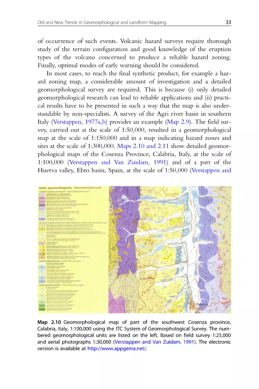
6. Applied Geomorphological Surveying and Mapping
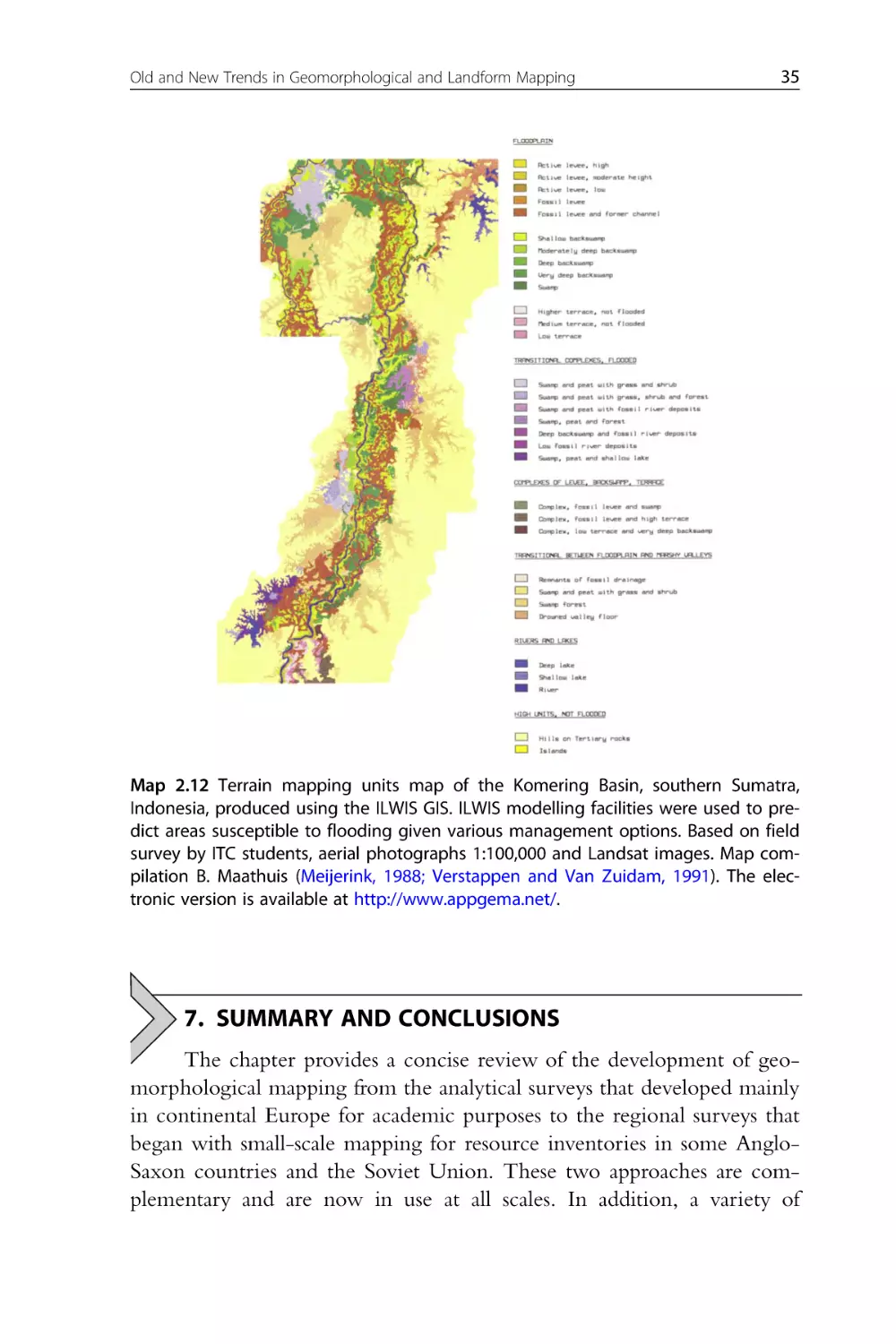
7. Summary and Conclusions

3. Nature and Aims of Geomorphological Mapping
Francesco Dramis, Domenico Guida and Antonello Cestari
1. Introduction
2. Types of Geomorphological Maps
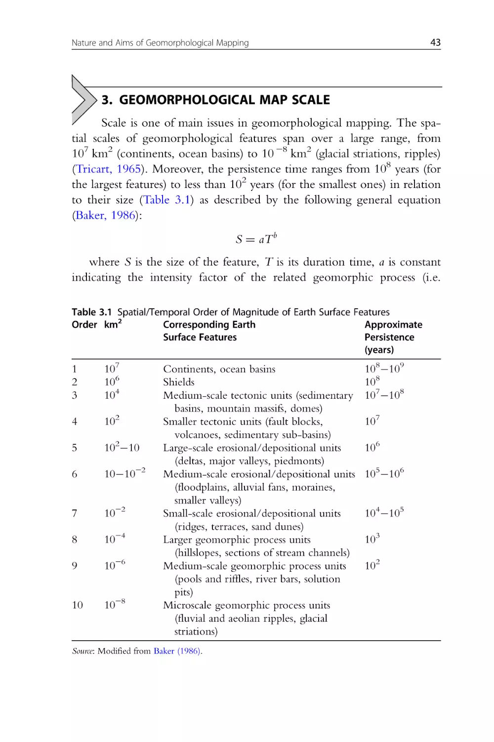
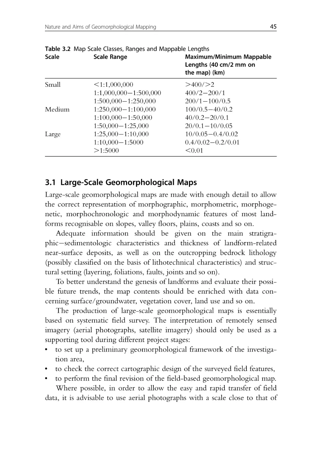
3. Geomorphological Map Scale
4. New Tools in Geomorphological Mapping
5. Problems and Efforts in Current Geomorphological Mapping
6. Experiences of GIS-Based, Object-Oriented Multiscale Geomorphological
Mapping
7. Concluding Remarks

4. Makers and Users of Geomorphological Maps
Paolo Paron and Lieven Claessens
1. Introduction
2. Geomorphological Mapping Characteristics

xi
xvii
1
3
6
7
8

13
13
15
19
23
27
31
35

39
39
41
43
49
53
58
64

75
75
76

v

vi

Contents

3.
4.
5.
6.

5.

Makers and Users
Examples of Nationwide Map Makers
Users
Conclusions

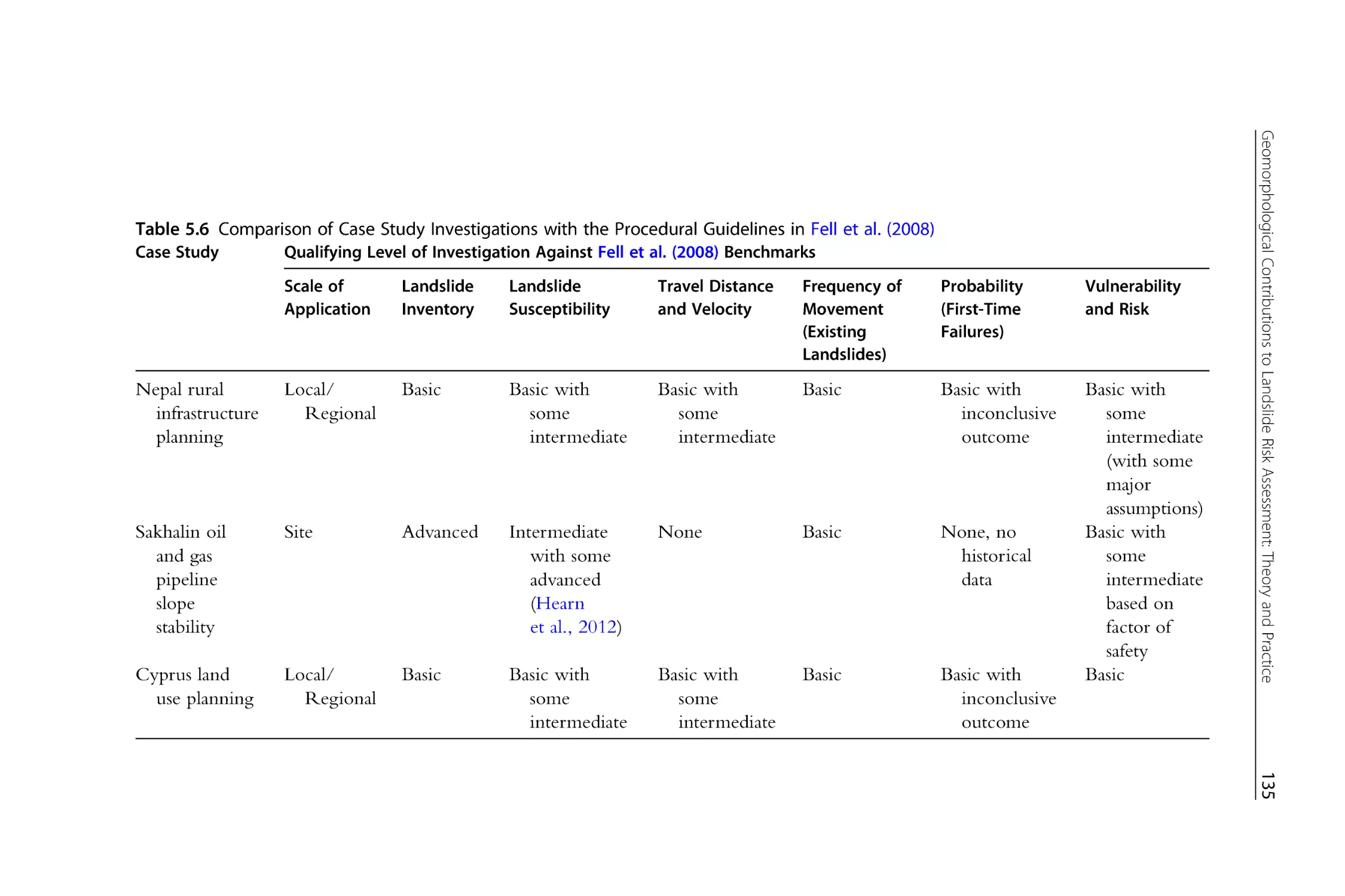
Geomorphological Contributions to Landslide Risk
Assessment: Theory and Practice
Gareth J. Hearn and Andrew B. Hart
1. Introduction
2. Landslide Susceptibility, Hazard and Risk
3. Experience from Industry
4. Landslide Hazard and Risk Mapping for Rural Infrastructure
Planning in Nepal
5. Sakhalin 2 Phase II Oil and Gas Pipeline in Russia
6. Landslide Mapping for Land Use Planning in Cyprus
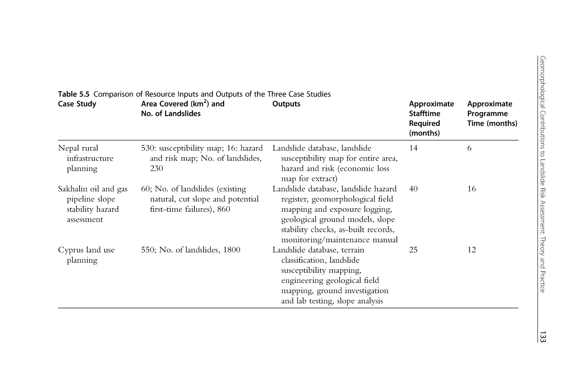
7. Discussion
8. Conclusions

SECTION 2:

6.

TECHNIQUES IN APPLIED GEOMORPHOLOGICAL
MAPPING

Geomorphological Field Mapping
Jasper Knight, Wishart A. Mitchell and James Rose
1. Introduction
2. Procedures and Protocols of Geomorphological Field Mapping
3. Examples of Geomorphological Field Mapping in Upland Terrain
4. Discussion
5. Conclusions and Outlook

7.

Data Sources
Takashi Oguchi, Yuichi S. Hayakawa and Thad Wasklewicz
1. Introduction
2. Analogue Data
3. Digital Data
4. Recent Trends, Problems and Future Perspectives

8.

Digital Mapping: Visualisation, Interpretation
and Quantification of Landforms
Mike J. Smith
1. Introduction
2. Mapping Methods

78
80
93
102

107
107
110
111
112
120
126
132
141

149
151
151
154
161
177
180

189
189
190
197
211

225
225
230

vii

Contents

3.
4.
5.
6.
7.

File Formats
Visualisation
Quantification
Errors
Summary

9. Cartography: Design, Symbolisation and Visualisation
of Geomorphological Maps

235
236
242
245
247

253

Jan-Christoph Otto, Marcus Gustavsson and Martin Geilhausen
1. Introduction
2. Elements of Cartographic Map Design
3. Geomorphological Legend Systems and Map Symbols
4. Map Production and Dissemination
5. Geomorphological Maps on the Internet
6. Conclusions

254
255
264
276
284
292

10. Semi-Automated Identification and Extraction of
Geomorphological Features Using Digital Elevation Data

297

Arie Christoffel Seijmonsbergen, Tomislav Hengl and Niels Steven Anders
1. Introduction
2. Geomorphological Mapping
3. Case Study Boschoord The Netherlands
4. Case Study Lech Austria
5. Closing Remarks

SECTION 3:

CASE STUDIES

11. Mapping Ireland's Glaciated Continental Margin Using Marine
Geophysical Data
Paul Dunlop, Fabio Sacchetti, Sara Benetti and Colm O'Cofaigh
1. Introduction
2. Case Study: Mapping Ireland's Glaciated Continental Margin
3. The Glacial Geomorphology of the North and Northwest Irish Shelf
Description and Interpretation
4. The Glacially Related Geomorphology of the Northwest Irish
Continental Margin
5. Discussion and Conclusions

298
299
310
320
329

337

339
339
342
346
351
353

viii

Contents

12. Submarine Geomorphology: Quantitative Methods
Illustrated with the Hawaiian Volcanoes
John K. Hillier
1. Introduction
2. Case Study: Hawaii
3. Discussion and Conclusions
4. Software and Data

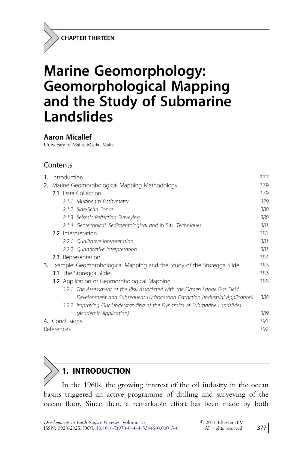
13. Marine Geomorphology: Geomorphological Mapping
and the Study of Submarine Landslides

359
359
364
371
372

377

Aaron Micallef
1. Introduction
377
2. Marine Geomorphological Mapping Methodology
379
3. Example: Geomorphological Mapping and the Study of the Storegga Slide 386
4. Conclusions
391

14. The Cherry Garden Landslide, Etchinghill Escarpment,
Southeast England
James S. Griffiths, E. Mark Lee, Denys Brunsden and David K.C. Jones
1. Introduction
2. Site Topography
3. Site Geology
4. Mapping Methodology
5. Mapping Results: Main Geomorphological Units
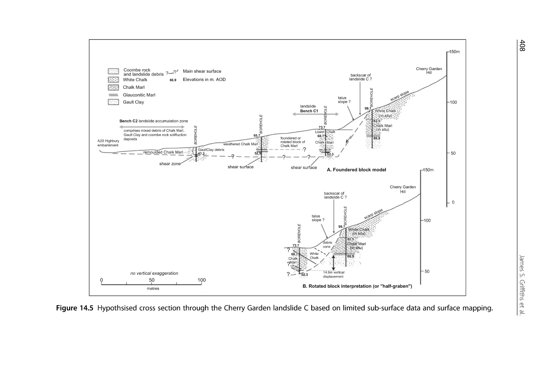
6. Mapping Results: The Cherry Garden Landslide
7. Geomorphological Interpretation
8. Conclusion

15. The Application of Geomorphological Mapping in
the Assessment of Landslide Hazard in Hong Kong
Steve Parry
1. Hong Kong and Landslide Hazards
2. Natural Terrain Landslides in Hong Kong
3. Geological and Geomorphological Setting
4. Approach and Methodology for Landslide Assessments in Hong Kong
5. Conceptual Ground Models
6. Site-Specific Field Mapping
7. Case Study
8. Conclusions

397
397
398
398
402
404
404
409
410

413
414
414
416
419
421
425
426
439

Contents

ix

16. A Geomorphological Map as a Tool for Assessing Sediment
Transfer Processes in Small Catchments Prone to Debris-Flows
Occurrence: A Case Study in the Bruchi Torrent (Swiss Alps)
443
David Theler and Emmanuel Reynard
1. Introduction
2. The Development of a Dynamic Geomorphological Mapping Method
3. Example of Application in the Bruchi Torrent
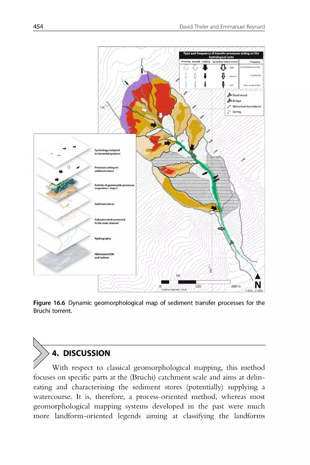
4. Discussion
5. Conclusions and Perspectives

17. Geomorphological Assessment of Complex Landslide Systems
Using Field Reconnaissance and Terrestrial Laser Scanning
Malcolm Whitworth, Ian Anderson and Graham Hunter
1. Introduction
2. Study Area
3. Field Landslide Mapping
4. Terrestrial Laser-Scanning Survey
5. Conclusions

18. Digital Terrain Models from Airborne Laser Scanning for the
Automatic Extraction of Natural and Anthropogenic Linear
Structures
Rutzinger Martin, Höfle Bernhard, Vetter Michael and Pfeifer Norbert
1. Introduction
2. Related Work
3. Method
4. Data Set and Test Site
5. Results
6. Conclusion

19. Applied Geomorphic Mapping for Land Management in the
River Murray Corridor, SE Australia
Colin F. Pain, Jonathan D.A. Clarke and Vanessa N.L. Wong
1. Introduction
2. Previous Studies
3. Methodology
4. Results
5. Applications
6. Conclusions

443
445
450
454
455

459
459
460
462
464
472

475
475
477
479
481
483
486

489
489
492
494
495
500
503

x

Contents

20. Monitoring Braided River Change Using Terrestrial Laser
Scanning and Optical Bathymetric Mapping
Richard Williams, James Brasington, Damia Vericat, Murray Hicks,
Fred Labrosse and Mark Neal
1. Introduction
2. Technological Developments
3. Data Collection
4. Processing Methodology
5. Results: DEMs of Difference
6. Conclusion

21. Uses and Limitations of Field Mapping of Lowland Glaciated
Landscapes
Jasper Knight
1. Introduction
2. Methods
3. The Context of Glacial Landforms in North-Central Ireland
4. Results
5. Discussion
6. Conclusions

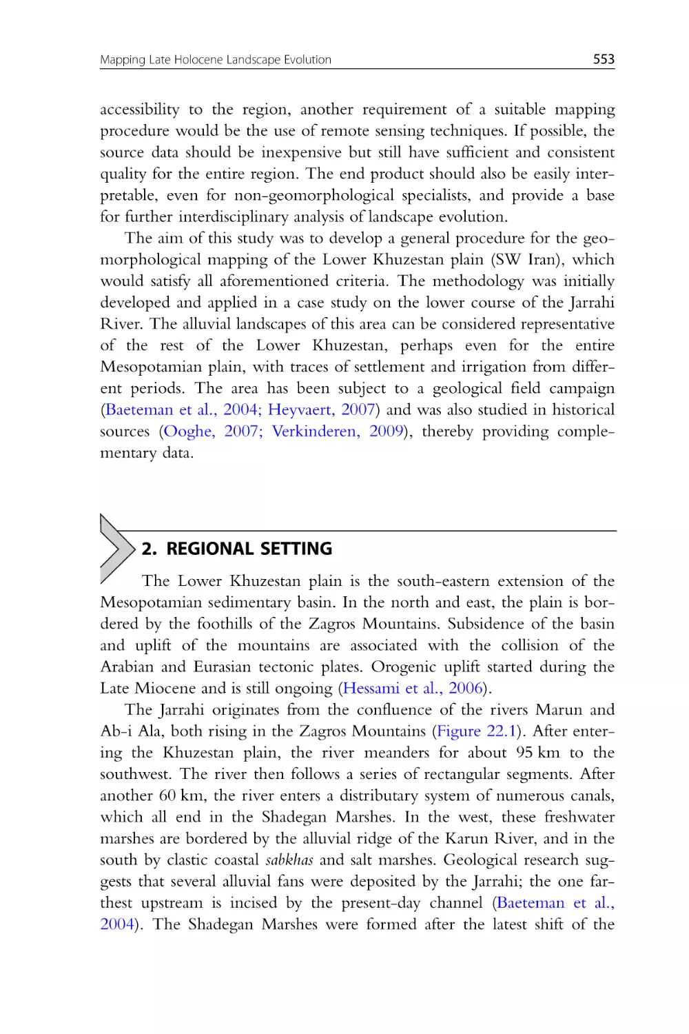
22. Mapping Late Holocene Landscape Evolution and Human
Impact A Case Study from Lower Khuzestan (SW Iran)
Jan Walstra, Vanessa M.A. Heyvaert and Peter Verkinderen
1. Introduction
2. Regional Setting
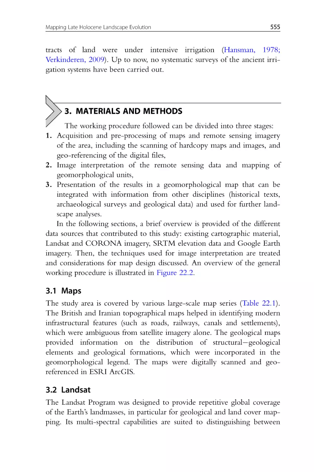
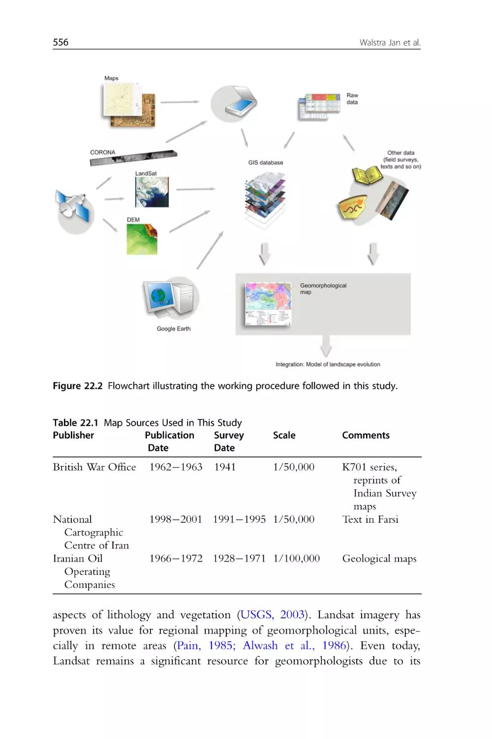
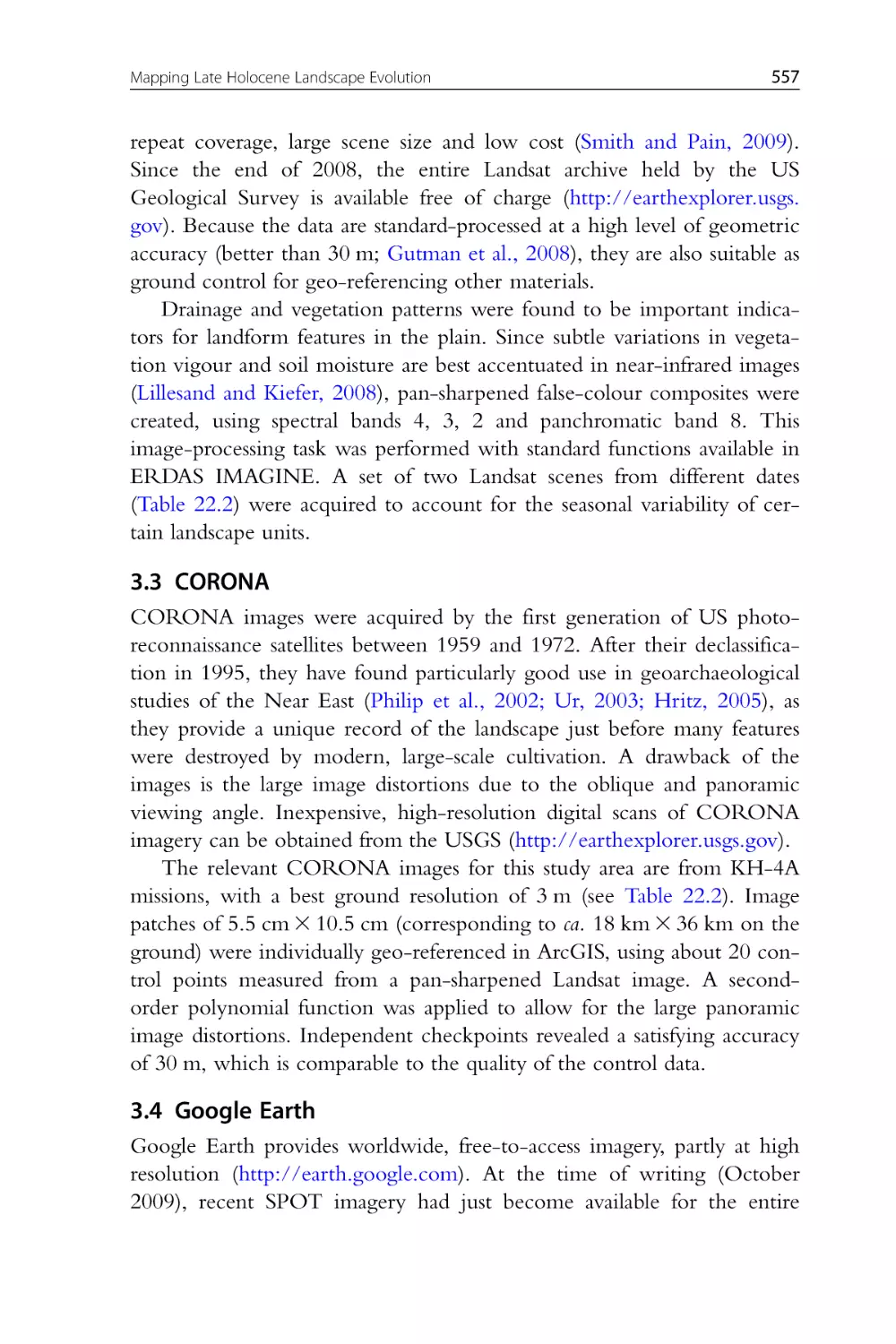
3. Materials and Methods
4. Results
5. Discussion
6. Conclusions

23. Military Applied Geomorphological Mapping: Normandy
Case Study
Peter L. Guth
1. Introduction
2. The Normandy Landings in World War II
3. Terrain Analysis
4. Geomorphic Maps of Normandy
5. Conclusion

24. Future Developments of Geomorphological Mapping

507

508
509
511
516
522
528

533
533
536
538
539
545
547

551
552
553
555
561
571
573

577
577
578
579
580
587

589

Mike J. Smith, James S. Griffiths and Paolo Paron

Index

595

FOREWORD
When Paolo Paron first suggested the idea of this book on geomorphological mapping to me several years ago, I immediately recognised the potential
of the concept for several reasons. First of all, my own interest in the topic
began more than four decades ago when I originally discovered the gaps in
my own rather Davisian education. I well remember the excitement I felt
back in the 1960s when on my first trip to Europe, I was introduced to
detailed geomorphologic mapping where many new symbols and detailed
geomorphological maps were being introduced by Demek (1967, 1972),
Verstappen (1970, 1983) and many others. At about the same time when
I was returning to the United States, St. Onge (1968) first introduced the
concept of large-scale geomorphological mapping in North America
when he wrote a paper on the topic in Fairbridge’s (1968) seminal
Encyclopedia of Geomorphology. This was the volume that first taught me geomorphology beyond Thornbury’s (1954/1968) Principles of Geomorphology
of my undergraduate and graduate education. Thornbury had little to say
about geomorphologic mapping even though the book had a whole chapter devoted to the ‘Tools of the Geomorphologist’. Instead, only standard
topographic maps and aerial photographs were mentioned by Thornbury,
probably because in those days the techniques of geomorphologic mapping
had not yet been refined to the fine art and science they later became.
Another factor that Paolo Paron and I discussed when we planned this
volume was our mutual desire to try to make the newer ideas and techniques of geomorphological mapping more available to the poorer nations
of the lesser developed world. We did not necessarily achieve this because
the costs and uncertainties of the modern publishing world necessitated a
fairly high price for this publication, but the increasing availability of
these materials in electronic domains that can be more easily accessed
over the Internet means that we will have succeeded at least in part in
our original objectives. This book, Geomorphological Mapping: Methods and
Application, is thus an attempt to explain and give examples of how this
highly technical methodology can be applied and utilised to solve complex problems in land use and provide some of the more benign answers
to development in the developing world.
As one might expect, the origins of geomorphological mapping are
diverse and the resultant techniques are replete with differences, as this
xi

xii

Foreword

volume shows. The history of the development of geomorphological
mapping grew from a need for a more analytical approach to interpretation of landforms more than half a century ago. As Hayden (1986) has
noted, the study of landforms in the nineteenth and early years of the
twentieth century was marked by rather static descriptive physiographies
in which landscapes were discussed largely in writing. These older papers
and books were generally accompanied by artistic block diagram drawings
to illustrate the author’s conclusions about what could be some wholly
imagined geologic history.
An approximate dividing line between these older notions of geomorphology and newer thinking was World War II (Klimaszewski, 1982),
after which the science of geomorphology took on a more modern and
useful flavour. A more pragmatic geomorphology emerged, particularly in
Europe, where geomorphologists became interested in comprehensive
regional analyses of landforms that considered all the features and aspects
of the landscape together. The natures and relationships of past landform
processes in an area were compared and contrasted to the active processes
of the present day. The significance and influences of landforms and relief
on vegetation, hydrology and human cultural development were investigated. The interpretation of the complexity of such landscapes necessitated objective scientific methods of graphic portrayal of these landform
factors. The detailed geomorphological map thus became, in many countries, the main research method in geomorphology (Demek, 1982).
Extensive, complex and highly colourful graphic symbologies were developed, commonly different for different countries or for different applications. Some subjectivity unfortunately crept into some of the maps,
particularly where loosely documented geologic histories were allowed to
control some age assignments. The overall result, however, was the fairly
accurate geomorphologic mapping of much of Europe, particularly where
maps in planning, engineering and management were desired. In North
America, however, a certain distaste existed for many aspects of central
planning, with the result that the mapping techniques were not applied
much there. As the editors note herein (Smith et al., 2011), the continued
fragmentation of legend systems between the different users and other
problems led to the relegation of much geomorphologic mapping
throughout the remainder of the twentieth and into the present century
as a rather adjunct activity. The new viewpoints and methods expressed
herein, however, seem to have signalled an end to such lack of recognition of the true usefulness of this methodology. In fact, a bit of a

Foreword

xiii

renaissance in geomorphological mapping seems to be underway at the
present time, as is attested to by Pavlopoulos et al. (2009), and especially
by the recent 41st International Binghamton Geomorphological
Symposium that was held on Geospatial Technologies and Geomorphological
Mapping (Bishop et al., 2011).
This current volume, Geomorphological Mapping: Methods and
Applications, is the fifteenth in our series on Developments in Earth Surface
Processes. It is a professional handbook of techniques and applications targeted at academics and practitioners who wish to use geomorphological
mapping in their work. This volume synthesises an historical perspective
to the use of field-based geomorphological mapping in which new digital
tools and techniques are now being used effectively in the process.
Material is brought together for digital mapping from remote sensing into
environments of cartography, geographic information systems and digital
terrain analysis. Extensive case studies with plentiful use of diagrams and
colour plates in the volume show the diverse nature of geomorphological
mapping as it is practiced in the twenty-first century. Accompanying electronic resources can add to the usefulness of the work for geomorphologists who are interested in mapping in the field. Those active in
geomorphology, engineering geology, the insurance industry, assessors of
environmental impacts and allied areas should find the text of considerable
value in their work. The authors and editors are convinced that the integrative methodology displayed in this volume has much to offer the practitioners and others who may wish to learn more about this increasingly
specialised but highly useful, analytical methodology.
John F. Shroder Jr.
Editor-in-Chief
Developments in Earth Surface Processes

REFERENCES
Bishop, M.P., James, A., Walsh, S.J., Shroder Jr., J.F., 2011. Geospatial technologies and
geomorphological mapping: concepts, issues and research directions. In: Bishop, M.P.,
James, A., Walsh, S.J. (Eds.), Geospatial Technologies and Geomorphological
Mapping: 41st International Binghamton Geomorphological Symposium. Elsevier.
Demek, J., 1967. Generalization of geomorphological maps. In: Progress Made in
Geomorphological Mapping, vol. 9. Geografický ústv ČSAV, Brno, pp. 36 72.
Demek, J. (Ed.), 1972. Manual for Detailed Geomorphological Mapping. IGU
Commission on Geomorphic Survey and Mapping, Academia, Prague.
Fairbridge, R.W., 1968. Encyclopedia of Geomorphology. Rheinhold Book Co., New
York, NY.

xiv

Foreword

Hayden, R.S., 1986. Geomorphological mapping. In: Short, N.M., Short, R.W. (Eds.),
Geomorphology from Space: A Global Overview of Regional Landforms. NASA,
Washington, DC, pp. 637 656.
Klimaszewski, M., 1982. Detailed geomorphological maps. ITC J. 3, 265 271.
Pavlopoulos, K., Evelpidou, N., Vassilopoulos, A., 2009. Mapping Geomorphological
Environments. Springer-Verlag, Berlin.
Smith, M.J., Griffiths, J., Paron, P., 2011. Future developments of geomorphological
mapping. In: Smith, M.J., Paron, P., Griffiths, J. (Eds.), Geomorphological Mapping:
Methods and Applications. Elsevier, London, pp. 589 593.
St. Onge, D., 1968. Geomorphological maps. In: Fairbridge, R.W. (Ed.), Encyclopedia of
Geomorphology. Rheinhold Book Co., New York, NY, pp. 388 403.
Thornbury, W.D., 1954. Principles of Geomorphology. John Wiley & Sons, New York,
NY.
Verstappen, H.Th., 1970. Introduction to the ITC-system of geomorphological survey.
Geogr. Tijdschr. 4 (1), 85 91.
Verstappen, H.Th., 1983. Applied Geomorphology: Geomorphological Surveys for
Environmental Development. Elsevier, Amsterdam, pp. 255 275.

FOREWORD
Between the International Association of Geomorphologists’ (IAG)
International Conferences in Zaragoza (2005) and Melbourne (2009), the
IAG decided to establish a series of new working groups concerned with
important issues in the discipline which would benefit from international
collaboration. One of these issues was that of Applied Geomorphological
Mapping.
As Professor Verstappen points out in Chapter 2, geomorphological
mapping is not in itself new, and when the British Geomorphological
Research Group, a parent of the IAG, was established five decades ago,
one of its first roles was to try and establish a certain uniformity and logic
of approach and annotation. Pioneering symbol-based geomorphological
mapping was also carried out in many European countries but sometimes
suffered from the fact that the aims, scale and purpose of the mapping
were not always clearly identified. Such maps were all too frequently seen
to be the object of research rather than a tool of research. Moreover, it was
not always clear to whom they were aimed. This approach was sometimes
derided and geomorphological mapping ceased to be as fashionable as it
once had been. A strong regional and descriptive bent in geographical
geomorphology, into which geomorphological mapping fitted, was
replaced by a move towards reductionist process studies. Having said that,
some first-class mapping work was undertaken that proved to be of great
value in resource mapping and hazard evaluation, not least by organisations such as ITC in the Netherlands, CSIRO in Australia, and various
UK geomorphologists working in the Middle East and elsewhere.
Recent years have seen a resurgence in the use of geomorphological
maps for applied research. This is reflected in this volume, which contains
an impressive range of studies and a list of authors who are impressive for
their internationalism. Maps remain a very powerful tool for transmitting
information to clients, but their value has been hugely magnified of late
because of the availability and use of new techniques, including remote
sensing, computation, digitisation, geostatistics, modelling, GPS, GIS, etc.
This is all made clear by Dramis et al. in Chapter 3, who draw attention
to the value of a multi-scale approach. The use of geomorphological
maps has now been extended to new environments, and planetary and
submarine geomorphological mapping are particularly exciting areas of
xv

xvi

Foreword

research. Maps tell us where things are, what they are like, how their
properties and distributions have changed through time and how phenomena correlate spatially. These functions are fundamental for locating
and understanding resources and risks, the twin foundations of applied
geomorphology.
I believe that this timely volume will highlight the fact that skills in
applied geomorphological mapping are a very necessary and basic part of
the training for all geomorphologists.
Andrew Goudie
IAG President 2005 2009

LIST OF CONTRIBUTORS
Niels Steven Anders
Institute for Biodiversity and Ecosystem Dynamics, University of Amsterdam,
Nieuwe Achtergracht 166, WV Amsterdam, The Netherlands
n.s.anders@uva.nl
Ian Anderson
Halcrow Group Ltd, Martlett House, Chichester, UK
Sara Benetti
School of Environmental Sciences, University of Ulster, Coleraine BT52 1SA,
Northern Ireland
James Brasington
Department of Geography, University of Canterbury, Private Bag 4800,
Christchurch 8140
james.brasington@canterbury.ac.uk
Denys Brunsden
Vine Cottage, Sea Lane, Chideock near Bridport, Dorset DT6 6LD, UK
Antonello Cestari
C.U.G.R.I., Great Risks Interuniversity Consortium, University of Salerno,
via Ponte Don Melillo, Fisciano, SA 84084, Italy
acestari@unisa.it
Lieven Claessens
Land Dynamics Group, Wageningen University and Research Centre, Wageningen,
The Netherlands
International Potato Center (CIP), Sub-Saharan Africa Regional Office, Nairobi, Kenya
Jonathan D.A. Clarke
Geoscience Australia, P.O. Box 378, Canberra, ACT 2601, Australia
Francesco Dramis
Department of Geological Sciences, Roma Tre University,
Largo San Leonardo Murialdo 1, Rome, Lazio 00146, Italy
dramis@uniroma3.it
Paul Dunlop
School of Environmental Sciences, University of Ulster, Coleraine BT52 1SA,
Northern Ireland
p.dunlop@ulster.ac.uk
Martin Geilhausen
Department of Geography and Geology, University of Salzburg, Hellbrunnerstr. 34,
A-5020 Salzburg, Austria
martin.geilhausen@sbg.ac.at

xvii

xviii

List of Contributors

James S. Griffiths
SoGEES, University of Plymouth, Drake Circus, Plymouth, Devon PL4 8AA, UK
jim.griffiths@plymouth.ac.uk
Domenico Guida
Department of Civil Engineering, University of Salerno, Via Ponte Don Melillo,
Fisciano, SA 84084, Italy
dguida@unisa.it
Marcus Gustavsson
Helsingforsgatan 71, S-75264 Uppsala, Sweden
Peter L. Guth
Department of Oceanography, United States Naval Academy, 572C Holloway R,
Annapolis, MD 24102, USA
pguth@usna.edu
Andrew B. Hart
Geo-Hazard, Scott Wilson Ltd, Scott House, Alencon Link, Basingstoke, UK
Yuichi Hayakawa
Center for Spatial Information Science, University of Tokyo, 5-1-5 Kashiwanoha,
Kashiwa 277-8568, Japan
hayakawa@csis.u-tokyo.ac.jp
Gareth J. Hearn
Geo-Hazard, Scott Wilson Ltd, Scott House, Alencon Link, Basingstoke, UK
gareth.hearn@scottwilson.com
Tomislav Hengl
Institute for Biodiversity and Ecosystem Dynamics, University of Amsterdam,
Nieuwe Achtergracht 166, 1018 WV Amsterdam, The Netherlands
t.hengl@uva.nl
Vanessa M.A. Heyvaert
Geological Survey of Belgium, Royal Belgian Institute for Natural Sciences,
Jennerstraat 13, B-1000 Brussels, Belgium
Murray Hicks
National Institute for Water and Atmosphere, New Zealand
m.hicks@niwa.co.nz
John K. Hillier
Department of Geography, Loughborough University, Leics, UK, LE11 3TU
j.hillier@lboro.ac.uk
Bernhard Höfle
Department of Geography, University of Heidelberg, Heidelberg, Germany
Graham Hunter
3D Laser Mapping Ltd, 1a Church Street, Bingham, Nottingham, UK
David K.C. Jones
Horsepen, Main Street, Beckley near Rye, Sussex TN31 6RS, UK

List of Contributors

Jasper Knight
School of Geography, Archaeology and Environmental Studies, University of the
Witwatersrand, Private Bag 3, Wits 2050, Johannesburg, South Africa
jasper.knight@wits.ac.za
Fred Labrosse
Department of Computer Science, Aberystwyth University, UK
ffl@aber.ac.uk
E.Mark Lee
15 Whernside Avenue, York YO31 0QB, UK
Aaron Micallef
IOI-Malta Operational Centre, University of Malta, Level 3, Chemistry Building,
MSD 2080, Malta
micallefaaron@gmail.com
Wishart A. Mitchell
Department of Geography, Durham University,
Durham DH1 3LE, UK
w.a.mitchell@durham.ac.uk
Mark Neal
Department of Computer Science, Aberystwyth University, UK
mjn@aber.ac.uk
Colm Ó Cofaigh
Department of Geography, Durham University, Durham DH1 3LE, UK
Takashi Oguchi
Center for Spatial Information Science, University of Tokyo, 5-1-5 Kashiwanoha,
Kashiwa 277-8568, Japan
oguchi@csis.u-tokyo.ac.jp
Jan-Christoph Otto
Department of Geography and Geology, University of Salzburg, Hellbrunnerstr.
34, A-5020 Salzburg, Austria
jan-christoph.otto@sbg.ac.at
Colin F. Pain
Geoscience Australia, P.O. Box 378, Canberra, ACT 2601, Australia
colin.pain@ga.gov.au
Paolo Paron
UNESCO-IHE, Institute for Water Education, Delft, The Netherlands
School of Geography and the Environment, Oxford University,
Oxford, UK
P.Paron@unesco-ihe.org
Steve Parry
GeoRisk Solutions Ltd, Suite 1502, Hollywood Centre, 233 Hollywood Road,
Sheung Wan, Hong Kong, China
parrysteve@gmail.com

xix

xx

List of Contributors

Norbert Pfeifer
Institute of Photogrammetry and Remote Sensing, Vienna University of Technology,
Vienna, Austria
Emmanuel Reynard
Institute of Geography, University of Lausanne, Anthropole, CH-1015 Lausanne,
Switzerland
James Rose
Department of Geography, Royal Holloway, University of London,
Egham, Surrey TW20 0EX, UK
British Geological Survey, Keyworth, Nottingham, UK
j.rose@rhul.ac.uk
Martin Rutzinger
ITC-Faculty of Geo-Information Science and Earth Observation, University of Twente,
Enschede, The Netherlands
rutzinger@itc.nl
Fabio Sacchetti
School of Environmental Sciences, University of Ulster, Coleraine BT52 1SA,
Northern Ireland
Arie Christoffel Seijmonsbergen
Institute for Biodiversity and Ecosystem Dynamics, University of Amsterdam,
Nieuwe Achtergracht 166, 1018 WV Amsterdam, The Netherlands
a.c.seijmonsbergen@uva.nl
Mike J. Smith
School of Geography, Geology and the Environment, Kingston University,
Penrhyn Road, Kingston upon Thames, Surrey KT1 2EE, UK
michael.smith@kingston.ac.uk
David Theler
Institute of Geography, University of Lausanne, Anthropole, CH-1015 Lausanne,
Switzerland
dtheler@hotmail.com
Damià Vericat
Forest Technology Centre of Catalonia, Spain
damia.vericat@ctfc.cat
Peter Verkinderen
Department of Languages and Cultures of the Near East and North Africa,
Ghent University, Sint-Pietersplein 6, B-9000 Ghent, Belgium
Herman Theodore Verstappen
International Institute of Geo-Information Science and Earth Observation (ITC),
University of Twente, Mozartlaan 188, Enschede 7522HS, The Netherlands
hergraverstappen@planet.nl

List of Contributors

Michael Vetter
Institute of Photogrammetry and Remote Sensing, Centre of Water Resources,
Vienna University of Technology, Vienna, Austria
Jan Walstra
Department of Languages and Cultures of the Near East and North Africa,
Ghent University, Sint-Pietersplein 6, B-9000 Ghent, Belgium
jan.walstra@ugent.be
Thad Wasklewicz
Department of Geography, East Carolina University, A-227 Brewster Building,
Greenville, NC 27858, USA
wasklewiczt@ecu.edu
Malcolm Whitworth
School of Earth and Environmental Sciences, University of Portsmouth, Drake Circus,
Portsmouth, Devon PL4 8AA, UK
malcolm.whitworth@port.ac.uk
Richard Williams
Institute of Geography & Earth Sciences, Aberystwyth University, Llandinam Building,
Penglais Campus, Aberystwyth, SY23 3DB
rvw@aber.ac.uk
Vanessa N.L. Wong
Geoscience Australia, P.O. Box 378, Canberra, ACT 2601, Australia
Present address: Southern Cross GeoScience, Southern Cross University, P.O. Box 157,
Lismore, NSW 2480, Australia

xxi

LIST OF FIGURES

CHAPTER TWO
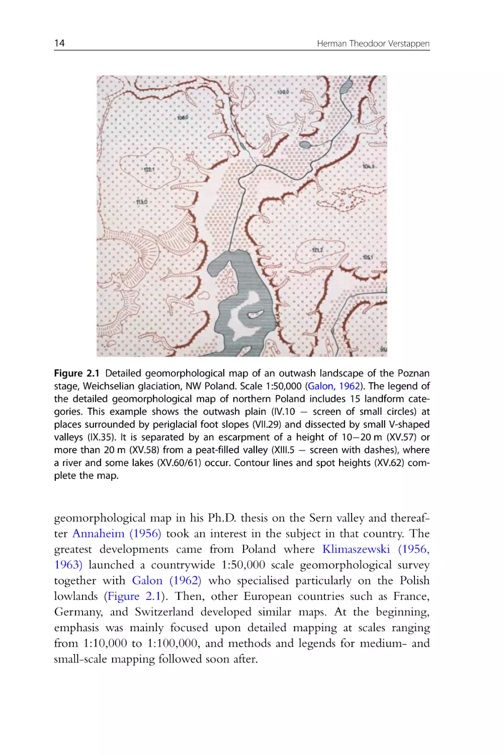
Figure 2.1 Detailed geomorphological map of an outwash landscape of
the Poznan stage, Weichselian glaciation, NW Poland. Scale 1:50,000
(Galon, 1962). The legend of the detailed geomorphological map of
northern Poland includes 15 landform categories. This example shows
the outwash plain (IV.10 
 screen of small circles) at places surrounded
by periglacial foot slopes (VII.29) and dissected by small V-shaped valleys (IX.35). It is separated by an escarpment of a height of 10
20 m
(XV.57) or more than 20 m (XV.58) from a peat-filled valley (XIII.5 

screen with dashes), where a river and some lakes (XV.60/61) occur.
Contour lines and spot heights (XV.62) complete the map.
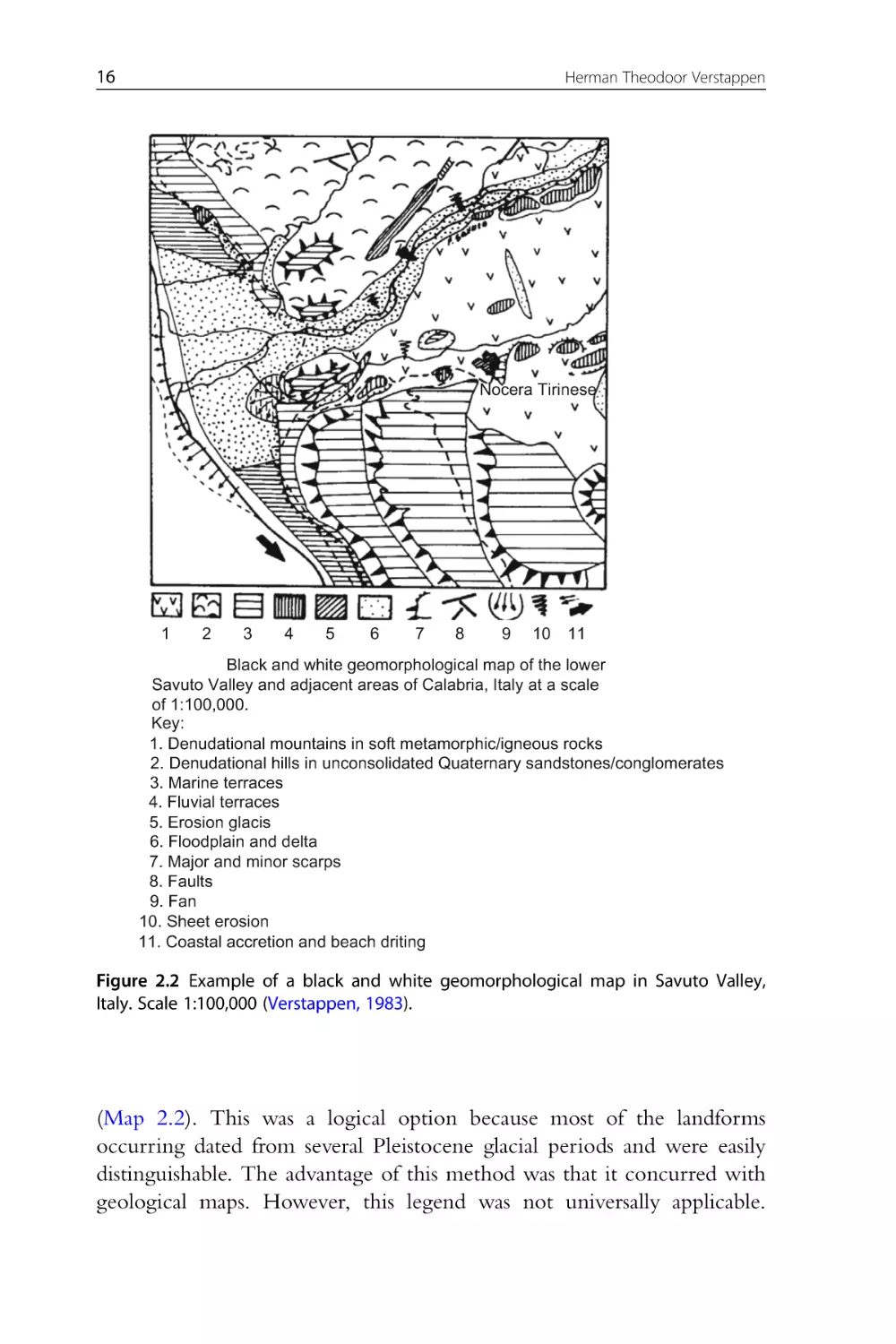
Figure 2.2 Example of a black and white geomorphological map in
Savuto Valley, Italy. Scale 1:100,000 (Verstappen, 1983).
Figure 2.3 Contents and relationships of various types of geomorphological maps (Verstappen and Van Zuidam, 1991).
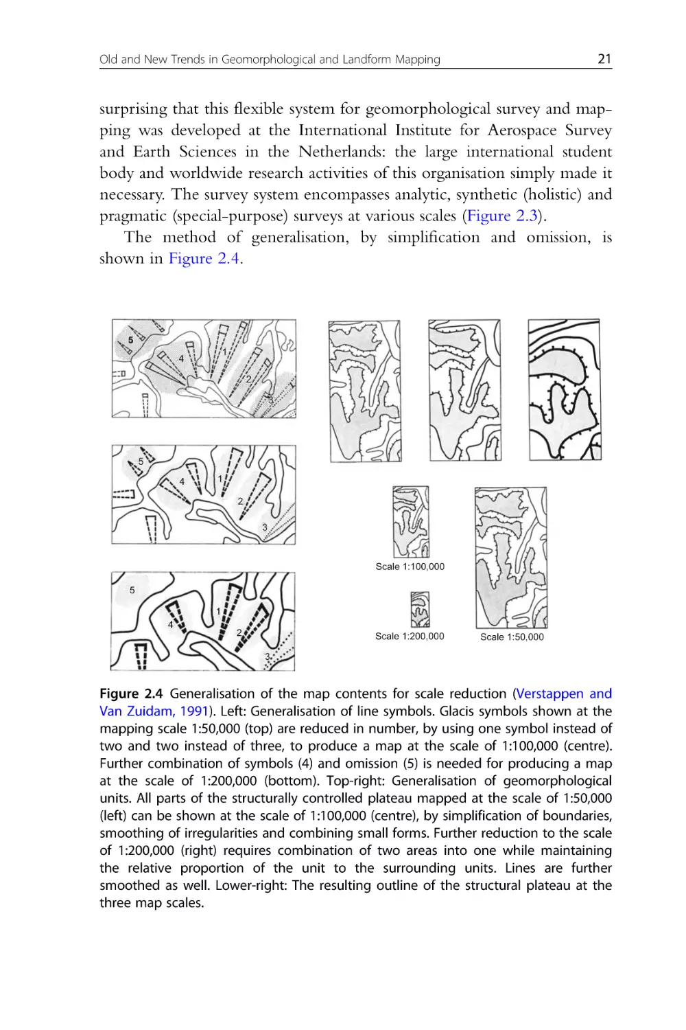
Figure 2.4 Generalisation of the map contents for scale reduction
(Verstappen and Van Zuidam, 1991). Left: Generalisation of line symbols. Glacis symbols shown at the mapping scale 1:50,000 (top) are
reduced in number, by using one symbol instead of two and two
instead of three, to produce a map at the scale of 1:100,000 (centre).
Further combination of symbols (4) and omission (5) is needed for producing a map at the scale of 1:200,000 (bottom). Top-right:
Generalisation of geomorphological units. All parts of the structurally
controlled plateau mapped at the scale of 1:50,000 (left) can be shown
at the scale of 1:100,000 (centre), by simplification of boundaries,
smoothing of irregularities and combining small forms. Further reduction to the scale of 1:200,000 (right) requires combination of two areas
into one while maintaining the relative proportion of the unit to the
surrounding units. Lines are further smoothed as well. Lower-right:
The resulting outline of the structural plateau at the three map scales.

xxiii

xxiv

List of Figures

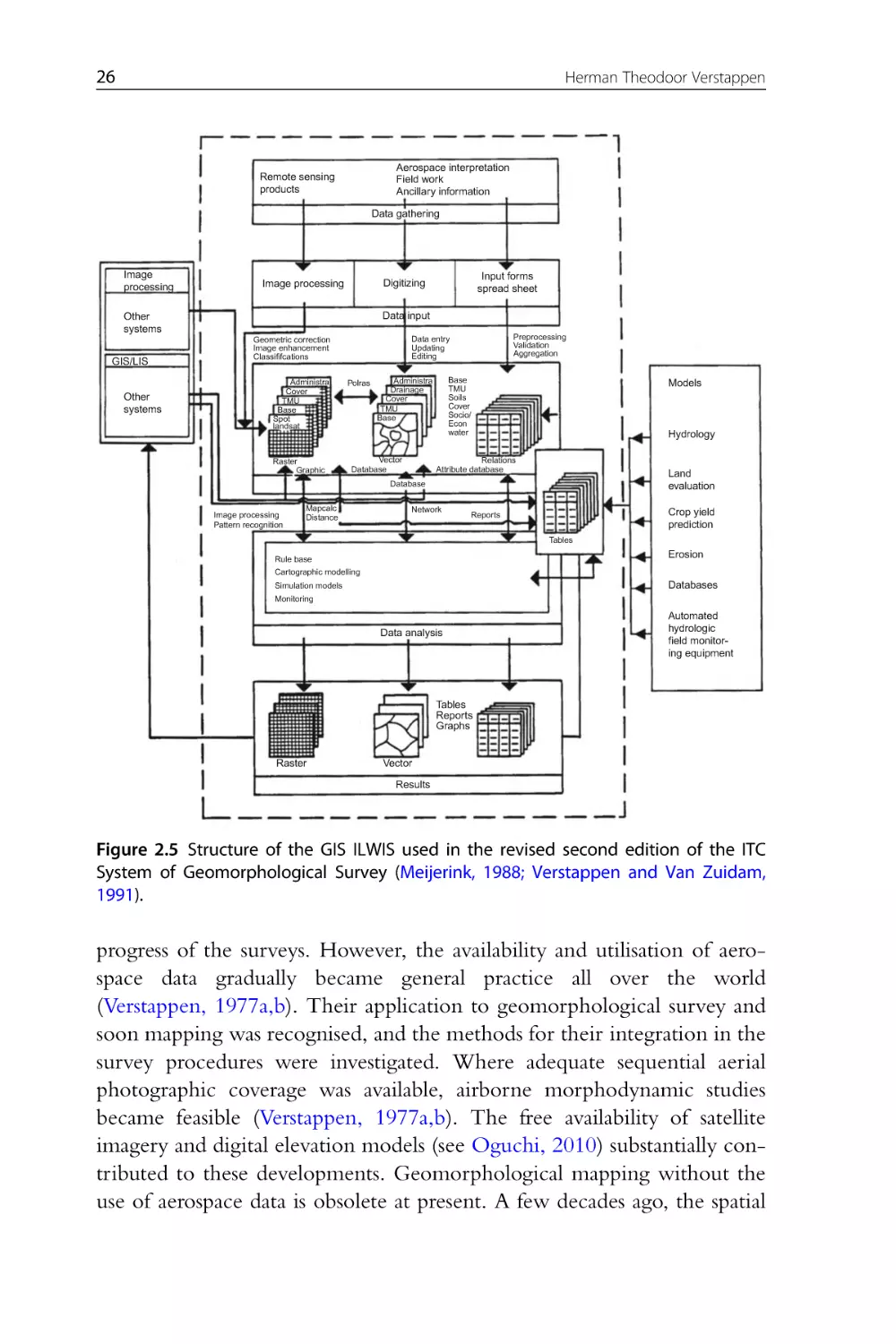
Figure 2.5 Structure of the GIS ILWIS used in the revised second edition
of the ITC System of Geomorphological Survey (Meijerink, 1988;
Verstappen and Van Zuidam, 1991).
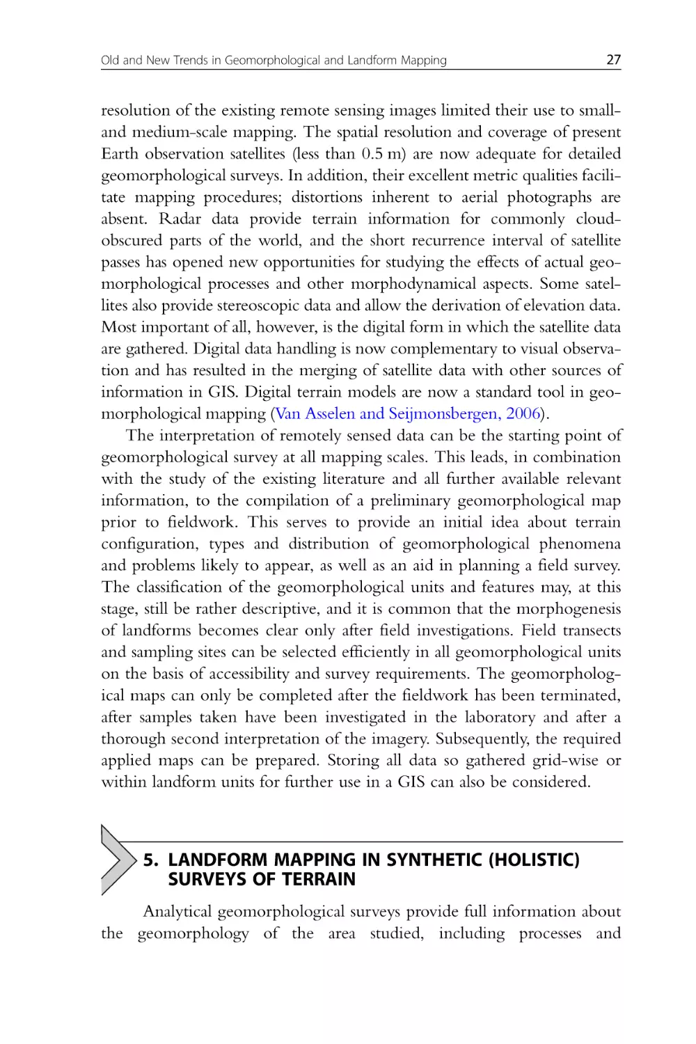
Figure 2.6 Block diagram of the Masaka land system, Uganda, illustrating
a DOS resource survey: (1) plateau crest, (2) quartzite ridge, (3) convex
interfluve and slope, (4) small valley and (5) main valley floor (Brunt,
1967).
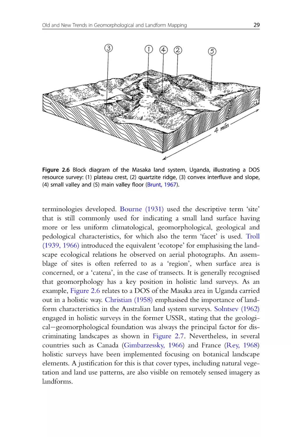
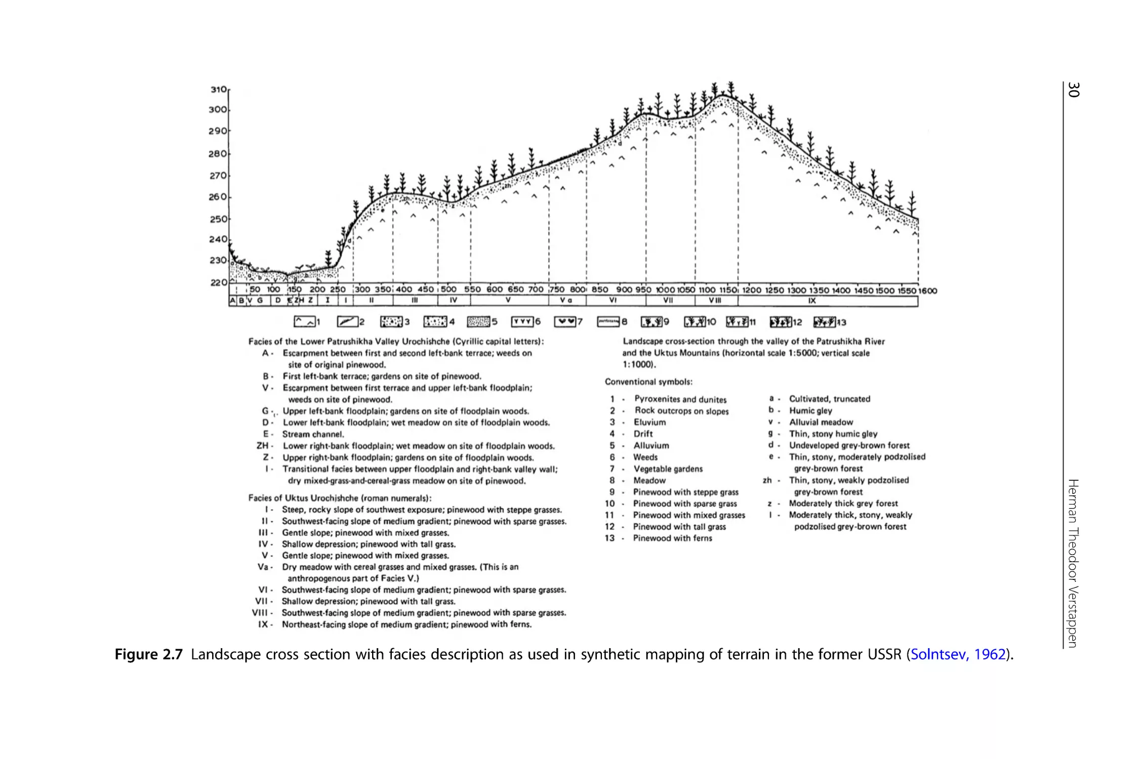
Figure 2.7 Landscape cross section with facies description as used in synthetic mapping of terrain in the former USSR (Solntsev, 1962).

CHAPTER THREE
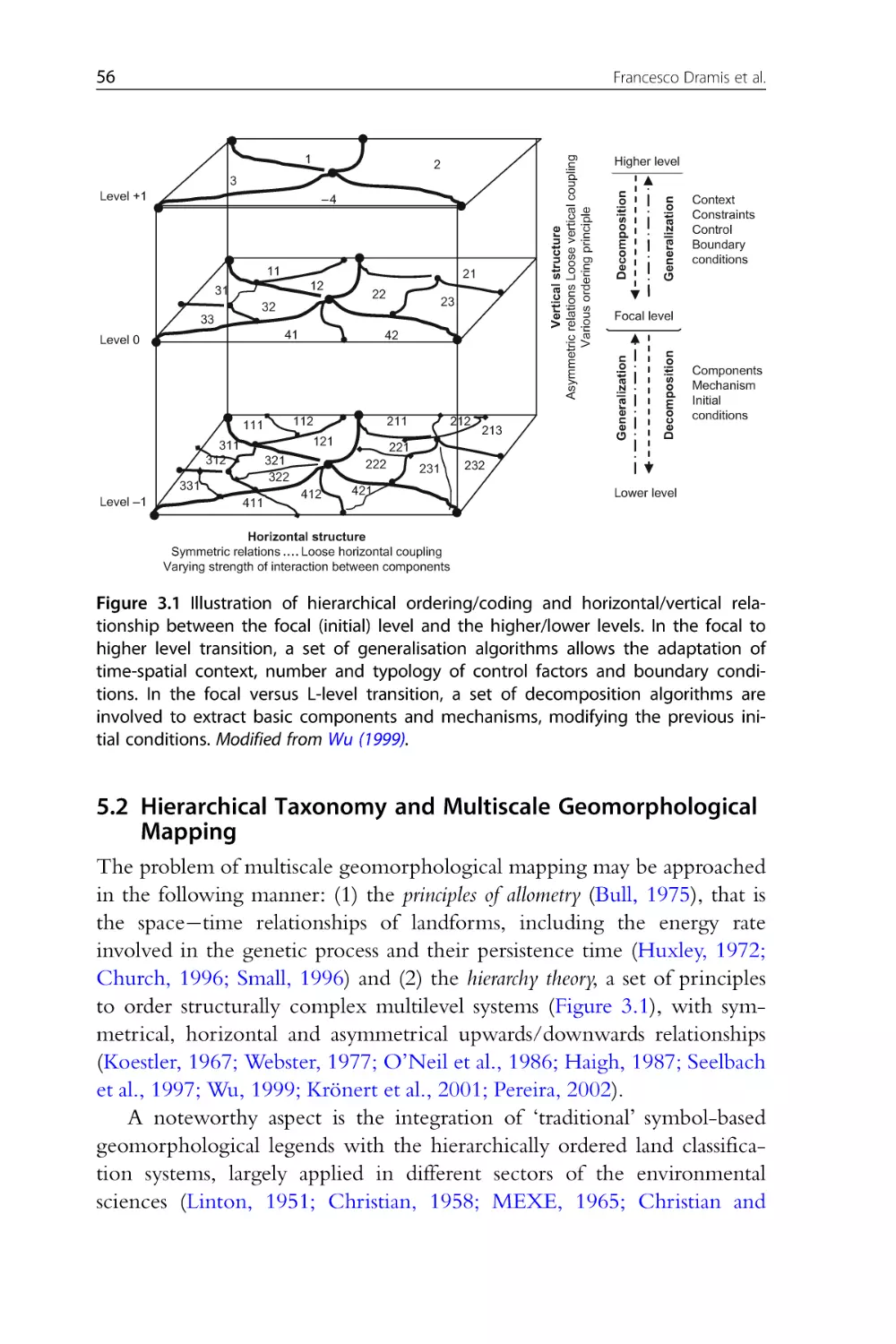
Figure 3.1 Illustration of hierarchical ordering/coding and horizontal/
vertical relationship between the focal (initial) level and the higher/
lower levels. In the focal to higher level transition, a set of generalisation algorithms allows the adaptation of time-spatial context, number
and typology of control factors and boundary conditions. In the focal
versus L-level transition, a set of decomposition algorithms are involved
to extract basic components and mechanisms, modifying the previous
initial conditions. Modified from Wu (1999).
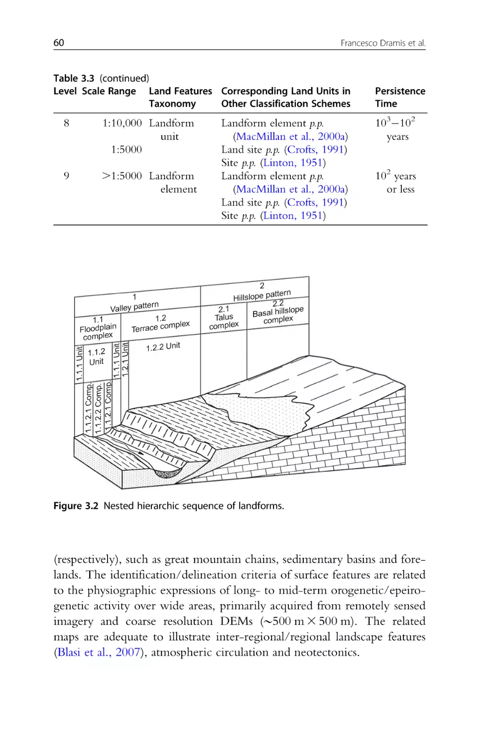
Figure 3.2 Nested hierarchic sequence of landforms.
Figure 3.3 Flow diagram of the Salerno University geomorphological
mapping system. The progressive numbers indicate the sequence of
steps and sub-steps; the trapezoidic shapes indicate the field, laboratory
and analytical data inputs; the rhomboid shapes indicate the graphical
or code tools used to transfer inputs into preliminary (1c), intermediate
(2c) and final (4) geomorphological map; the rhombus indicates the
decision about the acceptance of the map into the GmIS.

CHAPTER FOUR
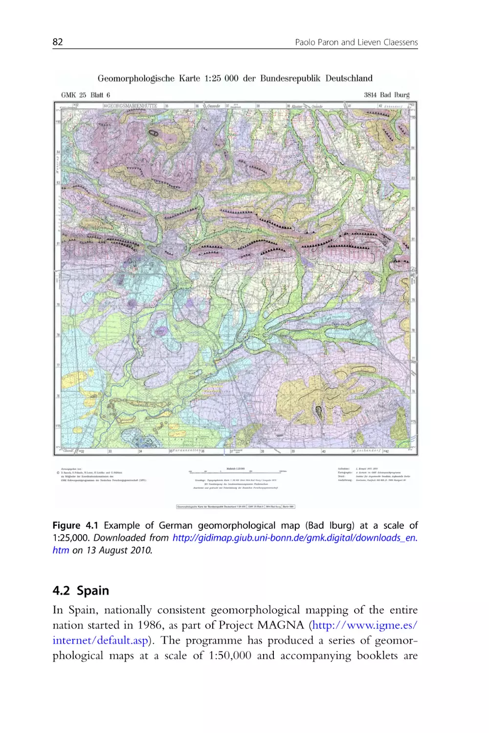
Figure 4.1 Example of German geomorphological map (Bad Iburg) at a
scale of 1:25,000. Downloaded from http://gidimap.giub.uni-bonn.de/
gmk.digital/downloads_en.htm on 13 August 2010.

List of Figures

xxv

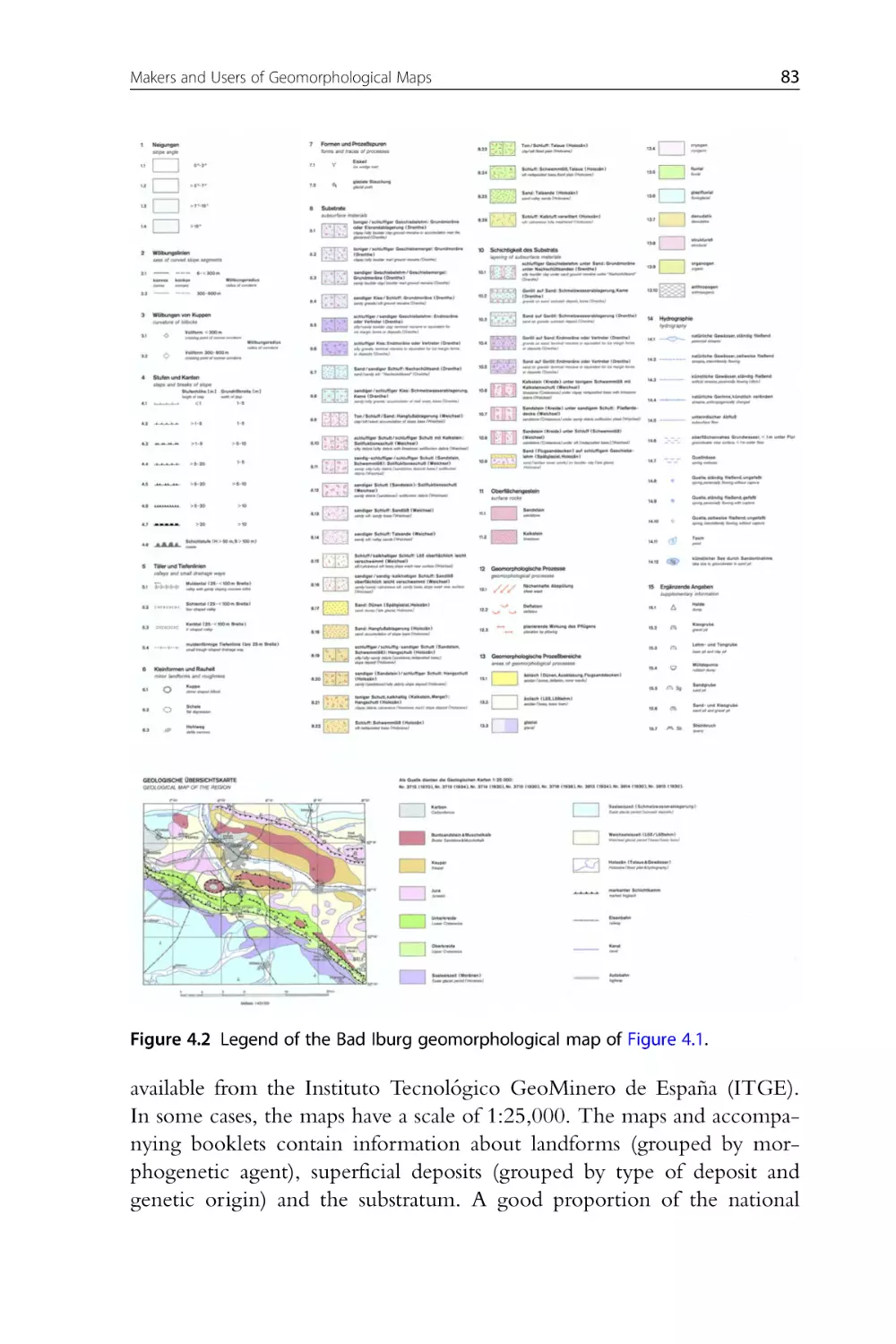
Figure 4.2 Legend of the Bad Iburg geomorphological map of Figure 4.1.
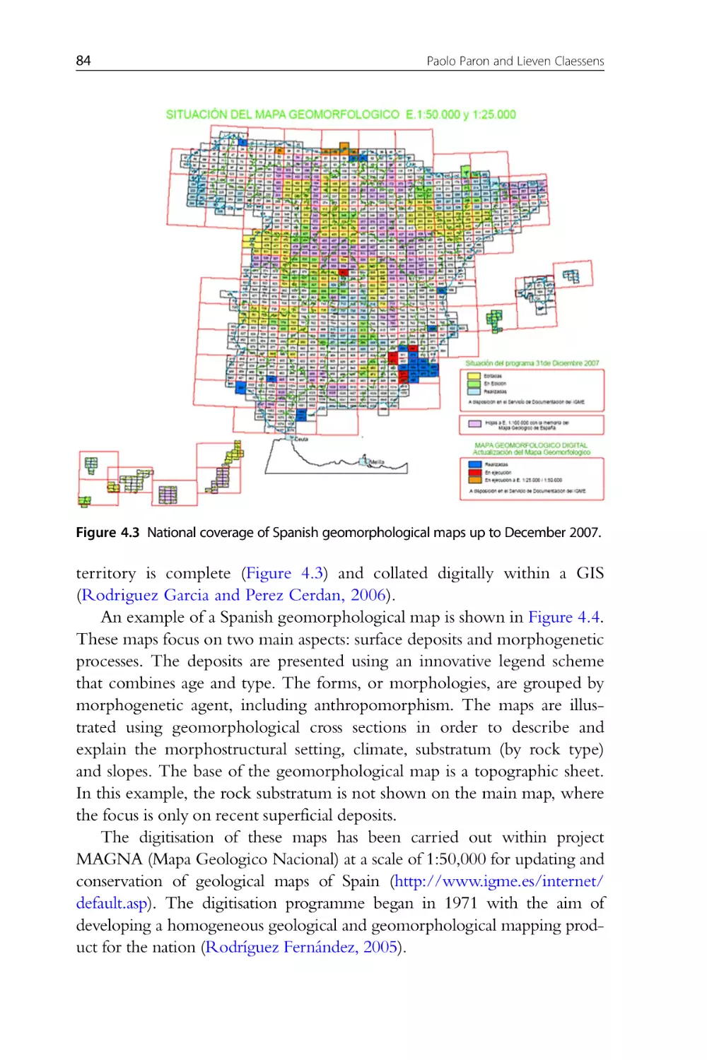
Figure 4.3 National coverage of Spanish geomorphological maps up to
December 2007.
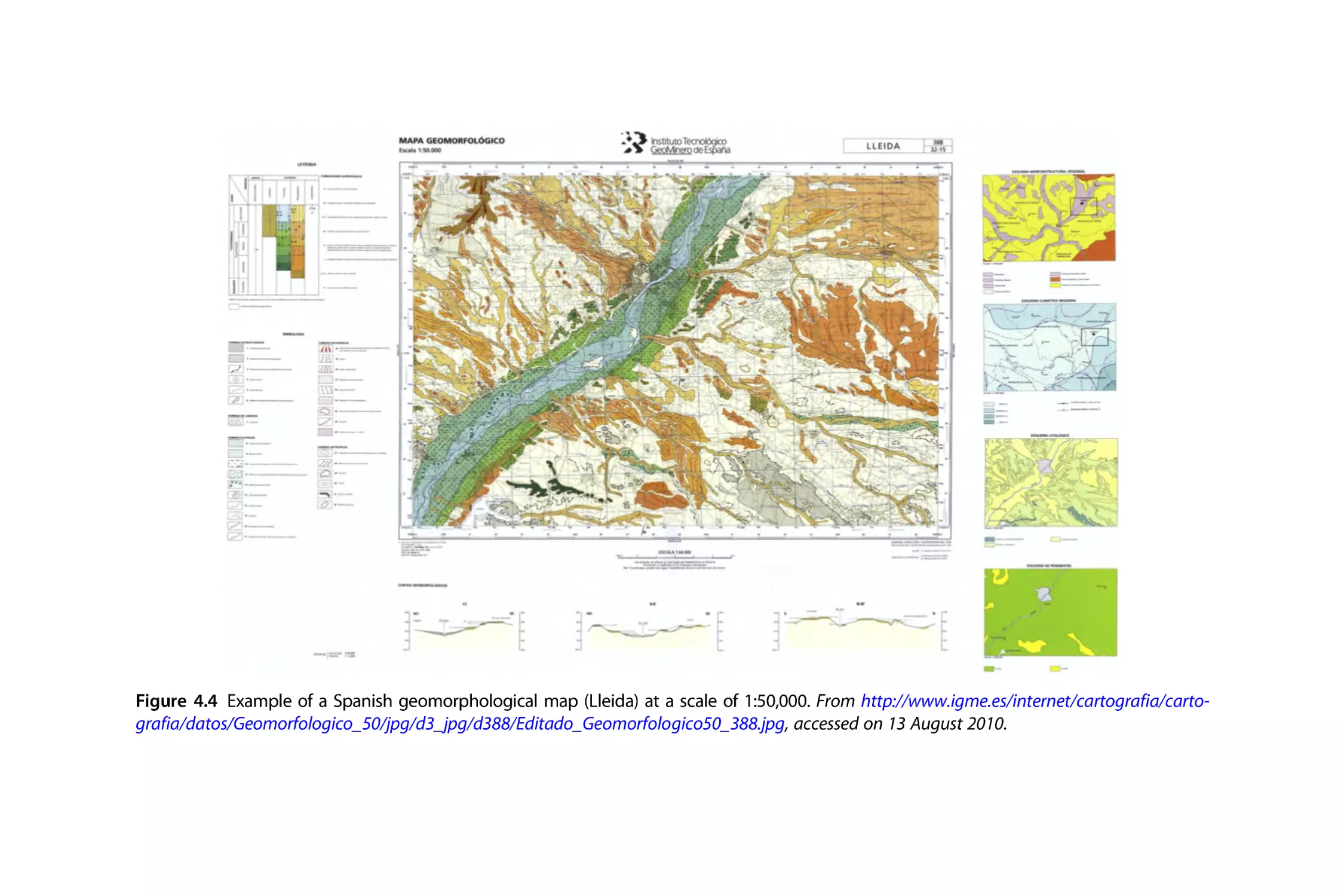
Figure 4.4 Example of a Spanish geomorphological map (Lleida) at a scale of
1:50,000. From http://www.igme.es/internet/cartografia/cartografia/datos/
Geomorfologico_50/jpg/d3_jpg/d388/Editado_Geomorfologico50_388.jpg,
accessed on 13 August 2010.
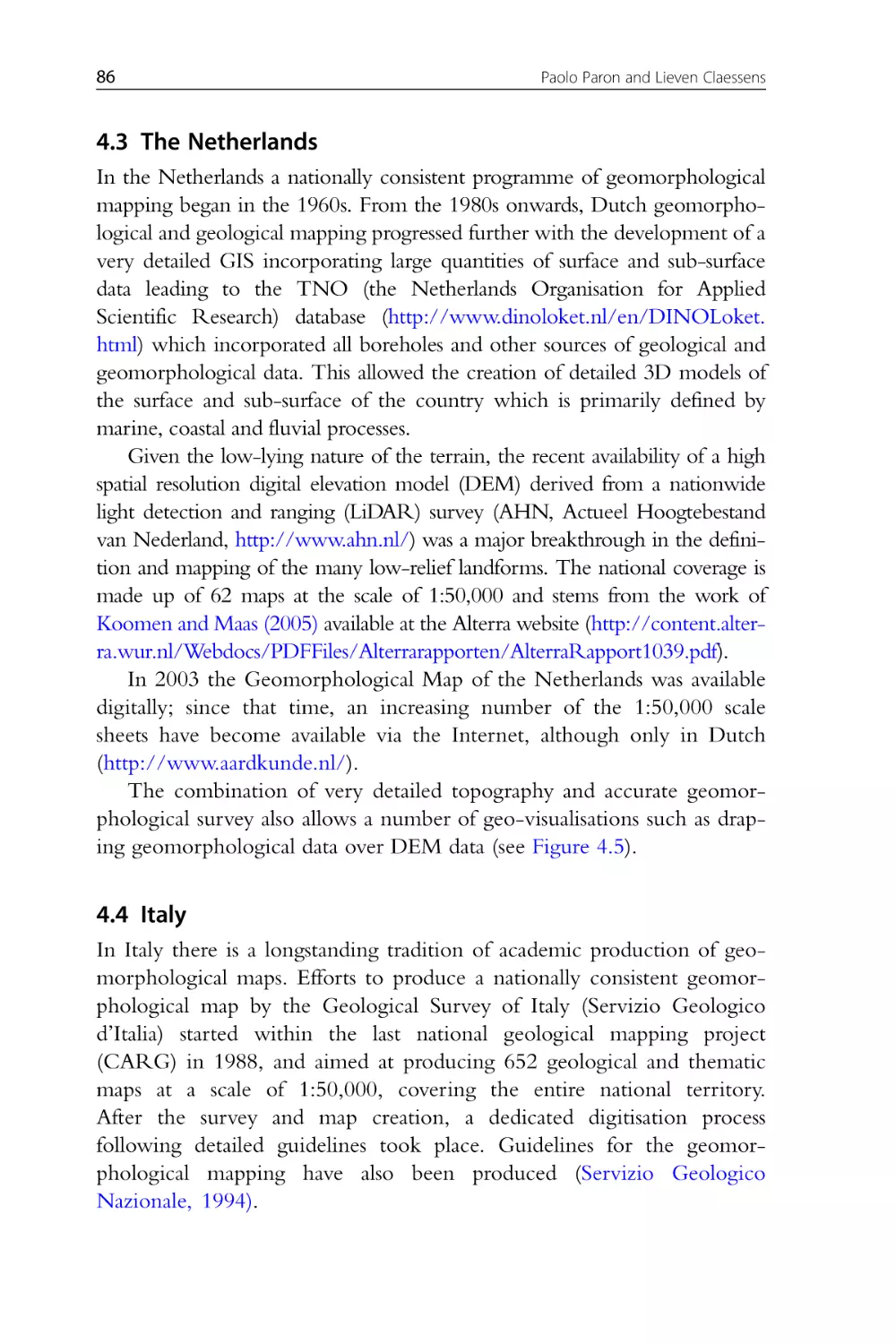
Figure 4.5 Draping of geomorphological information on the LiDARderived DTM. From http://www.aardkunde.nl/.
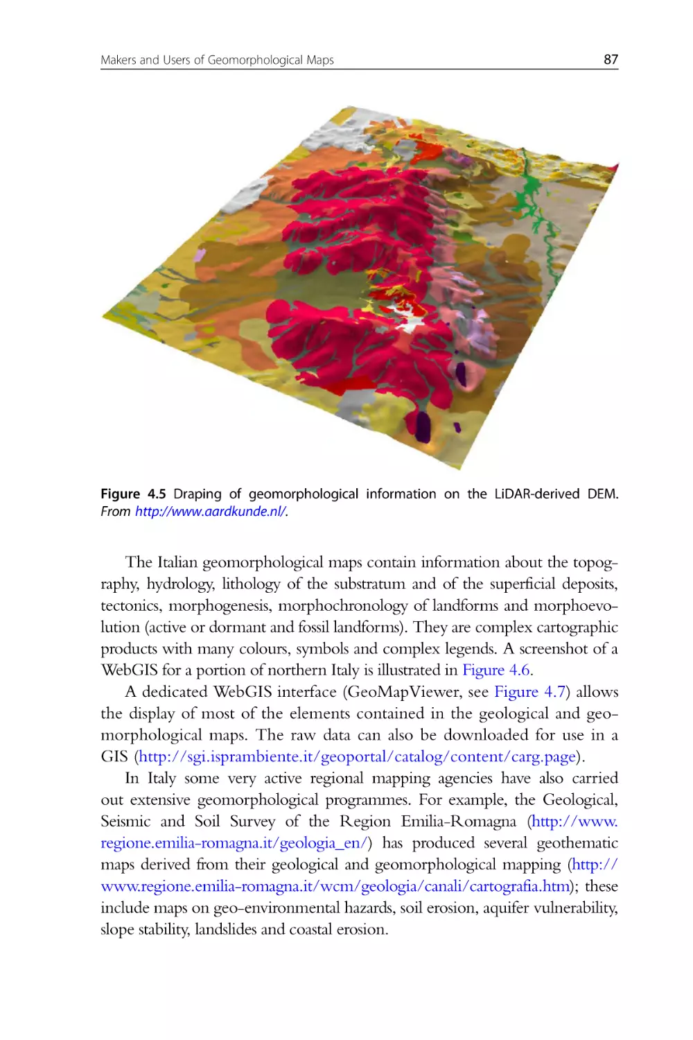
Figure 4.6 Excerpt from the geomorphological map of the Regione
Veneto at an original scale of 1:50,000. For the legend, see the link to
the handbook on geomorphological mapping.
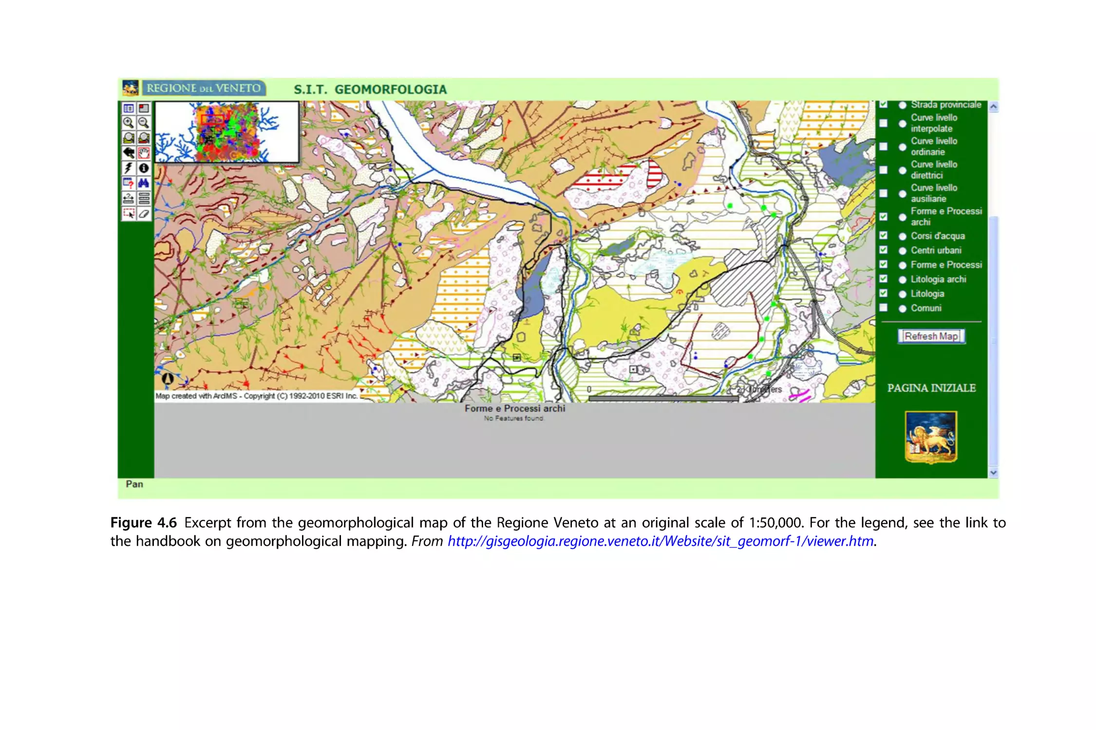
Figure 4.7 Screenshot of the Italian GeoMapViewer.
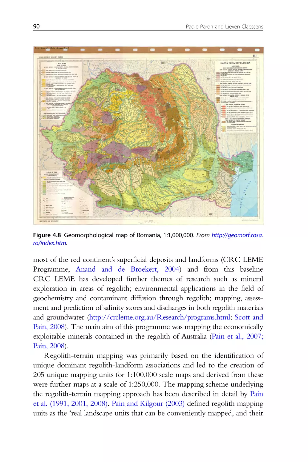
Figure 4.8 Geomorphological map of Romania, 1:1,000,000.
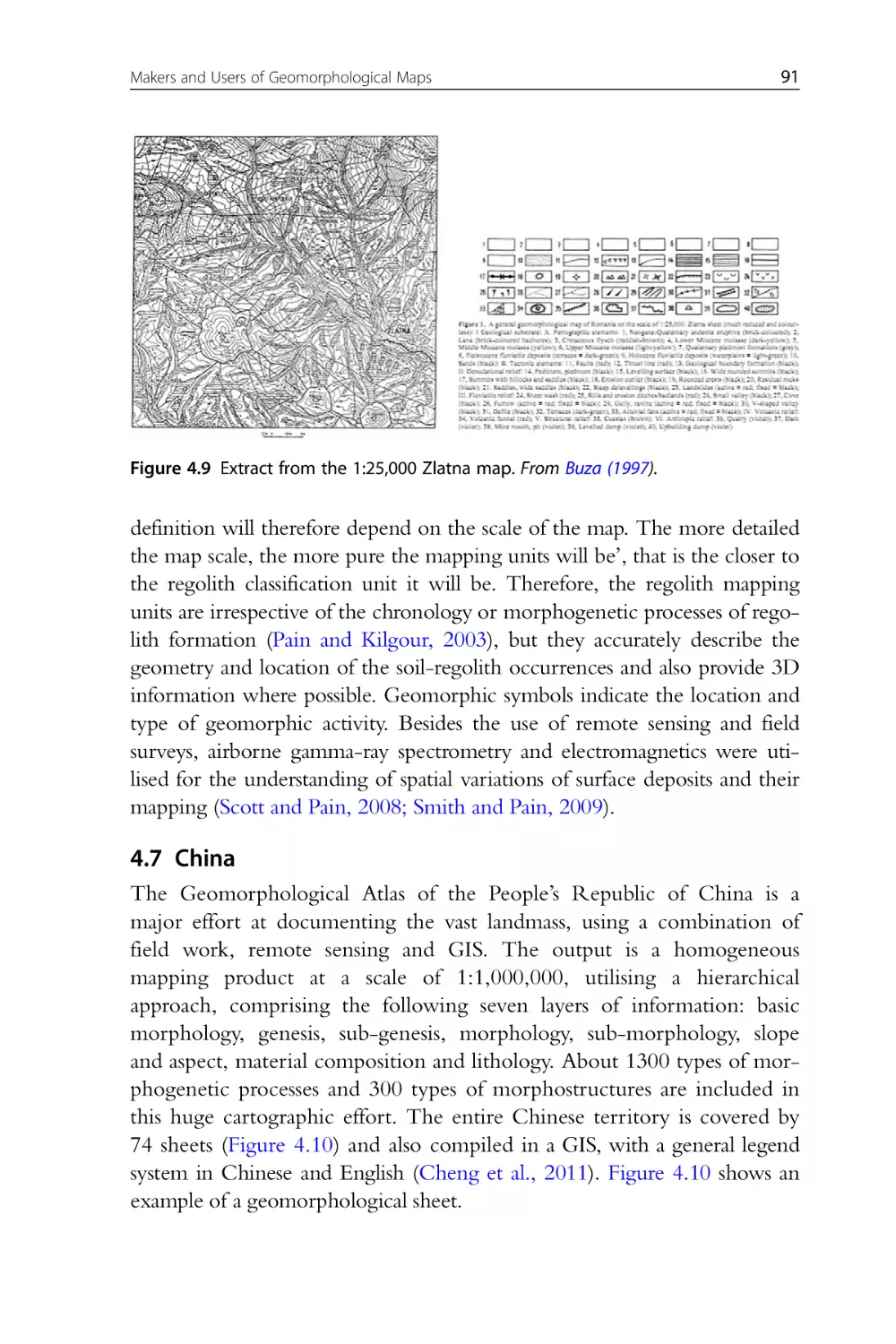
Figure 4.9 Extract from the 1:25,000 Zlatna map. From Buza (1997).
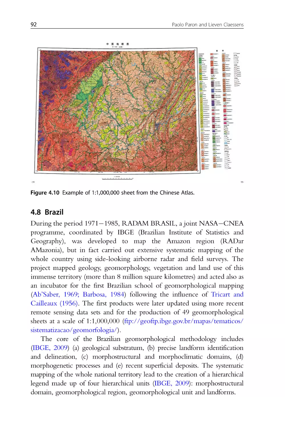
Figure 4.10 Example of 1:1,000,000 sheet from the Chinese Atlas.
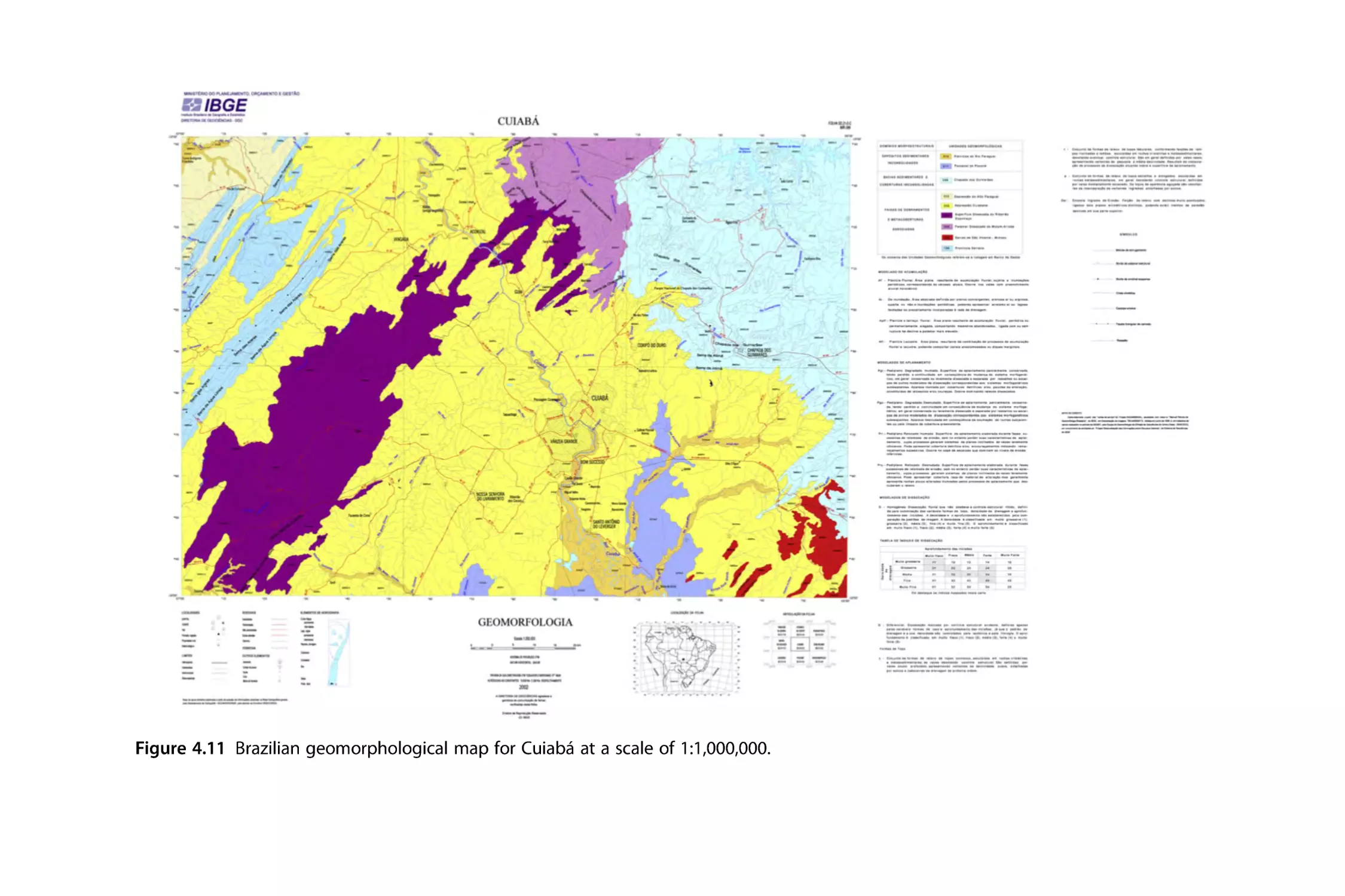
Figure 4.11 Brazilian geomorphological map for Cuiabá at a scale of
1:1,000,000.
Figure 4.12 Volcanic fires affecting an area in Eastern Congo 
 North
Kivu region in January 2010 (UNOSAT map).
Figure 4.13 Flood-affected areas in Pakistan during the floods of August
2010 (UNOSAT map).
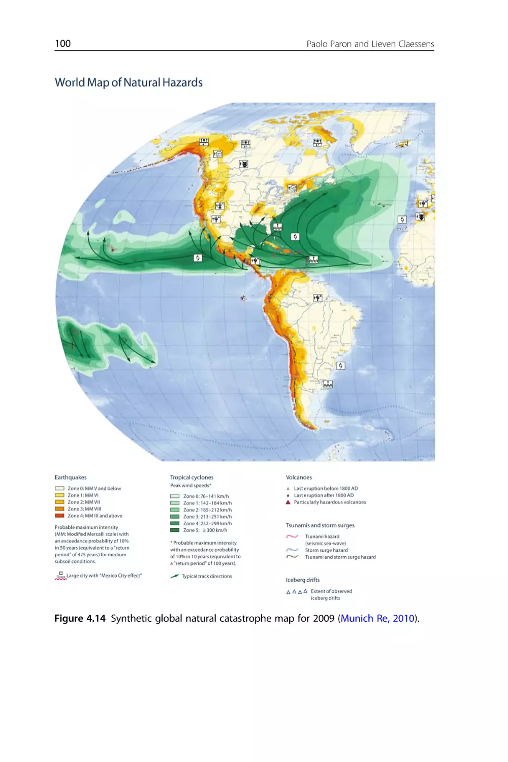
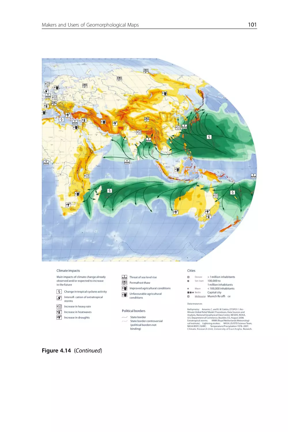
Figure 4.14 Synthetic global natural catastrophe map for 2009 (Munich
Re, 2010).
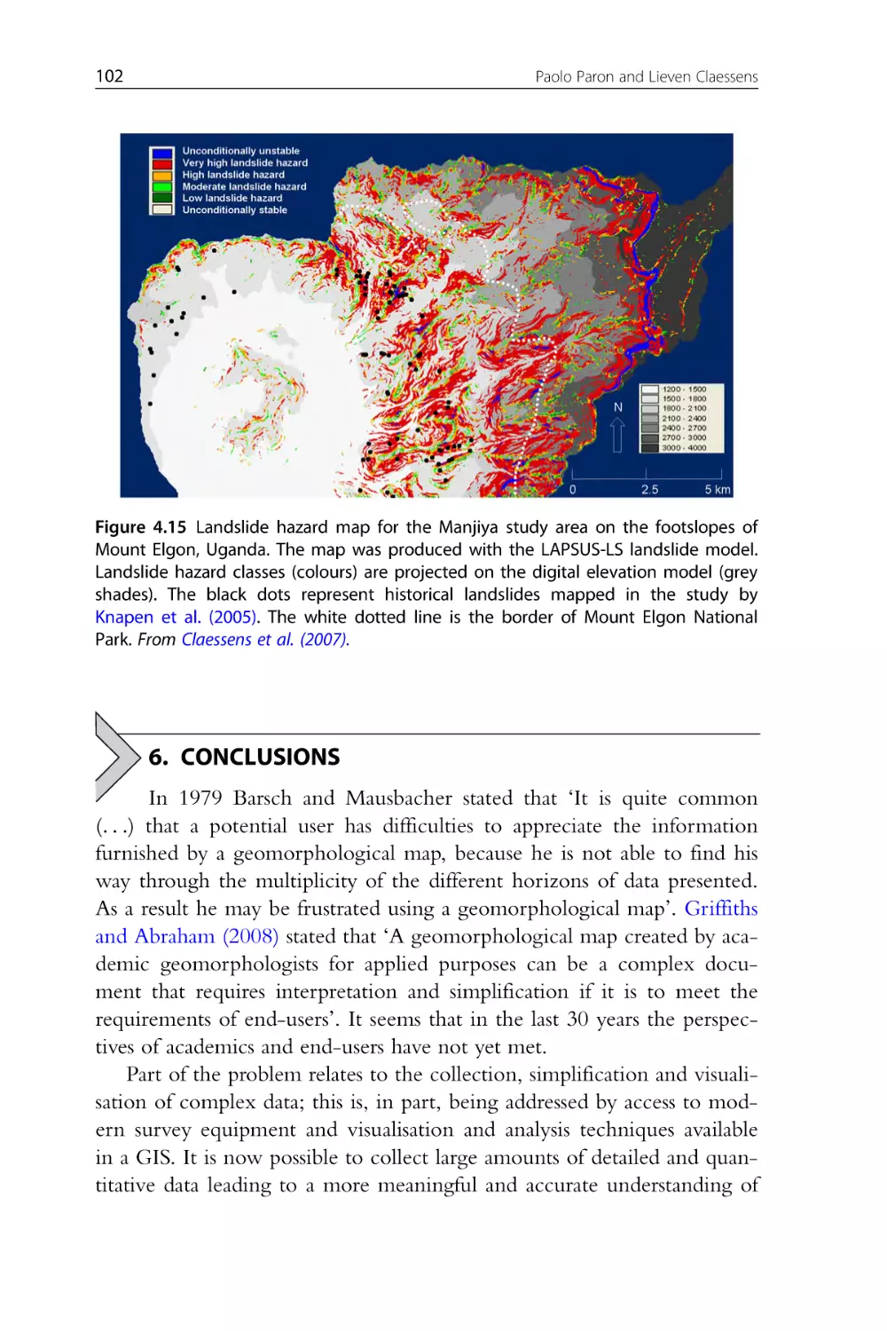
Figure 4.15 Landslide hazard map for the Manjiya study area on the footslopes of Mount Elgon, Uganda. The map was produced with the
LAPSUS-LS landslide model. Landslide hazard classes (colours) are projected on the digital elevation model (grey shades). The black dots represent historical landslides mapped in the study by Knapen et al.
(2005). The white dotted line is the border of Mount Elgon National
Park. From Claessens et al. (2007).

CHAPTER FIVE
Figure 5.1 Typical damage to roads in the Central Cordillera of the
Philippines following typhoons Ondoy and Pepeng in 2009 (Hearn 2011).

xxvi

List of Figures

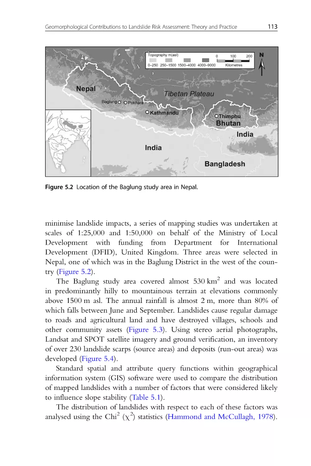
Figure 5.2 Location of the Baglung study area in Nepal.
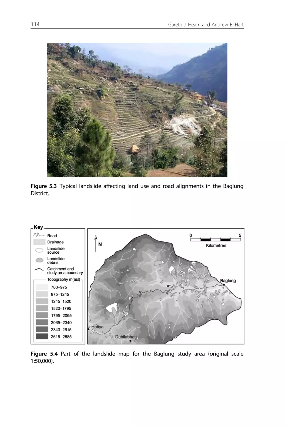
Figure 5.3 Typical landslide affecting land use and road alignments in the
Baglung District.
Figure 5.4 Part of the landslide map for the Baglung study area (original
scale 1:50,000).
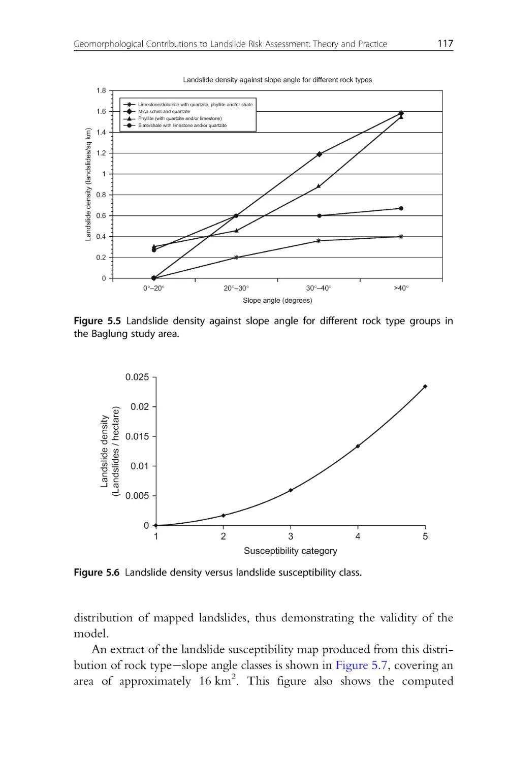
Figure 5.5 Landslide density against slope angle for different rock type
groups in the Baglung study area.
Figure 5.6 Landslide density versus landslide susceptibility class.
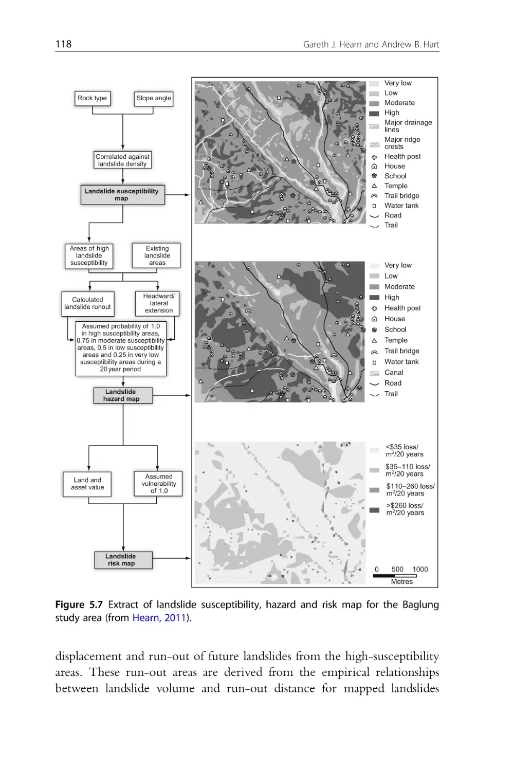
Figure 5.7 Extract of landslide susceptibility, hazard and risk map for the
Baglung study area (from Hearn, 2011).
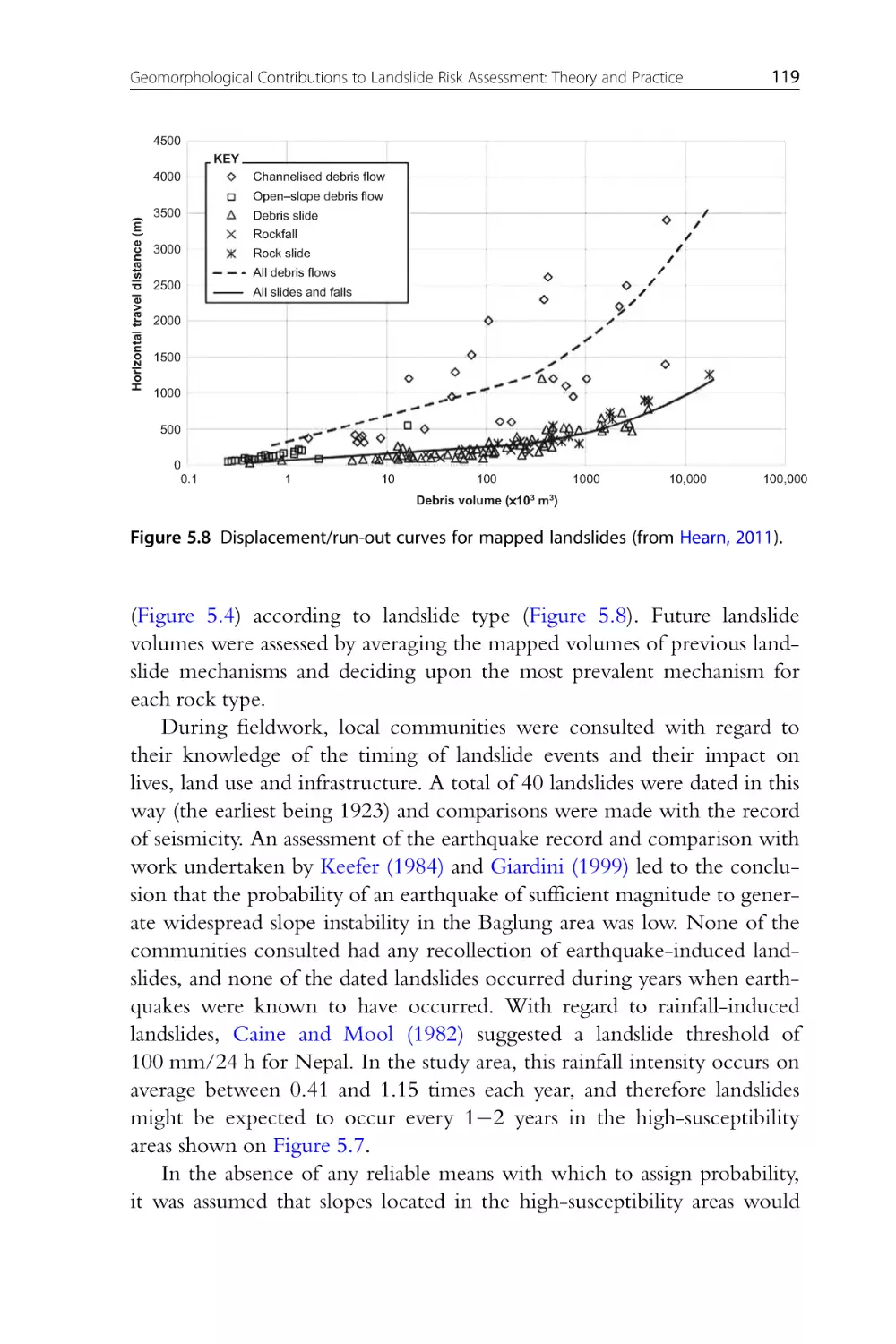
Figure 5.8 Displacement/run-out curves for mapped landslides. From
Hearn (2011).
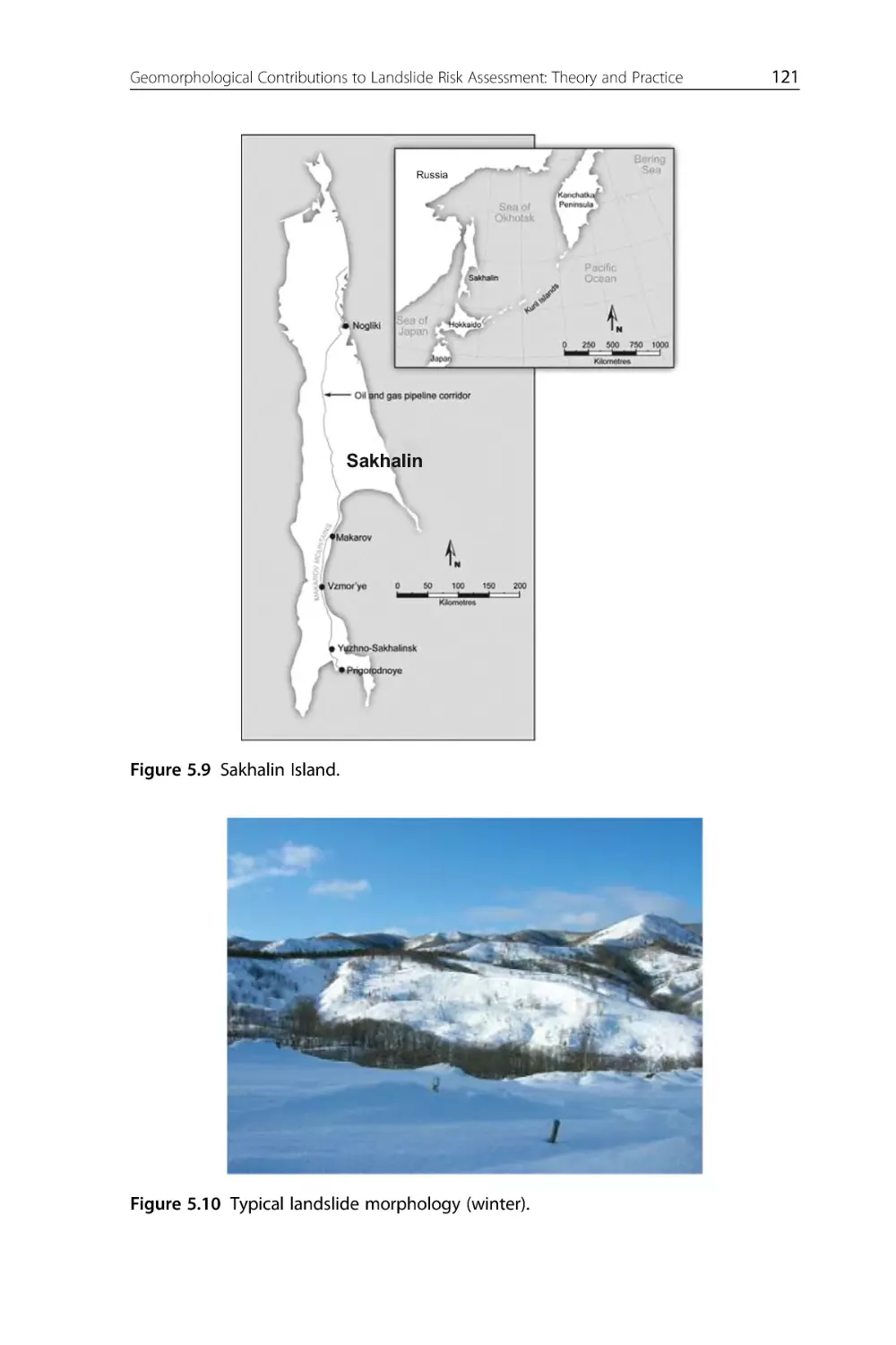
Figure 5.9 Sakhalin Island.
Figure 5.10 Typical landslide morphology (winter).
Figure 5.11 Geomorphological map of part of the alignment corridor.
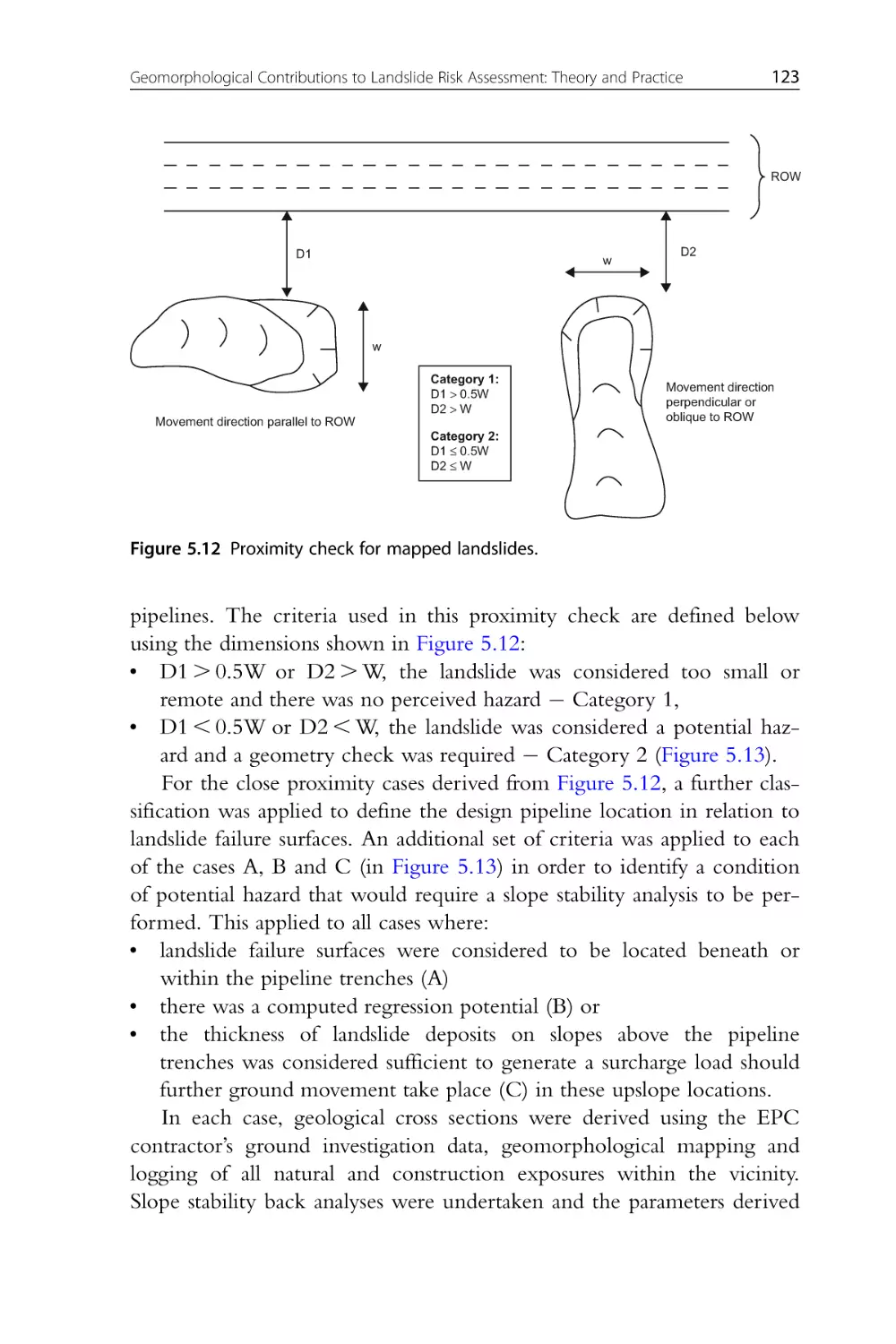
Figure 5.12 Proximity check for mapped landslides.
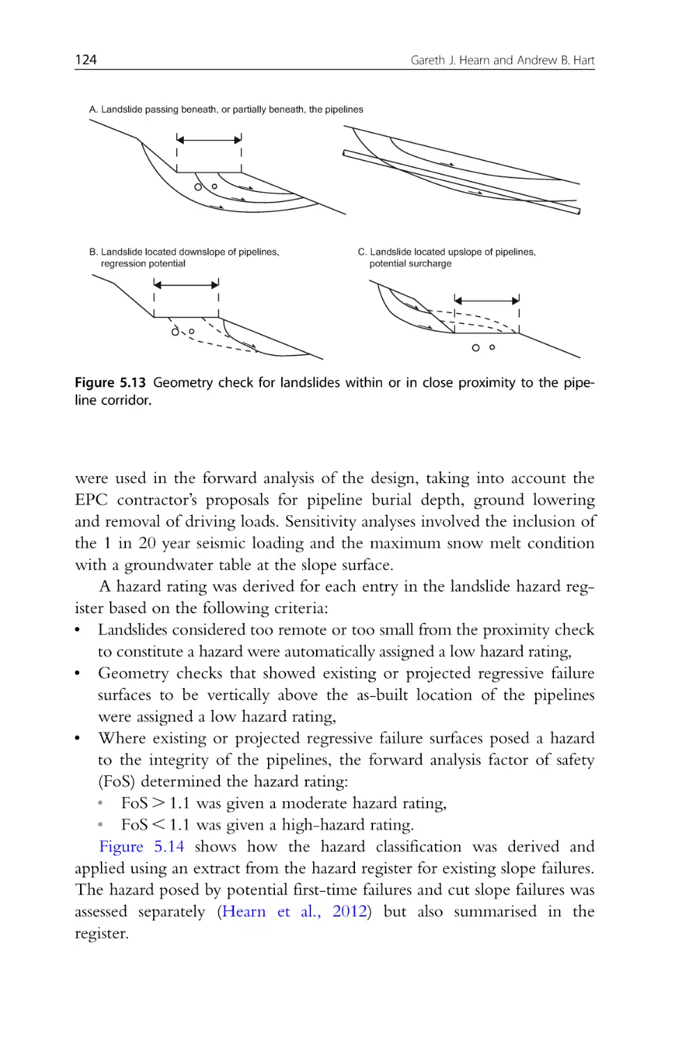
Figure 5.13 Geometry check for landslides within or in close proximity
to the pipeline corridor.
Figure 5.14 Extract from the hazard register for existing landslides.
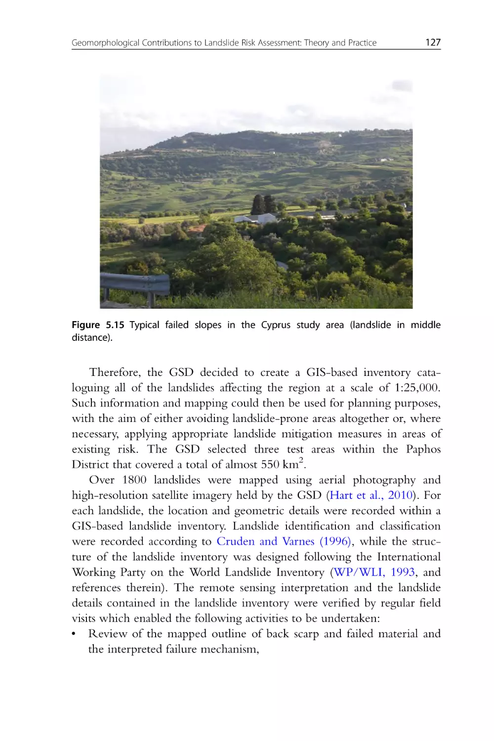
Figure 5.15 Typical failed slopes in the Cyprus study area (landslide in
middle distance).
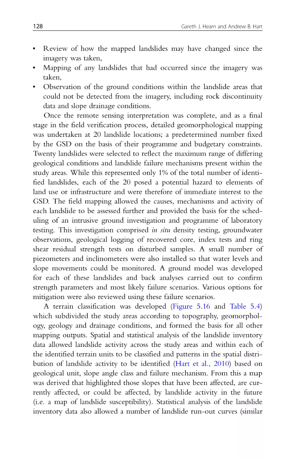
Figure 5.16 Terrain classification map for the three Paphos study areas.

CHAPTER SIX
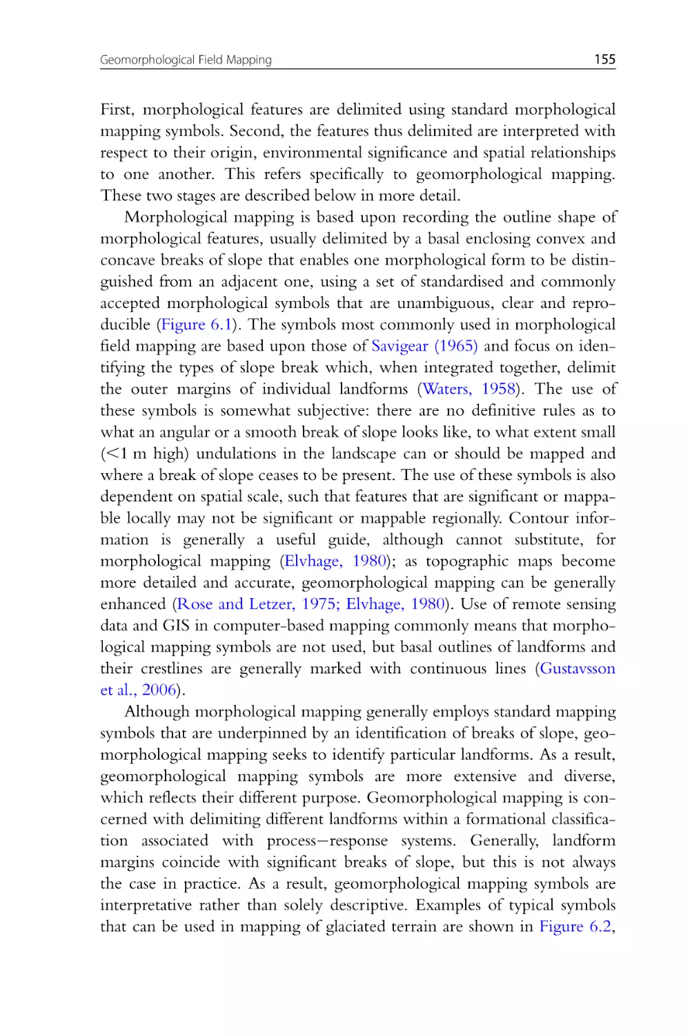
Figure 6.1 Basic morphological mapping symbols. From Cooke and
Doornkamp (1974).
Figure 6.2 Typical morphological mapping symbols (left) and examples of
geomorphological mapping symbols used in upland terrain (right).
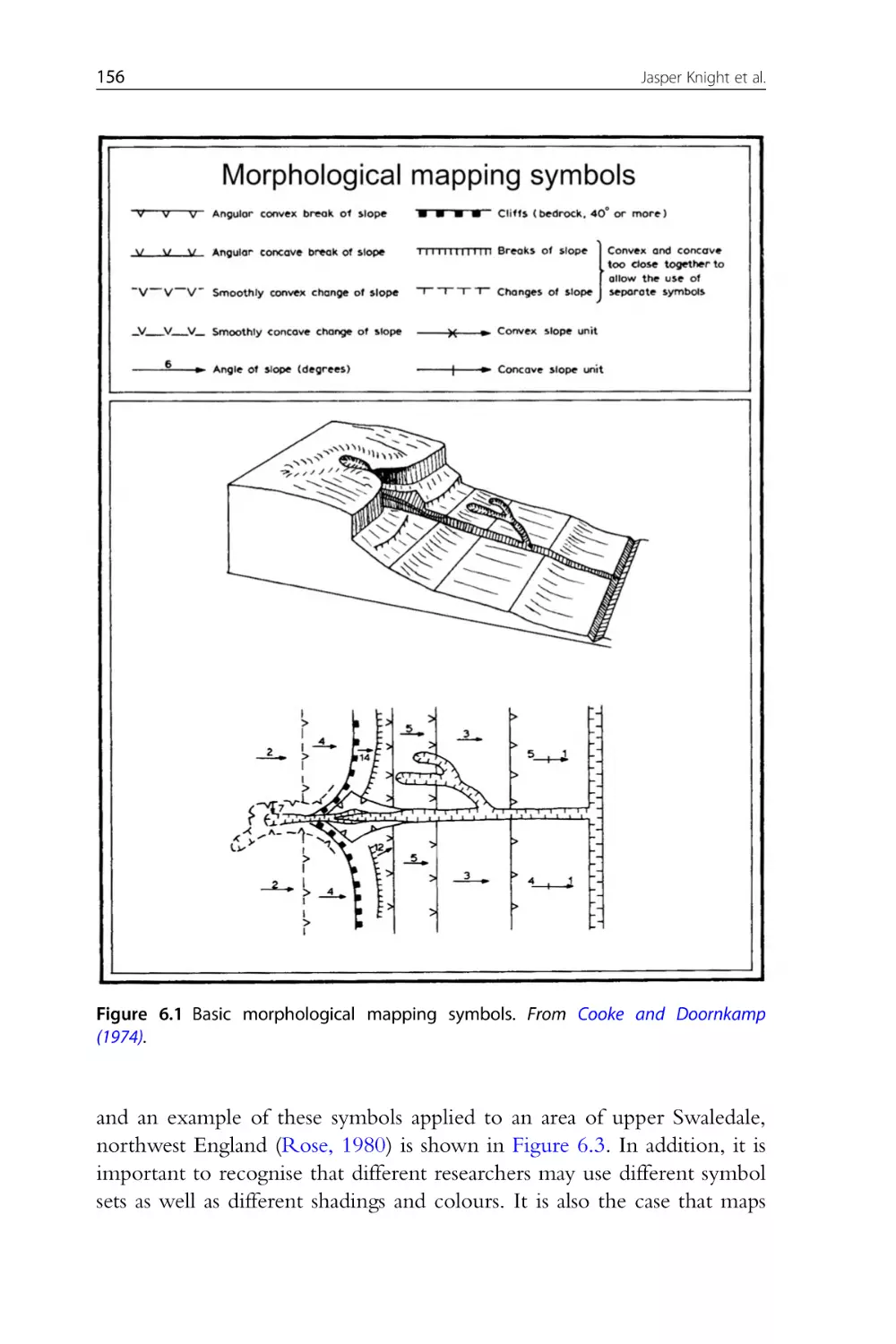
Figure 6.3 An example of geomorphological mapping in part of a glaciated upland region, Kisdon, upper Swaledale, Lake District, northwest
England. From Rose (1980).
Figure 6.4 Examples of drumlin mapping in different landscape settings,
Lake District, northwest England (mapping by W.A. Mitchell). (a) Copy
of a field slip showing geomorphological mapping in mid-Widdale.
Drumlins are located along hill flanks, and drumlins around river margins

List of Figures

xxvii

show fluvial erosion and slope failure. (b) Geomorphological mapping in
flatter terrain in Grisedale, showing superimposed drumlin forms.
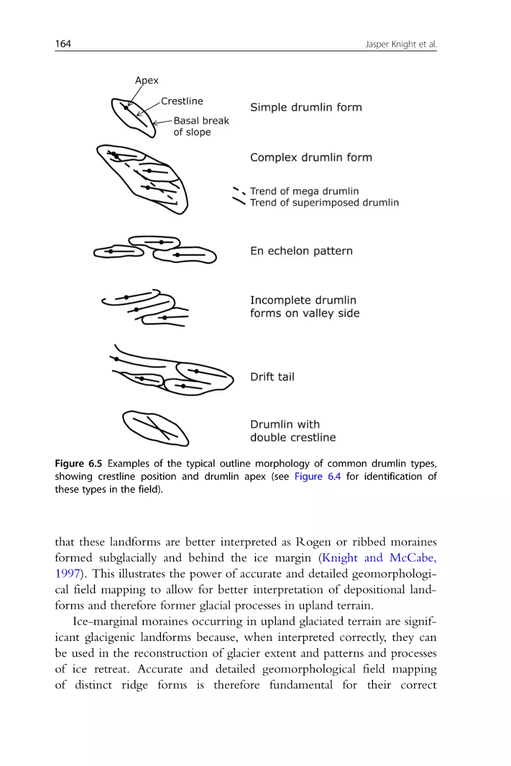
Figure 6.5 Examples of the typical outline morphology of common
drumlin types, showing crestline position and drumlin apex (see
Figure 6.4 for identification of these types in the field).
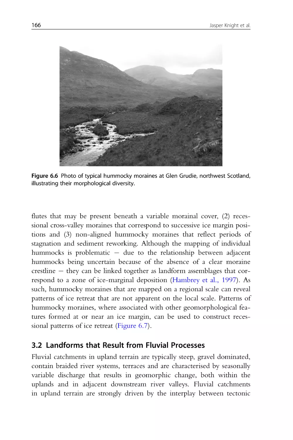
Figure 6.6 Photo of typical hummocky moraines at Glen Grudie, northwest Scotland, illustrating their morphological diversity.
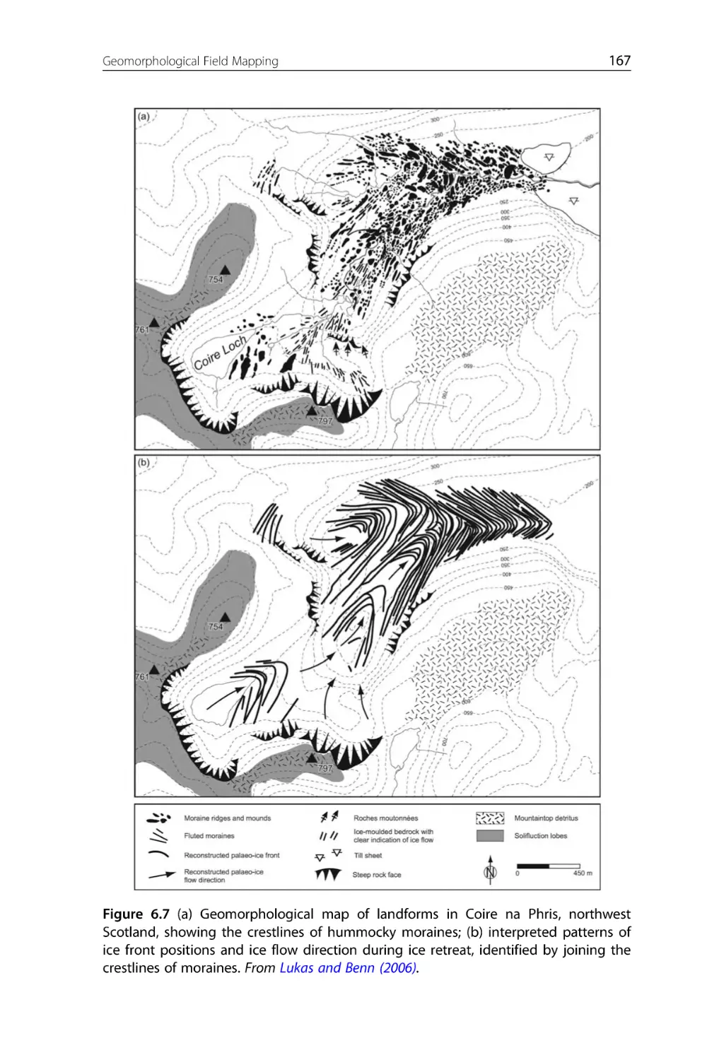
Figure 6.7 (a) Geomorphological map of landforms in Coire na Phris,
northwest Scotland, showing the crestlines of hummocky moraines; (b)
interpreted patterns of ice front positions and ice flow direction during
ice retreat, identified by joining the crestlines of moraines. From Lukas
and Benn (2006).
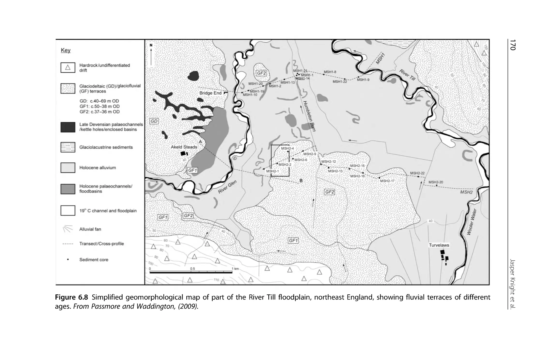
Figure 6.8 Simplified geomorphological map of part of the River Till
floodplain, northeast England, showing fluvial terraces of different ages.
From Passmore et al. (2009).
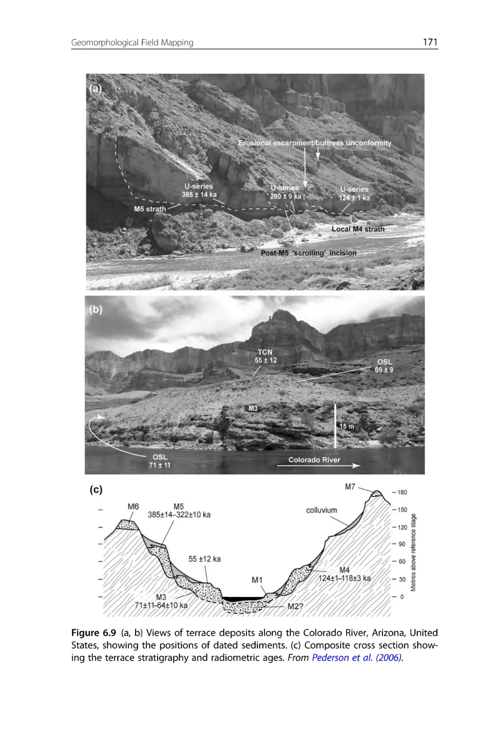
Figure 6.9 (a, b) Views of terrace deposits along the Colorado River,
Arizona, United States, showing the positions of dated sediments. (c)
Composite cross section showing the terrace stratigraphy and radiometric ages. From Pederson et al. (2006).
Figure 6.10 Maps of channel and bar morphology at different time periods at Llandinam, Upper Severn River, central Wales (from Passmore
et al., 1993). See text for discussion of how geomorphological and sediment budget changes are calculated.
Figure 6.11 Geomorphological map of the Stonebarrow Hill area,
Dorset, southern England. From Goudie (1981).
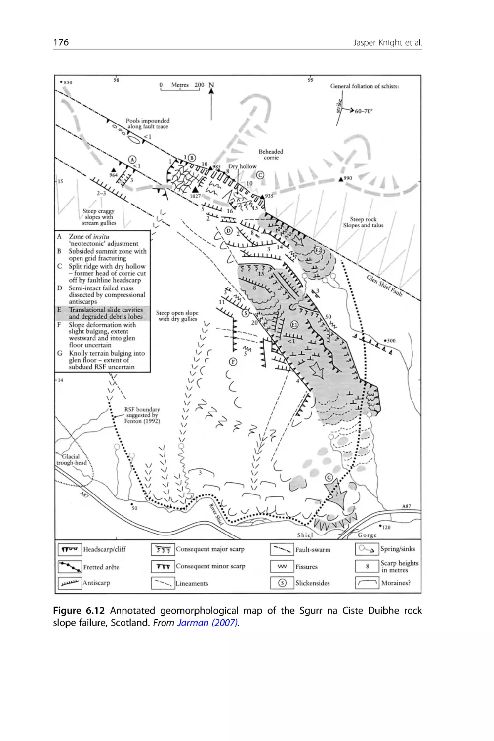
Figure 6.12 Annotated geomorphological map of the Sgurr na Ciste
Duibhe rock slope failure, Scotland. From Jarman (2007).
Figure 6.13 Geomorphological map of the Keylong Serai rock avalanche,
northwest Indian Himalaya. From Mitchell et al. (2007).

CHAPTER SEVEN
Figure 7.1 An eighteenth-century map showing contour lines of the riverbed in the Netherlands (Van den Brink, 2000).
Figure 7.2 (a) Landsat image and (b) derived raster land cover for a part
of the Brahmaputra River, Bangladesh (Takagi et al., 2007).

xxviii

List of Figures

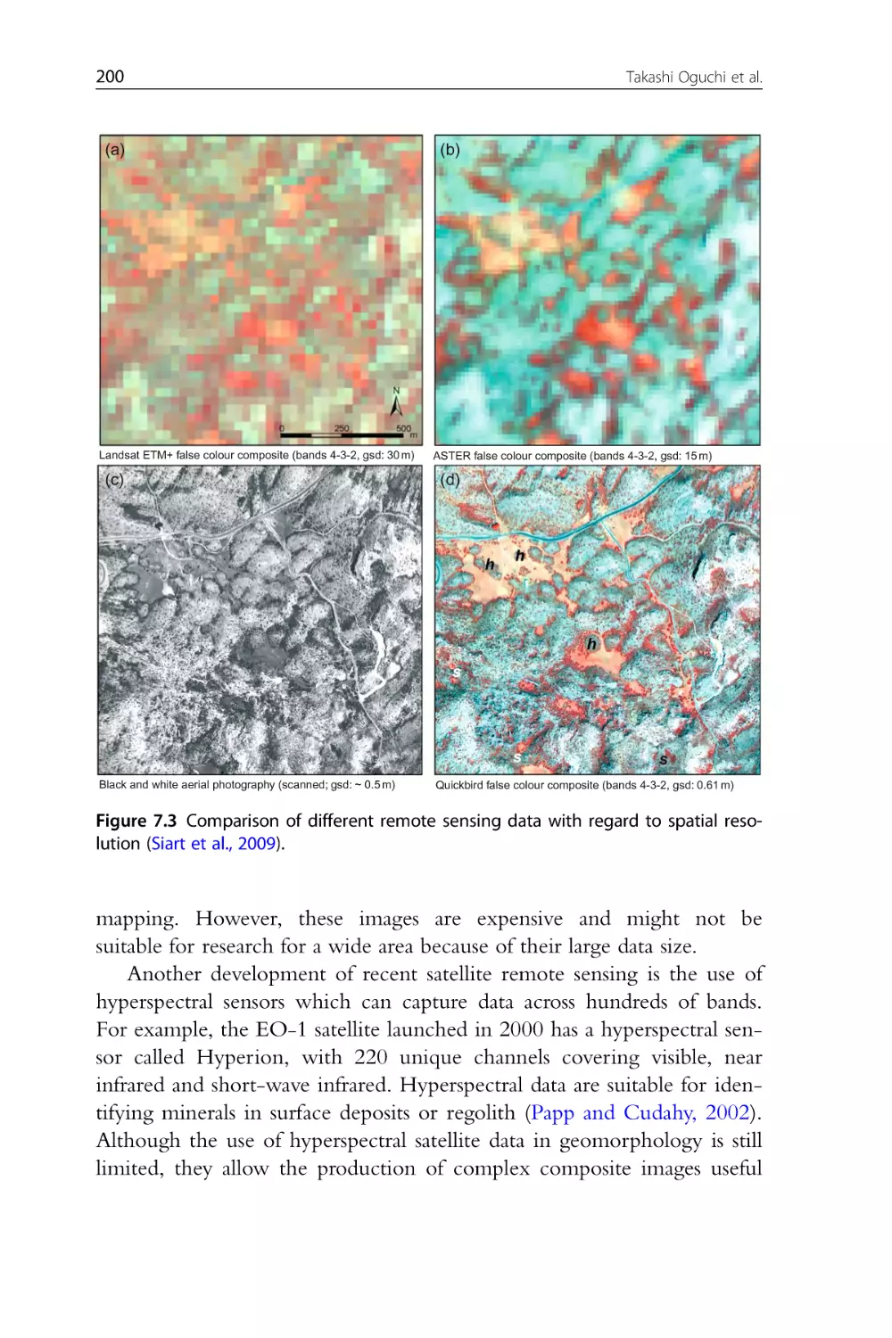
Figure 7.3 Comparison of different remote sensing data with regard to
spatial resolution (Siart et al., 2009).
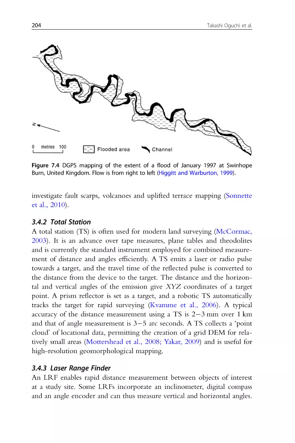
Figure 7.4 DGPS mapping of the extent of a flood of January 1997 at
Swinhope Burn, United Kingdom. Flow is from right to left (Higgitt
and Warburton, 1999).
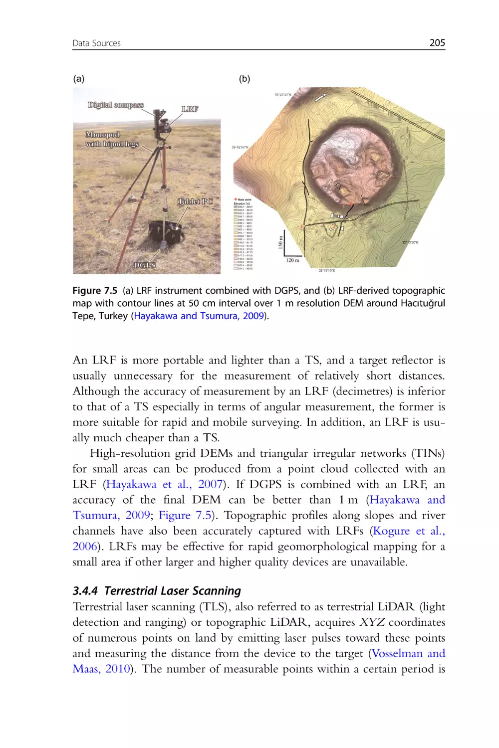
Figure 7.5 (a) LRF instrument combined with DGPS, and (b) LRF-derived
topographic map with contour lines at 50 cm interval over 1 m resolution
DEM around Hacıtuğrul Tepe, Turkey (Hayakawa and Tsumura, 2009).
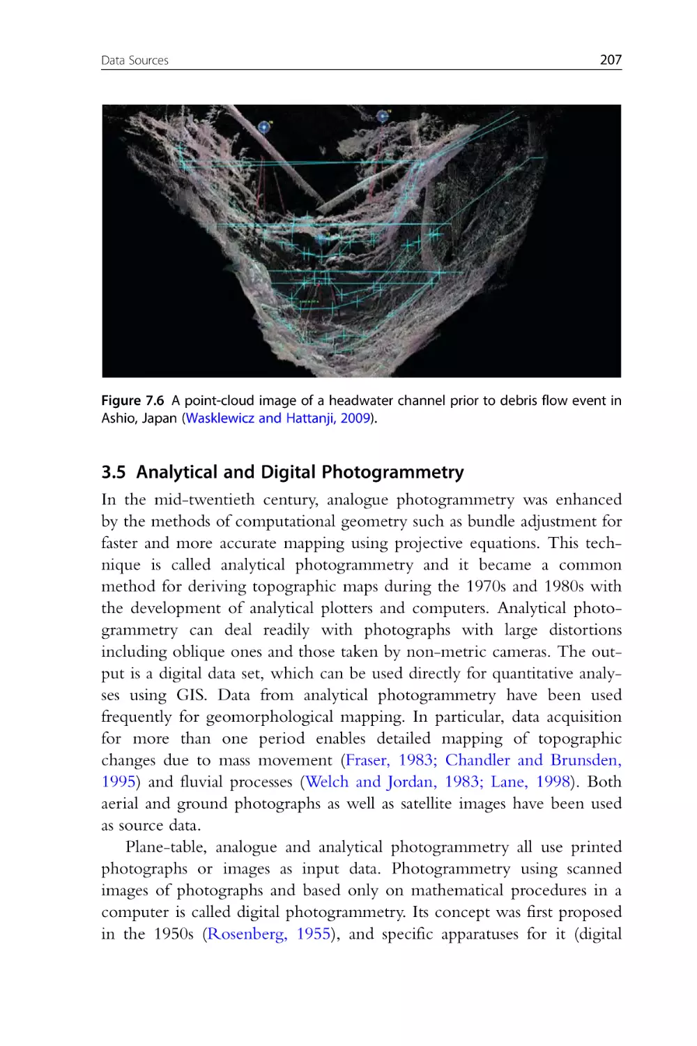
Figure 7.6 A point-cloud image of a headwater channel prior to debris
flow event in Ashio, Japan (Wasklewicz and Hattanji, 2009).
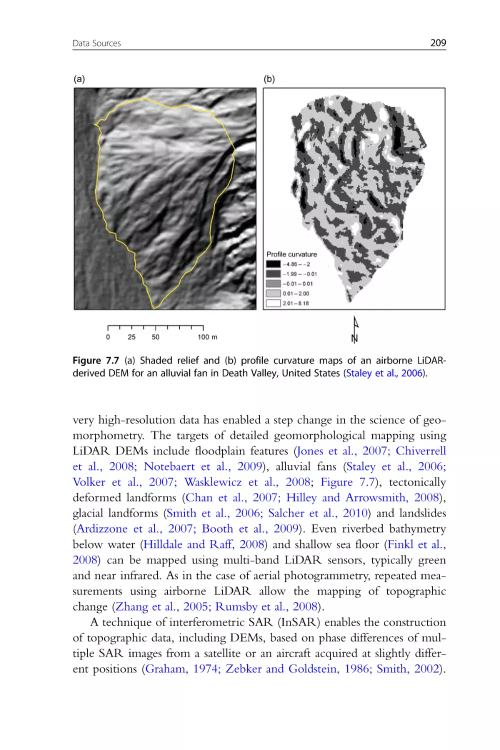
Figure 7.7 (a) Shaded relief and (b) profile curvature maps of an airborne
LiDAR-derived DEM for an alluvial fan in Death Valley, United States
(Staley et al., 2006).
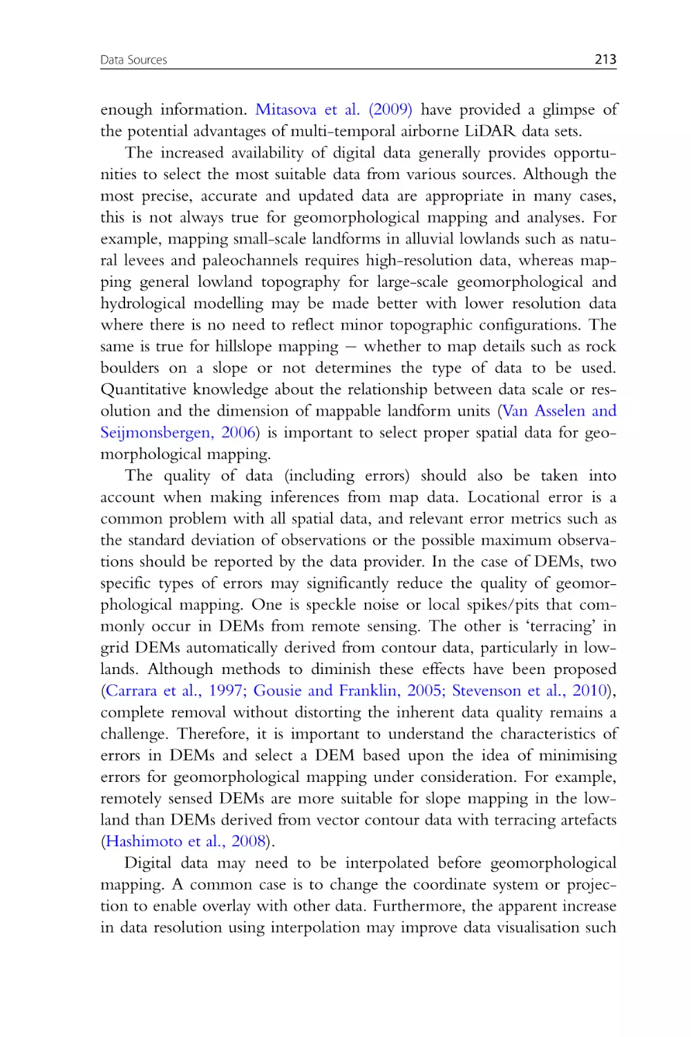
Figure 7.8 Comparison of LiDAR DEM imagery and field mapping
(Smith et al., 2006).

CHAPTER EIGHT
Figure 8.1 Illustration of the effects of relative size on the detectability of
drumlins. Spatial resolution of the DEM is fixed at (a) 50 m and (b)
150 m. Reproduced from Ordnance Survey Ireland, Copyright Permit
MP001904.
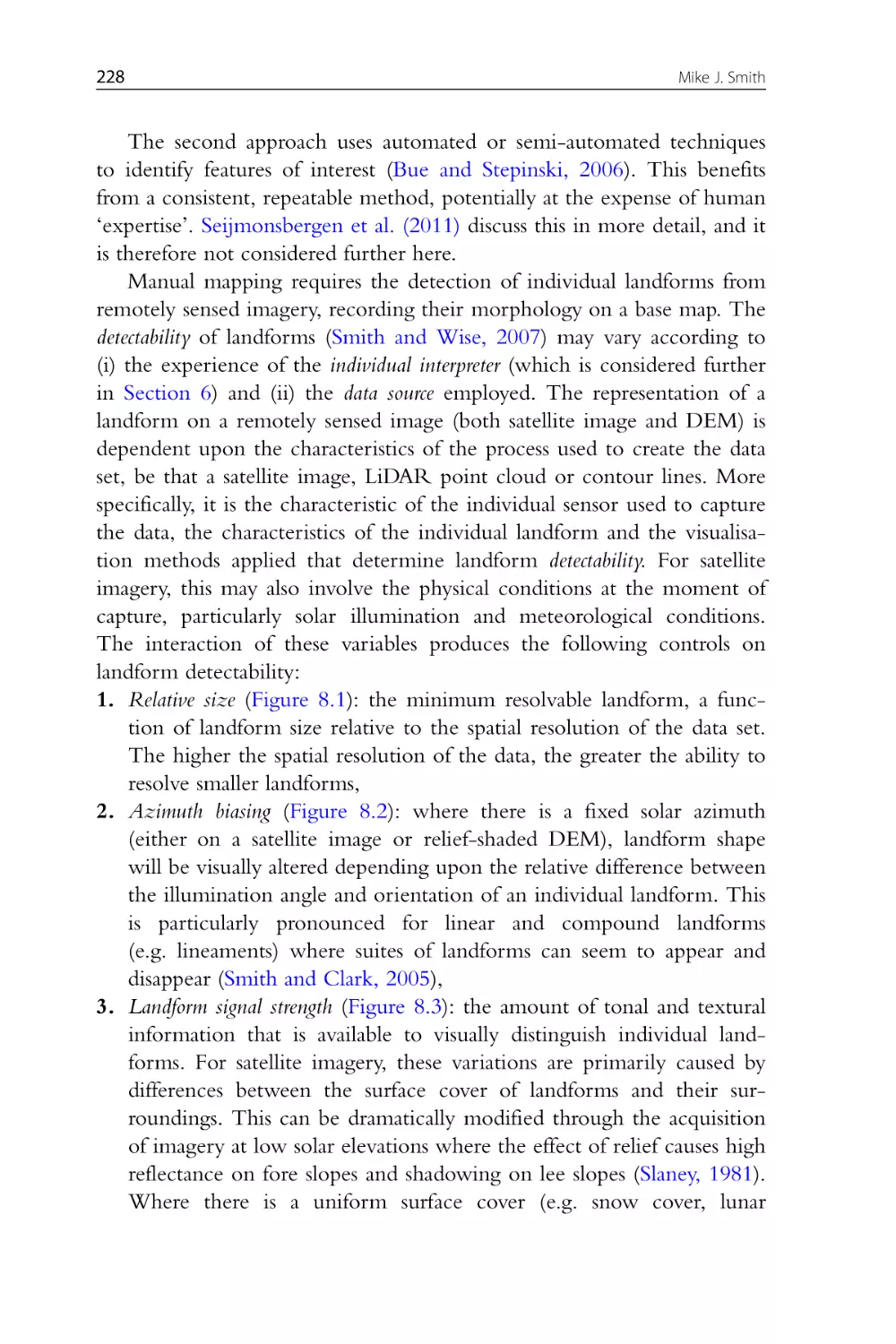
Figure 8.2 Illustration of the effects of azimuth angle on the detectability
of drumlins from a relief-shaded DEM. (a) Azimuth angle parallel to
the dominant drumlin orientation and (b) orthogonal to the principal
drumlin orientation. Arrows indicate azimuth angle (see http://www.
appgema.net/). Reproduced from Ordnance Survey Ireland, Copyright
Permit MP001904.
Figure 8.3 Illustration of the effects of landform signal strength through
the use of Landsat TM imagery of the same location acquired on contrasting dates with (a) low solar elevation (11 ) and (b) high solar elevation (48 ).
Figure 8.4 Satellite images and DEMs are raster data products. For example,
(a) a relief-shaded DEM is a collection of (b) picture elements (pixels)
shaded from black to white. (c) These reflect the underlying pixel value.
Figure 8.5 Vector data can be composed of three main feature types:
points, lines and polygons.

List of Figures

xxix

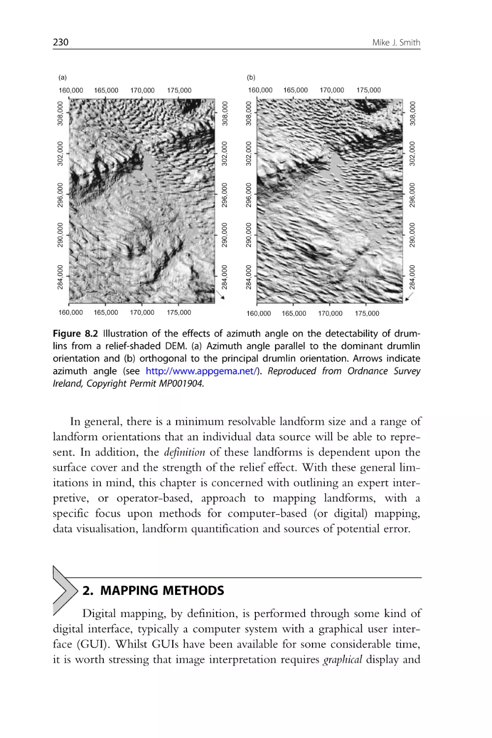
Figure 8.6 Screenshot illustrating the setup of thematic layers within
ESRIs ArcGIS. Note that a polygon feature is currently being digitised,
using the underlying raster DEM data as a backdrop.
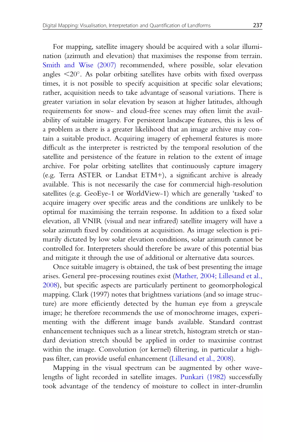
Figure 8.7 DEM visualisation using (a) greyscaling and (b) relief shading
(illumination angle 20 ). Reproduced from Ordnance Survey Ireland,
Copyright Permit MP001904.
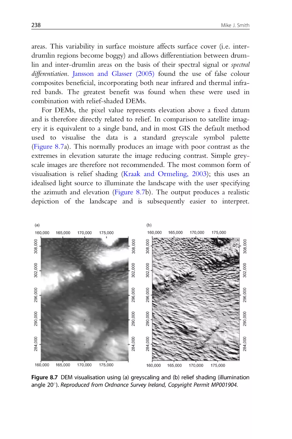
Figure 8.8 DEM visualisation using (a) gradient and (b) curvature. Reproduced
from Ordnance Survey Ireland, Copyright Permit MP001904.
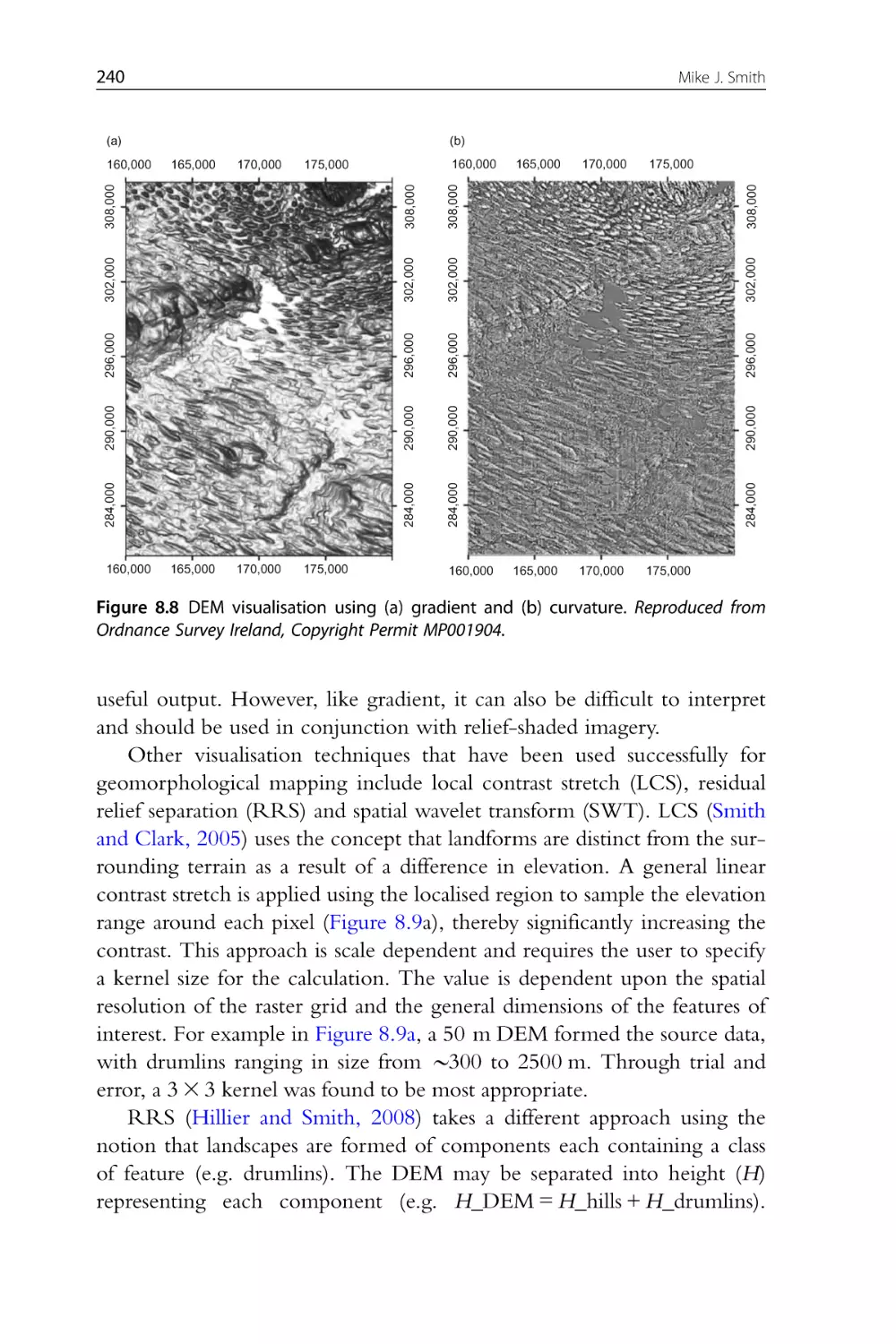
Figure 8.9 DEM visualisation using (a) LCS and (b) RRS. Reproduced
from Ordnance Survey Ireland, Copyright Permit MP001904.
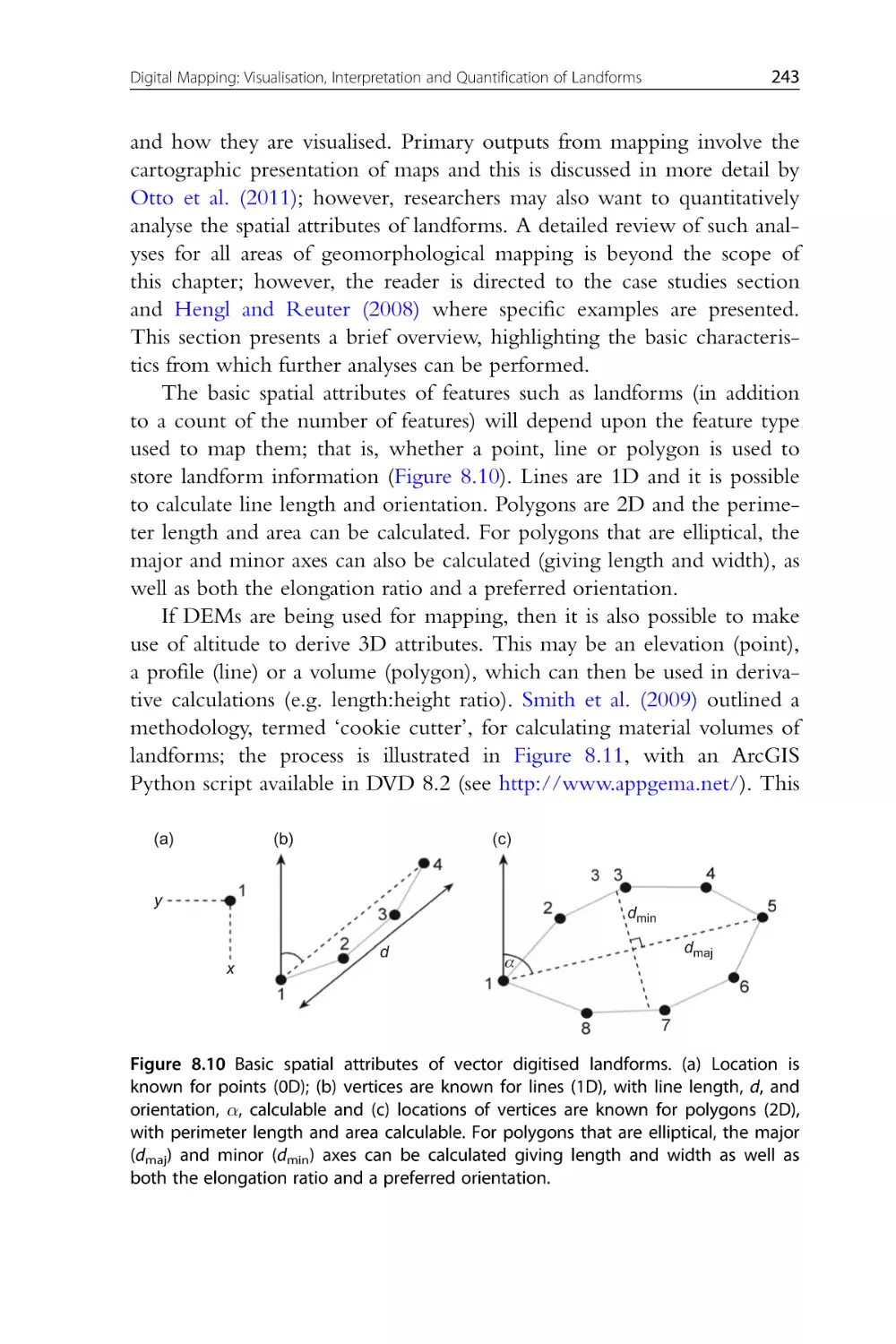
Figure 8.10 Basic spatial attributes of vector digitised landforms. (a)
Location is known for points (0D); (b) vertices are known for lines
(1D), with line length, d, and orientation, α, calculable and (c) locations of vertices are known for polygons (2D), with perimeter length
and area calculable. For polygons that are elliptical, the major (dmaj) and
minor (dmin) axes can be calculated giving length and width as well as
both the elongation ratio and a preferred orientation.
Figure 8.11 Workflow for the calculation of landform volume. The
example is of a drumlin located at Bowridge (NS 7880). (a) Example
of a drumlin, (b) raw DEM data, (c) relief-shaded visualisation of terrain, with mapped drumlin outlines, (d) DEM voids, (e) interpolation
of drumlin basal surfaces and (f) relief-shaded visualisation of drumlin
volumes (1.51 m3 3 106 m3). Note the ‘stepping’ in (e), a result of
artefacts at the edges being interpolated across the basal surface.
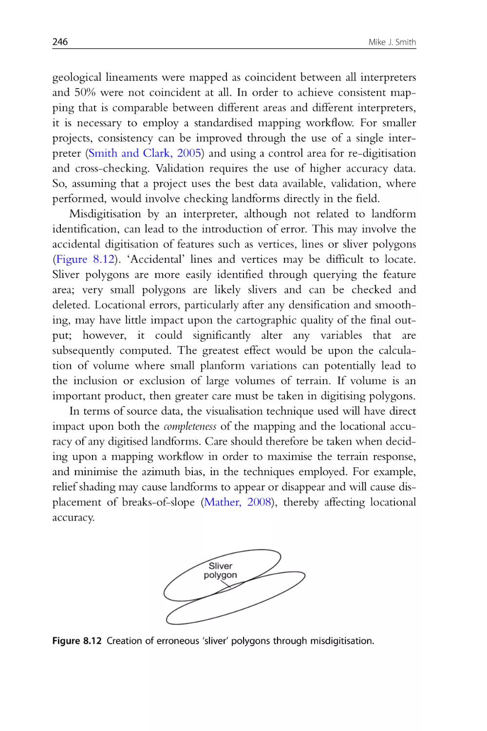
Figure 8.12 Creation of erroneous ‘sliver’ polygons through
misdigitisation.

CHAPTER NINE
Figure 9.1 Primitives of map symbols and visual variables. (y 5 yellow,
r 5 red, g 5 green).
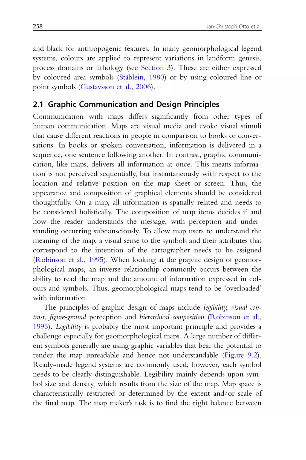
Figure 9.2 Section of the geomorphological map 1:25,000, sheet 8114
Feldberg, from the GMK 25 mapping programme in Germany. Colour
intensity and the density of symbols render this map hard to read.
Extracted from Geilhausen, Otto and Dikau (2007).
Figure 9.3 Illustrating the figure-ground relationship: (a) A simple black
line on white does not help to differentiate between different levels of

xxx

List of Figures

information. (b) The grey colour now separates the different features
on the same map, but the outcome is still ambiguous. (c) By adding
lines representing rivers, the separation of land and ocean becomes
more obvious. Inspired by Robinson et al. (1995).
Figure 9.4 Section of the geomorphological map 1:25,000 Turtmanntal,
Switzerland (Otto and Dikau, 2004). This map contains several hierarchical levels of information: coloured area symbols represent the process
domains, light grey (orange in the coloured image) symbol fills show surface material information, black point and line symbols indicate landforms
and processes, and point symbols in light grey depict active processes.
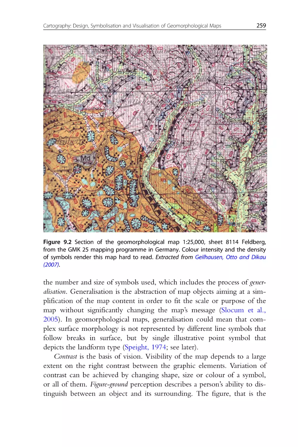
Figure 9.5 Typical items of a geomorphological map.
Figure 9.6 Comparing the symbols for moraine ridge and fluvial terrace
of the different legend systems presented in this chapter.
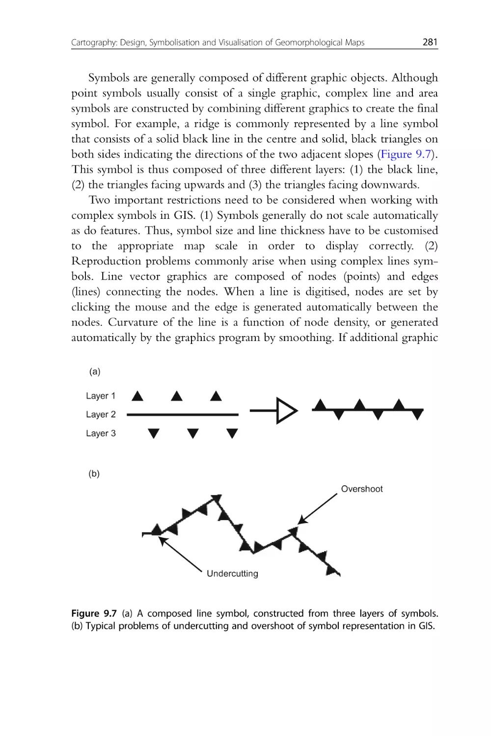
Figure 9.7 (a) A composed line symbol, constructed from three layers of
symbols. (b) Typical problems of undercutting and overshoot of symbol
representation in GIS.
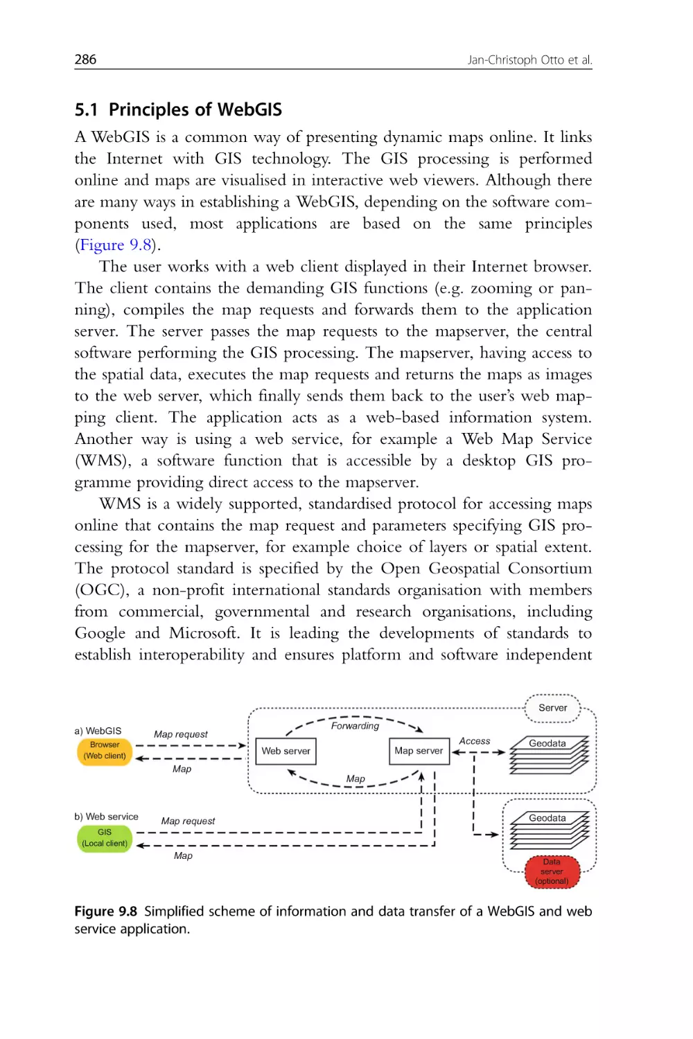
Figure 9.8 Simplified scheme of information and data transfer of a
WebGIS and web service application.
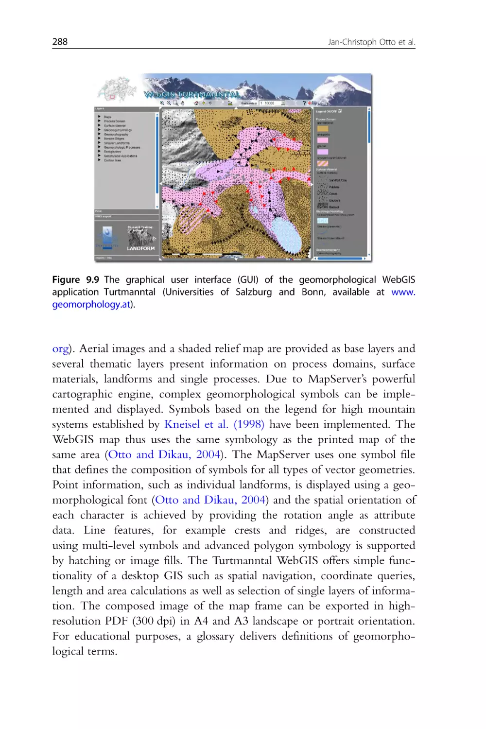
Figure 9.9 The graphical user interface (GUI) of the geomorphological
WebGIS application Turtmanntal (Universities of Salzburg and Bonn,
available at www.geomorphology.at).
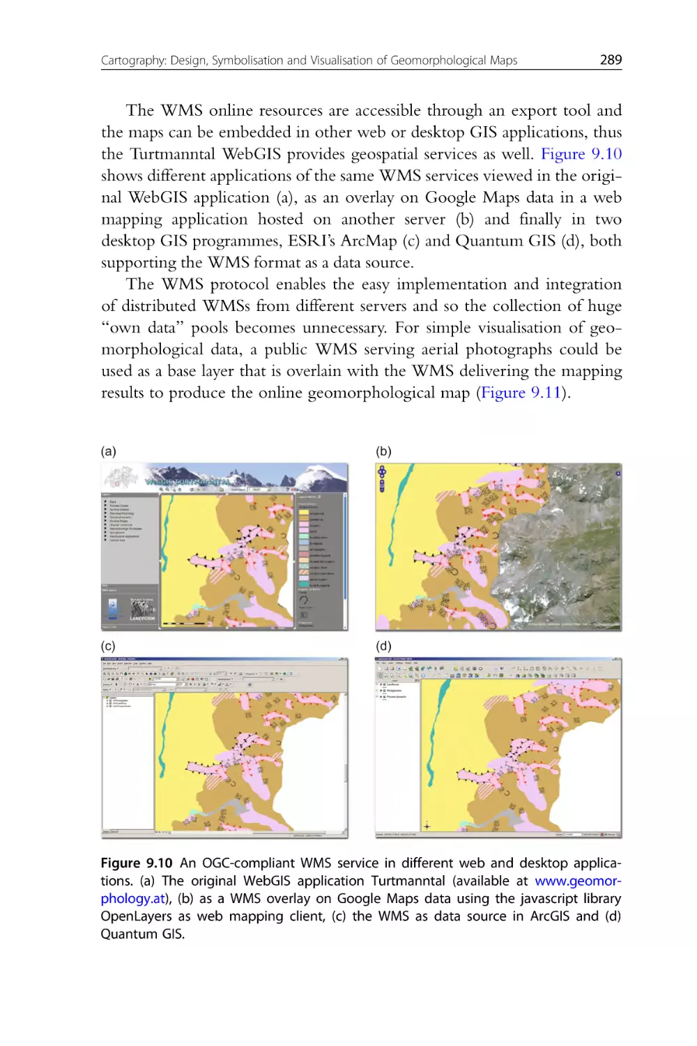
Figure 9.10 An OGC-compliant WMS service in different web and desktop applications. (a) The original WebGIS application Turtmanntal
(available at www.geomorphology.at), (b) as a WMS overlay on Google
Maps data using the javascript library OpenLayers as web mapping client, (c) the WMS as data source in ArcGIS and (d) Quantum GIS.
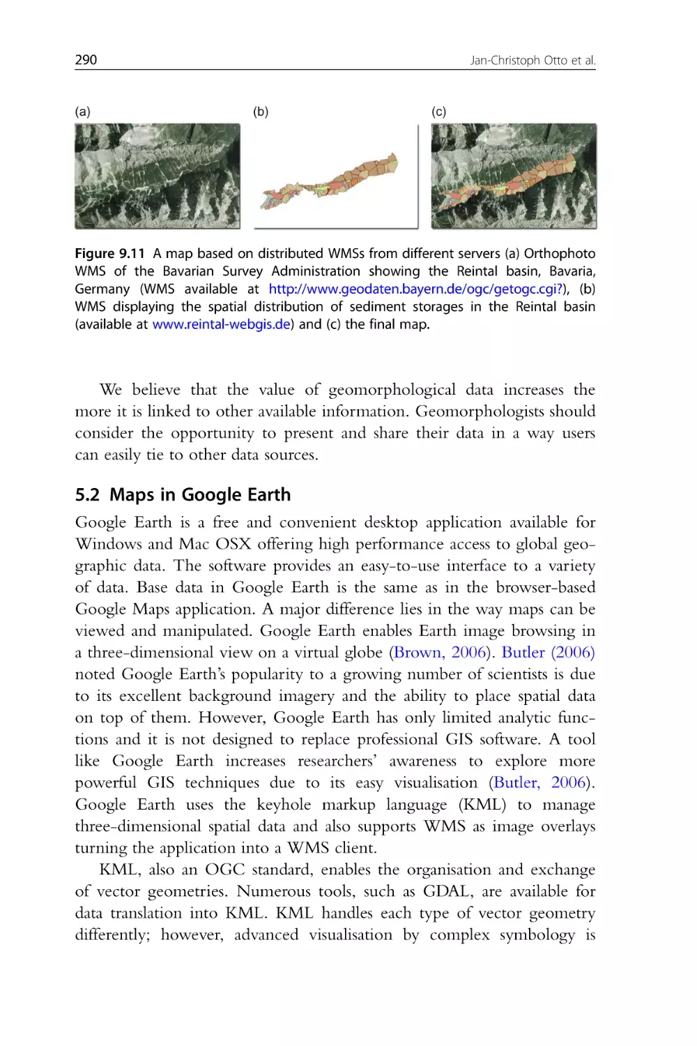
Figure 9.11 A map based on distributed WMSs from different servers (a)
Orthophoto WMS of the Bavarian Survey Administration showing the
Reintal basin, Bavaria, Germany (available at http://www.geodaten.
bayern.de/ogc/getogc.cgi?), (b) WMS displaying the spatial distribution
of sediment storages in the Reintal basin (available at www.reintal-webgis.de) and (c) the final map .
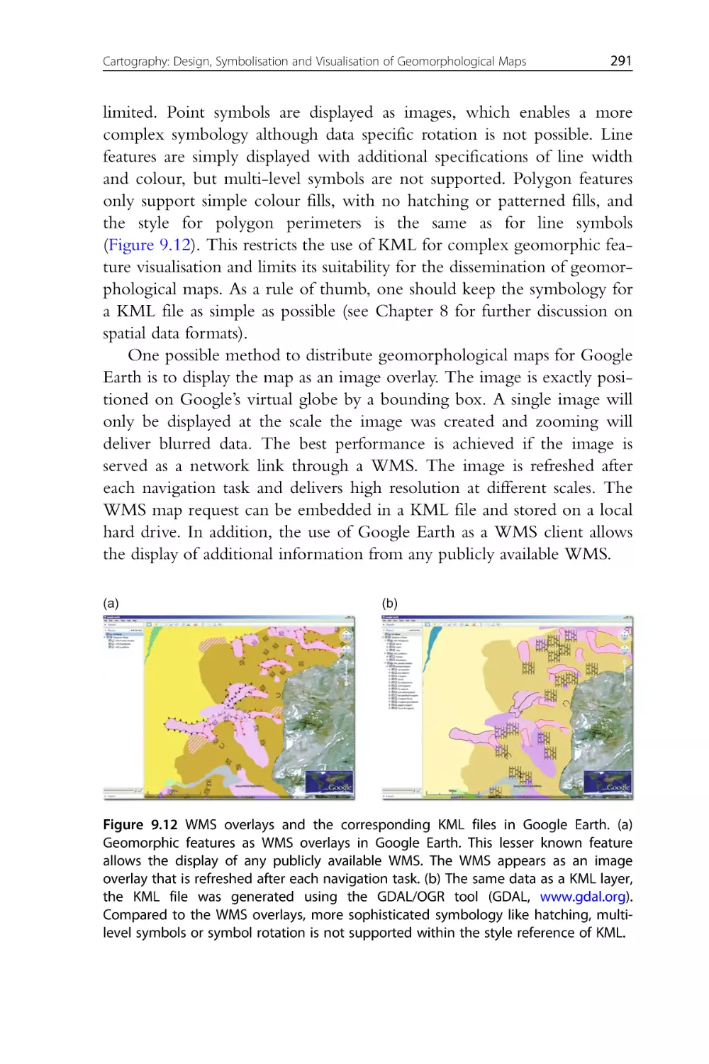
Figure 9.12 WMS overlays and the corresponding KML files in Google
Earth. (a) Geomorphic features as WMS overlays in Google Earth. This
lesser known feature allows the display of any publicly available WMS.
The WMS appears as an image overlay that is refreshed after each navigation task. (b) The same data as a KML layer, the KML file was generated using the GDAL/OGR tool (GDAL, www.gdal.org). Compared
to the WMS overlays, more sophisticated symbology like hatching,

List of Figures

xxxi

multi-level symbols or symbol rotation is not supported within the style
reference of KML.

CHAPTER TEN
Figure 10.1 (a) Classic geomorphological map fragment of map sheet Gurtis
overlaid with manually digitised geomorphological polygons and a point
file linked to additional information. Two examples of linked additional
information are shown: (b) a photo of an ice marginal terrace, the location
indicated by a black outline in the geomorphological unit map and (c) a
derived map of scientific relevance. After Seijmonsbergen (1992).
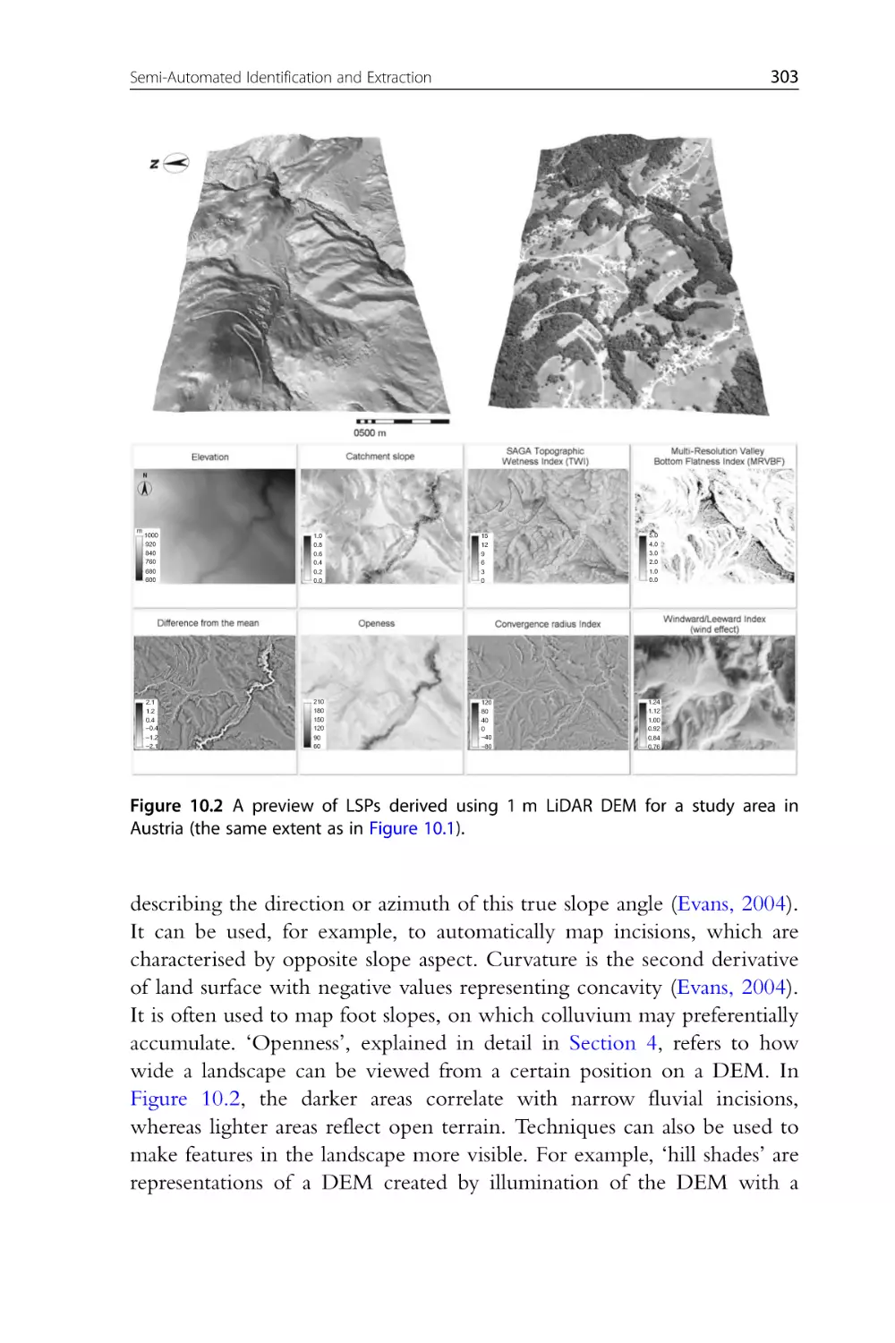
Figure 10.2 A preview of LSPs derived using 1 m LiDAR DEM for a
study area in Austria (the same extent as in Figure 10.1).
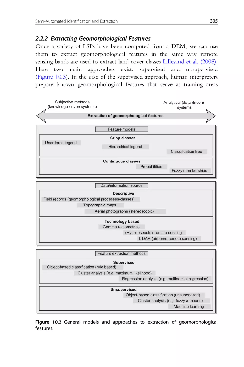
Figure 10.3 General models and approaches to extraction of geomorphological features.
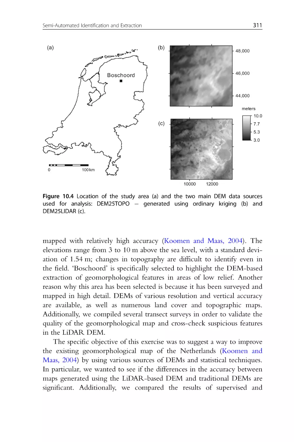
Figure 10.4 Location of the study area (a) and the two main DEM data
sources used for analysis: DEM25TOPO 
 generated using ordinary
kriging (b) and DEM25LIDAR (c).
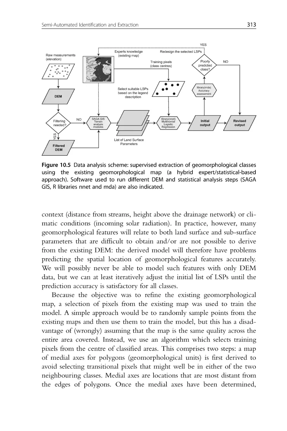
Figure 10.5 Data analysis scheme: supervised extraction of geomorphological
classes using the existing geomorphological map (a hybrid expert/statistical-based approach). Software used to run different DEM and statistical
analysis steps (SAGA GIS, R libraries nnet and mda) are also indicated.
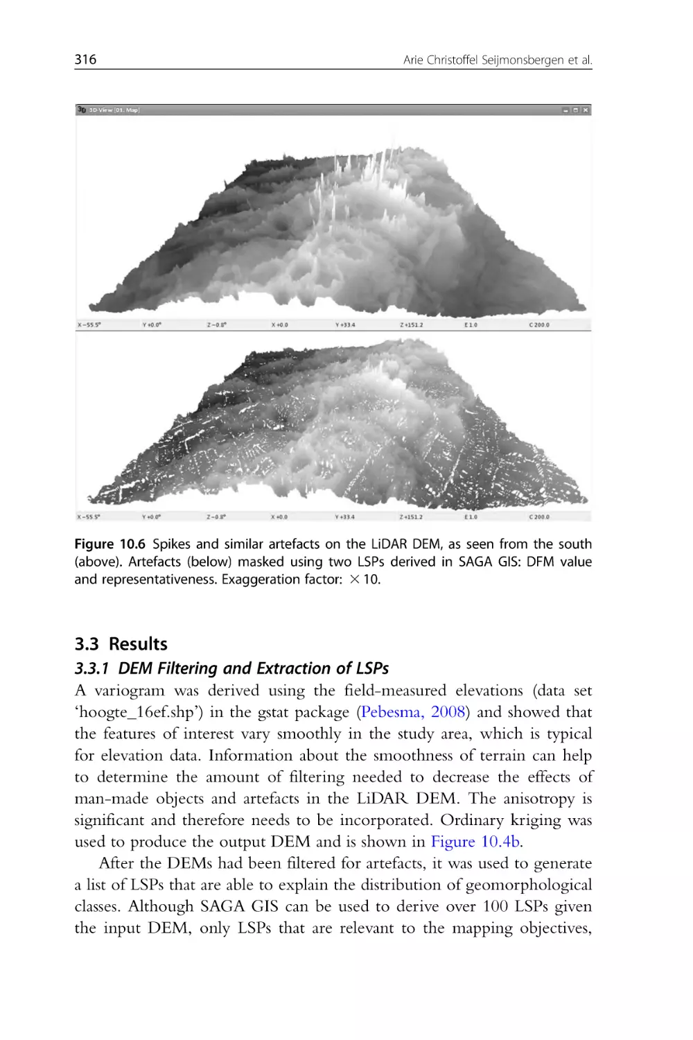
Figure 10.6 Spikes and similar artefacts on the LiDAR DEM, as seen
from the south (above). Artefacts (below) masked using two LSPs
derived in SAGA GIS: DFM value and representativeness. Exaggeration
factor: 3 10.
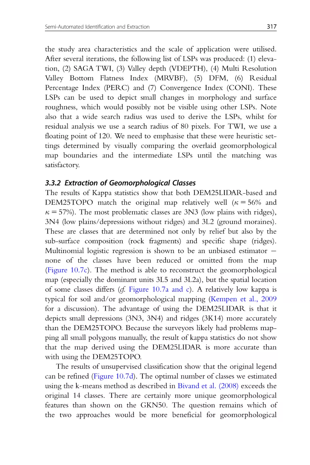
Figure 10.7 Results of supervised classification for Section 3: (a) the original geomorphological map and the training pixels (along medial axes);
(b) classes predicted using the multinomial logistic regression and
DEM25TOPO; (c) classes predicted using multinomial logistic regression and DEM25LIDAR; (d) results of unsupervised classification using
the same number of classes (no legend). See text for description of classes in the legend.
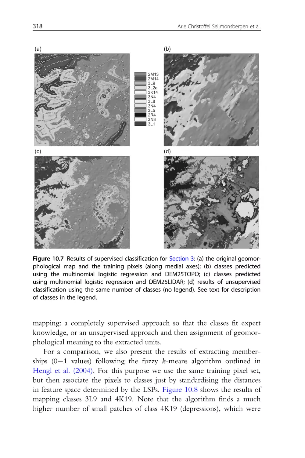
Figure 10.8 Membership maps for geomorphological classes 3L9 (low
dunes+plains) and 4K19 (low dunes/depressions); both based on the
DEM25LIDAR. Visualised in SAGA GIS.

xxxii

List of Figures

Figure 10.9(a) White box indicates the location of the ‘Lech’ study area
(DEM in (b)) in Vorarlberg, Western Austria. (b) DEM of study area
(vertical exaggeration of 1.5). (c) Bare gypsum karst geomorphology
near Lech, location photo indicated by the white box in (b).
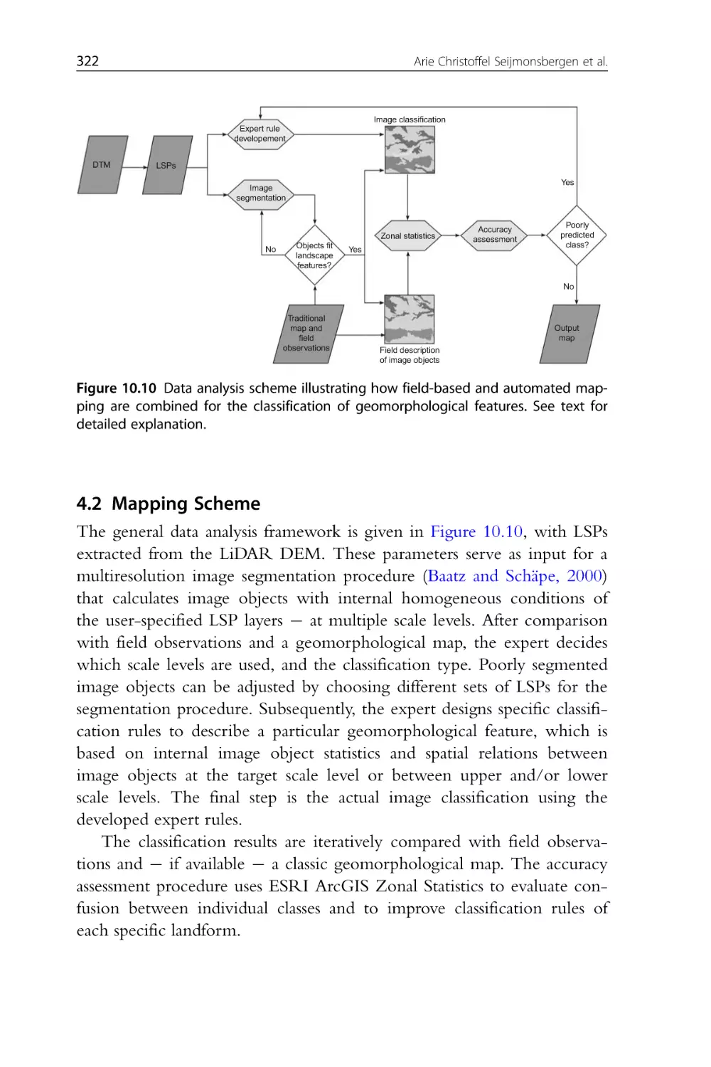
Figure 10.10 Data analysis scheme illustrating how field-based and automated mapping are combined for the classification of geomorphological
features. See text for detailed explanation.
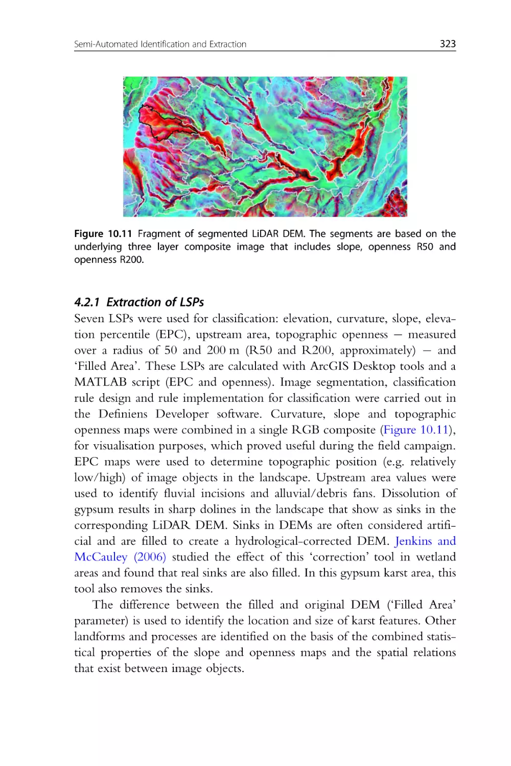
Figure 10.11 Fragment of segmented LiDAR DEM. The segments are
based on the underlying three layer composite image that includes
slope, openness R50 and openness R200.
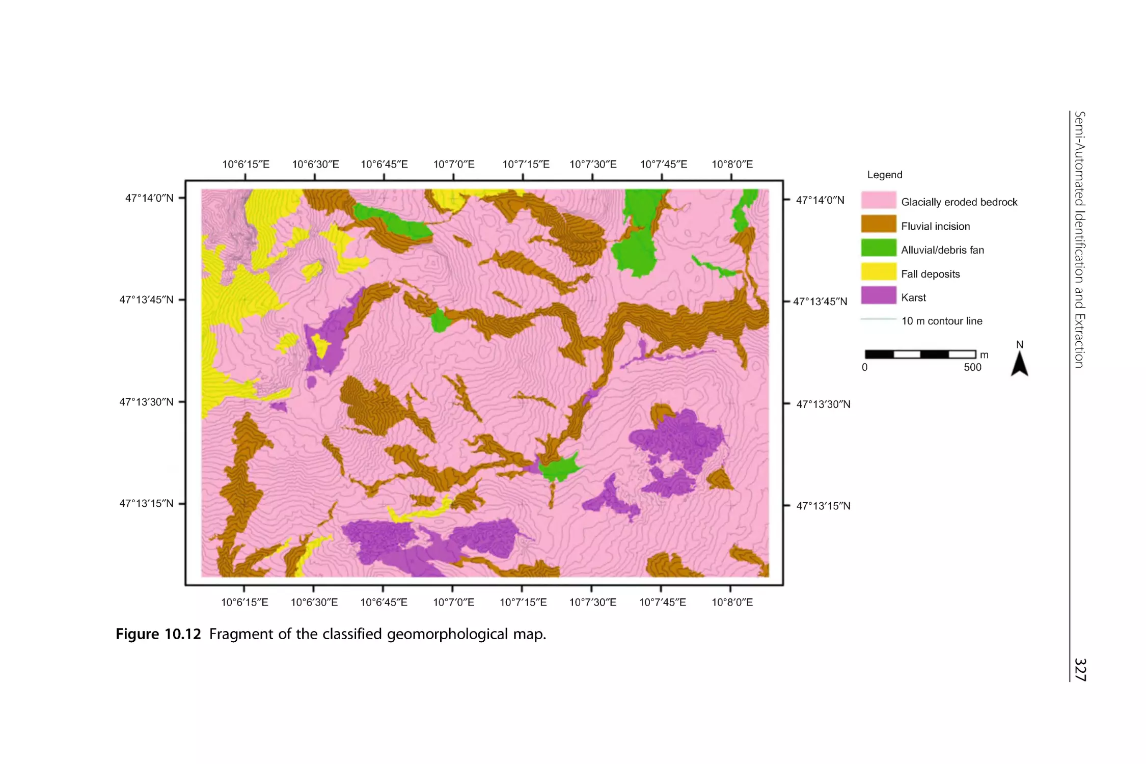
Figure 10.12 Fragment of the classified geomorphological map.

CHAPTER ELEVEN
Figure 11.1 Geomorphological interpretation of the continental shelf off
northwest Ireland showing all the glacial and glacially related features
identified on the INSS/INFOMAR multibeam swath bathymetry data.
The location of Figures 11.3, 11.4 and 11.5 are shown by grey boxes
on the map.
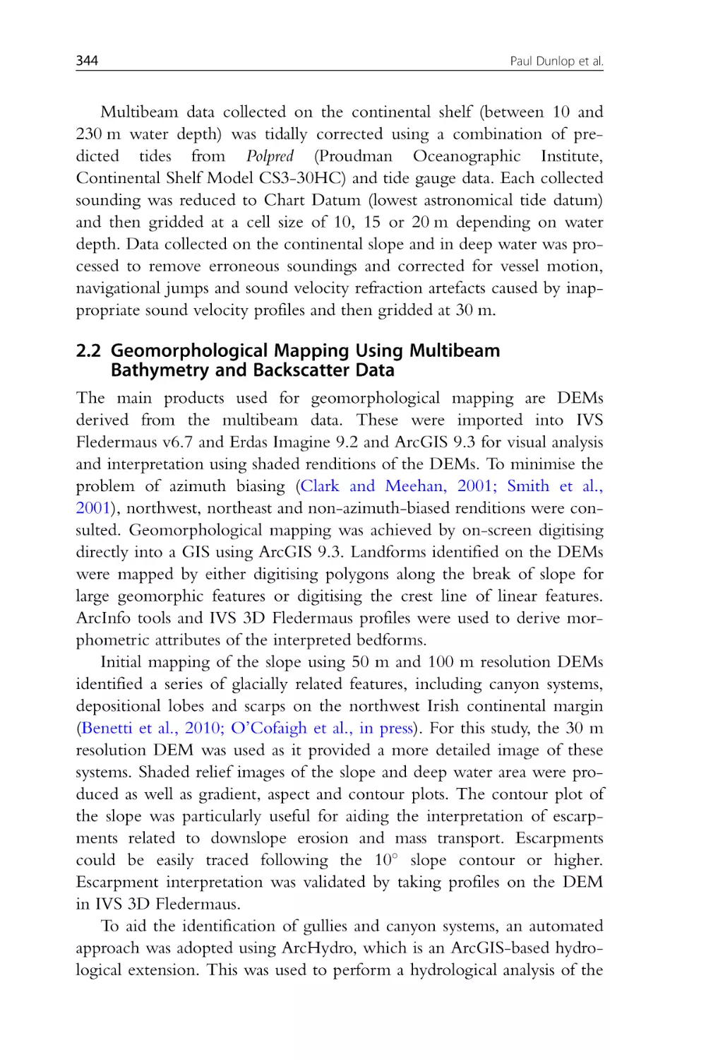
Figure 11.2(a) Flow accumulation map computed using the ArcHydro
hydrological algorithm. (b) Filtered flow accumulation map only showing cells with high accumulation rate. (c) Final canyon and gully interpretation derived from the filtered flow accumulation map and manual
editing of the remaining spurious data. (d) Oblique image showing
how cross-sectional profiles taken across the DEM were used to verify
the presence of gully or canyon systems identified by ArcHydro. The
horizontal distance across the bottom of (d) measures 8.5 km. Vertical
exaggeration 8.5 3 .
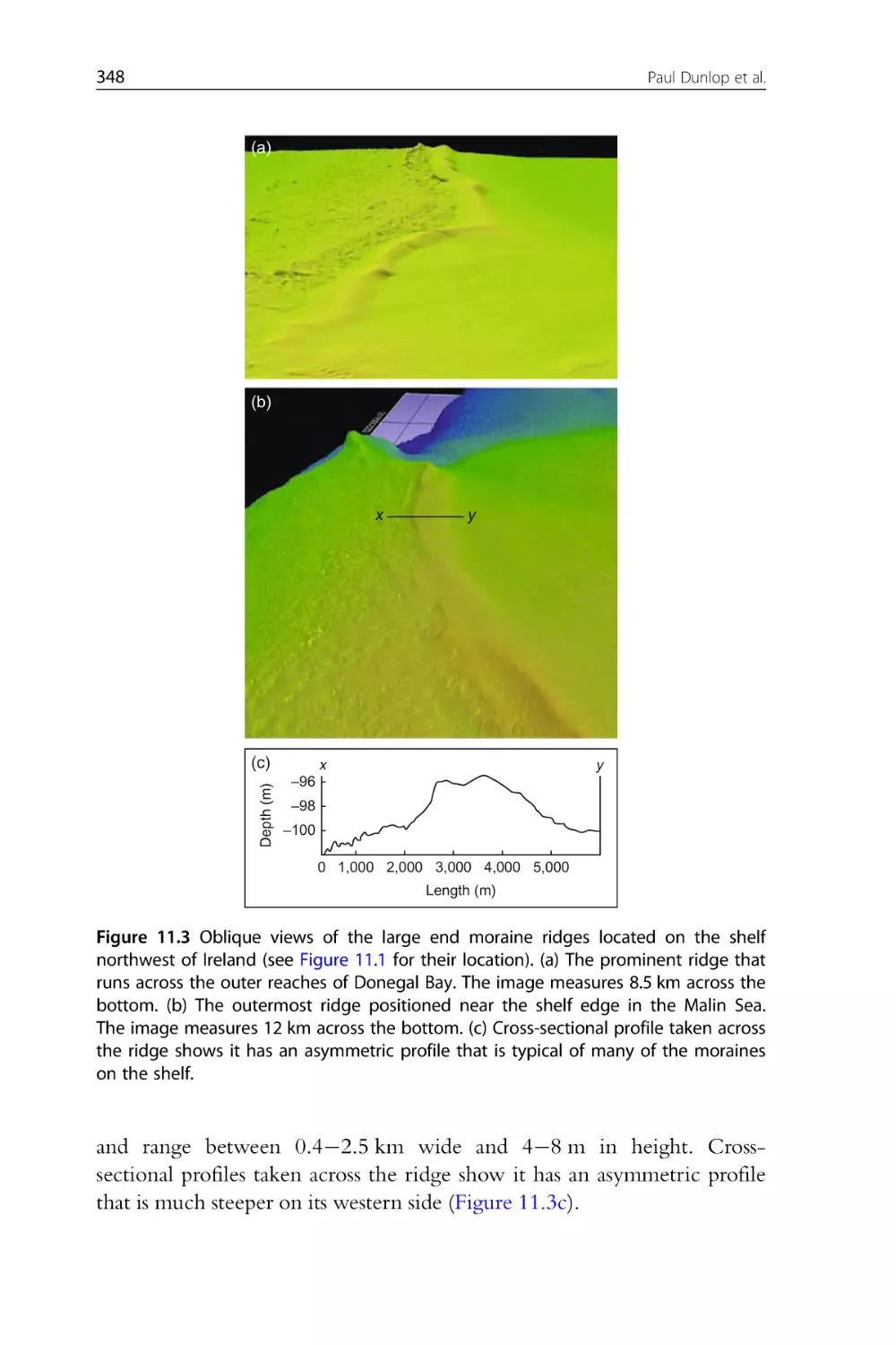
Figure 11.3 Oblique views of the large end moraine ridges located on the
shelf northwest of Ireland (see Figure 11.1 for their location). (a) The
prominent ridge that runs across the outer reaches of Donegal Bay.
The image measures 8.5 km across the bottom. (b) The outermost
ridge positioned near the shelf edge in the Malin Sea. The image measures 12 km across the bottom. (c) Cross-sectional profile taken across
the ridge shows it has an asymmetric profile that is typical of many of
the moraines on the shelf.

List of Figures

xxxiii

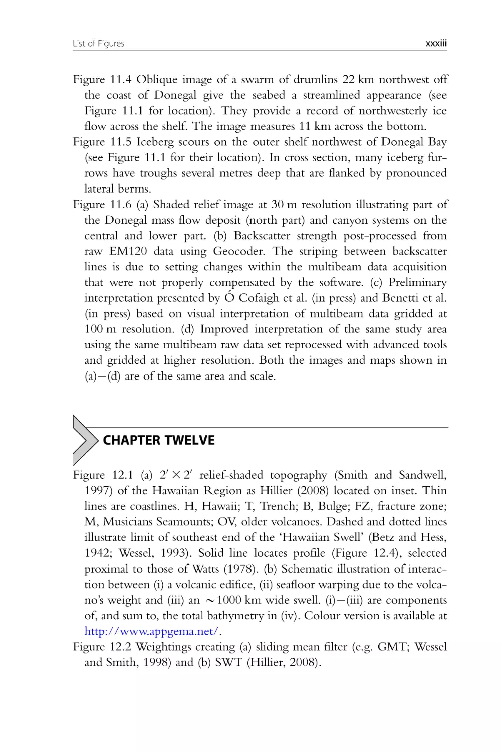
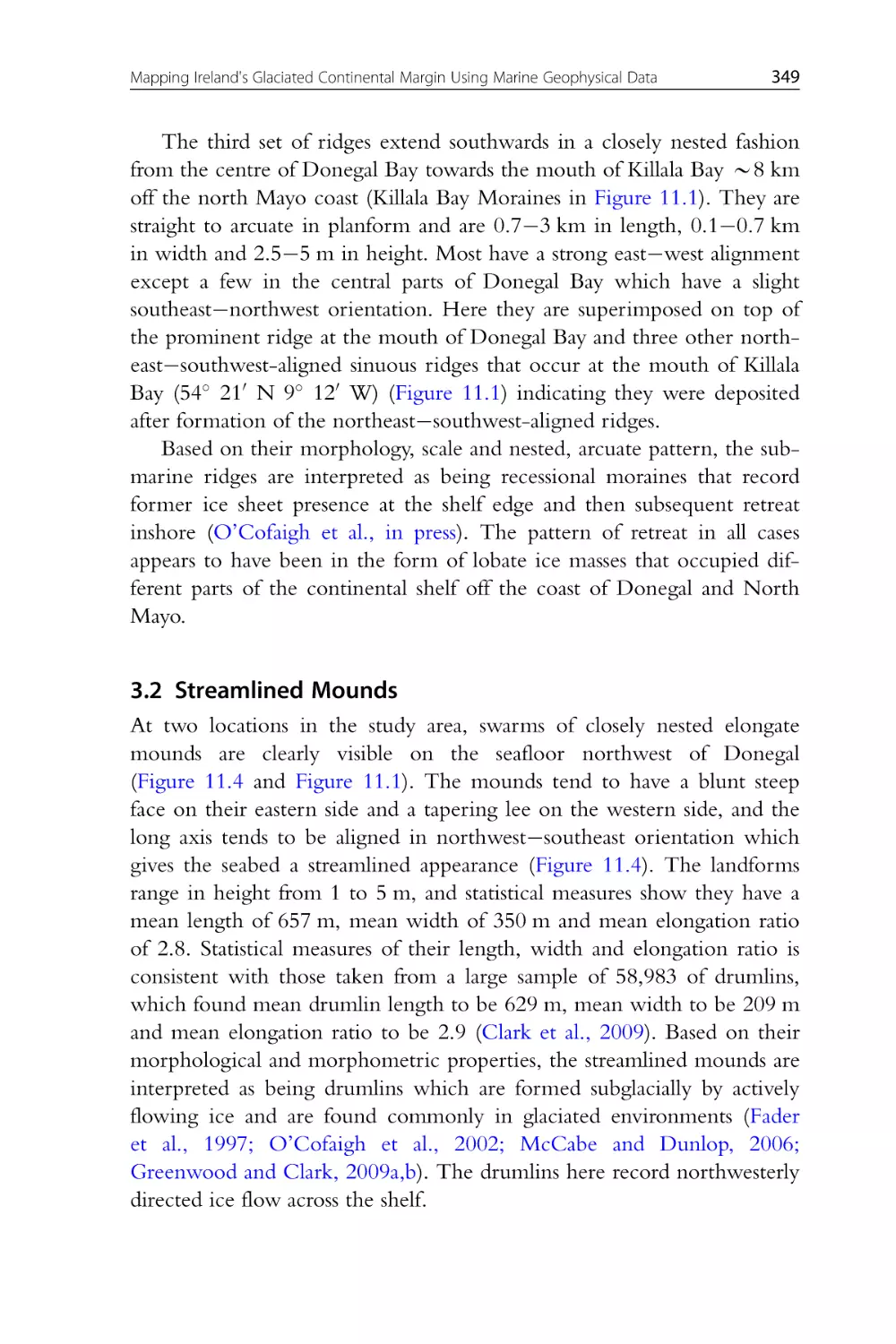
Figure 11.4 Oblique image of a swarm of drumlins 22 km northwest off
the coast of Donegal give the seabed a streamlined appearance (see
Figure 11.1 for location). They provide a record of northwesterly ice
flow across the shelf. The image measures 11 km across the bottom.
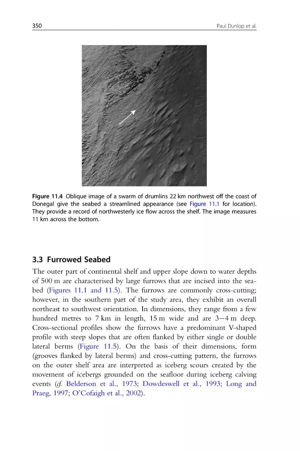
Figure 11.5 Iceberg scours on the outer shelf northwest of Donegal Bay
(see Figure 11.1 for their location). In cross section, many iceberg furrows have troughs several metres deep that are flanked by pronounced
lateral berms.
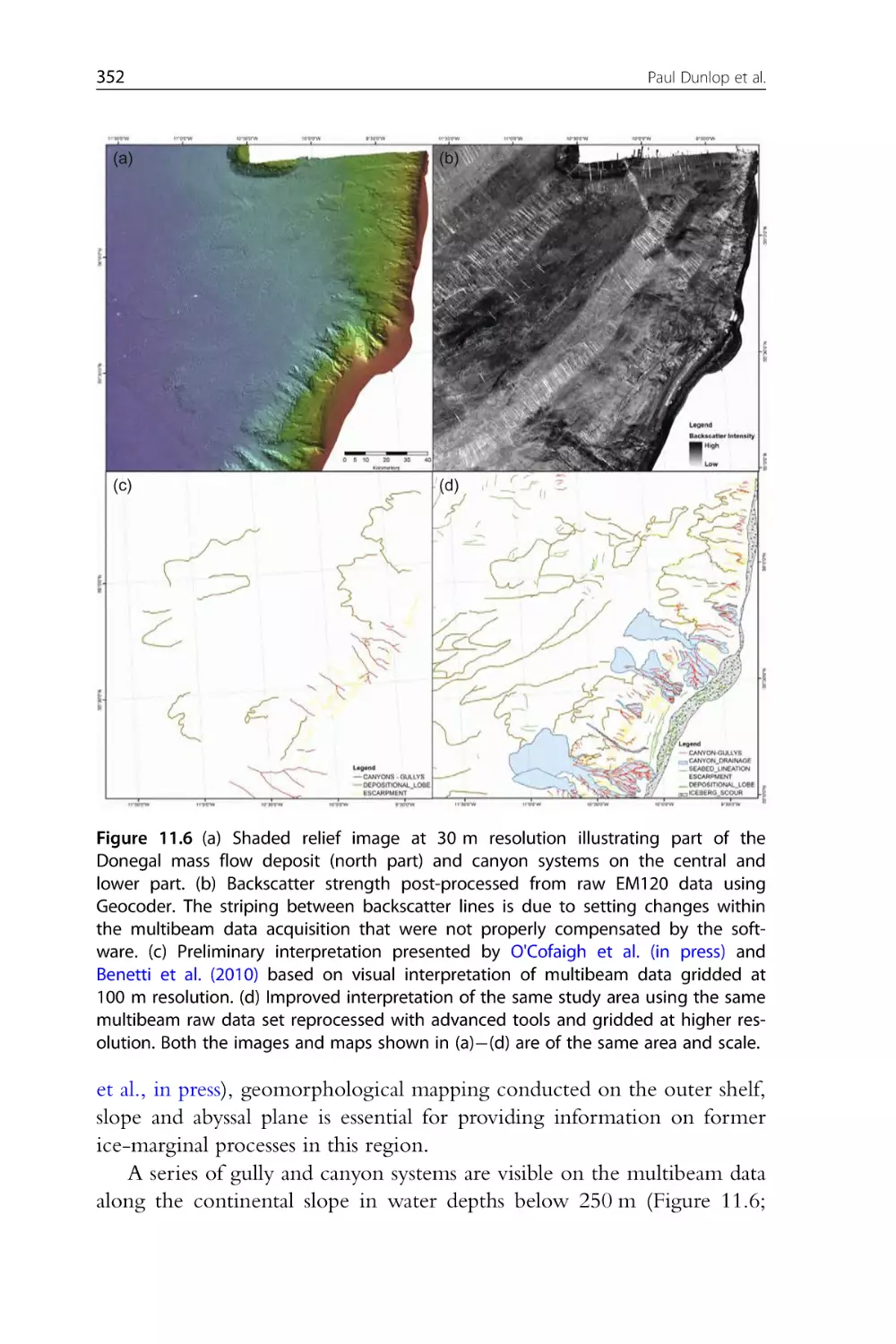
Figure 11.6 (a) Shaded relief image at 30 m resolution illustrating part of
the Donegal mass flow deposit (north part) and canyon systems on the
central and lower part. (b) Backscatter strength post-processed from
raw EM120 data using Geocoder. The striping between backscatter
lines is due to setting changes within the multibeam data acquisition
that were not properly compensated by the software. (c) Preliminary
interpretation presented by Ó Cofaigh et al. (in press) and Benetti et al.
(in press) based on visual interpretation of multibeam data gridded at
100 m resolution. (d) Improved interpretation of the same study area
using the same multibeam raw data set reprocessed with advanced tools
and gridded at higher resolution. Both the images and maps shown in
(a)
(d) are of the same area and scale.

CHAPTER TWELVE
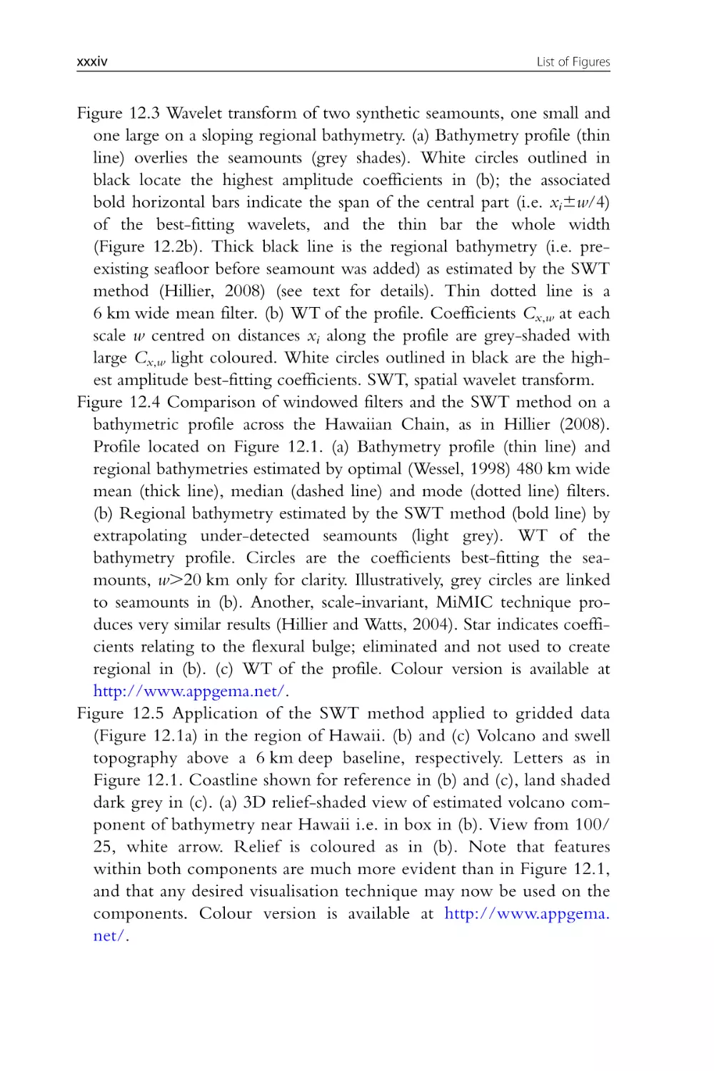
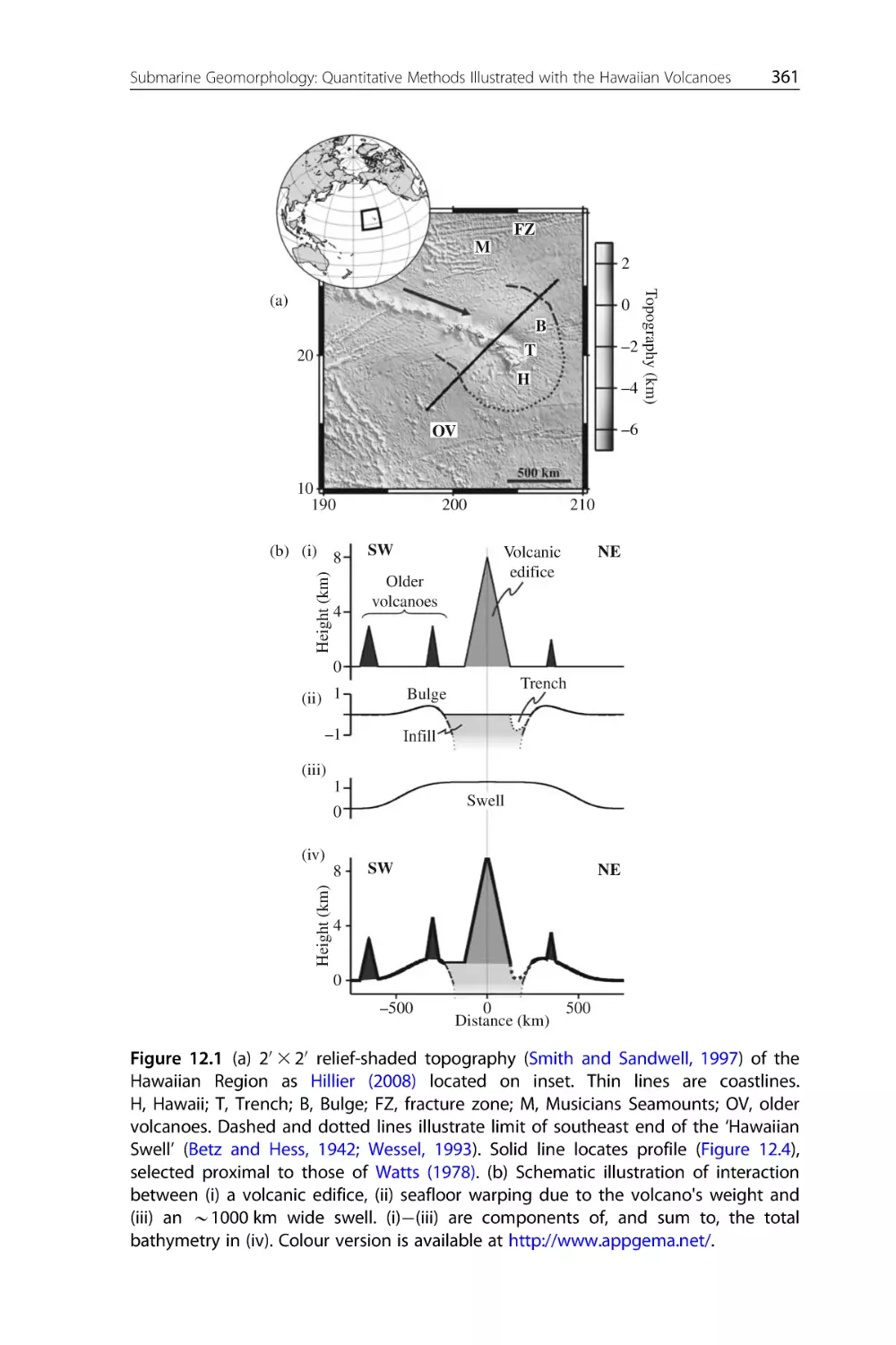
Figure 12.1 (a) 20 3 20 relief-shaded topography (Smith and Sandwell,
1997) of the Hawaiian Region as Hillier (2008) located on inset. Thin
lines are coastlines. H, Hawaii; T, Trench; B, Bulge; FZ, fracture zone;
M, Musicians Seamounts; OV, older volcanoes. Dashed and dotted lines
illustrate limit of southeast end of the ‘Hawaiian Swell’ (Betz and Hess,
1942; Wessel, 1993). Solid line locates profile (Figure 12.4), selected
proximal to those of Watts (1978). (b) Schematic illustration of interaction between (i) a volcanic edifice, (ii) seafloor warping due to the volcano’s weight and (iii) an B1000 km wide swell. (i)
(iii) are components
of, and sum to, the total bathymetry in (iv). Colour version is available at
http://www.appgema.net/.
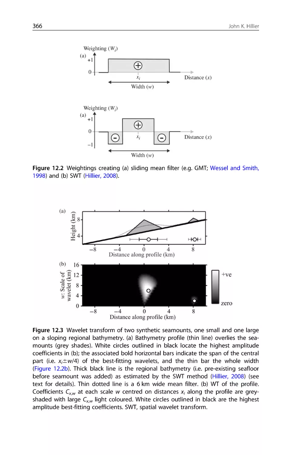
Figure 12.2 Weightings creating (a) sliding mean filter (e.g. GMT; Wessel
and Smith, 1998) and (b) SWT (Hillier, 2008).

xxxiv

List of Figures

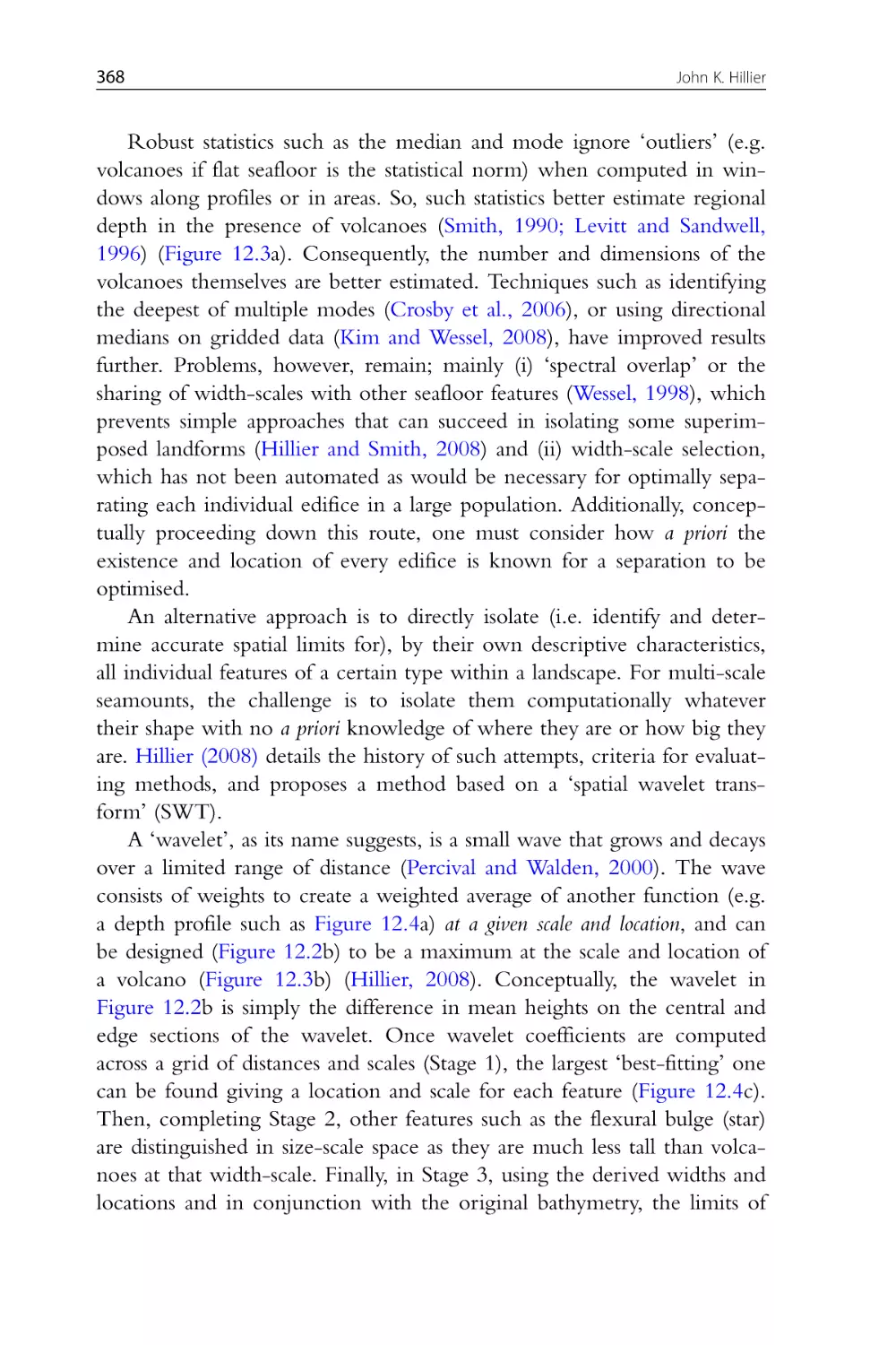
Figure 12.3 Wavelet transform of two synthetic seamounts, one small and
one large on a sloping regional bathymetry. (a) Bathymetry profile (thin
line) overlies the seamounts (grey shades). White circles outlined in
black locate the highest amplitude coefficients in (b); the associated
bold horizontal bars indicate the span of the central part (i.e. xi6w/4)
of the best-fitting wavelets, and the thin bar the whole width
(Figure 12.2b). Thick black line is the regional bathymetry (i.e. preexisting seafloor before seamount was added) as estimated by the SWT
method (Hillier, 2008) (see text for details). Thin dotted line is a
6 km wide mean filter. (b) WT of the profile. Coefficients Cx,w at each
scale w centred on distances xi along the profile are grey-shaded with
large Cx,w light coloured. White circles outlined in black are the highest amplitude best-fitting coefficients. SWT, spatial wavelet transform.
Figure 12.4 Comparison of windowed filters and the SWT method on a
bathymetric profile across the Hawaiian Chain, as in Hillier (2008).
Profile located on Figure 12.1. (a) Bathymetry profile (thin line) and
regional bathymetries estimated by optimal (Wessel, 1998) 480 km wide
mean (thick line), median (dashed line) and mode (dotted line) filters.
(b) Regional bathymetry estimated by the SWT method (bold line) by
extrapolating under-detected seamounts (light grey). WT of the
bathymetry profile. Circles are the coefficients best-fitting the seamounts, w.20 km only for clarity. Illustratively, grey circles are linked
to seamounts in (b). Another, scale-invariant, MiMIC technique produces very similar results (Hillier and Watts, 2004). Star indicates coefficients relating to the flexural bulge; eliminated and not used to create
regional in (b). (c) WT of the profile. Colour version is available at
http://www.appgema.net/.
Figure 12.5 Application of the SWT method applied to gridded data
(Figure 12.1a) in the region of Hawaii. (b) and (c) Volcano and swell
topography above a 6 km deep baseline, respectively. Letters as in
Figure 12.1. Coastline shown for reference in (b) and (c), land shaded
dark grey in (c). (a) 3D relief-shaded view of estimated volcano component of bathymetry near Hawaii i.e. in box in (b). View from 100/
25, white arrow. Relief is coloured as in (b). Note that features
within both components are much more evident than in Figure 12.1,
and that any desired visualisation technique may now be used on the
components. Colour version is available at http://www.appgema.
net/.

List of Figures

xxxv

CHAPTER THIRTEEN
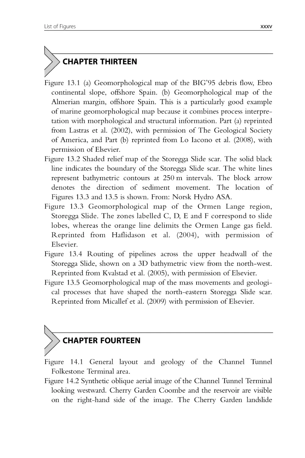
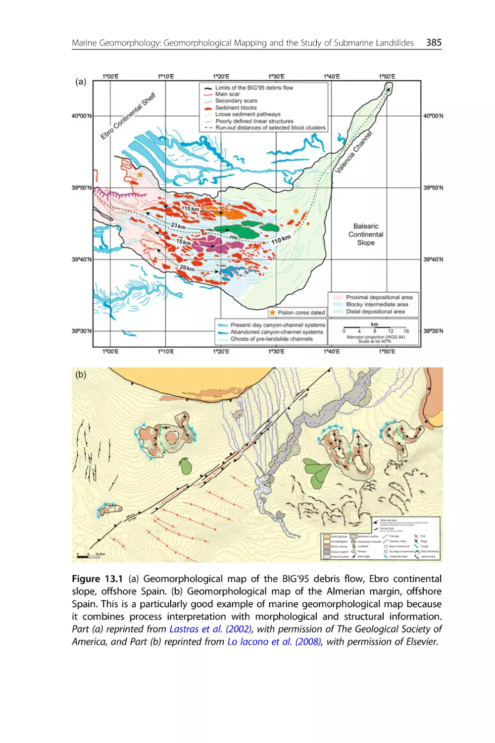
Figure 13.1 (a) Geomorphological map of the BIG’95 debris flow, Ebro
continental slope, offshore Spain. (b) Geomorphological map of the
Almerian margin, offshore Spain. This is a particularly good example
of marine geomorphological map because it combines process interpretation with morphological and structural information. Part (a) reprinted
from Lastras et al. (2002), with permission of The Geological Society
of America, and Part (b) reprinted from Lo Iacono et al. (2008), with
permission of Elsevier.
Figure 13.2 Shaded relief map of the Storegga Slide scar. The solid black
line indicates the boundary of the Storegga Slide scar. The white lines
represent bathymetric contours at 250 m intervals. The block arrow
denotes the direction of sediment movement. The location of
Figures 13.3 and 13.5 is shown. From: Norsk Hydro ASA.
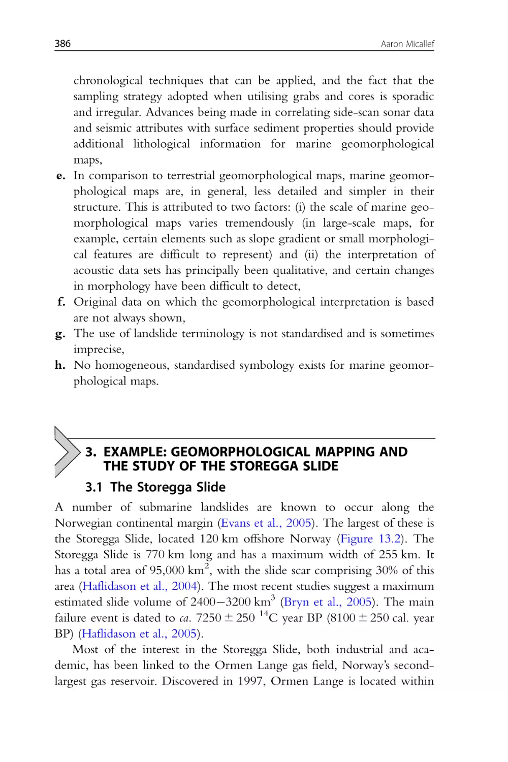
Figure 13.3 Geomorphological map of the Ormen Lange region,
Storegga Slide. The zones labelled C, D, E and F correspond to slide
lobes, whereas the orange line delimits the Ormen Lange gas field.
Reprinted from Haflidason et al. (2004), with permission of
Elsevier.
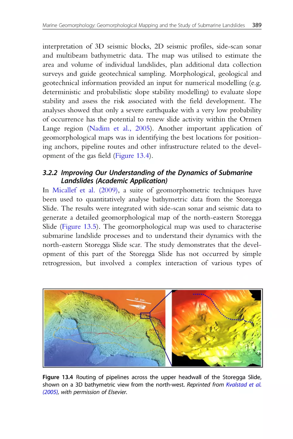
Figure 13.4 Routing of pipelines across the upper headwall of the
Storegga Slide, shown on a 3D bathymetric view from the north-west.
Reprinted from Kvalstad et al. (2005), with permission of Elsevier.
Figure 13.5 Geomorphological map of the mass movements and geological processes that have shaped the north-eastern Storegga Slide scar.
Reprinted from Micallef et al. (2009) with permission of Elsevier.

CHAPTER FOURTEEN
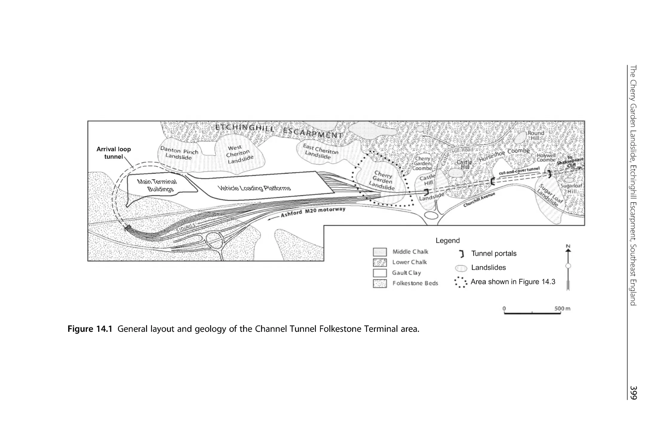
Figure 14.1 General layout and geology of the Channel Tunnel
Folkestone Terminal area.
Figure 14.2 Synthetic oblique aerial image of the Channel Tunnel Terminal
looking westward. Cherry Garden Coombe and the reservoir are visible
on the right-hand side of the image. The Cherry Garden landslide

xxxvi

List of Figures

complex occupies the centre of the image from the top of the Etchinghill
escarpment down to, and beyond, where the rail lines converge before
entering the Castle Hill tunnel portal. Google Earth copyright.
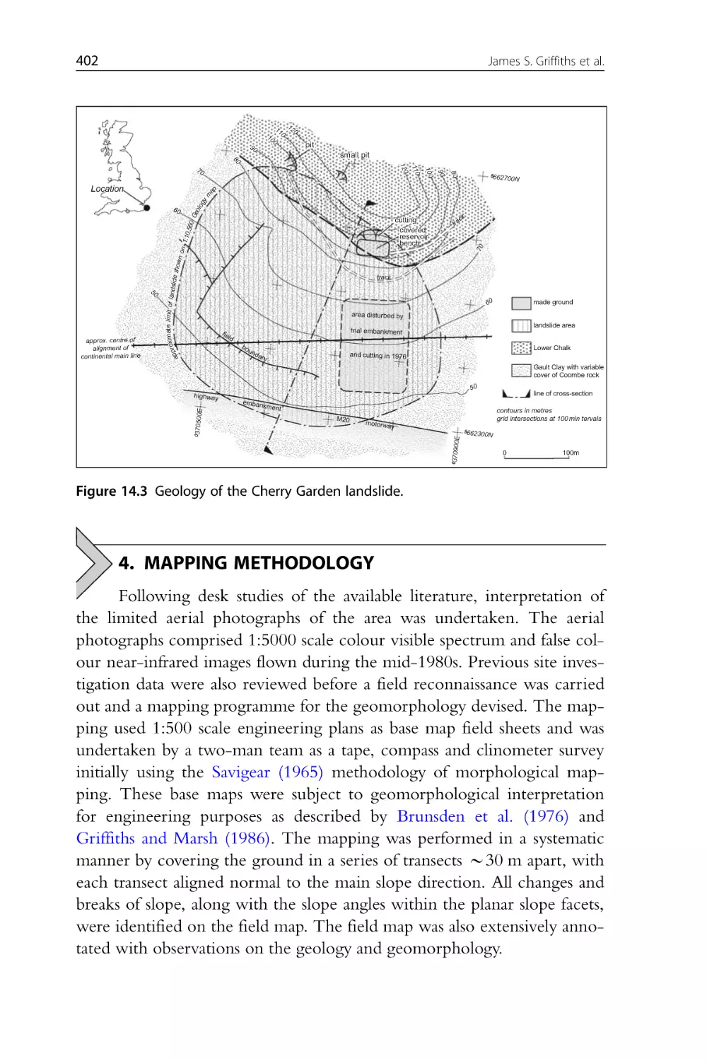
Figure 14.3 Geology of the Cherry Garden landslide.
Figure 14.4 Geomorphological map of the Cherry Garden Landslide.
Figure 14.5 Hypothsised cross section through the Cherry Garden landslide C based on limited sub-surface data and surface mapping.

CHAPTER FIFTEEN
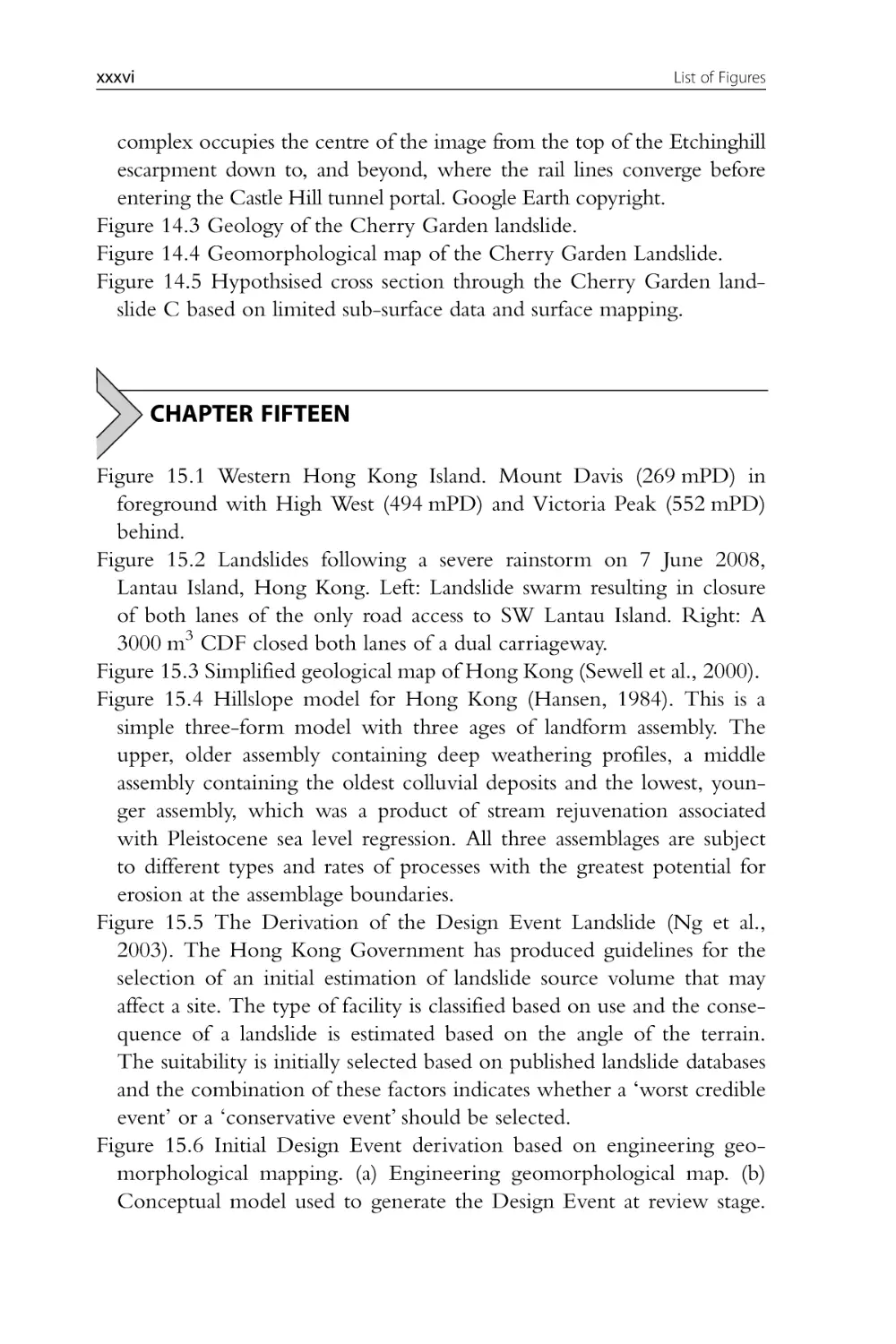
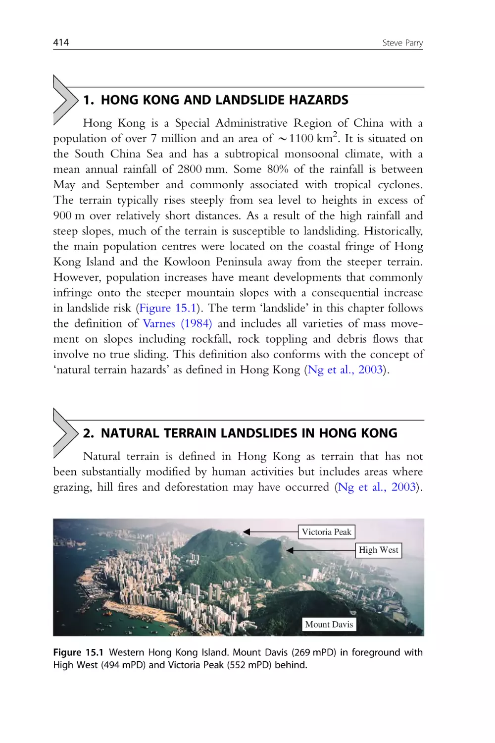
Figure 15.1 Western Hong Kong Island. Mount Davis (269 mPD) in
foreground with High West (494 mPD) and Victoria Peak (552 mPD)
behind.
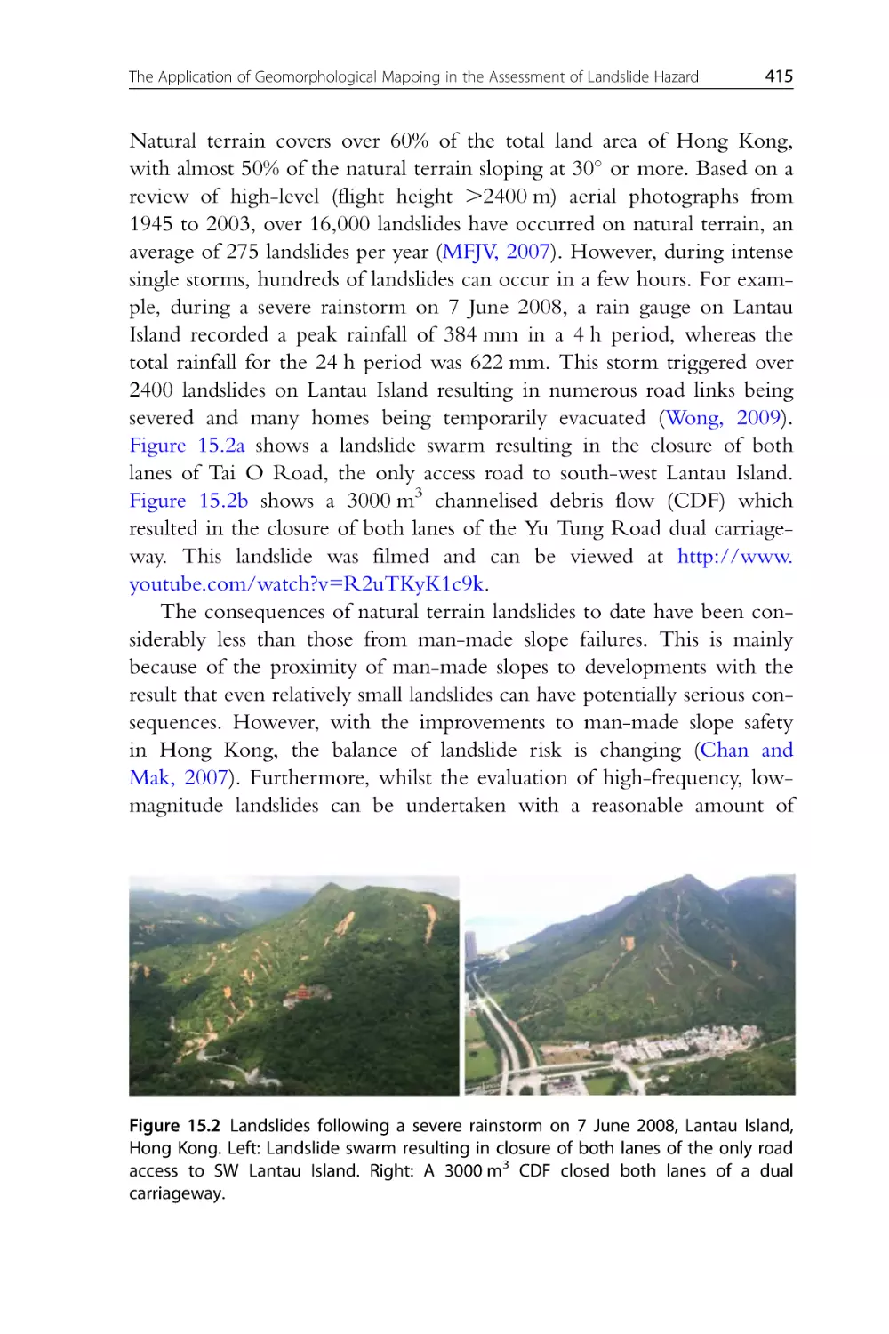
Figure 15.2 Landslides following a severe rainstorm on 7 June 2008,
Lantau Island, Hong Kong. Left: Landslide swarm resulting in closure
of both lanes of the only road access to SW Lantau Island. Right: A
3000 m3 CDF closed both lanes of a dual carriageway.
Figure 15.3 Simplified geological map of Hong Kong (Sewell et al., 2000).
Figure 15.4 Hillslope model for Hong Kong (Hansen, 1984). This is a
simple three-form model with three ages of landform assembly. The
upper, older assembly containing deep weathering profiles, a middle
assembly containing the oldest colluvial deposits and the lowest, younger assembly, which was a product of stream rejuvenation associated
with Pleistocene sea level regression. All three assemblages are subject
to different types and rates of processes with the greatest potential for
erosion at the assemblage boundaries.
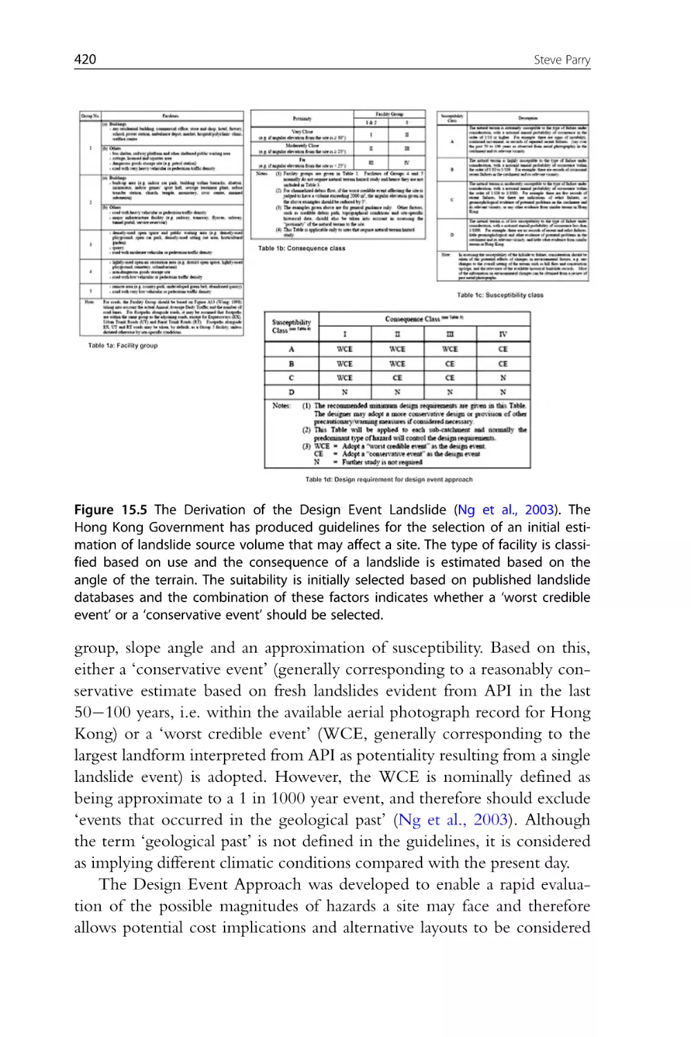
Figure 15.5 The Derivation of the Design Event Landslide (Ng et al.,
2003). The Hong Kong Government has produced guidelines for the
selection of an initial estimation of landslide source volume that may
affect a site. The type of facility is classified based on use and the consequence of a landslide is estimated based on the angle of the terrain.
The suitability is initially selected based on published landslide databases
and the combination of these factors indicates whether a ‘worst credible
event’ or a ‘conservative event’ should be selected.
Figure 15.6 Initial Design Event derivation based on engineering geomorphological mapping. (a) Engineering geomorphological map. (b)
Conceptual model used to generate the Design Event at review stage.

List of Figures

xxxvii

Both are based on API and were re-evaluated during subsequent field
mapping. Incising drainage lines form two adjacent catchments. Within
both catchments, extensive areas of rock outcrop are present. Also
shown are ENTLI landslides. The Upper Terrain above the incision
was interpreted as potentially containing thicker saprolite. Part (b)
shows the conceptual model based on the engineering geomorphology
with potential design events varying with setting. The largest initial
design event was considered to be a failure of deeper saprolite in the
Upper Terrain (1500 m3) with the landslide entraining a further
1400 m3 of colluvium, resulting in a total volume of 2900 m3.
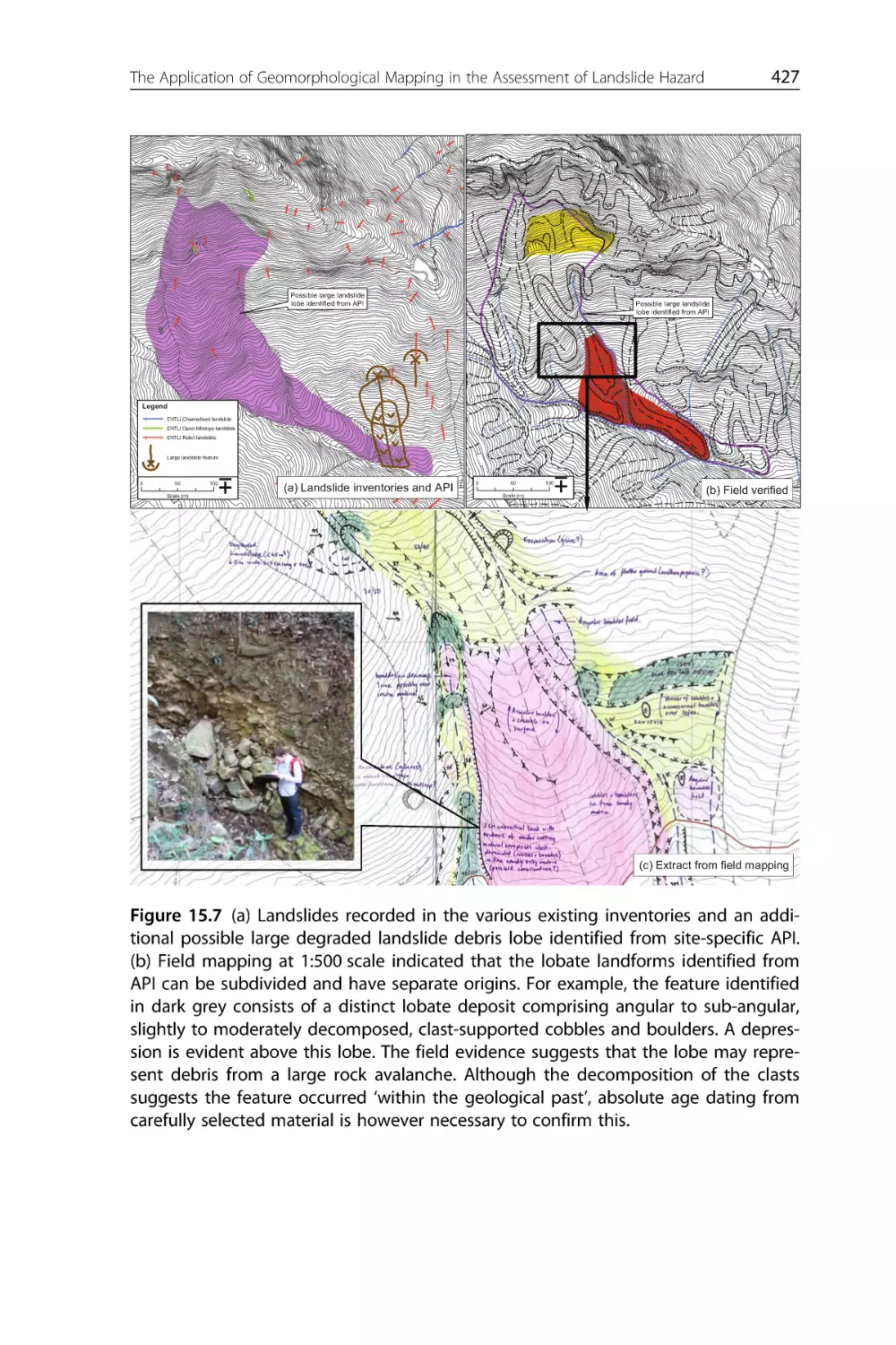
Figure 15.7 (a) Landslides recorded in the various existing inventories and
an additional possible large degraded landslide debris lobe identified
from site-specific API. (b) Field mapping at 1:500 scale indicated that
the lobate landforms identified from API can be subdivided and have
separate origins. For example, the feature identified in red consists of a
distinct deposit comprising angular to sub-angular, slightly to moderately decomposed, clast-supported cobbles and boulders. A depression
(yellow) is evident above this lobe. The field evidence suggests that the
lobe may represent debris from a large rock avalanche. Although the
decomposition of the clasts suggests the feature occurred ‘within the
geological past’, absolute age dating from carefully selected material is
however necessary to confirm this.
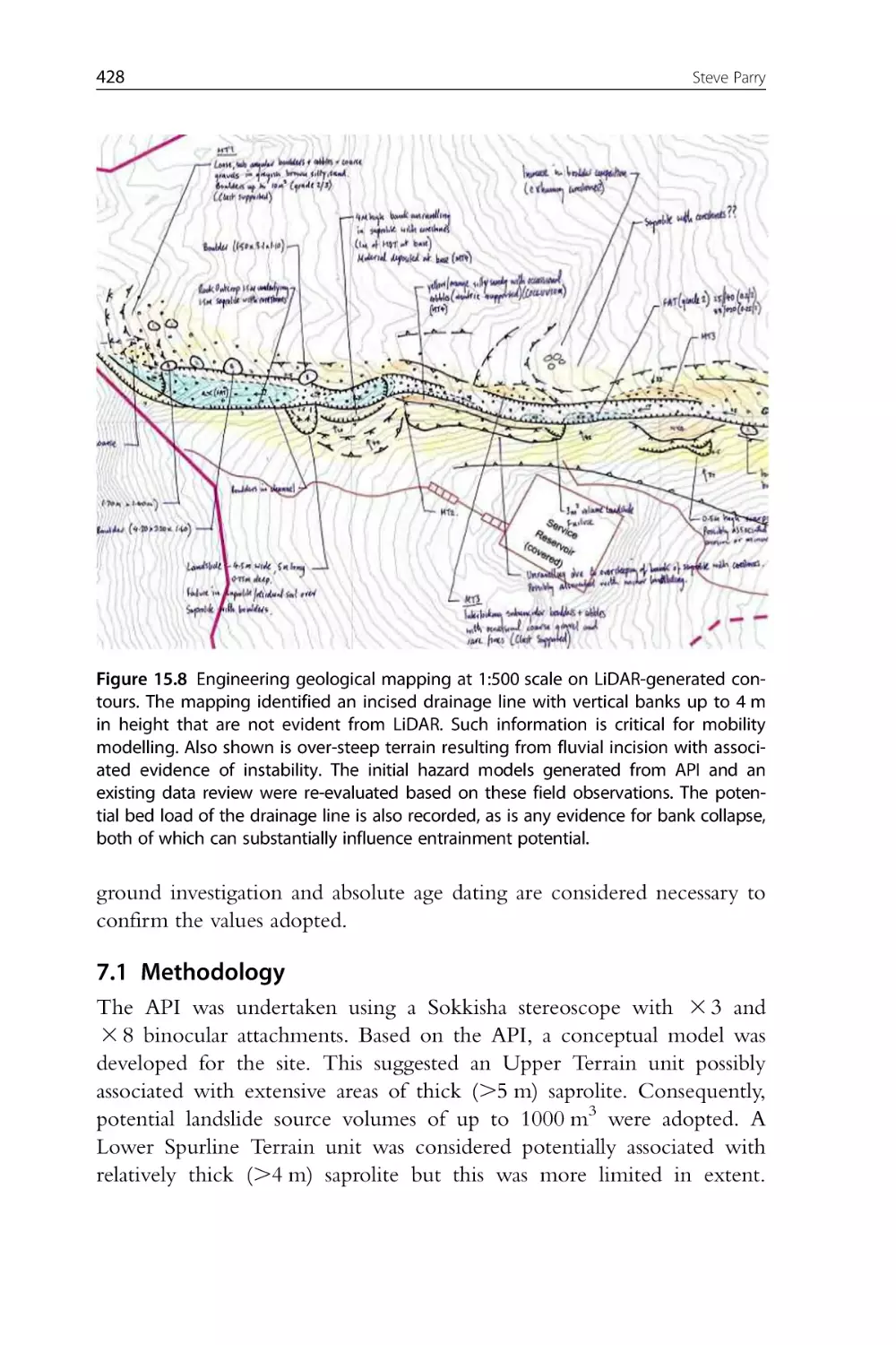
Figure 15.8 Engineering geological mapping at 1:500 scale on LiDARgenerated contours. The mapping identified an incised drainage line
with vertical banks up to 4 m in height that are not evident from
LiDAR. Such information is critical for mobility modelling. Also
shown is over-steep terrain resulting from fluvial incision with associated evidence of instability. The initial hazard models generated from
API and existing data review were re-evaluated based on these field
observations. The potential bed load of the drainage line is also
recorded, as is any evidence for bank collapse, both of which can substantially influence entrainment potential.
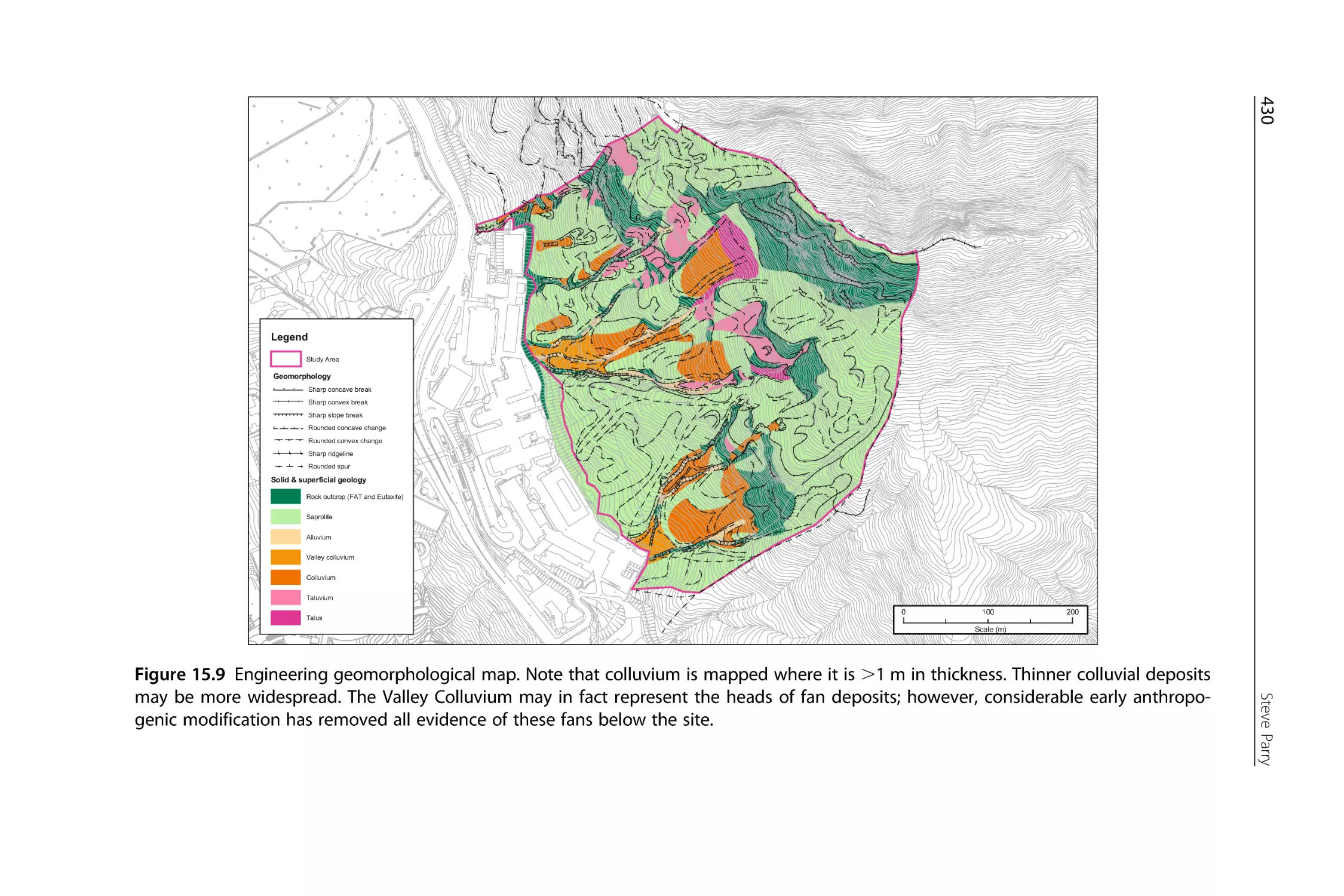
Figure 15.9 Engineering geomorphological map. Note that colluvium is
mapped where it is .1 m in thickness. Thinner colluvial deposits may
be more widespread. The Valley Colluvium may in fact represent the
heads of fan deposits; however, considerable early anthropogenic modification has removed all evidence of these fans below the site.
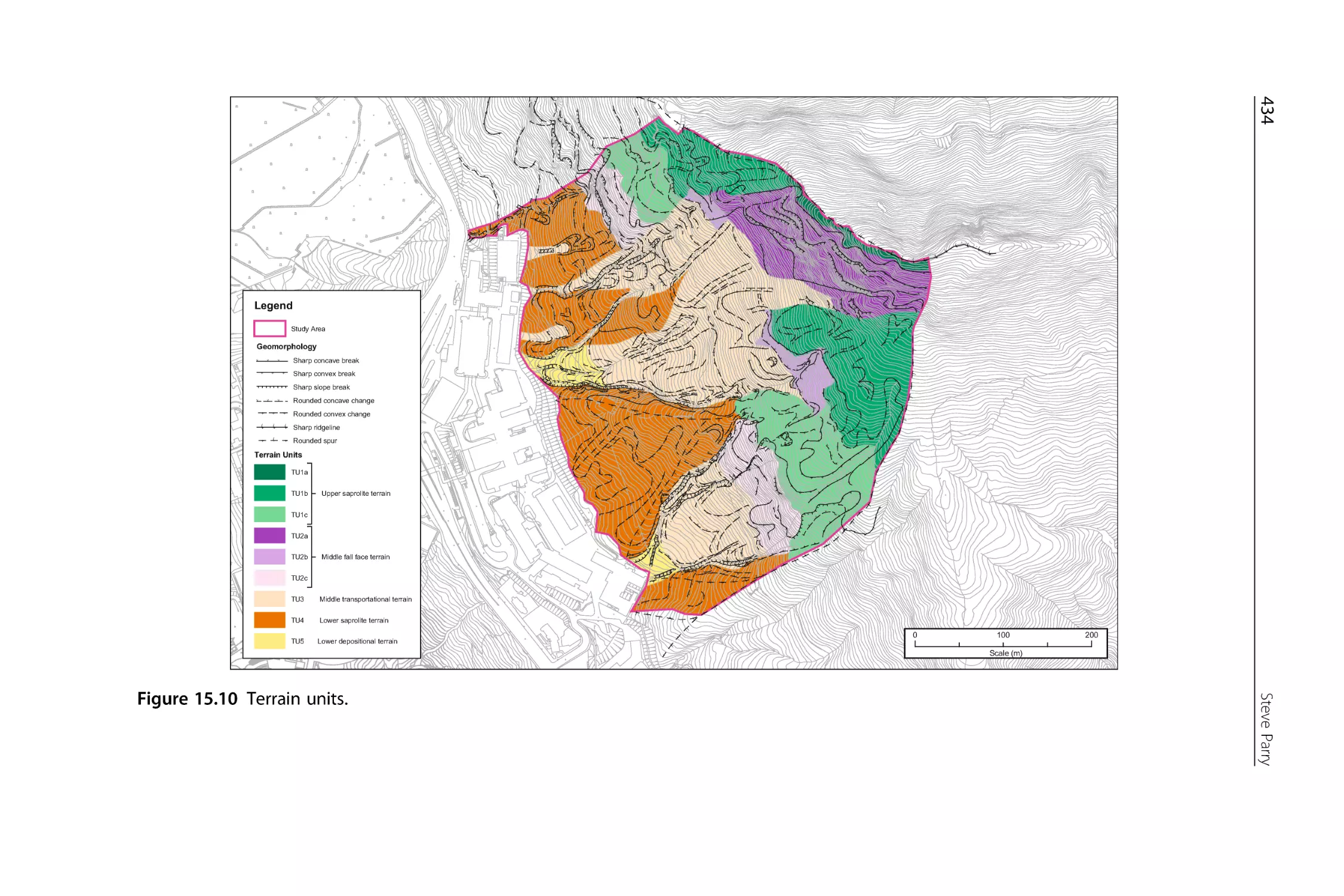
Figure 15.10 Terrain units.
Figure 15.11 Adopted Design Events by catchments.

xxxviii

List of Figures

CHAPTER SIXTEEN
Figure 16.1 Extracts of some geomorphological maps produced in
Switzerland. (a) Small-scale geomorphological map of Switzerland
(Swisstopo, 2007). (b) Map of Geomorphology of Grindelwald,
Switzerland: Scale 1:10,000. (c) Map of regional instabilities of
Lausanne-East (Noverraz, 1985). (d) Geomorphological map of
Zentralen Aargaus (Moser, 1958). (e) Geomorphological hazards map
of Grindelwald (Baumann, 1976). (f) Geomorphological map of
Tsanfleuron, scale 1:10,000 (Reynard, 1993). (g) Phenomena maps for
gravitational processes (1) and snow avalanches (2). (h) Improvement of
the phenomena legend (Kienholz and Krummenacher, 1995) in
Illgraben torrent by making a distinction between punctual and potential areal alimentation of a debris-flow channel. The strict application
of ‘the phenomena legend’ may result in a loss of information about
the potential alimentation of the debris flows (Bardou, 2002).
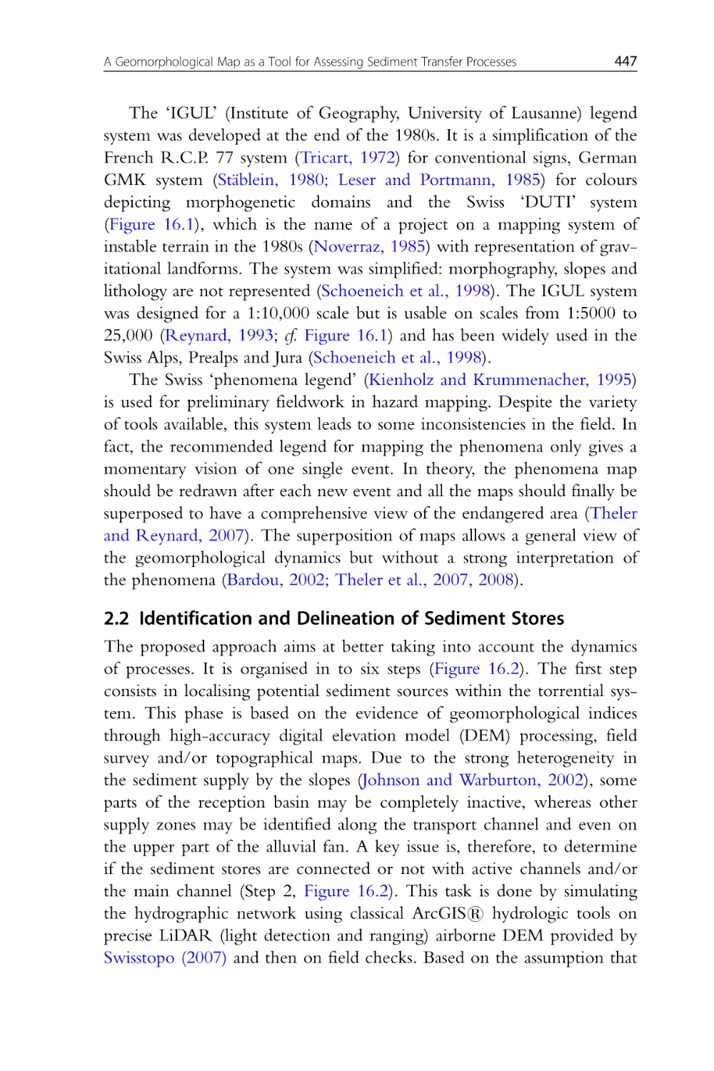
Figure 16.2 Flow chart of the procedure used in the mapping method for
small alpine catchments.
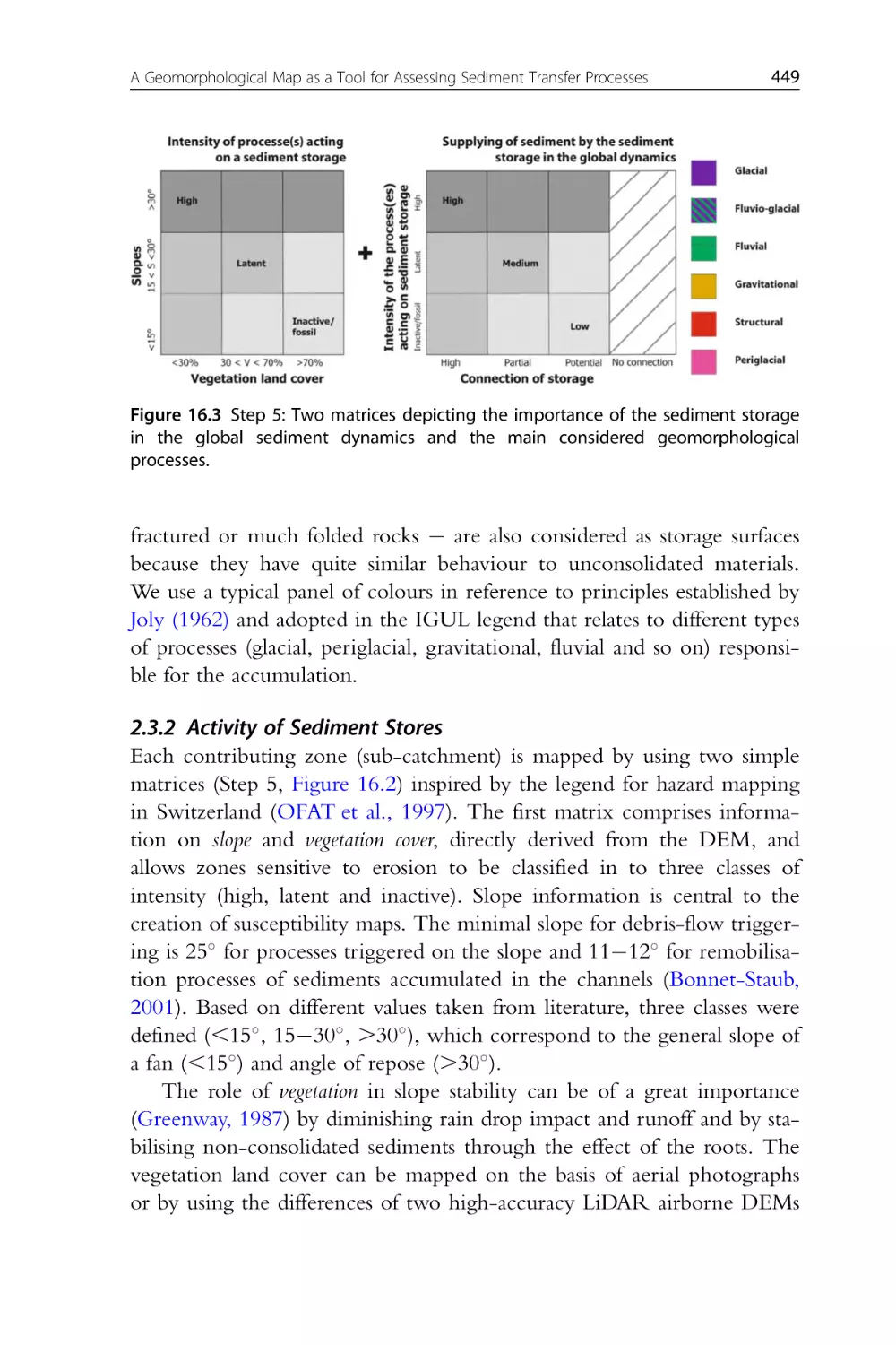
Figure 16.3 Step 5: Two matrices depicting the importance of the sediment storage in the global sediment dynamics and the main considered
geomorphological processes.
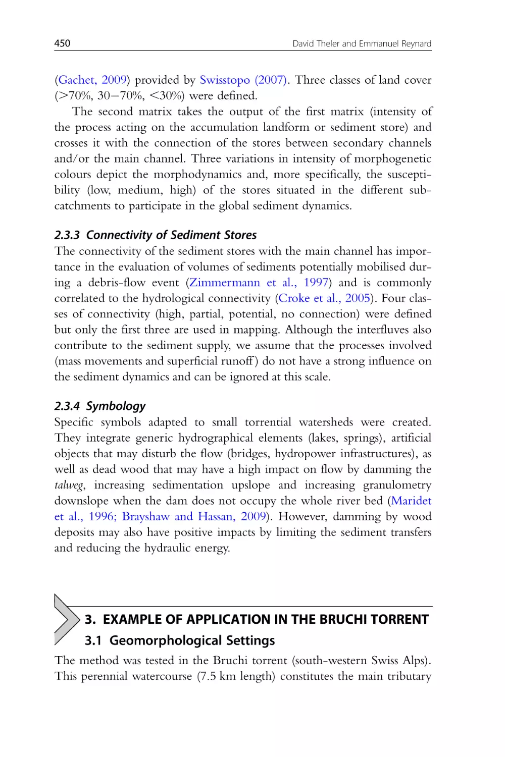
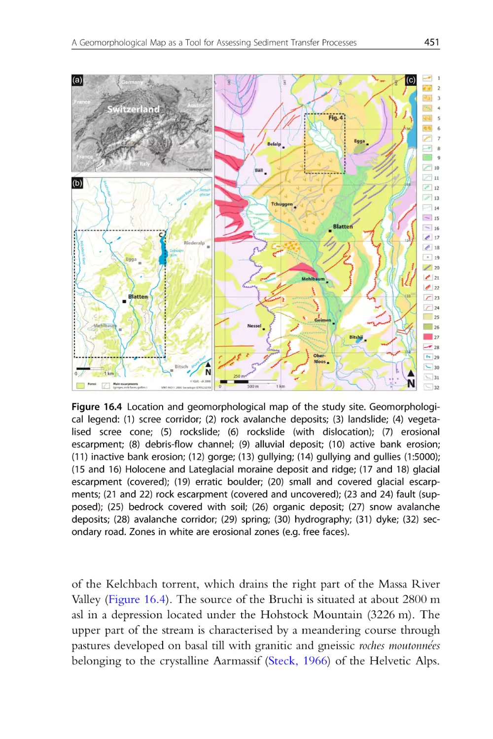
Figure 16.4 Location and geomorphological map of the study site. Geomorphological legend: (1) scree corridor; (2) rock avalanche deposits;
(3) landslide; (4) vegetalised scree cone; (5) rockslide; (6) rockslide
(with dislocation); (7) erosional escarpment; (8) debris-flow channel;
(9) alluvial deposit; (10) active bank erosion; (11) inactive bank erosion;
(12) gorge; (13) gullying; (14) gullying and gullies (1:5000); (15 and
16) Holocene and Lateglacial moraine deposit and ridge; (17 and 18)
glacial escarpment (covered); (19) erratic boulder; (20) small and covered glacial escarpments; (21 and 22) rock escarpment (covered and
uncovered); (23 and 24) fault (supposed); (25) bedrock covered with
soil; (26) organic deposit; (27) snow avalanche deposits; (28) avalanche
corridor; (29) spring; (30) hydrography; (31) dyke; (32) secondary
road. Zones in white are erosional zones (e.g. free faces).
Figure 16.5 Different sedimentary stocks present in the studied area: (a)
main channel of Bruchi torrent; (b) lateral landslide periodically drained
by debris flows; (c) fractured rock escarpment at the top of the drainage
basin; (d) general view downstream from the top of the basin; (e-h)

List of Figures

xxxix

rapid changes (erosion, collapses, deposit of natural levee) in different
kind of stores (Pictures: April and July 2007).
Figure 16.6 Dynamic geomorphological map of sediment transfer processes for the Bruchi torrent.

CHAPTER SEVENTEEN
Figure 17.1 Location of the study area (dashed lines) on the Cotswolds
escarpment to the west of the village of Broadway.
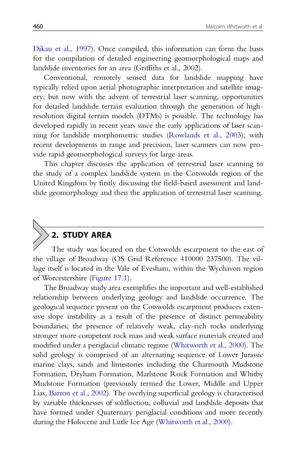
Figure 17.2 The landslide profile of valley slopes in the Cotswolds
(Whitworth et al., 2005).
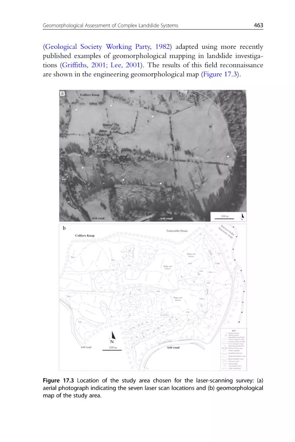
Figure 17.3 Location of the study area chosen for the laser-scanning survey: (a) aerial photograph indicating the seven laser scan locations and
(b) geomorphological map of the study area.
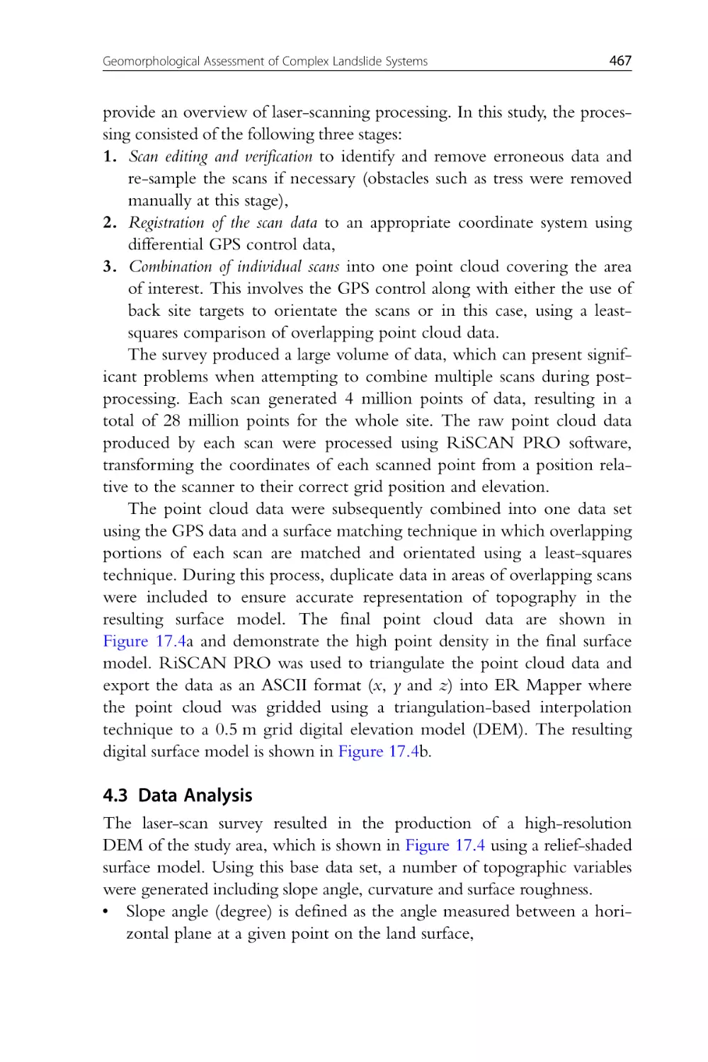
Figure 17.4 (a) Laser scan point cloud data and (b) relief-shaded image for
the Broadway valley generated using terrestrial laser scanning.
Figure 17.5 (a) Relief-shaded image and (b) slope-angle image derived
from the digital elevation model of the Broadway valley generated
using terrestrial laser scanning.
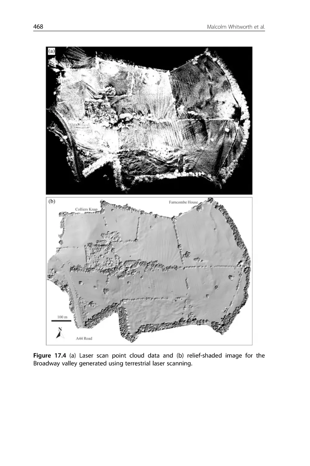
Figure 17.6 (a) Plan curvature image and (b) surface roughness image
derived from the digital elevation model of the Broadway valley generated using terrestrial laser scanning.

CHAPTER EIGHTEEN
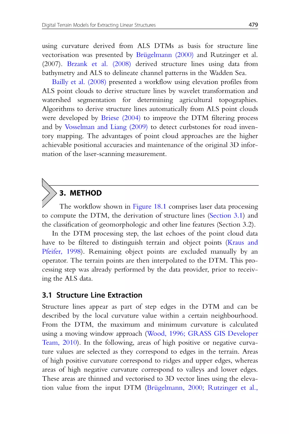
Figure 18.1 Workflow for DTM processing, structure line derivation and
classification.
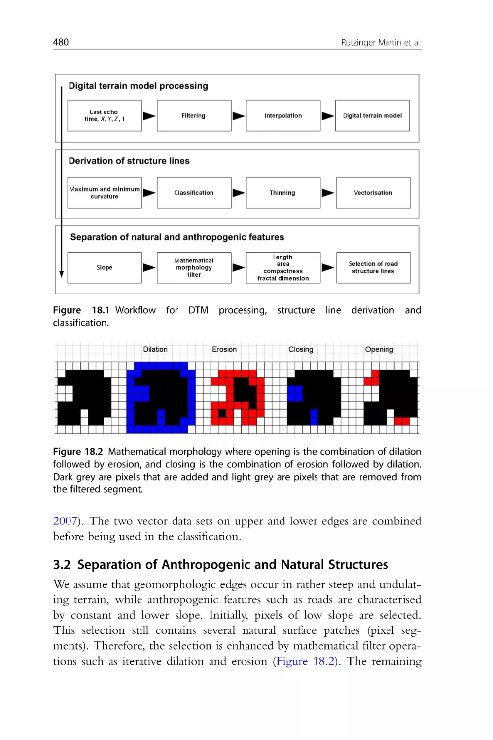
Figure 18.2 Mathematical morphology where opening is the combination
of dilation followed by erosion, and closing is the combination of erosion followed by dilation. Blue are pixels that are added and red are
pixels that are removed from the filtered segment.
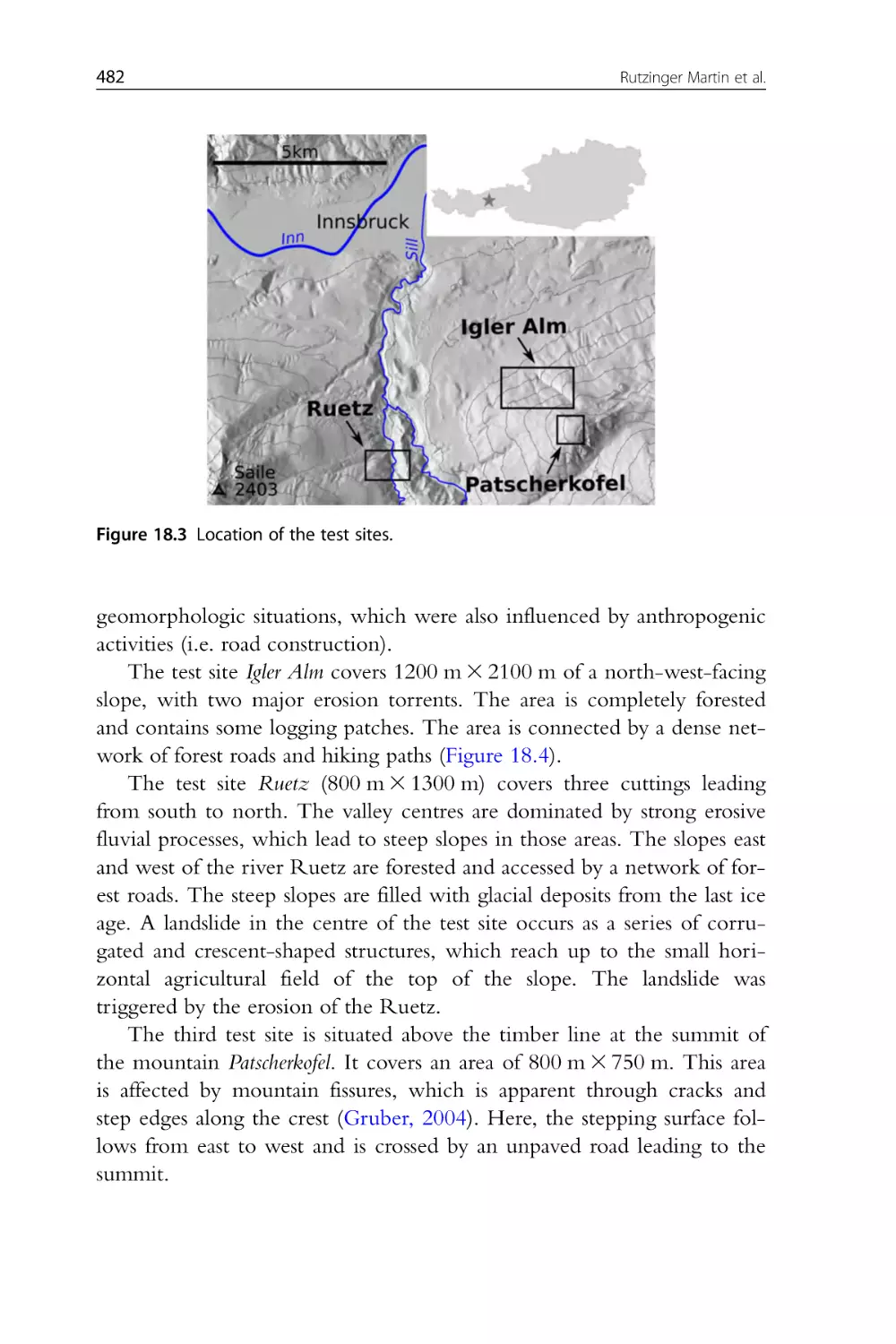
Figure 18.3 Location of the test sites.
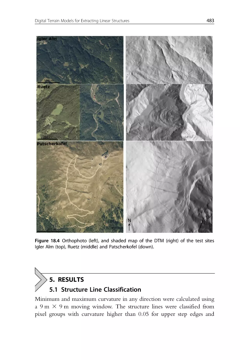
Figure 18.4 Orthophoto (left), and shaded map of the DTM (right) of
the test sites Igler Alm (top), Ruetz (middle) and Patscherkofel (down).
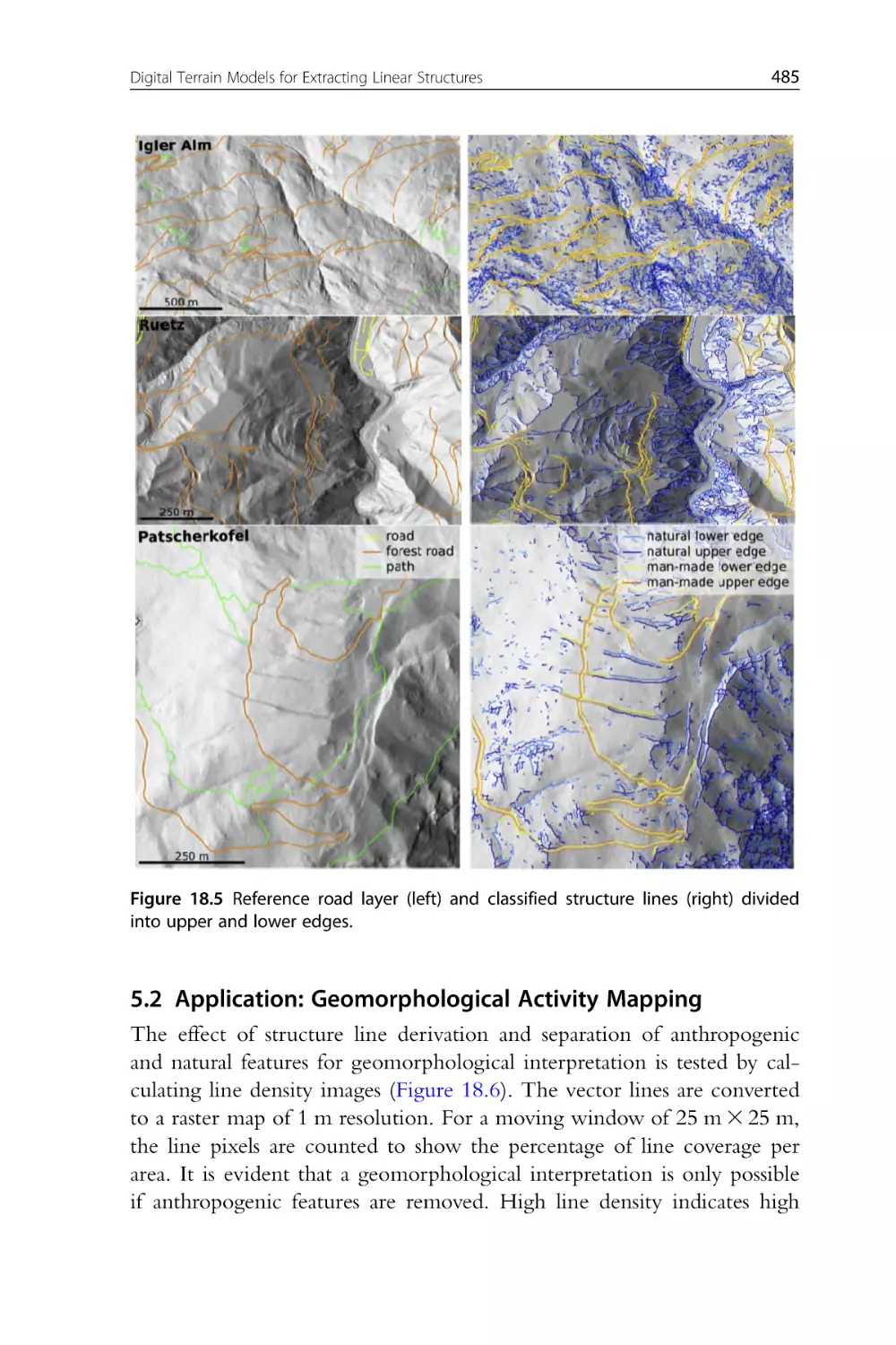
Figure 18.5 Reference road layer (left) and classified structure lines (right)
divided into upper and lower edges.

xl

List of Figures

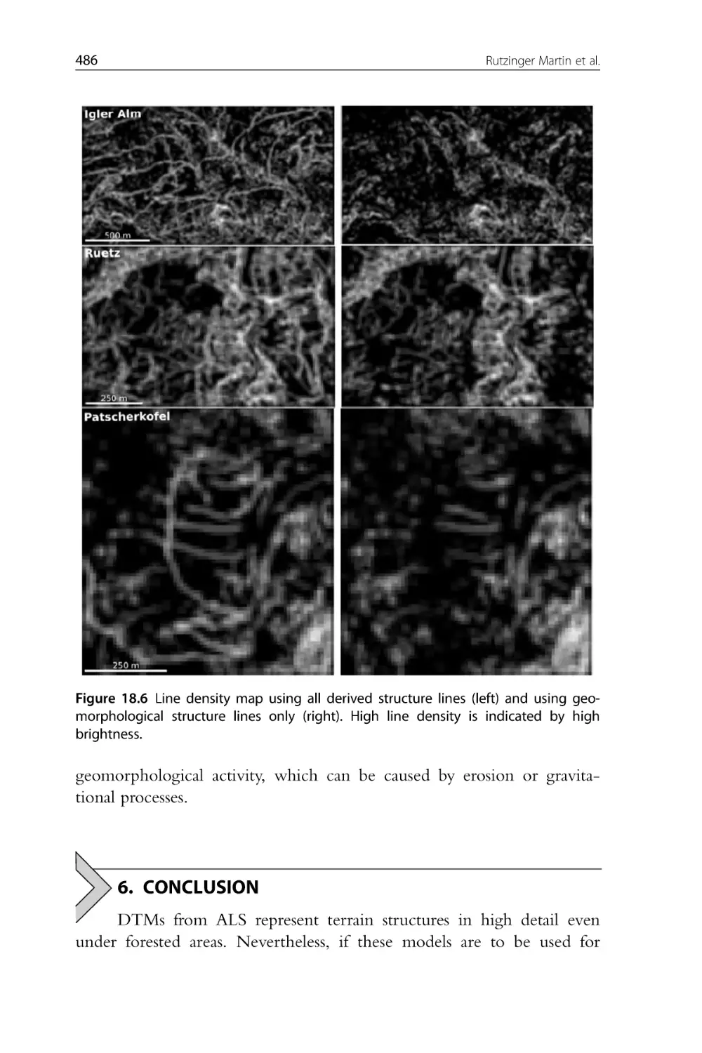
Figure 18.6 Line density map using all derived structure lines (left) and
using geomorphological structure lines only (right). High line density
is indicated by high brightness.

CHAPTER NINTEEN
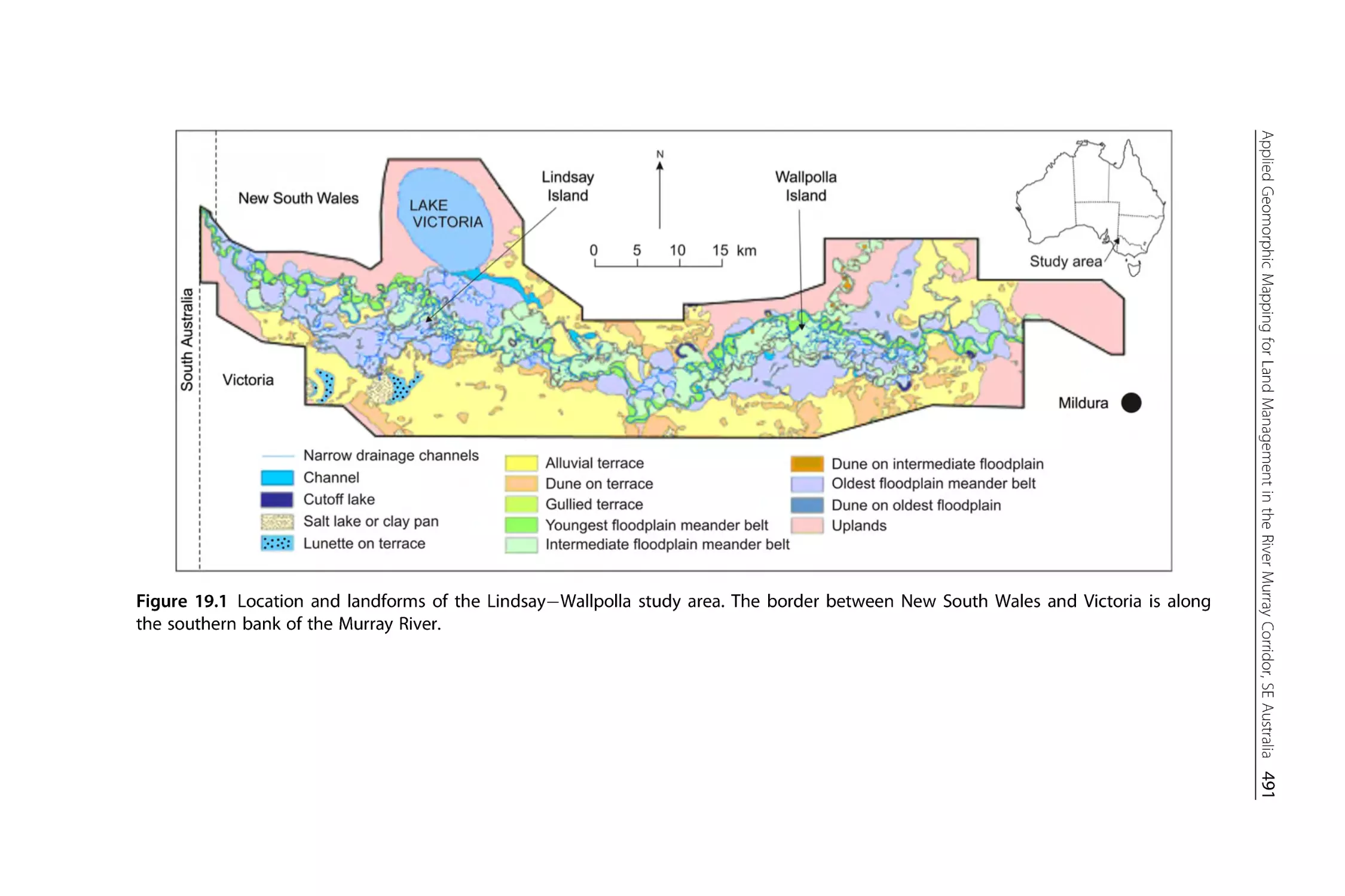
Figure 19.1 Location and landforms of the Lindsay
Wallpolla study area.
The border between New South Wales and Victoria is along the southern bank of the Murray River.
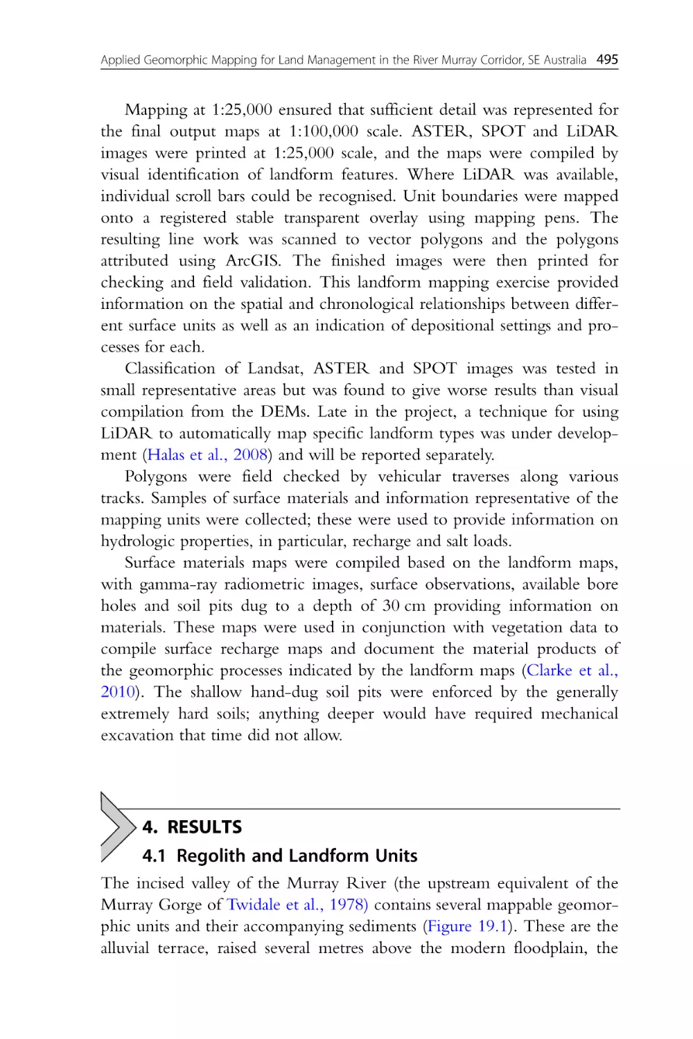
Figure 19.2 Diagrammatic representation of relationships between geomorphic and stratigraphic units. The Coonambidgal and Monoman
Formations (Fm units) are inset to the Rufus Formation (Ta). The Rufus
Formation varies from 5 to 12 m thick, as does the Coonambidgal
Formation. The Monoman Formation is about 10 m thick at the western
end and thins towards the east. The clay drape on Fm1 is absent and then
increases from 0.5
1.5 m on Fm2 to 2
2.5 m on Fm3.
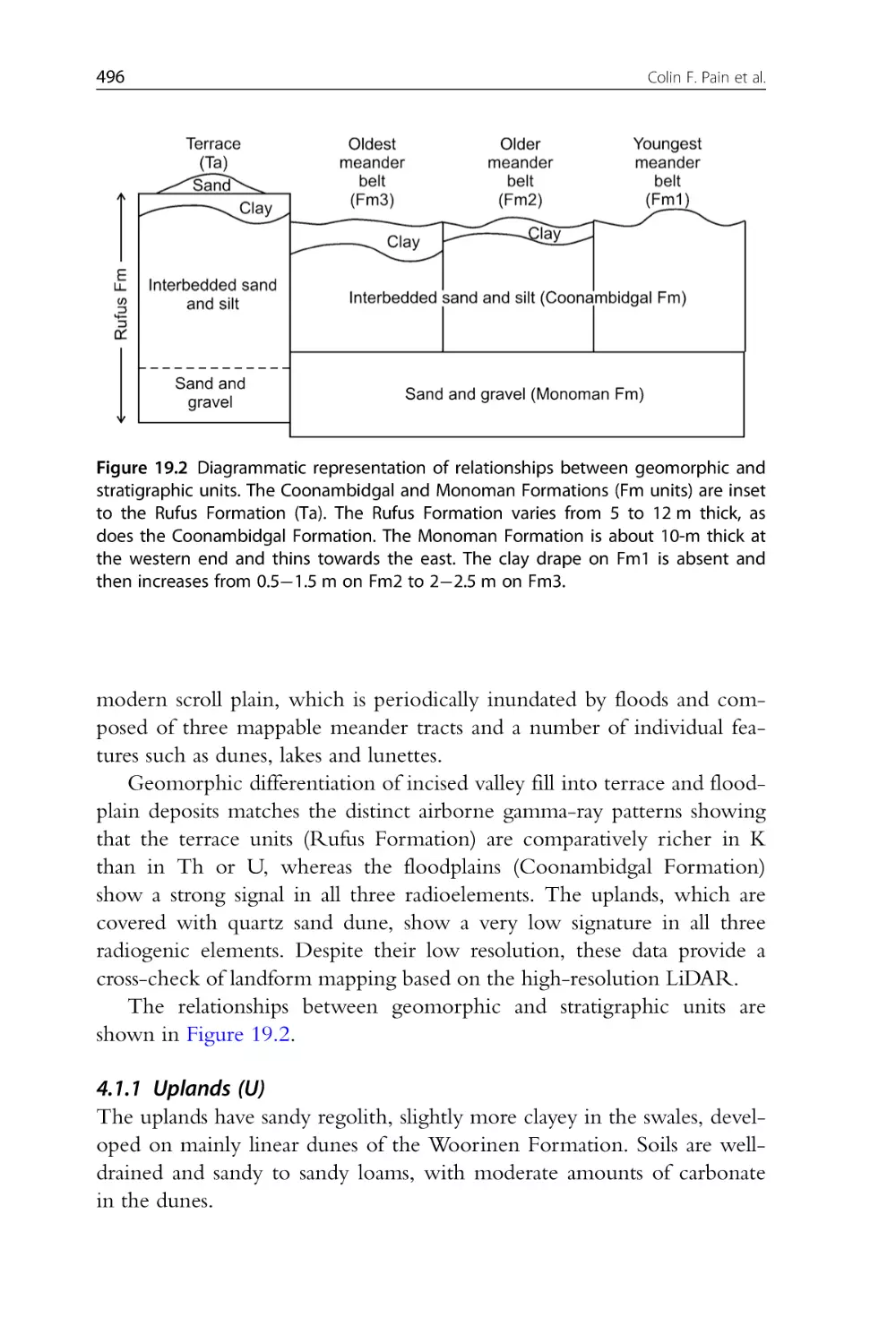
Figure 19.3 AEM slice of the western part of the study area showing conductivity from 0 to 5 m below the surface. The southern part of the
image is in the terrace and clearly shows the complex of palaeo-oxbow
and other palaeo-stream features that underlie the terrace landform
unit. Lower conductivity values (blues) show water-filled sandy sediments underlying young floodplains adjacent to the Murray River.
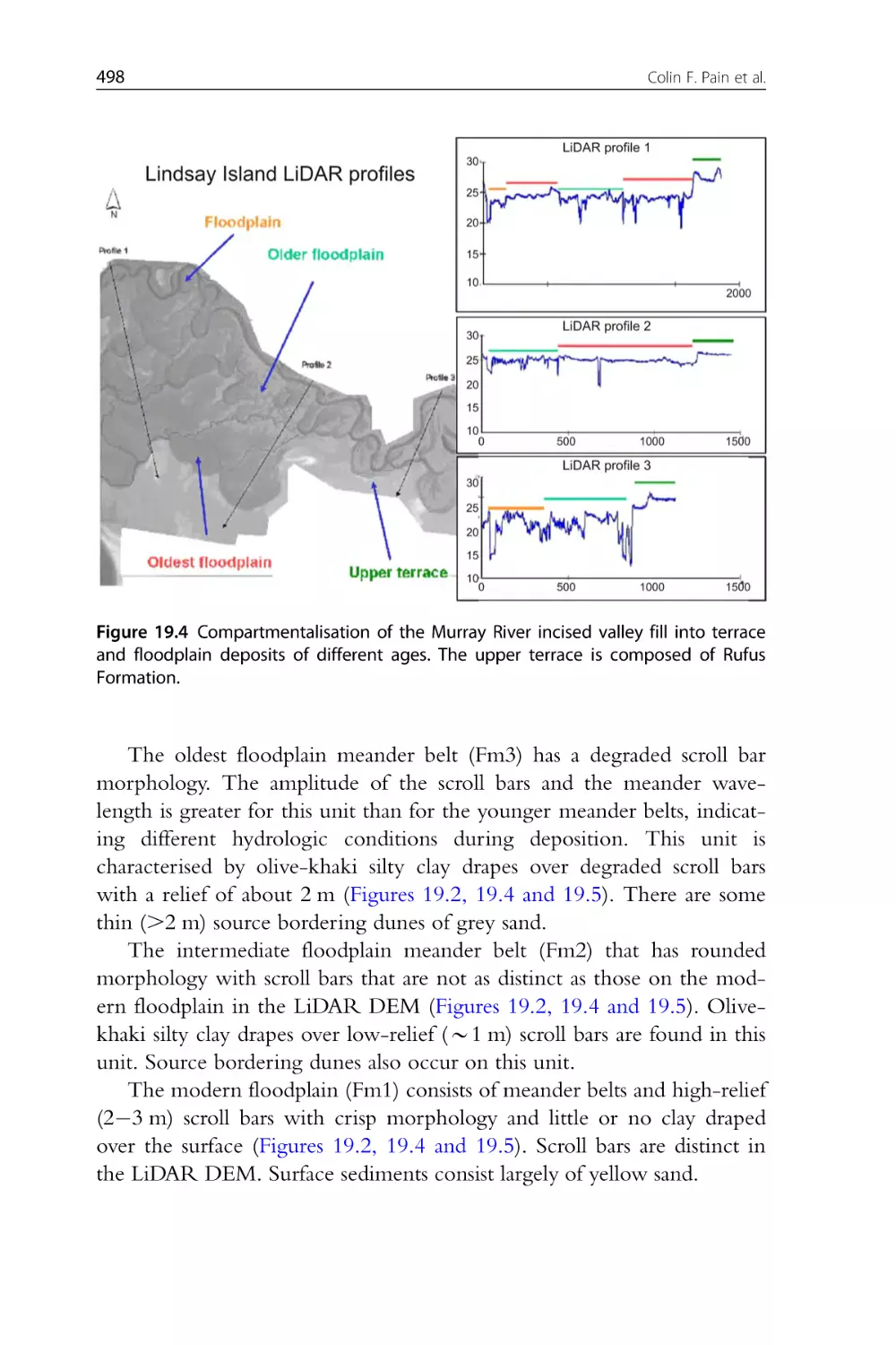
Figure 19.4 Compartmentalisation of the Murray River incised valley fill
into terrace and floodplain deposits of different ages. The upper terrace
is composed of Rufus Formation. Colour text on the left matches colour bars on the right.
Figure 19.5 Oblique projection looking west from the Murray River at
Merbein showing part of the LiDAR DEM and geomorphic elements
(annotated). Width of image B5 km. Elevation ranges from high (red)
to low (dark blue).

CHAPTER TWENTY
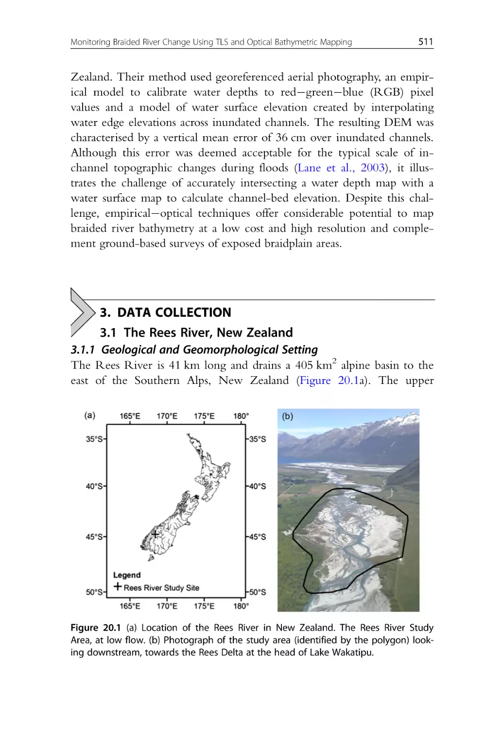
Figure 20.1 (a) Location of the Rees River in New Zealand. The Rees
River Study Area, at low flow. (b) Photograph of the study area

List of Figures

xli

(identified by the polygon) looking downstream, towards the Rees
Delta at the head of Lake Wakatipu.
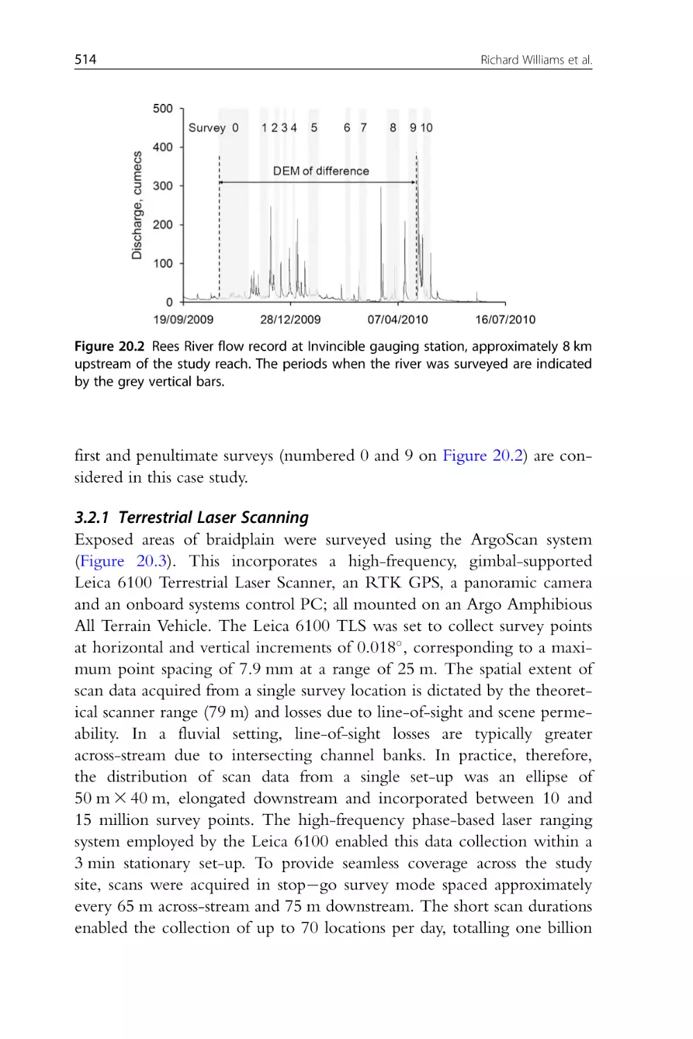
Figure 20.2 Rees River flow record at Invincible gauging station, approximately 8 km upstream of the study reach. The periods when the river
was surveyed are indicated by the grey vertical bars.
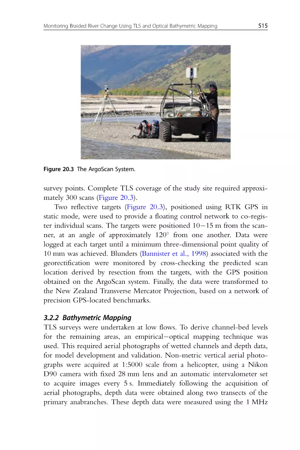
Figure 20.3 The ArgoScan System.
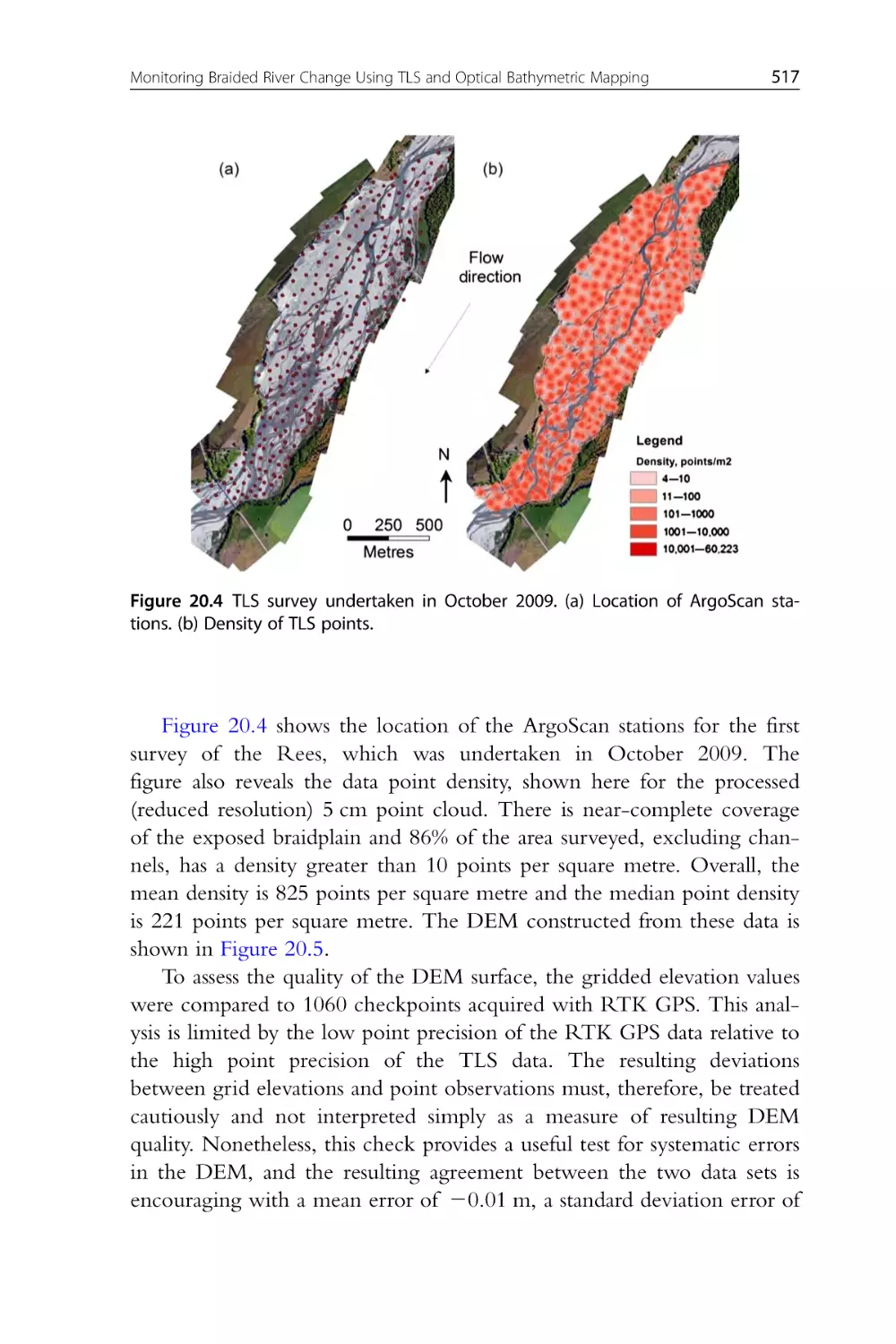
Figure 20.4 TLS survey undertaken in October 2009. (a) Location of
ArgoScan stations. (b) Density of TLS points.
Figure 20.5 (a) Detrended DEM. The surface has been produced by calculating a mean longitudinal bed slope and subtracting this from a
DEM of elevations above sea level. (b) Map of water depth derived by
optical
empirical techniques.
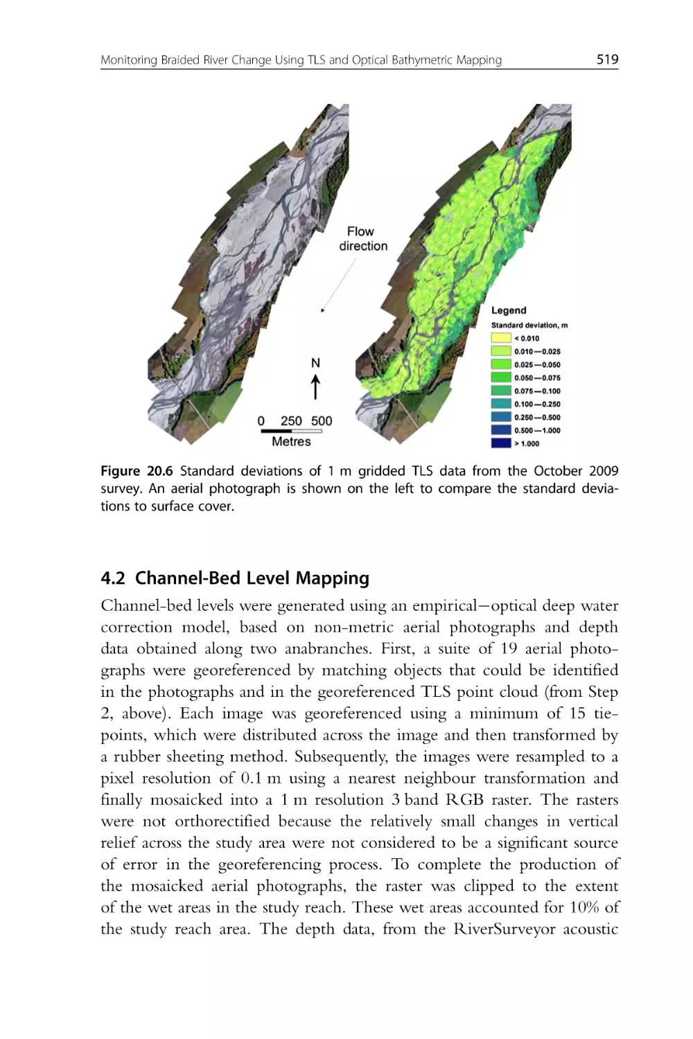
Figure 20.6 Standard deviations of 1 m gridded TLS data from the
October 2009 survey. An aerial photograph is shown on the left to
compare the standard deviations to surface cover.
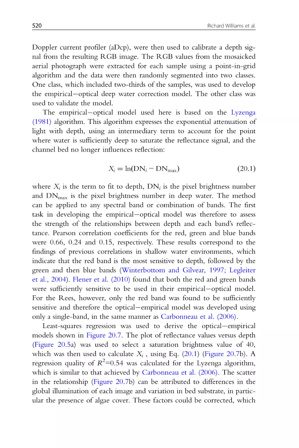
Figure 20.7 Empirical
optical model used to map channel depth. (a)
Pixel brightness (BN) values and measured depths for Band 1 (Red).
(b) Empirical
optical model for Band 1. (c) Modelled versus measured
depths for the class of measurements used to validate the model.
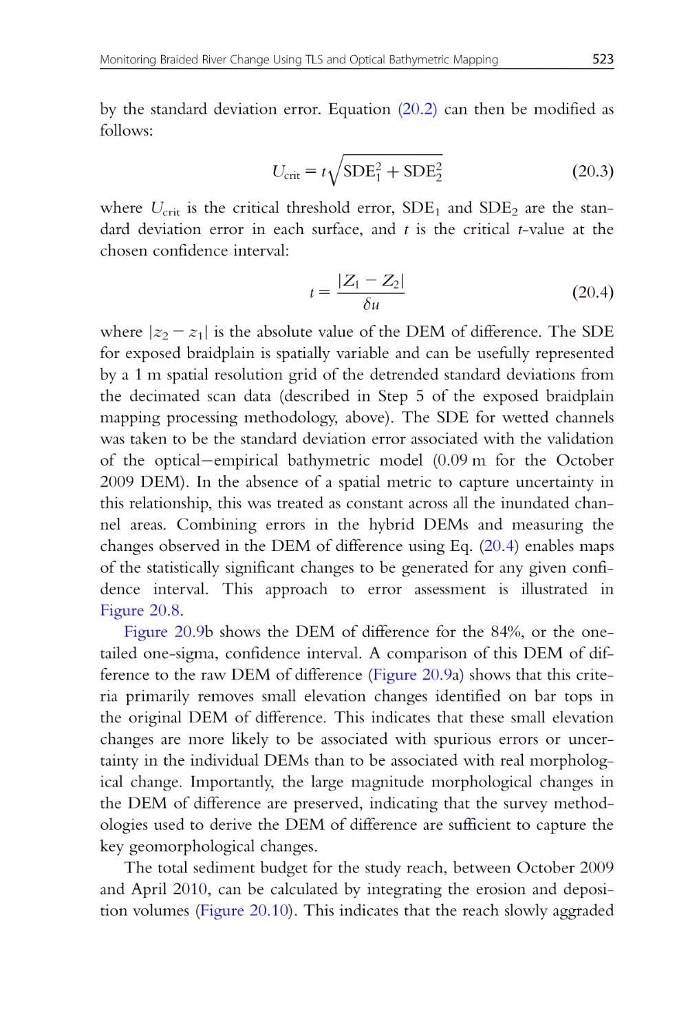
Figure 20.8 Overview of approach used to calculate DEMs of difference
for particular confidence intervals. The data used to produce the DEM
of difference is classified to identify the source of δu. Subsequently, δu
is calculated and a t-score derived. The DEM of difference is then segmented for a chosen confidence interval.
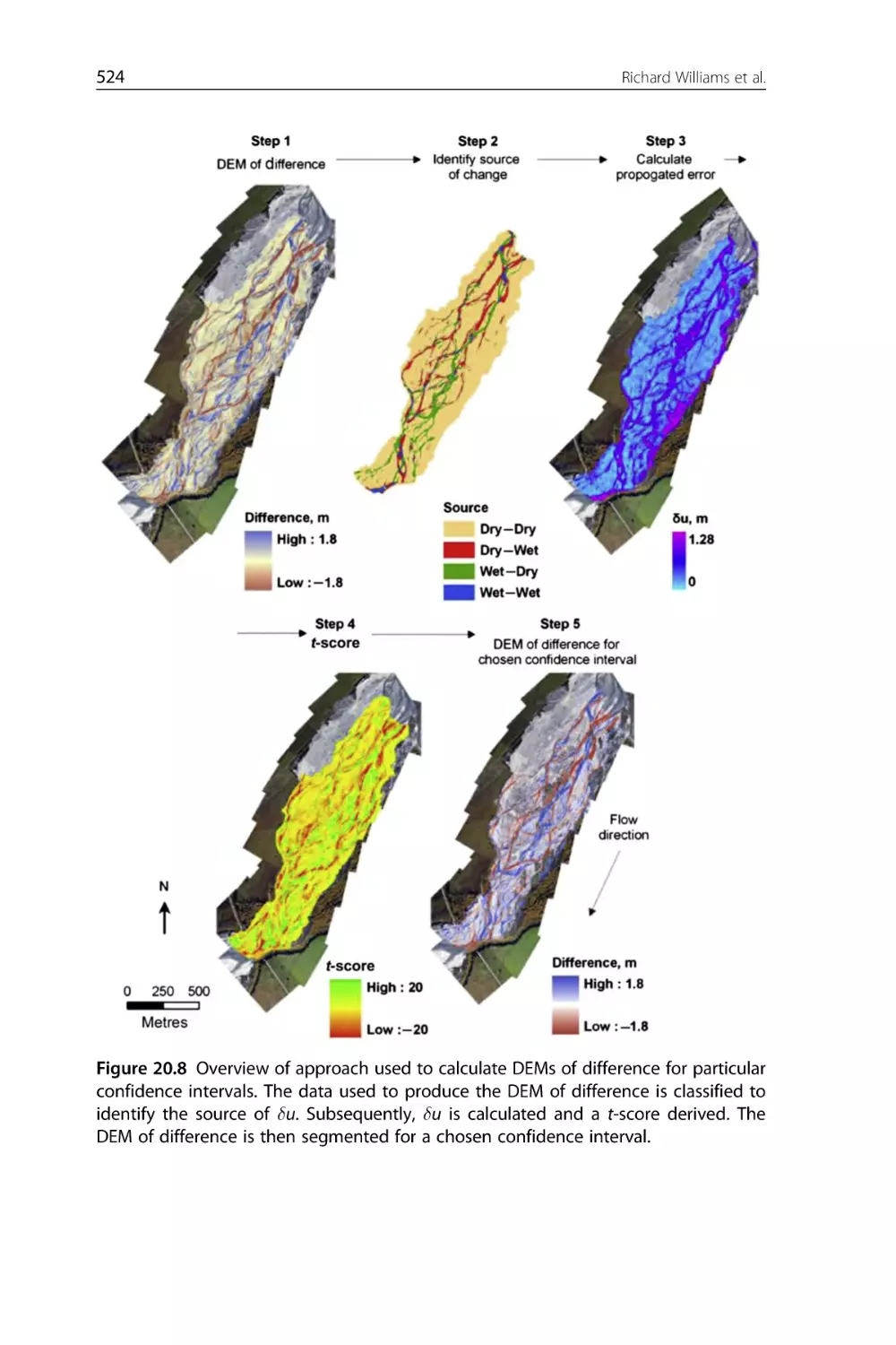
Figure 20.9 (a) DEMs of difference and (b) DEM of difference for the
84% confidence interval.
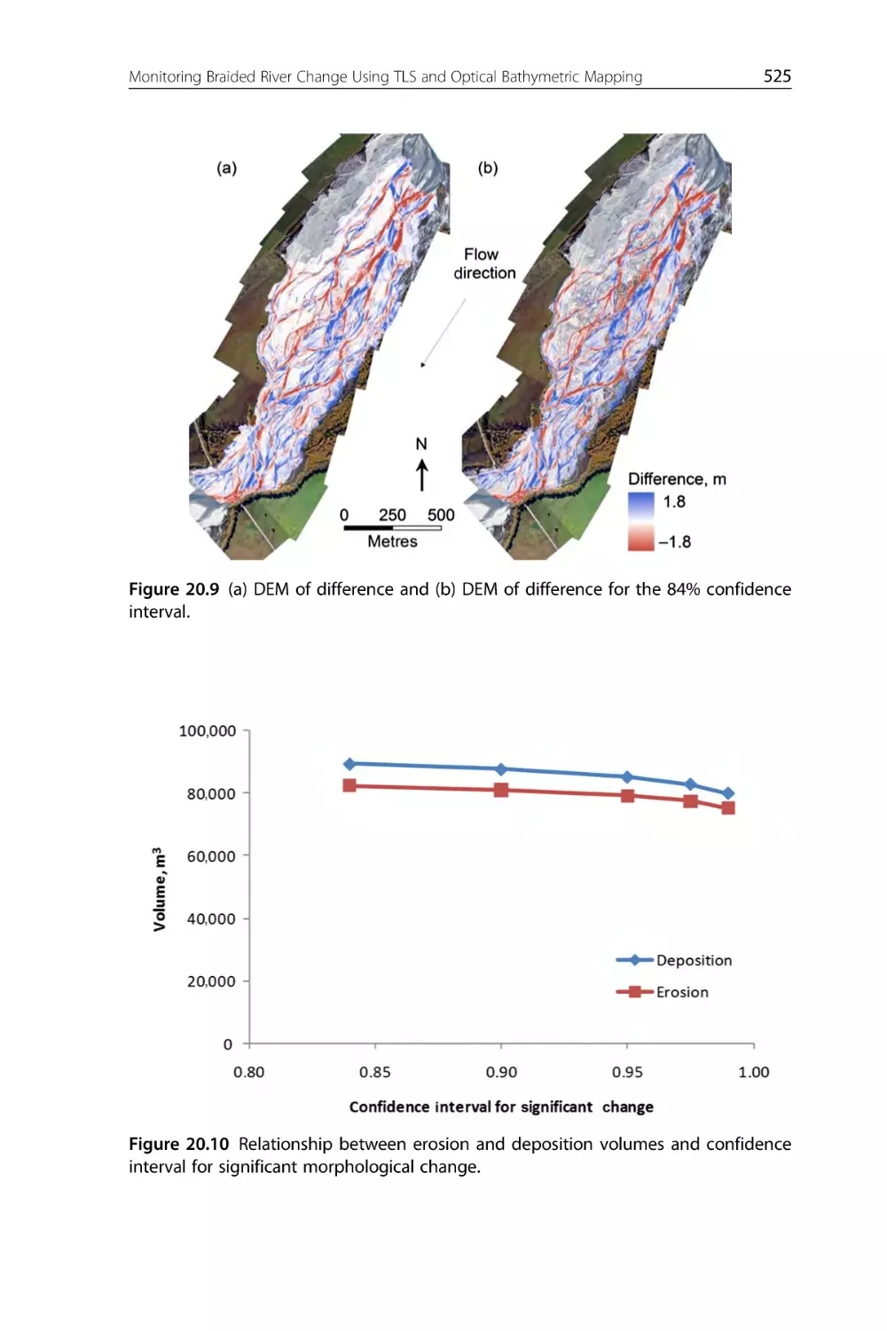
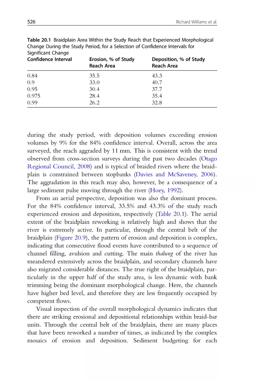
Figure 20.10 Relationship between erosion and deposition volumes and
confidence interval for significant morphological change.

CHAPTER TWENTY-ONE
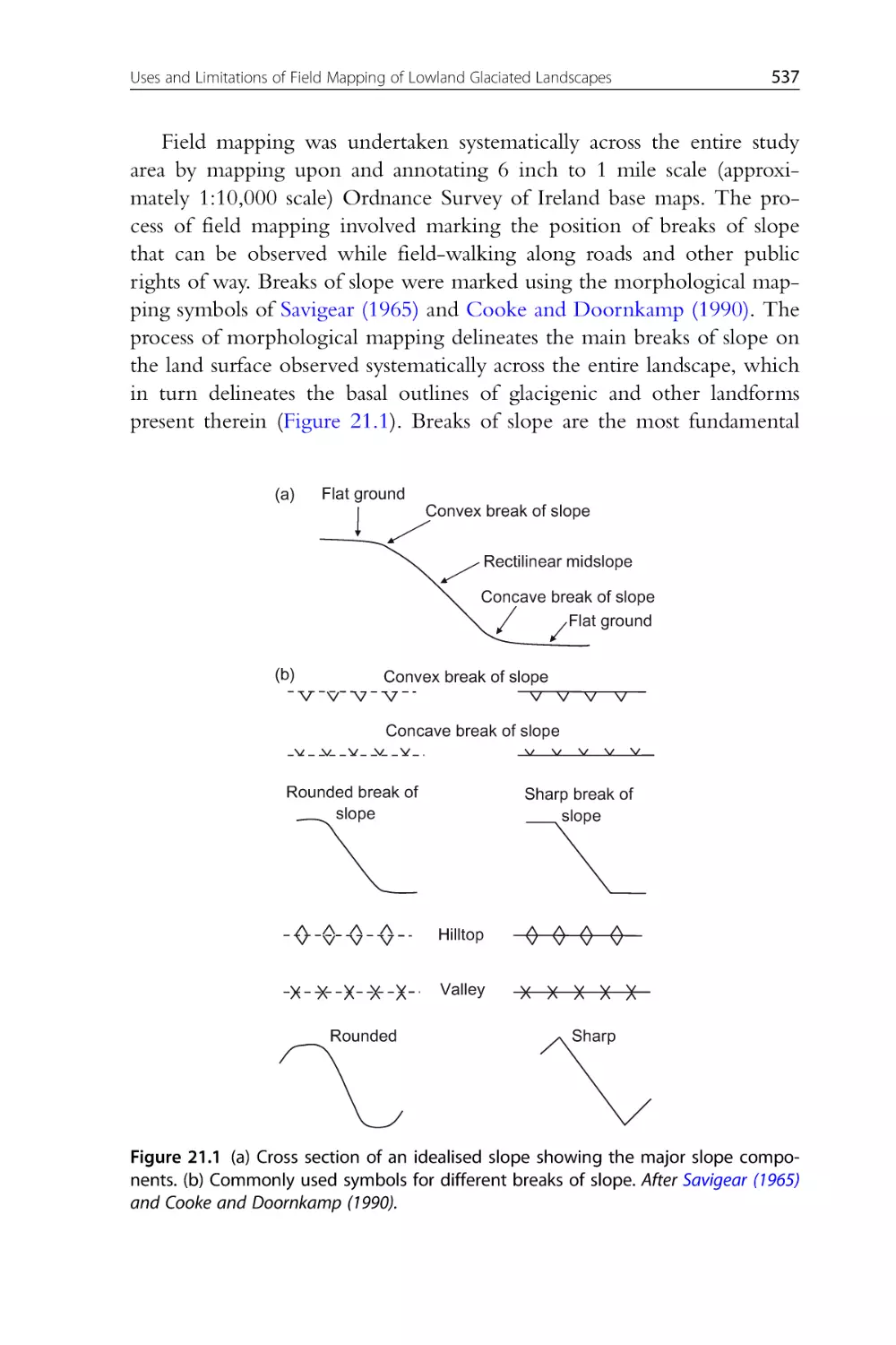
Figure 21.1 (a) Cross section of an idealised slope showing the major
slope components. (b) Commonly used symbols for different breaks of
slope. After Savigear (1965) and Cooke and Doornkamp (1974).
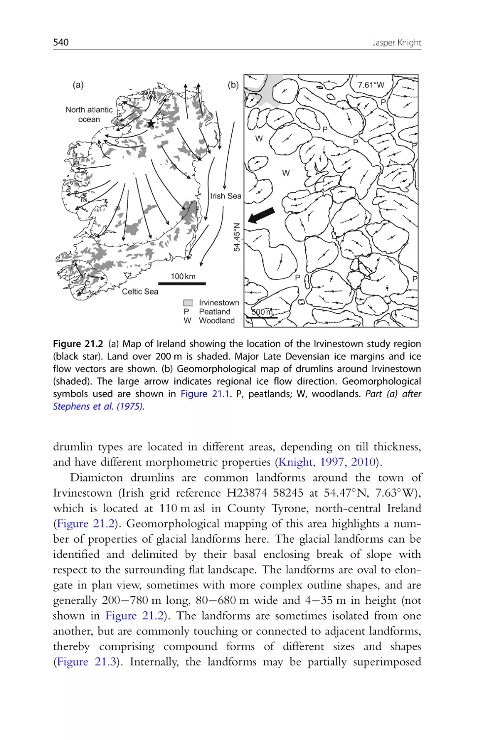
Figure 21.2 (a) Map of Ireland showing the location of the Irvinestown study
region (black star). Land over 200 m is shaded. Major Late Devensian ice
margins and ice flow vectors are shown. (b) Geomorphological map of
drumlins around Irvinestown (shaded). The large arrow indicates regional

xlii

List of Figures

ice flow direction. Geomorphological symbols used are shown in
Figure 21.1. P, peatlands; W, woodlands. Part (a) after Stephens et al.
(1975).
Figure 21.3 Annotated photograph of the drumlin landscape around
Irvinestown showing a concave break of slope at the drumlin base,
which demarcates a flat area of inter-drumlin peat, a convex break of
slope along the drumlin crest and areas of variations in slope angle on
the drumlin sides. Note that these breaks of slope are relatively smooth
and are not complex over very local spatial scales. This field evidence
matches with the patterns of breaks of slope identified in Figure 21.2.
Figure 21.4 Geomorphological map of glaciolacustrine deltas south of
Gortin. The regional location of Gortin is shown by the white star in
Figure 21.2. Geomorphological symbols used are shown in
Figure 21.1. The figure caption shows the morphological description
and (in brackets) its interpretation. Delta surfaces (D) have their surface
elevations shown (m asl).
Figure 21.5 Annotated photograph of the flat delta surfaces and kettle
holes at Gortin.

CHAPTER TWENTY-TWO
Figure 22.1 Location of the study area in Lower Khuzestan.
Figure 22.2 Flowchart illustrating the working procedure followed in this
study.
Figure 22.3 Geomorphological map of the study area.
Figure 22.4 Sample of the geomorphological map at scale 1/:100,000 (for
legend see Table 22.3).
Figure 22.5 Typical examples of irrigation patterns visible on CORONA
imagery (extracts from frame DS1045-2182DF080): abandoned ‘herringbone’ patterns of fan J2 (a and b) and active distributary system of
fan J3 (c and d). The line drawings are a schematic representation of
both irrigation networks (e and f).

CHAPTER TWENTY-THREE
Figure 23.1 Shaded relief map of the Normandy Peninsula. The front
lines at key dates during the first 2 months of the campaign are

List of Figures

xliii

indicated and four regions with different landforms are labelled from
‘A’ to ‘D’.
Figure 23.2 Slope map of the Normandy Peninsula, with slopes in per cent.
Figure 23.3 Slope map of the invasion beaches, at the full resolution of
the 3v DEM.
Figure 23.4 Regions subject to flooding in Normandy.
Figure 23.5 Terrain organisation (Guth, 2003) map of Normandy. These
length of the lines show the degree to which valleys and ridges share
similar orientations, and the orientation of the lines shows the direction
in which cross-country mobility will be maximised.
Figure 23.6 Ridge and valley classification of Normandy. Note that the
areas of the original landings have very complex, fine scale patterns,
and that the ridges and valleys have a much larger scale pattern in the
regions where the breakout took place.
Figure 23.7 Edge map from ETM+ Band 8, using Laplace or Gaussian filter for the region around Omaha Beach.
Figure 23.8 Corine land cover 2000 (CLC2000) for Normandy. r EEA
(2007), Copenhagen.

LIST OF TABLES

CHAPTER THREE
Table 3.1 Spatial/Temporal Order of Magnitude of Earth Surface Features
Table 3.2 Map Scale Classes, Ranges and Mappable Lengths
Table 3.3 The Salerno University Hierarchical Multiscale Taxonomy

CHAPTER FOUR
Table 4.1 Users and Makers of Different Types of Maps

CHAPTER FIVE
Table 5.1 Factors Examined in Relation to the Distribution of Mapped
Landslides
Table 5.2 Observed/Expected Landslide Distribution According to Rock
Type
Table 5.3 Observed/Expected Landslide Distribution According to Slope
Angle
Table 5.4 Terrain Unit Descriptions
Table 5.5 Comparison of Resource Inputs and Outputs of the Three
Case Studies
Table 5.6 Comparison of Case Study Investigations with the Procedural
Guidelines in Fell et al. (2008)

xlv

xlvi

List of Tables

CHAPTER SIX
Table 6.1 Table Showing a Workflow Model for Undertaking
Geomorphological Field Mapping

CHAPTER EIGHT
Table 8.1 Definitions of Geomorphometric Terms

CHAPTER NINE
Table 9.1 Definitions of Hue, Value and Chroma
Table 9.2 Representation of Different Geomorphological Parameters in
the Legend Systems Introduced
Table 9.3 List of Several Open-Source (*) and Commercial Software
Products Providing and Supporting the WMS Format

CHAPTER TEN
Table 10.1 Overview of the LSPs and Criteria Used in the Step-By-Step
Feature Extraction
Table 10.2 Confusion Matrix Showing the Number of Pixels of Classified
Geomorphological Features within the Reference Data Set

CHAPTER FOURTEEN
Table 14.1 General Geology of the Study Area
Table 14.2 Average Strata Thickness and Some Typical Intact Properties
Table 14.3 General Geomorphology of the Study Area

List of Tables

xlvii

CHAPTER SEVENTEEN
Table 17.1 Summary of the Properties of the Riegl Laser Scanner Used in
this Study (Riegl, 2009)

CHAPTER EIGHTEEN
Table 18.1 Knowledge-Based Classification Rules

CHAPTER NINTEEN
Table 19.1 Stratigraphy of the Lindsay Wallpolla Study Area

CHAPTER TWENTY
Table 20.1 Braidplain Area Within the Study Reach that Experienced
Morphological Change During the Study Period, for a Selection of
Confidence Intervals for Significant Change
Table 20.2 Contribution to Erosion and Deposition Estimates by
Different Conditions of Change in the DEM of Difference, for the
84% Confidence Interval

CHAPTER TWENTY-TWO
Table 22.1 Map Sources Used in This Study
Table 22.2 Remote Sensing Data Used in This Study
Table 22.3 Image Interpretation Key and Legend Designed for
Geomorphological Mapping of the Alluvial Plains in Lower Khuzestan

xlviii

List of Tables

CHAPTER TWENTY-THREE
Table 23.1 Data Sets Used

�SECTION

1

Geomorphological
Mapping

CHAPTER ONE

Introduction to Applied
Geomorphological Mapping
James S. Griffithsa, Mike J. Smithb and Paolo Paronc
a

SoGEES, University of Plymouth, Plymouth, UK
School of Geography, Geology and the Environment, Kingston University, Surrey, UK
UNESCO-IHE, Institute for Water Education, Delft, NL & School of Geography and the Environment,
Oxford University, UK
b
c

Contents
1. Geomorphological Mapping
2. Techniques of Applied Geomorphological Mapping
3. Case Studies in Applied Geomorphological Mapping
References

6
7
8
9

The survival of humans is heavily dependent on a very narrow zone
within the Earth’s crust, from the water on the surface, to the few metres
depth of agricultural soil, to the couple of hundred metres from which we
extract potable groundwater. Although we do extract mineral resources
and some groundwater from greater depths, the vast majority of human
activities take place on the land, in rivers and lakes, or in the coastal and
nearshore zone and predominantly within 100 m of the ground surface.
The main exceptions to this depth limit are as follows: hard rock tunnels;
deep sea drilling and production rigs; hydrocarbon exploration and exploitation; cross-ocean cables and deep mining. However, it is realistic to conclude that the overwhelming majority of human activities interact with
the landforms that make up the surface and near surface of terrestrial,
nearshore and offshore ‘landscapes’. The scientific investigation of these
landscapes, the processes that have formed them over time, the materials
which they are composed of, the individual elements that combine to create them and the way they will evolve through time is the discipline of
geomorphology. Understanding geomorphology, therefore, can be seen as
fundamental to the safe, economic and sustainable development of the
planet Earth.
Geomorphology is part of the broad range of disciplines that fall under
the general heading of earth sciences, which includes both geology and
Developments in Earth Surface Processes, Volume 15
ISSN: 0928-2025, DOI: 10.1016/B978-0-444-53446-0.00001-X

© 2011 Elsevier B.V.
All rights reserved.

3

4

James S. Griffiths et al.

geography. In Europe geomorphology has traditionally been associated
with ‘physical geography’, whereas in North America it has usually been
regarded as part of ‘physical geology’. Until the 1960s, a significant part of
geomorphological research was engaged in the history of landscape development, but during the 1960s and 1970s there was a shift in AngloAmerican geomorphology into smaller scale process studies (Smith et al.,
2002). However, landscape development continued as a core component
of physical geology studies in the United States (Costa and Graf, 1984).
The original geomorphological emphasis on the study of landscapes meant
that, in common with the rest of the earth sciences, there has always been
the need to compile spatial data and then to present these data in plan
form as maps. Although the methodology and representation of much
spatial data has a long history (e.g. accurate geological maps date back to
William Smith’s first map of the United Kingdom in 1815; Winchester,
2001), the presentation of geomorphology in map form has not reached
the same level of standardisation, despite some attempts in Europe to produce comprehensive legends (Demek and Embleton, 1978).
The combination of a lack of a standard methodology or commonly
accepted legend, plus the move of academic geomorphologists away from
spatially extensive studies of landscape development, led to geomorphological mapping being regarded as a somewhat sterile area of study
(Gustavsson et al., 2006). The indications are that it was seen as being of
limited value in mainstream geomorphological research. However, at the
time that the process response geomorphologists were beginning to concentrate on small-scale studies, the compilation of geomorphological
information was found to be fundamental to many applied studies of the
Earth’s surface, including coastal zone management; route alignment
work for roads, railways and pipelines; soil erosion studies; military work
using terrain classification for trafficability and tactical analysis; river
catchment management; geohazard assessments, notably for civil engineering projects and, increasingly, in offshore studies particularly when
seeking resources and identifying the potential hazards to their exploitation (e.g. gas hydrates and submarine landslides). Thus, since the 1980s
we have seen the creation and use of applied geomorphological maps from
many terrestrial and marine environments, and these have been produced
by practitioners of applied geomorphology rather than academic geomorphology. In order to understand this development, it is necessary to define
what the technique of geomorphological mapping entails. Lee (2001)
described geomorphological mapping as one of the group of techniques

Introduction to Applied Geomorphological Mapping

5

under the general category of ‘terrain evaluation’ employed to systematically record the shape or morphology of the ground, landforms,
landscape-forming processes and materials that constitute the surface of
the Earth. Lee (2001) identified three forms of geomorphological map:
1. Regional surveys of terrain conditions, for general geomorphological
investigations, land use planning or in baseline studies for environmental impact assessment (e.g. the 1:25,000 scale maps of Torbay;
Doornkamp et al., 1988),
2. General assessments of resources or geohazards at scales between
1:50,000 and 1:10,000 (e.g. Bahrain Surface Materials Resources
Survey; Doornkamp et al., 1980; ground problems in the Suez City
area, Egypt; Jones, 2001),
3. Specific-purpose large-scale surveys to delineate and characterise particular landforms (e.g. the 1:500 scale investigations around the
Channel Tunnel portal, Folkestone; Griffiths et al., 1995).
Given this background, and the widening interest in the role and
importance of geomorphological mapping, the International Association
of Geomorphologists commissioned this volume to provide a state-ofthe-art review of the development of the technique and see the way it is
now being employed both in the academic and in the professional world.
The intention of this book is not to produce a standardised mapping
methodology or to provide a detailed geomorphological legend, but it is
an attempt to bring together leading exponents in the preparation and use
of geomorphological maps and illustrate how they are being used to
investigate a wide range of environmental issues. The book is divided into
three sections:
1. Geomorphological mapping: It details the history of geomorphological
mapping, focusing upon the development of methods and their evolution within different national ‘schools’; outlines the aims and objectives of mapping and looks at quantitative risk assessment,
2. Techniques of applied geomorphological mapping: It reviews the techniques
of mapping, including traditional field mapping and recognises the
increasing use of digital data gathering techniques for mapping,
3. Case studies in applied geomorphological mapping: It presents examples of
different industrial applications of geomorphological maps from a variety of environmental settings to demonstrate the wide range and
application of mapping in both academic and professional arenas.
The actual content of each of these sections is described in more
detail below. A final conclusion looks at the future development of

6

James S. Griffiths et al.

geomorphological mapping. What became apparent to the editors during the compilation of this volume is that the techniques employed to
create geomorphological maps are becoming increasingly sophisticated
and the range of applications of the maps is becoming ever wider. This
volume demonstrates that geomorphological mapping is a technique
that all geomorphologists should be familiar with and be able to utilise
in the collection and presentation of geomorphological data. The technique is also one that can provide a firm basis for the investigation of
many environmental issues, notably in the field of geohazards and risk
assessment.

1. GEOMORPHOLOGICAL MAPPING
Geomorphological mapping flourished in different countries and
schools all with different aims, especially during the 1960s 1980s. The
first contribution in this section is by Verstappen (2011) who illustrates
the early development of geomorphological and landform mapping in
Europe (western and eastern) and Australia with several examples of legend types and cartographic development. Dramis et al. (2011) focuses
on the types, purposes and content of geomorphological maps, spanning
from the ‘traditional’ symbol-based maps to the most modern digital
techniques. This chapter presents some of the state-of-the-art techniques in object-oriented geomorphological mapping, with examples
from Italy. It highlights the importance of moving towards an objective
and multi-scalar method for the representation of the landscape that can
be of great benefit to a wider community of users, including environmental analysts and planners. Paron and Claessens (2011) focuses on the
need to integrate geomorphological mapping in national mapping programmes, natural hazard zonations and emergency programmes and
landscape planning. The chapter shows how the new digital mapping
and web-mapping reality can aid in disseminating the importance of
geomorphological investigation and mapping. The last chapter of this
section by Hearn and Hart (2011) looks at the practical issues involved in
quantitative risk assessment/analysis of landslides, showing how some of
the conceptual models are quite theoretical. This contribution attempts
to bridge the gap between the diffuse hazard susceptibility maps and the

Introduction to Applied Geomorphological Mapping

7

more useful hazard and risk maps required for quantitative risk assessment of landslides. The examples in this chapter from less economically
developed countries illustrate well the need for practical but sound hazard mapping in data poor environments where vulnerability may be
increasing as new developments take place.

2. TECHNIQUES OF APPLIED GEOMORPHOLOGICAL
MAPPING
The systematic recording of landform morphology requires some
kind of geodetic framework and a methodology through which this is
performed. Early geomorphological mapping required physical site visits
in order to record plan-form position and, in some instances, composition on to a topographic base map. Knight et al. (2011) detail the techniques used for field-based geomorphological mapping and whereas, by
volume, it has largely been replaced as a technique, it remains a common,
and important, aspect of large-scale surveys.
One of the drivers of the resurgence in geomorphological mapping
is technology: the availability of new data sources has allowed new
insights and rapid mapping to be performed, organised within the
framework of a geographic information system (GIS). The addition of
new sources of digital spatial data has opened up vast regions of the
Earth’s surface (and indeed other planets) for study that would have otherwise been uneconomic or impossible to achieve. Oguchi et al. (2011)
detail the vast range of data sets that are currently available and outline
their potential application areas.
More mundanely, but of no less significance, is the organisation of spatial data into a digital data framework. The ability to use a ‘layers’ paradigm
to organise input data and produce layers of thematic, mapped, output is of
great significance. Smith (2011) outlines this ‘layered’ approach and introduces methods for the visualisation and digital recording of landforms.
This remains an entirely manual process, limited by the skill and experience of the operator. Accurate automated and semi-automated landform
extraction techniques remain a current research focus, and Seijmonsbergen
et al. (2011) introduce the main techniques and their applications. Finally,
no technical section would be complete without discussion of the

8

James S. Griffiths et al.

presentation of mapped landforms. Otto et al. (2011) provide a brief synopsis
of cartographic techniques and their applications to geomorphological
mapping. There is specific focus upon the review and selection of an
appropriate legend system. The chapter concludes with the digital dissemination of geomorphological information and, in particular, web servers,
virtual globes and static maps.

3. CASE STUDIES IN APPLIED GEOMORPHOLOGICAL
MAPPING
Thirteen case studies have been compiled, including three from the
marine environment. The three marine examples illustrate how the use
of modern marine geophysical techniques has revolutionised our ability
to interpret marine geomorphology. Dunlop et al. (2011) used publically
available multi-beam swath bathymetry data to construct a glacial geomorphology map of the continental margins north and northwest of
Ireland. Hillier (2011) has created digital elevation models of the
Hawaiian volcanoes to establish their height and volume, data that are
critical to understanding the volcanic hazard. Micallef (2011) demonstrates how the range of marine geophysical techniques can be used to
produce geomorphological maps in order to assess submarine landslides,
presenting a case study of the Storegga slide in the North Sea between
Norway and Scotland.
The value of geomorphological mapping in mass movement investigations is a theme that emerges from a number of the terrestrial case studies.
Griffiths et al. (2011) use traditional field mapping and remote sensing interpretation to produce an engineering geomorphological map of a landslide
that potentially could have affected the Channel Tunnel Terminal in Kent,
United Kingdom. Parry (2011) looks at mapping as a technique for assessing
landslide risk in Hong Kong. In a more academic investigation, Theler and
Reynard (2011) use mapping as a tool for assessing sediment transfer processes in small catchments in Switzerland prone to debris flows. Whitworth
et al. (2011) make use of terrestrial laser scanning to produce geomorphological assessments of complex landslide systems in the Cotswolds area of
the United Kingdom. As a useful adjunct to this, the value of airborne laser
scanning for compiling a range of geomorphological data is illustrated by
Rutzinger et al. (2011) for three different test sites in the Austrian Alps.

Introduction to Applied Geomorphological Mapping

9

Pain et al. (2011), also use airborne laser scanning alongside airborne electromagnetic surveys and satellite imagery to evaluate the hydro-geomorphology of the River Murray area in southeast Australia. Williams et al.
(2011) have embraced the new geomatics technology as well, using terrestrial laser scanning coupled with high-resolution digital elevation models in
the investigation of sediment transport rates in a braided river system in
New Zealand. By way of contrast, Knight (2011) provides an example of
more traditional field mapping approach, linked to remote sensing interpretation, to compile maps of a lowland glaciated landscape in north-central
Ireland.
The final two case studies illustrate the role geomorphological mapping
can have in anthropological investigations. Walstra et al. (2011) map the
late Holocene evolution and human impact in the Mesopotamian region
(southwest Iran) using remote sensing and a GIS. As a contrast, Guth
(2011) provides a case study from the D-Day landings in Normandy (June
1944) of the way geomorphological maps allow military commanders to
see the way the landscape will influence military operations.
The range of case studies presented is only illustrative of the potential
applications of geomorphological mapping. They do illustrate the move away
from traditional field mapping through increasing use of digital data capture
systems. However, what does emerge from the studies is that interpretation of
the data requires extensive and detailed understanding of geomorphological
processes and landforms; this is a knowledge and skills base that still requires
widespread fieldwork experience. It is also apparent that geomorphological
maps are complex tools and to be of value beyond the academic community
may often require careful explanation and presentation. The critical importance of communicating geomorphological data effectively remains a
challenge that new multimedia tools are helping us to address.

REFERENCES
Costa, J.E., Graf, W.I., 1984. The geography of geomorphologists in the United States.
Prof. Geogr. 36, 82 89.
Demek, J., Embleton, C. (Eds.), 1978. Guide to Medium-Scale Geomorphological
Mapping. International Geographical Union, Stuttgart.
Doornkamp, J.C., Brunsden, D., Jones, D.K.C., Cooke, R.U., 1980. Geology,
Geomorphology and Pedology of Bahrain. GeoBooks, Norwich.
Doornkamp, J.C., Griffiths, J.S., Lee, E.M., Tragheim, D., Charman, J.H., 1988.
Applied Earth Science Mapping of the Torbay Region. 2 vols.+11 maps. Open File
Research Report for the Department of the Environment and Torbay Borough
Council.

10

James S. Griffiths et al.

Dramis, F., Guida, D., Cestari, A., in press. Nature and aims of geomorphological mapping. In: Smith, M.J., Paron, P., Griffiths, J. (Eds.), Geomorphological Mapping: A
Handbook of Techniques and Applications. Elsevier, Amsterdam.
Dunlop, P., Sacchetti, F., Benetti, S., Ó Cofaigh, C., in press. Mapping Ireland’s glaciated
continental margin using marine geophysical data. In: Smith, M.J., Paron, P.,
Griffiths, J. (Eds.), Geomorphological Mapping: A Handbook of Techniques and
Applications. Elsevier, Amsterdam.
Griffiths, J.S., Brunsden, D., Lee, E.M., Jones, D.K.C., 1995. Geomorphological investigation for the Channel Tunnel and Portal. Geogr. J. 161, 257 284.
Griffiths, J.S., Lee, E.M., Brunsden, D., Jones, D.K.C., in press. The Cherry Garden landslide, Etchinghill escarpment, South-east England. In: Smith, M.J., Paron, P.,
Griffiths, J. (Eds.), Geomorphological Mapping: A Handbook of Techniques and
Applications. Elsevier, Amsterdam.
Gustavsson, M., Kolstrup, E., Seijmonsbergen, A.C., 2006. A new symbol-and-GIS based
detailed geomorphological mapping system: renewal of a scientific discipline for
understanding landscape development. Geomorphology 77, 90 111.
Guth, P.L., in press. Military applied geomorphological mapping: Normandy case study.
In: Smith, M.J., Paron, P., Griffiths, J. (Eds.), Geomorphological Mapping: A
Handbook of Techniques and Applications. Elsevier, Amsterdam.
Hearn, G., Hart, A., in press. Goemorphological contributions to landslide risk assessment: theory and practice. In: Smith, M.J., Paron, P., Griffiths, J. (Eds.),
Geomorphological Mapping: A Handbook of Techniques and Applications. Elsevier,
Amsterdam.
Hillier, J.K., in press. Submarine geomorphology: quantitative methods illustrated with
the Hawaiian volcanoes. In: Smith, M.J., Paron, P., Griffiths, J. (Eds.),
Geomorphological Mapping: A Handbook of Techniques and Applications. Elsevier,
Amsterdam.
Jones, D.K.C., 2001. Ground conditions and hazards: Suez City development, Egypt.
In: Griffiths, J.S. (Ed.), Land Surface Evaluation for Engineering Practice, 18.
Geological Society Engineering Geology Special Publication, pp. 159 170.
Knight, J., in press. Uses and limitations of field-mapping of lowland glaciated landscapes.
In: Smith, M.J., Paron, P., Griffiths, J. (Eds.), Geomorphological Mapping: A
Handbook of Techniques and Applications. Elsevier, Amsterdam.
Knight, J., Mitchell, W., Rose, J., in press. Geomorphological field mapping. In: Smith,
M.J., Paron, P., Griffiths, J. (Eds.), Geomorphological Mapping: A Handbook of
Techniques and Applications. Elsevier, Amsterdam.
Lee, E.M., 2001. Geomorphological mapping. In: Griffiths, J.S. (Ed.), Land Surface
Evaluation for Engineering Practice, vol. 18. Geological Society Engineering
Geology Special Publication, pp. 53 56
Micallef, A., in press. Marine geomorphology: geomorphological mapping and the study
of submarine landslides. In: Smith, M.J., Paron, P., Griffiths, J. (Eds.),
Geomorphological Mapping: A Handbook of Techniques and Applications. Elsevier,
Amsterdam.
Oguchi, T., Hayakawa, Y., Wasklewicz, T., in press. Data sources. In: Smith, M.J., Paron,
P., Griffiths, J. (Eds.), Geomorphological Mapping: A Handbook of Techniques and
Applications. Elsevier, Amsterdam.
Otto, J.-C., Gustavsson, M., Geilhausen, M., 2011. Cartography: design, symbolisation
and visualisation of geomorphological maps. In: Smith, M.J., Paron, P., Griffiths, J.
(Eds.), Geomorphological Mapping: A Handbook of Techniques and Applications.
Elsevier, Amsterdam.
Pain, C.F., Clarke, J.D.A., Wong, V.N.L., in press. Applied geomorphic mapping for land
management in the River Murray corridor, SE Australia. In: Smith, M.J., Paron, P.,

Introduction to Applied Geomorphological Mapping

11

Griffiths, J. (Eds.), Geomorphological Mapping: A Handbook of Techniques and
Applications. Elsevier, Amsterdam.
Paron, P., Claessens, L., in press. Makers and users of geomorphological maps. In: Smith,
M.J., Paron, P., Griffiths, J. (Eds.), Geomorphological Mapping: A Handbook of
Techniques and Applications. Elsevier, Amsterdam.
Parry, S., in press. The application of geomorphological mapping in the assessment of
landslide hazard in Hong Kong. In: Smith, M.J., Paron, P., Griffiths, J. (Eds.),
Geomorphological Mapping: A Handbook of Techniques and Applications. Elsevier,
Amsterdam.
Rutzinger, M., Höfle, B., Vetter, M., Pfeifer, N., in press. Digital terrain models from airborne laser scanning for the automatic extraction of natural and anthropogenic linear
structures. In: Smith, M.J., Paron, P., Griffiths, J. (Eds.), Geomorphological Mapping:
A Handbook of Techniques and Applications. Elsevier, Amsterdam.
Seijmonsbergen, A.C., Hengl, T., Anders, N.S., in press. Semi-automated identification
and extraction of geomorphological features using digital elevation data. In: Smith,
M.J., Paron, P., Griffiths, J. (Eds.), Geomorphological Mapping: A Handbook of
Techniques and Applications. Elsevier, Amsterdam.
Smith, B.J., Warke, P.A., Whalley, W.B., 2002. Landscape development, collective amnesia
and the need for integration in geomorphological research. Area 33 (4), 409 418.
Smith, M.J., in press. Digital mapping: visualisation, interpretation and quantification of
landforms. In: Smith, M.J., Paron, P., Griffiths, J. (Eds.), Geomorphological Mapping:
A Handbook of Techniques and Applications. Elsevier, Amsterdam.
Theler, D., Reynard, E., in press. A geomorphological map as a tool for assessing sediment transfer processes in small catchments prone to debris-flows occurrence: a case
study in the Bruchi torrent (Swiss Alps). In: Smith, M.J., Paron, P., Griffiths, J. (Eds.),
Geomorphological Mapping: A Handbook of Techniques and Applications. Elsevier,
Amsterdam.
Verstappen, H.T., in press. Old and new trends in geomorphological and landform mapping. In: Smith, M.J., Paron, P., Griffiths, J. (Eds.), Geomorphological Mapping: A
Handbook of Techniques and Applications. Elsevier, Amsterdam.
Walstra, J., Heyvaert, V.M.A., Verkinderen, P., in press. Mapping late Holocene landscape
evolution and human impact
a case-study from Lower Khuzestan (SW Iran).
In: Smith, M.J., Paron, P., Griffiths, J. (Eds.), Geomorphological Mapping: A
Handbook of Techniques and Applications. Elsevier, Amsterdam.
Whitworth, M., Anderson, I., Hunter, G., in press. Geomorphological assessment of
complex landslide systems using field reconnaissance and terrestrial laser scanning.
In: Smith, M.J., Paron, P., Griffiths, J. (Eds.), Geomorphological Mapping: A
Handbook of Techniques and Applications. Elsevier, Amsterdam.
Williams, R., Brasington, J., Vericat, D., Hicks, M., Labrosse, F., Neal, M., in press.
Monitoring braided river change using terrestrial laser scanning and optical bathymetric mapping. In: Smith, M.J., Paron, P., Griffiths, J. (Eds.), Geomorphological
Mapping: A Handbook of Techniques and Applications. Elsevier, Amsterdam.
Winchester, S., 2001. The Map that Changed the World. Penguin Books, London,
338 pp.

CHAPTER TWO

Old and New Trends in
Geomorphological and Landform
Mapping
Herman Theodoor Verstappen
International Institute of Geo-Information Science and Earth Observation (ITC), University of Twente,
Enschede, The Netherlands

Contents
1. The Advent of Geomorphological Mapping
2. The Diversity of Legends
3. The Needs for Standardisation and Flexibility
4. The Use of Aerial Photographs and Satellite Data
5. Landform Mapping in Synthetic (Holistic) Surveys of Terrain
6. Applied Geomorphological Surveying and Mapping
7. Summary and Conclusions
References

13
15
19
23
27
31
35
36

1. THE ADVENT OF GEOMORPHOLOGICAL MAPPING
Geomorphological mapping began about a century after the advent
of geological mapping and the standardisation of a legend system (Finkle,
1988). The earliest geomorphological map was probably made by Passarge
(1914) on the Stadtremba 1:25,000 topographic map sheet in Germany.
The legend of Passarge’s map differed from modern examples because it
did not encompass all aspects of geomorphology, and it emphasised mainly
descriptive morphographic features and metrical elements. It did not
receive much attention at that time, and geomorphologists tended to produce ‘sketch’ maps at small scales that were either largely structural or
physiographic-pictorial (Raisz, 1931). Most of the maps from this early
period dealt with only one phenomenon (e.g. river terraces) and left large
portions of the map sheet blank.
The development of modern concepts of geomorphological mapping
started in the early 1950s. In Switzerland, Helbling (1952) included a
Developments in Earth Surface Processes, Volume 15
ISSN: 0928-2025, DOI: 10.1016/B978-0-444-53446-0.00002-1

© 2011 Elsevier B.V.
All rights reserved.

13

14

Herman Theodoor Verstappen

Figure 2.1 Detailed geomorphological map of an outwash landscape of the Poznan
stage, Weichselian glaciation, NW Poland. Scale 1:50,000 (Galon, 1962). The legend of
the detailed geomorphological map of northern Poland includes 15 landform categories. This example shows the outwash plain (IV.10
screen of small circles) at
places surrounded by periglacial foot slopes (VII.29) and dissected by small V-shaped
valleys (IX.35). It is separated by an escarpment of a height of 10 20 m (XV.57) or
more than 20 m (XV.58) from a peat-filled valley (XIII.5 screen with dashes), where
a river and some lakes (XV.60/61) occur. Contour lines and spot heights (XV.62) complete the map.

geomorphological map in his Ph.D. thesis on the Sern valley and thereafter Annaheim (1956) took an interest in the subject in that country. The
greatest developments came from Poland where Klimaszewski (1956,
1963) launched a countrywide 1:50,000 scale geomorphological survey
together with Galon (1962) who specialised particularly on the Polish
lowlands (Figure 2.1). Then, other European countries such as France,
Germany, and Switzerland developed similar maps. At the beginning,
emphasis was mainly focused upon detailed mapping at scales ranging
from 1:10,000 to 1:100,000, and methods and legends for medium- and
small-scale mapping followed soon after.

Old and New Trends in Geomorphological and Landform Mapping

15

Since the essence of geomorphological mapping is the representation
of the terrain configuration, landforms are the cartographic units to be
distinguished, regardless of the mapping scale. However, while in detailed
mapping geomorphological processes are emphasised, the underlying
structural factors in landform development became important particularly
in medium- and small-scale mapping. This explains why morphostructure
was advocated as the highest category of landform classification especially
by geomorphologists of the former Soviet Union where small-scale geomorphological mapping was the trend (Simonov et al., 1960, in St-Onge,
1964; Bashenina, 1972). It is evident that making a small-scale geomorphological map from detailed maps does not only amount to data reduction and generalisation but also requires a different approach. Most
analytical geomorphological maps are complex as a result of the diversity
of the data to be included, such as morphography, morphogenesis, morphodynamics, morphometry, chronology, and lithology. This has led to
the development of a great variety of legends in different countries on
the basis of which some common concepts gradually emerged.

2. THE DIVERSITY OF LEGENDS
When comparing early geomorphological maps and their legends,
one is struck by the diversity of the then prevailing concepts and cartographic conventions. This results in part from the terrain configuration of
the surveyed areas. For example, legends for lowland areas tend to be simpler than those required in hilly and mountainous terrain and the need
for coloured symbols is thus limited (Figure 2.1). That simple legends
may, to a certain extent, also be feasible in areas of relief is shown in
Figure 2.2 which depicts marine terraces in southern Italy (Verstappen,
1983).
However, the use of colours is inevitable for the cartographic representation of all types of geomorphological information. The coloured
area symbols are at present commonly used for indicating morphogenesis,
as proposed first by Klimaszewski (1956) in Poland (Map 2.1) and Joly in
France. Gellert and Scholz (1960) produced maps of the lowlands of the
former Deutsche Demokratische Republik (DDR) with coloured area
symbols indicating the chronological sequence of landform development

16

Herman Theodoor Verstappen

Nocera Tirinese

1

2

3

4

5

6

7

8

9

10

11

Black and white geomorphological map of the lower
Savuto Valley and adjacent areas of Calabria, Italy at a scale
of 1:100,000.
Key:
1. Denudational mountains in soft metamorphic/igneous rocks
2. Denudational hills in unconsolidated Quaternary sandstones/conglomerates
3. Marine terraces
4. Fluvial terraces
5. Erosion glacis
6. Floodplain and delta
7. Major and minor scarps
8. Faults
9. Fan
10. Sheet erosion
11. Coastal accretion and beach driting

Figure 2.2 Example of a black and white geomorphological map in Savuto Valley,
Italy. Scale 1:100,000 (Verstappen, 1983).

(Map 2.2). This was a logical option because most of the landforms
occurring dated from several Pleistocene glacial periods and were easily
distinguishable. The advantage of this method was that it concurred with
geological maps. However, this legend was not universally applicable.

Old and New Trends in Geomorphological and Landform Mapping

17

Map 2.1 Detailed geomorphological map of Poland. Two examples from the area of
Southern Poland (1:25,000 1:50,000) (Klimaszewski, 1956). The electronic version is
available at http://www.appgema.net/.

Map 2.2 Morphogenetic map of the former DDR. Sheet Berlin (Nord) 1:200,000
(Gellert and Scholz, 1960). The electronic version is available at http://www.
appgema.net/.

18

Herman Theodoor Verstappen

Another option is to relate coloured area symbols to lithology as applied
by Tricart (1955, 1969, 1972) in France.
The legend developed by Klimaszewski (1956) was first used in the
denudational hills and mountains of southern Poland. It was therefore
considerably more complex than the one used by Galon (1962) farther
North. Klimaszewski introduced landforms as the highest category of his
legend and gave further information on geomorphological processes and
chronology. The legend of the geomorphological map of western
Germany [then Federal Republic of Germany (FRG)], introduced by the
German Research Council, is of comparable complexity (Leser, 1974). At
the Centre for Applied Geomorphology (CGA) in Strasbourg (France),
emphasis was put on lithology, for which the coloured area symbols were
used. This was justified because of the obvious relations that exist
between rock types, landforms and geomorphological processes.
Morphochronology was also included (Tricart, 1955, 1969; Bourdiec
et al., 1963). Tricart produced many maps of this type, placing the
emphasis on the granulometry and chemical/mechanical characteristics of
the rocks and superficial deposits. He used line symbols in various colours
for indicating chronology. Joly (1963) proposed a slightly different
approach for the compilation of the detailed geomorphological map of
France at the scale of 1:50,000 (Tricart, 1970), with a legend depicting
superficial deposits, their thickness and granulometry. Colours were used
for the various morphogenetic systems with different hues showing successive generations of landforms. A decimal system was devised for the
taxonomic classification of these landforms. In the legend used in
Hungary (Pecsi et al., 1962; Pecsi, 1964), the coloured area symbols were
used for distinguishing the major morphogenetic landform types.
However, lithological influences were also stressed, while the processes
were indicated by screens. An interesting contribution is that the chronology is indicated by ciphers. This is a very flexible solution because the
ciphers can simply be omitted where the age of the landforms is not
exactly known. The legends used in the former Soviet Union were essentially morphogenetic (Bashenina, 1972). The coloured mapping units
thus represent major landform types and complexes called mesoforms.
The chronology was also emphasised and was indicated by density of colours. Lithology was a minor component as well as morphometric information. Morphostructures were emphasised in medium- and small-scale
maps. A map of Quaternary surface deposits was added where their thickness exceeded 10 m. Morphometric data rank high in a number of

Old and New Trends in Geomorphological and Landform Mapping

19

Belgian geomorphological maps next to the morphogenetic information
(Macar et al., 1960). The same principles were applied to the legend of
the geomorphological map of the Netherlands at the scale of 1:50,000
(Maarleveld et al., 1974; Van Noord, 1993). This map was complementary to the earlier existing geological and soil map series at the same scale
and this explains the strong emphasis on morphometry. The coloured
area symbols were allocated to eight major relief classes, defined by slope
gradient and length and subdivided into 18 relief types according to relief
amplitude. Morphogenesis and past and present processes were listed in
the legend where they are represented by screens.

3. THE NEEDS FOR STANDARDISATION AND
FLEXIBILITY
Considerable efforts have been made to unify the legends used in
various countries or at least to make them more easily comparable. From
1960 onwards, the Sub-commission for Geomorphological Mapping of
the International Geographical Union (IGU) Commission on Applied
Geomorphology (since 1968, the IGU Commission of Geomorphological
Survey and Mapping) has been diligent in this field. It produced a
manual for detailed and medium-scale geomorphological mapping
(Demek, 1972). An attempt was even made at compiling a unified key for
worldwide use (Gellert, 1968; Bashenina, 1972; Gellert and Scholz,
1974).
Although a universal legend designed to the smallest detail is unlikely
to be practical, the efforts served well for achieving agreement on essential issues such as the use of coloured area symbols for large morphogenetic (groups of) landforms. The legends of analytical geomorphological
maps tend to be very complex as a result of the diversity of data to be
included on the morphometric, morphographic, morphogenetic, morphochronologic characteristics of the terrain and, in addition to morphostructures, lithology and surficial deposits. The geomorphological maps
produced generally contained a great amount of information and are
documents of high scientific value. This mapping methodology enabled
geomorphologists to study and depict all aspects of every part of the terrain. As a result, it gave impulse to the development of modern geomorphological research in the same manner as the introduction of modern

20

Herman Theodoor Verstappen

approaches to field observations, laboratory investigations and modelling.
Overcrowding of maps should be avoided, however, because this hampers
their efficient use particularly when only a part of the map content is relevant and when interdisciplinary research projects are concerned in which
non-specialists participate.
Full standardisation is only required in the case of the production of a
map series at a national or international level. Otherwise, it is more
appropriate to apply general concepts with some flexibility as to optimally
suit the purpose of the survey and specific characteristics of the mapped
area. One may even contemplate the production of one or several specialpurpose maps, on the basis of an analytical geomorphological survey.
Another consideration is that in many parts of the world there is insufficient topographic and geomorphologic information for producing a geomorphological map on the basis of the systems developed in Europe and
other parts of the world. The first attempt at overcoming these problems
is the ITC (International Institute for Geo-information Science and
Earth Observation; formerly International Training Centre for Aerial
Survey) System of Geomorphological Survey (Verstappen and Van
Zuidam, 1968/1975; revised edition 1991; Verstappen, 1970). It is not
Synthetic (holistic) surveys
Lithology

Landforms

Soils/
Sediments

Surface/
groundwater

Natural/
cultivated
vegetation

Climate

...

Analytic surveys

Morphometry

Morphography

Processes

Morphogenesis

Slope gradient maps
Trafficability surveys
Visibility/cover surveys
Visual aspects of terrain (scenic)
Morpho conservation maps
Hydro-morphology maps
Flood hazard zoning
Drought susceptibility surveys
Hazard zoning (various)
...

...

Morphochronology

Pragmatic (special purpose) surveys

Figure 2.3 Contents and relationships of various types of geomorphological maps
(Verstappen and Van Zuidam, 1991).

21

Old and New Trends in Geomorphological and Landform Mapping

surprising that this flexible system for geomorphological survey and mapping was developed at the International Institute for Aerospace Survey
and Earth Sciences in the Netherlands: the large international student
body and worldwide research activities of this organisation simply made it
necessary. The survey system encompasses analytic, synthetic (holistic) and
pragmatic (special-purpose) surveys at various scales (Figure 2.3).
The method of generalisation, by simplification and omission, is
shown in Figure 2.4.

5
1

4

2
3

5
4

1
2
3

Scale 1:100,000
5
1
4

2

Scale 1:200,000

Scale 1:50,000

3

Figure 2.4 Generalisation of the map contents for scale reduction (Verstappen and
Van Zuidam, 1991). Left: Generalisation of line symbols. Glacis symbols shown at the
mapping scale 1:50,000 (top) are reduced in number, by using one symbol instead of
two and two instead of three, to produce a map at the scale of 1:100,000 (centre).
Further combination of symbols (4) and omission (5) is needed for producing a map
at the scale of 1:200,000 (bottom). Top-right: Generalisation of geomorphological
units. All parts of the structurally controlled plateau mapped at the scale of 1:50,000
(left) can be shown at the scale of 1:100,000 (centre), by simplification of boundaries,
smoothing of irregularities and combining small forms. Further reduction to the scale
of 1:200,000 (right) requires combination of two areas into one while maintaining
the relative proportion of the unit to the surrounding units. Lines are further
smoothed as well. Lower-right: The resulting outline of the structural plateau at the
three map scales.

22

Herman Theodoor Verstappen

Map 2.3 Geomorphological map of part of the Crati Basin, southern Italy, 1:25,000
ITC System of Geomorphological Survey (Verstappen and Van Zuidam, 1968/1975;
Verstappen, 1970). The electronic version is available at http://www.appgema.net/.

Map 2.4 Morpho-conservation map of the area shown in Map 2.3. The electronic
version is available at http://www.appgema.net/.

A map example of an area in southern Italy (Verstappen, 1977b) is also
given in Map 2.3, the mode of generalisation is shown in Map 2.4 and two
types of applied maps are shown in Maps 2.5 and 2.6, respectively.

Old and New Trends in Geomorphological and Landform Mapping

23

Map 2.5 Hydro-morphological map of the area shown in Map 2.3. The electronic version is available at http://www.appgema.net/.

Two more recent map examples, from southern Italy and northern
Spain (Verstappen and Van Zuidam, 1991), respectively, are given in
Maps 2.7 and 2.8. The survey starts with the compilation of a topographic base maps with drainage lines and contour lines or spot heights,
on which subsequently the various morphogenetic units and sub-units are
plotted, using coloured area symbols. Geomorphological processes are
indicated by black line symbols, lithology by grey screens or hachures and
chronology by a numbering system. The same base map is also used for
compiling applied, special-purpose maps, as required. The possibility of
storing the collected data in a database instead of making maps has been
included in the revised edition. Geographical Information Systems (GIS),
such as the Integrated Land and Water Information System (ILWIS)
developed at ITC, serve this purpose (Meijerink, 1988). The methodology of this procedure is shown in Figure 2.5.

4. THE USE OF AERIAL PHOTOGRAPHS
AND SATELLITE DATA
In some countries, particularly in Eastern Europe, access to existing
aerial photographs was difficult or even completely impossible for scientific purposes. This situation affected the precision of the maps and the

24
Herman Theodoor Verstappen

Map 2.6 Scale reduction and generalisation of the area shown in Map 2.3: 1:100,000 and 1: 250,000. The electronic version is available at
http://www.appgema.net/.

Old and New Trends in Geomorphological and Landform Mapping

25

Map 2.7 Applied Geomorphological map of the Oliva basin, Italy, scale 1:70,000,
from a 1:10,000 survey, using the ITC System of Geomorphological Survey, second
ed. Geomorphological units are shown by colours; erosion classes by hachures and
geomorphological details by line symbols (RAO, 1975; followed by Verstappen and
Van Zuidam, 1991). The electronic version is available at http://www.appgema.net/.

Map 2.8 Slope classification (colours) and cover types (screens) of the area shown in
Map 2.7. The electronic version is available at http://www.appgema.net/.

26

Herman Theodoor Verstappen

Aerospace interpretation
Field work
Ancillary information

Remote sensing
products

Data gathering

Image
processing

Data input

Other
systems
GIS/LIS

Other
systems

Input forms
spread sheet

Digitizing

Image processing

Administra
Cover
TMU
Base
Spot
landsat

Raster
Graphic

Preprocessing
Validation
Aggregation

Data entry
Updating
Editing

Geometric correction
Image enhancement
Classififcations
Polras

Base
TMU
Soils
Cover
Socio/
Econ
water

Administra
Drainage
Cover
TMU
Base

Vector
Database

Models

Hydrology

Relations
Attribute database

Land
evaluation

Database

Image processing
Pattern recognition

Mapcalc
Distance

Network

Crop yield
prediction

Reports
Tables

Erosion

Rule base
Cartographic modelling

Databases

Simulation models
Monitoring

Data analysis

Automated
hydrologic
field monitoring equipment

Tables
Reports
Graphs

Raster

Vector
Results

Figure 2.5 Structure of the GIS ILWIS used in the revised second edition of the ITC
System of Geomorphological Survey (Meijerink, 1988; Verstappen and Van Zuidam,
1991).

progress of the surveys. However, the availability and utilisation of aerospace data gradually became general practice all over the world
(Verstappen, 1977a,b). Their application to geomorphological survey and
soon mapping was recognised, and the methods for their integration in the
survey procedures were investigated. Where adequate sequential aerial
photographic coverage was available, airborne morphodynamic studies
became feasible (Verstappen, 1977a,b). The free availability of satellite
imagery and digital elevation models (see Oguchi, 2010) substantially contributed to these developments. Geomorphological mapping without the
use of aerospace data is obsolete at present. A few decades ago, the spatial

Old and New Trends in Geomorphological and Landform Mapping

27

resolution of the existing remote sensing images limited their use to smalland medium-scale mapping. The spatial resolution and coverage of present
Earth observation satellites (less than 0.5 m) are now adequate for detailed
geomorphological surveys. In addition, their excellent metric qualities facilitate mapping procedures; distortions inherent to aerial photographs are
absent. Radar data provide terrain information for commonly cloudobscured parts of the world, and the short recurrence interval of satellite
passes has opened new opportunities for studying the effects of actual geomorphological processes and other morphodynamical aspects. Some satellites also provide stereoscopic data and allow the derivation of elevation data.
Most important of all, however, is the digital form in which the satellite data
are gathered. Digital data handling is now complementary to visual observation and has resulted in the merging of satellite data with other sources of
information in GIS. Digital terrain models are now a standard tool in geomorphological mapping (Van Asselen and Seijmonsbergen, 2006).
The interpretation of remotely sensed data can be the starting point of
geomorphological survey at all mapping scales. This leads, in combination
with the study of the existing literature and all further available relevant
information, to the compilation of a preliminary geomorphological map
prior to fieldwork. This serves to provide an initial idea about terrain
configuration, types and distribution of geomorphological phenomena
and problems likely to appear, as well as an aid in planning a field survey.
The classification of the geomorphological units and features may, at this
stage, still be rather descriptive, and it is common that the morphogenesis
of landforms becomes clear only after field investigations. Field transects
and sampling sites can be selected efficiently in all geomorphological units
on the basis of accessibility and survey requirements. The geomorphological maps can only be completed after the fieldwork has been terminated,
after samples taken have been investigated in the laboratory and after a
thorough second interpretation of the imagery. Subsequently, the required
applied maps can be prepared. Storing all data so gathered grid-wise or
within landform units for further use in a GIS can also be considered.

5. LANDFORM MAPPING IN SYNTHETIC (HOLISTIC)
SURVEYS OF TERRAIN
Analytical geomorphological surveys provide full information about
the geomorphology of the area studied, including processes and

28

Herman Theodoor Verstappen

morphogenesis. However, they do not normally include data about other
environmental parameters concerning geology, soils, hydrology, vegetation
and land use which may be required for purposes of regionalisation and
land management. A synthetic, holistic, approach therefore may provide
the additional information required to place the geomorphological information in an environmental context and make it operational for planned
resource development and environmental management. In holistic land
surveys, the breakdown of terrain into units of several levels is usually
based on geomorphology, and particularly on landforms and processes;
the integration of mono-disciplinary, analytical, surveys and multidisciplinary, synthetic, land surveys does not pose major problems. It is evident
that the introduction of aerial photographs and, more recently, satellite
imagery gave further impetus to holistic surveys. First, because they provide an exact and detailed picture of the landforms, and second, because
they give insight into the ecological relationships existing in the region
between the various landscape elements such as lithology, geomorphology, soils, hydrology, vegetation, and land use.
Early attempts at holistic surveys predate the advent of aerial photography. However, its development is, in various ways, distinct from that of
analytical geomorphological survey and mapping. The emphasis from the
outset was mainly on pragmatic issues and particularly with the exploration
of extensive and insufficiently explored areas (e.g. in Siberia or in
Kazakhstan; Blagovolin and Timofeev, 1993). Small- and medium-scale
mapping thus became common practice. In contrast with the general trend
in analytical geomorphological surveying and mapping, detailed holistic
surveys are more recent. There is also a difference in the countries where
the methodology for analytical geomorphological and holistic reconnaissance surveying was developed. The latter occurred in countries with large
unexplored areas and in organisations engaged in regional development.
The British Directorate of Overseas Surveys (DOS), for example, worked
in former British territories in Africa, whilst the Commonwealth Scientific
and Industrial Research Organisation (CSIRO) launched land system surveys in Australia. Also in Canada, the former USSR, and more recently
Brazil, similar developments occurred.
The concept of subdividing a territory into a number of characteristic
regions and sub-regions dates back to the early nineteenth century.
However, its further development was slow and occurred simultaneously
in various countries. As a result, a variety of classifications and

Old and New Trends in Geomorphological and Landform Mapping

29

Figure 2.6 Block diagram of the Masaka land system, Uganda, illustrating a DOS
resource survey: (1) plateau crest, (2) quartzite ridge, (3) convex interfluve and slope,
(4) small valley and (5) main valley floor (Brunt, 1967).

terminologies developed. Bourne (1931) used the descriptive term ‘site’
that is still commonly used for indicating a small land surface having
more or less uniform climatological, geomorphological, geological and
pedological characteristics, for which also the term ‘facet’ is used. Troll
(1939, 1966) introduced the equivalent ‘ecotope’ for emphasising the landscape ecological relations he observed on aerial photographs. An assemblage of sites is often referred to as a ‘region’, when surface area is
concerned, or a ‘catena’, in the case of transects. It is generally recognised
that geomorphology has a key position in holistic land surveys. As an
example, Figure 2.6 relates to a DOS of the Masaka area in Uganda carried
out in a holistic way. Christian (1958) emphasised the importance of landform characteristics in the Australian land system surveys. Solntsev (1962)
engaged in holistic surveys in the former USSR, stating that the geological geomorphological foundation was always the principal factor for discriminating landscapes as shown in Figure 2.7. Nevertheless, in several
countries such as Canada (Gimbarzessky, 1966) and France (Rey, 1968)
holistic surveys have been implemented focusing on botanical landscape
elements. A justification for this is that cover types, including natural vegetation and land use patterns, are also visible on remotely sensed imagery as
landforms.

30
Herman Theodoor Verstappen

Figure 2.7 Landscape cross section with facies description as used in synthetic mapping of terrain in the former USSR (Solntsev, 1962).

Old and New Trends in Geomorphological and Landform Mapping

31

6. APPLIED GEOMORPHOLOGICAL SURVEYING
AND MAPPING
The importance of geomorphological survey and mapping for a
variety of practical purposes was gradually understood not only among
geomorphologists but also by many scientists of neighbouring disciplines
engaged in natural resource inventories and planned development. With
time, decision-makers in governmental circles and in the private sector
also became aware of the usefulness of geomorphological surveying and
mapping for specific purposes. This methodology flourished to the benefit of society and also of our science. Among the early workers in applied
geomorphological surveys, the names of Brunsden (1993), Pecsi (1964),
Tricart (1955, 1969) and Verstappen (1970, 1983, 1991) and their collaborators should be mentioned.
Early applications were in the area of river floods and the related
drainage basin development and in the area of accelerated erosion in agricultural areas and the required measures of slope stabilisation. Engineering
applications soon followed. However, not all information contained in
analytical geomorphological maps and in synthetic, holistic surveys is
required for these specific types of survey. Thus, a careful selection from
among all the available information has to be made to satisfy the requirements for such specific purposes. To do this properly, a full understanding
of the problem at hand is essential, and this can be achieved only in cooperation with all those involved in a project. Flexibility of the legend and
the map contents is thus essential. Where the focus is on natural disaster
reduction, a risk assessment map quantifying the number of people
affected and estimating the potential damage to dikes, buildings and infrastructure has become a common extension of the survey work. It serves
to convince decision-makers that it makes sense to spend money on protective measures, formulating and legalising emergency scenarios and fostering other means of preparedness. These applied geomorphological
surveys thus not only become an interdisciplinary issue but also involve a
multi-sectorial component that combines several segments of society.
These applied surveys are usually implemented project-wise by researchers
at the request of, and in cooperation with, local or national government
authorities and the private sector of international organisations.
The interdisciplinary context of applied geomorphological surveys
needs some explanation. The beginning should always be a thorough

32

Herman Theodoor Verstappen

geomorphological analysis of the area of study on the basis of which in
combination with information from other scientific disciplines
one or
more applied maps can then be compiled. This procedure has already
been briefly mentioned earlier in this chapter, using the ITC System of
geomorphological survey as an example (see Maps 2.3 2.6). A more
elaborate example is shown in the map of the Oliva Basin in Calabria,
southern Italy (Rao, 1975; Map 2.7). The geomorphological map shows
the geomorphological units by coloured area symbols, the erosion hazard
classes by screens and specific erosion features by line symbols (Map 2.7).
In addition, the slope gradient classes and the erosion-related land cover
types are represented in Map 2.8. Other criteria have to be considered in
the case of flood hazard surveys. It is then essential to establish a linkage
between the hydrological regime and the landform characteristics of the
drainage basin(s) concerned. In this way, it becomes possible to establish
the areas that are susceptible to flooding and to determine the frequency

Map 2.9 Geomorphological map of part of the Agri Basin, Basilicata, southern Italy,
1:150,000. The inset map shows the hazard zones and hazard sites for the entire
basin; 1:300,000. Based on a field survey at the scale of 1:50,000 using aerial photographs 1:35,000, Landsat images and existing topographic and geologic maps
(Verstappen and Van Zuidam, 1991). The electronic version is available at http://
www.appgema.net/.

Old and New Trends in Geomorphological and Landform Mapping

33

of occurrence of such events. Volcanic hazard surveys require thorough
study of the terrain configuration and good knowledge of the eruption
types of the volcano concerned to produce a reliable hazard zoning.
Finally, optimal modes of early warning should be considered.
In most cases, to reach the final synthetic product, for example a hazard zoning map, a considerable amount of investigation and a detailed
geomorphological survey are required. This is because (i) only detailed
geomorphological research can lead to reliable applications and (ii) practical results have to be presented in such a way that the map is also understandable by non-specialists. A survey of the Agri river basin in southern
Italy (Verstappen, 1977a,b) provides an example (Map 2.9). The field survey, carried out at the scale of 1:50,000, resulted in a geomorphological
map at the scale of 1:150,000 and in a map indicating hazard zones and
sites at the scale of 1:300,000. Maps 2.10 and 2.11 show detailed geomorphological maps of the Cosenza Province, Calabria, Italy, at the scale of
1:100,000 (Verstappen and Van Zuidam, 1991) and of a part of the
Huerva valley, Ebro basin, Spain, at the scale of 1:50,000 (Verstappen and

Map 2.10 Geomorphological map of part of the southwest Cosenza province,
Calabria, Italy, 1:100,000 using the ITC System of Geomorphological Survey. The numbered geomorphological units are listed on the left. Based on field survey 1:25,000
and aerial photographs 1:30,000 (Verstappen and Van Zuidam, 1991). The electronic
version is available at http://www.appgema.net/.

34

Herman Theodoor Verstappen

Map 2.11 Fragment of a geomorphological map of the Huerva Valley, northern Spain,
1:50,000. Based on field survey and aerial photographs 1:30,000 (Verstappen and
Van Zuidam, 1991). The electronic version is available at http://www.appgema.net/.

Van Zuidam, 1991) compiled using the ITC System of geomorphological
survey and mapping. Both served as a basis for further applied research.
Integrating the geomorphological data obtained during the field survey
and from remotely sensed imagery with information derived from other
kinds of survey and with statistical data used to be a tedious and timeconsuming procedure. At present, however, GIS are at our disposal to
pursue this aim efficiently. Map 2.12 of the Komering basin in southern
Sumatra (Meijerink, 1988) exemplifies this. It shows the geomorphological units by coloured area symbols and can be used for predicting their
flood susceptibility given various management options, using the modelling facilities of the GIS ILWIS.

Old and New Trends in Geomorphological and Landform Mapping

35

Map 2.12 Terrain mapping units map of the Komering Basin, southern Sumatra,
Indonesia, produced using the ILWIS GIS. ILWIS modelling facilities were used to predict areas susceptible to flooding given various management options. Based on field
survey by ITC students, aerial photographs 1:100,000 and Landsat images. Map compilation B. Maathuis (Meijerink, 1988; Verstappen and Van Zuidam, 1991). The electronic version is available at http://www.appgema.net/.

7. SUMMARY AND CONCLUSIONS
The chapter provides a concise review of the development of geomorphological mapping from the analytical surveys that developed mainly
in continental Europe for academic purposes to the regional surveys that
began with small-scale mapping for resource inventories in some AngloSaxon countries and the Soviet Union. These two approaches are complementary and are now in use at all scales. In addition, a variety of

36

Herman Theodoor Verstappen

applied geomorphological mapping systems for specific purposes have
been developed. The contents of these maps accentuate the geomorphological factors most relevant for the specific purpose and the legends are
designed accordingly. A number of electronic maps, based on the ITC
System and other methods of geomorphological survey, illustrate the survey methods.
It can be concluded that geomorphological maps have now become a
generally recognised geoscientific document in much the same way as
geological and soils maps. Furthermore, it is evident that systematic geomorphological surveying has contributed substantially to the advancement
of geomorphology and to the development of a variety of applications.
These results have become possible by the rapid development of remote
sensing on one hand and by the increasing global need for reliable environmental information on the other.
Access to remotely sensed data, initially obtained from aerial photographs only, has been significantly increased with the advent of satellite
remote sensing. High-resolution satellite data (less than 0.5 m) are valid
for detailed mapping, while low-resolution satellite data can be used for
reconnaissance mapping and global monitoring. The development of GIS
and modelling techniques has also opened up new opportunities for
applied geomorphological survey and mapping.

REFERENCES
Annaheim, H., 1956. Zur Frage der geomorphologischen Kartierung. Petermanns Geogr.
Mitt. 103, 315 319.
Bashenina, N.V., 1972. Geomorphologische Kartierung des Gebirgsrelief im Maszstab
1:200,000 auf Grund einer Morphostruktur Analyse. Z. Geomorphol. NF 16/2,
125 128.
Blagovolin, N.S., Timofeev, D.A., 1993. Geomorphology in the former USSR.
In: Walker, J.H., Grabau, W.E. (Eds.), The Evolution of Geomorphology. A Nationby-Nation Summary of Development. John Wiley & Sons, pp. 483 499.
Bourdiec, F., 1963. Légende des cartes géomorphologiques détaillées, 1:20,000 et 1:25,000.
Publ. C.G.A., Strasbourg, France.
Bourne, R., 1931. Regional survey and its relation to stock taking of the resources of the
British Empire. Oxford Forestry Mem. 13, 16 18.
Brunsden, D., 1993. The nature of applied geomorphology. In: Panizza, M., Soldati, M.,
Barani, D. (Eds.), Proceedings of the First European Intensive Course on Applied
Geomorphology, Modena-Cortina d’Ampezzo, 24 June 3 July 1992, pp. 3 11.
Brunt, M., 1967. The methods employed by the Directorate of Overseas Surveys in the
assessment of land resources. Etudes de Synthèse 6, 3 10.
Christian, C.S., 1958. The concept of land units and land systems. Proceedings of Ninth
Pacific Science Congress 20, pp. 75 81.

Old and New Trends in Geomorphological and Landform Mapping

37

Demek, J. (Ed.), 1972. Manual of Detailed Geomorphological Mapping. IGU
Commission for Geomorphological Mapping. Academia, Prague.
Finkle, Ch.F.J., 1988. The Encyclopedia of Field and General Geology. Van Nostrand
Reinhold Company, New York, pp. 1 911
Galon, R., 1962. Instruction to the detailed geomorphological map of the Polish lowland.
Geography and Geomorphology Department, Polish Academy of Sciences, Torun.
Gellert, J.F., 1968. Das System der Komplexgeomorphologischen Karten. Petermanns
Geogr. Mitt. 112 (3), 185 190.
Gellert, J.F., Scholz, E., 1960. Konzeption und Methodik einer morphogenetischen Karte
der DDR. Geogr. Berich. 14, 1 19.
Gellert, J.F., Scholz, E., 1974. Bemerkungen zur international vereinheitlichten Legende
für mittelmassstäbliche Übersichtskarten von 1:200,000 zu 1:500,000. Stud. Geograf.
Brno 41, 32 36.
Gimbarzessky, Ph., 1966. Land inventory interpretation. Photogramm. Eng. 32 (6),
967 976.
Helbling, E., 1952. Morphologie des Serntales. Ph.D Thesis. University of Bern, Bern.
Joly, F., 1963. Recherche d’une méthode de cartographie géomorphologique pour une
carte des pays arides et semi-arides du monde à l’échelle du 1:1.000.000. B.S.
Hellénique, Athène 4, 82 99.
Klimaszewski, M., 1956. The principles of the geomorphological map of Poland.
Przeglad Geograficzny 28 (Suppl.), 32 40.
Klimaszewski, M., 1963. The principles of the geomorphological map of Poland. Geogr.
Stud. 46, 69 70.
Leser, H., 1974. Geomorphologische Karten im Gebiete der BRD nach 1945. Bericht
über die Aktivität des Arbeitskreises ‘Geomorphologische Karte der BRD’. Catena 1,
297 326.
Maarleveld, C.G., ten Cate, J.A.M., de Lange, G.W., 1974. Die geomorphologische Karte
der Niederlande. Z. Geomorphol. NF 18/4, 484 494.
Macar, P., de Béthume, P., Mammerickx, J., Seret, G., 1960. Travaux préperatoires à
l’élaboration d’une carte géomorphologique détaillée de Belgique. Ann. Soc. Géol.
Belge 84, 179 198.
Meijerink, A.M.J., 1988. Data acquisition and data capture through terrain mapping units.
ILWIS, Integrated Land and Water Information System. ITC Publ. 7, Enschede, pp.
23 44.
Oguchi, T., Hayakawa, Y., 2011. Data sources. In: Smith, M.J., Paron, P., Grifith, J.
(Eds.), Geomorphological Mapping: A Handbook of Techniques and Applications.
Elsevier, London.
Passarge, S., 1914. Morphologischer Atlas. Erläuterungen zu Lief. 1, Morphologie des
Messtischblattes Stadtremba (1:25,000). Mitt. Geogr. Gesell. Hamburg 28.
Pecsi, M., 1964. Geomorphological mapping in Hungary in the service of theory and
practice. Applied Geography in Hungary. Akad. Kiadó, Budapest, pp. 1 18.
Pecsi, M., Ádám, L., Góczán, L., Hahn, Gy., Keresztesi, Z., Marosi, S., et al., 1962.
Zeichenschlüssel zu der genetischen geomorphologische Übersichtskarte Ungarns.
Hung. Acad. Sci. Publ. Budapest 1 85.
Raisz, E., 1931. The physiographic method of representing scenery on maps. Geogr. Rev.
21, 297 304.
Rao, D.P., 1975. Applied geomorphological mapping for erosion surveys: an example
from the Oliva basin, Calabria. ITC J. 3, 341 350.
Rey, P., 1968. Photographie Aérienne et vegetation. Proceedings Toulouse Conference
on Aerial Surveys and Integrated Studies. UNESCO, Paris, pp. 187 207.
Solntsev, N.A., 1962. Basic problems in Soviet landscape science. Sov. Geogr. 3, 3 15.

38

Herman Theodoor Verstappen

St-Onge, D., 1964. Geomorphological map legends, their problems and their value in
optimum land utilization. Geogr. Bull. 22, 5 12.
Tricart, J., 1955. Un nouvel instrument au service de l’agronomie. Afr. Soils 4/1, 1 12.
Tricart, J., 1969. Cartographic aspects of geomorphological surveys in relation to development programmes. UN/ECOSOC 9, 75 83.
Tricart, J., 1970. Normes pour l’établissement de la carte géomorphologique détaillée de
la France. Mém. Doc. CNRS 12, 1 267.
Tricart, J., 1972. Cartographie géomorphologique. Mém. Doc. CNRS 12, 1 267.
Troll, C., 1939. Luftbildplan und ökologische Bodemforschung. Z. Ges. Erdkunde Berlin
53, 241 298.
Troll, C., 1966. Landscape ecology. ITC Publ. S4 Delft, pp. 1 14.
Van Asselen, S., Seijmonsbergen, A.C., 2006. Expert-driven semi-automated geomorphological mapping for a mountainous area using a laser DTM. Geomorphology 78,
309 320.
Van Noord, H., 1993. A geomorphological mapping system at scale 1:10,000 and its
application possibilities. In: Panizza, M., Soldati, M., Barani, D. (Eds.), Proceedings of
the First European Intensive Course on Applied Geomorphology, Modena-Cortina
d’Ampezzo, 24 June 3 July 1992, pp. 31 42.
Verstappen, H.Th., Van Zuidam, R.A., 1968/1975. ITC system of geomorphological survey (English, French and Spanish). Delft/Enschede, ITC-Textbook VII 2, 1 53.
Verstappen, H.Th., Van Zuidam, R.A. (with Meijerink, A.M.J. and Nossin, J.J.), 1991.
The ITC System of Geomorphic Survey: A Basis for the Evaluation of Natural
Resources and Hazards (English, French and Spanish). Revised ed. Enschede, ITC
Publ. 10, 1 89.
Verstappen, H.Th., 1970. Introduction to the ITC System of geomorphological survey.
Geograf. Tijd. 4 (1), 85 91.
Verstappen, H.Th., 1977a. Remote Sensing in Geomorphology. Elsevier, Amsterdam, pp.
1 214.
Verstappen, H.Th., 1977b. A geomorphological survey of the SW Cosenza Province,
Calabria, Italy. ITC J. 1777 (4), 578 594 (map compilation: M.E. HoschtitzkyDantas).
Verstappen, H.Th., 1983. Applied Geomorphology. Geomorphological Surveys for
Environmental Development. Elsevier, Amsterdam, pp. 1 437.

CHAPTER THREE

Nature and Aims of
Geomorphological Mapping
Francesco Dramisa, Domenico Guidab and Antonello Cestaric
a

Department of Geological Sciences, Roma Tre University, Rome, Italy
Department of Civil Engineering, University of Salerno, Fisciano, Italy
C.U.G.R.I., Great Risks Interuniversity Consortium, University of Salerno, Fisciano, Italy

b
c

Contents
1. Introduction
39
2. Types of Geomorphological Maps
41
3. Geomorphological Map Scale
43
3.1 Large-Scale Geomorphological Maps
45
3.2 Medium-Scale Geomorphological Maps
48
3.3 Small-Scale Geomorphological Maps
48
4. New Tools in Geomorphological Mapping
49
4.1 Global Positioning System
49
4.2 Satellite Imagery
50
4.3 Digital Elevation Models
50
4.4 Geographical Information System
51
5. Problems and Efforts in Current Geomorphological Mapping
53
5.1 Interoperability
55
5.2 Hierarchical Taxonomy and Multiscale Geomorphological Mapping
56
5.3 Full-Coverage Object-Oriented Mapping
57
6. Experiences of GIS-Based, Object-Oriented Multiscale Geomorphological Mapping 58
7. Concluding Remarks
64
References
64

1. INTRODUCTION
Geomorphological maps are amongst the best tools for understanding the physical context of the Earth’s surface. They provide a full objective description of landforms (morphography) identified with specific names
and depicted with their correct shape or, where not allowed by the map
scale, by appropriate symbols. Geomorphological maps should include

Developments in Earth Surface Processes, Volume 15
ISSN: 0928-2025, DOI: 10.1016/B978-0-444-53446-0.00003-3

© 2011 Elsevier B.V.
All rights reserved.

39

40

Francesco Dramis et al.

information on the spatial properties (dimensions, slope, curvature, relief)
of landforms (morphometry); their origin and evolution in relation to
endogenous/exogenous genetic agents and processes (morphogenesis), also
considering the effects of bedrock lithology/structure control; their relative
or absolute age (morphochronology); their activity status and rate of genetic
processes (morphodynamics) and the type of bedrock and near-surface
deposits.
These data, collected at different scales in relation to the purposes of an
investigation, from systematic field survey and the interpretation of aerial
photographs and/or satellite imagery, are commonly reported on topographic sheets or on enlarged remotely sensed images (ortho-photomaps,
ortho-photoplans, photo-mosaics and so on) in order to highlight their
spatial distribution and mutual relationships.
Since the first published geomorphological map (Passarge, 1914), the
importance of these documents has increased progressively, as testified
to by the large number of scientific programmes of systematic survey and
mapping promoted in different countries, even at a national level
(Klimaszewski, 1956; Macar et al., 1961; Galon, 1962; Pecsi, 1963;
Savigear, 1965; Tricart, 1965, 1972; Verstappen, 1970; Maarleveld et al.,
1974; Barsch and Liedtke, 1980; Ten Cate, 1983; Barsch et al., 1987;
Evans, 1990; Brancaccio et al., 1994; Buza, 1997; Kneisel et al., 1998;
Wakamatsu et al., 2002; Baker, 2009; Gustavsson and Kolstrup, 2009).
Today, geomorphological mapping is present as a preliminary investigation method in practically all land management projects and geological
risk assessment and zoning. Moreover, geomorphological baseline data are
increasingly required by other sectors of environmental research such as
land ecology, forestry and soil science (Tricart, 1969; Cooke and
Doornkamp, 1974; Panizza, 1978; Guida et al., 1996; Brunsden, 2003).
The following sections are dedicated to ‘traditional’ symbol-oriented
geomorphological maps distinguished in terms of purpose and scale. After
a short description of the modern tools available for the acquisition, storage and display of geomorphic data, the efforts currently performed by
geomorphologists in the transition process from traditional symbol-based
mapping systems to full-coverage, multiscale, object-oriented geomorphological models will be discussed. The last part of the chapter will present the geographical information system (GIS)-based, object-oriented
method of geomorphological mapping presently applied to landslide
hazard assessment at Salerno University (Italy).

Nature and Aims of Geomorphological Mapping

41

2. TYPES OF GEOMORPHOLOGICAL MAPS
Two main categories may be distinguished among geomorphological maps: basic geomorphological maps and derivative geomorphological maps
(Dramis and Bisci, 1998).
Basic geomorphological maps (analytical maps; Verstappen, 1977) are produced by simple graphic transfer of data directly collected from field survey or aerial-photograph interpretation (Verstappen and van Zuidam,
1968; Klimaszewski, 1982; van Zuidam, 1985), from geological maps, soil
maps, vegetation maps, land use maps and so on. A typical aspect of these
maps is the ability to make interpretations not necessarily previewed by
the practitioner.
Basic geomorphological maps may be made following two different
perspectives: the first is concerned with the evolution of the landscape
over geological timescales (morpho-evolution maps); the second takes into
consideration the typology, and activity status, of geomorphological processes affecting the investigation area (morphodynamic maps).
Morpho-evolution maps represent Earth surface evolution in relation
to endogenous agents (such as large-scale crustal vertical movements, surface tectonics and volcanism) and exogenous processes connected with
past to modern climates, and, for more recent times, human activities.
These maps are produced at scales that are not too large, in order to allow
a general view of fairly large geomorphological features (such as planation
surfaces, alluvial and marine terraces and fault scarps) that can be recognised more easily over a relatively wide area, even after being modified by
subsequent geomorphological processes or tectonics.
Morphodynamic maps consider phenomena connected with present
surface geodynamics including the effects of human activities. They are
made at a more detailed scale, thus representing, with the necessary accuracy, all the landforms and near-surface deposits related to geomorphological processes affecting the investigated area. In this type of map, a detailed
representation of bedrock lithology (possibly classified according to the
mechanical behaviour of outcropping formations) and structural setting is
important. According to the survey project purpose, some additional information could be provided concerning ‘non-geomorphological’ aspects
such as paleoseismology, volcanic activity, soils, surface water, groundwater,
vegetation cover and land use (synthetic maps; Verstappen, 1977).

42

Francesco Dramis et al.

From the analysis of morphodynamic maps it is possible to outline the
overall framework of the recent/present morphogenesis of the investigated
area as well as to formulate reasonable predictions of the future behaviour of
recognised surface phenomena, also assessing scenarios of first-generation
geomorphological events in previously unaffected areas. Therefore, regardless of their significant scientific value, morphodynamic maps may assume a
primary role in land management projects (urbanisation, road construction,
pipelines, parks and so on) and in projects aiming to mitigate geological
risks.
Derivative geomorphological maps are obtained through selection, generalisation and reuse of data reported in basic maps with the purpose of zoning the spatial/temporal distribution of significant geomorphological
processes such as landsliding, floods, co-seismic surface deformations, volcanic eruptions and tsunamis (pragmatic geomorphological maps; Verstappen,
1977; Ten Cate, 1990). Derivative maps are more easily readable than the
original basic maps and may also be used by non-specialists, including
engineers, land planners and decision-makers. A typical example is that of
geomorphological stability maps (Panizza, 1973).
Geomorphological hazard maps are derivative maps that describe the
‘nature of risk-causing surface phenomena, and their magnitude and frequency of occurrence’ (Petley, 1998). They can be based either on the
knowledge of an expert geomorphologist or on the application of statistical/deterministic models.
Computer-assisted procedures, mostly based on the analysis of geological
geomorphological, meteo-climatic and land use parameters, may
be used to assess the susceptibility of land (i.e. the probability that a geomorphological event of given typology and magnitude may occur in a
given area) to the occurrence (expanded, reactivated or newly generated)
of potentially dangerous processes (Dikau, 1990; Parise, 2001; Cardinali
et al., 2002; van Westen et al., 2008; Leoni et al., 2009). If the recurrence
time interval of events triggering surface processes (extreme rainfall, high
magnitude earthquakes) is considered, it is possible to assess, for the study
area, different levels of geomorphological hazard (i.e. the probability that
a geomorphological event of a given typology and magnitude may occur
in a given area over a given time interval). Notwithstanding unavoidable
assessment uncertainties and mistakes, hazard maps derived from largescale geomorphological maps may be particularly useful (Petley, 1998).

43

Nature and Aims of Geomorphological Mapping

3. GEOMORPHOLOGICAL MAP SCALE
Scale is one of main issues in geomorphological mapping. The spatial scales of geomorphological features span over a large range, from
107 km2 (continents, ocean basins) to 10 28 km2 (glacial striations, ripples)
(Tricart, 1965). Moreover, the persistence time ranges from 108 years (for
the largest features) to less than 102 years (for the smallest ones) in relation
to their size (Table 3.1) as described by the following general equation
(Baker, 1986):
S ¼ aT b
where S is the size of the feature, T is its duration time, a is constant
indicating the intensity factor of the related geomorphic process (i.e.
Table 3.1 Spatial/Temporal Order of Magnitude of Earth Surface Features
Order km2
Corresponding Earth
Approximate
Surface Features
Persistence
(years)

1
2
3

107
106
104

4

102

5

102
10

6

10
1022

7

1022

8

1024

9

1026

10

1028

Continents, ocean basins
Shields
Medium-scale tectonic units (sedimentary
basins, mountain massifs, domes)
Smaller tectonic units (fault blocks,
volcanoes, sedimentary sub-basins)
Large-scale erosional/depositional units
(deltas, major valleys, piedmonts)
Medium-scale erosional/depositional units
(floodplains, alluvial fans, moraines,
smaller valleys)
Small-scale erosional/depositional units
(ridges, terraces, sand dunes)
Larger geomorphic process units
(hillslopes, sections of stream channels)
Medium-scale geomorphic process units
(pools and riffles, river bars, solution
pits)
Microscale geomorphic process units
(fluvial and aeolian ripples, glacial
striations)

Source: Modified from Baker (1986).

108
109
108
107
108
107
106
105
106
104
105
103
102

44

Francesco Dramis et al.

rapidity of expenditure energy per unit area) and b is a scaling factor
(equal to about 1.0).
Taking into account the timescale of geomorphological phenomena,
Baker (1986) considers three main categories:
1. macroscale, over which major phases of erosion/deposition occur, controlled by regional warping, mountain building and crustal plate
movement,
2. mesoscale, which treats major changes in landforms and landscapes over
hundreds to thousands of years involving a complex interplay between
tectonic and climatic controls on geomorphological processes (e.g.
growth/recession of glaciers, aggradation/degradation of river bed and
progradation/recession of shorelines),
3. microscale, over which the major variables of tectonism and climate are
assumed to be constant (processes that characterise sand dunes,
glaciers, rivers or beaches reflecting only the short-term events that
dictate local flow physics).
Considering that genetic mechanisms, persistence times and, more
generally, the nature of the geomorphological features change with
changing landform dimensions (Schumm and Lichty, 1965; Cullingford,
1980; Brunsden, 1993, Evans, 2003, Slaymaker et al., 2009), it follows
that maps with significantly different scales cannot address the same geomorphological contexts unless they have different objectives. Therefore,
the choice of the map scale is strongly constrained by the project targets
(Brunsden et al., 1975; Baker, 1986).
According to the level of cartographic detail, geomorphological maps
were classified by Demek and Embleton (1978) into three groups:
• large-scale geomorphological maps (map scale .1:100,000),
• medium-scale geomorphological maps (map scale from 1:100,000 to
1:1,000,000),
• small-scale geomorphological maps (map scale ,1:1,000,000).
However, considering the previous definition of geomorphological
maps, it seems more appropriate to apply the scheme proposed by Dramis
and Bisci (1998) (Table 3.2):
• large-scale geomorphological maps (map scale .1:25,000),
• medium-scale geomorphological maps (map scale from 1:25,000 to
1:250,000),
• small-scale geomorphological maps (map scale ,1:250,000).

45

Nature and Aims of Geomorphological Mapping

Table 3.2 Map Scale Classes, Ranges and Mappable Lengths
Scale
Scale Range
Maximum/Minimum Mappable
Lengths (40 cm/2 mm on
the map) (km)

Small

Medium

Large

,1:1,000,000
1:1,000,000
1:500,000
1:500,000
1:250,000
1:250,000
1:100,000
1:100,000
1:50,000
1:50,000
1:25,000
1:25,000
1:10,000
1:10,000
1:5000
.1:5000

.400/.2
400/2
200/1
200/1
100/0.5
100/0.5
40/0.2
40/0.2
20/0.1
20/0.1
10/0.05
10/0.05
0.4/0.02
0.4/0.02
0.2/0.01
,0.01

3.1 Large-Scale Geomorphological Maps
Large-scale geomorphological maps are made with enough detail to allow
the correct representation of morphographic, morphometric, morphogenetic, morphochronologic and morphodynamic features of most landforms recognisable on slopes, valley floors, plains, coasts and so on.
Adequate information should be given on the main stratigraphic
sedimentologic characteristics and thickness of landform-related
near-surface deposits, as well as on the outcropping bedrock lithology
(possibly classified on the basis of lithotechnical characteristics) and structural setting (layering, foliations, faults, joints and so on).
To better understand the genesis of landforms and evaluate their possible future trends, the map contents should be enriched with data concerning surface/groundwater, vegetation cover, land use and so on.
The production of large-scale geomorphological maps is essentially
based on systematic field survey. The interpretation of remotely sensed
imagery (aerial photographs, satellite imagery) should only be used as a
supporting tool during different project stages:
• to set up a preliminary geomorphological framework of the investigation area,
• to check the correct cartographic design of the surveyed field features,
• to perform the final revision of the field-based geomorphological map.
Where possible, in order to allow the easy and rapid transfer of field
data, it is advisable to use aerial photographs with a scale close to that of

46

Francesco Dramis et al.

the base topographic map sheet. Field observations should also be supported by laboratory analyses (sedimentological, paleontological, palinological, chronological) as well as by computer-assisted topographic analyses
developed using digital elevation models (DEMs).
Field work should also include a detailed survey of bedrock lithology,
possibly classified according to the main lithotechnical characteristics of
the outcropping formations (Tricart, 1965; Panizza, 1972; Peh
 a Monné,
1997; Dramis and Bisci, 1998). Data should also be collected on bedrock
stratigraphy and structure (layering attitude, faults, jointing), as well as on
the nature and thickness of near-surface deposits and weathering horizons, especially in the case of process-oriented (morphodynamic) maps
(Evans, 1990; Dramis and Bisci, 1998).
Even if data concerning bedrock geology can be taken from pre-existing
large-scale geological maps, it is best practice to inspect rock outcrops during the survey campaign (if necessary, with the help of an expert geologist).
The same process should occur for near-surface deposits whose characteristics (lithology, texture, fabric, thickness, water content) play an important
role in landscape evolution.
The analysis of the lithological composition of clasts may also be useful
(Bridgland, 1986; Jones, 2000; McClanegan et al., 2001; Wanders et al.,
2004):
• to reconstruct the extension and boundaries of ancient fluvial basins
prior to the formation of contemporary systems,
• to quantify the individual contribution to moraine construction by
glacial tongues originating from lithologically different valleys,
• to understand if debris deposits are fed by the upper slope or have
been transported long distances.
Clast fabric may provide information on transportation/deposition
mechanisms and transporting fluid direction. Particularly important in this
context are the orientation of clast long axis (commonly perpendicular to
flow lines in river channels) and clast imbrication, the best indicator of
flow direction (Yagishita, 1989; Nichols, 2009).
The chronological reference of landforms is essentially based on the age
of related deposits as provided by dating with different relative and absolute
methods (14C, Uranium series, 39Ar/40Ar, 40K/40Ar, 210Pb, OSL 
 optically
stimulated luminescence, TL 
 thermoluminescence and so on) of material
included therein (Lowe and Walker, 1997). Some specific methods (cosmogenics, dendrochronology, lichenometry, weathering level) also allow the
dating of surfaces (Darlymple, 1991; Winchester and Harrison, 2000;

Nature and Aims of Geomorphological Mapping

47

Watchman and Twidale, 2002; Gosse, 2007). In any case, independently
from the existence of absolute dates, both landforms and near-surface deposits should be placed within a temporal succession (on the base of their reciprocal spatial relationships). Indirect information regarding the landform/
deposit age and paleoenvironmental genetic conditions may be obtained by
paleomagnetic or thermo-chronological data.
In the case of morpho-evolution maps, it is convenient to organise
near-surface deposits not in contact among each other according to morphostratigraphic sequences (North American Commission on Stratigraphic
Nomenclature, 1983).
The activity status of surface features may be deduced by field observations (e.g. detailed stratigraphic observations, archaeological investigations,
characteristics of vegetation cover, lichenometry) supported by the comparison of multitemporal aerial photographs and/or high-definition satellite
images and the analysis of archive data (local history, periodicals, newspapers, minutes of governmental meetings, notarial acts, maps, paintings,
photographs, scientific papers and reports and so on) (Dramis and Bisci,
1998). Significant data can be obtained from the examination of cracks and
other disturbances affecting buildings (Coltorti et al., 1986). For more
recent events, interviews with residents may provide useful information.
A possible field classification of landforms, in terms of activity, may
consider three main categories (Dramis and Bisci, 1998):
1. Active landforms 
 landforms visibly evolving under the action of their
genetic agents and related geomorphic processes,
2. Quiescent landforms 
 active landforms characterised by discontinuous,
step-like evolution mapped in a dormant stage,
3. Inactive landforms 
 landforms produced in a geomorphological context definitely different from the present one and evolving under the
action of agents (different from the genetic ones) that generally tend
to destroy or bury them.
At scales above 1:5000, geomorphological maps are particularly
suitable for outlining a detailed framework of the spatial
temporal evolution of landforms (and related deposits) such as shorelines, river beds,
landslides and weathering features (Sauro, 1977; Fenti et al., 1979;
Seijmonsbergen and van Westen, 1990; Faccini et al., 2008). Mapping
activities may also include geophysical investigations, exploration boreholes, field/laboratory geotechnical data (regarding near-surface deposits
and outcropping bedrock) and instrumental monitoring of landform activity status. Also information on surface/groundwaters may be included to

48

Francesco Dramis et al.

better understand the morphodynamics of the investigated area. These cartographic documents, called engineering geomorphological maps (Griffiths and
Marsh, 1986; Fookes, 1997; Griffiths, 2001), can play a significant role in
land management activities such as stability analysis in built-up areas, preliminary investigations for engineering works, waste disposal areas and
seismic microzoning.

3.2 Medium-Scale Geomorphological Maps
Medium-scale geomorphological maps provide a representation of large
landscape units (volcanic hills, fault slopes, tectonic basins, mesas, cuestas,
inselbergs, planation surfaces, alluvial/coastal terraces, alluvial plains, glacial valleys, dune fields and so on) which can be reproduced in full, or at
least for a large part of their extension, thus allowing the depiction of
mutual relationships and morphochronologic sequences.
Smaller landforms, such as those present on slopes and valley floors,
are grouped together or reproduced by means of not-to-scale symbols.
Also the subdivisions of landforms, near-surface deposits and genetic processes should be necessarily more generalised than in large-scale maps. As
an example, slope processes connected with gravity (landslides, soil creep)
and running water slope processes (slope wash, gullying) may be grouped
in the single category of denudation processes. At smaller scales, it is
more appropriate to use comprehensive terms such as fluvio-denudational
slope and fluvial-depositional plain.
As far as bedrock geology is concerned, the relevant data are normally
extracted from pre-existing cartographic documents. In some cases,
bedrock geology is represented together with landforms as geological
geomorphological units (e.g. fluvio-denudational slope on limestones
and planation surface on sandstone).
Where not derived by the generalisation of large-scale maps, mediumscale geomorphological maps are essentially produced by concurrent
aerial-photograph interpretation and field work. Field observations are
usually restricted to sample areas or representative transects with the aim
of collecting interpretative keys from remote sensing analysis.

3.3 Small-Scale Geomorphological Maps
Small-scale maps can be classified into three groups:
1. Maps produced by a number of ‘desk studies’ such as the generalisation of previous larger scale maps, extrapolation of known situations

Nature and Aims of Geomorphological Mapping

49

from comparable areas and bibliography data (e.g. the IGU
Geomorphological Map of Europe on the scale of 1:2,500,000 by
Bashenina et al., 1968, 1971),
2. Maps directly derived from satellite imagery interpretation (e.g. the
1:15,000,000 scale geomorphological map of the world directly constructed from space imagery by Bashenina and Talôskaya, 1981; the
1:1,000,000 scale map of Argentine Pampa by Canoba, 1982; the
landforms map of part of New South Wales, Australia, by Pain, 1985),
3. Derivative maps, simply obtained by generalisation of larger scale geomorphological maps.
Small-scale geomorphological maps represent the structural framework
of the land surface and the long-term geomorphological history of major
depositional and erosional units, volcanic hills and effusive rocks and morphotectonic mega- and macro-structures. They are used in education to
‘show the complex integration of the natural environment’ (Embleton,
1985) as well as in land management at the country level, providing a
‘first approach’ land classification particularly useful for wide regions.

4. NEW TOOLS IN GEOMORPHOLOGICAL MAPPING
The recent advances in satellite technology and the ability of modern personal computers to manage large volumes of digital data have
introduced radical changes in geomorphological mapping, providing a
positive solution to some ‘classical’ problems of the ‘traditional’ cartographic approach.
Particularly relevant in this context is the role of the global positioning
system (GPS), satellite imagery data, high-definition DEMs and GIS.
Oguchi et al. (2011) provided a more detailed description of data sources,
whereas Smith (2011) details manual mapping and Seijmonsbergen et al.
(2011) detail automated and semi-automated mapping techniques.

4.1 Global Positioning System
The GPS can provide accurate measurements of the latitude, longitude
and elevation of a survey/sampling point by means of geometric trilateration (a method for determining the intersections of three sphere surfaces
given their centres and radii) of a constellation of geostationary satellites

50

Francesco Dramis et al.

(Leick, 1995). For this reason, GPS has become more and more widespread among field geomorphologists (Cornelius et al., 2006), particularly
for active processes (Coe et al., 2003). Voženı́lek (2000) compared GPSaided geomorphological mapping and conventional surveying techniques,
highlighting the utility of the tool in terms of accuracy and data
management.

4.2 Satellite Imagery
Data collected by satellite sensors, mostly in a digital form, offer the opportunity of observing the landscape at a regional scale (some even stereoscopically), permit identification of features not perceptible on site or on larger
scales as well as landscape changes at regular intervals of time (Campbell,
1987; Drury, 1990; Smith and Pain, 2009). Satellite imagery cannot be
substituted in full for those collected by field work and aerial-photograph
analysis, however the use of high-resolution satellite imagery (up to 0.5 m
with GeoEye-1) may provide valuable support to the geomorphologic
interpretation of the landscape, especially in constructing medium/smallscale maps (Ulaby and McNaughton, 1975; Townshend, 1981; Hayden,
1986; Bocco et al., 2001; Etzelmüller et al., 2001; Rao, 2002).
Multispectral sensors (panchromatic, colour, and near infrared, short
wave infrared and mid infrared bands), thermal radiation scanners and
active microwave sensors (side-looking airborne radar or synthetic aperture radar) may provide detailed information on land surface features,
highlighting small elevation differences and ground irregularities even in
cloudy regions. Radar data can also provide information on land surface
properties such as slope and dielectric behaviour of outcropping materials.

4.3 Digital Elevation Models
DEMs, that is digital imagery in which each matrix point has a value corresponding to its altitude above sea level, can be derived by digitising
elevation data from topographic maps or, directly, from stereo imagery,
interferometric synthetic aperture radar or light detection and ranging
(LiDAR) (Dikau, 1989, 1992; Oguchi, et al., 2011). These models provide a 3D representation of the investigation area allowing observations
from different viewpoints and with different vertical scales. These may
also be rendered by draping over the DEM aerial photographs, topographical maps, geological maps and geomorphological maps (Teeuw,
2007; Aringoli et al., 2008). Moreover, morphometric data, such as slope

Nature and Aims of Geomorphological Mapping

51

gradients and breaks, slope aspect, altimetric belts, surface roughness or
grain, as well as parameters concerning hydrographic networks can be
automatically extracted from DEMs.
The availability of detailed DEMs allows analysis of landscape morphology and related processes in terms of topographic morphometry or
geomorphometry (Wilson and Gallant, 2000; Hengl et al., 2008). This investigation method, in particular, provides a significant contribution to tectonic geomorphology, whose principal goal is to extract information
regarding the rates and patterns of active deformation from landscape
topography (Montgomery and Brandon, 2002). In this context, the study
of bedrock channels plays an important role, especially in understanding
the relationship between relief, elevation and denudation rates (Howard
et al., 1994; Whipple et al., 1999). Indeed, the long profiles of bedrock
rivers may yield valuable information about the distribution of recent
deformation within the underlying region (Merritts and Vincent, 1989;
Burbank et al., 1996; Lavé and Avouac, 2001; Montgomery and
Brandon, 2002).

4.4 Geographical Information System
GIS packages are reference tools for the collection, storage, analysis and
cartographic display of geospatial data (Burrough, 2000; Krönert et al.,
2001), including topographic base data. Input land surface elements from
geomorphological mapping may be selected and distributed into different
georeferenced layers, which can be superposed and compared, enabling
advanced spatial data analyses such as map overlay, adjacency, connectivity
and containment to be performed. A GIS built on geomorphological
data, criteria and rules is termed a geomorphological information system
(GmIS) (Meijerink, 1988; Létal, 2005).
Although ‘traditional’ cartographic documents are ‘static maps’ (that is
not modifiable after their printing), those produced by means of GmIS
may be considered ‘dynamic maps’, whose printouts are simple reproductions taken at a given update stage (Eklundh, 2001). Moreover, a GmIS
allows the simple and rapid processing of thematic layers and production
of numerical analyses. Further advantages include the automatic extraction of data from topographical maps, such as calculating slope gradient
and aspect, changing map scale, projections and coordinate systems
(Bonham-Carter, 1994; Longley et al., 2001), joining two or more adjacent maps without loss of design quality or selecting geomorphological

52

Francesco Dramis et al.

features from the database to produce special purpose maps. This last feature provides a positive solution to the ‘classical’ problem of geomorphological maps in fully representing, in a readable form, all the requested
aspects of the land surface (Gustavsson, 2005). However, there remain
graphic limitations in the reproduction of classical readable general purpose
geomorphological maps, covering the whole scientific remit of land surface features.
In a GmIS database, land surface features can be stored on map layers
as pixels (raster data) or points, open lines or polygons (vector data) which
may be combined with attribute data, describing their characteristics (see
Smith, 2011). These latter can be divided into spatial data (feature location, topology and geometry), temporal data (feature age or time of data
collection) and thematic data (feature type).
In more detail, the GmIS structure should include the following data
organised according to a cross-validation scheme with informative levels
verifying each other (congruence control):
• Vector data representing land features (geomorphological database sensu
stricto),
• Raster data representing images (output data from pixel/object-oriented analysis),
• Triangulated irregular networks (TINs) representing land surface by means
of irregularly distributed nodes and lines with three-dimensional coordinates (x, y and z) that are arranged in a network of triangles (physical model of the investigated area),
• Addresses and locators defining geographical positions (depository of surveyed data).
Moreover, a GmIS database should include information about surface
and sub-surface properties such as stratigraphy and lithology.
GmIS data can also be stored as objects and groups of objects, not separated into layers but gathered into hierarchically arranged classes. This
latter approach reflects more accurately the ‘real world’ even if it has the
disadvantage of time-consuming problems (Heywood et al., 2002).
Some limitations in application of input data may result from their
accuracy and reliability (as an example, the data extracted from geological
maps, such as layering or lithological boundaries, are sometimes uncertain,
inhomogeneous and imprecise, combining original field mistakes with
map drawing mistakes). Therefore, it would be necessary to review the
survey methods, substituting generic descriptions with GPS-located
numerical data and ordering field-surveyed land features in a pre-processed

Nature and Aims of Geomorphological Mapping

53

model based on remotely sensed data. The conceptual validity of the
model should be verified by definition and cross-validation of numerical
parameters obtained from pixel/object-oriented analysis. The field data
should be recorded on bespoke forms (paper based) or transferred to a laptop and directly processed using mobile GIS software (e.g. ArcPad from
ESRI, TerraSync from Trimble and Mobile GIS from Tensing).

5. PROBLEMS AND EFFORTS IN CURRENT
GEOMORPHOLOGICAL MAPPING
As discussed earlier, a geomorphological map should contain substantial information regarding landform genesis, chronology and dynamics
as well as near-surface and outcropping bedrock. However, this goal has
proved hard to achieve (Gustavsson, 2005; Gustavsson et al., 2006). In
fact, the huge amount of data to be mapped and the need to keep maps
sufficiently readable has forced geomorphologists from different countries
to adopt legends which, under the influence of local environmental conditions and academic schools, do not consider sufficiently, or even ignore,
some of these fundamental landscape aspects (Gilewska, 1967; Demek
et al., 1972; Demek and Embleton, 1978; Salomé et al., 1982;
Gustavsson, 2005). For example, bedrock lithology is not present in
Polish maps (Klimaszewski, 1982), whereas different outcropping rocks
represent the fundamental landform units in French and Italian geomorphological maps (Joly and Tricart, 1970; Tricart, 1972; Panizza, 1988;
Brancaccio et al., 1994; Dramis and Bisci, 1998); geometrically homogeneous land sectors divided by discontinuity lines are used as basic landform units in the British and Alpine Geomorphology Research Group
(AGRG) legends (Savigear, 1965; Cooke and Doornkamp, 1974;
Brunsden et al., 1975; De Graaff et al., 1987; Rose and Smith, 2008); in
contrast, ITC legends (Verstappen and Van Zuidam, 1968; Verstappen,
1970, 1977; van Zuidam, 1982) show slope form as contour lines whereas
the base map units generally are large genetically homogeneous areas.
Some legends are extremely complicated and difficult to read (Barsch and
Liedtke, 1980; Barsch et al., 1987; Kneisel et al., 1998), whereas others
are extremely simple with limited information (Kienholz, 1978).
Summarising, the ‘traditional’ symbol-based mapping systems adopted
in different countries, sometimes for national projects, are not comparable

54

Francesco Dramis et al.

with each other and unable to provide a complete representation of landscape complexity (features and evolution processes) at the different scales
and are therefore insufficient to fulfil all the scientific and practical needs
of society (Klimaszewski, 1982, 1990; Barsch et al., 1987; Ten Cate,
1990; Gustavsson et al., 2006).
On the other hand, multiscale mapping models, coherently managed
with a GIS (Mark and Smith, 2004) and easily readable and applicable to
multidisciplinary landscape studies at the regional level, are increasingly
required by land administrators and decision-makers in different sectors of
land management (such as geo-hazard zoning for risk mitigation, land
conservation, inventory of geo-sites, soil mapping, hydrology, landscape
ecology, environmental engineering, forestry and agronomy).
To fulfil these requirements, geomorphological maps should represent,
as precisely as possible, the spatial properties of landforms, reducing the
use of symbols in favour of correctly bounded geometric elements (fullcoverage mapping). In this regard, the extremely wide range of landform
sizes implies the need for new mapping models, able to represent correctly the same area at different scales.
These models should:
• increase typology, quality, quantity and combinations of manageable
and representable geomorphological data. In particular, the information associated with each ‘object’ should be flexible enough to allow
the representation of all related attributes (e.g. the terrace edge of
Figure 3.2, besides being a linear entity, is also part of the polygon
which defines the terrace itself and the underlying river bed),
• interact with the analysis and data representation of other disciplinary
sectors at different scales,
• conform with spatial data transfer standard (SDTS) in order to promote
and facilitate the transfer of digital spatial data between dissimilar computer systems (Goodchild et al., 1999).
A positive response to these requirements is provided by the use of
GIS-based mapping models rooted on the following principles:
• Exhaustivity and mutual exclusivity: All the geomorphological objects
should be recognised, delimited by discrete or indeterminate boundaries according to the fuzzy
set theory (Borrough, 1996) and classified
in only one distinct class (Fisher et al., 2000, 2004, 2007; MacMillan
et al., 2000b; Arrel et al., 2007) or in fuzzy non-exclusive geomorphic
types (Zhu, 1999; Borrough et al., 2000, 2001),

Nature and Aims of Geomorphological Mapping

55

Understandability and applicability: Terminology, classification schemes
and procedures should be easily understandable and applicable,
• Repeatability and independence: The obtained products (in particular the
object limits) should be reproducible and independent from any operator decision, possibly by automatic landform recognition,
• Hierarchical multiscalar congruence: The mapping process should cover
adequately and congruently, areas with different geomorphological
characters at scales of different detail,
• Operational flexibility and structural coherence: The GIS structure should
be modifiable by the inclusion of further data and goals without
implementing new classification schemes.
Problems and efforts in current geomorphological mapping may be
synthesised in the following basic points: data interoperability, hierarchical
data structure and full-coverage object-oriented data management.

•

5.1 Interoperability
In geomorphology, as in other earth sciences, specified land objects and
their structural/functional interrelations ‘have to be seen as a mental
model, simplifying real world conditions’ (Dikau et al., 1991). Therefore,
the semantic rules supporting a GIS-based geomorphological mapping
system can be defined as relationships between computer representations
and the corresponding ‘real world’ features within a certain context
(Bishr, 1998). Moreover, GIS-based mapping operators should be able to
interact among them even if working at different sites and with different
computer systems.
A possible way to achieve this state of interoperability may be provided by the development of a definitive and authoritative ontological
nomenclature of the geospatial domain, grounded on the idea that a
knowledge base can be defined through the development of a set of
unique, domain-specific concepts for objects and processes describing
geospatial information. In the ‘concept space’, a set of such concepts
exists as an interlinked network of nodes between and within
domains. Based on existing equivalency between concepts and category meanings, each node in the ‘category space’ can be linked to its
corresponding node in the ‘concept space’ (Ng, 1998). By explicitly
defining these links, a formal ontological data structure can be
created.

56

11

21
12

31

22

23

32
33
41

Level 0

112

111

211

121

311
312

321
322

331
Level –1

42

411

213

Context
Constraints
Control
Boundary
conditions

Focal level

Components
Mechanism
Initial
conditions

221
222

412

212

Generalization

–4

Decomposition

Level +1

Higher level
Decomposition

2

3

Generalization

1

Vertical structure
Asymmetric relations Loose vertical coupling
Various ordering principle

Francesco Dramis et al.

231

421

232
Lower level

Horizontal structure
Symmetric relations
Loose horizontal coupling
Varying strength of interaction between components

Figure 3.1 Illustration of hierarchical ordering/coding and horizontal/vertical relationship between the focal (initial) level and the higher/lower levels. In the focal to
higher level transition, a set of generalisation algorithms allows the adaptation of
time-spatial context, number and typology of control factors and boundary conditions. In the focal versus L-level transition, a set of decomposition algorithms are
involved to extract basic components and mechanisms, modifying the previous initial conditions. Modified from Wu (1999).

5.2 Hierarchical Taxonomy and Multiscale Geomorphological
Mapping
The problem of multiscale geomorphological mapping may be approached
in the following manner: (1) the principles of allometry (Bull, 1975), that is
the space
time relationships of landforms, including the energy rate
involved in the genetic process and their persistence time (Huxley, 1972;
Church, 1996; Small, 1996) and (2) the hierarchy theory, a set of principles
to order structurally complex multilevel systems (Figure 3.1), with symmetrical, horizontal and asymmetrical upwards/downwards relationships
(Koestler, 1967; Webster, 1977; O’Neil et al., 1986; Haigh, 1987; Seelbach
et al., 1997; Wu, 1999; Krönert et al., 2001; Pereira, 2002).
A noteworthy aspect is the integration of ‘traditional’ symbol-based
geomorphological legends with the hierarchically ordered land classification systems, largely applied in different sectors of the environmental
sciences (Linton, 1951; Christian, 1958; MEXE, 1965; Christian and

Nature and Aims of Geomorphological Mapping

57

Stewart, 1968; Ollier, 1977; Howard and Mitchell, 1980; Bailey, 1987;
Speight, 1990; Dikau et al., 1991; Bisci and Dramis, 1992; Guida et al.,
1996; Wielemaker et al., 2001; Pain and Kilgour 2003; McKenzie et al.,
2005; Blasi et al., 2007; Pain et al., 2007; Paron et al., 2007). Through
this approach, the land surface can be viewed as a mosaic of geomorphic
objects that, by increasing observation detail, can be decomposed into
smaller and smaller ones and vice versa. In this ordering system, called a
nested sequence, each hierarchy level ‘includes the cumulative effects of
lower levels in addition to some new considerations (called emergent
properties in the technical literature)’ (Slaymaker et al., 2009).

5.3 Full-Coverage Object-Oriented Mapping
Full-coverage object-oriented mapping may be performed by expert judgement-based intercomparison between ‘traditional’ field mapping and pixel
or object-oriented grid analysis for automatic landform recognition (Heil,
1980; Franklin, 1987; Molenaar, 1989; Hughes, 1991; Graff and Usery,
1993; Fels and Matson, 1996; Schmidt and Hewitt, 2004). The second
procedure is based on grid segmentation techniques, allowing the partitioning of DEMs or remotely sensed imagery into non-overlapping regions
(segments) representative of geomorphic entities (Baatz and Schäpe, 2000;
MacMillan et al., 2000b; Blaschke and Strobl, 2001; Schiewe et al., 2001;
Blaschke, 2003; Burnett and Blaschke, 2003; Drăguţ and Blaschke, 2006;
Anders et al., 2009). With this technique, the geomorphic entities are
designed with ‘non-subjective’ and repeatable boundaries better achieving
quantitative landscape analysis and environmental design.
Two image objects are considered similar when they are near to each
other in a certain ‘feature space’; the semantic links between image
objects are established on principles of object-oriented programming.
An object is constituted by certain sub-objects; sub-objects are elements
of super-objects. Sub-objects inherit certain characteristics from their
respective super-objects and vice versa (Blaschke and Strobl, 2001). The
decomposition of land features into smaller units, characterised by distinctive mechanisms, magnitude and evolution rates, may provide a positive
contribution to a deeper understanding of their evolutionary trends, also
in view of assessing related risk levels and setting up appropriate remedial
measures.
Object-oriented geomorphological mapping is increasingly used in the
automatic or semi-automatic definition of landforms, with particular

58

Francesco Dramis et al.

reference to those connected with slope and fluvial processes. The capacity of
overcoming the ‘three-dimensional’ limitations related to symbol-oriented
methods and grid-based analysis (boundary/segment representation of geomorphic entities) will induce widespread diffusion of this system in the future.
However, the transition to the full use of object-oriented geomorphological
mapping will be not simple or immediate. In fact, before reaching the goal of
a reliable automatic recognition of landforms from remote sensing imagery,
the ‘traditional’ symbol-oriented mapping system will continue to be used at
least as the first operative step of the object-oriented methodology.

6. EXPERIENCES OF GIS-BASED, OBJECT-ORIENTED
MULTISCALE GEOMORPHOLOGICAL MAPPING
A new GIS-based, full-coverage, object-oriented geomorphological
mapping system has been applied in Italy, in several national and regional
projects on engineering geomorphology, landscape ecology and hydrology (Cascini et al., 2005; Rossi et al., 2006; Blasi et al., 2007). These
activities constitute the ‘core sector’ of a GmIS at the Department of
Civil Engineering and Great Risks interuniversity Consortium, Salerno
University (Italy).
Intercomparison between ‘traditional’ mapping (‘expert judgementbased’) and automatic landform recognition allows a ‘non-subjective’ and
repeatable delineation of the geomorphic entities in order to better pursue quantitative landscape analyses and environmental design. The hierarchical taxonomy shown in Table 3.3 is a modified version of the scheme
applied in these projects (Guida et al., 1996, 2009 Cascini et al., 2005;
Blasi et al., 2007; De Pippo et al., 2007). The informatic structure of the
different taxonomic levels is organised in terms of ‘nested topologic entities’ (closed polygons, open lines and punctual symbols) supported by an
attribute list. Moving upward towards smaller scales, polygons may
change to lines or symbols. Moving downwards, symbols may change to
lines or polygons, lines may change to polygons, whereas polygons may
be decomposed into smaller features (Figure 3.2). In cartography this is
termed a scale-dependent renderer.
Levels 1 (physiographic domain), 2 (physiographic region) and 3 (physiographic province) correspond to morphologically distinctive surface features
significant at the continental, subcontinental and regional levels

Nature and Aims of Geomorphological Mapping

Table 3.3 The Salerno University Hierarchical Multiscale Taxonomy
Level Scale Range Land Features Corresponding Land Units in
Taxonomy
Other Classification Schemes

1 ,1:1,000,000 Physiographic Physiographic domain
domain
(MacMillan et al., 2000a)
Land region p.p. (Crofts, 1991)
Land system p.p. (Linton, 1951)
2
1:1,000,000 Physiographic Physiographic region
region
(MacMillan et al., 2000a)
1:500,000
Land region p.p. (Crofts, 1991)
Land system p.p. (Linton, 1951)
Geotectonic region (Blasi et al.,
2007)
3
1:500,000 Physiographic Physiographic province
province
(MacMillan et al., 2000a)
Land region (Crofts, 1991)
1:250,000
Land system p.p. (Linton, 1951)
Morphotectonic province
(Guida et al., 1996; Blasi
et al., 2007)
4
Physiographic system p.p.
1:250,000 Landform
system
(MacMillan et al., 2000a)
1:100,000
Land region (Linton, 1951)
Morphological system p.p.
(Guida et al., 1996; Blasi
et al., 2007)
5
Land system p.p. (Linton, 1951)
1:100,000 Landform
sub-system Land system (Crofts, 1991)
1:50,000
Morphological system p.p.
(Guida et al., 1996; Blasi
et al., 2007)
6
Landform type p.p. (MacMillan
1:50,000 Landform
pattern
et al., 2000a)
1:25,000
Land facet (Crofts, 1991)
Facet (Linton, 1951)
Morphological unit (Guida
et al., 1996; Blasi et al.,
2007)
7
Landform type p.p. (MacMillan
1:25,000 Landform
complex
et al., 2000a)
1:10,000
Land facet p.p. (Crofts, 1991)
Facet p.p. (Linton, 1951)

59

Persistence
Time

108
109
years
108 years

107
108
years

107 years

106 years

105
106
years

104
105
years

(continued)

60

Francesco Dramis et al.

Table 3.3 (continued)
Level Scale Range Land Features Corresponding Land Units in
Taxonomy
Other Classification Schemes

8

1:10,000 Landform
unit
1:5000

9

.1:5000 Landform
element

103
102
years
102 years
or less

2
ttern
Hillslope pa
2.2
2.1
lope
Basal hills
Talus
mplex
co
ex
compl

1.1.1 Unit
1.1.2.1 Comp.
1.1.2.2 Comp.
1.1.2.1 Comp.
1.1.1 Unit
1.2.1 Unit

1
rn
Valley patte
1.2
1
1.
mplex
Terrace co
Floodplain
complex
1.2.2 Unit
1.1.2
t
Uni

Landform element p.p.
(MacMillan et al., 2000a)
Land site p.p. (Crofts, 1991)
Site p.p. (Linton, 1951)
Landform element p.p.
(MacMillan et al., 2000a)
Land site p.p. (Crofts, 1991)
Site p.p. (Linton, 1951)

Persistence
Time

Figure 3.2 Nested hierarchic sequence of landforms.

(respectively), such as great mountain chains, sedimentary basins and forelands. The identification/delineation criteria of surface features are related
to the physiographic expressions of long- to mid-term orogenetic/epeirogenetic activity over wide areas, primarily acquired from remotely sensed
imagery and coarse resolution DEMs (B500 m 3 500 m). The related
maps are adequate to illustrate inter-regional/regional landscape features
(Blasi et al., 2007), atmospheric circulation and neotectonics.

Nature and Aims of Geomorphological Mapping

61

Level 4 (morphological system) includes prominent landscape components such as plateaus, valleys, plains and coastal belts. Their identification/delineation criteria imply the definition of coarse topo-position,
polygenetic and polyphase consistency, acquired by automatic landform
recognition from satellite imagery and coarse resolution DEMs
(B100 m 3 100 m). Additional data from previous studies and selected
field surveys may be required. The resulting maps may be used for subregional landscape analysis (Guida et al., 1996; Blasi et al., 2007), environmental planning and hydro-geomorphology studies.
Level 5 (morphological sub-system) includes mid-size landscape components such as small ridges, hillslopes, large valley floors, piedmonts and
moraine amphitheatres. The identification/delineation criteria imply the
definition of detailed landform topo-position, morphometrics and morphogenetic consistency, acquired by automatic landform recognition from
mid-resolution DEMs (B25 m 3 25 m), and aerial-photograph interpretation with supplementary field work. The resulting maps may be used in
local landscape analysis (Guida et al., 1996; Blasi et al., 2007), environmental planning and detailed hydro-geomorphology studies.
Level 6 (morphological pattern) includes large compound landforms (e.g.
alluvial terraces, glacial cirques, coastal cliffs, talus belts). The identification/delineation criteria imply the definition of landform detailed topoposition, morphometrics and morphogenetic consistency, acquired by
automatic landform recognition from mid- to mid-fine resolution DEMs
(B25 m 3 25 m to B10 m 3 10 m), aerial-photograph interpretation and
field work. The resulting maps may be used in detailed landscape analysis
(Guida et al., 1996; Blasi et al., 2007), local environmental planning and
detailed hydro-geomorphology studies.
Levels 7
9 are essentially based on detailed field survey. The identification/delineation criteria imply the definition of landform detailed
topo-position, morphometrics and morphogenetic consistency, acquired
by automatic landform recognition from fine DEMs (B10 m 3 10 m to
B5 m 3 5 m), and the interpretation of large-scale aerial photographs.
The resulting maps are commonly used as preliminary tools for programming further in situ investigations (Guida et al., 1996; Blasi et al., 2007).
Level 7 (landform complex) includes mid-size landform produced by single
or multiple geomorphic processes (e.g. large river channels, coastal arcs,
large compound landslides).
Level 8 (landform unit) includes small landforms formed by single or
multiple geomorphic processes (e.g. alluvial terrace scarp, moraine arcs

62

Francesco Dramis et al.

and mid-size landslides) or landform components (e.g. terrace scarp slide,
alluvial fan channel, coastal cliff notch, landslide scar and landslide accumulation zone). Level 9 (landform element) includes non-decomposable
landforms with reference to the project purposes. Mapping at this level
typically includes special investigation methods such as geotechnical tests,
geophysical soundings, boreholes, laboratory tests and instrumental
monitoring.
Level 8 usually represents the starting (focal) point for the production of
lower level maps by nested landform composition. However, the focal scale
level may change substantially in relation to the mapping project purposes.
The Salerno University mapping procedure (Guida et al., 2009)
includes the following steps (Figure 3.3):
1. Production of a ‘traditional’ field-surveyed, symbol-based geomorphological map, normally at scales ranging between 1:5000 and
1:25,000, in relation to the mapping project purpose, focusing on
morphography, morphometry and morphogenesis. The data source is a
detailed field survey supported by aerial-photograph interpretation (1a);
the legend is a symbol-oriented list of significant relief features (1b); the
result is a ‘traditional’ field-surveyed, symbol-based geomorphological
map (1c). The geological aspects of bedrock and near-surface deposits as
well as other geomorphological/environmental relevant aspects of land
units (such as dominant process and age) are digitally recorded as attributes and transferred into the database,
2. Aerial-photograph interpretation (2a), at a scale close to that of the
survey base toposheet, to produce a full-coverage geomorphological
map (2c) from expert judgement. At this stage, the geomorphological
features are delimited and coded in a nested structure with boundary
lines at different reliability levels (2b),
3. Primitive topological transformation (3a) of the mapped units supported by attribute list (3b),
4. Construction of an object-oriented, GIS-based geomorphological
map,
5. DEM-based geomorphometrical analysis (5a), automatic multiscale
landform recognition (5b) and object-oriented remotely sensed imagery processing (5c) (Baatz and Schäpe, 2000; Baatz et al., 2002; Arko
and Stein, 2005; Minàr and Evans, 2008; Schneevoigt et al., 2008).
The main topics of the Salerno University geomorphological mapping
model are presented in the annexes A and B. Annexe A illustrates the
transition steps from a traditional symbol-oriented geomorphological map

63

Nature and Aims of Geomorphological Mapping

Topographic
map

Detailed field
survey
(1a)

Aerial-photograph
geomorphology
(2a)

Primitive
graphics
topology (3a)

Geomorphometry
analysis (5a)
Grid/object-based
automatic
landform
recognition
(5b)
Segmentation
Image processing
(5c)

Traditional
symbol-oriented
geomorphological
field map (1c)

Full coverage
symbol-oriented
geomorphological
map (2c)

Traditional
symbol-oriented
geomorphological
legend (1b)

Expert
geomorphological
delimiting and coding
(2b)

Object-oriented
geomorphological map
(4)

Geomorphic
attributes
(3b)

Multiscale
validation (6)

Digital elevation
Model
(7)
Aerial
photographs
Satellite imagery

GIS-based, hierarchic, multiscale, object-oriented geomorphological map

Figure 3.3 Flow diagram of the Salerno University geomorphological mapping system. The progressive numbers indicate the sequence of steps and sub-steps; the trapezoidic shapes indicate the field, laboratory and analytical data inputs; the
rhomboid shapes indicate the graphical or code tools used to transfer inputs into
preliminary (1c), intermediate (2c) and final (4) geomorphological map; the rhombus
indicates the decision about the acceptance of the map into the GmIS.

to a full-coverage, object-oriented geomorphological map (landslide hazard map of Roveta Valley, Abruzzi, Italy). In Annexe B, the Salerno
University GmIS (UNISA_GmIS) and the generalisation process from the
1:5000 (focal level) object-oriented geomorphological map of the
Fisciano Campus area to 1:25,000 and 1:100,000 scales are presented.
Annexe C shows some examples of ‘traditional’ symbol-oriented geomorphological maps.

64

Francesco Dramis et al.

7. CONCLUDING REMARKS
Over the last few decades, traditional symbol-oriented geomorphological mapping methods have been widely used for land management,
especially in the field of geo-hazard evaluation and risk mitigation.
However, these methods are not able to meet the current scientific and
technical requirements of land management. In fact, despite major improvements introduced by new investigation tools and GIS-based procedures,
symbol-oriented legends are unable to provide a suitable representation of
the landscape complexity for a multipurpose, multidisciplinary and multiscalar approach to land management.
A proper representation of landscape complexity can be obtained
through the characterisation of the spatial properties of landforms based
on hierarchically arranged geometric elements (geomorphological
objects), translatable from larger to smaller scales and vice versa by generalisation/decomposition. In this context, the GIS-based, object-oriented
mapping system applied at the Salerno University may be considered as a
milestone in a ‘road map’ towards a shared ‘cartographic language’, which
preserves the previous experiences and provides, at the same time, appropriate support for present-day environmental projects.

REFERENCES
Anders, N.S., Seijmonsbergen, A.C., Bouten, W., 2011. Segmentation optimization and
stratified object-based analysis for semi-automated geomorphological mapping. Rem.
Sens. Environ. doi:10.1016/j.rse.2011.05.007.
Aringoli, D., Calista, M., Gentili, B., Pambianchi, G., Sciarra, N., 2008.
Geomorphological features and 3D modelling of Montelparo mass movement
(Central Italy). Eng. Geol. 99 (1
2), 70
84.
Arko, L., Stein, A., 2005. Texture-based landform segmentation of LiDAR imagery. Int.
J. Appl. Earth Obs. Geoinformation 6 (3
4), 261
270.
Arrell, K., Fisher, P., Tate, N., Bastin, L., 2007. A fuzzy k-means classification of elevation
derivatives to extract the natural landforms in Snowdonia, Wales. Comput. Geosci. 33
(10), 1366
1381.
Baatz, M., Benz, U., Dehghani, S., Heynen,M., Höltje, A., Hofmann, P., et al., 2002.
Definiens imaging 
 eCognition user guide 3. München. ,http://www.definiensimaging.de/documents/userguide.htm. (accessed 10.07.04).
Baatz, M., Schäpe, A., 2000. Multiresolution segmentation 
 an optimization approach
for high quality multi-scale image segmentation. In: Strobl, J., Blaschke, T.,
Griesebner, G. (Eds.), Angewandte Geographische Informationsverarbeitung, XII.
Wichmann-Verlag, Heidelberg, pp. 12
23.
Bailey, R.G., 1987. Suggested hierarchy of criteria for multiscale ecosystem mapping.
Landsc. Urban Plan. 14, 313
319.

Nature and Aims of Geomorphological Mapping

65

Baker, C., Skene, D., Babu, D., 2009. A nationally consistent geomorphic classification of
the Australian Coastal Zone. Abstracts of the Seventh International Conference on
Geomorphology, July 2009, Melbourne, Australia (CD-ROM).
Baker, V.R., 1986. Introduction: regional landform analysis. In: Short, N.M., Blain Jr., R.W.
(Eds.), Geomorphology From Space: A Global Overview of Regional Landforms.
NASA, Scientific and Technical Information Branch, Washington, DC. Chapter 1 

GES DISC, Goddard Earth Sciences. ,http://disc.sci.gsfc.nasa.gov/geomorphology/
GEO_1/GEO_CHAPTER_1.shtml..
Barsch, D., Fischer, K., Stäblein, G., 1987. Geomorphological mapping of high mountain
relief, Federal Republic of Germany (with geomorphology map of Königsee, scale
1:25,000). Mt. Res. Dev. 7 (4), 361
374.
Barsch, D., Liedtke, H., 1980. Principles, scientific value and practical applicability of the geomorphological map of the Federal Republic of Germany at the scale of 1:25,000 (GMK
25) and 1:100,000 (GMK 100). Z. Geomorphol. N.F. Suppl. Band 36, 296
313.
Bashenina, N.V., Talôskaya, N.N., 1981. Space imagery analysis for a geomorphological
map of the world. Sov. J. Remote Sens. 6, 861
871.
Bashenina, N.V., Blagovolin, N.S., Demek, J., Dumitrashko, N.V., Ganeshin, G.S.,
Gellert, J.F., et al., Legend to the International Geomorphological Map of Europe
1:2,500,000, Fifth version. Czechoslovak Academy of Sciences, Institute of
Geography, Brno.
Bashenina, N.V., Gellert, J., Joly, F., Klimaszewski, M., Scholz, E., 1968. Project to the
unified key to the detailed geomorphological map of the world. Folia Geogr. Ser.
Geogr. Phys. 2, 1
40.
Bisci, C., Dramis, F., 1992. Geomorphologic-seismic zonation of the Marche Region
(Central Italy) using computer aided techniques: preliminary considerations. ITC J.
1992-2, 196
201.
Bishr, Y., 1998. Overcoming the semantic and other barriers to GIS interoperability. Int.
J. Geogr. Inf. Sci. 12 (4), 299
314.
Blaschke, T., 2003. Object-based contextual image classification built on image segmentation. IEEE Proceedings, Washington, DC (CD-ROM).
Blaschke, T., Strobl, J., 2001. What’s wrong with pixels? Some recent developments interfacing remote sensing and GIS. GIS-Zeitschrift für Geoinformationssysteme 6, 12
17.
Blasi, C., Guida, D., Siervo, V., Paolanti, M., Michetti, L., Capotorti, C., et al., 2007.
Defining and mapping the landscape of Italy. Advance and Application of Landscape
Character Mapping, Proceedings of the 7th IALE Congress 
 part 1, pp. 572
573.
Bocco, G., Mendoza, M., Velázquez, A., 2001. Remote sensing and GIS-base regional
geomorphological mapping 
 a tool for land use planning in developing countries.
Geomorphology 39, 211
219.
Bonham-Carter, G.F., 1994. Geographic Information Systems for Geoscientists 

Modelling with GIS. Pergamon Press, Oxford.
Brancaccio, L., Castiglioni, G.B., Chiarini, E., Cortemiglia, G., D’Orefice, M., Dramis,
F., et al., 1994. Carta geomorfologica d’Italia 
 1:50.000. Guida al Rilevamento.
Quaderni del Servizio Geologico Nazionale, ser. III 4, 1
42.
Bridgland, D.R., 1986. Clast Lithological Analysis. Technical Guide 3. Quaternary
Research Association, Cambridge, UK.
Brunsden, D., 1993. The persistence of landforms. Z. Geomorphol. N.F. Suppl. Band 93,
13
27.
Brunsden, D., 2003. Geomorphology, engineering and planning. Geogr. Pol. 76, 185
205.
Brunsden, D., Doornkamp, J.C., Fookes, P.G., Jones, D.K.C., Kelly, J.M.H., 1975. Largescale geomorphological mapping and highway engineering design. Q. J. Eng. Geol. 8,
227
253.

66

Francesco Dramis et al.

Bull, W.B., 1975. Allometric change of landforms. GSA Bull. 86 (11), 1489
1498.
Burbank, D.W., Meigs, A., Brozovic, N., 1996. Interactions of growing folds and coeval
depositional systems. Basin Res. 8, 199
223.
Burnett, C., Blaschke, T., 2003. A multi-scale segmentation/object relationship modelling
methodology for landscape analysis. Ecol. Modell. 168, 233
249.
Burrough, P.A., 1996. Natural objects with indeterminate boundaries. In: Burrough, P.A.,
Frank, A.U. (Eds.), Geographic Objects with Indeterminate Boundaries. Taylor &
Francis, London, pp. 3
28.
Burrough, P.A., 2000. Principles of Geographical Information Systems, Spatial
Information Systems and Geostatistics. Clarendon Press, Oxford.
Burrough, P., van Gaans, P., Hansen, A., 2000. High resolution landform classification
using fuzzy k-means. Fuzzy Sets Syst. 113 (1), 37
52.
Burrough, P., Wilson, J., van Gaans, P., Hansen, A., 2001. Fuzzy k-means classification of
topoclimatic data as an aid to forest mapping in the Greater Yellowstone Area, USA.
Landsc. Ecol. 16, 523
546.
Buza, M., 1997. A general geomorphological map of Romania on the scale of 1:25,000,
Zlatna sheet. GeoJournal 41 (1), 85
91.
Campbell, B., 1987. Introduction to Remote Sensing. Guilford Press, New York.
Canoba, C.A., 1982. Geomorphological mapping using Landsat imagery: a case study in
Argentina. ITC J. 1982
3, 324
329.
Cardinali, M., Reichenbach, P., Guzzetti, F., Ardizzone, F., Antonini, G., Galli, M., et al.,
2002. A geomorphological approach to the estimation of landslide hazards and risks
in Umbria, Central Italy. Nat. Hazards Earth Syst. Sci. 2, 57
72.
Cascini, L., Guida, D., Lanzara, R., Sorbino, G., 2005. Il Sistema Informativo del Presidio
Territoriale. Rubbettino, Cosenza.
Christian, C.S., 1958. The concepts of land units and land systems. Proceedings of
the Ninth Conference of the Pacific Science Association, Bangkok, Thailand, 1957,
vol. 20, pp. 74
81.
Christian, C.S., Stewart, G.A., 1968. Methodology of integrated surveys. Proceedings
of the Toulouse Conference, 1964, Natural Research Series, UNESCO, vol. 6,
pp. 233
280.
Church, M., 1996. Space, time and the mountain: how do we order what we see?
In: Rhoads, B.L., Thorn, C.E. (Eds.), The Scientific Nature of Geomorphology. John
Wiley & Sons, Chichester, pp. 17
170.
Coe, J.A., Ellis, W.L., Godt, J.W., Savage, W.Z., Savage, J.E., Michael, J.A., et al., 2003.
Seasonal movement of the Slumgullion landslide determined from global positioning
system surveys and field instrumentation, July 1998
March 2002. Eng. Geol. 68,
67
101.
Coltorti, M., Dramis, F., Gentili, B., Pambianchi, G., Sorriso-Valvo, M., 1986. Aspetti
geomorfologici. In: Crescenti, U., (Ed.), La grande frana di Ancona, Studi Geologici
Camerti, vol. spec., pp. 29
39.
Cooke, R.U., Doornkamp, J.C., 1974. Geomorphology in Environmental Management.
Clarendon Press, Oxford.
Cornelius, S.C., Sear, D.A., Carver, S.J., Heywood, D.I., 2006. GPS, GIS and geomorphological field work. Earth Surf. Process. Landforms 19 (9), 777
787.
Crofts, R.S., 1991. Mapping techniques in geomorphology. In: Goudie, A., Anderson, M.,
Burt, T., Lewin, J., Richards, K., Whalley, B., et al., Geomorphological Techniques,
second ed. George Allen & Unwin, London, pp. 66
75.
Cullingford, R.A., Davidson, D.A., Lewin, J., 1980. Timescales in Geomorphology. John
Wiley & Sons, Chichester.
Darlymple, G.B., 1991. The Age of the Earth. Stanford University Press, Stanford, CA.

Nature and Aims of Geomorphological Mapping

67

De Graaff, L.W.S., De Jong, M.G.G., Rupke, J., Verhofstad, J., 1987. A geomorphological
mapping system at scale 1:10,000 for mountainous areas. Z. Geomorphol. N.F.
13 (2), 229
242.
Demek, J., Embleton, C. (Eds.), 1978. Guide to Medium-Scale Geomorphological
Mapping. E. Schweizerbart’sche Verlagsbuchhandlung (Nägele u. Obermiller),
Stuttgart.
Demek, J., Embleton, C., Gellert, J.F., Verstappen, H.T. (Eds.), 1972. International
Geographical Union Commission on Geomorphological Survey and Mapping.
Academia, Prague.
De Pippo, T., Guida, D., Lanzara, V., Siervo, V., Valente, A., 2007. Criteri, metodi e procedure innovative per la redazione di cartografia geomorfologica gerarchica multiscalare: proposte operative in ambiente GIS. Convegno Nazionale AIGEO ‘Ambiente
Geomorfologico e Attività dell’Uomo: Risorse, Rischi, Impatti’, Torino, 28
30
marzo 2007, pp. 230
234.
Dikau, R., 1989. The application of a digital relief model to landform analysis. In: Raper,
J.F. (Ed.), Three Dimensional Applications in Geographical Information Systems.
Taylor & Francis, London, pp. 51
77.
Dikau, R., 1990. Derivatives from detailed geoscientific maps using computer methods.
Z. Geomorphol. N.F. 80, 45
55.
Dikau, R., 1992. Aspects of constructing a digital geomorphological base map. Geol.
Jahrb. A 122, 357
370.
Dikau, R., Brabb, E.E., Mark, R.M., 1991. Landform classification of New Mexico by
computer. US Department of the Interior, US Geological Survey. Open-file report,
pp. 91
634.
Drăguţ, L., Blaschke, T., 2006. Automated classification of landform elements using
object-based image analysis. Geomorphology 81, 330
344.
Dramis, F., Bisci, C., 1998. Cartografia Geomorfologica. Manuale di Introduzione al
Rilevamento ed alla Rappresentazione Degli Aspetti Fisici del Territorio. Pitagora
Editrice, Bologna.
Drury, S.A., 1990. A Guide to Remote Sensing. Interpreting Images of the Earth. Oxford
Science Publications, Oxford.
Eklundh, L. (Ed.), 2001. Geografisk Informationsbehandling. second ed.
Byggforskningsrådet, Stockholm.
Embleton, C., 1985. Techniques, problems and uses of mega-geomorphological mapping.
In: Hayden, R.S. (Ed.), Global Mega-Geomorphology, NASA CP-2312, pp. 84
88.
Etzelmüller, B., Hoelze, M., Heggem, E.S.F., Isaksen, K., Mittaz, C., Vonder Mühll, D.,
et al., 2001. Mapping and modelling the occurrence and distribution of mountain
permafrost. Nor. Geogr. Tidsskr. 55, 186
194.
Evans, I.S., 1990. Cartographic techniques in geomorphology. In: Goudie, A., Anderson,
M., Burt, T., Lewin, J., Richards, K., Whalley, B., et al., Geomorphological
Techniques, second ed. George Allen & Unwin, London, pp. 97
108.
Evans, I.S., 2003. Scale-specific landforms and aspects of the land surface. In: Evans, I.S.,
Dikau, R., Tokunaga, E., Ohmori, H., Hirano, M. (Eds.), Concepts and Modelling
in Geomorphology: International Perspectives. TERRAPUB, Tokyo, pp. 61
84.
Faccini, F., Piccazzo, M., Robbiano, A., Roccati, A., 2008. Applied geomorphological
map of the Portofino Municipal Territory (Italy). J. Maps 2008, 451
462.
Fels, J.E., Matson, K.C., 1996. A cognitively based approach for hydro-geomorphic land
classification using digital terrain models. Third International Conference/Workshop
on Integrating GIS and Environmental Modeling, Santa Fe, New Mexico, 21
25
January 1996, National Centre for Geographic Information and Analysis, Santa
Barbara, CA (CD-ROM).

68

Francesco Dramis et al.

Fenti, V., Silvano, S., Spagna, V., 1979. Methodological proposal for an engineering geomorphological map. Forecasting rockfalls in the Alps. IAEG Symposium on Engineering
Geological Mapping for Planning, Design and Construction in Civil Engineering,
Newcastle Upon Tyne, UK, September 1979. Bull. Eng. Geol. Environ. 2007, 134
138.
Fisher, P.F., 2000. Sorites paradox and vague geographies. Fuzzy Sets Syst. 113 (1), 7
18.
Fisher, P.F, Wood, J., Cheng, T., 2004. Where is Helvellyn? Multiscale morphometry and
the mountains of the English Lake District. Trans. Inst. Br. Geogr. 29, 106
128.
Fisher, P.F., Wood, J., Cheng, T., 2007. Higher order vagueness in a dynamic landscape:
multi-resolution morphometric analysis of a coastal dunefield. J. Environ. Inform.
9 (1), 56
70.
Fookes, P.G., 1997. Geology for engineers: the geological model, prediction and performance. Q. J. Eng. Geol. 30, 293
424.
Franklin, S.E., 1987. Geomorphic processing of digital elevation models. Comput.
Geosci. 13, 603
609.
Galon, R., 1962. Instruction to the Detailed Geomorphological Map of the Polish
Lowland. Geography Institute, P.A.N., Torun.
Gilewska, S., 1967. Different methods of showing the relief on the detailed geomorphological maps. Z. Geomorphol. N.F. 11 (4), 481
490.
Goodchild, M.F., Egenhofer, M.J, Fegeas, R., Kottmann, C.A. (Eds.), 1999.
Interoperating Geographic Information Systems. Kluwer, New York.
Gosse, J.C., 2007. Cosmogenic nuclide dating: overview. In: Elias, S.A. (Ed.),
Encyclopedia of Quaternary Science. Elsevier, Amsterdam, pp. 409
411.
Graff, L.H., Usery, E.L., 1993. Automated classification of generic terrain features in digital elevation models. Photogramm. Eng. Remote Sens. 59, 1407
1409.
Griffiths, J.S. (Ed.), 2001. Land Surface Evaluation for Engineering Purposes. The
Geological Society of London, London, , Special Publication.
Griffiths, J.S., Marsh, A., 1986. The role of geomorphological and geological techniques
in a preliminary site investigation. In: Hawkins, A. (Ed.), Site Investigation Practice.
Engineering Geology Special Publication, vol. 2., Geological Society of London,
pp. 261
267.
Guida, D., Guida, M., Lanzara, R., Vallario, A., 1996. Unità territoriale di riferimento
per la pianificazione ambientale: esempi a diversa scala nell’area di Monte Bulgheria
(Cilento, Campania). Geologia Tecnica e Ambientale 3 (1996), 1
66.
Guida, D., De Pippo, T., Cestari, A., Siervo, V., Valente, A., 2009. Applications of the
hierarchic GIS-based geomorphological mapping system. In: Marchetti, M., Soldati,
M. (Eds.), The Role of Geomorphology in Land Management, Abstract Volume,
Third AIGEO National Conference, 13
18 September, Modena, Italy, pp. 109
110.
Gustavsson, M., 2005. Development of a Detailed Geomorphological Mapping System and
GIS Geodatabase in Sweden. Licentiate Thesis, May 2005, Uppsala University, Sweden.
Gustavsson, M., Kolstrup, E., 2009. New geomorphological mapping system used at different scales in a Swedish glaciated area. Geomorphology 110, 37
44.
Gustavsson, M., Kolstrup, E., Seijmonsbergen, A.C., 2006. A new symbol-and-GIS based
detailed geomorphological mapping system: renewal of a scientific discipline for
understanding landscape development. Geomorphology 77, 90
111.
Haigh, M.J., 1987. The holon hierarchy theory and landscape research. Catena 10, 181
192.
Hayden, R.S., 1986. Geomorphological mapping. In: Short, N.M., Blain Jr., R.W. (Eds.),
Geomorphology From Space: A Global Overview of Regional Landforms. NASA,
Scientific and Technical Information Branch, Washington, DC. Chapter 11 
 GES
DISC, Goddard Earth Sciences. ,http://disc.sci.gsfc.nasa.gov/geomorphology/
GEO_11/GEO_CHAPTER_11.shtml..

Nature and Aims of Geomorphological Mapping

69

Heil, R.J., 1980. The digital terrain model as a data base for hydrological and geomorphological analysis. Auto-Carto IV, vol. II. Proceedings of the International
Symposium on Cartography and Computing: Applications in Health and
Environment. Reston, VA, American Congress on Surveying and Mapping.
American Society of Photogrammetry. Falls Church, VA, pp. 132
139.
Hengl, T., Hannes, I., Reuter, H.I., 2008. Geomorphometry: Concepts, Software,
Applications. Elsevier, Amsterdam.
Heywood, I., Cornelius, S., Carver, S., 2002. An Introduction to Geographical
Information Systems. second ed. Pearson Prentice Hall, Upper Saddle River, NJ.
Howard, A.D., Dietrich, W.E., Siedl, M.A., 1994. Modeling fluvial erosion on regional to
continental scales. J. Geophys. Res. 99, 13971
13986.
Howard, J.A., Mitchell, C.W., 1980. Phyto-geomorphic classification of landscape.
Geoforum 11, 85
106.
Hughes, J.H., 1991. Object-Oriented Databases. Prentice Hall, Englewood Cliffs, NJ.
Huxley, J.S., 1972. Problems of Relative Growth. second ed. Dover, New York.
Joly, F., Tricart, J., 1970. Légende pour la carte géomorphologique de la France au
1:50.000, vol. 77. Centre National de la Recherche Scientifique, Paris, 78 pp.
Jones, A.P., 2000. Late quaternary sediment sources, storage and transfers within mountain
basins using clast lithological analysis: Pineta Basin, central Pyrenees, Spain.
Geomorphology 34 (3
4), 145
161.
Kienholz, H., 1978. Maps of geomorphology and natural hazards of Grindelwald,
Switzerland: scale 1:10,000. Arct. Antarct. Alp. Res. 10 (2), 169
184.
Klimaszewski, M., 1956. The principles of the geomorphological survey of Poland.
Przegl. Geogr. 28, 32
40.
Klimaszewski, M., 1982. Detailed geomorphological maps. ITC J. 1982
3, 265
271.
Klimaszewski, M., 1990. Thirty years of geomorphological mapping. Geogr. Pol. 58,
11
18.
Kneisel, C., Lehmkuhl, F., Winkler, S., Tressel, E., Schröder, H., 1998. Legende für geomorphologische kartierungen in Hochgebirgen (GMK Hochgebirge). Trierer
Geographische Studien 18, 7
24.
Koestler, A., 1967. The Ghost in the Machine. Macmillan, New York.
Krönert, R., Steinhardt, U., Volk, M. (Eds.), 2001. Landscape Balance and Landscape
Assessment. Springer-Verlag, Berlin.
Lavé, J., Avouac, J.P., 2001. Fluvial incision and tectonic uplift across the Himalayas of
Central Nepal. J. Geophys. Res. 106, 26561
26592.
Leick, A., 1995. GPS Satellite Surveying. second ed. John Wiley & Sons, New York.
Leoni, G., Barchiesi, F., Catallo, F., Dramis, F., Fubelli, G., Lucifora, S., et al., 2009. GIS
methodology to assess landslide susceptibility: application to a river catchment of
Central Italy. J. Maps 2009, 87
93.
Létal, A., 2005. Aplikace GIS v geomorfologické mapové tvorbě. Disertačnı́ práce,
Přı́rodovědecká Fakulta, University Karlovy, Prague.
Linton, D.L., 1951. The delimitation of morphological regions. In: Stamp, L.D.,
Wooldridge, S.W. (Eds.), London Essays in Geography, Annals of the Association of
American Geographers, 41(3), pp. 199
218.
Longley, P.A., Goodchild, M.F., Maguire, D.J., Rhind, D.W., 2001. Geographic
Information Systems and Science. John Wiley & Sons, Chichester.
Lowe, J.J., Walker, M.J.C., 1997. Reconstructing Quaternary Environments. second ed.
Longman, New York.
Maarleveld, G.C., Ten Cate, J.A.M., De Lange, G.W., 1974. Die geomorphologische
karte der Niederlande. Z. Geomorphol. N.F. 18 (4), 484
494.

70

Francesco Dramis et al.

Macar, P., de Béthune, P., Mammerickx, J., Seret, G., 1961. Travaux préparatoires à
l’èlaboration d’une carte géomorphologique de Belgique. Annales del la Societé
Géologique de Belgique 84, 179
197.
MacMillan, R.A., McNabb, D.H., Jones, R.K., 2000a. Automated landform classification
using DEMs: a conceptual framework for a multi-level, hierarchy of hydrologically
and geomorphologically oriented physiographic mapping units. Fourth International
Conference on Integrating GIS and Environmental Modeling 
 Problems, Prospects
and Research Needs. GIS/EM4, Banff, Alberta, Canada, September 2000. ,http://
www.colorado.edu/research/cires/banff/pubpapers/198/..
MacMillan, R.A., Pettapiece, W.W., Nolan, S.C., Goddard, T.W., 2000b. A generic procedure for automatically segmenting landforms into landform elements using DEMs,
heuristic rules and fuzzy logic. Fuzzy Sets Syst. 113 (1), 81
109.
Mark, D.M., Smith, B., 2004. A science of topography: from qualitative ontology to digital representations. In: Bishop, M.P., Shroder, J.F. (Eds.), Geographic Information
Science and Mountain Geomorphology. Springer-Verlag, Berlin, pp. 75
100.
McClenaghan, M.B., Bobrowshy, P.T., Hall, G.E.M., Cook, S.J., 2001. Drift
Exploration in Glaciated Terrain. Geological Society of London, London, Special
Publication 185.
McKenzie, N.J., Jacquier, D.W., Maschmedt, D.J., Griffin, E.A., Brough, D.M., 2005.
The Australian Soil Resource Information System Technical Specifications, Version
1.5. Australian Collaborative Land Evaluation Program, National Committee on Soil
and Terrain Information. ,http://www.asris.csiro.au..
Meijerink, A.M.J., 1988. Data acquisition and data capture through terrain mapping unit.
ITC J. 1, 23
44.
Merritts, D., Vincent, K.R., 1989. Geomorphic response of coastal streams to low, intermediate and high rates of uplift. Mendocino triple junction region, northern
California. Geol. Soc. Am. Bull. 101, 1373
1388.
MEXE 
 Military Engineering Experimental Establishment, 1965. The classification of
terrain intelligence. Reports of the Combined Pool (AER), 1960
64. Report 915.
Minàr, J., Evans, I.S., 2008. Elementary forms for land surface segmentation: the theoretical basis of terrain analysis and geomorphological mapping. Geomorphology 95,
236
259.
Molenaar, M., 1989. Single valued vector maps. A concept in Geographic Information
Systems. GIS 2 (1), 18
26.
Montgomery, D.R., Brandon, M.T., 2002. Topographic controls on erosion rates in tectonically active mountain ranges. Earth Planet. Sci. Lett. 201, 481
489.
Ng, T.D., 1998. Semantic interoperability for Geographic Information Systems. DLI 98
Berkeley, All Project Meeting, University of Arizona, Berkeley.
Nichols, G., 2009. Sedimentology and Stratigraphy, second ed. Wiley-Blackwell,
Chichester.
North American Commission on Stratigraphic Nomenclature, 1983. North American
stratigraphic code. Am. Assoc. Pet. Geol. Bull. 67 (5), 841
875.
Oguchi, T., Hayakawa, Y., Wasklewicz, T., 2011. Data sources. In: Smith, M.J., Paron, P.,
Griffiths, J. (Eds.), Geomorphological Mapping: A Handbook of Techniques and
Applications. Elsevier, Amsterdam.
Ollier, C.D., 1977. Terrain classification: methods, applications and principles. In: Hails, J.R.
(Ed.), Applied Geomorphology. Elsevier, Amsterdam, pp. 277
316.
O’Neil, R.V., De Angelis, R.L., Waide, J.B., Allen, T.F.H., 1986. A Hierarchical Concept
of Ecosystems. Princeton University Press, Princeton, NJ.
Pain, C.F., 1985. Mapping of landforms from Landsat imagery: an example from New
South Wales, Australia. Remote Sens. Environ. 17, 55
65.

Nature and Aims of Geomorphological Mapping

71

Pain, C.F., Chan, R., Craig, M., Gibson, D., Kilgour, P., Wilford, J., 2007. RTMAP
Regolith Database Field Book and Users Guide, second ed. CRC LEME report 231.
,http://crcleme.org.au/..
Pain, C., Kilgour, P., 2003. Regolith mapping 
 a discussion. In: Roach, I.C. (Ed.),
Advances in Regolith. CRC LEME Geoscience Australia, Canberra, pp. 309
313.
Panizza, M., 1972. Schema di legenda per carte geomorfologiche di dettaglio. Bollettino
della Società Geologica Italiana 91, 207
237.
Panizza, M., 1973. Proposta di legenda per carte di stabilità geomorfologica. Bollettino
della Società Geologica Italiana 92, 303
306.
Panizza, M., 1978. Analysis and mapping of geomorphological processes in environmental
management. Geoforum 9, 1
15.
Panizza, M., 1988. Geomorfologia Applicata. La Nuova Italia Scientifica, Rome.
Parise, M., 2001. Landslide mapping techniques and their use in the assessment of the
landslide hazard. Phys. Chem. Earth C 26 (9), 697
703.
Paron, P., Vargas, R., 2007. Landform of selected study areas in Somaliland and Southern
Somalia. Integrated landform mapping approach at semi-detailed scale using remote sensing and GIS techniques. FAO-SWALIM, project report. L-02, Nairobi, Kenya. ,http://
www.faoswalim.org/ftp/Land_Reports/Cleared/L-02%20Landform%20of%20Selected
%20Study%20Areas%20in%20Somaliland%20and%20Southern%20Somalia.pdf..
Passarge, S., 1914. Morphologischer Atlas. Lieferung I: Morphologie des Messtiscb lattes
Stadtremda. Mittelungen der Geographischen Gesellschaft, Hamburg.
Pecsi, M., 1963. Legende der Dettailierten Geomorphologischen Karten Ungarns
Budapest Geographische Institut. Bayerische Akademie der Wissenschaften, Munich.
Peh
 a Monné, J.L., 1997. Cartografia Geomorfologica Basica y Aplicada. Geoforma
Ediciones, Logroh
 o.
Pereira, G.M., 2002. A typology of spatial and temporal relations. Geogr. Anal. 34 (1),
21
33.
Petley, D.N., 1998. Geomorphological mapping for hazard assessment in neotectonic terrain. Geogr. J. 164 (2), 183
201.
Rao, D.P., 2002. Remote sensing application in geomorphology. Trop. Ecol. 43 (1), 49
59.
Rose, J., Smith, M.J., 2008. Glacial geomorphological maps of the Glasgow region, western central Scotland. J. Maps 2008, 399
416.
Rossi, G., Cancelliere, A., Giuliano, G., 2006. Role of decision support system and multicriteria methods for the assessment of drought mitigation measures. In: Andreu, J.,
Rossi, G., Vagliasindi, F., Vela, A. (Eds.), Drought Management and Planning for
Water Resources. Taylor & Francis, Boca Raton, FL, pp. 204
240.
Salomé, A.I., Van Dorsser, H.J., Rief, Ph.L., 1982. A comparison of geomorphological
mapping systems. ITC J. 1982
3, 272
274.
Sauro, U., 1977. Propositions pour une cartographie morphologique à grande échelle des
champs de lapiés. Studi Trentini di Scienze Naturali 54, 163
176.
Savigear, R.A.G., 1965. A technique of morphological mapping. Ann. Am. Assoc. Geogr.
55 (3), 514
538.
Schiewe, J., Tufte, L., Ehlers, M., 2001. Potential and problems of multi-scale segmentation methods in remote sensing. GIS 
 Geo-Informationssysteme 6, 34
39.
Schmidt, J., Hewitt, A., 2004. Fuzzy land element classification from DTMs based on
geometry and terrain position. Geoderma 121 (3
4), 243
256.
Schneevoigt, N.J., van der Linden, S., Thamm, H., Schrott, L., 2008. Detecting Alpine
landforms from remotely sensed imagery. A pilot study in the Bavarian Alps..
Geomorphology 93, 104
119.
Schumm, S.A., Lichty, R.W., 1965. Time, space and casuality in geomorphology. Am. J.
Sci. 263, 110
119.

72

Francesco Dramis et al.

Seelbach, P.W., Wiley, M.J., Kotanchik, J.C., Baker, M.E., 1997. A landscape-based ecological classification system for river valley segments in lower Michigan (MI-VSEC
Version 1). Fisheries Division Research Report 2036, Department of Natural
Resources, State of Michigan, Lansing, USA.
Seijmonsbergen, A.C., van Westen, C.J., 1990. Geomorphological, geotechnical, and natural hazard maps of the Hintere Bregenzerwald area (Voralberg, Austria). Alpine
Geomorphology Research Group Laboratory for Physical Geography and Soil
Science University of Amsterdam, The Netherlands.
Seijmonsbergen, A.C., Hengl, T., Anders, N.S., in press. Automated mapping. In: Smith,
M.J., Paron, P., Griffiths, J. (Eds.), Geomorphological Mapping: A Handbook of
Techniques and Applications. Elsevier, Amsterdam.
Slaymaker, O., Spencer, T., Dadson, S, Slaymaker, O., Spencer, T., Embleton-Hamann,
C. (Eds.), 2009. Geomorphology and Global Environment Change. Cambridge
University Press, Cambridge.
Small, C.G., 1996. The Statistical Theory of Shape. New York. Springer-Verlag.
Smith, M.J., in press. Digital mapping. In: Smith, M.J., Paron, P., Griffiths, J. (Eds.),
Geomorphological Mapping: A Handbook of Techniques and Applications. Elsevier,
Amsterdam.
Smith, M.J., Pain, C., 2009. Applications of remote sensing in geomorphology. Prog.
Phys. Geogr. 33 (4), 568
582.
Speight, J.G., 1990. Landform. In: McDonald, R.C., Isbell, R.F., Speight, J.G., Walker, J.,
Hopkins, M.S. (Eds.), Australian Soil and Land Survey Field Handbook, second ed.
Inkarta Press, Melbourne, pp. 9
57.
Teeuw, R.M., 2007. Mapping Hazardous Terrain Using Remote Sensing. Geological
Society, London, Special Publication 283.
Ten Cate, J.A.M., 1983. Detailed systematic geomorphological mapping in the
Netherlands and its applications. Geologie en Mijnbouw 62, 611
620.
Ten Cate, J.A.M., 1990. Sea-level rise and geomorphological mapping. Geogr. Pol. 58,
19
39.
Townshend, J.R.G., 1981. Regionalization of terrain and remotely sensed data.
In: Townshend, J.R.G. (Ed.), Terrain Analysis and Remote Sensing. George Allen
and Unwin, London, pp. 109
132.
Tricart, J., 1965. Principes et Méthodes de la Géomorphologie. Masson et Cie, Paris.
Tricart, J., 1969. Cartographic aspects of geomorphological surveys in relation to development programs. World Cartography, vol. 9, U.N. Department of Economic and
Social Affairs, New York, pp. 75
83.
Tricart, J., 1972. Normes pour l’établissement de la carte geomorphologique detaillée de
la France: (1:20.000, 1:25.000, 1:50.000). Memoires et Documents, année 1971, n.s.
12, Paris, France, 105 pp.
Ulaby, F.T., McNaughton, J., 1975. Classification of physiography from ERTS imagery.
Photogramm. Eng. Remote Sens. 41, 1019
1027.
van Westen, C.J., Castellanos Abella, E.A., Sekhar, L.K., 2008. Spatial data for landslide
susceptibility, hazards and vulnerability assessment: an overview. Eng. Geol. 102
(3
4), 112
131.
van Zuidam, R.A., 1982. Consideration on systematic medium-scale geomorphological
mapping. Z. Geomorphol. N.F. 26 (4), 473
480.
van Zuidam, R.A., 1985. Aerial Photo-Interpretation in Terrain Analysis and
Geomorphologic Mapping. Smits Publishers, The Hague.
Verstappen, H.Th, 1970. Introduction to the ITC system of geomorphological survey.
Koninlijk Nederlands Aardrijkkundig Genootschap. Geografisch Nieuwe Reeks 4 (1),
85
91.
Verstappen, H.Th, 1977. Remote Sensing in Geomorphology. Elsevier, Amsterdam.

Nature and Aims of Geomorphological Mapping

73

Verstappen, H.Th., Van Zuidam, R.A, 1968. ITC Textbook of Photo-Interpretation, VII:
2 
 ITC System of Geomorphological Survey. ITC, Delft.
Voženı́lek, V., 2000. Spatial database for geomorphological mapping by GPS techniques.
Geographica 36, 97
105.
Wakamatsu, K., Matsuoka, M., Kubo, S., Hasegawa, K., Sugiura, M., 2002. A nationwide
gis-based engineering geomorphological map and site characteristics of K-net and
Kik-net stations. Proceedings of the Japan Earthquake Engineering Symposium,
September 2002, Tokyo, Japan, vol. 11, pp. 47
52.
Wandres, A.M., Bradshaw, J.D., Weaver, S., Maas, R., Ireland, T., Eby, N., 2004.
Provenance analysis using conglomerate clast lithologies: a case study from the Pahau
terrane of New Zealand. Sediment. Geol. 167 (1
2), 57
89.
Watchman, A.L., Twidale, C.R., 2002. Relative and ‘absolute’ dating of land surfaces.
Earth Sci. Rev. 58 (1), 1
49.
Webster, R., 1977. Quantitative and Numerical Methods in Soil Classification and
Survey. Clarendon, Oxford.
Whipple, K., Kirby, E., Brocklehurst, S., 1999. Geomorphic limits to climate-induced
increases in topographic relief. Nature 401, 39
43.
Wielemaker, W.G., de Bruin, S., Epema, G.F., Veldkamp, A., 2001. Significance and
application of the multi-hierarchical landsystem in soil mapping. Catena 43, 15
34.
Wilson, J.P., Gallant, J.C., 2000. Terrain Analysis. John Wiley & Sons, Chichester.
Winchester, V., Harrison, S., 2000. Dendrochronology and lichenometry: colonization,
growth rates and dating of geomorphological events on the east side of the North
Patagonian Icefield, Chile. Geomorphology 34 (3
4), 181
194.
Wu, J., 1999. Hierarchy and scaling: extrapolating information along a scaling ladder.
Can. J. Remote Sens. 5 (4), 367
380.
Yagishita, K., 1989. Gravel fabric of clast-supported resedimented conglomerate.
In: Taira, A., Masuda, F. (Eds.), Sedimentary Facies in the Active Plate Margin.
Terra Scientific Company, Tokyo, pp. 33
42.
Zhu, A., 1999. A personal construct-based knowledge acquisition process for natural
resource mapping. Int. J. Geogr. Inf. Sci. 13 (2), 119
141.

CHAPTER FOUR

Makers and Users of
Geomorphological Maps
Paolo Parona,b and Lieven Claessensc,d
a

UNESCO-IHE, Institute for Water Education, Delft, The Netherlands
School of Geography and the Environment, Oxford University, Oxford, UK
Land Dynamics Group, Wageningen University and Research Centre, Wageningen, The Netherlands
d
International Potato Center (CIP), Sub-Saharan Africa Regional Office, Nairobi, Kenya
b
c

Contents
1.
2.
3.
4.

Introduction
Geomorphological Mapping Characteristics
Makers and Users
Examples of Nationwide Map Makers
4.1 Germany
4.2 Spain
4.3 The Netherlands
4.4 Italy
4.5 Romania
4.6 Australia
4.7 China
4.8 Brazil
5. Users
5.1 The Special Role of the Reinsurance Companies
5.2 An Example of Landslide Mapping in Uganda
6. Conclusions
References

75
76
78
80
81
82
86
86
89
89
91
92
93
98
99
102
103

1. INTRODUCTION
Geomorphology is a young discipline compared to geology and soil
science emerging from earth science and geography, and systematic geomorphological mapping is even younger, becoming widely used as a tool
of investigation mainly in Europe, during the 1950s and 1960s (St-Onge,
1968, 1981; Verstappen, 1983; Hayden, 1986; Griffiths, 2002). As in other
disciplines, mapping in geomorphology has developed as a means of

Developments in Earth Surface Processes, Volume 15
ISSN: 0928-2025, DOI: 10.1016/B978-0-444-53446-0.00004-5

© 2011 Elsevier B.V.
All rights reserved.

75

76

Paolo Paron and Lieven Claessens

theoretical and applied research, beyond simply the graphical representation of data (Hayden, 1986). Over the last 60 years, mapping has contributed significantly to the understanding of landscape evolution in the
geologically recent past and has adapted techniques from other fields for
the study of the landforms (see Gregory, 2010, pp. 17 39 for a concise
history of geomorphology). After initial development of geomorphological mapping programmes, interest in the technique declined. However, the
relatively recent availability of remotely sensed data is seeing this trend
reversed (Lee, 2001; NAP, 2010). Software developments have stimulated
further work, allowing the storage, analysis and output of complex data
sets. This chapter aims to review who makes and who uses
geomorphological maps outside the academic world. It goes through a
partial review of the national technical geological surveys, applied research
institutions, humanitarian organisations and the private sector to show
different aims, scales and foci of national geomorphological mapping programmes. It also provides an example of a specific type of geomorphologic
mapping applied to natural hazards in a developing country. Finally, it provides suggestions for better integration between makers and external users
of geomorphological information.

2. GEOMORPHOLOGICAL MAPPING CHARACTERISTICS
Some characteristics of geomorphology are quite distinct as the technique lies at the interface of several bio-geosciences, and this is both a barrier to its use and application as well as a potentially rich source of
innovation. Having such a complex, broad, base poses significant challenges in, for instance, understanding surface processes and their interrelations with the lithosphere, biosphere, atmosphere, hydrosphere and
anthrosphere. At the same time, this broad base requires that geomorphologists necessarily have a holistic view of landforms and their evolution.
Nevertheless, this complexity can become an obstacle when there is a need
for displaying the landscape, its forms, materials and processes on a single
map. Even the advent and utilisation of geographical information systems
(GIS), which allow the grouping, layering and 2.5/3D visualisation of
landforms (Smith and Clark, 2005), have not ameliorated the significant
graphical density of geomorphologic maps and this can present a barrier
for users who are not trained as geomorphologists. This poses a major challenge for the dissemination and widening of the user community.

Makers and Users of Geomorphological Maps

77

Geomorphological maps share many similarities with geological and
pedological maps. Yet the economic importance of geomorphology has
rarely been exploited by government and commercial users, in comparison
to the development of geology and pedology (AGI, 2004). This is also
reflected by the number of now almost universally accepted unifying theories
and underlying paradigms that have been developed in geological and soil
sciences (e.g. plate tectonics and catena concepts). In contrast, whilst geomorphology has its own theories, such as cascading process systems (Chorley
and Kennedy, 1971), morphological evolutionary systems (Thornes and
Brunsden, 1977) and climatic geomorphology (Bűdel, 1980), these have not
received universal acceptance in the geomorphological community.
Geological mapping programmes initially developed due to the need to
identify economic resources in rocks, including metalliferous minerals, oil,
gas and groundwater. Arising from these mapping programmes has been a
greater understanding of geological processes. In the field of geological mapping, national geological surveys are present in almost every country in the
world. One of the main mandates of all geological surveys is to provide a
national baseline in terms of geological mapping of the rocks, minerals and
resources of the country. Furthermore, in an effort for the global standardisation of geological information, a number of international programmes have
been developed, e.g. OneGeology (http://www.onegeology.org/).
A similar path has been followed by the soil science communities with
global efforts focused upon standardising mapping units and symbology;
for example, soil standards and mapping (e.g. http://www.isric.org/,
http://soils.usda.gov/use/worldsoils/mapindex/ and http://eusoils.jrc.ec.
europa.eu/) and land cover mapping (e.g. http://www.glcn.org/index_en.
jsp and http://edc2.usgs.gov/glcc/glcc.php).
The process of standardisation of mapping criteria has not been fully
developed by geomorphologists, though efforts have been made (Demek,
1972; Gustavvson et al., 2006).
The semiotic and semantic complexity of geomorphological maps
imposes a graphical simplification when used in applied contexts and
when the end-users are not geomorphologists. This simplification follows
two directions: (1) the representation of just one of several layers on a
map (Savigear, 1965) and (2) the creation of compound terrain units
that group together a variety of information (e.g. the Land System units
of developed by CSIRO in the ’60s in Australia and conterminous countries, http://www.publish.csiro.au/nid/289.htm last access 7th Oct 2011).
More recent examples of the application of geomorphological maps in
engineering studies have also followed the first form of simplification thus

78

Paolo Paron and Lieven Claessens

targeting specific user needs (Verstappen, 1970; Brunsden et al., 1975,
1979; Schmitz, 1980; Griffiths et al., 1995).
Table 4.1 summarises the mapping approaches of a range of disciplines
and specifically whether they are used predominantly by non-specialists or
experts. It is clear that most thematic maps are primarily used by a restricted
community of expert users and this makes their dissemination relatively
limited. This is currently the case for geomorphological mapping.

3. MAKERS AND USERS
It is possible to identify three major classes of geomorphological
map’s makers and users and are as follows:
1. national technical departments, which generally produce omnicomprehensive geomorphological maps, commonly at scales ranging
from 1:100,000 to 1:25,000,
2. private companies, generally in the field of engineering, environment,
insurance and so on, usually with scales of 1:10,000 or bigger,
3. research and development institutions, primarily some United Nations specialised agencies (e.g. FAO, UNEP, CGIAR, UNESCO), usually with
scales of 1:250,000 or smaller.
The main difference between the first group of national technical departments and the second two groups of companies and institutions is that the
departments are guided by the broad need to explain and display morphology, morphogenesis, evolution, activity, and the related deposits, of all landforms of a given area. The companies and institutions tend to be query
driven and therefore present simpler maps answering specific questions such
as ‘which areas are flood prone?’, ‘where is the highest probability of landslide activity?’, ‘which landform information can be used for digital soil
mapping?’, ‘where are sand and gravel deposits?’, ‘what will happen to river
morphology after the opening of a bed mine?’, ‘where is the safest location
for the next refugee camp?’ and so on. Another difference between the
three groups is that they generally focus upon different geographical extents
and scales: the private companies are concerned with relatively small areas for
operational purposes, whereas the research and development agencies
characteristically have supranational scope with purposes varying from identifying mapping standards for specific topics to creating global data sets. The
national surveys have generally national or sub-national coverage, with the

79

Makers and Users of Geomorphological Maps

Table 4.1 Users and Makers of Different Types of Maps
Type of Maps
Makers
NonSpecialised

Specialised

Lay people
Trekkers
...

Topographers
Planners
Civil protection
agencies
Geologists
Geomorphologists
Soil scientists
Military
...
Planners
Express courier
and taxi drivers

Topographic maps

Ordnance survey

Street maps

Ordnance survey
Lay people
Commercial navigation Taxi and
companies
truck
drivers
Geographical
Trekkers
software developers
Open source
GPS users
Geospatial community
Meteorological surveys Lay people
Trekkers

Weather maps

Nautical charts

Navy and ordnance
survey

Geological maps

Geological surveys
Geologists

Soil maps

Soil survey
Soil scientists

Geomorphological Geomorphologists
maps

Users

Holiday
makers
Sailors
Holiday
makers
...
Amateur
geologists

Farmers

...

Meteorologists
Civil protection
agencies
Military
...
Commercial
maritime traders
Marine
conservationists
Military
Geologists
Engineers
Architects
Land planners
Environmentalists
Pedologists
Planners
Agronomists
Archaeologists
Geomorphologists
Pedologists
(continued)

80

Paolo Paron and Lieven Claessens

Table 4.1 (continued)
Type of Maps
Makers

Users
NonSpecialised

Landscape maps

Emergency

Landscape ecologists
Ecologists
Architects and urban
planners
UNOSAT
Respond consortium

Specialised

Archaeologists
Ecologists
Environmentalists
...
Planners
Ecologists
Architects

Civil
UN
population Civil protection
agencies
Ushahidi (http://www
NGO
.ushahidi.com)

production of several sheets covering the entire territory of a country. In
this chapter, we identify the national survey as producers of geomorphological maps, given their broad-based approach, and the other two actors as
users given their question-driven approach. The next sections of this chapter
follow this double classification. We do not consider the purely academic
development of geomorphological maps.

4. EXAMPLES OF NATIONWIDE MAP MAKERS
There has been a long tradition of geomorphological mapping in
European universities (Klimaszewski, 1956, 1982; Galon, 1962; Tricart,
1965; Verstappen and van Zuidam, 1968) and international organisations
such as the International Geographical Union (Demek, 1972; Demek and
Embleton, 1978; see also Chapter 2). However, it is not common
for national technical departments (e.g. geological surveys, forestry departments, soil departments) outside Europe to produce geomorphological
maps. Most ‘industrialised’ nations have completed their national geological mapping programmes and for many these are regularly updated. Fewer
countries have nationwide geomorphological mapping programmes. In

Makers and Users of Geomorphological Maps

81

Europe geomorphological mapping is moving forward while in the United
States, for instance, there is no such programme.
In Europe there are many examples of extensive national geomorphological mapping programmes, for instance, Austria, the Netherlands, France,
Germany, Hungary, Italy, Poland, Romania, Spain and Switzerland. Outside
Europe, Russia developed an extensive geomorphological mapping programme, Australia has a regolith mapping programme that uses extensively
geomorphological mapping principles, and China has recently developed a
geomorphological atlas of China. India has also developed nationwide geomorphic mapping, and in South America, Brazil has completed extensive
mapping of the geomorphology of both the Amazon rainforest and parts of
its arid lands. In the following sections, examples from some of the abovementioned countries are presented, in order to briefly illustrate the variety
of methods, scales and maps that have been produced. A new UK twomap sheet at 1:1 million has just been published by the British Geological
Survey that presents the engineering geology of both bedrock and superficial deposits. This latter one contains a great deal of geomorphological
information.

4.1 Germany
In Germany a priority research programme on Digital Geomorphological
Mapping of the Federal Republic of Germany ended in 1986. It produced
two sets of geomorphological maps: 8 sheets and accompanying booklets at
a scale of 1:100,000 and 27 sheets (with 24 booklets) at a scale of 1:25:000
(http://gidimap.giub.uni-bonn.de/gmk.digital/home_en.htm). All these
products are available for interrogation and viewing using a WebGIS
(http://gidimap.giub.uni-bonn.de/gmk.digital/webgis_en.htm), with static
raster versions available for download (http://gidimap.giub.uni-bonn.de/
gmk.digital/downloads_en.htm). In addition, there is access to a detailed
bibliography on geomorphological mapping and a set of geomorphological
mapping symbols.
At both scales these maps present a complex legend that accounts for
a detailed surface and sub-surface lithology description, geomorphological
processes, morphometry, hydrology and the age of the substratum. The
base of the geomorphological maps is given by the related topographic
sheet. An example of a German geomorphological map at the scale of
1:25,000 is shown in Figure 4.1. Figure 4.2 shows the detailed legend for
the same sheet.

82

Paolo Paron and Lieven Claessens

Figure 4.1 Example of German geomorphological map (Bad Iburg) at a scale of
1:25,000. Downloaded from http://gidimap.giub.uni-bonn.de/gmk.digital/downloads_en.
htm on 13 August 2010.

4.2 Spain
In Spain, nationally consistent geomorphological mapping of the entire
nation started in 1986, as part of Project MAGNA (http://www.igme.es/
internet/default.asp). The programme has produced a series of geomorphological maps at a scale of 1:50,000 and accompanying booklets are

Makers and Users of Geomorphological Maps

83

Figure 4.2 Legend of the Bad Iburg geomorphological map of Figure 4.1.

available from the Instituto Tecnológico GeoMinero de España (ITGE).
In some cases, the maps have a scale of 1:25,000. The maps and accompanying booklets contain information about landforms (grouped by morphogenetic agent), superficial deposits (grouped by type of deposit and
genetic origin) and the substratum. A good proportion of the national

84

Paolo Paron and Lieven Claessens

Figure 4.3 National coverage of Spanish geomorphological maps up to December 2007.

territory is complete (Figure 4.3) and collated digitally within a GIS
(Rodriguez Garcia and Perez Cerdan, 2006).
An example of a Spanish geomorphological map is shown in Figure 4.4.
These maps focus on two main aspects: surface deposits and morphogenetic
processes. The deposits are presented using an innovative legend scheme
that combines age and type. The forms, or morphologies, are grouped by
morphogenetic agent, including anthropomorphism. The maps are illustrated using geomorphological cross sections in order to describe and
explain the morphostructural setting, climate, substratum (by rock type)
and slopes. The base of the geomorphological map is a topographic sheet.
In this example, the rock substratum is not shown on the main map, where
the focus is only on recent superficial deposits.
The digitisation of these maps has been carried out within project
MAGNA (Mapa Geologico Nacional) at a scale of 1:50,000 for updating and
conservation of geological maps of Spain (http://www.igme.es/internet/
default.asp). The digitisation programme began in 1971 with the aim of
developing a homogeneous geological and geomorphological mapping product for the nation (Rodrı́guez Fernández, 2005).

Figure 4.4 Example of a Spanish geomorphological map (Lleida) at a scale of 1:50,000. From http://www.igme.es/internet/cartografia/cartografia/datos/Geomorfologico_50/jpg/d3_jpg/d388/Editado_Geomorfologico50_388.jpg, accessed on 13 August 2010.

86

Paolo Paron and Lieven Claessens

4.3 The Netherlands
In the Netherlands a nationally consistent programme of geomorphological
mapping began in the 1960s. From the 1980s onwards, Dutch geomorphological and geological mapping progressed further with the development of a
very detailed GIS incorporating large quantities of surface and sub-surface
data leading to the TNO (the Netherlands Organisation for Applied
Scientific Research) database (http://www.dinoloket.nl/en/DINOLoket.
html) which incorporated all boreholes and other sources of geological and
geomorphological data. This allowed the creation of detailed 3D models of
the surface and sub-surface of the country which is primarily defined by
marine, coastal and fluvial processes.
Given the low-lying nature of the terrain, the recent availability of a high
spatial resolution digital elevation model (DEM) derived from a nationwide
light detection and ranging (LiDAR) survey (AHN, Actueel Hoogtebestand
van Nederland, http://www.ahn.nl/) was a major breakthrough in the definition and mapping of the many low-relief landforms. The national coverage is
made up of 62 maps at the scale of 1:50,000 and stems from the work of
Koomen and Maas (2005) available at the Alterra website (http://content.alterra.wur.nl/Webdocs/PDFFiles/Alterrarapporten/AlterraRapport1039.pdf).
In 2003 the Geomorphological Map of the Netherlands was available
digitally; since that time, an increasing number of the 1:50,000 scale
sheets have become available via the Internet, although only in Dutch
(http://www.aardkunde.nl/).
The combination of very detailed topography and accurate geomorphological survey also allows a number of geo-visualisations such as draping geomorphological data over DEM data (see Figure 4.5).

4.4 Italy
In Italy there is a longstanding tradition of academic production of geomorphological maps. Efforts to produce a nationally consistent geomorphological map by the Geological Survey of Italy (Servizio Geologico
d’Italia) started within the last national geological mapping project
(CARG) in 1988, and aimed at producing 652 geological and thematic
maps at a scale of 1:50,000, covering the entire national territory.
After the survey and map creation, a dedicated digitisation process
following detailed guidelines took place. Guidelines for the geomorphological mapping have also been produced (Servizio Geologico
Nazionale, 1994).

Makers and Users of Geomorphological Maps

87

Figure 4.5 Draping of geomorphological information on the LiDAR-derived DEM.
From http://www.aardkunde.nl/.

The Italian geomorphological maps contain information about the topography, hydrology, lithology of the substratum and of the superficial deposits,
tectonics, morphogenesis, morphochronology of landforms and morphoevolution (active or dormant and fossil landforms). They are complex cartographic
products with many colours, symbols and complex legends. A screenshot of a
WebGIS for a portion of northern Italy is illustrated in Figure 4.6.
A dedicated WebGIS interface (GeoMapViewer, see Figure 4.7) allows
the display of most of the elements contained in the geological and geomorphological maps. The raw data can also be downloaded for use in a
GIS (http://sgi.isprambiente.it/geoportal/catalog/content/carg.page).
In Italy some very active regional mapping agencies have also carried
out extensive geomorphological programmes. For example, the Geological,
Seismic and Soil Survey of the Region Emilia-Romagna (http://www.
regione.emilia-romagna.it/geologia_en/) has produced several geothematic
maps derived from their geological and geomorphological mapping (http://
www.regione.emilia-romagna.it/wcm/geologia/canali/cartografia.htm); these
include maps on geo-environmental hazards, soil erosion, aquifer vulnerability,
slope stability, landslides and coastal erosion.

Figure 4.6 Excerpt from the geomorphological map of the Regione Veneto at an original scale of 1:50,000. For the legend, see the link to
the handbook on geomorphological mapping. From http://gisgeologia.regione.veneto.it/Website/sit_geomorf-1/viewer.htm.

Makers and Users of Geomorphological Maps

89

Figure 4.7 Screenshot of the Italian GeoMapViewer.
From http://sgi1.isprambiente.it/GeoMapViewer/index.html.

4.5 Romania
In Romania geomorphological mapping was undertaken during the period
1976 1990 by the Bucharest-based Institute of Geography. They produced a
set of fifty 1:200,000 scale maps covering the entire country (Buza, 1997;
see Figure 4.8) that have recently been digitised. The legend contains 167
elements (Badea and Sandu, 1992), although it has not been published in
hardcopy. The Institute of Geography also produced larger scale maps of
Romania, at a scale of 1:25,000 1:50,000, which is currently ongoing.
Figure 4.9 provides an example of the 1:25,000 map (Buza, 1997).
These detailed maps present a legend showing geological substratum,
tectonic elements, broad units of relief and nine different geomorphological ‘reliefs’ (denudational, fluvial, lacustrine and marine, glacial and periglacial, karst, aeolian, volcanic, structural and anthropic) (Buza, 1997).

4.6 Australia
Australia represents an exception to the general lack of national level mapping in Anglo-Saxon countries where it was a forerunner in morphological
mapping particularly in remote territories. It was Australian scholars who
developed the land-systems mapping method in the 1950s and 1960s for
subdividing territory into homogeneous compound units for applied purposes (Beckett and Webster, 1965; Christian and Steward, 1968; Ollier,
1977). More recently a regolith-landform mapping programme has covered

90

Paolo Paron and Lieven Claessens

Figure 4.8 Geomorphological map of Romania, 1:1,000,000. From http://geomorf.rosa.
ro/index.htm.

most of the red continent’s superficial deposits and landforms (CRC LEME
Programme, Anand and de Broekert, 2004) and from this baseline
CRC LEME has developed further themes of research such as mineral
exploration in areas of regolith; environmental applications in the field of
geochemistry and contaminant diffusion through regolith; mapping, assessment and prediction of salinity stores and discharges in both regolith materials
and groundwater (http://crcleme.org.au/Research/programs.html; Scott and
Pain, 2008). The main aim of this programme was mapping the economically
exploitable minerals contained in the regolith of Australia (Pain et al., 2007;
Pain, 2008).
Regolith-terrain mapping was primarily based on the identification of
unique dominant regolith-landform associations and led to the creation of
205 unique mapping units for 1:100,000 scale maps and derived from these
were further maps at a scale of 1:250,000. The mapping scheme underlying
the regolith-terrain mapping approach has been described in detail by Pain
et al. (1991, 2001, 2008). Pain and Kilgour (2003) defined regolith mapping
units as the ‘real landscape units that can be conveniently mapped, and their

Makers and Users of Geomorphological Maps

91

Figure 4.9 Extract from the 1:25,000 Zlatna map. From Buza (1997).

definition will therefore depend on the scale of the map. The more detailed
the map scale, the more pure the mapping units will be’, that is the closer to
the regolith classification unit it will be. Therefore, the regolith mapping
units are irrespective of the chronology or morphogenetic processes of regolith formation (Pain and Kilgour, 2003), but they accurately describe the
geometry and location of the soil-regolith occurrences and also provide 3D
information where possible. Geomorphic symbols indicate the location and
type of geomorphic activity. Besides the use of remote sensing and field
surveys, airborne gamma-ray spectrometry and electromagnetics were utilised for the understanding of spatial variations of surface deposits and their
mapping (Scott and Pain, 2008; Smith and Pain, 2009).

4.7 China
The Geomorphological Atlas of the People’s Republic of China is a
major effort at documenting the vast landmass, using a combination of
field work, remote sensing and GIS. The output is a homogeneous
mapping product at a scale of 1:1,000,000, utilising a hierarchical
approach, comprising the following seven layers of information: basic
morphology, genesis, sub-genesis, morphology, sub-morphology, slope
and aspect, material composition and lithology. About 1300 types of morphogenetic processes and 300 types of morphostructures are included in
this huge cartographic effort. The entire Chinese territory is covered by
74 sheets (Figure 4.10) and also compiled in a GIS, with a general legend
system in Chinese and English (Cheng et al., 2011). Figure 4.10 shows an
example of a geomorphological sheet.

92

Paolo Paron and Lieven Claessens

Figure 4.10 Example of 1:1,000,000 sheet from the Chinese Atlas.

4.8 Brazil
During the period 1971 1985, RADAM BRASIL, a joint NASA CNEA
programme, coordinated by IBGE (Brazilian Institute of Statistics and
Geography), was developed to map the Amazon region (RADar
AMazonia), but in fact carried out extensive systematic mapping of the
whole country using side-looking airborne radar and field surveys. The
project mapped geology, geomorphology, vegetation and land use of this
immense territory (more than 8 million square kilometres) and acted also as
an incubator for the first Brazilian school of geomorphological mapping
(Ab’Saber, 1969; Barbosa, 1984) following the influence of Tricart and
Cailleaux (1956). The first products were later updated using more recent
remote sensing data sets and for the production of 49 geomorphological
sheets at a scale of 1:1,000,000 (ftp://geoftp.ibge.gov.br/mapas/tematicos/
sistematizacao/geomorfologia/).
The core of the Brazilian geomorphological methodology includes
(IBGE, 2009) (a) geological substratum, (b) precise landform identification
and delineation, (c) morphostructural and morphoclimatic domains, (d)
morphogenetic processes and (e) recent superficial deposits. The systematic
mapping of the whole national territory lead to the creation of a hierarchical
legend made up of four hierarchical units (IBGE, 2009): morphostructural
domain, geomorphological region, geomorphological unit and landforms.

Makers and Users of Geomorphological Maps

93

An example of the final output is given in Figure 4.11, where the geomorphology of Cuiabá region in Mato Groso do Sul region is presented.

5. USERS
The primary supporters of applied geomorphological mapping are
the hydrocarbon industry, civil engineering, and the environmental consultancy and planning community, particularly in Anglo-Saxon countries.
This is paradoxical as many of these countries have no state programmes
of geomorphological mapping.
Since the 1970s (Anonymous, 1972), the collaboration between geomorphologists, engineers and other professionals has resulted in a joint approach
to the solution of complex civil, environmental and water problems, as well
as leading to savings in time and money. Some of the applications are in oil
pipeline alignment (Fookes et al., 2001), civil engineering construction
(Birch, 1989; Birch and Griffiths, 1996), natural hazard assessment (Hearn,
1995), water resources (Jones et al., 2007), planning (Griffiths and Abraham,
2008), soil erosion (Charman and Griffiths, 1993), groundwater recharge
(Barsch and Mausbacher, 1979), precision farming (Ciba Foundation, 1997;
MacMillan et al., 2000), geoheritage (Catani et al., 2002) and so on.
The distance between academic makers and objective-driven users still
remains wide, though there are increasing amounts of collaboration
(Brunsden et al., 1975; Doornkamp et al. (1975); Cooke and
Doornkamp, 1990; Fookes, 1997; Griffiths, 2001, 2002; Fookes et al.,
2007; Smith, 2011). Academics are often interested in displaying the full
morphogenetic evolution, including forms, processes and deposits leading
to an understanding of the actual landform setting. Applied users may not
need such complexity and demand simpler task-driven maps, which nevertheless must be prepared by expert geomorphologists incorporating the
full geomorphological history of the area mapped. A similar approach has
been also proposed by Fookes (1997) for the Total Geological Approach.
Griffiths and Abraham (2008) present an excellent example of the dichotomy between the academic and client communities, showing the stages
of generalisation from an ‘academic’ approach through to the clientdriven needs for a simple visualisation of the processes acting on natural
or anthropic landforms.
Across the spectrum of users, the primary message that is evident is the
need for more effective dialogue between the various professional

Figure 4.11 Brazilian geomorphological map for Cuiabá at a scale of 1:1,000,000.

Makers and Users of Geomorphological Maps

95

communities in order to educate each other on the needs, lexicon and
requirements of each field of application. In particular, land planners, engineers, architects and, probably most urgently, the personnel in the technical
departments of various ministries (environment, land, water, planning, infrastructure and so on) need to be aware, and capable, of understanding maps
aimed at showing, for instance, the natural hazards of a particular area of
their country. The academic geological and geomorphological communities
need to dedicate further resources to rigorously translate difficult concepts
into terms that can be easily understood by the non-geoscientist.
The Dutch programme of ‘Map4Planners’ is an earth science example
of what could potentially be achieved in geomorphology. Experts at TNO
make a number of spatial data sets available to the users’ community and,
where necessary, run interactive consultation workshops where the group
explores and analyses the spatial data in order to answer user-oriented
queries
(http://www.tno.nl/content.cfm?context=markten&content=
product&laag1=188&laag2=392&item_id=1521).
With such data availability, it has been easy for the private sector and
the ecological community to integrate geomorphological mapping into
their work.
An example of this type of collaboration is provided by emergency
mapping organisations where, for example, UNOSAT (http://unosat.
web.cern.ch/unosat/) and the Respond Consortium (http://www.
respond-int.org/) have a mandate to prepare maps to facilitate the aid
intervention in post-conflict areas. They rely on regularly updated
remotely sensed images, which are then used to prepare simple and clear
maps for areas most affected that inform emergency and rescuing teams.
These include, for example, volcanic eruptions (Figure 4.12) and flood
extent (Figure 4.13) and provide clear examples of simple outputs derived
from geomorphological and remote sensing expert knowledge.
Global scale work has seen the application of geomorphometric principles
from a global DEM data set (SRTM 90 m) and lead to the creation of the world
SOil and TERrain Digital database (SOTER; http://eusoils.jrc.ec.europa.
eu/projects/soter/index.htm). SOTER is a UN ISRIC joint programme, in
which global SRTM digital elevation data are used to derive landform
units and terrain information (Dobos et al., 2005). From this process, a
new large-scale terrain-unit data set has been created utilising a unique
combination of physiographic and soil characteristics that constitute a
new baseline for digital soil mapping. Here geomorphometry (in this
specific case a combination of slope gradient, terrain roughness,

Figure 4.12 Volcanic fires affecting an area in Eastern Congo

North Kivu region in January 2010 (UNOSAT map).

Makers and Users of Geomorphological Maps

97

Figure 4.13 Flood-affected areas in Pakistan during the floods of August 2010
(UNOSAT map).

98

Paolo Paron and Lieven Claessens

hypsometry and degree of dissection; Dobos and Montanarella (2004))
plays a major role, informing pedologists of the location of different soil
types. As a global data set, the map scale is at 1:5,000,000, although
scales of the final products will vary from 1:5M to 1:500,000. The
SOTER data set constitutes the baseline for applications such as assessment of soil degradation and soil vulnerability to pollution and will
contribute to larger global programmes such as the Land Degradation
Assessment project (http://www.fao.org/nr/lada/).

5.1 The Special Role of the Reinsurance Companies
The reinsurance companies (Munich Re, Swiss Re, AoN and others) play
an increasingly important role in collecting information about natural
hazards and in zoning territories according to the degree of impact of a
variety of natural hazards. For example, the Munich Re Disaster prevention
programme (http://www.munichre-foundation.org/StiftungsWebsite/
Topics/DisasterPrevention/) focuses on statistical analysis of the impact of
natural hazards on a more populated world and on ways to prevent these
impacts. They have set up and maintain one of the largest databases of
global natural hazards that is instrumental in formulating risk zonation of
different parts of the world to various hazards.
In addition to meteorological hazards, geomorphological and geological hazards are increasingly important in insurance company statistics
(Munich Re, 2010; Figure 4.14). This can be seen as a positive driver
for the mapping and zonation of countries in terms of natural hazards,
where applied geomorphological mapping plays a fundamental role. The
process combines geological and geomorphological mapping principles
with modelling to enable the delineation of the most likely areas to be
affected by, for example, cyclones, tsunamis, landslides, floods, avalanches and volcanic flows. The following section presents an example
for a developing nation (Uganda) where a study on landslide risks was
performed but not endorsed by the appropriate stakeholders. In this
case, the maps defining the affected areas could have played a major role
in informing the communities of the imminent danger. An after-event
assessment of the map/modelling has proved that this mapping was fitfor-purpose.
Reinsurance companies could play a driving role in enabling individual nations to develop proper hazard cartography, including applied geomorphological mapping.

Makers and Users of Geomorphological Maps

99

5.2 An Example of Landslide Mapping in Uganda
The footslopes of Mount Elgon in East Uganda are known to be vulnerable
to rainfall-triggered landslides. Settlements increasingly encroach on the forested slopes as part of the expansion of small-scale agriculture. In 2006 a
study was conducted documenting the characteristics and causal factors of
historical landslides in the Manjiya study area (Knapen et al. 2005). In total,
98 recent landslides that displaced approximately 11 million cubic metres of
slope material were mapped and investigated. By statistically comparing topographical characteristics from landslide sites with those from the whole study
area, it was shown that landslides occur predominantly on steep concave
slopes that are oriented towards the main rainfall direction (northeast) and at
a relatively large distance from the water divide. Furthermore, the Manjiya
area was divided into different zones based on landslide type (rotational or
translational) and frequency of occurrence. Expanding upon these results,
Claessens et al. (2007) investigated the suitability of the LAPSUS-LS landslide
model (Claessens et al., 2005) to delineate zones which are prone to landsliding in general and to group the observed landslides into a specific landslide
type and hazard category. Furthermore, an attempt was made to revisit the
main causal factors for landsliding in Manjiya and to use the model to simulate possible future landslide scenarios with resulting sediment yields and geomorphic impacts for the region. By constructing a landslide hazard map
(Figure 4.15) and simulating future landslide scenarios with the model, slopes
in Manjiya County were identified as inherently unstable, and volumes of
soil redistribution were predicted to yield four times higher than currently
observed. More than half of this quantity could be deposited in the stream
network, possibly damming rivers and causing major damage to infrastructure, as well as the siltation and pollution of streams. It was concluded that
the combination of a high population density, land shortage and a high vulnerability to landslides would likely prolong the issue of population sustainability for the region. Unfortunately, the landslide hazard map, whilst
published, was never disseminated to populations living in the area of potential landslide hazards. On 1 March 2010, heavy rainfall caused widespread
landsliding in the region causing loss of more than 300 lives and property.
It is desirable that insurance and reinsurance companies leverage governments of the developing and developed world to define the most at-risk
areas, making good use of their global and local knowledge of areas under
risk and thus saving human life. Preventive geomorphological mapping, like
the case of Mount Elgon, will play a major role in the territory zonation.

100

Paolo Paron and Lieven Claessens

Figure 4.14 Synthetic global natural catastrophe map for 2009 (Munich Re, 2010).

Makers and Users of Geomorphological Maps

Figure 4.14 (Continued)

101

102

Paolo Paron and Lieven Claessens

Figure 4.15 Landslide hazard map for the Manjiya study area on the footslopes of
Mount Elgon, Uganda. The map was produced with the LAPSUS-LS landslide model.
Landslide hazard classes (colours) are projected on the digital elevation model (grey
shades). The black dots represent historical landslides mapped in the study by
Knapen et al. (2005). The white dotted line is the border of Mount Elgon National
Park. From Claessens et al. (2007).

6. CONCLUSIONS
In 1979 Barsch and Mausbacher stated that ‘It is quite common
(. . .) that a potential user has difficulties to appreciate the information
furnished by a geomorphological map, because he is not able to find his
way through the multiplicity of the different horizons of data presented.
As a result he may be frustrated using a geomorphological map’. Griffiths
and Abraham (2008) stated that ‘A geomorphological map created by academic geomorphologists for applied purposes can be a complex document that requires interpretation and simplification if it is to meet the
requirements of end-users’. It seems that in the last 30 years the perspectives of academics and end-users have not yet met.
Part of the problem relates to the collection, simplification and visualisation of complex data; this is, in part, being addressed by access to modern survey equipment and visualisation and analysis techniques available
in a GIS. It is now possible to collect large amounts of detailed and quantitative data leading to a more meaningful and accurate understanding of

Makers and Users of Geomorphological Maps

103

the landscape and its evolution. At the same time, it is also easier to display only relevant data or to interpolate more dense information into simpler visualisations that can be used by the non-specialist.
This chapter has outlined the need and importance for an academic
understanding of landscape evolution and that it is vital for governments
to develop a national capacity in the preparation of applied geomorphological maps in order to inform and augment civil protection and planning projects. These derived and thematic maps could also serve the
private sector and, more specifically, the reinsurance industry could accelerate the further derivation of simpler information. It seems that there is
a need for stronger feedbacks between the makers and users of geomorphological maps and surveys.
The recent popularisation of geography, thanks to media such as Google
Earth, Bing Maps, and NASA World Wind, could play a major role in
informing and stimulating non-experts so that they can formulate more precise questions to the community of geomorphologists and Earth scientists.
These knowledge communities should benefit more and more from these
new dissemination tools to educate the wider lay community on the potential of geomorphological mapping for practical purposes (Tooth, 2009), particularly for hydro-meteorologically linked natural hazards that pose a threat
to increasing and encroaching populations (Bates et al., 2008).

REFERENCES
Ab’Saber, A.N., 1969. Problemas do mapeamento geomorfológico no Brasil.
Geomorfologia, Universidade de São Paulo, Instituto de Geografia, São Paulo, 6, 1 16.
AGI, 2004. In: Thomas, W.A. (Ed.), Meeting Challenges with Geological Maps.
American Geological Institute, Alexandria, VA, pp. 1 69.
Anand, R.R., de Broekert, P. (Eds.), 2004. Regolith landscape evolution across Australia. A
compilation of regolith-landscape case studies and landscape evolution models. ,http://
crcleme.org.au/Pubs/Monographs/RegLandEvol.html.. (accessed 17.12.10).
Anonymous, 1972. The preparation of maps and plans in terms of engineering geology.
Q. J. Eng. Geol. 5, 297 367.
Badea, L., Sandu, M., 1992. The general geomorphological map of Romania on a
medium scale (1:200,000). Revue Roumaine de Géographie 36.
Barbosa, G.V., 1984. Evolução da metodologia para mapeamento geomorfológico do
projeto RADAM BRASIL. Projeto RADAM BRASIL, Salvador, 187 pp. (Boletim
técnico do Projeto RADAM BRASIL. Série Geomorfologia).
Barsch, D., Mausbacher, R., 1979. Geomorphological and ecological mapping.
GeoJournal 3.4, 361 370.
Bates, B.C., Kundzewicz, Z.W., Wu, S., Palutikof, J.P. (Eds.), 2008. Climate change and
water. Technical Paper of the Intergovernmental Panel on Climate Change, IPCC
Secretariat, Geneva, 210 pp.
Beckett, P.H.T., Webster, R., 1965. A classification system for terrain. Mil. Eng. Expt.
Estab., Christchurch, Report no. 872, p. 29.

104

Paolo Paron and Lieven Claessens

Birch, G.P., 1989. Applications of geomorphology to small hydro schemes. Q. J. Eng.
Geol. 22, 231 239.
Birch, G.P., Griffiths, J.S., 1996. Engineering geomorphology. In: Harris, C.S., Hart, M.B.,
Varley, P.M., Warren, C.D. (Eds.), Engineering Geology of the Channel Tunnel.
Thomas Telford, London, pp. 64 75. Chapter 4.
Brunsden, D., Doornkamp, J.C., Fookes, P.G., Jones, D.K.C., Kelly, J.M.H., 1975. Large-scale
geomorphological mapping and highway engineering design. Q. J. Eng. Geol. 8, 227 253.
Brunsden, D., Doornkamp, J.C., Jones, D.K.C., 1979. The Bahrain Surface Materials
Resource Survey and its application to regional planning. Geogr. J. 145 (1), 1 35.
Budel, J., 1980. Climatic and Climatomorphic geomorphology. Z. Geomorph. NF
Suppl., 36: 1 8.
Buza, M., 1997. A general geomorphological map of Romania on the scale of 1:25,000,
Zlatna sheet. Geogr. J. 41 (1), 85 91.
Catani, F., Fanti, R., Moretti, S., 2002. Geomorphologic risk assessment for cultural heritage conservation. In: Allison, R.J. (Ed.), Applied Geomorphology. John Wiley &
Sons, Chichester, pp. 303 316.
Charman, J.H., Griffiths, J.S., 1993. Terrain evaluation methods for predicting relative
hazard from soil erosion, mass movement, and flooding in the developing world.
In: Merriman, P.A., Browitt, C.W.A. (Eds.), Natural Disasters: Protecting Vulnerable
Communities. Thomas Telford, London, pp. 167 183.
Cheng, W., Zhou, C., Chai, H., Zhao, S., Liu, H., Zhou, Z., 2011. Research and compilation of the Geomorphologic Atlas of the People’s Republic of China (1:1,000,000).
J. Geogr. Sci. 21 (1), 89 100.
Chorley, R. J., Kennedy, B. A., 1971. Physical Geography: A systems approach. London:
Prentice-Hall International.
Christian, C.S., Steward, G.A., 1968. Methodology of integrated surveys. Aerial survey
and integrated studies. Proceedings of Toulouse Conference, UNESCO, Paris, pp. 233 280.
CIBA Foundation, 1997. Precision agriculture: spatial and temporal variability of environmental quality. CIBA Foundation Symposium, John Wiley & Sons, UK, p. 210.
Claessens, L., Heuvelink, G.B.M., Schoorl, J.M., Veldkamp, A., 2005. DEM resolution
effects on shallow landslide hazard and soil redistribution modelling. Earth Surf.
Process. Landforms 802 (30), 461 477.
Claessens, L., Knapen, A., Kitutu, M.G., Poesen, J., Deckers, J.A., 2007. Modelling landslide hazard, soil redistribution and sediment yield of landslides on the Ugandan footslopes of Mount Elgon. Geomorphology 90, 23 35.
Cooke, R.U., Doornkamp, J.C., 1990. Geomorphology in Environmental Management.
A New Introduction. second ed. Oxford University Press, Oxford, 410 p.
Demek, J., 1972. Manual of Detailed Geomorphological Mapping. Academia, Prague.
Demek, J., Embleton, C. (Eds.), 1978. Guide to Medium Scale Geomorphological
Mapping. IGU, Stuttgart.
Dobos, E., Montanarella, L., 2004. The development of a quantitative procedure for soilscape delineation using digital elevation data for Europe. Digital Soil Mapping
Workshop. Montpellier, France, 14 17 September.
Dobos, E., Daroussin, J., Montanarella, L., 2005. An SRTM-based Procedure to Delineate
SOTER Terrain Units on 1:1 and 1:5 Million Scales. Office for Official Publications of
the European Communities, Luxembourg, EUR 21571 EN, 55 pp.
Doornkamp, J.C., Brunsden, D., Jones, D.K.C., Cooke, R.U., Bush, P.R., 1975. Rapid
geomorphological assessments for engineering. Q. J. Eng. Geol. 12, 189 204.
Fookes, P.G., 1997. Geology for engineers: the geological model, prediction and performance. Q. J. Eng. Geol. 30, 293 424.
Fookes, P.G., Lee, E.M., Sweeney, M., 2001. Pipeline route selection and ground characterization, Algeria. In: Griffiths, J.S. (Ed.), Land Surface Evaluation for Engineering

Makers and Users of Geomorphological Maps

105

Practice. Geological Society, London, pp. 115 122. Engineering Geology Special
Publication, 18.
Fookes, P.G., Lee, E.M., Griffiths, J.S., 2007. Engineering Geomorphology, Theory and
Practice. Whittles Publishing, Scotland, 279 pp.
Galon, R., 1962. Instruction to the detailed geomorphological map of the Polish
Lowland. Polish Academy of Science, Geography Institute of Geomorphology and
Hydrography of the Polish Lowland at Torun.
Gregory, K.J., 2010. The Earth’s Land Surface. SAGE, London, 348 pp.
Griffiths, J.S., 2001. Engineering geological mapping. In: Griffiths, J.S. (Ed.), Land
Surface Evaluation for Engineering Practice. Geological Society, London, pp. 39 42.
Engineering Geology Special Publication, 18.
Griffiths, J.S., 2002. Mapping and engineering geology: an introduction. In: Griffiths, J.S.
(Ed.), Mapping in Engineering Geology, 1. The Geological Society, Bath, pp. 1 5.
Key Issues in Earth Sciences.
Griffiths, J.S., Abraham, J.K., 2008. Factors affecting the use of applied geomorphology
maps to communicate with different end-users. J. Maps 2008, 201 210.
Griffiths, J.S., Brunsden, D., Lee, E.M., Jones, D.K.C., 1995. Geomorphological investigations for the Channel Tunnel Terminal and Portal. Geogr. J. 161, 275 284.
Gustavvson, M., Kolstrup, E., Seijmonsbergen, A.C., 2006. A new symbol-and-GIS based
detailed geomorphological mapping system: renewal of a scientific discipline for
understanding landscape development. Geomorphology 77, 90 111.
Hayden, R.S., 1986. Geomorphological mapping. In: Short, N.M., Blair, R.W.J. (Eds.),
Geomorphology from Space. NASA, Greenbelt, MD.
Hearn, G.J., 1995. Engineering geomorphological mapping and open-cast mining in
unstable mountains: a case study. Trans. Inst. Min. Metall. Sect. A Miner. Ind. 104,
A1 A17.
IBGE, Instituto Brasileiro de Geografia e Estatistica, 2009. Manual Tecnico de
Geomorfologia, second ed. Manuais Tecnicos de Geosciecas, numero 5, 175 pp.
Jones, A.F., Brewer, P.A., Johnstone, E., Macklin, M.G., 2007. High-resolution interpretative geomorphological mapping of river valley environments using airborne LiDAR
data. Earth Surf. Process. Landforms 32, 1574 1592.
Klimaszewski, M., 1956. The principles of the geomorphological survey of Poland.
Przeglad Geograficzny 28 (Suppl.), 32 40.
Klimaszewski, M., 1982. Detailed geomorphological maps. ITC J. 1982-3, 265 271.
Knapen, A., Kitutu, M.G., Poesen, J., Breugelmans, W., Deckers, J., Muwanga, A., 2005.
Landslides in a densely populated county at the footslopes of Mount Elgon (Uganda):
characteristics and causal factors. Geomorphology 73 (1 2), 149 165.
Koomen, A.J.M., Maas, G.J., 2005. Geomorfologische Kaart Nederland (GKN).
Achtergronddocument bij het landsdekkende digitale bestand. Wageningen, Alterra,
Alterra Report no. 1039, 38 pp.
Lee, 2001. Geomorphological mapping. In: Griffiths, J.S. (Ed.), Land Surface Evaluation
for Engineering Practice. Geological Society, London, pp. 53 56. Engineering
Geology Special Publication, 18.
MacMillan, R.A., Pettapiece, W.W., Nolan, S.C., Goddard, T.W., 2000. A generic procedure for automatically segmenting landforms into landform elements using DEMs,
heuristic rules and fuzzy logic. Fuzzy Sets Syst. 113 (1), 81 109.
Munich Re (2010). TOPICS GEO natural catastrophes 2009. Analyses, assessments, positions.
,http://www.munichre.com/touch/naturalhazards/en/natcatservice/default.aspx..
(accessed 17.12.10).
NAP, 2010. Landscape on the edge. New Horizons for Research on Earth’s Surface.
Edited by Committee on Challenges and Opportunities in Earth Surface Processes.
The National Academies Press, Washington, DC.

106

Paolo Paron and Lieven Claessens

Ollier, C.D., 1977. Terrain classification, principles and applications. In: Hails, J.R. (Ed.),
Applied Geomorphology. Elsevier, Amsterdam, pp. 277 316.
Pain, C., Chan, R., Craig, M., Hazell, M., Kamprad, J., Wilford, J., 1991. RTMAP
BMR regolith database field handbook. BMR Record 1991/29.
Pain, C.F., Craig, M.A., Gibson, D.L., Wilford, J.R., 2001. Regolith-landform mapping:
an Australian approach. In: Bobrowsky, P.T. (Ed.), Geoenvironmental mapping,
method, theory and practice A.A. Balkema, Swets and Zeitlinger. Publishers, The
Netherlands, pp. 29 56.
Pain, C.F., 2008. Field Guide for Describing Regolith and Landforms. CRC LEME
Publishing, Canberra, 108 p.
Pain, C., 2008. Field guide for describing Regolith and Landforms. CRC-LEME,
Camberra, Australia, 96 pp. ISBN 978-0-9806030-0-2.
Pain, C.F., Kilgour, P., 2003. Regolith mapping
a discussion. In: Roach, I.C. (Ed.),
Advances in Regolith. CRC LEME Publishing, Canberra, pp. 309 313.
Pain, C.F., Chan, R., Craig, M., Gibson, D., Kilgour, P., Wilford, J., 2007. RTMAP regolith database field book and users guide. CRC LEME Publishing, Canberra, Open
File Report 231.
Rodrı́guez Fernández., L.R., 2005. El Plan MAGNA: evolución histórica y perspectivas
futuras. Boletı́n Geológico y Minero, 116 (4): 281 289. ISSN: 0366-0176
Rodriguez Garcia, J.A., Perez Cerdan, F., 2006. Normas de organizacion de la informacion del Mapa Geomorfologico Nacional digital. Version 1.0. TSIG, Instituto
Geologico ey Minero de Espana, Madrid, Spain, 42 pp.
Savigear, R.A.G., 1965. A technique of morphological mapping. Ann. Ass. Am. Geog.
53, 514 538.
Schmitz, G., 1980. A rural development project for erosion control in Lesotho. ITC J. 2,
349 363.
Scott, K.M., Pain, C.F., 2008. Regolith Science. CSIRO Publishing, Collingwood, 472 p.
Servizio Geologico, Nazionale, 1994. Carat Geomorfologica d’Italia 1:50,000. Guida al
rilevamento. Quaderno n.3 del SGN, a cura del Gruppo di Lavoro per la Cartografia
Geomorfologica. Istituto Poligrafico e Zecca dello Stato 42.
Smith, M.J., 2011. Digital mapping: visualisation, interpretation and quantification of
landforms. In: Smith, M.J., Paron, P., Griffiths, J. (Eds.), Geomorphological Mapping:
A Handbook of Techniques and Applications. Elsevier, Amsterdam.
Smith, M.J., Clark, C.D., 2005. Methods for the visualisation of digital elevation models
for landform mapping. Earth Surf. Process. Landforms 30, 885 900.
Smith, M.J., Pain, C.F., 2009. Applications of remote sensing in geomorphology. Progr.
Phys. Geogr. 33 (4), 568 582.
St-Onge, D.A., 1968. Geomorphic maps. In: Fairbridge, R.W. (Ed.), Encyclopedia of
Geomorphology. Reinhold, New York, pp. 388 403.
St-Onge, D.A., 1981. Theories, paradigms, mapping and geomorphology. The Can.
Geogr. XXV (4), 307 315.
Thornes, J.B., Brunsden, D., 1977. Geomorphology and time. Methuen, London, 208 pp.
Tooth, S., 2009. Invisible geomorphology. Earth Surf. Process. Landforms 34, 752 754.
Tricart, J., 1965. Principes et Méthodes de la Geomorphologie. Masson, Paris, 496 p.
Tricart, J., Cailleaux, A., 1956. Introduction à la Géomorphologie Climatique. Sedes, Paris.
Verstappen, H.T., 1970. Introduction to the ITC system of geomorphological survey.
Koninklijk Nederlands Aadrijkkunding Genootschap, Geografisch Niewe Reeks, 4.1,
pp. 85 91.
Verstappen, H.T., 1983. Applied Geomorphology: Geomorphological Surveys for
Environmental Development. Elsevier, Amsterdam.
Verstappen, H.Th, van Zuidam, R.A., 1968. ITC textbook of Photo-Interpretation,
VII:2 ITC system of geomorphological survey. ITC, Delft, The Netherlands.

CHAPTER FIVE

Geomorphological Contributions
to Landslide Risk Assessment:
Theory and Practice
Gareth J. Hearn and Andrew B. Hart
URS Scott Wilson Ltd, Scott House, Alencon Link, Basingstoke, UK, RG21 7PP

Contents
1.
2.
3.
4.
5.
6.
7.

Introduction
Landslide Susceptibility, Hazard and Risk
Experience from Industry
Landslide Hazard and Risk Mapping for Rural Infrastructure Planning in Nepal
Sakhalin 2, Phase II Oil and Gas Pipeline in Russia
Landslide Mapping for Land Use Planning in Cyprus
Discussion
7.1 Case Studies
7.2 Landslide Hazard and Risk Studies
7.3 Landslide Susceptibility Mapping Studies
7.4 Landslide Run-out
7.5 The Contribution of Geomorphology
8. Conclusions
Acknowledgements
References

107
110
111
112
120
126
132
132
136
138
139
140
141
143
143

1. INTRODUCTION
Landslides, debris flows and floods pose an ever-increasing risk to
communities and infrastructure in many parts of the world. This apparent
increase in risk is fuelled primarily by the expansion of development and
infrastructure into more hazard-prone areas. Changing land use and
drainage patterns can lead to increased levels of hazard, while population
expansion and the investment in higher value land uses result in potentially increased levels of risk (see discussions in Cascini et al., 2005 and
Petley, 2010). For example, typhoons Ondoy and Pepeng hit the island of

Developments in Earth Surface Processes, Volume 15
ISSN: 0928-2025, DOI: 10.1016/B978-0-444-53446-0.00005-7

© 2011 Elsevier B.V.
All rights reserved.

107

108

Gareth J. Hearn and Andrew B. Hart

Figure 5.1 Typical damage to roads in the Central Cordillera of the Philippines following typhoons Ondoy and Pepeng in 2009 (Hearn 2011).

Luzon in the Philippines in September and October 2009, with the former depositing an unprecedented 450 mm of rain in 12 h in Manila, and
the latter being responsible for a total of 850 mm of torrential rains in
Baguio, located in the Central Cordillera further north (GFDRR, 2009).
Several landslides occurred in the vicinity of Baguio giving rise to numerous fatalities and major damage to infrastructure (Figure 5.1). The road
that links Baguio with the rice terraces of Banaue to the north (Hart
et al., 2002) 
 a lifeline for a large number of rural communities and
roadside industries 
 became blocked by landslides in 30 locations over a
20 km section. More significantly, the foundation of the road itself failed
in eight locations over the same 20 km section. Typhoons that have swept
through the area during the last 20 years have generally caused less damage, but engineers, planners and civil defence authorities can expect
recurrent future damage or destruction to infrastructure, and injury or
loss of life, during such events.
When planning and maintaining infrastructure, and attempting to protect communities and the public from geo-hazards of this nature, the
principal questions that need to be answered are as follows:
What geo-hazards are present?
Where are the current high-hazard areas?

Geomorphological Contributions to Landslide Risk Assessment: Theory and Practice

109

What are the controlling factors?
Where might they occur in the future?
What degree of damage or loss will occur?
When will they occur?
How frequently will they occur?
Are there any means of forewarning?
What are the effective means of mitigation?
In the Philippines, as with many countries, despite the frequency with
which landslide, debris flow and flood hazards recur, there is generally
inadequate information with which to answer these questions other than
to say where they have occurred in the past and what have been the most
likely causes. From this, suppositions can be drawn as to where they
might occur in the future, from what causes and with what impacts. On
the opposite side of the Philippine Sea, Hong Kong does have an accumulated knowledge and event database with which to make significant
inroads into answering these questions as it is one of the most documented areas of the world in terms of topography, ground conditions and
geo-hazard. However, even in Hong Kong, attempts to quantify and
predict landslide hazard and risk are also hampered by information gaps,
and Ho and Lau (2010) describe a number of instances where problems
have occurred as a result of a failure to fully understand and design for
the ground conditions encountered and the slope failures that actually
take place.
Another factor that serves to limit the reliability with which outcomes can be predicted is the often extremely localised nature of rainfall
and storm events. In mountain areas, and particularly those in the tropics
and subtropics, it is this meteorological uncertainty that poses one of
the greatest challenges for geo-hazard preparedness at any particular
moment in time. Although substantial investments might be made in
improving geological and geotechnical databases for slope stability assessments, it will be the unpredictable distribution of rainfall from one
catchment or slope to the next that will generally be the ultimate factor
in controlling where the greatest damage occurs, and particularly over
short time frames.
Despite these constraints, it is imperative that the most reliable assessment of landslide hazard is undertaken and fully utilised, whether for planning purposes spanning several decades or engineering decision-making
over much shorter time frames. This chapter outlines some of the methods
of landslide hazard and risk assessment that have been developed, and

110

Gareth J. Hearn and Andrew B. Hart

discusses and illustrates their use on three projects at different application
scales and programme stages. Importantly in all three illustrations:
• limited data availability was a constraining factor;
• mapping outputs were required for decision-making over short time
frames;
• maximum use was made of geomorphological mapping techniques
and simple interpretative methods to yield the required outputs.

2. LANDSLIDE SUSCEPTIBILITY, HAZARD AND RISK
Much has been written on the subject of landslide assessment for
planning and engineering purposes (Turner and Schuster, 1996; Lee and
Jones, 2004; Glade et al., 2005), and the concepts of landslide susceptibility, hazard and risk are most commonly referred to (Box 5.1), with quantified risk assessment being the ultimate goal for decision-making (see, for
example, the reviews contained in Aleotti and Chowdhury, 1999, and
Guzzetti et al., 1999, and the procedural guidelines set out in AGS, 2007,
Box 5.1

Landslide susceptibility is defined as the relative extent to which a particular
slope might be more prone to failure than another.
Landslide hazard is defined as the potential posed by an existing or possible future landslide to cause damage or loss (economic and social). Hazard
combines size, probability and intensity; parameters that are determined by
magnitude
frequency relationships (Cascini et al., 2005), areal extent and
depth of failure, and speed of movement. Commonly, hazard is considered as
the product of magnitude (including intensity) and probability of movement
in a given area over a given time, such that:
Hazard ðHÞ ¼ Magnitude ðMÞ 3 Probability ðPÞ
Landslide risk is defined as the actual or potential damage or loss that may
occur as a result of a landslide movement taking place. Risk combines hazard
(H) with the value of the assets (engineering, environmental and social) at risk
and their vulnerability (degree of loss) to the landslide movement should it
take place. Risk is therefore commonly considered as the product of hazard
and value and vulnerability, such that:
Risk ðRÞ ¼ Hazard ðHÞ 3 Value ðVaÞ 3 Vulnerability ðVuÞ

Geomorphological Contributions to Landslide Risk Assessment: Theory and Practice

111

and Fell et al., 2008). The risk posed by landslides that have already been
documented, and from ground movements that are active and observable,
can usually be defined with reasonable confidence from historical records
and the actual damage and injuries or fatalities that have resulted. The difficulty usually occurs where landslides are identified in areas where there
are no reliable records of ground movement or impact and where there is
limited or non-existent geotechnical information available with which to
assess factors of safety and the likelihood of future reactivated movement.
Moreover, the hazard and risk posed by future, first-time landslides, i.e.
landslides that have not yet occurred, can also rarely be fully evaluated
because there are:
• multiple and commonly indeterminate parameters that ultimately dictate hazard, including:
• conditioning and triggering factors responsible for the initiation of
slope movement,
• areal extent and depth of movement when it does occur,
• speed, frequency and timing of movement,
• displacement distance, or run-out in the case of mudflows, debris
flows and avalanches.
• multiple assets at risk, including engineering structures, traffic, land
use, land resources, population and social infrastructure,
• multiple vulnerabilities to hazard, including damage, partial loss or
complete loss, either repairable or irreparable (replacement required)
in the case of infrastructure and land resources.

3. EXPERIENCE FROM INDUSTRY
The authors have been engaged on engineering and planningrelated projects over the past 20 years where assessment has been required
of the hazard posed by landslides to structures and land use. Many of these
projects have been in remote locations where desk study data are limited,
and information on existing and past landslide events varies from sketchy
to non-existent. In addition, information on ground conditions is often
extremely limited, and so geological models for slope analysis become
reliant on what can be interpreted from an inspection of the ground surface. Furthermore, the time and resources available with which to carry

112

Gareth J. Hearn and Andrew B. Hart

out landslide susceptibility, hazard and risk assessment are often limited by
programme and budgetary constraints. In nearly all cases, there have been
no published landslide records or mapping of any kind to fall back on,
and hence the assessments have had to be made from first principles using
remote sensing and field mapping (Hearn, 2011). In these circumstances,
and these are considered to prevail in many parts of the world, it is geomorphology that offers the greatest potential in yielding an interpretation
for design and decision-making within the constraints of limited data,
limited time and limited budget.
This chapter describes how geomorphology has been used to yield the
information required to assess susceptibility, hazard and risk for engineering and planning projects using three case histories. It reviews the scope
of the approaches adopted in the light of the procedural guidelines contained in Fell et al. (2008), and it comments on the value of the output as
a function of the time and resources available to carry out the work.
Other published studies are also reviewed in terms of their ability to yield
mapping outputs for planning and engineering purposes when faced with
varying levels of input data.
The first case study concerns the development of landslide susceptibility, hazard and risk maps for infrastructure and land use planning purposes
in Nepal, relying principally on desk study and landslide inventory and
broad geological and geomorphological indicators. The second and third
involve assessments for linear infrastructure and regional planning purposes in the Russian Far East and Cyprus, respectively, and take greater
account of engineering geological, geomorphological and geotechnical
considerations.

4. LANDSLIDE HAZARD AND RISK MAPPING FOR
RURAL INFRASTRUCTURE PLANNING IN NEPAL
Rural infrastructure development in Nepal and much of the
Himalayan region below approximately 4000 m and above 250 m asl is
affected significantly by landslides. Road access represents an increasingly
important element in the sustainability of the rural economy and the provision of health care to remote mountain communities. Unfortunately,
roads are commonly disrupted by landslides, debris flows and earthworks
failures. In order to assist in the planning of rural infrastructure to help

113

Geomorphological Contributions to Landslide Risk Assessment: Theory and Practice

Topography m(asI)

0

0–250 250–1500 1500–4000 4000–9000

Nepal

100

200

Kilometres

Tibetan Plateau

Bhutan
India
India
Bangladesh
Figure 5.2 Location of the Baglung study area in Nepal.

minimise landslide impacts, a series of mapping studies was undertaken at
scales of 1:25,000 and 1:50,000 on behalf of the Ministry of Local
Development with funding from Department for International
Development (DFID), United Kingdom. Three areas were selected in
Nepal, one of which was in the Baglung District in the west of the country (Figure 5.2).
The Baglung study area covered almost 530 km2 and was located
in predominantly hilly to mountainous terrain at elevations commonly
above 1500 m asl. The annual rainfall is almost 2 m, more than 80% of
which falls between June and September. Landslides cause regular damage
to roads and agricultural land and have destroyed villages, schools and
other community assets (Figure 5.3). Using stereo aerial photographs,
Landsat and SPOT satellite imagery and ground verification, an inventory
of over 230 landslide scarps (source areas) and deposits (run-out areas) was
developed (Figure 5.4).
Standard spatial and attribute query functions within geographical
information system (GIS) software were used to compare the distribution
of mapped landslides with a number of factors that were considered likely
to influence slope stability (Table 5.1).
The distribution of landslides with respect to each of these factors was
analysed using the Chi2 (χ2) statistics (Hammond and McCullagh, 1978).

114

Gareth J. Hearn and Andrew B. Hart

Figure 5.3 Typical landslide affecting land use and road alignments in the Baglung
District.

Figure 5.4 Part of the landslide map for the Baglung study area (original scale
1:50,000).

Geomorphological Contributions to Landslide Risk Assessment: Theory and Practice

115

Table 5.1 Factors Examined in Relation to the Distribution of Mapped Landslides
Factor
Source of Data

Slope angle
Rock type
Wet areas (water table at surface)
Slope angle and aspect versus
bedding/foliation dip and dip
direction (kinematic feasibility)
Slope aspect
Rainfall distribution
Earthquake distribution

Proximity to faults and folds
Relative relief
Areas of erosion
Terrain classification
Land use

Digitised contours from published map
Digitised from published map
Tonal appearance on air photos and
spectral reflectance in Landsat imagery
Published geological map and field
observations
GIS polygons from digitised contours
From daily records for three recording
stations
Downloaded from the website of the USGS
Earthquake Hazards Program (http://
earthquake.usgs.gov/earthquakes/)
Measured on digitised geological map
Digitised contours from published map
Interpreted from air photos and spectral
reflectance in Landsat imagery
Derived from air photo interpretation
Digitised from published map

The criteria used to select which of the factors listed in Table 5.1 to
include in the susceptibility mapping are listed below:
• More than 75% of total existing landslides lie within the highest two
susceptibility classes in a fivefold classification,
• Less than 20% of the total existing landslides lie within the lowest two
susceptibility classes,
• The χ2 value is significant at the 0.001 confidence level,
• The landslide density increases with susceptibility class,
• The relationships so derived make sense geotechnically.
The comparison between the observed (O) number of landslides within
a given factor class, such as rock type or slope angle interval, with that
expected (E) had the distribution been random, provides a useful indicator
of the susceptibility of each factor class to slope failure, with the higher O/E
values indicating greater susceptibility. Rock type and slope angle were
found to be most significantly correlated with the landslide distribution
(Tables 5.2 and 5.3). Most of the other factors analysed were either:
• not significantly correlated, or
• correlated but with anomalous results, probably brought about by
auto-correlation amongst factors.

116

Gareth J. Hearn and Andrew B. Hart

Table 5.2 Observed/Expected Landslide Distribution According to Rock Type
Formation Name
Major Lithology
O/E
Susceptibility

Dandagaon Phyllite
Benighat Slates
Nourple Formation
Malekhu Limestone
Dhading Dolomite
Robang Phyllite
Raduwa Formation
Kuncha Formation

Phyllite with subordinate quartzite beds
Carbonaceous slates with calcareous beds
Variegated phyllite, quartzite and
limestone
Dolomitic to argillaceous limestone
Thick to massive stromatolitic dolomite
Phyllite with intercalation of quartzite
Garnet schist with micaceous quartzite
Phyllite and quartzite/phyllitic quartzite

2.04
0.92
0.9
0.44
0.41
0.08
0.00
0.00

Table 5.3 Observed/Expected Landslide Distribution According to Slope Angle

Slope Angle ( ) Range
O/E Susceptibility

50+
46
50
41
45
36
40
31
35
26
30
21
25
16
20
11
15
0
10

1.14
2.41
1.30
0.90
1.18
0.72
0.87
0.51
0.47
0.22

Furthermore, the quality and completeness of the data sets across the
study area varied according to contour accuracy on topographic maps,
errors in the published geological maps, cloud cover on aerial photographs
and difficult access where data sets were reliant on field observations for
their derivation.
As the susceptibility of any given slope angle class varies with lithology
(Figure 5.5), the distribution of landslides was then analysed according to
slope angle classes within each lithology and grouped according to
observed susceptibility. Figure 5.6 shows how landslide density varies
according to the final landslide susceptibility classes. The combined rock
type
slope angle susceptibility classes were then tested using landslides
mapped from aerial photographs of the Arun Valley in east Nepal
(Figure 5.2) where approximately the same rock types are exposed. The
susceptibility classes were more than 90% successful in predicting the

117

Geomorphological Contributions to Landslide Risk Assessment: Theory and Practice

Landslide density against slope angle for different rock types
1.8

Landslide density (landslides/sq km)

1.6

Limestone/dolomite with quartzite, phyllite and/or shale
Mica schist and quartzite
Phyllite (with quartzite and/or limestone)
Slate/shale with limestone and/or quartzite

1.4
1.2
1
0.8
0.6
0.4
0.2
0
0°–20°

30°–40°

20°–30°

>40°

Slope angle (degrees)

Figure 5.5 Landslide density against slope angle for different rock type groups in
the Baglung study area.

Landslide density
(Landslides / hectare)

0.025
0.02
0.015
0.01
0.005
0
1

2

3

4

5

Susceptibility category

Figure 5.6 Landslide density versus landslide susceptibility class.

distribution of mapped landslides, thus demonstrating the validity of the
model.
An extract of the landslide susceptibility map produced from this distribution of rock type
slope angle classes is shown in Figure 5.7, covering an
area of approximately 16 km2. This figure also shows the computed

118

Gareth J. Hearn and Andrew B. Hart

Rock type

Very low
Low
Moderate
High
Major drainage
lines
Major ridge
crests
Health post
House
School
Temple
Trail bridge
Water tank
Road
Trail

Slope angle

Correlated against
landslide density

Landslide susceptibility
map

Areas of high
landslide
susceptibility

Existing
landslide
areas

Very low
Low
Moderate

Calculated
landslide runout

Headward/
lateral
extension

High
Health post
House

Assumed probability of 1.0
in high susceptibility areas,
0.75 in moderate susceptibility
areas, 0.5 in low susceptibility
areas and 0.25 in very low
susceptibility areas during a
20 year period

School
Temple
Trail bridge
Water tank
Canal
Road

Landslide
hazard map

Trail

<$35 loss/
m2/20 years
$35–110 loss/
m2/20 years

Assumed
vulnerability
of 1.0

Land and
asset value

$110–260 loss/
m2/20 years
>$260 loss/
m2/20 years

Landslide
risk map

0

500

1000

Metres

Figure 5.7 Extract of landslide susceptibility, hazard and risk map for the Baglung
study area (from Hearn, 2011).

displacement and run-out of future landslides from the high-susceptibility
areas. These run-out areas are derived from the empirical relationships
between landslide volume and run-out distance for mapped landslides

Geomorphological Contributions to Landslide Risk Assessment: Theory and Practice

119

4500
KEY
4000

Channelised debris flow

Horizontal travel distance (m)

Open–slope debris flow
3500

Debris slide
Rockfall

3000

Rock slide
All debris flows

2500

All slides and falls

2000
1500
1000
500
0
0.1

1

10

100

1000

10,000

100,000

Debris volume (×
×103 m3)

Figure 5.8 Displacement/run-out curves for mapped landslides (from Hearn, 2011).

(Figure 5.4) according to landslide type (Figure 5.8). Future landslide
volumes were assessed by averaging the mapped volumes of previous landslide mechanisms and deciding upon the most prevalent mechanism for
each rock type.
During fieldwork, local communities were consulted with regard to
their knowledge of the timing of landslide events and their impact on
lives, land use and infrastructure. A total of 40 landslides were dated in this
way (the earliest being 1923) and comparisons were made with the record
of seismicity. An assessment of the earthquake record and comparison with
work undertaken by Keefer (1984) and Giardini (1999) led to the conclusion that the probability of an earthquake of sufficient magnitude to generate widespread slope instability in the Baglung area was low. None of the
communities consulted had any recollection of earthquake-induced landslides, and none of the dated landslides occurred during years when earthquakes were known to have occurred. With regard to rainfall-induced
landslides, Caine and Mool (1982) suggested a landslide threshold of
100 mm/24 h for Nepal. In the study area, this rainfall intensity occurs on
average between 0.41 and 1.15 times each year, and therefore landslides
might be expected to occur every 1
2 years in the high-susceptibility
areas shown on Figure 5.7.
In the absence of any reliable means with which to assign probability,
it was assumed that slopes located in the high-susceptibility areas would

120

Gareth J. Hearn and Andrew B. Hart

fail during a 20 year period. This period is considered appropriate to the
life cycle of rural infrastructure planning and probabilities of 1.0, 0.75,
0.5 and 0.25 were applied to slope failure from high-, moderate-, lowand very low-susceptibility areas, respectively. In terms of vulnerability, it
was assumed that a section of road, a building or an area of cultivated
land, for example, that was located in the source or run-out areas of
future landslides would be destroyed during the event, i.e. their vulnerability to the event would be 1.0. Clearly this is an oversimplification in
many cases as slow ground movements beneath a road, for example, do
not necessitate its complete reconstruction, whereas debris run-out onto
a cultivated field might destroy a year’s crop production, but the material
can generally be ploughed and cultivation can be resumed during following years. The market value of agricultural land and the reconstruction
costs associated with buildings and roads were calculated and the total
economic loss likely to arise as a result of landslides occurring during a
nominal 20 years was determined. A risk map showing the areal distribution of these losses is shown in Figure 5.7. This map shows asset losses
only and does not include injury or fatality to the local population.
Although calculations were made of value of life according to age group,
these were not included in the calculation of loss because they provoked
too much emotive controversy when discussed with local development
authorities and community representatives.

5. SAKHALIN 2, PHASE II OIL AND GAS PIPELINE
IN RUSSIA
Twin oil and gas pipelines run almost the entire north
south length
of Sakhalin Island, located off the east coast of Russia, and convey hydrocarbons from the point where they are brought onshore at Nogliki in the
north to an all-season port at Prigorodnoye, in the far south of the island
(Figure 5.9). Approximately 120 km of this alignment is located within the
Makarov Mountains. These mountains range up to 1600 m asl and are
underlain by tightly folded Cretaceous mudstone and Tertiary sandstone,
siltstone, coal measures and conglomerate with lavas and tuffs at certain
horizons. Through the interpretation of stereo aerial photography, a total
of 414 landslides (Figure 5.10) were mapped at a scale of 1:5000 and subsequently ground-truthed within a 500 m wide corridor. The Engineering,

Geomorphological Contributions to Landslide Risk Assessment: Theory and Practice

Russia

Sakhalin

Figure 5.9 Sakhalin Island.

Figure 5.10 Typical landslide morphology (winter).

121

122

Gareth J. Hearn and Andrew B. Hart

Procurement and Construction (EPC) contractor developed the detailed
horizontal alignment to avoid these landslides wherever possible and
adjusted the vertical alignment in order to construct the pipelines beneath
the failure zone of those landslides that could not be avoided.
A hazard register was required to be produced for all known landslides
and areas considered to be the potential locations for future first-time failures (Hearn et al., 2012). Although the EPC contractor undertook a
ground investigation as part of the design, this had to be supplemented
with detailed aerial photograph interpretation, geomorphological mapping (Figure 5.11) and field observations during right of way and pipeline
trench excavations in order to enable an assessment to be made of the
potential hazard posed by landslides to the pipeline corridor. The first
stage in this assessment was to develop a proximity check in order to be
able to select those landslides that were in close enough geographical
proximity to be of potential relevance to the stability and security of the

Figure 5.11 Geomorphological map of part of the alignment corridor.

Geomorphological Contributions to Landslide Risk Assessment: Theory and Practice

123

ROW

D1

w

D2

w

Movement direction parallel to ROW

Category 1:
D1 > 0.5W
D2 > W

Movement direction
perpendicular or
oblique to ROW

Category 2:
D1 ≤ 0.5W
D2 ≤ W

Figure 5.12 Proximity check for mapped landslides.

pipelines. The criteria used in this proximity check are defined below
using the dimensions shown in Figure 5.12:
• D1 . 0.5W or D2 . W, the landslide was considered too small or
remote and there was no perceived hazard 
 Category 1,
• D1 , 0.5W or D2 , W, the landslide was considered a potential hazard and a geometry check was required 
 Category 2 (Figure 5.13).
For the close proximity cases derived from Figure 5.12, a further classification was applied to define the design pipeline location in relation to
landslide failure surfaces. An additional set of criteria was applied to each
of the cases A, B and C (in Figure 5.13) in order to identify a condition
of potential hazard that would require a slope stability analysis to be performed. This applied to all cases where:
• landslide failure surfaces were considered to be located beneath or
within the pipeline trenches (A)
• there was a computed regression potential (B) or
• the thickness of landslide deposits on slopes above the pipeline
trenches was considered sufficient to generate a surcharge load should
further ground movement take place (C) in these upslope locations.
In each case, geological cross sections were derived using the EPC
contractor’s ground investigation data, geomorphological mapping and
logging of all natural and construction exposures within the vicinity.
Slope stability back analyses were undertaken and the parameters derived

124

Gareth J. Hearn and Andrew B. Hart

A. Landslide passing beneath, or partially beneath, the pipelines

B. Landslide located downslope of pipelines,
regression potential

C. Landslide located upslope of pipelines,
potential surcharge

Figure 5.13 Geometry check for landslides within or in close proximity to the pipeline corridor.

were used in the forward analysis of the design, taking into account the
EPC contractor’s proposals for pipeline burial depth, ground lowering
and removal of driving loads. Sensitivity analyses involved the inclusion of
the 1 in 20 year seismic loading and the maximum snow melt condition
with a groundwater table at the slope surface.
A hazard rating was derived for each entry in the landslide hazard register based on the following criteria:
• Landslides considered too remote or too small from the proximity check
to constitute a hazard were automatically assigned a low hazard rating,
• Geometry checks that showed existing or projected regressive failure
surfaces to be vertically above the as-built location of the pipelines
were assigned a low hazard rating,
• Where existing or projected regressive failure surfaces posed a hazard
to the integrity of the pipelines, the forward analysis factor of safety
(FoS) determined the hazard rating:
• FoS . 1.1 was given a moderate hazard rating,
• FoS , 1.1 was given a high-hazard rating.
Figure 5.14 shows how the hazard classification was derived and
applied using an extract from the hazard register for existing slope failures.
The hazard posed by potential first-time failures and cut slope failures was
assessed separately (Hearn et al., 2012) but also summarised in the
register.

125

Geomorphological Contributions to Landslide Risk Assessment: Theory and Practice

Hazard (impact potential on pipelines)

Hazard

Landslide category
Cat 1/Cat 1A
Cat 2
A1
A2
B1
B2
C1
C2
Cat 3

Low
L
L
L
L
L
L
M

Likelihood of occurrence
Mod
High
L
L
L
L
M
H
L
L
L
M
L
L
H
H
M

Pipelines notes:
1. Cat 1/Cat 1A are either too remote or small or abandoned without an oversteepened back scar to pose
anything other than a low impact potential,
2. A1, B1, C1 by definition have no impact on the pipelines,
3. A2 and B2 have the potential to deform the pipeline, but the A2 class has the potential to rupture the
pipeline, and therefore this class has been assigned a higher impact potential,
4. C2 represents the case where a failure surface already exists beneath or through the pipeline trench and
therefore is assigned the highest impact potential to rupture the pipeline,
5. Cat3 represents the case where debris flows occur across the pipeline. Their likelihood of occuring over the
design life is considered high, but their depth or scour potential is not known and so an impact potential of
moderate is assigned.
Existing landslides (EL) review
Landslide
category

EL landslide
class

Length of
Landslide
right of way
length,
width, depth (RoW) final
profile
(m)
affected (m)

Priority action
recommended

Hazard (impact potential)

RoW
(Oil)

RoW
(Gas)

Pipeline
(Oil)

Pipeline
(Gas)

Y/N

110

L

L

L

L

N

?,?,4

50

M

M

M

M

N

Oil

Gas

2

C1

C1

700,120,5

3

B3

B3

1

NA

NA

60,60,4

NA

L

L

L

L

N

1

NA

NA

100,70,4

NA

L

L

L

L

N

3

B3

B3

?,?,3

50

M

M

M

M

N

–

–

–

–

–

–

–

–

–

–

2

C2

C2

300,160,6

80

H

H

H

H

Y

3

B3

B3

?,?,4

70

M

M

M

M

N

Figure 5.14 Extract from the hazard register for existing landslides.

For landslides with a high-hazard rating, outline remedial measures were
proposed (including earthworks, drainage and slope retention measures). A
prioritised monitoring scheme was developed for slopes of moderate and

126

Gareth J. Hearn and Andrew B. Hart

high hazard that combined routine visual and photographic observation and
proforma-based records with piezometric and inclinometric movement
monitoring.
As far as potential future first-time failures were concerned, a study
was undertaken to identify those hitherto unfailed slopes that might
become unstable in the future due to toe erosion, elevated groundwater
during snow melt or summer rain and seismicity (Hearn et al., 2012). A
fourfold approach that combined back analysis and sensitivity analysis,
landslide susceptibility analysis, quantitative factor analysis and geological
and geomorphological judgement was applied. The slopes identified in
this way were checked in the field and those that were considered to pose
a potential hazard were included in the hazard register.

6. LANDSLIDE MAPPING FOR LAND USE PLANNING IN
CYPRUS
The Paphos District contains the most landslide-prone terrain in
Cyprus (Pantazis, 1969; Northmore et al., 1986, 1988). A combination of
high relief, steep slopes, intense winter rainfalls and periodic earthquakes
coincide with exceptionally weak rocks, including melange and bentonite
clay overlain by a capping chalk aquifer. The resultant slope instability has
had a significant impact on the local population of the area with a number of villages being relocated, roads damaged or destroyed and loss of
productive agricultural land (Pantazis, 1969; Hadjigeorgiou et al., 2006).
This situation is exacerbated by the rapid increase in tourist and retirement home development and associated infrastructure in recent years,
which is increasingly encroaching onto unstable or potentially
unstable slopes, thereby increasing the risk posed to life and infrastructure
in the region.
The Geological Survey Department (GSD) of Cyprus identified that
part of the reason for this situation was the lack of detailed information
about which slopes:
• had been affected by landslides in the past,
• were affected by ongoing landslide activity (Figure 5.15),
• had the potential to become unstable in the future or be affected by
landslide run-out.

Geomorphological Contributions to Landslide Risk Assessment: Theory and Practice

127

Figure 5.15 Typical failed slopes in the Cyprus study area (landslide in middle
distance).

Therefore, the GSD decided to create a GIS-based inventory cataloguing all of the landslides affecting the region at a scale of 1:25,000.
Such information and mapping could then be used for planning purposes,
with the aim of either avoiding landslide-prone areas altogether or, where
necessary, applying appropriate landslide mitigation measures in areas of
existing risk. The GSD selected three test areas within the Paphos
District that covered a total of almost 550 km2.
Over 1800 landslides were mapped using aerial photography and
high-resolution satellite imagery held by the GSD (Hart et al., 2010). For
each landslide, the location and geometric details were recorded within a
GIS-based landslide inventory. Landslide identification and classification
were recorded according to Cruden and Varnes (1996), while the structure of the landslide inventory was designed following the International
Working Party on the World Landslide Inventory (WP/WLI, 1993, and
references therein). The remote sensing interpretation and the landslide
details contained in the landslide inventory were verified by regular field
visits which enabled the following activities to be undertaken:
• Review of the mapped outline of back scarp and failed material and
the interpreted failure mechanism,

128

•

Gareth J. Hearn and Andrew B. Hart

Review of how the mapped landslides may have changed since the
imagery was taken,
• Mapping of any landslides that had occurred since the imagery was
taken,
• Observation of the ground conditions within the landslide areas that
could not be detected from the imagery, including rock discontinuity
data and slope drainage conditions.
Once the remote sensing interpretation was complete, and as a final
stage in the field verification process, detailed geomorphological mapping
was undertaken at 20 landslide locations; a predetermined number fixed
by the GSD on the basis of their programme and budgetary constraints.
Twenty landslides were selected to reflect the maximum range of differing
geological conditions and landslide failure mechanisms present within the
study areas. While this represented only 1% of the total number of identified landslides, each of the 20 posed a potential hazard to elements of
land use or infrastructure and were therefore of immediate interest to the
GSD. The field mapping allowed the causes, mechanisms and activity of
each landslide to be assessed further and provided the basis for the scheduling of an intrusive ground investigation and programme of laboratory
testing. This investigation comprised in situ density testing, groundwater
observations, geological logging of recovered core, index tests and ring
shear residual strength tests on disturbed samples. A small number of
piezometers and inclinometers were also installed so that water levels and
slope movements could be monitored. A ground model was developed
for each of these landslides and back analyses carried out to confirm
strength parameters and most likely failure scenarios. Various options for
mitigation were also reviewed using these failure scenarios.
A terrain classification was developed (Figure 5.16 and Table 5.4)
which subdivided the study areas according to topography, geomorphology, geology and drainage conditions, and formed the basis for all other
mapping outputs. Spatial and statistical analysis of the landslide inventory
data allowed landslide activity across the study areas and within each of
the identified terrain units to be classified and patterns in the spatial distribution of landslide activity to be identified (Hart et al., 2010) based on
geological unit, slope angle class and failure mechanism. From this a map
was derived that highlighted those slopes that have been affected, are currently affected, or could be affected, by landslide activity in the future
(i.e. a map of landslide susceptibility). Statistical analysis of the landslide
inventory data also allowed a number of landslide run-out curves (similar

Geomorphological Contributions to Landslide Risk Assessment: Theory and Practice

129

Figure 5.16 Terrain classification map for the three Paphos study areas.

to Figure 5.8) to be generated for different rock type and landslide mechanism combinations. Field observations of active landslides enabled landslide regression rates to be estimated. This information was added to the
terrain unit descriptions and used to identify areas that could potentially
be impacted by either landslide run-out or regression.
There are reports and publications that link a small number of landslides
within the study areas to certain periods of (apparently) higher than average
rainfall or specific earthquake events (Pantazis, 1969). Unfortunately, much
of this linkage appears to be based on anecdotal or circumstantial evidence
and therefore can only provide limited information for assessing the frequencies of triggering events. This lack of detailed historical and observational data highlights the problems and issues that need to be addressed
when attempting to assess levels of landslide susceptibility, hazard and risk
across large areas. It was agreed with the GSD that terrain classification,
combining the existing landslide distribution with an assessment of future

130

Table 5.4 Terrain Unit Descriptions
Unit Name
Geology and Topography

Plateau

Valley-side
slopes

Landslide
Density

• Very limited landslide activity
• Small-scale rockfalls along edges of
bedding in incised drainage lines
• Potential for larger failures to cut into
plateau areas where terrain is incised by
drainage lines, possibly related to
(gently) folded and weaker beds
(gypsum?)

0.6 landslides
per km2

• Limited landslide activity
• Predominantly, rockfalls along incised
drainage lines

2.0 landslides
per km2

• Landslide activity includes rotational
slides, block slides, flows, rockfalls and
topples

4.2 landslides
per km2

Gareth J. Hearn and Andrew B. Hart

Coastal-facing
slopes

• Chalk and limestone forming broad plateau
areas with distinctly rounded terrain that
highlights the sub-horizontal bedding
• Localised fault zones and structural
lineaments influencing hydrogeological
flow paths: some sinkholes and minor karst
features evident
• Localised ‘Mushrooms’ of reef limestone
outliers, commonly at lower elevations
• Marine terraces overlying chalk or
limestone
• Slopes formed by wave action and marine
erosion during periods of previous high sea
levels
• Rounded terrain
• Chalk and/or limestone overlying melange
or igneous material
• Overlain in some places by alluvial terraces
• Commonly incised by minor streams and
drainage channels

Typical Landslide Activity

Valley floor

• Canyons affected by small-scale rockfalls
and topples
• Badlands affected by slides and flows
that erode very quickly
• Where the clays are overlain by harder
rock (forming escarpments), landslides
include rotational slides, block slides,
rockfalls and topples

4.4 landslides
per km2

• Occasionally, undercutting of valleyside slopes can lead to formation of
small-scale rockfalls and topples. These
are commonly related to meander
bends cutting into rock slopes
• Some relict meander bends can appear
to resemble landslide blocks

0.5 landslides
per km2

Geomorphological Contributions to Landslide Risk Assessment: Theory and Practice

Canyons and
badlands

• Landscape characterised by more
competent ‘cap rock’ overlying significantly
‘weaker’/‘softer’ material (e.g. chalk or
limestone overlying melange material)
• Canyons characterised by steep/vertical
cliffs of rock material 
 typically marine
terraces, chalk, limestone or igneous
material
• Badlands formed by the erosion of melange
material, bentonitic clays and highly
weathered igneous material
• Badlands characterised by subdued rounded
terrain
• Alluvial and fluvial deposits relating to
Quaternary development of drainage
network
• Relatively level ground related to the main
river and drainage lines of the study area

131

132

Gareth J. Hearn and Andrew B. Hart

potential source areas, regression areas and run-out zones, was the most
useful for planning and monitoring purposes.

7. DISCUSSION
The three case studies described illustrate how pragmatic approaches,
based on the maximum utilisation of geomorphological information and
interpretation, have been used to yield the required outputs for planning
and decision-making. However, data limitations have served to restrict the
extent to which full hazard and risk assessment can be performed.
This discussion commences with a comparison of the approaches
adopted by the three case studies (a) in relation to one another and (b) as
far as the procedural guidelines contained in Fell et al. (2008) are concerned. The discussion ends with a review of some other published
examples and how these have been able to yield assessments of landslide
susceptibility, hazard and risk under conditions of varying input data.

7.1 Case Studies
The three case studies described illustrate the methods used to derive outputs that met end-user requirements for engineering and planning purposes. Table 5.5 summarises the approximate resources and programme
time needed to derive the required outputs. The greatest investment of
the three was made on the Sakhalin oil and gas pipeline study because
detailed work was required to evaluate landslide hazard as part of the final
design during the construction phase. The project was also financed by a
private sector client, whereas the other two case studies were both public
sector supported with limited budgets. The Sakhalin study was not able
to quantify hazard, but it was able to derive quantitative and analytical
surrogates that enabled the required design assessments to be made. The
Cyprus land use planning study covered approximately the same area in
square kilometres as the infrastructure planning study of Nepal, though
the resource provision was approximately double. In the Cyprus case, the
number of landslides mapped was significantly more and the end product
would become used in its entirety as a means of hazard assessment for
reviewing future planning and development proposals. In the Nepal case,
the objective was to identify broadly stable corridors within which more
detailed studies could later follow, and therefore the required investment

Nepal rural
infrastructure
planning

530: susceptibility map; 16: hazard
and risk map; No. of landslides,
230

Sakhalin oil and gas
pipeline slope
stability hazard
assessment

60; No. of landslides (existing
natural, cut slope and potential
first-time failures), 860

Cyprus land use
planning

550; No. of landslides, 1800

Landslide database, landslide
susceptibility map for entire area,
hazard and risk (economic loss
map for extract)
Landslide database, landslide hazard
register, geomorphological field
mapping and exposure logging,
geological ground models, slope
stability checks, as-built records,
monitoring/maintenance manual
Landslide database, terrain
classification, landslide
susceptibility mapping,
engineering geological field
mapping, ground investigation
and lab testing, slope analysis

Approximate
Stafftime
Required
(months)

Approximate
Programme
Time (months)

14

6

40

16

25

12

Geomorphological Contributions to Landslide Risk Assessment: Theory and Practice

Table 5.5 Comparison of Resource Inputs and Outputs of the Three Case Studies
Outputs
Case Study
Area Covered (km2) and
No. of Landslides

133

134

Gareth J. Hearn and Andrew B. Hart

in data collection and analysis was less. In all three cases, the outputs were
judged to be fit-for-purpose and were approved by the client concerned.
Table 5.6 assesses the levels of investigation undertaken in each of the
three case studies against the levels of detail defined in the procedural
guidelines contained in Fell et al. (2008). It should be pointed out that
the column headings are simplified from the susceptibility, hazard and risk
parameters contained in these procedural guidelines.
As far as the Nepal case study is concerned, all activities qualify as basic
according to the Fell et al. (2008) criteria. This is considered to be fitfor-purpose, bearing in mind the intended outcome of the mapping. The
inventory and susceptibility mapping outputs were based on the interpretation of small-scale aerial photographs and field observations, both of
which were heavily dependent upon geomorphological interpretation.
Run-out predictions were based on the analysis of the landslide inventory
data and the mapping of source areas and run-out zones. The use of a test
area, independent of the study area, enabled the susceptibility model to
be verified. The inability to properly assess probability, and hence risk,
without the need for major assumptions, is symptomatic of many applications. Had the study been taken to a more detailed level following the
selection of an alignment corridor, hazard would have been evaluated
using qualitative and deterministic methods, namely geomorphological
and engineering geological mapping, ground investigation and slope analysis, i.e. areal-based statistical methods would probably not have been
undertaken. Risk assessment would have been reliant on considerations of
factor of safety combined with engineering judgement.
In the Cyprus study, all activities, again, qualify as basic. The purpose
of the study was to develop an inventory of existing landslides and susceptibility maps to assist in the development of future planning initiatives.
Again, lack of data prevented a full hazard and risk assessment from being
undertaken. Instead, a qualitative assessment of hazard and risk based on
terrain classification enabled the client to consider the basic principles for
planning purposes. Risk, of course, cannot be fully assessed until the proposed infrastructure or change in land use is known and its vulnerability
assessed, and this information was not available to the study.
In the Sakhalin case, the landslide inventory and susceptibility assessment qualified as advanced or intermediate/advanced due to the fact that the
route corridor for the pipelines had already been selected by the time the
work was undertaken. The production of a landslide hazard register for a
narrow pipeline corridor was the principal aim of the study at the outset

Case Study

Qualifying Level of Investigation Against Fell et al. (2008) Benchmarks
Scale of
Application

Landslide
Inventory

Landslide
Susceptibility

Travel Distance
and Velocity

Frequency of
Movement
(Existing
Landslides)

Probability
(First-Time
Failures)

Vulnerability
and Risk

Nepal rural
infrastructure
planning

Local/
Regional

Basic

Basic with
some
intermediate

Basic with
some
intermediate

Basic

Basic with
inconclusive
outcome

Sakhalin oil
and gas
pipeline
slope
stability

Site

Advanced

Intermediate
with some
advanced
(Hearn
et al., 2012)

None

Basic

None, no
historical
data

Cyprus land
use planning

Local/
Regional

Basic

Basic with
some
intermediate

Basic with
some
intermediate

Basic

Basic with
inconclusive
outcome

Basic with
some
intermediate
(with some
major
assumptions)
Basic with
some
intermediate
based on
factor of
safety
Basic

Geomorphological Contributions to Landslide Risk Assessment: Theory and Practice

Table 5.6 Comparison of Case Study Investigations with the Procedural Guidelines in Fell et al. (2008)

135

136

Gareth J. Hearn and Andrew B. Hart

and the activities undertaken were designed and streamlined to achieve
this. The qualitative hazard ratings were based on a combination of
feature geometry and its relation to pipeline trench and right of way
proximity, both in a horizontal and vertical sense, and used factor of safety
to assist in the hazard assessment. The geomorphological contributions to
this exercise focused on the identification of landslides and their detailed
mapping in relation to the pipeline corridor, and particularly with respect
to the assessment of regression potential. The approach was a pragmatic
one, given the number of features identified and the need to adopt
screening that enabled residual hazards to be defined and assessed with
focused geotechnical analysis. The resources required to derive these outputs (Table 5.5) reflect the need to devote sufficient time and effort to the
modelling of slope stability and the assessment of landslide hazard for
engineering purposes. The work extended into and contributed to the
construction period, and a greater degree of detailed study and analysis
was required over a much smaller area than the other two case studies.
The hazard register contained entries for residual hazard from existing
landslides and the hazard posed by potential future first-time slope failures. The presentation of these areas both in the form of a register and as
a series of maps in conjunction with as-built details provided a very useful
platform for the design of slope monitoring and slope inspections during
pipeline operation.
This comparison between the three case studies and the procedural
guidelines demonstrates the difficulty in achieving levels of analysis and
output data that can be classed as anything other than basic or intermediate.
In all three cases, and in the case of projects where even less resources and
programme time are available, a pragmatic approach is relied upon to
yield the required interpretation for decision-making. There is no
formula for this pragmatic approach, but it must be based on maximum
utilisation of available information, combined with geological, geomorphological and geotechnical interpretation and judgement to bridge the
gap between inadequate data and decision-making. A review of some of
the published literature allows these observations to be viewed in terms of
what has been achieved in other studies.

7.2 Landslide Hazard and Risk Studies
Many significant advances have been made in the last decade or so,
whereby data sets of recorded hazard and vulnerability, or loss, have been
utilised in risk assessment. For example, Hardingham et al. (1998),

Geomorphological Contributions to Landslide Risk Assessment: Theory and Practice

137

Malone (1998) and Reeves et al. (1998) described early illustrations of
some Hong Kong practice in quantitative risk assessment (QRA), whereas
Jaiswal et al. (2010) used landslide records spanning a period of 21 years
on the Nilgiri Railway in southern India to develop QRA for hazard and
risk management purposes. Nevertheless, although there is an extensive
body of literature that describes the concept and procedure of landslide
hazard mapping and risk zoning, few published examples actually depict
these in quantitative terms. Among the most notable exceptions to this,
for example, is the work undertaken by Bonachea et al. (2009) where risk
maps showing potential economic losses resulting from damage to infrastructure, buildings and land use were prepared for parts of northern
Spain for various landslide frequency scenarios, using vulnerability data
collected over 50 years of record. Michael-Leiba et al. (2005) combined
elements at risk in order to yield a risk map for planning purposes in the
Cairns region of Australia. However, several limitations were noted in the
data and methodology adopted, including the judgement-based assessment
of vulnerability.
Cascini et al. (2005) described and illustrated a number of landslide
and risk maps but noted that significant errors can be made when there is
insufficient information available to properly evaluate hazard intensity and
probability. Huabin et al. (2005) and Lee (2009) made similar observations
with the latter concluding that landslide probability cannot be calculated,
and the process of risk assessment is left to judgement, leading to a range
of estimates by different specialists even when using the same data.
Corominas and Moya (2008) pointed out some of the difficulties associated with the development of a magnitude
frequency record of landslides for probability assessment due to limited data on large
magnitude
low-frequency events and the fact that small landslides may
become removed from the landscape by erosion.
Glade and Crozier (2005, p. 71) noted that ‘if none of the information
sources is available, (landslide) impacts to elements at risk have to be estimated based on examples from other regions, or even other processes
(e.g. earthquakes and floods)’. In the case of earthquakes, rainstorms and
floods, long-term and continuous records enable the frequency, and
hence probability, of events with different magnitudes to be ascertained.
If it can be demonstrated that significant landsliding is triggered by an
earthquake or a rainstorm of a certain intensity or threshold (Caine,
1980; Corominas et al., 2002; Ahrendt and Zuquette, 2003; Dai and Lee,
2003; Guzzetti et al., 2004, 2008; Dahal and Hasegawa, 2008; Jaiswal and

138

Gareth J. Hearn and Andrew B. Hart

van Westen, 2009; Wu and Chen, 2009), then the likelihood of a landslide occurring over a given time period can be approximated through
associated probability. However, the required data are commonly unavailable to make these linkages with any degree of certainty. Dai et al. (2002,
p. 82) provided a summary of international practice and concluded that
‘there are few reliable techniques available for assessing landslide hazard
. . . (and it is) . . . virtually impossible to forecast the location, magnitude
and timing of specific future events.

7.3 Landslide Susceptibility Mapping Studies
If quantitative landslide hazard and risk mapping is constrained by a lack
of data, then planners and civil engineers may find that it is landslide susceptibility mapping that is able to yield sufficient information to assist in
important decision-making. The least robust of these techniques rely on
judgement to apply scores to various conditioning or triggering factors in
the derivation of a composite susceptibility rating. The most robust are
based on the correlation between recorded landslides and mapped variability in controlling factors. Weights-of-evidence analysis is a technique
that calculates the weight (level of importance) of each mapped or measured factor based on the presence or absence of landslides within each
mapping unit (van Westen et al., 2003; Mathew et al., 2007; Dahal et al.,
2008).
Dahl et al. (2010) used mapped landslides to create a susceptibility
map based on threshold slope angles for failure in soils developed on
basaltic rocks. An independent set of landslide locations was used to validate the model, and it was found to be 69% successful. The authors noted
that the accuracy could have been improved had other factors, such as
geology, soil depth, slope aspect and land use, been analysed. Wu and
Chen (2009) used six factors, including slope angle, geology, vegetation,
soil moisture, road development and historical record of landslides to
develop a landslide susceptibility threshold rating. This rating was then
combined with a rainfall factor that included 24 h total and 10 day antecedent rainfall. The resulting susceptibility map comprised three classes:
lower than; slightly above and significantly above the threshold. Validation
using an independent set of landslide locations demonstrated a significant
relationship with these three classes. Other studies that have included a
range of factors in the susceptibility analysis are described, for example,
by Dai and Lee (2003), Guinau et al. (2005), Mathew et al. (2007), Dahal
et al. (2008), Rossi et al. (2010) and Jimenez-Peralvarez et al. (2011).

Geomorphological Contributions to Landslide Risk Assessment: Theory and Practice

139

The latter study combined terrain units, incorporating gradient, aspect
and roughness, with lithology, bedding orientation and land use to
develop susceptibility models using linear discriminant analysis, quadratic
discriminant analysis, logistic regression and neural network analysis and a
data set of landslides recorded between 1941 and 1996. The models were
compared against landslide locations that occurred between 1997 and
2005, and the highest prediction rates obtained were in excess of 90%.
The work by Rossi et al. (2010) is particularly noteworthy as it
has benefited from a long record of landslide events and has rigorously
analysed their distribution using factors that have direct and meaningful
relevance to landslide potential. However, some other studies have developed landslide susceptibility maps based on factors that do not have a
direct physical relationship with slope failure and issues such as chance
relationships and auto-correlation between factors can result.
Furthermore, unless the boundaries of mapping units that make up the
susceptibility map are based on real variability in controlling factors, significant generalisations and errors can result. Das et al. (2010) compared
the outcome of landslide susceptibility mapping using logistic regression
analysis with site-based assessments of rock slope stability using rock mass
classification systems and kinematic considerations. Although there was
significant spatial correlation between the two techniques, due to the
generalisations in the statistical method, the susceptibility mapping was
found to miss some slopes that were considered to be only marginally
stable from a geotechnical perspective.

7.4 Landslide Run-out
This review so far has focused on source area susceptibility. Once a landslide is initiated, it can travel over significant distances thus exposing a
much greater area to potential hazard. Methods devised to model landslide run-out are based on empirical, analytical and simulation approaches
(Dai et al., 2002) and are described, for example, in Scheidegger (1973),
Hsü (1975), Hutchinson (1986), Corominas et al. (1988), Sousa and
Voight (1991), Corominas (1993), Evans and Hungr (1993), Hearn
(1995a, 2002b, 2004), Hungr (1995), Corominas (1996), Lau and Woods
(1997), Evans and King (1998), Hadley et al. (1998), Chen and Lee
(2000), Dai et al. (2002), Hungr et al. (2005), Fell et al. (2007),
Hürlimann et al. (2008), Fannin and Bowman (2010) and Dahl et al.
(2010). The simplest and probably most conservative of the empirical
approaches are based on the angle of reach. For example, Dahl et al. (2010)

140

Gareth J. Hearn and Andrew B. Hart

found that the angle of reach was able to predict 92% of landslide run-out
distances. Relationships have been found between run-out length and the
volume and mechanism of slope failure (Corominas, 1996), though some
studies indicate that only volume becomes significant above a certain
threshold (Scheidegger, 1973; Dahl et al., 2010). Difficulties therefore
remain in the modelling of run-out with the accuracy and confidence
required for planning and engineering purposes, particularly when landslide
source areas are also difficult to predict, both in terms of location, size and
timing.

7.5 The Contribution of Geomorphology
Geomorphology has been used frequently to provide qualitative hazard
and risk assessments for engineering and planning purposes where quantitative assessments are not possible (Baynes and Lee, 1998). Attempts to
add numbers to the assessment, primarily through the use of inventories
(see, for example, Hearn, 1995b, for mining and road projects, Ko Ko
et al., 2004, for railway projects and AGS, 2007, for general practice) add
objectivity to the assessment. Maximising the use of engineering geology
and geomorphology in these numerical assessments is the only way of
ensuring that they can be relied upon to provide robust indicators of hazard and risk.
The largest contribution that the discipline of geomorphology has
made to planning and engineering is through mapping landforms and
processes. Geomorphological maps have been prepared at national,
regional, local and site level for a range of applications and are illustrated,
for example, by Anonymous (1972), Brunsden et al. (1975), Demek and
Embleton (1978), Verstappen (1983), Varnes (1984), Griffiths (2001),
Hearn (1995a, 2001, 2002a,b), Fookes (1997) and Fookes et al. (2005).
Detailed geomorphological maps record the morphological details of
individual landslides and are commonly produced at scales greater than
1:10,000, i.e. at the local and site-specific zoning scales defined by Fell
et al. (2008). These maps assist in the delineation of failed areas, the
assessment of failure depth and landslide activity (Hearn and Massey,
2009). They can contribute directly to the development of an engineering geological ground model for stability analysis and the review and
design of mitigation works.
Hearn (1995a) used geomorphological mapping to develop a data set of
past landslide events and run-out distances. Failure volumes and angle of
reach were determined for various failure mechanisms and the results

Geomorphological Contributions to Landslide Risk Assessment: Theory and Practice

141

compared with the relationships obtained by Scheidegger (1973), Hsü
(1975), Davies (1982), Li (1983), Ikeya (1989) and Nicoletti and SorrisoValvo (1991). In the majority of cases, run-out was significantly overestimated by these relationships, and it was concluded that this was most likely
due to the fact that the data set contained small-volume landslides; the
majority were less than 50,000 m3. Instead, linear and log regression relationships were developed combining slope geometry in the failure and runout zones with run-out distance. The analyses were undertaken with the
data set first differentiated according to landslide volume and then landslide
mechanism. The models were then used to predict run-out distances for
potential future first-time failures based on anticipated failure volume and
mechanism derived from geomorphological mapping and landslide susceptibility analysis. Mitigation measures were proposed accordingly.

8. CONCLUSIONS
A wide range of published studies describe landslide susceptibility, hazard and risk assessment for research, planning and engineering purposes.
Some of these studies benefit from high quality data sets that include landslide event and consequence records that extend over long periods of time,
thus allowing landslide hazard and risk to be assessed with reasonable confidence. Unfortunately, in the authors’ experience, and as illustrated in much
of the published literature, there are usually insufficient data available with
which to make these assessments. The work of AGS (2007) and Fell et al.
(2008) is to be commended for its progress in the standardisation of procedures but it seems unlikely that, given this lack of necessary data, most
attempts at hazard and risk mapping will achieve much beyond the basic
level of output. Landslide susceptibility mapping may also be difficult to
progress beyond the basic level of output in many cases.
This general observation needs to be considered in the context of scale.
Where small-scale mapping applications are required, the ensuing generalisation may be reasonable and acceptable for the decision-making that has to
be made at that scale. By contrast, when dealing with large-scale mapping
(and something much more relevant to basic infrastructure, e.g. roads, railways, pipelines and housing), the predictions may be too vague or too inaccurate to be of any real use. In an attempt to resolve this, some studies have
resorted to the inclusion of tenuous indicators of landslide potential in the

142

Gareth J. Hearn and Andrew B. Hart

development of susceptibility and hazard models. Others have benefited
from detailed and long-period data sets and have been able to develop models that closely reflect landslide initiation and movement, and it is these that
offer the proven strategies for future practice (Fell et al., 2008).
Unfortunately, lack of suitable data is the norm rather than the exception in
many parts of the world and therefore a pragmatic approach is usually
required to achieve these outcomes that maximise the combined use of
geology, geomorphology and geotechnical assessment.
The case studies presented here were carried out with varying degrees
of data availability, data quality, time and budget, and, in each case, the
approach adopted allowed the objectives to be realised. Geomorphology, as
part of an holistic approach, played a key role in ensuring that the important
controls on stability were included in the assessment. Opportunities were
taken, wherever possible, to include multiple assessment methods, combining analytical, statistical and judgement-based approaches in order to yield
the most representative of outputs. Each case study involved a discussion of
the outputs with the end-users to ensure that outputs matched expectations
and that decision-making was undertaken in the light of the limitations and
uncertainties with the available data. Although a review of some of the published literature illustrates that significant advances have been made, this lack
of data remains a key limitation that can only be resolved by the development of long-term data sets of event magnitude and frequency and risk and
vulnerability outcomes. Unfortunately, some countries have a much longer
way to go in achieving this than others, and the main observations to take
forward in this regard are that:
• susceptibility mapping, based on available landslide data sets and geological, geomorphological and geotechnical control on the factor analysis, offers the greatest value to planning and engineering decision
making,
• hazard and risk assessment, at the moment at least, is best left to specialist judgement utilising all available data and an holistic approach
that maximises geomorphological interpretation,
• end-user liaison is imperative to ensure that outputs match expectations and that the limitations inherent in the assessment are fully
recognised and allowed for in decision-making
These conclusions may be obvious to most readers, but they need to
be seriously borne in mind when developing and applying landslide
assessment for planning and engineering projects under the typical conditions of limited data, limited time and geotechnical uncertainty.

Geomorphological Contributions to Landslide Risk Assessment: Theory and Practice

143

ACKNOWLEDGEMENTS
The authors wish to thank the Ministry of Local Development of Nepal, Sakhalin Energy
Investment Company Ltd and the Geological Survey Department of Cyprus for the
opportunity to carry out the case studies described and permission to publish the extracts
contained herein. The work in Nepal was funded by the UK DFID. The authors would
also like to thank D. Petley, I. Hodgson, P. Ward, W. Crick, A. Bhandari, B. Upadhaya
and S. Tiwari in relation to the Nepal case study, P. Fookes, C. Morgan, C. Massey, D.
Wise, J. Conway, P. Quinlan, M. Ruse, A. Kaldy, G. Pettifer, J. Mitchell, F. Baynes and
N. O’Donnell in relation to the Sakhalin case study and M. Ruse, P. Quinlan, J. Mitchell,
P. Hobbs (British Geological Survey) and M. Efthymiou and K. Hadjicharalambous
(Cyprus GSD) for their contributions to the Cyprus case study. The authors would also
like to thank F. Guzzetti, J. Corominas and T. Hunt for their useful comments on the
draft paper and K. Jones for assistance with the drawings.

REFERENCES
AGS, 2007. A national landslide risk management framework for Australia. J. News Aust.
Geomech. Soc. 42 (1), 182.
Ahrendt, A., Zuquette, L.V., 2003. Triggering factors of landslides in Campos do Jordao
city, Brazil. Bull. Eng. Geol. Environ. 62, 231
244.
Aleotti, P., Chowdhury, R., 1999. Landslide hazard assessment: summary review and new
perspectives. Bull. Eng. Geol. Environ. 58 (1), 21
44.
Anonymous, 1972. The preparation of maps and plans in terms of engineering geology.
Q. J. Eng. Geol. 5, 297
367.
Baynes, F.J., Lee, E.M., 1998. Geomorphology in landslide risk analysis, an interim report.
In: Moore, D., Hungr, O. (Eds.), Proceedings of the Eighth International IAEGE
Conference, Vancouver, Canada, 21
25 September. A.A. Balkema, Rotterdam,
pp. 1129
1136.
Bonachea, J., Remondo, J., Gonzalez-Diaz, A., Diaz de Taran, J.R., Cendrero, A., 2009.
Landslide risk modelling: an experience from northern Spain. In: Malet, J.P.,
Remaitre, A., Bogaard, T. (Eds.), Landslide Processes from Geomorphological
Mapping to Dynamic Modelling. Strasbourg European Centre on Geomorphological
Hazards (CERG), Strasbourg, pp. 259
264.
Brunsden, D., Doornkamp, J.C., Fookes, P.G., Jones, D.K.C., Kelly, J.M.H., 1975. Large
scale geomorphological mapping and highway engineering design. Q. J. Eng. Geol. 8,
227
253.
Caine, N., 1980. The rainfall intensity-duration control of shallow landslides and debrisflows. Geogr. Ann. 62A, 23
27 .
Caine, N., Mool, P.K., 1982. Landslide in the Kolpu Khola Drainage, Middle Mountains,
Nepal. Mt. Res. Dev. 2 (2), 157
173.
Cascini, L., Bonnard, C., Corominas, J., Jibson, R., Montero-Olarte, J., 2005. Landslide
hazard and risk zoning for urban planning and development. In: Hungr, O., Fell, R.,
Couture, R., Eberhardt, E. (Eds.), Landslide Risk Management. Proceedings of the
International Conference on Landslide Risk Management, Vancouver, Canada. A.A.
Balkema, Taylor Francis Group, London, 199
235.
Chen, H., Lee, C.F., 2000. Numerical simulation of debris flows. Canadian Geotechnical
Journal 37, 146
160.
Corominas, J., 1993. Spatial prediction of landslides. In: Nemec, J., Nigg, J.M., Siccardi,
F. (Eds.), Prediction and Perception of Natural Hazards. Kluwer Academic Publishers,
Dordrecht, 125
132.

144

Gareth J. Hearn and Andrew B. Hart

Corominas, J., 1996. The angle of reach as a mobility index for small and large landslides.
Can. Geotech. J. 33 (2), 260
271.
Corominas, J., Moya, J., 2008. A review of assessing landslide frequency for hazard zoning
purposes. Eng. Geol. 102, 193
213.
Corominas, J., Penaranda, R., Baeza, C., 1988. Identificacion de factores que condicionan
la formacion de movimentos superficiales en los valles altos del Llobregat y Cardener.
II Symp Taludes y Laderas Inestables, Andorra La Vella, pp. 195
207.
Corominas, J., Moya, J., Hürlimann, M., 2002. Landslide rainfall triggers in the Spanish
eastern Pyrenees. In: Proceedings of the Fourth Plinius Conference on Mediterranean
Storms, European Geophysical Society, Mallorca, Spain.
Cruden, D.M., Varnes, D.J., 1996. Landslide types and processes. In: Turner, A.K.,
Schuster, R.L. (Eds.), Landslides Investigation and Mitigation. Special Report 247 of
the Transport Research Board, National Research Council. National Academy Press,
Washington, DC, 36
75.
Dahal, R.K., Hasegawa, S., 2008. Representative rainfall thresholds for landslides in the
Nepal Himalaya. Geomorphology 100 (3
4), 429
443.
Dahal, R.K., Hasegawa, S., Nonomura, A., Yamanaka, M., Dhakal, S., Paudyal, P., 2008.
Predictive modelling of rainfall-induced landslide hazard in the Lesser Himalaya of
Nepal based on weights-of-evidence. Geomorphology 102, 496
510 .
Dahl, M.-P.J., Mortensen, L.E., Veihe, A., Jensen, N.H., 2010. A simple qualitative
approach for mapping regional landslide susceptibility in the Faroe Islands. Nat.
Hazards Earth Syst. Sci. 10, 159
170.
Dai, F.C., Lee, C.F., 2003. A spatiotemporal probabilistic modelling of storm-induced
shallow landsliding using aerial photographs and logistic regression. Earth Surf.
Processes Landforms 28, 527
545.
Dai, F.C., Lee, C.F., Ngai, Y.Y., 2002. Landslide risk assessment and management. An
overview. Eng. Geol. 64, 65
87.
Das, I., Sahoo, S., van Westen, C., Stein, A., Hack, A., 2010. Landslide susceptibility assessment using logistic regression and its comparison with a rock mass classification system,
along a road section in the northern Himalayas (India). Geomorphology 114, 627
637.
Davies, T.R.H., 1982. Spreading of rock avalanche debris by mechanical fluidisation.
Rock Mech. 15, 9
24.
Demek, J., Embleton, C., 1978. Guide to Medium-Scale Geomorphological Mapping.
IGU, Stuttgart.
Evans, N.C., King, J.P., 1998. The Natural Terrain Landslide Study. Debris Avalanche
Susceptibility. Technical Note No. TN 1/98. Geotechnical Engineering Office, Hong
Kong, 96 pp.
Evans, S.G., Hungr, O., 1993. The assessment of rock fall hazards at the base of talus
slopes. Can. Geotech. J. 30, 620
636.
Fannin, R.J., Bowman, E.T., 2010. Debris flows 
 entrainment, deposition and travel distance. In: Williams, A.L., Pinches, G.M., Chin, C.Y., McMorran, T.J., Massey, C.I.
(Eds.), Geologically Active. Proceedings of the Eleventh IAEGE Congress, Auckland,
New Zealand, 5
10 September. Taylor and Francis Group, London, pp. 1111
1118.
Fell, R., Glastonbury, J., Hunter, G., 2007. Rapid landslides: the importance of understanding mechanisms and rupture surface mechanics. The Eighth Glossop Lecture. Q.
J. Eng. Geol. Hydrogeol. 40, 9
27.
Fell, R., Corominas, J., Bonnard, C., Cascini, L., Leroi, E., Savage, W.Z., 2008.
Guidelines for landslide susceptibility, hazard and risk zoning for land use planning.
JTC-1 Joint Technical Committee on Landslides and Engineered Slopes. Eng. Geol.
102, 85
111.
Fookes, P.G., 1997. Geology for engineers: the geological model, prediction and performance. The First Glossop Lecture. Q. J. Eng. Geol. 30, 293
424.

Geomorphological Contributions to Landslide Risk Assessment: Theory and Practice

145

Fookes, P.G., Lee, E.M., Milligan, G., 2005. Geomorphology for Engineers. Whittles
Publishing, Dunbeath, Caithness, 851 pp.
GFDRR, 2009. Philippines: Typhoons Ondoy and Pepeng. Post-Disaster Needs
Assessment. Global Facility for Disaster Reduction and Recovery, Philippines, 26
November 2009, 62 pp.
Giardini, D., 1999. The global seismic hazard assessment program (GSHAP), 1992/1999.
Ann. Geofis. 42, 857
876.
Glade, T., Crozier, M.J., 2005. The nature of landslide hazard impact. In: Glade, T.,
Anderson, M., Crozier, M.J. (Eds.), Landslide Hazard and Risk. John Wiley & Sons,
Chichester, 43
74.
Glade, T., Anderson, M., Crozier, M.J. (Eds.), 2005. Landslide Hazard and Risk. John
Wiley & Sons, Chichester, , 802 pp.
Griffiths, J.S. (Ed.), 2001. Land Surface Evaluation for Engineering Practice. Geological
Society, London, Engineering Geology Special Publications, 18, The Geological
Society of London, London.
Guinau, M., Pallas, R., Vilaplana, J.M., 2005. A feasible methodology for landslide susceptibility assessment in developing countries: a case study of NW Nicaragua after
Hurricane Mitch. Eng. Geol. 80, 316
327.
Guzzetti, F., Cardinali, M., Reichenbach, P., Cipolla, F., Sebastian, C., Galli, M., Salvati, P.,
2004. Landslides triggered by the 23 November 2000 rainfall event in the Imperia
Province, Western Liguria, Italy. Eng. Geol. 73, 229
245.
Guzzetti, F., Carrara, A., Cardinali, M., Reichenbach, P., 1999. Landslide hazard evaluation: a review of current techniques and their application in a multi-scale study,
Central Italy. Geomorphology 31, 181
216.
Guzzetti, F., Peruccacci, S., Rossi, M., Stark, C.P., 2008. The rainfall intensity-duration
control of shallow landslides and debris flows: an update. Landslides 5, 3
17.
Hadjigeorgiou, J., Kyriakou, E., Papanastasiou, P., 2006. A road embankment failure near
Pentalia in Southwestern Cyprus. In: International Symposium on Stability of Rock
Slopes in Open Pit Mining and Civil Engineering. The South African Institute of
Mining and Metallurgy, Cape Town, 343
352.
Hadley, D., Hearn, G.J., Taylor, G.R., 1998. Debris flow assessments for the Foothills
Bypass, Hong Kong. In: Li, K.S., Kay, J.N., Ho, K.K.S. (Eds.), Slope Engineering in
Hong Kong. Proceedings of the Annual Seminar on Slope Engineering in Hong
Kong, Hong Kong Institution of Engineers. A.A. Balkema, Rotterdam, 153
162.
Hammond, R., McCullagh, P.S., 1978. Quantitative Techniques in Geography: An
Introduction. Clarendon Press, Oxford, UK.
Hardingham, A.D., Ho, K.K.S., Smallwood, A.R.H., Ditchfield, C.S., 1998. Quantitative
risk assessment of landslides: a case history from Hong Kong. In: Li, K.S., Kay, J.N.,
Ho, K.K.S. (Eds.), Slope Engineering in Hong Kong. Proceedings of the Annual
Seminar on Slope Engineering in Hong Kong, Hong Kong Institution of Engineers.
A.A. Balkema, Rotterdam, 145
151.
Hart, A.B., Ruse, M.E., Hobbs, P.R.N., Efthymiou, M., Hadjicharalambous, K., 2010.
Development of a landslide inventory to assess landslide hazard in Paphos District,
Cyprus. In: Williams, A.L., Pinches, G.M., Chin, C.Y., McMorran, T.J., Massey, C.I.
(Eds.), Geologically Active. Proceedings of the Eleventh IAEGE Congress, Auckland,
New Zealand, September. Taylor and Francis Group, London, 229
239.
Hart, J., Hearn, G., Chant, C., 2002. Engineering on the precipice: mountain road rehabilitation in the Philippines. Q. J. Eng. Geol. Hydrogeol. 35, 223
231.
Hearn, G.J., 1995a. Engineering geomorphological mapping and opencast mining in
unstable mountains: a case study. Trans. Inst. Min. Metall. A104, A1
A18.
Hearn, G.J., 1995b. Landslide and erosion hazard mapping at Ok Tedi copper mine,
Papua New Guinea. Q. J. Eng. Geol. 28, 47
60.

146

Gareth J. Hearn and Andrew B. Hart

Hearn, G.J., 2001. Low-cost road construction and rehabilitation in unstable mountain
areas. In: Griffiths, J.S. (Ed.), Land Surface Evaluation in Engineering Practice, vol.
18. Geological Society of London Special Publication, London, 135
141.
Hearn, G.J., 2002a. Engineering geomorphology for road design in unstable mountainous
areas: lessons learnt after 25 years in Nepal. Q. J. Eng. Geol. Hydrogeol. 35, 143
154.
Hearn, G.J., 2002b. Natural terrain hazard assessment: the art of applied science. In:
Proceedings of the Conference on Natural Terrain a Constraint on Development?
Institution of Mining and Metallurgy, Hong Kong Branch, 39
60.
Hearn, G.J., 2004. The role of geology in landslide risk assessment for civil engineering
purposes. In: Jardine, R.J., Potts, D.M., Higgins, K.G. (Eds.), Advances in
Geotechnical Engineering. Institution of Civil Engineers, Thomas Telford, London.
The Skempton Conference, vol. 2. 1316
1329.
Hearn, G.J., 2011. Slope Engineering for Mountain Roads. Geological Society of
London Special Publication, No 24, London, in press.
Hearn, G.J., Massey, C.I., 2009. Engineering geology in the management of roadside
slope failures: contributions to best practice from Bhutan and Ethiopia. Q. J. Eng.
Geol. Hydrogeol. 42 (4), 511
528.
Hearn, G.J., Hart, A.B., Morgan, C., Wise, D., O’Donnell, N., 2012. Assessing the
potential for future first-time slope failures to impact the oil and gas pipeline corridor
through the Makarov Mountains, Sakhalin Island, Russia. Q. J. Eng. Geol.
Hydrogeol. in press.
Ho, K.K.S., Lau, J.W.C., 2010. Learning from slope failures. Q. J. Eng. Geol. Hydrogeol.
43 (1), 33
68.
Hsü, K.J., 1975. Catastrophic debris streams (sturzstroms) generated by rockfalls. Geol.
Soc. Am. Bull. 86, 129
140.
Huabin, W., Gangjun, L., Weiya, X., Gonghui, W., 2005. GIS-based landslide hazard
assessment: an overview. Prog. Phys. Geogr. 29 (4), 548
567.
Hungr, O., 1995. A model for the runout analysis of rapid flow slides, debris flows and
avalanches. Can. Geotech. J. 32, 610
623.
Hungr, O., Corominas, J., Eberhardt, E., 2005. Estimating landslide motion mechanism, travel distance and velocity. In: Hungr, O., Fell, R., Couture, R.,
Eherhardt, E. (Eds.), Landslide Risk Management. Taylor and Francis Group,
London, 99
128.
Hürlimann, M., Rickenmann, D., Medina, V., Bateman, A., 2008. Evaluation of
approaches to calculate debris-flow parameters for hazard assessment. Eng. Geol. 102,
153
163.
Hutchinson, J.N., 1986. A sliding-consolidation model for flowslides. Canadian
Geotechnical Journal 23, 115
126.
Ikeya, H., 1989. Debris flow and its countermeasures in Japan. Bull. Int. Assoc. Eng.
Geol. 40, 15
33.
Jaiswal, P., van Westen, C.J., 2009. Estimating temporal probability for landslide initiation
along transportation routes based on rainfall thresholds. Geomorphology: an international journal of pure and applied geomorphology, 12, 1-2, 96
105.
Jaiswal, P., van Westen, C.J., Jetten, V., 2010. Quantitative assessment of landslide risk
along transportation lines in southern India. In: Williams, A.L., Pinches, G.M., Chin,
C.Y., McMorran, T.J., Massey, C.I. (Eds.), Geologically Active. Proceedings of the
Eleventh IAEGE Congress, Auckland, New Zealand, 5
10 September. Taylor and
Francis Group, London, 1185
1193.
Jimenez-Peralvarez, J.D., Irigaray, C., Hamdouni, R.El., Chacon, J., 2011. Landslide susceptibility mapping in a semi-arid mountain environment: an example from the
southern slopes of the Sierra Nevada (Granada, Spain). Bulletin of Engineering
Geology and the Environment 70 (22), 265
278.

Geomorphological Contributions to Landslide Risk Assessment: Theory and Practice

147

Keefer, D.K., 1984. Landslides caused by earthquakes. Geol. Soc. Am. Bull. 95,
406
421.
Ko Ko, C., Flentje, P., Chowdhury, R., 2004. Landslide qualitative hazard and risk assessment method and its reliability. Bull. Eng. Geol. Environ. 63, 149
165.
Lau, K.C., Woods, N.W., 1997. Review of methods for predicting the travel distance of
debris from landslides on natural terrain. Technical Note, TH 7/97. Geotechnical
Engineering Office, Hong Kong.
Lee, E.M., 2009. Landslide risk assessment: the challenge of estimating the probability of
landsliding. Q. J. Eng. Geol. Hydrogeol. 42 (4), 445
458.
Lee, E.M., Jones, D.K.C., 2004. Landslide Risk Assessment. Thomas Telford, London.
Li, T., 1983. A mathematical model for predicting the extent of a major rock fall.
Z. Geomorphol. NF 27, 473
482.
Malone, A.W., 1998. Risk management for slope safety in Hong Kong. In: Li, K.S., Kay,
J.N., Ho, K.K.S. (Eds.), Slope Engineering in Hong Kong. Proceedings of the
Annual Seminar on Slope Engineering in Hong Kong, Hong Kong Institution of
Engineers. A.A. Balkema, Rotterdam, 3
17.
Mathew, J., Jha, V.K., Rawat, G.S., 2007. Weights-of-evidence modelling for landslide
hazard zonation mapping in part of Bhagirathi valley, Uttarakhand. Curr. Sci. 92 (5),
628
638.
Michael-Leiba, M., Baynes, F., Scott, G., Granger, K., 2005. Quantitative landslide risk
assessment of Cairns, Australia. In: Glade, T., Anderson, M., Crozier, M.J. (Eds.),
Landslide Hazard and Risk. John Wiley & Sons, Chichester, 621
642.
Nicoletti, P.G., Sorriso-Valvo, M., 1991. Geomorphic controls of the shape and mobility
of rock avalanches. Geol. Soc. Am. Bull. 103, 1365
1373.
Northmore, K.J., Charalambous, M., Hobbs, P.R.N., Petrides, G., 1986. Engineering
geology of the Kannaviou, Melange and Mamonia Complex formations 
 Phiti/
Statos area, SW Cyprus: engineering geology of cohesive soils associated with ophiolites, with particular reference to Cyprus. Report of the EGARP Research Group
British Geological Survey, No. EGARP-KW/86/4; Report of the Geological Survey
Department of Cyprus, No. G/EG/15.
Northmore, K.J., Hobbs, P.R.N., Charalambous, M., Petrides, G., 1988. Complex landslides in the Kannaviou Melange and Mamonia formation of South-West Cyprus. In:
Bonnard, C. (Ed.), Landslides Glissements de Terrain, Proceedings of the Fifth
International Symposium on Landslides, vol. 1. A.A. Balkema Publishers, Brookfield,
WI, 263
268.
Pantazis, T.M., 1969. Landslide in Cyprus. Geological Survey Department, Ministry of
Commerce and Industry, Bulletin No. 4. 1
20.
Petley, D.N., 2010. On the impact of climate change and population growth on the
occurrence of fatal landslides in South, East and SE Asia. Q. J. Eng. Geol. Hydrogeol.
43 (4), 487
496.
Reeves, A., Chan, H.C., Lam, K.C., 1998. Preliminary quantitative risk assessment of
boulder falls in Hong Kong. In: Li, K.S., Kay, J.N., Ho, K.K.S. (Eds.), Slope
Engineering in Hong Kong. Proceedings of the Annual Seminar on Slope
Engineering in Hong Kong, Hong Kong Institution of Engineers. A.A. Balkema,
Rotterdam, 185
191.
Rossi, M., Guzzetti, F., Reichenbach, P., Mondini, A.C., Peruccacci, S., 2010. Optimal
landslide susceptibility zonation based on multiple forecasts. Geomorphology 114,
129
142.
Scheidegger, A.E., 1973. On the prediction of the reach and velocity of catastrophic landslides. Rock Mech. 5, 231
236.
Sousa, J., Voight, B., 1991. Continuum simulation of flow failures. Geotechnique 41,
515
535.

148

Gareth J. Hearn and Andrew B. Hart

Turner, A.K., Schuster, R.L. (Eds.), 1996. Landslides Investigation and Mitigation. Special
Report 247. Transport Research Board, National Research Council, National
Academy Press, Washington, DC.
van Westen, C.J., Rengers, N., Soeters, R., 2003. Use of geomorphological information
in indirect landslide susceptibility assessment. Natural hazards: journal of the international society for the prevention and mitigation of natural hazards, 30 3, 399
419.
Varnes, D.J., 1984. Landslide Hazard Zonation: a Review of Principles and Practice.
International Association of Engineering Geology, Commission on Landslides and
Other Mass Movements on Slopes, UNESCO, Paris.
Verstappen, H.T., 1983. Applied Geomorphology: Geomorphological Surveys for
Environmental Development. Elsevier, Amsterdam.
WP/WLI, 1993. A suggested method for describing the activity of a landslide. UNESCO
Working Party on World Landslide Inventory. Bull. Int. Assoc. Eng. Geol. 47,
53
57.
Wu, C.-H., Chen, S.-C., 2009. Determining landslide susceptibility in Central Taiwan
from rainfall and six site factors using the analytical hierarchy approach.
Geomorphology 112, 190
204.

CHAPTER SIX

Geomorphological Field Mapping
Jasper Knighta, Wishart A. Mitchellb and James Rosec,d

a
School of Geography, Archaeology and Environmental Studies, University of the Witwatersrand,
Johannesburg, South Africa
b
Department of Geography, Durham University, Durham, UK
c
Department of Geography, Royal Holloway University of London, Egham, Surrey, UK
d
British Geological Survey, Keyworth, Nottingham, UK

Contents
1. Introduction
2. Procedures and Protocols of Geomorphological Field Mapping
2.1 Geomorphological Mapping in Upland Terrain
3. Examples of Geomorphological Field Mapping in Upland Terrain
3.1 Landforms that Result from Glacial Processes
3.2 Landforms that Result from Fluvial Processes
3.3 Landforms that Result from Mass Movement Processes
4. Discussion
5. Conclusions and Outlook
Acknowledgement
References

151
154
160
161
161
166
173
177
180
181
181

1. INTRODUCTION
This chapter deals with the techniques and methodology of geomorphological field mapping. Such mapping serves both as a means of collecting field observations and in generating and organising a spatial database,
such as through a geographic information system (GIS) that reflects the
landform distribution in a specific area from which morphometric and
other properties can be derived (Demek and Embleton, 1978; St Onge,
1981; Gardiner and Dackombe, 1983). This means that geomorphological
field mapping has to be purposeful and with a clearly defined and articulated set of aims and objectives. This includes the scale of investigation,
techniques to be used and the types of landforms that are the focus of
the project. It is also important at the outset to distinguish between morphological and geomorphological mapping as the two methods have

Developments in Earth Surface Processes, Volume 15
ISSN: 0928-2025, DOI: 10.1016/B978-0-444-53446-0.00006-9

© 2011 Elsevier B.V.
All rights reserved.

151

152

Jasper Knight et al.

fundamentally different purposes, although they both involve representation of surface form.
Morphological mapping sets out to describe changes of slope character
across a land surface by identifying inflections and sharp breaks of slope,
describing convex or concave slope profiles and quantifying these by measuring slope attributes such as angle and direction of maximum surface
slope (Waters, 1958; Savigear, 1965; Crofts, 1981). Such breaks of slope
are the fundamental tools by which a landscape can be described in terms
of the morphological attributes that make it up. The first stage of describing these attributes is to identify, map and interpret slope elements.
Morphological mapping is a tool that provides a graphical representation
of the form of a terrain without any genetic implications.
Geomorphological mapping, in contrast, seeks to identify, interpret
and represent the landforms according their form (morphology) and formational processes (Hubbard and Glasser, 2005). Geomorphological mapping records not only the nature of the individual landforms observed in a
landscape but also the materials of which they are composed and an indication of the process response geomorphic systems associated with their
formation (Cooke and Doornkamp, 1974; St Onge, 1981; Klimaszewski,
1990; Rhoads and Thorn, 1996). Although large-scale (1:10,000 or
1:25,000) geomorphological field mapping has long been a fundamental
means of data collection in the geological sciences (Barsch and Liedtke,
1980), production of specific geomorphological maps has had less emphasis than the mapping of superficial deposits. Thus many studies are only
concerned with producing low-resolution geomorphological maps with
little attempt to accurately record landforms in terms of detailed morphology and spatial distribution. In some cases, this has reflected the lack of
detailed topographic base maps available, which are a prerequisite for
high-quality field mapping, although experienced mappers can produce
detailed geomorphological maps using basic surveying procedures.
Undertaken correctly, geomorphological field mapping can distinguish
between description and interpretation. Morphological maps are a visual
representation of spatial patterns of breaks of slope, and as such they build
together to delimit the land’s form (relief) rather than individual landforms. Geomorphological maps, by contrast, result from the correct
genetic interpretation of specific landforms and so have wider application
to environment management and planning. However, morphological
mapping alone does not provide the necessary conditions required for
accurate interpretation because of the naturally variable morphological
range of all landform types and due to equifinality (Rhoads and Thorn,

Geomorphological Field Mapping

153

1996). Accurate interpretation also depends on supporting data, including
topography, geology and sedimentology.
Production of comprehensive geomorphological maps has been developed in a number of European countries as part of national surveys
(Demek and Embleton, 1978; Barsch and Liedtke, 1980; Ten Kate, 1983;
Klimaszewski, 1990). However, geomorphological maps can also be drawn
for specific research projects concentrating on thematic landforms. In the
United Kingdom, for example, geomorphological mapping for the
purpose of identifying the distribution of late Pleistocene glacial landforms
became an important research tool from the 1960s onwards with the
greater availability of aerial photographs and topographic maps. This can
be exemplified in the work of Sissons (1972, 1974, 1977a,b, 1979, 1980)
who mapped glacial and periglacial landforms to allow reconstructions of
former glaciers and ice retreat patterns in the Scottish Highlands. The use
of air photos in geomorphological mapping developed mainly in the 1950s
and 1960s, where landforms were mapped for spatial patterns and morphometric properties and based on a spatial scale of around 1:10,000
(Svensson, 1964; Welch and Howarth, 1968). Satellite-derived digital data,
from the 1970s onwards, enabled more remote areas to be mapped, higher
resolution data to be obtained on different spatial scales and repeat-pass
imagery used to examine landscape change over time (Welby, 1976). More
recently, the advent of higher resolution elevational data of increasingly
smaller grid size to produce high-resolution digital elevation models
(DEMs), such as NextMap and LiDAR/InSAR (see Oguchi et al., 2011
for discussion), means that resultant DEMs can be used to produce highquality geomorphological maps more quickly than by field survey. Such
remote mapping alone, however, cannot substitute for the experience and
outcomes of field mapping, and remote observations should be groundtruthed in test areas. Many recent papers also use GIS software presentation
and analysis to produce geomorphological maps in different physical environments (Greenwood and Clark, 2010; Clark et al., 2011). However, it has
been shown that a combination of NextMap DEM, GIS and field survey
produces the best maps with the highest ground truth (cf. Smith et al.,
2006; Gustavsson et al., 2006, 2008). Thus field mapping must remain an
important technique for geomorphology allowing practitioners to gain
real-world experience.
An important paradigm within geomorphological field mapping is the
concept of landsystems, whose origin lies in large-scale geomorphological
and soils mapping programmes undertaken across various terrains particularly in the Australian CSIRO reports (Crofts, 1981; Eyles, 1983; Evans,

154

Jasper Knight et al.

2003). Landsystems refer to integrated landform-sediment assemblages
that occur within discrete geomorphic systems and can be used to explain
morphogenetic relationships between distinctive constructional landforms
and sediments and thus allowing interpretation of depositional environments (Eyles, 1983; Evans, 2003). Use of landsystems’ concepts provides
an interpretive context for geomorphological field mapping and facilitates
mapped landforms to be linked together more effectively. This can also
be achieved by consideration of supporting data including bedrock geology and structure, sediments, lithostratigraphy, radiometric dating, soils,
ecology and archaeology. A landsystems approach tends to lead to a field
mapping procedure that maps all landscape elements in the region of
interest. This is because all these landscape elements can potentially be
linked to one another through the landsystems approach (Evans et al.,
2009). However, most geomorphological mapping campaigns are selective
or targeted, in-as-much as they are focused on mapping only particular
features, not everything, within the region of interest. For example, this
includes mapping of landslides (Jarman, 2007) and moraines (Lukas and
Lukas, 2006) and is discussed in detail in this chapter.
This chapter considers the major procedures and protocols of geomorphological field mapping. We first describe the context and methodology
of geomorphological field mapping and their application to different
depositional environments. We focus specifically on environments affected
by glacial, fluvial and mass movement processes in upland terrain. We
focus on these environments because relationships are linked in upland
terrain between climate change and geomorphic evolution, and mapping
and monitoring changes in upland terrain are important for evaluating
geohazards and quantifying environmental resources. This can also be
facilitated by the use of DEMs that are based on high-resolution topographic data from satellites and displayed within a GIS. Although
described with respect to upland terrain, these methods are valid for other
landscapes including lowlands and coasts.

2. PROCEDURES AND PROTOCOLS OF
GEOMORPHOLOGICAL FIELD MAPPING
Geomorphological mapping, from either field or remotely sensed
observations or a combination of both, involves two sequential stages.

Geomorphological Field Mapping

155

First, morphological features are delimited using standard morphological
mapping symbols. Second, the features thus delimited are interpreted with
respect to their origin, environmental significance and spatial relationships
to one another. This refers specifically to geomorphological mapping.
These two stages are described below in more detail.
Morphological mapping is based upon recording the outline shape of
morphological features, usually delimited by a basal enclosing convex and
concave breaks of slope that enables one morphological form to be distinguished from an adjacent one, using a set of standardised and commonly
accepted morphological symbols that are unambiguous, clear and reproducible (Figure 6.1). The symbols most commonly used in morphological
field mapping are based upon those of Savigear (1965) and focus on identifying the types of slope break which, when integrated together, delimit
the outer margins of individual landforms (Waters, 1958). The use of
these symbols is somewhat subjective: there are no definitive rules as to
what an angular or a smooth break of slope looks like, to what extent small
(,1 m high) undulations in the landscape can or should be mapped and
where a break of slope ceases to be present. The use of these symbols is also
dependent on spatial scale, such that features that are significant or mappable locally may not be significant or mappable regionally. Contour information is generally a useful guide, although cannot substitute, for
morphological mapping (Elvhage, 1980); as topographic maps become
more detailed and accurate, geomorphological mapping can be generally
enhanced (Rose and Letzer, 1975; Elvhage, 1980). Use of remote sensing
data and GIS in computer-based mapping commonly means that morphological mapping symbols are not used, but basal outlines of landforms and
their crestlines are generally marked with continuous lines (Gustavsson
et al., 2006).
Although morphological mapping generally employs standard mapping
symbols that are underpinned by an identification of breaks of slope, geomorphological mapping seeks to identify particular landforms. As a result,
geomorphological mapping symbols are more extensive and diverse,
which reflects their different purpose. Geomorphological mapping is concerned with delimiting different landforms within a formational classification associated with process response systems. Generally, landform
margins coincide with significant breaks of slope, but this is not always
the case in practice. As a result, geomorphological mapping symbols are
interpretative rather than solely descriptive. Examples of typical symbols
that can be used in mapping of glaciated terrain are shown in Figure 6.2,

156

Jasper Knight et al.

Figure 6.1 Basic morphological mapping symbols. From Cooke and Doornkamp
(1974).

and an example of these symbols applied to an area of upper Swaledale,
northwest England (Rose, 1980) is shown in Figure 6.3. In addition, it is
important to recognise that different researchers may use different symbol
sets as well as different shadings and colours. It is also the case that maps

Geomorphological Field Mapping

157

Figure 6.2 Typical morphological mapping symbols (left) and examples of geomorphological mapping symbols used in upland terrain (right).

and mapping symbols employed in the field may be different to those
used on a final, published map. In all cases, the technique of field mapping is most effective in regions where the landforms have a discrete
recognisable shape and have not been significantly modified by subsequent processes. In the United Kingdom, it has been most effectively
applied to areas within the margins of the last ice sheet, such as the drumlin areas of northern England (Rose and Letzer, 1977; Mitchell, 1994;
Mitchell and Riley, 2006) or the glacial landforms associated with Loch
Lomond Stadial glaciers and ice caps within the British mountains
(Sissons, 1974, 1979, 1980).
The process of field mapping at scales of 1:3000 to 1:25,000 (most
commonly at 1:10,000 scale) is laborious and time consuming (Crofts,
1981; Mitchell, 1991a,b), requiring detailed examination of the landscape
under investigation by walking over all the ground and viewing landforms
from several directions. A typical workflow model for field mapping is
shown in Table 6.1, which identifies the key tasks to be undertaken
before, during and after the field mapping period. During mapping,
breaks of slope (and landform margins) are mapped by standing on them
and traversing them to minimise inconsistencies that can arise due to a
perspective gained from only observing the landform from one point,
thereby leading to marking inaccurate boundaries on the field slip leading

158

Jasper Knight et al.

Meltwater
channel
Kame
Esker

Keld

Kettle hole
Kame
terrace
Keld side

River
channel
River
terrace
Small
river fan
Landslip
Village

Hart Lakes

Angram

Thwaite
Muker
Kilometre

Figure 6.3 An example of geomorphological mapping in part of a glaciated upland
region, Kisdon, upper Swaledale, Lake District, northwest England. From Rose (1980).

to distortion and poorly defined landforms (Mitchell, 1991b; Smith et al.,
2006; Rose and Smith, 2008). Field mapping and plotting of breaks of
slope can also be facilitated by the use of a global positioning system
(GPS) which can provide digital data suitable for input into a GIS
(Dykes, 2008). In order to achieve this, GPS waypoints need to be taken
as the field mapper is actually standing on the break of slope or landform
margin, which may not be possible in all cases. Some technological problems also arise in using a GPS in areas of woodland or high relief where
interference reduces the accuracy of the signal.

Geomorphological Field Mapping

159

Table 6.1 Table Showing a Workflow Model for Undertaking Geomorphological Field
Mapping
Time Period
Activity

Pre-mapping • Identify the geographical region of interest
• Identify and articulate the purpose or goal of mapping
• Identify and obtain remote sensing data, including
topographic survey data, stereo air photos, satellite imagery,
topographic maps and DEMs
• Design and create a GIS database using digital and digitised
remote sensing data
• Identify and articulate the field mapping protocol to be used,
including the purpose of field mapping
• Map major morphological forms using remotely sensed data as
indicative tools
• Create paper field maps at a suitable scale for field
mapping (1:10,000 or 1:5000 scale)
• Obtain permission for access to the mapping region, where
necessary
• Conduct a risk assessment for the planned mapping activities
• Ensure whether appropriate information on weather, tide times
and so on is available
During
• Conduct field mapping following the agreed protocol,
mapping
including walking the area effectively, using morphological
mapping symbols, confirming any breaks of slope and
landforms identified using the remote sensing
• Use of hand-held GPS to mark tracks or waypoints
• Write notes and take photos, which should be positioned using
GPS
• Adhere to health and safety issues and/or update the risk
assessment
• Download and integrate GPS data with the existing GIS
Postmapping
database
• Compare field and remote sensing mapping data in order to
validate remotely sensed observations
• Write up notes, integrate written notes and field photos to
locations within the GIS
• Produce a final geomorphological map
• Draw final geomorphological map, using analogue or digital
cartographic symbols
• Write/present (digital) explanatory notes accompanying the map
• Apply geomorphological map output to issues in identifying
and interpreting landscape patterns, identifying geohazards and
considering the sensitivity of relict landscapes to external
forcing
Not all possible activities are shown and not all steps shown here are appropriate in all situations.

160

Jasper Knight et al.

In field mapping, a potential problem for the mapping process, and
the subsequent interpretation of such maps, is the small number of identifiable geometric forms that occur within a landscape. Ridges, mounds
and hollows together with distinctive linear breaks of slope that define
different slope facets within a landscape can occur in a number of distinctive environmental settings and do not necessarily reflect the operation of
specific process response systems. Hence, interpretation of the morphology can only be concluded where distinctive forms occur in juxtaposition
allowing an interpretation to be proposed. In some situations this is far
from simple, with polygenic constructional ridges of similar morphology
occurring in similar upland environments being wrongly interpreted,
which can have far-reaching consequences. A good example of this is
ongoing scientific discussion between ridges that have been interpreted as
moraines, protalus ramparts and landslides (Mitchell, 1991b,c, 1996;
Shakesby and Matthews, 1996; Shakesby, 1997; Wilson, 2004, 2009).
This means that accurate mapping and interpretation of complex landscapes are facilitated by expert knowledge, experience of the field mapper
and where exposures of subsurface sediments are present.

2.1 Geomorphological Mapping in Upland Terrain
There is a long history of geomorphological mapping in upland terrain
affected by glacial, fluvial and mass movement processes. For example,
most early studies in glacial landscapes simply stippled or shaded areas
where moraines or glacial lake deposits are located (Reade, 1893;
Charlesworth, 1928, 1929). Drumlins and eskers were mapped in particular, largely because their upstanding nature and clear margins are easily
defined (Sollas, 1896; Dryer, 1901; Wright, 1912; Fairchild, 1929). More
recently, geomorphological field mapping has focused on more complex
glaciated landscapes, including mountains (Mitchell et al., 2007; Sahlin
and Glasser, 2008), piedmonts/mountain valleys (Mitchell, 1994; Mitchell
and Riley, 2006; Rose and Smith, 2008) and glacier forefields (Kjaer
et al., 2008; Evans et al., 2009), where landforms are morphologically
diverse, may be superimposed and record several climatic phases.
The process and outcomes of geomorphological field mapping are
best demonstrated in upland terrain for two main reasons. First, many
constructional landforms in these areas were dominantly shaped during or
following the late Pleistocene glaciation, and as such the landforms are
geomorphically fresh and of generally high relief. This tends to make

Geomorphological Field Mapping

161

morphological mapping easier and allows accurate location of breaks of
slope and landform interpretation. Second, the dominant role of glacial,
periglacial and other upland geomorphological processes in these landscapes means that these landforms are well developed and have not been
significantly modified by other processes. Landscapes whose landforms are
dominated by a single formational environment or set of processes tend
to be more easily interpreted than landscapes that have been formed over
long time periods, that are palimpsest, or that have been affected by multiple climate cycles and concomitant changes in formational environment.
However, many upland landscapes generally exhibit a strong geologic,
structural and topographic control, and so accurate geomorphological
mapping can help distinguish between these different factors in their
influence on the evolution of their component landforms.

3. EXAMPLES OF GEOMORPHOLOGICAL FIELD
MAPPING IN UPLAND TERRAIN
We here describe examples of geomorphological field mapping in
upland terrain, focusing on glacial, fluvial and mass movement processes.
These examples illustrate the range of geomorphological processes that
are present in upland terrain. (Other processes such as periglacial processes
are also present, but are not considered in detail here.) The interplay
between different processes in upland terrain results in the formation of
different landforms and the juxtaposition of landforms of different
origins.

3.1 Landforms that Result from Glacial Processes
Many upland terrains at the present time and in the recent past have been
glaciated. Furthermore, glacierised catchments are significantly different
to adjacent non-glaciated catchments in terms of their relief, sediment
dynamics and hydrological regime (Bartsch et al., 2009). In particular, the
glacial processes that contribute to substrate erosion and deposition, and
patterns and processes of ice retreat, are of greatest significance in upland
terrain. This is because small valley glaciers and ice caps are sensitive to
climate change, evidence for which can be seen in mapped patterns of
their component landforms. Drumlins and moraines are described here
because they are common features of glaciated landscapes.

162

Jasper Knight et al.

Drumlins have been extensively mapped in the field (Evans et al.,
2005). The process of mapping in drumlin landscapes is relatively straightforward since drumlin outer margins are generally clearly delimited by a
concave break of slope that commonly coincides with field boundaries.
Accurate mapping of drumlin margins is important because it enables
length, width, area and shape properties to be calculated (Chorley, 1959;
Reed et al., 1962; Smalley and Unwin, 1968; Rose and Letzer, 1975).
These are very useful measures that reflect the dynamics of the overlying
glacier (Hill, 1973; Mitchell, 1994). For example, drumlins characteristically become smaller and more closely spaced nearer the ice margin as a
result of a decrease in driving stress (Trenhaile, 1975; Karczewski, 1976;
Aario, 1977; Smalley and Warburton, 1994). Examples from early studies
in drumlin field mapping during the early twentieth century were
described by Charlesworth (1957). More complex drumlin forms have
been identified in areas of upland relief where drumlin formation on
slopes has altered the simple planform (Figure 6.4; Mitchell, 1991a,b,
1994). Where drumlins are located on a hill flank (Figure 6.4a), their
crests lie parallel to the slope and are located on the upslope side of the
drumlin. Where drumlins are located on flatter terrain (Figure 6.4b),
drumlin forms are generally better developed but more complex superimposed and cross-cutting morphologies may be present especially where
drift thickness is greater (Rose and Letzer, 1977; Mitchell, 1994; Knight,
1997, 2010). Drumlins can be superimposed, aligned en echelon, or be
composed of several geomorphological elements that are fused together
(Figure 6.5). This means that accurate and meaningful measurements of
geometric properties cannot be so easily made. Superimposed, crosscutting and overprinted bedform patterns are useful, however, because
they characteristically reflect successive ice flow stages with different
directional components, which means that such geomorphic patterns
commonly have high interpretive power (Rose and Letzer, 1977; Boots
and Burns, 1984; Hättestrand et al., 1999; Mitchell and Riley, 2006).
Mapping where fluvial erosion and undercutting have influenced drumlin
shape also helps identify areas of potential land surface instability and geohazards. Geomorphological field mapping has also been a significant tool
in the reinterpretation of subglacial landform patterns (Rose and Smith,
2008). For example, in north-central Ireland nested patterns of elongate
ridges were previously interpreted as ice-marginal moraines, reflecting
stages of ice retreat (Charlesworth, 1924). More detailed geomorphological mapping, including identifying areas of surface streamlining, shows

Geomorphological Field Mapping

163

Figure 6.4 Examples of drumlin mapping in different landscape settings, Lake District, northwest England (mapping by W.A. Mitchell).
(a) Copy of a field slip showing geomorphological mapping in mid-Widdale. Drumlins are located along hill flanks, and drumlins around
river margins show fluvial erosion and slope failure. (b) Geomorphological mapping in flatter terrain in Grisedale, showing superimposed
drumlin forms.

164

Jasper Knight et al.

Figure 6.5 Examples of the typical outline morphology of common drumlin types,
showing crestline position and drumlin apex (see Figure 6.4 for identification of
these types in the field).

that these landforms are better interpreted as Rogen or ribbed moraines
formed subglacially and behind the ice margin (Knight and McCabe,
1997). This illustrates the power of accurate and detailed geomorphological field mapping to allow for better interpretation of depositional landforms and therefore former glacial processes in upland terrain.
Ice-marginal moraines occurring in upland glaciated terrain are significant glacigenic landforms because, when interpreted correctly, they can
be used in the reconstruction of glacier extent and patterns and processes
of ice retreat. Accurate and detailed geomorphological field mapping
of distinct ridge forms is therefore fundamental for their correct

Geomorphological Field Mapping

165

interpretation as terminal or lateral moraines. Such ice-marginal moraines
that have a ridge form with a crestline parallel to the former ice margin
can be most clearly mapped in the field, and their relationship to the ice
margin position can then be inferred. However, some ice-marginal moraines do not display a simple ridge form but comprise a number of partly
connected mounds that have complex basal outlines, and undulating longand cross profiles that may be superimposed or overlapping. Such ‘hummocky moraines’ have been identified in particular in western Scotland,
Canada and Svalbard and linked to a range of formative processes including areal stagnation (Sissons, 1967), englacial and proglacial thrusting and
stacking of debris bands (Hambrey et al., 1997; Dyke and Savelle, 2000;
Lukas, 2005), soft-sediment deformation (Eyles et al., 1999) and subglacial
meltwater erosion (Munro and Shaw, 1997). This clearly shows that the
geomorphological field mapping of such complex landforms can have significant implications for their resultant interpretation. Bennett (1994)
described how views of the formation and interpretation of hummocky
moraines in northwest Scotland have changed over time, with active and
stagnant ice models proposed at different times. What was originally
thought to be a chaotic pattern (Sissons, 1967) is today better mapped as
distinctive moraine ridges that demonstrate active and ordered glacier
recession rather than disordered areal stagnation (Lukas and Benn, 2006).
This shows that accurate geomorphological mapping of moraines is very
significant with respect to correct interpretation of ice retreat patterns and
subglacial conditions. Hummocky moraines occur most commonly in
association with former corrie and valley glaciers. These moraines are of
generally high relief and comprise a mixture of drift and upstanding bedrock that is partly intact and partly thrust up as rafts into the moraine.
Moraine elements with a high rock and/or debris content tend to have a
high relief, but meltout of buried ice can cause re-sedimentation and
inversion of relief. Hummocky moraine may therefore reflect a complex
history of variable synformational glacitectonic and post-formational gravity and mass movement processes. As a result, the geomorphic patterns of
hummocky moraines are a palimpsest of geomorphological processes and
variable geologic and glaciological controls.
Deglaciation from the Younger Dryas readvanced ice limit in northwest Scotland resulted in extensive areas of hummocky moraine formation within bedrock valleys and on valley sides (Bennett and Boulton,
1993; Lukas and Lukas, 2006) (Figure 6.6). In detail, these geomorphic
patterns comprise three separate components: (1) small drumlins and

166

Jasper Knight et al.

Figure 6.6 Photo of typical hummocky moraines at Glen Grudie, northwest Scotland,
illustrating their morphological diversity.

flutes that may be present beneath a variable morainal cover, (2) recessional cross-valley moraines that correspond to successive ice margin positions and (3) non-aligned hummocky moraines that reflect periods of
stagnation and sediment reworking. Although the mapping of individual
hummocks is problematic
due to the relationship between adjacent
hummocks being uncertain because of the absence of a clear moraine
crestline they can be linked together as landform assemblages that correspond to a zone of ice-marginal deposition (Hambrey et al., 1997). As
such, hummocky moraines that are mapped on a regional scale can reveal
patterns of ice retreat that are not apparent on the local scale. Patterns of
hummocky moraines, where associated with other geomorphological features formed at or near an ice margin, can be used to construct recessional patterns of ice retreat (Figure 6.7).

3.2 Landforms that Result from Fluvial Processes
Fluvial catchments in upland terrain are typically steep, gravel dominated,
contain braided river systems, terraces and are characterised by seasonally
variable discharge that results in geomorphic change, both within the
uplands and in adjacent downstream river valleys. Fluvial catchments
in upland terrain are strongly driven by the interplay between tectonic

Geomorphological Field Mapping

167

Figure 6.7 (a) Geomorphological map of landforms in Coire na Phris, northwest
Scotland, showing the crestlines of hummocky moraines; (b) interpreted patterns of
ice front positions and ice flow direction during ice retreat, identified by joining the
crestlines of moraines. From Lukas and Benn (2006).

168

Jasper Knight et al.

uplift, climate and fluvial downcutting (Hovius et al., 2004; Korup and
Clague, 2009; Bridgland et al., 2010). Decreased temperatures caused by tectonic uplift can also contribute to increased sediment supply through more
active physical weathering (Kirkby, 1995). Changes in base level, leading
to river downcutting and formation of strath and aggradational terraces,
are enhanced in mountains and upland terrain where uplift by tectonics
and isostasy affects mountain headwaters. In the Himalaya this results in
steep river valley sides incised into bedrock, with large thicknesses (several
kilometres) of fluvial gravels contained within fault-bounded basins. Such
steep and unstable bedrock slopes can also increase the sediment flux into
these catchments by high-magnitude landslides and other catastrophic mass
failures (Mitchell et al., 2007; Jarman, 2009). Landforms that are most
commonly mapped within upland terrain are river terraces and braided
channel bars. These are now examined in turn.
River terraces are formed as a result of sediment deposition on floodplains or adjacent to channels by overbank sedimentation during flood
events. Fluvial incision into these unconsolidated sediments, which can
be driven by changes in base level or high river discharge, causes the
development of a steep scarp face that delimits the proximal edge of the
flat terrace surface (Bridgland and Westaway, 2007; Bridgland et al.,
2010). As such, river terraces are relatively easy to map in plan view, but
distinguishing between different generations of terraces requires accurate
measurement of terrace surface elevation. These different terraces are
formed by successive episodes of floodplain aggradation followed by incision. Terrace fragments are commonly paired and nested within valleys
such that the oldest terrace has the highest elevation and younger terraces
occur at successively lower elevations closer to the river. Although terrace
margins can be mapped relatively easily and with high precision because
their scarped edges are generally well defined, small terrace fragments
may be too small to map at the chosen scale. Slope attributes of very
gently sloping terrace surfaces are more difficult to map because significant breaks of slope are uncommon. As steep terrace faces are commonly
inaccessible in the field, terraces are most commonly mapped from a high
landscape position or from air photos. More recently, LiDAR and GPS
have been used (Jones et al., 2007; Meikle et al., 2010). Other analytical
methods that enhance these field observations include sedimentology in
section, coring, radiometric dating of organic and inorganic materials
(using radiocarbon, cosmogenic and luminescence techniques), pollen
and faunal analysis and ground-penetrating radar (Cotton et al., 1999).

Geomorphological Field Mapping

169

Much work has been done on the late Pleistocene Holocene development of river systems in northern England (Passmore et al., 1993;
Howard et al., 2000; Jones et al., 2007; Bridgland et al., 2010) and New
Zealand (Berryman et al., 2000; Kasai et al., 2001; Litchfield and
Berryman, 2005), where river dynamics have been strongly affected by
the impacts of glaciation (cf. Church and Ryder, 1972). In northern
England, river terrace development shows a complex relationship with
glacigenic sediment supply and glacio-isostatic unloading history
(Bridgland et al., 2010; Mitchell et al., 2010). Glacial and periglacial processes are contributory factors to the provision of high sediment supply in
river headwaters. For example, in the basin of the River Till, a tributary
of the River Tweed in northeast England, postglacial river patterns were
established as the drainage was downcut into glaciolacustrine delta deposits, forming multiple paired terrace sequences that reflect downstream
sediment reworking (Figure 6.8) (Passmore and Waddington, 2009). Similar
paired terrace sequences occur in eastern North Island, New Zealand, where
they reflect multiple episodes of sediment aggradation. Regional climate or
base-level controls on terrace formation are most likely because similar dated
periods of aggradation occur in different catchments (Litchfield and
Berryman, 2005). However, in detail, base-level controls are more common
in downstream locations, and climate and deforestation controls are
more common in upstream locations. An important point is that terrace
morphology is the same irrespective of forcing factor, thus that morphology
alone cannot be used to interpret the evolution of these forms. Figure 6.9
shows the complex geomorphic relationships between partially preserved
terraces and bedrock valley sides around the eastern Grand Canyon,
Arizona, United States, during the late Pleistocene (Pederson et al., 2006).
Here, fluvial incision into bedrock provides the sediment source for river
terraces, but the patterns of incision and deposition are not spatially or
temporally uniform. In addition, landforms that are morphologically similar
to terraces can also occur in these piedmont environments, including
solifluction sheets, alluvial fans and glaciolacustrine deltas.
Geomorphological mapping of braided river environments in upland
terrain has focused on the dynamics of within-channel bars, including
their spatial and temporal evolution. Bridge (1993) showed how channel
planform patterns evolve as a result of variations in river discharge and
sediment supply that cause changes in bar morphology. Accurate morphological mapping can aid the calculation of braid channel ratio, channel
wavelength and sinuosity, which vary with water depth and therefore

170
Jasper Knight et al.

Figure 6.8 Simplified geomorphological map of part of the River Till floodplain, northeast England, showing fluvial terraces of different
ages. From Passmore and Waddington, (2009).

Geomorphological Field Mapping

171

Figure 6.9 (a, b) Views of terrace deposits along the Colorado River, Arizona, United
States, showing the positions of dated sediments. (c) Composite cross section showing the terrace stratigraphy and radiometric ages. From Pederson et al. (2006).

172

Jasper Knight et al.

flood state. Bertoldi et al. (2009) showed that there is a relationship
between braiding morphology, water discharge and stream power. In
addition, higher river discharge leads to increased network complexity
(i.e. greater bar dynamism by erosion and deposition). Passmore et al.
(1993) used historic maps and field mapping from the Llandinam experimental catchment in the Upper Severn River, central Wales, in order to
examine changes in braided river morphology in the period 1890 1983
(Figure 6.10). Geomorphological mapping can identify changes in bar
position within the channel, and changes in channel margins over time,
from which patterns of erosion and deposition can be determined.
Brewer and Passmore (2002) described how variations in bar morphology
can be used to calculate variations in sediment budget at different points
through the river system. They first use their geomorphological maps
from different time periods to identify different channel elements, including the bar platform and chute channel. The volumetric change of each
geomorphological element over the time period is first calculated. The
volumetric change for all elements is then summed in order to calculate
changes in the total sediment budget. In this environment, if bars aggregate together then sediment export is reduced along with the river’s wetted perimeter. Channel form and position then become more fixed, and
channel bar dynamic behaviour decreases.

Figure 6.10 Maps of channel and bar morphology at different time periods at
Llandinam, Upper Severn River, central Wales (from Passmore et al., 1993). See text for
discussion of how geomorphological and sediment budget changes are calculated.

Geomorphological Field Mapping

173

3.3 Landforms that Result from Mass Movement Processes
The limited number of morphological units (ridge, mound, depression)
that occur within a landscape can be interpreted in different ways
depending on the possible explanation of geomorphological environment.
This means that there is a possibility of incorrect interpretation of such
forms and that many landforms may have a composite nature (Wilson,
2009). This has proved to be particularly true in mountain and upland
areas where the juxtaposition of different cold climate process response
systems has seen an over reliance on the role of glaciation to interpret
constructional ridges and mounds found in such environments as moraines; there is now increased appreciation of the interaction of different
non-glacial processes associated with the transition of a landscape from
glacial to non-glacial conditions, in particular mass movement processes
(Hewitt, 2006; Wilson, 2009).
Such landscape disturbance will be reflected in the operation of periglacial processes, particularly associated with permafrost as the spatial
extent of ice is reduced with time. Also the increasing exposure of rock
slopes previously buried beneath a glacier will lead to stress changes that
may initiate rock slope failures (RSFs) and other types of landslides
(Hewitt, 2006). Much of this has been explained by overextending the
original definition of ‘paraglacial’ related to sediment flux within glacially
influenced catchments (Church and Ryder, 1972) to encompassing geomorphic processes associated with landscape adjustment to the termination of a period of glaciation at a variety of temporal and spatial scales
(Ballantyne, 2002). However, this is an oversimplification, generally at the
expense of an appreciation of the role of periglacial processes during this
time of important landscape change (André, 2009). Rather, attention
should focus on mountain and upland periglacial and nival processes,
particularly the presence of permafrost and its role in controlling mass
movements.
Mapping of RSF and landslides is a more difficult challenge than
many glacial landsystems, given that mass movements characteristically
construct smaller more complex forms that cannot be picked up on presently available DEMs in upland areas and which are commonly areas for
which LiDAR is unavailable; thus this area of geomorphology may still
require field mapping to allow for detailed maps to be constructed. To
adequately present such landforms requires detailed high-resolution maps,
generally at scales larger than 1:10,000 and now using GPS to determine

174

Jasper Knight et al.

precise location. However, this can become complicated where tree cover
(woodland/forest) disrupts the GPS signal.
Mapping mass movements begins with the identification of two distinct subsystems associated with the failure scars and resultant landslide
debris leading to consideration of different failure mechanisms (cf. Cooper,
2007; Jones and Lee, 1994). Although it is generally straightforward to
quickly ascertain the slope area affected by slope failure, many landslides
are complex forms and have a subsequent superimposition of later material
and constructional forms on earlier event features. From a mapping perspective, many studies have commenced with morphological mapping to
identify key breaks of slope allowing the identification of morphological
elements of scarps, benches, steep slopes, mounds and lobes (Jarman,
2006). This then allows an interpretation of the style of landslide, as the
different failure mechanisms (fall, topple, rotation, slide and flow) (Dikau
et al., 1996; Cooper, 2007). This can result in distinctive morphological
units within different parts of the landslide system, with the upper slopes
dominated by scarps and rotated rock blocks associated with mass loss,
mid-slopes associated with sediment transportation resulting in increased
disaggregation of rock and the commencement of flow and the lower slopes
reflecting deposition in the forms of thick debris lobes, commonly with
evidence of compression. Mapping will incorporate bedrock exposures
along exposed scarps and, where exposed, displaced transported debris
to determine the presence/absence of rotation. It may also be important to
distinguish areas of active slope failure on the resultant geomorphological
map in comparison to areas on a slope that have become stabilised
with time.
Most published geomorphological maps of landslide systems do not
attempt to map the fine detail of the different morphological elements in
detail; rather, symbols are employed to indicate key breaks of slope that
are characterised by specific landforms related to specific slope processes
(Guzzetti et al., 2000; Cardinali et al., 2002; Hervás et al., 2003; Jarman,
2007). Some of the earlier maps relate to investigations that were carried
out on the Dorset coast, southern England (Brunsden and Jones, 1972),
showing the major breaks of convex and concave slopes as well as zones
of present-day slope movement (Figure 6.11); more detail may in fact
obscure overall morphological patterns as well as being extremely hazardous on liquefied moving sediment. In fact, many schematic maps of landslides only identify the main scarp and the overall spatial extent of the
resultant landslide debris (cf. Cooper, 2007).

Geomorphological Field Mapping

175

Figure 6.11 Geomorphological map of the Stonebarrow Hill area, Dorset, southern
England. From Goudie (1981).

Use of aerial photographs has been successfully employed to produce
geomorphological maps of a number of large-scale (.0.25 km2) RSFs
within many parts of the Scottish Highlands (cf. Jarman, 2006, 2007).
Here, detail is limited to allow visual appreciation of the key morphological
elements that have been generalised to characterise the different parts of
the RSF area (Figure 6.12). This example from Sgurr na Ciste Duibhe in
the Scottish Highlands illustrates the primary features of a RSF geometry
with the main scarps that characterise the upper slopes allowing quantification of the result cavity. Attention is focused on the important antiscarps
that characterise the upper zone southeast of the mountain summit, with
less attention focused on the detail of the lower slopes (Jarman, 2003).
Use of aerial orthophoto enlargements, to a nominal scale of 1:3000, as
base maps allows the construction of a detailed geomorphological map of
different landslides in conjunction with the latest digital imagery and using
a GPS. Such large-scale mapping is time consuming but does produce a
map illustrating the wealth of surface forms that reflect the complexity of
mass movement processes related to displacement and movement of a slope
in response to extension and compression. An example of this mapping
methodology can be demonstrated from one of the complex landslides that

176

Jasper Knight et al.

Figure 6.12 Annotated geomorphological map of the Sgurr na Ciste Duibhe rock
slope failure, Scotland. From Jarman (2007).

Geomorphological Field Mapping

177

characterise the through valley of Mallerstang in the western Pennines of
northern England. Here, the west-facing slopes of Hangingstone Scar show
a complex sequence of small scarps and ridges that can be mapped for
about 1 km of the slopes towards the valley bottom (Mitchell, 1991b).
Much of this area is covered in large angular boulders of the local
Carboniferous gritstone, which have been removed from the map except
where they form discrete and relevant lobes, particularly on the upper
slopes and in the lower compressional toe zone. From this detailed mapping, a number of discrete events can be determined as mudslides stack on
top of each other associated with ongoing failure of sections of the head
scarp.
In many parts of the world, lack of reliable topographic maps and
aerial photographs may require the production of a geomorphological
map using simple field mapping techniques of compass orientation/triangulation and a GPS. Such mapping can be used to supplement mapping
using satellite imagery and topographic data. For example, within a large
(12 km2) catastrophic rock avalanche at Keylong Serai in the Indian
Himalaya, only the largest ridges within the carapace of large angular
blocks could be mapped to delimit a series of large lobes (Figure 6.13,
Mitchell et al., 2007). Such large-scale rock avalanches form important
geomorphological elements within many high mountain areas and
their correct interpretation and distinction from glacial deposits forms
ongoing research into sediment flux within high mountain environments
(cf. Hewitt, 2006). The production of detailed geomorphological maps of
individual rock avalanches will aid our appreciation of their formation,
their significance within mountain landscape development and role in
hazard assessment. The increased identification of mass movements at a
variety of spatial scales as a consequence of high resolution imagery has
been important in advancing models of landscape transition and development in such upland and mountain terrains and their role in geomorphic
change (Dikau et al., 1996).

4. DISCUSSION
Geomorphological mapping is important as an investigative process
to better understand landform patterns and genesis. It is the first and probably the most important stage in quantifying landscape attributes and

178

Jasper Knight et al.

Figure 6.13 Geomorphological map of the Keylong Serai rock avalanche, northwest
Indian Himalaya. From Mitchell et al. (2007).

Geomorphological Field Mapping

179

resources, and so is closely related to the practice of environmental
management. It is strongly driven by technological change in remote
sensing and GIS, which has enabled more powerful analyses of landform
morphometric properties and spatial patterns to take place. However,
computer-based interpretations are only as good as the geomorphological knowledge and field experience of the operator; thus ground truth
and field checking become increasingly important as emphasis changes
to GIS. The application of geomorphological mapping in upland terrain
includes
1. identifying and interpreting landscape patterns, Geomorphological mapping
can help identify and interpret landform properties, patterns and
resources, including their physical and cultural attributes. The physical
properties of landscapes include the morphometrics and spatial patterns
of their component landforms. Accurate geomorphological mapping is
therefore an important prerequisite for identifying the commonness/rarity of certain landform types, their spatial distribution and their relationships to adjacent landforms. An important outcome of this mapping is
that landscape planning, resource and environmental management can be
better informed by an understanding of landscape properties (Knight
et al., 1999). More practically, geomorphological mapping underpins
assessment of regional geodiversity, which is the basis for geoconservation
(Gordon, 2010) and for engineering and planning purposes (Brunsden,
2002).
Landforms are the building blocks of landscapes, so measuring
the morphometric properties of landforms can help evaluate how
and why the physical attributes of landscapes vary over time and
space, and landform morphometry, based on geomorphological mapping, can therefore help distinguish between landscapes of different
regions and their relative values. For example, Leopold (1969) used
46 morphometric, biological, landuse and human properties in order
to calculate the ‘uniqueness factor’ of upland fluvial landscapes.
Ergin et al. (2006) proposed a similar scheme to distinguish between
different coastal landscapes. The ‘uniqueness factor’ can be linked
directly to landscape spatial scale and qualitative measures of landscape scenic value such as its beauty and spectacle and relationships
to cultural aspects of the landscape such as archaeological patterns
(Knight, 2001).
2. identifying geomorphological processes and events that result in geohazards,
Geomorphological mapping can be used to identify evidence for past

180

Jasper Knight et al.

geohazard events and to identify those locations that may be susceptible
to future geohazards. Geomorphological evidence for past events
includes oversteepened or ice-contact slopes, landforms such as RSFs
and landslides and evidence for reworking of previously deposited sediment by debris or mass flows (Kienholz, 1977; Rupke et al., 1988).
When coupled with data on the spatial and temporal patterns of past
events, risk analysis can take place, which considers the likelihood of
occurrence of an event of a certain magnitude and the range of possible
impacts that such an event may have (Fuchs, 2009). Accurate geomorphological mapping can yield a better understanding of past geohazards
and their impacts. Where data sources (maps, air photos, satellite imagery) are available for different time periods, spatial and temporal patterns
of geohazard occurrence can be established. As such, geomorphological
mapping can be used as an effective management tool to identify past,
monitor present and predict future environmental change.
3. evaluating the sensitivity of relict landscapes to climate or external forcing, The
high-resolution, digital remote sensing data now available for many
upland terrains mean that geomorphic features can be mapped quickly
and effectively. Protocols for automated (‘objective’) mapping using
remotely sensed data have been established for different physical environments (Smith and Pain, 2009). Where repeat-pass data are available,
spatial and temporal changes in landscape geomorphology can also be
mapped. Geomorphological mapping now can be used as a tool to
monitor landscape responses to external forcing by climate or human
activity. This is an exciting trajectory for geomorphological mapping
because, when matched with contemporary climate records, it can reveal
the sensitivity of the landscape to external forcing and the magnitude
and/or time lags of response to hazardous events. Remote sensing
enables generally remote areas affected by rapid or catastrophic landscape
change to be imaged quickly and accurately and can be used as input
into geomorphological or geophysical models of landscape response to
jökulhlaups, glacial lake outburst floods, rock mass failures or landslides.

5. CONCLUSIONS AND OUTLOOK
Geomorphological mapping has evolved from a purely field-based
exercise aimed at accurate depiction of landforms on a map with limited

Geomorphological Field Mapping

181

interpretation to highly interpretive maps at different scales that are
mainly based on digital remotely sensed data with limited ground-truthing
in the field in some places. Modern geomorphological mapping is strongly
set within the technical capabilities of multimedia, digital data and imagery
at different scales, including presentation of geomorphological mapping
using a GIS, DEMs, and in colour (Gustavsson et al., 2006). This facilitates
the interpretation of landscape mapping with respect to the relationships
between geomorphology and other landscape variables such as underlying
geology. However, given the complexity of present-day landscapes and
their wealth of geological evidence for former geomorphological systems,
correct interpretation based on field observations is still a prerequisite in
landform interpretation. These relationships highlight the application of
geomorphological mapping for landscape, environmental and resource
evaluation and management.
This increased use of technology has also meant that the use of standard morphological mapping techniques and symbols has decreased over
time. This has also resulted from geomorphological mapping moving
away from national surveys towards more focused and localised studies
centred on environmental management and monitoring. A future imperative is to ensure that the integrity and objectivity of morphological and
geomorphological mapping are maintained for the user whilst integrating
supporting data effectively within real landscapes.

ACKNOWLEDGEMENT
We thank Sven Lukas, Harry Seijmonsbergen and Mike Smith for their comments on a
previous version of this chapter.

REFERENCES
Aario, R., 1977. Associations of flutings, drumlins, hummocks and transverse ridges.
GeoJournal 6, 65 72.
André, M.-F., 2009. From climatic to global change geomorphology: contemporary shifts
in periglacial geomorphology. In: Knight, J., Harrison, S. (Eds.), Periglacial and
Paraglacial Processes and Environments. Geological Society, London, Geological
Society Special Publication No. 320, pp. 5 28.
Ballantyne, C.K., 2002. A general model of paraglacial landscape response. Holocene 12,
371 376.
Barsch, D., Liedtke, H., 1980. Principles, scientific values and practical applicability of the
geomorphological map of the Federal Republic of Germany at a scale of 1:25000
(GMK 25) and 1:100000 (GMK 100). Z. Geomorphol. 46, 296 313.
Bartsch, A., Gude, M., Gurney, S.D., 2009. Quantifying sediment transport processes in
periglacial mountain environments at a catchment scale using geomorphic process
units. Geogr. Ann. 91A, 1 9.

182

Jasper Knight et al.

Bennett, M.R., 1994. Morphological evidence as a guide to deglaciation following the
Loch Lomond Readvance: a review of research approaches and models. Scott. Geogr.
Mag. 110, 24 32.
Bennett, M.R., Boulton, G.S., 1993. A reinterpretation of Scottish ‘hummocky moraine’
and its significance for the deglaciation of the Scottish Highlands during the Younger
Dryas or Loch Lomond Stadial. Geol. Mag. 130, 301 318.
Berryman, K, Marden, M., Eden, D., Mazengarb, C., Ota, Y., Moriya, I., 2000. Tectonic
and paleoclimatic significance of Quaternary river terraces of the Waipaoa River, east
coast, North Island, New Zealand. N. Z. J. Geol. Geophys. 43, 229 245.
Bertoldi, W., Zanoni, L., Tubino, M., 2009. Planform dynamics of braided streams. Earth
Surf. Process. Landforms 34, 547 557.
Boots, B.N., Burns, R.K., 1984. Analyzing the spatial distribution of drumlins: a twophase mosaic approach. J. Glaciol. 30, 302 307.
Brewer, P.A., Passmore, D.G., 2002. Sediment budgeting techniques in gravel-bed rivers.
In: Jones, S.J., Frostick, L.E. (Eds.), Sediment Flux to Basins: Causes, Controls and
Consequences. Geological Society, London, Geological Society Special Publication
No. 191, pp. 97 113.
Bridge, J.S., 1993. The interaction between channel geometry, water flow, sediment transport and deposition in braided rivers. In: Best, J.L., Bristow, C.S. (Eds.), Braided
Rivers. Geological Society, London, Geological Society Special Publication No. 75,
pp. 13 71.
Bridgland, D.R., Westaway, R., 2007. Climatically controlled river terrace stairways: a
worldwide Quaternary phenomenon. Geomorphology 98, 285 315.
Bridgland, D.R., Westaway, R., Howard, A.J., Innes, J.B., Long, A.J., Mitchell, W.A., et al.,
2010. The role of glacio-isostasy in the formation of post-glacial river terraces in relation to
the MIS2 ice limit: evidence from northern England. Proc. Geol. Assoc. 121, 113 127.
Brunsden, D., 2002. Geomorphological roulette for engineers and planners: some insights
into an old game. Q. J. Eng. Geol. Hydrogeol. 35, 101 142.
Brunsden, D, Jones, D.K.C., 1972. The morphology of degraded landslide slopes in
south-west Dorset. Q. J. Eng. Geol. 5, 205 222.
Cardinali, M., Reichenbach, P., Guzzetti, F., Ardizzone, F., Antonini, G., Galli, M., et al.,
2002. A geomorphological approach to the estimation of landslide hazards and risks
in Umbria, Central Italy. Nat. Hazards Earth Syst. Sci. 2, 57 72.
Charlesworth, J.K., 1924. The glacial geology of the north-west of Ireland. Proc. R. Ir.
Acad. 36 (B), 174 314.
Charlesworth, J.K., 1928. The glacial retreat from central and southern Ireland. Q. J.
Geol. Soc. 84, 293 344.
Charlesworth, J.K., 1929. The South Wales end-moraine. Q. J. Geol. Soc. 85, 335 358.
Charlesworth, J.K., 1957. The Quaternary Era, 2 vols. Edward Arnold, London.
Chorley, R.J., 1959. The shape of drumlins. J. Glaciol. 3, 339 344.
Church, M., Ryder, J.M., 1972. Paraglacial sedimentation: a consideration of fluvial processes conditioned by glaciation. Geol. Soc. Am. Bull. 83, 3059 3071.
Clark, C.D., Hughes, A.L.C., Greenwood, S.L., Jordan, C., Sejrup, H.-P., 2011. Pattern
and timing of retreat of the last British-Irish Ice Sheet. Quat. Sci. Rev.
Cooke, R.U., Doornkamp, J.C., 1974. Geomorphology in Environmental Management.
Clarendon, Oxford.
Cooper, R.G., 2007. Mass Movements in Great Britain. Geological Conservation
Review Series, 33. Joint Nature Conservation Committee, Peterborough.
Cotton, J.A., Heritage, G.L., Large, A.R.G., Passmore, D.G., 1999. Biotic response to late
Holocene floodplain evolution in the River Irthing catchment, Cumbria.
In: Marriott, S.B., Alexander, J. (Eds.), Floodplains: Interdisciplinary Approaches.

Geomorphological Field Mapping

183

Geological Society, London, Geological Society Special Publication No. 163,
pp. 163 178.
Crofts, R.S., 1981. Mapping techniques in geomorphology. In: Goudie, A.S. (Ed.),
Geomorphological Techniques. Allen and Unwin, London, pp. 66 75.
Dikau, R., Brunsden, D., Schrott, L., Ibsen, M-L. (Eds.), 1996. Landslide Recognition.
Wiley, Chichester.
Demek, J., Embleton, C., 1978. Guide to Medium-Scale Geomorphological Mapping.
IGU Commission on Geomorphological Survey and Mapping, Brno.
Dryer, C.R., 1901. Certain peculiar eskers and esker lakes of northeastern Indiana. J.
Geol. 9, 123 129.
Dyke, A.S., Savelle, J.M., 2000. Major end moraines of Younger Dryas age on Wollaston
Peninsula, Victoria Island, Canadian Arctic: implications for paleoclimate and for formation of hummocky moraine. Can. J. Earth Sci. 37, 601 619.
Dykes, A.P., 2008. Geomorphological maps of Irish peat landslides created using handheld GPS. J. Maps 2008, 258 276.
Elvhage, C., 1980. An experimental series of topo-geomorphological maps
with an
example from a deglaciated mountain area in Jämtland, Sweden. Geogr. Ann. 62A,
105 111.
Ergin, A., Williams, A.T., Micallef, A., 2006. Coastal scenery: appreciation and evaluation. J. Coast. Res. 22, 958 964.
Evans, D.J.A. (Ed.), 2003. Glacial Landsystems. Arnold, London.
Evans, D.J.A., Clark, C.D., Mitchell, W.A., 2005. The last British Ice Sheet: a review of
evidence utilised in the compilation of the Glacial Map of Britain. Earth Sci. Rev. 70,
253 312.
Evans, D.J.A., Twigg, D.R., Rea, B.R., Orton, C., 2009. Surging glacier landsystems of
Tungnaárjökull, Iceland. J. Maps 2009, 134 151.
Eyles, N., 1983. Glacial geology: a landsystems approach. In: Eyles, N. (Ed.), Glacial
Geology. An Introduction for Engineers and Earth Scientists. Permagon, Oxford,
pp. 1 18.
Eyles, N., Boyce, J.I., Barendregt, R.W., 1999. Hummocky moraine: sedimentary record
of stagnant Laurentide Ice Sheet lobes resting on soft beds. Sediment. Geol. 123,
163 174.
Fairchild, H.L., 1929. New York drumlins. Proc. Rochester Acad. Sci. 7, 1 37.
Fuchs, S., 2009. Susceptibility versus resilience to mountain hazards in Austria paradigms
of vulnerability revisited. Nat. Hazards Earth Syst. Sci. 9, 337 352.
Gardiner, V., Dackombe, R.V., 1983. Geomorphological Field Manual. Allen and Unwin,
London.
Gordon, J.E., 2010. Scottish Landform Example 41: the geological foundations and landscape evolution of Scotland. Scott. Geogr. J. 126, 41 62.
Goudie, A.S., 1981. Geomorphological Techniques. George Allen and Unwin.
Greenwood, S.L., Clark, C.D., 2010. The sensitivity of subglacial bedform size and distribution to substrate lithological control. Sedimentary Geology 232, 130 144.
Gustavsson, M., Kolstrup, E., Seijmonsbergen, A.C., 2006. A new symbol-and-GIS based
detailed geomorphological mapping system: renewal of a scientific discipline for
understanding landscape development. Geomorphology 77, 90 111.
Gustavsson, M., Seijmonsbergen, A.C., Kolstrup, E., 2008. Structure and contents of a
new geomorphological GIS database linked to a geomorphological map
with an
example from Liden, central Sweden. Geomorphology 95, 335 349.
Guzzetti, F., Cardinali, M., Reichenbach, P., Carrara, A., 2000. Comparing landslide
maps: a case study in the Upper Tiber River basin, central Italy. Environ. Manage.
25, 247 263.

184

Jasper Knight et al.

Hambrey, M.J., Huddart, D., Bennett, M.R., Glasser, N.F., 1997. Genesis of ‘hummocky
moraines’ by thrusting in glacier ice: evidence from Svalbard and Britain. J. Geol.
Soc. 154, 623 632.
Hättestrand, C., Goodwillie, D., Kleman, J., 1999. Size distribution of two cross-cutting
drumlin systems in northern Sweden: a measure of selective erosion and formation
time length. Ann. Glaciol. 28, 146 152.
Hervás, J., Barredo, J.I., Rosin, P.L., Pasuto, A., Mantovani, F., Silvano, S., 2003.
Monitoring landslides from optical remotely sensed imagery: the case history of
Tessina landslide, Italy. Geomorphology 54, 63 75.
Hewitt, K., 2006. Disturbance regime landscapes: mountain drainage systems interrupted
by large rockslides. Prog. Phys. Geogr. 30, 365 393.
Hill, A.R., 1973. The distribution of drumlins in County Down, Ireland. Ann. Assoc.
Am. Geogr. 63, 226 240.
Hovius, N., Lague, D., Dadson, S., 2004. Processes, rates and patterns of mountain-belt
erosion. In: Owens, P.N., Slaymaker, O. (Eds.), Mountain Geomorphology. Arnold,
London, pp. 109 131.
Howard, A.J., Macklin, M.G., Black, S., Hudson-Edwards, K.A., 2000. Holocene river
development and environmental change in Upper Wharfedale, Yorkshire Dales,
England. J. Quat. Sci. 15, 239 252.
Hubbard, B., Glasser, N., 2005. Field Techniques in Glaciology and Glacial
Geomorphology. John Wiley & Sons, London.
Jarman, D., 2003. The Glen Shiel rock slope failure cluster. In: Tipping, R. (Ed.), The
Quaternary of Glen Affric and Kintail; Field Guide. Quaternary Research
Association, London, pp. 165 183.
Jarman, D., 2006. Large rock slope failures in the Highlands of Scotland: characterisation,
causes and spatial distribution. Eng. Geol. 83, 161 182.
Jarman, D., 2007. Sgurr na Ciste Duibhe. In: Cooper, R.G. (Ed.), Mass Movements in
Great Britain. Joint Nation Conservation Committee, Peterborough, Geological
Conservation Review Series, 33, pp. 62 69.
Jarman, D., 2009. Paraglacial rock slope failure as an agent of glacial trough widening.
In: Knight, J., Harrison, S. (Eds.), Periglacial and Paraglacial Processes and
Environments. Geological Society, London, Geological Society Special Publication
No. 320, pp. 103 131.
Jones, D.K.C., Lee, E.M., 1994. Landsliding in Great Britain. HMSO, London.
Jones, A.F., Brewer, P.A., Johnstone, E., Macklin, M.G., 2007. High-resolution interpretative geomorphological mapping of river valley environments using airborne LiDAR
data. Earth Surf. Process. Landforms 32, 1574 1592.
Karczewski, A., 1976. Morphometric features of drumlins in western Pomerania.
Quaestiones Geogr. 3, 35 42.
Kasai, M., Marutani, T., Reid, L.M., Trustrum, N.A., 2001. Estimation of temporally averaged sediment delivery ratio using aggradational terraces in headwater catchments of the
Waipaoa River, North Island, New Zealand. Earth Surf. Process. Landforms 26, 1 16.
Kienholz, H., 1977. Kombinierte Geomorphologische Gefahrenkarte 1:10000 von
Grindelwald. Catena 3, 265 294.
Kirkby, M.J., 1995. A model for variations in gelifluction rates with temperature and
topography: implications for global change. Geogr. Ann. 77A, 269 278.
Kjaer, K.H., Korsgaard, N.J., Schomacker, A., 2008. Impact of multiple glacier surges a
geomorphological map from Brúarjökull, East Iceland. J. Maps 2008, 5 20.
Klimaszewski, M., 1990. Thirty years of detailed geomorphological mapping. Geogr. Pol.
56, 11 18.
Knight, J., 1997. Morphological and morphometric analyses of drumlin bedforms in the
Omagh Basin, north central Ireland. Geogr. Ann. 79A, 255 266.

Geomorphological Field Mapping

185

Knight, J., 2001. A geocultural classification of landscapes in Northern Ireland: implications for landscape management and conservation. Tearmann 1, 113 124.
Knight, J., 2010. Basin-scale patterns of subglacial sediment mobility: implications for
glaciological inversion modelling. Sediment. Geol. 232, 145 160.
Knight, J., McCabe, A.M., 1997. Identification and significance of ice flow-transverse subglacial ridges (Rogen moraines) in northern central Ireland. J. Quat. Sci. 12, 519 524.
Knight, J., McCarron, S.G., McCabe, A.M., Sutton, B., 1999. Sand and gravel aggregate
resource management and conservation in Northern Ireland. J. Environ. Manage. 56,
195 207.
Korup, O., Clague, J.J., 2009. Natural hazards, extreme events, and mountain topography.
Quat. Sci. Rev. 28, 977 990.
Leopold, L.B., 1969. Landscape esthetics. Nat. Hist. 78, 36 45.
Litchfield, N.J., Berryman, K.R., 2005. Correlation of fluvial terraces within the
Hikurangi Margin, New Zealand: implications for climate and baselevel controls.
Geomorphology 68, 291 313.
Lukas, S., 2005. A test of the englacial thrusting hypothesis of ‘hummocky’ moraine formation: case studies from the northwest Highlands, Scotland. Boreas 34, 287 307.
Lukas, S., Benn, D.I., 2006. Retreat dynamics of Younger Dryas glaciers in the far NW
Scottish Highlands reconstructed from moraine sequences. Scott. Geogr. J. 122,
308 325.
Lukas, S., Lukas, T., 2006. A glacial geological and geomorphological map of the far NW
Highlands, Scotland. J. Maps 2006, 43 55.
Meikle, C., Stokes, M., Maddy, D., 2010. Field mapping and GIS visualisation of
Quaternary river terrace landforms: an example from the Rı́o Almanzora, SE Spain.
J. Maps 2010, 531 542.
Mitchell, W.A., 1991a. Glaciation of Upper Wensleydale and Adjoining Watershed
Regions. Unpublished Ph.D. Thesis. University of London, London.
Mitchell, W.A., 1991b. Geomorphological mapping. In: Mitchell, W.A. (Ed.), Western
Pennines: Field Guide. Quaternary Research Association, London, pp. 19 23.
Mitchell, W.A., 1991c. Loven Scars and Hangingstone Scar. In: Mitchell, W.A. (Ed.),
Western Pennines: Field Guide. Quaternary Research Association, London,
pp. 82 90.
Mitchell, W.A., 1994. Drumlins in ice sheet reconstruction, with reference to the western
Pennines, northern England. Sediment. Geol. 91, 313 331.
Mitchell, W.A., 1996. Significance of snowblow in the generation of Loch Lomond
Stadial (Younger Dryas) glaciers in the western Pennines, northern England. J. Quat.
Sci. 11, 233 248.
Mitchell, W., Riley, J.M., 2006. Drumlin map of the western Pennines and southern Vale
of Eden, northern England, UK. J. Maps 2006, 10 16.
Mitchell, W.A., McSaveney, M.J., Zondervan, A., Kim, K., Dunning, S.A., Taylor, P.J.,
2007. The Keylong Serai rock avalanche, NW Indian Himalaya: geomorphology and
palaeoseismic implications. Landslides 4, 245 254.
Mitchell, W.A., Bridgland, D.R., Innes, J.B., 2010. Late Quaternary evolution of the
Tees Swale interfluve east of the Pennines: the role of glaciation in the development
of river systems in northern England. Proc. Geol. Assoc., 121, 410 422.
Munro, M.J., Shaw, J., 1997. Erosional origin of hummocky terrain in south-central
Alberta, Canada. Geology 25, 1027 1030.
Oguchi, T., Hayakawa, Y., Wasklewicz, T., in press. Data sources. In: Smith, M.J., Paron, P.,
Griffiths, J. (Eds.), Geomorphological Mapping: A Handbook of Techniques and
Applications. Elsevier, London, pp. 189 224.
Passmore, D.G., Macklin, M.G., Brewer, P.A., Lewin, J., Rumsby, B.T., Newson, M.D.,
1993. Variability of late Holocene braiding in Britain. In: Best, J.L., Bristow, C.S.

186

Jasper Knight et al.

(Eds.), Braided Rivers. Geological Society, London, Geological Society Special
Publication No. 75, pp. 205 229.
Passmore, D.G., Waddington, C., 2009. Paraglacial adjustment of the fluvial system to
Late Pleistocene deglaciation: the Millfield Basin, northern England. In: Knight, J.,
Harrison, S. (Eds.), Periglacial and Paraglacial Processes and Environments. Geological
Society of London, Special Publication, 320, 145 164.
Pederson, J.L., Anders, M.D., Rittenhour, T.M., Sharp, W.D., Gosse, J.C., Karlstrom, K.E.,
2006. Using fill terraces to understand incision rates and evolution of the Colorado
River in eastern Grand Canyon, Arizona. J. Geophys. Res. 111, F02003, doi:10.1029/
2004JF000201.
Reade, T.M., 1893. The Drift Beds of the Moel Tryfaen area of the North Wales coast.
Proc. Liverpool Geol. Soc. 7, 36 79.
Reed, B., Galvin Jr., C.J., Miller, J.P., 1962. Some aspects of drumlin geometry. Am. J.
Sci. 260, 200 210.
Rhoads, B.L., Thorn, C.E., 1996. Towards a philosophy of geomorphology. In: Rhoads,
B.L., Thorn, C.E. (Eds.), The Scientific Nature of Geomorphology. John Wiley &
Sons, Chichester, pp. 115 143.
Rose, J., 1980. Landform development around Kisdon, upper Swaledale, Yorkshire. Proc.
Yorkshire Geol. Soc. 43, 201 219.
Rose, J., Letzer, J.M., 1975. Drumlin measurements: a test of the reliability of data
derived from 1:25,000 scale topographic maps. Geol. Mag. 112, 361 371.
Rose, J., Letzer, J., 1977. Superimposed drumlins. J. Glaciol. 18, 471 480.
Rose, J., Smith, M.J., 2008. Glacial geomorphological maps of the Glasgow region, western central Scotland. J. Maps 2008, 399 416.
Rupke, J., Cammeraat, E., Seijmonsbergen, A.C., Van Westen, C.J., 1988. Engineering
geomorphology of the Widentobel catchment, Appenzell and Sankt Gallen,
Switzerland. A geomorphological inventory system applied to geotechnical appraisal
of slope stability. Eng. Geol. 26, 33 68.
Sahlin, E.A.U., Glasser, N.F., 2008. A geomorphological map of Cadair Idris, Wales. J.
Maps 2008, 299 314.
Savigear, R.A.G., 1965. A technique of morphological mapping. Ann. Assoc. Am. Geogr.
55, 514 538.
Shakesby, R.A., 1997. Pronival (protalus) ramparts: a review of forms, processes, diagnostic criteria and palaeoenvironmental implications. Prog. Phys. Geogr. 21, 394 418.
Shakesby, R.A., Matthews, J.A., 1996. Glacial activity and paraglacial landsliding activity
in the Devensian Lateglacial: evidence from Craig Cerrig-gleisiad and Fan Dringarth,
Forest Fawr (Brecon Beacons), South Wales. Geol. J. 31, 143 158.
Sissons, J.B., 1967. The Evolution of Scotland’s Scenery. Oliver and Boyd, Edinburgh.
Sissons, J.B., 1972. The last glaciers in part of the south-east Grampians. Scott. Geogr.
Mag. 88, 168 181.
Sissons, J.B., 1974. A Late-glacial ice cap in the central Grampians, Scotland. Trans. Inst.
Br. Geogr. 62, 95 114.
Sissons, J.B., 1977a. The Loch Lomond Readvance in the northern mainland of Scotland.
In: Gray, J.M., Lowe, J.J. (Eds.), Studies in the Scottish Lateglacial Environment.
Pergamon Press, Oxford, pp. 45 59.
Sissons, J.B., 1977b. The Loch Lomond Advance in southern Skye and some palaeoclimatic implications. Scott. J. Geol. 13, 23 36.
Sissons, J.B., 1979. The Loch Lomond Advance in the Cairngorm Mountains. Scott.
Geogr. Mag. 95, 66 82.
Sissons, J.B., 1980. The Loch Lomond Advance in the Lake District, northern England.
Trans. R. Soc. Edinb. Earth Sci. 71, 13 27.

Geomorphological Field Mapping

187

Smalley, I.J., Unwin, D.J., 1968. The formation and shape of drumlins and their distribution and orientation in drumlin fields. J. Glaciol. 7, 377 390.
Smalley, I., Warburton, J., 1994. The shape of drumlins, their distribution in drumlin
fields, and the nature of the sub-ice shaping forces. Sediment. Geol. 91, 241 252.
Smith, M.J., Pain, C.F., 2009. Applications of remote sensing in geomorphology. Prog.
Phys. Geogr. 33, 568 582.
Smith, M.J., Rose, J., Booth, S., 2006. Geomorphological mapping of glacial landforms
from remotely sensed data: an evaluation of the principal data sources and an assessment of their quality. Geomorphology 76, 148 165.
Sollas, W.J., 1896. A map to show the distribution of eskers in Ireland. Sci. Proc.
R. Dublin Soc. 5, 785 822.
St Onge, D.A., 1981. Theories, paradigms, mapping and geomorphology. Can. Geogr.
4, 307 315.
Svensson, H., 1964. Aerial photographs for tracing and investigating fossil tundra ground
in Scandinavia. Biul. Perygl. 14, 321 325.
Ten Cate, J.A.M., 1983. Detailed systematic geomorphological mapping in the
Netherlands and its applications. Geol. Mijnb. 62, 611 620.
Trenhaile, A.S., 1975. The morphology of a drumlin field. Ann. Assoc. Am. Geogr. 65,
297 312.
Waters, R.S., 1958. Morphological mapping. Geography 43, 10 18.
Welby, C.W., 1976. LANDSAT-1 imagery for geologic evaluation. Photogramm. Eng.
Remote Sens. 42, 1411 1419.
Welch, R., Howarth, P.J., 1968. Photogrammetric measurements of glacial landforms.
Photogramm. Rec. 6, 75 96.
Wilson, P., 2004. Relic rock glaciers, slope failure deposits, or polygenic features? A reassessment of some Donegal debris landforms. Ir. Geogr. 37, 77 87.
Wilson, P., 2009. Rockfall talus slopes and associated talus-foot features in the glaciated
uplands of Great Britain and Ireland: periglacial, paraglacial or composite landscapes?
In: Knight, J., Harrison, S. (Eds.), Periglacial and Paraglacial Processes and
Environments. Geological Society, London, Geological Society Special Publication
No. 320, pp. 133 144.
Wright, W.B., 1912. The drumlin topography of south Donegal. Geol. Mag. 9,
153 159.

CHAPTER SEVEN

Data Sources
Takashi Oguchia, Yuichi, S. Hayakawaa and Thad Wasklewiczb
a

Center for Spatial Information Science, University of Tokyo, Kashiwa, Japan
Department of Geography, East Carolina University, Greenville, NC, USA

b

Contents
1. Introduction
2. Analogue Data
2.1 Text Descriptions
2.2 Hand-Drawn Illustrations
2.3 Analogue Photographs and Videos for Visual Interpretation
2.4 Data from Classical Ground Surveying
2.5 Topographic Data from Plane-Table and Analogue Photogrammetry
2.6 Topographic Maps and Thematic Maps
3. Digital Data
3.1 Digital Ground/Aerial Photographs and Videos for Visual/Optical
Interpretation
3.2 Digital Satellite Imagery for Visual/Optical Interpretation
3.3 Digital Aerial Imagery for Visual/Optical Interpretation
3.4 Topographic Data from Modern Ground Surveying
3.4.1
3.4.2
3.4.3
3.4.4

Global Navigation Satellite Systems
Total Station
Laser Range Finder
Terrestrial Laser Scanning

189
190
191
191
192
194
194
195
197
197
198
201
202
202
204
204
205

3.5 Analytical and Digital Photogrammetry
3.6 Height Data from Airborne LiDAR and Airborne/Satellite InSAR
3.7 Compiled Height Information
3.8 Digital Topographic Maps and Thematic Maps
4. Recent Trends, Problems and Future Perspectives
Acknowledgement
References

207
208
210
211
211
215
215

1. INTRODUCTION
Spatial data are fundamental for any mapping activities and they can
be classified into two types: raw and derived. For geomorphological mapping, raw data include information about the distribution of height such
Developments in Earth Surface Processes, Volume 15
ISSN: 0928-2025, DOI: 10.1016/B978-0-444-53446-0.00007-0

© 2011 Elsevier B.V.
All rights reserved.

189

190

Takashi Oguchi et al.

as contour lines and spot heights on a topographic map and a raster digital
elevation model (DEM). In a sense, the acquisition of such elevation data
can be called geomorphological mapping. In addition, thematic maps
showing the spatial distribution of landform units are typical geomorphological map products for which both raw and derived data are used.
Derived data include DEM derivatives such as slope angle, curvature
and aspect. Results of the visual interpretation of topographic maps and
aerial/satellite images are also derived data useful for applied geomorphological mapping.
Another common binary classification of spatial data is analogue versus
digital. Classic spatial data are in an analogue format such as printed maps
and handwritten illustrations in field notes. Although analogue data have
contributed to the development of geomorphology, the qualitative and
subjective nature of these data make them difficult to analyse directly with
computers. Since the 1980s, digital maps have largely superseded traditional analogue data sources, and topographic maps have been replaced by
DEMs, with their analysis facilitated by related technologies such as fast
personal computers and geographical information systems (GIS).
This chapter deals with the various types of spatial data used for geomorphological mapping in both analogue and digital formats. Like the
other fields of science and technology, the shift from analogue to digital
data is historically important in geomorphology. Therefore, we first
describe analogue data and then digital data. The basic characteristics, historical background and some examples of geomorphological mapping
using the data are described.

2. ANALOGUE DATA
Analogue data for mapping have been important tools within society. Ancient maps such as those carved on clay tablets in ancient
Mesopotamia and those drawn on papyrus in ancient Egypt were based
on analogue data representing people’s knowledge about geographical
locations. By comparison, digital data are recent phenomena developed
in the mid-twentieth century when information storage and management
using electronic data processing became possible. Despite this recent
development, there are many cases where data for mapping are not always

Data Sources

191

available in a digital format. Therefore, it is important to review the
nature of analogue data usable for geomorphological mapping.

2.1 Text Descriptions
Information about the characteristics of landforms is generally written in
text. A typical example is the description of field sites, recorded as notes
during a field survey. The location of each site must be known in order
to use such information for geomorphological mapping. One common
way for recording locations in the field is to carry a printed topographic
map and document site locations on it directly. Another common way in
recent years is to use the global positioning system (GPS) to record geographic coordinates whenever a text description is made.
Text descriptions are not only used to describe particular sites but
they also play an important role in recording observed relationships
between different landforms. Any reader of geomorphological research
articles will be familiar with statements such as geomorphological mapping
was conducted based on field surveys, although such mapping is usually supported by other methods including map reading and aerial-photograph
interpretation (Bocco et al., 2005; Gutiérrez-Santolalla et al., 2005; Van
der Schriek et al., 2008). In these cases, text descriptions in field notes
played a certain role in the mapping, although they tend to be subjective
and qualitative. Text descriptions included in published material may also
be used for geomorphological mapping if locational information for each
description is available.

2.2 Hand-Drawn Illustrations
Geomorphological descriptions in a field note may also include handdrawn illustrations or field sketches. These usually take the form of scaled,
schematic diagrams and are used to illustrate the characteristics and distributions of landforms; sedimentological sections and exposures; and simple
maps depicting the approximate distribution of landforms and sites.
Hand-drawn sketches of scenery were a major source of geomorphological descriptions when the use of photography was limited. Such black
line sketches were also suitable for publications when printing technology
was limited, and many early articles and books in geomorphology included
such sketches (Miller, 1883; Barbour, 1933). To this day, the ability to draw
accurate, representative field sketches remains an important skill for

192

Takashi Oguchi et al.

geomorphologists. A merit of such drawings is to provide details of target
landforms and neglect information about non-essential elements.
However, this approach is inevitably subjective because the individual has
intentionally focused on a landform at the detriment of the landscape and
the image reflects the individual’s interpretation of the landform. The subjectivity of the drawings brings into question the comparability of this data
source from location to location.
Some old maps also contain handwritten illustrations of landforms to
represent topographic relief. For example, one of the oldest maps of the
United States (L’America Settentrionale, published in 1677) shows the
locations of mountain chains with cartoon-like symbols (hill profiles).
Similarly, manual map-drawing techniques such as hachures and hill
shading were developed to illustrate topographic relief, although their production required tedious work by a skilled person until methods were
automated by computers. Such information on old maps may be useful
even today if topographic conditions in the past need to be considered for
a particular geomorphological mapping. However, their credibility is relatively low and their quantitative interpretation is difficult.

2.3 Analogue Photographs and Videos for
Visual Interpretation
Geomorphological articles and monographs published in the early twentieth century generally included analogue photographs taken in the field
(Huntington, 1907; Jones, 1924). Although photography was invented in
1826 by Nicephore Niépce and commercial cameras became available in
Europe in the mid-ninteenth century, the use of cameras for geomorphological studies was limited until their availability and portability increased
in the twentieth century. Ground photographs have commonly been used
for realistic geomorphological descriptions in publications. If the locations
of taking photographs are recorded accurately, their information such as
small-relief features becomes more useful. However, the role of ground
photographs as the basic material of geomorphological mapping is relatively minor because their viewpoints close to the ground led to geometrically distorted images, and their field of vision is usually narrow.
Aerial photographs have been more commonly used for geomorphological mapping than ground photographs. In 1858 Gaspard-Félix
Tournachon took a picture of a broad area of Paris from a balloon at a
height of ca. 80 m, which is considered the first aerial photograph. In the
late ninteenth and early twentieth centuries, photographs from a kite or a

Data Sources

193

bird were also tried. After the invention of the airplane by the Wright
Brothers in 1903, aerial photography developed rapidly particularly during
World War I because it was found to be effective for reconnaissance work.
The quality of cameras, films and camera-mounting systems for aerial photography was also improved, and aerial photographs taken by governmental
agencies became available. For example, about two-thirds of the conterminous United States was photographed from air by the beginning of the
1940s (Smith, 1941).
The potential of aerial photographs for geoscientific mapping was
recognised in the early twentieth century (Tieje, 1929). Smith (1941)
evaluated the various applications of aerial photographs in geomorphology and indicated that effective mapping and studies are possible if contour maps and information obtained by field surveys are used along with
aerial photographs. Stereo viewing of a pair of photographs to visually
understand relief features also contributed to geomorphological mapping.
Increasing usage of colour and near-infrared aerial photographs in the late
twentieth century has enabled the detection of minor features such as natural levees and abandoned channels on floodplains.
Visual interpretation of aerial photographs has been a major method
for manual description, classification and mapping of landforms (Speight,
1977; Easterbrook and Kovanen, 1999). Advantages of aerial photographs
are their high resolution, high availability in many places and relatively
low cost. Even today, aerial photographs play a significant role in mapping
landforms, despite other types of remote data having become available.
Recent examples include morpho-tectonic research (Modenesi-Gauttieri
et al., 2002), creation of landslide inventories (Van Westen et al., 2008)
and analysis of past glacial flow (Jansson et al., 2002).
Videos taken on the ground and from the sky have applications similar
to that of ground and aerial photographs. Although the resolution of videos
tends to be lower than that of photographs, videos may be suitable for preliminary mapping based on a reconnaissance field survey using a vehicle or
a train. In addition, videos and stop-motion photographs can be used
for recording and mapping earth-surface movement such as landslides.
The term ‘remote sensing’ was coined by an American geographer,
Evelyn L. Pruitt, around 1960 (Estes and Senger, 1974). The Corona satellite
programme (1960 1972) was conducted as the first systematic trial of
remote sensing from the space (Ruffner, 2005). A significant difference
between current space satellites and the Corona satellites is the type of sensors. The Corona satellites carried analogue cameras for panchromatic films,

194

Takashi Oguchi et al.

not digital sensors. Although the Corona programme was mostly successful
and high-resolution (1.8 7.5 m) photographs were acquired, all of them
were classified for military purposes. Therefore, geomorphological studies
based on the satellite images did not develop during the 1960s. An exceptional case study by Verstappen and Van Zuidam (1970) utilised photographs
taken by Gemini and Apollo astronauts, as well as low-resolution telemetered images from meteorological satellites including Nimbus and
Environmental Science Services Administration (ESSA), to create a generalised geomorphological map of the Sahara. In 1995 the photographs acquired
by the Corona satellites were declassified and have been sold at reasonable
prices. They have been used for mapping and understanding surface conditions before the Landsat era (Grosse et al., 2005; Takagi et al., 2007).

2.4 Data from Classical Ground Surveying
A plane table has long been used as a measurement instrument since the
sixteenth century, and after the establishment of triangulation by
Willebrord Snellius in the Netherlands in the early seventeenth century, it
became a popular tool for surveying. Although the classical planetable method has been mostly replaced with the modern methods as
described later, it is still often taught in schools and universities as a basic
method of surveying.
Based on the principle of triangulation, the plane-table survey uses a
portable table, a tape to measure the lengths of a few base lines and a theodolite (also referred to as transit) to measure the horizontal angle
between two target points. An alidade, often equipped as a part of a theodolite, can measure vertical angles to obtain height differences. The
method has been applied to geomorphological and archaeological field
surveys for small areas (Low, 1952; He and Oguchi, 2008).
Levelling survey, using a small hand level or a larger one on a tripod, is
another classic surveying method to obtain height differences between
points. It can be employed to produce topographic sections for the rapid
identification and classification of geomorphic surfaces (Oguchi et al., 2008).

2.5 Topographic Data from Plane-Table and Analogue
Photogrammetry
In the mid-ninteenth century, Dominique Francois Jean Arago and Aime
Laussedat in France proposed the concept and a prototype of photogrammetry for topographic surveys (Mellor, 1999). The method is called

Data Sources

195

plane-table photogrammetry, which is an extension of the conventional
plane-table surveying (Konecny, 1985). Exposed photographs were oriented on a plane table and directions to different objects were transferred
onto the map sheet. Cameras useful for plane-table photogrammetry and
methods to acquire higher accuracy data were developed in the late ninteenth century, particularly by Albrecht Meydenbauer in Germany
(Meyer, 1987). However, these trials were experimental, and practical
usage of photogrammetry was very limited at that time.
As noted, aerial photography developed significantly in the early
twentieth century. At the same time, mechanical instruments for stereoscopic plotting using overlapping photographs without particular association with a plane table were invented. The Zeiss company started selling
such instruments, leading to the propagation of aerial photogrammetry.
This method is called analogue photogrammetry and was found particularly useful for making contour maps of mountainous areas with limited
access. For example, Finsterwalder (1931) and Petrie and Price (1966)
conducted geomorphological mapping of glaciated areas using analogue
photogrammetry. The method, however, required tedious work of a
skilled operator, and only dealt with nearly vertical photographs with
minimal distortion, captured by a metric camera. Consequently, in the
field of geomorphology, data obtained directly from analogue photogrammetry were only infrequently used before more advanced photogrammetric methods became widely available in the 1980s. A few exceptions
include Lewin and Weir (1977) who mapped landforms on a floodplain
in Scotland. However, general topographic maps produced by governmental agencies with an aid of analogue photogrammetry became common in the mid-twentieth century (Bagley, 1941), and they served as
basic data sources for numerous geomorphological studies.

2.6 Topographic Maps and Thematic Maps
Although very old maps indicate relative terrain height using symbols and
illustrations such as hill profiles, they do not describe landforms quantitatively. Maps with topographic contours were first produced in the mideighteenth century to represent river depths in the Netherlands (Van den
Brink, 2000; Figure 7.1) and the technique was soon applied to terrestrial
areas in France (Friendly and Denis, 2005). In the late eighteenth century,
the first multi-sheet topographic map series of an entire country
was completed in France (Carte géométrique de la France). Since then
many governmental institutes have been charged with making official

196

Takashi Oguchi et al.

Figure 7.1 An eighteenth-century map showing contour lines of the riverbed in the
Netherlands (Van den Brink, 2000).

topographic maps, such as the Ordnance Survey in the United Kingdom.
This reflects the strong military demand for accurate topographic information. Such institutes produced numerous medium- to large-scale topographic maps (typically 1:100,000 to 1:20,000).
Governmental topographic maps have contributed significantly to
geomorphology. For example, classic studies of quantitative landform
analyses in the mid-twentieth century such as Horton (1945) and Strahler
(1952) depended on such maps, and morphometric data were retrieved
manually from contours and spot heights on the maps. Topographic maps
have also supported many regional case studies of geomorphological mapping, particular before DEMs and GIS became widely available (De
Graaff et al., 1987).
Thematic maps other than topographic maps may be also used for
geomorphological mapping. For example, if landforms are strongly controlled by lithology, geological maps provide useful information on their

Data Sources

197

distribution (Garrote et al., 2006). Land use/cover maps may also be useful for geomorphological mapping; for example, in lowlands, different
land use/cover types may correspond to subtle height differences such as
those between a natural leveé and an adjacent floodplain. However, such
maps are much less frequently used for landform mapping compared to
topographic maps because the correlation between proxy data and landforms is not always high.

3. DIGITAL DATA
Since the development of digital information storage in the midtwentieth century, various types of digital topographic data have become
available. Geomorphological research now relies heavily on digital topographic data collected from a variety of sources (Smith et al., 2006).
The data vary in scale depending on the data source, and different scales
of digital data are selected by geomorphologists dependent upon the
scale of the features under investigation. Digital topography has also
entered mainstream usage with the advent of digital 3D globes such as
Google Earth (Google), World Wind (NASA) and Bing Maps
(Microsoft) (Tooth, 2006).

3.1 Digital Ground/Aerial Photographs and Videos for Visual/
Optical Interpretation
Since the mid-1990s, digital cameras and videos have been replacing analogue ones. Therefore, most photographs and videos recorded during field
surveys are now in digital formats, permitting efficient data handling and
storage using a computer. Digital cameras with GPS, or GPS track recorders whose locational records can be transferred to photographs taken by a
digital camera based on time stamps, facilitate geomorphological mapping.
In most cases, digital photographs are used for visual and qualitative interpretation such as analogue photographs. Graphic software enables the
modification of digital photographs for better visual interpretation through
the application of filters such as sharpening and edge enhancement as well
as colour and histogram adjustment (Lillesand et al., 2008). Digital photographs can also be used for quantitative photogrammetric measurements.
Analysis of digital video data using specific software facilitates reconnaissance surveys for geomorphological mapping (Sas et al., 2008).

198

Takashi Oguchi et al.

Aerial photographs can also be taken using digital cameras, including
both metric and non-metric types (Dugdale et al., 2010). For obtaining
very high-resolution photographs, radio-controlled unmanned aerial vehicles and blimps with lightweight gas can also be used (Lejot et al., 2007;
Vericat et al., 2009).

3.2 Digital Satellite Imagery for Visual/Optical Interpretation
The end of the Corona satellite project in 1972 coincided with the
beginning of the new US satellite programme, Landsat (originally called
ERTS, Earth Resources Technology Satellites). The Landsat satellites
were equipped with digital electromagnetic sensors: Multi-Spectral
Scanner (MSS) since the beginning of the programme (ca. 80 m resolution for Landsat-1 to -5) and later Thematic Mapper (TM), enhanced
thematic mapper (ETM) and ETM+ (mostly 30 m resolution, for
Landsat-4 to -7). The acquired images were transmitted to Earth using
radio waves. Landsat images became widely available to researchers because
the programme was designed for resource monitoring and scientific studies. The images were soon found to be useful for geomorphological
research (e.g. geomorphology-related papers in Freden et al., 1973) and
various applications were made during the 1970s particularly in relation to
neotectonics (Welby, 1976; Kayan and Klemas, 1978), mass movement
hazards (Ives et al., 1976; Cotecchia, 1978) and general geomorphological
mapping (Verstappen, 1977; Johansson and Strömquist, 1978).
A marked advantage of Landsat and more recent satellite imagery is
the availability of analysis of multi-frequency (band) data from the optical
spectrum. The MSS sensor could take four-band images (green, red and
two near-infrared bands) and the TM sensor seven-band images (blue,
green, red, and one near-, two middle- and one thermal-infrared bands).
Combining three of the bands, a variety of colour composite images can
be derived with false and natural colours, enabling easier identification of
landform components based on subtle differences in land cover
(Figure 7.2) and ground moisture. Another merit of these satellite images
is that data are in a digital format from the beginning, permitting direct
processing by computers.
A wide range of earth resources and meteorological satellites have since
been launched, resulting in a dramatic increase in the availability of satellite
images. Meteorological satellites with advanced very high-resolution radiometer (AVHRR) sensors have been in operation since 1978. However,
only a few geomorphological studies (Cuq, 1993) used AVHRR images

Data Sources

199

Figure 7.2 (a) Landsat image and (b) derived raster land cover for a part of the
Brahmaputra River, Bangladesh (Takagi et al., 2007).

because their resolution (ca. 1 km) is low for non-meteorological applications. French SPOT (Satellite Pour l’Observation de la Terre) satellites
have been collecting images since 1986 that are more suitable for geomorphological studies. The resolution of SPOT images (2.5 20 m) is better
than that of Landsat images, giving an advantage for detailed geomorphological mapping (Callot et al., 1994). However, studies using SPOT images
(Smith G.R. et al., 2000) have been limited probably because they are
more expensive than Landsat images (Grasso, 1993). Since 2000, low-cost
Terra/ASTER (Advanced Spaceborne Thermal Emission and Reflection
Radiometer) images with 15 m resolution became available, which have
been more frequently used for geomorphological applications including
mapping (Fourniadis et al., 2007; Harrison et al., 2008).
A major advancement was the emergence of very high-resolution
images from Ikonos in 1999 and Quickbird in 2000. Their ca. 1 m (panchromatic) or 3 4 m (multi-band) resolution is equivalent to aerial
photographs and has changed the concept of satellite remote sensing
(Figure 7.3). These digital data sources have been used for detailed geomorphological mapping and interpretations (Bacon et al., 2008; Siart
et al., 2009) particularly for describing small features (Gupta and Liew,
2007). The WorldView and GeoEye satellites launched in the late 2000s
have been providing higher resolution images (ca. 0.5 m for panchromatic, 2 m for multi-band), which are all the more suitable for detailed

200

(a)

Landsat ETM+ false colour composite (bands 4-3-2, gsd: 30 m)

(c)

Black and white aerial photography (scanned; gsd: ~ 0.5 m)

Takashi Oguchi et al.

(b)

ASTER false colour composite (bands 4-3-2, gsd: 15 m)

(d)

Quickbird false colour composite (bands 4-3-2, gsd: 0.61 m)

Figure 7.3 Comparison of different remote sensing data with regard to spatial resolution (Siart et al., 2009).

mapping. However, these images are expensive and might not be
suitable for research for a wide area because of their large data size.
Another development of recent satellite remote sensing is the use of
hyperspectral sensors which can capture data across hundreds of bands.
For example, the EO-1 satellite launched in 2000 has a hyperspectral sensor called Hyperion, with 220 unique channels covering visible, near
infrared and short-wave infrared. Hyperspectral data are suitable for identifying minerals in surface deposits or regolith (Papp and Cudahy, 2002).
Although the use of hyperspectral satellite data in geomorphology is still
limited, they allow the production of complex composite images useful

Data Sources

201

for landform mapping based upon differences in surface materials (Wang
et al., 2010).
The satellites and sensors described above are all for passive remote
sensing, i.e. the detection of reflected or emitted electromagnetic radiation from natural sources. Active remote sensing using synthetic aperture
radar (SAR) is another method of obtaining satellite imagery (Palmann
et al., 2008). It became available first in 1978 (Seasat, which was only in
operation for 3 months), then in the 1980s through the space-shuttle
imaging radar (SIR). For example, Seasat data facilitated mapping drumlin
fields (Ford, 1981), and SIR data contributed to the discovery and mapping of subsurface valleys (McCauley et al., 1982). Since the 1990s, several satellites with SAR have been launched: ERS-1 and -2, JERS-1,
RADARSAT-1, Envisat, ALOS and TerraSAR-X; and visual/optical
interpretation of their images has contributed to geomorphological mapping (Li et al., 1998; Glenn and Car, 2004). The major advantages of
SAR images include (1) obtaining data through clouds, (2) sensing at
both day and night, (3) sensing subsurface conditions and (4) high sensitivity to ground moisture conditions. The first point is particularly important for geomorphological mapping in tropical areas with frequent cloud
cover (Haruyama and Shida, 2008).
Images from different satellites and sensors have both advantages and
disadvantages. Therefore, many geomorphological studies deal with
images from more than one satellite (Coulibaly and Gwyn, 2005; Glasser
et al., 2008), and use each, or combinations, of them depending on the
characteristics of the target landforms such as dimensions and spatial
extent. Gilvear and Bryant (2003), Gupta (2003) and Smith and Pain
(2009) reviewed and summarised various applications of remote sensing
in geomorphology including geomorphological mapping.

3.3 Digital Aerial Imagery for Visual/Optical Interpretation
Digital sensors similar to those used in satellite remote sensing can be
used for airborne remote sensing from fixed-wing aircraft and helicopters.
Lower flying heights, compared to satellite remote sensing, provide higher
resolution images. Like satellite remote sensing, the most common airborne measurement has been visible and near-infrared multi-spectral
imagery. Indeed, airborne sensors similar to the Landsat MSS and TM
(AMSS and ATM: A=Airborne) have been used for geoscientific applications since the 1980s (Belanger and Rencz, 1983; Saraf and Cracknell,

202

Takashi Oguchi et al.

1989). Other airborne multi-spectral or hyperspectral sensors such as
CASI (Compact Airborne Spectral Imager; Lillesand et al., 2008) have
also been developed.
Applications of airborne digital images related to geomorphological
mapping until the mid-1990s included landform identification in a
remote area (Dean and Morrissey, 1988) and paleochannel mapping based
on soil moisture content (Davidson and Watson, 1995). Recent studies
deal with more quantitative aspects such as grain-size distribution of
gravel-bed rivers (Carbonneau et al., 2004; Dugdale et al., 2010) and
bathymetric characteristics based on optical relationships between water
depth and reflectance levels (Winterbottom and Gilvear, 1997; Bryant
and Gilvear, 1999). Compared to satellite remote sensing images, however, airborne images have been used less for geomorphological mapping,
simply because the latter are not collected regularly.
In the United States, governmental 1 m resolution aerial images called
digital orthophoto quarter quads (DOQQs) are available for almost the
entire country and are free in most states. Although they are usually
regarded as aerial photographs, they have either blue-green-red or greenred-near-infrared coverage. Similar multi-band data are provided in some
countries instead of conventional aerial photographs, as a useful data
source for geomorphological mapping.

3.4 Topographic Data from Modern Ground Surveying
Digital topographic data are often acquired using modern surveying techniques that became readily available in the late twentieth century, developed in and after the 1990s. Four major techniques are introduced below,
which are well developed and commonly used for geomorphological
mapping.
3.4.1 Global Navigation Satellite Systems
Global navigation satellite systems (GNSS) are satellite-based positioning
systems which provide three-dimensional geodetic coordinates of a measurement point (Hofmann-Wellenhof et al., 2008). The GPS developed
by the US Department of Defence is the most popular GNSS service.
Parallel GNSS are also available or under development by a number of
other countries and consortia including the GLONASS by Russia,
Galileo by the European Union/European Space Agency and COMPASS
(BeiDou) by China. The following description of these systems relates
primarily to the GPS.

Data Sources

203

A GPS device receives signals via radio waves from a constellation of
Earth-orbiting satellites. This signal provides information on the distance
from the receiver to the satellite, through the travel time, and also additional information on the precise orbital location of the space vehicle.
Measurements from at least four satellites are necessary to determine the
XYZ coordinates of a ground measurement point. Positioning using a single GPS receiver without ‘augmentation’ usually results in error of .10 m.
A variety of methods have been developed to enhance the positioning
accuracy. The most popular of these augmentation systems is differential
GPS (DGPS) positioning, which uses two GPS receivers with one (the
base) located at a fixed, known location. Collation of data from the base
and mobile (rover) stations can be undertaken either in real time or
through post-processing and can enhance 3D position accuracy down to
centimetric precision. The satellite-based augmentation systems enables
real-time differential correction, which is now widely available in most of
the commercial GPS receivers giving position accuracy at several metres
down to 1 m.
A further augmentation system is carrier-phase GPS (or tracking),
which is based on the correspondence of radio wave pulses from different
satellites (integral bias) giving better positional accuracy than DGPS. A
static carrier-phase measurement, which requires tens of minutes, gives
the best accuracy of about 5 mm. Kinematic measurement (a variant of
the carrier-phase techniques) requires less measurement time (usually less
than a minute) and is suitable for measuring many points with an accuracy in the range of centimetres. The real-time method (real-time kinematic GPS, RTK-GPS) using a wireless connection is a more recent
advance that is designed to provide a quick and stable means for differentially correcting data collected with the carrier-phase approaches.
GPS with augmentation has been applied to geomorphological studies
(Cornelius et al., 1994; Dykes, 2009). Higgitt and Warburton (1999)
mapped landforms in an upland fluvial system using DGPS (Figure 7.4)
and found a trade-off of measurement accuracy and efficiency between
DGPS and conventional methods. DGPS can be combined with other
instruments such as a laser range finder (LRF) (Hayakawa and Tsumura,
2009) or data such as satellite imagery (Vassilopoulou et al., 2002). If carrier-phase GPS is used, repeated mapping of moving landforms including
active landslides and glaciers can be performed at millimetre scale
(Malet et al., 2002; Hubbard and Glasser, 2005). Tectonic and volcanic
geomorphologists have also taken advantage of the carrier-phase GPS to

204

Takashi Oguchi et al.

Figure 7.4 DGPS mapping of the extent of a flood of January 1997 at Swinhope
Burn, United Kingdom. Flow is from right to left (Higgitt and Warburton, 1999).

investigate fault scarps, volcanoes and uplifted terrace mapping (Sonnette
et al., 2010).
3.4.2 Total Station
A total station (TS) is often used for modern land surveying (McCormac,
2003). It is an advance over tape measures, plane tables and theodolites
and is currently the standard instrument employed for combined measurement of distance and angles efficiently. A TS emits a laser or radio pulse
towards a target, and the travel time of the reflected pulse is converted to
the distance from the device to the target. The distance and the horizontal and vertical angles of the emission give XYZ coordinates of a target
point. A prism reflector is set as a target, and a robotic TS automatically
tracks the target for rapid surveying (Kvamme et al., 2006). A typical
accuracy of the distance measurement using a TS is 2 3 mm over 1 km
and that of angle measurement is 3 5 arc seconds. A TS collects a ‘point
cloud’ of locational data, permitting the creation of a grid DEM for relatively small areas (Mottershead et al., 2008; Yakar, 2009) and is useful for
high-resolution geomorphological mapping.
3.4.3 Laser Range Finder
An LRF enables rapid distance measurement between objects of interest
at a study site. Some LRFs incorporate an inclinometer, digital compass
and an angle encoder and can thus measure vertical and horizontal angles.

Data Sources

205

Figure 7.5 (a) LRF instrument combined with DGPS, and (b) LRF-derived topographic
map with contour lines at 50 cm interval over 1 m resolution DEM around Hacıtuğrul
Tepe, Turkey (Hayakawa and Tsumura, 2009).

An LRF is more portable and lighter than a TS, and a target reflector is
usually unnecessary for the measurement of relatively short distances.
Although the accuracy of measurement by an LRF (decimetres) is inferior
to that of a TS especially in terms of angular measurement, the former is
more suitable for rapid and mobile surveying. In addition, an LRF is usually much cheaper than a TS.
High-resolution grid DEMs and triangular irregular networks (TINs)
for small areas can be produced from a point cloud collected with an
LRF (Hayakawa et al., 2007). If DGPS is combined with an LRF, an
accuracy of the final DEM can be better than 1 m (Hayakawa and
Tsumura, 2009; Figure 7.5). Topographic profiles along slopes and river
channels have also been accurately captured with LRFs (Kogure et al.,
2006). LRFs may be effective for rapid geomorphological mapping for a
small area if other larger and higher quality devices are unavailable.
3.4.4 Terrestrial Laser Scanning
Terrestrial laser scanning (TLS), also referred to as terrestrial LiDAR (light
detection and ranging) or topographic LiDAR, acquires XYZ coordinates
of numerous points on land by emitting laser pulses toward these points
and measuring the distance from the device to the target (Vosselman and
Maas, 2010). The number of measurable points within a certain period is

206

Takashi Oguchi et al.

much larger than those of TS and LRF devices: a modern TLS device can
measure 104 106 points per second with an accuracy of 10 21 100 cm.
Bespoke software packages are generally required for managing and analysing the data because of the large amount of data stored in a TLS point
cloud. A point cloud may be converted into a grid DEM to facilitate topographic mapping and spatial analyses.
TLS instruments are commonly broken into three categories based on
the distance the laser light can travel to record a point in a field-of-view:
short-, medium- and long-range scanners. TLS devices optimised for a
long range (several hundreds of metres to kilometres) have been applied
to measuring spatially larger areas (Hunter et al., 2003; Abellán et al.,
2006), whereas shorter range scanners measure spatially smaller areas (up
to several hundred metres) in greater detail and accuracy (Heritage and
Large, 2009), reflecting a trade-off between the pulse rate and energy of
laser light. For short-range scanners, the interval between adjacent measurement points can be up to 1 mm, although such densities are not practical for all but the smallest areas. A potential limitation to TLS
approaches in geomorphology is the weight of the instrument (.20 kg
including the battery), but as with many technologies lighter devices are
being developed.
TLS use in geomorphology has been driven by the need to produce
rapid topographic data that are accurate and precise (Heritage and Large,
2009). The precision and accuracy of TLS techniques permit scientists to
conduct repeat surveys that are vital to unravelling complex space time
variations in landforms and landscapes. This, in conjunction with data
describing process-mechanics, provides strong linkages between processes
and forms that are needed to detect environmental change. This has been
employed in a number of scenarios. Research in hillslope channel coupling has combined hydrological and topographical changes in alpine
drainages to provide an unprecedented view of channel changes (McCoy
et al., 2010). This work has built upon TLS techniques that capture digital micro-topographic data used to analyse channel response to debris
flow events (Wasklewicz and Hattanji, 2009; Figure 7.6). Similar
approaches have been applied to other geomorphic features including
gravel-bed rivers (Hodge et al., 2009) and fault surfaces (Candela et al.,
2009; Sagy et al., 2009). Compared to airborne laser scanning, described
later, the application of TLS to geomorphology is a relatively recent
advancement that has concentrated on smaller spatial extents of the landscape (Heritage and Hetherington, 2007; Schaefer and Inkpen, 2010).

Data Sources

207

Figure 7.6 A point-cloud image of a headwater channel prior to debris flow event in
Ashio, Japan (Wasklewicz and Hattanji, 2009).

3.5 Analytical and Digital Photogrammetry
In the mid-twentieth century, analogue photogrammetry was enhanced
by the methods of computational geometry such as bundle adjustment for
faster and more accurate mapping using projective equations. This technique is called analytical photogrammetry and it became a common
method for deriving topographic maps during the 1970s and 1980s with
the development of analytical plotters and computers. Analytical photogrammetry can deal readily with photographs with large distortions
including oblique ones and those taken by non-metric cameras. The output is a digital data set, which can be used directly for quantitative analyses using GIS. Data from analytical photogrammetry have been used
frequently for geomorphological mapping. In particular, data acquisition
for more than one period enables detailed mapping of topographic
changes due to mass movement (Fraser, 1983; Chandler and Brunsden,
1995) and fluvial processes (Welch and Jordan, 1983; Lane, 1998). Both
aerial and ground photographs as well as satellite images have been used
as source data.
Plane-table, analogue and analytical photogrammetry all use printed
photographs or images as input data. Photogrammetry using scanned
images of photographs and based only on mathematical procedures in a
computer is called digital photogrammetry. Its concept was first proposed
in the 1950s (Rosenberg, 1955), and specific apparatuses for it (digital

208

Takashi Oguchi et al.

photogrammetric workstation) were designed in the early 1980s
(Sarajakoski, 1981; Case, 1982). However, real digital photogrammetry
without analogue procedures only became available in the mid-1990s
(Walker, 1995). Digital photogrammetry has made a significant contribution to geomorphological mapping, especially in the measurement of
topographic change over small areas. Target landforms include gravel bars
(Heritage et al., 1998), rock glaciers (Berthling et al., 1998), dunes
(Brown and Arbogast, 1999) and mountain slopes (De Rose et al., 1998).
Digital photogrammetry has also facilitated the use of oblique ground
photographs (Chandler et al., 2002).
Although analytical/digital photogrammetry allows systematic mapping using various types of photography (Mikhail et al., 2001), landform
dimensions and topographic changes can be approximately measured with
ground photographs and relatively simple measurement tools (Graf, 1985;
Butler and DeChano, 2001; Maas et al., 2006). Development of this kind
of methodology is necessary because typical analytical/digital photogrammetry requires a large amount of indoor work.

3.6 Height Data from Airborne LiDAR and Airborne/Satellite
InSAR
The principle and technology of range measurement using airborne
LiDAR (Baltsavias, 1999) are the same as those of terrestrial LiDAR
(Vosselman and Maas, 2010). Measurement from the sky instead of the
ground is suitable for obtaining height distribution in a relatively broad
area. To enable stable measurement from a moving airplane or a helicopter, a laser scanner is integrated with RTK-GPS and an inertial measurement unit. Data are typically acquired at a low relative height
(200 2000 m from the ground), producing swathes of survey observations of similar width to flying height. The collected point cloud of
height includes the height of objects on the ground such as trees and
buildings. In the case of trees, it may be possible to obtain both tree and
ground surfaces by measuring both first and last returns from a single
pulse; the first return should represent the canopy top and the last return
should penetrate the tree cover and may represent the ground surface.
Conversion of the point-cloud data, including the subtraction of object
height, yields a grid DEM with a typical resolution of 0.5 5 m.
Data collected with airborne LiDAR have significantly facilitated geomorphological studies since the turn of the twenty-first century (Lohani
and Mason, 2001; Woolard and Colby, 2002). The capability to collect

Data Sources

209

Figure 7.7 (a) Shaded relief and (b) profile curvature maps of an airborne LiDARderived DEM for an alluvial fan in Death Valley, United States (Staley et al., 2006).

very high-resolution data has enabled a step change in the science of geomorphometry. The targets of detailed geomorphological mapping using
LiDAR DEMs include floodplain features (Jones et al., 2007; Chiverrell
et al., 2008; Notebaert et al., 2009), alluvial fans (Staley et al., 2006;
Volker et al., 2007; Wasklewicz et al., 2008; Figure 7.7), tectonically
deformed landforms (Chan et al., 2007; Hilley and Arrowsmith, 2008),
glacial landforms (Smith et al., 2006; Salcher et al., 2010) and landslides
(Ardizzone et al., 2007; Booth et al., 2009). Even riverbed bathymetry
below water (Hilldale and Raff, 2008) and shallow sea floor (Finkl et al.,
2008) can be mapped using multi-band LiDAR sensors, typically green
and near infrared. As in the case of aerial photogrammetry, repeated measurements using airborne LiDAR allow the mapping of topographic
change (Zhang et al., 2005; Rumsby et al., 2008).
A technique of interferometric SAR (InSAR) enables the construction
of topographic data, including DEMs, based on phase differences of multiple SAR images from a satellite or an aircraft acquired at slightly different positions (Graham, 1974; Zebker and Goldstein, 1986; Smith, 2002).

210

Takashi Oguchi et al.

Images for InSAR can be obtained through single-pass or repeat-pass
measurements depending on the type of mission (Bürgmann et al., 2000).
Compared to airborne LiDAR, satellite InSAR provides a DEM with a
coarser resolution but covering a much broader area. A representative
example is the global Shuttle Radar Topography Mission (SRTM) DEM,
compiled from the InSAR data obtained during the single-pass measurement of SRTM (in February 2000; Rabus, 2003; Kobrick, 2006). Its
original resolution is 1 arc second (ca. 30 m); however, outside North
America, the product is downgraded to a resolution of 3 arc seconds.
The SRTM DEM has been used for geomorphological mapping for
broad areas (Iwahashi and Pike, 2007; Ehsani and Quiel, 2008). A new
global DEM with ca. 12 m resolution will be produced using SAR images
from the TerraSAR-X and TanDEM-X satellites flying in constellation.
InSAR using airborne radar images provides higher resolution DEMs; for
example, 5 m NextMap DEMs for all of Europe and the conterminous
United States.
Another important product from InSAR data is a map of elevation
change based on the technique called differential InSAR (DInSAR;
Gabriel et al., 1989). Such maps showing detailed topographic change, or
displacement, have contributed to various fields in geomorphology
including mass movement (Cascini et al., 2010), tectonic deformation
(Fialko et al., 2005), volcanic deformation (Massonnet et al., 1995),
ground subsidence (Castañeda et al., 2009), aeolian processes (Liu et al.,
2001) and fluvial erosion/deposition (Smith L.C. et al., 2000).

3.7 Compiled Height Information
As noted, modern surveying, photogrammetry and active remote sensing
provide digital elevation data, but the raw data from these methods (point
clouds) are usually not directly used for geomorphological research.
Typically, the data are rearranged by interpolation and compiled into a
DEM with a fixed grid size. Topographic information on analogue maps
can also be converted into a DEM by interpolating digitised contours and
spot heights (Cole et al., 1990). The obtained grid DEMs permit quantitative analysis using GIS software and terrain representation in the form
of elevation tints and shaded relief maps (Thelin and Pike, 1991).
Many countries have national DEMs covering the whole territory.
For example, the National Elevation Dataset (NED) compiled by the
USGS has facilitated the study of landforms in the United States. Some

Data Sources

211

regional/global DEMs have also been released; in 1996 the GTOPO30
DEM with a resolution of 30 arc seconds (ca. 1 km) became available, and
during the last decade, the 1 or 3 arc seconds SRTM data, the 1 arc second
ASTER GDEM and the 5 m NextMap DEM were also released.
Numerous researchers have analysed these DEMs for geomorphological
mapping and analyses (see Chapter 8 by Smith and Chapter 10 by
Seijmonsbergen et al.). They are particularly useful for studies in developing
countries which do not have access to high-quality national DEMs.

3.8 Digital Topographic Maps and Thematic Maps
Topographic maps published by governmental agencies and private companies are generally available in both analogue and digital formats.
However, most ‘digital’ topographic maps are only images, with each
layer of map components (such as contours) unavailable. The usefulness
of such images for geomorphological mapping does not differ significantly
from that of analogue topographic maps. Even where contours and spotheight data in vector format are available, they are usually converted into
a grid DEM before analysis (Takahashi et al., 2003). Although some
methods of geomorphological analyses using vector contours have been
proposed (Mizukoshi and Aniya, 2002), their applications have been
limited.
Thematic maps such as geology and land cover/use maps are commonly available in the digital vector or raster format. When geology or
land cover/use corresponds to specific landform types, such digital data
facilitate geomorphological mapping using GIS. Although not essential,
digital data showing basic components in a geographical space such as
administrative boundaries, major roads and city locations can be added to
geomorphological maps to increase map readability.

4. RECENT TRENDS, PROBLEMS AND FUTURE
PERSPECTIVES
Although manual cartographic methods using analogue data are
still in some places employed for geomorphological mapping, digital
data and GIS are currently the most common for mapping activities.
The shift from analogue to digital has various advantages such as much

212

Takashi Oguchi et al.

reduced time for map production, flexible modification of pre-production maps, easy application of effective visualisation techniques such as
hill shading and direct reflection of the result of quantitative morphometric analysis. The drastic decrease in the cost for digital mapping has
also facilitated this shift. Free or low-cost digital data are now widely
available and the price of GIS software and fast computers have
decreased markedly.
Moreover, there is also a fundamental shift in the scale and resolution
of digital data now available. For example, although detailed DEMs were
commonly produced using aerial photographs and analytical/digital photogrammetry where fine-scale topographic data for a relatively small area
were needed, DEMs from airborne LiDAR can now not only fulfil this
niche but also provide comparable quality data over much larger areas.
The main reason for this shift is that the photogrammetric workflow
required to produce a point-cloud or elevation contours from photographs is unnecessary if LiDAR data are used. However, both photogrammetric and LiDAR data require a common conversion procedure: from a
digital surface model to a DEM. The conversion generally requires
tedious manual work, although significant effort is currently being
invested in the development of reliable automated methods (Sohn and
Dowman, 2008). This example indicates that the production of base geomorphological mapping still tends to be difficult.
As noted, LiDAR and InSAR/DInSAR allow the detailed detection
and analysis of temporal change of topography. However, only very recent
topographic changes can be dealt with because these methods only
became available in the late twentieth century. The ability to detect longer term topographic changes using additional data for a longer period is
important and requires a broader discussion by geomorphologists to
determine how to attain this needed information in a manner that is
comparable to currently used, and future, digital data sets. To obtain such
data with a resolution comparable to that of LiDAR and SAR data, photogrammetry applied to high-quality aerial photographs is effective. For
example, Dewitt et al. (2008) examined the movement of landslides since
the mid-twentieth century using both photogrammetric and LiDAR
DEMs. Such approaches have still been limited, partly because it is challenging to compile and handle data from different sources. It will be
some time before LiDAR and SAR data can be used to reconstruct longterm topographic changes, and more research combining mixed data
sources will be required to bridge the gap in the time required to compile

Data Sources

213

enough information. Mitasova et al. (2009) have provided a glimpse of
the potential advantages of multi-temporal airborne LiDAR data sets.
The increased availability of digital data generally provides opportunities to select the most suitable data from various sources. Although the
most precise, accurate and updated data are appropriate in many cases,
this is not always true for geomorphological mapping and analyses. For
example, mapping small-scale landforms in alluvial lowlands such as natural levees and paleochannels requires high-resolution data, whereas mapping general lowland topography for large-scale geomorphological and
hydrological modelling may be made better with lower resolution data
where there is no need to reflect minor topographic configurations. The
same is true for hillslope mapping whether to map details such as rock
boulders on a slope or not determines the type of data to be used.
Quantitative knowledge about the relationship between data scale or resolution and the dimension of mappable landform units (Van Asselen and
Seijmonsbergen, 2006) is important to select proper spatial data for geomorphological mapping.
The quality of data (including errors) should also be taken into
account when making inferences from map data. Locational error is a
common problem with all spatial data, and relevant error metrics such as
the standard deviation of observations or the possible maximum observations should be reported by the data provider. In the case of DEMs, two
specific types of errors may significantly reduce the quality of geomorphological mapping. One is speckle noise or local spikes/pits that commonly occur in DEMs from remote sensing. The other is ‘terracing’ in
grid DEMs automatically derived from contour data, particularly in lowlands. Although methods to diminish these effects have been proposed
(Carrara et al., 1997; Gousie and Franklin, 2005; Stevenson et al., 2010),
complete removal without distorting the inherent data quality remains a
challenge. Therefore, it is important to understand the characteristics of
errors in DEMs and select a DEM based upon the idea of minimising
errors for geomorphological mapping under consideration. For example,
remotely sensed DEMs are more suitable for slope mapping in the lowland than DEMs derived from vector contour data with terracing artefacts
(Hashimoto et al., 2008).
Digital data may need to be interpolated before geomorphological
mapping. A common case is to change the coordinate system or projection to enable overlay with other data. Furthermore, the apparent increase
in data resolution using interpolation may improve data visualisation such

214

Takashi Oguchi et al.

as DEM-based hill shading (Oguchi et al., 2003). It should be noted that
interpolated data are secondary products and tend to include additional
errors resulting from the interpolation procedure (Hu et al., 2009). The
choice of an appropriate interpolation method for each data set is important to minimise such errors. However, researchers are warned against
applying GIS software default settings without paying attention to the
characteristics of the methods and data.
Although DEMs are important source data for geomorphological
mapping, many studies also use other data such as remote sensing images
and field descriptions. It may be also necessary to validate the result of
DEM-based mapping through a comparison with field-based mapping
(Figure 7.8). This reflects the fact that automated landform classification
and mapping using only DEMs is still under development, despite recent
case studies highlighting their importance (Iwahashi and Pike, 2007;
Stepinski and Bagaria, 2009). Indeed, commonly used landform units
such as alluvial fans, river terraces and glacial moraines are generally
detected based on a heuristic approach including visual interpretation of
maps and images; the detection of such units based solely on an automated method is still difficult. Geomorphological mapping has a long history since the era of analogue data and manual cartography, and heuristic
approaches have played an important role because landforms are complex
objects affected by various factors, and it is impossible to quantify all their
characteristics.

Figure 7.8 Comparison of LiDAR DEM imagery and field mapping (Smith et al.,
2006).

Data Sources

215

Combining quantitative data like DEMs, qualitative data like aerial
photographs and expert knowledge for geomorphological mapping is a
challenging task. Although quantitative and objective approaches are
recommended to provide geomorphological maps as reliable information
sources (Guzzetti et al., 1999), a certain level of subjective reasoning is
still required in many cases. Numerous examples of geomorphological
mapping are based on both quantitative and qualitative data and/or both
automated and heuristic approaches. However, few studies have discussed
what kind of combination is the most effective for geomorphological
mapping. There is no simple answer to this it is commonly dependent
upon the type of landforms and the mapping purpose. Concerning landform types, geomorphological mapping has many targets as shown by the
examples illustrated earlier in this chapter. In relation to the purpose of
mapping, geomorphological maps are created not only for scientific reasoning but also practical applications such as land use planning (Bocco
et al., 2001). The combination of data sources and mapping system used
(Gustavsson et al., 2006) should reflect the purpose of mapping.
Summarising these complex aspects is difficult, but relevant knowledge
needs to be accumulated through future studies for effective geomorphological mapping based on appropriate data sources.

ACKNOWLEDGEMENT
We thank M.J. Smith and J. Brasington for their helpful review comments that improved
the manuscript.

REFERENCES
Abellán, A., Vilaplana, J.M., Martı́nez, J., 2006. Application of a long-range terrestrial
laser scanner to a detailed rockfall study at Vall de Núria (Eastern Pyrenees, Spain).
Eng. Geol. 88, 136 148.
Ardizzone, F., Cardinali, M., Galli, M., Guzzetti, F., Reichenbach, P., 2007. Identification
and mapping of recent rainfall-induced landslides using elevation data collected by airborne Lidar. Nat. Hazards Earth Syst. Sci. 7, 637 650.
Bacon, S.N., McDonald, E.V., Baker, S.E., Caldwell, T.G., Stullenbarger, G., 2008.
Desert terrain characterization of landforms and surface materials within vehicle test
courses at U.S. Army Yuma Proving Ground, USA. J. Terramech. 45 (5), 167 183.
Bagley, J.W., 1941. Aerophotography and Aerosurveying. McGraw-Hill, New York, 324.
Baltsavias, E.P., 1999. Airborne laser scanning: basic relations and formulas. ISPRS J.
Photogramm. Remote Sens. 54, 199 214.
Barbour, G.B., 1933. Pleistocene history of the Huangho. Geol. Soc. Am. Bull. 44,
1143 1160.
Belanger, J.R., Rencz, A.N., 1983. Prospecting in glaciated terrain-integrating airborne
and Landsat MSS. Adv. Space Res. 3, 187 191.

216

Takashi Oguchi et al.

Berthling, I., Etzelmiller, B., Eiken, T., Sollid, J.L., 1998. Rock glaciers on Prins Karls
Forland, Svalbard. I: internal structure, flow velocity and morphology. Permafrost
Periglacial Process. 9, 135 145.
Bocco, G., Mendoza, M., Velazquez, A., 2001. Remote sensing and GIS-based regional
geomorphological mapping
a tool for land use planning in developing countries.
Geomorphology 39, 211 219.
Bocco, G., Velazquez, A., Siebe, C., 2005. Using geomorphologic mapping to strengthen
natural resource management in developing countries. The case of rural indigenous
communities in Michoacan, Mexico. Catena 60, 239 253.
Booth, A.M., Roering, J.J., Perron, J.T., 2009. Automated landslide mapping using spectral analysis and high-resolution topographic data: Puget Sound lowlands,
Washington, and Portland Hills, Oregon. Geomorphology 109, 132 147.
Brown, D.G., Arbogast, A.F., 1999. Digital photogrammetric change analysis as applied to
active coastal dunes in Michigan. Photogramm. Eng. Remote Sens. 65, 467 474.
Bryant, R.G., Gilvear, D.J., 1999. Quantifying geomorphic and riparian land cover
changes either side of a large flood event using airborne remote sensing; River Tay,
Scotland. Geomorphology 23, 1 17.
Bürgmann, R., Rosen, P.A., Fielding, E.J., 2000. Synthetic aperture radar interferometry
to measure Earth’s surface topography and its deformation. Ann. Rev. Earth Planet.
Sci. 28, 169 209.
Butler, D.R., DeChano, L.M., 2001. Environmental change in Glacier National Park,
Montana: an assessment through repeat photography from fire lookouts. Phys. Geogr.
22, 291 304.
Callot, Y., Mering, C., Simonin, A., 1994. Analysis of sand hills massifs on high resolution
images: an application to the Great. Western Erg (Algeria). Int. J. Remote Sens. 15,
3799 3822.
Candela, T., Renard, F., Bouchon, M., Brouste, A., Marsan, D., Schmittbuhl, J., et al., 2009.
Characterization of fault roughness at various scales: implications of three-dimensional
high resolution topography measurements. Pure Appl. Geophys. 166, 1817 1852.
Carbonneau, P.E., Lane, S.N., Bergeron, N.E., 2004. Catchment-scale mapping of surface
grain size in gravel-bed rivers using airborne digital imagery. Water Resour. Res. 40,
W07202, doi:10.1029/2003WR002759.
Carrara, A., Bitelli, G., Carla, R., 1997. Comparison of techniques for generating digital
terrain models from contour lines. Int. J. Geogr. Inf. Sci. 11, 451 473.
Cascini, L., Fornaro, G., Peduto, D., 2010. Advanced low- and full-resolution DInSAR
map generation for slow-moving landslide analysis at different scales. Eng. Geol. 112,
29 42.
Case, J., 1982. The digital stereo comparator/compiler (DSCC). Int. Arch. Photogramm.
Remote Sens. 24, 23 29.
Castañeda, C., Gutiérrez, F., Manunta, M., Galve, J.P., 2009. DInSAR measurements of
ground deformation by sinkholes, mining subsidence, and landslides, Ebro River,
Spain. Earth Surf. Processes Landforms 34, 1562 1574.
Chan, Y.-C., Chen, Y.-G., Shih, T.-Y., Huang, C., 2007. Characterizing the Hsincheng
active fault in northern Taiwan using airborne LiDAR data: detailed geomorphic features and their structural implications. J. Asian Earth Sci. 31, 303 316.
Chandler, J., Ashmore, P., Paola, C., Gooch, M., Varkaris, F., 2002. Monitoring riverchannel change using terrestrial oblique digital imagery and automated digital photogrammetry. Ann. Assoc. Am. Geogr. 92, 631 644.
Chandler, J.H., Brunsden, D., 1995. Steady state behavior of the Black Ven mudslide: the
application of archival analytical photogrammetry to studies of landform change.
Earth Surf. Processes Landforms 20, 255 275.

Data Sources

217

Chiverrell, R.C., Thomas, G.S.P., Foster, G.C., 2008. Sediment-landform assemblages
and digital elevation data: testing an improved methodology for the assessment of sand
and gravel aggregate resources in north-western Britain. Eng. Geol. 99, 40 50.
Cole, G., MacInnes, S., Miller, J., 1990. Conversion of contoured topography to digitalterrain data. Comput. Geosci. 16, 101 109.
Cornelius, S.C., Sear, D.A., Carver, S.J., Heywood, D.I., 1994. GPS, GIS and geomorphological fieldwork. Earth Surf. Processes Landforms 19, 777 787.
Cotecchia, V., 1978. Systematic reconnaissance mapping and registration of slope movement. Bull. In. Assoc. Eng. Geol. 17, 5 37.
Coulibaly, L., Gwyn, Q.H.J., 2005. Integration of optical and radar satellite image data
and of topographic data for geomorphologic mapping. Canadian J. Remote Sens. 31,
439 449.
Cuq, F., 1993. Remote sensing of sea and surface features in the area of Golfe d’Arguin,
Mauritania. Hydrobiologica 258, 33 40.
Davidson, D.A., Watson, A.I., 1995. Spatial variability in soil moisture as predicted from
airborne thematic mapper (ATM) data. Earth Surf. Processes Landforms 20,
219 230.
Dean, K.G., Morrissey, L.A., 1988. Detection and identification of Arctic landforms:
an assessment of remotely sensed data. Photogramm. Eng. Remote Sens. 54,
363 371.
De Graaff, L.W.S., De Jong, M.G.G., Rupke, J., Verhofstad, J., 1987. A geomorphological
mapping system at scale 1:10,000 for mountainous areas (Austria). Z. Geomorphol.
31, 229 242.
De Rose, R.C., Gomez, B., Marden, M., Trustrum, N.A., 1998. Gully erosion in
Mangatu Forest, New Zealand, estimated from digital elevation models. Earth Surf.
Processes Landforms 23, 1045 1053.
Dewitte, O., Jasselette, J.-C., Cornet, Y., Van Den Eeckhaut, M., Collignon, A., Poesen,
J., et al., 2008. Tracking landslide displacements by multi-temporal DTMs: a combined aerial stereophotogrammetric and LIDAR approach in western Belgium. Eng.
Geol. 99, 11 22.
Dugdale, S.J., Carbonneau, P.E., Campbell, D., 2010. Aerial photosieving of exposed
gravel bars for the rapid calibration of airborne grain size maps. Earth Surf. Processes
Landforms 35, 627 639.
Dykes, A.P., 2009. Geomorphological maps of Irish peat landslides created using handheld GPS second edition. J. Maps v2009, 179 185.
Easterbrook, D.J., Kovanen, D.J., 1999. Interpretation of Landforms from Topographic
Maps and Air Photographs: A Laboratory Manual. Prentice Hall, Upper Saddle
River, NJ.
Ehsani, A.H., Quiel, F., 2008. Geomorphometric feature analysis using morphometric
parameterization and artificial neural networks. Geomorphology 99, 1 12.
Estes, J.E., Senger, L.W. (Eds.), 1974. Remote Sensing: Techniques for Environmental
Analysis. Hamilton Publishing, Santa Barbara, CA.
Fialko, Y., Sandwell, D., Simons, M., Rosen, P., 2005. Three-dimensional deformation
caused by the Bam, Iran, earthquake and the origin of shallow slip deficit. Nature 435
(7040), 295 299.
Finkl, C.W., Becerra, J.E., Achatz, V., Andrews, J.L., 2008. Geomorphological mapping
along the upper southeast Florida Atlantic continental platform; I: Mapping units,
symbolization and geographic information system presentation of interpreted seafloor
topography. J. Coast. Res. 24, 1388 1417.
Finsterwalder, R., 1931. Geschwindigkeitsmessungen an Gletchern mittels Photogrammetrie.
Z. Gletscherk. 19, 251 262.

218

Takashi Oguchi et al.

Ford, J.P., 1981. Drumlin fields and glaciated mountains A contrast in geomorphic perception from Seasat radar images. International Geoscience and Remote Sensing
Symposium, Washington, DC, 8 10 June 1981, pp. 864 869.
Fourniadis, I.G., Liu, J.G.., Mason, P.J., 2007. Regional assessment of landslide impact in
the Three Gorges area, China, using ASTER data: Wushan-Zigui. Landslides 4,
267 278.
Fraser, C.S., 1983. Photogrammetric monitoring of Turtle Mountains: a feasibility study.
Photogramm. Eng. Remote Sens. 49, 1551 1559.
Freden, S.C., Mercanti, E.P., Becker, M.A. (Eds.), 1973. Symposium on Significant
Results obtained from the Earth Resources Technology Satellite-1 Symposium.
National Aeronautics and Space Administration, Washington, DC.
Friendly, M., Denis, D., 2005. The early origins and development of the scatterplot.
J. Hist. Behav. Sci. 41, 103 130.
Gabriel, A.K., Goldstein, R.M., Zebker, H.A., 1989. Mapping small elevation
changes over large areas
differential radar interferometry. J. Geophys. Res. 94,
9183 9191.
Garrote, J., Cox, R.T., Swann, C., Ellis, M., 2006. Tectonic geomorphology of the southeastern Mississippi Embayment in northern Mississippi, USA. Geol. Soc. Am. Bull.
118, 1160 1170.
Gilvear, D.J., Bryant, R., 2003. Aerial photography and other remotely sensed data.
In: Kondolf, M., Piegey, H. (Eds.), Tools in Fluvial Geomorphology. Wiley,
Chichester, pp. 211 247
Glasser, N.F., Jansson, K., Harrison, S., Kleman, J., 2008. The glacial geomorphology and
Pleistocene history of South America between 38 S and 56 S. Quat. Sci. Rev. 27,
365 390.
Glenn, N.F., Carr, J.R., 2004. The effects of soil moisture on synthetic aperture radar
delineation of geomorphic surfaces in the Great Basin, Nevada, USA. J. Arid
Environ. 56, 643 657.
Gousie, M.B., Franklin, W.R., 2005. Augmenting grid-based contours to improve thinplate DEM generation. Photogramm. Eng. Remote Sens. 71, 67 79.
Graf, W.L., 1985. Geomorphologic measurements from ground-based photographs.
In: Pitty, A.F. (Ed.), Themes in Geomorphology. Croom Helms Publishers, London,
pp. 211 225
Graham, L.C., 1974. Synthetic interferometer radar for topographic mapping. Proc. IEEE
62, 763 768.
Grasso, D.N., 1993. Applications of the IHS color transformation for 1:24,000-scale geologic mapping: a low cost SPOT alternative. Photogramm. Eng. Remote Sens. 59,
73 80.
Grosse, G., Schirrmeister, L., Kunitsky, V.V., Hubberten, H.-W., 2005. The use of
CORONA images in remote sensing of periglacial geomorphology: an illustration
from the NE Siberian coast. Permafrost Periglacial Process. 16, 163 172.
Gupta, A., Liew, S.C., 2007. The Mekong from satellite imagery: a quick look at a large
river. Geomorphology 85, 259 274.
Gupta, R.P., 2003. Remote Sensing Geology. second ed. Springer-Verlag, Heidelberg.
Gustavsson, M., Kolstrup, E., Seijmonsbergen, A.C., 2006. A new symbol-and-GIS
based detailed geomorphological mapping system: renewal of a scientific
discipline for understanding landscape development. Geomorphology 77,
90 111.
Gutiérrez-Santolalla, F., Gutiérrez-Elorza, M., Marı́n, C., Desir, G., Maldonado, C.,
2005. Spatial distribution, morphometry and activity of La Puebla de Alfindén sinkhole field in the Ebro River valley (NE Spain) applied aspects for hazard zonation.
Environ. Geol. 48, 360 369.

Data Sources

219

Guzzetti, F., Carrara, A., Cardinali, M., Reichenbach, P., 1999. Landslide hazard evaluation: a review of current techniques and their application in a multi-scale study,
Central Italy. Geomorphology 31, 181 216.
Harrison, S., Glasser, N.F., Winchester, V., Haresign, E., Warren, C., Duller, G.A.T.,
et al., 2008. Glaciar León, Chilean Patagonia: late-Holocene chronology and geomorphology. Holocene 18, 643 652.
Haruyama, S., Shida, K., 2008. Geomorphologic land classification map of the Mekong
Delta utilizing JERS-1 SAR images. Hydrol. Process. 22, 1373 1381.
Hashimoto, A., Oguchi, T., Hayakawa, Y., Lin, Z., Saito, K., Wasklewicz, T.A., 2008.
GIS analysis of depositional slope change at alluvial-fan toes in Japan and the
American Southwest. Geomorphology 100, 120 130.
Hayakawa, Y.S., Tsumura, H., 2009. Utilization of laser range finder and differential GPS
for high-resolution topographic measurement at Hacıtuğrul Tepe, Turkey.
Geoarchaeology 24, 176 190.
Hayakawa, Y.S., Oguchi, T., Komatsubara, J., Ito, K., Hori, K., Nishiaki, Y., 2007. Rapid
on-site topographic mapping with a handheld laser range finder for a geoarchaeological survey in Syria. Geogr. Res. 45, 95 104.
He, H., Oguchi, T., 2008. Late Quaternary activities of the Zemuhe and Xiaojiang faults
in southwest China from geomorphological mapping. Geomorphology 96, 62 85.
Heritage, G., Hetherington, D., 2007. Towards a protocol for laser scanning in fluvial
geomorphology. Earth Surf. Processes Landforms 32, 66 74.
Heritage, G., Large, A. (Eds.), 2009. Laser Scanning for the Environmental Sciences.
Wiley-Blackwell, Chichester, , 278 pp..
Heritage, G.L., Fuller, I.C., Charlton, M.E., Brewer, P.A., Passmore, D.P., 1998. CDW
photogrammetry of low relief fluvial features: accuracy and implications for reachscale sediment budgeting. Earth Surf. Processes Landforms 23, 1219 1233.
Higgitt, D.L., Warburton, J., 1999. Applications of differential GPS in upland fluvial geomorphology. Geomorphology 29, 121 134.
Hilldale, R.C., Raff, D., 2008. Assessing the ability of airborne LiDAR to map river
bathymetry. Earth Surf. Processes Landforms 33, 773 783.
Hilley, G.E., Arrowsmith, J.R., 2008. Geomorphic response to uplift along the Dragon’s
Back pressure ridge, Carrizo Plain, California. Geology 36, 367 370.
Hodge, R., Brasington, J., Richards, K.S., 2009. In situ characterization of grain-scale fluvial
morphology using terrestrial laser scanning. Earth Surf. Processes Landforms 34, 954 968.
Hofmann-Wellenhof, B., Lichtenegger, H., Wasle, E., 2008. GNSS Global Navigation
Satellite Systems: GPS, GLONASS, Galileo & More. Springer, New York.
Horton, R.E., 1945. Erosional development of streams and their drainage basins: hydrophysical approach to quantitative morphology. Geol. Soc. Am. Bull. 56, 275 370.
Hu, P., Liu, X., Hu, H., 2009. Accuracy assessment of digital elevation models based on
approximation theory. Photogramm. Eng. Remote Sens. 75, 49 56.
Hubbard, B., Glasser, N.F., 2005. Field Techniques in Glaciology and Glacial
Geomorphology. Wiley, Chichester, 400 pp.
Hunter, G., Pinkerton, H., Airey, R., Calvari, S., 2003. The application of a long-range
laser scanner for monitoring volcanic activity on Mount Etna. J. Volcanol. Geotherm.
Res. 123, 203 210.
Huntington, E., 1907. Some characteristics of the glacial period in non-glaciated regions.
Geol. Soc. Am. Bull. 18, 351 388.
Ives, J.D., Mears, A.I., Carrara, P.E., Bovis, M.J., 1976. Natural hazards in Mountain
Colorado. Ann. Assoc. Am. Geogr. 66, 129 144.
Iwahashi, J., Pike, R.J., 2007. Automated classifications of topography from DEMs by an
unsupervised nested-means algorithm and a three-part geometric signature.
Geomorphology 86, 409 440.

220

Takashi Oguchi et al.

Jansson, K.N., Kleman, J., Marchant, D.R., 2002. The succession of ice-flow patterns in
North-central Québec-Labrador, Canada. Quat. Sci. Rev. 21, 503 523.
Johansson, D., Strömquist, L., 1978. Interpretation of geomorphology and vegetation of
LANDSAT satellite images from semi-arid central Tanzania. Nor. Geol. Tidsskr. 32
(2), 49 54.
Jones, A.F., Brewer, P.A., Johnstone, E., Macklin, M.G., 2007. High-resolution interpretative geomorphological mapping of river valley environments using airborne LiDAR
data. Earth Surf. Processes Landforms 32, 1574 1592.
Jones, O.T., 1924. The upper Towy drainage system. Q. J. Geol. Soc. London 80,
568 609.
Kayan, I., Klemas, V., 1978. Application of LANDSAT imagery to studies of structural
geology and geomorphology of the Mentese Region of southwestern Turkey.
Remote Sens. Environ. 7, 51 60.
Kobrick, M., 2006. On the toes of giants: how SRTM was born. Photogramm. Eng.
Remote Sens. 72, 206 210.
Kogure, T., Aoki, H., Maekado, A., Hirose, T., Matsukura, Y., 2006. Effect of the development of notches and tension cracks on instability of limestone coastal cliffs in the
Ryukyus, Japan. Geomorphology 80, 236 244.
Konecny, G., 1985. The International Society for Photogrammetry and Remote Sensing
75 years old, or 75 years young: keynote address. Photogramm. Eng. Remote Sens. 51,
919 933.
Lane, S.N., 1998. The use of digital terrain modelling in the understanding of dynamic
river channel systems. In: Lane, S.N., Richards, K.S., Chandler, J.H. (Eds.), Landform
Monitoring. Modelling and Analysis. Wiley, Chichester, pp. 311 342.
Kvamme, K.L., Ernenwein, E.G., Markussen, C.J., 2006. Robotic total station for microtopographic mapping: an example from the northern Great Plains. Archaeol.
Prospect. 13, 91 102.
Lejot, J., Delacourt, C., Piégay, H., Fournier, T., Trémélo, M.-L., Allemand, P., 2007.
Very high spatial resolution imagery for channel bathymetry and topography from an
unmanned mapping controlled platform. Earth Surf. Processes Landforms 32,
1705 1725.
Lewin, J., Weir, J.C., 1977. Morphology and recent history of the Lower Spey. Scott.
Geog. Mag. 93, 45 51.
Li, W., Bénié, G.B., He, D.-C., Wang, S., Ziou, D., Gwyn, Q.H.J., 1998. Classification of
SAR images using morphological texture features. Int. J. Remote Sens. 19,
3399 3410.
Lillesand, T.M., Keifer, R.W., Chipman, J., 2008. Remote Sensing and Image
Interpretation. Wiley, New York.
Liu, J.G., Black, A., Lee, H., Hanaizumis, H., Moore, J.M., 2001. Land surface change
detection in a desert area in Algeria using multi-temporal ERS SAR coherence
images. Int. J. Remote Sens. 22, 2463 2477.
Lohani, B., Mason, D.C., 2001. Application of airborne scanning laser altimetry to the
study of tidal channel geomorphology. ISPRS J. Photogramm. Remote Sens. 56,
100 120.
Low, J.W., 1952. Plane Table Mapping. Harper, New York, 365 pp.
Maas, H.-G., Dietrich, D., Schwalbe, E., Bäßler, M., Westfeld, P., 2006. Analysis of the
motion behaviour of Jakobshavn Isbræ glacier in Greenland by monocular image
sequence analysis. Int. Arch. Photogramm. Remote Sens. Spatial Inf. Sci. XXXVI
(Part 5), 179 183.
Malet, J.P., Maquaire, O., Calais, E., 2002. The use of global positioning system techniques for the continuous monitoring of landslides: application to the Super-Sauze
earthflow (Alpes-de-Haute-Provence, France). Geomorphology 43, 33 54.

Data Sources

221

Massonnet, D., Briole, P., Arnaud, A., 1995. Deflation of Mount Etna monitored by
spaceborne radar interferometry. Nature 375 (6532), 567 570.
McCauley, J.F., Schaber, G.G., Breed, C.S., Grolier, M.J., Haynes, C.V., Issawi, et al.,
1982. Subsurface valleys and geoarcheology of the eastern Sahara revealed by shuttle
radar. Science 218, 1004 1020.
McCormac, J.C., 2003. Surveying. fifth ed. Wiley, Chichester.
McCoy, S.W., Kean, J.W., Coe, J.A., Staley, D.M., Wasklewicz, T.A., Tucker, G.E., 2010.
Evolution of a natural debris flow: in situ measurements of flow dynamics, video
imagery and terrestrial laser scanning. Geology 38, 735 738.
Mellor, J.P., 1999. Automatically recovering geometry and texture from large sets of calibrated images. Massachusetts Institute of Technology Artificial Intelligence
Laboratory, A.I. Technical Report No. 1674, 133 pp.
Meyer, R., 1987. 100 years of architectural photogrammetry. Kompendium
Photogrametrie 19, 183 200.
Mikhail, E.M., Bethel, J.S., McGlone, J.C., 2001. Introduction to Modern
Photogrammetry. Wiley, New York.
Miller, H., 1883. River-terracing: its methods and their results. Proc. R. Phys. Soc.,
Edinburgh 7, 263 306.
Mitasova, H., Overton, M.F., Recalde, J.J., Bernstein, D.J., Freeman, C.W., 2009. Rasterbased analysis of coastal terrain dynamics from multitemporal LiDAR data. J. Coast.
Res. 25, 507 514.
Mizukoshi, H., Aniya, M., 2002. Use of contour-based DEMs for deriving and mapping
topographic attributes. Photogramm. Eng. Remote Sens. 68, 83 93.
Mondenesi-Gauttieri, M.C., Hiruma, S.T., Riccomini, C., 2002. Morphotectonics of a
high plateau on the northwestern flank of the continental rift of southeastern Brazil.
Geomorphology 43, 257 271.
Mottershead, D.N., Duane, W.J., Inkpen, R.J., Wright, J.S., 2008. An investigation of the
geometric controls on the morphological evolution of small-scale salt terrains,
Cardona, Spain. Environ. Geol. 53, 1091 1098.
Notebaert, B., Verstraeten, G., Govers, G., Poesen, J., 2009. Qualitative and quantitative
applications of LiDAR imagery in fluvial geomorphology. Earth Surf. Processes
Landforms 34, 217 231.
Oguchi, T., Aoki, T., Matsuta, N., 2003. Identification of an active fault in the Japanese
Alps from DEM-based hill shading. Comp. Geosci. 29, 885 891.
Oguchi, T., Hori, K, Oguchi, C.T., 2008. Paleohydrological implications of late
Quaternary fluvial deposits in and around archaeological sites in Syria.
Geomorphology 101, 33 43.
Palmann, C., Mavromatis, M., Sequeira, J., Brisco, B., 2008. Earth observation using radar
data: an overview of applications and challenges. Int. J. Digital Earth 1, 171 195.
Papp, E., Cudahy, T., 2002. Hyperspectral remote sensing. In: Papp, E. (Ed.), Geophysical
and Remote Sensing Methods for Regolith Exploration, CRCLEME Open File
Report 144, pp. 13 21.
Petrie, G., Price, R.J., 1966. Photogrammetric measurements of the ice wastage and morphological changes near the Casement Glacier, Alaska. Can. J. Earth Sci. 3, 827 840.
Rabus, B., Eineder, M., Roth, A., Bamler, R., 2003. The shuttle radar topography
mission
a new class of digital elevation models acquired by spaceborne radar. J.
Photogramm. Remote Sens. 57, 241 262.
Rosenberg, P., 1955. Information theory and electronic photogrammetry. Photogramm.
Eng. Remote Sens. 21, 543 555.
Ruffner, K.C. (Ed.), 2005. Corona: America’s First Satellite Program. CIA History
Staff, Center for the Study of Intelligence, Central Intelligence Agency,
Washington, DC.

222

Takashi Oguchi et al.

Rumsby, B.T., Brasington, J., Langham, J.A., McLelland, S.J., Middleton, R., Rollinson,
G., 2008. Monitoring and modelling particle and reach-scale morphological change
in gravel-bed rivers: applications and challenges. Geomorphology 93, 40 54.
Sagy, A., Brodsky, E.E., Axen, G.J., 2009. Evolution of fault-surface roughness with slip.
Geology 35, 283 286.
Salcher, B.C., Hinsch, R., Wagreich, M., 2010. High-resolution mapping of glacial landforms in the North Alpine Foreland, Austria. Geomorphology 122, 283 293.
Saraf, A.K., Cracknell, A.P., McManus, J., 1989. Geobotanical application of airborne thematic
mapper data in Sutherland, north-west Scotland. Int. J. Remote Sens. 10, 545 555.
Sarajakoski, T., 1981. Concept of a completely digital stereo plotter. Photogramm.
J. Finland 8, 95 100.
Sas Jr., R.J., Sklar, L.S., Eaton, L.S., Davis, J., 2008. A method for developing regional
road-fill failure hazard assessments using GIS and virtual fieldwork. Environ. Eng.
Geosci. 14, 221 229.
Schaefer, M., Inkpen, R., 2010. Towards a protocol for laser scanning of rock surfaces.
Earth Surf. Processes Landforms 35, 417 423.
Siart, C., Bubenzer, O., Eitel, B., 2009. Combining digital elevation data (ASTER/
SRTM), high resolution satellite imagery (Quickbird) and GIS for geomorphological
mapping: a multi-component case study on Mediterranean karst in Central Crete.
Geomorphology 112, 106 121.
Smith, G.R., Woodward, J.C., Heywood, D.I., Gibbard, P.L., 2000. Interpreting
Pleistocene glacial features from SPOT HRV data using fuzzy techniques. Comp.
Geosci. 26, 479 490.
Smith, H.T.U., 1941. Aerial photographs in geomorphic studies. J. Geomorphol. 4,
171 205.
Smith, L.C., 2002. Emerging applications of interferometric synthetic aperture radar
(InSAR) in geomorphology and hydrology. Ann. Assoc. Am. Geogr. 92, 385 398.
Smith, L.C., Alsdorf, D.E., Magilligan, F.J., Gomez, B., Mertes, L.A.K., Smith, N.D.,
et al., 2000. Estimation of erosion, deposition, and net volumetric change caused by
the 1996 Skeidararsandur jokulhlaup, Iceland, from synthetic aperture radar interferometry. Water Resour. Res. 36, 1583 1594.
Smith, M.J., Pain, C.F., 2009. Applications of remote sensing in geomorphology. Prog.
Phys. Geogr. 33, 568 582.
Smith, M.J., Rose, J., Booth, S., 2006. Geomorphological mapping of glacial landforms
from remotely sensed data: an evaluation of the principal data sources and an assessment of their quality. Geomorphology 76, 148 165.
Sohn, G., Dowman, I.J., 2008. A model-based approach for reconstructing a terrain surface from airborne LIDAR data. Photogramm. Rec. 23, 170 193.
Sonnette, L., Angelier, J., Villemin, T., Bergerat, F., 2010. Faulting and fissuring in active
oceanic rift: surface expression, distribution and tectonic volcanic interaction in the
Thingvellir Fissure Swarm, Iceland. J. Struct. Geol. 32, 407 422.
Speight, J.G., 1977. Landform pattern description from aerial photographs.
Photogrammetria 32, 161 182.
Staley, D.M., Wasklewicz, T.A., Blaszczynski, J.S., 2006. Surficial patterns of debris flow
deposition on alluvial fans in Death Valley, CA using airborne laser swath mapping
data. Geomorphology 74, 152 163.
Stepinski, T.F., Bagaria, C., 2009. Segmentation-based unsupervised terrain classification
for generation of physiographic maps. IEEE Geosci. Remote Sens. Lett. 6, 733 737.
Stevenson, J.A., Sun, X., Mitchell, N.C., 2010. Despeckling SRTM and other topographic data with a denoising algorithm. Geomorphology 114, 238 252.
Strahler, A.N., 1952. Hypsometric (area altitude) analysis of erosional topography. Geol.
Soc. Am. Bull. 63, 1117 1142.

Data Sources

223

Takagi, T., Oguchi, T., Matsumoto, J., Grossman, M.J., Sarker, M.H., Matin, M.A., 2007.
Channel braiding and stability of the Brahmaputra River, Bangladesh, since 1967:
GIS and remote sensing analyses. Geomorphology 85, 294 305.
Takahashi, A., Oguchi, T., Sugimori, H., 2003. Effects of digital elevation model resolution on topographic representation: a case study in the Tama area, western Tokyo.
Geogr. Rev. Japan 76, 800 818 (in Japanese with English abstract).
Thelin, G.P., Pike, R.J., 1991. Landforms of the conterminous United States
a digital
shaded-relief portrayal. USGS Map I 2206.
Tieje, A.J., 1929. The study of geology by aeroplane. Science 69 (1785), 301 302.
Tooth, S., 2006. Virtual globes: a catalyst for the re-enchantment of geomorphology?
Earth Surf. Processes Landforms 31, 1192 1194.
van Asselen, S., Seijmonsbergen, A.C., 2006. Expert-driven semi-automated geomorphological mapping for a mountainous area using a laser DTM. Geomorphology 78,
309 320.
Van Den Brink, P., 2000. River landscapes: the origin and development of the printed
river map in the Netherlands, 1725 1795. Imago Mundi 52, 66 78.
Van der Schriek, T., Passmore, D., Franco Mugica, F., Stevenson, A.C., Boomer, I.,
Rola~o,, J., 2008. Holocene palaeoecology and floodplain evolution of the Muge tributary, Lower Tagus Basin, Portugal. Quat. Int. 189, 135 151.
Van Westen, C.J., Castellanos, E., Kuriakose, S.L., 2008. Spatial data for landslide susceptibility, hazard, and vulnerability assessment: an overview. Eng. Geol. 102,
112 131.
Vassilopoulou, S., Hurni, L., Dietrich, V., Baltsavias, E., Pateraki, M., Lagios, E., et al.,
2002. Orthophoto generation using IKONOS imagery and high-resolution DEM: a
case study on volcanic hazard monitoring of Nisyros Island (Greece). ISPRS
J. Photogramm. Remote Sens. 57, 24 38.
Vericat, D., Brasington, J., Wheaton, J., Cowie, M., 2009. Accuracy assessment of aerial
photographs acquired using lighter-than-air blimps: low-cost tools for mapping river
corridors. River Res. Appl. 25, 985 1000.
Verstappen, H.Th., 1977. Remote Sensing in Geomorphology. Elsevier, Amsterdam, 214
pp..
Verstappen, H.Th., Van Zuidam, R.A., 1970. Orbital photography and the geosciences: a
geomorphological example from the central Sahara. Geoforum 2, 33 47.
Volker, H.X., Wasklewicz, T.A., Ellis, M.A., 2007. A topographic fingerprint to distinguish alluvial fan formative processes. Geomorphology 88, 34 45.
Vosselman, G., Maas, H.-G., 2010. Airborne and Terrestrial. Laser Scanning. Whittles
Publishing, Dunbeath.
Walker, A.S., 1995. Analogue, analytical and digital photogrammetric workstations: practical investigations of performance. Photogramm. Rec. 15 (85), 17 25.
Wang, J., Chen, Y., He, T., LV, C., Liu, A., 2010. Application of geographic image cognition approach in land type classification using Hyperion image: a case study in China.
Int. J. Appl. Earth Obs. Geoinf. 12, S212 S222.
Wasklewicz, T.A., Hattanji, T., 2009. High-resolution analysis of debris flow-induced
channel changes in a headwater stream, Ashio Mountains, Japan. Prof. Geogr. 61,
231 249.
Wasklewicz, T.A., Mihir, M., Whitworth, J., 2008. Surface variability of alluvial fans
generated by disparate processes, eastern Death Valley, CA. Prof. Geogr. 60,
207 223.
Welby, C.W., 1976. Landsat-1 imagery for geologic evaluation. Photogramm. Eng.
Remote Sens. 42, 1411 1419.
Welch, R., Jordan, T.R., 1983. Analytical non-metric close-range photogrammetry for
monitoring stream channel erosion. Photogramm. Eng. Remote Sens. 49, 367 374.

224

Takashi Oguchi et al.

Winterbottom, S.J., Gilvear, D.J., 1997. Quantification of channel bed topography within
gravel bed-rivers using aerial photography and multi-spectral imagery. Earth Surface
Processes and Landforms 13, 1 11.
Woolard, J.W., Colby, J.D., 2002. Spatial characterization, resolution, and volumetric
change of coastal dunes using airborne LiDAR: Capte Gatteras, North Carolina.
Geomorphology 48, 269 287.
Yakar, M., 2009. Digital elevation model generation by robotic total station instrument.
Exp. Tech. 33 (2), 52 59.
Zebker, H., Goldstein, R., 1986. Topographic mapping from interferometric synthetic
aperture radar observations. J. Geophys. Res. 91 (B5), 4992 4999.
Zhang, K., Whitman, D., Leatherman, S., Robertson, W., 2005. Quantification of beach
changes caused by Hurricane Floyd along Florida’s Atlantic coast using airborne laser
surveys. J. Coast. Res. 21, 123 134.

CHAPTER EIGHT

Digital Mapping: Visualisation,
Interpretation and Quantification
of Landforms
Mike J. Smith
School of Geography, Geology and the Environment, Kingston University, Kingston upon Thames,
Surrey, UK

Contents
1. Introduction
1.1 Development of Data and Approaches
1.2 Terminology and Data Format Used
1.3 Manual Mapping: Overview and Limitations
2. Mapping Methods
3. File Formats
4. Visualisation
5. Quantification
6. Errors
7. Summary
Acknowledgements
References

225
226
226
227
230
235
236
242
245
247
249
249

1. INTRODUCTION
Geomorphology is that part of physical geography that deals with
the form of the Earth’s land surface and the processes that act upon and
shape it. Geomorphological mapping specifically deals with recording the
location and distribution of landforms of interest for the production of
geomorphological maps in their own right or as observational inputs into
modelling and, within the context of scientific investigation, dates from
the mid-1800s (Close, 1867). Since the 1950s, remotely sensed data
sources have become more widely available (Smith and Pain, 2009), initially through the rapid increase in the collection of aerial photography.
Photography covers relatively large areas, vertically and in stereo, allowing

Developments in Earth Surface Processes, Volume 15
ISSN: 0928-2025, DOI: 10.1016/B978-0-444-53446-0.00008-2

© 2011 Elsevier B.V.
All rights reserved.

225

226

Mike J. Smith

the mapping and interpretation of morphology that would previously
have been difficult from the ground, as well as access to remote or
inhospitable regions. In addition, the use of remotely sensed data can
increase the rate of geomorphological mapping by at least an order of magnitude. Rates of field mapping are B2 km2 per day (Knight et al., 2010) in
comparison to B10 100 km2 per day for remote mapping. Combined,
these factors drove the establishment of geomorphological mapping from
remotely sensed data.

1.1 Development of Data and Approaches
Although aerial photography was generally acquired at medium resolutions (B1:5000 1:50,000), it was the advent of satellite-based imaging
that allowed the study of regional geomorphology as exemplified by Short
and Blair (1986). The emergence and use of satellite imagery within
geomorphology occurred during a general period of transition to digital
data and digital processing. Not surprisingly, there was considerable investment in digital cartography through, for example, the Experimental
Cartography Unit (ECU; Rhind, 1988) in the United Kingdom. ECU
research looked at the digital representation of terrain, with Evans (1972)
reviewing the geomorphometric framework for the quantitative analysis
of the land surface. Digital elevation models (DEMs) formed the primary
inputs to geomorphometric studies and were principally digitised contours
(Pike et al., 2008). It was not until the 1990s that a general increase in the
amount of DEM data occurred through the proliferation of collection
techniques and providers. Oguchi et al. (2011) document the use of digital
photogrammetry, interferometric synthetic aperture radar (InSAR) and
light detection and ranging (LiDAR) for the provision of data for geomorphological mapping, and any project should be aware of the different data
sources and their potential limitations. The wide availability of satellite
imagery has generally decreased the unit cost (per km2) of acquisition, and
whilst not strictly a geomorphological consideration, many nationally
collected data sets, for example those funded by the federal government
in the United States, are made available free from charge to the end-user.

1.2 Terminology and Data Format Used
There is a varied and inconsistent use of terminology throughout the
geomorphometric literature and this impacts upon digital mapping. For
consistency, this chapter uses the definitions of Pike et al. (2008) shown
in Table 8.1. In addition to varied terminology, several data models exist

Digital Mapping: Visualisation, Interpretation and Quantification of Landforms

227

Table 8.1 Definitions of Geomorphometric Terms
Term
Definition

Landform
Landscape
Terrain

Topography
Altitude

Relief

A feature related to a process (or process-complex), usually
composed of several ‘elementary forms’
Generally refers to a broad area which can have both human
and physical attributes
Applied imprecisely (with both qualitative and quantitative
applications) and is therefore used in the same manner as
landscape, except that it specifically refers to the land surface
Generally refers to the physical shape of the landscape, but has
broader connotations (e.g. topographic map)
Refers to the vertical distance above the sea surface and is
generally synonymous with elevation (although elevation is
also used to denote rates of uplift)
Best used to mean a range in altitude, although again it is used
interchangeably with topography

Source: After Pike et al. (2008).

for the storage of altitudinal data. The gridded raster, triangulated irregular network (TIN) and point cloud (Pike et al., 2008) are common data
models. However, it is the raster grid that has become the de facto standard
for geomorphometric analysis and is therefore used for the examples presented in this chapter.

1.3 Manual Mapping: Overview and Limitations
The availability of digital remotely sensed data allows two approaches to
geomorphological mapping. First, manual mapping is based upon the
expertise and experience of the interpreter to identify and outline landforms of interest in the same manner that has been used for interpreting
analogue aerial photographs (Colwell, 1983). This is a subjective process
using complex visual heuristics to develop relationships between features
in the displayed image leading to feature identification and has been continuously extended with the introduction of new data sources such as
thermal and radar data and digital imagery (Philipson, 1997). Interpretive
techniques include the assessment of shape, size, tone, texture, shadow,
pattern, location and association. A ‘convergence of evidence’ allows the
successful identification of an object. Estes et al. (1983) ordered the above
techniques, thereby providing a hierarchical framework to image interpretation methodology.

228

Mike J. Smith

The second approach uses automated or semi-automated techniques
to identify features of interest (Bue and Stepinski, 2006). This benefits
from a consistent, repeatable method, potentially at the expense of human
‘expertise’. Seijmonsbergen et al. (2011) discuss this in more detail, and it
is therefore not considered further here.
Manual mapping requires the detection of individual landforms from
remotely sensed imagery, recording their morphology on a base map. The
detectability of landforms (Smith and Wise, 2007) may vary according to
(i) the experience of the individual interpreter (which is considered further
in Section 6) and (ii) the data source employed. The representation of a
landform on a remotely sensed image (both satellite image and DEM) is
dependent upon the characteristics of the process used to create the data
set, be that a satellite image, LiDAR point cloud or contour lines. More
specifically, it is the characteristic of the individual sensor used to capture
the data, the characteristics of the individual landform and the visualisation methods applied that determine landform detectability. For satellite
imagery, this may also involve the physical conditions at the moment of
capture, particularly solar illumination and meteorological conditions.
The interaction of these variables produces the following controls on
landform detectability:
1. Relative size (Figure 8.1): the minimum resolvable landform, a function of landform size relative to the spatial resolution of the data set.
The higher the spatial resolution of the data, the greater the ability to
resolve smaller landforms,
2. Azimuth biasing (Figure 8.2): where there is a fixed solar azimuth
(either on a satellite image or relief-shaded DEM), landform shape
will be visually altered depending upon the relative difference between
the illumination angle and orientation of an individual landform. This
is particularly pronounced for linear and compound landforms
(e.g. lineaments) where suites of landforms can seem to appear and
disappear (Smith and Clark, 2005),
3. Landform signal strength (Figure 8.3): the amount of tonal and textural
information that is available to visually distinguish individual landforms. For satellite imagery, these variations are primarily caused by
differences between the surface cover of landforms and their surroundings. This can be dramatically modified through the acquisition
of imagery at low solar elevations where the effect of relief causes high
reflectance on fore slopes and shadowing on lee slopes (Slaney, 1981).
Where there is a uniform surface cover (e.g. snow cover, lunar

229

Digital Mapping: Visualisation, Interpretation and Quantification of Landforms

(b)

180,000

308,000
302,000
290,000

290,000

284,000

284,000

296,000

302,000
296,000
290,000

175,000

165,000

170,000

175,000

308,000

175,000

170,000

302,000

170,000

165,000

160,000

296,000

165,000

284,000
160,000

160,000

290,000

180,000

284,000

175,000

308,000

170,000

302,000

165,000

308,000

160,000

296,000

(a)

Figure 8.1 Illustration of the effects of relative size on the detectability of drumlins.
Spatial resolution of the DEM is fixed at (a) 50 m and (b) 150 m. Reproduced from
Ordnance Survey Ireland, Copyright Permit MP001904.

surface), the reflectance observed in the image is entirely a function of
relief; this effect can actually be used to calculate a DEM, a process
termed photoclinometry (Kirk et al., 2004). For relief-shaded DEMs,
solar elevation has a limited effect as visual ‘response’ is modelled
entirely from the relief, although as solar elevation approaches nadir
(vertical) the image essentially represents changes in gradient
(i.e. slope). It is also worth noting that SAR imagery has successfully
been used to map landforms (Ford, 1984) as the oblique viewing
geometry of the sensor highlights topography. SAR is not considered
further here, but details on image processing for geomorphological
mapping are presented by Vencatasawmy et al. (1998).
For satellite imagery, the greater the difference in reflectance properties of the surface cover of the landform when compared to surrounding
terrain and the greater the relief effect, the greater the tonal differentiation
of the landform on the image (Smith and Clark, 2005). Depending upon
the landform of interest and the context in which it is being mapped,
spectral differentiation may be applicable (Punkari, 1982).

230

Mike J. Smith

(b)

165,000

170,000

175,000

308,000

308,000
302,000
290,000

290,000

284,000

284,000

296,000

302,000
296,000
290,000

175,000

302,000

175,000

170,000

160,000

296,000

170,000

284,000
160,000

165,000

290,000

165,000

160,000
308,000

175,000

302,000

170,000

296,000

165,000

308,000

160,000

284,000

(a)

Figure 8.2 Illustration of the effects of azimuth angle on the detectability of drumlins from a relief-shaded DEM. (a) Azimuth angle parallel to the dominant drumlin
orientation and (b) orthogonal to the principal drumlin orientation. Arrows indicate
azimuth angle (see http://www.appgema.net/). Reproduced from Ordnance Survey
Ireland, Copyright Permit MP001904.

In general, there is a minimum resolvable landform size and a range of
landform orientations that an individual data source will be able to represent. In addition, the definition of these landforms is dependent upon the
surface cover and the strength of the relief effect. With these general limitations in mind, this chapter is concerned with outlining an expert interpretive, or operator-based, approach to mapping landforms, with a
specific focus upon methods for computer-based (or digital) mapping,
data visualisation, landform quantification and sources of potential error.

2. MAPPING METHODS
Digital mapping, by definition, is performed through some kind of
digital interface, typically a computer system with a graphical user interface (GUI). Whilst GUIs have been available for some considerable time,
it is worth stressing that image interpretation requires graphical display and

231

Digital Mapping: Visualisation, Interpretation and Quantification of Landforms

(a)
165,000

170,000

175,000

180,000

155,000

160,000

165,000

170,000

175,000

180,000

155,000

160,000

165,000

170,000

175,000

180,000

155,000

160,000

165,000

170,000

175,000

180,000

296,000 299,000 302,000 305,000 308,000 311,000

160,000

296,000 299,000 302,000 305,000 308,000 311,000

155,000

296,000 299,000 302,000 305,000 308,000 311,000

296,000 299,000 302,000 305,000 308,000 311,000

(b)

Figure 8.3 Illustration of the effects of landform signal strength through the use of
Landsat TM imagery of the same location acquired on contrasting dates with (a) low
solar elevation (11 ) and (b) high solar elevation (48 ).

the greater the size and number of pertinent displays, the easier interpretation potentially becomes. It is also essential for all work to be performed
within a geographical information system (GIS) in order to ensure that

232

Mike J. Smith

input imagery and interpreted data sets maintain the same geographical
coordinate system. This allows data export into other geographic products
and facilitates accurate map production and quantitative analyses.
Interpreters need to be familiar with the operation and use of a GIS, and
familiarity with the principles of remote sensing is beneficial. Introductory
texts describing GIS, remote sensing and image processing include Longley
et al. (2006), Lillesand et al. (2008) and Mather (2004).
Primary input data sets used for digital geomorphological mapping
include satellite imagery, DEMs and aerial photographs. These are typically raster data and, just like ordinary digital photos, are comprised of
individual pixels (Figure 8.4) which are the minimum resolvable unit of
information defined by a real-world area on the ground (termed spatial
(a)

(b)

(c)

Figure 8.4 Satellite images and DEMs are raster data products. For example, (a) a
relief-shaded DEM is a collection of (b) picture elements (pixels) shaded from black
to white. (c) These reflect the underlying pixel value.

Digital Mapping: Visualisation, Interpretation and Quantification of Landforms

233

resolution). All recently collected data sets from these sources will be digital
and usually supplied in a projected coordinate system. Only in the case of
historical or legacy data will there be a requirement to convert from a
paper-based analogue format in to a digital format. This may involve the
scanning of, for example, aerial photography or the digitisation of contours from topographic maps (Oguchi et al., 2011).
Output data sets will include the interpreted geomorphological features
identified on the input imagery. Within a GIS, this is conceptually the
same as overlaying tracing paper on an aerial photograph and tracing the
outlines of features of interest. Landform interpretation takes the complexity of the real world, as shown in the input image, and abstracts it to
a meaningful representation for the end-user. Morphological mapping (or
morphographic; Waters, 1958) concerns the determination of elementary
forms in the landscape through the identification of breaks-of-slope;
geomorphological mapping (Rose and Smith, 2008) uniquely identifies individual landforms, assigning an interpretation as to their genesis. All interpretations are digitally stored as vector data, comprised of points, lines or
areas (more commonly termed polygons; Figure 8.5); these are generically
termed feature types and, within a GIS, can be visually ‘stacked’ as layers.
Prior to beginning a mapping project, it is important to predetermine
the features that are of interest (Clark et al., 2004; Sahlin and Glasser,
2008; Latocha, 2009); these should be grouped thematically (e.g. fluvial,
glacial, peri-glacial and mass movement). For example, Clark et al. (2004)

Figure 8.5 Vector data can be composed of three main feature types: points, lines
and polygons.

234

Mike J. Smith

used 20 thematic layers to represent a range of terrestrial and offshore glacial landforms. Within the file storage system, it is not usually possible to
mix different vector feature types (e.g. points and polygons) and they
therefore need to be created as separate layers. The choice of feature types
will depend upon the landform being digitised and the scale of mapping,
and it is important to remember that feature types are simplified categorisations of reality. Polygons approximate outlines of 2D features, or area
features, such as drumlins or landslides. However, at bigger scales, lines
and points can also be used to represent some area features. For example,
regional scale mapping may represent drumlins as lines and landslides as
points. Feature types are also selected based upon the nature of the source
data and requirements of the project. As Smith et al. (2006) noted, mapping protocols ‘need to be set-out as fit-for-purpose in terms of the
objectives of the mapping exercise, and the resolution of the methods
employed’. This approach to the categorisation of features to be mapped
is best executed using a structured organisation of project data files.
Once the primary remotely sensed data sets have been acquired and
processed, the features to be mapped decided upon and the data layers for
mapping created, the actual process of digital mapping can begin. During
manual interpretation, it is normal to use breaks-of-slope within the landscape, in conjunction with contextual information, to identify and outline
individual landforms (Figure 8.6). Digitisation is the electronic filing of
geographic coordinates, usually through a mouse click at the position
identified on screen. Digitising a single vertex creates a new feature in a
point layer, whilst ‘strings’ of vertices combine together to form lines.
Area features again take ‘strings’ of vertices, joining them together, but
also ‘closing’ the line feature by linking the start and end vertices. The
GIS will simply store the points, lines and polygons using default symbols
to represent the features on screen. Most GIS have a layout mode where
spatial data and graphical symbols can be combined in the creation of
maps; Otto et al. (2011) discuss this further.
Image interpretation and digitisation is often an iterative process,
involving repeated mapping ‘sessions’, using a variety of data sources and
visualisation techniques. During digitising, it is common to review and
remap regions as the visual interpretative system is generally drawn to primary features. This should be performed at a variety of scales in order to
identify landforms of different sizes, with the addition of alternative data
sets and visualisation techniques in order to view the landscape using different terrain parameters and within different contexts.

Digital Mapping: Visualisation, Interpretation and Quantification of Landforms

235

Figure 8.6 Screenshot illustrating the setup of thematic layers within ESRIs ArcGIS.
Note that a polygon feature is currently being digitised, using the underlying raster
DEM data as a backdrop.

Since repeated digitising can be both time consuming and tedious,
various techniques have been developed in an attempt to increase the efficiency of the digitisation process and help reduce digitisation errors. For
instance, an alternative to single mouse clicks, a GIS can be set to ‘stream’
points at pre-defined distance or time intervals to record movements of
the pointer on screen. For certain types of work this can be beneficial,
with trial and error suggested to ascertain optimum settings. Alternative
input technologies include the use of a graphics tablet where a digital pen
can be used to enter vertices or the use of a computer tablet where digitisation occurs directly on screen. Finally, many GIS can interpolate additional vertices and contain both smoothing and line generalisation
algorithms to improve the visual appearance of the digitised features and
reduce their complexity.

3. FILE FORMATS
Geomorphological mapping can be performed in a variety of free/
open-source and commercial GIS, so different file formats for storing

236

Mike J. Smith

mapped interpretations of landscapes exist. Ideally, after the completion of
a project, data files are archived so that they are available to potential
future users. It is therefore pertinent to discuss the file formats used for
data storage as this is central to the ability to share and archive any resultant mapping.
The ESRI Shapefile is the de facto standard for vector files that do not
require support for topological relationships. Although the format is proprietary, the specification is published and widely supported. This makes
it an ideal candidate for geomorphological mapping as it will remain
accessible for future users, as well as easy to disseminate. Text files remain
the most robust form of storage, and the Open Geospatial Consortium
(OGC; www.opengeospatial.org) have defined an internationally agreed
standard (ISO 19136:2007) for expressing geographical features called the
Geography Markup Language (GML). This is recommended for longterm storage and archival.
For raster files, the Tagged Image File Format (TIFF) has become the
most popular format due to its open specification and versatility. As a
result, it has been adapted for geospatial needs through the addition of
geocoding information (GeoTIFF) and now includes support for image
files greater than 4 Gb (BigTIFF). Although this chapter is not specifically
concerned with cartographic output, any vector features will have a
default symbolisation applied within a GIS. Currently no standard exists
for storing symbology, meaning that this information remains proprietary
to the system being used. The OGC Styled Layer Descriptor standard
may possibly be able to fulfil this role in the future; however, it is primarily designed for web mapping systems and support remains limited.

4. VISUALISATION
Primary inputs to the mapping process are remotely sensed digital
data and these will be either satellite imagery or DEMs, usually delivered
as raster grids. Prior to digitising landforms, it is necessary to process the
imagery in order to optimise the visual information presented to the
interpreter for the task in hand. This section will discuss methods of
image manipulation and visualisation for satellite imagery and DEMs,
respectively.

Digital Mapping: Visualisation, Interpretation and Quantification of Landforms

237

For mapping, satellite imagery should be acquired with a solar illumination (azimuth and elevation) that maximises the response from terrain.
Smith and Wise (2007) recommended, where possible, solar elevation
angles ,20 . As polar orbiting satellites have orbits with fixed overpass
times, it is not possible to specify acquisition at specific solar elevations;
rather, acquisition needs to take advantage of seasonal variations. There is
greater variation in solar elevation by season at higher latitudes, although
requirements for snow- and cloud-free scenes may often limit the availability of suitable imagery. For persistent landscape features, this is less of
a problem as there is a greater likelihood that an image archive may contain a suitable product. Acquiring imagery of ephemeral features is more
difficult as the interpreter is restricted by the temporal resolution of the
satellite and persistence of the feature in relation to the extent of image
archive. For polar orbiting satellites that continuously capture imagery
(e.g. Terra ASTER or Landsat ETM+), a significant archive is already
available. This is not necessarily the case for commercial high-resolution
satellites (e.g. GeoEye-1 or WorldView-1) which are generally ‘tasked’ to
acquire imagery over specific areas and the conditions are unlikely to be
optimal for maximising the terrain response. In addition to a fixed solar
elevation, all VNIR (visual and near infrared) satellite imagery will have a
solar azimuth fixed by conditions at acquisition. As image selection is primarily dictated by low solar elevation conditions, solar azimuth cannot be
controlled for. Interpreters should therefore be aware of this potential bias
and mitigate it through the use of additional or alternative data sources.
Once suitable imagery is obtained, the task of best presenting the image
arises. General pre-processing routines exist (Mather, 2004; Lillesand et al.,
2008), but specific aspects are particularly pertinent to geomorphological
mapping. Clark (1997) notes that brightness variations (and so image structure) are more efficiently detected by the human eye from a greyscale
image; he therefore recommends the use of monochrome images, experimenting with the different image bands available. Standard contrast
enhancement techniques such as a linear stretch, histogram stretch or standard deviation stretch should be applied in order to maximise contrast
within the image. Convolution (or kernel) filtering, in particular a highpass filter, can provide useful enhancement (Lillesand et al., 2008).
Mapping in the visual spectrum can be augmented by other wavelengths of light recorded in satellite images. Punkari (1982) successfully
took advantage of the tendency of moisture to collect in inter-drumlin

238

Mike J. Smith

areas. This variability in surface moisture affects surface cover (i.e. interdrumlin regions become boggy) and allows differentiation between drumlin and inter-drumlin areas on the basis of their spectral signal or spectral
differentiation. Jansson and Glasser (2005) found the use of false colour
composites beneficial, incorporating both near infrared and thermal infrared bands. The greatest benefit was found when these were used in
combination with relief-shaded DEMs.
For DEMs, the pixel value represents elevation above a fixed datum
and is therefore directly related to relief. In comparison to satellite imagery it is equivalent to a single band, and in most GIS the default method
used to visualise the data is a standard greyscale symbol palette
(Figure 8.7a). This normally produces an image with poor contrast as the
extremes in elevation saturate the image reducing contrast. Simple greyscale images are therefore not recommended. The most common form of
visualisation is relief shading (Kraak and Ormeling, 2003); this uses an
idealised light source to illuminate the landscape with the user specifying
the azimuth and elevation (Figure 8.7b). The output produces a realistic
depiction of the landscape and is subsequently easier to interpret.
(b)

165,000

170,000

175,000

308,000

308,000
302,000
290,000

290,000

284,000

284,000

296,000

302,000
296,000
290,000

175,000

302,000

175,000

170,000

160,000

296,000

170,000

165,000

290,000

165,000

284,000
160,000

160,000
308,000

175,000

302,000

170,000

296,000

165,000

308,000

160,000

284,000

(a)

Figure 8.7 DEM visualisation using (a) greyscaling and (b) relief shading (illumination
angle 20 ). Reproduced from Ordnance Survey Ireland, Copyright Permit MP001904.

Digital Mapping: Visualisation, Interpretation and Quantification of Landforms

239

However, because an illumination source has been introduced, azimuth
biasing will impact upon the detectability of landforms, with greater
effects for more elongate landforms. Figure 8.2 illustrates this effect, contrasting drumlins that are illuminated parallel and orthogonal to their long
axes; azimuth biasing is also effectively illustrated in DVD 8.1
(Multimedia 8.1), an animation that illuminates the same DEM at 5 azimuthal increments. This illustrates how suites of landforms appear and
disappear although, of course, always existing in the DEM being visualised. It is the position of the breaks-of-slope in the direction of illumination that change, which has the effect of altering the apparent shape of
area-based features. This reiterates the fact that what you see does not
necessarily reflect the ‘true’ shape of the feature physically present in the
landscape defined by some quantitative, objective and morphology-based
criteria. This is an important point: although a DEM provides a consistent data source that represents the terrain surface, the method by which
this is visualised can introduce inconsistencies.
As a result of the problems identified above, a variety of other manipulations of DEMs have been explored, many of which are reviewed by
Smith and Clark (2005). These have been developed to process elevation
data in order to highlight landforms, taking advantage of characteristic
features or traits. Slopes make up the ‘building blocks’ of terrain as they
control the gravitational force available for geomorphic processes (Evans,
1972) and, at a single point, are defined as a plane tangential to the terrain
surface. This is characterised by the steepness (or gradient) and orientation
(or aspect) of the tangent. Gradient is one of the most common manipulations as many landforms have relatively steep sides which should allow
their identification (Figure 8.8a). Many interpreters find gradient to be
less intuitive than relief-shaded imagery, so it is beneficial to view both
data sets when mapping. One way to improve the visualisation quality of
gradient is to use an inverted greyscale with increasing lightness for flatter
areas. The resulting image has a similar appearance to relief-shaded
terrain, without the illumination bias.
Although gradient measures the rate of change of elevation, curvature
measures the rate of change of slope and is comprised of three elements
(Schmidt et al., 2003): profile, planform and tangential curvature. Of particular interest is profile curvature as this measures downslope curvature and
helps identify breaks-of-slope (Figure 8.8b). As breaks-of-slope are commonly used in the identification and mapping of landforms, this forms a

240

Mike J. Smith

(b)

165,000

170,000

175,000

308,000

308,000
302,000
290,000

290,000

284,000

284,000

296,000

302,000
296,000
290,000

175,000

302,000

175,000

170,000

160,000

296,000

170,000

165,000

290,000

165,000

284,000
160,000

160,000
308,000

175,000

302,000

170,000

296,000

165,000

308,000

160,000

284,000

(a)

Figure 8.8 DEM visualisation using (a) gradient and (b) curvature. Reproduced from
Ordnance Survey Ireland, Copyright Permit MP001904.

useful output. However, like gradient, it can also be difficult to interpret
and should be used in conjunction with relief-shaded imagery.
Other visualisation techniques that have been used successfully for
geomorphological mapping include local contrast stretch (LCS), residual
relief separation (RRS) and spatial wavelet transform (SWT). LCS (Smith
and Clark, 2005) uses the concept that landforms are distinct from the surrounding terrain as a result of a difference in elevation. A general linear
contrast stretch is applied using the localised region to sample the elevation
range around each pixel (Figure 8.9a), thereby significantly increasing the
contrast. This approach is scale dependent and requires the user to specify
a kernel size for the calculation. The value is dependent upon the spatial
resolution of the raster grid and the general dimensions of the features of
interest. For example in Figure 8.9a, a 50 m DEM formed the source data,
with drumlins ranging in size from B300 to 2500 m. Through trial and
error, a 3 3 3 kernel was found to be most appropriate.
RRS (Hillier and Smith, 2008) takes a different approach using the
notion that landscapes are formed of components each containing a class
of feature (e.g. drumlins). The DEM may be separated into height (H)
representing each component (e.g. H_DEM = H_hills + H_drumlins).

241

Digital Mapping: Visualisation, Interpretation and Quantification of Landforms

(b)

180,000

308,000
302,000
290,000

290,000

284,000

284,000

296,000

302,000
296,000
290,000

175,000

165,000

170,000

175,000

308,000

175,000

170,000

302,000

170,000

165,000

160,000

296,000

165,000

284,000
160,000

160,000

290,000

180,000

284,000

175,000

308,000

170,000

302,000

165,000

308,000

160,000

296,000

(a)

Figure 8.9 DEM visualisation using (a) LCS and (b) RRS. Reproduced from Ordnance
Survey Ireland, Copyright Permit MP001904.

Hillier and Smith (2008) use the observation that classes of features occur
at different width-scales to approximate the large-scale ‘regional’ relief
and then extract the small-scale ‘remainder’ (or residual). The residual,
now ideally containing only features of interest, can be analysed or visualised, with Hillier and Smith (2008) normalising it using a LCS
(Figure 8.9b). The technique defines ‘width-scales’ to perform the separation and these must be specified in the form of kernels prior to the operation. As a result, the output will incorporate all features that are present
at that width-scale, regardless of their origin. This could therefore incorporate anthropogenic feature (e.g. buildings).
Hillier (2008) used wavelets to isolate seamounts from the seabed, a
process termed SWT (see also Hillier, 2011). Again, a component of the
landscape containing features is isolated from the regional relief. A wavelet
transform is computed, using appropriate coefficients, along a profile or a
mesh of profiles across a raster DEM. Then, with the location and scale
of each seamount known, the seamount boundaries are determined. The
greatest advantage in this approach is that it is scale invariant and can
identify multiple landforms at different sizes; however, it is yet to be
applied to geomorphological mapping.

242

Mike J. Smith

This section has introduced the main visualisation techniques for satellite imagery and DEMs currently used for geomorphological mapping,
and its conclusions can be summarised as follows. Simple greyscale viewing is not appropriate and should be avoided during mapping and for the
production of any maps. Currently, the most common technique is relief
shading. It is widely supported by software packages, is very fast to compute and is easy to interpret. It also highlights subtle topographic features
in the landscape. Unfortunately, the use of an illumination introduces azimuth biasing in output, altering the position of breaks-of-slope such that
features may change shape, appear or disappear. To a certain extent this
can be mitigated through the use of at least two relief-shaded images
(shaded orthogonal to one another); however, this will not be correct for
all errors. As a result, greater use has been made of techniques that produce imagery with no azimuth biasing. Along with elevation, slope and
curvature form the basic attributes of a surface (Evans, 1972). Within the
context of geomorphological mapping, it is gradient and profile curvature
that are recommended for use in identifying landforms and whilst interpretation of the imagery may require some experience, there is no azimuth bias as the images are not illuminated. The remaining three
techniques (LCS, RRS and SWT) successfully utilise a variety of methods
to extract or isolate landforms from the underlying regional relief and
again offer the advantage of no azimuth bias. Smith and Clark (2005) and
Hillier and Smith (2008) review these methods and conclude that there is
no single visualisation technique that is ideally suited to geomorphological
mapping. Gradient, profile curvature, LCS, RRS and SWT are methodologically preferred as they do not introduce azimuth biasing. However,
relief-shaded images are not only easy to interpret but are also able to
highlight subtle topographic features. Best practise therefore involves initial mapping using a bias-free visualisation technique and, once complete,
supplementing the work with mapping from relief-shaded imagery.

5. QUANTIFICATION
Although the primary concern of this chapter has been to outline
the rationale for digital mapping, detailing the structural framework for
digitisation, a specific focus has been upon satellite imagery and DEMs

243

Digital Mapping: Visualisation, Interpretation and Quantification of Landforms

and how they are visualised. Primary outputs from mapping involve the
cartographic presentation of maps and this is discussed in more detail by
Otto et al. (2011); however, researchers may also want to quantitatively
analyse the spatial attributes of landforms. A detailed review of such analyses for all areas of geomorphological mapping is beyond the scope of
this chapter; however, the reader is directed to the case studies section
and Hengl and Reuter (2008) where specific examples are presented.
This section presents a brief overview, highlighting the basic characteristics from which further analyses can be performed.
The basic spatial attributes of features such as landforms (in addition
to a count of the number of features) will depend upon the feature type
used to map them; that is, whether a point, line or polygon is used to
store landform information (Figure 8.10). Lines are 1D and it is possible
to calculate line length and orientation. Polygons are 2D and the perimeter length and area can be calculated. For polygons that are elliptical, the
major and minor axes can also be calculated (giving length and width), as
well as both the elongation ratio and a preferred orientation.
If DEMs are being used for mapping, then it is also possible to make
use of altitude to derive 3D attributes. This may be an elevation (point),
a profile (line) or a volume (polygon), which can then be used in derivative calculations (e.g. length:height ratio). Smith et al. (2009) outlined a
methodology, termed ‘cookie cutter’, for calculating material volumes of
landforms; the process is illustrated in Figure 8.11, with an ArcGIS
Python script available in DVD 8.2 (see http://www.appgema.net/). This
(a)

(b)

(c)

y

dmin
x

d

α

dmaj

Figure 8.10 Basic spatial attributes of vector digitised landforms. (a) Location is
known for points (0D); (b) vertices are known for lines (1D), with line length, d, and
orientation, α, calculable and (c) locations of vertices are known for polygons (2D),
with perimeter length and area calculable. For polygons that are elliptical, the major
(dmaj) and minor (dmin) axes can be calculated giving length and width as well as
both the elongation ratio and a preferred orientation.

244

Mike J. Smith

Figure 8.11 Workflow for the calculation of landform volume. The example is of a
drumlin located at Bowridge (56.003085, 23.956384). (a) Example of a drumlin, (b)
raw DEM data, (c) relief-shaded visualisation of terrain, with mapped drumlin outlines, (d) DEM voids, (e) interpolation of drumlin basal surfaces and (f) relief-shaded
visualisation of drumlin volumes (1.51 m3 3 106 m3). Note the ‘stepping’ in (e), a
result of artefacts at the edges being interpolated across the basal surface.

utilises the polygons digitised during the landform mapping process to
‘cookie cut’ (or remove) the area of the landform from the underlying
DEM leaving a void. Using the boundary elevation values, a ‘new’ base is
interpolated across the void. When subtracted from the original data,
relative elevation is computed allowing the subsequent calculation of volume. This process is applicable across a range of landform types both for
positive (e.g. eskers) and negative (e.g. landslide scars) relief features.
Material volumes can also be calculated using RRS. Once the regional

Digital Mapping: Visualisation, Interpretation and Quantification of Landforms

245

relief has been calculated (Wessell, 1998; Hillier, 2007), the ‘remainder’
represents relative elevation. Landform volume is then computed using
relative elevation inside the digitised outlines.
In addition to elevation, DEMs can also be used to calculate parameters for landforms, including gradient, aspect, profile/plan curvature
and roughness. Hengl and Reuter (2008) provide a detailed outline of
geomorphometry and its applications, including a review of parameter
calculations within a variety of software products.

6. ERRORS
This final section briefly reviews potential errors that can occur during geomorphological mapping. The introductory section outlined the
concept of landform detectability which is dependent upon both the data
source(s) used and expertise of the individual interpreter. Three main
errors result from this:
1. Completeness: the correct inclusion of all landforms that actually exist.
There are two types of errors:
• false negatives: failure to portray landforms where they actually
exist,
• false positives: portrayal of landforms where they do not actually
exist.
2. Classification,
3. Locational accuracy.
The effect of completeness error is mitigated through appropriate
selection and visualisation of source data. Care should also be taken to
ensure consistency during mapping, whereas manual interpretation can
also lead to landform classification errors. Locational accuracy is more
complex as this can occur as a result of any, all or some of misdigitisation,
the incorrect geolocation of the source data and the visualisation technique employed. These issues are considered further below.
As mapping is a subjective process, interpreter contributed error
relates to expertise in terms of the manual identification of features of
interest and an appraisal of their significance. The experience and skill of
individual interpreters may vary considerably, and Siegal (1977) reports
upon an experiment using five different interpreters where only 5% of

246

Mike J. Smith

geological lineaments were mapped as coincident between all interpreters
and 50% were not coincident at all. In order to achieve consistent mapping that is comparable between different areas and different interpreters,
it is necessary to employ a standardised mapping workflow. For smaller
projects, consistency can be improved through the use of a single interpreter (Smith and Clark, 2005) and using a control area for re-digitisation
and cross-checking. Validation requires the use of higher accuracy data.
So, assuming that a project uses the best data available, validation, where
performed, would involve checking landforms directly in the field.
Misdigitisation by an interpreter, although not related to landform
identification, can lead to the introduction of error. This may involve the
accidental digitisation of features such as vertices, lines or sliver polygons
(Figure 8.12). ‘Accidental’ lines and vertices may be difficult to locate.
Sliver polygons are more easily identified through querying the feature
area; very small polygons are likely slivers and can be checked and
deleted. Locational errors, particularly after any densification and smoothing, may have little impact upon the cartographic quality of the final output; however, it could significantly alter any variables that are
subsequently computed. The greatest effect would be upon the calculation of volume where small planform variations can potentially lead to
the inclusion or exclusion of large volumes of terrain. If volume is an
important product, then greater care must be taken in digitising polygons.
In terms of source data, the visualisation technique used will have direct
impact upon both the completeness of the mapping and the locational accuracy of any digitised landforms. Care should therefore be taken when deciding upon a mapping workflow in order to maximise the terrain response,
and minimise the azimuth bias, in the techniques employed. For example,
relief shading may cause landforms to appear or disappear and will cause displacement of breaks-of-slope (Mather, 2008), thereby affecting locational
accuracy.

Figure 8.12 Creation of erroneous ‘sliver’ polygons through misdigitisation.

Digital Mapping: Visualisation, Interpretation and Quantification of Landforms

247

The introduction also noted how the source data will impact upon
relative size and landform signal strength, thereby affecting detectability.
Further impact will result from surface features in the landscape not
related to terrain. Most notably, these are anthropogenic features (e.g.
buildings) and vegetation. Where present, these obscure the terrain surface making the retrieval of landform shape more difficult. Where volumetric outputs are required, they will erroneously introduce extra volume
in to the calculations. Certain DEM products may be able to mitigate
against this; for example, LiDAR data can, at least partially, penetrate vegetation canopies and therefore extract the terrain surface. However, care
should be exercised as ‘bare-earth’ products apply bespoke ‘surface clutter’
removal algorithms (Sithole and Vosselman, 2004). Although these might
be fit-for-purpose with some applications, Smith et al. (2006) demonstrate that subtle topographic features can also be removed during this
process.
The reader is referred back to Oguchi et al. (2011) for the selection
of source data; however, Smith et al. (2006) provide an example of the
impact of data source type on the geomorphological mapping of glacial
landforms in Scotland. The authors used original field mapping for a
100 km2 study area to validate mapping performed from six different ‘offthe-shelf ’ DEM products.

7. SUMMARY
This chapter has outlined a method for digital geomorphological
mapping, detailing the framework that is required in order to produce
detailed maps of consistent quality. Prior to starting any project, it is necessary to understand the constraints that are imposed upon mapping and,
more specifically, the detectability of individual landforms as a result of
the experience of an individual interpreter and the source data being
used. It is important to put in place procedures to ensure that interpreters
are consistent in the approach they take to mapping and that, where
appropriate, validation is performed through field-checking selected
aspects of the mapping. Ultimately, manual mapping utilises the experience and expertise of an individual and, more generally, the ability of the
human visual perspective system to identify complex patterns. This offers

248

Mike J. Smith

great benefits with the visual heuristics used to develop landform associations very hard to reproduce using automated methods. However, the
weakness in this approach is in maintaining high levels of consistency in
mapping not only between interpreters but also between individual mapping ‘sessions’.
Interpreters have extensive control over the source data used for mapping, and the detectability of landforms will be dependent upon relative
size, azimuth biasing and landform signal strength. For satellite imagery, it
is necessary to review the project goals in order to determine the spatial
resolution (and so relative size) that is best suited. For example, for moderate-scale regional mapping, it is desirable to balance high spatial resolution
data with large areal coverage and low cost. Either Landsat ETM+ or
Terra ASTER may be ideally suited for such prerequisites. For a detailed
survey (not involving field mapping), either aerial photography or high
spatial resolution commercial satellite imagery (e.g. GeoEye-1) are more
suitable data sources. Azimuth biasing is particularly problematic as it is
selective (rather than random), causing the visible breaks-of-slope to
change position, with greater effects on elongate landforms. This can
only be mitigated through the use of alternative data sources. Landform
signal strength can be maximised through the acquisition of imagery with a
low solar elevation and, where appropriate, the spectral manipulation of
imagery.
For DEMs, data source selection will again depend upon the stipulations of the project under consideration. Spatial resolution will impact
directly upon the size of landforms that are visually perceptible (Smith
et al., 2006); however, the method used for data collection (e.g. InSAR,
LiDAR, contours) will also have an impact upon data quality. Azimuth
biasing remains a problem as relief shading is one of the most popular
techniques for visually assessing a DEM. A bias-free visualisation technique (e.g. gradient, RRS) is recommended for initial mapping, which
can then be supplemented with relief-shaded images.
Mapping is typically performed within a GIS using on-screen digitising. Feature types that can be mapped include points, lines and polygons
(or areas). Prior to digitising, it is necessary to determine which landforms are to be mapped and the feature types that will be used to represent them. Feature types cannot be mixed within single data files and so
strict adherence to an organisational schema where landform types are
separated into separate layers will prevent later problems and the requirement for restructuring.

Digital Mapping: Visualisation, Interpretation and Quantification of Landforms

249

Although the outputs of digital mapping are commonly used within
cartographic products (Otto et al., 2011), for example in journal publications or reports to project clients, they can also be used for quantitative
assessments. Basic attributes of the digitised vector data include vertex
location (point, line and polygon), orientation/line length (line), area/
perimeter length (polygon). For polygons it is also possible to calculate
the major and minor axes and so determine elongation and preferred orientation. DEMs also allow the derivation of other physical attributes and
the reader is directed to Hengl and Reuter (2008).
Finally, all projects will incorporate some level of error. This will be
composed of elements relating to completeness, classification and locational
accuracy. The detectability of the landform (the visual presence of a feature) will depend upon the expertise of an individual interpreter and
representation on an image (relative size, azimuth biasing and landform
signal strength). The interpreter will also be responsible for the correct
classification of a landform, whilst misdigitisation, the geolocation of the
source data and the visualisation technique employed all contribute to
locational accuracy.

ACKNOWLEDGEMENTS
I gratefully acknowledge the support of the Kingston University Research Development
Fund for a sabbatical during which this chapter was prepared and Intermap Technologies
for the supply of NextMap Britain data used in Figure 8.4.

REFERENCES
Bue, B.D., Stepinski, T.F., 2006. Automated classification of landforms on Mars. Comput.
Geosci. 32, 604 614.
Clark, C.D., Evans, D.J.A., Khatwa, A., Bradwell, T., Jordan, C.J., Marsh, S.H., et al.,
2004. Map and GIS database of glacial landforms and features related to the last
British Ice Sheet. Boreas 33, 359 375.
Close, M.H., 1867. Notes on the general glaciation of Ireland. J. R. Geogr. Soc. London
1, 207 242.
Colwell, R.N., 1983. Manual of Photographic Intrerpretation. American Society of
Photogrammetry, Falls Church, Virginia, USA.
Estes, J.E., Hajic, E.J., Tinney, L.R., 1983. Fundamentals of image analysis: analysis of visible and thermal infrared data. In: Colwell, R.N. (Ed.), Manual of Remote Sensing.
American Society of Photogrammetry, Falls Church, VA.
Evans, I.S., 1972. General geomorphometry, derivatives of altitude and descriptive statistics. In: Chorley, R.J. (Ed.), Spatial Analysis in Geomorphology. Harper and Row,
New York, pp. 17 90.
Ford, J.P., 1984. Mapping of glacial landforms from Seasat radar images. Quat. Res. 22,
314 327.
Hengl, T., Reuter, H.I., 2008. Geomorphometry: Concepts, Software, Applications.
Elsevier, Amsterdam, 796 pp.

250

Mike J. Smith

Hillier, J., 2007. Pacific seamount volcanism in space and time. Geophys. J. Int. 168 (2),
877 889.
Hillier, J., in press. Submarine geomorphology: quantitative methods illustrated with the
Hawaiian volcanoes. In: Smith, M.J., Paron, P., Griffiths, J. (Eds.), Geomorphological
Mapping: A Handbook of Techniques and Applications. Elsevier, Amsterdam.
Hillier, J., Smith, M.J., 2008. Residual relief separation: DEM enhancement for geomorphological mapping. Earth Surf. Process. Landforms 33, 2266 2276.
Hillier, J.K., 2008. Seamount detection and isolation with a modified wavelet transform.
Basin Res. 20, 555 573.
Jansson, K.N., Glasser, N.F., 2005. Using Landsat 7 ETM+ imagery and digital terrain
models for mapping lineations on former ice sheet beds. Int. J. Remote Sens. (26),
3931 3941.
Kirk, R.L., Squyres, S.W., Neukum, G., 2004. Topographic mapping of Mars: from hectometer to micrometer scales. Twentieth ISPRS Congress, Istanbul, Turkey.
Knight, J., Mitchell, W., Rose, J., in press. Geomorphological field mapping. In: Smith, M.
J., Paron, P., Griffiths, J. (Eds.), Geomorphological Mapping: A Handbook of
Techniques and Applications. Elsevier, Amsterdam.
Kraak, M.-J., Ormeling, F., 2003. Cartography: Visualisation of Spatial Data. Prentice
Hall, Harlow.
Latocha, A., 2009. The geomorphological map as a tool for assessing human impact on
landforms. J. Maps v2009, 103 107.
Lillesand, T.M., Kiefer, R.W., Chipman, J.W., 2008. Remote Sensing and Image
Interpretation. sixth ed. John Wiley & Sons, New York, 1164 pp.
Longley, P.A., Goodchild, M.F., Maguire, D.J., Rhind, D.W., 2006. Geographic
Information Systems and Science. second ed. John Wiley & Sons, London, 536 pp.
Mather, K., 2008. Drumlins in the Howgills. Unpublished M.Sc. Dissertation, Cambridge
University, Cambridge, 98 pp.
Mather, P.M., 2004. Computer Processing of Remotely-Sensed Images. Wiley-Blackwell,
London, 442 pp.
Oguchi, T., Hayakawa, Y., Wasklewicz, T., in press. Data sources. In: Smith, M.J., Paron,
P., Griffiths, J. (Eds.), Geomorphological Mapping: A Handbook of Techniques and
Applications. Elsevier, Amsterdam.
Otto, J.-C., Gustavsson, M., Geilhausen, M., in press. Cartography: design, symbolisation
and visualisation of geomorphological maps. In: Smith, M.J., Paron, P., Griffiths, J.
(Eds.), Geomorphological Mapping: A Handbook of Techniques and Applications.
Elsevier, Amsterdam.
Philipson, W.R., 1997. Manual of Photographic Interpretation. second revised ed.
American Society of Photogrammetry, Bethesda, MD, 700 pp.
Pike, R.J., Evans, I.S., Hengl, T., 2008. Geomorphometry: a brief guide. In: Hengl, T.,
Reuter, H.I. (Eds.), Geomorphometry: Concepts, Software, Applications. Elsevier,
Amsterdam, pp. 3 30.
Punkari, M., 1982. Glacial geomorphology and dynamics in the eastern parts of the Baltic
Shield interpreted using Landsat imagery. Photogramm. J. Finland 9, 77 93.
Rhind, D., 1988. Personality as a factor in the development of a discipline: the example
of computer-assisted cartography. Am. Cartogr. 15 (3), 277 289.
Rose, J., Smith, M.J., 2008. Glacial geomorphological maps of the Glasgow region, western central Scotland. J. Maps v2008, 399 416.
Sahlin, E.A.U., Glasser, N.F., 2008. Geomorphological map of Cadair Idris, Wales. J.
Maps v2008, 299 314.

Digital Mapping: Visualisation, Interpretation and Quantification of Landforms

251

Schmidt, J., Evans, I.S., Brinkmann, J., 2003. Comparison of polynomial models for land
surface curvature calculation. Int. J. Geogr. Inf. Sci. 17 (8), 797 814.
Seijmonsbergen, A.C., Hengl, T., Anders, N.S., in press. Semi-automated identification
and extraction of geomorphological features using digital elevation data. In: Smith,
M.J., Paron, P., Griffiths, J. (Eds.), Geomorphological Mapping: A Handbook of
Techniques and Applications. Elsevier, Amsterdam.
Short, N.M., Blair, R.W., 1986. Geomorphology from Space: A Global Overview of
Regional Landforms. NASA SP-486, Washington, DC.
Siegal, B.S., 1977. Significance of operator variation and the angle of illumination in lineament analysis of synoptic images. Mod. Geol. 6, 75 85.
Sithole, G., Vosselman, G., 2004. Experimental comparison of filter algorithms for bareEarth extraction from airborne laser scanning point clouds. ISPRS J. Photogramm.
Remote Sens. 59, 85 101.
Slaney, V.R. (Ed.), 1981. Landsat images of Canada
a geological appraisal. Geological
Survey of Canada Paper 80-5, 102 pp.
Smith, M.J., Clark, C.D., 2005. Methods for the visualisation of digital elevation models
for landform mapping. Earth Surf. Process. Landforms 30 (7), 885 900.
Smith, M.J., Pain, C., 2009. Applications of remote sensing in geomorphology. Prog.
Phys. Geogr. 33 (4), 568 582.
Smith, M.J., Wise, S.M., 2007. Mapping glacial lineaments from satellite imagery: an
assessment of the problems and development of best procedure. Int. J. Appl. Earth
Obs. Geoinf. 9, 65 78.
Smith, M.J., Rose, J., Booth, S., 2006. Geomorphological mapping of glacial landforms
from remotely sensed data: an evaluation of the principal data sources and an assessment of their quality. Geomorphology 76, 148 165.
Smith, M.J., Rose, J., Gousie, M.B., 2009. The cookie cutter: a method for obtaining a
quantitative 3D description of glacial bedforms. Geomorphology 108, 209 218.
Vencatasawmy, C.P., Clark, C.D., Martin, R.J., 1998. Landform and lineament mapping
using radar remote sensing. In: Lane, S.N., Richards, K.S., Chandler, J.H. (Eds.),
Landform Monitoring and Analysis. John Wiley & Sons, Chichester, pp. 165 194.
Waters, R.S., 1958. Morphological mapping. Geography 43, 10 18.
Wessell, P., 1998. An empirical method for optimal robust regional-residual separation of
geophysical data. Math. Geol. 30, 391 408.

CHAPTER NINE

Cartography: Design,
Symbolisation and Visualisation
of Geomorphological Maps
Jan-Christoph Ottoa, Marcus Gustavssonb and Martin Geilhausena
a

Department of Geography and Geology, University of Salzburg, Salzburg, Austria
Helsingforsgatan, Uppsala, Sweden

b

Contents
1. Introduction
2. Elements of Cartographic Map Design
2.1 Graphic Communication and Design Principles
2.2 Map Layout and Graphic Organisation
3. Geomorphological Legend Systems and Map Symbols
3.1 Presentation of Different Legend Systems
3.1.1
3.1.2
3.1.3
3.1.4
3.1.5
3.1.6
3.1.7
3.1.8

254
255
258
262
264
265

The IGU Unified Key
The ITC Geomorphological System (Enschede, The Netherlands)
The German GMK Mapping Systems
British Geomorphological Maps
The AGRG Geomorphological Mapping System (Amsterdam, The Netherlands)
The IGUL Mapping System (Lausanne, Switzerland)
Mapping System by Gustavsson et al. (2006)
The Swiss BUWAL Mapping System

4. Map Production and Dissemination
4.1 Map Creation Using Graphic Software
4.2 Map Creation Using GIS Software
4.3 Creation and Utilisation of Standardised Digital Symbols in a GIS

267
269
270
271
272
273
274
275

276
277
279
280

4.3.1 Creation of Point Symbols
4.3.2 Creation of Line Symbols
4.3.3 Creation of Area Symbols

282
282
282

4.4 Map Reproduction
5. Geomorphological Maps on the Internet
5.1 Principles of WebGIS
5.2 Maps in Google Earth
6. Conclusions
References

283
284
286
290
292
293

Developments in Earth Surface Processes, Volume 15
ISSN: 0928-2025, DOI: 10.1016/B978-0-444-53446-0.00009-4

© 2011 Elsevier B.V.
All rights reserved.

253

254

Jan-Christoph Otto et al.

1. INTRODUCTION
Map design is the creative act of visual communication, with the
composition of the map, choice of symbols and colours and the compilation of map content requiring thoughtful consideration to transfer the
message of the map. Geomorphological maps are highly complex thematic
maps depicting the composition of the Earth’s surface and the processes
working there. To deliver this complex information, geomorphological
maps commonly make full use of the various elements of cartographic
design. Different kinds of symbols and colours need to be arranged and
composed carefully in order to generate a readable map that clearly
expresses the map content and message.
Before starting the process of map design, it is necessary to review the
following questions:
• What is the purpose, message and central aspect of the map?
• Who is the map aimed at?
• Who will be using the map?
• How will the reader use the map (i.e. office, field)?
Applications of geomorphological maps range from simple descriptions of a field site, for example accompanying a journal publication or
construction site report, to specialised land system analyses, for example
for land management or natural hazard assessment. It is equally important
to consider the production process and dissemination of the final product.
Is it a paper map? Is the map produced in colour or black and white? Is
the map accompanying a journal publication? Will it be published online?
These issues strongly influence how you compile and arrange your data,
which symbols are used, how the various map items are composed and
whether colours can be used or not.
Prior to data collection, for example going into the field or digitising
from aerial photographs, fundamental decisions need to be made in relation to the mapping area, scale (field scale and output scale) and in the
choice of the symbols to be used. These settings influence the design,
shape and final appearance of the map. When all data are collected, specifications for map composition and production need to be considered:
What map sheet format shall be used? Can colour be used? What will be
the size of symbols and text? Which coordinate system will be used?
How will topography be represented on the map?

Cartography: Design, Symbolisation and Visualisation of Geomorphological Maps

255

Besides accuracy and quality of the data, good design creates a good
map. In this chapter, we will briefly review principles and elements of
cartographic design and communication through maps, before we introduce common legend systems available for geomorphological mapping.
Practical issues of map and symbol creation using graphic and geographical information system (GIS) software are provided, and some basic material concerning final map production are introduced. Map dissemination
through the Internet is increasingly important for geomorphologists
(Hake et al., 2001), and therefore, technical issues on web mapping are
presented towards the end of this chapter.

2. ELEMENTS OF CARTOGRAPHIC MAP DESIGN
Geomorphological legends commonly use complex, sometimes pictorial symbols to represent landforms or landform characteristics, surface
materials and processes. What differentiates geomorphological maps from
other thematic maps is that qualitative information prevails over quantitative or classified data. Quantitative information in geomorphological
maps is delivered by displaying proportional landform sizes (large-scale
maps) or, for example, by providing data on depth, age or grain-size composition of deposits. In order to understand the differences between different symbol types and their role in map design, we will now look at the
basic elements of cartographic design.
The basic representations of objects in maps are the symbol primitives
of point, line and area (Figure 9.1). These are also referred to as dot, dash
and patch, or termed marker, line and polygon (area) symbols in many
GIS applications (Robinson et al., 1995). Whether a linear feature in
nature is represented by a line symbol on the map is mainly a question of
scale. For example, a river could be depicted by a blue line. On larger
maps (with increasing size of the map items), the river would be depicted
using an area symbol. The map scale also determines if a landform is
depicted by a point symbol or if it is split up into its morphological components. Rock glaciers, for example, could be represented by a single
point symbol on small-scale maps or by the assemblage of line and area
symbols that differentiate the step height of the rock glacier front, furrows
and ridges and the accumulation of boulders and blocks on top of the
rock glacier, if the map scale increases.

256

Jan-Christoph Otto et al.

Shape

Texture

Hue

Line
Area

Value

y

Point

Size

r
g
y
g
r

g
y
r

Figure 9.1 Primitives of map symbols and visual variables (y 5 yellow, r 5 red, g 5 green).

A differentiation of these basic representations, to express relationships
among or differences between the data, can be achieved by variations of
the basic visual variables: shape, size, orientation, texture or colour
(Robinson et al., 1995; Kraak and Ormeling, 2002). Shape refers to different forms of the graphic symbol for points (marker) and lines
(Figure 9.1). Shape variation demonstrates qualitative differences and is
the most commonly applied visual variable in geomorphological maps
because of the great number of different symbols for different landforms.
Difference in symbol size will be apparent by changing geometric dimensions, such as area, length or width of the symbol. Size variations are typically used to represent nominal differences, for example to underline
variations of importance, size or activity of a landform or process.
Differences in shape and size always refer to the variations of the symbol
itself and not to changes of the object shape. When using area symbols,
pattern orientation can be altered to depict qualitative or quantitative information differences. Texture variations represent changes that result when
the shape, orientation or the spacing of components that generates a pattern is modified. Furthermore, the spatial arrangement of the pattern, for
example systematically ordered or randomly distributed, is a way to illustrate symbol differences. Patterns or hatched symbols are used in geomorphological maps, for example, to depict lithology or slope gradient.
Colour is an important visual variable, mainly used to depict qualitative
differences. However, geomorphological maps are commonly produced
in black and white, especially when they are part of a journal publication
to keep production costs low. If colour is used, variation of colour

Cartography: Design, Symbolisation and Visualisation of Geomorphological Maps

257

characteristics, that is hue, value (lightness) and chroma (saturation) are
the most powerful tools to emphasise certain aspects of the map
(Table 9.1). As the human visual perception is adapted to colours, we
strongly react to differences in colour. We can use colour variations to
draw the reader’s attention to specific features, or to convey information,
sometimes in a subjective way (e.g. the colour red has a connotation with
danger). The use of colour also demands great care because the perception of colours has physical and psychological aspects. These include the
ability to differentiate contrasts between different colours, or to perceive
colours in very small areas. Certain colours have conscious or unconscious
connotations, for example the so-called warm (red, yellow) and cold
(blue) colours. Most connotations are the result of the different wavelengths that lead to different moments when the colour reaches the eye.
Long wavelengths (e.g. red) are seen ‘earlier’ and appear to be ‘nearer’,
while short wavelengths (blue or green) are seen later and appear ‘further
away’ (Rouleau, 1993). Wrong usage and composition of colours can
destroy the readability of the map or lead to misunderstanding. Within
cartography, some colour conventions exist that should be acknowledged
to avoid confusion. For example, on topographic maps blue is used for
objects related to water, for example rivers, springs or lakes; green generally represents areas covered by vegetation. A valuable assistance for colour
selection is provided by the online tool ‘Colorbrewer’ (Brewer, 2009).
The tool assists in choosing the right composition of colours by displaying
different colour schemes. Colour combinations can be tested on a complex map sample that enables the user to experience the differentiation
and perception of the colours used. Geomorphological maps use blue colours generally to represent features related to the hydrological processes
Table 9.1 Definitions of Hue, Value and Chroma

Hue
Value

Chroma

Refers to the colour we perceive. It describes the dominant
wavelength of light (e.g. red, blue and yellow)
Refers to the relative lightness or darkness of a hue. Light
variations of a hue are referred to as high value, and dark
changes have a low value
Describes the colour saturation. It represents the ‘colourfulness’ of
a hue, which can be reduced adding white or black. Chroma
can range from a greyish hue with no apparent colour pigment
(or proportion of light of the specific wavelength reflected) to a
pure, intense hue.

258

Jan-Christoph Otto et al.

and black for anthropogenic features. In many geomorphological legend
systems, colours are applied to represent variations in landform genesis,
process domains or lithology (see Section 3). These are either expressed
by coloured area symbols (Stäblein, 1980) or by using coloured line or
point symbols (Gustavsson et al., 2006).

2.1 Graphic Communication and Design Principles
Communication with maps differs significantly from other types of
human communication. Maps are visual media and evoke visual stimuli
that cause different reactions in people in comparison to books or conversations. In books or spoken conversation, information is delivered in a
sequence, one sentence following another. In contrast, graphic communication, like maps, delivers all information at once. This means information is not perceived sequentially, but instantaneously with respect to the
location and relative position on the map sheet or screen. Thus, the
appearance and composition of graphical elements should be considered
thoughtfully. On a map, all information is spatially related and needs to
be considered holistically. The composition of map items decides if and
how the reader understands the message, with perception and understanding occurring subconsciously. To allow map users to understand the
meaning of the map, a visual sense to the symbols and their attributes that
correspond to the intention of the cartographer needs to be assigned
(Robinson et al., 1995). When looking at the graphic design of geomorphological maps, an inverse relationship commonly occurs between the
ability to read the map and the amount of information expressed in colours and symbols. Thus, geomorphological maps tend to be ‘overloaded’
with information.
The principles of graphic design of maps include legibility, visual contrast, figure-ground perception and hierarchical composition (Robinson et al.,
1995). Legibility is probably the most important principle and provides a
challenge especially for geomorphological maps. A large number of different symbols generally are using graphic variables that bear the potential to
render the map unreadable and hence not understandable (Figure 9.2).
Ready-made legend systems are commonly used; however, each symbol
needs to be clearly distinguishable. Legibility mainly depends upon symbol size and density, which results from the size of the map. Map space is
characteristically restricted or determined by the extent and/or scale of
the final map. The map maker’s task is to find the right balance between

Cartography: Design, Symbolisation and Visualisation of Geomorphological Maps

259

Figure 9.2 Section of the geomorphological map 1:25,000, sheet 8114 Feldberg,
from the GMK 25 mapping programme in Germany. Colour intensity and the density
of symbols render this map hard to read. Extracted from Geilhausen, Otto and Dikau
(2007).

the number and size of symbols used, which includes the process of generalisation. Generalisation is the abstraction of map objects aiming at a simplification of the map content in order to fit the scale or purpose of the
map without significantly changing the map’s message (Slocum et al.,
2005). In geomorphological maps, generalisation could mean that complex surface morphology is not represented by different line symbols that
follow breaks in surface, but by single illustrative point symbol that
depicts the landform type (Speight, 1974; see later).
Contrast is the basis of vision. Visibility of the map depends to a large
extent on the right contrast between the graphic elements. Variation of
contrast can be achieved by changing shape, size or colour of a symbol,
or all of them. Figure-ground perception describes a person’s ability to distinguish between an object and its surrounding. The figure, that is the

260

Jan-Christoph Otto et al.

object, should be clearly separated from the less distinct (back)ground.
This happens automatically as a natural and fundamental characteristic of
human visual perception. In relation to maps, a common example is the
discrimination of land and water on a simple map of continents. The
figure-ground differentiation is generated choosing different hues (brown
and blue) or values (light and dark) to generate a contrast from which
the continents clearly emerge from the surrounding seas (Figure 9.3).
Figure-ground perception is supported when the figure is familiar.
Unfamiliar objects need special effort to allow figure recognition.
Geomorphological maps require a good differentiation of map
element structuring. Hierarchical organisation and visual layering enable separation of meaningful characteristics in order to depict differences, interrelationships or hierarchies. Different line symbols of roads on a road
map, for example, are used to differentiate between different levels of
(a)

(b)

(c)

Figure 9.3 Illustrating the figure-ground relationship: (a) A simple black line on white
does not help to differentiate between different levels of information. (b) The grey
colour now separates the different features on the same map, but the outcome is
still ambiguous. (c) By adding lines representing rivers, the separation of land and
ocean becomes more obvious. Inspired by Robinson et al. (1995).

Cartography: Design, Symbolisation and Visualisation of Geomorphological Maps

261

road types like highways, major roads and local roads. Typical rules of cartographic language only apply marginally for geomorphologic maps.
These rules are related to the appropriate use of the visual variables in
order to represent the level of relationship among the data types. For
example, quantity relationships are depicted by varying symbol size, order
relationships can be expressed using different tonal values or changing
symbol size (Bertin, 1982; Rouleau, 1993). On geomorphological maps,
relationships between map elements are usually expressed by the composition of the legend (see Section 3) that may put a visual focus on one set
of information (e.g. morphogenesis) by altering the visual variables. The
various layers of information, such as morphostructure, processes or subsurface material, can be arranged specifically to highlight one layer
according to the purpose of the map (Figure 9.4). A geomorphological
map created for the purpose of hazard assessment, for example, will probably highlight the active, hazardous processes. This is performed using the
graphic principles mentioned above.

Figure 9.4 Section of the geomorphological map 1:25,000 Turtmanntal, Switzerland
(Otto and Dikau, 2004). This map contains several hierarchical levels of information:
coloured area symbols represent the process domains, light grey (orange in the coloured
image) symbol fills show surface material information, black point and line symbols indicate landforms and processes, and point symbols in light grey depict active processes.

262

Jan-Christoph Otto et al.

2.2 Map Layout and Graphic Organisation
Geomorphological maps characteristically include a great number of symbols, organised in thematic categories. This requires a large portion of the
map sheet to be reserved for the legend. However, the final map is not
only composed of the mapped data, its symbols and its legend, but typically includes other map components such as a title, scale bar, border and
additional information (GITTA, 2006). These components set the
mapped data into a spatial and topical context and help to identify
the place, symbolisation and orientation of the map. Map components
have to be systematically arranged to generate visual harmony and balance
and to deliver the message of the map. Just like preparing a presentation
or a publication, it can be useful to produce a basic outline of the map
beforehand in the form of a sketch. This helps to get an idea where to
place the title, legend, main map and other information on the
map sheet. Experimenting with different layouts during the process of
map making helps to find the right visual composition, which makes the
map reader focus on the content and not on the layout.
Map layout consists of the arrangement of the map components into a
functional composition and a meaningful and aesthetically pleasing design
to facilitate the visual communication (GITTA, 2006). Geomorphological
maps characteristically include the following map elements surrounding
the main map (Figure 9.5): title, legend, scale, directional indicator (north
Map title

Coordinate grid

Geomorphological map of...

Logo

1:25,000
0 50
5
200 metres

Additional Information

Legend

Main map

Inset
map

Scale text Scale bar Nor
North arrow

Figure 9.5 Typical items of a geomorphological map.

Cartography: Design, Symbolisation and Visualisation of Geomorphological Maps

263

arrow), coordinate grid or border, information on coordinate system and
map projection, and author credits. Commonly, inset maps are included
to show the location of the mapped area (essential for large-scale maps),
an overview of the geological situation or other additional information
on the study area (e.g. a slope map). These items need to be arranged
carefully to guide the viewer’s eyes towards the focus of the map. Just like
a book, a map also has a reading direction, which is usually from top-left
to bottom-right. The visual centre of the map is located slightly above
the actual centre (Krygier and Wood, 2005). The map reader tends to
focus on the visual centre, implying that the most important information
should be positioned here. This is of course not always possible on geomorphological maps, because there is probably more than just one important feature. However, the arrangement of the map elements should
account for this phenomenon of human perception. Geomorphological
maps generally require a coordinate grid to allow special referencing.
Borders around other map elements, such as the legend or scale, should
be avoided as borders separate objects and interrupt the flow of visual
perception.
Between the different map components, a visual balance should be
achieved to generate focus and keep the reader’s attention on the map.
Balance refers to the variable weight and direction of the map items.
Lighter features are small, dully coloured or irregularly shaped, while
heavier items are larger, brightly coloured and more compact in shape.
Balance may be symmetrical or asymmetrical that is achieved using a central axis (vertical or horizontal). Due to the reading direction of the map,
components placed in the upper part of the map and at the right side are
heavier compared to objects located towards the bottom or left border of
the sheet. With increasing distance to the visual centre of the map, a
component’s weight increases proportionally (GITTA, 2006). Using an
imaginary grid may help to structure the positioning of map components.
The grid subdivides the map sheet into horizontal and vertical spaces and
generates sight-lines that create stability of the layout. Map items should
be aligned along the grid to generate order and visual harmony between
them (Krygier and Wood, 2005).
Colours draw the viewer’s attention strongly to certain areas. The
strongest colours should be used for the most important information. On
many topographical maps, for example, rivers and lakes are characteristically the first features one perceives, because the dark rich blue colour
contrasts strongly with more gentle colours such as green, brown and

264

Jan-Christoph Otto et al.

grey used for other information on the map. To verify the visual focus of
the map, look at it from a distance and see what dominates the layout.

3. GEOMORPHOLOGICAL LEGEND SYSTEMS
AND MAP SYMBOLS
Finding new ways to describe and visualise the landscape surrounding us has a long tradition. Even though early maps were not aimed at
scientific purposes, but rather for easier orientation, military or economical uses, they did describe the landscape using simplifying symbols (later
using colour) (Klimaszewski, 1982). Since the early twentieth century, the
requirement for a more detailed scientific description of the landscape has
been linked to a need for new symbols and cartographic designs for landscape description in geomorphological maps. Whether the symbol sets or
mapping systems are used to construct thematic or comprehensive
geomorphological maps, they are important both for the readability and
the scientific content of the maps.
No matter what scale is chosen, depicting the physical landscape in an
exact manner would be an impossible task, and thus the purpose of geomorphological mapping systems is to show an interpreted, generalised
and understandable picture of the area/feature mapped. The tools available for this are the symbols and colours summarised in the legend.
When constructing a geomorphological legend, an important task is
to enable the separation of descriptive and interpretative information.
This is important since it opens the possibility for other map readers to
draw their own conclusions or at least clarify what underlies the map
maker’s interpretation of the area. This also enables both the description
of individual landforms, for example morphogenesis, and their relation to
other forms and processes in their surroundings (St-Onge, 1981).
Regarding descriptive and interpretative information, there are two commonly used models in use. The first is the Landform Pattern Model, which
is a more interpretative model, and here the landforms are presented as
repeatable, easily definable forms or patterns (e.g. hills, ridges and channels) usually not drawn at scale. The second model is the Landform
Element Model where the landforms are described as combination of geometric elements (e.g. slope, crest and plain) and thus presents a more
descriptive picture of the morphology (Speight, 1974). Depending on

Cartography: Design, Symbolisation and Visualisation of Geomorphological Maps

265

scale, however, the latter model often has to be complemented with the
first model in various degrees. It is also an advantage if the mapping system is flexible, allowing the user to adopt the symbols most appropriate
for the mapped landscape and if the mapping system is to be used at
different scales (Verstappen, 1970).

3.1 Presentation of Different Legend Systems
This section outlines some of the more commonly used or recently
developed detailed geomorphological mapping systems, that is mapping
systems designed at scales 1:100,000 or larger (Demek et al., 1972). In
addition to these there are also numerous other mapping systems or separate map sheets not connected to any mapping system published. The
descriptions below outline the general characteristics of the mapping systems regarding both their scientific content and their graphical layout.
More detailed descriptions of these mapping systems and their legends
can be found in the references cited in each section.
The basis for most geomorphological maps is generally a base map
(commonly a topographic map with reduced contrast) presenting contour
lines (sometimes together with hypsometric shading) and the general layout of the hydrography. Some infrastructure may also be shown. National
or global grids generally are included or indicated with ‘ticks’ in the margins. Also commonly found is the use of line and pattern symbols, or
shadings, for illustrating information on gradient (or morphography).
Many, but not all, geomorphological mapping systems also follow the
guidance established by the International Geographical Union (IGU)
Subcommission of Geomorphological Survey and Mapping (Gilewska,
1968) by, for example, putting the emphasis on morphogenesis and
expressing this information in colour.
Even though most mapping systems share this common base for map
construction, the appearance of geomorphological maps and their content
varies (Table 9.2). Many of the differences in the construction of geomorphological mapping systems can be explained by the fact that the appearance of geomorphological maps is very much a result of the scientific
tradition of the mapping geomorphologist and the purpose of the map
and thus on what geomorphological information the emphasis is placed.
These differences are reflected in the legends and consequently also in the
appearance of the map sheets. Maps covering the same area but mapped
by different geomorphologists using different mapping systems can

Morphometry/
Morphography

Hydrography

Lithology

Structure

Process/
Genesis

IGU, Unified Key
(1968)

Contour lines and
symbols

Lines and symbols
in blue

Not indicated

Not indicated

ITC, Verstappen
and van Zuidam
(1968)
The Netherlands,
Maarleveld et al.
(1977)

Contour lines,
Hatching, lines and Patterns, lines and
symbols and lines
symbols in blue
symbols

Not indicated

Colours, patterns, Letter code
lines and
symbols
Colours and
Colours in
symbols
separate map

Contour lines,
colour intensity
and code contour
lines
Contour lines, grey
shading symbols
and lines
Grey contour lines,
symbols for
breaks, etc.,
arrows and
figures for slopes
Grey contour lines,
symbols for
breaks, etc.,
arrows and
figures for slopes

GMK 25, Barsch
et al. (1987)
AGRG, De Graaff
et al. (1987)

Gustavsson et al.
(2006)

Source: Modified from Gustavsson et al. (2006).

Age

Lines, areas and
symbols in blue

Not indicated

Partly in legend

Code, legend

Code/legend

Lines, areas,
symbols and
patterns in blue
Lines, areas,
symbols and
patterns in blue

Red pattern and
separate map

Not indicated

Colours, red and
black symbols

Colour

Separate transparent
maps, based on
existing
geological maps

Not indicated

Colours, symbols

Relative age
according to
youngest
progress

Symbols for
unconsolidated/
letter

Red lines and
symbols

Coloured
symbols,
colours

Separate map
Coloured
letter code for
consolidated
rock

Lines, areas,
symbols and
patterns in blue
(and black)

Jan-Christoph Otto et al.

Mapping System

266

Table 9.2 Representation of Different Geomorphological Parameters in the Legend Systems Introduced

Cartography: Design, Symbolisation and Visualisation of Geomorphological Maps

267

therefore give completely different impressions, depending upon whether
the emphasis is on morphometry/morphography, chronology, lithology
or genesis/processes.
In order to illustrate differences between the legend systems introduced, Figure 9.6 illustrates how a moraine ridge and a fluvial terrace are
represented by map symbols.
3.1.1 The IGU Unified Key
The IGU Unified Key mapping system was the result of the IGU
Subcommission of Geomorphological Survey and Mapping (Gilewska,
1968) presented by Demek et al. (1972) in the Manual of Detailed
Geomorphological Mapping. Another version of the mapping system
designed for mapping at smaller scales was also published as the Guide to
Medium-Scale Geomorphological Mapping (Demek and Embleton, 1978).
The legend of the Unified Key is comprehensive, presenting information about genesis, lithology, morphometry/morphography and age.
However, since the legend is used for many different scales, the detail of
this information varies. Although there is an attempt to make a comprehensive geomorphological mapping system for the whole world with an
extensive legend, Demek et al. (1972) claims that it is not a ready unified
legend covering all forms and processes and that the legend sometimes
needs to be extended or modified to fit local or regional conditions
(Demek et al., 1972; Barsch et al., 1987).
The IGU Unified Key includes 353 symbols representing different
landforms, which enables a detailed inventory of the landscape. The main
information in the legend is on morphogenesis, and thus this is expressed
in 10 colours in combination with texture, line- and point symbols. The
genesis is further divided into 3 form groups representing endogenic processes and 13 form groups representing exogenic processes. The red colour is reserved for endogenous landforms, black for biogenic/
anthropogenic forms or data, grey for contour lines and slope classes and
blue for water surfaces and hydrography. The rest of the colours describe
different erosional and depositional exogenous forms. To describe landforms with complex genesis, two colours can be used where the first, used
as a base colour, shows the original genesis, and symbols in the second colour shows the modifications of the landform. According to the IGU
Commission on Geomorphological Survey and Mapping, the altitude in a
detailed geomorphological mapping system should be described with contour lines while surface inclination should be described by the shade of the

IGU Unified Key
(Demek et al., 1972)

Landform
Moraine ridge
Fluvial terrace

Emphasis

268

Legend system

Morphogenesis

Process/genesis

Genesis

Form/genesis

Genesis/
surface material
Morphogenesis
/landforms
Morphogenesis

Figure 9.6 Comparing the symbols for moraine ridge and fluvial terrace of the different legend systems presented in this chapter.

Jan-Christoph Otto et al.

Process/landform

Cartography: Design, Symbolisation and Visualisation of Geomorphological Maps

269

genesis colour, and thus the mapping system developed uses both these
ways to express information on slope. The slopes are classified into six categories according to their gradient (0 2 , 2 5 , 5 15 , 15 35 , 35 55
and .55 ). The IGU Commission on Geomorphological Survey and
Mapping also suggests that, in some areas, a classification based on other
critical slope values may be used. Information on geological age is
expressed with a letter code in black. When possible the landforms are
represented by figures at scale and in other cases they are shown by symbols
(Demek et al., 1972; Klimaszewski, 1982).
3.1.2 The ITC Geomorphological System (Enschede, The Netherlands)
In 1968 the Dutch International Institute for Aerial Survey and Earth
Sciences (ITC) published a comprehensive geomorphological mapping
system for all scales. The ITC maps are, however, divided into two
groups: (1) large- and medium-scale maps and (2) small-scale maps.
Depending on their content, reliability and degree of generalisation, the
two map groups can also be further subdivided into several classes
(Verstappen and Zuidam, 1968). The ITC geomorphological mapping
system presents information about morphometry/morphography, processes/genesis, age and lithology (with particular attention to rock-type
properties). Stress is placed on geomorphological processes, which determines the landscape units shown on the map.
In the ITC system, colours are used in two ways. First, shading is used
to define larger landscape units based on the dominant process, which
gives a good overview with pronounced geomorphological units. Second,
10 colours are used for line symbols describing processes and genesis of
smaller landscape elements. The symbols in the ITC system are subdivided into 14 groups based on process/genesis, morphometry, lithology,
chronology and topography. In addition to this there are also two specialpurpose map legends. The use of these almost 500 unique line symbols
makes the production of maps printed in greyscale possible. If presented
in greyscale, the symbols describing geomorphological processes are
printed in black while topography and lithology are printed in grey.
There are also additional symbols available for some specialised maps connected to the system (e.g. the morpho-conservation map and the hydromorphological map). A disadvantage of this legend size is that it gets
complex and hard to use for geomorphologists not familiar with the
system. The age of the landforms is indicated by a letter code in black
(Verstappen and Zuidam, 1968; Salomé et al., 1982).

270

Jan-Christoph Otto et al.

3.1.3 The German GMK Mapping Systems
Geomorphological mapping has a long tradition in Germany with early
work (Passarge, 1912) generally related to concepts of landform analysis
(Kugler, 1964). In 1976 a research programme on geomorphological
mapping was initiated, managed by D. Barsch; for 9 years B40 groups
from German universities mapped different landscape types typical of the
Central European landscape. The research programme resulted in 27 geomorphological maps at 1:25,000 scale (GMK 25) and eight geomorphological maps at 1:100,000 scale (GMK 100). All available maps of the
research programme are available online at the homepage of the German
Working Group on Geomorphology (www.ak-geomorphologie.de).
In Central Europe, the GMK (GMK = Geomorphologische Karte)
maps have been created with two main practical applications in mind: (1) to
create a planned cultural landscape and (2) to reduce the destruction of the
natural environment, in order to keep the ecology in as natural a state as possible. The GMK 25 legend system allows for the production of derivative
and interpretation maps, such as the GÖK (Geoökologische Karte) 25, a
geo-ecological map (Barsch and Liedtke, 1980b; Barsch et al., 1985). The
development of the GMK has resulted in three versions of the legend: the
red legend (1972), the green legend (1975) and the white legend (1990).
The earliest legends had problems with the delineation of slope angles; this
was solved by the use of mean slope angles. In 1998 a complement to the
legend for mapping in alpine environments was published in the GMK
Hochgebirge. This complement provided additional symbols for permafrost
phenomena, slope forms and mass movement (Kneisel et al., 1998). Symbols
of the GMK Hochgebirge are available for ArcGIS software and can be
downloaded at http://www.geomorphology.at/ (Otto, 2008).
The information in the GMK mapping system is presented in a legend
consisting of eight layers of information presenting: (1) areas of process
and structure (in colours), (2) hydrography (blue), (3) actual processes
(black+red), (4) subsurface material/surface rock (reddish brown), (5) curvatures (black screen), (6) steps/minor forms/valleys/roughness (black),
(7) slope angles (grey raster) and (8) situation/topography (grey) (Barsch
and Liedtke, 1980a,b). Bright red is used in the maps to highlight recent
geomorphological processes or to give attention to active morphodynamics and areas of potential danger. Since the legend is constructed like
a construction kit, individual layers can be easily modified extending the
use of the mapping system to areas outside Europe where, for example,
other surface forms occur.

Cartography: Design, Symbolisation and Visualisation of Geomorphological Maps

271

In the GMK 25, areas larger than 50 m 3 100 m are represented at
accurate scale while the smallest landform presented at accurate scale in
the GMK 100 is 200 m 3 400 m (Barsch and Liedtke, 1980b; Barsch
et al., 1987; Klimaszewski, 1990; Kuhle, 1990).
Each map sheet displays a relevant part of the complete GMK legend
printed in the margin. A separate geological reconnaissance map at
1:300,000 scale printed in the margin of the GMK maps presents a good
overview of the main geological conditions of the mapped area. On the
main map, detailed information on lithology is presented as grain-size
compositions of substrate material. When the substrate material is composed of easily weathered bedrock such as limestone, the weak resistance
to weathering is also presented. In coastal areas, some submarine features
are also included.
The GMK system enables a detailed and informative presentation of
the geomorphology and also shows the degree of anthropogenic change
in the landscape. The amount of information presented in the maps however makes them hard to read at first. In the GMK system, the symbols
describing morphography and morphometry are genetically similar, and it
is therefore hard to separate similar landforms originating from different
genesis. Also the substrate pattern is presented in a highly differentiated
symbol key inherited from a standard of pedological mapping. When
this reddish pattern is printed on a similar colour describing ‘areas of process and structure’, it is hard to read the content. There are many colours
used for describing ‘areas of process and structure’, and this sometimes
makes the differences between them too small to differentiate. On the
GMK 100, problems may arise with the placement of generalised symbols, for example by using the same symbol for deep narrow valleys and
broader flatter ones (Barsch and Liedtke, 1980b; Barsch et al., 1987;
Kuhle, 1990). It is also hard to get a clear picture of the shape on valleys.
This is especially true for flat-floored valleys. The results of a survey in
alpine environment in Switzerland also show that the information in the
GMK 25 is too dense to be readable. To solve these problems, suggestions
were made by Kneisel and Tressel (2000) to change the colour intensity
of some features in the map legend.
3.1.4 British Geomorphological Maps
In Britain a geomorphological mapping system has been developed using
the Ordnance Survey 1:25,000 as a base map. Emphasis has mostly been
put on mapping form and genesis for particular groups of landforms. The

272

Jan-Christoph Otto et al.

tradition in Britain has been to construct geomorphological maps using
the Landform Element Model (Speight, 1974) and thus the emphasis has
been on morphology. Because slope gradient is an important variable for
many processes and applications, classification of relevant slope class limits
has been considered especially important. The maps have been shown to
be useful in developing an ‘eye for the landscape’, and practical applications have been made in landslide areas. Depending on the purposes of
the maps, materials are classed in different ways. Geomorphological maps
made for geological and soil surveys classify materials based on a combination of both genesis and characteristics (till, glacial sand, gravel and so
on), whereas maps constructed to describe current processes and hydrology describe the materials based on their physical properties (grain-size
distribution). For the description of bedrock, special emphasis is placed
on the degree of jointing (Cooke and Doornkamp, 1990; Evans, 1990).
3.1.5 The AGRG Geomorphological Mapping System (Amsterdam,
The Netherlands)
The detailed geomorphological mapping system of the Alpine
Geomorphology Research Group (AGRG, Amsterdam, The Netherlands)
has been developed in the alpine surroundings of Vorarlberg, Austria.
Although developed in alpine areas, the legend has also successfully been
used in areas with less pronounced relief (with minor modifications). Due
to the complex geomorphology of alpine environments, the maps are
commonly made at 1:10,000 scale or larger.
The legend presents information about morphography/morphometry,
lithology, process/genesis and hydrography as four different layers on a
base map showing contour lines and other administrative information in
grey. Because the emphasis is on the process/genesis, this information is
expressed in six colours used to print the symbols. Unconsolidated materials are presented as pattern-like symbols that also can be used to indicate
the direction of transport of materials. The hydrography is indicated by
blue symbols with additional symbols in black for artificial drainage.
The geomorphological information is printed on a base map presenting infrastructure and contour lines in grey. Additional information about
the physical and chemical properties of the materials is printed on a separate geotechnical overlay map. A natural hazard overlay map has also been
developed (De Graaff et al., 1987).
Because many periglacial and nival processes working in an alpine
environment are very similar to other degradational processes and thus

Cartography: Design, Symbolisation and Visualisation of Geomorphological Maps

273

difficult to objectively map in the field, these processes have been
grouped together. Also fluvial erosion and avalanches (as far as they are
geomorphologically active) are treated in the same way. Some special features (protalus ramparts, rock glaciers and stone stripes) have been separated in the legend. The AGRG mapping system does not make a
distinction between active and relict processes but presents indirect information about relative age for a few features (De Graaff et al., 1987).
The materials are subdivided into four classes based on process/genesis: sediments formed in or by water, glaciogenic or related sediments,
slope deposits and organic deposits. A further division of materials is
made on the basis of depositional environment and/or texture (De Graaff
et al., 1987).
The original legend is focused on materials (based on genesis) and
processes occurring in the Alps and lacks many symbols useful elsewhere. The construction of the legend is similar to the construction of
the legend of the GMK with several layers overlapping each other. The
AGRG mapping system however uses an open framework, supported by
contour lines, to indicate the morphography by use of the Landform
Element Model (Speight, 1974). This framework and the absence of
covering colours make the maps difficult to read for geomorphologists
not accustomed to the system but gives the advantage of possibilities
of many combinations of forms and processes. Another advantage is
that the colours do not obscure other information (De Graaff et al.,
1987).
3.1.6 The IGUL Mapping System (Lausanne, Switzerland)
A simple mapping system for high and middle mountain areas was developed at the Institute de Géographie de l’Université de Lausanne (IGUL),
Switzerland, in the late 1980s (Schoeneich, 1993). The system has a strong
morphogenetic and morphodynamic focus and only depicts landforms. It
combines several principles of previously published Swiss, French and
German mapping systems. According to the German system GMK 25 (see
Section 3.1.3), colours are applied to express processes. However, colours
are used to differentiate between the line and area systems, following the
French system of Tricart (1965), to present genetic information for the
landforms mapped. A differentiation of erosional and depositional dynamics is provided using white and coloured surfaces, respectively (Schoeneich
et al., 1998). Morphographic information and lithology is not provided.
The legend system is mainly used for educational purposes but has been

274

Jan-Christoph Otto et al.

applied to landform inventories and the analysis of sediment dynamics
(Theler and Reynard, 2008; IGUL, 2010).
3.1.7 Mapping System by Gustavsson et al. (2006)
Using parts of the basic concept of the AGRG mapping system
(De Graaff et al., 1987), the mapping system of Gustavsson et al. (2006) is
constructed through a thorough study of earlier developed geomorphological mapping systems. It has tried to solve specific problems often
occurring in the presentation of comprehensive geomorphological data,
for example presentation of sediment of mixed composition, diagenesis,
presentation of bedrock lithology and the separation between descriptive
and interpretative geomorphological data. An aim has also been to enable
a detailed presentation of varied and complex geomorphological environments without the use of complex legends (Demek et al., 1972). Since
the scale of a geomorphological map varies due to landscape complexity
and mapping purpose, the mapping system is designed to be used at different scales using the same legend (tested at 1:5000 to 1:50,000 scale)
(Gustavsson and Kolstrup, 2009).
The mapping system is not aimed at being as detailed and precise in
information as other more comprehensive mapping systems (Verstappen and
Zuidam, 1968; Demek et al., 1972), but uses a simple structure where information is based on the combination of individual descriptive data. These
data are combined in an easy-to-use legend, which enables simple conversion to a geomorphological GIS database constructed in parallel with the
mapping system (Gustavsson et al., 2006). The less-extensive legend also
allows for additions and improvement according to the needs of the user.
To reduce the subjectivity and to increase the possibilities for application, the mapping system presents basic descriptive geomorphological data
as far as possible. Thus, the legend of the mapping system enables all geomorphological data presented to be read separately (e.g. material, process,
genesis or morphography), and it is the combination of these data that
enable the map reader to interpret the landscape (St-Onge, 1981). As in the
AGRG mapping system, the morphography is expressed at scale (where
permitted) by means of the Landform Element Model (Speight, 1974).
To enhance the readability, this mapping system avoids a saturated
combination of several layers of symbols in various colours. Like the
AGRG mapping system, this system instead uses an open framework that
enables additional point and line symbols together with a pattern describing the materials to be more clearly presented.

Cartography: Design, Symbolisation and Visualisation of Geomorphological Maps

275

As with the GMK and the AGRG systems, the system presents
detailed information on anthropogenic influence, and the system also
enables the description of biogenic genesis of forms and materials and
point descriptions of known stratigraphy. Whereas most mapping systems
include karst processes as genesis or as specific features, the legend incorporates weathering, which also includes weathering of non-calcareous
rocks as a morphogenesis or origin of materials. Unconsolidated lithologies are expressed as grain-size distributions whereas bedrock types are
described in letter codes printed in colour of geological age according to
the Elsevier Geological time table (Haq and Eysinga, 1987).
Morphography and materials, both described by the use of symbols and
their genesis (11 different genesis types), are then expressed through the
use of colours. Diagenesis or, for example, surface-washed materials can
be expressed by combining colours. This use of coloured symbols enables
the original field observations of materials and forms to be seen in the
map, which allows the map reader to see what the interpreted genesis is
based upon. This separation also makes the conversion to a GIS database
easy. A disadvantage of this combination of data is, of course, that the
maps are harder to interpret by non-geomorphologists.
3.1.8 The Swiss BUWAL Mapping System
The BUWAL mapping system (BUWAL: former Bundesamt für
Umwelt, Wald und Landschaft
Swiss Federal Agency for Environment,
Forest and Landscape, today BAFU: Bundesamt für Umwelt
Swiss
Federal Agency for the Environment) for natural hazards has been developed
for applied mapping of potentially hazardous processes and landforms
(Kienholz, 1976, 1978; Kienholz and Krummenacher, 1995). Maps of
natural phenomena are regarded as a prerequisite for natural hazard assessment and hazard management in Switzerland. Implemented within the
procedure of hazard management, the map is considered the first step in
the recognition and documentation of hazards. The final purpose of these
maps is to support the hazard assessment and decision process by increasing transparency and traceability towards the engaged parties.
The legend system is compiled as a construction set to enable a greater
degree of freedom and flexibility for map creation and to accommodate
the purpose and requirements of the individual project. It follows three
formal principles:
1. Applicability for different map scales ranging from 1:1000 to 1:50,000.

276

Jan-Christoph Otto et al.

2. Applicability for specialised (restricted to one process) or general hazard maps (several sources of hazard on one sheet),
3. Map compilation generated from a combination of simple and limited
basic elements (construction set).
The legend focuses on the mapping of processes and the related landforms of erosion and deposition. Three main differentiations of graphic
variables are provided regarding the topical map content: (1) difference in
colour (hue) depicts the various processes and (2) variations in colour
intensity (value) or (3) symbol size represent changes in process intensity,
activity, evidence, age or depth. Due to its origin, the symbol set concentrates on processes with hazardous potential in mountain areas and their
forelands. These processes include avalanches, debris flows, rock fall, landslides and hydrological hazards (flooding). Maps generated using this mapping system contain specialised symbols for areas of process origin,
transfer zones and depositional zones. What differentiates this legend from
others is its potential for predictive mapping of potentially hazardous locations, for example location within small creeks that indicate the potential
for blocking by woody debris during debris-flow events. Thus, these
maps not only document existing phenomena but also provide an interpretation of the mapped objects with respect to hazard assessment.

4. MAP PRODUCTION AND DISSEMINATION
Traditionally, geomorphological features are mapped in the field, or
at the desk using tracing paper or drawing film draped over an aerial photograph or a topographical map sheet (Evans, 1990; Lee, 2001). These
field maps are then digitised or scanned to transfer the information into
the computer. Alternatively, geomorphologic features are digitised
directly on the screen (see Chapter 8 for further details) or by using a
portable mapping device in the field (see Chapter 6 for further details).
Combined with a GPS, a portable device delivers georeferenced information in a GIS format e.g. (Dykes, 2008). The final production of the map
is generally performed using graphic or GIS software. Although graphic
software is used for on-screen visual design, GIS software focuses on spatial data management, analysis and map creation. One advantage of map
creation using a GIS is the geographical referencing of the input data so
that it can be analysed and used for several applications. Although not

Cartography: Design, Symbolisation and Visualisation of Geomorphological Maps

277

comparable to graphic design software, the capabilities remain very good.
The main difference in map creation is that within the GIS, every drawn
point, line or area becomes an object in the database, whereas the graphic
software enables the manual combination of graphical strokes and points
to generate more complex objects and symbols.
The production of a geomorphological map requires the following
steps:
• Selection of the legend system,
• Mapping of the geomorphological objects (processes, landforms, materials) in the field, or from secondary data,
• Generation of a digital symbol set (optional),
• Transfer to the mapping software which may involve the following
steps:
• scanning of the field maps,
• georeferencing of the scanned image (only necessary for a GIS),
• digitising of features.
• Generalisation of map data including:
• simplification of complex objects to fit the map sheet,
• exaggeration of features that are too small to show at the scale of
the map.
• Printing or online publication of the map.
Geomorphological maps are composed of different layers of information. The base layer is generally a topographical map or simple contour
lines as a reference source. As this information should not dominate or
influence the geomorphologic information on the map, the base layer
should be displayed using light colours (e.g. light grey). Thematic layers
differ between the mapping systems, depending on the focus of the map.
Typically, a geomorphological map includes layers on morphography
and/or landforms, process distribution, hydrology and subsurface material.
Changing the composition and the visual hierarchy of these layers allows
shifting the focus of the map. Such specialised geomorphological maps,
focused on, for example, process distribution or subsurface material, can
be of interest for application in natural hazard management or engineering projects.

4.1 Map Creation Using Graphic Software
Graphic software can be differentiated into programs focusing on the creation of vector graphics (e.g. Adobe Illustrator, Corel Draw and Inkscape)
or raster images (e.g. Adobe Photoshop, Corel Photo Paint and Gimp).

278

Jan-Christoph Otto et al.

Vector graphics are made up of points (nodes) and paths (edges), whereas
raster graphics are based on rectangular pixels organised on a grid. Raster
graphics are typically used to edit photographical images or create artistic
illustrations. Because vector graphics are not composed of a certain number of pixels, they can be scaled without losing image quality (Slocum
et al., 2005). Complex graphics and sketches produced for printing are
usually generated using vector graphics. The geometrical primitives,
points, lines and polygons that compose a geomorphological map are best
represented using vector graphics and produced with vector graphics
software.
The main advantage of graphical software with respect to the generation of geomorphological maps is the great number of tools for the creation and modification of graphic objects. Generally these can be adjusted
and customised to the user’s needs and exceed the possibilities provided
by GIS software. Common to all graphic software (as well as to GIS software) is the ability to organise the objects in different layers. This feature
is particularly useful for map creation and should be utilised for the organisation and structure of items and different topical layers of the map.
Using layers enables certain objects to be fixed in order to prevent unintentional modification, while working on neighbouring features. By
deactivating or masking a layer, the number of objects on the screen is
reduced during the process of mapping, allowing for a clear view of the
object in preparation.
The greatest challenge in the process of map production is the generation of reusable symbols (see Section 4.3). Graphic software allows the
definition of any drawing as symbol templates for points, lines or area fills
(e.g. in Adobe Illustrator: symbol, brushes and swatches). A large number
of ready-made symbols can be found on the Internet, very few however
are specially made, or useful for geomorphological maps. Although point
and area symbols are generally easier to apply, line symbols commonly
have problems in drawing symbols at corners and curves (see Section 4.3)
and thus require more effort to generate.
Due to the great number of graphic tools, graphic software offers
many options for symbol creation and enables the creation of maps using
very complex symbols. Graphic software is designed to produce highquality print products and thus provide many tools for print optimisation.
However, this software is often very complex and requires some expertise
in order to fully handle the functionality and tools available.

Cartography: Design, Symbolisation and Visualisation of Geomorphological Maps

279

4.2 Map Creation Using GIS Software
The performance of GIS software goes beyond making maps. Data analysis
(queries, overlays and so on), data management and database storage are
central features of GIS software (Longley et al., 2005). Prior to transferring field data into a GIS, the structure and design of the database
should be considered. In the database, geomorphological information
should be stored in a logical manner and prepared for analysis and query.
Each object in the map is thereby linked to the database by its table of
attributes. The database provides additional information on the object
that is either gathered during the mapping campaign or generated afterwards. Thus, GIS offers the ability to combine basic information on
landform/process/material type and geometry with secondary data on
feature characteristics (e.g. from sampling, dating, laboratory, geophysical
or GIS analyses). A simple structure for a database connected to a geomorphological map may include the following levels of information: (1) geomorphological features (landforms, processes), (2) geological/lithological
data, (3) hydrological information and (4) additional data used for map
construction, such as topographical maps, digital elevation models or aerial
photographs. An example of a geomorphological database structure using
Environmental Systems Research Institute, Inc. (ESRI) ArcGIS software is
given by Gustavsson et al. (2008).
GIS analysis commonly results in the compilation of a map and
consequently GIS software includes mapping facilities and graphic design
capabilities. Among these are automatic tools to generate the legend, scale
bar, north arrow and coordinate grid. These map elements are automatically adapted to changes, for example the scale or symbol type. Often
special symbol editors are provided to compose and define the symbol set
for the map (see Section 4.3). As with graphic software, GIS software
offers tools to digitise vectors (points, line, polygons) with high accuracy
and the ability to modify single vector nodes. As the data structure in a
GIS is organised into different layers, these can be combined to form map
frames. By combining several map frames, inset maps can be created,
geographically referenced and created within the same GIS project.
One of the advantages of using a GIS is the geographical referencing
of the data. The geomorphological map can easily be rescaled, for example, to enlarge certain areas or to fit a special sheet size. Further, the coordinate grid and direction indicator (e.g. north arrow) are automatically
generated and adapted.

280

Jan-Christoph Otto et al.

4.3 Creation and Utilisation of Standardised Digital
Symbols in a GIS
Graphic symbols are the most fundamental element of cartographic language on geomorphological maps. They must be created to clearly
express the geographic location of the feature and to display relationships
between features with respect to differences, quantities or ranking
(Rouleau, 1993). There are few ready-made symbol sets for standard GIS
software freely available (Otto and Dikau, 2004; Otto, 2008) and therefore legend symbols commonly will need to be created. By defining the
symbol type used for each data set, digitised points, lines or areas are
automatically replaced by map symbols. Every graphic element on a map
is a symbol that is systematically linked to the data and content of the
map. In contrast to other thematic maps that commonly display numerical
data, geomorphological maps depict a composition of real-world features
and their interpretation, for example process activity, or genesis of landforms. Just like topographical maps, where contour lines represent elevation and therefore the shape of the land surface, geomorphological maps
refine this representation of the surface using symbols, commonly with
topographical maps providing base or background information. The
majority of geomorphological symbols represent qualitative rather than
quantitative data, because most geomorphological maps focus on the
inventory and location of objects on the land surface. Land surfaces are
commonly composed of a complex set of landforms and processes creating a very dense display of information. To allow good legibility and
facilitate understanding of the map, symbols need to be created that are
easily distinguished and understood. Understanding is closely connected
to familiarity of what we see. Thus, well-chosen illustrative symbols can
remind the viewer of the related feature. Abstract symbolisation requires a
greater ability of spatial thinking and visual perception. However, as many
users of geomorphological maps are familiar with landscapes, they will be
able to perceive the map content as a whole even if some of the symbols
are not familiar, as long as the map is readable and permits the perception
of the land surface.
In the past, geomorphological maps and the symbols used have been
drawn by hand. The transfer of these handmade symbols into a GIS often
suffers from graphical restrictions produced by the computer and has to
do with the composition and reproduction of vector graphics on the
computer.

Cartography: Design, Symbolisation and Visualisation of Geomorphological Maps

281

Symbols are generally composed of different graphic objects. Although
point symbols usually consist of a single graphic, complex line and area
symbols are constructed by combining different graphics to create the final
symbol. For example, a ridge is commonly represented by a line symbol
that consists of a solid black line in the centre and solid, black triangles on
both sides indicating the directions of the two adjacent slopes (Figure 9.7).
This symbol is thus composed of three different layers: (1) the black line,
(2) the triangles facing upwards and (3) the triangles facing downwards.
Two important restrictions need to be considered when working with
complex symbols in GIS. (1) Symbols generally do not scale automatically
as do features. Thus, symbol size and line thickness have to be customised
to the appropriate map scale in order to display correctly. (2)
Reproduction problems commonly arise when using complex lines symbols. Line vector graphics are composed of nodes (points) and edges
(lines) connecting the nodes. When a line is digitised, nodes are set by
clicking the mouse and the edge is generated automatically between the
nodes. Curvature of the line is a function of node density, or generated
automatically by the graphics program by smoothing. If additional graphic
(a)
Layer 1
Layer 2
Layer 3

(b)
Overshoot

Undercutting

Figure 9.7 (a) A composed line symbol, constructed from three layers of symbols.
(b) Typical problems of undercutting and overshoot of symbol representation in GIS.

282

Jan-Christoph Otto et al.

objects are positioned along the line, for example triangles on the left and
the right, overshoots and misplacements of the symbol parts can occur in
GIS (Figure 9.7). Because the software automatically places these symbol
parts between the nodes of the line, an exact and regular positioning is
not always possible. This effect can however be removed manually by
changing the node position.
4.3.1 Creation of Point Symbols
Symbols for geomorphological point features are generally used for single
landforms and/or single processes that are too small to be represented at
scale. Thus, point symbols are commonly applied where features have
been generalised and their shape and size commonly does not represent
the real extent of the object. Point symbols are the most illustrative symbols and are generally created using drawings (simple bitmap graphics) or
font characters. These predefined images are created in graphic or special
font character software and later imported into the GIS. Point symbols
can show orientation of an object defined by an angle of rotation. If the
feature direction varies between different objects, the rotation angle needs
to be stored within the feature’s database (e.g. attribute table).
4.3.2 Creation of Line Symbols
Line symbols are commonly applied for structural and linear features, for
example ridges, moraines and rivers. Simple line symbols use solid, dotted
or hashed lines. More complex symbols combine pictures or characters
that are added to the line or replace the line along its length. Line symbols can have a direction, for example indicating the flow direction of a
river, or the direction of valley. Direction then is indicated by a special
arrangement of the symbol elements. In GIS, line direction is commonly
dependent on the direction of digitising, but can also be changed by flipping the start and end node of the line.
4.3.3 Creation of Area Symbols
Not all geomorphological mapping systems make use of area symbols.
However, if they are applied, area symbols mostly represent spatially continuous information, for example subsurface material or slope gradient.
Area symbols are generally composed of colour or hatch (texture) fills.
Variation in area symbols is therefore performed by changing colour,
hatch orientation and density, or by changing the texture shape. A typical
example is symbolisation for grain size, which can be depicted by

Cartography: Design, Symbolisation and Visualisation of Geomorphological Maps

283

increasing dot size according to different grain sizes. In contrast to line
and point symbols, areas cannot indicate a feature orientation. However,
this information is not relevant to most features depicted by area symbols.

4.4 Map Reproduction
Despite dissemination of maps via the Internet or within journals, many
geomorphological maps are still reproduced on paper. Whichever method
is chosen, the choice affects many steps of map design and production.
Maps that will be printed have different requirements concerning, for
example, colours or resolution than maps that are viewed on a computer
screen. The map design thus has to be customised with the output
method of the map in mind.
Special attention is required when preparing maps that will be printed.
One common problem is that the colours of the printed map do not match
the ones composed on the computer. Problems of colour management are
related to the different use of colours on computer screens and printing
devices. The main difference in colour representation is the process of colour combination, which can be additive or subtractive (Rouleau, 1993;
Slocum et al., 2005). Computer monitors use the combination of three colours, red (R), green (G) and blue (B), to create all other colours. The RGB
system is an additive method which means that when all three colours are
added, white colour is generated. RGB colours are composed giving a
value for each of the three colours (e.g. the combination of R: 250,
G: 250, B: 0 produces a bright yellow colour). The RGB colour system
should primarily be used for maps that are viewed on the computer. When
a map is printed, simple computer printers generally are able to reproduce
RGB colour; however, more sophisticated computer and commercial printers require a conversion into the CMYK colour system. This colour
system is a subtractive process using the basic colours cyan (C), magenta
(M), yellow (Y) and black (K). When combining the first three colours C,
M, Y all light is absorbed or subtracted from the vision and the result is
black. The same yellow given in the example above would be composed in
CMYK by choosing: C 11%, M 0%, Y 91%, K 0%. Graphic software usually enables a conversion of colours from RGB into CMYK and vice versa.
Another issue for map production is the display or print resolution of
the graphics. Computer monitors display at a lower resolution in comparison to printed maps. Image resolution is measured in dots per inch
(DPI), which describes the density of individual points that are placed
(displayed or printed) within a linear inch. Computer monitors have a

284

Jan-Christoph Otto et al.

resolution of 96 DPI, whereas printers generally require a minimum resolution of 300 600 DPI in order to produce sharp graphics. This needs to
be considered when the map is prepared for printing.
The final step of production is the transfer of the map to the printer.
Printers generally use different file formats than the standard graphic format
generated by the graphic or GIS software. The digital map file needs to be
converted into this printer file format, which is generally done by the application software (GIS or graphics). The most common file format used for
printing is the PDF (portable document format) that contains the graphic
and page description information. PDF is a standard format that can be processed by many graphic software and printers without loss of information.
A GeoPDF includes one or multiple map frames within the PDF page
associated with a coordinate reference system. It enables the sharing of
geospatial maps and data in PDF documents. Multiple, independent map
frames with individual spatial reference systems are possible within a
GeoPDF, for example, for map overlays or insets. Geospatial functionality
of a GeoPDF includes scalable map display, layer visibility control, access
to attribute data, coordinate queries and spatial measurements. Adobe
Readert (starting with Version 9.0) supports geospatial functions of
GeoPDFs. However, full functionality of GeoPDFs require a free and
user-friendly plug-in for Adobe Readert, the TerraGot toolbar (see
www.terrago.com). GeoPDFs can be created either directly from GIS
(e.g. ArcGIS 9.3) or using a specific software called TerraGo Publishert
that is integrated into GIS applications such as ESRI’s ArcGISt,
Intergraph’s GeoMediat or ERDAS Imaginet. A GeoPDF enables fundamental GIS functionality turning the formerly static PDF map into an
interactive, portable georeferenced PDF map. It is an interesting and valuable way of dissemination of geomorphological maps. Some geospatial
data providers such as the United States Geological Survey (USGS) and
the Australian Hydrographic Service (AHS), have already started publishing interactive maps using the GeoPDF format.

5. GEOMORPHOLOGICAL MAPS ON THE INTERNET
With the digital production of geomorphological maps, the dissemination of research outputs now extends beyond simple paper products.
Internet technologies can contribute to both the dissemination of

Cartography: Design, Symbolisation and Visualisation of Geomorphological Maps

285

geomorphological maps and access to geomorphologic data and help to
make geomorphological knowledge available to the general public.
Indeed, many national geological surveys employ end-to-end digital
workflows from data capture in the field to final map production and dissemination (e.g. USGS
see http://seamless.usgs.gov/). This section
therefore deals with the potential of web mapping applications for the distribution of geomorphological information.
Mitchell (2005) mentioned two general types of Internet maps: static
and dynamic maps. Static maps, scans or image exports from GIS software, are the easiest way of displaying maps on the Internet. They are
simply embedded in web pages as images and detailed knowledge of web
development is not required. Because static maps have been produced
using GIS or graphic software, no limitations to design or symbology
exists. However, web sites constrain extent and graphic resolution of the
map to the capabilities of the computer screen. The term ‘static’ refers to
the definite status of the map. Just like hard-copy maps, static maps on
the web cannot be modified by the user. This implies spatial navigation
and views at variable scales are impossible. There is no spatial reference so
the image cannot be used by other applications, even if the map has been
previously produced in a GIS.
Dynamic maps, in contrast, are characterised by interactive capabilities: the user can interact with the map by zooming, panning or adding
further thematic layers, with the map refreshed after each task. Web mapping applications such as Google Maps are currently very popular and
widespread and have increased the interest and access to mapping.
Depending on the system components, advanced symbology, map overlays from different applications and their integration into a Desktop GIS
is possible. The interoperability is achieved through the use of international open standards that include mechanisms for the integration and
visualisation of information from multiple sources.
The motivation to write about the online distribution of geomorphological maps originates in the increasing number of web mapping applications available today. They indicate that the Internet has become a medium
for displaying geographical information in rich forms and user-friendly
interfaces. So, why not use the Internet to distribute geomorphological
maps and enhance their practical application? Web mapping can play a key
role in the movement towards the global dissemination of geomorphological information. We present two examples, WebGIS and Google Earth,
and focus on the generation and display of complex symbols.

286

Jan-Christoph Otto et al.

5.1 Principles of WebGIS
A WebGIS is a common way of presenting dynamic maps online. It links
the Internet with GIS technology. The GIS processing is performed
online and maps are visualised in interactive web viewers. Although there
are many ways in establishing a WebGIS, depending on the software components used, most applications are based on the same principles
(Figure 9.8).
The user works with a web client displayed in their Internet browser.
The client contains the demanding GIS functions (e.g. zooming or panning), compiles the map requests and forwards them to the application
server. The server passes the map requests to the mapserver, the central
software performing the GIS processing. The mapserver, having access to
the spatial data, executes the map requests and returns the maps as images
to the web server, which finally sends them back to the user’s web mapping client. The application acts as a web-based information system.
Another way is using a web service, for example a Web Map Service
(WMS), a software function that is accessible by a desktop GIS programme providing direct access to the mapserver.
WMS is a widely supported, standardised protocol for accessing maps
online that contains the map request and parameters specifying GIS processing for the mapserver, for example choice of layers or spatial extent.
The protocol standard is specified by the Open Geospatial Consortium
(OGC), a non-profit international standards organisation with members
from commercial, governmental and research organisations, including
Google and Microsoft. It is leading the developments of standards to
establish interoperability and ensures platform and software independent
Server
a) WebGIS

Map request

Browser
(Web client)

Map server

Web server
Map

b) Web service

Forwarding

Map request

Access

Geodata

Map

Geodata

GIS
(Local client)

Map

Data
server
(optional)

Figure 9.8 Simplified scheme of information and data transfer of a WebGIS and web
service application.

Cartography: Design, Symbolisation and Visualisation of Geomorphological Maps

287

Table 9.3 List of Several Open-Source (*) and Commercial Software Products
Providing and Supporting the WMS Format
WMS Servers
Web Mapping Clients
Desktop Clients

UMN Mapserver*
GeoServer*
Degree*
ArcGIS Server
ArcIMS
GeoMedia
Express Viewer
ERDAS Apollo Server
Demis Web Map Server

OpenLayers*
Mapbender*
ka-Map!*
Mapbuilder*
Chameleon*
ArcGIS Explorer
Autodesk MapGuide
Oracle Map Viewer
Worldkit
ERDAS Titan

GRASS GIS*
Quantum GIS*
ArcGIS/ArcView
ArcGlobe
MapInfo
Global Mapper
Autodesk AutoCAD
ERDAS Imagine
uDig*
OpenJUMP*
Google Earth
NASA World Wind
Demis Mapper
Gaja
GDV Spatial Commander

usability of geospatial services and data sharing. WMS is one of the most
frequently used protocols in web mapping, which is supported by many
open-source and commercial software (Table 9.3).
The introduction to all available software components for WebGIS
applications would go beyond the scope of this chapter. One popular
package available for Windows is Maptool’s ‘MapServer for Windows’
(www.maptools.org/ms4w/), which uses open-source components to
provide a mapserver environment including libraries for data input and
output. MapServer is GIS software running on a web server that enables
interaction with GIS data over the Internet and generates cartographic
output of geographic content. In addition, the Geospatial Data
Abstraction Library (GDAL, www.gdal.org), a powerful tool for data
translation and processing (which is used by several GIS programmes
including GRASS, and ArcGIS) is included. An introduction to the most
common WebGIS tools is given by Mitchell (2005).
Figure 9.9 shows a WebGIS that visualises the results of a geomorphological field mapping campaign in the Turtmann valley (Switzerland),
which is available online at www.geomorphology.at. The application
employs MapServer generating the maps as WMS, the spatial database
management system PostgreSQL (www.postgresql.org) maintaining the
geometries and the web mapping client Mapbender (www.mapbender.

288

Jan-Christoph Otto et al.

Figure 9.9 The graphical user interface (GUI) of the geomorphological WebGIS
application Turtmanntal (Universities of Salzburg and Bonn, available at www.
geomorphology.at).

org). Aerial images and a shaded relief map are provided as base layers and
several thematic layers present information on process domains, surface
materials, landforms and single processes. Due to MapServer’s powerful
cartographic engine, complex geomorphological symbols can be implemented and displayed. Symbols based on the legend for high mountain
systems established by Kneisel et al. (1998) have been implemented. The
WebGIS map thus uses the same symbology as the printed map of the
same area (Otto and Dikau, 2004). The MapServer uses one symbol file
that defines the composition of symbols for all types of vector geometries.
Point information, such as individual landforms, is displayed using a geomorphological font (Otto and Dikau, 2004) and the spatial orientation of
each character is achieved by providing the rotation angle as attribute
data. Line features, for example crests and ridges, are constructed
using multi-level symbols and advanced polygon symbology is supported
by hatching or image fills. The Turtmanntal WebGIS offers simple functionality of a desktop GIS such as spatial navigation, coordinate queries,
length and area calculations as well as selection of single layers of information. The composed image of the map frame can be exported in highresolution PDF (300 dpi) in A4 and A3 landscape or portrait orientation.
For educational purposes, a glossary delivers definitions of geomorphological terms.

Cartography: Design, Symbolisation and Visualisation of Geomorphological Maps

289

The WMS online resources are accessible through an export tool and
the maps can be embedded in other web or desktop GIS applications, thus
the Turtmanntal WebGIS provides geospatial services as well. Figure 9.10
shows different applications of the same WMS services viewed in the original WebGIS application (a), as an overlay on Google Maps data in a web
mapping application hosted on another server (b) and finally in two
desktop GIS programmes, ESRI’s ArcMap (c) and Quantum GIS (d), both
supporting the WMS format as a data source.
The WMS protocol enables the easy implementation and integration
of distributed WMSs from different servers and so the collection of huge
“own data” pools becomes unnecessary. For simple visualisation of geomorphological data, a public WMS serving aerial photographs could be
used as a base layer that is overlain with the WMS delivering the mapping
results to produce the online geomorphological map (Figure 9.11).

(a)

(b)

(c)

(d)

Figure 9.10 An OGC-compliant WMS service in different web and desktop applications. (a) The original WebGIS application Turtmanntal (available at www.geomorphology.at), (b) as a WMS overlay on Google Maps data using the javascript library
OpenLayers as web mapping client, (c) the WMS as data source in ArcGIS and (d)
Quantum GIS.

290

(a)

Jan-Christoph Otto et al.

(b)

(c)

Figure 9.11 A map based on distributed WMSs from different servers (a) Orthophoto
WMS of the Bavarian Survey Administration showing the Reintal basin, Bavaria,
Germany (WMS available at http://www.geodaten.bayern.de/ogc/getogc.cgi?), (b)
WMS displaying the spatial distribution of sediment storages in the Reintal basin
(available at www.reintal-webgis.de) and (c) the final map.

We believe that the value of geomorphological data increases the
more it is linked to other available information. Geomorphologists should
consider the opportunity to present and share their data in a way users
can easily tie to other data sources.

5.2 Maps in Google Earth
Google Earth is a free and convenient desktop application available for
Windows and Mac OSX offering high performance access to global geographic data. The software provides an easy-to-use interface to a variety
of data. Base data in Google Earth is the same as in the browser-based
Google Maps application. A major difference lies in the way maps can be
viewed and manipulated. Google Earth enables Earth image browsing in
a three-dimensional view on a virtual globe (Brown, 2006). Butler (2006)
noted Google Earth’s popularity to a growing number of scientists is due
to its excellent background imagery and the ability to place spatial data
on top of them. However, Google Earth has only limited analytic functions and it is not designed to replace professional GIS software. A tool
like Google Earth increases researchers’ awareness to explore more
powerful GIS techniques due to its easy visualisation (Butler, 2006).
Google Earth uses the keyhole markup language (KML) to manage
three-dimensional spatial data and also supports WMS as image overlays
turning the application into a WMS client.
KML, also an OGC standard, enables the organisation and exchange
of vector geometries. Numerous tools, such as GDAL, are available for
data translation into KML. KML handles each type of vector geometry
differently; however, advanced visualisation by complex symbology is

Cartography: Design, Symbolisation and Visualisation of Geomorphological Maps

291

limited. Point symbols are displayed as images, which enables a more
complex symbology although data specific rotation is not possible. Line
features are simply displayed with additional specifications of line width
and colour, but multi-level symbols are not supported. Polygon features
only support simple colour fills, with no hatching or patterned fills, and
the style for polygon perimeters is the same as for line symbols
(Figure 9.12). This restricts the use of KML for complex geomorphic feature visualisation and limits its suitability for the dissemination of geomorphological maps. As a rule of thumb, one should keep the symbology for
a KML file as simple as possible (see Chapter 8 for further discussion on
spatial data formats).
One possible method to distribute geomorphological maps for Google
Earth is to display the map as an image overlay. The image is exactly positioned on Google’s virtual globe by a bounding box. A single image will
only be displayed at the scale the image was created and zooming will
deliver blurred data. The best performance is achieved if the image is
served as a network link through a WMS. The image is refreshed after
each navigation task and delivers high resolution at different scales. The
WMS map request can be embedded in a KML file and stored on a local
hard drive. In addition, the use of Google Earth as a WMS client allows
the display of additional information from any publicly available WMS.
(a)

(b)

Figure 9.12 WMS overlays and the corresponding KML files in Google Earth. (a)
Geomorphic features as WMS overlays in Google Earth. This lesser known feature
allows the display of any publicly available WMS. The WMS appears as an image
overlay that is refreshed after each navigation task. (b) The same data as a KML layer,
the KML file was generated using the GDAL/OGR tool (GDAL, www.gdal.org).
Compared to the WMS overlays, more sophisticated symbology like hatching, multilevel symbols or symbol rotation is not supported within the style reference of KML.

292

Jan-Christoph Otto et al.

6. CONCLUSIONS
The perception and mapping of landscapes is a subjective process.
The usability and quality of geomorphological maps is therefore not only
dependent upon the choice and familiarity of the legend system and symbols but also to a greater extent upon good map design. Cartography provides valuable principles and techniques to focus the reader’s attention to
the main content of a map. To apply these principles, geomorphologists
should be aware of the different cartographic elements that compose geomorphological maps and their usage when creating a map. Legibility is
probably the greatest challenge to geomorphological maps. A clear hierarchical organisation, the thoughtful application of colour, contrast and
symbol density and a well-balanced arrangement of map items are good
preconditions for well-designed maps that deliver the intended message.
This chapter has introduced many different legend and mapping systems. The choice often depends on the author’s scientific context or the
purpose of the map. A legend system should be adjusted to the specific
conditions of the study area and the message of the map, sometimes
requiring the creation of new symbols. Due to recent advances in graphic
and map design functionality, GIS software provides increasing possibilities for map creation and creative map design. However, graphics software
still enables more flexible symbol generation and map creation. To make
full use of GIS functionality, database structure, layer composition and
data formats need to be considered prior to map creation. This enables
not only the storage and distribution of data but also helps to create a
clear hierarchical organisation of the map contents.
The Internet is a valuable platform for storage, exchange and dissemination of geomorphological information. Web mapping is a central part of
the Internet that can be used for geomorphological maps as well. Either by
static or dynamic techniques, geomorphological maps are easily published
online using free software and data. Interoperability and exchange of geomorphological maps and data are provided by data and protocol standards for
web mapping (e.g. WMS). Publication of geomorphological data through
the Internet will contribute to the distribution and application of geomorphological maps in other scientific and non-scientific fields. In order to
assure that geomorphological maps deliver the information aimed for,
whether through online or printed maps, a clear and understandable design
and composition of the geomorphological map is required.

Cartography: Design, Symbolisation and Visualisation of Geomorphological Maps

293

REFERENCES
Barsch, D., Liedtke, H., 1980a. Methoden und Anwendbarkeit Geomorphologischer
Detailkarten
Beiträge zum GMK-Schwerpunktprogramm II, Berliner
Geographische Abhandlungen.
Barsch, D., Liedtke, H., 1980b. Principles, scientific value and practical applicability of the
geomorphological map of the Federal Republic of Germany at the scale of 1:25,000
(GMK 25) and 1:100,000 (GMK 100). Z. Geomorphol. Suppl. 36, 296 313.
Barsch, D., Fränzle, O., Leser, H., Liedtke, H., Stäblein, G., 1985. Geomorphological
mapping in the Federal Republic of Germany. First International Conference on
Geomorphology, Manchester.
Barsch, D., Fischer, K., Stäblein, G., 1987. Geomorphological mapping of high mountain
relief, Federal Republic of Germany (with geomorphological map Königssee, scale
1:25.000). Mt. Res. Dev. 7, 361 374.
Bertin, J., 1982. Semiology of Graphics. University of Wisconsin Press, Madison, WI.
Brewer, C.A., 2009. Colorbrewer. ,http://www.ColorBrewer.org. (accessed September
2009).
Brown, M.C., 2006. Hacking Google Maps and Google Earth. Wiley, Chichester.
Butler, D., 2006. The web-wide world. Nature 439, 776 778.
Cooke, R.U., Doornkamp, J.C., 1990. Geomorphology in Environmental Management.
A New Introduction. Clarendon Press, Oxford.
De Graaff, L.W.S., De Jong, M.G.G., Rupke, J., Verhofstad, J., 1987. A geomorphological
mapping system at scale 1:10,000 for mountainous areas (Austria). Z. Geomorphol.
31, 229 242.
Demek, J., Embleton, C., 1978. Guide to Medium-Scale Geomorphological Mapping.
E. Schweizerbart’sche Verlagsbuchhandlung, Stuttgart.
Demek, J., Embleton, C., Gellert, J.F., Verstappen, H.T., 1972. Manual of Detailed
Geomorphological Mapping. International Geographical Union Commission on
Geomorphological Survey and Mapping. Academia, Prague.
Dykes, A., 2008. Geomorphological maps of Irish peat landslides created using hand-held
GPS. J. Maps v2008, 258 276.
Evans, I.S., 1990. Cartographic techniques in geomorphology. In: Goudie, A. (Ed.),
Geomorphological Techniques. Unwin Hyman, London.
Geilhausen, M., Otto, J.-C., Dikau, R., 2007. GMK.digital
Geomorphologische
Karten im Netz. ,http://gidimap.giub.uni-bonn.de/gmk.digital/home.htm.
(accessed September 2009).
Gilewska, S.K.M., 1968. Project of the Unified key to the geomorphological map of the
World. Folia Geographica, Ser. Geographica-Physica, II. Polska Akademia Nauk,
Kraków.
GITTA, 2006. Layout design settings/graphical semiology. Geographic Information
Technology Training Alliance. ,http://www.gitta.info/LayoutDesign/en/html/
DefOrgMapEle_learningObject1.html. (accessed January 2010).
Gustavsson, M., Kolstrup, E., 2009. New geomorphological mapping system used at
different scales in a Swedish glaciated area. Geomorphology 110, 37 44.
Gustavsson, M., Kolstrup, E., Seijmonsbergen, A.C., 2006. A new symbol-and-GIS based
detailed geomorphological mapping system: renewal of a scientific discipline for
understanding landscape development. Geomorphology 77, 90 111.
Gustavsson, M., Seijmonsbergen, A.C., Kolstrup, E., 2008. Structure and contents of a
new geomorphological GIS database linked to a geomorphological map
with an
example from Liden, central Sweden. Geomorphology 95, 335 349.
Hake, G., Grünreich, D., Meng, L., 2001. Kartographie. Visualisierung raum-zeitlicher
Informationen. de Gruyter, Berlin.

294

Jan-Christoph Otto et al.

Haq, B.U., Eysinga, F.W.B., 1987. Geological Time Table. Elsevier, Amsterdam.
IGUL, 2010. La légende géomorphologique de l’IGUL. ,http://www.unil.ch/igul/
page40935.html. (accessed January 2010).
Kienholz, H., 1976. Kombinierte geomorphologische Gefahrenkarte 1:10000 von
Grindelwald. Catena 3, 265 294.
Kienholz, H., 1978. Maps of geomorphology and natural hazards of Grindelwald,
Switzerland: scale 1:10000. Arct. Antarct. Alp. Res. 10, 169 184.
Kienholz, H., Krummenacher, B., 1995. Symbolbaukasten zur Kartierung der
Phänomene. Mitteilungen des Bundesamtes für Wasser und Geologie Nr. 6. Bern,
Bundesamt für Umwelt, Wald und Landschaft (BUWAL).
Klimaszewski, M., 1982. Detailed geomorphological maps. ITC J., 3, 265 271.
Klimaszewski, M., 1990. Thirty years of geomorphological mapping. Geogr. Pol. 58,
11 18.
Kneisel, C., Tressel, E., 2000. Zur Anwendung der neuen GMK Hochgebirge mit einer
Beispielkartierung aus den Ostschweizer Alpen. Trierer Geographische Studien 23,
113 132.
Kneisel, C., Lehmkuhl, F., Winkler, S., 1998. Legende für geomorphologische
Kartierungen in Hochgebirgen (GMK Hochgebirge). Trierer Geographische Studien
18: 24S.
Kraak, M.-J., Ormeling, F., 2002. Cartography: Visualization of Geospatial Data. Prentice
Hall, Upper Saddle River, NJ.
Krygier, J., Wood, D., 2005. Making Maps: A Visual Guide to Map Design for GIS. The
Guilford Press, New York.
Kugler, H., 1964. Großmaßstäbige Geomorphologische Kartierung und Geomorphologische
Reliefanalyse. Universität Leipzig, Leipzig, Dissertation.
Kuhle, M., 1990. Quantificational reductionism as a risk in geography instanced by the
1:25000 Geomorphological map of the Federal Republic of Germany. Geogr. Pol.
58, 41 54.
Lee, E.M., 2001. Geomorphological mapping. In: Griffiths, J.S. (Ed.), Land Surface
Evaluation for Engineering Practice. The Geological Society, London, Special
Publication No. 18.
Longley, P.A., Goodchild, M.F., Maguire, D.J., Rhind, D.W., 2005. Geographic
Information Systems and Science. Wiley, Chichester.
Maarleveld, G.C., ten Cate, J.A.M., de Lange, G.W., 1977. Geomorfologische kaart van
Nederland schaal 1:50 000. Legenda, 20pp 1 Toelichting op de legenda, 91 pp.
Stichting voor Bodemkartering, Wageningen/Rijks Geologische Dienst, Haarlem.
Mitchell, T., 2005. Web Mapping Illustrated. O’Reilly, Sebastopol, CA.
Otto, J.-C., 2008. Symbols for geomorphologic mapping in high mountains for ArcGIS.
,http://www.geomorphology.at/index.php?option=com_content&task=view&id=133
&Itemid=176. (accessed September 2009).
Otto, J.-C., Dikau, R., 2004. Geomorphic system analysis of a high mountain valley in
the Swiss Alps. Z. Geomorphol. N.F. 48, 323 341.
Passarge, S., 1912. Physiologische morphologie. Mitt. Geogr. Ges. Hamburg 26,
135 337.
Robinson, A.H., Morrison, J.L., Muehrcke, P.C., Kimerling, A.J., Guptill, S.C., 1995.
Elements of Cartography. Wiley, Chichester.
Rouleau, B., 1993. Theory of cartographic expression and design. In: Anson, R.W.,
Ormeling, F.J. (Eds.), Basic Cartography, vol. 1: Manual Series Basic Cartography for
Students and Technicians. Butterworth-Heinemann, Oxford, pp. 65 91.
Salomé, A.I., Dorsser, H.J., Rieff, P.L., 1982. A comparison of geomorphological
mapping systems. ITC J., 3.

Cartography: Design, Symbolisation and Visualisation of Geomorphological Maps

295

Schoeneich, P., 1993. Comparison des systémes de légendes francais, allemand et suisse
principes de la légende IGUL. In: Reynard, E., Schoeneich, P. (Eds.), Cartographie
Géomorphologique, Cartographie des Risques, Travaux et Recherches, 9,
pp. 15 24.
Schoeneich, P., Reynard, E., Pierrehumbert, G., 1998. Geomorphological mapping in
the Swiss Alps and Prealps. In: Kriz, K. (Ed.), Hochgebirgskartographie Silvretta ’98.
Wiener Schriften zur Geographie und Kartographie, 11, pp. 145 153.
Slocum, T.A., Mcmaster, R.B., Kessler, F.C., Howard, H.H., 2005. Thematic
Cartography and Geographics Visualization. Prentice Hall, Upper Saddle River, NJ.
Speight, J.G., 1974. A parametric approach to landform regions. Progress in
Geomorphology, Special Publication. Institute of British Geographers, Oxford,
pp. 213 229.
St-Onge, D.A., 1981. Theories, paradigms, mapping, and geomorphology. Can. Geogr.
25, 307 315.
Stäblein, G., 1980. Die Konzeption der Geomorphologischen Karten GMK25 und
GMK100 im DFG-Schwerpunktprogramm. Berl. Geogr. Abhandlungen 31, 13 30.
Theler, D., Reynard, E., 2008. Geomorphological maps of a high mountain watershed:
sedimentary dynamics of the Bruchi torrent, Swiss Alp. J. Maps v2008, 289.
Tricart, J., 1965. Principes et Methodes de la Geomorphologie. Masson, Paris, 465 pp.
Verstappen, H.T., 1970. Introduction to the ITC System of Geomorphological survey. K.
N.A.G. Geographisch Tijdschrift IV, 87 91.
Verstappen, H.T., Zuidam, R.A., 1968. ITC Textbook of Photo-Interpretation,
VII: 2-ITC System of Geomorphological Survey.

CHAPTER TEN

Semi-Automated Identification
and Extraction of
Geomorphological Features
Using Digital Elevation Data
Arie Christoffel Seijmonsbergen, Tomislav Hengl and
Niels Steven Anders
Institute for Biodiversity and Ecosystem Dynamics, University of Amsterdam, Amsterdam, the Netherlands

Contents
1. Introduction
2. Geomorphological Mapping
2.1 Classic Geomorphological Mapping
2.2 DEMs and Land Surface Parameter

Schools and Approaches

2.2.1 Introduction to DEM Analysis
2.2.2 Extracting Geomorphological Features
2.2.3 Current Limitations, Future Opportunities

302
305
306

2.3 Contemporary Applications
3. Case Study Boschoord The Netherlands
3.1 Study Area and Data Sets
3.2 Data Processing and Analysis Steps
3.2.1
3.2.2
3.2.3
3.2.4

307
310
310
312

Supervised Extraction of Geomorphological Units
Unsupervised Extraction of Landforms
Software and Scripting
DEM Data Sources

312
314
314
315

3.3 Results

316

3.3.1 DEM Filtering and Extraction of LSPs
3.3.2 Extraction of Geomorphological Classes

316
317

3.4 Discussion and Conclusions
4. Case Study Lech Austria
4.1 Study Area and Data Sets
4.2 Mapping Scheme

319
320
320
322

4.2.1 Extraction of LSPs
4.2.2 Image Segmentation and Rule Sets for Classification
4.2.3 Field Observations

323
324
324

4.3 Results

326

4.3.1 Discussion and Conclusions

Developments in Earth Surface Processes, Volume 15
ISSN: 0928-2025, DOI: 10.1016/B978-0-444-53446-0.00010-0

298
299
299
302

326

© 2011 Elsevier B.V.
All rights reserved.

297

298

Arie Christoffel Seijmonsbergen et al.

5. Closing Remarks
Acknowledgements
References

329
329
330

1. INTRODUCTION
Classic geomorphological maps are slowly being replaced by geomorphological maps that are extracted from digital elevation models (DEMs). A
simple visual inspection of detailed hill-shaded representations of fine elevation data reveals a wealth of information about the landscape, which often
goes beyond the detail that is available in hand-drawn classical geomorphological maps. Use of DEMs for quantitative and qualitative description of
landscape is the focus of the relatively new discipline of geomorphometry
(Pike et al., 2008). The name ‘geomorphometry’ was first used by Von
Humboldt in 1849 (Dikau et al., 1995), but it was the first DEMs in the
1960s and 1970s that motivated researchers to develop various methods and
applications. Today, various geomorphometric algorithms are implemented
in commercial and/or open-source geographical information system (GIS)
software packages. Existing ‘classical’ geomorphological maps can be used to
train and validate automatically derived landforms. In this way, the ‘expert
knowledge’ is converted into sequences of mathematical calculation rules,
which make it possible for any end-user to derive digital maps of the Earth’s
surface in an automated or semi-automated manner.
This chapter discusses semi-automated methods for the identification
and classification of terrestrial geomorphological features, illustrated
through two case studies of contrasting environments, one from the
Drenthe area in the northern part of the Netherlands (low relief), and a
second case study from an alpine area in Western Austria (high relief). We
specifically emphasise the importance of hybrid expert-knowledge and
statistical approaches to the extraction of geomorphological features. In
Section 2, we first review both past and recent developments in classic
and automated geomorphological mapping. The case studies are then presented and processing steps described. In the first case study (Section 3), a
5 m resolution light detection and ranging (LiDAR) DEM is used to
increase the detail of an existing geomorphological map by applying multinomial logistic regression techniques in an open-source software package. In the second case study (Section 4), a 1 m resolution LiDAR data

299

Semi-Automated Identification and Extraction

set from a high alpine mountain area is used in an object-based segmentation, combining ‘topographic openness’ with slope parameters at multiple
scale levels using commercial software. Special attention is paid in
Section 4 to the potential of ‘topographic openness’, which is an angular
measure of enclosure of an object or pixel in the landscape (Yokoyama
et al., 2002). It can be used in multi-scale landscape analysis since openness can be measured over user-specified distances. According to Prima
et al. (2006), slope in combination with topographic openness can be
used for genetic interpretation of topography. Combinations of slope,
broad-scale openness values (measured over a search radius of 200 m) and
fine-scale openness (measured over a search radius of 50 m) in a single
RGB composite image enhance the recognition of geomorphological
features.
All scripts, data, process trees and methods used in this chapter can be
obtained from http://www.appgema.net and the www.geomorphometry.org
website.

2. GEOMORPHOLOGICAL MAPPING
2.1 Classic Geomorphological Mapping
and Approaches

Schools

Geometric descriptions of the Earth’s surface have their roots in ancient
history, but classic geomorphologic mapping systems independently developed in several, mainly, European countries. For thorough reviews of the
geomorphological mapping systems, refer to, for example, Gilewska and
Klimek (1968), Demek and Embleton (1978), Salomé et al. (1982),
Klimaszewski (1990), Evans (1990), Gustavvson et al. (2006), Otto et al.
2011 and Verstappen (2011). Various ‘mapping schools’ developed and
promoted different methods for representing the land surface, mostly by
using symbol-based legends. Classic geomorphological mapping systems
are often thought to be subjective (Carrara, 1992), non-reproducible
(Van Westen et al., 1999), time consuming and designed only for scientific
goals (Salomé et al., 1982). The International Geomorphological Union
(IGU) mapping system (Gilewska and Klimek, 1968) was originally developed to standardise various schools and support geomorphological mapping at a global scale, but this system has not been adopted.

300

Arie Christoffel Seijmonsbergen et al.

The skills of a trained geomorphologist permit the interpretation of
polygenetic landscapes and document landscape history, former and currently active processes and materials underlying the landforms, and summarise their knowledge in a single map layer. A serious criticism of the
classical approach to geomorphological mapping is that it makes no distinction of the type of boundary between the units, and the units are
forced into predefined categories at specific mapping scales by the expert.
In reality, three types of common geomorphological boundaries may
occur in a landscape sharp, gradational and diffuse (Batten, 2001). This
illustrates a need for new models to represent geomorphological features.
In addition, classic geomorphological maps are commonly not supplemented with information or an evaluation of possible map errors. It is
clear that particular landforms or landform elements are open to alternative interpretations, especially if surface exposures are absent and the
terrain is inaccessible or to a large extent covered by dense vegetation.
The onset of GIS-assisted mapping that started in the 1990s gave an
impulse to automated geomorphological mapping and caused a paradigm
shift. In parallel, new statistical techniques and GIS models evolved that
allowed the enrichment of geomorphological maps. However, no standards yet exist to formalise digital geomorphological mapping in terms of
unique GIS legends, map representation schemes and derivation methods
(Van Westen et al., 2000; Bocco et al., 2001; Seijmonsbergen and de
Graaff, 2004). Recently, Gustavsson et al. (2008) presented a standardised
geomorphological GIS database, designed to be used as a basis for digital
mapping projects, where geomorphological vector data, raster data and
tabular data are stored in a geomorphological geodatabase. A promising
initiative to document and store maps is demonstrated by the open access
journal Journal of Maps (http://www.journalofmaps.com/)
it publishes
both classic and GIS-based geomorphological maps, which allows further
comparison and merging of the ‘classical’ and ‘digital’ approaches.
High-resolution DEMs, in combination with detailed orthophotos,
make it possible for a surveyor to refine relative stratigraphy of deposits and
events and introduce detail to geomorphological maps not known to traditional mappers (Newell and Clark, 2008). The use of new technology is
also cost effective: it reduces fieldwork, speeds up the map making process
and increases the use of geomorphological maps. For example, in the
Netherlands, the national 1:50,000 geomorphological map (Koomen and
Maas, 2004), used in combination with a LiDAR DEM (submeter altitude
information of lowland areas), became crucial for flood protection at the

Semi-Automated Identification and Extraction

301

national level. New technologies have demonstrably changed and revitalised geomorphology, however, old information should not be thrown
away: it is the integration of classic and digital mapping that can significantly contribute to applied problems (van Asselen and Seijmonsbergen,
2006; Gustavsson et al., 2008). Historic photographs, information from literature, historical records and DEM-based parameters either stored in the
same attribute table or in local or remote databases can be analysed in combination with digital geomorphometric data and then used to solve reallife problems. Figure 10.1 shows a classic geomorphological map fragment
overlaid with digital geomorphological polygons and two examples of
additional clickable information used as a basis for geoconservation in
Western Austria.
The photo shows a key location for reconstruction of the Würm
deglaciation history. The small map shows how individual geomorphological units translate into ‘scientific relevance’. Therefore, it is important
that traditional sources of information are digitised, integrated into a GIS
and used in combination with digital- and remotely sensed layers.

Figure 10.1 (a) Classic geomorphological map fragment of map sheet Gurtis overlaid
with manually digitised geomorphological polygons and a point file linked to additional information. Two examples of linked additional information are shown: (b) a
photo of an ice marginal terrace, the location indicated by a black outline in the
geomorphological unit map and (c) a derived map of scientific relevance. After
Seijmonsbergen (1992).

302

Arie Christoffel Seijmonsbergen et al.

2.2 DEMs and Land Surface Parameter
2.2.1 Introduction to DEM Analysis
Geomorphological features can be detected, isolated, mapped and characterised using a variety of automated techniques. Some methods target a
particular class of feature (Behn et al., 2004; Hiller and Smith, 2008),
whereas others aim to completely divide an area into zones of different
morphological characteristics. Approaches to automated analysis include:
a. mimicking the mapping method of a manual interpreter in an automated and reproducible way for a class of feature (Hillier and Watts,
2004),
b. proposing robust statistics and objective metrics to optimally isolate
individual features (Wessel, 1998),
c. using algorithms that search a landscape for a class of feature using
scale-invariant or multi-scale parameters (Wessel, 2001; Behn et al.,
2004),
d. simultaneously using multiple land surface parameters (LSPs) in order
to categorise areas within a landscape into classes with distinctive
properties that relate to a type of feature.
The basis of LSPs is the DEM, a digital representation of the land surface topography (Pike, 1995; Hengl et al., 2008). DEMs may be derived
from many sources (Oguchi and Hayakawa, 2011). For further information on the DEM production methods, DEM sources, accuracy, cell sizes
and preparation techniques, see, for example, Maune (2001), Fisher and
Tate (2006), Reuter et al. (2008) and Nelson et al. (2008).
Once created, LSPs may be derived from a DEM in order to create
geomorphological information. A classic geomorphological map contains
information represented in one layer a paper or polygon-based map of
geomorphological units. This layer is complex in a sense that it is an
expert summary assimilating diverse information about the landscape,
geology, stratigraphy and geomorphometry. An LSP extracted from a
DEM on the other hand pertains to one aspect of this whole each layer
carries specific information that may be interpreted in terms of a feature
(Pike et al., 2008). A selection of LSPs are shown in Figure 10.2, and
refer to the same area as depicted in Figure 10.1. A common LSP is slope
angle, which is the rate of change of altitude in the direction where that
rate is maximised. The ice marginal landforms documented in the map in
Figure 10.1 correlate well with low angle slopes presented in Figure 10.2.
Closely linked to slope angle is aspect
a circular variable (0 360 )

303

Semi-Automated Identification and Extraction

1000
920
840
760

1.0
0.8
0.6
0.4

15
12
9
6

5.0
4.0
3.0
2.0

680
600

0.2
0.0

3
0

1.0
0.0

2.1
1.2
0.4
–0.4

210
180
150
120

1.24
1.12
1.00
0.92

–1.2
–2.1

90
60

120
80
40
0
–40
–80

0.84
0.76

Figure 10.2 A preview of LSPs derived using 1 m LiDAR DEM for a study area in
Austria (the same extent as in Figure 10.1).

describing the direction or azimuth of this true slope angle (Evans, 2004).
It can be used, for example, to automatically map incisions, which are
characterised by opposite slope aspect. Curvature is the second derivative
of land surface with negative values representing concavity (Evans, 2004).
It is often used to map foot slopes, on which colluvium may preferentially
accumulate. ‘Openness’, explained in detail in Section 4, refers to how
wide a landscape can be viewed from a certain position on a DEM. In
Figure 10.2, the darker areas correlate with narrow fluvial incisions,
whereas lighter areas reflect open terrain. Techniques can also be used to
make features in the landscape more visible. For example, ‘hill shades’ are
representations of a DEM created by illumination of the DEM with a

304

Arie Christoffel Seijmonsbergen et al.

virtual source. The selected LSPs shown in Figure 10.2 are only a small
sample of what can be extracted from DEMs. Hengl and MacMillan
(2008) argued that more than 100 basic and complex LSPs are currently
available for characterising the landscape.
Computational techniques developed to extract and classify LSPs from
DEMs have become integrated into commercial software packages such
as ESRI ArcGIS,1 ERDAS Imagine2 and Definiens Developer.3 Standard
geometric calculations can be used as built in toolboxes, and special toolboxes are developed and freely distributed via the Internet (Wood, 2008).
Examples of free software and open-source packages specialised for
processing DEMs include SAGA GIS,4 ILWIS GIS,5 GRASS GIS,6
TOPAZ,7 TAPES,8 Anudem,9 LandSerf10 and MicroDEM.11 Recent
progress in geomorphometry can be best followed via the activities of the
geomorphometry12 research group. This is possibly the best platform for
exchanging new applications, development tools/scripts and experiences
in the analysis of DEMs.
LSPs can be roughly divided into: (1) basic local (e.g. slope, aspect
and curvature), regional (e.g. catchment area, slope length, proximity to
local streams and ridges, relative relief, visual exposure) and statistical
parameters (e.g. terrain roughness, complexity, anisotropy, fractal dimension), (2) LSPs connected with hydrology (e.g. topographic wetness index
(TWI), height above channels) and (3) LSPs connected with climatic
modelling (e.g. solar insolation, wind exposure). Basic LSPs can be
derived directly from a DEM without further understanding of the area
(Olaya, 2008), other LSPs require some input parameters to be set by the
analyst. For overviews of LSP types, refer to Mark (1975), Wilson and
Gallant (2000), Iwahashi and Pike (2007), Minár and Evans (2008) and
Hengl and Reuter (2008).

1

http://www.esri.com/
http://www.erdas.com
3
http://www.definiens.com/
4
http://saga-gis.org
5
http://www.ilwis.org/open_source_gis_ilwis_download.htm
6
http://grass.itc.it
7
http://homepage.usask.ca/Blwm885/topaz/
8
http://uscgislab.net/incEngine/?art=software
9
http://fennerschool.anu.edu.au/publications/software/
10
http://www.landserf.org
11
http://www.usna.edu/Users/oceano/pguth/website/microdem/microdemdown.htm
12
http://geomorphometry.org/
2

305

Semi-Automated Identification and Extraction

2.2.2 Extracting Geomorphological Features
Once a variety of LSPs have been computed from a DEM, we can use
them to extract geomorphological features in the same way remote
sensing bands are used to extract land cover classes Lillesand et al. (2008).
Here two main approaches exist: supervised and unsupervised
(Figure 10.3). In the case of the supervised approach, human interpreters
prepare known geomorphological features that serve as training areas
Subjective methods
(knowledge-driven systems)

Analytical (data-driven)
systems

Extraction of geomorphological features
Feature models
Crisp classes
Unordered legend
Hierarchical legend
Classification tree
Continuous classes
Probabilities
Fuzzy memberships

Data/information source
Descriptive
Field records (geomorphological processes/classes)
Topographic maps
Aerial photographs (stereoscopic)
Technology based
Gamma radiometrics
(Hyper-)spectral remote sensing
LiDAR (airborne remote sensing)

Feature extraction methods
Supervised
Object-based classification (rule based)
Cluster analysis (e.g. maximum likelihood)
Regression analysis (e.g. multinomial regression)
Unsupervised
Object-based classification (unsupervised)
Cluster analysis (e.g. fuzzy k-means)
Machine learning

Figure 10.3 General models and approaches to extraction of geomorphological
features.

306

Arie Christoffel Seijmonsbergen et al.

from which classification rules can be developed. The unsupervised
approach lets an algorithm automatically find the best fit of LSPs into a
particular number of categories, which can be assigned meaning after the
classification. In both approaches, challenges are similar: ‘how to handle
and calculate with large data sets?’, ‘how to filter DEMs to improve their
reliability?’ and ‘how to design more efficient LSPs that may reflect the
detail of topography at multiple scales?’.
A limitation of the pixel-based classification of LSPs is that it ignores
spatial continuity. Geomorphological features can be described as groups
of pixels i.e. bodies covering an area of the landscape, which asks for alternative approaches of digital landscape classification (Blaschke et al., 2004).
Techniques such as image segmentation can be used to divide a DEM or
(combinations of) extracted LSP rasters into image objects (polygons).
The constructed image objects can then be classified into real-world features. Object-based classification is an alternative to pixel-based classifications and is commonly applied to remote sensing imagery and complex
landscapes (Hay et al., 2003; Van Asselen and Seijmonsbergen, 2006), perhaps because it visually compares to existing fragmentation in landscapes.
Much effort has been put into finding the correct image object size for
subsequent classification into geomorphological features. It seems that, in
general, it is more efficient to cluster the pixels to a level slightly finer
than the final classification (see Section 4).
2.2.3 Current Limitations, Future Opportunities
Geomorphometrical synthesis of the landscape from DEMs aims for
objective delineation of LSP data. However, despite the variety of programmed operations and statistical classification techniques, thresholds in
the classifications are generally iteratively adjusted in response to subjective considerations (Iwahashi and Pike, 2007). For example, if landforms
resulting from the analysis do not satisfy a priori expectations based on
field data and/or existing classic maps (cross validation), then the classification parameters are reset. This process may be iterative, which depends
on the users’ knowledge of the landscape under investigation (Reuter and
Nelson, 2008).
In the future, DEM-based classification should aim to go beyond the
recognition of LSPs that classify basic shapes, such as hills, slopes, channels
and plateau areas (Minár and Evans, 2008). DEM-based extraction of
geomorphological feature should be able to distinguish landforms according to their formational process or ‘morphogenetics’ and even be able to

Semi-Automated Identification and Extraction

307

discern something about the current activity level of processes. Thus,
computationally derived information may come to closely resemble classic
geomorphological information.
Similar to existing classifications of remote sensing imagery, any automated DEM classifications should ideally be accompanied by a methodology to assess precision and accuracy. This is necessary because it is evident
that errors in DEMs will propagate to derived LSPs and modelling results
in a way that is not easily predicted (Maune, 2001; Oksanen and
Sarjakoski, 2005; Temme et al., 2008). As with all (semi-) automated
mapping techniques (Starck et al., 2000; Wessel, 2001), it is crucial for
the progress of geomorphological mapping that DEM-based digital mapping techniques all become reproducible and that standards become
accepted. In this context, access to sample data sets, open-source or commercial software and relevant instruction manuals are indispensible
(Neteler and Mitasova, 2008).

2.3 Contemporary Applications
From the mid-1970s, simple LSPs such as slope, aspect, hydrographical
pattern and shaded relief derived from DEMs were used to improve geomorphological understanding (Adediran et al., 2004). The basic geomorphic unit to be identified and classified from LSPs was the slope (Giles
and Franklin, 1998). The catena concept of Milne (1935), the nine-unit
land surface concept of Dalrymple et al. (1968) and the morphological
classes proposed by Speight (1990) served as early examples for automatic
morphometric classifications of the landscape. The relatively new research
field of pedometrics, which is the application of mathematical and
statistical methods for the study of the distribution and genesis of soils
(Heuvelink, 2003), still contributes to concepts and examples of soillandscape models, which are based on terrain modelling (Hengl and
Rossiter, 2003; Grunwald, 2006). Pike (1988) introduced the concept of
geometric signatures in landslide terrain, which presented a further
challenge for automated geomorphological feature extraction from
DEMs. For example, Dikau et al. (1995) recognised five landform
types plains, tablelands and three hills and mountains types, subdivided
into 24 landform classes, and based on morphometric analysis of a 200 m
DEM from New Mexico.
Since then, many statistical techniques and classification procedures
have been applied to DEMs of many types
all to characterise the
Earth’s surface shape in an efficient manner. MacMillan et al. (2000) used

308

Arie Christoffel Seijmonsbergen et al.

unsupervised neural network (UNN) analysis on slope, profile and plan
curvature of a 5 m resolution DEM to produce ‘Element and Landform
Classifications’. Burrough et al. (2000) applied fuzzy k-means techniques
for landform classification which resulted in classified LSP maps.
Multivariate statistics were used by Adediran et al. (2004) for the classification of morphometrical parameter maps, based on various DEM
sources. Drăguţ and Blaschke (2006) prepared data layers of LSPs that
were segmented at several levels using object-oriented image segmentation. This resulted in nine classes of landforms, which were based on fuzzy membership relations. Prima et al. (2006) used supervised classification
techniques based on topographic openness, slope and standard deviation
of slope to typify seven landform classes in a volcanic mountain area
in Japan. Region growing classification was used by Etzelmuller et al.
(2007), based on amongst others profile and plan curvature, spatial scale
and landform object, to classify 25 landform classes for Norway, which
were then merged into 10 landform types. Iwahashi and Pike (2007)
made an impressive effort to automate unsupervised classifications of the
Earth surface based on an iterative nested-means algorithm and a threepart geometric signature (based on slope gradient, local convexity and
surface texture). Bue and Stepinski (2006) used unsupervised classification
based on the self-organising map technique to divide pixels into landform
classes on the basis of similarity between attribute vectors, to produce a
geomorphic map of part of the surface of Mars.
The production of high-resolution elevation models from LiDAR
technology is a technical development that may further initiate digital
landform mapping. A LiDAR scanning system employs multiple measurements of distance and the amount of energy reflected from the target.
Over a vegetated surface, laser scans are generally able to penetrate
through the canopy and therefore record information about both the canopy and the topographic surface below (Kraus and Pfeifer, 1998). The
digital terrain and surface model combinations can be used for forestry or
ecological applications (Lefsky et al., 2002), whereas the surface model
below the canopy may hold geomorphometric information at greater
detail than standard DEMs. LiDAR, in combination with high-resolution
orthophotos, provides detailed visualisations of landscapes that show far
better fit with geomorphological features than, for example, virtual globe
systems such as Google Earth. Detailed monitoring of the dynamics
of fine-scale land surface elements is now possible, such as riverbank

Semi-Automated Identification and Extraction

309

erosion assessment and sediment yield calculation (Thoma et al., 2005),
automated mapping of the topographic signatures of deep-seated landslides (Booth et al., 2009) and using characteristic eigenvalues and slope
filter values to extract recent landslide activity (Kasai et al., 2009).
McKean and Roering (2004) reported that contrasts in surface roughness
can be interpreted to identify bedrock landslides, map their spatial extent
and investigate the landslide internal kinematics. Dewitte et al. (2008)
used (multi-temporal) DEMs from various sources to monitor and map
deep-seated landslide activity in Belgium. In this respect, Arrell et al.
(2007) notes that morphometric classes exhibit resolution dependency in
their geographical extents (cf. also Schmidt and Andrew, 2005). Anders
et al. (2009) used a LiDAR DEM to set initial parameters for modelling
channel incisions and alpine slope development. In glaciology studies,
Arnold et al. (2006) used LiDAR DEMs to derive mass balance information and detailed meltwater channel and crevasses dynamics.
MacMillan and Shary (2008) argued that automated classification of
landforms almost always represent an attempt to replicate some previously
conceived system of manual landform classification and mapping.
Interesting in this respect is the article of Minár and Evans (2008) who
proposed a concept of elementary forms (segments, units) that are defined
by constant values of fundamental morphometric properties and limited
by discontinuities of the properties. They further argued that geomorphological map unit boundaries in general follow morphometric boundaries.
The internal homogeneity and external contrasts of segments in terms of
their geometry should reflect their genesis and recent dynamics.
Therefore, it is a challenge to automatically delineate and classify morphogenetic landscape units from DEMs, based on LSPs, rather than to
focus only on the morphometric unit.
Several books on digital terrain analysis (i.e. geomorphometry) have
been published. The following six, however, need to be emphasised.
Wilson and Gallant (2000) focused on working with the TAPES-C DEM
package for hydrological application of DEMs and integration with ecosystem modelling. The DEM Users Manual (Maune, 2001) summarised the
sources, accuracy, user requirements, applications and analyses of DEMs.
Other important sources showing the recent status of the field are the conference proceedings of the Terrain Analysis and Digital Terrain Modelling
conference (Zhou et al., 2008) and the Digital Terrain Modeling book by
Li et al. (2004). The most recent edition of the GRASS book (Neteler and

310

Arie Christoffel Seijmonsbergen et al.

Mitasova, 2008) contains many illustrative examples of DEM processing.
Recently, Hengl and Reuter (2008) compiled an extensive review of geomorphometry. In this book, Evans et al. (2008) listed three main automated applications of DEMs in geomorphology:
1. Automated recognition and quantification of geomorphological
properties,
2. Automated extraction of hydrologic/denudation structures and
3. Automated extraction of landforms.
To reflect these main groups of applications, we have selected two
case studies that focus on (1) recognition and (2) extraction, both in contrasting environments.

3. CASE STUDY BOSCHOORD

THE NETHERLANDS

3.1 Study Area and Data Sets
The case study ‘Boschoord’ (3024 ha) is a small area located in the province of Drenthe, in the northern part of the Netherlands (Figure 10.4a).
The Boschoord area is part of the Drenthe Plateau which is underlain by
till deposited by the second last (Saalien) ice sheet. After deglaciation,
local rivers incised during low sea level stands into the plateau. In contrast, valleys were filled during high interglacial sea level stands, mostly
with slope deposits derived from the surrounding plateau areas. During
periglacial conditions in the last ice-age (Würm), several pingos developed
in the plateau and cover sands were deposited on and along the plateau
edges. During the Holocene, the remnants of the till plateau were partly
overgrown by a mantle of peat. Deforestation in historic times has
resulted in renewed river incision, whereas peat was stripped for fuel and
the area was drained by a series of small canals, to lower groundwater
tables. Local ‘plaggen’ farming during medieval and recent periods disturbed the local heath vegetation on top of the cover sand, after which
the formation of irregular dune topography began. This rather complex
genesis created a fragmented landscape in which hydrological differences
are strongly linked to this polycyclic landscape development (see
Figure 10.7a).
What makes this data set especially interesting is that it is an area of
low relief but with distinct geomorphological classes that have been

311

Semi-Automated Identification and Extraction

(a)

(b)

48,000

46,000

Boschoord

44,000
meters
10.0

(c)

7.7
5.3
3.0

0

100 km

10000

12000

Figure 10.4 Location of the study area (a) and the two main DEM data sources
used for analysis: DEM25TOPO
generated using ordinary kriging (b) and
DEM25LIDAR (c).

mapped with relatively high accuracy (Koomen and Maas, 2004). The
elevations range from 3 to 10 m above the sea level, with a standard deviation of 1.54 m; changes in topography are difficult to identify even in
the field. ‘Boschoord’ is specifically selected to highlight the DEM-based
extraction of geomorphological features in areas of low relief. Another
reason why this area has been selected is because it has been surveyed and
mapped in high detail. DEMs of various resolution and vertical accuracy
are available, as well as numerous land cover and topographic maps.
Additionally, we compiled several transect surveys in order to validate the
quality of the geomorphological map and cross-check suspicious features
in the LiDAR DEM.
The specific objective of this exercise was to suggest a way to improve
the existing geomorphological map of the Netherlands (Koomen and
Maas, 2004) by using various sources of DEMs and statistical techniques.
In particular, we wanted to see if the differences in the accuracy between
maps generated using the LiDAR-based DEM and traditional DEMs are
significant. Additionally, we compared the results of supervised and

312

Arie Christoffel Seijmonsbergen et al.

unsupervised classifications using the same set of DEM parameters. The
data set consists of three groups of layers:
• Elevation
This includes the 5 m LiDAR DEM (surveyed in 2004)
and a point data set with 5010 measurements of heights (surveyed in
1960 1969). Both data sets show elevations measured with a high
precision (610 20 cm),
• Geomorphological map (GKN50)
The map contains 12 classes:
ground moraines (3L1), low plains with ridges (3N3), peat bog
depressions (2R4), cover sand undulated (3L5), low plains/depressions
without ridges (3N4), low dunes+plains (3L8), cover sand undulated
(3K14), ground moraines (high) (3L2a), low dunes+plains (3L9), areas
partially covered with cover sand (2M14), low dunes (4K19) and cover
sand areas (2M13),
• Topographic data Includes all roads and infrastructure, land use classes and similar features from the TOP10VECTOR basic topographic
map of the Netherlands (1:5000 scale). This data is used only for orientation purposes.
The original data set can be downloaded from http://www.appgema.net
and the geomorphometry.org website.13

3.2 Data Processing and Analysis Steps
3.2.1 Supervised Extraction of Geomorphological Units
Statistical prediction of geomorphological classes follows the computational framework shown in Figure 10.5. The heart of this framework is
the multinomial logistic regression algorithm, as implemented in the multinom method of the nnet package (Venables and Ripley, 2002) within
the R Statistical Environment (http://www.r-project.org); this method
iteratively fits logistic models for a number of classes given a set of training pixels. The output predictions can then be evaluated against the complete geomorphological map to see how well the two maps match and
where the most problematic areas are. There are two inputs to the supervised classification scheme in Figure 10.5: (1) raw elevation measurements
(either points or un-filtered rasters); (2) existing map. The raw elevations
are used to generate the initial DEM, which is filtered for artefacts. After
that, the expert needs to define a set of suitable LSPs that can be used to
parameterise the features of interest. For example, we can derive DEM
parameters that describe shape (curvature, wetness index), hydrologic
13

http://geomorphometry.org/content/boschoord-case-study

313

Semi-Automated Identification and Extraction

YES
Experts knowledge
(existing map)

Raw measurements
(elevation)

Training pixels
(class centres)

+ + + + + ++
+ ++++ + + +
++
+
++
+ +

YES
Filtered
DEM

NO

SAGA GIS
Terrain
analysis
modules

Poorly
predicted
class?

NO

library(mda)
Accuracy
assessment

Select suitable LSPs
based on the legend
description

DEM

Filtering
needed?

Redesign the selected LSPs

library(nnet)
Multinomial
Logistic
Regression

Initial
output

Revised
output

List of Land Surface
Parameters

Figure 10.5 Data analysis scheme: supervised extraction of geomorphological classes
using the existing geomorphological map (a hybrid expert/statistical-based
approach). Software used to run different DEM and statistical analysis steps (SAGA
GIS, R libraries nnet and mda) are also indicated.

context (distance from streams, height above the drainage network) or climatic conditions (incoming solar radiation). In practice, however, many
geomorphological features will relate to both land surface and sub-surface
parameters that are difficult to obtain and/or are not possible to derive
from the existing DEM: the derived model will therefore have problems
predicting the spatial location of geomorphological features accurately.
We will possibly never be able to model such features with only DEM
data, but we can at least iteratively adjust the initial list of LSPs until the
prediction accuracy is satisfactory for all classes.
Because the objective was to refine the existing geomorphological
map, a selection of pixels from the existing map was used to train the
model. A simple approach would be to randomly sample points from the
existing maps and then use them to train the model, but this has a disadvantage of (wrongly) assuming that the map is the same quality across the
entire area covered. Instead, we use an algorithm which selects training
pixels from the centre of classified areas. This comprises two steps: a map
of medial axes for polygons (geomorphological units) is first derived to
avoid selecting transitional pixels that might well be in either of the two
neighbouring classes. Medial axes are locations that are most distant from
the edges of polygons. Once the medial axes have been determined,

314

Arie Christoffel Seijmonsbergen et al.

points can be selected using the rpoint function of the spatstat package
(see Figure 10.7a; and the R script14 on the http://www.appgema.net for
details). This will randomly allocate N points given a mask map. In this
case study, we have considered that N=1000 is enough to build a model;
higher sampling densities are also possible but could significantly increase
the time needed to fit the model. The advantage in using medial axes to
locate the training pixels is that relatively small polygons will be represented in the training pixels set. Or in other words, with this technique,
large polygons will typically be proportionally under-sampled; it is important to have a balanced representation of features regardless of the spatial
extent.
3.2.2 Unsupervised Extraction of Landforms
An alternative approach to extract geomorphological classes is the cluster
analysis approach, i.e. different versions of unsupervised classification. In
this case study, we considered only the fuzzy k-means clustering approach
as implemented in that stats package (Venables and Ripley, 2002) and the
results of supervised extraction of memberships as explained in Hengl
et al. (2004). For this purpose, we use the same list of LSPs previously
selected for the supervised classification and also the same number of classes as found on the geomorphological map. Refer to the R script on the
http://www.appgema.net website for more details.
3.2.3 Software and Scripting
The computational framework described above is implemented using a
combination of the R software for statistical computing (R Development
Core Team, 2009) and the open-source desktop GIS packages SAGA GIS
and ILWIS GIS. This combination is referred to as ‘R+GIS’. SAGA GIS
(Conrad, 2007) is used to extract DEMs, reproject and rescale maps and
run various types of filters. ILWIS GIS is used to visualise the data and to
run additional processing on the maps. The complete data set and the
scripts used to extract geomorphological features shown in this section are
available on the http://www.appgema.net website. Users who would like
to repeat this analysis will need to obtain and install (in chronological
order): R and necessary packages (RSAGA, maptools, rgdal, gstat), SAGA
GIS and ILWIS GIS. In principle, R has full control over SAGA and ILWIS
GIS, hence the complete processing can be run from a single R script.
14

Boschoord. R available at http://geomorphometry.org/content/geomorphological-mapping

Semi-Automated Identification and Extraction

315

3.2.4 DEM Data Sources
The supervised extraction of geomorphological units is repeated using a
DEM of the same study area derived from two different sources
(Figure 10.4b and c):
1. hoogte_16ef.shp
the 5020 field measurements of elevation (land
survey) collected in the 1960s by the ‘Meetkundige Dienst
Rijkswaterstaat’. This was used to generate the 25 m DEM25TOPO.
2. ahn5m.img
the 5 m LiDAR-based DEM distributed by the
Ministry of Transportation and Water Management (measurements in
centimetre). This data set is also known as ‘Actueel Hoogtebestand
Nederland’ (AHN15) (van Heerd et al., 2008).
The LiDAR DEM shows much higher detail and depicts small depressions and elevations not visible from the DEM25TOPO (Figure 10.4).
There are also considerable differences in elevation (up to B2 3 m)
between the measurements in 1960 and the LiDAR DEM in areas with
peat soils (northwest part of the area) due to oxidation of peat and resultant lowering of the land surface.
Although the original LiDAR product has already been filtered for
forest canopy and human-built objects, we identified several artificial
spikes by isolating pixels with much higher elevation values than the
neighbouring pixels (Figure 10.6). We visited these areas in the field
(GPS PDA system with a map overlay) and found that these are all areas
of densely planted pine trees. Such dense parts of forest are obviously difficult for LiDAR to penetrate, hence only the upper object surface model
has been generated.
Spikes, roads and similar linear features are not really connected with
the geomorphology and need to be filtered before we can use the DEM
for geomorphological mapping (Milledge et al., 2009). The unusual
spikes and linear features can be detected (in SAGA GIS) using two parameters: ‘difference from the mean (DFM) value given a search radius’ and
‘representativeness index’ (Conrad, 2007). Where the value of either of
the two LSPs exceeds a threshold value, we can remove the LiDAR
values and then re-interpolate them from the neighbouring pixels using
the ‘close gap’ operation in SAGA GIS (Figure 10.6). By visually inspecting the results of the analysis and the search radius/smoothing parameters,
optimal parameters were manually set, which allowed us to mask out
.90% of ‘suspicious’ pixels.
15

http://www.ahn.nl

316

Arie Christoffel Seijmonsbergen et al.

Figure 10.6 Spikes and similar artefacts on the LiDAR DEM, as seen from the south
(above). Artefacts (below) masked using two LSPs derived in SAGA GIS: DFM value
and representativeness. Exaggeration factor: 3 10.

3.3 Results
3.3.1 DEM Filtering and Extraction of LSPs
A variogram was derived using the field-measured elevations (data set
‘hoogte_16ef.shp’) in the gstat package (Pebesma, 2008) and showed that
the features of interest vary smoothly in the study area, which is typical
for elevation data. Information about the smoothness of terrain can help
to determine the amount of filtering needed to decrease the effects of
man-made objects and artefacts in the LiDAR DEM. The anisotropy is
significant and therefore needs to be incorporated. Ordinary kriging was
used to produce the output DEM and is shown in Figure 10.4b.
After the DEMs had been filtered for artefacts, it was used to generate
a list of LSPs that are able to explain the distribution of geomorphological
classes. Although SAGA GIS can be used to derive over 100 LSPs given
the input DEM, only LSPs that are relevant to the mapping objectives,

Semi-Automated Identification and Extraction

317

the study area characteristics and the scale of application were utilised.
After several iterations, the following list of LSPs was produced: (1) elevation, (2) SAGA TWI, (3) Valley depth (VDEPTH), (4) Multi Resolution
Valley Bottom Flatness Index (MRVBF), (5) DFM, (6) Residual
Percentage Index (PERC) and (7) Convergence Index (CONI). These
LSPs can be used to depict small changes in morphology and surface
roughness, which would possibly not be visible using other LSPs. Note
also that a wide search radius was used to derive the LSPs, whilst for
residual analysis we use a search radius of 80 pixels. For TWI, we use a
floating point of 120. We need to emphasise that these were heuristic settings determined by visually comparing the overlaid geomorphological
map boundaries and the intermediate LSPs until the matching was
satisfactory.
3.3.2 Extraction of Geomorphological Classes
The results of Kappa statistics show that both DEM25LIDAR-based and
DEM25TOPO match the original map relatively well (κ 5 56% and
κ 5 57%). The most problematic classes are 3N3 (low plains with ridges),
3N4 (low plains/depressions without ridges) and 3L2 (ground moraines).
These are classes that are determined not only by relief but also by the
sub-surface composition (rock fragments) and specific shape (ridges).
Multinomial logistic regression is shown to be an unbiased estimator
none of the classes have been reduced or omitted from the map
(Figure 10.7c). The method is able to reconstruct the geomorphological
map (especially the dominant units 3L5 and 3L2a), but the spatial location
of some classes differs (cf. Figure 10.7a and c). A relatively low kappa is
typical for soil and/or geomorphological mapping (Kempen et al., 2009
for a discussion). The advantage of using the DEM25LIDAR is that it
depicts small depressions (3N3, 3N4) and ridges (3K14) more accurately
than the DEM25TOPO. Because the surveyors likely had problems mapping all small polygons manually, the result of kappa statistics do not show
that the map derived using the DEM25LIDAR is more accurate than
with using the DEM25TOPO.
The results of unsupervised classification show that the original legend
can be refined (Figure 10.7d). The optimal number of classes we estimated
using the k-means method as described in Bivand et al. (2008) exceeds the
original 14 classes. There are certainly more unique geomorphological
features than shown on the GKN50. The question remains which of
the two approaches would be more beneficial for geomorphological

318

Arie Christoffel Seijmonsbergen et al.

(a)

(b)

2M13
2M14
3L9
3L2a
3K14
3N4
3L8
3N4
3L5
2R4
3N3
3L1

(c)

(d)

Figure 10.7 Results of supervised classification for Section 3: (a) the original geomorphological map and the training pixels (along medial axes); (b) classes predicted
using the multinomial logistic regression and DEM25TOPO; (c) classes predicted
using multinomial logistic regression and DEM25LIDAR; (d) results of unsupervised
classification using the same number of classes (no legend). See text for description
of classes in the legend.

mapping: a completely supervised approach so that the classes fit expert
knowledge, or an unsupervised approach and then assignment of geomorphological meaning to the extracted units.
For a comparison, we also present the results of extracting memberships (0 1 values) following the fuzzy k-means algorithm outlined in
Hengl et al. (2004). For this purpose we use the same training pixel set,
but then associate the pixels to classes just by standardising the distances
in feature space determined by the LSPs. Figure 10.8 shows the results of
mapping classes 3L9 and 4K19. Note that the algorithm finds a much
higher number of small patches of class 4K19 (depressions), which were

319

Semi-Automated Identification and Extraction

3L9

4K19

1.0
0.9
0.8
0.7
0.6
0.5
0.4
0.3
0.2
0.1
0.0

Figure 10.8 Membership maps for geomorphological classes 3L9 (low dunes+plains)
and 4K19 (low dunes/depressions); both based on the DEM25LIDAR. Visualised in
SAGA GIS.

indicated at only few locations on the geomorphological map (cf. with
Figure 10.7a). This demonstrates that the LIDAR DEM is particularly
suitable at improving the spatial detail of small patchy classes.
The advantage of using membership is that one can observe how crisp
transitions between certain classes are, and where the confusion of classes
is high (Hengl et al., 2004). This way the analyst has an opportunity to
focus on mapping a single geomorphological unit, adjust training pixels
where necessary and improve the quality of resulting maps.

3.4 Discussion and Conclusions
The results of this case study indicate that the LiDAR DEMs can be used
to improve geomorphological mapping in areas of low relief. For
instance, we were able to map many small features (depressions and
ridges) that have been overlooked by previous surveyors (e.g. class 4K19
in Figure 10.8). This demonstrates that multinomial logistic regression
can be used to increase the detail of existing geomorphological maps,
without a need for manually delineating such features. The results of this
case study show that the predictions are unbiased and the main features
match the existing map moderately well (Figure 10.7). The number of
spatial features (polygons) in the new map has increased by 50 100%.
Further field validation, however, is needed to determine if these small
patches represent the landscape more accurately than the classical geomorphological map.

320

Arie Christoffel Seijmonsbergen et al.

There are several remaining issues about LiDAR data processing. For
example, we are still not certain if the DEM filtering could be completely
automated, and therefore should all artificial objects be filtered out or
included as separate classes in the legend? Furthermore, how should an
optimal set of LSPs for a given study area be selected? Our experience is
that the LSPs of interest for geomorphological mapping need to be iteratively fine-tuned in order to allow optimal information extraction. We
can foresee that, in the near future, automated optimisation algorithms
will be developed that iteratively compare the LSP settings until an optimal product is reached (maximisation of the classification accuracy). This
could, however, become computationally intensive as the number of
combinations is rather high. For example, LSPs such as MRVBF or TWI
require numerous initial parameters to be set by the user (e.g. initial slope,
number of iterations and search radius). To test which combination is the
best, one would need to rerun the analysis on hundreds and hundreds of
variants of LSPs.

4. CASE STUDY LECH AUSTRIA
4.1 Study Area and Data Sets
The Lech area is a high alpine area in the province of Vorarlberg,
Western Austria. The elevation ranges between 1650 m in the valleys and
2450 m at the highest summit (Figure 10.9). The area is underlain by the
‘Lechtal Decke’, a tectonic nappe composed mainly of limestone, marl
and evaporatic formations. The geomorphology reflects glacial, fluvial,
mass movement and karst landforms. The Lech area has been subject to
severe glacial erosion and subsequent postglacial mass wasting, which
includes rock fall, slide and flow-type mass movement (Cammeraat, 1986;
Ruff and Czurda, 2008). Landforms related to bare and covered gypsum
karst are common. Recently, successful automated geomorphological
mapping of alpine areas from DEM data has been performed using
object-based classification (Drăguţ and Blaschke, 2006) and the morphometric parameterisation through self-organising maps (Ehsani and Quiel,
2008), despite the mountains’ morphometric complexity (Rasemann
et al., 2004). However, geomorphologists are also interested in the morphogenetic background (Minár and Evans, 2008). The specific objective
of this case study is to suggest a semi-automatic and object-based method

321

Semi-Automated Identification and Extraction

(a)

9°30′E

9°40′E

9°50′E

10°0′E 10°10′E 10°20′E

2450 m

(b)

1.7 k

47°30′N

m

1650 m

47°20′N
2.5 k

m

(c)

N

47°10′N

47°0′N

46°50′N

Figure 10.9 (a) White box indicates the location of the ‘Lech’ study area (DEM in (b))
in Vorarlberg, Western Austria. (b) DEM of study area (vertical exaggeration of 1.5).
(c) Bare gypsum karst geomorphology near Lech, location photo indicated by the
white box in (b).

of image analysis for the classification of geomorphological landforms in
complex alpine terrain. In this method, a geomorphological feature is
likely described by a set of pixels (Blaschke et al., 2004). Specific classification rules for each geomorphological feature are applied to the DEM to
identify and categorise the various geomorphological classes.
For this study, we used parameters derived from a 1 m LiDAR DEM,
kindly provided by the Land Vorarlberg.16 In addition, 0.25 m resolution
false-colour ortho-rectified air photos were used as a reference for a field
campaign, during which the pre-field constructed objects were classified
using a mobile GIS device. A classic 1:25,000 scale geomorphological
map of Cammeraat (1986) was used for validation of image object
boundaries. The classification method has been tested in the study area
and will be applied to other mountain areas (not shown here). The data
set and process tree used in Definiens Developer is available on the
http://www.appgema.net website.
16

http://www.vorarlberg.at

322

Arie Christoffel Seijmonsbergen et al.

Image classification
Expert rule
developement
DTM

LSPs
Yes

Image
segmentation

Zonal statistics
No

Objects fit
landscape
features?

Yes

Accuracy
assessment

Poorly
predicted
class?

No

Traditional
map and
field
observations

Output
map
Field description
of image objects

Figure 10.10 Data analysis scheme illustrating how field-based and automated mapping are combined for the classification of geomorphological features. See text for
detailed explanation.

4.2 Mapping Scheme
The general data analysis framework is given in Figure 10.10, with LSPs
extracted from the LiDAR DEM. These parameters serve as input for a
multiresolution image segmentation procedure (Baatz and Schäpe, 2000)
that calculates image objects with internal homogeneous conditions of
the user-specified LSP layers at multiple scale levels. After comparison
with field observations and a geomorphological map, the expert decides
which scale levels are used, and the classification type. Poorly segmented
image objects can be adjusted by choosing different sets of LSPs for the
segmentation procedure. Subsequently, the expert designs specific classification rules to describe a particular geomorphological feature, which is
based on internal image object statistics and spatial relations between
image objects at the target scale level or between upper and/or lower
scale levels. The final step is the actual image classification using the
developed expert rules.
The classification results are iteratively compared with field observations and if available a classic geomorphological map. The accuracy
assessment procedure uses ESRI ArcGIS Zonal Statistics to evaluate confusion between individual classes and to improve classification rules of
each specific landform.

Semi-Automated Identification and Extraction

323

Figure 10.11 Fragment of segmented LiDAR DEM. The segments are based on the
underlying three layer composite image that includes slope, openness R50 and
openness R200.

4.2.1 Extraction of LSPs
Seven LSPs were used for classification: elevation, curvature, slope, elevation percentile (EPC), upstream area, topographic openness
measured
over a radius of 50 and 200 m (R50 and R200, approximately)
and
‘Filled Area’. These LSPs are calculated with ArcGIS Desktop tools and a
MATLAB script (EPC and openness). Image segmentation, classification
rule design and rule implementation for classification were carried out in
the Definiens Developer software. Curvature, slope and topographic
openness maps were combined in a single RGB composite (Figure 10.11),
for visualisation purposes, which proved useful during the field campaign.
EPC maps were used to determine topographic position (e.g. relatively
low/high) of image objects in the landscape. Upstream area values were
used to identify fluvial incisions and alluvial/debris fans. Dissolution of
gypsum results in sharp dolines in the landscape that show as sinks in the
corresponding LiDAR DEM. Sinks in DEMs are often considered artificial and are filled to create a hydrological-corrected DEM. Jenkins and
McCauley (2006) studied the effect of this ‘correction’ tool in wetland
areas and found that real sinks are also filled. In this gypsum karst area, this
tool also removes the sinks.
The difference between the filled and original DEM (‘Filled Area’
parameter) is used to identify the location and size of karst features. Other
landforms and processes are identified on the basis of the combined statistical properties of the slope and openness maps and the spatial relations
that exist between image objects.

324

Arie Christoffel Seijmonsbergen et al.

4.2.2 Image Segmentation and Rule Sets for Classification
A hierarchical structure of image objects is used as the result of multilevel segmentation. This means that relatively large image objects contain
smaller, fine-scale image objects. These fine-scale image objects can only
belong to one single broad-scale object. Each scale level of image objects
is processed in (semi-) automated image analyses in which relations with
objects from other scale levels can be used. The number and scale parameter of image object levels are controlled by the user and depend on the
purpose of analysis. The process tree that is used for identification of geomorphological features from LSPs can contain pixel-based values (min,
max and so on), object-based internal statistics (mean, standard deviation
and so on), shape (length/width ratio, area and so on) and relations to
sub, super or neighbouring image objects (bordering to, existence of and
so on).
In our method, image classification follows a step-by-step procedure:
easily recognised geomorphological features with sharp boundaries are
classified first. These are erosion channels or gypsum dolines which can
be identified from relatively small image objects. Smooth geomorphological features (e.g. glacial erosion or depositional landforms) are more efficiently extracted using relatively large image objects. After the extraction
and classification of fluvial incision and gypsum dolines, the unclassified
image objects are aggregated into larger objects before further classifications are made. Since individual geomorphic units, such as a fluvial incision, often consist of several image objects, the extraction needed several
steps before a combination into the desired geomorphic unit was made.
This means that each geomorphic unit is extracted by applying a unique
rule set, which is based on feature-specific parameter criteria (Table 10.1).
Such classification rules are set up by the expert, based on comparison
between field knowledge or observations of landscape features and LSP
values.
4.2.3 Field Observations
During a field campaign prior to the final classification we validated
the image objects using a Trimble Mobile GIS device in combination
with digital ortho-rectified air photos and the RGB composite of slope
and topographic openness parameters. We used the classes ‘glacially eroded
bedrock’, ‘fluvial incision’, ‘alluvial/debris fan’, ‘landforms underlain by
fall deposits’ and ‘karst’. For each image object, we evaluated the primary
geomorphological process responsible for that landform, along with the

325

Semi-Automated Identification and Extraction

Table 10.1 Overview of the LSPs and Criteria Used in the Step-By-Step Feature
Extraction
Step Action

Scale

Feature

LSP

Criteria

1

10

Low high

EPC

0 1

20 50

Gypsum dolines Filled area
Slope subject to Mean curvature
karst
Adjacent to gypsum
dolinea
Fluvial incision Upstream area
Mean curvature
Mean openness (R200)
Existence of low/
medium featuresa
Length/width ratio
Mean slope
Landforms
Brightness (defined by
underlain by
elevation, EPS,
fall deposits
slope and openness)
Mean slope
Alluvial/debris Upstream area
Mean curvature
fan
Mean slope
Bordering to classified
fluvial featuresa
Glacially eroded Mean EPC
Bedrock
Standard deviation
(summits)
openness
Standard deviation
slope
Karst
Filled area
Bordering to karst area
(step 2) a
Fluvial incision Filled area
Mean openness (R200)
Mean slope
Alluvial/debris Mean curvature
fan
Mean EPC
Glacially eroded Mean openness (R200)
bedrock
Landforms
Mean openness (R200)
underlain by
fall deposits

2

3

4

a

Define position in
the landscape
Classify active
erosion features

Classify fossil
erosion or
deposition
features

Classify unclassified
objects

100

100

Value acts as a Boolean number: 0, no; 1, yes.

.50 m3
.1
1
.10,000 m2
,23
110 170
1
.2
.25
640 700

25 40
.75,000 m2
0 0.5
0 15
1
.0.4
.5
.8
.5 m3
1
,10 m3
,170
.22
,20.5
,0.4
.140
,140

326

Arie Christoffel Seijmonsbergen et al.

current activity weight of this process. For example, a glacially eroded bedrock slope has no current activity since glaciers are no longer present. In
addition, secondary processes acting on such a slope, e.g. solifluction, are
evaluated in a similar way. The derived data set covers 100% of the study
area and serves as a reference to determine the final classification’s accuracy, based on percentages of classified geomorphological features within
the reference image objects (Van Asselen and Seijmonsbergen, 2006).

4.3 Results
The final extracted geomorphological map is shown in Figure 10.12. The
five major legend categories in the landscape occur in clear patterns and
visually match the classic geomorphological map quite well. The confusion matrix in Table 10.2 shows a comparison between the field observations and the classified map and reveals an overall accuracy of 76.5%.
Glacially eroded bedrock (84.1%) and karst features (76.6%) show relatively high classification scores.
Fluvial incisions (52.9%), alluvial/debris fans (49.7%) and fall deposits
(62.5%) are sometimes confused with other classes. Fluvial incisions are
often confused with glacially eroded bedrock.
4.3.1 Discussion and Conclusions
During the field inspection, the composite RGB of slope and openness
values, in combination with LiDAR-derived contour lines, proved useful
for recognition of the image objects. Although human interference in this
landscape is relatively high, our experience was that the occurrence of
roads, houses, ski-runs and other infrastructure did not greatly affect the
segmentation shape. Within larger image objects, often smaller patterns of
openness reflected ‘secondary’ geomorphological processes, such as shallow incisions into glacially eroded bedrock. Field observations confirm
these assumptions. This may represent a gradual transition between glacially eroded bedrock under influence of postglacial fluvial erosion and
may result in overlap between two classes in the confusion matrix. A fuzzy approach to landscape classification (see also MacMillan et al., 2000;
Schmidt and Hewitt, 2004; Arrell et al., 2007), rather than crisp geomorphological units, might help to overcome this problem. This understanding is promising for further rule-set optimisation. The relatively low
accuracy values of the classes ‘alluvial/debris fan’ and ‘fall deposits’ are
also caused by confusion between the classes since their morphology and
internal object statistics are relatively comparable. This is especially true if

10°6′30″E

10°6′45″E

10°7′0″E

10°7′15″E

10°7′30″E

10°7′45″E

10°8′0″E
Legend

47°14′0″N

47°14′0″N

Glacially eroded bedrock
Fluvial incision
Alluvial/debris fan
Fall deposits

47°13′45″N

Karst

47°13′45″N

10 m contour line
N
0
47°13′30″N

47°13′30″N

47°13′15″N

47°13′15″N

10°6′15″E

10°6′30″E

10°6′45″E

10°7′0″E

10°7′15″E

10°7′30″E

10°7′45″E

m
500

Semi-Automated Identification and Extraction

10°6′15″E

10°8′0″E

Figure 10.12 Fragment of the classified geomorphological map.
327

328

Table 10.2 Confusion Matrix Showing the Number of Pixels of Classified Geomorphological Features within the Reference Data Set
Geomorphological Unit
Classification
Glacially Eroded
Bedrock

Fluvial
Incision

Alluvial or
Debris Fan

Fall
Deposits

Karst

Total

Correctly
Classified

2,638,920

325,362

51,924

70,673

63,348

3,150,227

84.1

114,939
0
139,729
186,013

393,894
1,848
9,085
14,832

225
51,527
23
0

7,033
0
157,926
17,213

871
0
2,306
218,061

516,962
53,375
309,069
436,119

52.9
49.7
62.5
76.6

Total

3,079,601

745,021

103,699

252,845

284,586

4,465,752

Overall accuracy
Average user’s accuracy
Average producer’s
accuracy
Kappa coefficient

76.5
65.2
61.6

Congalton (1991)
Story and Congalton (1986)
Story and Congalton (1986)

0.52

Congalton and Green (1999)

Arie Christoffel Seijmonsbergen et al.

Glacially eroded
bedrock
Fluvial incision
Alluvial/debris fan
Fall deposits
Karst

Semi-Automated Identification and Extraction

329

the original landforms are transformed by secondary processes, such as
solifluction. Further rule-set optimisation and additional LSPs are necessary to improve final accuracies.

5. CLOSING REMARKS
Two contrasting landscapes, LiDAR and DEMs, have been analysed
to illustrate the variety and possibilities in the use of LSPs for geomorphological feature extraction. Both case studies demonstrate that existing
classic geomorphological information is a valuable source for fine-tuning,
selection and classification of the relevant LSPs. Landscape management
will certainly profit from the improvements that are made to existing
information sources by automated classification of fine-scale DEMs. The
importance and added value of DEMs for geomorphological mapping
will increase significantly, especially for countries/regions with limited
budgets and limited thematic information.
The future of automated mapping using technologies such as
LiDAR is in combination with other optical, radar and hyperspectral
sensors. This will enable an analyst to work with surface and sub-surface parameters that describe all aspects of a terrain/surface material so
that important geomorphological properties are not overlooked. In this
respect, we welcome further developments within open-source modelling environments, GIS and morphometrical analysis software. Further
refinement of existing statistical models could also improve the mapping
of landform categories; these include regression trees or machine learning algorithms.

ACKNOWLEDGEMENTS
This research was carried out in the context of the Virtual Laboratory for e-Science project supported by a BSIK grant from the Dutch Ministry of Education, Culture and
Science (OC&W) and is part of the ICT innovation programme of the Ministry of
Economic Affairs (EZ). We are grateful to the ‘Land Vorarlberg’ in Austria for allowing us
to use the 1 m resolution LiDAR data. We also thank ‘inatura, Naturerlebnis Dornbirn’
for their continuous support. Our colleague Erik Cammeraat of IBED is thanked
for allowing us to use his classic geomorphological map of the Northern Lech
Quellengebirge.

330

Arie Christoffel Seijmonsbergen et al.

REFERENCES
Adediran, A.O., Parcharidid, I., Poscolieri, M., Pavlopoulos, K., 2004. Computer-assisted
discrimination of morphological units on north-central Grete (Greece) by applying
multi-variate statistics to local relief gradients. Geomorphology 58, 357 370.
Anders, N.S., Seijmonsbergen, A.C., Bouten, W., 2009. Modelling channel incision and
alpine hillslope development using laser altimetry data. Geomorphology 113, 35 46.
Arnold, N.S., Rees, W.G., Devereux, B.J., Amable, G.S., 2006. Evaluating the potential
of high-resolution airborne LIDAR data in glaciology. Int. J. Remote Sens. 6,
1233 1251.
Arrell, K.E., Fisher, P.F., Tate, N., Bastin, L., 2007. A fuzzy c-means classification of elevation derivatives to extract the morphometric classification of landforms in Snowdonia,
Wales. Comput. Geosci. 33, 1366 1381. ,http://dx.doi.org/10.1016/j.
cageo.2007.05.005.
Baatz, M., Schäpe, A., 2000. Multiresolution segmentation
an optimization approach
for high quality multi-scale image segmentation. In: Strobl, J., Blaschke, T.,
Griesebner, G. (Eds.), Angewandte Geographische Informationsverarbeitung, vol.
XII. Wichmann, Heidelberg, pp. 12 23.
Batten, P., 2001. A new approach for landscape mapping. Proceedings of the Sixth
International Conference on Geocomputation. University of Queensland, Brisbane,
Australia, 24 26 September.
Behn, M.D., Sinton, J.M., Detrick, R.S., 2004. Effect of the Galápagos hotspot on seamount volcanism along the Galápagos Spreading Center. Earth Planet. Sci. Lett. 217,
331 347.
Bivand, R., Pebesma, E., Rubio, V., 2008. Applied Spatial Data Analysis with R. Use
R Series. Springer, Heidelberg.
Blaschke, T, Burnett, C., Pekkarinen, A., 2004. Image segmentation methods for objectbased analysis and classification. In: De Jong, S.M., Van der Meer, F.D. (Eds.),
Remote Sensing Image Analysis: Including the Spatial Domain. Kluwer Academic,
Dordrecht.
Bocco, G., Mendoza, M., Velásquez, A., 2001. Remote sensing and GIS-based regional
geomorphological mapping
a tool for land use planning in developing countries.
Geomorphology 39, 211 219.
Booth, A.M., Roering, J.J., Perron, J.T., 2009. Automated landslide mapping using spectral analysis and high resolution topographic data: Pudget Sound lowlands,
Washington, and Portland Hills, Oregon. Geomorphology 109, 132 147.
Bue, B.D., Stepinski, T.F., 2006. Automated classification of landforms on Mars. Comput.
Geosci. 32, 604 614.
Burrough, P.A., van Gaans, P.F.M., MacMillan, R.A., 2000. High resolution landform
classification using fuzzy k-means. Fuzzy Sets Syst. 113, 37 52.
Cammeraat, L.H., 1986. A Geomorphological Investigation of the Northern
Lechquellengebirge, Vorarlberg, Austria. Unpublished M.Sc. Thesis. Laboratory for
Physical Geography and Soil Science, Universiteit van Amsterdam, Amsterdam, 174 pp.
Carrara, A., 1992. Landslide hazard assessment. Proceedings of 1er Simposio Internacional
sobre Sensores Remotos y Sistemas de Informacion Geografica (SIG) Para el Estudio
de Riesgos Naturales. Bogota, pp. 329 356.
Congalton, R.G., 1991. A review of assessing the accuracy of classification of remotely
sensed data. Remote Sens. Environ. 37, 45 46.
Congalton, R.G., Green, K., 1999. Assessing the Accuracy of Remotely Sensed Data:
Principles and Practices. Lewis Publishers, Boca Raton, FL, 137 pp.

Semi-Automated Identification and Extraction

331

Conrad, O., 2007. SAGA
Entwurf, Funktionsumfang und Anwendung eines Systems
für Automatisierte Geowissenschaftliche Analysen. Ph.D. Thesis. University of
Göttingen, Göttingen, 221 pp.
Dalrymple, J.B., Blong, R.J., Conacher, A.J., 1968. A hypothetical nine unit land surface
model. Z. Geomorphol. 12, 60 76.
Demek, J., Embleton, C. (Eds.), 1978. Guide to Medium-Scale Geomorphological
Mapping. IGU Commission on Geomorphological Survey and Mapping. E.
Schweizerbart’sche Verlagsbuchhandlung, Stuttgart.
Dewitte, O., Jaselette, J.-C., Cornet, Y., Van den Eeckhout, M., Collignon, A., Poesen, J.,
et al., 2008. Tracking landslide displacements by multi-temporal DTMs: a combined aerial
stereophotogrammetric and LIDAR approach in western Belgium. Eng. Geol. 99, 11 22.
Dikau, R., Brabb, E.E., Mark, R.K., Pike, R.J., 1995. Morphometric landform analysis
of New Mexico. Z. Geomorphol. Suppl. 101, 109 126.
Drăguţ, L., Blaschke, T., 2006. Automated classification of landform elements using
object-based image analysis. Geomorphology 81, 330 344.
Ehsani, A.H., Quiel, F., 2008. Geometric feature analysis using morphometric parameterization and artificial neural networks. Geomorphology 99, 1 12.
Etzelmuller, B., Romstad, B., Fjellanger, J., 2007. Automated regional classification of
topography in Norway. Norw. J. Geol. 87, 167 180.
Evans, I.S., 1990. Cartographic techniques in geomorphology. In: Goudie, A., Anderson,
M., Burt, T., Lewin, J., Richards, K., Whalley, B., et al. (Eds.), Geomorphological
Techniques, second ed. Routledge, London, pp. 97 108.
Evans, I.S., 2004. Geomorphometry. In: Goudie, A.S. (Ed.), Encyclopedia of
Geomorphology. International Association of Geomorphology. Routledge, London,
pp. 435 439.
Evans, I.S., Hengl, T., Gorsevski, P., 2008. Applications in geomorphology. In: Hengl, T.,
Reuter, H.I. (Eds.), Geomorphometry: Concepts, Software, Applications.
Developments in Soil Science, vol. 33. Elsevier, Amsterdam, pp. 497 525.
Fisher, P.F., Tate, N.J., 2006. Causes and consequences of error in digital elevation models.
Prog. Phys. Geogr. 30, 467 489.
Giles, P.T., Franklin, S.E., 1998. An automated approach to the classification of slope units
using digital data. Geomorphology 21, 251 264.
Gilewska, S., Klimek, M., 1968. Project of the Unified key to the detailed geomorphological map of the World, Folia Geographica, Series Geographica-Physica, vol. II.
Polska Akademia Nauk, Kraków.
Grunwald, S. (Ed.), 2006. Environmental Soil Landscape Modeling: Geographic
Information Technologies and Pedometrics. CRC Press, Taylor & Francis, New
York, 488 pp.
Gustavsson, M., Seijmonsbergen, A.C., Kolstrup, E., 2008. Structure and contents of a
new geomorphological GIS database linked to a geomorphological map
with an
example from Liden, central Sweden. Geomorphology 95, 335 349.
Gustavvson, M., Kolstrup, E., Seijmonsbergen, A.C., 2006. A new symbol-and-GIS based
detailed geomorphological mapping system: renewal of a scientific discipline for
understanding landscape development. Geomorphology 77, 90 111.
Hay, H.J., Blascke, T., Marceau, D.J., Bouchard, A., 2003. A comparison of three methods
for the multiscale analysis of landscape structure. ISPRS J. Photogramm. Remote
Sens. 57, 327 345.
Hengl, T., MacMillan, R.A., 2008. Geomorphometry a key to landscape mapping and
modelling. In: Hengl, T., Reuter, H.I. (Eds.), Geomorphometry: Concepts, Software,

332

Arie Christoffel Seijmonsbergen et al.

Applications. Developments in Soil Science, vol. 33. Elsevier, Amsterdam,
pp. 433 460.
Hengl, T., Reuter, H.I. (Eds.), 2008. Geomorphometry: Concepts, Software,
Applications. Developments in Soil Science, vol. 33. Elsevier, Amsterdam, , 525 pp.
Hengl, T., Rossiter, D.G., 2003. Supervised landform classification to enhance and replace
photointerpretation in semi-detailed soil survey. Soil Sci. Soc. Am. J. 67, 1810 1822.
Hengl, T., Walvoort, D.J.J., Brown, A., 2004. A double continuous approach to visualization and analysis of categorical maps. Int. J. Geogr. Inf. Sci. 18 (2), 183 202.
Hengl, T., Bajat, B., Reuter, H.I., Blagojevic, D., 2008. Geostatistical modelling of topography using auxiliary maps. Comput. Geosci. 34, 1886 1899.
Heuvelink, G., 2003. ‘The Definition of Pedometrics’. Pedometron (International
Working Group on Pedometrics
Provisional Commission on Pedometrics of the
International Union of Soil Sciences, 15, pp. 11 12. ,http://www.pedometrics.org/
pedometron/pedometron15.pdf.
Hiller, J.K., Smith, M.J., 2008. Residual relief separation: digital elevation model
enhancement for geomorphological mapping. Earth Surf. Process. Landforms 33,
2266 2276, doi:10.1002/esp.1659.
Hillier, J.K., Watts, A.B., 2004. ‘Plate-like’ subsidence of the East Pacific Rise
South
Pacific superswell system. J. Geophys. Res. 109, B10102, doi:10.1029/2004JB003041.
Iwahashi, J., Pike, R.J., 2007. Automated classifications of topography from DEMs by an
unsupervised nested-means algorithm and a three-part geometric signature.
Geomorphology 86, 409 440.
Jenkins, D.G., McCauley, L.A., 2006. GIS, SINKS, FILL, and disappearing wetlands:
unintended consequences in algorithm development and use. Twenty-First Annual
ACM Symposium on Applied Computing, Dijon, France, pp. 277 282.
Kasai, M., Ikeda, M., Asahina, T., Fujisawa, K., 2009. LiDAR-derived DEM evaluation
of deep-seated landslides in a steep and rocky region of Japan. Geomorphology 113,
57 69.
Kempen, B., Brus, D.J., Heuvelink, G.B.M., Stoorvogel, J.J., 2009. Updating the
1:50,000 Dutch soil map using legacy soil data: a multinomial logistic regression
approach. Geoderma 151, 311 326.
Klimaszewski, M., 1990. Thirty years of geomorphological mapping. Geogr. Pol. 58,
1 18.
Koomen, A.J., Maas, G.J., 2004. Geomorfologische Kaart Nederland (GKN).
Achtergrond document bij het landsdekkende digitale bestand. Alterra rapport 1039,
Wageningen.
Kraus, K., Pfeifer, N., 1998. Determination of terrain models in wooded areas with airborne laser scanner data. ISPRS J. Photogramm. Remote Sens. 53, 193 203.
Lefsky, M.A., Cohen, W.B., Parker, G.G., Harding, D.J., 2002. LiDAR remote sensing for
ecosystem studies. BioScience 52, 9 30.
Li, Z., Zhu, Q., Gold, C., 2004. Digital Terrain Modeling: Principles and Methodology.
CRC Press, London, 323 pp.
Lillesand, T.M., Kiefer, R.W., Chipman, J.W., 2008. Remote sensing and image interpretation. John Wiley and Sons, New York.
MacMillan, R.A., Shary, P.A., 2008. Landforms and landform elements in geomorphometry. In: Hengl, T., Reuter, H.I. (Eds.), Geomorphometry: Concepts, Software,
Applications. Developments in Soil Science, vol. 33. Elsevier, Amsterdam,
pp. 227 354.
MacMillan, R.A., Pettapiece, W.W., Nolan, S.C., Goddard, T.W., 2000. A generic procedure for automatically segmenting landforms into landform elements using DEMs,
heuristic rules and fuzzy logic. Fuzzy Sets Syst. 113, 81 109.

Semi-Automated Identification and Extraction

333

Mark, D.M., 1975. Geomorphometric parameters: a review and evaluation. Geogr. Ann.
57A, 165 177.
Maune, D.F. (Ed.), 2001. Maryland, MD. American Society for Photogrammetry and
Remote Sensing, , 539 pp.
McKean, J., Roering, J., 2004. Objective landslide detection and surface morphology mapping using high-resolution airborne laser altimetry. Geomorphology 57, 331 351.
Milledge, D.G., Lane, S.N., Warburton, J., 2009. The potential of digital filtering of
generic topographic data for geomorphological research. Earth Surf. Process.
Landforms 34, 63 71.
Milne, G., 1935. Some suggested units of classification and mapping particularly for East
African soils. Soil Res. 4, 183 198.
Minár, J., Evans, I.S., 2008. Elementary forms for land surface segmentation: the theoretical basis of terrain analysis and geomorphological mapping. Geomorphology 95,
236 259.
Nelson, A., Reuter, H.I., Gessler, P., 2008. DEM production methods and sources.
In: Hengl, T., Reuter, H.I. (Eds.), Geomorphometry: Concepts, Software,
Applications. Developments in Soil Science, vol. 33. Elsevier, Amsterdam, pp. 65 85.
Neteler, M., Mitasova, H., 2008. Open Source GIS: A GRASS GIS Approach, third ed..
The International Series in Engineering and Computer Science, vol. 773. Springer,
New York, 406 pp.
Newell, W., Clark, I., 2008. Geomorphic map of Worcester County, Maryland, interpreted from a LiDAR-based, digital elevation model. Open-File Report 2008 1005.
U.S. Geological Survey, 34 pp. ,http://pubs.usgs.gov/of/2008/1005/.
Oguchi, T., Hayakawa, Y., 2011. Data sources. In: Smith, M.J., Paron, P., Griffiths, J.
(Eds.), Geomorphological Mapping: A Handbook of Techniques and Applications.
Elsevier, Amsterdam, pp. 189 224.
Oksanen, J., Sarjakoski, T., 2005. Error propagation of DEM-based surface derivatives.
Comput. Geosci. 31, 1015 1027.
Olaya, V., 2008. Basic land-surface parameters. In: Hengl, T., Reuter, H.I. (Eds.),
Geomorphometry: Concepts, Software, Applications. Developments in Soil Science,
vol. 33. Elsevier, Amsterdam, pp. 141 169.
Otto, J.-C., Gustavsson, M., Geilhausen, M., 2011. Cartography: design, symbolisation
and visualisation of geomorphological maps. In: Smith, M.J., Paron, P., Griffiths, J.
(Eds.), Geomorphological Mapping: A Handbook of Techniques and Applications.
Elsevier, Amsterdam.
Pebesma, E., 2008. Interpolation and geostatistics. In: Bivand, R., Pebesma, E., GómezRubio, V. (Eds.), Applied Spatial Data Analysis with R. Use R Series. Springer,
Heidelberg, pp. 191 236.
Pike, R.J., 1988. The Geometric Signature: Quantifying Landslide-Terrain Types from
Digital Elevation Models. Math. Geol. 20 (5), 491 511.
Pike, R.J., 1995. Geomorphometry
progress, practice, and prospect. Z. Geomorphol.
Suppl. 101, 221 238.
Pike, R.J., Evans, I.S., Hengl, T., 2008. Geomorphometry: a brief guide. In: Hengl, T.,
Reuter, H.I. (Eds.), Geomorphometry: Concepts, Software, Applications.
Developments in Soil Science, vol. 33. Elsevier, Amsterdam, pp. 3 30.
Prima, O.D.A., Echigo, A., Yokoyama, R., Yoshida, T., 2006. Supervised landform classification of Northeast Honshu from DEM-derived thematic maps. Geomorphology
78, 373 386.
R Development Core Team, 2009. R: A Language and Environment for Statistical
Computing. R Foundation for Statistical Computing, Vienna, Austria. ISBN
3-900051-07-0. ,http://www.R-project.org.

334

Arie Christoffel Seijmonsbergen et al.

Rasemann, S., Schmidt, J., Schrott, L., Dikau, R., 2004. Geomorphometry in mountain
terrain. In: Bishop, N., Schroder, J.F. (Eds.), Geographic Information Science in
Mountain Geomorphology, Springer-Praxis. pp. 101 145.
Reuter, H.I., Nelson, A., 2008. Geomorphometry in ESRI packages. In: Hengl, T.,
Reuter, H.I. (Eds.), Geomorphometry: Concepts, Software, Applications.
Developments in Soil Science, vol. 33. Elsevier, Amsterdam, pp. 269 291.
Reuter, H.I., Hengl, T., Gessler, P., Soille, P., 2008. Preparation of DEMs for geomorphometric analysis. In: Hengl, T., Reuter, H.I. (Eds.), Geomorphometry: Concepts,
Software, Applications. Developments in Soil Science, vol. 33. Elsevier, Amsterdam,
pp. 87 120.
Ruff, M., Czurda, K., 2008. Landslide susceptibility analysis with a heuristic approach in
the Eastern Alps (Vorarlberg, Austria). Geomorphology 94, 314 324.
Salomé, A.I., van Dorsser, H.J., Rieff, Ph.L., 1982. A comparison of geomorphological
mapping systems. ITC J. 3, 272 274.
Schmidt, J., Andrew, R., 2005. Multi-scale landform characterization. Area 37, 341 350.
Schmidt, J., Hewitt, A., 2004. Fuzzy land element classification from DTMs based on
geometry and terrain position. Geoderma 121, 243 256.
Seijmonsbergen, A.C., 1992. Geomorphological Evolution of an Alpine Area and its
Application to Geotechnical and Natural Hazard Appraisal in the NW. Rätikon
Mountains and S. Walgau (Vorarlberg, Austria). Ph.D. Thesis. University of
Amsterdam, Amsterdam, 109 pp.
Seijmonsbergen, A.C., de Graaff, L.W.S., 2004. Geomorphological mapping and geophysical profiling for the evaluation of natural hazards in an alpine catchment. Nat.
Hazards Earth Syst. Sci. 6, 185 193.
Speight, J.G., 1990. Landform. In: McDonald, R.C., Isbell, R.F., Speight, J.G., Walker, J.,
Hopkins, M.S. (Eds.), Australian Soil and Land Survey Field Handbook, second ed.
Inkarta Press, Melbourne, pp. 9 57.
Starck, J.L., Bijaoui, A., Valtchanov, I., Murtagh, F., 2000. A combined approach for
object detection and deconvolution. Astron. Astrophys. Suppl. Ser. 147, 139 149.
Story, M., Congalton, R.G., 1986. Accuracy assessment: a user’s perspective.
Photogramm. Eng. Remote Sens. 52, 397 399.
Temme, A.J.A.M., Heuvelink, G.B.M., Schoorl, J., Claessens, L., 2008. Geostatistical simulation and error propagation in geomorphometry. In: Hengl, T., Reuter, H.I. (Eds.),
Geomorphometry: Concepts, Software, Applications. Developments in Soil Science,
vol. 33. Elsevier, Amsterdam, pp. 121 139.
Thoma, D.P., Gupta, S.C., Bauer, M.E., Kirchhoff, C.E., 2005. Airborne laser scanning
for riverbank erosion assessment. Remote Sens. Environ. 95, 493 501.
Van Asselen, S., Seijmonsbergen, A.C., 2006. Expert-driven semi-automated geomorphological mapping using a laser DTM. Geomorphology 78, 309 320.
Van Heerd, R., Kuijlaars, E., Teeuw, M., Van ’t Zand, R., 2008. Productspecificatie
AHN 2000. Rijkswaterstaat, Adviesdienst Geo-informatie en ICT, Delft, 23 pp.
Van Westen, C.J., Seijmonsbergen, A.C., Mantovani, F., 1999. Comparing landslide
hazard maps. Nat. Hazards 20, 137 158.
Van Westen, C.J., Soeters, R., Sijmons, K., 2000. Digital geomorphological landslide hazard mapping of the Alpago area, Italy. Int. J. Appl. Earth Obs. Geoinf. 2 (1), 51 60.
Venables, W.N., Ripley, B.D., 2002. Modern Applied Statistics with S. fourth ed.
Springer, Heidelberg.
Verstappen, H., 2011. Old and new trends in geomorphological and landform mapping.
In: Smith, M.J., Paron, P., Griffiths, J. (Eds.), Geomorphological Mapping: A
Handbook of Techniques and Applications. Elsevier, Amsterdam, pp. 13 38.
Wessel, P., 1998. An empirical method for optimal robust regional residual separation of
geophysical data. Math. Geol. 30, 391 408.

Semi-Automated Identification and Extraction

335

Wessel, P., 2001. Global distribution of seamounts inferred from gridded Geosat/ERS-1
altimetry. J. Geophys. Res. 106, 19431 19441.
Wilson, J.P., Gallant, J.C. (Eds.), 2000. Terrain Analysis: Principles and Applications.
Wiley, New York, 303 pp.
Wood, J., 2008. Overview of software packages used in geomorphometry. In: Hengl, T.,
Reuter, H.I. (Eds.), Geomorphometry: Concepts, Software, Applications.
Developments in Soil Science, vol. 33. Elsevier, Amsterdam, pp. 257 267.
Yokoyama, R., Shirasawa, M., Pike, R.J., 2002. Visualizing topography by openness: a
new application of image processing to digital elevation models. Photogramm. Eng.
Remote Sens. 68, 257 265.
Zhou, Q., Lees, B., Tang, G., 2008. Advances in Digital Terrain Analysis. Lecture Notes
in Geoinformation and Cartography. Springer-Verlag, Berlin, 456 pp.

CHAPTER ELEVEN

Mapping Ireland's Glaciated
Continental Margin Using Marine
Geophysical Data
Paul Dunlopa, Fabio Sacchettia, Sara Benettia and Colm O'Cofaighb
a

School of Environmental Sciences, University of Ulster, Coleraine, Northern Ireland
Department of Geography, Durham University, Durham, UK

b

Contents
1. Introduction
1.1 Advances in Marine Remote Sensing Techniques
2. Case Study: Mapping Ireland's Glaciated Continental Margin
2.1 Acquisition and Processing of Data from the Shelf
2.2 Geomorphological Mapping Using Multibeam Bathymetry and Backscatter
Data
2.3 Backscatter Data
3. The Glacial Geomorphology of the North and Northwest Irish Shelf 
 Description
and Interpretation
3.1 Submarine Ridges
3.2 Streamlined Mounds
3.3 Furrowed Seabed
4. The Glacially Related Geomorphology of the Northwest Irish Continental Margin
5. Discussion and Conclusions
Acknowledgements
References

339
340
342
342
344
346
346
346
349
350
351
353
354
355

1. INTRODUCTION
The continental shelf northwest of Ireland is located in the southern
regions of the glaciated continental margin of Northwest Europe where
glacial processes are known to have heavily influenced the evolution of
the shelf (Weaver et al., 2000; Sejrup et al., 2005). Since ice sheets are climatically controlled systems (Imbrie et al., 1993), research on former ice
sheet margins, which are sensitive to climatic forcing, can provide important insights into the nature and timing of regional climatic events
Developments in Earth Surface Processes, Volume 15
ISSN: 0928-2025, DOI: 10.1016/B978-0-444-53446-0.00011-2

© 2011 Elsevier B.V.
All rights reserved.

339

340

Paul Dunlop et al.

(McCabe and Clark, 1998). Research conducted on the margins of the
former British Irish Ice Sheet (BIIS) has shown that it extended onto the
continental shelf at various stages during the Pleistocene (Belderson et al.,
1973; Bailey et al., 1974; Fyfe et al., 1993; Stoker et al., 1993; Gordon
et al., 1997) meaning important information on how the ice sheet
responded to climate forcing remains concealed beneath present sea level.
Unravelling the submerged glacial record on the continental shelf is
therefore a major research challenge that is essential for developing a spatially consistent understanding of the climatically sensitive BIIS.

1.1 Advances in Marine Remote Sensing Techniques
Although traditional marine surveys using single-beam sonar, seismic and
sedimentary coring techniques have been critical for developing our
understanding of glaciated continental margins (Stoker et al., 1993;
Sejrup et al., 2005), the spatial distribution of the collected data is not
always suitable for geomorphological mapping. For example, single-beam
sonar or seismic lines taken across the seabed are excellent for showing
the cross-sectional morphology of submarine landforms (King et al.,
1998). However, geomorphological mapping is best achieved when imagery showing the shape of the entire landform is available. This allows
more detailed morphological analysis to be conducted, which aids the
production of detailed geomorphological maps (Bradwell et al., 2008;
Spagnolo and Clark, 2009). Terrestrial remote sensing data sets, which
have national coverage, are routinely used for detailed geomorphological
mapping onshore, where large sectors of former ice sheets, or entire ice
sheet beds, have been mapped (Boulton and Clark, 1990; Dunlop and
Clark, 2006a,b; McCabe and Dunlop, 2006; Clark et al., 2009;
Greenwood and Clark, 2009a,b). Here, landforms, such as drumlins,
which provide a proxy record of former ice flow, are mapped to help
identify the former ice dispersal centres and trajectory pathways of the ice
sheet. Moraine systems are mapped in order to help locate the maximum
extent of glaciation and the retreat pattern of the ice sheet during deglaciation. This approach has been less developed offshore where the limiting
factor is the lack of data suitable for geomorphological mapping.
However, the recent development of multibeam swath bathymetry systems allows the seabed to be imaged at resolutions previously unobtainable, and multibeam data are now being used to address this shortfall.
Multibeam swath bathymetry systems retrieve depth measurements of the
seabed in a large swath that radiates outwards beneath the survey vessel.
These data points are then used to create seamless high-resolution

Mapping Ireland's Glaciated Continental Margin Using Marine Geophysical Data

341

Digital Elevation Models (DEMs) of the seafloor that provide detailed
three-dimensional views of the seabed that are suitable for geomorphological mapping. A large range of glacial landforms have now been identified using multibeam data which has led to significant breakthroughs in our
understanding of the extent and dynamics of ice sheet activity along
formerly glaciated continental margins and the Antarctic shelf (O’Cofaigh
et al., 2002; Ottesen et al., 2005; Bradwell et al., 2007). Multibeam
surveys therefore offer real potential for mapping the glacial geomorphology of the continental shelf. This potential, however, has been limited by
the fact that multibeam surveys are very time consuming to collect in shallow water (due to the restricted swath width) and, as a result, most research
programmes are forced to target areas of specific interest rather than undertaking systematic regional-scale surveys of large areas of the continental
shelf. As a result, multibeam coverage is patchy and this has limited our
ability to perform ice sheet reconstructions over large parts of the continental shelf.
Where multibeam coverage does not exist, other large data sets have
been used to great effect. An example is the Olex echo-sounder bathymetry database, which provides imagery of the seabed over large parts of the
North Atlantic, Greenland and Canadian margins. Olex is a compilation
of bathymetry data collected mainly from fishing vessels and is managed
by the Norwegian company Olex AS. The Olex database is a bathymetric
DEM with a cell size of 5 m, positional accuracy generally better than
10 m and vertical accuracy of 1 m in water depths .100 m and 0.1 m at
depths ,100 m which makes it suitable for glacial geomorphological
mapping. Recently, it has been used to reconstruct ice sheet events on
80% of the Icelandic shelf (Spagnolo and Clark, 2009) and on the shelf
around northern Britain where it has been used to show how the former
British and Fennoscandian Ice Sheets were coalescent at the last glacial
maximum (ca. 30 and 25 ka BP) (Bradwell et al., 2008).
Although large-scale studies such as these are improving our understanding of the morphology of the Northwest European margin, the precise extent and timing of shelf glaciation(s) offshore of Britain and Ireland
remains controversial. This is largely due to the fragmentary nature of the
evidence in many areas (Bowen et al., 2002; Boulton and Hagdorn, 2006;
O’Cofaigh and Evans, 2007; Bradwell et al., 2008) and historically, a lack
of data on the shelf around Ireland where surveys investigating glacial
processes were traditionally of an exploratory nature (King et al., 1998).
This changed in 1999 when under the auspices of the Irish National
Seabed Survey (INSS) and Integrated Mapping for the Sustainable

342

Paul Dunlop et al.

Development of Ireland’s Marine Resource (INFOMAR) programmes,
the Geological Survey of Ireland and the Irish Marine Institute initiated
the first systematic multibeam survey of the seabed within Ireland’s territorial waters. To date, the INSS/INFOMAR programmes have acquired
and processed over 850,000 km2 of multibeam bathymetry and backscatter data of the Irish seabed. As one of the most comprehensive surveys of
its kind, the INSS/INFOMAR programmes have provided an unprecedented opportunity to conduct detailed mapping of the submerged glacial
record in Irish territorial waters.

2. CASE STUDY: MAPPING IRELAND'S GLACIATED
CONTINENTAL MARGIN
This chapter presents results from the first systematic investigation of
the submerged glacial record on the northwest Irish shelf using data from
the INSS/INFOMAR programmes (Dunlop et al., 2010; Benetti et al.,
2010; O’Cofaigh et al., in press) (Figure 11.1). This work has been important in establishing direct evidence for the expansion and retreat of
the former BIIS across the northwest shelf off the coast of Donegal. The
primary acoustic data used for mapping in this study was multibeam
echo-sounder-derived bathymetric and backscatter data. The main techniques used to acquire, process and map glacial and glacially related geomorphological features on the Irish shelf are summarised below.

2.1 Acquisition and Processing of Data from the Shelf
The primary acoustic data collected by INSS/INFOMAR1 on the Irish
shelf and in deep water (.200 m water depth) is multibeam echo-sounder
bathymetric and backscatter data. The continental shelf off the north and
northwest coast of Ireland was surveyed in the period 2002
2008 by the
RV Celtic Explorer and RV Celtic Voyager using a hull-mounted Simrad
EM1002S and EM3002D on the RV Celtic Voyager and an EM1002 on the
RV Celtic Explorer with decimetric vertical and horizontal accuracy from
10 to 50 cm according to water depth. The deep water regions were surveyed between 2000 and 2002 by the RV Bligh using a hull-mounted
Kongsberg-Simrad EM120 multibeam echo-sounder with horizontal and
1

Bathymetry data from the INSS and INFOMAR projects are freely available for download from
the Geological Survey of Ireland archives via their Interactive Web Data Delivery System: https://
jetstream.gsi.ie/iwdds/index.html

343

Mapping Ireland's Glaciated Continental Margin Using Marine Geophysical Data

11°0′0′W

10°0′0′W

9°0′0′W

8°0‘0’W

N
UK boundary

56°0‘0’N

Donegal Fan

W

E

6200000

S

Malin Sea

6,160,000

Rockall Trough

Figure 11.3b

Legend

6,120,000

Figure 11.4

55°0‘0’N

Contours
Drumin
Malin shelf moraines
Killala Bay moraines
Slope moraine
Iceberg scours

6,080,000

NW shelf morainea

Figure 11.5

Erosional furrows
Depositional lobe
Escarpment
Figure 11.3a

Carry cm and gully

e

n
pi

Donegal Bay

Carry on drainage

B

Lateral moraine
Irish coast

u
rc
Po

6,040,000

Seabed lineation

k

an

Elevation (m)
High : 1337

Killala
Bay

Low : 0
380,000

420,000

460,000

500,000

540,000

580,000

Figure 11.1 Geomorphological interpretation of the continental shelf off northwest
Ireland showing all the glacial and glacially related features identified on the INSS/
INFOMAR multibeam swath bathymetry data. The location of Figures 11.3, 11.4 and
11.5 are shown by grey boxes on the map.

vertical resolutions of a few metres. The frequency used by these systems
varies between 11.75 and 12.75 kHz for the EM120 to 95 kHz for the
EM1002S and up to 300 kHz for the EM3002D. On average they can
achieve an angular coverage sector of up to six or seven times the water
depth. Each collected beam is accurately positioned and fully compensated
for pitch, roll and yaw using high-accuracy, differential global positioning
system (DGPS) and real-time heading and attitude systems. Bathymetric
and backscatter data were processed using CARIS/Hydrographic
Information Processing System (HIPS) and CARIS/Sonar Image
Processing Software (SIPS) v6.1 and v7.0 from Universal Systems Limited.

344

Paul Dunlop et al.

Multibeam data collected on the continental shelf (between 10 and
230 m water depth) was tidally corrected using a combination of predicted tides from Polpred (Proudman Oceanographic Institute,
Continental Shelf Model CS3-30HC) and tide gauge data. Each collected
sounding was reduced to Chart Datum (lowest astronomical tide datum)
and then gridded at a cell size of 10, 15 or 20 m depending on water
depth. Data collected on the continental slope and in deep water was processed to remove erroneous soundings and corrected for vessel motion,
navigational jumps and sound velocity refraction artefacts caused by inappropriate sound velocity profiles and then gridded at 30 m.

2.2 Geomorphological Mapping Using Multibeam
Bathymetry and Backscatter Data
The main products used for geomorphological mapping are DEMs
derived from the multibeam data. These were imported into IVS
Fledermaus v6.7 and Erdas Imagine 9.2 and ArcGIS 9.3 for visual analysis
and interpretation using shaded renditions of the DEMs. To minimise the
problem of azimuth biasing (Clark and Meehan, 2001; Smith et al.,
2001), northwest, northeast and non-azimuth-biased renditions were consulted. Geomorphological mapping was achieved by on-screen digitising
directly into a GIS using ArcGIS 9.3. Landforms identified on the DEMs
were mapped by either digitising polygons along the break of slope for
large geomorphic features or digitising the crest line of linear features.
ArcInfo tools and IVS 3D Fledermaus profiles were used to derive morphometric attributes of the interpreted bedforms.
Initial mapping of the slope using 50 m and 100 m resolution DEMs
identified a series of glacially related features, including canyon systems,
depositional lobes and scarps on the northwest Irish continental margin
(Benetti et al., 2010; O’Cofaigh et al., in press). For this study, the 30 m
resolution DEM was used as it provided a more detailed image of these
systems. Shaded relief images of the slope and deep water area were produced as well as gradient, aspect and contour plots. The contour plot of
the slope was particularly useful for aiding the interpretation of escarpments related to downslope erosion and mass transport. Escarpments
could be easily traced following the 10 slope contour or higher.
Escarpment interpretation was validated by taking profiles on the DEM
in IVS 3D Fledermaus.
To aid the identification of gullies and canyon systems, an automated
approach was adopted using ArcHydro, which is an ArcGIS-based hydrological extension. This was used to perform a hydrological analysis of the

Mapping Ireland's Glaciated Continental Margin Using Marine Geophysical Data

(a)

(b)

(c)

(d)

345

Figure 11.2 (a) Flow accumulation map computed using the ArcHydro hydrological
algorithm. (b) Filtered flow accumulation map only showing cells with high accumulation rate. (c) Final canyon and gully interpretation derived from the filtered flow
accumulation map and manual editing of the remaining spurious data. (d) Oblique
image showing how cross-sectional profiles taken across the DEM were used to verify the presence of gully or canyon systems identified by ArcHydro. The horizontal
distance across the bottom of (d) measures 8.5 km. Vertical exaggeration 8.5 3 .

raster grids. Various hydrological surfaces were generated including flow
direction, flow accumulation and stream orders, which can aid the identification and classification of gully and canyon systems (Strahler, 1957).
The flow accumulation cells were first filtered to remove spurious data
and then converted into an ArcGIS shape file that showed the canyon
and gully systems identified by the analysis. The shape file was then
imported in IVS 3D Fledermaus and draped onto the DEM where its
accuracy was assessed (Figure 11.2).

346

Paul Dunlop et al.

2.3 Backscatter Data
A second important data set that is derived by multibeam systems is
acoustic backscatter data. The acoustic backscatter returned to the multibeam sonar is the result of interactions of the acoustic wave front with
the seafloor. The acoustic energy returned to the multibeam transducer
carries important information about the seafloor morphology and physical
properties that can aid geomorphological interpretations of the seabed
(de Moustier and Matsumoto, 1993; Hughes-Clarke et al., 1997).
Backscatter data were analysed using the Geocoder algorithm, which is a
recently developed method implemented in IVS 3D Fledermaus v7.0 and
Caris Hips and Sips v7.0 (Fonseca and Calder, 2005; Fonseca et al.,
2009). On the continental rise and abyssal plain, seabed features, such as
depositional lobes from turbidite or mass transport deposition, tend to
lose their topographic expression and so backscatter was used to aid their
interpretation.

3. THE GLACIAL GEOMORPHOLOGY OF THE NORTH
AND NORTHWEST IRISH SHELF 
 DESCRIPTION AND
INTERPRETATION
A range of glacial and glacially related landforms have now been
identified on the North and Northwest Irish shelf. These provide a proxy
record for a number of ice sheet processes and events from former ice
sheet extent, dynamic ice flow, sediment delivery pathways and ice sheet
break-up and retreat during deglaciation. The following sections discuss
the geomorphology of the various features that have been mapped on the
shelf and used to reconstruct this sector of the BIIS (Dunlop et al., 2010;
Benetti et al., 2010; O’Cofaigh et al., in press).

3.1 Submarine Ridges
The most conspicuous geomorphological features in the study area are
sequences of large submarine ridges that are oriented in three distinct
arrangements across the shelf. By far the most striking sequence is a set of
closely nested northeast
southwest-oriented ridges that stretch from the
centre of Donegal Bay to the shelf break B90 km off the northwest
coast of Donegal (Northwest Shelf Moraines in Figure 11.1). The two

Mapping Ireland's Glaciated Continental Margin Using Marine Geophysical Data

347

outermost ridges in the sequence extend discontinuously for B125 km
across the shelf break forming a large prominent arc on the outer shelf
(Figure 11.1). The outermost ridge is widest in its northwestern section
being up to 11 km wide and 14 m high. In the central and southeastern
parts it is much narrower and lower in height, being B0.5 km wide and
6 m high. The ridge behind is similar in size. At its widest part it measures 11 km and is up to 6 m in height. At its western end, it splinters
into finger-like ridges that are narrower than the main ridge and range
from 0.5
2 km in width and up to 7 km in length (Figure 11.1).
Immediately to the south (54 520 N 10 030 W), the ridge becomes narrower and more fragmented. Individual sections are straight to arcuate in
planform and are 2.5
25 km in length, 1
1.5 km in width and 1
2 m
in height. The ridges form a closely nested sequence across the shelf
towards outer Donegal Bay, 18 km to the southeast. The eastern-most
ridges are lobate in form and can be traced for 40
70 km across the shelf.
The nested ridges are much narrower than the ridges at shelf break and
vary in width from 0.2 to 3.5 km. They are also generally lower in relief,
ranging from 1 to 4 m in height. The most prominent ridge in the
sequence is a B35 km long ridge that stretches across the mouth of
Donegal Bay between 54 440 and 54 270 N, and along 9 20 W
(Figure 11.3a). This ridge ranges from 1 to 2.5 km in width and is up to
15 m in height. Generally in the central and southern parts of the bay, the
ridge is sharp crested with a steeper eastward (landward) face and gentler
westward side however; further to the north the ridge has a broader, flatter profile. The final ridge in this sequence is located B5 km to the east
of this ridge in the centre of Donegal Bay (54 280 N 8 570 W). It is
16 km in length, 1 km in width and 3
5 m in height.
To the north in the Malin Sea, a sequence of northeast
southwestaligned ridges step eastwards across the Malin Shelf from the shelf break
(Malin Shelf Moraines in Figure 11.1). The ridges are similar in morphology to the ridges on the northwest shelf; however, they are shorter in
length and occur less frequently. The most prominent examples are
located in the western sector of the shelf where they form two large discontinuous arcs on the seabed (Figure 11.3b). The most westerly ridges
are the most prominent on the seafloor and form a sequence of coalescing
sinuous ridges B45 km long (ridge centre located at 55 340 N 8 590 W).
The most continuous section of the ridge measures 30 km in length,
2.5 km wide and is up to 5 m in height. The smaller sections vary in length

348

Paul Dunlop et al.

(a)

(b)

x

Depth (m)

(c)

y

x

y

–96
–98
–100
0 1,000 2,000 3,000 4,000 5,000
Length (m)

Figure 11.3 Oblique views of the large end moraine ridges located on the shelf
northwest of Ireland (see Figure 11.1 for their location). (a) The prominent ridge that
runs across the outer reaches of Donegal Bay. The image measures 8.5 km across the
bottom. (b) The outermost ridge positioned near the shelf edge in the Malin Sea.
The image measures 12 km across the bottom. (c) Cross-sectional profile taken across
the ridge shows it has an asymmetric profile that is typical of many of the moraines
on the shelf.

and range between 0.4
2.5 km wide and 4
8 m in height. Crosssectional profiles taken across the ridge show it has an asymmetric profile
that is much steeper on its western side (Figure 11.3c).

Mapping Ireland's Glaciated Continental Margin Using Marine Geophysical Data

349

The third set of ridges extend southwards in a closely nested fashion
from the centre of Donegal Bay towards the mouth of Killala Bay B8 km
off the north Mayo coast (Killala Bay Moraines in Figure 11.1). They are
straight to arcuate in planform and are 0.7
3 km in length, 0.1
0.7 km
in width and 2.5
5 m in height. Most have a strong east
west alignment
except a few in the central parts of Donegal Bay which have a slight
southeast
northwest orientation. Here they are superimposed on top of
the prominent ridge at the mouth of Donegal Bay and three other northeast
southwest-aligned sinuous ridges that occur at the mouth of Killala
Bay (54 210 N 9 120 W) (Figure 11.1) indicating they were deposited
after formation of the northeast
southwest-aligned ridges.
Based on their morphology, scale and nested, arcuate pattern, the submarine ridges are interpreted as being recessional moraines that record
former ice sheet presence at the shelf edge and then subsequent retreat
inshore (O’Cofaigh et al., in press). The pattern of retreat in all cases
appears to have been in the form of lobate ice masses that occupied different parts of the continental shelf off the coast of Donegal and North
Mayo.

3.2 Streamlined Mounds
At two locations in the study area, swarms of closely nested elongate
mounds are clearly visible on the seafloor northwest of Donegal
(Figure 11.4 and Figure 11.1). The mounds tend to have a blunt steep
face on their eastern side and a tapering lee on the western side, and the
long axis tends to be aligned in northwest
southeast orientation which
gives the seabed a streamlined appearance (Figure 11.4). The landforms
range in height from 1 to 5 m, and statistical measures show they have a
mean length of 657 m, mean width of 350 m and mean elongation ratio
of 2.8. Statistical measures of their length, width and elongation ratio is
consistent with those taken from a large sample of 58,983 of drumlins,
which found mean drumlin length to be 629 m, mean width to be 209 m
and mean elongation ratio to be 2.9 (Clark et al., 2009). Based on their
morphological and morphometric properties, the streamlined mounds are
interpreted as being drumlins which are formed subglacially by actively
flowing ice and are found commonly in glaciated environments (Fader
et al., 1997; O’Cofaigh et al., 2002; McCabe and Dunlop, 2006;
Greenwood and Clark, 2009a,b). The drumlins here record northwesterly
directed ice flow across the shelf.

350

Paul Dunlop et al.

Figure 11.4 Oblique image of a swarm of drumlins 22 km northwest off the coast of
Donegal give the seabed a streamlined appearance (see Figure 11.1 for location).
They provide a record of northwesterly ice flow across the shelf. The image measures
11 km across the bottom.

3.3 Furrowed Seabed
The outer part of continental shelf and upper slope down to water depths
of 500 m are characterised by large furrows that are incised into the seabed (Figures 11.1 and 11.5). The furrows are commonly cross-cutting;
however, in the southern part of the study area, they exhibit an overall
northeast to southwest orientation. In dimensions, they range from a few
hundred metres to 7 km in length, 15 m wide and are 3
4 m deep.
Cross-sectional profiles show the furrows have a predominant V-shaped
profile with steep slopes that are often flanked by either single or double
lateral berms (Figure 11.5). On the basis of their dimensions, form
(grooves flanked by lateral berms) and cross-cutting pattern, the furrows
on the outer shelf area are interpreted as iceberg scours created by the
movement of icebergs grounded on the seafloor during iceberg calving
events (cf. Belderson et al., 1973; Dowdeswell et al., 1993; Long and
Praeg, 1997; O’Cofaigh et al., 2002).

351

Mapping Ireland's Glaciated Continental Margin Using Marine Geophysical Data

X

Y

3 km
Y

Depth (m)

X
–160
–161
–162
–163
0

100

200

300

400

500

600

Distance (m)

Figure 11.5 Iceberg scours on the outer shelf northwest of Donegal Bay (see
Figure 11.1 for their location). In cross section, many iceberg furrows have troughs
several metres deep that are flanked by pronounced lateral berms.

4. THE GLACIALLY RELATED GEOMORPHOLOGY OF
THE NORTHWEST IRISH CONTINENTAL MARGIN
It is now well established that the delivery of sediments and meltwater from ice sheet margins that were situated near the shelf edge had a
controlling influence on the geomorphology of the continental slope, rise
and abyssal plain along glaciated continental margins. Here, frequent sediment failures, large trough mouth fans and the development of submarine
canyons have been related to ice-marginal processes (Klaucke and Hesse,
1996; Ó Cofaigh et al., 2003; Piper, 2005; Sejrup et al., 2005; Skene and
Piper, 2006; Noormets et al., 2009). Since the moraine systems on the
northwest Irish shelf record an ice margin at the shelf break (O’Cofaigh

352

Paul Dunlop et al.

(a)

(b)

(c)

(d)

Figure 11.6 (a) Shaded relief image at 30 m resolution illustrating part of the
Donegal mass flow deposit (north part) and canyon systems on the central and
lower part. (b) Backscatter strength post-processed from raw EM120 data using
Geocoder. The striping between backscatter lines is due to setting changes within
the multibeam data acquisition that were not properly compensated by the software. (c) Preliminary interpretation presented by O'Cofaigh et al. (in press) and
Benetti et al. (2010) based on visual interpretation of multibeam data gridded at
100 m resolution. (d) Improved interpretation of the same study area using the same
multibeam raw data set reprocessed with advanced tools and gridded at higher resolution. Both the images and maps shown in (a)
(d) are of the same area and scale.

et al., in press), geomorphological mapping conducted on the outer shelf,
slope and abyssal plane is essential for providing information on former
ice-marginal processes in this region.
A series of gully and canyon systems are visible on the multibeam data
along the continental slope in water depths below 250 m (Figure 11.6;

Mapping Ireland's Glaciated Continental Margin Using Marine Geophysical Data

353

Elliott et al., 2006; O’Reilly, 2007; O’Cofaigh et al., in press). The gullies
have a U-shaped profile and are typically 1
20 km long, 1
3 km wide
and are up to 200 m deep. They merge downslope into larger and deeper
V-shaped canyons up to 6 km wide and up to 40 m deep. The canyons
extend for 10
35 km downslope to water depths of B2700 m. Improved
cleaning and processing of INSS multibeam data (see Sections 2.1 and
2.2) has revealed extensive depositional lobes throughout the study area,
frequent escarpments in the upper and mid-slope and well-developed
canyon systems south of 55 300 N (Figures 11.1 and 11.2).
These canyon systems have been related to the incision of the slope by
downslope transport during the Pliocene (5.3
2.6 Ma; Elliott et al.,
2006), and it is likely that they acted as pathways for ice-sourced meltwater and sediment when the ice margin was sitting near the shelf edge.
This downslope redistribution of glacially derived sediment may have
contributed to further deepening the large canyon systems observed south
of 55 300 N (cf. Cronin et al., 2005; O’Reilly et al., 2007). In other
places, glaciomarine debris has prograded onto the slope, as in the upper
reaches of the Donegal Fan, and failed downslope as large mass wasting
events that resulted in the progradation of large depositional lobes onto
the Rockall Trough basin (Figure 11.6). The escarpments situated
between canyon systems on the upper and mid-slope are a result of this
style of mass transport. O’Cofaigh et al. (in press) have argued that the
difference in these slope depositional processes is related to variations in sediment flux related to palaeoglaciology, with a main zone of ice-streaming
focused in the area of the Donegal Fan.

5. DISCUSSION AND CONCLUSIONS
Glacial geomorphological mapping using recently acquired multibeam data of the Irish shelf has provided direct evidence that northwest
of Ireland the former BIIS was grounded as far as the shelf break.
Evidence of ice sheet extension to the shelf edge is indicated by the presence of the large arcuate moraine systems, whose configuration indicates
different phases of lobate ice sheet activity on the shelf. The sequence of
northeast
southwest moraines offshore of Donegal Bay records the former presence of a large ice lobe, which extended over 80 km from the
mouth of Donegal Bay to the shelf edge and was about 120 km across at

354

Paul Dunlop et al.

its widest point. This lobe would have been fed by ice from dispersal centres in the Donegal mountains and the Omagh Basin (McCabe, 2008).
The extensive zones of iceberg scours distal to the outermost moraine
indicate that the initial retreat from the shelf edge was associated with an
episode of ice sheet break-up and calving (O’Cofaigh et al., in press).
The pattern of continuous, closely spaced nested arcuate moraines implies
episodic, possibly slow, ice-marginal recession across much of the shelf,
punctuated by occasional minor readvances or oscillations (cf. Shipp et al.,
2002; Nygård et al., 2004; O’Cofaigh et al., 2008). The orientation of
the moraines in the Malin Sea suggests the ice lobe here was formed by
ice that advanced from western Scotland onto the shelf and then subsequently retreated eastwards across the Malin Shelf during deglaciation.
The fact that the Killala Bay Moraines are superimposed on top of the
large moraine that cuts across the mouth of Donegal Bay implies they are
younger than the Donegal Bay moraine system. The most likely explanation is that the Killala Bay Moraines represent a late-stage readvance into
the southern part of Donegal Bay from ice centred in County Mayo
(O’Cofaigh et al., in press). The well-developed system of gullies and
canyons on the slope have been interpreted as recording a former
line-sourced sediment supply related to an ice sheet margin that was positioned at or close to the shelf edge (as indicated by the distribution of the
arcuate moraines) and would have acted as pathways for the downslope
transfer of sediment via turbidity current activity and mass wasting
(O’Cofaigh et al., in press).
Currently, no dated sediment cores from the moraines are available to
age constrain these ice sheet events. However, O’Cofaigh et al. (in press)
have used marine stratigraphic records from the wider northwest margin to
argue that ice sheet extension to the shelf edge most likely occurred around
29
27 cal ka BP, prior to the globally defined last glacial maximum and
that retreat from this shelf edge occurred after 24 cal ka BP. Although dated
sediment cores are required to resolve this key issue, this study clearly
demonstrates the contribution that geomorphological mapping can make
towards unravelling former ice sheet events on the continental shelf.

ACKNOWLEDGEMENTS
The authors would like to thank the Irish Marine Institute and the Geological Survey of
Ireland for providing access to the entire INSS and INFOMAR data sets and for help and
support throughout the project.

Mapping Ireland's Glaciated Continental Margin Using Marine Geophysical Data

355

REFERENCES
Bailey, R.J., Grzywacz, J.M., Buckley, J.S., 1974. Seismic reflection profiles of the
continental margin bordering the Rockfall Trough. J. Geol. Soc. Lond. 130,
55
69.
Belderson, R.H., Kenyon, N.H., Wilson, J.B., 1973. Iceberg plough marks in the northeast Atlantic. Palaeogeogr. Palaeoclimatol. Palaeoecol. 13, 215
224.
Benetti, S., Dunlop, P., O’Cofaigh, C., 2010. Glacial and glacially-related features on the
continental margin of northwest Ireland mapped from marine geophysical data.
J. Maps 2010, 14
29.
Bradwell, T., Stoker, M.S., Golledge, N.R., Wilson, C.K., Merritt, J.W., Long, D., et al.,
2008. The northern sector of the last British Ice Sheet: maximum extent and demise.
Earth Sci. Rev. 88, 207
226.
Bradwell, T., Stoker, M.S., Larter, R., 2007. Geomorphological signature and flow
dynamics of the Mich palaeo-ice stream, northwest Scotland. J. Quat. Sci. 22,
609
617.
Boulton, G.S., Clark, C.D., 1990. A highly mobile Laurentide Ice Sheet revealed by satellite images of glacial lineations. Nature 346, 813
817, doi:10.1038/346813a0.
Boulton, G.S., Hagdorn, M., 2006. Glaciology of the British Isles Ice Sheet during the
last glacial cycle: form, flow, streams and lobes. Quat. Sci. Rev. 25, 3359
3390.
Bowen, D.Q., Phillips, F.M., McCabe, A.M., Knutz, P.C., Sykes, G.A., 2002. New data on
the Last Glacial Maximum in Great Britain and Ireland. Quat. Sci. Rev. 21, 89
101.
Clark, C.D., Hughes, A.L.C., Greenwood, S.L., Spagnolo, M., Ng, F.S.L., 2009. Size and
shape characteristics of drumlins, derived from a large sample, and associated scaling
laws. Quat. Sci. Rev. 28, 677
692.
Clark, C.D., Meehan, R.T., 2001. Subglacial bedform geomorphology of the Irish Ice
Sheet reveals major configuration changes during growth and decay. J. Quat. Sci. 16,
483
496.
Cronin, B.T., Akhmetzhanov, A.M., Mazzini, A., Akhmanov, G., Ivanov, M., Kenyon, N.
H., 2005. Morphology, evolution and fill: implications for sand and mud distribution in
filling deep-water canyons and slope channel complexes. Sediment. Geol. 179, 71
97.
de Moustier, C., Matsumoto, H., 1993. Seafloor acoustic remote sensing with multibeam
echo-sounders and bathymetric sidescan sonar systems. Mar. Geophys. Res. 15 (1),
27
42.
Dowdeswell, J.A., Villinger, H., Whittington, R.J., Marienfeld, P., 1993. Iceberg scouring
in Scoresby Sund and on the East Greenland continental shelf. Mar. Geol. 111,
37
53.
Dunlop, P., Clark, C.D., 2006a. The morphological characteristics of ribbed moraine.
Quat. Sci. Rev. 25, 1668
1691.
Dunlop, P., Clark, C.D., 2006b. Distribution of Ribbed Moraine in the Lac Naococane
Region, Central Québec, Canada. J. Maps v2006, 59
70.
Dunlop, P., Shannon, R., McCabe, M.A., Quinn, R., Doyle, E., 2010. Marine geophysical evidence for ice sheet extension on the Malin Shelf: new evidence for the western limits of the British Irish Ice Sheet. Mar. Geol. 276, 86
99.
Elliott, G.M., Shannon, P.M., Haughton, P.D.W., Praeg, D., O’Reilly, B., 2006. Mid- to
Late Cenozoic canyon development on the eastern margin of the Rockall trough,
offshore Ireland. Mar. Geol. 229, 113
132.
Fader, G.B.J., Stea, R.R., Courtney, R.C., 1997. A seabed drumlin field on the inner
Scotian Shelf, Canada. In: Davies, T.A., Bell, T., Cooper, A.G., Josenhans, H.,
Polyak, L., Solheim, A., et al.,Glaciated Continental Margins: An Atlas of Acoustic
Images. Chapman and Hall, London, pp. 50
51.

356

Paul Dunlop et al.

Fonseca, L., Brown, C.J., Calder, B., Mayer, L., Rzhanov, Y., 2009. Angular range analysis of acoustic themes from Stanton Banks Ireland: a link between visual interpretation
and multibeam echosounder angular signatures. Appl. Acoust. 70, 1298
1304.
Fonseca, L., Calder, B., 2005. Geocoder: an efficient backscatter map constructor.
Proceedings of the U.S. Hydrographic Conference 2005, San Diego.
Fyfe, J.A., Long, D., Evans, D., 1993. The Geology of the Malin-Hebrides Sea Area,
United Kingdom Offshore Regional Report. British Geological Survey, HMSO,
London.
Gordon, B.J., Rudolph, R.S., Courtney, R.C., 1997. A seabed drumlin field on the inner
Scotian shelf, Canada. In: Davies, T.A., Bell, T., Cooper, A.G., Josenhans, H., Polyak,
L., Solheim, A., et al. (Eds.), Glaciated Continental Margins: An Atlas of Acoustic
Images. Chapman and Hall, London, pp. 50
51.
Greenwood, S.L., Clark, C.D., 2009a. Reconstructing the last Irish Ice Sheet 1: changing
flow geometries and ice flow dynamics deciphered from the glacial landform record.
Quat. Sci. Rev. 28, 3085
3100.
Greenwood, S.L., Clark, C.D., 2009b. Reconstructing the last Irish Ice Sheet 2: a geomorphologically-driven model of ice sheet growth, retreat and dynamics. Quat. Sci.
Rev. 28, 3101
3123.
Hughes-Clarke, J., Danforth, B.W., Valentine, P.C., 1997. Areal seabed classification using
backscatter angular response at 95kHz. SACLANTCEN Conference Proceeding
CP-45, Lerici.
Imbrie, J., Berger, A., Boyle, W.A., Clemens, S.C., Duffy, A., Howard, W.A., et al., 1993.
On the structure and origins of major glaciation cycles 2. The 100,000 year cycle.
Palaeoceanography 8, 699
735.
King, E.L., Haflidason, H., Sejrup, H.P., Austin, W.E.N., Duffey, M., Helland, H., et al.,
1998. End moraines on the northwest Irish continental shelf. Third ENAM II
Workshop, Edinburgh, 1998 (abstract volume).
Klaucke, I., Hesse, R., 1996. Fluvial features in the deep-sea: new insights from the glacigenic submarine drainage system of the Northwest Atlantic Mid-Ocean Channel in
the Labrador Sea. Sediment. Geol. 106 (3
4), 223
234.
Long, D., Praeg, D., 1997. Buried ice scours: 2D vs. 3D-seismic geomorphology.
In: Davies, T.A., Bell, T., Cooper, A.K., Josenhans, H., Polyak, L., Solheim, A.,
Stoker, M.S., Stravers, J.A. (Eds.), Glaciated Continental Margins: An Atlas of Acoustic
Images. Chapman and Hall, London, pp. 142
143.
McCabe, A.M., 2008. Glacial Geology and Geomorphology: The Landscapes of Ireland.
Dunedin Academic Press, Edinburgh, 274 pp.
McCabe, A.M., Clark, P.U., 1998. Ice-sheet variability around the North Atlantic Ocean
during the last deglaciation. Nature 392, 373
377.
McCabe, A.M, Dunlop, P., 2006. The Last Glacial Termination in Northern Ireland.
Geological Survey of Northern Ireland, Belfast, 93 pp.
Noormets, R., Dowdeswell, J.A., Larter, R.D., Ó Cofaigh, C., Evans, J., 2009.
Morphology of the upper continental slope in the Bellingshausen and Amundsen
Seas 
 implications for sedimentary processes at the shelf edge of West Antarctica.
Mar. Geol. 258, 100
114.
Nygård, A., Sejrup, H.P., Haflidason, H., Cecchi, M., Ottesen, D., 2004. Deglaciation
history of the southwestern Fennoscandian Ice Sheet between 15 and 13 14C ka.
Boreas 33, 1
17.
O’Cofaigh, C., Dunlop, P., Benetti, S., in press. Marine geophysical evidence for Late
Pleistocene ice sheet extent and recession off northwest Ireland. Quat. Sci. Rev.
doi:10.1016/j.quascirev.2010.02.005.
O’Cofaigh, C., Dowdeswell, J.A., Evans, J., Larter, R.D., 2008. Geological constraints on
Antarctic palaeo-ice stream retreat. Earth Surf. Process. Landforms 33, 513
525.

Mapping Ireland's Glaciated Continental Margin Using Marine Geophysical Data

357

O’Cofaigh, C., Evans, D.J.A., 2007. Radiocarbon constraints on the age of the maximum
advance of the British
Irish Ice Sheet in the Celtic Sea. Quat. Sci. Rev. 26,
1197
1203.
O’Cofaigh, C., Pudsey, C.J., Dowdeswell, J.A., Morris, P., 2002. Evolution of subglacial
bedforms along a palaeo ice stream, Antarctic Peninsula continental shelf. Geophys.
Res. Lett. 29, 1119
1136.
O’Cofaigh, C., Taylor, J., Dowdeswell, J.A., Pudsey, C.J., 2003. Palaeo-ice streams,
trough mouth fans and high-latitude continental slope sedimentation. Boreas 32,
37
55.
O’Reilly, P.M., Shannon, B.M., Readman, P.W., 2007. Shelf to slope sedimentation processes and the impact of Plio
Pleistocene glaciations in the northeast Atlantic, west
of Ireland. Mar. Geol. 238, 21
44.
Ottesen, D., Dowdeswell, J.A., Rise, L., 2005. Submarine landforms and the reconstruction of fast-flowing ice streams within a large Quaternary ice sheet: the 2500-kmlong Norwegian-Svalbard margin (57 
80 N). Geol. Soc. Am. Bull. 117 (7
8),
1033
1050, doi:10.1130/B25577.1.
Piper, D.J.W., 2005. Late Cenozoic evolution of the continental margin of eastern
Canada. Norw. J. Geol. 85 (4), 305
318.
Sejrup, H.P., Hjelstuen, B.O., Dahlgren, K.I.T., Haflidason, H., Kuijpers, A., Nygård, A.,
et al., 2005. Pleistocene glacial history of the NW European continental margin. Mar.
Pet. Geol. 22, 1111
1129.
Shipp, S.S., Wellner, J.S., Anderson, J.B., 2002. Retreat signature of a polar ice stream:
sub-glacial geomorphic features and sediments from the Ross Sea, Antarctica. In:
Dowdeswell, J.A., Ó Cofaigh, C. (Eds.), Glacier-Influenced Sedimentation on HighLatitude Continental Margins. Geological Society, London, Special Publication 203,
pp. 277
304.
Skene, K.I., Piper, D.J.W., 2006. Late Cenozoic evolution of Laurentian Fan: development of a glacially-fed submarine fan. Mar. Geol. 227 (1
2), 67
92.
Smith, M.J., Clark, C.D., Wise, S.M., 2001. Mapping glacial lineaments from satellite
imagery: an assessment of the problems and development of best procedure. Slovak
Geol. Mag. 7, 263
271.
Spagnolo, M., Clark, C.D., 2009. A geomorphological overview of glacial landforms on
the Icelandic continental shelf. J. Maps v2009, 37
52.
Stoker, M.S., Hitchen, K., Graham, C.C., Abraham, D.A., Ritchie, J.D., 1993. The
Geology of the Hebrides and West Shetland Shelves, and Adjacent Deep-Water Areas.
United Kingdom Offshore Regional Report, British Geological Survey, HMSO,
London.
Strahler, A.N., 1957. Quantitative analysis of watershed geomorphology. Trans. Am.
Geophys. Union 8 (6), 913
920.
Weaver, P.P.E., Wynn, R.B., Kenyon, N.H., Evans, J., 2000. Continental margin sedimentation, with special reference to the north-east Atlantic margin. Sedimentology
47, 239
256.

CHAPTER TWELVE

Submarine Geomorphology:
Quantitative Methods Illustrated
with the Hawaiian Volcanoes
John K. Hillier
Dept. Geography, Loughborough University, Leicestershire, UK, LE11 3TU

Contents
1. Introduction
1.1 Historical Development
1.2 Data Development
1.3 Regional
Residual Relief Separation
2. Case Study: Hawaii
3. Discussion and Conclusions
4. Software and Data
References

359
360
362
362
364
371
372
373

1. INTRODUCTION
Humans cannot directly observe the vast majority of the seafloor as
seawater absorbs nearly all light by a depth of a few hundred metres,
which is in direct contrast to the sub-aerial landscape; contrast, for example, a pilot looking down from an aircraft and a sailor looking over the
side of his craft. Electronic geophysical equipment is therefore necessary
to measure the deep ocean at any level beyond the most cursory and
crude, which opened a divide; on land there was no reason to strive in
the same way for automated measuring equipment capable of giving relatively sparse height measurements.
Analysis of the seafloor has been strongly linked to geophysics. Since
the early 1970s, digital elevation models (DEMs), although they were not
called that at the time, and quantitative analyses have predominated. First,
Section 1.1 describes the historical developments leading to this situation.
Section 1.2 then documents the development of digital bathymetric data,

Developments in Earth Surface Processes, Volume 15
ISSN: 0928-2025, DOI: 10.1016/B978-0-444-53446-0.00012-4

© 2011 Elsevier B.V.
All rights reserved.

359

360

John K. Hillier

culminating in the recent convergence of both submarine and sub-aerial
topography data towards high-resolution DEMs. Section 1.3 introduces
Regional
Residual Separation, leading into the Hawaii case study.
Submarine volcanoes are difficult to isolate accurately, so the Hawaiian
volcanoes are ideal to illustrate quantitative techniques and indeed have
driven their development. Equally, the Hawaiian region is chosen because
the mapping and geomorphological quantification of that region’s features
has been critical to improving our understanding of volcanism and its
causes. To conclude, the final section draws together wider opportunities
and lessons about quantitative analysis in submarine geomorphology.

1.1 Historical Development
Knowledge of water depth has long been critical for navigation, with
depth measured by ‘soundings’ using a variety of techniques. Initially,
sounding used a long pole; from the 1870s hemp rope with a lead weight
attached was used (e.g. the steamer Albatross) until the early twentieth
century when a wire cable method began to be used. These soundings
were, however, neither quick nor cheap to obtain, so only a few thousand
were available in the deep oceans. Further, substantial progress was not
made until 1935 when USS Ramapo of the US Navy took some of the
first ‘sonic soundings’, measuring the return time of a sound pulse, at relatively closely spaced intervals (Menard, 1964). So, although many local,
detailed sub-aerial observations were made, submarine geomorphology
resolved features at scales of hundreds or even thousands of kilometres.
Depth data, however, were electronically collected, if not yet electronically stored.
Using sonic soundings, Betz and Hess (1942) produced one of the
earliest bathymetry maps of the Pacific, or indeed any ocean, with ‘many’
soundings (Menard, 1964) i.e. c10,000. They likened its resolution to a
map of North America created from an airplane flown at 200 mph across
the continent 100 times taking soundings every 10 mins. Broad features
were, however, represented ‘with a fair degree of accuracy’; for instance,
they noted and named the ‘Hawaiian Swell’ (e.g. Figures 12.1a and
12.5c). Subsequently, this feature’s morphology has been the inspiration
for, and is still a critical constraint upon, many theories about the processes driving the vigorous flows within the planet, how the Earth melts
and volcanism (Crough, 1978; McKenzie et al., 1980; Wessel, 1993;
Ribe and Christensen, 1999; Watts and Zhong, 2002). Similarly, using

Submarine Geomorphology: Quantitative Methods Illustrated with the Hawaiian Volcanoes

361

FZ
M
2
0
B
T

20

–2

H

–4
–6

OV

10
190

Height (km)

(b) (i) 8
4

200
SW
Older
volcanoes

Topography (km)

(a)

210
Volcanic
edifice

NE

0
(ii) 1

Trench

Bulge

–1

Infill

(iii)
1

Swell

0
(iv)
Height (km)

8

SW

NE

4
0
–500

0
500
Distance (km)

Figure 12.1 (a) 20 3 20 relief-shaded topography (Smith and Sandwell, 1997) of the
Hawaiian Region as Hillier (2008) located on inset. Thin lines are coastlines.
H, Hawaii; T, Trench; B, Bulge; FZ, fracture zone; M, Musicians Seamounts; OV, older
volcanoes. Dashed and dotted lines illustrate limit of southeast end of the ‘Hawaiian
Swell’ (Betz and Hess, 1942; Wessel, 1993). Solid line locates profile (Figure 12.4),
selected proximal to those of Watts (1978). (b) Schematic illustration of interaction
between (i) a volcanic edifice, (ii) seafloor warping due to the volcano's weight and
(iii) an B1000 km wide swell. (i)
(iii) are components of, and sum to, the total
bathymetry in (iv). Colour version is available at http://www.appgema.net/.

362

John K. Hillier

echo-sound data Menard and Smith (1966) were able to verify the hypsometric curve (i.e. area versus depth) of Murray and Hjort (1912) and discuss modes of formation of the deep oceans. This is a form of analysis
also used for sub-aerial (Willgoose and Hancock, 1998; Montgomery
et al., 2001) and planetary (Rosenblatt et al., 1994) geomorphology.
Perhaps because of the electronic nature of data collection, a digital
global seafloor depth map (or DEM) called SYNBAPS was created in the
1970s (Van Wyckhouse, 1973). Quantitative, and even computational,
analyses of the shapes of different classes of feature on the seafloor became
common from this time (Menard, 1969; Sclater et al., 1971; Watts, 1976,
1978; Parsons and Sclater, 1977; McKenzie et al., 1980).

1.2 Data Development
Ocean-wide digital bathymetry maps (GEBCO, 2003, ETOPO-5
(NOAA, 1988)) from soundings now contain B40 3 106 km of measurements along ship tracks (Hillier and Watts, 2007). Interpolation between
these sparse soundings has been improved by using bathymetry predicted,
via a derived gravity field, from satellite altimetry (Smith and Sandwell,
1997). Additionally, high-resolution data have been collected (RMBS,
2009). Even though all publicly available data only cover a small fraction
(i.e. few percent) of the deep ocean (Smith and Sandwell, 2004), swath
bathymetry has allowed the morphology of many other types of smaller
feature to be examined; for example seamounts (Smith and Cann, 1992;
Scheirer and Macdonald, 1995), abyssal hills (Mitchell and Searle, 1998;
Behn et al., 2002) and lava flows (White et al., 2000). Concurrently, this
increase in data resolution (commonly to {100 m grid cells) has started to
permit quantitative geomorphological investigation of features more commonly associated with sub-aerial processes (e.g. landsliding, Mitchell,
2001; Watts and Masson, 2001, and canyon formation). Equally subaerially, satellite-derived DEMs (e.g. NASA’s SRTM data with 90 m 3
90 m grid spacing) have recently become available, are at similar resolutions and permit similar quantitative analyses of these same processes.

1.3 Regional
Residual Relief Separation
To better understand processes that affect the Earth’s surface, landforms
(or ‘features’) are divided into classes or categories, based on some similarity of form, or a priori knowledge that they relate to the physical process
under investigation. Implicit in this categorisation is the notion that

Submarine Geomorphology: Quantitative Methods Illustrated with the Hawaiian Volcanoes

363

landscapes are composed of, and can be divided into, meaningful classes,
or ‘components’, of features related to a process. If H is height,
H_DEM=H1+H2+?+Hn, where n is the number of components.
Regional
residual separation methods (Sclater et al., 1975; Wessel, 1998)
aim to divide the landscape, so that all features of interest are completely
and uniquely in one component. The features in, and the process represented by, the component may then be more easily quantified, analysed
and investigated. Although regional
residual separation allows features to
be more clearly seen, by whatever visualisation technique is chosen (see
Chapter 8 by Smith), it must be emphasised that such separation is conceptually very different from visualisation alone and has the benefit that
numerical analyses can be separately performed for each class of feature
even where they are superimposed.
Nature is complex, so regional
residual separation is often difficult.
Features within components may be separate or overlapping and may vary
in shape and size. For example, submarine volcanoes range from ,100 m
to 6.7 km in height (Hillier and Watts, 2007). Features in different components may be superimposed on each other, for example 200 m wide
drumlins superimposed on 10 km wide rolling hills. As the last example
suggests, the skill is identifying a distinctive difference such as ‘widthscale’ (Hillier and Smith, 2008) between components. Most simply, but
effectively, features of interest can be identified manually and a trend
extrapolated underneath them (Smith et al., 2009). Usually, the aim is
automated and objective determination of the larger scale regional from
which the smaller residual features can be derived (McKenzie et al., 1980;
Hillier and Smith, 2008), or the direct isolation (i.e. identifying and
determining accurate spatial limits for) of all individual features of a certain type within landscapes (Hillier and Watts, 2004) leaving the regional
trend.
In short, geophysics has a long history, using various techniques, of
dividing the seafloor into components. Techniques vary with the task in
hand. For more regional
residual separation techniques, references and
background, the reader is referred to Wessel (1998). The case study below
illustrates the development of geomorphological techniques as applied to
Hawaii and geological insights gained. The older techniques are good first
approximations here and remain excellent solutions in some situations
(Hillier and Smith, 2008). The desire, however, for more accurate observations (e.g. of height and volume), preferably of many volcanoes and
without the possibility of influencing the result through subjective choice

364

John K. Hillier

separation parameters (e.g. width-scale), has driven the development of
methods. In a wider context, these methods have application in many
analogous situations.

2. CASE STUDY: HAWAII
Figure 12.1a shows Hawaii, a large volcano of diameter B250 km
in the Pacific Ocean, at the southeast end of the Hawaiian Island Chain.
The volcanoes in the chain get progressively younger towards Hawaii [H]
(Clouard and Bonneville, 2005), a current ‘hot-spot’ (Christofferson,
1968) of volcanic activity. Figure 12.1b(iv) is a simplified profile across
the chain: Hawaii is dark grey and older, smaller volcanoes are black.
Hawaii sits atop an B1000 km wide ‘super-Gaussian’ shaped (Wessel,
1993) bulge or swell, also shown in Figure 12.1b(iii). Hawaii is directly
surrounded by a trench then, farther away, a bulge. The scars of old fracture zones (large inactive fault systems) are also present (Figure 12.1a).
The paragraph above describes the geomorphology of the seafloor in
the region of Hawaii, but what can this usefully tell us about our planet?
What do the shapes mean? To interpret this window into the Earth’s
interior, geomorphological techniques and mapping must be used. The
paragraph below illustrates the spectrum of what geomorphology can
tell us, and then the case study focuses on the mechanics of isolating
volcanoes.
Through isolating the various features and using them as constraints in
physical models, we now much better understand the main processes acting to cause this fascinating array of geomorphological features. The swell
is probably caused (directly or indirectly) by an upward flowing jet of hot
material also feeding the volcanism (Wilson, 1963; Morgan, 1971). The
volume of the volcanoes constrains, for example, the temperature of the
jet, which limits how vigorously it can push up and how much it can
reheat the tectonic plate; both of these processes could cause the swell
(Crough, 1978; Ribe and Christensen, 1999). The volcano volumes also
record the waxing and waning of this jet through time: its dynamics
(White, 1993; Ark and Lin, 2004). Seafloor warping (i.e. bulge and
trench) is due to Hawaii’s weight (Vening-Meinesz, 1941; Watts, 2001:
equation 3.25), so these shapes are indicative of the strength of the tectonic plates. Lastly, the shape of the Hawaiian Swell is a further constraint

Submarine Geomorphology: Quantitative Methods Illustrated with the Hawaiian Volcanoes

365

upon possible origins of both itself and the volcanoes (Wessel, 1993). It is
therefore important to isolate geomorphic components in the DEM.
Volcanoes are the most striking component of the DEM but, since
key to successful regional
residual separation is identifying a distinctive
difference between the component of interest and others, there are a
number of difficulties in isolating them. This, however, makes them ideal
to illustrate the progression of techniques. The main complications are as
follows:
• There are 40610 thousand of them taller than 1 km (Hillier and
Watts, 2007), which strongly favours the use of automated techniques,
• Heights range from ,0.1 km to 10 km, and diameters from ,1 km to
250 km (Wessel, 2001; Behn et al., 2004), which limits the use of a
‘width-scale’ or a size-related distinction,
• Approximately conical, volcanoes’ shapes vary enormously ( Jordan
et al., 1983), so there is no distinctive defining shape for pattern
matching,
• Volcanoes overlap, are superimposed, and some have been tilted,
• Volcanoes occur on slopes, in trenches, and sometimes in very high
spatial densities, which complicates any universal attempt to directly
determine a regional.
Initial processes for regional
residual separation involved the definition of a regional larger scale trend from which the “residual” containing
small features (i.e. volcanoes) could be calculated. The earliest efforts
were manual (Menard, 1973; Sclater et al., 1975). Computationally, early
methods used efficient ‘frequency domain’ filters (Watts and Daly, 1981;
Cazenave et al., 1986) to retain long wavelengths (λ), for example
400,λ,4000 km, but these ‘are not a good quantitative translation of
“regional” in a seamount province’ (Smith, 1990). Alternatively, regional
depth can be estimated from a ‘linear combination’ of data within an
area, the simplest of which is the mean (Watts, 1976). A mean computed
within a window and output to the window’s central point is a sliding
mean or ‘boxcar’ filter. Figure 12.2a illustrates the (equal) weights
assigned to the data within the window for a mean; variants include using
a Gaussian weighting (McKenzie et al., 1980). These work well with an
appropriately selected filter width where residual topography is both positive and negative around the regional, and work reasonably where ‘normal’ flat seafloor overwhelmingly dominates. Figures 12.3a and 12.4a,
however, show the computed output on simplified and observed volcano
topographies, respectively, which highlight Smith’s (1990) point. Because

366

John K. Hillier

Weighting (Wi)
(a)
+1
0

xi

Distance (x)

Width (w)

Weighting (Wi)
(a)
+1
0

xi

Distance (x)

–1
Width (w)

Figure 12.2 Weightings creating (a) sliding mean filter (e.g. GMT; Wessel and Smith,
1998) and (b) SWT (Hillier, 2008).

Figure 12.3 Wavelet transform of two synthetic seamounts, one small and one large
on a sloping regional bathymetry. (a) Bathymetry profile (thin line) overlies the seamounts (grey shades). White circles outlined in black locate the highest amplitude
coefficients in (b); the associated bold horizontal bars indicate the span of the central
part (i.e. xi6w/4) of the best-fitting wavelets, and the thin bar the whole width
(Figure 12.2b). Thick black line is the regional bathymetry (i.e. pre-existing seafloor
before seamount was added) as estimated by the SWT method (Hillier, 2008) (see
text for details). Thin dotted line is a 6 km wide mean filter. (b) WT of the profile.
Coefficients Cx,w at each scale w centred on distances xi along the profile are greyshaded with large Cx,w light coloured. White circles outlined in black are the highest
amplitude best-fitting coefficients. SWT, spatial wavelet transform.

(a)

0

Depth (km)

Submarine Geomorphology: Quantitative Methods Illustrated with the Hawaiian Volcanoes

2

367

Mean
Median

4

Mode
6
0

Depth (km)

Distance along profile (km) – SE to NW
(b)

2

Hawaii
4
Flexural
bulge

6
w: Wavelet width (km)

(c)

Flexural
bulge

300
+ve
200
100
zero
0
0

1,000
500
Distance along profile (km) – SE to NW

1,500

Figure 12.4 Comparison of windowed filters and the SWT method on a bathymetric
profile across the Hawaiian Chain, as in Hillier (2008). Profile located on Figure 12.1. (a)
Bathymetry profile (thin line) and regional bathymetries estimated by optimal (Wessel,
1998) 480 km wide mean (thick line), median (dashed line) and mode (dotted line)
filters. (b) Regional bathymetry estimated by the SWT method (bold line) by extrapolating under-detected seamounts (light grey). WT of the bathymetry profile. Circles are
the coefficients best-fitting the seamounts, w . 20 km only for clarity. Illustratively,
grey circles are linked to seamounts in (b). Another, scale-invariant, MiMIC technique
produces very similar results (Hillier and Watts, 2004). Star indicates coefficients relating to the flexural bulge; eliminated and not used to create regional in (b). (c) WT of
the profile. Colour version is available at http://www.appgema.net/.

all volcanoes protrude upwards, height is never removed, just spread
around. In both cases the width, height and volume of edifices are underestimated, and smaller volcanoes isolated in Figure 12.4b are completely
missed. ‘Robust’ statistics can mitigate this (Smith, 1990).

368

John K. Hillier

Robust statistics such as the median and mode ignore ‘outliers’ (e.g.
volcanoes if flat seafloor is the statistical norm) when computed in windows along profiles or in areas. So, such statistics better estimate regional
depth in the presence of volcanoes (Smith, 1990; Levitt and Sandwell,
1996) (Figure 12.3a). Consequently, the number and dimensions of the
volcanoes themselves are better estimated. Techniques such as identifying
the deepest of multiple modes (Crosby et al., 2006), or using directional
medians on gridded data (Kim and Wessel, 2008), have improved results
further. Problems, however, remain; mainly (i) ‘spectral overlap’ or the
sharing of width-scales with other seafloor features (Wessel, 1998), which
prevents simple approaches that can succeed in isolating some superimposed landforms (Hillier and Smith, 2008) and (ii) width-scale selection,
which has not been automated as would be necessary for optimally separating each individual edifice in a large population. Additionally, conceptually proceeding down this route, one must consider how a priori the
existence and location of every edifice is known for a separation to be
optimised.
An alternative approach is to directly isolate (i.e. identify and determine accurate spatial limits for), by their own descriptive characteristics,
all individual features of a certain type within a landscape. For multi-scale
seamounts, the challenge is to isolate them computationally whatever
their shape with no a priori knowledge of where they are or how big they
are. Hillier (2008) details the history of such attempts, criteria for evaluating methods, and proposes a method based on a ‘spatial wavelet transform’ (SWT).
A ‘wavelet’, as its name suggests, is a small wave that grows and decays
over a limited range of distance (Percival and Walden, 2000). The wave
consists of weights to create a weighted average of another function (e.g.
a depth profile such as Figure 12.4a) at a given scale and location, and can
be designed (Figure 12.2b) to be a maximum at the scale and location of
a volcano (Figure 12.3b) (Hillier, 2008). Conceptually, the wavelet in
Figure 12.2b is simply the difference in mean heights on the central and
edge sections of the wavelet. Once wavelet coefficients are computed
across a grid of distances and scales (Stage 1), the largest ‘best-fitting’ one
can be found giving a location and scale for each feature (Figure 12.4c).
Then, completing Stage 2, other features such as the flexural bulge (star)
are distinguished in size-scale space as they are much less tall than volcanoes at that width-scale. Finally, in Stage 3, using the derived widths and
locations and in conjunction with the original bathymetry, the limits of

Submarine Geomorphology: Quantitative Methods Illustrated with the Hawaiian Volcanoes

369

the volcanoes are determined. Figure 12.4c clearly shows that the SWT
method works accurately for the whole size-range of volcanoes, even in
the presence of several other topographic components.
Figure 12.5 shows the application of the SWT method to gridded
data, isolating Hawaii from its swell. Currently, the SWT method is only
coded to work along profiles, so this result is produced using a mesh of
profiles across the grid. Scatter, produced by differences between profiles,
is random about the desired regional, so a 100 km wide median filter was
applied before computing components for display. The components in
Figure 12.5b and c sum together to make the DEM in Figure 12.1a, and
the success of the separation can be judged by the absence of seamounts
in Figure 12.5c and the absence of swell in Figure 12.5b.
The three stages used by Hillier (2008) provide an analytical framework and are entirely interchangeable with any equivalent preferred by a
future investigator. For instance, the ‘spatial wavelet’ does not conform to
some mathematical strictures usually taken to define wavelets and so has
great flexibility. For example, to eliminate large artefacts at the edge of
trenches, the coefficient was reduced to zero if either edge was above the
centre; this is not easily possible with formal wavelets; however, depending upon the task, one may prefer a readily available wavelet such as a 2D
‘Mexican Hat’ (Gonzalez-Nuevo et al., 2006). Likewise, rules to distinguish features of interest in the size-scale space of the WT can be customised, as can the translation of this information into outlines of features.
The SWT is also relatively computationally efficient. For the 750 data
spaced at 2 km intervals across the Hawaiian chain (Figure 12.4a and b), a
1.33 GHz ibook with 512 MB RAM took 0.8 s to find the 38 features.
Analysis of gridded data is considerably slower: the 844 profiles took
22 min 43 s to analyse, compared to 13 min 57 s for the traditional
480 km wide median filter (grdfilter of GMT).
Automated detection and isolation of seamounts has permitted work
such as the geophysical dating of B2000 Pacific volcanoes (Hillier, 2007),
and the refinement of the estimate of the global volcano population taller
than 1 km from 10
100 thousand to 40610 thousand (Hillier and Watts,
2007). Additionally, however, the automated isolation permitted a large,
self-consistent and morphologically parameterised catalogue of seamounts
to be created, which has generated interest in diverse communities such
as those studying fisheries and habitats for corals (Tittensor et al., 2009).
Similarly, large (e.g. 100,000 entries), self-consistent and parameterised
catalogues of features could assist in sub-aerial geomorphology such as the

370

John K. Hillier

Figure 12.5 Application of the SWT method applied to gridded data (Figure 12.1a)
in the region of Hawaii. (b) and (c) Volcano and swell topography above a 6 km
deep baseline, respectively. Letters as in Figure 12.1. Coastline shown for reference
in (b) and (c), land shaded dark grey in (c). (a) 3D relief-shaded view of estimated volcano component of bathymetry near Hawaii i.e. in box in (b). View from 100/25,
white arrow. Relief is coloured as in (b). Note that features within both components
are much more evident than in Figure 12.1, and that any desired visualisation technique may now be used on the components. Colour version is available at http://
www.appgema.net/.

Submarine Geomorphology: Quantitative Methods Illustrated with the Hawaiian Volcanoes

371

study of drumlins and their formation processes. These opportunities exist
as part of a wider context and are summarised below.

3. DISCUSSION AND CONCLUSIONS
Quantitative analysis of DEMs of the seafloor has existed since the
early 1970s, and this case study illustrates some of the regional
residual separation techniques used by focusing on the important region around
Hawaii. The techniques divide the submarine landscape into ‘components’ containing features representing processes. Such division is
extremely valuable. First, it permits better visualisation and mapping of
features, but more importantly the features and thus the processes can be
quantitatively analysed (e.g. via volcano volume). The mapping and subsequent analysis of the Hawaiian region’s morphology has been a major
contributor to our understanding of how, why and when the Earth melts,
rises and erupts to the surface.
Always, the skill in performing a successful regional
residual separation is determining a property that makes the features you wish to isolate
distinctively different. If, for instance, features of interest are B100 m
wide and have a complex morphology but lie on a gently undulating
regional topography with undulations of 1 km in width, then determine
the shape of the simple component, the regional: a sliding mean may be
appropriate. If, however, both regional and residual topographies have
complex and varied morphologies but the features of interest are known
to be constructional (i.e. always build upwards): a wavelet detecting areas
that rise above their surroundings may be appropriate.
By dint of how submarine and sub-aerial topography has to be measured, the available data has differed. Now, however, as data in both
environments tend to high-resolution DEMs, a re-merging of submarine
and sub-aerial geomorphology is occurring. This presents a great opportunity for exchange of knowledge about processes, technical expertise and
thus opportunities for improving our understanding of our planet.
Drawing on work presented in the session on ‘Seafloor expression of
tectonic and geomorphic processes’ at the 2007 EGU General Assembly,
Hillier et al. (2008) identify key future opportunities in submarine geomorphology. They promote a vision where submarine geomorphology (i) unites processes typically studied in sub-aerial geomorphology (e.g. landsliding
and channel erosion) and marine geophysics (e.g. volcanism, tectonics and

372

John K. Hillier

geodynamics), (ii) strives to progress beyond qualitative methods and
embrace quantitative approaches and (iii) integrates bathymetry with standard marine techniques that readily image sub-surface structures.
Methodological progress will have a significant impact. Several areas
for progress are as follows:
• Increasingly quantitative analysis,
• Time-lapse studies, for instance repeated multibeam studies (Smith
et al., 2005), to reveal the kinematics and link a feature with its formational process. Possible targets: Coastal erosion by wave cutting; how
does material disperse after a sea-cliff fails? How do sedimentary dunes
migrate?
• Further integration of bathymetry information with seismic and other
techniques that image the sub-surface in a similar way to combining
data from multiple satellites.
Four prospective or emergent areas of study highlighted to have great
potential are as follows:
• The interaction between submarine erosional or mass wasting processes (e.g. landsliding and turbidity flows) and tectonics, which has
proved fruitful on land (Montgomery et al., 2001),
• Quantitative comparison between sub-aerial and submarine analogues,
such as slope-area scaling relations and channel morphology (Ramsey
et al., 2006), using the same techniques,
• Insight into the way earthquakes create landscapes by examining the
evolution of a surface expression through time as recorded in the morphology of surface and sub-surface layers. Reflection seismic data is
routinely recorded at sea, whilst fully excavating a structure on land
using trenches is rarely done,
• Understanding the processes of landform creation by resolving their
interior structures and relationship to bedrock, for example drumlins
formed during the last ice age that are now drowned and are visible
on OLEX data (Spangolo and Clark, 2009), or possible signatures of
catastrophic floods (Gupta et al., 2007).

4. SOFTWARE AND DATA
GMT (Generic Mapping Tools) is an open-source collection of
B60 tools for manipulating Cartesian and geographic data sets, and

Submarine Geomorphology: Quantitative Methods Illustrated with the Hawaiian Volcanoes

373

producing simple x
y scatter plots to artificially illuminated perspective
views. GMT is downloaded from http://gmt.soest.hawaii.edu/
(Windows, UNIX, Linux and Mac OSX). Code, c-shell scripts and compilation checks for MiMIC (Hillier and Watts, 2004) and SWT (Hillier,
2008) as used in the production of the papers are, without any guarantee
whatsoever. If used or altered, the appropriate reference should be cited.
(Available at http://www.appgema.net/).

REFERENCES
Ark, E.V., Lin, J., 2004. Time variation in igneous volume flux of the Hawaii-Emperor
hot spot seamount chain. J. Geophys. Res. 109, B11401, doi:10.1029/2003JB002949.
Behn, M.D., Lin, J., Zuber, M.T., 2002. Mechanisms of normal fault development at
mid-ocean ridges. J. Geophys. Res. 107 (B4), 2083, doi:10710.1029/2001JB000503.
Behn, M.D., Sinton, J.M., Deitrick, R.S., 2004. Effect of the Galapagos hotspot on seamount volcanism along the Galapagos Spreading Center. Earth Planet. Sci. Lett. 217,
331
347.
Betz, F., Hess, H.H., 1942. The floor of the North Pacific Ocean. Geogr. Rev. 32,
99
116.
Cazenave, A., Dominh, K., Allègre, C.J., Marsh, J.G., 1986. Global relationship between
oceanic geoid and topography. J. Geophys. Res. 91, 11439
11450.
Christofferson, E., 1968. The relationship between sea-floor spreading in the Pacific to
the origin of the Emperor Seamounts and the Hawaiian Island chain (Abs.). Eos
Trans. AGU 49, 214.
Clouard, V., Bonneville, A., 2005. Ages of seamounts, islands, and plateaus on the Pacific
plate. In: Foulger, G.R., Natland, J.H., Presnall, D.C., Anderson, D.L. (Eds.), Plates,
Plumes and Paradigms. Geological Society of America Special Paper 388, pp. 71
90.
Crosby, A., McKenzie, D., Sclater, J.G., 2006. The relationship between depth, age and
gravity in the oceans. Geophys. J. Int. 166, 553
573.
Crough, T.S., 1978. Thermal origin of mid-plate hot-spot swells. Geophys. J. R. Astron.
Soc. 55, 451
469.
GEBCO, 2003. 1-Minute grid. ,http://www.gebco.net/..
Gonzalez-Nuevo, J., Argueso, F., Lopez-Caniego, M., Toffoatti, L., Snaz, J.L., Viela, P.,
et al., 2006. The Mexican hat wavelet family: application to point. Mon. Not. R.
Astron. Soc. 369, 1603
1610.
Gupta, S., Collier, J., Palmer-Felgate, A., Potter, G., 2007. Catastrophic flooding origin of
shelf valley systems in the English Channel. Nature 448, 342
345.
Hillier, J.K., 2007. Pacific seamount volcanism in space and time. Geophys. J. Int. 168,
877
889, doi:10.1111/j.1365-246X.2006.03250.x.
Hillier, J.K., 2008. Seamount detection and isolation with a modified wavelet transform.
Basin Res. 20, 555
573.
Hillier, J.K., Smith, M.J., 2008. Residual relief separation: digital elevation model
enhancement for geomorphological mapping. Earth Surf. Process. Landforms 33,
2266
2276, doi:10.1002/esp.1659.
Hillier, J.K., Watts, A.B., 2004. ‘Plate-like’ subsidence of the East Pacific Rise 
 South
Pacific superswell system. J. Geophys. Res. 109, B10102, doi:10.1029/2004JB003041.
Hillier, J.K., Watts, A.B., 2007. Global distribution of seamounts from ship-track bathymetry data. Geophys. Res. Lett. 34, 1
5, doi:10.1029/2007GL029874.
Hillier, J.K., Tilmann, F., Hovius, N., 2008. Submarine geomorphology: new views on
an ‘unseen’ landscape. Basin Res. 20, 467
472.

374

John K. Hillier

Jordan, T.H., Menard, H.W., Smith, D.K., 1983. Density and size distribution of seamounts in the Eastern Pacific inferred from wide-beam sounding data. J. Geophys.
Res. 88, 10508
10518.
Kim, S., Wessel, P., 2008. Directional median filtering for the regional
residual separation
of bathymetry. Geochem. Geophys. Geosyst. 9, 1
11, doi:10.1029/2007GC001850.
Levitt, D.A., Sandwell, D.T., 1996. Modal depth anomalies from multibeam bathymetry:
is there a South Pacific superswell? 139, 1
16Earth Planet. Sci. Lett. 139, 1
16.
McKenzie, D.P., Watts, A.B., Parsons, B., Roufosse, M., 1980. Planform of mantle convection beneath the Pacific Ocean. Nature 288, 442
446.
Menard, H.W., 1964. Marine Geology of the Pacific. McGraw-Hill, New York.
Menard, H.W., 1969. Elevation and subsidence of oceanic crust. Earth Planet. Sci. Lett.
6, 275
284.
Menard, H.W., 1973. Depth anomalies and the bobbing motion of drifting islands.
J. Geophys. Res. 78, 5128
5137.
Menard, H.W., Smith, S.M., 1966. Hypsometry of ocean basin provinces. J. Geophys.
Res. 71, 4305
4325.
Mitchell, N.C., 2001. Transition from circular to stellate forms of submarine volcanoes.
J. Geophys. Res. 106, 1987
2003.
Mitchell, N., Searle, R.C., 1998. Fault scarp statistics and the Galapagos spreading centre
from deep tow data. Mar. Geophys. Res. 20, 183
193.
Montgomery, D.R., Balco, G., Willett, S.D., 2001. Climate tectonic and the morphology
of the Andes. Geology 29, 579
582.
Morgan, W., 1971. Convection plumes in the lower mantle. Nature 230, 42
43.
Murray, J., Hjort, J., 1912. The Depths of the Ocean: A General Account of the Modern
Science of Oceanography Based Largely on Scientific Researches of the Norweigian
Steamer Michael Sars in the North Atlantic. Macmillan, London, 821 pp.
NOAA, 1988. Data Announcement 88-MGG-02, Digital Relief of the Surface of the
Earth. National Geophysical Data Center, Boulder, CO.
Parsons, B., Sclater, J., 1977. An analysis of the variation of ocean floor bathymetry and
heat flow with age. J. Geophys. Res. 82, 803
827.
Percival, D.B., Walden, A.T., 2000. Wavelet Methods for Time Series Analysis.
Cambridge University Press, Cambridge, pp. 1
19.
Ramsey, L., Hovius, N., Lauge, D., Liu, C.S., 2006. Topographic characteristic of the
submarine Taiwan orogen.. J. Geophys. Res. 1
21, doi:11110.1029/2005JF000314.
Ribe, N.M., Christensen, U.R., 1999. The dynamical origin of Hawaiian volcanism.
Earth Planet. Sci. Lett. 171 (4), 517
531.
RMBS, 2009. RIDGE Multibeam Synthesis Project. ,http://ocean-ridge.ldeo.columbia.
edu..
Rosenblatt, P., Pinet, P.C., Thouvenot, E., 1994. Comparative hypsometric analysis of
Earth and Venus. Geophys. Res. Lett. 21, 465
468.
Scheirer, D.S., Macdonald, K.C., 1995. Near-axis seamounts on the flanks of the East
Pacific Rise, 8N to 17N. Mar. Geophys. Res. 100, 2239
2259.
Sclater, J.G., Anderson, R.N., Bell, L.M., 1971. Elevation of ridges and evolution of the
Central Eastern Pacific. J. Geophys. Res. 76, 7888
7915.
Sclater, J.G., Lawver, L.A., Parsons, B., 1975. Comparison of long-wavelength residual
elevation and free air gravity anomalies in the North Atlantic and possible implications
for the thickness of the lithospheric plate. J. Geophys. Res. 80, 1031
1042.
Smith, D.K., Cann, J.R., 1992. The role of seamount volcanism in crustal construction at
the Mid-Atlantic Ridge. J. Geophys. Res. 97, 1645
1658.
Smith, D.P., Ruiz, G., Kvitek, R., Iampietro, P.J., 2005. Semiannual patterns of erosion
and deposition in the upper Monterey Canyon from serial multibeam bathymetry.
Geol. Soc. Am. Bull. 117, 1123
1133.

Submarine Geomorphology: Quantitative Methods Illustrated with the Hawaiian Volcanoes

375

Smith, W.H.F., 1990. Marine Geophysical Studies of Seamounts in the Pacific Ocean
Basin. Columbia University, New York, 216 pp.
Smith, W.H.F., Sandwell, D.T., 1997. Global sea floor topography from satellite altimetry
and ship depth soundings. Science 277, 1956
1962.
Smith, W.H.F., Sandwell, D.T., 2004. Conventional bathymetry, bathymetry from space,
and geodetic altimetry. Oceanography 17, 8
23.
Smith, M.J., Rose, J., Gousie, M.B., 2009. The cookie cutter: a method for obtaining a
quantitative 3D description of glacial bedforms. Geomorphology 108, 209
218.
Spangolo, M., Clark, C., 2009. A geomorphological overview of glacial landforms on the
islandic continental shelf. J. Maps 37
52.
Tittensor, D.P., et al., 2009. Predicting global habitat suitability for stony corals on seamounts. J. Biogeogr. 1
18.
Van Wyckhouse, R., 1973. SYNBAPS Technical Report TR-233. National
Oceanographic Office, Washington, DC.
Vening-Meinesz, F.A., 1941. Gravity over the Hawaiian Archipelago and over the
Madeira area. Proc. K. Ned. Akad. Wet. 44, 1
14.
Watts, A.B., 1976. Gravity and bathymetry in the Central Pacific Ocean. J. Geophys. Res.
81, 1533
1548.
Watts, A.B., 1978. An analysis of isostasy in the world’s oceans 1. Hawaiian-Emperor seamount chain. J. Geophys. Res. 83 (B12), 5989
6004.
Watts, A.B., 2001. Isostasy and Flexure of the Lithosphere. Cambridge University Press,
Cambridge, 458 pp.
Watts, A.B., Daly, S.F., 1981. Long wavelength gravity and topography. Anomalies Annu.
Rev. Earth Planet. Sci. 9, 415
448.
Watts, A.B., Masson, D., 2001. New sonar evidence for recent catastrophic collapses of
the north flank of Tenerife, Canary Islands. Bull. Volcanol. 63, 8
19.
Watts, A.B., Zhong, S., 2002. Constraints on the dynamics of mantle plumes from uplift
of the Hawaiian Islands. Earth Planet. Sci. Lett. 203, 105
116.
Wessel, P., 1993. Observational constraints on models of the Hawaiian hot spot swell.
J. Geophys. Res. 98, 16095-16104.
Wessel, P., 1998. An empirical method for optimal robust regional
residual separation of
geophysical data. Math. Geol. 30, 391
408.
Wessel, P., 2001. Global distribution of seamounts inferred from gridded Geosat/ERS-1
altimetry. J. Geophys. Res. 106, 19431
19441.
Wessel, P., Smith, W.H.F., 1998. New, improved version of generic mapping tools
released. Eos Trans. Am. Geophys. Union 79, 579.
White, R.S., 1993. Melt production-rates in mantle plumes. Philos. Trans. R. Soc. Lond.
A 342, 137
153.
White, S.M., Macdonald, K.C., Haymon, R.M., 2000. Basaltic lava domes, lava lakes,
and volcanic segmentation on the East Pacific Rise. J. Geophys. Res. 105,
23519
23536.
Willgoose, G., Hancock, G., 1998. Revisiting the hypsometric curve as an indicator of
form and process in transport limited catchments. Earth Surf. Process. Landforms 23,
611
638.
Wilson, J.T.A, 1963. Possible origin of the Hawaiian Islands. Can. J. Phys. 41, 863
870.

CHAPTER THIRTEEN

Marine Geomorphology:
Geomorphological Mapping
and the Study of Submarine
Landslides
Aaron Micallef
University of Malta, Msida, Malta

Contents
1. Introduction
2. Marine Geomorphological Mapping Methodology
2.1 Data Collection
2.1.1
2.1.2
2.1.3
2.1.4

377
379
379

Multibeam Bathymetry
Side-Scan Sonar
Seismic Reflection Surveying
Geotechnical, Sedimentological and In Situ Techniques

2.2 Interpretation

379
380
380
381

381

2.2.1 Qualitative Interpretation
2.2.2 Quantitative Interpretation

381
381

2.3 Representation
3. Example: Geomorphological Mapping and the Study of the Storegga Slide
3.1 The Storegga Slide
3.2 Application of Geomorphological Mapping
3.2.1 The Assessment of the Risk Associated with the Ormen Lange Gas Field
Development and Subsequent Hydrocarbon Extraction (Industrial Application)
3.2.2 Improving Our Understanding of the Dynamics of Submarine Landslides
(Academic Application)

4. Conclusions
References

384
386
386
388
388
389

391
392

1. INTRODUCTION
In the 1960s, the growing interest of the oil industry in the ocean
basins triggered an active programme of drilling and surveying of the
ocean floor. Since then, a remarkable effort has been made by both
Developments in Earth Surface Processes, Volume 15
ISSN: 0928-2025, DOI: 10.1016/B978-0-444-53446-0.00013-6

© 2011 Elsevier B.V.
All rights reserved.

377

378

Aaron Micallef

industrial and academic institutions to generate a wealth of information
about submarine landscapes and to better understand the geologic processes that shaped them. The more geologists have learnt about the ocean
floor, the clearer it became that submarine landslides are ubiquitous features of submarine slopes (Canals et al., 2004; Hühnerbach and Masson,
2004). During the last decade, the effort made to characterise submarine
landslides along the European margins has significantly increased our
understanding of these geological phenomena (Mienert and Weaver, 2002
and references therein; Locat and Mienert, 2003). Submarine landslides
have been shown to be common on both active and passive margins, and
occur in a wide range of geological settings and depths (Hampton et al.,
1996; Mienert et al., 2002). From a geological point of view, submarine
landslides are important processes because they are the most effective
agents through which sediments are transferred across the continental
slope to the abyssal plains (Prior et al., 1982; De Blasio et al., 2004;
Masson et al., 2006). Sediment and rock transport in submarine landslides
is mainly gravity-driven and occurs on very low slopes (Mulder and
Cochonat, 1996). A range of submarine mass movement processes have
been recognised, although slides, debris flows and turbidity currents are
the most widespread (Weaver et al., 2000; Masson et al., 2006).
Submarine landslides can be complex events that vary largely in size and
features, depending on the amount of disintegration that the mobilised
sediment or rock undergoes. They can be up to three orders of magnitude bigger than the largest known terrestrial landslide (Haflidason et al.,
2004; Guthrie and Evans, 2007). Slide deposits can measure hundreds of
metres in thickness, and displacement of sediment can be in the range of
hundreds of kilometres (Masson et al., 1998; Lykousis et al., 2002; Canals
et al., 2004). The triggers of submarine landslides are both intrinsic (e.g.
loading and underconsolidation of slope sediments, and the associated
development of excess pore pressure; presence of ‘weak layers’ due to the
alternating deposition of sediments with different geotechnical characteristics) and extrinsic (e.g. earthquakes; eustatic changes in sea level; storms;
volcanic activity; gas hydrate phase changes) (Locat and Lee, 2002;
Masson et al., 2006).
In the last decade, geomorphological mapping has become a fundamental tool in the study of submarine landslides (Lastras et al., 2002;
Haflidason et al., 2004). Geomorphological maps constitute the best
explanatory presentation of landforms and landscape development in
marine geomorphology today. The main uses of geomorphological maps

Marine Geomorphology: Geomorphological Mapping and the Study of Submarine Landslides

379

in the study of submarine landslides are (i) to display collected data and
their interpretation, (ii) to summarise geological information, (iii) to estimate landslide dimensions, (iv) to identify the main geomorphological
processes and reconstruct the evolution of the landscape and (v) to plan
future data collection surveys and sampling programmes. The mapping
procedure of marine geomorphology varies from that used in the production of terrestrial geomorphological maps for two reasons: (i) submarine
landslides are inaccessible, and the data collection and interpretation techniques are different, and (ii) generally, the mapping has been carried out
by scientists who are not trained geomorphologists. The objectives of this
chapter are (i) to review the methodology adopted by marine geomorphologists to generate geomorphological maps, (ii) to assess the characteristics of marine geomorphological maps, (iii) to demonstrate how
geomorphological mapping has improved our understanding of submarine landslide processes and (iv) to suggest ways in which marine geomorphological mapping can be improved. Although the focus of this chapter
is on submarine landslides, most of what will be discussed is equally applicable to the study of other marine geological processes.

2. MARINE GEOMORPHOLOGICAL MAPPING
METHODOLOGY
2.1 Data Collection
Since direct observation and fieldwork are impossible to undertake when
studying submarine landslides, the marine geomorphologist has had to
rely on a number of acoustic data acquisition systems and seabed sampling
techniques to survey the seafloor. The following are amongst the most
popular systems used.
2.1.1 Multibeam Bathymetry
Bathymetry is the study of underwater depth and it constitutes the main
source of information on the morphology of the seafloor. Depth is estimated by measuring the time it takes for a beam of sound to travel from a
sounder to the seafloor and be reflected back to the sounder. Bathymetric
maps are typically compiled using a multibeam echo sounder mounted
beneath or over the side of a research vessel. The echo sounder features
tens of narrow adjacent beams arranged in a fan-like swath 90 180

380

Aaron Micallef

across. The beams update many times a second, allowing a wide coverage
of the seafloor and generating bathymetric maps and digital elevation
models (DEMs) that can have a horizontal resolution of just a few centimetres. Nowadays, such high-resolution bathymetric data are collected
using remotely operated vehicles (ROVs), which are unoccupied, highly
manoeuvrable underwater robots operated by a person aboard a surface
vessel, or autonomous underwater vehicles (AUVs), which are robotic
devices designed to perform a pre-programmed set of manoeuvres. The
state-of-the-art in the use of multibeam bathymetry to map submarine
landslides has been discussed at the recent International Conference on
Seafloor Mapping for Geohazard Assessment in Ischia, Italy, in May 2009.
2.1.2 Side-Scan Sonar
The side-scan sonar is a category of sonar system that is used to create an
image of large areas of the seafloor. The system consists of a sonar device
that is towed from a research vessel and emits fan-shaped pulses down
towards the seafloor across a wide angle perpendicular to the path of a
sensor. The intensity of the acoustic reflections from the seafloor is
recorded as a series of cross-track slices that have a nominal resolution of
tens of centimetres. Acoustic soundings have been principally used to
obtain information about seafloor morphology, although recent studies
have shown that they can reveal additional information on surface sediment properties, such as density, water/sediment density ratios, texture,
compaction, porosity and benthic vegetation cover (Urick, 1975;
Mitchell and Clarke, 1994; Medialdea et al., 2008).
2.1.3 Seismic Reflection Surveying
Seismic reflection is a method of exploration geophysics that provides information about the sub-surface structure of the seafloor. The general principle involves sending artificially generated acoustic waves down the water
column and into the seafloor, where the different structures and objects
within the Earth’s crust reflect this energy back according to their acoustic
impedance. These reflected energy waves are recorded by hydrophones,
and the data are processed to produce a visual representation of the seabed
sub-surface. 2D seismic reflection methods, used for high-resolution subbottom profiling, produce individual vertical cross sections, whereas 3D
seismic reflection methods reveal the three-dimensional geometry of geological structures down to kilometres depth with a resolution of tens of

Marine Geomorphology: Geomorphological Mapping and the Study of Submarine Landslides

381

metres. Ultra-high resolutions for shallower depths can be achieved using
Chirp profiling systems.
2.1.4 Geotechnical, Sedimentological and In Situ Techniques
Samples of the surface and sub-surface rocks and sediments can be
obtained via the use of grabs, cores and geological drillings. The collected
rocks and sediment are then analysed in the laboratory using a wide range
of techniques to determine their geotechnical and sedimentological properties (e.g. texture, composition, density, water content and shear
strength), to ground-truth geophysical interpretations and to perform age
analyses. Additional sediment properties and processes, such as excess
pore water pressure and seabed displacement, can be measured using in
situ direct monitoring systems (Strout and Tjelta, 2005).

2.2 Interpretation
2.2.1 Qualitative Interpretation
The approach to analysing the acoustic data from multibeam bathymetry,
side-scan sonar and seismic reflection systems has predominantly involved
the visual interpretation of charts of contour bathymetry or shaded relief
maps, of grey-scale sonographs and of acoustic profiles, respectively
(Laberg and Vorren, 2000; Clouard and Bonneville, 2001; Lastras et al.,
2002; Lykousis et al., 2002; Imbo et al., 2003). In geohazard risk assessment exercises, the best results have been obtained when different types
of data were integrated (Evans et al., 2007; Kvalstad, 2007; Moore et al.,
2007). Data are nowadays integrated in a geographic information system
(GIS), and the interpretation procedure involves the identification of
forms or patterns that may be indicative of a landform or a geological
process. This procedure is carried out across several dimensions and
depends on the experience of the interpreter. It is therefore both time
consuming and subjective.
2.2.2 Quantitative Interpretation
2.2.2.1 Multibeam Bathymetric Data

General geomorphometry refers to the measurement and analysis of those
characteristics of landforms that are applicable to any continuous rough
surface (Evans, 1980). When general geomorphometric techniques were
first applied to terrestrial environments in the 1960s, attempts were
made to transfer the techniques directly to the submarine environments.

382

Aaron Micallef

The results of such studies were, however, limited by the one-dimensionality and low resolution of the bathymetric data available at the time
(Krause and Menard, 1965; Neidell, 1966). In the last two decades, significant improvements in acoustic data acquisition techniques have resulted
in a renewed interest in geomorphometry and its application in the study
of seafloor morphology. General geomorphometric techniques used in
the study of submarine landscapes are, however, less numerous and varied
than those used in terrestrial geomorphology. The majority of studies
have involved either spectral analyses of the bathymetric data or the statistical analysis of morphometric attributes (Fox and Hayes, 1985; Mitchell
et al., 2000). This is due to the fact that submarine landscapes and bathymetric data have a number of characteristics that make the application of
terrestrial general geomorphometric techniques problematic (Micallef
et al., 2007a):
(i) In comparison to terrestrial landscapes, submarine topographies are
generally smoother and changes in elevation occur over more extensive areas (Shepard, 1963), which means that the range of morphometric attributes and their statistics, over which changes in the
landscape can be observed, are in general much narrower than for
terrestrial terrains.
(ii) Submarine DEMs cover larger areas than terrestrial DEMs; they
include data sets with different resolutions and they are generally difficult to ground-truth. As a result, general geomorphometric techniques for the study of submarine landscapes need to be more robust
than their terrestrial counterparts.
A novel methodology for general geomorphometry for the improved
quantitative analysis of submarine elevation data has been recently
proposed by Micallef et al. (2007a). The method integrates three main
geomorphometric techniques: (1) morphometric attributes and their statistical analyses, (2) feature-based quantitative representation and (3) automated topographic classification. The application of these techniques
allows the user to characterise morphology objectively, extract and
map morphological features automatically and reveal patterns in the
spatial organisation and distribution of these features. The capabilities
significantly enhance marine geomorphological mapping based on
visual interpretation, as shown by the application of the methodology in
the investigation of two aspects of submarine slope instability:
spreading (Micallef et al., 2007b) and slide development (Micallef et al.,
2009).

Marine Geomorphology: Geomorphological Mapping and the Study of Submarine Landslides

383

2.2.2.2 Side-Scan Sonar Data

The quantitative characterisation of the seabed using acoustic backscatter
is an emerging field, and one of the goals of current research is to extend
the quantitative interpretation of side-scan sonar data to enable direct
extraction of specific seafloor properties such as mean grain size and
lithology. Data produced by sonar are, however, nonlinear and the extraction of quantitative information is therefore a difficult process. Several
methods have been applied to classify side-scan sonar data and detect
features. Some of them are as follows:
(i) Textural analysis (Huvenne et al., 2002),
(ii) Neural networks (Stewart et al., 1994),
(iii) Edge-detecting algorithms (Pratt, 1978),
(iv) Power spectra (Pace and Gao, 1988),
(v) Basic image processing and unsupervised classification techniques
(Reed and Hussong, 1989).
In textural analysis, the grey-level distribution of a side-scan sonar
image is modelled using second-order statistical techniques, which have
been shown to be the most adaptable tools to capture the textural content
of an image (Haralick, 1979). A popular way to describe the average
spatial relationship between grey levels is by calculating grey-level cooccurrence matrices (GLCMs). GLCMs quantify the frequency of occurrence of two grey levels at specified distances and angles from each other.
GLCMs are difficult to interpret, so statistical measures or indices are
used to describe them. Out of 25 textural indices available in the current
literature, only two indices have been found to be useful for explaining all
the variation in texture of high-resolution side-scan sonar images: entropy
and textural homogeneity (Blondel, 1996). General textural analysis of
side-scan sonar imagery has been incorporated into software called TexAn
(Blondel et al., 1998).
Neural networks have also been particularly successful in classifying
side-scan sonar images. In comparison to statistical methods, neural networks make no a priori assumption about the distribution of input data.
Neural networks offer a high tolerance to noise, integrate information
from multiple sources and are more efficient than statistical classifiers in
terms of parallel processing (Stewart et al., 1994).
2.2.2.3 Seismic Data

Apart from travel time, amplitude, phase and frequency, seismic data can
provide additional quantitative information in the form of seismic

384

Aaron Micallef

attributes. Since the 1970s, numerous seismic attributes have emerged
from a variety of computational methods in order to predict and map
lithology, facies, porosity or fluid type, amongst others. Geometrical attributes, for example, depict spatial and temporal patterns related to bedding
geometries, discontinuities such as faults and fracture swarms, bedding
similarity, bedding dips and depositional patterns (Taner, 2001).

2.3 Representation
A geomorphological map should ideally contain information about morphometry, lithology, structure, age and process/genesis (Gustavsson et al.,
2006). In marine geomorphology this goal has been hard to achieve, and
geomorphological maps generally tend to represent a scientific understanding of landscapes and their development that is dictated by mapping
scale and the geological characteristics given the highest priority.
Combined with the fact that many of the scientists who compile marine
geomorphological maps have not been trained in geomorphology, this
has resulted in the majority of marine geomorphological maps sharing
the following characteristics:
a. The large majority of marine geomorphological maps are thematic
and interpretational rather than holistic, scientific maps. The representation of processes and landform genesis has been given the highest
priority (Masson, 1996; Laberg et al., 2002; Lastras et al., 2002)
(Figure 13.1). The focus is generally on the most recent processes that
acted upon the seafloor. The number and type of processes included
tends to vary according to selective expert criteria, the scale of the
map and the geology of the area,
b. There is no standard theoretical base for the definition and delineation
of mapping units, and the segmentation process of the seafloor into
landforms or landform elements is subjective,
c. Although the primary information layer of most marine geomorphological maps is bathymetry, morphological information is generally
absent or poorly represented. Rarely, bathymetric contours may be
provided. When morphological information is included, it is morphographic rather than morphometric (Tricart, 1965), and the description
of landform shape is predominantly qualitative and intuitive,
d. Information about lithology and age is generally absent. Obtaining a
complete coverage of lithological and chronological data in the submarine environment is challenging because of the limited number of

Marine Geomorphology: Geomorphological Mapping and the Study of Submarine Landslides

385

(a)

(b)

Figure 13.1 (a) Geomorphological map of the BIG’95 debris flow, Ebro continental
slope, offshore Spain. (b) Geomorphological map of the Almerian margin, offshore
Spain. This is a particularly good example of marine geomorphological map because
it combines process interpretation with morphological and structural information.
Part (a) reprinted from Lastras et al. (2002), with permission of The Geological Society of
America, and Part (b) reprinted from Lo Iacono et al. (2008), with permission of Elsevier.

386

e.

f.
g.
h.

Aaron Micallef

chronological techniques that can be applied, and the fact that the
sampling strategy adopted when utilising grabs and cores is sporadic
and irregular. Advances being made in correlating side-scan sonar data
and seismic attributes with surface sediment properties should provide
additional lithological information for marine geomorphological
maps,
In comparison to terrestrial geomorphological maps, marine geomorphological maps are, in general, less detailed and simpler in their
structure. This is attributed to two factors: (i) the scale of marine geomorphological maps varies tremendously (in large-scale maps, for
example, certain elements such as slope gradient or small morphological features are difficult to represent) and (ii) the interpretation of
acoustic data sets has principally been qualitative, and certain changes
in morphology have been difficult to detect,
Original data on which the geomorphological interpretation is based
are not always shown,
The use of landslide terminology is not standardised and is sometimes
imprecise,
No homogeneous, standardised symbology exists for marine geomorphological maps.

3. EXAMPLE: GEOMORPHOLOGICAL MAPPING AND
THE STUDY OF THE STOREGGA SLIDE
3.1 The Storegga Slide
A number of submarine landslides are known to occur along the
Norwegian continental margin (Evans et al., 2005). The largest of these is
the Storegga Slide, located 120 km offshore Norway (Figure 13.2). The
Storegga Slide is 770 km long and has a maximum width of 255 km. It
has a total area of 95,000 km2, with the slide scar comprising 30% of this
area (Haflidason et al., 2004). The most recent studies suggest a maximum
estimated slide volume of 2400 3200 km3 (Bryn et al., 2005). The main
failure event is dated to ca. 7250 6 250 14C year BP (8100 6 250 cal. year
BP) (Haflidason et al., 2005).
Most of the interest in the Storegga Slide, both industrial and academic, has been linked to the Ormen Lange gas field, Norway’s secondlargest gas reservoir. Discovered in 1997, Ormen Lange is located within

Marine Geomorphology: Geomorphological Mapping and the Study of Submarine Landslides

387

–1

50

0m

–1

75

0m

–2

25

–2

0m

50

0m

Figure 13.5

–1

25

0m

–1

00

0m

–75

0m

Figure 13.3
0m

–50

–250 m

Figure 13.2 Shaded relief map of the Storegga Slide scar. The solid black line indicates the boundary of the Storegga Slide scar. The white lines represent bathymetric
contours at 250 m intervals. The block arrow denotes the direction of sediment
movement. The location of Figures 13.3 and 13.5 is shown. From: Norsk Hydro ASA.

the scar created by the Storegga Slide, some 3000 m below sea level
(Solheim et al., 2005). Since the first survey was carried out, state-of-theart acoustic data acquisition systems and geotechnical techniques have
been employed to survey the slide scar seafloor. Today, the database
includes multibeam bathymetry images, 2D and 3D seismic data, sidescan sonar imagery, sub-bottom profiles, ROV images, piston cores, gravity cores, geotechnical/geological drillings and in situ measurements of
excess pore water pressure. The analyses of these data have resulted in
numerous academic publications and industrial reports that have addressed
various geological aspects of the Storegga Slide (Berg et al., 2005;
Kvalstad et al., 2005).

388

Aaron Micallef

3.2 Application of Geomorphological Mapping
Geomorphological mapping has been employed in the investigation of
two important aspects of the Storegga Slide.
3.2.1 The Assessment of the Risk Associated with the Ormen Lange
Gas Field Development and Subsequent Hydrocarbon
Extraction (Industrial Application)
The ‘Ormen Lange Project’ was initiated by the license partners to secure
a safe development of the Ormen Lange gas field. The aim of the project
was to understand whether small slides, triggered naturally or induced by
human activities, could threaten field installations and generate tsunamis.
The approach adopted was a multidisciplinary one, and the role of geomorphological mapping was to classify the slide scar into morphological
provinces and present the boundaries of the 63 identified submarine landslides (Haflidason et al., 2004). The geomorphological map of the Ormen
Lange region, shown in Figure 13.3, was based on a thorough visual
600,000

620,000

640,000

7,000,000

7,020,000

7,040,000

7,060,000

580,000

10 km

Figure 13.3 Geomorphological map of the Ormen Lange region, Storegga Slide. The
zones labelled C, D, E and F correspond to slide lobes, whereas the orange line delimits the Ormen Lange gas field. Reprinted from Haflidason et al. (2004), with permission of Elsevier.

Marine Geomorphology: Geomorphological Mapping and the Study of Submarine Landslides

389

interpretation of 3D seismic blocks, 2D seismic profiles, side-scan sonar
and multibeam bathymetric data. The map was utilised to estimate the
area and volume of individual landslides, plan additional data collection
surveys and guide geotechnical sampling. Morphological, geological and
geotechnical information provided an input for numerical modelling (e.g.
deterministic and probabilistic slope stability modelling) to evaluate slope
stability and assess the risk associated with the field development. The
analyses showed that only a severe earthquake with a very low probability
of occurrence has the potential to renew slide activity within the Ormen
Lange region (Nadim et al., 2005). Another important application of
geomorphological maps was in identifying the best locations for positioning anchors, pipeline routes and other infrastructure related to the development of the gas field (Figure 13.4).
3.2.2 Improving Our Understanding of the Dynamics of Submarine
Landslides (Academic Application)
In Micallef et al. (2009), a suite of geomorphometric techniques have
been used to quantitatively analyse bathymetric data from the Storegga
Slide. The results were integrated with side-scan sonar and seismic data to
generate a detailed geomorphological map of the north-eastern Storegga
Slide (Figure 13.5). The geomorphological map was used to characterise
submarine landslide processes and to understand their dynamics with the
north-eastern Storegga Slide scar. The study demonstrates that the development of this part of the Storegga Slide has not occurred by simple
retrogression, but involved a complex interaction of various types of

Figure 13.4 Routing of pipelines across the upper headwall of the Storegga Slide,
shown on a 3D bathymetric view from the north-west. Reprinted from Kvalstad et al.
(2005), with permission of Elsevier.

390

Aaron Micallef

Figure 13.5 Geomorphological map of the mass movements and geological processes that have shaped the north-eastern Storegga Slide scar. Reprinted from
Micallef et al. (2009) with permission of Elsevier.

submarine landslide processes. In the new development model proposed
in the study, spreading, sediment evacuation, debris sliding and compression are shown to play a prominent role (Micallef et al., 2009). The
development model also demonstrates how submarine landslides have the

Marine Geomorphology: Geomorphological Mapping and the Study of Submarine Landslides

391

potential to evolve between different types, and that the same type of sediment can fail in different ways, according to the nature of sub-surface
structures.

4. CONCLUSIONS
Submarine landslides are significant from a geological point of
view they are important processes in terms of their widespread occurrence, their size and the volume of sediment they displace (Canals et al.,
2004). Submarine landslides also constitute a geohazard to humans and
their infrastructure, not just in terms of rock/sediment mobilisation that
can damage seabed infrastructure, but also in the generation of tsunamis
(Gracia et al., 2003) and the dissolution/dissociation of gas hydrates,
which may contribute to climate change (Kennett et al., 2003).
Despite their geological importance, submarine landslides are still not
very well understood, and there are still many gaps in our understanding
of submarine mass movement processes. For example, the causes and
triggers of slope failures, and the mode of failure and mechanisms that
characterise submarine landslides, are poorly constrained (Locat, 2001;
Bünz et al., 2005; Masson et al., 2006). This is mainly due to the fact that
submarine landslides are largely inaccessible. Since the main type of information available on the seabed is morphological, geomorphological mapping constitutes a fundamental research tool that provides many
promising applications in the study of submarine landslides, as demonstrated by its employment in the study of the Storegga Slide. Marine
geomorphological maps are, however, characterised by a number of limitations. The following are some suggestions to improve the compilation
and representation of geomorphological maps of submarine landslides and
other marine geological processes:
a. The geomorphological map should be built into a GIS. Apart from its
holistic scientific potential, a GIS allows greater precision and easy
transfer into a digital database or mathematical model,
b. The mapping system should be constructed in a way that allows the
reader to see the original data upon which the map is based. In this
way, the geomorphological map is open to alternative interpretations,
c. The morphologic element of the marine geomorphological map must
be of primary importance because the defensible representation of the

392

Aaron Micallef

genetic element depends on an accurate appreciation of morphology.
Geomorphological map unit boundaries should follow morphological
boundaries (Lee, 2001). In this respect, general geomorphometric
techniques are extremely useful because, in comparison to visual
interpretation, they allow an easier and more precise identification of
natural geomorphic boundaries. Also, an integrated geomorphometric
methodology can compensate for the difficulty in validating map
interpretations and landscape classification in the field,
d. Geomorphological legends should be standardised and basic mapping
units should be strictly defined.

REFERENCES
Berg, K., Solheim, A., Bryn, P., 2005. The Pleistocene to recent geological development
of the Ormen Lange area. Mar. Pet. Geol. 22, 45 56.
Blondel, P., 1996. Segmentation of the Mid-Atlantic Ridge south of the Azores, based on
acoustic classification of TOBI data. In: MacLeod, C.J., Tyler, P.A., Walker, C.L.
(Eds.), Tectonic, Magmatic, Hydrothermal and Biological Segmentation of MidOcean Ridges. Geological Society, London, pp. 17 28. Special Publication 118.
Blondel, P., Parson, L.M., Robigou, V., 1998. TexAn: textural analysis of sidescan sonar
imagery and generic seafloor characterisation. Paper Presented at Oceans ‘98 IEEE/
OES Conference Proceedings, Nice, France.
Bryn, P., Berg, K., Forberg, C.F., Solheim, A., Kvalstad, T.J., 2005. Explaining the
Storegga Slide. Mar. Pet. Geol. 22, 11 19.
Bünz, S., Mienert, J., Bryn, P., Berg, K., 2005. Fluid flow impact on slope failure from
3D seismic data: a case study in the Storegga Slide. Basin Res. 17, 109 122.
Canals, M., Lastras, G., Urgeles, R., Casamor, J.L., Mienert, J., Cattaneo, A., et al., 2004.
Slope failure dynamics and impacts from seafloor and shallow sub-seafloor geophysical
data: case studies from the COSTA project. Mar. Geol. 213, 9 72.
Clouard, V., Bonneville, A., 2001. A giant landslide on the southern flank of Tahiti
Island, French Polynesia. Geophys. Res. Lett. 29, 2253 2256.
De Blasio, F.V., Elverhøi, A., Issler, D., Harbitz, C.B., Bryn, P., Lien, R., 2004. Flow
models of natural debris flows originating from overconsolidated clay materials. Mar.
Geol. 213, 439 455.
Evans, I.S., 1980. An integrated system of terrain analysis and slope mapping.
Z. Geomorphol. N.F. Suppl. 36, 274 295.
Evans, D., Harrison, Z., Shannon, P.M., Laberg, J.S., Nielsen, T., Ayers, S., et al., 2005.
Palaeoslides and other mass failures of Pliocene to Pleistocene age along the glaciated
European margin. Mar. Pet. Geol. 22, 1131 1148.
Evans, T., Moore, R., Usher, N., 2007. Management of Geotechnical and Geohazard
Risks in the West Nile Delta. Sixth International Conference, Offshore Site
Investigation and Geotechniques: Confronting New Challenges and Sharing
Knowledge, Society for Underwater Technology, London.
Fox, C.G., Hayes, D.E., 1985. Quantitative methods for analyzing the roughness of the
seafloor. Rev. Geophys. 23, 1 48.
Gracia, E., Dañobeita, J.J., PARSIFAL Team, 2003. Mapping active faults offshore
Portugal (36 N-38 N): implications for seismic hazard assessment along the southwest
Iberian margin. Geology 31, 83 86.

Marine Geomorphology: Geomorphological Mapping and the Study of Submarine Landslides

393

Gustavsson, M., Kolstrup, E., Seijmonsbergens, A.C., 2006. A new symbol-and-GIS based
detailed geomorphological mapping system: renewal of a scientific discipline for
understanding landscape development. Geomorphology 77, 90 111.
Guthrie, R.H., Evans, S.G., 2007. Work, persistence, and formative events: the geomorphic impact of landslides. Geomorphology 88, 266 275.
Haflidason, H., Sejrup, H.P., Nygård, A., Bryn, P., Lien, R., Forsberg, C.F., et al., 2004.
The Storegga Slide: architecture, geometry and slide-development. Mar. Geol. 231,
201 234.
Haflidason, H., Lien, R., Sejrup, H.P., Forsberg, C.F., Bryn, P., 2005. The dating and
morphometry of the Storegga Slide. Mar. Pet. Geol. 22, 123 136.
Hampton, M.A., Lee, H.J., Locat, J., 1996. Submarine landslides. Rev. Geophys. 34,
33 59.
Haralick, R.M., 1979. Statistical and structural approaches to texture. Proc. Inst. Electr.
Electron. Eng. 67, 786 804.
Hühnerbach, V., Masson, D.G., 2004. Landslides in the North Atlantic and its adjacent
seas: an analysis of their morphology, setting and behaviour. Mar. Geol. 213,
343 362.
Huvenne, V.A.I., Blondel, P., Henriet, J.P., 2002. Textural analyses of sidescan sonar
imagery from two mound provinces in the Porcupine Seabight. Mar. Geol. 189,
323 341.
Imbo, Y., De Batist, M., Canals, M., Prieto, M.J., Baraza, J., 2003. The Gebra Slide: a
submarine slide on the Trinity Peninsula Margin, Antarctica. Mar. Geol. 193,
235 252.
Kennett, J.P., Cannariato, K.G., Hendy, I.L., Behl, R.J., 2003. Methane hydrates in
quaternary climate change: the clathrate gun hypothesis. Am. Geophys. Union Spec.
Publ. 54, 216.
Krause, D.C., Menard, H.W., 1965. Depth distribution and bathymetric classification of
some seafloor profiles. Mar. Geol. 3, 169 193.
Kvalstad, T.J., 2007. What is the current ‘best practice’ in offshore geohazard investigations? A state-of-the-art review, Offshore Technology Conference, Houston.
Kvalstad, T.J., Nadim, F., Kaynia, A.M., Mokkelbost, K.H., Bryn, P., 2005. Soil conditions and slope stability in the Ormen Lange area. Mar. Pet. Geol. 22, 299 310.
Laberg, J.S., Vorren, T.O., 2000. The Trænadjupet Slide, offshore Norway morphology,
evacuation and triggering mechanisms. Mar. Geol. 171, 95 114.
Laberg, J.S., Vorren, T.O., Mienert, J., Evans, D., Lindberg, B., Ottesen, D., et al., 2002.
Late Quaternary palaeoenvironment and chronology in the Trænadjupet Slide area
offshore Norway. Mar. Geol. 188, 35 60.
Lastras, G., Canals, M., Hughes-Clarke, J.E., Moreno, A., De Batist, M., Masson, D.G.,
et al., 2002. Seafloor imagery from the BIG’95 debris flow, western Mediterranean.
Geology 30, 871 874.
Lee, E.M., 2001. Geomorphological mapping. In: Griffiths, J.S. (Ed.), Land Surface
Evaluation for Engineering Practice. Geological Society, London, pp. 53 56. Special
Publication 18.
Locat, J., 2001. Instabilities along ocean margins: a geomorphological and geotechnical
perspective. Mar. Pet. Geol. 18, 503 512.
Locat, J., Lee, H.J., 2002. Submarine landslides: advances and challenges. Can. Geotech. J.
39, 191 212.
Locat, J., Mienert, J. (Eds.), 2003. Dordrecht. Kluwer Academic Publishers, 540 pp.
Lo Iacono, C., Gràcia, E., Diez, S., Bozzano, G., Moreno, X., Dañobeitia, J., et al., 2008.
Seafloor characterization and backscatter variability of the Almerı́a Margin (Alboran
Sea, SW Mediterranean) based on high-resolution acoustic data. Mar. Geol. 250,
1 18.

394

Aaron Micallef

Lykousis, V., Roussakis, G., Alexandri, M., Pavlakis, P., Papoulia, I., 2002. Sliding and
regional slope stability in active margins: North Aegean Trough (Mediterranean).
Mar. Geol. 18, 281 298.
Masson, D.G., 1996. Catastrophic collapse of the volcanic island of Hierro 15 ka ago and
the history of landslides in the Canary Islands. Geology 24 (3), 231 234.
Masson, D.G., Canals, M., Alonso, B., Urgeles, R., Huhnerbach, V., 1998. The Canary
Debris Flow: source area morphology and failure mechanisms. Sedimentology 45,
411 432.
Masson, D.G., Harbitz, C.B., Wynn, R.B., Pedersen, G., Løvholt, F., 2006. Submarine
landslides: processes, triggers and hazard prediction. Philos. Trans. R. Soc. 364,
2009 2039.
Medialdea, T., Somoza, L., León, R., Farrán, M., Ercilla, G., Maestro, A., et al., 2008.
Multibeam backscatter as a tool for sea-floor characterization and identification of oil
spills in the Galicia Bank. Mar. Geol. 249, 93 107.
Micallef, A., Berndt, C., Masson, D.G., Stow, D.A.V., 2007a. A technique for the morphological characterization of submarine landscapes as exemplified by debris flows of
the Storegga Slide. J. Geophys. Res. 112, F02001.
Micallef, A., Masson, D.G., Berndt, C., Stow, D.A.V., 2007b. Morphology and mechanics
of submarine spreading: a case study from the Storegga Slide. J. Geophys. Res. 112,
F03023.
Micallef, A., Masson, D.G., Berndt, C., Stow, D.A.V., 2009. Development and mass
movement processes of the north-eastern Storegga Slide. Quat. Sci. Rev. 28 (5 6),
433 448.
Mienert, J., Weaver, P.P.E. (Eds.), 2002. European Margin Sediment Dynamics: Side-Scan
Sonar and Seismic Images. Springer Verlag, Berlin, , 309 pp.
Mienert, J., Berndt, C., Laberg, J.S., Vorren, T.O., 2002. Submarine landslides on continental margins. In: Wefer, G., Billet, D., Hebbeln, D., Jørgensen, B.B., Schlüter, M.,
van Veering, T. (Eds.), Ocean Margin Systems. Springer Verlag, Heidelberg,
pp. 179 193.
Mitchell, N.C., Clarke, J.E.H., 1994. Classification of seafloor geology using multibeam
sonar data from the Scotian Shelf. Mar. Geol. 121, 143 160.
Mitchell, N.C., Tivey, M.A., Gente, P., 2000. Seafloor slopes at mid-ocean ridges from
submersible observations and implications for interpreting geology from seafloor
topography. Earth Planet. Sci. Lett. 183, 543 555.
Moore, R., Usher, N., Evans, T., 2007. Integrated multidisciplinary assessment of West
Nile Delta geohazards. Sixth International Conference, Offshore Site Investigation
and Geotechniques: Confronting New Challenges and Sharing Knowledge, Society
for Underwater Technology, London.
Mulder, R., Cochonat, P., 1996. Classification of offshore mass movements. J. Sediment.
Res. 66, 43 57.
Nadim, F., Kvalstad, T.J., Guttormsen, T., 2005. Quantification of risks associated with
seabed instability at Ormen Lange. Mar. Pet. Geol. 22 (1 2), 299 310.
Neidell, N.S., 1966. Spectral studies of marine geophysical profiles. Geophysics 31,
122 134.
Pace, N.G., Gao, H., 1988. Swathe seabed classification. IEEE J. Oceanic Eng. 13,
83 90.
Pratt, W.K., 1978. Digital Image Processing. Wiley, Chichester.
Prior, D.B., Coleman, J.M., Bornhold, B.D., 1982. Results of a known seafloor instability
event. Geo. Mar. Lett. 2, 117 122.
Reed, T.B., Hussong, D., 1989. Digital image processing techniques for enhancement and
classification of SeaMARC I1 side scan sonar imagery. J. Geophys. Res. 94 (B6),
7469 7490.

Marine Geomorphology: Geomorphological Mapping and the Study of Submarine Landslides

395

Shepard, F.P., 1963. Submarine Geology. second ed. Harper and Row, London.
Solheim, A., Bryn, P., Sejrup, H.P., Mienert, J., Berg, K., 2005. Ormen Lange an integrated study for the safe development of a deep-water gas field within the Storegga
Slide Complex, NE Atlantic continental margin; executive summary. Mar. Pet. Geol.
22, 1 9.
Stewart, W.K., Jiang, M., Marran, M., 1994. A neural network approach to classification
of sidescan sonar imagery from a mid-ocean ridge. IEEE J. Ocean Eng. 19 (2),
214 224.
Strout, J.M., Tjelta, T.I., 2005. In situ pore pressures: what is their significance and how
can they be reliably measured? Mar. Pet. Geol. 22, 275 285.
Taner, M.T., 2001. Seismic attributes, CSEG Recorder, pp. 48 56, September Issue.
Tricart, J., 1965. Principes et Méthodes de la Géomorphologie. Masson & Cie, Paris.
Urick, R.J., 1975. Principles of Underwater Sound. McGraw Hill, New York.
Weaver, P.P.E., Wynn, R.B., Kenyon, N.H., Evans, J., 2000. Continental margin sedimentation, with special reference to the north-east Atlantic margin. Sedimentology
47, 239 256.

CHAPTER FOURTEEN

The Cherry Garden Landslide,
Etchinghill Escarpment,
Southeast England
James S. Griffithsa, E. Mark Leeb, Denys Brunsdenc and
David K.C. Jonesd
a

SoGEES, University of Plymouth, Plymouth, UK
York, UK
Chideock near Bridport, Dorset, UK
d
Beckley near Rye, Sussex, UK
b
c

Contents
1. Introduction
2. Site Topography
3. Site Geology
4. Mapping Methodology
5. Mapping Results: Main Geomorphological Units
6. Mapping Results: The Cherry Garden Landslide
7. Geomorphological Interpretation
8. Conclusion
References

397
398
398
402
404
404
409
410
410

1. INTRODUCTION
The Channel Tunnel between England and France was investigated,
designed and built between 1986 and 1990 (Varley and Warren, 1995). As
part of the investigations for the project, geomorphological surveys were
undertaken (Birch and Griffiths, 1995), notably at the location of the
main UK terminal near Folkestone in Kent (Griffiths et al., 1995).
Previous investigations in this area had indicated there were extensive
areas of landsliding associated with both large-scale failures from the
Etchinghill Escarpment, a scarp developed in Upper Cretaceous rocks
and engineering soils (Lower Chalk overlying Gault Clay), and smaller
scale solifluction features possibly including cambering and coombe rock

Developments in Earth Surface Processes, Volume 15
ISSN: 0928-2025, DOI: 10.1016/B978-0-444-53446-0.00014-8

© 2011 Elsevier B.V.
All rights reserved.

397

398

James S. Griffiths et al.

deposits (Kerney et al., 1980), relicts of the intensive periglacial activity
that occurred in this part of England during the Devensian glacial period
(80,000
10,000 year BP). Large-scale (1:500) geomorphological mapping
was carried out across the whole of the terminal footprint, the main tunnel portals and in an area of cut-and-cover tunnelling. Of particular interest was the Cherry Garden Coombe area (an embayment in the scarp
occupied by a reservoir) where all the rail lines from the terminal came
together to form two mainlines (Figures 14.1 and 14.2). At this junction,
the rail lines crossed a landslide complex that had previously been identified on 1:10,560 scale British Geological Survey (BGS, 1967) maps and,
subsequently, investigated during a previous attempt to get the Channel
Tunnel project underway (Aarons et al., 1977). In this chapter, the results
from the 1987 large-scale geomorphological mapping of the site are
described with comments on the value of the technique when carried
out at such large scales. The main aims of the mapping were to define the
nature and extent of the landslide and periglacial features in the area and
to provide a framework for designing the subsequent detailed ground
investigations.

2. SITE TOPOGRAPHY
The site is dominated by the Etchinghill escarpment that reaches a
height of 160 m AOD (above Ordnance datum) and is aligned roughly
east
west through the area (Figures 14.1 and 14.2). This can be divided
into the steep southward facing scarp slope and the undulating plateau of
the north-facing dip slope. Indented into the escarpment are several
embayments known as coombes. The scarp slope is concave, flattening
downslope to form a flat lowland at around 90 m AOD.

3. SITE GEOLOGY
The overall site geology of the area is presented in Table 14.1 and
shown in Figure 14.1. The details of the surface geology at the Cherry
Garden landslide complex are shown in Figure 14.3. Neither the bedrock
formations of Lower Cretaceous Folkestone Beds and Upper Cretaceous

Main Terminal
Buildings

Vehicle Loading Platforms

Legend
Tunnel portals
Landslides
Area shown in Figure 14.3

The Cherry Garden Landslide, Etchinghill Escarpment, Southeast England

Arrival loop
tunnel

Figure 14.1 General layout and geology of the Channel Tunnel Folkestone Terminal area.

399

400

James S. Griffiths et al.

The Etchinghill Escarpment
–viewed looking west
Chalk plateau
Chalk scarp slope
Cherry
Garden Hill

Channel
tunnel
terminal
Flat lowlands
Landslide
complex

Cherry Garden
Coombe
Reservoir

Portal

Figure 14.2 Synthetic oblique aerial image of the Channel Tunnel Terminal looking
westward. Cherry Garden Coombe and the reservoir are visible on the right-hand
side of the image. The Cherry Garden landslide complex occupies the centre of the
image from the top of the Etchinghill escarpment down to, and beyond, where the
rail lines converge before entering the Castle Hill tunnel portal. Google Earth
copyright.

Middle Chalk nor the unconsolidated Tertiary and Quaternary deposits
had an influence on the development of the main landslide complex,
although the stratigraphical relationship between the landslide debris and
the Late Glacial coombe rock deposits is important in helping to ascribe a
date to the landslide movements.
From the engineering geological and geomorphological perspective,
the most effective subdivision of the Cenomanian, Lower Chalk deposits
was into the White Chalk and the Chalk Marl devised by the BGS
(Smart et al., 1966). Within these broad categories, there was a useful further subdivision of the Lower Chalk Marl into the grey chalk, upper and
lower chalk marl, glauconitic marl and a basal transitional bed with the
underlying Gault Clay, possibly also of Albian age and known as Zone
6A. Each unit of this subdivision has distinctive geotechnical, structural
and lithological characteristics which have had a significant bearing on
the development of the landslide complex (Table 14.2).

Recent
Colluvium
Late- and Early Post-Glacial Landslides
Coombe rock
Allerød soil
Tertiary (undifferentiated)

Clay-with-flints

Upper Cretaceous

Turonian Middle Chalka
Cenomanian Lower Chalka

Albian Gault Clay

Lower Cretaceous

Aptian Folkestone Beds

Description

Chalky silt and clay (hillwash accumulation), generally ,1 m
Chalk and Gault Clay blocks and debris
Soliflucted chalky silt and clay debris
Thin brown to black organic silt
Whole sequence generally ,3 m thick
Sub-angular to sub-rounded flint cobbles and gravel in a matrix of silt
and clay; variable thickness but normally ,5 m
Strong, nodular yellowish white Chalk (Melbourn Rock) ca. 15 m
thick
Top of the sequence identified by the occurrence of the Plenus Marl
overlying moderately weak white chalk (the White Chalk), over
weak clayey chalk (the Grey Chalk of the upper Chalk Marl) and
weak clayey carbonate mudstones (the chalk marl of the lower
chalk marl). Overall thickness ca. 80 m, with a basal horizon of
moderately strong to weak glauconitic sandy marl (Glauconitic
Marl) 1
2 m thick. The Glauconitic Marl overlies a transition
zone (possibly of Albian Age) of moderately weak calcareous,
glauconitic mudstone (labelled Zone 6A)
Stiff blue, blue-grey or grey-brown fissured, heavily overconsolidated
silty clay becoming a weak calcareous clayey mudstone, ca.
40
50 m thick
Weakly cemented fine to medium sandstone with lenses (doggers) of
strong sandy limestone

The Cherry Garden Landslide, Etchinghill Escarpment, Southeast England

Table 14.1 General Geologya of the Study Area
Geological Period
Deposit

a

401

The geological chronology and stratigraphy of the Upper Cretaceous Period has undergone significant refinement and updating since the site work was carried
out (Harris et al., 1995b; Mortimore et al., 2001; Rawson, 2006). However, this was the system used during the mapping as it was the preferred system in place at
the time and had been set up by the BGS (Smart et al., 1966).

402

James S. Griffiths et al.

111 12200
0
100 0
00

900

pit
small
pit
small pit
800

662700N

on 11
::1100,,55
6600
G
Geeoo
lloogg
yy

mm
aapp

900

Location

10000

70

11100

12200

800

50

approx. centre of
alignment of
continental main line

el
roximat imit of landslide
show
app
n

60

ck

tra

70

cutting
cutting
covered
covered
reservoir
reservoir
reservoir
bench
bench

track

60

made ground

area disturbed by
landslide area

trial embankment

fi e
ld
bo

un
d

Lower Chalk

and cutting in 1976

ar y

Gault Clay with variable
cover of Coombe rock
50

embank

ment
M20

line of cross-section
contours in metres
grid intersections at 100 min tervals

motorwa

y
370900E

370500E

highway

662300N

0

100m

Figure 14.3 Geology of the Cherry Garden landslide.

4. MAPPING METHODOLOGY
Following desk studies of the available literature, interpretation of
the limited aerial photographs of the area was undertaken. The aerial
photographs comprised 1:5000 scale colour visible spectrum and false colour near-infrared images flown during the mid-1980s. Previous site investigation data were also reviewed before a field reconnaissance was carried
out and a mapping programme for the geomorphology devised. The mapping used 1:500 scale engineering plans as base map field sheets and was
undertaken by a two-man team as a tape, compass and clinometer survey
initially using the Savigear (1965) methodology of morphological mapping. These base maps were subject to geomorphological interpretation
for engineering purposes as described by Brunsden et al. (1976) and
Griffiths and Marsh (1986). The mapping was performed in a systematic
manner by covering the ground in a series of transects B30 m apart, with
each transect aligned normal to the main slope direction. All changes and
breaks of slope, along with the slope angles within the planar slope facets,
were identified on the field map. The field map was also extensively annotated with observations on the geology and geomorphology.

Grey Chalk
Upper Chalk Marl
Lower and Basal
Chalk Marl
Glauconitic Marl
Transitional bed
(Zone 6A)
Gault Clay

Calcium
Carbonate (%)

Coefficient of Mass
Permeability (m/s)

75
50
60

2 3 10 26
2 3 10 26 to 4 3 10 27
1 3 10 27 to 7 3 10 28

5
20
12

3.75
4.25
1.75
3.75

c0 , 675 kPa; φ0 , 39
c0 , 675 kPa; φ0 , 39
c0 , 590 kPa; φ0 , 36

2.5
8

6.5
1.75
3.0

c0 , 1 MPa; φ0 , 40

15
30

5 3 10 25 to 5 3 10 210
5 3 10 25 to 5 3 10 210

17

1.0

c0 , 520 kPa; φ0 , 24

10

10 29

Source: Summarised from Harris et al. (1995a,b).

The Cherry Garden Landslide, Etchinghill Escarpment, Southeast England

Table 14.2 Average Strata Thickness and Some Typical Intact Properties
Material
Average
Intact Undrained
Peak Effective
Thickness (m)
Strength (Mpa)
Strength

403

404

James S. Griffiths et al.

5. MAPPING RESULTS: MAIN GEOMORPHOLOGICAL
UNITS
The site can be divided into six significant geomorphological units
as presented in Table 14.3 and Figures 14.1 and 14.2 (based on Griffiths
et al., 1995).

6. MAPPING RESULTS: THE CHERRY GARDEN
LANDSLIDE
The Cherry Garden landslide complex (Figures 14.3, 14.4 and 14.5)
has developed from the scarp slope associated with the Upper Cretaceous
Lower Chalk and involved disruption to the Grey Chalk, Chalk Marl,
Glauconitic Marl, Zone 6A and the Gault Clay (Figure 14.3). The landslide area can be subdivided into four major identifiable landslide units
(labelled A, B, C and D in Figure 14.4) plus a number of smaller features
produced by more superficial movements (notably the feature labelled
landslide E in Figure 14.4). Each of the main landslides has a backscar
located in the Chalk scarp slope, although none reach to the top of the
escarpment. There are a series of dislocated landslide blocks in midslope,
and the movements extend downslope to form part of the lower footslopes
that grade into the lowlands formed in the Lower Cretaceous Folkestone
Beds (Figures 14.1 and 14.2; Table 14.3).
Landslide A is located on the eastern flanks of Cherry Garden Hill
adjacent to Cherry Garden Coombe and has a south-easterly movement
vector. The arcuate backscar is clearly defined with slopes in excess of 40 .
There are two separate landslide blocks beneath the backscar (benches A1
and A2 in Figure 14.4) separated by a 2 m bluff. The scarp in front of
bench A2 has a slope of 14 , which is too high for Gault Clay, suggesting
the block comprises Lower Chalk Marl. The concavity at the base of the
lower footslopes is taken to be the limit of the main landslide movement.
The morphology of landslide B suggests it was truncated on both flanks
by later landslide movement (landslides A and C), indicating it is probably
the oldest of the landslide movements. The extent of the landslide was difficult to define as it has been heavily disturbed by earthworks. The backscar
lies in the vicinity of a bench cut for a small, now disused, covered reservoir. The lower limits have been obliterated by the excavations associated

Table 14.3 General Geomorphology of the Study Area
Geomorphological Unit and Description
Geomorphological History

Chalk plateau
Long period of sub-aerial denudation,
Gently inclined (,5 ) northward
probably since the Palaeogene (see
Jones, 1980). Major joint sets
dipping undulating surface developed
developed during the warping
in the Middle and Upper Chalk subparallel to the chalk bedding.
associated with the formation of the
Contains a number of dry valleys and
Wealden anticlinorium (Alpine
is covered by a variable thickness of
orogeny). These joint sets control
solifluction deposits, clay-with-flints
the distribution and pattern of the
and plateau drift with the greatest
dry valleys that in part formed
thicknesses lying in the valleys
during periods of higher
groundwater levels during the
Tertiary and Quaternary. Frostshattered chalk, fossil ice wedges,
solution pipes and infilled dolines are
also present as relict periglacial
features formed during the
Pleistocene
Chalk scarp slope
Scarp probably reached its present
location as a result of scarp retreat by
A steeply inclined (.20 ) slope
sub-aerial processes by the end of
developed in the Lower Chalk that
the Tertiary Period (Jones, 1980).
approximately follows the line of
Meso-scale morphology modified by
strike. Disrupted in many places by
major landslides and subject to soil
repeated periglacial activity
creep and soil erosion
throughout the Pleistocene and
subject to Late and Early PostGlacial landsliding
Chalk Marl footslope
Low-angle (,10 ) hillside slopes
developed on the low permeability
Chalk Marl. Formed primarily by
Formation of both the Chalk Marl
higher rates of surface flow resulting
footslope and the lower valleyside
in sheetwash. Surface has thin cover
slopes developed in the Gault Clay
(,5 m) of periglacial coombe rock
are associated with sub-aerial
and colluvium and has been subject
processes that occurred during the
to cryoturbation. Has been disrupted
long-term retreat of the Chalk scarp
by the large-scale landsliding
slope throughout the Tertiary
Lower valleyside slopes developed in the
Period. Sheetwash, gelifluction and
Gault Clay
cryoturbation shaped these lower
Low-angle slopes (,5 ) developed in
hillside slopes during the Pleistocene
the low permeability Gault Clay,
before the occurrence of Late and
located below the Chalk Marl
Early Post-Glacial landsliding
footslope but formed in a similar
way. Surface has the same thin cover
of periglacial coombe rock and
colluvial deposits and has also been
subject to cryoturbation. In the area
(continued)

406
Table 14.3 (continued)
Geomorphological Unit and Description

James S. Griffiths et al.

Geomorphological History

closest to the scarp slope, the deposit
has been disrupted by large-scale
landsliding, with the main shear
surfaces located within clayey zones
in the Gault Clay sequence
Flat lowlands
Vale created by the long-term erosion
General flat (slopes ,5 ) lowland area
of the Wealden anticlinorium
initially through fluvial downcutting
south on the Etchinghill Escarpment
and lateral erosion in the Tertiary
developed in the Lower Greensand
Period and subsequently modified by
Folkestone Beds
periglacial processes during cold
phases of the Pleistocene
Coombes
The present coombes developed under
In a number of locations, the scarp
periglacial conditions during the
slope has been eroded into
Devensian (Kerney et al., 1980),
embayments or coombes. These
although may have been initiated
were formed by a combination of
during earlier cold phases during the
gelifluction (including debris flows)
Pleistocene. Their location is related
under periglacial conditions (Kerney
to the major joint sets that are
et al., 1980) and subsequent erosion
associated with warping during the
Alpine orogeny during the Tertiary.
by spring-head sapping. These
During the Post-Glacial period,
coombes are the major source of the
these coombes will have been
coombe rock deposits that cover the
subject to further retreat through
lower valley side and lowlands
spring-head sapping and general
hillwash
Landslides
All the landslides in the vicinity of the The landslides are likely to be Late- to
Early Post-Glacial in age, probably
Channel Tunnel terminal have
either Older or Younger Dryas. The
backscars in the chalk scarp slope,
landslide toes appear to interdigitate
but also disrupted the lower hillside
with different levels of the coombe
slopes and involved the Chalk Marl
rock deposits suggesting they are in
and Gault Clay
part contemporaneous.

The Cherry Garden Landslide, Etchinghill Escarpment, Southeast England

407

Figure 14.4 Geomorphological map of the Cherry Garden Landslide.

Coombe rock
and landslide debris ? ?
White Chalk
66.9

backscar of
landslide C ?

Glauconitic Marl

BOREHOLE

Chalk Marl
talus
slope ?

BOREHOLE

landslide
Bench C1

comprises mixed debris of Chalk Marl,
Gault Clay and coombe rock solifluction
deposits

remoulded Chalk Marl

BOREHOLE

Bench C2 landslide accumulation zone

65.7

weathered Chalk Marl

GaultClay debris
Gaul
47.2

shear zone

?

52.9

BOREHOLE

Gault Clay

A20 Highbury
embankment

Cherry Garden
Hill

Main shear surface
Elevations in m. AOD

slo

100

82.5

Chalk Marl
(in
(in situ)
situ)
66.9

Chalk Marl

?

50

52.3

?

shear surface

pe

rp

sca

White Chalk
(in situ)
situ)
(in

73.7
Lower Chalk
68.7

foundered or
rotated block of
Chalk Marl

?

99.7

408

150m

shear surface

A. Foundered block model

150m

Cherry Garden
Hill

backscar of
landslide C ?

BOREHOLE

talus
slope ?

BOREHOLE

0

99.7

debris
cone

73.7

?

White
Chalk

r

sca

100

White Chalk
(in situ)
82.5

Chalk Marl
(in situ)
66.9

?Marl
no vertical exaggeration

0

50
metres

?
100

52.3

14.6m vertical
displacement

50

B. Rotated block interpretation (or "half-graben")

Figure 14.5 Hypothsised cross section through the Cherry Garden landslide C based on limited sub-surface data and surface mapping.

James S. Griffiths et al.

68.7
Chalk

pe

lo
ps

The Cherry Garden Landslide, Etchinghill Escarpment, Southeast England

409

with a trail cutting and embankment during a previous investigation for
the Channel Tunnel (Aarons et al., 1977). Two landslide benches (benches
B1 and B2 in Figure 14.4) are visible with bench B2 being marked lower
in elevation than bench A2 to the east and slightly lower than the extensive
bench C1 to the west. The general landslide movement direction appears
to have been due south.
Landslide C appears to be the largest landslide within the complex. The
backscar is well defined and suggests a movement in the south
southwest
direction. There is a marked concavity between the 33 slopes of the backscar and the relatively flat surface of the main disrupted landslide block
(bench C1). This block has a maximum width of 30 m when the shallow
front scarp is included. An earlier site investigation survey put a borehole
through this bench (shown in the cross section in Figure 14.5), which
showed it was composed of intact but displaced White Chalk and Chalk
Marl. In front of bench C1, marked by a convex change of slope, lies a
long convexo-concave slope (8 
3 ) that leads down to the narrow, elongate bench C2. This lower bench and the slightly steeper 5 
6 scarp at
the front of it are taken to be downslope limits of the landslide C movements and likely to comprise Lower Chalk and Gault Clay landslide debris
mixed with coombe rock deposits (Figure 14.5).
Landslide D is a more complex unit on the western side of the Cherry
Garden Hill with one clear backscar (slope 32 
38 ), which is located
upslope of a well-defined landslide bench (bench D). Downslope of the
bench, the landslide grades into a general area of undulating ground that
also contains a shallow landslide, landslide E. This is probably a more recent
degradational failure. The direction of movement is west
southwest. The
boundary between landslides D and C is obscured by a hedgerow.

7. GEOMORPHOLOGICAL INTERPRETATION
The surface morphology of landslides A
E suggests the forms of
movements are generally planar in the lower zones of the landslides,
which produced the benches A2, B2 and possibly C2. However, there
appears to have been upslope retrogression possibly on quasi-rotational
failure surfaces that gave rise to benches A1, B1 and possibly C1. The
limited borehole data available along the direction of movement for landslide C1 (Figure 14.5) allow the use of the Glauconitic Marl as a marker

410

James S. Griffiths et al.

horizon to show that bench C1 had been subject to nearly 15 m of vertical displacement. However, whether bench C1 failed as a single ‘foundered’ block or if there were several rotated blocks within the bench
could not be determined during the mapping. The main planar movements appear to have taken place along a shear surface in the Gault Clay,
and it is possible that the failure was a non-rotational block slide with a
now-infilled graben. The lower components of the slide movements in
the vicinity of bench C2 could not be disentangled from the coombe
rock solifluction debris. This suggests that the main movements of landslide C were contemporaneous with the deposition of the coombe rock,
indicating a Late Glacial age. Landslides A and B are likely to be similar
in age with landslide B probably slightly older than A, but the indications
are that landslides D and E occurred later, and indeed landslide D shows
signs of relatively recent movements.

8. CONCLUSION
The engineering geomorphological mapping clarified the nature
and extent of the landslide area shown on the geological maps of the area
and formed the basis for more detailed ground investigations of the site.
These were to be primarily aimed at clarifying the nature of the failure
mechanisms of the landslides A
D. There was also concern that there
might have been retrogressive block disruption or cambering (see
Horswill and Horton, 1976) upslope of the main backscars. The downslope limits of landslides movements would also need determining to
establish how the rail construction would affect the overall stability of the
landslides. Although the maps were not updated when the new ground
information became available, they did form the basis for the engineering
geological and geomorphological ground model (Fookes, 1997;
Brunsden, 2002) against which new findings were checked and the interpretation of ground conditions re-examined.

REFERENCES
Aarons, A., Weeks, A.G., Parkes, R.D., 1977. Site investigation for the Channel Tunnel
British ferry terminal. Ground Eng. May, 43
47.
Birch, G.P., Griffiths, J.S., 1995. Engineering geomorphology. In: Harris, C.S., Hart, M.B.,
Varley, P., Warren, C.D. (Eds.), Engineering Geology of the Channel Tunnel. Thomas
Telford, London, pp. 64
75. (Chapter 6).

The Cherry Garden Landslide, Etchinghill Escarpment, Southeast England

411

British Geological Survey, 1967. Geological Sheet TR 23 NW. Published by the British
Geological Survey, scale 1:10,560 (6 inches to the mile).
Brunsden, D., 2002. Geomorphological roulette for engineers and planners: some insights
into an old game. Q. J. Eng. Geol. Hydrogeol. 35, 101
142.
Brunsden, D., Doornkamp, J.C., Fookes, P.G., Jones, D.K.C., Kelly, J.M.H., 1976. Large
scale geomorphological mapping for highway engineering. Q. J. Eng. Geol. 8,
227
253.
Fookes, P.G., 1997. Geology for engineers: the geological model, prediction and performance. Q. J. Eng. Geol. 30, 290
424.
Griffiths, J.S., Marsh, A.H., 1986. BS 5930: the role of geomorphological and geological
techniques in a preliminary site investigation. In: Hawkins, A.B. (Ed.), Site
Investigation Practice: Assessing BS 5930. Geological Society, London. Engineering
Geology Special Publication 2, pp. 261
267.
Griffiths, J.S., Brunsden, D., Lee, E.M., Jones, D.K.C., 1995. Geomorphological investigations for the Channel Tunnel Terminal and Portal. Geogr. J. 161, 275
284.
Harris, C.S., Hart, M.B., Varley, P., Warren, C.D. (Eds.), 1995a. Engineering Geology of
the Channel Tunnel. Thomas Telford, London, 526 pp.
Harris, C.S., Hart, M.B., Wood, C.J., 1995b. A revised stratigraphy. In: Harris, C.S.,
Hart, M.B., Varley, P., Warren, C.D. (Eds.), Engineering Geology of the Channel
Tunnel. Thomas Telford, London, pp. 398
420. (Chapter 26).
Horswill, P., Horton, A., 1976. Cambering and valley bulging in the Gwash Valley at
Empingham. Philos. Trans. R. Soc. Lond. Ser. A 283, 427
462.
Jones, D.K.C., 1980. The Tertiary evolution of south-east England with particular reference to the Weald. In: Jones, D.K.C. (Ed.), The Shaping of Southern England.
Academic Press, London.
Kerney, M.P., Preece, R.C., Turner, C., 1980. Molluscan and plant biostratigraphy of
some Late Devensian and Flandrian deposits, Kent. Philos. Trans. R. Soc. Lond. Ser.
B 291, 1
43.
Mortimore, R.N., Wood, C.J., Gallois, R.W., 2001. British Upper Cretaceous
Stratigraphy. Joint Nature Conservation Committee, Geological Conservation
Review Series, 23.
Rawson, P.F., 2006. Cretaceous: sea levels peak as the North Atlantic opens.
In: Brenchley, P.J., Rawson, P.F. (Eds.), The Geology of England and Wales.
Geological Society, London, pp. 365
394. (Chapter 15).
Savigear, R.A.G., 1965. A technique of morphological mapping. Ann. Assoc. Am. Geogr.
53, 514
538.
Smart, J.G.O., Bissom, G., Worssam, B.C., 1966. The Geology of the Country Around
Canterbury and Folkestone. Memoir of the British Geological Survey.
Varley, P.M., Warren, C.D., 1995. History of the geological investigations for the Channel
Tunnel. In: Harris, C.S., Hart, M.B., Varley, P., Warren, C.D. (Eds.), Engineering
Geology of the Channel Tunnel. Thomas Telford, London, pp. 5
18. (Chapter 2).

CHAPTER FIFTEEN

The Application of
Geomorphological Mapping in
the Assessment of Landslide
Hazard in Hong Kong
Steve Parry
GeoRisk Solutions Ltd, Hollywood Centre, Sheung Wan, Hong Kong, China

Contents
1.
2.
3.
4.
5.
6.
7.

Hong Kong and Landslide Hazards
Natural Terrain Landslides in Hong Kong
Geological and Geomorphological Setting
Approach and Methodology for Landslide Assessments in Hong Kong
Conceptual Ground Models
Site-Specific Field Mapping
Case Study
7.1 Methodology
7.2 Landslides
7.3 Superficial Deposits
7.3.1
7.3.2
7.3.3
7.3.4
7.3.5

Alluvium
Colluvium
Taluvium
Talus
Boulders

432
432
432
433
433

7.4 Terrain Units
7.4.1
7.4.2
7.4.3
7.4.4
7.4.5

433

Upper Saprolite Terrain (TU1)
Middle Fall Face Terrain (TU2)
Middle Transportational Terrain (TU3)
Lower Saprolite Terrain (TU4)
Lower Depositional Terrain (TU5)

435
435
436
436
436

7.5 Hazard Types
7.6 Design Event Assessment
8. Conclusions
Acknowledgements
References

Developments in Earth Surface Processes, Volume 15
ISSN: 0928-2025, DOI: 10.1016/B978-0-444-53446-0.00015-X

414
414
416
419
421
425
426
428
431
431

437
437
439
439
440

© 2011 Elsevier B.V.
All rights reserved.

413

414

Steve Parry

1. HONG KONG AND LANDSLIDE HAZARDS
Hong Kong is a Special Administrative Region of China with a
population of over 7 million and an area of B1100 km2. It is situated on
the South China Sea and has a subtropical monsoonal climate, with a
mean annual rainfall of 2800 mm. Some 80% of the rainfall is between
May and September and commonly associated with tropical cyclones.
The terrain typically rises steeply from sea level to heights in excess of
900 m over relatively short distances. As a result of the high rainfall and
steep slopes, much of the terrain is susceptible to landsliding. Historically,
the main population centres were located on the coastal fringe of Hong
Kong Island and the Kowloon Peninsula away from the steeper terrain.
However, population increases have meant developments that commonly
infringe onto the steeper mountain slopes with a consequential increase
in landslide risk (Figure 15.1). The term ‘landslide’ in this chapter follows
the definition of Varnes (1984) and includes all varieties of mass movement on slopes including rockfall, rock toppling and debris flows that
involve no true sliding. This definition also conforms with the concept of
‘natural terrain hazards’ as defined in Hong Kong (Ng et al., 2003).

2. NATURAL TERRAIN LANDSLIDES IN HONG KONG
Natural terrain is defined in Hong Kong as terrain that has not
been substantially modified by human activities but includes areas where
grazing, hill fires and deforestation may have occurred (Ng et al., 2003).

Victoria Peak
High West

Mount Davis

Figure 15.1 Western Hong Kong Island. Mount Davis (269 mPD) in foreground with
High West (494 mPD) and Victoria Peak (552 mPD) behind.

The Application of Geomorphological Mapping in the Assessment of Landslide Hazard

415

Natural terrain covers over 60% of the total land area of Hong Kong,
with almost 50% of the natural terrain sloping at 30 or more. Based on a
review of high-level (flight height .2400 m) aerial photographs from
1945 to 2003, over 16,000 landslides have occurred on natural terrain, an
average of 275 landslides per year (MFJV, 2007). However, during intense
single storms, hundreds of landslides can occur in a few hours. For example, during a severe rainstorm on 7 June 2008, a rain gauge on Lantau
Island recorded a peak rainfall of 384 mm in a 4 h period, whereas the
total rainfall for the 24 h period was 622 mm. This storm triggered over
2400 landslides on Lantau Island resulting in numerous road links being
severed and many homes being temporarily evacuated (Wong, 2009).
Figure 15.2a shows a landslide swarm resulting in the closure of both
lanes of Tai O Road, the only access road to south-west Lantau Island.
Figure 15.2b shows a 3000 m3 channelised debris flow (CDF) which
resulted in the closure of both lanes of the Yu Tung Road dual carriageway. This landslide was filmed and can be viewed at http://www.
youtube.com/watch?v=R2uTKyK1c9k.
The consequences of natural terrain landslides to date have been considerably less than those from man-made slope failures. This is mainly
because of the proximity of man-made slopes to developments with the
result that even relatively small landslides can have potentially serious consequences. However, with the improvements to man-made slope safety
in Hong Kong, the balance of landslide risk is changing (Chan and
Mak, 2007). Furthermore, whilst the evaluation of high-frequency, lowmagnitude landslides can be undertaken with a reasonable amount of

Figure 15.2 Landslides following a severe rainstorm on 7 June 2008, Lantau Island,
Hong Kong. Left: Landslide swarm resulting in closure of both lanes of the only road
access to SW Lantau Island. Right: A 3000 m3 CDF closed both lanes of a dual
carriageway.

416

Steve Parry

certainty, natural terrain has the potential for relatively high-magnitude,
low-frequency events, and the evaluation of such failures is a key focus of
any engineering assessment.

3. GEOLOGICAL AND GEOMORPHOLOGICAL SETTING
The geology of Hong Kong is well documented in Sewell et al.
(2000) and Fyfe et al. (2000). The majority of the land area (B80%)
comprises Mesozoic plutonic and volcanic rocks with the remaining area
underlain by sedimentary rocks of Devonian to Tertiary age (Figure 15.3).
The sedimentary units are generally restricted to country parks with limited development in the eastern side of Hong Kong or as buried marble
beneath alluvial floodplains in the north-west New Territories. As a
result, the Mesozoic plutonic and volcanic rocks form the vast majority of
the natural terrain from which landslides have the potential for significant
consequences.
Much of the present-day landscape of Hong Kong is commonly
assumed to have been formed during the Quaternary. However, the subtropical weathering that affects Hong Kong may have commenced as early
as the Tertiary (Fyfe et al., 2000). The weathering results in the decomposition of rock and the development of thick saprolite (rock weathered
to a soil in which the original structure and fabric are preserved; Fookes,
1997a). Natural terrain landslides are typically triggered by the transient
elevation of pore water pressures during and after rainstorms, commonly
at geological interfaces such as colluvium/saprolite or saprolite/rock interfaces. In addition to tropical weathering, significant climatic variations
have also influenced the rate of hillslope denudation. Of particular importance are episodic changes in sea level promoting fluvial downcutting
during low sea level stands. The influence of these changes will have varied depending upon location and geology, and consequently, landscape
responses are commonly complex and site specific. Hansen (1984) presented a landscape evolutionary model for Hong Kong based on geomorphological principles. He proposed a simple three-form model with three
ages of landform assembly. The upper, older assembly containing deep
weathering profiles, a middle assembly containing the oldest colluvial
deposits and the lowest, younger assembly, which was a product of stream
rejuvenation associated with Pleistocene sea level regression. All three

The Application of Geomorphological Mapping in the Assessment of Landslide Hazard

Figure 15.3 Simplified geological map of Hong Kong (Sewell et al., 2000).

417

418

Steve Parry

assemblages are subject to different types and rates of processes with the
greatest potential for erosion at the assemblage boundaries. In particular,
streams above the over-steep lower assemblage are likely to be incising
into thicker superficial deposits (Figure 15.4).

Figure 15.4 Hillslope model for Hong Kong (Hansen, 1984). This is a simple threeform model with three ages of landform assembly. The upper, older assembly containing deep weathering profiles, a middle assembly containing the oldest colluvial
deposits and the lowest, younger assembly, which was a product of stream rejuvenation associated with Pleistocene sea level regression. All three assemblages are subject to different types and rates of processes with the greatest potential for erosion
at the assemblage boundaries.

The Application of Geomorphological Mapping in the Assessment of Landslide Hazard

419

As a result of this complexity, whereas the solid geology of Hong Kong
is well documented, the superficial deposits and in particular the age and
process involved in the evolution of the present-day landscape are less well
understood. Consequently, in order to understand and evaluate landslide
risk, each assessment requires a site-specific, geomorphological assessment.

4. APPROACH AND METHODOLOGY FOR LANDSLIDE
ASSESSMENTS IN HONG KONG
Unlike many regions in the world, where landslide assessments on
natural slopes are carried out at a regional scale and relatively large degrees
of uncertainty may be acceptable, the majority of Hong Kong’s landslide
assessments are facility driven, resulting in the study of relatively small areas,
often comprising small first-order drainage line catchments, cut by manmade slopes associated with residential developments at their toe. Where
larger scale studies have been undertaken, these have been related to the
generation of landslide swarms, i.e. the 2000 landslide swarm at Tsing
Shan, western New Territories (Parry et al., 2002) and the 2007 landslide
swarm in SW Lantau (Parry et al., 2010). Consequently, even relatively small
natural landslides have the potential to impact on the facilities. As a result,
uncertainties in the assessment could have potentially serious consequences.
The engineering geomorphological input to landslide assessments in
Hong Kong is typically undertaken in the following three inter-related
and iterative stages:
Stage 1: The preliminary assessment, based on a desk study with considerable emphasis on aerial photograph interpretation (API) and the
development of a conceptual ground model,
Stage 2: Verification/amendment of the conceptual model by sitespecific, detailed engineering geomorphological and engineering geological mapping,
Stage 3: The determination of appropriate design events for each
hazard identified.
In Hong Kong the majority of natural terrain assessments are carried
out following the ‘Design Event Approach’. Hong Kong Guidelines
(Ng et al., 2003) present a framework for assessment based on notional
susceptibility of the terrain, the type of facility and the steepness of the terrain. Figure 15.5 shows the derivation of the design event based on facility

420

Steve Parry

Figure 15.5 The Derivation of the Design Event Landslide (Ng et al., 2003). The
Hong Kong Government has produced guidelines for the selection of an initial estimation of landslide source volume that may affect a site. The type of facility is classified based on use and the consequence of a landslide is estimated based on the
angle of the terrain. The suitability is initially selected based on published landslide
databases and the combination of these factors indicates whether a ‘worst credible
event’ or a ‘conservative event’ should be selected.

group, slope angle and an approximation of susceptibility. Based on this,
either a ‘conservative event’ (generally corresponding to a reasonably conservative estimate based on fresh landslides evident from API in the last
50 100 years, i.e. within the available aerial photograph record for Hong
Kong) or a ‘worst credible event’ (WCE, generally corresponding to the
largest landform interpreted from API as potentiality resulting from a single
landslide event) is adopted. However, the WCE is nominally defined as
being approximate to a 1 in 1000 year event, and therefore should exclude
‘events that occurred in the geological past’ (Ng et al., 2003). Although
the term ‘geological past’ is not defined in the guidelines, it is considered
as implying different climatic conditions compared with the present day.
The Design Event Approach was developed to enable a rapid evaluation of the possible magnitudes of hazards a site may face and therefore
allows potential cost implications and alternative layouts to be considered

The Application of Geomorphological Mapping in the Assessment of Landslide Hazard

421

at the feasibility stage. The guidelines note that the Design Event should
be reviewed and modified as the study progresses. However, it is commonly assumed that the largest landslides occurring within the time frame
of aerial photograph coverage (defined as ‘recent’) is a ‘conservative event’
and the largest landform interpreted from the aerial photographs as a
landslide (defined as ‘relict’) is the ‘WCE’ with little or no consideration
of the site setting or with minimal field mapping. Such a simplistic
approach, particularly with respect to the WCE, can seriously under- or
overestimate the landslide hazard. The importance of placing a site within
its geomorphological context so that the complex interrelationships
between susceptibility, magnitude, frequency, entrainability and run-out
can be evaluated in terms of past, present and potential future geomorphological processes cannot be over emphasised.

5. CONCEPTUAL GROUND MODELS
The conceptual ground model developed from the desk study, in
particular, the API is, in the author’s opinion, crucial to a successful
assessment. The approach adopted follows that discussed by Fookes
(1997b), whereby the site is the product of a sum of its geological and
geomorphological history. The development of a conceptual ground
model allows for the following:
• focused mapping, which is especially important given the generally
restricted access as a result of the dense subtropical vegetation present
over much of Hong Kong’s natural landscape,
• the development of alternative hypotheses,
• the consideration and documentation of uncertainty.
As with any model, however, continuous verification and openness to
new ideas are critical to the success of this approach.
Aerial photographs of Hong Kong date back to 1924, but the first virtually territory-wide coverage dates from 1963. This set of aerial photographs is commonly used as a baseline because of their clarity, scale
(1:5400 to 1:7800) and the relatively low vegetation cover. In addition,
annual high-level aerial photograph coverage has been available since
1978 (1:20,000 to 1:25,000).
Despite the comprehensive aerial photograph coverage in Hong
Kong, the certainty with which an individual morphological feature can

422

Steve Parry

be interpreted and identified as being related to landslide processes will
vary depending on a number of factors. These include the following:
• Original source volume: Larger failure scars tend to be preserved longer in the landscape. Sewell and Campbell (2005) reported that the
upper bound age for the large relict landslides they examined was
B34,000 years BP, i.e. landsides within the API record can be in
excess of 1000 years old. With respect to a lower bound age, Evans
et al. (1997) suggested that a landslide source would typically be 90%
re-vegetated after 20 years,
• The presence of associated debris below the feature: This provides the
clearest evidence that a landslide has occurred. However, unless the
landslide is relatively large in size or the debris is deposited as levees
outside of a drainage line, fluvial erosion commonly results in the
removal/reworking of the debris with time,
• The sharpness of the feature: Landslide scarps tend to degrade with
time, although this may be affected by subsequent minor failures of
the oversteepened scarp area,
• The position of the feature within the landscape: Landslides are commonly interpreted as such when a depression is inconsistent with the
adjacent landform.
In addition to the identification of landslides, the API should also
place the site in the context of its geomorphological setting, i.e. in a
framework that integrates surface features such as form, materials, processes and age as well as the underlying geological controls such as lithology and geological structure on past and future landform development,
i.e. a conceptual model.
A Hong Kong landslide inventory (the Enhanced Natural Terrain
Landslide Inventory or ENTLI) exists which provides a valuable starting
point for hazard assessments (MFJV, 2007). However, there are three
main limitations to this data set:
1. Although guidelines were produced to improve consistency with
respect to the interpretation of relict landslides during the ENTLI
(Parry et al., 2006), the interpreters’ classification varied both with
experience and training,
2. There was no field verification,
3. Given the project constraints (over 105,000 aerial photographs were
reviewed in 16 months), the interpreters could only examine for
relatively clear evidence of landslides, e.g. obvious scarps, with very
little time to consider geomorphological setting, often critical with

The Application of Geomorphological Mapping in the Assessment of Landslide Hazard

423

respect to the identification of older degraded and possibly landslide
related features.
In addition, a separate Large Landslide Database also exists (Scott
Wilson (Hong Kong) Ltd., 1991), which is based on a more detailed API
of possible landslide features .20 m in width with very limited field verification. However, to date there has been no systematic comparison of
the two data sets. Consequently, there is concern that:
• the existing landslide inventories, which have been developed without
field verification, may be used mechanically and without appreciation
of their compilation methodology and limitations,
• degraded landforms that may represent high-magnitude, low-frequency landslide events and that are not identified in the data sets will
be overlooked.
Figure 15.6 shows the development of a conceptual model and initial
design event for a hillside, predominantly based on API (Parry and Ng,
2010). The hillside of concern rises from 90 to 295 mPD and comprises
two catchments with a total area of about 56,000 m2. Figure 15.6a is
an engineering geomorphological map derived from API which shows
considerable areas of rock and intermittent rock outcrop associated with
incising drainage lines, saprolite on the spurlines and thicker saprolite in
the upper terrain. Superficial deposits, predominantly comprising taluvium
(defined below in Section 7.3.3), are associated with the drainage lines.
Figure 15.6a also shows the location of ENTLI features which are predominantly located in the incising terrain. Figure 15.6b shows the conceptual
model for the site focusing on the likely location and magnitude of landslides. Based on the Design Event approach, a WCE is applicable. In order
to generate a WCE, rather than simply using the largest ENTLI feature, an
evaluation was undertaken of the largest section of steep terrain adjacent to
the boundary of the upper terrain unit which could potentially fail based
on the interpreted morphology selected, whereby a source landslide would
result in the debris impacting upon the greatest extent of taluvium within
the incising terrain unit below. Where the taluvium is considered to be
underlain by rock or intermittent rock outcrop (typically steeper terrain), it
has been assumed that all the taluvium, over the width of the source landslide, would mobilise under the impact of the debris. The thickness of taluvium was conservatively assigned as 4 m at this time. Such a WCE
corresponds to an initial landslide source volume of 1500 m3 in the upper
terrain saprolite combined with a secondary failure of 1400 m3 in the taluvium, resulting in a total volume of 2900 m3.

424

Steve Parry

(a)

(b)

Figure 15.6 Initial Design Event derivation based on engineering geomorphological
mapping. (a) Engineering geomorphological map. (b) Conceptual model used to generate the Design Event at review stage. Both are based on API and were re-evaluated
during subsequent field mapping. Incising drainage lines form two adjacent catchments. Within both catchments, extensive areas of rock outcrop are present. Also
shown are ENTLI landslides. The Upper Terrain above the incision was interpreted as
potentially containing thicker saprolite. Part (b) shows the conceptual model based
on the engineering geomorphology with potential design events varying with setting. The largest initial design event was considered to be a failure of deeper saprolite in the Upper Terrain (1500 m3) with the landslide entraining a further 1400 m3 of
colluvium, resulting in a total volume of 2900 m3.

The Application of Geomorphological Mapping in the Assessment of Landslide Hazard

425

The subdivision of the landscape into Terrain Units is a key component of the conceptual model and is extremely beneficial. Terrain
Units are components of the landscape comprising similar material, age
and processes. As a result, they are commonly associated with similar
magnitude/frequency relationships with respect to landslide source
volumes. In this example, the Upper Terrain was interpreted as potentially older and hence probably comprises thicker saprolite and appeared
less active. Below this is Middle Terrain also comprising saprolite but
interpreted as being thinner. Fluvial incision is related to the formation
of Incising Terrain which has affected a large proportion of the Middle
Terrain. The conceptual hazard model suggests a WCE comprising
a low frequency but high-magnitude source landslide originating in
the Upper Terrain with significant secondary entrainment within the
Incising Terrain.
Obviously, there are uncertainties associated with such conceptual
ground models, e.g. the potential source volumes and the amount of
entrainment, but critically such models provide focus for subsequent field
mapping and ground investigation. They also allow a preliminary evaluation of the types of mitigation works potentially required and allow factors such as cost and environmental impact to be considered at an early
stage. In the example given, an initial evaluation of the maximum potential landslide magnitude was derived and key areas delineated for targeted
ground investigation, i.e. thickness and stability of the upper saprolite and
depth and entrainability of the taluvium.

6. SITE-SPECIFIC FIELD MAPPING
A combination of steep and densely vegetated terrain and high temperatures/humidity from May to September makes field mapping in
Hong Kong both difficult and physically demanding. However, such
mapping is an essential component for assessing the potential hazards
affecting a site. The purpose of the mapping is threefold:
• to evaluate observations and validate interpretation from API,
• to evaluate the conceptual model,
• to record any additional evidence with respect to the geomorphological processes that control the location, magnitude and frequency of
landsliding. One key area is in estimating potential entrainment with

426

Steve Parry

respect to channelised debris flows. The evaluation of such potential
from API alone is very problematic.
Given the limitations of API, during the field mapping geomorphological processes are re-evaluated and possible landslide features are inspected
and verified. This results in a more accurate determination of previous
source volumes, the examination of the failure mechanism and assessment
of the mobility of the past failures (Figure 15.7). The field mapping also
allows the identification of landslides that are not evident from API, e.g.
where complete detachment of a previous landslide has not occurred or
where landslides are obscured by vegetation. The field work should be carried out by the same personnel who undertook the API.
It should be noted that the Design Event is continuously evaluated
and revised during this process, particularly during field mapping that
includes field mapping of API-identified landslides, evaluation of entrainable material and determination of potential hazard not identified from API,
e.g. first-time failures.
Field mapping is undertaken at scales of 1:500 to 1:1000 and utilises
the 1:1000 scale topographical maps and global positioning system (GPS).
For Hong Kong Island, high-quality airborne, LiDAR-derived data exist
and the contour maps generated from the LiDAR data are a considerable
improvement on the existing 1:1000 topographical maps, with respect to
evaluating landslide run-out. However, relatively large-scale topographical
variations that can affect the mobility analysis may not be evident from
LiDAR and require detailed evaluation of channel morphology (see also
Parry and Jonas, 2007) (Figure 15.8).

7. CASE STUDY
The case study discusses the methodology and results of a hazard
assessment of natural terrain in Hong Kong. The site covers an area of
B90,000 m2 and rises from 160 to 495 mPD. At the toe of the study
area, a number of permanently occupied facilities are present. The Design
Event approach indicates that a WCE is applicable. The case study serves
to illustrate the application of the use of geomorphological mapping in
assessing design events for different types of natural terrain hazards including landslides, rockfalls and boulder falls. As discussed below, focused

427

The Application of Geomorphological Mapping in the Assessment of Landslide Hazard

v

+

v

+

+ v

+
v

+

+

v

+ +

+
v

+

+

+ + +














+ + 
+ +

+

+

+

+



v

+

+

+ v
+ v+ v
+ +

+

+

+ +

+ +
+v +v + +

v

+ v + v+
+v

+
v

+

v+

v

v+

+

+

+ +

+
+ + + +

+

v

+ + + + +
+ +v v v v
+ +

v
v

v

v
v

v

v

+ +



+



+ +
+

v





+
+ v

+



+
v

+
+
+

+
+

+

+ +

+

+

+

+




+

+

+ +
+ +
v



+ + +



+





+

v

+

v+ v



+ + + + +





+



+ + + + + +
+




+

+v +v



+

+
+

+ +
+

+

+

+

+

+

v

+

+

+

+ + +

+ +

+

v

+

+





+
+

++

v

v

+

+ +

++ +

v

+ + +

v

v

+ + +
+

+

+

+

+

+
+
v

+ +

v

+

+ +

+

v

+ +

v

+

+

+
+

+
v

v

v

+
+ +
+ + +
+ +

v

+
v

+


+
+ v
+ v

v












+ +
+
v

+

v



v

v

v

+

+
+


+ +
+ +v + v
+ + +















+

+ +
+v + + +



+

+

+v

+

+v +

v

v



v

v






+ + + + + + + + + +
v
v



+



+

+
+

v



+







!

+ +
++ +
+v + v +

v

v

+
v
v

+ +
+ v+

!

+
+ v

+

!

!

!



+

+

+ + +v +

!
!

!

+

+ +

+

+

+

!

v



+

+

!



+

!

!

+

+

v+

+

!

!



v

v

+ v
+ v

v

+

+

+

+

v+ v

v

v

+
v

!



v

+

!

+

v

+ +

+

!

!

+
+ +
+ +v v
v

v

+

+

v
v

±

v

v

+ +

+

+

v

+

+

+ + + + +

v

v

v

+

+

v

v

+
+

+ +

+

v
v

+ v

+ +

+



!

v

+

+

v

!

v

+

+

+



+ +

v

+



+

+





+ +

+

+



+

+

+ +



+

+

v

+

v

v



+

+

v

+

+

+ +

+

+ +
+ + +

v+

v

!
!
! !

+
+

v

+ +

+

+ + +

+

+
+

+ +

v

+ +v
+ + +

+ + +

v

+

v

+ + +

+
+ +
+ +

+
v

v +

!

!

+

+

+

+ +

+
+ + +

+

v

v

+ +
v

v

+v

+



+

+

+v

+

+

v

v

(b) Field verified
+







+ +
+ + 
+

+

+

+

+

+

+

+

+

!
!

+ +

+

+

+

!

+

!

+

+ +

v

+

v
v+

+

+

+ +
+ v
+ +

v

+

+

!

!
!

v

+

vv

+

+ + +

+

!

Y Y
Y Y

Y

Y Y

+

v

v

v

+

!

Y

!

v

+ + + +

Y Y Y Y Y

!

v

Y

!

v

v

!

v

v

+

+

+



+



+



+





+

+ +





v

v

+

+





v

v

+



+



+

+ v

+ +

v

+

+ +

v

+
+ v

v

+



v

+

+

+

+

+
v

+ +
+ +

+
v
+ +
+ v v

v



v

v

+
+ +

+ + +
+ +

v

v

v

+ +

v

v

v

+

v

++

v

v

v

+ +

+ +
+ ++
+ + +
+ + +

v

+ v+ +
v
v

+



v

v

v

v

+

+ +
+ + + +

v

v

+

+

+ +

+

v

+

+

v

+



v

+

+

v

v

+ +

v

+

v

v

+ +
+

+

v

+

+

+

v

+

v

v

v

v

v

v

+

v

v

+

+v

v

v

v

+ +

+
v

+

v

v

v

v

v

+ +v +v

+
v

+

+

+

+

v

v

+ +

+

+

v

+

+

+



v

+

+

v

+

v

+

v

!

v

+

+

+



+
v

+ + v+
+

+

v

!

+
+

v

+

+



+

v

v

v

+ +

v

v

+


v

v

+

+

+ +

+

v

v

v

+



v

+

+

v



v+

v

v

v

v

v



+ + +
+ + +
+

+ + +
+ +
+ + + + + + +
+

v

v

+

+

v

v

Possible large landslide
lobe identified from API

+



v
v



+

+



v

+

+

+ +
+ + +

v

+ +
+



+

+

+
+ + +
+
+



+
+ +

+

v



v
v

+ +

v

v

+
v

v

v

+



v

v

+v + v

v

v



+ +

+

+ + + +



+
+

+ +
+ + +
v

!

+ + +

+v

+ +
+
+ + +



+

+ +

+v

+v

v



+ + 
v
v
+
+ v v
+ +

+

+v



+

+

!!

v
+ + + + + +
+ +

+

v

v

+

+





v

v

+

+

v

v

v

v

+



+

+ +
v

v

+

v

!

+


+ + +
+ +

v

+
++ + +v +v +v
v

v

+



+ +
+ + +
+ + +



+

v

+ +
+
+ + + +

+

+



+

v

+

v

+ + +
+ +

+





+ +

+





+

+

+ + +

v

v

+

!

!



!


v

+

+

Scale (m)



+

!

v

v

v

v

v

+

+

+

v

+
+ +

100



+

v

v

v

v+

+

!

!



50

v

v

+ +

+ +
+ + +



+

+ +

+ +
+ +

+

+

+

+

+ +

+



+

+

v

v

v

+

+

+

+



+

+
+

v

v

+

+

+
v

v

+

+ + + + + +
+
v

v

v

+

+

+ +

+ +

+

!

!

!

±

!

!

!

(a) Landslide inventories and API

+v

+

!

Scale (m)

+
v

++

0

+

+

v

v

v

v



v

+

v

v

v

+

+

+

+




v

+v

+

+

+

100

+

+

+ +
+
+ + +

v

v

+

+

Large landslide feature

50

+

+

v



+

+

+ +

+

+

+

ENTLI Relict landslide

+
+ + + + ++ v
+

+ +v
+ + v
+ v v
+ + v+ v

ENTLI Open hillslope landslide

+

+ +

+

+

v

+

+
+ +
+ +
+ + +
+

+

+ +
+

+

v

+ + +

Legend

0

+

v

+
v

+ + +

+ +
+ +v v v + v + v
+ + + +
+ +
+ + + + v
+ +
v
+
+

+

+

v

v

v

v
v

+

+

+
+ +
+

+

+

+

v

+v +v +
+ +

+v

+

v

v

+

!

!
v

+

+ v

v

v + v+ +
v

!

v

+
+v +

+ +

v

v v

+ +

+ + +

!

+



+

v

v

+

!

!

!

v

v

v

+

Possible large landslide
lobe identified from API

ENTLI Channelised landslide

v

v

v

v

v

v



+
+ +
+

v

v

v

v

+

+ v
v

v

+

+

+v

+

v

+

v

+ +

v

+

+
+ +

+ +

+

+

v

v
v

+v + v

v

+ +

+

!

v

+

!

+

+ +
+ v + v+ v

!

(c) Extract from field mapping

Figure 15.7 (a) Landslides recorded in the various existing inventories and an additional possible large degraded landslide debris lobe identified from site-specific API.
(b) Field mapping at 1:500 scale indicated that the lobate landforms identified from
API can be subdivided and have separate origins. For example, the feature identified
in dark grey consists of a distinct lobate deposit comprising angular to sub-angular,
slightly to moderately decomposed, clast-supported cobbles and boulders. A depression is evident above this lobe. The field evidence suggests that the lobe may represent debris from a large rock avalanche. Although the decomposition of the clasts
suggests the feature occurred ‘within the geological past’, absolute age dating from
carefully selected material is however necessary to confirm this.

428

Steve Parry

Figure 15.8 Engineering geological mapping at 1:500 scale on LiDAR-generated contours. The mapping identified an incised drainage line with vertical banks up to 4 m
in height that are not evident from LiDAR. Such information is critical for mobility
modelling. Also shown is over-steep terrain resulting from fluvial incision with associated evidence of instability. The initial hazard models generated from API and an
existing data review were re-evaluated based on these field observations. The potential bed load of the drainage line is also recorded, as is any evidence for bank collapse,
both of which can substantially influence entrainment potential.

ground investigation and absolute age dating are considered necessary to
confirm the values adopted.

7.1 Methodology
The API was undertaken using a Sokkisha stereoscope with 3 3 and
3 8 binocular attachments. Based on the API, a conceptual model was
developed for the site. This suggested an Upper Terrain unit possibly
associated with extensive areas of thick (.5 m) saprolite. Consequently,
potential landslide source volumes of up to 1000 m3 were adopted. A
Lower Spurline Terrain unit was considered potentially associated with
relatively thick (.4 m) saprolite but this was more limited in extent.

The Application of Geomorphological Mapping in the Assessment of Landslide Hazard

429

Consequently, potential landslide source volumes of up to 500 m3 were
considered applicable in this terrain. An Upper Depositional Terrain was
associated with source volumes up to 300 m3 and a Lower Depositional
Terrain considered to possess the potential for 400 m3 landslide source
volumes.
Based on a failure within the Upper Terrain, it was considered that
debris could potential impact and mobilise deposits of colluvium farther
downslope. It was assumed that mobilisation (either associated with secondary failure or with entrainment) would occur with a width similar to
that of the landslide source area. Additional entrainment was estimated
for each regolith unit over which the debris may flow. This resulted in
initial estimates of the WCE varying between 1000 and 2700 m3 depending on the location of initial failure. In addition, open hillside slope failures of 500 and 400 m3 were considered and based on an area of
potentially unstable rock identified during site reconnaissance, a possible
rockfall/rock avalanche with an estimated volume of 800 m3. Although it
was noted that secondary entrainment from a large rockfall could occur,
this was not estimated due to the uncertainty at that time.
Engineering geomorphological and geological mapping was carried
out based on the approaches given in Anonymous (1972), Anonymous
(1982) and Brunsden and Griffiths (2001). These approaches are also in
accordance with Geoguide 2 (GCO, 1987) and Geoguide 3 (GCO,
1988). The field mapping was focused on evaluating the observations
and initial models developed from API. Where accessible, potential
landslide features identified during the API were inspected as were geomorphological boundaries. In accordance with Geoguide 3 (GCO,
1988), the underlying volcanic rock with decomposition Grade I to III
was mapped as ‘rock’, whereas decomposition Grades of IV to V were
mapped as ‘saprolite’.
Much of the site is covered with dense vegetation and so a combination of GPS positioning using a hand-held Garmin 60CSx and tape and
bearing were used for location purposes. In addition to the dense vegetation, a large proportion of the site comprises steep (.45 ) rock outcrops
also restricting access. All field observations were transferred on to a series
of 1:500 scale working maps to ensure that all data were systematically
recorded and evaluated. These working maps were subsequently interpreted to generate the Engineering Geomorphological Map (originally at
a scale of 1:2000) shown in Figure 15.9.

430

(

(

v

v

+

+

+

+
+

(
+

(

+
+

+
+

+
+

+

+

+

+

+

+
v

(

+

+

v

+

+

(

v

v

+

+

+

+

v

+v

+

+ +

+

(

+

+

v

+

+

+

+

v

+

v

+

+
+
+v

+v

v

v

v

v

v

+
+

+

+

v

+

+

+

v+

+

v+

+

+

v

+

+

+v +

v+

+

+
+

+
v

v

+

v

v

+

v

v+

v+

+

+

+

+

+

+

v

v

+

v

+

v

v

+

v

+

v

+

v

+

v

+

+

v

+
v

+

v

+v

v
v

v

+

v

+

v

+

v

+

+

+

v

v v

v

+

v

v

v+

+
v

v

v

+

v

(

v

v

+

+

v+

v

(

v

+

+

v

(

v

v

+
v

+v
+

v

v

(

v

+

v

+

+

+

+

v

+

v

v

v

+
+

+

+

+

+

v+

+v

+

+

+

(

v

+

+
v

v

+

+

+
v

v

+

+

v

+v

+

+

+

+v

+

+

+v

v

v

+

v

+

+

v

+

+

+
v

+

+

+

+

+

v v
+

+

v

+

+

+

+

+

+

+

+v

+

+

+

v

+

+

+

+

+

+

+
v+

v+
v

+

+

+

+v

+

+

+

+

+v

+
(

v

+

v

+

+

+

+
+

+

+

+

v

+

+

+
+

v

+

+

+

+

+

v

(

+

+

+

+

+

v

(

+

v

+

v

+

+v

+
+

(

+

+

v

v

+

v

+

+

+

+

(

+
+

+

+
v

+
v

+

+

+

+

+

+

+

+

+v

+

+

+

+

+

+

+

+

v v

+

+

+

+

+

+

+

+

+

+

+

+
(

+

+

+

+
+

+

v

+

+

+

+v

v

+

+

+

+

+

+

v

+

+

v

+

v

v

v

+

+

+

+
v

v

+v

(

+

+

v

+

v

+

+

+

+

+
v

+

+

v

+

(

(+

+

+

+

+

+

v

v

(

+

+

+

+

+

v

+

+

+

v

v

v

+

+

v

+

(

+(

v

+

v

+

+

v

+

+

+(

+

+ +

v

+

v

v

+

+
+

v

v

+

v

v

v+

v

+

v

+

v+

+

+

+

v

v

++

v

v

+

v

v

+

(

+

v

+

+

v

v+

(

v

v

v

+v

+

+

(+

+

v

+

+

v

v

+

(+

+

v

+

v+

+

+

v

v

+

v

+

v

(

v

v

+

v

+

+
v

v

(

+
(

+

+

v

v

v

+v

+

(
+

v

v+

+

v

(

+

+

+

v

+

v

+

(+

+

+

v

+

v

+

(

+

+

+

+

+

v

(

+

(

+

v

v

+
+

v

+

+

+v

+

(
+

(

+

(

+

v

v

v

v

(

(

+

+

v

v

v

(

v

+

+

v

+

v

+

(

+
+

+

(

+

(

v

+

(

Taluvium

v

v

+

+

+
+

+
v

+

Colluvium

v

+

+

+

+

+v

v

Valley colluvium

v

+

v

v v+

+

v

v

v

v

+

+

+

v

+

v

+

v

v

+

+

v

+

+

v

+

+

v

v

v

+
+

+
v

+

+

v
v

v

+

+

+

+

+

+v

v

(+

+

v

v

+

v

v
v

v

v+

v

+

+

v+

+

v

v

v

+

(

v

+

+

+

Alluvium

v

+
v

v

+

v

+

Saprolite

+

(

+
+

Rock outcrop (FAT and Eutaxite)

v

v

v

v

v

+

v

+

v

v

+

+v
+

+

+

v

(
+
+

+

v

v
v

+

v

v+

+

+

v

+

v

+

+

+

+v

+

v

Rounded spur

Solid & superficial geology

+

+

+(

+

+

v

+

v

+

+

v

+

v
v+

+

v

+

v

v

+

+

+v

v

+

v
v

+

+

+

+

(

+
v

+

+

+

Sharp ridgeline

+

+v
(

+
+

+

(
+

+

v

+

+

+
v

+

v

+v

+v

(

+

v

v+

(
+

v

v

+

+

(
+

v

(

(

+v

+v

+

+v

v

Rounded convex change

v

v

+

+

+

+

(

+v

v

v

+(
+

v

v

+v

+v

+
v

+

+

v

v

v

v+
v

v

+

+

+

+

+

(

+
v

+

+

v

v

v

+

v

v

+

v

+

+

v

v

+
v

+v

v

+

+
v

v

v

+

v

+

+

v

v

v

+

+v

+v

+v

+v

v

v

v

Rounded concave change

v

+

+

+

Sharp convex break

v

v

+

(

Sharp slope break
v

+

+

v

+

v

v

v

v

+

+

+

+

v

+

+
+

v

v

v

v+

v v

v

+v
vv

+

+

v

v

v

v

+

Sharp concave break

v

+

v

v

v

v

v

v

+

+
+
v

+ v
+ +

v

+

+

+

v

v

v

+

+
v

+

+
v

v

(

+

+

v v

+

+

+

+

+

v
v

v

v
v

v

Geomorphology
v

+
+

v

+v

+

+

v

v

+

v

v

v

+

v

+

v+

+

v

v

+

+

v

v

v

v

+
v

v

v

+

+

+

+

+

+

v

v
v

+

+

v

v

+

v

v

+

v

v

+

+

v

v

+

v

+
v

+

+

v+

v

+

v

Study Area

v

+

+
+

v

v

+

+

+

v

v

+

v

+

+

+

+
v

+

+
+

+

v

+

v

+

v

+
+v

+

+

v
v

v

v v

+

v

+

+

+

+

+

+

+

v

+

v

+

v

+

v+

+

+

v

v

+

+

v

+

+

v

+

+

+

v

+

+

+

+
+

v

+

+

+

v

+

+

v

+

+

+

v

+

+

+

v

+

v

v

v

+

+
v

+

v

Legend

+

v

+

+

+

+

+ +

+ +

v

v

+

+
+v

+

v

v

+

v

+

v

+

v

+

v

v+

+

v

(

v

v

+
v

+

+

v

v

+

v+

+

v

v

+

+

v

+

+v

+
+

v

v

v
v

vv

v

+

v

v

+

v

+

+v

v

+

v

+v

+

v

+

+

+

+

v

v

+

v

+

v
v

v

v+

+
v

v

+

+v

v

+

+v +

v

+

v

v

+

v

v

v

v

v

+v

v

+

v

v

+
v

v

+

+

(

+

+
v

v

+

+

v

v

v

v

+

v

v

(

+

+

+

v

v

+

v

+

+

v

+

+

v

+

+

+

+

v

v

+

+

v

+

+

+

v

(
+

0

100

200

(

Talus
+

Scale (m)

Steve Parry

Figure 15.9 Engineering geomorphological map. Note that colluvium is mapped where it is .1 m in thickness. Thinner colluvial deposits
may be more widespread. The Valley Colluvium may in fact represent the heads of fan deposits; however, considerable early anthropogenic modification has removed all evidence of these fans below the site.

The Application of Geomorphological Mapping in the Assessment of Landslide Hazard

431

7.2 Landslides
The ENTLI records seven recent landsides and 62 relict landslides within
the study area. The Large Landslide Inventory records no features within
the study area. Where accessible, morphological depressions identified
from API were inspected, and based on the geomorphological setting,
morphology and material characteristics, an interpretation was made as to
whether the origin of the morphological feature involved landsliding.
Where, based on the balance of evidence, the feature was considered to
have involved a landslide it was mapped as such on the engineering
geological map and an estimate made of the source volume adopting the
formula 1/6π 3 D 3 L 3 W (IAEG, 1990).
A total of 10 recent natural terrain landslides were confirmed during
detailed field mapping and/or API. All recent landslides except two have estimated source volumes ,50 m3. These small events typically represent bank
collapse along the deeply incised drainage lines. Of the two exceptions one
could not be accessed due to dense vegetation and a source volume (140 m3)
and debris run-out of 70 m (with a further 150 m run-out due to fluvial
reworking) was estimated from the 1976 aerial photographs. The second
landslide has an estimated source volume based on field mapping of 150 m3.
Thirty-seven relict landslides were observed during detailed field mapping and/or API. The relict landslides were degraded to varying degrees
and, consequently, there is a degree of uncertainty with respect to the
original source volume. It is considered that regression of some of the
original steep main relict scarps have probably resulted in enlargement of
the features into that visible today. As a result, the source volumes estimated have an inherent degree of conservatism and as such represent
maximum volumes. Due to the degradation, it was not possible to classify
the type of landslide. However, based on the geomorphological setting, it
is considered that the majority were debris avalanches. Landslide debris
was not evident below the main scarp of any relict landslide, so the actual
travel distance of these landslides is unknown. The difference in numbers
between the ENTLI relict landslides and site-specific relict landslide
inventory is considered to be due to a number of joint controlled rock
erosional features being misclassified as landslides during the ENTLI.

7.3 Superficial Deposits
The superficial deposits were interpreted from API and verified and
described during field mapping and the following material types identified.

432

Steve Parry

7.3.1 Alluvium
Alluvium was observed in all drainage lines in the study area and is probably derived from the channel banks by fluvial erosion. The alluvium typically comprises slightly gravelly, angular to sub-rounded cobbles and
boulders. The thickness of the alluvium varies substantially along each
drainage line. In some locations, the alluvium comprises a few isolated
cobbles over rock outcrop, whereas in other locations it can reach up to
1 m thick. Locally the alluvium contains a matrix of sand and silt forming
banks up to 0.5 m high.
7.3.2 Colluvium
Colluvium is defined as ‘a superficial deposit transported predominantly
by gravity containing ,50% of material of .60 mm in size’ (i.e. cobbles).
Colluvium comprises dense, silty sand with many cobbles and boulders
and is generally located in the lower and middle portions of the study
area. The colluvium appears to be intermittent in extent, separated by
extensive zones of saprolite and rock outcrop. This suggests that the present-day occurrence of colluvium may reflect the remnants of a much
more extensive colluvium drape which has been subsequently removed
by fluvial incision exposing the underlying saprolite and rock. Exposures
along drainage lines suggest that the colluvium may be up to 3 m thick.
Valley colluvium, a subdivision of colluvium, was mapped in the lower
portions of study area where the terrain generally becomes shallower
(10 20 ). The material is typically matrix supported and comprises
dense, sandy, gravelly silt with much rounded to sub-angular cobbles and
sporadic boulders. The valley colluvium has been severely incised by
drainage lines in the study area and exposures of valley colluvium up to
2.5 m high were recorded. Within valley colluvium, a lobate deposit of
boulder dominant colluvium is present. The boulders within this material
are atypical, reaching a maximum size of 58 m3. Although no obvious
source area(s) were mapped, it is possible that this deposit represents a large
debris lobe comprising one or more events. Based on its mapped extent
and assuming a thickness of 4.5 m, a conservative total volume of about
3500 m3 was estimated. This was not evident in the API due to its masking by fluvial incision and dense vegetation.
7.3.3 Taluvium
Taluvium (transported by mass movement, i.e. landslides and screes;
Fookes et al., 2007) is defined as ‘a superficial deposit transported

The Application of Geomorphological Mapping in the Assessment of Landslide Hazard

433

predominantly by gravity containing .50% of material, typically angular
in nature, .60 mm in size’. The taluvium comprises dense, light greyish
brown, angular to sub-rounded, cobbles and boulders with a matrix of
finer material (gravelly, sandy silt). The taluvium is generally limited to
the upper and middle portions of the study area and is typically deposited
on either rock steps (B10 ) or on the moderately steep terrain (25 35 )
downslope of rock outcrop. The taluvium observed on the rock steps is
typically ,1 m thick and has been completely removed by fluvial incision
within the drainage lines. Taluvium on the moderately steep terrain is
generally poorly exposed. However, a shallow recent landslide scar suggests that the taluvium deposits may be ,1 m thick.
7.3.4 Talus
Talus was observed on the steep terrain (.35 ) at the foot of the upper
cliffs and typically comprises interlocking angular bounders ,2 m3 in volume with occasional larger boulders of ,8 m3. The talus is considered to
be generally ,2 m thick, although limited exposures of this material gives
a large degree of uncertainty to this estimate. Talus is generally restricted
to within 30 m of the foot of a cliff located above 300 mPD. However,
talus was also recorded B90 m downslope of the upper cliff (i.e. above
260 mPD). This increased distance from the cliffs may be the result of fluvial reworking.
7.3.5 Boulders
A total of 118 individual boulders (excluding boulders within talus deposits), with volume .1 m3, were mapped where encountered in the field.
The largest boulder has an estimated volume of 58 m3, although many of
the boulders mapped (B65%) had volumes ,3 m3. Field evidence suggests
that they may have been transported by gravity either by mass movement
or by rockfall events and are not exhumed corestones. The recorded
boulders do not represent a complete boulder inventory for the study area
as large portions of the terrain was not examined during field mapping due
to dense vegetation and steep terrain. However, they were considered to
provide a reasonable sample size to evaluate boulder size and distribution.

7.4 Terrain Units
On the basis of the API and field mapping, the study area was subdivided
into five Terrain Units based on the location, morphology, geomorphological processes and solid and superficial geology (Figure 15.10). The terrain

434

(

(

v

v

+

+

+

+

+

(
+
v

+
+

+
+

+
+

+

+
+

+

+

+

+

+

v

+

+

+

v

v

+

(

+
v

+

+

v

+v

v

+

+

v

+

+

+

+

+

+

v

+

v

+

+v

+

+

v

+

v

+

+

+

+v
v

v

+

+

v

+

+

v

+

+

+

+v +

+

v

+

v+

+

+

v

+

+
v

v

+

v

v

+

v

v+

v+

+

+

+

+

+

+

v

v

+

v

+

v

+

v

v

+

v

v

+

v

+

v

+

+
v
v

v

+

+

+v

+

v

+

v

+

v

+

+
+

+

v

v v

v

+

+v

v

v

+

v

(

v

v

v

v

(

v

+

v

(

+

v

v

v

(

+

+

+

v

v

v+

v

+
v

+

+

+
+

v+

v

v

v+

+

+

+v

+
v

v

+

+

+v

+

++

v

+

+

+

(

+
v

v

v

+v

+

v

+

+

+

+

+

v+

+v

+v

v

+

+

v

+
v

+v

+

v

+

+

+

+

+
v

+

+

+

v

+

(

+

+

v

v

v

+

+

v v
+

+

v

+

+

+

+

+

+

+

+
+

+v

+

+

+

+
+

+

+

+

+

+

v

+

v

+

+
v+

+

+

v

+

+

+

+

+

+
+
+

+v

+

v+

+

v

+

+
v

+

+

+

(

v

+

v

+

+
v

+

+
v+

+v

(

+

+

+

+

+

(

v

v

v

+v

+
+

+

+

+

+

+
v

v
v

+

+

+

+

+

v

+

+

+

+v

v

(

+

+

(

(

+

+

+

v

v v

+

+

v

v

+

+ +

+

+

v

+

+

+

+
+

+

+

(

+

+

+

+

+

+

+v

+

+
v

+

+

v

+

+

+

(

+

+

v

+

+

+

+

+

+

+

+

v

v

(

+

+
+

+

+

+

+

v

+

+

+

+

+

(

+

+v

v
v

+

(

+

+

+
(

+

+

+

v

+

+

+

v

+

+

v

+

+

+

+

v

+

+

+

+

v

v

+

+

(

+

+

v

+

+

v

+

v+
+

+

+

v

+

+

v

v

+

+

v

+

+
+

v

+

v+

+

+

+

v

+v

+v

+

+

(

+

+

+

+

+

(

+

v

(

(

+

+
+

+

v

v

v

+v

v

v

+

v+

v

+

+

v

v

+

(

+

+

v

+

+

v

v

+

+

v

++

v

+

v

v

+

+

(

v

+

v

+

(
+

+

v

+

v

v

v

v

+

v

+

+

v

v

v

+
v

+

+

(

v

+(

v

+

v

+

+

v

v

+

+

(

+

v

v

v

v

v

(

+

+

+

+(

+

v

+

v+

v

v

+

+

+

(
+
v

+

v

v

+

(

+

v

v

+

v

+

+

+

+

+

(

+

(

+

(

+

+

v

+

v

+

+

+

(

v

+

+

v

+

(

v

+

+
+

+

(

+

(

v

+

(

(

Lower saprolite terrain
Lower depositional terrain

+

+v

(

v

+

+

+

v

TU5

v

v

+

v

+

+v

(

TU4

+

v

+

v

+

+v

v

v

+

(+

+

+

+

+

+

+

+

+

v

v v+

v

+

v

v

+

v

+

v

v

v

(+

+

+

v

+

+

v

v
v

+

v

+

v

v

v

+

v

v

v

v

+

Middle transportational terrain

+

v

+

v

TU2c

v

+

+

+

+

v+

v

v

v

v

v

v

v

v+

+

+

+v

v

v
v

v

TU3

v

v

+

v

+

+

v

v

v

v

+

+

+

+
v

v

v

+

+

+

+

+

Middle fall face terrain

v

v

v

+

v

+

TU2b

+

v

+

+

v

(

+

v

(+

+

v

v+

+

+

v

+

v

+

+

v

(+

(
+

+

+

v

v

+

v

+

+

v

+

+
v+

v

+

v

+(

+

+

+

+

+v

v

v

+

v

v

+

+

v

v

+

v

+
+

+
v

+

+v

+

+

(

v

v

+

+
v

v+

TU2a

+
v

+(
+

+

v
v

v

v

+v

+

v

v

v

+v

+v

v

+

+

+

+

+
v

v

+

+

(

+

v

+

v

v

v

v+
v+

v v

+v
v

+

+
+

v

+

+

+

+

v

+

(

(

+

v

v

v

v

v

v

+

+v

+v

+v

v

+

v

+

v

+

v

+v

+

TU1c

v

+

v

+

+

Upper saprolite terrain

+

+

+v

v

TU1b

v

v

+

v

+

v

v

+ v
+

v

v

+v

v

+

+

+v

+

(

v

Rounded spur

TU1a

v

+

v

v

(

+

+

v

+

+v
+

+
v

+

+

v

(

+
v

+

v

+

+

v

+

+
+

+

v

+

Sharp ridgeline

Terrain Units

v

v

+
+v

+

v

(

v

+

v

+

+

+

+

v

+

v

v

+

+

+
v

+

+v
vv

+v

v

v

+

v

+

+

v

+

+

+

v

v

v

+
+

v v

v

+

+

v

v

+

Rounded convex change

+

v

+v

+

v

v

+

v

+
v

v

+

v

+

+

v

+

+

v

(

+

v

v

+

+

v

v

+

+

v

v

+

v v

+

v

v

v

v

v

+

+

v

v

+

+

+

+

+

+

+

v
v

+

v

(
+

+

+

+

v

v

+

v

+

+

+

(
+

+

+

v
v

v

+

(
+

+

v

+

v

+

v
v

+

v

+

+

v

v

Rounded concave change

v

+

v

+

v

+
v

Sharp convex break
Sharp slope break

v

+

v

+

+

+

v

v

+

v

+

+

v

+

+

v

v

+

Sharp concave break

v

+

+
+

v

+

+

+

+

+ +

+ +

v

+

v

+

v

+

+

+

v

Geomorphology

+

v

+
+

v

+

v+

v

+

v

v

v

+

+

v

+
+

+

v

+

+

v

+

Study Area

v

v

+
+

v

Legend

+

+v

v

+

+

v

+

+

v

+

v+

v

v

v

+

v

+

+v
v

+

v

+

+

v

v

v

+

+

v

v

v

+

+v

v

+

+

v+

+

v

v

v

v

v

+v

+

v

+

+v

+
+

v

v+

v

v

+
+

(

v

v

+

v

+

v
v

v

v
v

vv

+

v

+v

v

v

v

v

+v +

v

+

v

+

v

v

v

v

+

v

+
+
v

(

+

+

+

v

v

+

v

+

+

v

v

+

+

+

+

v

v

+

+

v

v

+

+

v

+

+

+

+

v

v

+

+

+

v

+

+

+

v

+

100

200

(
+

Scale (m)

Steve Parry

Figure 15.10 Terrain units.

0

The Application of Geomorphological Mapping in the Assessment of Landslide Hazard

435

units shown are broadly similar to those derived during the generation of the
conceptual model based predominantly on API.
7.4.1 Upper Saprolite Terrain (TU1)
The Upper Saprolite Terrain consists of rounded topography with localised areas of intermittent rock outcrop and numerous depressions of
varying size and sharpness. The lower boundary of the Upper Saprolite
Terrain is generally marked by a distinct, sharp convex break in slope
and is typically associated with surface or near-surface rock material,
commonly forming rock cliffs. Drainage lines within this terrain unit
are generally broad, although deeper incision in the lower portions of
the terrain was observed in one drainage line. Given the topographical
position, the Upper Saprolite Terrain may represent the oldest landforms in the study area. Based on the relative location of the rock cliffs
that form the toe of this terrain unit, the Upper Saprolite Terrain has
been tentatively divided into three subunits, possibly reflecting differing
ages.
The main active process associated with the Upper Saprolite Terrain
is considered to be mass wasting. The Upper Saprolite Terrain contains
23 relict landslides and two recent landslides. The landslides in the
Upper Saprolite Terrain include the largest landslide (630 m3) in the
study areas.
7.4.2 Middle Fall Face Terrain (TU2)
A series of three main cliffs/areas of steep intermittent rock outcrop form
the Middle Fall Face Terrain at the base of the Upper Saprolite Terrain.
The rock cliffs are between 40 and 100 m high. From API the rock cliffs
exhibit numerous sharp breaks which are associated with two sub-vertical
and one sub-horizontal joint sets. Overhanging rock blocks and dilated
joints were observed within the rock mass.
As with the Upper Saprolite Terrain, based on the relative location of
the rock cliffs, the Middle Fall Face Terrain has been tentatively divided
into three subunits, possibly reflecting differing ages.
The main active process associated with the Middle Fall Face Terrain
is considered to be rockfall, with talus and taluvium commonly present
below much of this terrain. Given the lack of access, these were assessed
using photogrammetry techniques and the largest block is estimated to be
100 m3 and is comparable to the 58 m3 boulder observed during field
mapping.

436

Steve Parry

7.4.3 Middle Transportational Terrain (TU3)
Below the Middle Fall Face Terrain, a series of superficial deposits are
present which grade from talus to taluvium to colluvium, reflecting material sorting downslope and the change from gravity to fluvial processes.
Given the distribution of the superficial deposits, it was considered
that these were probably more extensive in the geological past and have
been gradually removed by fluvial incision exposing the underlying saprolite and rock.
The main active processes associated with the Middle Transportational
Terrain are considered to be small magnitude mass wasting and fluvial erosion and transportation along drainage lines. The Middle Transportational
Terrain contains five relict landslides (,200 m3) and two recent landslides
(,50 m3). These landslides are associated with shallow failures within the
taluvium deposits which are estimated to be ,2 m thick.
7.4.4 Lower Saprolite Terrain (TU4)
Lower Saprolite Terrain is present in the study area typically below
280 mPD and comprises a series of spurlines that extend downslope from
the convex break in slope that forms the boundary with the Middle Fall
Face Terrain to the toe of the study area. The spurlines are generally
rounded and appear to be predominantly formed in saprolite, although
some occasional intermittent rock outcrop was also observed.
The main active process associated with this terrain is mass wasting.
The Lower Saprolite Terrain contains nine relict landslides and two recent
landslides (,10 m3). Three of the relict landslides, including the largest
landslide (420 m3), are probably associated with a deeper weathering profile associated with the largest extent of Lower Terrain saprolite. The
remaining six relicts within the terrain unit are ,250 m3 and are probably
associated with shallower rock head.
7.4.5 Lower Depositional Terrain (TU5)
Lower Depositional Terrain is present in part of the study area and was
probably evident further downslope elsewhere. However, these deposits
are no longer evident due to anthropogenic modification. The terrain is
associated with gently inclined (,10 ) slope gradients and is predominantly associated with valley colluvium. The main active process associated within the lower depositional terrain is considered to be fluvial
reworking of mass wasting deposits. The possible large debris lobe is
located within this terrain unit.

The Application of Geomorphological Mapping in the Assessment of Landslide Hazard

437

7.5 Hazard Types
Given the geomorphological setting, landslides will travel downslope and
intersect drainage lines. Consequently, most of the landslide hazards associated with the study area can be categorised as CDF. Open hillslope
landslide (OHL) hazards do exist; however, these are restricted to areas
located at the toe of the study area. Rockfall hazards also exist.
Based on the results of the site-specific engineering geological mapping, the largest credible worst landslide source volume is estimated to be
630 m3and is located within the Upper Saprolite Terrain. The landslides
from such an event would enter into drainage lines and transform into
CDF. Entrainment potential of these CDF is related to material type and
geomorphological location. Based on the site-specific mapping, entrainment was considered to be generally restricted to areas of loose alluvium
located within the drainage lines. The exception to this is where steep
incised channels are present and it is considered that bank failure could
occur resulting in additional entrainment.
In addition to this scenario, it was considered that a large source volume rockfall could trigger secondary failure in the underlying talus in the
central portion of the study area. Finally, OHLs with a source volume of
420 m3 were adopted as the WCE in the Lower Saprolite Terrain.

7.6 Design Event Assessment
Based on the site-specific mapping, the source volume for the WCE
within the Upper Terrain was reduced from 1000 to 630 m3. In addition,
specific entrainment values in drainage lines were then derived to estimate
the maximum credible volume for each individual drainage line.
In the central portion of the study area, the Upper Terrain is largely
absent. Consequently, a design event comprising 100 m3 rockfall from the
Middle Fall Face Terrain and secondary failure of the talus below was
adopted. Assuming that the entire thickness of talus over this width was
mobilised, it was conservatively estimated that the secondary entrainment due
to the rockfall impact would be 1100 m3. Such a hazard and design-event
magnitude is not apparent from the evaluation of the landslide scars alone.
With respect to entrainment within the channels, the vertical geometry of the debris run-out paths was derived from LiDAR data, whereas
the dimensions of the source area and the horizontal width of the debris
run-out path (channel width) were measured during detailed field mapping. In order to model entrainment from bank collapse for sub-vertical

Critical WCE for C1 is CDF
3
- Source Volume = 630 m
3
- Entrainment = 670 m
3
- Active Volume = 1,300 m

!

Critical WCE for C2 is CDF
3
- Source Volume = 630 m
3
- Entrainment = 0 m
3
- Active Volume = 630 m

438

3

!

Possible debris lobe (~3,500m ). This
has been assumed to have occurred in
the "Geological Past" (Ng et al. 2002) and
has been excluded from the Design Event
derivation. However this should be confirmed
by absolute age dating.

Critical WCE for C3 is CDF
3
- Source Volume = 630 m
3
- Entrainment = 220 m
3
- Active Volume = 850 m

!
!
!

!

!

!

!

!

!
!

!
!

!

!

!

!

!

!

!

Critical WCE for D1 is CDF
3
- Maximum Rock Failure Vol = 100 m
3
- Max Secondary Failure Vol = 1,100 m
3
- Entrainment = 2,700 m
3
- Active Volume = 3,900 m

!

!

!
!
!

!
!

!

!

!

!

!

!

Legend

!

Study Area

Critical WCE for D2 is CDF
3
- Source Volume = 630 m
3
- Entrainment = 770 m
3
- Active Volume = 1,400 m

Hillside Segment
!

!

Hazard type
!

Channelised debris flow

!

Open hillslope

!

!

Worst credible event source volume

!

1,100m3

!

!

630m3

!

420m3

Critical WCE for D3 is CDF
3
- Source Volume = 630 m
3
- Entrainment = 370 m
3
- Active Volume = 1,000 m

!

!
!

Potential rock fall
Possible debris lobe

Debris mobility modelling profiles
!

Section (frictional rheological model)

!

Section (voellmy rheological model)

100

200

Scale (m)

Steve Parry

Figure 15.11 Adopted Design Events by catchments.

0

The Application of Geomorphological Mapping in the Assessment of Landslide Hazard

439

channel banks .2 m high, it was conservatively assumed that the current
banks would upon failure, reduce back from a current slope angle of
about 80 60 . This results in an additional 1.8 m3 of entrainable material per metre length of channel bank. With respect to an OHL hazard, a
WCE of 420 m3 was adopted based on an evaluation of relict landsides
within similar terrain, i.e. the Lower Saprolite Terrain (TU4).
The resulting design event for each catchment is shown in
Figure 15.11 with the design event for mitigation purposes varying
from a CDF with volumes ranging from 630 to 1400 m3 in the NW
and SE catchments (compared with 1000 2700 m3 estimated from the
API alone), a rock avalanche event of 3900 m3 in the central catchments and open hillslope failures of 420 m3 within the Lower Saprolite
Terrain.

8. CONCLUSIONS
A significant degree of engineering geological input is crucial to
the successful assessment of landslide hazards from natural slopes in
Hong Kong. Specifically, engineering geomorphological knowledge and
experience provides the basis for the identification of geological and
geomorphological controls on the location, type, magnitude, frequency
and run-out characteristics of the hazards concerned. This allows the
evaluation of design events beyond those evident from API alone. Such
mapping skills are fundamental to the evaluation of landslide risk. Of
particular importance is the use of conceptual hazard models, in particular, evaluating similar geomorphological settings or terrain units and
evaluating the magnitude and frequency relationships with respect to
landslide sourced volumes. Field mapping is of critical importance with
respect to the identification of processes not evident from API and for
the evaluation of entrainment and the derivation of parameters for
mobility modelling.

ACKNOWLEDGEMENTS
This study is published with the permission of the Head of the Geotechnical Engineering
Office and the Director of Civil Engineering and Development, Government of the
Hong Kong Special Administrative Region, the client for the case study. The case study
was carried out as part of a larger study undertaken by Fugro Hong Kong Ltd.

440

Steve Parry

REFERENCES
Anonymous, 1972. The preparation of maps and plans in terms of engineering geology.
Quarterly Journal of Engineering Geology 5, 295 382.
Anonymous, 1982. Land surface evaluation for engineering practice. Q. J. Eng. Geol. 15,
265 316.
Brunsden, D., Griffiths, J.S., 2001. Land surface evaluation: conclusions and recommendations. In: Griffiths, J.S. (Ed.), Land surface evaluation for engineering practice. The
Geological Society of London, London, pp. 241 243. , Geological Society
Engineering Geology Special Publication No. 18.
Chan, R.K.S., Mak, S.H., 2007. Landslide risk management in Hong Kong. In: Ho, K.,
Li, V. (Eds.) Proceedings of the 2007 International Forum on Landslide Disaster
Management, Hong Kong Institution of Engineers, Hong Kong, 10 12 December
2007, pp. 17 47.
Evans, N.C., Huang, S.W., King, J.P., 1997. The Natural Terrain Landslide Study Phases I &
II. Special Project Report No. SPR 5/97. Geotechnical Engineering Office, Hong Kong.
Fookes, P.G. (Ed.), 1997a. Tropical Residual Soils. Geological Society Professional
Handbook. A Geological Society Engineering Group Working Party Revised
Report. The Geological Society of London, London.
Fookes, P.G., 1997b. Geology for engineers: the geological model, prediction and performance. (The First Glossop Lecture). Q. J. Eng. Geol. 30, 293 424.
Fookes, P.G., Lee, E.M., Griffiths, J.S., 2007. Engineering Geomorphology, Theory &
Practice. Whittles Publishing, Caithness.
Fyfe, J.A., Shaw, R., Campbell, S.D.G., Lai, K.W., Kirk, P.A., 2000. The Quaternary
Geology of Hong Kong. Geotechnical Engineering Office, Hong Kong.
GCO, 1987. Geoguide 2. Guide to Site Investigation. Geotechnical Control Office,
Hong Kong Government, 360 pp.
GCO, 1988. Geoguide 3. Guide to Soil and Rock Descriptions. Geotechnical Control
Office, Hong Kong Government, 186 pp.
Hansen, A., 1984. Engineering geomorphology: the application of an evolutionary model
to Hong Kong’s terrain. Z. Geomorphol. N. F. Suppl. 51, 39 50.
IAEG, 1991. A Suggested Method for a Landslide Summary. Bulletin of the International
Association of Engineering Geology. No. 41 5 12.
MFJV (Maunsell Fugro Joint Venture), 2007. Final Report on the Compilation of the
Enhanced Natural Terrain Landslide Inventory. Geotechnical Engineering Office,
Hong Kong.
Ng, K.C., Parry, S., King, J.P., Franks, C.A.M., Shaw, R., 2003. Guidelines for Natural
Terrain Hazard Studies. GEO Report No. 138. Geotechnical Engineering Office, Hong
Kong. ,http://www.cedd.gov.hk/eng/publications/geo_reports/geo_rpt138.htm.
Parry, S., Jonas, D.A., 2007. The use of LIDAR for landslide hazard assessments: Hong
Kong case studies. Proceedings of the Conference: Engineering Geology in
Geotechnical Risk Management, Hong Kong Regional Group of the Geological
Society of London, London, pp. 155 161.
Parry, S., Ng, K.C., 2010. The assessment of landslide risk from natural slopes in Hong
Kong: an engineering geological perspective. Quarterly Journal of Engineering
Geology and Hydrogeology 43 (3), 307 320.
Parry, S., Massey, C.I., Williamson, S.J., 2002. Landslide susceptibility analysis for natural
terrain hazard studies
Tsing Shan foothills area. Proceedings of the Conference:
Natural Terrain
A Constraint on Development? Institute of Mining and
Metallurgy, Hong Kong Branch, Hong Kong, 14 November 2002, pp. 113 123.
Parry, S., Ruse, M.E., Ng, K.C., 2006. Assessment of natural terrain landslide risk in
Hong Kong: an engineering geological perspective. Proceedings of the 10th

The Application of Geomorphological Mapping in the Assessment of Landslide Hazard

441

Conference of the International Association of Engineering Geology, Nottingham,
UK, 14 17 September 2006, Accepted Paper No. 299.
Parry, S., Clahan, K.B., Krug, K.. Millis, S. 2010. The importance of reading the landscape: the use of engineering geomorphology in regional landslide hazard assessments.
A case study from Hong Kong. Proceedings of the 11th IAEG Conference New
Zealand. Taylor & Francis Group, London, UK.
Scott Wilson (Hong Kong) Ltd., 1999. Specialist API Services for the Natural Terrain
Landslide Study
Interpretative Report. Report to Geotechnical Engineering
Office, Hong Kong, 32 pp. Plus 6 Appendices.
Sewell, R.J., Campbell, S.D.G., 2005. Report on the Dating of Natural Terrain Landslides
in Hong Kong. GEO Report 170. Geotechnical Engineering Office, Hong Kong,
151 pp. ,http://www.cedd.gov.hk/eng/publications/geo_reports/geo_rpt170.htm.
Sewell, R.J., Campbell, S.D.G., Fletcher, C.J.N., Lai, K.W., Kirk, P.A., 2000. The PreQuaternary Geology of Hong Kong. Geotechnical Engineering Office, Hong Kong.
Varnes, D.J., 1984. Landslide Hazard Zonation: A Review of Principles and Practice.
International Association of Engineering Geology, Commission on Landslides and
Mass Movement, UNESCO, France.
Wong, H.N., 2009. Rising to the challenge of natural terrain landslides. Natural Hillsides:
Study and Risk Mitigation Measures. Proceedings of the 20th Annual Seminar,
Geotechnical Division, Hong Kong Institution of Engineers, Hong Kong,
pp. 15 54.

CHAPTER SIXTEEN

A Geomorphological Map as a
Tool for Assessing Sediment
Transfer Processes in Small
Catchments Prone to DebrisFlows Occurrence: A Case Study
in the Bruchi Torrent (Swiss Alps)
David Theler and Emmanuel Reynard
Institute of Geography, University of Lausanne, Anthropole, Lausanne, Switzerland

Contents
1. Introduction
2. The Development of a Dynamic Geomorphological Mapping Method
2.1 Quick Overview of Geomorphological Mapping in Switzerland
2.2 Identification and Delineation of Sediment Stores
2.3 Mapping Sediment Stores as Geomorphological Units
2.3.1
2.3.2
2.3.3
2.3.4

Delineating Morphogenetic Sediment Stores
Activity of Sediment Stores
Connectivity of Sediment Stores
Symbology

443
445
445
447
448
448
449
450
450

3. Example of Application in the Bruchi Torrent
3.1 Geomorphological Settings
3.2 Results
4. Discussion
5. Conclusions and Perspectives
References

450
450
452
454
455
456

1. INTRODUCTION
In the Swiss alpine range (Rhone River valley), non-exhaustive surveys related to hydrological hazards indicate that B235 localities could be
reached by sediment-laden floods (Theler et al., 2007, 2008). Among these
hydrological phenomena, debris flows are one of the most important
Developments in Earth Surface Processes, Volume 15
ISSN: 0928-2025, DOI: 10.1016/B978-0-444-53446-0.00016-1

© 2011 Elsevier B.V.
All rights reserved.

443

444

David Theler and Emmanuel Reynard

processes of sediment transfer in mountainous areas (Sterling and
Slaymaker, 2007) and are triggered in many geomorphological contexts.
Factors acting on triggering of debris flows depend on meteorological
(intensity and duration of rainfall, temperatures, snow cover), topographic
(slopes), geomorphological ((in)activity of geomorphological processes,
instabilities, particle size and thickness of sediment stores), thermic (permafrost evidence), geological (faults and lithological characteristics) and
hydro(geo)logical (shape of the hydrological network, flow regimes,
underground water circulations, glacier occurrence) parameters. All of
these elements may combine so that it is difficult to define a typology of
the events and to model and predict these phenomena.
Finally, a correlation between rainfall and debris-flow occurrence is
not always established and a number of debris flows seem to occur when
a geomorphological threshold in the channel is reached (Bovis and Jakob,
1999; Glade, 2005; Brayshaw and Hassan, 2009).
In terms of territorial planning and hydrological natural hazard management, the estimation of sediment volumes potentially mobilised in
small torrential systems, as well as the identification of processes responsible of their mobilisation and transfer within the torrential system (main
channel), is of great importance.
The estimation of sediment volumes potentially mobilised and transported by debris flows can be studied with the concept of ‘sediment cascades’ that allows the calculation of sediment budgets of several subsystems
included in a geosystem (Barsch and Caine, 1984; Schrott et al., 2002).
The calculation of a sediment budget necessitates the identification of processes of erosion, transportation and deposition acting within the catchment and their rates and controls (Reid and Dunne, 1996; Otto and
Dikau, 2004; Otto, 2006; Beylich and Warburton, 2007). Identification
and differentiation of the main sediment stores are central for conceptualising torrential systems as a succession of connected reservoirs varying in
storage periods and emptying velocity. In this context, a geomorphological
map is a useful tool for evidencing the processes responsible for the formation of sediment volumes in the sediment sources of alpine streams.
This chapter presents the inputs of a pragmatic geomorphological
method for mapping the sediment stores in the triggering zones of debris
flows. It aims at identifying, mapping and estimating, semi-quantitatively,
the volumes that could reach a debris-flow channel and that could be potentially mobilised during a rain event. The method is based on both field and
geographic information system (GIS) mapping, and it is particularly adapted

A Geomorphological Map as a Tool for Assessing Sediment Transfer Processes

445

to small and steep catchments where classical geomorphological mapping is
difficult due to access difficulties and, sometimes, vegetation land cover. The
mapping method and results obtained for the Bruchi torrent (Western Swiss
Alps) are presented and discussed.

2. THE DEVELOPMENT OF A DYNAMIC
GEOMORPHOLOGICAL MAPPING METHOD
2.1 Quick Overview of Geomorphological Mapping in
Switzerland
Mapping sediment transfers in mountain watersheds involves identifying
all the processes and landforms included in the erosion deposition cycle
as well as their relationships. The combination of different processes,
depending on the scale, may be very complex and difficult to map.
In fact, classical geomorphological maps are generally insufficient to
appreciate and represent dynamic environments like debris-flow systems,
especially because their related landforms (natural levees, gullies, erosion
scarps and so on) may change very quickly over a short time and space
scale (Theler and Reynard, 2008). At large scales (1:10,000, 1:5000 or
higher) delineating such landforms precisely and especially distinguishing
erosion and accumulation landforms becomes difficult and sometimes
subjective. This distinction is, however, the basis of numerous geomorphological legends that aim at designing morphogenetic maps; these are
quite limited in terms of process analysis, natural hazard prevention and
land planning.
This is the case for most of Swiss geomorphological mapping systems
developed in the country since the 1940s and among these the ‘Swiss
legend’ was the first (Figure 16.1). We present, briefly, the three most
common Swiss legend systems. Developed in the 1940s by Annaheim
(1944), this first legend combines two colours
red (and/or black, e.g.
Baumann, 1976; Figure 16.1) for erosional landforms and green for
accumulation landforms
with frames and signs in the same colours
corresponding to landforms with a descriptive and morphogenetic meaning (Kienholz, 1979; Kienholz et al., 1993; Schoeneich, 1993a,b). The
main advantage of these ‘morphodynamic’ maps is their simplicity by
showing an instant overview of the dynamics. However, landform
genesis is not clear and sometimes difficult to understand (Schoeneich,
1993a,b).

(d)

(g1)

446

(a)

(g2)

(b)
(e)

Kienholz and
Krummenacher (1995)

Debris flow
channel
Lateral levee
Recent deposits
(Debris flows)
Block deposits
(0.5–2 m)

(f)

Unstable bank
talus (active)

Bardou (2002)

Pt1

Narrow section

I2-0
I1-0

Past events
(chronology)

(h)

Rockslide deposits
(1961)
Temporary channel/
ephemeral stream

(c)
David Theler and Emmanuel Reynard

Figure 16.1 Extracts of some geomorphological maps produced in Switzerland. (a) Small-scale geomorphological map of Switzerland
(Swisstopo, 2007). (b) Map of Geomorphology of Grindelwald, Switzerland: Scale 1:10,000. (c) Map of regional instabilities of LausanneEast (Noverraz, 1985). (d) Geomorphological map of Zentralen Aargaus (Moser, 1958). (e) Geomorphological hazards map of Grindelwald
(Baumann, 1976). (f) Geomorphological map of Tsanfleuron, scale 1:10,000 (Reynard, 1993). (g) Phenomena maps for gravitational processes (1) and snow avalanches (2). (h) Improvement of the phenomena legend (Kienholz and Krummenacher, 1995) in Illgraben torrent
by making a distinction between punctual and potential areal alimentation of a debris-flow channel. The strict application of ‘the phenomena legend’ may result in a loss of information about the potential alimentation of the debris flows (Bardou, 2002).

A Geomorphological Map as a Tool for Assessing Sediment Transfer Processes

447

The ‘IGUL’ (Institute of Geography, University of Lausanne) legend
system was developed at the end of the 1980s. It is a simplification of the
French R.C.P. 77 system (Tricart, 1972) for conventional signs, German
GMK system (Stäblein, 1980; Leser and Portmann, 1985) for colours
depicting morphogenetic domains and the Swiss ‘DUTI’ system
(Figure 16.1), which is the name of a project on a mapping system of
instable terrain in the 1980s (Noverraz, 1985) with representation of gravitational landforms. The system was simplified: morphography, slopes and
lithology are not represented (Schoeneich et al., 1998). The IGUL system
was designed for a 1:10,000 scale but is usable on scales from 1:5000 to
25,000 (Reynard, 1993; cf. Figure 16.1) and has been widely used in the
Swiss Alps, Prealps and Jura (Schoeneich et al., 1998).
The Swiss ‘phenomena legend’ (Kienholz and Krummenacher, 1995)
is used for preliminary fieldwork in hazard mapping. Despite the variety
of tools available, this system leads to some inconsistencies in the field. In
fact, the recommended legend for mapping the phenomena only gives a
momentary vision of one single event. In theory, the phenomena map
should be redrawn after each new event and all the maps should finally be
superposed to have a comprehensive view of the endangered area (Theler
and Reynard, 2007). The superposition of maps allows a general view of
the geomorphological dynamics but without a strong interpretation of
the phenomena (Bardou, 2002; Theler et al., 2007, 2008).

2.2 Identification and Delineation of Sediment Stores
The proposed approach aims at better taking into account the dynamics
of processes. It is organised in to six steps (Figure 16.2). The first step
consists in localising potential sediment sources within the torrential system. This phase is based on the evidence of geomorphological indices
through high-accuracy digital elevation model (DEM) processing, field
survey and/or topographical maps. Due to the strong heterogeneity in
the sediment supply by the slopes (Johnson and Warburton, 2002), some
parts of the reception basin may be completely inactive, whereas other
supply zones may be identified along the transport channel and even on
the upper part of the alluvial fan. A key issue is, therefore, to determine
if the sediment stores are connected or not with active channels and/or
the main channel (Step 2, Figure 16.2). This task is done by simulating
the hydrographic network using classical ArcGISs hydrologic tools on
precise LiDAR (light detection and ranging) airborne DEM provided by
Swisstopo (2007) and then on field checks. Based on the assumption that

448

David Theler and Emmanuel Reynard

Aerial photographs, DEM,
historical topographic maps

Identification of sediment sources

Step 1

ArcGIS hydrologic tools

Simulating the hydrographic network

Step 2

Fieldwork

Connectivity of sediment sources (outlet)

Step 3

ArcGIS hydrologic tools

Delineating sub-catchments

Fieldwork/aerial photographs/
hillshaded DEM

Mapping sediment stores (morphogenesis, seven classes)

Step 4

ArcGIS analysis

Estimating intensity of geomorphological
processes acting on sediment store

Step 5

ArcGIS analysis

Connectivity of parts of sediment stores
within the sub-catchment

Step 6

No

Not mapped

Geomorphological map of sediment
processes at the sediment source scale

Figure 16.2 Flow chart of the procedure used in the mapping method for small
alpine catchments.

sedimentary transfers correspond to hydrological fluxes, this step allows
areas that drain water (and sediments) to a common outlet to be determined (Theler and Reynard, 2008; Theler et al., 2008). Drainage areas
corresponding to the connected preferential channels are then delineated
after verification of the connection points in the field. The approach
allows, therefore, the delimitation of small geomorphological units (subcatchments) more or less in the same way as it was proposed by Pasuto
and Soldati (1999) or Bartsch et al. (2009). The properties of the subcatchments, which may be composed of various sediment stores, are then
described and mapped (Step 4).

2.3 Mapping Sediment Stores as Geomorphological Units
2.3.1 Delineating Morphogenetic Sediment Stores
Step 4 (Figure 16.2) consists in delineating sediment stores under a simple
morphogenetic approach. We propose a classification of six types of stores
corresponding to six processes typical of mountain contexts (Figure 16.3)
such as glacial, fluvio-glacial, fluvial, gravitational, structural and periglacial landforms. Structural surfaces i.e. free faces or rock escarpments on

A Geomorphological Map as a Tool for Assessing Sediment Transfer Processes

449

Figure 16.3 Step 5: Two matrices depicting the importance of the sediment storage
in the global sediment dynamics and the main considered geomorphological
processes.

fractured or much folded rocks
are also considered as storage surfaces
because they have quite similar behaviour to unconsolidated materials.
We use a typical panel of colours in reference to principles established by
Joly (1962) and adopted in the IGUL legend that relates to different types
of processes (glacial, periglacial, gravitational, fluvial and so on) responsible for the accumulation.
2.3.2 Activity of Sediment Stores
Each contributing zone (sub-catchment) is mapped by using two simple
matrices (Step 5, Figure 16.2) inspired by the legend for hazard mapping
in Switzerland (OFAT et al., 1997). The first matrix comprises information on slope and vegetation cover, directly derived from the DEM, and
allows zones sensitive to erosion to be classified in to three classes of
intensity (high, latent and inactive). Slope information is central to the
creation of susceptibility maps. The minimal slope for debris-flow triggering is 25 for processes triggered on the slope and 11 12 for remobilisation processes of sediments accumulated in the channels (Bonnet-Staub,
2001). Based on different values taken from literature, three classes were
defined (,15 , 15 30 , .30 ), which correspond to the general slope of
a fan (,15 ) and angle of repose (.30 ).
The role of vegetation in slope stability can be of a great importance
(Greenway, 1987) by diminishing rain drop impact and runoff and by stabilising non-consolidated sediments through the effect of the roots. The
vegetation land cover can be mapped on the basis of aerial photographs
or by using the differences of two high-accuracy LiDAR airborne DEMs

450

David Theler and Emmanuel Reynard

(Gachet, 2009) provided by Swisstopo (2007). Three classes of land cover
(.70%, 30 70%, ,30%) were defined.
The second matrix takes the output of the first matrix (intensity of
the process acting on the accumulation landform or sediment store) and
crosses it with the connection of the stores between secondary channels
and/or the main channel. Three variations in intensity of morphogenetic
colours depict the morphodynamics and, more specifically, the susceptibility (low, medium, high) of the stores situated in the different subcatchments to participate in the global sediment dynamics.
2.3.3 Connectivity of Sediment Stores
The connectivity of the sediment stores with the main channel has importance in the evaluation of volumes of sediments potentially mobilised during a debris-flow event (Zimmermann et al., 1997) and is commonly
correlated to the hydrological connectivity (Croke et al., 2005). Four classes of connectivity (high, partial, potential, no connection) were defined
but only the first three are used in mapping. Although the interfluves also
contribute to the sediment supply, we assume that the processes involved
(mass movements and superficial runoff ) do not have a strong influence on
the sediment dynamics and can be ignored at this scale.
2.3.4 Symbology
Specific symbols adapted to small torrential watersheds were created.
They integrate generic hydrographical elements (lakes, springs), artificial
objects that may disturb the flow (bridges, hydropower infrastructures), as
well as dead wood that may have a high impact on flow by damming the
talweg, increasing sedimentation upslope and increasing granulometry
downslope when the dam does not occupy the whole river bed (Maridet
et al., 1996; Brayshaw and Hassan, 2009). However, damming by wood
deposits may also have positive impacts by limiting the sediment transfers
and reducing the hydraulic energy.

3. EXAMPLE OF APPLICATION IN THE BRUCHI TORRENT
3.1 Geomorphological Settings
The method was tested in the Bruchi torrent (south-western Swiss Alps).
This perennial watercourse (7.5 km length) constitutes the main tributary

451

A Geomorphological Map as a Tool for Assessing Sediment Transfer Processes

(a)

(c)

Germany

France

Austria

France
Italy

(b)

Figure 16.4 Location and geomorphological map of the study site. Geomorphological legend: (1) scree corridor; (2) rock avalanche deposits; (3) landslide; (4) vegetalised scree cone; (5) rockslide; (6) rockslide (with dislocation); (7) erosional
escarpment; (8) debris-flow channel; (9) alluvial deposit; (10) active bank erosion;
(11) inactive bank erosion; (12) gorge; (13) gullying; (14) gullying and gullies (1:5000);
(15 and 16) Holocene and Lateglacial moraine deposit and ridge; (17 and 18) glacial
escarpment (covered); (19) erratic boulder; (20) small and covered glacial escarpments; (21 and 22) rock escarpment (covered and uncovered); (23 and 24) fault (supposed); (25) bedrock covered with soil; (26) organic deposit; (27) snow avalanche
deposits; (28) avalanche corridor; (29) spring; (30) hydrography; (31) dyke; (32) secondary road. Zones in white are erosional zones (e.g. free faces).

of the Kelchbach torrent, which drains the right part of the Massa River
Valley (Figure 16.4). The source of the Bruchi is situated at about 2800 m
asl in a depression located under the Hohstock Mountain (3226 m). The
upper part of the stream is characterised by a meandering course through
pastures developed on basal till with granitic and gneissic roches moutonnées
belonging to the crystalline Aarmassif (Steck, 1966) of the Helvetic Alps.

452

David Theler and Emmanuel Reynard

The retreat of the Aletsch glacier system was followed by slope debuttressing, which triggered deep rockslides that particularly affected a slope
located near the settlement of Tschuggen. This slope is also characterised
by large gullies, inherited from geomorphological processes more active
in the past by the Kelchbach and the Bruchi torrents. The whole sediment load of the Bruchi torrent is transported periodically by channelised
debris flows and comes from a large active gully (4.2 km2) situated midfield of the stream course (1600 2000 m asl). The perimeter has evolved
rapidly between 1940 and 1999 (Bollschweiler, 2003), especially near the
road Blatten Tschuggen Belalp, where regressive erosion has reached
about 70 m in 30 years (Theler and Reynard, 2008).
The geomorphic activity varies spatially from one part to the other. In
the upper part of the main gully, talus accumulation due to solifluction
processes active in the subvertical headwalls at the top of the area is dominant. Some elements are stored temporarily at the foot of the cliffs in
shallow debris accumulations, and localised rockslide deposits are also visible in the north-eastern part of the zone. On the right side of the gully,
material is transported and accumulated preferentially by fluvial processes
in a network of secondary gullies that are active only during pluviometric
events. On the left side, the gully network, the steep slopes and the scarce
vegetation cover are all indicators that these units are very active alimentation zones. This sector corresponds to the triggering zone of most debrisflow events due to the convergence of superficial runoff coming from the
cliffs and flow coming from springs. Important stocks of older fluvial sediments corresponding to natural levees cover the bank and are also visible
along the main channel of the Bruchi torrent. Absence of trees and
lichens shows that the store is clearly unstable and is eroded during
medium to large flows (Figures 16.5 and 16.6).

3.2 Results
A dynamic geomorphological map of the gullying zone of the Bruchi
was established with the proposed methodology and is presented below.
White and black arrows inform about the type and frequency of the main
geomorphological processes acting on the sub-catchments. This information was developed using different methods to estimate sediment fluxes
and denudation rates adapted for debris-flows environments (Schrott
et al., 2002; Beylich and Warburton, 2007). Reference coloured lines,
painted stones and wooden markers were installed during summer 2007

A Geomorphological Map as a Tool for Assessing Sediment Transfer Processes

(a)

453

(b)

(d)

(c)

(h)

(e)

(f)

(g)

Figure 16.5 Different sedimentary stocks present in the studied area: (a) main channel of Bruchi torrent; (b) lateral landslide periodically drained by debris flows; (c) fractured rock escarpment at the top of the drainage basin; (d) general view
downstream from the top of the basin; (e-h) rapid changes (erosion, collapses,
deposit of natural levee) in different kind of stores (Pictures: April and July 2007).

and observed regularly until June 2009. These measurements highlighted
a strong supply activity of two geomorphological units (that correspond
to a landslide eroded at the surface by debris slides, respectively on the
right and left sides of the Bruchi channel) at almost each pluviometrical
event.

454

David Theler and Emmanuel Reynard

Figure 16.6 Dynamic geomorphological map of sediment transfer processes for the
Bruchi torrent.

4. DISCUSSION
With respect to classical geomorphological mapping, this method
focuses on specific parts at the (Bruchi) catchment scale and aims at delineating and characterising the sediment stores (potentially) supplying a
watercourse. It is, therefore, a process-oriented method, whereas most
geomorphological mapping systems developed in the past were much
more landform-oriented legends aiming at classifying the landforms

A Geomorphological Map as a Tool for Assessing Sediment Transfer Processes

455

according to the main processes active in the area. Nevertheless, the proposed approach does not completely abandon the genetic approach as it
classifies the stores according to the processes responsible for the deposits
that are typical of alpine environments. One improvement is the use of
intensities of colours aiming at representing the susceptibility of sediment
stores to reach the main channel. In this sense, the proposed methodology
tries to combine morphogenetic and morphodynamic information. The
final aim is to give a first evaluation of the sediment volumes that can be
potentially mobilised by a hydro-meteorological event (Figure 16.3).
The second item of interest with the method is the possibility of
implementing the sediment cascade concept in a cartographic system.
Not only are the different interconnected reservoirs defined but they are
also mapped, with an indication of the type of deposits (genetic classification of deposits). This improvement gives a better comprehension of the
spatial relationships of the sediment reservoirs at different scales.
Nevertheless, the method is still not sufficient for really quantifying
the volumes that could be mobilised during an event. Moreover, the
dynamic and frequency of the processes involved in the deposition of
sediments in the main channel are also approached in a qualitative manner
based on simple field measurements. This is the reason why the cartographic information must be complemented by field measurements (e.g.
LiDAR) carried out in the most sensitive areas defined by the mapping
method. Finally, delineation of morphogenetic stores can be problematic
at this scale, and it is often not simple to delineate them.

5. CONCLUSIONS AND PERSPECTIVES
The aim of this study was to improve the morphogenetic approach
traditionally used in geomorphological mapping in order to be better
adapted to process-oriented methods usually used in natural hazard
studies.
At the moment, the proposed method does not take into account the
secondary stores and considers only the original supply process and the
connection between the several stores within a hydro-geomorphological
unit. Although sediment transfer starts generally from the hill slopes
where physical weathering followed by gravitational processes are predominant the time of residence of sediments in the upper catchment is very

456

David Theler and Emmanuel Reynard

variable depending on the topographic setting and the intensity of processes. The next step will be to assess the transfers quantitatively, estimated
based on values already published and available in the geomorphological
literature.

REFERENCES
Annaheim, A., 1944. Begleitwort zur Legende zur morphologischen Grundkarte der
Schweizer Alpen. Basel, Manuskript (unpublished).
Bardou, E., 2002. Méthodologie de diagnostic des laves torrentielles sur un bassin versant
alpin. Ph.D. Thesis (2479), EPFL, Lausanne, Switzerland.
Barsch, D., Caine, N., 1984. The nature of mountain geomorphology. Mt. Res. Dev. 4,
287 298.
Bartsch, A., Gude, M., Gurney, S.D., 2009. Quantifying sediment transport processes in
periglacial mountain environments at a catchment scale using geomorphic process
units. Geogr. Ann. 91A, 1 9.
Baumann, T., 1976. Geomorphologische Gefahrenkarte von Grindelwald. Blatt 2.
Geographischen Institut der Universität Bern.
Beylich, A.A., Warburton, J., 2007. Analysis of Source-to-Sink-Fluxes and Sediment
Budgets in Changing High-Latitude and High-Altitude Cold Environments.
SEDIFLUX Manual, first ed. NGU Report 2007.053.
Bollschweiler, M. 2003. Frequenzanalyse von Murgangereignissen anhand dendrogeomorphologischer Untersuchungen. Murkegel Bruchji, Blatten b. Naters, Wallis, Schweiz.
Diploma Thesis, University of Fribourg, Fribourg.
Bonnet-Staub, I., 2001. Une méthodologie d’analyse et de cartographie de l’aléa ‘initiation de laves torrentielles’
Application au torrent du Bragousse (France). Int. Bull.
Eng. Geol. Env. 59, 319 327.
Bovis, M.J., Jakob, M., 1999. The role of debris supply conditions in predicting debris
flow activity. Earth Surf. Process. Landforms 24, 1039 1054.
Brayshaw, D., Hassan, M.A., 2009. Debris flow initiation and sediment recharge gullies.
Geomorphology 109, 122 131.
Croke, J., Mockler, S., Fogarty, P., Takken, I., 2005. Sediment concentration changes in
runoff pathways from a forest road network and the resultant spatial pattern of catchment connectivity. Geomorphology 68, 257 268.
Gachet, G., 2009. Analyse et exploitation des données de LIDAR aéroportés pour la caractérisation des milieux boisés de la Suisse. Thèse n 4283, EPFL, 294 pp.
Glade, T., 2005. Linking debris-flow hazard assessments with geomorphology.
Geomorphology 66, 189 213.
Greenway, D.R., 1987. Vegetation and slope stability. In: Anderson, M.G., Richards, K.S.
(Eds.), Slope Stability. Wiley, Chichester, pp. 187 230.
Johnson, R.M., Warburton, J., 2002. Annual sediment budget of a UK mountain torrent.
Geogr. Ann. 84A (2), 73 88.
Joly, F.M., 1962. Principes pour une méthode de cartographie géomorphologique. Bull.
Ass. Géogr. Franç. 309/310, 271 277.
Kienholz, H., 1979. Maps of geomorphology and natural hazards of Grindelwald,
Switzerland: Scale 1:10,000. Arct. Alp. Res. 10 (2), 168 184.
Kienholz, H., Krummenacher, B., 1995. Légende modulable pour la cartographie des
phénomènes. Recommandations. Dangers naturels, OFEFP et OFEE, Berne, 19 pp.

A Geomorphological Map as a Tool for Assessing Sediment Transfer Processes

457

Kienholz, H., Fitze, P., Haeberli, W., Leser, H., Maisch, M., Monbaron, M., 1993.
Geomorphology in Switzerland (46). In: Walker, H.J., Grabau, W.E. (Eds.), The
Evolution of Geomorphology. A Nation-by-Nation Summary of Development. John
Wiley & Sons, Chichester, pp. 429 439.
Leser, H., Portmann, J.-P., 1985. Die geomorphologische Kartierung in der Schweiz.
(unpublished report).
Maridet, L., Piégay, H., Gilard, O., Thevenet, A., 1996. L’embâcle de bois en rivière : un
bienfait écologique ? Un facteur de risques naturels ? La Houille Blanche 5, 32 38.
Moser, S., 1958. Studien zur Geomorphologische des zentralens Aargaus. Mitt. Geogr.
Ethn. Ges. Basel X, 1 98.
Noverraz, F., 1985. Détection et utilisation des terrains instables. Rapport final. Ecole
polytechnique fédérale de Lausanne (EPFL), 229 pp.
OFAT, OFEE, OFEFP, 1997. Prise en compte des dangers dus aux crues dans le cadre des
activités de l’aménagement du territoire. Recommandations 1997, Dangers naturels,
Berne, 32 pp.
Otto, J.-C., 2006. Paraglacial Sediment Storage Quantification in the Turtmann Valley,
Swiss Alps. Doctoral Thesis, Rheinischen Friedrich-Wilhelms-Universität Bonn,
Bonn, 195 pp.
Otto, J.-C., Dikau, R., 2004. Geomorphologic system analysis of a high mountain valley
in the Swiss Alps. Z. Geomorphol. N.F. 48, 323 341.
Pasuto, A., Soldati, M., 1999. The use of landslide units in geomorphological mapping:
an example in the Italian Dolomites. Geomorphology 30, 53 64.
Reid, L.M., Dunne, T., 1996. Rapid evaluation of sediment budgets. Catena Verlag,
Reiskirchen 200 pp.
Reynard, E., 1993. Comparaison de cartes géomorphologiques à différentes échelles: le
cas de la vallée de la Morge. In: Schoeneich, P., Reynard, E. (Eds.), Cartographie
géomorphologique, cartographie des risques. Institut de Géographie, Université de
Lausanne, Travaux et Recherches 9 pp. 25 30.
Schoeneich, P., 1993a. Cartographie géomorphologique en Suisse. Une bibliographie
commentée et des propositions. In: Schoeneich, P., Reynard, E. (Eds.), Cartographie
géomorphologique, cartographie des risques. Institut de Géographie, Université de
Lausanne, Travaux et Recherches 9, pp. 1 12.
Schoeneich, P., 1993b. Comparaison des systèmes de légendes français, allemand et suisse
principes de la légende IGUL. In: Schoeneich, P., Reynard, E. (Eds.),
Cartographie géomorphologique, cartographie des risques. Institut de Géographie,
Université de Lausanne, Travaux et Recherches 9, pp. 15 24.
Schoeneich, P., Reynard, E., Pierrhumbert, G., 1998. Geomorphological mapping in the
Swiss Alps and Prealps. Wiener Schriften zur Geographie und Kartographie Band 11,
145 153.
Schrott, L., Niederheide, A., Hankammer, M., Hurfschmidt, G., Dikau, R., 2002.
Sediment storage in a mountain catchment: geomorphic coupling and temporal variability (Reintal, Bavarian Alps, Germany). Z. Geomorphol. N.F. 127, 175 196.
Stäblein, G., 1980. Die Konzeption der Geomorphologischen Karten GMK 25 und
GMK 100 im DFG-Schwerpunktprogramm. Methoden und Anwendbarkeit geomorphologischer Detailkarten. Berl. Geogr. Abhan. 31, 13 30.
Steck, A., 1966. Petrographische und tektonische Untersuchungen am Zentralen
Aaregranit und seinen altkristallinen Hüllgesteinen im westlichen Aarmassiv im
Gebiet Belalp-Grisgighorn. Beitrage zur Geologischen Karte der Schweiz, Stämpfli,
Bern, 99 pp.
Sterling, S., Slaymaker, O., 2007. Lithologic control of debris torrent occurrence.
Geomorphology 86, 307 319.

458

David Theler and Emmanuel Reynard

Swisstopo, 2007. Géodonnées. Geodata-news 14, 1 4.
Theler, D., Reynard, E., 2007. Geomorphological mapping in high mountain watersheds:
the contribution of geomorphology to the evaluation of sediment transfer processes.
Landform Anal. 5/2007, 85 86.
Theler, D., Reynard, E., 2008. Mapping sediment transfer processes using GIS applications. Proceedings of Sixth ICA Mountain Cartography Workshop, Lenk,
Switzerland, pp. 227 234.
Theler, D., Reynard, E., Bardou, E., 2007. From geomorphological mapping to risk
assessment: a project of integrated GIS application in the western Swiss Alps.
Proceedings of the Fifth Mountain Cartography, Bohinj, Slovenia, pp. 236 241.
Theler, D., Reynard, E., Bardou, E., 2008. Assessing sediment dynamics from geomorphological maps: Bruchi torrential system, Swiss Alps. J. Maps 2008, 277 289.
Tricart, J., 1972. Normes pour l’établissement de la carte géomorphologique détaillée de
la France: classification codée, critères d’identification et légende pratique (1/20,000,
1/25,000, 1/50,000). CNRS 12, 37 105.
Zimmermann, M., Mani, P., Romang, H., 1997. Magnitude-frequency aspects of alpine
debris flows. Eclogae Geol. Helv. 90, 415 420.

CHAPTER SEVENTEEN

Geomorphological Assessment of
Complex Landslide Systems
Using Field Reconnaissance and
Terrestrial Laser Scanning
Malcolm Whitwortha, Ian Andersonb and Graham Hunterc
a

School of Earth and Environmental Sciences, University of Portsmouth, Portsmouth, UK
Halcrow Group Ltd, Martlett House, Chichester, UK
3D Laser Mapping Ltd, Bingham, Nottingham, UK

b
c

Contents
1. Introduction
2. Study Area
3. Field Landslide Mapping
3.1 Landslide Geomorphology
4. Terrestrial Laser-Scanning Survey
4.1 Background
4.2 Laser-Scanner Survey
4.3 Data Analysis
4.4 Results
5. Conclusions
References

459
460
462
464
464
464
465
467
469
472
473

1. INTRODUCTION
Geomorphological mapping is a widely accepted part of conventional terrain evaluation and plays an important role in slope-stability
assessments, especially where it is supported by complimentary methods
such as desk study and historical analysis, aerial photographic interpretation, sub-surface investigation and monitoring (Griffiths, 2001; Lee,
2001). Standard field-based morphometric and morphological techniques
are appropriate for landslide mapping, where terrain features such as slope
morphology, drainage and vegetation can be used to identify slope instability (Crozier, 1984; Bromhead, 1992; Soeters and Van Western, 1996;
Developments in Earth Surface Processes, Volume 15
ISSN: 0928-2025, DOI: 10.1016/B978-0-444-53446-0.00017-3

© 2011 Elsevier B.V.
All rights reserved.

459

460

Malcolm Whitworth et al.

Dikau et al., 1997). Once compiled, this information can form the basis
for the compilation of detailed engineering geomorphological maps and
landslide inventories for an area (Griffiths et al., 2002).
Conventional, remotely sensed data for landslide mapping have
typically relied upon aerial photographic interpretation and satellite imagery; but now with the advent of terrestrial laser scanning, opportunities
for detailed landslide terrain evaluation through the generation of highresolution digital terrain models (DTMs) is possible. The technology has
developed rapidly in recent years since the early applications of laser scanning for landslide morphometric studies (Rowlands et al., 2003); with
recent developments in range and precision, laser scanners can now provide rapid geomorphological surveys for large areas.
This chapter discusses the application of terrestrial laser scanning to
the study of a complex landslide system in the Cotswolds region of the
United Kingdom by firstly discussing the field-based assessment and landslide geomorphology and then the application of terrestrial laser scanning.

2. STUDY AREA
The study was located on the Cotswolds escarpment to the east of
the village of Broadway (OS Grid Reference 410000 237500). The village itself is located in the Vale of Evesham, within the Wychavon region
of Worcestershire (Figure 17.1).
The Broadway study area exemplifies the important and well-established
relationship between underlying geology and landslide occurrence. The
geological sequence present on the Cotswolds escarpment produces extensive slope instability as a result of the presence of distinct permeability
boundaries; the presence of relatively weak, clay-rich rocks underlying
stronger more competent rock mass and weak surface materials created and
modified under a periglacial climatic regime (Whitworth et al., 2000). The
solid geology is comprised of an alternating sequence of Lower Jurassic
marine clays, sands and limestones including the Charmouth Mudstone
Formation, Dryham Formation, Marlstone Rock Formation and Whitby
Mudstone Formation (previously termed the Lower, Middle and Upper
Lias, Barron et al., 2002). The overlying superficial geology is characterised
by variable thicknesses of solifluction, colluvial and landslide deposits that
have formed under Quaternary periglacial conditions and more recently
during the Holocene and Little Ice Age (Whitworth et al., 2000).

Geomorphological Assessment of Complex Landslide Systems

461

Figure 17.1 Location of the study area (dashed lines) on the Cotswolds escarpment to the west of the village of Broadway.

462

Malcolm Whitworth et al.

Figure 17.2 The landslide profile of valley slopes in the Cotswolds (Whitworth et al.,
2005).

The landslides of the Cotswolds escarpment and similar Lias clay slopes
have been widely studied (Chandler, 1970, 1971, 1974; Hawkins and Privett,
1979; Forster, 1992; Hawkins, 1996). In the Cotswolds, they described a
common downslope landslide sequence that consists of the following:
1. Cambered strata in the Inferior Oolite which caps the upper part of
the escarpment,
2. Zone of large-scale rotational landslides below the Inferior Oolite,
3. Zone of successive shallow rotational landslides,
4. Extensive shallow mudslides and translational landslides on the lower
escarpment slopes.
This distribution involves multiple rotational failures on upper slopes,
which degrade downslope through a sequence of progressively shallower
successive rotational and translational failures (Figure 17.2).

3. FIELD LANDSLIDE MAPPING
The first stage of the study involved field-based geomorphological
assessment of the site. This involved recording morphometric and morphographic terrain information in order to identify and map landslides in
the study area. During this investigation, the landslide classification scheme
described by Dikau et al. (1997) was used during field reconnaissance,
assisted by other published landslide identification schemes by Bromhead
(1992), Crozier (1984) and Soeters and Van Western (1996). The mapping
system used was from the Engineering Geology Working Party report

Geomorphological Assessment of Complex Landslide Systems

463

(Geological Society Working Party, 1982) adapted using more recently
published examples of geomorphological mapping in landslide investigations (Griffiths, 2001; Lee, 2001). The results of this field reconnaissance
are shown in the engineering geomorphological map (Figure 17.3).

Figure 17.3 Location of the study area chosen for the laser-scanning survey: (a)
aerial photograph indicating the seven laser scan locations and (b) geomorphological
map of the study area.

464

Malcolm Whitworth et al.

3.1 Landslide Geomorphology
The landslides observed at Broadway are representative of the style and
distribution of slope instability typically found on the Cotswolds escarpment. The morphology of the study area is controlled by a fault controlled re-entrant valley that has been eroded into the escarpment face.
The top of the escarpment is dominated by a wooded scarp face forming a distinct arcuate embayment in the escarpment, which delineates the
top of the valley and the edge of the Inferior Oolite that caps the escarpment at the east (Figure 17.3). The eastern part of the study area is characterised by a zone of multiple rotational landslides on the flanks of the
Inferior Oolite scarp. These form benches at various levels on the scarp
face and consist of a series of degraded backscarps and flat or back-tilted
slope units. The northern flank of the valley (below Farncombe House) is
dominated by an extensive mudslide and complex translational landslide,
whose distinct form indicates continued landslide activity. The area at
Colliers Knap is dominated by a lithological bench formed by the presence of the more competent Marlstone Rock Formation at the top of the
Dryham Formation.
The southern flank of the fault valley is dominated by a complex zone
of shallow landslide activity consisting of a repeating sequence of mudslide lobes and rotational landslides (with water seepages). Below this,
irregular mudslides and translational slides have disrupted the ridge and
furrow cultivation system (Whitworth, 2000).

4. TERRESTRIAL LASER-SCANNING SURVEY
4.1 Background
The recent development of ground-based laser-scanning systems presents
opportunities for the remote acquisition of high-density digital elevation
data. The laser-scanning technology is based upon that used in traditional
total stations; however, the laser scanner is an automated system that is
able to acquire a dense point cloud of data from surfaces at significant distances from the scanner location. The scanner uses time-of-flight to
determine the distance between the laser and a point on a reflective surface while concurrently recording the relative direction and elevation
angle of each measurement. Using the known location of the scanner, it

Geomorphological Assessment of Complex Landslide Systems

465

is then possible to determine the location of a reflective point to within
5 10 mm; and by repeated scanning, a laser scanner is able to record
locations of millions of closely spaced points on the ground surface
(termed a point cloud).
The laser system is combined with a differential GPS system and calibrated colour digital camera (although infrared cameras can also been
fitted) to produce surface topographic data and photographic imagery.
Typically, landslide mapping and monitoring use medium- to long-range
laser scanners with above 500 m range, and the survey will often require
multiple scan locations in order to image an area covered in vegetation
or where the landslide is large and complex. Terrestrial laser scanning
has been used to study both coastal and inland landslides (Hobbs et al.,
2002; Rowlands et al., 2003; Jaboyedoff et al., 2009) and rock slope
stability (Ruiz et al., 2004; Mikoš et al., 2005). Other studies have
taken advantage of repeated surveys for change detection and temporal
studies of landslide movement (Hsaio et al., 1994; Glenn et al., 2006)
and landslide monitoring (Jones, 2006; Teza, 2007; Teza et al., 2008;
Prokop and Panholzer, 2009).

4.2 Laser-Scanner Survey
The purpose of the laser-scanner survey was to generate a high-resolution
topographic model of the main valley at Broadway in order to assess the
use of laser scanning for landslide terrain evaluation. The study site was
chosen for two reasons: firstly for the complexity of the geological terrain
and associated landslides, and secondly, for the presence of ancient cultivation remains which have been disrupted by landslide activity
(Whitworth et al., 2000, 2005). The aerial photograph and geomorphological map of the study area are shown in Figure 17.3.
Terrestrial laser scanning was chosen due to its high resolution, wide
field of view and speed of data acquisition. Survey data was acquired at
the Broadway study site using a Riegl LMS-Z420i scanner operated by
3D Laser Mapping. The scanner is a tripod-mounted system with a range
of up to 800 m and a scan rate of up to 12,000 points per second
(Table 17.1). The scan head is able to rotate in a 360 arc around the
scanning location with a rotating mirror, which is able to scan vertically
up to an 80 angle, 40 above and below the horizontal plane. A connected laptop collects recorded data on range, angles and signal amplitude
for each returned laser pulse via a network connection. The scanning

466

Malcolm Whitworth et al.

Table 17.1 Summary of the Properties of the Riegl Laser Scanner Used in this Study
(Riegl, 2009)
LMS-Z420i

Vertical scan angle
Horizontal scan angle
Range of laser scanner
Measurement accuracy
Measurement rate
Laser wavelength

80
360
300 800 m
10 mm
Up to 12,000 points per second
Near-infrared (0.9 µm)

system also collects simultaneous photography using a digital camera,
which is mounted on top of the scanner head. These can be used to generate ortho-photography when combined with the topographic data during post-processing.
Laser scanners are line-of-sight survey instruments and so when mapping complex terrain, multiple scan locations are generally required in
order to provide complete coverage where the extent of the area exceeds
the scanner’s range or where the ground surface is obstructed by trees or
buildings. The Broadway valley itself is 1000 m long and 800 m wide and
consists predominantly of pastureland with isolated pockets of woodland
and hedgerows (see aerial photograph in Figure 17.3). In order to provide
complete coverage, the area was imaged using seven scanning sites located
at vantage points on each side of the valley (Figure 17.3).
At each location, the scanner was programmed to collect data with a
resolution of 0.75 m at 700 m distance resulting in a scan time of 12 min
per location. To ensure the accuracy of the scanning process, ground control was provided by Leica differential GPS system, which was mounted
on the scanner system. A base GPS receiver was installed at a known
location for the duration of the survey. These GPS data would subsequently be used during post-processing to provide accurate location for
each scanner position in order to provide the horizontal and vertical control required for the correct orientation of the surface models and georeferenced to the UK National Grid coordinate system.
The resulting data consist of a point cloud of reflected points that are
heterogeneously distributed in 3D space depending on characteristics of the
reflective surfaces, visibility of the surface and presence of obstacles such as
tress and vegetation (Prokop and Panholzer, 2009). Consequently, postprocessing is required alongside the GPS positional data. Teza et al. (2007)

Geomorphological Assessment of Complex Landslide Systems

467

provide an overview of laser-scanning processing. In this study, the processing consisted of the following three stages:
1. Scan editing and verification to identify and remove erroneous data and
re-sample the scans if necessary (obstacles such as tress were removed
manually at this stage),
2. Registration of the scan data to an appropriate coordinate system using
differential GPS control data,
3. Combination of individual scans into one point cloud covering the area
of interest. This involves the GPS control along with either the use of
back site targets to orientate the scans or in this case, using a leastsquares comparison of overlapping point cloud data.
The survey produced a large volume of data, which can present significant problems when attempting to combine multiple scans during postprocessing. Each scan generated 4 million points of data, resulting in a
total of 28 million points for the whole site. The raw point cloud data
produced by each scan were processed using RiSCAN PRO software,
transforming the coordinates of each scanned point from a position relative to the scanner to their correct grid position and elevation.
The point cloud data were subsequently combined into one data set
using the GPS data and a surface matching technique in which overlapping
portions of each scan are matched and orientated using a least-squares
technique. During this process, duplicate data in areas of overlapping scans
were included to ensure accurate representation of topography in the
resulting surface model. The final point cloud data are shown in
Figure 17.4a and demonstrate the high point density in the final surface
model. RiSCAN PRO was used to triangulate the point cloud data and
export the data as an ASCII format (x, y and z) into ER Mapper where
the point cloud was gridded using a triangulation-based interpolation
technique to a 0.5 m grid digital elevation model (DEM). The resulting
digital surface model is shown in Figure 17.4b.

4.3 Data Analysis
The laser-scan survey resulted in the production of a high-resolution
DEM of the study area, which is shown in Figure 17.4 using a relief-shaded
surface model. Using this base data set, a number of topographic variables
were generated including slope angle, curvature and surface roughness.
• Slope angle (degree) is defined as the angle measured between a horizontal plane at a given point on the land surface,

468

Malcolm Whitworth et al.

Figure 17.4 (a) Laser scan point cloud data and (b) relief-shaded image for the
Broadway valley generated using terrestrial laser scanning.

Geomorphological Assessment of Complex Landslide Systems

469

Curvature (or convexity) is defined as the rate of change of slope and is
the second derivative of elevation. There are two components of convexity: profile convexity, which is the rate of change of slope along a
slope line, and plan convexity, which is the rate of change of aspect
along a contour. Positive curvature represents surface convexity, while
negative curvature indicates concavity,
• Topographic roughness is a measure of variability in either elevation or
slope angle and is typically calculated using a standard deviation filter.
These topographic derivatives are typically calculated from a digital
elevation model array using a 3 3 3 moving kernel window to create a
separate DTM of the surface. These are the most commonly generated
indices for landslide and slope-stability studies (McKean and Roering,
2003; Moreno et al., 2003).
•

4.4 Results
The topographic variables have been used as part of a qualitative study
into the application of digital topographic data for landslide identification
and mapping. This has involved the interpretation of a range of topographic variables derived from the original DEM data including slope,
curvature and topographic roughness, which have been analysed in conjunction with geomorphological maps of the area. The comparative
images are presented and discussed.
The slope-angle image (Figure 17.5) is a very powerful tool for geomorphological assessment. This is exemplified in this example where the
landsides are clearly visible in the resulting slope-angle image. This
includes zones of rotational failures indicated by flat and low-angle
benches alongside steep, commonly arcuate backscarps, shallow landslide
activity and mudslides (Figure 17.5).
The lobate mudslide on the slopes south of Farncombe House is
clearly visible along with a detailed image of the internal morphology of
the landslide, which is enhanced by the slope-angle image. On the opposite side of the valley an area of disturbed ridge and furrow that has been
disrupted by shallow landslide activity is visible; the zone upslope of this
area contains extensive instability including rotational slides and mudslides. In this area, a sequence of successive rotational landslides is evidenced by the repeated slope changes that reflect the backscarps of these
individual failures.

470

Malcolm Whitworth et al.

Figure 17.5 (a) Relief-shaded image and (b) slope-angle image derived from the digital elevation model of the Broadway valley generated using terrestrial laser
scanning.

Geomorphological Assessment of Complex Landslide Systems

471

Figure 17.6 (a) Plan curvature image and (b) surface roughness image derived from
the digital elevation model of the Broadway valley generated using terrestrial laser
scanning.

472

Malcolm Whitworth et al.

The upper slopes below the main Inferior Oolite scarp face consist of
a series of benches reflecting landslide activity at the boundary with the
underlying Whitby Mudstone Formation. These have been overprinted
by more recent mudslide activity and the slope-angle image highlights the
frontal lobes of these landslides. At the top of the slope, the remains of a
large rotated block identified during field mapping can be identified in
the image (Figure 17.5).
Plan curvature was generated for the area using the digital elevation
data. The results reflecting changes in slope, either convex or concave and
so curvature is a useful geomorphological tool for the delineation of landslides since the measure is sensitive to changes in slope angle. In the
Broadway valley, the curvature image (Figure 17.6) is particularly useful at
identifying areas with pronounced slope changes such as the front of
lobate mudslides and enhancing sharp slope changes associated with arcuate backscarps and displaced blocks of rotational landslides.
Finally, topographic roughness was generated by the application of a
slope-angle filter and standard deviation statistical filter. The resulting
image illustrates the variation in slope angle across the valley, highlighting
areas where the topography is either rough or smooth. In terms of landslide mapping, this has proven useful in enhancing irregular or hummocky topography associated with areas of surface disruption from
landslide movement. Consequently, areas of high topographic roughness
are typically associated with areas identified as landslide, a relationship that
is evident in Figure 17.6.

5. CONCLUSIONS
DTMs derived from terrestrial laser scanning provide highresolution data sets for the geomorphological assessment of landslide terrains. The data have proven particularly useful in helping to understand
the complex landslide systems present on the Cotswolds escarpment,
where the use of topographic variables such as slope angle and curvature
can provide important geomorphological information for landslide
discrimination.

Geomorphological Assessment of Complex Landslide Systems

473

REFERENCES
Barron, A.J.M., Sumbler, M.G., Morigi, A.N., 2002. Geology of the Morton in Marsh
district. Sheet description of the British Geological Survey, Sheet 217 (England and
Wales). British Geological Survey, Keyworth, Nottingham.
Bromhead, E., 1992. The Stability of Slopes. second ed. Blackie, London.
Chandler, R.J., 1970. The degradation of Lias clay slopes in an area of the East Midlands.
Q. J. Eng. Geol. 2, 161 181.
Chandler, R.J., 1971. Landsliding on the Jurassic escarpment near Rockingham,
Northamptonshire. In: Brunsden, D. (Ed.), Slopes: Form and Process. Institute of
British Geographers Special Publication 3. Institute of British Geographers, London,
pp. 111 128.
Chandler, R.J., 1974. Lias clay: the long-term stability of cutting slopes. Geotechnique 24
(1), 21 38.
Crozier, M.J., 1984. Field assessment of slope instability. In: Brunsden, D., Prior, D.B.
(Eds.), Slope Instability. John Wiley & Sons, Chichester, pp. 103 142.
Dikau, R., Brunsden, D., Schrott, L., Ibsen, M.L. (Eds.), 1997. Landslide Recognition:
Identification, Movement and Consequences. John Wiley & Sons, Chichester,
pp. 1 12.
Forster, A. (1992) The Slope Stability of the Lincolnshire Limestone Escarpment between
Welbourne and Grantham. 1:50,000 Geological Map Sheet 127. British Geological
Survey Technical Report WN/92/5.
Geological Society Working Party, 1982. Land surface evaluation for engineering practice:
report by a Working Party under the auspices of the Geological Society. Q. J. Eng.
Geol. 55, 265 316.
Glenn, N.F., Streutker, D.R., Chadwick, D.J., Thackray, G.D., Dorsch, S.J., 2006.
Analysis of LiDAR-derived topographic information for characterizing and differentiating landslide morphology and activity. Geomorphology 73 (1 2), 131 148.
Griffiths, J.S., Mather, A.E., Hart, A.B., 2002. Landslide susceptibility in the Rio Aguas
catchement, SE Spain. Quarterly J. Eng. Geol. Hydroge. 35, 9 17.
Griffiths, J.S., 2001. Development of a ground model for the UK Channel Tunnel portal. In:
Griffiths, J.S. (Ed.), Land Surface Evaluation for Engineering Practice. Geological Society
Engineering Geology Special Publications 18. Geological Society, London, pp. 129 133.
Hawkins, A.B., 1996. Observation and analysis of the ground conditions in the Jurassic
landslip terrain of southern Britain. Proceedings of the Seventh International
Symposium on Landslides, vol. I, Trondheim Norway, 17 21 June, pp. 3 16.
Hawkins, A.B., Privett, K.D., 1979. Engineering geomorphological mapping to elucidate
areas of superficial structures with examples from the Bath area of the Cotswolds.
Q. J. Eng. Geol. 12, 221 233.
Hobbs, P., Humphreys, B., Rees, J., Tragheim, D., Jones, L., Gibson, A., et al., 2002.
Monitoring the role of landslides in ‘soft cliff ’ coastal recession. In: McInnes, R.,
Jakeways, J. (Eds.), Instability
Planning and Management. Thomas Telford,
London, pp. 589 600.
Hsiao, K. Lui, J. Yu, M. and Tseng, Y., 1994. Change detection of landslide terrains using
ground based Lidar data. Proceedings of the 20th ISPRS Congress, Istanbul, Turkey,
12 23 July 2004. Commision VII, WG VII/5. ,http://www.isprs.org/istanbul
2004/.
Jaboyedoff, M., Demers, D., Locat, L., Locat, A., Locat, P., Oppikofer, T., et al., 2009.
Use of terrestrial laser scanning for the characterization of retrogressive landslides in
sensitive clay and rotational landslides in river banks. Can. Geotech. J. 46 (12),
1379 1390.

474

Malcolm Whitworth et al.

Jones, L.D., 2006. Monitoring landslides in hazardous terrain using terrestrial LiDAR: an
example from Montserrat. Q. J. Eng. Geol. Hydrogeol. 39 (4), 371 373.
Lee, E.M., 2001. Geomorphological mapping. In: Griffiths, J.S. (Ed.), Land Surface
Evaluation for Engineering Practice. Geological Society Engineering Geology Special
Publication 18. Geological Society, London, pp. 53 56.
McKean, J., Roering, J., 2003. Objective landslide detection and surface morphology
mapping using high-resolution airborne laser altimetry. Geomorphology 57 (3 4),
331 351.
Mikoš, M., Vidmar, A., Brilly, M., 2005. Using a laser measurement system for monitoring morphological changes on the Strug rock fall, Slovenia. Nat. Hazards Earth Syst.
Sci. 5, 143 153.
Moreno, M., Levachkine, S., Torres, M., Quintero, R., 2003. Geomorphometric analysis
of raster image data to detect terrain ruggedness and drainage density. Lect. Notes
Comput. Sci. 2905, 643 650.
Prokop, A., Panholzer, H., 2009. Assessing the capability of terrestrial laser scanning for
monitoring slow moving landslides. Nat. Hazards Earth Syst. Sci. 9, 1921 1928.
Riegl, 2009. RiScan Pro User Manual: Operating and Processing Software for Riegl
Laser Scanners. Version 1.5. Riegl LMS. ,www.riegl.com.
Rowlands, K.A., Jones, L.D., Whitworth, M., 2003. Landslide laser scanning: a new look
at an old problem. Q. J. Eng. Geol. Hydrol. 36 (2), 155 157.
Ruiz, A., Kornus, W., Talaya, J., Colomer, J., 2004. Terrain modelling in an extremely
steep mountain: a combination of airborne and terrestrial lidar. Proceedings of the
XXth ISPRS Congress Geo-Imagery Bridging Continents, Istanbul, Turkey, 12 23
July 2004. Commission III, WG III/3.
Soeters, R., Van Western, C.J., 1996. Slope instability recognition, analysis and zonation.
In: Turner, A.K., Schuster, R.L. (Eds.), Landslides: Investigation and Mitigation.
Special Report 247. Transportation Research Board, National Research Council.
National Academy Press, Washington, DC, 121 314.
Teza, G., 2007. Terrestrial laser scanner to detect landslide displacement fields: a new
approach. Int. J. Remote Sens. 28 (16), 3425 3446.
Teza, G., Pesci, A., Genevois, R., Galgaro, A., 2008. Characterization of landslide ground
surface kinematics from terrestrial laser scanning and strain field computation.
Geomorphology 97, 424 437.
Teza, G., Galgaro, A., Zaltron, N., Genevois, R., 2007. Terrestrial laser scanner to detect
landslide displacement fields: a new approach. Int. J. Rem. Sens. 28 (16), 3425 3446.
Whitworth, M.C.Z., Murphy, W., Giles, D.P., Petley, D.N., 2000. Historical Constraints
on Slope Movement Age: a Case Study at Broadway, United Kingdom. Geogr. J. 166
(2), 139 155.
Whitworth, M.C.Z., Giles, D.P., Murphy, W., 2005. Airborne remote sensing for landslide hazard assessment: a case study on the Jurassic escarpment slopes of
Worcestershire, United Kingdom. Q. J. Eng. Geol. Hydrogeol. 38 (3), 285 300.

CHAPTER EIGHTEEN

Digital Terrain Models from
Airborne Laser Scanning for the
Automatic Extraction of Natural
and Anthropogenic Linear
Structures
Rutzinger Martina, Höfle Bernhardb, Vetter Michaelc and
Pfeifer Norbertc

a
ITC-Faculty of Geo-Information Science and Earth Observation, University of Twente, Enschede,
The Netherlands and Institute of Geography, University of Innsbruck, Innsbruck, Austria
b
Department of Geography, University of Heidelberg, Heidelberg, Germany
c
Institute of Photogrammetry and Remote Sensing, Vienna University of Technology, Vienna, Austria

Contents
1. Introduction
2. Related Work
3. Method
3.1 Structure Line Extraction
3.2 Separation of Anthropogenic and Natural Structures
4. Data Set and Test Site
4.1 Data Set
4.2 Test Sites
5. Results
5.1 Structure Line Classification
5.2 Application: Geomorphological Activity Mapping
6. Conclusion
References

475
477
479
479
480
481
481
481
483
483
485
486
487

1. INTRODUCTION
Recently, digital terrain models (DTMs) derived from laser scanning point clouds have became an important input for automated geomorphologic analysis and mapping. Since the 1990s, the operational
usage of airborne laser scanning (ALS) in many mountainous areas such as
Developments in Earth Surface Processes, Volume 15
ISSN: 0928-2025, DOI: 10.1016/B978-0-444-53446-0.00018-5

© 2011 Elsevier B.V.
All rights reserved.

475

476

Rutzinger Martin et al.

the Alps has demonstrated the feasibility of this remote sensing technique
for generating high-resolution DTMs with high accuracy. In the ALS
case, the laser scanner is mounted on an aeroplane or a helicopter. The
position of the laser scanner is determined by a global positioning system
(GPS) integrated with inertial measurement unit (IMU) measurements.
The IMU additionally provides the angular attitude of the sensor platform. ALS measures the travel time of the emitted laser pulse to the hit
target and back. Knowing all those components, the 3D position of the
reflection (or echo) is computed with decimetre up to centimetre accuracy depending on several system and flight parameters. Depending on
the system type the emitted beam is deflected on a rotating or oscillating
mirror, which causes typical scanning patterns. The scan angle determines
the width (swath) of the area captured within one flight strip. The reflections are stored as point coordinates (in x, y and z) with an intensity (or
amplitude) value, which is related to the strength of the recorded echo.
By comparison to elevation information extracted from traditional photogrammetry, laser scanning has the ability to penetrate the canopy of high
vegetation and provides ground measurements even in forested areas
(Kraus and Pfeifer, 1998). For further reading on the principle of laser
scanning, the reader is referred to Shan and Toth (2009) and Vosselman
and Maas (2010).
Since the original laser measurements represent reflections on objects
(such as buildings, trees, temporal objects, fences and walls) and ground
surface, it is necessary to classify them into reflections from bare Earth
and from objects, which is an essential step before geomorphological
mapping. The classification into terrain points also known as filtering is a
very active research field where several algorithms and methods have been
developed (Sithole and Vosselman, 2004; Pfeifer and Mandlburger, 2009;
Briese, 2010). Finally, the 3D point cloud is interpolated and converted
into a 2.5D raster model, the DTM, which is the input for many georelated applications such as hydrological modelling, natural hazard analysis
and geomorphological mapping (Geist et al., 2009).
The highly detailed representation of the Earth surface in ALS DTMs
lead on the one hand to higher precision in the delineation of geomorphological units by mapping, but on the other hand it limits the application of
traditional mapping approaches because the data contains disturbing subfeatures, which were not apparent in DTMs with coarser resolution.
To be able to handle distortions from large-scale objects in small-scale
object classification, concepts such as multi-resolution, object-based,

Digital Terrain Models for Extracting Linear Structures

477

image analysis were introduced. The basic idea is to segment homogeneous regions in the data. For these segments, features are calculated and
then used to classify the scene into the classes representing the objects of
interest. Finally, these objects are merged to superior objects for a specific
application scale (Blaschke et al., 2008). For geomorphological mapping,
this means that terrain features from a larger scale can appear on a superior geomorphological unit, which can have a disturbing effect on automated geomorphological mapping techniques at a certain scale. For
example, a landslide can be segmented into several artificial sub-units by a
road winding along a mountain slope. This problem did not affect DTMs
with coarser resolutions or DTMs in forested areas from photogrammetry,
where only low accuracy could be achieved. Hence, geomorphological
phenomena are not always apparent in their original and natural shape.
The Earth’s surface may have been reshaped by anthropogenic activities
such as the development of settlements or the construction of infrastructure, which makes it sometimes difficult to analyse the geomorphologic
surface in its original appearance. Concluding, anthropogenic features
disturb geomorphometric analysis or geomorphological mapping approaches. For automated geomorphological mapping, techniques are needed
that are able to process the large amount of high-resolution data such as
from laser scanning. Furthermore, this demands a separation of natural
and anthropogenic features in the DTM.
This chapter introduces an automated method for the separate extraction of geomorphological structure lines and line features originating
from roads in an ALS DTM. The chapter is structured as follows:
Section 2 provides an overview of related work on line extraction and
automatic geomorphological mapping using high-resolution DTMs:
Section 3 introduces the method for lineament extraction and the knowledge-based classification approach for the separation of natural and
anthropogenic features; Section 4 describes the data sets used and the test
sites; Section 5 presents the settings of the tested workflow, discusses the
results and applies the classification to recognise geomorphologic active
areas. The chapter closes with a conclusion in Section 6.

2. RELATED WORK
The following state of the art focuses on line extraction from
remote sensing data related to geomorphology. A comprehensive

478

Rutzinger Martin et al.

overview of geomorphologic applications and the use of ALS data from
a technological perspective can be found in Höfle and Rutzinger (in
press).
Several studies showed the feasibility of the derivation of geomorphological line structures from remotely sensed data using edge preserving
filters (Clark and Wilson, 1994; Wladis, 1999; Jordan and Schott, 2005;
Nyborg et al., 2007). Mavrantza and Argialas (2008) used five bands
from Landsat ETM+ and additional derivatives such as the Normalized
Difference Vegetation Index (NDVI), principal component analysis
(PCA) and clustering results from automatic Iterative Self-Organising
Data Analysis Technique (ISODATA) classification. Segmentation was
performed using the multi-scale segmentation approach in eCognition
(Benz et al. 2004) and an edge preserving filter for lineament extraction.
Then a hierarchical knowledge-based classification was performed using a
fuzzy-logic rule base and nearest neighbour classifiers to extract tectonic
lineaments and a lithology layer of the test site. Since images of a passive
sensor were used, assumptions on changing vegetation cover caused by
certain geological situations had to be taken into account, which
increased the uncertainty of the final classification output.
Geomorphologic studies using DTMs derived from ALS data are feasible for (i) high-resolution mapping and (ii) vegetation penetration.
Glenn et al. (2006) and McKean and Goering (2004) used ALS DTMs to
describe and parameterise geomorphological phenomena. They derived
morphometric parameters from ALS DTMs to describe landslide morphology and activity. Anders et al. (2009) used an ALS DTM for simulating landscape evolution in an Alpine catchment. Asselen and
Seijmonsbergen (2006) used a slope map derived from an ALS DTM for
semi-automated geomorphological mapping in an Alpine test site. They
used eCognition to segment homogeneous slope surface patches, which
are then classified to the final units corresponding to a geomorphological
map from field survey.
Several methods have been developed to extract structure lines from
ALS data. Knowledge on terrain breaklines is not only valuable information for geomorphological interpretation but also a prerequisite for DTM
enhancement in filtering (Briese, 2010). Raster-based approaches are
based on first- and second-order derivatives derived from the DTM.
Wood (1996) demonstrated that these terrain derivatives such as slope,
aspect and curvature can be used to classify the terrain into elementary
landforms such as peaks, ridges, passes, channels, pits and planes. Methods

Digital Terrain Models for Extracting Linear Structures

479

using curvature derived from ALS DTMs as basis for structure line
vectorisation was presented by Brügelmann (2000) and Rutzinger et al.
(2007). Brzank et al. (2008) derived structure lines using data from
bathymetry and ALS to delineate channel patterns in the Wadden Sea.
Bailly et al. (2008) presented a workflow using elevation profiles from
ALS point clouds to derive structure lines by wavelet transformation and
watershed segmentation for determining agricultural topographies.
Algorithms to derive structure lines automatically from ALS point clouds
were developed by Briese (2004) to improve the DTM filtering process
and by Vosselman and Liang (2009) to detect curbstones for road inventory mapping. The advantages of point cloud approaches are the higher
achievable positional accuracies and maintenance of the original 3D information of the laser-scanning measurement.

3. METHOD
The workflow shown in Figure 18.1 comprises laser data processing
to compute the DTM, the derivation of structure lines (Section 3.1) and
the classification of geomorphologic and other line features (Section 3.2).
In the DTM processing step, the last echoes of the point cloud data
have to be filtered to distinguish terrain and object points (Kraus and
Pfeifer, 1998). Remaining object points are excluded manually by an
operator. The terrain points are then interpolated to the DTM. This processing step was already performed by the data provider, prior to receiving the ALS data.

3.1 Structure Line Extraction
Structure lines appear as part of step edges in the DTM and can be
described by the local curvature value within a certain neighbourhood.
From the DTM, the maximum and minimum curvature is calculated
using a moving window approach (Wood, 1996; GRASS GIS Developer
Team, 2010). In the following, areas of high positive or negative curvature values are selected as they correspond to edges in the terrain. Areas
of high positive curvature correspond to ridges and upper edges, whereas
areas of high negative curvature correspond to valleys and lower edges.
These areas are thinned and vectorised to 3D vector lines using the elevation value from the input DTM (Brügelmann, 2000; Rutzinger et al.,

480

Figure 18.1 Workflow
classification.

Rutzinger Martin et al.

for

DTM

processing,

structure

line

derivation

and

Figure 18.2 Mathematical morphology where opening is the combination of dilation
followed by erosion, and closing is the combination of erosion followed by dilation.
Dark grey are pixels that are added and light grey are pixels that are removed from
the filtered segment.

2007). The two vector data sets on upper and lower edges are combined
before being used in the classification.

3.2 Separation of Anthropogenic and Natural Structures
We assume that geomorphologic edges occur in rather steep and undulating terrain, while anthropogenic features such as roads are characterised
by constant and lower slope. Initially, pixels of low slope are selected.
This selection still contains several natural surface patches (pixel segments). Therefore, the selection is enhanced by mathematical filter operations such as iterative dilation and erosion (Figure 18.2). The remaining

481

Digital Terrain Models for Extracting Linear Structures

segments are selected by features describing the segment extent and shape
such as length, area, compactness (Eq. (18.1)) and fractal dimension
(Eq. (18.2)). High compactness and fractal dimension are significant for
strongly undulating segment outlines. An ideal segment with the shape of
a circle results in low compactness and fractal dimension.
Compactness ¼

Perimeter
pffiffiffiffiffiffiffiffiffiffiffiffiffiffiffiffi
2 3 π 3 area

Fractal dimension ¼ 2 3

logðperimeterÞ
logðareaÞ

ð18:1Þ
ð18:2Þ

The separation of structure lines is enhanced by considering neighbouring lines by their length and distance to each other. Rather long line
segments mainly belong to roads. Hence, all lines with a certain length
are considered as seed lines to select smaller ones in the proximate neighbourhood. This procedure excludes short structure lines on non-anthropogenic-influenced terrain and reclassifies them to natural lines.

4. DATA SET AND TEST SITE
4.1 Data Set
The ALS data used was acquired in November 2005 using an Optech
ALTM 3100 laser system mounted in an aircraft. The laser unit recorded
x, y, z coordinates and intensity for each echo. It can record up to 4 echoes per laser shot, which mainly occurs in forested areas. The average
point density in the test sites is about 4 points per square metre. The raw
data point cloud was filtered using robust interpolation (see Section 3).
Remaining gross errors were removed manually. The resulting DTM has
a resolution of 1 m2.
For all three test sites, reference data representing the road network
was digitised by an independent operator using shaded relief maps of the
ALS DTM, orthophotos (taken in 2004) and existing road vector maps
(TIRIS, 2009). The road network was classified according to their width
into roads (.4 m), forest roads (24 m) and hiking paths (,2 m).

4.2 Test Sites
The test sites are located in the Austrian Eastern Alps, south of
Innsbruck, Tyrol (Figure 18.3). They represent areas with different

482

Rutzinger Martin et al.

Figure 18.3 Location of the test sites.

geomorphologic situations, which were also influenced by anthropogenic
activities (i.e. road construction).
The test site Igler Alm covers 1200 m 3 2100 m of a north-west-facing
slope, with two major erosion torrents. The area is completely forested
and contains some logging patches. The area is connected by a dense network of forest roads and hiking paths (Figure 18.4).
The test site Ruetz (800 m 3 1300 m) covers three cuttings leading
from south to north. The valley centres are dominated by strong erosive
fluvial processes, which lead to steep slopes in those areas. The slopes east
and west of the river Ruetz are forested and accessed by a network of forest roads. The steep slopes are filled with glacial deposits from the last ice
age. A landslide in the centre of the test site occurs as a series of corrugated and crescent-shaped structures, which reach up to the small horizontal agricultural field of the top of the slope. The landslide was
triggered by the erosion of the Ruetz.
The third test site is situated above the timber line at the summit of
the mountain Patscherkofel. It covers an area of 800 m 3 750 m. This area
is affected by mountain fissures, which is apparent through cracks and
step edges along the crest (Gruber, 2004). Here, the stepping surface follows from east to west and is crossed by an unpaved road leading to the
summit.

Digital Terrain Models for Extracting Linear Structures

483

Figure 18.4 Orthophoto (left), and shaded map of the DTM (right) of the test sites
Igler Alm (top), Ruetz (middle) and Patscherkofel (down).

5. RESULTS
5.1 Structure Line Classification
Minimum and maximum curvature in any direction were calculated using
a 9 m 3 9 m moving window. The structure lines were classified from
pixel groups with curvature higher than 0.05 for upper step edges and

484

Rutzinger Martin et al.

Table 18.1 Knowledge-Based Classification Rules
Maximum
Minimum
Minimum
Area (m2)
Compactness
Area (m2)
(m 21)

Minimum Fractal
Dimension (m 21)

Igler Alm
Ruetz
Patscherkofel


1.80
1.79

20
20
20

1,000
10,000
12,000

2.0
3.0
4.0

lower than 20.05 for the lower step edges, respectively. After vectorisation and smoothing, lines smaller than 10 m were removed to avoid noise
from further processing. Road segments are selected from a slope map
smaller than 15 . After iterative mathematical morphology, filtering lines
shorter than 20 m are removed. The settings of the knowledge-based classification for enhancing those road segments are shown in Table 18.1.
Very small and large areas are excluded. Road segments have rather high
compactness and fractal dimension.
The construction of roads and paths on a sloped surface covered with
sediments cuts a step into the natural surface. Material is deposited
beneath the road track, whilst above the road, sediments tend to sink.
This can lead to up to four parallel structure lines, which are caused by a
single road.
Figure 18.5 shows the comparison of the digitised reference road network (left column) and the classified structure lines (right column). Most
structure lines belonging to forest roads were detected correctly. Hiking
paths with a smaller width are not evident because the 9 m 3 9 m moving
window for curvature computation is too large for these structures. This
means that they do not meet the target scale of this analysis and can
therefore not be detected.
Manual inspection shows that the method produces reliable results. In
the Igler Alm test site, the separation of roads and geomorphological lines
works especially well. In the Ruetz test site, the road crossing the landslide could be separated from the line structures belonging to the landslide. Forest roads may be underestimated if they have longer sections,
which are steeper than 15 (e.g. test site Ruetz, centre, north). An overestimation of road structure lines occurs if geomorphological lineaments
are rather straight and flat (e.g. test site Patscherkofel, centre). Ambiguity
remains if roads follow natural line structures of the terrain, which, for
example, is the case in the Patscherkofel test site.

Digital Terrain Models for Extracting Linear Structures

485

Figure 18.5 Reference road layer (left) and classified structure lines (right) divided
into upper and lower edges.

5.2 Application: Geomorphological Activity Mapping
The effect of structure line derivation and separation of anthropogenic
and natural features for geomorphological interpretation is tested by calculating line density images (Figure 18.6). The vector lines are converted
to a raster map of 1 m resolution. For a moving window of 25 m 3 25 m,
the line pixels are counted to show the percentage of line coverage per
area. It is evident that a geomorphological interpretation is only possible
if anthropogenic features are removed. High line density indicates high

486

Rutzinger Martin et al.

Figure 18.6 Line density map using all derived structure lines (left) and using geomorphological structure lines only (right). High line density is indicated by high
brightness.

geomorphological activity, which can be caused by erosion or gravitational processes.

6. CONCLUSION
DTMs from ALS represent terrain structures in high detail even
under forested areas. Nevertheless, if these models are to be used for

Digital Terrain Models for Extracting Linear Structures

487

geomorphological analysis and mapping tasks, further processing is
required in order to detect anthropogenic terrain features such as roads.
The presented concept to extract terrain structure lines of upper and
lower edges is fully automated. The lines are then classified into roads and
geomorphological structure lines. After classification, the line density
maps show the enhanced interpretation possibilities if anthropogenic lines
are removed.
If the aim is to study the current geomorphological processes, then all
terrain features have to be considered in the analysis. If, on the other
hand, the aim is to understand the overall picture and main geomorphological units as a whole, then it is necessary to exclude anthropogenic
influences on the terrain surface. ALS provides reliable high-resolution
terrain information for both cases of geomorphologic analysis and mapping tasks.

REFERENCES
Anders, N.S., Seijmonsbergen, A.C., Bouten, W., 2009. Modelling channel incision and
alpine hillslope development using laser altimetry data. Geomorphology 113 (12),
3546.
Asselen, S., Seijmonsbergen, A., 2006. Expert-driven semi-automated geomorphological
mapping for a mountainous area using a laser DTM. Geomorphology 78 (34),
309320.
Benz, U., Hofmann., P., Willhauck, G., Lingenfelder, I., Heynen, M., 2004. Multi-resolution, object-oriented fuzzy analysis of remote sensing data for GIS-ready information. ISPRS J. Photogramm. Rem. Sens 58 (34), 239258.
Bailly, J., Lagacherie, P., Millier, C., Puech, C., Kosuth, P., 2008. Agrarian landscapes linear features detection from LiDAR: application to artificial drainage networks. Int. J.
Remote Sens. 29, 34893508.
Blaschke, T., Lang, S., Hay, G. (Eds.), 2008. Object-Based Image Analysis, Lecture Notes
in Geoinformation and Cartography. Springer, Berlin.
Briese, C., 2004. Three-dimensional modelling of break lines from airborne laser scanner
data. In: IAPRS, vol. 35, Part B3, pp. 10971102.
Briese, C., 2010. Extraction of digital terrain models. In: Vosselman, G., Maas, H.-G.
(Eds.), Airborne and Terrestrial Laser Scanning. Whittles Publishing, Boca Raton, FL.
Brügelmann, R., 2000. Automatic breakline detection from airborne laser range data. In:
IAPRS, vol. 33, Part B3, pp. 109116.
Brzank, A., Heipke, C., Goepfert, J., Soergel, U., 2008. Aspects of generating precise digital terrain models in the Wadden Sea from lidar  water classification and structure
line extraction. ISPRS J. Photogramm. Remote Sens. 63 (5), 510528.
Clark, C.D., Wilson, C., 1994. Spatial analysis of lineaments. Comput. Geosci. 20 (78),
12371258.
Geist, T., Höfle, B., Rutzinger, M., Pfeifer, N., Stötter, J., 2009. Laser scanning  a paradigm change in topographic data acquisition for natural hazard management.
In: Veulliet, E., Stötter, J., Weck-Hannemann, H. (Eds.), Sustainable Natural Hazard
Management in Alpine Environments. Springer, Heidelberg, pp. 309344.

488

Rutzinger Martin et al.

Glenn, N.F., Streutker, D.R., Chadwick, D.J., Thackray, G.D., Dorsch, S.J., 2006.
Analysis of LiDAR-derived topographic information for characterizing and differentiating landslide morphology and activity. Geomorphology 73 (12), 131148.
GRASS Developer Team, 2010. Geographic Resources Analysis Support System
(GRASS) Software. Version 6.4.0. ,http://grass.osgeo.org. (accessed 19.04.10.).
Gruber, A., 2004. Jahrbuch der Geologischen Bundesanstalt, Geological Survey of
Austria, Vienna, in Bericht 2004 über geologische Aufnahmen im Quartaer der
Noerdlichen Tuxer Alpen auf Blatt 148 Brenner, pp. 337343.
Höfle, B., Rutzinger, M., in review. Topographic airborne LiDAR in geomorphology: a
technological perspective. Z. Geomorphol.
Jordan, G., Schott, B., 2005. Application of wavelet analysis to the study of spatial pattern
of morphotectonic lineaments in digital terrain models. A case study. Remote Sens.
Environ. 94 (1), 3138.
Kraus, K., Pfeifer, N., 1998. Determination of terrain models in wooded areas with airborne laser scanner data. ISPRS J. Photogramm. Remote Sens. 53 (4), 193203.
Mavrantza, O., Argialas, D., 2008. An object-oriented image analysis approach for the
identification of geologic lineaments in a sedimentary geotectonic environment.
In: Blaschke, T., Lang, S., Geoffrey, H. (Eds.), Object-Based Image Analysis, Lecture
Notes in Geoinformation and Cartography. Springer, Berlin, pp. 383398.
McKean, J., Goering, J., 2004. Objective landslide detection and surface morphology
mapping using high-resolution airborne laser altimetry. Geomorphology 57 (34),
331351.
Nyborg, M., Berglund, J., Triumf, C., 2007. Detection of lineaments using airborne laser
scanning technology: Laxemar-Simpevarp, Sweden. Hydrogeol. J. 15 (1), 2932.
Pfeifer, N., Mandlburger, G., 2009. LiDAR data filtering and DTM generation. In: Shan,
J., Toth, C.K. (Eds.), Topographic Laser Ranging and Scanning  Principles and
Processing. CRC Press, Taylor & Francis, London, pp. 307334.
Rutzinger, M., Maukisch, M., Petrini-Monteferri, F., Stötter, J., 2007. Development of
algorithms for the extraction of linear patterns lineaments from airborne laser scanning data. In: Kellerer-Pirklbauer, A., Keiler, M., Embleton-Hamann, C., Stötter, J.
(Eds.), Proceedings Geomorphology for the Future. Innsbruck University Press,
Obergurgl, Austria, pp. 161168.
Shan, J., Toth, C.K. (Eds.), 2009. Topographic Laser Ranging and Scanning  Principles
and Processing. CRC Press, Taylor & Francis, London.
Sithole, G., Vosselman, G., 2004. Experimental comparision of filter algorithms for bareEarth extraction from airborne laser scanning point clouds. ISPRS J. Photogramm.
Rem. Sens 61 (1), 3346.
TIRIS, 2009. Tiroler Rauminformationssystem. ,http://tiris.tirol.gv.at. (accessed
1.08.09.).
Vosselman, G., Liang, Z., 2009. Detection of curbstones in airborne laser scanning data.
In: IAPRS, vol. 38, Part 3/W8, pp. 111116.
Vosselman, G., Maas, H.-G. (Eds.), 2010. Airborne and Terrestrial Laser Scanning.
Whittles Publishing, Boca Raton, FL.
Wladis, D., 1999. Automatic lineament detection using digital elevation models with second derivative filters. Photogramm. Eng. Remote Sens. 65 (4), 453458.
Wood, J.D., 1996. The Geomorphological Characterisation of Digital Elevation Models.
Ph.D. Thesis, University of Leicester, Leicester.

CHAPTER NINETEEN

Applied Geomorphic Mapping for
Land Management in the River
Murray Corridor, SE Australia
Colin F. Pain, Jonathan D.A. Clarke and Vanessa N.L. Wong1
Geoscience Australia, Canberra, Australia

Contents
1.
2.
3.
4.

Introduction
Previous Studies
Methodology
Results
4.1 Regolith and Landform Units

489
492
494
495
495

4.1.1 Uplands (U)
4.1.2 Alluvial Terrace (Ta)
4.1.3 Floodplain (Fm1, Fm2, Fm3)

496
497
497

5. Applications
5.1 Application of Landform and Surface Materials Data to AEM Interpretation
5.2 Hydrogeological Issues
5.3 Relevance to Land Management Questions
6. Conclusions
Acknowledgements
References

500
500
500
501
503
503
504

1. INTRODUCTION
Airborne electromagnetic (AEM) data are increasingly being used
to map the 3D distribution of conductivity and its relationship to the distribution of materials (Worrall et al., 1999; Cresswell et al., 2007). This
approach has considerable potential for enhancing studies of various geomorphic environments, for example, in the Lower Balonne area of southern Queensland (Kernich et al., 2009).
1

Present address: Southern Cross GeoScience, Southern Cross University, Lismore, NSW, Australia.

Developments in Earth Surface Processes, Volume 15
ISSN: 0928-2025, DOI: 10.1016/B978-0-444-53446-0.00019-7

© 2011 Elsevier B.V.
All rights reserved.

489

490

Colin F. Pain et al.

In early 2007, an AEM survey was flown along a 450 km reach of the
Murray River in SE Australia. The complete study area stretches from
the South Australian border eastwards to Gunbower in Victoria. A total
of 24,000 line kilometre of AEM data were acquired. The overall survey
area encompasses iconic wetland areas, national and state forest parks and
areas of irrigation and dry-land farming. This chapter uses the
Lindsay Wallpolla area, which is a subset of the AEM survey adjacent to
the South Australian border (Figure 19.1), as an example.
Salinity of groundwater and of rivers is an important issue in Australia
and elsewhere. The Murray River provides water for many settlements in
SE Australia, the most important being Adelaide, the capital of South
Australia. It is well known that saline aquifers underlie much of the lower
Murray River basin, so it is important to understand any connections
between ground and surface waters. It is also important to understand the
current and potential impact of land use on the salinity of both ground
and surface waters. The aim of this survey, therefore, was to provide information vital for addressing salinity, land management and groundwater
resource issues along the River Murray Corridor (Lawrie et al., 2009).
Within the project area, key land management questions included:
1. What is the impact of irrigation on the floodplain, river and groundwater system?
2. What is the distribution of saline groundwaters where these have the
potential to impact on the floodplain and river?
3. Where are the salt stores in the unsaturated zone within the
floodplain?
4. What is the potential for salt mobilisation during managed environmental inundation actions and natural flood events?
5. What is the extent of losing and gaining effects along different reaches
of the river system?
Maps of salt store distribution, saline and fresh groundwater and the
hydraulic properties of soil and regolith materials in the shallow sub-surface were required to address the land management questions. These
maps provide a 3D perspective of the connection between salt stores
and saline groundwaters to surface waterways and the land surface. Subsurface interpretations in the survey areas are hampered by a low density
of useful borehole data in the floodplain and a paucity of soil and landscape surface mapping at appropriate scales throughout the project area.
Therefore, new maps of the landforms and surface materials of the area
and a newly evolved geomorphic understanding of the project area were

Applied Geomorphic Mapping for Land Management in the River Murray Corridor, SE Australia 491

Figure 19.1 Location and landforms of the Lindsay Wallpolla study area. The border between New South Wales and Victoria is along
the southern bank of the Murray River.

492

Colin F. Pain et al.

required to constrain the interpretation of the AEM surveys and to
address the land management questions.
The study area consists of Lindsay and Wallpolla ‘islands’, areas of the
floodplain surrounded by secondary anastomosing channels that branch
off from the southern side of the Murray River and the corresponding
floodplain on the northern side of this reach of the Murray River
(Figure 19.1). It includes RAMSAR-listed wetlands. Also, on the northern side is Lake Victoria, a giant oxbow system lying on an anabranch
formed by Frenchman’s Creek and the Rufus River (Figure 19.1). Several
salt pans exist in the vicinity of Lake Victoria. The Darling River and its
Anabranch also enter the Murray River in this reach at Wentworth and
B15 km west of Wentworth, respectively.
The main objective of this project was to provide information for
constrained inversion of AEM data as a first step in interpreting those data
to provide answers to land use questions posed for the area by the Mallee
and Lower Murray-Darling Catchment Management Authorities. The
studies also provide information about the materials that make up the various floodplain units to provide a framework within which to assess the
utility of the AEM data to help answer the land management questions.
This chapter briefly describes the compilation of geomorphic maps of
the Murray River floodplain and their use to aid interpretation of the
AEM data to help answer some of the important land management
questions.

2. PREVIOUS STUDIES
The regional geomorphic context of the project area was described
by Bowler and Magee (1978) and Bowler et al. (2006). Studies of the
Murray River floodplain include those that relate largely to the geology
and its evolution in the region and soils and pedogenesis (Gill, 1973;
Hills, 1975; Macumber, 1977; Brown and Stephenson, 1991). A number
of studies have been undertaken in the Riverine Plain of Victoria and
NSW, upstream of the present study area. These have been extrapolated
to the Murray River floodplain region with respect to similarities in their
evolutionary histories (Bowler and Harford, 1966; Pels, 1966; Butler
et al., 1973). There have been few highly integrated studies in which
geology, geophysics, soils and geomorphology have been used to address

Applied Geomorphic Mapping for Land Management in the River Murray Corridor, SE Australia 493

questions of land management, with the study by Rowan and Downes
(1963) being a notable exception. This is particularly important, given
that the floodplain of the Murray River in this region acts as an interface
between the river and the regional groundwater systems, with the potential to mobilise large stores of salt under altered hydrological regimes.
Previous geomorphological studies in the region have identified a
number of terraces (Kotsonis et al., 1999) in the Murray floodplain.
Thoms et al. (1999) recognise that the present-day channels and rivers in
this region are inset within intermediate channel systems and are therefore
associated with relict floodplain surfaces that contain numerous palaeochannels and oxbow lakes. Gill (1973) named materials underlying the
oldest terrace the Rufus Formation.
The Lake Victoria lunette has been emplaced and remodelled over
20,000 years of deflation (Gill, 1973). The river banks and sides of Lake
Victoria are subjected to erosion with extensive blowouts and sand-falls,
while the lunette associated with the lake is unusually wide and preserves
horizontal bedding (Gill, 1973). The salt pans near Lake Victoria may be
relicts of a former single large lake, as indicated by the presence of a shallow gypsiferous layer above the Blanchetown Formation, where the
groundwater occurs within a metre of the ground surface beneath the
overall area (Chen, 1995).
Stratigraphic units in the area are listed in Table 19.1. The study area
is a semi-arid region with extensive aeolian deposits overlying either the
Pleistocene lacustrine Blanchetown Clay or Pliocene marine sands of the
Loxton-Parilla Formation. Aeolian deposits (the Woorinen Formation)
occur in a regular series of linear dunes with an east-west trend stabilised
Table 19.1 Stratigraphy of the Lindsay Wallpolla Study Area
Age
Murray Gorge
Floodplain

Mid-late Coonambidgal
Formation
Early
Monoman
Formation
Pleistocene Late

Uplands

Terrace

Holocene

Middle
Early
Pliocene

Blanchetown Clay
Loxton-Parilla Sands

Rufus
Formation

Woorinen
Formation

494

Colin F. Pain et al.

by vegetation except for the very local active sand patches. The dunes
generally have calcareous B horizons with buried palaeosols. The material
of which the east-west dunes are composed is pale to dark reddish-brown
calcareous sand with some clay (Hills, 1975).
Reid (2007) described the hydrogeology of the Victorian side of the
Murray River in the Gunbower Island to Lindsay Wallpolla reach.

3. METHODOLOGY
The principal satellite images used to compile surface polygons were
from ASTER and SPOT. Landsat images were used for comparison and
infill, but they were not routinely used because SPOT and ASTER coverages were generally adequate for the Murray River Corridor project area.
Airborne gamma-ray images from Geoscience Australia’s Australia
Wide Geophysics Survey (AWAGS) were used to supplement areas with
poor coverage of high-resolution digital elevation models (DEMs) and to
provide regional scale information about lithological partitioning at the
landscape surface. This is effective because the materials of the terrace
composed of the Rufus Formation (Gill, 1973) are distinct from those of
the active floodplain on ternary gamma-ray images. The distribution of
this material as seen in the gamma-ray data was used where the absence
of light detection and ranging (LiDAR) coverage precluded mapping the
position of terraces by more accurate means.
Three DEM coverages were used for most of the map compilation:
1. High-resolution (2 and 5 m) LiDAR DEMs were used for the primary
interpretation. Tiles at 1 m resolution were stitched together using
ESRI ArcInfo and re-sampled to both 2 and 5 m,
2. Two DEMs derived from digitised contour maps at 10 m resolution
and 20 m resolution were also used where necessary. The 10 m grid
has a stated vertical accuracy of 2 m Australian Height Datum (AHD).
These DEMs were used for infilling where LiDAR coverage was not
available. A DEM acquired during the AEM survey was examined but
was not used because of extreme anisotropy of the resolution along
and across flight lines,
3. The Shuttle Radar Terrain Mission (SRTM) DEM was used to provide base information where other data were not available. At a scale
of 1:25,000, the vertical and spatial resolutions of the SRTM DEM
are too low, while the noise level is too high for mapping purposes.
Therefore, the SRTM DEM was used for infill only.

Applied Geomorphic Mapping for Land Management in the River Murray Corridor, SE Australia 495

Mapping at 1:25,000 ensured that sufficient detail was represented for
the final output maps at 1:100,000 scale. ASTER, SPOT and LiDAR
images were printed at 1:25,000 scale, and the maps were compiled by
visual identification of landform features. Where LiDAR was available,
individual scroll bars could be recognised. Unit boundaries were mapped
onto a registered stable transparent overlay using mapping pens. The
resulting line work was scanned to vector polygons and the polygons
attributed using ArcGIS. The finished images were then printed for
checking and field validation. This landform mapping exercise provided
information on the spatial and chronological relationships between different surface units as well as an indication of depositional settings and processes for each.
Classification of Landsat, ASTER and SPOT images was tested in
small representative areas but was found to give worse results than visual
compilation from the DEMs. Late in the project, a technique for using
LiDAR to automatically map specific landform types was under development (Halas et al., 2008) and will be reported separately.
Polygons were field checked by vehicular traverses along various
tracks. Samples of surface materials and information representative of the
mapping units were collected; these were used to provide information on
hydrologic properties, in particular, recharge and salt loads.
Surface materials maps were compiled based on the landform maps,
with gamma-ray radiometric images, surface observations, available bore
holes and soil pits dug to a depth of 30 cm providing information on
materials. These maps were used in conjunction with vegetation data to
compile surface recharge maps and document the material products of
the geomorphic processes indicated by the landform maps (Clarke et al.,
2010). The shallow hand-dug soil pits were enforced by the generally
extremely hard soils; anything deeper would have required mechanical
excavation that time did not allow.

4. RESULTS
4.1 Regolith and Landform Units
The incised valley of the Murray River (the upstream equivalent of the
Murray Gorge of Twidale et al., 1978) contains several mappable geomorphic units and their accompanying sediments (Figure 19.1). These are the
alluvial terrace, raised several metres above the modern floodplain, the

496

Colin F. Pain et al.

Figure 19.2 Diagrammatic representation of relationships between geomorphic and
stratigraphic units. The Coonambidgal and Monoman Formations (Fm units) are inset
to the Rufus Formation (Ta). The Rufus Formation varies from 5 to 12 m thick, as
does the Coonambidgal Formation. The Monoman Formation is about 10-m thick at
the western end and thins towards the east. The clay drape on Fm1 is absent and
then increases from 0.5 1.5 m on Fm2 to 2 2.5 m on Fm3.

modern scroll plain, which is periodically inundated by floods and composed of three mappable meander tracts and a number of individual features such as dunes, lakes and lunettes.
Geomorphic differentiation of incised valley fill into terrace and floodplain deposits matches the distinct airborne gamma-ray patterns showing
that the terrace units (Rufus Formation) are comparatively richer in K
than in Th or U, whereas the floodplains (Coonambidgal Formation)
show a strong signal in all three radioelements. The uplands, which are
covered with quartz sand dune, show a very low signature in all three
radiogenic elements. Despite their low resolution, these data provide a
cross-check of landform mapping based on the high-resolution LiDAR.
The relationships between geomorphic and stratigraphic units are
shown in Figure 19.2.
4.1.1 Uplands (U)
The uplands have sandy regolith, slightly more clayey in the swales, developed on mainly linear dunes of the Woorinen Formation. Soils are welldrained and sandy to sandy loams, with moderate amounts of carbonate
in the dunes.

Applied Geomorphic Mapping for Land Management in the River Murray Corridor, SE Australia 497

141°30′0″E

141°0′0″E

141°15′0″E

141°30′0″E

34°0′0″S

141°15′0″E

34°0′0″S

141°0′0″E

Figure 19.3 AEM slice of the western part of the study area showing conductivity
from 0 to 5 m below the surface. The southern part of the image is in the terrace
and clearly shows the complex of palaeo-oxbow and other palaeo-stream features
that underlie the terrace landform unit. Lower conductivity values (light tones) show
water-filled sandy sediments underlying young floodplains adjacent to the Murray
River.

4.1.2 Alluvial Terrace (Ta)
This unit consists of clay and fine sandy alluvium and represents the Rufus
Formation of Gill (1973) (Figures 19.2 and 19.3). The terrace surface has
a discontinuous cover of sand dunes (Woorinen Formation) and is about
60,000 years old (Rogers and Gatehouse, 1990). The terrace is flat, with
local orange sand dunes and sand sheets. Where sand is absent, the surface
of the terrace consists of olive-khaki silty clays. Most soils are slightly to
moderately saline. Loamy sands of relict dunes locally overlie the floodplain clays (Figure 19.2). AEM data for the 0 to 5 m slice (Figure 19.3)
show that this unit is underlain by a complex of meander features.
4.1.3 Floodplain (Fm1, Fm2, Fm3)
The floodplain is formed on sediments of the Coonambidgal Formation
(Butler, 1958) and consists of three distinct meander belts with welldeveloped scroll bars (Figures 19.2, 19.4 and 19.5).

498

Colin F. Pain et al.

Figure 19.4 Compartmentalisation of the Murray River incised valley fill into terrace
and floodplain deposits of different ages. The upper terrace is composed of Rufus
Formation.

The oldest floodplain meander belt (Fm3) has a degraded scroll bar
morphology. The amplitude of the scroll bars and the meander wavelength is greater for this unit than for the younger meander belts, indicating different hydrologic conditions during deposition. This unit is
characterised by olive-khaki silty clay drapes over degraded scroll bars
with a relief of about 2 m (Figures 19.2, 19.4 and 19.5). There are some
thin (.2 m) source bordering dunes of grey sand.
The intermediate floodplain meander belt (Fm2) that has rounded
morphology with scroll bars that are not as distinct as those on the modern floodplain in the LiDAR DEM (Figures 19.2, 19.4 and 19.5). Olivekhaki silty clay drapes over low-relief (B1 m) scroll bars are found in this
unit. Source bordering dunes also occur on this unit.
The modern floodplain (Fm1) consists of meander belts and high-relief
(2 3 m) scroll bars with crisp morphology and little or no clay draped
over the surface (Figures 19.2, 19.4 and 19.5). Scroll bars are distinct in
the LiDAR DEM. Surface sediments consist largely of yellow sand.

Applied Geomorphic Mapping for Land Management in the River Murray Corridor, SE Australia 499

Figure 19.5 Oblique projection looking west from the Murray River at Merbein
showing part of the LiDAR DEM and geomorphic elements (annotated). Width of
image B5 km.

The floodplain has a number of channels with several morphological
types. The main Murray River channel sustains active although highly
regulated flow and consists of a typical migrating meandering channel.
Abandoned channels of the Murray River consist of broad oxbow
billabongs filled with semi-permanent water. There are also sinuous anastomosing channels that have fixed banks. These channels have been
superimposed on the intermediate floodplain deposits, sometimes exploiting abandoned channels, and elsewhere cutting across scroll bar and
floodplain deposits. Flow in these is determined by water level in the
main Murray River. During the period of observation some were flowing, while others were stagnant or dry and lined with clay, as described by
Knighton and Nanson (2000).
Most soils on the floodplain are slightly to moderately saline. Loamy
sands of relict dunes locally overlie the floodplain clays. Clays within the
floodplain are typically smectitic and sodic. They are highly dispersive and

500

Colin F. Pain et al.

form an impermeable seal after modest rain. Minor variations in floodplain elevation can significantly affect soil development. Scroll bars found
on the oldest and intermediate floodplain units exhibit more profile
development with heavier textures and are highly structured in swales
compared to the corresponding crest than those on the youngest scroll
bar sets. Due to the formation of a surface seal, water infiltration is limited to the upper layer of the soil profile, leading to surface ponding after
rainfall and loss through evaporation.

5. APPLICATIONS
5.1 Application of Landform and Surface Materials Data
to AEM Interpretation
Mathematically, constraining the AEM data from landform mapping was
not possible because the landform units could not be reduced to a single
mathematic value. However, the boundaries delineated by landform mapping guided the interpretation of patterns in the AEM data, especially at
shallower depths. For example, there was a close correlation between the
AEM patterning in the upper depth slices and distribution of landforms,
such as the different generations of meander plain units, the alluvial terrace, salt and clay pans and sand dunes (Figure 19.3). This correlation
allowed interpretation of the lower depth slices in terms of both sediment
types and depositional environments.

5.2 Hydrogeological Issues
Compartmentalisation of the sediments has already been mention on page
498. It also appears that materials filling the incised valley of the Murray
River are inset within intermediate Murray basin units. In this reach, the
Blanchetown Clay is covered by dunes and slope deposits. Similarly, the
Coonambidgal Formation is inset within the Rufus Formation, as suggested by Gill (1973) and shown in cross sections by Rogers and
Gatehouse (1990). Modern, intermediate and oldest floodplain units and
deposits compartmentalise the Coonambidgal Formation, as suggested
above. Different ages of the units result in different properties. This is particularly apparent in the amount of clay at the surface which has important implications for recharge (see below). These differences occur across

Applied Geomorphic Mapping for Land Management in the River Murray Corridor, SE Australia 501

the axis of the floodplain because of poor interconnections between sedimentary units, and possibly down axis, within morpho-sedimentary units.
Thus the following recharge characteristics are predicted:
• All but the youngest floodplain sediments are sealed by dispersive clays
with little or no recharge on intermediate and oldest floodplain and
terrace units,
• Active channels have sandy bottoms and become clay-lined when
active flow ceases, resulting in no recharge via abandoned channels
flow. Cracking clays are of limited spatial extent and occur only in
abandoned channels. There is limited recharge through surface clays
via these desiccation cracks early in heavy rainfall events,
• The presence of sand dunes on the terrace leads to localised high infiltration, which results in local perching of water on the underlying
floodplain clays. There may be a direct connection between source
bordering dunes on the older floodplain meander belts and the underlying scroll bars, bypassing the clay drapes. However, the spatial extent
of this type of dune is insignificant.

5.3 Relevance to Land Management Questions
The results of the study to date can be placed in the context of the five
land management questions noted above. We make the following tentative conclusions with respect to each; considerably more work will be
undertaken on these issues by the Catchment Management Authorities,
using the project information:
1. What is the impact of irrigation on the floodplain, river and groundwater system?
Irrigation has created groundwater mounds which increase the local
hydraulic gradient and can cause acceleration of the flow of saline
regional groundwater. Some of the irrigation mounds appear to have
reached a dynamic equilibrium (Cummins and Thompson, 2005).
Depending on the flow directions and depth to the water table, this
may result in increased salt load into creeks and rivers or discharge of
saline springs on the floodplain. Landform data and surface materials
provide constraints on groundwater flow pathways and material properties of the aquifer units. They also identify zones of vertical recharge
where surface salts may be flushed to the water table. This allows prediction of the impact of irrigation.

502

Colin F. Pain et al.

2. What is the distribution of saline groundwaters where these have the
potential to impact on the floodplain and river?
The distribution of saline groundwater can be mapped using the AEM
depth slices. The landform and materials maps provide constraints on the
nature of materials in the aquifers and on groundwater flow pathways.
This information can then be used to assess potential impacts on the
floodplain and river. Groundwater beneath the floodplain is dominantly
saline, with areas of brackish water adjacent to the river flush zone.
Compared to the main river channel, the creeks do not have welldeveloped flush zones and are essentially surrounded by saline groundwater. All these data and considerations suggest that at the time of the
survey very little saline water was being discharged to the river and that it
was more likely to be moving from the river to the groundwater.
3. Where are the salt stores in the unsaturated zone within the
floodplain?
This question is answered, in part, using analysis of surface soil samples
to identify areas of salt storage in the floodplain. A combination of the
AEM depth slices and shallow (above the water table) borehole sample
analysis allows compilation of a series of products including conductive soils, surface salinity, salinity hazard and salt store maps, all
included in Cullen et al. (2009). In general, the highest salt stores in
the unsaturated zone are in areas remote from the Murray River and
its various tributaries and anabranches.
4. What is the potential for salt mobilisation during managed environmental inundation actions and natural flood events?
Integration of the surface data (LiDAR DEM, soil pits and satellite imagery) with AEM depth slices and borehole data was undertaken to answer
this question. Products relating to salt mobilisation potential are maps of
flush zones associated with the Murray River, groundwater recharge,
conductive groundwater, conductive soils, surface salinity, salinity hazard
and salt store maps (Cullen et al., 2009). The geomorphological interpretation of the data suggests that shallow groundwater flow may be
strongly compartmentalised along the Murray River Corridor between
different aged floodplain units, and possibly between different sedimentary units within each of the three mapped floodplain units. At depth,
where similar sandy units of different ages may be juxtaposed, cross flow
between meander belts of different ages is possible. However, preliminary interpretation suggests that environmental inundation may not
move much salt within the floodplain.

Applied Geomorphic Mapping for Land Management in the River Murray Corridor, SE Australia 503

5. What is the extent of losing and gaining effects along different reaches
of the river system?
Similarly, integration of the surface data (LiDAR DEM, soil pits and satellite imagery) with the AEM survey and borehole data plays a large role
in answering this question. These data allow identification of various
potential flow pathways, particularly the channels and surface depressions
along which surface and groundwater flow are most likely to occur.
Integrated products relating to the losing and gaining nature of various
reaches of the Murray River are found in Cullen et al. (2009), including
the thickness, extent and conductivity of the flush zones, groundwater
recharge, conductive groundwater, conductive soils, surface salinity,
salinity hazard and salt store maps. Broad flush zones, which are also
commonly deep, can be interpreted as places where the river is losing
water, whereas places with no or very narrow flush zones may be
stretches where the river is either not losing or may be gaining water.
Deep flush zones occur along much of the Murray River in the study
area suggesting that most of its length is losing water.

6. CONCLUSIONS
Compilation of the landform map of the Lindsay Wallpolla area
was greatly facilitated by the availability of a high-resolution LiDAR
DEM over much of the area. The AEM data also contributed to map
compilation by providing information about the conductivity variations
in the materials underlying the floodplain and terrace.
The landforms and surface materials maps provided some spatial constraints on interpretation of the AEM data and were particularly useful for
answering land use questions relating to the nature of materials under the
floodplain, potential flow paths both on and beneath the surface and the
relative rates and distribution of potential recharge across the floodplain.

ACKNOWLEDGEMENTS
We thank H. Apps, K. Cullen, D. Gibson, L. Halas, K.P. Tan and team members who
gave us considerable help with this work while also busy with their own part of the larger
project. K.L. Lawrie as project leader provided much needed support. The project was
carried out under the auspices of the Australian Government’s Community Stream
Sampling and Salinity Mapping Project and managed by the Bureau of Rural Sciences.
This study is published with the permission of the CEO, Geoscience Australia.

504

Colin F. Pain et al.

REFERENCES
Bowler, J.M., Harford, L.B., 1966. Quaternary tectonics and the evolution of the riverine
plain near Echuca, Victoria. J. Geol. Soc. Aust. 13, 339 354.
Bowler, J.M., Magee, J.W., 1978. Geomorphology of the Mallee region in semi-arid
northern Victoria and western New South Wales. Proc. R. Soc. Victoria 90, 5 25.
Bowler, J.M., Kotsonis, A., Lawrence, C.R., 2006. Environmental evolution of the
Mallee region, western Murray Basin. Proc. R. Soc. Victoria 118, 116 210.
Brown, C.M., Stephenson, A.E., 1991. Geology of the Murray Basin, southeastern Australia.
Bureau of Mineral Resources, Geology and Geophysics Australia, Bulletin 235.
Butler, B.E., 1958. Depositional systems of the Riverine Plain of south-eastern Australia
in relation to soils. Commonwealth Scientific and Industrial Research Organisation,
Soil Publication No. 10, 35 pp.
Butler, B.E., Blackburn, G., Bowler, J.M., Lawrence, C.R., Newell, J.W., Pels, S., 1973.
A Geomorphic Map of the Riverine Plain of South-eastern Australia. Australian
National University Press, Canberra.
Chen, X.Y., 1995. Geomorphology, stratigraphy and thermoluminescence dating of the
lunette dune at Lake Victoria, western New South Wales. Palaeogeogr.,
Palaeoclimatol., Palaeoecol. 113, 69 86.
Clarke, J.D.A., Gibson, D., Apps, H., 2010. The use of LiDAR in applied interpretive
landform mapping for natural resource management, Murray River alluvial plain,
Australia. Int. J. Rem. Sens. 31, 6275 6296.
Cresswell, R.G., Mullen, I.C., Kingham, R., Kellett, J., Dent, D.L., Jones, G.L., 2007.
Airborne electromagnetics supporting salinity and natural resource management decisions at the field scale in Australia. Int. J. Appl. Earth Obs. Geoinf. 9, 91 102.
Cullen, K., Apps, H., Halas, L., Tan, K.P., Pain, C., Lawrie, K., et al., 2009. River
Murray Corridor AEM Salinity Mapping Project Atlas: Lindsay Wallpolla and Lake
Victoria Darling Anabranch. Geoscience Australia GEOCAT # 68773.
Cummins, T., Thompson, C., 2005. Gap Analysis for the Mallee Zone Basin Salinity
Management Strategy Five-Year Rolling Review. Prepared for the Murray-Darling
Basin Commission. February 2005.
Gill, E.D., 1973. Geology and geomorphology of the Murray River region between
Mildura and Renmark, Australia. Mem. Natl. Museum Victoria 34, 1 97.
Halas, L., Clarke, J., Tan, K.P., 2008. Integrated geomorphic techniques for the mapping
of the Murray River floodplain, South Australia, using high-resolution DEM data set.
Second International Salinity Forum, Adelaide.
Hills, E.S., 1975. Physiography of Victoria: An Introduction to Geomorphology.
Whitcombe & Tombs Pty. Ltd., Australia, 373 pp.
Kernich, A.L., Pain, C.F., Clarke, J.D.A., Fitzpatrick, A.D., 2009. Geomorphology of a
dryland fluvial system: the Lower Balonne River, southern Queensland. Aust. J. Earth
Sci. 56, S139 S153.
Knighton, A.D., Nanson, G.C., 2000. Waterhole form and process in the anastomosing
channel system of Cooper Creek, Australia. Geomorphology 35, 101 117.
Kotsonis, A., Cameron, K.J., Bowler, J.M., Joyce, E.B., 1999. Geomorphology of the
Hattah Lakes region on the River Murray, southeastern Australia: a record of late
Quaternary climate change. Proc. R. Soc. Victoria 111, 27 42.
Lawrie, K.L., Tan, K.P., Pain, C.F., Apps, H.A., Clarke, J.D.A., Cullen, K., et al., 2009.
River Murray Corridor Final Report
Lindsay Wallpolla. Geoscience Australia
Record 2009/xx, GeoCat # 68771.
Macumber, P.G., 1977. The geology and palaeohydrology of the Kow Swamp fossil hominid site, Victoria, Australia. J. Geol. Soc. Aust. 24, 307 320.

Applied Geomorphic Mapping for Land Management in the River Murray Corridor, SE Australia 505

Pels, S., 1966. Late Quaternary chronology of the riverine plain of southeastern Australia.
J. Geol. Soc. Aust. 13, 27 40.
Reid, M., 2007. Hydrogeological Review of the Victorian Side of the Murray River
Floodplain Site (Gunbower Island to Lindsay Wallpolla). CRC LEME Restricted
Report 257R, 71 pp.
Rogers, P.A., Gatehouse, C.G., 1990. Late Quaternary stratigraphy of the Roonka archaeological sites. Q. Geol. Notes Geol. Surv. South Aust. 113, 6 14.
Rowan, J.N., Downes, R.G., 1963. A study of the land in North-Western Victoria. Soil
Conservation Authority of Victoria Technical Communication No. 2. Government
Printer, Melbourne.
Thoms, M.C., Ogden, R.W., Reid, M.A., 1999. Establishing the condition of lowland
floodplain rivers: a palaeo-ecological approach. Freshwater Biol. 41, 407 425.
Twidale, C.R., Lindsay, J.M., Bourne, J.A., 1978. Age and origin of the Murray River
and gorge in South Australia. Proc. R. Soc. Victoria 90, 27 42.
Worrall, L., Munday, T.J., Green, A.A., 1999. Airborne electromagnetics
providing
new perspectives on geomorphic processes and landscape development in regolithdominated terrains. Phys.Chem. Earth A 24, 855 860.

CHAPTER TWENTY

Monitoring Braided River Change
Using Terrestrial Laser Scanning
and Optical Bathymetric Mapping
Richard Williamsa, James Brasingtonb, Damia Vericatc,
Murray Hicksd, Fred Labrossee and Mark Nealf

a
Institute of Geography and Earth Sciences, Aberystwyth University, Aberystwyth, SY23 3DB, United
Kingdom. rvw@aber.ac.uk
b
Institute of Geography and Earth Sciences, Aberystwyth University, Aberystwyth, SY23 3DB, United
Kingdom
c
Forest Sciences Center of Catalonia, Crta. Sant Llorenç de Morunys, km 2 (direcció Port del Comte),
25280 Solsona, Lleida, Catalunya, Spain
d
NIWA, 10 Kyle Street, Riccarton, Christchurch, 8011, New Zealand
e
Department of Computer Science, Aberystwyth University, Aberystwyth, SY23 3DB, United Kingdom
f
Department of Computer Science, Aberystwyth University, Aberystwyth, SY23 3DB, United Kingdom

Contents
1. Introduction
2. Technological Developments
2.1 Terrestrial Laser Scanning
2.2 Bathymetric Surveying
3. Data Collection
3.1 The Rees River, New Zealand

508
509
509
510
511
511

3.1.1 Geological and Geomorphological Setting
3.1.2 Study Reach

511
512

3.2 Survey Strategy

513

3.2.1 Terrestrial Laser Scanning
3.2.2 Bathymetric Mapping

514
515

4. Processing Methodology
4.1 Exposed Braidplain Mapping
4.2 Channel-Bed Level Mapping
5. Results: DEMs of Difference
6. Conclusion
Acknowledgements
References

516
516
519
522
528
529
529

Developments in Earth Surface Processes, Volume 15
ISSN: 0928-2025, DOI: 10.1016/B978-0-444-53446-0.00020-3

© 2011 Elsevier B.V.
All rights reserved.

507

508

Richard Williams et al.

1. INTRODUCTION
The morphological approach (Church and Ashmore, 1998) has
become established as a key tool for investigating sediment transport in large
braided rivers (Carson and Griffiths, 1989; Brasington et al., 2000; Lane
et al., 2003; Wheaton et al., 2010). The approach applies the sediment continuity equation to determine the bed material flux from repeated topographic
surveys, and thus it links directly the spatial evolution of river morphology to
areas of sediment erosion and deposition. Historically, the morphological
approach has been applied in one-dimension, using cross-section data
(Church and Ashmore, 1998). More recently, the availability of two-dimensional topographic data and digital elevation models (DEMs), provided by a
range of new geomatics technologies and methods, has transformed this
approach. These new data sources include digital tacheometry (Milne and
Sear, 1997), real-time kinematic (RTK) global positioning system (GPS)
(Brasington et al., 2000), digital softcopy photogrammetry (Winterbottom
and Gilvear, 1997; Westaway et al., 2003), multi-beam echo sounding (Calder
and Mayer, 2003), and in the last few years, airborne light detecting and ranging (LiDAR) (Thoma et al., 2005; Cavalli et al., 2008) and terrestrial laser
scanning (TLS) (Milan et al., 2007). With these technological advances, new
opportunities have emerged to investigate the feedbacks between flow, bed
material and structure, sediment transport and vegetation, and link these to
their influence on channel planform dynamics. Potentially, data can now be
acquired at spatial scales that are sufficiently large to interpret reach-scale morphological change but at temporal scales commensurate with individual flood
events.
In this case study, we describe a methodology that has been developed
to apply TLS and empirical
optical bathymetric mapping to monitor the
evolution of the braided Rees River, New Zealand, through a sequence of
competent flood events. Section 2 of this chapter reviews recent developments associated with TLS and empirical
optical bathymetric mapping and
considers how these technological advances can improve the geomorphological mapping of braided rivers. Section 3 introduces the Rees River
study site, explains why this river was chosen for intense monitoring and
describes data that were collected using TLS and optical bathymetric mapping. Section 4 presents the processing methodology used to (i) map
exposed braidplain and inundated channel-bed levels and (ii) create seamless
high-resolution DEMs of river bed topography. This is followed by a discussion of monitoring channel change using DEMs of difference and the

Monitoring Braided River Change Using TLS and Optical Bathymetric Mapping

509

management of data errors. Finally, an analysis of observed channel changes
in the Rees over the summer flood season of 2009
2010 is presented.

2. TECHNOLOGICAL DEVELOPMENTS
2.1 Terrestrial Laser Scanning
Of all the technologies to emerge in recent years, TLS has transformative
potential for mapping channel change, particularly in braided and ephemeral
rivers, where much of the bed is sub-aerially exposed at low flow. Uniquely,
TLS offers a combination of high individual point precision (2
4 mm in
xyz), high-resolution point spacing (sub-centimetre) and fast data acquisition
rates (50 kHz
1 MHz). To date, most applications of TLS in fluvial geomorphology have been restricted to small-scale investigations, generally relying
upon scans acquired from a single or only a few scan locations. At this ‘patch
scale’ (B1 m2), TLS has been applied to capture the micro-scale morphology
of coarse- and fine-grained gravels (Hodge et al., 2009) and has been shown
to reproduce effectively the geometric properties of these complex natural
surfaces (Hodge, 2010). At a larger spatial scale, Heritage and Milan (2009)
surveyed a 180 m2 gravel point bar using TLS and showed that local variations in TLS-derived elevation data were strongly related to grain size.
Although TLS can be used to map surface sedimentology at the patch
and bar scale, it can also be used to map larger scale topography and
through repeat survey, can be used to monitor geomorphic change. This
has been aptly demonstrated by Milan et al. (2007) who monitored
changes in a 6000 m3 reach of a braided-proglacial outwash fan in the
Swiss Alps. Surveys were undertaken daily, over 10 days, and achieved
average point densities of 1600 points per square metre with vertical
errors of 60.02 m in exposed braidplain topography. The resulting DEMs
and DEMs of difference allowed direct quantification of erosion and
deposition volumes and their spatial distribution. Although demonstrating
the potential of TLS, the geomorphological insights gained from data of
Milan et al. (2007) are limited by the spatial extent of braidplain surveyed.
This was constrained by the rate at which the scanner could be deployed
at different survey stations in-between flood events. To increase the scan
frequency and thus extend the spatial scope of TLS, a number of developmental survey systems have been developed recently which deploy scanners on ground-based vehicles (Barber et al., 2008) and boats (Alho et al.,
2009). These mobile or kinematic TLS systems offer the potential to

510

Richard Williams et al.

acquire up to 109 survey points per day. Although highly attractive, the
cost of such systems currently remains prohibitive, and a fully ruggedised
vehicular scanning system, suitable for navigating the undulating terrain
and shallow waters of braided rivers, has not yet been presented.

2.2 Bathymetric Surveying
A particular challenge associated with mapping braided rivers is surveying
the inundated channel beds. Inundated areas may account for less than 10%
of a braidplain at low flow, as has been observed in a range of braided river
contexts (Brasington et al., 2000, 2003; Ashmore and Sauks, 2006). These
inundated areas are, however, highly susceptible to topographic evolution
during flood events, so it is critical to map these areas with techniques associated with minimal vertical error. Laser ranging technologies hold promise
to bridge this missing link through the application of high-power, high-frequency water penetrating lasers. However, the power limitations on such
systems restrict the collection of data to large footprint scans acquired from
distance on airborne platforms and at significant cost. Although such ‘bathymetric LiDAR’ systems have been widely applied to monitor coastal topography at coarse resolution (Wedding et al., 2008; Chust et al., 2010), to date
only one prototype system, the experimental advanced airborne research
LiDAR (Brock et al., 2004) has been developed to map topography at the
spatial resolution (,2 m spacing) required to reliably represent fluvial topography (McKean et al., 2008). As such, current strategies to survey river systems require sub-aerial data to be supplemented with externally sourced
bathymetric data so that channel change in both exposed and inundated
areas can be adequately quantified.
In fluvial environments, where inundated areas are typically shallow at
low flows, high-resolution bathymetric maps (Gao, 2009) can be rapidly
acquired using a range of active remote sensing (radar and sonar) and passive remote sensing (optical) techniques (Carbonneau et al., 2006; Flener
et al., 2010). Of these approaches, empirically calibrated optical methods
are particularly attractive for fluvial applications since they can be applied
to readily available aerial photography, and they offer good detections of
depth down to 12 m (Gao, 2009) if waters are not so turbid that the bottom of the channel is obscured. Empirical
optical methods have been
demonstrated to be effective in a range of rivers (Winterbottom and
Gilvear, 1997; Carbonneau et al., 2006). Westaway et al. (2003) have also
successfully used empirical
optical techniques to derive inundated river
topography along a 3.3 km reach of the Waimakariri River, New

Monitoring Braided River Change Using TLS and Optical Bathymetric Mapping

511

Zealand. Their method used georeferenced aerial photography, an empirical model to calibrate water depths to red
green
blue (RGB) pixel
values and a model of water surface elevation created by interpolating
water edge elevations across inundated channels. The resulting DEM was
characterised by a vertical mean error of 36 cm over inundated channels.
Although this error was deemed acceptable for the typical scale of inchannel topographic changes during floods (Lane et al., 2003), it illustrates the challenge of accurately intersecting a water depth map with a
water surface map to calculate channel-bed elevation. Despite this challenge, empirical
optical techniques offer considerable potential to map
braided river bathymetry at a low cost and high resolution and complement ground-based surveys of exposed braidplain areas.

3. DATA COLLECTION
3.1 The Rees River, New Zealand
3.1.1 Geological and Geomorphological Setting
The Rees River is 41 km long and drains a 405 km2 alpine basin to the
east of the Southern Alps, New Zealand (Figure 20.1a). The upper

Figure 20.1 (a) Location of the Rees River in New Zealand. The Rees River Study
Area, at low flow. (b) Photograph of the study area (identified by the polygon) looking downstream, towards the Rees Delta at the head of Lake Wakatipu.

512

Richard Williams et al.

catchment is dominated by schist belonging to the Mount Aspiring lithologic group (Turnbull, 2000). These schist deposits are composed of
quartz
feldspar
mica, with greenshist bands (McSaveney and Glassey,
2002). The sediments are finely grained and highly susceptible to physical
weathering. The upper Rees River is confined to a single channel, which
has eroded into the schist bedrock. The Richardson mountains rise to the
east, or true left, and the Forbes mountains rise to the west, or true right.
Both mountain ranges are characterised by peaks exceeding 2000 m in
elevation and glaciers sit upon the high, south-facing slopes. Present-day
uplift rates across the Southern Alps, based on measurements and modelling, are up to 5 mm/year (Beavan et al., 2010). Landslides are common
along the steep valley sides, and large alluvial fans extend from tributaries
onto the valley floor, providing a plentiful supply of sediment.
The Rees basin was cut out by the Tyndall Glacier during the
Pleistocene. This glacier is now confined to the high slopes of Snowy
Creek, a former tributary to the Rees which has now been captured by the
adjacent Dart River. The lower Rees slopes and valley floor are dominated
by Holocene alluvial deposits derived from the erodible upper schist catchments. Downstream of the mountain front, the Rees has developed a wide,
labile, braided gravel-bed. Together with the adjacent Dart River, the Rees
has formed a major delta at the head of Lake Wakatipu. From an analysis of
mapping and aerial photography, it is estimated that the average rate of
Dart
Rees delta advanced from 1895 to 2001 was 1.4
1.6 m/year (Mabin,
2007). The incorporation of bathymetric survey data into estimates of delta
advance suggests that between 1966 and 2007 the annual rate of sedimentation was approximately 2.7 3 105 m3/year, which equates to an average
catchment denudation rate of 0.3 mm/year (Wild et al., 2008). Thus, rates
of sediment transport are very high in the Rees, making it an ideal catchment to study changes in river planform.
3.1.2 Study Reach
This case study focuses upon a 2.5 km 3 0.7 km braided reach of the
Rees River that is located approximately 7 km upstream from the Rees’
mouth at Lake Wakatipu. The boundaries of the study area are shown in
Figure 20.1b. Historic aerial photography indicates that this reach is
highly dynamic, with the main channel thalweg frequently moving across
the braidplain (Otago Regional Council, 2008). The true left of the
braidplain is bounded by a near-continuous willow plantation. On the
true right, a combination of stopbanks, cross banks and lines of willow

Monitoring Braided River Change Using TLS and Optical Bathymetric Mapping

513

trees defend adjacent pastoral land from erosion and flooding. The coarse
gravel deposits on the braidplain are approximately 17 m deep and underlain by lacustrine silts and clays (Lalor and Purvis, 1970). Cross-section
surveys of the Rees River braidplain have been undertaken on five occasions between 1984 and 2006, with the primary objective of monitoring
gravel reserves (Mabin, 2007). These surveys indicate that the braidplain
within the study area is slowly aggrading, with average rates of 27 mm/
year and 16 mm/year upstream and downstream of the bridge, respectively. This evidence supports anecdotal evidence, reported by local residents, that the bridge’s freeboard is reducing (Otago Regional Council,
2008).
The dynamic nature of Rees River study reach provides a good environment to study the interactions between flow, form and sediment transport. The braidplain can easily be accessed by vehicle, and the braidplain’s
width lends itself to the spatial scale that TLS and optical
empirical
bathymetric mapping can be applied to. There is also a strong local interest in the dynamics of the Rees River since the position of the main thalweg, and levels of the braidplain, can influence flood hazards in the nearby
township of Glenorchy (Whyte and Ohlbock, 2007; Otago Regional
Council, 2010).

3.2 Survey Strategy
During the austral summer of 2009
2010, the evolution of the braidplain
was intensively monitored to quantify flood-driven morphological change
through a sequence of competent events. A gauging station was installed
in a bedrock gorge approximately 8 km upstream from the study reach.
The austral summer hydrograph is shown in Figure 20.2. The most common cause of precipitation in the catchment are northwesterly cold fronts
moving across the main divide of the Southern Alps. Due to the steep
slopes and thin soils of the catchment, the rising limb of each event is
very steep. During the spring and early summer, the falling limbs are
attenuated by snowmelt. By late summer, dry antecedent conditions cause
very steep flood recessions; these are damped as the catchment wets up in
the autumn. Winter flows tend to be low, with precipitation in the upper
catchment falling as snow. Superimposed upon the hydrograph, shown in
Figure 20.2, are bars that indicate when the study reach was surveyed,
using a combination of TLS, aerial photography and channel depth profiling. The survey strategy is discussed below, but only the results from the

514

Richard Williams et al.

Figure 20.2 Rees River flow record at Invincible gauging station, approximately 8 km
upstream of the study reach. The periods when the river was surveyed are indicated
by the grey vertical bars.

first and penultimate surveys (numbered 0 and 9 on Figure 20.2) are considered in this case study.
3.2.1 Terrestrial Laser Scanning
Exposed areas of braidplain were surveyed using the ArgoScan system
(Figure 20.3). This incorporates a high-frequency, gimbal-supported
Leica 6100 Terrestrial Laser Scanner, an RTK GPS, a panoramic camera
and an onboard systems control PC; all mounted on an Argo Amphibious
All Terrain Vehicle. The Leica 6100 TLS was set to collect survey points
at horizontal and vertical increments of 0.018 , corresponding to a maximum point spacing of 7.9 mm at a range of 25 m. The spatial extent of
scan data acquired from a single survey location is dictated by the theoretical scanner range (79 m) and losses due to line-of-sight and scene permeability. In a fluvial setting, line-of-sight losses are typically greater
across-stream due to intersecting channel banks. In practice, therefore,
the distribution of scan data from a single set-up was an ellipse of
50 m 3 40 m, elongated downstream and incorporated between 10 and
15 million survey points. The high-frequency phase-based laser ranging
system employed by the Leica 6100 enabled this data collection within a
3 min stationary set-up. To provide seamless coverage across the study
site, scans were acquired in stop
go survey mode spaced approximately
every 65 m across-stream and 75 m downstream. The short scan durations
enabled the collection of up to 70 locations per day, totalling one billion

Monitoring Braided River Change Using TLS and Optical Bathymetric Mapping

515

Figure 20.3 The ArgoScan System.

survey points. Complete TLS coverage of the study site required approximately 300 scans (Figure 20.3).
Two reflective targets (Figure 20.3), positioned using RTK GPS in
static mode, were used to provide a floating control network to co-register individual scans. The targets were positioned 10
15 m from the scanner, at an angle of approximately 120 from one another. Data were
logged at each target until a minimum three-dimensional point quality of
10 mm was achieved. Blunders (Bannister et al., 1998) associated with the
georectification were monitored by cross-checking the predicted scan
location derived by resection from the targets, with the GPS position
obtained on the ArgoScan system. Finally, the data were transformed to
the New Zealand Transverse Mercator Projection, based on a network of
precision GPS-located benchmarks.
3.2.2 Bathymetric Mapping
TLS surveys were undertaken at low flows. To derive channel-bed levels
for the remaining areas, an empirical
optical mapping technique was
used. This required aerial photographs of wetted channels and depth data,
for model development and validation. Non-metric vertical aerial photographs were acquired at 1:5000 scale from a helicopter, using a Nikon
D90 camera with fixed 28 mm lens and an automatic intervalometer set
to acquire images every 5 s. Immediately following the acquisition of
aerial photographs, depth data were obtained along two transects of the
primary anabranches. These depth data were measured using the 1 MHz

516

Richard Williams et al.

vertical acoustic beam of a Sontek S5 RiverSurveyor located using an
integrated RTK GPS, mounted on a lightweight boat. This system
enables precise geo-located depth soundings to be acquired at 10 Hz frequency as the boat was guided downstream on tethers by a single operator. Typical surveys of each anabranch took 30
40 min to acquire,
resulting in 3000
4000 depth measurements along each anabranch at a
point spacing of approximately 1 m.

4. PROCESSING METHODOLOGY
DEMs were derived using a data fusion of the TLS and bathymetric
mapping to account for exposed braidplain and channel-bed levels.

4.1 Exposed Braidplain Mapping
Terrestrial laser scan data were processed through six main steps to generate a DEM of the exposed braidplain:
1. Individual point clouds were georeferenced to the NZTM map projection and cross-checked against the GPS-derived location of the
ArgoScan system.
2. Georeferenced point clouds were merged into a single, unified point
cloud containing approximately 6 billion survey points.
3. The unified point cloud was reduced to a quasi-uniform point spacing
of 5 cm to limit redundancy and constrain data processing during
DEM construction.
4. The decimated point cloud was manually edited to remove significant
objects such as the ArgoScan system, reflective targets and their associated tripods and vegetation. Artefacts associated with laser range errors
and poor-quality returns from wetted channels and atmospheric particles were also removed.
5. The cleaned cloud was spatially filtered to extract local and detrended
surface statistics at a 1 m horizontal resolution. These included the
maximum, minimum and mean elevations; the detrended standard
deviation of elevations and higher order moments of the elevation
distribution.
6. The local minimum elevation values were interpolated using
Delaunlay triangulation which was then linearly resampled to a 1 m
horizontal resolution raster DEM.

Monitoring Braided River Change Using TLS and Optical Bathymetric Mapping

517

Figure 20.4 TLS survey undertaken in October 2009. (a) Location of ArgoScan stations. (b) Density of TLS points.

Figure 20.4 shows the location of the ArgoScan stations for the first
survey of the Rees, which was undertaken in October 2009. The
figure also reveals the data point density, shown here for the processed
(reduced resolution) 5 cm point cloud. There is near-complete coverage
of the exposed braidplain and 86% of the area surveyed, excluding channels, has a density greater than 10 points per square metre. Overall, the
mean density is 825 points per square metre and the median point density
is 221 points per square metre. The DEM constructed from these data is
shown in Figure 20.5.
To assess the quality of the DEM surface, the gridded elevation values
were compared to 1060 checkpoints acquired with RTK GPS. This analysis is limited by the low point precision of the RTK GPS data relative to
the high point precision of the TLS data. The resulting deviations
between grid elevations and point observations must, therefore, be treated
cautiously and not interpreted simply as a measure of resulting DEM
quality. Nonetheless, this check provides a useful test for systematic errors
in the DEM, and the resulting agreement between the two data sets is
encouraging with a mean error of 20.01 m, a standard deviation error of

518

Richard Williams et al.

Figure 20.5 (a) Detrended DEM. The surface has been produced by calculating a
mean longitudinal bed slope and subtracting this from a DEM of elevations above
sea level. (b) Map of water depth derived by optical
empirical techniques.

0.09 m and a root mean square error (RMSE) of 0.05 m. The negative
mean error likely reflects sampling of the particle tops by the non-invasive
laser scanner, while the pole-mounted GPS measurements typically sampled elevations of the gravel interstices. The spatial pattern of errors
revealed no obvious systematic error.
The quality of the DEM surface was also assessed by mapping a 1 m
spatial resolution grid of standard deviations from the decimated scan data
(Figure 20.6). The spatial pattern of standard deviations is closely linked
to the character of the braidplain surface. A comparison between the
reach aerial photograph and the standard deviation map (Figure 20.6)
shows that the standard deviations across areas of exposed gravels are typically in the order of centimetre, whereas vegetated islands and banks have
standard deviations .7.5 cm. The low standard deviations across exposed
gravels indicate that the survey technique is capable of measuring surface
topography with high precision. Thus, small magnitudes of change should
be detectable from consecutive surveys.

Monitoring Braided River Change Using TLS and Optical Bathymetric Mapping

519

Figure 20.6 Standard deviations of 1 m gridded TLS data from the October 2009
survey. An aerial photograph is shown on the left to compare the standard deviations to surface cover.

4.2 Channel-Bed Level Mapping
Channel-bed levels were generated using an empirical
optical deep water
correction model, based on non-metric aerial photographs and depth
data obtained along two anabranches. First, a suite of 19 aerial photographs were georeferenced by matching objects that could be identified
in the photographs and in the georeferenced TLS point cloud (from Step
2, above). Each image was georeferenced using a minimum of 15 tiepoints, which were distributed across the image and then transformed by
a rubber sheeting method. Subsequently, the images were resampled to a
pixel resolution of 0.1 m using a nearest neighbour transformation and
finally mosaicked into a 1 m resolution 3 band RGB raster. The rasters
were not orthorectified because the relatively small changes in vertical
relief across the study area were not considered to be a significant source
of error in the georeferencing process. To complete the production of
the mosaicked aerial photographs, the raster was clipped to the extent
of the wet areas in the study reach. These wet areas accounted for 10% of
the study reach area. The depth data, from the RiverSurveyor acoustic

520

Richard Williams et al.

Doppler current profiler (aDcp), were then used to calibrate a depth signal from the resulting RGB image. The RGB values from the mosaicked
aerial photograph were extracted for each sample using a point-in-grid
algorithm and the data were then randomly segmented into two classes.
One class, which included two-thirds of the samples, was used to develop
the empirical
optical deep water correction model. The other class was
used to validate the model.
The empirical
optical model used here is based on the Lyzenga
(1981) algorithm. This algorithm expresses the exponential attenuation of
light with depth, using an intermediary term to account for the point
where water is sufficiently deep to saturate the reflectance signal, and the
channel bed no longer influences reflection:
Xi ¼ lnðDNi 2 DNmax Þ

ð20:1Þ

where Xi is the term to fit to depth, DNi is the pixel brightness number
and DNmax is the pixel brightness number in deep water. The method
can be applied to any spectral band or combination of bands. The first
task in developing the empirical
optical model was therefore to assess
the strength of the relationships between depth and each band’s reflectance. Pearson correlation coefficients for the red, green and blue bands
were 0.66, 0.24 and 0.15, respectively. These results correspond to the
findings of previous correlations in shallow water environments, which
indicate that the red band is the most sensitive to depth, followed by the
green and then blue bands (Winterbottom and Gilvear, 1997; Legleiter
et al., 2004). Flener et al. (2010) found that both the red and green bands
were sufficiently sensitive to be used in their empirical
optical model.
For the Rees, however, only the red band was found to be sufficiently
sensitive and therefore the optical
empirical model was developed using
only a single-band, in the same manner as Carbonneau et al. (2006).
Least-squares regression was used to derive the optical
empirical
models shown in Figure 20.7. The plot of reflectance values versus depth
(Figure 20.5a) was used to select a saturation brightness value of 40,
which was then used to calculate Xi , using Eq. (20.1) (Figure 20.7b). A
regression quality of R2=0.54 was calculated for the Lyzenga algorithm,
which is similar to that achieved by Carbonneau et al. (2006). The scatter
in the relationship (Figure 20.7b) can be attributed to differences in the
global illumination of each image and variation in bed substrate, in particular the presence of algae cover. These factors could be corrected, which

Monitoring Braided River Change Using TLS and Optical Bathymetric Mapping

521

Figure 20.7 Empirical optical model used to map channel depth. (a) Pixel brightness
(BN) values and measured depths for the red band of the aerial photograph.
(b) Empirical optical model for the red band of the aerial photograph. (c) Modelled
versus measured depths for the class of measurements used to validate the model.

may reduce the scatter. For example, the illumination of each image
could be modified, a moving window could be used to sample multiple
0.1 m pixels on a fine-resolution georeferenced image and the different
bed substrates could be classified and then used to develop a set of
empirical
optical relationships. Here, however, a simple approach was
adopted and a universal model applied.
The quality of the empirical
optical model was assessed by using the
derived relationship to model channel depths for the second class of depth
measurements. Figure 20.7c shows the relationship between the modelled
and measured depths, giving R2 5 0.52, similar to that obtained for the
calibration. The mean error was 20.01 m, the standard deviation error
was 0.09 m and the RMSE 0.10 m. Although the RMSE is higher than
that associated with the TLS data, the error is of the same order of
magnitude.
The optical
empirical model was used to estimate channel depth for
each 1 m pixel in the wetted areas of the aerial photograph mosaic. The
subsequent depth map is shown in Figure 20.5b. To produce a map of
channel-bed elevations, these depth data must be subtracted from an estimate of the water surface elevation. This was obtained using methods
applied by Brasington et al. (2003) and Westaway et al. (2003). Water
edge TLS points used to construct the exposed bed DEM were used to
interpolate across wetted channels and thus produce an estimated water
surface elevation map. The estimated channel depths were then subtracted
from the water surface elevations and then combined with the
TLS-derived DEM of exposed areas to give a DEM for the whole study
reach.

522

Richard Williams et al.

5. RESULTS: DEMS OF DIFFERENCE
The low errors associated with the TLS-derived DEM and channel-bed level maps suggest that the methodology is capable of delivering
high-quality topographic models of the braided Rees River, which is
characterised by a large spatial extent and low vertical relief. In addition
to the DEM derived from surveys in October 2009, a second DEM was
also constructed from survey data collected at the end of the flood season
in April 2010. As shown in Figure 20.2, during the time that elapsed
between these two surveys, there were a number of competent flood
events. The morphological change resulting from the integration of these
events can be revealed by subtracting the two (after and before) surface
models to generate a DEM of difference (Figure 20.9a).
The DEM of difference derived from the fusion of TLS and empirical
optical mapping reveals spatially coherent patterns of erosion and
deposition, analogous to maps of braided river evolution derived using
photogrammetry and airborne LiDAR (Lane et al., 2003) and RTK GPS
(Brasington et al., 2000). However, to assess whether the DEMs of difference can be used to quantify sediment budgets reliably, it is necessary to
distinguish real geomorphic change from apparent changes that might
arise from spurious errors or uncertainty in the individual DEMs. This
theme has received substantial previous attention (Lane et al., 1994;
Milne and Sear, 1997; Wheaton et al., 2010). Here, the methodology
described by Brasington et al. (2003), which draws on Taylor (1997), is
applied to analytically estimate a threshold level of detection (LOD) to
distinguish spurious changes in DEMs of difference.
This approach attempts to predict the probability of observed changes
captured by the DEM of difference, relative to an estimate of the combined uncertainty resulting from the subtraction of two error-prone surfaces. By assuming that the errors in each DEM are independent, the
total, combined error in the calculation of a derived variable, U, from the
addition or subtraction of two variables, Z1 and Z2, can be estimated as:
qffiffiffiffiffiffiffiffiffiffiffiffiffiffiffiffiffiffiffi
δu ¼ δz21 þ δz22
ð20:2Þ
where z1 and z2 are the errors associated with the variables Z1 and Z2,
respectively. The total error can then be subjected to probabilistic thresholding by assuming that the estimates of δz are reasonably approximated

Monitoring Braided River Change Using TLS and Optical Bathymetric Mapping

523

by the standard deviation error. Equation (20.2) can then be modified as
follows:
qffiffiffiffiffiffiffiffiffiffiffiffiffiffiffiffiffiffiffiffiffiffiffiffiffiffiffiffi
ð20:3Þ
Ucrit 5 t SDE21 þ SDE22
where Ucrit is the critical threshold error, SDE1 and SDE2 are the standard deviation error in each surface, and t is the critical t-value at the
chosen confidence interval:
t5

jZ1 2 Z2 j
δu

ð20:4Þ

where jz2 2 z1j is the absolute value of the DEM of difference. The SDE
for exposed braidplain is spatially variable and can be usefully represented
by a 1 m spatial resolution grid of the detrended standard deviations from
the decimated scan data (described in Step 5 of the exposed braidplain
mapping processing methodology, above). The SDE for wetted channels
was taken to be the standard deviation error associated with the validation
of the optical
empirical bathymetric model (0.09 m for the October
2009 DEM). In the absence of a spatial metric to capture uncertainty in
this relationship, this was treated as constant across all the inundated channel areas. Combining errors in the hybrid DEMs and measuring the
changes observed in the DEM of difference using Eq. (20.4) enables maps
of the statistically significant changes to be generated for any given confidence interval. This approach to error assessment is illustrated in
Figure 20.8.
Figure 20.9b shows the DEM of difference for the 84%, or the onetailed one-sigma, confidence interval. A comparison of this DEM of difference to the raw DEM of difference (Figure 20.9a) shows that this criteria primarily removes small elevation changes identified on bar tops in
the original DEM of difference. This indicates that these small elevation
changes are more likely to be associated with spurious errors or uncertainty in the individual DEMs than to be associated with real morphological change. Importantly, the large magnitude morphological changes in
the DEM of difference are preserved, indicating that the survey methodologies used to derive the DEM of difference are sufficient to capture the
key geomorphological changes.
The total sediment budget for the study reach, between October 2009
and April 2010, can be calculated by integrating the erosion and deposition volumes (Figure 20.10). This indicates that the reach slowly aggraded

524

Richard Williams et al.

Figure 20.8 Overview of approach used to calculate DEMs of difference for particular
confidence intervals. The data used to produce the DEM of difference is classified to
identify the source of δu. Subsequently, δu is calculated and a t-score derived. The
DEM of difference is then segmented for a chosen confidence interval.

Monitoring Braided River Change Using TLS and Optical Bathymetric Mapping

525

Figure 20.9 (a) DEM of difference and (b) DEM of difference for the 84% confidence
interval.

Figure 20.10 Relationship between erosion and deposition volumes and confidence
interval for significant morphological change.

526

Richard Williams et al.

Table 20.1 Braidplain Area Within the Study Reach that Experienced Morphological
Change During the Study Period, for a Selection of Confidence Intervals for
Significant Change
Confidence Interval
Erosion, % of Study
Deposition, % of Study
Reach Area
Reach Area

0.84
0.9
0.95
0.975
0.99

35.5
33.0
30.4
28.4
26.2

43.3
40.7
37.7
35.4
32.8

during the study period, with deposition volumes exceeding erosion
volumes by 9% for the 84% confidence interval. Overall, across the area
surveyed, the reach aggraded by 11 mm. This is consistent with the trend
observed from cross-section surveys during the past two decades (Otago
Regional Council, 2008) and is typical of braided rivers where the braidplain is constrained between stopbanks (Davies and McSaveney, 2006).
The aggradation in this reach may also, however, be a consequence of a
large sediment pulse moving through the river (Hoey, 1992).
From an aerial perspective, deposition was also the dominant process.
For the 84% confidence interval, 33.5% and 43.3% of the study reach
experienced erosion and deposition, respectively (Table 20.1). The aerial
extent of the braidplain reworking is relatively high and shows that the
river is extremely active. In particular, through the central belt of the
braidplain (Figure 20.9), the pattern of erosion and deposition is complex,
indicating that consecutive flood events have contributed to a sequence of
channel filling, avulsion and cutting. The main thalweg of the river has
meandered extensively across the braidplain, and secondary channels have
also migrated considerable distances. The true right of the braidplain, particularly in the upper half of the study area, is less dynamic with bank
trimming being the dominant morphological change. Here, the channels
have higher bed level, and therefore they are less frequently occupied by
competent flows.
Visual inspection of the overall morphological dynamics indicates that
there are striking erosional and depositional relationships within braid-bar
units. Through the central belt of the braidplain, there are many places
that have been reworked a number of times, as indicated by the complex
mosaics of erosion and deposition. Sediment budgeting for each

527

Monitoring Braided River Change Using TLS and Optical Bathymetric Mapping

Table 20.2 Contribution to Erosion and Deposition Estimates by Different Conditions
of Change in the DEM of Difference, for the 84% Confidence Interval
Erosion
Deposition
Change Condition

Dry-Wet
Wet-Dry
Dry-Dry
Wet-Wet

Area (%)

Volume (%)

Area (%)

Volume (%)

22.7
0.3
74.8
2.1

43.9
0.3
53.5
2.3

0.4
20.3
77.4
1.9

0.3
39.7
57.8
2.2

Figure 20.8 shows the spatial extent of the conditions of change that are tabulated above. Dry
indicates exposed braidplain and wet indicates channel, at the time of surveys in October 2009 and
April 2010.

competent flow event would provide a more accurate assessment of morphological change because the impact of compensating erosion and deposition would be removed. Moreover, discretisation of the reach at the
braid-bar or streamline unit would reveal further information on the
morphological dynamics of the braidplain.
A further assessment of the DEM of difference’s quality can be made
by calculating the contribution to the sediment budget from different
conditions of change in the DEM of difference. Since the survey methods
used to derive the elevations of the exposed braidplain (referred to as dry)
and channel bed (referred to as wet) are associated with different reliabilities, it is valuable to determine the relative contributions to the sediment
budget from TLS data, which are more precise than the bed levels
derived from the empirical
optical bathymetric mapping. The 84% confidence interval DEM of difference was classified for the four change conditions: wet
wet, wet
dry, dry
dry and dry
wet (top, middle map in
Figure 20.8). Subsequently, the relative areas and volumes for both erosion and deposition were calculated (Table 20.2). For both erosion and
deposition, the majority of the braidplain area that underwent morphological change, and the majority of the sediment volume, were derived
from areas of the DEM of difference that were based only on TLS data
(dry
dry). The remaining sediment budget was primarily calculated from
areas of the DEM of difference that were based on one TLS surface
(wet
dry and dry
wet). Only approximately 2% of the area and
volumes, for both erosion and deposition, were based upon the least precise detection condition (wet
wet). Overall, the result that the majority
of the DEM of difference is based upon the integration of two TLSderived surfaces, with most of the remainder being derived from at least

528

Richard Williams et al.

one TLS-derived surface, indicates that the sediment budget is primarily
based upon precise TLS data.
The quality of the sediment budget calculations can also be assessed by
evaluating how the budget changes as increasingly stringent confidence
interval criteria are imposed (Figure 20.10; Table 20.1). As expected,
both the volumes and areas of morphological change decrease with more
stringent criteria. The rate of this change is, however, relatively slow.
Thus, despite high confidence intervals, the pattern of morphological
change remains consistent. Together with the other assessments of DEM
quality, this indicates that the fusion of TLS and empirical
optical mapping is capable of producing high-precision and high-resolution DEMs of
difference.

6. CONCLUSION
This case study describes a new methodology for monitoring the
evolution of braided rivers. The development of the ArgoScan system,
which incorporates TLS and RTK GPS, has enabled up to a billion highprecision survey points to be collected per day. This has facilitated the
acquisition of ground-level data along a 2.5 km long braided river reach
within the typically week-long low-flow conditions that occur between
flood events. The surveys are characterised by high levels of precision,
densely spaced scan points and a reach-scale survey extent, all of which
are unparalleled in the monitoring of braided river evolution. In particular, the high density of survey points provides data for assessing the errors
in the morphological budget and also has the potential for constructing
sub-metre resolution DEMs. The coupling of TLS with empirical

optical bathymetric mapping has been shown to be an effective method
for deriving channel-bed levels in areas inundated at the time of survey.
The resulting DEMs of exposed and wet braidplain areas are rich in
detail. Consequently, DEMs of difference are capable of revealing very
subtle geomorphological changes which, when spatially integrated across
the broad braidplain, nonetheless represent significant volumes of erosion
and deposition with important consequences for the estimation of sediment budgets and transport rates by the morphological method.
The focus of this case study has been upon applying TLS to generate
DEMs for use in quantifying sediment budgets using the morphological

Monitoring Braided River Change Using TLS and Optical Bathymetric Mapping

529

approach. In order to achieve this, scan data have been decimated and
spatially filtered to produce statistical measures of surface elevations at the
1 m spatial resolution. In the subsequent analysis, the primary focus has
been on constructing DEMs from the minimum elevation values and on
using the detrended standard deviations for error analysis. Although this
approach is appropriate for the problem being considered, it does not
exploit the full richness of the scan data. For example, the spatially
detrended standard deviation data are an important source of information
on grain roughness and bed sedimentology. In addition, the high spatial
density of the TLS points presents opportunities to undertake mapping at
sub-metre spatial resolutions. Thus, the scan data have the potential to be
used for micro-scale modelling as well as reach-scale analysis.
The techniques that have been introduced in this chapter are valuable
for mapping landscape evolution in a range of geomorphological environments. Although data volumes from TLS can be considerable, the processing steps described here are not particularly onerous in terms of
computer processing. With appropriate uncertainty analyses, the techniques are capable of differentiating real geomorphic change from likely
errors. The fusion of TLS with techniques such as optical
empirical
bathymetric mapping therefore provide a compelling approach for measuring topography in unprecedented detail. The interpretation of the
resulting maps is likely to be an extremely valuable pursuit for explaining
the feedbacks between driving processes and topographic change and for
quantifying sediment budgets using the morphological approach.

ACKNOWLEDGEMENTS
This work was funded by the United Kingdom’s Natural Environment Research Council
Grant NE/G005427/1 with additional support from the NERC Geophysical Equipment
Facility along with New Zealand’s Foundation for Research Science and Technology
Grant C01X0308 and Spain’s Ministry of Science and Innovation’s Jose Castillejo travel
fund. Becky Goodsell, Michaela Cowie, Colin Rennie, Mark Smith, Jo Hoyle and
Ramon Batalla assisted with fieldwork and data processing. The support of Lee Pimble
and Mark Sievers of YSI Hydrodata, who assisted with setting up the Invincible Gauging
Station and advising on aDcp methods, is greatly appreciated. The comments from a
reviewer improved the clarity of the manuscript.

REFERENCES
Alho, P., Kukko, A., Hyyppa, H., Kaartinen, H., Hyyppa, J., Jaakkola, A., 2009.
Application of boat-based laser river survey. Earth Surf. Process. Landforms 34 (13),
1831
1838.

530

Richard Williams et al.

Ashmore, P., Sauks, E., 2006. Prediction of discharge from water surface width in a
braided river with implications for at-a-station hydraulic geometry. Water Resour.
Res. 42 (3), 11.
Bannister, A., Raymond, S., Baker, R., 1998. Surveying. Seventh ed. Prentice Hall,
Englewood Cliffs, NJ, 512 pp.
Barber, D., Mills, J., Smith-Voysey, S., 2008. Geometric validation of a ground-based
mobile laser scanning system. ISPRS J. Photogramm. Remote Sens. 63 (1), 128
141.
Beavan, J., Denys, P., Denham, M., Hager, B., Herring, T., Molnar, P., 2010.
Distribution of present-day vertical deformation across the Southern Alps,
New Zealand, from 10 years of GPS data. Geophys. Res. Lett. 37, 5.
Brasington, J., Rumsby, B.T., McVey, R.A., 2000. Monitoring and modelling morphological change in a braided gravel-bed river using high resolution GPS-based survey.
Earth Surf. Process. Landforms 25 (9), 973
990.
Brasington, J., Langham, J., Rumsby, B., 2003. Methodological sensitivity of morphometric estimates of coarse fluvial sediment transport. Geomorphology 53 (3
4),
299
316.
Brock, J.C., Wright, C.W., Clayton, T.D., Nayegandhi, A., 2004. LIDAR optical rugosity
of coral reefs in Biscayne National Park, Florida. Coral Reefs 23 (1), 48
59.
Calder, B.R., Mayer, L.A., 2003. Automatic processing of high-rate, high-density multibeam echosounder data. Geochem. Geophys. Geosyst. 4, 22.
Carbonneau, P.E., Lane, S.N., Bergeron, N., 2006. Feature based image processing methods applied to bathymetric measurements from airborne remote sensing in fluvial
environments. Earth Surf. Process. Landforms 31 (11), 1413
1423.
Carson, M.A., Griffiths, G.A., 1989. Gravel transport in the braided Waimakariri River 

mechanisms, measurements and predictions. J. Hydrol. 109 (3
4), 201
220.
Cavalli, M., Tarolli, P., Marchi, L., Fontana, G.D., 2008. The effectiveness of
airborne LiDAR data in the recognition of channel-bed morphology. Catena 73 (3),
249
260.
Church, M., Ashmore, P.E., 1998. Sediment transport and river morphology: a paradigm
for study. In: Klingeman, P.C. (Ed.), Gravel-Bed Rivers in the Environment. Water
Resources Center, Highlands Ranch, CO, pp. 115
139.
Chust, G., Grande, M., Galparsoro, I., Uriarte, A., Borja, A., 2010. Capabilities of the
bathymetric hawk eye LiDAR for coastal habitat mapping: a case study within a
Basque estuary. Estuar. Coast. Shelf Sci. 89 (3), 200
213.
Davies, T.R., McSaveney, M.J., 2006. Geomorphic constraints on the management of
bedload-dominated rivers. J. Hydrol. 45 (2), 111
130.
Flener, C., Lotsari, E., Alho, P., Käyhkö, J., 2010. Comparison of empirical and theoretical
remote sensing based bathymetry models in river environments. River Res. Appl.
10.1002/rra.1441.
Gao, J., 2009. Bathymetric mapping by means of remote sensing: methods, accuracy and
limitations. Prog. Phys. Geogr. 33 (1), 103
116.
Heritage, G.L., Milan, D.J., 2009. Terrestrial laser scanning of grain roughness in a gravelbed river. Geomorphology 113 (1
2), 4
11.
Hodge, R.A., 2010. Using simulated terrestrial laser scanning to analyse errors in highresolution scan data of irregular surfaces. ISPRS J. Photogramm. Remote Sens. 65
(2), 227
240.
Hodge, R.A., Brasington, J., Richards, K., 2009. In situ characterization of grain-scale
fluvial morphology using terrestrial laser scanning. Earth Surf. Process. Landforms 34
(7), 954
968.
Hoey, T., 1992. Temporal variations in bedload transport rates and sediment storage in
gravel-bed rivers. Prog. Phys. Geogr. 16 (3), 319
338.

Monitoring Braided River Change Using TLS and Optical Bathymetric Mapping

531

Lalor, R.M., Purvis, J.G., 1970. Report on Drilling 
 Rees Valley Scheelite Prospect,
Glenorchy District, New Zealand. Report, Kaiser Mining & Development Ltd, 19 pp.
Lane, S.N., Chandler, J.H., Richards, K.S., 1994. Developments in monitoring and
modelling small-scale river bed topography. Earth Surf. Process. Landforms 19 (4),
349
368.
Lane, S.N., Westaway, R.M., Hicks, D.M., 2003. Estimation of erosion and deposition
volumes in a large, gravel-bed, braided river using synoptic remote sensing. Earth
Surf. Process. Landforms 28 (3), 249
271.
Legleiter, C.J., Roberts, D.A., Marcus, W.A., Fonstad, M.A., 2004. Passive optical remote
sensing of river channel morphology and in-stream habitat: physical basis and feasibility. Remote Sens. Environ. 93 (4), 493
510.
Lyzenga, D.R., 1981. Remote sensing of bottom reflectance and water attenuation parameters in shallow water using aircraft and Landsat data. Int. J. Remote Sens. 2 (1),
71
82.
Mabin, M., 2007. Glenorchy Area Geomorphology and Geo-Hazard Assessment. Report,
Otago Regional Council, Dunedin, New Zealand, 83 pp.
McKean, J.A., Isaak, D.J., Wright, C.W., 2008. Geomorphic controls on salmon nesting
patterns described by a new, narrow-beam terrestrial-aquatic LiDAR. Front. Ecol.
Environ. 6 (3), 125
130.
McSaveney, M.J., Glassey, P.J., 2002. The Fatal Cleft Peak Debris Flow of 3 January 2002,
Upper Rees Valley, West Otago. Report, Institute of Geological and Nuclear
Sciences, Lower Hutt, New Zealand.
Milan, D.J., Heritage, G.L., Hetherington, D., 2007. Application of a 3D laser scanner in
the assessment of erosion and deposition volumes and channel change in a proglacial
river. Earth Surf. Process. Landforms 32 (11), 1657
1674.
Milne, J.A., Sear, D.A., 1997. Modelling river channel topography using GIS. Int. J.
Geogr. Inf. Sci. 11 (5), 499
519.
Otago Regional Council, 2008. Channel Morphology and Sedimentation in the Rees
River. Report, Otago Regional Council, Dunedin, New Zealand, 27 pp.
Otago Regional Council, 2010. Natural Hazards at Glenorchy. Report, Otago Regional
Council, Dunedin, New Zealand, 50 pp.
Taylor, J.R., 1997. An Introduction to Error Analysis. second ed. University Science
Books, Sausalito, CA, 327 pp.
Thoma, D.P., Gupta, S.C., Bauer, M.E., Kirchoff, C.E., 2005. Airborne laser scanning for
riverbank erosion assessment. Remote Sens. Environ. 95 (4), 493
501.
Turnbull, I.M., 2000. Geology of the Wakatipu Area. Institute of Geological & Nuclear
Sciences Limited, Lower Hutt, New Zealand, 72 pp.
Wedding, L.M., Friedlander, A.M., McGranaghan, M., Yost, R.S., Monaco, M.E., 2008.
Using bathymetric LiDAR to define nearshore benthic habitat complexity: implications for management of reef fish assemblages in Hawaii. Remote Sens. Environ. 112
(11), 4159
4165.
Westaway, R.M., Lane, S.N., Hicks, D.M., 2003. Remote survey of large-scale braided,
gravel-bed rivers using digital photogrammetry and image analysis. Int. J. Remote
Sens. 24 (4), 795
815.
Wheaton, J.M., Brasington, J., Darby, S.E., Sear, D.A., 2010. Accounting for uncertainty
in DEMs from repeat topographic surveys: improved sediment budgets. Earth Surf.
Process. Landforms 35 (2), 136
156.
Whyte, G., Ohlbock, K., 2007. Glenorchy Floodplain Flood Hazards Study. Report,
URS New Zealand Limited, Christchurch, 41 pp.
Wild, M., Cochrane, T., Davies, T., Hicks, D.M., Painter, D., Palmer, G., 2008. Recent
sedimentation rates for the Rees
Dart braided river delta. Paper In J. Schmidt,

532

Richard Williams et al.

T. Cochrane, C. Phillips, S. Elliot, T. R. Davies & L. Basher (Eds.), Sediment
Dynamics in Changing Environments (IAHS Red Books Publ. 325 ed., pp. 312
315):
Wallingford: IAHS Press, c2008.
Winterbottom, S.J., Gilvear, D.J., 1997. Quantification of channel bed morphology in
gravel-bed rivers using airborne multispectral imagery and aerial photography. Regul.
Rivers Res. Manage. 13 (6), 489
499.

CHAPTER TWENTY-ONE

Uses and Limitations of Field
Mapping of Lowland Glaciated
Landscapes
Jasper Knight
School of Geography, Archaeology and Environmental Studies, University of the Witwatersrand,
Johannesburg, South Africa

Contents
1. Introduction
1.1 Significance of Geomorphological Mapping in Glacial Landscapes
1.2 Aims
2. Methods
3. The Context of Glacial Landforms in North-Central Ireland
4. Results
4.1 Drumlins
4.2 Deltas
5. Discussion
5.1 The Application of Field Mapping in a Satellite Era
6. Conclusions
References

533
535
536
536
538
539
539
542
545
546
547
547

1. INTRODUCTION
In landscapes that have been recently glaciated, such as mid-latitude
continental Europe and North America, glacial landforms are very significant mesoscale (102 104 m dimensions) landscape features occurring in
both upland and lowland areas and on coastal plains. Key glacial landforms occurring across the glaciated mid-latitudes include drumlins,
eskers, deltas and moraines, which are all upstanding, positive-relief landforms composed of glacigenic debris and associated with phases of continental ice retreat mainly in the period 20,000 13,000 years before

Developments in Earth Surface Processes, Volume 15
ISSN: 0928-2025, DOI: 10.1016/B978-0-444-53446-0.00021-5

© 2011 Elsevier B.V.
All rights reserved.

533

534

Jasper Knight

present (BP). These landforms and the sediments contained within them
are a proxy record of ice dynamics and as such are of high scientific
importance. The relief that these landforms impart to the land surface,
however, is also important because such landforms very strongly influence
land surface patterns and properties, which include soils (soil type, thickness, geochemistry), attributes of slope drainage (depth of regolith, soil
porosity, eluviation) and river patterns (locations of hills and valleys)
(Collins, 1971; Mitchell and Ryan, 1997). Furthermore, glacial landforms
have also strongly influenced the style and patterns of biogeography and
human activity as these glacial landscapes were recolonised following ice
retreat (Mitchell and Ryan, 1997; Knight, 2004) by facilitating or impeding migration routes. Today’s landscapes reflect this through patterns and
types of agriculture and ecosystems, and distribution of archaeological
features, settlements, transport patterns, and past and present distributions
of environmental resources including freshwater, peat and sediment types
(Cooney and Grogan, 1994; Knight, 2001). Evaluation of all of these
issues requires, as a prerequisite, accurate mapping of glacial landforms in
the field (Knight, 2004).
Mapping the spatial patterns of glacial landforms has, historically, gone
alongside and has emerged from standard field-based geologic mapping
and surveying (Elvhage, 1980; Klimaszewski, 1990) that has been undertaken by national geological (and later by soil) surveys from the 1860s
onwards. From the 1950s, remotely sensed data (air photographs and satellite imagery, including synthetic-aperture radar (SAR), Landsat
MultiSpectral Scanner (MSS), Thematic Mapper (TM) and SPOT data)
have been used as a common mapping tool in glacial landscapes
(Derbyshire, 1958; Welch and Howarth, 1968; Ford, 1984; Rees and
Squire, 1989; Szczesny, 1991). These have the advantage of being able to
image much larger spatial scales that often correspond to the scale of the
entire ice sheet. Digital terrain models (DTMs) have also recently been
used that can visualise the nature of the land surface in three dimensions.
These DTMs can be built from global digital data (e.g. SRTM), that are
widely available and can fit with ground-based data mapped with the aid
of differential global positioning system equipment. In many local case
studies, high-resolution LiDAR and NEXTmap data have also been used
(Notebaert et al., 2009). For a summary of recent mapping tools and
techniques that have application to glacial landscapes, see Verbyla (1995)
and Pavlopoulos et al. (2009).

Uses and Limitations of Field Mapping of Lowland Glaciated Landscapes

535

1.1 Significance of Geomorphological Mapping in Glacial
Landscapes
Accurate and high-resolution geomorphological mapping has several
important applications in glaciated landscapes and are as follows:
1. Mapping through regional-scale remote sensing is a means by which
spatial patterns of glacial landforms can be identified across an ice sheet
bed. This has been performed, in particular, in Britain and Ireland
(Greenwood and Clark, 2008, 2009), Scandinavia (Punkari, 1985,
1993; Ronnert and Nyborg, 1994; Hättestrand et al., 1999) and North
America (Boulton and Clark, 1990). This mapping reveals both generalised patterns of subglacial lineations including drumlins and flutes
(Boulton and Clark, 1990; Clark, 1993) and more detailed patterns that
correspond to the relative age relationships of different types of bedforms (Knight and McCabe, 1997; McCabe et al., 1999; Greenwood
and Clark, 2009). These data can also be used to reconstruct ice flow
patterns and extent (Greenwood and Clark, 2009) and therefore help
evaluate the controls on ice sheet evolution and dynamics as well as the
geometry of the ice sheet (Fretwell et al., 2008).
2. The spatial properties and patterns can be integrated within a geographic
information system (Clark, 1997) in order to examine interrelationships
between different landscape elements, which may include underlying
geology, topography, glacial landform patterns (including different landform types and geometries), archaeological sites and agricultural patterns.
These relationships can then be quantitatively examined in order to test
theories of landform development (Greenwood and Clark, 2010).
3. Mapping of the outline shapes of glacial landforms such as drumlins
enables a quantitative examination of their geometric properties such as
elongation (width/length ratio), density and surface area (Clark et al.,
2009; Spagnolo et al., 2010). These properties are significant because they
can help deduce landform genesis and ice sheet processes (Greenwood
and Clark, 2009). For example, elongate landforms can be indicative of
fast ice flow within ice streams (Stokes and Clark, 2002). Spatial patterns
of elongation ratios and drumlin density can be related to oscillatory flow
within the overlying ice sheet (Hill, 1973; Knight, 1997).
4. Accurate geomorphological mapping can help identify and quantify
landscape resources of different types. For example, Knight et al.
(1999) used aerial photographs and field mapping to find the distribution of glaciofluvial sand and gravel landforms, including eskers and

536

Jasper Knight

deltas, in Northern Ireland. The sand and gravel contained within
these landforms are a source of industrial aggregate, and they form
landscapes of high scenic value, which has implications for evaluating
potential conflict of landscape and resource management in regions
where landforms have multiple uses or where they are valued by different users (Hodges, 1995; Knight, 1998). All these varied uses of
mapping analysis require accurate spatial data to be available, which
yields confidence in any associated analysis derived from them.

1.2 Aims
In order to examine the application of geomorphological mapping techniques to glacial landforms found in lowland areas, this chapter presents
case studies of (1) subglacial drumlins and (2) proglacial glaciolacustrine
deltas found in lowland glacial landscapes and formed by the last (Late
Devensian) ice sheet in north-central Ireland. These examples are then
examined with respect to the complexities and challenges of geomorphological mapping in lowland glaciated landscapes, including some recommendations for their successful deployment.

2. METHODS
Geomorphological field mapping presented in this chapter is set
within a wider regional mapping framework that was provided by remote
sensing methods. Regional mapping was undertaken using two satellite
imagery data sets: (1) from black and white Landsat MSS and false-colour
composite Landsat TM imagery at a scale of 1:250,000. TM images had
winter-scene coverage using bands 4, 5 and 6, which is a good combination for geological mapping purposes (Lillesand et al., 2008) and (2) using
European remote sensing (ERS-1) SAR images at a scale of 1:70,000.
These data were acquired on 8 April 1993 and therefore did not show a
high degree of image disturbance by vegetative backscattering of the
microwave radar signal. Regional geomorphological mapping from satellite data was enhanced by mapping from black and white aerial photographs at a scale of 1:10,000 and dated mainly from summer acquisition
(June September) in 1954/1955. Images were viewed stereoscopically,
and major breaks of slope, demarcating individual landforms, were transferred onto 1:10,000 scale maps.

Uses and Limitations of Field Mapping of Lowland Glaciated Landscapes

537

Field mapping was undertaken systematically across the entire study
area by mapping upon and annotating 6 inch to 1 mile scale (approximately 1:10,000 scale) Ordnance Survey of Ireland base maps. The process of field mapping involved marking the position of breaks of slope
that can be observed while field-walking along roads and other public
rights of way. Breaks of slope were marked using the morphological mapping symbols of Savigear (1965) and Cooke and Doornkamp (1990). The
process of morphological mapping delineates the main breaks of slope on
the land surface observed systematically across the entire landscape, which
in turn delineates the basal outlines of glacigenic and other landforms
present therein (Figure 21.1). Breaks of slope are the most fundamental
(a)

Flat ground
Convex break of slope
Rectilinear midslope
Concave break of slope
Flat ground

(b)

Convex break of slope
Concave break of slope

Rounded break of
slope

Sharp break of
slope

Hilltop
Valley
Rounded

Sharp

Figure 21.1 (a) Cross section of an idealised slope showing the major slope components. (b) Commonly used symbols for different breaks of slope. After Savigear (1965)
and Cooke and Doornkamp (1990).

538

Jasper Knight

and objective method by which to identify landscape morphology,
because they are non-genetic, and it is in this sense that they are used
here. Many studies have used additional symbols in order to denote certain physical features such as surficial boulders (Sahlin and Glasser, 2008),
but care must be taken to ensure that such symbols are descriptive rather
than genetic. Following the completion of field mapping, the identified
landforms can then be classified into different types (such as drumlins and
eskers) based on both their morphology and internal sedimentology (not
described here). This chapter presents two case studies of different types
of glacial landforms that are representative of some of the wider issues
associated with field geomorphological mapping in lowland glaciated
landscapes.

3. THE CONTEXT OF GLACIAL LANDFORMS IN NORTHCENTRAL IRELAND
The last (Late Devensian) ice sheet in Ireland was uniquely positioned to record the downstream effects of rapid climate changes in the
adjacent North Atlantic (McCabe et al., 1998). The ice sheet as a whole,
therefore, responded dynamically and over short time scales to climatic
variability. This dynamic behaviour is imprinted on the preserved record
of glacial landforms and in three main ways. First, the location of ice
sheet centres can be deduced from radial patterns of subglacial landforms
such as drumlins and ribbed (Rogen) moraines and striations (Smith
et al., 2008; Greenwood and Clark, 2009). Changes in the location of ice
sheet centres are very closely related to changes in temperature (leading
to changes in ice thickness) and precipitation (leading to migration of the
ice centres closer to, or further away from, the Atlantic precipitation
source) (Knight, 1999). Second, patterns of subglacial landforms reflect
the deformation processes by which available sediment is squeezed and
moulded into landforms such as drumlins that reflect glacier direction,
velocity and supply of available sediment by subglacial abrasion (Knight,
2010). Deformation can only take place under warm- and wet-based glaciers, so the presence of such landforms is an indicator of high-sediment
mobility under a temperate ice sheet (Hart, 1997). However, cold/dry
patches at the glacier bed, under a polythermal ice sheet, can preserve
older landforms and give rise to a spatially variable pattern of sediment

Uses and Limitations of Field Mapping of Lowland Glaciated Landscapes

539

reworking and landform overprinting and superposition (Knight, 2002).
This is seen in many areas of north-central Ireland where some drumlins
are superimposed upon older ribbed moraine ridges (Knight and
McCabe, 1997). Third, patterns of ice margin retreat can be reconstructed from the position and morphology of key glacial landforms such
as terminal moraines, outwash and deltas. These can reveal the processes
and dynamic behaviour of the ice margin, in particular, in areas adjacent
to upland blocks, which can be interpreted with reference to both ice
sheet processes and wider climatic controls (Knight, 2003, 2006). Glacial
landform evidence, therefore, can be applied in these three ways with reference to interpretation of regional-scale climate and ice sheet properties
and dynamics. Accurate geomorphological mapping is a prerequisite for
these interpretations.

4. RESULTS
4.1 Drumlins
Drumlins and other subglacial bedforms are common features across lowland areas of north-central Ireland (Knight, 1997), which was a primary
centre of ice dispersal during the Late Devensian glaciation (McCabe,
1987, 1993; Greenwood and Clark, 2009; Figure 21.2). The detailed distribution of drumlins in this region has been described by several workers
using field mapping and remote sensing (aerial photographs and satellite
imagery) but only rarely by using a combination of both methods
(Charlesworth, 1924; Chapman, 1970; Knight, 1997; Knight and
McCabe, 1997; McCabe et al., 1999; Greenwood and Clark, 2008). The
landform patterns identified in these studies are qualitatively different to
one another, which is a function of the different data sources used and
their resolution, the individual interpreter and advances in understanding
of glacial landforms. Different spatial patterns of landforms in these studies
lead in turn to different interpretations of ice sheet dynamics, which can
be resolved through better mapping procedures and outputs. In this
region, drumlins of two major types occur (Knight, 1997). Diamicton
(till) drumlins are composed internally of a poorly sorted admixture of
glacigenic sediments that were formed and deposited subglacially. Rockcored drumlins are those where the drumlin shape is developed almost
entirely in bedrock with a minor and discontinuous till cover. These

540

Jasper Knight

(a)

(b)

7.61°W

P
North atlantic
ocean

P
W

P

P

W

54.45°N

Irish Sea

100 km

P

P

Celtic Sea
Irvinestown
P Peatland
W Woodland

500 m

Figure 21.2 (a) Map of Ireland showing the location of the Irvinestown study region
(black star). Land over 200 m is shaded. Major Late Devensian ice margins and ice
flow vectors are shown. (b) Geomorphological map of drumlins around Irvinestown
(shaded). The large arrow indicates regional ice flow direction. Geomorphological
symbols used are shown in Figure 21.1. P, peatlands; W, woodlands. Part (a) after
Stephens et al. (1975).

drumlin types are located in different areas, depending on till thickness,
and have different morphometric properties (Knight, 1997, 2010).
Diamicton drumlins are common landforms around the town of
Irvinestown (Irish grid reference H23874 58245 at 54.47 N, 7.63 W),
which is located at 110 m asl in County Tyrone, north-central Ireland
(Figure 21.2). Geomorphological mapping of this area highlights a number of properties of glacial landforms here. The glacial landforms can be
identified and delimited by their basal enclosing break of slope with
respect to the surrounding flat landscape. The landforms are oval to elongate in plan view, sometimes with more complex outline shapes, and are
generally 200 780 m long, 80 680 m wide and 4 35 m in height (not
shown in Figure 21.2). The landforms are sometimes isolated from one
another, but are commonly touching or connected to adjacent landforms,
thereby comprising compound forms of different sizes and shapes
(Figure 21.3). Internally, the landforms may be partially superimposed

Uses and Limitations of Field Mapping of Lowland Glaciated Landscapes

541

Figure 21.3 Annotated photograph of the drumlin landscape around Irvinestown
showing a concave break of slope at the drumlin base, which demarcates a flat area
of inter-drumlin peat, a convex break of slope along the drumlin crest and areas of
variations in slope angle on the drumlin sides. Note that these breaks of slope are
relatively smooth and are not complex over very local spatial scales. This field evidence matches with the patterns of breaks of slope identified in Figure 21.2.

and characteristically show breaks of slope that are located on the midslope area of the landforms. There are also some minor mounds located
between some of the larger forms. The long-axis orientation of the landforms, identified on the basis of their longest and shortest sides, also varies
across the mapped area (not all are shown in Figure 21.2). Generally, the
long-axis orientation corresponds to that of the regional ice flow direction (arrowed on Figure 21.2). Based on the mapped pattern and geometric properties of the landforms, they are interpreted as flow-parallel
drumlins. Also of note is that some drumlin elements form partly connected landforms (ribbed or Rogen moraine) that are elongate in a
northwest-southeast direction (Figure 21.2). This suggests that overlying
ice partially streamlined pre-existing ridges, forming drumlinised surfaces
over their crests, consistent with regional patterns (Knight and McCabe,

542

Jasper Knight

1997). Drumlins here are also separated by flat areas that are presently
poorly drained fen or peatland, and some drumlin margins have been
oversteepened by meltwater channel incision during phases of ice retreat.
In this example, geomorphological mapping successfully denotes the basal
outlines of the drumlins and illustrates some of the minor breaks of slope
on the drumlin surfaces and is an accurate non-genetic representation of
the landforms as observed in the field.

4.2 Deltas
Glaciolacustrine deltas are common features formed where ice retreat
takes place in meltwater-rich, topographically controlled environments
around the margins of lowland regions where ice can become buttressed
against rising bedrock slopes. In the Sperrin Mountains, located immediately to the north of the drumlin region previously described, glacial lakes
were common features formed during ice retreat by a combination of
high production of glacial meltwater and topographic control by the position of ice margins against bedrock slopes (Colhoun, 1970; Dardis, 1986).
This interplay between ice margins, topography and meltwater/sediment
generation created a pattern of dynamic lake formation and drainage that
was controlled by movement of the ice margin variously blocking off or
revealing drainage outlets. The glaciolacustrine deltas occurring south of
the town of Gortin, County Tyrone (at Irish grid reference H49550
84504, at 54.70 N, 7.23 W) are very fine examples of such features
(Figure 21.4).
The deltas are located on the south side of an east west trending valley
on the southernmost edge of the Sperrin Mountains. Morphologically,
these landforms comprise a series of isolated, flat-topped hills that have
steep, rectilinear slopes (Figure 21.5). The hills are not connected to each
other or to the adjacent rock slopes located directly to the south
(Figure 21.4). The flat tops of the landforms are not accordant with one
another (not seen on the plan-view map of Figure 21.4) but are located at
different elevations, at 256 and 210 m asl, with the 256 m level being the
most extensive (0.3 km2) and which extends the greatest distance northwards (0.5 km from the bedrock ridge to the south). Located in between
the isolated hills is a flat to slightly undulating lower surface that is continuous across the mapped region (at 180 m asl) into which are developed nine
isolated, enclosed, water-filled depressions (Figure 21.5). Incised channel
features dissect the flat-topped hills and also into the 180 m surface. These

543

Uses and Limitations of Field Mapping of Lowland Glaciated Landscapes

D
252

7.22°W
n
Gortin Gle

D
210

D
210

500 m
D 256

D
210
D
256

Al

tav

ar

an

Gl

en

54.7°N

D
256

D Isolated hills
(delta fragments (m asl))
Enclosed depressions
(kettle hole)
Incised channels
(meltwater channels)
Flat area
(180 m asl delta level)
Upper drift limit

Figure 21.4 Geomorphological map of glaciolacustrine deltas south of Gortin. The
regional location of Gortin is shown by the white star in Figure 21.2. Geomorphological
symbols used are shown in Figure 21.1. The figure caption shows the morphological
description and (in brackets) its interpretation. Delta surfaces (D) have their surface elevations shown (m asl).

incised channels are north-going, steep-sided, and they have generally
poorly marked channel start and end points. A deeply incised rock-cut
channel (,40 m deep) is present at Altavaran Glen, but this channel loses
its identity northwards.
The non-genetic morphological description of these landforms can be
interpreted with respect to ice dynamics and glacial lake formation and
drainage. The flat-topped landforms are interpreted as proglacial delta
tops that record phases of sediment deposition from south to north into a
water body impounded by Sperrin ice (Colhoun, 1970). Meltwater and
sediment from the decaying north-central Ireland ice sheet issued northwards through Altavaran Glen and into a lake with a water surface level at

544

Jasper Knight

Flat 256 m surface

210 m surface
Kettle hole

180 m surface

(256 m surface)

Figure 21.5 Annotated photograph of the flat delta surfaces and kettle holes at
Gortin.

256 m asl. Topset sediments within the deltas show that the delta surfaces
corresponded to the elevation of the water surface at this level, and that
this highest delta prograded northwards uniformly. Subsequently, due to
lake level fall, this delta surface was partially preserved as meltwater
incised downwards into the loose sand and gravel, forming the 210 m
level and then the 180 m level (Figure 21.4). These three levels therefore
record the three stages of glacial lake infilling and drainage. These surfaces
decrease in elevation northwards, indicating that the lake level fell over
time as retreat of Sperrin ice revealed progressively lower water outlets.
The enclosed depressions are interpreted as kettle holes, formed by the
burial by delta sediments of ice blocks detached from the ice margin,
probably by iceberg calving (Benn et al., 2007). The presence of the kettle holes shows that the north-central Ireland ice margin was located right
at this site, most likely near the drift limit boundary (Figure 21.4).
Melting of these blocks left the kettle hole lakes that are closely associated
with this ice-marginal depositional system.

Uses and Limitations of Field Mapping of Lowland Glaciated Landscapes

545

5. DISCUSSION
Mapping of formerly glaciated lowland landscapes allows for the
relationship between past (relict) geomorphological processes and presentday landscapes to be evaluated and the relationship between contemporary landscape patterns and human activity assessed. The landforms of
these relict landscapes are no longer being affected by glacial processes,
but they are however, affected by postglacial slope processes and paraglacial relaxation, resulting in a decrease in slope angle over time that leads
to more topographically subdued landforms (Curry et al., 2009). This is
particularly the case in clay-rich sediments, such as glacial till, that move
under gravity when water-saturated. In addition, many landscapes have
been strongly influenced by human modification and engineering which
has also altered the external shape of many landforms. Accurate geomorphological mapping can be used as a tool to help distinguish between
these factors that affect landform morphology (Minar and Evans, 2008;
Smith and Pain, 2009). Few studies have considered aspects of objectivity
in the procedure of field mapping, but a general problem is the role of
extrapolation from limited observations. Most commonly, landforms cannot be easily observed in the round, and therefore some breaks of slope
may be extended around the ‘back’ of the landform based upon observations that have already been made as well as assumptions of what the
landform ‘should’ look like. For example, the basal outlines of drumlins
are generally assumed to be contour-parallel but in some cases they are
not.
The drumlins around Irvinestown show that, in detail, they are highly
diverse in their morphology but that their basal outline can be mapped
quite easily since the drumlins are surrounded by flat areas of postglacial
infill (Figure 21.3). The geometry and outline shape of the drumlins are
therefore clearly identifiable. Smaller, superimposed forms on top of the
larger drumlins are often less easily identified or mapped. This is because
these forms are located on top of a sloping surface; therefore, breaks of
slope may change in direction, angle and can disappear. Long-axis orientation of drumlins is dependent on identifying the longest and shortest
axes, so accurate geomorphological mapping is vital if a primary goal is
to identify former ice flow direction (Clark et al., 2009). There are several other mapping issues in drumlin landscapes. Postglacial infill and
slope relaxation mean that some drumlin forms have been partly buried,

546

Jasper Knight

which acts to reduce geomorphological complexity. Postglacial soil and
ecosystem development also tends to reduce the number of breaks of
slope, as slopes are smoothed out over time and can also make field mapping more difficult where slope breaks are obscured. Drumlin landscapes
also commonly comprise a combination of till with bedrock protrusions.
Morphological mapping cannot easily convey patterns of different sediment type and thickness or identify drift limits.
The deltas near Gortin can be accurately mapped because they have
sharp convex breaks of slope that define the delta surface edge and rectilinear midslopes formed by clean meltwater incision into their internal
sands and gravels. In this environment, geomorphological mapping cannot, in itself, distinguish between delta surfaces of different elevations,
which is critical in order to identify and correlate different delta formation stages or identify drift limits such as the termination of the rock-cut
Altavaran Glen. Mapping is also unable to distinguish between relative
ages of landforms which, although interpretive, are based upon relationships between delta surfaces and meltwater channels observed in the field.

5.1 The Application of Field Mapping in a Satellite Era
The advantages of applications of remote sensing, in particular satellitederived data, to geomorphological mapping have been discussed in a
number of studies, most recently by Smith and Pain (2009). In summary,
the main advantages of remote sensing mapping are as follows: (1) it is
cost-effective in terms of time and money, (2) numerical data of different
sorts can be manipulated and analysed easily, with known data errors and
with a high degree of statistical confidence, (3) these data are widely available and use now-standard computer software and visual spatial tools
such as Google Earth, (4) the data cover many spatial scales and geographical areas that would otherwise be inaccessible and (5) geomorphological mapping can go alongside and complement ecosystem and other
spatial data. Increasingly, mesoscale remote sensing is also being used to
identify and quantity land surface changes over time (Petit et al., 1991),
which is a purpose for which field mapping has also been used (Savigear,
1962; Williams and Morgan, 1976).
The major disadvantage of remote sensing is that it cannot replace all
elements of field investigations, in particular, identifying physical processes
or reconstructing past environmental change which is dependent on collecting field data for sediment analysis, radiometric dating, pollen and
microfossil analysis and so on. Any remotely sensed data also need to be

Uses and Limitations of Field Mapping of Lowland Glaciated Landscapes

547

verified and calibrated with respect to field observations which are particularly important as these data are used to drive computer models of land
surface change or ice sheet dynamics (Greenwood and Clark, 2008).
Finally, field geomorphological mapping is a valuable tool in students’
skills training, and remote sensing cannot replicate its sensory experience.
Field mapping still has a valuable place, therefore, in the range of investigative techniques used to examine Earth surface landforms and processes.

6. CONCLUSIONS
Field-based mapping in any landscape requires time and experience,
but in glaciated lowland landscapes accurate and meaningful maps are particularly important because they are used as primary data to reconstruct
past glacial processes and dynamics. Both drumlins and deltas, as examples
of typical landforms of glaciated lowlands, pose some mapping problems,
but these can be overcome where time and experience are applied, where
field observations are placed in a wider, regional, context using remotely
sensed imagery and backed up by observations of internal sediments.

REFERENCES
Benn, D.I., Warren, C.R., Mottram, R.H., 2007. Calving processes and the dynamics of
calving glaciers. Earth Sci. Rev. 82, 143 179.
Boulton, G.S., Clark, C.D., 1990. The Laurentide ice sheet through the last glacial cycle:
the topology of drift lineations as a key to the dynamic behaviour of former ice
sheets. Trans. R. Soc. Edinburgh: Earth Sci. 81, 327 347.
Chapman, R.J., 1970. The Late-Weichselian glaciation of the Erne basin. Ir. Geogr. 6,
151 161.
Charlesworth, J.K., 1924. The glacial geology of the north-west of Ireland. Proc. R. Ir.
Acad. 36B, 174 314.
Clark, C.D., 1993. Mega-scale glacial lineations and cross-cutting ice-flow landforms.
Earth Surf. Process. Landforms 18, 1 29.
Clark, C.D., 1997. Reconstructing the evolutionary dynamics of former ice sheets using
multi-temporal evidence, remote sensing and GIS. Quat. Sci. Rev. 16, 1067 1092.
Clark, C.D., Hughes, A.L.C., Greenwood, S.L., Spagnolo, M., Ng, F.S.L., 2009. Size and
shape characteristics of drumlins, derived from a large sample, and associated scaling
laws. Quat. Sci. Rev. 28, 677 692.
Colhoun, E.A., 1970. On the nature of the glaciations and final deglaciation of the
Sperrin Mountains and adjacent areas in the North of Ireland. Ir. Geogr. 6, 162 185.
Collins, C.W., 1971. The influence of drumlin topography on field patterns in Dodge
County, Wisconsin. Trans. Wisc. Acad. Sci. Arts Lett. 59, 55 66.
Cooke, R.U., Doornkamp, J.C., 1990. Geomorphology in Environmental Management:
A New Introduction. second ed. Clarendon, Oxford, pp. 410.

548

Jasper Knight

Cooney, G., Grogan, E., 1994. Irish Prehistory: A Social Perspective. Wordwell, Dublin,
276 pp.
Curry, A.M., Sands, T.B., Porter, P.R., 2009. Geotechnical controls on a steep lateral
moraine undergoing paraglacial slope adjustment. In: Knight, J., Harrison, S. (Eds.),
Periglacial and Paraglacial Processes and Environments. Geological Society of
London, Special Publications No. 320, pp. 181 197.
Dardis, G.F., 1986. Late Pleistocene glacial lakes in south-central Ulster, Northern
Ireland. Irish J. Earth Sci. 7, 133 144.
Derbyshire, E., 1958. The identification and classification of glacial drainage channels
from aerial photos. Geogr. Ann. 40, 188 195.
Elvhage, C., 1980. An experimental series of topo-geomorphological maps
with an
example from a deglaciated mountain area in Jämtland, Sweden. Geogr. Ann. 62A,
105 111.
Ford, J.P., 1984. Mapping of glacial landforms from Seasat radar images. Quat. Res. 22,
314 327.
Fretwell, P.T., Smith, D.E., Harrison, S., 2008. The last glacial maximum British Irish
ice sheet: a reconstruction using digital terrain mapping. J. Quat. Sci. 23, 241 248.
Greenwood, S.L., Clark, C.D., 2008. Subglacial bedforms of the Irish ice sheet. J. Maps
2008, 332 357.
Greenwood, S.L., Clark, C.D., 2009. Reconstructing the last Irish ice sheet 1: changing
flow geometries and ice flow dynamics deciphered from the glacial landform record.
Quat. Sci. Rev. 28, 3085 3100.
Greenwood, S.L., Clark, C.D., 2010. The sensitivity of subglacial bedform size and distribution to substrate lithological control. Sediment. Geol. 232, 130 144.
Hart, J.K., 1997. The relationship between drumlins and other forms of subglacial glaciotectonic deformation. Quat. Sci. Rev. 16, 93 107.
Hättestrand, C., Goodwillie, D., Kleman, J., 1999. Size distribution of two cross-cutting
drumlin systems in northern Sweden: a measure of selective erosion and formation
time length. Ann. Glaciol. 28, 146 152.
Hill, A.R., 1973. The distribution of drumlins in County Down, Ireland. Ann. Assoc.
Am. Geogr. 63, 226 240.
Hodges, C.A., 1995. Mineral resources, environmental issues, and land use. Science 268,
1305 1312.
Klimaszewski, M., 1990. Thirty years of detailed geomorphological mapping. Geogr. Pol.
56, 11 18.
Knight, J., 1997. Morphological and morphometric analyses of drumlin bedforms in the
Omagh Basin, north central Ireland. Geogr. Ann. 79A, 255 266.
Knight, J., 1998. The geological conservation of glaciofluvial sand and gravel resources in
Northern Ireland: an integrated approach using natural areas. In: Bobrowsky, P.T.
(Ed.), Aggregate Resources: A Global Perspective. Balkema, Rotterdam, pp. 71 86.
Knight, J., 1999. Problems of Irish drumlins and Late Devensian ice sheet reconstructions.
Proc. Geol. Assoc. 110, 9 16.
Knight, J., 2001. A geocultural classification of landscapes in Northern Ireland: implications for landscape management and conservation. Tearmann 1, 113 124.
Knight, J., 2002. Glacial geological evidence for stick-slip basal ice flow. Quat. Sci. Rev.
21, 975 983.
Knight, J., 2003. Geomorphic evidence for patterns of Late Midlandian ice advance and
retreat in the Omagh Basin. Ir. Geogr. 36, 1 22.
Knight, J., 2004. The Ice Age inheritance of the Irish landscape. In: Parkes, M.A. (Ed.),
Natural and Cultural Landscapes
the Geological Foundation. Proceedings of a
Conference 9 11 September 2002, Dublin Castle, Ireland. Royal Irish Academy,
Dublin, pp. 29 32.

Uses and Limitations of Field Mapping of Lowland Glaciated Landscapes

549

Knight, J., 2006. Geomorphic evidence for active and inactive phases of Late Devensian
ice in north-central Ireland. Geomorphology 75, 4 19.
Knight, J., 2010. Basin-scale patterns of subglacial sediment mobility: implications for glaciological inversion modelling. Sediment. Geol. 232, 145 160.
Knight, J., McCabe, A.M., 1997. Identification and significance of ice flow-transverse
subglacial ridges (Rogen moraines) in northern central Ireland. J. Quat. Sci. 12,
519 524.
Knight, J., McCarron, S.G., McCabe, A.M., Sutton, B., 1999. Sand and gravel aggregate
resource management and conservation in Northern Ireland. J. Environ. Manage. 56,
195 207.
Lillesand, T.M., Kiefer, R.W., Chipman, J.W., 2008. Remote Sensing and image interpretation. John Wiley and Sons, New York.
McCabe, A.M., 1987. Quaternary deposits and glacial stratigraphy in Ireland. Quat. Sci.
Rev. 6, 259 299.
McCabe, A.M., 1993. The 1992 Farrington Lecture: drumlin bedforms and related icemarginal depositional systems in Ireland. Ir. Geogr. 26, 22 44.
McCabe, A.M., Knight, J., McCarron, S.G., 1998. Evidence for Heinrich event 1 in the
British Isles. J. Quat. Sci. 13, 549 568.
McCabe, A.M., Knight, J., McCarron, S.G., 1999. Ice flow stages and glacial bedforms in
north central Ireland: a record of rapid environmental change during the last glacial
termination. J. Geol. Soc. London 156, 63 72.
Minar, J., Evans, I.S., 2008. Elementary forms for land surface segmentation: the theoretical basis of terrain analysis and geomorphological mapping. Geomorphology 95,
236 259.
Mitchell, F., Ryan, M., 1997. Reading the Irish Landscape. Town House Press, Dublin,
392 pp.
Notebaert, B., Verstraeten, G., Govers, G., Poesen, J., 2009. Qualitative and quantitative
applications of LiDAR imagery in fluvial geomorphology. Earth Surf. Process.
Landforms 34, 217 231.
Pavlopoulos, K., Evelpidou, N., Vassilopoulos, A. (Eds.), 2009. Mapping
Geomorphological Environments. Springer, Berlin.
Petit, C., Scudder, T., Lambin, E., 1991. Quantifying processes of land-cover change by
remote sensing: resettlement and rapid land-cover change in south-east Zambia. Int. J.
Remote Sens. 22, 3435 3456.
Punkari, M., 1985. Glacial geomorphology and dynamics in Soviet Karelia interpreted by
means of satellite imagery. Fennia 163, 113 153.
Punkari, M., 1993. Modelling of the dynamics of the Scandinavian ice sheet using remote
sensing and GIS methods. In: Aber, J.S. (Ed.), Glaciotectonics and Mapping Glacial
Deposits. Canadian Plains Research Center, University of Regina, pp. 232 250.
Rees, W.G., Squire, V.A., 1989. Technological limitations to satellite glaciology. Int. J.
Remote Sens. 10, 7 22.
Ronnert, L., Nyborg, M.R., 1994. The distribution of different glacial landscapes on
southern Jameson Land, East Greenland, according to Landsat Thematic Mapper
Data. Boreas 23, 311 319.
Sahlin, E.A.U., Glasser, N.F., 2008. Geomorphological map of Cadair Idris, Wales. J.
Maps 2008, 299 314.
Savigear, R.A.G., 1962. Some observations on slope development in north Devon and
north Cornwall. Trans. Inst.Br. Geogr. 31, 23 42.
Savigear, R.A.G., 1965. A technique of morphological mapping. Ann. Assoc. Am. Geogr.
55, 514 538.
Smith, M.J., Pain, C.F., 2009. Applications of remote sensing in geomorphology. Prog.
Phys. Geogr. 33, 568 582.

550

Jasper Knight

Smith, M.J., Knight, J., Field, K.S., 2008. Glacial striae observations for Ireland compiled
from historic records. J. Maps 2008, 378 398.
Spagnolo, M., Clark, C.D., Hughes, A.L.C., Dunlop, P., Stokes, C.R., 2010. The planar
shape of drumlins. Sediment. Geol. 232, 119 129.
Stephens, N., Creighton, J.R., Hannon, M.A., 1975. The Late-Pleistocene period in
north-eastern Ireland: an assessment 1975. Ir. Geogr. 8, 1 23.
Stokes, C.R., Clark, C.D., 2002. Are long subglacial bedforms indicative of fast ice flow?
Boreas 31, 239 249.
Szczesny, R., 1991. Quaternary landforms and deposits in southern Spitsbergen on the
ground of photointerpretation. Pol. Polar Res. 12, 289 343.
Verbyla, D.L., 1995. Satellite Remote Sensing of Natural Resources. CRC Press,
London.
Welch, R., Howarth, P.J., 1968. Photogrammetric measurements of glacial landforms.
Photogram. Rec. 6, 75 96.
Williams, A.R., Morgan, R.P.C., 1976. Geomorphological mapping applied to soil erosion evaluation. J. Soil Water Conserv. 31, 164 168.

CHAPTER TWENTY-TWO

Mapping Late Holocene
Landscape Evolution and
Human Impact A Case Study
from Lower Khuzestan (SW Iran)
Jan Walstra, Vanessa M.A. Heyvaert and
Peter Verkinderen
Geological Survey of Belgium, Royal Belgian Institute of Natural Sciences Jennerstraat 13 B-1000 Brussels
Belgium

Contents
1. Introduction
2. Regional Setting
3. Materials and Methods
3.1 Maps
3.2 Landsat
3.3 CORONA
3.4 Google Earth
3.5 Shuttle Radar Topographic Mission
3.6 Image Interpretation
3.7 Mapping Procedure
3.8 Map Design
4. Results
4.1 Interpretation Key and Map Legend
4.2 The Geomorphological Map
4.2.1
4.2.2
4.2.3
4.2.4

552
553
555
555
555
557
557
558
559
560
560
561
561
568

Fan J1
Fan J2
Fan J3
Palaeochannel Jx

569
569
569
571

5. Discussion
5.1 Chronology
5.2 Wider Implications
6. Conclusions
Acknowledgements
References

Developments in Earth Surface Processes, Volume 15
ISSN: 0928-2025, DOI: 10.1016/B978-0-444-53446-0.00022-7

571
571
572
573
573
573

© 2011 Elsevier B.V.
All rights reserved.

551

552

Walstra Jan et al.

1. INTRODUCTION
The Mesopotamian alluvial plain is dominated by major rivers,
most notably the Euphrates, Tigris and Karun, which throughout the
Holocene have transported water and sediment from their uplands
towards the Persian Gulf. The combination of a gentle gradient and high
sediment supply promoted the aggradation of alluvial ridges and recurrent
avulsions (channel shifts) (Morozova, 2005; Heyvaert and Baeteman,
2008). Since ancient times, societies have always depended on the position of these rivers for their economic survival: the rivers supplied irrigation water necessary for agriculture and served as principal transport
routes (Adams, 1981; Cole and Gasche, 1998). There is ample evidence
of human activities that influenced the natural avulsion processes in order
to control the distribution of water across the plain (Alizadeh et al., 2004;
Morozova, 2005; Heyvaert and Baeteman, 2008). The present-day landscape is the result of this complex interaction between natural and anthropogenic processes.
Most of the current knowledge about past river and settlement patterns is derived from ancient textual sources and archaeological surveys in
the 1970s (Adams, 1981; Cole and Gasche, 1998). Although some generalised descriptions of the physical landscape are available (Buringh, 1960;
Verhoeven, 1998), such a geomorphological-based context is often lacking in landscape interpretations (Hritz and Wilkinson, 2006). Recent
advances in the field of remote sensing have led to a revival of landscape
studies in the Mesopotamian region; in particular, following the release of
declassified CORONA imagery (Pournelle, 2003; Hritz, 2005), the
development of high-resolution satellite sensors (Baeteman et al., 2004;
Jahjah et al., 2007; Cultraro et al., 2009), access to global imagery
through online services such as Google Earth (Ur, 2006) and the availability of global elevation data through the Shuttle Radar Topographic
Mission (SRTM) (Hritz and Wilkinson, 2006).
Although the prolonged presence of civilisations in the region is the
basis for its unconcealed archaeological value, it also complicates a thorough understanding of the landscape. A geomorphological study can only
be meaningful if it takes into account the interaction between natural and
anthropogenic processes. Therefore, such an approach should not only
focus on alluvial processes in the semi-arid environment but also consider
humans as an important agent. Given the vast size, and limited

Mapping Late Holocene Landscape Evolution

553

accessibility to the region, another requirement of a suitable mapping
procedure would be the use of remote sensing techniques. If possible, the
source data should be inexpensive but still have sufficient and consistent
quality for the entire region. The end product should also be easily interpretable, even for non-geomorphological specialists, and provide a base
for further interdisciplinary analysis of landscape evolution.
The aim of this study was to develop a general procedure for the geomorphological mapping of the Lower Khuzestan plain (SW Iran), which
would satisfy all aforementioned criteria. The methodology was initially
developed and applied in a case study on the lower course of the Jarrahi
River. The alluvial landscapes of this area can be considered representative
of the rest of the Lower Khuzestan, perhaps even for the entire
Mesopotamian plain, with traces of settlement and irrigation from different periods. The area has been subject to a geological field campaign
(Baeteman et al., 2004; Heyvaert, 2007) and was also studied in historical
sources (Ooghe, 2007; Verkinderen, 2009), thereby providing complementary data.

2. REGIONAL SETTING
The Lower Khuzestan plain is the south-eastern extension of the
Mesopotamian sedimentary basin. In the north and east, the plain is bordered by the foothills of the Zagros Mountains. Subsidence of the basin
and uplift of the mountains are associated with the collision of the
Arabian and Eurasian tectonic plates. Orogenic uplift started during the
Late Miocene and is still ongoing (Hessami et al., 2006).
The Jarrahi originates from the confluence of the rivers Marun and
Ab-i Ala, both rising in the Zagros Mountains (Figure 22.1). After entering the Khuzestan plain, the river meanders for about 95 km to the
southwest. The river then follows a series of rectangular segments. After
another 60 km, the river enters a distributary system of numerous canals,
which all end in the Shadegan Marshes. In the west, these freshwater
marshes are bordered by the alluvial ridge of the Karun River, and in the
south by clastic coastal sabkhas and salt marshes. Geological research suggests that several alluvial fans were deposited by the Jarrahi; the one farthest upstream is incised by the present-day channel (Baeteman et al.,
2004). The Shadegan Marshes were formed after the latest shift of the

554

Walstra Jan et al.

Figure 22.1 Location of the study area in Lower Khuzestan.

Karun, which caused a downstream blockage of the Jarrahi (Heyvaert,
2007).
The climate of the study area is hot and arid: in summer temperatures
may rise up to 58 C, with annual rainfall is less than 200 mm (Potts,
1999). The Jarrahi receives most of its discharge from autumn and winter
rains in the Zagros Mountains, causing extensive seasonal flooding of the
marshes.
The capital of the district is Shadegan (Figure 22.1), which was
founded in the 1740s on the banks of the Jarrahi (Layard, 1846). Limited
archaeological evidence from the region proves that occupation dates
back at least to Achaemenian times (539 331 BC). During the Sasanian
(221 640 AD) and Early Islamic (ca. 640 13th century AD) periods, large

Mapping Late Holocene Landscape Evolution

555

tracts of land were under intensive irrigation (Hansman, 1978;
Verkinderen, 2009). Up to now, no systematic surveys of the ancient irrigation systems have been carried out.

3. MATERIALS AND METHODS
The working procedure followed can be divided into three stages:
1. Acquisition and pre-processing of maps and remote sensing imagery
of the area, including the scanning of hardcopy maps and images, and
geo-referencing of the digital files,
2. Image interpretation of the remote sensing data and mapping of
geomorphological units,
3. Presentation of the results in a geomorphological map that can be
integrated with information from other disciplines (historical texts,
archaeological surveys and geological data) and used for further landscape analyses.
In the following sections, a brief overview is provided of the different
data sources that contributed to this study: existing cartographic material,
Landsat and CORONA imagery, SRTM elevation data and Google Earth
imagery. Then, the techniques used for image interpretation are treated
and considerations for map design discussed. An overview of the general
working procedure is illustrated in Figure 22.2.

3.1 Maps
The study area is covered by various large-scale map series (Table 22.1).
The British and Iranian topographical maps helped in identifying modern
infrastructural features (such as roads, railways, canals and settlements),
which were ambiguous from satellite imagery alone. The geological maps
provided information on the distribution of structural geological
elements and geological formations, which were incorporated in the
geomorphological legend. The maps were digitally scanned and georeferenced in ESRI ArcGIS.

3.2 Landsat
The Landsat Program was designed to provide repetitive global coverage
of the Earth’s landmasses, in particular for geological and land cover mapping. Its multi-spectral capabilities are suited to distinguishing between

556

Walstra Jan et al.

Figure 22.2 Flowchart illustrating the working procedure followed in this study.
Table 22.1 Map Sources Used in This Study
Publisher
Publication
Survey
Date
Date

Scale

Comments

British War Office

1962 1963

1/50,000

National
Cartographic
Centre of Iran
Iranian Oil
Operating
Companies

1998 2001 1991 1995 1/50,000

K701 series,
reprints of
Indian Survey
maps
Text in Farsi

1966 1972 1928 1971 1/100,000

Geological maps

1941

aspects of lithology and vegetation (USGS, 2003). Landsat imagery has
proven its value for regional mapping of geomorphological units, especially in remote areas (Pain, 1985; Alwash et al., 1986). Even today,
Landsat remains a significant resource for geomorphologists due to its

Mapping Late Holocene Landscape Evolution

557

repeat coverage, large scene size and low cost (Smith and Pain, 2009).
Since the end of 2008, the entire Landsat archive held by the US
Geological Survey is available free of charge (http://earthexplorer.usgs.
gov). Because the data are standard-processed at a high level of geometric
accuracy (better than 30 m; Gutman et al., 2008), they are also suitable as
ground control for geo-referencing other materials.
Drainage and vegetation patterns were found to be important indicators for landform features in the plain. Since subtle variations in vegetation vigour and soil moisture are best accentuated in near-infrared images
(Lillesand and Kiefer, 2008), pan-sharpened false-colour composites were
created, using spectral bands 4, 3, 2 and panchromatic band 8. This
image-processing task was performed with standard functions available in
ERDAS IMAGINE. A set of two Landsat scenes from different dates
(Table 22.2) were acquired to account for the seasonal variability of certain landscape units.

3.3 CORONA
CORONA images were acquired by the first generation of US photoreconnaissance satellites between 1959 and 1972. After their declassification in 1995, they have found particularly good use in geoarchaeological
studies of the Near East (Philip et al., 2002; Ur, 2003; Hritz, 2005), as
they provide a unique record of the landscape just before many features
were destroyed by modern, large-scale cultivation. A drawback of the
images is the large image distortions due to the oblique and panoramic
viewing angle. Inexpensive, high-resolution digital scans of CORONA
imagery can be obtained from the USGS (http://earthexplorer.usgs.gov).
The relevant CORONA images for this study area are from KH-4A
missions, with a best ground resolution of 3 m (see Table 22.2). Image
patches of 5.5 cm 3 10.5 cm (corresponding to ca. 18 km 3 36 km on the
ground) were individually geo-referenced in ArcGIS, using about 20 control points measured from a pan-sharpened Landsat image. A secondorder polynomial function was applied to allow for the large panoramic
image distortions. Independent checkpoints revealed a satisfying accuracy
of 30 m, which is comparable to the quality of the control data.

3.4 Google Earth
Google Earth provides worldwide, free-to-access imagery, partly at high
resolution (http://earth.google.com). At the time of writing (October
2009), recent SPOT imagery had just become available for the entire

558

Walstra Jan et al.

Table 22.2 Remote Sensing Data Used in This Study
Sensor

Landsat ETM+

Acquisition
Date

28 July 2001

Scene IDs

Path 165,
row 39
Landsat ETM+ 20 January
Path 165,
2002
row 39
CORONA KH- 23 September Revolution
4A: mission
1966
040D,
1035-1
frames
16 19
CORONA KH- 5 February
Revolution
4A: mission
1968
182D,
1045-2
frames
78 82
Google Earth/
2003 2007
QuickBird
Google Earth/
2008 2009
SPOT
SRTM
11 22
Tile 46_06
February
2000

Number Resolution
of
Bands

Comments

8

15/30/60 m Wet season

8

15/30/60 m Dry season

1

ca. 3 m

Acquired from
USGS; ca.
30% cover

1

ca. 3 m

Provided by
CAMEL;
full cover

3

0.6 m

ca. 34% cover

3

2.5 m
90 m

DEM

study area, dating from 2008 to 2009. Smaller parts of the area are currently covered by QuickBird imagery, mostly acquired between 2003 and
2007. The downside of using this imagery is the lack of control over
image quality and acquisition time. Nevertheless, the superior resolution
proved helpful for identifying features that otherwise remained ambiguous
from Landsat imagery alone.

3.5 Shuttle Radar Topographic Mission
The SRTM produced the most complete, high-resolution digital elevation model (DEM) of the entire Earth (Farr et al., 2007). The DEM has a
ground resolution of 90 m and its accuracy was estimated at 1.1662.57 m
(based on 37 spot heights from topographical maps). However, due to the
extremely low relief, small systematic and random errors resulted in unfavourable striping and salt-and-pepper patterns. The presence of such
noise prevented a quantitative analysis of DEM derivatives, other than
average slopes along surface profiles.

Mapping Late Holocene Landscape Evolution

559

In this study, free post-processed SRTM data from the Consortium
for Spatial Information of the Consultative Group for International
Agricultural Research (CGIAR-CSI) were used (http://srtm.csi.cgiar.
org). Visual interpretation of the DEM was performed in ArcGIS, while
analysis of slope profile was carried out in ERDAS IMAGINE.

3.6 Image Interpretation
Like traditional aerial photo-interpretation, the visual analysis of satellite
imagery relies on several basic characteristics of the surface. These are
tone, texture, pattern, shape, context and scale, all qualitative attributes,
and their use is very much a matter of experience and personal bias
(Drury, 1987).
• Tone refers to the colour or relative brightness; it is related to reflectance properties of the surface material, but also to illumination conditions, image processing and printing or display; therefore, absolute
tone is of less use than relative tonal differences between objects,
• Texture is a combination of the magnitude and frequency of tonal
change in an image; scale and resolution determine which features
dominate texture,
• Pattern is the result of the spatial arrangement of different tones and
textures which make up the image scene; it is related to the arrangement of vegetation, topographic features, drainage channels or geological structures,
• Interpretation of particular tones, textures, patterns and shapes always
depends on their context and scale.
The image attributes may change depending on the time of day and
year of image acquisition, due to changes in illumination conditions, vegetation cover and soil moisture content. Also, the attributes vary within
the radiometric spectrum; subtle differences in soil and rock can be more
readily detected using multi-spectral combinations instead of panchromatic images.
Image interpretation techniques have found extensive use in certain
fields of landscape research, such as landslide inventories (Soeters and
Van Westen, 1996) and archaeological prospection (Scollar et al., 2009).
In these fields, standardised mapping procedures have been developed in
order to improve their objectivity. So far, this has not been the case for
flat alluvial landscapes in semi-arid environments such as Lower
Khuzestan.

560

Walstra Jan et al.

3.7 Mapping Procedure
All above-mentioned source data were combined in an ArcGIS project,
allowing management and interpretation of data in separate layers. First,
modern infrastructural elements displayed on contemporary topographical
maps were identified and traced from the Landsat imagery. This not only
provided a useful reference layer but also avoided confusion of these elements with other linear features, as ground checks were not readily possible.
The hydrological network was mapped using both Landsat and
CORONA imagery. Natural watercourses (including meandering, straight
and incised river sections, crevasse channels and ephemeral streams) and
anthropogenic elements (irrigation and drainage canals) were all combined in a single layer. In the case of migrating meanders, their position
was recorded from both image sources. Small alluvial landforms were
digitised simultaneously, including meander cut-offs (oxbows), scroll bars
and crevasse splays.
Palaeohydrological features were mapped in another layer.
Superimpositions and connections revealed the relative chronology of
palaeoriver channels, irrigation patterns and their associated alluvial landforms. Their identification was based principally on the interpretation of
CORONA images. On a few occasions, traces of palaeochannels were
detected from Google Earth, which were apparently not noticed from the
CORONA images. Although these instances indicate the limitations,
CORONA imagery remained the most effective data source, as large tracts
of land are subject to modern land use, thereby obscuring the traces of
palaeofeatures.
The final stage in the mapping process was the identification of the
broad landscape units, based mainly on the interpretation of land use, vegetation and drainage patterns from Landsat imagery. The combination of
two scenes from different seasons helped the distinction of seasonal
marshes. The SRTM DEM was helpful for identifying alluvial ridges,
which rise several metres above the surrounding floodplains, and the anticlines that border the study area. In addition, surface profiles extracted from
the DEM were used to estimate average slope angles of the alluvial fans.

3.8 Map Design
Geomorphological maps are transmitters of information about the form,
origin, age and distribution of landforms together with their formative
processes, rock type and surface materials (Brunsden et al., 1975). They

Mapping Late Holocene Landscape Evolution

561

are not only a way of presenting data but also the result of a method of
research, revealing associations of landforms, which is essential for the
understanding of both individual landforms and landscapes (De Graaff
et al., 1987).
A general geomorphological map can emphasise different aspects of
landforms (Van Zuidam, 1985): morphology (describing the relief), morphogenesis (describing origin and process), morphochronology (relative
dating) and morphoarrangement (describing spatial arrangements and
relationships). These different aspects can be depicted in the map by
coloured area symbols, patterns and line symbols, depending on the
importance that is assigned to each aspect. Also an important quality of a
map is the readability of relevant information (Gustavsson et al., 2006),
even more so when it is to be used by non-specialists.
The map legend developed in this study was designed in line with the
rationale of the project, that is reconstructing the evolution of alluvial and
human-induced Holocene landscapes. It was therefore decided that the
geomorphological map should distinguish at the highest levels on the
basis of genesis and chronology, both depicted by colour. Further subdivision of alluvial landforms was represented by symbol patterns, whereas
their associated hydrological elements were coloured consistently, according to their (relative) chronology. Since the alluvial plains in Lower
Khuzestan are extremely flat, descriptors of relief were mostly irrelevant;
only escarpments of alluvial terraces and incised channels were depicted
by line symbols.
Although the image interpretation and digitisation of geomorphological features was performed at a scale of 1/50,000, the final map sheets were
produced at a scale of 1/100,000. Bearing in mind the dimensions of
mapped features and the vast size of the study area (9.6 3 103 km2), this
was considered an appropriate scale. Printed map sheets were fitted with a
topographical background to aid orientation at a desk or in the field.

4. RESULTS
4.1 Interpretation Key and Map Legend
The image interpretation key in Table 22.3 summarises the diagnostic
characteristics of all map units, as observed from the satellite imagery. The

* Anthropogenic features
Paved road
Unpaved road

Tarmac surface
Car or cattle track

Railway
Embankment

Urban area
Archaeological site
(small/large)

Mixture of buildings, roads
and gardens
Abandoned settlement or
ruins

Artificial watercourse for
irrigation/drainage of
cultivated land, currently
active

Ancient irrigation/
drainage canalb

Abandoned artificial
watercourse

T, L
T, L

Soil contrasting with surroundings; no
or disturbed vegetation; often
circular shape; poor drainage
ponding in local depressions, erosion
gullies on mounds
Dark, usually straight line (but sinuous
when reuse of a former natural
channel); dense vegetation in/along
canal; clearly associated with modern
land use
Bright-coloured line (contrasting with
darker floodplain); ancient field
systems may be visible as angular
patterns

C, GE

T, L
T, C, GE

T, L

T, L

L, C

Walstra Jan et al.

Irrigation/drainage
canal

Dark, distinct straight line
Bright straight line (easily confused
with abandoned canals or
embankments)
Dark, distinct straight line
Bright-coloured line (contrasting with
darker floodplain), usually on
riverbank
Grey, mottled texture

562

Table 22.3 Image interpretation key and legend designed for geomorphological mapping of the alluvial plains in Lower Khuzestan
Map unit
Symbol
Definition
Characteristics Visible on Images
Sourcea

Alluvial chronologyb
River channel with
migrating meanders

River channel with
stable meanders
Straight river channel

Incised river channel
Palaeoriver channel

Ephemeral stream
Scroll bars

III

IIa
II
Ia
Natural, meandering
watercourse; evidence of
migrating meanders after
1960s
Natural, meandering
watercourse; stable
meanders after 1960s
Natural watercourse; low
sinuosity, possibly humancontrolled
Natural watercourse; incised
in older floodplain
Abandoned river channel

Natural watercourse; only
carries water periodically
Ridges and swales on inside
of river bends, resulting
from lateral accretion

I
Unknown
Dark water surface (but bright in visible
colour when high sediment load);
adjacent lands usually intensively
cultivated; migration of meanders
judged from multi-temporal images

L, C

L, C

L, C

Mapping Late Holocene Landscape Evolution

* Alluvial/fluvial landforms

L, C
L, C

L, C
C

(continued )

563

Dark, upsilted channel (poorly drained)
and/or scroll bars; may remain visible
in cultivated land as soil/vegetation
marks or in field pattern
In dry season bright, unvegetated; in
wet season dark
Curved lines due to contrast in soil and
vegetation between ridges (bright,
sparse vegetation) and swales (dark,
poorly drained, dense vegetation)

Definition

Characteristics Visible on Images

Sourcea

Oxbow

Former meander, cut off
from main channel and
filled with water or marsh

C

Crevasse channel

Ephemeral channel
branching out on a fanshaped body, formed after
breach through levee
Fan-shaped body, formed
after breach through levee
Fan-shaped body, induced
by human activity (e.g.
diversion of floodwater or
dike breach)
Flat terrain adjacent to river,
subject to flooding;
terrace levels result from
lateral erosion after river
incision; higher floodplain
levels may be out of reach
of present river floods
Sharp edge between
floodplain levels
Ridge formed by river,
raised decimetres/meters
above floodplain as result
of overbank deposition

U-shaped, dark soil, poorly drained;
may remain visible in cultivated land
as soil/vegetation marks or in field
pattern
Distributary channel system, usually
leaving from a cut in the outside
bend of the main river
Bright soils contrast with dark-coloured
flow paths; patchy vegetation
Associated with canal and/or
embankment

L, C, GE

Dark, poorly drained soils adjacent to
river channel; traces of oxbows and
scroll bars may be present; higher
terrace levels have brighter, welldrained soils and sparse vegetation

S, L, C, GE

Evidence of gully erosion and/or
irregular vegetation cover
Bright soils, contrasting with darker
floodplain; good internal drainage;
alluvial ridges of present rivers
usually have intensive land use;
abandoned ridges often nonvegetated and scoured by wind

S, L, C, GE

Crevasse splay
Human-induced splay

Floodplain, incised or
terraced

Terrace scarp

L, C, GE

L, C, GE

S, L, C

Walstra Jan et al.

Alluvial ridge

Symbol

564

Table 22.3 (continued)
Map unit

L, C

S, L, C

Lake

Low-lying area, periodically
flooded; formation of salt
crusts in dry season
Permanent water body

Bright soils; drainage via multiple
braided, ephemeral streams; sparse
vegetation
Open water or dense vegetation in wet
season; bright soils and mottled, dead
vegetation in dry season
Open water in wet season; extremely
bright soils in dry season; poorly
drained; no vegetation
Open water year-round

L

* Aeolian landforms
Dune field

Area of windblown deposits

Bright soils; well drained; no vegetation

L, C

Channel in tidal flat, subject
to tidal cycle
Mudflats and sandbanks
along the coast;
intersected by network of
tidal channels

Curved line, contrasting colour with
surrounding flats
Dark uniform soils; no vegetation;
drained by tidal channels

L

Bajada

Flood basin, marsh

Continental sabkha

* Coastal landforms
Tidal channel
Tidal flat

Fan-shaped body, deposited
by avulsive channels,
characterised by a
(seemingly) distributary
channel system
Apron of alluvial fans at the
foot of steep hills,
resulting from flash floods
Low-lying area, periodically
flooded

L

L

Mapping Late Holocene Landscape Evolution

Bright soils; drainage via meandering or
distributary channels; patches of
dense vegetation and land use

Alluvial fan

L

565

(continued )

Characteristics Visible on Images

Sourcea

Supratidal zone of the tidal
area, covered with salt
crust; only inundated
during spring tides
* Geological-structural features and landforms

Extremely bright soils; no vegetation

L

Geological stratum

Outcropping solid rock

Colour depending on rock type; usually
rugged relief, densely drained by
ephemeral streams; sparse vegetation

GM, L

Anticline

Central axe of upwardcurving fold
Central axe of downwardcurving fold
Fracture in solid rocks

Symbol

Definition

Clastic coastal sabkha

Syncline
Fault, joint

566

Table 22.3 (continued)
Map unit

GM
GM
May be visible due to linear disturbance
of vegetation, or drainage anomalies

GM

a

C, CORONA; GE, Google Earth; GM, geological maps; L, Landsat; S, SRTM DEM; T, topographical maps.
Chronological order (I-III) of alluvial landforms and irrigation systems is depicted by colour or grey shades.

b

Walstra Jan et al.

Mapping Late Holocene Landscape Evolution

567

table also presents the map symbols used in the legend. At the highest level,
landforms are subdivided into anthropogenic, alluvial, aeolian, coastal and
geological-structural units, each represented by a different colour or grey
shade. The relative chronology of alluvial and anthropogenic elements is
also depicted by colours or grey shades. A common colour/grey shade
scheme is applied to both anthropogenic and alluvial features in order to
emphasise their relationships.

Figure 22.3 Geomorphological map of the study area.

568

Walstra Jan et al.

4.2 The Geomorphological Map
Figure 22.3 shows a generalised version of the geomorphological map of
the study area. A sample of the map at full scale (1/:100,000) is displayed
in Figure 22.4.
The map reveals three alluvial fans successively deposited by the
Jarrahi River (units J1, J2 and J3). The fans were distinguished based on
their characteristic irrigation patterns, which clearly indicate that human
control played an important role in their development.

Figure 22.4 Sample of the geomorphological map at scale 1/:100,000 (for legend
see Table 22.3).

Mapping Late Holocene Landscape Evolution

569

4.2.1 Fan J1
The first, and largest, fan stretches from the location where the Jarrahi
enters the plain to the tidal flats of Khor Musa. In the northwest and
southeast, the fan gradually merges into adjoining fans. SRTM elevation
drops from 32 m at the head to 2 m at the toe, with an average slope of
about 0.05%. At the fan’s apex is a 1.5 km wide river valley, cut 8 m deep
into the original surface. Within this river section, the Jarrahi flows
through anastomosing channels, and the valley bottom is dotted with
numerous meander cut-offs. After 8 km the valley suddenly narrows, and
the river continues via a series of entrenched meanders. Further downstream, the river gradually emerges from its entrenchment and continues
over an elevated alluvial ridge.
Dense patterns of ancient irrigation canals were identified across the
fan. A network of distinct canals diverges from the fan’s apex and spreads
across the fan over a distance of more than 20 km on both sides of the
incised river valley (indicated as unit J1a). Less distinct linear features
‘emerge’ next to the valley, their upper sections apparently eroded by the
incising river. Further away from the Jarrahi, the surface of the fan
becomes mottled and featureless, indicative of long-term inactivity and
weathering. Still, some faint, curvilinear traces were observed and
mapped. These lines coincide with the position of slightly elevated lobes
visible on the SRTM DEM and were interpreted as old alluvial ridges of
the Jarrahi.
4.2.2 Fan J2
The second fan is located immediately downstream of the first one. Its
surface is intersected by a large, diverging network of ancient canals, all
ending in typical ‘herringbone’ field patterns (Figure 22.5). SRTM elevation of the fan ranges from 12 to 2 m above sea level, with an average
slope of about 0.04%. The alluvial ridge of the present-day Jarrahi is
raised 2 3 m above the fan surface; its deposits and modern land use patterns have obscured most of the earlier traces alongside the river.
4.2.3 Fan J3
The third fan comprises the currently active system, extending westwards
into the Shadegan Marshes. Numerous canals branch off from the Jarrahi
and distribute water and sediment over countless ditches. The extremely
narrow, elongated fields between the closely spaced ditches are used for
intensive rice and date cultivation (Figure 22.5). The irrigation canals are

570

Walstra Jan et al.

Figure 22.5 Typical examples of irrigation patterns visible on CORONA imagery
(extracts from frame DS1045-2182DF080): abandoned ‘herringbone’ patterns of fan
J2 (a and b) and active distributary system of fan J3 (c and d). The line drawings are
a schematic representation of both irrigation networks (e and f).

Mapping Late Holocene Landscape Evolution

571

typically curvy and irregular in contrast to the straight plan forms of the
second fan. Some main branches on the eastside of the fan are abandoned,
leaving bare patches of land behind. SRTM elevation of this fan varies
between 10 and 2 m, with an average slope of only 0.02% 0.04%.
4.2.4 Palaeochannel Jx
To the west of the present-day fan, a meandering palaeoriver channel
crosses the Shadegan Marshes. Its levees are clearly visible, raised above
the water surface even at high water. At both ends the channel is covered
by recent alluvial deposits: in the east by the Jarrahi alluvial fan and in the
west by the alluvial ridge of the Karun. The size and orientation of the
palaeochannel suggest it represents a former course of the Jarrahi.

5. DISCUSSION
5.1 Chronology
The chronological framework of the landscape was further developed
with the help of information from other disciplines, taking into account
the close association between ancient settlements, irrigation patterns and
the alluvial landforms. This multidisciplinary approach led to the following reconstruction.
• Initially, the Jarrahi built up the large fan (J1) at the foot of the Marun
and Agha Jari anticlines. An earlier course of the Jarrahi deposited a
south-directed alluvial ridge, along the archaeological site of Tell
Tendy. The site was populated at least between the Achaemenian and
Parthian periods, but probably had a long occupation history before
(Hansman, 1978),
• Incision of the river into the fan cuts off the water supply and leads to
abandonment of the irrigation canals and Tell Tendy. A dam across the
river and large intake canals near the site of Ja Nishin represent an
ambitious effort to revive irrigation of the old fan. Dated material
alongside the canals indicates that the system was active in Sasanian
times (Hansman, 1978), but an earlier date cannot be ruled out,
• The channel incision could be explained by several external factors,
such as tectonic activity, a change of base level or a change in river
discharge. However, fan-head entrenchment is a common process

572

•

•

•

Walstra Jan et al.

(Bridge, 2003) and simply can be the result of an avulsion and internal
adjustment of the river to its new (downstream lower) gradient,
While incising into the first fan, the Jarrahi started building up a new
fan (J2). The sheer size of the irrigation patterns suggests a Sasanian or
Early Islamic origin (Verkinderen, 2009), although there is no direct
archaeological evidence available,
Eventually, the locus of sedimentation shifted again further westwards,
building up the present-day fan (J3). The earliest historical evidence is
the founding of Shadegan in the 1740s (Layard, 1846), whereas
archaeological remains of the previous capital town Medina/Dawraq
were dated to the seventeenth to eighteenth centuries AD (Hansman,
1978). A radiocarbon-dated sample of organic material (350 430 cal
BP; Baeteman et al., 2004) underlying the alluvial deposits confirmed
the recent age of this fan,
The position of palaeochannel Jx within the chronological framework
is unclear, except it predates both the present-day Jarrahi and Karun.

5.2 Wider Implications
In this study, a variety of irrigation patterns were detected from satellite
imagery. Their close association with alluvial landforms demonstrates the
importance of human-induced processes in the evolution of the landscape
in this region. On the other hand, the irrigation patterns also reflect the
organisation of the societies that built them. Their detailed recording is
therefore not only essential for the understanding of Mesopotamian landscapes but also of the past societies that formed an integral part of it.
Massive, technically advanced works, like the dam of Ja Nishin and
the canals of fan J2, would have been possible only through strong central
administration. They fit perfectly well in the large colonisation programmes of the Khuzestan plain, of which remnants have been attested
throughout Khuzestan (Graadt van Roggen, 1905). Traditionally, these
weirs are attributed to Sasanian times, but it should be stressed there is no
material proof for this date (Verkinderen, 2009).
It is known that after the beginning of the twelfth century, population
and agriculture declined throughout Khuzestan; the great irrigation systems decayed and large areas reverted to extensive cultivation
(Christensen, 1993; Verkinderen, 2009). The relatively primitive system
of the present-day fan should be seen in this light. This irrigation network simply uses gravity flow from the naturally elevated position of the

Mapping Late Holocene Landscape Evolution

573

alluvial ridge, without the need for technological infrastructure. Similar
practices are well known from ancient times when natural crevasse-cuts
formed ideal loci for irrigation and settlement (Wilkinson, 2003;
Morozova, 2005).

6. CONCLUSIONS
In this study, a working procedure was developed that can be used
for the consistent geomorphological mapping of the Lower Khuzestan
alluvial plain, based on easily accessible and inexpensive remote sensing
data. The map legend is specifically suited to the landscapes of this region,
dominated by alluvial processes and with significant human-induced
influences. The presented image interpretation key provides guidance on
the recognition of relevant landscape elements from satellite imagery.
The working procedure was developed within the context of a case
study on landscape evolution in Lower Khuzestan. The produced geomorphological map provided insights into the Late Holocene evolution
of the Jarrahi River. Extensive irrigation patterns cover the different
alluvial fans and clearly illustrate the important role of human impact on
the landscape. It is therefore recommended to use a multidisciplinary
approach in such landscape studies.

ACKNOWLEDGEMENTS
We would like to thank Cecile Baeteman and Anne Mather for comments on an earlier
draft of this paper. We thank Olivier Wambacq for the drawing of Figures 22.2 and 22.5.
The Center for Ancient Middle Eastern Landscapes, University of Chicago, kindly provided the digital scans of CORONA mission 1045-2 (including the imagery displayed in
Figure 22.5). The research was undertaken within the framework of the Interuniversity
Attraction Pole ‘Greater Mesopotamia: Reconstruction of its Environment and History’
(IAP 6/34), funded by the Belgian Science Policy.

REFERENCES
Adams, R.M., 1981. Heartland of Cities: Surveys of Ancient Settlement and Land Use on
the Central Floodplain of the Euphrates. University of Chicago Press, Chicago, IL.
Alizadeh, A., Kouchoukos, N., Wilkinson, T.J., Bauer, A.M., Mashkour, M., 2004.
Human environment interactions on the Upper Khuzestan plains, Southwest Iran.
Recent investigations. Paléorient 30 (1), 69 88.
Alwash, M.A., Zaidi, S.M.S., Terhalle, U., 1986. Description of arid geomorphic features
using Landsat-TM data and ground truth information (Wadi Fatima, Kingdom of
Saudi Arabia). Catena 13 (3), 277 293.

574

Walstra Jan et al.

Baeteman, C., Dupin, L., Heyvaert, V.M.A., 2004. The Persian Gulf Shorelines and the
Karkheh, Karun, and Jarrahi Rivers: a geo-archaeological approach. First Progress
Report. 1. Geo-environmental investigation. Akkadica 125, 155 215.
Bridge, J.S., 2003. Rivers and Floodplains: Forms, Processes, and Sedimentary Record.
Blackwell Publishing, Oxford.
Brunsden, B., Doornkamp, J.C., Fookes, P.G., Jones, D.K.C., Kelly, J.M.H., 1975. Large
scale geomorphological mapping and highway engineering design. Q. J. Eng. Geol. 8
(4), 227 253.
Buringh, P., 1960. Soils and Soil Conditions in Iraq. Ministry of Agriculture, Baghdad.
Christensen, P., 1993. The Decline of Iranshahr: Irrigation and Environments in the
History of the Middle East 500 B.C. to A.D. 1500. Museum Tusculanum Press,
Copenhagen.
Cole, S.W., Gasche, H., 1998. Second and first millennium B.C. rivers in northern
Babylonia. In: Gasche, H., Tanret, M. (Eds.), Changing Watercourses in Babylonia.
Towards a Reconstruction of the Ancient Environment in Lower Mesopotamia.
Ghent University, Ghent, pp. 1 64.
Cultraro, M., Gabellone, F., Scardozzi, G., 2009. The virtual musealization of archaeological sites: between documentation and communication. Third ISPRS International
Workshop 3D-ARCH 2009, Trento, Italy.
De Graaff, L.W.S., De Jong, M.G.G., Rupke, J., Verhofstad, J., 1987. A geomorphological
mapping system at scale 1:10,000 for mountainous areas. Z. Geomorphol. 31,
229 242.
Drury, S.A., 1987. Image Interpretation in Geology. Allen & Unwin, London.
Farr, T.G., Rosen, P.A., Caro, E., Crippen, R., Duren, R., Hensley, S., et al., 2007. The
Shuttle Radar Topography Mission. Rev. Geophys. 45. ,http://dx.doi.org/10.1029/
2005RG000183.
Graadt van Roggen, D., 1905. Notice sur les anciens travaux hydrauliques en Susiane.
Mémoires de la Délégation en Perse VII, 167 207.
Gustavsson, M., Kolstrup, E., Seijmonsbergen, A.C., 2006. A new symbol-and-GIS based
detailed geomorphological mapping system: renewal of a scientific discipline for
understanding landscape development. Geomorphology 77, 90 111.
Gutman, G., Byrnes, R., Masek, J., Covington, S., Justice, C., Franks, S., et al., 2008.
Towards monitoring land-cover and land-use changes at a global scale: the global land
survey 2005. Photogramm. Eng. Remote Sens. 74 (1), 6 10.
Hansman, J., 1978. Seleucia and the Three Dauraks. Iran 16, 154 161.
Hessami, K., Nilforoushan, F., Talbot, C.J., 2006. Active deformation within the Zagros
Mountains deduced from GPS measurements. J. Geol. Soc. 163, 143 148.
Heyvaert, V.M.A., 2007. Fluvial Sedimentation, Sea-Level History and Anthropogenic
Impact in the Great Mesopotamian Plain: A New Holocene Record. Ph.D. Thesis,
Vrije Universiteit Brussel, Brussels, Belgium.
Heyvaert, V.M.A., Baeteman, C., 2008. A Middle to Late Holocene avulsion history of
the Euphrates river: a case study from Tell ed-Dēr, Iraq, Lower Mesopotamia. Quat.
Sci. Rev. 27 (25 26), 2401 2410.
Hritz, C., 2005. Landscape and Settlement in Southern Mesopotamia: A GeoArchaeological Analysis. Ph.D. Thesis, University of Chicago, Chicago, IL.
Hritz, C., Wilkinson, T.J., 2006. Using Shuttle Radar Topography to map ancient water
channels in Mesopotamia. Antiquity 80 (308), 415 424.
Jahjah, M., Ulivieri, C., Invernizzi, A., Parapetti, R., 2007. Archaeological remote sensing
application pre-post war situation of Babylon archaeological site
Iraq. Acta
Astronaut. 61, 121 130.
Layard, A.H., 1846. A description of the province of Khúzistán. J. R. Geogr. Soc. Lond.
16, 1 105.

Mapping Late Holocene Landscape Evolution

575

Lillesand, T.M., Kiefer, R.W., Chipman, J.W., 2008. Remote sensing and image interpretation. John Wiley & Sons, New York.
Morozova, G.S., 2005. A review of Holocene avulsions of the Tigris and Euphrates rivers
and possible effects on the evolution of civilizations in lower Mesopotamia.
Geoarchaeology 20 (4), 401 423.
Ooghe, B., 2007. Off the Beaten Track: Travellers, Maps and the Landscapes of Ottoman
Mesopotamia. Ph.D. Thesis, Ghent University, Ghent, Belgium.
Pain, C.F., 1985. Mapping of landforms from Landsat imagery: an example from eastern
New South Wales, Australia. Remote Sens. Environ. 17 (1), 55 65.
Philip, G., Donoghue, D., Beck, A., Galiatsatos, N., 2002. CORONA satellite photography: an archaeological application from the Middle East. Antiquity 76 (291),
109 118.
Potts, D.T., 1999. The Archaeology of Elam: Formation and Transformation of an
Ancient Iranian State. Cambridge University Press, Cambridge.
Pournelle, J.R., 2003. Marshland of Cities: Deltaic Landscapes and the Evolution of Early
Mesopotamian Civilization. Ph.D. Thesis, University of California, San Diego, CA.
Scollar, I., Tabbagh, A., Hesse, A., Herzog, I., 2009. Archaeological Prospecting and
Remote Sensing (Topics in Remote Sensing). Cambridge University Press,
Cambridge.
Smith, M.J., Pain, C.F., 2009. Applications of remote sensing in geomorphology. Prog.
Phys. Geogr. 33 (4), 568 582.
Soeters, R., Van Westen, C.J., 1996. Slope instability recognition, analysis, and zonation.
In: Turner, A.K., Schuster, R.L. (Eds.), Landslides. Investigation and Mitigation
(Special report (National Research Council (U.S.) Transportation Research Board).
National Academy Press, Washington, DC, pp. 129 177.
Ur, J., 2003. CORONA satellite photography and ancient road networks: a northern
Mesopotamian case study. Antiquity 77 (296), 102 115.
Ur, J., 2006. Google Earth and archaeology. SAA Archaeol. Rec. 6 (3), 35 38.
USGS, 2003. Landsat: a global land-observing program (fact sheet 023-03, March 2003).
,http://landsat.gsfc.nasa.gov/pdf_archive/USGS_landsat_factsheet.pdf.
(accessed
25.10.09).
Van Zuidam, R.A., 1985. Aerial Photo-Interpretation in Terrain Analysis and
Geomorphological Mapping. Smits Publishers, The Hague.
Verhoeven, K., 1998. Geomorphological research in the Mesopotamian flood plain.
In: Gasche, H., Tanret, M. (Eds.), Changing Watercourses in Babylonia. Towards a
Reconstruction of the Ancient Environment in Lower Mesopotamia. Ghent
University, Ghent, pp. 159 245.
Verkinderen, P., 2009. Tigris, Euphrates, Karun, Karhe, Jarrahi: Tracking the Traces of
Five Rivers in Lower Iraq and Khuzistan in the Early Islamic Period. Ph.D. Thesis,
Ghent University, Ghent, Belgium.
Wilkinson, T.J., 2003. Archaeological Landscapes of the Near East. University of Arizona
Press, Tucson, AZ.

CHAPTER TWENTY-THREE

Military Applied
Geomorphological Mapping:
Normandy Case Study
Peter L. Guth
Department of Oceanography, United States Naval Academy, Annapolis, MD

Contents
1. Introduction
2. The Normandy Landings in World War II
3. Terrain Analysis
4. Geomorphic Maps of Normandy
5. Conclusion
Acknowledgement
References

577
578
579
580
587
587
587

1. INTRODUCTION
Geomorphology affects military operations, even when soldiers
have no technical understanding of the Earth sciences. The landscape
determines the speed and ease of travel, produces obstacles and makes
some locations key terrain for both sides in a conflict. Borders often follow natural routes or barriers, and landforms dictate invasion routes.
Armies differ in their employment of geoscientists and in the training in
geoscience they provide to officers, but they have always recognised that
the terrain can provide a significant force multiplier.
Geomorphological mapping can be applied for current operations or
retrospectively for historical operations to understand what happened and
apply those lessons to current operations. Tate (2006) described terrain
analysis for decision-making in military geography, whereas Fleming et al.
(2009) described the role of geographical information systems in military
operations. The US Army doctrine on terrain analysis (Department of

Developments in Earth Surface Processes, Volume 15
ISSN: 0928-2025, DOI: 10.1016/B978-0-444-53446-0.00023-9

© 2011 Elsevier B.V.
All rights reserved.

577

578

Peter L. Guth

the Army, 1990, 2000) has not kept up with advances in computer technology and is not written from an Earth science perspective.
Military operations exist at a number of scales, and the geomorphological mapping required and the data resolution change dramatically. As
spatial scales become larger (generally considered better), the volume of
data and processing time increase exponentially, and the area that can be
examined in detail decreases. At the smallest scale (largest area of operations), digital elevation models (DEMs) with a point spacing of 30v or
1 km allow visualisation of an entire theatre of operations. Satellite sensors
like MODIS, with a 250 m spatial resolution and near-daily temporal resolution, can show weather systems, snow cover and vegetation condition.
At intermediate scales, DEMs like the 3v (90 m) SRTM provide detail for
brigade or battalion level planning, and satellites like the 30 m resolution
Landsat Thematic Mapper provide regional coverage but with only a 2 3
week revisit capability. The largest scale analysis can use LiDAR DEMs
with 1 m or better spatial resolution, and imagery with comparable scales,
and will show every building, boulder and shrub. While vital to a platoon
or squad in combat operations, the level of detail may be detrimental to
higher level military units that can view the detailed coverage as noise. A
division commander does not plan where each tank goes but only needs
to know which terrain allows reasonable tank mobility.

2. THE NORMANDY LANDINGS IN WORLD WAR II
The Allied landings in Normandy in World War II represent perhaps the largest combined arms operation in military history, involving
air, land and sea forces from a number of nations (Cole, 1951;
Hammond, 1994). After landing on 6 June 1944, the Allies spent the
next 6 weeks fighting through the bocage terrain with small fields and
pastures surrounded by dense shrubbery and flooded marshes along the
coast. On 25 July, American units launched an attack to break out of
Normandy, and within days armored and mechanised units had broken
the German lines and begun a mad dash across France.
The Allies employed geoscientists to prepare maps (Rose et al., 2006;
Rose, 2008) to plan the Normandy landings and subsequent operations.
The maps in this chapter show the locations of the front lines digitised

Military Applied Geomorphological Mapping: Normandy Case Study

579

from the daily situation maps of the First United States Army Group
(FUSAG) and later the Twelfth Army Group (Library of Congress, 2009).
These maps have a scale of 1:500,000 and show the situation depicted by
the Allied headquarters
the fog of war and generalisation could affect
the accuracy, and the roughly 80 m pixels on the maps means that when
zooming in on Google Earth, the locations for the front lines will be
only approximate.
For clarity, in this chapter, the front lines for only six dates are shown
on the maps; daily location for all dates is available at www.appgema.net
for display in Google Earth.
1. 7 June 1944: One day after the landings, Allied forces were split with
a western region around Utah Beach and inland drop zones for airborne forces, and a long, narrow belt along the other beaches.
2. 12 June 1944: Allied forces had a single front line well inland from
the beaches, with the largest penetration inland moving from Omaha
Beach towards the town of Saint-Lô.
3. 25 July 1944: The Cherbourg Peninsula had been cleared but otherwise the front lines had not advanced significantly. On this day, the
COBRA Operation began.
4. 1 August 1944: In 1 week, Allied forces had advanced over 40 km on the
west side of the Normandy Peninsula, with little change on the east side.
5. 3 August 1944: Elements of six divisions had broken out, passing
Rennes, 80 km from the front lines on 1 August. From this point on,
the German army would be unable to establish a continuous Western
front until the middle of October along the border of Germany.
6. 8 August 1944: Allied divisions had reached Saint-Malo, Rennes,
Laval, and, up to 120 km from the front lines on 1 August.

3. TERRAIN ANALYSIS
This study uses readily available digital data (Table 23.1) to show
the kinds of analysis possible anywhere in the globe. The scale of these
data ranges from 15 to 450 m, appropriate for looking at strategic considerations of the Normandy campaign. These data postdate World War II
by 50 60 years, but the general features of the landscape have probably
not changed significantly at this scale.

580

Peter L. Guth

Table 23.1 Data Sets Used
Data Set

SRTM 3v (90 m) digital elevation model
15v (450 m) drainage network and drainage basins
Water bodies
Coastline
Landsat ETM+ imagery (15 m panchromatic band
and 30 m for five multispectral bands)
Corine land cover 2000, 100 m resolution
(CLC2000)

References

Farr et al. (2007)
Lehner et al. (2008)
USGS (2009)
NGA (2009)
GLCF (2009)
EEA (2007), Copenhagen

Military success depends on the friendly and enemy troops, the commanders and the weather in addition to the terrain, so that geomorphic
mapping cannot explain all past operations or predict success in the
future. Nevertheless, understanding the landscape may be one of the most
important aspects to understanding military operations.

4. GEOMORPHIC MAPS OF NORMANDY
The simplest but probably most effective application of geomorphic mapping uses digital topography to provide base maps to display
the military situation and the area of operations. The most effective displays use shaded relief (also known as hillshading or reflectance maps) to
clearly show the nature of the terrain (Kraak and Ormeling, 2010). This
can be combined with colour tinting from the elevation (Figure 23.1)
or created in greyscale when additional overlays require the use of colour. Four regions in Figure 23.1 illustrate how geomorphology affected
the campaign. Region A has flat, low terrain along the coast, and the
front lines here changed little during the first 2 months. After 7 weeks
of slow going to expand the beachhead and clear the Cherbourg
Peninsula, the initial drive that opened up the battle started near SaintLô along moderately higher ground. The final breakout occurred
through region D, again with moderately higher ground, and not in the
highest terrain around C.
Slope maps can be rapidly computed from DEMs and supply predictions of cross-country mobility. Where soils, vegetation and the weather

Military Applied Geomorphological Mapping: Normandy Case Study

581

Figure 23.1 Shaded relief map of the Normandy Peninsula. The front lines at key
dates during the first 2 months of the campaign are indicated and four regions with
different landforms are labelled from ‘A’ to ‘D’.

also affect mobility, getting these into digital format greatly complicates
the analysis. Figure 23.2 shows a slope map for Normandy. Although
isolated slope values up to 85% occur, the colour scale stops at 45%, the
limit for tank mobility (Department of the Army, 1990). At this scale,
large slopes stand out along some of the river valleys and especially in the
‘Normand Switzerland’. The smallest slopes occur in the region taken
before 25 July, and the breakout occurred in regions with mostly moderate slopes. Figure 23.3 shows the slopes along the landing beaches and
clearly shows the steep cliffs that border Omaha Beach. This unfavourable
terrain undoubtedly contributed to significantly higher casualties at
Omaha Beach.

582

Peter L. Guth

Figure 23.2 Slope map of the Normandy Peninsula, with slopes in per cent.

Figure 23.3 Slope map of the invasion beaches, at the full resolution of the 3v DEM.

Military Applied Geomorphological Mapping: Normandy Case Study

583

Geomorphic maps can combine terrain categories and reveal difficult
terrain. Figure 23.4 shows the terrain in Normandy under 10 m in elevation and with slopes less than 3% which could be easily flooded. Two
regions stand out: the blocked eastern flank of the allied beachhead and
the region between the Omaha and Utah beaches.
Guth (2003) developed a method to quantify terrain organisation, the
degree to which ridges and valleys align in the same direction.
Figure 23.5 shows an organisation overlay for Normandy, computed for
regions 2500 m on a side; this parameter depends on the size of the analysis region. The orientation of the lines depicts the orientations of the
ridges and valleys, and the length of the lines depicts the strength of the
organisation. Cross-country mobility will be greatest parallel to the lines
and most restricted perpendicular to the lines.

Figure 23.4 Regions subject to flooding in Normandy.

584

Peter L. Guth

Figure 23.5 Terrain organisation (Guth, 2003) map of Normandy. The length of the
lines show the degree to which valleys and ridges share similar orientations, and the
orientation of the lines shows the direction in which cross-country mobility will be
maximised.

Curvature and convexity measures can also help to show topography.
Schmidt et al. (2003) discussed the challenges in mapping curvature as a second derivative compared to slope as a first derivative. Wood (1996) developed landform classifications that can identify ridges and valleys, although
his algorithm requires three to four parameters and must be tuned to the
characteristics of the DEM and the study region. MICRODEM (Guth,
2008) provides two alternative and simpler methods as shown in Figure 23.6
(with ridges in green and valleys in blue on the color monitor). At this scale,
the contrast between the fine texture of the bocage country in Normandy
and the more open terrain where the Allies broke out appears obvious.

Military Applied Geomorphological Mapping: Normandy Case Study

585

Figure 23.6 Ridge and valley classification of Normandy. Note that the areas of the
original landings have very complex, fine scale patterns, and that the ridges and valleys have a much larger scale pattern in the regions where the breakout took place.

In addition to traditional geomorphological mapping, satellite imagery
provides useful information for military operations. Figure 23.7 shows an
edge filter using a Laplace or Gaussian filter for the 15 m resolution Landsat
ETM+ Band 8. This highlights roads, streams, coastlines and the hedgerows along the field margins that created many of the obstacles that slowed
military operations in Normandy. This overlay can be rapidly and automatically generated and provides an estimate of the obstacle density. Satellite
imagery from the Landsat series of satellites can also be used for land classification. This can be performed in image processing software using supervised or unsupervised classification, whilst a number of national and
international organisations have published land cover data sets (Figure 23.8).

586

Peter L. Guth

Figure 23.7 Edge map from ETM+ Band 8, using Laplace or Gaussian filter for the
region around Omaha Beach.

Figure 23.8 Corine land cover 2000 (CLC2000) for Normandy. r EEA (2007),
Copenhagen.

Military Applied Geomorphological Mapping: Normandy Case Study

587

These typically show two to three dozen categories (often far fewer in any
given area), which will depict human impacts on the landscape and the type
of vegetation, both of which will impact military operations.

5. CONCLUSION
The physical landscape affects military operations. Whether planning current or future operations, or trying to understand historical
events, geomorphic mapping provides powerful tools. Shaded relief maps
provide the most useful and intuitive displays, but slope, curvature and
organisation maps allow for additional exploration of the battlefield. In
the Normandy campaign of 1944, Allied forces took almost 2 months to
slowly build up forces and fight though restrictive terrain near the landing
beaches. While other factors of troops, equipment and leadership played
their roles, the breakout coincided with reaching more favourable terrain
for rapid mechanised operations.

ACKNOWLEDGEMENT
KMZ files for the maps shown in this chapter are available online at http://www.usna.
edu/Users/oceano/pguth/website/kml/normandy_geomorph/normandy_geomorph_
mapping.htm and can be overlaid on current high-resolution imagery in Google Earth.

REFERENCES
Cole, H.M., 1951. Cross-Channel Attack. U.S. Army in World War II. Government
Printing Office, Washington, DC. Available at ,http://www.history.army.mil/books/
wwii/7-4/7-4_Contents.htm#toc.
Department of the Army, 1990. Terrain Analysis: Field Manual 5-33. Available at
,http://www.globalsecurity.org/military/library/policy/army/fm/5-33/index.html.
Department of the Army, 2000. Topographic Operations: Field Manual 3-34.230. Available
at ,http://www.globalsecurity.org/military/library/policy/army/fm/3-34-230/index.
html.
EEA [European Environment Agency], 2007. Corine Land Cover 2000 (CLC2000) 100
m
Version 9/2007. Available at ,http://dataservice.eea.europa.eu/dataservice/
metadetails.asp?id=1007.
Farr, T.G., Rosen, P.A., Caro, E., Crippen, R., Duren, R., Hensley, S., 2007. The shuttle
radar topography mission. Rev. Geophys. 45 (2), RG2004, doi:10.1029/
2005RG000183.
Fleming, S.D., Hendricks, M.D., Brockhaus, J.A., 2009. The role of GIS in military strategy, operations and tactics. In: Madden, M. (Ed.), Manual of Geographic Information
Systems. American Society for Photogrammetry and Remote Sensing, pp. 967 985.
GLCF [Global Land Cover Facility], 2009. Available at ,http://glcf.umiacs.umd.edu/
index.shtml.

588

Peter L. Guth

Guth, P.L., 2003. Eigenvector analysis of digital elevation models in a GIS: geomorphometry and quality control. In: Evans, I.S., Dikau, R., Tokunaga, E., Ohmori, H.,
Hirano, M. (Eds.), Concepts and Modelling in Geomorphology: International
Perspectives. Terrapub Publishers, Tokyo, pp. 199 220.
Guth, P.L., 2008. Geomorphometry in MICRODEM. In: Hengl, T., Reuter, H.I. (Eds.),
Geomorphometry: Concepts, Software, Applications. Developments in Soil Science
Series. Elsevier, Amsterdam, pp. 351 366.
Hammond, W.M., 1994. Normandy: US Army Center of Military History. Available at
,http://www.history.army.mil/brochures/normandy/nor-pam.htm.
Kraak, M.-J., Ormeling, F., 2010. Cartography: Visualisation of Spatial Data. Third
Edition. Prentice Hall, Harlow, Essex.
Lehner, B., Verdin, K., Jarvin, A., 2008. HydroSHEDS Technical Documentation. Available at
,http://gisdata.usgs.net/HydroSHEDS/downloads/HydroSHEDS_TechDoc_v11.pdf.
Library of Congress, 2009. World War II Military Situation Maps. Available at ,http://
memory.loc.gov/ammem/collections/maps/wwii/date.html.
NGA [National Geospatial-Intelligence Agency], 2009. Prototype Global Shoreline Data
(Satellite Derived High Water Line Data). Available at ,http://msi.nga.mil/
NGAPortal/DNC.portal?_nfpb=true&_pageLabel=dnc_portal_page_72
Rose, E.P.F., 2008. British military geological terrain evaluation for Operation Overlord:
the Allied invasion of Normandy in June 1944. In: Nathanail, C.P., Abrahart, R.J.,
Bradshaw, R.P. (Eds.), Military Geography and Geology: History and Technology.
Land Quality Press, Nottingham, pp. 215 233.
Rose, E.P.F., Clatworthy, J.C., Nathanail, C.P., 2006. Specialist maps prepared by British
military geologists for the D-Day landings and operations in Normandy, 1944.
Cartographic J. 43 (2), 117 143.
Schmidt, J., Evans, I.S., Brinkmann, J., 2003. Comparison of polynomial models for land
surface curvature calculation. Int. J. Geogr. Inf. Sci. 17, 797 814.
Tate, J., 2006. Terrain analysis for decision making. In: Mang, R., Häusler, H. (Eds.),
International Handbook Military Geography. Ministry of Defense, Vienna,
pp. 321 333.
USGS [US Geological Survey], 2009. Shuttle Radar Topography Mission Water Body
Dataset. Available at ,http://edc.usgs.gov/products/elevation/swbd.html.
Wood, J.D., 1996. The Geomorphological Characterisation of Digital Elevation Models,
Unpublished Ph.D. Thesis, University of Leicester, Leicester. Available at ,http://
www.soi.city.ac.uk/Bjwo/phd/.

CHAPTER TWENTY-FOUR

Future Developments of
Geomorphological Mapping
Mike J. Smitha, James S. Griffithsb and Paolo Paronc
a

School of Geography, Geology and the Environment, Kingston University, Surrey, UK
SoGEES, University of Plymouth, Plymouth, UK
UNESCO-IHE, Institute for Water Education, Delft, NL & School of Geography and the Environment,
Oxford University, UK
b
c

The formalisation of geomorphological mapping (Savigear, 1965) as a
central platform for recording landform data cemented its role as a key
organisational framework for the study of landforms, their history, materials and the processes associated with them. However, geomorphology has
a reach far beyond its academic origins and is a key integrating discipline,
cross-cutting both academic and professional applications. In short, knowing where a landform is and why, as well as what it is made of and how it
has changed, is an incredibly powerful tool for understanding and managing the landscape. So, although geomorphological mapping has already
proved useful for a large number of applications for some considerable
time, the importance and number of these is only set to increase.
Geomorphological mapping has re-emerged from a hiatus since the
1980s as the core interface between academic subjects working on commercial, governmental and research projects; it has seen the development
of a pivotal role in terms of synthesising a diverse range of data. This has
been partially driven by technological developments and, in particular,
access to a variety of remotely sensed data sets (Smith and Pain, 2009). It
is now possible to map remote regions, in greater (topographic) detail,
over increasingly smaller time periods. However, it is the availability of
ever higher resolution topographic data that has transformed our study of
terrestrial landforms, whereas the advent of multibeam swath bathymetry
and side-scan sonar has had a similar effect in the investigation of submarine landforms.
Landforms are composed of ‘stuff ’, and remotely sensed imagery
(principally satellite imagery) provides information on electromagnetic
reflectance at different wavelengths. This, of itself, is useful, however, for
Developments in Earth Surface Processes, Volume 15
ISSN: 0928-2025, DOI: 10.1016/B978-0-444-53446-0.00024-0

© 2011 Elsevier B.V.
All rights reserved.

589

590

Mike J. Smith et al.

mapping; we are often interested in ‘shape’; this can be gleaned using
reflectance as a proxy (through, for example, the use of shadowing), but it
is preferable to acquire data on surface elevation as a direct measure of
landform surface expression and thereby shape. Archive elevation data are
comprised of terrestrial surveys (usually from topographic maps) and up
to 15 years of synthetic aperture radar (SAR) data, but the emergence of
space, aerial and terrestrial data sets has provided the opportunity for the
development of compelling new applications. This is based upon the collection of space and aerial survey data using SAR and light detection and
ranging (LiDAR) techniques at relatively high resolutions over increasingly larger regions. Indeed, Intermap’s NextMap product leverages the
capacity of SARs for operating at higher altitudes to cover large regions
meaning that they are able to offer a single, consistent, digital elevation
model (DEM) product for the whole of western Europe and conterminous United States a remarkable achievement. As a result of the development of these technologies, field mapping is becoming more prevalent.
Whereas theodolites and total stations have long been used for field mapping, they are now being augmented, and in some instances replaced, by
terrestrial LiDAR surveying (Hodge et al., 2009).
The previous paragraph highlights the importance of elevation, but
that is not to say that other complimentary data sets are unimportant. Far
from it, geomorphological mapping is concerned with shape, materials,
process and history. Therefore, techniques such as radiometrics (composition of the upper 50 cm of the surface), aeromagnetics (imaging subsurface features) and airborne electromagnetics (3D conductivity down to as
deep as 100 m) are vitally important for the development of the discipline. And reflectance remains important, particularly with the increased
development of spaceborne hyperspectral remote sensing. The investigation of materials is of vital importance for the understanding of past and
future landform evolution: traditional field techniques are now presented
with an incredible array of methodologies, such as modern radiometric
dating, for even the loosest of sediments (e.g. aeolian sands) and can provide unprecedented insights into, for example, rates of sedimentation on
alluvial plains. The miniaturisation of probes and data loggers augment
the amount of information that can be collected on the surface and near
subsurface and also increases the frequency of data collection for the
contexts where repeated observations are needed (e.g. hydrology).
Geomorphological mapping, and the development of thematic information, can now easily and cheaply tap into these techniques and methods.

Future Developments of Geomorphological Mapping

591

The increasing resolution of geophysical data gathering technologies
in the marine environment has revolutionised the investigation of submarine landforms. High-resolution bathymetric maps can now be compiled
through the use of remotely operated vehicles (ROVs) or autonomous
underwater vehicles (AUVs). This high-resolution information is used in
conjunction with bathymetry, side-scan data and seismic reflection surveying collected by surface vessels to provide detailed images of the seabed that are then subject to geomorphological interpretation. Although
not cheap, this work has a major role to play in the assessment of offshore
resources and submarine hazards.
The technologies outlined above have allowed us to capture massive
data sets at higher resolutions over shorter timescales and with increased
frequency. This provides a revolutionising change to the way we can analyse and understand the Earth’s surface, but it also brings with it a range
of problems related to data management and manipulation. Geographic
information systems (GIS) provide the ideal management solution, utilising the paradigm of data ‘layers’, geodetically referenced to one another,
to combine and analyse. The ability to handle, manipulate and analyse
large, parallel, data sets will slowly begin to be realised, but remains a significant problem, particularly with increasingly complex algorithms for
data analysis. As a result, computer processing power and storage space
will remain a potential constraint within current computing paradigms.
However, the move towards server and software virtualisation will lead to
an improvement in both stability and scalability. Although this can be
conveniently conflated with ‘cloud computing’, this should not be confused with current consumer implementations. This is an environment
focused upon server-based applications, delivered to the desktop, that are
expandable and ideally suited to intensive processing tasks. As a result, it
is simply a case of purchasing greater capacity, as and when required, that
can then be automatically expanded.
Geomorphological mapping is now going through a period of renaissance; initial academic development during the 1960s and 1970s saw
huge potential, but the fragmentation of legend systems and, more widely,
a change to large-scale geomorphological field studies led to its relegation
as an adjunct fringe activity. However, it was enthusiastically employed by
applied fieldworkers in areas such as engineering geology, who saw its
potential as an integrating practice. The dramatic increase in activity over
the last decade has been driven by technology; the ability to access data
over new, unexplored, regions in greater amounts of detail, all within a

592

Mike J. Smith et al.

digital workflow, has been enthusiastically taken up by academics and
practitioners alike. Of greater importance is the realisation that geomorphology really is an ‘interface’ discipline, providing a key link between
pure and applied sciences that seek to understand and manage the Earth’s
surface and near surface.
Geomorphology therefore finds itself in a position of some importance, representing one of the key linkages as part of society’s effort to
better understand and manage its environment both currently and for
future generations. So in the same way that geological mapping is a key
underpinning of resource exploitation by society, geomorphology is
increasingly being seen as a societal necessity. Indeed, this book should be
seen as part of this general trend that emphasises the increased interest
and requirement for geomorphological mapping. We have a background
and history which is important for understanding the current status of
geomorphological mapping, a rapidly developing set of methodologies
and techniques for exploiting increasingly detailed and complex data sets
and an amazingly diverse range of applications. Although this has farreaching implications in and of itself, the training of geomorphologists to
meet these new demands becomes more critical as the subject becomes
increasingly recognised as a genuine applied science. However, the skills
needed to develop and use the new methodologies and technologies will
not reduce the importance of the practicing geomorphologist acquiring
field-based expertise and experience. The best geomorphologists will still
be those who have seen, mapped and measured the most landforms.
At the same time, the digital, economic and educational divide
between the great and less economically developed countries may well
increase and at greater rates. For this reason, there should be a stronger
imperative for cooperation on research and educational programmes
between these regions. The vast quantities of data available through the
Internet for western countries are remarkable but remain a dream for
developing countries. This is in part due to a lack of investment in data
collection programmes, as well as the availability of broadband Internet
access facilities, with subsequent detrimental impacts upon education,
research and professional practise. It is also a matter of fostering collaboration and exposure between African, South American and Asian geomorphologists with other communities around the world.
Future trends will undoubtedly see geomorphological mapping become
more ubiquitous and the products made widely available. Producers
of geomorphological data and derived mapping will seek to engage

Future Developments of Geomorphological Mapping

593

stakeholders and, increasingly, the general public. Dissemination will therefore make use of distribution channels and, in particular, digital routes
including virtual globes and their capacity for landscape and landform visualisation, web mapping and GeoPDFs. The sophistication with which
these data sets are managed, maintained and analysed will increase. Indeed,
the accelerating trend of capturing more data, in greater detail, over shorter
time periods will continue, with a particular focus upon elevation point
clouds and derived DEMs. The next decade should be viewed with anticipation as the discipline is significantly enhanced.

REFERENCES
Hodge, R., Brasington, J., Richards, K.S., 2009. In situ characterization of grain-scale
fluvial morphology using terrestrial laser scanning. Earth Surf. Process. Landforms 34,
954 968.
Savigear, R.A.G., 1965. A technique of morphological mapping. Ann. Assoc. Am. Geogr.
55 (3), 514 538.
Smith, M.J., Pain, C.F., 2009. Applications of remote sensing in geomorphology. Prog.
Phys. Geogr. 33, 568 582.

INDEX
A
Active landforms, 47
Addresses and locators, 52
Adobe Readert, 284
Advanced very high-resolution radiometer
(AVHRR) sensors, 198 199
AEM data. See Airborne electromagnetic
(AEM) data
Aerial photograph interpretation (API),
419 420
Aerial photographs, 192 193, 202
advantages of, 193
use, 23 27
AGRG. See Alpine Geomorphology
Research Group (AGRG)
Agri Basin, Italy
geomorphological map of, 32f, 33 34
Airborne electromagnetic (AEM) data, for
Murray River Corridor land
management, 495 503
Airborne laser scanning (ALS), DTMs
form
advantages, 478
anthropogenic and natural structures
separation, 480 481, 480f
data set, 481
filtering, 476
geomorphological activity mapping
(application), 485 486
line density map, 485 486, 486f
method, 479 481
process overview, 475 477
related work, 477 479
results, 483 486
structure line classification, 483 484,
484t, 485f
structure line extraction, 479 480
test sites, 481 482, 482f
workflow, 480f
Airborne LiDAR
height data from, 208 209, 209f,
212 213
vs. InSAR, 209 210

Airborne remote sensing, 201 202
Alidade, 194
Allied landings in Normandy in World
War II, 578 579
Alluvium, 431 433
Alpine, Swiss (Bruchi Torrent)
case study. See Bruchi Torrent (Swiss
Alps)
Alpine Geomorphology Research Group
(AGRG)
geomorphological mapping system,
268f, 272 273
ALS. See Airborne laser scanning (ALS)
Analogue data, 190, 190 197. See also
Digital data; Spatial data
analogue photogrammetry, 195
from classical ground surveys, 194
field sketches, 191 192
handdrawn illustrations, 191 192
photographs, 192 194
plane-table photogrammetry, 194 195
text descriptions, 191
thematic maps, 196 197
topographic maps, 195 196, 196f
videos, 192 194
vs. digital data, 211 212
Analogue photogrammetry, 195, 207. See
also Photogrammetry
Analytical maps, 19
Analytical photogrammetry, 207, 208. See
also Photogrammetry
Annaheim, H., 13 14
Anthropogenic structures
and natural structures, separation using
ALS DTM, 480 481, 480f
Anudem, 304
API. See Aerial photograph interpretation
(API)
Arago, Dominique Francois Jean, 194 195
Area symbols, 281
creation of, 282 283
ArgoScan system, 514 515, 515f, 517f
ASTER, 494, 495

595

596
Attribute data, in GIS, 52
Australia
geomorphological mapping and, 89 91
Australian Hydrographic Service (AHS),
284
Australia Wide Geophysics Survey
(AWAGS), 494
Austria
Lech, case study. See Lech (Austria), case
study
Austrian Eastern Alps
test sites for ALS derived DTMs
processing, 481 482, 482f
Autonomous underwater vehicles (AUV),
379 380, 591
AUV. See Autonomous underwater
vehicles (AUV)
AVHRR. See Advanced very highresolution radiometer (AVHRR)
sensors
AWAGS. See Australia Wide Geophysics
Survey (AWAGS)
Azimuth biasing
landform detectability, 228, 230f, 246,
248

B
Backscatter data, of Irish seabed, 346
BAFU. See Bundesamt für Umwelt
(BAFU)
Baglung District (Nepal)
landslide hazard mapping in, 111 120,
113f, 114f, 115t, 116t, 117f, 118f,
119f
Balance, in graphic organisation, 263
Basic geomorphological maps, 41
‘Bathymetric LiDAR’ systems, 510
Bathymetric mapping, 510 511,
515 516. See also Empirical-optical
bathymetric mapping
Bathymetry, defined, 379 380
Bedrock lithology, outcropping, 41, 45, 46
Bodies, defined, 306
Boschoord (The Netherlands), case study,
310 320
Boulders, 433
Braided rivers, monitoring, 507 528

Index

Brazil
geomorphological mapping and, 92 93,
94f
Britain
geomorphological mapping system in,
268f, 271 272
British geomorphological maps, 268f,
271 272
British Irish Ice Sheet (BIIS), 339 340
Bruchi Torrent (Swiss Alps), case study,
450 453
Bucharest-based Institute of Geography, 89
Bundesamt für Umwelt, Wald und
Landschaft (BUWAL)
mapping system, 268f, 275 276
Bundesamt für Umwelt (BAFU), 275
BUWAL. See Bundesamt für Umwelt,
Wald und Landschaft (BUWAL)

C
CARIS/HIPS, 342 343
CARIS/SIPS, 342 343
Carrier-phase GPS, 203
Cartography, 253. See also
Geomorphological map(s)
elements of, 255 264, 256f
graphic communication and design
principles, 258 261
legends, diversity of, 15 18
map layout and graphic organisation,
262 264
overview, 254
scale and, 255
symbols in. See Symbols
Case studies
Boschoord (The Netherlands). See
Boschoord (The Netherlands)
Bruchi Torrent (Swiss Alps). See Bruchi
Torrent (Swiss Alps)
Cyprus, landslide hazard mapping,
126 136, 127f, 129f, 130 131t, 133t
glaciated continental margin, mapping
(Ireland), 342 346
Hawaiian volcanoes, 361f, 364 371,
366f, 367f
landslide hazard, in Hong Kong,
426 439

Index

Lech (Austria). See Lech (Austria)
Nepal, landslide hazard mapping,
111 120, 113f, 114f, 115t, 116, 116t,
117f, 118f, 119f, 132 136, 133t, 135t
Sakhalin Island (Russia), landslide hazard
mapping, 120 126, 121f, 122f, 123f,
124f, 125f, 132 136, 133t, 135t
CASI. See Compact Airborne Spectral
Imager (CASI)
‘Category space,’ 55
‘Catena,’ defined, 28 29
CDF. See Channelised debris flow (CDF)
Centre for Applied Geomorphology
(CGA), 18 19
Channel-bed level mapping
using empirical-optical deep water
correction model, 519 521, 521f
Channelised debris flow (CDF), 414 415,
415f, 437
Channel Tunnel, 397 398, 399f
Cherry Garden landslide (Etchinghill
Escarpment), 398 408 (398 410).
See also Etchinghill Escarpment
(Cherry Garden landslide)
China
geomorphological mapping and, 91, 92f
Chroma, cartography, 256 258, 256f, 257t
Chronological framework of the landscape,
571 572
Ciphers, 18 19
Classic geomorphological mapping, 301f
overview, 298
schools and approaches, 299 301
Classification errors, 245, 249
Clast, lithological composition of, 46
CMYK colour system, in map
reproduction, 283
Colluvium, 432
Colorbrewer, 256 258
Colours
AGRG geomorphological mapping
system, 272, 273
cartography, 256 258, 256f, 257t, 263 264
GMK mapping system, 270, 271
IGUL mapping system, 273 274
IGU Unified Key, 267 269
ITC system, 269

597
Commonwealth Scientific and Industrial
Research Organisation (CSIRO), 28
Compact Airborne Spectral Imager
(CASI), 201 202
Completeness error, 245, 246, 249
Complex landslide system,
geomorphological assessment of, 459
in Cotswolds, United Kingdom,
460 462, 461f, 462f
field-based assessment. See Field
landslide mapping
study area, 460 462, 461f, 462f
terrestrial laser scanning for. See
Terrestrial laser scanning (TLS)
Concept space, defined, 55
Conceptual ground models, 421 425, 424f
ENTLI in, 422 423
taluvium, 423
terrain units, 425
uncertainties associated, 425
Consultative Group for International
Agricultural Research (CGIAR-CSI),
559
Contrast, graphic design principles,
259 260
Cookie cutter, 243 245, 244f
Coombes, defined, 398
CORONA, 557
CORONA imagery, 552
The CORONA satellite programme,
193 194
Cosenza province, Italy
geomorphological map of, 33f
Cotswolds, United Kingdom
complex landslide system in, 460 462,
461f, 462f
field landslide mapping and. See Field
landslide mapping
Crati Basin, Italy
geomorphological map of, 22f
CSIRO. See Commonwealth Scientific and
Industrial Research Organisation
(CSIRO)
Curvature, defined, 469
Cyprus
landslide mapping in, 126 136, 127f,
129f, 130 131t, 133t, 135t

598

D
Dart-Rees delta, 512
Data. See Spatial data
Dating, of surfaces, 46 47
DDR. See Deutsche Demokratische
Republik (DDR)
Debris flows
factors on, 443 444
geomorphological map as tool for
assessing sediment transfer processes in
small catchments prone to, 443
Deltas
glaciolacustrine, 542 544, 543f, 544f
DEM. See Digital elevation models (DEM)
DEM25LIDAR, 311f, 317, 318f
DEM of difference
from fusion of TLS and empiricaloptical mapping, 522 528, 524f, 525f
DEM25TOPO, 311f, 317, 318f
DEM Users Manual, 309 310
Department for International Development
(DFID), 112 113
Derivative geomorphological maps, 41, 42
Design event approach, 420 421,
437 439, 438f
Deutsche Demokratische Republik
(DDR), 15 18
morphogenetic map of, 17f
DFID. See Department for International
Development (DFID)
DGPS. See Differential GPS (DGPS)
positioning
Diamicton (till) drumlins, 539 542, 540f
Differential global positioning system
(DGPS), 203, 342 343
Differential InSAR (DInSAR), 210
Digital data, 190, 197 211. See also
Analogue data; Spatial data
aerial imagery, 201 202
airborne LiDAR, 208 209, 209f, 212 213
DEM, data compilation, 210 211
global navigation satellite systems
(GNSS), 202 204, 204f
InSAR, 209 210, 212 213
interpolation, 213 214
Laser range finder (LRF), 203 205, 205f
photogrammetry, 207 208
photographs, 197 198

Index

satellite imagery, 198 201, 199f, 200f
terrestrial laser scanning (TLS),
205 206, 207f
thematic maps, 211
topographic maps, 211
total station (TS), 204
videos, 197 198
vs. analogue data, 211 212
Digital elevation models (DEM), 50 51,
86, 153, 154, 226, 297, 494, 578
advantages, 478
anthropogenic and natural structures
separation, 480 481, 480f
applications, in geomorphology,
309 310
of channel-bed level mapping using
empirical-optical model, 519 521
coverages for map compilation,
494 495
data set, 481
data sources, Boschoord (case study),
315, 316f
of exposed braidplain using TLS,
516 517, 517f, 518f, 519f
filtering, 476
filtering, Boschoord (case study),
316 317
geomorphological activity mapping
(application), 485 486
height information and, 210 211
LiDAR, 298 299, 308 309, 310 320,
323, 323f. See also LiDAR DEMs
line density map, 485 486, 486f
LSP and, 302 307
method, 479 481
process overview, 475 477
product, 589 590
related work, 477 479
results, 483 486
structure line classification, 483 484,
484t, 485f
structure line extraction, 479 480
test sites, 481 482, 482f
validation, 214, 214f
visualisation for, 238 239, 238f, 240f
workflow, 480f
Digital geomorphological mapping, 225
data, development, 226

Index

data models, 226 227
errors, 245 247, 246f
file formats for storing, 235 236
input data sets for, 232 233, 232f
methods, 230 235, 232f, 233f, 235f
output data sets for, 233, 233f
quantification, 242 245, 243f, 244f
terminology, 226 227, 227t
visualisation, 236 242, 238f, 240f, 241f
Digital Geomorphological Mapping of the
Federal Republic of Germany, 81
Digital orthophoto quarter quads
(DOQQs), 202
Digital photogrammetry, 207 208. See also
Photogrammetry
Digital softcopy photogrammetry, 508
Digital tacheometry, 508
Digital Terrain Modeling, 309 310
Digital terrain models (DTM), 23 27, 86,
87f. See also Digital elevation models
(DEM)
Digitisation, 234
DInSAR. See Differential InSAR
(DInSAR)
Directorate of Overseas Surveys (DOS),
British, 28, 29f
Donegal Bay, 343f, 346 347, 348f, 350f,
351f
DOQQs. See Digital orthophoto quarter
quads (DOQQs)
DOS. See Directorate of Overseas Surveys
(DOS), British
Drumlins, 160, 539 542, 540f, 541f,
545 546
types, 539 540
Dynamic geomorphological mapping
method. See also Digital elevation
models (DEM)
development of, 445 450
sediment stores and. See Sediment stores
in Switzerland. See Switzerland
Dynamic maps, 51 52, 285
WebGIS, 286 290, 286f, 287t, 288f,
289f, 290f

E
eCognition, 478
Emergency maps, 79 80t

599
Empirical-optical bathymetric mapping,
508 509, 510 511
channel-bed level mapping using,
519 521, 521f
and fusion of TLS, DEM of difference
from, 522 528, 524f, 525f
Engineering, Procurement and
Construction (EPC) contractor,
120 122
Engineering geomorphological maps,
47 48
England, southeast. See Etchinghill
Escarpment (Cherry Garden landslide)
Enhanced natural terrain landslide
inventory (ENTLI), 422 423
Enhanced thematic mapper (ETM), 198
Enschede, The Netherlands
ITC geomorphological system of, 268f,
269
ENTLI. See Enhanced natural terrain
landslide inventory (ENTLI)
Environmental Science Services
Administration (ESSA), 193 194
EPC contractor. See Engineering,
Procurement and Construction (EPC)
contractor
Errors
classification, 245, 249
completeness, 245, 246, 249
digital geomorphological mapping,
245 247, 246f
false negatives, 245
false positives, 245
locational, 213, 245, 249
spatial data, 213
Eskers, 160
ESRI Shapefile, 236
Etchinghill Escarpment (Cherry Garden
landslide), 397 398, 399f, 400f
geomorphological interpretation,
409 410
geomorphological units, 404,
405 406t
mapping methodology, 402 403
mapping results, 404 409
site geology, 398 401, 400f, 401t, 402f,
403t
site topography, 398

600
ETM. See Enhanced thematic mapper
(ETM)
Exposed braidplain using TLS, 516 517,
517f

F
False negatives, error, 245
False positives, error, 245
Fan-head entrenchment, 571
Federal Republic of Germany (FRG),
18 19
Field landslide mapping, 462 464
for complex landslide system, 459
landslide geomorphology, 464
Field mapping
in satellite era, 546 547
site-specific, 425 426, 427f, 428f
Field reconnaissance, for complex landslide
system, 462 463, 463f
Field sketches, 191 192
Figure-ground perception, graphic design
principles, 259 260, 260f
File formats
for digital geomorphological mapping,
235 236
Filtering, 476
Flexibility, for geomorphological mapping,
19 23
Fluvial processes, landforms from
geomorphological field mapping in,
166 172, 170f, 171f, 172f
France
geomorphological map, legend of,
18 19
Full-coverage object-oriented mapping,
54, 57 58
GIS-based, experiences of, 58 63
Furrowed seabed, on Irish shelf, 350, 351f

G
Galon, R., 13 14, 18 19
General geomorphometry, defined,
381 382
Generalisation, 22f, 258 259
of map contents, 21f
Generic mapping tools (GMT), 372 373
GeoEye satellites, 199 200

Index

Geographical information systems (GIS),
23, 26f, 51 53, 591
based, object-oriented multiscale
geomorphological mapping, 58 63
creation and utilisation of standardised
digital symbols in, 280 283, 281f
Google Earth, 290 291, 291f
internet maps and, 285
mapping models of, principles, 54 55
map production and, 284
software, for map creation, 276 277,
278, 279
WebGIS, 286 290, 286f, 287t, 288f,
289f, 290f
Geography Markup Language (GML), 236
Geohazards, 108 109
geomorphological field mapping in,
179 180
geomorphological map and, 98, 101f
prediction, limitations, 109
Geological, Seismic and Soil Survey of the
Region Emilia-Romagna, 87
Geological maps, 79 80t
Geological Survey of Ireland, 341 342
Geological Survey of Italy, 86
Geometric trilateration, 49 50
Geomorphic maps of Normandy, 580 587
Geomorphological field mapping, 151
fluvial processes, landforms from,
166 172, 170f, 171f, 172f
in geohazards identification, 179 180
glacial processes, landforms from,
161 166, 163f, 164f, 166f, 167f
landscape patterns, identification, 179
landscape responses to external forcing
and, 180
landsystems and, 153 154
mass movement processes, landforms
from, 173 177, 175f, 176f, 178f
overview of, 151 154
problems, 160
procedures and protocols of, 154 161,
156f, 157f, 158f, 159t
symbols used in, 155 157, 156f, 157f,
158f
in upland terrain, 160 161, 177 180
Geomorphological hazard maps, 42

Index

Geomorphological information system
(GmIS), 51 52
Geomorphological Map, 568 571
Fan J1, 569
Fan J2, 569
Fan J3, 569 571
Palaeochannel Jx, 571
Geomorphological map(s)
contents, generalisation of, 21f
design. See Cartography
general purpose, 51 52
on internet, 284 291
large-scale, 44, 45 48
medium-scale, 44, 48
quantitative information in, 255
scale, 43 49, 43t, 45t
small-scale, 44, 48 49
symbolisation and visualisation
of, 253
as tool for assessing sediment transfer
processes in small catchments prone to
debris-flows occurrence, 443
types, 41 42
types, contents and relationships of, 20f
Geomorphological surveys
aerial photographs and satellite data, use
of, 23 27
applied, 31 34
Geomorphology, 3 4, 75 76, 225 226,
592
landslide risk assessment and, 140 141
Geomorphometry, 51, 298
general, defined, 363 364
GeoPDF, for map production, 284
Geoscience Australia
Australia Wide Geophysics Survey
(AWAGS), 494
Geospatial Data Abstraction Library
(GDAL), 287, 290 291
Geotechnical technique, in marine
geomorphology mapping, 381
German Research Council, 18 19
German Working Group on
Geomorphology, 270
Germany
geomorphological map, legend of,
18 19

601
geomorphological mapping and, 81, 82f,
83f
GMK mapping systems in, 268f,
270 271
GIS. See Geographical information systems
(GIS)
Glacial landscapes mapping, 533
aims of, 536
applications, 535 536
drumlins, 539 542, 540f, 541f
glaciolacustrine deltas, 542 544, 543f,
544f
historical perspectives, 534
marking of breaks of slope, 537 538,
537f
methods, 536 538
in north-central Ireland, 538 539
by regional-scale remote sensing,
535, 536
results, 539 544
significance of, 535 536
tools for, 534
Glacially related geomorphology
of Irish continental margin, northwest,
351 353, 352f
Glacial processes, landforms from
geomorphological field mapping in,
161 166, 163f, 164f, 166f, 167f
Glaciated continental margin, mapping
(Ireland)
case study, 342 346
using marine geophysical data, 339
Glaciolacustrine deltas, 542 544, 543f,
544f, 546
GLCM. See Grey-level cooccurrence
matrices (GLCM)
Global navigation satellite systems (GNSS),
202 204, 204f
Global positioning system (GPS), 49 50,
475 476
laser scanners and, 466
GmIS. See Geomorphological information
system (GmIS)
GMK 25, 270, 271
GMK 100, 270, 271
GMK Hochgebirge, 270
GMK mapping systems, 268f, 270 271

602
GML. See Geography Markup Language
(GML)
GMT. See Generic mapping tools (GMT)
GNSS. See Global navigation satellite
systems (GNSS)
Google Earth, maps in, 290 291, 291f
Google maps, 285, 289
GPS. See Global positioning system (GPS)
Gradient, 239, 240f
Graphical user interface (GUI), 230 232
Graphic software, for map creation,
277 278
Grey-level cooccurrence matrices
(GLCM), 383
Grid, imaginary
in map layout, 263
Gridded raster, 226 227
Grid segmentation techniques, 57
GUI. See Graphical user interface (GUI)
Guide to Medium-Scale
Geomorphological Mapping, 267

H
Handdrawn illustrations, 191 192
Hawaii, case study, 361f, 364 371, 366f,
367f
Hawaiian Swell, 360 362, 361f, 364 365
Height measurement
airborne LiDAR for, 208 210
compiled information, 210 211
Hierarchical organisation, graphic design
principles, 260 261, 261f
Hierarchical taxonomy, 56 57, 56f, 60f
levels of, 58 60, 59 60t, 61 62
multiscale, 59 60t
Hierarchy theory, 56
HIPS. See Hydrographic information
processing system (HIPS)
Holistic surveys
of terrain, landform mapping, 27 30,
29f, 30f
Hong Kong. See also Landslide hazard, in
Hong Kong
approach and methodology for landslide
assessments in, 419 421, 420f
geological and geomorphological
setting, 416 419, 418f

Index

landslide hazards in, 414, 414f
natural terrain landslides in, 414 416
Hong Kong Guidelines, 419 420
Hue, in cartography, 256 258, 256f, 257t
Huerva Valley, Spain
geomorphological map of, 34f
Humboldt, Von, 298
Hungary
geomorphological map, legend of,
18 19
Hydrocarbon extraction
and Ormen Lange gas field, 388 389,
389f
Hydrographic information processing
system (HIPS), 342 343
Hyperspectral sensors, 200 201

I
Igler Alm
as test site for ALS derived DTMs
processing, 482, 482f, 483f
IGU. See International Geographical
Union (IGU)
IGUL. See Institute de Geographie de
l’Universite de Lausanne (IGUL)
ILWIS GIS, 304, 314
IMU. See Inertial measurement unit (IMU)
Inactive landforms, 47
Indonesia, Sumatra
terrain mapping units map of, 35f
Industry
landslide risk assessment and, 111 112
Inertial measurement unit (IMU),
475 476
INFOMAR. See Integrated Mapping for
the Sustainable Development of
Ireland’s Marine Resource
(INFOMAR) programmes
Input data sets
for digital geomorphological mapping,
232 233, 232f
InSAR. See Interferometric SAR (InSAR)
INSS. See Irish National Seabed Survey
(INSS)
Institute de Geógraphie de l’Université de
Lausanne (IGUL)
mapping system, 268f, 273 274, 447

603

Index

Instituto Tecnológico GeoMinero de
España (ITGE), 82 84
Insurance companies
geomorphological map and, 98, 101f
Integrated Land and Water Information
System (ILWIS), 23, 26f
Integrated Mapping for the Sustainable
Development of Ireland’s Marine
Resource (INFOMAR) programmes,
341 342
Interferometric SAR (InSAR)
DInSAR, 210, 212 213
height data from, 209 210, 212 213
vs. airborne LiDAR, 209 210
Intergraph’s GeoMediat, 284
International Association of
Geomorphologists, 5
International Geographical Union
(IGU), 299
Commission on Applied
Geomorphology, 19
Subcommission of Geomorphological
Survey and Mapping, 19, 265,
267 269
Unified Key, 267 269
International Institute for Aerial Survey
and Earth Sciences (ITC), Dutch
geomorphological system, 268f, 269
International Institute for Aerospace
Survey and Earth Sciences, 20 21
Internet
geomorphological maps on, 284 291
Interoperability, data, 55
interpretation key and map legend,
561 567
Ireland, glaciated continental margin,
mapping, 339, 342 346
Irish continental margin, northwest
glacially related geomorphology of,
351 353, 352f
Irish Marine Institute, 341 342
Irish National Seabed Survey (INSS),
341 342
ISODATA. See Iterative Self-Organising
Data Analysis Technique (ISODATA)
Italy
applied geomorphological map of, 25f

black and white geomorphological map
in, 16f
geomorphological mapping and, 86 88,
88f, 89f
slope classification and cover types of,
25f
southern, geomorphological map of, 22,
22f, 32f, 33 34, 33f
southern, hydro-morphological map, 24f
southern, morpho-conservation map of,
23f
southern, scale reduction and
generalisation of, 22f
ITC. See International Institute for Aerial
Survey and Earth Sciences (ITC),
Dutch
Iterative Self-Organising Data Analysis
Technique (ISODATA), 478
ITGE. See Instituto Tecnológico
GeoMinero de España (ITGE)

J
Journal of Maps, 300

K
Keyhole markup language (KML),
290 291, 291f
Killala Bay, 343f, 349
KML. See Keyhole markup language
(KML)
Komering Basin, Sumatra
terrain mapping units map of, 35f

L
Landform complex, taxonomic levels, 61
Landform detectability, 228 229
azimuth biasing, 228, 230f
landform signal strength, 228 229, 231f
relative size, 228, 229f
Landform element, taxonomic levels,
61 62
Landform element model, 264 265
Landform mapping
old and new trends in, 13
in synthetic (holistic) surveys of terrain,
27 30, 29f, 30f
Landform pattern model, 264 265

604
Landforms
classification of, 47
landform element model, 264 265
landform pattern model, 264 265
nested hierarchic sequence of, 60f
Landform signal strength
landform detectability, 228 229, 231f,
247, 248
Landform unit, taxonomic levels, 61 62
Landsat, 494, 495
imagery, 570
microscale, 44
multi-spectral scanner (MSS), 198
program, 555 557
satellites, 198, 199f
ETM+, 478
Landscape maps, 79 80t
Landscape patterns, identification
geomorphological field mapping in, 179
Landscapes, development of, 3 4
Landslide hazard
defined, 110
mapping for rural infrastructure planning
in Nepal, 111 120, 113f, 114f, 115t,
116t, 117f, 118f, 119f
studies, 136 138
Landslide hazard, in Hong Kong, 414,
414f. See also Hong Kong
assessments of, approach and
methodology, 419 421, 420f
case study, 426 439
conceptual ground models for,
421 425, 424f
design event assessment, 437 439, 438f
methodology, 428 430
natural terrain, 414 416, 415f
site-specific field mapping for, 425 426,
427f
superficial deposits and. See Superficial
deposits
terrain units in. See Terrain units
types, hazard, 437
Landslide hazard map
for Mount Elgon, Uganda, 99 101,
102f
Landslide risk

Index

defined, 110
studies, 136 138
Landslide risk assessment, 107
Cyprus, 126 136, 127f, 129f,
130 131t, 133t, 135t
evaluation, 110 111
geomorphology, contribution of,
140 141
industrial experience, 111 112
Nepal, 111 120, 113f, 114f, 115t, 116t,
117f, 118f, 119f, 132 136, 133t, 135t
overview, 107 110
Sakhalin Island (Russia), oil and gas
pipelines, 120 126, 121f, 122f, 123f,
124f, 125f, 132 136, 133t, 135t
Landslide run-out, 139 140
Landslide(s)
defined, 414
geomorphology, 464
in Hong Kong, case study, 431. See also
Landslide hazard, in Hong Kong
submarine. See Submarine landslides
systems, geomorphological assessment
of, 459
Landslide susceptibility
defined, 110
mapping studies, 138 139
Land surface parameter (LSP)
DEM and. See Digital elevation models
(DEM), and LSP
extraction of, Boschoord (case study),
316 317
extraction of, Lech (case study), 323,
323f
selection of, 303f
Landsystems
geomorphological field mapping and,
153 154
Land use planning
in Cyprus, 126 136, 127f, 129f,
130 131t, 133t, 135t
Lantau Island, Hong Kong
natural terrain landslides on, 414 415,
415f
Large-scale geomorphological maps, 44,
45 48

605

Index

Laser range finder (LRF), 203 205, 205f
vs. TS, 204 205
Laser scanning, 475 476. See also
Airborne laser scanning (ALS)
terrestrial, 464 466
Lausanne, Switzerland
IGUL mapping system of, 268f,
273 274
Laussedat, Aime, 194 195
Layers, georeferenced, 51
LCS. See Local contrast stretch (LCS)
Lech (Austria), case study, 320 329
data sets, 320 321
discussion and conclusions, 326 329
field observations, 324 326
image segmentation and rule sets for
classification, 324, 325t
LSPs, extraction of, 323, 323f
mapping scheme, 322 326, 322f
results, 326 329, 327f, 328t
study area, 320 321, 321f
Legends systems, geomorphological,
264 276
of AGRG geomorphological mapping
system, 272
of British geomorphological maps, 268f,
271 272
of BUWAL mapping system, 275 276
different, presentation of, 265 276,
266t, 268f
diversity of, 15 19
of GMK mapping systems, 268f,
270 271
of IGUL mapping system, 273 274,
447
of ITC geomorphological system, 268f,
269
landform element model for, 264 265
landform pattern model for, 264 265
standardisation, needs for, 19 23
of Switzerland, 445
of Unified Key mapping, 267 269
Legibility, graphic design principles,
258 259, 259f
Leica 6100 Terrestrial Laser Scanner,
514 515, 515f

Levelling survey, 194
LiDAR. See Light detection and ranging
(LiDAR)
LiDAR DEMs, 298 299, 300 301,
308 309, 310 320, 323, 323f. See
also Digital elevation models (DEM);
Light detection and ranging
(LiDAR)
LSPs derived using, in Austria, 303f
spikes and similar artefacts on, 316f
Light detection and ranging
(LiDAR), 50 51, 298 299,
308 309
coverage, 494, 495, 502 503
DEMs. See LiDAR DEMs
field mapping and, 426, 428f
survey, 86
Lindsay-Wallpolla study area
AEM survey, 490, 491f, 492
stratigraphic units of, 493 494, 493t
Line extraction, using ALS DTM
anthropogenic and natural structures
separation, 480 481, 480f
line density map, 485 486, 486f
structure line classification, 483 484,
484t, 485f
structure line extraction, 479 480
workflow, 480f
Line symbol, 281, 282
creation of, 282
Local contrast stretch (LCS), 240 241,
241f, 242
Locational accuracy
errors, 213, 245, 249
Locators and Addresses, 52
Lower Depositional Terrain (TU5), 434f,
436
Lower Khuzestan plain (SW Iran), 553
Lower Saprolite Terrain (TU4), 434f, 436
LRF. See Laser range finder (LRF)
LSP. See Land surface parameter (LSP)
Lyzenga algorithm, 520

M
Macroscale, 44
Malin Sea, 343f, 347 348, 348f

606
Manual mapping, 227 230
limitations, 228 229, 230
overview, 227, 228
Map creation, 276 284
creation and utilisation of standardised
digital symbols in GIS, 280 283,
281f
GIS software for, 276 277, 278, 279
steps for, 277
using graphic software, 277 278
Map Design, 560 561
Mapping Ireland’s glaciated continental
margin (case study), 342 346, 343f
multibeam bathymetry and backscatter
data, geomorphological mapping
using, 344 345, 345f
shelf, acquisition and processing of data
from, 342 344
Mapping Procedure, 560
Map4Planners, 95
Map(s), 555. See also specific entries
balance in layout, 263
components, 262 263, 262f
focus of, 262 263
geomorphological. See
Geomorphological map(s)
in Google Earth, 290 291, 291f
graphic design, principles of,
258 259
grid in, imaginary, 263
internet, 284 291
layout, 262 264, 262f
marine geomorphological maps,
characteristics, 384 386, 385f
production and dissemination, 276 284.
See also Map creation
reproduction, 283 284
symbol. See Symbols
Marine geomorphology mapping,
methodology, 379 386. See also
Submarine landslides
characteristics, of map, 384 386
data collection, 379 381
geotechnical, sedimentological and in
situ techniques, 381
interpretation, data, 381 384

Index

multibeam bathymetry in. See
Multibeam bathymetry
qualitative data interpretation, 381
quantitative data interpretation,
381 384
representation, data, 384 386
Marine remote sensing techniques,
advances in, 340 342
Mass movement processes, landforms from
geomorphological field mapping in,
173 177, 175f, 176f, 178f
Medium-scale geomorphological maps, 44,
48
Mesoforms, defined, 18 19
Mesoscale, 44
Microscale, 44
Middle Fall Face Terrain (TU2), 434f, 435
Middle Transportational Terrain (TU3),
434f, 436
MODIS, 578
Moraine systems, 340 341
Morphochronology, 39 40, 46 47
Morphodynamic maps, 41, 42
Morphodynamics, 39 40
Morpho-evolution maps, 41
Morphogenesis, 39 40
Morphography, 39 40
Morphological mapping, 233
vs. geomorphological mapping, 151,
152 153
Morphological pattern, taxonomic levels,
61
Morphological sub-system, taxonomic
levels, 61
Morphological system, taxonomic levels,
61
Morphometry, 39 40
Morphostructures, 18 19
Mount Elgon (Uganda)
landslide hazard map for, 99 101, 102f
MSS. See Multi-spectral scanner (MSS)
Multibeam bathymetry, in marine
geomorphology mapping
data collection method, 379 380
quantitative data interpretation,
381 382

607

Index

Multi-beam echo sounding, 508
Multibeam swath bathymetry systems,
340 341, 344 345
Multiscale geomorphological mapping,
56 57
Multi-scale segmentation approach, 478
Multi-spectral scanner (MSS), 198
Multispectral sensors, 50
Munich Re Disaster prevention
programme, 98
Murray River Corridor, SE Australia
AEM survey. See Airborne
electromagnetic (AEM) data, for
Murray River Corridor land
management
applied geomorphic mapping for land
management in, 489
salinity of groundwater and, 490

N
National Elevation Dataset (NED),
210 211
Natural structures
and anthropogenic structures, separation
using ALS DTM, 480 481, 480f
Natural terrain landslides, in Hong Kong,
414 416, 415f
Natural watercourses, 560
Nautical charts, 79 80t
NDVI. See Normalized Difference
Vegetation Index (NDVI)
NED. See National Elevation Dataset
(NED)
Nepal
landslide hazard mapping in, 111 120,
113f, 114f, 115t, 116t, 117f, 118f,
119f, 132 136, 133t, 135t
Nested sequence, defined, 56 57
Netherlands
AGRG geomorphological mapping
system of, 268f, 272 273
Boschoord, case study. See Boschoord
(The Netherlands), case study
geomorphological map, legend of,
18 19
geomorphological mapping and, 86, 87f

ITC geomorphological system of,
268f, 269
Neural networks, for side-scan sonar
data, 383
Nimbus, 193 194
Normalized Difference Vegetation Index
(NDVI), 478
Normandy in World War II, Allied
landings in, 578 579
North-central Ireland
drumlins, 539 542, 540f, 541f
glacial landscapes mapping in, 538 539
Norway
Storegga slide in. See Storegga slide

O
OGC. See Open Geospatial Consortium
(OGC)
OGC Styled Layer Descriptor, 236
OHL. See Open hillslope landslide (OHL)
hazards
Olex echo-sounder bathymetry database, 341
Oliva basin, Italy
applied geomorphological map of, 25f
Open Geospatial Consortium (OGC), 236,
286 287
Open hillslope landslide (OHL) hazards,
437
Orientation, pattern
in cartographic design, 256
Ormen Lange gas field, 386 387
development, risk assessment, 388 389,
388f
hydrocarbon extraction and, 388 389,
389f
Output data sets
digital geomorphological mapping,
233, 233f

P
Passarge, S., 13
Patscherkofel
as test site for ALS derived DTMs
processing, 482, 482f, 483f
PCA. See Principal component analysis
(PCA)

608
Phenomena legend, Swiss, 447
Photogrammetry
analogue, 195, 207
analytical, 207, 208
digital, 207 208
plane-table, 194 195, 207 208
Photographs
analogue, 192 194
digital, 197 198
Physiographic, taxonomic levels, 58 60
Pixels, 232 233
Plan convexity, defined, 469
Plan curvature, 471f, 472
Plane-table photogrammetry, 194 195,
207 208. See also Photogrammetry
Plane-table survey, 194
Point cloud, 226 227
Point cloud data, laser scan, 464 465,
467, 468f
Point symbols, 281
creation of, 282
Poland
detailed geomorphological map of, 14f,
17f
Polpred, 344
Polygons, 233, 233f
Portable document format (PDF)
for map production, 284
Positive curvature, defined, 469
Postglacial soil, 545 546
Pragmatic geomorphological maps, 23
Principal component analysis (PCA), 478
Principles of allometry, 56
Profile convexity, defined, 469
Profile curvature, 239 240, 240f
Project MAGNA, 82 84
Pruitt, Evelyn L., 193 194

Q
Quantification
of digital geomorphological mapping,
242 245, 243f, 244f
QuickBird imagery, 557 558
Quiescent landforms, 47

R
RADAM BRASIL, 92
Radar data

Index

in geomorphological survey, 23 27, 50
Raster data
in GmIS, 52
Raster images, 277 278
Real-time kinematic (RTK) global
positioning system (GPS), 508, 515
Rees River, New Zealand, 511 513. See
also Braided rivers, monitoring
bathymetric mapping, 515 516
cross-section surveys of, 512 513
geological and geomorphological
setting, 511 512, 511f
study area, 511f, 512 513
survey strategy, 513 516, 514f
terrestrial laser scanning, 514 515, 515f
Region, defined, 28 29
Regional-residual relief separation,
362 364
Hawaiian volcanoes, case study,
364 371
Regional-scale remote sensing
glacial landscapes mapping by, 535, 536
regional setting, 553 555
Regolith-terrain mapping, 90 91
Reinsurance companies
geomorphological map and, 98, 101f
Relative elevation, 243 245
Relative size
landform detectability, 228, 229f, 247,
248
Relict landslides, in Hong Kong, 431
Remotely operated vehicles (ROV),
379 380, 591
Remote sensing, 193 194
advantages of, 546
airborne, 201 202
disadvantage of, 546 547
Residual relief separation (RRS),
240 241, 241f, 242
Resolution, print
in map production, 283 284
RGB system, in map reproduction, 283
Riegl laser scanner, properties of,
465 466, 466t
RiverSurveyor acoustic Doppler current
profiler (aDcp), 519 520
Robust statistics, for volcanoes, 368
Rock-cored drumlins, 539 540

Index

Romania
geomorphological mapping and, 89, 90f,
91f
ROV. See Remotely operated vehicles
(ROV)
RRS. See Residual relief separation (RRS)
RTK GPS. See Real-time kinematic
(RTK) global positioning system
(GPS)
Ruetz
as test site for ALS derived DTMs
processing, 482, 482f, 483f
Rural infrastructure planning in Nepal
landslide hazard mapping for, 111 120,
113f, 114f, 115t, 116t, 117f, 118f,
119f, 132 136, 133t, 135t
Russia
oil and gas pipelines, landslide risk,
120 126, 121f, 122f, 123f, 124f,
125f, 132 136, 133t, 135t
RV Bligh, 342 343
RV Celtic Explorer, 342 343
RV Celtic Voyager, 342 343

S
Sakhalin Island (Russia)
oil and gas pipelines, landslide risk,
120 126, 121f, 122f, 123f, 124f,
125f, 132 136, 133t, 135t
Salerno University
geomorphological mapping model,
62 63
hierarchical multiscale taxonomy,
58 60, 59 60t, 61 62
mapping procedure, steps, 62 63, 63f
SAR. See Synthetic aperture radar (SAR)
Satellite era
field mapping in, 546 547
Satellite imagery, 559, 589 590
digital, 198 201, 199f, 200f
visualisation for, 237 238
Satellite imagery data, 50
use of, 23 27
Satellite Pour l’Observation de la Terre
(SPOT) satellites, 199, 494, 495
Savuto Valley, Italy
black and white geomorphological map
in, 16f

609
Scale
cartographic design, 255
geomorphological mapping, 43 49,
43t, 45t
GMK mapping system, 270, 271
Scanners, laser. See Laser scanner
Schools, mapping
geomorphological mapping systems and,
299 301
Sediment cascades, 444
Sedimentological technique, in marine
geomorphology mapping, 381
Sediment stores
activity of, 449 450
connectivity of, 450
delineating morphogenetic, 448 449,
449f
identification and delineation of,
447 448, 448f
mapping, as geomorphological units,
448 450
symbology, 450
Seismic microzonation
engineering geomorphological maps in,
47 48
Seismic reflection, in Marine
geomorphology mapping
data collection method, 380 381
quantitative data interpretation,
383 384
Shadegan Marshes, 553 554
Shape, in cartographic design, 256, 256f
Shelf, Irish
acquisition and processing of data from,
342 344
furrowed seabed, 350, 351f
glacial geomorphology of the north and
northwest, 346 350
streamlined mounds, 349, 350f
submarine ridges, 346 349
Shuttle Radar Terrain Mission (SRTM)
DEM, 494
Shuttle Radar Topographic Mission
(SRTM), 552, 558 559
Side-scan sonar, in marine geomorphology
mapping
data collection method, 380
quantitative data interpretation, 383

610
SIPS. See Sonar image processing software
(SIPS)
SIR. See Space-shuttle imaging radar (SIR)
‘Site,’ defined, 28 29
Site-specific field mapping, 425 426,
427f, 428f
Size, symbol
in cartographic design, 256, 256f
Slope angle, defined, 467 468
Slope-angle image, for geomorphological
assessment, 469, 470f
Small-scale geomorphological maps, 44,
48 49
Snellius, Willebrord, 194
SOil and TERrain Digital database
(SOTER), 95 98
Soil maps, 79 80t
Sonar image processing software (SIPS),
342 343
Sonic soundings, 360 362
SOTER. See SOil and TERrain Digital
database (SOTER)
Sounding, water depth by, 360
Space-shuttle imaging radar (SIR), 201
Spain
geomorphological map of, 34f
geomorphological mapping and, 82 85,
84f, 85f
Spatial data
analogue, 190 197. See also Analogue
data
derived, 189 190
digital, 190, 197 211. See also Digital
data
errors, 213
future perspectives, 211 215
in GIS, 52
qualitative, 215
quality of, 213
quantitative, 215
raw, 189 190
sources, 189
Spatial data transfer standard (SDTS), 54
Spatial resolution, 232 233
Spatial wavelet transform (SWT), 240, 241,
242, 368 369, 370f
Spectral differentiation, 237 238

Index

SPOT. See Satellite Pour l’Observation de
la Terre (SPOT) satellites
SRTM DEM. See Shuttle Radar Terrain
Mission (SRTM) DEM
Standardisation, of geomorphological
mapping
needs for, 19 23
Static maps, 51 52, 285
Storegga slide, Norway, 386 387, 387f
geomorphological mapping, application
of, 388 391
hydrocarbon extraction, 388 389, 389f
Ormen Lange gas field, development.
See Ormen Lange gas field
submarine landslides, dynamics of,
389 391, 390f
Streamlined mounds, 349, 350f
Street maps, 79 80t
Structure line classification, 483 484,
484t, 485f
Structure line extraction, 479 480. See
also Line extraction
Submarine geomorphology, quantitative
methods, 359
data development, 362
Hawaiian volcanoes, case study. See
Volcano(es), Hawaiian (case study)
historical development, 360 362
overview, 359 364
regional-residual relief separation,
362 364
software and data, 372 373
Submarine landslides, 377
dynamics of, 389 391, 390f
geomorphological mapping for,
378 379
overview, 377 378
Submarine ridges, across Irish shelf, 346 349
Sumatra
terrain mapping units map of, 35f
Superficial deposits, during field mapping,
431 433
alluvium, 431 433
boulders, 433
colluvium, 432
talus, 433
taluvium, 432 433

Index

Switzerland
Bruchi Torrent, case study. See Bruchi
Torrent (Swiss Alps)
BUWAL mapping system of, 268f,
275 276
geomorphological mapping, overview
of, 445 447, 446f
IGUL mapping system of, 268f,
273 274
legend systems of, 445
SWT. See Spatial wavelet transform (SWT)
Symbols, 264 276
AGRG geomorphological mapping
system, 272, 273
area, 281, 282 283
in cartography, 255, 256, 256f
in geomorphological field mapping,
155 157, 156f, 157f, 158f
in GIS, creation and utilisation of
standardised digital, 280 283, 281f
GMK mapping system, 268f,
270 271
IGU Unified Key, 267 269, 268f
ITC system, 268f, 269
line, 281
point, 281, 282
size of, 256, 256f
workflow model, 157 158, 159t
SYNBAPS, 362
Synthetic aperture radar (SAR), 201,
212 213
Synthetic (holistic) surveys
of terrain, landform mapping, 27 30,
29f, 30f
Synthetic maps, 21

T
Tagged Image File Format (TIFF), 236
Talus, 433
Taluvium, 423, 432 433
TAPES, 304
TAPES-C DEM, 309 310
Temporal data, in GIS, 52
Terminology
digital geomorphological mapping,
226 227, 227t
TerraGo Publishert, 284

611
Terrain
analysis, 579 580
landform mapping in synthetic (holistic)
surveys of, 27 30, 29f, 30f
natural, in Hong Kong, 414 416, 415f
Terrain Analysis and Digital Terrain
Modelling conference, 309 310
Terrain units, landslide hazard in Hong
Kong, 433 436, 434f
in conceptual ground models, 425
Lower Depositional Terrain, 434f, 436
Lower Saprolite Terrain, 434f, 436
Middle Fall Face Terrain, 434f, 435
Middle Transportational Terrain, 434f,
436
Upper Saprolite Terrain, 434f, 435
Terrestrial laser scanning (TLS), 205 206,
207f, 464 472. See also Light
detection and ranging (LiDAR)
background, 464 465
braided rivers monitoring, 509 510,
514 515, 515f
data analysis, 467 469
DEMs of exposed braidplain using,
516 517, 517f, 518f, 519f
and fusion of empirical-optical mapping,
DEM of difference from, 522 528,
524f, 525f
laser-scanner survey, 465 467
Leica 6100 Terrestrial Laser Scanner,
514 515, 515f
results, 469 472
Terrestrial/topographic LiDAR. See
Terrestrial laser scanning (TLS) ; Light
detection and ranging (LiDAR)
Test sites
for ALS derived DTMs processing,
481 482, 482f
TexAn, 383
Textural analysis, for side-scan sonar data,
383
Texture
in cartographic design, 256, 256f
Thematic data, in GIS, 52
Thematic mapper (TM), 198
Thematic maps, 196 197
digital, 211

612

Index

TIFF. See Tagged Image File Format (TIFF)
Timescale, 44
TIN. See Triangulated irregular networks
(TIN)
TLS. See Terrestrial laser scanning (TLS)
TM. See Thematic mapper (TM)
TOPAZ, 304
Topographic maps, 79 80t, 195 196,
196f
digital, 211
Topographic openness, 298 299
Topographic roughness, 471f, 472
defined, 469
Total station (TS), 204
vs. LRF, 204 205
Triangulated irregular networks (TIN), 52,
205, 226 227
Triangulation, 194
Tricart, J., 18 19
Trilateration, geometric, 49 50
TS. See Total station (TS)
Typhoons Ondoy and Pepeng, 107 108,
108f

Upper Saprolite Terrain (TU1), 434f, 435
USS Ramapo, 360

U

W

Uganda
landslide hazard map for, 99 101, 102f
Unified Key mapping system, IGU,
267 269
United Kingdom, Cotswolds
complex landslide system in, 460 462,
461f, 462f
United States Geological Survey (USGS),
284
Upland terrain, geomorphological field
mapping in, 160 161, 177 180
fluvial processes, landforms from,
166 172, 170f, 171f, 172f
glacial processes, landforms from,
161 166, 163f, 164f, 166f, 167f
mass movement processes, landforms
from, 173 177, 175f, 176f, 178f

Waimakariri River, New Zealand,
510 511
Wavelet, 368 369
WCE. See Worst credible event (WCE)
Weather maps, 79 80t
WebGIS, 81, 87
principles of, 286 290, 286f, 287t,
288f, 289f, 290f
Web Map Service (WMS), 286 287, 287t,
289, 289f, 290, 290f, 291
WMS. See Web Map Service (WMS)
WorldView satellites, 199 200
Worst credible event (WCE), 419 421,
423

V
Value, in cartography, 256 258, 256f, 257t
Vector data, in GmIS, 52
Vector graphics, 277 278
Videos
analogue, 192 194
digital, 197 198
Visibility, graphic design principles,
259 260
Visualisation
of digital geomorphological mapping,
236 242, 238f, 240f, 241f
Volcano(es), Hawaiian (case study), 361f,
364 371, 366f, 367f
complications, in isolation, 365
discussion and conclusions, 371 372
regional-residual relief separation
techniques, 364 371
robust statistics for, 368
wavelet for, 368 369

Z
Zagros Mountains, 553 554