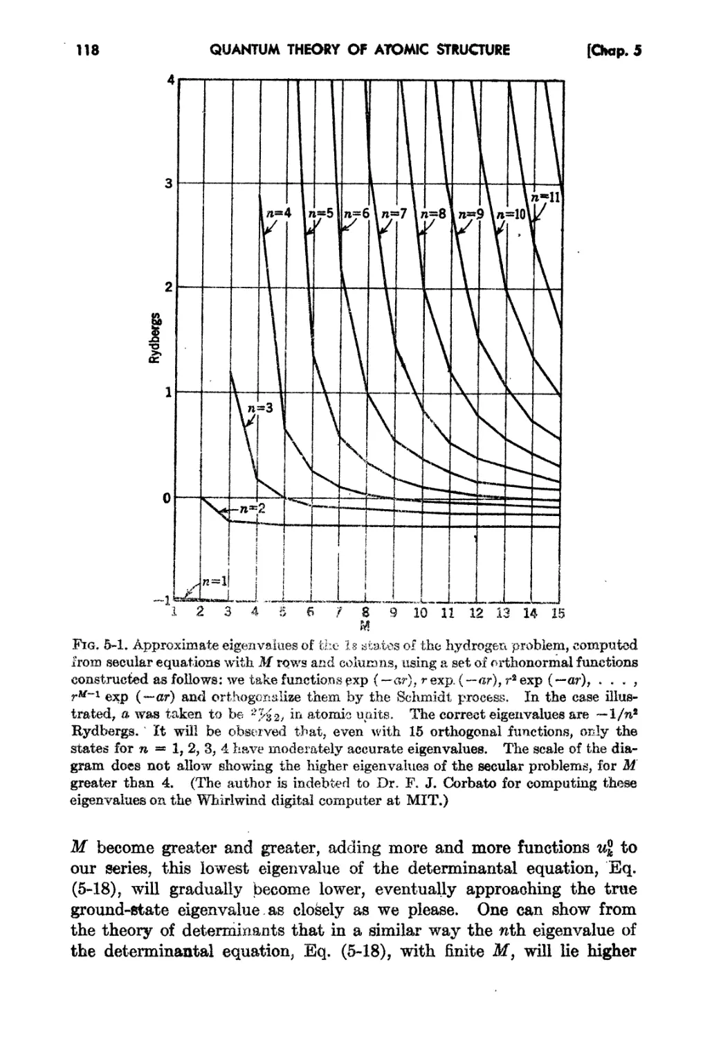
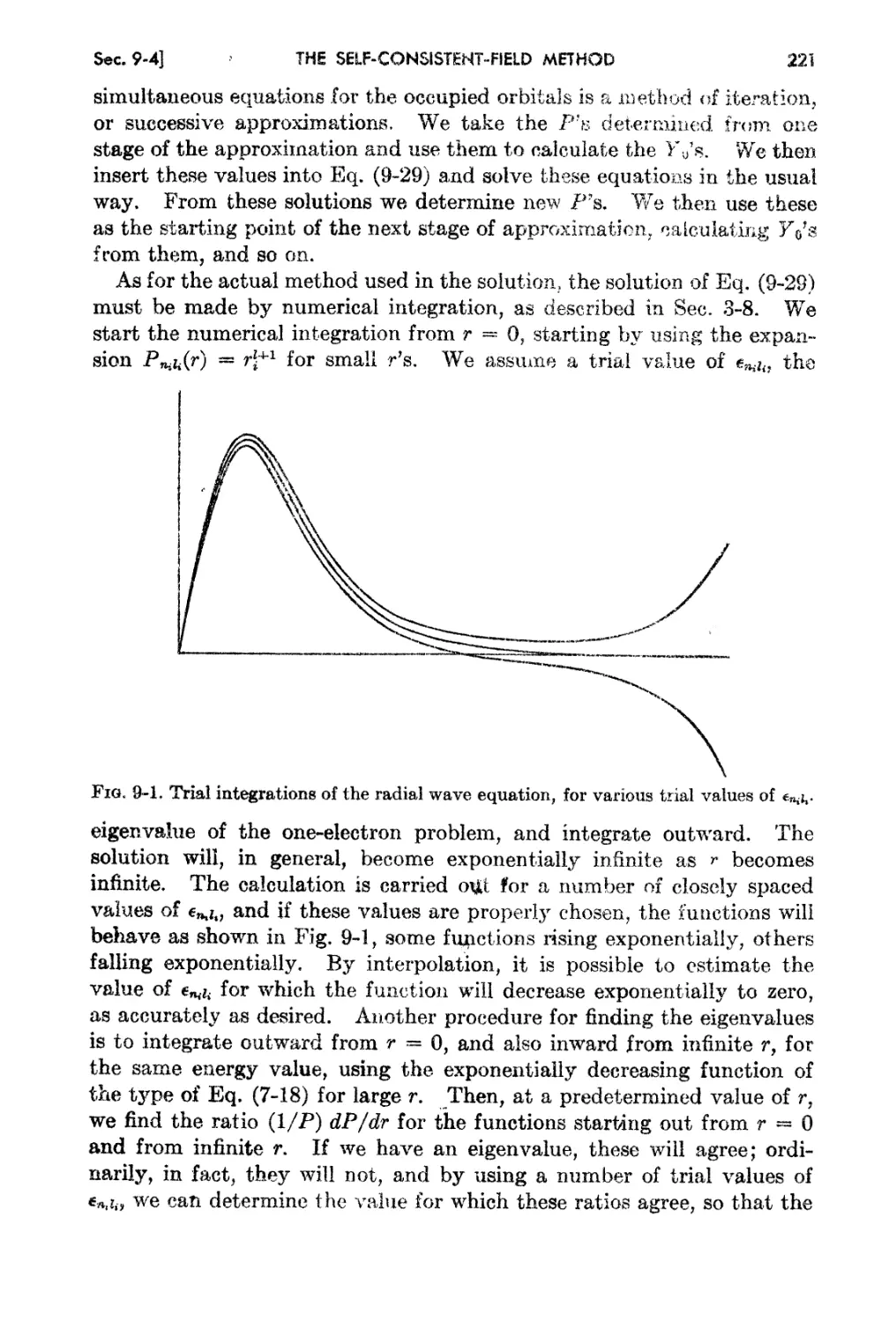
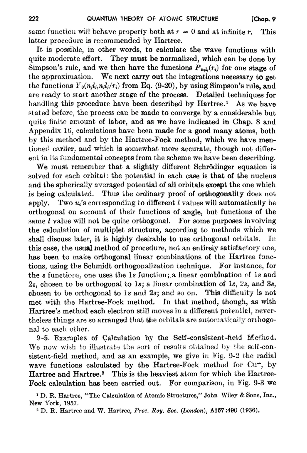
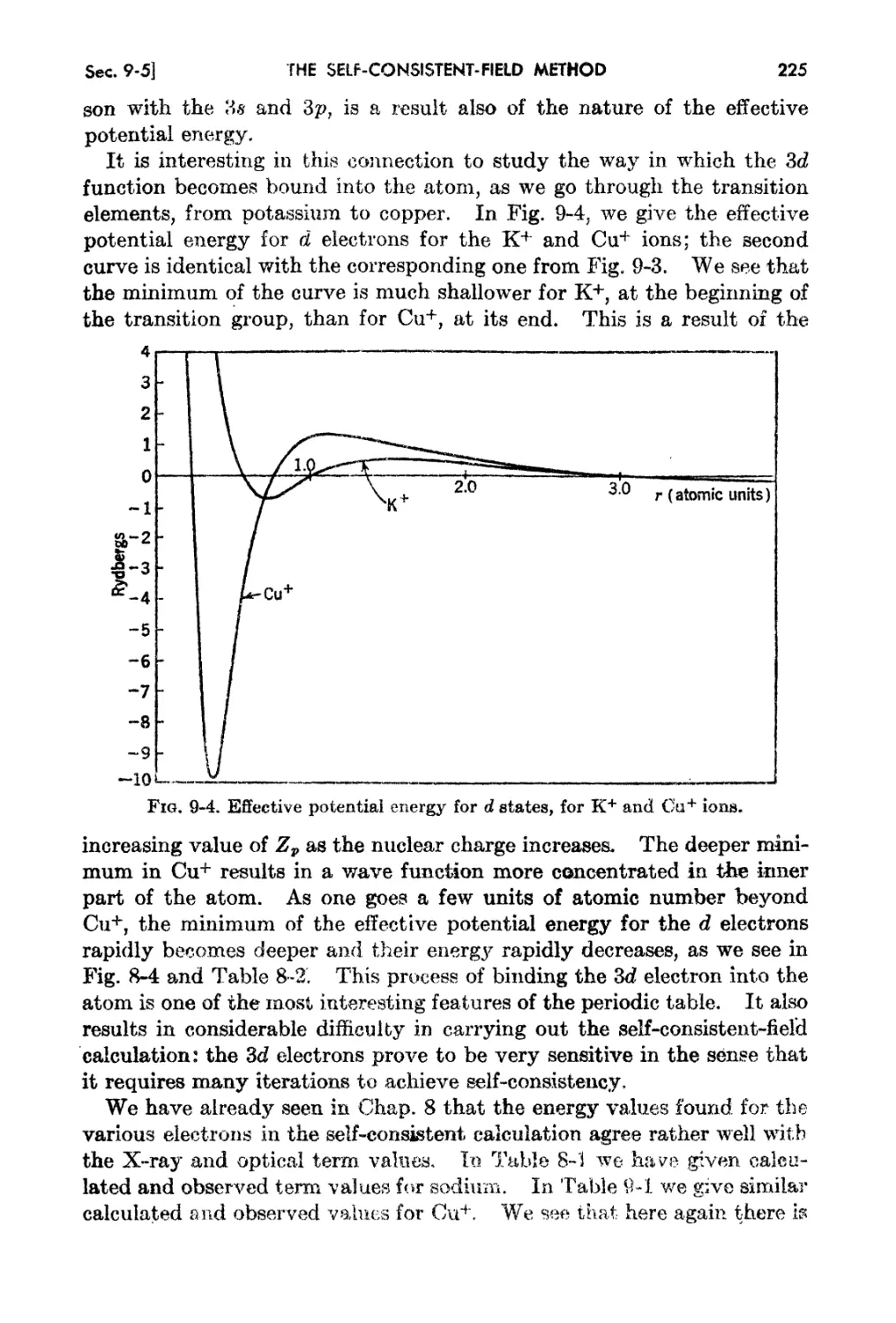
/


Author: Slater J.C.
Tags: physics mathematical physics mcgraw hill publisher quantum theory quantum theory of atomic structure
Year: 1960


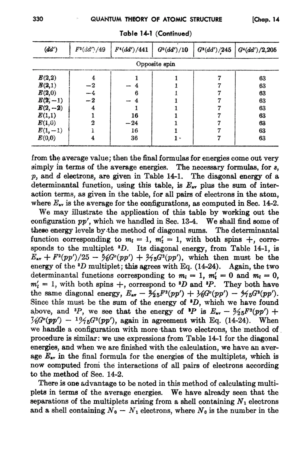
Text
QUANTUM THEORY OF
ATOMIC STRUCTURE
v () Jl IT M E I
JOHN C. SLATER
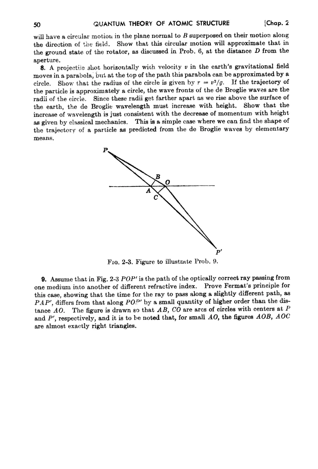
I nstitute Prof e880r
M 0,88achusetts Institute of Technology
MeGRA W-HILL BOOK COMPANY, INC.
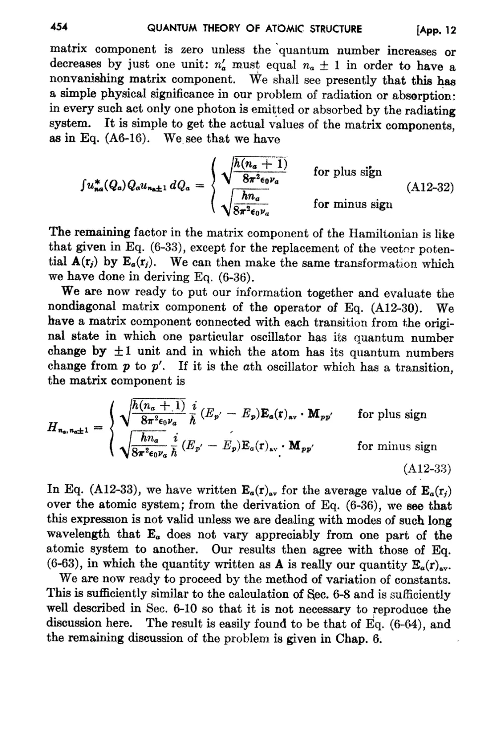
N e
Y York l'oronto London 1960
QUANTt™ THEORY OF ATOMIC STRUCTURE
VOLUME I
Copyright @ 1960 by the l\fcGraw-Hill Book Compa.ny, Inc4 Printed
in the United States of America.. All rights reserved. This book, or
parts thereof, may not be reproduced in any form without permission
of the publishers. Library 0/ Congres8 Ca.talog Card Nu'niber 60-6985
THE MAPLE PRESS COMPANY, YORK, PA.
58040
. Preface
This t\vo-voluTnc work is the first of a series of books which I hope.to
write, cove.ring the field of the application of quantull'l mecllanics to the
structure of atoills, molecules, aud oljds and to the theory of the physi-
cal and chemical propertjes of matter. Ever since the development of
wave Inechanics in 1926, it bas been clear trlat we had the theoretical
basis for the study of matter; but th.e theory has been difficult enough
so that progress in TNorking it out has been stO\V.. Ne-,:/ertheless, even in
the first ten yea.rs following 1926, the generaJ outlines of the theory began
to be clear, and by now a great many of the details llav'e bf}erl worked out.,
though there is still a great deal to be done. The subject ha,s' grow'n
enormously and is constantly developing. This expansion, in a sense, is
lnirrored in a sequence of books which I have already written. In 1933
Professor Frarlk and I, in U Introduction to Theoretical Physics," included
about 200 pages Of! the quantum theory and its applicat,ions to the study
of matter. In 1951, in uQuant1.1m Theory of Matter," I enlarged this
material to a full-length book of some 500 pages. Now I am taking two
volumes to go over the material on atoms which is treated in the first
200 pages of "Qllantum Theory of Matter." Arid I hope that there are
a number of volumes still to come.
I have here followed the same general plan which was used in those
two earlier books; that is, to start with the principles of wave mechanics,
then to LIse these to discuss the hydrogen atom, the central-field problem,
and more complicated atoms. Since some of the same ground was
covered in the earlier books, I have not hesitated to use mat.erial from
them when it seemed appropri.ate, and the reader will find that in the
first volume 'of the present work, essellt.ially all the top cs are covered
which are taken up in the first seven cllapt.ers of H Quantum Theory of
Matter." But it is obvious, 'from the increased length, that there is
much more besides, and I hope that the presen'tation is significantly
ilnproved. The second volume of tile present work is almost entirely
new material, which was not covered at all in either of the earlier books.
v
vi
PREf.o,CE
It, has been my aim to \vrite the t1,VO volumes of the present work on
rather different levels of difficulty+ The first volume starts with tIle
beginning of wave mechanics, and I believe that it can well be used as
an introduetory text. in quantum me( hanics, as well as in atomic struc-
ture. It uses on]y the more eJementary methods to discuss the structure
of atolns and yet gets far enough so tha.t the two final chapters of the
volUlne gj"ve n rather con1plete surve:.v" of pr-esent work on the structure
of SOlne of the more irfiportant of the atoms.. It is my view that every-
thing in this volurne is really ne ded by anyone who expects to go on to
the study of qua.ntunJ chelnistry, or the theory of solids, or any aspect
of the theory of matter. 'Vith the nee<!s of the fairly elementary student
in mind (that is) of perhaps a firRt-year graduate student) I have included
problen18, appendixes coverin such topics as tb.e p81rts of classical
IDcechanies li.eeded to disCl1SS quantun mechanics, a.nd enough references
to enable the student to get started studying the literature.
The Recond ,reAu.me, on the other lland, is on a level which will proba-
bly nlake It nlostly used as a reference vlork in the more advanced aspects
of the theory of atoITlic structure. In its appendixes it includes con r ..
siderable t.abular lYlaterial which would be v aluable to the professional
student of atornic theory. It contains a rather full bibliogra.phy of the
major papers relat.ing to the de\relopment bot,h of W3,1ve mechanics and of
atomic structure. l\lany of t.he topics taken up in tllis second volume
are 3.8 e8sential as those in the first vo]urne for those going on with
chemical or solid-sta.te theory; 80Ine other part.s, suell as Racall's meth-
()ds, for exaInple, hn.,re so far found fewer applications outside the field of
atomic strueture but are likely to prO' le more useful in the future, and
J believe it very desirable for the student t.o have them available, even
t.hough he may not study therrl in his gradu8Jte work. This second vol-
unle carries the subject in most respects as far as the excellent arid well-
kno,vn work of Condon and Shortley, "rrheory of Atomic Spectra"
(Canlbridge lJni ,rersity Press, 1935), and in Inany respects it goes further,
81nee there htl>ve been ma,ny" .advances in the field since that book was
,vritten. 1 mu.st ackno,vledge here Iny debt to that book and my respect
for its pioneering effort ill the field.
.A.s I mentioned at the beginning of th.is J?reface, it. is my hope to follow
this book v/ith further ones, on n10re or Jess the same level, treating the
theory of molecules and of solids. These later books will make use of
the present one to give the fundar.nental grounding ,vhich they require;
for practically all the more advanced met.hods of molecular and solid-
state tlleory. are the outgrowths of problems which are already met in
the study of atomic structure.
In the present state of science the study of atomic structure is needed
by many persons other than the theoretical physicist. The cllemlst, the
PREFACE
vii
metallurgist, the electrical engineer, all are meeting problems of the appli-
cat.ion of quantum theory to the study of matter as very esselltial parts
of their subjects. Often tllese other \vork rs have not hati as thorough a
grounding in quantum mechanics and its lpplicatioDS as they need to
handle their subjects properly. I have had them in mllld, just as much
as the professional physicist, in writing this book and shull continue to
keep therrl in mind in the further books in this series. I believe that it is
a mistake to think that a chemist or an engineer who wishes to study the
application of quantUITl mecha.nics to Ilis field can be satisfied with a more
superficial treatment than a physicist oan.. In other words I do not
think tllat the present two volumes go too far for these workers. But
since they' often ha,re a restricted background in theoretical physics, I
}l&Ve tried to m.ake this book as complete as possible, so tt1at it can be
read witllOUt the need of consulting other texts, aside from those on
mathematics, \tvith \Vllich in these days :rnost engineers are well acquainted.
There is one other con1rnent which I might. make concerlling the theo-
retical physicistj. In these days physics h3.1S become divided very sharply
into two categories: nuelear and nonnuclear physics, the latter including
the topics taken up in ti1e present series of books. rrhe training of nuclear
physicists is often deficient in the study of chemical and solid-state
physics. I hope that the present series of books may help remedy this
deficiency. I feel, specifically, that there is nothing in the present two
"'"olumes ,,, hich is not as essential to a nuclear physicist as to a chemical
or soJid-state physicist. Many of the topics coming into nuclear theory,
such as multiplet theory, vector coupling, and so on, are taken o,rer rather
directly from ordinary atonlic theory. It may well b e that the present
work will prove to be a useful introduction to these topics, for nuclear
phy icists.
Finally I should like to acknowledge tbe great stimulation; in the 'V it -
ing of this book and of the otrlers which I hope will follow it, of the mem-
bers of the Solid-State and Mol ular Theory' Group at the lVIH.ssachusetts
Institute of Technology, and in particular of Professor cJ. F. Koster of
that group. The chance of talking over the various problems of the
quant-urn theory of lYiatter with the members of the group, over the past
eight ) ears Ol nl0re, has been as helpful to me as I hope it has been to the
members of the group. I should also l ke to acknowledge the helpfulness
of tIle Office of Naval Research, and of the Lincoln Laboratory, in
extending the financial support which has made that group possible.
J oh:n C. Slater
Contents
Preface .
Chapter 1. The Historical Development of Modern Phy, &ics from. 1800
Bohr's Theory .
1-1. Introduction .
1-2. 1"he Electron and th Nuclear Atom
1-3. The Development of the Quantum Theory from 1901 to 1913.
1-4. The State of Atomic Spectroscopy in 1913
1-5. The Postulates of Bohr's Theory of Atornic Stl"Ucture .
1-6. The Quantum Conditions, and Bohr'g Theory of Hydrogen
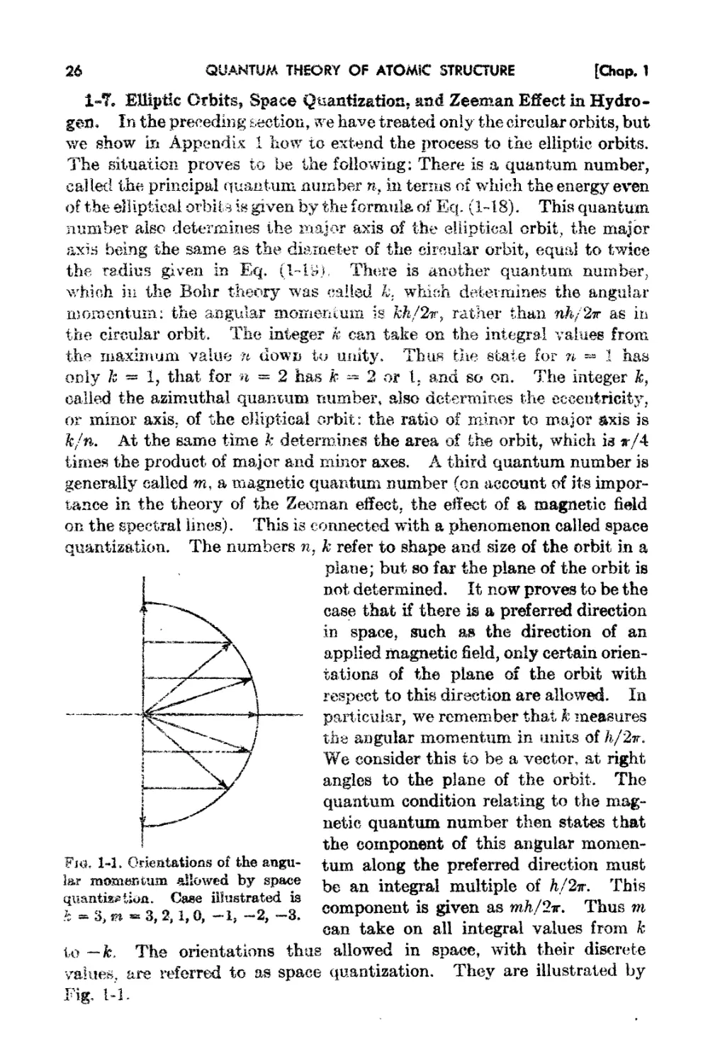
1-7. Elliptic Orbits, Space Quantization, and Zeema,n F.Jl'ect in Hydrogeu.
1-8. Sommerfeld's Quantu!l1 Condition for the l,inear Oscillator.
Chapter 2.. Modern Physics from Bohr's Theory to Wave Mechanics
2-1. Introduction .
2..2. Waves and Photons in Opties .
2-3. The Wave Hypothesis of de Broglie
2-4. Newtonian Mechanics as a Limit of de Broglie's ',Vave Hypothesis
2-5. Wa.ve Packets and the tJncertainty Principle
2-6. Schrooinger's Equation .
.
2-7. Suggested References on AtODlic Physics and Quant.um A1echanics
Chapter 8,. Schrodinger's Equation and Its Solutions in One-dimensional
Problems. 51
3-1. Hamiltonian Mechanics and Wave Meohanics . 5]
3-2. Schrodinger's Equation, and the Existence of Stationa.ry St.ates 54
3-3. Motion of &. Partiole in a Region of Constant Potential 58
3-4. Joining Conditions at a Discontinuity of Potential . 61
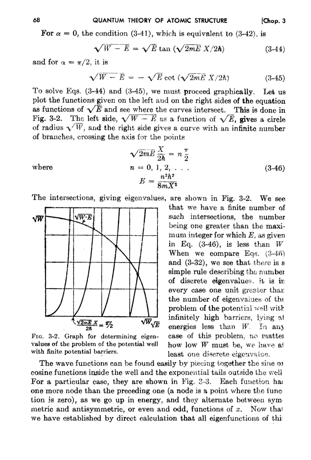
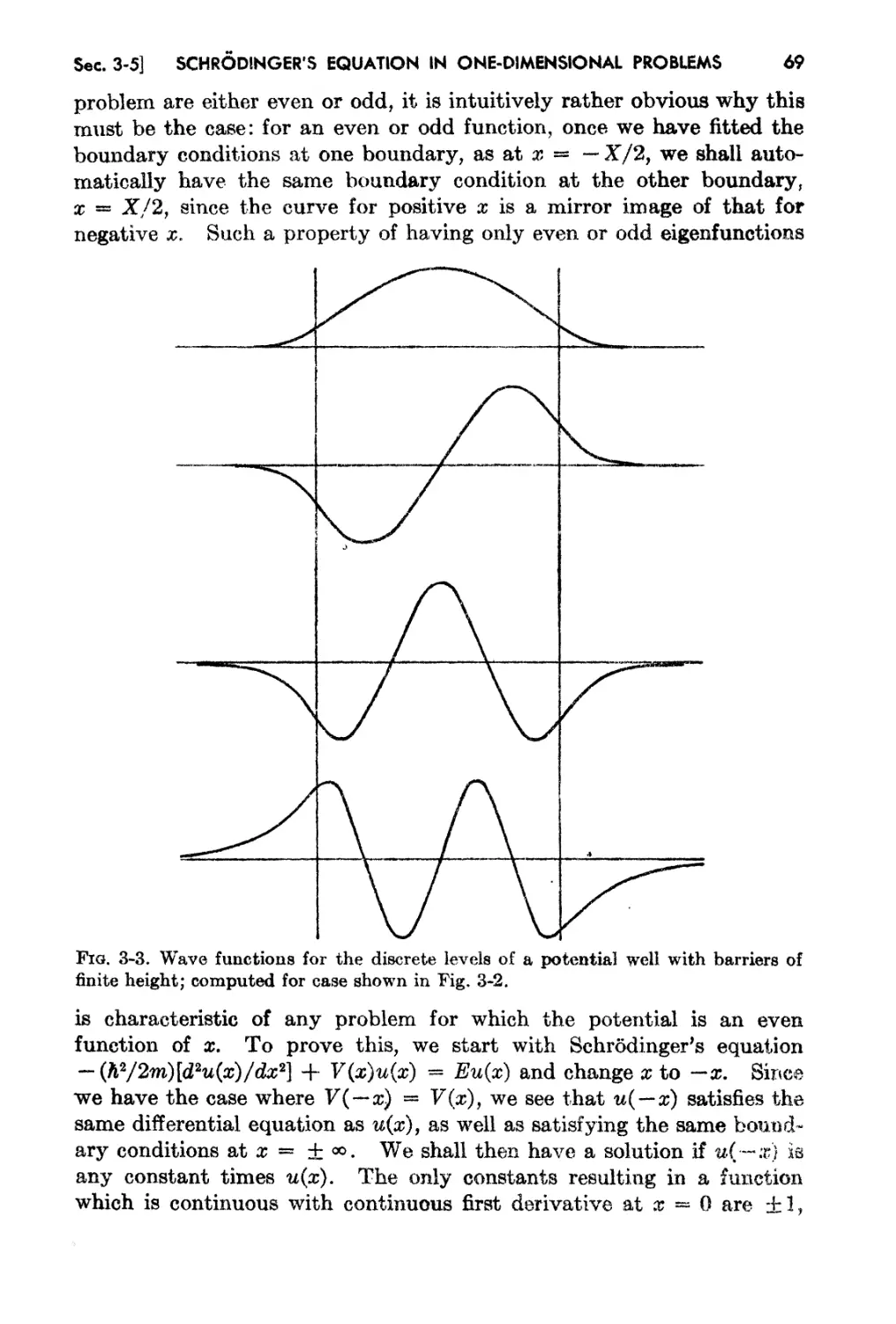
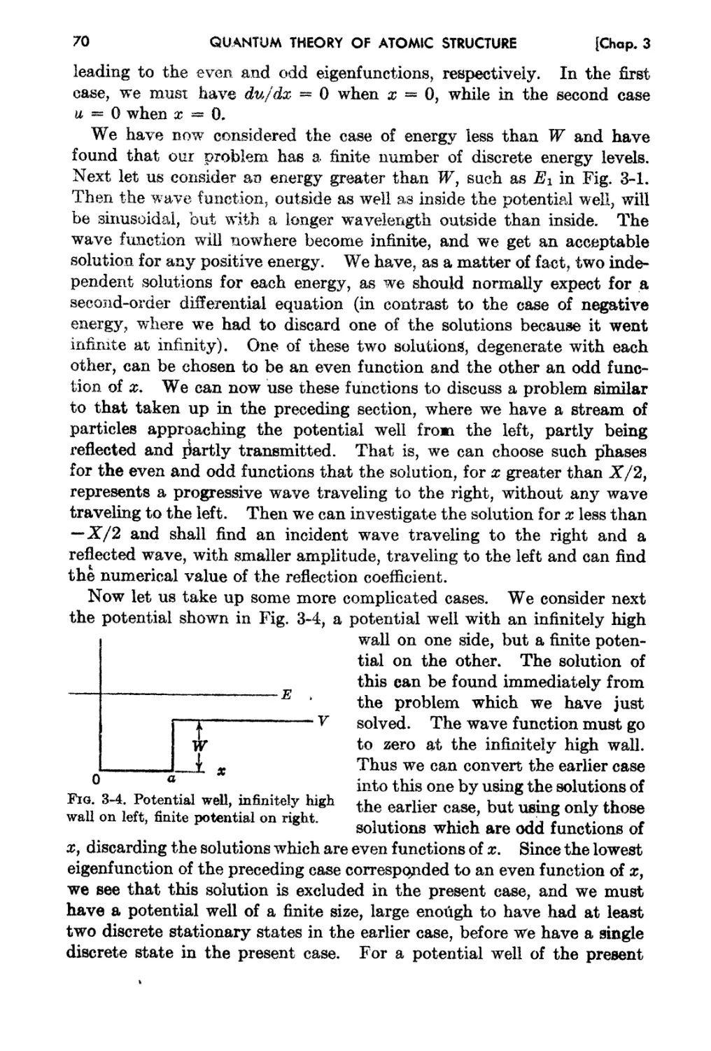
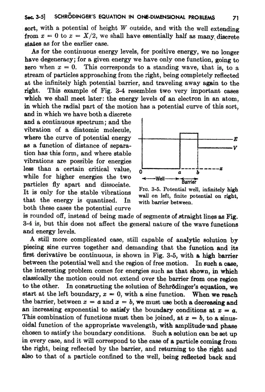
3-5. Wave Functions in's Potential Well, and Other Relat.ed Problems 65
3..6. The WKB Solution and the Quantum Condition 74
3-7. The Linear Oscillator 79
3-8. The Numerical Solution of 8chrodinger's Equation . 83
Chapter 4. Average Values and Matrices . 86
4-1. Introduction . 86
4-2. The Orthogonality of Eigenfunctions, and t.he General Solution of Schro-
dinger's Equation 86
4-3.4The Average Values of Various Qua.ntities 92
, ix
v
to
1
1
3
12
17
19
22
26
27
31
31
32
35
37
40
44
47
A
.t"'" o ,.t-"'!!I.,t ",'
". . .rn t:!..
4-4.. Matrix Components ..
4-5. Borne Theorems Rega.rding I\fs..t:deBR .
4-6e !vIa.t.rix Componenta for the !..;ineal' OaciHator
4-7. .t-\.yerage Values {i,nd the Motion of \Va,ve Packets
4-8. 1 b.e Equation of Cont.inuit.y for the Probability :Oensity
Chapter 5. The Variation and Perturbation Methods.
95
98
102
104
105
110
5-1. The Variation Pl'in iple . 110
5-2. The Expansion of the Wave Function in Orthogf;tisJ .FunctioHS 113
5-3. The Seoular Problem with Two Eigenfunctions . 119
5-4.. The Perturbat.ion l\,iethod in the Geu rai ( ase . 123
5-5. Propertie8 of Unitary TransfornlatirulB 126
Chapter 6. The Inter&ction of Ra.diation And J\.fl!tte: 131
6-1. "fhe Qua.ntizatkrn uf the Electromagnet c «Field 131
6-2. Quantum Sta.twticB and the Average Ji nergy of aD ()scillator 133
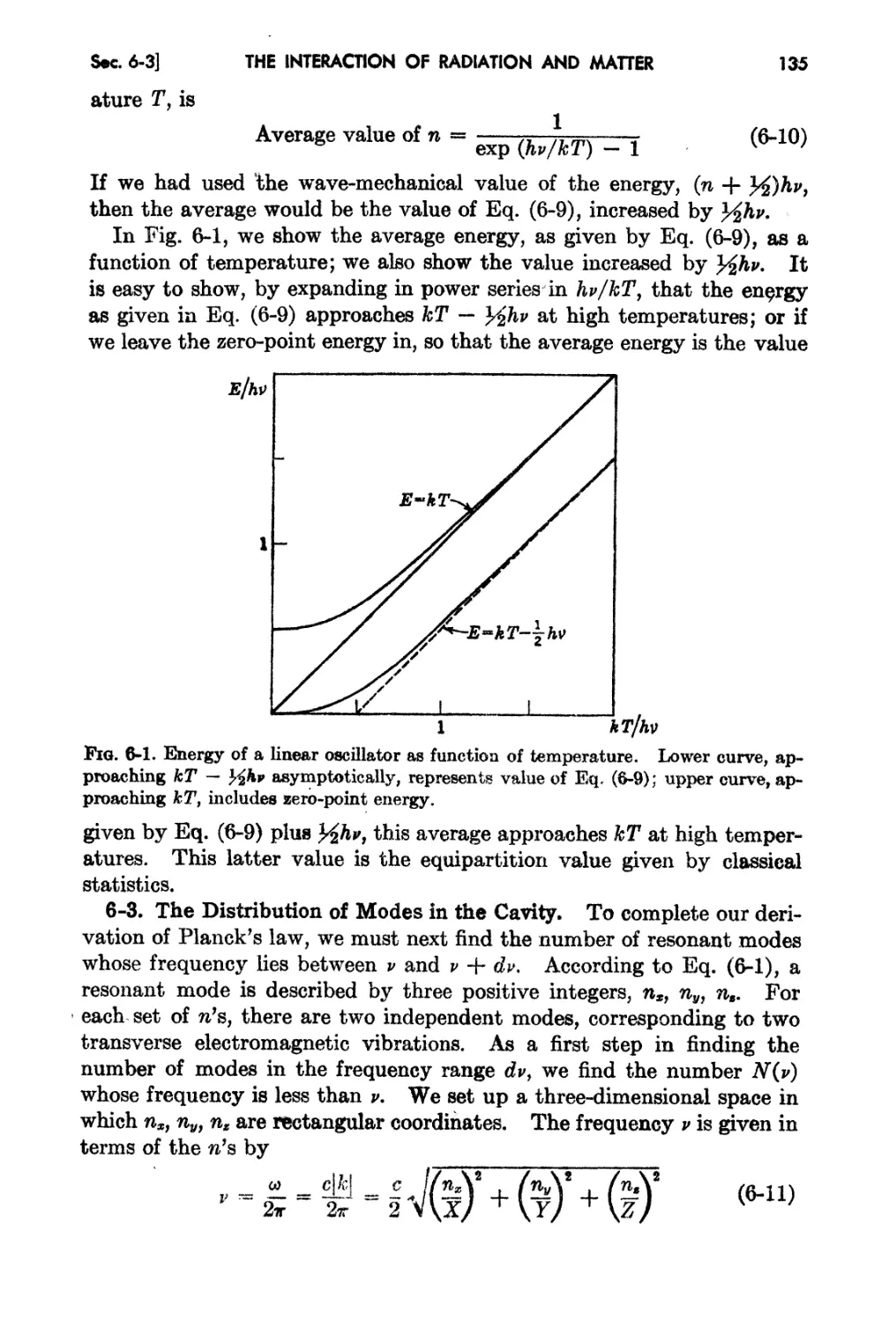
6-3. The Distribution of '!ode8 in tae Cavity. 135
6-4. Einstein's Probabilities and the EquilibriuIr'. of ]{adia.tion and .lRtter 137
6-5. Quantum. "Theory of the Int.eraction of Radiatiun and 1\lattel . 140
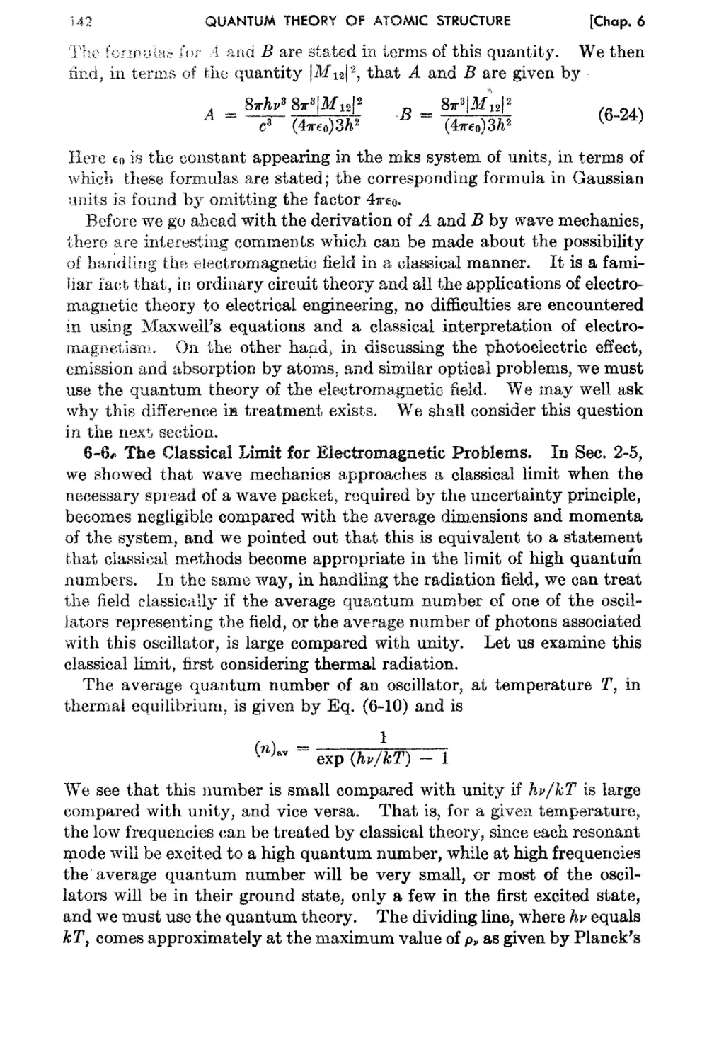
6-6.. The Cla.ssical Limit for fJlect.rornagnetic Pluhlenls . 142
6-7. Ha.miltonian and Wave-mechanical Treat.ment. of an J\.tomir: System in s.
Classical PW3.dia tion Field 144
&.8. The Method of Vari tion of (;.onstants for Transitk.n Probabilities 148
6-9. The 'Kramers-Heisenberg I)iftpersion Formula 154
6-10.. Dirao'.a ThcQry of th Int.era.ction of Rs,diation and IVfatter 168
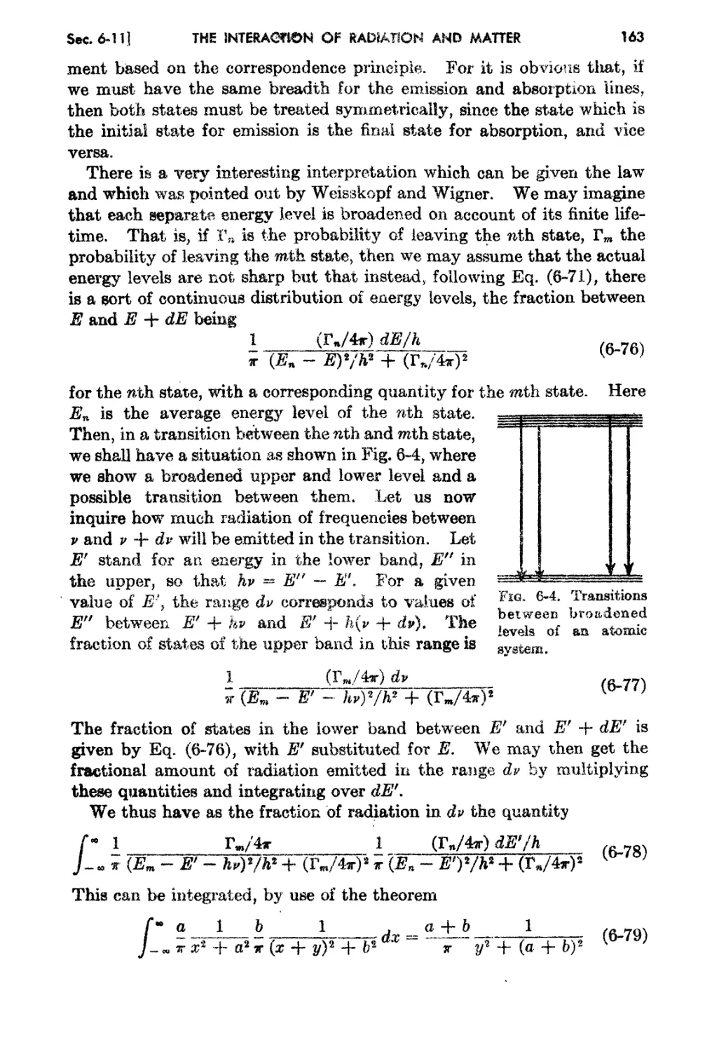
6-11. .Tbe Breadth of Spectrum Linea ]59
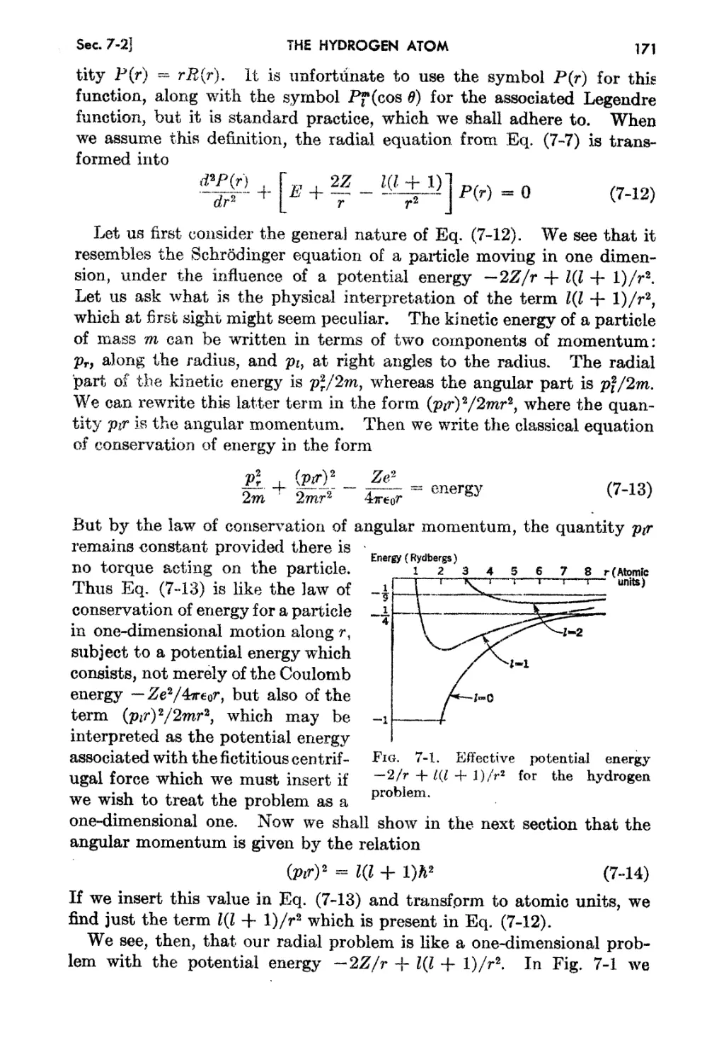
Chapter 'i. The Hydrogen Atom. 166
7-1. 8chrodinger's Equf\oItion. for Hydrogen. 166
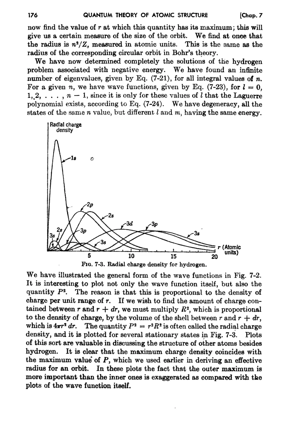
7-2. The Radial Wave Function for Hydrogen 170
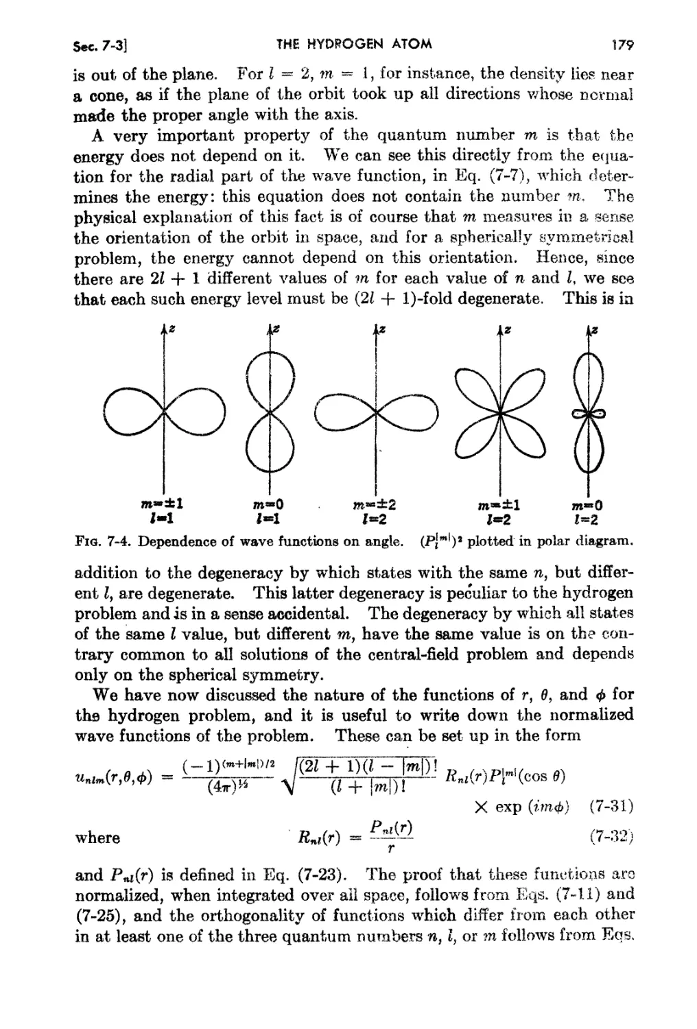
7 3. The Angul:i.r h10mentum j l)ependence of the Wave Funetinn on Angles. 177
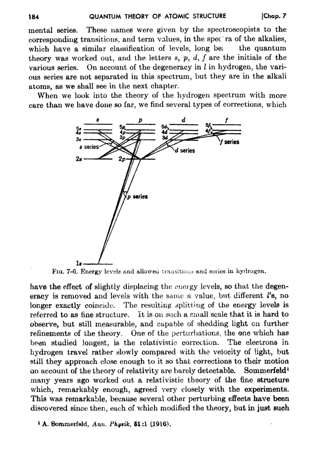
7-4. Series and Selection Rulee . 182
Chapter 8. The Central-field Mode! ior Atomic Structure 188
8-1. Introduction .
s..2. The PostuJ$.tcs of the Central-field Ivletnod .
8..3.. The Periodic Table of the Elernen t3 .
8-4. Spectroscopic Evidence for the C:entl'al-tield fi10del .
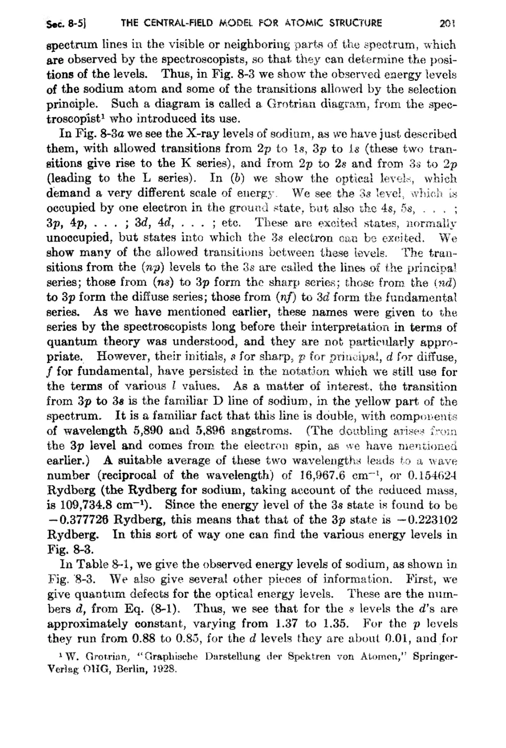
8<A5. .A.n Example of .t;4..tomic Spectra.: the Sodiun1 Atom .
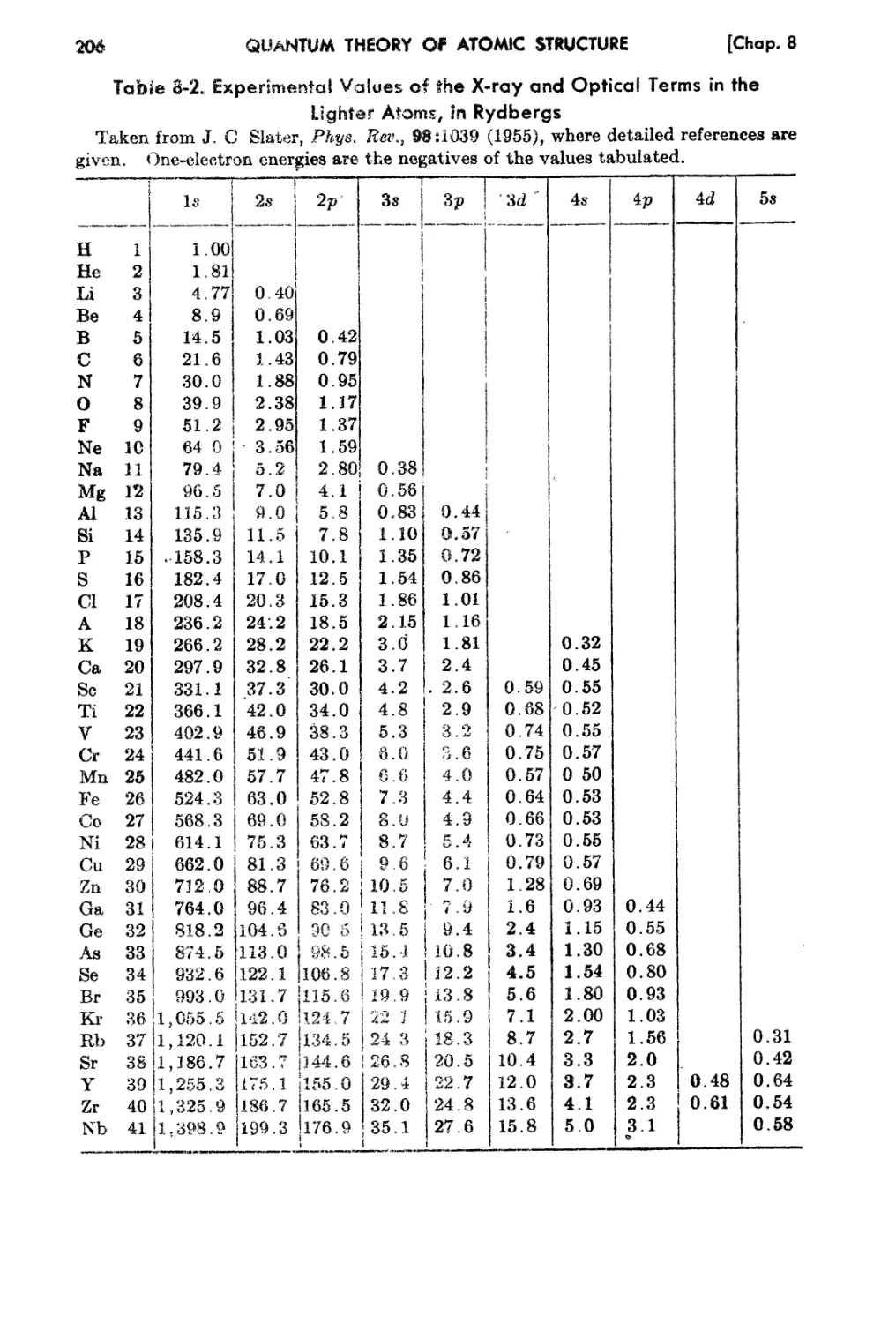
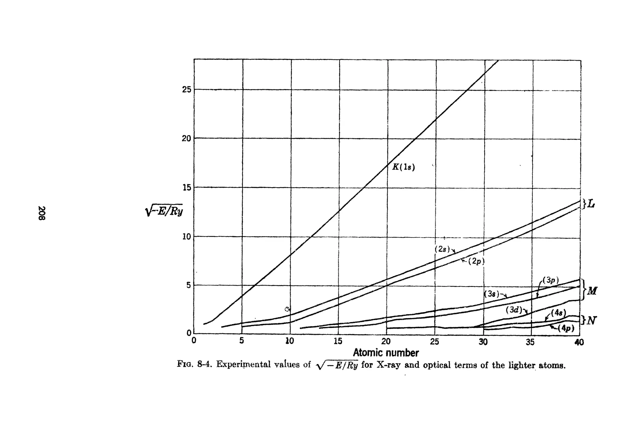
8-0. Optical a.nd X-ray Energy L-evels of the Atoms.
8-7, Dhnensions of Electronic Wa.ve Funetions in AtonH-)
188
189
192
196
199
205
209
Chapter 9,. The Self-consistent-field Method . 213
9-1. Hartree's Assurnption fer the .t\tODlic ,,-rave Function 213
9-2. The A.verage Hamiltonian for an Atom 215
9-3. Energy Integrals for the fIartree CnJculation 216
9-4. The Rartree Equations as Deterutmed by t.he Variatiou IV!ethod . 219
9-5. Exanlplea of Calculation by the Self-consistent....field Iethod 222
9-6. The One-eleotron and l\1any-electron Energies of an Atom. 226
9..7. Inner and Ou t.er Shielding . 227
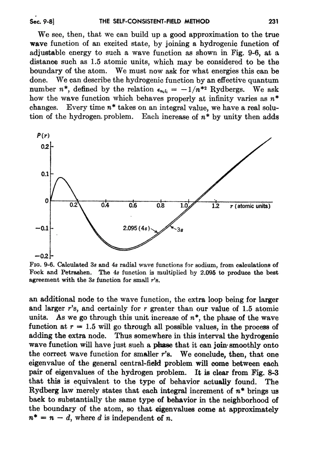
9-8. Interpretation of the Rydberg FOl'IDUla. . 229
CONTENTS xi
ChaptE:f 10$ The '\lectol"" A-irrd:el of the Atom 234
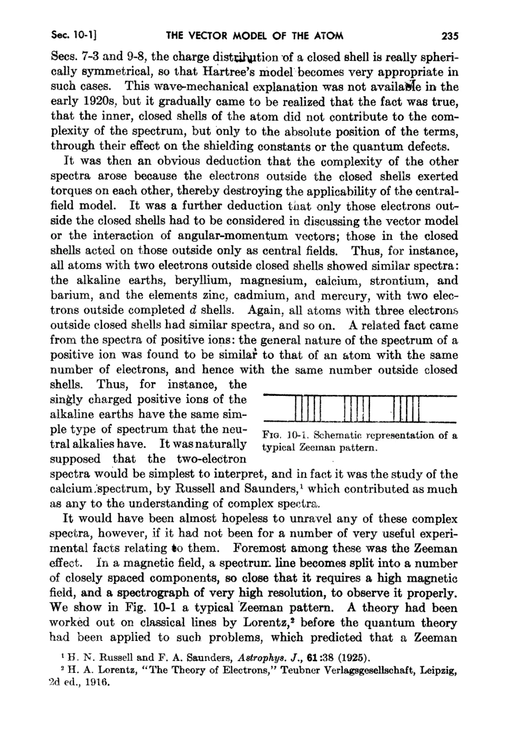
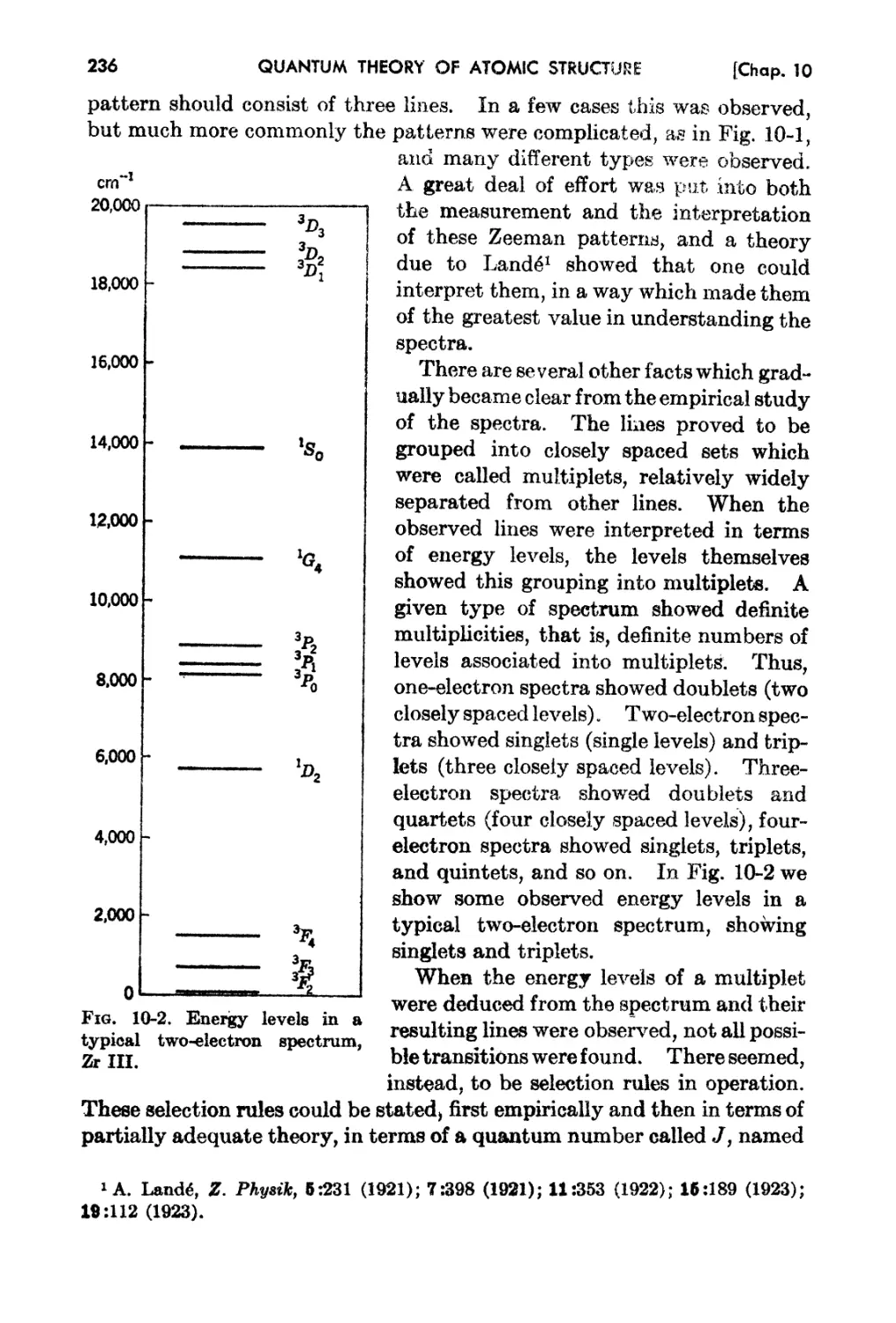
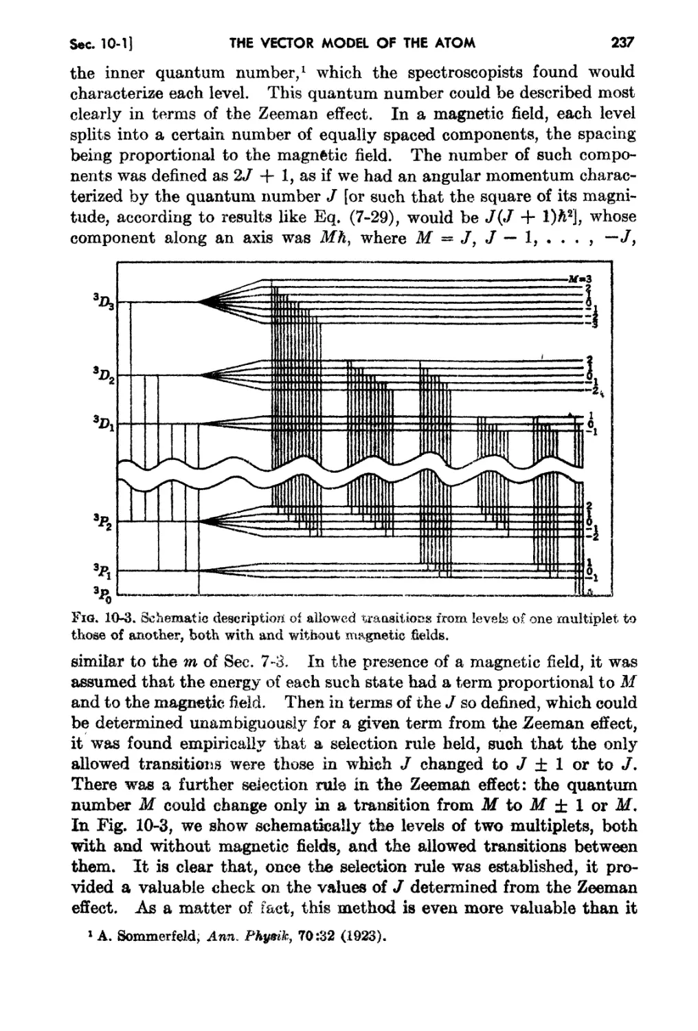
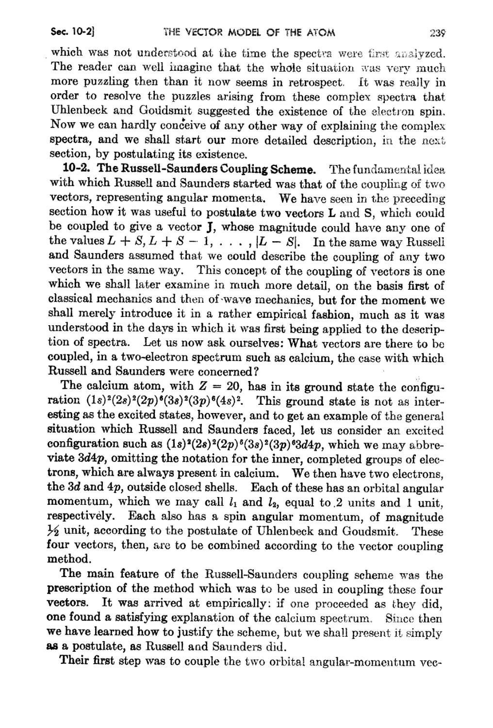
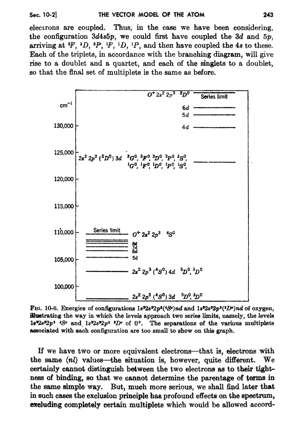
10-1. IvIultiplets in C.orn:plcx Spl3<Jtra, 2a4.
10-2. "rhe RusseU,.Saundel's Cou.pling Schenle . 239
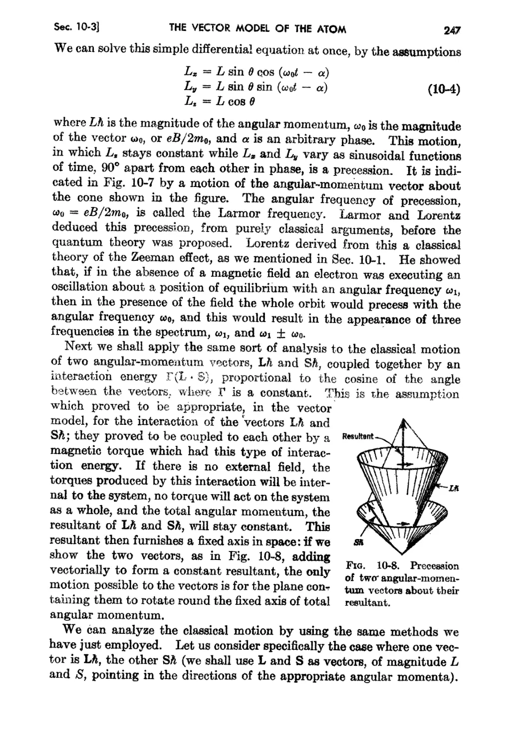
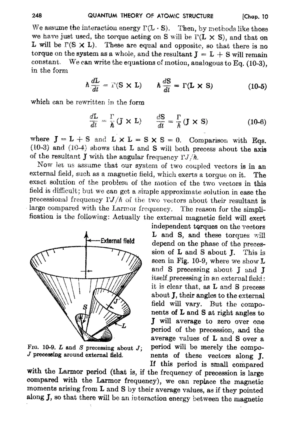
1{)...3. The Classjcal lVIechauics of Vector Coupling. 245
10-4. Lande's Theory' of l'llultiplet Separation and the Zeeman Effect . 249
10-5. Genera18urv y uf \Vave...mechanical Theory of Multiplet St.ructure 252
Chapter 11. T'ha Behavior of Angular-momentum Vectors in Wave Mechanics 255
11-1. The .A.ngular !\:Iomentun1 of an Electron in a Central Field 255
11-2. The Precession 1)f the \.Dgular-momentuln. Vector . 258
11-3. General Derivation 'Of lVIatrix Cornponents of Angular Momentum 259
11..4. Application of i\llgular-lnomentum Pl"Operties to C...omplex )t.tO!I18 264
11-5. The Nature of Spin<.( :;.rbitft.J.s 271
11-6. TJse of Atlgular-molTlentum Operators in Cases Including Spins 274
Chapter 12. Al1tisYInmetry of Waye Functions and the Determinanta1 Method 279
12-1. Wave Functions and 1\:f atrix Components of the Hanliltonian for the Two-
electron System . 279
12-2. Syn1metric and Anti9ymmetric Wave Functions; and Pauli's Exclusion
,. Principle. ' . 282
12-3. Spin Coupling- in the 1'wo-electron System 286
12-4. The Antisymmetrio "\Vav2 }4unction in the N-elootron Case 288
12-..5. Matrix Compooonts of Operators with Resp t to DeterminantaJ Wave
Functions . 291
Chapter 1S. The Elementary Theory of M uItiplats 296
13-1. The Secula.r Problem in Russell-8aundera Coupling. 296
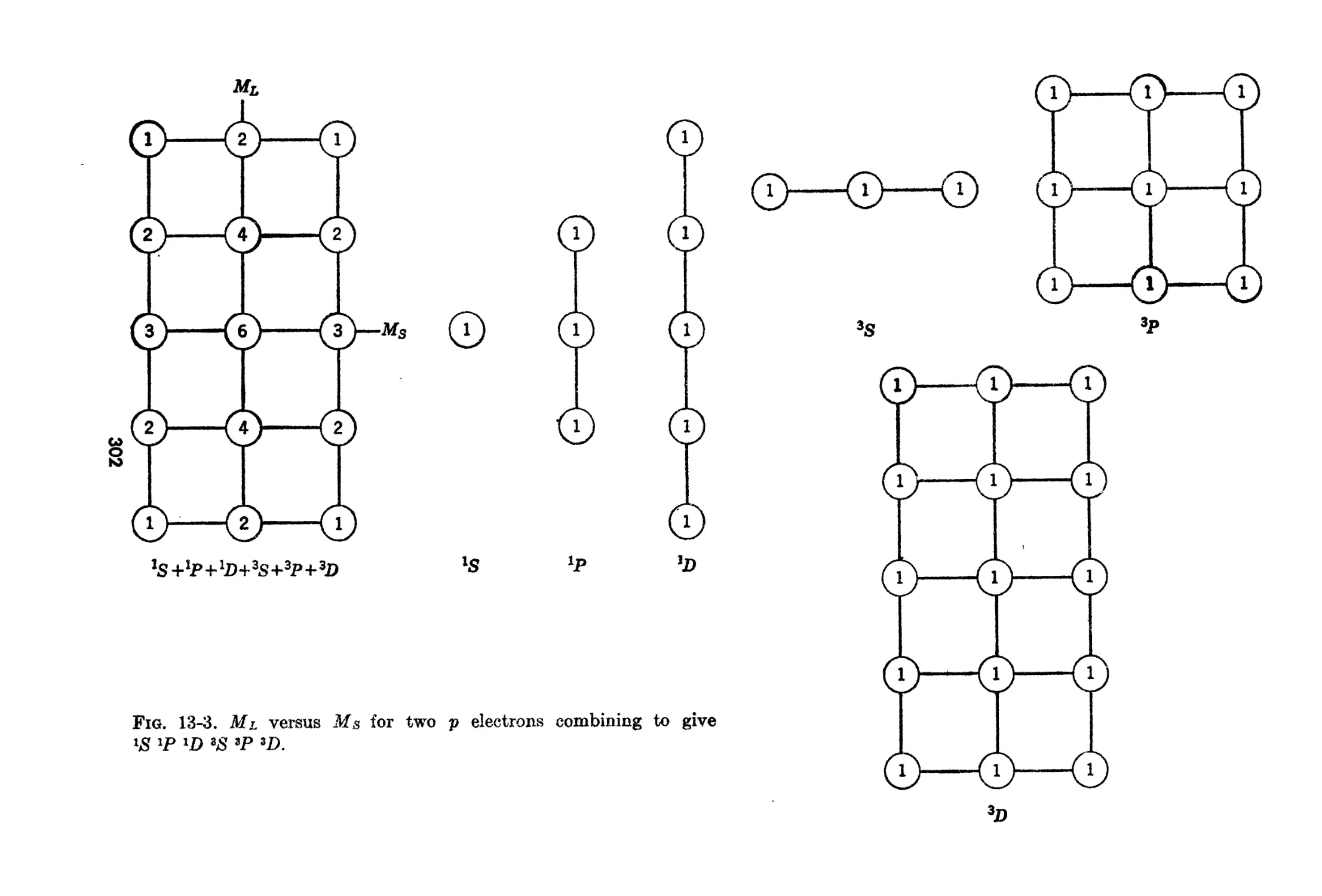
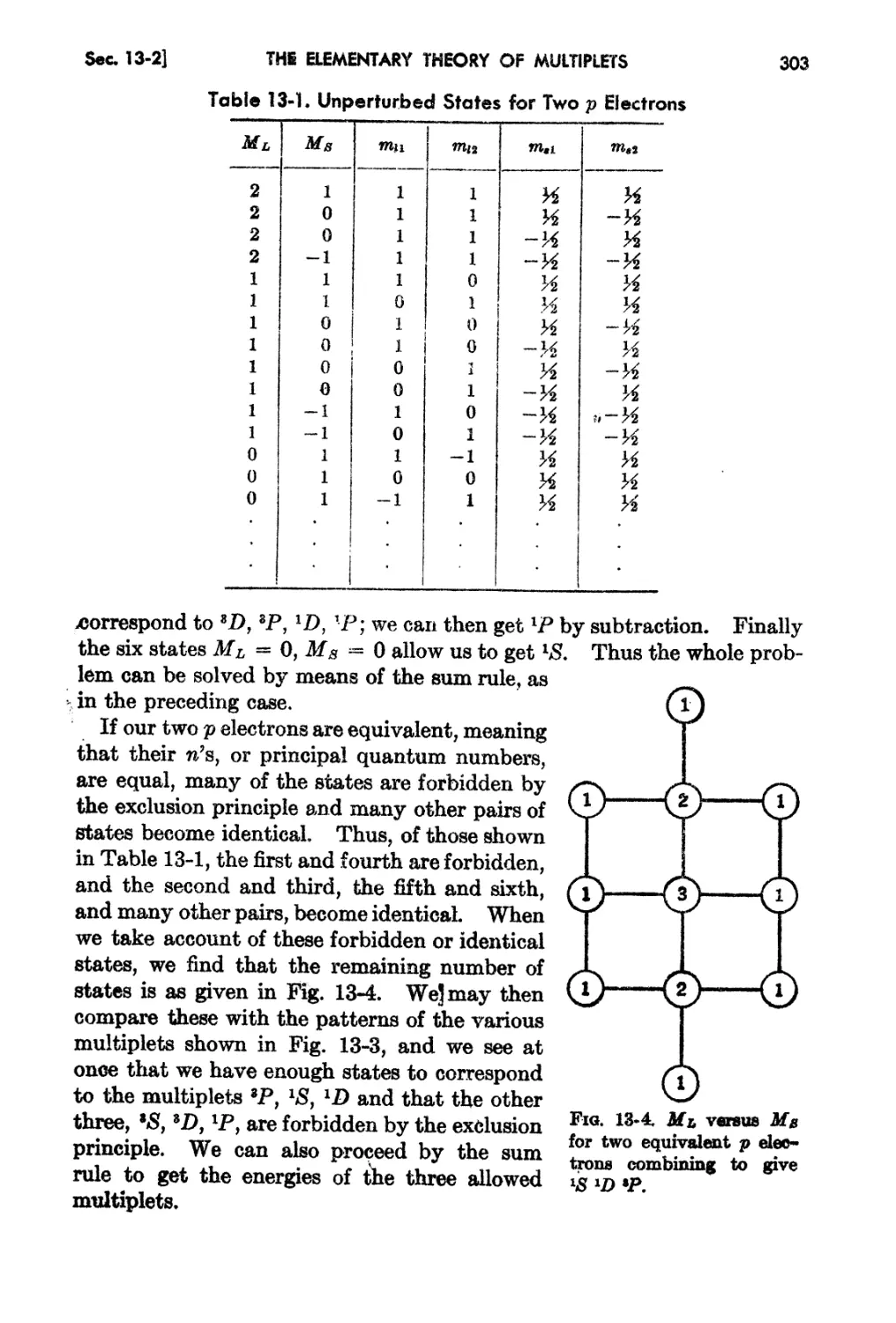
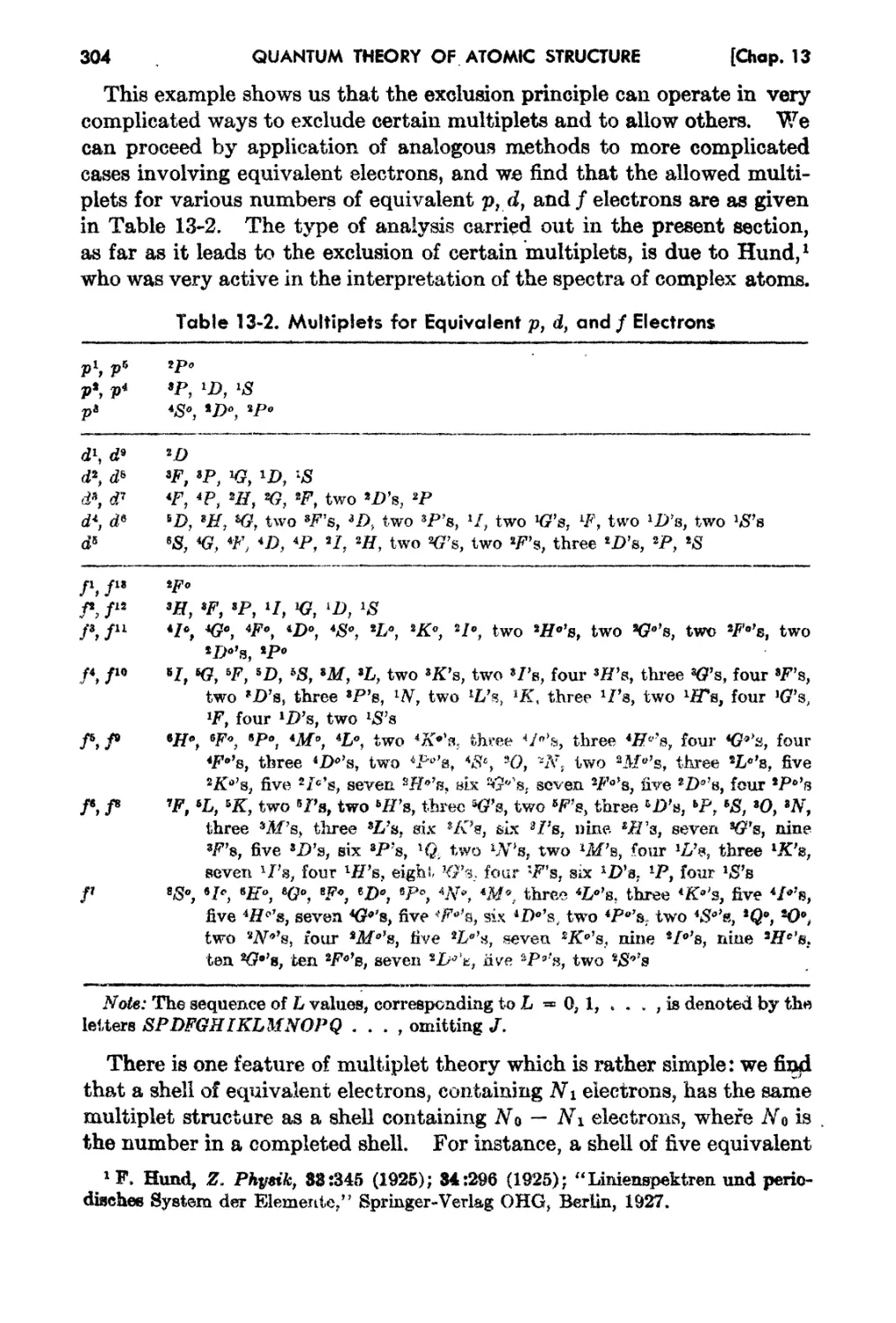
13-2. Further Examples of the Secular Problem 301
13-3. Matl'L Components of the Hamiltonian for the Central""field Problem 306
13-4. Energy Values for Simple 1ultiplets . 312
Chapter 14. Further Results of Multiplet Theory: Closed Shells and Average
Energies ... 316
14-1. Closed and Almost Closed Shells . 316
14-2. The Average Energy or a Configuration . 322
14-3. Formulation of Mu}tipl t Calculations in Terms of Average Energy . 326
Chapter 16.. Multiplet Catetdations for Light Atoms , 332
15-1. Introduction . 332
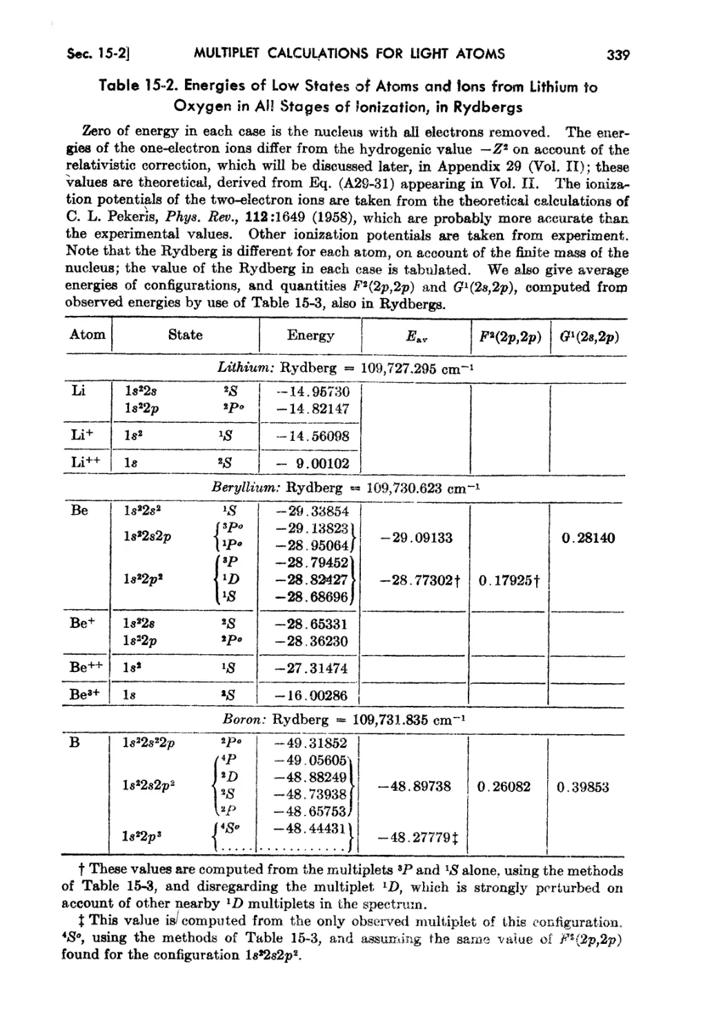
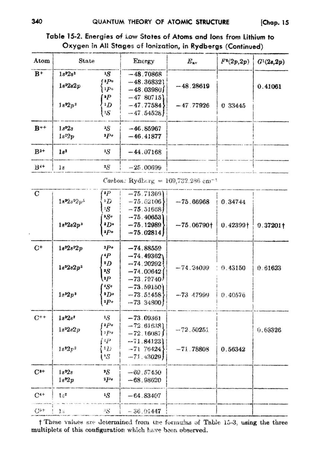
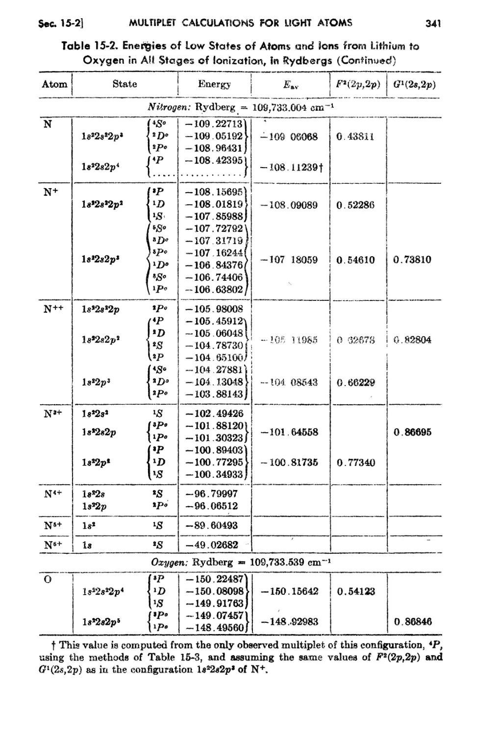
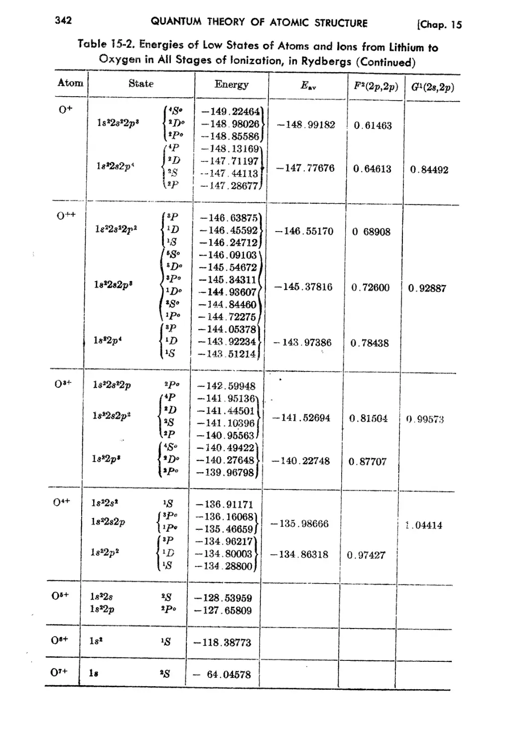
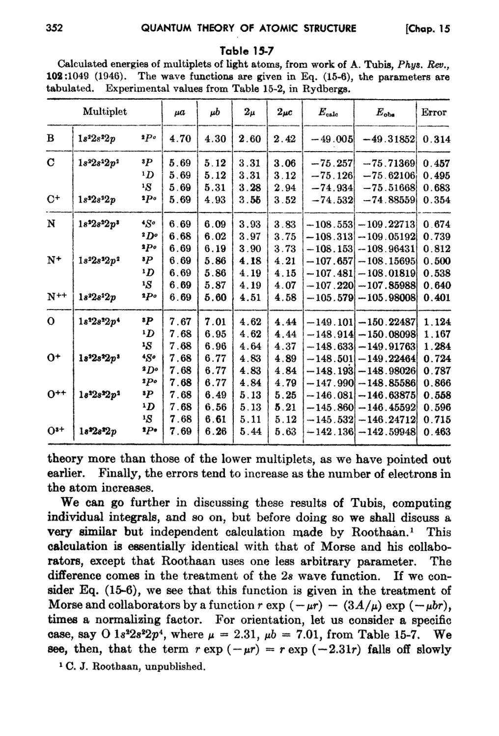
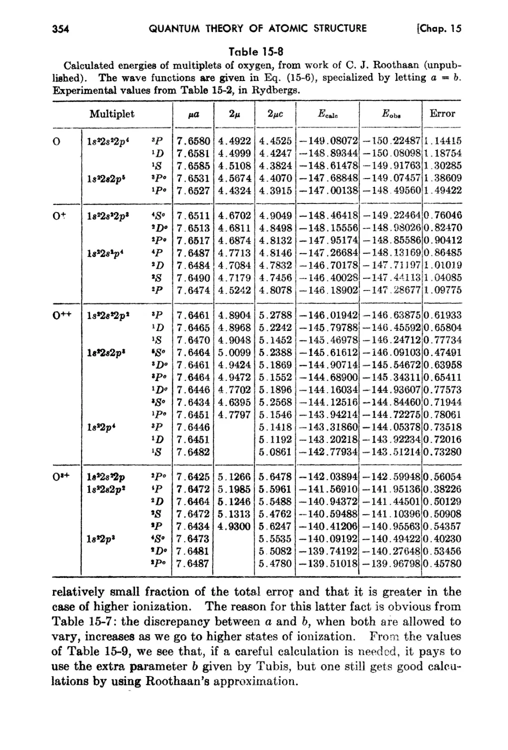
15-2.. l1;xperirnental En2rgy Levela of Light Elements 337
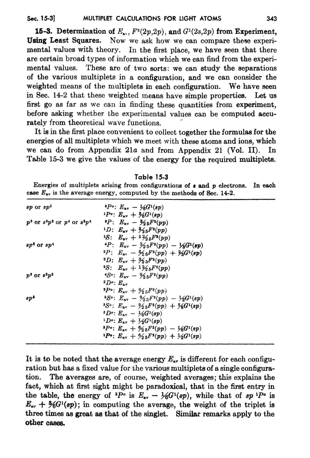
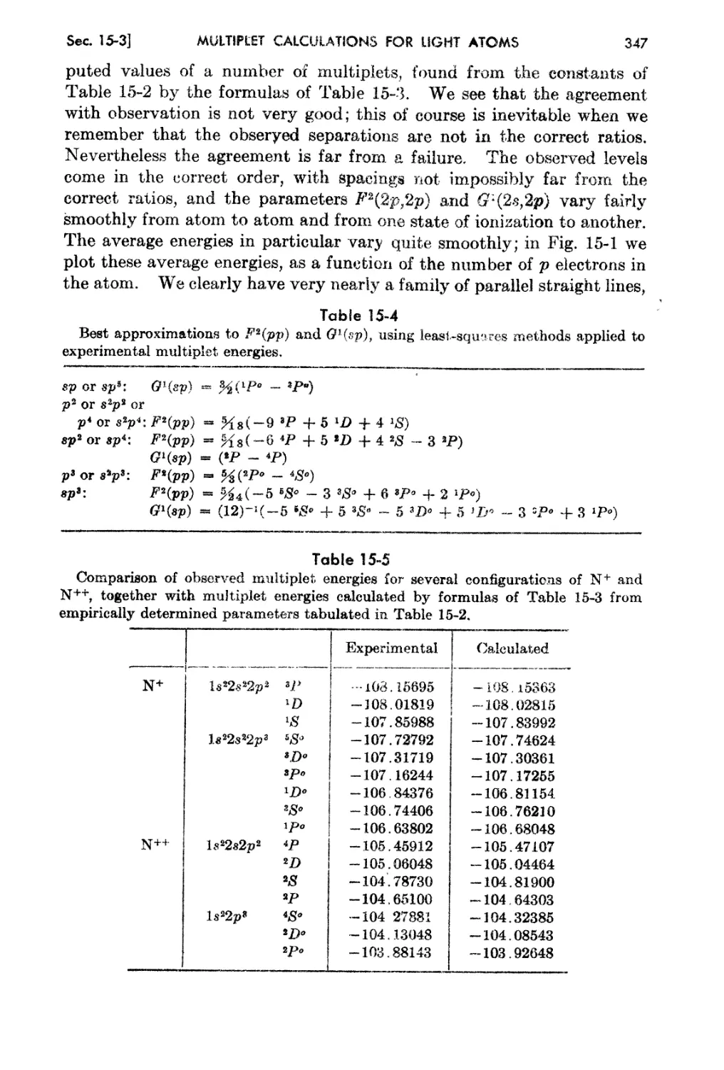
15-3. Determination of Eav, F1.(2p,2p), and Gl(28 t 2p) from Ex pf> f't Hlf.'nt. lIsing
I .. So 343
eas tuarea.
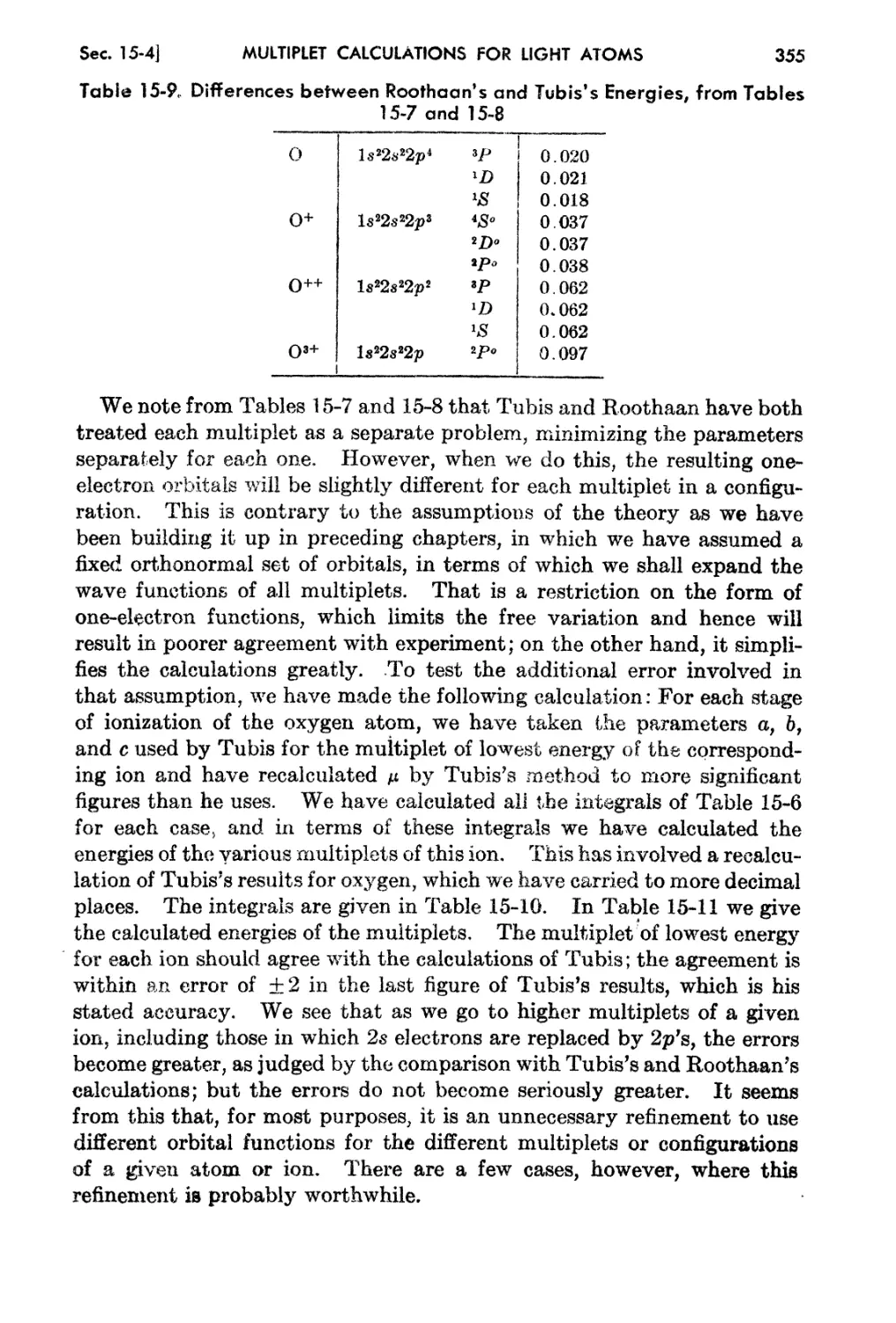
15-4. SimplA Analytic Mode18 for Wave Functions and Energi 8 of Light "' toms 348
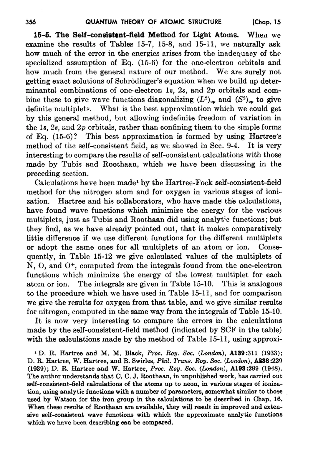
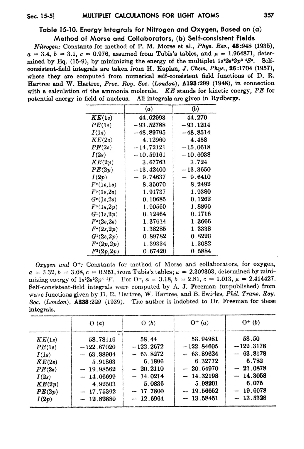
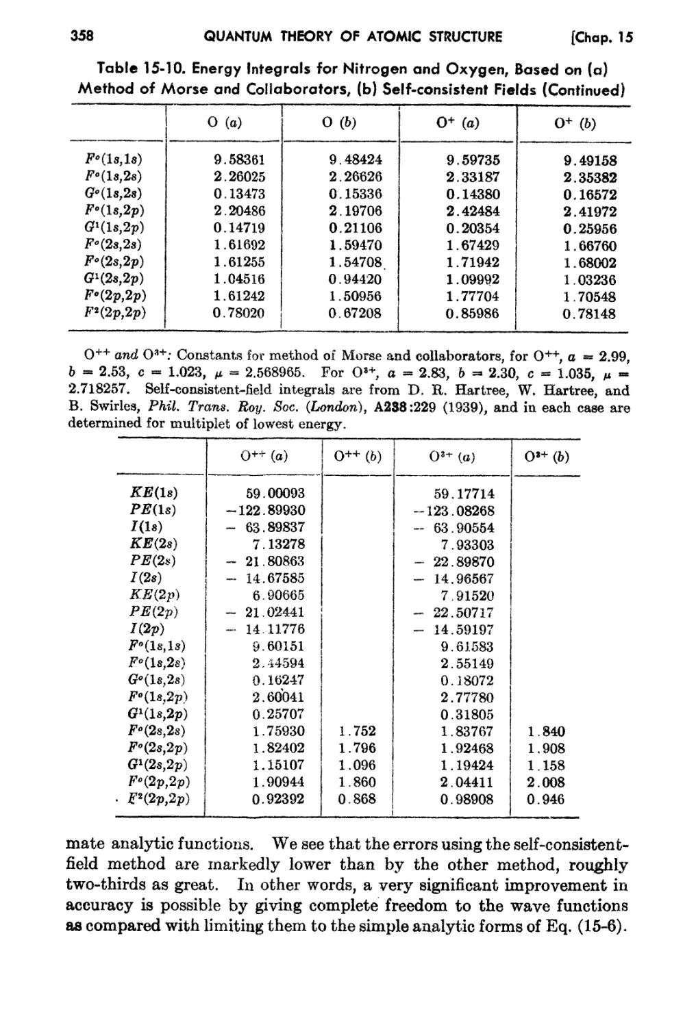
15-5. The Self-consistent-field fethod for Light Atoms 356
15...8, Ionization Potentials and X-ray Energy Levels . 364
15-7. Sinlplified Treatment of IJight Atoma . 368
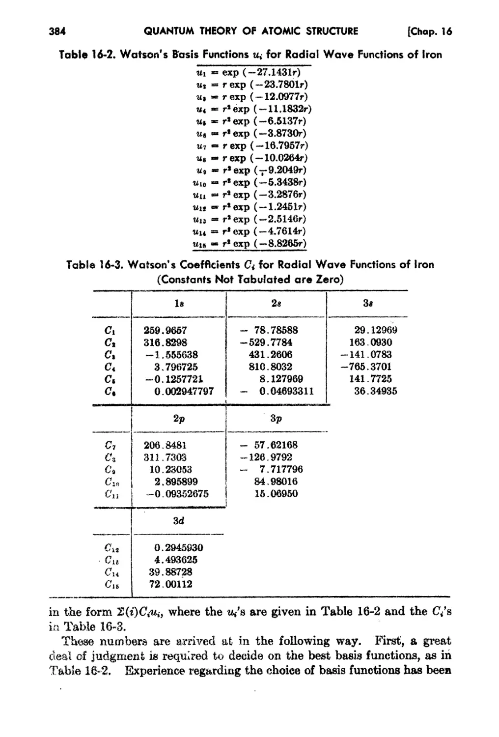
Cha,pter 16. MuJ.dple Calculations for Iron-croup Elements 374
1&.1. Introduction . 3'74
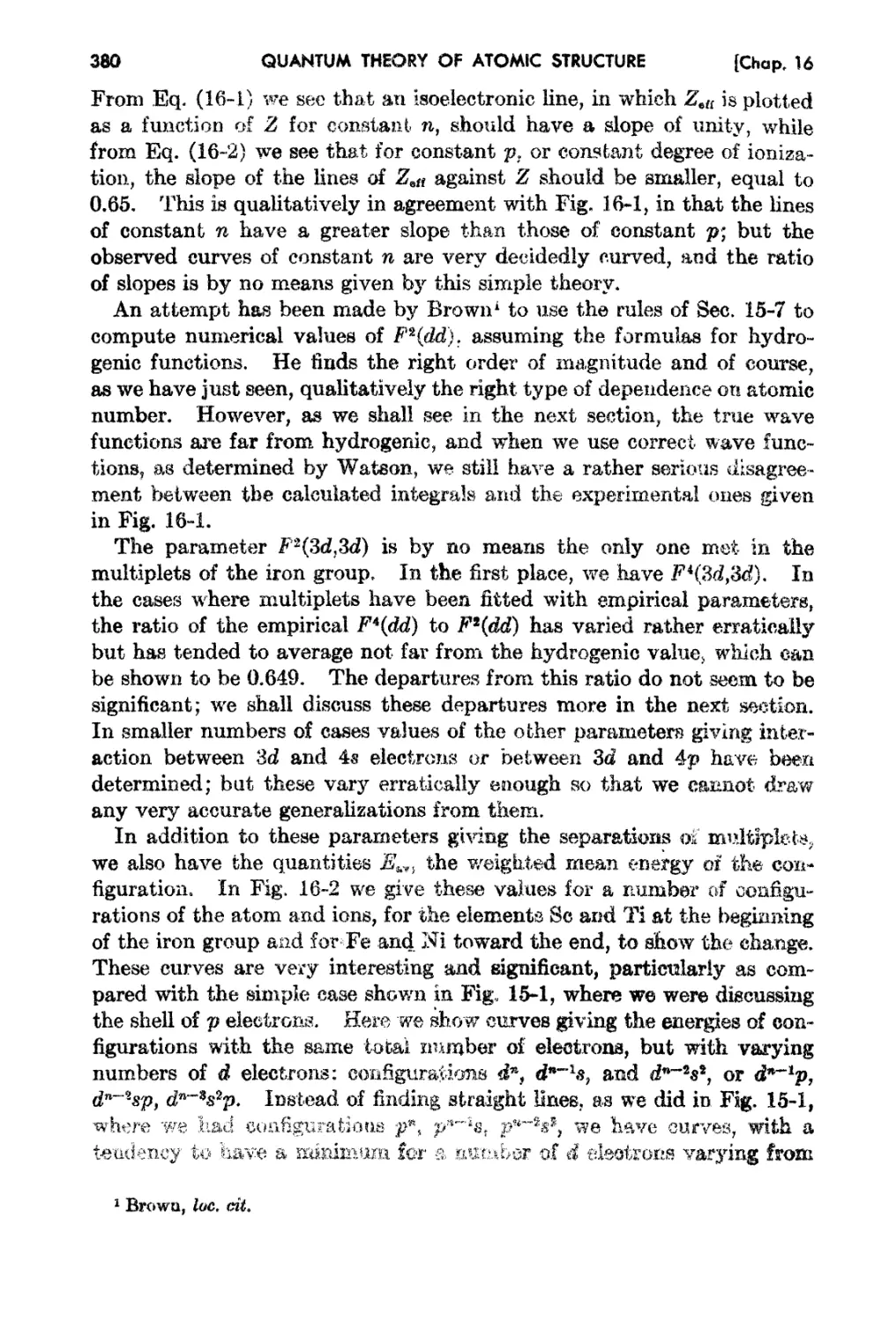
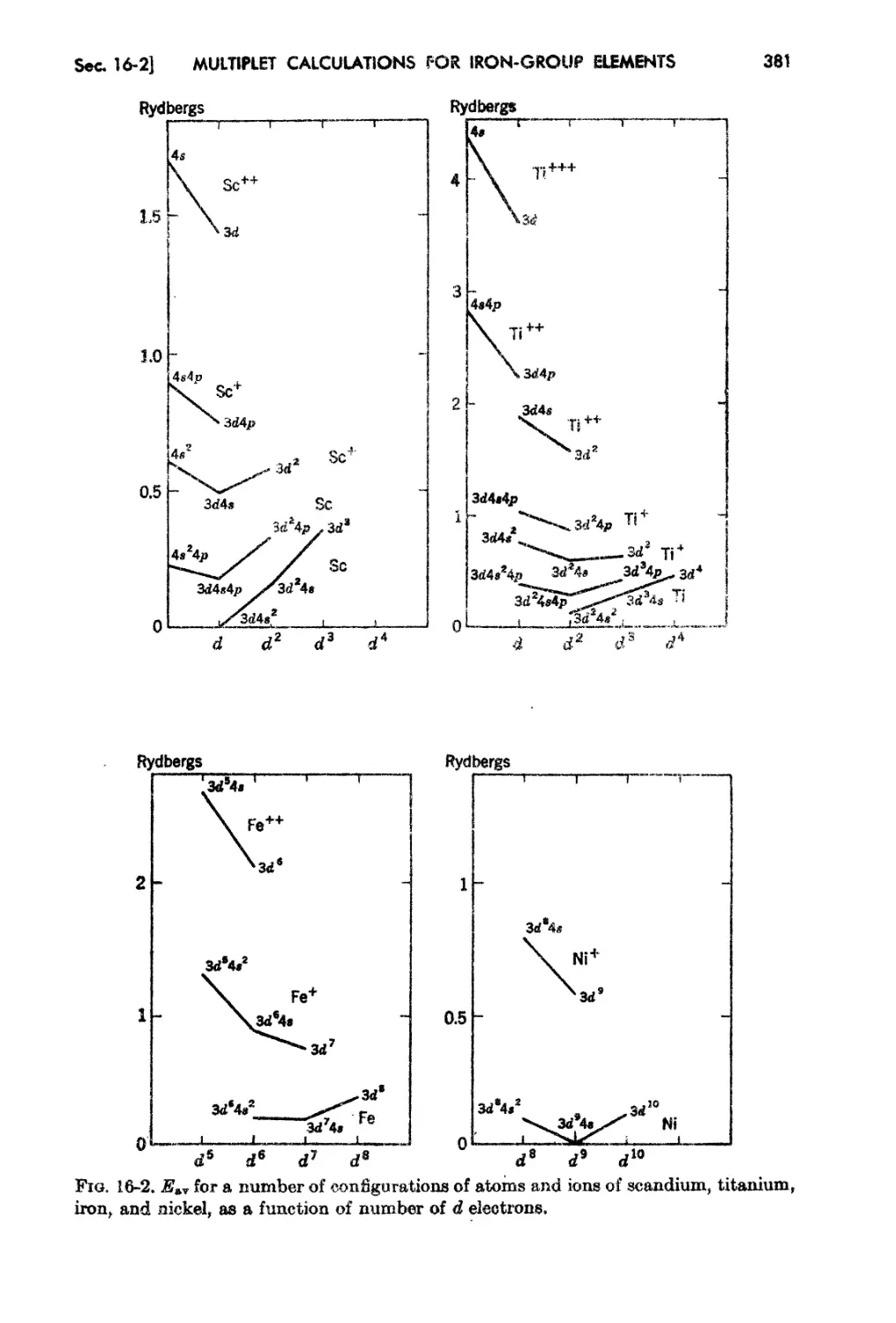
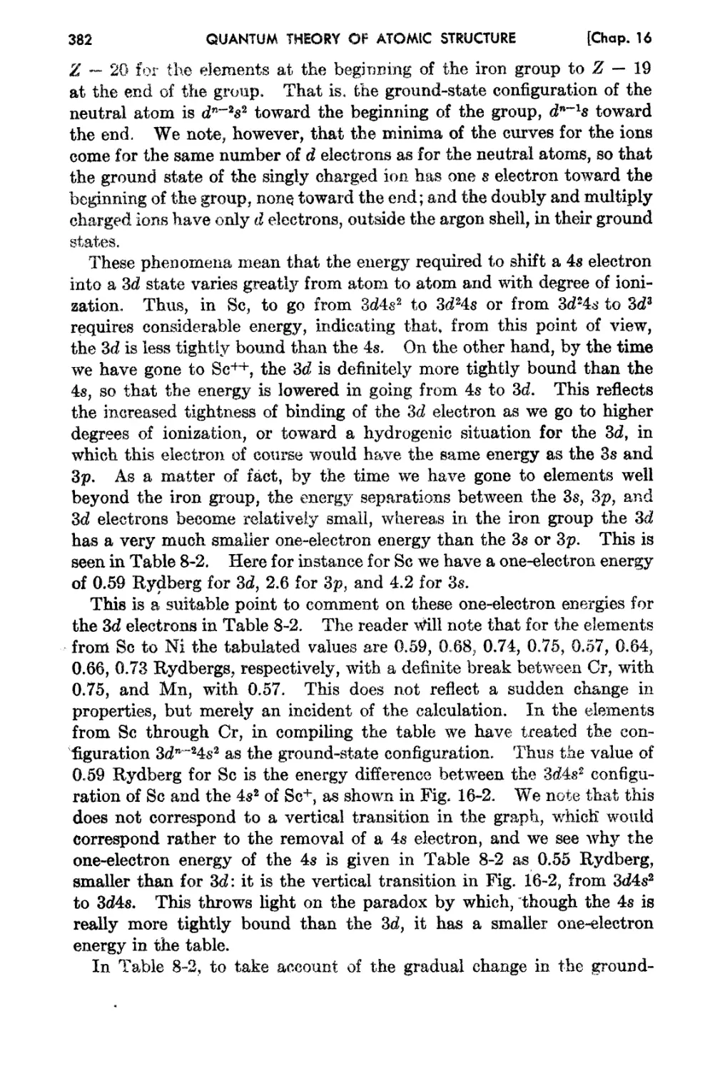
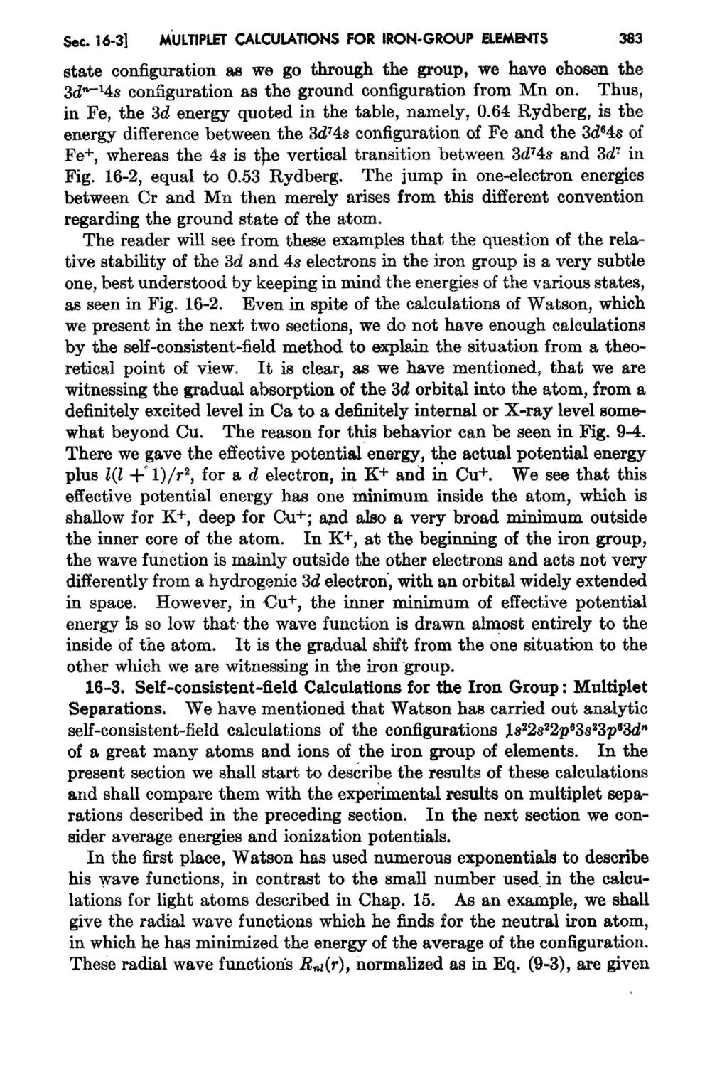
1&.2. ExperimentaJ Results fan Irun-group Multiplet.s . 376
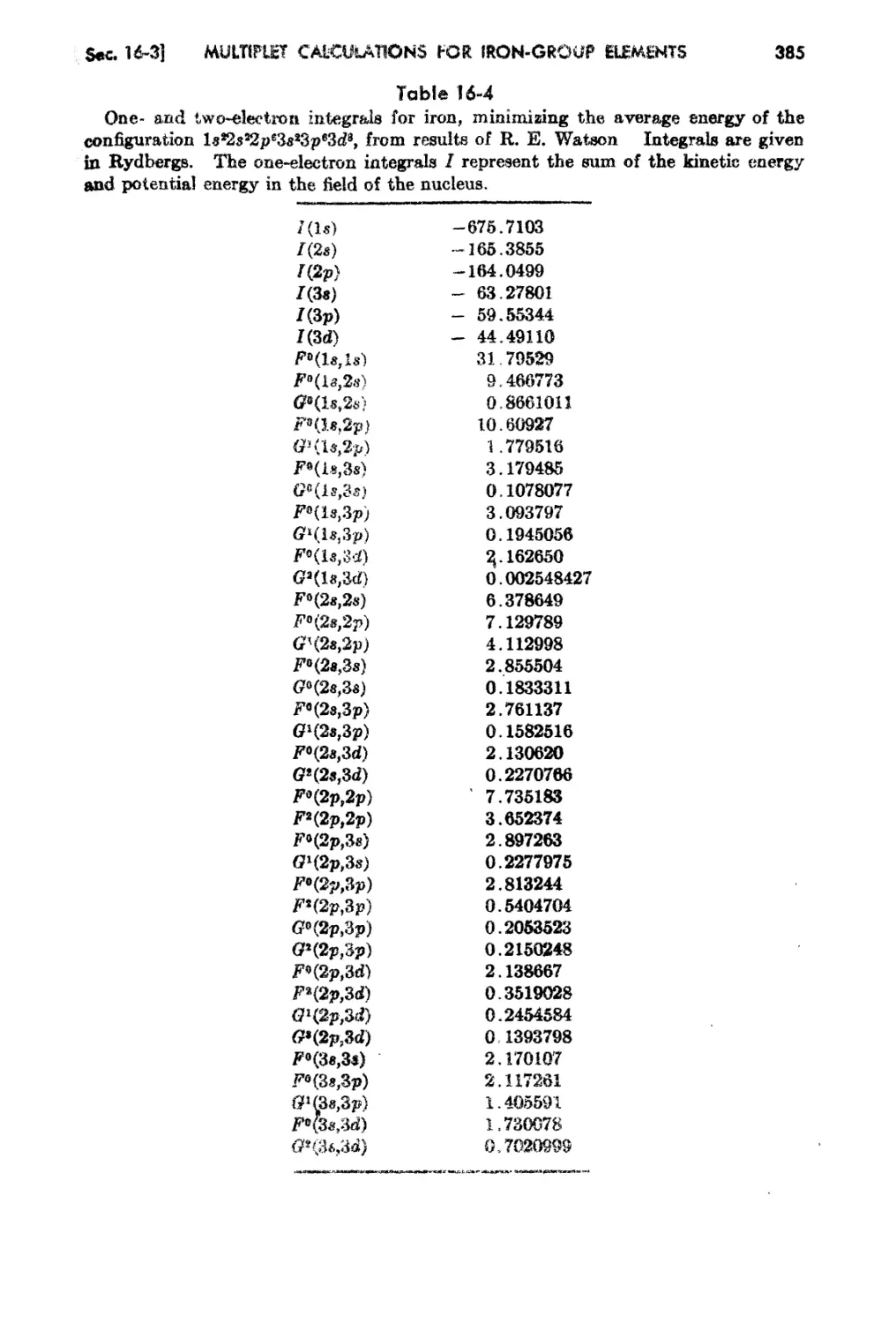
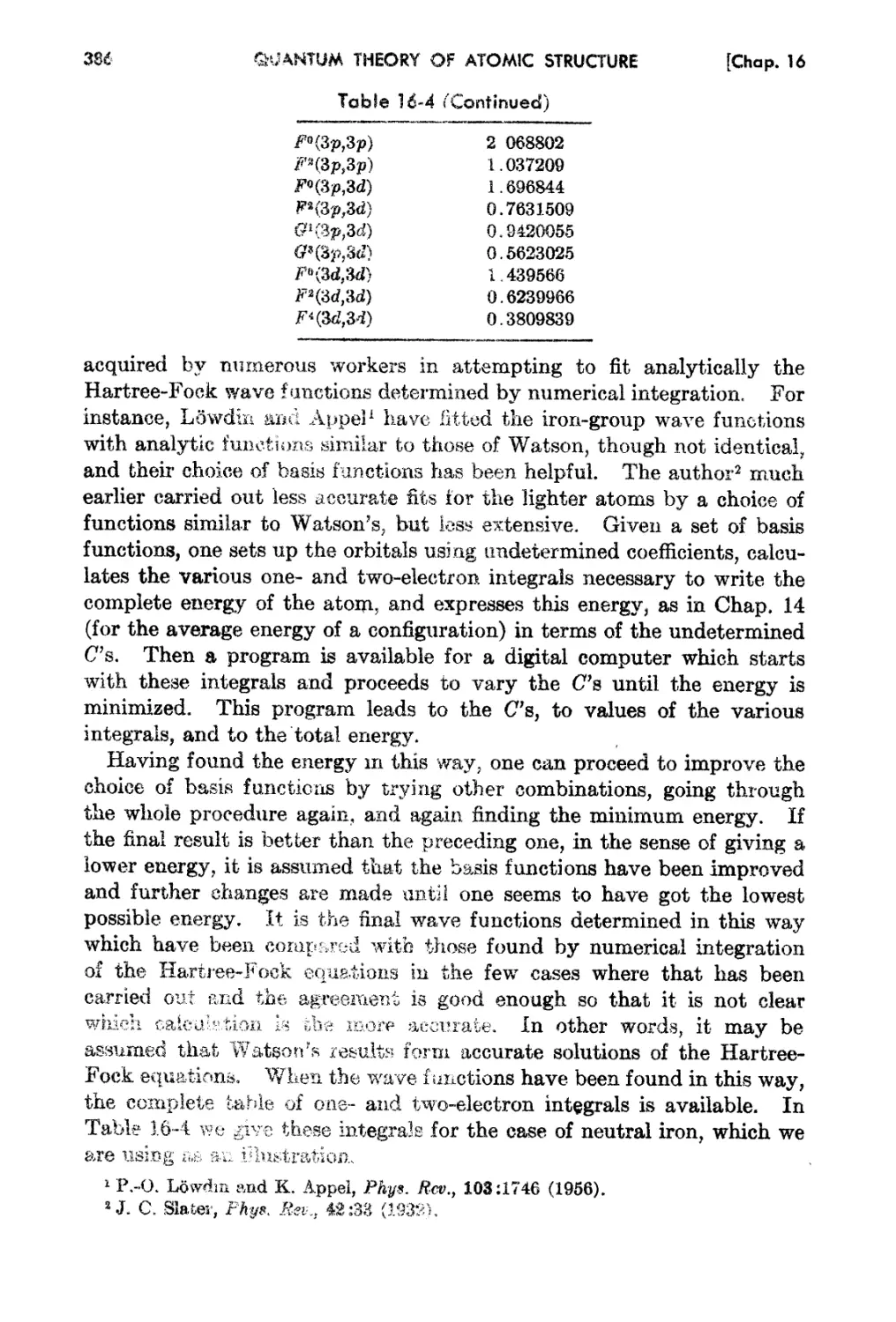
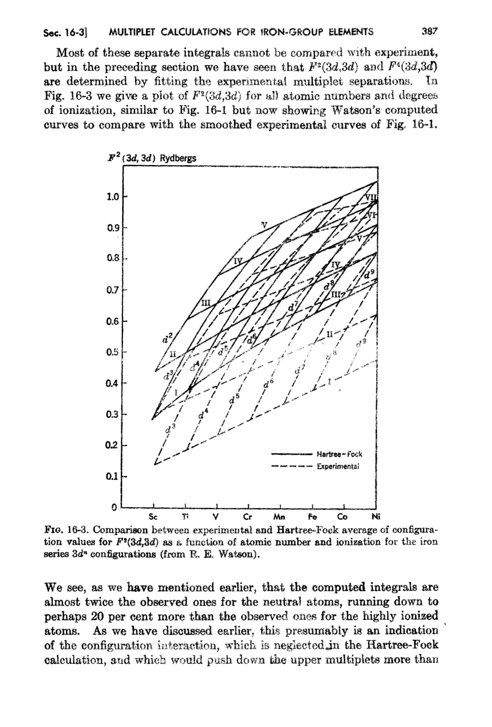
16- a. Self-coUf;hltent...iield ( alcrdatio-ns for the Iron Group: l\rlultip!ct Separa-
twns 383
xU
CONTENTS
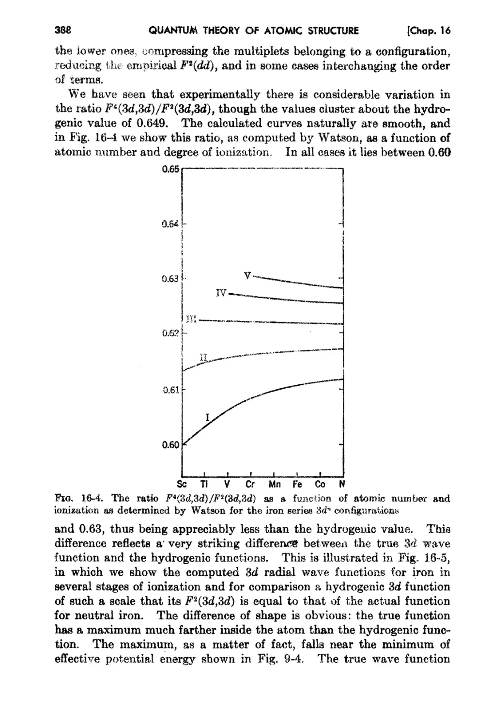
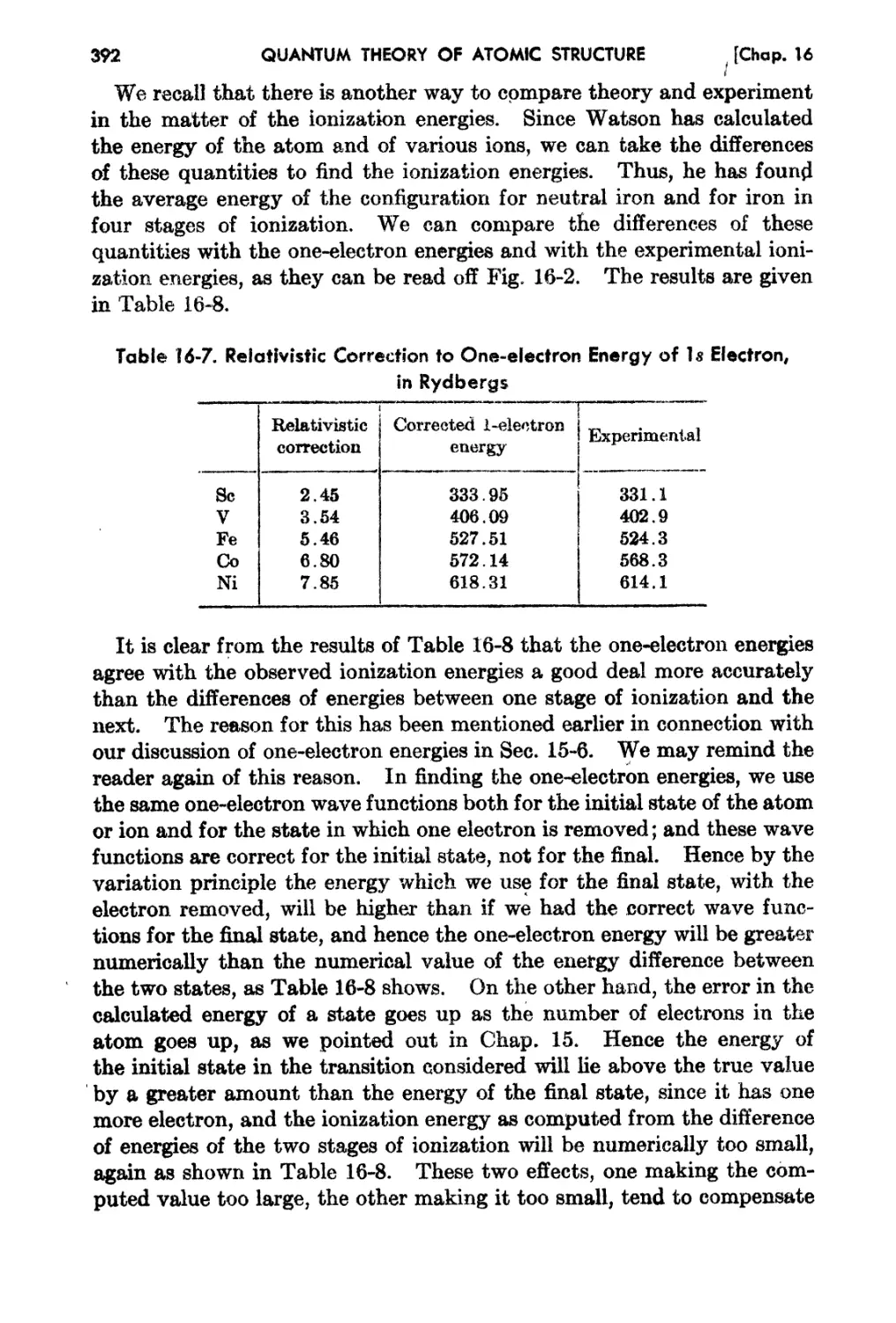
16-4 Comparison of Theory and Experiment for Total Energy and Ionization
Potentials - 389
AppendIx 1. Boh,:,'s Theory for Motion in a Central Field 395
2_ The PrinciJ)le of Least Action 402
3" 'Wave Packets and Their Motion 405
4. Lagrangis,n and Hamiltonian Methods in Classicai Mechanics. 412
5. The WKB Method 420
6.. Properties of the Solution of the Linear-oscillator Probleln . 422
74 The Hermitian ( haracter of Ivlatrices . 426
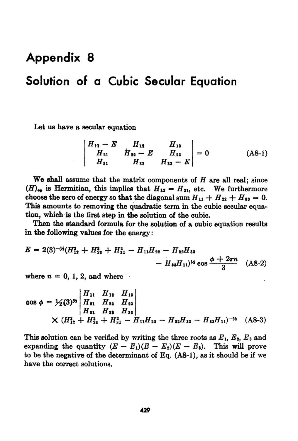
8. Solution of Cubic Secular Equation , 429
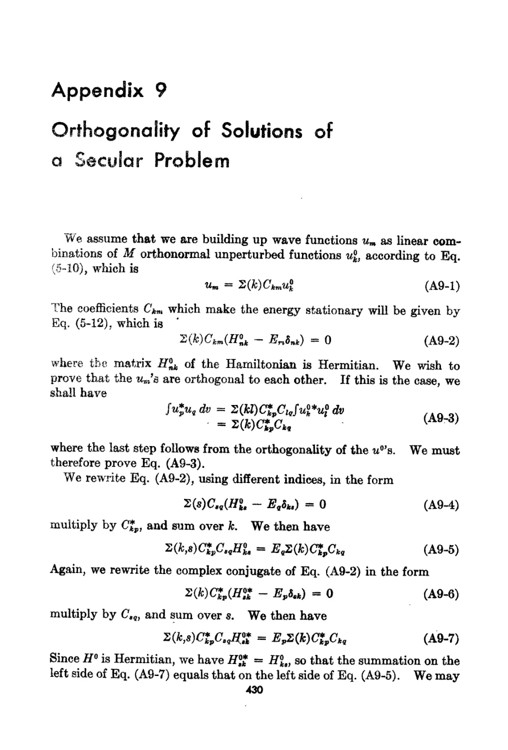
9. OrthogOlu.\]ity of Solutions of a Secular Problem 430
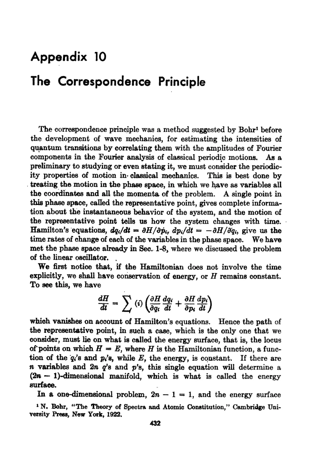
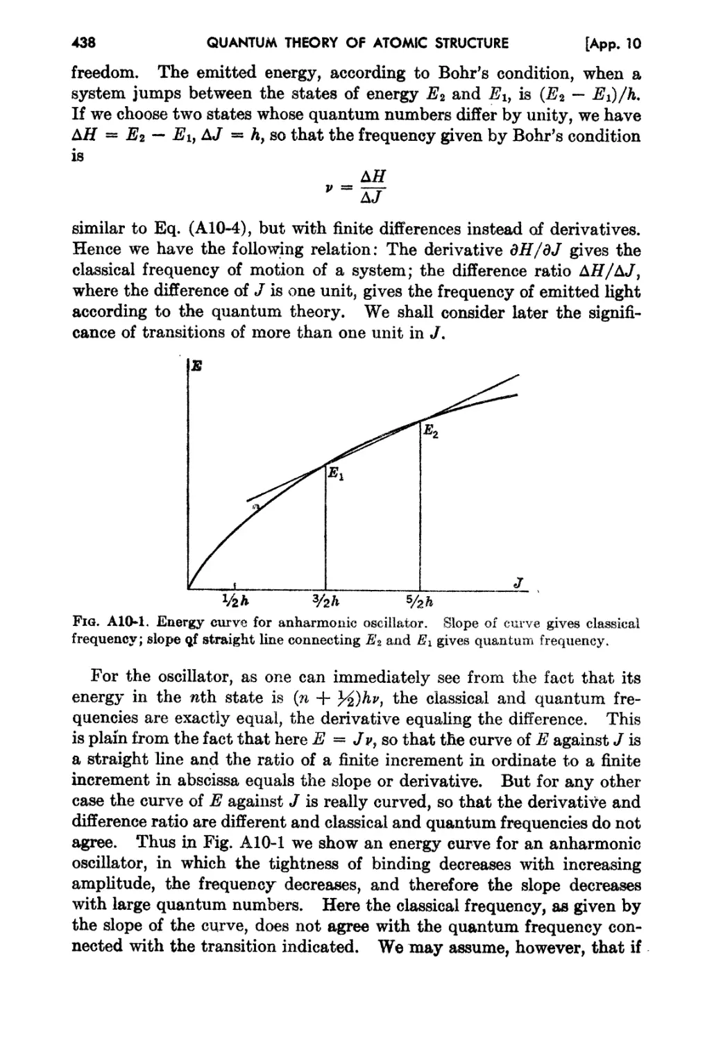
JO. rfhe Correspondence Principle . 432
l.L rfhe Surn Rule for Oscillator Strengths 441
12. The Quantum Theory of the Electromagnetic Field . 443
18, Schrodinger'a E quat,ion for the Central-field P:rot.l( w 455
14. Properties of the AssociaJ,ed Legendre Function.s , 451
15. Solutions of th Hydrogen Radial Equation . 461
16. Bibliography of the Hartree and Hartrec-Jt'ock lVlethods 468
17. The Thomas-F'erlui Method for Aton-As. 480
18. Cornmutation Properties of Angular 1omenta for A.tonu3 484
19. Positive Nature of Exchange Integrals. 486
20a. Tabulation of c's and a's for Multiplet Theory for 8 , p, and d
Electrons . 488
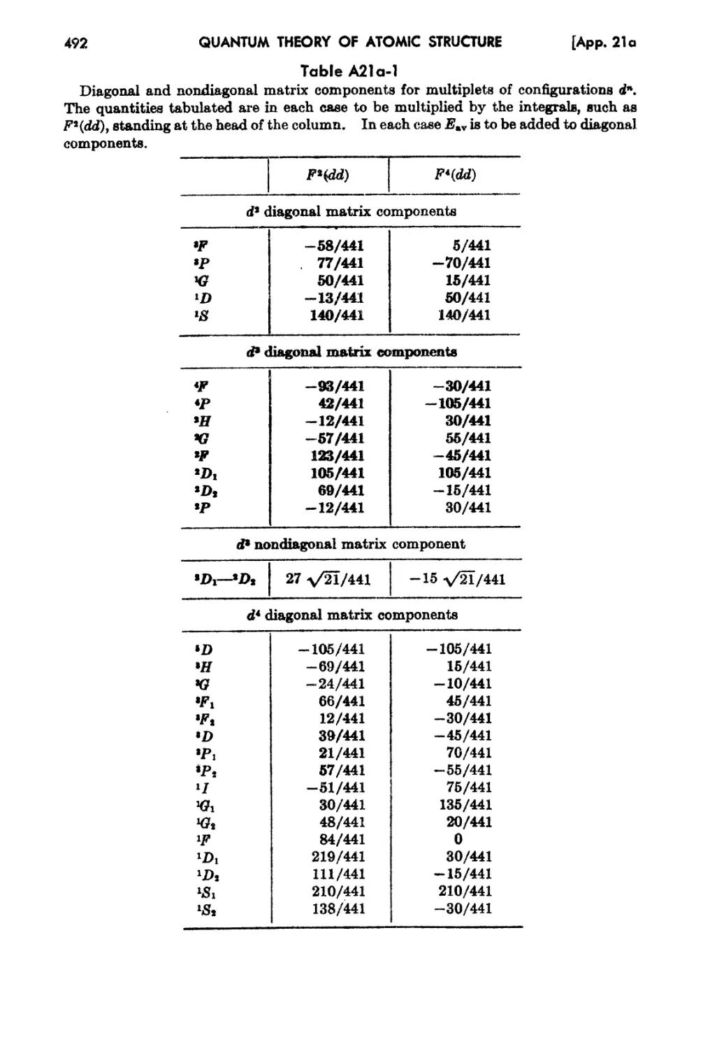
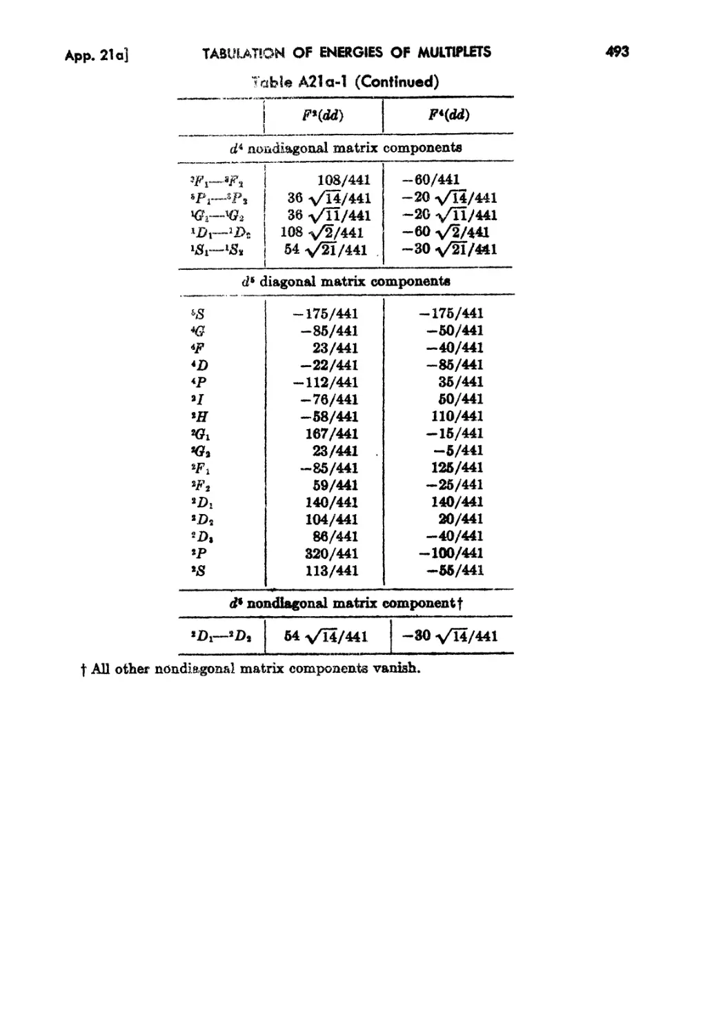
21a.. Ta.bulation of Energies of Multiplets 491
495
Index
1
The Historical Development of Modern
Physics, from 1900 to Bohr's Theory
1-1.. Introduction. l'he first half of the present century llas been one
of the most fruitful periods in the developnlent of physics. It has seen
the theory of relativity} the quantum theory, and nl0Jern ideas of the
structure of atoms, molecules, and solids come into existence. There
have been 3everal other very exciting times in the history of physics.
One came with the development of classical mechanics, by Galileo, .
Huygens, Kepler, and Newton, in the seventeenth celltury. Another
was the development of the wave theory of light, by Young and "F'resnel,
at the beginning of the nineteenth century. Still another "ras the devel-
opment of our ideas of electromagnetism, starting ,vith Oersted, ]'araday,
and others, and culminating in tIle theoretical work of Max\vell, show-
ing that electromagnetie \vaves and light were identical; this was a prod-
uct of the middle of the nineteenth century. A later nineteenth-century
development was the theory of heat, leading to the kinetic theory of gases
and the theory of statistical' mechanics, by CJausius, Boltzmann, and
Gibbs. All these great advances in the science were essentially complete
by 1900, and the stage was set for another and different developlnent,
along atomic lines. The present cent11ry has seen this developnlellt, and
it deserves to rank with tile others in importance, if it does not in fact
overshadow them. Perhaps the leading names to be attached to these
twentieth-century discoveries are P18tnck,1 Einstein, 2 .Rutherford,;) Bohr,4
Heisenberg; i and SchrOdinger. 6 1'11ey rank with the great physicists of
history.
1 M. Planck, Ann. Physik, 4 :553 (1901).
2 A. Einstein, Ann. Physik, 11 :891 (1905); 18 :639 (1905)0
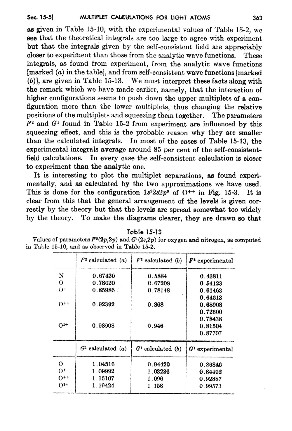
a E. Rutherford, Phil. Mag., !1 :669 (1911).
N. Bohr, Ph'1:Z. Jvf ag., 26(1) :476 (1913).
i W. Heisenberg, Z.' Ph.ysik, 83 :879 (1925).
l} E. SchrOdinger, Ann. Phy.8ik, 79 :361 489, 734; 80 :437, 81 :109 (1926).
1
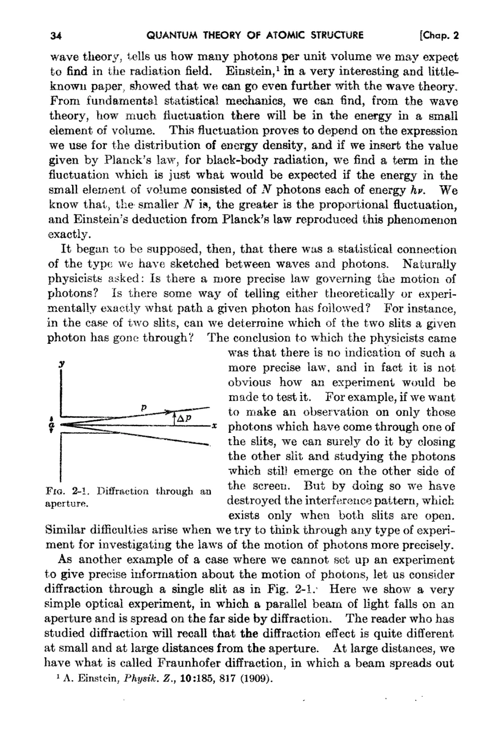
2 QU.-'NTUM THEORY OF ATOMIC STRUcrURE [Chap. i
The layman has become b tter acquainted witb the IUtrI18 of Einstein
and his theory of relat.ivity than with any of the othf r results of twentieth-
century phJTsics. Ilia famous equ.ation E = 1nc 2 j where 'in is (l mass, c the
veiocity of light J and where the equation states tll:J..tJ this lr;aBS is equiva-
lent to an energy E, is familiar to everyone, along \vith its ft.pplication to
nuclear physics and the development of nuolear energy& In contrast;
Rutherford, who made tIle discovery of the nuclear atoln, and Planck;
Bohr, Heisenberg, and Schrodinger who developed the (lUantunl theory
and its application'to atomic structure, 8Jre less \vell kl}ZY"t'Vl1, 1'he physi-
cist ranks t.hem as equally significant, hO\VeVf l" The vviH concern us in
our ,york Inorc thnn Einstein and the tl1eory of relativit.y. 1';hat t.heory
is particularly inlportant when we are dealing witll ver}'" high energies,
very great velocities ftppro;tching the "{telocity of light. Sueh questions
concern ''Us hetl \ve are dealing with the atolllic nucleus. 13ut one of
the facts enlerging from our presellt kllowledge of the at,oui 3S t.hat there
is a very clear-cut digtinction between the phenomena of the ntomic
Jillcleus and t}lose of the outer part of the atorn. ...t\i1 ordir TY effects of
heat, light, electricity an.d magnetism, cllemistry, llictallurgy, a!ld so on,
arise entitely fron1 the o11ter part of the atom. They' are not concerned
with v'ery great energies; and, for them, relativity plays tIle part of a
n1.inor correction to classical rnechanics. On the contrary, it is for jtIst
such. problerns rela.til1g to very small systems, on an atomic scale, that
the <!'uH.Iltu1n theory is needed. Our task in this volume will be t.o .review
the present theory of t}lese phenomena which arise from the outer pii-l'ts
of atoms; vie shall omit the nuclear phenomena, not because they are not
inlportant but becallse to include them would make an impracticably
large boolc Henee 'we shall use relativity only incidentally, but, the
quant,urn theory rn.ust be our principal topic.
The de"\telopnlent of the quantum theory stretched o {er 25 years, and
there are three v'ital dates to remember in conne-otion \\"ith it j at the
bcginnh:1g. the Iniddle, a.nd the e11d of the p( .ri )d 111 1901 Planck m.ado
the first suggest!,)!). of t}1e quantllffi theory. In 191:-S Bohr f0und how to
apply it tf) th.e theory o,f th.e hydrogen ato:rn] 1ttaking t.he -first real advance
· 1.... . 1:" i · f + 1 .. 'Ii . th t f\"
111 our unnerstlR!H1Hlg 0; tne aynamlcs 0 t} le partIcles In '.t e a 0111. L1.nd
in 1926 Scbri)dinger diseovered the equation ,vhj h bears his name, which
f · h 1 d 'i 1 . . 1 b . f th ' · ... b .
... Ut111S.tec {;fH; reLH ITI.tttHen.1tlt,lca aSlS 0 .1C 1,JoeorY'1 a tJaSlS W ..lC.i1 was
1 ,. · .... d . 192 ."" .. . fl " t b t ·
part.y lores.aaO.OVlcct tn Lne preee lUg year, b n a dl teren u equIv-
alent forrn hy Heisenberg. Since 1926, ,.ve ha.ve beel! engaged in work-
ing out COllsec!uenccs of Schrodinger 1 s forrrlulation of the theory,
which is kr\0\9.n aB \A'a,ve Inechanics, and in H;pplying it to t11e InatlY prob-
lerrls of at-canie, inoleenlac and solid-state f5tructure We feel that the
" t
theory t iU no\:v fOl'In.ulatefl, pJ"ovidcs the preeit;e xnH.thematic;a.l founda.tion
for aU t31t8e ph :.nfHn just as Ne\-vt.on's lav ':3 .PlGVlr..1e the foundation for
Sec. 1-2]
MODERN PHYSICS FROM 1900 TO 80HR'S THEORY
3
classical mechanics and Maxwell's equations that for electromagnetism.
Unfortunately, /ave mechanics is a much more difficult branch of n1athe-
matics than either of these others, and we aTe still far from having worked
out all the consequences of the theoretical discoveries made in 1926.
But. the progress has been great, and we can nov; give as very convincing
picture of the structure of atoms and of their behavior under all sorts of
external conditions. This is the topic of our books
In the lnajor part of t.he present \vork, we shall assume tIle principleR
of wave mechanics as the fOUl1dation of our treatment, just as a text on
classical mechanics ass'umes Newton's law or one on electrornagnetisTI1
aSSUDles Maxwell's equatio11S, and we shall proceed ftom these principles
in a deducti'".Je way, to try to explairl the behavior of matter. But the
reader will not appreciate the subject properly if he is not familiar with
the process n- of discovery which had to be passed through in the period
from 1901 to 1926, to develop these laws.. Such an i11dllctive period in
. science is in some Vtays more stimulating than a deducti";re period, in
which one is merely ,\yorking out the consequences of pr>incip]es which
everyone adnlits are true. To giv'e tIle rea,der a lit.tle of this appreci-
ation, we presellt in t.he first t,\\'"o chapters a sllort. sketch of the historicaj
development of physics, during the n10mentous quarter century from
1901 to 1926.
1-2. The Electron and the Nuclear Atom. A number of observations
during the nineteenth century had indicated that atoms had SOlne sort
of internal structure, of an electrica.l na.ture.. One type of information
came fronl t'araday's experIments on elect.rolysis. Faraday' found that,
when .electric current passed through an ionic solution, material ,vas
deposited on the electrodes. But, furthennore, he observed that the
amount deposited was always proportional to the amount of charge trans-
ferred by the current.. It wa.8 a.s if each ion that had passed through the
electrolytic tank had carried just 80 much charge. If there had been a
good measurelnent of the mass or 81n ato!n in those days F'araday from
his experinlents could have said just h()1.v big this charge was" Crude
estimates of atoll1.ic ma.S8eR \vere available] and hOllce crurle guesses as t.n
this charge were possible& vVe kno\v no,,, that the eharge, for a mono.
valent ion, is just one electronic eharge; nfHl; in the " vay indicated, there
were rough estirnates of t.his qUHutity by the end of t.hf; nineteenth cen .
tur y . rrhe IU1111C electron for this unit of charge. \vae ilr 7f;nted bv t.he
J J i. v
Englishman Stoney, in i,he 18808.
Before the end of the century i the electron 11:J..d bf;en disc(Plere(l as a,n
isolated particle. Crookes, J. J. Thonlson, and Illi \'r()' others had been
Dlaking experin1ents on eleetrical discha,rges in gases. "'rhey found very
good evidenee that charged particles, carryihg bf}tb. positi-vc and negati'ie
charges, existed in these discharges. The y. detteet+ d those patUcles in
4 QUANTUM THEORY Of ATOMIC STRUCTURE [Chap. 1
electric and magnetic fields, just about at the close of the century, and
from their dynamics made estimates of the ratio of their charge to mass.
From this information it was found tllat some of the negatively charged
particles had a mass small compared with an atomic mass; it was assumed
that these particles were the electrons themselves The p sitively
charged particles, however, caUed ions, proved to have masses of atomic
.
Slzee
There was evidence that atoms contained not only electrons but build-
ing blocks of other typP..,S as welL One could not fail to observe, as Prout
had noticed fairly early in the nineteenth centut'Y ths.t the atomic weights
of Iflany of the elements proved to be surprisingly close to integers; and
Prout had suggested. that they were made out of fundamental particles,
perllaps hydrogen atoms) all alike This hypoth ':tis of COllrse came up
against the obvious obstacle that some of the atomic weights were very
far frOIll integers, s,nd it remained for the discovery of isotopes in the
present century to remove this difficulty and show that Prout's hypothe-
sis really had foundation.
Finally, during the last years of the century 1 two nevv discov'eries
greatly excited the pbysicists. Rontgen in 1895, discovered the X rays)
or }90entgen rays These rays? capable of pa8sin g through matter, viera
completely different from anything observed before. Their discovery
was followed almost immediately by' Becquerel's discovery of radio-
activity, from the obser,ratioD. that uranium emitted rays which, like the
X rays; could pass through matter and in fact could blacken a photo-
-graphic plate even if it were wrapped up in an opaque co"\rering. It was
discovered that in radioactive disintegra.tions se'veral types of radiation
were emitted, and by 1900 J" J. Thomson, the Curies, Crookes, Ruther-
ford, and Boddy were all working actively on the problem of finding
what they were. Soon, also, the chemical Sep}lr8 tion of radium from
uranium by the Curies, and other similar experiments, had shown that
a numl)er of elements were radioactive.
It did not take long to establish the nature of the types of radiation
ernitted by radioactive atoms, which R'ltherford called alpha, beta, an,d
gamma radiation. It was shown. that the alpha and beta rays were
deflected by electrio and magnetic fields, so that they consisted of streams
of charged particles, while the gamma ra lS were not deflected. By
experiments on the defiection, it was shown that the beta ra rs were
electrons, with the same rat.io elm, or ratio of charge to mass, ,vhich
the electrons h d already been found to have by J. J Thomson. The
alpha particles, however were found to be positively' charged, rather than
negatively as t11e electrons ,vere, an.d to lls,'ve a value of e/ m indicating
that their mass W8 q in the neighborhood of atomic masses, Jnuch greater
than the electronic mass By cOlnparison 'Tyvitb. elm experiments on other
Sec. 1-2]
MODERN PHYSICS FROM 1900 TO BOHR'S THEORY
5
positive ions, it appeared tha"t they were helium ions with a charge equal
to twice the electronic charge. As for the gamma rays, which could not
be deflected, it was soon shown that they were identical in nature with
X rays, which had been shown to be electromagnetic waves like light;
the X rays, however, had wavelengths muoh shorter than ordinary light,
and the gamma rays had still shorter wavelengths.
. The next qu estion which arose was: How did these radiations come to
be emitted from the radioactive atonls? 'l'his question was closely con-
nected with another on8" whicll at first seemed very puzzling: when a
sample of radioactive materi81 was examined, ita properties often changed
with, time, in complicated ways, as if its composition ,vera not staying
constant. Rutherford and Boddy, in 1903, proposed an explan&t on
which has proved to be correct and which tied together all the knoWD.
facts about r3Jdioactivity. This explanation suggested that radioactive.
atora.s could spontaneously explode, tra11sforming themselves into other
atoms 1 and that such explosions were going on all the time, so that in a
given time interval a certain fraction of the atoms would blow 11p, quite
indepen.dent of outside influences. If we have a number of atoms of
which a fixed fraction is destroyed per second, this means that the num-
ber remaining at any time will decrease exponentially with the time
(provided there are no new atoms being produced), and the length of
time required for the number to be reduced to half its original value is
calle(1 the half-life" Rutherford and Boddy found elements with all sorts
of half-lives, from short ones of a few millutes to long ones of thousands
cr millions or billions of years.
The theory of Rutherford and Soddy went much further than this
simple hypothesis of explosion, for they also were able to find out what
were the products of one of the explosions. If an atom when it explodes
transforms itself iIlto another, then the nUD}ber of atoms of this other
type will gradually increase with time, unless an equilibJ.ium is estab-
lisb.ed by a subsequent explosion of the ne\v type of atoms.. By an
elaborate series of teste, Rutherford and Boddy were able to show which
atoms were transformed radioactively into which others, with the half-
lives of each type. They' were able to set up simul aneous differential
equations for the numbers of atoms of the various types as ftlnctions of
time, to solve these equations, and to show that they gave a complete
explana.tion of the complicated effects which they had observed as to the
time dependence o.f radioactivity. The case they ma.d out for the trans-
formation hypothesis was so convincing that it has never been questioned.
They found extremely interesting correlations between th chemical
properties of the various radioactive elements whicli they discovered
and the types of radiations which they emitted. The,y found that, when
an atom emitted an alpha particle, the resulting atomic species showed
6
QUANTUM THEORY Of ATOMIC STRUCTURE
tChap 1
t hemicu. propert.iefS ,vhich '.;vould place it t\yO units before the parent atom
in the periodic table of the elempnts, while if it en11tted a bet.a, particle,
its chemical properties \tYOllld indicate that it should be onf unit. beyond
the parent at01l1. 'T'l1J.s suggested an extremely in1portant generaliza-
tion, ",rhich is in. at vlay t.he found8.tion of our ,vllole pre.'Se11t understanding
of the periodic systeul of the elements: it suggest.ed tha.t the <trdinal
number of all H.torn In the periodlc table of the eler!lcnts, starting with
hydrogen 1, heliun1 2, lithium 3, and so on, ,vhich we now call the atolllic
11umber, repre8enLed in some \vay tile nUlllber of units of positive charge
in -the a/tom. F'er if this ,vere the case, the emissioll of an alpha partiele,
which llas tvt"O i.11tits of positive charge, should decreilse the atolni((
ntlnlber by 2J \vluJe the emission of a beta particle, ;vith one unit of nega.
tive charge, SllOU!d inerease the atomic nunlber by unity Many sort.s
of subsequent e\ridellee have verified the correct.ness of tbis hypothesis.
A corollary' of the hy pothesi8 is obvious: since an atolIi as a whole is
11Ilcharged) a, neutral f1tom must contain a nUlnber of electrons equal
numerically to its atomic number.
One of the early veriilcations of this corollary" regarding the nUlnber
of electrons eanlC from the so-called 'l'lhomson scattering fornlula for
X rays. Th, OT!lSOn assuming that J{ rays \vere sirfiply elect-ronulgnetic
rays of s:hort.'ir\raveJength, investigated the I8JW of scattering by matt.er
containirlg electrons. His forlnu1a showed that tIle scatterirlg ShOll1d be
proportional t.o the nunlber of electrons per unit volume. It was later
sho"\vn that Xv-ra:Y' scat.tering is really n1uch more cOITlpJicated than this,
on account of cryst.aJ diffraction; but t.here are important cases where
Thomson's sce..tterhlg formula holds, and it ,vas shown experilnentally
by Barkla aIld others that the scattering ,vas approximately in agreenient
'\vith the hypothesis that the number of scattering electrons per atom \ ,ras
equal to the aton-lie !ltnnl)er..
Rutherfo "d find 80ddy could dr a\'V" definite conclusions regarding a,tolnic
" < , -- h h 1t · ., 1 " h f
rnasses: or D:.. -.. L Uf; \VeigL7,S. l' e _ellUITt atom, or alp 1ft partlCte, as our
. t f } ". 1..J ',' 1 i i if " . 1 t_
tlnl .8 0 aT,GrrU.e v"'eignt,, ..Lienee l{, IS C car. nat, an atolll elluts an a pIla
part.icle, t.he IhY\;V f1tCHll resulting froln it r.nust have an atoJnie ,veight
which is less bv' four uHits. The electron. or. beta J )3.rticle {)n the other
... ; ""- I
hand, has practicaHy no mass cOlnparcd. ,vith the Inass nf an at.om, so
that 1 if an atoIn BBlits ft beta particle, its fttonlic weight shou ld not. change.
There ,vere a IHl111ber of cases where these h:ypot.heses could be ''\lerified.
I 1- · 1 '2 } . .. ..f: .." 1 ..
n parocu 8,,1" t.ne l"aCUoactlve senes 01 eienl(\!.i.ts terrnJllolt$d 1[1 e,ad as a
TIIlsl p1:oduct, f3.rid tbe atomic weight of this lea.d could bo deterIllined
from certain rninerah whose lead content apparelltly rcsu]1A:d a,s an end
product of rHJdioactive disilltegration; its atomic ,veight ha.(f the predicted
1 l< d '.. .J 1... · .4- h . h .. 1. ,.....
va lIe, as IGUn tronlLl.l..e uranium or tJ lOflun1 W jC!1 VV-H.S tIle oflgJ.nai
element frorn \VhjCJ1 the lead ,vas descended. FurtherrnGrc tb.e atomic
Sec. 1-2] MODERN PHYSICS FROM 1900 TO BOHR'S THEORY 7
weight of this lead was different Iron1 that of ordinary lead 1 a fact ,vhich
seemed very remarkable to the chemists of that tin1e but which became
clear soon afterward with the discovery of isotopes. Thus radium dis-
integrates into lead of atomic weight 206, thorium into lead of atomic
weight 208, while ordinary lead has an atornic \veight of about 207.
Thel1tomic weight. of heliun1 is almost exactly 4, so that, in a series of
radioactive eleme11tS'- in vlhich one is produced from another by the
enlission of an alpha or a betr part.icle, the atonlic ,veights of successi\ e
elements differ alrnost exactly by four units. These atomic weig:ht.s were
found to be .v ry close to integers. As a result, the physicists of the time
began to tlake very seriously Prollt's hypothesis that tIle tJTue atomic
weights of 3.11 atoms are integers} and the current explanation was that
they were made up out of protons !t11d. electrons. '\7 e now know th.at
t11is explanation ,vas not complete. "\Ve no'\v understand the nuclear
natllre of the atom, which was not knovvn until Rutherfofcl proved it in
1'911, and ,ve l{now t,}lat the nuclei are built up out of protons, hydrogen
nuclei with a unit p.ositive charge and a 11nit mass or aton1ic weight, and
neutrons, unch.arged particles with a mass almost the sanle as that of the
proton.. rI'he alpha particle consists of t\VO neutrons 3,nd t\VO protons,
accounting for its charge of 2 (froln the charges on the t\VO protons)
and its atomic vveigllt of 4 (frorn the fOl1r particles). 'vVe also know that
a stable nucleus contains approximately equal nlt bers of protons and
neutrons, as tile alpha particle does; this explains the empirical fact that
atonlic ,\\yeights are approxilnately t'v'trice the atoIrlic numbers. The
nurnber of neut.rons is, in fact, sOlnewhat greater than tile number of
protons, for the lleavier elements, so that. the atoITlic ,veight is somewhat
more than t,vice the atolnic number.
We also kno\v now that artificially radioa.ctive atolns can be formed, in
which there are too many 11eutrons, or too many protons, for the ideal
COl11position corresponding to stabilit r" These atorns can disintegrate
by errlission of ""/arious types of particles, with the release of various
amounts of energy, We kno,v] furthcrrriore, that; on account of EiJ1-
stein's relation E :::: 1nc 2 , the release of a certa .n al110unt of energy makes
a corresponding change in the mass. The mass equiv"alent of the energy
released is sInal! compared ,vith a unit of atomic weight; and the net
result of this is that the atonlic weights of the va.rious atoms are almost.
integers, but not quite. As we say, we now understand these matters
relating to the masses of the various atoms quite thoroughly, but they
were not understood in the I1tlriod around 1911 of t 11cll we are ,vritil1g.
The first observation of artificial radioactivity came in 1919, when
Rutherfora produced the artificial isintegration of an atom, bombarding
a nitrogen atom with Bin alpha particle 1 and knocking off a proton. It
was 110t until 1932 that Chadwiok, in. studyillg the disintegration of
8 QUANTUM THEORY Of ATOMIC STRUCTURE lCha . 1
beryllium by alpha particle-s, knocked off a neutral particle which came
to be known as the neutron. Until this discovery of the neutron in 1932
. it was believed that the nucleus was made of.protons and electrons. But
we are getting ahead of our story: in the period around 1911, it was
surmised that true atomic weights were integers, as Prout had supposed
a hundred years earlier, but it was not even known that the nucleus of the
atom existed It was popular, following ideas of Thomson, to think
of the positive charge in the atom as being spread throughout the volume
of the atom, perhaps in a uniformly charged sphere. Let \IS return to
this period and consider the discoveries which led to the understanding
of the nuclear atom4i
There was, in tb.e first place, an obvious experimental object.ion to
Prout's hypothesis: the existence of chemical elements, like chlorine with
its atomic weight of 35.46, whose atomic we ghts were not integral. The
n\uuber of elements with integral atomic weigllts ,vas far too large to be
explained by chance, but hovt could one explain these nonintegral values?
A solution was immediately suggested by Rutherford and Soddy's expla-
nation of radioactive disintegration. They found in a number of cases
that there were several elements of the same atomic n.umber, but of
different atomic ,veight, arising in various stages of radioactive dis-
integrations; the case of lead, which we have alread.y mentioned, 'was an
obvious Olle. Their hJ1>othesis indicated that the cb.emical properties
of the element depended only on the atomic number.. lIenee these
elements ShOllld be chemically identical, and il1 fact, as far as chemical
tests showed, they were. It was very natural to assume that the same
thing might be going on among the nonradioactive elements: that many
of our\ordiriary elements might be mixtures of a number of differe11t
nuclear species, all with the same atomic number, but viith different
atomic weight8 The elements whose atomic weights were known to be
integral would be assl1med to consist of only one such nuclear species 1
whereas those, like chlorine, which obviously h8"d fractional atomic
.weights would have to be mixtures.
This hypothesis was soon verified, in a brilliant way, by the ,york of
Aston with Ilis mass, spectrograph, following up the pioneer work of
Thomson. 'l'homson and Aston examined ordilUtIJr elements, neon being
one of the very early ones worked on, found the ValtleS of elm for tbe
ions, and hence found the masses of the atoms. And they found that
in many cases the elements as they existed in natu.re did in fact consist
of mixtures of atoms of different atomic weights and that these ato ic
,veights were integers, as accurately as they could tell at the time. SOOdy
had invented the name isotopes, to represent the different atoms with
the same atomic number, and hence chemical behavior, but different
atomic weight. Continuation of this work of Aston into the 19208
Sec. 1-2] MODERN PHYSICS FROM 1900 TO BOHR'S THEORY 9
and later has disclosed the isotopic constitution of all the elements and
has shown that the chemical atomic weights are n.othing but a suitably
weighted mean of the atomic weights of the various isotopes. The fact
that the chemical atomic weight is found to be the same in almost all
natural samples of a given element shows that the matter composing the
earth must have been once well mixed, presumably while the earth
was still molten, so that all chlorine, for instance, is made up from the
original mixture having defirlite ratios of its various isotopes. The only
observed cases where natural atomic \veights vary are in those elements
whibh have boon produced by radioactive disintegration since the earth
solidified.
The measurements we have been discussing are those of elm, the
ratio of charge to mass of the ion" In addition to these, measurements
of the electronic charge e were necessary, which, by means of the measured
elm, led to absolute deterrn.inations of the masses of the atoms, and hence
. of Avogadro's number, the number of atoms in a gram-molecular weight.
Rough estimates of the charge of positive nuclei had been made early
in the study of radioactivity; since atoms are electrically neutral, the
positive ions mus.t carry numerIcally the same charge as an electron or a
multiple of it. In radioactive diBintegratiolls, where. charged particles
are thrown off by nuclei, the nu.mber of disintegrations could be estimated
by observing nuclear processes by s''3in.tillation methods. Br allowing
the particles to impinge on a luminescen.t screen, each nuclear disintegrar-
tion became visible and could be seen with a microscope. The total
amount of charge releas€' in such disintegrations could be measured by
electrical methods. }i'rom these two pieces of information, the charge
in.volved in a single disil.Ltegration could be found. 1\leasurements of
this type were not accurate, however; and it was not until the develop-
ment of Millikan's well-known oil-drop experiment in 1911, refining a
method used earlier by To,vnsend in a cruder form, that ve had really
good measurements of the electronic charge. This brought with it, as
we see, a determination of the masses both of the electron and of atoms,
and consequelltly of "t\,\rogadro)s number.
We have now sketched the main outlines of the arguments that went
into tIle elucidation of the relations between atomic number, atomic
weight, and chemical propert,ies The next great step was that taken by
Rutherford in 1911, whell his experilnents on the scattering of alpha
particles by matter led to the hypothesis of the nuclear atom. Ruther-
ford allowed a beam of alpha particles to pass through matter and
observed that most of the particles showed very slight deviations from a
straight path. However, occasional particles showed deflections through
very large angles, and calculation of the dynamics of a collision between
an alpha particle and an electron showed that such 8; deflection could
10 QUANTUM THEORY Of ATOMIC STRUCTURE [Chap" 1
not result from such a collision, under any circumstances; the electron
is too light to be able to deflect a heavy particle t,hat much, no matter
how close the collision is. This mathematical analysis showed that such
a sharp deflection could come only from a oollision of a heavy particle
with another of comparable mass and at such a small distanee that the
electrical force of attraction or repulsion was extremely great
StIch an obse lation was completely incomprehensible if the positive
charge in the atom was spread OU.t over the whole atom, as Thon1son had
assumed. The only sort of exp1anation which could be given was hat
the positive charge was very concentrated, in a minute nucleus, carrying
almost all the mass, arid yet so small that t lO nuclei could approach
to a distance very snlall cOIrlpared with atomic d4nensiol1s. Rutherford
therefore concluded that the alpha particle, and the nuclei, nlust be
essentially point particles, containlng ahnost the ,vhole mass of the atom,
and with positive charges equal numerically to tIle atomic ntlnlber times
the electronic cllarge, so that the alpha particle would have a charge
of two units. He used the theory of scattering, assuming that the par-
ticles repelled eacll other according to the Coulomb law of electrostatics,
with a force inversely proportional to the square of the distance between
and proportionaJ to the product of the charges, and predicting how many
alpha particles should be scattered through each angle. When this
fOrJIlula was compared with the experimental results, it checked very
satisfactorily, verifying the assumption that the charges on the nuclei
were given by the atomic llumbers and that they acted electrostatically
on each other.
This experiment, then, furnished the experimental proof of the nuclear
atom. Rutherford at once was able to give a general picture of an. atom.
It consisted of a very minute nucleus, containing practically all the mass
of the atom, with a positive charge equal to the atomic number times the
magnitude of the electronic charge. For electrical neutrality, the nucleus
\vould have to be surrounded by a number of electrons equal to the atomic
number. The forces exerted between two nuclei were shown to be given
by the Coulomb, or inverse-square, law, down at least to a very small
distance, of the- order of a small multiple of 10- 12 em; for the largest
deflections of alpha particles were shown to come from encounters at 8,
distance of this order of mV.lgnitude, and the scattering law, derived on the
basis of the Coulomb law, held for these deflections. This deduction
of the nuclear nature of the atom formed one of the most important
discoveries of the century in the field of atomic structure.
Two consequences of this postulate were obvious. In the first place,
the atom as a whole must have some analogy to the solar system. There
was a very heavy but concentrated nucleus, attracting the electrons
according to the inverse-square lawc They had a very much smaller
Sec. 1-2]
MODERN PHYSICS FROM 1900 TO BOHR'S THEORY
11
mass and would {laVe to be assunled to be at a comparativel large dis-
tance from the nucleus. "rhus, '''Ie have seen that the nucleus cannot be
of dimensions larger than the order of 10- 12 em. On the other hand,
atomic dimensions, as one can tell from a great variety of evidence, are
of the order of magnitude of 10-- 8 em. 'fhis evidence COfiles from many
independent sources. JTor instance, frorn the kinetic theory of gases, it is
possible t.o estimate the radii of molecules from measurements of the vis-
cosity and thermal conductivity of gases, which depend on the mean free
paths of Inolecules. Tile study of the properties of imperfect gases also
lCBJds to values of moleeular dimensions. Much rnore dIrect a'vidence is
aVidlable, however; in a liquid or solid, we may merely assume that the
atoms fill IIp most of the space, and since we know how many atolns or
molecules there are in a given volume, from Avogadro's Ilumber and the
density, we can immediately compute the molecular v()lumes. All these
types of evidence agree in leadiIlg t.o atomic dimensions of the order of
magnitu.de of 10- 8 dm., as we have stated.
"\Xlith such a snlall nucleus and such a comparatively large atom, the
resemblance to the planets m.oving round the sun is obvious. Since the
nucleus is so heavy compared with U1e eleetrons, it Dlust relnain approxi-
mately fixed as the electron moves ro'und. it in its orbit; therefore its mass
will be unimportant in the dynamics of tIle electrons, and only its charge,
which produces the attraction between :nucleus and electrons and holds
them in their orbits, will be significan.t in determining their motion.
Hence] we see how the nlotion of the electrons is determined by the atomic
nlunber but not the atornic weight of tile atolu, so t,hat we under-
stand ho,v it is that different isotopes oan have the same chemical
properties.
The other deduction is that the study of atomic struoture can be
divided into two quite separate parts: the structure of the nucleus, and
that of the outer electronic system. This separation has persisted and
has led to an almost complete separation of atomic physics into two .parts,
nuclear and nonnuclear physics. The reason is the great difference in
size bet,veen the nucleus and the rest of the atom.. Nuclear phenomena-
radioactive disintegration, artificial radioactivity, and so on go on in
the very small volume of the nucleus, of dimensions 10- 12 em, and are con-
cerned with very high energies. They are ailnost completely unaffected '
by the bellavior of th.e outer electrons of the atoln. On the other hand,
the behavior of the outer electrons is deternlined almost completely by
only one property of the nucleus, its charge, or atomic number. It is
the outer electrons ,vhioh determine the ordin:.try properties of the atom
witll whieh \\"'e are familiar: its spectruln, its chemicai properties, the
behavior of the molecules and solids whicJl it can fonn. Thus it can
come about that one can treat these outer electrons almost without refer-
12
QUANTUM THEORY Of ATOMiC STRO(;TURi:
[Chap. 1
ence -to any other nuclear prOI)erties tb.an the ch9xge, 2,n,d this is what we
shall do in the ls,rger part of our treatLflent.
There are fUler details, ho'\vever, in \vbien, other properties of the nuclells
affect the m.otion of the o11t,er electrons. The nuelea.r masses come in to
a. slight extent: th01.1gh the rntclei 9Jl'C vf ry hea vy onl pared with. t.he elec-
trons, still they !nove slighily alon.g with the c]cctloll:ie motion and. this
produces minor correctio11S in the ti1eory, which can be used to check the
nuclea,r masses. In addition, the nuclei pro""e to have magnetic moments,
and these produce appreciab:, ? tll0Ugh very snla11" effects 011 the motion
of the outer electrons, observ-ed in tile fornl of llyperfine structure and
nuclear magnetic resonance. "fhese interconnecti.ons between nnelear
and electronie behavior are of great t,heoretical interest, and we shall
tR,ke the!::1 up later; bl1t vlhen ...ve consider tberri in con1pari8on with the
fundsJmental fact that nlost TJrOperties of the eleetronic Inotion d.epend
only on the nucl r charge} we see th.at they are comparati rel:r unimpor-
tant in the stlldy of mattet- in bulk
Rutherford's discovery of the nuclear nature of the atorn came in 1911;
the striking progress in atomic structl1re in the years follov/ing thiR 'V 1S
in the study of t.he outer electronic struetuTe of tIle atoln. Bohr's t,heory
of the structure of the hydrogen aton1 eZ:1Ine in 1 J13\ only' 2 jrears after
Ruth.arford's disco rery of the nuclear atonl 1 he di covery of X-Aray
diffraction, and its application to the nature of crystals, as well as to the
X-ray spectra. of the atoms, came at the saIne tin1e. These loci to Bohr's
explanattion of the periodic systenl of the elements, to the interpret.atioll
of atomic spectra, and finally to th.e d.iscov'ery of 'ave r.necllanics by
Schrodinger in 1926. But Bollr's theory 'was baserl only partially on the
nuclear nature of the ator!lo Its other foutldatioTl was the quantum
theory? which as we have stated had been Stlggested first in'19010 We
must now go back to look into its history] so as to understand the sort of
dynamical concepts which Bohr ha,d to deBJ v.Jith in. his atteJllpt. to explain
atomic st-ructure.
1..3. The Development of the Quantum Theory from 1901 to 1913.
The quantuDl theory had its origin jll a sOID.e,v}lat invo1ved problern the
theory of black ..body radiation. To,,"ard the latter part of the nineteenth
ceIltury, it had been proved that the radiation inside a tot,ally enclosed
ca,vitj1, such as a furnace,. maintained at a constant temperat.ure, was a
fU11ction of the temperature only and was identical with the radis,tion
wt-Lich 'would be emitted bj' a perfectly black body at 1jh.e same temper-
ature.. This radiation had been inv'estigated. experimentally. At a mod-
erately low temperature it is of course invisible) lying entirely in the
infrared part of the spectrum: btlt as tIle temperature rises, tIle body
begins to emit visib]e radiation, as it b,ecolnes first red-hot, then white-
hot. It was found. that, at a given temperature, the hltensity rose to a
s.c. 1-3] AODERitf ¥h SICS FROM 1900 TO BOHR 7 5 THEORY 13
peak at a ce:.-tain wavelength, falling botb at lower and at higher wave..
lengths. 'Two elnpirical laws regarding the radiatioIl had been verified
by theory based on fundamental thermodynamics: 'Vian's displacement
law, sta.ting that t,he wavelength corresponding to the IIl&ximum intensity
was inversely proportional to the absolute telnpera,ture r and. the Stefan-
Boltzmann law, stating that the total intensity emitted in all wa'velengths
Vias proportional to the fourth power of tb.e absolute telnperature. But
all efforts to deriv€: an equation giving tIle intensity 'as a function of wave-
len.gth had failed. Wi en I18Al atterr pt.ed a derivation, gettillg something
in rough agreement with 'xperirnent, b11t it was believed, with good
reason, that there w(:}re fto,'"N6 ill his d.erivation.. A lnore fundaInental
approach was made by Rayleigh a:nd Jeans, and the la which they
derived, and which we are I10W convinced represents the authentic pre-
diction of classical thermodynamics a,ad mechanics, was absurdly incor---
rect,: it predicted that, at any temper3,t\lre, t,he intensity would increase
continuously with decrea,sing \vaVelerlgth, 80 that there would be no ma.."d-
mum b11t instead a.n infinitely high intensity in the X-ray part of the
spectrull1& T}rls ,vas an extremely puzzling discrepancy, for the assump-
tions leadirig to the derivation were fundamental to classioa.l theory, and
there was no way t,o see how tlley could be altered.
The problem of black-body radiatioIl is rather complioated, and we
shall postpone its details until Chap.. 6 2 here we shall take it up from
the point of ,riew of wave mechanics.. V\l e can state here, ho\vever, that
the place where the diffioulty in. t.h dJ livation seemed to e was in the
principle of equipartition of energy. trhis is the principle, fundamental
in classical statistical DJeeha.nics, according to whicl1 the mean kinetic
energy of each coordinate;; or del9rr{ eGX freedom;"a.t a given temperature,
O quals l L 2 1_ T W ' 1 1 er u 1" 11nJ':'.! 'f";'H:\t n l;;: ( nr\M t ..(t "' " 'r' + he Q, bsolu + e temp c -
..., 721\1,... v!tl . g . V""l''''' 'c"...;.a. .!J,A.," ,.J .".......t.:J.."' t .'{{!J .' iI V . ".i.'
ature. In a linear' osciUator-,wBl. pfl :ti(;Ie held to t poaition of equilibrium.
by a force proportional t.o th.e displf.tCeIuent, 80 tb.at it oscillates sinus-
oidally with a freqllency iJ.< - tlu .rlle tn pot o 3utial an T'gy') by' sir.o.ple princi-
ples of mechanics, equals the n:lean kinetic energy, fJot}1at the total ener
equals kl'. 1.'he Rayleigh-J'eans law predicted that the in enaity at a
given frequency stlould var,,' propo,rtiqnally to T, and this proportionality
could l)e traced back to the 18.1"''' of equipf.utition; the la.wwas
8.1( ' k Yon
IJ .:= --- ''1
· !9 C S
(1-1)
where PIl dv represents the energy per unit volume in the frequency range
dv., where c is the velocity of Jig!:r!", and \vhere ttle term kT oomes from
eq.uipartition vV'e see ifl I 1q" (l...l) th.e way in vithich the intensity
increases indefinitei:y ,vith fre(l\lerlcy SIt constant tenlperatu.re.. The
other a. pect of it, aCi)ording to which tria intensity is proportional to
. .
14 QUANTUM THEORY OF ATOMIC STRUCTURE [Chap. 1
temperature at a given frequency, is equally in complete contradictiqn
to experiment. If we consider, for instance, a frequency in the visible
part of the spectrum, we know' t.hat a hot body emits no radiation at
this frequency until.it is heated enough to glow; thereafter the radiation
increases rapidly. The intensity, in other ,vords, follows a law which
starts out at zero when T = 0, hardly becomes appreciable at all until
quite a high temperature is reached, b11t then rises very rapidly. This is
completely different from equips.lrtition. .
It was at this poin that Planck made his revolutionary proposal of
1901, leading to the q'lantum theory. Planck had the insight to realize
that equipartition could not be circumvented except by a cOInplete depar...
ture from. classical me hat1.ics, and he could see the type of departure
which was required. He proposed that an oscillator of frequency",
instead of being able to take on all P9ssible energy values, could have
only one of an equally spaced set of values of energy equal to zero, hv,
2hv, . . . , or in general nh"1 where n is an integer, and where It is a. con-
stant, which is now knOWl1 as Planck's constant. The unit hv of energy
of an oscillator, which cannot be subdivided according to this proposal,
was oalled a quantum by Planck, leading to the name of the theory.
If one makes Planck's assumption, it is then possible to show that
there vv.ould be a departure of just the proper sort frorn equipartition.
We can, in fact, reproduce his argunlent very simply. Accordirlg to
fundamental thermodynanlic p:r:inciplea, the probability of finding a .sys-
em with an energy E, at temperature T, is proportional -to the so-called
'Boltzmann fact,or, e-ElkT If the probability of 'finding the oscillator
with an energy nnv is proportional to e--nhp/ffT, the average energy of the
oscillator is
QO
L nh ve-A '/"'7'
11-0
hv
eA)I!kT ...- 1
(1-2)
..
e- nh " I'"
1'-0
We shall go further into the derivation of this formula iTl Chap" 6. This
function of Eq. (1-2) ha.s just the desired type of deviation froln equi-
11&1tition.. At low temperatures! where eAJPll T » 1, it approaches hve-A /kT
and is exceedingly small" At high temperatureS, where we can expand
the exponential in the form eh.,/kT == 1. + hv/kT + · · · , the f.unct,ion
pproaches the classical value kT.
'\Vhen Planck inserted Eq. (1-2) into the. theory of black-hody radi-
ation, his formula for the iIlterlsity at frequency 11 was
Son'v 2 It'll
p :::.::.. _ .. ....-----._M- _-
'# ( 3 61..'1$1: _ ]
(1-3)
Sec. 1.. ] MODERN PHYSICS F OM 1900 TO BOHR'S THEORY 15
in place of the R.aJ 7 1eigh-Jeans law of Eq. (1-1). Planck's la,," proved
to be in perfect agreement with experiment; and as a result, his revo-
lutionary assumption about the energy of a linear oscillator had to be
accepted by every physicist, and the quantum theory was born The
value of h was found, with .very considerable accuracy; by fitting Eq. (1-3)
to the already rather accurate experiments on black-body radiatioll..
Planck's hypothesis soon received support from another quarter, tIle
theory of the specific hea.t of solids. . If we ha,,"e a m011atonlie crysta J
containing N atoms, eac}l of these will be capable of vibration in each bf
the three coordinate dir ctions. We can handle th.e X 1 y, and z motions
separa,tely, and if equipartition is assumed, 'we sllall find an average
energy of kT for each of these, or of 3NkT for the whole crystal. The
heat capacity, the derivative of the energy ',vit.l} respect to t.he temper-
ature, is then 3Nk. This law had beep. known. experin1entally since th.e
early n net,eenth century, when it ,vas discovered elnpirieally by I)ulong
and Petit But b r the ertrly ,years of the present centltry, it had been
found experh:nentally that tb.ough the law of .iJ ulong and Petit held at
,!lit
moderately hig"h temper3Jt.n.res> uch as room telnperature or above] t,he
specific heat actually fell to zero at the absolute zero of temperature.
. EiIlsteic.,l in 1906, pl'oposed an explanation of t'h-ig fact. He suggested
that the oscillating atoms of t he crystal behaved just as Planck had
assumed, having energies wlliell were integral multiplf s of the quantu.rn
hv, and hence having an average energy at temperat.urt 1 1 as given by\'
Eq. (1-2). If we assume th.at the vibrational energy equals 3!\l tilnesthe
expression of Eq. (1-2), then at 'high temperatures it eq 1 1als 3NkT, so that
the Dulong-Petit lav r follo\vs at tllese temperatures; but at ternperat:lires
so lO'\Xl that k'1."1 is small. conlpared with hv, tile energy becomes 9-hnost
independent of temperature, and the specific heat falls to zero. 'fllliS
Einstein's suggestion explained qualitatively the behavior of tbe specific.
heat.> Debye, in 1!-)12, impro,'ed the theory, by taking aCCoullt of the
fact that actually a solid has 111any modes f elastic vibration of different
frequency, and he '\vol'ked out a theory of specific heat which. agrees vtell
quantitat.ively, as well as qualitatively, ,vith experiment. It was clear
from ihis work that Planck's suggestion about the quaIltization of the
energy of an oscillator,had to be taken very seriously.
Both these applications of the quantuln theory, to black-body l adi-
ation a.lld tile specific heat of solids, were based on rather in'volved
thermodynamics. In contrast, another suggestion of } instein,2 this one >.
in 1905, made an application \>f the quantum theory which was so
straightforward that it appealed to everyone and showed \vhat a revo-
lutionary theory it really ,vas. This ,vas to the theory of the photo-
1 'A. Einstein, Ann. Physik, 21 :180 (1906).
i A. Einstein, A1in. Physik, 1'1 :182 (1905).
16 QUANTUM THEORY OF ATOMIC STRUCTURE [Chap. 1
electric effect. It had been known for some time that light, falling on a
metallic surface, caused electrons to be ejected from the surface. There
was nothing very remarkable about this, at first sight; it was known that
electrons could be ejected thermionically, if the temperature were high
enough. Obviollsly, the light falling on the surface carried energy, this
energy could be absorbed by the electrons, and they could thus acquire
energy just, as tlley could from thermal agita,tion and so be able to escape
the potential barrier which ,vould keep slow electrolls from leaving the
metal. .
It was only when the laws of photoelectric emission began to be
exanuned qU8Jnt.itatively that its truly remarkable bellavior was dis-
covered. The Gerr.o.an physicist Lenard made some of the first studies
of these la n ; later Millikan made the results Inore quantitative. Lenard
found that, 'Nhen th( intensity of the in1pll1ging light was changed, with-
Otlt changing jfs spect.ral distribution, the energy of tIle ejected electrons
did :not ch,u,nge, but onl}T their n11mber. We kllOW no,v that this con-
tinues, ns the light gets weaker and weaker, \lntil the rate of emission
ctl.n be so small t.hat. onl}'" a fe.",? electrons per second are ejected. Each
of these fe\V", howev'er, has a large energy, which can well be several
electron vo1ts. Millikan estahlished just \vhat this energy was, by study--
ing phC'toeleetric emission in ease t.he impillging light 'was monochromatic..
He found that the energy of the electrons was dist,ributed through a
range of ene gies, UI> to a maximum limit, which equaled Itv - et/J, where
h was the san1e Pla11ck's constant which we have n1entioned arlier,
v. ,vas the frequency of t,he light, e was the magnitude of the electronic
charge, and !/> t.he '"'\fork fUllctioll, which was k110\VIl from the work of
R:ichardson on ther!IllOnic enlission, and which represented the difference
in elecirieal potential bett.\"een tbe interior of the metal and empty space
t . 'i
ou Blae.
TheBe results looked exactly as if ea.ch electron liberated inside the
metal by the action of t.he light v{ere initiallJ" given an energy hJ./, of which
it. then lost an amount ecp in getting through the surface, and a further
arbitrary amount in its collisions with the atoms 011 the way out, so that
the ejected electron.s would have an energy anywhere from hp - eq, on
do'vv"n, t.he mn.ximum representing the case where 110 energy )vas lost on
collision 'But this result seemed almost inconceivable, when one looked
at tl1e case of light of \veak intensity, in which electrons were ejected
Ollly occasionally_ One could compute the energy in the light wave
falling on the sample and compare it with the energy of the ejected
electrons On the average, things came out all right; the impinging
energy was greater trlan the energy of the electrons. But it seemed as
if, ill the case of "1'eak light, almost all the light falling on the whole
sample for an appreciable fraction of a second would have to be concen...
6ec. 1-4) MODtRN PHYSICS fROM 1900 TO BOHR'S THEORY 17
trated in one single electron, to give it the required energy. How could
this possibly happen?
It was to explain this fact, kIlown qualitativel y from the work of
Lenard, though Millikan had not yet performed his more accurate experi-
ments, that Einstein made' the bold hypothesis which really put the
quantum theory on its feet. He aSSlltned that the energy in the radiation
field really existed in discrete particles, quanta (now called photons),
each of amount A'll, and that it was not continuously distributed through
the field at all, as classical electrody"naIHies would suggest. In that case,
the photoelectric results no ji)"uger seenled queer. In a weak ligh.t,
there were very few photons pel' second; but! when one of these photons
strock the sample, it could COIT ley all its energy to a singlo electron
with which it collided, and the electron would then behav'e just as Lenard
and 1\lillikan had found that it did. 1\. change in the intensity of light
would mean merely a change ill the number of photons per seoond, and
hence in the number of ejected electrons. But so long as the fr quency
stayed the same, each photon would 8tHI have the same energy. Of
course, there was an obvious difficulty with this proposal: it seemed to
contradict ,the wave nature of light, and )Tet interference and diffraction
provided indisputable proof of the correctness of the wave theory. We
shall come in See.. 2-2 to the type of compromise which finallr satisfied
People as an explanation of this paradox: essentially a coexistence of
the two types of theories, the ellergy being carried in photons, but with
a wave field to guide th m. It was only with the development of
wave mechanics in 1926, when it appeared that the same sort of duality
occured in mechanics too, thtit physicists felt satisfied with this state of
things.
1-4. The State of Atomic Spectroscopy in 1913. We have now
sketched the main points of the nuclear na,ture of the atom, and of the
quantum theory, as they were known in 1913, when Bohr produced his
theory of the hydrogen atom. . To put his theory into proper perspec-
tive, we need to know a third thing: the Ilature of the spectrum of hydro-
gen, and of atoms in generaL Experimental spectroscopy had been
studied since the middle of the nineteenth century, and it was known
that atomic spectra. consisted of sharp lines of definite frequencJr. Some
atoms had very complicated spectra, though that of hydrogen. was simpleQ
The 8pect oscOl)ists Balmer and Rydberg had been able to fit the fre-
quencies of hydrogen, and of S0l11e of t116 simpler spectra, with very
aoourate empirIcal formulas. J:ialn1er's formula for hydrogen was
Freq\lency := R ( !. - .; )
, 4 n 2
where R is a constant and 11. is all integer, equal to 8, 4,
'1-4)
\ ".'
f
1'his
18
QUANTUM THEORY Of ATOMIC STRUCTURE
[Chap. 1
. ,s
Baln1er forlnula was similar to Rydberg's formula, ,vhich worked for the
alkali metals and some other cases. Rydberg's formula was
Frequency = R [ constant - (n 1 d)2 ]
(1-5)
where n again is an integer, d is a constant, and R is, rema.rkably enough,
the same constant found ill Balmer's formula. This constant, called the
Rydberg frequency, equal approximately to 3.29 X 10 16 cycles/see,
pointed to a far-reaching relation betweeIl the spectra of different chen1-
ical elements.
In both Balmer's formula, Eq. (1-4), and Rydberg's forlnula, Eq. (1-.5),
the frequency appears as the difference of two quantities. llitz, another
spectroscopist, showed in 1908 that these were special cases of a more
general principle, which is now called Ritz's combination principle. He
showed experimentally that,. in any atomic spectrum, we could set up
tables of quantities, which he called terms, of the dimensions of fre-
..quencies, such that the observed frequencies could be written as the
differences between two term values. TllUS, in Balmer's case, the
quantity R/4 would b one term, and the values R/n2 ,vduld be other
terms; similarly, ill Eq. (1-5), the quantity R(constant) is a ternl, and
R/(n - d)2 are other terms. The spectroscopists found that, if one
made up tables of terms and tried takjng differences of all possible term
values, some of these differences would appear in the observed spectra,
while others would not; and there appeared to be a priIlciple, which
was called a selection rule, specifying \vhich pairs of terms could lead to
observed spectrum lines. It was natural, in the hydrogenic case, to
assunle that the complete set of terms was given by the set of numbers
R/n2, where n could have any integral value. rfhe first ternl in Balmer's
formula, Eq. (1-4), is that with n -= 2. It was natural to suspect the
existence of a tern1 for n. = 1. In 1906 'such a term was in fact fou d by
Lyman; he fouDd a series of lines in the hydrogen spectruln, in the far
ultra,riolet, known as the Lyman eries, with frequencies given by the
form.l11a
Frequency = R (1 - 2 ) n = 2, 3, 4, . . . (1-6)
And in 1908 Paschen found a series in the infrared given by the fOTAdula
F R 11 1 )
requency = t - - -
,3 2 n 2
n == 4, 5, . . .
(1-7)
Ritz's c0111bination principle therefore seemed to imply, in hydrogen,
that the difference of any two terms could lead to an observed spectrum
line.
$.(: . 1..5] MODERN PHYSICS FROM 1900 TO BOHR'S THEORY 19
We see, then, the type of spectroscopic information which Bohr had
iLt his disposal. But this spectroscopic information seemed to be in
: olent disagreement ,vith the implications of Ilutherford's nuclear a.tom.
'If one studies the motion of a. charged particle, like the electron, Dloving
accordiIlg to classical Ine<;hanics in an inverse-square field such as the
nucleus nlust provide, one finds that the electron continually ).adiates
,energy, of a frequency equal to its rotational frequency about the nucleus.
By studying the dynarrlics of a particle Ino'\ring according to 1-an in" erse- I
square attraction, we easilJr find that the orbit becomes smaller, and t.he
'frequency of rotatioll in the orbit greater, as the energy decreases. If,
then, an electron rotating in such an orbit radiates energy away, it ,vill
move into orbits of successively smaller radii, successively higher fre-
quency of rotation, and will continue to radiate more and more energy,
of higher and higher frequency until it falls into the nucleus.. This
catastrophe would have to happen to a classically constructed atom cpn-
sisting of a nucleus and electrons. It clearly cannot be happening with
the atoms of our experience; they radiate fixed frequencies, sharp spectral
lines, and have a permanent existence. What prevents the catastrophe?
It was this problem which Bohr undertook to solve.
1-5. The Postulates of B<>hr's Theory of Atomic Structure. Bohr
used in his theor:y a Inost ingenious combinatiorl of the ideas about the
quantum theory ,vhich had been eveloped up to 1913. His assumptio:ns
seemed contradictory, and yet they worked. These postulates, supple-
mented by certain clarifying developments suggested by Sommerfeldl
and Einstein 2 in 1916 and 1917, were the follo,ving:
1. An atomic system cannot exist .,vith any arbitrary energy, but only
with certain discrete energies, c lled energy levels, which can be denoted
by the ,ralues Et, E 2 , . . . , Ei., . . .. These energies are determined
by a modification of the classical mechanics, which in Bohr's theory
took the f rm of superposing certain conditions, called quantum con-
ditions, onto classical mechanics, so that only those solutions of Newton's
laws of motion ,vhich simultaneously St1tisfied the quantum conditi ons
could really exist. The most convenient form of the quantum conditions
was suggested by Sommerfeld in 1916, essentially equivalent to proposals
ma'de by Bohr in 1913. These quantized states were described by cer-
tain quantum numbers, one or more integers whose value deternlined
the energy level considered, so that the subscript i on an energy value E i
really stands for all the various quantum numbers re9uired to describe
the state..
2. In the absence of any interaction with radiation, the atomic system
would continue to exist permanently in one of the energy levels, which
l,A. Sommerfeld, Ann. Physik, 11:1 (1916).
I A. Einstein, Physik. Z., 18 :121 (1917)'.
20
QUANTUM THEORY OF ATOMIC STRUCTURE
,
[Chap. 1
for that rea,son are called statliona.ry states. However, under actual
con.ditions t the systenl has a certain probability of having a transition.
from the stationary state E i which it happens to be in to any other state
Eje 1'his transition is brought about by intersJction with external radia-
tion. If the energy of the state }J j is less than E i , then t.he transition is
accompanied by the loss of energy E i - E j by the atomic system. This
energy appears as energy in. the radiation field, and the frequency of the
emitLed radiation is given by Bohr's frequency condition
E, - E j = h,
(1-8)
where h is Planck's constant. 1 he energy which appears in the radiation
field forms a photon, which according to Einstein's hypothesis concern-
ing the photoelectric effect has many of the characteristics of a material
particle. If on. the contrary the energy of the state E i is greater than Ei"
so that the energy of the atom is increased in the transition, a photon is
absorbed by the atom in the process, its frequency again being given by
Bohr's frequency condition, which in this case would be E j - E i == hv.
3. The probabilities of transitiorl of the sort described in the preceding
paragraph are given by a hypothesis of Einstein, stated in 1917, in the
following way: Let PI' be the energy deI!sity of external radiation of
frequency v, where 11 is given by Bohr's frequency condition. By energy
density, which we have met earlier in Sec. 1-3, we mean the following:
We can imagine electromagnetic radiation-thermal radiation, micro-
wave or r.adio-frequency radiation, visible radiation, etc.-to be localized
in space, so that there is a certain amount per unit volume. This
radiation will have a spectrum of frequencies, and the energy .per unit
volunle, in the frequency range betweeIl v and v + dv, is defined to be
pJI dv. Then, in terms of this definition of energy density, Einstein
assumed that the probability of transition of a system in state E, to .a
lower energy level E" with emission of a photon of radiation of frequency
given by Bohr's frequency condition, is '
Probability of radiation = A + Bp"
(1-9)
where 4. and B are constants characteristic of the transition. Here the
term A is called the pro};>ability of spontaneol1s emission, since it occurs
whether or not there is external radiation present, and 'the tenn Bp"
is called the probe"bility of induced emission? since it is proportional to the
external energy density. For a transition from a state E, to a higher
energy level Ei' with absorption of a photon of radiation, the probability
of absorption according to Einstein is
Probability of absorption = BpJI
(1-10)
See. 1..5] M,ODERN PHYSICS FROM 1900 TO &OHR'S THEORY 21
Einstein showed that these probabilities of transition would satisfy the
laws of thermodynamics only if A and B were related by the equation
A Srh\p S
....... = -..
B . c.
(1-11)
In these definitions, when we speak of the probability of transition, we
mean that, if at time to there are "AT systems in the energy level E i , then
in time dt following this time a number N(A + Bp,,) dt or NBp" dt,
respectively, will have had transitions to the state E;, so that the number
of systems in stsJte E, will have decreased b:y' this number, there being a
compensating increase in the number of systems in state EiD
From these principles, we can calculate the average number of systems
found in any state E. in thermal equilibrium at temperature T, for whioh
the energy density Pv is given by Planck's law of black-body radiation,
Eqa (1-3)" We find that the number of systems in state E i under these
conditions is proportional to e- Bi / 1cT , where k is Boltzmann's constant.
This is the Boltzmann relation which we have entioned" .earlier, and
which holds both in classical and in quantum statistics. vVe notice
that, as we go to low temperatures, the Boltzmann factors e- B ;.IkT for
states of low energies are much greater than those for high energies, and
as T approaches the absolute zero, the factor for the very lowest energy
level is indefinitely greater than for any other, so that, at the absolute
zero, all systems will be found in this lowest energy level, which is known
as the ground state.. High.er states will be reached by thermai excitation
at higher temperatures, or by absorption of external radiation, and are
called excited states.
The first consequence of Bohr's postulates was an explanation of the
existence of speotral terms, and the Ritz combination principle. For
Eq.. (1-8) states that the freque11cies are differences of quantities Elk.
These, then, must be the spectral terms; and the experimental work of
the spectroscopists in deducing these terms from the observed -spectra
immediately provides one with an experimental table of the energy levels
of the atom. Bohr was able to set up quantum conditions for hydrogen,
which led to a prediotion of the spectral terms R/ll's which we-have already
seen exist for that atom. But before we go on to describe his quantum
conditions, we should note that his hypotheses explained many other
observations as well. For example, it is clear from his theory why the
frequencies of emission and absorption lines are observed to be the same.
We can also understand why not all emission lines are observed in absorp-
tion: in a cold gas, the atoms will all be found in their ground states, and
therefore only those frequencies can be absorbed which correspond to
transitions from the ground state up to some excited state"
22 QUANTUM THEORY Of ATOMIC STRUCTURE [Chap. 1
'I'he general idea of statioDs.ry' states 8,lso suggested a quite different
type of experiment. It is kno,vn that a gas is rendered luminous when it
forms an electric arc. In this arc, there are electrons wandering round
with a COItsiderable energy. 'l he mechanism of excitation seems clear.
An electron strikes an atom in its ground state. If the electron has
enough energy, it ( an raise the atom to one of its exoited states; to do
this, the electron must have an energy at least equal to the difference of
energy bet\veen the ground state B.nd the excited state, an amount called
the excitation energy. The excited atom then can radiate and return to
its ground state. Clearly, for example, for hydrogen, there will be a
. variety of excitation energies, given b)- the frequencies R(l - Iln 2 ),
where fl. is any integer greater than 1, multiplied by h. Larger and la,rger
values of 'n will correspond to l1igher and higher excited states, with the
electron in larger and larger orbits. There is obv-iously a Ihnit, when 11,
beC0111eS infinite; we shall see shortly that this corresponds to an infinitely
large orbit or a ca8e in which the electron is entirely removed froru the
nucleus) or the atom is ionized. This limiting value R theIl corresponds
to the ionization potential of the hydrog.en atom, the energy required for
an electron to ionize it. l\1easured in electron volts, it is abOtlt 13.6 eVe
The suggested etperiment, then, is one in which a gas, say atomic
hydrogen, js bombal doci by electrons of carefully controlled energy. If
the energy is too sInall, no transitions of the atoms ,vill be possible2 The
bombarding electrons cannot lose energy and will have what we call an
elastic coUisiorl; the gas will emit n radiation" As the energy is innreased
to become equal to the first excitation energy) many electrons t'ID collide
wit,h atOIrlS, losing just enough energy to raise them to the first excited
states. We shall have y ihat, are called inelastic collisions; the bombard-
ing eleetrons come away from the collisions with reduced energies, reduced
by just the amount whieh they have lost in exciting the atoms. At the
same time, the atoms ,vill start to radiate the line associated with the
transition from the lo" est excited state to the ground state. If the
electron energy is raised still further, some bombarding electrons may be
able to raise atoms to hig:her excited states. With still greater bombard-
ing energy, electrons can ionize the gas, and we can me:-tsure an ionization
o1Jent.ial, the n:inj ;):111m energy with which ionization is possible. Franck
and Hertz started experiments of this sort immediat.ely after Bohr's expla-
nation of the nl},ture of stationary states, in 1913. Their experimen
result.ed in a complete confirmation of these ideas, and a. great deal of
subsequent work of the 8a4me sort, by many physicists, has completely
verified the idea of stationary states and of the transitions between them.
1-6. The Quantum Condition, and Bohr's Theory of Hydrogen. We
now turn to Bohr's mnin problem, th9"t of finding the stationary states
of the hydrogen atom. This atom consists of an electron of charge - e
Sec. 1-6)
MODERN ? iYS'CS fROM 1900 TO BOnres THEORY
23
(we shall use £ for tht. magllitude of t.he electronic ehflrge) and mass 1nc
(we shaH call th eleetronic JnaS8 mO;1 t.o distinguish it. from a quantum
nUIrtber m which \ve shaH introduce), nloving lbout a Ijroton ( f chs..rge e
and of n1u.ss so la.rge t.ha it enn be eonsidered infinite in a first. approxi-
mation, under the let.ion of the inverse-8quare electrostatic at.traction
bet,veen the opposite cbarges. 1.'hf; orbit of the electron in .the general
case is an elJipse, as in planetary Illotion; for simpliciiJ l "re shall treat
only the special case "vhere H, is 3, ch:cl taking lip the nlore genernJ
elliptical ease in Appendix 1, where "\ve also discuss the case wh re the
finite mass of the proton IDllBt be taken into accou:n.t,.. FOl" t.he circular
. 't 1 ", . t 1. 1 s 1" . " I '"
motl0n, \vnere tne electron .cnoves WI U !inca.? Vel.OCIty v in a CIre e or
radius 1., the centripetal arcceleration is li 'l !?, b.y. eler!ielltary' fneehanic .
There Inust thell be a force rnov21r puHing it to the center, and thIs must
be tIle electrostatic att.r[ ction, \vhich in the rutionalized nlk:s systeln of
units is e 2 / 41rEor2, where to is the perluit tivity of free space, or in tile
nonrationalized cgs units it i e 2 jr 2 . WI... then ha.ve
1noV e'
r - 41r -Or2
for nlks units; the eorresponding formula in cgs units is obtained by
omitting the factor 41rEO. I.Jet us compute various mechallical quantit.ies
\vhieh we shall want for our discussion. ""\'T e have
Kinetic energy
1 / 2 1 e 2
-- 7"1 1n ot' :.""".:;,; - ---
2 4hrtor
(1-12)
Potential energy
c'
- - 4 L =. 2 X kinet.ic energy
1f or
(1,,13)
1 2 .
rotal energy -- - 2 _1 _ -_. = - kInetIc energy
K€or
r----
J e 2 rnor
Angular monlentuIn :;: rnoV?':= j--
'J 47rfo
The results which we have just gi'len are those resulting from classical
nlechanics, for the circular orbits. Next We nlust consider the quantun1
condit.ion; we have state.d that the most useful forIn is the Sornmerfeld
quantulll condition. Thia COll(iition is stated most simply for a particle
moving in one-dilnensionaJ motion. Thus let tilc particle have a coordi-
nate q, a nlass mo, velocity v, and Dlomentum p = moV. IJet, it oscillate
back and forth along q periodically llnder the action of some type of force
capable of producing suc ari oscillation classically (it is only for such
periodic motions that the quantuln COlldition can be applied). Then iet
us calculate what is called tIle phase integral jlp dq. Here we are to
find the momentum p at every point of the path and integrate p with
(1-14)
(1-15)
24 QUANTUM THEORY {)f ATOMIC STRUCTURE [Chap, 1
respect to q from a particular starting point l'ou.nd the complet.e path of
the particle, first to its extreme displacement in one direction, then back
to its extreme displa()ement in the other direc.tion (when the particle. is
going back, both p and dq will be negativ e, so that the contribution to
the integral here 'h i11 be posi ive, as it is when the particle travels for-
ward), and finally b J,ck to the starting point. 'fhe integr8,.l sign; indi-
cates that. the integral is to be taken round I:t complete cyele. Then
Sommerfeld's quant1.1ID. condition is that the phase integra.i nlust be an
i tegral It1ultiple of Planck's constant h,
,;p dq = 'nh
(1-16)
This condition, superposed on classical mechanics, leads to the stationarJT
states of Bohr:s theory.
In our cas \ we have tile Ination of a particJe in three dirn.ensions,
rather thaI! in one dinleIlsion as in the case just describe(L Sommer-
feld's quantuln conditio}} for this case takes 9J simple form: to find the
phase integraJ, ',;:' "e must integrate the mOIIlentum \vith respect to the
distance round the cirKJumJerence of the circu13.1f orbit; that is, we multi-
ply the constant tIIOfi16ntU:Ul 'ni(tv by the circumference 2'1f'r. We then have
.f'p dq ::.:= 21."rno'lYf = 211" X angular Inomenturn ::: nh
nh .
Angular mOlnentum = 211'
(1-17)
We may then combi:ne Eqs (1-15) .and (1.-17) to find the radii of the
orbits, insel<t these radii in Eq. (1-14)1 and find the energies. Thus we
find
7\ 2r 2 moe 4 1.
Energy = -.. 14 )2h 2 -:2
l. ?rEo 11;
R d . 2 h2( 4ITE O)
a ll18 = n
4Jr2moe 2
(1-18)
(1-19)
In Eq. (1-18) "re ba" le the energy levels, proportional to 1/n2, in agree-
ment ,vith experiment; in Eq. (1-19) we have the corresponding radii of
the orbits. TIle pot ntial and kinetic energy can be found from Eqs.
(1-13) and (1-14)
It is the energy levels of Eq. (1-18) which Bohr found to agree with
experiment.. To (;lleck this agreement, VIe need not only the proportion-
ality with l/n'J, but also the absolute value of the constant factor, which
should lead to t.he B.,ydberg.. Let us therefore insert numerical values in
the expression. We 11se the best modern values of the various constants,
rather than the somewhat less accurate values available in 1913. We
have
Sec.. 1..6J
41. "-.t'\,..,""'); 'o,, Y""' '&.' FROM 1900 TO BOHR ' S T U EO ""'v
'f \..-,d....!:;fl.1)"i rn. ';Fc ' , 0 p "('.
2S
( ..,. 2.9973 X 10 8 m./sec
;:; 2.9973 X 10 10 em/see
to = 8.8542 X 10-- 12 farad/rn
h : 6.625 X 10- 34 joule-see
= 6.625 X 10- 27 erg-see
c ::= 1.6021 X 10- 19 coulomb
-= 4.8029 X 10- 10 esu
rno ;. 9.1085 X 10- 31 kg
9.1085 X 10- 28 g
The calculations are siraple in the nlks units. It is Dot usually of interest
to find t.he .H..yd berg, 21r2rnoe4/ (41rEo) 2h z , in energy UIlits. Instead, we wish
the corresponding frequency, related to the energy by the equation
E = Itv; or the energy- n electron \lO]ts, given by E ;,::;' e v"', \\'here V is
the voltage; or the 'wave number, the reciprocal of the wavelengttl, given
by E = hc(l/A), wh.ere l/h represents the wave number.. Then we have
(1-20)
R .. b " 21r 2 moe 4
yet Jfn:g lrequency = (41r E O)2h 3
_ 2r 2 X 9.1085 X 10- 31 X (1.6021 X 10-19)4
-- (4?r X 8.8542 X 10-. 12 )2(6.625 X 10⁻³⁴)3
=: 3.290 X 101fi cycles/see (1-21)
21f" 2 moe 3
Rydberg energy (ev - ( 41r E o)2h 2
= 13.605 ev (1-22)
2 2 4
R db 1 ( l' - _ 1r moe X 10 -2
y erg nUllloer cnl-)
(41r E o) 2h a c
3.290 X 10 15 n
:= 2.9973 X 108 X 10-
= 109,737 cm- 1 (1-23)
'l'his latter :n J.rnber, th Itydberg number, is carried to more decimal
places tll8.,ll vvould be \va.rranted from the constants which go into it;
unlike the ot.her constaln:,s, it can be determined ' jt.h spectroscopic accu-
racy, so tjhaJ, the nUInher given is the experimen1Jat value, correct to the
last signifieant figure. It agrees with the calculated value to within the
error of the various constants going into it. WOe see, thel1 that the value
of the Il)rdberg predicted by Bohr's theory is in perfect agreement with
experirnent, verifYIng the correctness of the theory. FlDally, we find
that the l adjus oi the first Bohr orbit is
h 2 ( 4 1rE o)
at) =
4r 2 moe 2
0.5292 X 10- 10 m
= 0.5292 angstrom
,(1-24)
QUANTUJA THEORY OF ATOMiC STRUCTURE [Chap. 1
1-'le> Elliptic Orbits, Space Quantization, and Zeeman Effect in Hydro-
gen In the pre eding E;ectioli, ,"1"e have treated only' the circular orbit.s, but
,ve show IT! Appendix 1 ho\y to ext.end the process to file elliptic orbits.
1'he sittuation proves to be tIle follo\ving: There is :], quantum number,
called t,he principal quant-unl nurnber n,. ill terrns of '\vhieJl the energy even
of the el1ipticaJ oTbib3 is given b:V tJH; formula of Eq- (1-18). This qtlantuxn
nunlber also deter.rD.ines the rnajofaxis of the elliptical orbit, t.he Irlajor
aXl:i being ,the samE' as the di$ rneter of the circular orbit, equ tl to t,-vice
tbe t'2,dius given in E;q. (l lH), There is another quantulLt nUlnber,
\vhieh ju tIle Bollr tl1eory ,vas aHeu. k; wIlle}l detelrnlnes the angular
IlH)DJCnturn: the a.ngular mOIIlentu1l1 18 kh/21 r , rather than nh/21r as in
the circular orbit. 1"'he integer k call take on the int gral values fronl
tlH rua.xlnnlnl value 'u,. dOWll to UIlity ThuH tIle state for n. = 1 has
only k '= 1, tllat for n = 2 has if; = 2 or l and so on. The integer k,
oalled the azimt1thal quan'turn n:umber also dcternlines t,}1e eccentricity,
or InillOI' axis: of the eHipt.ical orbit: the ratio of 111inor to major axis is
kin. At the same time k deterrn.i.nes the area of t he orbit, \vhicll is 1r/4
tirne the product of m8Jjor and minor axes. r\ t.hird quantum number is
generally called m, a ulagnetic quan.tum number (on c},ccount of it.s impor-
ta.nce in the theory of the Zeoman effect, the eiIe- t of a magnetic field
on the spectral lines). This is connected w-ith a phenomenon called space
quantiza.tion. The numbers n, k refer to shape 311d size of the orbit in a
p13.1ne; but so far the plane of the orbit is
not determined. It now proves to be the
cas that if there is a preferred direction
in space, such as the direction of an
applied magnetic field, only certain orien-
ta,tjons of the plane of the orbit with
respect to this direction are allovved. In
particular, we remember that k !neasures
th angular moment\lITl in units of h/21rt;
We consider this to be a vector, at right
angles to the plane of the orbit.. rfhe
quantum condition relatling t.o the mag-
netic quantum number then state.s that
the component of this angular monlen-
turn along the preferred direction must
be an integral multiple of h/21r. "fhis
component is given as mh/2r. Thus m
can take on all integral values from k
1;0 - k The orientations thus allowed in space, with their discret.e
' llt!Ues! are referred to as space quantization. Tiley are illustrated by
26
!-'
I
I <
t"--=-<
------- - . - " 4 -. - - -
i ,'-- .
"'.___... ____ I
M ____
i ",
i
.
t
,
FJo. 1...1. Orientations of the angu-
lar mO!116D turn .alh:J\ved by space
quantiz tioIL C e illustrated is
=- 3,; m == 3, 2, 1, 0, -1 1 - 2, -3.
J"\ig 1-1.
See.. 1-8] MODERN PHYSICS FROM 1900 TO BOHR'S THEORY 27
The relation of space quantization to the magnetic problem is silnple.
It can be shown by electromagnetic theory (see Appendi.x 1) that associ-
ated with an orbit of a given angula.r momentum is a given magnetic
moment. This arises because the electron rotating in its orbit has the
characteristics of a current circulating in a loop, or a solenoid. 1'his
magnetic moment, furthermore, is proportional to the angular monlen-
turn, being equal to e' -e/21no times the angular momentum in the mks
system of units, or -e/2moc times the angular ID.Omentum in the Gaussian
system, where -e is the electronic charge, mo its mass (not to be confused
with the quantum number .m), and c tIle velocity of light. There is
then a natural unit of rftagnetic moment eh;/41r'ln.{) or eh/4?r1noe in ITlks
and Gaussian units, respectively, called the Bohr magnetorl and often
denoted as JJ.B,. We then see that m, the rnagnetic qu.antllm nUlnber!
measures the negative of tIle component of nlagnetic moment along the
axis in units of Bohr ma.gnetons. In a magnetic field B along the axis,
the energy of the magnetic moment will be mjJ.BB, the'product of mag-
netic field and the component of moment along the field, the energy
being a minimum when the magnetic moment points along the field.
Thus there will be a modification of the energy levels, produced by the
magnetic field, and proportional .to it; this efIect on the spectrum is
called the Zeeman effect.
There are many further interesting points connected ,vith the hy-drogen
spectrum, and with ot,her atolnic spectra, which ,vere attacked by Bohr's
theory; we have given enough, however, to indicate the sort of results
which it obtained. It ,viII be well to state here that rnany, but not all,
of its results were correct and are taken over into wave mecb.anics.
The principal modifications relate to space quantizt1tion, the Zeeman
effect, and related subjects.. There the general idea is correct; but in
details there have to be modifications. In particuiar, complications
arise between use of the integer k and of another integer lone unit
snlaller; and there are ftlrther cornplications on account of the existellce
of an intrinsic angular momentum and magnetic moment of t.he electron
itself, generally called the electron spin, the angular momentum having
the magnitude J. (h/2T), and the magnetic moment 1 Bohr magneton.
We mention these matters now, though they will not become clear until
later, only to put the reader on his guard, and to indicate that there were
enOtlgh difficulties with the Bohr theory, before the a<lvent of wave
mechanics, to show that it needed modification..
1-8. Sommerfeld's Quantum Condition for the 1Linear Oscillator.
Bohr's theory and SOlnmerfeld's quantum condition were by n means
limited to he hydrogen atom. They provided a system of dynamics
which could be applied to a wide range of problems, and a particularly
interesting one is the linear oscillator, on account of the ilnportance
28 QUANTUM THEORY 0' ATOMIC STRUcrJRt: [Chap.. "
which it had in the development of the quantum theorYi in the hands of
Planck. Let us carry through this case. We have a particle of mass 1n 1
held t,o a. positioil of eqllilibrium by a force F ,vhich eqlls1s - kq, where k
is a COllstant, q the displacement from the equilibrium position. The
potential energy is kq2/2} whose negative deri'\"/ative gives the force..
TIle classical equation of motion is
d 2 q
m dt 2 = -- kq
(1-25 )
whose s()ltJ.l ioI}. is a sinusoidal oscillation vvith . frequency v, where
r-:--
JI = ;; (1-26)
We nov:; wish to apply the quantum condition, Eq. (1",,16) o see what
energies are allowed in Bohr's form of the quantllnl theory.
To carry out the integrat,ion of Eq. (1-16), we must know tIle moment11m
p, as (\ function of the coordillate q. We can do this from. tile COl1Sertla-
tion of energ:f. If the total energy is E, we can express t:he law of eon-
serVd.tiQD of energy in the form.
E = lItv2 + Mkq2
2
= im + J1kq2 (1-27)
where p = mtJ is the mor11entum. In Eq. (1-27) we have a relation
between p and q, which we may write
p
q We can solve this equation for p,
substitute in Eq. {1-16), and carry out
the integ a"tion directly; we \eav'e this
direct t: ppJ<'{.I M h for 3, problem and
FIG.. l,.. t PhW3C Rp3.Ce for linear oscil- show tb.at Vie can get the quantum
lator: with line of constant energy E.
COIldition in. an alternative way,
using a coordina.te space in which q is plotted &S abscissa, p as ordinate.
Sueh a space, in whicll momentum is plotted against coordinaJte, is
called a p}18"se space and is of great use in stJatistical mechanics. In this
phase space, Eq. (1-28) is the equation of an ellipse, of semiaxis V2E/k
along tIle abscissa,-"\I/ 2mE along the ordinate, as shown in Fig. 1-2.. To
find the n10mentum corresponding to any coordinate, we need only look
up the value of pOll this curve correspondiug to the given q. Tthe two
possible values (positive and negative) corresl)ond to the t'fO cases in
which t.he partiele is moving in the direction of in.creasing q or in the
'1I2mE
p2 k q 4J
2mE + 2E = 1
(1-28)
Sec. 1-8]
MODeRI" PHYSICS FROM 1900 TO BOHR'S THEORY
29
opposite direction. In either case trle point representing the particle,
called the representative point, is rotating in a clockwise direction around
the ellipse. TIle amplitude of oscilla.tion is vl 2E/k ; for this value of q,
the momentum, and hence the velocity, reduces to zero, and the particle
reverses its motioD.,
We can now carry out the calculation of the integral jJp dq by ele-
mentary methods. If we travel round 011r ellipse in tIle clockwise direc-
tion, which'is the direction in which the representative point would
traverse it, t11e whole integral .!fp dq is seen to be simply the area of the
ellipse.. But the area of an ellipse is ?r times the product of t.he two semi-
axes; thus our quantum conditioIl becomes 2?r E vi m/k =: nh. This can
be written in another form, by using Eq. (1-26) for th.e frequency;
it is equivalent to
E = nh.",
(1-29 )
Hence we have derived from the Bohr-Sommerfeld form of quantum
theory the energy levels of a linear oscillator! ftgrceing -with Planck's
hypothesis, which we discussed in Sec. 1-3. Here as in the case of
hydrogen, the Bohr theory, though near the truth, proves not to agree
exactly with the results of wave rnechanics; we shall find later that
Eq. (1-29) has to be modified to the form E = (n +, '2)hv, when we
take up wave mechanics.
PROBLEMS
1. A Thomson atom consists of a charge of total amount e, uniformly distributed
over the volume of a sphere of radius Ro, and an electron oj charge - e oscillating inside
the sphere of positive charge. Show that the electron will oscilla.te with simple har-
monic motion, and find the frequency of oscillation_ Him: Note that, when the elec-
tron is at a distance r from the center of the sphere (r < Ro), the force on the electron
CaD be found by principles of electrostatics, by assuming all the positive charge
located in the sphere of ra,dius r to be located at the origin, and by disregarding the
positive charge outside this sphere.
2. LTse the results of Prob. 1 to find the frequency of oscillation of an electron in a.
Thomson atom whose radius Ro equals Go, the radius of the first Bohr orbit for hydj"o...
gen, as given In Eq (1-24). Express the result as a multipJe of the Rydberg fre-
quency, given in Eq. (1-21).
3. Two experimental laws of black-body radiation, knovm' before the Planck law
was discovered, are known as Wien's displacement law and the Stefan...Boltzmann
law. Wien's displs)ceraent law states that the frequency in the spectrum for which
the energy density PJl is a maximum, at a given temperature:- is proportional to the
temperature. The Stefan-Boltzmann law states that the total energy per unit
volume in black...body radiation, integrated over all frequencies, is proportional to
T4." Show that both these laws follow from Planck's law, Eqe (l-3)e
4. If atoms. are surrounded by black-body radiation at temperat.tu'e T, obeying
Planck's law, show that the 'Proba.bility Bp p of absorption. or induced emisaion is small
compared with the probability A f spontaneous emission, provided the frequency J1
30
QUANTUM THEORY Of ATOMIC STRUCTURE
[Chap. 1
is large compared \vith the frequency for which the Planck distribution PI' has ita
maxinlum value, but t.hat the reverse is the case if the frequenl.;Y is loVy compared with
that for which PJ' has its maxUnuIJ1.
0.. Prove that, for a given azimutbal qtUtI1 t.u.n number k, the closest approach of an
eHipiieal hydrogen orbit to the nucleus approaches aok2/2 as n ber-ornes large.
ft An electron in 3, Bohr atom in a. magnetio field can have a. transition in which
only its quantum nuns-ber tn cha.nges, the other quantum numb rs n and k remaining
11llchanged. Find the emitted frequency, and COlnpH.re it with the frequency of
classical r0tation of free electron in the sanle magnetic field.
7. Lise the results of 4 ppendbr 1 to find the fi( quency of rotation of an electron in an
UipticaJ Bohr orbit Sho\v that this fl'eq\H ncy is independent of the azimuthal
qu.antuDl nun}ber k and depends only on fb.e prineipal qua.ntun nunlber n..
8,. If you ,averH,ge the classical freQuency 01 rotation, H: iven in Prob. 7, with reSpt et
to the principal quaut:rnn. nunlber n, frorn a giycn n to n + J. prove t.h8t the resulting
a...V'erHge frequency equals tht' emission frequency ,,,,hleh woul!l be found in quantum
th r-'/ lor the tra!Oi iti }a t'ttHh the state ;v1th filUtntUtn nunlh t 3f 1'; + 1 t.o t.hat. with n.
.
9. l;heck the forrnula. of k q. (1-29) for the energy levels of a line r oseillator hy
dir ct. evaiution of t,h ;fitegrsJ Go 1) d-q. exp.rnssing p in term of q by l q. (1-27)..
2
Modern Physics from Bohr's Theory to
Wave Mechanics
.,.
2-1. Introduction. During the period froln 1913 (or 1916, if we recall
that Sommerfeld's contributions to Bohr's theory came in t!lat year)
to 1926 or from Bollr' theory of hydrogen to Schrodinger's proposal
of wave mechanics, there ,vas extremely active development of physics,
essentially along two separate lines. First, a great deal of tll0Ught was-
devoted to trying to remove the paradoxes of Bohr's theor)T to reconcile
wa"\:/e theories with the discontinuities irlvolved in quantUi11 jumps and
\vith the existence of photons. It was this line of thought which resulted
directly in the discovery of wave mechanic88 Second, there was an effort
to. extend the methods which Bohr had applied so successfully to hydro-
gen, the simplest atom, to more complicated atoms and to molecules.
These attempts t.o explain atomic structure on the basis of Bohr's th ory
progressed fairly far, but it became clear that there were places where
the theory was deficient and incapable by any minor modification of
being applied to the real problems. Even more in molecular structure,
no success at all was achieved by using Bohr's ITlethods" Tllis 'work on
atoInic and molecular tlleory helped to conv;Ilce physieists that the theory
in the simple form of Bohr and Sommerfeld could not be completely
correct and nlade theIn ready to accept wave mechanics \vhen it arrived,
()tlr object in the present book is to investigate the structure of atoms,
rath 1r than to follow liistory. Consequently we shall not take up these
part.ially BuccessfuI applications of Bohr's method to problems in at.ornic
structure; we shall rather wait to discuss these problems until ,ve have
presented wa.ve mechanics, which furnishes the really successful method
.
of attacking them. Therefore at the moment we shall skip over many
topics--the discovery of X-ray diffraction and its application both to
crystal structure and X-ray speotra, the expls.lnation giverl by Bohr
of the periodic systeIn of the elements, the explanatioh of ato h; spectra;
both simple and cOI:nplex, the Pauli exclusion principle, the electrol1 Spill
31
32
QUANTUf\-\ THEORY OF ATOMIC STRUCTURE
fChap. 2
which V\.-rere the D1ajor concern of most pllysicists during the years we are
discussing 6 vVe shun take up all these topics later in great detail, but
from the point of vievl of wave mechanics, and shall now .proceed to the
line of argument ""r:hlCh led directly to the development of wave mechan...
ics We mention t,hese other topics here only to warn the reader that
we are l'ather doing violence to historical order; many of the problelfis
which we shall discuss by lneans of wa,,"e mechanics had been treated,
with very considerable success, by the older Bohr theory, and their study
had corttributed greatly to the ideas which stimulated \vave mechanics
2-2. Waves a:nd Photons in Optics. In Sec. 1--3, in discussing the
quantum theory' and its application to the photoelectric effect, we pOillted
out the paradoxical situation according to which the pll0ton theory
seems to apply to light and yet seems con1pletely COlltrary to wave
theory. tI'he trutll of ,vave theor:)T of course is sho"\vn by classical experi-
ments on interference and diffraction, dating back to the beginning of the
nineteenth century.. But the reality of photons was shown not only by
Einstein's theory of the photoelectric effect, but more particularly by. the
Compton effect, discovered in 1923. COlnpton l found that, when X rays
are scattered by matter, some of the scattered radiatioll has a longer
wavelength than the incident rays. He measured the amount of the
shift and produced a theory which explained the experiments perfeotly..
He assumed that tIle incident radiation consisted of photons, which nad
momentum as well as energy.. From the theory of relativity, one can
find the relation bet,veen nlomentum and energy, and if the energy of a
photon is hll, one can sho,v that the nlomentum must be hlA, where A is
the wavelength.. We note that, ..since All = c, the velocity of light, this
means that the momentum must be hv/c, which is reasonable for the
following reason From Einstein's relation between mass and energy, a
photon of energ:y h" must be equivalent to a mass hvjc 2 (since the energy
of any mass equals the mass times c 2 ) u TheIL the momentum of this
HlaS2, if it rnoved v?lth the velocity of light, should be c times the ma,ss,
or hvl c as .e ha ve 1ust fU3sumed.
r r -
t)ompton t.l'eated the nolJision of a photon of energy hv., mornentum
hv / c, colliding viit,11 a free electro!1 initially at rest, as if he '\vere dealing
with a collision 01 ordinary ffis,terial particles. The electron will recoil,
in order to satisfy sirnultal1eousl J r the laws of conservation of energy' and
of monlentuIJl, and th.e plloton lin be scattered in son1e definite direction.
Since the electron after recoil has some kinetic energy, it is clear that the
plloton will h9J"\iC lost BOtne energy, to satisfy conservation of energy 9
Si11ce its energy equals hv, it is obvious that its frequency after sca,ttering
will be less than. the origillal frequency. Compton worked out the details
1.Ad H. ( omptoQ, PhY8. Rev" 22 :409 (1923).
Sec92-2} MODERN PHYSICS FROM BOHR'S THEORY TO WAVE MECHANICS 33
of the ( ollision and found 8, formula for the frequency of the scattered
radiation which exactly agreed with experiment.
This experimeilt, more than anything else, convinced ph'ysicists of
the reality of photons and of the necessity of bringing together the
wave theory &nd the corpuscular theory. Gradually a feeling grew U.p
that maybe tJhe two theories were not contradictor)"; perha.ps each one
expressed some of the properties of light, and perhaps both theories
were simultaneously right. We can UP 1erstand the nature of the situa-
tion if we think, for instance, about tIle optical problem of tIle formation
of interference fringes with extremely weak light. Let us suppose that
we have a beam of parailellight falling on a screen in which there are
two slits. We k110W by classical ,vave optics that interference fringes
will be formed on t.he far side of the slits. Let us suppose that the light
is so weak that photons come through the slits only infrequently" We
may detect tIle photons by means of counters; present techniques make
it easily possible to cou.nt each photon as it comes aloIlg. Let us assume
that the counter is prov-ided with an input window of very small aperture,
so that it wiU detect only the photon.s falling' on this 'small area. We
can then perform experiments with the counter in differeJ1t parts of the
interference pattern and see what we get. Similar experiments are
actually carried out every day in the X-ray part of the spectrum, where
diffraction pa.t erns produced by crystals are measured by means of
cG unters.
The result of such an experiment is then found to be as follows:: If
the counter is placed at a position where the wave theory tells us that
there shouid be stroIlg intensity, we shall find many photons per second
coming along. If it is at a place where wave theory indicates only weak
intensity, few photons will be fOl.lnd. If a quantitative study is made of
the number of photons per second crvssing unit area at a given point
in the pattern, the result will be proportional to the intensity of radiation
which wave theory would predict at that point. This of course is sub-
ject to certaill fluctuations; if we are measuring tJle number of photons
per second and counting only a finite number of photons, there are inher-
ent errors in the experiment on account of the finite number we are deal
ing with, a type of error encountered in any counter experiments But
subject to this inevitable error, which can be decreased in its proportional
effect by COul1ting many particles, the results of the wave theory check
. the number of counts actually measured.
It seems, then, as if the purpose 01 the wave theory were to provide
statistical information abo'lt the motion of the photons: the intensity of
radiation, calculated by wave theory, tells us how many photons will
cross unit area per second.. Or, expressed somewhat differently, the
density of radiation, or the ellergy per unit volunle, ...as calculated by
34
QUANTUM THEORY Of ATOMIC STRUCTURE
[Chap. 2
wave tlleory, tells us how many photons per unit 'v'olume we may expect
to find in the radiat.ion field. Einstein,l in a very interesting and little-
knowll paper} sho,ved that we can go ev en further with the wave theory"'
Fronl funda.mental statistical mechanjcs, we can find, froIn the wave
theory, 110'V IYluch. fluctuation there will be in the energy in a small
element of volume. This fluctuation proves to depend on the expression
we use for t.he distribution of energy density, and if we insert the value
given by Planck's la"r} for black-bod:y radiation, we fine I a term in tIle
fluctuation \vhich is just what would be expected if the energy in the
small eJelnent of volume COl1sisted of N photons each of energy hll. We
kno\v that) the. smalier .N i , the greater is the proportional fluctuation,
and EinsteinJs deduction from Planck's law reproduced this phenomeIlon
exactly.
It began to be supposed, then, that there was 3, statistical connection
of the type we have sketched between waves and photons. Naturally
physicists asked: Is t.here a n}ore precise law governing the motion of
photons? Is there sorne way of telling either theoretically or experi-
mentally exactly vvhat path a given photon has fol1o\ved? For instance,
in the case of t1VO slits, can ,ve determine which of t.he two slits a given
photon has gone through't rfhe conclusion t.o -w-hich the ph rsjcists came
,vas that there is no indication of such a
Inore precise la\v, and in fact it is not
obvious ho'\v an experiment would be
made to test it. For example, if ,ve want
to ITlake an observation on only those
x photons which have come through one of
the slits, we can surel:;; do it by closing
the other slit and studying the photons
which still emerge on the other side of
the screen. n11t by doing so we have
FIG. 2-1. Diffraction through an
t destro y ed the interferencij P attern , whicc
aper ,ure.
exists only Then bot.l1 slits are open.
Similar difficulties arise \vhen we try to think through an.y type of experi-
ment for investigatiIlg the la,vs of the motion of photons more precisely.
As another example of a case where we cannot set up an experiment
t.o give precise inforIIlation about the motion of photons, let us cOllsi.der
diffraction through a single slit as in Fig. 2-1: Here we shovv a very
simple optical experiment, in which a parallel bealn of light falls on an
aperture and is spread on the far side by diffractioll.. The reader Wll0 has
studied diffraction will recall that the diffraction effect is quite different,
at small and at large distances from the aperture. At large distances, \ve
have \vhat is called Fraunhofer diffraction, in ,vhich a beam spreads out
1 i\. Einstein, Physik. Z., 10:185, 817 (1909).
:y
.L
?
p
p
Sec. 2-3] MODERN PHYSICS FROM BOHR'S THEORY TO WAVE MECHANICS 35
with an angula:r aperture of the order of magnitude of }.,/a, wb.ere A is th€
wavelengtll of the light, a t,he diameter of tIle aperture. This type of
diffraction takes over at distances large eIlough 80 that t,he spreading
beam, indicated in the figure, has a width of a .or greater$ At smaller
distances, we ha.ve Fresnel diffraction, in which we have the beam of
approximate width a, but with gradually de,reloping fringt48 along its
sides.
Now let the pattern fall 011 a screen wllose distance fronl the aperture
is great enough so that we are in the range of Fraunhofer diffraction.
Let us consider a photon falling on Olle particular point of this sereon,
say toward the side of the Fraunhofer pattern_ Let us ask ,vhat part
of the aperture this photon has come through. 'The o!ll,y way ,ve can
think of answering this question is to block off part of the aperture
and see whether the pllotons passing through the snlaller aperture that
is left open will reach the point on the screen which we are investigating.
But, by doing so} we defeat our purpose; for if the aperture a is' reduced
to a smaller value a', the Fraunhofer pattern will be spread more, to an
angular aperture X/a', and the whole problem is changed. .\nyattempt
to limit the position in the aperture which the photon has passed through
autoInatically spreads out the Fraunhofer beam and leads to an increased
uncertaillty about tIle precise direction in which the photon has traveled
since leaving the aperture..
Consideration of such experim.ents as this gradually convinced physi-
cists that it mB,de no sense to ask for laws of motion of tIle photons more
precise than the statistical statement that the intensity of the wave
determined the probability of finding photons at the point in question.
It was in this sense that the apparent conflict between a wave and a
corpuscular theory of opt.ics came to be reconciled: both are right, but
we lack allY nleans of setting up a precise and determined theory of the
motion of photOllS. We annot determine the pat.h of an individual
phot.on in such a problem as is illust.rated in Fig 2-1; we cannot do more
thaIl say that t.he photon will be fOUIld in the illuminated region, as
dedllced from \V}1Ve theory, a11d is more likely to be found at bright spots
in the patterrl than in dark ones..
2-3c The Wave Hypothesis of de BrogUe. The sketch w hich.we hav"'e
just given of the state of the theory of light, in the period just before
1926, will show that physicists were beginning to get used to the idea of
a duality between waves and particles, with only a statistical relation-
ship bet\veen them. But the decisive step to be taken wa not in the
theory of optics, but in mechanics. In his tllesis in Paris in 1924, pub-
lished in 1925, the physicist L.. de Broglie l made the new suggestion that
a duality bet,veen waves and particles existed in mechanics as well as in
1 L. de Broglie, Ann.. phys.. 8 :22 (1925).
36 QUANTUM THEORY OF ATOMIC STRUCTURE [Cha
optics. He suggested tha.t waves somehow accompanied electrons and
other particles, just as they seemed to accompany photons; and, by mak-
ing this hypothesis, he was able to give the first plausible explanation
a,s to why the quantum conditions existed. His idea was very simple.
Suppose we have an electron moving round its orbit. If a wave accom-
panies it, going round and rOtlnd, we shall have som.ething like a stand-
ing wave. The condition of stability of a standing wave is that there
be a whole number of wavelengths in the complete cirouit, from one point
back to the same poir...t again, so that the wave can interfere construc-
tively with itself. Why sb.ould not such a condition apply in mechanics)
and why should not the qllantllDl condition merely be a statement of the
integral number of ,vllole wavelengths demanded for this interference?
This argument was can1-ed further by de Broglie, using rather compli-
cated language on account of the fact tha.t he used relativistic mechanics.
Since then, it has been fOU11d that one can give just as convincing a form
of the argumellt using classical mechanics, and we shall do sOG Suppose,
reversing the argument which we used in connection with the Compton
effect: that we aSSUff!e that the vra,relength connected with a wave accom-
panying a particle of given momenturll is found by the relation that the
momentum equais hl'A. (De Broglie went through the justification of
this assumption, in terms Qf the theory of relativity.) Suppose the wave
circulates round the orbit of the particle. Then the number of waves in
a small interval dq of distance round the orbit is equal to dq/X, so tha\
the total number of waves in the orbit is -' dq/X, where the integral is
taken round the orbit. This, according to de Broglie's hypothesis, should
be &n integer. Bllt l/A = p/h, where p is the momentum, according to
the hypothesis we ave jllst described. Hence the condition for con-
structive interference of the waves is
!fp dq = nh
(2-1)
or just the Sommerfeld quantum condition..
This simple explanation of the quantum condition was not carried
further by de Broglie; it remained for Schrodinger, in 1926, to supply
the additional suggestion needed to turn it into a complete theory..
Justification for the hypothesis of de Broglie regarding waves accom-
panying particles, however, caJne very soon from a quite different source.
It was noticed, soon after de Broglie's paper, that, if he were correct,
particles such as electrons should show diffraction effects. It was possi-
ble immediately to find the wavelengtl1S of the waves accompanying
electrons of moderate energies, and it was evident that these wavelengths
were of the same order of magnitude as X-ray wavelengths, so that one
might expect to get electron diffraction by crystal lattices, just as it was
known to be possible to get X-ray diffraction. This prediction was soon
Sec.. 2..4] MODERN PHYSICS FROM BOHR'S THEORY TO WAVE MECHANICS 37
verified, in a ,\Tery striking way, by Davisson and Germer and by G. P..
Thomson, who observed electron-diffraction effects of precisely the type
predicted by de Broglie's theory.
It was clea.r, then tb.at de Broglie's hypothesis had two strong con-
firmations: it. preclict,ed tIle quantum condition, and it explained the
newly discovered phenomenon of elelJtron diffraction. This was not
enough, however: if it proposed to furnish. a substitute for classical
mechanics, it had to reduce to the ordinary Newtonian mechanics in the
limit where that theory was known to apply.. Let us therefore oonsider
the application of de Broglie's waves to problems on a large scale and
show 1 as h.e did, that the tJheory redtlced to Newtonian mechanics. Then
let us consider the limitations of cla,ssical mechanics and show that these
limitations are unposed by the phenomenon of diffraction and lead to
what is called the principle of uncertainty_
2-4. Newtonian Mechanics as a Limit of de Broglie's Wave Hypothe-
sis.. TIle charact ristic of Newtonian mechanies is that we can define
precisely the POSjtiOIl of the particle ati all values of the time. rrlhe
associat,ed de Broglie wave must then be Olle whose intensity is zero
except where the particle is known to ))e; it is very large at that point.
Such a wav is cal]ed a wa've packet. 'We can set up a wav'e packet in
the case of, electromaglletic theor t, and it 11elps us III l1nderstanding the
de Broglie case if we consider this electronlagnetic wave packet. The
first step in setting up such a wave paoket is to set up a ray of light;
we let a pa.rallel wave fall on a pinhole, and what comes through is a
narro,v bundle of rs,diation., or a ray. Next we equip the pinhole with a
shutter an.d allow this to open only for an exceedingly small length of
time, so short that the light corneS throl1g11 in a sort of puff, trav'eling
along the ray ]ike a particle. Yrh.e result is a Vf'ave packet. It will go
in a straight line in a medium of constant index of refrs,ction, and its
velocity "\iri11 be the 'velocity of light. rrhe situation is different if the
index of refraotion changes from point to point, as it does in heated air
in the well-known phenomenon of tIle mirage.. Ffhere the ray is curved,
the velocity of the ,vave changes from point to point, and the result is a
packet traveling with variable velocity: called the group velocity, along
a curved path..
The law' giving the pat,h of the ray, in a medium where the index of
refraction changes from point to point, is known as Fermat's principle,
_ or the principl€J of least time. If one takes a ray starting at a point P 1
and passing through a point P:I and computes the time taken for the light
to pass from Pl to Pi, traveling along the ray with the velocity v, one finds
J:' '
38
QUANTUM THEORY OF ATOMIC STRUCTURE
[Chap. 2
where ds is an element of distance along he path. Fermat's principle
states that this time, computed for the true ray, is shorter than for an y
other path joining PI and P26 This can be stated in anot.her and nlore
informing way. 1'he velocity lJ equals AV, the product of the lavelength
tand frequency. The frequency remains constant along the ray, even in
a me iuln whose index of refract.ion varies froITt point to point; it is the
wavelength A ,vhich varies \vith position. 1'he integral f ds/v appearing
in :Fermat's principle then equals (l/v)f d8/X. Since v remains constant,
we can state Fernlat's principle in the form that
j "'P2 ds
PI A
is shorter for the true path tl!an for any other curve connecting Pt and P2.
Here the wavelength is assumed to be a known function of posit.ion: at
each point, we know the index of refraction, and hen.ce the wavelength,
for Ii gIlt of the particular frequency v vve are' considering. Fermalt's
priIlciple can be proved in several different ways, but the most informing
proof is based on interference theory We note tl1at J dS/A measures the
number of wavelengths in the path. Fermat's principle states that this
number, being a minimunl for the true path, is stationary, or varies by
only a srnall amount of higher order, if we go from the true path to a
neighboring one. In other words, light traveling along neighboring paths
can interfere constructively along the ray. A. treatment by means of
interference theory proves that the ray is just that path along ,vhich
light can interfere constructiv9ly in this way. ·
In classical mechanics there is a principle, very similar to ]?ermat'a
principle, determining the path of a particle. It is called tIle principle
of least action and is stated in the following wa,y: At each point of space,
we find the momeIltum p which a particle "\vould have if it were located
there. In doing this, we use the equation of conservatioIl of energy,
p2/2m + V = E, \vhere p2/2m is the kinetic energy, V the potential
energy (a known function of position), and It th.e tot al engrgy . Thus,
if the total energy is determined, we have p = V 2ni (E - V). If we
take the path of a particle traveling from point PI to P2:r with the energy
E, and compute
(PI P dB
}Pl
from Pi to P2, where p is computed at each point of t.he path and we are
extending the integral ftlong the path, then we find that this integral is
smaller for the true path of the particle than for any other path... The
integral is called the action, and the principle is the pri11ciple of least
action. By the-calculus of varia,tions, we can show that the principle
Sec. 2..4] MODERN PHYSICS FROM BOHR'S THEORY TO W AVE MECHANICS 39
of least action leads to Lagrange's equations, or to Newton's equations
of motion, as the equat.ions giving the motion of a particle '\vhich obeys
"the principle. '1'his principle, or a closely related one called Ilamilton's
principle, stated in silnilar language, is often considerep a fundamental
formlliation of the wllole of mechanics, more fundanlental than Newton's
laws of mot,ion. ,IV. e djscuss it in Appendix 2.
But no,,/ \ve see that, if we use Fermat's principle, a fundamental
result of any ,va,ve theory, and combine it V\rith de Broglie's assumption
regarding the relation betvveen rnOInentum a.nd Vv'avelength, ,ve are led
at once to the principle of least action. F'or de Broglie assunled that
p = h/X. Hence \' rith this assumption, Fernlat's principle, the state-
ment that
rp2 8
JPl A
is a minirnunl becornes the statement that
1 (P2
h IF P ds
fi PI
is a ffilnlIDUffi. In other ,,"ords, if ,ve use de Broglie's aSSuDlptions, the
two principles are identical and a proof of Fermat's principle from general
wave theory leads to the proof that a ,vave packet of de Broglie waves
will follow the path preserihed b)T l' e,vtonian mechanicR. It is a remark-
able fa.ct. thut Ifftmilton, in etting up the equations of n'lotion ' Thich are
known by hi nnme, o\rer 100 years before Schrodingf'r, was guided by
an optical analogy of just t.he sort ""TC halv been describing. Ha nilton
realized th t it was rnathematically !)ossible to set up a ,vave Jnotion
such that the rays associated vvith thiB \\ra,ve were the trajectories of
particles, according t.o Ne\vtonian lIlechanics. The whole mathematical
background of Hamiltonian mechani«, 18 based on an analogy with geo-
metrical optics in ,ft mediuIrt of variable index of refraction. Hamilton
thus, in a very real serlSe, anticipated de Broglie B,nd Schrodinger by
100 years, for Hamilton's waves and de Broglie's were in many ways
equivalent. But Hamilton, of course, knew nothing of quantum effects
or of the other features which no,v lead us to URe vvave mechanics for
handling phenomenn on an atomic Acal .
To complete our demonstration of the relation bet\veen vV,1ve meehanics
and Newtonian mechanics, 1've should sho\v that the ,va.ve packet moves
along the ray with the correct v.eloeity. It is a. familiar fact of "\vave
motion that a pa,cket doet> not rnO'te \vith the phase 'lelocity Av but with
the group velocity V g . ='. ,dJ.'/d(l/A). (Soo Appendix a for a discussion.)
If we have propagation in three-dimensional space, the quantity I/X
becomes a vector function of position, its direction being the direction
40
QUANTUM THEORY OF ATOMIC STRUCTURE
, [Chap. 2
of the wave normal, its rnagnitude ttle nlagnitude of 1/1\. In that case,
if we call the three cOlnponents {3 , fJl', {1.l, we have the vector relation of
which the x component is (vg)z = dV / a fJ:J; , with similar expressions for the
other components. Now in our case we h.ave v = Elk} l/X = p/hj the
vector quantity related to l/) is obviously a vector of magnitude p/h,
pointing along the direction of the mOIrle11tum. Tile energy E is to be
expressed as a function of coordinates and of either tbe wavelength or p.
But the energy, as expressed in t.erms of the coordinates and components
of momentum, is kno,vn as the IT&'I)1i1tonian function' j denoted by H.
Tb,us our expression for group velocity leads to the result
(tJo)z = ?!!
iJPf1:
,, all
\1.lg)lI == 8p ;
? H '
J'? '\ ;..)
V (,,' he ::= ; ---
0'P
[2..,2)
\ f
The reader familiar with Halnilton's equ8,tions (see Appondix 4) win r
recognize these as three of Iiar:Llilton's equations for this parthJuhtf proh<",
lem, stating tllat V g is in faet the ,,-elocity of t.he particle" "fo In: dtrst''i3t, nd
this, we need only take the expli.eit. formula for .H)
P 2 + . P ", 2 + P
H :r: ?J IJ' .-,
= -- -2m---- +.
where r is the potential energy. Then we have (J.fllap = p /'!1L, which
certainly should be V:e a,ccording to classical mecha:nics..
A8 u result of this derivation, we must, be or! our gllard tn distinguisll
properly bct\veen the group veloeity, gi""\Ten by Eq. (2-2);- /}lieh is the
velocity of the classical particle or of the Wf:tve packet arid t,bs phase
velocity, given. by AV = E!l) Tllis phase velocity has no direct inter-
pretation in cla,ssical mechanics. It is, h.O\VtlVer, the quantity v which
appears in our discussioll of Fermat's principle"
The derivation we have given in the pre..CJent section shows that wave
meohanics reduces :properly to classical D1eclu-tmcs in tb.e limit where we
C;-lH neglect t.he size of the wavelength. In Chap. 4 fjJnd 1\ppendix :3 we
shall be able to gi le an e,ren. simpler derivatio a proving straigrltfoT1ryard.ly
that the center of 'gravity of a wave packet moves precisely according to
the Hamiltonia.n equations of motion, or in Rcco1"dan.u€c '{{lth N e' t0I1'8
law's. Weare thuFJ justified. in u.si:ng Ql:1ssical mechal1ics in any problem
in. ',vhich a ,vave paoket call be set up 1tvmc,h does not spreaAl appreciabl yo
N'ext we sh.all consider the limitatio-n on classical mechanics imposed by
diffraction.
2-0. Wave Packets an.d the Uncertainty Principlee We h8fve t3e Il
thats a wave p l('iket con }t1"ucted of de Broglie waves rno,res according to
classical Newtonian Ineeha.nit sl We Jl1USt remember, hOVi"'e.ver, that the
existence of a wa've theory of t ldst )rpe imposes a fundam.ent .l Hmitation
on !nech.:JfUics. .Just as with opt iCS3 \"-ve a,. Slu:ne tbat tJH int6Ilsity of tIle
See. 2 51 MODERN PHYSICS FROM BOHR'S THEORY TO WAVE MECHANICS 41
wave gives the probability of finding the particle at a givell point and
that there are no more precise laws determining the position of the par-
ticle. We cannot localize a particle rnore ( losely than to say tllat it lies
within the wave packet. We are led to ask, then: IIow small can the
wave packet be? A first, very Cl'llde answer to this question is that it
must be at least as great as a wavelength in each of its dimensions, so
that a particle cannot be localized more prt ci8ely than this. By stlldy-
ing diffract.ion more carefully llowever, we can state the limitation in a
more definite form, and in this form it becomes IIeise11berg's principle of
uncertainty 1 1 st.ating the lllnitations 011 the accuracy of deternlining the
position and IrlOTilentun1 of a part.ic:]e, on account of the fundamental
fact, that its nlotion is determined by a wave thaor:y..
Let us cO!lsider the diffractioll experiment described in Fig. 2-1. Here.,
if the apert,ure has a dimension a and if y is alollg the diret$ion in t:he
pl:1ne of tile apert11re , we see that. t,he fStCt that a particle has gone through
the aperture fixes its y coordiuate, at the instBJnt that it went through;
with an error Qr uncertainty, of a. ";N e may oall this y. At the sarrl0
time 1 on account of Fraunllofer diffraction, we do not know precisely tIle
direction if! which the particle istrav"eling after passing through t.he
apertllre.. We .kno"," only that it lies within the diffracted ray, 'fvb.ich
is a spreading wave, the wave DorInals 111aking angles up to about "P../!t
,vith the x xis Thus, if \ve use de Broglie's assulnption that the TI10rn.en-
tum equals hilt; there 'Vvi11 be a c01l1ponen1i of momentum along tile 11
axis, in the diffracted t)eam, whic will equal p tirnes the sine of the al1g1e
between the momentum and the x axis, or 8/Il.ythil1g up to approxinJately
pA/a = h/a" In otJler words, there is an unoertainty in the y cOfi1ponent
of momentun1, which we may call Apt}, of about tIils am.ount. Hen.ee we
have
ah
1111 d P1I = -- := h
" (j
(2-3)
This is an example of the uncertainty principle concerning the amount
of UIlcertaint:r inherent in. the description of th motioll of particles by
the wave theOl"Y. 1\;fore generally, it proves to be the case that, ,vhen allY
coordinate x is specified with an uncertainty x a corresponding llncer-
tainty I.!1p appears in the momenturn a&'Jociate,l v ith it, of al110unt
gi-clen equally for any wave theory, nd hence equally for optics or for
mechanics.
similar relatioll holds between energy and time. Suppose we hS;Vb
a shutter over our hole and opell it and close it very rapidly, so !1S t.o
allow light, or particles, to paS: tllf0 1 J.gh for only a very short interval
of time t. Then the wave on the far side is an interrupted sinusoid l
1 W. Heiqenberg, Z. PhY8ik, 43:172 (1927).
42 .
QUANTUM THEORY OF ATOMIC STRUCTURE
[Chop. 2
train of vaves, and if we analyze this train by Fourier analysis, we find
that the frequency is no longer a definitely determined value but is spread
out through a frequency band of breadth v, given by
JI/JJ = l/(number of waves in train)
(see Appendix 3 for discussion). Now the number of waves in the tram
is 11 t, so that we have
1J t = 1
(2-4)
If ,ve use the expression E = hv, this gives
LlE t1t =-= h
(2-5)
which is a,D uncertainty relation between E and t, showing that energy
and tin1e are equivalent to monlentun1 and coordinate; if we try to meas-
ure exactly' when particles go tllfOUgh the hole, their energy becomes
eorrespo:ndingl:l indeterminate..
Fro)]) the uJ1certainty principle of Eq. (2-3), we can get back to our
cruder form of statement, namely, tha.t we cannot localize a particle more
accurately than a wfi,4f{elength.. r rhus, let the momentum be so poorly
defined that ,ve allo\y a variation tJ.p COIn parable with p itself. Then
Eq. (2..3) stated that the uncertaint,y q in the corresponding coordinate
still win be l1t least as great as hip, or the wavelength. It is now inter-
esting to eonsider numerical values and ask what sort of practiea.llimita-
tion is placed 011 the pplication of classical mechanics by the uncertainty
principle.
We find that, classical nlechanics forms a correct treatm.ent of a prob-
leln in which the wavelengths of the particles are very small compared
with any signific9xlt dimension of the problem, while quantum theory
must be nsed if the wavelengths are comparable with other dimensions.
In opties; we know tllat the case where the effect of finite wavelength
mllst be considered leads to the phenomena of physical optics, while
jf the \Y9"velnngth is so sInall that it can be neglected, we ha.ve geometrical
optics. lIenee geometrical optics is analogous to classical mechanics, and
physical opties to quantum meeha,nics. If a significant; dimension is
called q and the InoIl!eil um p, so that the wavelengtll is hip, we then
find tha.t tIle number of wavelengths in this dimension is pq/k or, if p
depends on q it is Jp dq/h, which is Sommerfeld's quantum number.
In otller words, we expect tllat classical mechanics will be an adequate
descriptIon if the quantum nmnber is large, or if pq/h is large, where q is a
significant dimension of the problem.
As a first illustration, let us consider problems. on large SQ8.1e, such
as we meet in everyday' life. If masses are of the order of a gram, veloci-
ties of the order of centimeters per second, dimensions of the order of .
Sec. 2-5] MODERN PHYSICS FROM BOHR'S THEORY TO W AVE MECHANiCS 43
centinleters, pq will be of the order of magnitude of erg-seconds, enor-
xnously large compared with h} which is 6.63 X 10- 27 erg-sec. Thus in
such problenls classical mecllanics is completely adequate, and this holds
even more in such problems as astronomical motions, where the masses,
velocities, and dimensions are much greater. It is clear that, to get
situations where we must use quantum mechanics, we must redtlce greatly
the momentun1, the eoordinate, or both. We know that in atomic and
molecular processes we ordinarily n1eet rather large velocities; thus
it is in the reduction of the masses and dimensions that we look for an
approach to a region of applicability of quantum mechanics.
For atoms, we are dealing with electrons of mass approximately
9 X 10- 28 g, moving with velocities about 10" cnl/sec, in dimensions
of the-order of magnitude of 10-- 8 cm. Hence we have pq equal approxi-
mately to 9 X 10- 28 X 10 9 X 10- 8 = 9 X 10- 27 erg-see, just of the same
order of magnitude as h. In other words, the electrons in the atom must
be handled by quantum mechanics. This of course is no accident; it is,
in fact, precisely the way in which the magnitude of atomic dimensions
is fixed. The electrons are in states of very "low quantum numbers.
For the vibrations of atolns as a whole, in molecules and crystals, one
finds that the quantum numbers are quite small if the vibrations have the
energies corresponding to t.hermal excitation at temperatures small com-
pared with room ten perature. However, if they go to temperatures
considerably above room temperature, the quantum numbers become
large enough 80 that we may use classical theory to a good approximation.
Here the energy is nh", where v is the frequency of vibration. At a
temperature T, according to thermodynamics, the average energy' is
approximately kT Consequently the quantum number is of the order
of magnitude of kT /hll. The vibrational frequencies. of atoms in mole-
cules and crystals are of the order of magnitude of 10 13 cycles/sec. If
we ask for & corresponding temperature, by the equation kT = hv, where
J1 is given this va]ue, we find a temperature of about 500 o K, so that we
must have a temperature considerably above this value, for vibrators
of this frequency, before a classical treatment becomes approximately
correct.
'or different frequencies of oscillation, the dividing point comes at
different temperatures. A heavy atom tends to vibrate with lower
f.requency than a light one, since t:he restoring forces do not vary greatly
with the mass of the atom and the frequency of a classical vibrator varies
as the square root of the elastic constant divided by the mass. Thus
for a heavy atom the transition temperature comes at low temperatures
compared with room temperatures. In a solid this temperature is closely
related to the Debye temperature, which occurs in the theory of specific
heats. Above the Debye temperature, the specific heat of a solid is given
" QUANTUM THEORY OF ATOMIC STRUCTURE [Chap. 2
with good accuracy by cls/RSical meohanics and statistics; below the
D bye temperature, characteristio quantum effects come into play.
.i\.,nd, as a general rule, Debye temperatures tend to be well below room
temperature for solids composed of hea'vj'- atoms, whereas for very light
atoms these temperatures can be comparable with room temperature or
even higher.
a-6. Schrodinger's Equation. vVe have now seen some of the conse-
quen es of de Broglie's proposal of waves accorrlpanying particles, which
he :nade in 1924. De Broglie's argtlments had been largely qualitative,
of the sort outlined in the preceding sections, though buttressed by more
use of relativistic mechanics than we employed. Schrodinger, however,
was a mathematical ph)TSicist well acquainted with the mathematics of
vibrating media, and he ,vas in the habit of expressing such problems
by means of wave eql1ations. With this backgro lnd, when he considered
de BrogUe's llypothesis, he was led quite unambigllously and simply
to th equa t .io11 which bears his nanle; 1 and when he started to solve it, he
found that the results of Bohr's theory of the hydrogell atom, the theory
of the linear osc\llatof) and tbe other problems of quantum mechanics
to which he applied it came out as 8imple and elegant results. His
equation has been tested by problems of successively greater and g!.eater
difficulty, and it has emerged successfully for each such test. We seem
to be justified ill concluding that Schrodillger's formulation of wave
mechanics in terms of a, wave equation forms a fundamental law of
nature, applying with great generality to quantum mechanies (and, by a
passage to the Im1it, to l:lassica,l Inec4anics) in the sa.file sort of general
way in whieh N'ewton 7 s la\vs of nlotion fornl the fundamental laws of
classical nlechanics or faxwell'8 equations those for electromagnetism.
"lo"t of the i'"est. of our atlldy, in fact, will consi31 of t,he application of
bch.l"bdillge1' H Inethod to special problelns.
'ro Undtfstand Schrodinger's arguI'aent, we must be familiar ,vith wave
equations in general.. Th.e Sllllp}eBt wa,rt: equation which WC1 meet in
physics arises frorn the probleln of the vibra.ting string. Let the trans-
verse dH:1plat3 n1ent of a string fro.ul its undispla.ced position be "y, a func-
ion of x (the di taHce aloIlg the strin ) a-nd t (the time). Then Vl(j
e( n8ider an element of length of the string dx and apply Newton's
equation f = rna to this element, where f is t.ho force, m the mass, a the
acceleration. The force arises on account of the fact that the tension T
in the string will ,be acting in different directio on tile two ends of the
elernent dx. Thus the transverse component of the tension force is
B,pproxiInateiy 'J' 01/1/ dX, as shown in Fig. 2-2. At the POiIlt x -t- dz, this
cOD1ponent is ']1 (;..p /83'; 9,8 computed at the point x -I- dz; but at the point
x therf; h, 8j force of the oppor;ite sign} .- r at/l/ox , where the derivative is
't E. 5ehrOdinger. A.nYi. Physik, 19 :361 J 489, 734; ":437; 81 :109 (1926).
Sec. 2-6] MODERN PHY61C6 fROM BOHR'S THEORY TO WAVE MECHANICS 45
noW to be computed at the point x. The sum of these two gives a total
transverse force, and it can be written approximately as T(a 2 1/1j<1x 2 ) dx.
This force must be equal to the mass times/the acceleration. If J.t is tIle
mass per unit length, the 11lRSS of the element dx is p, dx. The accelera.-
tion is o21/1/at?. Thus we have the equation
a 2'if! a 21/1
T ax 2 == p. - iJf2
(2-6)
This is the 'wave equation for the vibrating string.
T '(x+dx)
t/I (x+dx)
x x+dx
FIG. 2-2. Tensions on an element of string. Vertical component at x + dx is T sin 6..
If we a.pproximate sin 8 by tan 8, this is T 8t/t/ax, computed at x + dx. Similarly,
at x the vertical component is -T ay;/ax, computed at x.
Ordinarily we are interested in solutions of Eq. (2-6) which vary
sinusoidally with the time, so that '" depends on time through a factor
sin wt, where w is an angular frequency; tllUS let", = u(x) sin wt, where
JJ gives the dependence on x. In this case (J21/J / at 2 equals - w"¥I, and
Eq. (2-6) may be rewritten, canceling out the time dependence, in the
form
d 2 u P,
dx' + ",2 T U = 0
Equation (2-7) is now the equation for a sinusoidal oscill!ttion,
. 211"x
U = slnT
(2-7)
where X is the wavelength, given by
=
(2-8)
,Thus we may rewrite Eq. (2-7) in the form
d 2 u ( 21r ) 2
--+ - u=o
dx 2
This is a standard form of the wave equation with the tinlc eliminated.
Similar equations hold in many other branches of physics in. problems
(2-9)
46
QUANTUM THEORY OF ATOMIC STRUCTURE
[Chap. 2
of wave propagation in electrical lines, in acoustics, and in the vibrations
of men1branes, solids, electronlagnetic cavities, and so 011. In cases
where the nledium exterlds through t\VO or three dimensions, as a mem-
\
brane or a solid, u is a function of x and y, or of x, y, and z, and the
second derivative d 2 u/dx 2 has to he replaced by the sum of the two or
tllrce partial derivati"ves of '(t 'with respect to x, y, and z, symbolized by
the expression \J2U, called the Laplacian of 'u.
The wave equation (2-9) is the simple case holding when the properties
of the string, or, more gerJ.erally, of the medium, do not vary ironl point
to point. rrhe more general case is that in which the properties, and
hence the wB,velength, depend on position. It is clearly this case which
we must use t,o set IIp a wave equation for the de Broglie waves. We find
a hint as to how to proceed froIIl the form (2-7) of the wave equation.
Suppose t.Ile densit y J.t of the string ,raried from point to point. Then the
wavelength as defined by Eq. (2-8) would vary with position. But we
see tllat Eq. (2-9) 'ould still preserve the same fornl, provided only we
define X to be a suitable function of x, by Eq. (2-8). This same equation,
then, is the appropriate one for a wavelength varying with position;
but then A call be any arbitrary function of x, and it becomes a differential
equatioIl of much greater mathematical difficulty, an equation which
can 'be solved ana.lytically only in certain specially simple cases. It is
this general form, however, which we encounter in setting up Schro
dinger's equation.
We have no'" enough mathematical background to be able to retrace
the path, really a very simple one, by Wllich Schrodinger was led to his
wa've equation. Suppose we have a particle of mass m, moving along the
x a/xis subjent to a force whose pot.ential energy is Vex). 'Ve can then
proceed, just as we did in the diseussion of the linear osciHator in Sec. 1-8,
to find the momentum, and hence the \\Tavelengtll, at e,rery point of th.e
path, by use of the energy equation. rrhe c011servation of energy states
that E, t,he total energy, equals '1nlj !/2 + V, or p2/2rrl, + V. Thus ,ve
have
l} \/r 2m (.E -- V)
(2-fO)
But by de Broglie's hypothesiH P = h/A, and we thus have the wave-
length which must be substituted iu Eq. (2-9) to get the wave equatio .
Substituting (2-10) in (2-9) we have at once
d 2 8 .
- ...' + - 7r. '-!!, (1) - V) u = 0
dJ.;2 h'i.
(2-11)
, l qufttion (2-')1), \vhere V js an appropriate function of x (different of
course 1'01' each problenl), IS Sch.rijdinger:-s equation. In case the par-
ticle is capahle of mO"iling in threo dimensions rather than one, as of
Sec. 2..7] MODERN PHYSICS FROM BOHR'S THEORY TO WAVE MECHANICS 47
course is usually the case, Eq. (2-11) is to be replaced by
811" 2 m
V 2 u + h 2 -- (}tJ -- V)u = 0
(2-12)
where the Laplacian V 2 u is as defined above, and "\vhere V is now a func-
tion of x, y, and z. Such an equation, with an arbitrary V, is a partial
differential equation of a type which is very hard indeed to solve, though
some general properties can be stated. Nevertheless we have in. Eq.
(2-12) a general formulation of the motion of a particle, according to
wave mechanics. .
Schrodinger in his ser&s of papers in 1926 proposing the {vave mecharl-
ics went far beyond the mere stat.ement of his equation and it.s solution
in special cases, such as the Hnear oseillator and tho Iljidrogen atom... He
also gave a general formulation. of W9Jve nlechaIlics, starting with the
e;eqeral Hamiltonian method of classical mechanics, setting up the wa"\-re
equation for a general dynamical system, and proposing methods of great
generality for getting information about the statistical behavior of a
system in wa've meehanics. 'This furms}les a set of postulates, suggest.ed
n.ot only by the line of argulnent we have sketclled but also by kJl0wledge
of Hanliltonian mechan:ics, which illa,y be taken as the fur danlental b 1 is
of wave mechanics. Weare led in this W t r to the existeJ.H e of stationary
states, to the wa)7' of calculating properties of atoms, to the interp.eetation
of Bohr's frequency condition, to the understanding of intera,ction with
radiation and transitions between statiollary states. Beginning with
the next chapter, ,vc shall state these postulates and explore their conse-
quences, assuming that they are correct and that the properties of nature
are to be deduced from them. This is quite a different type of argument
'from what we have follo"\ved so far, ,vhere we have been studying the
processes which led up to the great genera.lization of wave mechanicsQ
The correctness of wave mechanics is proved 0111)T by the fact that the
onsequences which we derive from it are in agreement with experiment.
The rest of our study will be devoted to exploring those consequences
and comparing them with experiment. ;'
2-7. Suggested References on Atomic Physics and Quantum Mechan-
ics. This is an appropriate point, where ,ve have finished our sketch
of the development of atomic physics up to the formulation of Schro-
dinger's equation, to pause and suggest certain books to .the student
\vho wishes to go nlore into det.a.il than ,ve do in this volume. Accord-
ingly ,ve list below a nUDlber of books of 'various types. Some of therrl
re modern textbooks of atomic physics and quantum mechanics.
Others, however, are particularly interesting for their historical role in
the developIIlent of t.he subject. They are partly books by the physicists
1'.
who developed quantum theory, partly books which were in general
48 QUANTUM THEORY Of ATOMIC StRUCTURE [Chap_ 2
use at the tinle tIle ideas were being built up. Often one gains a better
insight into tlhe development of t.h.e subject from these older books,
written in a period of partial knowledgf , thaIl from Inodern textbooks.
In additioll to the books melltioned in the present section and others
mentioned throughout the text, it} is of course "very important for the
reader to becolne familiar with the original papers. We have given
references to a fe,v of the most important ones in this cha.pter and the
preceding one; further references are given in later chapters, and a quite
inclusive bibliography will be given at the end of VoL II. We no,v list
the suggested reference books:
Aston, F. W.; ":rvfass-a otra and Isotopes," t.ongma,ns, Green & Co., Inc., New York,
1 n33.
BohIn, D.: H ( uo.nturn 'I'heory,'1 Pl'entice-Hall, lrr\." I Ilglewood \_ liffs, N.J., 1952.
Bohr, N.: HThe Theory of Spe(1t.ra and Atomic (Jonstitutio11," Calnbridge tJniversity
I)res8 New 1:" ork, 1922.
Born, M.: ".Atomie Physics/' Hafner Publishing Company, New York (many
t3wtions) ..
Condon, E. D., and 1:\ M. Morse: "Quanturrl r1:echanic8/' McGraw-Hill Book Com-
pany, Inc., New York, 1929.
I)ampier, W. C.: HHist.ory of Science/' CaJmbridg\3 University Press, London; 3d ed.,
The Macmillan Company, New York, 1942.
Darrow, K.. K.: "Introduction to Contemporary Physics," D. Van Nostrand Com-
pany, Inc., Prinoeton, N.J., 1939.
Eiustein, A.., and L. Infelrl: <'The Eyolut.ion of Physics," Simon and Schuster, Inc.,
New York, 1938.
Foot.e; p D., and .F. L. A-lohler: "TIle )rigin of Spectra," Reinhold Publiohing
Cot'poration, New York, 1922.
Frenkel, J..: " Wave Mechanics) Elementary 1:'heory"j Dover Publica.tions, I ew York,
1950.
Gurney, R. W.: HElementary Qua.ntum lVlechanim ," Cambridge University Press,
New York, 1934.
Heisenberg, W.: "The Physical Principles of the Quantum 'Theory," University of
Chioago Press, Chicago, 1930.
Beitler, W.: "Elementary Wave Mechanics," Clarendon Press, Oxford, 1 }4fi,
Jeans, J. H.: "Report on Radiation and the Quantuln Theory/' 2d ed., Physioal
Society of London, 1924.
Kemblc 1 E. C.: oS. Fundarnental Principles of Quantum lVre{ hH.nicG/ N(cGr w-Hi11
Book Company, Inc. s New York, 1937.
]}1illikan, R'. A. = l Eleotrons (+ and -), Protons, Photons, Neutrons, MeG !;tlrons,
and Cosmic Rays," University of Chicago Press, Chicago, IP47 A
Mott, N. F., and I.. N. Snedden: "Wave Mechanics and Its Applications,' Clarendon
Press, ,Oxford, 1948.
: 14Elements of Wave Mechanics," Cambridge TJniver,sity Press New York,
1952.
Oldenberg, 0.: U Introduction to Atomic Physios/' 2d ed., ?v[cGraw..Hill Book C..om-
pany, Inc ., New York, 1954.
Pauling, L.., and E. Bright Wilson, Jr.: "Introduction to Quantum Mechanics,"
McGraw-Hill Book Company, Inc., New 'York, 19'35.
Sec.2-7] MODERN PHYSICS FROM BOHR'S THEORY TO WAVE MECHANICS 49
Planck, 1\'1.: "The Theory of Heat Radiation," trans. by M. Masius, P. Blakiston's
Son & Company, Philadelphia, 1914.
- : "Scientific Autobiography," -Philosophical Library, Inc., New York, 1949.
Richtmyer, F. K., E. H. Kennard, and T. Lauritsen: Itlntroduction to Modern
Physics," 5th ed., McGraw-Hill Book Company, Inc., New York, 1955.
Rojansky, V.: "Introductory Quant,um Mechanics," Prentice-Hall, Inc., Englewood
Cliffs, N.J., 1938..
Ruark, A. E., and H. C. Urey: "Atoms, Molecules, and Quanta," McGraw-Hill
Book Oompany, Inc , New York, 1930.
Rutherford, E., J. Chadwick, and C D. Ellis: ' Radiations frOD1 Radioact.ive Sub-
stances," Cambridge Uniyersity Press, London; The lVlaemillan Conlpany,
New York, 1930.
Schiff, L. I.: uQuantum Mechanics," 2d 00., McGraw-Hill Book CompanYJ Inc.,
New York, 1955.
Schrodinger, E.: H Collected Papers on Wave {echanics," Blackie & Son, YAd. r
Glasgow, 1929.
Slater, J. C.: HModern Physics," McGraw-Hill Book Company, Inc., New York,
1955.
Sommerfeld, A..: "AtoInic Structure and Spect,ral Lines," E. P. I)utton & Co., In( .,
New Y.ork, 1934.
PROBLEMS
1. An electron moves with energies of 1 ev; 100 ev; 10.1000 eVe Find the de Broglie
wavelength in each case, and consider whether the wavelengths would be appropriate
for use in electron-diffraction experiments with crystals.
J. A hydrogen atom moves with the energy %kT associated with 1"' == 300 o K.
Find the de Broglie wavelength, and consider whether atoms of such energies would
be expected to be diffracted by crystals.
8. A beam of particles of mass 1m, traveling with velocity v (v « c), falls on a slit of
width d. Mter traveling a distance D (D »d), the diffraction pat.tern i$ observed.
For 'Yhat value of d will this diffraction pattern have minimum width? (Use the
uncertainty principle rather than working out the details of the diffraction pattern.)
4. A microscope cannot resolve objects much smaller than a. wavelength. What
energy of electrons (in electron volts) would be required to give a theoretical resolving
power of 1 angstrom in an electron microscope? (Note: Rea.l electron microscopes so
far are still rather far from attaining theoretical resolving power.)
I. Show that the difference of radii of successive Bohr circular orbits for hydrogen
is of the same order of magnitude as the de Broglie wavelength in one of the orbits.
Since the uncertainty principle does not allow under any circunlstances that a beam of
particles can be of cross sect.ion much less than a ,yavelengtb, this means that accord-
ing to the unc rtainty principle the electrons cannot be localized sharply enough to
tell which of two adjacent orbits they are occupying.
6.. An electron moves in a circular path round the lines of force of a magnetic field.
Apply the quantum condition to the rotation.. Find the radius of the oI.bit corre...
sponding to a quantum number of unity in a magnetic field of 10' gauss, and find the
kinetic energy (in electron volts) of the electron in this orbit.
'I. An electron beam passes through a small circular aperture adjusted so as to givip)
the beam a minimum diameter after traveling a distance D. There is a magnetic
field B along the direction of the beam, so that the electroDs which acquire any com-
ponent of velocity in the plane normal to B, on accoun.t of the uncertainty prinniple
50
QUANTUM THEORY OF ATOMIC STRUCTURE
[Chap_
will have a circular mot.ioll in t.he plane normal to B superposed on their nlotion along
the dire0tion of the field. Show that this circular motion will approximat.e that in
the ground state of the rotator, as discussed in Prob. 6, at. the distance D from the
aperture.
8. A projectHe .shot horizontally with velocity v in the earth's gravitational field
moves in a parabola; but at the top of the path this parabola can be approximated by a
circle. Sho\\' t.hat the radius of the cirele is given by r = tJ2 / g. If the trajectory of
the particle is approximately a circle, the wave fronts of the de Broglie waves are the
radii of the eircle. Since these radii get farther apart as we rise above the surface of
the earth, the de Brogli wavelength must increase with height. Show that the
increase of wavelength is just consistent with the decrease of momentum with height
as given by classical mechanics. This is a simple case where we can find the shape of
the traject.ory of a particle 8,S predicted from the de Broglie waves by element.ary
means.
p'
}""'IG. 2-3. Figure to illustt<ite Probe 9.
9. Assume that in Fig. 2-3 POP' is the path of the optically correct ray passing from
one medium into another of different refractive index. Prove Ferma.t's principle for
this case 1 showing that the time for the ray to pass along a slightly different path, as
PAP', differs from that along POI ' by a small quantity of higher order t.han the dis-
tance AD. The figure is drawn so that AB, CO are arcs of circles with centers at P
and P', respectively, and it is to be noted that, for small .A.O, the figures AOB, AOC
are almost. exaetly right triangles.
3
Schrodinger's Equation and Its Solutions
in One-dimensional Problems
3-1. Hamiltonian Mechanics and Wave Mechanics. In studying the
structure of matt.er, we are considering the mechanics of an asselnbly of
particles, electrons and nuclei, acted on by forces of an electromagnetic
nature. By far the largest of these forces are the electrostatic, or
Coulomb, attractions and repulsions bet,veen the particles, which can be
d rived from a potential energy which is a fuJiction of the positions of the
particles, though in the presence of magnetic fields there are other forces
depending on the velocities- Let us consider for the presellt the simple
case of particles under the influence of a potential energy function like
that arising from the Coulomb forces.
If these particles moved according to classical mechanics, their Inotions
would be given by Newton's laws of D}0tion. If the coordinates of the
particles were XIYIZI for the first particle, X2Y2Z2 for the second, nd so on,
down to the Nth, with coordinates XNYNZN, then we know that the force
acting on anyone of these coordinates, such as Xi, is given by the nega-
tive partial deriv"ative - a 1 l / aXj of the potential energy ,vith respect to
the appropriate coordinate. If the mass of the jth particle is mj, then
Newton's second law states that the force component equals the mass
times acceleration, or
d 2 Xj
m. --- =
J dt 2
a1'T
--
aXj
(3-1)
For purposes of advanced study, these equations of motion are often
put in what is called the I-Iamilt.onian form. This involves in the first
place defining a momentum associated with, or, as it is often expressed,
conjugate to, each coordinate. Thus, in the present case, the momentum
component P I conjugate to Xj would be defined in an obvious way as
, dXj
Px, = mj dt
51
(3-2)
S2
QUANTUM THEORY OF ATOMIC STRUCTURE
{Chap. 3
Ordinarily, in setting up the coordinates and momenta of the system,
one does not distinguish betV\1'een x, y, and z coordinates but merely
denotes all the coordinates by a set ql, q2, . . . ,qn, where in the present
case ql = Xl, q2 = Yl, qa = Zl, q4 = X2, · . . , qaN = ZN, and denotes the
momentum component conjugate to qi as Pi; the q/s and pis are referred
to as generalized coordinates and momenta. The simple definition of
momentum component given in Eq. (3-2) is not general, thOl1gh it applies
in our special case; the general definit,ion is given in Appendix 4, where
we discuss the IIamiltonian method more in detail and give examples of
cases where Eq. (3-2) does not apply. 'l'wo such examples come from
particles moving in a magnetic field and particles moving according to
the principle of relativity, with velocities so great that classical mechanics
does not apply.
The 11ext step in Hamiltonian mechanics is to define what is called the
Hamiltonian function. This in ordinary cases is the energy, expressed in
tenns of the coordinates and momenta; here again in Appendix 4 we con-
sider the general definition of the Hamiltonian function. When we are
dealing with our present simple problem and are using rectangular coordi-
nates, the kinetic energy is a .sum of terms like mi(dxi/dt)2, which can
be rewritten as (p ;) 2/2mj, and the potel1tial energy is V, which is a func-
tion of the coordinates, 80 that in this case ,ve have
H = 1 (j) i!j + V(Ql, · · · ,q,,) (3-3)
Then we set up equations of motion called Hamilton's equations, which
are
dQj _ aH dpj _ aH . (3-4)
dt - - OPi dt - - 8qj -
In our simple case, aH/api = Pi/mj, so that the first of Hamilton's equa-
tions is identical with Eq. (3-2). It is the sanle equation which we have
met earlier in Eq. (2-2), in discussing group velocity in wave mechanics,
The second of Hamilton's equations is simplified by use of the fact that
aH/aqj = aV/iJqj, which shows that it is equivalent to Newton's law
Eq. (3-1), when we take aCC011nt of Eq. (3-2). Thus we see that Bamn-
ton's equations are merely a way of re"rriting Newton's equations. The
importance of IIamilton's equations in classical mechanics arises because
they form a convenient way of setting up the equations of motion in
generalized coordinates, such as, for instance, polar or other types of
coordinate systems. The importance for our present problem. is, ho,,,r-
ever, quite different: they furnish a basis for the general formulation of
Schrodinger's equation and ,vave mechanics.
N ewton's equations, or Hamilton's equations, allow us to integrate
the motion of a system, in classical mechanics. That is, if \ve kno,v the
Sec. 3..1 J SCHRODINGER'S EQUA TtON IN ONE-DIMENSIONAL PR08LEMS 53
values of all q/s and 'p/s : t au. initial time, say t = 0, we can find the
values of these same quantities at any later time. This is particularly
clear froln HamiltonJs equationtt, Eq. (3-4): if we know the q's and p's
at one inst,ant, and h.t3JICe tl.ie HalnBtonian function, we can find the
derivatives aH/OPh all/ aqf, and hence the time ra.te of change of the q's
and p's. This allows U t.o fiu.d the \Talues of the <Is and p's at a later
time t + dt f "\vhen \y'e CB,n again find H, and 80 on. Often the results of
this integration are exhibited, itl classical meohanics, by setting up a
phase space, a, man:y-dimensional space in which the q/s and pis are
plotted as varial)les" A single point in this many-dimensional phase
space gives all t.he q'g an.a p's of the system; it is called a representative
point. If \ve kno \;-- the position of the representative point at t = 0,
HalT.dltonJs equ vtlons al1o"r us to predict its subsequent motion. In
"'ig., t...2 we hH.ve seerl a v'cry simple exaInple of a phase space, for a one-
dl111ensional problem, with a two-dimensional phase space. The line of
constant (3nergy in that diagram is the path of the representative p int.
In ('.ontrH.st to Newtonian mechanics, wave mechanics does not allow
us to find the coordinates of the particles as a function of time. Instead,
as 'Yc 'b ave seeIl in tile preceding chapter, it gives us only statistical infor-
nla.t.ioTi. about the rnotion of the particles. The type of information
,vhieh \\ e can give is the following: If the probability of finding the
e00rdinates in the ra,nges dXl dYl dZ 1 · · · dZ N at time to is P O (XIYt · · ·
Z/\ <i dXl dY1 · · · dz N ) then we can predict that the probability of finding
tlH: n.1 in eorrespoIlding ranges at time t is P(XIYl · · · ZN,t) dXl dYl · · ·
dz.:{ where 1:1 reduces to Po at time to.. The quantity P is called the
probability density. .
'To show the relation of wave mechs,nics to classical mechanics, we pro-
ceed as in the preceding chapter and set up a probability density P of a
type called a wave packet, as concentrated in space as possible, subject
to the uncertainty principle; we try to arrange it to give as small fluctu-
ation of the momentum as possible consistent with its extension in space
(which we C8Jn test. for instance, by computing the mean-square devi-
ation of the mOnlen"tum from its mean value). In the classical limit,
this' probability 4ensity, as we have seen, can indicate that both coordi-
nates and mornenta are so well determined that for practical purposes
ttley are exactly kno,vn. We then investiga.te tIle subsequent motion
of the systems described by this wave packet, finding the subsequent
values of the average coordinates and momen'La of the systems making
up the WftVe packet. We can prove that this av'erage motion exactly
follows classical mechanics. Thus, in any case in which the spread of
coordinates and momenta demanded by the uncertainty principle is
of negligible importB.lnce, classical mechanics will apply correctly. In
Appendix 3 we discuss wave packets, their relation to the principle of
54
QUANTUM THEORY OF ATOMIC STRUCTURE
[Chap. 3
uncertainty, and their average motion and relation to classical mechanics,
in detail.
It is necessary to clarify the concept of probability which ,ve have just
introduced. We cannot speak of a probability unless we have a large
number of individuals to which statistical methods can be applied. The
individuals concerIled here are a great many repetitions of the same
experiment. Such a collection of repetitions of the same experiment is
what is called an ensemble in statistical mechanics. By the probability
of finding coordinates in certain ranges we mean the fraction of all repeti-
tions in which the coordinates in question are found'in this range. In
dealing with such an ensemble, we always in conception pass to the limit
in which we have an infinite number of individuals in the ensernblc. It
is necessary to understand this statistical ensemble thoroughly and to
understand that the average values over the ensemble, whicll we shall
later introduce, definitely do not refer either to averages over time or
averages over large numbers of particles. We can set up an enselnble
and' perform an average over it, at a specific time, and dealing vvith a
system containing only one particle. Even with such a system, successive
repetitions of the same experizpent will lead to different results. As an
example, ,ve may be dealing with the experilnent of diffraction througll
a slit, described in Fig. 2-1. Each time a particle coriles through the slit
and hits the screen, we can detect precisely the poin.t of the screen where
it hits. We could repeat the experiment many times, each time allow-
ing only one particle to come through. Every time the particle would
hit a different point of the screen. If we continued this long enough,
we could set up a smooth function of position, giving the fraction of trials
in which the particle hit in a given range of t1;>.e screen. rI'his would be
the probability function P of which we are speaking.
3-2. Schrodinger's Equation, and the Existence of Stationary States.
In wave mechanics, the probability density P is expressed in terms of the
wave function 1/;, also a function of the coo,rdinates XIYl · · . ZN and the
time t. This is the quantity, like the 1/1 of Eq. (2-6), which satisfies
Schrodinger's equation. This wave function in general is a. complex
number, and its complex conjugate is written as 1/;*. Then the funda-
mental postulate of wave mechanics is that P = 1/;*if;, or that, tho proba-
bility that the system be found in the region dXl dYl · . . dZ N a,t time t is
given by the quantity
.
Probability = Y,*(XI · · · ZN,t)t/1(Xl · · · zz./,t) dXl · · · dZ N ::::: "p*if; dv
. (3-5 )
where dv is the generalized element of volume in the 31V-ditnensional
space with coordinates Xl . . · ZN. The quantity if;*tf; is the square of
the absolute value of if;; this dependence of the probability on the square
ec. J-AlJ SCHRODINGER'S EQUATtON IN ONE-DIMENSIONAL PR08LEMS 55
of the ampHtude of the wave function is al1alogou to tho situation in
electrolnagnetic theory, ,vhere the Poynting vector and eIlergy density,
which detefluine tile probability of finding photons in a given region of
space, are proportional to tlle square of the electric- or magnetic-field
amplitudes.
Since the probability t.hat t,he system IrlUst be sOITle\vhere is unity,
we must have the integral of Eq. (3-5) over all values of the coordinat.es
equal to unity, that is,
f 0 · · f ",. *1/1 dx 1 · · · dz N = 1
(3-6)
where the integration is to be over all possible 'vall1tJS of aU the coordi-
nat.es Xl . . . ZN. This condition given in Eq. (3-6) is called the normal-
izatioIl cond;tion. Our probability postulate of I q. (3-5) can give us
inform Jtion about individua] particles. 1"hus, for inst.ance, if we wish
to kno,v the probability that ;1 will be found in the range dXl, irrespec-
tive of what the other coordinates YIZIX2 · . · ZN may be, vve may inte-
grate Eq. (3-6) over all values of these other coordina,tes, leading to
Probability that Xl be in dXl is
(f . . · Jy;*-.p dYl dZ l · · . dz N ) dXl (3-7)
where the integration is to be over all values of the variables Yl .. ZN.
From what we llave already seen about the wave function t/1 and its
relation to the probability density, we can s e that the analogy between
wave mechanics and optics is not as close as we have been indicating up
to this point. We have just stated that the electrie and l lagl1.etic fields
lead to Poynting's vector and the energy density. vllich determine the
probability of finding a photon at a given POil.kt of space. But the electro-
..
magnetic field is defined in an ordinary three-dinlensional pace, nnd a
single field gives information about an indefinitely large number of
pllotons. Its intensity is an indication of ho'\v many photons are in the
field. Or the other hand, our wave function is in a ITluny-dimensional
space, and separate dimensions give information about, the various parti-
e les, It is normalized, which the electromagnetic field is not; it IIleans
nothing to speak of Olle \vave function as being morp int n8e than aJ}other,
so to speak.
It is not possible in an elementary way to set up a single lave func-
tion, in t11ree-dimensional space, to give probability informa.tion about a
large number of particles. It can be shown that such a treatment is
possible only for nonlnteracting particles; this is the reaSOl1 why it is
possible for pllotons, "rhich do not interact with each other to an appre-
ciable extent, but not for electrons and charged particles, which act on
each other with Coulomb interactions. From these remarks we see that
the a.nalogy between optics and mechanics, which \vas so useful in the
S6
QUANTUM THEORY Of ATOMIC STRUCTURE
[Chap. 3
development of wave meohanics, is not anything to PUSll too far. As 8,
matter of fact, when we come to discu s quantuDl electrodynamics, in
Chap. 6, we shall set up a many-din1ensional wave function.. quite analo-
gous to our 1/1, and Ollr traatment will be very different from 11 siInple one
which would Inerely use the electron1agIletic field to deterln.ine tIle proba-
bility of finding photons in giv'en regions of space..
We have llO'V defined the wave function 1ft; we must next state how it is
to be found. It is determined, according to the postulates of wave
mechanics, by' the. reql1ireJJlent that it satisf)T Schrodinger's equation.
This equat-ton, in the general case, is set up in the following way: We
start with. the l-lanliltonian ftlTlction H (qj;PJ) appropriate 'fJO the problem
according to e1assical mechanics, w]1cre we hflve '\vr"lttlen qj, Pi to symhol-
ize the whole set of coord-inates an.d rOOU10n tift,. Then we make an
operator out of it, by replacing each p, wherever it )cours, by
p' _ 1- = --ili.i. (3-8)
1 21ri qj dQj
wllere h is Planck's constant, A = h/21r, and i = V - 1. Thus in case H
is given by Eq. (3-3), the Hamiltonian operator is
(H)op = 2: w ( - 2'::; 0::2 ) + V(q;) (3-9)
Then we set up the differential equation
(H)opl/1 = ill,
\(3-10)
which ill the case above becomes
2: " . ) ( If' d 2 "' ) + V . ) .1. 'i mjI
\J - -- - (qj "Y = 'tn-
2m- iJ q .2 at
'J )
(3-11)
where again the qi in V(qj) symbolizes the whole set of coordinates. This
equation, Eq. (3-10) or (3-11), is SchrOdinger's equation. It is to be
solved subject to the condition that 1/1 be a continuous function whioh is
not allowed to have such singularities that the normalization integral of
Eq. (3-6) diverges..
Schrodinger's equation, Eq. (3-10), has solutions which can be written
as products of a function of the coordinates, which we shall write u(qj),
and a function of the time, which we shall write 7"(t). To prove this,
let us substitute this product into Eq. (3-10) and divide through by 1/1 or
by'UT. We find
1 1 . dT
- ( H ) u = -tli-
u o T dt
(3-12)
Sec. 3..2] SCHRODINGER'S 'EQUATION IN ONE-DIMENSIONAL PROBLEMS 57
The left side of Eq. (3-12) is a function of the coordinates only, whereas
the right side is a function of the time only. It is impossible for this
equation to be satisfled for aB values of the coordinates and time, 11nless
eacti side of Eq. (3-12) is a constant. Let us caJl this constant E; we
shall later show that it is the energy. Then we have two equations,
which rnay be written
(II)opu = Eu
dT -iET
di - ---,;-
(3-13)
'fhe second equation of Eq. (3-1:1) has as its solution T = constant
e-iEtiA. If ,ve absorb the constant into the function u, we find that we
have a solution of Schrodinger's equation in the form
.
y;(qj,t) == u.(qj)e-iEtIA
(3-14 )
where 'u satisfies the first equa,tion of Eq. (3-13), (H)opu = Eu, which is
called Schrodinger's equation '\vith the time eliminated. This latter
equation, for a problen1 involving only one particle, is
h 2
-- ._- V21,t -1- V.u = Eu
2m
(3-15)
Vvhich is idelltical \vith. Eq (2-12). In other words, our present very
general fol'mulation of Schrodingerts equation leads, in this simple case,
to the equation which 've arrived 9 t rath r intui.tively in the preceding
chapter, thro'ugh de Broglie's postulate of waves accompanying particles.
If we ha.ve }}I solutIon of Schrodinge'e's equation in the form given in
Eq (3-14), ,ve l1c'tte that the probability densjty, given by
r. "¥tf ,.'
\41 "'p ::::.-; 'U r,u
(3-16)
} d .. .j. t .J. U '" d .... t ' F h -
( Bpe:ns on Lne coo!"() u l[ ,eS on (y anu 16 lIHlepen' ent 01 Ime. or t IS
1"e2i.son sUCl1 [t solut.ion !'t-t,pre8ents a stationary state. Generf11 solutions
of Seh,r&bnger G eq Ui.t:r iOJ : as ," ;'e shall SllO'N h.tter, can be writ,te11 as linear
corn.blf1lttioub of .soluthHt! (Jf: the type of Eq. (3-1..1:), and they' do not have
this prop( rty of having; E proba.biHty density independent of time. A
,vave packet, for insts,:ne:e, is g)ven by such a linear combination of
stationarv statl 8.
...
A very interestIng fe=lt,ure of the solutioh which we have found in
Eq. (3-14) is the \t\YiLY' in 'v;;-hicll the time dependence of the wave function
is given by a complex exponential function. This is. a very different
situation from that fOU11d in any other branch of matqematical physics.
It is very common irt all sorts of problem,s in vibrations to assume solu-
tions varying exponentiaHy with time, in the form e:i:"-'t. This is always
done, however, as a devic : to simplify the solution.. In the ordinary wave
equation of rna,thenlatic!-J physics with a second time derivative, as in
58 QUANTUM THEORY OF ATOMIC STRUCTURE [Chap. 3
Eq. (2-6), we find that either the plus or the minus sign in the exponential
leads to an acceptable solution; and when we want physical re Jllts, we
take the real part of tile resulting function, which is also a solution, and
use this real function. OUf present situation, with the first time deriva-
tive, as in Eq. (3-10) or (3-11), and with the factor i appearing explicitly
in the wave equation, is fundamentally different. Only the solution
varying as the complex exponential of Eq. (3-14) forms an acceptable
solution of Eq. (3-11). We are not allowed to take its real part; this
would not be a solutJion of .Schrodinger's equation. Our wave function
is inherently a complex quantity; and \ve see that it was the complex
nature of the time dependence \vhich led to t.he probability density
independent of time, in :D q. (3-16), and \vhich gives stationary states, in
agreement with Bohr's origina,l cuncepts and w'ith experiment. Since
the probability density nlust be real, we see why a postulate like that of
Eq. (3-5) is required to produce a real probability density from a complex
wave function; for we reIij.ember that the product of any complex number
and its complex conjugate is real.
3-3. Motion of a Particle in a Region of Constant Potential. Schro-
dinger's equation, with V given as an arhitrary function of the coordi-
nates, .cannot be solved exactly in general, and yet we lnust become
familiar with the general llature of t.he solution in order to proceed
intelligently with our discussion. Fortunately there is one broad class
of problems which can be solved exactly and which will allow us to study
enough types of potentials so thai; we can understBJnd the general case.
rrhis is the case of a one-dilneHsional motion in which the potential has
one constant .vab.H!. in oue range of eoordlna.tes, !).nother in another:- B,nd
so on, with discontinuities bet\1reen. Here, inside eacll region of constant.
potential, the bolution is sinusoidal or exponential, and the conditions
at the point of diseontinuity prove to be <Iuite sirnp1e: the solutions 'must
join froln one region to tho next with continuous va.lues' of the f\lnction
an.d slope. These are simple enough conditions so that we CRn set up
exact solutions in this ,yay, ,vithout analytical difficulti{ s. A..ccordingly
we shall proceed \vith this 1l1et,hod, and '\vit.h. the discussion of a wide
range of problems by means of it.
First we consider the solution of Schrodinger's equation in a one-
dinlensional problem with a constant potential. If"J,T = 0, SchrOdinger's
equation with the tiIIle eliminated takes the form
h 2 d 2 u
- - - = Eu
2m dx 2
which has as a genera.! solution
u = A exp (i y 2mE x/h) + B exp (-i y 2mE x/ft.)
(3-17)
(3-18)
Sec. 3..3) SCHROD NGER'S EQUATiON IN ONE-DIMENSIONAL PROBLEMS 59
where A, B are arbitrary constants. If we combine these functions with
the time-depend ent f actor, as in Eq. (3-14), we have
1/1 = A exp [i( v 2mE x - Et)jh) + B exp [i( - V 2mE x - Et)jh] (3-19)
The first term represents a wave traveling along the x direction and the
second a wave traveling along '-x. Such waves can be expressed in the
form.
1/1 = A exp [i(27rxIX - 2?rvt)] + B exp [i( -2?rxIX - 2,,-vt)] (3-20)
wh re X is the wavelength, v the frequency. In this case, we see that
X and 11 are determined in accordance with the assumptions of Planck
and de Broglie. That is, we have A = h/p, where p = V 2mE , and
v = Elk.
We must assume that the square of the amplitude A measures in
some way the intensity of the wave traveling along x, while the square
of the amplitude B measures the intensity of the wave traveling along
-x. This is a special case in which the wave function cannot be normal-
ized, for if we tried to extend an integral, such as that of Eq. (3-6), over
all space, we should get an infinite result if A and B were finite. In
such problems as this, we must adopt alternative methods of normaliza...
tion. We can assume that the solution of Eq. (3-19) refers to a situation
, in which we have particles traveling both to the rig ht a nd to the left
along t e x axis, with the energy E, momentum + V2mE, and that the
probability of finding a particle traveling to the right is proportional to
A * A and that of finding a particle traveling to the left is proportional to
B*B. By choosing B = A, we can set up a special case of Eq. (3-19) of
the form
1/1 = 2A cos (V 2mE x/h) exp (-iEt/h)
and, by setting B = - A, we have
1/1 = 2iA sin (V 2mE x/Ii) exp (-iEtjli)
(3-21 )
(3-22)
which are standing waves, rather than traveling waves. These corre-
spond to streams of particles of equal amplitudes tra,reling both to the
right and to the left.
The possibility of making these linear combinations of traveling waves
arises because we have two independent solutions of Schrodinger's equa-
tion for the energy E, with different coefficients A and B in Eqh (3-19)
A case, such as this, in which we have more than one soh-Ition correspond-
ing to the same energy, is called a case of degeneracy. In every such
case, it is immediately obvious from the linear nature of Schrodinger's
equation that an arbitrary linear combination of the degenerate solutions
is an equally good solution corresponding to the same energy. As inde..
60 QUANTUM THEORY OF ATOMIC STRUCTURE [Chap. 3
pendent solutions of the tim(s iudependent equation (3-17), in the present
case, we could hftve taken exp (i y 2mE x/h) and exp (- i V2 mE x/h);
we could equ9JJy well kave taken cos (y 2mE x/h) and sin (V 2mE .:clft).
An arbitrary linear combination of the functions of either set will repre-
sent the general solution of Schrodinger's equation for the energy E..
Let us consider .p*\j; or 'u, *'u'. It is more convenient to do this if the
constants A and B, whicll 0:111 be complex, Hre expres8ed in terms of their
amplitudes and phases, in the form
...4. = A oe iao
B = B oei{j()
(3-23)
where Ao, Bo, ao, {3o are real. Then \ve find
1/1*1/; = u*'u ;=: .A.a + B5 -\- 2./4 oRo eos t (2 y' imE x/h) Ai- au - pnl
,1' 3 0') 4)
\ . -
, ,
"fhis represents the interference het-\veen the \vaves trav"'eli 1 1g in t.he two
opposite directJ\ons" Superposed 011 the ( onst,ant 'value A + B5, we
have it siIlusoidal oscillation of probability density, oscillf:tting with hnlf
the ,vavelength of the 1Nave function f, and resulting n a periodic oscilla-
tion of ..p*1/! bet\"\'eell tile lilnits (A 0 + BO)2 This is the sort of behavior
found in other exarnples of interference of ""'aves traveling in opposite
directions. It is found, for instance, in the study of standing-wave
ratios in wave guides or other microwave tran mission lines. It, has a
physical interpretation: it leads to a sinusoidal oscillation of the prob-
ability of finding an electron at a given point of space, whellever we hav.e
two streams of particles traveling in opposite directions, or whenever
we ha,"e a standirlg wave. Such oscUlations of probability are of 'very
great physical significance in lllallY aspect of the theory of matter.
The solutions we have been considel"ing are those for 'V\Thlch E! is posi-
tive. If E is negative, ,ve can more conveniently rewrite "E q. (3-18) in
the form
U = .Ii exp (V -2mE x/h) + I-J exp (-- .V= -2ml!J x/h) (3-25)
where no\v V l - 2m!? is real, so that our solution, instead of representing
traveling waves, represents funet.ions "\\'"hich are exponentially damped in.
going along x. 'rhe first function of J:i q.. (3--25) beconles infillite as x
becomes infinite, and the second becomes infinite as x becomes negatively
infinite. Hence lleither function carl be used to represelit a physical
situation: in either case, th.e probability of finding the particle at infinite
distance would ,be infinitely greater than that of finding it at a finite
value of :t 8 'The IlorrnaHzatJon. ga.ve us difficulty in the earlier case of
travelhlg \vaves; btlt here it leads to a In"'lch greater difficulty. We con-
clud tilen: that, if we are dealing ,vith free part.icles in infInite space,
they cannot move ,,,ith 11egative kinetic energy. '"This is in lgreemel1t
with classical meehanlcs.
..
Sec.3.4J SCHRODiNGER'S EQUATION IN O E"'DtMENSIONAL PROBLEMS 61
The situation 1s. quite different: however, provtded \ve al.{ dealing only
\vith. a finite region of space, 8uch as \ve snaH meet 1iVhen 'Ne begin joining
solutions for finite regions in which the potential is eonstant. For
instance, if we are interested in. a solution holding only for positive values
of x, there is no reason why the solution exp (._n 'VJ ':-21n e ;z /h) should not
/---
be used. ()n tile other hand the other 8ohltion? exp (-\.1 - 2mE x/h),
\vould becon1e infinite vhe.n x became infinite ftnd ,vould have to be ruled
out. Hence it COD.1eS about} tllat in \\rave meeeitanics "' ve can have a
I situation which is not met in classical mechanies: partic]es can penetrate
into regiolls \vhere their kinetic energy is neg8!tive, pro,'ided these regions
fill only part of space. In these regions, the Vltt'Ve funetion is of an expo-
nentially decreasing na.ture, inst.ead of vB,rying sinnsoidaHy. 'Ve RhaH
find that such exponentially decreasing t.aBs for our W.tL-ve fU.lletions in
· f 1' 11 .. . 1 1
regIons 0 spac \v...1erp IJ'0 c usslcal pnr-flc..e cou...d not penetrgte a,re a
very characteristic feature of solutions of pl>oLlexn in "rave lneel1arucs.
We have taken -the case wl1ere the potential energy was zero 1\.
giallce at Schrodinger's equation ,viII show th.at., if the potentia.l energy
is everywhere constant, equal to Yo, the only difference in the situation
is that we must replace E by E - V o wherever it appe£l,rs in Eqs. (3-17)
to (3-25). The quantity E - V o is the kinetic energy, B,nd our re1narks
of the preceding paragraph, as we indicated there, depend on v;11ether
the kinetic energy is posjtive or negative, not on the sign of the total
energy, wbich is .imma erial; we can always add an arbitra.ry eonst!lnt
to the potential energy and an equal constant to the total energy vvithout
making any change whatever in Schrodinger's equatioIl or in the "ra've
function.
3-44 Joining Conditions at a Discontinuity of Potential. We nr;w
approach the more general problem where the potential is one constarJt
in one region, another constant in another region, with a discontinuity
at the boundary between the two regions. In each region, we must
have a solution of the type discussed in the preceding section, but these
solutions must join somehow at the boundary Let us inquire what are
the boundary conditiorls.
In the first place, by our fundamental postulate we wish the wave
function u to join contin11ously across the discolltinuity of potent,ial.
The second condition, whicb. is not quite so obvious, is tllat the first
derivative of the wave function must be continuous. Let us see why
this must be the case. 'We can see this by approaching the discontinuous
potential by a limiting process, first letting the potential change very
rapidly but at a finite rate from one value to the other in a small but
finite distance along x, then letting this distance decrease to zero so that
.the jump of potential becomes discontinuous. When the change is in a
distance x, let us assume that we call set up the exact solut.ion of
62 QUANTUM THEORY Of ATOMIC STRUCTURE [Chap. 3
Schrodinger's equation by some means. We then know that, within the
range x, we have
d 2 u 2m
- = - (V - E)u
dx2 "'2
a finite quantity, which does not go to infinity as dx is reduced to zero.
Let us integrate this expression over the rallge dX; we have then
du I du [ 2m l +A.x
_ I - -! = - (V - E)u dx
dx x+Az dx J:r; A2 %
As AX goes to zero, the integrand on the right stays finite and the range
of integration goes to zero; thus the right side of Eq. (3-26) goes to zero.
But we see that tllis is simply the change in first derivative of the function
as ,ve go across the discontinuity of potent.ial; hence in the limit there is
no change in first derivative, or the first derivative is continuous.
If we th.en know the solution of Schrodinger's equation on one side
of a discontinuity of potential, we use its value and the value of jts first
derivative to determine the values
of these quantities for the solution
El on the other side of the discontinuity.
Since two arbitrary constants are
enough to determine a solution of
a second-order differential equation
uniquely, we see how to join solu-
tions across such a discontinuity. It
is frequently convenient to state the
joining conditions in a someV\That
different form: we demand the continuity of tile function and of the ratio
of first derivative to the function itself. The latter ratio is the logarith-
mic derivative,
(3-26 )
Energy
I
I
1
I' -:
. --------x 2
o
FIG. 3-1. Potential for case of a single
discontinuity.
1 du
udx -
dIn 11,
dx
(3-27)
Let us now demonstrate how the process works by taking the case where
the potential has only one discontinuity, at x = o.
Let' us assume, then, that the potential energy has one value, which
we may take to be zero, for negative x and another value, which we take
to be W (we assume W > 0), for positive x. Thus we hav.e the situation
shown in Fig. 3-1. We have two cases to consider: first, where E is
greater than W, so that the solution is sinusoidal both for positive and
negative x; second, where E is less than W, but greater than zero, so
that tbe solution is exponential for positive x, sinusoidal for negative x.
'The third possible case, where E is negative, does not result in any
solutions ,v11ich are admissible; all solutions in this case go infinite for
positive or negative values of x.
.,
Sec. 3....4] SCHRODINGER'S EQUATION IN ONE..DIMENSIONAL PROBLEMS 63
For the fir8t case, we may take the solution for negative x to be
u == A exp (i y 2mE x/h) + B exp (-i V2m,E x/h)
and for positive :f; to, be
u = C exp [1: y 2m(E -- W) x/h] + D exp [-i v2m(E - W) x/Ii]
If we compute d In u/ dx and eq11ate the values for the two functions, at
x = 0, we find
/-:-:; 1 - . B/ A / ------ 1 - DIG
v Ii) -------- == "\ E -- W
1 ..t. B/A 1 + D/G
(3-28)
We cannot determine the solutioll further tIlan this in the general case.
However: if we consider the physical rneaning of this problem, we see
. that a less general solution is more interesting. The optical analogy to
this problem is that where a wav.e falls from a medium with one index of
refraction on.to a medium with another index. We know in the optical
case that in general part of the incident \vave will be reflected, part
- refracted. The SaITle thing happens in the present problem. If the
incident wave approaches from the left, then we may expect an incident
and a reflected wave in the region to the left and a transmitted wave
in the region to the right. In other words, we seek in this case a solution
which has D = 0, indicatirlg no wave traveling to the left, for positive x.
For such a special solution, Eq. (3-28) can be solved directly for the
ratio B/ A, and we find
B yE - yEl--w
A - yE + yE _ T W
(3-29)
The ratio B / A is a quaIltity whose square gives the ratio of reflected
to incident intensity. Thus we see that the reflected wave beconles Inore
intense the greater W is in proportion to E. This is similar to the case
of optical reflection, where the reflection coefficient at a boundary
between air and a refracting m dium with an index of refraction n has the
value (1 - n)j(l + n), becomillg greater the more n departs from unity.
We can set up a similar solution in which an incident wave approaches
from the rigllt, so that we have only a transmitted wave for negative x.
In that case we must have A< = 0, and we find a reflection coefficient
for the wave in the right-hand region equal numerically to .the value
found jn the earlier case; there is an equal probability of reflection, no
matter which side the particle is coming from. In either case we can
easily find the amplit11de of the transmitted wave, USillg the condition
of continuity of the wave function, as well as the continuity of the
logarithmic derivative.
64
QUAt-tTUM THEORY Of ATOMIC STRUCTURE
[Chap. 3
Next let us consider the seeond casc J for \vhich E - W is negative.
In this case tIle solution for negative x takes the same forIn as before,
but for positive x we Inu t have
'U --= L) exp [-.. -v 21n( V=-E) x/Ii]
since the other solut,ion, with an increasing exponential, 'would become
infinit.e for large x W'hen 'rye equate logarithIIlic derivatives of the two
solutions at x == 0 1 we find
B _ V E - i VTV - E
A - ,7}] +. i VW= E
(3-30)
This value is the ratio of a conlplex nunlber to its cOIllplex conjugate
(that is, the value obtained by changing the sign of 'i vlherever it appears),
and such a raLlo 1R al\\'ays a eo!nplex nUlnber \i\'hose ruagllitude is unity,
though it, has a phase differont frOl1:l zero. 1"this is analogous to the case
of total reflection in optics, where the reflected alnplitude is equal in
magnitude to the incident amplitude but vvhere there is a change of phase.
The exponential decrease of \vave function in the region of positive x,
where the clft8s'icHI kinetic energy would be negative, is an example of t.h.e
penetration of particles into regions of negative kinetic energy in \va ve
mechanics, of which we have spoken earlier. Here again there is an
9Jualogy to the optical case of total reflection: in that case, just as l'lere y
there is an exponentially deereasip.g disturbance in the region wllere 110
sinusoidal propagation is possible. Still anothe'r familiar ease of similar
phenomena is found in the study of wave guides. There are certain
ranges of frequt:Ilcy in which a wa've guide ca,nnot propagate a sinusoidal
disturbance in It gi'v"'en mode; it is said to be beyond cutoff, and onljr an
c;xponentially decreasing disturbance CftXl exist in it. .If there is 8. j\.1.11C''''
<; · . d f h h t .. t ..,
'(.lOIt O(:: t veen 1/\'\'0 ,v '/e gUt es, one 0 W IC can propagsJ e a SlnU801( al
wave for th.e frequeney in equation, while the other is beyond cutoff, 'vre
again meet it si tuation of total reflectioTt , ,vith challge of ph.ase but; 110t of
i1tlnp!itude and B)I'. exponentially decreaf3ing wave in the g\licie which is
beyoIld cutoff
It is interestil1J.\ to inquire vi.ha.t happer.lcl to tbe joining conditions in
tile case ,vhere the potential ior positiv'e x becomes Hlfinitel:y large; (H
tIle case of Et-n infinItely high potential barrier. Here the rate of decay
of the exponentially' deerc-;asing wave in the rigllt-hand mocliunl be1JOn1eS
infinitely fast, or tIle wave is danlped to zero for infinitesimal values of x.
This means that the 'ivave funetien itself 58 zero at t,be boundary. We can
see this also from Eq. (3-30) by setting fJr -= {."Q'I in '\v hich case B/ A = -1
l?rOlIl Eq. (3-22) we know that tllis means that the WAve function in the
. ''1 1 · . I .I i,)- -1:; I }. ., .. t h 0
. \IL lt"'nantl 11leUIurn. V::tfles as SHl \."".,,/. .. vm t!,: C/ rl), gOIng 0 zero w en x = ..
\I\bi boundary eonJltion, ths)t the \:vave function goes to zero at an
Sec. 3-5] S(i}iRc50INGER J S I:QUATiOr- IN ONt DIMENSiONAl PR08t!:MS 65
infinitely higll barrier, is often very useful. 'f11is is a case in whieb. ,the
first derivative of the waive function is discontinuous, a result of the
infinitely high potential barrier.
3-6. Wave Functions in a Potential Well. and Other Related Problems.
For the problerl1s which \ve have considered so far, solutions were pos-
sible for any positive energy. It is easy to set up cases however, for
which we have only discrete allowed erlergy values. The simplest such
case is the potential well, the case in which V = 0 for a finit,e r1-1nge of x,
but where V is infinitely large outside this range. Thus, let V = 0 fr0l11
x = 0 to x = X, but let V be infinite outside this range. Then, as we
have j11St seen, 11, must go to zero at the potel1tial burriers. But JlO\V
there are t'\-yO such barriers, at x = 0 and x = X, and to hav'e 9. function
which goes to zero at both barriers, we IIlust have
U = .11 sin (V2'mJl x/lt) (3-31)
where sin (\t12 ni.:E .X/h) == 0
'I'he second condition of Eq. (3-31) requires that V2 mE X/It = 1 1r,
where n is an integer. Hence we find that
A . n'7l"x
Un = SIn _.
X
n 2 1( 2 h 2 n 2 h 2
En = 2mX2 = 8mX2
(3-32)
Here n plays th.e part of a quantum nUlrlber; we have solutions only for
n = 1,2, . . ... We llave used n as a subscript on the function 'Un and
on En to indicate which value we are dealillg with.
This is the first example \Vllieh we hav'e seen where ,ve have onl y a
discrete set of allowed wave ftlnctions and energy values. In such :t case,
the Un'S are called eigenfunctions, and the En's are called eigenva.}ue i (or
characteristic functions and characteristic numbers, respecti\"e]y).. As a
rule, we have situations with discrete eigenvalues only if the potentia.l
is such that the particle cannot go to infinity on account of the existence
'of potential barriers. We call the discrete set of En's a discrete spectrum
of eigenvalues, by analogy ,vith an optical spectrum. In the t)1'pe of case
which we have met earlier, in which any energy is allowed, we say that
we hav'e a continuous spectrunl t.f eigenvalt 1 es. We shall shortly see
that tllere can be cases \vhere the two situations are combined, and "\\ e
have both a discrete arid a continuous spectrum.
Let us look into the relation betw"een our allowed energy valud8 ; nd'
the Sommerfeld quantum condition. In Eq. (2-1), wllere we exarnified
the relation between de Broglie's hypothesis s,nd the q\lantum condition,
we saw that the quantum condition W8.S equivalent to the st.atement t.haJt
the total number of waves: in a completo circuit round tJbe orbit;; frorn
one turning point to the other nod back ngain 1 should, be an integer.
That is, in our casc tllere Bhou1d be a ,vhole nUD1bcr of 1131£ 'wj),velengths
66
QUANTUM THEORY OF ATOMIC STRUCTURE
[Chap. 3
bet\veen X = 0 arid 2; = X Rut tl1is is just what \ve have achieved with
our soiution of qo (3-32). This corresponds to a wavelength of 2X/n,
so that there are n half wavelengths in the distance X, and it. is Sommer-
feld. s quarltuln condition which has fixed the allowed energy levels of
Eq. {8-32).
TIle eigenfunctions of Eq. (3-,32) sat.isfy Olle oondition which will prove
to be generaJ, and very inlpt)l"tant. 1"his is the property called orthogo- 3
nality. Stated mathenlatically 1 it is the property tllat
( 'u*u dx = 0
"" n tn,
ifn rn
(3-33 )
where 1 and rn are t\VO different qU:1ntum, num bers. Here the integra-
tioD. is t,o be extended over all space, but since the W'a'Tf:- functions are zero
except III the range from 0 to :x , we ca,n state the condition in this case,
!o · n1rX · m:1TX.. 0
x Sin _ Sln -- dx =
o X X
That this' theorem holds can be pro.ved at once frorn elementary proper-
ties of the sine functions. We shall later S}lO\V that the property of ortho-
gOIlality holds generally for solutions of Schrodinger's equation.
It is convenient to nornlalize the v.n's, just as we have normalized the
whole wave function in Eq. (3-6). That is, it is convenient to choose
the arbitrary' constant A, in Eq. (3-32) so that
f 'U. Un dx = 1 = .!ox A2 sin 2 T dx (3-35)
The integral fox sin 2 (n7rx/X) dx equals X/2. Hence, if we choose
A = (X /2)-" , our functions w'iH De Ilorrrlalized; for the normalized
functions, we ha,re .
ifn m
(3-34 )
. i 2 · n7rX
......,,- .....,
1,('", -- :y sJ.n -X
(3-36)
For functions satisfying both the orthogonality and Ilorma.lization con-
ditions, it is con"'vTenient stD,te the conditions in th form
'", .*, .--3,.. _
J Un £,('m r.J,..t ..- Unm
.__ J 1 if n = m
C'iHtt ,..-. i -.. ° f ..J.
to 1 n,,-m
The symbol 8 1'r" is called the T(ronecker, or Weierstrass, delta symboL
A set of Junetions like the n,,/s, which are normalized' and orthogonal,
is cBlled a set of orthonormal fUllctions. The normalization is, of course,
requjril,d so tn.at ii'1ve set. up a solution of Sch.rodinger's equation of the
'" f J ' , » ., t . . gl t " t t th . f
Iornl 0 ' q. \.d'''l4:), repre enT,rng 2) srn e sta.}}onary s a e, I IS wave unc-
tion will be normalized.
where
(3-37)
..
Sec. 3-5] SCHRODINGER'S EQUATION IN ONE..DIMENSiONAl PROBLEMS 67
Now let us look for some'Vvhat more general examples of th_e solution of
,Sahrodinger's equation for a potential of the type we are considering
consisting of different constant val es in different regions of space, i\.S
a next example, let us take a potential well bounded by barriers which
are not infinitely high, but only of height tV". It is !!lore conv.enient In
this case to place the center of the well at the orjgin, so that we can taJke
dvantage of the sYlnme'Ll'Y about the center of the 'welL We b.ave, tllen,
tIle case\].n which Tl = 0 for x between -X/2 and X/2, w,hile = JV,
a positive quantity, outside that range. We consider first the CaSf} where
the energy E is less than W, bU.t greater (han zero: this leads to discrete
or quantized energy levels.
In this case, for x less than - X /2, th6 solution is
u = A ex p r / 2m,TW -=- E') ;f. ; /hl
,.V \ "..I
f; _ Fn
\-- "/
i
ill order to have a solut.ion which behaves properly for x negfttively
infinite. For x between -- X /2 and X /2, it is IrlOre convenient to take
a solution in the form
u = ,R COB (y 2m,E xl'" - a)
(3-89)
. .
expressing{ the arbitrary constants in the form, of an amplitude B and a
phase constant a. For x greater than X/2, "' e have
I--- -"':'--' " -- -
u = C ex p [ "'- V 2rn( J;i 7 .-.- E') xlh)
\ " .!
( 40)
For the joining conditions at x == - /2 vve equate
derivatives of both solutions and have
t 1 1 .1;:A
}.... '; ',,-,
10garithtnic
yW- - E = - y E tan (-- / 2m E }1:j2h .- a)
For the joining co ndition s at x = X/2, ,ve hav"e
- ",/W - E = - V E tan (#l v / 2mE X/2h -- a)
By combining Eqs. (3-41) and (3-42), we have
tan (y2 mE X/2ft + a) = tan (y 2mE X/2h - a)
(3.., ! 1 )
(3-42 )
(3-43 )
which shows that adding 20: to the argument of tJ;1e tallgent leaves it
unchanged. Since. the tallgent is periodic with period of 1J", this means
that 2a must be an integral multiple of 1J", or a is zero, 7r /2, 1r, 311"/2, . . . .'
In other words, in Eq. (3-39), we must have either the cosine or the sine
for the solution in the range bet.ween - X/2 and X/2. These possibili-
ties are covered by the tw o clloices a = 0 and a == 11"/2; the other values
repeat tIle saine solutions for u. For €X =:= 0, \ve see tb.at u.is t-tn ever!
function of x, and for a = 1r/2, U is an odd funet.ion of x. Let us 110W
consider th.ese tvvo cases together.
68
QUANTUM THEORY OF ATOMIC STRUCTURE
[Chap. 3
For a = 0, the condition (3-41), whjch is equivalent to (3-42), is
v"1i :' -E} = V' E tan <v/ 2mE 4hY/2h)
and for 1)(. = 1r /2, it is
(3-44)
yW--=- E - yF] cot (,/ '2m E -"Y/2h.) (3-45)
To solve EJqs. (3-44) and (;3-45), we nlust proceed graphically. Let us
plot the functions given on the left aud on the right sides of the eq\lation
as functions of yE and see where the curves intersect. This is done in
Fig. 3-2. 1"he left side) y W - -=- 13; us a f\illction of -VE, gives a circle
of radius ,,/ TfT , and the right side gives a curve with an infinite num.ber
of brallches:e erossing the axis fot the points
.-- --- X 1r
v' 2mE 2h = n
n = 0, ], 2, .
] T _ n 2 h'J
:J - g'mX 2
where
(3-46 )
The intersections, gIvIng eigen"'values, are shown in Fig. 3-2. We see
that ,ve have a finite number of
vw such intersections, the number
being one grea.ter than the maxi..
mum integer for which E, .as given
in Eq. (3.-46) , is less tlian JV
When we compar Eqs. \:3 .. J))
and (3-32), we see that there is 8
simple rule describing tJ-.1(j rrUIrlbeI
of discrete eigenvalue8. it is itJ
every case one unit gre ,ter thalJ
tlle number of eigenvalues of th
problem of the potential VJ .,n \vit.r.
infinitely high ba.rrlers, lyinga1
x ;: % energies less than Ii"". In all
FIG. 3-2. Ctraph for determining eigen... case of this problem no rnatlte]
values of the probleln of the potential ,""ell how low ffT must be, "ve h xFe ai
\vith finite potential ba riers. least one discrete eigc lva loe..
The wave functions can be found easily by piecing t.()gether t,hfj sine OJ
cosine functions inside the well and the exponential tails outside the vvell
For a particular case, they are shown in J.i ig. 3 3 Each function ha
one Inore node than the preceding one (a node is a point v/llere the func.
tion js zero), as we go up in energy, and t.hey alternate bet,-,"ree-n sym.
Inetric and antisymmetric, or even and odd, functions of x.. Now tlla1
,ve have established by direct calculation that all eigenfunctions of trhi:
Sec. 3..5] SCHROCINGER'S EQUATION IN ONE-DIMENSIONAL PR08LEMS 69
prob1em are either even or odd, it is intuitively rather obvious why this
m\lst be the case: for an even or odd function, once we have fitted the
boundary conditions at Olle boundary, as at x = - X/2, we shall auto-
matically have the same boundary condition at the other boundary,
x = X/2, since t.he curve for positive x is a mirror image of that for
negative x. Such a property of having only even or odd eigenfunctions
,.)
FIG. 3-3. Wave functions for the discrete levels of a potential well with barriers of
finite height; computed for case shown in Fig. 3-2.
is characteristic of any problem for which the potential is an even
function of x. To prove this, we start witll Schrodinger's equafJion
- (h 2 /2m) [d 2 u(x)Jdx 2 ) + V(x)u(x) = Eu(x) and change x to -x. Since
we have the case where V( -x) = V(x), we see that u( -x) satisfies the
same differential equation as u(x), as well as satisfying the same bou.ud-
ary conditions at x = + 00. We shall then have a solution if u,(.--- : .} i6
. .
any constant times u(x). The only constants resulting in a 1Ullction
which is continuous with continuous first derivat.ive at x = 0 are -1- 1,
70 QU.ANTUM THEORY OF ATOMIC STRUCTURE [Chap. 3
leading to the even. and odd eigenfunctions, respectively. In the first
case, we must ba've duj dx = 0 when x = 0, while in the second case
u = 0 when x = 0..
We have now considered the case of energy less than Wand have
found that our problem has 3. finite number of discrete energy levels.
Next let us COIlsider an energy greater than Ul, such as El in Fig. 3-1.
TheIl the V.lave function; outside as ,veIl 3,S inside the potential well, will
be SiIlusoidal, but \vith a longer wavelength outside than inside. 1"'he
wave fllllction will nowhere becofile infinite, and we get an acceptable
solutio.n for any positive energy. We have, as a matter of fa,et, two inde-
peIldent solutions for each energy, as we should normally expect for .8
secoJld-order differential equation (in contrast to the case of negative
energy, wllere we had to discard one of the solutions because it went
infinite at infinity). One of these two solutions, degenerate with each
otller, can be chosen to be an even function and the other an odd func-
tion of x. We can now use these fu'nctions to discuss a problem similar
to that taken up in the preceding section, where we have a stream of
particles approaching the potential well from the left, partly being
! eflected and partly transmitted. That is, we can choose suoh phases
for the even and odd functions that the solution, for x greater than X/2,
represents a progressive wave traveling to the right, without any wave
traveling to the left. Then we can investigate the solution for x less tIlan
-X/2 and shall find an incident wave traveling to the right and a
reflected wave, with smaller amplitude, traveling to the left and can find
the numerical value of the reflection coefficient.
Now let us take up son1e more complicated cases. We consider next
the potential shown in Fig. 3-4, a potential well with an infinitely high
wall on one side, but a finite poten-
tial on the other. The solution of
this can be found immediately from
the problem which we have just
V solved. The wave function must go
to zero at the infinitely high wall.
Thus we can convert the earlier case
illto this one by using the solutions of
the earlier case, but U8 ng only those
solutions which are odd functions of
x, discarding the solutions which are even functions of x. Since the lowest
eigenfunction of the preceding case correspqpded to an even function of x,
we see that this solution is excluded in the present case, and we must
have a potential well of a finite size, large enough to have had at least
two discrete stationary states in the earlier case, before We have a single
discrete state in the present case. For a potential well of the present
E )
-1%
o a
FIG. 3-4. Potential well, infinitely high
wall on left, finite potential on right.
..
See. 3-5] SCHRODINGER'S EQUATION IN ONE-DIMENSIONAL PROBLEMS 71
\ sort, with a potential of height W outside, and with the well extending
\from x = 0 to x = X/2, we shall have essentially half as many, discrete
states as for the earlier case.
As for the continuous energy levels, for positive energy, we no longer
have degeneracy; for a given enetgy we have only one function, going to
ero when x = o. This corresponds to a standing wave, that is, to a
stream of particles approaching from the right, being completely reflected
at the infinitely high potential barrier, and traveling away again to the
right. This example of Fig. 3-4 resembles two very important cases
which we shall meet later: the energy levels of an electron in an atom,
in which the radial part of the motion has a potential curve of this sort,
and in which we have both a discrete
and a continuous spectrum; and the
vibration of a diatomic molecule,
where the curve of potential energy
as a function of distance of separa-
tion has this form, and where stable
vibrations are possible for energies
I
less than a certain critical value, 0
while for higher energies the two -. Well
particles fly apart and dissociate.
It is only for the stable vibrations
that the energy is quantized. In
both these cases the potential curve
is rounded off, instead of being made of segments of .straight lin s as Fig.
3-4 is, but this does not affect the general nature of the wave functions
and energy levels.
A still more complicated case, still capable of analytic solution by
piecing sine curves together and demanding that the function and its
first derivative be continuous, is shown in Fig. 3-5, with 8, high barrier
between the potential well and the region of free motion. In such a case,
the interesting problem comes for energies such as that shown, in which
classically the motion could I not extend over the barrier from one region
to the other. In constructing the solutian of Schr&linger's equation, we
start at the left boundary, x = 0, with a sine function. When we reach
the barrier, between x = a and z = b, we must use both a decreasing and
an increasing exponential to satisfy the boundary conditions at z == a.
This oombination of functions must then be joined, at x = b, to a sinus-
oidal function of the appropriate wavelength, with amplitude---and phase
chosen to satisfy the boundary conditions. Such a solution can be set up
in every case, and it will correspo d to the case of a particle coming .from
the right, being reflected by the barrier, and returning to the right and
also to that of a particle confined to the well, being refleoted back and
E
V
I
.
I I
__...._ J..... -.... __
a b
... '1: . )It.
Ijsrr,er
FIG. 3-5. Potential well, infinitely high
wall on left, finite potential on right,
with barrier between.
72 QUANTUM THEORY OF ATOMIC STRUCTURE [Chap. 3
forth there. There will be certain energies for which a particle in the,
potential well would have stationary states, if the barrier were infinitely
high, and others for which it would not. It proves to be true that in the
first case the amplitude of the wave function within the well is much
greater than outside the barrier, whHe in the second case it is much less.
In any case, the amplitude is not zero within the barrier itself, so that
there is some chance of finding the particle within the barrier..
This problem becomes much more interesting if, instead of dea,ling
only with stationa,ry states, ,ve build up wave packets. men one
examines Schroditlger's equation involving the time, which we have not
yet done in detail, one finds that the following procedure is allowed:
to take each wave function corresponding to a given energy E, multi-
ply it by a sin.usoidal function of the tinJe, with freql1ency v given bjr
de Broglie's relation E = hv, and add any number of such solutions, with
appropriate phases and amplitudes. This process of addition is analo-
gous to that which is carried out with vibrating strings, in which the .
general solution of the mot on of a vibrating string is a superposition of
all its possible overtone vibrations, each with its own frequency, and witll
arbitrary phases and amplitudes. Such a superposition is always neces-
sary to produce a wav:e packet, or in fact any disturbance except one
which is only a sinusoidal function of the time. We oan now b\lild up
wave packets corresponding to certain initial condition.; examine the
behavior of these packets as time goes on; and as the different wave
functions associated with different stationary states get out of step with
each other on accouflt of their different frequencies, deduce the way in
which systems change with time. .
In the present case, one possible circumstance whioh we might want to
describe is that in which, at the initial time t = 0, the particle is known
to be located within the potential well, with an energy which would corre-
spond to a stationary state if the walls of the well were infinitely high.
We can set up such a wave packet by suitable superposition of wave
functions of different energies. It will have large amplitude within the
well, no amplitude outside it. But each of the wave functions of whic}t
it is composed has some amplitude outside the well, as well as within the
barrier; the packet has no amplitude outside the well only because we
arrange to have complete destructive interference of those parts of the
wave functions to the right of the barrier. 'fhis interference becomes
inoperative after a sufficiently long time, because the waves have differ-
ent frequencies, and their phase relationships are eventually lost. Tile
result is that, after a certain lapse of time, intensity begins to appear to
the right of the barrier, and correspondingly the-intensity \vithin the well
decreases. We interpret this as saying that paIiicles can penetrate the
barrier, even though classical mechanics says that it would be impene-
Sec. 3-5] 5CHRODINGER J 5 EQUATION IN ONE-DIMENSIONAL PROBLEMS 73
trable. Calc.ulat.ion 8h.()v rs that the rate of penetration gets rapidly'
slower as the bart-iflt 'oeeornes either wider or higher. 'This process of
pCIletrating ba.rriers is cffJ/lled the t\lnnel effect and is an important non-
classical effect. of qU ]J.nturn rnechanicB. It is encountered, among other
..
places, in th{ tl1l t Il'.v c f r Mijoacti.ve decay, where the poten i8,l energy of
a nucleH,r PGrticle h in S(Fn-le eases ainlilar to the one we have just been
-----, [-h V
-- r_-= ---- t n- . W E
L --- --T
El lG , 3-H. T,\-\fO equal potential wells, with barrier between.
cousideriDg. It, is worth noting that the penetration of barriers works in
the other" direction, too: we can build up a wave packet corresponding to
it, pnrticle approaching the barrier from the right, with no intensity within
t,he .,\. tj and after a lapse of time intensity will be found within the well,
eorresponding to penetration of the barrier by the incoming particle.
f\utherlnore, \ve find that, if the energy corresponds to the approxi-
ma,tel y quantized energies within the \vell, the probability of penetrating
is !n.neh greater than it is in other cases.
i\ fival case} again involving penetration of barriers, is the case of a
particle in two identical potential wells, separated by a barrier, as shown
in Fig. 3-6. Here, since the particle is confined to a limited region of
space, there '9\r ill be .real stationary
states, and they will be close to the
stationary states of a particle in a
single potential welL An interest-
ing fact now appears_ Correspond-
ing to each stationary state of a
single \vell, t:here will be t",.o for the
probJem of t,vo ,vells, separated
from each ot.ller by ftll energy differ-
ence which is smaller, the higher or
wider the barrier between them, so
th.at their energy levels finally coin-
cide in the lilnit as the barrier gets
infinitely high. The wave func-
tions corresponding to these two
energy levels are particlilarly inter-
esting. They look as in Fig. 3-7;
one is symmetrical, the other aIltisYIIlmetrical, ill the mid-point of the
barrier. The antisymmetrical wave function corresponds to the higher
energy (for it proves to be a general rule that, the more nodes or
FIG. 8-7. Syn1metric and antisymmetric
wave functions for problem of two equal
potential wells. Classical turning points
shown by vertical lines.
74 QUANTUM THEORY OF ATOMIC STRUCTURE [Chap. 3
zeros a wave function has, the higb.er is its energy). Tllis splitting of
each energy level into two, with symmetrical and antisyn1ITletrical wave
functions, when the number of potential Ininilna is doubled, is a general
characteristic of all such problems of two potential minima, not confined
o the particular potential function which we have in this case. It is
found, for instance, in the probleln of the diatomic molecule composed of
two identical atoms, in which the potential energy of an electron has
minima at each atom, and in which there are both synlmetric and anti-
symmetric wave functions, with different energies.
Here, as in the preceding case of a single potential b:1rrier, we have
interesting results if we set up wave packets. Let us superpose the sym-
metric and antisymlnetric wave functions at a certain i!lstant of ,time,
with equal amplitudes. Then the amplitude of the resultant wave func-
tion will be large in one of the potential wells, where the two functions
have the same sign, and will be small in the other well, where they are
opposite to each other. After a lapse of time, however, the two waves
will have got opposite in phase, and the wave functions will reinforce on
the other side of the barrier, so that we shall say that the particle has
penetrated the barrier. After another lapse of time it will have gone back
to the original side and, in general, will oscillate bet,veell one side and the
other. The frequency of this oscillation is the difference between the fre-
quencies of the two waves, just as in the phenomenon of beats in acoustics.
Thu , the closer the energies of the two states (that is, as we have seen,
the higher or wider th barrier), the less frequent will be the oscillation
of the particle from one side of the barrier to the other. Ttlis example
shows particularly simply the mathematical mechanisms behind the pene-
tration of barriers by particles and the process of oscillation of H, particle
between different equivalent minima. This process is often called reso-
nating, since it occurs when the particle in either well would have the
same natural, or resonant, frequency, and it furnishes the first example
which we have seen of a process which proves to be of great importance
in the theory of the covalent bond and in many other cases. A corre-
sponding situation exists in tIle case of many identical potential inima,
a situation which occurs in a crystalline solid; there, instead of having
just two wave functions corresponding to almost identical energies, we
have as many wave functions as there are identical potential minima.
In all these cases, we must emphasize that it is only when we set up
wave packets, composed of the superposition of many stationary states,
that we get these phenomena of oscillation; if ,ve consider a single sta-
'tionary state, the charge density is always independent of tiTHe.
3-8. The WKB Solution and the Quantum COIldition rhe problem
we have been taking up in the preceding sections, a one-dimensional
problem in which the potential has one constant value i.n ont r:tl1ge
Sec. 3-6] SCHRODINGER'S EQUATION IN ONE-DIMENSIONAL PROBLEMS 75
of x, another in another, and so on, is one « t.he fe"\v soluble cases of
Schrodinger's equation. There are a few others-the linear oscillator,
the hydrogen atom, and some others--which we shall consider later.
But beyond these simple cases, there are hardly any important soluble
c_ases. There is, however, an approximate solutioll called the WKB
method (a,bbreviation for the names of WeJltzel,l Kramers,2 and Bril-
louin, 8 who separately suggested it, as in fact several other persons also
did), which gives a good deal of insight into the nature of solutions of
Schrodinger's equation, and which is sometimes useful for calculation.
This method is very closely related to the quantl1m condition. Like
the case we have been taking up, it is readily 'applied only to the one-
dimensional case.
The idea behind the WKB method, \vhich is a Inethod applicable to
any problera of ,vave propagation in a mediurn where the wavelength
depends on position, is that, if the wa'velength varies only slowJy with
positiQn, the wave function u in a restricted range of coordinates will be
very similar to what would be found if the wavelength were constant and
equal to the average value through the range considered. We already
know that such a solution is a sinusoidal oscillation, si ilar to sirl (2rx/X),
where X is the local value of the wavelength. Such a sohltion really has
three parameters determining its character: the wavelength, the ampli-
tude, and the pllase. The WKB method assumes that the wave function
can be written approximately in the form of a sinusoidal fUIlction with
the amplitude, as well as the wavelength varying appropriately with
position. It operates by substituting such a function. in Schrodinger's
equation and finding the differential equations obe {ed by the amplitude
and wavelength. Such differential equations are set up in Appendix 5.
It then proves to be possibJe to state very simple rules telling how these
quantities must va.ry with x, provided the relati'le change of wavelength
is small in a distance of one wavelength..
The result of the WKB method is that u, tIle solution of Eq (2-12) or
(3-15), can be writterl approximate]y in the fornl
u= Jp SinG! Pdx+a)
(3-47)
where p is to be determined from the equation p = v2m(E - V) as a
function of x, V being a function of x, and where A, a are arbitrary con..
stants. 'This type of sohltion holds in the regions where .E - V is posi-
tive, or ,,'"here the classical kinetic energy is positive. Let us now e.xamine
1. G. Wentzel, Z. Physik, 38 :518 (1926).
2 II. .A. Krti,mers, Z. Physik, 39 :828 (1926).
& Ii. BriUo.lin, J. phys. 1'ad'£'t£,'Yn '( :353 (1926).
76
QUANTUM THEORY Of ATOMIC STRUCTURE
[Chap. 3
the interpretation of this solution and see \vhy. it is rea,sonal)le. First,
the quantity (111) Jp dx + a increases in a distance dx by' the arnount
(2". /}..) dx, the correct increment for a sine function of wa,,'"clength :x ; thus
Eq. (3-47) is correctly associated wit,b. the wavelength varying with
position which we have already assunled. A for the arC\.plitude, pro-
portioIlal to l/V p, the interpretation is simple. It willlc9Jd to a proba-
bility density, which is proportional to the square of u, varying inversely
as the velocity of the classical particle. This is what we should expect.
For a station,ary state, though not in general, the statistical average
contemplated in. Schrodinger's theory is equivalent. to a time average.
If we bad a classical particle traveling along the x axis, the length of
time it ,vould be found in a distance dx wotlld be simply dx/v, where
v was its velocity. We should expect statisticitHy. theH that the proba-
bility of finding the particle in a range dx, or the probability density,
should be inversely proportional to the veloeity, as vve have found.
In a region where E - V is negati,re, or 'v here the classical kinetic
energy is negative, the approximate solution equivalent to that of Eq.
(3-47) is
1L = [2m(V - E)]-H{B exp [(l/h)f v2m(V - E) dxJ
+ Cf exp [( -l/h) f v2m(i T - E) dx]} (3-48)
That is, we have exponentially increasing and decreasing functions, just
as in the case of a constant potential, and we m'ilst set either B or C equal
to zero, so as not to have an exponential \vhich becomes infinite. As
with the. case of constant potentials, which we have been takillg up in
preceding sections, the sinusoidal functions like (3-47) mu t be joined to
the exponential functions, like (3-48), a.t the point "There E -- V goes to
zero. rl'his joining process, however, is not simple, as it wa,s in the earlier
case. 'We note that on account of the fourth root of E - V, or of V - E,
in the denominator; the functions of Eq. (3-47) or (3-48) become infinite
where V = E. In other words, these approximations, thOtlgh they are
good when we are some distance away from the point where V = E,
diverge as we approach that point, so that we cannot apply any such
simple joining condition as that the fun.ction s and their slopes must be
continuous at tIle point ,vhere V == E.
The joining conditions have been examined in detail by Wentzel,
Kramers, and Brillouin in the papers cited above. We shall not go into
the proper method of joining but can point out a very simple method of
looking at the problem. In the neighborhood of the point where V = E,
we can see, by looking at Schrodinger's equation, that d 2 u/dx 2 = -0, or
w'e have the equation. of a straight line; in fact, this is just the condition
f
which demands that u have a point .of inflection where V = E. Hence
we may use Eq. (3-47) some distan( e away froln the point '\vhere V := E
Sec. 3..61 SCHRODINGER'S' EQUATION IN ONE..DIMENSIONAL PROBLEMS 77
in the region where the kinetic energy is positive, and (3-48) some dis-
tance away in the region ,vhere the kinetic energy is n gative, and interpo-
late with a strajght line. 1'his i a rather indefinite procedure, but as we
have stated, the exact tlleory prescribes the joining conditions exactly,
telling us the relation between the constants A and ex holding in the
region of positive kinetic energy and the constants Band C in the region
of negative kinetic energy.
. o
n==l
net!
\I
It-WKB approximation
i
- .
A
f \ I \
--l-
vV
{\
n 12
FIG., 3-8. Wave fUl1ctions for the linear oscillator. V erticallines sho\y classical turning
points. \VKB 8 pproxilnation 1bo'wn, for case n = 12.
The accura{ y of thf} WJ(l approximation is indicated in Fig. 3-8,
'\vhicll shows sc'veral of tIle eigcnfunct.ions for the linear oscillator, deter-
mined by the exact method which we sllall discuss in the next section.
For the case n = 12, we have sho,vn trle behavior of the WKB approxi-
mation, in the neighborhood of the classical turning point, the point wh re
E = V. Here we see how both exponential and sinusoidal approxi-
matioIls go infinite just at tIlls POillt. However, when we go slightly
away from tilc turning point, the WI{B approximation b comes so good
78 QUANTUM THEORY OF ATOMIC STRUCTURE [Chap. 3
that it is indistinguishable from the true wave function, on a graph of the
s.cale we are using.
It is interesting to consider how a solution of fixed energy and phase
(in the sinusoidal region) behaves as we pass into the region where the
kinetic energy is negative. In Fig. 3-9, we show a series of solutions of
Schrodinger's equation, for a fixed energy and different phases a, joined
Classical
turning point
I
FIG. 3-9. Joining of exponential and sinusoidal functions at classical turning point of
orbit, with different phases.
.
smoothly to combinations of increasing and decreasing exponentials in
the region of negative kinetic energy. 'l'hese represent exact solutions,
which do not show the misbehavior of WKB approximations near the
classical turning point. We observe that, for one particular phase, we
have only the exponentially decreasing function but that, as the phase is
varied slightly from this value, we have an exponentially increasing func-
tion as well. Only the solution with the decreasing exponential is, of
course, admissible. 'This then determines Ii definite phase in the sinus-
oidal region. We observe that the sine curve occurring to the right of
the classical turning point is not headed precisely to zero at this turning
point, since it joins onto the decreasing exponential. As a matter of fact,
..
Sec. 3..7] SCHRODINGER'S EQUATION IN ONE-DIMENSIONAL PROBLEMS 79
the more exact theory of the WI\:B approximation which we have men-
tioned earlier shows that, to a good approximation, it is as if one used up
one-eighth of a wavelengt,h to the left of the classical turning point4
If we now consider a problem in which the classical motion would have
two turning points, as with the linear oscillator, there will be a boundary
conditioll of the type we have considered at eaoh turning point: tJle phase
of the oscillation, in the region where the classical !notion would oc)cur,
will be set by the condition that the wave function must go to zero at
infinity in eac direction. In general, t.hese two conditions will be incon-
sistent with each other. They will be consistent only if a. single osoilla'
tory solution satisfies the two conditions simultaneously, having an eighth
of a wavelength extending outside of the classical regions of rnotion on
each end. If Xl and X2 are the two turning points, the n\lmber of walle-
lengths between these two points is
l :.t.!p
-dx
Xl h
and the nunlber of half wavelengths is twice as great.. Our condition is
then that the number of half wavelengths between Xl and X2, plus a
quarter wavelength to account for the two ends (or half of a half wave-
length), must be an integer. That is,
2 1 ' dx + = integer
21 ' p dx = (n + )h n = 0, 1,2,
This is like the quantum condition of Eq. (1-16), only using half integers
instead of integers; for twice the integral of p dx from Xl to X2 i the inte-
gral round the complete cycle, as in Eq. (1-16).
It is an interesting fact that the quantum condition of Eq. (3-49),
though it is derived from the WKB approximation, which is only approxi-
mately correct, nevertheless gives exactly the correct values for energy
levels for several imports/TIt problems, in particular for the linear oscil-
lator and the hydrogen atom. 1 he wave functions determined by the
WKB method, however, are only approximate, as is clear from the fa,ct
that the analytical formula breaks down at the turning point of the
classical orbit. Nevertheless it is still capable of giving rather good
approximations in actual cases, and it is often very useful.
3-7. The Linear Oscillator. We have discussed. some exact solut.ions
of Schrodinger's equation, namely, those eases in which the potellt.jal is
made up of severa.l constant value8 in differ n.t regions of x, and a useful
approximation, the WKB method. Now we shall take up OJle of the
most famous of the exactly soluble eases, the lines,r oscillator. Here we
(3-49 )
80 QUANTUM THEORY Of ATOMIC STRUCTURE [Chap. 3
have a turning point at each end of the path, and the arguments of the
preceding section hold for it, so that the quantum condition is as in
Eq. (3-49). The phase integral has been computed in the discussion. of
Eq. (1-29) and is E / v. Hence we see, from Eq. (3-49), tllat tile energy
1evels according to the WKB method are giv'en by
E = (n t- yz)h1l
(3-50)
As we have stated in the preceding paragraph, this is a case where the
WKB ITlethod gives exactly t.he correct energy levels. Let us proceed
with thE-) exact. 3Jllalytical solutio1l and verify" this fact.
1'he potential el1erg y of a particle moving ,vith simple harmonic nlotion
with natural frequency v, in classical mechallics) is V = 21r 2 m1l 2 x 2 .
Schrodinger's equation is -then
d 2 u 8r 2 m
- + ( E - 27r 2 1nv 2 x2)u = 0
dx 2 h 2 '
(3--51 )
In getting solutions of such differential equatio11S, it is generally he1pful
to find how the solutions beha've ill the limits where x is large. Frere the
WKB method can be used. Fro'm Eq. (3-48), the solution for large x
will involve tIle exponential
exp {( -11ft) J[2'm(21r 2 mv 2 x 2 - E)] dx}
(3-52 )
If x is 13Jrge enough, we can disregard the energy E in comparison with
the potential energy, which increases proportionaily to x 2 . If \ve do this,
the integration in, Eq. (3-52) can be carried out and we find that the
function will involve the exponential
exp ( -21r2n vx2/h)
(3-53 )
For large negative values of x, the decreasing solution is the saIne as is
giVe!l ill Eq. (3-53). rr11is suggests in the first place that it would be
convenient to make a change of "variables .to remove the various dinlen-
sional constantsp If \:ve let :lI := 21tX ;v'1nv/h the exponentia.J abov€;
becomes exp (_H y'!. /51.) a,nd t,}1e differeIltiaJ equation, Eq (3- w 51), is tra,ns-
fOfrned into
{"J';",' t ' (f) k- \
4- i:/ -- y2) 1t = 0
Since we kI10W that the function 'll tnust act like exp (-y2/2) for
nunlerienlly It1rge values of y, it is reasonable to w rite u in the form
U =:: lJ exp <. -- l/ /:n \\Then we do thIS; \ve find tha:L
(3-54)
d 2 v . , ? .. . dv , ( '2E - \ 0
-- .(; Y -r: +- . - i "" = .3
dy2 (vtl \, l" J '- ."
(3-5.5)
"4
SeC. 3..7] SCHRODI GERJS EQUATION iN ONE..DIMENSIONAl PROBLEMS 8 \
This equation 11M one very sinlple solution: if 2E/hv =: 1) or E =:: Y2 hv ,
corresponding to n = 0 in Eq. (a-50), \ve call set 11 equal to :' consta,Ilt
and Eq. (3-55) is satisfied 1'his 18, then, tile solutiorl tor tIle ground
state of the linear oscillator.. For the higher levels, 11(YWeVer, we must
look for solutions of Eq.. (3-55) correspondin.g to differellt values of the
energy E.
We can get the general solution of Eq. (3-55) by expanding v as a
power eries in y and determinillg the coefficients of this expansion, a
standa.rd method of attack on such diffeTcntial equatioIls. "If 'Ne ass 1 1n1e
v = A 0 + A lY .+ A 2y2 + .. · "
we can differentiate the series to obtain the derivatives needed in Eq.
(3-55), substitute in that equation, and combine terms in the same power
of y. The resulting equatiofl can be \vritten in the form
0')
2: [ (n + 2)(n + 1)A"+2 + ( - 1 - 2n) A,,] y" = 0 (3-56)
n-O
This is a.power series in y which must be equal to zero for every value of
y if Eq. (3-55) is ,to be satisfied. But no power series can equal zero for
all values of the argument unless all its ooefficients are zero.. Hence
each of the expressions in brackets ill Eq. (3-56) must be sepa.rately zero.
'This gives us an equatioll for An+2 in terms of An- If we assume values
for Ao and At [the two arriitrary constants which we must have in the
..
general solution of a second-order differential equation. like Eq. (3-55)],
we can then determine all tIle other A's from these and we have the
completa solution of Eq. (3-55) in power-series form.,
The resulting function is not of elementary form; if it had been, we
should have been able to solve Eq. (3-55) directly, without resorting to
power-series expansion.. Ho'wever, we can investigate its behavior for
very large values of y, a.nd this is important to our problerrl, beca.use thi8
is the region of negative kinetic energy, where we hope the function 1"
will behave like exp (-y2/2). On the other hand, if the energy E is not
an eigenvalue of the problem, we must expect that u will il)crease for
large y like exp (y2/2), the increasing exponential solution rather tllan
tIle decreasing function; it is only for the eigenvalues that we expect to
have a fUllction which goes exponentially to zero at illfil1ity. Since
u = vexp (-y2/2), it must then be that in general v will act, for large y,
like exp (y2); somehow 1 for the eigenvalues, we must avoid this type of
beha ViOl.
We can now show quite generally that, if the series for v is really an
infinite series, its behavior for large y will be like the function exp (y2).
82
QUANTUM THEORY OF ATOMIC 5TRUCTURE
[Chap" 3
If \\ e (. xptess tIle funet.ion exp (y2) in power Beries} we may writ.e it
exp (y2) = \' (n = 0, 2, 4, . . .) - ( O ) , yn (3-57)
Lr ,n/.tJ "
where "¥ile hav"'e expressed it as a series 0\"01' even integ rs n. If '\ve let the
eoeflicient 1/ ( n/2) I of the term in yn be Bn, ,ve see th.at
B B n
n+2 = (rlt +- 2)/2
or
(n + 2)B n + 2 - 2Bn = 0
(3-58)
J3ut this recursion fOl'lnula for the B,/s is just the same that we should
get. for the ,A ,/8 f1"0111 Eq. (3-56) if we had SUCll a large value of 'n that
2Ejhv co ld be neglect.ed in comparison with n; for then we could
approximatel.r write the condition of Eq. (3-56) in the form
(-n + 2) (n -t-o 1) An+2 --- 2( n -1- 1) .A" = 0
vlhich is equivalent to Eq. (3-58). As far as the terlns of high powers of
yare coneel'ned, then, the function 1) is e<luivalent to exp (y2). But, at
very large tI values, it is these terms in very high powers of y that a.re
important. Hence, in the limit of large y, we see that our function v does
in fact approach exp (y2), if it is expressed in power series, and the func-
tioll u approaches exp (y2/2).
We n1ust now ask how this situation can be avoided, so that u will in
fact behave like exp (-.y2/2) at infinity, rather than like exp (y2/2).
There is only one possible answer: the power series for v must not have
an r terms corresponding to large n values. This can be accon1plished
. only if tIle series breaks off somewhere and is only a polynomial iusto8.,d
of n.n infhiite serics We have alrea/dy seen one example of tl:ds ill the
solution for the ground state, for which v is a const.ant. If it '\vere a
polynomial whose highest term was in yn, "\vith n a definite lnJjeger, the
behavior of 'It for very large values of y would be like the function
yfl, exp (- y2/2), and the exponential makes the function decrease so
strongly for large y's that even this function goes to zero as y apP1>oaches
inftnity, in spite of the factor y'n. But we can now see easily fronl Eqe
(3-56) how to make the series for v break off after tbe rt,th. tenn. If we set
2E/hv - 1 - 2n = 0, or
E = (n + %)hv (3-59)
then we see from Eq. (3-56) that An+2 = 0, and from that .4 1 .+ 4 .= 0,
An+6 = 0, and so on. In other words, if n is e'ven, all the even terms
beyond that in yn will be zero, or if n is odd, all the odd terms beyond
that in yn will be zero. Let us then choose A 1 = 0 if n is even, or
Ao = 0 if n is odd, so that v will have only even or only odd terms,
respectively, and we shall find a polynomial for v, 80 that the function u
u
Sec. 3-8] SCHRODINGER'S EQUATION IN ONE-D;MEt' SiONAl PROBlEA-\5 83
will go expc)nentia]ly to zero a,s y beCOlTleS inJinite. 'rhese are {,he ,va ve
functions of the problern; frorn Eq. (3...56) 'Ve ;il}1 get the recursion for-
mula to set up the coefficients of the poJyrloIllial in ternlS of .elo or AI;
and the energy lo'vels, as given by Eq. (3-59), are those already founu from
tl e qua,nt-unl condition as 1 iven by the WKB method. In Appendix .6
we give further properties of the WU"v€ functions, including the method
of nornlalizing tIlt,H.11.
In Fig. 8-8 ,ve have aI-ready ShO'V'll a number of the wave functions
for this problen1. \\/e see the w'aiY in 'f.JvJlicll the wave function for a given
value of n has essentittlly n 't- 1 half wavelengths in the ,v hole range of
the 'variable, or has 1l nodes. F\lrthertnore r lor the case of large 'fl, value
which we have included: \ve see how the amplitude of tb.c oscillation and
tIle wavelength both increase as '\ve approach the turning point: of the
classical motion, in agreeInent with the requirement of the WKB
approximation We also note the resemblance et"YeeIl these wave
functions for the linear oscillator and those given in Fig. 3-3 for the
potential well ,vith finite barriers.
3-8. The Numerical Solution of Schrodinger's Equation. We have
seen in this chapter a number of examples of exact or approximate solu-
tions of SchrOdinger's equation for problems in Olle dimension. In many
important cases, an exact solution is impossible by analytical means, and
t.he WKB approximation is not good enough to satisfy us. In sueh cases}
we can always resort to numericai integration of the differential eqllation.
This is a wan.-kllown procedure, ,vhich carl alvt3JYs be 11sed with differ-
ential equations of this type. Briefly, the method is as follows: To a
first approxirnation, a first deriv8Jtive of a function can be replaced by
a first difference and a second derivative by a second difference. rfhese
differences have the following signlfieance: If we have 8J table of values
of a (unction J(x), at eq'ually spaced values of x, say separated. by an
amount h, we can denote these values as iI, i2, fa, . d .... rrhen a first
difference is in - /n-1; and the first derivative is approxinlately equal to
(fn - !n-l)/h. The second difference is (fn+l - In) -- (f1 - f"'-I), or
!"+1 - 2f" + /n-l, and the second derivative is approxilnately equal to
(f' +l - 2j,. + !n-l)/h CJ . Now if we have a differential equation of the
form of
Z = F(x)'
(3-60 )
which Schrodinger's equation is, we can approxima.tely replace this by
(f +l - 2f. + !,._1)/h 2 == F n (3-61)
where FA is the value of F(x) computed for x". We may rewrite this in
the form
1"'1 = 2/'1& - /.-1 + h 2 F.
(3-62)
84 QUANTUM THEORY OF ATOMIC STRUCTURE [Chap. 3
If, then, we have a table of values of the function f, extending up to the
entry in, Eq. (3-62) aJlows us to compute fn+l" We can then use the
same procedure to find fn+2 by the eql.lation
!n+2 =-.= 2fn+l - in + h 2 F n+1 (3-63)
and tl1is process can be extended to make up a complete table of values
of the fUllction. Th,is scllem,(1 can be made into a very "' orkable proce-
dure for integrating Schrodinger's equation in a practical way. Hence
we ma:/" assume that any ol1e-ditnensioIlal Schrodinger equation can be
solved, in the sense of deriving its solution in the form of a table of values.
lJnfor(lunately this scheme is very difficult to extend to problems with
more than one independent 'variable.
PRO BlE;AS
1" Bessel's equation is
d 2 y 1 dy ( m )
+ - -- + 1 - --- 1.}:= 0
dx' x dx x!
ShCf r that by t1Hl,'king the change of v8riables u -= y .v; the differential eqUf4.H 2 1 for
1t has tho form of Schrodingcr's oquation. lIso the \v"'KB mothod t.o get an 8p}u'oxi-
mate solution for J ..(x), the so)ution of .Beget:s equation above, "Thieh remains finite
at :t - O.
I. Uaing the appr.oxhnatiou of I)rob. I, compute' approximate YBlues of tbe fUIt
tioul .1. .aud J 1 fOt a nUJIlber of values of x, and s11ef'"" 'by a. table of vlt.1u'=»3 how well
these agroo 'with tb.( norr .et fUl1ctionl!. ChOO8C th t\rhit,rary arnplitude and ph,
factors to xna.ke the fUf.tctiou8 agree wit.h the vahl€' of J o u,nd tJ-;. whieh you an find in
tab1GS of 'B8I&sel'S fuuctiolll, for examplf , rnaking the Z( r08 agreo hy a.djllsting tlhe
ph ,ge fttld the tnaxhna by adjusting t.he arnplitud. t taking such vs.i\lcS as to get the
b,;.)::, , .' 'j' etY!( n.l. oOtw..hte for lartJ' z's.
,.l e""
4 " i tf) ,tlHt,t in. 1 i::5 f.rf: equation, when m > 0) tlhel'e is a region neat the origin
'wne i e ,e \\. .l(Ji &'pp:oxhn:tte solution is exponential rather than 8inttBoidal. DitroUti3
th(!o 8olnt.ioD q uaHt i. :, ;vely for x < m, where .nl tf; fairly large, ghowing .how tibiA eolu-
i"'Hl jurr ont.o tJ.,:; slu ;oidal one Sound in I'>}: nb. 1. ..
t Ccrrq-,ut,€:. ll(i plot wave functionti O'I the linear o8(dllator corresponding to
:.'1. :.u 0, 1, 2, a .1. .[i' orJl the graphs find tne region in whi,ch the gaIn (.ion is oaeilbt.tory
. . \ · .. \. . J. · \. · J!' -1 I . , T"\ t 1 t t " 1 d
(tnat 18, '"lle regH)J) (v:t\.V( tnl T'l.\/ p<H.ntb O.J. ?nh'[_ nUon). L.r[toW ; 1e po leIl la curve an
th,:j y llte8 of E COflcspondint.; to these five st.ntioPfi.FY .states} and. show thHt 7Jle Illation
ia 08cillatory in t.he re ;io:n whe!'e the kineti(' fjnergy is positive.
0.. Set up the 11.p;.rroxirnate Holut.ioTJ f(w he linear..osciHD..tor problem by the WKB
1ll.0thod, get.ting expte;1sions for the functions in both the inusoidal and exponential
ra.nf es. lLl1Jestiga.if" to fM 8 how 11vell these functions join 011 at the point of infleotion.
S. Compute aud })}nt the approxin:l1 .tion of I'rob. 5 corresponding to n =: 4, and.
10IU'Dare \vith the exact, &lut.ion.
...
7.. 'fhe potentieJ energy in fJ; e11rodinger problem 1S as 2b.OWT in Fig. 3-10. Set up
the. SXaA.rt, solution of Selrrodin.t er's -equation, for E < W, finding the equation deter-
!!1,jr.Jng the statioHH,:ry stat 8. For E'« f, sho\v that you can g f;t, approximate
B.aalytie solutions fO'r .th energi-es: of t.he Y1!nnetric and an.tisymmetric wave functions.
Sec.. 3-8]
SCHRODINGER'S EQUATION IN ONE-DiMENSIONAL PROBLEMS
85
Sho'lv ho'w th separation between the energies of s rmmetrie and antisyn1met.ric
states deereases to zero as the barrier gets larger 3 either W or b becoming infinite.
-r
w
FIG. 3-10. Figure to illustrate Prob. 7.
8. In the case E « W in Prob. 7, set up a solution which at t = 0 corresponds 3:5
closely as possible to the particle being in the left-hand potential ,veIl, with no prol>8....
bility that it is in the right-hand well. Investigate the beat phenoln non, finding after
how long a time the particle will be found. in th right-hand well. IIow does ' his tinle
depend on the height and breadth of the barrier?
9. The potential energy of a particle is everywhere zero, except in a potential ba,r-
ner between x == 0 and x == d, where it equals i'J"'", greater than zero. Set up a solu...
tio of Sc.hrodinger's equation representing a wave of particles of en rgy B approach-
ing the barrier and heing partially reflected backward. To simplify the problem,
assume that d is very small compared with the wavelength and that W is very small
compared with the energy of the particle. Find the amplitude of the reflected wave..
10. A particle moves in a potential as sho'wn in Fig. 3-11, with an energy E so much
less than W that y 2m(W -- E) (X2 "- Xl) Iii is large compared with unity. Show
that the amplitude of the wave function in the region 0 < x < Xl is small compared
with that in the region X2, < x, except in the special case where the energy is almost
exactly eq l1al to one of the energy levels of a particle confined by infinitely high, b,J.r-
riers at x =:t 0 and x == Xl.
+--r
W E
L
. 0 Xl. %2
F1:G. 3-11. Figure to illustrate Probe 10.
11. Solve Schrodinger's equation for the linear oscillator, Eq. (3-54), by numerical
integration for the state n == 0, E -2hJl. YQU will find that intervals of 0.1 for 11
will give fairly good results. Since we know that the eigenfunction for the state is
symmetric, take 1.1,(0) = constant, say 1. Find u(O.l) from the power-series expan-
sion of the solution 1 exp (-y2/2), an expansion which could be found direetly fr .nn
the differential equation without having aft analytic solution. Carryon from t11er
by Eq. (3-62). Carry the ealculation out to a large enough value of y to 3"hnw that
the calculated function is behB.ving approximately right at large y. CO l1pa.}.e tl1e
compu d values with the correct solution £ == ex}) (--"y /2). rfhe errors conl it'ora
.the use of an interval as large as 0.1; anjnterval ton tirnes tUllaHeJ ",vo11ld giv .:uoh
more accur'te results
.%
.4
Average Values and Matrices
4-1" Introduction In the preceding chapter we have seen how
Schrodingcr's equation is to be set up and how it results in solutions
\vhich, in the case of motioIl which WOllld be periodic according to classi-
cuI mec11anics 1 have acceptable prop rties only for certain disorete values
of the energy, which we interpret as the energy levels of the problem.
Weare now ready to look at Schr6dihger's equation and its solutions in
a rather broader manner. "\Ve recall tllat in Chap. 2 we have Been that
the de Broglie wave had a statistical connection with the motion of
particles. Its interlsity measured the pr9bability of finding the particle
at a giveIl point. We saw that we could set, up waves which were in the
form of wav.e packets, ,hose motion approximated the motion of classi-
cal partioles. Tllese packets, however, could not be too sharply localized
in space; 'we \V"13re 1imited by tbe uncertainty principle. The stationary
state and discre1ie energy levels v\rf)re a re8ult of standing de Broglie
,va ves; but tJlesc fo:tln DItty"" a pa.rt of the ,vl101e problem of i.nterpreting
,;vave rnechanics, In tIle preseut chapter ,;ye consider the gelleral ques-
t.ion of the stt1tlsticaJ relations bet"'een th ,va ve fUIlction and the motion.
of particles and related qllestioIlE of average values of physical qualltities..
We look Inore closely into the llfi/l,Uft: of WR,\re packets and their behavior
and the whole pro'blel!l of the physical interpretation of the wave func-
tion. III connection '\vi'th tlds? ,ve encounter an interesting mathematical
aspect of tIle probltrn1 the- J{.1Iat.ion of certain quantities to the matrices
n1et in the study of HJgebra 'I he first step in our discussion will be to
set up the g neral 8ohltlon of Selyrodinger's equation involving the time,
alid the relation of the orthogonality of the eigenfunctions to this solution.
4-2 The Orthogonality of Eig nfunctions, and the General Solution
of Schrodinger's Eqltatio:n. In the preceditlg chapter we have seen that'
Sehr{1dinger"'s equ.a.tion not involving the tirne has acceptable solutions
{)ul.y t CT . 11 energy 'vaJu.e 'l{hich W . cnJled eigenvalues, the corre-
spondIng fu:nctions being e Jled eigenfunct.ions. We saw an example of
this in 'Eq. (3-32), and a,gai:u. in the discussion of the linear oscilla,tor.
86
Sec. 4-2]
AVERAGE VALUES AND MATRICES
87
The general situation is th lt this equation ha.s solution.s Un only for cer-
tain values En, wh.ich satisfy the equation
(H)opu n = Enu.,r.
(4-1)
There is a very inlportant property which the set of eigenfunctions Un
for all eigenvalues En possesses: they form ","hat is called 3, complete set
of functions, which means that any arbitrary function can be expanded
as a linear combination of these functions. The simplest example of this
is the Fourier series. If we have a particle in a potential well extending
from x = 0 to x = X, we have seen in Eq. (3-36) tllat the normalized
'eigenfunctions are given by Un. = (2/..lY)H sin (n1l"xjX). An expansion
r ( 2 ) \." Y' n'i1'X
Lt (n)Cnu,,(x) = X Lt (n)C n 8m X
(/!-2)
is tllen a sine Fou.rier series, and we know from the theory of Fourier
series that any arbitrJtry function, subject to certain conditions of con...
tinuity, can be exp;lnded in the range fronl x :-:::: 0 to x = )( in suell a
series. Similarly in general we can prove that an arbitrttry function cal
be expanded in the 'un'S appropriate to any Schrodinger problem. That
is, any arbitrary function, again subject to certain conditions of con-
tinuity, can be expanded as a series (n)CnUn, where tbe u;/s a,re the
solutions of Eq. (4-1).
The determination of the coefficients C n in such a,n expansion is made
very simple by the orthogollality of the eigenfunctions, whieh we have
stated for the sine functions in Eq. (3-34), and which \ve shall shortly
prove in general. Let us suppose our eigenfunctions are normalized as
well as orthogonal, so that they satisfy the equation
f u:'u m dv = Onm
(4-3)
where we are now dealing with a problem with many dimensions, and
where the integration over dv symbolizes the integration over all coordi-
nates. If we have an arbitrary function "'0 expanded in the form
iflo = (m)CmUm (4-4)
we may then multiply both sides of Eq. (4 4) by u:, and integrate over
all coordinates. We have
Ju:1/to dv = 1;(m)C;t m Ju:U m dv = (rn)Cn#' n = C n (4-5)
furl1ishing a very simple means of finding C n - This is analogous to the
method of determining the coeffidients of a Fourier expallsion. The
reader will realize that there are two parts to the discussion of the Fourier
representation of a given function. First, one Ipust find tIle coefficients;
this is very simple 3)nd is analogous to Eq. (4..5). Ne:xt, one !nust prove
88
QUANTUM THEORY OF ATOMIC STRUCTURE
[Chop. 4
that the series so determined, analogous to Eq. (4-4), really conY'erges to
repres nt the function. This is a difficult. process, either for Fourier
series or for the general case, and ,ve sha,ll not give such a proof.
We shaH shortly' give the general proof of tIle orthogonality of solu-
tions of Eq. (4-1). Before'doing so, llowever, let us shovv how this allows
us to give a simple general solution of Schrodinger's equation involving
the time, Eq. (3-10), or
' H) " .1# .k 01/1
t op'Y = 1, at
We knovi that a particular solution of this equation, following Eq. (3-14),
18
(4-6 )
= 'Un exp (-'£pl n t/n)
(4-7)
"T e observb; fron i the lineH,r n9ture or Eq. (4-G) that a linear combination
of solutions, \vith [1rbitrary coefficients, is also a solution Thus we can
set up 5J rnore general s'Jlution of Eq. (4:-6) in tbe form
'" = };(n)Cn exp ( -- £l nt/ 't) (4-8)
We can I10W SllOYI that this iEi in fact the general solution of Eq. (4-6);
any solution ca,n be V\rritten in this forIn.
Schrodinger's equation is a first-order differential equation as far a(,
the thne is coneerned, so tbat. if we' knovl the value of '" as a function. of
coordinates at a given initial time, say t = 0, the equation allo\vs us to
predict the subse uellt behayjor of 1/;. In other words, the nlost gene:::al
sohltion of Eq. (4-6) will be found by giving a perfectly genernJ \liilue 1/10
for the wave function, as a funetioll of coordinates, at t =.:: O. But, tb.e
solution of Eq. (4-8) reduces to '" :''7.: 'l:(n)Cnu n when t = O. In Eqs. (4-4)
and (4-5) .we have learned how to find coefficients C n so as to 1Tlake this
expansion reduce to an arbitrary funetion 1/10. If we substitute these
coeffi ieIlts, from Eq. (4-5), in Eq (4,-8), we shall have a fUl1ction which
satisfies Schrodinger's equation and whicl1 redllces to Vr'o y;/hen t :..= o.
It is, then, the general solution of Schrf>dingnr)s equation. le observ'e,
as we have mentioned earlier, that it takes the form of a sl.lperposition
of solutions referring to the various stationary states, just a.H the general
solution of the problem of a vibrating string is a superposition of the
solutions describing the various harlnonics, or overtone vibra.1j]VfiS. "'N e
have also mentioned earlier that the solutIon. for a wav-e packet or other
time-dependent problem must be set up in the for n of Eq. (4-8) arid.
cannot be expressed in terms of a single stationary state. We remind
the reader that the case of ' wave packets is taken up in Appendix 3.
Now let us come to the proof of orthogonality, which is fundamental
if a.: these results. We write an equation like Eq (4-1) for 'u'rn anQ4 multi-
p11 this equation by u: [where in "\vriting the product we are careful to
Sec. 4-2]
AVERAGE V ALUES AND MATRICES
89
write u: to the left of (H)opu m , since we adopt the convention that the
operator (H)op operates on everything to the right of it]. We integrate
the result over all values of tIle coordinates, obtaining
f u: (ll)opu m dv = Emf U:71,1 dv
(4-9)
Next we take the complex conjugate of Eq. (4-1)J multiply by Um, and
integrate, obtaining
f urn,(H*)opu: dv = En.! U m l 1j,: dv
(4-10)
Next we prove that (H)op has a property which is described by saying
that it is a Hermitiall operator, namely, that
f u:(H)opu m dv = f1lt m (H*)opll: dv
(4- J ] )
011 aCCowlt of this proof, lvhich we shall give in the next paragraph, we
can subtract Eq. (4-10) froln Eq. (4-9), obtaining
O -- (Tf'r - E ' ) f , * d
- \.II..Am 11. ... Un1lm V
!', -f n
\. 1:""' .l 4 }
which states tllat either Em =: En or f u:u m dv = o. FroIn this conehlsion
we shall sho,v shortly that the orthogonality can be proved.
We must prdve Eq. (4-11). In the first place, the two integrals
Ju:Vu m dv and fU m V*u: dv, where V is the potential energy, are obTvi-
ously equal, since V is merely a multiplicative operator and is real. As
for the integrals involving the partial derivatives, we can use an inte-
gration by parts, which is equivalent to a 3J.V-dimensional Green's t,heorem
(we are still assuming that the coordinates of the problem are Xl · e · ZN).
Let us take tIle term (-h,2/2mj)}u:(iJ 2 u m /ax;) dv from Eq. (4-9), and let
us integrate first over Xj, then o'ver all tIle relnaining 3N - 1 coordina.tes,
symbolizing the latter by int.egrating over a volume element dv'. We
take the integral f1 :(a2U'm/axJ) dXj and integrate by pa.rts with respect to
Xi, obtaining
f u* iJ 2 u m dx. = u* oUm, :&/" - f au: Um dx. ( 4-1a )
n !}", 2 J n J
vX j UXi :el vXj vXj
where the integrated terms are to be computed at the limits xj' xi of
the integration. In the ordinary case the integral is over all spacc! unci
we are dealing with eigenfunctions which fall off exponentially as we go
to infinity, so that 'the integrated terms in Eq. (4-13) will vanish; we
consider in a later paragraph the cases where this is not true. ''''f" to see)
then, that, if the integrated terms vanish, the terms of Eq. (4-9) involvi.ng
the partial derivatives can be expressed in the form
11,2 \' (j) 2 -- r t: a,, dv (4-1.4)
.i.( mj.J trXj uXj
9C
( UA".'fYU ;\ THEORY Of ATOMiC STRUCTURE
[Chap. 4.
\vhers the summfllt,ion b.1cludes terms in Xi, Yh Zi. But. examination of
Eq. (4-10) SllO\VS th;3,t, if we had performed a similar integration by parts
on it, "re could have reduced the terms involving the partial derivatives
to a forUl idel1tieal with that of Eq. (4-14). Thus we complete the proof
of Eq. (4 11) provided the integrated terms vanish.
Let us 110Vl Sl10'Y how Eq. (4-12) leads to orthogonality. First, if
Em En: Vi"e have f'U:1-lm, d1J = 0, or the orthogonality which we wished
to prove. In the otller case, where Em = En, we get no information from
Eq. (4-12) about the possible orthogonality of Un and u m - We can .have
Em = En in either of t,vo cases. First, we may have n = m, in which
case it is obvious tJhat the int.egral f u:u m dv will not be zero, since by
Eq. (4#.3) it v\rill be unity.. Second, we nlay have the case of degeneracy,
whcte two or rnore different eigenfunctions have the same eigenvalue.
\Ve call have a case of p-fold degeneracy, where there are p eigen-
functions, say Ui+l, Uj+2, .. . . , Uj+p, which all belong to the same eigen-
value EJ, and which are linearly independent in the sense that no one of
then"t ean be expressed as a linear combination of the others. We can at
on0e prove that an:y linear combination of these functions will satisfy
Eq. (4-1), as we see by direct substitution of such a linear combination
in -the equation. Then we can always set up p linear combinations of the
p functions Uj+l, Ui+2, .. 4 . , Ui+p, which are orthogonal to each other.
}t"'or exalnple, "\ve can use tIle function Ui+l, the function CIUi+l + C2 U j+2,
",here the ratio C2/ Cl is determilled to make the .combination orthogonal
to Ui+l and Cl is deternlined to normalize the function, and so on, each
linear combination involving one more of the functions Uj+l, Ui+2, .. . . ,
Ui+p a.nd being orthogonaliz ed to the preceding liD. ear combinations. Tllis
particu13,r way of settiIlg up p ortb.ogonal linear combinations is known
as the Schmidt method; it is only one out of at1 infinite number of ways
of setting up such a set of orthogonal fu nctions. Thus we see that,
though Eq.. (4-12) does not require that eigenfunctions 9JsBociated with
degenerate eigenvalues be orthogonal to each other, nevertheless we carl
always use the arbitrariness which exists in the specification of the eigen-
functions associated with degenerate eigenvalues to choose eigenvalues
which are orthogonal to each otller. Hence we lnay interpret Eq. (4-3)
in the sense that. two eigenfullctions associat.ed with different eigenvalues
must be orthogonal to each other, while two different eigenfunctions
associated with the same degerlerate eigenvalue can always be chosen
to be orthogonal to each other.
We have passed over the case in which the integrated terms in Eq.
(4-13) do not vanish, e1len though we extend our integration over an
indefinitely large volume of space. F'or discrete eigenvalues, for which
the eigenfunctions falloff exponentially as we go out of the region where
the motion can occu.r classically, we never meet such a situation; ,ve c'an
I
Sec. 4-2j
AVERAGE VALUES AND MATRICES
91
meet it only if the " ave fUI1Ctiol1s extend to infinity with finjte amplitude.
This is also the case in which we have trol.lble carrying through normali-
zation. Special nleans must be used to handle such a situation, involving
a continuous spectrum of eigenvalues. The simplest method of taking
care of it, which will be satisfactory for our purposes, is to modify the
system by imagining that it is enclosed in an extremel)l' large box, large
compared with any of the physical systems we are illterested in, bounded
by infinitely high barriers. Then the wave function must go to zero on
the surface of the barrier. This will have the effect of cOIlverting the
continuous spectrunl into a discrete spectrum., but \vith extremely.closely
spaced energy levels. So long as the volume enclosed in the barrier is
finite, though \rery large, ,ve can Horrrlalize the eigcl1functions. Further-
more, the integrations in Eq. (4-13) will now be carried to trle barrier,
where the wave function goes to zero, so that the integTated terms vanish,
and the proof of orthogonality goes tllrougll without trouble. Whenever
we h.a've a problem ,vith a continuous spectfmn, we she"!l assume that we
are adopting this device to convert it into a discrete spectrum and to
renlove the difficulties connected with orthogoIlality and normalizatioll.
We can then make the volunle enclosed by the barrier indefinitely large
without runrling into trouble.
J.-Jet us now return to our general case and the significance of the ortho-
gonality and normalization of the eigenfunctions, as stated in Eq.. (4-3).
There is a close relatioll between these orthogonality and normalization
conditions for two functions and corresponding relatio118 for two vectors.
If we :have two vectors, Un and U m , each of unit magnitude (or normalized)
and at right angles to each. other (or orthogonal), the scalar product
Un · U m will be unity if n = m and zero if 11, 1n, or will be 8nm, so that
the scalar product Un. U m and the integral fu:u m dv can be treated as
being analogous. rrhis analogy will guide us in all our treatment of
ortllogonal functions, and it is the reason why they are called orthogonal.
To see more clearly why trle analogy sllould hold, let us assume that
Un and 'u'm, instead of being functions of a set of continuous variables
Xl · · · ZN, are defined only at discrete 'values of the variables, say at
points 1, 2, . . . , g, in tile 3N-dimensional space. The closest thing-to
the integral which we can define will then be something like the sum-
mation (k)u:(k)um(k), where k denotes Olle of the g discrete points;
more generally, we should have };(k)w(k)u:(k}um k), where w(k) is a
weighting function, represerlting the volume of the 3N-dimensional space
associated with the kth point. However, this is a generalization of the
scalar product, which can be written 1:t(k) Un"U mk , where now k is to go
over three indices, indicating the x, y, and z components of the vectors
Un alld U m in a three-dimensional space. If we go .to a g-dimensional
spac , we get something "rhich appr<;>aches the integral, as g becomes
92
QUANTUM THEORY OF ATOMIC STRUCTURE
[Chap. .4
hlfinite.. Such an infinite-dimensional space, in which a single point, or
sil1g1e vector, represents a whole function, is sometimes called a function
space, and the ortllogonality of our functions Un is analogous to the
orthogonality of vectors ill such a space. OJle feature of our wave-
mechallical theory does not have a simp1e geometrical analoglle: the fact
that we are dealing with complex quantities Un and that in forrning the'
sum, or integral, we must use the complex conjugate of 'Un. We can stiU
use the geolnetrical analogy, however, in spite of this complication.
I et us use the idea of the function space t.o discuss the orthogonality
of solutions of Schrodinger's equation in a degenerate case. Suppose we
have the p-fold degenerf t.(-: solutions Uj+l, .. .. . , Uj+p of SC}lrodinger's
equation, which we have just been COl1sidering. \Ve know that any arbi-
trary linear combination CIUj+l + C2 .tj+2 + . .. .. + CpUj+p is a oolution of
Schrodinger's equation, for the degenerate eigerlvalue. But now con .
sider the p-dimensional subspace of tIle fUlletion space, deterrnine.d by
all linear combinations of this type. For instance, if p = 3, to have a
specific case in rnlnd, all linear combinations Cl'U'i+l + C2Uj+2 + Cs'llj+8 will
till a tllree-dimensional space. We rnay then choose any three vectlors
of unit magnitude and at right angles to eacll other, in this space, just
as if we were choosing the unit vectors of a11 ordinary coordinate system;;
and these three vectors, or functions, will have the property of s&rtisfying
Schrodinger's equation nd at the sanle tinle of being orthOgOllSl and
normalized. The choice can obviously be made in an infinite number of
ways, just as we can set up an infinite number of sets of rectangular
coordinates in space.
4-3. The Average Values of VariotlS Quantities. An essential part of
wave mechanics, in addition to Schrodinger's equation determining the
wave function and hence the probh,bility density, is the rule for finding
the average value of any physical quantity, averaged over the \va-ve
function. Suppose we have a function F of the coordinates and momenta
of the system, so that we can ",vrite it F(q;,p;), where qj, Pi are typical
coordinates and momenta, as before.. Then we can make an operator
from it, by using the same method used in making an operator fronl the
Hamiltonian function, in Eq. (3-8). That is, we replace each Pi, ,vherever
it occurs, by a differential operator - ihiJ / oqj. Then the postulate of
wave mechanics is that the average value of the quantity F, which we
shall denote by (F)avJ is given by
/'
(F)av == f ,p*(F)oP¥l dI
(4-15 )
where (F)op is assumed to operate on tbe function 1/1 which follows it, and
where the integration with respect to dv is to be C9.rried over all values of
all coordinates of the system.
See. 4-3] AVERAGE VALUES AND MATRICES 93
The r'ule of Eq. (4-15) is self-evident if P'is a function of the coordi-
nates only.. }"'or then (F)op is not a differential operator, but only an
ordinary function of the coordinates. Then the mean of Eq. (4-15)
becomes an ordinary weighted mean, in which we multiply the function
F( ) by the probabiUt,y ,j,t*1Il(q;,t) dv that the coordinates fJj are to- be
found in the ,rolume element dv, and sum over all volume elements.
The really illteresting applications of Eq. (4-15) come rather when F
involves the momentum components; for then we see how to extract
information about the momenta from a probability distribution in coordi-
nate space alOllO.
As a first Hlrlst.ratjon of an. operator inv'olving the momenta, let us take
the Ha,miltonian operator (H)op. We know that if we are using a wave
r'.lnction of th.e type of Eq. (4-7), describing a stationary state, then
(H)op1/; =: Ena/l. Then, from Eq. (4-15), combined with the normalization
condition of Eq. (4-3), we have
(H)av :=J En
(4-16)
rl.la,t is, the para.meter En which we have found, in our stationary-state
solution-.of Schrodinger's equation, represents the average energy of th
l ystems in this stationary state. We can go further than this, however,
a:nd pro've tb.at all systems in the stationary state have the same energy.
To do this, let us compute the mean-square de ation of the.energy from
its mean value. We have
[{H - E,,)'}av = (H2)av - 2E n (H)av + E:
= (H2)av - E;
(4-17)
where we use Eq. (4-16). But (H2)opyi == (H)op(H)op1/l = (H)o ,,1/I = E';1/;,
so that (H2)av = E;, and 'the mean-square deviation given in Eq. (4-17)
is zero. But the mean-square deviation, being the mean of a quantity
which is necessarily positive, cannot be zero unless the quantity, the
deviation, is e'ver rwhere zero. In other words, for systems in a sta-
tionary state, there is no deviation from the a.verage energy, or all sys-
tems have the same energy. Thus we have the justification for our
assumption, in, the preceding chapter, that the parameter Eft appearing
in Schrodingep's equation represented the energy.
We can get a better understan.ding of our method of finding the aver-'
age Of a function involving the momenta if we consider the c e of a
particle in ritee space. If we have a single particle, with no potentia'
energy, Sohr6dinger's equation becomes
A 2 81/1
- - V 2 y, = ih - = Ey,
2m at
(4-18)
94 QUANTUM THEORY OF ATOMIC STRUCTURE [Chap. -4
where V2 = [J'Jjax 2 + a'J/a y 2 + (}'/az 2 , and where the latter form of the
equation refers to a stationary-state solution. We can find a solution
of this equation of the form
If = exp [i(k + k ll y + k.z)] xp (-iEtjA)
= exp [i(k · r - EtjA)]
( 4-19)
where k , k", k., or the vector k, represent constant quantities and r is
the vector whose components are x, y, z This is a three-dimensional
generalization of the solution of Eq. (3-19). In order that Eq. (4-19) be
a solution of Schrodinger's equation, we must have
k'A2 = E
2m
( 4-20)
The function of Eq. (4-19) represents a plane wave, whose wave normal
is along the<' direction of the vector k, and which has a wavelength A
given by the relation
Jkl = 2r
( 4-21)
Now let us apply our met.hod to find the average value of the momen-
tum, for such a case. The operator associated with p:&, the x component
of momentum, is -iA a/ax. Hence we have
(p..)oplf = -ill. - k.,A.p
uZ ,
(4-22)
From Eq. (4-22) we can deduce that the average value of pz is k:r:h, and
by using an argument like that involved in Eq. (4-17), we find that all
systems described by the wave function of Eq. (4-19) have the same
momentum, whose magnitud is 'pl = hi}.., given by de Broglie's relation.
We see, then, that our operator method of finding averages of functions
of the momentum. extracts information about the momentum from the
complex phase of the wave function, while the information about the
coordinates comes from the amplitude, or the magnitude of the complex
number representing the wave function. Thus the amplitude of the
functi01i of Eq. (4-19) is unity: tf;*1/I = 1, showing that the particle is
equally likely to be found at any point of space. On the other hand, in
this case, the momentum is definitely detennined. This is an extteIne
case of the principle of uncertainty, in which the uncertainty in the
momentum has gone to zero, that in the coordinates has become infinite.
We note that here, as in Sec. 3-3, it is impossible to normalize a wave
function like that of q. (4-19) over all space. TIle fUflction we have
used is normalized over unit volume, which is sometimes convenient.
;1
See. 4-4] AVERAGE VALUES AND MATRICES 95
From the result of Eq.. (4-22), that the momentum of the particles
represented by the wave function of Eq: (4-19) is definitely determined
and equal to kli, we see that Eq. (4-'20) has a very simple meaning:
it merely states that p2/2m = E, as itl the classical case, the left-hand
side being the kinetic energy. We further observe that we can have
cases in which the energ T E is not the only quantity which is definitely
determined in a stationary state, and remains independent of time,' for
\ all systems in the stationary state: here each component of momentum
, has the same property. We realize, that the constancy of such a quantity
is equivalent to a conservation' theorem. In all cases which can be
handled by the Hamiltonian method, energy is conserved, so that the
existence of stationary states, in whicll the energy remains constant for
all systerns, is equivalent to the conservation of enel-gy. In the present
case, where there is no external force, the three oomponents of momen-
tum will be conseryed in addition, and this is the reason why we have
found definite values for P Z 1 PII' and p . More gellerally, ,ve call see that
if we have any operator F, such that
(F)opu =q constant u
(4-23)
,
as we have for the energy in Schrodinger's equation or f6r the components
of momentum in Eq. (4-22), we can prove that the corr sponding quantity
is conserved, or is constant for all systems in a stationary stJate. Such an
op rator (F)op represents what Dirac calls an observable: a quantit,y' whose ,
-value can be directly observed, for systerns in \a given stationary state.
For a quantity which does not sat sfy S11Ch a relation, we can give only
. statistical information.
"-4. Matrix Components. We have f011nd in Eq. (4-8) a general solu-
tion of Schrodinger's equation,
1/1 ;:--= };(n)C n 1.i n exp ( -iEntjh)
It is now very interestillg to substitute this solutio11 int.o the expression
. tJ;*1/; for the probability density and into tIle expression of Eq. (4-15) for
the average value of an operator.. First, the probability density is
1/1*1/1 = (n,m)C:CmU:Um exp [i(E" - E m )t/l1]
(4-24)
We note that this expression contains terms of two kinds: those for which
n = m, and those for which n m.. The terms of the first type refer
ekch to a single stationary state. and are independent of time. We can
interpret a wave function of the form of that given by Eq.. (4-8) by the
statement that there is a certain probability of finding the system in
each of its stationary states, and this probability is given by C:C n , called
96 QUANTUM THEORY Of ATOMIC STRUCTURE [Chap. .4
the occllpation number of tb.e nth stationarj"', state. We shall justify this
interpretation shortly, when we 'corne to find the average vaiues of various
qu'antities over the wave function. "fllese probabilities satisfy OHe obvi-
ous requirement, nam,ely
};(n)C Cn = 1
(4-25)
as we find by integrating Eq. (4-24) over all values of the coordinates
Xl .. .. · ZN and using the fact that the probability density is normalized,
Eq. (3-6).. We fllrthermore verify in this way t11e fact that it is possible
to norrnalize tlle probability density independent of time, even with the
most general solution of SC}lri:)dinger's oquat.ir,n, aD, obvious requirement
if we are to be able to interpret. y.,*\jJ as a probability density.
The second ty'pe of term 4n Eq. (4-24) comes for '.VJ, m and is oscil-
lating sinusoidally with time, with the angula.r frequency (En - E )/h.
This is the frequency given by Bohr's frequency condition,
E" - Em = h'll
(4-26)
as the fre uency of radiation emitted or absorbed when we have a tran-
sition between stationary states whose energies are En and Em; it is ill
this way that Bohr's condition enters into wave mechanics. We shall
find later, when we study the radiation field, that the oscillations of prob-
ability density given by these terms give rise t.o oscillations of charg-e,
and to emission and absorption of electromagnetic radiation, with fre-
quencies given by Bohr's condition. " We note th.at such terms occur in
th probability d.ensity in pairs: if n equals a, particular number, say 1, ,
and rn eql1als another number, say 2, then we naturally' group with this
term the other one in whibh n equals 2, m equals 1. 'l'hat is, in Eq.. (4-24)
we may sum over eacll pair of different indices n, m only once but t",ke
the two terms explicitly, in the form .
C:CmU:Um exp [i(En - Em)t/Ii] + conjugate (4-27)
since the term with nand m interchanged is the conjugate of the one
written explicitly in Eq. (4-27). Thus we see that these oscillating terms
in the probability density are real, as they must be to represent real
probabilities.
From Eq. (4-24), we can understand the rather arbitrary way in which.
the complex quantities are manipulated in setting up the theory of wave
mechanics. It is only because we took'" to be a complex quantity, and
multiplied by its conjugate in Eq. (4-24), that all the sin'Usoidal oscil-
lations came out with frequepcies given by Bohr's condition.. If instead
we had first taken the real part of 1/1, then squared, we should have found
terms, not only in the differences, but also in the sums, of the energies,
which is contrary to assumptions of! quantum -theory.
"Sec. 4-4]
AVERAGE VALUES AND MATRICES
97
Now let us find the average value of an operator (F)op, averaged over
the wave function of Eq. (4-.8).. When we use Eq.. (4-15), this is
(F)av = 'X(n,m)C:CmF nm exp (i(E n - Em)t/h]
F ftm = fu:(F)op1A,n dv
where
(4-28)
(4-29)
The quantities F nm are called the matrix components, or matrix elements,
of the operator (F)op..l They are ordinarily written in a square array,
with the rows denoting the first index n, the columns the second inde m,
as follows:
}rl1 '12 F'13
J?21 22 J?23
J?31 Jr S2 J?33
( 4-30)
III such an array, we call t e Inatrix componerlts [t'nn, whicll appear along
the diagonal in the expression (4-30), he diagonal matrix components,
and the "Components Fnm, for which n m, are called nondi,agonal matrix'
components.. All the opera/tors which we shall meet in such a con.nection
as this -are what are called HermitJian operators; that is, they have
F: n = Fnm
( 31)
This is required in order that {F)av of Eq. (4-28) should be real. In'
Appendix 7 we prove tllat the ordinary operators \vith which we are
concerned are IIernlitian. 'Ve lla,re already giVerl such a proof for -the
HamHtoID3,n operator in Sec. 4-2; we see that Eq.. (4...11)1 which was used
there a.s a. deD.llitio!l of a !,Iernlit.lan operator, is equivalent to Eq.. (4-31)4
Sortie operato;-s have diagorlall'Xlatrices; t.hat is, the Gi'1ly' norrvanislling
matrix components are th.e dit gonal componeIlts In such. 3, case, we see
froDl Eq.. (4-28) that tile a"rerage value of su.cb. an operator is independent
of tirne. We can see tllat any' )perator satisfying Eq. (4-23), namely
th t (F)op'u m = constant X 'Uric., JD.Ust llave this property; ,va fleed only
multip]y l?Y u:, and integrate over the .coordinates and use the ortho-
normal properties of the U'R, to prove it. Our present proof from the
expression of J! q. (4-28) that the average value of such all operator is
independent of t.ime is equivalent to the proof of the same result which
we gave in our discus5ion of Eq. (4-28).. Th.e simplest example of an
operator of this type is a l1ulnerical cons ant,; ill this case, all diagonal
atrix components are equal, and equal to t.he constant.. For a less
1 Ma.ny writers use the symbol <1l t}1''I'um.>, introduced by Dirac, for the ma.trix com-
'\i1Onent F tun.. The latter nots/tion) which we use, was introduced by Heisenberg,
ho developed the use of matrix methods before wave Inechanics was'mvented, in a
t! per whose reference is Za .Physik, 83 :879 (1925).
98
QUANTUM THEORY OF ATOMIC STRUCTURE
[Chap. .4
trivial example, we have the Hamiltonian, whose diagonal matrix com-
ponents are the energ)r values Em-
The average value of an operator having a diagonal matrix, or satis-
fying Eq. (4-23), is
(F)av = };(n)C:C,Fnn (4...32)
We have seen, from our discussion of Eq. (4-2"3), that in th,e nth sta-
tionary state all systems will have an equal value of the quantity F,
its value being F nn- Thus Eq. (4-32) represents a weight ' i mean of
these values, and this weighting process indicates tllat we wer correct in
interpretiqg C:C ft as the probability of finding the system ill the nth
stationary state.
It is to be noted that a 111atrix depellds on two things: first, tIle oper-
ator, and second, the set of ortllogonal functions with respect to which
it is conlputed_ Thus a given operator, such as energy or angular
mOIIlentUIn or x ooordinate, ca,ll have it.s matrix computed with respect
to any set of orthonormal functions.' Wllc,n vve hav"e stated thaJt the
Hamiltonian funetion., or energy, has a diagonal matlix, we are assuming
tllat its matrix components are being computed wi h respect to the set
of functions whicIl are so]utions of SC]lrodinger's equation. The problem
of solving Schrodinger's equatiorl with a given energy operator ma.y, in
fact, be considered as that of filldillg the particular set of orthogonal
fUD.ctions which makes th.e mat;rix derived from that operator diagonal.
I:tl a similar waY1 "\ve can find a set of orthogonal functions which would
make an]' other {lesired operator h.ave 3, d.iagonal matrix. SODletimes
we can find a set of ftlHctions with respect to which two operators, as tI1e
eneJJgy and H. eorllponent of liIlear or anguh.:tJr Inomentum Simtll1J8,;neoui31y
have diagonal nlatrices, or are COIlst9Jnt; for t he a'r(rrage value of any
operator "which has a diagonal matrix is ne( essarily independent of tirne.
We sllall inquire late!. regarding t,he neeessary condit.ion for this to be
possible>
4-6. Some Theorems Regarding Matrices. We can compttte the
matrix componeIlts of an arbitrary operator by the rule of Eq. (4...2Q);
but sometimes it is a help to be able to find the matrix of a complicated
function from the nlatrix components of simpler functions, by processes
analogous to ordinary algebra. rro solve such problems, we set up as
> set of rules, called matrix algebra, which we shall now consider. As a
preliminary step, we must. note that there is one difficulty which has not'
previously been pointed out in conIlection with our rule (4-29). It turns
out tb.at, if ther are a.ny terms of F involviIlg products of coordinates
and momenta j the answer will depend on the order in which they occur.
The best exltmple is the case of the product P:x:X, where x is one of the
coordinates, p.r: the nlonlentum conjugate to it. Vie have
Sec. 4-5]
AVERA\3E VALUES AND MATRICES
(p.,x)..... = f 1/1* [ -ih :X (X1/!) ] dv
= f 1/1* ( -ih1/1 - iAx : ) dl?
= -ih + f 1/1* (-ilix a ) 1/1 dv
= -iA + (Xpz)av
(P:eX - XP )aT = -ill,
99
( 4-33)
This is the so-called commutation rule; it states that interchange, or
commutation, of the order of a coordinate and momentum operator
changes the value, sinoe the difference is not zero. In most actl1al cases
that we meet, we shall not be troubled by this diffioulty of noncom-
mutability of coordinates and momenta, but it is SODlething against
which we must be on our guard..
Let us now approach o'ur problem of building up the matrJx of a
complicated function fronl the rnatrices of simpler functions. We can
do this if we kll0W how to find the matrix of the sum of two functions
F and G from the matrices of Ii' and G separately and how tb :find the
matrix of the product. As far as the sum is cOIlcerfied, the result is
trivial; we can prove at once that the matrix components of the sum of
two operators are the sum of the matrix components of the separate
operators. But the result for the product is not trivial. We shall now'
derive the formula for fillding the matrix components of the operator
(FG)op if the matrix components of (F)op and (G)op are known separately.
As a first step in our proof, let us take the function (G)opu m and expand
it in a series of the orthon rmal functions Un; we know that any function
can be expanded in such a'series. If we assume that
"
(G)opU'(tJ = '2(k)C"UIo
(4-34 )
multiply by the conjugate of one of the functions, and integrate, &8 in
our derivation of Eq. (4-5), we have
C k = jttr(G)opU m dv = G"m
( 4-35)
whioh leads to
(G)op'U m = ];(k)GImJUk
(4-36)
We note th t Eq. (4-23) is the special case of Eq. (4-36), when (G)op has
a diagonal matrix.. Next we write (F),.(G)opu m , expressing (G)op'U m if! the
tonn of Eq. (4-36)1 multipl)T by u:, and iIltegrate. We have
(FG),.. == Ju:(FG)GPu. av
= (k)f'U:(F)opGkmUk dv
= (k)FnkGk'm
(4-37)
, [Chap."
I
The multiplication rule of Eq. (4-37) is the same one whicll holds for
matrices in algebra, justifying us in treatirlg our quantities F,tm as alge-
braic matrices. In applyillg this multiplication rule, we m'ust rernember
that w e have shown in Eq. (4-33) that operators do not always commute;
conseq\leIltly their matrix components do not comnlute either. For
exalnple, if \va take matrix components of an equation like Eq. (4-33),
we ha,ve the matrix equation
(Pq;X - XPz)n'm. = -ih nm
showing that (p:,;X)nm is not equal to (Xpz)nm.
A study of the 'colnmutation properties of operators and their matrices
gives us much useful information. In particular, we shall no,v prove that
any quantity whose operator commutes with the energy, or Hamiltor.dan,
represents a quantity wllich is independent of time.. W e shall find in
important cases that there are other ynamical quantities besides the
ellergy which remain constant, as, for example, the momentunl of a
particle 011 \vhich no forces act or tIle an.gular monlentum of a system
on which no torques act. Thus, let
(FH - HF)nm = 0 (4-39)
which will be t.he case for all ,ralues of 11, and m. if the operator (F)()p com-
ITlutes with the Hamiltonian.. We use Eq. (4-37) and write out this
equation in terms of the matrix com.ponents of (F)up and (II)op, ta,king
advantage of the fact that H has a diagonal ffi'atrix. Then we find
Fnm(Hmm - Hnr ) = 0
or F nm(.E m , En.} = 0
This tells us that the nondiagonal matI'ix components F m are necess(1;'riJy'
zero, except bet'\veen two states which are degenerate with e;a( I1 ot,tlit3r
80 that they have the same energy. But now consider I q. ([1-..28) for tIle
average value of any quantityo We see thJ:iJt aJl the non {:1,nislling ternlS
of (F)a.v, when (F)op conllnutes with the energy, either are diagonal there--
fore independent of time, or have En = Em, whjcll means tllat the tin\( '
dependent term, exp ri(l n - Em)t/h,], is really a constant. independent of
time. Hence we hitVe Oli..r proof that, if the operator F corrlffiutas with
the energy, it represents a quan'tity \\"hose avera,g@ 'value doe'S not del)erld
on timeb
The result ''\Ye hav'e just stated suggests that the comn1utator (Fill -
HF)nm, which v9,nishes if [I' represents a constant quantity, Inight be con-
nected viith tIle expression for t,he tirne rate of change of F. This is the
case.. ro pr(} ife it) let us start with Eq. (4-28) for the Ayerage value of
an opera/tor (F')0P and, dirIererltiate wit.ll respect to tirrte. We t,l).en have
100
QUANTUM THEORY OF ATOMIC STRUCTURE
( 4-38)
(4 40)
( ).v = 2: (n,m) nc".F"",li(E.. - E m )/hl exp {i(E.. - E..)t/h]' (4-41)
See. .4-5] AVERAGE VALUES AND MATRICES
But this must equal
(n,m)C:C", raf t ) exp [i(En - E.)t/lt]
\u 1
By comparing t)errns, we see tllat
101.
(4-42)
(0:; )"", = [i(E.. - E...)fhW..".
( 4-43)
But this can be written in the form
ih (0:; )"", = (FH - HF).....
when we use the multiplicatioll rule. of Eq. (4-37) a.nd take advantage of
the fa,ct that H has a diagonal Irlatrix. We have ShO'Vl1 that Eq. (4-44)
holds for each matrix component; but one can prove tllat if two oper-
ators have all their matrix components eq 1 1al to each ot.her, with respect
to a complete set of functions, the operators must be identical.. Hence
we have the operator equation
(444)
ih ( oF ) = ( Ill! -- HF )
at .
op A
(4-45).
This supplies our desired relation between the cornmutator of an oper-
ator F with H and the time derivatrv'e of F.. It shows that, if we have
an operator represeIltin.g a quantity independent of time, it must com-
mute with the Halniltonian, the inverse of our earlier theorem that, if arl
operator commutes with the Hamiltonian, it must represent a quantity
independent of time.
It is a rather remarkable fact that the method of operating with
matrices was discovered before wave mecharucs. The multiplication
rule and method of differentiating with respect to time, as ,veIl as the
commutation rule, were postulated by Heiserlberg and developed by
Born, Heisenberg, Jordan, .Pauli, and Dirac,l in 1925, a year before
Schrodinger's equation was suggested. They were used for a number of
complicated calculations, without use of wave functions, for examp]e for
finding the energy levels of the linear oscillator, its matrix components of
x, and even the energy levels of the hydrogen atom. For most of these
problems the metllod of matrices is more complicated than that <;>f wave
functions, but this is by no means always the case. For getting a general
1 Heisenberg, we. cit ; M. Born and P. Jordan, Z. Pny8ik, 34 :858 (1925); M. Born,
W. Heisenberg, and P. lordan, Z.. PhY8ik, 36 :557 (1926); W. Pauli Jr", Z. Physik,
186:336 (1926); W. Heisenberg and P. Jordan, Z.. Physik, 87:263 (1926); P. A. M.
Dirac, Proc. Roy. Soc. (London), Al09 :642 (1925); Al10 :561 (1926); A111 :281 (19 6).
102
QUANTUM THEORY Of ATOMIC STRUCTURE
[Chap. ..
understanding of the structure of quanturll mechanics, on an advanced
level, the matrix methods are more appropriate than the use of Schro-
dinger's equation, and these nlethods are used irl two of the very ilnpor-
tant advanced texts on quantum mechanics, those of Dirac 1 and of
von NeUmanI1. 2 III tIle next section, we shall give some of the proper-
ties of the matrix components of the linet:tr oscillator, as an illustration of
matrix methods.
4-6. Matrix Components for the Linear Oscillator. In Appendix 6,
where we treat the properties of the wave functions of the linear oscil-
lator more In detail, we how that the matrix components of the coordi-
nate x are given hy
X....+1 = Xn+l.n = ;:; :h
X nm = 0 unless m = n + 1
( 4-46)
where tn is any integer equal to or greater than zero. We can draw two
conclusions from this. In the first place;, the diagonal matrix compo-
neIlts of x are zero. That is, the average value of x in 8 stationary state
is zero, which is natural by comparison with the classical case, since we
expect the particle to be oscillating in such a way that it has positive
values of x as often as negative values. In the second pIace, the only
nondiagonal Irlatrix components come "Then n changes by just one unit.
We shall show in Chap. 6 that this means that a linear oscillator can
jump, under the action of radiation, only by one unit of quantum num-
ber. On aCCOllnt of the very simple form which the matrix components
for x have, this furnishes us with a convenient example to use in illus-
trating some of the properties of matrices which we have just been
discussing.
We should expect from Eq. (4-43) that the matrix components of the
velocity would be given by
Xntn+l = - X n +l,n = - 21riJlX n ,-n.-f-l
,
( 4-4 7)
where x indicates the time rate of change of x, and where we have used
the fact that En+l - Eft = hJl.' It seems plausible that the ITlatrix com.
ponents of the momentum p should be m times those of the veJocity. x;
we shall later prove in Eqs. (4-52) t (4-56) that tIns must be the case.
If we assume this, and insert the value of Xn,n+l in Eq. (4-47), we find
. (n + l)mhv
pn,n+l = -pn+l.n = - 2
(4-48)
1 P. A. M. Dirac, "Quantum Mechanics," Oxford University Press, New York,
1st ed., 1930, 4th ed., 1958.
J J. von Neumann, It Mathematical Foundations of Quantum Mechanics," Princeton
:University Press, Princeton, N.J., 1955.
Sec. 4--6] AVERAGE VALUES AND MATRices 103
We can now check the commutation rule, Eq. (4-38). We find by substi-
tution that .the nondiagonal matrix components of (px -- xp)op are zero,
and for the diagonal components, which by the rule for matrix products
are
(px - xp) n,n == pn,n+l X n+l,ft + pn,fi-1Xn-l,n
- X ft ,,*lPA+l,,. - X n ,n-lpn-l,. (4-49)
we find -iii, as we ,should, when we substitute the matrix components
from Eqs. (4-46) and (4-48).
, Now that. we have the matrix cOlIlponents of x and p, we can find the
m-atrLx components of kinetic and potential energy and check the fact
that the total energy ha.s a diagonal mat,rix. We find that the only non-
vanishing matrix conlponents of the kinetic energy are
( p2 ) 1
2m n... = 2m (Pn,n+1Pn+l,n + P..._IP..-l...)
. = (n + n (4-50)
( p2 ) ( p2 ) 1
and 2m n.n+2 = 2m n+ 2 ,,, = 2m P...n+1Pn+l.n+2
h '
= - ; v(n + l)(n + 2) (4-51)
For the potential energy, the diagonal matrix componeIlt is the same as
for the kinetic energy, an.d the nondiagonal component is the negative
of that for the kinetic energy. Hence the total energy has a diagonal
matrix, and the matrix components agree with those given in Eq. (3-59).
As for the potential and kinetic energies separately, their diago11al com-
ponents or time averages are equal, as in classical nlechanics, where the
mear! kinetic and potential energies of a linear oscillator are equal. l'heir
nondiagonal matrix components, corresponding to a jump of two units in
qualltum number, suggest the classical case, in which the kinetic or poten-
tial energies of a linear oscillator have terms like 00S2 wt or sin 2 wt, where
w is the angll1ar frequency, so that they can be expanded in terms of
cosine functions of angular frequency 2w. '
We see, in other words, that in this case it is easy to check our general
matrix relations by direct calculation. It is an interesting fact that for
this problem the process can be reversed: from the commutation rule for
p and x, and the constancy of the energy, w can work backward to
deduce the matrix components of and p uniquely. This was done dur-
ing tIle year 1925, when as we mentioned earlier the matrix methods
were available, but not wave mechanics. In this particular case, this is
a somewhat simpler way to deduoe the matrix components than by direct
use of the wave function.
104 QUANTUM THEORY OF ATOMIC STRUCTURE [Chap. .4
4-7. Average Values and the Motion of Wave Packets. In earlier
chapters we have made statements about the way in .which packets move
according to wave mechanics; now we can investigate their motion by
simple and straightforward methods. We shall investigate the motion
of the center of gravity of a wave packet, the point whose coordinates are
{X)av, (Y)"Y1 and (z)&V, and shall show that in fact it moves precisely accord-
ing to Newton's equations of rnotion. This is then, in a sense, the funda-
mental theorem of classical mechsll1ics, or a proof of Newton;s laws from
wave mechanics. Fortunately we can give a perfectly general-proof, first
given by Ehrenfest 1 in 1927, without having to assume any particular
form for the wave packet; as long as the wave function is concentrated
enough so that we can identify any value of x found within the wave
.packet with the average value of x, we can say that any system described
by the wave packet obeys Ne,vtonian n100hanics.
Tne first step in our proof is to show that the time rate of change
of the average value of one of the coordinates equals the corresponding
average value of the momeIltum, divided by the mass.. If we have a
system of N particles, a!ld if Xi represents a typical coordinate, we ,vish to
sho,v that
d 1
dt (Xi)av = mi (Pi)..v
This is the theorern which ,ve have already presupposed in going from.
Eq. (4-47) to (4-48) . We start. our proof by setting up (X,)av = f ,,*x,1/! dv
and differentiating with respect to the time. We differentiate under the
integral Sigll and note that x, i.s 110t, differentiftted, since it is an inde-
pendent variable. Thus we h.l:\ve
(4-52)
(Xi)"" = f Qt x..J; dv + J {I*x. dv
We then substitute fOl' fj1/t/at fr )Jn Eq. (3-11) and for a1jl*jat from the
CO:}jtigate ()f t.hat eql1ation. We" find inlmediately t11at the terT1"lS in the
I
potential energy c JnoeI, and by a imple integratioll by parts, like that
used in Eq. (4-13)j WH show that a.ll ternJ.s involving differentiations with
respect to any variable except Xi ancel. The only other tel'ID then
in'V'olves
( 4-53)
11 2 i J ( a * a )
- b_ - --- Xi't/1 - ¥/*Xi - dXi
2m..- Ii ax ax
· f, t,
( 4-54)
where we first integrate with respect to d:lri, later integratiIlg with respect
to the other variables. Vi e integratie by parts, discarding the integrated
1 P. Ehrenfest, Z. [JhY8ik, 46 :455 (1927).
Sec. 4-8]
AVERAGE 'VALUES AND MATRICES
105
terms as in Eq. (4-13), and the expression above reduces to
f ( t* - y;* a", ) dXi (4-55)
2mi aXi iJx.j,
Another integration by parts of the first term shows that it is identical
with the second, so that ,ve finally have
- ih f 1/; * 01/1 dXi ( 4-p6)
mi aXi
When we integrate over the remaining variables, we have the proof of
Eq. (4-52). This result gives us a justification of the rule for calculating
the average value of the momentum.
The remaining part of the proof of Newton's laws comes by differ-
entiating Eq. (4-52) again, with respect to time, to get the acceleration.
of the center of mass, or the time rate of ohan e of the momentum. We
should like, in fact, to prove tllat the time rate of charlge of the average
momentum equals the average over the wave packet of the force. Now
the x, component of force is - a v / OXi. Thus we wish to prove that
d(p;)av = _ ( a V ) (4-57)
dt 8Xi &v
To do this, we multiply Eq. (4-52) by m, and differffntiate with respect to
. J
time. We have
d(P')av :::t - ili f ( 1/1* ii 01/1 + iil/l* iJI/I ) do (4-58)
dt at aXi at OXi
We interchange the order of differentiation in the first term and substi-
tute for o.p/at and Ot/I*jat from Eq. (3-11) and its conjugate. The terms
arising from the kinetic energy all vanish when we integrate by parts,
and we find that the only nonvanishing terms are
d(Pi)av = _ f 1/1* iiV 1/1 do (1-59)
dt OXi
which is the result which we wished to prove. We thus have a general
proof that the c nter of gravity of a wave packet, or in fact of any wave
funotion (for we have not made any assumptions regarding the nature
Qf 1/1), satisfies Newton's equations of motion if we interpret the force a,B
the average force averaged over {he wave function. In AppeIldix 3 we
give a corresponding proof for any arbitrary Hernlitian Hamiltonian.
4 . The Equation of Continuity for the Probability Density. "IV{ 0
have seen that the qualltity 1/I*yJ1 plays the pttrt of a prol)ability density,
in the sense that .,*1/1 dv gives the probability of fiudin.g tIle syster!y i11 th
volume el ent dv. Let us inquire whether we cannot! set, up g"function
I ..
106
QUANTUM THEORY Of ATOMIC STRUCTURE
[Chop. 4
representing the density of particles, and also a vector quantity repre-
senting the flux of the particles, such that the component of flux normal
to any given surface gives tJhe amount of material crossing unit area of
the surface per second. If the density is ,P, the flux density f, then we
always ha,re the so- alled equ'ation of continuity,
op + V .. f = 0 ( 4-60 )
at .
This has the following signifioance: ap/at represents the increase in the
amount of material per unit volume in unit time. By the divergence
theorem, the integral V. f over unit volume can be converted into the
surface integral of the outward flux of f over the surface of the unit
volunle. Thus Eq. (4-60) states that the amount of increase of mate-
rial in unit time is the negative of the out\vard flux, or is the inward flux
of material. In other words, the material is conserved: the amount
within the unit volume increases in unit time by just the amount which
has flowed in over the surtace of the volume, and no material is created
inside.
Now let us find the expressions for p and f in wave mechanics. We
assume that our system consists of many identical particl s, such as elec-
trons, so that we can find the density merely by finding the number of
particles per unit volume. In Eq. (3-7) we have found that the proba-
bility of finding the coordinat s Xl of the first particle i.n a range dx l is
(f · · · f 1/;*1/; dYl dZ 1 · . · dz N ) dXl, where the integ;ration is to be over
all values of the variables Yl . · "ZN. In a similar way, the probability
that the first particle be in a volume element dx! dYl dZ l is PI dXl dy dz 1 ,
where ,,""
Pl(XlYlZl) = f.. · f tjI*tj1 dX2 dY2 · · · dZ N
( 4-61)
where the integration is extended over all values of the variables
X2Y2Z2 · · · ZN. We may regard the quantity pl(X,y,Z) as a density
function for the first particle, giving the probability of finding this
particle per unit volunle at the position XIYIZI. For the total'density
at an arbitrary po.int xyz of space, we may simply add the densities of
the various particles Bolt this POiIlt:
p(x y,z) F "Z(i)Pi(X,y,Z) (4-62)
Here pi(X,y,Z) is defined ill a ma11ner analogous to that of Eq. (4-61) ;
that is, we integrate t/I-1/I o\rer all values of all coordinates except those
of the itll partiele and set the coordinates of that particle equal to x, y, z.
We must 110"' xpect that 8tlr density function Pi will have a flux den-
sity 8Jssociated with it, such that 'the two together will satisfy the con-
tinu ty equation, Eq. (4-60), so that, when we add the densities of all
particles, as in Eq. (4-62), and the fluxes of all particles, the total den-
See. 4-8]
AVERAGE VALUES AND MATRICES
107
sity and flux will also satisfy the continuity equation. 'ro guide us in
setting up this.flux density, we point out that a flux f is often written in
an alternative way as pV, where p is the density, v the velocity, of the
material, for the amount of material crossing unit area per second is
always the density, times the component of velocity perpendicular to
the surface. Thus there should be a relation between the flux density
of a particle and its average velocity: if we integrate pV over space, or
find f pV dv, we should be finding a weighted mean of the velocity, or the
average velocity. Since we know how to find the average velocity of an
individual particle, from Eq. (4-52), we at least know the integral of our
desired flux density over all space. If we call f i the flux density of the
ith particle, we must have
Iff f. dv = - ::. f.. · f "'*V.1/I dv
( 4-63)
where we have used Eq. (4-56), and where the flux f i is a function in
three-dimensional space, hereas the integration on the right side of
Eq. (4 63) is over a 3N-dimensional space. The operator Vi refers to
differentiation with respect to the coordinates of the ith part.icle.
We might plausibly assume, then, that our flux f i should be given b:y
.h f ' f
- . ... "'*'i1 Nt dv'
( 4-64)
where dv ' indicates integration over all coordinates except those of the
ith particle. However, this is an impossible assumption, for it gives a
, complex quantity, and it does not satisfy the continuity equation. In
its place, Schrodinger assume that we must take the real part of the
expression of Eq.: (4-64), or half the sum of this quantity and its conjugate,
f. = - ;::". f.. · f <"'*V.'" - "' .1/;*) dv'
( 4-65 )
where again the integration is to extend over all coordinates except those
of the ith particle. This expression follows from Eq. (4-55) r ther than
(4-56); by integration by parts, as in paseing from Eq. (4-55) to (4-56),
we can show that the integral of Eq. (4-65) over all values of the coprdi-
nates of the ith particle is identical with the integral of Eq. (4-6 ).
One can now substitute the density Pi and flux f i of the fth particle in
the continuity equation, Eq. (4-60), and prove that that equation is
satisfied. In finding Vi. fi, "re find Laplacians under the integral sign,
which ate evaluated from Schrodinger's equation, and it ie a straight-
for\vard process to demonstrate the equation of continuity. This then
is a justification of our assumptions about the densities of particles and
. ""
.
108 QUANTUM THEORY OF ATOMIC STRUCTURE [Chap..4
of flux. The flux fi as given in Eq (4-65), bas an important place in
quantum nlecha,nics, as we see by a11alogy with electromagnetic theory.
In that theory, we remember that there are quantities analogous to the
density ftnd. flux: they are the energy density in the electromagnetic field
and Poyrlting's vector, measuring the flux of energy across a surface"
When ,ve set IIp the connection between classical electromagnetics and
the quantum theory, we assume that the- energy density measures the
probability that a photon will be found in a given volume and that
Poynting's vector measures the probability that a photon will cross a
given surface. In a sirnilar way llere Pi measures the probability of find-
ing a part.icular particle in a given vo]ume, and f i measures the proba-
bility tllat it will cross a given surface. In other words, it has an analogy
to Poynting's vector, and is used in the same sort of way that Poynting's
vector is, in cOlnputing the fio'iv of particles. We find it particularly
useful, for instance, in studying electrical conduction, where we wish to
get the flow of electrons constituting a current
PROBLEMS
1. Prove that a coordinate COlnnlutea with another coordinate, a momentum com-
mutes with another momentuxu, and a coordinate cornmutes with a momentum con-
jugate to another coordinate.
I. 'Write down the operato.rs lor the three cOInponents 'ef angular momentum in
rectangular coordinates.. '
a. Find wh ;t p q .-- q'p'l. is equt.d to, using the COll!nlutation rule for pq - qp
4.. Solve Schrodinger'g equation for a rotator, whose kinetic energy is ' .!OJJ in
the absence of an external force. Find wave functions, showing that th angular
momentum is an integral multiple of 1. Compute the matrix of R cos f), one com-
ponent of the displacement of a point attached to the rotator at a. distanet' Ft froJrn the
axis. Show that all matrix components are zero except those in which the angular
momentum changes by + 1 unit.
G. Show that exp [(l/ )pa]u(x), where p is the x component of momentum 0: is a
constant, is..equal to u(x + a). tT86 Taylor's expansion of the exponenti tl operator.
6. Write down SchrOdinger's equation in spherical polar coordinates, by using the
Laplacian in these coo dina.tes, assuming a potential V(r). Discuss the rilethod of
deriving the equation from the Hamiltonian by replacing the momenta hy differentia-
tions, showing that the former method is consistent with the latter, but that the latter
m6thod does not lead to unique results.
'1. A particle moves in a region of constant potential, bounded by infinitely high'
potential barriers at x := 0 and x =- L. From the normalized wave functioDs find'
the matrix components of the momentum operator. Find also the matrix co.ru-
ponents of the coordinate. From this find the ms.trix components of the velocit:r 'by
differentiating with respect to time. Prove by direct) comparison that the matrix of
the velocity is 11m times that of the momentum, where m is the mass of t,he particle.
6. A wave packet can be represented at time t = 0 by a function exp (ikx)
exp [-a(x - Xe) I], or II sinusoidal ; wave with propagation constant k, modulated by a
Gauss error curve which has its amplitude fall off as we go away from x == Xo. Assume'
that the wave, packet is set up at t == 0, for the Schrodinger problem of motion of 8
Sec. 4-8]
AVERAGE VALUES AND MATRICES
109
free particle in a region between x == 0 and x = L, bounded at each limit by an
infinitely high repulsive barrier. Find the coefficients C, for the expansion of this
wave packet in terms of the wave functions of the problem.
S. In the preceding problem it might be supposed that the wave packet would move,
as time went on, with the group velocity (or velocity of the particle) along the x axis'.
Set up an expression for such a moving wave packet, and investigate how nearly this .
represents the appropriate solution of Schrodinger's equation.
5
The Variation and Perturbation Methods
5-1«> The Variation PrincipJe. In the preceding pters, we have
stated Schrodinger's equation, have given its general physical interpreta-
tion, and have indicated some simple cases in which the equation can be
solved exactly. Unfortunately, there are many more cases, including
. most of the important ones which we shall meet, in which exact solutions
are impossible and we are foroed to use approximate methods to attack
our fundamental problem of solving Schrodinger's equation. It has been
found that one of the most useful ways of getting approximate solutions
is to set up functions containing a number of parameters, which by suit-
able variation of the parameters may approximate the true solution quite
accurately. The question is: How do we choose the8Q" parameters so
that our function will form the best approximation of the given form ,to a
solution of Schrodinger's equation? An answer to this question is pro-
vided by the variation principle of wave mechanics.
This principle is stated as follows: Let us take a function u, which is
variable at will, subject only to the condition that it be aJways normalized.
Let us compute the average value of the Hamiltonian operator for this
function:
(H)av = fu*(H)opu dv
(5-1)
Let us vary the function u at will and find the way in which (H)..v varies.
Then we n prove that for certain values of the function u the integral -
(H).v will be stationary; that is, a small change in u will not make any
first-order change in (H).v, but only a second-order change, of the order
of magnitude of the square of the change in u. We can prove further-
more that these functions are the eigenfunctions of SchrOdinger's equa-
.tion. In other words, SchrOdingftr's equation can be replaoed by a vari-
ation principle. We shall shortly prove this theorem.
If for the moment- we grant the correctness of the variation principle,
we can draw various conclusions from it. H an integral like (B).v is -sta-
tionary, this can mean anyone of three things. The integral may be an
110
Sec. 5-1]
THE VARIATION AND PERTURBATION METHODS
111
absolute minimum, such that all possible changes in the funct.ion u will
increase its value by small quantities of the second order; it can be such
that some changes in u increase its value, some decrease it; or it can be
an absolute maximum, such that all possible changes in u decrease its
value. Now of all the eigenfunctions Uti of the variation problem, or
functions which render the integral (H)..v stationary, one will have the
owest eigenvalue, or value of (H)av.. It is obvious that this must be an
j1,bsolute minimum, since oth rwise some changes in Un would decrease
the integral, which is contrarY to hypothesis. In other words, the aver-
e energy (H)av for the true ground-state eigenfunction is lower than for
MY other function whatever. #'
It is this aspect of the variatioll principle which proves II).ost useful in
p! ctice.. As stated earlier, we ordinarily take a function u which con-
tains certain parameters which we can vary at will, thus varying the
fu:qction.. It is impracticable to have a completely flexible function, but
we try to use a function which, by proper choice of the parameters, comes
as close as possible ito what we imagine to be the true eigenfunction of
t4e proble\I1. Then we compute the integral (H)av and vary the para.me-
ters to minimize this integral. The IQwest value which we can find for
this integral will lead to values of the parameters which give what may
be considered the best approximation to the true ground-state eigen-
function which we can set up using the function we have assumed. And
the energy integral (H)av will represent the best approximation to the
ground-state energy, which we can set up but will necessarily lie higher
than the true value. H we know the true value, for instance" by experi-
ment, we can fann some estimate as to the accuracy of our approxi-
mation by finding how much our average (H).v lies above the true
ground-state energy.
(Now let us fill in our argument by proving the variation principle.
Let us start with a function u and go from that to a varied funotion
u + 8u, where both u and 8u are functions of the variables Xi, and where
au is considered to be small of the tt first order. We can find the change in
,
(H)..v made by this change in u by using Eq. (5-1). We must remember
that an arbitrary change in u will in general destroy its normalization
and that Eq. (5-1) is not correct for an 11nnormalized function. More
generally, if u is unnormalized, then the corresponding normalized func-
tion is u/ (f u.u dv) . Then, if we use his function, we find that
( H ) - f u*(H)op'U at)
av - J u*u dv
(5-2)
We now replace u by u + 8u, let the correeponding value pf average
energy be (H)av + 6(H)av, and solve for 8(H).v, discarding terms of t:be
112
QUANTUM THEORY OF ATOMIC STRUCTURE
[Chap. 5
second or higher order in the small quantities. We find
8(H) = f(u* + 8u*)(H)op(u + 8u) dv _ (H)
\;.. f(u* + 8u*)(u + 8u) dv aT
= f OU* (H)opu dv + fu*(H)op OU dv /
- (H)av(f OU*U dv + fu* OU dv) + higher terms (5-3)
in which we have assumed that the unvaried function u was normaliz d.
We wish to set &(H)av equal to zero, for our variation principle. In doihg
this, we make use of the fact that (H)op is Hernlitian, which implies,)as
we show in Appendix 7 that fu*(H)op OU dv equals f OU (H) pu* dv, ot is
the complex conjugate of J liu* (H)opu dv. Then we can write our vari-
ation pril1ciple in the form
f ou* [(H)op - (H)av]u dv + complex conjugate = 0 (5-4)
In Eq. (5-4) we have the statement that a certain quantity
f 8u* [(H)op - (ll}avlu dv plus its conjugate is zero. We satisfy this by
letting the quantity itself equal zero, which automatically means that
its conjugate also equals zero. We then have the integral of a per-
fectly arbitrary variation function u*, multiplied by another function
[(H)op - (H)av]u, equal to zero. This cannot be satisfied for all values
of the coordinates unless the function [(H p - {H)av]u is everywhere
zero. But this demands that
(H)opu = (H)avu
(5-5)
which is Schrodinger's equation, when \\ e remember that the eigenvalue
E of Schrodinger's equation is equal to (II)av. Hence we have proved
that the imposition of the variation principle leads to eigenfunctions u
which are solutions of Schrodinger's equation, 80 that the v"ariation
principle is merely an alternative formulation of Schrooinger's equation.
There is another slightly different way of applying the variation
principle to this problem, leading to the same answer, but proving more
convenient in the use which we shall ,later nlake of the method. This is
the method of undeterlnined multipliers, a n1ethod used v{hen we wish to
make the variation of a certain integral equal to zero, subject to the
auxiliary condition that another integral (or integrals) should remain
constant. In our present case, we wish o vary u so as to make (H)av
stationary, subject to the conditio11 that the normalization integral
f u *u dv should reItlain constant, equal to unity.
If we wish to accomplish this, the Inethod of undetermined mliitipliers
states that we are to set up a linear combination of all the integrals con-
cerned, with undetermined multipliers, and set the variation of this linear
combination equal to zero. That is, if integrals 1 0 , 1 1 , . . . , I k are 8,11
See. 5.. 2}
THE V AR'A TtON AND PERTURBATION METHODS
113
to ha,.ve simultaneously 2 ero ilariation, we .set
o (1" 0 -t- \ 1 I 1 + A 21 2 + · · · + A le l1:) = 0
(5-6)
where the A's are con8t 1nt.R wllose values are to be determined later. If
this equatioll is satisfted, t,hen we see that for any variations which make
oJ t = (), fJJ 2 = 0, · 4> · , oJ Ie =--= 0, we shall necessarily have 81 0 = 0,
which is \vhat ,ve require.
In our present ca.se,. \ve h.ave
o[ (H)f1.v + Xf u *u dv] :::: 0
(5-7)
As in F qs. (5-3) and (5-4), we can write o(H).v as the sum of a quantity
and its complex ( onjugate, and we can do the same for 8fu*u dv. AB
before, we carl set this quantity alone equal to zero, which amounts to
varying u* in tIle integrals and leaving u unchanged. That is, we oan
rewrit.e Eq (5-7) in the form
f ou* [(H)op + AU] dv + oomplex conjugate == 0 (5-8)
r rb.en." just as in the derivation 9f Eq. (5-5), we may conclude that the
't8,1ria.tion principle demands that
(H)opu = - u
(5-9)
'?\rhich again is Schrodinger's equation. We furthermore see that the
undetermined coefficient X is necessarily equal to - {H)av.
\ 'ftTe have now proved the variation method and have shown that, if the
fuootion u is Qapable of completely flexible variation, the functions which .
satisfy the variation principle form solutions of Schrodinger's equation.
This method has been used for the most accurate approximate solutions
of Schrodinger's equation which we possess. As we shall show in the
next section, it can be made the foundation of one of the most useful
procedures for setting up approximate solutions of Schrodinger's equa-
tion: the process of approximating the solution as a linear combination
of a nunlber of functions, the coeffioients being the parameters to be
determined by variation methods.
6-2. The Expansion of the Wave Function in Orthogonal Functions.
Any arbitrary function, and therefore in particular a solution of Schr6-
. dinger's equation, can be expanded as a series of any convenient com-
plete set of orthonormal functions. We can then convert the problem
of solving Schrodinger's equa\ion into tllat of finding the coefficients of
the expansion, all algebraic problenl. Thus, let one of the true solutions
of Schrodinger's equation, 'U, be expanded in series in a given complete
orthonormal set of functions u:.. W e ( an write
\
u = (k)Cj;'U2
(5-10)
114
QUANTUM THEORY OF ATOMIC STRUCTURE
[Chop. 5
We note that if we calculate the matrix components of the Hamiltonian
with respect to these wave functions, which we may denote as
H m = fu:*(H)opu dv
(5-11)
the m trix will not be diagonal, for the uO's are not solutions of Schro-
dinger's equation. Our problem is now to find the expansion coefficients
(;k.
Let us express one of the true solutions 'of Schrodinger's equation in
the form of Eq. (5-10) and substitute this quantity into Schrodinger's
equation, (H)opu = Eu. We multiply on the left by one of the func-
tions 11,:" and integrate over the coordinate space. We take advantage
of the o!thonormal character of the uo,s, use the definition of Eq. (5-11),
and find .
'1;(k)Ck(H k - E8n,,) = 0
(5-12 )
We have an infinite number of simultaneous equations of the type of
Eq. (5-12), obtained by giving n all possible values. That is, the equa-
tions when written out have the form
Cl(H ) - E) + CJI 2 + C8H 3 +
C1H 1 + C2(H 2 - E) + CJl 3 +
C1H 1 + CJIg 2 + Cs(Hg a - E) +
=0
=0
=0
(5-13)
........................
If we could solve the algebraic equations, .Eq. (5-12) or (5-13), for the
C,/s and the eigenval,ue E, we'sh6uld have the solution of our problem,
With an infinite'set of unperturbed functions, this is not practicable. If
the series of Eq. (5-10) converges moderately rapidly, however, we oan
choose a finite set of functions u :' where k goes from 1 to an upper limit M,
in terms of which we ca'n get a moderately satisfactory description of our
wave function. We then ask how to determine the coefficients C le in this
case. For this purpose it is natural to use the variation principle: we are
expressing the funotions in terms of the parameters C t , and we vary these
to make the average enex-gy stationary. This will give the best approxi-
,mation to a solution of Schrodinger's equation which we can get in the
assumed form of a linear combination of our M functions.
If 'we approximate u in the form of Eq. (5-10), using now a finite sum-
mation from k = 1 to M, we can write the energy and normalization
integrals for the function u in the following form:
(H)av = f(n,k)a:C1eH 1c
fu*u dv = (n)C:C,.
(5-14)
(5-15)
We can then vary the functions by changing CD into Cft + dC."" and so on,
and substitute in Eq. (5-7). We proceed as in the derivation. of Eq. (5-8),
Sec. 5-2]
THE VARIATION AND PERTURBAJION METHODS
115
again using the IIerlnitian character of the Hamiltonian, and find
[(H)av + Xfu*u dv] = 0
= };(n,k) dC: Ck(H k + X8 n A;) + conjugate (5-16)
Since/ the quantities dC: are perfectly arbitrary, the coefficient of each
must be zero. That is, we have the equations
(k)Ck(H k + XOnk) = 0
(5-17)
where now the summation over k runs from 1 to M, and where we have
M separate equations, for each-value of n from 1 to M. We see that
Eqs. (5-17) are identical with Eq. (5-12) or (5-13), provided as before
we set the coefficient A equal to - E, and provided we now understand
that the summations run only from 1. to M.
In other words, Ne have found that Eq. (5-12) or (5-13), which we
formerly derived by taking the general expansion of the eigenfunction
in a series of a complete set of orthonormal functions, is the same set of
equations which we get by breaking off the expansion at M terms, choos-
ing the coefficients of this finite expansion so as to satisfy the variation
principle, and then passing to the limit as M becomes infinite.. As we
have stated, in practical cases we must limit ourselves to a finite value
of M, and it is simpler to describe the solutions of Eq. (5-12) or (5-13)
in this case of finite M, since then we can use our knowledge of the
algebra of a finite numQer of simultaneous linear equations.
In Eq. (5-12) or (5-13), for the case of M functions) \ve have a set of
M simultaneous algebraic linear equations for the J.."11 constants C k ,
k = 1, . . . ,M. These are homogeneous 1ineal f quat.ions: there are
terms linear in the C's, bllt 110 constant. t.errns independent of the CiS.
Such a set of equations in general has no solut.ious, other than C k = 0"
To see the reason for this, we can divide Eqs. (5-17) by OIle of the (}'s,
say C 1 . Then only the ratios Ck/C 1 appear in tha quatjons. There are
M - 1 of these ratios. We have lrf equ.al/ions for IvI --. 1 unkno\vns,
and these in general are incornpatible. It is shown in algebra that the
equations will be compatible with each other only in case a special con-
.dition is satisfied, namely, that the deternliIlant of coefficients vanish, as
',follows:
det IH k - Eonkl = 0
(5-18)
wbere the rows and columns of the determinant are given by using the
\various:. values of the indices nand k. To see why this should be the
;qondition of compatibility, let us remind the reader of a few facts about
the solution of simultaneous linear equations in algebra.
, Suppose we have M simultaneous linear equations for M unknowns
C 1 , . . . , CM, of the form
116
QUANTUM THEORY Of ATOMIC STRUCTURE
atlC l + a12C 2 + . . · + alM(,:'M = b i
a 21 C 1 + a 22 C 2 + . . · + a 2M C M = b 2
(Chap. .5
............<]:0.........
(5-19)
aMICI + a M2 C 2 + " · · + aMMC M = b M
These form the general case of simultaneous linear equations. In Eq.
(5-13), the a's are obviously given by the equation ank = H k - E8,.k.
Our case of Eq. (5-13) is the special one where the b's are zero. Now the
general solution of Eq. (5-19) for tIle C's is well known from algebra and
can be written in terms of determinants. For C 1 , for instance, we have
I b 1 a12 . " . a Li\fI I
b 2 at! . . . a2M
. . " . . .
C 1 = b M aM2 aMM (5-20)
all a12 aIM
a l a22 a2M
. .. . . . . .
aMI aM2 . . . aMM
The similar eqpation for any of the other C's is obtained by replacing the
appropriate column of a's in the determinant in the numerator by the b's.
I
The general solution of Eq. (5-20) is not applic ble in our case of the
homogeneous equations. The reason is seen at once by considering the
determinant in the numerator of Eq. (5-20) i11 case all the b's are zero,
as they are if the equations ate hODlogeneous.. 111 this case the determi-
na.nt is zero, for each on,e of the products out of which the detenninant is
constructed contains one of the b's as a factor. Thus we should conclude
that all the O's were zero, except in one special case: that in which the
determinant in the denominator was also zero.. In that case the C's
wouJd be indeterminate, each equal to the rat,io 0:0, and they coukl.well
be different from zero.. In other words, our homogeneous case haS no
nonvanishing solut.ions unless the deteIminant of coefficients is zero, t4e
conditipn which we have stated for our case in Eq. (5-18). .
The terminanta,l equation, Eq.. (5-18), is often called the secular equa-
tion. The reason foY this comes from 8. problem in celestial mechan cs.
It is common to solve the problems of the perturbations' of the planet ry
orbits by other planets by a perturbation 'method, a.pplied to classical
mechanics of oscillating' systems, which has a considerable analogy to
our present methods. In place of E, the equation similar to Eq.. (5-18)
gives the perturbed frequencies of oscillation. Sometimes these pertur-
bations lead to frequencies which, instead of being real, are pure imagi.-
nary; that is, the oscillations, instead of being given by all oscillatory
term like exp (ic"t), are given by a real exponential, exp (at), increasing
Sec. 5-2]
THE VARIATION AND PERrURBATION METHODS
117
exponentially with the time. Such an exponential increase, denoting an
unstable situation, is called a secular perturbation, and the equation
analogous to Eq. (5-18) tells us whioh perturbations are secular. It is
from this use that the term" secular equatioll" arose. Equations simi-
lar to this are Inet in many branches of mathematical physics.
The secular equation, Eq. (5-18) in our case, is an alge1?raic equation
of the 111 th degree and as sueh has M roots. Vv T e can see this more
clearly if \ve write out the equation. It is
H l - E H 2 H M
H l H 2 - E Htv =0 (5- 21 ,
. . . . . . . . . . . .
H l H 2 H l\l - E
We remember that tIle determinant is defined as follows: We take all
possible products of M elements, choosing only one from each row, one
from eftch column; there 8Jre J,f! such. products. We give each a coeffi-
cient + 1, according as the n11mber of traJIlspositions of rows or columns
required to bring this product into the principal diagonal is even or odd,
and add the products with t.heir appropriate coefficients. We see, then,
that the term with the highest power of E is found by multiplying the
terms 011 the principal diagonal and that we shall in fact have a terln
( - E)M as the leading term in the expansion of the determinant in
descending powers of E. We thus prove our statement that Eq. (5-21)
is an algebraio equation of the M th degree.
The roots of the secular eq1.1ation are called the eigenvalues of the
algebraic probleln, and vie see that, if we llse M basis functions, we find
IJ.' eigenvalues. 'There is a theorem in algebra which states that the
eigenvalues of an equ.ation sucll as Eq. (5-21) are all real, provided the
matrix components are Hermitian, as the Hamiltonian is. We inay, if
we choose, number the eigetlValues in order of increasing value, Em, where
m is the ordi al number of tlH. eigenvalue. ., For e ch of the M eigen-
values, we can solve Eq. (5-13) for a set of coefficients C le ., which then
form the expansion coefficient,s of the corresponding function U m in series
in the u 's, according to Eq. (5-10). 'rhis expansion, of course, will not
give an exact olution of, Schrodinger's eq'latioll for a finite value of M,
btlt by letting M approach infinity, we can approach the true expansion
of a solution of Schrodinger's equation in a complete set of functions u2,
k = 1, . . . , 00.
The lowest eigenvalue of Eq. (5-18) will be the best approximation to
the true eigenvalue of the ground state obtail1able by using as approxi-
\
mate eigenfunction the linear combination of the M functions uZ, k = 1,
. . . , M, and as we have seen frQffi our earlier discussion, it must n ces-
sarily lie higher than the true eigenvalue of the ground state. As we let
118
QUANTUM THEORY OF ATOMIC STRUCTURE
(Chap. S
4
1
3
2
j
"0
Q::
o
!! ,I I I
i! I! I
I ii I I I I
-1 n=l -.l....LlliL.LJ. -L.L
1 2 3 4 t 6 1 S 9 10 11 12 13 14 15
M
FIG. 5-1.. Approximate eigenva.lues of tJK: 18 Btates of the:; hydrogen problem, computad
.from secular equat.ions \vith M rQVlE and c\)lu,C)ns, using a set of prthonormal functions
constructed as follows: ,ve take flIDctions r,xp (-ar), r expo ( --ar), r 2 exp (-al'), . . .. ,
r M - 1 e p (-ar) and ort.hogonalize them by the Schmidt prOC6S8. In the carse illus-
tra.ted 1 (J, was taken to be 2 J. 2, in R,tomic upits. The correct eigenvalues are -l/nl
Rydbergs. ' It will be observed t.hat, even ,vith 15 orthogonal functions, only the
states for n =: I, 2, 3, 4 have moden1tely accurate eigenvalues. The scale of the dia-
gram does not allo"vv showing the higher eigenvalues of the secular probletT1s, for M'
greater tban 4. (The author is indebt.ed to Dr. }i'.. J. Corbato for computing these
eigenvalues on the Whirlwind digital computer at MIT.)
M become greater and greater, adding more and more functions u2 to
our series, t,his lo'"\Vest eigenvahle of the determinantsl equation, 'Eq..
(5-18), will gradually pecome lower, eventua ly approaohing the tnte
ground-state eigenvalue - as closely as we please. One can show from
the theory of deterniinants that in a similar way the nth eigenvalue of
the det.erminantal equation, Eq. (5-18), with finite M, will lie higher
See. S-3J THE VARIATION AND PERTURBATION METHODS 119
than the nth true eigenvalue of the problem but will also approach the
true value as M becomes infinite. 1
As an illustration of this behavior, we show in Fig. 5-1 a calculation,
which was made purely for the sake of providing an example, in which
the true eigenfunctions of the hydrogen atom were expanded in terms of
a set of functions which were not particularly appropriate for the p'urpose
We see the way in which the ground state, n == 1, is well deseribed by
only about three terms of the series. We get: f1 good 'Talue for tbe next
state, ? = 2, with M = 4, but it requires abollt 10 terrrlS to give a good
value for n = 3 and about 15 for n = 4. Even with 20 terms, which is
as far as the calculation was carried, the n = 5 term \vas not very well
represented.
It is clear from the example we have just given that, in using this
determinantal method, we are faced with serious al-gebraic difficulties in
solving the secular equation. Of course, if we have only two functions,
it is a quadratic equation; this case is discussed in the next section. For
three or four functions, there are formulas for solving the algebraic equa-
tion; in Appendix 8 we give the form which the solution of the cubic
equation by formula takes for the secular problem. But it we must go
further than this, present technique favors solving the problem by means
of digital computers. TIley can, for instanee, relatively easily handle a
determinantal equation with 20 rows and columns (often referred to as 8,
20 X 20 secular equation), and son1e of them have been programmed for
secular equations approaching 50 X 50, but this represents a great effort,
not only in the solution of the secular equation, but in the computation
of the matrix components H k. Thus our practical interest is ill finite
sets of basis functions, and we hope that we can find such finit.e sets in
terms of which the true wave functions can be approximated. with
. reAsonable aCQuracy. '
6-3. The Secular Problem with Two Eigenfunctions. For Inany pur-
poses we are dealing with a fairly large value of M and with solution of
the secular equation by means of computers. However, our understand-
ing of the problem is muell enhanced if we study the case of small M and
cases in which we can get approximate'solutions of the secular problem
by simple methods. The first case which we shall take up is that of
M = 2, where we can get the exact solution of the seeular problem as
the solution of a quadratic, and yet where mallY of the problen1s met in
more complicated cases are encountered.
Here the equations for the C's, Eq. (5-13), reduce to
C 1 (Hfl - E) + (}2H 2 = 0
C1Hg 1 + C2(H 2 E) = 0
(5-22)
1 For proof, see E. A. Hylleraas and B. Undheirn, Z. Pky. ik1 66 :759 (1930).
120 QUANTUM THEORY Of ATOMIC STRUCTURE [Chap. S
where we have omitted the second subscript m on the Ckm's and the sub-
script m on E'm. We shall restore these subscripts as soon as we have
solved the secular problem, using m = 1 for the state of lower energy,
m = 2 for that of lligher energy.. For the sake of definiteness, we shall
assume that Hfl < Hg 2 ..
We now notice that we can divide each equation by e l , so that there is
only one quantity, C J 2 /C 1 , which is unknown., in addition to E. 'Vith
two equations, we carl solve for these two quantities; but obviously we
cannot filld C 1 and C 2 separately, but only their ratio. This is natura:!;
Schrodinger's equatioIl can110t deterlniIle the functions uniquely, but only
to an arbitrary factor, which must be determined by normalization. 'l'he
easiest way to solve the simultaneous equations, Eq. (5-22), is to set up
the ratio C2/C from each and equate them.. 'That is, we have
C 2 _ H l _OE _ Hg 1
C 1 - - H 2 - Hg 2 - E
(5-23 )
Using the last two, we have
(.H l - E) (H: 2 - E) - Hf2H 1 :.; 0
(5. 24 )
This is a quadratic for E, and if we multiply it out and solve it by forrr,ula,
we find
E = !f l -; H: 2 + (H 2 2 l Y :+ Hf2Hg (5-25)
In Eq (5-25) o we have an expression for the two values of E, a/rising
from the two signs of the square root. We ha,re already stated that we
shall denote the lower one, or that "tith the minus sign, as E 1 and the
upper one, with the plus sign, as E 2 , so that
E - Hfl + Hg 2 ' ( Hg 2 - H'fl ) 2 + _ 8 0 H -
1 - 2 - '\j - 2 - 12 21
(5-26) .
E H l + H 2 + I ( H:2 ' - [lfl ) 2 + H o H o 1
2 - 2 '\j --2----. 12 21
Now that Em has been determined, for m = 1, 2, we can substitute in
Eq* (5-23) and find the r jtio ()2m/C h "" for m = 1, 2, and hence can find
the eige11ftlnetio as "Tell as tile eigenvalues. We note that Eq.. (5-24),
for deterlnining the energy', is identical with Eq.. (5-18), for the expres-
sion on tIle left of Eq. (5-24) is just the deterIninant of coefficients. We
also note that, since the Hamiltonian. ht\S a Henrlitian matrix, 11 1 = H :,
so tl1at the product, Jlt21I 1 is the product of a con1plex quantity and its
conjugate, 'V4ihich equal& the square of itR absolute value, and is neces-
g,rily positive.. l]ence the square root in. Eq. (5 ,2()) is tIle square root
of a positive quantity, verifying in t.his special ca.se that the roots El and
Sec. 5-3]
THE VARIATION AND PERTURBATION METHODS
121
E 2 are real. We see, in other words, how our special case of }f = 2 falls
in with the general scheme outlined in the preceding aection_
There .re several interesting special cases of our problem in which we
can get simple solutions. First, if the nondiagonal matrix component
H 2 equals zero, then we expect that our orIginal functions u and ug them-
selves represent the two best approximations to solutions of Schrodinger's
equations which ,ve can set IIp as linear combinatio of these two func-
tions. In his case, Eq. (5 26) leads to E 1 == H H E" = H 2' and when we
substitute these values in Eq. (5-23), we find C 21 /C 11 = 0, C S2 /C 12 = 00.
That is, C 21 = 0, C 12 = 0, as we can see more directly from Eq. (5-22).
For normalization, we must then h.ave C l1 , C 22 each equal to unity, in
absolute magllitude; the phase is not deterrrdned by the normalization
condition. We thus verify that our earlier statero.eDt was true, that
u and 'u forD1ed the l)est. approxinlations of 'the ty'pe which we' are
considering.
A second interesting special case is t.hat of degeneracy: the case where
HY! == H 2. lIere '\ve have
El = H l - tfI 2!
E 2 = H l + IH 21
C 21 _ lH 21 _ H l
C ll -- - Hi2 - - iLff; :
c 22 _ III 2i _ Jig!
C' 12 - II ; - iH 2t
(5-27)
In other words, if the diagonal matrix components of the two states are
identical with respect to the original wave functions, the eigenvalues will
be spread apart when we Inake linear combinations of the two fU.nctior18
by + the magnitude of the nondiagonal matrix component of energy
between the states. And the resultant wav'e functions will be linear
ombinationE of the two original wave functions in which the two coeffi-
cients have the same absolute magnitude, though different ph ses. The
simplest case is that in which Hf2 'is real and positive, in ,vhich case
Ul"= (2)4-i(u - ug)
'U, = (2)- i(u¥ + u )
where the factor (2)- i is required for normalization. That is, the wave
functions are proportional to the 811m and difference of the original
· functions"
As a somewhat more general case, we take that in which H 2 is s all
oompared with the differeI1Ce fIg 2 - Hfl of the diagonal matrix compo-
nents.' This is the case usually known as that of a l1erturbation, for the
following reason: 1'here are many problems in, which one' term in the
liamiltonian can be considered as a perturbation. We assunle that we
(5-28)
122 QUANTUM THEORY OF ATOMIC STRUCTURE [Chap..S
ea.n solve the unperturbed problem, which lacks the perturbing term in
the HamiltoniaIl. We tllen choose for the functions the solutions of
Schrodinger's equation for the unperturbed problem. We must find the
matrix components of the true Hamiltonian of the problem with respect
to these Ullperturbed wave functions. The unperturbed Hamiltonian
has no nondiagonal matrix components with respect to these unperturbed
wave functions, by hypothesis, 80 that the' nondiagonal matrix compo-
nents must arise op.ly from the perturbative terms in the Hamiltonian,
and therefore they will be small if the perturbatioll is smalL
In such a case, provided the energy differences H ! - H 1 arising from r
the unpert rbed Hamiltonian are J.arge--that is, provided the unper-
turbed problem is not degener9lte--we can expa d the solution in power
series ill H 2, or, more generall)", in the nondiagonal matrix components
of energy. We can do this explicitly in our case of M = 2 by expanding
the square root of E q. (5-26) in binomial series. We find
E - HO + IH 212 IHf21 4 +
. 1 - 11 H o _ H o (H O _ H o ) 3
11 22 11 22
E - H o + IHgl12 IH g 1 1 4 +
2 - 22 H o -- li ef -- (H O - H o ) 8 ...
22 - 11 22 - 11
(5-29)
The series converges only when IH 2f < H 2 - H l' and for rapid con-
vergence we should have IH?21 quite small compared with Hg, - Hfl.
Thus the series method diverges long before we approach the situation
of degerleracy. The first t€,rm in the expressions of Eq. (5-29) is referred
t.o as coming from first-order perturbation th ory, stating that to this
order of approximation the energy eql als the average value of the correct
Hamiltonian averaged over the unperturbed wave function. The next
term is called the second-order perturbation, the last one written in Eq.
(5-29) the fourth-order perturbatiol1. A great deal of use is made of the
second-order term, but not much of the fourth order term.
From Eq. (5-29) we can see that the effect of the perturbation is to
push the energies of the two states apart, in the sense that the second-
order teFm in El is necessarily negative, that in E 2 necessarily positive,
so that El is less than H l' E 2 greater than 'H 2. This is consistent with
the following variation principle: making a linear combination of the
two functions tt and' u lU18 "tesu.lted in a wav(" function Ul w"b.ose eigen-
value E 1 is lower than the value H l arising froln th\3 function u alone.
We note further that the &,rerage value of El and E 2 equa,ls the average
of H l and H: 2 , or, stated differently, the sum of the unperturbed energies
,H l and H 2 equals the sum of the perturbed energies El + E 2 . We can
see this directly from the quadratic solutions of Eq. (5-26), and we shall
shortly prove that this is a special case of a general sum rule holding for
any value of M. In our particular case of M = 2, this meanS that E 2 is
as much greater than H 2 as E 1 is less than H l.
Sec. 5-.4]
THE VARIATION AND PERTURBATION METHODS
123
The wave functions U1 and U2, which we may call the perturbed wave
functions, can be found by use of Eq.. (5-23). Their values, correct to
the same approximation as the second-order perturbation of the energy,
are
_ 0 + H l 0
Ul -. U 1 H o _ H - (I U 2 -
11 22
_ O. H f. 0
U2 - u. 2 -r H o =- H o Ul -
22 .11
(5-30 )
The effect of the perturbation, then, is to modify eacll unperturbed wave
function by adding to it a small amount of the unperturbed wave func-
tion associated "rith the other stationary state.. The coefficient of this
other function is proportional to the nondiagonal matrix cQmponent of
energy between the two states and inversely proportional to the energy
. difference between them.. Thus, the closer the two unperturbed energy
levels, and the larger the nondiagonal matrix component between them,
the greater will be the perturbation.. A pertu.rbation, then, in a sense
mixes up the unperturbed wave functions. We shall find this same situ-
ation to hold in the general case, and it gives us a valuable physical
insight into the effect of perturbations and the way in hich a real sta-
tionary state can be, in a sense, a mixture of several unperturbed states.
6-4. The Perturbation Method in the General Case. We ha va been
able to give a complete discussion of the problem for two uIlperturbed
functions, M = 2. For the case of arbitrary M, we cannot go so far,
but still we can carry through the problem of second-order perturbations,
even in this general case, in the following way: Suppose we are interested
in finding the approximate values of U m and Em, for a particular m. We
write Eq. (5-12), for the function U m , and discard all nondiagonal matrix
,components H k for which nand k are both different from m; further
examination shows that these matrix components enter only in the next
higher approximation. Then the equations become
(H: n - Em)C nm + H mCmm = 0
};(k)Ckm(H k - EmOmk) = 0
From Eq. (5-31), we have
C C I{ m
nm = mm E _ HO
m nn.
nF-m
(5-31 )
( 5-32)
n m
(5-33)
or
and when we substitute Eq. (5-33) in Eq.. (5,.0 ), we have
(H ,.. - Em) + L: (k r£ m) E 1i: = 0
E - H o + \' (k ) IH tt2
m - "'''' L..t r- m E. - H2 .
(5-34)
(5-35)
124
QUANTUM THEORY OF ATOMIC STRUCTURE
(Chap. 5
If we are working only to the order of second-order perturbations, we can
replace Em, in the second term of Eq. (5-35), by its approximate value
H _ and get the approximate result
Em = ll'in". + (k ;16. m) HoIH I o + · · · (5-36)
L.t mm kk
In Eq. (5-36) we have the general form for the energy in second-order
perturbations; we observe that Eq. (5-29), for M = 2, forms a special
case of it.
We see from Eq. (5-36) that the effect of the nondiagonal matrix com-
ponents of the energy is to push the energy levels apart. The first
approximation to Em, as before, is H m. Each of the sta.tes whose diago-
nal energy lies above H m contributes a negative term to Eq. (5-36), or
tends to push the energy down, ,vhile each one whose diagonal energy lies
below H:,. tends to push the energy up. Just as for the case M = 2,
the lowest energy level will always be pushed down by the perturbation.
We must be on our guard, however, against using the second-order for-
mula of Eq. (5-36) in cases where it does not apply, that is, where the
perturbation temlS are large enough so that further tenns in the 'series
are appreciable'. The series of Eq. (5-36) is an alternating series, as in-
the case of M = 2, Eq. (5-29), so that if we use only second-order pertur-
batioIls, we shall generally get too low a value for the energy of the
lowest state, in Borne cases 10wer than the true energy; the further terms
in the serie8 would raise this value to the correct point.
Froln Eq. (5-33), \ve can get the perturbed wave functions, correct'to
the same a.pproxilnation as Eq. (5-36).. The wave function can be ,vritt'en
11°
'U,n :;;:: 'U + (k =F= 'm) E m HO u2
m lek
\vhit:h call be a.pproximated, corresponding to Eq. (5-36), as
2: HO .
U m = u + (k m) 110 ::..m IIG u + · · ·
.mm kk
..ro the first order of approxitnation, U m of Eq. (5-38) is normalized.
F 8fCh perturbing term, as we see, makes a contribution to the ,perturbed
wa.ve function, wl11ch is proportional to the nondiagonal matrix compo-
nent of energy between the two states, divided by the difference of diago-
na] energy between them.
We ha ve men.tioned earlier the sum rule: the 'fact that the sum of the
diagon-al matrix components. of energy with 'respect to the unperturbed
wave functions eqtlals the sum of the eigenvalues of the perturbed prob-
lem, which means that the perturbatione have pushed the energy levels
apart but have not altered their center of gravity. We can easily give
( 5-37)
(5-38) .
Sec. 5...4]
I
THE VARIA TIOM AND PERTURBATION METHODS
125
..
the rigorous proof of this result; that is, we can prove that
1;(k)H: k := (k)E1c (5-39)
where the summation goes from 1 to M. To pro,re this, we write the
determinant of Eq. (5-21) in descending powers of E. The terms of
the highest, and next highest, order in E are all derived from the product
of terms along the principal diagonal; we have -
( - E)M + (- E)M-l (k)HZlc + · · · == 0 .
(5-40)
ut we know that an algebraic equatiop of the Mth degree can be written
in the form .
C(E - E1)(E - E!) · · · (E - EM) = 0
(5-41)
where C is a constant and E 1, E 2, . . . , EM are the roots. Let us
expand this equation, like Eq. (5-40), in descending powers of E. We
have
GEM - CEM-l 'Z(k)E i + · · » = 0
(5-42)
To make the terms in EM agree, we must have C = (-l)M. Then Eqs.
(5-42) and (5-40) must agree identically, which means that the ternis in
EM-l must agree. This leads at once to Eq. (5-39). This result is some-
times called the diagonal sum ruleD
We derived Eqs. (5-33) and (5-35) s steps in the process of deriving
the second-order perturbation calculation; but we notice that these two
equations gave exact solutions of the s cular problem, for the case where,
the only nonvanishing nondiagollal Inatrix components of energy were
those for which either n or k, in the term H:.., was equal to m This
case is called that of a bordered determinant, and the exact solution can
be very useful in some oases.
Thus, suppose we have solved the secular problem for a set of M - 1
unperturbed functions and have set up functions uf, .'. . , Ulr..-l' such
that the matrix of the energy with respect to these M - 1 functions is
diagonat Let us now add the Mth function, uJt, to the list of functions
in terms of which we are expanding the correct eigenfunction. The only
nonvanishing nondiagonal matrix components of energy will be those for
which n or k eqtlals M. Thus, in the determinant-of Eq. (5-21), the only .
nonvanishing matrix components win be along the principal diagonal and
in the right-hand column and the bottom row, which is tile reason for the
name bordered determinant. We can now solve tllis M X M secular
equation exactly for EM by use of Eq. (5-35). Since EM appears on both
sides of the equation, we call best solve it by iteration: we use our best
guess 'of EM (which presumably would be H'lcM) 011 the right side of the
equation, compute a value of EM from the equation, substitute this com-
puted value on t:\le right" compute again, fl,nd 80 on, continuing until the
126 QUANTUM THEORY OF ATOMIC STRUCTURE [Chap. 5
'"
value of EM ,vhinh we substitute on the right equals the result given by
the equation_ This process is usually not very tedious to apply. In this
way, vie ha've found the Mth eigenvalue, and substitution in Eq. (5-33)
immediately gives the coefficients for expansion of the Mth eigenfunction.
We can also proceed equally easily to find the other eigenvalues, and
hence eigenfunctions, of this problem. In place of Eqs. (5-31) and (5-32),
we have
(H n -- Em)C nm + H MCfMm = 0 n :;t. M
'X(k)C km (Il'1k - EmO Mk ) = 0
From Eq.. (5-43) we have
C C H M M
fl.m = jfm E __ 110 n
m nn
(5-43)
(5-44 )
(5-45)
We substitute this in Eq. (5-44) and can write the resulthlg equation in
the form holding when m rr= M,
E = HO + IH MI2 ( 5-46 )
m mm \' tHo 1 2
Em - H M - (k m,M) Em MH:k
The last term in the denominator on the right reIlders this an exact
equation, rather than an approximation. We can solve this by a process
of iteration, as we have just described for finding EM, and when we have
found Em, we can at once fil1d the expansion coefficients of the eigen-
functions U m from Eq. (5-45).
dr By this procedure, it is not impractical to find the solution of a seoular
equation wit.h M rows and columns' when we have already diagonalized
the energy for the secular equation with M - 1 rows and columns. We
can then make this a basis of a procedure for solving allY secular problem:
we proceed by adding one function at a time, each time finding the suita-
ble linear combinations of the unperturbed Wave functions to diagonalize
the energy. When we have solved for the eigenfunctions of this problem
with M rows and columng, for instance, we can use this as a starting point
for the problem with M + 1 ro,vs and columns, and so on. Though this
pro edure is not. that ordinarily programmed for the digital computers,
it is one of the more convenient schemes to use if one must solve a secular
equation vvith a fairly large M value accurately by means of a desk
computer. .
5-6. Properties of Unitary Transformations. The set of M eigenfunc-
tions U m , m = 1, . . . ,A-f, which we find from solving our secular prob-
lem with M ro,vs and columns, can be proved to be orthogonal to each
other, just ftS 'are the real eigenfunctions of Schrodinger's equation; the
proof is given in /iPpendix 9. Then the linear transformation from the
functions u2 to the functions 1.l m , defined by Eq. (5-10), has the charac-
See. 5-51
THE VARIATION AND PERTURBATION METHODS
127
teristic that it transforms an original set of orthonormal functions u to
another set of functions U m which are also orthonormal. Such a trans-
formation is known as a unitary transformation, and we shall investigate
some of the properties of such transformations.
In the first place, we are often interested in the inverse transformation
.to the one given above. Thus, if Un = (k)Cknu2, we may wish the coef-
ficients in the transformation u . = "2(k) Dknu'k" We find'at once that
u = x'(k,l)DknClkul (5-47)
which demands that
};(k)CZkD kn = at,. (5-48)
This relation, stating that the matrix product of the matrices of C and
D is the unit matrix, is used as the definition of a reciprocal or inverse
matrix: D is reciprocal or inverse to C alld may be denoted as a- 1 .
We can now easily find the relatiol1 between the C's.and the O-l'S fQr
the case of the unitary transformation, from the property tha the u's
and the uO's are orthonormal. For ,ve can see immediately that
fu2*u n dv = C kn
(5-49)
on account of the orthogonality of the uo's, and similarly'
.
fu:u dv = (C-l)kfi (5-50)
\.
on account of the orthogonalit)T of the u's. But we can no,v take the
conjugate of Eq. (5-49), intercllal1ge the subscripts, and find that
(C-l)kn = C: k (5--51)
1'he condition of Eq. (5-51) is oft n used as the definition ()f a unitary
matrix.
We often wish to find the matrix components with respect to the func-
tions Un of an operator (F)op whose matrIx components we know with
respect to the basis functions u2. If we use Eq. (5-10), we can prove
at once that
Fnm = (k,l)C:nF2zC1lm
= (k,l)(C-l)nkF2lClm (5-52)
where Fnm represents the matrix co nponents with respect to'the un'S,
F2, with respect to t.he u 's. A transformation of the type of Eq. (5-52)
is called a similarity transformation. As a first example, let u.s consider
the consequences of tIle fact that both the un's and the u2's are ortho-
normaL Thus, let us take as our operator the unit operator, whose
matrix components with respect to both sets of functions "till be delta
functions. If we make this assumption in Eq. (5-52), we have
8nm = };(k,l)C:", OklC Zm
= (k)C:nChm (5-53)
128
QUANTUM THEORY Of ATOMIC STRUCTURE
[Chap. 5
But we can inter-change "the role of the functions Un and u2 if we also
interchange the matrices C , ,,. and (C-l)Ic". That is, we have in addition
to Eq. G5-53)
8,,,,, = (k)(C-l):ftQC-l)km
= (k)C:kC.k (5-54)
The two rules of Eqs. (5-53) and (5-54), which hold for any unitary.
transformations, are frequently useful.
.Ai; another example of Eq. G5-52), let us consider the Hamiltonian.
From Eq. 5-12), we have (l)H:IC,. = EmC km . If we substitute this in
Eq. (5-52), we have /
H,.. = 1;Gkt)C:"E m C km = Em8.. (5-55)
where we hav used Eq. Q5-53). Thua we have verified that the matrix
of the H;amiltonian is diagonal, with respect to the functions Une In
other words, our transformation of Eq. (5-10) is one which has made
the Hamiltonian into a diagonal matrix, or, as we say, which has diago-
nalized the Hamiltonian. When we are using a finite set of basis func-
tions, we regard the problem of solving Schrodinger's equation as that of
finding the unitary transformation from the basis functions u% to new
functions Un which diagoqalize the Hamiltonian.
In our discussions of the present and the preceding sections, we have
not used any properties of the Hamiltonian except its Hern1itian nature.
We can consequently use similar methods to find a unitary transfOl-mation
which will diagonalize any' other Hermitian operator. The procedure for
finding the coefficients of the transformation would be equiva1ent to the
use of Eqs.. (5-11) and (5-12), except that we should have another oper-
ator in place of H. A question which often arises is: Are t.here any
other operators F which can be diagonalized simultaneously with the
Hamiltonian? The answer is that any I-Iermitian operator which com-
mutes with the Hamiltonian can be diagonalized simultaneously with it
Let us prove this fact.
J.Aet F commute with H, and let us assume that H has a di1-1tgonal
matrix. Then ,ve can write the commutation relat ion in. the fornl
FH - Hli),un = 0 = F,.m{Hmm - Hnn) (5-56)
identical with Eq. (4-40). This tells us that F can h91ve nondiagoTIi1.1
matrix components only between states which are degenerate '\vith eac h
other. But any linear combination of a num'ber of degenerate 8tate is
itself a solution of Schrodinger's equation, or still diagonalizes the flamil-
tonian. We can always diagonalize a matri lil{e F ft. by making suitable
linear combinations of the functions bet\veen which it has matrix, com-
ponents. On account of Eq. (5-56), we have just seen that this does not
destroy the diagonalization of H, so that we see that we can always
Sec. 5-5] THE VARIATION AND PERTURBATION METHODS 129
diagonalize an operator F which commutes with the Hamiltonian and
simultaneously preserve the diagonalization of the Hamiltonian.
On the other hand, suppose we have two operators F and G, each of
which commutes with H, but which do not commute with each other.
Either F or G can be diagonalized simultaneously with H, but in general
they cannot both be diagonalized at the same time, fft)r ordinarily the
linear transformation of the degenerate eigenfunctions which is suitable
to diagonalize F will not at the same time diagonalize G. The operator
which is not diagonafized, then, will obey Eq. (5-56), and since by
hypothesis it has nondiagonal matrix components, this means that we
must have degeneracy, or there must be eigenvalues Hmm and H,.,,, for
the energy which are equal to each other and yet which correspond t.o
different eigenfunctions and different values 11, and m. Hence we see
that the existence of noncommuting operators which commute with the
energy is inti ately tied up with the subject of degeneracy. We shall
find an interesting example of this situation in Chap. 11 when we con-
sider the operators representing the angular momentum of a particle on
which no torques act. We shall find that the three rectangular com-
ponents of the angular momentum all commute with the Hamiltonian,
so that anyone of the components can be diagonalized sim.ultaneously
with the Hamiltonian. However, the -three components of angular
momentum do not commute with ach otheF, so that in general we can
diagonalize only one of these components. Closely related to this situ-
ation is the degeneracy which we meet with the central-field problem.
PROBLEMS
1. Show that, if we expand the correct wave functions in a series of functions which
are not exactly orthogonal or normalized, the equations for the transformation coef-
ficients, equivalent to Eq. (5-12), are
1;(k)CIt(H - Ed",,) == 0
where d,,1t == fu:*u dv, which now is not diagonal and is not equal to a"k.
I. Consider a degene te system in which there are two unperturbed wa.ve functions,
each having equal diagonal energies H l .. H: t , which are norlbalized but not orthogo-
nal to each other, so that d u == fu .u: dv o. Show that the two energy le)"els
arising from the perturbation problem are
H l + H 2
1 + d 12
H l - H 2
1 - dJ.2
where it is assumed that H 12 is real, so that H 12 == H 21.
S. Show that the two correct ,vave functions in Prob. 2 are
u +u
-.1.- ___
V2(1 + d 12 )
o 0
U 1 - U t
V2(1 - d 12 )
respectively. Prove them to be normalized and orthogonal.
130 QUANTUM THEORY OF ATOMIC STRUCTURE [Chap. 5
4. Assume that you have solved the Schrodinger equation for the lowest eigen-
function of the problem of a potential well of width X, potential energy zero within
. the well a.nd W outside, as was discussed in Sec 3-5. Consider how these eigen-
functions can be used to help out in the approximate solution of the problem of two
such potential wells, as shown in Fig. 3-6. As two unperturbed functions use the
solutions appropr ate to each of the wells separately. Make linear combinations of
these wo solutions to approximate the solution of the problem of two wells. $ First
show that the correct linear combinf'tions of the unperturbed functions are the sym-
metric and antisymmetric combinations) as mentioned in Sec. 3-5. Find the energies
of these states by first-order perturbation theory.
6. Discuss the problem of a particle in thr.ee identical and equally spaced potential
wells, an extension of the case of two potential wells taken up in Probe 4, by using the
same method of linear combinations of solutions of the separate potential wells. If
you proceed directly, you will encounter a cubic secular equation. To avoid having to
solve this, note that all solutions may be expected to be either symmetric or antisym-
metric in the mid-point of the system of wells. Set up symmetric and antisymmetric
combinations of the solutions of the separate wells, and use these as the unperturbed
solutions. You will find that there are no matrix components of energy between a
symmetric and an antisymmetric function, and this will simplify the problem enough
so t.hat you can solve the problem of degeneracy. Draw the form of the correct wave
functions found from perturbation theory 1 discuss their qualitative nature, and find
the energy levels.
6.. Find whether a rotator's energy is affected, to the first or higher orders of approxi-
mation, by a constant external field in the plane of the rot8,tor.
7. Prove by perturbation theory that the energy levels of a linear osciilator ate not
. .
affected by a constant external field, except in absolute value, all being shifted up or
down together. Why should this be expected physically?
8. A linear oscillator is perturbed by having a small perturbative potential ax',
where x is the displacement from equilibrium. Find the matrix components of the
perturbative energy 0 (Hint: y()U can do this easily by matrix algebra from the matrix
components for x found in Sec. 4-6.) Will this perturbation make any first-order
change in the energy levels?
9. In Sec. 3-7, it is shown that the wave function for the ground state of the linear
oscillator is exp (-y'J./2), where y is given in that section. Suppose you did not know
this solution but felt that a function exp (-cyJ) 1 where c is to be determined, might
well form al). acceptable wave function. Use this function exp (-cy'), compute the
avera.ge energy for it, vary c to minimize the energy, and show that the resulting solu-
tion is identical with the exa t solution of Schrodinger's equa.tion.
10. Carry out the same calculation as in Prob. 9, but for the lowest antisymmetrio
wave function of the linear oscillator, expressing it in the form yexp (-cy2), and vary-
ing c to minimize the energy.
6
The Interaction of Radiation and Matter
"It.
6-1. The Quantization of the Electromagnetic Field. In Sec. 1-3 we
bave sketched the development of the quantum theory and have men-
tioned briefly the origins of Planck's law of black-body radiation. Then
in Sec. 1-5 we have taken up the postulates of Einstein regarding the
probabilities of emission and absorption of radiation, expressed in Eqs.
'(1-9) and (1-10). In the present chapter, we wish to treat these prob-
lems in much greater detaiL So far, our disc\lssion of wave mechanics, x
f
in the preceding three chapters, has dealt entirely with the existence and
properties of stationary states. We must now learn how transitions
between stationary states are to be handled. Since these problems are
tied..up so closely with the nature of radiation, and particularly of tem-
petature radiation, we shall start our discussion by giving one of the
important and early derivations of Planck's law: that given by Deby l
in 1910. This is a method of treatment, going back originally to Jeans
and his derivation of the Rayleigh-Jeans la\v, which is particularly suited
for introducing the subject of quantum electrodynamics.
Jeans and Debye started by considering the type of electromagnetic
field which could exist in a rectangular cavity bounded by perfec ly
reflecting walls, such as is now used for a microwave cavity. Standing
electromagnetic waves can be set up in such a cavity, and in the absence
of any interaction with matter, each mode can oscillate with an arbitrary
phase and amplitude, with a frequency de rmined by the wavelength.
If there is any absorbing matter in the cavity, however, electromagnetic
waves will be absorbed by the matter, or emitted by it, until they reach
the intensity characteristic of thermal rad\ation at the temperature of
the matter. The equilibrium between the radJation and the matter was
studied extensively by Kirchhoff, Planck, and others in the latter days
of ' the nineteenth century. We shall consider it shortly. But to start
with, let us consider the nature of the electromagnetic field in the empty
cavity.
1 P. Debye, Ann. Physik, 33 :1927 (1910).'
131
132 QUANTUM THEORY OF ATOMIC STRUCTURE. [Chap. 6
Perfectly reflecting walls, for an electromagnetic cavity, ar equivalent
to perfect conductors. At such a surface, there can be no tangential
component of the electric field. The reason is that we can prove from
Maxwell's equations that the tangential component of the field is con-
tinuous at a surface of discontinuity, 80 that a tangential component. of
E outside the surface would lead to the existence of an equal tangential
componeIlt ll.Lside the surface, and by Ohm's law the existence of a finite
value of E inside the perfect conductor would lead to an infinite current
density, which is impo8sible
Let us assume that the cavity is 'bounded by walls at x == 0, x == X,-
y = 0, y = Y, z = 0, z = Z. We must then hS"f/e E z = 0 when 11 = 0,
Y..= Y, z := 0, I = Z, with corresponding conditions on the other com-
ponents. An oscillating solution for the electric field E satisfying these
conditioI18 is
E.. = E cos n x sin n . sin ft.: C06 (CAlt - a)
E E o. n,Jll"x ny'lrY. n.1rZ ( )
'II = JJ SIn X cos -y sm Z cos ClJt - Q
E E o. n z'l'X · t t/"Ir1l n.1rZ ( t )
II = . SIn X sIn ---y- cos Z COB '" - a
-(6-1)
where n s , nfl, nil are integers. In order that this may satisfy Maxwell's
}equations, we must have V · E = 0, and E must satisfy the wa've equati n.,
V2E - 1:.. atE = 0 (6-2)
c 2 lJt'/.
where c is the velocity of light.
The standing-wave solution of Eq. (6-1) is a superposition of eight
traveling waves, which could be written in an exponential form,
E = EO exp [i(wt - a - k · r)]
(6-3)
where r is the radius vector, of components x, y, and z, and k is a propa-
gation vector, of magnitude 211"/)., where 1\ is the wavelength, whose x,
y, z components are :tna:'Ir/X, + nw'lr/Y, :i:n.r/Z, respectively. If we
take the divergence of Eq. (6-1) and demand that it be zero, we have
( n.... E: + n.,r E: + n.7r E: ) . n z 1rX . n ll 'lrY . n.rz
- X y Z SIn X SIn y BIn Z
X 008 (CJJt - a) = 0 (6-4)
For this equation to be satisfied, we must have the first parentheses
equal to zero, which means that'the vector of components E , E , E must
be at right angles to the particular vector k whose components are nz'lr / X,
'n"ff/Y, n.r/Z. For the wave equation to be satisfied, we find that we
Sec:. 6-2] THE INTERACTION OF RADIATION AND MATTER 133
must have the magnitude of k equal to wi c, thus giving the ordinary
relation between wavelength and frequency.
" The conditio'n that the vector of components E:, E:, E: be at right
angles to k cag. be satisfied in an infinite number of ways. It is the
requirement that E be a transverse vector, at right angles to the rec-
tion of propagation of the wave. For a given vector k, we can, however,
set up only two independent waves, with two different vectors E:, E:, E:,
wruch must be at right angles to each other, as well as at right angles to k.
The possibility. of these two different ve tors corresponds to the two direc-
tions of polat.ization of a transverse wave. Each of these two waves can
have an independent amplitude, and phase a, for its oscillation.
If we were dealing with classical mechanics, this is as far as we could
go with the free oscillations of the cavity. In quant theory, however,
we mugt a&'Jume that the energy in the electromagnetic field is quantized:
it exist8 as photons, of energy hv or Aw. Let us ask how this is to be
fitted in with our treatment.. A single one of the waves we have been
discussing, or a single mode of oscillation, has many analogies to a linea.r
oscillator. It represents an oscillation of frequency JI. It seems very
plausible, then, that its energy should be quantized, just as is the energy
of an ordinary mechanical oscillator. That is, in the older Bohr theory,
vve should assume that t.he energy of such a mode of oscillation was 'nth",
where n w'as a quantum number, or in wave mechanics we should assume
that it ,vas (n + )hv. A change 01 this quantum number by one unit
\\,Quld correspond to a change in the energy of the radiation field of hv.
It is this change of energy which we interpret as the addition of a photon
to the radiation field or the removal of a photon. If we se wave
mechanics, in which the energy in the mode is (n + )h", we consider
that the energy hv, ordinarily called the zero-point energy, is simply an
additive term in the energy, and no n1atter which type of theory we use,
'we consider that the quantum number n, relating to one of the oscillators,
measures the number of photons of energy hv in that oscillator.
We no\v see \vhat is necessary according to this picture to carry out a
derivation of Planck's law. First, we must find the average energy in
one of the modes of oscillation at temperature T. Second, we must find
how many of these modes have frequency between 'II and 'II + dll. By
combining these two pieces of information, we can find the energy in the
raIlge of frequencies between J1 and 1) + dv. In the next two sections
we proceed to carry through these calculatioDS.
6-2. Quantum Statistics and the Average Energy of an OscUlator.
It is a fundamental principle of statistical mechanics that, if a body is
able o interchange energy with an object at a given temperature and is
in a steady state, it must have the same temperature as that object.
Our radiation field in the cavity, then, if it can interchange energy with
134
QUANTUM THEORY OF ATOMIC STRUCTURE
[Chap. 6
some piece of matter in the cavity, will come to the same temperature
as that piece of mattero Furthermore, quantum statistics shows that,
at a given temperature, a system does not necessarily have a definite
energy. Rather, there is a chance of finding it in many different energy
levels. But the important practical result of statistical mechanics is the
statement regarding the probability of finding the system in a given
energy level. This is the statement that the probability of finding an
isolated system in an energy level of energy Ei' at absolute telnperature T,
in thermal equilibrium, is given by the Boltzmann fact.or,
P b b O l o exp ( - Ei/kT)
. ro a Ilty = (j) exp ( - Ei/kT)
( 6-5)
where k is Boltzmann's constant.
If the energy E i is nhv, then it is very simple to find the average value
of the energy or of n, as \ye have fi,lready indicated in Eq 0 (1-2). We use
the weighting factor of Eq. (6-5) and find the weighted mean of the
energy. This is
co
I nhvexp (-nhv/kT)
Average energy = n = 0 co (6-6)
l exp (-nhv/kT)
n=O
To evaluate this expression, we note that the denominator is the StIrn of a
geometric series,
to
2: exp (-nhv/kT) = 1 + x + x 2 +
n-O
1 1
= 1 - x = 1 - exp (-hv/kT) (6-7)
where x = exp (-hvjkT). Similarly the numerator is
hv(x + 2X2 + 3x 3 + .) = xhv :x (1 + x + x' + · - -)
d 1 xhv
= xhv -dx (1 -- x)- = (1-=-' X)2
Then the average energy of Eq. (6-6) is
(6-8)
xhll
Average energy = 1
-x
hv
exp (hv/kT) - 1
(6-9)
in agreement with Eqo (1-2). The averag,e value of the quantunl num-
ber n, or of the number of photons in the mode in question at temper-
Sec. 6-3]
ature T, is
THE INTERACTION OF RADIATION AND MAnER
135
1
Average value of n = exp (hll/kT) _ 1 (6-10)
H we had used the wave-mechanical value of the energy, (n + )hv,
then the average would be the value of Eq. (6-9), increased by hv.
In Fig. 6-1, we show the average energy, as given by Eq. (6-9), as a
function of temperature; we also show the value increased by "72h". It
is easy to show, by expanding in power series"in hv/kT, that the enE}rgy
as given in Eq. (6-9) approaches kT - Y2hv at high temperatures; or if
we leave the zero-point energy in, so that the average energy is the value
1
E/hJJ
1 kT/hV
FIG. 6-1. Energy of a linear oscillator as function of temperature. Lower curve, ap-
proaching kT - '2"'J1 asymptotically, represents value of Eq. (6-9); upper curvet ap-
proaching kT, includes zero-point energy.
given by Eq. (6-9) plus %,h", this average approaches kT at high temper-
atures. This latter value is the equipartitioIl value given by classical
statistics.
6-3. The Distribution of Modes in the Cavity. To complete our deri-
vation of Planck's law, we must next find the number of resonant modes
whose frequency lies between 1I and p + dJ,'. According to Eq. (6-1), a
resonallt mode is described by three positive integers, n s , ny, n.. For
I each, set of n's, there are two independent modes, corresponding to two
transv"'erse electromagnetic vibrations. As a first step in finding the
number of modes in the frequency range dv, we find the number N(v)
whose frequency is less than v. We set up a three-dimensional space in
which n%, ny, n are rectangular coordinates. The frequency v is given in
terms of the n's by
en cl kl c ' ( nz ) 2 ( nil ) ! ( n. ) 2
'== 21r = 2;.-L =2" X + y + z
(6-11)
136
. QUANTUM THEORY Of ATOMIC STRUCTURE
[Chap. 6
If we plot surfaces of constant frequency in the space in which n:z;, ny, n.
are variabl s, as in Fig. 6-2, the surfaces are ellipsoids with semiaxes
2Xv/c, 2Yv/c, 2Zvlc. To find the number of modes whose frequency is
less than J', we must count the number of points corresponding to inte-
gral '11,'8 V\vithin the first octant (since we use only positive 'n's) and Inulti-
ply by 2 (since there are two transverse modes for each set of n's). But
there is just one point per unit volume, so that if we disregard the error
arising from small cubes in Fig. 6-2 which are cut through by the ellip-.
soidal surface the number of modes with frequency less than v will be
"'3
F
-.
- ...........
---..... t
'-- .. J
i!I...
" l\.
'\
\
\
2Yv
C-
n.
c
FIG. 6-2. Surface of constant frequency in a space in which n., , n. are variables. All
points shown lead to resonant modes, so that the number of resonant modes is approxi-
mately fOlmd by computing the volume of the first octant enclosed by the ellipsoidal
frequency surface..
twice the volume of the first octant enclosed within the ellipsoid, or one-
fourth the volume of the ellipsoid. Since the volume of an ellipsoid is
411-/3 times the product of the semiaxeB, we have
N(lI) == ! 4r 8XYZ,,1 = &rv V
43 c' Se.
(6-12)
where V == XYZ is the volume of the cavity. When we differentiate
with respect to 11 to find the number of modes in dv, we have
. Sr.,2
dN == - V clv
c8
(6-13)
We can now combine Eq. (6-9) and Eq. (6-13) to derive Planck's law
aocording to the method of Debye.' In the frequency range dJl, in unit
volume, we have a number of modes equal to (8 1tp 2/c8) dv. Each of these
modes has an average energy given by Eq. (6-9). Hence the energy
density, the quantity p", such that p, dll represents the energy per unit
Sec. 6-4]
THE INTERACTION OF RADIATION AND MATTER
137
volume in the frequency range dv, is given by
87rv 2 hv
pv :; 7 exp (hv/kT) - 1
(6-14)
or Planck's law, agreeing with Eq. (1-3).
.
6-4. Einstein's Probabilities and the Equilibrium of Radiation and
Matter. Next let us ask how Einstein's probability assumptions, stated
in Eqs. (1-9) and (1-10), fit in with our problem of radiation in the cavity.
Let us assume that we have an atom in the cavity, which has among other
energy levels two, El and E2, which we shall consider particularly. If
E i is greater than El, as \ve shall assume, the atom will emit. a photon of
frequency given by E 2 - El = hv when it falls from state 2 to state 1
and will absorb a photon of the same frequency when it is excited from
state 1 to state 2. 1"his atom, in other words, is a mechanism for inter-
changing energy with the particular oscillating modes of the cavity hav-
ing this frequency. If there are N 1 such atoms in state 1 and N 2 in state 2
and a radiation density p" at the frequency concerned, then Einstein's
assumption is that N lBpJ' atoms will rise per second from state 1 to state 2,
absorbing photons, and N 2 (A + BplI) will fall per second from state 2 to
state 1, emitting photons. If we consider only these two states and only
this transition, we then shall lla ve
dN 1 dN 2
- = - - = -N1Bp" + N 2 (A + Bp )
dt dt r
(6-15)
since each upward transition results in an increase of unity in the atoms
in the excited. state and a decrease of unity in the atoms in the lower state,
and vice versa.
First let us consider the steady state, in which N 1 and N 2 are iDde-
pendent of time. Then we have
N1Bp, = N 2 (A + Bpv)
N 2 Bp,
N l - A + Bp"
(6-16)
If ,ve use Eq. (6-14) for Pi', a.ssuming temperature radiation, and if we
remember that cording to Einstein's assumption of Eq. (1-11) we have
A/B = &rhv'/c 3 , we find frOIn Eq. (6-16)
N " - hll
N 1 = exp kT (6-17)
Since E 2 - E 1 = hv, Eq. (6-17) states that N 2 /N 1 equals the ratio of the
Boltz ann factors (6-5) for the two states, so that if the atoms come to .
a steady state in equilibrium with temperature vibration, their distribu-
tion will be governed by the Boltzmann factors, or will be in accordanee
wi h statistical theor.y.
138
QUANTUM THEORY OF ATOMIC STRUCTURE
[Chap. 6
We could equally well proceed in the opposite direction. Whenever
there is a process of emitting or absorbing photons, not only does the
number of atoms in the states 1 and 2 vary, according to Eq. (6-15), but
at the same time the number of photons of the frequency 11 varies. If
we have atoms maintained at the temperature T, and hence-with a dis-
tribution given by the Boltzma.nn factors, tIle radiation density PI' must
come into equilibrium with them. This leads to the saIne equation, Eq.
(6-16), as before; but now we should assume Eq. (6-17) and solve for p".
Then we should be led to Planck's Jaw. This argument was used by
Einstein,l in the paper in which he proposed the transition probabilities,
and was used as a derivation of Planck's law.. It is this argument which
tells us that if we have a cavity containing matter which can emit and
absorb radiation, and if the matter is at temperature T, the radiation
field will autolnatically corrie to the same temperature. For this to hap-
pen, of course, the matter must be able to emit and absorb radiation of
all frequencies, not just of one particular frequency. In the older papers
dealing with this subject, this is handled by the postulate that the piece
of matter is a small carboll particle, on account of the assumption that a
carbon particle, being black, can absorb and therefore emit any wave-
length of light..
We must not get the idea that Einstein's assumptions, and the equa-
tions like Eq. (6-15) derived from them, are limited to thermal 'equ lib-
rium; they are intended to apply under any circumstances, and whether
or not the energy deIlsity p" is tempera.ture radiation. Su.ppose, for
instance, that we were working at an exceedingly low temperature but
that we shone an intense radiation on a group of atoms of just the fre-
quency which they could absorb in going fror!), their ground state, vlhich
,ve now identify with state 1, to an excited state 2. We still.shall reach
a steady state, as far as the atoms are concerned, in which N 2/ N 1 will be
gIven by Eq (6-16); but we do not need to regard this as being a state of
thermal equilibrium. ]'or instance, in microwave resonance problems,
we deal with excited states so close to the ground state that the frequency
v is in the n1icrowave part of the spectrum, where the energy density p" in
black-body radiation at an ordinary temperature is negligible. The
microwave energy density is not negligible, however, and it is this which
would be t,he p" in Eq. (6-16). .. We see that, if p" were made sufficiently
great, the term BpJI could become large compared with the term A, so that
the ratio N 2/ N 1 would approach unity, a ratio which could not be reached
by thermal means without going to a quite high temperature.
The case we have considered, with only two states, ,is oversimplified
as compared with the situations really met in pr ctice. Ordinarily there
are many di fferent states, with the possibility of transitions from one to
1 A. Einstein, PhY8ik. Z , 18:121 (1917).
Sec. 6-4]
THE iNTERACTION OF RADIAT!ON ANI) MATTER
139
another. For each sta,t.e, 1lle ha v€' an expresRiolJ J irn ilaT to T q. (6-1.5)
giving t.he tilne ra,te of cha.nge of the IHln1ber of aton1.S in this state.
This is given as a l]uea,r cornbination of the N's of all states, the coef-.
ficients involving Bpi! or 4 + 13pv terms, ,vith the energy density of the
appropria.te frequency These equations must e solved a.s simultaneou8
equations for the N'J s , setting t.he dN jdt's equal to zero, to get. the steady-
state solution. In case the exteruaJ radiation is not tCfilpera,ture ratn ,
ation, the steady-state valaes of tJ1e j:V"s can be 'very differf rd.. frorn
arising frOln thermal equilibriun1. It, is even possible, in t.he Hlicr(r\l/ l\/e
case, to have h. rger numhers of atoms in excited stateR th .tn ht lCr\'J'er
states. It. is worth\vhile, in some such cases, to introduee effeet.ive or
ficti ous temperatures, such that the Boltzmann factors eornputed for
these effective temperatures ,vouJd ]ead to the ratios of ;t/'s f<;>und in
the steady-state condition, and in such a case, if there re more at.onlS
in excited tha,n in the ground state, one is led to negative effective
te peratures. .
We can apply th.e equations, not only to steady states, but aLso to
transient phenonlena 'I'hu8, for instance) let us take the siInple exan1ple
given in Eq. (6-15), and let us assume that at t = 0 the values of N l and
N 2 do not correspond to thern1al equilibrium but that the value of P;I is
f
correct for thermal equilibrium. I.Jet us then find the tin1e dependence
of N l and N 2 . We note thBJt. the sum of lV 1 and N 2 remains fixed in tllis
simple case; let it be N. We then find that the equilibrium values of
N 1 and N i, which will be reached at infinite value of the time, are
A + Bp"
N 1ao = N A + 2Bp"
N N Bp"
200 = A + 2Bp,.
(6 .18)
These are determined so that their ratio will be given by Eq, (6-16) a.nd
so that their SUIn ,viII be N. Then Eq. (6-15) can be rewritten in the forIn
deN 1 - N 1(1())
dt
deN 2 -- lv 2 ) "_
-(1&------ --
- - (A. + 2Bpll)(N 1 - Nl J
(6-19)
- (A + 2Bpv)(N 2 - N2 )
The solutions of these equat.ions are
N 1 = Nl i- (.:\T 10 - N 1oo ) exp [-'CA. + 2BplI)t]
N, =: N 200 + (N 20 - N 2oo ) exp [- (A + 2Bpv)t]
Here N 10, N 20 are the values of these quantities at t = O. We see that
N l and N 2 approacll their asymptotic values exponentia]ly, and the tinlC'
in which the exponentials fall t.o 1/ e of their initial value is given by
(A + 2Bp,,)-1. Similar, but rnuch more complicated, results for tile
transients will be found in nlore general cases; as a rule, there will be
(' 0- 20)
\ J
140
QUANTUM THEORY OF ATOMIC STRUCTURE
[Chap. 6
many exponential terms, with different time oonstants. This is the same
sort of situation mathematically' wbich one meets in the theOf). of radio-
aotive decay, where 0118 can have many successive products decaying into
each other.
6-6. Quantum Theory of the Interaction of Radiation and Mattere
We have becpme familiar ill the preceding sections with the general
approach to the problem of radiation and its interaction with matter a
develop'ed by Planck, Debye} and Einstein. This theory has a great
drawback: no method is provided for finding the Einste probabilities
A, and B, though their ratio is known. Bohr endeavored to fill this gap,
in the days before the developmetlt of wave mechanics, by a method
called the correspondence principle, based on analogies between classical
mechanics and qua.ntum theory . We discuss this method in Appendix 10;
though it is now supplanted by the wave-mechanica' methods, it still is
of great iJnportance, particularly for the light it throws on the classical
limit of wave mechanics. TIle correspondenpe principle did not gi1e
numerical values for the A's and B's, but it Ct)uld indicate their ge11eral
orders of magnitude and in particular could show that in some cases they
should be zero. In such a case, the transition cnnnot oocur, and we are
said to bave It selection rule. These selection rules are of great impor-
tance in the interpretation of spectra.
With the development of wave mechanics, it became clear that for the
..first time a quantitative method was available for finding the A's a B's
from the wave funotions. The first attempts 1 were not entirely success-
ful. They treated the,i external electromagnetic field as a perturbative
term in the Hamiltonian, dcwending explicitly on time. They showed
that, under the action of such a field, atomic sJ 1 stems developed polari-
zation charges, osqillating in synohronism with the external fields. 'rhese
polarizations acted very much like thoS0 whioh had been postulat,ed in
tIle older classicJ¥, theory of dispersion. III the first place,! they prodllced
electromagnetic fields which combined with the incident field to account
for the phenoDlcnon of dispersion, the existence of an. in.dex of refraction
different from unity. IIi the second place, they led to a calcu.latiol1 of
the rate of absorption., and hence to Einstein's coefficients B.. But this
theory was not able to aecOtlut. for the existence of Einstein's coefficients
A. It was clearly' n.ot a complete theory. It is, however, extremely
useful for those probleIrls 'which it CaJl handle..
Soon after these atternpts to lu);ndle the interaction of radiation and
ma.tter, Dirac 2 procluced an alterIlative theory', leading to the same values
of the B'B whicl1 had beon found b J f the semiclassical theory, but lead g
1- p, A 'L !)ir.a.{;,: Ptoc" l?Qu. 80f:;. (.LondvnL ll2 661 (1926); J. (,. Slater, Proc.
Natl. A cad. Sci. U.S., 13:7 (1927).
, P. A. f. Dirac, ]:a roc . Roy. SO£:. (Lond:)n), All' :248 (1927)..
Sec. 6..51
THE INTERACTION OF RADIATION AND MATTER
141
also to the A's and to a conlplete explanation of Einstein's probabilities.
This differed from the earlier theory in tha,t the radiation field Wf-tS nOli
"treated merely as a perturbation: it was considered as part of the systern j
which consisted of atoms and ltadiation combined. Dirac started with
an unperturbed problem in which the interaction bet"veen the atoms and
the field was neglected"" In this case the radiation field ,vas char :tcterizet:l
by the quantum numbers n associated with the various modes of oscil-
lation which we have been setting up in this chapter, an.d the atomic
system was characterized by ordinary atomic quantum numbers. In the
absence of interaction, such a system has stationary states, in ,vhich e8.ch
of the n escribing the radiation remains oonstant and the atoms 8ta ;r
in fixed stationary states.
When the interaction is taken int.o account, howe"ver, one finds non-
diagonal matrix components of the Hamiltonian between states with dif-
ferent values of the radiation n's and of the atomic qU}1ntum numbers.
In other words, we no longer have stationary states of the system of the
ordinary sort, and instead we must haIldle the probleln by" a perturbation
lnethod" A special form of perturbation theory is used) called the method
of variation of eOIlstants, "rhich leads directly to transitions between sta-
tionary states. The result is, as we mentioned e,arlier, that we find just
such probabilities of transition as Ein.stein bad postulated, but ,vith
explicit formulas for the A'8 and B's fi.6Bociated wittl a ran8ition.
We shall go into both these methods of handling the interaction
between radiation and atoms and shall derive the A and B. For practi-
cal purposes, however, the single formula for A and B is the essential
result of these rather involved calculations, and for the benefit of the
reader who wishes only this result, we shall state it here. It is stated in
terms of the matrix component of the electric dipole nl0ment of the
atomic system, between tIle two stationary states between which we are
finding transition probabilities. The dipole mOU.1ent of an atom is a
vector quantity, whose x component is the sum of the charges of each
particle, times their x coordinates, with respect to the nucleus of the atom.
This becomes, in ,vave mechanics, an operator, which we can write as
(kl z)op = (j)ejxj
(6-21)
where ej is the charge of the jth particle (ordinarily the electronic ha,rge
-e, where e is its magnitude) and Xj is the x coordinate of this particle.
If we denote tIle initial atomic wave function as Ul and the final wave
ftlnction as 11.2, then we have as the matrix component
(M x) 12 = f ui(.l\l x)op U 2 dv (6-22)
We similarly COlnpute (Mg)12 and (1\1,:112, and
1M 121 2 = (M;r)i2(J!Z)12 + (Mu)T2(1"fY)12 -1- (M"')!2(M')12 (6-23)
'142 QUANTUM THEORY OF ATOMIC STRUCTURE [Chap. 6
f ),rrn for and B are stated in terrns of this quantity. We then
fie.d, in terrns of the quantit.y Iltt! 1212, that A and B are given by ,
87rhv 3 81r 3 1M 12 1 2
A ::=
A c3 (41T'€o)3h 2
.B = 87r 3 11}f 121 2
( 4 1rE o)3h 2
(6-24 )
IIere EO is the constant appearing in the mks system of units, in terms of
,vhich these formulas f)lre stated; the corresponding fOflIlu]a in Gaussian
units is found bj'? ornitting the factor 41r€o.
Before ,ve go ahead with the derivation of A and B by wave mechanics,
there are interesting comrnenLS which can be made about the possibility
of har dling; the electrornagnetic field in a. classical manner. It is a fan1i-
liar fact that., in ordinary circuit theory and all the applications of electro-,
magnetic theory to electrical engineering, no difficulties are encountered
in using laxwell's equations and a classical interpretation of electro-
magnetiSl1L On the other ha ld, in discussing the photoelectric effect,
emission and absorption by atolns, and sirTlilar opt.ica.l problems, we must
use the qu.antum theory of tIle electromagnetic fleld We may well ask
\vhy this difference ill treatnlent exists We shall consider tllis question
j n the next, section..
6-6,1) The Classical Limit for Electromagnetic Problems. In Sec. 2-5,
we showed that wave mechanics 3!pproaches a classical limit when the
necessary spread of a wave packet required by the uncertainty principle,
becomes negligible compared witll the average dinlensions and momenta
of tIle system, and we pointed out that this is equivalent to a statement
t.hat classieal rn.ethods become appropriate in the limit of high quantum
numbers. In the san1e ,yay, in handling the radiation field, \ve can treat
the fie1d ciassiccllly if the average quantuIll number of one of the oscil-
lators representing the field, or the average number of photons associated
with this oscillator, is large comps/red "vith unity. Let us examine this
classical limit, first considering thermal radiation.
The average qua.ntum number of an oscillator, at temperature T, in
thernlal equ, ilibriuIrl is given by Eq. (6-10) and is
1
(n)..v = exp (h"jkT) - 1
We see that this nurnber is small cOlnpared ,¥ifh unit:v if hv/kT is large
compared witll unity, and vice versa. That is, for a given temperature,
the lovv frequencies can be treated by classical theory., since each resonant
Ip.ode ,viII be excited to a high quantum number, while at high frequencies
the' average quantum number will be very small, or most of the oscil-
lators will be in their ground state, only a few in the first excited state,
and vve must use the quantum theory. The dividing line, where hll equals
kT, comes approximately at the nlaximum ,-ralue of p" as given by Planck's
.See.6-6]
THE INTERACTION OF RADIATION AND MATTER
143
law. For the lower frequencies, where the classical treatment is correct 1
we can expand exp (hv/kT) in power series and find for the limiting form
of Planck's law
8,...,.,2 1 T
p" = 7
the Rayleigh-Jeans law, already given in Eq. (1-1).
For all ordinary temperatures, the frequency given by hI' = kT lies in
the infrared part of the spectrum. Thus it conies about that there is a
dividing line in practice betv¥"een the frequencies which can be handled
classically and those which must be handled quantum-mechanically:
those frequencies lower than the infrared, including all those ordinarily
met in electrical engineering, even including the .whole of the microwave
spectrum, can be handled classically, while the visible and everything of
higher frequency must be handled by quantum theory. This is the reason
why the quantum theory has developed from a study of optical spectra,
where it is absolutely necessary, while the electrical engineers have been
able to use the classical Maxwell' equations perfectly properly as' the
be.,sis of their work, except ,,,hen they deal with atomic problems.
Let us examine our staten1ents in a little lnore detail. First let us con-
sider the visible part of the spectrum. For v in the visible, the quantity
hv/kT is large compared with unity, and we n1ust use the quantum.
theory, unless the temperature is raised to a good many thousand degrees;
this fact is well known from the qualitative fact that the surface temper-
ature of tIle sun, around 6000°, corresponds approximately to the situ...
ation where the maximum of the Planck distribution curve lies in the
middle of the visible spectrum, a fact gener lly related to the sensitivity of
the eye, which has developed so as to have its maximum sensitivity where
the sunlight is strongest. We see, then, that, so long as we are dealing
with energy densities of radiation in the visible which are less than that
present at the surface of the sun in this range of frequencies, we must use
the quantum theory. We realize how very difficult it is in laboratory
experiments to build up a radiation density in the visible spectrum com-
parable with that found at the surface of the sun and can readily see that
we are almost always working with energy densities, in this frequency
range, where the quantum tlleory must be used.
The situation is just the opposite in the icrowave range, particularly
ao at the lower frequencies. 'Thus, if we take T = 300 0 K, the fre-
quency for which hv/kT = 1 is about 6 X 10 12 cycles/sec, corresponding
to a wavelength of 0.05 mm. At all microwave frequencies we are well
on the long-wave side of this value, Thus, at a wavelength of 1 mIn,
we have hJ1/kT = 310, at room temperature, corresponding to an average
quantum number of about 20 in the oscillators of this frequency, arisiIlg
fr m thermal radiation alone. But this thermal radiation can be shown
144
QUANTUM THEORY Of ATOMIC STRUCTURE
[Chap. 6
to be identical with the t!herrnal, or Johnson, noise, familiar in the theory
of noise or fluctuations in electrical systelns. Any experiment at micro-
wave frequencies .deals with po,ver levels Wllich are a.t least above that of
t,hermal noise and which are ordinarily a good deal above. Hence we see
that the classical electromvignetie theory "rill always be adequate at
mjcro\vave frequencies. The Ol11y exception to this staternent might
con1e a,t tile extrenle short wavelengths of rnillimeter waves, in case the
systerrl were refrIgerated t,,) one of t.wo degrees Kelvin to Irlinimize thermal
noise a.nd experinlents were earried out; vlith po\ver levels so low as to be
comparable with thermul noise tlt that very low temperatule Then we
should be barely on the edge of phenolnerla where the quantum theory
would make apprechtblB cOtTe{ t,ions.
In connection \vith this discussion of the classical limit for electro-
magnetic pheTionlena, there is })., very interesting "\vay in which we can
rega.rd J:i instein1 probability A -t. Bpll' If '\rve take account of the ratio
bet\veen Lt alld B given by Eq. (1-11), we find, using Eqs. (6-10) and
(6-14), that
11 -+ BpJl = 4[1 -1-- (n)av]
(6-25)
\Vhefe (n)tlV is t.he average quantum nurnber of the oscillators of frequency
II. 1: / e see, in other \ lords, that the spontaneous radiation A is oniy
1/ (n)U'17 tirries the indueed emission Bpv. In the visible part of the spec-
trum, \iVhere \'Ve llc),ve seen that (n)",v is nlways srnall compared witll unity,
the in.duOO(f emission is aJways sn)all eornpa.red with the spo11taneous
elnissiorl. ()n t.}le other hand, in the miero,vB:ve or l"aJdio-{requency range,
where (n)a.v It5 V'e:fY large compared vlith unitY1 ind lced emission. is large
cornpa.red "'ti.tll 3pontancous clnission and in t.his r;')J: ge v\tC lnay disregard
spontane0U emission, to the sarne a.e( nracy to which 'VB can d.isregard
· '. · t (' 1 1 h ' " t t . ....] .. .
unJty 111 c :rnlp \.ru n . to \n)v\r IS 6uggests th3t J., e 1I1c..\.leCet ClnlSSlon IS
in . OOJ)g a claESical t.:ype of phenomenou) representing the efJect wtticll
vie find in tli lirnit of high quanturn llUlnberf: for the radiation, w'hile
the FpontaneoUS 'radiation is a quant-uIn ty'pe of pheuolnenon, which we
CBnnot explain if ,ve treat tIle radiation 1n a classical fashion. This
Inakes it seenl teasonable that tile selnicla.st ieal treatment of tlle inter-
aetion of radiation and rnatter, which \lve ha.\/e already mentioned, {-tnd
which we shall treat in t.he next seetion, is able tiO give a pr\)l)er expla-
nt\tion of the indueed erLlission an,(l the absorption but fails to explain
the sponLaIleOU '3 eillission
6-7 Hamilto.t1i !l aud Wave-mecha.nical TreatInent of an Atomic 8ys-
iem in a Classic8J Radiation Field" rro handle a. radiation field -in -a
ciassictl.,1 manner, we rnust find the Hamiltonian of an atomic system in
;1n external eleetrornagnetie field \'nd tilen use this to set up Schrodinger's
,
equation for the atorn1C system, 'We can describe tllis external field by
Sec. 6..71
THE INTERACTION OF RADIATION AND MATTER
145
means of a scalar potent.ial <p and a vector potential A, according to the
equations
aA
E=-Vcp--
at
B=vxA
(6-26)
where E is the electric field, B the magnetic induction. Then by the
methods of Appendix 4 we show that the Hamil onian of a system of
charges, such as electrons and nuclei, in this external field, and acting on
each other by Coulomb forces, is
H = 2: (j) { [Pi - 2e;;<r j )]2 + ejcP(rj)} + V(XI · · · ZN) (6-27)
where mj is the IIlass of the jth partiele, ej its charge, Pi its momentuIn,
r; its vector position, ACr;) and 4>(rj) are the vector and scalar potentials
at its position, and V(Xl · · · ZN) is the potential energy of the Coulomb
interactions between the pairs of particles. The first of Halnilton's equa-
tions then is
dXi aH 1
(jj = iJpz; = mj [p"; - ejA,,(rj)]
(6-28)
which shows that tIle monlentum, in the presence of a vector potential,
is not equal to the mass times the velocity but that rather there is an
additional term ejA: which must be added to the mass times velocity.
The second of Hamilton s equations leads, as we show in Appendix 4, t.o
d 2 x.
m. _.2 = e. [ E + ( v. X B )]
, dt 2' J :&
(6-29 )
where E is the value of the electric field at the jth particle, both that
arising from the Coulomb interactions with other particles and the exter-
nal field of Eq. (6-26), and B is the external magnetic field, arising from
Eq. (6-26). The quantity Vi is the velocity of the jth particle. The
force on the right-hand side of Eq. (6-29) is the ordinary Lorentz force.
This Hamiltonian is not entirely complete, in that it does not take
account of magnetic interactions between the particles of tIle atomic
system, but it is adequate for our present purposes, where the A conlCS
from an external radiation field.
We shall use the Hamiltonian of Eq. (6-27) to set up the Schrodinger
equation for the atomic system in the presetlce of radiatiop... Before we
do this, however, let us stop to investigate the implications of Eq. (6-28).
When we compare it with Eq. (4-52), we see that we have an additional
term, in. the vector potential. 1'his leads to an additional t€1"nl in the
average value of the velocity, Eq. (L1- 56) and in the flux t Eq. (4-65).
146
QUANTUM THEORY Of ATOMIC STRUCTURE
[Chap. 6
rfhe flux now becomes
f, = - ; i f.. · f (1/1*V,1/1 - 1/tV.1/1*) dv' - . f.. · J 1/t*A(ri)1/t dv'
(6-30 )
where the notation is tIle same as in Eq. (4-65). We shall come back in
Chap. 23 (VoL II) to an explanation of the additional term in the flux.
We shall see that it is the induced C\lrrent, set up. by ordinary electro-
magnetic induct.ion in the process of building up the magnetic field.
Now let us return to Eq. (6-27) and Schrodinger's equation. This
becomes
2: (j) { 2 2 V, + i [A(rj) · Vi] + el :)t + e i 4>(r i )} 1/t + V1/t = ih f
(6-31 )
We ha ,re three types of ternlS arisi11g from the external field: the term
linear in A, that quadratic in A, and that in cp. For discussing, inter-
action with radiation, we do not need the term in cp, because the radiation
field can be described in terms of a vector potential only. Furthermore,
for radiation fields of the size that we need consider, the vector potential
is small enough so that the term in A 2 is negligible compared with that
in A. Hence the only interaction term which we need consider is the
linear term in A. We shall meet other problems in later chapters, how-
ever, in which the term in ,A.2 is essential. This will not come in the
interaction with oscillating fields, like a radiation field. but in interaction
vvith etatic magnetic fields; it is this term, for instance, which is respon-
sible for the phenomenon,of dianlagnetism.
There is one POiIlt to be noticed in connection with tile Hamiltonian
of Eq. (6-31). We have a tern1 in the classical Hamiltonian given by
- (ej/mi)Pi. A(rj). When we convert this into an operator, we are uncer-
tain whether the operator for Pi should be written "before or after A(ri),
which is a function of coordinates; in classical mechanics the order of the
terms is immaterial, \vhereas we know that in general it is important in
quantum mechaIlics.. IIowever, we can choose the vector potential so
t.hat its divergence is zero, and t,his choice is regularly made in treat-
Inents of quanturn electrod:lnamics. We remember the vector relation
which states that V. (At/;) = A · Vt/1 + ,p(V · A). In this case, where
V · A = 0, this lea.ds to V · A.,; = A · V,p, which shows that the operators
I) and A commute \\"ith ' ach other, so that we can write them in either
order in setting up the Hamiltonian. As we show in Appendix 7, the
1-Iamiltoniarl including this term is then Hermitian..
We shall start our calculation of the interaction of radiation and matter
bYe disregarding tIle coupling term between the two, so that we have the
simple Schrodinger equa,ftl)n
Sec. 6-7]
THE INTERACTION Of RADIATION AND MATTER
147
'\' (j) -h 2 V >/t + V>/t = ih o>/t (6-32)
2mj J at
for the atomic system. We shall assume that this can be solved and
that its solutions, for eigenvalues deIloted by quantum numbers n, are
Un exp (-iEntjh), in the ordinary way. The perturbation term will then
have matrix components between these functions, which we regard as the
unperturbed wave functions of a perturbation calculation.. Such a matrix
component, between states denoted by quantum numbers nand m, is
H:... = f u: 2: (j) [ i A(rj) · V j ] u... dv (6-33)
We.must now evaluate this matrix component before going further '\vith
our calculation.
In the general case, where we have an extended atomic system, we
cannot simplIfy the matrix component (6-33) further. However, if we
are dealing with an atom, whose wave function does not extend very far
out fronl the nucleus, and if the wavelength of the electromagnetic radi-
ation is long compared with atomic dimensions, then we may treat the
vector potential A as being constant over the region where the atomic
wave function is different from zero. This is legitimate if we are dealing
with visible light but could not be done with X rays; in tha.t case, in fact,
the variation of A with position within the atom is what leads to the
atomic scattering factor, in X-ray scattering.
When we take the factor A(ri) out of the integral and replace 'it with
its value at the nucleus, the I'emaining integral in Eq. (6-33) is the sum,
over all charges, of the product of - Bj and the velocity operator of the
corresponding particle, as we see from Eqs. (4-52) and (4-56).. We do not
need to worry about the extra term in the vector potential appearing in
the velocity operator derived from Eq. (6-28), in the presence of an
external field, for this extra term is of a smaller order of magnitude than
those which we are retaining in our calculation and can be neglected.
We can then use Eq. (4-43) and convert the velocity operator, and its
matrix components, into a form involving the matrix components of the
displacements of the charged particles.' Thus we have
f u: L (j) i:t; :Xi U", dv = - L (J)ej f u: ( h ) iJ i u", dv
- - 2: (j)eJ f u: ( ) u", dv
( . ) f * i(En - Err ) d
- - 3 Bj Un It XjU m V
i(En - Em) f * '\' ( :\ ( ) d
= II, Un J) - ejXj U m V
148 QUAN1:UM THEORY Of ATOMIC STRUCTURE [Chap. 6
T he integral which appears on the right side of Eq. (6-34) is the negative
of the cOlnponent of the dipole moment of the atom, as given in Eq. (6-22) :
I u:"1;(j)ei X jU m dv = (M x)nm (6-35)
Thus finally we have
i(Em - En)
H m = -;t---- A · (M)nm
(6-36 )
where (M) nm is the vector whose x component is (!v! )"'m' We remember
that A is to be computed at the position of the nucleus and that it is
supposed to vary so slowly with position that it can be treated as con-
stant over the atom.
N ow we must write down the expression for the vector potential, in
terms of the modes of oscillation of t,he cavity, which we have described
in. Eq. (6-1). ,We relnember that we have many modes, of different fre-
quencies; the number of modes in the frequency range dv, according to
Eq. (6-13), is dN = (81TV 2 /C 3 )V dv. Each of these modes can have a
different phase and amplitude. We can then write A as a sum over
the modes, of the form
A = (JI)AJ' cos (21l"vt - a Jl )
(6-37)
where the direction of All is fixed (it, must be in the same direction as the
vector of components E , E , E for the mode in question, since in the
absence of a scalar potential we have E = -8A/at), but its amplitude
and the value of the phase aJl are arbitrary. We shall later find a relation-
ship between the magnitude of All nd the energy density in the radiation
field.
If we insert Eq. (6-37) into Eq. (6-36), we have our complete assump-
ion as to the nondiagonal matrix conlponen s of the Hamiltonian, arising
from the coupling between the electromagnetic field and the atomic sys-
Gem. N QW we shall proceed to discuss the perturbations produced by
Ghese nondiagonal matrix components, using the perturbation method
alled the method of variation of constants.
6-8. The Method of Variation of Constants for Transition Probabili-
ties. Before going ahead with our radiation problem, 'rye shall explain
bhe method of variation of constal1ts in general terms, then shall ShO l
tlow' it is to be applied to our special case. Let us expand the \vave
[unction 1/1 of a quantum-mechanical problem in a series of Ullperturbed
)rthonormal functions, in an expansion
1/1 = (k)Ck(t)u2
(6-38)
where the u:'s are the unperturbed'functions, and where the C'8, func-
jions of time, would be pure exponentials, Ck exp (-iEJrt/h), wllere the
k'S are constants, if the uZ's were correct solutions of tIle probleln.
See. 6-8]
THE INTERACTION Of RADIATION AND MATTER
149
Whether correct or not, we can al\vays make the expansion above, for
at any instant 1/1 can be expressed in series in the orthonormal f\lnctions
u2, the coefficients being functions of time. If the perturbations are
small, we can assume that the exponential behavior of C k is not far from
correct. In other words, if we write
Ck(t) = Ck(t) exp (-iI12kt/h)
(6-39 )
where Hfk would be the eigenvalue if the unpelturbed functions were
correct, we may expect that Ck(t) will be a slowly varying function of time.
Let us then combine Eqs. (6-38) and (6-39) and substitute into Schro-
dinger's equation CH)op1/1 = ilta1/;/at and see what restrictions this imposes
on the time dependence of the c,/s.
If we make this substitution, multiply both sides of the equation on
the left by u *, and integrate over the volume, we have
J u:*(H)op 2: (k)Ck(t) exp (-iH "t/h)u. dv
J fe a \'
= 'ih u * at (k)c,,(t) exp ( -iHg"t/h.)u dv
which leads to
2: (k)c"(t)H:,, exp (-iH ,.tIh) = (ih n + H nCn) exp (-iH:..tjA)
and to
= - 2: (k r= n)c"(t)H:,, exp li(H: n -- H I:)t/h]
These equations are exact, and tl1ey shoyt us, as we expected, that tihe
time rates of change of the en's are small, since they depend on the non-
diagonal matrix components H 1c of the Hamiltonian, which are assumed
to be small. In our case, they will be given by Eq. (6-36) and are hence
proportional to the external field.
The general solution of Eq. (6-40) is very difficult, but we can make a
simple and valid approximation, which will allow us to find the transition
probabilities we are looking for. We shall assume that at t = 0 the sys...
tern is entirely in a particular state,- which we may denote by the sub-
script m. The time rates of change of the c,/s are small enough so th t
for some little time c,,,, will be pra.ctically unity, the other c's practically
zero. Let us then use Eq. (6-40) for finding the time rate of change of
one of the c,/s corresponding to a state for which n m, that is, the rate
at which a state builds up. 011 the right side of Eq. (6-40), we can then
approximately replace the values Ck(t) which appear inside the Rurnmation
by their values at t = 0; that is, we can replace C m by unity, the other c's
(6-40)
150
QUANTUM THEORY OF ATOMIC STRUCTURE
(Chap. 6
by.zero. When we do this, Eq. (6-40) reduces to a single term,
== - > i HO ex p L: ( HO - H" ) t j fli ]
dt A . P.n ..
(6-41)
N ow we are ready to replace t,he m trix component H:. of the perturb-
ing Hamiltonian, in Eq. (6-41), by the value found in Eqs. (6-36) and
(6-37), for our particular problem. In doing this, it is convenient to
expand the cosine in Eq. (6-37) in complex exponential form. When we
do so, we find
dd7 = - 11';? M"",. 2: (v)A {exp (-ia.) exp [2ri(v + v....)t]
+ exp (ia v ) exp [ - 2ri(v - Vnm)t]} (6-42)
where we have used the definition
hVn. = H:" - H?m
( 6-41)
\vhich is positive if the nth state lies above the mth, negative if it lies
bclo"\\T. We now integrate with respect to time, from t = 0 to t == t,
using as an initial condition the requirement that c. = 0 when t == O.
We find
rivnm M L ( ' )A { ( . ) ex p [2ri(v + v"",)t] - 1
C n = h 10m · P" exp - a" - +
V Pam
_ exp (ia ) exp [-2ri(v - v.....)t] - I } (6-44)
, - Vftm
Next we are interested in finding c:c., the probability of finding the
system in the nth state, as a function of time. In this, we have a produot
of two sums over 11, which is, therefore, a double sum. Each such term
for which we have different frequencies in the two factors has a term
exp [i(:l:a" + a,l)], which, on account of the random nature of the phases,
is as likely to be positive as negative, and which on the average cancels.
Thus we are left with only the squares of the individual terD;lS, in which
the a's drop out. Further, each of these squaree has terms whose denomi-
nators are respectively (v + lI,.m)2, (v + Vnm)(V - V"fA) , (v.- 11"..)2. The
frequency VAm is so defined that it is positive if the nth state lies above
the mth, which we assume to be the case for the moment. When 71
becomes nearly equal to v.., the term (11 - V nm )2 is very small, the term
with this as denominator very large. Since v is always positive, it is not
possible for the other t,erms, involving 11 + V nm in the denominator, yto
become large. To an approximation, then, we neglect all terms except
the last, btaining
. = 41r2v m L ( )(M . A ) 2 Bin2"/(' (v - Vnm)t
CnC", h 2 V nm., ( _ ) 2
V Vnm
(6-45)
See. 6-8] THE INTERACTION OF RADIATION AND M.\TTER 151
If we had taken the other case, where the nth state lies below the mth,
we should have kept only the terms for which the denominator is v + v..
and the result would have been the same as in Eq. (6-45), except that
v.", would be replaced by I v.",I.
We can now convert the summation in Eq. (6-45) into an integration.
We remember that the modes of oscillation of the cavity, of frequency P,
are very closely spaced; the number in a small frequency range dv is
(&71 2 / c 3 ) V dv, so that the average spacing between modes is the recipro-
cal of this quantity, Av == [(Srv 2 /C B )V]-1. If we now have a function of
'II, F(v), like the quantity to be summed in Eq. (6-45), we may make a
diagram such as that of Fig. 6-3, in which we show the frequency SJds
subdivided into intervals A'll by the frequencies for which there are modes
T
F(II)
b.v
I)
FIG. 6-3. Step function whose integral would equal };(,,)F(.,,).
of oscillation. We erect the rectangles shown, of height F(JI)/l1v, 80 that
ach such rectangle has an area of F(v). H we integrate the area under
the step function, we get the sum of the rectangular areas, or (v)F(,,),
the summation we wish to evaluate. But we can approximately replace
this by the smooth curve drawn, so that the sum is approximately equal
to the integral under the smooth curve. In other words, we have
approximately
}J(lI)F(v) = f F(,,) dv
J1
(6-46)
We must now evaluate the function F(v), inside the summation of
Eq. (6-45). Both magnitudes and directions of the vectors A" will vary
erratically from one> mode to the next. On account .of the erratic vari-
atjon of direction, the angle between M nm and A" will take on all values
with equal probability, and the square of the cosine of this angle will
average to . On account of the erratic variation of the magnitude of
A", ditferent modes will contribute quite different to the energy density,
but nevertheless we must assume that, in the neighborhood of a given
152 QUANTUM THEORY OF ATOMIC STRUCTURE [Chap" 6
frequency'll, there will be an average value of IA,,12 such that the energy
density in the mode of frequency v will, on the average, equal the value
p" v. This is necessary so that the total energy density in any range dv
may be equal to p" dv. Let us ask what is the energy density in the
mode of frequency v, with a particular value of the quantity A1u
From electromagnetic theory we know that. the energy density in a
field equals (Eo/2)E2 + (IJo/2)H2, where E and Hare electric- and mag-
netic-field intensities, EO and JJo are the fundamental constants; we are
using mks units and assuming empty space, without dielectric or mag-
netic materials. We further know that in such a field the average elec-
tric energy equals the average magnetic energy, so that we can get the
total energy density by doubling the electric energy. In our case, the
'vector potential is A. cos (211"vt - a,,) and the electric field is the nega-
tive time derivative of this quantity, or 27rvA" sin (21fvt - cr.,,). Its square
is 4r'v 2 A: sin 2 (2?rvt - all). Since the time average of the sin 2 is , the
average electric energy is (Eo/2)21r2J12A and the total energy is twice this,
or 211"2V2EoA=. This must, from the argument of the preceding paragraph,
equal p" ". In other words, we may replace the summation of Eq.
(6-45) by
f M;", PI' sin 2 1J" (v - Jlnm)t dv
3 211" 2 V 2 EO (I' - Vnm)2
(6-47)
where we have used Eq. (6-46).
The integration in Eq. (6-47) should be carried out over all frequencies.
How:ever, the quantity sin 2 'JI"(v - vnm)tl(v - V nm )! is large only for a
narrow range of frequencies around Vnm. It has a peak, of value 1f' 2 t 2 , at
v = v.", and falls to zero when (v - Vnm)t = 1, or when v - VAm = lit.
Outside this range of frequency, the quantity is small. If the time t is
long enough to eq al many periods of the oscillation of frequency PAm,
which we shall assume to be the case, then the frequency range in which
the function is large is only a small fraction of ""m. Over this range of
frequencies, we may assume that p" is practically constant and may take
it outside the integral sign. We may also take Jl2 out of the integral,
replacing it by v;m. We replace 1r(v - Jlnm)t by a variable x. Then the
integral of Eq. (6-47) becomes '
M 2 f oo · 2
---1!.!__ rt sIn !C dx
3 2... 2 V:mEO - DO x!
We use the fact that
f DO sin2 x
-- dx == 1r
-. X
and find that
* 8... 3 M;", t
c,.c n = 3 (41r Eo)h2 P.
(6-48)
Sec.6-8} THE INTERACTION Of RADIATION AND MATTER 153
The net result of our calculation, then, is that, if the system is in the
mth state at t = 0, the probability that it will be in the nth state at
time t is a constant t.irrles t; the constant is p" times the value of B given
in Eq. (6-24). This is just what we should expect according to Einstein's
probability method, provided we disregard the spontaneous transitions.
For if we start with .N m systems in state m at t = 0, and none in state n,
Einstein's theory would indicate that the number N n in state n will be
governed b:y the differential equation
dN n dN m ( N
(if = - (if = - n + N",)Bp"
(6-49)
analogous to Eq. (6-15). We can set up the general solution of these
f;quation8) f1.S in Eqs. (6-18) to (6-20), setting A == O. We have
N
N noo = N",oo = -
2
N N
N, .::: 2 11 - exp (-2Bp Jl t)] N m = '2 [1 + exp (-2Bp"t)]
(6-50 )
v/here ,\\'e assume that at t = 0 we have N n = 0, N m = N. For a time
slnr:ull cOlnpared with (2Bp,,)-1, we can expand the exponentials in power
:'0'l'ies 9,nd use only the linear term, obtaiIling
Nfl, = NBp"t
N fA = N(l - Bp"t)
(6-51)
T'he fraction of atoms in the nth state, N nl N, is then Bp"t to this linear
approximation, in agreement with Eq. (6-48). We should have been able
to get higher approximations, involving higher powers of t, if we had not
made the approximation of disregarding all terms in Eq. (6-40) except for
k = m, but as we can see, this is unnecessary for the determination of B.
It is much easier to find B as we have done and then use instein'8
methods, in the fonn of equations like Eq. (6-15), for carrying the prob-
lem to longer time intervals.
There is one question which we should e JrA.min e: Were we justified, in
carrying out the integration of Eq. (6-47), in assuming that we could let
l be a time of many periods of oscillation of the frequency v A _? We were
not, unless this is compatible with our other approximation, namely that
we may use the linear approximatio 8 of Eq. (6-51),1 which means that
t is short compared with (2Bp,,)-1. Once one has computed B in actual
cases, one can check the validity of this approximation and it turns out
to be completely justified. The time taken for the N's to build up to
half or to lie, of their final values is ordinarily many million periods of
oscillation. fIence one can easily take a time small compared with this
time, but still Qontaining many periods.
154
QUANTUM THEORY OF ATOMIC STRUCTURE
[Chap. 6
This is a result of the small interaction between the atomic system and
the electromagnetic field. In more advanced study of field theory, this
situation is described as saying that there is weak coupling between the
atomic system and the electromagnetic field, on account of the numerical
values of various physical constants. It is this weak ooupling which
allows us to carry out our calculations of atomic systems by first assum-
ing that there is no radiation, so that, we can find stationary states, and
then treating the radiation as a perturbation. If on the contrary there
were strong coupling, which would mean that radiation would cause an
atomic system to jump from one stationary state to another in a fe\v
periods of oscillation, or even more in a fraction of a period, then the
concept of stationary states would lose its meaning and we should have
use quite different methods of calculation. Some of the current
theories of nuclear behavior involve field theories with strong coupling,
and it is natural, for this reason, that they are far more difficult than the
elee,tromagnetic problem which we are taking up in the present chapter.
S-9. The Kramers-Heisenberg Dispersion Formula. In the present
section we shall consider, not the tran tion8- between stationary states,
but rather the induced dipoles set up in an atomic system by an external
radiation field. 1 It is these induced dipoles which, according to disper-
sion theory, are responsible for the fact that the index of refracti<?n of a
substance is different from unity. They also are responsible for the
scattering of light in an inhomogeneous medium. We sha.ll not go here
into these applications but shall content ourselves with finding the
induced dipoles and showing the ways in which they resemble the dipoles
postulated in the classical theory of dispersion, before the quantum
theory was developed. _
We may take our external field to be produced by a single component
of the vector potential postulated in Eq. (6-37), and our object is now to
find the component in the dipole moment which oscillates in synchronism
with the field and is proportional to it. On account of the proportionality
to the field, we can assume a negligibly small field, small enougll so that
we can disregard the transitions prod ced by it. We shall assume the
atomic system is in its mth state, as before, and shall look for the com-
ponent of en involving the sinusoidal oscillation with frequency v. Thus,
instead of Eq. (6-44), which satisfied the initial condition that C n was zero
when t = 0, we take only the oscillatory terms and have
ri"". (M A ) { ( ' ) exp [2.ri(v + vAm)t]
c,., == h Am. ., exp - 'tall + -
II Vntn
_ exp (ia,,) exp [ - 2ri(v - vnm)t] } (6-52)
P - V3m
1 See E. Schr&linger, Ann. Physik, 81 :109 (1926), for the first wave-mechanical
derivation of the dispersion formula.
Sec. 6-9]
THE INTERACTION OF RADIATION AND MATTER
155
We assume t.hat all c,/s are very small, on account of the proportionality
with the field, so that to a first approximation C m is unity. When we
substitute there c,/s in Eq. (6-38) and tlSe Eq. (6-39), we find that the
pert'lrbed wave function, to the first order of sma'}l quantities, is
'" = exp (-iH mt/h) {u + 2: (n r" m) 1ri nm (M nm A.)u
X [ ( ' ) exp (27rivt) _ ,. ( ;' \ exp ( - 2 7rillt) ] }
exp - ap exp aJl) ----- --
v + Jl nm 11 -" 1Inm
(6-53)
We can now set up the probability density tf;*t/I and find that it has a
constant term u *u and then a series of tern1S proportional to AI', coming
fron1 the products u *u or u *u . These terlns are oscillating with the
frequency v and represent the induced distribution of charge. They will
result in an oscillating dipole moment, proportional to tile electric field.
Let us assume that A" is a vector ill t.he x directiQn, for convenience.
TheIl, in the expression M ntn · A", we are dealing with the x component
qf the dipole moment M nm . We shall then compute the x COJIlpOnerlt
of the induced dipole momellt. The possibility is not excluded that
there may be y and z components of the induced dipole as well, bllt we
shall perform shortly an average over different orientations of the atom,
and when such an average is carried out, all components of the dipole
except the x component will disappear, though we shall not discuss these
orientational effects here. Let us, then, find the average value of the
operator (Mz)op, averaged over the wave function of l q. (6-53). When
we do this, we find that it is
(M ,,)... = f {U *(M ,,).>p 2: (n ;oC m) 1ri ",!! (M ..m)"A.",u
[ ( '" ex . p (2r.ivt) , . ) ' exp ( - 2 rivt) ]
exp -J.,av) ------ - exp \1,a p "
;" + Vnm " J' - V,...'m.
+ conjugate} dv
- ( \ I (l1fnm)x/2 ') A
- L.t n r" 1n) - h -- ..1rV"m p",
sin (21rvt - a,,) ( - --- - - - )
p V nm V -- V nm
= (n r" m) I (M h m ),,/2 (2v.....)21rvA.'" sin (21rvt - a.) 2 2
L.t Jl nm J1 .
= [2: (n r" m) 1 (M.. m ),,!2 . 2 v nm ] E (6-54)
h ,,2 - V 2
Am
where E = 21rvA"z sin (2'11"vt - a.,), the electric field, and ,vhere as before
hV nm = H: n - H?nm.
156 QUANTUM THEORY Of ATOMIC STRUCTURE [Chap. 6
In Eq. (6-54) we have the Kramers-Heisenberg 1 dispersion fornlula,
which was worked out before wave nlechani{ s by lneans of nn argument
based on the correspondellce principle. It is very similar to the formula
worked out in the elementary classical theory of optics. 'I'here it is
assumed that an electron in an atom is held to a position of equilibrium
by a linear restoring force. If its mass is mo, its charge is eo, and itB
natural frequeIlcy of vibration is Vo, the equation of motion in the pres-
ence of the external field E is
1na ( : + 411" JI X) = caE (6-55)
If we assume that the externaJ field is oscillating with frequency JI and
that x oscillates with the sanle frequency, we llave
411" 2m o( _)12 + v )x = eoE
e 1
eoX = -- . E
4;,-2mo Jf - v 2
(6-56)
Since eoX is the induced dipole mOInent, we see the close resemblance
between this classical result and Eq. (6-54). The wave-mechanical result
gives a sum of terms of the classical type, one for each transition which is
possible from the stationary state m in which the atom is located. On
account of the fact that V"m is positive if the nth state is higher than
the mth in energy, negative if it is below, we see that in the quantllm-
mechanical expression, Eq. (6-54), we can have both terms of the same
sign as the classical one, for transitions upward from the mth state, and
terms of the opposite sign, called negative dispersion, for transitions
downward.
It is a con\Tcnient thing to rewrit Eq. (6-54) in a form suggestive of
Eq. (6-56), the ( las8ical formula. Thus, we can rewrite Eq. (6-54) in
the form
(M z)av = [ (n F m) tMr = - l",:... 2 J E (6-57)
4 mo V nm ."
where !mn, a dimensionless quantity, is called the oscillator strength of
the transition in question. By equating this expression and Eq. (6....54),
we see that
.f _ 8r2mOJl1lmt (M 11m) xl ( 6-58 )
Jmn - e h
If we assume that atolns are equally likely to be oriented in any direction,
we shall find that
I(M "m)%12 = I(M nm)!l12 = '(M n.).12 = ' I(M »171)1 2
(6-59)
1 H. A. Kramers, Nature, 118 :673, 114: :310 (1924) j H. A. Kramers and W. Heisen-
Jerg, z. PhY8ik, 31 :681 (1925).
Sec. 6-9] THE INTERACTION OF RADIATION AND MATTER
In terms of this, we can theIl rewrite Eq. (6-58) in the form
f = 87r2 OVnm' eM 11m) 1 3
mn 3e5h
1"
(6-60 )
In terms of this expression, we can rewrite Eq. (6-24) in the form
B = ?re lfmnl
mohl Vnml (4?rEO)
(6-61 )
The importance of the oscillator strengths is partly that they provide
convenient dimensionless quantities proportional to the B's, but partly
also on account of an important theorem, the Kuhn-Thomas 1 sum rule.
This rule states that
(n)!tnn = N
(6-62)
where the sum is over all final states 'n, for a given initial state m, tran-
sitions to upper states having positive !mn'S, those to lower states having
nega,tive !'s, and where N is the total number of electrons in the atomic
system. We prove this sum rule in Appendix 11 and show that it follows
directly from the commutation rule of Eq. (4-33). It was originally
proved by Kuhn and Thornas before wave mechanics. They showed
that, if the dispersion formula v/ere to reduce properly to the Thomson
scattering formula at high frequencies, the rule would have to be obeyed.
Heisenberg gave the wave-lnechanical proof in terms of Eq. (4-33)./ As
a matter of fact, the historical importance of the rule is shown by the
fact that Heisenberg was led from the existence of the sum rule, as
dernonstrated by Kuhn and Thomas, to believe that the commutation
rllle nitlst hold, and this led hiII). ill his first paper on matrix mect1aniC8 J
to this fundamental postalate of quantum mechanics.
Let us see what is this linliting Thomson scattering formula which led
K'lhn and Thomas to the sum rule. Thomson considered the scattering
of X rays by free electrons. Such all electron would obe)' Eq. (6-55),
witl1 110 equal to zero. lIenee the dipole moment arising frQm such an
electron would be given by Eq. (6-56), again with Po set equal to zero.
If there are lV electrons in the systerrJ., ,ve have N times as great a dipole
moment. Btlt now if the wa,re-mechaIlical dipole moment is given by
Eq. (6-57)} and if we consider frequencies so great. that all the vnm'S can
be neglected in comparison with II, we see when we consider the sum rule,
Eq. (6-62), that the result for the dipole moment will be the same as is
given by the classical formula. It is this Thomson scattering formula
which we quoted in Sec. 1-2, as an early piece of evidence regarding the
number of electrons in an atom.
1 W. Kuhn, Z. Ph1lBik, 83:408 (1925); W. Thomaas.. 1&_ (1926);
W. Heisenberg, Z. Ph1Jsik, 38 :879 (1925).
158 QUANTUM THEORY OF ATOMIC STRUCTURE [Chap. 6
8-16 Dirac's Theory of the Interaction of Radiation and Matter. We
have seen the shortcoming of the semiclassical method of handling the
interaction of radiation and matter, which we have been discussing: it
fails to account for the probability A of spontaneous emission. 'This
shortcoming is remedied in Dirac's treatment, which puts radiation theory
on a really sound basis. Fortunately, however, the more general theory
shows that the results of the semiclassical method are correct as far as
they go, and they are considerably simpler to use. We shall go into
Dirac's theory in considerable detail in Appendix 12 and shall merely
sketch the steps here.
Dirac! handled the radiation field quantum-mechanically, as well as
the atomic system. He assumed that each mode of oscillation of the
electromagnetic field would have a quantum number n, in the absellce
of coupling betwee11 the radiation and the atoms, and that the atomic
system would have a set of quantum numbers which we shall now sym-
bolize by p (since we shall be using n for the radiation quant\Im numbers).
Then, when we take account of the interaction between radiation and
matter, transitions occur, in which the quantum numbers of the atomic
system change, say from p to p', and simtlltaneouBly there is a change in
quantum numbers of the field, of a sort to indicate the emission or absorp-
tion of photons. We calculate the nondiagonal matrix components of the
Hamiltonian for such a traIlsition. This Hamiltonian, which we- discuss
in Appendix 12, is a more general one than we have considered so far and
includes the radiation as well as the atoms. We find that the 0111y 11on-
.vanishing nondiagonal matrix con1ponents come when just one of the
radiation modes has a change of quantum number, and its qual1tum num-
ber must cllange by only + 1 unit, indicating that in a radiation tran-
sition only one photon is emitted or absorbed. 'fhe matrix components
for these two possibilities prove to be
o /(n + l)h i
H",.v:n+l.pl = 'J 811"2 EOV h (E p ' - Ep)A · M pp '
--
nh i
H .p;n-l.p' = &z-2EOV h (El" - Ep)A · M pp '
(6-63)
There are several matters about tllese formulas which must be
explained. The quantum number n is assumed to be tha.t associated
with the particular radiation mode which gains or loses a. phot n in the
transition, and the frequency p is the frequency of this mode. 'I'he
square 'roots will be recognized as the matrix components of the linear
oscillator, from Eq. (4-46), with EO substituted for the mass. They come
into the formula since the radiation modes are treated as linear oscil-
1 P. A. M. Dirac, Proc. Roy. Soc. (London), Al14 :243 (1927).
See.. 6...11]
THE ;r Tj:RACTiON C)F RADIATiON AND MATTER
159
lators. TIle remaining f9Jctor if! the JI1Htrix CCfrn.ponerd:.s Jooks Ukp the
matrix component of Eq. (G-36), but there is a fundan1cntal difference
which we shall describe, rather than ,vritillg in a Inathenlatieal formuia.
The quantit,y A, which appei rs in it, looks like the A of '[i q. (6-36), but
it is actually quite different, though closely related. It is the value of
a vector field, whose dependence 011 position is like that of E in Eq. (6-1),
but which unlike that vector field is independerlt of time, and is norn"lal-
ized so that the square of its magnitude, integrated over th.e volume of
the cavity, equals unity.
The transitions produced by these non diagonal matTix components are
treated, as in the senliclassical method, by the method of variation of
constal1ts. Here, ho,vever, the transitions are those in ,vhich the energy
of the whole systenl, radiation plus atolns, is very nearly conserved. We
meet a [formula which looks superficially like Eq. (6-45); but instead of
having v - Pnm, we have the energy differ011ce bet ;\'eerl the initia,] and
final state of the \'vhole systern, which IS prH , eti(;al1y zero. ¥l e COl1\tert
the summation into an integration, essentially by Eq (6-40), f4,nd as .iIl
Eq. (6-48), we finally end up ",'"itlt cticp' cOining out proportionally to tinle.
The result is as follo,vs:
* __ 81r 3 flv! PP'I2 81Th1l 3 f ( , \ + 1 "' . ' . 1-
Cp,Cpl - :3 (41r E o)h 2 c3-- l h};;.\' '(I
== 87r _I lit! 11»'1 2 81rhv ( ) t
a (4 1rE o)h 2 c3 n av
for emission
for absorption (6....64)
Here the initial atomic state is denoted by p, the final one by p', and
the case of elnission is that where the energy of the state p' is below that
of tIle state p, ,vhile for absorption it is above The quantit.)T (n)av is the
average nllmber of photons ill the radiation mode of frequency v, corre....
sponding to the transition in question. The existence of the terms
(n).v + 1, (n)"v is directly tied up to the square roots in Eqo (6-63). On
the other hand, WheJl we examine Eqs. (6-24) and (6-25), we see that
Eq. (6-64) gives just \v}lat ftle sbould have expected, includinK the term A,
which arises from the 1 in the expression. (n) w + 1.. Furthermore, "" e see
that the value of B arising from Eq. (6-64), is the same one w;hich 'we
have already found by the semiclassical method.
6-11. The Breadth of Spectrum Lines. The spectrum of a radiated
spectral line is not infinitely sharp; it }las a finite half-breadth, f;hough
ordinarily this is only a,D extrelTlely minute fraction of the frequency.
This is a result of t,he finite tinle t3!kell to radiate, and consequent,ly the
finite length of tile wave train. '"rh118, in .Eq.. (2-4) and ... ppendix 3 j ' we
have pointed out that, the llfieertaint,y ill frequcney, or bl'"ead.tll 1 of 11
spectrum line is of the order- of mag:nitude of the reciprocal of the time
taken to em.it t.he radiat.ion '.rhis ho]d8 botl1 in the classical and t.h
160
QUANTUM THEORY OF ATOMIC STRUCTURE
(Chap.. 6
quantum theorY4 As a first step in discussing it, let us consider the
classical case..
We shall start with the classical equation of Dlotion, Eq. (6-55). How-
ever, this equation as it stands is not adequate, for it ha,s no term in it
which would result in a damping of the amplitude of oscillation. We
must include a resistive term, giving force opposing the lTIotion and pro-
portional to the velocity, to lead to the correct bellavior. Thus, let us
assume an equation
( d 2 X + dx + 4 2 2 ) E
mo df2 g dt 7r VoX, = eo
where moO dx/dt represents the resistive term. If we assume that the
oscillator is excited by' sorrle sort of collisioH, and its oscillatjon then
proeeeds to decay in the absence of an external field E: T\'ve C9Jn solve for
the darnped oscilla.tion in the usual V\"ay a,nd firld
(6-65 )
-
x = Xo exp [- (g/2)t) exp {2?ri[v5 -- (g/41r)2]}it}
(6-66 )
a darrlp d oscillation wh-ich falls to lie of its initial amplitude in a tjme
2/ goO It g is small eornpared \vjth Vo, as it is in t:he cases we are con-
sidering, \ve lIU1.Y neglect (g / 41r) 2 conlpared with. v5 arld write the sinus-
oidal ternl as exp (2rivut): We may now expect that the half-breadth of
tIle emitted spectral line will be of the order of magnitude of g/2
We can easily verify that this is actually the case by making a spectral
analysis of the disturbance of Eq. (6-66) by Fourier's integral, as in
Appendix 3. To find the amplitude of the oscillation of frequency v
in the spectrum, we m"ust multiply the expression of Eq. (6-66) by
exp (-- 21r1 vt) and integrate over tIle tiIn.e ,vhen t,he radiation is being
emitted, or from t = 0 to 00. 1 he result is
x 0 (.. ex p f L - fl + 21fi (v 0 .-- II) ] t dt :=.: -'-.r--------.!. -;---- -. - ; (6...67\
)0 2 gj 2 .-- 2n\l"O - V) , /
To find th€ intensity at frequency v, which is proportiona11 o the square
of the amplitude, \ve 1 1ultiply trte expression of Eq (6...67) by its com-
plex conjugate t.o get. the square of its rnagnitllde. We have
2
XD
4 : 2( --=- ;) 2 -t --- cg / 2) 2
(6-68)
The half-breadth, or frequency difference bet"'\veen the two frequencies
at which this expression lias hfil£ its Inaxim\lm value, is
(j
It 'Ii -- ""
/J.y - 2;:
(6-69)
Sec. 6- 11 ]
THE INTERACTION OF RADIATION AND MATTER
161
as we see by sett.ing 411"2(VO - 11)2 = (g/2)2, so that the half-breadth is of
the expected order of magnitude (the uncerta,inty relations give infor-
mation only as to order of magnitude, not as to the specific numerical
factor). It is convenient to have a norma.lized form of Eq. (6-68), giving
the fraction of the intensity of the liIle found in tIle range dv. This can
be found at once by use of the relation t.h3;t
f dx 1r
-:)C :1;2- + a 2 - a
(6-70 )
It is
1 (g / 411") dv
1r (;;-=- /) 2 '+ (g? 4?r) 2
' 6 1 )
\. -, ,
It is no\v interesting to ask what effaet the resistive Lerro. in Eq. (H-65)
has on the dispersion formula. If we proceed. as in t,he derivation of Eq.
(6-56), assun1ing a sinusoidal external field of frequene:y ", varying as
exp (21N:vt), we find that
e 2 1
eoX = - ----- E
41r 2 mo v - ,,2 + ivg/21r
(6-72)
One finds, in studying dispersion theory, that the absorption of light by
the atom depends on the iInaginary part of th.e coefficient rnultiplying E,
in Eq. (6-72); this coeffieient is the pola!'izability of the atom, or the ratio
of dipole momellt to field. If we rewrite thi.s polarizability in terms of its
real and imaginary pal ts, V\'e have
· · 4 __ e5 (V5 - 112) - ivg/21t
Polarlzab1l1ty .-- _ 4 -'2-- ( 2 2)2 + ( /2 f i
7r mo Po - 11 l l (}/ "K
(6-'73)
If the frequency is close to resonfulce, \ve nlay J'e TritJe the expressioll
v - ,,2 in the denominator, whieh equals (Jlo - p) (PIJ + v), as approxi...
mately equal to 2 V O("0 -. v) and \ve may replace the factor v, whioh
ffillitiplies g, by V'o. Thus, approximately', close to resonance, we have
1 . .. . eg 1 (po - v) - ig /411"
Po arlzablhty = 4?ro'l _ 2 ( )2 + ( /4 )2
Amo Po Po - V g 1r
(6-74)
We now observe the very interesting fact that the imaginary part of Eq.
(6-74), which determines the absorption, has the same frequency depend-
ence as Eq. (6-71), expressi11g the shape of the emission line. Thie is in
accordance with Kirchhoff's law, a fundamental law of radiation, wbich
states that th.e emission of a body, and its absorption coefficient, Hltlst
have the same dependence on frequency.. Kirchhoff's law is a funda-
mental result of thermodynamics and as such must hold both in the
classical and in quantum tlleory.
162
QUANTUM THEORY OF ATOMIC STRUCTURE
[Chap_ 6
rfllis sketch of the spectral resolution of a,n emission line in classical
theory, and its reh1tion to the absorption coefficient, "rill prepare us for
the situation ,,,"hich is found in wave mechanics. Dirac's radiation theory
must be used ill studying the shape of the emission line, for we have seen
that the semiclassical treatlnent of radiation cannot account for the
spontaneous radi{ttion p t all. A study of the sh.ape of an enlission line
according to Dirac's theory has been made by \Veisskopf and "Vigner. 1
rrhey proceeded along the general lines sketched in Sec. 6-10 but made
two' cllB,nges in tiTcatment, which allowed thenl to study this spectral dis-
tribution. First: they did not limit thenlselves to short tilnes during
which} as in I q (6...,48), the quantities c:c; increased proportionally to
the trLi.le. RathtH",1Jley assumed ths/t they would l1ave solutions for t.he
l n'S ,vhich b lilt up aceortiing to exp-onential functions of the tilne, of the
sort stlggested by q (6-.20)} but with tIle exponential terms undeter-
mined FrIley substituted these expressions in the equ.ations, similar to
Eq. (6-40), \vhicll they Inet in using the method of variation. of constants
and sh.o'\ved tllat they could get exact solutions for these equations in this
form Bind that they could determine the constants in the exponential
expressions froln tllese equations" The expOllentials of course worked
Ollt as in E q" (f). 20), thereby justifying our simpler procedure of solving
only for a short time, durin.g whicll c:c n was building up linearly with time.
The second res:pect ifi which Welsskopf and W"rigner went beyond our
treatment is tha,t tlley investigated the average quantum numbers or
intensities of the modes of radiation, to see v"hich ones had increased in
the cOU.rse of tne radiation process. 1'h y could ftnd tIle ,vay the iIlcrea,se
of the average quantum number n varied wit.h frequency' 1/, iu the neigh-
borhood of Vo, the ordinary frequency of the quant.urn t,ransition, an!l
they found an expression of the general fOrITl of Eq. (6-71) for the r sult-
ing shape of the spectral line. The interesting feature of their studs' was
the value ,vhich they found for the quantl1m-theory equivalent of the
quantity expressed as g/47r in Eq. (6-71). For a transition between the
nth and mth states, they found
.
g = sum of probabilities of leaving nth and 1nth. at,ates (6-75)
1"'hat is, 'tor instance, in the case Wllich "re took up in Eq" (6-20") wb.ere
the probability of leaving state 1 ,vas Bp p and tllat of leaving STAite 2 was
A '1- Bp", they ,vould find g = A + 2Bp". .
Tllis sYlnmetrical dependence of the breadth of a spectral line on both
initial and final stationary states is required by Kirchhoff's law; it had
been pointed out before wave mechanics by the author,2 using an argu-
1 V. Weisskopf and E. 'Vigner, Z. PhY8ik, 63 :54 (1930).
t J. C. Slater, l::Jhys. Rev., 26 :395 (1925).
Sec. 6- 11 ]
THE INTERAeflON Of RADiATION AND MATTER
163
ment based on the correspondence principle. F'or it is obvious tb.at., if
we must have the same breadth for the ernission and absorption lines,
then both states Inust be treated synu:net,ricaUy, since the state which is
the initial state for emission is the final state for absorption, and vice
versa"
There i a very interesting interpretation which can be giver! the law
and whicll was pointed O'lt by Weis:3kopf and Wigner. We may imagine
that each separate energy level is broadened on account of its finite life-
time. That is, if 1\. is t.he probability of leaving t e 'nth state, r m the
probability of leaving the m/th stolte) th( n we may assume that the actual
energy levels are not sharp but that instead y follo\ving Eq. (6-71), there
is a $Ort of contiIluoUS distribution of energy levels, the fraction bet,veen
E and E + dE being
for the nth state, with a corresponding quantity for the 1nth state.
En is the average energy level of the r th state.
Then, in a transitioIl l)etween the 11th and mth state,
we shall ha"'ve a situation as shown in Fig. 6-4, where
we show a broadened upper and lower level and a
possible tratlsition between them. Let us now
inquire how r.nuch radiation of frequencies between
JI and 11 + dv will be emitted in the transition. Let
E' stand for an energy in the lower band, E" in
the upper, so t,hat hv -: E" - E'," F'or a given
. value of E/ 'j the range dv corresponds to 'val'ues of
E" between E' + hv and E' i- h(v + dll). The
fraction of states of the upper band in t.hi range is
1 (r./41r) dE/h
r (E" - E)2/h'l. + (r,./4?r)2
(6-76)
Here
L,. \ II " "
..
FIG 6-4. rrransitions
between broadened
levels of an atomic
system.
1. (I'm/tk) dv
;. {En" - E' -, hV)2/h 2 + (r m /41f)2
The fraction of states in tIle lower band between E' and E' -t. dE' is
given by Eq" (6-,76), with E' substituted, for E. We may then get the
fractional amount of radiation emitted in t.he range dll by rou.ltiply'ing
these quantities and integratiIlg over dE'.
We thus have as the fraction 'of radjation in dv the quantity
f co 1 r ./4. 1 (r n/41r) dE' /h
_'" ;;: (E: ' - E' - h"P/h 2 + (r m /4r) t 11' ( En - E')2/h 2 + (f',./4r)2 (6-78)
(6-77)
This can be integrated, by use of the theorem
f-..... : x 2 ,:t- a 2 ex + y 2 ' + b 2 dx = - t y + (; + b) 2 (6-79)
16.4 QUANTUM THEORY OF ATOM!C STRUCTURE (o.ap 6
vtbich can be proved by expanding the integrand in partial fractions.
Then as the fraction of radiation ill dv "re find
1 {f n + r,n)/4 1r dv ( 6-80)
;: (v :-::'- v) 2 + (r n -+ r",.) / 4r 2
Here hV mn = .E m - En. We see th.at Eq. (6-80) is of the form of Eq.
(6-71), with g given by Eq. (6-75). r-rhe meaning of Eq. (6-80) is the
interesting fact that, if t'\vo energy levels, of the form given by Eq. (6-71),
combine to give an emit.ted spectrum line, the half-breadth of the line is
the sum of the half-breadths of the two lev.els.
This 'very simple result, then, expresses the conclusions of Weisskopf
and Wigner regarding the broa'daning of emission lines. It is to be under-
stood that, in the general case the transition probabilities r", and r m
\vbich appear in Eq. (6-80) ca,n include the transition probabilities not
ITlerely for Jnaking the trallsitiollS 1i -" rn or rn -) n, respectively, but also
for making transit.ions to other qtlite independent states. l'1hus it ca,n be
tllat. a given energy Ie"vel n is broadened on account of there being a large
transition probability for a t,ransition frorn this state to a state ie, say; this
,viU still ha"ve the effect of broadenirlg correspondingly the line emitted in
the tru.nsition frorn a state m to the state n. Weisskopf and 'Vlguer have
exan1ine(1 such cases and have found the behavior to be in accordance
with these statements.
"\Veisskopf a:nd Wigner did not investigate the corresponding broaden-
ing of the absorption lines, and the resulting terms in the polarizabilit.y
like those in g in Eq. (6-74); this is a gap in. the de,,"elo:pnlcnt of quantuln
eleetrody fU1Inies 1rvhicll should be filled in. Howe.ver, on. account of
Kirehhoff 1 s la' i) it is geIlera.lljr assumed t.hat th.e r sult "rill bo th.at the
J{cf\n.1er8-I-leisen beIr; dispersion fOfnfula, I:Jq. «(;-54), should be suppje...
rnetJtled b;l 8..bsorption ternlS, jH t as Yve have found correspon.ding t.f. r'(nH
in the t;{ic\6sic%1.1 ca.se, in Eq. (6-72); and it is assulned tha,t th.e g appearing
here, tor H given ahsorption line, Sfiou}r{ be given by jq. (fj.. 75), justl as
it. is in the CUBe of emission. Such absorption terms are experinlentaUy
found, a/rid their effect on the obser,," d index of refraction and absorption
( oefficjent is ,veIl known.
FikOBlEMS
1" j j) GJassi al electrornagnetic theory 1 an electric dipole whoRe electric 1110ment is
,"1' ! 08 ;.,t radiates energy at a rate of 1
111 2 ("" .
fic 3 ( 4; J
. St:( . fOf iORtt1.n-( e, J. (:. Slat.nr Hnd N. IL Frank, { :£4 lectl'omagnetisn1, n p. 159,
l\'t{ (jra"v -l.UU J300k (;ofnpany, lne '1 1' ew York, 1947.
Sec. 6.. 11 ]
THE INTERA.CTION OF RADIAT=ON At' D MATTER
'16t
Set up a differential equation for the Lir.(l ; rate of chang€: of energy, and show that thif<
leads to an exponential decay of the energy of the dipole. Find the daIuping con-
stant, corresponding to g (if Sec t1..11.
S. Use the classical discussion of Sec. 6-11, and the rate of dtunping given in Prob.
1, to find the breadth of the spectrum line emitted by the classical oscillat0r darnped
only by its l'adiation., This i3 called its natural line width. Find not only' All, but
also AA, whe h is the wavelengtih, and show tha,t t:\" is ind6pendent of tbe \va velength
of the radiation. Compute ita value. Show' from this that the rU\JturH,lline width is
a more important phenomenon for X rays than for visible radia't,itHi.
8. Note thai in quantum theory, ( orresponding to a transition fr01U state 1 to
state 2, we have a dipole moment which contains the terms M 12 exp { --i(E 2 -. Edt/It]
and M 21 exp [i(E 2 - E1)t/fl-], whose sum is 2M 12 COS (1'::2 -- Et)tjft. Suppose you had a
classical oscilla,tor with this dipole moment. Find the rate of ("adiHtion by the Inethod
of Prob. 1. Show that this rate of radiation is A.1iV) wher( A i8 det.ermifil d from M 12
by Eq. (6-24). This fact was used before Dirac's r8 diatioll theory was available, to
give a. semiclassical treatrnent. of spontaneous radiation,
4. Use the matrix components of :X for a linear oscillator given. in Sec. 4-i3 to find the
A, B, and oscillator strength lor traI:lliitiollS of a linear oscillator. Use Eq (6...58) for
the oscillator strength, since this is s, one-dimensional problem. Verify the sum rule
for oscillator strengths
&. A linear oscilla.tor is in ita nth state. Find the rate of spontaneous radiation of
energy to the (n _M l)st stO,to ac(:c(rding to the quantum t,heory, using the value of A
found in Prob. 4, and compare with the classical rate of radiation of an oscillator of
the same energy.
6. The sodium atorn. ill its ground state has a transition to an excited state at a
wavelength of 5,890 angstJ"0111S (the I) line), which ha.s an oscillator strength very
close to unitY1 all other traneitions to excited states having oseillator strengths which
are small compared with unity. Find the quantity A for the transition involved in
the D line. If we started out at t := 0 with an assembly of sodium atoms in the excit,ed
state associated with the D line, find the half-life of these excited 9.tonlS (the time at
which half the atonlS have had tr }nsition.s to the ground state).
1.. In a sodium vapor, there is an inert gas present which has the effeet of producing a
collision with an excited sodium atom after an average time of 10- 1 see, interrupting its
stationary sta.te and hence broadening the energy level. Work out the half-width of
the D line both with and without the inert gas..
8. The polarizability ex of an atom eqill\ls the dipole moment divided by the ele{;-
tric fie1d. If there are N atolns per unit volume, t,he dielectric constant equalB
1. + (Na/Eo). If the polariu.bility depends on frequency, this lea.ds to a frequency-
dependent dielectric constant. The optical index of refraction 11- is given by the rela...
tion n 2 == dielectric constant. Assume that a crystal contains one atom per cube of
linear dilnension 3 angstroms. I.let each atom have only one unportaut absorption.
frequency at an optical wavelength of 2,000 angstroms, and Jet the oscillator strength
. corresponding to this transitiou be unity. Compute the dielectloj(, cons1 &.nt at lere
frequency and the index or refra.ction for ladi9.tio:o of 6,000 aud 4tOOO ,n.g tJ'{)ro. "
9. Assume an upper nd a lower en.ergy level ea.ch broadened into a (}aussi8,n fn'o.r
curve, rather than into the type of band given in Eq. (6-76), generally calleJ a LOT,9utZ'"
ian curve. Apply the same 80rt of analysis used in the deriv&tion of Eq. (6-80), to
show that the width of the emitted spectrum line will equal the sum of t.he widt.h 3 of
the two levels, the distribution of intensity in the emitted liue being Gii ussi8,n"
7
The Hydrogen Atom
'1 -101 Schrodi.nger's Equation for Hydrogen. In the preceding chap-
ters we ha,ve been studying the general principles of wave Inechanics
Vv" e are now ready to start our fiB,in task, the invest,igation of tIle st.ruc-
ture of. atoms. In this chapt.er we take up the simplest of the atoIns,
hydrogen? w'hich is not only ilnportant ill itself, but which furnishes a
model for all the others.. 'VVe llave seerl in the first chapter that Bohr's
success in explahling the structure of hydrogen according to the older
quantum theory was the greatest triumph of that theory but that, never-
theless, there wel'e minor features in which it needed eorrection. When
Schrodinger set up his equation, hydrogen was the first problem 011 which
it ,vas tested a nd here again the success formed a convincing proof of the
correctness of the theory. 'Va n w proceed to the discussion of the
structure of the llydrogen atom on the basis of wave. mechanics.
In the h.:rdrogen l:tton1, \.ve ha\re all electron nloving in the field of foree
of the proton; its nucleus. .r 11e proton attracts tlH elect1"on according to
th.e inverse-square law, or ()oulomu's la\v of attraction, met in electro-
statics; but marlY of our results aTe more general than t11is law and hold
for n.ny central force, that is, any' radial force directed toward a center of
attraction and depending only on the distance, not, on the angle. This is
important, for we srutll find that ,ve can approximate the general atomic
problem by a ( entr'al field) ,vbieh, however, differs from an inverse-square
field 1 so. tllat GOlJle of th.e results of the present chapter can be used later.
The feature of the pre8ent problenl which allows us to generalize it is the
fact 'that a central field q aJn exert no torque, or IT10ment of force, on the
particle; thus, by ! €r,vton'8 second law, the angular momentum of the
particle is constant in classical mecha.nics, and this has a simple analogue
in wa.ve l nech lnics. 'flus results in siInple and importaIlt consequences
in the qualrtlz9J;ion oft}le angular momentum. For generality, we shall
t.reat i10t rneI"ely hydrogen" !yut the pro.bleln of a single electron moving
at)out a n\lcleus of ch9Jrge Ze, \\rhel'e Z is an integer, e the magnitude of
the electronic cl1arge. 1'h.is vUl allow us to d.iscuss ions of heavier atoms
166
Sec. 7.. 1 ]
THE HYDROGEN ATOM
167
\vith atonlic number Z; it ",-ill also prove to give valuable information
about the inner lectrons of other atoms.
The first thing that we notice about qur problem is that the nucleus is
very heavy compalred with an electron.. Now" if we hav'e a single elec-
tron and a single nucleus, exerting forces on eacll other, 'He filld, in wa,re
'mecllanics as ill classical Inechanics, that tIle center of gravity of the sys-
tem moves with uniform velocity in a straight line, es.ch particle rotating
about the common center of gravity. ''''''e discuss this problem of the
nuclear motion by classical lIlechanics in i\.ppendix 1. Since the nlass
of the proton is 1,836 times that of the 'e]ectroIl, the center of gravity
divides the ,rector joining nucleus a,nd electron in the ratio of 1: 1,83n
so that the nucleus executes only a ver)r slight 1110tion and we can almost
treat it as being fixed and the elect.ron as moving about a fixed center of
attractio11 at the nucJeu8 In ...t\ppendix 1 we show that tllis beoomes
an exact method of handling the probJeu1 of electronic rotation, provided
we assign to the eleetron a so-called reduced mass, p., slightly different
frOIn it.s tru.e mass, and determined by the equatiOJl
1 1 1
- = -- -t- -
Ji. mo M
1n rJ.{
/l = ------
'mo + M
(7..! )
where mo is the electronic mass, j\;1 the n1ass of the nucleus, Sinee M
for the proton is approximately 1,836mo, \ve see that j.J. is less tha:n mo
by about OIle part in 1,836. It is not h.artl to show that the saIne methods
can be used in \va,re mechanics as well.
}"\he problem of the electronic motion, then, is that of an elect.ron of
charge - e, mass p" moving in a central field of force. The attractiv"e
force of the nucleus has a potential energy -- Ze2/41rEor, in n1ks units,
where we remember that here, and in other cases, we can get the result in
no hrationalized Gaussian units by eliminating the factor 47rEo. Thus
SchrOdinger's equation, with the time eliminated, is
( h2 Ze 2 )
(H)o u = - - \72 - --- U = Eu
p 2 E
We shall find it convenient in all our atomi problems to introduce at
the outset atomic units of distance and energy, whic will eliminate the
various dimensional constants \vhich "'He meet in Eq. (7-2). .As the l1nit
of distance, we shall use
(7-2)
h 2 ( 4 1re o)
ao 4r2 e2 (7-3)
which is the radius of the first Bohr orbit, according to Bohr's tlleory,
as given in Eq. (1-24). We note that our definitiofl involves 1'-, slightly
different from mo; the first Bohr radius ao would similarly involve J.& if ,ve
had considered the nuclear motion in the Bohr tlleOl'Y, as w'e show in
168
QUANTUM THEORY Of ATOMIC STRUCTURE
[Chap. 7
Appendix 1. SunHarly for .the UI}it of energy "ra shall u'se the I{ydberg
energy,
21r 2 JJ.e 4
Ry = ( 4'It'"€o)2h
as in Eq. (1--] 8), except again for using the reduced mass p., ,vhich agaiIl
appears in the Bohr theory if tIle nuclealr mntion is considered. We have,
then, slightly different units ao alld Ry for each nucleus. For anything
exeept quite accurate work, tllis "variation of ao and Ry with M can be
disregarded, and we can use th.e 'valu Q approI>riate for the case M =: ex>.
'I\here iB one point. to be noticed in connection \vith our clloice of the
Rydberg as a 'unit of energy. Hartree, in his writing on the theory of
the self ft -col1sisteIlt field, has used a unit of energy twice as great, and t.he
atomic unit of Hartree is used a great deal in the literature. In some
.i"esp( cts, l-lartree's cll0ice is nlore conveniel1t than ours when it comes to
the method of writing the equations, though there is very small choice
between \ thell1. flovlever,. when it comes to comparing with numerical
values, the e"Xperifiu::nters allnost alw'ays use Rydbergs as units of energy,
and this seerns to the present vlriter to be a deciding factor III favor of
writing tIle theory. jn tern1S of Rydbergs.. But. the reader is cautioned
to be orl his guard in conlparing our results with those of papers using
Hartree's atolnic units.
Now we ean rewrite Eq. (7-2) in terms of the atomic units. We let
n nV" values of the coordinates equal the old values divided by ao, and a
new vahle of the energy be the old value divided by Ry.. We then find
,that Eq (7-.2) is tiransfornled into
(7 -4 )
( 2Z )
- 1;72 -- r:- = E'u (7-5)
where the derivatives are to be taken '\vit,h respect t.o t.he ne,v Xt Y=, z.
rfhe coefficient 2 in the potential energy appears in the process of chang-
ing variaJ)les, the potential energy of two electronic charges being 2/1' in
these units. In contrast if we had used Hartree's atolnic units, we
should ha,,(e had in place of :Eq. (7'05) the equation
( - V2 - ; ) U = Eu
in the kinetic energy, rather tIlan it fact,or. 2 in the
(7-6)
with a factor 72
potential energy r
The next step i.n solving Schrodinger's equation, Eq. (7--5), is to intro..-
duce spherical polar coordinates and carry out tIle process known as
separation of variables. 1."his is a farrliliar process in matllematical
physics, and we give the details in Appendix 13. The result is that we
can write u as a product of functions R, 8, P, ,vhich are functions, respec-
See. 7-1]
THE HYDROGEN ATOM
169
tively, of r, 0, q" the three spherical coordinates. We can find separate
differential equations for these three functions; and these differential
equations prove to be
- ( r 2 dR ) + [ E + 2Z - l(l + l) J R = 0
r 2 dr dr r r 2
s T 8 d (Sill (J ) + [l(l + 1) - si:: 8 J e = 0
d 2 cp
- + m 2 <J> = 0
dq:,2
(7-7)
Here l, m are constants which are introduced in connection \vith the
separation of variables (m is not to be COllfused with the electronic mass)
and which have to be determined from further conditions. The solution
of the last equation is obvious: we must have = exp (:timq,), or cos mcp
or sin mcp. In order to have <P a single-valued function of cP, m must be
an integer. The other equations are more complicated.
The equation for e in Eq. (7-7) is well known in mathematical physics;
it is a form of I..!egendre's equation, and its solutions are the associated
Legendre functions, denoted by Plml(cos 8). We solve it by a lnetllod
which reminds us some,vhat of the solution of the problem of .the linear
oscillator in Sec. 3-7. We make a transformation to the fornl
e = sin 1ml O(A o -t- A 1 COB (J + A 2 cos 2 fJ + · .) (7-8)
where the A's are to be determined. When we substit,ute this series into
the differential equation, w,e get a recllrsion for1nula for the A's. This is
derived by the saIne sort of argument used in deriving Eq (3-56) and is
AI: = AI: 2 + Iml --. l)(k +: Iml - 2) - l(l + ,1 . (7-9)
- k(k -- 1)
For integral l's, this series breaks off, the last nonvanishing term being
for k = l - Iml. This is the reason \vhy we wrote tIle separation con-
stant in Eq. (7-7) in the form we did. If the series does not break off,
it proves to diverge in the limit where cos fJ = 1, the function going
infinite, in much ttle same way that, we found divergence in the problem
of the linear oscillator if we allowed the series to continue. Since we
cannot allow our solution to be infirlite when cos fJ = 1, this means that
we must choose l to be an integer. In order for the series to break off,
we see from Eq. (7-9) that l must be greater than or equal to Iml. Fur-
thermore, if l - Iml is even, it is only the expansion in even powers whicll
will break off, so th'at we must set At z= 0, while if l - Iml is odd, only
the expansion in odd pow'ers will break off, and we must set Ao = o
The functions resulting in this way, and expressed in a standard form,
with suitably chosen 'values of the coefficients, are the associated Legendre
170
QUAr TUM THEORY Of ATOMIC STRUCTURE
[Chapc 7
functions They are ordinarily expressed, not as in Eq. (7-8) in a series
of increasing powers of cos 6, but in a series of descending powers, start-
ing "rith the term 01 highest power.. In this forIn, tlley are defined as
. sin m 8(2i:)! r, l- (1 -- 1n)(l - .rn ..- 1) l-m-2
Pr(iJOS 8) ::::: .-\ . '-:----- . _ I ,COB 8) 'In -- - . .,-----.- (COB 8)
l < 2 ' l!(l..- rn) I 2(2l -.- 1)
, '-'
tl -- 'r(i) (l - 'tn - 1) (l -- 'in - 2)(l -- 'm - 3), . ' l-m.-4
.+ ---"-'--'--"---I(---;.-7---; -'----'------ \CCO 0) --.. .. ·
') c 4 j )1 -- 1 J ' f?l ._ 3)
_I \. -'f .., \. .... I
(-l)p(t' '-m.){l-'m' .l) .. (l-m-21J+1)
,,+ ...--_.-.:_- ._--- _.:...-_-----_. -.------ (cos 8)l--m--2 p
2 ' t} · . · (2p)(21 - 1)(2l - 3) . . . (2l - 2p + 1)
- · · .] (7-10)
\yhere rn is zero or a positive integer. To show the identity. of tIns
expression with that of Eq. (7-8), we need merely show that tIle ratio
of successive coefficients is as given irl Eq.. (7-9). To do this: we may
identify the term in (COB tJ)l-m-2 P in Eel. (7-10) with the tern1 in (cos 8)k-2
in Eq. (7-8) and the term in (COB 8)l-m--2P+2 in Eq. (7-10) with that in
\.C08 6)k in Eq. C7-8). When we do this and take tIle ratio of coefficients
from Eq. (7-10), we find that it is the same as gi,ren in Eqo (7-9), so that
Eq. (7-10) forms a legitimate \vay of writing tile solution of Eq. (7-8).
1 '.he constarlt factor multiplying tIle series in Eq. (7,.10) is chosen so as
to simplify certain formulas.
1"he associated Legendre functjons have many important pr?perties,
SOIne of which are given in Appendix 14, but for our present purposes
the most useful ones are tlleir orthogonality and horlnalization relations.
It can be proved that
/ 1 P;(x) P';(x) dx = r... Pj'(cos 0) Pj\'(cos 0) sin (J dB
-1 Jo
= 0 if l :r£ l'
_ 2 (l ...t- m) I
- '2Z-+ 1 (l -':-1n) I
if l = l'
(7 -11 )
In this formula, as in others in which we have not written Im,l ,vitti abso-
lute value SigIl8, it is understood that m is zero or a positive integer; the
associated Legendre functions are not defirled for negative values of m. t
7-2. The Radial Wave Function for Iiydlogen. \Ve have considered
the nature of the angular dependence of the wave function for hydrogen
and shall examine it in more detail in Sec. 7-3. Before doing 80, let us
consider the radial wave equation froIn Eq. (7-7) and the related wave
function R. This equation becomes simplified if we introduce the quan-
t Some writers define associat.ed Legendre functions for negative m's, but this is
likely to lead to confusion, and we sball not do so.
Sec. 7-2]
THE HYDROGEN ATOM
171
tity Per) = rR(r). It is unforttlnate to use the synlbol P(r) for this
function, along wit'h the syrnbol Pi(cos 8) for the associated Legendre
functioIl, but it is standard practice, which we shall adhere to. When
we assume this definition, the radial equation fronl Eq. (*7-7) is trans-
formed into
d'Af'<[ l + r E + 2 - £( ! + 12 ] P(r) = 0 (7-12)
dr 2 L r r 2
I.Jet us first consider the genera] nature of Eq. (7-12). \tVe see that it
resembles the Schrodinger equation of a particle moving in one dimen-
sion, under the influence of a potential energy -2Z/r + l(l + 1)/r 2 .
Let us ask "\vhat is tIle pllysical interpretation of the terln l(l + 1)/r 2 ,
which at first sight Inight seem peculiar. TIle kinetic energy of a particle
of Irlass m can be written in terms of t\VO cornponents of momeIltum:
PI', alorlg the radius, and pz, at right angles to the radius.. The radial
part of t.he kinetic energy is p;/2m, whereas the angular part is pl/2m.
We can rewrite this lat.ter term in the form (pzr)2/2mr 2 , where the quan-
tit l plr is the allgular momentum. Then we write tile classical equation
of conservation of energy in the form
p; (pzr) 2 Ze 2
--. + ----- - -- := energy
2m '2mr 2 41rEoT
(7-13)
But by tIle law of conservation of angular mon1entum, the quantity pzT
remains -constant provided there is '
no torque acting on the particle.
ThtlS Eq. (7..13) is like the ]a\v of
conservation of energy for a particle
in one-dimensioIlal motioIl along r,
sllbject t.o a potential energy which
consists, not merely of the Coulonlb
energy - Ze 2 /47rEor, but also of the
term (pt r )2/2mr2, \vhich may be -1
interpreted as the potential energy
associated with the fictitious centrif - FIG. 7-1. Effective potential energy
ugal force which we must insert if -2/r + l(l + ])/r 2 for the hydrogen
we wish to treat the problem as a problem.
one-dimensional one. N ow we shall sho,v in tIle next. section that the
angular momentum is givell by the relation
(pzr)2 ::-.: l(l + 1)h 2 (7-14)
If we insert this value in Eq. (7-13) and transfprm to atomic units, we
find just the term l(l + 1)/r 2 which is present in Eq. (7-12).
We see, then, that. our radial problem is like a one-dimensional prob-
lem with the potential energy -2Z/r -1- l(l + 1)/r 2 . In Fig. 7-1 ,ve
Energy ( Rydbergs )
1 2 3 4 5 6 7 8 r(Arom
. I I' 1 units )
1-2
"-
Z-l
Im<O
172 QUANTUM THEORY OF ATOMIC STRUCTURE [Chap. 7
show this potential energy, for the case Z = 1, as a function of r, for
various values of l. We also draw lines at constant energy, correspond-
ing to the actual energy levels of the problem, which prove to be given,
in wave mechanics as in Bohr's theory, by - Ry/n2, where n is an integer.
We see that in the case of each value of l horizontal lines corresponding
to those energy levels for which n is equal to or greater than l + 1 "till
c;fOSS the potential-energy curve twice. Betvleen two limiting values of r,
the points where the curves cross, tIle classical kinetic energy is positive,
and the wave function behaves in a more or less sinusoidal fashion. Out-
side this range the classical kinetic energy is negative, and the wave
function rapidly decreases t.o zero. We see t.hat the sinusoidal ranges
rapidly increase in size as n increases. In Fig. 7-2" we sho,,"' radial 'Nave
functions P(r), for a number of values of 11, and l, for hJTdrogen. If we
eX8/mine these functions carefully, we see t.hat each function behaves in
a sinusoidal fashion just in the range of r indicated itl Fig. 7-1, starting to
decrease rapidly outside that range.
T.Jet us now start to -consider the bellRvior of the wave function an&-
lytically Its behavior for small and for large r, outside the sinusoidal
region, can be determined by gen ral argunlents. For 'v'ery small r, the
term in liT! in Eq. (7.-12) is large compared ,vith the tenns E and 2Z/r.
If we disregard the two latter terms, so that we have
d 2 P(r) _ l(l + 1) P ( r) = 0
dr 2 r 2
(7 -15)
we find that we have two independent solutions,
Per) = rl+t, r- 1
(7-16)
Since we do not allow a wave function which becomes infinite at r = 0,
we have the former type of behavior, so that P(r) must behave like l"z+J
at small r. Next we consider the case of very large values of r, for which
the terms 2Z/r and -l(l + 1)/r 2 can be neglected, and the differential
equation can be approximated by
d r) + EP(r) = 0
(7 -17 )
whose solutions are
P(r) = exp ( + -V-= E r)
(7-18)
If E is negative, the positive exponential will lead to a function becolning-
infinite at infinity, which we nlust discard, so that our wave funetion
must behave like the negative expollential. This is the case leading to
discrete eigenvalues. On the other hand, for positive E, the, solution is
sinusoidal for large r f aIld any positive energy gives an allowed solution,
just as we found in Chap. 3 for the case of the potential well.
--0.2
-03
-0.4
-0.5 1-0
0.5
0.4
0.3
0.2
0.1
0
4
--0.]
-- 0.2
I
-0.3 t 1-1
-0.4
0.4
0.3
0.2
0.1
P(r)
0.8
0.1
0.6 .
0.5
0.4
().3
00 2 4 6 8 10 12
1-2 r (atomic units)
FIG. 7-2. Radial wave functions P(r) for hydrogen.
173
174
QUANTUM THEORY OF ATOMIC STRUCTURE
[Chap. 7
Between the two limits which we have discllssed, the wave function
behaves in a generally sinusoidal fashion. It seems reasonable to try to
expand the wave function in a series of the form
P(r) = rl+l exp (-- V - E r)(.A. o + AIr + A 2 r 2 + . ..) (7-19)
since this will have the correct behavior like rZ-t-l for small r and like
e p (- v::::E r) for large r (unless this behavior at large r is interfered
with by tIle power series). If we substitute this expressioIl into Eq.
(7.12) and proceed as in the problem of t}.le linear oscillator, \Ve find that
we have a solution provided the A's satisfy the recursion formula
! Z ,- (l + k) Vi - E
,ATe = -2Ak_l (l + k)(l + k + 1) - 1(1 + 1)
(7-20)
We can now use arguments similar to those encountered in the linear-
oscillator problem in Sec. 3-7 to show tllat the series of Eq. (7-20) repre-
sents a function going infinite as r becomes infinite, unless it bref&Y..s off .
to form a polynomial. III fact, we call SllOW that' the series beeolnes
infinite like exp [V .-E (2r)], so that Per) goes infinite like exp C,/r:::lJJ r)
under these circumstances, and represents the exponentially increasing,
rather than the expol1entially decreasing, functioll in tllis region of large r.
To get a usable function, which decreases exponentially to zero for large T,
we must have the series break off, and this demands that there be some
integer k for which the D.Ulnerator of Eq. (7-20) should vallish. This
will come about if
E=
Z2
--
n 2
Rydbergs
(7-21)
where n, which equals l + k, is an illteger, the principal quantum num-
ber, agreeing with Bohr's formula, Eq. (1-18).
Now that we have determined the energy, it is more converlient to
express the recursion formula of Eq. (7-20) in terms of 1 . It is, as a
matter of fact, convenient to introduce a quaIltity x, given by
2Zr
X=---
n
(7 -22)
and, in terms of this, we can ",Trite
.,
P nZ(r) =
( n - l - l ) 'Z
· xl+le-:t/2 L2l+1 ( X )
n 2 [ (n + l) 1]3 n+1
(7-23 )
Here we have proviaed P nl(r) with subscripts to indicate the t,\yO quan-
tum numbers, nand Z, which characterize it. The quantity L ltzl(X) is
called a Laguerre polynomial. It is descriljed" by the relations
Sec.7-2J
THE HYDROGEN ATOM
L;. -+:l(x) = Bo + B1x + B 2 x 2 .+ · · . + B'._I_..IXn-Z-l
n-l---k
Bk = -Bk-.l (l + k)(l --+ k - -If =-Z(l -:-+ 1)
B - ( - l) n+l (n + l)!
n-l-l- (n-l-l)!
where 1'" - l - 1 must be zero or positive, so that'n = l + 1, l + 2, '. . . ,
or where l = 0, 1, . . . , n - 1.
The function P nZ(r) defined by Eq. (7 -2:3) is norlualized, in the sense
that
175
(7-24)
10" [P nZ(r)]2 dT = 1
(7..25)
We recall that r is here measured in atomic units. If we wish to set up
a functiol1 expressed ill tenns of ordinary units, we let x = 2Zr / aon, and
we m1..1st insert an extra factor ao- in Pnl(r).to..compensate for t.he use of
ordinar}T units in the element of lerlgth. We can prov'e thaJt the P nZ(r)'s
are orthogonal in the sense that
10 '" P nl(r)P '.'l(r) dT = 0
if n n'
( 7...26)
This fact can be proved directly from Eq. (7-12), by the same meijbods
used in Sec. 4-2. rrhere are many otller important properties of these
radial wave functions, which we take IIp in Appel1dix 15.
It is interesting to consider specifically the behavior of 1ihe ,vave rl1nc-
tion for small and for large values of r, which '\ve have- already considered
in a gerleral way in Eqs. (7-16) a,nd (7-18). For small r, P goes as r l + 1 .
That is, the greater l is, the Dlore rapidly the f\ulction approaehes' zero
\
as r approaches ze o. This is natura] fron1 .Fig 7-1: for " ,re see that) the
larger l is, the greater is the effective potential energy near the origin,
and heIlce the greater the negative kinetic energy.. rrhis corresponds to
the classical situation.. In i\.ppendix 1, we saw' that classical orbi.ts of
large angular InomentU111 (there denoted by kit) dhi not penetrate close
to the nucleus, while those of sInall angular momentum penetrated very
c]ose. y.,'" e shall see that k is equivalent to l -t- 1, so that. these results
are consistent with our present observation_s th?lt tho wave functioilS are
large near the nucletls for smalll values, sInall for large l vahles"
.lror large values of r, the limit to the classical motion is set mostly by
the total energy, or by n, the principal quantunl number. The greater
n is, the larger the c]assical orbit. Corresponding to t,his, tIle Schro-
dinger ,vave function has large values farther out, for large n values.
It is (}asy to find approximately 110W large the orbit 1s. Fc)r large .va!ues
of r, t,he most. ilnportunt t.erm in the function }) is that in the highest
power of r. From Eq (7-23) we see that the highest po\tver of r is n,
so that for large r the function P approaches r n exp,(.- Z'r/n). 'Ve can
176 QUANTUM THEORY OF ATOMIC STRUCTURE [Chap. 7
now find the value of r at which this quantity has its maximum; this will
give us a certain measure of the size of the orbit. We find at once that
the radius is n t / Z-f measured in atomic units. This is t,he saIne as the
radi\lS of the corresponding circular orbit in Bohr's t1!eory.
We have now determined completely the solut ons of the hydrogen
problem associated with negative energy. We have found all infinite
number of eigenvalues, given by Eq. (7-21), for all integral values of n.
For a given n, we have wave fUllctiens, given by Eq. (7-23), for l = 0,
1,.2, . . . , n - 1, since it is only for these 'values of l that the Laguerre
polynomial exists, according to Eq. (7-24). We have degeneracy, all the
states of the sanle n value, but different land m) having the same energy.
Radial charge
density
1. 4'!J
- r (Atomic
5 10 15 20 units)
FIG. 7-3. Radial charge density for hydrogen.
We have illustrated the general form of the wa,ve functions in Fig. 7-2.
It is interesting to plot not only the wave function itself, but also the
quantity P2. The reason is that this is proportional to the density of
charge per unit range of r. If we wish to find the amount of charge con-
tained between rand r + dr, we must multiply R2, which is proportional
to the density of charge, by the volume of the shell between rand r + dr,
which is 4rr' dr. The qut\ntity p2 = r 2 R! is often called the radi l charge
density, and it is plotted for several stationary states in Fig. 7-3. Plots
of this sort are valuable in discussing the structure of other atoms besides
hydrogen. It is clear that the maximum charge density coincides with
the maximum value of P, which we used earlier in deriving an effective
radius for an orbit. In these plots the fact that the outer maximum is
more important than the inner ones is exaggerated as compared with tae
plots of the wave function itself.
Sec. 7-3]
THE HYDROGEi ATOM
177
As the energy goes through slnaller and smaller negative values to zero,
the principal qllantum number n becol11ing larger and larger, the orbits
get larger and larger and for positive energies they extend to infinity..
At the same time, the Ination ceases ,to be quantized, and we have a
continuous spectrun1. This is similar to the case taken up in Sec. 3-5,
where we showed a potent.ial we]l leading to, quantized energy levels for
small energies, and a continuous spectrum for high energy. The con-
tinuous spectrum is observed in experinlents on the hydrogen atom. An
electron can absorb energ.y sufficient to raise it from a low energy level,
SUCll as the ground state (with n :.=: 1), to the continuous band of ener-
gies, and as a result, it can absorb any frequency greater than that corre-
sponding to the series limit (that is, to the energy sufficient to raise it to
the state E = 0, or n = (0). At t,he san1e time, the electron becomes
free, or ionized; the potential corresponding to the energy necessary to
raise the electron to the series Ihl1it is the ionization potential.
7..3. The Angular 1Ylomentuln; Dependence of the Wave Function on
Angles. We have already' mentione(! that the classical kinetic energy
can be written 1 J ;/21n t (pt r )2/2rnr2A The corresponding operator in
wa Te mechanics, as \'l€ tlnd it in Apper dix 13, is
- - h 2 _ ( r'2 ) -.. -- [ -;- ._" _ L ( sin () ' ) + -. . ] (7--27)
2mr 2 iJr dt' 2mr 2 SIn 0 GO ao Sln 2 Oocp2
By comparison, it seeIns reasonable tJUtt the operat?r for (Plr)2 is
(Plr) 2 := .__/t al [ -- ._- - ( 'sin e iJ_' + . 1 _ ...? :- ] (7-28)
op un (} ao \ ()(j I 8111 () i1 2 _
We sh,aJJ get) a ruore formal proof or this fact in Sec. 11--1. But now iron,
tlte diff(..u e11tial e,qu3,ti:)llS for ( a ld 4>;0 Eq. {7-7), \ve ea Hy have, using this
(\ I)era tor 1
(Plt) p 11.. ::--= l(l .+ 1 )h 2 u (7-29)
rfhat is, (Pir) p has a diagon::t1 matri., since (Plr) pu is a constant times u,
witllout llny terms in other characteristic funetions , and the diagonal
v'alu.e is l(l -1:- 1)h 2 , so t.hHt tJ.1B total angular mOlnentum is constant, as it
IDtlst be i11 the absence of torques. We can also easily find the compo-
l1ent of angular mOfnentuln. along the z a/xis" The ngular momentunl
along tIns axis is the momentum cOlljugate to the angle. of rotation
about this axis, so t11at its opera.tor is -- ih (J / ocP. Now ta.ke the solu-
tions where cp enters into the wa,ve function as the exponential exp (imq,J.
Then we have
-1 au :t..
-1,1£ -- = 1nntt
a
This again is diagonal, S110wiIlg that the component of aIlgular mOlnentum
along the axis remains constant and t.llat its component is mh.
(7-30)
178 QUANTUM THEORY OF ATOMIC STRUCTURE {Chap. 7
We thus see that our quanturh number l takes t.he place of the quan-
tum number k of BohrJs theory, discussed in Sec. 1-7. It is called the
azimuthal quantum number, and it measures in a way the total angular
momentum of the electron, in units A. More 6pec fically, the mSJgnitude
of the angular momentum, from Eq. (7-29), is VZ(l + 1) It, slightly dif-
ferent from lA. Since k takes on the values 1, 2, . . . , n, while l goes
from 0 to n - 1, we see that 1 is one unit less than k. There is a con-
-
venti on which grew up long ago in spectI'OSCOp -, according to which the
various l 'Talues are known by certain syn} boIs, whose meaning will be
described later. These symbo]s are
7 -- 0 8
11.1 - ,
1, p
2, d
3 .r
, ,J
4,g
5 h
,
6, 7:
7; k
We use a simple syrnl)ol to denote tllt 'n a.n.d l vaiuea of a state, COIlBiat-
ing of the value of 'n and the synlbol foJ" 1.. Thus; for instance; ft statJe
witll '(1, = 3, l = 0" is called a 38 stater and one \\lith 1 = 2, l = 1, is a 2p,
and so on" We liot-e that..". on aeeount of the HIItltation on 'values of l,
accordi.ng to which it can t.ak.e OIl values 0; 1.. " " a , n, - 1 r.h.e lo\vest
t . t · -i n t 1 1 (" T t'l t '-,;-", :..... 1. · i-Th I. I:" th 1 "';'-'.\. "",'-.:':"'". "',I".;. '
8 S a e IS 1 , Jne "" el-.) . P l . '"L:p, a.du so Ofl j tJ.slat .h:; :.. e OWt ';., t,t'"'t it '" .;d;t.1
any vahle of t 11."3 .gi {en b:v 11" :.:.-.:. l -+- ;..
The quanturn IH.unber fn" \vhich 118 \\le have seen lrH-;Er, nlre8 tbe eOI1:.iJYu- o
nent of angular mOln.entunJ alotlg tIle axis, can take on values l 1 -- 1,
l'- 2, . . .. , -l: u.ceording to the properties of the associated Legendre
functions. We can interpret these different values of m in terms of space
qUR11tization 1 as in the .Bohr theory, and as we illustrated in FiJi;. 1-1.
Howev'er, we Cf llr:.Ot draw unique conclusions from such a diagram, for
it "rould iInply t,hat the orbit lay in a plane nOITllal to the vector repre-
senting the angular monientum, whereas, on account of the principle of
uncertail1ty, the real orbit does not lie in a plane but is spread out in
,space. We can get a more US fl11 picture of the distribution of the w'ave
{unctions in angle by ShOVlil1g polar diagrams of the functions of angle,
plotting the square of t}he furlction p ml(cos 8) as a function of aIlg10.
This is done in . 'ig. 7-4, for Z = 1, m == 1 and 0, and l = 2, rn == 2, 1, 0
(l = 0 does not depend on angle). If 'we imagine these figures rotated
about the axes,' we see tllat, for m = l the figure indicates that most I)f
the densit J T is near the plane Dorclial to the axis but a considerable part
1
Sec. 7-3] THE HYDROGEN ATOM 179
is out of the plane. For l = 2, 1n = 1, for inst,ance, the density lies near
a cone, as if the plane of the orbit took up all directions v/hose Dornlal
made the proper angle with the axis.
A very important property of the quantum nu.rnber m is t.hat the
energy does not depend on it. " e can see this directly from the equa-
tion for the radial part of the wave function, in Eq. (7-7), ,vhich deter
mines the energy: this equation does not contain the nurn ber 1n. The
physical explanation of this fact is of course that m lIleasUt.es in a sense
the orientation of the orbit in space, and for a sphericalJy sYlllrnetrlcal
problem, tbe energy cannot depend on this orientation. lIenee, since
there are 2l + 1 different 'values of 1n for each value of nand l, ,ve sce
that each such energy level rnust be (2l + I)-fold degenerate. This is in
z
z
I
m- l m-O m- 2
'-1 ' 1 1=2
FIG. 7-4. Dependence of wave functions on angle.
z
m=-:t:l m-O
Z=2 1=2
(pi"'!)! plotted'in polar diagram.
addition to the degeneracy by which states with the same n, but differ-
ent l, are degenerate. This latter degeneracy is peculiar to the hydrogen
problem and is in a sense accidental. The degeneracy by Wl1ich all s'tates
of the 'same l value, but different m, have the same value is on the con-
trary common to aU solutions of the central-field problem and depends
only on the spherical symmetry.
We have now discussed the nature of the functions of r, 8, and cP for
th9 hydrogen problem, and it is useful to write down the normalized
wave functions of the problem. These can be set up in the form
( -1)(m+lm D /2
U n l m (r,8,q,) = (4 )12
TrJ' J'
where
(2l + l)(l - mj)! R (" p lml ( . fJ )
(l + 1m!)! nl,f) L COS v
X exp (1: rn <p)
(7 -31)
" 7 ' OJ')',
( -.J..;j
and P "l(r) is defined in Eq. (7-23). l'he proof tbat these funetio 1S arc
normalized, when integrated over all space, follo)ys fronl Eqs (7-11) and
(7-25), and tIle ortllogonaHty of functions which differ frorn each other
in at least one of the three quantum numbers n, l, or 'in follo,vs frOJIl Eqs.
. R",(r) = !??tl(r2
r
1-80 QUANTUM THEORY OF ATOMIC STRUCTURE {Chop "
,
((-II) and '(Z-26). The.choice of the sign for the ftincti1)n, in,"Eq.' (7-31);.
is. made for a pllrpOBe whicrl ",'ill become. clear in Sec. II-f. ',:It!( .
sponds to the rule that we use a. positive sign for negative m, arid :even..
positiy m, but a minus sign for odd positive m.
Table 7-1. Angular Wave Functions, for 8, p, and d Functions
8: l =:c 0, rn = 0: 1
p: l:r:: 1, m -= :f: 1: 0'? sin 8 exp ( + i,p)
m :::...: 0: ,/3 COB (I
d: l = 2, .tn == + 2: Vl sini 8 exp (;f:2i )
m == :f: 1: y l;.i sin 8 cos (1 ext:> .< f:iq,)
rn == 0: 0 ( eoe 2 fJ - 1)
It is interesting to consider a little more in detail the 8, p, and d ,vave
functions; which are very importa.nt in molecular binding, and ,vhich we
have I alrea,dy illustrated in polar diagrams in Fig. 7-4. In Table 7-]
we give the values of the fUl1ctions
(2l + 1)(l -=lmrH plml(c08 8) exp (imq,) (7-33)
(l+ f1n1 )! I
,vbich we see from Eq. (7-31) are pr portiollal to the a,ngular part of the
llormA,lized wave function, for the various states for l = 0, 1, and 2. The -
fu ction8 as hey ,st nd are not-very easy to visualize, since. they repre-
sent complex functions. However; we call n1ake simple reallinJar combi-
nations of them. . Thus, we can take the-sum 'of funct,iollB for a'positive
and..an equal negative m and divide by 0, or we cun take the differ,.
e _and ,divide by i '\1' 2 . These functions will be real ana will be nor-
malized and orthogonal, 80 that this transformat.ion represents a unitary
transformation. The esulting functions take a sinlpler forIll if we
express them in tern1S of the rectangular coordinates, x = r in 8 COB q,1
Y = r sin 8 sin , z = r COB (J. We then find tIle functions given in
Table 7-2.
Table 7-2. Real Normalized Angular Wave fun tions, for 8, p, Clnd d functions
: n I:: 0:
rn :::. U:
1
1 3 - x - j-:j Y
V -, v oJ -
r r
,-- z
v'3 -
r
,--
11.5 Cc:i '- .y2) /- X11
\ 1...-;-- -'"---..-.-----, v 15 ':-
'1 r:J 'f'l
p: j'ml == 1.:
,i , : 1r ! ;,.,. 2:
'fir c 1).
,r;,-' J'Z ,/.... V Z
'\.,. ., [, '. --;, -, 'v J [1 ;".'
r" r'"
. I) 1. -" ( .. , \
r.'. ;"'. . ..,1) ;r." or H /
_\/i j ::.. __ . _ .:::.. , _: ____u ._.!!......!..
r 2
lrni f. --: J:
See. 7-3]
THE HYDROGEN ATOM
181
We can indicate tIle behavior of these angular funct10ns b\V consider-
ing the behavior of their noda.! surfaces. 1'he Lhree p functions, in the
order in Wllich they are given in Table 7-2, obviously'llave an x, y, z type
of symmetry ind are oft ell denoted by Ps:, Pi" Pfi, respeetively. 'fheir
nodes are the planes x = 0, y = 0, Z :.= O The nOlhl1 surfaces of the
d functions arising from I-ml = 2 are t\VO planes ,passing through the
z axis and at right angles to each otller; for the first of the two func-
tions they are tIle planes x :=: y and x = ".- y [since x 2 -. U 2 factors into
,(x - y)(x + y)], and for the second of the t\VO functions they are the
planes :e := 0 and y = o. }1"'or the d functions arising fronl i1nl = 1 we
again have t\VO nodal planes, in the first ease the planes x = 0, Z =. 0,
\
( 1
U
P;5
I
l
/
,,/'
-p
I I J
\:'- f .__ /
'
P. .
? ,
.1./ --........ \
Y ,\
/
"
......--.
....-
I(
I
---
dxy %2- y2 XZ j'Z 3z2- r
FIO. 7-5. ...\.ngular dependence of p and d W i ..e functions, indicated by nod.al surfaceR
on a. sphere. .
and in the second case the pla:ne !I = 0, . = O. l'he d fu ction \vith
m = 0 is different: the nodal surface is a conical sutface Inaking an angle
given by 3 cos 2 8 = 1 = O. We sho\v these nodal surfaces oy means of
their intersections with a sphere in Fig. 7-5.
We have noted that the three p functions in Table 7-2 show an 'X, ,y, t
type of symn1etry. Three of the five d functions clearly show ,a similar-
type of symlnetry: y 15 yz, y' 15 ZX, y 15 xy, in which we go from one
function to the next by 8t cyclic advancement of the letters, as .we do with
x, y, and z. TIle other two functions, however, do not at first sight show
any simple form of symmetry. This is only apparent, however, as we
can show by considering the three functions x 2 - y2, y2 - Z2, Z2,- x 2 ,
which do show such a symn\ctry, and of which the first is proportional
to one of the t,vo functions. We cannot use the other t,vo functions, for
we Jlote th!1t the sun1 of the three functions above is zero, so that they
are not Hnearly independent and cannot be orthogonal to ea.ch other
182
QUANTUM THEORY OF ATOMIC STRUCTURE
[Chap_ 7
We can form only one linear combination of the second and third func-
tions y2 - Z2 and Z2 - x 2 which is orthogonal to x 2 - y2, and it proves
to be the function Z2 - 1/2(x 2 + y2) which we meet for m = O.
There is one very interesting general theorem regarding the angular
dependence of the wave functions: if we add the-squares of the Inagni-
tudes of all the angular wave functions corresponding to a given l value,
the result is independent of orientation Thus, for the p states, we see
at once that the sum of squa,res is 3(x 2 + y2 + z2)/r 2 = 3. For the d
functions, it is a little more complicated, but we finO. that the sum of
squares equals 5. To get a general proof, we ca,n use a well-known
theoren'i genera.U' " e9Jh: d. the addition theoreln of spherical h;.'trmoni s:
I
l · 1\'
Pl(cos ;y ) =. ) .L_ -=- ! .L' plml(cos 81,>p z lml ( C08 82 ) ex p [ i1n ( A.l - "'2 )]
" 1-1 (l + i 1n j)! ,. J 'f' 'f'
WP= - l
(7 -34)
.vhere 'Y is the angle between the direction given by the angles 91, cPl and
that given b,y 8 2 , CP2. We iet (Jl = O 2 , cJ>1 = .2, so that 'Y = 0,. and have
I
P ( ) )' U - I fnf) ! [P i I ( )]2
I 1 = -;- ----- 1 m cos 8
i--I {J -+. I 111 I) !
"I, Ia; --[
(7 -35)
In Eqs. (7-34) lnd (7-35), P(cos",) is the ordinary Legendre function,
identical with Pf(cos "I). These Legendre functions are so de ned that
they all equal unity \-vhen 'Y = 0, or COB 'Y = 1. When we use these facts,
\ve have
l
2: (2] l (1 i) mJl. ! [Plml(cos fJ) exp (im.p)]*[Plml(cos fJ) exp (imcp»)
m--l
::: 2l + 1 (7-36)
As we se from Eq. (7-36), this leads, to just. the result ,ve wished, namely,
that the sum over 1n of the squares of the magnitudes of the \vave func-
tions of all states with the same l vvJue, but different 1n's, is independent
of angle; furt.hermore, we check the result we found by direct ca16ulation,
namely, that the slIm was 3 for a 1) state, 5 for a d state. 'The inlportan(;e
of the result we }lave just proved will be seen later, wllen \ve talk about
the structure of complicated atoms. l
7-4. Series and Selection Rules. We have mentioRed that all the
states for a given value of land n, but different rn, have the same function
1 This theorem is generally called tJnsold'e theorem. See A. Unsold, Ann. Physi7C,
89 :355 (1927).
Sec.7-4}
THE HYDROGEN ATOM
183
of r and the same energy. Thus we often group together the variou
substates with the same land n, but different m, regarding them as COll-
stituting a single degenerate state with a (2l + I)-fold degelleracy. It is
convenient to group all the states of the same l value, but different n,
together to form a series, since they are closely connected physically,
having the same functions of angle The series of different l values, as
we have already mentioned, are denotefl by the letters 8 7 p, d, j, etc.,
derived from spectroscopy.
The c assification into series beeornes important when \ve consider the
transition. probabilities fron1 one level to another. We recall that these
are determined by the' nlatrix components of the electric 1110ment between
the states in question.. When these cOInponents are computed, it is found
that there are certairl selection rules:
1. The component is zero unless the l's of tIle two states differ by
:t: 1 unit.
2. The component is zero unless the m's differ by 0 or 1: 1 unit.
This latter rule is easily proved. For suppose we compute the matrix
components of x + iy, x -- iy, and z, which are simple combinations of
x, .'y, z, the three components of displacement. If we find the matrix
componeIlts of all three of these to be zero for a given transition, the
transition will be forbidden. Now these three quantities, in polarvcoordi-
nates, are r sin 8 exp (iq,), r sin 8 exp (-icp), and r COB 8, respectively. If
u is R9 exp (imq,), we have
(x + iy)u = rR sin 0 e exp [i(m + 1)</>]
(7 -37)
showing th&,t this quantity has a matrix component only to states having
the quantum number m + 1, siJJ.ce the quantity on the right could be
expanded in series of functioIls with many values of nand l, but only
the one value m + 1. Similarly (x - iy)u = rR sin 8 e exp [i(m - 1),,],
allowing transitions only from m to m - 1, and zu = r R cos (J e exp (imcp) ,
allo,ving transitions in Wllich m does not change. The proof of the selec-
ti n principle for l is slightly more difficult, involving the theorem that
. sin 8 Plm'{cos 8) or cos 8 Pt-'(cos 0) can be expanded in spherical harmonics
\vhose lower index is l + 1 or l - 1 only. We shall go into these selec-
tion rules in detail later, in Chap. 25 (Vol. II).
1"'he selection rules have the following results: If we arrange the series
in' order, 8, p, d, f, . . . , a leve] of one series can have transitions onl r
to the immediately adjacent series. "fhis gives us the transitions indi-
cated in Fig. 7-6 (all the transitions between upper states are not indi-
cated; merely some of the more important ones down to lower states).
The series of lines arising from transitions of the p st.ates to the Is is
called the principal series; from the 8 terms to 2p, the sharp series; from
the d terms to 2p, the diffuse series; from the I terms to 3d, tbe funda,-
184
QUANTUM THEORY OF ATOMIC STRUCTURE
[Chap_ 7
nlental series. These names were given by the spectroscopists to the
corresponding transit.ions, and term vJ,lues, in the spec I ra of the alkalies,
which llave a similar classification of levels, long bel the quantum
theory was worked out, and the letters s, p, d, f are the initials of the
various series. On account of the degeneracy in l in hydrogen, the vari-
ous series are not separated in this spectrum, but they are ill the alkali
atoms, as we shall see in tlle next chapter.
When \ve look into the theory of the hydrogen spectrum with more
care than we have done so far, we find several types of corrections, which
B P d f
5._ :
4.
3, f series
8 series
2B
1.
FIG. 7-6. Energy levels B,nd allo\vea tntHsition> B,nd fl0Jfies in hydrogen.
have the effect of slightly displacing the energy levels, so th.at the degen-
eracy is renu)ved and levels ,vith the sartle 'It value, but different l's, no
longer exactly coincide. The resulting dplitt\ug of the energy levels is
referred to as fine structure. It is ou such a srnall scale that it is hard to
obser've, but still measurable, and capable of shedding light on further
refinements of the theory. One of the perturbations, tIle one which has
been studied longest, is the relativistic correction. The ( lectrons in
hydrogen travel rather slowly compared with the velocity of light, but
still they approach close enough to it so that corrections to their motioQ
on aceOllnt of the jheory of relativity are bf1rely detectable. Somm.erfeld 1
many years ago worked out a relativistic theor y of ,the fine st cture
\vhich', reID:arkably enough, agreed very closely with the experiments.
This was remarkable, because several other perturbing effects have been
'1iscovered since then, each of ,,'Chich modified the theory, but in just suoh
1. A. Sommet;fald, An'n. Phll8ik, 11:1 (1916).
Sec. 7 -4J
"tHE HiDROGEt ATOM
185
a way s t,o leave the net resuJt very close to the origina,l prediction of
Sommerfeld.
The most, important of theRe effects is the electron spin. It was dis-
covered by Uhlenbeck and GOUdS111it,1 guided by the theory of more
complicated spectra than that of hydrogen, that the electron it: elf pos-
sesses a magnetic moment and an angular InomeHturH quite a ide frotn
its rotation in BIn orbit. This intrinsic E1pin ffitlst be eonsidered. in the
theory of atolnic spectra, and we sha]l meet it many times in our future
,vork. As far as its eff.ect on the hydrogen spectrunl is concerned} it pro-
duces perturbations of the same order of nlagnitude as the relativity
correction. In the first place, there proveS to be a space quantization
of the electronic spin with respect to the orbital angular 1110mentum,
resulting in most cases in a doubling of t.he nUDlber of energy levels.
These energy levels are split apart by the magnetic energy associated
with the magnetic interaction between the rn"agnetic moments of orbital
motion and of spin. By extraordinary coincidence, as ,ve h"ave Irlen":
tioned, the net result of thiR splitting and displaeenlent of levelA is to
have new levels, with a different interpretation from the old ones, never-
theless lying at just the saIne energies that Sommerfeld predicted. 'Ve
shall not go further into this effect here, since it is relatively unimportant
in hydrogen, whereas we shall later find it to be of great importance in
<;liscussing the heavier atoms. We sllaU take it up first in Chap. 10, and
then in greater detail in Chaps. 23 and 24 and Appendix 29 (VoL II).
There is a final type of perturbation, recently disco,rered, called the
Lamb-Retherford!. shift, resulting from a higher-order interaction t.ernl
in the energy, involving interaction' between electrostatic energy and
radiation energy. This involves quantum electrodynamics, in forms
which we hardly touched on in the precedi1tlg chapter, and while it is
of considerable theoretical interest, it is of small practical importance.
We shall not consider it further in this volume.
In addition to these small perturbative effects in the hydrogen spec-
trum, which occur in tIle absence of external field, t.here are, of course,
perturbations produced by external n1agnetic or electric fields. We have
already mentioned in Chap_ 1 the Zeeman effect, the effect of an. external
magnetic field, producing displacelnellt of the levels by an amount pro-
portional to the field strength and to the magnetic quanturn number 'In.
This effect is greatly complicated by the electronic spin, and we postpone
its discussion until Chap. 10, where ,ve shall take up -the general theory
of multiplet structure and the Zeeman effect. Similarly an exterllal
1 G. E. Uhlenbeck and S. Goudsmit, Natur'wiB8., 18 :953 (1925); Natu.re J 117 :2(),1
(1926). "
2 W. E. lsamb and R. C. Retherford, PhY8." Rev,} 19 :549 (1950); 81 :222 (1951);
81 : 59 (1952); 86 :1014 (1.952).
186
QUANTUM THEORY OF ATOMIC STRUCTURE
(Chap. 1
electric field produces a perturbation, the Stark effect, which is inter-
esting in some connections, but which we shall not discuss further.
PRO BlEMS
1. Carry out the solution of the radial wave equation for hydrogen, deriving Eq.
(7-20), following the method outlined in the text, and verifying that, if the series does
not break off, it represents a function which becomes infinite as r approaches infinity.
2. Assume that the solution of Schrodinger's equation for hydrogen, Eq. (7-12),
ca.n be expressed in the form P = r n exp ( -ar) (1 + Al/r + A2/r t + · . .). Find
the recursion forrnula for the A '8, and the value of a. Find the condition that the
series break off. Show that the re8ul ing function is the same as that found in ascend-
ing powers of l' in the text.
3. 1'he solution of the preceding problem can be used to discuss the outer part of
the wave function of a nonhydrogenic problem in which the potential energy is 2Z /r
in the outer part of the orbit but deviates further in. In such a case the energy levels
will be different from the hydrogen values. Consider the nature of the solution for an
arbitrary energy value. Show that as r 0 the series diverges. This does not inter-
fere with this use of the solution, in which t.he potential departs from the hydrogenic
value for small r, so that we do not use the solution in this region.
(
4. Set up the solution of the radial Schrodinger equation for hydrogen by the WKB
metho'd. Carry the solution as far as you can, and compare with the exact solution.
8. Apply the variation method to the determination of the wave function for the
ground state of hydrogen, in the following way: Assume that the wa.ve function is 8
constant times exp (-ar), where a is an arbitrary parameter to be determined. Com-
pute the average energy for this function, vary a to minimize the energy, and show that
the minimum is found for that value of a which makes the solution agree with the
exa.ct solution of Schrodinger's equation.
8. One can obtain a fairly good, though far {rom perfect, approximation to the
wave function of the ground state of hydrogen in the fomi of a Gaussian function, a
constant times exp (-a.r 2 ). Apply the variation method to this function, varying a
to minimize the energy. Find the average energy corresponding to this value, and
show that it lies above the true energy of the ground state. Compare the resulting
wave function graphically with the true wave function.
., . Work ou t the angular functions for l == 3, and draw diagram.s from them similar
to Fig. 7-4.
8. Prove from the differential equation that the associated LegeI).dre functions are
orthogonal. Verify this for t.he cases of l == 1 and 2.
9. Draw an energy-level diagran1 in which the suJ?states of different m's 8,re shown,
drawing them as if slightly separated, including states 18, 28, 38, 2p, 3p, 3d. Indica.te
all transitions allowed by the selection rules for land m, as in Fig. 7-6.
10. Set up the angular part e of the wave function corresponding to l =s 0, m .. 0;
l =s 1, m := 0; l == 2, m == 0; l == 3, m == o. Then investigate the selection rule for l
by showing that cos 9 el can be expanded in terms of 9&-1 and 01+1, so that there are
only t.ra.nsitions for ,vhich 1 - l ::1:: 1. Carry out for l == 1, 2.
11. Set up norulalized hydrogen wave functions corresponding to n .. 2, l - 1,
m == 1, 0, --1, and n' = 1, l == o. Find the nlatrix components of electric moment
for the transit.ions from the n == 2 levels to the grouDd state n -= 1. Compute Ein-
stein's A and B coefficients for these transitions.
12. Set up Schroding r's eqt)at-lon for a particle moving in t::n electric and a magnetic
field, using the Hamiltonian of Eq. (.A.4-32). Work out the special case of this for a
Sec. 7-4]
THE HYDROGEN ATOM
187
particle acted on by a spherically sYlnmetrical potential V(r) and a constant magnetic
field along the z axis.
18. Use the Schrodinger equation derived in Probe 12 to discuss the Zeeman effect
in hydrogen. Disregard the electron spin, and proceed by perturbation theory.
Use the ordinary hydrogen wave functions as set up in this chapter as unperturbed
wave functions, and find the average value of the perturbed Hamiltonian, including
magnetic terms, over these unperturbed wave functions. Show that there are two
sorts of terms: terms proportional to the magnetic field, and to the magnetic quantum
number; and terms proportional to the square of the magnetic field, and to the mean
value of the quantity x 2 + y2 over the orbit. The terms of the first sort are those
concerned in the ordinary Zeeman effect, and we shall later find that those of the
second sort explain the phenomenon of diamagnetism.
8
The Central-field Model for Atomic Structure
8-1. Introduction. TIle hydrogen atom is a simple mathematical
problem. in wave n)echanics, but any ntoIH with more than one electron
is so diffieult that an exact solution is impossible. For the two-electron
atom, heliurn) very elaborate approximate solutions of Schrodinger's
equation have been set up, by Hylleraas 1 and others, whiclt give results
agreeing ,vith experiment within experimental error. rrhis agreenlent
has convinced physicists that Schrodinger's equation for the many-body
problem provides the cortectl starting point for a study of more eompli-
cated atoms. But the methods used for helium are too complicated to
apply to at.oniS with more than two electrons, and we are forced to rely
on simpler approximations for their treatment.
Fortunately we have approximations which are good enough to give
very good qualitative, and quite good quantitative" agreelnent "Nitli
experiment, though with far larger errors than for the helium calculations
we ha"\"e just quoted. These approximations will occupy us for retost of
the rest of this volume. They are divided into two parts. Ji"irst, we find
that a good starting point is provided by a,ssuming that eae}l electron
moves in a central, or spherically synllnetrical, force field, produced by
the Ilucleus and the other electrons.. This is a gOQd enough approxi-
filat.ion to 3,ccount for the periodic system of the elements and the general
size and energies of the atoms. For the atoms of tIle alka1ies, it is good
enough to explain the spectrum in fair detaiL The second part of the
approximate theory deals with complex multiplet structure; 'Nhich is a
feature of the spectra of all atoms more complicated tha,n the alkalies.
It arises on account of torques exerted by one electron 011 allother, which
are neglected in the central-field model.
In he present and the following chapters, we shall handle the ccntral-
field approximation, then shall go on in subsequent chapters to tile multi-
p}et theory. 'l'he cent.ral-field rnodel "''"as worked out. during t.he 19208)
1 E. A. llyl1eraas, Z. Physik, 54 :347 (1929); rr. Kinoshita, Phys. Rev.) 106:1490
(1957); C. IJ. Pekeris, Phys. Rev., 112 :1649 (1958).
188
Sec. 8-2]
THE CENTRAL-fiELD MODEL fOR ATOMIC STRUCTURE
189
starting with Bohr's1 first proposals for the explanation of the periodic
table, in 1922, supplenlented by the discovery of the electron spin by
Uhlenbeck and Goudsmit 2 and of the exclusion principle by Pauli,3 both
in 1925, and completed with Hartree's4. proposal of the method of the
self-consistent field in 1928 and with the so called Hartree-Fock 5 nlethod
in 1930. ",[,he st uctures of many atoms have been worked out since then,
but by use of principles which have been known since 1930 (see Appendix
16 for references). The development of the postulates of the method
was a difficult and confusing process, and rather than carrying the reader
through the rather puzzling steps, we sha]l start by stating the general
outline of the scheme as it was fillally worked out and then shan show
how the type of evidence available leads to a verification of the method.
8-2. The Postulates of the Central-field Method. There are three
ingredients going into the central-field method. One of these follo\vs
from wave mechanics as we have already described it and is merely an
approximate method of solving Schrodinger's equation for the many-body
problem of Z electrons moving about a nucleus of charge Z units. The
other two are extensions of the wave-mechanical principles we have
described. These are the postulate of the electron spin and of the
Pauli exclusion principle. We shall now describe these three ingredients
in succession.
First we have the central-field approximation itself, which really is
practically identical with the method of the self-consistent field. In this
method, we replace the instantaneous action of all the electrons of an
atom on one of their number, which would result in a mechanical prob-
lem so difficult that it could not be solved, by the much simpler problem
in which each electron is assumed to be acted on by the averaged charge
distribution of each other electron, averaged by taking the quantity f*1/I
for the corresponding wave function. This charge distribution, summed
over the electrons of an atom, is very nearly spherically symmetrical,
and in the central-field approximation, one takes a spherical average,
so that the potential arising from this spherically averaged charge dis-
tribution, and from the nucleus, is itself spherically symmetrical, or is a
central field.
Then, following Hartree, we proceed in the follo,ving fashion: We
assume that each electron moves in such an averaged potential arising
from the other eleotrons. We solve Schrodinger's equation for an elec-
1 N. Bohr, Z. Physik, 9:1 (1922).
2 G. E. Uhlenbeck and S. Goudsmit, NaturwiB3., 18:953 (1925); Nature, 117:264
(t926).
a W. Pauli, Jr., Z. Physik, 81 :765 (1926).
4 D. R. Hartree, Proc. Cambridge Phil. Soc., 14 :89, 111 (1928).
, V. Fock, Z. Phll8ik, 61 :126 (1930), 61 :795 (1930).
190
QUANTUM THEORY OF ATOMIC STRUCTURE
[Chap. 8
tron moving in that potential, a simple problem on account of the spheri-
cal symmetry. We choose the wave function of the desired quantum
number in that potential and assume that this wave function 1/1 is to be
used in finding the charge density arising from the particular electron in
question. We build up th.e total charge density arising from the elec-
trons present in the atom, find the potelltial arising from this charge den-
sity by electrostaticB, and then make the requirenlent of self-consistency;
this final potential must agree with the initial one which llad been assumed
in setting up Schrodinger's equation.
This type of approximation is not unfamiliar: we meet essentially t e
same thing in the theory of the space charge in a vacuum tube. There
we have a 'very great number of electrons acting on each other.. Instead
of trying to handle the interaction in detail, we replace the electrons by
a COlltin.uous density of space charge, find a potential from this space
cha.rgc by Poisson's equation, find the motion of electrons in this po en-
tial by Newtonian mechanicB, find the current density and charge density
arising from these electrons, and apply the condition of self-consistency,
that this charge density be identical with that which we had assumed at
the outset.. In a simple case, such as the familiar Child-Langmuir equa-
tion for space-charge-limited elnission of a cathode, these conditions can
be combined into a single equation, Wllich results in the familiar law that
the emitted current is proportional to the % power of the voltage.
In the case of the self-consistent field in an atom, the problem is much
more complicated, partly 0ecause the motion of the electrons Inust be
bandIed by wave mechanics rather than by classical mechanics, and we
cannot get a direct and straightforward solution as in the. space-charge
case. However, Hartree found that he could set up a very manageable
procedure for determining his self-consistent field, based on a method of
iteration, or successive approximations. He started by assuming trial
wave functions, which he hoped were fairly near the final ones. From
these functions he determined charge densities, potentials, solved Schro-
dinger's equation, and came out with final wave functioIls. Since he could
not have expected to have achieved self-consistency, these final functions
would not agree with the initial ones. But then he started a new cycle
of operation, using the final functions of one step as the starting func-
tions of the next step, finding charge densities, potentials, and so on,
from them, and proceeding just as before. Fortunately he found that
this process converged; by carrying through a number of cycles, he came
out with wave functions which were self consistent, to a very good
approxim.ation.
The wave function of an electron in such a spherical field is very similar
to the hydrogenic function given in Eq. (7-31). Its dependence on angle
is exactly the same, and the only difference is in the radial function Rn,(r).
Sec. 8..2]
THE CENTRAL-FIELD MODEL FOR ATOMIC STRUCTURE
191
It is then characterized by the same three quantum numbers, the princi-
pal quantum number n, the azimuthal quantum number l, and the ma.g-
netic quantum number m. As before, l determines the. total angula.r
momentum of th electron, in-the sense given in Eq. (7-29); the operator
representing the square of the angular momentum is diagonal, with a
diagonal matrix component equal to l(l + 1)11. 2 . The quantum number
m, as befQre, determines the component of angular momentum alone;
the axis of coordinates, which is m1i, where m can take on the values
l, l - 1, . . . , -l. We shall examine later the detailed nature of the
radial wave function and of the energy levels. As with hydrogen, the
energy is independent of m, but unlike tIle case of hydrogen, the energy
depends on l as well as on n.
Next we must consider the electron spin. As we have mentioned
briefly in Sec. 7-4, the electron is found to have an intrinsic spin, corre-
sponding to an azimuthal quantum number of ; that is, the operator
representing the square of its angular momentum has a diagonal matrix
component equal to ( ) (%)1&2, and the component of angular momen-
tum along the axis is m,l1" where the quantum number m, can take on
just the two values , - %. To distinguish the quantum number m
from m.s, it is customary to denote the quantum number which we have
so far called m by the symbol ml, which we B all henceforth do. The
angular momentum described by l is called the orbital angular momen-
tum, to distinguish it from the spin angular momentum. The evidence
for the existence of the electron spin comes from a study of complex
spectra, and we shall therefore put off a discussion of this evidence until
later.
Weare now in a position to state the third postulate of the central-
field method, the Pauli exclusion principle. This states that no two
electrons in the same atom can have the same values of all four quantum
numbers, n, l, mZ, m,. Since m, can take on the values I, % - 1, . . . ,
-l, or 2l + 1 values in all, and m, can take on the values , - %, or
ttwo values, we see that there are 2(2l + 1) different states, with different
values of the m's, for a given set of values of nand l, or a given (nl) value,
as we may express it. These states will all have the same energy, or will
be degenerate, since the energy does not depend on ml or on m., in a
central-field problem. In an atom, we can then have anywhere from
zero to 2(2l + 1) electrons of a given (nL) value. If 'Ye have the fun
number, 2(2l + 1), we shall refer to them as a completed group, or a
closed shell, of (nl) electrons; if there are Jewer, we have an incompleted
group, or partially filled shell. Pauli's principle was formulated as a
result of the study of the periodic table of the elements, principally by
Bohr, during the years from 1920 to 1925. We shall now go into the
structure of the periodic table and into the types of experimental infor-
192
QUANTUM THEORY OF ATOMIC STRUCTURE
[Chap. 8
mation about the atoms which have contributed to our understanding
of the central-field model.
8-3. The Periodic Table of the Elements. Two main types of informa-
tion, chemical and spectroscopic, have led to our interpretation of the
periodic table. Mendelyeev, in the latter half of the nineteenth century,
discovered that, if the elements were arranged in the order of atomic
weight (or, as we now realize, in order of atomic number), their chemical
properties showed a regular behavior which wa& very striking and which
led to the concept of the periodic table. This regularity is now more
easily understood than it was in Mendelyeev's time, since we now know
all the inert gases, helium, neon, argon, krypton, xenon, and radon, with
atomic numbers 2, 10, 18, 36, 54, and 86, Wl1ich were not known to
Mendelyeev, and which really form the key to the periodic system. The,
atoms with one more electron than the inert gases, namely, lithium,
sodium, potassium, rubidium, and cesium, and the unfamiliar element
francium, with atomic numbers 3, 11, 19, 37, 55, and 87, are the alkalies,
having a single easily detachable electron, so that they easily form singly
charged positive ion'S. Those with two electrons more than the inert
gases, namely, beryllium, magnesium, calcium, strontium, barium, and
radium, with atomic numbers 4, 12, 20, 38, 56, and 88, are the so-called
alkaline earths and have two easily removable electrons, forming doubly
cllarged positive ions. Similar situations hold for the next few elements
in each row of the periodic table. On the other hand, the elements with
one less electron than the inert gases, namely, fluorine, chlorine, bromine,
iodine, and the unfamiliar element astatine, with atomic numbers 9, 17,
35, 53, and 85, are the halogens, and they readily form singly charged
negative ions, attracting to thell1selves an extra electron. In a similar
way the elements two places before the inert gases, oxygen, sulfur, sele-
nium, tellurium, and polonium, with atoITlic numbers 8, 16, 34, 52, and
84, form doubly charged negative ions, with attachment of two extra
electrons.
These facts, or as many of them as were known, convinced the chemists
that the inert gases had particularly stable electronic configurations,
since, in all the ions we have mentioned, enough electrons were removed
or added to produce the same electronic configuration as for an inert gas.
During the period from 1916 to 1919, Kassel,l Lewis,2 and I angmuir8
speculated a great deal about the probable meaning of these stable inert-
gas structures. Langmuir particularly noted the way in which the addi-
tion of eight electrons to heliupl produces neon and addition of eight to
neon produces argon. This led him to postulate a particularly stable
1 W. Kossel, Ann. Physik, 49 :229 (1916).
I G. N. I...ewis, J. ACS, 88 :762 (1916).
I I. Langmuir, J. ACS, 41 :868 (1919).
Sec. 8..3] THE CENTRAL-FIELD MODEL FOR ATOMIC STRUCTURE 193
stnlcture of eight electrons, \vhich he called an octet. It was natural to
think of these groups of electrons as shells of some sort and to think that
one shell ,vas compl ted at helium, consisting of two electrons; a second
shell of eight, one of Langmuir's octets, would be completed at neon, a
third shell at argon, and so on. This would imply that the inner shells
remained in the heavier atoms, presumably shrinking in size so that they
could. be accolnmodated in the interior of the atom. ..
These sinlple and fUD.dalnental facts about the periodic system found
their explanatio11, f\,S Bohr 1 showed in 1922, in terms of the central-field
model of the atom, coupled with tbe restriction on the number of elec-
trons accoTIuTIodated in a completed group, which was later formulated
D$ I)auli's exclusion principle. We shall shortly look into the energy
levels of a.n electron in such a central field as we find in an atom, and
V'le RhaB filld that the order of the energy levels, starting with the most
tiglltly bound, is 18, 28, 2p, 38, 3p, 3d, 48 (though for a number of atoms
the 3d and 48 have almost identical energies, and in some cases 48 is more
tiglttly bound than 3d), 4p, 4d, 58 (though here again the 4d and 58 have
ah.nOf'it identical energies for some atoms), 5p, 68, 4f, 5d, 6p, 78, 51, 6d.
'rhe]} one gets an essentially complete explanation of the periodic system
1)y assuming that the electrons of any atom go into the lowest energy
levels availG1,ble for them] filling them up until they form co pleted
groups. Let l1S see how this explains the shells of electrons, and the
inert gases..
We give in l(ig 8-1 the periodic system of tile elenlel1ts, in essentially
the form used by Bohr. Starting from the beginning, hydrogen has one
18 electron, and helium has two, thus completing the group of 18 elec-
trons, and furming an inert gas. Lithium has one 28 electron outside
the closed shell of Is electrons. This 28 is easily detached, as we shall
see when we study the energy values, and is the valence electro of
lithium Beryllium has two 28'S, boron has in addition a 2p, and we go
on to neon, Z = 10, with six 2p's. We indicate the number of electrons
in such an atom by a symbol such as (18)2(2s)2(2p) 6. Such an assign-
ment of electrons to quantum numbers is called a configuration.
After neon, we add one 38 electron in sodium; two 38'S in magnesium;
a 3p in aluminum; and so on, until we have argon, = 18, with the
configuration (Is) 2(2s) 2 (2p) 6(38)2(3p) 6. We see, in other words, that
Langmuir's octets consisted of the eight electrons (28)2(2p)8 or (38)2(3p)6.
We shall see shortly that the 28 and 2p are approximately equally tightly
bound, and similarly the 38 and 3p, so that there is no break in properties,
or formation of an inert gas, at the point where the 28 or 38 group is
completed, namely, at beryllium or magnesium.
1 Bohr, loco cit.
194
QUANTUM THEORY OF ATOMIC STRUCTURE
[Chap. 8
Cs 55 Fr 87 B
Ba 56 Ra 88 8 2
La 57 Ac 89 8 2 d
Ce 58 Th 90 8 2 df
Pr 59 Pa 91 s2df2
Nd 60 U 92 8 2 df3
Pm 61 Np 93 8l df4
8m 62 Pu 94 8 2 df5
Eu 63 Am 95 8 dr
Gd 64 Cm 96 8 2 df7
Tb 65 'Bk 97 s2dJ8
Dy 66 Cf 98 ,2df9
Ho 67 E 99 s2dfl0
Er 68 Fml00 g2dfl1
Tu 69 Mv 101 81. df12
Vb 70 8 2 df13
Lu 71 8 2 14
Hf 72 8 2 d 2
la 73 ,2d 3
W 74 ids
Re 75 8 2 d 5
Os 76 8 2 a 6
Ir 77 8 2 d 7
Pt 78 s2d 8
Au 79 sd 10
80 8 2
11 81 8 2 p
Pb 82 2p2
Bi 83 8 2 1'3
Po 84 8 2 ,4
t 8 2 5
Rn 86 8 2 9 6
FIG. 8-1. Periodic table of the elements, with electron configurations of the lowest
states. The electron configurations do not in every case represent the absoiutely
lowest state, but in every case the state indicated at least is very close to the ground
state. The lines are drawn to indicate ohemically similar elements.
3 Ha 11
4 M 1
5 AI 13
6 Si 14
7 p 15
8 S 16
9 CI 17
10 A 1
K 19
Ca 20
Sc 21
Ti 22
V 23
Cr 24
Mn 25
Fe 26
Co 27
i 28
Cu 29
n 30
Ga 31
Ge 32
As 33
Se 34
Br 35
Kr 36
Rb 37
Sr 3
y 39
Zr 40
Nb 41
Mo 42
Te 43
Ru 44
Rh 45
Pd 46
Ag 47
Cd 48
In 49
Sn 50
Sb 51
Te 52
I 53
Xe 54
Mter argon, one 48 electron is added in potassium, and two in calcium;
for these elements, the 48 is more tightly bound than the 3d. But next
we start a set of elements called a transition group, quite different in
properties from those which come earlier in the periodic table,. Here the
3d electrons begin/to be bou d into the atom. We start with scandium;
',with the configuration (18)2(28)2(2p)6(38)2(3p)6(48)23d, then titanium with
Sec. 8-3] THE CENTRAL-FIELD MODEL FOR ATOMIC STRUCTURE 195
(4s) (3d)2 outside the inner shells, which we shall no longer bother to
repeat each time, and so o.n, to iron, with the configuration (46) 2 (3d) 6,
cobalt with (4S)2(3d)7, and nickel with (48)2(3d)8. As a matter of fact,
the relative energies of 48 and 3d shift about at this point, and actually
the configuration (4s)(3d)9 of nickel lies slightly below (4-s)2(3d) 8. It is
these elements, iron, cobalt, and nickel, "\Vllich show the most conspicuo'us
magnetic properties in the periodic table, and it is the incomplete group
of 3d electrons which proves to be responsible for this magnetism. Also,
the ions of the elements in this neighborhood tend to be brilliantly colored
in sol-ution, and this als9 is ascribed to the incomplete group of 3d's.
These experimental facts TNere pointed out by Bo:hr in his first study of
the periodic table, though the complete explanation waited for a long
time before it could be given.
In the next element, copper, the ground state has the configuration
(48) (3d) 10, so that ,vith this element the 3d grollp is completed. Copper
has a slight chemical resemblance to the alkalies, having one easily detach-
able 48 electron outside completed groups of electrons, and having a tend-
ency to form a singly charged positive ion. However, the last 3d electron
is also easily detached, and copper often loses this electron as well, form-
ing a divalent positive ion. Beyond copper we have zinc, with two 48
electrons, resembling an alkaline earth.
With the next element, gallium, which is quite similar in some ways to
aluminum, we start adding 4p's, and this process is completed at krypton,
the next inert gas. Then we start the same process allover again. The
58, 4d, and 5p electrons resemble closely the 48, 3d, and. 4p in their general
energy relationship, and all are more tightly bound than the 4/. Thus,
in the elements from rubidium to xenOI1, we go trtrough another tran-
sition group, in which the 4d electrons are being added, including such an
important metal a molybden um. The elen1ent palladium resembles
nickel, and the element silver, with one 58, resembles copper. Mter
that we add electrons until we have a complete inert-gas configuration in
xenon, with two 58'S and six 5p's.
Following after xenon, we add a 68 electron in cesium and another in
barium, similar to rubidium and strontitlm. Then in lanthaIlum the
first 5d electron is added. But at this point, something new happens:
the 4f level, which previously had been less tightly bOUlld than the others,
becomes more tightly bound, and we have 8, series of 14 elements in which
4f electrons are added, one by one, with in each case three other electrons
(two 68 8,nd one 5d, or one 68 and two ad). These 14 elem nts are the
rare earths. Their outer electrons, which are mostly responsible for their
chemical properties, are the same for each. They differ only in the num-
ber of 4/ electrons, whose orbits are far inside the atom, even though
they are not tightly bound. It is for this reason that the rare earths are
,
196
QUANTUM THEORY Of ATOMIC STRUCTURE
[Chop. 8
RO hard to separate chemically. Also, having partly filled iEner shells,
they have interesting magnetic and optical properties, like the iron group.
After the rare earths are cOlnpleted, at luteciunl, the 5d shell begins to be
filled again, and we go through the elements from hafnium to platinum,
similar to the,group ending with palladium" Gold, similar to copper and
.silver, comes next, with one 68 electron, and we go through another series
of elements ending with the inert gas radon, with two 68'S and six 6p's.
Finally, we start to build up the 78 and 6d shells, radium having two
78 electrons and being all alkaline earth. Actinium has one 6d electron;
but immediatel)r beyond that point, the 5f electrons become more stable,
as the 4/'s did in the rare earths, and we start a ne'\v- series of rare earths,
\vhich includes thorium, protactirlium, uranium, and the radioactive
transuranic elements neptunium, plutJonium, and so on, stretching up
slightly beyond atomic number 100. This is as far as the periodic table
goes, not for lack of electronic orbits, but because the nuclei become so
unstable fhat they do not last long enough to be examined. It is likely
that a fe\v additional ones may be fOUlld; but there are good reasons for
thinking that they will rapidly get more unstable with further increase in
atomic number.
Here, then, we have the outline of the periodic system of the elements.
The genera.! interpretation was worked out by Bohr on the basis of chemi-
cal evidence and the post.ulate about the number of electrons that could
be acconlmodated in a completed group of electrons. Spectroscopic evi-
dence, hoV\rever, ,vas extremely useful as well, and in the next section we
turn to tIle spect.ra, botll optical and X-ray, and the information which
they giT re regarding the periodic system and the nature of the elements.
8-4. Spectroscopic Evidence for the Central-field Model. The prin-
cipal types of atomic spectra are of two sorts, tIle opticaJ spectra, lying in
the visible or near ultraviolet or infrared parts of the spectrum, and the
, X-ray spectra. The optical spectra have been known for longer, since
they were investigated extensively in the nineteenth ceIltury and early
twentieth century. It was found that these showed a close correlation
to the chemical behavior of the atoms. The alkalies have by far the
simplest spectra, and the spectra of the various alkalies resemble each
oth.er very strongly and have a rather close resemblance to the hydrogen
spectrurn. Their terms fall into series) with energies given rather accu-
rately by a law discovered by Rydberg,
1
E--
- (n - d ) 2
Rydber s
(8-1)
where n is an integer, d, a constant called the quantunl defect. The close
resemblance of this to the hydrogenic case convinced physicists that a
theory similar to that of hydrogen must un erlie the structure of the
Sec. 8-4]
THE CEr'tTRAl..FIELD MODEL FOR ATOMIC STRUCTURE
197
alkali atoms. However, as soon as one goes beyond these atoms, the
spectra become bewilderingly complicated. It seems very clear that a
single electron outside an inert-gas structure behaves very simply, almost
as sinlply as the single electron ill the hydrogen atom, but that, if we
have more than one electron outside the inert-gas core, they interact with
each other in a very cOIIlpJicated manner.
The X-ray spectra were discovered in the years immediately following
1912. In that year, it occurred to yon Laue tha,t X rays must have
_.
_ . __"'K __
_______. __l_ k-.__K__...._
Ca
Sc
Ti
V
-
Cr
Mn
Fe
..-
"---,--- -- _.._-
-.--.--- - , -j --.. --
--_.._-
Co
I.._...___,,"", _ .__u, ._..... ___
I, ,
I I I
,-.....--....-----,- -L--_.__- . -i
: i f Zr.
L..-.-. ________ ______ ._.a... "'''____. ____._, __________._ _J
14'IG-. 8-2., I:(X ..t'ay Hnes of ." nn nhet nf successive elenlents, a.s ohb.\tned by l\-lc.seleJT
and ot.her. workers.
,vavelengths of the sanle order of ffi8,gnitu,de as the spacillgs between
at,OIl1S in a erystal, an<! that, cOl1Beque:ntly it nligrit be possible to diffract
X rays by passing t.tiem fJ rO)lg1l a crystal. Tllis ,prov:ed -to be the easel
and in t"hat way tV1ro ne\v fields were opened up, the study of crystal
structure, and oi X-rny Hpectra. Vt,T. H.. and W. IJ. Bragg, father and
SOIl, devised practical methods of ha,ndlil1g the X rays, including the
de ign of an X-ray spectrometer. Their principal research was in the
crystal-structure aspect of the problem, which we shall not go into here,
but &8 far as X-ray spectra were concerned, tlley were studied in great
detail 1 f),rat by Moseley,) ,vho ,vas killed in the First World War very
1 H. G. 'J.T Moseley, Phil. AI ay., 26 :1024 (1913).
198
QUANTUM THEORY OF ATOMIC STRUCTURE
[Chap. 8
shortly afterward, then by a number of other investigators, of whom the
best knowrl was Siegbahn. It was found that, in contrast to the case of
the optical spectra, the X-ray spectra showed great simplicity, and in
particular the spectra of successive elements were very similar to eact!
other, with no trace of the periodicity which is shown in the optical
spectra or in the chemical properties. Thus, ill Fig. 8-2, we show the
lines of one of the X-ray series, the K series, for the atoms from calcium,
Z = 20, to zinc, Z = 30. The regular progressio from one atom to the
next is striking. This simple dependence on atomic number, and relative
independence of the periodic structure of the elements, suggested that
the X rays were cQncerned with the inner shells of electrons, while the
hemical properties and atomic spectra were concerned with the outer-
most shells.
This C011viction ,vas deepened by a study of the actual term values of
the X-ray terms. It was found that there were several series of terms,
which were named the K series, L series, M series, and so on. The term
values of the K series proved to be given rather accurately by
Energy = - (Z - 8)2 Rydbergs (8-2)
where 8 was a small quantity, depending only slightly on the atomic
number Z. Similarly the term values of the L series were given approxi-
mately by
(Z - 8')2
Energy = - -4-
R.ydbergs
(8-3)
where 8' was a considerably larger quantity than 8. These simple laws,
rather closely related to laws for the frequencies of the eInitted lines
which were given by Moseley, resemb]ed Bohr's theory of hydrogen.
We ha"',e seen in Eq. (7-21) that the energy of a state with principal
quantum number n, for a one-electron atom with nuclear charge Z units,
is -Z2/n2 Rydbergs. This suggested that the I{ series of terms was
similar to a hy'drogenic problem with 'n == 1, the L series to a llydrogenic
problem with 11, = 2. Similarly the 1\1 series appeared related to 'n = 3,
and so on.
It was then l1ecessary to explain the quantities 8 and 8'. Naturally
an electron, in a neutral atom, is acted on, not only by the nucleus, but
by the other electrons as well. These other electrons will partly shield
the nuclear attraction. Thus a single electron near the nucleus will feel
the whole nuclear charge of Z units, whereas if it is in the outer part, of
the atom, the remaining Z - 1 electrons will shield the nucleus, and it
will feel only a net charge of 1 unit. The field felt by an electron, then,
would be expected to vary from that of a charge of Z units when it is
very close to the nucleus, down to a charge of 1 unit when it is far out-
ide. It was naturally assumed that the quantities Z - 8 and Z - 8',
Sec.8-5j THE CENtRAL-fiELD MODEL FOR ATOMiC STRUCTURE 199
of Eqs. (8-2) and (8-3), represented the effective charges ,vhicll an elec-
tron felt at the radius of the orbit in question. The quantity 8 or 8'
would represent the shielding effect of the electrons, and for this reason
it was called a shielding constant. The fact that 8' ,vas greater than 8
was connected with the larger orbit which' an electron with n = 2 would
:t)
have as compared with one with n = 1.
It was found experimentally that, though the K level ''las single there
were in fact three closely spaced L levels, five M levels, and RO on. This
did not agree with what one might have anticipated from our expla.nation
of these levels. We might well expect two L levels, coming from tIle "28
and 2p levels in a central-field probleln, alld three M levels, coming frOIrl
38, 3p, and 3d. It was for some time a puzzle why the observed number
of levels was greater than this.. The p1.1zz1e ,vas later removed when the
effect of the electron spin was better un.derstood: it was found that it
resulted in a doubling of all levels except 8 levels, so that the 2p, 3p, and
3d levels were all double. The doubling of the levels fillds a r.ollnterpart
in the doubling of all optical levels of an alkali spectrurrl except the 8
levels; here again the explanation comes from the electron spin, as we
shall see. later.
8-&. An Example of Atomic Spectra: the Sodium Atom. Let us now
look more closely at a particular case, to understand the type of infor-
mation which the optical and X-ray spectra are able to give regarding
the structure of the atom and of the periodic table. We shall choose an
alkali atom, for it is only the alkalies ttlat show simple spectra; in par-
ticular we shall choose sodium, on which a great deal of work was done
during the 1920s, to test the general concept of the central field. We
recall that, according to Bohr's explanation of the periodic table, the
ground state of sodium has the configuration (ls)2(28)2(2p)63s. First let
us consider the information given about this atom from X-ray spectra.
Actually some of the transitions which in heavier atoms would come in
the X-ray part of the spectrum are in the far ultraviolet for sodium, but
we shall treat them as if they were observe4 by X-ray techniques.
The X-ray term values of an atom are observed experimentally in two
different ways. First, one can bombard the atom with electrons of con-
trolled energy and try to remove one of the X-ray electrons £rom the atom.
Unless the bombarding electrons have enough energy to remove one of
the electrons from the atom, nothing happens, except an elastic collision,
but above a sharply defined energy value, we find ionization of tIle el c-
tron in question. The energy of the bombardi g electrons required to
produce ionizat.ion can be accuratelt measured, and in this way one finds
the ionization potent.ials, or term values. One finds in this way that to
remove a 18 ,electron froIn tIle sodium atorr requires all energy which,
expressed in Rydbergs, is 79.4 Rydbergs; to remove a 28 requires 5.2
200
QUANrUM THEORY OF ATOMIC STRUCTURE
[Chap. 8
Rydbergs, and to remove a 2p requires 2.80 Rydbergs. Hence the energy
of a ] 8 electron jn the atonl is 79.4 Rydbergs, that of a 28 is - 5.2
Rydbergs, and of a 2p it is .--- 2.80 I-tydbergs. (1'hese siat ment should
really be qualified. In the first place, not all these va1uf.\s a,re actually
observed for sodium; for SOIne of t.he111, we must deduc( the nurnbers hy
extrapolation fronl neighboring element,s. Secoud# on account of th.e
doubling of tlie 2p level, the value we ha-ve quoted is a. suitable average
of the two levels rhird, the observations are Illade u ing Jl1etalHc
sodium, and tn atternpt has been. Blade, in the quoted values, to correct
for this, and to give the values ,vhich would be ol)ser'\red in an isolated
sodium atom, if such experiments could be carried out on it.)
The second way in which the X-ray term v3Jues are ObSe.fved if) front
the X ray" emission spectrunL If a I{ or ls, electron has been reuloved,
by bombardment by an electron wllich has given up l.tH energy" of 7904
Rydbergs to the atom; there is a vaeane:v in the 18 sheH. An outer elec-
th f 11 d . f. .. ." '% . n '" 1 . .'
tron can , en a own In to t11E'; "\/V Jl ttl t J8 ioeairon (he se ( Ct10U prIncI-
ple, which forbids transitions unless the f1szinJ:utha.l quantUJTl nUlnber l
hanges by -1- 1 unit, prev"'ents a. tranEntion of a 28 eleetroH t.o the \''['Jeant
18 state, but a 2p electron can fall to the 1 S Rtateo .It\fter thiR transition
has occurred, the atom is left in just the sarne state as if a 2p electron
had been removed from a neutral atonl. We have seen th3.t, the €Ubegy
of this state is - 2.80 Rydbergs. In other words, the energy lib 3rated
,vhen a 2p elect.ron falls to a Is level shou1d be
79.4 .- 2.80 = 7tt6
Rydbergs
This energy will he liberated in a photon, corresponding to an X-ray line
in the so-called K series of X ra.YR. We should theIl observe this fre-
quency in the .X-ray spectrum of sodium. Such frequencies are observed
for the atoms (th.ongh, iu the speeific case of sodiurn, the observ'ation
has not been rnade), and they agree very a,ccurately 'witll tlh3 values pre
dieted froITJ. the term vahles as determined from ele( tronic bombardment.
For sodium, we then deduce in this way that the energy required to
remove a 18 electron, or its ionization potelltial, is 79.-4 Rydbergs, th.at
for 28 is 5.2 Rydbergs, and for 2p it is 2.80 Rydbergs. 1'hese are tbe
electrons in thp inner sheBs of tIle aton). The remaining electron in the
ground state of (',he atom is the as, the v81en( e electron, \vhicb. Vfe f,,,S8Ulne
to be Inuch Inore easily ren1nvea. ] his is actually the case: the ioniz9,'"
tiOll potential of thf 38 ele0tro:u ea.l1 be fo'und by eleetron-bombardment
experimellt , and it is found to be 0.38 Rydberg. :From optical 8pec-
tl'oscopy, one ean observe the energies of a great many levels aside from
the as. ]{ or t}}{ valenee elect-I'on can be excited froDl its ground state?
the as, to rna,ny differellt exeited states and can hn,'\.rp tr':1nsiti:on froln onc
to another of theBe states. These transitions result ill the emission of
Sec. 8..5J
THE CENTRAL-FIELD MODEL fOR ATOMIC STRUCTURE
201
spectrum lines in the visible or neighboring parts of the spectrum, \ivhich
are observed by the spectroscopists, so that tiley can det.ern1ine ttle posi-
tions of the levels. Thus, in Fig. 8-3 we sho""i" th.e observed energy levels
of tbe sodium atom and some of the trar18itions allo\\rerl by the selection
prinoiple. Such a diagram is called a. (}rotrian diagrarn, fronl the spec-
troscopIst l who introduced its use.
In Fig. 8-3a we see the X-ray lev'els of sodium., as we have ju t described
them, with allowed transitions froJn 21) to l , 3p to Is (these two tran-
sitions give rise to the K series), aIld from 2p to 28 and from as to 2p
(leading to the L series). In (b) \ve show the optical leveh ., "\vhich
demand a very different scale of energ.y. We see the .3( level \v hieh
occupied by one electron in the ground t.atE", but 3Jso tb.e 4s, 58) . . . ;
3p, 4p, .. .. . ; 3d, 4d, .. .. .. ; etc. 1"hese }}('e exeited :-;tates, norrnaHy
unoccupied, but states into ,vhich the 8s electron cu;n be exeited. vVe
show many of the aHowed transitions bct"Teen these levels. 1""he tran-
sitions from the (np) levels to the 3s are ealled the lines of th.e IH'incipal
series; those fron1 (ns) to 3p fOlem the sharp series; t}lose froDl the (nd)
to 3p form the diffuse series; those from (nf) to 3d form th.e fundanlental
series. As we have mentioned earlier, these names were given to th.e
series by the spectroscopists long before tlleir illterpretaJtion in terms of
quantl1ID theory was understood, and they are Dot particularly appro-
priate., However, their initials, , for sllarp, 'p for priueival, d f lJr diffuse,
f for fundamental, have persisted in the Ilota,tioIl ,vhich ,ve still use for
the terms of variolls 1 values. As a Inatter of interest, the transition
from 3p to 38 is the farniliar D line of sodium, in the yellow part of the
spectrum.. It is a farniliar fact that this line is double, ,vith eomponents
of wavelength 5,890 and 5.896 B,ngstroms (The dou.bling it1)i8e; frcnn
tbe 3p level a.nd comes frolfi th.e electron spin., as I ve :have nlentioned
earlier.) A suitable average of these t\VO \v8,'telengtht-t leads t.o ft 'vav'f
number (reciprocal of the wavelength) of 16,967.6 em-I, or O.15462..t
Rydberg (the Rydberg for sodiuBl, taking aecount of the reduced n1aS8,
is 109,734.8 em-I). Since the energy level of the 38 state iR found to be
-0.377726 Rydberg, tl1is means that that of the 3p state is -0.223102
Rydberg. In this sort of way one can find the various energy levels in
Fig. 8-3.
In Table g...1, we give the observed energy levels of sodium, as sllo"\vn in
Fig. '8-3. W also give scveral other pieces of inforn1a tion. ir8t, \ve
give quantum defects for the optica.l energy levels. 'I'hese are the nurn-
bers d, from Eq. (8--1)" Thus, we see that for tIle s lev pIs the d's are
approximately constant, varying from 1.37 to 1.35. For the p levels
they run from 0.88 to 0.85, for the d levels they a.re about 0.01, and ,fOf
1 W. Grot.rinn, &< Graphische DursteHung del' Spektren von Atomcn," Springer-
Ver]a,g {)1IG, Berlin, ] H28.
Energy
( Rydbergs )
-5
-10
-15
-20
-25
--30 -
--35
-40 (a)
-45
-50
-55
-60
-65
-70
-75
-SO 1.
Energy Hydrogen
( Rydbergs ) levels
n-5
5p n-4
n=3
-Diffuse series
(b)
3p
-- ---- n=2
-0.3 Principal series
"3s
FIG. 8-3. Energy levels of the sodium aton!. (a) X-ray levels; (b) optical levels.
202
Sec. 8-5] 1t1 CENTRAL-FIELD MODEL FOR ATOMiC STRUCTURE 203
'he j levels they are much smaller than that. The fact that they vary
slightly with principal quantum Ilumber shows that Rydberg's law, Eq.
(8-1), is not an exact law, but their approximate constancy shows that
nevertheless it is a rather accurate approximation to the facts. We shall
consider later the question as to why the qU!:tntum defect d decreases in
this way with increasing .azimuthal quantum number.
A second piece of information in Table 8-1 is labeled Effective Z for
Energy. This is the value of Z '- 8 or Z - 8' which must be used in
Eq. (8-2) or (8-3) to reproduce properly the observed X-ray term value.
We see that for the 18 level, where Z = 11, Z - 8 = 8.91, we have
8 = 2.09. For the 28, Z - 8' = 4.56, so tllat , ' = 6.44, and for the 2p,
Table 8-1. Observed and Calculated Energy levels of the Sodium
Atom in Ryd'bergs
Observed energies from optical and X-ray spectra.. Calculated energies from
V: Fock and M. Petrashen, Physik. Z. Sowjetunion, 6 :368 (1934). Quantum defects
tl are from Rydberg law, energy == -l/(n - d)t. Effective Z for energy is given
by the equation, energy = -Z:ff/nt. Effective Z for wave function is value used.in
hydrogenic function; values from Fock and Petrashen, who have determined them by
variation method.
State Energy Energy Quantum Effective Z Effective Z for
observed calculated defect for energy wave function
18 -79.4 -81.2 8.91 10.68
28 - 5.2 - 6.0 4.56 8.44
3, - 0.377726 - 0.372 1.3729
48 - 0.143162 - O. 1406 1.3571
58 - 0.075172 1.3527
I
68 - 0.046266 1.3509
78 - 0.031326 1.3500
2p - 2. 80 - 3.66 3.35 6.98
3p - 0.223102 0.2188 0.8829
4p - O. 101873 0.8669
5p - O. 058393 0.8617
6p - 0.037840 0.8593
3d - 0.111877 0.0103
4d - 0.062887 0.0]23
5d - 0.040214 0.0133
6d - 0.027907 0.0140
4J - 0.062524 0.00077
5J - 0.040024 0.00150
61 - 0.027790 0.00132
5g - 0.040000 I I 0.00000
204
QUANTUM THEORY OF ATOMIC STRUCTURE
[Chap. 8
Z - 8' = 3.35, and 8' = 7.65. We see, then, the way in which the 8' for
the L electrons is much greater than the 8 for the K electrons; as we
mentioned earlier. We shall comment 'later on the column headed
Effective Z for Wave Function.
Bohr, in his treatment of the structure of the periodic table, worked out
syntheses of the type we have described for the various atoms, deducing
the quantum numbers appropriate for the optical term values. Before
his explanation, this had not been at all clear. The Rydberg formula,
Eq4 (8-1), does not uniquely determine the value of n from the observed
spectrurn. Thus, if one knows the optical energy levels of the sodium
atom, as given in Fig. 8-3b, but does not know how to assign the values
of n, there is no way to tell whether tIle ground state should be 38, with
d = 1.37, or 28, with d 0.37, or 18, with d = -0.63, or even 48, with
d = 2.37, etc.. Any of these possibilities would lead to the same value of
n - d, and hence to the same term vallIe. U11certainties of this sort
persisted in the interpretation of the spectra of the alkalies, until Bohr
resolved them by showing the way ill which the lower n values of each
series belonged to the X-ray levels, and the higher n values to the optical
values, so that the lower levels could be described by formulas of the type
of Eqs. (8-2) aIld (8-3), the lligher levels by Eq. (8-1).
Once it was clear that we had in a diagram like that of Fig. 8-3 a com-
plete set of energy levels for such an atom as sodium, it was natura11y a
matter of great interest to ask whether these energy levels could really
be described ill terms of a central field. Durillg the years from 1921 to
1924, a number of workers, among them Schrodinger, Hf1rtree, and
Lindsay,l undertook to work bnck\vard from the observed energy lev ls
of sodium and to find whether a ( entral field could be found in which
the energy levels would have the ,raltles found experinlerltally. They
were, of course, llsing the Bohr tllcory for the motion of an electron in a
central field, rather than wave mechanics but. tIle results are not. greatly
different. The conclusion to which tllese workers caIne was that such f
potential 'could be set up and that it could reproduce fairly well the
observed energy levels. This clearly gave a very useful verification of
Bohr's ideas.
Once "rave mechanics came alo-ng, and Hartree's formulation of the
method of t.he self-consistent field, one could find the central field appro-
priate for sodium by direct applioation of Hartree's method, rather than
by working backward from the observed spectrum. In 1'able 8-1, we
give calculated energies for a number of the terms, found in this way.
1 E. Schrodinger, Z. Physik, 4 :347 (1921); E. Fues, Z. Ph1l8ik, 11 :364 (1922);
11:1 (1922); D. R. HartJ'ee, Proc. Camhr'id,ge l)hil. SOCe: 21 ;625 (1923); IS :409 (1924);
A. Th. van Urk, Z. Physik, 13 :268 (1923); R. B. Lindsay, J. Math. and PhY8" 3 :191
(1924).
Sec. 8-6]
THe CENTRAL-FIELD .MODEL fOR ATOMIC STRUCTURE
205
These were not, as a matter of fact, found by IIartree's original D1ethod,
but by the improved Hartree-I ock method, which we have mentioned,
and which we shall take up in Chap. 17 (VoL II); this case of sodium
was the one chosen by Fock and Petrashen for the fi( st test of the'IIartree-
Fock method.. One can Bee by inspection of Table 8-1, that most of the
energy levels calculated by Fock and Petrashen show remarkably close
agreement with the observations, though there are some rather bad dis-
crepancies. At any rate, the agreement is good enough so that there is
no doubt that we are on the right track in our interpretation of the
sodium spectrum and of the periodic table of the elements. We have
used sodium as an example here, for the reason that it was studied more
intensively in the 19208 than any other element, but now ,ve have self-
consistent-field calculations of many atoms, and the agreements in general
re just as good as for sodium.. . In Appendix 16 we give references to
the literature for the cases which have been calculated.
There is an alternative, simpler, and less accurate method of approach
to the potential and charge density within an atom, called tIle l homas-
Fermi 1 method. We shall not describe it here, but we discuss it in
Appendix 17. I t is very useful as a first approxima ion and ,directly
yields values of the potential within any atom. It has been suggested
that a first st,ep toward the solution of the Hartree problem, for the many
atoms for which that problem has not been solved, might be to find the
wave functions of an electron satisfying Schrodinger's equation in a
ThomaS-Fermi potentia1.! Such a program has been parried through
by Latter. a He has made calculations for a large number of atoms
scattered through the periodic table. The accuracy of these results is
not as good as for the Hartree method but is not very much poorer.
Results like these tell us that, while these approximations are not perfect,
still they form a very good first approximation to the solution of the
problem of atomic structure.
8-8. Optical and X-ray Energy Levels of the Atoms. We have gone
in detail through the example of sodium to show the type of experimental
information which is found from the X-ray and optical spectra of the
elem nts. N ow we shall give information of the same sort, for all the
lighter atom. . Before giving this information, there is one comment
which should be Inade. It is only for the alkalies that the optical spec-
trum has the simple form which we have been describing. For the other
atoma, the spectrum is very much more complicated. Instead of having
1 L. H. ThomM, Proc. Cambridge Phil.. 8oc.., 28 :542 (1927); J. Chem.. Phys., 22 :1758
(1964).. E. Fermi, Atti. accad. nad. Lincei, 6 :602 (1927); 7 :342 (1928); Z.. Physik,
68:73 (1928), 4:9 :550 (1928).
:& M. G.. Mayer, Phyi. Rev., 60:184 (1941).
"R. Latter, Phys. Rev., 99 :510' (1955).
206
QUANTUM THEORY Of ATOMIC STRUCTURE
[Chap_ 8
Tobie 8-2" Experimental Values of the X-ray and Optical Terms in the
Lighter AtOM$, in Rydbergs
rraken frOln J. (j Slater, Phys. Rei 1 .; 98 :1039 (1955), where detailed references are
given. f)ne-electron energies are the negatives of the values tabulated.
-- ! ! I! I
____J_ _ 18 _ _ I _ 2 _1 _ ._ 38 -L 3p J. 3d_ __
H I' 1.00 I I I
He 2 1.81 I ! i t
Li 3 ' 4.771 0_40\ I I I
Be 4 8. 9 I 0 . 69 I
B 5 14. 5 1 .03 O. 42 I
C 6 21 . 6 1. . 43 0 . 79 I
N 7 30 . 0 1 . 88 0 . 95 :
o 8 39 . 9 2.38 1 . 17 ' I !
F 9 51.2 i 2.95 1.37 I
Ne 10 64 0 i . 3.56 1.59 I I
N a 11 79 . 4 I D . 2, 2 . 80, 0.38. I '
I I
Mg 12 96.5 I 7.0 I 4.1 i O. 56 t
AI 13 115. 1 I . 0 I 5,8 109 83
Si 14 135 . 9 11 . 5 t 7 . 8 i 1. 10
P 15 ,.158.3 14.1 10.1 I 1.35
S 16 182 . 4 17 . 0 12 . 5 I 1. 54
CI 17 208 . 4 20 . 3 15 . 3 1 . 86
A 18 236.2 24'.2 18.5 2.1.5
K 19 266 . 2 28.2 22.2 3 . d
Ca 20 297 . 9 32. 8. , 26. 1 3 . 7
Sc 21 331 . 1 37 . 3 30. 0 4 . 2
Ti 22 366 . 1 42 .0 34.0 I 4 . 8
V 23 402 . 9 46 . 9 38. 3 5 . 3 a .2
Cr 24 I 441 . 6 51 . 9 43 .0 1 6 . 0 iL 6 j
Mn 25 482 . 0 I 57. 7 47 . 8 I t1. 6 4 .0
Fe 26 524 .3 63 .0 . 52. 8 7, 4 . 4
Co 27 568 ,3 I ' 69. 0 58 . 2 8 . U 4 .
Ni 28 I 614.1 75.3 63. '7 8.7 5.4
.' I
Cu 29' 662.0 I 81. 3 I 6\1. {) i 9.6 6. 1
Zn 30 712.0 88.7 76.2 i 10.5 7.0
Ga 31 764.0 96.4 83 .0 , 11 .8 7 , 9
Ge 32\ 818.2 104.6 I gO £) ! 1: ,5
As 33 8/"41.5 113.0 ' I )8.5 i 15.4
Se 34 9 ;.611:2.1 , O .8 i :7.a
Br 5 I 9 3 .? ; 1: 1. 7 i : b . 6 1 ; . 9
Kr 916; 1 , 0.)5 ..J j 1 £1:2 . 0 112 i ,7 I J:... 1
Rb 37 1, 120.1 1152.7 ! l s/l. is ,2 i a
Sr 38 1, ] 86 . 7 1 163. 7' i 144 . 6 ! 26. 8
Y 30 1,255, i It"''). 1 : 155.0 ' 29. '*
Zr 40 11 325 _ 9 \1.86. 7 1165.5 32 .0
N-b 41 11 398 . 1 199.3 II 76. 9 : 35. 1
I I,
i
0.44\
0.57
0.72
0.86
1.01
1,16
1.81
I 2.4
I. 2.6
I
I 2.9
!
!
I
!
I
\
I
i
I
i
I 9.4
! 10,8
112.2
I
j 13.8
IlfL9
i 18.3
! 20.5
122.7
i 24.8
{27.6
I
'.'0
0.32
0.45
0.59 0.55
O. 68 / 0 . 52
0"74 0.55
0.75 0.5"7
0.57 0 50
0.64 0.53
0.66 0.53
I O. 73 0 . 55
j O. 79 0 . 57
I 1. 28 0 . 69
1 1 . 6 0 . 93
2.4 1.15
I 3 · 4 1 . 30
I 4. 5 1 . 54
5 . 6 1 . 80
I 7.1 2.00
8.7 2.7
10.4 3.3
12.0 3.7
13 .6 4. 1
15.8 5.0
4p
0.44
0.55
0.68
0.80
0.93
1.03
1.56
2.0
2.3
2.3
3.1
I '"
4d
0.48
I 0.61
58
0.31
0.42
0.64
0.54
0.58
Sec. 8-6)
THE CENTRAL-FIELD MODEL FOR ATOMIC STRUCTURE
207
simple energy levels associated with each configuration, \vith only the
doubling observed in the alkalies, we find that a given configuration
results in many different energy' levels, falling into groups of closely
spaced levels whicll we shall refer to as mult,iplets. 1 One can, however,
as we shall explain in Secs. 14-2 and 15....6, find a Buitable average of the
levels arising from a given configuration which amounts to averaging
uover different orientations of the angular momenta of the various elec-
trons. This represents the equivalent of the energy level which would
be found for the atom in question if one used the central-field approxi-
'mation, without taking account of the torques exerted by one electron
on another. We shall use these averages of th,e energy levels in a con-
figuration for the purpose of the present disel1ssion.
With this simplification, we no,v give in Table 8-2 the term values as
determined experimentally for both X-ray and optical terms in the lighter
atoms. Among the optical terms, ,\ve include only those levels \vhich are
occupied in the ground state of the atom. "fhese same results are shown
gr aphically in Fig. 8-4. There we have plotted the results in the form of
V - E / Ry. That is, we have taken the negative of the energy, or the .
ionization potential, expressed in Rydbergs, and then have taken its
square root, which would be equal to (Z - s)/n, where 8 is the shielding
constant, 1t the principal quantum number, if Eq. (8-2) or (8-3) were
correct.. Thus, we might expect these curves to be linear functions of
atomic number, with a slope of unity for the K series, a slope of for
the L,series, an so on. Such diagrams were given, by Bohr and Coster,2
in the original papers in WIlich the Qorrelation between the X-ra)T levels
and the structure of the periodic table was explained.
These diagrams give very complete information about the l1atllre of
the periodic table. In the first place, we notice that each type of elec-
tron first puts in its appearance at the element where it would be expected
1 There, is not complete agreement concerning the nomenelature regarding multi-
plets. The name was introduced by M. A. Catalan, Phil. Trans. Roy. Soc. (London),
123 :127 (1922), to describe the array of spectrum lines arising frOIlt transitions between
two closely spaced groups of energy levels of the type we have just mentioned. Many
writeJS, suoh as E. U. Condon and G. H. Shortley, "Theory of Atomic Spectra, H
Cambridge University Press, N ew York, 1935, continue to use this notation and refer
to such a closel:y spaced group of levels as a term. In the present work, h<?wever, we
have preferred to refer to the groups of levels themselves as multiplets, a notation used
by some other writers, as, for instance, R. F. Bacher and S. Goudsmit, "Atomic
Energy States," McGraw-Hill Book Company, Inc., New York, 1932 (see p. 7).
Since we refer to these groups of levels as singl<\ts, doublets triplets, etc., the name
multiplets seems an appropriate generic name for them, whereas the expression term
does not suggest the multiplicity. Since we shalLbe referring in a very large majority
of the cases to energy levels, and only occa,sionally to the lines arising from transitions
between these levels, our use of the word multiplet will hardly result in confusioD.
IN. Boht and D. Coster, Z. Physik, 12 :342 (1922). .
Q)
V- E/Ry
25
1
---
1
I
i
i
,
I
20
15
10
5
o
o 5 10 15 20 25 30 35
Atomic number
FIG. 8-4. Experip1ental values of V - E / Ry for X-ray and optical terms of the lighter. atoms.
Sec 8",7] THE CENTRAl..AELD MODEL FOR ATOMIC STRUCTURE 209
according to Bohr's theory; the 28 at lithium, Z = 3; the 2p at boron,
Z = 5; the 38 at sodium, Z = 11; the 3p at aluminum, Z = 13; the 48
at potassium, Z = 19; the 3d at scandium, Z = 21; the 4p at gallium,
Z = 31; the 58 at rubidium, Z = 37. Similar situations are found for
the heavier atoms, which we have not included in our table and figure.
We observe furthermore that the value of the energy is such that the
lowest levels are occupied ill the ground state, agreeing with the funda-
mental postulate underlying the theory of the periodic table. We note
that, in the transition group from scandium to nickel, the 3d and 48 elec-
trons are bound with practically equal tightness, as we have mentioned
.before. We notice furthermore that those electrons which are easily
removed from atoms to form positive ions, like the valence electrons in
the alkali and alkaline-earth atoms, have small ionization potentials,
while the outermost electron in an inert gas, for instance, requires very
much more energy to ionize.
8-7. Dimensions of Electronic Wave Functions in Atoms. As we have
stated, the self-consistent-field method results in central fields in which
the energy levels reproduce these experimental values, with approxi-
mately the same accuracy as in sodium. In the next chapter we shall
go into the deta.ils of that method. There is one result ,vhich we may
well give here, however, rather than waiting until we have discussed the
method in detail, and that relates to the sizes of the atoms. We realize,
of course, that there is no definite Ineaning to the question' as to how
large an atom is, or how large is the wave function of any (nl) value, or
any shell of electrons. The reason is that the radial wave function is a
continuous function of r, and charge is distributed all the way from r = 0
to infinity. However, a good measure of the size of any particular shell
of electrons is given by the radius at which the quantity P = r R of the
electron in question has its maxinluffi; as we saw in Sec. 7-2, in the dis-
cussion of Fig. 7-3, this is the radius at which the radial charge density
of the electron in questi n has its maximum. In Table 8-3 we give the
radius, as determined by the method of the self-consistent field, for the
maximum radial charge density for th'! various electrons of the lighter
atoms. Since only a relatively small fraction of the atoms have been
worked out by this method, a great deal of interpolation has beep required
to set up the values in this table, but they are believed to be relatively
accura te.
There are a number of interesting consequences to be noticed from this
table. First, of course, we notice how the size of any particular wave
function decreases as we go to heavier and heavier atoms. This is a
consequence of the Bohr theory of hydrogen, in which we find that the
size of the orbit of an electron of given quantum numbers, in the field of
a nucleus of charge Z units, is inversely proportional to Z. This comes
210
QUJ..NTUM THEORY Of ATOMIC STRUCTURE
[Chap. 8
Table 8-3
Radius of maximum radial charge density for the various wave functions of the
light atoms as determined by self-consistent-field calculations. Since such calcula-
tions have been Inade for relatively few atoms, many of the values tabulated are
interpolated but a.re believed to be fairly accurate. Values are given in angstroms.
18 28 2p 38 3p 3d 48 4p
H 0.53
He 0.30
Li I 0.20 I 1.50
,
Be o . 143 1.19
B 0.112 0.88 0.85
C 0.090 0.67 0.66
N 0.080 0.56 0.53
0 0.069 0.48 0.45
F 0.061 0.41 0.38
Ne 0.055 0.37 0.32
Na 0.050 0.32 0.28 1.55
Mg 0.046 0.30 0.25 1.32
AI 0.042 0.27 0.23 1.16 1.2] I
Si 0.040 0.24 0.21 0.98 1.06
P 0.037 0.23 0.19 0.88 0.92 f
S 0.035 0.21 0.18 0.78 0.82
Cl 0.032 0.20 0.16 0.72 0.75
A 0.031 0.19 o . 155 0.66 0.67
K 0.029 0.18 o . 145 0.60 0.63 .20
Ca 0.028 0.16 O. 133 0.55 0.58 2.03
Be 0.026 0.16 o . 127 0.52 0.54 0.61 1.80 1
Ti 0.025 o . 150 0.122 0.48 0.50 0.55 1.66
V 0.024 0.143 0.117 0.46 0.47 0.49 1.52
Cr 0.023 0.138 0.112 0.43 0.44 0.45 1.41
Mn 0.022 o . 133 0.106 0.40 0.41 0.42 1.31
Fe 0.021 o . 127 0.101 0.39 0.39 0.39 1.22
Co 0.020 o . 122 0.096 0.37 0.37 0.36 1.14
Ni 0.019 0.117 0.090 0.35 0.36 0.34 1.07
Cu 0.019 0.112 o . 085 0.34 0.34 0.32 1.03
( 0.97
Zn 0.018 0.106 0.081 0.32 0.32 0.30
Ga 0.017 0.103 0.078 0.31 0.31 0.28 0.92 1.18
Ge 0.017 0.100 0.076 0.30 0.30 0.27 0.88 1.06
As 0.016 0.097 0.073 0.29 0.29 0.25 0.84 1.01
Be 0.016 0.095 0.071 0.28 0.28 0.24 0.81 0.95
Br 0.015 0.092 0.069 0.27 0.27 0.23 0.76 0.90
Kr 0.015 0.090 0.067 0.25 0.25 0.22 0.74 0.86
in wave mechanics from Eq. (7-22), in which the wave function is a
function of x = 2Zr/n, so that the radius is inversely proportional to Z.
With the shielding taken into account, we should expect that the size of
the orbit should be equal to that of a corresponding hydrogenic orbit,
divided by Z - 8, where 8 is a shielding constant. In Table 8-1, we have
See. B-7} THE CENTRAL-FIELD MODa fOR ATOMIC STRUCTURE 211
given in the column Effective Z for Wave Function values of Z - 8 whi h
determine the scale of the orbits in this way, fQr the 18, 28, and 2p orbits
of sodium. We notice that they are quite different from the effective Z
for energy, and we shall comment on the explanation of this discrepancy
in the next chapter. Nevertheless, this does not affect the fact that in
general the orbit of a given type has a radius which' is approximately
proportional to l/(Z - 8), where 8 is a suitably chosen shielding' con-
stant.. This means that, by the time we get to Z = 100, the size of the
'18 orbit, instead of being 1 atomic unit as in hydrogen, has shrunk to
about 0..01. atomic unit.
A reSlllt of the shrinkage of the orbits, as we go to higher atomic num-
ber, is that more electrons can be accommodated inside an atom of about
the same size. The radius of the outermost electronic shell of the alkali
atoms, for example, increases only slightly as we go from lithium to
sodium, potassium, rubidium, and cesium. In other words, the atoms
J . .
increase only slightly in size as we go up the period table. Neverthe-
less the number of electrons increases greatly; this is possible because
they are packed more tightly into the atom.. The same thing, is observed
when the sizes of atoms are studied in other ways. For instance, in a
solid, we can estimate the sizes of the atoms by- assuming that they act
like rigid spheres and pack closely together. The estimates of atomic
sizes yve get in this way do :t,lot, of course, agree with the figures of Table
8-3, which give the radii of maximum radial charge density, but never-
theless there is a good parallelism between them, and the radii observed
from crystal structure show the same feature as the radii of Table 8-3,
namely, that they do not increase nearly as fast, in going from light to
heavy atoms, as we might have supposed from the great increase in the
number of electrons.
Ther is one final, rather specialized observation which we can make
from Table 8...3. This is the fact that the radii of maximum radial charge
density for the 3d electrons, in the elements from scandium to nickel or
copper, are much smaller than those for the 48, even though the energies
are about the same.. This is contrary to the usual trend, which is that,
the more tightly bound an electron is, the smaller is its radius. The
reason for the discrepancy comes in the very ditTerent shape of the wave
functions for the 3d and 48.. We shall give examples later to show the
different shapes. A result of this is that the d electrons, in the transition
groups of elements, in many ways act as inner electrons, even though
they are easily removed from the atom..
PROBLEMS
1. The helium atom, with two electrons, can be approximated fairly well by the self-
consistent-field method, replacing the wave function of each electron by a hydrogen-
212
QUANTUM THEORY Of ATOMIC STRUCTURE
[Chap. 8
1iJre function exp (- ar), where a is a parameter to be determined by the variation
principle. The present problem and the three following show how the calculation is
to be made. First normalize the wave function; then use this normalized function to
compute the potential energy of one electron in the field of the nucleus and of the other
electron. Show that this potential energy, in atomic units, is - (2/r)[1 + (1 +
aT) exp (-2ar)}. Hint: The potential is the sum of that arising from the nucleus,
and the other electron. ' A charge q (in atomic units), distributed over the surface of a
shell of radius rl, has a potential energy, at a point whose distance from the origin is
r, equal to 2q/r if r > 11 and 2q/r.. if 1 < 11; that is, the shell acts at exterior points
as if the charge were concentrated at the origin, whereas the potential is constant
inside the shell.. I
2. Let one electron have a charge distribution arising from the wave function
exp (-atr), so that the potential energy of an electron in the electrostatic field of the
nucleus and this electron, by Probe 1, is - (2/r)(1 + (1 + a2r) exp (-20: 2 r)]. Find
the average potential energy of an electron whose wave function is exp (-atr) in the
field of this other electron.
8. Find the average kinetic energy of an electron whose wave function is exp (-air),
and hence its total energy, using the result of Probe 2 lor the potential energy. Now
vary aa to minimize this total energy, keeping a2 fixed. This gives the best approxima-
tion to 8r I, solution of Schrodinger's equation for the potential in question.
,. After performing the variation of Probe 3, set a2 == at, to achieve self-consistency,
and find the resulting energy of the helium 18 electron in the field of the other. Com-
pare with the experimental value of -1.81 Rydbergs.
I. Use the wave function of Probe 4 to find the radius of maximum radial charge
density in the helium atom, and compare with the radius given in Table 8-3.
6. It is often convenient to write the potential energy of an electron in the field of
the nucleus and the other electrons as -2Zp/r, 80 that, in the case taken up in Prob. 1,
ZI' a& 1 + (1 + ar) exp (-20:r). Compute and plot this function ZI' as a function
of T. Also compute and plot,the Zp which would arise if all the charge were concen-
trated on the surface of a spherical shell whose radius is that found in Prob. 5. Com-
pare these two functions Zp, and show that the Zp .derived from the spherical shell
model forms & .crude approximation to that arising from the hydrogenic wave function.
7. The result of Prob. 6 suggests a simplified method of getting at an approximate
self-consistent-field potential for any atom. Carry this approximation out for the
potentia's energy acting on the valence electron of sodium, in tbe following way:
Assume hat there are two 18 electrons on the surface of 8 sphere of radius 0.050
angstrom (as given in Table 8-3), two 28 electrons on the surface of a sphere of radius
0.32 angst rom and six 2p'8 on the surface of a sphere of radius 0.28 anptrom. Find
Z" &8 a fu 'ction of r, and plot the resulting function.
8. The potential found in Probe 7 is that of a sodium ion lacking a 38 electron. The
potential of a neutral sodium atom would be given by adding also a 38 electron, which
may be approximated as if it were on a shell of rt),dius 1.55 angstroms. Compute and
plot the Z" arising in this way for the sodium atom.
9. In Appendix 17 is given the Thomas-Fermi approximate formula for Zp as a
function of r, for any neutral atom. Compute Zp for sodium from that formula, and
compare with the value found in Probe 8. ·
9
The Self-consistent-field Method
9-1/, Hartree's Assumption for the Atomic Wave Function. In Sec.
8-2, we hav'c studied the general principles underlying Hartree's method
of the self-consistent field. Now we shall go into the details of the
method First we ask ourselves: What type of wave function for the
atom does i-Iartree's method presuppose? He tarts by assuming that
each electron moves in a central field, produced by the nucleus, and the
spherically averaged potential fields of each other electron. We have
DJre:1dy pointed out that the angular dependence of t}le solution of SChfO-
dinger's equation in an arbitrary central field is the same as 1J1at for
hydrogen, and as given in Eq. (7-31). The reason is that the separation
of variables, as discus ed in Appendix 13, goes through just the same
when the potential is a general function of r as it does for the Coulomb
potential, and the equations for the functions of f) and q, are the same as
in hydrogen. Hence we may start our discussion .by using Eq. (7-31)
for the one-electron wave Junctions, with the understanding that the
radial wave functions Rnt(r) will have a different. form from what they do
in hydrogen but that the normalizatioll faators, and angular functions,
as given in Eq. (7-31), still apply in the present case. That is, we assume
that the one-electron wave functions, or orbitals as we shall call them,
have the form
( -1)("'rH-dH2
u..1.,(r,8,q,) =. V 4r
(2l + 1) (l - 1m,) I
(l + Im, f) t
X R.,(r)Plm,l(cos 8) exp (im,</»
R.,(r) :- . p ,.,(r)
r
(9-1)
(9-2)
where
and where Rnl, or P .1, is normalized so that
. !o III [P .1 (r)] 2 dr = 1
213
(9 3)
214
QUANTUM THEORY OF ATOMIC STRUCtURE
[Chap. 9
Next we inquire how a wave function for the N-electron aton1 can be
constructed out of these one-electron orbitals. Each electron is supposed
to move quite independently of the others, being acted on by the others
only in an averaged manner. Hence the quantity 1/;.1/;, the probability
density, where'" is the N-electron wave function, should be a product of
probability densities for the various electrons, as we should have for inde-
pendent motion. This implies that the wave function'" should be a
product of functions of the various electrons. In other words, we start
by assuming a ,vave function of the form
t/I(r 1 8 1 <P-l . . · TN8N<PN) = Unl11m'1(r181<Pl) · · UnNlNml}.' (rN8NCPN) (9-4)
where the u's on the right side of Eq. (9-4) are orbitals of the type of
Eq. (9-1), each one a function of the coordinates of a single electron.
We assign the quantum numbers n1llml1 .. · · nNlN'mI N of the various elec-
trons according to the configurations in which we expect the atom to be
found, as discussed in the preceding chapter. The wave function, in the
method we are using at the moment, does not depend on the spin quan-
tum number ma, but in aocordance with Pauli's exclusion pri,nciple, we
may assign no more than two electrons to a given set of (nlmz) values,
of which we assume that one has m, = ,72, the other has ms = -72.
We can now go through the postulates of Hartree's method, find the
spherically averaged potential arising from the nucleus and all electrons
but one, set up Schrodinger's equation for an electron moving in this
potential, and assume that each of he orbitals satisfies such a Schro-
dinger equation. Before we are through, we shall write down those
equations. But it must occur to the reader that there should be another
way of deriving these equations. rrhe function of Eq. (9-4) is not an
exact solution of Schrodinger's equation for the atom; it is an approxi-
mate function, containing the undetermined radial functions R n1l1 (r),
R",'lt(r), . . . , RnNZN(r) as quantities which we may vary. Why do we
not use the variation method, l varying these radial functions so as to
minimize the energy 6£ the atom, as computed from the approximate
wave function of Eq. (9-4)? We can carry through this variatioll prob-
lem, and the wave functions prove to be very nearly those of Hartree.'s
method. If we modify the calculation very lightly, we get just Hartree's
equations: we modify it by computing, the average energy, not exactly,
but by making the spherical average of the potential of an electron which
underlies Hartree's approximation. Later, in Chap. 17 (Vol. II), when
we discuss the Hartree-Fock method, we shall remove this limitation,
computing the energy exactly, and shall find that this nlakes a very slight
correction to the results of Hartree's method.
1 See J. C. Slater, Ph1J8. Rev., 36 :210 (1930), for suggestion of this method.
See. 9-2]
THE SELF-CONSISTENT-fiELD METHOD
.. 15
Since this variation procedure is a satisfying method of deriving
Hartree's equations, showing that they are not simply the result of
intuition, we shall derive them in this way and after we have derived
them, we shall show that they have the interpretation which Hartree
gave to them.
9-2. The Average Hamiltonian for an Atom. The first step in apply-
ing the variation method to Hartree's wave function is to compute the
&veI;age value of the Hamiltonian for the wave function of Eq. (9-4),
making the approximation of spherical averaging. The Hamiltollian for
an N-electron atom, with atomic number Z (by allowing N to be different
,from Z we give the possibility of handling ion.s as well as atoms), is
(H)op = - " (i)V; - \" (i) 2Z + \' (pairs i,j) ! (9-5)
L, L, ri L, Tij
where the summation over i is over all N el ctrons, that over pairs is
. over each pair counted once, excluding the case i = j. The first term in
Eq. (9-5) is the sum of the kinetic energies of all electrons, the s.econd is
the potential energy in tbe field of the nucleus, ri being the distance from
the nucleus to. the ith electron, a,nd the last is the repulsive Coulomb
potential of interaction between the ith and jth electrons, Tii being th.e
distance between the ith and .ith electrons. We understand that we are
to perform a spherical average of this epulsive interaction. The Hamil-
tonian of Eq. (9-5) is in atomic units. It is convenient to rewrite this
Hamiltonian in the form .
(H)op = "l;(i)fi + 2;(pairs i,J)Uii
f . 2 2Z" 2 "
i = -Vi _\ gf,j = -
Ti · rii
The characteristic of the fi's is that each operates on the coordinates of
only one elec.on, while each gij operates on the coordinates of two elec-
trons; consequently they are called one-electron and two-electron oper-
ators, respectively.
We now let the operator of Eq. (9-5) or (9-6) operate on the wave
function of Eq. (9-4), multiply by the conjugate of tIle wave function,
and integrate over all values of the coordinates. First we consider one of
. .
the one-electron operators Ii- It opeJ;ates only on the orbital U ni 4;mli (r t 0 8itPi,).
\
In integrating over the coordinates of the electrons, we can integ:rate first
over the coordinates of all electrons except the ith, each such integral
giving unity on account of the normalization of the orbitals. Hence the
contribution of an operator fi to the 3'\i"erage .value of the Hamiltonian is
f u:iZ;mh (ri8iq,i)ftun,l,mu(r,.fJ.q, ) dVi = (ilf Ii) (9-8)
where the expression (ilf/i) is an abbreviation for the integral. Next
we consider. one of the two-election operators gii. It operates on two
where
(9-6)
(9-7)
216
QUANTUM THEORY OF ATOMIC STRUCTURE
(Chap. 9
orbitals, with indices i-andj. We can then integrate first over the coordi-
t
nates of all electrons except these two and find as the contribution of this
operator gij to the average Hamiltonian
If U:ilim14 (r i8if/Ji) u: jl 1 '"'If ( rj8iCPi)giiUftiZamli (ri8ict-i)
X U iljmli(ri8iq,i)].T dVi dVi = (ij/q/ij)ay (9-9)
where the subscript av referS to the spherical average which we are to
perform, and where (ij/g/ii) is a notation for the integral of Eq. (9-9),
without any spherical average.
We then may combine these results, and we find that .
(H).v = '1;(i)(i/f/i) + (pairs i,j) (ij/U/i;j)av
f
(9-10) ,
where we have defined the integrals in Eqs. (9-8) and (9-9).. We shall
now go on in the next section to the evaluation of these integrals, for
wave functions of the type given in Eq. (9-1).
9-3. Energy Integrals for the Hartree Calculation. The operator
-V", met irl the kinetic-energy part of ii, is found in Eq. (7-27), though
that equatic.n is stated in terms of ordinary rather than atomic units.
We allow the corresponding operator in atomic units to operate on a
function of the type given in Eq. (9-1) and use the equation satisfied by
Plthl'(cos 8), namely, Eq. (7-7). We proceed as in deriving Eq. (7-12)
and find
-V 2 u = (-1)<.i+I.">/2 1 (2l + l)(l - t ln]
V 4r "\}' (l + ImzD I
· . 1 [ d2 l(l + 1) ]
Pl""',(cos 8) exp ,(imtq,) r - d r 2 + , r 2 PnZ{r)
(9-11)
where u, n, 'l, mz, r, (J, cP stand for U" ?ti, li, mu, T" (J;" q,.. if we are IIdealing
with the function 'Ui. We multiply by uj and integra e ove\- coordinates,
making use of the properties of the associated Legendre functions given in
Eq. (7-11). We then find '
f U:'I.....10 (r..(J.tf>.) ( - V:)u...l;..u(T.8. />i) dV4
r- [ ' d" li(li + 1) ]
.... Jo P ...,,(r.) - d11 + r · P ..",(r.) dr. (9-12)
As for the term -2Z/ri in the operator Ii, we can carry out immediately
the integration over angles and are left with a radial integration only.
Hence we arrive at the result
oo [ dl l.(" + 1) 2Z ]
(ilf/i) = P"'i" (ri) - d l + I - - P..,,(r,) dr, (9-13)
o r, r, r, .
Sec. 9-3]
T S.ELF-CONSISTENT -FIELD METHOD
217
We shall denote this one-electron integral by
(ilf Ii) :c: I (nili)
(9-14 )
which indicates the quantum numbers on which it depends; we observe
it does not depend on mz,. In Cllap. 13 we shall indicate several alterna-
tive forms for the integral, which are sometimes more convenient for
actual calculation.
Next we consider the two-electron integral of Eq. (9-9). This repre-
sents the Coulomb interaction energy between a charge distribution
u:ilimzi (r iO i<pi) Unil i mil (r i8i,<Pi)
and another charge distribut.ion
U:,limlj (ri 8 jcpj) Un,lim'i (rj8jcpj)
\vhere it is Ullderstood that we are to perform a spherical average of the
charges or potentials. We know frorn electrostatics that rather than
carry out the integral over the coordinates of both electrons, as in Eq.
(9-9), we can regard our problem in a differ nt light. We can first com-
pute the quantity
J U:.l 7nl'. (r;j8 i <l>i) un1Zimli (rj O i4>i) ( ! ) dVj (9-15)
J, j r ..
j
This is the electrostatic potential (in atomic units) of the charge distri-
bution of the jth electron at the position of the ith. Then we multiply
this by the charge distribution 'tl:ili1nli( "lJ,i.cPi)UniZi1nlj(rlhcpi) of the ith elec-
tron and integrate ov<?r dVi. 1"his is exaet.ly .what Eq. (9-9) says, but it
amount.s to giving a physIcal intel'pretat.ion to each step of the process.
In addition to this, we must perforrrl a spherioal average. Electro-
static theory sho,vs tllat the spherical average of suell a poteBtial as is
gi"tlen in Eq. (9-15) is identical ,vith the potential of the spherically aver-
aged cha.rge dellsit y. IJet us then find this spheric111 average.of the charge
density of the jth electron. We must take the total charge enclosed in a
spb.erical shell bounded by spheres of radii rj, ri + dri, and we are to
replace the actual charge by a charge distribution in which this same
charge is unif<?rmly distributed through, the shell. Now the charge
located in the volume bounded by rj, rj + dr;, 8j, 8} + dO;, <Ph tPi. + dt/Jj is
the volume element rj sin 8, drj dfJ; dcl>i times the product of the wave i 1unc-
tiOD of Eq. (9-1) and its cOlljugate (times, of course, the electronic charge
-e, if we are using ordinary units). Henoe the charge located in the
spherical shell will be the integral of this quantity over f) and tP; or
..!.. (21:; + l)(l; - 'mIJt)! p2 ( , ) d. f»r df/J.
4r (IJ + Imjl) r fli'i TJ r, Jo 'J
X 10'" [1>l7"i'(cos 9;)]2 sin 9j dej (9-16)
218
QUANTUM THEORY OF ATOMIC STRUCTURE
[Chap. 9
again times - e if we are using ordinary units. The integral over ()i is
given in Eq. (7-11). The integral over f/Ji is 211". When we combine these
facts, we find that the charge located in the shell between ri and rj + drj is
r ;ly(Tj) drj (9-17)
times -e. In other words, as far as the spherical average is concerned,
the result is just as if we had disregard'ed the functions of angles in Eq.
(9-1) and used P;.,. directly as the radial charge density.
, I
To find the electrost,atic potential of Eq. (9-15), we now wish to find
the potential energy of an electron at distance ri fronl the origin, in the
presence of a shell of radius rj and of charge equal to P;.,,(rj) drj, using
J J
atomic units in which the potential energy of interaction between two
electrons at a distance r is 2/r. By elementary principles of electro-
statics a spherical shell of charge has a potential at external points equal
to that of a point charge of the same total charge concentrated at the
origin, and at points inside the shell the potential is constant, equal to
its value at the surface of the shell. (This fact has already been used in
the probfems for Chap. 8.) Then the potential energy of the electron
at distance ri from the origin, in the presence of the shell, is .
2
- P;.l (rj) drj
Ti 1 1
2 P;.z.(rj) drj
rj , I
if ri >. ri
(9 18)
if r i < r j
The totaJ potential energy of the electron at distance r;, from the origin,
in the presence of the electron "vhose wave function is given b .r P '/iJli(r:;-),
is then
Potential energy = y o (njlJ,njlj/ri)
(9-19 )
where
fri 2 t ( ri )
Yo(njlj,njlj/ri) = } Pn.I.('1'J) dTj + P .l.(rj) - drj (9-20)
o 1 1 fa 1 1 rj
The notation Yo(nl,nl/r) was introduced by Hartree and is a speeial case
of a mOJ;e general notation which we shall meet later in Chap. 17 (V 01. II),
and which is used in finding the potential arising from a distribution
whiolt is not necessarily spherically symmetric.
To evaluate the int.egral of Eq. (9-9), we must next multiply this
potential energy by the spherically averaged charge distribution of the
ith electron and h1tegrate over the coordinates of that electron. The
result, which we shaH denote as FO(nili;njlj), is
FO(n,l,; lj) = [fIO P;. z .(ri) ( 2 ) Yo(njlj,njli/ri) dri
)0 ' , ri
reo r «) -2
= }o Jo. P;,,,(r')P;;zs(rj) r(b) dr, drj
(9-21 )
See. 9..4]
THE SelF CONSiSTENT .fIELD METHOD
219
where r(b) is the larger of the t,vo variables 't'i, ri; that is, 1\Then Ti > fh
r(b) = rj, and when r, <: Tj, r(b) = rj
We now have found the values of the various integrah involved in the
average value of the Hamiltonian, and Eq. (9-10) can be rewritten in
the form
(H).v = };(i)l(ntli) + 1: (pairs i,j)FO(nili;njlj)
(9-22)
This gives the total energy, as conlputed subject to Hartree's a.ssun1p
tion of spherical a'veraging.
9-'- The Hartree Equations as Determined by the VaI'iatic,n Metllod.
Weare now ready to carry out Ollr variatiorl of the one-electron orbitals,
so as to minimize the average Hamiltonian of Eq. (9-22). Since ,ve wish
to minimize this Hamiltonian with respect to variation of each one of
the radial wave functions, we can handle these functions separately:
(H)av must be a minimun1 as a part.icular function P nil; is varied. The
terms of Eq. (9-22) which depend on this function are
(Hi)av =: 1 (nili) + "2(j i)FO(nili;njlj)
(9 23)
Let us now vary this quantity, subject to the condition that tIle normali-
zation integral fo" P ,,(r.) dr. should remain equal to unity. We use the
method of undetermined multipliers, as in Eq. (5-7), and following our
experience there, we shall let the multiplier X be written as - EfJilo where
En,,', is the ei«eDvalue of the problem. That is, we shall aSSUIIle that
(H.).... - E..,,,8 !O.. P ,r,(r.) dr. = 0
We must then compute the variation of the integrals concerned.
First, we have
(9-24)
_ . i oo [ d2 ( + 1) 2Z ]
iI(ni ) - 8PRi l , - - d 2 + 2 - - Pftili dr.
o r i
L ao [ d2 l.(l.,. ..t- 1) 2Z ]
+ P Y. - - - t .!-_- - - 8P .J.dr.
f111" dr r r . n..-:t'
.,.; 0 , $
lo co [ d2 li(li + 1) 2Z ]
= 2 oP Y.i - - d 2 + 2 - - P 'fIili dri (9-25)
o r,
where the last step follows as in Eq. (5-4), and where the integral is real,
so that it equals its own conjugate.. Next, we have
(f#j r" 2
BPO(n.l.;j1#,Jl;) = 2 Jo )0 6P ",r,(r.)P ",z.(r..)P:tl/(ri) r(b) dr; drj
= 2 .. 8P ",I, (r..)P ..,li(ri) Y o (nJ,J,""jl;/ri) dr. (9-26)
Last we have
!c ClC .., t t<O-
f)2 ,d<,,, _ l) -; D . 1'''
It 0 '" !IiI; \/,1 i -,", "" 0 I -lJ'il 1 , li ii-I i
{u_'2' 1 '
'\ t1r.:", Ii;rI "t
220
QUANTUM THEORY Of ATOMIC STRUCTURE
[Chap. 9
Then, when ,ve in ert these values in Eq. (9-24), we have
j ,. QO [ d2 J (l I 1" "Z
2 oP . l .(1"') __. __ . ti'\ .. T / -
n. t \ , d 2' 2
o r i r, r
+ 2: Ci i) Y n (nk n iV1",) - En't.l P"..l.(r.) dr. = 0 (9-28)
'\;Ve can no\v proo&cd. as in See. 5-1: the integrui of Eq. (9-28) IHUS!, be
zero for any v8Jue of the \lariation function of) li(r ), \vhich !neans t.h 1t
the remaining part of the integrand must be zero. Hence we hB:ve
[ d2 li(li + 1) 2Z + 2: ( . ' ) 2 Y ( l l I ) 'l J P ( \
- -- .-J_. - - -- J , -- (, 1'1' - n. ' / ' r, , r . j
dr ' r Ti f1. v'.1J, 'J.1 n,,, ,,
, , .
- £. J ) ( ')" '\
- o;;nilt fbil, I "J
{9...29 )
In Eq.. (9-29) we have the fundamental equation of the 11t!lrtree Hl{ thod,
I . b b . d . h E (9 2()) d .c:.' 1,";' J 1 j '\ 1 T of 'i '
t IS to e conl rne WIt qG ..... J' - ennlng .l o\llflj(nj i/"f.i). .l'.. U"'j',' (;l.lftt
we have deri\red it fronl tIle varia.tion 1n )J.lod, Ne can see thut i Ls inter.-
pretation is very simple. It is the radial 'Nave equation for an electron
moving in a spherical potential produced by the nuclear eha.rge of Z 'units
and by the spherically averaged charge distrloutionR of 3Jl otllee elec-
trons. In other words, we are led to precisely' the set of equation vrhich
would be derived from Hartree's original, intuitively derived p.c,stulf'Jte
of the self-consistent field.
It is often convenient to rewrite the potential energy in the form
-2Zpi/ri, where
Zpi = Z - (j i) J" o (nihnjlj/ri)
so that the Hartree equations become
r - d 2 _ + (li -t_ l2 - 2Zpi ] P n l.(r.) :::::: E.n.Z;P n.:t. ( r: )
d 2 r 2 r . t . . . . .. '"
_ ( i i 1
(9-30)
, .. ' 0") 1 )
',- .=,
ThiR is j tlst the radial part of the general Schrodinger equation for tJ'le
orbital U1t 11mx,;(rJh4>i) in the self-consistent field, ,vhich is
( - M2 - P:. \ ) U l (r . O .A.. ) = (H . ) ,., I
\ '._ . "tJ . mu t 0/'1 op '....ni "..
J 'I
= En,Zimli. Ufitilimu
1'(' (H>' )
\. ,}df).tJ"
where in Eq (9-82) we ha've defined o.ur one-electron operat.or s.s (lI,)op.
This is the one-eleetron }Iamiltonian of an electron moving in the Held
of the nllcleus, and all Otll€l' electrons than the ith, spherically a,reragoo.
IIa,rtree's equations are of a form called integrodifferen.tial equations:
th.e unkne:j\vn f lnction P -nAi(r) a,ppears both in the ordinary way found in
· nl" . d - 1 . f rt . · t 1 t L. Y '
; . \l11TcrentlH.f 'hqua:tlon nn" i1 so Hl t,erms 0 ee aln In egra S, -He fJ s.
As ve h,ave inda:a.ted, the )nly practical method of solving the set of
Sec. 9..4]
THE SELF-CONSISTENT-FIELD METHOD
221
siInultaneous equations for the occupied orbitals is a luethod of iteration,
or successive approximations. We take the [irg det.ernlined. 1'1'on1 one
stage of the approxirnation and use thenl to C1alculate the }" u' . We then
insert these values into q. (9-29) and solve these equations in the usual
way. From these solutions we deterlnine ne'i\' })'8. VV' e then use these
as the starting point of the next stage of approxiInatio11 7 ( alculating Yf/s
from them, and so on.
As for the actual method used in the solution} the solution of Eq. (9-29)
must be made by numerical integration, as described in Sec. 3-8. Vv" e
start the numerical int.egration froln r = 0, starting by using the expan-
sion P n;Z,(r) = r +l for small r's. We aSStllne a trial value of Enil u the
-...
N
--
\
/
..---./"
-------"
.------........_ 'Ioo1k.
FIG. 9-1. Trial integrations of the radial wave equation, for various trial values of f.nil .
eigenvaille of the one-electron problelll, and integrate out",,"ard. The
solution will, in general, become exponent.ially infinite as r becomes
infinite. The calculation is carried out for a number of closoly spaced
values of En-I., and if these values are properly chosen, the functions will
be}lave as shown in Fig. 9-1, some flWctions rising exponentially, others
falling exponentially. By interpolatIon, it is possible to estimate the
value of Eff.ili for which the function -rill decrease exponentially to zero,
as accurately as desired. Another procedure for finding the eige11values
is to integrate outward from r = 0, and also inward from iTrfinite r, for
the same energy value, using the exponentially decreasing fUIlction of
tJie type of Eq. (7-18) for large r. , Then, at a predeterrn.ined value of r,
we find the ratio (liP) dP/dr for the functions startling out from r = 0
and from infinite r. If 've have an eigenvalue, these will agree; ordi-
narily, in fact, they ,vill not, and by using a number of trial values of
E1\,Z., we can determine the value for which these ratios agree, so tha,t the
222 QUANTUM THEORY Of .ATOMIC STRUCTURE {Cbap. 9
same function "viH behave properl:r both at r = 0 and at infinite r. This
latter procedure is recommended by I-Iartree.
It is possible, in other words, to calculate the wave f nction8 with
quite moderate effort. They must be normalized, which can be done by
Simpson's rule, and we then have the functions P ii(ri) for one stage of
the approxinlatiol1. We next carry out the integrations necessary to get
the functions Y o (1t j l;,ng l i/ r i) from Eq. (9-20), by using Simpson's rule, and
are ready to start another stage of the process. Detailed techniques for
handling this procedure have been described by Hartree. 1 As we have
stated before} the process can be made to converge by a considerable but
quite finite a.Inount of labor, and as we have indicated in Chap. 8 and
Appendix 16, calculations have been made for a good many atoms, both
by this method and by the Hartree-Fock method, which we have men-
tioned caI'lier and which is so.n1.ewhat more accurate" though not differ-
ent in it.s fundamental concepts from the schenle we have been describing.
We must remeD1ber that a slightly different Schrodinger equation is
solved for e h orbital: the potential in each case is that of the nucleus
and the spherically a.veraged potential of all orbitals except the one which
is being calculated. Th\lS the ordinary proof of orthogonality does not
apply. Two u./s corresponding to different l values will automatically be
orthogonal on account of thei.r functions of angle, but functions of the
same l vallIe wiIlllot be quite ortllogonaL For SOIne purposes involving
the calc;ulation of multiplet struoture, according to methods which we
shall discuss later, it is highly desirable ,to use orthogonal orbit3:ls. In
this case, the -usual method of procedure, not an entirely satisfactory one,
has been to make orthogonal linear combiruttions of the IIartree func-
tions, using the Schmidt orthogonalization technique. For instance, for
the 8 functions, one uses the 18 function;. a linear combina.tion ( f 18 and
28, chosen to be orthogonal to 18; a linear combination of 18, 28, and 38,
chosen to be orthogonal to 18 nd 28; and so on. This difficulty is not
met with the Hartree-Fock method. In that method, though, as with
Hartree's method each electron still moves in a different potential, never-
the]ess tbings are so arranged tlul,t tile orbitals are a"utoTI18,ticaIly orthogo-
nal to each otller"
9-5 Exa.mples of Galculation by the Self-consIstent-field l eth.odfi
\V'e no' v \\?ish t,C illustratf-j tXl( St)rt of results obtai-ned hy t.he self .con....
sistent-iield IIlethod, and as an example, we give itl Fig. 9-2 the radial
wave functions calculated by the Hartree-Fock method for Cu+, by
Hartree and Hartree. 2 This is the heaviest atom for which the Hartree-
Fock calculation has been carried out. For comparison, in Fig. 9-3 we
1 D. R. Hartree, "The Calculation of Atomic Structures," John Wiley & Sons, Inc.,
New York, 1957.
2 D. R. Hartree and W. Hartree, Proc. Roy. Soc. (London), A167 :490 (1936).
Sec. 9-5]
per)
THE SaF-CONSISTENT -FIELD METHOD .
223
1
1.0 1.5 r (atomic units)
2
o
-1
(a) 8 functions
-2
per)
2
1
( b) p functions
o
1.0
r (atomic units)
-1
P(r)
2
1
(e) d functions
.f
°0 0.5 1.0 1.5 r (atomic units)
.'
FIG. 9-2. Radial wave functions Pnl(r) for Cu+, as determined by the Hartree-Fock
method by Hartree and Hartree.
224 QUANTUM THEORY OF ATOMIC STRUCTURE [Chap. 9
give the effective potential energy -2Zp/r + l(l + 1)/r 2 for this case.
This diagram of Fig. 9-3 is not really complete: we should properly have
a different curve for each electron of the atom. The Zp used in Fig. 9-3
is that giving the potential actipg on the valence electron, which is miss-
ing in the Cu+ ion; we should be using slightly different curves for the
other electrons, but the difference is not enough to interfere with the
qualitative description of the situation.
The wave functions of Fig. 9-2 to a first approxitnation resemble hydro-
genic functions, with suitably chosen effective Z's. If we attempt to fit
them with hydrogenic functions, however, we find tbat the fit is rather
en -50
.!-60
-0
>.
0:: - 70
1.0
1.5 r (atomic units)
s states
l=O
....( .-....-.,.-......,
ji'J(L 9..: . .Effective potential energy -.2Zp/r + l(l + l)/r' for Cu+ ion.
[>oor, good { nou.gh to be useful in a first very rough approximation, but
not fu! t.h0r. .f}8"rticularly' interesting in lQgQ 9-2 is the behavior of the
3d yv'nVl fun,, tjoni as compared ,vith tIle 38 and. 3p.. We notice that these
lla'Vt; tb.eir nli xill:U11 at about the same vaJues of r; but the 3d wave func-
tion has a '",rel'JT rnuch longer tail than the others and extends ,vith con-
si.derable amplitude out to large values of r, ,vhi( h the other functions
do not. Thiz behavior is a result of the nature of the ffectiv'e potential
ellergy of FIg 9-3, for tIle d wave functions. The term l(l + 1)/r 2 almost
canoels the other term "'.'2Zp/r over a wide range of r, for the d functions,
\
80 that the second derivative of "the wa\re function, which measures the
kinetic energy, is very much lesS than for the 8 Or p wave functions,
resulting in a wave function with much smaller curvature in the neighbor-
hood of its maximum. It is this property which is responsible for the
long tail. The small ionization potelltial of the 3d electroIl, in compari-
,"
Sec. 9-5] THE SElf-CONSISTENT-FIELD METHOD 225
son with the ;).9 and 3p, is a result also of t:he nature of the effective
potential energy.
It is interesting in this eonnection to study the way in which the 3d
function becomes bound into tIle aton1, as we go through the transition
elements, from potassium to copper. In Fig. 9-4, we give the effect.ive
potential energy for d electrons for the K+ and Cu+ ions; the second
curve is identical with the corresponding one from Fig. 9-3. We see that
the minimum f the curve is n1uch shallower for K+, at the beginning of
the transition group, than for Cu+, at its end. This is a result of the
4 - -..
3
2
1
o
-1
-2
.8- 3
-0
-4
r (atomic units)
2.0
3.0
-5
-6
-7
-8
--9
-10L- ---- ,- ......
FIG. 9-4.. Effective potential energy for d states, for K+ and (;u + ions.
J
increasing value of Zp as the nuclear charge increases. The deeper mini-
mum in Cu+ results in a wave function more cGIlcentrated in the inner
part of the atom. As one goes a few units of atomic number beyond
Ou+, the minimum of the effective potential energy for the d electrons
rapidly becomes deeper and their energJ' rapidly decreases, as we see in
li'ig. 8-4 and Table 8..2'. This process of biIlding the 3d electron into the
atom is one of the Inost interesting features of the periodic table. It also
results in considerable difficulty in carrying out the self-consistent-fielf:l
'calculation: the 3d electrons prove to be very sensitive in the sen8e t11at
it requires many iterations to acllieve self-consistency
We have already seen in C;hap 8 that the energy 'va,!ues found. for. the
various elect.rons in the self-consistent calculation agree rather w'ell \vith
the X -ra:y' and optical term valuc In rruble 8-1 ,ve :have gi\t n calcu-
lated and observed term va]ues for sodhrfl1. In jTable f'f-l vie give sinlilar
calcula ed and observed v 11ucs for Cu+. 'W e sef that here a,gain here l
226
QUANTUM THEORY OF ATOMIC STRUCTURE
[Chap. 9
Table 9..1. Calculated and Observed Term Values for Cu. i -: in Rydbergs
, I
i CalClllated i ()bserverl
-- --- ___1.._,_.. --.---- 1 ------
18 658.4 I 662.0
28 82.30 i 81.3
2p 11.83 I 69.6
3s 10.651 I 9.6
I
3;0 7 . 279 I 6 . 1
3 j "
3d 1 . 61 I 0 .. 9
l
quite good agreelnent bet\veen calculated and observed values. We shall
discuss further comparisons between calculation and observation in
Chaps. 15 and 16.
9-8. The One-electron and Many-electron Energies of an Atom.
From the agreelnent of calcula,tions and experiment which we have just
mentioned) and which we illustrated in Chap. 8, we see that the one-
electron energy parameters €n, agree quite well "rith the negatives of the
ionization potentials of the 'various el&.'1trons in the atom. I.Jet us see
why this should be the case. The energy of the 'whole atom, according
to the present approximation, is given by Eq. (9-10) or Eq.. (9-22). This
is a negative quantity; the kinetic energy and the repulsive Coulomb
interactions between pairs of electrons are positive, but the negative
attractive terms coming from the interaction between the nucleus and
the electrons more tIlan out,weigh theTa. 'rhis means that it would
require work to rem(rve the eleetrons frorn t11e atom and leave the'ln. at
rest at infinitYJ Just as it (Ices i! , tIle slnlplest. atOITi, hydrogen
The energ y required to refnn'v': : a single e]ectron from the atoln is then
equal to the ener r of tl e jon fotn1.nd by removing this electron; minus
tIle energy of .the bJtoln. \ l e ecul l calculate t js ionization energy by
solving the self scon8istcnt-,ficld pfobh In for the ion, then for t)1e atom)
and subt.racting their energies. I:n IHost cases, this has not been done,
though Vle sflall gi-rve exa,Inples of this TI1ethod in Chap. 16, and we ask.:
CftD. '''''0 not COIYipute tl'Je hn).i. : f Jtion c:nergies 8om.ehow from the ;:;o1utlon
for trle a. torn. v"lone"r ' V'e CE;;'j; il vve 3:!'e '\-villing to approximate th.e wave
fuuetion of the ion tlS t)J prod.uct. of orbitals of the atolll, of t.he forIn of
.Eq. (9- / !), for fhose eJeetroHS prer:: ent in the ion, assurning that the chan.ge
in each orbital bet"\veell the atoln and the ion is snlalL This is not a very
gooll approxin1.ation, hut he( 8USt of t}lC minimum principle, the use of
a V/flve fU.nct.i )n for' th iOIl th, 1}t 18 incorrect by a small quantity of the
first order ,viH rnRkr. DDJ}t a. seco,n.d-order error in the energy. But t e
en ;rgy ', 1l.Hl i iLJ ralct: at( d froln a 'Va ve function made up of t.he
orbitals of the atoln) 'w'ould have just the form of Eq. (9-22) except that
it ,,;ould lack a.ll those 1jeru S ;:J,:3so{ iat.ed with the electron ,vhich has been
Sec. 9..7}
THE SElF-CONSISTENT-FIELD METHOD
227
remo.ed. It, is just these ternlS '\vhieh forIn the quantity ;)r,w of J q,.
(9-2:1) > Henee \ve conclude that the ionization l nergy) as dr t9;; rln.ined by
this metllod, is the negative of (II )av. But froIll Eq. (9 .32), we fl.nd that
(Hi)",v equals E ni l 1 , as we can see by multiplying that equat.ion on both
sides by U: ti1T'li and integrating. Hence 'Ne h9,ve verified our statement
that the €'ni£ 111eaSUres to a good A,pprox.iInation the negatj ve of the ,ioni-
zation potential of the lith electron.
It ,is important to notice that the sum (i)€1\iii of the olle electron
energies is not equal to the total energy of the ato!n, as \ve might be
tempted to suppose. Whell we use I qs. (9-22) and (9...2;3) and ren1em-
ber that (H i)av = Enil o "\ve find
};(i)€nil == (i) I (nili) + 2 (pairs i,j)FO(nili;njlj)
= (H)av + (pairs '£,j) Ii' ° (nili ;njlJ)
(9-33 )
The reason for the factor 2 in the sumrna,tion over pairs is that, if ,ve SUIn
(Hi)av of Eq. (9-23) over i, ,ve ha've a double sum over 1: and j of the terms
FO(nili;njlj), so that each pair of indices 1: 1nd j is counted twice, instead of
once as in Eq. (9...22). lIenee we see that the sum of trle one-electron
energies lies higher on an energy- scale by the amount of the double sum,
which is the total repulsive interaction energy of the electrons.
Let us inquire why there should be this difference, from physical rather
than mathematical arg.uments. Ijne of the - En-iii'S is the energy required
to remove the ith electron from a neutral atom. On the other hand,
- (H)a.v is the sum of the energies required to remove the electrons in
suc_cession, from more and more highly ionized atoms, lea"ving tIle nueleus
with all electrons removed. To remove a given electron fron). 9J positive
ion requires more work than to remove it from a neutral atom, beeause
the nuclear attraction is less shielded by t.he cloud of electrons surround-
ing it. Thus the SUfil of successive ionization potentials from the ions in
successively higher stages of ionization mU.st be grea,ter than the Burri of
the ionization potentials required to reI110Ve eaeh. one of the electrons
from the neutral atom. This is t.he difference whieh Wp ha,ile sho'\vn
is equal to the total {..;oulomb repulsive interaction bet\,"een pajIs of
electrons.
9-7. Inner and Outer Shielding. In Sec. 8-4 we have introduced
shieldil1g constants 8, and effective nuclear charges Z - 8, such that the
energy of arl X-ray term value was approximately - (Z - t )2/n2. In
Ta.ble 8-1 we gave values of such effective Z's for the Is, 28, and 2p elec-
trons, called Effective Z for Energy. We. also gave in 'rable 8-1 quanti-
ties labeled Effective Z for Wave Function, on which we hav.e not yet
commented: these are effective Z's such tha.t f:t hydrogen \vave function,
using this effective Zj would give as good a fit as posRible to the calcu-
lated self-consistent-field wave {tInctioIl.. rl"'hese t ,.o sets of effective Z's,
22-8
QUANTUM THEORY Of ATOMIC STRU(:TURE
(Chap. 9
the! Grst for energy 1Jhe 8econd for wave fUDCt.10H) do not :J,gr€e at aU well.
W e arc no\v in a position to discuss the effective Z\B and to explain this
appareu't discrepancy.
W e can r(-f\vri te the expression of Eq. (9-30) in the form
Zpi(ri) = Z - i r ' 2: (j i)P II;Cr;) dr,
--.1, 2: (j r! i)P jlj(rj) dr, (9-34)
Here Z minus the first integral repre-
sents the total .charge inside the
sphere of radius "i, arising both irOD1
the nucleus and from the other elec-
trons. This effect of the electrons in-
side the sphere is called inner shield-
ing. 'I'he rerrlaining term arises from
the electronE outside the sphere and
is called o'uter shielding. If we were
computing, not the potential energy
of an electron ill the field of the
others, but the electrostatic field, we
should rlot have the outer.-sllielding
t.erln. For we remember that, ac-
cording to electrostatics, a spherical
shell of charge exerts a field at exter-
nal points as if it were concentrated
at the center of the sphere but
exerts no field at internal points..
Thus the field at any radius fi vlould
be that of a charge Zj,e at the origin, where
Z
11
10
Effective .Z for wave function
Effective Z for energy
9
8
7 -
6
5
4
3
2 ..
1
o
o
__ I
t
1.5
0.5 1.0
r (atomic units)
FIG. 9-5. Zp.. and ,Z /i, as functions of r"
for the potential in which the 18 elec-
tron moves in the sodium atom, as de-
termined by Fock and Petrashen.
Z/i = Z - Fr. \' (j i)P;'l.(rj)drj
}'o 11
( 9-35)
The quantities Z/i and ZPi can b6 quite different. Thus, in F'ig. 9-5, we
show the 'values of ZPi and Z/i as functions of r, for the potential and field
in which the 18 electron moves, in sodium. The difference between these
curves, for a definite r value, is a measure"of he outer shielding.
The inner and outer shielding appear in quite different ways if we com-
pute the potential energy of the electron, rat.her tban Zp.;. r.rhus vve have
Potential energy ==
-- - [ z --
T,
{"l j \.- . -1
Jo L (J 7'" i}P ;I/rj) drj J
+ roO)' (j i)P ll/rJ) ,2. dr;
)'i'j '-I r j .
(9-36)
Sec.9-8}
THE SELF-CONSISTENT -FIELD METHOD
229
If we happened to be at a value of Tj where (j =;t. i)P ili(ri) was small,
so that the integrals were almost independent of r" we should then see
that the potential energy was like a hydrogenic potential energy: with an
effective Z of Z I" plus an almost constant correction term in the energy
arising from the outer shielding. If we had this situation, the wave func-
tion would be hydrogenic, with an effective Z given by Z/l; for the almost
constant correction term arising from the outer shielding would not affect
the shape of the wave function, but only its total energy. The energy
level, on the contrary, would have the outer shielding effect added in,
so that it would be given more nearly by a hydrogenic formula with the
effect,ive Z equal to Zpi. We can show that this is approximately the
case by plotting points giving effective Z for energy and effective Z for
wave function, froln Table 8-1, on the curves of Fig. 9-5, using a value
of r equal to the radius of maximum radial charge density for this elec-
tron, as given in Table 8-3. We do this in Fig. 9-5 for the sodium Is
electron and find as we should expect that the effective Z for energy lies
very nearly on the ZPi curve and the effective Z for wave function very
nearly on the Z Ii curve. Such a calculation is only qualitative and sug-
gestive, but it does tell us why the two types of effective Z's given in
Table 8-1 are so different.
There is a simple relation between Zp, and ZI.. We can get at it from
the fact that
d ( Z", ) _ Z/i _ ZPl 1 dZ pj
- dr r - r 2 - r 2 - r dr
which must be true since the potential energy ZPi/r results in the field
Z'i/r2. Eql1ation (9-37) leads to
Z dZ Pi Z
p" - r dr = "
(9-37)
(9-38)
As a consequence of this equation, we see that there is a geometric
relationship between the curves of ZPi and ZIi1 illustrated in Fig. 9-5:
the tangent to the ZPi curve, projected backward to the vertical axis,
intersects it at a height equal to Z/i.
9-8. Interpretation of the Rydberg Formula. In the preceding sec.
tion we have seen that the inner and outer shielding give us an under-
standing of the nature of the shielding constants for the X-ray energy
levels. Now we should consider why it is that Rydberg's law, Eq. (8-1),
holds for the outer, optical energy levels, in particular ior the alkalies.
We note in the first place that, for an alkali atom, the valence eleetron
moves in the field of the inner, filled shells. Their charge density, accord-
ing to Eq. (7-36), is rigorously spherically symmetrical, since the sum of
the charge distributions of all wave functions with different mz's, and the
saine l is independent of angle. This result, Unsold's theorem, already
mentioned in Sec. 7-3, shows that Hartree's proc dure is more accurate
230
QUANTUM THEORY OF ATOMIC STRUCTURE
(Chap. 9
for the alkalies than in other cases, in that the averaging procedure is not
really necessary: we should get the same result, for the potential acting
on the valence electron, if we had not carried it out. Furthe ore, the
motion of the inner electrons is almost precisely independent of the
behavior of the outer electron, which can result only in an outer-shielding
effect on the inner electrons and therefore cannot affect their wave func-
tions or cha.rge distributions. Therefore we are justified in using the
same potential field for describing the valence electron, not merely in its
ground state, but in any excited state; this potential is that arising from
the nucleus and the spherically symmetrical charge distributions of the
closed shells forming the inert gas core of the alkali atom. Hence our
problem of interpreting Rydberg)s law is rigorously that of investigating
the excjted energy levels of an electron in a central field of the type we
meet in an alkali ion.
The value of ZPi "in which the valence electron moves, in sodium, is
nearly enough like that of Fig. 9-5 so that we do not have to give another
figure to illustrat it. We note that, for r greater than about 1.5 atomic
units, Zp becomes practically equal to unity. That is, for all larger
values of r, the potential is exactly hydrogenic. The energies, however,
as we see from Table 8-1, are not characteristic of hydrogen. We can
describe the outer part of the orbital by a solution of t.he hydrogen radial
,vave equation, corresponding to the actual energy, but reducing to zero
at infinity. If we used this energy in a radial wave equation which was
hydrogenic for all values of r, the wave function which behaved properly
at infinity would become infinite as r approached zero, behaving accord-
ing to Eq. (7-16) like r- z as r approached zero. However, we may not
use this solution for r's smaller than about 1.5 units. We must instead
join the solution at this point onto a solution of the actual problem, with
ZPi similar to that of Fig. 9-5, which behaves properly at the origin.
Now this actual solution for small r's is very nearly independent of
energy, over the narrow range of energies covered by the excited states
(in our case, the range from - 0.377 Rydberg to zero) . We can see this
from Fig. 9-6, in which we have plotted the calculated 38 and 48 wave
functions in this range, with such multiplying factors that they agree
with each other as closely as possible. The reason for this approxi-
mate independenc of energy is that in this range of r the quantity
2ZJ'I(r)/r - li(l, + 1)/r 2 is very large numerically compared with E liJ
so that small variations in E'IltiZ, make very small relative changes in the
classical kinetic energy, or in the quantity d2Pnili/dr2 of Eq. (9-31), and
hence in the wave function. Put more physically when the electron
penetrates into the interior of the atom, it speeds up so much on account
of the nuclear attraction that its motion is almost independent of the very
small amount of kinetic energy which it had when it entered the atom.
...
Sec. 9-8] THE SELF-CONSISTENT-FIELD METHOD 231
We see, then, that we can build up a good approximation to the true
wave function of an excited state, by joining a hydrogenic function of
adjustable energy to such a wave function as shown in Fig. 9-6, at a
distance such as 1.5 atomic units, which may be considered to be the
boundary of the atom. We must now ask for what energies this can be
done. We can describe the hydro genic function by an effective quantum
number n*, defined by the relation Enil i = -1/n*2 Rydbergs. We ask
how the wave function which behaves properly at infinity varies as n *
changes. Every time n * takes on an integral value, we have a real solu-
tion of the hydrogen. problem. Each increase of n * by unity then adds
per)
0.2
o
0.4
0.6
1.2 r (atomic units)
0.1
-0.1
2.095 ( 48 )
-0.2
FIG. 9-6. Caloulated 38 and 48 radial wave functions for sodium, from caloulations of
Fook and Petrashen. The 48 function is multiplied by 2.095 to produce the best
agreement with the 38 function for small r's.
an additional node to the wave function, the extra loop being for larger
and larger r's, and certainly for r greater than our value of 1.5 atomic
units. As we go through this unit increase of n*, the phase of the wave
function at r = 1.5 will go through all possible values, in the process of
adding the extra node. Thus somewhere in this interval the hydrogenic
wave function will have just such a phase that it can join(smoothly onto
the correct wave function for smaller r's. We conclude, then, that one
eigenvalue of the general central-field problem will come between each
pair of eigenvalues of the hydrogen problem. It is clear from Fig. 8-3
that this is equivalent to the type of behavior actually found. The
Rydberg law 'merely states that each integral increment of n * brings us
back to substantially the same type of behavior in the neighborhood of
the boundary of the atom, so that eigenvalues come at approximately
n * = n - d, where d is independent of n.
232
QUANTUM THEORY OF ATOMIC STRUCTURE
[Chap. 9
We understand from this argument the general explanation of the
Rydberg formula, but we should also consider the rapid decrease of the
quantum d fect d with increasing l value. Thus, we have found for
sodium that it is about 1.35 for s levels, 0.86 for p levels, but very small
for the other levels. The point is that the magnitude of the quantum
defect depends on the alnount of penetration of the orbit into the interior
of the atom. If ,ve plot d and f wave functions, in the manner of Fig.
9-6, we find that they are very small in the region for r less than 1.5
atomic units. Hence their boundary' condition is very nearly that they
should go to zero at the value r = 1.5, and this is substantially the same
condition which we should have for hydrogen itself. 'This is the reason
why the energy levels are almost exactly as in hydrogen. .L S a simple
rule, we can state that those l values for which there are no occupied
states in the atom will have nonpenetrating wave functions, and their
energies will be almost hydrogenic. As we go from these l values to tIle
lower ones for ,vhich there are occupied states, the quantum defect very
rapidly increases.
PROBLEMS
1. Assume that the wave function for the two electrons in the ground state of the
helium atom is proportional to exp [-0:('''1 + r2)], where rl, r2 are the dista.nces to the
two electrons from the nucleus and a is a parameter to be determined by the variation
method. Set up the average 'energy of the atom, using this approximate wave func-
tion, and vary 0: to minimize the energy. Show that the resulting value of a is the
same as that determined in Prob. 4, Chap. 8.
2. Take the- average energy of the heJium atom, as found in Prob. 1, subtract from
it the energy of the He+ ion lacking an electron, and hence derive a value for the
ionization potential of helium, and compare it with the observed ionization potential,
1.81 Rydbergs. Compare the value with the one-electron energy derived in Prob. 4,
Chap. 8.. Explain why these two values do not agree with each other..
S. In Prob. 1, Chap. 8, we give the potential a.cting on a helium Is electron, using
a hydrogenic approxiInation. Use this potentia] in Schrodinger's equation, and
solve the radial Schrodinger's equation numerically, 80 as to get a better wave func-
tion than the hydrogenic value. Integrate for a number of values of energy near the
experimental value, so as to be able to find the eigenvalue and eigenfunction. Com-
pare the resulting eigenvalue with that found in Probe 4, Chap. 8, and compare the
wave function with the exponential function used in that chapter.
4:. Carry out numerical integration for the same potential as in Probe 3, for the 28
and 8 wave functions. Compare the eigenvalues with the experimental values of
the energies of the 1828 and 1838 configurations in helium, namely, -0.336 Rydberg
and -:,0.134 Rydberg, respectively. (Note: For the benefit of the reader who has
read ahead and realizes that the 1828 and 1838 configurations have both a. singlet and a
triplet state, we mention that the experimental values quoted are the weighted means
of these two multiplets.)
6. Find how closely the observed 18 2 , 1828, s,nd 1838 energies of the helium atom fit
a Rydberg formula.
Se<;. 9..8J
THE SElF CONSI5TENT-fIELD METHOD
233
6. ITse the salli<; method emplvyed in Probe 1 to find the wave functions and energy
of the IJi+, Be++, Ba+, . . 10ft8. Compare the energies with the experimental values
given in r.rable 15-2.
7. ITse the approximate va1ue of Z , for sodium found in Prob.. 7, Chap. 8, to set up &
radial wave equation for the 3. orbital. Solve Schrodinger's equation using this
potentia.l 1 for the 18, 28, 38, and 4.8 'w'ave functions, and compare their energies with
the experimental values of 'l'able 8-1.
8. The Zp for sodium llsed in the preceding problem is meant to be used for the 3&
orbital but is not exactly rjght for the 18 or 28. Set up instead the appropriate ZI' for
the 18, integrate Schrodinger's equation for t.his potential, and find how much error
W88 invol'v'ed. in using the incorrect potential of Prob. 7.
90 Carry out a olilculation like that of Probe 7, for the 2p and 3d wave functions of
sodium comparing the eigenvalues with the observed energies.
10
,
The Vector Model of the Atom
10-1. Multiplets in Complex Spectra. In the early days of spectros-
copy, the spectra of hydrogen, of the alkalies, and of copper, silver, and
gold stood out as almost the only simple ones. The others showed a
bewildering complexity of energy levels, which seemed hopeless to under-
stand. The spectrum of iron, for example, was regarded as an utterly
confusing set of lines, filling up the whole spectrum. It is one of the 'v"ery
great triumphs of twentieth-century science that these complex spectra
have been worked out and comp etely explained. A large part of the
pioneering work was done during the period from 1920 to 1926; the main
features of the theory of complex spectra were worked out before wave
mechanics was developed. On the other han , there were great puzzles
in the theory at this period, which were explained on.ly by means of wave
mechanics. The general picture which proved capable of untangling the
complications of these spectra was based on t.he interaction of the angular-
momentum vectors of the various electrons in the atom; for this reason,
we can describe it in terms of a vector model of the atom. We shall
start by describing this model in the semiclassical language which was
used in the early 1920s, for this gives us a more physical picture of the
situation than the wave-mechanical explanation which cam.e latera
The first key to the understanding of the spectra came from the fact
that the alkalies and copper, silver, and gold had simple spectra, while
all others were complicated. It was this fact which rea.lly led to .the
central-field model, which we have been discussing in the two preceding
chapters. It certainly appeared that these spectra could be described in
terms of a single electron moving in a central field. But these were
spectra in which we had a single elect rOll outside closed shells: in the case
of the alkalies, a closed shell of 8 and p electrons, and in the case of
copper, silver, and gold, closed shells of 8, p, and d electrons. This sug-
gested very clearly that these closed shells acted on the electrons outside
them like spherical force fields. We have seen the explanation of this in
terms of wave mechanics: on account of ITnsold's theorem, mentioned in
234
Sec. 10-1] THE VECTOR MODEL OF THE ATOM 235
Sees. 7-3 and 9-8, the charge dist tion of a closed shell is really spheri-
cally symmetrical, so that Hartree's moderbecomes very appropriate in
such cases. This wave-mechanical explanation was not availaMe in the
early 1920s, but it gradually came to be realized that the fact was true,
that the inner, closed shells of the atom did not contribute to the com-
plexity of the spectrun1, but only to the absolute position of the terms,
through their effect on the shielding constants or the quantum defects.
It was then an obvious deduction that the complexity of the other
spectra arose becal1se the electrons outside the closed shells exerted
torques on each other, thereby destroying the applicability of the central-
field model. It was a further deduction th.at only those electrons out-
side the closed shells had to be considered in discussing t,he vector model
or the interaction of angular-momentum vectors; those in the closed
shells acted on those outside only as central fields. Thus, for instance,
all atoms with two electrons outside closed sllells showed similar spectra:
the alkaline earths, beryllium, magnesium, calcium, strontium, and
barium, and the elements zinc, cadmium, and mercury, with t"vo elec-
trons outside completed d shells. Again, all atoms with three electron&
outside closed shells had similar spectra, and so 011. A related fact came
from the spectra of positive io s: the general nature of the spectrum of a
positive ion was found to be similar to that of an atom ,vith the same
number of electrons, and hence with the same number outside closed
shells. Thus, for instance, the
singly charged positive ions of the
alkaline earths have the same sim-
ple type of spectrum that the neu- FIG. ]0-1. Schematie representation of a
tral alkalies have. It was naturally typical Zeelnan pattern.
supposed that the two-electron
spectra would be simplest to interpret, and in fact it was the study of the
calcium#'spectrum, by Russell and Saunders,1 'which contributed as much
as any to the understanding of complex spectra,
It would have been almost hopeless to unravel any of these complex
spectra, however, if it had not been for a nurnber of very 'useful experi-
Inental facts relating .0 them. Foremost among these was the Zeeman
effect. In a magnetic field, a spectruIr... line becomes split into a number
of closely spaced components, so close that it requires a high magnetic
field, and a spectrograph of very high resolution, to observe it properly.
We show ill Fig. 10-1 a typical 'Zeeman pattern. A theory had been
worked out on classical lines by Lorentz,! before the quantum theory
had been applied to such problems, which predicted that a Zeeman
..illIDTIIL. --
1 H. N. Russell and F. A. Saunders, A8trophys. J., 61 :38 (1925).
2 If. A. Lorentz, "'rhe Theory of Electrons," Teubner Verlagsgesellschaft, Leipzig,
2d ed., 1916.
236
QUANTUM THEORY OF ATOMIC STRUCTURE
[Chap. 10
pattern should consist of three lines. In a few cases this was observed,
but much more conlIDonly the patterns were complicated, aa in Fig. 10-1,
and many different types "rere observede
A great deal of effort W8,g put into both
the measurement and th{j interpretation
of these Zeeman pattern , and a theory
due to Lande 1 showed that one could
interpret theIn, in a way which lnade them
of the greatest value in understanding the
spectra.
There are several other facts which grad-
ually beca,me clear from the empirical study
of the spectra. The Ihles proved to be
grouped into closely spaced sets which
were called multiplets, relatively widely
separated from other lines. When the
observed lines were interpreted in terms
of energy levels, the levels themselves
showed this grouping into multiplets. A
given type of spectrum showed definite
multiplicities, that is, definite numbers of
levels associated into multiplets'. rrhus,
one-electron spectra showed doublets (two
closely spaced levels) Two-electron spec-
tra showed singlets (single levels) and trip-
lets (three closely spaced levels). Three-
electron spentra. showed doublets and
quartets (four closely spaced levels), four-
electron spectra showed singlets, triplets,
and quintets, and so on. In Fig. 10-2 we
show some observed energy levels in a
typical two-electron spectrum, showing
singlets and triplets.
When the energy le,rels of a multiplet
were deduced from the spectrum and t.heir
resulting lines were observed, not all possi-
ble transitions were found. There seemed,
instead, to be selection rules in operation.
These selection rules could be stated; first empirically and then in terms of
partially adequate theory, in terms of a quantum number called J, named
crl1- t
20,000
3D
3
3
a D2
VI
18,000
16,000
14.000
IS
o
12,000
IG
4
10,000
3R
3 2
PI
3 R
o
8.000
6,000
ID
2
4,000
2,000
o
FIG. 10-2. Energy levels in a
typical two-electron spectrum,
Zr III.
1 A. Lande, Z. Physik, 6 :231 (1921); '1 :398 (1921); 11 :353 (1922); 16 :189 (1923);
19 :112 (1923).
Sec. 10-1]
THE VECTOR MODEL OF THE ATOM
237
the inner quantum number,l which the spectroscopists found would
characterize each level. This quantum number could be described most
clearly in tern1S of the Zeeman effect. In a magnetio field, each level
splits into a certain number of equally spaced components, the spacing
being proportional to the magn tic field. The number of such compo-
nent.s was defined as 2J + 1, as if we had an angular nlomentum charac-
terized by the quantum number J [or such that the square of its magni-
tude, according to results like Eq. (7-29), would be J(J + 1)1i2], whose
component along an axis was Mh, where M = J, J - 1, . . . , -J,
3,R
2
M-3
j
I 1
----:...= - :1,
-
- - ... 1
- 'I 1
l.
"..., "" ;-""', ,- l-/ -/""
"-""" '---'
'rr ' .-!'rI' -'" ./ ,
-
-Iii !I
---.:: -
---...: 1
- .2 1
-- o.t""""""'"
--- P"._Wl " Vb. ..................- . 1!I' """4 * r f
3
3n
2
3D!
3Pl
3
l' IG. 10-3. Schematic description of aUowed "tn).flsitions from levels of one multiplet. to
those of another, both with and without l\1Htgnetic fi{ lds.
similar to the m of Sec. 7-3 In tile presence of a magnetic field, it was
assumed that the energy of each such state had a term proportional to III
and to the nlagneti{ field.. Then in terms of the J so defined, which could
b determined unambiguously for a given term from t e Zeeman effect,
it was found empirically that a selection rule b.eld, such that the only
allowed transitions were those in which J changed to J :t 1 or to J.
There was a further seJectioIl rule in the Zeematl effect: the quantum
number M could change only in a transition from M to M :J: 1 or M.
In Fig. 10-3, we show schematically the levels of two multiplets, both
with and without magnetic fields, and the allowed transitions between
them. It is clear that, once t.M selection rule was established, it pro-
vided a valuable check on the values of J detennined from the Zeeman
effect. As a matter of fact, this method is even more vah.lable than it
1 A. Sommerfeld; Ann. PhJjltik, 70:32 (1923).
238
QUANTUM THEORY OF ATOMIC STRUCTURE
[Chap. 10
seems, for the Zeeman effect is so difficult to observe that many spec-
troscopists were forced to deduce the J values of spectral terms without
use of the Zeeman effect, or with 011ly partial use of it.
The spectroscopists went further than we have described in their
attempts to assign quantum numbers to the various levels of a spectrum.
Suppose, for instance, that they found a triplet with values of J equal to
4, 3, and 2. They found it useful to assume that these formed the
resultants of two vectors of magnitudes 3 units and 1 unit, respectively,
which could form resultants equal to all integrally spaced values between
the sum (4) and the difference (2) of the vectors. In this case, it is the
vector of magnitude 1 unit which deterrnines that we are dealing with a
triplet. The spectroscopists designated this vector, which determined
the multiplicity, by the symbol S, and the other vector by the symbol L,
so that in the case we are describing, we should have L = 3, S = 1, and
J = L + S, L + S - 1, . . . , iL - SI. The multiplicity, as we can see,
is given by 28 + 1; provided L S, there are 28 + 1 different values of
J arising from the given Land Af!,. They saw a certain similarity between
the quantum number L and the azimuthal quantum number l of a single
electron, and a notation grew up in. whicll different L values were descril?ed
according to symbols similar t,o those introduced in Sec. 7-3, namely"
L=08
,
1, P
2, D
3, F
4 G
,
5, II
6, I
7 K
,
8, L
(10-1 )
They introduced sYlnbols for a given level, in which the multiplicity was
indicated by a superscript ahead of a letter, given by Eq. (10-1), denoting
the value of L, while a subscript after the letter gave the value of J.
Thus a level with S = 1,. L = 4, J' = 5, wou]d be denoted as 3(]6.
All this notation) with the assignment of quantum numbers to levels,
grew up in the years following 1920. Then, in the interpretation of two-
electron spectra, it fIrst began 1io be clear what the real interpretation
of the quantum numbers Land S was in terms of the angular momenta
of the electrons. This interpretation was known as the Russell-Saunders
coupling scheme, after the two workers who introduced these concepts
in the interpretation of the spectrum of calcium. We shall Bee that the
interpretation depends essentially on the existence of the electron spin,
Sec. 10.2J
"'(HE VECTOR MODEL OF THE AYOh\
239
. which was not understood at the time the spectra \vel'€ first [('IiBJyzed.
The reader can well irna.gine that the whole situation va.s v"ery lunch
more puzzling then than it no,v seems in retrospect, It was reaHy in
order to resolve the puzzles arising from these com.plex spectra that
Uhlenbeck and Goudsnlit suggested the existence of the electron spin
No\v we can hardly conceive of any other way of explaining the complex
spectra, and we shall st.art our more detailed description, in the next
section, by postulating its existence.
10-2. The Russell-Saunders Coupling Scheme.. The fundamcl1tal idea
with which Russell and Saunders started was that of the coupling of tV/O
vectors, representing angular TIIOmenta. We have seen in tJhe preceding
section how it was useful to postulate two vectors Land S, which could
be cOllpled to give a vector J, whose magnitude COllld ha've anyone of
the values L + S, L + S -. 1, . . . , IL - SI. In the same way Russell
and Saunders assumed that we could describe the coupling of nny two
vectors in the sanle way. This concept, of the coupling of ,rectors is one
which we shaH later examine in rnuch more detail, on the basis first of
classical mechanics and then of ..wave mechanics, but for the moment we
shall merel " introduce it in a rather empirical fashion, Inucll as it ,vas
understood in the days in which it was first being applied to the descrip-
tion of spectra. Let us now ask ourselves: What vectors are there to be
coupled, in a two-electron spectrum such as calcium, the case with which
Russell and Saunders were concerned? .
The calcium atom, with Z = 20, has in its ground state the configu-
ration (18) 2(28) 2(2p) 6(38)2(3p) 6(48)2. This ground state is not as inter-
esting as the excited states, however, and to get an example of the general
situation which Russell and Saunders faced, let us consider an excited
configuration such as (18)2(2s)2(2p)8(3s)2(3p)63d4p, which we Inay 3Jbbre-
viate 3d4p, omitting the notation for the inner, completed groups of elec-
trons, which are always present in calciuln. We then have two electrons,
the 3d and 4p, outside closed shells.. Each of these has an orbital angular
momentum, which we may call II and l2, equal to.2 units and 1 unit,
respectively. Each also has a spin angular momentum, of magnitude
unit, according to t.he postulate of Uhlenbeck and Goudsmit_ These
four vectors, then, are to be combined according to the vector coupling
method.
The main feature of the Russell-Saunders coupling scheme was the
prescription of the method which was to be used in coupling these four
vectors. It was arrived at empirically: if one proceeded as t.hey did,
one found a satisfying explanation of the calcium spectrun10 Since then
we have learned how to justify" the scheme, but we shall present it simply
as a postulate, as Russell and Saunders did.
Their first step was to couple the t,vo orbital angular-momentum ,'ec-
240
QUANTUM THEORY OF ATOMIC STRUCTURE
[Chap_ 10
tors to form a r ..sultant L. This vector L could tilell have possible
magnitudes L equal to l1 + l2, II + l2 -- 1, . . .. , III - l21, or in the
present case 1" = 3} 2, and 1. Their second step ,vas to couple the two
spin angular-momentum 'vectors to form a resultant S. With t,wo spins,
tIle rnagnitude S of the vector S could be either 1 or o. These, they
postulated, Vlere the values of Land S "\\"hich wo'uld arise iron1 the con-
figuration 3d4p. 'I'tlen, in terms of t11e discussion of the preceding sec-
tion, we should find from this configuration the multiplets 3F 1 3D, ap,
IF, ID, J.p. In similar ways Russell and Saunders could predict the
em-I r -
40,000
I IJ -
-- --.,- .. Fa. 40531.86 em
39,000
3p , 39340.08
...-- A-_ -- 3pl, 39335.32
3po 39333.37
3D , 38259.10
LL", 3Di, 38219.09
3D! II 38192.37
38,000
_ LV-
37.000
· Jp 1 36731.62
36,000
:'J.:_
t..D:, 35835.40
3 G
1:-\ , 35896.89
"F . 35818.71 I
;F , 35730.45 _ --.J
35,000
FIG. 10-4. Energy levels frora 3d4p configuration of ralciuln.
multiplets which should arise fro In each of the lo\v coniigurations which
might plausibly occur in the calcium spectt.llID" When they looked at
the observ'ed. spectra, they found tha.t they had the illaltiplets which
would be expected? .in reasonable parts of the speetrunL 'rhus, in Fig..
10-4, we show the observed I:ilultiplets arising froin the 3d4p configu-
ratioll of calchln'l, according to the analysis of Russell and Saunders.
Simiiar group of ITluttipiets 'r;';iere found arising frOITl th.e other configu-
rations 'Nhicll Inight be expeeted from calcium. It is now clear why
atoms like this have such conlplicated spectra: each configuration, instead
of llaving only one level., really' has quitB a number of Inultiplets, and
when th.ey i)J'e an taken together, we have a very great number of levels
in the Rpeet"e n11.
f-' l ' "'< ;;' { !<{ ( ""''''':' t.;;;. ",\'f'" 1- ':) "..J " 4-\,,,!, 'il ) p.f ;f .")i..:I (' U "'<\'" f" wo-electrc \! n n toIns
l A :;, >") ,.1 ; ; A J ( , :>' ) '.' >:: J,,;, L V t:. Ct." ,;':hj !. .;! ,', "[..,, , .; ...i C,',,;, _A, I" 1 "1. " , Co&i I ..
Ho,vever; snnilar Ineth()d ',\iilere extended;. a]rnost imxn.ediately after this
Sec. 10-2]
THE VECTOR MODEL OF THE ATOM
241
work, to cases of atoms \vith more electrons outside closed shells, and
t,hey proved just as successful in these more general cases. ""rIle general
sche e was equally simple. First, we take the l's of each electron ,and
form theIn into vector sums L; then the spins of each eleetron (\ve m 1jt
oa,11 theln 8'8) and form them into sums S; finally we couple each L a11d A'5,
as in the preceding section, to form J, and to lead to a Dlult.iplet.. We
may well ask, howev"er, just how to proceed in coupling the three or
more l's or 8'8 into their resultants. Let us describe this process first in
connection with the 8'8.
8
5/2 Sextet
3/2 Qua(t t
2 Quintet
1 Triplet
2 3
Number of eiectrons
FIG. 10-5. The branching diagrarrl.
The way Russell and Saunders proceeded was to couple the vect.ors
one at a time. Thus, \vith three 8'S, we start by coupling t\VO of them.,
to get S = 1 or O. Then we couple an additional 8 of to each of these
8's. Thus, if \ye couple 8 = to S = 1, we caIn have S = 2, %; if we
couple to 0, ,ve can have J . In other words, by adding 8 = % to
any value of S, we get two ne' t S's, one a half llnit gl:eater, the other a
half unit less, than the original S (unless the original S is zero, in which
case we can l1ave only the half Ullit greater). We see from this example
that for three electrons we can have S = Y2 or %, or doublets and.
quartets, which agrees ,vith our earlier stat.ement. l\lore generally, we
have what is called the branching diagram, sho\tvn in ] ig. 10-5 in which
each line indicates the ,vay in which an S value a.ppropria1 e to one num-
ber of electrons spHts into {,1NO values when t.he nUlnbel' of electrons is
increased by unity.
°0
1
4
--
5
242
QUANTUM THEORY OF ATOMIC STRUCTURE
[Chop. 10
In :1 sirni]a,l' \vny, llusscH and Saunders coupled t]le l's one at a tiIne.
llere, ho\\t ,rV8r 1 the process was less obvious: which ones should one take
first? tl.u ans\ver 'w'hich they gave to th.is question dep8nded on study-
ing Llu.\ c;;;pectruffi} not only of the neutral atoul, but of its various ionized
states" rrhus) for instance, suppose we are interested in the configuration
3rlt.1sDp of the SCii)ndium atom, ",-hich has one more electron than calcium.
lTroro our l(llO\v-Iedge of t11e tightness of bil1( ing of the various electrons,
as found in IJle prt'( eding t\\TO ch3,pters, v{e know tha't the 5p electron
\iviU he nruch 1 \3 tightly' bound than the 3d or 48, which in a transition
elern.ent liko t: eandlu.nt a.re 8/pproximately equally bound. Then, if we
go to the Sc+ ion (that is, singly ionized scandium),. the most easily
removed electron, tb.e 5p, \\ ill pl"eSUllla,bly be relnoved, leaving the Sc+
in tllC configuration 3d48 This, then, suggests t,hat we first couple the
n1,ore tightly bDund electrons, d and -is, to each other, then couple the
less tightly bound 5p TIle 3d and 48 ,vililead to L = 2, S = 1, 0, or to
3 D, 1 D,'These are ca.lled the parent m ltipJets. If we start with the
3 D, or ,vith I.1 = 2, k'!, = 1, and couple th.e 5p electron to it, we shall have
I.J = 3, 2, 1 and ;.'3 = %, . Hence fronl the parent multiplet 3d48 3 D,
we shall have 4F, 4.D, 4p, 2F) 'l.D, 2P. Russell and Saunders would denote
these as 3d4s(3D).5p 4F, etc., giving the configuration and multiplet of the
parent state before adding the l' maining electron and stating its resulting
Inultiplet. In a silnilar way from the parent ID, we have 3d48(lD)5p
2F, 2 D, 2P.
It is not merely an academic ill.atter to refer multiplets to parent.
rnultiplets in this way. The less tightly bound the a.dded electron, tbe
smaller 'Hill be the energy separation between the different multiplets
arising front it. Thus, if we had added a 4p electron to 3d48, there ,"'QuId
have been a. considerable separati.on between the resulting multiplets
4F, 4[), 4P, 2F T , 'lD, 9.[J, [lrising from the 3]). This separation "':/ilou)d be
less if \ve a.dded a 5p, still less if we added a. 6p, alld so on. On tIle other
hand, tIle separation between the 3D and ID of the parent configui'ation
is a fixed thing, a.nd as we add a less tightly bound Ollt.er electron, the
energy levels of all the multiplets arising from a, gi\Ten parent tend to
cluster rouIld the energy of the parent multiplet.. In F'ig, lO t), v:)"e 8ho v
an example of this, in whicl1 ,ve can 3.ctually approach a series brl1it as
,ve go to higher and higher principal quantum nUmbtjfS of the added
electron. The terms in this case approach as series limits the parent
terms in the spectrum of the ion.
This concept of the parentage of terms is ,clear-cut if the electron
which is last added is definitely less tightly bound than the others, but
it is less clear if several electrons are approximately equally tightly bound.
Even in such. a case, it does no harm to use it. We can show tllat the
same multiplets ,,'"ill be predicted, irrespective of the order in'which the
Sec. 10..2J
THE VECTOR MODEL OF THE ATOM
243
elec"trons are coupled. Thus, in the case we have been considering,
the' configuration 3d485p, we could first have coupled the 3d and 5p,
arriving at 3F, 3D, ap, IF, ID, Ip, and then have coupled the 48 to these.
Each of the triplets, in accordance with the branching diagram, will give
rise to a doublet and a quartet, and each of the singlets to a doublet,
so that the final set of multiplets is the same as before.
0+ 28 2 21' 3 2»0 Series limit
cm- 1
6d
5d
4d
130,000
125,000
28 2 2 p 3 (2D o ) 3d 300, 3F O , 3»0, 3pO, 380,
IG O , IF ID O , lpG, 180,
L
120,000
115,000
Series limit + 2 2 2 3 4 8 0
--- ......... 08..'0
8fI
- 7d
6d
- 5d
.
110,000
105.000
2,2 2p3 (48°) 4d 5 D O,3 D O
100,000
28 2 2 p S (480) 3d 5D o , aDo
FIG. 10-6. Energies of configurations 18i2.22p'(4Bo)nd and 18'28I2p,(s.l)o)nd of oxygen,
iB1J8trating the way in which the levels approach two series funits, namely, the levels
1.'2822p3 4So and_ l,'28'2p8 J/)b of 0+. The separations of the variou8 luultiplets
associated with each configuration are too small to show on this graph.
H we have two or more equivalent electrons-that is, electrons with
the sattle (nl) values-the situation is, however, quite different. We
certainly cannot distinguish between the two electrons as to their tight-
ness of binding, so that we cannot determine the parentage of terms in
the same simple way.. But, mueh more seriouB, we shall fi. d later that
in such cases the exclusion principle has. profound effects on the spectrum,
exeluding completely certain multiplets which would be allowed accord-
244
QUANTUM THEORY OF ATOMIC STRUCTURE
[Chap. 10
ing to the vector model. Thus, for instance, two nonequivalent p elec-
trons, such as 2p and 3p, will give rise to the multiplets 3D, ap, 38, ID,
IP, IS. We shall show later, however, that if they are equivalent, for
example if both are 2p, the 3D, as, and tp multiplets do not exist, and
we have only the ap, ID, and IS. This fact cannot be derived in any
simple manner from the type of vector model We have described so far,
-and we shall have to use quite different methods in Sec. 13-2 to lead to
the prediction of such excluded muItiplets.. Since they are of very great
importallce in the understanding of spectra, we must realize that the
simple rules stated in this section are by no means complete. However,
for nonequivalent electrons, they predict correctly the multiplets which
will be observed, and they hav'e been of enOrmO'118 value in the int.erpre-
tation of the observed spectra.
In our description of the Russell-Saunders coupling scheme, we have
said nothing so far about the selection rules which are found to OCC1.1r,
aside from the rules stated in Sec. 10-1, namely, that J changes in a
transition by :t 1 or 0 unit, and similarly M changes by + 1 or 0 unit.
Several other selection rules are found to apply, SOlne exactl.y, SOIne only
approximately. The first of these rules is that, to an approximation, the
only allowed transitions are between configurations which differ in the l
of only one eleotroD, and this l must change by :J: 1 unit itl t,he transition.
These are the same transitions which would be allowed according to tIle
central-field approximation. As we ha,re larger, and larger devia.tions
from the central-field model, this selection rule becomes less cODlpletely
obeyed but there is Ii closely related rule whioh is rigorOtls1y true. This is
based on what is called the parity of it configuration" If we add the l's
of all the electrons, t.he parity is said to h even if the sum is even and
odd if the sum is odd.. Then it is a rigorous seleotion rule that we oan
have transitions only between a configuration of even parity and one of
odd parity, Since this is a very fU.1 d,nInental principle, it is common to
denote all multiplets of odd parity by it superscript 0 follo,ving the L,
symbol. Thus a up mu.ltiplet arising from the configuration 2s2p has
odd parity 8fl<) would be denoted sP", while one arising from the configu-
ration 2p3p w011ld have even parity' and ",vouId be denoted P. Even
this selection rule is rigoro:us only in a. certain sense: as lon.g as we a-re
considering the interaction between radiation and. the atom on)y by means
of the electric dipole moment, as in Chap. 6, the rule is rigorous, but there
are other terms in the interaction between radia.tion and atoms, which
we did not consider in that chapter, arising from lnagnetic dipoles and
electric quadrupoles. When we consider these terms, transitions between
two. states of even parity or between two states of odd, parity are allow d,
though the transition probability is very small compared 'with the proba-
bilities of allowed electric dipole transitions..
Sec. 10-3]
THE VECTOR MODEL OF THE A10M
245
The other selection rules which hold in Russell-Saunders coupling are
that L can change by only + 1 unit or 0 unit, and S does not change, so
that we do not have transitions between st.ates of different multiplicities.
Neither of these rules is rigorous. They both hold in the limiting case
where the energy separations between the various levels of a multiplet
are very small compared with the energy differences between the multi-
plets. If tllis is the case, the orbitaJ and spin angular momenta, given
by Land S, have very sInall torques acting on tl em and they are approx -
mately constant. If the interaction hetween Land S is very large hOVl-
evert resulting in a large separatiol1 between levels of different J in the
same multiplet} this means that there is a large torque between Land S,
80 that these two quantities no longer remain constant. As one says,
they are no longer good quantum numbers and an) selection rule based
on them breaks down. Now the interaction energy between Land S
proves to be of magnetic origin and to increase rapidly as \ve go to heavier
atoms. Hence these selection rules for L. and S hold quite accurately for
light atoms but not at all well for heavy atoms.
For heavy atoms for which the interaction between L and A?' becomes
large, the whole concept of R,ussell-SauIlders coupling breaks down. In
such cases; one approaches what is called j-j coupling. This is the case
where the interaction between the land 8 of a single electron is rnuch
greater than between the l's of different electrons or between the 8'8 of
different electrons. In this case, it proves to be nearer the truth first to
couple the land 8 of each electron together to form a j and tllen to couple
the j's of the various electrons to form ..1. The whole spectrum in this
case becom much more complicated, and we shall not go further lllt,o
j-j coupling at this point.
10-3. The Classical Mechanics of Vector Coupling. We have seen in
preceding sections that the vector model of the atom is based on the
concept of the coupling together of two vectors to form a resultant.
This is a concept which becomes much clearer if we investigate the
classical behavior of angular-momentum vectors acted on by torques.
'TV e shall therefore proceed to t.he treatment of these problems by classi-
cal mechanics, as a preliminary to our later treatment of them by wave
mechanics. As a first step, we consider the behavior of a single classical
angular-momentum vector such as the orbital angular momentum of an
electron in a central field, when it is at.ted OJ1 by' all external torque such
as &.rises from an impressed magnetic field..
The treatment is based on Newton's second law of n10tion, wrtich t.akes
the form that the time rate of change of the anguJar Illomentu1l1 equals the
torque acting on it" This is a ,rector equation. The a.ngulft!' Inomcntuln
has direction as well as In.ag nitude; and the torque' i defined as :"t vector
whose magnitude is the moment of the external for e and ',v!1use dir( etion
246 QUANTUM THEORY OF ATOMIC STRUCTURE [Chap_ 10
is the axis about which it is trying to produce rotation. In the case in
which we are iut,ere.. ted, the directjon of the torque is at right angles to
the anglilar-moment11nl vector, and in this case its effect is, not to change
the magnitude of the angular velocity, but rather to change the direction
of the angular-momentum vector, keep-
ing its magnitude fixed, leading to a
type of motion called precession. This
is illustrated in Fig. 10-7, where we show
an _ angular momentum vector LA; a
Angular momentum Lli torque at right angles to LA, in the
horizontal plane; and the resulting mo-
tion of LA, taking up successive posi-
FIG. 10-7. Angular mO:Qlentum and tions on a cone with a vertical axis.
torque for precessing motion of sym- This is the type of motion which a sym.-
metrioal rigid body.
metric rigid body, like a spinniIlg top,
undergoes when a gravitational torque acts on it, trying to pull the axis
of the top downward.
We meet such a case in a,tomic pllysicg when we deal "rith the Zeeman
effect, and we shall use this as a quantitative example. We havf3 poil1ted.
out in Sec. .1-7 that, in a magI1etic field B along the z axis, an electron
with magnetic quantum number m will have an energy mJ.LBB, where /J.B
is the Bohr magneton, equal to e1i/2moJ where e is the magnitude of the
el1? tronic cllarge and mo is the electronic mass. Stated otherwise, the
eIlergy is mh(eB/2mo), where mli is the component of angular momentum
along the axis and eB /2mo is a qllantity of the dimensions of an angular
frequency, which we shall denote by C o. We shall later show that the
same formula hoids in wave nlecha.Dics Let us handle our angu]ar-
mornentum vectors according to classicallIlechanics, and let us consider
the whole orbital angula1. momentllm of an atom, which ma,y contain
one or more electrons.. 'V'f) sb.alilet LJi. be the vector l:U1.guJar morllcntum
and shall let its component alollg the z axis be L1i cos 8, so that the energy
is LA cos 8 000. 'l"he magnitude of t.he torque is the negative derivative
of the energy with respect to the angle; that ,is, it is Lh sin 8 6Jo- Let us
set up the torque in vector langua.ge. If o is a vector whose magnitude
is WOf pointln l.Jong the .z axic , then the vector (.)0 X L1i has a magnitude
Lh sin 0 ( o and 1ut:.; the djreet;nr of the torque, 'so that we have
L sin 8
Torque
r"t Lh
'r.1"'{',.. :=: "t'!' X
L '6 lIJ.,. "1 \.....J..... f4, t..1
(10-2)
w can no!,v state l B"vtoB'S senond law in vector language; it is
elL
--- = 6)0 X L
dt
( 10-3)
Sec. 10..3J THE VECTOR MODEL Of THE ATOM 247
We can solve this simple differential equation at once, by the assumptions
La; = L sin 8 QOS (wot - a)
LlI = .L sin 8 sin (wot - a) (10-4)
Lit = L cos 8
where Llt is the nl8.,gnitude of the angular mOlnentum, Wo is the magnitude
of the vector <->0, or eB / 2m o, and ex is an arbitrary phase. This motion,
in which L. stays constant while L. and L" vary as sinusoidal functions
of time, 90° apart from each other in phase, is a precession. It is indi-
cated in Fig. 10-7 by a motion of the angular-momenttlill vector about
the cone shown in the figure. The angular frequency of precession,
"'0 = eB/2 1n o, is called the Larmor frequency. Larmor and Lorentz
deduced this precession, from purelJT classical argun1ents, before the
quantum theory was proposed. Lorentz derived froDl this a classical
theory of the Zeeman effect, as we ment.ioned in Sec. 10-1.. He showed
that, if in the absence of a magnetic field an electron was executing an
oscillatiorl about a position of equilibrium with an angular frequency '-"1,
then in the presence of the field the whole orbit would precess with the
angular frequency o, and this WOllld result in the appea ance of three
frequencies in the spectrum, CtJl, and WI :t wo.
N ext we shall apply the same sort of analysis to the classical motion
of two angular-nlomentllm vect.ors, Lh a,nd Sh, coupled together by an
i:nteraction energy f(ll. E )J proportional to the cosine of the angle
bet'ween the vectors: '\V'11ere r is a C011stant. r is is tlhe assumption
which proved to be appropriate, ill the vector
model, for the interaction of the "vectors LA and
Sh; they proved to be coupled to each other by a
magnetic torque which had this type of interac-
tion energy. If there is no external field, the
torqtles produced by this interaction will be inter-
nal to the system, no torque will act on the system
as a whole, and the total angular momentum, the
resultant of LA and SA, "ill stay constant. This
resultant then furnishes a fixed axis in space: if we
show the two vectors, 8S in Fig. 10...8, adding
vectorially to form a constant resultant, the only
motion possible to the vectors is for the plane con.,.
tail1ing them to rotate round the fixed axis of total
angular momentum.
We can analyze the classical motion by using the same methods we
have just employed. Let us consider specifically the case where one vec-
tor is Lh, the other SA (we shall use Land S as vectors, of magnitude L
and S, pointing in the directions of the appropriate angular momenta).
Ui.
FIG. 10-8. Precession
of two-' angular-momen-
tum vectors about their
resultant.
248
QUANTUM THEORY Of AJOMiC STRUCTURE
[Chap. 10
le 9n. sume the intera,ction energy r(L S). Then, by lTlcthods like those
,ve haJVfJ just used, the torque acting on S ,vlll be 1'(L X S), and tbat on
1., will be I'(S XL). 1'hese are equal and opposite, so that there is no
torque on the system as a whole}. and the resultant J = L .+ S ""Till remain
constant. We can write the equations o.f Inotion, analogous to Eq. (10-3),
in the forn1
A dL .= 1."' ( 8 X L )
'dt
which can be rewritten in the form
dL r
dt- : ii (J X L)
h dS = f(L X S)
dt
(10-0)
= !:: (J X S)
dt h,
(10-6 )
where J = L t Sand L X L = S X S = O. Comparison with Eqs.
(10-3) and (10-4) sho\vs that J.J an.<l S will both precess about the axis
of tbe result.ant J with tIle angular frequency PtJf/h.
Now jet us assume that our systern of two coupJed vectors is in an
external field, such as a magnetic field, whicIl exerts a torgue on it. The
eX9,c.t solution of the prob!ern of the fi10tion of the t\yO vectors in this
field is difficuJt; but w'e can get a si-m.ple approxima.te solution in case the
precessionaJ frequency I'J / n of tbe t,vo veetors about their resultant is
. large compared ""Titll the Larmol' frequency. 'I'hc reason for the simpli-
fication is the follo"iing: Actually the external Dlagnetic field will exert
independent tqrques on the "'veotors
Land 5, and these torq11es 'pi/ill
depend on the phase of the preces-
sion of Land S about .J. tThis is
seen in Fig. 10-,9, where we shoyv J..
and S precessing about. J nd J
itself.precessing in an extern.al tie]:d:
it is clea,r that, as Land S precess
about J, their angles to the external
field will vary. But the compo-
nents of Land S at right allgles to
J will average to zero over one
period of the precession, and the
average .values of Land S over a
FIG. 10-9. Land .8 precessing about J; period wi11 be Inerely the compo-
J precessing around external field. nents of these vectors along J.
If this period is sinall compared
with the Larmor period (that is, if the frequency of precession is large
compared with the Larmor frequency), we can replace the magIletic
moments arising from Land S by their average values, as if they pointed
along 1, so that there will be an iuteraction energy bet,veen the magnetic
External field
Sec. 10-4]
THE VECTOR MODEL Of THE ATOM
249
moments and the external field proportional to the cosine of the angle
between] and the field, and the whole system will precess in the external
field just as 'we have described in Eqs. (10...3) d (10-4). This type of
motion suggested to Land ' certain formulas for multiplet separation and
for Zeeman effect which he proposed with great success before wave
mechanics. VIe shall describe these formulas in the next section.
10-4. Lande's Theory of Multiplet Separation and the Zeeman Effect.
Lande's theory of multiplet separation was based on the assumption that
the int,eraction energy between the angular momenta Land S could be
given by t-he formula r(L · S), which we have just been assuming, and
which, as he showed, was reasonable if the interaction energy between
them arose from magnetic coupling between the magnetic moments of
the orbital and spin angular momenta. Since J = L + S, we can square
this vector relation, obtaining
J2 = L2 + 2(1, · S) + 8 2 (10-7)
where J2, L2, 8 2 are the squares of the respective vectors. From his
we have
r(L · S) = ; (J2 - L2 - 8 2 ) (10-8)
This suggested, then, the form of dependence of the energy on tT, L, and
8 resulting from this magnetic interaction. However, Lande found that
this did not agree with experiment; to get agreement, he had to modify it
to the form
r(L. S) -+ [J(J + 1) - L(L + 1) - 8(8 + 1)] (10-9)
At the period when Lande made this modification, it was not obvious
why it should be done. We can now see it much more clearly, on the
basis of wave mechanics. As we shall see later, we are to regard (L · S)
as an operator and must consider Eq. (10-8) as "an operator equation.
Then Eq. (10-9) represents the diagonal matrix component of the oper-
ator in question, and the diagonal matrix components of the squares of
the various angular-momentum operators proved to be given by relations
like Eq. (7-29). The faot that Eq. (10-9) had been established empiri-
cally was a valuable verification of Eq. (7-29) when it was first derived
from wave mechanics.
The form in which Lande's, relation of Eq. (10-9) proved to be most
useful is in what is called Lande's interval rule. 'rhis is the formula
giving the energy separation between the state with a given J and that
with the value J - 1. From Eq. (10-9), this is
r
2 [J(J + 1) - (J - l)J] = rJ (10-10)
which proves to be rather well obeyed in many observed multiplets.
250
(; UANTUM THEORY OF ATOMIC STRUCTURE
[Chop. 10
In addition to the mult,iplet separations, Lande suggested a treatment
of the Zeeman effect whicll proved to be correct. In the first place, he
argued, as we did at the end of the preceding section, that we could
compute the energy f the atom in the'ma,gnetic field by using onl) the
average valueg of 1. and S, averaged over 1jhe period of their precession
about their resultant J. Tllese average values, as we have seen, are
sinlply tllelr corn ponents along ], which in vector language are
fL ) ' = J(L · J)
"av J2
(8) = J(8 · J)
BV J2
(10-11)
:Next;; Lande assumed that the energy of the orbital angular momentum,
in the presence of the external magnetic field, V\Tas the ,,-alue we have
stated ea,rlier, namely, J.LBB times the component of the orbit'al angular
n10mentum along the axis. If J is space-quantized, with component M
along tIle axis, this jmplies that the energy of the orbital magnetic
moment in the external field, as we see from Eq. (10-11), is
Magnetic energy of L = :M ( 2' J) BB
(10-12)
For the spin angul r 111ome11tum, howevTer, he found that he had to
use a different formula, to get agreement with experiment: he had to
assume that the magnetic energy of a spin angular momentum in the
presence of the fieJd was twice as great as that of an orbital angular
mon1entum of equal value. That is, he assumed
· M(S · J)
MagnetIc energy of ;S = J2 2P B B
(10-13)
There was no theoretical reason at the tilne for .using this factor 2; it was
done purely from empirical reasons. We must remember that at that
time, 1921 to 1923, it was not even understood that S came from elec-
trorl spins, or in fact that spins existed; the spectroscopists were merely
manipulating ,rectors and quantum numbers in a way to get agreement
with experiment. Now, however, this assumption of Lande's is built
into our theories of the magnetic spin: it is assumed that each electron
spin, though its angular momentum is only }2/i, nevertheless has a mag-
netic moment of 1 Bohr magneton, twice as big as we s}lould anticipate
for such an angular momentum. As we shall see later, in Chap. 23
(V 01. II), Dirac'sl theory of the spinning electron, based on relativistic
principles, automatically leads to this result, but that was not known
until 1928, a number of years after Lande's work in the early 1920s.
1. P. A. 1\1. Dirac, Proc. Roy. Soc. (London), A117 :610 (1928); All8 :351 (1928)
Sec. 10-4] THE VECTOR MODEL OF THE ATOM 251
Lande's arguments immediately led to the result that the magnetic
energy of the whole atom was
Magnetic energy = M[(L j2 2S ) · JI p.BB = gMp.BB (1()"'14)
where 0, known as Lande's g factor, is a dimensionless quantity given by
(L + 25) ..,.J
g = J2
(10-15)
When we remember that vectorially L + 28 = J + S, we ca.n rewrite
c
Eq. (10-15) in the form 1
S · J J2 - L2 + 8 2
g = 1 + J2 = 1 + 2J2
(10-16)
,vhere we have used L = J - 5, L2 = J2 - 2(8 · J) + St. Just as with
the multiplet-separation formula, Lande found that, to get agreement
with experinlent, Eq. (10-16) had to be Irlodified to the form
= 1 + J(J + 1) - L(L + 1) + S(S + 1)
g 2J(J + 1)
(10-17)
As with Eq. (10-9), we know now that this has to be done because Eq.
(10-16) is an operator equation, and the average value, or diagonal matrix
component, is given by Eq. (10-17).
This formula of Eq. (10-17) proves to give c9rrectly the g factors of
the energy levels of multiplets in Russell-Saunders coupling, and its use-
fulness in checking the quantum numberE of multiplets, in experimental
spectroscopy, is very great. It proves to be the case that the magnetic
energy follows Eq. (10-14), varying linearly with the magnetic field, only
provided the magnetic splitting of a level is small compared with the
separation of the various levels of the multiplet, associated with differ-
ent J values. This is equivalent to the statement that it is correct only
when the magnetic precession frequency is small compared with the pre-
cession frequency of the two vectors Land S about their resultant J,
which we earlier saw to be necessary for the justification of the classical
model on which Eq. (10-14) is based. For higher magnetic fields, there
are deviations from the formula, as we shall see later, called the Paschen-
Back effect. These effects are also observed experimentally, and they
are found to agree well with the theory, which we shall present later.
A/!, a result of the fact that the Lande g factor is different from unity,
we see that the precession of the J vector in a magnetic field does not
take place with the Larmor frequency, but rather with g times this fre-
quency. It is this which results in the complicated nature of the Zeeman
252 QUANTUM THEORY 011 ATOMIC STRUCTURE {Chap. 10
patterns, as shown in Fig. 10-1. The factor g is, as we oan see, propor-
tional to the ratio of magnetic moment to angular momentum; for a very
simple argument shows that the magnetic moment 01 the atom, as well
as its component along the axis, is equal to ge/2mo times the angular
mom.entum. This ratio of magnetic moment to angular momentum is
often caned the gyromagnetic ratio, and this name is sometimes used to
refer to the g factor itself. .
10':'6. General Survey of Wave-mechanical Theory of Multiplet Struc-
ture. We must now start & treatment of the vector model and mtlltiplet
theory, using the methods of \vave mechanics, instead of the semiclassical
arguments which we have ooen using in the preceding sections and which
were all that was available in the early 1920sv Those simple argulnents
lead correctly to the classification of the multiplets, with their various
quantum numbers, and to a fairly complete understanding of multiplet
separations and of the Zeeman effect. They fllrnish no method, how-;-
ever, for calculating the energy separa.tion between the various multiplets
arising from a given configuration. The magnitudes of these separations,
88 we see from Figs. 1()"2 and 10-4, are far greater than would be explained
by magnetic terms in the energy for the magnetic terms prove to be of
the right order of magnitude to explaUr the much smaller separations
between the various J values in a' single multiplet. It seems plausible
that the torques rei\Ponsible for coupling of the l's of the various electrons
together should be electroStatic; the charge density of an electron will
certainly depend on its m value, whether we interpret it in terms of Bohr's
orbits or in terms of wave functions, and we should expeot that there
would be an interaction energy between two orbits, depending on thei
m values or on the resultant angular momentum L. But no attempt was
made to calculate these torques, or the resulting energy values, until
after wave mechanics came along .
Much more puzzling is the dependence of the energy on S, or on the
relative orientation of the spins. From Fig. 10-4, for instance, we see
that the separations between multiplets with the same L, but different S,
are of the same order of magnitude as those between states with the same
8, but different L. In other words, the empirical evidence indicates that
these separations also are of electrostatic origin, for this is the only type
of energy of the required order of magnitude. But why should different
orientations of the electron spin result in large electrostatic terms in the
energy? This puzzle remained until wave mechanics was developed,
when Heisenberg! and Dirac' made a proposa.l relating to the symmetry
of the wave function which tied together this aspect of multiplet struc-
ture, the nature of the electron spin, and the Pauli exclusion principle
1 W. Heisenberg, Z. PhY8ik; 88:411 (1926); 39:499 (1926); '1 :239 (1927).
I P. A. M. Dirac, Proc. Roy. Boc. (London), A11S :661 (1926)..
Sec.l0..5J THE VECTOR MODEL OF THE ATOM 253
in a way which really furnished t.he basis for the whole wave-mechanical
theory of atomic structure.
In the meantime, however, a grea.t deal of work had been applied to
. the problem of the wave-mechanical treatment of angular-momentum
vectors. This work started before the development of wave mechanics,
by use of the correspondence principle, which we have described. in
Appendix 10. In t,urn; this led Ifeisenberg 1 t{) propose the concept of
matrix components, g,nd Born, Heisenberg, and Jordan 2 developed a
complete treatment of angular-momentum vectors in 1925, before the
development of 'wa.ve mechanics. It turns out to be more convenient to
handle angrdar''''mODlentum vectors directly by matrix methods, rather
than throu[{h ,Yi\Ve functions and wave- mechanics, and as .. result, we
fino. that lateJt work, such as a fundamental paper by Guttinger and
Patlli 3 in 1931} which was the first one giving many of the details of the
veet t or-C011pling scheme of two vectors, still uses matrix methods. These
matrix Illethods are adaptable to treating, not only angular-momentum
veotors, but. a,1so the lnatrix components of the electric moment, required
for studying tbe selection principles.
'l\he \vhole study of complex spectra by wave-mechanical methods,
irrvol\:.ing the an 11ar-momentum vectors, the symmetry properties of
the wa:,re fU.llction f 8,J1d its relation to multiplet structure, is a oompH-
c8,ted theory which will take us sevePal chapters to describe fully. We
shall start our discussion, in the next Bhapter, with the matrix properties
of the angula.r-momentum vectors, then shall go on in Chap. 12 to the
symmetry properties of the wave function, and sW only thenibe pre-
pared, in Chap. 13, to calculate the matrix components of the Hamil-
tonian batween the unperturbed wave functions which we shall be wril\g
and to solve the secular problem involved in expanding the wave fUnc-
tions of the problem in terms of unperturbed wave functions.
Even then we shall be only part way through our task, for we shall
have to describe many applications which have been made of the method,
which has now been carried to the point where it can handle almost aU
of even the most complicated multiplet problems. Thia' will all be done
with only a superficial treatment of the 8pinning electron and its mag-
netic properties; and we shall have to work out later, in Chaps. 23 and 24
(V 01. II), the correct theory of electronic structure, as derived by Dirac
from relativistic theory. Then we must apply our methods, not only to
the positions of the energy levels, hut to the transition probabilities
1 W. Heisenberg, Z. Physik, 33:879 (1925).
I M. Born and P. Jordan, Z. PhY8ik, 84:858 (1925); M. Born, W. Heisenberg, and
P. Jord&Il, Z. Phy8ik, 86:557 (1926); W. Heisenberg and P. Jordan, Z. Ph,,1.UC,
8'1 :263 (1926).
a P. Giittinger and W. Pauli, Z. PhY8ik, 67 :743 (1931).
254 QUANTUM THEORY OF ATOMIC STRUCTURE [Chap. 10
between them, which we have merely stated without proof in the present
chapter. Finally' we shall come to hyperfine structure, the interaction
between the angular-momentum vectors of the electronic part of the
atom with the angular-momentum vectors of the nucleus, which we have
been neglecting. All this forms an ambitious program, which will occupy
us for much of the second volume of this work.
PROBLEMS
1. Prove that an S level, no matter what the multiplicity, has only one sublevel
(one J value) and that a P level never has more than three sublevels.
I. Consider the transitions from the various J values of a 8PO multiplet to a 3D.
Assume that the total width of the aD multiplet is 20 per cent less than the total width
of the 'po and that Lande's interval rule is obeyed in each case. Draw a diagraln
showing the levels, indicating the allowed transitions, and work out the relative fre-
quencies of the various spectral lines -of the multiplet arising from these transitions.
Show the spectrum graphica.lly, as it would be observed in a spectrometer.
3. Find the Lande g values for the various levels of a apo and 3D multiplet, as indi-
cated in Prob. 2.
4. Find the way in which the levels 8 Da and I are split up in a magnetic field,
using the values of the g factors worked out in Prob. 3. Draw a diagram of the sub-
levels into which these two levels split, and indicate the allowed transitions, using the
fact that the selection principle for :At is A.M = :I: I, O. Find the relati,'e frequencies
of the various spectrum lines, and show the Zeeman pattern graphically.
6. Proceed as in Prob. 4, with the remaining spectrum lines arising in Prob. 1.
6. The D lines of sodium come from the transition 3p 2p .% --+ 38 2S}i. Work out
the Zeeman patterns for the levels, including the g values, and from thie deduce the
Zeeman patterns of the resulting spectrum lines.
11
The Behavior of Angular-momentum
Vectors in Wave Mechanics,
11-1. The Angular Momentum of an Electron in a Central Field. In
Sec. 7-3 we have given a very brief discussion of the angula:r- Inomentum
of an electron in a central field, according to wave mechanics. In Sec.
10-3 we have shown how a single angular-momentum vector behaves in
classical mechanics and how we treat the coupling of two angular-
momentum vectors. Our first step in going further with the problem
will be to amplify those discussions. In quantum me hanics, of course,
we treat the angular momentum as an operator; since it is a vector, we
have three operators, representing the x, 'U, and z components. We deal
with the matrix components of these operators, with respect to wave
, functions of the type 'we have found in Eq.. (7-31), characterized by the
quantunl numbers n, l, m,. Our first task win be to discuss the angular
momentum of a single electron in a central field, B,ccorqing to these
methods.. Later we shall find that the discussion is n1uch more genera
than this example would suggest: the behavior of any angular-momentum
opern,tor which would remain constant in classical ulechanic8, or 011 which
no torques act, is practically identical to that of a single electrQn. Thus
we can use the same principles to discuss the total orbital angular momen-
tum of an atom or its total spin angular momentum, provided the spin-
orbit interaction is small enough so that there is no appreciable torque
between them; or we can use them for the total angular momentum,
orbital plus spin, even if there is a spin-orbit interaction. Let us then
begin tl is discussion.
First, what is the operator giving the angular momentum of an elec-
tron in wave mechanics? T e classical angular momentum of a particle
is r X p, where r is the radius vector; p the momentum vectorj it is a
vector at right angles to both the radius vector and the momentum,
whose magnitude is the magnitude of the momentum, times the projec-
tion of the radius vector perpendicular to the momenttlm, or times the
255 .
256 QUANTUM THEORY OF ATOMIC STRUCTURE [Chap. 11
lever arm. Consequently the operator associated v,rith the angular
momentum is in ordinary units -iA(r X \7), or in atomic units, in ,vhich
A is the unit of angular momentum,
whose components are
(Lz)op = - i ( y!... - z )
iJz iJy
(LfJ)oP :::::; -1: ( 'z !.... - x !... )
ax dZ
f L ' " ( a a )
\ )o = ._ x --- ,- v--
:p o'Z' v x
J v..
Since the wave function is expressed in spherical polar coordinates, we
wish to express these three operators in spherical polar coordinates. It
is a straightforward problem in changing variables in partial differenti-
ation to do this, and we find
(L",)op = i (sin r/J :9 + cot 9 cos r/J : )
(LII)op = i ( - COB r/J :9 + cot 9 sin )
(L.)op = -i
(L2)op = - si 8 :0 (sin 6 aOo ) - Si;2 (J :;2
From, these operators and the properf,ie.. of the associated Legendre
functions, we prove at once t.hat
(L,)op 1J "nJr. = 1nU n l m
(L2)..pU.' m = l(l + 1)1t 1t l m
in agreement ,vith Eqs (7'-29) and (7-30). Thus we find that (L )op and
(L2)op have diagonal matrices, siJ:lce operating on the wave function with
them gives a constant times the wave function. Hence they. represent
constant quantities, and m (times the unit 11, if we are using ordinary
11nits) measures the component of the angular momentum along z, alld
l(Z + 1) (times 1t 2 in ordinary units) measures the square of the absolute
value of the angular momentum, so that l is closely related to the magni -
tude of the angula.r momentum. More properly we should use VZ(l + 1)
to measure this quantity, 80 that the interpretation which we gave earlier
of the rule that Iml could not be gr ter than l is not quite as simple as
we indicate<L
For future use, we shall need also the lIls,trix omponents of (L:x:)op and
(L,)up, which are somewhat more troublesome to compute. In working
(L)op = --i(r X '\7)
(11-1)
(11-2)
( 11-3)
(11-4)
s.c. 11-1) ANOtULAR..MOMENTUM VECTORS IN WAVE MECHANICS 257
them out, we must differentiate the Legendre function Pi(cos fJ) with
respect to 8. In doing this, we make use of the following mathematical
relations, which are among those tabulated in Appendix 14,
dPr :os 8 2 = _ Pr+1(cos 8) + m cot 8 pr(cos 6) (11-5)
m cot 8 Pr(cos 8) = %[Pi+ 1 (cos 8) + (l + m)(l - m + l)P;'-l(cos 8)
(11-6 )
where Eq. (11-6) holds only for m > O whereas Eq. (11-5) holds for any
positive value of m and for zero.. When we make use of these equations
and consider separately the positive and negative values of m, which is
necessary on account of the absolute ,ralue signs in Eq. (7-31), we find
the following equations:
(L tt )op1J'nlm = %r VI ( l -- , it) ( f tm + 1) Uft t ltm+l
, -t- V (l - m + 1)(l + 'In) U n ,l,m-l]
.
(L 1I )opu n ,. = [- .\,/ ( l - m)(l + m + 1) U n ,l,m+l
d
+ 'V (l - .tn + 1) (l + m) 'Un,l,m-l] (11-7)
(L:I: + iLiyJopUnl m == V '({ '::-' rn)if;:-m+I ) U n ,l,m+l
(L:e ,- iLJ/)opU.,.,lm = y'(l -:"'- " 'm -+ l)(l + m) U1 ,l,m-l
(Lz)opUnl m = rrl11u,lm
We ca.n use the same forraulas for both. positive and negative m's. Tbe
reason for the peculiar nl10ice of signs jn tlle.definitivIl of our wave func-
tions, in Eq. (7-31), was ill order to get these convenient formu19Js for ,the
rnatrix components of (L.;r) {';" a,nd (.LY)lfJpa i"
We now. notie , signitieant fa,ct 1bout (Lft;),i3P and (I.JyJ-.1r): these ope;r-
at;o} s, operatirli on ::t wave functiou, give H,g a li near combina.tion of ,just
two V{I/a ile fUD.ctiont HalYL(- ly those V\r'lth. the same n. 1nd l 'values, lJ'ut
wit]l "If" va.iues equal to th6 () aiginal 1rallle :l:: I, and (1Jx :.r: iL lI )op each gives
t1 single wave funetio.n, ' lb.o8e 'Tn is greater or less than the original value
by one unit" respectively. For this reaSOl1. 1 (Ls -I- iL lI )op and (L -- iLu)QP
are caUed step-lIp and step-down operators, respectively, since when they
operate on a wave fl1netioD they increase or decrease m by one unit,
depel1diIlg on t!le SigD. of the term + 'i(Ly)opa
V\T e can \writ\:' i'/he mnt:rix components of (Lt:)op, (LJI)op, (L.)op from Eq.
(11-7), multiplying on the left by the conjugate of one of the wave func-
tions, integrating over the coordinates, and taking advantage of the
orthonornlal properties of the 'U'S. \Ve find that these components can
t See It U. Condon and G. II. Shortley, "'rheory of A.tolnic Spectra," Cambridge
tJllivcrsity PrCfJs.. NEf\,y Y oI'k} 1935, for further information regarding this point. and
regarding rnany Hth( r matters treat d in. this text..
258
QUANTUM IHEORY OF ATOMIC STRUCTURE
[Chap.. 11
all be combined into the equations
(Lz)m.m+l = (L z )m +l,m = -i(Ly)m,m+l = i(L'II)m+l,m
== Vel - m)(l + m + 1)
(L.)m,m = m
(11-8)
.In these expressions, it is understood that the nand l values are identical
in initi 'and final states and only the m changes as indicated.
11-2. The Precession of the Angular-momentum Vector. We have
found the matrix components of Eq. (11-.7) or (11-8) by straightforward
calculation from the wave function. Let us now inquire what is their
significance and how they describe in wave-mechanical language the same
precession of the angular-momentum vector which we have been con-
sidering classically in Sec ] 0-:3. In the first place, £z has a diagonal
matrix, according to Eq. (11-7) or (11-8). This ties ill with the CQl1-'
stancy of the z component of angular momentum according to Eq. (10-4);
and the diagonal matrix component m, or mh, from Eq. (11-8), is just
what would be indicated by Eq. (10-4) wllere we find that Lz equals
L cos 0, or the projection of L along the axis.
The nondiagonal11ature of the matrix components of Lx, and Lu, frOD1
Eq. (11-7) or (11-8); is related to the precession, thelact that L:J: and J.11/
according to Eq. (10-4) vary sinusoidally with the time. If we have a
perturbative term in the ellergy, of the forin m.fJ.BB, as discussed in Sec.
10-3, the various states of the same lr but different rn, will have..different
energy, so that in tb.e expressions for the average values of L z and L'lI'
averaged over the wave functioll, as in Eq. (4-28), but not over time,
we shall have terlns varying sinusoidally with time Thus, from that
equation we have
(Lt& + iLu)av = (m',ln)C ,Cm(L:; + iLv)"lm exp [.i(Em' - Em)t/hJ (11-9)
where m', m are two quantum numbers. Now from Eq. (11-7) we find
that the only nonvanishing Inatrix oomponent of (L z + iLy) is of the type
..
(L + iL1J)t +l,m = V (l - m) (l + m + 1)
(11-10)
Thus we can handle all terms if we convert the double sum in Eq. (11-9)
into a single sunl over m, letting m' = m + 1. Furthermore, we have
Em' - Em = (m + l)p. B B - 'mp.1JB = J.LBB. Thus we have
(LfI; + iLu)av = (1n)C:+ICm V (l - m)(l + m + 1) exp (iwof,) (11-11)
where CI) =- 'uBB/h = eB/2mo, the Larmor frequency defined in Sec. 10-3.
See. 11-3] ANGULAR-MOMENTUM. VECTORS IN WAVE MECHANICS 259
This expression of Eq. (11-11) is. to be compared with the expression
L= + iL1J = L sin 0 exp [i(wot - a) ] (11-12) ,
whi h follows from Eq. (10-4). Here L sin (J = y l2 -- m 2 , if l is the
azimuthal quantum number and m is the magnetic q11antum number.
In the limit of large quantuln numbers, in which we expcet 1jO get a,
parallelism between wave nlechanics and clas sical mechanjes J tIllS is
approximately equal to y (l - 7n)(l + m + 1), since ill tl13Jt lio1it we
can disregard unity compared with l or m. In the case of large quantum
numbers, we can set tIp a wave packet: we can choose the Cm's to vary
smoothly with m, but to be large only when m is near a certain speci-
fied value. Then in the summation of Eq. (11-11) we may take the
square root and the exponential outside the summation, b4ftng left with
E(m)C:.rlC m . But by hypothesis in our wave packet the C's vary slowly
with m, so that this is nearly the same as :E(m)C:C m , which is \lnity.
Hence Eq. (11-11) becomes approximately equivalent to Eq. (11-12),
except for the absence of the phase factor exp (ia), which we could have
obtained by a slightly different assumption regarding the C's. In other
words, we see that the nondiagonal matrix components of Lx and L y are
just what are needed to describe/the precession of the a,ngular-mo entum
vector, as described classically in Eq. (10-4).
11-3. General Derivation of Matrix Components of Angular Moment..
tum. We have so far proceeded by quite elementary methods, wor ing
directly from the wave functions of the central-field problem, an$1 using
properties of the associated Legendre functions. It was shown, however,
by Born, Heisenberg, and Jordan, in the papers quoted in Sec. 10-5, that
these same results can be deriv d from much more general points of view,
without using the formulas for the properties of the associated Legendre
functions. These general derivations are particularly important when
we come to consider atorns containing more than one electron, for this
general derivation C&1;' be used in these more complicated cases just as
well as for the single electron, but no such simple derivation as we have
used so far, in terms of the associated Legendre functions, can con-
veniently be given.
We shall find that it 1s very helpful to consider the commutation
properties of the operators representing the three components of angular
momentum. In classical mecllanics, tIle angular momentum of a parti-
cle acted on by a central force, or witll a potential energy depending on r
only, stays constant, since no 'torques act. Correspondingly we should
expect that, in quantum mechanics, the angular-momentum operators
would comm.ute with the Hamiltonian, provided we are neglecting nny
such torques as those arising from external magnetic fields, since we have
seen that tb.is is the nharacteristie of a. quant.ity which stays constant.
260
QUANTUM THEORY OF ATOMIC STRUCTURE
[Chap. 11
"ro denl0Ilstrf1te tlutt. this is true, let us first consider the Laplacian, or
kinetic energy We ha ve
( y _ z i. ) V2U = yV2 ( au ' ) __ ZV2 ( au )
\ az iJy Bz ay
(11-13)
"12 ( y au _ z au ) = yV 2 ( au ) -1- 2 _ a 2 u __ ZV2 ( au ) _ 2 _ iJ 2 u
. az iJy az iJy oz ay dZ By
From Eq. (11-13), we see that
( y - z 0 _ ) V2U = V 2 ( y 8 _ - z \ ) 'it (11-14)
iJz fJy · OZ ay
or the Laplacian commutes with (L,;)op. An equan y silnple proof holds
for any sph rically sYlnmetrical pot.ential energy V(r), 80 that ea.ch com-
ponent Qf the angular momentum COlnnlutes ,vitb the ilaUll1tonian.
On the other hand, though each COJYlpOnent of (l,\,p corrrnHItes with.
the energy, we find that the components d.o not COInmute \vith each other
but that rather we have the eornrnutation relatjons
(L 1I )op(L z )op -- (Lt)op(IeY)QP = i(Lz)op
(L )op(IJ:r,)op - (I",,)op(.Lr)oIt = i(Ly)op
(L x )op(L 1I )op - (Ly)op(LZI)ort = i(L. )op
where we are using atomic units, as in Eq. (11-2). Since these oper-
ators do not commute with each other, they cannot be sirntllt,:.tneously
diagonalized, though anyone of theni can be diagonalized. This is the
reason why we found in Sec. 11-1 that (L.)op has a diagonal matrix,
whereas (L:x;)op and (LfI)oP have 110t. IIowever, as we saw in Eq (4...40)
any quantity whose operator oommlltes with the Hamiltonian can ha'te
nondiagonal matrix components only between states of t11c same erlergj ,
which explains '\vhy we have found nonvanishing Inatrix con1pollent;: of
(L:e)op and (L 1I )op only between states of the same nand l V&llleS, but.
different m. Even t,hough (L,;}o ) (Lv)QP' and (L,)op do llot all COIn.tIllIte
with each other, nevertlle]es8 011e can prove that each one commutes with
the square of the anguh1r IriOmentum, (Lf 2 )op = (L;)op + (L;)'JP + (L:)oy>
This square also eOIlllnutes ,yith the ellergy. It is for this reason that
we can find a set of wave functions which have diagonal matrices for
(L2)op as v "ell as (L,,)op.
We have calcuiated the matrix components of the angular-momentu:rn
vector by direct evalu.ation from. the Schrodinger wave functions. We
have stated, however, that these matrix components were found by Born,
Heisenoorg, a.nd Jordan in 1925 from the matrix mechanics which pre-
ceded ' VBive mecl!anics. They 'Were derived only from the commutation
rules and follo\v uniqu{ ljr (except for ambiguity of signs) frorrl these
eomn.\utation ruleB We sha,ll now show how this calculation can be
(11-15)
Sec. 11-3] ANGULAR-MOMENTUM VECTORS IN WAVE MECHANICS 261
made. The importance of this method of derivation, as we have men-
tioned above, will become evident when we come to the many-electron
atom; for the one-electron problem it is not appreoiably simpler than that
making use of the Schrodinger operator method. For the many-electron
case, however, we shall still find that the operator representing the total
angular momenttlm of the electrons will commute with the Hamiltonian,
since that is merely an expression of the constancy of the angular momen-
tum of the whole atom, wIlen no torques aet on it. Furthermore, we
shall be able to prove even in this general case that the oommutation
rules of Eq. (11-15) hold for the total angular momentum. Since we are
now going to show that t,he matrix components of angular momentum
follow from these facts alone, tllis allows us to use the matrix method
directly for investigating the angular-momentum properties in a many-
. electron atom, wherea.s for tllis case, unlike the one-electron problem, the
wave functions are quite complicated, and the evaluation of the matrix
components from the Schrodinger operator method involves considerable
difficulties.
Let us start our discussion by assuming that (L.)op has a diagonal
matrix; since it commutes with the energy, we can certainly achieve this.
We kno that (Lz)op and (Ly)op do not commute with (L,)OP7 and hence
they oannot have diagonal matrices, provided we are dealing with degen-
erate states. On account of Eq. (4-40), howev-er, since (L:&)op and (L 1J )op
commute with the energY1 they ean have non diagonal matrix components
only between states of th(\ saine energy. Let 'm be a quantum number
denoting the various wave functions of this degenerate set between which
(L:e)op and (Ly)op llave nondiagonal matrix components. Let us assume
that we are dealing with a finite set of degenerate states, consisting of
2l + 1 different states, where l is an integer (or an integer plus > , a
possibility which did not occur in our earlier discussion). We shall
choose the numbers m to run by unit steps from -l to l Then (LI&)oPJ
(LfI)oP will have matrix components between states of different m value,
so that we shall have finite matrices for them.
. Let us now write the m, m' component of the first two equations of
Eq. (11-15) in matrix form, making use of the 'fact that (L.)09 has a
diagonal matrix We have
(Lu)mm,(I.J,)m1m' - (Lil),nmCl'y)mm' = (Lyjmm'{(L )m'm' - (Lz)mm]
== i(Lz)mm' (11-16)
and similarly
(Lz)_m'[(I.J )nlm' .- (L') M] = -i(Ly)mm' (11-17)
Both Eqs. (11-16) and (11-17) give values for the ratio (L:J;)mm,/(L,,)mm'.
If we equate these valuefo$, we have an equation for L,; it is
[(L.)n£'m' - (L.)mm]2 = 1 (11-18)
262
QUANTUM THEORY OF ATOMIC STRUCTURE
[Chap. 11
It is legitimate to write such an equation only for two states mm' between
which (Ls)op and (L lI )op have nondiagonaJ. matrix components, for other-
wise the ratio (L:»)mm'/(L,,)mm' is indeterminate. We then find from Eq.
'(11-18) that the difference of diagonal matrix components of L., between
two states between which L and L1I have nondiagonal matrix components,
must be + 1.
This gives us two pieces of information: the differences between the
diagonal matrix c0mponents of L. must be integers, and L z and Lv can
have nondiagonal components only between states differing by a single
unit. Since the states are numbered by means of the qltantuni number
m, we can write the diagonal matrix components of Lf: as 'In, thereby
achieving the correct differences betwee11 the I"z values of s11ccessive
states. '1-le remember that we haJ,'-e af:sulned that m runs from -l to l,
which means that "te arfj impJyi.ng t.tlftt (Lz)'in'ln a.lso rtrcs from. -l to l,
80 that for every' st91te ,,,tit!:! ) given (lJ$)mm. there is another state wittl the
negative of t:his v'a}ue. \\T6 InuRt, as a Inatter of fact, make this assump-
tion, for we shall see l ter tha,t, unless;ve ha \t e tllis sort .:>f symmetry
. between positive and negative rn's, we cannot satisfy the required con-
ditions for the matrix conlponents of L:r; and Lu.
No,¥' that we llave established the value of (L:e)mm, we can use either
Eq. (11-16) or (11-17) to show tllat
(L )
r m,m:;tl = + i
(LIJI )m, m:i: 1
(11 19)
where the upper or lower signs are to be used together, respect.i,rely.
This shows that, if, for instance, the matrix components of L z are real,
those of L 1 / are imaginary. We shall choose this case; if we had mad.e
the opposite choice, the eventual results for any physically observ.al)le
quantity ""ouId be the same. It foUows from Appendix 7 th.at the
matrices of Lx and L1J are IIermitian; t hu vve ean conclude tllttt
(Lx)m,m+l = (L x )m+l,m = - i(Ly)m,m l = i(LTJ)m+l.m
(11-20)
We can now use the third equation of Eq. (11-15) to establish the
common value of these matrix components. We use the formulas for
matrix product and set up this equation for the mm componeIlt We ha,ve
(L z )m,m+l(L'lI)m+l,m + 1La;)m,m-l(L'J/)m-l,m - (Ly)'n,m+l (L z ) m-t'!tt',",
- (Lu)m,m-l(Lz)m-l.n" = i(L )1nm = 1;1n (11 n 21)
If we use Eq. (11-20), this is transformed into
[(La;)m.m+l]2 - [(L':)m,m_l]2 =
m
(11-22)
-- -
2
4 s... 11-3] ANGULAR..MOMENTUM VECTORS IN WAVE MECHANICS 263
The maximum value of m l, so that there is no matrix component of
L" corresponding to a transitioll from l to l + 1. Hence we have
l
[(I'z)Z.I_1]2 = 2
(11-23)
T en we can use Eq. (11-22) to get successive values of the squares of
the matrix components of L:s. We have
[(LZ)Z_l,l_2]2 = [(L Z )l,l_1]2 + Y2 (l - 1)
= %[l + (1 - 1)]
[(LZ)l_2,l_: ]2 = [l + (l - 1) + (l - 2)]
(11-24)
..... ...................
[{Lz)m+l.m]2 = [l + (l - 1) + (l - 2) + · · · + (m .t 1)]
= (l - m)(l + m + 1)
If we take the square root of this and combine with Eq. (11-20), we
arrive at Eq.. (11-8). We note that Eq. (11-24) automatically makes the
matrix component zero between the state with m = -l and m = -l - 1,
which is necessary in order that the series break off and give us a finite
number of states. We should not have had this situation for the nega-
tive m's unless we had the type of symmetry between positive and nega-
tive m's which we have achieved by having l an integer or an integer
plus . Our derivation, then, has resulted in the same formulas for
matrix components which we found by direct use of the Schrodinger wave
functions. Thus we verify oUr earlier statement that these matrix com-
ponents follow directly from the commutation rules.
We note that there is one feature in which our present derivation 'is
more. general th n the earlier one: we can have a solution if l is an integer
plus , and similarly the m.'s are integers plus ,Y2, as well as when they
are integers. There are no wave functions in the form of Legendre func-
tions which lead'to such matrL", component8 of the angular momentum,
but we see that they are consistent with the commutatioll rules. We
meet these matrix components when we study the electron spin. We
have already indicated that Uhlenbeck and Goudsmit's hypothesis that
the electron .had an intrinsic angular momentum of magnitude hj2 led to
an understanding of many previously puzzling features of atomic spectra.
This would correspond to l =,Y2. Pauli 1 suggested soon after that we
could describe this spin angular mOlnentum by using two wave functions,
one connected with the quantum number m. = ! , the other with
m. == -72, and that the matrix components of the spin angular momen-
tum, which we can denote by S, b tween these wave functions, were
1 W. Pauli, Z. Physik, 43 :601 (1927).
264
given by
QUANTUM THEORY OF ATOMIC STRUCTURE
[Chap. 11
(Sz) .- = (S3:)- , = -i(SIl)_ t
= i( Sy) ,_} =
(S ) it i = (JSz)_ ,._ = - %
(11-25)
'VIllCh tollows directly from Eq. (11..8), if we set 1 = %.
11-4. Application of Angular-momentttm Properties to Complex Atoms.
Any angular nlomentum on which :(10 torques act bebaves like that
described in the previous section; for if no torqu.es act, its tin1e derivative
is zero and this means, according to Eq,. (4-45), that it commutes with
the I-Iamiltonian. Let us th.en make three different applications of these
methods to the case of complex atorns in Russell-Saunders coupling.
First, if the spin-orbit hlteraction is l1egligible, the total orbital angular
rnOfllentunl and the total spin angular momentum will have no torques
acting on them. Then ea.ch. one must behave according to the results of
t.he preceding section There must be a quantum number L, such that
tb-e operator representing the squa,re of ,he orbital angular momentum
operating on the wave function gives L(L + 1) times the wa've function
(in atomic llnits), and a quantum number M L , which can t8Jke on all
values froln - L to L, such that the operator representing tIle z compo-
nent of orbital angular momentum operating on the, wave fllnction gives
Jf L tinles the wave fUllction. The x and y components ()f orbital angular
1110m-entuul lIlU.st have matrix components between the st.ates oharacter-
ized _by different vahles of ML, given by Eq. (1.1-8), in whicll we reph:\rce
l an.d m, by Lund ltl L. TIle states of different il! L, but the sam.e L, nlust
have tlle satne energy" In other worda, we are led to the wave-lnecha,nicaI
,h.1J"tific}2,tiou of the quantum numt.>er IJ introd'uced in Chap O. In a
..:illdl 1.r '/lt3..)'" lNe rnust tHtVe quantum. IlurIlb rs Sand M s charaoterizing
t,hJ2' :rr,j.n H/n ul&r fftOmentuln. The existence of these q11antum 11'urnbers
depell(t::; on 'f;"\ ,r{J things 'which seem plausible, b'lt "vhich sllould be proved:
}J:H operatol' ) representing t,ht) or'bjtf l and spin a.ng\llar Inomenta should
bave t/he SfkIne eornn:rutati.on ruiGs which we have demonstrated in Eq.
(11..15) for th::: a.ngular-monlel1tun1 operator of a single electron, and they
should cornED,ute with. the Har.a:Htonian; tllese are the only post'ulates
which went into t:he dCIQ.onstration of Sec. 11-3. In Appendix 18 we
prove tbat tlley actually satisfy these oommutation relations.
If there is Jia spin-orbit interactioll, such as the term r(L · S), which we
discussed in Cl1ap. 10, the separate angular-momentum vectors of orbital
and spin motion. will no longer stay oonstant, or commute with the
Hamiltonian; in Appendix 18 we prove that neither will the operator
arising from L or froITt is commute with the quantity r(L · S). Hence we
CUll no longer pl'o've .in thIs cast} that the orbital and spin angular momenta
separately are qlutntized; the qllantities Land S are no longer good quan-
Sec. 11"'4] ANGULAR-tJ\OMEt-..lTUM VECTORS IN WAVE MECHANICS 265
turn nmnbers.. But the resultant ::tngular momentum still is constant,
ior commutes with the Hamiltonian as we prove in Appendix 18, 80 that
"we can introduce a quantum number J, suell that the operator repre-
,senting tIle square of the total angu]ar momentum, orbital plus spin, is
diagonal, with matrix conlponent J(J + 1), and its component along z is
also diagonal, with matrix component M, which can go from J to -J.
We can thus demonstrRte the existence of these various qllantum num:-
bers directly from the properties of the angular-momentunl operators.
We have to look more closely, however, into the rules for finding the
vector sums of various vectors. How do we know that, if L a.nd S are
coupled to give J, the values of J can nin from L + S to 11..1 - Sf or, if
we couple tWQ l vectors of two electrons'together to give I.J, ,ve ean have
L going from II + l2 to III - l21 ? We shall look into this 1Tlatter next;
it gives us a good deal of insight into the. type of calculation which we
make when we consider the coupling of angular.-rnomentum vectors,
according to wave mechanics" To have a specific example in mind, we
shall assume that the spin-orbit iIlteraction can be neglected, so that the
orbital and spin angular monlenta can be separately quantized, and we
shall consider the orbital angular momentum arising from two eleotrons,
showing that the value of L can go froIl't- II + l, to Ili - l21- To be even
more specific, we shall assume that t,he two electrons being coupled
together are p electrons) say a 2p and a. 3p (we wish for the moment to
avoid possible difficulties with the exclusion principle, so that we do ribt
wish to have two 2p electrons, whioh might involve such problems)_
OUI- prob em is then straightforward. We start with a 2p and 8 3p
electron moving in a central field; they might well be moving in the
central field arising from the Hartree method, as described in Chap. g,
We are now interested, however, in a better approxiIIlation thaI! we were
making in the central-field method. The oharge distributions of the 2p
and 3p orbItals are not sphelically symmetrical; they have insteBJd. the
angular dependence described in Sec. 7-3. Hence they will exert torques
on each other. We shall later calculate the electrostatic interaotion
energy between them and find the actual quantitative val\\eB of these
torques. In the presence of t.hese torques, the separate angular momenta
of the two electrons will no longer be quantized; their l's cease to be good
quantunl numbers, but their resultant J.J should be quantized, and by the
methods of Chap. 10, we expect, that this L can be 2, 1, or 0 units, since
it is the resultant of 1 1 and 1 2 , each of which is f unit magnitude. Let
us now ask how we can describe this situation in terms of the perturbation.
theory. .
W'e have seen in Cbap. 9 that Hartree's wave funnt,ions can IJe .v:ritte;!1
as produots of one-electroll wave ftrnctl011S or orbitals of the various elec-
troDS. In our case, where we have two electrons, we ha"'ire productt"3 of
266
QUANTUM THEORY OF ATOMIC STRUCTURE
[Chap_ 11
two such orbitals. If \ve denote tJle 2p orbital by U2p,ml1 and the 3p by
U3p,ml21 \vhere 'mn and m12 are the vallIes of the magnetic quantum num-
bers in the two eases such a ws)ve function is
I
U2p, mZl (rl 8 1 CPl)1l'Sp,ml% (r 2 8 2 <P2)
(11-26)
We can set up l1ine such wave functions, for mn arid mZ2 can eaoh take on
the three values 1, 0, -1, and these can be combined in any ","ay; more
generally, with any two electrons, ,ve can set up (2l 1 + 1)(2l 2 + 1) wave
fUl1ctions if II and l2 are the aziInuthal quantum numbers of the two
electrons. If we were dealing only vrith cerltra1 fields, each of these nine
wa,ve functions ,vould have the same energy. However, in the presence
of the torque betvleen the electrons, they will have different diagonal
matrix components (If the energy, and there will be nondiagonal matrix
cODlponent.s between v'arious ones of these wave functions. It is natural,
then, to assume that linear combinations of these nine functions, regarded
as unperturbed vrave functiollS, "rould give better approximations to the
true eigenfunctions than the functions (11-26) themselves. In other
'words, we ht-tve a secula.r problem, with a 9 X 9 secular equation [nlore
gellerally one with (2l 1 + 1)(2l 2 +- 1) rows and columns] which we Inust
solve. Let us inquire '\vhetller the angular...mon1entum properties can
help us in carrying out the solution
48 a first step, we allall find the matrix components of the z compo-
nent of orbital angular momentuln, with respeot to the functions of Eq.
(11-26). The angular-r.l10roentum operator is the sum of the operators
for the two electrons. The angular-rnomentum operator of the first elec-
tron, acting on the fUllct.ion (11-26), gives mll times the function, and
that of the second electron gives 1nf.2 tir.aes the function. Hence the z
eomponent of angular momentuIfi of the two electrons, operating on the
function (11-26), gives 'inu + mZ2 tirn.es lihe function, showing that this
operator is diagonal. We expect to find such a diagonal operator aft.er
\ve have solved Schrodinger's equa.tion and shall name it 1Jf L . \'Te see,
then, tllat the functions (11-26) ::l,re already chosen to diagonalize 1jhe
z compon.ent of angular In OInentu m, ana1 tbat the corresponding quantum
number is given by
]}[ D = rnll + mZ2
(11:..27)
On tb.e other Jland, if vIe \vere to set up the operator representing the
square of the angular lIlornentuln of the two electrons and let it operate
on tIle function (11-26) we should find that it was not diagonal.
Vite soaH next ShOTN t,hat. Eq. (11-27) allows us to m.ake a very impor-
tH.nt stclternent aho'of: t!he Inatrix cornponent of the Hamiltonian: if we
COlnpute Lhe rnatrix eOlIlponents of the IIamiltonian (inchiding the inter-
aetion bct,veen the t"'0 electr\.)ils) between the functions of Eq. (11-26),
Sec. 11..4]
ANGULAR-MOMENTUM VECTORS IN WAVE J\,\ECHANiCS
267
we shall find no nondiagonal matrix componerlts, except between two
states for which ifl L, or ntn + 'lnZ2, has the saDIe y'ttlue. This very greatly
limits the number of nondiagonal matrix components. Let us see how
we prov"e this staten1ent.
The first point is that the total aIlgular-monlentum operator of the
two electrons commutes ", ith the Hamiltonian, even when we are includ-
ing the interactions betvleen the two electrons.. This arises physically
because the torques they exert on each other are internal to tIle systeln,
leaving the vector sum of the angular Dl0menta constant. We prove it
for a similar case in Appendix 18. Let us call the operator representing
the z component of angular momentuln 1 whose eigellvalues are M L , by the
notation (Lte)op. Then our statenlerlt is that
(Lz)t,p(H)op - (ll)op(L.)op = 0 (11-28)
Let us now ta,ke the matrix component of the operator equation (11-28
between two of the llnperturbed functioqs (11-26) corresponding to differ-
ent M L, say M L and ]1,f .. When we remember the fact that (La)op is
diagonal with eigen values kI L, the result is
(M L - f )H L,ML' = 0 (11-29)
where H LfML' is the non diagonal matrix component of the Harniltonian
between unperturbed funetions charaeterized by quantum numbers .lvf L,
NI . The consequence of. Eq.. (11,,29) is that the nondiagonal rnatrix
component of the Harnilto'nian is zero, unless M L = M , 'which we
,vished to prove.
The result of tllis fact is very im.portant. We can make linear combi.
nations of just those UIlperturbed functions with a given M L vahle and
diagonalize the matrix of the Hamiltonian with respect to the functions
of this particular M L. In this way the process of solving the secular
equation breaks up into separate problems, one for each. M L value, so
that it is really very much simpler than it might seem at first sight. In
the case we are dealing witll, for instance, we shall find that the .worst
secular equation we meet is 3 X 3, instead of 9 X 9. :F'urthermore, in
making linear combinatiorls, we are combining unperturbed functions
all of which have t,he same diagonal matrix component of the diagonal
operator (Lz)op. Any linear combination of functions of the same M L
will still diagonalize this operator, with the same value or M L. In ot.her
words, Jolt! L will automatically be diagonal iJ) the final functipns which we
arrive at by diagonalizing the Hamiltonian. Since in solvin a secular
equatioll we always end up with as many functions as we start ' lith,
we see tha,t the number of states witll a given value of M L in the tTnal
result equals the llllIO her of unperturbed functions with the same !vI L
value. We can then Inake an inlmediate check as to whether we have
268 QUANTUM THEORY Of ATOMIC STRUCTURE {Chap. 11
the correct number of functions of each M L value to agree with our vector
rnodel, in Vv"hich the values of the quslntum nunlber I, should run from
II + l2 to III - l21- I..Iet us carry out this check for our oase of two p
electrons
IIll"'able 11-J we SllOW the nine unperturbed. wave functions} indicated
by giving tlle mn aD:d ml2 values, and. the corresponding value of M L.
v'le see that \ve have one unperturbed fUllction .wit,h AIL = 2, two witll
M 1i = J, three witll M L = 0, and so on. But if we have the case I.J = 2,
we should have lJ,l L = 2, 1) 0, -1, -2; for L = 1 we should have
M L = 1,0, -1; and for L = 0 we should have M L = o. We have just
the right numbe.r of states of eacll M L.. It is easy to sho , that the same
result holds i.n the general C3Be of two azimuthal quant"um numbers II
and l2-
We can draw furtller COIlclusions. From our discussion of Sec. 11-3,
we know that, after we have solved Sch.rodinger's equat.ion, we shall find
that, not only are (11)01,) and (L,)op diagonal, but also (L*)op. Further-
more, we kno,v that for each .L vahle we have a set of 2IJ + ] degenerate
states, characterized by values of M"L running from J-I to -L£ Hence we
may conclude that the follov.-ring things vvill be true in the case we are
considering: l he first! sta,te ill Table 11-1, corresponding to j"J L :-.= 2,
1nust arise fro!n IJ = 2. Sin( e there is .no secuL r equation to be solved
Taote 11.,:i Unperturb ed States for Comb!nat ion of Two p Electro:1
, A. .....f. -
inll , ntl!
------ !_--
I
I ! 1
1 0
o I 1
1 I - l
o 0
- '. 1 1
o -1
-1 0
-1 -1
ML
.,.
-1
-1
-2
2
1
1
o
o
o
in this case, it must be tllat (L2)op is diagonal for this unperturbed wa.ve
function, its eigenvalue being L(L + 1) = 2(3) = 6 Furtllerfflore, if \V'e
find the diagonal matrix component of the I-Iamiltcnian for t11is state
this must give us the energy of tp.e state L = 2 y or tb,e D 8tate. Next,
with the t"\vo states with M L = 1, we must solve a secular equation witjh
two rows al1d columns to diagonalize the Ha ltonian. When we have
done this, we shall also automatically diagonalize (L2)op and one of the
states must have an eigenvalue for this operator of 2(3), while the other
must have an eigenvalue of 1(2), corresponding to the case L = 1.. The
Sec. 11-4] ANGULAR...MOMENTUM veCTORS IN WAVE MECHANICS 269
eigenvalue of the Hamiltonian for the first of these two states, that with
L = 2, must be identical with the energy of the state L = 2, and M L = 2.
The eigenvalue of the other state must be that of the P state, with L == 1.
We could find these two perturbed states by solving a quadratic secular
equation; but this is not necessary, if we wish only to find the energies.
For we can use the diagonal sum rule, Eq. (5-39). It is easy to compute
the diagonal matrix components of the Hamiltonian for the two unper-
turbed states with M L = 1. But the sum of these two matrix compo..
nents must equal the sum of the eigenvalues of the states for L = 2 and
L == 1. Since we have already found the eigenvalue of the state for
L = 2 from the state with M L == 2, we can subtract and find the eigen-
value of the other state, with L = 1.. If we wish to find the eigenfunc-
tiona as well as the eigenvalues, we must really set up the proper linear
combinations of the two states with the same M L to diagonalize the
Hamiltonian; but it is a great help in doing this to know the eigenvalues
to start with, whioh we do from the sum rule. We shall find that one
linear combination of the two unperturbed states corresponds to L = 2,
another to L := 1; we cannot assume that either unperturbed. state by
itself is connected with a given L value. ..
We can proceed in a similar way with the tllroo states for M! = o.
After the secular problem between these states is solved and the matrix
of the Hamiltonian is diagonalized, 'One of the states- must correspond to
L == 2, on to L = 1, and one to L == O. Since we know the eigenvalues
of the Hamiltonian for L = 2 and L = 1, we can use the sum rule to find
that for L = 0, so _that the cubic secular equation does not have to be
Solved if we are interested only in the eigenvalues. If we have found the
eigenfunctions as well, we shall find that they diagonalize (L'J)op as well as
(H)op, having eigenvalues of (L'-)op of 2(3), 1(2), and 0(1), respectively..
The fact that (L2)op as well as (H)op is diagonal for the final eigenfunc-
tions allows us to find the eigenfunctions in a way which is sometimes
simpler than diagonalizing the Hamiltonian: if we diagonalize (L2)op
instead, we must come out with the same eigenfunctions. 1 We can regard
this in a slightly different light. We may write the vector equation
L = 1 1 + 1 2 , where 1 1 and 1 2 now represent the vector angular momenta
of the two electrons and L represents their resultant. We then have
L'J = II + II +'2(11 -1 2 ) (11-30)
We can convert this into an operator equation and allow it to operate
on the wave functions of the type of Eq. (11-26). Since (l )op operatc&
only on the wave function of the first electron, we find that it is diagoIUt.l,
multiplying the wave function by ll(ll + 1), and similarly (l )op is dia.gc..
1 See M. H. Johnson, Jr., PhY8. Rev., 89 :197 (1932), for suggestion and appJication
of this method.
270
QUANTUM THEORY Of ATOMIC STRUCTURE
[Chap. 11
nal, with an eigenvalue of l2(l2 + 1). These diagonal values are inde-
pendent of 11 and m'2 and hence hold for anyone of our (2l 1 + 1) (2l 2 + 1)
unperturbed functi9ns or for any linear combination of them. When we
are dealing with the unperturbed functions, (L2)op is not diagonal and
cOllsequently (A 1 · 12)op is not diagonal. After we have diagonalized (L2)op,
however, Eq. (11-30) shows tiS that (1 1 0 1 2 )op will also be diagonal. The
matrix components of (11. 1 2 )op for a set of functions like those of Eq.
(11-26) are simpier to set up than those of the Hamiltonian, and it is
often more convenient to diagonalize this operator than the Hamiltonian;
once the linear cODlbinations have been found which dh1gonalize (11 · 1 2 )op,'
they will diagonalize the Hamiltonian as well. This does not imply at
all that the interaction between the two electrons has the silnple form
(1 1 · 1 2 ), proportional to the cosine of the angle between the angular
Inonlenta. It does imply, however, that any internal torque will have
an eIlergy which is some function of the angle bet teen the angular
Inomenta, so that, if the Hamiltonian is diagonalized, the cosine of the
angle will also be diagonal.
There are still further uses which can be made of the angular momen-
tum, resulting from the step-down operators of Eq. (11-7). We can set
up a step-down operator related to the total angular momentum, not
Inerely to that of a single electron. Such all operatot, operating, for
instance, on the function for M L = 2, L = 2, of Table 11-1, will give the
function for M L = 1, I, = 2 directly. We do not need to solve any
secular equation at all to find this eigenfunction. Similarly, if we oper-
ate or1 this function for M L = 1, L = 2, we can get that for M L = 0,
L = 2, and so on. 'rhus we can find all the functions of 8. given L value,
once one of them is known. We can then proceed easily to :find the
functions for L = 1. Out of the two functions for M L = 1, the step-
down operator has given us that corresponding to L = 2. But there can
be only two eigenfunctions for this ML value, orthogonal to each other,
and linear combinatiorls of the original unperturbed functions. If we
then look for a linear combination of these two functions orthogonal to
the known function for L = 2, it must be that of L = 1. We can then
apply step-down operators to this function to find the fUIlctions for L = 1,
lrf L = 0, and M L = -1. Filially we can find a linear combination of
the three functions for M L = 0, orthogonal to the known functions for
L = '2 and L = 1; it nlust give the function for L = o. t
We have s.ketched very briefly a number of the uses of angular-momen-
tum op rators in solving such problems as we have in the coupling of two
angular-momentum v ctors. There are still other, very powerful appli-
cations. We shall, however, postpone the use of these angular-momen-
t See N. M. Gray and L. A. Wills, PhY8. Rev., 88:248 (1931), for suggestion and
applications of this method.
Sec. 11--5] ANGULAR-MOMENTUM VECTORS IN WAVE MECHANICS 271
turn methods until Chap. 20 (Vol. II), where we explain and illustrate
them and give references to the literature. The simple diagonal sum
method applied to the problem of diagonalizing the Hamiltonian will give
us the energy values of the multiplets, in a great majority of the cases
we are interested in, and we shall concentrate on the use of that method
for a number of chapters, using it to derive as many results as possible,
before we come back to these more powerful methods based on angular-
momentum vectors, in the second volume.
"'-
11-5. The Nature of Spin-orbitals. In the preceding section, we have
been considering the coupling of two orbital angular-mom tum vectors,
without speaking about the spin. The case of orbital angular momen-
tum is simple and straightforward: we know how to calculate the matrix
components of angular n1omentum, we can understand why the Hamil-
tonian should depend on the angle between the two angular-momentum
, vectors, and there are no unfamiliar problems connected with the solu-
tion. On the other hand, so ,far we have not explained enough properties
of the spin to allow us to carry out the corresponding operations with the
spin angular momentum. We shall not go into all the details of the spin
until Chap. 23 (Vol. II), where we discuss Dirac's theory of the electron,
which gives a thorough expla,nat.ion of the properties of the spin. In the
meantime, we must anticipate and state the properties which we wish to
use more or less in the form of postulates, expecting to justify them later
on the basis of Dirac's theory.
Before we go further, we must ask how to incorporate the existence of
the spin into the wave function for a single electron. The first tbing to
notice in this connection is that there are really four things to be meas-
ured in order to determine an electron's behavior: not merely the coordi-
nates x, y, and z, but also the component of spin along a fixed axis. This
is shown particularly clearly by the famous Stern-Gerlach 1 experiment
of atomic beams. These workers, in the ear)y 19208, wished to demon-
strate the space quantization of atoms experimentally. They produced
a beam of atoms of silver vapor, by evaporatillg them from an oven and
suitably collimating the beam of relatively slow atoms. They then
passed these atoms through a transverse magnetic ffeld, which would be
expected to space-quantize the angular momenta transverse to the direc-
tion of motion, and then through a transverse inhomogeneous magnetic
field in the same direction, which would exert a transverse force on each
atom, since its north pole would be in a stronger field than its south pole,
or vice versa. Atoms with space quantization in opposite directions
would be accelerated in opposite directions, and they were observed to
split into two beams, which could be detected separately, after traveling
10. Stern, Z. PAysik, 7 :249 (1921); W. Gerlach and O. Stern, Z. PhY8ik, 8 :110
(1922); 9 :349, 353 (1922).
272 QUAN!fUM THEORY OF ATOMIC STRUCTURE [Chap.. 11
a sufficiently long distance. This experiment provides a method of
observing separately the atoms with different orientations of their mag-
netic moments. In silver, where the only electron outside closed shells
is an s electron, we are observing directly the spin orientation in this way.
We have, then, a method of observing which direction the spin is
orient.ed in. We could, for instance, let one of the two beams pass
through a sInall aperture, and on the far side we should have a wave
packet consisting of atoms all located in a small region of space, and at
the same time with a given spin orientation. We must then enlarge our
ideas of the wave function: the wave function must be a function, not
only of the coordinates, but also of the orientation of the spin. Thus,
in the Stern-Gerlach experimellt, the wave functioll associated with
upward-pointing spins is large in that region of space where the beam
formed from upward-pointing spins is located, while that associated with
d.ownward-pointing spins is large in the region of space where the beam
of downward-pointing spins is located. It is useful to employ a wave
function for a sirlgle electron which is a function of four variables: x, y, z,
the ordinary space coordinates, and a fourth quantity which we shall
call 8, which can take on only two values, one assooiated with upward-
pointing spins, the other with downward-pointing spins. If these two
values are called and - , respectively (the angular momenta of the
electron along the axis in the two cases, in multiples of Ii), we may say
that the wave function is 1/I(x,y,z,s), which really consists of two separate
functions of x, y z, namely, 1/I(x,y,z, ) and ,,(x,y,z, - ). As we have
just seen, we interpret 1f.(x,y,z; )",(z,y,z, ) dx dy elt as giving the prob-
ability of finding the electron with upward-pointing spin in dx dy dz and
.(x,y,z, - %)y,,(x,y,z, - ) dx dy dz as the probability of finding the elec-
tron with downward-pointing spin in dx dy dz. Since the probability of
finding the electron somewhere with some spin is unity, the normalization
condition must be
"2(s)f 1/J*(x,y,z,s)y,,(x,y,z,s) dx dy d,t, = 1
(11-31)
where the summation is over the two values 8 = , - .
Now let us ask what type of ftInction ..p(x,y,z,s) we should expect for
an electron moving in a central field, with no spin-orbit interaction or
other magnetic forces. Since there is no interaction between the coordi-
nates and the spin, we should expect that the wave function would sepa-
rate into the product of a function of coordinates and a funotion of spin.
The function of coordinates would be expected to be the usual type,
'U.'.I(r(J<p). As for the function of spin, we should expect it to have a
quantum number m a , which can take on the values , - . Let us
denote this function of spin by the symbol vm.(s). What, then, do we
expect the function V i(8) to represent? If m, = , we certainly expect
.Sec 11-.5J ANGULAR-MOMENTlfr.A VECTORS IN WAVE MECHANICS 273
that tIle spin OJieJltation wHl be u.long the +z axis. In other words, we
expect to find
v ( ) = 1
v ( - 72) = 0
(11-32)
so tha,t i11 tllis ease the wave function 'Unlml(r8q,)v 'J(s) will be zero if
8 = -- , indicating no challce of finding the electron with spin pointing
down, whereas if . ::0:: >"1 11d the spin points upward, the wave function
equals 'lt n 1 1J1 lr8<i», which 1eacJs to the probability of finding the electron,
witll spin :! , HIL gi\ en point,s of space. Similarly we expect to have
v__ ( ) = 0
v_ ( - 2) = 1
(11-33)
so that, if rnJ :.;: - , thf re is certainty that the spin orientation is along
-f , Following Pauli, we often use the notation
V 2(8) = a(8) V_ (8) = (8) (11-34)
"r-he t.:ype of central-field wave function which we expect to use is then
giv'en hy
unlmlrfJ t/> )v m . (8) (11-35)
wb.t te ::} is defined in Eqs. (11-32) and (11-33). A function like that of
Eq (11.-;'15) is called a spirl-,orbital. It represents a stationary state in
whi,?h tl1( ql1antum nU'lIibers 1'L, l, m, of the orbital motion are definitely
kn[)\vn and in ,,'hieh the qUf:;ntum number ms is determin.ed as well.
v ' f' n sh.ould then properly build up a wa,"e function for an atom, not
'Jte:rely ),S t1 product of orbitals such as is given in Eq. (11-26), but as a
produ.ct of spin-orbitals. And in studying a configuration, we are inter-
ested in all the product functions corresponding to different values, not
merely of the mt's of the various electrons, but also of the 11't,'8. We see,
then, that our treatment of See.. 11-4 was incomplete, in that we took no
account of the spin functions.
We can no'\v underst.and the interpretation of Eqs.. (11-25), giving the
matrix compOl1ents of t.he x, y, and z components of the spin angular
momentum of a single electron. They are to be interpreted in terms of
spin operators, operating on the functions a and .. Thus, by analogy
with Eq. (11-7), we expect to find
(Sz)opa(s) = Y2 (8) (StJ:)op (8) = 72 a (8)
.
(S,,)opa(s) = ; (:J(s) .< ( )op(:J(8) = - ; a(s)
(11-36)
(S.)opa(s) = 2a(s) (S.)opj3(8) = - }-2 (8)
(Sz + iSy)opa(s) = 0 (8:& + iSt/)oJJ(s) = a(8)
(8 z - iS y )opa(8) = {3(8) (SfIi - iS 1l )op{j(8) = 0
r
To derive the first equation of Eq. (11-36), for example, we start with the
first equation of Eq. (11-7), replace l by , m by 7 , Unl m by a(s), and
U,.lm-l by (3(8)" The other equations follow in similar ways.
274 QUANTUM THEORY OF ATOMIC STRUCTURE [Chap. 11
We can follow the general lead of Eq. (11-31) and set up a. rule for
finding the matrix component of an operator which may involve both
orbital and spin parts, between two spin-orbitals. This rule .is
F nlm,m..n'l'mlm.' == (8) f u:z m ,(r84> )V:.(8)
X (F)op'l!:n'l'mz'(rfJcp)vm.'(s) dx dy dz (11-37)
In applying this rule, we have to know how to find the effect of oper-
ating with (F)op on the spin function as well as on the orbital function.
For the case of the spin angular-momentum operators, we have just set
up the definition, in Eq. (11-36). We shall be able to "rOl'k out the other
operators we shall meet, by' u e of Eq. (11-36).
Let us then apply Eq. (11-37), and Eq. (11-36), and see flOW to inter...
pret Eq. (11-25). For instance, let us find the matrix cOlnponent of
(8 z )op between two states. Since this operator affects only the spin func-
tion, we see tllat Eq. (11-37) can be rewritten in the form
(S )nlml'm'tn'z'1nlm.' = J u: lmz (r8cp )Un'l'ml(r()q,) dx dy dz
X 2;(s)v: s (S:r)opv m / (11-38)
The integral is zerQ unless n' = n, l' = l, ml' = 'mz, on 31ccount of ortho-
gonality of the space orbitals, in "Thich case it is unity. 'This is a special
example of the general relation that an operator affecting only the spins
has no nonvanishing matrix components except between two states for
which the orbital quantum numbers are identical. We then. have the case
(Sx)"lml ,nlml- = };(s)a*(s) ( ';x)oPI3(8)
=- (8)a*(8) /ia(s) =
(11-39)
where, in the sum over 8, we note th9Jt, when 8 = , a(8) - 1 and, ,vhen
8 = - %, a(s) = 0, so that the latter case does not contribute to the
summation. Thus this result agrees with Eq. (11-25).
From the result we have just proved we note that
>;(s)a*(s)a(s) = 1 (11-40)
so that in a sense the functions V m . are normalized. Also, we see at once
from Eqs. (11-32) and (11-33) that -
];(s)a*(s)p(s) = 0 (1]-41)
so that the functions a and (3 are. orthogonal. As a resultl of this, two
spin-orbitals corresponding to opposite spins are automaticttlly orthogo-
nal to each other. These results can be cOlnbined in the statenlent
2;(s)v:.(s)V m ;t'(S) = Om,m.' (11-,42)
11-8. Use of Angular-momentum Operators in Cases Includirlg Spins.
We have now learned the general rules for incorporating th.e spin into
Sec. 11..6j
ANGULAR-MOMENTUM VECTORS IN W AVE MECHANICS
275
Iii
the one-electron functions, rules which we shall justify later in terms of
Dirac's electron theory. Now let us use these methods to study the
coupling of angula,r-momentum vectors, including spins, in complex
atoms. There are several rules regarding the commutation of angular-
momentum operators, and of the Hamiltonian, which we can prove very
simply, and which we need in our discussion. If we have a Hamiltonian
involving the coordinates only, independent of spins, as we shall have if
all magnetic effects are disregarded, then the Hamiltonian will commute
with all spin angular-momentum operators. If the Hamiltonian involves
no external torques, then as before it will coxp.mute .with the orbital
angular-momentum operator of the whole atom. Furthermore, the
orbital and spin angular-momentum operators will COIDlnute \vith each
other. Thus in this case, where we are disregarding spin-orbit coupling,
we can sirnultaneously quantize the orbital 9Jnd spin angular-momenta
separatel t. rrtlat is, we have, not only the quantum numbers I.J, M L
which we discussed in Sec. 11-4, but also S, Ms. Tllere will be matrix
components of the orbital angular-mo entum operators only between
two \vave functions with identical values of the spin quantum numbers
of each electron and matrix components of the spin angular-lnomentum
operators only between two wave functions with identical values of the
orbital quantum numbers of each electron. The matrix components will
have the form already given in Eq. (11-8), with the same form for those
representing the total spin angular momentum of the whole atom. The
Hamiltonian will have nonvanishing matrix components only bet,veen
two states which have not only the same M L value, as in I (l. (11-29), but
also the same M s value. We find, therl, tha,t if "ve aIlaJyze the many--
electron wave functions according to botll their ;.1{ L, and },f s values, we
break do\vn the secular equation into a great many separate equations
and can use t.he diagonal SUIn rule very effectively ill finding the en.el"gies
1-
of the various multiplets. We shall now give examples of how these
methods can be used in t,he configu.rations found in actual spectra. We
shall confine ourselves to two-electron atoms, but the same methods can
be extended easily to cases with more than two electrons.
The first example which we sha,n take is the very simple cOllfigtlration
1828, Wllich according to the vector model leads to 18' and 38. Tws is
particularly simple becatlSe there is no orbital angular momentum to be
considered. Let us make a table like Table 11-1 to justify the rule of
vector addition in this case, in which the two spins of % unit each com-
bine to give S = 1, O. We have only foufunpertl1rbed ftlnctions given
by the four combinations of tn.! == :l: Y2, m.2 = + . . These four func-
tions are shown in Table 11-2. For Ms = 1 we have one state, for
J."1f,s = 0 we have two, and for M 8 = -1 one.. rfhis is what would be
expected for the two vectors with S = 1 and O. The state with M B -= 1
276
QUANTUM THEORY OF ATOMIC STRUCTURE
[Chap. 11
Table 11-2. Unperturbed States for Conflguration 1828
Ms 1 n lt md
1 },i
0 -
0 -
-1 - ->i
must belong to the triplet, S = 1. The diagonal matrix component of
the Hamiltonian for this state will give the triplet energy. The two
states for M,g = 0 must lead to the states of 8 == ! and 0 with M 8 == o.
Hence, by the Bum rule, the sum of the diagonal matrix cornponents of
these states must equal the sum of the triplet and singlet energies; from
which the singlet energy can be found by subtraction..
A slightly more complicated c e is that of a configuration ls2p. In
this case we have 12 unperturbed states, as shown in Table 11-3. We
Table 11-3. Unperturbe States for Conflguration 182p
M L Ms m'l mtl mal
- -
1 1 I
1 0 1 ji - t
1 0 1 - J
1 -1 1 - -
0 1 0 '}i 3i
0 0 0 -
0 0 0 -
0 -1 0 -J,) -Mi
-1 1 -1 16 %
-1 0 -1 M -
-1 0 -1 - i
-1 -1 I -1 - -
t ..
now have both M L and Ms to consider, though M L arises from one elec-
tron only. The vector model tells us that we should have 8P and Ip
multiplets arising from this configuration. The ap should have nine
components, with M L == 1,0, -1, Ms == 1,0, ....1, oombined in any way,
and Ip should have three, with M L =: 1,0, -1 and Ms == O. In Table
11-3 we have just the right number of S'tattes for each set of values of
¥ L, M 8. The sum rule would allow US very easily to find the energies
of both multiplets. Thus, for Distance, the state with M L = 1, Ms = 1
must belong to ape There is only one state with these M's, and conse-
quently e diagonal matrix component of tpe Hamiltonian for this state
must give the 'P energy. Again , th Jtwo states with M L = 1, Ms == 0
See. 11-6]
ANGULAR-MOMENTUM VECTORS IN WAVE MECHANICS
'07
must result in cOlnponents of both 3p and IP. We can find the sum of
the diagonal matrix components of tIle Hamiltonian for these two unper-
turbed states, subtract tile known energy of ap, and get that of IP.
There are numerous other combinations which could be used, and each
must give the same result. .
In Chap. 13, we shall go over these examples, and other more conlpli-
cated ones, and shall really carry them through, computing the matrix
components of the Hamiltonian, and finding the energies of the various
multiplets. Before we do this, however, there is a situation to be con-
sidered which we shall take up in the next chapter. We can point out
this situation by considering the configuration 1828, treated in Table 11-2.
Here we have four unperturbed WRve functions, differing only in the spin
functions. But the Hamiltonian depends only on coordinates. Hence,
if we proceed according to the methods \ve have outlined, we should find
the same diagonal matrix component of the Hamiltonian for each of the
four functions; in applyillg Eq. (11-37) to the calculation of the diagonal
matrix component, the spin functions wiU drop out, and the energy will
come only from an int1egral over the functions of coordinat,es, which will
be identical in eaoh of the four cases. Hence we should conclude tllat
the is and 88 multiplets should have the same energy. This is only
natural; why should tb.ey differ in energy, when the only difference
between them is the orientation of -the spins, and the energy does not
depend on the spins? This paradox could not be resolved in the oidel-
quantum theory, where it ,vas an outstanding puzzle why the energy
sh9 u1d depe:nd strongly on the spin orientation, as we have seen it to do
in Fig. 10-,1. 11he paradox was ren10ved in an ullexpected way ill wave
menllanicB by study of the synlmetry properties of the Vlave function,
and we take tIp tbese properties in the next chapter; using our case of
1828 as an illustration.
PROBtEMS
1. Consider three p functions, conoesponding to the same 11- value and to m, == 1,
Or -1; denote these by Ui, Uti, U-1, respectively. l:.lee Eq. (11-7) to find the eiiect of
operat.ing with (L )op: (L:/)fJ!), (IJj:)oP on each of these. Then use the law of matrix
multiplication to find the effeot of operating ,vith (1-. 1 )0» =- (L:>op + (L:)op + (L:)op
on each of thesc!O Prove in this ?lay that. these functions diagonalize the operator
(La)op, with a diagonal matrix oomponent l(l + 1) == 1(2) .. 2.
I. Proceed in the same way as in Prob. 1, with the five d functions corresponding, to
fnJ .. 2, 1, 0, 1, -21'
8. Consider the unperturbed wave functions for the case of two nonequivalent p
electrons, as given in Table 11-1.. Denote these functions by two subscripts, as
'Uu, UIO, ttOl, '. . .. {lee Eq. (11-7) to find the effect on these funotions of the opera-
tors (L.)op = (L'd + L#;v.)c,pt (L lI )op -= (L1Il + L lIs )op, (L.)op" (IJId + Ld)op, where
(Lst)op is the operator corresponding to the first electron, (L.1)op to the second eleo-
278
QUANTUM THEORY Of ATOMIC STRUCTURE
[Chap. 11
tron, etc. Find the effect of each of these operators on the functions Un, UI0, U01.
Use this information to find the etlect of operating with (Lt)op on the function Uu,
and prove that this function is aD eigenfunction of the operator, with the eigenvalue
L(L + 1) = 2(3) == 6 characteristio of a D function, with L == 2.
4. Set up a step-down operator which, operating on the first function of Table 11-1,
Un, which is the eigenfunction of the D state, L =: 2, corresponding to ML == 2, will
yield the D function for ML == 1. Show that this resulting function is a linear com-
bination of the functions UI0 and UOl of Table 11-1.
I. Set up a combination of the functions tho and UOl of Table 11-1 which is orthogo-
nal to the function for L == 2, M L == 1, described in Probe 4. This must be an eigen-
function of the operator (L2)op corresponding to a P state, or L == 1. Prove that this
is the case.
S, Apply the step-down operator to the function for L =: 1, ML == 1, determined in
Prob. 5, and also to the function for L = 2, M L = 1, to get the functions for l == 1
and 2, M L == O. Set up a linear combination of the three functions for M L == 0 from
Table 11-1, orthogonal to the funotions so obtained for L == 1, 2. This must be the
eigenfunction for the B state, L == 0.. Prove that it diagonalizes (LI)QP' with an eigen-
value appropriate to an S state.
'1. A sum rule applies to the operator (L2)op: the sum of the diagonal matrix com-
ponents of this operator is not affected by making a unitary transformation. Check
this sum rule by the funetions of Table 11-1, and the functions found in Prob. 6, for
M L =: 0; that is, prove that the sum of the diagonallnat.rix con1ponents of the operator
for the three functions of 1"'1able 11...1 for ML = 0 equals the sum of the eigenvalues,
2(3) + 1 (2) + 0(1), found from the eigenfunctions of the D, P, and lJ states.
8. Use the spin operators on the functions of Table 11-2 to prove that the first and
fourth functions are triplets and to set up the linear com,binations of the second and
third functions to give the eigenfunctions for the triplet and singlet states.
9. Use both orbital and spin angular-ulomentum operators, as in the preceding
problems, to set up the linear cOlnbinations of the unpert.urbed states for the con-
figuration ls2p, given in Table 11-3, corresponding to the 3P, IP functions for the
vaT."ious 1Jl L, At s values.
12
Antisymmetry of Wave Functions and the
Determinantal Method
12-1. Wave Functions and Matrix Components of the Hamiltonian
for the Two-electron System. We have mentioned at the end of the
preceding chapter that there is a very important part of atomic theory
which we have not yet touched on at all. It relates to the symmetry
properties of many-electron wave functions, when the coordinates of two
electrons are interchanged. This in turn is closely conne<fted with Pauli's
exclusion principle, as was realized very early in the development of wave
meohanics by Heisenberg 1 and Dirac. 2 Furthermore, it leads to the
understanding of the way in which spin angular-momentum vectors can
interact by means of torques of electrostatio origin. We shall discuss
these interrelated problems in the present chapter.
We start, in the present section, with the construction of wave func-
tions for a two-electron atom, as a simple case, and the actual calculation
of the matrix cpmponents of the Hamiltonian for these wave f\lDctions.
As an example to introduce the ideas, we take the configuration 1828,
leading to multiplets 18 and as, which we have been discussing in Sec.
11-6. and particularly in Table 11-2. For the electron with quantum
numbers 18, we can have 11 , equal to either 34 or - Y2- We can, then,
build up two spin orbitals for this electron: ul,(r)a(s) and 'Ut.(r)I3(8),
where we symbolize the 18 wave function by 'UtI, and where we use
Pauli's notation for the spin fUllction. Similarly for the 28 electron we
have two spin-orbitals, u;,(r)a(s) and u2.(r)(3(s). We can combine these
in four ways, as in Table 11-2. We start with the approximation in
which the two electrons move independently of each otb.er and then
introduce their interaction as a perturbation. We ,recall that, if we have
two independent systems, the wave function describiIlg them. both is the
product of the individual wave functions. That is, for our combined sys-
1 W. Heisenberg, Z. Physik, 88 :411 (1926); 89 :499 (1926); 41 :239 (1927).
I P. A. M. Dirac t Proc. RO'J}. Boc. (London), Al12 :661 (1926).
279
280
QUANTUM THEORY OF ATOMIC STRUCTURE
[Chap. 12
tem we can llse wave functions like, for instance, u1s(rl)a(sl)u2s(r2)a(s2).
We can make tlp four such. functions, in which the electron of coordi-
nates fl is in tIle 18 state, that wit.h coordinates r2 is in the 28 state,
wit h tbe four possible ppjn cO{nbinations. But in addition, correspond-
ing to eaeh of these functions, there is another equaHy vaJid function,
entirely disregarded in (;hap. 1"1, in which the electron of coordinat,es r1 is
in the 28 state, that of coordinates r in tJle 18 stateo 1'hus, if the func-
tion written above is ealled [1 1 , we have a related function lJ 2, giv-en by
[J 1 = 'Ub(rl)('(Sl}U2,(r,)a:(.s2)
U 2 = U2.(rl)a(Sl}U'1B(r2)a(82)
We llave in nl1 eight 'unperturbed f\lnctions, not four as before. We
must novv set up maltrix components of th"e HalnHtonian bel weell these
eight fUIlction8 and find linear cornbh.lfttinJ18 of theIll w]lh;h wHI diago-
nalize the IIamiltonian rnH!trix..
We shall assurne tIle H arnilto111an of J! q.. ( -{)), containing tern1S arising
from t,he kinetic energy of eaeh eleetron, their potential energy in the
field of the nucleus of cbarge Z units, and their repulsive COUl0111b inter-
action witll eacfl otlLcr. In atomic units this is
( 12-1 )
where
2Z ,)rl 2
(H)op =: -. v"i .- \i _ _: _ f -+. --
r 1 T2 T12
= 11 + 12 .,1- g12
-vi - 2Z 12 --v _. 2Z
Tl T2
(12-2 )
i1 =
2
g12 = -
1'12
Here the Laplacian V operates on the eoordinates of the first electron,
V on those of t,he second, r1 and T2 are the distances of eacll electron
from the nucleus, alld r12 i8 the dista.sIlce betw en the eleetron The
characteristic of the f's is that eacll one depcl1ds on th coor<linates of a,
single electron orl1y, wllel"eas g depends orl tb. coordinates of a pair of
electrons. We llote thatJ tlle IIanlil1JoIllan of Eq. (12-2) includ.eB only
electrostatic terlns} Ilot magueti\J arid spin-orbit, interaction tertl18; 'we
shall disregard the;.;e il1a,gnetic and. spin-orbit effects in thi: present chap-
ter all(l shall concentrate 01:1 the el ctrostfttio part of the energy..
Let us now apply (HiT r111e 1)f Eq. (1.1-87) for calculating th.e m trix
components of va.riouR Uperfittors. V{ e si;al by ii.nding Ii 11, the diagonal
matrix component of energy ior fl1e first state of Eq. (12-1) This is
:\ ( \,. * ( ) "*' . *' . . , ( " ....... ) ( ) ( )
81 , ?5!lJJU'h ,rl a (,8 Ju'2J\r?,)o:; \.. 2)\11) "U'18 tl"ct Si
X u?-8(r2)a(St) dVl dV2 (12-3)
Ther tht, in'Ceg'} ation is over tho eo.}rdinates of tIle two electrol1S
and the summation is o'ver their spin\3 vVe may remove th factors
a*{sl)a*(s2)a(sl)a(s2) irolJ} under the iutegjOal sign and perform the sum-
Sec. 12.. 1 ]
ANTtSYMMETRY AND THE DEl w ERMINANTAl METHOD
281
matioD over 81 and 82 separateJy, since (H)Q'P does not operate on the
spin functions- '\rVe get a contributioll only frOTIl t.he case "'There 81 == Y2J
8, == , in wbich case we have nnit)T" Then H 11 red\lCeS to an integral
over coordumtes, \vhich is
H 11 :.-.:; Jui.(rl) urs (r2) (/1 + f2 + gl't)'Ul (rl)1 28(:P2) dt'l dV2 (12-4)
The operator i1 operates only on the coordinates of the first electron;
hence, in the contribution from this term, t.he integration over the coordi-
nates of the second electron can be carried out. separately, and on account
of the normalization of the 'u/s, ,ve find that this terrn in the operator
contributes to the integral the amount,
f utI (r 1)/1 U 18 (r 1) dv] = ( 1 s /1/ j 8)
( j 2-5)
where (18/i/ls) is a eon"\renJ.eut syrnboJ for this integral, already used in
Eq. (9-8). Sirnilarty the terln f'J. eOIltributes
I U: Jt \fz).f'2;u,2B(r2) d V 2 :-.. (28// /28) (12 v .6)
The fUllction arising from (l12 eanl10t be ftlrther silnplified and Inay [)e
abbreviated
f Urs(rl)7t:.(r2)g12'Uh(rt)u2.(r2) dVl dt'2 = (] 8,2s/ g/ 1. 28)
(12-7 )
as in FJq.. (9-9). 'Then \ve bii,ve
'.
.H Il :.': (18/f/'18) -t , (28/1/28) + (18,28/0/1s}2s)
(12-8 )
We readily find that H Z2 has tIle same value.
J-iet tIS next consider the nondiagoIlal matrix compone11t of energy, H 13-
We find that the spin Sllmmation can be carried out as before, and we are
left with
H 12 = f Ur,(r1)U a(r2) (H)opU2t(rl)U18(r2) dv] dV2
(12-9 )
When we substitute the value of (H)op from Eq. (12 M 2), we see that the
'tar.ms 11 and 12 contribute nothing, for '1\--'e shall assume that U18 and 'lit.
are orthogonal to each other as we have mentioned in Sec. 9-4. Thus,
for /1, "re hav'e
J ut/rl)f(U2t(rl) df}lf'u .(1'2)uh(rt) dV2
(12- 1 9)
ill whicll the second faotor IS zero. We are left only with the term
arising from g12, which is
H 11 = f ui,(rl)Ur.(r2)g12U2.t(rl)U1a( ) dVl dv,
= (ls 28/g/28,18)
(12-11)
An integral of the forIf! of Eq. (12-11), in which the order of the one-
282
QUANTUM THEORY OF ATOMIC STRUCTURE
[Chap. 12
electron functions is interchanged on the right side of tIle integral from
what it is on the left, is called an exchange integral.
It is worthwhile inquiring about the physical meaning of the various
terms in our matl'ix component!. Thus, (18/f/18) is the sum of the
kinetic energy of the is orbital and its potential energy in the field of
the nucleus; similarly with (28/1/28). The expression (18,28/g/18,2. ) is
the Coulomb interaction energy of a distribution of charge given by
uT.(rl)uh(rl) with another distribution given by Urs(r2)U2.t(r2); we find the
integral by taking the charge from the first distribution located in dVl,
multiplying by the charge of the second distributioIl located in d V 2,
dividing by the distance between, and integrating, which is just the way
to compute the electrostatic repulsive energy It is ordinarily ca.lled a
Coulomb integral. In a similar way the exchange integral of Eq. (12-11)
is the electrostatic illteraction of the charge density uf,(rl)u2S(rl), which is
called the exchange charge, with the distribution u s(r2)ul,(r2), which is
the complex conjugate of the first charge distribution, or in the present
case, where the u's are real, which. equals the first charge distrib\ltion.
It is interesting to point out that such an exohange integral must always
be positive. In electrostatics, vie can conv'ert the electrostatic inter-
action of a charge distribution with itself into the integral o,rer all space
of the square of the electric fi.eld arising from this oharge distribution,
which necessarily is positive" 'I'his represents merely a transforrnation
of the integral by integration by parts, and we show in Appendix ] 9 that
this same argument can be applied here, to prov"e that the exc:ha,nge
integral is positive.
I
We now have round the matrix components H 11, H 12, H 22 of the }lam.il-
tonian between the two functions of Eq. (12-1), which differ from each
other by a transposition of the electron coordillates. We could go on to
find all the matrix components between the eight ul1perturbed functions,
but this does not prove to be the most useful step to take next. It proves
to be the case that if we set up linear cornbinations of U I and U 2 which
diagonalize the Hamiltonian, proceed similarly with the next two fune..
tions U 3 and U 4, and so on, then the whole problem of solving the secular
equations with eight unperturbed functions is greatly SiUlplified. Let us
then proceed with this problem of two ro"rs and tVtTO colurnns, US1Ilg rl 1
and [J 2 as unperturbed functions.
12-2. Symmetric and Antisymmetric Wave Functions, 8.Ild PaulPs
Exclusion Principle. To set up a secular equation with two 1"0""8 and
columns between the first two functions Uland U 2, we can use the
methods of Sec. 5-3, and since the diagonal matrix conlponents of the
Hamiltonian for the two states are equal, we have the case of degeneracy,
given in Eqs. (5-27) and (5-28). That is, we find that the functions
which diagonalize the Hamiltonian are (2)-} ( U 1 + u 2), with energies
Sec. 12-2]
ANTISYMMETRY AND THE DETERMINANTAL METHOD
283
H 11 :t H 12- If we "\\"rite out the wave functions, they are
(2)-}S[ U u (rl)U2a (rt) + 1.l2. (rl)Ub (r2) Ja( 81)a( 82)
(12-12)
with energies
(18/f/18) + (28/1/28) + (18,28/g/18,28) :f: (18,2s/g/28,18) (12-13)
The first of the two functions in Eq. (12-12) is symmetric in the coordi-
nates and spins of the electrons: if we interchange rl, 81 with rt, 82, the
function is unchanged'. The second function is antisYffilnetric in inter-
change of the electrons: it changes sign when we interchange rl, 81 with
r2, Bt.
From each of the four starting functions, corresponding to each of the
arrangements of the spins of the two electrons, we can proceed as we
have done with the functions Uland U 2, and in each case, if we diago-
nalize the Hamiltonian 'With respect to the two functions obtained by
permuting the electron coordinates and spins, we find that we are led to
two linear combinations, one symmetric and one antisymmetric with
respect to interchange of the electron coordinates and spins. The result-
ing wave functions are .
ur =='{2)-J.t[ul.(rl)a(81)ub(rJ)a(82) + U28 (rt) a(8t) 1t 1.(r2)a(s2) J
uj= = (2)-U[ub(rl)Cl(81)u28(r2) (82) + U2.t(rl)p(81)U18(r2)a(82)]
UF = (2)- [Ull(rl)p(81)U2e(r2)a(82) + U2. (rl)a(sl)UlI (r2)I3(s2) ] (12-14)
tiT = (2)- [ub(rl)p(81)u26(r2) (82) + /U2a(rl)p(81)uh(ri) (82)]
Each of the four functions of Eq. (12-14) really represents two different
functions, on account of the + sign; we can denote them as ut, Ul, for
example.
We can now find the matrix components of the Hamiltonian with
respect to these wave functions. We find in the first place that there
are no nondiaao:nal matrix components between a sYlp.IIletric and an
antisymmetric wave function. It is obvious from elementary principles
that this must be the case. If we have, for instance, the integral
fut*(H)opU;- dv, where i and j are two of the indices 1 · · · 4, and where
the integration ineludes a summat.ion over. spins, and if we interchange
the spatial and spin coordinates of the two eleotrons, the integral cannot
be altered, since we are merely interchanging the names of the variables of
integration. On the other hand, when we do this, ut* will be unchanged
and u; will change sign. Since (H)op, as given in Eq. (12-2), depends in a
symmetric&! way on the coordinates of the two electrons, (H)opuJ will
also chaage sign. Then the integral must change sign. But an integral
cannot simultaneously.:remain unchanged and change sign unless it is zero.
Our secular problem with eight rows and columns is then reduced to
two problems, each with four rows and columns, one for the ymmetric
284 QUANTUM THEORY OF ATOMIC STRUCTURE [Chap. 12
and one for the antisymmetric wave functions. Each of these problems
is entirely analogous to that discussed earlier in connection with Table
11-2. We find withou . trouble that the nOllvanishing matrix compo-
nents are the following:
H I1 = H44 = (18/fl1s) + (28/1/28)
+ (18,28/0/ 18 ,28) + (18,2s/g12s,ls)
H 22 = Has = (18/fl1s) + (28/1/28) + (18,2s/g/18,28)
H 23 = :l:: (18,28/g/28,18)
(12-15)
where as in Eq. (12-14) the upper signs refer to the symmetric, the lower
to the antisymmetric functions. It is now simple to solve the secular
problem. We note that there are no nondiagonal matrix components
between the states Ul, U4 and any others, as we should conclude from our
discussion of Table 11-2; the state Ul has Ms = 1, u" has Ms = -1.
The only secular problem remaining is that between U2 and Us, each hav-
ing M s = 0.. These Blre degenerate, so tb.at the resulting eigenfunctions
are then (2)- times their Stlm and difference, and we find the eigen-
fu.nctions, which diagonalize the Hamiltonian for the complete problem
of eight unperturbed states', and eigenvalues, as given in Table 12-1.
In Table 12-1, we have denoted the states by the symbols of spectrum
theory, namely, 18, 3S, with Ms taking on appropriate values.' We shall
justify these flotations in the next section, where we show that the func-
tions diagonalize the operators (S2)op and (l, )op, with eige11values indi-
cating the q\lantum ntlmbers consistent \vith the spectral notation.
Hence we have found, corresponding to each type of symmetry, a singlet
and a triplet state, with energies differing by t\vice the exchange integral
Table 12-1
Energies and wave functions arising frolIi the secular problem of Eq. (12-14).
Upper signs refer to symmetric, lower to antiaymmetric, eigenfunctions.
18: Bnergy =- (18///]8) + (28/1/28) + (lH}2s/g/18,2s) + (18,28/g/2s,ls)
avefunCUon, bIs 0:
(2)- [U13(rl)u .(r2) 1= u (r!)Uh(r2)](2)- [a(Bl)tJ(82) - fJ(Sl)a(s,)J
as: Energy as (Is/fils) + (28///28) + (18,2s/g/18,28) :I: (18,28/g/28,18)
Wave function, M 8 == 1:
(2)- [ull(rt)'U (rt) ::t Ut,,(rl)ul.(r2)]a(s,)a(St)
Ms = 0:
(2)- ['Ub(rl)'UIa(rl) + 'Us. (rl) 'U1I (rz) ] (2)-}i{a(81)tJ(St) -t- ,3(81)a(81»)
Ms - -1: ,
(2)-}i[1 b(rl)'Uh(rt) 'U2.(rl)ub(r2)J (81)P(8t)
,Sec 12..2] ANTIS MMETRY AND THE DETERMINANTAL METHOD 285
(18,28/g/28,ls). This result disagrees with experiment, as we shall now
show, and it illustrates the reason which led Heisenberg and Dirac to
assume fundamental relations between the symmetry of the wave func-
tion and the exclusion principle, which we have mentioned in Sec. 12-1.
It is found in experimental spectroscopy that the 1828 configuration
of a two-electron atom, which we are considering, leads to only one
singlet and one triplet, the energy of the triplet lying lo'wer than that
of the singlet; the rule according to which the multiplet of higher multi-
plicity generally has a lower energy than one of lower multiplicity is
known as Bund's rule and is generally obeyed experimentally. This
behavior would be characteristic of the antisymmetric solution of Table
12-1, which leads to only one singlet and one triplet, the triplet lying
below the singlet by the amount 2{18,2s/g/28,ls). It thus seems that
there is no place for the symmetric solution in ordinary spectrum theory.
This conclusion is reinforced if we consider the case where both elec-
trons are in 18 states, so that we encounter the operation of the exolu-
sion principle. If we change U2s into Uta, we find that the" function
U1a(rl)uu(r2) - 'Ul.(rt)Ute(r2) is obviously zero. That is, the 18 of the
symmetric functions and the as of the antisymmetric would be excluded,
leaving only the antisymmetric 18 and the symmetric 88 arising from the
configuration 18 1 . But we know that this yse, met in the ground state
of helium, 8.-q>erimentally leads only to a state 18. This again agrees
with the hypothesis that there is no place in the spectrum for the sym-
metric solution.
These faots, and others like them, led Heisenberg and Dirac to the
fundamental postulate that only the antisynlDletric solution existed in
nature and that the symmetric soluiion represented a solution which we
do not find in the ordinary universe. And they pointed out that, if we
make this assumption, it automatically leads to Pauli's exolusion principle
in its elementary form. If we have two spin-orbitals, "'1 and "'I, and
denote the spatial and spin coordinates by the symbols 1 and 2, the anti-
symmetric function, can be written as (2)-U[t/rl(1)tl(2) - #.(1)"'1(2)J.
. It is obvious that if 1/11 == "'2, as will be the case if the spatial and spin
quantum numbers of the spin-orbitals are identical, the anti symmetric
funotion 'Will automatically vanish. That is, no antisymmetric function
can be set up which disobeys Pauli's exclusion principle, which is t,hen
seen to be a consequence. of the more fundamental postulate of anti-
symmetry. As for the explanation of that postulate, however, we must
realize that it does not follow from any principles of qtlan.tum mecbani{'..B
but JIlust be accepted as an additional assumption, justified because it
leads to results in agraement with experiment. As for its vaJidit)'., we
should point out that we shall later prove rigorously, not merely by use
of apprdXimations as we have done here, that ail solutions of the t?{o...
286
QUANTUM THEORY Of ATOMIC STRUCTURE
[Chap. 12
electron problem must be either antisymmetric or sy:mmetric,. so that we
are on sound ground in accepting only the antisymmetric functions as
existing in nature.
12-3. Spin Coupling in the Two-electron Sy tem. Before we go on to
consider problems with' more than two electrons, let us consider more
carefu}]y the int.eraction of t.he spins in the problem w& have been taking
up.. Our four antisymmetric functions, from Table 12-1, are
IS, Ms = 0:
(2)- i[ula(rl)u2,(r2) + U2a(rl)U18(r2) ](2)-} [a(81)p(82) - (81)a(82)]
as, M 8 = 1:
(2)- 2[ul,(rl)u28(1.2) - u2,(rl)U18(r2) ]a(St)a(s2)
38, M8 = 0: "
(2) - [U1a(rl)U2;(r2) - U28(rl)U18(r2)J(2)- [a(sl) (S2) + p(Sl)a(s2)]
8S, Ms = -1:
(2)- ['Uls(rl)u28(r2) - 'U2,(rl)ul,(r2) ]/3(Sl)t3(S2)
(12-16)
Let us first show how to justify our assignment of S values to these wave
functions, by showing that the operator (S2)op is diagonal for these func-
tions, where it represents the square of the total spin angular momen-
tum, and that the diagonal matrix cOlnponent is S(S + 1), or 1(2) = 2
for t.he triplets, 0(1) = 0 for the singlet. ,-
The method we se is similar to that found in Prob.. 8, Chap. 11.
However, a slight modification of that nlethod leads to the most con-
venient v;ay to carry out this calculation. The problem is simplified if
we use the identity
(S2)op = (Sx + iSy)op(/{]; -- iSy)op + (S;)op - (Sz)op
(12-17)
which holds for any angular-momentun1 operator satisfying the commu-
tation rules of Eq. (11-15), as we can readily prove'directly from those
commutation rules. It is simpler to apply, on account of its use of
step-up and step-down operators, t.han the more obvious relationship that
(S2)op = (S;)op + (S;)op .+ (S;)op. We then combine Eq. (12-17) with
Eq. (11-36), and with the result. that the spin angular momentum of the
two-electron system is the sum of the angular momenta of the two elec-
trons. Let us show, for instance, how we prove that the first function
of Eq. (12-16) represents a singlet.
The spin operators have no effect on the function of coordinates, so
that we can get our desired. information by finding
(S2)c>p[a(sl),8(S2) - l3(sl)a(82)]
allowing the operator to operate only on the spin part of the' wave func-
tion. Let us first fin d the effect of operating on the function with
(Sz -- is'II)oP = « %l + 8 x 2 -- 1:81/1 -- ,zS,,2"J.oP1 where, for instance, (8zt)op is
See. 12-3]
ANTI SYMMETRY AND THE DETERMINANTAL METHOD
287
the corresponding operator for the first electron. We use Eq. (11-36)
t .
and have -..
(Sxl - is y1 )op[a(sl)l3(s2) - l1(sl)a(s2)] = (81)13(82)
Similarly we have
(Sz2 - i8 y 2)op[a(sl)I1(82) - /3(81)0:(82)] = -(j(81){3(82)
(12-18)
(12-19)
Hence the effect of operating on the wave function with the operator
(Sz - iS ll )op is to give zero. Similarly (Sz)op operating on t,he wave fune-
tion gives zero, and so does (Sz)op(S,:)op = (S:)op. Hence we verify that
(8 2 )01' operating on this wave function gives zero, which establishes the
fact that it is a singlet. Similar steps applied to the other functions
lead to a verification that they are triplet functions. .
We understand, then, the spin dependence of the singlet and triplet
wave functions in Eq. (12-16).. Now let us consider the n10re interesting
question: why the energies of the states differ by an electrostatic integral,
the exchange integral (18,28/0/28,18). This is the phenomenon which
was incomprehensible in the older'vector model of the atom before the
development of wave mechanics, and the phenomenon ,vhich Heisenberg
explained in terms of an argument similar to the one we are giving here.
The reason is to be found in the way in which the antisymmetry postu...
lated by Heisenberg and Dirac has resulted in different orbital parts of
the wave function for the singlet and the triplet: the orbital function is
a symmetric function of fl and r2 for the singlet, and antisymmetric for
the triplet; the antisymmetry of the wave function as a whole is pro-
vided by the fact that the spin function is antisymmetric in interchange
of 81 and 82 for the singlet, symmetric for the triplet.. These different
orbital wave functions, in turn, result in different average values for the
Coulomb interaction between the two electrons; and hence in different
ellergies for the singlet and triplet.
We can follow rather closely the feature of the wave function whi h
produces the difference of energy. We have pointed out that the triplet
will lie below the singlet in energy; the reason is that the exchange inte-
gral (18,28/ U/28,18) is positive, and it is subtracted in the triplet, added
in the singlet. Now, if we look at the orbital part of the wave function
for the triplet, U18(rl)u2s(r2) - u2.(rl)U18(r2), we note that it goes to zero
when r1 = r2. In other words, as a result of our antisymmetry, the
probability of finding two electrons of the same spin at the same point of
space is zero. There is no such situation for the singlet, where the wave
function U1B(rl)U2B(r2) + u2B(rl)UlB(r2) does not go to zero when Tl = r2.
Now, when the two electrons are at the same point of space, the Coulomb
repulsion between them is positively infinite, and when they are nearby,
it is very large and positive. They can get close together in the singlet,
288 QUANTUM THEORY OF ATOMIC STRUCTURE [Chap. 12
but not in the triplet. Hence the singlet has a positive contribution to
its potential energy which the triplet does not have (the integral is finite,
though the integrand is infinite when the two electrons are. at the same
position), BInd consequently the energy of the singlet is higher than that
of the triplet.. We shall find that this same general situation holds
throughout our work, explaining how it can be that merely changing the
orientation of the spins of the various eleotrons can make large changes
in the energy.
12-4. The Antisymmetric Wave Function in the N -electron Case.
The symmetry problem in the N -electron case is very much more compli-
cated than in the two-electron case. If we start with N spin-orbitals,
all different (on account of' the exclusion principle), which we may sym-
bolize as Ul · · · UN, where the subscripts stand for sets of quantum
numbers, and with electrons whose space and spin coordinates are sym-
bolized by 1t 2, D D . , N, we may set up a function like the U 1 of Eq.
(12-1) in the form
U 1 = 1tl(1)u2(2) · · · uN(N)
(12-20)
But now, instead of having only two such functions, we have Nf, since
any permutation of the ,sllbscripts of the u's, or of the arguments of the
electrons, will lead to such a function, alld there are N! permutations.
If we tried to solve the seeular problem between these N! funotions
directlYJ we should have an exceedingly complicated problem.
By means of the group theory, we carl show that, after this secular
problem h8 been solved, eacl} of the resulting linear combinations of the
U's will have a partioular type of symmetry. In particular, there.will be
one symmetric combination, which is simply the sum of all the if's.
There will be one antisymmetric combination, which is a linear combi-
nation of the U's with coefficients which are either 1 or -1, depending
on whether an even or an odd number of transpositions of pairs of sub-
scripts must be made to transform the lJ in question into U 1- In 3,ddi-
\
tion, there will be many combinations with much more oomplicated
sy'mmetry.properties. In Chap. 19 (Vol. II), where we discuss the group
theory and its application to wave mechanics, we shall give examples of
these more complicated types of symmetry.
Fortunately, the postulate of antisymmetry of Heisenberg and Dirac
makes a very great simplification at this point, as was pointed out by
the author;1 we need consider only the single antisymmetric combination.
Group theory can prove that the nondiagonal. matrix component of the
Hamiltonian between an antisymmetric function and a function of any
other sYlnmetry type is zero, so that we need deal only with the anti-
symmetric functions and shall never be called on to investigat any of
1 J. C.. Slater, Ph1l8. Rev. 1 34 :1293 (1929).
Sec. 12..4] ANTtSYMMETRY AND THE DETERMINANTAL METHOD 289
the other symmetry types. Such an antisymmetric function can be
written in the form of a determinant. It is
ul(l)
(NI)- u2(1)
1: .. · ·
Ul (2)
us(2)
.. ... Ul (N)
.. .. u2(N)
(12-21)
uN(l) UN (2) ... uN(N)
The factor (N 1)-}2 is added for normalization purposes, as we shall
explain in the next section..
Let us inquire why this determinant forms the desired antisymmetric
combination of the N! unperturbed functions. We recall the definition
of a determinant. It is a linear con1bination of the N! products of ele-
ments, choosing only one factor from each row, one from each column,
in each product. The coefficients are :t: 1, + 1 if it requires an even
Ilumber of transpositions of subscripts of the ,,-,'s to bring the product to
the principal diagonal, -1 if it requires an odd number of transpositions.
Thus, the product of terms on the principal diagonal, 'Ul(1)U2(2) · · .
uN(N), has a coefficient 1. Such a term as U2(1)Ul(2)ua(3) · · · UN(N),
which differs from the product of principal diagonal terms only by the
single transposition of the subscripts of the first two functions, has the
oGefficient -1, and so on. It is now clear that, if we transpose the coordi-
nates and spins of two electrons, we must make & single additional trans-
position in each product to bring it back to the principal diagonal, and
hence each product has the opposite sign to what it had in the original
deienninant. In other words, the determinantal function changes sign
when the coordinates and spins of two electrons are interchanged, or it
has the desired property of antisymmetry.
Another way to state this property is based on the theorem tp.at, if we
interchange two rows or two columns of a determinant, the determinant
changes sign. This must be true, on account of the argument given in
the preceding paragraph. But the interchange of the coordinates and
spins of two electrons involves the interchange of the corresponding col-
umns in the determinant.. Hence it must change the sign of the function..
Another application of the same theorem provides the proof of Pauli's
exclusion principle. Let us suppose that two of the spin-orbitals, such
as Ul and Uz, were identical. Then two rows of the determi ant of Eq.
(12-21) would be identical. But a determinant with t,vo identic!1 1 rows
or columns must be zero. The reason is that interchange of these rows
or columns must change the sign of the determinant, by the argument of
the preceding paragraphs. But if the rows or columns are identical, the
determinant cannot be changed by interchanging them. The only value
which the determinant can have whic1I simultaneously changes sign and
remains unchanged in this process is zero. Hence, if we try to set up a
290
QUANTUM THEORY OF ATOMIC STRUCTURE
[Chap. 12
determinantal function in which two electrons are in the same spin-
orbital, violating Pauli's principle, the result is zero; no such antisym-
metric function can be set up.
Still another application of. this theorem shoW'S that in general, in the
N-electron case, we have the same result which we pointed out in the
preceding section, namely, that the wave function goes to zero when
two elect,rons of the same spin go to the same point of space. For if this
were to happen, the, coordinates and spins of two electrons would be
identical, which would mean that two columns of the deterrninant would
become identical and the determinant, or wave function, ,vould go to
zero. Thus we see quite generally that the Coulomb repulsive energy
between two electrons will be decreased if the electrons have patallel
spins, for then they must keep out of each other's way, in a manner not
required if their spins are opposite. The explanation which we gave
earlier of the way in whioh the electrostatic energy depends on spin
orientation then carries through to the N -electron case.
Weare now ready to state the general procedure which we shall use in
the next few chapters, on the basis of determinantal wave functions, to
get a general solution of a problem in atomic structure, following the
method proposed by the author in the paper cited above. We set up, in
principle, a complete set of Qne-electron spin-orbitals. Ordinarily these
consist of a complete set of functions of coordinates, each one of which
can be combined with either the spin function ex or the spin function {:J.
From this complete set, ,we can pick out N spin-orbitals in an infinite
number of ways. From each choice of N spin-orbitals, we can construct
a determinantal wave function according to Eq., (12-21). We find the
matrix components of the Hamiltonian between these determinantal
functions and find linear oombinations of the determinantal functions
which make the Hamiltonian diagonal, or which in the language of vari-
ation principle make the average value stationary. These combinations
of determinantal functions will be the precise solutions of Schrodinger's
equation satisfying the condition of antisymmetry. In practical cases,
of course, we cannot use such infinite sets of functions, and we are often
driven to use a relatively small number of determinantal functions, con-
structed out of a small number of spin-orbitals. Our effort is to choose
these determinantal functions so that we get as good an approximation
as possible in this way.
In the cases which we have discussed in the preceding chapter and
which we shall be handling in the next few chapters, the determinantal
functions which we use are those arising from a single configuration: we
choose the spin-orbitals in such a way that ill each case we have the
desired number with ,each set. of nl values, but we take all possible combi-
nations of m, and m. consistent with this configuration. This is the
Sec. 12-5J ANTISYMMETRY AND THE DETERMINANTAL METHOD 291
simplest case which we can handle which gives anything like the correct
wave functions. Later, however, we shall discuss configuration inter-
action: the process of making li:g.ear combinations of determinantal func..
tions arising from different configurations, to get better approximate
solutions of Schrodinger's equation. This is necessary to get really
quantitative results, \ but an adequate description of multiplet theory
an be secured without bothering with it, and consequently we put off
the discussion of configuration interaction for the present.
12-6. Matrix Components of Operators with Respect to DeterminantaJ
Wave Functions. Since we shall be dealing from now on with deter-
minantal functions, it is essential to know how to compute the matrix
components of various operators with respect to them. There.'is a useful
general theorem which we shall first prove. Let us take two deter-
minantal functions of the form of Eq. (12-21), the first containing spin-
orbitals Ul, U2, . . . , UN, and the second u , u , .. . . , u . Let us com-
pute the matrix component of an operator (F)op, which might be the
Hamiltonian, angular momentum, or any of the other operators we are
interested in. The matrix component is then equal to
ut (1) . . . uT (N) ui(l) . . . u (N)
(NI)-l f . . . . ........ (F)op . . . . ........ Q,Vl · · · dv N
u (l) . . . u1,(N) u (l) . . . u (N)
(12-22)
where f.. · dVl · · · dVN is understood to include summation over the
spin variables as well as integration of the spatial coordinates.
Now let us consider that part of Eq. (12-22) in which we use only the
factor arising from the product of principal diagonal terms in the deter-
minant on the left. This term is
ui (1) ... ui (N)
(NI)-lfuT(l) · · · u=;(N)(F)op . · · · . · · · · · · · dVl · · · dVN
u (l) ... u (N)
(12-23)
This integral will have a particular value. But now consider another
*
such term, in which we use another of the products on t4e left; we know
that there are N! such terms in all. For example, we may have the term
u (1) ... u (N)
(N!)-lf - ur(1)u!(2)u:(3) · · · u1;(N)(F)op
.. ..........
u (l) ... u (N)
dVl · · · dVN (12-24)
in whioh we have interchanged the subscripts on the first two spin-
<?rbitals. We can now show that this integral is identical with that of
2 QUANTUM THEORY OF ATOMIC STRUCTURE [Chap. 12
q ' (12-23). The reason is that the val'iables of integration are purely
Lummy indices, which can be given other names without changing the
ralue of the integral, since we are integrating over them. Let us then
nterchange the meaning of the variables 1. and 2. The integral of Eq.
:12-24) is then identical with
u (2) u (l) ... u (N)
:NI)-l f - ut(2)uT(1)uf(3) . · · u1,(N) (F)op · · · · · · · · · · · · . · · ·
uN(2) u (l) ... u'H(N)
dVl · ',' dVN (12-25)
[n making this change, we must notice that, on account of the faot that
electrons are identical, {F)op must involve the coordinates of the elec-
hrons in a symmetric fashion, so that interchanging the names of elec-
trons 1 and 2 makes no change in {F)op.
We now notioe, however, that, if we take the integral of Eq. (12-25)
and interchange the first two columns in the determinant, we bring the
determinant into the same form as that of Eq. (12-23). We change its
sign, and this cancels the minus sign present in Eq. (12-25). The first
factor of Eq. (12-25) is already identical with that of Eq. (12-23), except
that the factors are written in &, different order. Hence we have shown
that the quantity of Eq. (12-25), and hence of (12-24), is identical with
that of Eq. (12-23). An analogous proof holds for each of the N! terms
in the expansion of Eq. (12-22). Hence the integral of Eq. (12-22) con-
sists of Nt identical terms, each like Eq. (12-23). This cancels the factor
{NO-I, and the result is that the matrix component of (F)dp between our
two determinantal functions is
u (1) ... u,i (N) I
fur(l) · · · u;(N)(F)op · · . · · · · · · · · . 1 dVl · · · dVN (12-26)
u (l) ... 'lt (N)
This formula is much more convenient to use than Eq. (12-22), since it
involves only a single summation over NI terms, rather than a double
summation.
Now let us investigate the nature of the matrix components of various
sorts of operators. The operators we deal with are usually constants
independent of the electron coordinates (as in computing the normali-
zation integral), operators which are sums of one-electron operators like
the fs of Eq. (12-2), or like angular-momentum operators, or operators
which are Bums of two-electron operators like the g'8 of Eq. (12-2). The
calculation of the matrix component is greatly simplified if we assume,
as we shall do, that all the spin-orbitals Ul, U2, . . . , UN, ui, u , . . . ,
'U are' orthogonal to each other, as well as being normalized. The rela-
tions can be set up for nonorthogonal orbitals, but they are much more
See. 12-5J ANTISYMMETRY AND THE DETERMINANTAL METHOD 293
complicated, and we shall not need them for work with atomic wave
functions. We then first notice that, if (F)op is a constant, the orthogo-
nality of the spin-orbitals will cancel most of the terms in the integraJ. of
Eq. (12-26). We shall get nothing, in fact, unless one of the permu-
tations of u (1)u.'(2) · · · u'H(N) is identical with ul(1)U2(2) · · · 'UN{N),
since if even one spin-orbital were different, the inteiral would be zero.
In other words, any two determinantal functions formed from different
spin-orbitals are orthogonall to each other. If the determinants are
identical, so t,hat u = Ul, etc., then only the product of principal diago-
nal terms in the determinant of Eq. (12-26) will give anything, and it
will give unity, showing that our determinantal function of Eq. (12-21) is
nprmalized.
Next let us oonsider an operator :t(i)f", where!i is a one-electron oper-
ator operating on the ith electron. Then the matrix component will be
nonv'anishing only if the function formed from the u"s has one of its
permutations in which it is identical with that formed from the 1"8 or if
it differs by only one spin-orbital. The first case is that of the diagonal
matrix component 7 the two determinantal functions being formed from
the same spin-orbitals. In the second case, we shall assume that the
second determinant is formed from the first by replacing 'Ui by u , all
other u's remaining unohanged and in the same order. The question of
the order of the one-electron functions in the determinant is important,
beoause a change of order in the spin-orbitals can change the sign of the
determinant, and hence the sign of nondiagonal matrix components.
We then have the following results:
Diagonal matrix component of };(i)f, = 1:,(i)(ilf/i)
(i/f/ ) = fu!(l)fl'Ui(l) dVl
where
and
(12-27)
(12-28)
Nondiagonal matrix component of (i)f, between
determinant formed from u's and determinant in
which Ui is replaced by 'U , all other u's remaining
unchanged and in the same order = (ilf Ii') (12-29)
where (ilfli,') == fu1(1)flu (1) dVl (12-30)
In the definitions of Eqs. (12-28) and (12-30), we are summing over spins
as well as integrating over the coordinates. . We have indicated'the varia-
ble of integration as being 1, the coordinates, and spin of electron 1; this
is only a dn'MJn Y index of integration, and the integral depends on the
orbitals u. and u , not on the variable associated with the electron.
We shall also have operators of the form (pairs i,J)g4l, where g# is
2/rih as in Eq. (12--2), TiS being the distance between the ith and jth elec-
trons, so that this represents the CoulQmb repulsion between pairs of
electrons. In this case there will be nonvanishing components if the set
294
QUANTUM THEORY OF ATOMIC STRUCTURE
[Chap. 12
of u"a is' identical with the set of u's, or if it differs by not more than
two spin-orbitals. Here, as before, we assume that the u"s which are
identical with the u's are arranged in the same order. Then we find
Diagonal matrix component of (pairs i,j)gij
= (pairs i,j)[(ij/g/ij) - (ijlg/ji)] (12-31)
where in ge:qeral
(ij/glrt) = f ut(1)u7(2)gI2 u r(I)Ut(2) WI dV2
(12-32)
where,as before the integration includes summation over spins, and where
tthe ooordinates 1 and 2 are again dummy indices of integration. We
have furthermore
Nondiagonal matrix component of (pairs i,j)gii between
determinant formed from u's and determinant in which
u, is replaced by u , all other u's remaining unchanged
and in the same order = (j i)[(ijjuli'j) - (ij/g/ji')] (12-33)
and finally
Nondiagonal matrix component of (pairs i,j)gij between
determinant formed from the u's and determinant in which
u, is replaced by u , 'Uj replaced by ui, all other u's remaining
unchanged and in the same order = (ij/g/i'j') - (ij/gjj'i') (12-34)
These rules of operation! tell us how to find the matrix components of
the operators we are interested in, between determinantal wave functions
of the type we meet in the atomic problem. In the next chapter we shall
take up the detailed methods of calculating the matrix components of
the Hamiltonian and shall apply these to a discussion of the problem of
solving the secular equation and approximating to the solutions of Schro-
dinger's equation for atOITlS, using the determinantal method.
There is one very important point to notice regarding the matrix com-
ponents of operators "l;(i)fi: these matrix components are identical with
what we should have if we used simple product functions, rather than
determina.nts. It is only the product forming the principal diagonal in
Eq. (1 -26) which enters into these formulas (12-27), (12-29). The
reason why this is important is that the angular momentum is such an
operator, and all our arguments in Chap. 11 were based on product
functions, which we now see are inadequate, since they are not anti-
symmetric.. Fortunately, however, the matrix components of the angu-
lar momentum with respect to the determinantal functions have the same
1 The rules for the diagonal matrix components were first set up by the author in the
paper cited above; for the nondiagonal matrix comp0I.lents, by E. U. Condon, Phys.
Rev., 8S :1121 (1930).
Sec. 12..5]
ANTI SYMMETRY AND THE DETERMINANTAL METHOD
29S
values assumed in Chap. 11, so that the conclusions reached in that
ohapter are valid, even using determinantal functions.
PROBLEMS
1. In Prob. I, Chap. 9, the ground state of the helium atom is discussed, with neglect
of electron spin and of the antisymmetry of the wave function. Show that that dis-
cussion is nevertheless jlJ.stified.
I. Consider the states 18, 88 of the helium atom. in the configuration 1828. Write
down the determinantal form of the wave function, in each case, and the expression
for the energy, in terms ot the various integrals concerned.
8. Consider a lithium atom in its ground state, 18'28 28. Write out the deter-
minantal wave funct.ion for this state, with Ms c= . Write out the expression for
the energy of this state in terms of the vanousintegrals concerned.
4. The configuration 182838 of lithium would lead to one 18 state, and two 18's.
Set up the determinantal functions corresponding to the various combinations of
m,'s, and derive the matrix components of the energy. Find the energy of the .S
state and the sum of the energies of the two 18's, using the sum rule for the latter case.
I. Consider the problem of the states 1S, 38 of the helium atom, in the configuration
1828, in case the 18 an:d 28 orbitals are not orthog()nal to each other. Find the expres-
sion for the energies of the two states, in terms of appropriate integrals.
6. Discuss the same problem considered in Prob. 4, but for the case whe e the 18,
28, and 38 orbitals are not orthogonal to each other, 80 that you cannot apply the rules
of Sec. 12-5.
13
The Elementary Theory of Multiplets
13-1. The Secular Problem in RusseU-Saunders Coupling. In the
preceding three chapters we have been laying the foundations for the
study of multiplet structure, but we h&ve not really faced the problem
of how to set up and solve the secular problem for a general configuration.
In the present chapter we shall give such general methods and illustrate
them by examples. We shall find that we can go a long way by rather
simple means, and for the benefit of the reader who may wish to under-
stand only the simpler approaches, we shall now recapitulate the impor-
tant results of the preceding chapters and shall endeavor to give a fairly
complete account of these simple procedures in this chapter and the next,
postponing the more complicated and advanced treatment for further
chapters, to be fotmd in the second volume.
The case which can be handled simply is that in which we are dealing
with only a single configuration; where we are treating the extreme case
of Russell-Saunders coupling, in which the magnetic spin-orbit inter-
action can be entirely neglected in comparison with the electrostatic
terms; and in which there is no more than one multiplet of a given L
and S value in tIle resulting spectrum. In this case there is a straight..
forward procedure for analyzing the problem, setting up secular equa-
tions for the determination of the energy; and we can get all the energy
values, or eigenvalues, by application of the diagonal sum rule, without
the necessity of solving any secular equations at all. This simple scheme
is in fact sufficient to get the energies of multiplets in many important
cases, and it is necessary to understand it before going on to the more
complicated cases where more advanced methods are required.
The first step in the process is to consider how many unperturbed
wave functions we are dealing with and to get some systematic way of
describing and tabulating them. Let us suppose that our configuration
includes a'"shell oapable of holding No electrons (eqVAl to 2(2l + ),
where l is the azimuthal quantum number], but containing 'in fact only
N 1 electrons, where Nt < No. We then have N o lj[N 1 t(N o - Nt)l) dif-
2t,
Sec. 13..1] THE aEMENTARY THEORY Of MULTIPLETS 297
ferent ways of picking out N 1 spin-orbitals to be occupied by the N 1 elec-
trons, leaving the remaining No -- N 1 spin-orbitals empty [in which we
disregard the N 11 ways of arranging the N 1 occupied spin-orbitals, and
the (No - N 1) I ways of arranging the No - N 1 empty spin-orbitals].
Each of these assignments of electrons to spin-orbitals will lead to' a
different unperturbed wave function. If the configuration includes more
than one incompleted shell, the total number of unperturbed wave func-
tions ill be the product of the quantities N ol/[N 11(N 0 - N 1) I] for eaoh
of these incompleted shells, since each assignment of electrons to spin-
orbitals of one shell can be combined with each assignment of another
shell We note that the factors lssociated with a filled shell are unity,
since there is jllst one possible way of picking out the spin-orbitals when
N 0 = N 1- In other words, a filled shell does not affeot the number of
unperturbed wave functions; it is only the incompleted shells which we
need to consider in counting them.
Each choice of occupied spin-orbitals leads to an unperturbed wave
function in the form of a determinant, as given in Eq. (12-21), as a result
of the Heisenberg-I)irac interpretation of the Pauli exclusion principle.
Each of the u's appearing in that determinant is a spin-orbitalj a product
of a function U n l mz (r6cp) of the coordinates of the electron, of the form
giVe!l in Eq. (7-31), only wit}l the radial function Rnz(r) deternrined by a
self-consistent-field method, as described in Cb.aps. 8 and 9; and a func-
tion V tlt ,(8), a function of the spin, of the type defined in Eqs. (11-33),
(11-34), where ?n$, the spin mUjglletic Q'uantl1.m number, can take on 0111y
the values + ) and "rhere V (8) is of-tell call( d a(s), V__ (8) is called (8).
He.re 8 is the spill varialble V/llich call tnke on the values 1: . " '''Va 8118:Jl
assumE;) 1ihe Rnz(r)'s to be ortllogonal to eaet'1 other, lS reLnar.K6d in Sec.
9-4; then .l] spin-orbitals \vill be o1"'thogo.nal to each other aDd normalized.
111 Sec» 12-5; we have seen III a general wa y how to fi:lld nlatrix compo-
nents of various operators between determinantal fU.netions of the t)"P e
we. s,re considering here. ' l e shall work out these general rules later .:'U
much more detail, so that we s}lall know precisel T how to find matrix
components of the I-iu,miltollian, Rl1gular momentum, and 80 on, between
determiria.n tal functions.
The 2(2l + 1) spin-orbitals associated with a given (nl) value arise
frorn conlbining trle two values of ma, B.nd the 2l + 1 values of mz, whioh
can take on the values l, l -- 1, . . . , - z.. We can describe one of the
determinantal functions by listing the values of the mJ's and m.'s of the
spin-orbitals which are occupied in this particular determinantal func-
tion, as in Tables 11-2, 11-3. We note that on account of the nature of
the deterII).inantal function, as given in Eq. (12-21), it makes no sense to
say that one particular electron occupies one particular spin-orbital. The
wave function depends in an antisymmetric way on the coordinates and
298
QUANTUM THEORY OF ATOMIC STRUCTURE
[Chap. 13
spins of all electrons, so that the interchange of two elect170ns has no
effect on the wave function beyond a change of sign.
As an example of this listing of the unperturbed wave functions, we
gave in Table 11-3 the unperturbed states for a configuration consisti:q.g
of one 8 and one p electron o11tside closed shells. It is not necessary to
list the occupied spin-orbitals for closed shells, for this is obvious: all
spin-orbitals associated \vith the (nl) value characterizing the shell are
occupied. Hence a table like Table 11-3 will hold for any configuration
so long as it has only an 8 and a p electron outside closed shells: it might,
for instance, be calcium in the configuration (ls)2(2s)2(2p)6(38)2(3p)8484p,
as well as the case 182p nlentioned in Table 11-3. The magnetic quan-
tum numbers of the 8 electron are denoted by mZl and mal; since mZI must
be zero for an 8 electron, we do not have to list it. For the p electron,
we have m'2 and m.2- The quantum nUInber m.l can take on two values,
mll can take on three, and m,2 can take on two, so that the total number
of unperturbed wave functions is the product of'these numbers, or 12,
each of which is listed in Table 11-3.
In Table 11-3 we also list M L and Ms, the sums, respectively, of the
mls and m.'s of the two electrons. These represent the components,
along the z axis, of the orbital and spin angular momentum of the whole
atom. In the case we are considering in which spin-orbit interaction is
entirely disregarded, each of these quantities is constant and is quantized,
and M Land M 8 are the corresponding quantum numbers. The con-
stancy means that the opera,tors representing the z component of orbital
or of spin angular momentum comrnute with the Hamiltonian, which is
the case when no torques act between orbital and spin angular Inonlen-
tum. We can tllen prove that the flamiltonian has no matrix conlpo-
nents, ,,1th respect to our lInperturbed wave functions, between t,vo
functions unless they have the same M Land M 8. This proof is similar
to t,he OIle which we gave in a slightly different connection in Eq. (11-29).
It is so important for our present purposes that we shall repeat the proof
here.
Let us write down the cOlnmutation relation between the 2 component
of orbital angular nlomentum, (Lz)op, and the Hamiltonian, and let us
take the matrix component of this commutation relation between two
states out of such a set as is given in Table 11-3. The operator (L.)op is
diagonal for the unperturbed wave functions, its diagonal matrix compo-
nent being M L, but the Hamiltonian is not in general diagonal, since we
are dealing with unperturbed functions. Thus we have
(M L - M )H L,MB;ML;,MB' = 0 (13-1)
where M L , M are values of M L in the two states and H L,M8;ML',M8' is
the matrix component of the Hamiltonian between one of the unper-
See. 13-1]
THE ELEMENTARY THEORY OF MULTIPLETS
299
turbed wave functions with quantum numbers M L, M s and one with
quantum numbers M , M . We see from Eq. (13-1) that the matrix
component must be zero unless M = M L . Similarly from the commu-
tation relation between (S.)o and the Hamiltonian, where (S.)op is the
operator representing the z component of the spin angular momentum,
we see that there will be no matrix component of the Hamiltonian except
between two unperturbed functions for which M := M 8- We shall then
have a separate secular problem for each combination of M Land M 8
values, greatly simplifying the solution of the secular equation. In the
case of Table 11-3, instead of having a secular equation with 12 rows and
lp
11l
<-
m-
-1
o
1
m-
3 -2
-1
B+P 0
1
3p 2
311 -1
0
'If» 1
0
'---v-=-' '----v---I '--v--l
Electrostatic M kt8mal
interaction interaction m: tiC
FIG. 13-1. Splitting of energy levels of multiplets arising from an 8 and a p electron,
from electrostatic interaction, magnetic spin-orbit interaction, and a weak externa.l
i'DJ.a.lq.etic field (schematic).
columns, between all 12 unperturbed functions, we have nine separate
secular problems, of which the six characterized by M L = 1, 0, -1 and
M 8 = 1, -1 have only one function each, while the three characterized
by M L = 1,0, -1 and Ms = 0 have two functions each.
Let us next inquire regarding the significance of these various secular
problems. According to the vector model, as outlined in Chap. 10, the
8 and p electrons should result in two multiplets, Ip and ap, since the spin
vectors of the two can lead to S = 0 or 1, and the orbital angular momen-
tum vectors must give L = 1, since the 8 electron has no orbital angulal'
momentum. When we take electrostatic interaction into account, these
multiplets will be separated from each other, as shown schematically in
Fig. 13-1. If we go further and include the magnetic spin-orbit inter-
action, the 3p multiplet will be split into three cOIIlponents, with J = 2,
1, 0, respectively, and finally in a magnetic field each level \vill be split
into 2J + 1 separate states. We are considering the approximation in
300 QUANTUM THEORY OF ATOMIC STRUCTURE [Chap. 13
which an magnet,ic effects are disregarded. Hence we expect to find only
the electrostat,i(; splitting between the Ip and the 8P'multiplets.
The I", and S 'lectors of each of these multiplets will be separately
space-quant,ized in this approximation; it is only when we consider the
spin-orbit h.1teraotion that we must consider that the resultant J of L
and ,,9 is quantized, and that its coniponent. J.7'J.' is q\lantized. It is Inuch
more eonvenient, in the simple methods we are now using, to use the
ML
J.P+3IJ
( \ "".1..,
. ,..1 t--' Mo { 1 -".,.. Mo
'-;/';' \ . Q
1 (
(1) (1} -".
,:.J , y
lp 3p
FIG. 13-2. Nt L verf::'i );.s JYI5 1 fOt" ,;n .S t\nd. \ p electron CuJn binjng to give lp acd 'II.
space quantiza.tion f f Ii a.3.1d separDJtely" 1'hen for the 1 p} where J.J '.-: 1. f
S = 0, we shalll.u1ve t,hree sta.tit?s, for M L = 1,0, -1,1\1"8 ::::: 0; and fot"
the 3P, wtlere II :..= Ij S = lr "ve shall have nine states, ,, ith tb.e v8.riou8
combinat,ions ar sin.g fron l .i.l11 = .; 1, 0, ......1 and ftl s = 1, 0, -.1. 'l'"Jb.ese
amourlt to just th stn.tes \vhioh are found ill Table 11-3. . We can show
this nlore clealrly in li'ig. 13..,2, where ,va ho'v diagrams of M 1, againet IV.( s.
The first diagrnIJl ShOVf8 the nine possible COID.binations of M L and. ji s ,
sind '(h<:i rplm.berH inside c leh. eircle give the n'umber of sta,tes, from Table
11 ,3J having the indieated\raJues of M Land 1118<' The seoond and third
diagralns ShOVl the correspollding states for lp arid 31'")" arid it is obvious
that tb.( two 8uperpoae to gi,v'e tb.e states found froIIl tIle first diagrarcL
Sec. 13-2]
THE ELEMENTARY THEORY OF MUlTlPI.ETS
301
To the approximation to which we are working in t,be p.resent chapter,
all terms of a multiplet will ha,,"'e the same energ)7. Heuce, if we sol,re
the nine secular equations arisillg frolrl our ca.se of all 8 and a p eleetron,
we must find the energy of the 3p nlultiplet from the six eases M L = 1,
0, --1, M s :== 1, ---1, for as 1ve see from Fig, 13-2, these tlliead to term.s
of the sp" The three secular equations corrc};ponding to ]J;I L = 1, 0, ...-1,
Ms = 0, each of ihich has two unperturbed functions, will have t.wo
eigenvalues, OIle agreeing with the same 3p energy already found, and
the other giving the Ip energy. But now v"Te see how we can get these
energies by use of the diagonal Stlm rule, without solving even the q11ad-
ratic secular equation corresponding to one of these cases M L = 1, 0, -1,
Ms = 0, For we recall tl1at, accordillg to Eq. (5-39), the sun1 of the
diagonal matrix components of the I-Iamiltonian with respect to the
UIlperturbed wave functions lAlllst equ9.l th.e sum of the eigenvalues. In
the present case, for il1stance for f L = 0, 'AI s = 0) we know that one of
the eigenvalues ,yill be the sp energy, wI-linh has already been determi11ed
as, for instance, the diagonal rnatrix component of the Han1iltoniaIl for
the unperturbed funetiol1 with M L = 1, Ms = 1. The s'um of the two
diagonal matrix components for the case ltf J4 = 0, Ms = 0 can be easily
fOUIld; then by subtraction we can find the unkno\vn energy of the multi-
plet lP. This is a very simple example of the application of t.he sum rule
to the determination of the multiplet energies. Before "\ve can make
quantitative use of it, of cou.rse we IllUS(; act;ually compute the matrix
components of the HamiH J oni:1n, Wl1ich ,va shall do later, in See..
13-3
13-2. Further Examples of the Secular Problem. In the preceding
section v. e have given a general sketch. of th.e procedure used in solving
a problem of multil)lets by use of the diagonal SUITi rule.. l'T ext \ve shaJl
take another problem which introduces son1e new features, t,hat of two
p electrons. The vector model indicates that the 1J\VO orbital angular...
momel1tum vectors can combine to give L = 2, 1, 0, and the two spin
to give S = 1, 0.. Hence the D1ultiplets ShOl11d be 3D, Sp, 3..';, ID, IP, ll:;.
In Table 13-1 we give part of the table, similar tiO Table 11-3, illustrating
the states. Similarly, in Fig. 13-3, we give tabulations of all the states,
according to their values of .ft.! Land M 8, and of the mult.iplets arising
from these two p electrons I et us see how far we can go with the d ago-
nal sum rule i11 ev'aluating the energies of these multipletso The state
M L = 2, ...7ttJ s = 1 corresponds obviously to the 3D; thus we can find its
energy from the unpertl1rbed wave functions. The two states with
M L == 2, M s = 0 correspond to 8 D and 1 D; hence tIle e'uergy of 1 D call
be found'by subtraction l."'he two statics \v1th l11 L == 1, 18 = 1. corre-
spond to aD and ap,-so tllat 8p can be found by subtraction, and similarly
from M. z . = 0, J.lJ1 s = 1, we can filld as. The four states J.,f L = 1, Ms = 0
.
ML
w
o
h)
18 +lp+lD+ 3 S+3p+3D
Ms
(0
IS
Ip
JD
FIG. 13-3. M L versus 1rl s for two p electrons combining to give
18 IP ID as ap 3D.
38
3p
3D
See. 13-2]
THI ELEMENTARY THEORY Of MULTIPLETS
303
Ta ble 13-1. Unp ertur.bed States for Two p Electrons
Ms I
M L I
-;-1
2
2
2
1
1
1
1
1
1
1
1
o
o
o
1
o
o
-1
1
1
o
o
o
{)
-1
-1
1
1
1
-
mu m'2 md md
----
I 1 1
1 1 -
1 1 -} 72
1 1 - -
1 0
0 1 i >'2 }
I 1 0 } /
I I - '2
I 1 I {} f - 1;.
! I .I
0 1 I >'2 -
0 1 -,} }i
1 0 - , -
0 1 - -
1 -1 I i }
I 0 0
-1 1
.
I I .
.
I !
A)orrespond to 3D, 3p, ID, 1.[.:1; we can then get Ip by subtraction. Finally
the six states M L = 0, M 8 = 0 allow us to get 18. Thus the whole prob-
lem can be solved by means of the sum rule, as
,in the preceding case.
. If our two p electrons are equivalent, meaning
that their n's, or principal quantum numbers,
are equal, many of the states are forbidden by
the exclusion principle a/n.d many other pairs of
states become identical. Thus, of those shown
in Table 13-1, the first and fourth are forbidden,
and the second and third, the fifth and sixth,
and many other pairs, become identical. When
we take account of these forbidden or identical
states, we find that the remaining number of
states is as given in Fig. 13-4. We' may then
compare these with the patterns of the various
multiplets shown in Fig. 13-3, and we see at
onoe that we have enough states to correspond
to the multiplets 'P, IS, ID and that the other
three, 'S, 3D, Ip, are forbidden by the exclusion
principle. We can also pro eed by the sum
rule to get the energies of the three allowed
multiplets.
FIG. 13. M.& versus M B
for two equivalent p elec-
t;rons combininS to give
18 lD ap.
304
QUANTUM THEORY OF. ATOMIC STRUCTURE
[Chap. 13
This example shows us that the exclusion principle can operate in very
complicated ways to exclude certain multiplets and to allow others. V.Te
can proceed by application of analogous methods to more complicated
cases involving equivalent electrons, and we find that the allowed multi-
plets for various number of equivalent p,. d, and f electrons are as given
in Table 13-2. The type of analysis carried O\lt ill the present section,
as far as it leads to the exclusion of certain °multiplets, is due to Hund,l
who was very active in the interpretation of the spectra of complex atoms.
Table 13-2. Multiplets for Equivalent p, d, and f Electrons
pI, pG
pi, p4.
p3
2po
'p ID 1 8
, ,
4 8 0 t Do i [>0
, ,
d 1 d 9
,
d 2 d 6
,
d,3, d 7
d -t, d 6
d a
11, i 18
:r, 1 12
f3, III
J4, /10
j6,jt
f",f8
J'
2D
3F sp 1G ID 1 8
, j , ,
4P 4P 2/1 !(j tpt two 2 D's 2P
, 1 , " ,
fiD BH two sF's JD two 3p'S 1[ two lG's Ip two ID>s two 18's
, , ,. 'J! 'J " ,
6 8 In t}1' "D 4p 21 2H two 2(j's two 2F'g three 2D's 2p ! s
, '"\.7, ) , , " , ..., "
iFo
3H, 3F, ap, II, 10, iD, 18
'[0, 4(}o, 4Fo, (DO, 480, ILo, tKo, '1.[0, two 'tHo's, two t(}o's, two 'JP'o's, two
S Do's, "po
&1, 6(}, 5F, 5 D, 68, 8M, 'L, two 3K's, two 31's, four 3H's, three 8(}'s, four sF's,
two "D's, three 3p'S, lN, two lL's) lK, three:' 11'a, two lIra, four JO's;
IF, four 1 D's, two 1S'S
6H(j, fiFo, "po, 4.Mo, 4Lo, two 4K.t8 thj ee 4jo)8, three 4.Ho's, four 4(}<)s, four
4Fo's, three 4Do's, two 4po'S, 4/30., 'J.(), ",;1", two 2J[Q'8, three 'Le's, five
'1.Kt)'s;j five 2[e's, seven 2fl"'s, six f!.{l'; s: seven 21!'o's, five 2Do'8, four 'po's
'F, iL, GK, two 51'8, two bH's, t.lu"ec 5G's, two 6F's) three f>D'tJ, "P, 68, 3D, aN,
three M's) three 3L's, si.\: "'/'::"g, $!X 3['S: nine Ell's, seven S(}'s, nine
3F's, five 3D's, six ap's, 1Q two llV}S, two 1M's, four lL'e 1 three lX'S,
seven lI'a, four lH'B eight. J{Ps.> four :F'S1 six ID's: lp, four 18's
88°, 6]e>, 6EO, 800, 8F<>, 6Do, 61)°, 4N , "M"'t three 'Lo'Sf three tKo)s, fiv '['D's,
five 4H{l1 S , seven "G tl1 s, fiv ifP"'S, six t Do's, two .po's;, two .So's, JQo, !Q0j
two 2Nf'J'st iour 'Mo'e, five 2£0'8, seven 2Ko's, nine i[O'S, nine 'He's:
tfen 2(}o's, ten 2Fo's, seven 2Jj<;!t:., nvp- p'J's, two 2Sf) S
N ole: The sequence of L values, corresponding to L '= 0, 1, " . v 1 is denoted by tht-1
lei/tela SPDFGHIKL f;lvOl)Q . . . , omitting J.
There is one feature of multiplet theory whioh is rather simple: we fiI;1ed
....J
that a shell of equivalent electrons, containing N 1 electrons, has the same
multiplet structure as a shell containing N 0 - N 1 electrons, where t{ 0 is >
the number in a completed shell. For instance, a shell of five equivalent
1 F. Hund, Z.. Phf/aik, 88 :345 (1925) j 8' :296 (1925); "Linieus-pektren und perlo-
diBehes System der Elementc r " Springer-Verlag OHG J Berlin, 1927.
See. 13-2] "'THE ELEMENTARY THEORY OF MULTIPlETS 305
P electrons has the saIne type of spectruln as a single p ele tron, and
nine d's have a spectrliln like a single d. This symmetry is shovvn in
Table 13-2. It follows in a very simple way from our general procedure.
If yte are dealing with a shell contairllng No - N 1 electrons, we can list
the mz's and ms's of the occupied orbitals, but we can equally we}] describe
the unperturbed functions by listing the unoccupied orbitals, and in that
case the resulting table, similar to Table 11-3 or 13-1, will be like that of
the shell containing N 1 electrons. The only difference is that the M L
and M s of a given state are the negative of the surns of the mz's and m/s
of the unoccupied orbitals. This does not change the appearance of the
figures such as Fig. 13-2, 13-3, and 13-4, which therefore lead to the same
set, of multiplets as for the shell containing N 1 electrons.
An important example of this situation is found in the X...ray apectra,
mentioned in Sec. 8-4. Here we have reploved an electron from an inner,
complete shell. We must find, then, tb.at the stationary state pf the
shell with one electron removed is like that of a single electron and hence
is a spectrum of doublets, the electron spin being oriented either parallel
or opposite to the orbital angular mon1entum. The relative orientation
of Land S affects the energy through spin-orbit interaction. This inter-
action is quite large or the inner, X-ray electrons; for it turns out to be
proportional to the mean inverse third power of ttle radius of the orbit.
Thus it comes about that the X-ray levels are split by quite appreciable
amounts by magnetic intera tion. This doubling of the levels is a quite
conspicuous feature of the observed X-ray spectra.
Another import t result of the symmetry between the multiplets
found for Nt and No - N l electrons is that a closed shell,has only a 1S
term in its spectrum. Since each value of mz and m. 'is occupied, we must
have M Land M s each equal to zero. The importance of this fact is tllat
a closed shell behaves as if it had no orbital or spin, angular moment\lDl;
in other words, it acts like a spherically symmetrical system and does not
take part in the multiplet structure of any e ectrons which may lie out-
side it. This is tIle feature which simplifies the problem of atomic spectra
80 greatly, in that only those electrons outside closed shells need to be
considered in the v'ectof model.
Let us now give a final example, in order to show the reader that we
cannot always get our answers by' use of the diagonal sur.n rule alone;
the success of this method in the cases we have 80 far taken ltp might
lead him to think it was always applicable. Let UI take the simple case
of three nonequivalent 8 electrons, which we have already taken up in
Prob. 4, ChaR 12. yrwo 8 eleottrons will give us the multiplet.s as and,lJ. ,
and when we add ,a third, -yve should have a 48 and 2S arising froln the 3 J S
as a parent and 2S arisin from't).le AS as a parent 'l'ha.t, tlus i the case
fQDows from Ts,ble 13-30 'l'he '.atate y ith Ma == % will correspo\1fl to
306
QUANTUM THEORY Of ATOMIC STRUCTURE
[Chap. 13
Table 13-3.. Unperturbed States for Three 8 Electrons
"4.
I
Ala f md md m"
---,---- _.
%
}1
}2
i
>-i
-- }-'2
;.i
-
}
'2
_.
the 48, so that its energy will be found from the unperturbed fun,ction.
Of the three states ''lith M s = , we shall have states from the 48 and
from each 2;..". Subtraction of the "8 energy from the sum of the diagonal
matrix components of the three unperturbed states will then give the
sum of the energies of the two 28's, but the diagonal sum rule cannot give
their separate erlergies. We mllst instead set up nondiagonal matrix
components of energy and sol'"le the secular equation. This will be a
cubic equatiorl, for t,he states .LY s = , but since we know one of its
roots, the energy of the 48 state, we can reduce it to a quadratic equa-
tion for the two 28's.. This problem is one of the simplest in which the
diagonal sum rule does not suffice, but there are many others. In fact,
we can see very sirnply that, whenever by the vector model we find that
there are several multiplets of the same Land S, we shall not be able to
get their separat.e energies by the diagonal sum rule but must solve a
secular equation of degree equal to the nUInber of such multiplets. We
shall later give exalnples of 110W this procedure is actu.aJly carried out.
13-3. Matrix Components of the Hamiltonian for the Central-field
Problem. To go further with our problem, we must be able to compute
the matrix cOlnponents of the lI9"nliltollia,n ",rith respect to our unper-
turbed wave functions. III Sec. 12-5, we have seen hO"f v to write these
matrix component.s ill terms of certain integrals over the wave functions
of one or of two elect. rOIlS " In tIle present section we shall go over the
methods of. conlputing these integrals when the one-electron functions
have tIle form given in Eq C"-31), We continue to disregard spin-orbit
interaction and magnetic effects, so th.at we shall be using the Hamil-
tonian of Eq (9-6)0 This is
(H)op = '];(i)fi + (pairs i,j)gii
2Z 2
f _,."2 g -
i - ,- vi - - ii - -
r i If ii
'Vf1 sba.ll fin.d that vV'c ean. evaluatt1 the various integrals met in Sec. 12-5
rather conlpletely, re(iucing them to radial integrals which Inust be com-
puted in terms of the ra,d.ial funntious Rnl.. Let us first consider the one-
"There
(13-2)
Sec. 13-3] THE ELEMENTARY THEORY OF MULTIPLETS 307
electron integrals. We take the integral (ilf/i / ) of Eq. (12-30) s,nd later
can get (ilf/i) from it by letting u = Ui.
We proceed as in Eq. (9-11) arId find
_ \'72 U '. = (- 1) (md+[mzl! )f2 1 ::+1)("lf-=:-r;LQ)1 P rm'ii'J (co :-. 6 )
v, V' 4?r -- \j (l + Im iD! . if J t3 I
. , 1 [ d2 l (l t- 1) J
X ex p ( 'tm z ,A.. ) v .t ( 8 ) - - -- + ------- p .'1.' ( 13-3 )
10 'I' m. t tJ r dr 2 r 2 110, 4i
We multiply by u: and integrate and sum o,,-er the coordinates and spins.
On acoount of the orthogonality of the a...qgociated Legendre functions,
the exponential, and the spin functions, the result is zero unless z.. = l ,
mu = m:" and msi == m i. We find
f ut( - V2)U dv = B(h,lD o(1nli,m ;) 8(1n'i,m J
, X r 'lj* ( r ) I f - + z.(li + 12 J I:> , (r) dr (13-4)
) 0 nil. dr' r2 fl.. lJ
By integratioll by parts we can put this integral into a more sym...
metrical form, exhibiting the Hermitian nature of the matrix of kinetic
energy, and expressing the kinetic energy in tenns of the product of first
derivatives rather than in terms of a second derivative. This form,
which i sometimes more oonvenient for the calculation than Eqa (13-4),.
can be written alternatively in two ways, as
J ut( - vt)u dv = O(li,l ) 8(mu,mfi) 8(mai,m )
r [ dR:'l' dB 'z ]
X } 0 'r 2 dr" d; , + li(l,; + 1) R:,l,R".;'l; dr
== O(li1l ) 8(mli,mfi) o(rn.8i,m i)
X {'" r 21 ,+2 !i. ( ) !i ( Rn.:z,) dr (13-5)
Jo dr fl. dr r l , I
The second of these forms, \vhich is not commonly found in the literature,
is due to Freeman arId J-Afhvdin 1 and is very convenient; for nurneric8J
calculation. The special case where 1: = i', 1ti === n , giverl in IGq. (9"",18),
follows in an obvious ma11ner from Eq. (13-4) or Eq (13-5).
The matrix components of the, potential energy in the field of the
nucleus are very simple" As in the preceding case, the matrix compo-
nent is zero unless l, ;::: l , mu = mfi, mlJi = m l. Then we have
f ut '( - 2;) u dv = O(li,l;) B(mli,mfi) c5(m.i,m )
X ( -2Z 10'" rR:.I,R..!!, dr) (13 6)
1 A"i J . Freeman and P. O. Lowdin, Phys. Rev., 111 :1212 (1958).
308
QUANTUM THEORY Of ATOMIC STRUCTURE
[Chap. 13
We shall find it convenient to have an abbreviation for the sum of tile
t,YO one-electron integrals, when we a e dealing with diagonal matrix
components: we shall let
l(nl) = f u ( -V2 - 2; ) Ui dv
== (00 r'r2l+:Z . d ( R:l ) !!.. ( !In ! ) b_ 2zrR*'Rnl ] dr ( 13-7 )
Jo l. dr r l dr r l I..
as in Eq. (9...14).
The two...electron oper'}ltors gij --= 2/rii are more complicated to handle.
'Ve shall discuss the general case of the integral (ij/g/rt) of Eq. (12-32).
We need to be able to express the quantity 1/r12 in tp...rms of t.he coordi-
nates in a convenient way. To do this, \ve use the familiar expansion
oc k
1 _ \' \' (k - 1m!)! r(a)k P lml ( 0 )p lmr ( 4 9 .
r12 - ( k + -Iml)! r (b)k+l k coa 1 k COS 2)
k-O ma-k
X exp [im(cpl - <P2)] (13-8)
Here r12 is the distance bet.ween tJle POillts given by the coordinates Tl,
8 1 , 4J1 and T2, 8 2 , 4>2 and r( a) is the sIrlaller t r(b) the larger of r1 and T2.
In terms of this expansion, we can then write the integral (ijjg/rt) in the
following form:
co k
( . . j / ') \' \' (k.- I m I)! ( . ) ( )
'ZJ u/ rt 1 :-= Lt (k + 1m'}! u msi,m,.r U m,j, 1n s'
k O m= --k
X (- 1.) (m ;+lmlil+mlj+lm'il+mlr+lml;.I+1ftu+iml ) 12
X f( l -+- l)(li - !muD! f C2l i + IH Z i - Iml;\)!
"J. (Ii + ImuD r "J' (lJ + 1 1n zi!)!
X f C2l. + 1) Cl. - Iml.\)! f (2l, -+- 1HZ, - Im"D I
"J (lr + Iml r \)! "J (It + Imu D !
X lo'" 10'" R:,l,(rl) R: j1j (r2) R...I, (rl) R n ,I,(r2) ;(b\ l riri drl dr
X loT P! "', 1(. cos 81) Pl "I (COS /1!) p "'1 (COB 8 1 ) au; 8 1 dOl
(r sin O 2
X Jo P\':'ljl(cos 8 2 )Pl:""I(coS 62)p ml(cos ( 2 ) 2 d6 2
(2r . dc/>l
X /0 exp [ ( -mu + m' r + m)c/>l] 2r
'"
(21t d4>2
X Jo e p [i( -m'i + mil - m)CP2] 21r
( 13-9)
Sec. 13-3] THE ELEMENTARY THEORY OF MULTIPLETS 309
The rather formidable expression of Eq. (13-9) simplifies on account of
the integrals over the q,'s. Each such integral is zero unless th exponent
is zero, in which case it is unity. Hence,. in order to have a nonvanishing
integral, we must have
from which
m == m,. - m' r = -m,; + mlt
mZi + mlj = mZ r + mil
(13-10)
(13-11)
That is, there is a nonvanishing matrix component of the Coulomb energy
only between two states for which the sum of the mz's is the same in both
initial and final states. Furthermore, since m must be fixed by Eq.
(13-10), we do not really have a summation over m in Eq. (13-9) but
have only one term out of this summation.
The integral over 8 in Eq. (13-9) involves the integral of a product of
three associated Legendre functions. Any such integral can be worked
out by elementary methods, since the associated Legendre functions are
known in terms of powers of sines and cosines. However, a general
formula has been given by (jaunt 1 and later in another form by Racah.
Gaunt's formula is as follows:
1 1 1 .
2 -1 P;(JJt)p:"(p.)P:(p,) dl!-
(1)..-m- em + v) I(n + w) 1(28 - 2n) Is I
== - (m - v) !(8 - l) !(8 - m) !(8 - n) !(28 -t- i)-t
x (t)( -1)' . (l + u + t) I(m + n - u - t)1 (13-12)
tIel - u -- t) !(m - n + u + t) ten - w - t) I
In this formula in the first place it is assumed that u, V 1 and w are zero or
positive and that
u=v+w
(13-13)
Thus we shall make different choices of 1.£ in the integrals of Eq. (13-9),
depending on the signs of the mz's. The quaIltity 8 in Eq. (13-12) is
defined as '
l + m + n = 28
(13-14)
where 8 is an integer; the integral is zero unless l +/ m + n is an even
integer. The integral is also zero unless
m+n l > m-n
(13-15)
the so-called triangular condition, according to which l, m, n can be
chosen to be the sides of a triangle. It is assumed that
m n
1 J. A. G&\Ult, Phil. Tram. Roy: 8oc. (Lcmdon), A118:151 (1929).
t G. Racah, Phya. Rev., 81 :186 (1942).
(13-16)
310
QUANTUM THEORY OF ATOMIC STRUCTURE
[Chap. 13
In the sumlnation over t, we are to go over just those values for ,vhich
all the factorials have a meaning; that is, t goes from the greater of 0,
-m + n - u to the smaller of m + n - u, l - 'U, and n - w..
In order to llave the final formulas in as simple a form as possible, it is
now con.ventiona!, as first suggested by Inglis and Shortley,l to define
certain coefficierltA which incorporate the integrals over 8 in Eq. (13-9),
and the square roots and powers of -1 which naturally go with theIne
The definition is
c1c(lm ;l" m ') = (- 1) [m+I.I+ .'+lm'I+(m-m')+fm-m'IJ /2
I (k - 1 m - m'D ! (2l + l)(l-lmJ)! (2l' + l)(l' -Im'f)!
X \j ( k + -f m - m'l)! (l + Iml) I (l' + Jm'l) r
X ; ! l P11III(J.t)Pi 'f(P)P --'I(p) d,.£ (13-17)
These c's can be computed from Eq. (13-12). They are, tabulated, for
all combinat,ions of electrons up to l 2, or d electrons, in' Appendix 20a.
In the more complete Appendix 20, contained in V ot II, we also include
the case of l := 3, f electrons.
In t,erms of these coefficients, the expression of Eq. (13-9) can be
rewritten in the form
(ii/girt) = o(mai,m sr ) o(msj,m.,) (mli + mZi, mZ r + mlt)
01)
X L c"(l.mu;l mlr)d'(ltmlt;lJmlj)Rk(ij;rt) (13-18)
k-O
where
Rk (ij ;rt)
= '" i '" R:.l.(rl) R:;lj (r2) R",l.(rl) R n ",(r2) [b l rv-i drl d r 2 (13-19)
We have defined the va.rious quantities in this expression to agree with
the notation in the well-known book of Condon and Shortley,2 except
tha.t we are using the Rydberg as the unit of energy, rather than Hartree's
atomic unit of 2 Rydbergs. One should note particularly the reversed
order of subscripts in the second factor ck(ltmlt;l,mli) in Eq. (13-18). One
notices also from the table of the ck's in Appendix 20a that the highe8t
value of k for which cJc is nonvanishing is l + l'; this follows from the
triangul& condition of Eq. (13-15), written in the alternative form
l + m ft. Z - 'In. Hence the summation in Eq. (13-18) is not really
1 D. R. Inglis, PhytJ. Rev., 3S :862 (1931); G. H. Shortley, Phys. Rev., 40:185
(1932); C. W. Ufford and G. H. Shortley, PhY8. Rev., 42 :167 (1932).
2 E. U. Condon and G. H. Shortley, "Theory of Atomic Spectra," Cambridge
University Press, New York, 1935.
Sec.. 13-3]
THE ELEMENTARY THEORY Of MULTIPLErS
311
from zero to infinity, but only to a finite upper limit which is the smaller
of the two quantities li + lr or li + l,. This means that the calculation
of the matrix components of the Coulomb energy is not at all an
unmanageable problem.
The special case of diagonal matrix components comes up so frequently
that it is worth while stating the form which Eqs. (13-18) and (13-19)
take in that case. From Eq. (12-31) we see that we need two types of
terms: the so-called Coulomb integral (ij/gjij), and the exchange inte-
gral (ij/g/ji). For the Coulomb integral, it is customary, following the
notation of the author, to write
where
and
Fk (nili ;njlj) = Rk (ij ;ij)
= (", (", R:. 1 .(rl)R:. 1 .(r2)R",/.(rl)R,,;lk2) 2(b 1 riri drl d r 2
Jo Jo $ , 1 1 r
(13-22)
01\
WI glii) ::... l a"'(l,mli;l,mlj)FJ.(Ttil.;n;z,)
k-O
ak(l,mlijlim'i) = c 1c (l,m'i;li m u)d'(l,1nZi;ltfn'i)
(13-20)
(13-21 )
The special case of.k = 0, given in Eq. (9-21), agrees with Eq. (13-22).
Though the ale's can be easily calculated from the ck's, it is convenient to
have them tabulated directly, and they are given in Appendix 20a and in
Appendix 20_ (VoL II). As for the exchange integrals, one writes
00
(ii/ g Iii) = 6(111"., m,j) l bJ. (l.ml.;ljml;)Gk (n.l. ;n;lj) (13-23)
i-O ,
where . bk(limZi;ljmZi) = [ck( mli;limZ;)]2 (13-24)
and
G/t: (nili jn'lli) = Ri (ij ;ji)
= .. '" R:,I,(rl)R: jl ;(r2)R"sl;Crl)R n ,l;(r2) ; rl riri drl d r 2
(13:'25)
It is so simple to get the bi's !om the ck's that a separate table is not
required. Follpwing Condon and Shortley,l one frequently introduces
integrals FI, and G le , equal to Fk / Dk and Gk / D k , respectively, where the
D.'s are the denominators occurring in the table of the a/t:'s and blJ's.
We shall not use this notation in the present volume.
1 E. U. Condon and G. H. Shortley, PhY8. Rev., 87 :1025 (1931).
12 QUANTUM THEORY OF ATOMIC STRUCTURE [Chap. 13
13-4:. Energy Values for Simple Multiplets. Now that we have found
how to compute the matrix elements of the Hamiltonian, we can go back
to the simple cases which we have discussed earlier in this chapter and
find the energy values of the various multiplets. Let us start with the
8 and p electrons, which we illustrated in Table 11-3 and Fig. 13-2. We
shall assume that there are no inner shells in the atom, but only the 8
and p electrons, as if we were dealing with a. configuration 182p of helium;
in the next chapter we shall take up the general question of the effect of
inner shells and shall show that they result only in an additive constant
added to all the multiplet energies of the configuration. Our first step is
to compute the matrix components of the Hamiltonian with respect to
the original determinantal fUIlctions. We find, as we expected from
general principles, that there is no matrix component of the Hamiltonian
between two states of different M L or M s values. Thus the six deter-
minantal functions corresponding to M L = 1, 0, - 1 r It! 8 = ::l: 1 are
eigenfunctions as they stand. When we compute the diagonal matrix
components of the Hamiltonian for these states, using the rules of the
preceding section, we find
Energy II=: 1(18) + I(2p) + FO(18,2p) - Gl(18,2p) (13-26)
These single determinants are all eigenfunctions corresponding to the 3 P,
80 that the energy of that state is given by Eq. (13-26).
Next we consider the cases in which there are two determinantal func-
tions with the same ML, Ms values, namely, the cases M L = 1,0, -1,
M. == O. We find in each case that the diagonal matrix component for
each of the two states is 1(18) + 1(2p) + FO(1s,2p) and the non diagonal
matrix component between them is - ( )Gl(18,2p). Since the two states
are degenerate, the solutions of the secular problem will be the diagonal
energy plus or minus the non diagonal matrix component, the first case
leading to the energy of the 8p state given in Eq. (13-26), and the second
leading to the energy of the Ip state,
Energy of Ip = 1(18) + 1(2p) + FO(18,2p) + Gl(18,2p) (13-27)
It is obvious that the energ.v of the Ip could have been found by the
sum rule, bu this secular problem is so simple to solve that it is imma-
terial whether we use the sum rule or not.
As a next example, we take the case of two nonequivalent p electrons,
as- given in Table 13-1 and Fig. 13-3. We consider first the single deter-
minantal function corresponding to M L :z: 2, Ms = 1, which is a state
of ID. We find that its diagonal energy is
Energy of 8 D = I (2p) + I (3p) + FO(2p,3p) + 72 SF2(2p,3p)
- GO(2p,3p) - Y25 G2 (2p,3p) (13-28)
Sec. 13-4}
THE ELEMEN1ARY THEORY Of MULTIPLETS
313
Next we consider the two states with M L = 1, Ms = 1. Here we must
have a'D and ap as the eigenf'unctions, so that the sum of the two diago-
nal matrix components of the unperturbed functions must equal the sum
of the eigenvalues of 3D and ap. Since we have already determined the
energy of aD, we can au bt1'8,ot and find the energy of 8 P. We find that it is
Ellergy of 3p I(2p) + I(3p) ..,.. FO(2p,3p) - %5 F2 (2p,3p)
+ GO(2p,3p) - %5(f1(2p,3p) (13-29)
In similar ways, ,ve can use the sum rule as: we have atPeady described it
in Sec. 13-2. We find for the energies of the remaining multiplets the
followin.g values:
Enf rgy of 3j.\j:
I(21i) + I(3p) 1- ft1°(2p,3p) + 1%5 F2 (2p,3p)
- GO(2p,3p) - 1%5 G '(2p,3p)
Energy of 1 D :
I (2p') r 1(3p) + FO(2p,3p) + %SF2(2p,3p)
+ GO(2p,3p) + 5G2(2p,3p) (13-30)
nergy of lP:
I(2p) -<1- I(3p) + FO(2p,3p) - %5F2(2p,3p)
- GO(2p,3p) + %5 G2 (2p,3p)
F l1( rgy of 18:
I(2p) +. 1(3p) + FO(2p,3p) + 1%5F2(2p,3p)
+ GC)(2p,3p) + 1%SG2(2p,3p)
In 91 trimilar ,yay we can proceed with the case of two equivalent p elec-
trons, which we have also discussed in Sec. 13-2 by means of the sum rule.
We find without trouble that
Energy of ap = 2I(2p) + FO(2p,2p) - %5F'(2p,2p)
Energy of ID = 2I(2p) + FO(2p,2p) + 5F2(2p,2p) (13-31)
Energy of 18 = 2I(2p) + FO(2p,2p) + 1%6Ft(2p,2p)
These simple examples show the power of the diagonal sum method:
in the case of the nonequivalent p electrons, the only secular problem in
which the 1S appears is that corresponding to M L = 0, M B == 0, which
involves a 6 X 6 secular equation, which would be very difficult to solve
if we did not have this feature simplifying the problem. The general
procedupe we have been using in this section has been applied in a great
many cases of multiplets. In Appendix 21a we tabulate the resulting
formulas for' the energies, in a number of simple cases. There is one
point concerning these formulas for which the reader will wish to consult
the following chapter: we give in that chapter a number of theorems
relating to the effeci of closed shells on multiplet energies, the average
314
QUANTUM THEORY OF ATOMIC STRUCTURE
[Chap. 13
energy of all the terms in a multiplet, and closely related theorems, ,vhich
help in interpreting the results. The energy values of Appendix 21a are
set up in terms of the average energies of the multiplets, as explained in
the following chapter, and for that reason differ by additive constants
from the examples which we have already given..
In Appendix 21, which is given in Vol. II, we give a greatly expanded
ver$ion of Appendix 21a, including many further cases, not only the
simple cases which can be handled by the sum rule, but also many other
c which have been discussed in the literature by methods to be given
in Vol. II. In cases where we have more than one multiplet with the
same, Land S value, there are nondiagonal matrix components of the
Hamiltonian between these multiplets. These nondiagonal components,
as well as the diagonal components, are given in Appendix 21, and of
course we must solve a secular equation to determine the eigenvalues.
The methods of setting up tb.ese nondiagonal matrix components will be
given in later chapters, particularly Chaps. 21 and 22 (Vol. II), but the
reader who does not wish to go into those more elaborate rn.ethods vV'"ill
still be able to make use of the results of ....t\ppendix 21. In addition to
this material included in Appendix 21, we lso give there a bibliogI:aphy
of some of the important papers in the development of multiplet, theory.
The reader will realize that in this chapter we have made practically
no use of the properties of the angular-momentum operators. For simple
cases which can be handled by the diagonal sum rule, we can avoid dis-
cussing the angular momentum, and for several chapters we shall be treat-
ing th problem without much use of the angular momenttlm. But for a
deeper understanding of the problem, and for 8l discussion of cases too
complicated to handle by the diagonal sum rule, a study of the angular-
momentum operators is essential and we shall come back to them in
Chap. 20 (Vol. II), where we shall take up the general question of finding
the eigenfunctions, as well as the eigenvalues, of our secular problem and
shall investigate the matrix components of the angular-momentum oper-
ators. After we have done that, we shall be prepared to go ahead with
more advanced discussion of multiplet theory, and with a. sttldy of spin-
orbit interaction, which we are also disregarding entirely in this chapter
and in a number of the following chapters.
PROBLEMS
1. ind the average energy of the multipleta in the configuration (2p)2, as given in
Eq. (13-31). This average is to be a weighted mean, in which a multiplet of a given
L, 8 value is weighted by the number (2L + 1)(28 + 1) of states involved in it.
Find the energy of each of the multiplets in this configuration, with respect to the
average. Compare with the values given for this configuration in Table 15-3 and
Appendix 21a, both of which are computed in terms of the average.
See. 13-4)
THE ELEMENTARY THEORY OF MULTIPLETS
315
2. Find the energies of the varlous multiplets of the configuration 182 p 2, referred to
the average energy, and compare with the values in Table] 5-3 and Appendix 21a.
S. Show that the energies of the lllultiplets of the configuration 182p., when referred
to the average energy, have the same formula as those of 182p2.
4. Find the energies of the various multiplets of the configurations 2p3 and 182p8
referred to their average energies, and compare with the values in Table 15-3 and
Appendix 21a.
6. Find the energies of the various multiplets of the configuration 3d', referred to
the average energy, and compare with the vlilues in Appendix 21a.
6. Assume that the 18 orbital is given by a normalizing factor times exp (-ar)
and the 2p orbital y a normalizing factor times a function of angle times r exp ( - cr),
according to the assumptions of Eq. (15-6) (setting the faotor p. which appears in that
equation equal to unity). Compute the one-electron inteirals 1(18) and I(2p) for
these orbitals, and show that they check the values given in Table 15-6.
7. Use the 18 and 2p orbitals described in Prob. 6, and compute the integrals
PO(18,18), FO(18,2p), FO(2p,2p), Gl(ls,2p), and F2(2p>2p), showing that they agree
with the values given in Table 15-6.
14
Further Results of Mu!tiplet Theory:
Cfosed Shells and Average Energies
14-1. Closed and Almost Closed Shells. In the preceding chapter W
have explored the general methods of handling multip ets, and in the
present chapter we shall extend these results in a number of respects,
without using more advanced methods. The first theorems which we
shall prove will concern the effect of closed shells of electrons. Briefly,
we shall show that the only effect of a closed shell on the calculation of
the multiplets arising from certain electrons in configurations outside the
closed shell is to contribute an additive constant to the energy.
This is what is to be expected intuitively on general grounds. From
the result of Eq. (7-36), that any closed shell corresponds to a spherically
symmetrical distribution of charge, we expect that, tIle electrostatic inter-
action between these closed shells and the Otlter electrons \viIl behave
just like a central field acting on these outer electrons. But we hav'e
seen in Eq. (13-6) that such a central field (as, for instance, the Coulomb
attraction of the nucleus) will give idelltieal contributions to the diago-
nal energy of all electronic wave functions of a giv'en (1 l) value, irresp c-
tive of their ml value (for that really determines only the orientation of
the orbit in space), and furthermore the central field will give 110 non.."
diagonal matrix components between different determinantal functions
associate with the same configuration, but. only betV\Teen determinantal
functiong' in which an orbital Ui in one determinant is replaced by an
orbital u of the same l, ml, 'Tn, but different n value in the other deter-
"
minant. It is only the electronic interactions, or the two-electron oper-
ators, wh h call give nondiagonal matrix components between functions
in the same configuration. In the present section, we shall show by
me h ds due to Shortleyl that closed shells act li e spherical potentials,
as far as the multiplet structure is concerned.
1 G. H. 8hortley, PhJl8. R8f1., 4:0 185 (1932).
316
See. 14-1] a.OSED SHELLS AND AVERAGE ENERGIES 317
We shall first show that in, the summation 1;(J) (ij/g/ij) ipvolved in the
diagonal matrix component of energy, where j goes over a closed shell
and i refers to an electron outside this shell, the result is independent of
the mz of the ith electron. From Eq. (7-31) for the wave functions and
Eq. (7-36), we find that
2: (j)Uj(X2)Uj(X2) = 2 4 ': 1 [R";I;(r2)]2
(14-1)
--
where X2 symbolizes the coordinates T2, 8 27 4>2, and spin 82 of the second
electron and where we have omitted the asterisk from R, since the R's
are real. The summation over j in Eq. (14--1) is over the various values
of mlj but not over mBj- If in addition we sum over mBl, the effect is to
multiply the right side of Eq. (14-1) by 2.
We now multiply by uT(X])Ui(xl)(2/r12), express 2/r12 in the fornl of
Eq. (13-8), and integrate over dVl and dtJ2, including sUlnmation over the
spins. We find that
1; (i) (ij/ {l/ j) == 2(2l j -f- l)FO(ij)
(14-2)
where we now extend the surnxnation over j to both 'Inl;' and m s ), or over
it
the 2(2l j + 1) states in the cornplete shell. The result, as we wished t.o
show, is independent of thf:: rnz of the ith electron.
N e-xt \ve wish to ShOVif tl1at the sa:n'ie situation holds witll the sum of
the exchanr e integralR, :!; Ci) (i)/ y/Ji). rrlds is a IDore difficult thing to do.
'I'he qua,ntity whicll \Vt?- wish t.o Gor.npute is.
"2,( j) J u; (J' 1)u.1 (:i 2) (2/r 12)-U;(:t.: l)U,,:,\x tJ dv l. rlv2
( 1 t... : .1 ) ;
.. ..,...- - .. J
We relnely.lb( ,.. th.a.t exchange integral:3 are .zero anleas ?n lit =:: 1ft,..;. Renee
we nlay 3.SBUlne frO'Ol \,he outset. th 1t. this is the case and njay iIlterpret
t.h.e h: tegration in Eq. (14-<1) as being on\y over Rpat,isl eoordi:nates J with.-
ou t su:rnrnation over gpb H11 the 'Ui 8..nd 't).} being interpreted 1S orbital func A '
tions of coo,.'d.hj. tt38. l:n (,his case ('i) includes only a sUlnlnation over
Tv"'alues of mli1 rnsj taking on only the val le equal to mai. As a first steP1
we no\ V COllsider the quan.tity '2 (j)U;(X2)'lt j(Xl) " We again useEq. (7-31)
for the wave functions and Eq. (7'-31) and now find that
2: (;J)14(X2)Uj(Xl) = \ ! R";I;h)R";I;(r2)PI;(COS 'Y)
(14-4 )
'\vbere 'Y ;s the angle between .tIle radius vectors to tIle two electroDs.
The quantity 1/1"12 in Eq. (14-3) carl be expanded in the form
1
""' r(a).
L (k) r(b)Hl P (cos 'Y)
(14c5)
........ =
r12
318 QUANTUM THEORY OF ATOMIC STRUCTURE (Chap. 14
"
where as before r(a) is the smaller, r(b) the greater of the two quantitie8
rl, rs and 'Y has the same meaning as above. This equation is one which,
by use of Eq. (7-34), results in the expression of Eq. (13-8), which we
have used earlier. Then we have
" (j)U:(X2)U;(Xl) 1- = " (k) 2 4+ 1 Rn;Z;(rl)Rn;Z/r2)
r12
r(a)k
X r(b)k+l Pk(COB 'Y)Pz;(COB 'Y) (14-6)
But now the product Pk(cos ,)PZj(cos 'Y) can be expanded in Legendre
functions of the angle 'Y, for any function of "y can be so expanded. That
is, we can write
p.(cos -y)Plj(COS 1') = 2;(l) A (k,lj,l)Pz(cos ) (14-7)
We shall shortly evaluate the coeffioients A (k,l;,l) , but first let us proceed
and see how the expansion of Eq. (14-7) allows us to prove our theorem.
We substitute Eq. (14-7) into Eq. (14-6) and substitute that in turn in
Eq. (14-3). We write Uf(Xl)Ui(X2) frorTI Eq. (7-31). We take P,(cos 'Y)
fr m Eq. (14-7) a11d expand it according to Eq. (7..:.34). Then we have
l
" ( . ) . { . . ; ! . . ) = " (k) " ( l ) " A ( k l- l ) (2li + l)(l - ImuD!
J j g J ' , (ll + i muD!
m =:t -l
X ( 2l i + l)(l - ImD_
(l + 1m!)!
( (0) ? I )h
X }o }o R"IZ;(rl) Rn;l;h) R";I, (rl) Rn;Z;(r2) ; ) + 1 rir dr! dr2
{r . sin 81
X }o Plmll'(COB 81)p}ml(cos (It) 2 dOl
(Y ,sin 8 2
X }o Pl:"u'(cos 02)Plm,(cos O 2 ) 2 dfJ 2
!o 21f dtP1 21r <::. dq,t
X exp [i(m - mli)</Jl] exp [-i(m - mli)tP2} 0_ (14-8)
o 0
In the integrals over tP1 and cf>2 ","e have zero unless m = mu, in which case
each integral equals unit,y. 'rhen, using Eq. (7-11), we see that each of
the integrals over 8 1 or Os is zero unless l = li, in which case each one equals
1 Cl. + tmlil)!
2l. + 1 (li - ImuD!
Furthermore, the integral over the r's in Eq. (14-8) equals G"(niZ,;;nJlj).
Then Eq. (14-8) can be rewritten
2: (j)(ij/g/ji) = 2: (lc) t A(k,l;,li)Gk(nili;ni ) (14-10)
(14-9)
Sec. 14..1]
aoS£9 SHELLS AND AVERAGE ENERGIES
:I-
In Eq. (14-10), the magnetic ql1antun1 number mZi no longer appears,
so that we have proved our point that the summation is independent of
the mz of the ith electron. We remember that the orbitals over vvhich we
were, summing had the same spin as the ith orbital; otherwise the terms
are zero.
We can now go further and evaluate the 'constant A(k,lj,li) in Eq.
(14-10), and hence get a closed formula for the summation we desire.
We multiply Eq (14-7) by PZi(cos "'I) sin "'I and integrate fronl 0 to 'If" with
respect to 'Y- We then use Eq. (7-11) in the special case where m = 0
and have
319
{yr P ( )P ( )P ( ) . d 2A (k,li.li) (14 11)
)0 I, COS 'Y Ii COS "'I k COB "'I SIn 'Y 'Y = 2Z ; + '1 -
Thus we have expressed A (k,lj,li) in terms of an integral of a product of
three Legendre functions, for which we have given a formula in Eq.
(13-12). It is oonvenient to express this quantity in terms of the c's,
which are defined in terms of these integrals in Eq. (13-17). That equa-
tion takes a very simple form in the present case, where the m's are zero,
and we have
,
A (k,lj,li) = ;t t ck(l.<>;ljO)
Thus finally, substituting in Eq. (14-10), we have
2: (j)(ij/g/ji) = ; : t 2: (k)ck(l.{);ljO)CP(n.l.jnjlj) (14-13)
(14-12)
In Eq. (14-13) we have a simple fornlula for the sum of the exchange
interactions of an electron i outside a closed'shell of electrons j ha,,-ing
the same spin as the ith. As we have pointed out before, this is inde-
pendent of the m, of the ith electron.
We have thus discussed the 'diagonal matrix components of energy for
an atom containing a closed shell and electrons outside the closed shell
and have shown that these matrix components involving interaction
between one of the outer electrons and the closed shell are independent
of the mz of the outer electron. This leaves the contributions to the
diagonal energy arising from Coulomb interactions oetween electrons out-
side olosed shells as the only ones for which there can be a dependence
on the mz's of the outer electrons; which is what we wished to prove.
To complete our discussion, we Inust sho\v that there are no non-
diagonal matrix components of energy arising from interactions wittl the
electrons in the closed shells. This can be proved easily in ways analo*.
gous to those used for the diagonal cOlnponents. First we have the terms
(j)(ij/g/i'j) - (ijjg/ji')J. We find easily tllat ternlS of this sort arise
.,
320
QUANTUM THEORY OF ATOMIC STRUCTURE
[Chap. 14
only for the case where li ::.-: l , mu = m;,;. Henc we find nondiagonal
matrix components arising from these terms only in case the orbital Ui is
ehanged to a..!lother orbital u \vith the same azimuth.al and magnetic
quantum nurnbers. It can tllen differ only in principal quantum num-
ber'ti,. Suclt nondiagonal matrix components do not occur in the case of
a single configuration, such as \ve are discussing in the present chapter,
though they could occur" in case we '\vere consideriIlg the interaction
bet\veen different configura.tions.. In that cu,se, they "",'"ould be of just
the same sort as nondiagonal matrix components which ,vould be pro-
duced by a central field, as we see from Eq. (13-6), "'There a central field,
in this case the Coulomb potential --2Z/r, produces nondiagonal matrix
components only betweell two deternlinantal functions differing by 8,
single orbital whose principal quanturrl Hum.ber is different but whose
other quantum numbers are the sarne in Ui and u;.
Finally We have the nondiagonal n1atrix components invol'ling the
change of two orbitals between tile init.ial 9Jud final determinan:tal func-
tions. We see from Eq. (12-34) thftt these ffiH.trix components involve
only the two electronic orbita,ls eoneerned ih the transition. Since these
must both refer to the electrol1S outside elosed shells, it is obvious that
the presence of the closed shells will have n(J effect on them. Thus ,ve
complete our proof that the effect of the closed shell on tIle multiplet
structure is of the sort which would be produced by a spheric9.111y sym-
metrical field.
N ext we shall consider the case of an almost. closed shell. In Sec. 13-2
we pointed out that a shell containing .N' o - N 1 electroIls has the same
n1ult,iplets as one cOIltaining N 1 electrons, where J.V 0 is the nunlbel. in the
completed shell. Going further than this, Heisenberg 1 sho"\ved in a sirnple
case that t.he Irltl1tiplet separations as well will be the same for it shell
lacking N 1 electronb as they' "viII be for the shell with N 1 electrons present..
We shall novv take up the general proof of t.his result.
First we consider the diagonal energy.. From the discussion just given:t
. we see that we do not need to COIlsider a11J closed shells, and we confine
ourselves to th.e shaH lacF.ing .L'{ 1 electrons. The contribution of this sllel]
to the diagonal energ,Y' is 2 (p£i,ir's ,j)[(ij/fl/ij) - (1."j/g/ji)], where th sum-
mation is over the oeeupied orbit.als in tIle shelL For convenience in the
present calculation, let us rtuJnber aU the orbitals in a complete shell, the
numbers frorl1 1 t.o .LV 0 - N 1 behlg occupied, those from No - N 1 + 1. to
No being empt:y. We not.e in the first place that our summation can be
,vritten as % times the BUIn over i and j separately, each running frorn
1 to No -- N 1 ., 1'his double sum includes the terms for wllich i = j,
which are zero anyway, so that it is imnlaterial wllether they are hlCluded
or not..
1 w. Hei...qe berg, -,,4nn. Phy ; ic, 10 :888 (1931).
Sec. 14.. 1 }
We then have
CLOSED SHEU.S AND AVERAGE ENERGIES
321
No }lo
Energy = l: l: [(ij/gjij) - (ijjg/ji)]
i=--=J.j==l
No No
2: 2: [(ij/y/ij)
i=l'vo-Nl+lj=l
No No
2: 2: (ij/gjij)
j=No--lvl+1 i=1
}lo No
+ " )'
J.J Lt k..f
i =-No- Nl+1 j:sNo- Nl-i-'1
1
(iJ / g jji) J
2
( 1:j/ g jJ-z") ]
[(?j/g/ij) .-- (1:j/y/ji)]
(14-14)
In Eq. (14-14), the first summation is over the complete shell and hence
gives a constant. The second term, for each value of i, involves a. sum-
mation over all j's in the oornplete shell and hence, by the results given
earlier in this section, gives a resu]t independent of the magIletic quantum
number mu of the missing electron. Similarly the third sUffirnation gives
a result independent of the magnetic quant.urn number mlj of the rnissing
electron. These prat. three terms, then are the snme for anyone of the
determinantal functions i.nvolved in the configura.tion 'They merely
contribute to the average energy of the configuration.
The last term is the one diiYering from one determinantal function of
the configuration to another, arld it is just the same term ,vhich we ShO\lld
have for a configuration in which the orbitals from 1 to No - N 1 were
empty, those from No - N 1 + 1 to No beillg filled. Hence we have
proved ow; result, that as far as the diagonallnatrix components of energy
ar concerned, a shell lacking N 1 electrorls has the same matrix compo-
nents (aside from constant terms, which of course arise from the inter-
action of the electrons with the spherically symmetrical charge distribu-
tion of the complete shell) as' a shell containing just N 1 electrons.
To complete our discussion, we must consider nondiagonal matrix
\ components. If a hole shifts from orbital u to 'Ui, and one from uj to
Uj, this is the same as an electron shifting from Ui to u , and one from
'Uj to uj.. From Eq. (12....34), the matrix component of energy will be the
same in eitb.cr case8 Thus the secular equation for the multiplets in the
complete shell lacking N 1 electrons is precisely the same, except for the
constant correction to the energy, as in the shell containing N l elec.trons.
Our result is then proved, that a closed shell lacking N 1 electrone has
the same multiplet structllre as a shell containing Jl 1 electrons.
If we have a configuration "rith several partially filled shells, such as 8,
322 QUANTUM THEORY OF ATOMIC STRUCTURE [Chap. 14
shell capable of holding N 0 electrons which has only N 1, and a shell
capable of holding N electrons which has only Ni, and so on, then we
can prove in the same way that tile multiplet separations are the same
as if th first shell had No - N 1 electrons, the second N - Ni, and so OD.
On the other hand, the situation if the first has :V 0 - N 1 electrons but
the second bas Ni is entirely different9 Thus, for exalnple, the multiplet
separations arising from -tho configuration (np)'(n'p)5 are the same as
theos arising from (np)(n'p), where nand n' are two principal quantum
nunlbers, but the separations arising from (np)5 n "p are quite different,
though vIe shall have multiplets of the sa.me L, S values as for the case
(np)5(n'p) 5. The 8 shell, "\;vhicl1 can contain only two electrons, forms a
special case, since the s shell lacking one electron is identical with that
containing one electlon. For this reason the multiplet separations aris-
ing, for inst.ance, from (np)5(n'8) are identical with those arising from
(np) (n/s) , or more generally an 8 electron outside a shell of electrons
capable of containing lV o electrons, but containing only N 1 , has multi-
plets ident.ical " vith an 8 electron outside the corresponding shell con-
taining .lv 0 - N 1 electrons.
14-2. The Average Energy of a Configuration. In Sec. 13-4, we have
seen that there are several terms in the energy of & multiplet which are
conlmon to all multiplets of a configuration, such as the quantities
I(2p) + I(3p) + FO(2p,3p) for the configuration 2p3p, whereas there are
other terms by which one multiplet differs from another. These common
terms appear in each diagonal matrix component. In a configuration
containing a number of closed shells, the number of such common terms
is very large. In :most calculations of multiplet separations in t.he liter-
ature, these common terms are disregarded, since the interest is generally
only in finding the separations bet,veen multiplets. However, these
common terms are needed if one is interested in the average anergy of
the multiplets We have poiI!ted out in Sec. 8-6 that these average
..
energies are important if we are comparing 81 simple central-field model
with experimental energy levels. We shall show in tIle present section,
following Shortley,l that simple and general formulas can be set IIp for
the average energies of all the multiplets in a configuration and tb.at this
fornlula for he average epergy can be used as the starting point in com-
puting the comrnon terms in the energies of the various multiplets.
By average we refer to a weighted mean, in which each multiplet, in
L-S coupling, is given a weight (2£ + 1)(28 + 1), equal t,Q the nUlnber
of separate wave functions con1prising this mu1tiI>let. When we use this
weighted Inean, we can use the diagonal sum rule, which tells us that
the sum of diagonal matrix components for the determinantal functions
equals the sum of the eigenvalues for all wa've functions Since the
1 G. H. Shortley, PhY8. Rev., 60 :1072 (1936).
Sec. 14-2]
CLOSED SHELLS AND AVERAGE ENERGIES
323
mean energy equals this BUIn. divided by the number of deternlinantal
functions, this shows that we can get the same answer by computing -the
mean energy for aU the detern1inantal functions as by computing the
weighted mean of the multiplets in L-S coupling. It is for this reason
that we find a simple result. We shall st&rt by considering the case
where all electrons are in a single partially filled shell and shall later
proceed to the case where there are any number of filled or pattially
filled shells.
Let us COllsider a shell which when filled would contain No electrons
but whicll actually contains N 1 electrons. There will then be N o!/
[N1!(N o - N 1 )!] determinant.al functions. The diagonal matrix compo-
nent of.the term 2;(pairs i,j)gij in the Hamiltonian, which is the only part
of the Hamiltonian abollt which there is any trouble, is the sum over all
pairs i, j of the quantity (ij/gjij) - (ij/g/ji). We note as in the pre-
ceding section that this quantity vanishes if i = j, so that it is immaterial
whetller we include the case i = j in the' sum over pairs or not.
Let us now consider a particular pair of spin-orbitals, denoted by i, j.
Out of all our determinantal functions, this pair will occur in (No - 2)!/
[(Nt - 2) t(N o - N I )!] determinants, for this is the number of ways of
choosing N 1 - 2 additional spin-orbitals to supplement .the itb and jth.
When we average over all determinants, the term (ijjgjij) - (ijjgjji)
connected with this pair of determinants will then occur with the
coefficient
(No - 2)1 N l !(lV o - N l )! _ N1(N 1 - 1)
(N 1 - 2) !(N o - N 1 )! No! - No(N o - -1)
(14-15)
This coefficient is the same for each pair of spin-orbitals. If we denote
the average value of the expression (ij/gjij) - (ijjgjji), averaged over
pairs i, j, where i j, by [(ij/gjij) - (ij/g/ji)]av, and if we remember
that, there are No(N o - 1)/2 pairs of spin-orbitals, we see that the con-
tribution of these two-electron operators to the sum of the energies of the
1 configuration containing .IV 1 electrons in a shell capable of holding No elec-
trons will be the product of No(N o - 1)/2 times the average times the
expression of Eq. (14-15), or will be
N 1 (N 1 - 1) [ ( · . / j . . ) ( · . / ! .. .', J
2 J g 'tJ - J g J ) av
(14-16)
Since N 1 (N 1 - 1)/2 is the number of pairs of electrons in the shell,
this means tp.at we can compute the average energy just as if each elec-
tron acted, on each other electron with an interaction energy equal to
[(ij/g/ij) ...:.. (ij/g/ji)]av. Let us then compute this average.
For the first term (ij/g/ij) , we can use Eq. (14-2), where we showed
that 1;(j)(ijjgjij) = (2l j + l)FO(ij). Here we were summing over the
324 QUANTUM THEORY OF ATOMIC STRUCTURE [Chap. 14
2l j + 1 orbitals of a given spin in a shell with .,zimuthal quantum num-
bel- lie For the second term (ij/gjji), we can use Eq. (14-13), which
becomes
"2(j) (ijj g/ji) = (k)ck(LO,lO)Ft(l,l)
(14-17)
for the case where both orbitals are in the same shell; an examination of
the derivation of Eq. (14-13) shows that, though it was intended for the
case where the orbitals are in different shells, it applies to the present
case as well. N ow in finding our average, we can take one-half the double
sum over i and j, which includes all pairs of spin-orbitals (including the
cases i = j, which as we have seen do not contribute to the sum) and
divide by NG(lvo - 1)/2 = (4l + 2)(4l + 1)/2, where l is the azimuthal
quantum number, the number of pairs of spin-orbitals which make non-
vanishing contributions to the average.
For the term (ij/U/ij), it is clear that the contribution to half the double
sum will be [(4l + 2)2/2]FO(l,l) This includes the cases i = j. For the
term (ij/g/ji), each of the 4l + 2 spin-orbitals will contribute a term
given by Eq. (14-17) to the double sum (this takes account of the fact
that only electrons of the same spin have no:pvanishing terms of this
type), so that in finding half the double sum we must multiply Eq. (14-17)
by (4l + 2)/2. This again includes the case i = j. Thus we find for
half the double sum
(4l + 2)'FO(l,l) - Y2(4l + 2)!t(k)ck(lO,lO)Fk(l,l)
(14-18)
We note from Appendix 20a that, for any l c 8 (lO,lO) = 1. lIenee we
may combine the term in FO(l,l) from the second term of Eq. (14-18)
with the first ternl, which then becomes (4l + 2)(4l + l)FO(l,l), leaving
t.h}; summation in the second term runlliIlg only over. th.e values k = 2,
4, .. . ..,. Finally' we have
[(ij/O/-ij) -- (ij/y/ji)]av = FO(l,l)
4l 1 [c t (lO,lO)F2(l,l) + c 4 (lO,lO)F4(l,l) · ..J (14-19)
This quantity then indicates t.he average interaction energy of a pair of
electrons in tIle shell with azimutl1al quantum number l.
When we use the values of Appendix 20a, we find
Interaction energy of pair of equivalent 8 electrons = PO(8,8)
p electrons: FO(p,p) - %5 F2 (p,p)
d electrons: FO(d,d) - 76a F2 (d,d) - %gF4(d,d) . (14-20)
f electrons: F°(f,!) - 1:5 Ft(f,f) - 1 3 F4(f,f) - 5 7 F6(fJ)
We see an example in the case of two equivalent p electrons, which we
examined in Eq.. (13-31). The weighted mean of the energies of the.'P,
Sec. 14-2]
CLOSED SHE 5 AND AVERAGE ENERGIES
325
tD, and IS multiplets is there 21(2p) + FO(2p,2p) - %sP"2(2p,2p), in
agreem.ent with Eq. (14-20).
N ext we must consider the interaction terms between an electron in
one shell and another electron in another. Let us consider one shell
containing N 1 electrons, the second containing N , where the correspond-
ing filled shells would contain No and N , respectively . We shall assume
for the moment that we have just these two shells present. By a dis-
cussion similar to that already given, we can show again that an pairs of
orbitals of which one is in one shell, the other in the other} will appear in
the weighted mean with the same weights, 80 that if we find the average
value of the energy term (ij/g/ij) - (ij/g/ji) , we can simply multiply
this by NIN , the number of pairs in which one orbital is in each shell,
to find the contribl1tion of these terms to the average energy.. In finding
the average of (ij/g/ij) - (ijjgjji), we can sum over the N 1 spin-orbitals
in the first shell and the N in the second and divide by NIN , the num-
ber of pairs of spin-orbitals. 'Ve use Eqs. (14-2) and (14-13) as before
and find
[(ij/g/ij) - (ij/Ojji)]av = IT?C(ll,l2)
- yi[(2l 1 + 1)(2l 2 + 1)]- 1;(k)Ck(l10;l20)Gk(ll,l2) (14-21)
From this we find
Interaction of pair of nonequivalent electrons
(8S'): FO(88') - %GO(88')
(sp): FO(sp) - Y6 G1 (BP)
(sd) : FO(sd) - M oG2(sd)
(81) : PO(sf) - Yl'4 G3 (sf)
(pp') : FO(pp') - "Y6GO(pp') - 7lS G2 (pp')
(pd): FO(pd) - 71SG1(pd) - OG3(pd) (14-22)
(pI): FO(pf) - oG2(pf) - %a G4 (pf)
(dd'): FO(dd') - 71 o GO(dd') - 73o G2 (dd') - 6G4(dd')
(df): PO(df) - oGl(df) - 31osG3(df) - %31 G "(df)
(ff'): FO(ff') - 3io5G2(ff') - 7G4(Jf') - 5f}i,ooSG6(ff')
Now that we have found these formulas for interactioll energies, we
can generalize at once for the case where we have many shells of elec-
trons. The rule is very simple: the average energy of a configuration is
given by
I(nl) + (pairs) interaction energy
(14-23)
where I(nl) is the one-electron integral given in Eq. (13..7), these terl11S
are to be summed over all electrons in the atom, aud the Interac,tion .
energies are given for equivalent electrons in Eq. (14- ) and for non-
326 QUANTUM THEORY OF ATOMIC STRUCTURE [Chap. 14
equivalent electrons in Eq. (14-22). This rule is very simple to apply,
and it shows' us that the weighted average energy of a configuration has
a fundamental meaning, since it is determined by such a simple rule.
The reader can give these results a simple test, by computing the weighted
mean of the levels of the configuration 2p3p, computed in Sec. 13-4. He
will find that the result agrees with Eq. (14-22).
For many purposes it is more convenient to state the formulas for the
various multiplets arising from a configuration in terms of the average
energy of this c6nfiguration. Thus, for the configuration 2p3p, or pp',
which we have just mentioned, we can rewrite Eqs. (13-28), (13-29), and
(13-30) in the forIn
aD = Eav + 5F2(pp') - %GO(pp') + 315 G2 (pp')
3p = Eav - 5F2(pp') + JiGO(pp') - 1915 G2 (Pp')
8S = E.v + 1%5 F2 (PP') - %GO(pp') - 2:Yi5 G o(PP') (14-24)
ID = Eav + ' 5F2(pp') + %GO(pp') + 5G2(pp')
Ip Eav - %5 1 ?2(pp') - %GO(pp') + 2C)1 s G2(pp')
IS = Eav + 1%5F2(pp') + J1,GO(pp') + 3915 G2 (PP')
The reader will readily verify that the weighted average of these values
equals Eav and that t.heir separations are as given in Eqs. (13-28), (13-29),
and (13-30). 1"he advantage of this method of writing the energy for-
mulas arises because we can calculate Eav so easily from Eq. (14-23),
thereby gett,ing the complete expressions for the energy of each multiplet,
including all the integrals between all shells in the atom. The tabulation
of the results of calclilations' of the energies of multiplets, given in
.L ppendix 21a arid in Appf::l1dix 21 (Vol. II), is in this form, involvillg Ea.v-
rrhe readel" }l&S obtained practice in \vriting formulas for multiplet ener-
gies in this way in the probJems of Chap. 13. It should be mentioned,
b.owever, that this method is not commonly used, so that our formulBJs
will appear differellt from those found in the literature. As a result of a
rather general lack of understanding of the average energy, the reader
will find in the literature many' misco:n.ceptions regarding the meaning of
the additive constant in:: Inultiplet energies, and he is warned to be on his
guard against incorrect interpretations of these additive constants.
14-3. Formulation of Multiplet Calculations in Terms of Average
Energy. In Chap. 13 \Vc have proceeded with our multiplet theory in the
conventional nlanner, as it appears in the literature. However, we have
just seen that it is sinlpler for n1any purposes to express multiplet ener-
gies in t,ernlS of th.e average (;nergy. If we wish to do this, itOis convenient
to introdllce the a '\/erHge energy f!"Onl the beginning. In place of the
forululH,S of See, 1:3-,g for t.he thtlgonal matrix components of the t"vor
electron operator Uij bet'\veen two one-electron functions, we may con-
veniently substitute formulas in 'Plhieh we give the deviation of the energy
Sec. 14-3]
CLOSED SHELLS AND AVERAGI ENERGIES
327
Table 14-1
Devia.tion of interaction energy (ijjujij) - (ij/U/ji) of Sec. 13-3 from average inter-
action energies. Interaction energies symbolized by E(ml,m ), where fn" m are qUB,n-
turn numbers of the two orbitals. The integral is unchanged if the SigDB of both
mz and m are simultaneously cbanged. Cases where the two orbita1s have the same
spin and opposite spin are handled separately. Note that, for equivalent electrons,
no entry appears for the case where mz == m and the spins are the same, since this
ease is forbidden by the exclusion principle. The entries in the table are to be multi-
plied by the quantities, such as FJ(pp)j25, appearing at the head of the columns.
Results are obtained from Appendix 204, from Appendix 20 (VoL II), and from Eqs.
· (14-20) and (14-22).
Equivalent electrons
(Pp) I F' (pp) /21)
Same spin
--- ) ---
E(l,O) I --3
I
E(1, -1) I --3
,
I
Opposite spin
---
E(1,1) 3
E(l,O) 0
E(l,-l) 3
E(O,O) 6
L- _ _
(dd) F2(dd)/441 i F4(dd)/441
I
Same spin
--
E(2,1) -58 &
E(2,O) -58 5
E(2, -1) - 4 -25
E(2, -2) 50 -55
_E(1,O) 23 -40
E(l -1) -31 -10
Opposi te spin
E(2,2) 50 15
E(2 1 1) - 4 10
E(2,O) -22 20
E(2, -1) .- 4 10
E(2, -2) 50 15
E(1,1) 23 30
E(I,O) 32 -10
E(l, -1) 23 30
E(O,O) 50 50
328
.
QUANTUM THEORY OF ATOMIC STRUCTURE
[Chap. 14
Table ;1.4-1 (Continued)
c t
N onequivalent electrons
\
I
(88') ! . 0°(88') /2
Same spin,
E(O,O) -1
Opposite spin
E(O,O)
1
.M.
(sp) \ Gl(!J;p) /t)
;
_____.__--l. .--:..---- - -.---.-.
Q -a 'r..,::-. ... V' 1
b.)(.1,; . t..:. It... 0 l" J ...4
_oJ:__ _..._...---___....____..______ -..-- --.....
I
E(O)l) -1
E(O,O) -.1
Opposite spin
E(O,l) 1
E(O,O) 1
-w-
(sd) OS(sd) /10
Same spin
E(O,2) -1
E(O,l) -1
E(O,O) -1
Opposi te spin
E(O,2)
E(O,I)
E(O,O)
(pp')
1
1
1
F2(pp') / t GO(pp') /6 G"(pp') /75
1
Same spin
___M
I
E(l,l) " 1 -5 2
I
E(I,O) -2 1 - 4
E(l, -1) 1 1 -13
E(O,O) 4 -5 - 7
Sec. 14..3]
t
CLOSED SHELLS AND AVERAGE !N&RGIES
Table 14-1 (Continued)
329
t
(pp') FI(pp') /25 0° (pp') /6 I OI(Pp') /7 5
Opposite spin
E(l,l) 1 1 5
B(l,O) -2 1 5
E(l, -1) 1 1 5
E(O,O) 4 1 5
(pd) FI(pd) /35 I 0 1 (pd) /15 I Ol(pd) /4 00
Same spin
E(1,2) 2 -5 15
E(I,I) -1 -2' 3
E(I,O) / -2 ° -15
E(I, -1) -1 1- -39
E(I, - 2) 2 1 -69
E(O,2) -4 1 - 9
E(O,l) 2 -2 -27
8(0,0) 4 -3 -33
Opposite spin
E(I,2) 2 1 21
8(1,1) -1 1 21
E(l,O) -2 1 21
E(l, -1) -1 1 21
E(l, -2) 2 1 21
E (0,2) -4 1 21
E(O,l) 2 1 21
E(O,O) 4 1 21
(cUl') I FI(dd') /49 I F4(dd')/441 GO (dd')/lO I CP(dd'},1245 G4(dd') /2,205
J Same spin
B(2,2) 4 1 -9 -13 58
.8(2,1) -2 - 4 ; 1 -23 38
.8(2,0) -4 6 1 -13 - .12
E(2, -1) -2 - " 1 7 -112
E(2, -2) 4 1 1 7 -287
E(l,l) 1 16 -9 2 - 17
8(1,0) 2 -24 1 2 - 87
B(I, -1) 1 16 1 -23 -137
B (0,0) 4 36 ,, -9 I -13 -11?
-
330
QUANTUM THEORY OF ATOMIC STRUCTURE
Table 1.4-1 (Continued)
[Chap. 14
I ,.....
(ad') F2(dd':/49 F'(dd')/441 GO (dd') /10 G2(dd') /245 G4(dd/) /2,205
,
'T 1" _.._ J
Opposite spin
I ---.....
I
E (2,2) 4 I 1 1 7 63
.8(2,1) -2 - 4 1 7 63
E(2,O) -4 6 1 7 63
.11(2; --1) -2 - 4 1 7 63
E(2, -2) 4 1 1 7 63
E(l,l) 1 16 1 7 63
E(l,O) I 2 -24 1 7 63
I
E(l, -1) 1 16 1 7 63
E(O,O) 4 36 1 " 7 63
...... "
from the average value; then the final formulas for energies come out very
to
simply in terms of the average energies. The necessary formulas, for 8,
p, and d electrons, are given in Table 14-1. The diagonal energy of a
determinantal function, using this table, is EaT plus the sum of inter-
action terms} as given in the table, for all pairs of electrons in the atom,
where Eav is the average for the col!1igurations, as computed in Sec. 14-2.
We may illustrate the application of this table by working out the
configuration pp', which we handled in Sec. 13-4. We shall find some of
thele energy levels by.the method of diagonal sums. The determinantal
function corresponding to 1nz = -I, m = 1, with both spins +, corre-
sponds to the multiplet 3D. Its diagonal energy, from Table 14-1, is
Eav + F2(pp')/25 - %Go(pp') + ;t5 G2 (pp'), which then must be the
energy of the 3D multiplet; this agrees with Eq. (14-24). Again, the two
determinantal functions corresponding to mz = 1, mt = 0 and ml = 0,
m == 1, with both spins +, correspond to aD and ap. They both have
the same diagonal energy, Ea. - %5F2(pp') + %Go(pp') - '7f5G2(PP').
Since this must, be the sum of the energy of aD, which we have found
a.bove, and sP, we see that the energy of 'P is Eav - %5F2(pp') +
%G&(pp') - 1915G2(Pp'), again in agreement with Eq. (14-24). When
we handle a configuration with more ,than two electrons, the 'method of
procedure is similar: we u'Se expressions from Table 14-1 for the diagonal
energies, and when. we are finished with the calculation, we have an aver-
age Eav in the final formula for the energies of the multiplets, which is
now computed from the interactions of all pairs of electrons according
to the method of Sec. 14-2.
There is one advantage to be noted in this method of calculating multi-
plets in terms of the average energies. We have already seen that the
separations of the multiplets arising from a shell containing N 1 electrons
and a shell containing No - N 1 electrons, where No is the number in the
Sec. 14-3]
CLOSED SHaLS AND AVERAGE ENERGIES
331
completed shell, are identical. Hence the formulas for the various multi-
plets of both configurations, expressed in terms of their average energies,
are identical. We have taken advantage of this fact in Appendix 21a
and in Appendix 21 (Vol. II). It is only the average energy E.... which is
different in the two cases, but this is.so simple to compute that it is no
bother.
PROBLEMS
1. Compute the average energies of the configurations 182p', 182p.,2p., 182p., 3d',
by the method of Sec. 14-2. Compare with the values found directly in Probs. 2, 3,
4, and 5, Chap. 18.
I. Use the method of Table 14-1 to derive the energies of the multiplef,s in the con-
figurations 182pl, 2p', 182p', 3d 2 , and compare with the values given in Table 15-3
and Appendix 20a.
3.. Use the method of Table 14-1 to derive the energies of the multiplets in the con-
figuration 3d 3 . Note that by the diagonal sum method you will be able to get only
the average energy of the two 'D's indicated for this case in Table 13-2. COmpare
your results with those of Appendix 20a. .
4:. Take the values given in Appendix 20a for the multiplets of the configuration
3d 4 . Compute the weighted mean of the energies of the various multiplets, and /
verify that it is equal to Eav as given in the formulas.
15
Multiplet Calculations for Light Atoms
16-1. Introduction. III the t,vo preceding chapteI:s, in Appendix 21a,
and in Appendix 21 (Vol. II), we have given the main theoretical result.s
concerning the energies of atomic multipleta-, in the approximation in
which we oan completely disregard spin-orbit interaction, treating all
levels of a multiplet; with given Land S values, as being degenerate
with each other. For the lighter atoms this is not a bad approximation,
though for the heavier atoms, for which spin-orbit interaction is more
import nt, it is not adequate. We have not yet treated the theory nearly
completely; we have made very little use of angular-momentum methods,
and we have not presented any method for ha.ndling the cases where we
have more than one multiplet of &, giv&n L, S value, though the answers
for these cases are tabulated in Appendix 21a and in Appendix 21 (Vol.
II). These deficiencies will be filled in in Chaps. 20, 21, and 22 (Vol. II),
after which we shall go on to handle spin-orbit interaction and multiplet
separations more completely than we have done so far. In spite of these
shortcomings, still we pave got far enough so that it will pay to stop,
survey the results of the theory, and ask how far they"agree with experi-
ment. We shall do this in the present and the next' chapters. In the
present chapter we shall treat the elements from lithium to neon, which
have been worked on very extensively. This will give us an idea of how
the theory works out for shells of eight electrons, In the next chapter
we shall take up the transition group in which the 3d electrons are being
added. These two detailed studies WIll give us a very good idea of how
the theory works out for different types of atolns.
There are, broadly ,speaking, three different types of comparisons
between spectrum theory and experiment which have been made. The
first, and simplest, is suggested 'by the form of the multiplet energies, as
indicated in Appendix 21a and in Appendix 21 (Vol. II). The separations
between the various multiplets associated with a configuration are given,
as we see there, in terms of certain integrals. In the simplest case, such
.as, for instance, the configuration 2 p 2, only one such integral is concerned,
332
Sec. 15- 1 ]
MULTIPLET CAtCULATIONS FOR LIGHT ATOMS
333
in that case F2(2p,2p); in other cases Bev ral more integrals are con-
cerned. In practically e'very case, ho\vever, there are more energy-level
separations than integrals. Thus a first test is: Can values for these
integrals be found empirically, \vhich will reproduce the observed mul i-
plet energies? For instance, in 2 p 2, the energy separations between 2p,
ID, and IS a.re all written in ter s of the one integral F2(2p,2p), so that'
the test is a simple OIle: Are the observed, separations in the ratios pre-
dicted by theory? By tIle time we get to the iron group, there are a
number of suell energy integrals. 'We may try to determine by least
squares a set of values for these integrals and ask how accurately they
will reproduce tIle observed ITlultiplets. There is a large body of liter-
ature devoted to exp10ring this question. Briefly, the agreement is
quaHtati-vely fairly good, in that .the observed multiplets fall approxi-
mat ly in the nrder predicted by theory, with separations similar to those
predicted bllt quantitatively the agreement is far from perfect, the ratios
betr\veen nrult1riets 'as observed differing quite markedly'from the theory.
The disorepaneies are ascribed, as we shall explain later, to the poor
approxin:ta.tioD involved in considering only a single configuration.
'I'he second type of comparison between theQry and experiment involves
the ca.10ulation of these energy integrals from the theoretical wave func-
tio! s. We have foun€i the equations for doing this. Suppose we use
self".consistent-field orbitals and compute the integrals; will they agree
Tit)h the ones deduced, by least squares, from the spectrum? If not,
3Jnd if we use the integrals calculated from the wave function as a start-
ing point., how had are the discrepancies between theory and experiment?
Here again there hlts been a good deal of work carrie out. The general
conclusion fro this is that the agreement is only moderately good
between tile integrals as computed from the wave functions and those
deduced by least squares ironl experinlent. In general, the integrals
comp11ted from the wttve functions lead to spacings between the multi-
plets \vhich are consider31bly larger than observed experimentally. Again
we ascribe the errors to the apltkoximations made in our method.
Finally, we may be concerned, not with the energy separation between
multiplets, but with the average energy of a multiplet. We may use
wave functions determined by self-consistent-field methods and calculate
all the integrals r quired to find the total energy of the atom-the nega-
tive of the energy required to remove all electrons from the atom. This
can be checked directly, for the lighter atoms, where we know the experi-
mental ionization potentials in all stages of ionization. . Or we IIlay calcu-
late the energy difference between the atom and its ion and compare this
with an observed ionization potential. We have seen in Sec. 9-5 that
these ionization potentials should agree closely with the one-electron
energies met in the Hartree method. Calculations of this type really
334
QUANTUM THEORY OF ATOMIC STRUCTURE
[Chap. 15
test the accuracy of the wave functions, and they have been made in a
considerable. Dumber of cases. They indicate rather good agreement
between theory and experiment.
For the second and third types of comparison just described, we need
one-electron wave. functions or orbitals. In some cases the functions
used have been determined by the self-consistent-field method, and the
calculation has been eamed out numerically, since these functions are
Ji:ven as tables of values. In other cases, parti9ularly for the light atoms,
.,.I¥I more reoently for the transition elements, a gres.!t deal of \18e has
been made of analytic functions which form good approximations to the
se1f-eonsistent-field functions and which have the advantage that the
oaloulations can be made analytically. We shall describe this analytic
approaoh in detail ihe present chapter. In connection with both t,hese
methods, we need to understand how the self-consistent-field method is
to be applied to cases more complicated than the alkali atomSe We have
so far diScussed only the Hartree method, in Chaps 8 and 9} 8.1nd not the
Hartree-Fock method, which we put off until Chap 17 (V 01.. II). It is
important, however, for the understanding of the comparisons of t,heory
and experiment, to understand what the Hartl"ee-F'ock method is, even
though its detailed analytic treatlnent will be postponed until later.
The general idea behind the Hartree- "ock met110d can be described
very simply. In Sec. 9-4, we showed that the I-Iartree method can be
formulated in terms of a variation method: we write the wave function
as 8, product oj one-electron orbitals and vary these orbitals so as to
minimize the energy of the whole atonl. The resulting orbitals are the
Hartree wave functions (except for Hartree's assumption that the poten-
tial acting on a given orbital is a spherical average of that really given
by the self-consistent-field method). But now we hav'e seen., in Chhp. 12,
that a product of one-electron orbitals is not the proper for!!l for the
wave function: we must have an antisymmetric function. rfhus we
shQuld set up such an antisymmetric function in terms of one-electron
o itals, compute the energy by using s h a function, and vary the one-
electron orbitals so as to minimize the energy. This is the essential pro-
cedure leading to the Hartree-Fock equation.
As we have seen, the expression for energy now involves certain
exchange integrals, and these appear in the Hartree-Fock rnethod as
certain terms in the Schrodinger equation of different form from those
met in the Hartree method. When act:ual calculations are n1ade, the
one-electron orbitals found by the two methods are appreciably differe t
from each other, though they are not strikingly different.. 'V may
expect the Hartree-Fock wave functions to be somewhat more accurate
and therefore' may expect calculations of multiplet structure and total
energy made with the Hartree-Ji'ock orbitals to bl-3 bett.er than those made
See. 15-1]
MULTIPLET CALCULATIONS FOR LIGHT ATOMS
335
with Hartree orbitals. We can, however, use either type of orbitals to
carry through the complete calculation of energy, multiplet structure,
and so on; the only difference is that the Hartree ..Fock orbitals are chosen
to minimize the energy' as computed properly from multiplet theory,
whereas ,ve saw in Chap. 9 that the Hartree orbitals minimize the energy
,
as computed from the one-elect rOIl i ltegrals I(nl), the integrals FO(nl,n'l').
but disregarding all other energy integrals.. Thus the Hartree orbitals
do not quite miIlimize the correct energy expression; b'tlt on account of
the fact that we are dealing with a variation problem, they will not lead
to a very much poorer value of total energy than the Hartree-Fock
orbitals. It is fortunate that this is true, for calculations by the Hartree
method have been made in a good many cases in which the more difficult
Hartree-Fock calculations have pot been carried through, so that we are
forced to use orbitals of both types in comparing theory and experiment.
The simplest case of the Hartree-Fock problem is that in which we are
dealing with an atom or ion containing only closed shells. Then the
atom is in a 1S sta e, and the w"ave function consists of a single deter-
minant. Hence often the Hartree..Fock nlcthod is described as that in
which we vary the orbitals in a single determinant to minimize its energy.
However, it is not hard, as Hartree 1 bas shown, to extend the method
to other cases, in which the wave function must be written as a linear
combination of determinants. The general procedure which Hartree has
adopted ill follows the same lines: we wHte the energy of the atom, in
the multiplet in which we are interested, in the form given in Appendix
21a or in Appendix 21 (Vol.. II), in terms of various one-electron and
two-electron integrals over tJle one-electron orbitals. "rIlen we vary the
radial parts of these orbitals so as to minimize the e!lt:rgy. In Chap.. 17
(Vol. II) we shall show that tllis ]eads to differentia! equations for the
orbitals which can be llandled ill a practical way and which have been
calculated in a good TIlany cases..
It is cle91r that in this W9! r we could carry out, a separate 'lariation
process for each multiplet, obtajning slightly different orbitals in each
case. Or we could use a simpler method, varying the energy of only one
multiplet, for Jnstance t at of lO Nest energy, finding orbitals fl"Om this,
and using thern to calculate the energies of the various multiplets. This
procedure is much simpler to carry out, for it gives orthogonal orbitals,
which we have presupposed in our multiplet calculations; on the other
hand, the sl1ghtly different orbitals which we snould get by varying each
multiplet separ.ately will not be orthogonal to each other. Later in this
chapter we shall give sonle examples. of cases in ,vmch each multiplet
('
1 1). R, flartree and W. Ha.rtree, P':'oc. Roy. Soc. (London), A150:9 (1935); AIM :588
(1936); D* R. Hartree, "The Calculation of AtOmi Structures," John Wiley & Sons,
Inc., New York r 1957; G. W. Shortley, Ph1J8. Rev", 1O:1U72 '(1936)..
:336
QUANTUM THEORY OF ATOMIC STRUCTURE
[Chap.. 1S
has been varied separately and shall. estimate the errors made if \ve do
not carry through this separate variation. Rather tilan varying the
energy of the multiplet of lowest energy, Shortley has suggested the
alternative scheme of varying the a\Verage energy of a configuration, as
we have computed it in Sec. 14-2, and determining the oIl€uelectron
orbitals from this variation l process. If we are interested in' applying
the present multiplet methods, this is probably the best procedure to use.
In the present chapter, we shall discuss a number of calculations which
have been made for the light atoms, using analytic functions, as we
mentioned earlier. Exactly the' same considerations come up here as
with the Hartree-Fock method, in the matter of variation of the parame-
ters of these analytic functioI1S. We cOlnpllte from the analytic orbitals
the tots..l energy' of the atom, either for a si11g1e m.ultiplet or for the aver-
age of a confIguration, then vary the paranleters involved in the analytic
functions to minimize the energy. If we had enough parameters so that-
tIle function could approach the Hartree-Fock orbitals as closely as we
please, the result would be the same as the Hartree-l ock method. We
shall describe examples of such calculations, for the iron group, in the
next chapter. Actually, however, many fewer parameters have been
used in most of the calculations for light atoms, so that the orbitals
-cannot approach the Hartree-Fock orbitals very closely. The final
- energy of the atom will then necessarily lie higher, as computed with
these orbitals, than with the Hartree-Fock orbitals; the discrepancy
,between the two and the comparison vv-ith experiment give us an inter-
esting check on the accuracy of the analytic orbitals.
As we have mentioned, the final result.s of our calculation, even using
Hartree-Fock orbit/als, are far from perfect: the total energies of the atom
are in error by somet.hing of the order of magnitl1de of a per cent, and
the ml11tiplet separations, being differences of quantities each of which is
in error by such an amount, are wrong by larger magnitudes. We ask
ourselves: Why do we have these errors? Is wave mechanics wrong, or
are the errOrs a result of our method of approximation ?' We shall answer
this question in Chap. 18 (VoL II), where we discuss the atom with
-two electrollS, helium, or a two-electron ion. Ifere the calculation of
HyUeraRs, which, ","e mentioned III Sec. 8-1, and In.ter more elaborate
calculations of Kinoshita l and Pel{eris 2 give result3 which agree with
experiment with great precision. Hence \va conclude that the trouble is,
'not with wave mechanics, but with the approximations based on the self-
consistent field. In that chapter, we shall be able to follow through in
detail the ulethods necessary to correct for these approxilnations. We
shall find that, if w set up all possible configurations, built up from a
complete set of orthonormal o bitals, and write the wave function as a
1 T. Kinoshita, PAY8. Rev., 101:1490 (1957).
2 C. L. Pekeris, Ph1l8. Rev., 112 :1649 (1958).
Sec. 15..2j 'MULTIPLET CALCULATIONS FOR LIGHT ATOMS 337
linea.r conlbination of those derived from all possible configurations, the
result is exactly correct; it is possible in helium to carry this process of
cOllfiguration interaction, 0.: configura ion · mixing as it is called, far
enough with a practicable amOuD,t of effort to remove all but a very
small part of the error. This process of configuration interaction is then
what has to be added to the Hartree-Fock method, and to our methods
of handling multiplets, in order to get improved accuracy. Unfortu-
nately it is too complicated and elaborate a process to carry very far,
except in such a simple atom as helium. But it shows us where the errors
arise, in the type of theory we shall be discussing in the present chapter.
16..2. Experimental Energy Levels of Light Elements. The first step
in comp ring theory a11d experiment in the multiplets of light elements
from lithium to neon is to look at the experimental facts. Most of the
lower energy levels of the light atoms, in m ny stages of ionization, have
been observed by the spectroscopists, and the experimental data are col-
lected in the volumes ent.itled "Atomic Energy Levels as .Derived from
A11alyses of Optical Spectra." 1 Every student of atomic strncture should
become thoroughly familiar with this invaluable tabulation. To describe
the nature of these tables, let us consider the case of beryllium, Z = 4.
In its ground state tIlls atoln has th configuration 18 2 28 2 , ,vith the multi-
plet 18. There are also low-lying configurations 1 282p, leading to
multiplets 3po and IPO, and ls22p2, 1eading to ap, lD, and IS. We shall
consider these config\lrations, in whictl all electrons have principal quan-
tum numbers of 1 or 2, bllt shall not. go into the higher levels, in which
one of ,the electrons is excited into a state n8, np, nd, etc., where n > 2.
Now, in the tables, vye find that the wave numbers of the various le,rels
of tIle multiplets \ve ha've enumerated are all tabulated, in units of cm-' l ;
the wave nl1mber, so called, in cm--\ is the reciprocal of file wavelength
f in centimeters. In very recent work, this unit cm- 1 is referred to as the
Kayser, abbreviated K. rhese Ilumbers can be converted at. once into
Rydbergs, by 11sing the value of the Rydberg in em-i. 1 his, on account
of the finite mass of the nucleus, is slightly different for each element,
as indicated in Eqs. (7-1) and (7-4). For beryllium, the value of the
Rydberg, in cm- l , is 109,730.623 em-I.
We then find entries in the tables as given in Table 15-1, for the terms
we are considering in Be I (that. is, neutral .beryllium).. The subscripts,
as in 8Pi, give the total angular momentum, or inner quantum number,
and we note that the three components of a triplet, for instance, are
separately tabulated. The lowest level is arbitrarily taken as a zero of
energy, and the series limit indicates the energy of the ion in which the
most easily removed electron, in this case a 28, has been removed We
have a similar table for Be II (that is, singly ionized beryllium, or Be+),
for Be III (doubly ionized, or Be++), and Be IV (triply ionized, or Bel+).
1 N all. Bur. Standard8 Circ. 467, 1949.
338 QUANTUM THEORY Of ATOMIC STRUCTURE [Chap. 15
.\ .
In each case the lowest level is taken as zero in the tabulations. How-
ever, by combining the series limits we can find the energy required to
remove all electrons from the" atom. Thus, we have seen tllat the energy
required to remove & 28 electron from neutral beryllium is 75,192.29 em-I,
Table 15-1. Energies of Low States f Be I, in Cm- 1
Be I 18128 2
1822a2p
18 0
ap:
:apr
spa
2
IpO
1
ID 2
, 'Po
aP I
aP2
ISO
18 2 2pS
Series limit
o
21,979.43
21,980.11
21,982.46
42,565.3
56,432.5
59,694.61
59,696.01
59,698.04
71,498.9
75, 192 . 29
the series limit. Sinlilarly we find that to remove the second 28 electron
from the Be+ ion requires 146,881.7 cm- 1 (the series limit for Be II), to
remove one of the 18 electrons from Be++ requires 1,241,225 cm- I , t and
to remove the final Is electron from Be 3 + requires 1,756,004 em-I. Thus
the energy required to remove all four electrons is the sum of these
quantities (we use Pekeris's value for the ionization potential of Be++),
which transformed to Rydbergs gives 29.33854 Rydbergs. If we wish to
use the state with. all electrons removed as a zero of energy, we should
then say tbat the ground state has an energy of - 29.33854 Rydbergs.
II). the presel1t chapter we are not C011sidering tile spjn orbit interaction.
We thus do not wish to be troubJed with the snlall el1ergy separations
between the various terIns of the same multiplet.. As the silnplest way
of eliminating these separatiolls, we take the weighted mean of the terms
of a multiplet, weighted according to the number of separate wave
functions with each J value, or 2J + 1. That is, for the multiplet
Be I 18 2 282p 3pO, we give a weight 1 to 3Po, 3 to 3Pi, and 5 to 2p , finding
a weighted energy of 21,981.34 cm- 1 for this multiplet. In the same
way, we can: ,find averaged energies for each multiplet of each stage of
ionization. When we refer these to the state of the atom with all elec-
trons removed as the zero of energy, the energies of the various multi-
plets, in Rydbergs, are as given in Table 15-2, where we also give similar
information for all the elements from lithium to oxygen, for all of which
we have experimental data for all stages of ionization.
t The last two figures of t,his quantity 1,241,225 cm- 1 are experimentally uncertain.
A BaOre accurate value is probably the computed value giveD. by Pekeri8, 9'{J.. cU.,
namely, 1,241,259.4 CIIl -1.
Sec. 15-2]
MULTIPLET CALCULATIONS FOR LIGHT ATOMS
339
Table 15...2. Energies of Low States of Atoms and tons from Lithium to
Oxygen in AU Stages of 'onization, in Rydbergs
Zero of energy in each case is the nucleus with all electrons removed. The ener-
gies of the one-electron ions differ from the hydrogenic value -Zt on account of the
relativistic correction, which will be discussed later, in Appendix 29 (V ot II); these
values are theoretical, derived from Eq. (A29-31) appearing in Vol. II. T'he ioniza-
tion potentials of the two-electron ions are taken from the theoretical calculations of
"
C. L. Pekeris, Phys. Rev., 112 :1649 (1958), which are probably more a,ccurate than
the experimental values. Other ionization potentials are taken from experiment.
Note that the Rydberg is different for each atom, on acoount of the finite mass of the
nucleus; the value of the Rydberg in each case is tabu]ated. We also give average
energies of configurations, and quant.ities F2(2p,2p) H,nd Gl(28,2p), computed froIn
observed energies by use of Table 15-3, also in Rydbergs.
Atom I State I Energy I Eav I F2(2p,2p) I GI(23,2p)
Lithiu1n: R.ydberg = 10 9,727.295 cm- 1
28 --14.96780 I
2po -14.82147
18 14.56098
2S - 9.00102
Li 18'28
19'2p
Li+ 18 2
Li++ 18
Be
18 2 28 2
Beryllium: Rydberg =: 109,73 0.623 cm- 1
11. I -- 29 . 33854 I
{ 3 P O -29 .13823 } I
Ipo -28.95064! -29.09133
l ap -28.79452 1
1D -28.82427 -28. 77302t 0.17925t I
18 -28.68696
28 -28.65331
'po -28.36230
18 -27.31474 _I
IS -16.00286 I
Boron: Ryd b erg = 109,731.835 cm- 1
2po -49.31852 I
{ 4 P -49. 05605 } I
2D -48.88249 I
28 -48, 73938 -48.89738
2p -48.65753
r .. " : } -48.27779t
0.28140
Is'2s2p
18 2 2p'
Be+
18'26
18 2 2p
Be++
18'
Be 3 +
18
B
18 2 2s 2 2p
18 2 2s2p2
0.26082
0.39853
1822 p 3
t These values are computed from the multiplets ap and 18 alone using the methods
of Table 15-3, and disregarding the multiplet 1 D, which is strongly p rturbed on
account of other nearby 1 D multiplets in the spectruIn.
!
This value is! computed from the only observed Inultiplet of this configuration.
48°, using the methods of Table 15-3, and assun:dng the sarne vu.lue of P'Il,(2p,2p)
found for the configuration 18'282p2.
340
QUANTUM THEORY OF ATOMIC STRUCTURE
[Chap_ 15
Table 15-2.. Energies of to,"' States of Atoms and Ions fron1 Lithium to
Oxygen In All Stage$. of Ionization, in Rydberg s (Cont inued)
i all, _'l-_ .. """U ..-.--.:o-.. __ ___ ..:u \ ..4- ,. '1""1' . ... .......
'I I
... tom State I F nerg:v'! Ea.v ]?1(2p,2p) Gl(2a,2p)
-13-:;--- -- -18 1 28' -' 18 "-1-- - 48-:-70868 -1
1 2 2 2 f 3 pc I I - 48 . 368321 1 -- 48 2861 n I !
8" 8 P 1Ip!; -48.03980 I.
J I P j - 47 807 15 1 I '
hl2p' t: ! =:; : : i -47.77926 I 0 3344.'; I
-;::- -J: 8 ---.------ ;-!-- :w 9 ;-1-.---.----1 .- +--
ls 2p 2po I -46.41877 I i
-...- ------ ---------.-.- --._--_._- _.,,-- _..._----_.!-, -- _. .-- I-.._.--- ._-
B:J+ 18 2 IS -44.07168 ill
4; --1-;:---'------;;-!--' -25.0 0 699 I -..- ---1- .---------1----
0.41061
-__ ...--.... -_,....,........___..._....._...____...___... _ ..._,.... _.. ......_M__ __ ..._.'"...,...... .,___ .......__ __......._...._d___..__.-.. _ _...-..__ __ ____.....-..-,.____.,_____..._ _____""
C ,I. ", v R ..ril-,(: ''}" __, l( l{\ I>;',H] -'1!{JC" -,
a7 uon. Y'.II.l",Xg ..,. J'Y7 v . .. ,.'.)'\) .rn .
-c---- : : - r I- . I f! U I - 7 . 66 ;-- . 3:744- - ----
{ < 6So --75.40653 1 1
a Dit -75. 12989 -75. 06790t 0.42399 to. 37201 t
'po --75.02814 I
t
-74.88 559 ----..---,
I
J 4p -74.49362 ) I
'lD --74.20202 '
\ 28 -74 .00642 } I -74 . 24099 (). 43150
2P --73. ';:974 0 J !
I 1 4 8'q, .-73.59150\ i
I I ls)2p3 "Do ' '-73,51458fl -.7 419f4Y ! O.405'i'6 I
2P., I --7a 34800 J i ! \
---I --.--.--.---!.----..- ---!.-.-- -----...--"'--- -.-.;....---"---:".---,-..---
C++ I 1812«1)2 18 I -73.09;:$61 1 I I
I f 3 po .- 72 . 6 J 6;U } " ! I
18 2 8 2p < -- "0, . 5i}2r. , ; "1: .1, · , f ,. . Q <I')t!
1 ] lirg - ,...,...... 1 6f )8}" I J;:, - '" _., I I VVf.; flV
I It,p _ fD l ' 8 . 4 ' l '? } 1 ! ' I '
, -*- I · - .....O ! t
, ls12;C.2 .\11/! --1176.<124: --71.,78808 0.56342
! '/3 I -- 7J . fi 029 J
--- ------ -...-. ------ ---1'--- ,'"----....,.. -.-- t.....----.--._-----. ---- .-- .. ._-----
C 3 + 18228 'B i .-6tL 57450 I
ls22 p 2po I -68. 98(j20 :
It!
- ----!. --- _.----- I.---.--- --..----..- ".-------1------- -.--
CH I h! is I -64.83407 I I
- ,. .. -., .... - '------..I-- --. '''. ._- -- "-..---- ----- ,,--_.,-_._- - ---- ---
,: S i -, 3n. 01447 : I
182282p 3
c+
18 2 2s 2 2p
2pO
1822. 2p2
0,61623
(} .
1:
, .-.,,,.,.....\ .......,,,,...__U;!_ "'.-"...s;....., "--".' .".<,""" ......,'.'".....,, ..,.",."'"_......... -i....,I .r........" .,...... ........ ., ......... _"o ,.<.. """'I"ca._ ...._ __.....,............... __
t rrhese vaJu( $ 8X{-' Jetermined f1'orn t11e f!')nJ1Ui of Tabl.e 1[)-3 using the three
multiplets of this configuration \v hieh ht.';(..r b en ()bserved"
Sec. 15-2]
MULTIPLET CALCULAT'ONS fOR LIGHT ATOMS
341
Table 15..2. Ene 1es of low States of Atoms and Ions frorn lithium to
Oxygen in AU Stag es of Ionization, In Ry dbergs (Contin ued)
State I- ;ner -- -;: - 1 [l1(2 p ,'J p ) 1 1(;;'2P; -
· . i
-------- .._---_.._----_..._- -_...._---_......-......--- ,....... --...------ --"'----
NUrogen: ydberg. =:. 109,733.004 cm- 1
\ 48 0 t -109..22713 } - -::------ i' ------1---'---
2 D9 -109.05192 "':"'109 06068 I ' O. 4 811 I
2po -108.96431
r . .. . : } -108 - 11239t
..-. i ----.. --- --'--'--
I Ip -108.15695) I
ID -108 01819 J -108.09089 0.52286
ll3 I -107 . 85988
58° -107 . 72792
aDo -107.31719
,po -107,16244
IDD -106. 1376 -107 18059 I 0.54610 0.73810
8.. 0 -106. 74406 t
::: :: ::i --,----I-------I-----
{ f P -105.45912) I ! !
J D -105 .06048 t Ii,) i'on 7 () i r 0'> 804
IS -104 _ 78730 I.: -- 1 11 985 : l .)"do () : _I. a""
tp -104" 65100} :
\ 4. S 0 I -104.27881 ' } i
I Do -.104 1 '1048 I
2po -103
_N6+ I 18 's -49
Oxygen: Ry dberg == 109,733.539 cm -- 1
------------ ! O.541 -
I
.L
Atom I
N
18 2 28 J 2p*
18 2 282 p 4
N+
18'28 2 2p2
lsl282p'
N++
18'28'2p
18'2s2 p 2
18 i 2 p 3
--- - I>..
N3+ 18 2 28 2
] st282p
1322 p l
---
N4+ 18!28
1822p
Nti+
18 1
18
{ a po
lpo
\ :
18
IS
sp(;
18
-89
-. _ u -- 104. 0854i1 0.66229
.88143 t
I
-- -
.49426 f
1. 8812O} I -101. 64508 0.86695
1 .30323 I
. 89403} I
. 77295 - 100.81735 0.77340
.34933 I
........ ..- .->--'" ,...-"'----
.79997 I
.06512
"'..J. --
.60493
I ------..
-
.02682 "
-102
-10
-10
-100
-100
-100
-96
-96
0 1 r p -150.22487}
I 18 2 2s22 p 4 lD -150.08098 -150.15642
18 -149.91763
{'po -149.07457} I
18'282p5 -148..92983
lp" -148.49560
-4 J U .... -
0.86846
t This value is computed from the only obseryed multiplet of this configura.tion 4Pp
using the n1ethods of Table 16-3, and assuming the Isame va.lues of F2(2p,2p) and
Gl(2s,2p) as in the configuration l,2282p ' of N+..
Table 15...2.. Energies of Low States of Atoms and Ions from Lithium to
Oxygen in All Stages of Ionization, in Rydbergs (Continued)
State Energy Eav F2(2p,2p) I G1(28,2p)
-- I - I
-148 . 99182 . O. 61463
I
1 4 8 0 f -149 '22464 )
2Do -148,98026
2po -148.85586
f 4P ! -.148. 13169 }
2 D I -147. 71197 I
?oS I --147.44113 -147.77676 0.64613 0.84492
t 2 P : -.147.28677
j !
-----./- -------,----1-- 1------- ____
0++ I 1 8P I -146,63875 ) ' I
! 18 2 2s 1 2p2 ID 1 -146.45592 -146.55170 0 68908
18 -146.24712
"So I -146.09103
aD" -1 .M6 I
apo -145.34311 -145.37816 0.72600 10.92887
IDo -144.93607
aso - ] 44 . 84460
Ipo -144.72275
l ap -144.05378)
1 D I -143. 92234 J ' -- 143 . 97386 0 . 78438
18 -143.51214 i '
342
Atom
0+
ls 2 28!2p8
1 S.t282p 4
18 1 282p'
ls J 2p4
QUANTUM THEORY Of ATOMIC STRUCTURE
[Chap. 15
03+ 18 2 28 2 2p 2po
fP
ls i 282p2 ID
28
"p
-142.59948
-141, 95136 } , .
-141.44501
-141.10;>96 I -141.52694
I -140.95563 I
I
I
I
I (),99578
I
,
0.81504
,.""
fSO -140.49422) I I
ls i 2p' 'Do -140.27648 I -140.22748 0.87707
'po -139.96798 I
I
-----
04+ 18"28" 18 -136.91171
ls 2 2s2p fPo -136. 16068} -135.98666 I I 1.04414
Ip" --135.46659 I I
I !
I fP -134.96217)
i
ls 2 2 p 2 ID -134.80003 -134.86318 0.97427 I
I
18 -1:34 .28800 I
I
- -- ,-------
06+ 18 2 28 28 -128.53959
, I
18 2 2p "po -127.65809
--
08+ Is" IS -118.38773
07+ 18 "S - 64..04578 I
I
Sec. 15-3] MULTIPLET CALCULATIONS FOR LIGHT ATOMS 343
1&-3. Detennination of Eav, F2(2p,2p) , and Gl(2s,2p) from Exper ent,
Using Least Squares. N ow we ask how we can compare the--8e experi-
mental vaJues with theory. In the first place, we have seen that there
are certain broad types of information which we can find from the experi-
mental values. rrhese are of two sorts: we can study the separations
of the various multiplets in a configuration, and we can consider the
weighted means of the multiplets in each configuration. We have seen
in Sec. 14-2 that these weighted means have simple properties.. Let us
first go as far as we ca,I1 in finding these quantities from experiment,
before asking whether the experimental values can be computed accu-
rately from theoretical wave functions. -
It is in the first place convenient to collect together the formulas for the
energies of all multiplets '\vhich we meet ,vith these atoms and ions, which
we can do from Appendix 21a and from Appendix 21 (Vol. II). In
Table 15-3 we give the values' of the energy for the required multiplets..
Table 15-3
Energies of multiplets arising from configurations of , and p electrons. In each
case Eav is the average energy, computed by the methods of Sec. 14-2.
8P or Sp5 'po: Eav - Gl(8p)
Ipo: E".,v + %Gl(Sp)
pi or 8 2 p2 or p. or slp4 'P: Eav - .% sF2(pp)
1 D : Eav + '2 5F2(pp)
18: Eav + 1%5F1(pp)
Bpi or sp" 4P: Eav - %5 F2 (pp) - > Gl(Ip)
2P: Ea'i - %SF2(pp) + %Gl(8p)
2D: Eav + %r,F2(pp)
28: Eav + 1%5F2(pp)
pI or 8 2 p3 48°: Eav - %SF2(pp)
2 D o. E
, · av
2po: Eav + %5 F2 (pp)
8p' 68°: Eav - %5 1 ?2(pp) -- %Gl(Sp)
'8°: Eav - 5F2(pp) + %Gl(Sp)
3Do: Eav - '6Gl(8p)
lDo: Eav + J. Gl(8p)
apo: Eav + %5 F2 (pp) -. '6Gl(8p)
Ipo: Eav + %5 FJ (PP) + Gl(8p)
It is to be noted that the average energy Eav is different for each configu-
ration but has a fixed value for tIle various multiplets of a single configura-
tion. The averages are, of course, weighted averages; this explains the
fact, which at first sight might be paradoxical, that in the first entry in
the table, the energy of 3po is Eav - Gl(8p), while. that of 8p Ipo is
Eav + %Gl(8p); in computing the average, the weight of the triplet is
three times as great as that of the singlet. Similar remarks apply to the
other cases.
344
QUANTUM THEORY OF ATOMIC STRUCTURE
[Chap. 15
When we examine the results of Table 15-3, we note that, in most cases,
the separations of the various multiplets in a configuration are determined
by fewer constants than the number of separations. rrhus, in the case of
p2, the two separations between the three terms are given in terms of one
quantity F2(pp). The same situation holds for p8 For Sp2 the three
separations are determined by two constants, and for Sp3 the five separa-
tions are determined by two constants. Thus an immediate form of
check with experiment is provi.ded by asking whether or not the separa-
tions have the proper relations to each other to be given by this smaller
number of constants. Even a superficial check of the experimental
values shows that these re1ations are not well satisfied. For instance, .in
nitrogen, we see an example of the configuration S2 p 3 in neutral N; the
separations between 48° and 2DQ al1d between 2])0 and 2pQ should be in the
ratio of 3: 2 according to 1'able 15-3. On the other hand, from the
experimental values of Table 15-2, the ratio is very close to 2: 1. In N+,
we have the configuration 2s 2 2 p 2, in whicll the ratio of the separation of
1 D from IS to the separation of 3 P from 1 D should again be 3 : 2 from the
theory; it is experimentally 1.14. In eacll case the discrepancy is in the
direction ,vhich could be described by saying that the topmost multiplet
arising from the configuration seems to be pushed down with respect to
the others: tIle 2po arising from N 2S22 p 3 is the topmost multiplet, and
it lies too low to fit in with the theory, and in a similar way the IS of
N+ 2s 2 2 p 2 i.s too low. Such discrepancies are found in almost every case,
both ill these light elements and in the tra.nsition-group elements which
we shall take up in the r ext chapter, and they obviously cannot be
expla.ined in terms of the simple theory \ve have been considering so far.
WheJl we consider the mixing of configurations, w can understand such
results: the rf\ultiplets are puslled downward by perturba,ti v'e interaction
,"\rith tigller eonfigul'ations, and this affects the higher IIlultiplet.s, which
!litv'e eloser neighbors, more than. the lower ones.
lJuder these eircun1stances, ,ve cannot use the experimental values to
deterlnine tIle constants F2(2p,2p) and Gl(2s,2p), Wllich occur in Table
15-3 1 in an unambiguous way. llowever, it is interesting to do as well
as possible in. finding these quantities' from experiment, and a. natural
thing is to use the method of lea.st squares. This can be done as follows:
We are Lroyi.ng to find a set of paralneters lin this case Eav, F2(pp), a.nd
(j! , (,s11)] which in case the theory worked perfectly v{ould be given by
equations such as
allXl + a12X2 + . . . + alnX n = Cl
a21Xl +- a22X?, -1- · . +. a21 Xft = CI
(15-1)
.... ...............,IIIj..."....
...
am IX 1 + a1lJ x 2 + . · · + Qm"X,... = C m
Sec. lS..3}
MUlTIPLET CALCULATIONS FOR LIGHT ATOMS
345
Here the. x's stand for the parameters, th.e a's are tIle nUlrlerical coeffi-
cients arising frOIn 1 able 15-3, and the CIS are the values of the energies
of the various multiplets.. Thus, if we were dealing with the case p2,
there would be two x's, namely, Eav and F2(pp), so t}1at. n would be 2;
there would be three c's, so that the equations would be
Eav - '25F2(pp) = 3p
Eav + %5 F2 (pp) = ID
Eav + 1%5 F2 (pp) = IS
( 15-2)
and in this case m would be 3, and we should have all = 1, Q,12 = - t 5,
a21 = 1, a22 = '2'5, a31 = 1, a32 = 1%5.
The theory, however, is Ilot perfect, and Eqs. (15-1) are I)ot satisfied.
" The error in the kth nlultiplet is (8)alc.x8 - Ck. l et us a'sk for those
values of the pa,rarrleters Xi which will minimize the nlean-square error,
weighted proportionaHy to the weight (2L + 1)(28 + 1) which we are
assigning to the multiplet Let this weight, for the kth ml11tiplet, be
called ak, so that in the case of Eq. (15-2) we sllould ha"\Te at = %5,
a2 = 9-151 aa = 715. We then wish to find values of the x's which will
minimize the quantity
};(k)ak[};(s)ak. X . - C ]2 (J 5-3)
We differentiate the expression of Eq. (15-3) with respect to one of the
x's, say Xi, set the derivative equal to zero, and find the equations
(8)[ (k)akakBaki]X. = (k)ak'akick
i = 1, 2, . . . , n (15-4)
Here we have n simultaneous linear equations for t11e n unkno"rns X"
rather than having the m simultaneous equati<?ns (in general rn > n)
of Eq. (15-1), which cannot be solved unless the c's are propf)rl { related.
In our case, where 'n is 2 or 3, it is easy to solve tllese eql1}1tions and to
find the expressions for the best values of the quantities E ftov ) F'2(pp), and
Gl(8p), in terms of the experimentally determined rnultiplet energies.
We note in the first place that the value of Eav found by this procedure
will be just the correctly determined weighted mean of the experimental
energies. To prove this, we note that, on account of the structure of
the formulas of rTable 15-3, the unknown quantity Eav ellters ,vith a unit
coefficient in each case; that is, akl = 1, independent of k. Let us then
set i = 1 in Eq. (15-4). We find
:E(8)[ (k)akak3Jx8 = };(k)akcrc (15--5)
Now (8)ak.x., as we see from Eq. (15-1), is t,be compuJ,od -value or th_(
energy of the kth mult.iplet, using th{ values of tht) pa.r IJneters . wttlCrt
we have determined from Eq.. (15-4), or from the least-squares method.
The quantity (k)ak (8)a.kjX, is then the "\')rt"ight-ed l1u a:n of these COln-
346 QUANTUM THEORY Of ATOMIC STRUCTURE [Cha,f- 15
puted energies, which must ,be Ea v , on account of the nature of the for-
mulas of Table 15-3. On the other hand, the quantity (k)aA:4 is the
weighted mean of the observed energies. Equation (15-5) then tells us
that the value of Eav' determined from Eq. (15-4) equals the weighted
mean of the experimental energies.
Rydbergs
- 28.4
- 49.0
fi':
4n _ E
p 'p2
p2 C++
sp
=::,2 ' / pSc+
'1'2
-75 ,2p L Bp 3
-76 s2p2 C
P. p2 p3
-28.6
- 28.8
- 29.0
- 29.2
B++
-47.5
Be
-48.0
-48.5
p
-98
-130
-100
-135
p
-102
N++
-104 ./p3 I
-106' p2 I -145
slp N+ j
/8p3 ,
82p2 sp4 "
3 l
P p2 p3 p4
FIG. 15-1. Average energie (}f H ht t t.on1.S and ions, as function of number of p
electrons.
'-140
-108
As for tIle other t\VO constituts F'2(1JP) and Gl(Sp), we ca.n easily solve
qg (15-4) in th.c cases diseussed in Ti1ble 15-3 and find the explicit for-
mulas for 1Jle least-squa1r<:':s arJproxinlation to these quantities in terms
of the experin1ent al ener! ies. .rh_ese fOfmulas are given in Table 15-4.
The:y a.llov l us at once t ) "\vrite down the best appreximation to these
quantiti.es iD tfarJr .s of t.lle observc{l ener g ies.
'.I.-
'We ha,re ive1.) i '-CHJ)te 15-2 the 'v.alues of Eav, F2(2p,2p) , and Gl(28,2p),
deterlnined by th.ls method, for those configurations of the light elements
for whieh we ha,ve sufneien.t. ' 'nforInation 11\ Table 15-5, we give com-
Sec. 15-3]
MUlTIPtET CALCULATIONS fOR LIGHT ATOMS
347
puted values of a nUlnber of rnultiplets, found froin the const.ants of
Table 15-2 by the formulas of 'l'ab]e 15-:1. We see that the a.greement
with observation is not very good; this of course is inevitable when we
remember that the observed separations are not irl the correct ratios.
Nevertheless the agreement is far from a failure. The observed levels
come in the correct order, '\vith spacings not impossibly far frorn the
correct ratios, and the parameters [i'2(2p,2p) arid G:(2s,2p) vary fairly
smoothly from atom to atom and frorn one state of ionization to another.
The average energies in particular vary quite smoothly; in Fig. 15-1 \ve
plot these average energies, as a function of the number of p electrons in
the atom. We clearly have very nearly a family of parallel straight lines,
Table 15..4
Best approximations to 1.1i'2(pp) and Gl(Sp), using leas1,-squ'Jres methods applied to
experimental nlultiplet energies.
8P or spy,: Gl(Sp) = r2 (lPO -- 3po)
p2 or 8 2 pJ or
p. or S2p4: F2(pp) == %8( -9 ap + 5 ID + 4- 18)
8p2 or sp': F2(pp) == 71s( -6 4p + 5 JD + 4 28 -- 3 'JP)
Gl(Sp) == (IP _ 4P)
p3 or s'p': Ft(pp):= % (2PO - 480)
spa: F2(pp) == 9- 4( -5 6So - 3 38° + 6 'po + 2 Ipo)
Gl(Sp) = (12)-1( -5 'So + 5 3SfJ 5 3Do + 5 1 Jjr; .- 3 'Jpo + 3 IPo)
Table 15..5
Comparison of observed multiplet energies for several configurations of N+ and
N++, together with multiplet energies calculated by formulas of Table 15-3 from
empirica lly determined parameters tabulated in "fable 15-2.
I I Experimental Calculated
1-- ------'.------'''-1-- ------ --.-----------
N+ I 1822s 2 2 p 2 ap I mlu3.15695 I - t08.15363
ID I -]08.01819 I - l08.02815
IS I -107.85988 --107.83992
ls22s 2 2p3 58» -107.72792 -107.74624
3.0 0 -107.31719 -107.30361
'po -107.16244 -107.17255
1 Do -106.84376 -106.8] 154
88 0 -106.74406 -106.762]0
Ipo -106.63802 -106.68048
N++ ls22s2p2 4p -105.45912 -105.47107
2D -105.06048 --105.04464
28 -104'.78730 -104.81900
sp -104.65100 --104.64303
ls22p8 48 0 --104 27881 -] 04.32385
2Do .-104.13048 -104.08543
2}'>0 -103.88143 --103.92648
348 QUANTUM tHEORY OF ATOMIC STRUCTURE [Chap. 15
indicating that it. requires approximately the same amount of energy to
raise an electron from a 28 to a 2p level in the atom or ion, irrespective of
the number of 28 or 2p electrons already present. This is an interesting
a:[)proximate generalization, which we shall consider in a later section.
15-4. Simple Analytic Models for Wave Functions and Energies. In
all our work so far on atomic multiplets, we ,have been presupposing the
existence of one-electron wave functions of the form given. in Eq. (7-31),
including radial functions Rnl(r)o The various integrals concerned in the
energy are to be computed from these radial functions by the fonnulas of
Sec. ]3-3. We have now reached the point where, to carry our discussion
. of the experimeIltal results further, we wish some specific radial functions,
so that we can carry out calculation of the integrals and see how they
:tgree \vith those given in Table 15-20 Many different sets f functions
have bet'B used J and we shall discuss a nunlber of them later. We shall
stHxt " \,jtJl ana.1ytje functions of a t)1"pe first used by Zener, 1 Eckart: 2 and
ethers and developed particularly by Morse and his collaborators. a
'-rhese are si1nple analytic functions) which give it moderately satisfactory
apprwoxh.nation to the solutions of the self-consistent-field problem and
are much simpler to handle; "'t\'"C shall discuss their accuracy in a later
section..
The functions used by lorse and his collaborators are given by
R(ls) == t4J.1I3a3)7 exp ( - (Jar) . '
R(28) = (4J.t6/3N) (r exp (-p.r) - (3A/p.) exp (-'JJbr)] (-15-6)
R(2p) = (4J.L6C6/3) r exp (- p.cr)
'41
where a, b, c, p. are pa,ran1eters to be determined and
(a + b)8
A = (a + 1)4
48A 3A 2
N=] ----- +-
(b + 1)4 b 3
(15-7)
The functions as defined in Eq. (15-6) are normalized in the sense of
JiJq. (7--25), fo" R2r 2 dr, = 1. The functions R(ls) and R(2s) are orthogo-
nal to each other; Eq. (15-7), defining A and N, leads to the. normaliza-
tion of R(2s) and its orthogonality to R(ls). The reason for writing the
four arbitrary exponents pa, p., p.b, and JAC in this form in t.erms of a fac-
tor p. will be explained later in this section. These arbitrary exponents
1 c. Zener, PhY8. Rev., 88 :51 (1930).
2 c. Ecka.rt, ,PhY8. Rev., 8a :878 (1930),
3 P. M. Morse, I". A. Young, and Eo Baurwitz, Phys.. Rev., 68 :948 (1935); A. 'rubis,
Phys. Rep., 101 :1049 (1946); P. M. Morae and H. Yilmu, H Tables for the '\1 ariationa.l
DeterlninatioD. of Atomic Wave Functions," Technology PreM, M.I.T., Cambridge,
Mass., 1956. [The reader should be warned against several typographical errors in
the papers of l\tIorse at a1.; in particular, the formulas in Tubis's papers equivalent to
Eqs. (15-6) and (15-7) contain several errors.}
See. 15-4]
MULTIPLET CALCULATIONS FOR LIGHT ATOMS
349
have been determined, for each configuration of each of the atoms, by
evaluating the energy of the atomic state and varying the exponents to
minimize this energy, making use of the variation principle. We shall
later tabulate the values of the exponents so obtained.
If we llse the radial functions of Eq. (15-6), it is a straightforward
procedure to use the formulas of Sec. 13-3 and to compute all the required
one- and two-electron integrals. We find that they have the values given
in Table 15-6.
We note that the integrals 1(18), 1(28)) I(2p) contain tenns in p,2 and
terms in p,. Of these, the first are the kinetic-energy integrals, the second
are the potential-energy. All the other illtegrals, which represent the
two-electron contributions to the potential energy, are proportional to J.I..
Thus we see that the total kinetic energy is proportional to 1-£2, the poten-
tial energy to p,:
Energy = C p 2 + Dp.
(15-8)
The reason for this dependence is simple. When we examine the wave
functions of Eq. (15-6), ,ve see that J.l. is of the nature of a scale factor:
if p, changes, but a, b, and c remain fixed, the linear dimensions of all
three wave functions vary proportionally to 1/ It but the shape of the
functions is unchanged. Since all terms in the potential energy are pro-
portional to the reciprocal of a linear dimension, it is clear that in this
case the total potential energy will be inversely proportional to the linear
dimensions of the wave function, or directly proportional to p.. As for
the kinetic energy, we remember that the kinetic-energy operator is a
second derivative with respect to a linear dimension, so that the kinetic
energy must vary inversely as the square of the linear dimension, or pro-
portionally to p,2. The dependence on JL which we have fOUlld in Eq.
(15-8) is then more general than our assumption of Eq. (15-6) regarding
the wave functions. Quite generally, if we have a scale factor such that
the linear dimensions of all wave functions are proportional to 1/ p" the
kinetic energy will have the form Cp,', the potential energy the form Dp..
We now see the advantage of including the factor p. in the way we
have done, in Eq. (15-6): the minimization of the energy with respect to
the variation of the parameter JJ can be carried out analytically. If we
differentiate the energy in Eq. (15-8) wit respect to JJ and set the deriva-
tive equal to zero, we find at onoe that
D
JAo = - -
20
( 5-9)
where the value /Jo of Eq. (15-9) is the value which Ininimizes the energy.
There are then only three parameters, in the present case, which must
really be varied to minimize the energy: a, b, and c. There is no con-
350
QUANTUM THEORY OF ATOMIC STRUCTURE
[Chap_ 15
Tesble 15-6
Values of energy integrals of light atoms, in terms of radial wave functions of
Eq. (15-6). Energies a.re in Rydbergs. '
1(18) == p.'l.a 2 - 2Zp.a
p.2 [ 48Ab(b - 2) 9A I ] Z/J [ 32A 6A I J
1(28) == 3N 1.+ (b + 1)4 + T - N 1 - (b -1- 1)8 + b2
1(2p) = p. 2 C 2 - Zp,c
F'O(18,ls) = ; p.a
FO(18,28) = '3. a { 2(a 1)5 (a' + Sa8 + lOa' + lOa + 2)
- { 2a ; A + 1)4 [ 2 ( b i Y + 8 ( b 1 )' + 12 ( b 1 ) + 3 ]
· + (a 3 )8 [( )' + 3 (n + I]}
_ 2J.'a 8 f 44 _ 128A [( a + b ) 3 ( a + b ) S
0°(18,28) - N 1 (a + 1)7 (a + b)t(2a + b + 1)4 a + 1 + 4 a + 1
· +6( :tn +i]+ (a :). }
FO(18,2p) = (aP :) 6 [( r + 5 (;)' + 10 ( r + 10 (n + 2 ]
56 3C6
Gl(18,2p) := (a + C)7
2p { 93 128 [ 16 48 60 45 9(b +1)
PO(28,2s) == N" 256 - (b + 3)6 (b + 1)3 + (b + 1)2 + b + 1 + '2 + 2
3(b + 1)2 ] 528At 3A2 ·
+ 8 + (0 + 1) 1 + b2(b + 1)6 (b 4 + 5b a + lOb' + lOb + 2)
- b.( :2 a1)4 [8 ( b 1 )' + 16 ( b 1 )' + 12 ( b 1 ) + ] + ' }
FO(28,2p) .. { 2(C I)' (CO + 7c. + 21c' + 35c ' + 21c' + 7c + 1)
- (b : 1)0 [ e 1 )' + 6 e 1 ) + 15 + 20 ( b 1 ) + 8 ( b 1 )'
+ ( b 1 )'] + (bA;:)6 [Gr +5(D + 10 + lO(n +20)'])
1 2pe& { 370 I 512A [ 5 ( c + I ) '
G (28,2p) := N "3 (c + 1)0 - (b + 2c + l)a(c + 1)1 "2 b + c
+15( : t ) +6 + (: tD ] + (b :)' }
93pe
PO(2p,2p) =- -
128
J 45pc
F (2p,2p) == 128
venient way to vary these parameters. In the work which we have
quoted, the total energy was simply computed for a variety of values of
these parameters, and those choices of parameters were made which gave
the lowest energy. Since this is a tediou process, a digital computer was
used to carry it out, in the work of Tubls which. we have quoted.
See. 15-4J
MULTIPLET CALCULATIONS FOR LIGHT ATOMs
351
The relation of Eq. (15-9) for p, has an interesting consequence, when
we combine it with Eq.. (15-8), in which we remember that the term Cp,t
is the kinetic energy, Dp, is the potential energy. We find
K . t . D2 P D2 (1 10)
Ine lC energy = 4C otential energy = - 20 5-
Potential energy = -2(kinetic energy)
Total energy = - kinetic energy
These relations express what is called the virial theorem, in its appli-
cation to the atomic problem. This is a general theorem, holding in
either classical or quantum mechanics, relating the total potential energy
to the total kinetic energy of a system. It has a much more general form
than is given in Eq. (15-11), but the special case holding for inverse-square
laws of force, which we are dealing with here, is what we find in Eq.
(15-11), and since that is the only application of the theorem ,vhich we
shall need in our problem of atomic structure, we shall not discuss the
general theorem here. We note that the true wave function of an atom
can be found by variation methods, since we have proved that they are
equivalent to Schrodinger's equation. A wave function which is com-
pletely free to vary must, am-ang other things, be able to change its scale,
as we have accomplished with our parameter p,. Thus the same demon-
.stration we have given applies rigorously to the true wave function, and
not merely to the approximate function we are using, so that Eq. (15-11)
holds 1 igorou81y for the true solution of Schrodinger's equation for an
atom (in the approximation in which we are disregarding spin-orbit
in teraction) .
Now we are ready to consider the results of Morse et al. In Table
15-7, we give some of these results, taken. from the work of Tubis. We
first give the atom, configuration, and multiplet. Next we give the
values of the exponents, in the form p.a, p,b, 2p" and 2pc; we shall explain
later why we have chosen these particular combinations. Next is E eale ,
the calculated energy of the multiplet under 4iscussion. The values of
pa, p,b , 21-&, and 2p,c are determined by minimizing this calculated energy.
In the next column we give the observed energy of the corresponding
multiplet, from Table 15-2, and in the final column the error of the calcu-
lated energy. We observe several things about hese errors. First, in
every case the calculated energy lies above the observed value, as would
be expected from the variation principle. Second, the errors are small,
of the order of magnitude of to 1 per cent of the total energy, show-
ing that we can get quite satisfactory energies by this method. Third,
the errors within a single configuration tend to be greatest for the highest
multiplet of the configuration, which means that the observed energies
of the highest multiplets tend to be pushed down in comparison with the
from which
(15-11)
352
QUANTUM THEORY OF ATOMIC STRUCTURE
[Chap. 15
Table 15-7
Calculated energies of multiplets of light atoms, from work of A. Tubis, Phys. Rev.,
101 :1049 (1946). The wave functions are given in Eq. (15-6), the parameters are
tabulated. Experimental values from Table 15-2, in Rydbergs.
Multiplet 1 p,b 2p 2,."c E c;&1c EOba Error
p,G
B ls 2 2s t 2p spo 4.70 4.30 2.60 2.42 -49.005 -49.31852 0.314
-
C 18 2 2s 1 2p2 3P 5.69 5.12 3.31 3.06 -75.257 -75.71369 0.457
ID 5.69 5.12 3.31 3.12 -75.126 -75.62106 0.495
1S 5.69 5.31 3.28 2.94 -74.934 -75.51668 0.683
c+ 18s28 2p "po 5.69 4.93 3.55 3.52 -74.532 -74.88559 0.354
-- ....---
N 18 s 28 2 2pa 48° 6.69 6.09 3.93 3.83 -108.553 -109.22713 0.674
2Do 6.68 6.02 3.97 3.75 -108.313 -109.05192 0.739
'po 6.69 6.19 3.90 3.73 -108.153 -108.96431 0.812
N+ 18 2 28 s 2 p 2 ap 6.69 5.86 4.18 4.21 -107.657 -108.15695 0.500
1D 6.69 5.86 4.19 4.15 -107.481 -108.01819 0.538
18 6.69 5.87 4.19 4.07 -107.220 -107 . 85988 0.640
N++ ls t 28 2 2p "po 6.69 5.60 4.51 4.58 -105.579 -105.98008 0.401
0 1s'28'2p" 8P 7.67 7.01 4.62 4.44 -149.101 -150.22487 1.124
lD 7.68 6.95 4.62 4.44 -148.914 -150.08098 1.167
IS 7.Q8 6.96 4.64 4.37 -148.633 -149.91763 1.284
0+ la t 2st2p8 4So 7.68 6.77 4.83 4.89 -148 . 501 -149.22464 0.724
tDo 7.68 6.77 4.83 4.84 -148.193 -148.98026 0.787
tpo 7.68 6.77 4.84 4.79 -147 . 990 -148.85586 0.866
0++ 18'2st2 p 2 ap 7.68 6.49 5.13 5.25 -146.081 -146.63875 0.558
lD 7.68 6.56 5.13 6.21 -145.860 -146.45592 0.596
18 7.68 6.61 5.11 5.12 -145.532 -146.24712 0.715
oa+ 18'28l2p tp. 7.69 6.26 5.44 5.63 --142.136 -142.59948 0.463
theory more than those of the lower multiplets, as we have pointed out
earlier. Finally, the errors tend to increase as the number of electrons in
the atom increases.
We can go further in discussing these results of Tubis, computing
individual integrals, and so on, but before doing so we shall discuss a
very similar but independent calculation lI\ade by Roothaan. 1 This
calculation is essentially identical with that of Morse and his collabo-
rators, except that Roothaan uses one less arbitrary parameter. The
difference comes in the treatment of the 28 wave function. If we con-
sider Eq. (15--6), we see that this function is given in the treatment of
Morse and collaborators by a function r exp ( - p.r) - (3Aj p,) exp (- JJbr),
times a normalizing factor. For orientation, let us consider a specific
case, say 0 18 2 28 2 2p4, where JJ. = 2.31, ILb = 7.01, from Table 15-7. We
see, then, that the term r exp (- J.tr) = r exp (-2.31r) falls off slowly
1 C. J. Roothaan, unpublished.
Sec. 15-.4]
MULTIPLET CALCULATIONS fOR UGHT ATOMS
,
353
with distance, both on a,CCOlJ.nt of the factor r and the small exponent,
as Qompared with the terln exp(--jJ.br) = exp(-7.0Ir). The former
term is the important one for large r's, or in the outer loop of the 28
function, while the latter is the important one for small r's, or in the
inner loop, since it does not. contain the factor r which makes the other
term go to zero as T' approacllas zero 0 Now, when we plot the function,
we find that the inner loop of the true wave function is quite small. _ It
looks almost like a Ininiat.ure version of the 18 wave function; and this
fact is correlated wit h the observation, which we can make from Table
15-7, that the exponent p,b occurring in the exponential exp (- p,br) is not
far different from the exponent J.La occurring in the 18 ftInction exp (- par).
It therefore seerns plHusible that we should not make a great error if we
al't»).t.rarily set b = a': 1 that is, if we used the same exponential for the inner
loop of the 28 function as for the 18 function. This is an approximation
Nhich bad alret1d.y been made before Roothaan's work, as we shall discuss
hl Sec. 15-7; and .it is the assumption made by Roothaan. Roothaan
t1rus used the same wave f11nctions given in Eq. (15-6), but with the
restrictioTl a = b, and he varied the two parameters a and c, and p" to
min.imize the energy, though he expressed his results in quite dlfferent
notation from that of Morse and Tubis.
ILoothaan }U1S carried out this process for more configurations than
Tu .bis has, but we shall not reproduce all his results. We shall choose
th.e various stages of ionization of oxygen as an example to carry through,
and in Table 15-8 we give Roothaan's calculated values, expressed in the
SEtl11e notation as in Table 15-7a We note by comparison with Table 15-7
that the parameters resulting from Roothaan's minimization procedure
are appteciabl J T different, even for the case of the 18 and 2p functions,
from t.hose of Tubis; ,vhether this is significant or merely an indication
of the difficulty of choosing those parameters which actually minimize
the energy is hard to say. Both writers find that one can make con-
siderable variations in the parameters with almost negligible change in
the energy, a result of the variation principle, which makes it hard to
determine the exact values of the parameters which really minimize the
energy.
The interesting point of the comparison of the two tables, however,
is not the small changes in parameters but the fact that, as we should
expect from the variation principle, Tubis's calculation in each case gives
a slightly lower energy than Roothaan's; the extra parameter which Tubis
has varied to minimize the energy has resulted in a slight lowering, as
compared with the arbitrary value a = b assumed by Roothaan. The
improvement is very small, hqwever. 'I'hus, in Table 15-9, we give the
lowering of energy in Tubis's calculation as compared with Roothaan's,
for the cases in which both have made calculations. We see that it is a
354
QUANTUM THEORY OF ATOMIC STRUCTURE
[Chap. 15
Table 15...8
Calculated energies of multiplets of oxygen, from work of C. J. Roothaan (unpub-
lished). The wa.ve functions are given in Eq. (15-6), specialized by letting a == b.
Experimental va.lues from Table 15-2, in Rydbergs.
I
Multiplet p'a 2p. 2p.c I E calc EObll Error
---------
0 ls22s 2 2p' 3p 7.6580 4.4922 4.4525 -149.08072 -150.'22487 1.14415
ID 7.6581 4.4999 4.4247 -148.89344 -150.08098 1.18754
1S 7.6585 4.5108 4.3824 -148.61478 .-149.91763 1..30285
Is 2 282p' 1po 7.6531 4.5674 4.4070 -147.688481-149.07457 1.38609
Ipo 7.6527 4.4324 4.3915 -147 .001381-148.49560 1.49422
0-9:" 18228 2 2pa 48° 7.6511 4.6702 4.9049 -148.46418 -149.22464 0.76046
"ADo 7.6513 4.6811 4.8498 -148.15556 -148.98026 0.82470
"po 7.6517 4.6874 4.8132 -147.95174 -148.85586 0.90412
18 2 28 1 p 4 4P 7.6487 4.7713 4.8146,-147.26684 -J.48.13]69 0.86485
"D 7.6484 4.7084 4 . 7832 -146. 70178 -147.71 J 97 1.01019
'S 7.6490 4.7179 4 . 74561- 146 . 40028 1 -147 .44113 1.04085
2P 7.6474 4.5242 4.8078' -146.189021 -147.28677 1.09775
.
0++ Ist28!2p' "p 7.6461 4.8904 5.2788 -146.01942 -146.63875 0.61933
ID 7.6465 4.8968 5.2242 -145.79788' -146.45592 0.65804
18 7.6470 4.9048 5.1452 -145.46978 -146.24712 1 0. 77734
18'282pl 'So 7.6464 5.0099 5.2388 -145.61612 -146.09103 0.47491
"Do 7.6461 4.9424 5. 1869 -144.90714 -145.54672 0.63958
apo 7.6464 4.9472 5.1552 -144.68900 -145.34311 0.65411
IDo 7.6446 4.7702 5 . 1896 -144.16034 -,144 . 93607 0.77573
ISo 7.6434 4.6395 5.2568 144.12516 -144.84460 0.71944
Ipo 7.6451 4.7797 5. 1546 -143.94214 -144.72275 0.78061
ls 1 2p' 3P 7.6446 5.1418 -143.31860 -144.05378 0.73518
lD 7.6451 5 . 1192 -143.20218 -143.9223410.72016
18 7.6482 5.0861 -142.77934 -143.51214 0.73280
0'+ 18 t 2822p 'J.po 7.6425 5 . 1266 5.6478 -142.03894 -142 . 59948 0.56054
18 1 282p2 f.p 7.6472 5 . 1985 5.5961 -141.56910 -141.95136 0.38226
2D 7.6464 1) . 1246 5.5488 -140.94372 -141.44501 0.50129
'8 7.6472 5.1313 5.4762 -140.59488 -141.10396 0.50908
"p 7.6434 4.9300 5.6247 -140.41206 -140.95563 0.54357
18S2p3 'So 7.6473 5.5535 -1.40.09192 -140.49422 0.40230
'Do 7.6481 5.5082 -139.74192 -140.2764& 0.53456
'po 7.6487 5.4780 -139.51018 -139. 96798/0. 45780
I
relatively small fraction of the tots.! error and that it is greater in the
case of higher ionization. The reason for this latter fact is obvious from
Table 15-7: the discrepancy between a and b, when both are allowed to
vary, increases as we go to higher states of ionization. Frorn the values
of Table 15-9, we see that, if a careful calculation is needed, it pays to
use the extra parameter b given by Tubis, but one still gets good calcu-
lations by using Roothaan's approxiutation.
Sec. 15-4]
MULTIPLET CALCULATIONS FOR LIGHT ATOMS
355
Table 15-9" Differences between Roothaan's and Tubis's Energies, from Tables
15-7 and 15..8
o ls 2 2.s 2 2 p 4
0+ ls 2 2s 2 2p3
0++ 18 2 2s 2 2p2
03+ ls 2 2s 2 2p
3[J
ID
IS
48°
2Do
2po
3p
ID
IS
2po
0.020
0.021
0.018
0.037
0.037
0.038
0.062
0..062
0.062
0.097
We note from 1:'ables 15-7 and 15-8 that Tubis and R.oothaan have both
treated each multiplet as a separate problem, minimizing tIle parameters
separately for each one" IIowever, when we do this, the resulting one-
electron orbitals "\vill be slightly different for each multiplet in a configu-
ration. This is contrary to the assumptions of the theory as we have
been building it up in preceding chapters, in which we have assumed a
fixed orthonormal set of orbitals, in terms of which we shall expand the
wave functions of a,}! multiplets. That is a restriction on the form of
one-electron functions, which limits the free variation and hence will
result in poorer agreement with experiment; on the other hand, it simpli-
fies the calculations greatly. .1:'0 test the additional error involved in
that assumption, 1Ne have made the following calculation: For each stage
of ionization of the oxygeIl atom, we have taken the parameters a, b,
and c used by Tubis for the muitiplet of lo'west energy of the cQrrespond-
ing ion and have recalculated J.L by Tubis's method to nlore significant
figures than he uses. W e have calculated all tlhe integrals of Table 15-6
for each case} and in terrrlS of these integrals we have calculated the
energies of the various Irlultiplets of this ion rhis has involved a recalcu-
lation of Tubis's results for oxygeIl, which we have carried to more decimal
places. The integrals are given in Table 15-10. In Table 15-11 we give
..
the calculated energies of the multiplets. The multiplet/of lowest energy
- for each ion should agree ,vith the calculations of rrubis; tIle agreement is
within a.n error of + 2 in the last figure of Tubis's results, which is his
stated acc'uracy. We see that as we go to higher multiplets of a given
ion, including those in which 28 electrons are replaced by 2p's, the errors
become greater, as judged by the comparison with Tubis's and Roothaan's
calculations; but the errors do not become seriously greater. It seems
from this that, for most purposes) it is an unnecessary refinement to use
different orbital functions for the different multiplets or configurations
of a give!l atom or ion. 1"'here are a few cases, however, where this
refinenlent is probably worthwhile.
356 QUANTUM THEORY Of ATOMIC STRUCTURE [Chap. 15
16-6. The Self-consiatent-field Method for Light Atoms. Wheu we
examine the results of Tables 15-7, 15-8, a.nd 15-11, we naturally ask
how much of the error in the energies arises from the inadequacy of the
specialized assumptioll of Eq. (15-6) for the one-electron orbitals and
how much from tile general nature of our method. Weare surely not
getting exact solutions of Schrodinger's equation when we build up deter-
minanta] combirlations of one-electron 18, 28, and 2p orbitals and com-
bine these to give wa.ve functions diagonalizing (L2)op and (S2)op to give
defiIlite rnultiplets. What is the best approximation which we could get
by this general method, but allowing indefinite freedom of variation in
the Is, 2s, and 2p orbitals, rather than confining them to the sinlple forms
of Eq. (15-6)? ,!"his best approximation is formed by using Hartree>s
method of the self-consistent field, as we ShO{Ned in Sec. 9-4. It is very
interesting t.o compare the results of self-consistent calculations with those
made by 'l'ubis and Roothaan, which we have been discussing in the
preceding section.
Calculations have been made 1 by the Hartree-Fock self-consistent-field
method for the nitrogen atom and for oxygen in various stages of ioni-
zation.. Hartree and his collaborators, who have made' the calculations,
have found wave functions which minimize the energy for the various
multiplets, just as Tubis and Roothaan did using analyt 1 c functions; but
they find, as we have already pointed out, t,hat it makes comparatively
little difference if we use different functions for the differerlt rflultiplets
or adopt the same ones for all multiplets of an aton1 or ion. Corise-
quently, in 1"able 15-12 we give calculated values of the multiplets of
N, 0, and 0+, computed from the integrals found froin the one-electron
functions which minimize the energy of the lowest n1ultiplet for each
atoln or ion. The integrals are given in Table 15-10. This is analogous
to the procedure ,vhich we have used in Table 15-11, and for comparison
we give the results for oxygen from that table, and we give similar results
for nitrogen, computed in the same way from the integrals of Table 15-10.
It is now very interesting to compare the errors in the calculations
made by the self-consistent-field method (indicated by SCF in the table)
with the calculations made by the method of Table 15-11, using approxi-
1 D. R. Hartree and M.. M. Black, Proc. Roy. Soc. (London) Al39 :311 (1933);
D. R.. Hartree, W. Hartree, and B. Swirles, Phil. 'l'ran8. Roy. Soc. (London), AI3S :229
(1939); D. R. Hartree and W. Hartree, Proc. Roy. Soc.. (London), Al9S :299 (1948).
The author understands that C.. C. J.. Roothaan, in unpublished work, has carried out
self-consistent-field calculations of the atoms up to neon, in various stages of ioniza-
tion, using analytic functions with & number of parameters, somewhat similar to those ,
used by Watson for the iron group in the calculations to be described in Chap. 16..
When these result.s of Roothaan are available, they will result in improved and exten-
sive self-consistent wave functions with which the approximate analytic fUJ).ctions
vlhich we have been describing can be compared.
See. 15-5]
MULTIPLET CALCULATIONS FOR LIGHT ATOMS
357
Table 15-10. Energy Integrals for Nitrogen and Oxygen, Based on (a)
Method of Morse and Collaborators, (b) Self-consistent Fields
Nitrogen: Constants for method of P. M. Morse et al., PhY8. Rev., 48:948 (1935),
a == 3.4, b == 3.1, c = 0.976, assumed from Tubis's tables, and p. == 1.964871, deter-
mined by Eq. (15-9), by minimizing the energy of the multiplet Is22812p348°. Self-
consistent-field integrals are taken from H. Kaplan, J. Chern. PhY8., 26 :1704 (1957),
where they are computed from numerical self-conaistent field functions of D. R.
Bartree and W. Hartree, Proc. Roy. Soc. (London), A193 :299 (1948), in connection
with a calculation of the ammonia molecule. KE stands for kinetic energy, 1 E for
potential energy in field of nucleus. All integrals are given in Rydbergs.
(a) (b)
KE(ls) 44.62993 44.270
PE(l.q) -- 93 . 52788 -93.1214
1(18 ) - 48 . 89795 -48.8514
KE(2s) 4.12960 4.458
PE(2s) --1.4.72121 -15.0618
1(28 ) -10.59161 -10.6038
KE(2p) 3.67763 3.724
PE(2p) -13.42400 -13.3650
I (2p) - 9.74637 - 9.6410
po (18, 18) 8.35070 8.2492
Fo(ls}2s) I 1.91737 1.9380
Go ('.8,28) 0.10685 O. 1262
Fo(ls,2p) 1.90560 1 . 8890
Gl (ls,2p) 0.12464 0.1716
1;"'0 (2s,28) 1.37614 1.3666
FfJ(2,,'f,2p) 1.38285 1.3338
G1 (28 ,2p )
Fo(2p, 2 p)
F2(2p,2p)
0.89782 I
1.39334
0.67420
0.8220
1.3082
0.5884
Oxygen and 0+: Constants for method of Morse and collabor3Jtors, for oxygen,
a := 1.32, b ;.-= 3.08, C := 0.961, frOlll Tubis)s tables; Ii. = 2.309303, determined by Inini-
luiz.ing energy of ls228 2p4 J.P. For 0+, a. = a.I8, b = 2.81, c == 1.013, J.' = 2.414427.
Self-cons;ste.at-field integrals V\7er computed by 1\. J. Freen1an (unpublished) from
wave functions given by D. 11" J-Ial'tree, W. IIartree, and B. Swirles, Phil. Trans. Roy.
Soc. (London), A238 :229 (1939). The author is indebted to Dr. }\.eeman for these
integrals.
KE(ls)
PEels)
1(18)
KE(28)
PE(23)
1(28 )
KE(2p)
PE(2p)
I (2p)
o (a) I 0 (b)
-;-1-----------
58.78116 I 58.44
-122.67020 ' -122.2672
63.88904 63.8272
5.91863 6.1896
19.98562 20.2110
14.06699 14.0214
4.92503 5.0836
17.75392 I I 17.7800
12.82889 L 1 2.6964
0+ (a)
0+ (b)
58.94981
-122 .84605
63.89624
6.32772
20.64970
14.32198
5.98201
19.56652
13.58451
58.50
-122.3178 '
63.8178
6.782
21.0878
14.3058
6.076
19.6078
13.5328
358
QUANTUM THEORY OF ATOMIC STRUCTURE
[Chap. 15
Table 15-10. Energy Integrals for Nitrogen and Oxygen, Based on (0)
Method of Morse and Collaborators, (b) Self-consistent Fields (Continued)
I
0++ and 03+: Constants for method of l\ilorse and collaborators, for 0++, a = 2.99,
b = 2.53, c == 1.023, p, = 2.568965. For 08+, a == 2..83, b == 2.30, c = 1.035, ==
2.718257. Self-consistent-field integrals are from D. R. Hartree, W. Hartree, and
B. Swirles, Phil. Trans. Roy. Soc. (London), A238 :229 (1939), and in each case are
determi ned for multi plet of lowest energy.
I. O + (a)
I 59.00093
-122.89930
- 63.89837
7.13278
21.80863
14.67585
6,90665
21.02441
14.11776
9.60151
2. :14594
0.16247
2.60'041
0.25707
1.75930 1.752
1 . 82402 1 . 796
1.15107 I 1.096
1.90944 1.860
0.92392 0.868
FO(ls,ls)
Fo (18,28)
Go(18,28)
FO(18,2p)
Gl(18,2p)
Fo(28,28)
Fo (2s,2p)
Gl(28,2p)
Fo(2p,2p)
F2(2p,2p)
KE(18)
PE(ls)
1(18)
KE(2s)
PE(2s)
1(28 )
KE(2p)
P E (2p )
I (2p)
FO(18,1s)
FO(18,2s)
GO(18,2s)
FO(ls,21 J )
0 1 (ls,2p )
FD(28,2s)
Fo(2s,2p)
Gl(2s,2p)
Fo(2p,2p)
T!2(2p,2p)
I
o (a) o (b) 0+ (a) 0+ (b)
-
9.58361 9.48424 9.59735 9.49158
2.26025 2.26626 2.33187 2.35382
O. 13473 0.15336 0.14380 0.16572
2.20486 2.19706 2.42484 2.41972
0.14719 0.21106 0.20354 0.25956
1.61692 1.59470 1.67429 1.66760
1.61255 1.54708 1.71942 1.68002
1.04516 I 0.94420 1.099Q2 1 .03236
1.61242 1.50956 1.77704 1.70548
0.78020 I
0.672081
0.85986 I
0.78148
0++ (b)
r 01+ (b)
0 8 1- (a)
59.17714
--123 .08268
63.90554
7.93303
22.89870
14.96567
7.91520
22.50717
14.59197
9.61583
2.55149
O. 18072
2.77780
0.31805
1.83767
1.92468
1.19424
2.04411
0.98908
1.840
1.908
1.158
2.008
0.946
mate analytic functions. We see that the errors using the self-consistent-
field method are rnarkedly lower than by the other method, roughly
two-thirds as great. III other words, a very significant improvement in
accuracy is possible by giving complete' freedom to the wave functions
as compared with limiting them to the simple analytic forms of Eq. (15-6).
Se, 15..5J
MULTIPLET CALCULATJONS FOR LIGHT ATOMS
359
Table 15..11
Calculated energies of multiplets of oxygen, using parameters and integrals given in
Table 15-10, based on a single set of analytic orbitals for each stage of ionization.
Calculated values of A. Tubis and C. J. R,oothaan are given for comparison, from
Tables 15-7 and 15-8, and experimental values from Table 15-2, all in Rydbergs.
Tabula.ted error is that of present calculation.
Multiplet E calc E (Tubis) E (Roothaan) E obs Error
0 18 2 2s t 2p4 3P -149.09967 -149.101 -149.08072 -150.22487 1.12520
ID -148.91243 -148. 914 -148.89344 -150.08098 1.16855
18 -148.63155 -148.633, -]48.61478 -149.91763 1.28608
ls 9 2s2p5 apo -147.69924 -147 .68848 -149.07457 1.37533
Ipo --147.00247 -147 .00138 -148.49560 1.49313
Is 2 2p6 IS -145.75385
0+ ls22.s22 p 3 48 0 -148.50107 -148. 501 -148.46418 - 1,19 . 22464 0.72357
sDo -148.19162 -148.193 -148.15556 -148.98026 0.78864
"po -147.98515 -147 . 990 -147.95174 -148.85586 0.87071
18 2 282 p 4 'p -147.28339 -147.26684 -148.13169 0.84830
ID -146.71039 -146.70178 -147.71197 1.00158
28 -146.40085 -146.40028 -147.44113 1.04028
2P -146.18347 -146.18902 -147.28677 1.10330
1.l2pl 2po -145.12588
0++ ls'28 2 2 p 2 3p -146.08069 -146.,.081 -146.01942 -1-1:6.63875 0.55806
ID -145.85895 -145.860 -145. 79788 -146.45592 0.59697
IS -145.52634 -145 . 532 -145.46978 -146.24712 0.72078
18t2s2p3 5Bo -145.66456 -145.61612 -146.09103 0.42647
. aDo -144.93825 -144.90714 -145.54672 0.60847
apol-144.71651 -144.68900 -145.34311 0.62660
IDo -144.17087 -144.16034 -144.93607 0.76520
38 0 -144.11910 -144.12516 -144.84460 0.72550
Ipo -143.94913 -143.94214 -144.72275 0.77362
ls 2 2p' 3P -143.30340 -143 .31860 -144.05378 0.75038
.
ID -143.08166 -143.20218 -143.92234 0.84068
IS -142.74905 -142.77934 -143.51214 0.76309
08+ 18'28 i 2p Ipo -142.13551 -142.136 -142.03894 -142.59948 0.46397
18'2s2p2 4p -141.62395 -141'.56910 -141.95136 0.32741
2D -140.98849 -140.94372 -141.44501 0.45652
28 -140.63242 -140.59488 -141.10396 0.47154
2P -140.42971 -140.41206 -140.95563 0.52592
18 2 2p' 48 0 -140.08355 -140.09192 -140.49422 0.41067
2Do -139.72748 -139.74192 -140.27648 0.54900
"po -139.49010 -139.51018 -139. 96798 0.47788
I
360
QUANTUM THEORY OF ATOMiC STRUCTURE
[Chap_ 15
Table 15-12
Calculated energies of multiplets of N, 0, and 0+, using integrals fronl self-con-
sistent-field method, compared with those calculated by method of Table 15-11 and
experimental values frOIU Table ] 5-2. Errors of both calculated values are given.
All energies in Rydbergs. On account of one-electron integrals, absolute errors in
E(BCF) can come in second decimal place, but relative accuraoy of different multiplets
is better than this.
I E (Table I E ab. 1
Multiplet E (SCF)
15...11 ) --I
N 18 2 28 2 2p8 48° -108.8209 -108.55186 -109.22713
2Do -108.6091 -108 .30915 --109.05192
2po -108.4679 .-:-108.14734 -108.96431
1822, 2p4 4.p -107 .9792 -107 .62668 -108.42395
iD -107.5640 -107 .16561
J 28 -107.3522 -106.92289
tp -107 .1572 -106.72856
I
--,
0 ls'2s 2 2 p 4 3p -149.57800 -149.09967 -150.22487
lD -149.41670 -148.91243 -150.08098
18 -149 . 17475 -148.63155 -149.91763
18'282 p 5 3po -148.32582 -147.69924 -149.07457
IpQ -147.69634 -147.00247 -148.49560
--
0+ ls'28 2 2 p 3 4So -148.65100 -148.50107 -149.22464
2Do -148.36966 -148.19162 -148.98026
Ipo -148.18210 -147.98515 -148.85586
1s 2 282 p 4 4p -147.57818 -147.28339 -148.13169
2D -147.04652 -146.71039 -147.71197
is -146.76519 1 -146.40085 -147.44113
'p -146.54584 --146.18347 .-147.286771
- I
Error, Error,
SCF' 1:'able 15-11
0.4062 1 0.67527
0.4428 0.74277
0.4964 I 0.81697
0.4447: 0.79727
I
O. 64687
0.66428
0.74288
0.74875
0.79926
1.12520
1.16855
1.28608
1 .37533
1.49313
o . 57364 0 . 72357
0.61060 0.78864
0.67376 0.87071
0.55351 0.84830
O.6651!5 1 .00158
0.67594 1.04028
o. 7 09 1_
Nevertheless, the remaining error is very considerable, of the order of
magnitude of % per cent of the total energy" And no"' ,ve see that this
is the inescapable error made by using our determinantal method. In
Chap. 18 (Vol. II) we shall exarlline in' detail the source of tllis remaining
error; for the present '\ve are interested only in evaluating tbe accuracy
of the variOtlS metllods, and '\ve see that even the quite crude method of
Roothaan can still give result.s \vith errors only about t.wice as grei1t as
those arising wiLll the self..consistent-fleld Inethod.
We have gone as far as possible in the direction of improving the one-
electron wave functions, and conseql1ently of lowering the total calcu-
lated energJ' of the atom or ion, when we use the method of the self-
consistent field. Thus we nlay consider tb.e integrals detennined in this
way, giv"en. by the columns marked (b) for nitrogen and oxygen in Table
15-10, as the best values to use. Let us now return to the discussion of
Sec. 15-5] MULTIPLET CALCULATIONS FOR LIGHT ATOMS 361
Sees. 15-2 and 15-3, in which we found v lues of the average energy of
configurations, and of the parameters F2(2p,2p) and Gl(2s,2p), by appli-
cation of, least-squares methods to the observatiollS, and let us see how
olosely these experimental values are reproduced by the theory. This is
a slightl:y different. method of con1paring theory and experiment from the
one we bave used ill Table 15...12, where we conlpared the experimental
and theoretical values for each multiplet.
First we consider the average energy of the configurationso We use
oxygen in its various stages of ionization as an example III Fig. 15-2
-140
./
0+ 3 ",.""
---- Analytical
..... ....-- Self-consistent
-- -- -- Experimental
.! -145 .
-0
:>,.
c:
P
",/
/-,//
0*"/
"I'
"....
,," ;'
-,," ;'
.. .. .I'
0+ ",/"
,;0"
......
."... ".
"," /
o .," //
./
-150
P p2 p3 p4 p5
FIG. 15-2. Average energy of oxygen atom and ions, as function of number of p
electrons, calculated from analytical wave functions, from self-consistent fleIa, and
experimental.
we give a diagram like that of Fig. 15-1, for oxygen, showing the average
energy of a configuration, as a function of the number of p electrons in
the atom or ion. We give theoretical values computed by the method
used in Table 15-11 (these values are merely the weighted eans of the
Ecalc. of Table 15-11) and also values computed from the self-consistent
field {the weighted means of E (SCF) of Table 15-12]. It is clear that
either set of theoretical values reproduces correctly the general trend of
the experimental curves, though the self-consistent-field valtles of course
lie closer to experiment. When we ask why the energy increases when a
28 electron is shifted to a 2p orbit, the answer is given in terms of the
integrals of Table 15-10. The most important change is that the one-
electron energy I(2p) in every case lies higher than 1(28). But the
numerous other integrals which enter into the energy difference have
, I
362
QUANTUM THEORY OF ATOMIC STRUCTURE
[Chap_ 15
cOl1siderable effect, and we cannot give a simple qualitative explanation
of ,yhy the lines of Fig. 15-2 are so nearly straight and para.lleL As in
most such cases of small changes in energy, the true explanation can be
found only by carefully cOlnputing all the terms in the 9nergy and seeing
how they change from one state to the other. And similarly we callnot
put our finger on a single integral which is responsible for the increased
0.9
0.8
0.7
0.61
I
0.5
0.4
0.3
0.2
0.1
...... --..--
- - ..-.... '" ...... 1,R
o
"
/'
/'
/'
","
"",------ -. """ - 3 8
". ,,"- n "' ... 0
__..._' / /."r ----"'- ---- IDo l
/'
/'
-_/ i
I.
en
cu 0
..Q
"'t:J
-O.l
3
------ 'R
o
---
3Do
-0.2
-0.3
-0.4
-0.5
-0.6
-0.7
-0.8
-0.9
-1.0
FIG. 15-3. Energy levels of multiplets of configuration ls'2s2 p 3 of 0++, as det.ermined
experimentally and by calculation from integrals (a) and (b) of 'ra,hIe 15-10, (a) being
from analytic functions, (b) from self-consistent fields. Average energies adjusted
to agree for each case.
"
,
,
,
,
' ..".
_--58
_-- 0
-
Exp.
(a)
(b)
accuracy of the self-consistent-field method as con1pared with the anfl-
lytic functions. All the integrals change slightly froIn one method to tIle
other, and a careful and accurate calculation of all these changes is
required if we wish to investigate the difference between the different
wave functions.
The mult.iplet separations are simpler to understand, for they depend
on only two integrals, F2(2p,2p) and Gl(2s,2p), rather than involvirtg all
the integrals as the average energy does. As ,ve compare these integrals,
Sec. 15-5]
MULTIPLET CAU:VLATIONS FOR liGHT ATOMS
363
as given in Table 15-10, with the experimental values of Tabie 15-2, we
see that the tlleoretical integrals are too large to agree with experiment
but that the integrals given by the self-consistent field are appreciably
closer to experiment than those fronl the analytic wave functions. 'I'hese
integrals, as found from experiment, from the analytic wave functions
[marked (a) in the table], and from self-consistent wave functions [marked
(b)], are given in Table 15-13. We IrlUst interpret these facts along with
the remark which we have made earlier, namely, that the interaction of
higher configurations seelns to push dovvn the upper rnultiplets of a con-
figuration more than the lower rnultiplets, thus changing the relative
positions of the multiplets B,nd squeezing theln together. The parameters
F2 and Gl found in Table 15-2 from experiment are influenced by this
squeezing effect, and this is the probable reason why they are smaller
than the calculated integrals. In most of the cases of Table 15-13, the
experimental integrals average around 85 per cent of the self-consistent-
field calculations. In every case the self-consistent calculation is closer
to experiment than the analytic one.
It is interesting to plot the multiplet separations, as found experi-
mentally, and as calculated by the two approximations we have used.
This is dOhe for the configuration ls 2 282 p 3 of 0++ in Fig. 15-3. It is
clear from this that the general arrangement of the levels is given cor-
rectly by the theory but that the levels are spread somewhat too widely-
by the theory. 1'0 make the diagrams clearer, they are drawn so that
TobIe 15-13
Values of paralneters F'(2p,2p) and Gl (2s,2p) for oxygen and nitrogen, as computed
in 1'able 15-10, and as observed in Table 15... 2.
-r; 1 calculated (a) i FI ca l ul ated (b) I FI experiment "
j ,
-------/-- -----------1
N I 0.67420 0.5884 I
o 0.78020 0,67208
0+ 0.85986 0.78148
0++
0.92392
0.868
0.43811
0.64123
0.61463
0.64613
0.68908
O. 72600
O. 78438
0.81504
0.87707
0 3 +
0.98908
0.946
r'-", L... V IllI
0 1 calculated (a) I Gl calculated (b) Gl experinlental
0 1.04516 O. 94420 0.86846
0+ 1.09992 1.03286 0.84492
0++ 1.15107 1.096 0.92887
03+ 1.1 424 1.158 0.99573
36.4 QUANTUM THEORY OF ATOMIC STRUCTURE [Chap. 1S
the 81verage energies of the experimental and theoretical multiplets agree,
though of course actually the theoretical energies will lie higher on the
average than the experimental ones, as is shown in Fig.. 15-2..
16-6. Ionization Potentials and X-ray. Energy Leyels. One of the
features of the spectrl1m which we have not emphasized 80 far in this
chapter is that of the ionization potentials of an atom: the energy required
to remove an electron from the atom, leaving a positive ion.. In our dis-
cussion of Table 15-..1, the series limit gives tbe ionization potential.
However, we have seen that this refers to the energy difference between
th.e lowest state of the atom alld the lowest state of the ion, and a more
significant quantity is the energy difference 'between the weighted average
of the lowest configuration of the atom and a similar weighted average
of the ion. Thus, from rable 15-2, we find that experimentally the
weighted mean energy of the configuration 18 2 28 2 2p. of oxygen, its lowest
configuration? is -.150.15642 ll.ydbergs. Similarly tIle weighted mean
of the configuratioIL 18 2 2s!2 p R of 0+ is -148..99182 R,ydbergs, so that the
energy difference is 1.16460 Ry'dbergs. We may very reasonably con-
sider that this is the experimental value of the energy requiretl t.o remov
a 2p electro'n from the oxygen atom; it 11as more significance than the
energy difference 150.22487 - 149.22464 = 1.00023 Rydbergs between
the lowest rrlultiplets of the t\VO configurations. In a similar way the
energy required to remove a 28 electron from the oxygen atom may be
taken to be the difference betweeIl the weighted mean of the lowest con-
tigurat.ion Gf oxygen, V\:-hich again is ,- 150.15642 Ry,lbergs, and the
'weighted mean of the configuration ls 2 2s2 p 4 of 0+, 'which is .-147.77676
R/ydbergs vrhaJt is, this energy the. averaged iomz8"tiorl energy of th.e
2,8 electron, ie 2Qa79{)o J{.ydh rg8 showing t,'hat it is rOltoh l\arder to
....,;,7r"J'.q.".q.,..,;, .J; <1l. J:3.!O ( tr - ""; t 1 }arl n ') p from tl '" .0. ; ton)
o. . '" . JLt.J.,..} . . t4J ,f ('J 'l./.<. '1;:. J ',) 1". 1.r.: .r....... .' J.. .1 J .
'le OLrn IY\3.ke it t.heoeet,icai calculation of these ionization energies from
tIle rnat8fh1J tfi.hu lated in 1'ables 15-11 and 15-12 rrhllS, if \\1'6 use the
analyt,lc functIons of 'I'abJe 1:)-11) we CH,n averB,ge the energies given thel.e
and find t hat. the average energy o 0 ls 2 2s 2 2 p 4 is --1.49.00605 Rydbergs,
that of ()+ 1 S 2822r)3 is --148.19152 R,ydbergs, while that of 0+ 18 2 282 p 4
is -.14G.81 :.jfj"l I{,ydb!f:'rgs. 1';hese give vHJues of O.S1453 and 2.] 9248
l'ty'dbet'gs, respeetively, for the ioniz;atl011 pot.entials of 2p ( J1d 28 elec-
tronsi' ( onsid.erftbly belo,v t.he experimental values of 1.16460 and 2.37966
RydbergB. Or ,ve ca.n use the self-consistent-field energies of Table 15-10,
from whiel\ w'e fiIld that the average energy of 0 18 2 28 2 2 p 4 is ---149.49735
R.Jrdber 8 that of 0+ ls22R 2 2 p 3 is --148.a6966 R.ydbergs, and that of
0+ 1 2282p4 is -1'17.1 i 1029 Rydbergs. These give ionization potentials
of 1, 127()9 and 2.35706 11ydbergs, respectively, much closer to the experi-
rof.:;n t.al va) ue .
These ea.l( ulat: ons represent the proper way to find ionization poten-
Sec. "50.6} MULTIPLET CALCULATIONS FOR LIGHT ATOMS 365
tials, and they sho,v that the self-cOllsistent-field rnethod can be quite
accurate. They have the dr3!wback, ho,vever, that one must solve a
separate self-consistent-field problem for t.he atom and the ion. 'Ve ask:
Is there not any way ill whicll we can get values of ionizat.ion potentials,
_even if not quite as accurate, from the wave function of the nelltral t;ttom
alone? There is a very obvious procedure which WB can use, a,lready
discussed in Sec. 9-5. The energy of the ion should be calculated, by the
methods discussed in the present chapter, from the wave functionR fi,nd
energy integrals appropriate for the' ion. But t.he one-electron wave
functions for the neutral atom are not very far from those for tIle ion,
and the integrals are quite similar, as we see from Table 15-10. We
know, from the variation principle, that if we use slightly incorrect wave
functions, we shall get an energy which is incorrect by OIlly a small
quantity of the secoIld order. III other words, we can calculate the
energy of the ion, but using the "rave functions and irltegrals appropriate
to the atom, .with only it sm:111 error. As :1n illustration, Vile may use
the integrals of type a frorn 'rable 15...10, deterTDined from the analytic
wave functions. 'Vhen we use the proper integrals for 0+ and compute
the average energies of the configurations 0+ ls 2 2s 2 2 p s and ls 2 2s2 p 4,
respectively, we find the values -148.19152 and -146.81357 Rydbergs,
respectively, quoted above. But if we use, not the integrals for 0+, but
those for the neutral oxygen atom, we find for 18 2 2s 2 2 p 3 and ls 2 2s2 p 4 the
values -148.06454 and -146.69518 Rydbergs, respectively. These are
higher than the values conlputed from the correct integrals by amounts
O 12698 and 0:11839 Rydbergs respectively. In other words: if we had
computed the ionization potentials by using these incorrect values for
the ion, we should have found for the 2p electron
0.81453 + 0.12698 = 0.94151 Rydberg
and for the 28 electron 2.19248 + 0.11839 = 2.31087 Rydbergs. These,
as a matter of fact) happen to be closer to the experimental values than
those found above. It is clear from this that acceptable approximations
to the ionization potentials can be found in this way.
There are very simple formulas for the ionization potentials, as com-
puted by this approximation. For when we proceed in this way, the
energy of the atom, as we see from Sec. 15...1, equals the SUITt of the one-
electron integrals of all electrons, plus the Bunl of interaction. en.ergies
of all pairs of electrons; the energy of the ion is the same thing for all
electrons present in the 1011, and in tbis 9,pproxi!nation, the 'va!ues of the
integrals are the same for atonl and ion. '1'h.us t.he lonizH,t.ion. potent,ial)
which is the energy of tbe ion inu t.tle energy of the j.lto:rn, is ulerely
the negative of the one"'-elect.ron integ al of the relnoved elect:ron, minus
the sum of in-teraction. energies betvleen thii; \ leet.ron :lIH1 J} OtllfYfS. F' or
366
QUAt TUM THEOR' OF ATOMIC STRUCTURE
[Chap. 15
instance, in the CaReS ve aile ,considerirlg \ve have
Ionization potential o,i 2p electron from () ls22s22 p 4
::= --1 (21') --. 2fFt 1 (' s,2p) -- 3-i(} 1 (ls,2p)]
- 2(I?O( s,21}) .- ;, (il(; .2p)1 -- 3[FO(2p,2p) - ' 51?2(2p,2p)]
Ionization potential of 28 elentron from 0 ls 2 28 2 2 p 4
-- .-'](28) ..- 2(PO(ls,2s) - J'2GO(ls,2s)1
-- P ' O(2s,2i'J) --' i[PO(2s,2p) -- /f3Gl (2s,2p)]
(15-12)
The reader can easiiy v'erify, using the integrals of Table 15-10, that
these formuiasgive the sam.e l e 3\l!ts already qlloted. P:l.S further exam-
ples of the use of this method, W 1nay take the case of nitrogen, in which
we have all the integrals for neutr9J nit.rogen, computed both. b} the
analytic and by the self-cortsist.ent-fleld rnethod. If we use the analytic
functions, we find for the ionizaticn potentiaJ of the 2p electron the
amount 0.83419 Rydberg; jf we use the selr.consistent field, we find
1.0044 Rydbergs; tll experirnk utaJva.lu.e is 05)6079 Itydberg. Again)
the analytic method gi ves for the 28 electron the value 1.78794 Rydbcrgs,
the self...consistent-field met.llod gives 1.89"10 Rydbergs, while the experi-
mental value is 1.88009 }lydbergs. It is clear that the final results litre
in very good agreemel1t with experiment, though this is partly a, reSl1lt
of compensation of errors: the natural tendency of our calculation is to
give too small tlleoretical va-lues for ionization potential, since the calcu-
lated energy lies above tIle experimental by a larger amount, the more
electrons there are in the_system But this is largely compensated by
the error whicll we make in finding the energy of tIle ion by using the
incorrect integrals, those appropria,t.e for the atom.
We fla,'ve used this proeedure so fa.r to give an alternative calculation
of quantities already calculnted by other methods; narnely, the ionization
potentials of the outer electrons of th.e atom. But we must reIllember
that the ionization potential of tl1H in.Her electrons is also a nleasur9J)le
quantity, through X-ray IDdt.hods; in the present case, we ma.y inquire
'Nhat is the ionization potentia:! of ,the 18 or K electron. '-IVe have not
solv"'ed the p-roblel11 of t.ht ion ia cl,cjng a 1 s electron; as a Illatter of fact,
no solutions, seli-.eonsistent UJ: Dther"Vvise, llave been worked OU for this
partieular case. B\lt if vie Itutke the sa,:rne approxilnation as before, that
we can describe the ion by using the saIne wave funetions and integrals
a.s for the rleutral atorn, '\ve ean inl1nediately set up fornlulas for the
X l"Dl'r "' l';lzn'( ( "t l l "'.:['. '.r:n.. t . ;f,i\.:: " 1 ' . hl " l . , f () f' O .xy "'T2: en, we - have
.-... C""J .It',d..l..'J(; J 01. JJ .i .P..It..,.tl ;.1.«.0\.,,,,-,, - .,,- ... "-"- ....
._. [(
j s eLeetr(H] fron:l 0 18 2 28 2 2p"
2[FfO(18 2s) --. 'fGO\18,28)J -- ]?0(18,18)
" 4(1?O(lt ,2p) - J Gl(18,2p)1 (15-13)
Ionizatiot:
Sec 15..6]
MULTIPLET CALCULATIONS f()R U<3HT ATOMS
t'J . " "'f
(;.l
When we insert the illtegrals frl)ffi '-fflble 1. -lO; using t lnsJytie \Ff11ues
of the integrals, we find the value 41 19835 RJ:y-dbergB_ f.fhe approximate
experimental value is 3U.9 R..ydbergs. J\gaiu; for njtrogell, using thf< ana-
lytic iIl.tegrals, 've find 31 ,,1648 Rydbergs j a:11d using the S(;JJ-.consistent-
field integrals, we have 8] .2712 Rydbergs. 'rhe. experimentfd value is
30.0 Rydbergs. Here aga.in \ve have fairly good agrf3elnent, \vitb errors
of the order of 2 or 3 per cent Presulnably the effeet on the \vavc fUNc-
tions of removing a 18 electron is ll11leh m.ore drastic than of remov"ing a
28 or 2p electron, '\vhich nleanH that the energy of the ion, conlputed by
using the atolnlc integrals, is t.oo 'high by a mneh la.rger arnount th::MJ in
tile earlier case explaining tIle laJrgerabsolute error, of sOITlething (PIer
1. Rydberg.
FrorH tllese exanlp}es ,ve see that this sinipli neth\Hl of ccnnputing
· .. .., 1 . ' h .,. ., " t 1 f 1.11
lonlza.tl0n poteut,ul,JS, o:y aSlng- r 3 same one-elect)fun orfn ,a s or DOfd1
at0111 and ion; is accurate eIlough to be ilery nseful. VY"'" e can see fronl
tIle discussion of Sec. 9-J3 th3,t it. is closely related to t.he 11se of the on -
electron nergies i ill the IIartree rnethod afl the negatives of the ioni-
zation potential . \Ve shall see later ill S(H . 17 -1 (VoL II) I ,\, here r:ve
discuss the I-Iartree-]'ock method that the ionization potentia) as eQln .
puted by tIle pr sent method. as the differenee hetvleen tl1e i;l.YerB, e
energy of a configura.tion of the atoln and the .ion.. ornpllted USilJg tbe:
same one-electron orbitale for at.orn fuUJ ion, are} Uf3t the nega :i"les the
d
1 t . 'L' t 11 i 1 h J. , 1 t '", . f '. 1
one-e ec Jron energJes "ND.1Cn 'V/f.; Sfla.l:.l 1.:1Uo. In fine par ,leUiaI' verSIon () ' 1e
I-Iartree-Fock rneth.od in v{hich V\ire deterrnine tIle orbitals by' ITiinimizing
the average energy of a. configuration
We have been conlparing these computed ioniz3,tiol1 potentials ',vith
those obtained from experinlent, by finding tIle average energies of eOH-
figurations in atom and ion and subtracting. It is the experimental
values obtained in this wa:y. which we llave discussed in Sec. 8-6, ta.bu-
la,ting them in Table 8-2, and plottillg them in J!'ig. 8-4. Tbe reader '\vill
see tllat the values for oxygen given in Table 8-2 are the SLtn1C ones vY'hlch
,ve b.ave quoted in the present sectiOl)e rhere are points connected vrtth
the experimental ,ralues of 'fable 8-2 which V\Te did not me11tion in Sec. 8-6,
The tabuls,ted energies for remova1 of inner, X-ray electrons are derived
from X-ray spectra, and the experimental information is far less accura.te
t.han for tbe outer eleet,fons. 'rhe X-ray measurements are practically
al,vays made on solid targets, not on isolated atolllS. rrhis mea,ns that
the energy levels of the outer electrons of the atcnns are greatly perturbed,
on aCCOllnt of their binding in the solid. \Vhat is ordina,rily observed as
the ionization potential is the energy required tCf rerno,"e 1,yl electron from
an X-ra,y level to the energ y bands of the olid "fh:i8 111tty differ by a
very considerable. amount frolD the iOl1izatioH potf;lltial of the same elec-
tron in arl isolated at,oul, yvhich w'ould he the energy required to remove
368 QUANTUM THEORY OF ATOMIC STRUCTURE [Chap.. 15
the electron to in'finity. The aut'hor! has attempted to correct for this
in deriving the values given in Table 8-2..
15-7. Simplified Treatment of Light Atoms.. Our effort in the preced-
iIlg sectioDR ha,8 been to outline the most accurate treatments which we
can give &stJ present for the light elements. However, the author 2 has
suggest.ed a very' much simplified treatment r b3Jsed on the Inet.hods we
have been discussing, whicll has proved to be very useful in a practical
way.. At the time when this schelne was suggested, we did not have the
extensive caleulations, of I\1orse and his collaborat,ors and of Roothaan,
which 'we have disctlSsed. In earlier sc( tions, but nevertheless there were
\ .
enough sueh caleulations available to i3Gggest the cherne which we sha.ll
discuss.. v, e s hal1 describe the Drethod by referel1ce to the ca.!euJat.ions
of J:lootha ln, tl: I (/ngh fhose calculations are really very recent.
1.Jet lIS consider wa,V"e functions of the type given in Eq. (15-6). The 18
functioIl is exp (-J,tar), ,vhich is like a hydrogenic Is function exp (-Zr),
with an effective Z equal to p.a. If we look at Tables 15-7 and 15-8, we
see that in the work of Tubis and Root.haan this effective Z is approxi-
mately equal to tIle real Z rrdnus a quantity between 0.30 and 0..35.
Similarly the 2p function is r exp ( - p,C1'), y ;,hicll is like a hydrogenic 2p
function 'f exp (- Zr/2), with B,n effective Z equal to 2p,c. The reason
why we have tabulated 2p.c in 1'ftbles 1.5-7 aud 15-8 is to make the COJI1-
parison with all effeetivt nuelea.r eharge eonvenient" The values of 2Ji.c
cannot be described as 81m.ply as those of Ila, but we shall indicate rules
later for predicting then1 approximately As for the 28 function, its
outer part is given by tIle term r exp ( - p,r), which \\rould be like the
corresponding ter!rl ill a hydrogenic function with an effective Z equal to
2p.. From l'ables 15-7 and 15-8 we see that this quantity 2JL differs o nly
slightly from 2}Lc, so that it is not a great error to use the same effective
Z for botll 28 aIld 2p electrons. The inrler part of the 28 functio11 s given
by the exponential exp (-p.br), can be approximated as Roothaan has
shown by the corresponding exponential exp (- !Jar) of tIle 18 function,
the coefficient being chosen to make the 28 function orthogonal to th{ Is.
W"'ith these facts in mind (though based on much less cornplete evi-
dence than we have now), the author suggested that we deseribe the
outer part of each wav'e function by a function r n - 1 exp (-Zeffr/n), where
n is the principal quantum number, Zeft an effeotive nuclear charge, and
he gave rules for deternlining these Zeff'S, which win be stated in a
moment. Once we ha,'e determined these outer parts of the functiort,
we can supplemellt them to give complete wave funetions. rrhat is, \vitlt
the 28 function, \ve proceed as in the case of Rootb.aan, adding to the
1 J. C. Slater, })hys. Rev., 98 :1039 (1955).
2 J. C. SlatBf , IJliys. Ref)., 86:57 (1930).
3 v. ( uillemin7 Jr., and C. Zener, Z. Physik, 61 :199 (1930); Zener, loe. cit.
See. 15-07j
MULTIPLET CALCULATIONS FOR LIGHT ATOMS
369
function r exp ( - Zeff r /2) enough of the 18 function to make the linear
combination, as given .in Eq. (15-6), orthogonal to the 18. With the 38
we add a linear combination of the 18 and 28 functions, to make the 38
orthogonal to both 18' and 28, and so on. This then prescribes the func- .
tions completely: once we have stated the rules for determining the Zeff'S.
The rules were st,ated, in the paper quoted above, f9r values of principal
qua.ntum number up to 6, but they really are rather quest.ionable for n
greater than 3, and for that reason we shall restrict the statenlent here
to n's up to 3.
The rules are as follows: If we denote the effective Z for any shell of
electrons by the expression Z - 8, where 8 is a shielding constant, Z the
true nuclear charge, then 8 is to be determined by dividing the electrons
into the following groups, each having a different shlelding constant: l. ;
28, 2Pi 33, 3p; 3d. That is, the 8 and p of a given n are grouped together,
but the d is sepa,rated. The shells are considered to be arranged from
inside out in the order named. The shielding constant 8 is formed, for
any group of electrons, from the followin.g contributions:
1. Nothing from any shell outside the one considered
2. An amount 0.35 from each other electron in the group considered
(except in the 18 group, where 0.30 is used instead)
3. If the shell considered is an 8, p shell, an amount 0.85 from each
electron with total quantum number less by 1, and an amount 1.00 from
each eleotron still further in; but in a 3d shell, an amou.nt 1.00 from every
electron inside it
In Table 15-14 we give the effective nuclear charges computed by these
rules for the cases tabulated in "fables 15-7 and 15-8, together with the
values of p,a, 21£, 2MC froln Table 15-7, which are to be compared wfth
them. It is clear that the simple rules reproduee the values calculated
Table 15-14
Values of Zeff(ls) and Zeff(2s,2p) for light elements, computed from rules in the
text, compared with values of j.l.a, 21£, a.nd 2pe from Table 15-7.
f Z .ft(18)_ I . 21£ I
a Zeff (2.s, 2p )
- --- --- _. I
j
B I 4.70 4.70 I 2.60 2.60
C 5.70 5.69 3.25 3.28-3.31
c+ 5.70 5.69 3.60 3.55
I 6.70 6.68-6.69 3.90 3.90-3.97
N+ 6.70 6.69 4.25 4.18-4.19
N++ 6.70 6.69 t 4.60 4.51
0 7.70 7.67-7.68 .. 4.55 4.62-4.64
0+ 7.70 7,68 4.90. 4.83-4 84
0++ 7.70 7.68 5.25 I 5 . 11--5 . 13
0 ' + 7.70 7.69 5.60 5 44
I
""""' "1Q'''''''---''''''''
2p,c
2.42
2.94-3.12
3.52
3.73-3.83
4.07-4.21
4.58
4.37-4.44
4.79-4.89
5.12-5.25
5.63
L .... . __ __
370
QUANTUM THEORY OF ATOMIC STRUCTURE
[Chap. 1 S
by nlininlizing the energy about as well as we could llope. This meal1S
that we C9Jl use- t.hese rules to set up functions of tt.e type of Eq. (15-6)
without further troub1e. 'Ve merely set p.a = Zeff(ls), JJb = Po,
2 = 2p.c = Zeff(2s,2p)
using the l'ul\18 above 'Ve can then proceed t.o calculate the integrals
and find the energy of the atoms or ions in any stages of ionization, just
as we ha-rle done using the values of f.L, a, b, and c given by Ttlbis or
Roothaan. On account of the variation principle, the energies will lie
higher than those found by "-rubis or Roothaan, since they minimized ,the
energy and. our parameters are somewhat different; but also on account
of the vnrintion principle, the energies found in this way will not, be very
filueh lligher tItan those given in Tables 15-7 and 15-8. Since the process
of 1ninirnizing the energy to find the best values of the parameters $.very
laboriolls, and since the determination of the parameters by our rulfJs
ulakes this process unnecessary, it is a great timesaver and this is he
reason ,vhy it has been so popular for a great many calculations involvinl
light atoms. We must remember, however, that the errors arising from
the use of this method will certainly be gre ter than those of the methods
of Tub-is and Roothaa,n and considerably greater than the errors of the
-jelf-consistent-fie]d IIlethod. For really quantitative work, one should
use the best wave fllnctions one can, namely, the self-consistent-field
wave functions. The rules suggested by the author were never intended
for an ything more than a first orientation, to be improved by later, more
accurate work.
The aut.hor, in the paper mentioned above, not only gave the rules we
have stated for determining Zetf bnt also gave a much simplified but rather
accurate method for finding the energy of the atom or ion in various con-
figurations. This method may be based essentially on the use of the
virial theorem. From t11at tlleorem, we know that the kinetic energy is
numerically equal to the total energy, but of opposite sign. Now the
kinetic energy depends on only a single integral for eacll electron, so that
it is much silnpler to compute than the potential energy. For a hydro-
. genic function with effective nuclear charge Z - 8 and principal quantum
number n, the kinetic energy, in Rydbergs, is (Z - s)2/n2. This formula
will be exactly correct for the analytic functions Is, 2p, 3d of the type
we have been discussing; for 28 , 38, 3p, which have nodes, it is not exactly
correct, since our functions are not exactly hydrogenic, on' account of the
fact that different exponelltials are used for the different terms. Never-
theless even in this case it is not a bad approximation. And the assump-
tion made by the author was that we could get an approximate value for
the total energy of an atom or ion by using the formula above, namely,
E = _ \' (Z - 8)2
-n 2 Rydbergs (15-14)
Sec. 15.7]
MULTIPLET CALCULATIONS FOR LIGHT ATOMS
371
whet: e the 8'8 are to be determined from the rules given earlier in this
section. As a matter of fact, those rules were set up by considering the
energy for a good many atoms in many states of ionization and by fitting
the 8'S 80 that Eq. (15-14) would give as good agreement with experiment
as possible.
In Table 15-15, we give the energies of the oxygen at.om and the ion in
various stages of ionization, computed by Eq. (15-14), S,lld for compari-
son the experimental energies. From these examples we see that this
simple method is able to predict the energies of the ions with very good
accuracy. The rules apply as well to ions lacking inner electrons, and
hence allow one to compute X-ray ionization potentials. Thus, for an
oxygen atom lacking one 18 electron, but with its six 28, p electrons, we
have -8 2 - 6(5.40)2/4 = -107.74 Rydbergs. Since we see from Table
8-2 that the ionization potential of the oxygen atom for removal of a 18
electron is about 39.9 Rydbergs, and since the experimental energy of the
ground state is -150.2 Rydbergs, the experimental energy of 0+ ls28'2p.
is about -110.3 Rydbergs. Thus the agreement of the simple rule for
this case is very nearly as good as for the ions with outer electrons
removed.
The accuracy of the rules remains fairly good up through the iron group.
Here we need the rule for the 48, 4p electrons as well as the electrons with
n = 3, and in the paper quoted above, it. was proposed that the shielding
constant for these electrons should be computed according to the rules
given earlier, but that an effective quantum number of n* = 3.7 should
Table 15-15
EnerlY of oxygen atom a.nd ions, by method of Eq. (15-14), compared with experi-
mental values Eav from Table 15-2, in Rydbergs.
E oa1o E exp
,
0 18'2s'2p' -148.9550 -150.15642
18'282 p 6 -148.9550 -148.92983
0+ 18228'2p3 -148.5925 -148.99182
18 2 2s2 p 4 -148.5925 -147.77676
0++ ls'2s 2 2p2 -146.1425 -146.55170
ls 2 2s2p3 -146.1425 .....: 145.37816
03+ ls 2 28 2 2p -142.1000 -142.59948
ls 2 282p' -142.1000 -141.52694
ls 2 2p3 -142.1000 -140.22748
04+ 18 2 28 2 -136.28125 -136.91171
18 2 282p -136 .28125 -135 . 98666
18 2 2p2 -136.28125 -134.86318
0&+ 18 2 28 -128. 5025 -128. 53959
ls'2p -128.5025 -127 . 65809
06+ 18 2 -118.5800 -118.38773
07+ Is - 64.0000 - 64.04578
372 QUANTUM THEORY Of ATOMIC STRUCTURE [Chap. 15
be used instead of the true quantum number n = 4. That is, for a 48 or
4p electron we use terrrl - (Z - s)2/n*2 in Eq. (15-14). This assump-
tion improves the agreement with the experimental energies. Then we
find, for example, for the iron atom, the following results:
Energy of normal atom: -2(25.70)2 - 8(21.85/2)2 - 8(14.75/3)2
-6(6.25/3)2 - 2(3.75/3.7)2 = -2,497 2 Rydbergs.
Atom lacking one 18 electron: -1(26.00)2 - 8(22.70/2)2 - 8(15.75/3)2
- 6(7.25/3)2 - 2(4.75/3.7)2 = -1,964.6 R,ydbergs.
Difference from energy of normal atom, 532.6 Rydbergs; experi-
mental energy of removal of 18 electron, 524.3 Rydbergs.
Atom laoking one 28, p electron: -2(25.70)2 - 7(22.20/2)2 - 8(15.60/3)2
- 6(7.25/3)2 - 2(4.75/3.7)2 = -2,437.7 Rydbergs.
Difference from energy of normal atom, 59.5 Rydbergs; experimental
energy of removal of 28 electron, 63.0 Rydbergs; 2p, 52.8 Rydbergs.
Atom lacking one 38, p electron: -2,491.1 R.ydbergs. Difference, 6.1
Rydbergs; .experimental energy of removal of 38 electron, 7.3 Ryd-
bergs; of 3p, 4.4 Rydbergs.
Atom lacking one 3d electron: - 2,496.4 Rydbergs. Difference, 0.8 Ryd-
berg; experitnental energy of removal of 3d electron, 0.64 Rydberg.
Atom lacking one 48 electron: -2,496.3 Rydbergs. Difference, 0.9 Ryd-
berg; experimental energy of removal of 48 electron, 0.53 Rydberg.
We see, in other words, that th rules are far from quantitative but that
nevertheless they give us good general orientation regarding the absolute
values of he energies of the atoms and ions..
PROBLEMS
1. Verify the formulas for 1(18), 1(2p), FO(ls,ls), FO(18,2p)f Gt(18,2p) in Table 15-6,
by direct evaluation of the integrals from the wave functions of Eq. (15-6).
I. Use Table 15-6 to set up the energy of the ground state of the helium atom, an.d
vary the quantity p.a of Eq. (15-6) to minimize the energy. Show that the result
agrees with that found in Probs. 1 to 4, Chap. 8, and Probe 1, Chap. 9.
8. Use Table 15-6 to set up the necessary integrals to compute the energy of 1ihH
configuration l,t28 1 2p of boron. Using the parameters given for this ease in Tabi
15-7, compute the numerical value of the energy, and check with the value given in
Table 15-7.
4:. Use the method of Sec. 15-7 to compute Zeff(ls) and Z.ff(28) for the configuration
18228 of the lithium atom. Find the energy of this configuration by the rule of Eq.
(15-14), and compare with the experimental value given in Table 15-2.
Ii. Use the values of ZeIf(ls) and Zeff(28) for lithium, found in Probe 4, to compute 18
and 28 wave functions, according to the method of Sec. 15-7. That is, for the 1. ,
use a normalized function proportiona.l to exp [-Z.1I(18)r] a.nd for 28 a linear combina..
tion of r exp [-Zeff(28)r /2] and of exp I -Zetf(la)r], with consta.nts chosen so that both
functions are normalized and are orthogona.l to each other. With the aid of Table
15-6, find the values of the various integrals needed to JJet up the energy of the lithium
Sec 15-7]
MULTIPLET CALCULATIONS FOR LIGHT ATOMS
373
atom in the configuration 1822a Find the ntunerical value of this energy, &nd com-
pare with experiDlent and with the value found in Prob. 4 from Eq. (15-14).
6. Proceed, as in Probs. 4 and 5, to find 18, 28, and 2p wave functions for the beryl-
lium atom in the configurat)on ]8'282p. Compute the values of Eav, Gl(28, p) and
the energies of the 3p and lpo sta.t.es. Compare these with the experimental values
given in Table 15-2.
'1. Proceed as in Probs. 4, 5, sud 6, to find the 18, 28, and 2p wave functions for the
sodium a.ttOrn in its ground etate. Compute the wave functions, and compare the
radii of the outerrrlo8t nU}JdtQfl,. of the functions P -= r R with the radii tabulated in
Table 8-3
8. Pro eed as in "Prob. 7 t.o find the wave function for the 38 electron in sodium.
Plot this waY function r a, function of r Compare the radius of the outermost
maximum of P r R with the value of Table 8-3. Find how accurately this radius
argreea with the vsJU(; r;.. 1 (Z -- 8), which would be correct if the wave function were
hyd!'ogeni( .
9" Use tbe apprOXinlf.\tioD. that the radius of the shell is nS/(Z - 8), mentioned in
the preceding pr:)bIe:m, where 8 is to be found by the methods of Sec. 15-7.. Compute
l'adii. for the atoms with Z up to 20 (compute only enough values to draw the curves).
Plo t curves of tbese radii, and compare with the values of Table 8-3.
1,0" "(soe $}ctronio sequences are sets of ions, all of the same number of electrons,
but vd,th dHj\ I'ent nuclear charges, and henc different degrees of ioniza.tion Com-
put ; 7ht, h1GJZat.ion potent1ials ls s 28'2p 18 1 28 2 , 18228 1 38 --+ 18'2. 1 for the atoms
Z ,':f' 5 'to lOr indicating what ions they are (as Z == 6, ls'2822p is C+), using the method
of E}J- ;15, 14). Compare these computed values with experiment. Investigate to
S('. ; whotJter or ltOt, these term values follow Moseley's law that the square root of the
tr;;lfQ f:/ft.}uJ) is 3, linear function of atomic number.
16
Multiplet Calculations for Iron-group
Elements
18-1. Introduction. In the preceding chapter we h8..ve 1>0C11 taJci.n.g
up ..the calculations which have been made on the elemel1tR frrnn lithium
to neon and their agreement with experiment. N ow we t ski]) the
next period of the periodic table, from sodiun1 to argon, and go ort to
the iron groUPt from calcium to copper.. The reason is t,wofold: first,
relatively few calcu]ations have been made on the elements from sodium.
to argon, whereas a great many have been made on ,the irOll group; second,
the iron group introduces something new, the partially filled d shell. It is
these configurations containing d electrons wbich will interest us in this
chapter. Once we go beyond this period in the periodic table, the next
really interesting group, presenting new problenls, is that of the rare
earths, with the partially filled 4f shell. We shall not treat this, because
work on it has not gone far enough. rrhe s}leIls of equivalent f electron.s
are much more complicated than the d shells, both theoretically and
experimentally, with the result that both the theoretical and experimental
work done on the rare earths is rather fragmentary, in contrast to the
iron group, ,vhere we have extensive information.
The work which has been done, as with the light elements, is of two
sorts. First, efforts have been made to fit the observed multiplets by
choosing empirical values of the F and G integrals. A great deal of work
has been expended in this direction, which we shall report in Sec. 16-2.
In this problem there are far more multiplets for a gi,,"en con.tigurat.iou
than for the light elements with their shells of p eleetrons; so that the
problem of fitting is much nlore severe and a good agreem.erlt between
the formulas and experiment is more significant than witll 'the light ele-
ments. One finds that integrals can be chosen which lead to agreement
with experiment in a broad way; there is approximate agreement betw'een
the order in which the terms are found experimenta,lly a,ud tbe predi( ted
order, though there are many' individual discrepancies, R,nd one can get
374
Sec. 16-1] MULTIPLET CALCULATIONS FOR IRON-GROUP ELEMENTS 375
something like quantitative checks ,vith suitably chosen integrals.. One
finds that the integrals vary more or less smoothly from element to ele-
ment. It is also interesting to study the variation of the experimental
value of E v fronl one configuration to another of each of the atoms, to see
the gradual changes in tIle relative stability of 48 and 3d electrons as we
go through. the period.
The second type of work which has been carried out is the determi-
nation of the F and G integrals and Eav, from direct calc'ulations of self-
consistent fields and a study of their agreement with experiment. Here
the major work has been perforlned very recently; until the last few years,
there were hardly any self-consistent fields for elements bet,veen calcium
and copper, al1d as a result there were efforts to interpolate between these
extreme elements to deduce some of the results for tIle iron gro'up. Now
we have extensive calculations, largely in unpublished work by Watson. 1
He has used analytic functions, similar to those of Tubis and Roothaan
as quoted in the preceding chapter, bl1t containing many IIlore terms y so
t.hat there is enough flexibility in the functions to permit of fitting the
true Hartree-F'iock fllnctions with high accuracy.. In a few cases, Watson
has been able to make direct comparison of his results with those of
nunlerieal Hartree-:F'ock calculations, .as, for instance, with the very
recent work of W orsley2 on V++. The agreement is very good r indi-
cating that Watson's analytic functions are probably as correct a descrip..
tion of the true Hartree-JTock functions as one would find by nllu1erical
solution of the IIartree-Fock equations, followed by fitting the numerical'
fUD.CtioD.s by analytic formulas.
The calculations of Watson have the greLtt advarltag;e over the con...
vent,ional Hartree- 'oek ealculations that tlleyw'er6 detern11ned by a
digital conlputer, and ill the process of calc1J.latio!:i, alJ the F alld G iIlte-
gr&ls concerned ill the energy of tIle altom, a..s vfell as t}18 nne-electron
integrals, were calcuiated, so that 'Vve can make detailed c(;mparisons of
theol'JT and eX'periI.ne11t at e1tery point. His cal ulations have been made
for ever fIfty cases of fttoms a.nd ions throughout the iron group, so that
,ve cain get a clear picture of the changes of ti1e v-arious integrals with
atoJnic number and with degree of ionization. Weare therefore for the
first tim.€: reall)' in a positiorl to compare theory with experiment in trle
iron group.
1 he results of Watson's calculatiollS and their agreement with experi-
mentj Vt""ili be described ill Secs 16-3 and 16-4. 1'he COIlclusion, very
briefly, is similar to that, which Vie have alread r found in discussing the
1 R.. E" Watson, Analytio Hart.ree,-FDck \Vave Functions for the Iron Series, MIT
th6ni 1 1959; Iron Series Hartfce-Fock CalculationB t MIT Solid-state and Molecular
']'heory Group, Tech. Rept.. 12, MI1" J.une 15, 1959.
:l B. J. W( r31ey, Pr(;c, Roy.. BfJC. (London), 41 :390 (1958).
376 QUANTUM THEORY Of ATOMiC STRUCTURf. [Chap. i6
light elements, as far as multiplet separations are concclned. The calcu-
lated F integrals determining the separations between 'the multiplets in
the configurations dr' come out very d.ecldedly greater than. the clnpirical
integrals found from the observed spectra. YVe get the impression, in
other words, that, just as in the earlier case, the configuratiol1 interaction
with higher configurations is very important, pushing down the higher
multiplets in the low configurations more than the lO'7v er multiplets, and
therehy squeezing tIle levels of tIle observed configurations in comparison
with the septtrations determined by the simple theory. This squeezing
can be as Inuch as to half the ca.lculated separations, for some of the
neutral atuIIlS f rurlning dovvn to a reduction of perhaps 20 per cent in
the ions wit! higher ionization" It is undoubtedly the different pertur...
batioIl of th.e various multiplets by contlgura.tioJ1 interaction wllich is
responsible for the very appreciable discrep11,neJeS between the order of
the levels as found experimentally and thttL predicted by the simple
theory. The squeezing of the configurations as a result of configuration
interaction, as revealed by Watson's calculations, is a good deal more
than has been suspected earlier on the basis of the fairly good agreement
between experiment and the calculation of multiplet separation using
empirical F and G integrals, and this puts us on our guard against uncriti-
cal use of the elementary theory of nlultiplet separationso
16-2. Experimental Results on Iron-group Multiplets. In the iron
group, in contrast to the light elements which we have beell discussing
in the preceding chapter, the experimental results are too extensive to
present in numerical detail. Each configuration leads to many multi-
plets, often of high multiplicity, so that there would be a great many
values to tabulate if ,ve were to try to present the eomplete data. VtJT e
shall therefore assemble the experimental results in graphical form, in
such a ¥!ay as to present the essentia.l physical features.
A good deal of work has been done in fitting the observed data with
empirical F and G integrals. The leading papers in this field have been
by Antunes, Bowman, Brown, Cady, Catalan and associates, Many,
Marvin, Merrill, Meshkov, Orgel, Ostrofsky, Racah, Rohrlich, Sank,
Schweizer, Stern, 1 anabe and 8ugano, rrrees, and Ufford. 1 They have
1 M. T. Antunes, PAys. Rev., 62 :362 (1942) [Co I, Ni I].
D. S. Bowman, PhY8. Rev., 18:386 (1941) [V II, Mn II].
D. A. Brown, J. Chem. Phys., 28 :67 (1958) [F and G integrals from hydrogenic
functions].
W. M. Cady, PhY8. Rev., "3 :322 (1933) [Ca I, Be II, Ti III, V IV, Cr V, Mn VI,
Fe VII, Co VIII, Ni IX].
M. A. Catalan and M. Ir. Antunes, Z. Physik, 102 :432 (193f» (general SUfyey of
iron group].
"F. Rohrlich, and A. G. Shenstone, Proc. Roy. Soc. (LondfJn), A211 :421 (1954)
(average energy of terms of highest multiplicities in iron group:.
See. 16-2]
MULTIPLET CALCUlATIONS fOR IRON-GROUP ELEMENTS
3T1
covered many, tllOUgh far from all, of the observed multiplets. If there
are 11, electrons in the outer shells of such an atom or ion (that is, outside
the 38 and 3p shells) the most commonly observed configurations are
3d", 3d n - 1 48, 3d n - 1 4p, 3d n - 2 48 2 , 3d n - 2 484p, all of which can be computed
from the formulas given in Appendix 21. Ma.nyof these have been dis-
cussed in the papers just quoted, both for neutral atoms and for ions.
In most cases F and G integrals, regarded as empirical parameters, have
been fitted to the observed spectra, frequently by use of least-squares
methods, as described in the preceding chapter, and the positions of the
multiplets as computed from these paranleters have been compared with
the experimental values. The autllor has recolnputed some of the same
values and has suppleInented these by computing some multiplets not
previously considered...
As a typical examp]f} of the sort of agreement between theory and
experiment which can be reached in tllis V\Tay, we give in Table 16-1
observed and calculated multiplet positions for the eonfiguration 3d!4p
of Sc I, using enlpirical parameters determined by the author. The
calculations pu,t tIne nlu1tiplets in. t,he right general order, though there
are exceptions, a.nd 1 Ye see that "\vlth rather few empirical parameters
"re can fit the data acceptably'} though far from exactly. The example
we have ohosen is a fairly cOlnplieated one, involving two and th:rec
multiplets of the same type, so that one must solve quadratic and cubic
secular equations to get tIle calculat,ed multiplets. A number of the
multipleta ha"{lc not been observed; t\liH is the case in almost all tIle more
COIDiJlieitted conf1gurat.iuns.. CalcuJat. ons \vere not. available; ill 1110St
cases. wheTl the spectra were analyzed; no,,' that it is more pructieal to
compute the multiplet J it may he anticipated that futr.tre workers \\'ill
..- _.. ".4_...... _.___."4__ . ...-..._.........-.__..,....._____ "1'...... ........__._
A. 1vfan.y, Phys. Rev., 70 511 .1946) rTi 1. ''fi II, V 11 1 V III].
H. II, farvin, Phll$. Jlev., 477521 (1935) [CA) I].
R. .At. Me1"rill, Phyg. Ite1J. 4 :487 (1934) [Fe I, ( r I, Ni I, Cu I].
s. le8hkov Phys. Rev., 91:871 (1953) (Ti II, Ti III]; 98:270 (1954) [V II, V 111]0
L. E. t)rf{el , J. Chern. PhYS'f 28 J 819 (lg55) [estimat.e of F's for Inany cases].
M. Ostrofsky, Phy . Rm:., 46 f.104, ,1934) [V II, Cr III).
G. Racah r .Phys, If(!'v 1 62 :4a8 (1942) fTi II, Ni II].
F Rohrlich, Phil:). Rei)" 74 :1381 (1948) [Ti I}.
N. Sack, Phys. Rev., lOa :1302 (1956) [Tl II, Ni II].
A. A. Schweizer, Phys. Rev., 80 :1080 (1950) [V I, Or IIJ.
F. Stern) Phys. Rev., 104 684 (1956) {Fe I].
y" Ta.nab( and s. Sugano, .T. l hy .. Soc. Japan, 9 :753, 766 (1954); 11 :864 (1956)
[estimate of F'a for nlany casesl.
R. E.. Trees, Phys. Rev"t 82 :688 (19:31) lFe IIIJ; 83 :756 (1951) [Mn II]; 84 :1089 (1951)
[Fe III}.
C. W. Ufford, PhYi). Rt;'1)., 44 ::7:32 (1 33) ['rj 11].
378
QUANTUM THEORY OF ATOMIC STRUCTURE
[Chap. 16
know more or less where to look for the missing terms and may have a
better chance of finding them.
Different workers treating the same configurations have in a number
of cases proceeded independently of each ottter, and each has been able
to fit the observed data acceptably with decidedly different values of the
parameters. Thus we cannot give too much fundamental significance to
them. Furthermore, an attempt to fit the parameters for various atoms
Table 16-1
Calculated and observed values of multiplet positions for configuration 3d 1 4p af Be I.
Calculations are made using empirical parameters as follows: Eav = 0.32499 Rydberg,
F!(dd) == 0.27359, F4.(dd} = 0.15524 , F2(pd) = 0.10046, Gl(pd) = 0.05126, G8(pd) ==
0.01980.
Multiplet ! ( aleulated I Observed
"Go 0.27045 0.28498
'J.Fo 0.28250 0.30185
ItF#' I 0.28340 o . 28408
2Dd I 0.28675 0.30587
4./)0 0,29960 0.29711
'Go ! O.3076 Q 30228
i
I
"So O.307lJl
"po I 0.33130 0.33179
48 0 I 0.33257 0.35156
t
"j'I'J 0.33859
I
"f)D I 0.3415.1: 0.34163
2DC! I 0.34157 0.33628
!
<Apn I 0.35115 O 35162
fJ(JtJ I 0.35135 0.34236
'111> 0.:36056 0.356aO
Do ! 0.38460 0.39774
I
"po 0.38742
2p"() I u.38920 0.36255
2P<? ; 0.46703
I
I
.....
in va.rious stages of ionization to smooth curves is not very successful.
This seeIns to be a result of the considerable latitude allowed to the indi-
vidual parameters in the fltting process. Several workers, however, have
tried to use such fit.ting prooesses to get smoothed values of the parame-
ters; in particular, Orgel, and Tanabe and Sugano, quoted earlier, have
used a considerable number of data to arrive at such curves. The author
and Watson have used a larger number of data, and in Fig. 16...;1 we give
smoothed cur'\fes showing F'2(dd), for the config'uratioDS 3d n , for all the
atoms and iOJ18 of the iron group, in different stages of ionization, with
points showing the various estimates of the parameters made by different
authors. In spite of the fluctuations from point to point, it seenlS likely
Sec. 16-2]
MULT!PLET CAltULATIONS FOR iRON-GROUP ELEMENTS
379
that these curves express adequately the t.rend of t,hia parameter with
atomic nunlber and degree of ionization.
'T'hese curves show the qualitative type of behavior which we might
reasonably expect: the value of F2(dd) increases both with atomic num-
ber for a constant, sta.ge of ionization and with degree of ionization for a
given atomic nUDlber. Even the simplest theory would indicate that
,2 ( 3d, 3d) Rydbergs
1.0
0.9
0.8
0.7 .
0.6
0.5
0.4
0.3
0.2
0.1
o J I I I
Sc Ti V Cr Mn Fe Co Ni
FIG. 16-1. Ft(3d,3d) as a. function of atomic number and ionization as deterlnined by
least-square fits of the iron series 3d n configuration spectra (from R. E. Watson).
this should be the case. Thus, if we use hydrogenic wave functions,
F2(dd) is proportional to tIle effective Z. From the simplified treatment
of wave functions for light atoms given in Sec. 15-7, the 3d electron in an
atom or ion of atomic number Z, in the configuration ls22822p63823p63dn,
would have an effective nuclear charge of
Zeft = Z - 18 - O.35(n - 1) = Z -- 17.65 - O.35n (16.-1)
If the degree of ionizatioIl is p, equal to zero for a neutral atom, 1 for a
singly charged ion, and so on, so that Z =-'": 18 + n +. p, we may l'e\vnte
Eq. (16-1) in the form
Zelf = Z - 17.65 - O.35(Z - 18 - p)
= O.65Z - 11.35 + O.35p (16-2)
380
QUANTUM THEORY OF ATOMIC STRUCTURE
[Chap 16
From Eq. (16-1) ' !e see t,hat an isoelectronic line, in which Z"el! is plotted
as a fUlletion of Z for constant, n, should have a slope of unity, while
from Eq. (16-2) we see that for constant p: or ( onstant degree of ioniza-
tion, the slope of t.he lines of Zeit against Z should be aIru..ller, eq'lal to
0.65. 'l'his is qualitatively in agreement with Fig 16-1, in that the lines
of constant n have a greater slope t.h9.1n those of constant p; but the
observed curves of constant n are very decidedly curved, H.nd the ratio
of slopes is by no means given b)r this sirrJ.ple tlleory..
An attempt has been IrJ.ade by Brown i to use tIle rules of Sec. 15-7 to
compute nunlerical vahles of F2(rld) assuming the formtllas for Jlydro-
genic functions. He 'finds the right order of II18Jgnitude and of course,
as we have just seen, qualitatively the right type of dependence on atomic
number. However, as we shall see in the next section, the true "rave
functions are far from hydrogenic, and when ,ve use correct \\i'ave func-
tiOl18, as determined by Watson, we still hu've a rather serious disagree...
ment between the calculated integrals and the experirnental ones given
in Fig. 16-1.
The parameter ]?2(3d,3d) is by no means the only one met ir! the
multiplets of the iron group. III th.e first place, ,ve have F4(3d,3d). In
the cases w-here D1ultiplets 11ave been fitted with empirical parameters,
the ratio of the empirical F4(dd) to l?"(dd) has varied ra'ther erratically
but has tended to average not far fronl the hydrogenic vallle whleh can
be shown to be 0..649. The departures fronl this ratio do not seem to be
significant; we shall discuss these departures more in the next set tion.
III smaller numbers of cases va]ues of the other parU,Inetera giving itlter-
action between 3d and 48 electrons or between 3d and 4p hcrvf: boon
determined; but these vary erratically enough so that we cannot d! J1"W
any very accurate generalizations from them.
In addition to these pararneters giving the separations of mnltiplet, ;:
we also ha,re the quantities E$t"!r} the \veighted rnean ( nergy or t.h.6 COlt...
figuratiollo In Fig. 16-2 we give t.hese values for a number of configu...
rations of the atom und ions, for ihe elements Se and r ri at the beginl1ing
of the iron group and for;\Fe ,arlQ. I\Ti toward the end, to sho'tv the change.
These ctlfves are very interesting and significant, particularly as com-
pared with the sinlple case shci\vl1 in Fig" 15-1, where we were discussing
the sIlell of p electrGn.l . Here 'we shfrw curves giving the energies of con-
figurations wit,h the same -t,otal Illunbor of eleotrons, but with 'varying
numbers of d. electrons: configura ( ion8 d;n, d--Ill, and d n - 2 8 2 , or d,n-lp,
d n - 2 sp, d n -- 3 S 2 p. Instead. of finding stl's.ight lines, B,S we did in Fig.. 15-1,
't'1r' h " ] ""t;:''' "fJ:.rt:;, It J1.' f t', r' f l (1"1'" : "il'.t .,..;('0 il' l . ,)')f.: "nt'i.... . , t ,,--2; , W i.. e h <;r e au lJf; rp.:f' Wi . th (1
.., . <.; J " V ", hAl'-. V 'I. f ..1 "''e'l <,.. .x .t-\ Vol .J' \.... r :r t,;: t i:' 2;)", I J.. ";' '( A · '_,...." . '"
t.e'ndeu{;y 1;a}-v e it IItirdnlunl f{lt" u,nllU,&b,ef of ti t leotrons "1r"'arying from
1 Brown, Zoo. mt..
See. 16-2)
MULTIPLET CALCULATIONS fOR IRON. GROUP ELEMENTS
381
Rydbergs Rydbergs
1 .. I I
48
Sc++ 4 'r;,+++
I
1.5 r 3d 2:&
i
1.0
84P ,
Sc'"
3d4p
B2 2
!-.., :3d
0.5
3d4s
l
I
I
J
2
3d4s
n++
3d.?
3dot.4p J
2 3d p Ti+ !
3d4, "J I
3d" Ti-4-
3d4s 2 4p 3d;24 3d4 I
d3dS i i
1i l 4s 2 ! t
-.--1 __ _..1_... __,_.,._ __c '<n"""
d d 2 d d 4
Sc""
1
Sc
0 d 3 o l
d d 4
Rydbergs
\ot. Fe ++
\34'
Rydbergs
r
----,-
2
1
U I 4s 2
3d l 4s
, Ni+
'3d'
1
0.5
3d'
3d'
34'4#2. 3d 1 4 2 10
. Fe · ,.._ 3d N "
t
O' t J J I 0 · ,
d 5 d 6 d 7 dB d 8 d' d 10
FIG. 16-2. Eav for a number of configurations of atoms and ions of scandium, titanium,
iron, and nickel, as a function of number of d eleotrons.
382
QUANTUM THEORY Of ATOMIC STRUCTURE
[Chap_ 16
Z -- 20 for th.e elements at the beginniJ1g of the iron group to Z - 19
at the end of tIle group. That is the ground-state configuration of the
neutral atom is d n - 2 8 2 toward the beginning of the group, dn-is toward
the end. We note, however, that the minima of the curves for the ions
com.e for the same number of d electrons as for the neutral atoms, so that
the ground state of the singly charged ion hns one 8 electron toward the
bcginrling of tb.e group, non toward the end; and the doubly and multiply
cllarged ion.s have only d electrons, outside tIle argon shell, in their ground
states.
These phenomena Inean that the energy required to shift a 48 electron
into a 3d state varies greatl:>, from atom to atom and "vith degree of ioni-
zation. Thus, in Sc, to go from 3d48 2 to 3d 2 48 or from 3d 2 4s to 3d 3
r quires considerable energy, indicating that. from this point of ,"iew,
the 3d is less tightly b011D.d than the 48. On the other hand, by the time
we have gone to Sc++, the 3d is definitely more tightly bound than the
48, so that the energy is lowered in going from 48 t.o 3d. This reflects
the increased tightness of binding of the 3d electron as we go to higher
degrees of ionization, or toward a hydrogenic situation for the 3d, in
which this electroll of cotlrse yvould have t.Ile same energy as the 38 and
3p. As a matter of fact, by the time we have gone to elements well
beyond the iron group, the e11ergy separations between the 38, 3p, and
3d electrons become relatively snlall, wheresJs in the iron group the 3d
has a very much smaller one-electron energy than the 38 or 3p. This is
seen in Table 8-2. Here for insta,nce for So we have a one-electron energy
of 0.59 Ry}lberg for 3d, 2.6 for 3p, and 4.2 for 38.
This is a Sllitable point to comment on these one-electron energies for
the 3d electrons in Table 8-2. TIle reader mIl note that for the elements
from Sc to Ni the tabulated values are 0.59, O 68J 0.74, 0.75, 0.57, 0.64,
0.66, 0.73 Rydbergs, respectively, with a definite break bet\veen Cr, with
0.75, and Mn, wit.h 0.57. This does not reflect a sudden change in
properties, but merely an incident of the calculation. In the elements
from Se through Cr, in compiling the table we have treated tb_e con-
'1iguration 3dn 2482 as the ground-state configuration. 'l'hus the value of
0,,59 Rydberg for Sc is the energy difference bet"reen tile ad4s 2 configu-
ration of Bc and the 48 2 of Sc+, as sho,vn in Fig" 16-2. We note that this
does not correspond to a vertical transition in the graph, whicli would
correspond rather to the removal of a 48 electron, and we see ,vhy the
one-electron energy of the 48 is given in r-fable 8-2 as 0.55 Rydberg,
smaller than for 3d: it is the vertical transition in Fig. 16-2, from 3d4s2
to 3d48. This throws light on the paradox by which, "though the 48 is
really more tightly bound than the 3d, it has a smaller one-electron
energy in the table.
In Table 8-2:s to take account of the gradual change in t.he grouDd-
Sec. 16-3] MULTIPLET CALCULATIONS fOR IRON.GROUP elEMENTS 383
state configuration as we go through the group, we have chosen the
3dn- 1 48 configuration as the ground configuration from. Mn on. Thus,
in Fe, the 3d energy quoted in the table, namely, 0.64 Rydberg, is the
energy difference between the 3d 7 48 cOl1figuration of Fe and the 3d 6 48 of
Fe+, whereas the 48 is tpe vertical transition between 3d 7 48 and 3d 7 ill
Fig. 16-2, equal to 0.53 Rydberg. The jump in one-electron energies
between Cr and Mn then merely arises from this different convention
regarding the ground state of the atom.
The reader will see from these examples that the qllestion of the rela-
tive stability of the 3d s,nd 48 electrons in the iron group is a very subtle
one, best understood by keeping in mind the energies of the various states,
as seen in Fig. 16-2. Even in spite of the calculations of Watson, which
we present in the next two sections, we do not have enough calculations
by the self-consistent-field method to explain the situation from a theo-
retical point of view" It is clear, as we have mentioned, that we are
witnessing the gradual absorption of the 3d orbital into the atom, from a
definitely excited level in Ca to a definitely internal or X-ray level some-
what beyond Cu. The reason for t behavior can 1;>e seen in Fig. 9-4.
There we gave the effective potential energy, the actual potential energy
plus l(l + 1)/r 2 , for a d electron, in K+ and h1 Cu+. We see that this
effective potential energy has one 'minimum inside the atom, which is
shallow for K+, deep for Cu+; and also a very broad minimum outside
the inner core of the atom. In K+, at the beginning of the iron ,group,
the wave function is rnainly outside the other electrons and acts not very
differently from a hydrogeIlic 3d electron, with an orbital widely extended
in space. However, in -Cu+, the inner minimum of effective potential
energy is so low that. the wave ftInction is drawn al ost entirely to the
inside of the atom. It is the gradual shift from the one situation to the
other which we are witnessing in the iron 'group.
16-3. Self-consistent-field Calculations for the Iron Group: Multiplet
Separations. We have mentioned that Watson has carried out analytic
self-consistent-field calculat.ions of the configurations Js22822p63823p63dn
of a great many atoms and ions of the iron group of elements. In the
present section we shall start to describe the results of these calculations
and shall compare them with the experimental results on multiplet sepa-
rations described in the preceding section. In the next section we con-
sider average energies and ionization potentials.
In the first place, Watson has used numerous exponentials to describe
his wave functions, in contrast to the small number 'used, in the calcu-
lations for light atoms described in Chap. 15. As an example, we shall
give the radial wave functions which he finds for the neutral iron atom,
in which he has minimized the energy of the average of the configuration.
These radial wave functions R",z(r), normalized as in Eq. (9-3), are giveIl
384
QUANTUM THEORY OF ATOMIC STRUCTURE
(Chap. 16
Tabl. 16-2. Watson's B'asis Functions Ui for Radia l Wave Functions of Iron
1£1 == exp (-27.1431 )
Ut == r exp ( -23..7801r)
u, == T exp ( -12.0977r)
114 -= r t exp (-11..1832r)
11,. :a: " exp ( -6..5137r)
Ua as ,.' exp (-3..873Or)
'U7 .. r exp (-16..7957r)
'Us .. r exp (-10.0264r)
Uo == r' exp (.9.2049r)
'UIO lID r l exp (-5.3438r)
'Uu =:a r l exp (-3.28761)
Uu .. r'exp (-1.24511')
Uu == r l exp (-2.5146r)
'Ul. == r J exp (-4.7614r)
Uti -= " eXl!J -8..8265r)
Table 16-3. Watson's Coefficients 0, for Radial Wave Functions of Iron
(Constants Not Tabulated are Zero)
T--' 18 28 38
-
C. 259.9657 - 78. 78588 29 .12969
C" 316.8298 - 529 .. 7784 163.0930
C. -1. . 555638 431.2606 -141.0783
C.. 3.796725 810.8032 -765.3701
C. -0.1257721 8. 127969 141.7725
C. 0.002947797 - 0.04693311 36.34935
2p 3p
-,- --
"'" 206.8481 - 57 w62168
"'7
(j3 311.7303 -126. 9792
0 9 10.23053 7.717796
C 10 2.895899 84 98016
C ll -0.09352675 15.06950
3d
---......--- --
0 12 0.2945930
. C u 4.493625
C t4 39.887 8
C 15 72.00112
--.........-...
in the form 'Z,(i)Ciu., where the u/s are given in Table 16-2 and the C/s
in 1"'able 16-3.
These nU!nber8 are 9Jrrivec\ at in the following way. First, a great
deal of judglnellG is requ red to decide on -the best basis functions, as in
T&,ble 16,.,2" Experience regarding the choice of basis functions has beeB
Sec- 16-3]
MULTlrLt'T cAtCu nONS fOR IRON-GROUP ELEMENTS
385
Table 16..4
One- and two-electron integrals for iron, minimizing the average energy of the
configuration lsI2822p 6 38 2 3p 6 3d 8 , from results of R. E. Watson Integrals are given
in Rydbergs. The one-electron integrals I represent the sum of the kinetic energy
and potentia] energy in the field of the nucleus.
1 (Is)
1(28 )
1 (2p )
1(38)
I (3p)
I (3d)
PO(18,ls)
FO(18 , 2s)
0 0 (18,28 )
F3(18 2J':t )
OJ (l$)2p)
FO(ls,3s)
GfJ (la,3 )
FO(ls,3p)
Gl(ls,3p)
FO(1.s,:$d)
G2(18/3d)
FO(2s,2s)
FO(2s,2p)
G' (28,2p)
FG(2a,3s)
GO (28,38)
FO (28,3p)
Gl(28 , 3p)
FO(28,3d)
G! (23,8d)
FO(2p,2p)
F2 (2p,2p)
FO(2p,3s)
Gl(2p,3s)
FO(2p,3p)
F2(2p,3p)
GO(2p 3p)
G2(2p,3p)
FC)(2p,3d)
F'(2p,3d)
0 1 (2p,3(1)
G'(2p 3d)
FO(38,3,) .
po (38 ,3p)
Gl<.38,3p)
FO(3s,:3d)
/'it:;':J ,.} "\
u<o \;J.b, .)a)
-675.7103
165.3855
-164.0499
63.27801
59.55344
44.49110
31,79529
9.466773
0.8661011
10.60921
1.779516
3.179485
0.1078077
3.093797
O. 1945056
.162650
0.002548427
6.378649
7.129789
4.112998
2.,855504
0.1833311
2.761137
0.1582516
2. 130620
0.2270766
7.735183
3.652374
2.897263
0.2277975
2.813244
0.5404704
o .2063623
0.2150248
2.138667
0.3519028
0.2454584
0, 1393798
2.17010 t 1
2.117261
1.405591
1.730078
0>7020099
.. h ..... 'III"CItlJ;t L .M." '4""' IDt.-"
38l,
CHJANTUM THEORY OF ATOI-AIC STRUCTURE
[Chap. 16
Table 16-4 (Continued)
po (3p,3p )
jif2(3p,3p)
FO(3p,3d)
Fi(3p,:3d)
01(8p,3d)
G3(3p,3d)
P6(3d;3d)
1?2(3d,:id)
F4 (3d, 34)
2 068802
1.037209
1.696844
0.7631509
0.9420055
0.5623025
1.439566
0.6239966
o . 3809839
acquired by nurnerous 'I,vorkers In attempting to fit analytica.lly the
Hartree-Fock \vave functions determined by numerical integration. For
instance, Lo,vdin and '-\.lJpe]l llave fitted the iron-group wave functions
with analytic fun\. tHHJS sinailar to those of Watson, though not identical;t
and their choice of basit; functions has been helpful. The author 2 m.uch
earlier carried out less aCctlf3/te fits for the lighter atoms by a choice of
functions simila.r to Watson's, but l,c ss extensive Given a set of basis
functions, one sets up the orbitals usjng undetermined coefficients, calcu-
lates the various one- and two-electroD. integrals 11ecessary to write the
cOInplete allergy of the atom, and expresses this energy, as in Chap. 14
(for the average energy of a configuration) in terms of the undetermined
C's. Then a program is available for a digital computer which starts
with these integrals and proceeds to v"'ary the C's until the energy is
minimized.. This program leads to the C's, to values of the various
integrals, and to the 'total energy. I
Having found the energy In this way, one Ce:Ul proceed to improve the
choice of basis function.s by trying otJler combinations, going thr"ough
the wllole proC'edure again, and again finding the millimum energy. If
the final result is better than the preceding one, in tIle sense of giving a
lower energy, it is assulned that the tasis functions have been improved
and further changes are made until one seems t.o have got the lowest
possible energy. It is the final wave functions determined in this way
,vhich have been conlpf"red vith those found by numerical integration
of the I-Ia.rtree- J:fock equations in the few cases where that llas been
" d d ' . . d " h h .. 1
carriet (rut HTi tn6 agreelnent 18 goo enoug so t at It IS not c ear
Vtlhic!l caleuI ]t,iOIl i;. rnotfA ;1eGUrate In other words, it may be
aSSlJ.Illed that vVa.t$on s l'B ;ults fornl accurate solutions of the Hartree-
Fock equation6q \Vl _en the wa've fUlictions have been found in this way,
the cornplete table of one-- aIld t\V'o-electron integrals is available. In
Table lOn-4 vire t{;iv,.r; these integrals for the case of neutral iron, which we
.. re 'g n U' ,-; ";' \-' i't ij) l ",' ' .;;-J + '''i, o
(? ._ WA'''''r (11):.' _4'.." .. .). ..Jt .I lt C'"d.?t'-tAr.,
1 P.-.O. Lowdul ttnd K. .l\.ppel, Phy.s. Rev., 103 1746 (1956).
2 J C Sla 4. e "'. v;' h R {,>/,). .to .<"JoQ f"t ( '')'')'
. ,,: b 1, r y..., ,'l,....l: : ';!!!:""""t)fJ \j.c 't.),,;"i.
Sec. 16-31
MULTIPLET CALCULATIONS FOR !RON-GROUP ELEMENTS
387
Most of these separate integrals cannot be compared '\vith experi:nlent,
but in the preceding section we have seerl that li'2(ad 3d) and F4(3d,3d)
are determjned by fitting the experilnental m'tlltiplet separations. In
Fig. 16-3 we give a piot of F2(ad,3d) for JJ} atomic nUDlbers and degrees
of ionization, sinlilar to }i'ig. 16-1 but now showing Wa.tson's' computed
curves to compare with the smoothed experimental curves of Fig. 16-1.
F 2 (3d, 3d) Rydbergs
1.0
0.9
0.8 -
0.7
0.6
0.5
0.4
0.3
0.2
0.1
o
."..f/It.............'V' ..b. 4 .....
'V" Hartree" Fock
- - - -..- Experimentai
Sc T. V Cr Mn Fe Co Hi
FIG. 1()"'3. Comparison between experimental and Hartree..J?ock average of configura-.
tion V'alues for F'(3d,3d) as 8. function of atomic number and ionization for the iron
series 3d n configurations (from R. E Watson).
We see, as we have mentioned earlier, that tbe computed integrals are
almost twice the obseI:ved ones for the neutral atoms, running down to
perhaps 20 per cent more than tbe observed ones for the highly ionized
atoms. s we have discussed earlier this presumably is an indication \
of the con.figlrration int.eraction, " hich is neglectedjn the Hartree-Fock
calculation, and whieh would p'ush down the upper multip\ets more than
388 QUANTUM TH'=ORY Of ATOMIC STRUCTURE {Chap. 16
the lo'wer ones; eOITlpressing the multiplets belonging to a configuration,
red'uei ng the enlpiricall l2 (dd), and in some cases interchanging t,he order
nf terU1S.
'Vv"'e have seen that experimentally there is considerable variation in
the ratio F'(3d,3d)/F2(3d,3d), though the values cluster about the hydro-
genic value of 0.649. The calculated curves naturally are smooth, and
in F'ig. 16-4 we show this ratio, as computed b.y \Vatson, as a function of
atomic number and degree of ionizfttion. In all cases it lies between 0.60
O. 65 i------------"l
o.64l
! t
! I
I
I
0.63 ' V -- -1
I
IV __________
IJI --"'_" ,""-.... ..._
t
0.52 f'
1 __ __
, .l'fJr .''''''''1't
a:.1:" l_.\);''''' ............ *'*I'N-
J.1......----
t.........,.,..........
t
0.61
/-----
Y
0.60
Sc Ti V Cr Mn Fe Co N
FIG. 16-4. The ratio F4(3d,3d)/F2(3d,3d) as a function of atomic nUDlber and
ionization as determined by Watson for the iron series 3d n configurationt\
and 0.63, thus being appreciably less tllan the hy'drogeuic value. T'bja
difference reflects 8,' very striking differe bet-weel1 the true 3d wave
function and the hydrogenic funct.ions. 1"this is illustrated in Fig" 16-5,
in which we show the computed 3d radial wave functions for i,ron in
several stages of ionization and for comparison a hydrogenic 3d function
of such a scale that its F2(3d,3d) is equal to that of the actual function
for neutral iron. The difference of shape is obvious: the true function
has a maximum much farther inside the atom than the hydrogenic func-
tion. The maximu , as a matter of fact, falls near the minim\lm of
effectiye potelltial energy shown in Fig. 9-4. 'fhe true wave function
Sec. 16..4} . MULTiPlET CALCULATIONS FOR IRON-GROUP ELEMENTS 389
has a much more slowly decreasing tail at large values of r than the
hydrogenic function. The change of shape of the true function with
increasing degree of ionization is striking: the maximum remains almost
exactly at the same place, while the tail shrinks greatly as the ionization
. inoreases, in contrast to the hydrogenic case, in which the whole scale
would shrink along the axis of abscissas, without change of shape, with
of course a compensating stretching along the vertical axis to maintain
normalization.
0.2
1.0
0.9
0.8
0.7
0.6
0.5
0.4
0.3
0.1
o
o 1 2 3 4
Atomic units
FIG. 16-5. Iron 3d wave fu ctions for. the 3d n con figJ.1ration , from R. E. Watson.
Functions for Fe I, Fe III, Fe V compared with hydro genic function which gives same
value of F"(3d,3d) as Fe I function.
16-6. Comparison of Theory and Experiment for Total Energy and
Ionization Potentials. Aside from the integrals F2(dd) and F4(dd), as we
have said, there are no other individual integrals which can be compared
with experime t. We can, however, consider the one-electron energies
and the differeIlccs of total energy between different stages of ionization,
both of which can be compared with observed ionization energies. The
total energy of the atom itself, unfortunately 1 is not known experimen-
tally, but even though the experimental total energies are not known,
it is interesting to g ve the computed values. We do this in Table 16-5,
in which the energies quoted are those of the atom in the lowest multiplet
of the configuration. It is interesting to compare these computed values
with the much cruder values given by the rules of Sec. 15-7 and applied
to the case of iron in that section (though for the configuration 3d n - 2 48 2
390 QUANTUM THEORY OF ATOMIC STRUCTURE [Chap. 16
rather than 3d n ) * For comparison we give the energies computed by this
method and see that the difference rapidly increases as we go through the
iron grOllp l)ut in DO case is greatJer than about 17'2 per cent.. We cannot
of course estirn,ate the error in Watson's calculation ing the self-con-
sistent field, btlt by analogy with. the cases of the lighter atoms treated in
Chap.. 15, we may surmise that his calculated energies are probably too
small numerically by about 1 per cent. This error, as we shall point out
in Chap 18 (Vol. II), arises from disregarding correlation in the Hartree-
Fock method and could be removed by a sufficiently elaborate treatment
of configuration interaction..
Table 16-5
C.!omputed energies of iron-group atoms in configuration ls22s22p 6 3s'3p 6 3d", in
Rydbergs. Fl or comparison we give the energies as computed by the simple method
of Sec. 15-7. Experimental values are not known. Calcula.tions neglect relativistic
correotion.
l
.E (Watson) E (Sec. 16-7)
Se -1,519.1242 -1,511.088
Ti -1,696.4843 -1,685.615
V -1 ,885 .5146 -1, 71.147
Cr -2,086.1818 -2,067.967
Mn -2,299.0412 -2,276.355
Fe -2,524.3137 -2,496.594
Co -2, 762.2763 -2,728.965
Ni -'3,013.2866 -2,008.536
N ow let us consider the ionization energies, in which we can make
comparisons between th ory and experiment in two different ways.
First, we can consider the one..electron energies as calculated, which by
Sec. 9-6 should agree with the ionization potentials. In fact, we shall
show in Sec. 17 -6 (Vol. II) that, if we calculate the one-electron energy
in the case where we are minimizing the average energy of a configu-
ration, this should agree to the first order with the observed energy differ-
ence between the average of the configuration for the atom and for the
ion. This allows us to make a comparison between the observed energies
of Table 8-2, which are computed in this way, and Watson's one-electron
energies, for the cases in which he has calTied out calculations involving
the average of configurations. In Table 16-6 we give such a comparison.
As for the experimental energies, the 3d entries differ from those of Table
8-2; as we have remarked earlier, those in Table 8-2 are computed using
a configuration 3d a - 2 48 2 or 3d n - 1 48 for the atom, while those in Table 16-6
are recomputed using a configuration 3d n for the atom, to match Watson's
calculations.
Sec. 16-4] MULTIPLET CALCULATIONS fOR IRON-GROUP ELEMENTS 391
The agreement between theQry and experiment, as give!) in Table 16-6,
seems remarkably good, probably better than one might have antici-
pated. The largest discrepancies come for the I, ionization energies,
Table 16-6
Watson's calculated one-electron energies (absolute values), compared with observed
ionization energies, in Rydbergs, in both cases dealing with avera es of configuration.
Se V Fe Co Ni
I
18: ,
Calculated. . . . . . . . . . . 331.50 402.55 522.05 56 .34 610.46
Experimental. . . . . . . . . 331.1 402.9 524.3 568 . 3 614. )
28:
Calculated. . . . . . . . . . . 37.80 47.23 63.11 68.88 74.97
J£xperi ental. ........ 37.3 46.9 63.0 69.0 75.3
2p:
Calculated. . . . . ... . . . . 30.99 39.59 54.08 &9.40 65.04
pe ental........ . 30.0 38.3 52.8 58.2 63.7
38:
Calculated. . . . . . . . . . . 4.77 5.85 7.60 8.22 8.91
peri ental........ . 4.2 5.3 7.3 8.0 8.7
31':
Calculated. . . . . . . . . . . 2.82 3.56 4.80 5.24 5.75
Experimental. . . . . . . . . 2.6 3.2 4.4 4.9 5.4
3d:
Calculated.......... . 0.23 O. 0.42 0.46 0.50
Experimental. . . . . . . . . 0.23 0.32 0.40 0.40 0.43
I
and they would have been eV6n larger, but in the opposite direction, if
Watson had considered the relativistic correction, which begins to become
important for the elements of the iron group. In Appendix 29, Eq.
(A29-31), appearing in Vol. II, we give.8 formula for the relativistic
correction to the energy of a hydrogenio level. For a 18 state, this
formula reduces to
ReI t . · · t . alZ'
a IV1stlC correc Ion == - 4
(16-3)
where a = MS7, Z is the atomic number, and the correction is in Ryd-
bergs. If we assume that this can be applied to a 18 electron in an atom,
using an effective Z equal to Z - 0.30, we find relativistic corr ct\ons to
the 18 levels as given in Table 16-7. We see that, with the relativistic
correction, the discrepan ies between observed and c lculated 18 ioniza-
tion energies have the opposite sign to what they did in Table 16-6, with-
out this correction, and are somewhat larger. Nevertheless, they are
still no more than 1 per cent of the ionization energies. The relativistic
correotions are insignificant in the other cases.
392 QUANTUM THEORY OF ATOMIC STRUCTURE [Chap. 16
I
,
We recalJ that there is another way to cpmpare theory and experiment
in the matter of the ionization energies. Since Watson has calculated
the energy of the atom and of various ions, we can take the differences
of these quantities to find the ionization energies. Thus, he has found
the average energy of the configuration for neutral iron and for iron in
four stages of ionization. We can conlpare the differences of these
quantities with the one-electron energies and with the experimental ioni-
zation energies, as they can be read off Fig 16-2. The results are given
in Table 16-.8.
Table "6-7. Relativistic Correction to One-electron Energy of 18 Electron,
in Rydbergs
j ............a.. A ....... , I ....""
Relativistic ; Corrected l-elet tron IE. t 1
correction xperlmen .a
energy I
- - -1----------------
Be 2.45 333.95 I 331.1
V 3.54 406 .09 402.9
Fe 5.46 527.51 524.3
Co 6.80 572.14 568.3
Ni 7.85 618.31 614.1
It is clear f om the results of Table 16-8 that the one-electron energies
agree with the observed ionization energies a good deal more accurately
than the differences of energies between one stage of ionization and the
next.. The reason for this has been mentioned earlier in connection with
our discussion of one-electron energies in Sec. 15-6. We may remind the
reader again of this reason. In finding the one-electron energies, we use
the same one-electron wave functions both for the initial state of the atom
or ion and for the state in which one electron is removed; and these wave
functions are correct for the initial state, not for the final. Hence by the
variation principle the energy which we us for the final state, with the
electron removed, will be higher than if we had the .correct wave func-
tions for the final state, and hence the one-elect,ron energy will be greatfjr
numerically than the numerical value of the energy difference between
, the two states, as Table 16-8 shows. On the other hand, the error in the
calculated energy of a state goes up as the number of electrons in tIle
atom goes up, as we pointed out in Chap. 15. Hence the energy of
the initial sta.te in the transition considered will lie above the true value
I by a greater amount than the energy of the final state, since it has one
more electron, and the ionization energy as computed from the difference
of energies of the two stages of ionization will be numerically too small,
again as shown in Table 16-8. These two effects, one making the com-
puted value too large, the other making it too small, tend to compensate
Sec. 16..4 j
MUlTIPLET CAtCULf.\t' QN5 FOR IRON-GROUP ELEMENTS
393
'Tif,Jble 16-8
Caleu1ated energie of Ft:' I. }! e. II Fe III) :Fe IV, Fe V, in each case fou.nd from aver-
age of con figura, tiun; differ('nt;. e;zJ t)f tbese values; one-electron energies; and observed
ionizat ion en ergies of :id el ct,ron. In Rydbergs.
- r ---"' En ----- 1 -;:::;-j One-el ectron E · t 1
erg J' ., Jx pe rlmen a
... dIfference ' e n.ergy
------,- -... ---- ----,.- -- ----<
:Fe i I .- .L524. a360 0.1335 0.4195 0.3989
'f. e II I ,'- ' 2 J 524 . J 025 1 , 1130 1 .3545 1 .2872
:Fe III I -- 2 } 522. 9895 I 2.3465 2.5585 2.4687
Fe I'!l ; ---2,520. fJ430 I, 3.7756 3.9507
Fe V i -M2 . .H3. 8674 5.5326
........._-.:JII______..fIl "'. ><........ .. ,. --.-...:
in t,ht )ne"'elf:;(rLruji energy, which thus is a very good approximation to
tht obBer'tl d ioniza'tion. energy.. This is fortunate, for it means that a
sin1ple self-co11sistent-field calculation in which we \lSe one-electron ener-
gies 'to represent ionization energies can have a very satisfactory reli-
'ahnit y. 'this Dbservation was made empirically by Hartree' from the
tiIn ni his hrst papers on the self-consistent-field method..
In H,ddition to the cOlnparisons with experiment which we bave out-
lini::d$ t.ht3}C'e is one itdditional feattire which Watson has calculated. He
has in tll0Sti uses ct\i:ried through calculations, not only in which he mini-
n?i.zes th8 energy of the average of a oonfiguration, but also in which he
In rdn)izes the cnergy of a spelfjific "muJtipJet, as was done in some of the
ea cu1atioIlS report.ed in Chap. 15. When this is done, he find8, as in
ttUtt ehapter t t}lat the separation.s between multiplets prove to be reduced
slightly,' therefore agreeing somewhat better with experiment.. But this
reduction is small compared with the outstanding discrepancies; the
multiplet separations remain too large by a considerable amount. This
is again as in C bap. 15" and it lends additional evidence for the point of
view presented ther , namely, that it is hardly worthwhile using different
one-electron wa,ve f\lnctiol1S for the different multiplets of a configuration.
It seernfc simpler to pl'oceed, as we have suggested, by minimizing the
average energy of the lowest configuration, in whi h case in addition the
one-electron energy' has a simple significance.. To improve the order of
accuracy, one will have somehow to introduce correlation into the wave
function, either by extensive configuration interaction, or through the
use of a wave function depending explicitly on the interelectronic dis-
tances, as we shall disc'ls.. in Chap. 18 (Vol. II)..
We have now gone about as far as is warran.ted by existing calculations
in comparing self-consistent-field theory and simple multiplet theory with
experiment.. Much more work iR obviously needed, both for handling
other atoms in other configurations, and for improving the accuracy of
results by means of configuration interaction. We now turn in Chap. 17 t
394 QUANTUM THEORY OF ATOMIC STRUCTURE (Chap. 16
the first one in Vol. II, to a consideration of the Hartree-Fock method,
which we have so far merely suggested, though really we have been dis-
cussing it in the two preceding chapters; then in Chap. 18 to methods of
improving the accuracy of atomic calculation. After that we shall be
ready to take up more powerful methods of handling multiplet theory
,
by group theory, the methods of Dirac and Van Vleck, and the methods
of Racah. We then pass on to discussions of spin-orbit and other mag-
netic interactions, using Dirac's theory of the electron; to the intensities
of spectrallinee; and to hyperfine structure. These topics form the sub-
jects of study in the second volume of this work.
PROBLEMS
Ie For iron, set up Zl' by use of the Thomas-Fermi method, using Table A17-1
From this, derive the effective potential energy in which a d electron mOYeB p and com-
pare with the corresponding curves for K+ and Cu+ given in Fig. 9-4.
2. Use the effective potential energy found in Probe 1, and carry out an approximate
numerical integration of SchrOdinger's equation to get the wave function and eigen-
value of the 3d electron in iron. Compare this eigenfunction with Watson's value
from Fig. 16-6 and the eigenvalue with Watson's value 0.42 Rydberg given in Table
16-8.
I. Watson's 3d radial wave function, from Tables 16-2 and 16-3, can be expressed
in the form r1(O.2946 exp (-1.245r) + 4.494 exp (-2,,515r) + 39.89 exp (-4.761r) +
72.00 exp (-8.827r)]. This must be an approximate so]ution of the radial wave
equation
d'P + [ E + 2Z p _ l(l + 1) ] P == 0
dr' r r 2
where P is r times the radial wave function. On the other hand, it must be an exact
solution of the differential equation above for a slightly incorrect function Z", which
can be found by solving the equation for Zp, computing d 2 P Idr 2 from the analytic
form of the function. Find this function Zp analytically, and compute its values at
several points (as r == 0, 0.5, 1, 2, 3). Compare it with the Thomas-Fermi function of
Frob. l.d
4. Proceed in the same way as in Prob. 3, using Watson's 18 and 2p radial wa.ve
functions for iron.
6. Use the integrals of Table 16-4 to compute'the average energy of the iron atom in
the configuration 1822822p63sz3p63d8, and verify the value for the energy given in the
text.
S. Use the integrals of Table 16-4 to find the calculated energies of the various
multiplets arising from the configuration 18 2 28 2 2p'3813p 8 3d 8 of iron.
T. Use the integrals of Table 16-4 to find the one-electron energies of the various
electrons in the iron atom, and compare with the values given in Table 16-6.
Appendix 1
Bohr's Theory for Motion in a Central Field
Our problem is to investigate the motion and quantization of the sys-
tem consisting of a nucleus of mass M and charge Z units and an electron
of mass mo, subject to an electrostatic attraction whose potential energy i
-Ze 2 /41r f or, ,vllere l' is the distance between the particles, e the magni-
tude of the electronic charge, as in Sec. 1-6. First, we shall show how
the two-body problem can be reduced to a 'one-body problem; then we
shall solve the one-body problem. We shall base our discussion on the
Lagrangian and Hamilt.onian methods discussed in Appendix 4, and we
suggest that the reader become familiar with that appendix before read-
ing the present one.
First we wish to set up the kinetic energy and Hamiltonian function.
Let Xl, Yl, Zl be the coordinates of the electron, X2, Y2, Z2 those of the
nucleus. The kiIletic energy is
T = '2mo(xi + 1i + it) + M(x + ti + i ) (AI-I)
where Xt stands for the time rate of change of x i} and similarly for the
others. We now make a ehange of variablcs 1 introdueing t.he coordinates
X, Y, Z of the center of m3JSS of the t\VO particles al1d x, y, z, the relative
coordinates of the electron referred to the nucleus, according to the
equations
x - m'OXl + };{X2 x = Xl - X2
- m :t"' M -
with corresponding formulas for the y and z coordinates We solve these
for Xl, X2) etc., finding
Xl = X + - x X2 = X --. 'lno x
mo + .Z1,1 rno + M
with sirnilar equatiolls for y and z. We use these equations and their
time derivatives to convert the kinetic energy to the new coordinates,
and we find
1 .."
T == i (rno .+ M)(X 2 -t- lY2 + Z2) + (X2 + y2 -t.. Z2)
(Al-2)
(A 1-3)
Mm()
p, = ---
M+mo
(A 1-4)
395
396
QUANTUM THEORY Of ATOMIC STRUCfUR
[Appa. 1
The quantity 1-£ which we have introlluced is the redueeJ rfl3.SS; since the
nuclear mass M is so much greater tllan the electronic mnJsP, 1no, it is very
little different from the electronic mass mo.
The Hamiltonian function is T + V, where l' is as given in Eq. (Al-4),
. a:nd w:here 1 l is the potential energy --Ze2/4TrEor, where
r 2 == x 2 + y'A -}- Z?
(Al-5)
'l"ha tis,
. 2 L 2 + 2 ( 2 + 2 + 2 )
if = PJ[-I-P:_ ____ _? l + pz _J1!-_ pz + V(r)
2( rn o -r j f) 2,.
(A 1-6)
where the p's are the momenta. Since.. l does t \jt depend 011 ,X If', and
Z, Hamilton/M eq\lations at or3ce lead to the eO)J.elusion that Px) Pi:, pz
are, constant, or the velocity of the center of rnass i8 constant.. We do
not need to consider this uniform motion uf Lh.e eenter of mass furth.er.
As for the relative coordinates, we have
dpx; _ d 2 x__
.-, - 1J -- -
dt dt 2
av
- --
ox
(A 1-7)
with similar equations for y aJld z. In other \vards, the motion of tIle
relative coordiIlates x, y, z is like tllat of a single particle whose mass
equals the reduced mass JI.; under the action of tIle potential e11ergy VCr).
This means that, in the treatment of Sec. 1-6;1 we should .really have used
the reduced mass p. rather tllan the electronic mass mu) which wiJl then
make a corresponding change in the formulas of that section. III par-
ticular, in the formulas of Eqs.. (1-18) al1d (1--19) for tIle energy ll,nd
orbital radius of the hydrogen problem, we should have used J.L rather
than rno in the formula. The quantities defined in Eqsn (1-21) to (1-24),
t,he Rydberg energy and the quantity' ao, are defined in terms of rno, as we
have done, which would be correct for a nucleus of infinite mass, for which
mo = p,; but this means that the corresponding Rydberg for hydrogen
'equals p,/mo times this Rydberg for infinite mass and ao for hydrogen
equals mo/ jJ times the ao for infinite mass.. These corrections must be
made in accurate numerical ,vork
Now let us consider the problem of the hydrogen. orbits, which as we
see from Eq. (Al-7) arise from the motion of a particle of mass p, in the
potential V. For the study of the size and shape of the orbits, we may
use polar coordinates in the pIa-lIe of the orbit. The equations of motion
are hen as given in q. (A4-23), in which V is a function of r only.
From these equations we see that the angular momentuDl PIJ is a COI1-
. (211'
stant.. Sommerfeld's quantum (}ondition then states that Jo pe dB === leih,
App. 1} BOHR S y FOR MOTION IN A CENTRAL fiELD
where k is a constant.. Since po is constant, this leads to
kh
p, =. - = kA
21r
397
(A 1-8)
where h = h/21r. This quantum number k is called the azimuthal quan-
tUIU number, as indicated in Sec. 1-7.
We may now use Eq. (A4-22), combined with the fact that the Hamil-
tonian fUllction If equals the energy E, to give
E = p; + k'Ai + V
2p 2pr 2
r- k 2 A2 2p,Ze2
pr = . + 1- -- + + 2 E =
"" r 2 41rEof
+ {R
- V:;:2
(AI-9)
where R = a t br + cr 2 , a :::;: -k 2 fL2, b = 2JjZe"/4rEo, c == 2pE. Som-
merfeld's quantun1. condition for the variable r is now .!Pr dr = nth,
where the jntegral is to be taken around a complete c:rc1e1 and where
n, is a quantum n'umber, called tIle radial quantum number
The radius If varies betw'een two limits rl arld T2 at which the radial
monlentum pt" becornes Zbro. These limits are given b y
- b + "l b 2 -= 4ac
Tl r2 == - ------
, 2c
(AI-tO)
as we see by solving the quadl atic equation arising b)T setting pr = o.
The motion of p.. and r Inay be shown graphically in a phase spa,ce in
\\ llicb we plot P1'<: as given in I-<Jq. (AI-9), as 8, functio11 of T. This is done
in Fig. 1\.1..,,]',.. 'Ve see that 'we have a closed curve, around whh: ll tht(
represelJta,t,ive point, in the sense of S C" 1:-8f revolves in a clock wise
directionu ,] lle tnt.egral ,}6<J ,.11' d '" of Sommerfeld's q'ua.ntum condition is
to be taken 9,round th18 ttU 'te.. From rl to r2 " e use the. upper branch
of thB curve, given by t,he !>ooitive sign in p.. in Eq. (AI-9), a.nd In'" p.. dr
for this half of the COIllplete cjrcle equals tb.e area of the closed figure
above the aXL'J of abseis8f],8.. From ' 2 back to r1 we use the negative sign
in pre 'Illis gives the a.rea of the lower half of the figure Hence we see
{ r;t
that .I' p,. dr -=- 2 1},' dro
J "I
We Inay now compute Somnlerfeld's integral. From standard integral
tables we find
f V R _. b .. -2cr-b
- - dr = V R + -- - / ---= sln-l I ___'_
If 2 "\ - -'\ b 2 - 4ac
_. r-:.. br -to 2a
- 'v -a sln-- 1 -.-- ....
\ r ,,/b 2 - 4ac
(Ai..!l)
398
QUANTUM THEORY OF ATOMIC STRUCTURE
[App. 1
Here we have chosen the correct form of the integrals for the case we are
considering, though there are alternative forms in terms of logarithms
and inverse hyperbolic functions. At the upper and lower limits, respec-
tively, the quantities whose inverse sines we are taking are + 1, so that
the differences of the inverse sines at the two limits are r; and the quantity
VR vanishes at both limits. Thus we have
Prdr = 21r( 2 =C - v -a) = 2r (41rEO :2#£E - kh)
= n,.h (Al-12)
We solve this equation for the energy and find
E = _ 2?r2 Z2e4 1 ( A )
(41rEO)2h2 (n r + k)2 1-13
which agrees with Eq. (1-18), if we make the correction we have men-
tioned earlier for the reduced mass, if we replace the quantum number n
by n r + k, and if we note that the energy formula for an atom of nuclear
charge Z units is Z2 as great as for hydrogen.
Pr (atomic units)
1.0
o
I
r 1 1
.-- - -_.- -' --1- ,
2 3 4
r (atomic units)
I
5
--t-------- 't-
6 1---" 1'2
.-"""---
...-
-1.0
FIG. AI-I. Phe"se space for pr versus r, for radial motion in hydrogen, 28 state, Bohr
theory.
In a moment we shall consider the shape and size of the orbit and the
way ill which these quantities are determined by the azimuthal quantum
number k and the principal quantum numbeJ; en, which equals n r + k.
First, however, let us consider the space quantization. For this purpose
we set up the problem in spherical coordinates, allowing the orbital plane
to be arbitrarily oriented in space. We use the Hamiltonian of Eq.
App.. 1]
BOHR"S THEORY fOR MOTION IN A CENTRAl. fiELD
399
(A4-24). We find from Halni]ton'8 equations tll;lt Pt is a constant, and.
when we look at the in.terpretatjon of this quantity j we find that it. is the
component of angular momentum along the z axis 1 in our spherical coordi-
nate system. Sommerfeld's quantum condition for this vttriable then
leads to the condition that PtP equals an integer times 't;' this integer j.s
defined as 7n'l the magnetic quantum number. "-Te ean proc6ed froIn t.bis
point to discuss the rest of the motion in spherical coordinates 1illd to
arrive at the existence of the azimut11al quantuin nllnlber in this way;
but this is more complicated than the method we have used of using
polar coordinates in the plane of the orbit, and iiJ leads to the same final
result.
N ow let us return to the study of the shape and size of the orbits.
We wish to demonstrate the results stated in Sec. 1-7, namely, that the
major axis of the elJiptical orbit equals the diameter of the circular orbit
of the same energy and the ratio of minor to n1ajor axis equals kin. As
a first step, we shall study the geometrical nature of ellipses and shaJI
prove that an orbit of negative energy 1 in a problem of mot/Ion under
an inverse-square force, is an ellipse. In Fig. Al-2 we show an ellipse
- 2a£
FIG. Al-2. Ellipse, with origin at right-hand focus.
with the origin at the right-han.d focus. Let the radius vector from the
origin to a point on the ellipse be ", making an angle of 0 with the axis of
abscissas, GO that r, [I are the polar coordinates of the point.. Let r' be
the distance to the other focus. We recall tthat the ellipse ,is defined, in
geometry, as the locus of prints such that the sum of the distances from
two fixed points is constant "That is, if the fixed points are the foci
shown in Fig.. Al-2, this condition is that r + r' = constant I.Jet the
constant be 20:) wl1ere we readily see that 2a equals the maj r axis,
a being the sen1imajor a" is. The distslnce between foci is ca11ed 2aE,
where E, which If1Ust be less than unit.y for an elHpse, is ca.Jled thf eeeen-
tricity. When re consider the point. £(;r 'which 1. =.:: r', 1ive find tlUtt t110
.. ... l A, /" 1 ------" -2 '.'1 t.... . ". ·
semlmmor aXIS IS gIven )'j" {3 =: av ."". E'. ,r raIn tne hrvq ox f OSlnes
we find that
r' = Vr 2 -t.. (2a )2 + 2r(2a ) COB iJ
(Al-14)
400
QUANTUM THEORY OF ATOMIC STRUCTURE
[App. 1
We write the equation of the ellipse in the form r + r' = 2a, use Eq.
(. 1-14) for -r', and eliminate r f to get a relation between rand 8. 'l'his is
a(l - E2)
r = 1 + f COS 8 (ili.l-15)
This is the equation of the ellipse, in polar coordinates.
Now we shall prov'e Kepler's first la'\\t, namely, that the orbit of a
particle rnovillg according to the inverse...square law is a conie section;
in particular, if it moves witll negative energy. it is an ellipse. \\Te start
',vith Eq. (A4-23), which in. the present. case gives
d 2 r Ze 2 p
p, T t 2 == - 41r 2 + --; (Al-lo)
U for 'p,T v
We wish t.o derive tll( eqllation of tlu:1 orbit the relation bet'\Kleen r iind e,
elinlinating t.he tllne, to show that this ta.kes t:he form of IDq. CA 1. lr) L
This is IHost easily done by making tbe dubstit\ltio111t -== lit. W,hen vIe
make this substitution and US6 the relation fJ ::::;; po/ Mr 2 frotH IDq, (A4-22),
we have
dr 1 du de _ p d1J;
fIt ,- -- u 2 de d t ..- lJ. de
d 2 r _ P ... 6 d2U d = _ ( P! ) 2 ?u u 2
dt 2 l d(}2 dt ; df)2
We substitute this result into E(l. (it} -16) and fil1d
d,2,u Z C zp.
-2 + 'Ii :=: -.. p- ,, -, 'z
de 41r' O )8
(1\.1-17)
(Al'318)
This is a differential equation of eleIIlentar:l forn1} 1Nl10Sn gene H.t :iolution
can be written in the form
1 Ze 2 p. + ..:) " " 1':' "
U = r = 47r e opi Ll (jO (. Ij -.. fjn'
(...y!.. t po 19 )
where A, 80 are arbitrary constants. , If we fix 61] :.-.;.': 0) it.i lS equivalent to
orienting the orbit a,s in Fig. Al-2. If we write
___. Ze 2u
A --- r- I . 'l\' J)
. - -- € ., t j ,"Ji
4 1rE oP6
we see tllat Eq. (ilJ IH) bfJ( 0}1'1fJi identical '\v'ith Eq. (AJ, ! b), viith
iIV (l ..._ 2 ) = 41rEo ( 1. 1 - 21)
VA. 'I;; r.;"" 2 ...""1 ,
LA! e /L
lIenee V\re see that the orbIt is an ellipse, proving Kepler's first Iv., v" In
Eq. (Al-21), ,YO lYlU.st 110t confuse (:, the eecelltricity of t.he eUipsi3:, and Eo,
the constant associated with mks 'units.
From Eq. (A4-23), givilig the 1:1amiltonian fUDct.ion, pvnd :Eq \A_ . v,17) I
App. 1] BOHR'S THEORY fOR MOTION IN A CENTRAL FIELD 401
giving dr/dt, we can comp\tte the energy, vVe find that it is independent
of E and that it equals
1 e2
E= ---.-
2a 4?rEQ
(Al-22)
If we combine this with Eq. (Al-13), we find
it 2 ( 4'lrf.o)
a = ( n r +, k) 2 -_._ -
Ze 2 p.
(Al-23)
When we remember that n, + k = n, this is identical, "ith Eq. (1'\.1-19),
except that now we are including tIle general case of nuclear charge Z
units, and we find that the orbital dinlensioIls are inversely proportional
to Z. The quantity ex is the semimajor axis of the ellipRe, \vhich equals
the radius for circular orbits; this is the reason \VllY we get agreement
with Eq.. (Al-19)" We also have the proof that the selmmajor axis of the
orbit is equal for all orbits of the same energy, o r of th e same n. We now
recall that the semiminor axis {1 equals ex VI - E 2 . Hence from Eq.
(Al-21) we have
fJ2 = k 2 h2(4rEo fJ _ k (Al-24)
ex Ze 2 p, a n
verifying our earlier statement tha,t the ratio of minor to Dlajor aXIs of
the ellipse is k/n
We now wish to derive 'K p]er's second law, to'get information which
we shall need in conlputing the magnetic moment, of th electron's orbit.
Kepler's second law state8 that. the area svvept out by the radius vector
is proportional to the time. This is a direct consequence of the equation
d8/dt = pel p,r'J. and holds for any central Inotion in Wllich the aIlgular
momentum is conserved, rlot merely for Inotion under th.e inverse-square
law. In time dt, the radius 'vector will sweep out a small triangle of
altitude r, base r dO, in consequence of the increase of 6,. This triangle
has an area 72r2 d8. Thus the rate of sweeping out of area is
ea l = 1 / 2 ' r 2 = 1!! (A i t) S)
dt 79 dt 2p, 1."
From this law, we integrate about a complete period and have
Period., = 2p (area) (Al-26)
. PI
We can now use this result to find the maglletic moment of the orbit.
In mks units, the magnetic moment of a curreIlt loop equals the current
times the area enclosed by it. In the electronJs orbit, the charge -e
rotates once in tilne 1', so that it is equivalent to a current -el1'. Then
we have the magnetic mOInent equal to (-e/T)(area), or the magnetic
moment is -e/2/l- times the angular momenttlm, as indicated in Sec. 1-7..
Appendix 2
The Principle of Least Action
TIle principle of: least BJction is a AtaIldard part of classical mec}lamcs,
treated in DlaIlY text,s.. We folIovl the treatment given by E. C. Kemble.!
\Ve consider (}nl r a problem of H. sil1gle particle, though it is not difficult
, '" "1/ . · t t 1 bi
tc extend th.t: (hSCUSSlon 0 a T11anv- p ar ,1C..e "Oro' eI1L
.. ..
(Jonsider B.r p:;.rt.icle of mass m, rnoviIlg under the action of a poterltial
energy l(}; y,z). The lnagnitude of its nlom ntum at any point of space
is then d.etermined from t,he energy equation
2
-r.-- -4- Tl =:: F:
rn
p = v2m(E - V)
(A2-1)
\\7 e rl(f l CC'IL ider a patb frOIH a point. 1'1 to a point} B and compute S,
the line integral of p along the path: S = J: p d8, where p is to be found
as a function or x, y, z by Eq. (.A2-1).. Th.e principle of least action th{ n
states that, if the path cOllnecting A and B is the actual trajector:y of a
particle traveling from A to B V\i.th. tIle energy E, the integral f p dB "rill
be stationa.ry", or its value along a neighboring path will differ from that
along the trajectory by a small quantity of higher order.
As a first step, follovving Kenlble, let tIS introduce a qllantity u, increas-
ing ITI0flotonically as we go aloIlg the path from A to B, in terms of
which we can express the equation of t.he path parametrically by the
relations x = .t\(u)., y = /2(U), Z = !a(U),. If dx/d1.l is defined as Xl,
dy/ du .as y', etc., we the'n have ds :.: (X'2 <+.. y'2 + Z'2) d1.,i, so that t11e
i..... t .. k}">r' -', .(;! }. rs. 0 r...WI ..... S
"'-.4.,l '_' C" ,).ld:g... p.__, J'</i..;\_ll: J.t.::,;.
s = fe 1 p(X'2 -+- y'2 + ZJ2pt d1.l
(.t\2...2 }
where we have arranged u in such a way that it takes on the "faiue 0
at the point A, 1 at the point B.
Now we are to construct a slightly different path, such that it is given
parametrically by x = !l(U) + ox(u), y =- f2(U) + oy(u), etc., where ox,
1 E. C. Kemble, "Fundamental PrL"'lciples of Quantum !vlechanics, t' appendix A,
McGra,v-Ilill Book Compn,llY, Inc., New York, 1937
402
App.2]
THE PRtNCIPlE OF lEAST ACTION
403
By, 8z are functions of u, and where these new functions are again set up
so that u will equal 0 at A, 1 at B. rrhe derivative of this new x with
respect to u will then be x' + d(ox)/du, "\vhere x' is as before. We can
now COD.struct the change in S, as given by Eq. (A2-2), when we inte-
grate along this slightly different path. In doing this, we are to take
account of the fact that p is to be computed at a slightly different point
for each value of u and also th t (X'2 + y'2 + Z'2) is to be found using
slightly different values of the derivatives. We then have
oS = (1 {( iJ P 5x + fJp oy + op liZ ) (X'2 + y'2 + Z'2) 2
Jo iJx iJy dZ
[ d d(o ) ' }
+ p --, (X'2 + y'" + Z'2) - + · · ,.j du (A2-3)
ax du J)
The second part of the integral of Eq. (A2-3) can be integrated by parts.
The integrated terms vanish, since OX, oy, OZ are zero at u = 0 and 1,
both paths passing throngll the points A and B. Thus the second part
o Eq. (A2-3) can be replaced by
- (1 { [ p (X'2 + y'2 + Z'2) ] x + · · . } du (A2-4)
)0 du ax'
We carry out the differentiation with respect to x' in Eq. (A2-4) and
remember that dB = (X'2 + y'2 + Z'2) dUe Then Eq. (A2-4) becomes
- (1 l - ( p d,x ) ox + · · - ] (X'2 + y'2 + Z'2) du
) 0 ds as
(A2-5)
'We now ins rt this modified tern! in Eq. (A2-3) and have
oS = hi {[ - (p ) ] oX + · · .} (X /2 + y'2 + Z'2) du (A2-6)
We now recall that the quantities ox(u), oy(u), oz(u) were entirely
independent and arbitrary functions of u, subject only to the condition
that they reduced to zero when u = 0 or 1. We can then not have the
integral in Eq. (A2-6), representing lJS, equal to zero, unless the coeffi-
cients of 8x, oy, oz inside the integral sign are separately equal to zero.
Hence we arrive at the differential equations
op _ ( p dX ) = 0
ox d8 d8
A2-7)
representing the patll of tIle particle. Any such problem as the present
one, dealing with the variation of an integral, leads in the calculus of vari-
ations to such a differential equation" called the Euler equation, and it is
40.4
QUANTUM THEORY OF ATOMIC STRUCTURE
[App.2
in this way, by deriving differential equations, that we can arrive at the
equations of motion of a mechanical problem from variation principles.
In the derivative 8p/ax, we now use the form of Eq. (A2-1) for p,
obtaining
ap =_ ( m )
ax p ax
In the derivative with respect to ds, we recall that p/m = v = ds/dt,
so that p/ds = mjdt. Thus Eq. (A2-7) becomes
_ m av _ m !!. ( m ax ) = 0 m tl 2 x = _ av
p ax p dt dt dt 2 ax
or the ordinary Newtonian equations of motion for the particle. The
path for which the integral S is stationary, as demanded by the principle
of least action, is then the trajectory of a particle obeying Newton'slaws,
as we wished to prove.
Appendix 3
Wave Packets and Their Motion
We shall first show how a wave packet can be set up, namely', a wave
function concentrated in a given small region of space, traveling with a
momentum as sharply defined as is allowed by the principle of uncer-
tainty. There are many different ways to set up a wave packet, but
the one which we ohoose is simple and straightforwards We shall assume
that, at t = 0, the wave function is z ro except within a small rectangular
volume, limited by x = Xo + X/2, y = yo :t: Y /2, Z == 20 :J: Z/2. Inside
this volume, we assume that it is given by a plane wave, exp [tEo · (r - ro)],
where ko is a propagation vector with components ko:c, ko", ko., r is the
radius vector with components x, y, z, and ro is the radius vector to the
center of the Viave packet, with components Xo, Yo, 20.
We shall first show that the mere fact of limiting the extension of the
wave packet in space results in an uncertainty in the momentum, as the
principle of uncertainty demands. To investigate the momentum, we
expand the wave function as a linear combination of plane waves. We
know that a single plane wave corresponds to a given momentum, given
. by leA, where k is the propagation constant, and in such an expansion
the square of the amplitude of any plane wave will correspond to the
probability of finding the particle with the corresponding momenturn.
The expansion is based on Fourier's integral theorem, which may be
written as
where
!(Xl) = i.... P(w) exp (iWX1) dw
1 f ·
F(w) = 2?r -co !(XI) exp (- WX2) dX2
(A3-1)
Here we express an arbitrary function !(Xt) as a sum or integral of func-
tions F(w) exp (iWX1), where J/'(w) is an amplitude, exp (itt'Xl) a sinus-
oidal function of the type expressing a plane wave. It is the square of
the amplitude F(w) which we sbaH uae to find the probability of the
particle having a given momentuln.
In our preseu.t 0&'30, we mt-ty express t.he wav'e function .;p(r)J for t = 0,
405
406
( UANTUMi THEORY OF A l'ON'.tC STRUCTURE
[App. 3
xn
,f',K (.')it,
';' ',1
J
-- 1
,) . (.(I
l " (
J
J ._"' !
f:", \
:c " )"'.V :} ./1.
'} J4. (k ) exp fik (1' - fo)j dk:r dk ll dk.
w'hes'f)
!", ' '\
,,4 i...k:t/
"1 ' ''...t y /2
t ZU.T - , -;' J,j
, _.. . :' f. ,.,. , .f -'
.-. '\'; 't,. I' \1 X J' II h, Ox \ ,J",
:G1r ixr.- _i/4
'>'- T"C'o i (i 1,.. '\ ;r,!
.,, - ';'\ . ): !__L'..: E.: _ . '-_::=-L.._.L_ .
'.- 'J'n" f z,. u_ &. \ X..... lr;,
.....I! \. !1I1j;1: ..t',;.>;-I ,t."" f (.r
(A3-2)
:ro)} exp [- ik,,(x - Xo)] dx
(A3-3)
'Nith slIniJar exprCSSiOl1B for t.he y a.xlii ; components; these results follow
irom use of Eq. ( A3-1). It is well kno\"\tn that the function of Eq" (A3- )
has a sha.rp peak \1i"hen k z = kO;t; and fnJIR to zero \vhen the argulnent of
the sine equalg ::tAr, or wilen
, X
( k o. . - k ) ---- ::.:::: .J_ 1
\, x x, oJ ..L
.../7r
( 1 ') - po "X :.-::: + h
, x Xj . . .
3 (A-4)
In the last expression, "Ne have u ed kh =:: 1\ where p is the momentum
and pu the Inomentuln sociated propagation constn,nt ko. We
see, then, that the linlits of momenturn found in the expansion of Eq.
(A3-a) are connecJied with the uncertainty of the eoordiIlate, which is X,
by Eq. (2...:3): exp'essing the uncertainty principle. There are of course
similar expressions for the y and z components.
Vie shall shortly investigate the time dependence of the wave function.
"re shall find that approximately it will oscillate sinusoidally, according
to an expression exp (-t'wot), where the angular frequency is related to
thB energy by Bohr's relatio.n Eo =- hwo =:. hllo. We shall also :find th3!t
the wave packet moves along ill space with the group velocity, whose
value vIe shall short.ly discuss.. ifhen the wa,re packet will pass a given
point, of space in a finite tirn.€ intetval 'It. lIenee the ,vave function, at
that. particular point of space 7 vdU bf ;l.erO except during this time inter-
val T, during which it ,¥in be oscilln.ting like exp (-iuJot)o We can then
apply Fourier's illtegt'8J tl eor ::: nl to the tillie depen(lance and find
.,
ijI'IJ)
( (1,)
.: : I ! (;.) \1 ex)) [iw( l - to)] du.'
I _. " - ,
"','v- - I ) T/2 1
fj RH2 i Cwo -- w .. j
- ? f '"l - 7--" --- --->"\- '1 - " / 1 2 .--
:;'.'n i\ '(I 0 - v:) J , '
(A3-5)
wh re
1:..'1,/ '
L) " ( d
(A3-6)
anaJogous to l q, (A3-3); the tirn.et fJ in Eq. (A3-5) is the mean time at
,vhich tlH "?/{t ve pa.ck )t pt-tsses the point in question. We have a peak
of alrtplitfud 1 or intt nsit \ 1Jt the angular frequency w = Wo, and the
., .- . , '1:
1 I "' t . t]") 11 ?' t l .) i: , - . l ' { . } 'p . ;r liC' I
Ii .,f, ....11 \".'.1. t,.. "_ ... " w . J. o.v ..
( W;J -,v,," , ,) n- :.::; +. ]
,:(!f
(.E - . :bJo)T = + h
(A3-7)
App:. 3]
WAVE PACKETS AND THEIR M()TION
..4lJ7
so that there i an uncertainty in frequency or in energy'gi'l }n OJ!' t.l1
uncertainty principle of Eq. (2-5).
From the uncertainty principle of E;qs. (.A3...4) ann (Aa-7), we see that}
if the uncertainty in momentum or energy is to be a srnall fraction of the
whole momentum or energy, there Inust be manjr waves in the train;
that is, as far as energy is concerned, T musi equal rnany pe!'iods of
oscHlation, wh-ich ,viII be tbe case if the dimenFjions of the ' Nave pa.cket
are many "'8,velengths in extent. 1'0 see this) vIe note thttt the period is
2nr/wo, so that the number of ,vaves in the train? ,vhieh is T' divided by
the period, is w011/21Te If we let this number 'be n, lNe can rewrite Eq.
(A3-7) in the form
wo-w__ ]
---- -- + -
")0 -- n
C L3 8)
verifying our 8t.a,ternf nt that n must 'be large if the uncertaint,y'? in fre '
quenc:y is it smaH fraetion of the frequency.
Next,we consider the formula for group velocity, \vhich we ha'/e given
in Eq. (2N.2) We ,visll to show that, if we start a wa,ve packet. at t .;:- 0
according to the method of the preceding paragraphs, it win m,ove as
time goes on with the group velocity. We know froni SecL 4...2 thl,i,t if
we analyze our wa,ve function at t = 0, not, irJ,to placne waves j but into
the eigenfunct.ions of 8chrodinger's equatio-n then a, linear cornbination
like that of Eq. (4-8), nD,111e1y 'if; = :Z(n)C n /u'f1r exp (-iErJ/h) will furnish
a general solution of 8eh'f.'i:.)dingeI)s equation , holding at an)' time. I.Jet
us then expand the fu'o.ction we have been considering previously in this
way, namely, tbe furlction which is a plane wav exp [ KQ 1\ (Is - fo)] inside
the wave packet, zero o11tside. I
Each of the eigeIlfunctions U'n will have a character in the neighbor..
hood of the wave packet ,vhirh is similar -to a plane wave. ;fhis ar .ses
on account of the properties of the \VI{B approxiIns,tion, which \vas dis-
cussed in Sec. -6, and in 'which it is shown that 'U" reseIrthle8 a sinusoidal
wave with slowly varying amplitude. To produce the exp! .nsion of the
wave packet, we shall require large arnplit\ldes for those 'u'n's correspond W7
ing to plane waves witll propagation constants k hl the neighborhood of
ko; the range of u,/s having large amplitudes C n will correspond to the
range of k's arising fro the uncertainty principle, as in 1! q (A.B-4).
These will have a corresponding range of energies. vV'e know from t.he
WI{B solution that the loeal propagation constant k and energy of a
solution E are relat.ed according to de Broglie>s relation)'
/--
Ipl =- '\;' 2m(E V) = ikl' -
Since tIle magnitudes tIle k's vary by only small .f1!llount8 '1 \rt' see in
Eq. {Aa...4)'J the energies will also vary only slightly; tllis was the basis of
408
QUANTUM THEORY OF A TOM Ie STRUCTURE
[App. 3
our earlier st.atelnent that the wave function within the .wave packet will
vary approxilnately according to the sinusoidal function exp (-iEotjh),
and we now see that Eo is the energy associated with the propagation
constant ko. But the different Un'S will still have slightly different ener-
gies, as well as k's. It is the interference of these waves with slightly
different wavelengths and slightly different frequencies which results in
the finite character of the wave packet. If we superpose the waves,
with their appropriate k's and E's, they will be in phase at t = 0 in the
immediate neighborllood of the wave packet but they will interfere
destructively as we go outside the wave packet, which is the way in
wllich we build IIp a solution ,vhich is large within the packet but zero
outside.
'I'o investigate t.he motion of the wa.ve packet, we must now ask how
the point. of constrllct.ive interference moves as time goes on. Let us
take two such wave functions, acting like t.wo plane waves of slightly
different k and E. To be specific, let us superpose a wave with propa-
gation constant ko + 5k, angular frequency Wo + ow, and one with propa-
gation constant ko - ok, angular frequency Wo - 5w. The sum of the
p]ane waves will be
exp {i[(k o + 8k) · (r - ro) - (wo + ow)t]}
+ exp {i[(k o - k) + (r - ro) - (wo - ow)t]}
= 2 exp {i[ko. (r - ro) -- wot]} cos [ok · (r - ro) - owt] (A3-9)
This takes the form of a plane wave, exp {i[ko. (r - ro) - (,Jot] I, modu*',
lated by.an an.1plitude function, cos [ak f> (r - ro) - owl]? which is a slowly
varying function of position or of tillIe, if 8k and 8C1J are small. I,at liS
find the velocity with which this modulating function moves along., "'\IVe
may, for instance, fix our attention on its maximum, which comes when
the argument ok. (r - ro) - owt = 0, an<i consider the Inotion of this
point, for short time intervals after t = 0, when the wave packet is
located at To-
The angular frequency w is functionally related to k, through de Bro-
glie's relation, as we have pointed out earliers That is" we Inust, h.a\tc
a ow aw
6u> = ok z ok z + ok" ku + ak" okl!
(A3-10)
Let us now take a point moving according to the relation
iJw
x = Xo + ak:A: t
For this point, the quantity
8k · (r - ro) = ok:z;(x - xo) + 3k ll (y - Yo) +, 8k,(z - zo) = (&w)t
dO)
Y = yo + - t
ak ll
dW
z = Zo + - t (A3-11)
ak#
App.3] WAVE PACKETS AND THEIR MOTION 409
when. we use Eq. (A3-10). Hence we see that k · (r - ro) - ( w)t = o.
for such a point, so that it moves with the maximum of the modulating
function. The velocity of this point, from Eq. (A3-11), has components
iJe,)
V z := ak
aw
V 1l = -
ak"
all)
v. = - k
a .
(A3-12)
independent of the value of ok, so long as it is small enough so that the
linear approximation of Eq. (A3-10) is valid. Hence, not only the pair
of waves we have been considering but all the waves which are super-
posed to form the wave packet will produce an interference pattern which
will travel along bodily with the velocity given by E . (A3-12) This is
the group velocity, as given in Eq. (2-2), when we write the energy E, or
H, as Ac" and the momentum p as Ak and cancel out Ii from numerator
and denominator.
We have now shown the general form of the wave packet. For further
study, we may exa.mine the motion of its center of gravity, as we do in
Sec. 4-7, and as a result. we show that its center of gravity moves accord-
ing to the equations of mQtion of classical mechanics. Let us do this,
not for the simple Hamiltonian used in Sec. 4-7, but for a general Hamil-
tonian which merely is Hermitian. In the ma.ny-dimensional case, it is
in the first place very simple to extend the arguments of the preceding
paragraphs so that we can form a wave packet in which each of the
'coordinates Xl · · · x" of the problem is limited to a finite region and
each of the corresponding momenta is limited as closely as is consistent
with the principle of uncertainty, 80 that we have a wave packet ln the
many-dimensional space.
We now wish to prove that Hamilton's equations hold for the center
of gravity' of the wave packet, that is, that
( ) .v = ( ) .v
( ).v = - ( ).v
(A3-13)
where x is one of the coordinates and p its conjugate momentum. For
the first relation, we have
( dX ) f ( * 8t/I a,,* )
dt av = 1/t x iJt + at X1/I dv
(A3-14)
in which we have written (X)av = f?/l*x.; dv a.nd have differentiated with
respect to time, remembering that z is an independent operator, not
involving the time directly. We use SchrOdinger's equation
(H)op1fi = ih
a" *
( H ) *al,. = -iA-
opY' at
410
QUANTUM THEORY OF ATOMIC STRUCTURE
[App. 3
aud substitute in Eq. (A3-14). We then find
( :). v = fh f (1/;*x(H)op1f - 1/;x(H):po/*] dv
(A3-15)
Since the operators x and (H)op are both Hermitian and x is real, we can
use Eq. (A7-9), applying it'to the last term of Eq. (A3-15), and we find
that
J 1/;x(H):pt/l* dv = J"'*(I-l)QPx dv
(A3-16)
When \ve substit.ute this into Eq. (A3-15), that equat10n becomes
( f)av = i f 1/;*[x(H)op - (H)opx]1f dv
'I 1 his result could have been derived from Eq. (4-45), but we have pre-
ferred to give a very general proof, depending only on the Hermitian
na,ture of (H)op.
Now we must consider the commutator x(H)op - (H)opx. ..The most
general fornl of (II)op which we shall meet can be written as a linear
combins,tion of terms, each of the form fl(X)pn'12(X)pn 2 · · ." Here we
have not explicitly written the dependence on coordinates and momenta
other than x and p, since x commutes with. these other coordinates and
momenta and we find no terms in the final result from this commutation.
IJet us nO'N co nsider x!1(X)pnl!2(X)pn2 · · .. Since x commutes with
fj(x), we first must consider xpn 1 . If this operates 011 a function u, we
have
(A3-17)
ant
xpn1u = (-ih)n1x - U
ox n1
(A3-18)
On the other hand, we have
. anI ( itnlu an1-1U )
pnl(xu) = (._ h)nl - (xu) = (-ih)n 1 x ---- + nl r
aX"1 ax nl 8X n l-- 1
(A3-19)
Hence we have
.1 111 - 1
( X p n 1 - P n1X ) 'll. === - n, ( -1:h ) nl U
op - aX n1 - 1
= ihnl(pn1-l)opU
(A3-20)
Therefore we see that
[Xfl(X) pn 1 f2 (X) p'n 2 · · .]()P = [fl(X)p n1 xf2(X)pn 2 . . .]op
+ ih [ f 1 (X) pnl f2(X)p n2 . . . J (A3-21)
Op op
We can now repeat this process, letting x pass beyond prt s , and adding
another term similar to the last term of Eq. (A3-21). When "\ve have
App.3] WAVE PACKETS AND THEIl MOTION 411
continued this the whole way, so that x has appeared at the right side
of the complete operator,
we find
(F)op ::-.; fl(X)p ft1 f2(X)pn a . · ·
x(F)"p - (F)o = ih ( : op
(A3-22)
(A3-23)
This very general relationship holds, as; we have shown, for any operator
of the form given in Eq. (A3-22) or; obviously, fOJ: BillY linear combination
of sucli.operators. As we have mentioned, aU. Hermitian operators whioh
we' meet can be written in this form. We now substitute Eq. (A3-23)
into Eq. (A3-17), and find at once that
( i \ == f 1/;* aM ,p dv = ( a-H )
dt J'av aT) op av
I
/
(A3-24)
which was to be proved.
Hamilton's second equation, froin E<h- (1\3-13), is more easily proved.
We start with (P)av = f1/l*( -iA'%x.)-/! tiJ &nd differentiate with respect
to time. We use SchrodiIlger's equation, as before, for 8{1/iJt and 81/1*jat.
We then find
( d P ) = f [ -tJl* ( aB ) 1/1 - 1/I*(H)op iJ1/I + ay, (H): 1/I* ] ' dv (A3-25)
dt 8.V ax op ox ox
Since (H)op is Ilermitian, we have
f 1/I*(H)op dv = f : (H) 1/I* dv
When we substitute this in Eq. (A3-25), we have
(A 26)
( d P ) - f tJI* ( 8H ) tit dIJ _ ( 8H )
dt av - - O:B OJJ) - - ax av
(A3-27)
which was to be proved. Hence we have-shown that the center of gravity
of a wave packet or of any form of WaNe function moves according to
Hamilton's equations, using any Hemnitian Hamiltonian, and therefore
including the cases of motion in an electromagnetic field and relativistic
motion.
Appendix 4
Lagrangian and Hamiltonian
Methods in Classical Mechanics
In classical Newtonian mechanics, Lagrange's and Hamilton's equa-
tions are commonly introduced to help in changing variables from rec-
tangular coordinates to what are called generalized coordiIlates, of which
simple examples would be- ordinary curvilinear coordinates such as polar
or spherical coordinates. We shall first show how these equations are
derived in such a case. Let us start with rectaugular coordinates
Xl · · · x" and introduce n new coordinates, functions of the x's, by the
equauoDB '
Xi = Zi( ql · · · q.)
i=l...n
(A4-1)
The rectangular velocity components are
. ( . ) ax" .
Xi = '-' J oq; qj
If FI is the component of force associated with the coordinate Xi, Newton's
equations of motion can be written in the form
(A4-2)
;t (Tnt;;;.) = F.
(A4-3)
where m. is the mass associated with this coordinate. Our problem is to
write equations equivalent to Eq. (A4-3) but expressed in terms of th\
generalized coordinates and their velocity components.
Firat we consider the kinetic energy, which we shall call T. When we
express it in terms of rectangular coordinates, it is
T' c:: };(i) : r (A4-4)
We' note that the oomponent of momentum associated with Xi, in rec-
tangular coordinates, is m.X., which is equal to IJT lax,. We can intro-
duce a corresponding definition of a generalized momentum associated
with, or-conjugate to, the generalized coordinate qi- By using Eq. (A4-2)
412
App.4] LAGRANGIAN AND HAMILTONIAN METHODS 413
and substituting into Eq. (A4-4), we can express the kinetic energy as a
quadratic function. of the generalized velocity components qj, with coef-
ficients arising from the p 1rti&1 derivatives aXi/aq; which can e expressed
as functions of the q's, by using the defining equations, Eq. (A4-I). Then
we define the generalized momentum Pi conjugate to the generalized
coordinate qi, as
aT
Pi=--
aqi
where it is understood. that T is to be expressed as a funation of the q's
and the q'8, in tIle man11er just described, and where these are treated as
independent 'lariables ir; carrying out the partial differentiation of Eq.
(.li4-5). Since T is a quadratic function of the velocity components t.li,
the :generalized rnomenta pi, will be linear functions of the velocity com.
ponents; it \"ill not be true in general that Pi depends only on ti" but
more gene. rally Pi can be a linear combination of the 4/s.
Next ,:\re Inust introduce generalized force components, related to the
ge:nerall:J.ied coordinates. The work done in a small displacement, dW,
by tl1e y,)!"ees F i is
(A4-5)
dW = (i)Fi dXi
(A4-6)
"/( now express this in ter1hs of the q's, as follows:
where
dW = 2: (ii)F. :: dq; = 2: (j)Qi dqj
Qi = 2: ( )Fj ::
(A4-7)
where Qi is the generalized force component associated with the general-
ized coordinate qi.
We might now Sllppose that we should have an equation similar to
dpi/dt = Qi, by analogy with the Newtonian equation, Eq. (A4-3). As
a matter of fact, the true. equation of motion is more complic&ted han
this, but it is an obvious first step to compute dpi/dt and see what it is
equal to. We use Eq. (A4-2) and find
aT ( . ) . aXj ( . ) . ax;
Pi = aqi = '-' J mixi aqi = '-' J 'mJXi aq,
:. = 2: (j) ( miX; ::: + i ;t :: )
Since aX/fati is a function of the q's, which in turn-are functions of time,
we have
(A4-8)
d ax; - 2: (k) . 8 2 x; ·
- - - qk
dt aqi 8q, 8q1c
(A 9)
.414 QUANTUM THEORY Of ATOMIC STRUCTURE [App. .4
We substitute into Eq. (A4-8), use Eqs. (A4-3) and (A4-7), and find
dPi Q + ( . k) · 02XJ · (A4- 1 0)
di = i '-' J mixi 8qi bq1c qk .
The first term on the right side of Eq. (A4-10) would give dpi/dt = Qi,
which we might have expected to be the equation of motion, but the
second term rema.ins. To put it in simpler form, let us compute aT / aqi.
This is
aT L: ( " ) . ax,. 2: ( . ) · a [ 1 "\"'\ (k ' iJx; . ] (A4 11)
- = J miX; - = J mix,. - oJ --.:. qk -
dqi dqi iJqi dqk
where we have used Eq. (A4-2). But this is just the last term of Eq.
(A4-10), so that we have
dPi == Q . + aT
dt 'iJqi
which holds in consequence of Newton's law and hence is tile generali-
zation of the equation of motion that holds in generalized coordinates,
The terms aT laq, are fictitious forces that appear because of the curva-
ture of the generalized coordinates. We see examples of them in Appen-
dix 1, where we treat the motion of a particle in spherical coordinates by
means of this method.
If there is a potential function V, then by definition the work done in
a small displacement is -dV, so that by Eq. (A4-7) we have
(A4-J 2)
Q- = -
1. iJqi,
(A4-13)
We insert this value into Eq. (A4-12), write Pi in terms of Eq.. (A4-5),
and define a function
L=T-V
(A4-14)
called the Lagrangian function, where T is a function of the coordinates
q and velocity components q and V is a function of the q's. We then find
as equations of motion
!i ( ) - ilL = 0 (A4-15)
dt dqi aqi,
In Eq. (A4-15) we have Lagrange's equations. We note that, in place
of the definition of Pi given in Eq. (A4-5), we may use
aL
Pi= .
vq,
(A4-16)
These equations, Eqs. (A4-15) and (A4-16), form the basis for the method
of generalized coordinates in mechanics.
App. .4} LAGRANGIAN AND HAMilTONIAN METHODS 415
The next step in the formulation of the Hamiltonian method, which is
an alternative procedure for setting up the equations of nlotion in general-
ized coordiIlates, is to define the IIamiltonian function H by the equation
H = (i)Pt.qi - L
(A4-17)
Here Pi is given in Eq. (A4-16), L in Eq. (A4-14). The function, as it is
written, is a function of the generalized coordinates and the velocity com-
ponents, qi. However, ,ve express the velocity components in terms of
the momeIlta by using Eq. (A4-16), whicll can be solved inversely for
the q ' s as functions of the pIS, and rewrite the function H in terms of the
coordinates and the momenta. This is implied whenever we speak of the
Hamiltonian function.
For t.he type of problem we have been considering, we can show -that
the Hamiltonian function is identical with the t,otal energy. From Eqs.
(A4-2) and (A4-4), the kinetic energy is
T l L 2: ( " . k) iJXi iJXi " ·
= 72 'tJ m, - - qjqk
oq; Oqk
a quadratic function of the velocity components. If we differentiate
with respect to one of the velocity components to get the corresponding
momentum, we note that we get terms both from differentiating the first
factor qj, when j happens to equal the index in question, and also from
differentiating the second tile, when k equals the index in question. Thus
we have
iJT 2: ( " " ) fJ:,D . "i a :;i .
--;- = ps = J mi -;-- --- q i
aq, , , i d li oqlt
We multiply by Q8, sum over s, and have at once
"'" \. ? T
k/t8}P8qS = 4J
(A4-18)
Thus we find
H = 2T - L = T -t- V
(A4-19)
or t.he Hamiltonian function equ\1ls the total energy, .2 xpressed as a func-
tion of coordinates and rnonlenta
Now that \ve have set up the Hamiltonian function, \ve shall compute
fJH/iJqi., We b.&ve
H = 'X(j)Piqj(Pk,qk) - L[qj(Pk,qk),qj]
in which we have indicated explicitJy that the tj's are to be expressed as
functions of the p's and q's. Then we have
aH
- .....-
iJqi
2: ( 6 ) fJqj 2: ( :\ ilL aq; iJL
J 'Pi- -- J) --:-- --
a 8qia a
416 QUANTUM THEORY OF ATOMIC STRUCTURE [App. 4
By Eq. (A4-16), the first t,, o terms cancel, so t}lat by Eq. (i\.1...15) we have
dPi _ dB
di - - dqi
(A4-20)
We shall next compute 8H/iJPi- We have
aH __ · + 2: (; ) dqi 2: ( 4 ) aL oqj
- .- q. v p' - - J --
iJp.' J apt 8q; api
The last two terms cancel as a result of Eq. (A4-16), leaving
dq. CJH (A4-21)
dt = OPi
Eq ation8 (A4-20) and (A4-21) are Hamilton's eql1ations.
We have stated that the commonest use of Lagrangian and Hamil-
tonian methods in classical mechanics is to introduce curvilinear coordi-
nates. Simple examples are found in the case of polar coordinates in a
plane or spherical coordinates in three-dimensional space. For polar
coordinates we have x = r cos (J, y = r sin 6. When we substitute into
Eqs. (A4-2), (A4-4), etc., we have
L = (1- 2 + r 2 8 2 ) - V
2
from which
Pr=mr
PI = mr 2 ;
2 2
H = Pr . + p, + V
2m 2mr 2
(A4-22)
Hamilt,on's equations are
dpr = _ av + pi
dt 8r mr l
dp6 _
dt -
av
--
88
(A4-23)
Here Pr is the ordinary radial momentum and p, is the allgular momen-
tums The term pi/mr 8 , which is equal to mr8 2 , is the ceIltrifugal force,
that is, the fictitious outward force which must be included in the radial
equation of motion, on ft,.Ccount of the ro tion. In a ca, where the
torque, which is -iJV /il8, is zero, the angular momentum remains
constant.
In spherical coordinates, we have z = r sin () cos f/>, y = r sin IJ sin t/J,
z == r 008 8, and we find
L - (tt + ,2'1 + ,1 sinl I .4>1) - V
PI' = mi-. PI = mr J ; P. :;: mr 2 sin 2 (J tb
222
H == p.. + p, + P. - + V
2m 2mr 2 2mr 2 sin 2 () I
(A4-24)
App. 4]
LAGRANGIAN AND HAMILTONIAN METHODS
417
We discuss this case in Appendix 1, in connection with the Bohr theory of
the hydrogen atom.
These applications of the Ilamiltonian method to curvilinear coordi-
nates are not, as a matter of fact, useful in wave mechanics. In Eq. (3-8)
we have given a rule for converting a. classical Hamiltonian into a wave-
mechanical operator. We might suppose that this could be done directly
in curvilinear coordinates, but as a matter of fact it oannot. We can
see why this is the case frolll the example of spherical coordinates, which
we have just mentioned. The kinetic-energy operator in spherical
coordinates is
- : [ r :r (r2 :r) + r 2 s n8 :8 (Sin 8 :8 ) + r2 si 2 8 aa;2 ] (A4-25)
If we wish to use Eq. (3--8), stating that to set up the Hamiltonian oper-
ator we replace each 1'Jj by -iA 810Qb we should suppose that this
method could be used in curvilinear coordinates as well as in rec angular J
coordinates. But the Hamiltonian which would lead to the operator of
EqB (A4-25) would be
H - 1 ( 1 I:r. + 1 . + .1 2 ) ( A A ' 26)
- _ 2 . "2 pr'l" 1J1" - 2 (J P8 sin fJ pe 2. 2 f) Pq, -r-"
mr .. rSln rsm
In classical mec}la.nics, V\yllere we can int.erchan.ge the order of momenta
and coordinates, this is identica] with the kinetic-energy part of the
Hamiltonian of Eq. (A4-24). But in the wave-mechs,nical case the order
of terms, 918 given in Eq. (A4-26), is essential, a.nd tb.is cannot be predicted
in the in,'erse direction froTa the classical Hamiltonian of Eq. (A4.-24).
Hence we cannot use these classical Hamiltonians as tile 8tarting I>oint
for setting up 5. Hamilt.onian operator in wave InechaD.ics. TIle case of
rectangular coordinsltes DS exceptional: there no ambiguity arises, and it is
for this reason that in wave mechanics one always starts in rectangular
coordinates) sets up Schrodinger's equation in those coordinates, and
then if necessary makes a change of variables in Schr6dinger J s equation,
as in Appendix 13.
The cases in which the complete Hamiltonian metllod is particularly
necessary in wave mechanics are problems of quite a different sort: prob-
lems in wllich we have external electromagnetic fields, or problems of
relativistic dynamics, in which the derivation as we have carried it out is
not applicable. In these cases, we do not have the expression of Eq.
(A4-4) for the kinetic energy and cannot use the derivation of Lagrange's
equations which we have given. Nevertheless, in each of these cases, it
is possible to set up a Lagrangian such that Lagrange's equations give
the correct equations of Inotion. F'or a particle of charge e, mass m, in an
external electric field E, and a magnetic induction B, expressed in terms
418
QUANTUM THEORY OF ATOMIC STRUCTURE
[App. .4
of a scalar potential tP and a vector potential A by the equation
E= -V(j>-A
B=VXA
we can use a Lagrangian function
mv 2
L = - + e(v · A) - eq,
2
(A4-27)
where v is the velocity of the particle. This leads to the correct equations
of motion for the particle, in the presence of the electric and magnetic
forces. Let us see why this is the case.
First, we notice that when we find the momentum components from
Eq. (A4-27), using Eq. (A4-16), we find
px = rai + eAx
with corresponding equations for the y and z eomponents.
that Lagrange's equations are
d ( · , A ) ( . aA x t . iJA lI + . iJ..i1 z ) ocp (A4 29)
-. n x + e z = e x - -r- y --- z --- - e '-;-- -
dt ax ax ax ax
and corresponding equations for tIle y and z components. The quantity
A:c is the value of the vector potential at the position of the particle.
Consequently we have
dA", = aA", + aAz :i + aA# iJ + z (A4-30)
dt at (Jx au dZ
When we insert Eq. (A.4-30) into Eq. (.A4-29) and take account of th.e
definitions of the electrie and rns.gnetic flelds, \ve find.
(A4-28)
We then fiIld
:i (mX) = e[E" + (v X B)",]
(A.4-31)
Th.is is the correct equation of rnotion for a particle of Inass m, under the
action of the electric force eE and the magnetic force e(v X B), which are
the ordinary Lorentz expressions for the forces on a charged particle
moving with \.relocity v, whbse e01o.ponellts [-ire X, y, Z..
In other words, t h.e I.JagrangiaIl of Eq. (A4-27) correctly describes the
motion of a charged particle; and yet it is llot of the form considered in
our derivation of IJagrange's equations For it is not obvious whether
the term e(v. A) in Eq. (A4-27) should be regarded as kinetic energy,
potential energy, or neither. Quite aside from this fact, however, Eqs.
(A4-15) and (A4-16) hold in this case, as 'we have demonstrated above.
Now, if we examine the derivation of the Hamiltonian equations, Eqs.
(A4-17), (A4-2P), and (A4-21), we see that they rest only on Eqs.. (A4-15)
and (A4-16), and pot on any of the preliminary discussion leading up to
Lagrange's equations. Hence, in such a case as this, the Hamiltonian
App. 4]
\oGRANGIAN AND HAMILTONiAN METHODS
419
function is still given by Eq. (A4-17), and IIarnilton's equations still
hold.. When we use the expressions of Eq. (A4-28) for the momenta,
Eq. (A4-27) for the Lagrangian, and set up the Hamiltonian according to
the prescription of Eq. (A4-17), we find that
H = (p - eA)2 + erp (A4-32)
. -2m
Hamilton's equations, using this Hamiltonian, lead to the same equations
of motion, Eq. (A4-31), which we have derived from Lagrange's equa .
tions.. It is this Hamiltonian of Eq. (A4-32) which we have u:3ed, in the
many-electron case, in Eq.. (6-27), as the basis of our study of the inter-
action of atomic systems and a radiation field.. It is clear that in such b
case we need the complete Lagrangian and Hamiltonian formalism, as
discussed in this appendix, in order to handle the problem.
In the case of a relativistic particle mOV1Ilg in the sa,me electromagnetic
field as before, we find that we an use the Lagrangian '
L = -moe 2 VI - V 2 /C 2 + e(v · A) - eq, (A4-33)
Here mo is the rest mass of the particle, c is the velocity of light.. We
then find that
PIa = vI VS/C2 + eA,. (A4-34)
differing from Eq. (A4-28), the corresponding classical expression, by the
replacement of the mass m by the relativistic mass mo(I - V 2 /C 2 )-YJ.
The equation of motion, arising from Lagrange's equations, is
d ( moi )
dt V - = e(E,. + (v B),.]
1 - v 2 /e!
This equation of motion, involving the relativistic momentum rather than
the N ewtoniaD value, is the correct equation of motion of the p rticle
according to relativistic mechanics, so that we have demonstrated in this
case as well that we can use Lagrange's equationa,.though the Lagrangian
of Eq. (A4-33) is not at all in the same form as the cl ical value.
Now, as before, we can use Eq. (A4-17) to derive the Hamiltonian.
We find that
(A4-35) .
fi
H = vmlc. + (p - eA)2c 2 + eq, (A4-36)
a Hamiltonian such that Hamilton's equations will lead to the same equa-
tion of motipn given in Eq. (A4-35). This, then, is to be used as the
basis of the wave-mechanical treatment of a relativistic particle in the
pre ence of an electromagnetic field, and it is identical with Ef (23-11),
whicll we have used for this purpose, when ,ve recall that Eq. (23-11) is
written for an electron of charge -e, ,vhile e in Eq (i\.4-36) stand8 for
the charge of the particle.
4f
Appenaix 5
The WK8 Method
In setting up the solution of Eq. (3-47) of Schrodinger's equation
acoording to the WKB meth'od, it seems almost intuitive that the sinus-
oidal function should be as written there. Let us then assume that
11 = /(x) sin [(l/A)fp dx + a], where I(x) is an mplitude function to be
determined, and substitute this into Schrodinger's equation, which we
can write in the form
d2u p2
d:r;2 + Ai U = 0
(A5-I)
to see what differential equationfwould have to satisfy. We remember,
of course"tha. p is a function of x. When we carry out the differenti-
ation and make the substitution, ,we :find that the term (p2/1i2)U is can-
celed, and the remaining part of the differential equation proves to be
2 sin (i J p dx + a) + (2 P : + f : ) (i ) COB (i J P dx + a) = 0
(A5-2)
, It
We shall now show that the first term can be neglected cOlnpared with
the seoond, provided p varies slowly eno'ugh \vith. position. Consider the
comparison of the qua:ntity d 2 f/dx 2 occurring in the first term witll the
quantity (piA) dfJdx occurring in the second. The ratio of the first to
the second is
it .!!.. In df
pdx dx
(A5-3)
Since hip is a wav'elength, this is the pToportional change in df/dx in
(2r)-1 wavelengths. If p v.aries by on]y a small fraction of itself in a wave-
length, ,ve majT reasona,bly assume thatl the same thing will be true of
df/d "C (aid we ua.n -iferif f this as soon as we get a solution for f III terms
of '()), rhus tile ratio of these two tern18 win be 81110.11 , and the first can
" ,
be l1eglected compa,red ,vith the second.
We are then justified in setting only the second term equal to zero,
420
App. 5] THE WKB METHOD
which leads to the differential equation
2p df + f dp = 0 d In f = - d In p
dx dx
In f == - In p + constant (A5-4)
f ;: constant X p-
agreeing with the solution of Eq. (3-47). Once we see that this expresses
the relation between J and p, we can find df/dx and its variation in a
wavelength and verify that this is in fact small if the fractional variation
of p in a wavelength is small. We also see that the term f dp/dx is
numerically equal to 2p df/dx, but of opposite sign, 80 that, in proving
that the term in dtf / dx l is small compared with the term in 2p dj / dx,
we have also shown that tt is small compared' with the term in f dp/dx.
We thus justify the correctness of our solution.
421
Appendix 6
Properties of the Solution of the
Linear-oscillator Problem
;.
In See.. 3.'7 we have shown tha,t the wave function Un of the linear-
o8cilla.to r problem can be written in the form exp (-y'l/2)v, where
,---
y = 21r V m-ll/h x, and where v is a polynomial in y, of the form Ao +
A I1J + A lU2 + · · · , where tIle coefficients are related by the recursion
formula of Eq. (3-56). If we "TJite this recursion formula for the nth
state, whose energjT is (n. + 7'2)hv, it is
(k + 2)(k + 1)Ak+2 + 2(n -- k)A k = 0
(A6-1)
F'or even 'n, ""re h.ave on):y' even 1jerInS in the polynonual and for odd n
only odd ternlS
It is now customar) to denote these polynomials, when written in a
suitable way, as Hermite polynomials, Hn(Y).. These are defIned as
n ( n - 1 ) n ( n -- l )( n - 2 )( n - 3\
Hn(Y) = (2y)n - 11 (2y)n-2 + 21 (2y)n-4
_ . . . + (_l)(,._)/2 n(n - 1) · _ ' · (m + 2)(m + 1) (2y)m
. [en, -- m)/2]!
+ · (A6-2)
W.hen we substitute
A = (-1)("-$>1 2 1!(n - 1) · · · (k -t: 2)(l; + 1.) 2 k
k [(n - k)/2]!
(A6-3)
from Eq. (A6-2) into the recursion formula of Eq. (A6-1), we find that
it is satisfied, so that exp (-y2j2)H.(y) forms a solution of tile linear-
oscillator problem, though it is not normalized.
We wish to determine the normalization constant of these functions
and to find the matrix components of the operator z between the various
eigenfunctions, to use in Sec. 4-6.. This is most conveniently done by
writing Hn in the form
, d n exp (_y2)
H,,(y) = (-1)"exp(y2) dy" (A6-4)
422
App. 6]
LINEAR-OSCILLATOR PROBLEM
423
We shall next prove this relation. We can prove that
d n + 2 exp (_y2) d n + 1 exp (_y2) d n exp (_y2)
dyn+2- = - 2y dyn+l - 2{n + 1) dy" (A6-5)
To do so, we proceed by induction. We assume that it is true for a
given value of n, then differentiate again with respect to y, and show
that it then nlust be true if n is greater by tlnity. We can prove immedi-
ately that it holds for n = 0, and hence it holds for all 'Talues of n. But
now from Eq. (A6-4) we have
, or, ( C# )
a ,- ex - <Of
(-1)'" Y = exp ( -y2)H..(y)
y'"
(A6-B)
where Hn(Y) is being defined by Eq. (A6-4). We differentiate Eq. '(A6-6)
and have
d n + 1 exp (_y2) ( dH )
( -l)n I.. = exp (_y2) - 2yHn
dyn+l' dy
( _1 ) n dn+2exp (_y2) = ( _ 2 ) [ d2Hn _ 4 dHn + ( 4 2 - 2 ) H' ]
dyn+2 exp y dy2 Y dy Y n
(A6-7)
When we substitute these expressions into Eq. (A6-5), we find that Hn
satisfies Eq. (3-55), so that it is the solution of the problem. To prove
the identification of Hn from Eq. (A6-4) with the series of Eq. (A6,-2),
we need only check the coefficient of the first term of the series; the other
coefficients will all follow from the recursion relation which Inust hold.
This is easily done: in Eq (A6-4), each time we ,differentiate exp (_y2)
'we multiply by -2y, and it is the product of n suc terms which appears
in the first term of Eq. (A6-2), verifying the coefficient of that terln.
Next we consider the Ilormalization. We define the normalized func-
tion as N n exp (-y2/2)Hn(Y), where N n is a normali' ation constant to be
determined. If this function is denoted as Un, we have
f oo 1 f oo
u dx = - - N exp (-y2)H;(y) dy
- 00 211"' mv - CIQ .
= J:.. I h N;( -I)" f aG d" exp _y2) H,,(y) dy (A6-8)
211'" "mv . -00 dy
We now integrate by parts repeatedly. The integrated terms drop out
at the limits, and we are left with
f oo 1 f . dnH ( )
u; d:c = - - N exp (_y2) _n" Y- dy
_to 21r mil -GO dy
(A6-9)
424
QUANTUM THEORY OF ATOMIC STRUCTURE
(App. 6
From the expansion of H",(y) given in Eq. (A6-2), we see that
d-H
= 2 n nl
dy"
Thus we have
f ClO I Jff;
u 2 dx = - - N I 2"n! .... ( A6-10 )
_ QO n 2r mll" v ...
But for a normalized functi,?n this must equal 1, 80 that we find that
N" == )J4 (2..-1nl)-
( 1rmll \ H _y' (A6-11)
u,. = T) (2"-1n1)- exp "2 H..(y)
The orthogonality of the un'S can of course be proved by the general
theorem giving orthogonality of eigenfunctions of Schrodinger's equation,
though it can also be proved directly.
N ext we consider the matrix components of z. Let us find the matrix
component X n ,,,,,'. This can be rewritten in the form
x.,..' = f-.... xu..(y)u..'(y) th
== 4r 'W f.... yu..(y)u.' (y) dy (A6-12)
We take the case where n < ",,'. Then yu.(y) will equal exp (-y'j2)
times a polynomial whose highest term is in y"+l. . This polynomial can
be written as a linear combination of H.+l, H", H'-I, . . It , Ho. That
is, yu", (y) can be ""fitten as a linear combination of 1'.+1, Un, 'Un-I, . . . .
If 'u'n' corresponds to n' greater than n + 1, the orthogonality properties
of the u's will result in the integral of Eq. (A6-12) vanishing. The only
nOn"itIlishing matrix component for n < n' is then that for which
n' = n + 1. Let us take that case.
To carry out the argument sketched above, we must know the coef-
ficient of Hn+l in the expansion of YUn(Y). . }'rom Eq. (A6-2), the first
term in yHn(Y) is 2nyn+l, which is one-half the first term in H.+ 1 (y).
Thus we have
yH. = lIn+l + terms in H , H.-t, . . . (A6-13)
'fhese other -terms all ntegrate to zero when multiplied by U-+l(Y), on
account of orthogonality. Hence, when we substitute from Eq. (A.6-11),
we are left" with .
x.....+1 = 4r 1I ( ) J.8 (2"-1nI)- (2"(n + 1)1]-
1-.... exp ( -y2)H41(y) dy (A6-14)
i\'Pp.6) UNEAR.OSCILLATOR PROBLEM 425
.
om the derivation of Eq. (A6-10) we find that
f-"'. exp (-y2)H 1{y) dy ::I 2-+1(n + l)lvr (A6-15)
'When we substitute this in Eq. (A6-14) and combine terms, we find
.
%",.+1 =
h(n + 1)
8r l m J1
(A6-16)
:jn agreement with Eq. (4-46). We can proceed similarly and show that
.+1,. = X a ,a+l, and furthermore X,*I,. is the only non,ranishing compo-
nent . for which n' < n.
Appendix 7
The Hermitian Character of Matrices
We have given two definitions of the Hermitian. character of operators
or of the matrices derived from theIne In Eq. (4-11), we have stated
that an operator (F)op is HerInitian provided we have
f'u:(F)opu m dv = fu;(F):p l: dv
(A7-1)
In Eq. (4-31), we have stated tha,t a. rrtatrix Fnm is Hermitian provided
F: n = Fnm
(A7-2)
The second statement follows obviously from the first; the left side of
Eq. (A7-1) expresses Fnm, according to the standard definition, and the
right side is tIle complex conjugate of F mn.
Yirst we shall prove that the ordinary operators which we habitually
meet are HerInitiano For'a function of 'the coordinates only, such 'as the
potential energy or the displacenlent x, it is obvious. The interchange of
the order of oper tions ih Eq. (A 1-1) is immaterial for such an operator
and since we are interested only in real functions of coordiI a,te8,
(F)op = (F):p. The other operators which we generally meet are the
momentum and the kinetic energy, '\vhich is proportional to the square of
the momentum. We call include hot.h these cases if we prove that the
operator pIG is Hermitia,tl. We shall prove this for a one-dimensional
problem; if our problem is rea.11y rnany-d ensional, the extension is
made in an obvious way,
V"vT e ha1,"'e .
r / () ) '"
( pk) "", "". J u: \ -- ih &x Um dx
(A7-3)
We integrate Eq. (r\:'1..3) by parts repeatedly. With each integration,
the intcgra,ted tern1S vanish, if we assume that the u's and their deriv-
e . r,,'" , I I } 1 . 0 f " W . th h
atpi S varUSIl :; urnele:r .t Y' strong y at t le Imlts 0 IntegratIon. 1 eac
integration, ,ve transfer one differentiation a/ax to a differentiation of u:
rather than of 'U m , and "\:ve intro(luce a minus sign.. Then, after the k
426
App. 7]
THE HERMITiAN CHARACTER Of MATRICES
417
integrations by parts, ,ve find that
(pk)nm = (-l)k f [( -ih :x y U:] U m ax
(A7-4)
'ill which the differentiations apply only to u:. This can be rewritten in
the form
( k ) - f ( .:k 4 a ) k * d - ( Ie ) *
P nm - U m n ax Un X - P mn
as was to be proved.
In the electromagrletic and relativistic Hamiltonians we meet lnore
complicated cases than th.ese, for example the tern1 p · A, ,,,here A is the
vector potential, which we find in the presence of a magnetic field. Here
we have an operator which is the product of a function of Inomenta and a
!
function of coordinates. Let us examine more generally the behavior of
an operator which can be written as the .product of two operators each of
which is Hermitian. Thus, let {F)op and (G)op bot}l satisfy conditions
like Eq. (A7-1), and let lIS inquire about the relations satisfied by the
product operator, (F)op(G)op. We have
(A7-5)
Ju:(F)op(G)o 'ltm dv = f[(G)opum](F):pu: dv
(A7-6)
in which we have used a relation like .Eq. (i 7-1) and tIle place of U m is
taken by (G)opu m ; we note tJlat, if (ll)op is I-Iermitian, Eq. CA.7-1) "iilliloid
for any functions u: and l.lm, satisfying the proper bellavior at the limits of
integration. In Eq. (A7-6), the operator (G)op is to operate only on u m .
We may then replace this equation by
J[(G)opu.,, l(F):pu: dv = J[(l?):pu:H(G)opu m ] dv
(A7-7)
where it is understood that (F):p operates only on 'u:: N O\V we can use
Eq. (A7-1) a,gain and find
'....
.J[(F):pu:][(G)oP.u m dv] = fum(G):p(F):pu: dv (A7-8)
Thus finally we find that
fu:(F)op(G)opu m dv = Jum(G):p(F):pu: dv (A\7-9)
where (F)DP and (G)op are Hermitian.
If the operators {F)op and (G)op do not commute with each other, the
.
right side of Eq. (A7-9) will not equal fum(F):p(G):pu,: dv, which it must
. do if the operator (F)op(G)op is to be Hermitian. In our special case of the
operator p. A, which we encountered in the electromagnetic theory,
tllese operators p and A do cO:p1ffiute with each other, provided we choose
the .vector potential so that V · A = 0, which we are free to ao, arid which
we discuss in Appendix 12. In general, we must be on our guard against
,
428 QUANTUM THEORY OF ATOMIC STRUCTURE (App.7
constructing operators by multiplying functions of coordinates by func-
tions of momenta, or more generally by multiplying noncommuting oper-:
ators. We note from the derivation of the preceding paragraph that an
operator- (F)oTl«(J)op + (G)op(F}op will always be Hermitian, provided (F)op
and (G)op are Hermitian. We must carry out an investigation, according
to the principl just described, to find whether any given .oomplicated
operator is Hermitian or not; we find, however, that the relativistic
Hamiltonian, including the electromagnetic term, is Hermitian, so that
we do not run into trouble in the cases which we are dealing with in this
volume..
Appendix 8
Solution of a Cubic Secular Equation
Let us have a secular equation
H 11 - B
H 21
Hal
HIt
iI 21 - E
HI'!.
H 13
H,23 = 0
H sa - E
(AS-I)
We shall assume that the matrix components of H are all real; since
(H)op is Hermitian, this implies that H 12 == H21, etc. We furthermore
choose the zero of energy 80 that the diagonal sum H 11 + H 12 + H 88 == o.
This amounts to removing the quadratic term in the cubic secular equa-
tion, which. is the first step in t1le solution of the oubic.
Then the standard formula for the solution of a cubic equation results
in the following values for the energy:
E == 2(3)-M(Hf2 + BJ. + H: 1 - H 11H 22 - H 92H 8a
o cp+2rn
- H.all 11) i COB 3 (A8-2)
where 1J, == 0, 1, 2, and where .
H 11 H 12 Htl
COS q, = (3) H 21 HI! H 23
Hal Hat Hal
X (HI! + HIs + HII - H l1l/22 - H 22H 33 - H a all 11)-'i (A8-3)
This solution can be verified by writing the three roots as EI, E 2 , Es and
expanding the quantity (E - Iftl)(E - E,)(E - Ea). This will prove
to be the negative of the determinant of Eq. (AS-I), as it should be if we
have the correct solutions.
29
Appendix 9
Orthogonality of Solutions of
a Secular Problem
"VV.e assume that we are building up wave functions u". as linear com-
binations of M orthonormal unperturbed functions u2, according to Eq.
.t ,... 10 \ hi 1 ·
\.:r .. , ), W ellS
U m = (k)CkmU2
(A9-1)
The coefficients C Ie ,,,. which make the energy stationary will be given by
Eq. (5-12), which is ·
X(k)Ckm(H: k - Eno nk ) = 0 (A9-2)
" vhere t.he matrix H k of the Harniltonian is Hermitian.. We wish to
prove that the um's are orthogonal to each other. If this is the case, we
shall have
fu:u q dv = 'Z(kZ)C:pCzqJuf*uf dv
. = "j;(k)C:pC it
where the last step follows from the orthogonality of the uO's. We must
therefore prove Eq. (A9-3).
"'Ne rewrite Eq. (A9-2), using different indices, in the form
(A9:-3 )
(8)CBq(H:. - E(J81c.) = 0
(A9-4)
muitiply by CZ'P7 and sum over k.. We then have
1;(k,s)Cr p OBfJH: B = E g 1;(k)C:"C kq (A9-5)
Again, we rewrite the complex conjugate of Eq. (A9-2) in the form
X(k)CZp(H:: - E p 8 411c ) = 0 (A9-6)
multiply by C. q , and um over 8. We then have
];(k,8)CrpCBql{ : = E;2(k)Cr p C kq (A9-7)
Since HO is Hermitian, we have H: = H2" so that the summation on the
left side of Eq. (A9-7) equals that on the left side of Eq40 (A9-5)4O We may
430
App. 9] ORTHOGONALITY OF SOLUTIONS OF A SECULAR PROBLEM 431
then equate the right sides of these two equations, and we find
(E p - E,)1:t(k)C:'PC1e'l == 0 (A9-8)
A8 in the. proof of the orthogonality of solutions of SchrOdinger's equa-
tion, Eq. (A9-8) tells us that, if states p and tJ are not degenerate, the wave
functions are orthogonal. If they are degenerate, we can make linear
combinations of the functions to bring about orthogonality.
Appendix 10
The Correspondence Principle
The correspondence princ,iple was a method suggested by Bohr! before
the development of wave mechanics, for estinlating the intensities of
qu.antum transitions by correlating them with the amplitudes of Fourier
components in the Fourier analysis of classical periodtc motions. As a
preliminary to studying or even stating it, we must consider the periodic-
ity properties of motion in- classical mechanics. This is best done by
. treating the. motion in the phase space, in which we l'\ave as variables all
the coordinates and all the momenta. of the problem. A single point in
this phase space, caned the representative point, gives complete informa-
tion about the instantaneous behavior of the system, and the motion of
the representative point tells us how the system changes with time. .
Hamilton's 'equations, tlq./d' == aH/fJpi, dpi/dt =: -lJH/aq" give 118 the
time rates of change of each of the variables in the phase space. We have
met the phase space already in Sec.. 1-8, where we discusse'd the problem
of the linear oscillator. .
We first notice that, if the Hamiltonian does not involve the time
explicitly, we shall have coriservation of energy, or H remains constant.
To see this, we have
= " ( ) ( dqi + d Pi )
tlt Lt aqe dt aPt dt
whioh vanishes on account of Hamilton's equations. Hence the path of
the representative point, in such a case, which is the only one that we
consider, must lie on what is called the energy surface, that is, the locus
of points on which H = H, where H is the Hamiltonian function, a func-
tion of the °gls and lIls, while E, the energy, is cqnstant. If there are
n variables and 2n q's and p'8, this single equation will determine a
(2ft - I)-dimensional manifold, which is what is called the energy
surface.
In a one-dimensional problem, 2n - 1 :::; 1, and the energy surface
1 N. Bohr, "The Theory of Spectra and Atomic Coll8titution," Cambridge Uni-
versity Press, New York, 1922.
432
App. 10] THE CORRESPONDENCE PRINCIPLE 433
degenerates to a curve in the phase space. For instance, for the linear
oscillator we have seen in Fig... 1-2 that this curve is an ellipse. If the
curve is closed, which it will be if tb.e motion does not go to infinity, the
motion then must be periadic. Hamilton's equations predict the velocity
of the representative point at each point of the curve H = E, 80 that it
takes a definite time for the point to move once around the path, and
once it does this it proceeds to do it again and again, exactly repeating
its mQtion each tim"e-
II we have more. than one coordinate in our problem, however, we no
longer have any requirement that the motion be periodic. In IOme cases
it is trt.le that we have periodie motions, even in two or three dim nsion8.
Thus the motion. of a part.icle under the action of an inverse-square field
is p\:j:riodio as 'w'e showed in Appen 1. Let us consider this case
further, using polar coordin.ates r, 8, in a plane" ,we did for most of Qur
discussion in .Appendix 1.. We know that the angular momentum stays
constant, a.s well as the. energy The angular momentum, like the
energy, is a function of the tl8 and p's; thus the representative point,
instead of being. able to reach every point of the thre&-dimenmonal
(2n -.. 1 == 3, if n ==: 2} enellY surface, can reach only every point of a
two...db:!lensionaJ region determined simultaneously by the two equations,
energy = constant, angl1 momentum = constant.
We can go further than this, aowever. We can take advantage of the
oonst.aney of the an ular momentum and set up an equation for the radiaJ:
motion only, as \\Te did in Eq. (A4-23), where we set p, = COD8 t.
lienee the motion of ,.. is periodic, like a one-dimensional motion. "Then
we can expand r, like &ny one-dimensional periodic motion, in a Fourier
series in the time:
'f == {k)Ak exp (ik6,t)
(AIO-l)
where t» is the angular frequency. We then use the relation PI == mr'l.;,
from Eq.. (A4-23), where p, is the constant angular momentum; and note
that ; == p,; mr 2 . Since r is periodic in time with angular frequency w,
the same mUst be true of p,/mr J . 'We integrate with respect to time and
find' that IJ similarly is periodic with the same angular frequency, aside .
from a term proportional to the time, coming from the integration .of the
constant term in b [t t is, the term arising from' Ao in Eq. (Al()"'l»). 'If
we denote this term proponional to time by ClJo/" we then have
6 = lIJot + 1;(k)B la exp (ikCIJt)
(A 10-2)
We now investigate the % and y coordinates and their time dependence;
ohr assumed in the correspondence principle that it was the Fourier
expansion of the electric dipole moment which determined the radiation,
\
just as we have found in wave mechanics in Chap. 6. We examine
,
434
QUANTUM THEORY OF ATOMIC STRUCTURE
[App.. 10
x + iy = r exp (in). We know that r is periodic with angular frequency
w, and so is the last term of 8. If we take exp [ (k)Bk exp (ikwt)], since
the quantity wllose exponential is taken is periodic with this same fre-
quency, the same must be true of the exponentiaL Thus finally we can
expand + iy in the Jorm -
z + iy = [exp ( wot)] (k)Ck exp (ikwt)
(A. 10-3)
But this is a summation of periodic terms, each having an angular fre-
quency (&)0 + kw. This is a special case of what is called a doubly periodic
motion. Such a motion is one in which t,he coordinates can be expanded
as a sum of periodic terms, having angular frequencies k 1 CJ)1 + k2W2, where
k l , k 1 are integers and '-'1, Wi fundamental angular frequencies. Our
special case is that in which one of the k's takes on only the value unity.
80 far we have used only the properties of a general central field, for
which the angular momentum po is constant, without using the specific
properties of the inverse-square field. We see, then, that in the general
central field the motion is doubly periodic, though of the special type
where k 1 takes on only the vaiue unity (or, if we were lllstead expanding
2: - iy, the value -1). In the special case of the inverse-square field,
the angular frequency 6.10 is equal to (A). Thus every term of x + iy has
the form of a periodic term of angular frequency kw, and the whole motion
is periodic. Let us see what are the implications of having a periodic or a
doubly periodic motion when 'va interpret them in the phase space. If
the motion is periodic, as with the inverse-square field, the representative
point t aces out a single closed curve in the phase space, just as it does in
a periodic ,motion in a one-dimensional problem. This curve, a one-
dimensional path, is determined by three separate equations between the
q's and p's; the energy is constant, the angular mementum is constant,
and the phase difference between tIle oscillations in r and in (J (when
properly defined) is constant. On the other hand, ill the doubly periodic
motion, though the energy and angular momentum stay constant, the
phase difference between these oscillations does not stay censtant; the
frequencies "'0 and '-> are different and, we assume, incommensurable with
each other. The representative point, then in the course of time fills up
the two-dimensional region determined by the constancy of the energy
and angular momentum. The way'in which a point in the course of its
travels can fill up a surface is familiar from the well-known Lissajous
figures in mechanics.
Let us now oonsider a motion in two dimensions in which the force is
:Plot central. Then not even the angular momentum stays constant, and
the representative point in the course of time fills up t.he v/hole energy
surface or comes. arbitrarily close to any poitrt of this energy surface.
Such a.motion is called quasi-ergodic. We ( an see that, if we start with
App. 10]
THE CORRESPONDENCE PRINCIPLE
435
the inverse-squ.are periodic motion and introduce a small perturbation in'
e form of a central field w ch does not follow the inverse-square law,
"the phase difference between the two oscillations, in rand 9, will gradually
change, so that the representative point will gradually fill the two-dimen-
sional region cnaracteristic of the doubly periodic motion; the sma r the
perturbation, the mere slowly the point fills up the region. Similarly,. if
,we introduce a small perturbation which is not central,- the angular
momentum will gradually change, and the representative point will
eventually fill up the energy surface, but it.will take longer to get around,
the sn1aller the perturbation. f
Situations similar to the ones we have described occur in many dimen-
sions. There are a few problems in tht-ee dimensions in which we can
separate variables, reducing the problem to three one-dimensional prob-
lems, and hence leading to triply periodic motion . The three-dimen-
sional central fiel{l and the field of two centers at.tracting according to the
inverser--square law are two of the very limited number of such problems.
In such a triply (or, more generally, a multiply) periodic problem, there
are n quantities, including the energy, which stay constant during the
motion; these quantities have properties similar to angular momenta ,
There remain (n.- 1) phase differences between the oscillations of the
various coordinates, and in very special cases some or all of these phase
differences can also be constant; if they are all constant, we have a periodic
problem. All of these multiply periodic cases are very exceptional, how-
ever; the general case is the quasi-ergodic motion, in which the representa-
tive point, in the course of time, comes arbitrarily close to every point of
the energy surface. This quasi-ergodic motion. is tlie basis of the ordinary
treatment of statistical mechan1cs.
The older quantum theory:, in the form used b:;r Bo and Sommerfeld,
could be applied only to cases in which the classical motion was m.ultiply
periodic; this was perhaps its greatest limitation alld the clearest indica-
"
tion that it was inadequate. Eaell of the 1'1, quan tities whicll stayed con-
stant during the motion was quantized by an 8>1ppropriate Sommerfela
quantum condition, so that it could take on only cert.ain discrete values.
The way of setting up these quantum conditions can be stated n10st gen-
erally by a change of variables, called 8 contact transformation, which
can usefully be made in the case of a classical multiply periodic motion.
These contact transformations are changes of coordinates of a par icular
type, so called because they transform two curves which are in contact
with each other in the original space into curv'es in contact in the new
space.
In the Lagrangian and Hamiltonian methods, which we ha've discussed
in Appendix 4, we. kllOW that if we introduce new coordinates q , which
are functions of the original coordins,tes ql · · · qn, we can still use
436
QUANTUM THEORY OF ATOMIC STRUCTURE
[App. fO
Lagrange's and Hamilton's equations in the new coordinates. The new
Lagrangian and Hamiltonian functions are defined in terms of the old ,
ones by simple rules, and the new Inomenta p are functions of the old
coordinates and mQmenta: p, = P (ql · · · qn, PI · · ., p-n,). Such a
transformation is oalled a point transformation. But in 8. contact trans-
formation, the new coordinates as well as the new momenta are functions
of both the old coordinates and momenta:
= (ql · · · qn,pl · · .. Pn)
p = p (qt · · · qn,pl · · · Pn)
.
There must naturally be rest.rictjons on the functions, just as in ordinary
point transformations we require that the new mornenta be derived from
the new Lagrangian function.! When these restrictions are pplied,
however, it proves to be the case that Hamilton's equatioDS'1L1,'e stillsatis-
tied in the new coordinat , though Lagrange's eq'l1ations are not. Such
eoDtaC transformatioll8 can often be very useful in complicated prob-
lems, reducing them. to forms which can be handled mathematicalty.
A oontact transformation can be most easily visualized simply &8 1 a
chance of variables in the phase space. For instance suppose we have
the phase space for a linear oscillator J as in Fig. 1-2'. We can easily
choose the scale 80 that the line\ of oonstant energy is a circle, rather than
an ellipse. Tl)en it is often useful to introduce polar coordina.tes in the
phase space, 80 that the motion is represented by a constant value of r
and a value of (J increasing uniformly with time. The angle 8, or rather
8/2". in this case, is often called the' angle variable and is used &8 the
coordinate. This is from analogy with the rotation of a body acted on
by no torques, where the angular momentum stays constant and the
angle increases linearly with the time. The momentuxn conjugate to the
angle variable, which stays constant with time, is not simply the radius,
as we should expect from the simple use of polar coordinates, but 'proves
to be proportional to the square of T; in fact, it is just ,,-r2,. or the area of
the circle. This, momentum is called the action variable, or phase.
integral, denoted by J, and the angle variable is denoted by to.
Since Hamilton's equations hold the transformed coordinates, and
since evidently the energy H depends only on J, being independent of w,
Hamilton's equations become
aN dJ
--=0==-
aw dt
'. 1 For further details about contact transformations, 88 well 88 more discussion of
various matters taken up in this appendix, see H. Goldstein, U Classical Mechanics,"
ehaps. "8 and 9, Addison-Wesley Publiahinl Company, Readinc, Mass., 1950.
App.10] THE CORRESPONDENCE PRINCIPLE
I
verifying the fact that J is a constant of the motion, and
aH dw
aJ == df
437
a quantity independent of time, verifying the fact that 'W increases uni-
formly with time. Now since w = 8/21f, it increases by unity in one
period, 80 that dw/dt is just liT, where T is the period, or is P, the fre-
quency of motion. Hence we have the important relation that
aH
11 = aJ
(A 10-4)
giving the frequency of motion in terms of the derivative of the energy
with respect to the action variable J.
It can be shown in a similar way that action and angle variables can
be introduced, in general, in one-dimensional periodic motions. In every
case the 1.O's increase uniformly with time, the frequency being, given by
Eq. (A 10-4). It also proves to be true, in general, that the action vari-
able J is given by the area of the path of the representative point in phase
space, which is the rea,son why it is called a phase integral. Thi8' area
can be written :fp dq, which proves to be equal to J.. Connected with
this is the criterion which a transformation of the p's and q's must satisfy.
if it is to be a contact transformation: it can be proved that it is a trans-
formation in which areas in the phase space are preserved, or are not
affected by the transformation, though the shape of an area in the new
coordinates may be very different from what it 'was in the old. An
immediate result of this is that the J's are the same no mattel t what
coordinates we may use for computing them.
Angle variables can also be introduced ill cases with several degrees o
freedom, provided tlie m.otion is IIlultiply periodic, by using a separate
angle variable for each coordinate. It is evident that the method could
not be used with motions which are not multiply periodic, for we have
seet} that it is only in the multiply periodic motions that there are quan-
tities, as, f9r example, angular momenta, which stay constant. . Yet the
action variRbles, or J's, must stay constant and consequently cannot be
introduced, for example, i qU8.si J:godic motions, where by hypothesis
constants of the motion of this sort do not exist.
Since the action variables J are equal to the integrals !fp dq, and these
are the quantities concerned in Sommerfeld's quan um cc,...1dition, it is
clear that the quantum conditions can be stated in the. form that each
J must be an integral multiple of Planck's constant k; this is the IIlost
general form of the Bohr-Sommerfeld quantum condition. We can now
make a very interesting connection bet}teen Eq. (AIO-4) and Bohr's fre-
quency condition. We first consider the case of only one degree of
438
QUANTUM THEORY Of ATOMIC STRUCTURE
[App. 10
freedom. The emitted energy, according to Bohr's condition, when a
system jumps between the states of energy E 2 and !tl, is (E 2 - E1)/h.
If we choose two states whose quantum numbers differ by unity, we have
J1H = E 2 - Ell J = h, so that the frequency given by Bohr's condition
.
18
J1H
JI =-
i1J
similar to Eq. (AIO-4), but with finite differences instead of derivatives.
Hence we have the follo,v ng relation: The derivative aH/aJ gives the
classical frequency of motion of a system; the difference ratio I1H / J1J,
where the difference of J is one unit, gives the frequency of emitted light
according to the quantum theory. We shall consider later the signifi-
cance of transitions of In ore than one unit in J.
E
J
- ,
l/ h 3/ 2 h 5/ 2 1&
FIG. Al()'l. Energy curve for anharmonic oscillator. Slope of curve gives classical
frequency; slope qf straight line connecting E 2 and E 1 gives quantum frequency.
For the oscillator, as one can immediately see from the fact that its
energ y' in the nth state is (1 + )hp, the classic91 and quantum fre-
quencies are exactly equal, the derivative equaling the difference. This
is plain from the fact that here E = J II, so that the curve of E against J is
a straight line an the ratio of a finite increment in ordinate t.o a finite
increment in abscissa equals tIle slope or derivative. But for any other
case the curve of E against J is really curved, so that the derivative and
difference ratio are different and classical and quantum frequencies do not
agree. Thus in Fig. AIO-l we show an energy curve for an anharmonic
oscillator, in which the tightness of binding decreases with increasing
amplitude, the frequency decreases, and therefore the slope decreases
with large quantum numbers. Here the classical frequency, as given by
the slope of the curve, does not agree with the quantum frequency con-
nected wit}} the transition indicated. We may assume, however, that if .
App. 10]
THE CORRESPONDENCE PRINCIPLE
439
we go to a very high quantum number, so that we are far out 011 the axis
of abscissas, any ordinary energy curve will become asymptotically fairly
smooth and straight, so that the chord and tangent to the curve will more
and more nearly coincide. This certainly happens in the import.ant
physical applications. In these cases Bohr's correspondence principle
states that, in the limit of high quantum numbers, the classical and
quantum frequencies become equal. This is essentially simply a special
case of the general result that in the limit of high quantum numbers the
classical and quantum theories become essentially equivalent.
In classical mechanics, certain problems, such as the central-field
motion, are separable, so that they can be broken up into several one-
dimensional motions. Since each of these motions was periodic, the
whole motion is multiply periodic in these cases. In these particular
problems, separation of variables can also be carried out in the quantum
theory. In phase space we can pick out the two-dimensional space
representing one coordinate and its conjugate momentum, and the pro-
jection of the representative point on this plane will trace out a closed
curve. There is a quantum condition associated with this coordinate,
the area enclosed by the curved path in the two-dimensional space being
an integer times h. Thus we have a quantum number associated with
each degree of freedom in such a problem. Further, we can irltroduce
angle and action variables connected with each of 'the coordinates, just as
if each formed a problem of orle degree of freedom. The various fre-
quencies of the multiple periodicity can be found by differentiating the
energy with respect to the various J's, and the correspondence principle
can be applied tQ connect these classical frequencies with the qu tum
frequencies associated with various possible trangions.
We have seen that a coordin.ate of, say, a doubly periodic motion can
be analyzed in a series of harmonic terms, in which we have oscillations
of angular frequency kIWI + k 2 !tJ2, or of frequency kl'111 + k 2 'P2, where k 1
and k 2 are arbitrary integers. N ow we can carry out a general corre-
spondence between anyone of these overtone or combination frequencies
and a corresponding transition. Thus let us consider the transition in
which J 1 changes by k 1 units, J 2 by k 2 units, and where J 1 and J s are
the two action variables. The quantum frequency emitted will be
E(J t ,J 2 ) - E(J 1 - k1h, J 2 - k 2 h)
h
where E is the energy, written as function of the J's. But if we are.
allowed to replace differences by derivatives, as we assume we are ill the
correspondence principle, this becomes
1 ( dE. aE )
- -- k1h + -- k 2 h = klPl + k 2 v2
h aJ 1 aJ 2
4«) QUANTUM THEORY OF ATOMIC STRUCTURE [App. 10
ap-eeing with the classical value, if ':1 = 8E/aJ 1, "2 = lJE/aJJJ,. Thus
we have a one-to-one correspondence between all possible overtone vibra-
tions of .he classical motion and all possible quantuln transitions.
We are now ready to see how it Wa.. that Bohr's correspondence princi-
ple could lead to predictions about the intensity of spectral lines. If we
carry out the expansion of the electric dipole moment of the atom, as a
series of sinusoidal terms in the time, we see that we shall have a sum of
terms of freqtlencies kIP! + k 2 J12 for a doubly periodic system or a sum of
such terms for a mtlltiply periodic system and we have just seen how
each of these sinllsoidal terms, can be correlated with a quantum tran-
sition. Each of tllese sinusoidal terms will have a definite amplitude,
and this amplitude will be the qURlltity whose square is proportional to
the intensity of the corresponding radiation, if we assume cIs,ssical
mechanics. Bohr assumed. that these amplitudes gav'e at least an indi-
cation of the radiated intensity, in the quantum theory. Tow that we
have the wave mechanics, we can see tile exact nat,11re of th.e corre-
spondence: we find that in the linlit of high quantum ]lumbers the ampli-
tudes of the classical sinusoidal terms approach the matrix cor.oponents
of the corresponding quantum transitions. For srrlall quantuln numbers,
we expect the quantum matrix component to be in some sense an aver-
age of ' e classical amplitude, averaged between the initial and final state.
We shall not go further into the details of this eorrespondence but shall
call attention to the case of selection rules. If a classical alnplitude is
zero, we can reasonably expect that the quantum amplitude, or the matrix
component, 6f the corresponding transition will also be zero.
By use of this rule, marlY selection rules \vere pro'ved before the avail.
ability of wave meohanics. Thus, with the linear oscillator the ola,ssical
motion is purely sinusoidal, without any harmonics. In otht)r words,
the amplitudes of all terms of frequency kIll 8Jre zero, e:x:cept, for k 1 ;:::. 1.
We infer then that all transitions of the lil16RJo oscHlator are forbIdden"
except those for which the q'uantum nunlber ch.anges by llruty. 1 his?
of course, is the re8ult found by '1t7f(ilC mechaxrics" Again, in the e 3ntr8j-
field motioIl in two dimel1sions, 1ve found earlier in this appendix that in
the analysis of the displaeement in SiIlusoidal terms we had all integral
multiples of the f1J./djal frequency (;,), but the frequenc.Y' Wo of angular
motion appeared only ,,'"ith a coefficient of unityw This angular frequency
can be ShOWll to be that, associated \vith the J leading to the &zimuthal
quantum number. 'rhUE we see tile proof, from the correspondenoe
principle y - th.(tt the' azinluthal "qualitanl number can change only by a
single unit in [ transit.ion, a selection rule rhich also follows from wa've
meohanics..
Appendix 11
The Sum Rule for OscillatJor
.
Stre n gths
We wish to prove that the sum of the oscillator strengths !ftfftf given
in Eq. (6-58), equals lv, the number of eleotrons in th.e atom. Here
Imn = 81r2mOllnmC {z);'m/e2h, where hVn,m = En - EtA and (M )n,,,, is the x
component of the matrix component of the electric moment between the
two states, given by (MfI:)"m = - f u: Ci)exfU,. dv. In these expressions
the electronic charge is -e, and its mass is mo.
The proof is based on the commutation rule of Eq. (4-33), which states
that p - XP3 = -ilt This commutation rule holds for a single coordi-
nate and its conjugate momentum.. If we writ,e a commutation rule for
the sum of the x's of all e]eetrons, we have
[X(i)Pzi]tJ;(j)xil - [ (j)Xj]( (£)p J -g.;rA,N
(All-I)
where the sums are over all .LV electrons. The reason for this is that the
commutator of each coordinate with its momentum is i"", buttthat of
one coordinate and another momentum is zero.
Next we use Eq. (4-52), relating the matrix of momentum to that of
the velocity, and Eq. (4-43), relating the matrix of the time derivative
of a quantity to the matrix of the quantity itself. We thus find that
[2: ( )P ]..... = mo i (E.. .- Em) [2: (i)X.].....
(A11-2)
We note furthermore that (Mz)tma = -e[:t(i)x.iJ"m. We put tllese pieces
of information tog(fther, insert them in Eq. (All-I), and take the diago-
nal m, nl, component of that equation. We then use the law of matrix
multiplication and find
2: (n) [(Em - E..)(M..)m..(M..)..... - (E.. - E..)(M"').....(M..)....]
= -. iAN
441
442
QUANTUM THEORY OF ATOMIC STRUCTURE
[App. 11
8?r 2 m-o '\' 2
or e 2 h (n)v"...I(1lf..).....1 = N (A 11-3)
which is the desired sum rule. It is to be noticed that we have proved
this sum rule separately for the x component of dipole moment; it holds
similarly for the y and z components, a result which we use in Eq. (25-13)
appearing in V 01.. II The sum rule for the oscillator strength of Eq.
(6-62) Jollows at once from this result.
Appendix 12
The Quantum Theory of the
Electromagnetic Field
In Eq. (6-27) we have a Hamiltonian which leads to the correct equa-
tions of motion of a system of electrons in an electromagnetic field; but
it does not lead to equations of nlotio11 of the field itself, which rather
must be handled classically_ Our first task will be to express Maxwell's
equations, the equations of the field, in Hamiltonian language, so that we
can use this Hamiltonian as the starting point of a quantum-theoretical
treatment of .the field. We shall start by treating an electromagnetic
field in a hollow cavity 'Yith perfectly reflecting walls, stIch as we con-
sidered in Sec. 6-1, with no electrons or atoms within the cavity.
We start our discussion by setting up an infinite set of orthogonal
functions within the' cavity, in terms of which we can expand the vector
potential as a sort of F011rier expansion. For a rectangular cavity such
as we took up in Sec. 6-1, these functions can be modeled after the solu-
tions of Eqo (6-1) for the electric field within the cavit.y. Thus, for the
ath function, whicih we shall. call Eo, a vector function of positio11, let lIS
assume
E E o n z 1f'x. ny1rY · n z 1rZ
t.I = . u: COS X SIn y SIn Z
Q E o. n z 1t'X n,,1rY. nz'll"Z
.cJGfI = GJI sIn X cos Y SIn Z
E E o. n ...x .. 'n1l'lrY n.1rZ
0.1 == 41 SIn X SIn y COS Z
For. each set of integers n , n 1n n z , we have two independent modes, with
two vectors E:; as in Sec. 6-1, each of these E:'s is perpendicular to the
propagation vector of components ntc'Ir/X, n ll 1r/Y, na1l'/Z, and the two E 's
are at right angles to each other.
We can at once prove that any two of these ftlnctions are orthogonal,
in the sense that the scalar product Ea · Eel integrates to zero, when we
integrate over the cavity. For two modes which differ in anyone of the
three integers n., n", n., this follows from the properties of the sines and
.443
(A12-1)
444
QUANTUM THEORY OF ATOMIC STRUCTURE
[ApI'- 12
cosines, and for the two modes with the same n z , nfl, n. it follows because
their E:'s are at right angles to each other. We no,,: determine the mag-
nitudes of the vectors E by a normalization condition: the square of E CI ,
integrated over the cavity, is to give unity. Then this infinite set of
functions Eo proves to be a suitable set in terms of which we can expand
the vector potential of a radiation field.. We note that the divergence
of each of the Ea's is zero, but we shall assume that V. A = 0, where
A is the vector potential, so that it is appropriate to expand it in terms
of functions with zero divergence. We can then expand the vector
potential of a radiation field within the cavity in the form
,
,
A = :t(a)QaEa
(A12-2)
where the Q(J's are functions of time, to be determined. Let us find the
differential equations satisfied classically by the Qa'S, in order that the
field a,rising from the vector potential may satisfy Maxwell's equations.
Maxwell's equations in empty spa.ce are
v X E + aB = 0
at
aD
vxH--=O
ill
V.B=O
(AI 2-3)
V.D=O
when expressed in mks units, coupled with the equations
D = oE
B = poll
(A12-4)
where the 'v'elocity of light c is given by the equation c 2 = l/EoPo. We
assume that E and B are given by a vector potential A, by the equations
aA
E= --
at
B=VXA
(A 12-5)
In empty space in the absence of charges, we assume no scalar potential.
We then. find, ,vhen we substitute Eqs. (A12-4) and (A12-5) into Max-
well's equations, that the first two equations are satisfied automatically
and the last two require that
V.A=O
1 (J"A
V 2 A - - - = 0
. c 2 at 2
(A 12-6)
Our expansion of A is chosen so that its divergence is zero, so that we
need merely require that each term QaE(J of Eq. (Al2-2) satisfy the wave
equation in order that the field determined from A may satisfy.Maxwell's
equations"
In. the fU.nction QaEa, the first factor is a function of time, the secQnd
of the coordinates. In Eq. (A 12-6) , we require the Laplacian jof this
Appit 12]
THE QUANTUM THEORY Of THE ELECTROMAGNETIC fiELD
445
function. We find from Eq (i\.12-1) that
V2Ea = - k;Ea
(A12-7)
where ka is the vector of cOlnponents n z '1r/X, 1'&:vr/Y, n.7rjZ. Then, when
we insert the fun.ction QaEa into the wave equation of Ji q. (A12-6), we
find
( - k:Q.. - c d .. ) E.. = 0
from which we see that Qo satisfies the differential equation
a'Q
dt'J° = -k;c 2 Qa = -w;Qa
(A12 .8)
(A12-9)
where we have introdllced CAJ a = kaC, W a being the angular frequency of the
oscillatory mode of the cavity which we 'are considering, as ",-e sa"\\ in
Sec. 6-1.
In Eq. (A12-9) we have the differelltial equation leading to a sinusoidal
oscillation of Qa, with angular frequency W a and arbitrary' phase and
amplitude; this represents the classical oscillation in this nlode, and the
linear combination of all modes, given in Eq. (A12-2), represents the
general classical solution for the field in the cavity, in the absence of
. charges. We now' wish to express the equations of motion in Hamil-
tonian form. It is natural to use the Qa'S as generalized coordinates.
We wish to set up a Hamiltonian function leading to Eq. (A12-9).
There is 110 unique way to do this, but the natural way is to demand tllat
the Hamiltonian function represent the ordinary electroDlagnetie energy
in the cavity. This, in the mks system, is the integral o'ter the cavity of
the quantity (Eo/2)E! + (1/2p,o)B2.
First we determine the electric field E from Eq. (Al2-5), using Eq.
(A12-2) for the vector potential. We integrate over the cavity and take
aecount of the orthonormal properties of the Ea's. We then find
Electric energy = 2: (a)Q;
(A12-10)
For the magnetic energy, we need the curl of A, v/hich requires the curl of
the function Ea, given in Eq. (A12-1). W find
( E ) (k E O ) . n 1rX fL 1I w:Y n::1rZ
V X a aJ = a X :.I G z SIn ---x- cos y cos -Z
I E ) ( 1,.. E O ) n 7rx. n,;1fY ne 1fZ
,V X a 11 = Aa X G 71 COS ...Y sm ._y- COB Z
( E ) (k E O ) n?J1rX n 1l 'ffY n.1:'z
V X Q. = (J X G z COB X cos -y . SIn Z -
(1\12-11)
446
QUANTUM THEORY Of ATOMIC STRUCTURE
[App. 12
We readily prove that any two of these functions (\7 X Ea) are orthog-
onal, in t.he sense that the integral of their scalar product over the cavity
,
IS zero. As for their Dorll1idizat.i.on, we take the scalar product of the
functioll wit.h it.self, integrate over -tl1e cavity, and use the vector identity
(k X EG\ ) 2 =. k 2 Eo2 - ( k . EO ) 2
,a a a a: a a
(A12-12)
which holds for any t\VO vectors. In trle present ca.se, since E2 is per-
pendieular to k a , we have an.iy the first term of Eq. (A12-12). Then we
can show that
J(\1 X Ea)2 dv = k; (A12-13)
when ,,"e remerTiher the norlnulizatiol1 of the Ea"s. We then find that the
magnetic energy is giyen by
Magnetic energy = ? 1 _ "V (a)k:Q;
f.J jJ. n Lt
_. ( (j v:- ) '"' ( ) 2 Q 2
.--- aw
9 a a
"'" .4-1
(A12-14)
where ,ve have used the relation W a :-.:: kac, and c 2 = 1/ €oJ.to.
We see from Eq. (A12-10) that, when we express the electromagnetic
field in this way, the electric energy has an analogy to the kinetic energy
and from Eq. (A12-14) that the magnetic energy has an analogy to the
potential energy. It is then natural to introduce a generalized momen-
tum conjugate to the coordinate Qa, which from Eq. (A4-5) should be
given by the derivative of the electric energy with respect to Qa. That is,
we have
)') - Q
.J: a -- EO a
(A12-15)
If we use this definition and express Qa in terms of Pa., we can set up a
Hamiltonian function HI as the SUIn of the electric and magnetic energies,
in the form
\ (P 2 2 )
/. a EoW a 2
81 ::' , fa) --- + - Q
" ,\,.. ') 2 a
/ {' ..,E O
(A12-16)
We v'erify that JiaI):jllton quations for this Hamiltonian lead to Eqs.
(A12-15) and (i\.12-H); 80 tha1 this Hamiltonian correctly leads to the
equations of Jnotion of the electrornagnetic field in an empty cavity..
Before ,ve go 011 to t.reat the case where charges are present in the
cav-ity, let us see how 1VC shouJd apply wav"e nlechanics to the radis,tion
field in ernpty spaee in the ca:vity. 1'he problem is exactly like a mechan-
ical prOl)JeD'1 vlith the infiniJ,e set of coordinates Qa We should handle
this by introdu:eing a v\'''"ave function '?arying sinusoidallJr with time and
with a space :part equa.l to a flu1ction u( Ql,Q2, . 0 .). This wave function
App. 12]
THE QUANTUM THEORY Of THE ElECTROMb GNETIC FIELD
447
would then satisfy the Schrodinger equation
( a ) ( - Ji2 ! + EO ; Q 2 ) U = 'lt
'--' 2Eo aQ 2 G,f;/ l.
(A12-17)
Since the Hamiltonian function is a Burri of terms, one depending on ea.ch
of the Q's, we can at once separate variables} "rriting
U = Ul(Ql)U2(Q2)
and find that U a satisfies the equation
lt 2 d'u a + EoW: ( ')9
- -0- dQ 2 . --0- l Ua == EaUa
...EO (I
(A12-18)
where fa is the energy of the ath mode, and where E ib the SUln of the
Ea'S But Eq. (A12-18) is just like the Schrodinger equation for a linear
oscillator, "\\ hich ,ve have solved in Sec. 3-7, so that we know its wave
functions and energy levels, and, in particular, we' know that
,
Eo = (n" + %)kv o
(A12-19)
where Va = (.e)c/21r. Thus we have verified that the energy of a normal
moqe of frequency 71 can take on only certain discrete energies, differing
by .the amount hll. A..s we have stated in C'hap 6, this \ an be regarded, as
Qne of the bases for the photo.n hy'pothesis, according to wh.ich the energy
of the radiation field can change only by an amount hv=
. We also have the justification for the remarks made in Sec. 6-6 about
the limiting case of large electromagnetic energy, in which the quant1.1m
numbers na are all large, so that we can approach the case of classical
electromagnetic theory, in which Qa would be a definitely deterlnined
function of time, instead of being described only statistically by a wave
function. By the methods' of Appendix 3, we can shovv that in tIle
classical limit the average Qa's, averaged over a wave packet set up in the
space in which Qa is a coordinate, "rill satisfy Eq.. (A12-9), or Hamilton's
equation, which is equivalent in this case to Maxwell's equations. The
principle of uncertainty, however, requires that in all cases the wave
packet have a certain width; that is, a certain fluctuation in Qa, or in the
field strength associated with the ath mode, is present in wave mechanics,
whereas in classical electromagnetic theory the amplitude of each mode is
a definitely deterlnined function of time.
There is one interesting, aspect of the uncertainty principle, related to
the question as to whether one can or cannot observe the phase of an
electromagnetic oscillation. At low radio frequencies, of course, this is
possible, and in the frequency range of the visible spectrum it is impossi-
ble. We can understand this difference in terms of the phase space for a
linear oscillator, as given in Fig. 1-2. The principle of uncertainty
¥
448
QUANTUM THEORY Of ATOMIC STRUCTURE
[App. 12
implies that a wave packet must cover.an area in such a phase space equal
at least to 11" that is, eql1al to the complete area of the range of this space
from the origin out to the line of constant energy asSociated with the first
quantum state.. In ca.se we are dealing with systems in a very low qtla.n-
tum number, then, the wave packet must cover all possible phases, so
that. we 8.1.e equally likely to find systems in any phase. On the other
hand, if we are dealing with £ystems mostly in the nth stationary state,
where .n is large, then as indicated in Fig. A12-1, we can have a wave
Wave padcei
FIG. A12-1. Phase space for linear oscillator, showing range covered b)? a wave packet
in which phase is localized as much as possible. In case shown" wave packet extends
over six units of quantuDl number and over phase 2r /6.
packet which extends over a range of phases of the order of magnitude of
21r/n. rrhus, if we are dealing with large quantum numbers, the phs/Be
can be fairly well determined, and in the frequency range used in elec-
trical engineering, this can be done 21,8 accurately as we please.
We have nOV\t considered the electromagnetic field in empty space and
are rea,dy to take up the question as to the field in the presence of elec-
tronic charges. First we shall put MaxweU's equations for this case in
HamiltoniaIl form. In the presence of a charge density p and current
density J, the first two of Maxwell's equations, Eq. (A12-3), are un.altered,
but the last two are changed to
aD
vxH--=J
at
V-D=p
(AI 2-20)
We now need a scalar potential cJ>, as well as the veetor potential A, and
. assume that the fields are determined from them by the equations
E = - V cp _ aA
at
B=VXA
(A12-21)
in plaoe of Eq. (A12-5). We. continue to assume that the divergence of A
is zero. If we now substitute from Eq. (A12-21) into Maxwell's equa-
App. 12] THE QUANTUM THEORY OF THE ELECTROMAGNETIC FIELD 449
tions, we find
V2cp = - 1!.
EO
1 alA 1 a
V2A - c 2 at 2 = - poI + c 2 at (Vq,)
The first equation of Eq. (A12-22) tells us that the scalar potential is
determined from the charge density by Poisson's equation. Therefore,
(
by well-known methods of electrostatics, the potential is to be determined
by Coulomb's law, as .
(A 12-22)
tP = f dv + ,po (Al2-23) .
for
Here we ar determining the soalar potential at a point within the cavity.
We take the charge p dv located in a volume element dv, divide by tile
distance r between the volume element and the point where the potential
is being computed, and sum over all volume elements ,in the cavity. The
additio al term <Po is a solution of Laplace's equation, therefore cor""
responding to an electrostatic potential which can exist in the absence of
charge. It is necessary to include such a term, so as to satisfy the
boundary conditions on the surface of the cavity. Since the walls are
perfect reflectors, they must be perfect conductors and therefore equi-
potentials. Consequently 4>0 is such a solution of Laplace's, equation
that, superposed on the first term of Eq. (A12-23), it reduces the potential
on the walls to a constant value, which we may take to be zero.
Next we consider the second equation of Eq. (A 12-22) , determining
the vector potential. As before, we expand A as a linear combination of
the ECI's, according to Eq. (A12-2). We find
2: (a) ( -k;QII - 8; . ) E.. = - OJ + (V,p) (A12-2t:)
To find the differential equation satisfied by Qa, we multiply Eq. (A12-24)
by one of the ECI's, integrate over the cavity, and use the orthonormal
properties of the Eo's. When we do so, we find 'that the term arising from
the scalar potential drops out. Let us first inquire why this is the case.
We have to compute fEa · V"dv. In doing this, we use the vector iden-
tity V · (<pEa) = <pV. Eo + Ea. Vf/>, coupled with the fact that V · ECI = o.
We then have
fEa · V" dv == Iv · (<pEa) dv = f(q,Ea)n dS (A12-25)
where in the last step of Eq. (A12-25) we have used the divergence
theo m, and where f (4)>E,,),, dB -indicates a surface integral of <p times the
normal component of E CJ , over the surface of the cavity. Since 4> is zero
over the surfaoe, this integral is zero. Thus we are led to the vanishing
of the contribution of the scalar potential to our result.
450
QU ANTUM THEORY OF ATOMIC STRUCTURE
[App" 12
We then find that
_k 2 Q 2 - .!.. d:lQa = -u o f J · E dv
a a c! dt'A r . (I
· 2Qf! + w 2 Q =!.. f J · Eo dv
dt2 fJ a EO .
as the differential equation satisfied by Qa. This is like 'the equation of a
classical oscillator with an external force, varying as a function of time
(since J is a function of time). We can solv'e the problem classically by
'well-knowll methods, and in ,this way we find the Qa'S, and hence the
vector potentia,} and field, set up by external currents. Equation
(A12-26), then, along with Eq. (A12-23) for the scalar potential, provides
the equiv'alent of Maxwell's equations.
\
If the charge distribution consists of a number of point charges, of
charge e.;, located at points with vector position ri, moving with veloci-
ties t i , we 0&11 rewrite the right side of Eq. (A12-26) in an alternative
form. rro do this, we note that the integral wiil have contributions only
from the places where the charges are. The ith charge will have a cur-
rent density "vvhich is infinite if it is really a point charge or which is
very large, equal to the charge density times the velocity if the charge
density is large but not infinite. If we integrate the current dens ty of
this charge over the volume, the result ,viII be the charge e, times the
velocity vector tie The value of Ea will have to be computed at the
.position ri of the charge. Thus we may rewrite Eq. (A12-26) in the form
d /J + ", Q.. = E 2: (i)et.. E..(ri) (A12-27)
It is this equation of motion which we wish to derive from Hamiltonian
methods.
We shall no"v show that the desired Hamiltonian can be set up in &
very simple ,vay.. In Eq. (A12-16) we have found a Hamiltonian which
describes the electromagnetic field in the empty cavity, and in Eq. (6-27)
we llave found a Hamiltonian for the particles, in the presence of the
field. We need only add these two functions, with a few obvious modifi-
cations, to get the Hamiltonian for the whole system. The modifications
which we must make are in Eq. (6-27). First, the vector potential A(ri)
appears in that equation; we replace it by its expression in terms of the
normal modes of the cavity, naIrlely, (a)Q"EG(ri). We shall disregard
any additional vector potential arising from currents outside the cavity,
though it is easy to include the effect of a constant magnetic field imposed
from outside by keeping an external term in the vector potential, not
expandable in terms of the normal modes. Second, the potential energy
'Jl(Xl · · . ZN) arising from Coulomb interactions between particles can
(A 12-26)
App. 12]' THE QUANTUM THEORY OF THE ELECTROMAGNETIC FIELD 451
be re"rritten explicitly as (pairs i, eiej/41rEori;, where fij is the distance
from the ith to the jth particle. We can include the effect of the scalar
potential tj)o, of Eq. (A12...23), arising from the boundary conditions, in a
term ejcpo(1j). Aside from this, we assume no external scalar potential.
When we make these modifications, we. have for the Hamiltonian
H = 2: (a) ( : + e Q )
+ 2: (i) { [Pi - ei1; Q..E..(ri)Jt + e.f/JO(ri) }
+ (pairs i,j) 4 e.ej (A12-28)
'-' 7rEor ij
We Inust now show that this IIamiltonian leads to the correct equations
of motion. As far as the motion of the charges is concerned, this proof
is no different from that given in Sec. 6-7 and Appendix 4. When we
find the equations .of motion of the Q,/B, however, we find new terms"
arising from the presence of Q4 in the part of the Hamiltonian of Eq.
(A12-28) arising from the particles. We compute these terms, make use
of Eq. (6-28), which gives the relation between the momentum and the
velocity of a particle, and find that we are led exactly to Eq. (A12-27).
Hence we find that Eq. (A12-28) is a classical Hamiltonian which leads
both to Newton's laws of motion for the particles, under the action of the
electromagnetic forces, and to Maxwell's equations for the field. It is
this Hamiltonian which we shall use as a basis of the formulation of
Schrodinger's equation for this problem.
Before w proceed with this quantum-mechanical formulation, it is
well to qualify a little the statement of the preceding paragraph that we
have formulated'our problem completely according to classical mechanics.
It is well known that, if we try to set up a complete classical theory of a
point electron, we :find an infinite electrostatic self-energy, for there is
an infinite- amount of electrostatic energy in the field immediately around
a given charge. We have avoided this term in our Hamiltonian by
including in V only the interactions between pairs of particles, excluding
the interaction of a charge with itself. Thi is legitimate here, but it
does not entirely get rid of self-energy troubles. The reason is that, in
addition, a moving point charge produces an infinite magnetic field in its
neighborhood, which exerts infinite magnetic forces on it, abd we have
not eliminated these magnetic interactions in our fo ulation. If we
used Eq. (A12-27) in a straightforward way to investigate the magnetic
fields produced by a moving point charge, we should find just the infinite
contributions to the field which we have just mentioned and these, in
turn, would produce infinite forces. Fortunately these terms will not
concern us in the use which we shall make of the m thod, which is the
452 QUANTUM THEORY OF ATOMIC STRUCTURE (App.12
study of the effect cf radiation fields emitted by one atom in causing
quantum transitions of another' atom. They should be enough to show
the reader, however, that the subject of quantum electrodynamics is one
with difficulties, in the way of infinite terms, whioh are fundamental and
not easy to"avoid.
The difficulties we have been mentioning fortunately do not oome in
in the problems we are considering in this appendix. Let us then take
our Hamiltonian H of Eq. (A12-28) and set up the related Schrlidinger
equation. We shall set it up in the form involving the time, for we wish
to investigate nonstationary states by the method of variation of con...
stants. We then have a wave function'" which is a function of the QtJ's
and the r/ . The Schrodinger equation is
(2: (a) ( - IO a : + EO;: Q:)
+ W { - 2 1&1 + ieIt [21(a)Q.E..(IJ») · V;
'--' mJ 'mJ
+ 2 [21(a)Q..E..(r;)]1 + es"'o(r;) }
+ 2: (pairs i,l) :ri) IJ1 = i1& (AI 2-29)
We note, as has been mentioned elsewhere, that in the term involving
VJ it is immaterial whether the operator is written before or after the
function EII(ri), since the two quantities commute on account of the fact
that the divergence of Ell is zero..
Equation (A12-29) is now the one which we must solve; but it is much
0$; too complieated to handle directly, even in the simplest cases. Hence
all discussions of it proceed by perturbation theory. There are two terms
involving both the coordinates of the radiation field and of the particles:
those involving (a)QaElJ(ri), one of the first power in the field/the other
of the second power. If these terms were {)mit , the Hamiltonian
would be a sum of terms dependmg only on the radiation field and terms
depending only on the particles. Then the problem could be separated,
'" being written as a product of a function of the field and a function of
the particles. The function of the field can be set up as described earlier,
as a product of solutions of linear-oscillator-like problems, one for eJ),ch
normal mode of the cavity, each characterized by a quantum number no,
indicating the number of photons in the corresponding mode of oscil-
lation. The function of the particles can be solved like all th problems
of interaction of particles which we consider in this volume, neglecting
radiation. Thus, at least in principle, we can set up a wave function of
the particles corresponding to the quantum numbers of the particles.
The unperturbed problem then is that of separated radiation field and
App. 12] THE QUANTUM THEORY OF THE ELECTROMAGNETIC FlaD 453
particles, and the energy is the sum of the energies of radiation field and
particles.
We then introduce the remaining terms in the Hamiltonian as pertur-
bations and proceed by perturbation theory. In the ordinary case we
use the method of varia ion of R()nstants. The essential quantity to
compute in this method is the matrix. component of the Hamiltonian
between unperturbed wave functions. We may denote an unperturbed
wave fUIiction by giving the quant'l:l:Jn numbers ?iI, n2, . . . of the various
oscillators representing the radiation field and the quantum numbers
desc bing the atomic system, which we may symbolize by p (but which
may include a Ilumber of quantum numbers). We are then interested
in tIle nondiagonal matrix component of energy between states with
quantum numbers nl, n2, . . . , p and n , n , . . . , p'. The only terms
of the Hamiltonian of Eq. (Al2-29) which can lead to such non-diagonal
terms are those involving QaEo(r/) ; and a more careful e aminat ion, which
we shall not give, shows that only the linear terms in. these quantities
need be retained for the present p ose8. The quadratic terms, being
ofa . smaller order of magnitude if the external fields are small, can be
neglected.
W e ' ish then to find the nondi gonal matrix component of the energy
2: (j) L (a) i:; Q .(ri) · Vi (A 12-30)
between two states of the system. Let us find the component of one term
ofO'this summation, (ieiA/mi) Q a E(M;(rJ)8/CJx/. We write the unperturbed
wave functions in the form U ft l(Ql)U,,2(Q2) · · ./ w.(rl · · CI r,,), where to
represents the wave function of the particles. The u's are the wave
functions of the oscillators representing the field. On account of their
orthogonality and the form of the -energy operator, which involves the
quantity Qa, it is clear that the nondiagonal matrix component will be
zero if any n"s (iiffer from the "corresponding n's, except for na. And on
account of normalization of the u's, we have
f u:t(Qt) · · · w:(rt · · ')Q"E...(ri)
X U ft l( Ql) · · · u fUI '( Qa) · · · wp'(rl · · .) dQl · · · drl 0
= f u:..(Q.)Q"u",'(Q,,) dQ" f w;(rl · · ')E"..(ri) -k wp'(rt · · .) drl · · ·
(A12-81)
The first factor in Eq. (A12-31) is the matrix component of the coordi-
nate Qa. between tWQ wave functions of a harmonic oscillator, character-
ized by. quantum numbers no and n . We have derived these matrix
components in Eq. (4-46) and Eq. (A6-16) and have found that the
454
QUANTUM THEORY OF ATOMIC STRUCTURE
[App. 12
matrix component is zero unless the quantum number increases or
decreases by just one unit: n must equal na + 1 in order to have a
nonvanishing matrix component. We shall see presently that this as
a simple physical significance in onr probleln of radiation or absorption:
in every such act only one photon is emitted or absorbed by the radiating
system. It is simple to get the actual values of the matrix components,
as in Eq.. (A6-16). We.see that we have
I h(n a + 1)
-V' 8r 2 EOPa
(hii;
-V Jla
for plus sign
fu:a(Qa) Q aUn tt 1 dQo =
(A12-32)
for minus sign
The remaining factor in the matrix component of the Hamiltonian is like
that given in Eq. (6-33), except for the replacemerlt of the vector pot.en-
tial A(r;) by Ea(ri). We can then make the same transform.ation which
we have done in deriving Eq. (6-36).
We are now ready to put our information together and evaluate th.e
nondiagonal matrix component of the operator of Eq. (A12-30). We
have a matrix component connected with each transition from the origi-
nal state in which one particular oscillator has its quantum number
change by + 1 unit and in which the atom has its quantum numbers
change from p to p'. If it is the ath oscillator which has a transition,
the matrix component is
H ?Jo. ncd: 1 =
h(na +.1) i
8 2 "i" (E p ' - Ep)Ea(r)av · M pp '
1r EOV a n
8 h2na : (E p ' - Iip)Ea(r)av · M pp '
EOV o , .
for plus sign
for minus sign
(A12-33)
In Eq. (A12-33), we have written Ea(r)av for the average value of Ea(rj)
over the atomic system; from the derivation of Eq. (6-36), we see that
this expreSSIon is not valid unless we are dealing with modes of such long
wavelength that Ea does not vary appreciably from one part of the
atomic system to another. Our results then agree with those of Eq.
(6-63), in which the quantity written as A is really our quantity EG(r)av.
We are now ready to proceed by the method of variation of constants.
This is sufficiently similar to the calculation of s.ec. 6-8 and is sufficiently
well described in Sec. 6-10 so that it is not necessary to reproduce the
I
discussion here. The result is easily found to be that of Eq. (6-64), and
the remaining discussion of the problem is given in Chap. 6.
Appendix 13
Schrodinger's Equation for the
Central-field Problem
Schrodinger's equation for the central-field problem is
( - \72 + V)u = Eu
\vhere Tl, the potential energy, is a function of r, \vhich is equ[;tr! to - 2Z/r
in atomic units for the Coulomb field as given in Eq. (7-5). We express
this equation in spherical polar coordinates, in which the equation
becomes
( r 2 au ) + 1 ( sin 6 au ) + 1 a 2 u
1'2 i)r ar r 2 sin () iJO ... a() r 2 sin 2 () i)rp2
= (V - E)1t (A13.-1)
We now assume, as in Sec. 7-1, that u can be written as a product of func-
tions R, 8, 4>, which are functions, respectiv01y'. of r, 0, (b. '\Ve substitut.e
this expression for u into 1q. (A13-1) and divide h: t ( the product 1(,8 .
We multiply by r 2 ; and then, rearranging tGrm8 \ve ean re'\'vrjte Eq.
(i\13-1) in the form .
1 d ( dR )
R dr r 2 dr' .- r 2 (V .- E) -
- Si; 8 :e (Sil1 ;J )
1 1 d 2 <f?
- --..---
) sin 2 0 d<f>2
( "-13-2)
In this eqllation the left side is a function of r aJone, the right side a func-
tion of tIle angles alone. These quantities caIlnot be equal, for all values
of r, 8, and cp, unless each side is a const.ftnt. Let this constant be called
l(l + 1). Setting the left side of Eq. (A13-2) equal to this constant, we
arrive at the first equation of Eq. (7-7).. Setting the right side of Eq.
(AJ3-2) equal to this constant, we may then multiply by sin 2 OJ rearrange
terms, and find '
1 d2 r lId ( . ete' ) ' 1 ,
- - = L -- - --;-- - SIn fJ - - l(l + l) J Sln2 I)
cp d</J2 e Slll (j dO de
455
(A13-3)
456 QUANTUM THEORY OF ATOMIC STRUcrURE [App.13
Here the left side is a function of q, alone, the right side a function of
9 alone; by the same argument used above, each side must then be a
constant, and we let this constant be called - m 2 . When we set the left
side of Eq. (.A13-3) eq\lal to this constal1t, we arrive at the third equation
of Eq. (7-7), and when we set tb.e right side equal to the same consta t,
we find the second equation of Eq. (7-7).
Appendix 14
Properties .of the Associated
Legendre Functions
In Eq. (7-7) we have given the differential equation satisfied by the
associated Legendre functions. For analytical purposes, it is con-
venient to write these functions a.s Pj'(x), where x = cos 8. In this case,
the differential equation becomes
(1 - 2) d; J - 2x dZ + [l(l + 1) - 1 :2 xl! ] P'{' = 0 (Al4-1)
'The important theorenls regarding these functions ,are proved from a
form of the function wJ.Uch we have not used in the text, namely,
-
1 d l +m(X2 - l)l
P , m ( x ) = - ( 1 - x 2 ) m/2 ----
2 ' l! dxl+m
(A14-2)
In Eq. (7...10) we have an expansion for Pr(cos 0). If we rewrite this in
terms of x, it is
1 (2l) ! [
Pr(x) = 2 1 l! (1 - x\!)'''/2 (l m51 r-
._ i - m)(l - m - 1) xl- m ..- 2 + . . . ] (A14-3)
2(2l - 1)
We may write Eq. (A14-2) or Eq. (Al4-3) in the form
1
Pr(x) = 2 l l! (1 - x 2 ) tn /2V(X) (A14-4)
where vex) is given alternatively as a derivative in Eq. (Al4-2) or as a
polynomial in Eq. (A14-3). If we substitute q. (Al4-4) in Eq. (A14-1),
we find that the differential equation satisfied by v must be
..
d 2 v dv
(1 - 2) tb: 2 - 2(m + 1)x dX + [l(l + 1) - m(m + 1)]v = 0 (A 14-5)
FrolQ. .our discussion in the te;xt, it is clear that the polynomial of Eq.
(Al4-8) wiU satisfy this difttre tial equ-.tion. We m 8t now p.rove that
4S1
458 QUANTUM THEORY OF ATOMIC STRUCTURE fApp.14
the derivative of Eq. (A14-2) also satisfies it and that the constant factor
in the polynomial is so chosen as to agree with the polynomial. Then we
shall have proved that the expression of Eq. (A14-2) is equivalent to that
of Eq. (A14-3).
We can prove at once that
d A + 2 (X 2 - l)l d n + 1 (X2 - l)l
(1 - x 2 ) . dxn+2 - - 2(n + 1 - l)x d ft+l
+ (2l - n)(n + 1) dn(x 1)1 = 0 (A14-6)
This is most easily pro,red by induction. If we substitute n = 0, we can
verify very easily, by direct differentiation of (x 2 - 1)1, that it holds.
But if it holds for any n value, we can then prove that it holds for n + 1,
by differeIltiating Eq. (_'\14-6) with respect to X; the result can be put in
the form of an identical expression, but with n + 1 in place vf n. Hence
Eq. (A14-6) must be true in general. If now we let n = l + m and
assume tl1at v = d l + rn (X2 - l)l/dxl+M, as in Eq. (A14-2)j then we find at
once that v satisfies Eq. (.LA14-5). BiBee this is a linear differential equa-
tion, it does not df terJnine t.he constant factor but aside from this we
have in this way a proof th3Jt Eq. (A14-2) gi,res a solution of Eq. (A14-1).
Next we must prove that the function of Eq. (A14-2) agrees with Eq.
(A14-3), even as far as the multiplicative constant is concerned. To do
this, we need sho\v only that the term of highest power in the polynomial,
namely, [(2l) !/(l - m) !]xl-m, agrees \vith the corresponding term in Eq.
(A14-.2); since both functions satisfy t he same differential equation, and
hence the saIne recursion forInula, this "vill gU.f:trantee that 8.11 the otber
terms agree. But the ternt of highest po"\ver in x COlnes ftGrn the terln X2
in the expression (:;;2 - 1 )l. That is, it is d l + m (;t 2l ) / d;J;l-t-,-?t; 1vhicll can
easily be shown to hU.VB the required value.
The factor 2 l l! in the deno.rninator of Eq. (A14-2) is chosen so that the
value of Pl(X), which is the ordinary notation for pr(x), should go to unity'
when x = I, or ,vheu 0 = :: o. IJet us 'v'erify this fact. FroIn Eq. (A14-2)
've have
Pl(X) = )l! d 1 [(x - l)l(X + 1)/]
(A14-7)
When x = 1, the factor x-I and all its powers go to zero. Therefore
the only terms remaining under these ciI cumstances are those in which
the differentiations all apply to (x - l)l, leaving (x + 1)1 untouched.
We then have
- ! _ 1 dl(x - l)l
Pl(X) 1"'=1 - 2/l! (x + 1) dXI x=l = 1 (A 1 4-8)
since ,vhen x == 1, (x -t- l)l = 2 t and dl(x - l)Zldx" = l!..
App. 14]
PROPERTIES OF THE ASSOCIATED LEGENDRE FUNCTIONS
459
Next we shall prove various relations between the functions, which
have been quoted in the text. In particular, we have Eqs. (11-5) and
(11-6) and Eqs. (25-2) and (25-4) (appearing in Vol. II), which can be
written in the form
. d
(1 - x 2 ) - Pi = -mxPr + Vl - x 2 Pi+ 1
dx
V I - x 2 Pi = 2(m - 1)xPr-1
- (l + m - l)(l - m + 2) VI - x 2 Pr- 2
(2l + 1) VI - x 2 Pi = Pi+ l - Pi-il
(l + m)l l:'l = (2l + l) xP i - (l - m + l)Pi+l
(11-5)
(11-6 )
(25-2)
(25-4)
We shall prove these relations from relations like Eq. (A14-6). From
Eq. (A14-6) directly, we su'bstit':lte n = l + m - 2,.< .mu1tiply by
(1 - x2)m!2/2'lI, and are led directly to Eq. (11-6).
For the other relations, we need the equations
d n + 2 (X2 - l)l d n + 1 (X2 - 1)l-1
- 2lx
dxn+2 dxn+l
- 2l(n + 1) d"(x 2 - 1)1-1 = 0 (A14-9)
dx n
and
d n + 2 (X2 - 1)1, d n (x 2 - l)l-l
dxn+2 - 2l(2l - 1) dx n
- 4l(l - 1) d"(x 2 - 1)1-2 = 0 (A 14-10)
dx n
These, like Eq. (A14-6) , can be proved by induction. If we now start
with Eq. (A14-9), let n = l + m - 1 and multiply by - x2)<m+1)/2/2llf,
the equation is converted into
pm+l == xl m+l + ( l + m ) - /1 - x2 pm
l l-l V I-I
(A14-11)
IfwetakeEq. (A14-10),letn = l + m - 2, and multiply' by (1 - x2)m!2/
2 l l!, we find
Pi = (2l - 1) VI - x 2 Pr--l + PZ--2 (A14-12)
In Eq. (A14-12), if we replace m by m + 1, l by l + 1, we find Eq. (25-2).
Let us no\v take Eq. (A14-1 1) and replace l by l + 1. We find
(l + m + 1) VI - x 2 Pr' = Pi+11 - xPr+1 (.A.14-13)
Let us subtract this from Eq. (25-2). We llave
(l - m) VI -- x 2 Pi = XPilt+1 - Pi.!l
(A14-14)
460, QUANTUM THEORY Of ATOMIC STRUCTURE {App. 14
Let us now multip1y Eq (A14-13) bJr l - m, Eq. (A14-14) by l + m + 1,
and subtract, so that the terms on the left cancel. We find
(l + 'm -1- 1)P't.. 1 =: (2l + 1)xPi+1 - (l - n )_z:)ml (A14-15)
If we replace Tn + 1 by m, this is Eq. (25-4). We have, then, proved
Eqs. (11-6), (25-2), and (25-4). To prove Eq. (11-5), we take Eq.
(A14-2), differentiate once witb respect to x, and the result follows
immediately. There are a good rnany ott.i.er r lations similar to the ones
we have given, obtained by combining expressions which we h 1ve already
found. Many of these are given by Kemble. 1
We still have not proved the relation
1 1 2 (l + m)!
-1 (Pr)tdx = 2l+ 1 (1 - m)!
(A.l4-16)
of Eq. (7-11), used in normalizing the wave functions in the central-field
problem. This relation is rather tedious to prove, though one starts with
Eq. (A14-2) and proceeds fairly straightforwardly. We shall not give
the proof, but it can be found, for instance, in Sommerfeld's book.
1 E C. Kemble, "Fundamental Prmciple8 of Quantum Mechanics/' p. 684,
MoGrsw-Hill Book Company, Inc., New York, 1937.
J A. Sommerfeld, tl Atombau und Spektrallinien," p. 71, Vieweg-Verlag, Brunswick,
Germany, 1939.
Appendix 15
Solutions of the Hydrogen Radial
Equation
In Eqs. (7-7) and (7....12) we have given two forms of the radi&l wave
equation for hydrogen. If ",va make the change of variables x = 2Zr/n
and E = -Z"/n 2 , of Eqs. (7-21) and (7-22), the wave equation for the
function P, which is r times the radial wave function, takes the fo
d,2p + [ _ 1 + n _ l(l + 1) ] P = 0 (A15-1)
dz 2 4 x x 2
In Eq. (7-23) we give 8 normalized radial wave function, a solution of
Eq. (Al5-1), in the form
P ( ) _ I{ - l - 1) !Z -U-l -x L 2l+1 ( ) (A15 - 2)
tal:t - '\}. n 2 [(n + l) !]8 -. exp 2 fi+l x
where L:'1l(x) = Bo + B1x + · · · + Bn-l-1Xn-l-l (A 15--3)
where the B's satisfy a recursion relation given in Eq (7-24), and where
B....z- 1 =- (-1)"+1 (n + l)!
(n ....- l - 1)1
The function of Eq. (A1S-2) is nonnalized in the 8en e that
(A154)
(00 \
Jo P I(X) dr -= 1
(A 15...5 )
where r is measured in atomic units and Pft'(x) is expJ;esaed in terms of r.
We now substitute the expression of Eq. (A15-2) into Eq. (A15-1), to
find the differential equation satisfied by L l. We find
d 2 L" dLII
X + (p + 1 - x) 7: + (q - p) L: = 0
(A15-6)
where we have used upper and lower indices p and q on the fU:lction L,
in place of the specialized values 2Z + 1 and n. + l found in Eq. (A15-2).
The function L:(x) is called an associated Laguerre polynomial. We
461
462
QUANTUM THEORY OF ATOMIC STRUCTURE
[App. 15
shall now show that it can be written in the form
where
d p
L (x) = dx iJ Lq(x)
d q
Lq(x) = ex dX IJ (xqe- )
(.A15-7)
(A15-8)
The functions Lq(x) are called Laguerre polynomials.
Let us verify that. Eq. (A15-6) is satisfied by the functions of Eq.
,,(A15-7). We may rewrite Eq. (A15-6) in the form
d p + 2 d p + 1 d p
X dx,,+2 L q + (p + 1 - x) dx p + 1 L q -t- (q - p) dx p L q = '0 (AI5-9)
We can now prove this equation by inductioll. If tIle equation is satis-
fied for one value of p, we can prove t.hat it is satisfied for p + 1, by
differentiating Eq. (AI5-9) with respect. to x and combining terms; we are
led immediately to the same equation, with p + 1 substituted for p. In
other words, Eq. (A15-6) is satisfied by Eq. (A15-.7), for all values of p,
provided it is satisfied for one value suell as zero. For p = 0, Eq. (A15-6)
reduces to
d 2 Lq I ? 1 ) dLq L 0
X--r\ -x --+q q=
dx 2 dx
(A15-10)
If we can show that Lq, as defined in Eq. (A15-8), satisfies Eq. (A15-10),
then we shall have proved that L r.:,.t, defined by Eq. (A15-7), at least is
proportional to the function given in Eq. (A15-3), since it satisfies the
same differential equation. We shall have to investigate the multiplir
cative const.ant factor later.
To prove Eq. (A15-10), we substitute Eq. (A15-8) into Eq. (A 15-10)
and find
d q + 2 d a + 1 d q
:t dX q f-2 (xqe- z ) + (1 + x) dx q + 1 (xqe- x ) + (q + 1) d,xq (xqe- x ) == 0
(A15-11)
In other ,,"ords, if we can prove Eq. (A15-11), we shall have dernon-
strated Eq. (A15-10), whieh is what we wish to do.
'To carry tb rough this proof, we next show that
It
d ft \' ( - 1 )-n }x q - n +&
dx" (xqe-o:) = q!e-o: '-' s!(n - 8) !(q - n + 8) I
8-0
(A15-12)
where n is any integer. This can be proved directly by differentiating
the product xqe- , or it can be proved by induction. To carry out the
latter proof, we differentiate once with respect to x, combine terms, and
App. IS) SOLUTIONS Of THE HYDROGfN RADIAL UATION 463
oan show that the resul is the same as Eq. (Al5-12), but with n + 1 in
place of n. Henee, if,Eq. (A15-12) holds for one value of n, it holds for
all larger values. But it obviously holds for n = 0, so that the equation
is satisfied.
We now use Eq.. (A15-12) to compute the derivatives occurring in Eq.
(A15-11).. When we substitute \hese into Eq. (A15-11), we can combine
terms and we find that it is satisfied. Hence we have completed our
demonstration, which we have described in a reverse order, working
backward from the answer which. we wished to prove. We have shown
from Eq. (Al5-12), wl1ich is straightforwardly proved, that Eq. (Al5-11)
holds. This is equivalent to Eq. (A15-10), provided L q is defin d by
Eq. (AI5-8). But then we have shown that Eq. (A15-6) is satisfied by
the function of Eq. (A15-7), provided Eq. (A15-10) holds, which we have
now proved. Consequently, working still one step along, we have shown
that the function of Eq. (Alp-2), in which the associated Laguerre func-
tion is defined by Eqs. (15-7) and (15--8), satisfies Schri>dinger's equation,
Eq. (Al5-1)..
There is only one solution of Eq. (A15-1) in polynomial form for a
given eigenvalue; the other solution of the equation is the one which goes
exponentially infinite. Hence the function of Eq. -{A15-7) must differ
from the function of Eq. (A15-3) at most by a constant factor. Let us
show' that this factor is unity. To do so, we compare the terms of
highest power in in the two expressions and prove that they agree;
since the functions must satisfy the same recursion formulas, on account
of satisfying tIle same differential equations, this guarantees that the
functions are identicaL The term of highest power in x in Eq. (A15-3),
using Eq. (A15-4), is found to be
(_!)n+Z ( '+ l) I Z.-l-l
(n - l - 1)1
(A15-13)
We have
d 2l + 1 [ da+l ]
2l+1 \ - 71+1 -:z:
L"+l (x) - dx21+1 ez dXn+l (x e )
(A15-14)
The term of highest power ill x, in the differentiation of Xfl+l6- , will arise
from differentiating e- Z each time, introducing merel r a factor -1 for
each differentiation, and resulting then in ('-l) J -+le-:r:\J As far as the
term of highest power in x is concerned, we then ha'9"e
d2l+ 1
L2l+1 ( X ) = ( -l ) n+l xn+l + terms of lower P owers
n+l dX2l+1
(n + l) J
= (-l)t +l -.,- '. x,.-l-l + terms of lower powers
(11, - l - 1)!
(A15-15)
464 QUANTUM THEORY OF ATOMIC STRUCTURE [App. 15
'"This agrees with Eq. (A15-13) and completes the proof of the identity
of the expressions of Eqs. (A15-3) and (A15-14).
Next let us check the norInalization of the function of Eq. (A15-2).
Since dr == (n/2Z) d:r, we shall find that Eq. (A15-5) is sat.isfied provided
2n [( n -t- ['\ ']2 h «l
-_.!..:..:-_. == x2l+2e--.t: fL 2l t 1 (x) J2 dx
(n .- l -- I)! 0 n i-l
(A15-16)
We shall no,v sho"\\. that this equatioIl holds. If \ve wrote I/;'1z2(x) in
the form given in .E q. (A15-3), we should have to square the polynomial
and integrate each term separat.ely. This could be done, but it v/ould
involve many terms, and it would be hard to sinlpliiy the result. It
proves to be sim.pler to write one of the two factors L; l(X) in the form of
Eq. (A15-3) and the other in tIle forrrl of Eq. (A15-14). \Vhen we do this,
)ve have
/ ,,",W
'). 2l+ 2 ",-'x f Y 2t + 1 {''J y; """-
(.I LJ n l \ . J , 1 \.,h '
eJ O
rv -l--l
"'0 r ().J d 2l + 1 [ dn+l ]
- L B. J 0 x 21 -j-2+"e- Z dX21+1 _ ex dx, .+i (xnHe- x ) _ dx
8111:10
, ,', 1"""
l, J)..J.. yJ-.J I )
flere Ba is giVeJ.l by the recursion formula of Eq. (7-24), in cornLination
\vith Eq. (A15.,.ii).
vVe next integrate by parts 2l + 1 tilneH In Eq. (Alf)-17). l'he inte-
grated terlns drop out, and the expreB:....l}o.n above become8 equa.l to
'i - x.- 1
,""\ _ ( QO d2L+ 1. - ,,jr/,+l
- . ) B J ----- (x21+2+ e--.z )e,1; .--- ( r,n+le-:l;) d:t (.A.J 5-18)
'--I 0 d:J;2l+1 \ dxn+l /
1;..:=«
vii'd nO'N USe Eq \A.15-12) to re'Nrj te t.he e pression
d "',1-'- 1
.... ,
( '>i_l .I.! _ ..\
-- --- ..c""" r.. .'t:" ...,}
d,;r,,2l+ J . I
11sing n == 2l -t 'I. q = 21 +. 2 + s, and ,ve find
d 2l + 1
___. (x2l+2+Be-;c)
d ",2l+1 " '
2l+1
, ( --1)t(21 + 1) !x a + 1 +£
= (2£ + 2 -t.. 8) !e- x ;.. £
t! (2T-+ 1 - t) !(8 + 1 + t) r
t,,:,::O
(A15-19)
iIt vvh ell we ha,ve introduced t as an index of sUlnmation. When we
App. 15]
SOLUTIONS OF THE HYDROGEN RADIAL EQUATION
465
insert this expression into Eq. CA)5-18)) that expression beconles equal to
2l+1
B '\"' (2l +" _ 2 + 8) !(2l + 1)!( -l) t r +l+t _ : +i _ ( itf-l]-x' d
a'-' t!(2l+1-t)!(s+1+t)! Jo X dxn+l X (, ) x
t-O
(A15-20)
'We now integrate by parts ri + l times in the integral of Eq.. (A15-20).
Again the integrated terms drop out, and we are lett. with
n - l-l
2:
,g:O
eo dn+l
x 8 + 1 + t (xn+le- x ) dx
o d 'Cn+l ,
j. "'oo dn+l
= (-l)n+l -- (x"+l+t)xn+le'- x dx
o dxn+l
= (-1)"+1 r.. (8 + 1 + t)! _ xo+1+te-x dx
Jo (8 + 1 + t - n - l) I
= (-1)"+1 [(8.+ 1 + t)W if 8 + 1 + t - n -l > 0
(8 + 1 + t -- n -- l)!
= 0 if 8 + 1 + t -- n - l < 0 (A15-21)
The case where 8 + 1 + t - n - l < 0 is that in which the differenti-
ations of x.+ 1+' reduce the integrand to zero.
Hence the integral wllich we are computing, from Eq. (A15-20),
reduces to
n-!-l 2Z'+1
)' '\"' (2l + 2 .+ 8) ! > 2( _ _t}1 !( t__l + t)!( -l)n+l : I-).
Lt B. '-' t!(2l + 1 - t) !(8 + 1 + t - n - l)!
.=-o t-O
(A 15-22)
wher the summation is to extend only over those values of f 9JDd t fo1'
which 8 + 1 + t - n - l > O. vVhen we examine the situation, \ve find
that the only terms in the double summation which contribute to the
result are, for 8 = n. -- l - 1, t = 2l and 2l + 1 and, for 8 = n -- l 2,
t == 2l + 1. These three terms are simpJe to compute, and we see the
advantage of this proce. ure, in that. we have reduced the problem to a
sum of onl}. three tern1S, instead of many terms as we should hav had
if we had proceeded direetly. We,. get Bn-l-l from Eq. (.1\15-4), Br,--l.-'2
from the recursion relation, Eq. (7-24)1 substitute int? Eq. (A15-2:2) a.nd
the terms simplify without trouble, leading to the result of 1 q. (A15-16).
This method, then, leads straightforwardly to the norrnalizatio11 inte-
gral. Ordinarily a more.i11\rolvecl proof is used, based on "vhat, is called
a generating function,! but, as we ha"ve seen 1 this is llnnc'cessa: r Y1 though
1 For 8uch 8, proof, see, for instance, A. 80lnmerfelr.i, H Atotnbq,u uDd Sp1!.kt,rallinien,"
Vieweg- Verlag, Brunswick!, Germany, 1939.
4.66
QU46..NTUM THEORY OF ATOMIC STRUCTURE
[App. 15
. .
the proof by means of th.e generating function is rather more elegant than
the one we have given.. We no\v readily see that the same method we
have used can be 31dapted for firlcling the diagonal matrix component of
an)' power of 1 or of x: "\ve insert au extra factor x", where k is the desired .
power, illto the integrand of Eq (l 15-17) and fronl that point proceed
by the same general method \\'e have used. \Ve sha,ll not give the steps,
\vhich are derived frum Waller,l b11t in T'able A15-1 we give the average
Table A15-1" Diagonal Matrix Components of r k , for k = 2, 1, -1, -2,
--3, -4, for the Hydrogenlike Wave Functions
" a n" { I 3 1 . l (l -t- 1) - 1i J }
{r 2 = -- 1 -1-.- 1 -- . --
, I d. Z2 I 2 n 2
rav = a ' {I + ['1 _ l(l 1) ] }
G \v
C ) av -
C )&v -
C ) &v -
z
aorl 2
Z <
'.I""
agn 3 (l f-- }. )
Z3
a n3l(l + ';'-2) (l + 1)
%Z4[1 - l(l + 1)/3n 2 ]
a n3(l + %) (l + 1) (l + 2)1(l - )
values of rk, for k = 2, 1, jj h--2, -3, -4, for the hydrogen " ave
functions, COD1put,erl in this way. fr'he case k = 2 is needed for st.udy
of d.ia.magnetism; k = - 1 for the potential energy; k :: - 3 for the spin-
orbit interaction. The same type of a,rgunlent Cftn be used for ca.1cu-
lating various other quantitjes: kl.Hetic energy, nondiagonal nlatrix com u
ponent::; of the dipole n101nent (needed for finding transition probabilities),
and for demonstrating tIle orthogoDaJity of the functions.
In See. 18-3 (V'" 01. II) re ha\re I1Jentioned that the funct.ions r l e-1J. r pro-
vide a set from ,\\Thich one ean eDllstrl!ct an infinite number of orthogonal
functions forming a cOJuplete SE:. t,! in terms of which it is COllvenient to
expand the heli.unl probJeJl1. rrh.t:8{:: functioT1S, 3,11 of which have the same
exponential, a,re to be contrasted w"ith the ordinary hydrogenic functions,
which have the exponential e- xI2 ; 'Vllere 'C =: 2Zr/1 , different f()r each
value of n. r-rhe functions w:hich we are now describing are related to
the hydrogeni( ones, h,o,,"ever, and can also be expressed in terms of the
Laguerre functions. 'l"'\hus, one can pl.ove that, if x is now defined as
1 I. Waller, Z. Physik, 38 :635 (1926).
App. 15]
,SOLUTiONS OF THE HYDROGEN RADiAL EQUATION
Jt67
x = 2ar, these functions can be expressed in the form
1 1
Unl = (n + 1 +ffi (n + T +1)(n :tTT( -:c +-l - J) -' -:-0 .l)
X e- xi 2 X l L l (x) (.A15-.23)
These functions are normalized in the sense that
!o 00 u !(X)X2 dx = 1
One carl use the same general methods just employed to prO\7e the
orthogonality and normalization of t.hese funct.ions; that is, H t.hat is
required to sho",,. that thf- A functjous oJ Eq. (A15-23) are in fa.ct those
described in the text. 'The proof;:, follov I-, as in our vrevious discussion,
by expressing one of the functions in tIle form of Eq. (A15-3), the other
in the form of Eq. (A15-14). After one has set up the function in the
form of Eq. (A15-23), one finds tha.t the integrals of the kinetic- and
potential-energy operators over the ,vave function can be expressed in
, ..
simple aIlalytic forms) the derivations using the same type of argunlent
alrea,dy employed.
Appendix 16
Bibliography of the Hartree and
He rtree-Fock Methods
In this appendix we give a bibliograpllY of papers dealing with the
Hartree and Hartree-Fock methods or, more broadly, with methods of
atomic calculations based on the variation principle. We include not
only those giving calculations by the methods but also those going into
the general principles. For convenience in following the development of
the subject, the bibliography is arranged chronologically and alphabeti..
cally within each year. In cases where the title is D.ot sufficientlj7
descriptive, we give a few additional comments as to the conten.ts of
t11e paper.
1928
Gaunt, J. A.: A Theory of Hartree'g Atomic Fields, Proc. Cambridge Phil. Soc.,
2' :328 (1928).
Hartree, D. R.: The Wave Mechanic8 of an Atom with a Noncoulomb CeDtral Field.
Part I. Theory and Methods. Part II" Some Results and Discussions, Proc.
Cambridge Phil. Soc., 24:89, 111 (192$). [Calculations on He, Rb+,. Rb Na+,
Cl-.}
: The Wave rvlechanics of an Atom wit.h a. Noncoulomb Cent.raJ }J'ield. Pn,rt
III. Term Values and Intensities in Series in Optics'! Spectra, Proc. Ca1nb,tidg
Phil. Soc., 24 :426 (1928).
Ilylleraa9, E. A.: tiber den Grundzustand des Heliumatorn.s. Z. Physik) 8 469
(1928).
Slater, J. C.: The Self Consistent Field and the Stru ture of i1..tolns, Phys. Rev.,
32 :339 (1928).
1929
Gaunt, J. A..: The 'rriplets of Helium, Proc. Roy. Soc. (Londl)n), A122 :513 (li 29);
[)hil. Trans. Roy. Soc. (London), A228 :151 (1929).
: Relativistic Theory of an Atom with Many Elec.trons, Pro . Roy. Soc.
(London), A124 :163 (1929).
· Hargreaves, J.: Dispersion Electrons of Li, Proc. Carnbridge Phil. Soc., 26:75 (1929).
Hartree, D. R.: The Wave l\Iechanics of an Atom with a Noncoulomb Central Field..
IV. Further Results Relating to Terms of the Optical Spectra, Proc. Carnbridge
Phil. Soc., 'i6 :310 (1929).
468
App. 16} BIBLIOGRAPHY OF THE HARTREE AND HARTREE-FOCK METHODS 469
Hylleraas, E.: Die Energle des Heliumatoms iUl G.rundzustande, Physik. Z., 30 :249
(1929) .
: Neue Berechnung der Energie des Heliuma im Grundzustande, Bowie des
tiefsten Terms von OrthoheJium, Z. Physik, 64 :347 (1929).
1930
Eckart, C.: Theory and Calculation of Screening Constants PhY8. Rev., 36 :878
(1930).
}i"'ock, V.: ]\1" aberungsmethode zur Losung des qUf1ntenmechanischen Mehrkorper-
proble1IlS, Z" Physik, 61 :126 (lg30).
: "Self-consistent Field n xnit Austausch fU1. Natriulll: Z. 1)hY8 'k, G2 :705
(1930) .
Guillemin, Jr., V., and C. Zener: tjber eine einfache Eigenfunktlon fur der... (jn_u d
zustand des Li-atoms und del' Jonen mit drei fI lektrone-n, Z. PhYS'lk, 61 :11"'9
(1930) .
Hylleraas, E.: Die Elektronenaffinitiit des Wasserstoffatoms nach. der '¥('HenIric.-
chanik, Z. Physik, 60 :624 (1930); 63 :291 (1930).
: tTher den Grundterm der Zweielektronenprobleme yon H-, He, LiT, 13('++
usw., z. ,PhY6ik, 65:209 (1930).
and B. UndheiIn: Numerische Eel\::;t 1 hnun.g der 2S-terme von Or.tho- Ul1d tJa > .
helium, Z. Physik, 66 :759 (193D).
.. : Die Para-orthoauispaltung und der Mittelwert der S-terroe yon Helinrn bei
hohen Quantenzahlen, Z. .Physik, 66 :453 (1930).
Slater, J. C.: Note on HaI'tree's Method, PhY8. Rev., 35:210 (1930),
: Atomic Shielding Constants, Phys. Ref)., 86 :57 (1930).
Zener, C.: Analytic Atomic Wave Functions, PhY8. Rev., 36:51 (1930).
· 1931
Lennard-Jones, J. E.: Wave Functions of Many-electron Atoms, Proc. Carnbridge
Phil. Soc., S7 :469 (1931).
1932
Brillouin, L.: Les Problemes de perturbations at lee champs self-consistents J. phys.
radium, 7 (3) :373 (1932).
McDougall, J.: Calculation of the Terms of the Optical Spectrum of an .AtOlli with
One Series Electron, Proc. ROY4 Soc. (London), Al88:550 (1932). [Calculations
for Si 3 +, Si 4 +, by Hartree-Fock method.]
Slat,er, J. C.: Analytic Atomic Wave Functions, Phys. RBfJ., 4 :33 (1932)..
Weinstein, D. H.: Lower Limit for the Ground State of the Helium Atom, PhYb. Rev.,
4.0 :797 (1932).
1933
Bartlett, Jr., J. H., and J. J. Gibbons, Jr.: Isotope Shift in Neon, l?hys. Rei 1 ., 4 .'f..,:)8
(1933). [Includes wave functions for neon.]
Brillouin, L.: La Methode du champ self-consistent, Actualit 8 sci. ind., vol. '71 (1 ' '1i5).
Brown, F. W.: Charge Distributions in Fluorine and Neon, Phys. Rav., 44: ]4 (1933),
[Calculations for F, F-, Ne.]
- -, J. H4 Bartlett, Jr., and CQ G. Dunn: Charge Distributions for th( J Torrohl
Atoms from Boron to Neon, Phys. Rev., 4:4 :296 (1933). [Calcul ,T.ion)oJ fvr B,
interpolation for C J N.]
Hartree, D. R., and M. M;. Black: A Theoretical Investigation of thf3' (ixygen ,Atom in.
470 QUANTUM THEORY OF ATOMIC STRUCTURE [App" 1;.
Various St,ates of Ionizat,ion, Proc. Roy. Boc. (LO'ndon), A18 :311 (1933). [Cal-
culations for O (). , 0++, 0 8 +.]
...: Results of Calculations of Atomic Wave Functions I. SUt"Vey, and Belf-
ccnsi9tent Fields for Cl- and Cu+, Proc. Roy. Soc. (London), Al'l :282 (1933).
Hylleraas, E.: Wgllenmechan1sebe Berechnung der Rydbergkorrektion der Helium-
terme, Z. Physik, 83 :739 (1933). .
Koopmans, T.. i\.: 'Uber die Zuordnung von Wellenfunktionen und Eigenwerten zu den
einzelnen Elektronen eines Atoms, PhyBica, 1 :10 (1933) Q
Vinti, J. Pe, and P. M. Morse: 'Variable Scale Atomic Wave functions, PhY8. Rev.,
48 :337 (1933). '
Wilson, Jr., E,. B.: Wave Functions for the Ground State of Lithium and Three-elec-
iI'on Ions, J. Chem. Phys.) 1 :210 (1 33).
1934
leJck: M. M.: Approximate Numerical Values of the Atomi Field and Radial Wave
Func.tions of the Silver Ion Ag+, Mem. Proc. Manchester Lit. & PAil. Soc., '19:29
(1934-1930).
Brillouin., L.: I s Champs "self-consistents " de Hartree et de Fock, Act'Ut'Jlithi Bei. ind.,
vol. 159 (1934).
: L'Atome de Thomas-Fermi et la methode du champ uself-consistent,"
Actualites Bci. ind., vol. 160 (1934).
: Le modele d'atomes de Foek-Dirac et l'existence des potentials d'ionisation,
J. pnY8. radium, 6 :185 (1934).
Fock., V.: and M. Petrashen: On the Numerical Solution of Generalized Equations of
the Self-consistent Field, Physik. Z. 8owjetv:nwn, 6:368 (1934)e
llartree, D. R.: Results of Calculations of Atomic Wave FunctioQ.s II. Results for
. K+ and Cs+, Proc. Roy. Boc. (London), A14a:506 (1934).
: Approximate Wave Functions and Atomic Fi lds for Mercury, Phys. Rev.,
46 :783 (1934).
Hylleraas, E.: Polarisations ffekt der Helium-D...terme, Dipol und Q'JadrupolefJekt,
Z. Physik, 88 :108 (1934).
Kennard, E. B., and E. Ramberg: Self-consistent Field and Some X-ray Terms of the
Sodium Atom, PhY8. Rev., 48 :1034 (1934).
M ller, C. J and M. S. Plesset: Approximate Treat:tnent for Many-electron Systems.
Phys. Reo., 48 :618 (1934).
Porter, A.: Approximate Determination of the Atomic Wave Function of Chromium,
Mem. Proc. Manche8ter Lit. & Phil. Soc., 79:75 (1934-35). [Calculations for
Or, Cr++.]
Torrance, C. c : Hartree Fields'for Carbon, PhY8. Rev., '6 :388 (1934).
1935
Bartlett, Jr., J. H., J. J. Gibbons, and C. G. Dunn: Normal Helium Atom, Phys. Rev.,
47 :679 (1935).
Fock, V., and Mary J. Petrashen: Analytical Wave Functions for Beryllium-like
Atoms, Physik. Z. Sowjetunion, 8:359 (1935). {Calculations for Be, B+, C++,
N'+, 0 4 +, by Hartree-Fock.]
and : Self-consistent Field with Excha.nge for Lithium, PhyBik. Z.
8owjetunion, 8 :547 (1935).
Gibbons, J. J., and J. H. Bartlett, Jr.: Magnetic Moment of the K39 Nucleus, Phys.
RAv., ":692 (1935). [Includes calculation of K valence electron.]
Hartree, D. R., and W. Hartree: Results of Calculations of Atomic Wave 'Functions
App.16) BIBLIOGRAPHY OF THE HARTREE AND HARTREE-FOCK METHODS 471
III. Results for Be, Ca, and Hg, Proc. Roy. Soc. (London), Al4:9 :210 (1935).
[Calculations for Be, Be++, Oa, Oa ++, Hg, Hg++.]
aDd : Self-consistent Field with Exchange for Beryllium, Proc. Roy.
S()C. (London), A160:9 (1935).
: Results of Calculations of Atomic Wave FUnctions IV. Results for F-,
Al+', and Rb+, Proc. Roy. Soc. (London), A161 :96 (1935).
Morae, P. M., L. A. Young, and Eva S. Haurwitz: Tables for Determining Atomic
Wave Functions and Energies, PhY8. Rev., 48:948 (1935)."
Romberg, W.: Lower Limit of the Helium Ground-state Calculated by the Ritz
Method, PAYlik. Z. 8owjetunion, 8 :516 (1935).
Swirles, B.: Relativistic Self-consistent Field, Proc. Roy. Soc. (London), Atlt :625
(1935).
Wilson, W. S., and R. B. Lindsay: Atomic Wave F'unctions for Excited States of
Helium, PAyS. Rev., 4'1 :681 (1935).
: Atomic Energy States for Excited Helium, Phys. Rev., 48 :536 (1935).
1936
(]oolidge, A. 8., and H. M. James: Wave Functions tor 1828 IS Helium, PhY8. Rev.,
49 :676 (1936).
Donley, H. L.: Atomic Wave Functions for Two Stages of Ionization of Silicon, Phys.
Rev., 60:1012 (1936). [Calculations for Si++, Si a +.]
Hartree, D. R., and W. Hartree: Self-consistent Field with Exchange for Beryllium
II. The 2,2p 'Pand I Pexcitedstates, Proc. Roy. Soc. (London), A1M:588 (1936).
and : Self-consistent Field# with Exchange, for CI-, Proc. Roy. Soc.
(London), Alle :45 (1936).
and : Self-consistent Field, with Exchange, for Cu+, Proc. Roy. Soc.
(London), Atl! :490 (1936).
James, H. M., and A. S. Coolidg : Ground State of Lithium, PAY8. Rev., '9 :688 (1936).
Manning, M. F., and J. Millman: Self-consistent Field for Tungsten, Phys. Rev.,
49 :848 (1936).
Swirles, Bertha: Relativistic Interaction of Two Electrons in the Self-consistent Field
Method. Proc. Roy. Soc. (London), A187 :680 (1936).
Wu, T.-Y., and 8. T. Ma: Variational Wav Functions of Doubly Excited States of
Helium l J. Chin83e Chem. 80c., 4:344 (1936).
1937
Bartlett, Jr., J. H.: Helium Wave Equation, Phys. Rev., &1 :661 (1937).
Gronwall, T. H.: Helium Wave Equation, Ph1/8. Rev., 61 :655 (1937).
Hqrlres, D. R., and Bertha Swirles: Effect of Configuration Interaction on the Low
Terms of the Spectra of Oxygen, Proc. Cambridge Phil. Soc., sa :240 (1937).
SteveDBOn, A. F.: Spherical Symmetry of Self-consistent Fields, Phys. R61J., &1 :285
(1937) .
: Generalization of the Equations of the Self-consistent Field for Two-electron
Configurations, Proc. Roy. Soc. (London), Al60 :588 (1937).
1938
Hartree, D. R., and W. Hartree: Self-consistent Field with Exchange for Calcium,
Proc. Roy. Soc. (London), Al64 :167 (1938). [Calculations- for Oa, Ca+, Oa++.]
and : Self-consistent Field with Exchange for Potassium and Argon,
Proc. Roy. Soc. (London), A166:450 (1938).
and : Wave Functions for Negative Ions of Sodium and Potassium,
Proc. Cambridge Phil. Soc., 34 :550 (1938).
472
QUANTUM THEORY OF ATOMIC STRUCTURE
{App. 16
Kritschagina, A., and M. Petrashen: Self-consistent Field with Exchange for Al++,
,T. Exptl. Theoret. PAY8. (U.S.S.R.), 8 :507 (1938).
Manning, 1\1. F., and L. Goldberg: Self-consistent Field for Iron, Phys. Rev., 68 :662
(1938).
Stevenson, A. F., and M. F. Crawford: Lower Limit for Theoretical Energy of Normal
State of Helium, PhY8. Roo., 54:375 (1938).
Swirles, B.: Construction of Zero-order Wave Functions for Complex Atoms, Mem.
Proc. Manchester Lit. & F1hil. Soc., 82 :21 (1938). .
Ufford, C. W.: Term Values in Carbon, Phys. Rev., 68 :568 (1938).
1939
Goldberg, L., and A. M. Clogston: Variational Atomic Wave Functions, Phys. Rev.,
66 :696 (1939).
Ha.rtree, D. R., W. Hartree, and B. Swirles: Self-consistent Field, Including Exchange
and Superposition of Configurations, with Some Results for Oxygen, Phil. Trans.
.Roy. Soc. (London), A2B8 :229 (1939). [Results for 0, 0+, 0++, 0 3 +.]
Jucys, A.: Self-consistent Field with Exchange tor Carbon, Proc. Roy. Soc. (London),
Al'1S:59 (1939). [Results for C, C++, C'+.]
Mooney, RIO L.: Self-consistent Field for Doubly-ionized Chromium, Phys. Rev.,
&6 :557. (1939).
Stevenson, A. F.: Method for Improved CalcuJation of Energies of Two-electron Con-
figurations from Hartree Functions: Application to 2p! Terms of 0 ITl, Phys.
BefJ., 16 :586 (1939).
Thatcher, W. A..: Calculated Wave Functions and Energy Values for X-ray Terms of
Potassium, Proc. Roy. Soc. (London), A17i :242 (1939).
1940
Williams, A. 0.: Relativistic Self-consistent Field for Cu+, Phys. Rev., 58 :723 (1940).
Yost, W. J.: Self-consistent Field for Doubly Ionized Magnesium, Phys. Rev., 67 :557
(1940) ..
: Self-consistent Fields and Diamagnetic Susceptibility for Magnesium III,
PhY8. Rev., &8 :557 (1940).
1941
Gray, R. B., and M. F. Manning: Self-consistent Field Calculation for Nickel, PhY8.
Rev., 69 :475 (1941).
Hartree, D. R., W. Hartree, and M. F. Manning: Self-consistent Field, with Exchange,
for Si IV and Si V, Phys. Rev., 60 :857 (1941).
Hartree, W., D. R.. Hartree, and M. F. Manning: Self-CoIlBistent Field Calculations
for Zn, Ga, Ga+, Ga+ 8 , Ge, Ge+2 As, .As+, J +2, As+3 , Phys. Rev., &9 :299, 306
(1941).
1942
Peter, G.: Berechnung der Energie des (48-5s)-triplett-8-zustandes des Ca-atoms,
Z. Physik., 119 :713 (1942).
Wheeler, T. S.: The Energy of the 1828 38 State of the Helium .Atom and Related Two-
eleotron Ions, Proc. Roy. Ir..,:sh Acad., 48 :43 (1942).
Williamson, R.. E.: The Wave Function for the Negative Hydrogen Ion, Phys. Rev.,
62 :'b38 (1942).
App. 16] BIBLIOGRAPHY Of 'fHE HARTREE AND HARTREE-FOCK METHODS 473
19.43
Chandrasekha.r, S", and lVL K. IGogdahl: On the Negative Hydrogen Ion and Its
Absorption Coefficient, A. ftrophY8. J., 98 :205 (1943).
1944
Chandrasekbar, S.: 'rhe T egs#tive Ions o( Hydrogen and Oxygen in Stellar AtnloS-
pheroo t Rev8. }'looe.r'n Phys., 16 :301 (1944).
Duncanson, W. E.. and 0.. A... ( oulBon; AtoT.a.lc Wave Functiou8 for Ground States of
Elements IIi to Ne, Proc. Roy. BotJ. Edinburgh, 61 :37 (1944).
Wu, 'I'.-Y"., and S. rr She1J.: Variational Energies of Anomalous States of 2- and 3-elec-
tron Configurat.ions of Light Atoms, Chi1l,ese J. Phys., 6 :150 (1944).
1945
KOtJ, T. ..J., 9,nd. fr.. ¥. )\TU: Hylleraasian Wave Function of 28 2 18 State of Helium,
Chinese J. Ph Js., 6 :50 (1945). t J
Ku, T. :t.; Separable \Vave Functions of the Ground State of Helium, Constructed
froIn Hylleraas's Wave Function, Chine8e J. Phys., 6 :21 (1945).
1946
Bierlna n, L.; Nornlierte "Tellenfunktionen verschiedener Zustande des Leuchtelek-
t::-onR :lnd OszillatorenstiLrken der ttbergangen zwischen ihnen fur Na, K, Mg+,
Sj.. > Al, 1.\' achr A.ko'ct WiBs. Gottingen, (2) :116 (1946)Q
Hartree, D" R.: The Caiculation of Atomic Structures, ReptB. Progr. Phys., 11 :113
(1946).
Huang, K.: Wave Function for the Ground State of Lithium, Phys. Rev., 70:197
(1946).
1947
Jucys, A.: Self-consistent Field with Exchange for the Configurations 1822a2p3 and
la'2p. of carbon, J. Phys. (U.S.S.R.), 11 :49 (1947).
1948
<Jonwell, E.: Non-product Wave Function for a Negative Ion, Phys. R8V., 74:268
(1948).
: Wave F.un tiona for H- Obtained by Variation Method, Phys. &11., ." :277
(1948) .
Hartree, D. R., and W. Hartree: Self-oonsistent Field, with Exchange, for Nitrogen
and Sodium, Proc. Ro'y. Soc. (London), A19S:299 (1948). [Results for N, N-,
Na, Na+.]
Tutihasi, J.: ... nalytical Expression of Self-consistent Wave Functions for Lithium,
Boron, Carbon, and Oxygen, J. PhfJ(s Soc. Japan, 3:135 (1948).
19.49
Biermann, L., and E. Trefftz: 'iVellenfunktionen und ttbergangswahrscheinlichkeiten
der Leuchtelektronen des Atom.a Mg I, Z. Astropkys., 26 :240 (1949).
Gold, M. T.: Wave Functions for Fe XIV, MOnthly Notices Roy. Astron. Soc., 109:471
(1949).
Trefftz, E.: Wellenfunktionen und tJDergangswa.hrscheinlichkeiten der Leuohtelek-
tronen des Atoms Mg I, II, Z. Astrophys., 18 :240 (1949).
. .
474
QUANTUM THEORY OF ATOMIC STRUCTURE
[App. 16
Wataki, W.: Analytical Expression of Self...consistent Functions and Doublet Intervals
for FI, Ne II, Mg IV, and AI IV, Progr. Theoret. Phys. (Kyoto), 4 :42 (1949).
Y utsis, A. P.: Interaction of Configurations in the Carbon Atom, J. Exptl. Theoret.
PhY8 (U.S.S.R.), 19 :565 (1949).
1950
Boys, S. F.: Electronic Wave Functions II. A Calculation for the Ground State of
the Beryllium Atom, Proc. Roy. Soc. (London), A201 :125 (1950).
Dickinson, W. C.: Hartree Computation of the Internal Diamagnetic Field for Atoms,
Phys,. Rev., 80:563 (1950). ...
Hylleraas, E. A.: A New Stable State of the Negative Hydrogen Ion, Astrophys. .J.,
111 :209 (1950).
and S. Skavlem; On the ?vlagnetic Shielding in He and H 2 , 1 hY8, Ji'ev., 79 :117
(1950)"
Majumdar, S. D., and D. C. Chowdhury: Wave Function for the Ground State of
Lithium, Z. Physik, 128 :455 (1950).
Pluvinage, P.: }t'onction d'onde approchee a un parametre pour Petat fondaluental des
a\omes a deux electrons, Ann. phys., 6:145 (1950).
Trefftz, E.: Wellenfunktionen und tlbergangswahrscheinlichkeiten beim Atom Mg I,
III. Der Einfiuss der Polarisation, Z. AstrophY8., S8 :67 (1950).
1951
Garstang, R. H.: Self-consistent Field, with Exchange, for Ne III, l roc. Cambridge
Phil. 80c., 4:'1 :243 (1951).
Kato; T.: On the Existence of Solutions of the Helium V\7a.ve Equation, Trans. Ant.
Math. Soc., '10 :212 (1951).
Luke, P. J., R. E. Meyerott, and W. W. Clendenin Wave }"'unction of Ionized Lith-
ium, Phys. Rev., 88 :847 (1951).
Meyerott, R. E., a.nd W. W. C]endenin: Wave Function of Ionized Lithiu , Phys.
Rev., 83 :847 (1951).
Pluvinage, P.: A New Family of Approximate Solutions for Certain Non-separable
Schrodinger Equations. Applica.tion to the Ground State of Helium? J. phys.
radium, -11 :789 (1951).
Slater, J. C.: A Simplification of the Hartree-Fock Method, Phys. Rev., 81 385 (1951).
: Magnetic Effects and the Hartree-Fock Equation, Phys. Rev., 82 :658 (1951).
Trefft., E.: Wellenfunktionen des neutralen Calcium atoms, Z. Astrophys., 29 :287
(1951).
Yutsis, A. P., and V. J. Kavetskis: Interaction of Configurations in Atoms of Beryllium
Type, J. Ezptl. Theoret. Phys. (U.S.S.R.), 21 :1139 (1951).
1952
BaJ;tlett, Jr., J. H.: Iterative Procedures and the Helium Wave Equation, PhY8. Rev.'J
88 :525 (1952).
Bernal, M. J., and S. F. Boys: Electronic W 3,ve Functions VIII. A Calculation of
the Ground States of Na+, Ne, a.nd F-, Phil. l'ran8. Roy. Soc. (London), A245 :139
(1952) .
Green, L. C., M. M. Mulder, C. W. Ufford, E. Slaymaker, E. Krawitz, a.nd R. T.
Mertz: Superposition of Configurations in the Ground State of He I, Phys. Rev.,
86 :65 (1952).
Lennard-Jones, J.. E., and J. A. Pople: The Spatial Correlation of Electrolli3 in Atoms
and Molecules I. Helium and Similar Two-electron Systems in Their Ground
States, Phil. Mag., 4:8 :581 (1952)..
App. 16] BIBLIOGRAPHY Of THE HARTREE AND HARTREE-fOCK METHODS 475
Luke, P. J., R. E. Meyerott" and W. W. Clendenin : Wave Function of Ionized Lith-
ium, Phys. Rev., 86 :401 (1952).
Mishra, B.: Waye Functions for Excited States of Mercury and Potassium, Proc_
Cambridge Phil. Soc., 48 :511 (1952).
Pratt, Jr., G. W.: Wave Functions and Energy Levels.for Cu+ as Found by the Slater
Approximation to the Hartree-Fock Equations, Phys. Rev., 88 :1217 (1952).
Taylor, R. G., and R. G. Parr: Superposition of Configurations: The Helium Atom,
Proc. Natl. Acad. Sci. (U.S.), 38 :154 (1952).
Trefftz, E., and L. Biermann: Wellenfunktionen und Oszillatorenstiirken des Cal-
ciumions Oa II; die Zustande 48, 4p, und 3d, Z. Astrophys.} 30 :275 (1952).
Yutsis, A. P.: Fock Equations in Many-configuration Approximation, J. Exptl.
Theoret. Phys. (U.S.S.R.), 29 :129 (1952).
-. : The Application of the Method of the Partial Separation of Va.riables to Two
Equivalent p-electrons, J. Exptl. Theoret. Phys. ([J.S.S.R.), 23 :357 (1952).
: The Generalization of the Theory of the Partial Separation of "aria-bles to
the Case of Polyvalent Atoms, J. Exptl. Theoret. Phys. (UcS.B.R.); 23 :371 (1952).
: The Fock Self-consistent Field for the Configuration 18 2 2 p :t of the Beryllium
.Atom, J. Exptl. Theoret. Phys. (U.S.S.R.), 23 :512 (1952).
1953
Boys, S. F.: Electronic Wave Functions IX. Calculation. for the Three Lowest StateR
of the Beryllium Atom, Proc. Roy. Soc. (London), A217 :136 ,(1953).
: Electronic Wave Functions X. A Calculation of Eight Variational Poly-
l)eter Wave Functions for Boron and Carbon, Proc. Roy. Soc. (London), AII'1 :235
(1953).
Chandraeekhar, S., D. Elbert, a.nd G. Herzberg: Shift of the 1 18 State of Helium,
Phys. Rev., 91 :1172 (1953).
Freeman, A. J.: Effective Nuclear Charges for Atoms from Self-consistent Field
Calculations, Phys. Rev., 91 :1410 (1953).
Green, L. C., M. M. Mulder, and P. C. Milner: Correlation I nergy in the Ground
State of He I, Pft,Y8. Rev.] 91 :35 (1953).
Katterbach, K.: Die Wellenfunkt.ionen des Al III und Al IV, Z. Astropkys., 31:]65
(1953).
L<)\vdin, P.-O.: Studie of Atomic Self-consistent, Fields I. Calculation of Slater
F'unctiop...s, Phys. Refl" 90 :120 (1953).
Slater, J. C.: . Generalized Self-consistent Field Method, j->hys. Rev., 91 :528 (1953).
\Villiams, Jr., A. 0,,: Two-electr(ju Self-consistent Field y Phys. Re,)., 90 :803 (1953).
Wu, 1'.-Y.: The Spet tnlm of l)jscrete Eigenvalues in a Negative Atomie Ion, Phys.
Rev. 89 :629 (1 5a).
1954
Boys, S. F., and V. E. Prine- Electronic VVave F lnet,ions XI. A Calculation of
'B ight Variational Wave }4'unctions for 01, Cl- r SJ and. S-! }')hil. 'J'rans. Roy. Bee.
(l.london), A246 :451 (19M).
Green, L. C., ?\1. N. Lewis, M. M. Mulder, C. W.. Wyeth, and J. W. Woll,Jr.: Correla-
tion Energies and Angular Components of the Wave Functions of the Ground
States of H-, He, and I,i II, PhytJ. Rev., 93 :273 (1954).
- , M. M. Mulder, M. N. Lewis, andJ. W. won, Jr.: AI)iscussion.of Analytic and
flartree-Fock Wave Function.s for 1s t Configurations fron} H- to C V, Phys. Rev.,
93 :757 (1954).
---, 'w , P. C. Milner, 1\:1. N. I ewia, J. W. Woll, Jr,? E. K. Kokhin, and D.
M9.ce; .A.nalysis of the Three Parameter "rave Function of Hylleraas for the
476
QUANTUM THEORY OF ATOMIC STRUCTURE
[App. 16
He I Ground State in Terms of Central F'ield Wave Ji1mctions, Phya. Ret'., 98 :319
(1954). ,
Henry, W. G.: The Self-consistent Field for Au +, Proc. Phys. Soc. (Landon), A67 :789
(1954).
LOwdin, P.-O.: Studies of Atornic Self-corrsistent Fields II. Interpolatioil. l"t1obleJllI,
Phys. Rev., 94 :1600 (1954).
Meyerott, R. E.: A.pproxhnate Hartree-type Wave Functions and Matl'Lx Elements
for the K and 1.1 Shell of Atoms and lOllS, Phys. Rev., 95 :72 (1954).
Morrow, J. C.: Hartree-Fock-Slat.er Self-consistent Field, and the Cal ulation of Some
Properties of the Cu+ Ion, .I. C em. PhYS'1 158 :245 (1954).
Munschy, G.) and P. Pluvinage: Fonctions d'onde a.pprochees A un parametre pour lea
6tats 28 de He L J. phys, radi t'ln, 16 :122 (1954).
1955
Altmann, S. L.: The Seif-consistent Field tor Zr+ 4 , Proc. Ph?!!;. 801]. (London), A88 :987
(1955).
Bartlett, Jr., J. H.: Helium Wave Equation, PAys. Re,'o, 98 ;1061 (1955).
Bolotin, A. B., I. B. Levinson, and L. I. Levin: The Two-configurational Approxi-
mation in the Case of Atoms of the Type of Carbon., J _ Exptl. Theoret. PA1/B.
(U.S.S.R.), 29 :449 (1955).
Chandrasekhar, S., and G. Herzberg; Energies of the Ground State of He, Li+, and
0+6, PAys. Rev., 98 :1050 (1955).. .
Douglas, A. 8":1 D. R. Ha.rtree, and W.. A. Runciman: Atomic Wa.ve Functions for
Gold and Thallium, Proc. Ca.mbridge Phil. Soc., 61 :486 (1955).
Glembotskii, I. I., V. V. Kibartas, and A. P.. Yutsis: Self-consistent Field of Fock in
the Two-configurational Approximation for Boron, J. Exptl. Theoret. PAt/'.
(U.S.S.R.), 19 :617 (1955).
Ha.rtree, D. R.: Approximate Wave }f'unctions, with Exchange, for Mn+ J , Proc.
Cambridge Phil. Soc., 61 :126 (1955)..
: The Interpolation of Atomic Wave Functions" Proc. Cam/;'ridgiJ Phil. Soc.,
61 :684 (1955).
Hol ien, E.: Note on a Search for Sinlple Analytic W' ve F"unction8 fO.f Configuration.CJ
18 2 28 and 18 1 28 2 in Atorns and Ions nom He to C, Proc. Phys. SOG. (London),
A68 :297 (1955).
Kibartas, V. V., V. I. Kave kil(, and A. P. Yut,sis: Self-consistent Field of Fock in the
Three-configurational Approximation for Beryllium, J. Exptl. Them'et Paya.
(U.S.S.R.), 29 :623 (1955).
Lowdin, P.-O.: Quantum Theory of Many-pa.rticle Systems, 1, II, III, PhY8. RefJ.,
97 :1474, 1490, 1509 (1955).
Mitler, H.: Correlation Energy of Helium, Phys. Rev., 9 :1835 (1955).
Pluvinage, P.: Approximations systematiqueR dans la resolution de l'equation de
Schrodinger des atomes a deux electrons I. Principe de 180 methode. tats 8
symetriques, J. phys. radium, 16:675 (1955).
Ridley, E. C.: The Interpolation of Ato])}ic Fields, Proc.. Cambridge Phil. 8oc. 61 :693
(1955).
: The Self-consistent Field for Mo+, Proc. Cambridge Phil. Boc., 61 :702 (1955).
Shull, H., and P .-0. Lowdin: Correlation ERects in Two-electron Systems, SVBn81c.
Kem. Tidskr., 6'1 :370 (1955).
: On the Selection ,?f Ort.hogonal Sets in the Method oi SupP3position of Con-
figurations, 8fJen8k. Kem. TidBkr., 67 :373 (1955).
and P.-O.. Lowdin: Concerning the Pauli Exclusion Principle.. 8ve88k. Kem.
Tidskr., 67 :375 (1955).
App.16] BIBLIOGRAraff pF THE HARTREE AND HARTREE-FOCK METHODS 477
Shull, H , and P.-O.Lowdin: Role of the Continuum in Superposition of Configura-
tions, J. Chem. PhY8.) 2S :1362 (1955).
and : Natural Spin-Orbitals for Helium, J. Chem. Phys., 23 :1565 (1955).
Y'umaz, H.: V.t ave Functions and Transition Probabilities for Light Atoms, Phys.
Re1J., 100:1148 (1953). '
Zirin, B. : Wave Functions, Spin-Orbit and Spin-Spin Parameters for the 1s 1 2.t2pf
Isoelectronic Sequence, Astrophys. J., 121 :52 (1955).
1956
Douglas, A. S.: A Method of Improving Energy-level Calculations for uSeries"
Electrons, Proc. Cambridge Phil. Soc., 12 :687 (1956).
Hartree, D.. R.: Approximate Wave FunctioDB for Some Atoms of the First Long
Period, J. Opt. Soc. Am., '8:350 (1956). [Approximate 3d and 48 wave functions
for Ti+, V++, Mn, Mn+, Zn++.]
Hol_ien, E.: Further Remarks on Atomic Component Orbitals for the Configurations
18'28 and 18'28 2 , Ark. Math. Natuividenskab., 63 (5): (1956).
Hylleraas, E. A., and J. Midtdal: Ground-state Energy of Two-electron Atoms, P/;.ys.
Rev., 103 :829 (1956). '"
Lowdin, P.-O. and H. Shull: Natural Orbitals in the'Quantum Theory of the Two-
electron System, Phys. Rev., 101 :1730 (1956).
and K. Appel: Studies of Atomic Self-oonsistent Fields. Analytic 'Wave
Functions for the Argon-liko Ions and for the First Row of the Transition Metals,
Phys. Rev" 108:1746 (1956).
Morse, P. M., and H. Yilmaz: "Tables for the Variatinnal Calculation of Atomic
Wave Functions," Technology Press, Cambridge, Mass., 1956.
Piper) W. W.: A Digital Computer Program for Determining Atomic Wave Functions,
Tran.s. Al.EE, (1) 75:152 (1956); Commu1l.s. ElecironiC8, no. 24 (1956).
Pluvinage, P.: On the Rigorous Solution of Schrodingcr's Equ&tlon for Atoms with
Two Fllectrons, Compt. rend., 942 :2109 (1956).
lllra.tt, Jr., G W.: {Jnreat.ricted Hartree- "ock Method, 1>hY8 Rev., 102:1303 (1956).
Ridle:,v} E. (i. A.pproximate Self-consistent Fields for In+ 8 and Sb+ o , Proc. Co"nbrldge
r'hil. St}Ctj 52 :098 (19b6).
Shull, H., and P,,-(). IJlowdin: Natural ()rbitals in the QU8.nturn rrheor,y of tI'w'o-electron
S f'stemSt Phys. Rev., 101 :1"130 (1956).
__uu.....'?_ and -----..: ( orrelatlon Splitting in Helium:like Ions, J. Chem. Ph,1I8., 25 :1035
(1956).
Sterr ..: SeJf-consistf}nt F'ield Calcuh1tion for Three Configurations of Atomic Iron,
Phys. Rev., 104 :684 (19£ .c).
Tsyunaitis, G. K..t V. V,. Kibartas, and A. P.. Yutsis: The Self-consistent Field for the
Basic Configuration of A.torn.s af Helium Type, Optika i Spekt1"oskopiya, 1:5
(1956). "
'lubis t A.: Tables of Atonlic \1,tT avo 'unctlons 8ind Energies for I..fight Elements, Phys.
Rev 1 102:1049 (JUfiB).
Vizbaraite 1 Va. 1.;, A. I KaDtsereviohyus, and A. P. Y'ltsis: Self-consistent Fock Field
for the Excited Heliunl Atom, Optilca i Spektroskopilla, 1:9 (1956).
Wllets, I., and I. J. Che.rry: Lower Bound to the Ground-state Energy and Mass
Polariza.tion in Helium-like Atoms, PhY8. Rev., 103 :112 (1956).
1957
Brigman, G. H., and F. A. Matsen: Open Configuration {';&lculi .tlioo.s for Lithiu1n)
J. Chem. Ph1l8., 2'1 :829 (1957)"
478
QUANTUM THEORY OF ATOMIC STRUCTURE
[App. 16
Froese, C.: Tb.e-Self-co istent Field with Exchange for Some 10 and 12. Electron Sys-
tems. Proc. Cambridge PAil. Boc., &8 :206 (1957).
and D. R. Hartree: Wave Functions for the Normal States of Ne+ 1 and Ne+.,
Prot. Cambridge Phil. 8oc., &8:663 (1957). .
: The Limiting Behavior of Atomic Wave Functions for Large Atomic NUinber,
Proo. Roy. Soc. (London), Al88 :311 (1957).
Hart, J. F., and G. Herzberg: Twenty-parameter Eigenfunctions and Energy Values
of the Ground States of He and He-like Ions, Phys. Rev., 106 :79 (1957).
Kinoshita, T.: Ground State of the Helium Atom, Phys. Rev., 106:1490 (1957).
l\.{ayers, D. F.: Relativistic Self-oonsistent Field Calculation for Mercury, Proc. Roy.
Soc. (London), AI41 :93 (1957).
Munschy, G., and P. Pluvinage: Resolution de l'equation de Schrodinger des atomes
A deux electrons II. Methode rigoreuse, tats S symetriqueB, J. phY8. radium,
18 :157 (1957).
Pluvinage, P.: Sur is, valeur ihoorique de l'energie de l'etat iondamental de He I,
J. phys. radiufn, 18 :474 (1957).
Stewart, A. L. : Wave Functjons for Heliuin aI}.d Similar Atomic Systems, Proc. Phys.
Soc. (London), A 70 :756 (1957).
Vainshtein, L. A.: 1'he Calculation of Atomic 'Nave Funct.ioDS and Oscillator Strengths
with an Electronic Computer, 01jtika i Bpektrvskopiya, S :313 (1957).
Wood, J. H., anti G. W. Pr8.tt, Jr.: 'Vave Functions and nergy Leve]s for Fe as
Found by the TJnrcstriet.ed Hu.rtrce-Fcek I\'1"ethod} P'hys, lip-v., 107:995 (1957).
1958
Breene, Jr., R. G.: Analytic Wave. PunntionR L l ,tt)ms with Is, 28 , and 2p Elec.'
trons, Phys. Rev., 111 :1111 (1958).
: Analytic Wave F'unetions II. At-)lnS with 18, 28, 2p, 38, and 3p Electrons,
PhY8. Rev., 113 :809 (1950).
Brigman, G. H., R. P. Hurst, J. D. Gran, and F. .A.. fatsen: Open Configuration
Calctilatio for Beryllhlrn, Jo Che,ut. Phys., 9 25i (It}fS8).
J3urke 1 E. A., and J. F. !\-IuUigan: ()pen-sheU Energjes of Lithium."tY'P lon ;i J. etteni-.
Phys., 28 :9H5 (1958).
F C ' f " L . . t o B h . j"' . "T 1;-' . /' L ' .
roese, .: lie lrol lng e aVIor 01 I\.tOffilC vyaVt} l' uncb.Grl& lOt' .arge l\.t(nnt<
Nunlber II, Proc. Roy. Soc. (London), A 44 ::390 (1958).
Gold, A., and R. S. Knox: Excited State Wave Functions, F xcitation Energies, ana
Oscillator Strengths for Te 2p 6 3s, PhY8. Rev., 118 :834 (1959).
Green, L. C., S. MatsuchinUi, C. Stephens, E. K. Kolchin, 1. M. Kohler, Y. Wang,
B. Bq Baldwin, and R. J. Wisner: Effect on the Energy of ..Increased Flexibility in
the Sep8,rabl Fact.or of Hylleraas-type Atomic Wa.ve Functions from H- to \
o VII, PhY8. Rev.) 112 :1187 (1958).
Giinther, M.: Two-quantum Interaction Correction for the Ground-state Energy of
the Helium atoln, PhY3. Rev., 111 :182 (1958).
Gupta., B. K , and V. 8. R I{.ao: Configuration Interaction in the Ground State and
Two Excited States 182.8 1S and 1838 18 of He Atom, Proc. PAys. Soc. (London),
71 :1015 (1958).
Hart,ree, D. R.: Variation of Atomic Wave .Functions with Atomic Number, Rev,.
Modern Phyt., 80:63 (1958).
: Representation of the Exchange Terms in Fock's Equations by a Quasi-
potential, . Phr.. RefJ., 109 :840 (1958).
Holllien, E.: The 28' 18 State Solution of the N onrelativistio Schrodinger Equation for
Helium and the Negat.ive Hydrogen Ion, Proc. Phys. Soc. (Londo-n) , '11 :357
(1958).
App. 16] BIBLIOGRAPHY OF THE HARTREE AND HARTREE-FOCK METHODS 479
Holt1!ien, E.: On the 2p' State Solution of the N onrelativistic SchrOdinger Helium Equa-
tiOll, Proc. Phlls. Soc. (London), '19 :141 (1958).
Horak, Z.: Ca.lculations of the Excited States of Atoms, CzechoslorJ. J. Phys., 8:271
(1958).
Hurst, R. P., J. D. Gray, G. H. Brigman, and F. A. Matsen: Open Shell Calculations
for the Two- and Three-electron Ions, lJ,folecular Phys., 1 :189 (1958).
Hylleraas, E. A., and J. Midtdal: Ground Stat Energy of Two-electron Atoms. Phys.
Rev., 109 :1013 (1958). . ,
Knox, R. S.: Excited-atate Wave Functions, Excitation Energies, -and Oscillator
Strengths for Argon 3p6rs, PAys. Rev., 110 :375 (1958).
Neebet, R. K., and R. E. Watson: Approximate Wave It''unctions for the Ground
State of Heliu , Phys. Rev., 110:1073 (1958).
Nicklas, J. P., and C. E. Treanor: Hartree-Fock Functions and Spectral Isotope Shift
for Excited States of Carbon and Oxygen, Phys. Rev., 110 :370 (1958).
Pekeris, C. L.: Ground State of Two-electron Atoms, Phys. Rev., 112 :1649 (1958).
Ridley, E. C.: Self-consistent Field without Exchange for U+8, Proc. Roy. Soc.
(London), Ala:422 (1958).
Satumo, A. F., and R. G. Parr: Improved Simple Analytical Wave Functions for
Atoms, J. Chem. PhY8., 29:490 (1958)
Snyder, L. C., and R. G. Parr: Some Extraordinary Functions for Improving Calcula-
tions of E\ectronic Energies, J. Cnem. PhY8., S8 :1250 (1958).
Traub, J., and H. M. Foley: Variational Calculations of the 2 38 State of Helium l
PAYS. Rea, 111 :1098 (1958).
Tycko, D. H., L. H. Thomas, and K. M. King: Numerical CaJculatiJn of the Wave
Functions and Energies of the] 18 and 2 3S States of Helium, Phys. Rev., 109 :369
(1958).
Watson, R. E.: Analytic Hartree-Fock Solutions for 0-, Phys. Rev., 111 :1108 (1958).
Worsley, B. H.: The Self-consistent Field with Exchange for Neon by FERUT Pro-
gram, Can. J. PhYB., 86 :280 (1958).
: Radial Wave Functions with Exchange for V++, Kr, and Ag+, Proc. Roy. Soc.
(London), A247 :390 (1958).
Appendix 17
The Thomas-Fermi Method for Atoms
The Thomas-Fern1i method is based on the Fermi-Dirac 1 theory of a
free-electron gas. Let us therefore first consider that theory. We con-
sider a gas consisting of free electrons, acted on by no forces, Dloving in
a cubical box bounded by illfinitely high potential barriers at x = 0,
X ::I A, y = 0, y = .A., Z = 0, Z = 44. Since actually these electrons will
exert repulsive forces on each other, we may assume that they are to be
handled by a self-con istent-field method and that we are to have a uni-
form density of positively charged material, throughout the box, of den-
sity just enough to balance the average negative charge density of the
electrons. The ordinary :Fel'mi-Dirac theory neglects exchange effects
and assumes that under trlese circumstances the electrons can be con-
sidered to move as jf they had no potential energy. We shall consider
the exchange effects later, in Appendix 22 (\T01. II).
The wave function for a free electron Iooving in such a box is
. n;.--;'lrX . ny7iY . n z 7rZ
U = SIll - 4. SIn A 8111 -11-
'fhis is not norrnalized, but we shall not have to use the normalization.
The kinetic energ r of the electron with th.is wa.ve function is
(A17-1)
E = - h ( n2 '1-- n .-}- n )
8rnA 2 x jj 4>
(A 17-2)
Here 'n x , n'1I, n,z are positive iutegers. The Tave function for the com-
pleted electronin system wilJ be a. product of functions of the type of
Eq. (A17-1) or} more properly, an antisymmetrized product or tleter-
minal1tat fl1nfJtion. WOe sha.ll take account of the antisynlmetry only to
the extent of assull1illg the exelusion principle, according to which no
more than one electron of eaeh spin 0an have a given set of n's.
We wish to find hGvt Innnjl electrons ha.ve energy less than a particular
value; _EI) IJet us take 8; 8f)f ,ee in which U.-r., n 1l , n z are plotted as rec-
1:b . .Ii\ rnli, z. Physik. B6:902 (192t3); P. /\, M.l)jra 1 P roc. Roy. Soc. (London) 1
A112 :661 (1926).
r tl)
App. 17]
THE THOMAS-FERMI METHOD FOR ATOMS
481
tangular coordinates. One wave function and hence 'two electrons, one
of each spin, are associated with each set of positive n's, or with each
unit volume in the first octant of this space. The surface of constant
energy is a sphere, as we see from Eq. (A17-2),_ with radius (8mA 2E o /h 2 )1/J..
The volume enclosed bjT the sphere is 41r /3 tilnes the eu"be of the radius.
The volume in tJ1e first octant is one-eightJl of thiH J a.nd since we have
two electrons for each set of n's, we find t11at the number of electrons
with energy less than Eo is
( SmA 2Eo ) % = 1r 1 l - 2'mEo) i
3 h 2 3 h 3
(A17-3)
where V, the volume, eql1;als A 8. If, then, all energy states with energy
up to Eo are filled, the number of electrons per unit volume will be
(&r/3)(2mEo)%/h3 and the electronic charge density is -e times this
quantity. rl'b.e continuous distribution of positive charge must then have
the same magnitude but opposite sign.
Now we are ready to consider the 'Thomas-Fermi assumptions. Let
the electrostatic potential at a point within the atom be V(r), a function
of r.' The potential energy of an electron at a point r will be -eV(r)..
Let us suppose that we have electrons at this point with all values of
kinetic energy from zero up to eV(r), such tllat the electrons of maxi-
mum kinetic energy have zero total energy and are just prevented from
escaping from the atom [we assume that V(r) goes to' zero as r becomes
infinite]. Then Thomas and Fermi assumed that the charge density of
electrons-at distance r from the nuc]eus would be determined from this
maximum kinetic energy just as it would be in a free electron gas with
the same maximum kinetic energy. In other words, they assumed that
the charge density p of electronic charge wa.s
81r [2meV( r)]
p == -e¥ h S -
A17-4)
In an atom, however, there is no uniformly distributed positive charge;
the positive charge is concentrated at the nucleus and is of amount Ze.
We can now apply essentiaHy the condition of self-consistency: the
electrostatic' potential VCr) must be determined by Poisson's equation
from the charge density p of the electrons, as given in Eq. (A17-4), and
from the nuclear charge. Poisson's equation is
V2V = _. = 8re [2mey(r)J.%
Eo 3Eo Jb3
(A17-5)
In Eq. (A17-5) we have the fundamental form of the Thomas-Fernli '
.482
QUANTUM THEORY OF ATOMIC STRUCTURE
[App. 17
equation determining the potential V. It is more eonvenient, however,
to put it in a different form.
Let us \vrite the potential V(r) in the form
V(r) = ZpJr)e
41rEor
(A 17-6)
,,,,here Zp is the same effective Z for potential ""Tllich we have used in the
text. Let us write
cp = Zp(r)
Z
r
x = '(aQ/4)(91r2/2Z)
(AI 7-7)
where Z is the atonlic number, tto the Bohr hydrogen radius. Then we
fin d that Eq. (ll 1 7-5) takes the form
d 2 q)
-- =-= </>%x- JA (A17-8)
dx 2
E<J.uation (17 -8) is the standard forIn of the T'homas-Fermi equation.
It cannot be solved analytically, but numerical solutions have been given.
We wish a sohltion which goes to unity when x = 0, since Zp must equal
Z at the origin, and which goes to zero at infinite x. This solution, BJJ
determined numerically, is given in Table A17-1.
Table A17-1
Thomas-Fermi function ,pJ 88 function of x, from Eqs. (A17-7) and (A17-8). Taken
from P. Gombas, "Die Statistische Theorie des Atoms und ihre Anwendungen,"
p. 45, Springer-Verlag, Vienna, 1949.
x tJ>
0.000 1.000
0.010 0.98S
0.020 0.972
0.030 0.959
0.040 0.947.
0.050 0.936
0.060 0.924
0.080 0.902
O. 100 0 . 882
0.150 0.835
0.200 0.793
0.300 0.721
0.400 0.660
0.500 0.607
0.600 0.562
0.700 0.521
0.800 0.485
0.900 0.453
1 . 000 0 . 42.5
x
1.2
1.4
1.6
1.8
2.0
2.2
2.4
2.6
2.8
3.0
3.5
4.0
5.0
7.5
10.0
20.0
30.0
40.0
50.0
<fJ
0.375
0.333
0.297
0.268
0.244
0.221
0.202
0.185
0.170
0.157
o . ] 30
0.108
0.0788
0.0408
0.0244
0.0058
O OO22
0.0011
0.00061
App.17] THE THOMAS-FERMI METHOD fOR ATOMS 483
The function </J(x), as tabulated in Table 17-1, gives a universal curve
of Z" as a function of r, to the approximation to which the Thomas-l?erlni
method is applicable. The quantity q" as we see from Eq. (A17-7), is
ZfJIZ. The quantity x is the distance, expressed in multiples of a unit
which numerically is O.8853ao/Z . ,The simple curve for Zp given in this
way represents with remarkable accuracy the general trend of the curves
derived by the method of the self-consistent field.
Ap pendix 18
Commutation Properties of Angular
Momenta for Complex Atoms
III Eq. (11-1 ) we have given tIle comrIlutation I'01at.ions which hold
for the orbital angular..momentum operator of a single electron. The
orbital angular-momentuIIl operator of a eonlplex atom equals the sum
of the operators for the various electrons. If we denote its x, y, and z
componerlts by 2; (Lz)or., etc., then "\ve wish. to prove that
'X(L lI )opx'(L.)op - 'X(L.)op (L1J)oP = };(Lfl;)OP
(.A.1 S-l)
atu. In the double sums, we have terms in which both operators, such as
(l'y)o1) and (L )QP' refer to the sam electron a11d other terms in w'hich they
refer t.o different electrons. In the latter case) they &l1.tonuttjcally com-
mu;te, for the coordinates and momenta of one particle commute with
those of another. B.ence the only nonvanislung terms on the left side of
Eq. (A18-1) come from tIle single sum of terrns (L 1i )op(L 2 )op - (L )(f'fr(I,,,)op
in vihich both operators refer to the same electron. In this case, Eq.
(11.) 5) h.oids for the operators of each electron and when Y\Te sum over
e1E.ct \}ns vIe are ed to Eq.. (A18-1). A similar proof 'win hold for the
spin operators.
V; e wish next to show that neither tile total orbital anguh).r mornentum
nor the total spin li11 commute \\ith the term ")'(L · S) in the lIa.lll1ltoniarl
but that the total angular momentuIn, orbital plus spin, will comrnute
with this term, as well as with aU other terms in the IIarr.tilto:ni9.n" I..et
us first consider a one-eleotro.n case We find that tIlt) components of
(L)op do not commute V\rith (L. S)op. For example, irOD] Eqr (11-15), we
(,an show that
tL )op[ (L:I:) Op (Sz) op i u (LII)op(Sy)op + (L.)op(S.)a-p]
-- [(L )op(Sa:)op -4" (I'1I}op(.S1')IJP .+ (. ;e)(Jp(S8)OP] (L:&)op
= [(ljx)o (LII)oP - (.LlI)op(l ::;)t)p) (81/)oP
+ [(L )op( L.I)oP - (La) op(L:c) op] (S.)op
:= i[(L.)QP{SlI)uP - (L lI )op(S.)op] (A 18-2)
484'
App.18] ANGULAR /MOMENTA fOR COMPLEX ATOMS 485
There is no reason why this should vanish. However, if we compute the
commutator of (S )op with (L. S)op in the same way, we find a result
which is 'the negative of that given in Eq. (A18-2). Hence we see that
(L. + S )op commutes with (L. S)op, which was to be shown. The fact
:that the total angular momentum commutes with the other terms in the
Hamiltonian can be proved very easily by dir ct calculation. The exten-
sion to the many-electron case follows as in the preceding paragraph"
Appendix 19
Positive Nature of Exchange Integrals
We wish to show that an exchange integral, such as
f uT (rl)U: (r2)g12 U 2(rl)1.l1 (r2) dVl dV2
is necessarily positive, where Tl, etc., symbolize Xl, Yl, Zl- If we write
uj(rl)u2(rl) = F(r!), the exchange integral may be rewritten in the form
Exchange integral = 2 J f F(rl)F*(r2) ...!.. dVl dv 2
r12
(A19-1)
in which we have written g12 = 2/r12- We may now define a potential, as
4>(rl) = f F*(r2) .! dv, (A 19-2)
r12
By Green's theorem, we kno,v that, for any function cP, we must have
cJ>(rl) = - _1.- f V2q,(r2) dV2 (A19-3)
41r r12
where the integration is over 911 space, and where it is assumed that t/>
vanishes sufficientl:r rapidly at infinity to avoid surface integrals. Hence
"qe must have
1
F*(r2) == - - V 2 t/>(r2)
47r
(A 19-4)
frOTn "hicll
1
f? ('Jr' . " ) .., ".:"12 * (r )
.t \,;' I - V '11 1
(A 19-5)
"r e Il1ay now use these results to rew.rite the exchange integral in the
fornl
Exchange integral = -. f q,(rl)V2q,*(rl) dVl
(A 19-6)
TI'"' · 1 n
vve nOVitt18e td.e \reetor Ic.entIty
V(q,Vt/>*) = V2t/J* + Vt/J . Vcp*
.486
(A19-7)
App. 19]
POSITIVE NATURE OF EXCHANGE INTEGRALS
487
which holds for any pair of functions ,4>*.. We integrate this equation
over all space. The divergence on tIle left side, by the divergence theo "
rem, integrates to a surface integral over the volunle enclosing the space,
and in the case we are assuming, the functions will vanish rapidly enough
at infinity 80 that these integrated term.s vanish. Hence we are left with
th.e result that t,
f <l>V 2 q,* dlJ = - JV q; . V t;p* dv
( A 1 (\ \
\.t:!. - )
That is, we have
Exchange integral = f IV.-p12 dv
(A19-9)
Since this is the integral of a square, it is necessarily posit.ive, \vhich ,vas
to be proved.
Appendix 20a
Tabulation of c's and a's for MultipJet
Theory for s, p, and d Electrons
In this appendix we give the values of ck(l.mzi;l)mli) and of a1:(l.m'i;ltmlJ),
as defined in Eqs. (13-17) and (13-21), respectively, for 8, p, and d elec-
trons. Values for higher l's are given in Appendix 20, in Vol. II. Note
thrit. C!c(limlj;liml';') = (-l)(ml,-m'i)ck(l.,;rrtu;l/mliJ. 'l'he values of fa and li are
given by the symbols 8, p, d of tile electrons. We now give values of c1G in
r!'able A20a-l and of ale in Table A20a-2.
488
App.200]
C'S AND A'S FOR S, '. AND D ELECTRONS
Table A20a-l. ck(l,m,.;lj,m'J) for 8, .p, d Electrons
489
,
k
m" m'l f ' I'"
0 1 2 4
- ... .
'8 0 0 1 0 0 0 0
., 0 :t:l 0 - 0 0 0
0 0 0 -0i 0 0 0
pp f:l i;1 1 - v'J?i 0 0 0
f:l 0 0 - '0 0 0
:tl +1 0 0 0 0
0 0 1 0 0 0
8tl 0 :f:2 0 0 0 0
0 :1:1 0 0 -v'% 0 0
0 0 0 0 0 0
pd :1:1 2 0 - VJ?5 0 45 0
%1 :I: I. 0 vRS 0 - "45 0
:t:l 0 0 - V116 0 "\1 1"45 ()
:1:1 =J:1 0 0 0 - V 8%4 0
:1:1 +2 0 0 0 V4:%.5 0
0 :i:2 0 0 0 0;)4S 0
0 :t:l 0 -v'JrG 0 - 21i45 J 0
0 0 0 0 2 } -245 0
dd :1:2 :f:2 1 0 - (0 1
:t:2 :f:l 0 0 '0 -V 41
,
:t:2 0 0 0 - 0 I v' i )
2 1=1 0 0 0 0 - YS'i,i
2 +2 0 0 0 0 V7 9 t
:t:1 :t:l 1 0 0 , - V I 4,1
:t1 0 0 0 9 0 ,, 13%41
%1 1=1 0 0 -v% 0 - v'i 9i
0 0 1 0 0 "\ /3 £
f /4;
-
Note: In cases where there are two :i: signs, the two upper or the two lower aigns
must be t&keD together.
490
QUANTUM THEORY Of ATOMIC STRUCTURE
Table A20a-2. a1c(l,mu;l,m'j) for I, p, d Electrons
[App. 20a
k
mil m,j
0 2 4
----- -"
88 0 0 1 0 0
BP 0 :f:l 1 0 0
0 0 I 0 0
pp :1:1 :f:l 1 "5 0
+ 1 0 1 - I 0
0 0 1 5 0
3d 0 %2 1 0 0
0 :f:l 1 0 0
0 0 1 0 0
pd :tl :f:2 1 6 0
:f:l :1:1 1 - 5 0
:f:l 0 1 - I 0
0 :1:2 1 - 5 0
0 ::1:1 1 %6 0
0 0 1 "'5 0
dd :f:2 :t:2 1 9 I 4.1
:f:2 :i:l 1 - 9 - %:4.1
:1:2 0 1 - 9 41
%1 :1:1 1 9 1 41
:f:l 0 1 9 - 2 41
0 0 1 9 3" 1
Note: In cases with two :f: signs, tbesigD8 ean be combined in any of the four possible
ways.
Appendix 210
Tabulation of Energies of Multiplets
In this appendix we list the energies of the multiplets pn and d n and
give Van Vleck's rule for getting the multiplets of p"s or dns from those of
pft or d ft . A much more complete tabulation of the energies of multiplets
is given in Appendix 21, contained in Vol. II. We first give the con-
figurations p2 and pI, already discussed in the text; we recall that the
multiplets for p. are identical with those of p2. The energies are
p2 3p: Eav - %5 F2 (pp)
ID: Eav + %5F2(pp)
IS: Eay + 1%5 F2 (pp)
p3 480: Eav - %5 F2 (pp)
2 D o. E
· av
2pO: Eav + %5 F2 (pp)
Next we give, in Table A21a-1, the energies for the configurations d 2 , d 3 ,
d 4 ,. dr.. WOe recall that d 6 is identical with d 4 , d 7 with d 3 , and d 8 with d 2 .
In this case, unlike that of p"', we find more than one multiplet with the
same value of Sand L, the first case being that of two 2D's in dB. We
have denoted these by subscripts, such as 1 and 2. In such cases we give
the nondiagonal matrix components of the .Hamiltonian between states
with the same Band L values, as well as the diagonal components. To
save writing, we omit the term Eav in writing the energies and present the
results in the form of tables: the quantities tabulated are in each case to
be multiplied by the integrals, such as F2(dd), standing at the head of the
column.
We next give Van Vleck's1 rule for writing the energy of a configuration
ZA8 (that is, P"'s for Z = 1, d"8 for l = 2), in case we know the energies of In.
By Van Vleek's theorem, we can write the energy of each multiplet of
this configuration as the sum of the energy of the parent -multiplet and a
diagonal term to be added to the diagonal matrix components of the
energy. We give the term to be added in each case, in Table A21a-2.
1 J. H. Van Vleck) PhY8. Rev., 4:6 :405 (1934); see also Vol. II, Eq. (21-52).
491
492
QUANTUM THEORY OF ATOMIC STRUCTURE
[App.210
Table A21a-1
Diagonal and nondiagonal matrix components for multiplets of configura.tions tl".
The quantities tabulated are in each case to be multiplied by the integrals, such as
F"(dd), standing at the head of the column. In each case Eav is to be added to diagonal
components.
Ft{dd)
F4(dd)
d' diagonal matrix components
'F -58/441 5/441
'P 77/441 -70/441
J(} 50/441 15/441
ID -13/441 50/441
18 140/441 141)/441
aa diagonal matrix components
-
cF -93/441 -30/441
'P 42/441 -105/«1
18 -12/«1 301«1
'I(J -57/441 55/441
111 lZJ/441 -45/441
ID 1 105/441 105/441
IDs 69/441 -15/441
'p -12/441 30/441
t/,I nondiagonal matrix component
ID1-'D. I 27 V21/441 I -15 y'2I/441
d 4 diagonal matrix components
aD
IH
J(J
IF!
'F.
aD
'P t
IPt
11
1(}1
1(J,
IF
ID 1
IDI
18 1
18 t
-105/441
-69/441
-24/441
66/441
12/441
39/441
21/441
67/441
-51/441
30/441
48/441
84/441
219/441
111/441
210/ 41
138/441
-105/441
15/441
-10/441
45/441
-30/441
-45/441
70/441
-55/441
75/441
135/441
20/441
o
30/441
-15/441
210/441
-30/441
App. 210]
TABULAT!ON Of ENERGIES Of MULTIPLETS
TrJble A21 a-1 (Continued)
493
"'", ¥"'_ 1I:l
I
____.l_-! :. dd )
p.(dtl)
d 4 nondig.gonal matrix components
--------T-'-
j
I
i
I
I
I
I
d' diagonal matrix components
P' l-.ijt'"Y'.l
'pr--$P2
1(Ja-'G2,
lDr-- 1 Dt
18r-18
108/441
36 v'i4/441
36 v'TI/441
108 v'2/441
54 v'2I /441 .
-60/441
-20 v'i4/441
.-20 v'IT/441
-60 v'2/441
-30 v'2I/441
&8
4F
4D
'p
'J[
'H
'G 1
t(J'J
iF 1
"it' 2
"Dl
JD'l
"Da
tp
'8
-175/441
-85/441
23/441
-22/441
-112/441
-76/441
-58/441
167/441
23/441
-85/441
59/441
140/441
104/441
86/441
320/441
113/441
-175/441
-50/441
-40/441
-85/441
35/441
60/441
110/441
-15/441
-6/441
126/441
-25/441
140/441
20/441
-40/441
-100/441
-65/441
tl' Dondlaconal matrix component t
ID1-ID 1 I 54 -30VIi/441
t All other n6ndiB,gonal matrix components vanish.
494
QUANTUM THEORY OF ATOMIC STRUCTURE
[App. 21 a
Table A21 a-2
Terms to be added to diagonal matrix components of configuration ln, to get diagonal
matrix components of l"8, according to Van Vleck's theorem. .
Parent
Multiplet Added term in energy
Doublet Zero
(TriPlet 1 G'(sl)
- -
22l+1
Singlet 3 G'(sl)
---
2 21 + 1
( Quartet Gl(sl)
2l + 1
J)oublet 2 G'(sl)
2l + 1
f Quintet 3 G'(sl)
-- -
2 2l + 1
\ Triplet 5 G'(sl)
-
2 2l .+- 1.
( Sextet _ 2 G'(sl)
2l + 1
Quartet Gl (sl)
3 -
2l + 1
( Septet 5 Gl(sl)
----
2 2l .J- 1
Quintet 7 G'(sl)
--
2 2l + 1
Singlet
Doublet
Triplet
Quartet.
Quintet
Sextet
Index
Absorptiton of light, 20, 137-142, 148-
154, 158-164
Actinium atom, 196
Action, least, 38-39, 402-404_
Action variables, 436
Alpha particle, +-12
Altmann, S. L., 476
Aluminum atom, 193, 209
Angle variables, 436
Angula.r dependence of wave functions,
169-170, 177-182, 451-460
Angular momentum, 23.....27, 177-182,
245-264, 484-485
preeession of, 246-249, 258-259
Anomalous dispersion, 154-164
Antisymmetric wave function, 68-69, 73-
74, 282-291
Antunes, M. J., 376
Appe], }r., 386
Argon atom, 193
Associated Legendre functions, 169-170,
308-310, 457-:460
Aston, F. W., 8, 48
Atomic units, 25, 167-168
Average energy of configuration, 322-
331, 339-342, 346, 361-381
Average values, 92-95, 104-105
Avogadro's number, 9-11
Azimuthal quantum number, 26-27,
178
Bacher)' R. F.., 207
Bald\vin, B. B., 478
Balmer's formula, 17-18
Barium atom, 195, 235
Barlda., C. G., 6
Bartlett, J. H., Jr., 469-471,474, 476
Becquerel, H. 4
Bernal, M. J., 474
Beryllium atom, 193,235,337-339,346
Beta particle, 4-12
Biermann, L., 473, 475
Black, M. M., ,357, 469, 470
Black-body radiation! 12-17, 131-164
Bohm, D., 48
Bohr, N., 1, 2, 12, 17--29, 31, 48 189-196,
204, 207 4 {2
Bohr's eentJ:al,.field probJem, 22-27. 189-
196, 204, 207; 395-401
Bohr's eorrespondcnce principle, 432--
440
Bohr's frequeney condition, 20, 96
Bohr's magf!.eton, 27 t 250
Bolotin, A. B'1 476
Boltzmann, L., 1, 21
BoltzInann distribution, 21, 134
Bordered determinant, 125-126
Born, M., 48, 101, 253, 259-260
Boron atoIn, 209, 339-340, 346, 352
Boundary conditions, 61-74
Bowman, D. S., 376
Boys, S. F., 474, 475
Bragg, W. H., 197
Bragg, W. L., 197
Branching diagram, 241-242
Breene, R. 0., Jr., 478
Brigman, G. H., 477--479
Brillouin, L., 75 1 46H j 470
Broadening of spectrum lines, 159-"-164
495 -
496
QUANTUM THEORY OF ATOMIC STRUCTURE
Brogue,L. de, 35-44
Brown}' D. A., 376
Brown, F. W., 469
Burke, E. A., 478
Cadmium atom, 235
Cady, W. M., 376
Calcium atom, 194, 236, 239-.240
Carbon atom, 340. 346, 352
Catalan, M. A.s 2}..)'1, 376
Central-field model, 188-211
Central-field problem, 22-27, 395-401,
4M-456
Cesiwn atom, 195
Chadwick, J., 7, 49
Cbandrasekhar, 8., 473, 475, 476
Charge dcnsity, radial, 209-211
Cherry, I. J., 477
Child-Langmuir equation, 190
. Chowdhury, D. C., 474
Chromium. atom, 379-383, 387, 390
Cla.uaius, R. J. E., 1
Clendenin, W. W., 474, 475
Clopton, A. M... 472
Closed sheDs, 316-322
Cob-.1t a.tom, 196, 879, 387, 390-392
CbInD1utation,98-GD,128-129,260,484-
485
Compatibility, condition of, 116-116
Compton, A. H., 32
Compton effect, 32-33
Condon, E. U., 48, 207, 294, 310, 311
Configura.tion, average energy -of, 322-
331, 339-342, 346, 361-381
Contact tran8formation, 436
Continuity, equation of, 106-108
Conwell, E., 473
<Joolidge, A. B., 471
Copper atom, 195, 222-226, 383
Correspondence principle, 432-440
Coster, D., 207
Coulomb law, 10
Coulson, C. A., 473
Coupling, RUlJ8ell-Baunders, 235-245, 251,
296-314
veotor, 238-249, 265....211
er..wford, M. F., 472
Crookes, W., 3-4
Cubic equation, 429
Curie; Marie, 4
Cwie, P., 4
Dampier, W. C., 48
Darrow, K K., 48
Davisson, C. J., 37
de Broglie, L., 35-44
de Broglie waves, 35-44
refiection of, 63-64
Debye, P., 15, 43, 131
Degeneracy, 59-61, 90-92, 121
Determinant, 116-117
Determin&ntal wave function, 289-295,
297
Diagonal SUM rule, 124-125
Diamagnetism, 146
Dickinson, W. C., 474
Diffraction, 33-35
Dipole moment, 141
Dirac, P. A. f., 95,97, 101, 102, 140, 168,
200,252,271,279,285-288,297,480
Dirac's radiation tbeol'"Y, 158-159, 443-
454
Disoontinuity of potential, 61-74
, 154-164
Distribution, Boltzmann, 21, 134
Donley, H. L., 471
Doublet spectrue, 199, 236, 305
Doubly periodic motion, 434
Douglas, A. B., 476, 477
Dulong and Petit's law, 15
D n ncaD80 n, W. E., 473
Dunn, C. G., 469, 470
Eckart, C., 848, 469
Etiective nuclear charge, 199, 227-232
Ehrenfest, P., 104
Ei«enfunction, 65, 86
Eigenvalue, 65, 86
Einstein, A., 1, 2, 1, IS, 17, 19-21, 32, 34,
48
Einstein probability coefficients, 19-21,
137-142, 148-154, 458-459
Einstein theory, of ra.diation, 15-17, 19-
21, 137-142
of relativity, 1, 2, 7, 419
of specific heat, 15
Elbert, D., 475
Electrolysis, 3
Electromagnetic field, quantum theory
of, 131-164, 418-419, 443-454
Electron charge and mass, 3-10
Electron orbits, radii of, 24-27
table of, 210
Electron spin, 185, 191, 239-245, 250, 286
Elements, periodio system of, 12, 192-
196
Ellis, C. D., 49
Emission, induced, 20, 137-142, 148-154,
158-159
spontaneoua,20, 137-142,158-159
Energy dellSity, 13, 136-137, 152
Energyinte a 216-219,280-282, 291
295, 306-311, 350
Energy levels, 19-29, 206, 339-342
one-electron,226-227,365-367
Energy matrix components in multiplets,
280-282,291-295,306-311,491-494
Equation, of continuity, 105-108
Hamilton's, 39-40, 409-419, 436-437
Lagrange's, 39, 412-419
Maxwell's, 3, 44, 132, 448-450
SchrOdinger's, 44-47, 51-84
secular, 116-117
wave,44-46
Equivalent electrons, 244, 303-304
Exchange energy, 282
Exchange integral, 282, 486-487
Exolusion principle, 191-192, 282-286,
297
Expansion in orthogonal functionsl 113-
119
Faraday, !v1.,. 1, :3
Fern1at's principle, 37-40
Fermi, E., 205, 480
Fermi st.a.tistica, 480
Flu.ctuations in radiation field, 34
}:"'Il ux , 106-108
Fook V. J 189, ?AJ3, 205, 231, 4t 9: 4:70
Foley, H. M , 479
Foote, P,' D., 48
Fourier analysis of wave packet 1 405-
407
F'ouxier coefficien.ts, 87
Franck, J., 22
}"rank, N. H., 164
Fraunhofer diffraction, 35
Freeman, A. J., 307, 357, 475
Frenkel, J., 48
Frequency condition, Bohr, 20, 96
Fresnel diffraotion, 1, 35
Froese, C., 478
Fues, E., 204
tion space, 91-92
INDEX
g factor, 251
GaJileo, 1
Gallium atom, 195, 209
Gamma rays, 4-5
Garstang, R. H., 474
Gaunt, J. A., 309, 468
Gerlach, W., 271
Germer, L. H., 37
Geometrical optics" 42
Gibbons, J. J., Jr., 469, 470
Gibbs, J. W., 1
Glembotskii, I. I., 476
Gold, A., 478
Gold, M. T., 473
Gold atom, 196
Goldberg, L., 472
Goldstein, H., 436
Gombas, P., 482
Goudsmit, S. A., 185, 189, 207
Gran, J. D., 478
Gray, J. D., 479
Gray, N. M., 270
Gray, R. B., 472
Green, L. C., 474, 475, 478
Gronwall, T. H., 471
Grotrian, W., 201
Group velocity, 39-40, 408-409
Guillemin, V., Jr., 368) 469
GiintheJ"y M., 478
Gupta, B. K.., 478
Gurney, R. W., 48
Guttinger, P., 253
'\
Gyromagneti( ratio, 27, 252
497
Hafnium atom, 195
Hamilton,. W., 39
Hamiltonian function, 40, 51-53, 145-
146, 215, 396, 407-419 1 451
Hamilton's equations, 39-40 , 409-419,
436-437
Hamilton's principle, 39
Hargreaves, J"'1 468
Bart, J. F., 478
Hartree, D. R., 168, 189-192, 204, 213-
226, 335, 356-357, 468-478
Hartree, W. (see Hartree, D. R.)
Hartree-F'ock method, 189, 203, 205, 214,
222, 334-336, 375-393
Haurwitz, E., 348, 471
Heisenberg, W., I, 2, 41, 48, 97, 101, 156-
157, 252-253, 259-260,279,286-288,
297, 320
498
QUANTUM THEORY OF ATOMIC STRUCTURE
Heitler, W., 48 __
Helium atom, 5, 6, 193
Henry, W. C., 476
Hermite polynomials, 422-425
Hermitian matrices and opersJtors, 89-97,
426-428
Hertz, G., 22
Herzberg, G., 475, 476, 478
Holf6ien, E., 476-479
Horak, Z., 479
Huang, K., 473
Hund, F., 285, 304
Hurst, R. P _, 478, 479
Huygens, C., 1
Hydrogen atom, 6, 12, 17-27, 166-18a,
193, 395-401, 455-456
Hylleraas, E. A., 119, 188, 336, 468--4'70,
474, 477, 479
Hyperfine structul'e, 12
Induced emission, 20, 137-142, 148-154,
158-159
Infeld, L., 48
Inglis, D. R., 310
Inner quantum number, 232-245
Interaction of two vectors, 238-249,
265-277
Interference, 33--35
Inverse-square field, motion in, 22-27,
395-401
Ionization potentials, 22, 364-368
Iron atom, 194-195, 21!, ;>73, 87H- 871
390-393
Iron group, 194-195,211,374--39-1
Isotopes, 7 12
j-j conpling 1 245
James, H. ]'\/L, 471
Jeans, J. H., 13, 48
..Johnson, Mo H., Jr., 269
Jordan, P., 101, 253, 259-260
Jucys, A., 472, 473
Kantserevichyus, A. I., 477
Kaplan, H., 356
Kato, T., 474
Katterbaeh,' K., 475
Kavetskis, V. I., 476
Kemble, E. C., 48, 402, 460
Kennard, E. H., 49, 470
Kepler, J f , 1, 400, 401
Kibartas, V. V., 476, 477
King, K. M., 479"
Kinoshita, T., 188, 336, 478
Kirohhoff's law, 161
Klogdahl, M. K., 473
Knox, R. S., 478, 479
Kohler, M. M., 478
Kolchin, E. K., 475, 478
Koopmans, T. J.","-., 470
Kossel, W., 192
Ko1.l, T. J., 473
Krarners, H. A., 75, 156
Kramers-Heisenberg dispersion formula,
154-157, 164
Krawitz, E., 474
Kritschagina, A., 472
Kronecker symbol, 66
Krypton atom, 195
Ku, T. Z., 473
Kuhn, W., 157
L-S coupling, 235-245, 251, 296-314
Lagrange's equations, 39, 412-419
Laguerre polynomial, 461-465
Lamb, W. E., 185
Lamb-Retherford shift, 185
Lande, A., 236, 249-262
Lande formula 249--262
Langmuir, I., 192
Lanthanwn atonl, 195
.. 1 . I
J..8,p aClan, -i.:O
Larmor frequency, 247-2"18
I;3.tter, R., 205
Laue, M. Yon, 197
Lauritsen, T.J 49
Lead atom" 6-1
Least action, principle of, 38-39, 402-
404
Least-squares met.hod, 344-345
Legendre function, aBsooiated, 169-170,
308-310, 457-460
Legendre's equation, 169
Lenard, P., 16
Lennard-Jones, J. E., 469, 474
Levin, L. I., 476
Levinson, I. B., 476
Lewis, G. N., 192
Lewis, M. N.1 475
Lindsay, R."1i., 204, 471
Linear oscillator, 27-29, 77, 79-83, 102-
103, 133-144, 422-425
Lithium atonl 1 6 J 193, 209, 339
Lorentz, H. A., 235, 247, 418
Lowdin, P.-O., 307, 386, 475-477
Luke, P. J., 474, 475
IJyman series, 18
Ma, S. T., 471
McDougall, J., 469
Mace, D., 475
Magnesium atom, 193, 235
Magnetic quantum number, 2&-27
Magneton, Bohr, 27, 250
Majumdar, S. D., 474
Manganese atom, 379-383, 387, 390
Manning, M. F., 471, 472
Many, A., 377
Marvin, H. H., 377
Matrices, Hermitian, 89, 97, 426-428
Matrix components, 95-10::3
Matsen, F. A., 477-479
Matsushima, S., 478
Maxwell, J. C., 1, 3, 44
Maxwell's equations, 3, 44, 132, 448-450
, Maxwell-Boltzmann distribution, 21, 134
Mayer, M. G., 205
Mayers, D. F., 478
Mean value, 92-95, 104-105
Mechanics, classical, 37-44, 51-53, 104-
105, 409-419
wave, 2, 35-129
Mercury atom, 235
Merrill, R. A., 377
Mertz, R. T., 474
Meshkov" S., 377
Meyerott, R. E., 474-476
Midtdal, J., 477, 479
Millikan, R. A., 9, 16-17, 481
Millman, J., 471
Milner, P. C., 475
Mishra, B., 475
Mitler, H., 476
Mohler, F. L., 48
M ller, C , 470
Molybdenum atom, 195
Momentum, 51-53,93-95
Mooney, R. L., 472
Morrow, J. C., 476
Morse, P. 1\;1., 48, 348, 351, 356--357, 368,
470, 471, 477
Moseley, H. G. J., 197-198
Mott, N. F., 48
Mulder, M" M., 474, 475
iNDEX
499
Jvr ulligan} J. F., 478
Multiplets, 207, 234-245, 264-277, 296-
314, 316-372, 374-394, 491-494
Multiplication, matrix, 99-100
Multiply periodic motion, 434-435, 440
l\.1.unschy, G., 476, 478
Neon atom, 8, 193
Neptunium atom, 196
Nesbet, R. E., 479
Neu ann, J. Yon, 102
Newton, I., 1, 44
Newtonian mechanios, lL-2, 37-44, 51-53,
104-105, 409-419
Newton's laws for wave packet, 37-44,
,105
NickelatoDl, 195,379-381,387,390-392
Nicklas, J. P., 479
Nitrogen atom, 341, 346-347, 352-'-360
Normalization, 55, 91--92, 90
Nuclear at.om, 3-12
Nuclei, motion of, 167, 395-396
Numerical solution of Schrodinger's
equation, 83-84
Oersted, H. C., 1
Oldenberg, 0., 48
One...electron spectra, 196-205
Operator, Haxniltonian, 56-57 1 145 146f
215, 409-411, 451
Optical 8,nalogy, 32-35
Optics, geometrical, 42
physical, 42
Orbits, circular, 23-25
electron, tab!e of radii, 210
elliptical, 26-27, 399-401
radii of, 24-27
Orgel, L. E., 377
Orthogonal functions, 66, 113-119
Orthogonality, 66, 86-92, 430-431
Orthonormal functions, 66
Oscillator, linear, 27-29, 77, 79-&'3, 102-
103, 133-144, 422-425
Oscillat.or strength, 156-157, 441-442
Ostrofsky, lVI., 377
Oxygen atom, 243 341-342,346,352-
366, 371
Palladiun} 3.tOft1, 195
Parent nlultiplet, 242-243
Pant R. G., 475, 47v
Pasnheo f) rieSf 18
500
QUAt- TUM THEORY OF ATOMIC STRUCTURE
Pauli, W., Jr., 101, 189-192, 253, 263, 273
Pauli exclusion pr.inciple, 191-192, 282 .
286, 297
Pauling, L., 48
Pekeris, C. I.;., 188, 336, 338, 479
Penetration or barriers, 71-74
Periodic system of elements, 12 1 192-196
Perturbations, 121-124
Peter, G., 472
Petrashen, .,203,205,231, 470,472
Phase integral, 23-29) 36, 39&-399
Phase space, 28, 53
Phase velocity, 39-40
Photoelectrio effect, 15-17, 32
Photon, 17, 32-35
Physical optics, 42
Piper, W. W., 477
Planck, M.) 1, 2, 14, 21, 28, 49
Planck's law, 14-15, 21, 131-137
Platinum atom, 195
Plessett, I. S., 470
Plutonium atom, 196
Pluvinage, P., 474, 476-478
Polarizability, 154-157, 161
PopIe, J. A., 474
Porter, A., 470
Potassium atom, 194, 209, 225
Potential well, 65-74
Poynting's vector, 108
Pratt, G. W., Jr., 475, 477, 478
Precession, 246--249, 258-259
Price, V. E., 475
Principal quantum number, 23-26
Principle, Fermat's, 37-40
Hamilton's, 39
of least action, 38-39, 402-404
uncertainty, 40--42, 447-448
Probability coefficients, Einstein.. 19-2tJ t
137-142, 148-154, 158-159
Probability density, 53-57, 105-108
Progressive waves,. 58-65
Protaetinium atoui, 196
Proton, 1
Prouti's hypothesis, 4, 7-8
Quantu yv . I")_.. l ry l "'? 1{)" C)G 36 -,4<'>
JI."-L, ... 'I,.i,) . Jd t i .. , . J ":I:i,)
Q t 't . . * . . .t" ',,. 1 ."
uan ;u!n efJnoJJtlo.D;I h"'}orrHne:n elU a , . h--
29, 36-43, 65-66, 79: 396-399
Quantum defect, 196, 203, 232
QuantuIH electrodyruJn1ieH J31-164 418--
. 419, 443- L 154
Quantum number, azimuthal, 26-27, 178
inner, 232-245
magnetic, 26-27
principal, 23, 26
Quasi-ergodic motion, 434-435
Racah, G., 309, 377
Radial charge density, 209--211
Radial wave function for hydrogen 170-
177, 461-467 .
Radiation, black-body, 12-17, 131-164
Radiation theory, Dirac, 158-159, 443-
454
Radiation thermodynamics, 13-15, 137-
144
Radii of electron orbits, 24-27, 210
Radioa.ctivity, 4-12
Radium atom, 4: 196
Radon. atom, 196
Ramberg, E., 470
Rao, V. 8. R., 478
Rare earths, 195
Ray, 37-40
Rayleigh-Jeans law, 13-15, 13l
Reoursion fornlula, 81, 169, 174
Reduced m8.88, 167, 396
Reflection of de Broglie waves, 63-64
Relativity, 1-2, 7, 419
Retherford, It. C,} 185
RichtrnYHr, F. !{., 49
Ridley, E. C., 476, 477} 479
Ritz combinat.ion priu(dple, 18 J 21
Roentgen, W. 1':':'., 4
Roh l' 1 1'..'; 3 .., 3 '""'''''
rJIC 1, .i.'., J tl, , 1
RojSll8ky, V.., 49
Romberg, W.} 471
Roothaan f C. C.. T. 325-360, 368
R k, A. E., 49
Rubidium atom, 195, 209
Runciman, W. A.$ 476
R n, H. N., 235
Russell-Sa.unders coupling, 235-245, 251,
296-314
Rutherford, E.., 1-12, 49
Rydberg forrnula, 18, 196 1 229-232
Rydberg unit, 18, 24-25, 346
8 as"- '" 1'\1 "') """ { INT i
..,;t.s. 5 h it .,)
Saturno }\.. F'J 479
Saunders, F. A., 235
Bcandiunl atoIn, 194, 209, 377-382, 387,
390 -'892
Schift, L. I., 49
Bc
dt orthogonalization, 90, 118
Sohr6dinger, E., 1, 2, 12, 31, 36, 44-47,
49, 154, 204
8chrOdinger'8 equation, 44-47, 51-54
involving time, general solution, 88
in. spherioal...(}oordinates, 417
Schweizer, A. A., 377
Secular equation, 116-117
Selection rules, 18, 140, 182-184, 244-
24:5, 440
Belf-consistent field, 189-191, 213-232,
358-363 .
Separation of variables, 168-169, 455-
456
Series, spectral, 17-18, 182-185,201-204
Bhen, B. T., 473
ShenstOne, A. G., 376
Shielding, electronic, 199, 227-229
8hortley, G. H., 207, 311, 316, 322, 335
ShuU, H., 476, 477
Siegbahn, M., 198
Silver atom, 195
Simultaneous equations, 115-117
Skav1em, B., 474
Slater, J. C., 49, 140, 162, 164, 214, 288,
368,886,468,469,474-475
S1aymak4'r, E., 474
Snedden, J. N., 48
Snyder, L. C., 479
Boddy, F., 4-8
Sodium atom, 193, 199-204, 209, 228-232
Sommerfeld, A., 19,....29, 31, 36, 49, 184,
237, 460
quantum condition, 19-29, 36-43, 65-
66, 79, 396-399
relativistic oorrection, 184
Space quantization, 26-27
Specific heat, 15
Spectroscopic terms, 18
Spectroscopy, 17-19
Spherical coordinates, 8chrOdinger's
equation in, 168-182, 417
Spherical harmonics, addition theorem
of, 182
(8" alao Legendre funotions)
Spm, electronic, 185, 191, 239-245, 250,
.2$6
Spin-orbitals, 271-274, 297
Spontaneous em_ion, 20, 137-142, 158-
159
Standing waves, 36, '65-70
INDEX
501
Stationary states, 20, 36, 57
Statistical nature of quantum t1!eory,
35-68
Stefan-Boltzmann law, 13
Step-down operator, 270
Stephens, C., 478
Stern, F., 377, 477
Stern, 0., 271
Stevenson, A. F., 471, 472
Stewart, A. L., 478
Stoney, J., 3
String, vibrating, 44-43
Strontium atom, 235
Sugano, S., 377
Sum rule, 124-125
in multiplet theory» 301-313
oscillator strengths, 157, 441
Superposition of normal vibrations, 72-
74, 88
Swirles, B., 357-358, 471, 472
Symmetric wave functions. 68-69, 73-74
Tanabe, Y., 377
Taylor, R. C., 476
Terms, spectroscopic, 18
Thatcher, W. A., 4:72
Thermodynamics of radiation, 13-16,
137-144
Thomas, L. H., 205, 479
Thomas, W., 157
Thomas-Fermi method, 205, 480-482
Thomson, G. P., 37
Thomson, J. J., 3-10, 157
Thorium atom, 6, 196
, Tiine derivative of a matrix, 100-101
Titanium atom, 194, 379-381, 387, 390
Torque, 245-249
Townsend, J. S. E., 9
Transition elements, 194-195, 211, 374-
394
'I'ransition probability,. 20-21, 137-142,
148-154, 158-164
Transuranic elements, 196
Traub, J., 479
Treanor, C. E., 479
Trees, R. E., 377
Trefftz, E., 473-475
Teyunaitis, G. X., 477
Tubis, A., 348-360, 368, 477
Tunnel effect, 71-74
TutiliaSi, J., 473
Ty40, D. H., 4-7'9
502
QUANTUM THEORY Of ATOMIC STRUCTURE
Ufford, C. W., 310, 377, 472, 474
Uhlenbeck, G. E., 185 1 189
Uncertainty principle, 40-42, 447-448
Undetermined multipliers, 112-113, 219-
220
Undheim, B., 119
Unitary transformation, 126-128
Units, 23-25
atonllC, 25, 167
168
Rydberg, 18, 24-25, 396
Unperturbed wa,ve functions t 121-124
UnsOld, A
: 182
TJnsold'a theor
mJ 182, 229
Uranium atoDl t 4, 196
Urey
H.. C.., 49
Vainshtain, L.. A., 478
Vana.dium atom, 379, 387, 390--392
van Urk, A. T., 204
Van Vleck, J. fl., 491, 494
Variables, action and angle, 436
separa.tion of, 168-169, 455- L !56
Variation of constants, 148
150
Variation prinoiple, 110--113, 219.:-220
Vector, Poynting's, 108
precession of, 246-249
Vector model, 234-254
Velocity, group, 39-40, 408-409
phase, 39-40
Vibrations, normal superposition of, 72-
74, 88
of string, 44-46
Vinti, J. P., 470
Virial theorem, 351
Vizbaraite, Va. I., 477
von Laue, M: 1 197
von Neumann, J., 102
Waller, I., 466
Wang, Y.., 478
Wataki, W., 474
Watson, R. E., 375, 379, 383-393, 479
Wave, de Broglie, 35-44
electron, 35-44
progressive, 58-65
standing, 36, 65-70
Wave equation, 44-46
Wave function, angular dependence of,
169-170, 177-182, 467-460
antmYDlInetric,68-69,73-74,282-291
Wave function., atomic} approximate,
348-355,368-372
central-field problem, 213
determinant aI, 289-295, 297
radial, for h
Tdrogen, 170-177, 461-467
symmetric, 60-69, 73-74
unperturbed, 121-124
Wave mecha.nics, 2, 35-129
VVavepacket, 40-42, 53, 72-74,88,104-
105, 405-411
Fourier analysis of, 405-407
Wavelength, de Broglie, 36--44
Wt)instein, D. H., 469
Weisskopf) V., 162
Wentzel, G., 75
Wheeler, T. S., 472
Wien displacement law, 13
Wigner, E., 162
Wilets, I., 477
Will, J. Vl., Jr., 475
Williams, A. 0., 472, 475
Williamson, R. E., 472
Wills, L. A., 270
Witson, E. B., Jr' J 48} 470
WilBon, W. S., 471
Wisner, R. J., 478
WKB method, 74-79, 407, 420-421
Wood, J. H., 478
Worsley, B. J., 375, 479
Wu, T.-Y., 471, 473, 475
Wyeth, C. W., 475
X-ray diffraction, 12
doublets, 305
term values, 197, 199-204:, 364-368
X rays, 4 , 6, 12, 147, 197, 199-204
Xenon atom, 195
Yilmaz, H., 348, 477
Yost, W. J., 472
Young, L. A., B48, 471
Young, T., 1
Yutsis, J.
' P., 474-477
Zeeman effect, 26-27, 185, 235-238, 246-
252
Zener, C., 348, 368, 469
Zino atom, 195, 235
Zirin, H.., 477