Lecture Notes in Physics
Monographs
Editorial Board
R. Beig, Wien, Austria
J. Ehlers, Potsdam, Germany
U. Frisch, Nice, France
K. Hepp, Zurich, Switzerland
W. Hillebrandt, Garching, Germany
D. Imboden, Zurich, Switzerland
R. L. Jaffe, Cambridge, MA, USA
R. Kippenhahn, Gottingen, Germany
R. Lipowsky, Golm, Germany
H. v. Lohneysen, Karlsruhe, Germany
I. Ojima, Kyoto, Japan
H. A. Weidenmuller, Heidelberg, Germany
J. Wess, Munchen, Germany
J. Zittartz, Koln, Germany
Managing Editor
W. Beiglbock
c/o Springer-Verlag, Physics Editorial Department II
Tiergartenstrasse 17, 69121 Heidelberg, Germany
Springer
Berlin
Heidelberg
New York
Barcelona
Hong Kong
London
Milan
Paris
Singapore
Tokyo http://www.springer.de/phys/
Physics and Astronomy
ONLINE LIBRARY

The Editorial Policy for Monographs
The series Lecture Notes in Physics reports new developments in physical research and
teaching - quickly, informally, and at a high level. The type of material considered for
publication in the monograph Series includes monographs presenting original research
or new angles in a classical field. The timeliness of a manuscript is more important than
its form, which may be preliminary or tentative. Manuscripts should be reasonably self-
contained. They will often present not only results of the author(s) but also related work
by other people and will provide sufficient motivation, examples, and applications.
The manuscripts or a detailed description thereof should be submitted either to one of
the series editors or to the managing editor. The proposal is then carefully refereed. A
final decision concerning publication can often only be made on the basis of the complete
manuscript, but otherwise the editors will try to make a preliminary decision as definite
as they can on the basis of the available information.
Manuscripts should be no less than 100 and preferably no more than 400 pages in length.
Final manuscripts should be in English. They should include a table of contents and an
informative introduction accessible also to readers not particularly familiar with the topic
treated. Authors are free to use the material in other publications. However, if extensive
use is made elsewhere, the publisher should be informed. Authors receive jointly 30
complimentary copies of their book. They are entitled to purchase further copies of their book
at a reduced rate. No reprints of individual contributions can be supplied. No royalty is
paid on Lecture Notes in Physics volumes. Commitment to publish is made by letter of
interest rather than by signing a formal contract. Springer-Verlag secures the copyright
for each volume.
The Production Process
The books are hardbound, and quality paper appropriate to the needs of the author(s) is
used. Publication time is about ten weeks. More than twenty years of experience guarantee
authors the best possible service. To reach the goal of rapid publication at a low price the
technique of photographic reproduction from a camera-ready manuscript was chosen.
This process shifts the main responsibility for the technical quality considerably from the
publisher to the author. We therefore urge all authors to observe very carefully our
guidelines for the preparation of camera-ready manuscripts, which we will supply on request.
This applies especially to the quality of figures and halftones submitted for publication.
Figures should be submitted as originals or glossy prints, as very often Xerox copies are not
suitable for reproduction. For the same reason, any writing within figures should not be
smaller than 2.5 mm. It might be useful to look at some of the volumes already published or,
especially if some atypical text is planned, to write to the Physics Editorial Department of
Springer-Verlag direct. This avoids mistakes and time-consuming correspondence during
the production period.
As a special service, we offer free of charge ETjiX and TjiX macro packages to format the
text according to Springer-Verlag's quality requirements. We strongly recommend authors
to make use of this offer, as the result will be a book of considerably improved technical
quality.
For further information please contact Springer-Verlag, Physics Editorial Department II,
Tiergartenstrasse 17, D-69121 Heidelberg, Germany.
Series homepage - http://www.springer.de/phys/books/lnpm

Alexander S. Holevo
Statistical Structure
of Quantum Theory
Springer

Author
Alexander S. Holevo
Steklov Mathematical Institute
Gubkina 8
117966 Moscow, GSP-i, Russian Federation
Library of Congress Cataloging-in-Publication Data applied for.
Die Deutsche Bibliothek - CIP-Einheitsaufnahme
Cholevo, Aleksandr S.:
Statistical structure of quantum theory / Alexander S. Holevo. -
Berlin ; Heidelberg ; New York ; Barcelona ; Hong Kong ; London ;
Milan ; Paris ; Singapore ; Tokyo : Springer, 2001
(Lecture notes in physics : N.s. M, Monographs ; 67)
(Physics and astronomy online library)
ISBN 3-540-42082-7
ISSN 0940-7677 (Lecture Notes in Physics. Monographs)
ISBN 3-540-42082-7 Springer-Verlag Berlin Heidelberg New York
This work is subject to copyright. All rights are reserved, whether the whole or part
of the material is concerned, specifically the rights of translation, reprinting, reuse of
illustrations, recitation, broadcasting, reproduction on microfilm or in any other way, and
storage in data banks. Duplication of this publication or parts thereof is permitted only
under the provisions of the German Copyright Law of September 9,1965, in its current
version, and permission for use must always be obtained from Springer-Verlag. Violations
are liable for prosecution under the German Copyright Law.
Springer-Verlag Berlin Heidelberg New York
a member of BertelsmannSpringer Science+Business Media GmbH
http://www.springer.de
© Springer-Verlag Berlin Heidelberg 2001
Printed in Germany
The use of general descriptive names, registered names, trademarks, etc. in this publication
does not imply, even in the absence of a specific statement, that such names are exempt
from the relevant protective laws and regulations and therefore free for general use.
Typesetting: Camera-ready copy from the author
Cover design: design & production, Heidelberg
Printed on acid-free paper
SPIN: 10720547 55/3141/du -543210

Preface
During the last three decades the mathematical foundations of quantum
mechanics, related to the theory of quantum measurement, have undergone
profound changes. A broader comprehension of these changes is now developing.
It is well understood that quantum mechanics is not a merely dynamical
theory; supplied with the statistical interpretation, it provides a new kind of
probabilistic model, radically different from the classical one. The statistical
structure of quantum mechanics is thus a subject deserving special
investigation, to a great extent different from the standard contents of textbook
quantum mechanics.
The first systematic investigation of the probabilistic structure of
quantum theory originated in the well-known monograph of J. von Neumann
"Mathematical Foundations of Quantum Mechanics" (1932). A year later
another famous book appeared - A. N. Kolmogorov's treatise on the
mathematical foundations of probability theory. The role and the impact of these
books were significantly different. Kolmogorov completed the long period of
creation of a conceptual basis for probability theory, providing it with
classical clarity, definiteness and transparency. The book of von Neumann was
written soon after the birth of quantum physics and was one of the first
attempts to understand its mathematical structure in connection with its
statistical interpretation. It raised a number of fundamental issues, not all
of which could be given a conceptually satisfactory solution at that time,
and it served as a source of inspiration or a starting point for subsequent
investigations.
In the 1930s the interests of physicists shifted to quantum field theory
and high-energy physics, while the basics of quantum theory were left in a
rather unexplored state. This was a natural process of extensive development;
intensive exploration required instruments which had only been prepared at
that time. The birth of quantum mechanics stimulated the development of
an adequate mathematical apparatus - the operator theory - which acquired
its modern shape by the 1960s.
By the same time, the emergence of applied quantum physics, such as
quantum optics, quantum electronics, optical communications, as well as the
development of high-precision experimental techniques, has put the issue of
consistent quantitative quantum statistical theory in a more practical setting.

VI Preface
Such a theory was created in the 1970s-80s as a far-reaching logical extension
of the statistical interpretation, resting upon the mathematical foundation of
modern functional analysis. Rephrasing the well-known definition of
probability theory1, one may say that it is a theory of operators in a Hilbert space
given a soul by the statistical interpretation of quantum mechanics. Its
mathematical essence is diverse aspects of positivity and tensor product structures
in operator algebras (having their roots, correspondingly, in the
fundamental probabilistic properties of positivity and independence). Key notions are,
in particular, resolution of identity (positive operator valued measure) and
completely positive map, generalizing, correspondingly, spectral measure and
unitary evolution of the standard quantum mechanics.
The subject of this book is a survey of basic principles and results of
this theory. In our presentation we adhere to a pragmatic attitude,
reducing to a minimum discussions of both axiomatic and epistemological issues
of quantum mechanics; instead we concentrate on the correct formulation
and solution of quite a few concrete problems (briefly reviewed in the
Introduction), which appeared unsolvable or even untreatable in the standard
framework. Chapters 3-5 can be considered as a complement to and an
extension of the author's monograph "Probabilistic and Statistical Aspects of
Quantum Theory", in the direction of problems involving state changes and
measurement dynamics2. However, unlike that book, they give a concise
survey rather than a detailed presentation of the relevant topics: there are more
motivations than proofs, which the interested reader can find in the
references. A full exposition of the material considered would require much more
space and more advanced mathematics.
We also would like to mention that a finite dimensional version of this
generalized statistical framework appears to be an adequate background for
the recent investigations in quantum information and computing, but these
important issues require separate treatment and were only partially touched
upon here.
This text was completed when the author was visiting Phillips-Universitat
Marburg with the support of DFG, the University of Milan with the support
of the Landau Network-Centro Volta, and Technische Universitat
Braunschweig with A. von Humboldt Research Award.
Moscow, April 2001
A.S. Holevo
1 "Probability theory is a measure theory - with a soul" (M. Kac).
2 This text is the outcome of an iterative process, the first approximation for which
was the author's survey [119], translated into English by Geraldine and Robin
Hudsons. The WT&X. files were created with the invaluable help of J. Plumbaum
(Phillips-Universitat Marburg) and S.V. Klimenko (IHEP, Protvino).

Contents
0. Introduction 1
0.1 Finite Dimensional Systems 1
0.2 General Postulates of Statistical Description 3
0.3 Classical and Quantum Systems 4
0.4 Randomization in Classical and Quantum Statistics 5
0.5 Convex Geometry and Fundamental Limits
for Quantum Measurements 6
0.6 The Correspondence Problem 8
0.7 Repeated and Continuous Measurements 8
0.8 Irreversible Dynamics 10
0.9 Quantum Stochastic Processes 11
1. The Standard Statistical Model
of Quantum Mechanics 13
1.1 Basic Concepts 13
1.1.1 Operators in Hilbert Space 13
1.1.2 Density Operators 15
1.1.3 The Spectral Measure 16
1.1.4 The Statistical Postulate 17
1.1.5 Compatible Observables 18
1.1.6 The Simplest Quantum System 20
1.2 Symmetries, Kinematics, Dynamics 22
1.2.1 Groups of Symmetries 22
1.2.2 One-Parameter Groups 23
1.2.3 The Weyl Relations 24
1.2.4 Gaussian States 27
1.3 Composite Systems 29
1.3.1 The Tensor Product of Hilbert Spaces 29
1.3.2 Product States 30
1.4 The Problem of Hidden Variables 31
1.4.1 Hidden Variables and Quantum Complementarity .... 31
1.4.2 Hidden Variables and Quantum Nonseparability 33
1.4.3 The Structure of the Set of Quantum Correlations .... 36

Contents
Statistics of Quantum Measurements 39
2.1 Generalized Observables 39
2.1.1 Resolutions of the Identity 39
2.1.2 The Generalized Statistical Model
of Quantum Mechanics 41
2.1.3 The Geometry of the Set of Generalized Observables . . 43
2.2' Quantum Statistical Decision Theory 45
2.2.1 Optimal Detection 45
2.2.2 The Bayes Problem 47
2.2.3 The Quantum Coding Theorem 50
2.2.4 General Formulation 53
2.2.5 The Quantum Cramer-Rao Inequalities 56
2.2.6 Recent Progress in State Estimation 59
2.3 Covariant Observables 61
2.3.1 Formulation of the Problem 61
2.3.2 The Structure of a Covariant Resolution of the Identity 62
2.3.3 Generalized Imprimitivity Systems 64
2.3.4 The Case of an Abelian Group 65
2.3.5 Canonical Conjugacy in Quantum Mechanics 67
2.3.6 Localizability 70
Evolution of an Open System 71
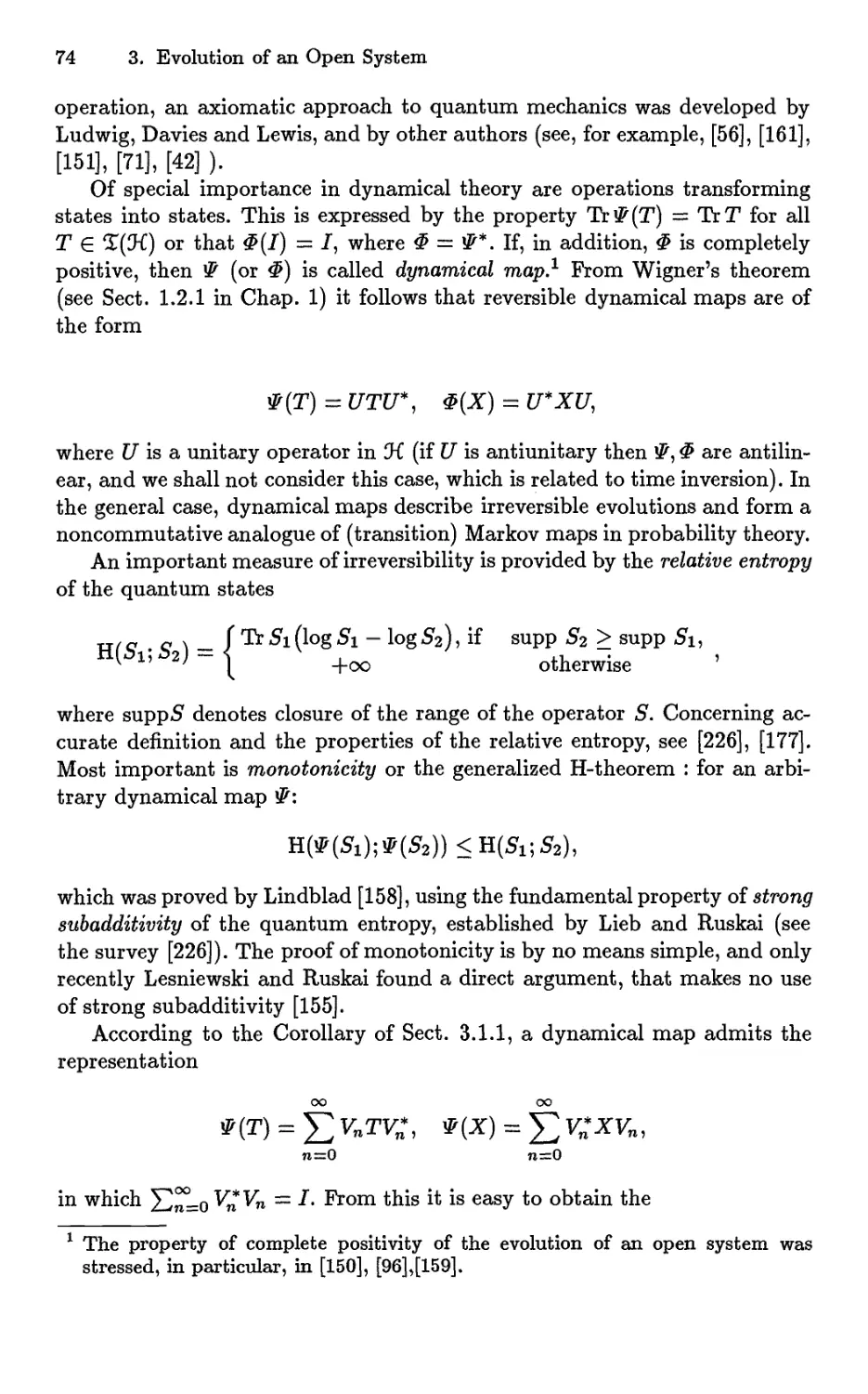
3.1 Transformations of Quantum States
and Observables 71
3.1.1 Completely Positive Maps 71
3.1.2 Operations, Dynamical Maps 73
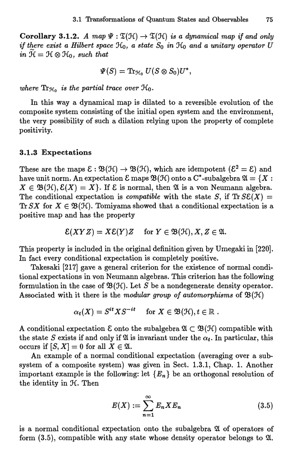
3.1.3 Expectations 75
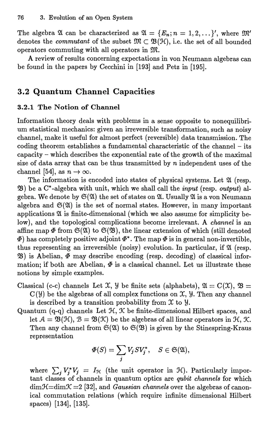
3.2 Quantum Channel Capacities 76
3.2.1 The Notion of Channel 76
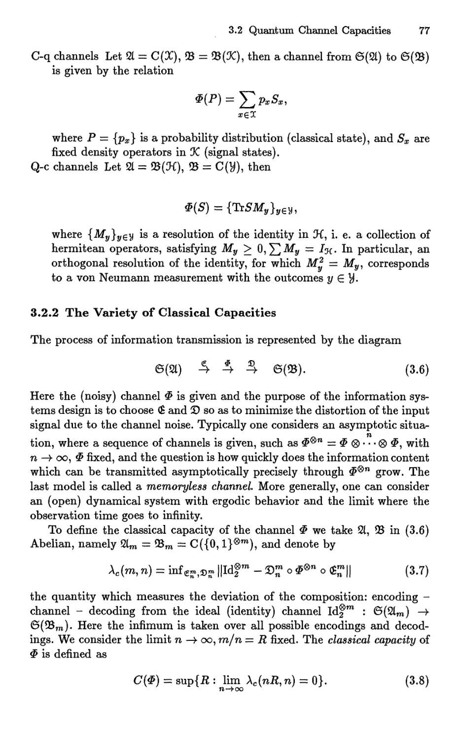
3.2.2 The Variety of Classical Capacities 77
3.2.3 Quantum Mutual Information 79
3.2.4 The Quantum Capacity 80
3.3 Quantum Dynamical Semigroups 81
3.3.1 Definition and Examples 81
3.3.2 The Generator 83
3.3.3 Unbounded Generators 85
3.3.4 Covariant Evolutions 88
3.3.5 Ergodic Properties 91
3.3.6 Dilations of Dynamical Semigroups 93
Repeated and Continuous
Measurement Processes 97
4.1 Statistics of Repeated Measurements 97
4.1.1 The Concept of Instrument 97
4.1.2 Representation of a Completely Positive Instrument .. 100

Contents IX
4.1.3 Three Levels of Description of Quantum Measurements 102
4.1.4 Repeatability 103
4.1.5 Measurements of Continuous Observables 105
4.1.6 The Standard Quantum Limit 106
4.2 Continuous Measurement Processes 108
4.2.1 Nondemolition Measurements 108
4.2.2 The Quantum Zeno Paradox 109
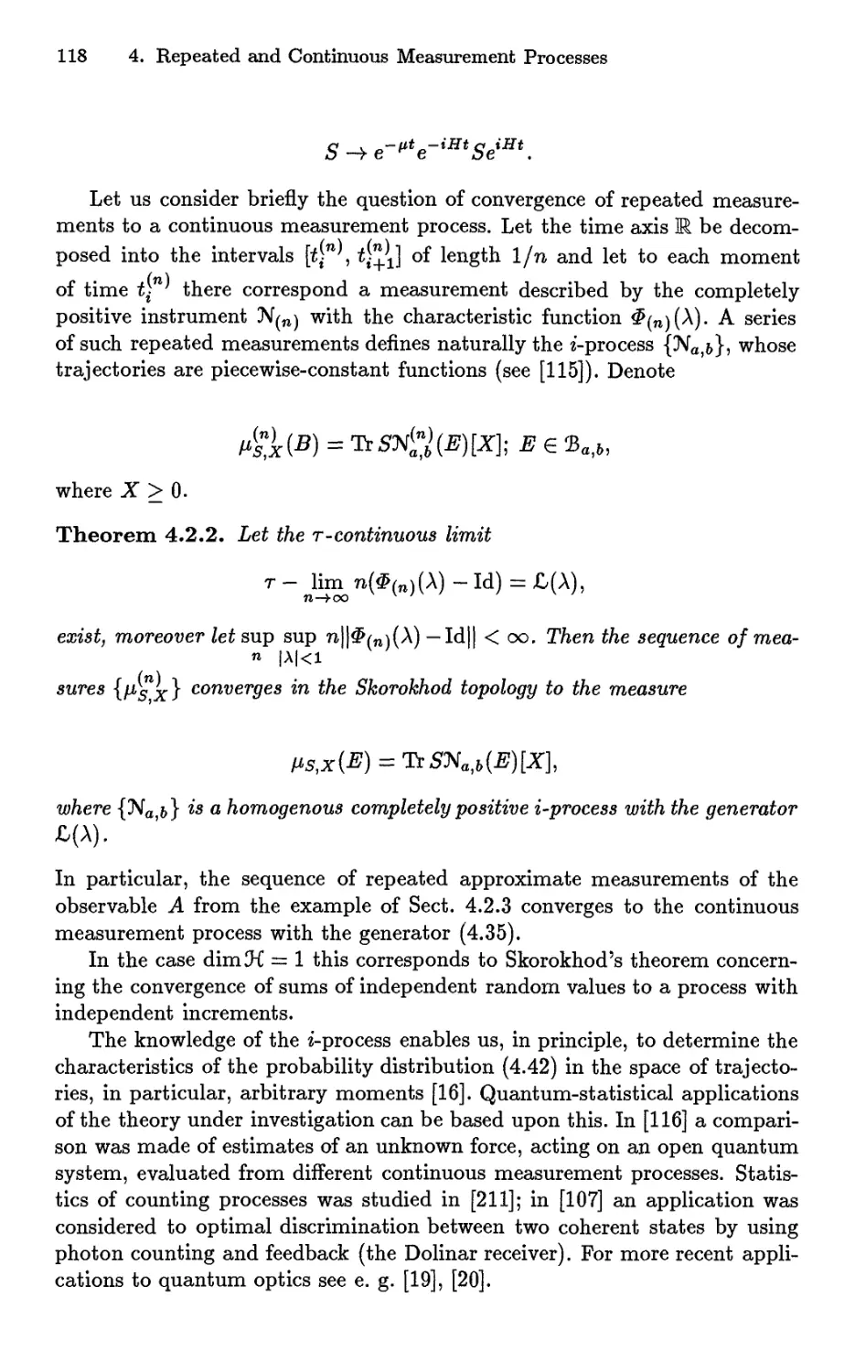
4.2.3 The Limit Theorem for Convolutions of Instruments . . Ill
4.2.4 Convolution Semigroups of Instruments 113
4.2.5 Instrumental Processes 115
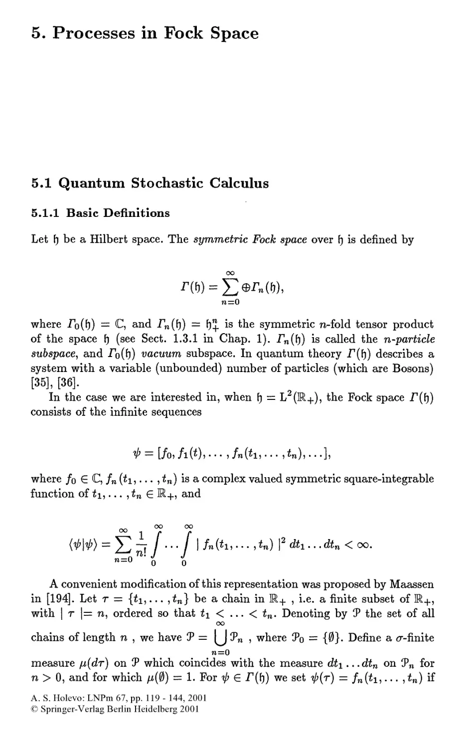
5. Processes in Fock Space 119
5.1 Quantum Stochastic Calculus 119
5.1.1 Basic Definitions 119
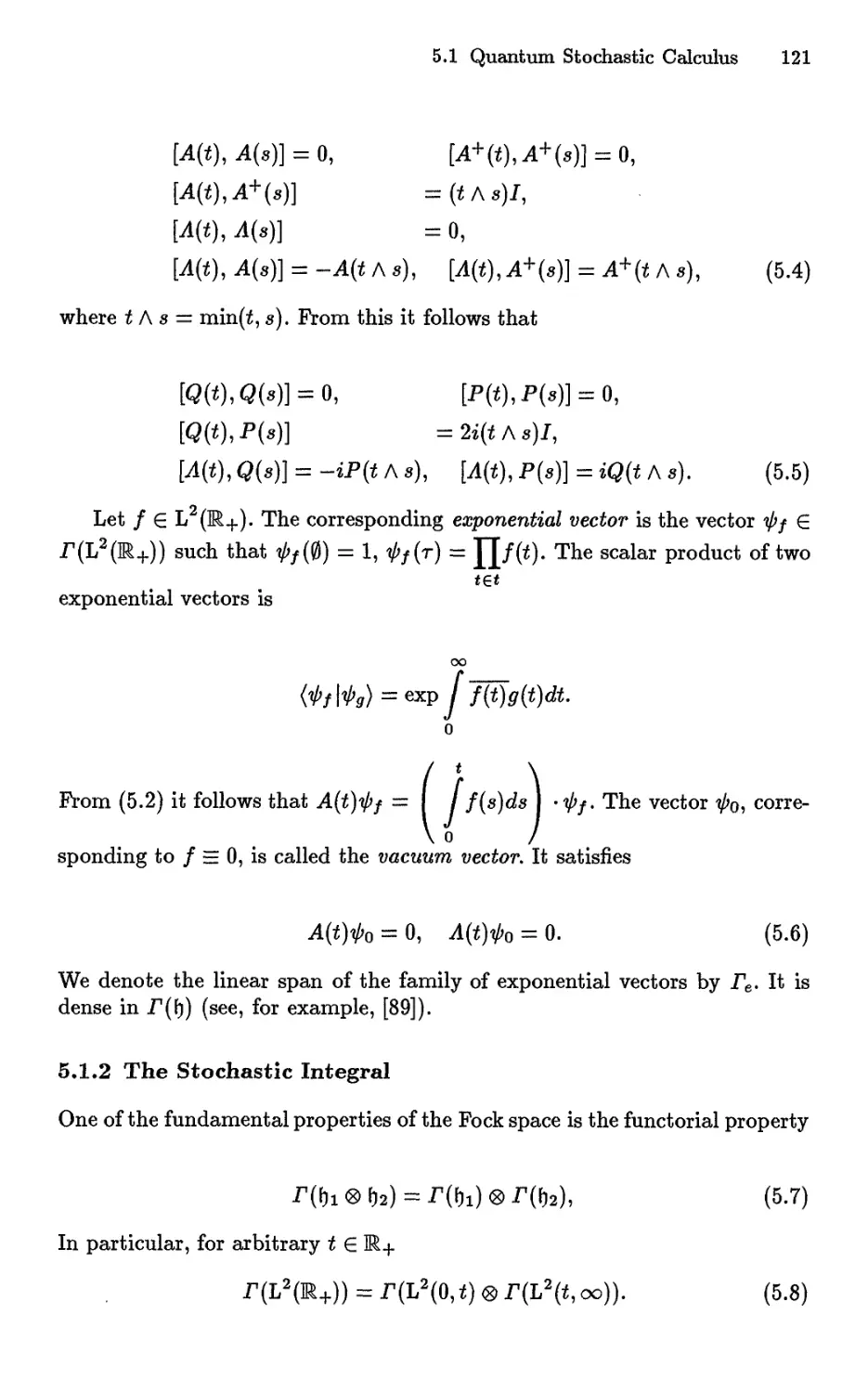
5.1.2 The Stochastic Integral 121
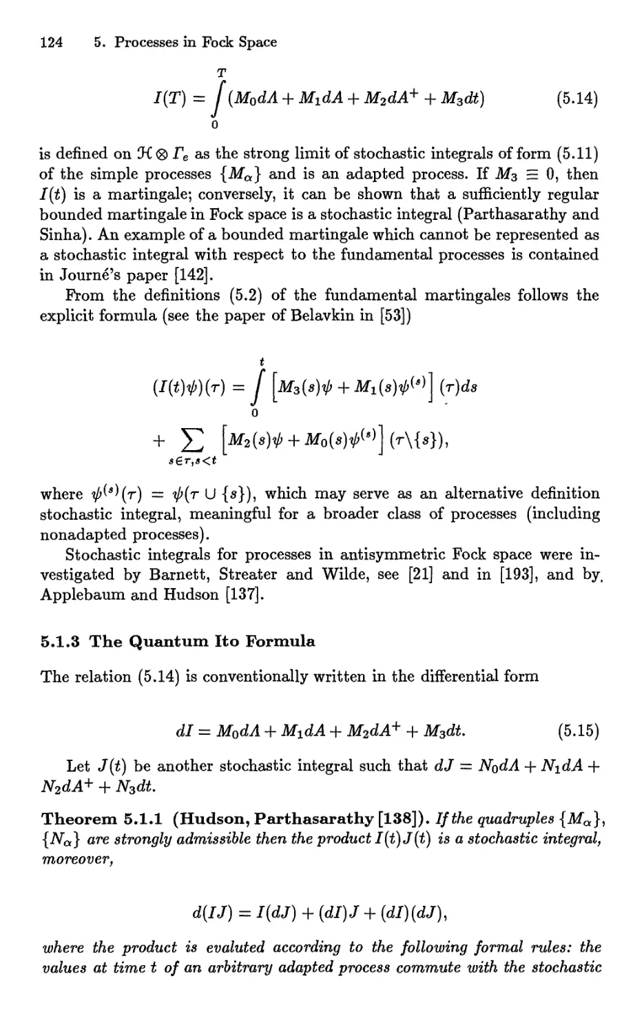
5.1.3 The Quantum Ito Formula 124
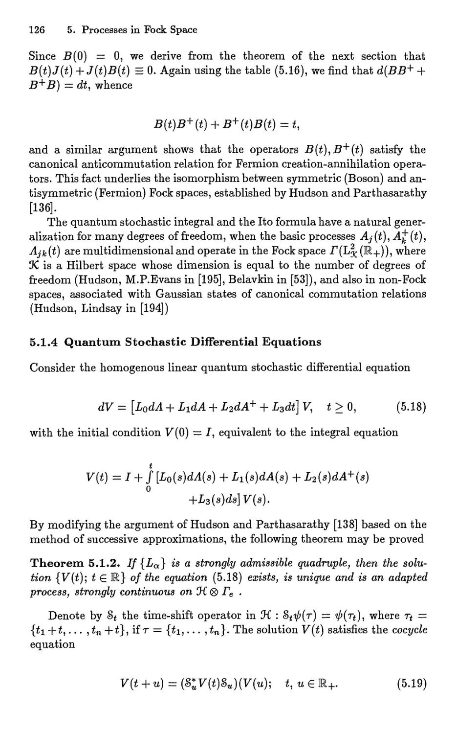
5.1.4 Quantum Stochastic Differential Equations 126
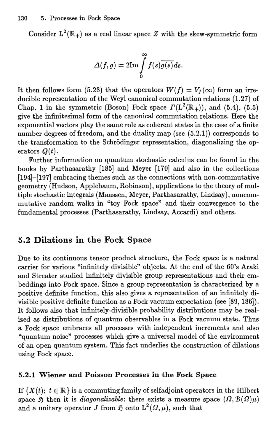
5.2 Dilations in the Fock Space 130
5.2.1 Wiener and Poisson Processes in the Fock Space 130
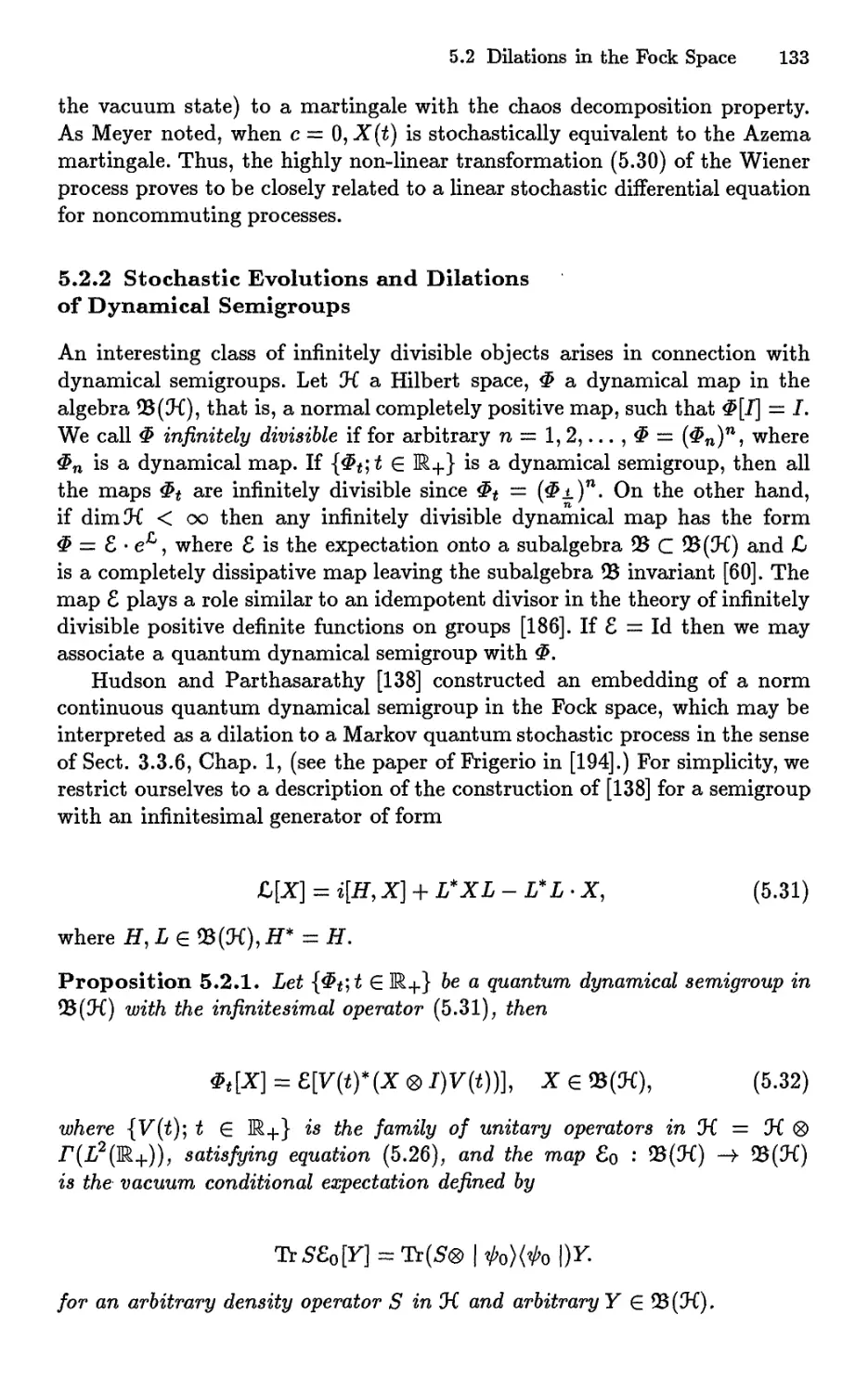
5.2.2 Stochastic Evolutions and Dilations
of Dynamical Semigroups 133
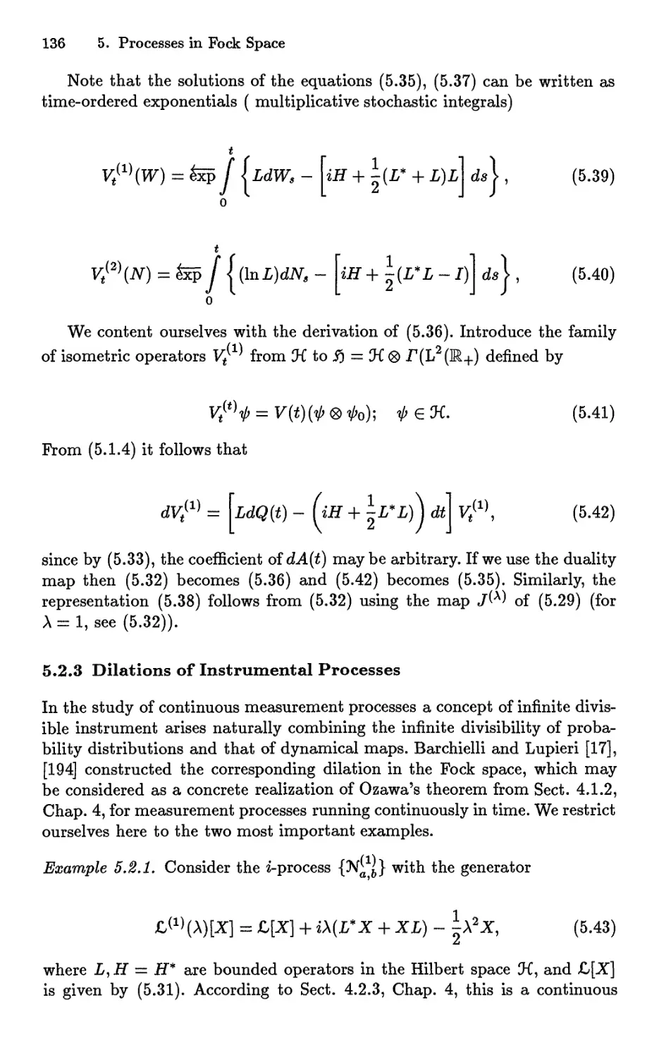
5.2.3 Dilations of Instrumental Processes 136
5.2.4 Stochastic Representations
of Continuous Measurement Processes 138
5.2.5 Nonlinear Stochastic Equations of Posterior Dynamics 140
Bibliography 145
Index
157

0. Introduction
0.1 Finite Dimensional Systems
Exposition of probability theory usually begins with a finite scheme.
Following this tradition, consider a finite probabilistic space Q := {1,..., JV}. Three
closely interrelated facts express in different ways the classical character of
the probabilistic scheme:
1. the set of events A C O forms a Boolean algebra,
2. the set of probability distributions P — [pi,.. . ,Pjv] on Q is a simplex,
that is a convex set in which each point is uniquely expressible as a
mixture (convex linear combination) of extreme points,
3. the set of random variables X — [Ai,..., Ajv] on fi forms a commutative
algebra (under pointwise multiplication).
The quantum analogue of this scheme is the model of a JV-level system.
The analogue of probability distribution - the state of such a system - is
described by a density matrix, that is a JV x JV Hermitian matrix 5, which is
positive definite and has unit trace:
5>0, TrS=l. (0.1)
The analogue of random variable - an observable - is described by an arbitrary
N x N Hermitian matrix X. Let
n
3=1
be the spectral representation of the Hermitian matrix X, where x\ < X2 <
■ • • < xn are the eigenvalues and E\,E2,..., En are the projectors onto the
corresponding eigenspaces. The family E = {Ej\ j = 1,.. .,n} forms an
orthogonal resolution of identity:
n
EjEk = SjkEj, 2_jEj = J, (0.3)
3=1
where I is the unit matrix. From the properties (0.1) and (0.3) it follows that
the relation
A. S. Holevo: LNPm 67, pp. 1-11, 2001
© Springer-Verlag Berlin Heidelberg 2001

2 0. Introduction
lt§ {xj) := Tr SEj for j = 1,..., n, (0.4)
defines a probability distribution on the spectrum SpX = {xi,...,a?n} of
the observable X. In quantum mechanics it is postulated that this is the
probability distribution of the observable X in the state S. In particular the
mean value of X in the state S is equal to
Es(X)=TrSX. (0.5)
If in this model we consider only diagonal matrices
then we return to the classical scheme with N elementary events, where,
in particular (0.5) reduces to Es(X) = Ylj=iPj^j- We obtain the same by
considering only simultaneously diagonalizable (that is commuting) matrices.
Since there are observables described by noncommuting matrices, the model
of AT-level system does not reduce to this classical scheme.
The role of indicators of events in the quantum case is played by
observables having the values 0 or 1, that is by idempotent Hermitian matrices,
E2 — E. Introducing the unitary coordinate space % — CN in which the
N x N- matrices operate, we may consider such a matrix E as an
orthogonal projector onto a subspace £ in 3i. In this way, quantum events can be
identified with subspaces of the unitary space %. The set of quantum events,
called the quantum logic, is partially ordered (by the inclusion) and possesses
the operations 8.± V 8.2 (defined as the linear hull Lin (£1, £2) of the subspaces
£1, £2 C 0i), £1 A £2 (defined as the intersection £1 C\ £2 of the subspaces
£1, £2 C Oi) and £' (defined as the orthogonal complement £x of £ C 0i)
with the well known properties. The non-classical character of the model of
JV-level system can be expressed in three different ways:
1. the quantum logic of events is not a Boolean algebra; we do not have the
distributivity law
£1 A (£2 V £3) = (£1 A £2) V (£1 A £3)
does not hold. Consequently there are no "elementary events" into which
an arbitrary quantum event could be decomposed;
2. the convex set of states is not a simplex, that is, the representation of a
density matrix as a mixture of extreme points is non-unique;
3. the complex linear hull of the set of observables is a non-commutative
(associative) algebra.
In the infinite-dimensional case, instead of the matrices one has to
consider operators acting in a certain Hilbert space "K. A mathematical exposition

0.2 General Postulates of Statistical Description 3
of the fundamental concepts of quantum mechanics in Hilbert space was first
given by J. von Neumann [175]. In particular he emphasized the distinction
between Hermitian (symmetric) and selfadjoint operators, which, of course,
had not occured in the preceding physicists' works, and pointed out that
it is in fact the condition of selfadjointness, which in the case of infinite
dimensional Hilbert spaces underlies an analogue of the spectral decomposition
(0.2). Another circle of problems in the case of an arbitrary Hilbert space is
associated with the concept of trace and the corresponding class of operators
with finite trace. This mathematical scheme, called the standard statistical
model of quantum mechanics, will be reviewed in the Chap. 1.
0.2 General Postulates of Statistical Description
Each of the mathematical structures - the quantum logic of events, the convex
set of states and the algebra of quantum observables - can be characterized
by certain system of axioms, but the characterization problems arising in
this way are highly nontrivial and constitute essentially separate research
field, a review of which goes beyond the scope of the present notes (see, in
particular [206], [162], [66], [71], [161], [222]). Since we are dealing with a
concrete object - the quantum theory in a Hilbert space - we do not have
to resort to one or another type of axiomatic systems; furthermore, it is
precisely the peculiar characteristics of this concrete object which provide the
fundamental motivation for various axiomatic schemes. However, one useful
lesson of the axiomatic approach is the revelation of the fruitful parallelism
between statistical descriptions of classical and quantum systems. The axioms
below are modifications of the first four axioms from [162] that are equally
applicable to both classical and quantum systems.
Axiom 1 Let there be a given set & whose elements are called states and a
set 0 whose elements are called (real) observables. For arbitrary S G <S and
X G 0 there is a probability distribution fi* on the cr-algebra 23 (M) of Borel
subsets of the real line M, called the probability distribution of the observable
X in the state S.
The state S is interpreted as a more or less detailed description of the
preparation of a statistical ensemble of independent individual
representatives of the system under consideration, and the observable X - as a quantity,
which can be measured by a definite apparatus for each representative in the
given ensemble. Axiom 1 thus presupposes the reproducibility of the
individual experiments and the stability of frequencies under independent repetitions.
The following axiom expresses the possibility of the mixing of ensembles.
Axiom 2 For arbitrary Si, S2 G <S and an arbitrary number p with 0 < p <
1, there exists S G <S such that fi* = pfj,^ + (1 — p)/^ for all X G O. S is
said to be a mixture of the states Si and S2 in the proportion p : (1 — p).

4 0. Introduction
The following axiom describes the possibility of processing the information
obtained from a measurement of observable. Let / be a Borel function from
R to R. UXUX2£D are such that for all S £ 6, B £ £(M)
»s2(B)=^1(f~1(B))
where f~1(B) := {x £ M : f(x) £ B}, then the observable X2 is functionally
subordinate to the observable Xi. In this case we shall write X2 — f o X\.
Axiom 3 For arbitrary X\ £ O and an arbitrary Borel function f there
exists X2 £ O, such that X2 = / o X\.
A pair of non-empty sets (6,0) satisfying the axioms 1 - 3 is said to be a
statistical model. The statistical model is said to be separated if the following
axiom is valid.
Axiom 4 From the fact that jj^ = //J for allX £ Q it follows that Si — S2
and from jjl*1 = jjl*2 for all S £ 6 it follows that X\ — X2.
For a separated model both the operation of mixing in @ and the
functional subordination in O are uniquely defined. Thus the set of states @
obtains a convex structure and the set of observables O - a partial ordering.
Observables X\,..., Xm are called compatible if they are all functionally
subordinate to some observable X, that is, Xj = fjoX for j = 1,.. .,m.
Compatible observables can be measured in a single experiment. The
observables which are compatible with all observables X £ O form the center or
the classical part of the statistical model.
0.3 Classical and Quantum Systems
Let (/?, !B(/?)) be a measurable space, let ^{Q) be the convex set of all
probability measures on Q and let O(O) be the set of all real random variables
with the natural relation of functional subordination. Let fip defined by
l4{B) := P{X-X{B)), B £ £(M)
be the probability distribution of the random variable X £ Q(Q) with
respect to the probability measure P £ ^{Q). The pair (^J(/?), £)(/?)) forms
a separable statistical model, which we call the Kolmogorov model. In this
model all observables are compatible and the center is all of O(O).
The statistical model for a iV-level quantum system was described in Sect.
0.1. If observable X has spectral decomposition (0.2), then the observable
/ o X is naturally defined as
n

0.4 Randomization in Classical and Quantum Statistics 5
Quantum observables X\,..., Xm are compatible if and only if the
corresponding matrices commute, that is
X{Xj = XjXi for i, j = 1,..., m.
The center of this model is trivial: it consists of the matrices which are
multiples of the identity; that is, only of the constant observables.
Existence of incompatible observables is a manifestation of the quantum
principle of complementarity. Physical measurements on microobjects are
implemented by macroscopic experimental devices, each of which requires
a complex and specific organization of the environment in space and time.
Different ways of such organization, corresponding to measurements of
different observables, may be mutually exclusive (despite the fact that they relate
to the identically prepared microobject); that is, complementary.
Complementarity is the first fundamental distinction between quantum and classical
statistical models.
One of the most controversial problems of quantum theory is that of
"hidden variables"; that is, the question of whether it is possible in principle to
describe quantum statistics in terms of a classical probability space. The first
attempt to prove the impossibility of introducing hidden variables was made
by J. von Neumann in [175] and for some time his arguments were held to
be decisive. In 1966 J. Bell, by analyzing Einstein-Podolski-Rosen paradox,
had shown the incompleteness of von Neumann's "proof" and distinguished
another fundamental property of the quantum-mechanical description which
may be called nonseparability. Mathematically it is related to the
superposition principle and to the fact that composite quantum systems are described
by tensor products rather than by the Cartesian products of classical
probability theory.
Complementarity and nonseparability are the fundamental properties of
quantum statistics underlying non-existence of physically acceptable hidden
variables theories (see Sect. 1.4 in Chap. 1).
0.4 Randomization in Classical and Quantum Statistics
Let us consider a classical random variable with a finite set of values {xj}.
Such a random variable can be represented in the form (0.2), namely
X = J2XjEj (0.7)
3=1
where Ej := 1bj is the indicator of the set Bj := {u> £ Q : X(u>) = Xj}. The
sets Bj (j = 1,..., n) form a partition of Q. At each point co £ Q observable
(0.7) assumes, with probability 1, one of the values Xj.

6 0. Introduction
In mathematical statistics, in particular, in statistical decision theory, it is
useful to consider "randomized" variables which are determined by
probabilities Mj(co) G [0,1] of taking the values Xj for the arbitrary elementary event
u>. The collection of functions M := {Mj : j = 1,..., n} is characterized by
the properties
n
mj (w) > o, J2 M3 (w)= l for a11 u e Q (°-8)
and describes an inexact measurement of the random variable X; that is,
a measurement subject to random errors. In particular, the measurement
is exact (without error) if Mj(u) = Ej(w). The probability distribution of
this measurement with respect to the probability measure P is given by the
formula
lt¥(xj) = jp(du,)MJ(u>) (0.9)
n
In this way arises another classical statistical model, the Wald model, after
the originator of statistical decision theory.
It is natural to introduce quantum analogue of the Wald model, in which
an observable with a finite set of values is described by a finite resolution of the
identity] that is, a collection of matrices (operators) M = {Mj : j = 1,..., n}
in the Hilbert space Oi of the system, satisfying the conditions
n
Mj>0, Y^Mi = 1- (°-10)
3=1
In analogy with (0.9) the probability of the j-th. outcome in the state
described by density operator S is
/if(xj)=TrSMj. (0.11)
It is possible to generalize these definitions to observables with arbitrary
outcomes. In this way one obtains the generalized statistical model of quantum
mechanics (see Sect. 2.1 of Chap. 2).
Non-orthogonal resolutions of the identity entered quantum theory in the
70-es through the study of quantum axiomatics [161], [71], the
repeatability problem in quantum measurement [56], the quantum statistical decision
theory [100] and elsewhere.
0.5 Convex Geometry and Fundamental Limits
for Quantum Measurements
In the 1940-50s D. Gabor and L. Brillouin suggested that the quantum-
mechanical nature of a communication channel imposes specific fundamental

0.5 Convex Geometry and Fundamental Limitsfor Quantum Measurements 7
restrictions to the rate of transmission and accuracy of reproduction of
information. This problem became important in the 60s with the advent of
quantum communication channels - information transmission systems using
coherent laser radiation. In the 70s a consistent quantum statistical decision
theory was created, which gave the framework for investigation of
fundamental limits of accuracy and information content of physical measurement (see
[94], [105]). In this theory, the measurement statistics is described by
resolutions of the identity in the Hilbert space of the system and the problems of
determining the extremum of a functional, such as uncertainty or Shannon
information, is solved in a class of quantum measurements subjected to some
additional restrictions, such as unbiasedness, covariance etc. (see Chap. 2).On
this way the following property of information openness was discovered: a
measurement over an extension of an observed quantum system, including
an independent auxiliary quantum system, may give more information about
the state of observed system than any direct measurement of the observed
system.
This property has no classical analog - introduction of independent
classical systems means additional noise in observations and can only reduce the
information- and therefore looks paradoxical. Let us give an explanation from
the viewpoint of the generalized statistical model of quantum mechanics.
Although the above generalization of the concept of an observable is
formally similar to the introduction of randomized variables in classical
statistics, in quantum theory nonorthogonal resolutions of the identity have much
more significant role than merely a mean for describing inexact
measurements. The set of resolutions of the identity (0.10) is convex. This means
that in analogy with mixtures of different states one can speak of mixtures of
the different measurement statistics'. Physically such mixtures arise when the
measuring device has fluctuating parameters. Both from mathematical and
physical points of view, the most interesting and important are the extreme
points of the convex set of resolutions of the identity, in which the classical
randomness is reduced to an unavoidable minimum. It is these resolutions of
the identity which describe the statistics of extremally informative and
precise measurements optimizing the corresponding functionals. In the classical
case, the extreme points of the set (0.8) coincide with the non-randomized
procedures {Ej : j = 1,..., n}, corresponding to the usual random variables.
However, in the quantum case, when the number of outcomes n > 2, the
extreme points of the set (0.10) are no longer exhausted by the orthogonal
resolutions of the identity (see Sect. 1.3 of Chap. 2). Therefore to describe
extremally precise and informative quantum measurements, nonorthogonal
resolutions of the identity become indispensable.
On the other hand, as M.A. Naimark proved in 1940, an arbitrary
resolution of the identity can be extended to an orthogonal one in an enlarged
Hilbert space. This enables us to interpret a nonorthogonal resolution of the
identity as a standard observable in an extension of the initial quantum sys-

8 0. Introduction
tern, containing an independent auxiliary quantum system. In this way, a
measurement over the extension can be more exact and informative than an
arbitrary direct quantum measurement. This fact is strictly connected with
the quantum property of nonseparability, mentioned in n. 0.3.
In the 90s, stimulated by the progress in quantum communications,
cryptography and computing, the whole new field of quantum information
emerged (see e. g. [32], [176]). The emphasis in this field is not only on
quantum bounds, but mainly on the new constructive possibilities concealed in
the quantum statistics, such as efficient quantum communication protocols
and algorithms. A central role here is played by quantum entanglement, the
strongest manifestation of the quantum nonseparability.
0.6 The Correspondence Problem
One of the difficulties in the standard formulation of quantum mechanics lies
in the impossibility of associating with certain variables, such as the time,
angle, phase, a corresponding selfadjoint operator in the Hilbert space of the
system. The reason for this lies in the Stone-von Neumann uniqueness
theorem, which imposes rigid constraints on the spectra of canonically conjugate
observables. To this circle of problems also are belong the difficulty with lo-
calizability (i.e. with the introduction of covariant position observables) for
relativistic quantum particles of zero mass.
By considering nonorthogonal resolutions of the identity as observables
subject to the covariance conditions arising from the canonical commutation
relations, one can to a significant extent avoid these difficulties (see Chap.
2). The general scheme of this approach is to consider the convex set of
resolutions of the identity satisfying the covariance condition, and to
single out extreme points of this set minimizing the uncertainty functional in
some state. In this way one obtains generalized observables of time, phase
etc. described by nonorthogonal resolutions of the identity. In spectral theory
nonorthogonal resolutions of the identity arise as generalized spectral
measures of non-selfadjoint operators. For example, the operator representing the
time observable, turns out to be a maximal Hermitian operator which is not
selfadjoint. One may say that at the new mathematical level the generalized
statistical model of quantum mechanics justifies a "naive" physical
understanding of a real observable as a Hermitian, but not necessarily selfadjoint
operator.
0.7 Repeated and Continuous Measurements
In classical probability irreversible transformations of states are described by
using conditional probabilities. Let a value Xj be obtained as a result of a

0.7 Repeated and Continuous Measurements 9
measurement of the random variable (0.7). Here the classical state, that is,
the probability measure P(du) on Q is transformed according to the formula
of conditional probability
fP(du)Ej{w)
HA)->P(A\Bi) = *p(dM)EM WGJKfl). (0.12)
n
Clearly, if there is no selection according to the result of the measurement,
the state P does not change:
n
P(A) -> $>(ii | Bi)P(Bj) = P(A)- (0.13)
i=i
In quantum statistics, the situation is qualitatively more complicated.
The analog of the transformation (0.12) is the well known von Neumann
projection postulate
Ei SEj
S^S< = Tts£< (°-14>
where S is the density operator of the state before the measurement, and Sj is
the density operator after the measurement of the observable (0.2), giving the
value Xj. The basis for this postulate is the phenomenological repeatability
hypothesis assuming extreme accuracy and minimal perturbation caused by
the measurement of the observable X. If the outcome of the measurement
is not used for a selection, then the state S is transformed according to the
formula analogous to (0.13):
n n
s -+y,sw*m = Y,EJSEj' (°-15)
3=1 i=i
However, in general Y^j=i Bj^Bj / ^5 this means? that the change of the
state in the course of quantum measurement does not reduce simply to the
change of information but also incorporates an unavoidable and irreversible
physical influence of the measuring apparatus upon the system being
observed. A number of problems is associated with the projection postulate;
leaving aside those of a philosophical character, which go beyond the limits
of probabilistic interpretation, we shall comment on concrete problems which
are successfully resolved within the framework of generalized statistical
models of quantum mechanics.
One principal difficulty is the extension of the projection postulate to ob-
servables with continuous spectra. To describe the change of a state under
arbitrary quantum measurement, the concept of instrument, that is a measure
with values in the set of operations on quantum states, was introduced [59].

10 0. Introduction
This concept embraces inexact measurements, not satisfying the condition of
repeatability and allows to consider state changes under measurements of ob-
servables with continuous spectrum. A resolution of the identity is associated
with every instrument, and orthogonal resolutions of the identity correspond
to instruments satisfying the projection postulate. The concept of
instrument gives a possibility for describing the statistics of arbitrary sequence of
quantum measurements.
New clarification is provided for the problem of trajectories, coming back
to Feynman's formulation of quantum mechanics. A continuous (in time)
measurement process for a quantum observable can be represented as the
limit of a "series" of n repeated inexact measurements with precision
decreasing as s/n [16]. The mathematical description of this limit [115] reveals
remarkable parallels with the classical scheme of summation of independent
random variables, the functional limit theorems in the probability theory and
the Levy-Khinchin representation for processes with independent increments
(see Chap. 4). Most important examples are the analog of the Wiener process
- continuous measurement of particle position, and the analog of the Poisson
process - the counting process in quantum optics.
An outcome of continuous measurement process is a whole trajectory; the
state St of the system conditioned upon observed trajectory up to time t -
the posterior state - satisfies stochastic nonlinear Schrodinger equation. This
equation explains, in particular, why a wave packet does not spread in the
course of continuous position measurement [29] (see Chap. 5).
From a physical viewpoint, the whole new fields of the stochastic
trajectories approach in quantum optics [43] and decoherent histories approach
in foundations of quantum mechanics [77] are closely related to continuous
measurement processes.
0.8 Irreversible Dynamics
The reversible dynamics of an isolated quantum system is described by the
equation
S -> UtSU^1, -oo < t < oo, (0.16)
where {Ut : —oo < t < oo} is a continuous group of unitary operators. If
the system is open, i.e. interacts with its environment, then its evolution
is in general irreversible. An example of such an irreversible state change,
due to interaction with measuring apparatus, is given by (0.15). The most
general form of dynamical map describing the evolution of open system and
embracing both (0.16) and (0.15) is
s^^vjsv;, (0.17)
3

0.9 Quantum Stochastic Processes 11
where ]T)» V/Vj ^ I- Among all affine transformations of the convex set of
states, the maps (0.17) are distinguished by the specifically noncommutative
property of complete positivity, arising and playing an important part in the
modern theory of operator algebras.
A continuous Markov evolution of an open system is described by a
dynamical semigroup; that is, a semigroup of dynamical maps, satisfying certain
continuity conditions (see [56]). Dynamical semigroups, which are the non-
commutative analogue of Markov semigroups in probability theory, and their
generators describing quantum Markovian master equations, are discussed in
Chap. 3.
0.9 Quantum Stochastic Processes
One of the stimuli for the emergence of the theory of quantum stochastic
processes was the problem of the dilation of a dynamical semigroup to the
reversible dynamics of a larger system, consisting of the open system and its
environment. By the existence of such a dilation the concept of the
dynamical semigroup is rendered compatible with the basic dynamical principle of
quantum mechanics given by (0.16).
In probability theory a similar dilation of a Markov semigroup to a group
of time shifts in the space of trajectories of a Markov stochastic process is
effected by the well-known Kolmogorov-Daniel construction. A concept of
quantum stochastic process which plays an important role in the problem of
the dilation of a dynamical semigroup, was formulated in [2]. In the 80s the
theory of quantum stochastic processes turned into a vast field of research
(see in particular [194], [195], [196], [197]).
The analytical apparatus of quantum stochastic calculus, which in
particular permits the construction of nontrivial classes of quantum stochastic
processes and concrete dilations of dynamical semigroups, was proposed [138].
Quantum stochastic calculus arises at the intersection of two concepts,
namely, the time filtration in the sense of the theory of stochastic processes and
the second quantization in the Fock space. It is the structure of continuous
tensor product which underlies the connection between infinite divisibility,
processes with independent increments and the Fock space. Because of this,
the Fock space turns out to be a carrier of the "quantum noise" processes,
which give a universal model for environment of an open Markovian
quantum system. Quantum stochastic calculus is also interesting from the point of
view of the classical theory of stochastic processes. It forms a bridge between
Ito calculus and second quantization, reveals an unexpected connection
between continuous and jump processes, and provides a fresh insight into the
concept of stochastic integral [185], [170]. Finally, on this foundation
potentially important applications develop, relating to filtering theory for quantum
stochastic processes and stochastic trajectories approach in quantum optics
(see Chap. 5).

1. The Standard Statistical Model
of Quantum Mechanics
1.1 Basic Concepts
1.1.1 Operators in Hilbert Space
Several excellent books have been devoted to the theory of operators in
Hilbert space, to a significant extent stimulated by problems of quantum
mechanics (see, in particular, [7], [199]). Here we only recall certain facts and
fix our notations.
In what follows "K denotes a separable complex Hilbert space. We use
the Dirac notation for the inner product (ip\ij)), which is linear in if> and
conjugate linear in (p. Sometimes vectors of "K will be denoted as |^»), and the
corresponding (by the Riesz theorem) continuous linear functionals on 'K by
(tf>\. In the finite dimensional case these are the column and the row vectors,
correspondingly. The symbol I^X^I then denotes the rank one operator which
acts on a vector % G Oi as
\i>)(<p\x = i>(<p\x)-
In particular, if (tf}\tf>) = 1 then IV'XV'I ^s the projector onto the subspace
spanned by the vector if> G 'K. The linear span of the set of operators of the
form IV'X^I is the se* of operators of finite rank in "K.
The Dirac notation will be used also for densely defined linear ((|) and
antilinear (|)) forms on J{, which are not given by any vector in "K. Let, for
example, "K = L2(K) be the space of square-integrable functions if)(x) on the
real line WL. For every x G M. the relation
(x\if>) = i/>{x)
defines a linear form (x\ on the dense subspace Co(M) of continuous functions
with a compact support. This form is unbounded and not representable by
any vector in "K. Another useful example, which is just the Fourier transform
of the previous one is
1 /»<X>
■y ZttTi J-oo
A. S. Holevo: LNPm 67, pp. 13 - 38, 2001
© Springer-Verlag Berlin Heidelberg 2001

14 1. The Standard Statistical Model of Quantum Mechanics
defined on the subspace of integrable functions.
If X is a bounded operator in IK, then X* denotes its adjoint, defined by
(<p\X*$) = {X<p\ij>) iox <p,$ e%.
A bounded operator X G 93 (IK) is called Hermitian if X — X*. An isometric
operator is an operator U such that U*U = I, where I is the identity operator;
if moreover UU* = I, then U is called unitary. An (orthogonal) projection is
a Hermitian operator E such that E2 = E.
The Hermitian operator X is called positive (X > 0), if {ij)\Xij)) > 0 for
all -0 G IK. A positive operator has a unique positive square root, i.e. for any
positive operator B there exists one and only one positive operator A such
that A2 = B.
For a bounded positive operator T the trace is defined by
00
TrT:=5](ei|Tet-)<oo, (1.1)
t'=i
where {et} is an arbitrary orthonormal Hilbert base. The operator T belongs
to the trace class, if it is a linear combination of positive operators with
finite trace. For such an operator the trace is well defined as the sum of an
absolutely convergent series of the form (1.1). The set %(Ji) of all trace class
operators is a Banach space with respect to the trace norm
and the set of operators of finite rank is dense in %(IK).
The set £(IK) forms a two-sided ideal in the algebra 93 (IK), that is, it is
stable under both left and right multiplications by a bounded operator. The
dual of the Banach space %(3i) is isomorphic to 93 (IK), the algebra of all
bounded operators in IK, with the duality given by the bilinear form
(T,X) =TtTX for Te1{Ji),Xe 93{%). (1.2)
The subscript h will be applied to sets of operators to denote the
corresponding subset of Hermitian operators. For example, 93/j(J{) is the real
Banach space of bounded Hermitian operators in "K. Then %h{^)* = 93/j(J{),
with the duality given by (1.2) as before.
Along with the convergence in the operator norm in 93/j (3i) some weaker
concepts of convergence are often used. One says, the sequence {Xn}
converges to X
• strongly if lim llXn^ — Xi{>\\ — 0 for all tj) £ J{,
n-+oo
• weakly if lim {<p\Xni})) — (<p\Xtj)) for all <p, tj) £ % and
n—i-oo
• *-weakly if lim TrTXn =TrTX for all T G ZCX).
n—>-oo
If a sequence of operators {Xn} is bounded with respect to the norm and
Xn < Xn+i for all n, then Xn converges strongly, weakly and *-weakly to a
bounded operator X (denoted Xn t X).

1.1 Basic Concepts 15
1.1.2 Density Operators
These are the positive operators S of unit trace
5>0, TrS=l.
The set of density operators &(0{) is a convex subset of the real linear
space Tft(!K) of the Hermitian trace class operators. Furthermore it is the
base of the cone of positive elements which generates £&((K). A point S of a
convex set 6 called extreme if from S = pS± -f (1 — p)52, where Si, 52 E &
and 0 < p < 1, it follows that S± = S2 = S. The extreme points of the sets
&(0i) are the one-dimensional projectors
S* = h/>XVi (i.3)
1. Any density operator can be represented as a
00
3-1
where (VvlVv) = 1? Pj •> 0 and Y^TLiPj = !• ^ne suc^ representation is
given by the spectral decomposition of the operator S, when the i/>j are its
eigenvectors and the pj are the corresponding eigenvalues.
The entropy of the density operator S is defined as
H{S) = -TrSlogS = -^AjlogAj,
3
where Xj are the eigenvalues of S, with the convention 0 log 0 = 0 (usually
log denotes the binary logarithm). The entropy is a nonnegative concave
function on &{3~C), taking its minimal value 0 on the extreme points of &(Ji).
If d = dim!K < 00, then the maximal value of the entropy is logd, and it is
achieved on the density operator S = d-1I.
Consider the set (£(!K) of projectors in 3i, which is isomorphic to the
quantum logic of events (closed linear subspaces of %). A probability measure
on <£(!K) is a real function fj, with the properties
!• 0 < p{E) < 1 for all E E <8(JC),
2. if {Ej} C <S(9C) and EjEk = 0 whenever 3 / k and £. E}- = I then
In respond to a question of Mackey, Gleason proved the following theorem
(see [162], [185])
Theorem 1.1.1. Let dimOi > 3. Then any probability measure \i on <£(!K)
has the form
where if) E Oi and (if>\if>)
convex combination

16 1. The Standard Statistical Model of Quantum Mechanics
}i{E) = TrSE for all E € <S(IK), (1.4)
where S is a uniquely defined density operator.
The case dimlK = 2 is singular - for it one easily shows that there are
measures not representable in the form (1.4), however they did not find
application in quantum theory. The proof of Gleason's theorem is quite non-
trivial and generated a whole field in noncommutative measure theory,
dealing with possible generalizations and simplifications of this theorem. (See e.
g. Kruchinsky's review in [193]).
1.1.3 The Spectral Measure
Let X be a set equipped with a <r-algebra of measurable subsets 03 (X). An
orthogonal resolution of the identity in 'K is a projector-valued measure on
05(X), that is a function E : 03(X) -> (S(IK) satisfying the conditions
1. if J3i, B2 G 03(X) and Bx n J32 = 0, then E(B1)E(B2) = 0,
2. if {Bj} is a finite or countable partition of X into pairwise nonintersecting
measurable subsets, then ^ • E(Bj) = I , where the series converges
strongly.
Let X be an operator with dense domain T)(X) C X. We denote by T)(X*)
the set of vectors <p for which there exists xGlK such that
(<p\X<i{>) = (x\i>)foi:a\\i>eT>(X).
We define the operator X* with domain T)(X*) by X*<p = x- The operator
X is said to be Hermitian (symmetric) iflCI* {V{X) C V(X)* and
X = X* on D(X)), and selfadjoint if X = X*.
The spectral theorem (von Neumann, Stone, Riesz, 1929-1932) establishes
a one-to-one correspondence between orthogonal resolutions of identity E
on the tr-algebra 23(M) of Borel subsets of the real line M and selfadjoint
operators in 'K according to the formula
X- / xE(dx), (1.5)
— oo
where the integral is denned in appropriate sense (see [199]). The resolution
of the identity E is said to be the spectral measure of the operator X. For an
arbitrary Borel function / one defines the selfadjoint operator

1.1 Basic Concepts 17
oo
foX:= ! f{x)E{dx).
— oo
The spectral measure F of / o X is related to the spectral measure of the
operator X by
F{B) = Eif-^B)) for B e B(R).
We denote by Q(0i) the set of all selfadjoint operators in Oi.
1.1.4 The Statistical Postulate
With every quantum mechanical system there is associated a separable
complex Hilbert space Oi. The states of the system are described by the density
operators in Oi (elements of <&(0i)). Extreme points of &{0i) are called pure
states. A real observable is an arbitrary selfadjoint operator in Oi (element
of O(0i)). The probability distribution of the observable X in the state S is
denned by the Born-von Neumann formula
/*J(B) = Tr SE(B) for B e B(R), (1.6)
where E is the spectral measure of X. We call the separable statistical model
(<&(0i),Q(0i)) thus denned the standard statistical model of quantum
mechanics.
From (1.5) and (1.6) it follows that the mean value of the observable X
in the state S
oo
ES{X)= j x^{dx)
— oo
is given by
Es{X)=TrSX (1.7)
(at least for bounded observables). The mean value of the observable in a
pure state is given by the matrix element
Es,pr) = MJty>.
Abusing terminology one sometimes calls an arbitrary element X G %$(0i)
a bounded observable. The relation (1.7) defines a positive linear normalized

18 1. The Standard Statistical Model of Quantum Mechanics
( Es(J) = 1) functional on the algebra 03(IK); that is, a state in the sense
of the theory of algebras (the preceding argument explains the origin of this
mathematical terminology). A state on 03{%) defined by a density operator
by (1.7) is normal, meaning that if Xn f X, then Es{Xn) ->• Es(X).
A von Neumann algebra is an algebra of bounded operators in "K which
contains the unit operator and is closed under involution and under
transition to limits in the strong (or weak) operator topology. For an arbitrary
von Neumann algebra 03, just as for 03(IK), there is an associated statistical
model in which the states are normal states on 03, while the observables are
selfadjoint operators affiliated with 03 . Such models occupy an intermediate
place between quantum and classical (when 03 is commutative), and play an
important role in the theories of quantum systems of infinitely many degrees
of freedom - the quantum field theory and statistical mechanics (see e. g. [36],
[40], [66]).
1.1.5 Compatible Observables
The commutator of bounded operators X and Y is the operator
[X, Y] := XY - YX.
Operators X, Y commute if [X, Y] — 0. Selfadjoint operators X and Y are
called commuting if their spectral measures commute.
The following statements are equivalent:
1. The observables X±,.. .,Xn are compatible, that is, there exists an
observable X and Borel functions /i,..., /n such that Xj = fjoX for
3- l,-..,n.
2. The operators X±,..., Xn commute.
Indeed, if E±,..., En are the spectral measures of compatible observables
Xi,..., Xn, then there is a unique orthogonal resolution of the identity E on
(S>{Rn) for which
E{B1 x• • • x Bn) = Ei(Bi) • • • En{Bn) for {Bj : j = 1,..., n} C B(R),
called the joint spectral measure of the operators X±,..., Xn.
The existence of incompatible observables is a manifestation of the
quantum complementarity. A quantitative expression for it is given by the
uncertainty relation. For observables X, Y having finite second moments with
respect to the state S (the n-th moment of a observable X with respect to
the state S is defined by J xnfj,-§ (dx)), the following bilinear forms are well
defined:

1.1 Basic Concepts 19
(X,Y)S := tt{TrYSX), [X,Y]S := 2%{TrYSX)
(see [105] Chap. 2). Let X := {Xi,...,Xn} be an arbitrary collection of
observables with finite second moments. Let us introduce the real matrices
DS(X):= ((Xi-IEsiX^Xj-IEsiXj)),)
\ /%,j = l,...,n
C5(X):= ([*,,Jtys).. .
\ /t,j=l,...,n
From positive definiteness of the sesquilinear forms (X, Y) —>■ Tr Y*SX and
{X,Y) ->• TrX5y* follows the inequality
DS(X)>±^CS(X), (1.8)
where the left and the right hand side are considered as complex Hermitian
matrices1. For two observables X = X\ and Y = X2 the inequality (1.8) is
equivalent to the Schrodinger-Robertson uncertainty relation
Ds(X)Ds(y) > (X - IES(X),Y- IES(Y))2 + \[X,Y]2S, (1.9)
where
(X)
BS(X)= J {x-Es(X))2^(dx)
—00
is the variance of the observable X in the state S. If X, Y are compatible
observables then the quantity
00 00
(X-IES(X),Y-IES(Y))S= j j {x-Es{X)){y-Es{Y))fifY{dxdy)
—00 —00
represents the covariance of X, Y in the state 5; in this case [X, Y]s = 0 and
(1.9) reduces to the Cauchy-Schwarz inequality for covariances of random
variables. For arbitrary bounded Hermitian operators X, Y
1 This inequality is due to Robertson; it was rediscovered later by many authors
(see [64]).

20 1. The Standard Statistical Model of Quantum Mechanics
{X,Y)s=TrSXoY, (1.10)
where
XoY :=UxY + YX)
is the Jordan (symmetrized) product of the operators X, Y. Quantities of the
form (1.10) are called correlations in quantum statistical mechanics, although
if the observables X, Y are not compatible, they are not associated in any
simple way with measurement statistics of X and Y.
A detailed review of various generalizations of the uncertainty relation
can be found in [64].
1.1.6 The Simplest Quantum System
In physics, a finite-dimensional Hilbert space usually describes internal
degrees of freedom (spin) of a quantum system. The case dimiK = 2 corresponds
to the minimal nonzero spin |. Consider two-dimensional Hilbert space 3i
with the canonical basis
it>=(J). u>=(j)- (i-n)
An important basis in D(3i) is given by the matrices
/:=(oi)' °"i:=(io)' a2:=\i~o)' °"3:=(o-°i)-
The matrices cr,- called the Pauli matrices arise from a unitary representation
of euclidean rotations in 3i and express geometry of the particle spin. In
quantum computation this simplest system describes an elementary memory
cell of a quantum computer - the qubit [212], [32]. Here the action of Pauli
matrices describes elementary errors which can happen in this cell: the spin
flip (Ti, the phase error cr3, and their combination cr2 = icricr^ .
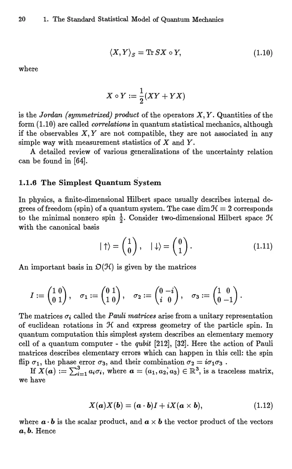
If X(a) := X)i=i°*<r*» where a ~ (01,02,'03) G M3, is a traceless matrix,
we have
X{a)X{b) = {a-b)I + iX{axb), (1.12)
where a - b is the scalar product, and a x b the vector product of the vectors
a, 6. Hence

1.1 Basic Concepts 21
TtX{a)X{b)=2a-b. (1.13)
Each density matrix can be expressed uniquely in the form
S(a) = i(l+ *■(*.)), (1.14)
where \a\ < 1. Thus as a convex set &(0i) is isomorphic to the unit ball in
M3, moreover the pure states correspond to points of the sphere \a\ = 1. In
this case
5(o) = Wo)X^(o)|, (1.15)
where
^fa)_[cos(/5/2)e(--/2)-
f[a) ~ [sin(/5/2)e(-/2)
is the unit vector of the state, and cos/5 = a3,sin/3e*a = ai + ia,2. The
parameters ck,/5 are the Euler angles of the unit vector a £ M3, describing the
direction of the particle spin. Pure states with |<x| = 1 are "completely
polarized" states with the definite direction of the spin, while their mixtures with
\a\ < 1 are "partially polarized". To a — 0 corresponds the "chaotic state"
5(0) = |J. A natural particle source usually provides chaotic state, while
a completely polarized state is prepared by "Stern-Gerlach filter" involving
application of an inhomogeneous magnetic field with gradient in the direction
a [187].
Since from (1.14) using (1.13) (y>(a)|V>(-a)) = TrS(a)S(-a) = 0, the
spectral decomposition of the observable X(a) is
X(a) = \i>(a)M*)\ ~ W-a)Xtf(-a)|, (\a\ = 1).
Thus the observable X(a) assumes the values ±1, with the probabilities
TrS(6)S(±a) = i(l±a-6)
in the state 5(6) (|fr| < 1).
The observable \X{a) (where h is the Dirac constant) describes the spin
component in the direction a. Prom (1.12) it follows that the observables
X(a),X(b) are compatible if and only if a and b are collinear. The Stern-
Gerlach devices measuring X(a),X(b) require application of inhomogeneous
magnetic fields with corresponding gradients, and hence are complementary
to each other.

22 1. The Standard Statistical Model of Quantum Mechanics
1.2 Symmetries, Kinematics, Dynamics
1.2.1 Groups of Symmetries
Consider a separable statistical model (©,£)). Let there be given a pair of
bijective (one-to-one onto) mappings & : <S —> <S and #:£)—>•£) such that
HX) _ x
for all S € & and X € O. Prom this it follows that \P is an affine map, that
is
n n
»=i *=i
for pi > 0, Yui^iP* = ■"•• We s^all call the map # a symmetry in the state
space, and the map # the corresponding symmetry in the space of observables.
Theorem 1.2.1 (Wigner). Every symmetry of the space of quantum states
&(0-C) has the form
IP (5) = USU*, (1.16)
where U is a unitary or antiunitary operator in 0-C.
For mean values of observables we have
E*(S)(-X") = Tr#{S)X = TrS#*{X) = ES{#*{X)),
where
&*{X) = U*XU. (1.17)
From the statistical viewpoint the transformation (1.16) of states is equivalent
to the transformation (1.17) of observables. In the first case one speaks of
the Schrodinger picture and in the second of the Heisenberg picture.
Let G be a group and let g -> \Pg a map from G into the group of
symmetries of &(0i) such that
*gi-g* = *gi ' *g* for all ffi, flf2 € G.

1.2 Symmetries, Kinematics, Dynamics 23
If G is a connected topological group and the map g —>■ )Pg is continuous,
then \Pg can be represented as
#g(S)=UgSUg*,
where g —>■ Ug is a projective unitary representation of the group G in the
space ft; that is, all Ug are unitary operators and satisfy the equation
Ug1Ug2=u{gi,g2)Ug1g3, (1.18)
where (gi, g2) —>■ w(<jfj., g2) - the multiplier of the representation - is a complex
function obeying certain algebraic relations (see, for example [222]).
The second alternative in the Wigner theorem can be rephrased in the
following way: let us fix some orthonormal base in ft and let A be the an-
tiunitary operator of complex conjugation in this base. Then A2 = I and
U — AU is unitary, therefore
&(S) = U*SU = U*S'U,
where S is complex conjugation, and S' is transposition of the operator's
matrix in the base. Thus the source of antiunitarity is complex conjugation,
which is associated in physics with the time inversion [36].
1.2.2 One-Parameter Groups
In the case G = M it is always possible to choose w(gi,g2) = 1, so that a one-
parameter group of symmetries always gives rise to a unitary representation
ofMin ft [222].
Theorem 1.2.2 (Stone). Let t —>■ Ut, t Gl be a strongly continuous group
of unitary operators in ft so that
UtlUt2 = Utl+t2 for all tx,t2 G It
Then there exists a selfadjoint operator A in ft such that Ut = ettA for
all t G M. Conversely, for an arbitrary selfadjoint operator A the family
{ettA :tGl} forms a strongly continuous one-parameter group.
Consider, for example, the group of spatial shifts along the given
coordinate axis. Let So be the state prepared by a certain device, then the new
state prepared by the same device shifted through a distance x along the axis
is

24 1. The Standard Statistical Model of Quantum Mechanics
e-iPxlhSQeiPxlh^ (L19)
where P is the selfadjoint operator of momentum along the axis. Here x
represents the parameter of the spatial shift.
On the other hand, let the state So be prepared at a certain time r. Then
the state prepared by the same device at the time r +1 is
eim/hSoe-iHt/h^ (L20)
where H is the selfadjoint operator called the Hamiltonian (representing the
energy observable of the system). Since the time shift r —> r + t in state
preparation is equivalent to the time shift r —> r — t in observation, the time
evolution of the state is given by
So -> St = e~iHtlhSoeiHtlh,
Then the infinitesimal time evolution equation (in the Schrodinger picture)
is
ih^ = [H,St]. (1.21)
If So = IV'oXV'ol is a pure state, then St = IV'tXV'tl f°r arbitrary t, where {tpt}
is a family of vectors in Oi, satisfying the Schrodinger equation
it&L = Hj>t. (1.22)
at
In general H is unbounded operator, so that in (1.21) and (1.22) domain
considerations are necessary.
In general, to every one-parameter group of symmetries of geometrical
or kinematic character there corresponds a selfadjoint operator, which is the
generator of transformations of quantum states according to formulas of the
type (1.20) and (1.19).
1.2.3 The Weyl Relations
The kinematics of non-relativistic systems is based on the principle of
Galilean relativity, according to which the description of an isolated system
is the same in all inertial coordinate frames. Let WXrV be the unitary
operator describing the transformation of states prepared by the device shifted
through a distance x and moving relative to the original frame with velocity
v = y/rn along a fixed coordinate axis (ra is the mass of the particle). Then
according to Sect. 1.2.1 (x,y) —> WXfV is a projective representation of the

1.2 Symmetries, Kinematics, Dynamics 25
group G = M2 in the Hilbert space Ji. If the representation is irreducible, i.
e. if there is no closed subspace of % invariant under all Wx,y, then one can
prove that (1.18) can be chosen in the form
w*xmWx*m = exp(-^r(ziZ/2 - X2Vi))WXl+X3lyl+ya. (1.23)
By selecting one-parameter subgroups - the group of spatial shifts Vx = Wx,o
and the group of Galilean boosts Uy = Wo,t, - relation (1.23) implies
UyVx = eixylhVxUy for S,j/el, (1.24)
moreover Wx,y = e ** VxUy. The relation (1.24) is called the Weyl canonical
commutation relation(CCR) [229].
According to Stone's theorem there exist selfadjoint operators Q and P
in Ji such that
Uy = eiyQ'h, Vx = e-ixP'h.
Considering Q as a real observable, we note that (1.24) is equivalent to
Vx*E{B + x)Vx = E{B), 5GS(1) (1.25)
for the spectral measure E of the operator Q. But this is equivalent to the fact
that the probability distribution of the observable is transformed covariantly
under the spatial shifts (1.19):
pfJix{B + x)=ix%{B), BeB(R),
for an arbitrary state S$. This allows us to call Q the position observable along
the chosen axis. A similar argument shows that £• is the velocity observable
of the isolated quantum system.
Any pair (V, U) of unitary families, satisfying the relations (1.24) is called
a representation of CCR. The following Schrodinger representation in Ji —
L2(M) is irreducible
Vxm = M - x), Ux1>(t) = e'^tf).
In this representation Q is the operator of multiplication by £ and P is the
operator jjc- The operators P, Q have a common dense invariant domain of
definition and satisfy on it the Heisenberg CCR:

26 1. The Standard Statistical Model of Quantum Mechanics
[Q,P] = ihI. (1.26)
The operators P, Q are called canonical observables. The transition in the
opposite direction from the Heisenberg relation to the Weyl (exponential)
relation involves analytical subtleties, associated with the unboundedness of
the operators P and Q, and has given rise to an extensive mathematical
literature (see [141]).
Of principal significance for quantum mechanics is the fact that the CCR
define the canonical observables P, Q essentially uniquely [162] :
Theorem 1.2.3 (Stone-von Neumann). Every strongly continuous
representation of CCR is the direct sum of irreducible representations, each of
which is unitarily equivalent to the Schodinger representation.
In particular, in any representation of the CCR, as in the Schrodinger
representation, the operators P, Q are unbounded and have Lebesgue spectrum
extended over the whole real line. Associated with this is the well known
difficulty in establishing a correspondence for different canonical pairs in quantum
mechanics. The problem is to define canonically conjugate quantum
observables, analogous to generalized coordinates and momenta in the Hamiltonian
formalism, and is related to the problem of quantization of classical systems.
For example, time and energy, like position and momentum, are
canonically conjugate in classical mechanics. However the energy observable H has
spectrum bounded from below, hence, by the Stone-von Neumann theorem,
that there is no selfadjoint operator T representing time, which is related
to H by the canonical commutation relation. These difficulties, which arise
also for other canonical pairs, can be resolved within the framework of the
generalized statistical model of quantum mechanics (see Sect. 2.3 of Chap.
The CCR for systems with arbitrary number of degrees of freedom are
formulated in a similar way. Let {Z,A} be a symplectic space, that is a real
linear space with a bilinear skew-symmetric form (z, z') —¥ A(z, z') : ZxZ —>■
M. A representation of CCR is a family z —)■ W(z) of unitary operators in the
Hilbert space J{, satisfying the Weyl-Segal CCR
W{z)W(z')=exp(-^.A(z,z'))W{z + z'). (1.27)
If Z is finite-dimensional and the form A is non-degenerate, then Z has
even dimension 2d, and there exists a basis {&i, ...,&<*, ci,..., cj} in which
d
3=1

1.2 Symmetries, Kinematics, Dynamics 27
where z = Ylj=ixjbj + VjCj and z' = Ylj=i xjfy + UjCj- Here the operators
of a strongly continuous Weyl representation can be written as
. d
W(z)=exp{^J2(xJPJ + yjQj))^ (L28)
where Pj,Qj are selfadjoint operators satisfying the multidimensional
analogue of the Heisenberg CCR (1.26)
[Qj, Pk) = iSjkhI, [Pj, Pk] = 0, [Qj, Qk) = 0.
The Stone-von Neumann uniqueness theorem also holds in this case.
For systems with an infinite number of degrees of freedom the uniqueness
is violated and there exists a continuum of inequivalent representations, which
is the cause of "infrared divergences" in quantum field theory (see e. g. [36],
[206], [66]). This non-uniqueness is closely related to the possible
inequivalence of probability (Gaussian) measures in infinite-dimensional spaces and
served as one of the initial motivations for the study of this problem, which
occupies a substantial place in the classical theory of random processes.
1.2.4 Gaussian States
The inequality (1.9) and the CCR (1.26) lead to the Heisenberg uncertainty
relation
Bs(P)Bs(Q) > *, (1.29)
from where it follows that there exists no state S in which P and Q
simultaneously assume exact values with probability 1. The states for which equality
is attained in (1.29), are called the minimal uncertainty states. These are the
pure states Sx,y = \^x,yMx,y\ defined by the vectors
Hx,y) = Wm,9\ih,o), (*,y) € M2, (1.30)
where |"0o,o) is the vector of the ground state, given by the function
(t\tfao)=(2*o*y*exp(-£s).
in the Schrodinger representation.
The states Sx,y are characterized by the three parameters

28 1. The Standard Statistical Model of Quantum Mechanics
y =ES«JP)
For fixed cr2 the vectors if)x^ form a family equivalent to the well known
family of coherent states in quantum optics ([82], [146]). For these states
(Q ~ Vs„,v (Q) • J, P - E5a!><, (P) • J}5aj y = 0 (1.31)
A larger class is formed by the pure states for which equality is achieved in
the uncertainty relations (1.9) (for P and Q), but (1.31) is not necessarily
satisfied. These states have been widely discussed in physics literature under
the name of squeezed states (see, for example, [191]).
From a mathematical point of view all these states, as well as their thermal
mixtures, are contained in the class of states that are a natural quantum
analogue of Gaussian distribution in probability theory [99], [6]. Let {Z,A}
be a finite dimensional symplectic space with nondegenerate skew-symmetric
form A and let z —^ W(z) be an irreducible CCR representation in the Hilbert
space 'K. The characteristic function of the density operator S 6 'K is defined
by
<p{z) := Tr SW{z) for z £ Z, (1.32)
and has several properties similar to those of characteristic functions in
probability theory (see e.g. [105], Chap. 5; [227]). In particular, the analog of the
condition of positive definiteness has the form
^2c~jCk(p(zj -zfe)exp (—A(zj,zk)) > 0 (1.33)
for all finite sets {c/} C C, {zj} C Z. The state S is Gaussian if its
characteristic function has the form
I
(p(z) = exp (im{z) - -a{z,z)),
where m(z) is a linear and a(z, z') a bilinear form on Z . This form defines
a characteristic function if and only if the relation
a{z, z)a{z\ z') > j[A{z, z')/h}2 for z, z' £ Z,
directly related to (1.33), is satisfied.
In quantum field theory such states describe quasi-free fields and are called
quasi-free states. In statistical mechanics they occur as the equilibrium states
of Bose-systems with quadratic Hamiltonians (see, for example, [41], [66]).

1.3 Composite Systems 29
1.3 Composite Systems
1.3.1 The Tensor Product of Hilbert Spaces
Let Oil, 3^2 be Hilbert spaces with scalar products (-\-)v (-\')2- Consider the
set L of formal linear combinations of the elements "01 x "02 €: 0i\ x IK2, and
introduce the scalar product in L defining
(<Pi x <P2\^i x -02) = (pi|^i)i ' (^2^2)2
and extending this to L by linearity. The completion of L (factorized by
the null-space of the form) is a Hilbert space called the tensor product of
the Hilbert spaces %l,IK2 and denoted Oil <g> IK2. The vector in Jii <g> IK2
corresponding to the equivalence class of the element -0i x -02 €: $ii x 3^2 is
denoted -01 <S> "02-
For example, if %l = L2(J?i, £4i), IK2 = L2( Q2, ^2), then the space Oil <g>
%2 — L2( Q\ x fi2i^i x ^2) consists of all functions (wi,w2) —> ,0(a,i?a,2),
square-integrable with respect to the measure \i\ x ^2, and the vector -0i <8)'02
is defined by the function (u>i,u>2) —> "01 (^l)^^).
If the IKj are finite dimensional complex Hilbert spaces then
dimDpii <8> !K2) = dimO(!Ki) dimD^).
But if the IKj are real Hilbert spaces then = becomes >, while for quaternion
Hilbert spaces (given some reasonable definition of Jii (8)^2), it becomes <.
This fact is sometimes regarded as an indirect argument for use of the field
of complex numbers in axiomatic quantum mechanics.
The tensor product "K\ <g> • • • <g> %n of arbitrary finite number of Hilbert
spaces is defined in a similar way. In quantum mechanics "K\ <g> • • • <8> "Kn
describes a system of n distinguishable particles. In quantum statistical
mechanics one considers systems of indistinguishable identical particles - bosons
or fermions. In the n-fold multiple tensor product
>- y
-v
n—times
describing n identical but distinguishable particles, one singles out two sub-
spaces: the symmetric tensor product O-Tj? , describing bosons, and the
antisymmetric tensor product 'H_ , describing fermions (in the case Oi —
L2(f2, p), the former consists of symmetric and the latter - of the
antisymmetric functions (u>i,..., u>n) —> i/>(wi,.. • , wn) in the arguments u>i,..., con £ O
). Systems of an indefinite (unbounded) number of particles are described by
Fock spaces; the symmetric Fock space

30 1. The Standard Statistical Model of Quantum Mechanics
oo
n=0
in the case of bosons and the antisymmetric Fock space
oo
n=0
for fermions (tt<.0) := M^ := J{(°) - C ). These spaces carry special
representation of the canonical commutation and anticommutation relations
respectively, associated with second quantization (see e. g. [35], [66], [41]).
1.3.2 Product States
The tensor product of operators X\ <g) X2, where Xj is an operator in 'Kj is
defined by
(Xi ® x2)(i>i ® i>t) := Xi^i ® x2i>2.
If Sj is a density operator in Mj, then Si<8>S2 is a density operator in IKi(8)3^2,
moreover
Tr(51<8)52)(X1<8)X2)=Tr51X1.Tr52X2 for X,-e »(#,■).
Operators of the form Jf <g) J2, where X 6 QS(IKi) and J2 is the identity
operator in K2, form a subalgebra 051 C QS(IKi <8> ^2), isomorphic to ^B(Ki).
The formula
8,(X1®X2) :=X1®(TrS2X2)l2 (1.34)
defines a map £ from Q$(IKi <8> ^2) onto Q$i, having the property of a
conditional expectation
ES{XY) = ES(£(X)Y) for X G <B(tti <8>^2),^ G <Bi,
for the state 5 = Si <8> S2- Conditional expectations play a less important
part in quantum than in classical probability, since in general the conditional
expectation onto a given subalgebra *B with respect to a given state S exists
only if OS and S are related in a very special way which in a sense reduces
the situation to the classical one; for more detail see Sect. 3.1.3 in Chap. 3.

1.4 The Problem of Hidden Variables 31
If S is an arbitrary density operator in Oil <g> IK2? then there is a unique
density operator Si in Jii such that
TrSiX = TrS(X<g>/2)forXe<B(:Ki). (1.35)
(Note that the trace on the left hand side is the trace in Oil while on the
right hand side the trace is taken in Oil <8> 3^2-) The same is true for linear
combinations of density operators, hence for an arbitrary trace class operator
T in Oil <8> ^2- Operator Si defined by (1.35) is called partial trace of the
operator S and denoted by Tr<k2 S. Operation of taking partial trace is similar
to calculating marginal distribution of one component of a two-dimensional
random variable in classical probability.
Let S = IV'XV'I be a pure state in Oil <8>3<2, and Si, S2 be its partial states
in 0ii,3i2.l$ S is entangled, that is not product state, the partial states are
not pure. Such situation can never happen for classical composite systems.
Let us show that Si, S2 have the same quantum entropy. Denoting by {ej} an
orthonormal base of eigenvectors of Si, and Xj the corresponding eigenvalues,
one has if) — ]T) • ej <8> hj, where (hj\hk) = ^jfeAj, so that
where {e|} is an orthonormal base of eigenvectors of S2. Therefore Si,S2
have the same nonzero eigenvalues and hence the entropy. This quantity
H{Si) = H(S2) is zero if and only if S is product state, and serves as a
unique measure of entanglement in the pure state. The problem of quantifying
entanglement in arbitrary state S is much more complicated; it appears that
there are different measures corresponding to different aspects entanglement
[32].
1.4 The Problem of Hidden Variables
The problem of hidden variables addresses the possibility of describing
quantum mechanics in terms of a classical phase space. Notwithstanding the
widely held opinion that such a description is not possible, the construction of
hidden variable theories continues (one of the most interesting such attempts
is stochastic mechanics [173]). An extensive literature (see for example [86])
is devoted to this problem. Here we content ourselves with a discussion of
the essential logical arguments pro et contra 'hidden variables'.
1.4.1 Hidden Variables and Quantum Complementarity
From a mathematical point of view, the problem of hidden variables concerns
the possibility of establishing correspondence S ^ S between classical and

32 1. The Standard Statistical Model of Quantum Mechanics
quantum states, that is between the probability distributions 5 on a
measurable 'phase space' (4?, $(!?)) and the density operators S in the Hilbert
space IK of a quantum system, and correspondence X —> X between the
random variables X and the observables X in Oi, which reproduce statistical
predictions of quantum theory and satisfy some further physically
motivated requirements. The minimal requirements, which arise naturally from the
concept of statistical model (see Sect. 0.2), are conservation, first, of the
functional subordination in the space of observables and, second, of the convex
structure in the set of states. A review of the resulting 'no-go' theorems for
hidden variables is given in [111]. In particular, the important results of Bell
[30] and Kochen and Specker [147] amount to the following:
Proposition 1.4.1. LetdimOi > 3. There does not exist an one-to-one map
X —y X from the set of quantum observables O(0i) into the set of random
variables on a measurable space Q, satisfying the following functional
condition:
1. if X —>• X, then f o X —Y f o X for an arbitrary Borel function f.
Proof One can assume that dim IK < oo. Let such a map exist. Then from
the property 1. one can derive the following properties
2. The spectral rule: X{u) G SpX for arbitrary oj G Q.
3. The finite sum rule: If the Xj are compatible observables and Xj —»• Xj
then £, *,->£,*,.
Let us fix u G O and consider the function of projectors /J.(E) := E(w),
where E —>• E. From 2. and 3. it follows that /z is a probability measure on
<S(IK), assuming only the values 0 and 1. By Gleason's theorem there exists
a density operator S with /Lt(E) = Tr SE, but then fi cannot be a two-valued
measure.
This improves the famous argument of von Neumann [175], the weakness
of which lies in the fact that it required the property 3. for arbitrary not
just compatible observables. The argument based on additivity of mean
values, which was proposed as the motivation for this requirement, essentially
excludes hidden variables theories ab initio (see e.g. [86], [111]).
The above proof indicates the impossibility of introducing hidden
variables by means of a scheme of partial observability, realized, for example, in
classical statistical mechanics, where there is a unique correspondence
between "macroscopic" observables and certain functions on a phase space.
However, it does not exclude the possibility that one and the same quantum
observable X can be measured by several different methods and hence the
correspondence X —y X is not one-to-one. Indeed, in quantum mechanics, there
are at least as many different methods of measuring the same observable X as

1.4 The Problem of Hidden Variables 33
there are representations X = /of by functions of other observables Y. If X
has a multiple eigenvalue, then there exist incompatible observables Y\ and
Y2, such that X = f\oY\ — fi 0Y2. The requirement that the correspondence
be one-to-one is then in direct contradiction with quantum complementarity.2
From this it follows that hidden variables theories must allow the possibility
that one and the same quantum observable can have different classical
representations. Bell called theories of this kind contextual. Similar remarks hold
for representations of quantum states by different mixtures of pure states. In
fact, the following proposition was proved in [111], [112] by giving an explicit
hidden variables construction which preserves the structure of the statistical
model.
Proposition 1.4.2. Let 'Kbe a Hilbert space. There exist a measurable space
Q and maps X -> X from a set of random variables onto &CH) and S -> S
from a set of probability measures onto &{'K) such that
1. if Sj -> Sj and {pj} is a finite probability distribution, then YljPj^j ~*
2. if X -> X and f is a Borel function then f o X -> f o X;
3. if X -> X and S -> S, then
[ X(u)S(dio) =TrSX.
n
In the case dim Ji > 3, the maps X -> X, and S -> S are necessarily not
one-to-one. This result shows that complementarity contradicts a classical
description of quantum statistics only under the additional requirement of this
description being one-to-one (that is, non-contextual). There are contextual
hidden variables descriptions of a single quantum system.
1.4.2 Hidden Variables and Quantum Nonseparability
Let us consider now a quantum system consisting of two components
described by Hilbert spaces %-y and ${%. The pure states of the system are
represented by unit vectors if} € Ji-y <8> ^2 , which are linear combinations
(superpositions) of the product vectors fa <g> ■02- If ^ — ^1 ® ^2 then both
components of the system are in uniquely defined pure states; but if ^ is not a
product vector, that is entangled, then there are specific correlations between
the two components which cannot be modelled by any classical mechanism
of randomness. This was pointed out by Bell [30], who showed that even in
2 If dim % = 2, then observables with multiple spectrum are constants, so that
there is no contradiction, and indeed a hidden variable theory satisfying the
conditions of the proposition can be constructed in a simple way ([30])

34 1. The Standard Statistical Model of Quantum Mechanics
a contextual hidden variables theory it is impossible to satisfy a natural
requirement which was called "Einstein locality". We discuss here the related
condition of separability [111].
Consider the observables
*i=*j1)<8>I<2>>i = ll...lnl
n=j(1)®I^(2)lfc = ll...lml
where /W is the identity operator in %i, which satisfy
(1.36)
[X/,n] = 0, (1.37)
that is, each Xj is compatible with each Yfc. Hence, for an arbitrary state S
in Oil <g> 9^2 the quantum correlations (Xj, Yf.)§ are measurable. The n x ra
matrix
C :=(<*,, n),)i=1 „
fc=l,...,ra
describes the statistical results of n- ra different experiments which are in
general mutually incompatible.
Proposition 1.4.3. Let n, m > 2. There does not exist a measurable space Q
together with maps S —>■ S, X —>■ X satisfying the spectral rule and following
the separability condition:
for arbitrary S and arbitrary Xi,...,Xn, Yj.,..., Ym of form (1.36) there
are Xj and Yk such that Xj —>• Xj, Yk —)■ Yk and
(Xj,Yk)§ = j Xj{u>)Yh{u>)S{du) forj = l,...,n,k = l,...,m,
n
whenever S —> S.
Proof It is sufficient to consider the case n = ra = 2. Consider the obervables
X\,X2,Y\,Y2 of form (1.36) and such that
ll*ill<i,linil<i- (i.38)
Assume that maps satisfying the conditions of the proposition exist and
let Xj, Yk be the corresponding random variables on the probability space
(O, 'B(Q), S). By the spectral condition one gets |Xj(w)| < 1, |Yfc(o>)| < 1 for
all w 6 Q, whence

1.4 The Problem of Hidden Variables 35
A"i(w)yi(w) + X1{u)Y2{u) + X2{u)Y1(u) - X2{u)Y2{u) < 2 for u € O.
By averaging over S(du) and using the separability condition, we obtain the
Bell-Clauser-Horn-Shimony (BCHS) inequality
(*i, Y!)s + {Xu Y2)s + (12, Y1)§ - {X2i Y2)§ < 2 (1.39)
It remains to give an example of observables Xj, Y& and a state S for
which the inequality (1.39) is violated. Consider a system of two particles
with spin | such that dimlKi = dim!H2 = 2 (see Sect. 1.1.6). Let S = IV'XV'I
be the pure state of the system given by the vector
tf = -T| [| U)~ 4t>] = -j= [Me) ® ^2(-e) - Vi(-e) ® ^(e)],
where i/?j (e) is a unit vector in the j-th component describing a completely
polarized state with spin direction e = (0, 0,1) (see (1.14), (1.15)). Put
X{a) = JfW(o) ® /(2), Y{b) = /M 0 X(2)(&),
where X^^(a) is the spin observable in "Kj (see Sect. 1.1.6). The correlations
between the spin components have the form
(X{a),Y{b))§ = (1>\xM{a)®xW{b)il>) =-a b.
Let the vectors aj, bu be as in Fig. 1.1, then if Xj = X(aj), Y& =
y(6fe), the left hand side of (1.39) takes the value 2\/2, which contradicts the
inequality and proves the proposition.3
In [144] the inequality
(xA + xxy2 + X& - x2y2)2 < 4/ - [xux2] • [yl5y2],
is shown to hold for arbitrary operators satisfying (1.37) and (1.38). From
this follow both the BCHS inequality (in the case [Xi,X2] = [^1,^2] = 0)
and the bound
3 Bell's work stimulated a number of experiments in which the violation of BCHS
type inequalities was confirmed (see, for example [86]).

36 1. The Standard Statistical Model of Quantum Mechanics
a 02
ai
—*-
Fig. 1.1. Choice of the vectors a,j and 6*.
\\XiYt + X{Y2 + X2Yi - X2Y2\\ < 2\/2,
from which it is clear that the BCHS inequality is maximally violated in the
above example.
Since the components of the composite system can be particles which are
spatially separated from one another by a macroscopic distance, a hidden
variables theory which describes them must be essentially non-local. 4 In the
paper of Summers and Werner [216] it is shown that the situation becomes
even sharper with the transition to a local quantum field theory: there the
BCHS inequality is maximally violated in an arbitrary entangled state.
1.4.3 The Structure of the Set of Quantum Correlations
In the paper [218] the convex set Cor(n, ra) of quantum-representable matrices
C=(ci*)i = 1>...,B
fc=l,...,m
was studied, whose elements can be represented as correlations
cjk — \Xj,Yk)§
For a discussion of nonlocality in stochastic mechanics see the paper [174].

1.4 The Problem of Hidden Variables 37
of some quantum observables Xj,Yk, satisfying (1.37) and (1.38). It turns
out that condition (1.36) which is formally stronger (and more natural) than
(1.37) defines the same set of correlation matrices C. This is seen from the
proof of the following theorem, which gives a transparent geometrical
description of the set Cor(n,ra).
Theorem 1.4.1. The matrix C belongs to the set Cor(n, m) if and only if
there exist vectors a±,..., an, b±,..., bm in Euclidean space of dimension
min(n, m) such that \\a,j\\ < 1, \\bk\\ < 1 and aj • bk — Cjk for all j, k.
We outline the construction which underlies the proof. Let C(n) be the
complex Clifford algebra with n Hermitian generators Xi,..., Xn, satisfying
X) = 1, XjXk-hXkXj = 0 for j,& = l,...,n, ;?'/&.
Since the elements Xj <8> Xj of the algebra C(n) <g> C(n) commute and their
spectrum consists of ±1, the number 1 belongs to the spectrum of the element
A = - (Xi <g> Xi + • • • + Xn <g> Xn)
n
One shows it has multiplicity 1. Let ir be an irreducible representation of the
algebra C(n) <8> C(n). Then there is a vector tf> in the representation space,
unique to within a scalar factor, such that ir(A)if) = -0. One can show that
(V>|7r(X(a)<g>X(&))V>) = a.6 for a, 6 G Mn,
where X(a) = X)i=iai-^i- ^ne vec*or tf> defines the state S in the faithful
representation of the algebra C(n) <g> C(n) such that
(Xj,Yk)s = arbk, (1.40)
where Xj = X(aj) ®I,Yk=I® X(bk) satisfy (1.36) and hence (1.37).
From this theorem a description of the extreme points of the set Cor(n, m)
is obtained in [218] , in particular, the inequalities defining the set Cor(2,2)
are found.
Denoting by Cori (n, ra) the set of classically-representable matrices C,
such that
cjk = J Xj(u)Yk{u)S{du),
where the Xj and Yk are random variables satisfying |X/(a;)| < 1 and
|Yfe(w)| < 1, we clearly have

38 1. The Standard Statistical Model of Quantum Mechanics
Cori(n, rn) C Cor(n, rn).
The non-coincidence of these sets is a mathematical expression for quantum
nonseparability. In particular, the BCHS inequality provides a hyperplane
separating the polyhedron Cori(2, 2) from the quantum-realizable matrix
7iG-i)eCor(2'2)-
It is natural to ask by how much Cor(n, rn) exceeds Cori(n, rn). Let k(n,rn)
be the smallest number having the property that
Cor(n, rn) C k(n, rn) Cori(n, rn).
The sequence k(n, rn) increases with n and rn. It was found in [218] from the
geometrical description of the set Cor(n, rn) that
k := lim k(n, rn)
coincides with the Grothendieck constant Kq < 2i (\A-Ji\ w l'?82, known
in the theory of normed spaces.
(1.41)

2. Statistics of Quantum Measurements
2.1 Generalized Observables
2.1.1 Resolutions of the Identity
Let (X, 23 (X)) be a measurable space. In what follows X is often a standard
measurable space, that is, a Borel subset of a complete separable metric space.
Standard measurable spaces of the same cardinality are isomorphic (see, for
example, [222] Chap. 5); therefore from a measure theoretical point of view
they are equivalent to Borel subsets of the real line IR.
A resolution of the identity in the Hilbert space IK is a normalized positive
operator-valued measure on 23 (X), that is, a set function M : 23 (X) —> 55(IK)
satisfying:
1. M(B) is a positive operator in 'K for arbitrary B € 23(X);
2. If {Bj} is a finite or countable partition of X into pairwise disjoint
measurable subsets, then
EiM(^i)=/,
where the series converges strongly.
If M(B)2 = M(B) for all B € £(X), then M is an orthogonal resolution
of the identity (see Sect. 1.1.3 in Chap. 1). Nonorthogonal resolutions of the
identity (on M. ) appeared first in the work of Carleman (1923) in connection
with the problem of spectral decomposition of non-selfadjoint operators, and
were studied in detail in the years 1940-1960 (see, for example [7], [199], [34]).
Theorem 2.1.1 (Naimark). Every resolution of the identity M : 23 (X) ->
?B(IK) in "K can be extended to an orthogonal resolution of the identity, i.e.
there exists a Hilbert space JiD "K and an orthogonal resolution of the identity
E : £(X) -> (S(IK) in "K such that
M(B) = PkE(B)\k for all B € $(X),
where P<x is^the projector from 'K onto "H.IfH is separable and X is
standard, then 'K can be chosen to be separable. There exists a minimal
extension, unique to within unitary equivalence, characterized by the property that
{E{B)\<Ki>;B e $(X), V» e 'K) is dense in $C.
A. S. Holevo: LNPm 67, pp. 39 - 70, 2001
© Springer-Verlag Berlin Heidelberg 2001

40 2. Statistics of Quantum Measurements
If there exists a cr-finite measure fj, such that ||M(B)|| < C • fi(B) for a
fixed C e M then
M{B) = f P{x)fj,{dx) for B G $(X), (2.1)
B
where P : X —> *&{%) is a measurable bounded function with values in 03(J{),
called the density of M with respect to the measure fj, (the integral converges
in the strong operator topology). If dimOi = oo, then an orthogonal
resolution of the identity cannot have density with respect to a cr-finite nonatomic
measure.
Example 2.1.1. In a Hilbert space 0i a system {ex\x € X} C Oi is called
overcomplete ([146], [35]) if
|M|2 = J\(e,\i>)\2fi{dx) for all f € H,
x
for some cr-finite measure ^ on !B(X), i.e.
/ |ea.Xe*|A*(daj) = i"-
X
A complete orthogonal system in % is an example of an overcomplete
system, however, in general, the vectors ex can be non-orthogonal and linearly
dependent. Every vector if) £ J{ has a (not necessarily unique) representation
i>= (ex\i>)exfi(dx) (2.2)
x
in terms of the vectors of the overcomplete system. The relation
M{B) = f \ex)(ex\(i(dx) (2.3)
B
defines a resolution of the identity with the density P(x) = |ea;Xea;|- For it
we give an explicit construction of the minimal Naimark dilation (see [56],
Chap. 8). Define an orthogonal resolution of the identity E in % = L2(X, fj,)
by

2.1 Generalized Observables 41
{E(B)f)(x) = 1B • f(x) for / G L2(X,/i),
where ljg is the indicator of the set B £ '£>(%). From (2.2) and (2.3) it follows
that
{Vil>)(x) := (ex\il>) for V eft
defines an isometric embedding V oi'K into !K, moreover
Af (£) = V*E{B)V.
The image VK of K in L2(X,ju) is a Hilbert space with reproducing
kernel %(x,y) := (e^ley); that is, the projector P from L2(X,/i) onto VK is
an integral operator with the kernel %.
2.1.2 The Generalized Statistical Model
of Quantum Mechanics
This is a separable statistical model (see 0.2) in which the states, like in the
standard model, are described by density operators, while observables are
resolutions of the identity in the Hilbert space K. The functional calculus for
the observables is defined by the relation (/ o M)(B) := M(f~1(B)).
If X is a measurable space then a generalized observable (respectively, an
observable) with values in X is an arbitrary (respectively orthogonal)
resolution of identity M on 'J3 (X). The probability distribution ^ of a generalized
observable M in the state S is defined by
fj,f{B) :=TtSM{B) for B £ £(X). (2.4)
This definition is justified by the following
Proposition 2.1.1 ([105]). The map S -» ^ is an affine map from the
convex set 6(!K) of quantum states into the set of probability measures on
$P(X). Conversely, every affine map from &(!K) into ^p(X) has the form
S —y [ijf, where M is a uniquely defined resolution of the identity on 'J3(X).
An affine map transforms mixtures of states into corresponding mixtures
of distributions
3
for arbitrary Sj £ @(ft), Pj > 0, ]T) • pj = 1, which has a direct interpretation
in terms of statistical ensembles. One may say that resolutions of the identity

42 2. Statistics of Quantum Measurements
give the most general description of the statistics of the outcomes of quantum
measurements which is compatible with the probabilistic interpretation of
quantum mechanics.
Using Naimark's theorem, one can prove (see [105], Chap. 1) that for an
arbitrary resolution of the identity M in 2C, there is a Hilbert space 0i0 , a
density operator So in Oio and an orthogonal resolution of the identity E in
0i <8> 9io, such that
fif{B) = Tr(S ® S0)E{B) , for all B G $(X) and S G ©((K). (2.5)
Equivalently M(B) = £.o(E(B)), where £o is the conditional expectation with
respect to the state So, defined analogously to (1.34) in Chap. 1. Thus, a
resolution of the identity describes the measurement statistics of an ordinary
observable in an extension of the initial system, containing an independent
auxiliary system in the state So. In this way the concept of generalized
observable is seen to be compatible with the standard formulation of quantum
mechanics.
Example 2.1.2. The minimum uncertainty state vectors (1.30) in Chap. 1
form an overcomplete system in Ji = L2(M),
J J \i>xMx,y\-^ = I,
([82], [146]), enabling us to construct a generalized observable with values in
M2by
M(B) = J! I^Xtf... \~ for B G 'J3(1R2). (2.6)
B
Let us indicate the construction relating M to an approximate joint
measurement of the position and momentum of a quantum particle. Let "Ho — L2(!l)?
let JPo and Qo be the canonical observables in %o and let So = |V'o,oXV'o,o| be
the ground state in 0i. The selfadjoint operators
Q = Q®Io-I®Qo, P = P®I0 + I®Po (2.7)
in 0i (8) Oio commute, and hence have joint spectral measure E. Using the
method of characteristic functions of Sect. 1.2.4 in Chap. 1 it can be shown
that for an arbitrary state 5, the probability distribution of the generalized
observable (2.6)

2.1 Generalized Observables 43
B
satisfies (2.5), that is, coincides with the joint probability distribution of
the observables Q, P in the state S ® So (see [105] Chap. 3). Concerning
approximate measurements of Q and P see also [56], [94], [221], [42].
2.1.3 The Geometry of the Set of Generalized Observables
The classical analogue of a generalized observable is a transition probability
n(B\co) from the space of elementary events Q to the space of outcomes X.
Assume that X is a standard space. Then the relation
JT(J3|w) = M/(w)) for w G Q
establishes one-to-one correspondence between random variables / with
values in X and deterministic transition probabilities, such that II(B\w) = 0 or
1, that is n(B\co)2 — i7(J3|w). The transition probabilities from Q to X form
a convex set, whose extreme points are precisely the deterministic transition
probabilities (see, for example, [100] Chap. 2).
The relation between observables and generalized observables in the
quantum case is significantly more complicated and interesting. Denote by
£Dt(X) the convex set of all generalized observables with values in X, by
Extr £Dt(X) its extreme points subset, and by ConvQJt the convex hull of a
subset 971 C £Dt(X). We introduce a natural topology in QJl(X); a sequence
(M(n)) C 97t(X) converges to M if for an arbitrary state 5 the sequence
of probability measures ^(B) = Tr SM(n)(B) converges in variation to
Hs{B)= TrSM(B). Let M denote the closure of a set 971 C 3tt(X).
Let us denote by £Dto (X) the subset of ordinary observables characterized
by the condition
E(B)2 = E(B) for B G £(X),
and let SDti(X) be the subset of generalized observables M, such that
[M(B1),M(B2)] = 0 for BuB2e'B(X).
In [95] it is shown that M G 97ti(X) if and only if
M{B) = Jn(B\zi)E(dz1), (2.8)
where E is an observable with values in a space Xi and II(B\xi) ls a
transition probability from Xi into X . By analogy with classical statistics,
observables described by orthogonal resolutions of the identity E can be regarded

44 2. Statistics of Quantum Measurements
as deterministic (for more detailed discussion see [112]). The observables in
£DTi(X), which are given by commuting resolutions of the identity are
classically randomized in the sense that each M € £DTi(X) is obtained from an
ordinary observable by means of transformation (2.8), involving a classical
source of randomness. One can also consider a similar transformation for
arbitrary generalized observable. The elements of Extr(£DT(X)) are then
generalized observables in which there is no classical randomness caused by a
measurement procedure [108]. An interesting example of such an extreme
point is given by the non-orthogonal resolution of the identity (2.6). On the
other hand, in view of (2.5) every generalized observable M 6 £DT(X) may be
considered as a quantum randomized observable in an extension of the system
involving an independent quantum system. The following theorem elucidates
the relation between quantum and classical randomizations, implying, in
particular, that quantum randomization is more powerful.
Theorem 2.1.2. Denote by m the number of outcomes in X. If m = 2
then 3tto(X) = Extr(M(X)) and £Pti(X) = Conv(97t0(X)) . If m > 2 then
mto(X) C Extr(3tt(X)) and £Dti(X) C Conv3tt0(X) C Wt{X), moreover if
dim2{ < oo, then the latter inclusion is strict. However, ifdimOi = oo, then
3tto(X) = SW(X).
Thus the situation is similar to the
classical one only in the case of two-valued
generalized observables1. In this case 371 = {M, M'},
where M' = 1 — M and as a convex set
£DT(X) is isomorphic to the order interval
{M : M G Q3ft(^),0 < M0 < J}, whose
extreme points coincide with the projectors in
"K (see for example, [56] Chap. 2).
To prove that JW0(X) ^ Extr JW(X) when
m > 2, it is sufficient to consider the case
m = 3 and dim2{ = 2 (see [106]). Consider
the nonorthogonal resolution of the identity
Fig. 2.1. Information optimum
for three vectors on plane.
Mk = glMV>fc)l>
A; =1,2,3, (2.9)
where iftki k = 1,2,3, are state vectors of a spin-| system (see Sect. 1.1.6
in Chap. 1) that are coplanar and form an equiangular triangle (see Fig.
2.1). The fact that (2.9) is an extreme point can be established either by
direct inspection or by using a criterion from St0rmer's paper in [71]: a finite
resolution of the identity M = {Mi,..., Mm} is an extreme point if and only
if for arbitrary Xi,...,Xm G ^(Oi) the relation J2=i^i^i^i ~ ® implies
EiXiEi = 0, where Ei is the support of M«, that is, the projector onto
1 Such observables, called "effects" play a central role in the axiomatic approach
of Ludwig [161] (see also Rraus [151]).

2.2 Quantum Statistical Decision Theory 45
the orthogonal complement of the null-space of M,-. If dim!K < oo, then by
Caratheodory's theorem, the existence of extreme points not belonging to
9tto(X) implies Conv(9?to(X)) ^ 9tt(X).
The proof that 97to(X) = SPT(X) in the case dim!K = oo can be based
on Naimark's theorem [106]. Let M <E SPT(X) and let (P(n)) be a
sequence of finite-dimensional projectors in Jt, converging strongly to I. Then
M^(B) := P^M(B)P^ defines a resolution of the identity in the finite-
dimensional space
ft(n) ._ p(n)^ which
can be extended to an orthogonal
resolution of the identity E^ in the separable Hilbert space
Since dim!K = oo we may assume that IK*") = !K. Denoting /^O8) =
TrS#(n)(.B), /a5(.B) = Tr SM{B), we have
4B)(S) - (is{B) = 2&Tr(I - pW)SPW[EW{B) - M(B)]
+ Tr(I - P^)S{I - p(n))[£(n)(.B) - M(B)],
whence
var^-^^GlKl-P^SIIx,
which proves the last statement of the theorem. Thus, in the case dim!K = oo
generalized observables are limit points of the set of ordinary observables.
2.2 Quantum Statistical Decision Theory
2.2.1 Optimal Detection
Let there be given a collection of density operators Se (9 — 1,..., m) in the
Hilbert space % of observed quantum system, describing possible states of
the system. An observer is allowed to make arbitrary quantum measurement
on the system. Basing on the outcomes of the measurement he must make a
decision in which of the states the observed system is; there is some criterion
to compare decision rules and one looks for the optimal one.
Mathematically the statistics of a whole decision procedure, including measurement and
possible information postprocessing is given by a resolution of the
identity M = {Mi,...,Mm}, called decision rule. The probability of a decision
u = 1,..., ra, if the system is in the state Se, is then
tM¥{u)=TrS9Mu. (2.10)
As in the classical statistics, the criterion is given by a functional of the
probabilities (2.10), and the problem is to find the extremum of this
functional in one or another class of decision rules. In physical problems the quantum

46 2. Statistics of Quantum Measurements
system is the information carrier and the state depends on the
"transmitted signal" 8. The "receiver" is realized by a quantum measurement, whose
outcomes are described by the resolution of identity M in 'K [94].
Under the Bayes approach, a priori probabilities 7r# for the hypotheses
9 — 1,..., ra and the deviation function We{u) (0,u = 1,..., m) are given.
The Bayes risk is defined by the usual formula
m m
X{M] := J>« £ W9(u)tf(u). (2.11)
0 = 1 M = l
The decision rule which minimizes R{M}, is called Bayes decision rule. The
case We (u) — 1 — 6$u and -kq = ^ is often considered when
%{M}~l-9{M}
where
- m
?{M}:=-£>f(0) (2.12)
m
0=1
is the average probability of the correct decision. The problem of finding
Bayes decision rule is then the question of maximizing J^M}, which is a
discrete analogue of maximal likelihood in mathematical statistics.
Another important measure of the quality of the decision rule is the
Shannon information
»w = f>X>n»)iog(F^"> ). (2.13)
Denote by 071 the set of all decision rules 071 = {M±,..., Mn}, by fJJli
the set of classically randomized rules (that is, such that the Mi commute,
i.e. MjMk = MkMj) and by QTto the class of deterministic decision rules
(MjMk = SjkMj). The functional (2.11) and (2.12) are affine, and (2.13) is
convex on the convex set SDT; hence they attain their extrema at the subset
Extr(SDT). In classical statistics, where Extr(37l) = 37t0? the optimal decision
rule can be chosen deterministic. As the discussion in Sect. 2.1.3 suggests, in
the quantum case the situation is drastically different.
Example 2.2.1 ([95]). Consider the problem of testing of the equiprobable
hypotheses
Se = \MM 0 = 1,2,3,

2.2 Quantum Statistical Decision Theory 47
where ipe are the three equiangular state vectors on the plane (see Fig. 2.1).
Then
max 3>{M} = max 3>{M} = i(2 + y/5) < I = max ?{M},
Mem0 x s Mem 6V ; 3 Mem x "
moreover the maximum is attained by the decision rule (2.9). Further,
max J{M} = max 3{M} w 0.429 < 0.585 w max U{M},
MG9J?o MG9J?i MG9J?
and the maximum is attained on the decision rule based on the vectors
ei,e2,e3, situated as shown on Fig. 2.1 [97].
This and other similar examples (see [58], [202]) show that quantum
randomization, unlike classical, can increase the information about the state
of observed system. Although this effect occurs only in finite-dimensional
Hilbert space (see the last statement of the theorem in the preceding
section), it clearly indicates the necessity of using generalized observables.
2.2.2 The Bayes Problem
The Bayes risk (2.11) may be represented in the form
R{M} = T*J2WUMU,
M = l
where Wu '= X)eLi ^eWe(u)Se is the operator of a posteriori deviation. Since
M —>• 01{M} is an affine functional on the convex set 371, the problem of its
minimization may be studied using the methods of linear programming.
Theorem 2.2.1 ([100]). The following duality relation holds:
min R{M} = m80t{TrA;AeZ{M),A<Wu]u=l,...,m\. (2.14)
The following conditions are equivalent:
1. M° := {M°} is Bayes decision rule;
2. there exists A0 G %{'K) such that
A° < Wu; {Wu - /)Mtt° = 0 for u = 1,..., m;
3. the operator A° = Y^=i WUM® is Hermitian and A0 < Wu (u
l,...,m).

48 2. Statistics of Quantum Measurements
The operator A0 is the unique solution of the dual problem in the right hand
side of (2.14)
The sufficiency of the condition 2. is most frequently used and most easy
to prove: for an arbitrary M = {Mu}
m mm
R{M} = Tr^WUMU >Tr,l^M° = Tr^WUM° = ^{M0}.
t*=i «=i «=i
Using this condition it is easy to verify the optimality of the decision rule
(2.9) in the example of the preceding section, with A0 = 11.
Example 2.2.2. Let the operators Wu — Wv (w, v = 1,..., m) commute, that
is, Wu = C + W° where the W° are commuting operators. Then there exists
a selfadjoint operator X and functions W„ (•) on M, such that
Let {Xfc} be a partition of M, such that W£(x) < Wj{x) for j / k and
x G Xfc. Put A0 -.- C + minfe Wfe°(X), Mfc° := lXfc(x) • Then condition 2. holds.
If C = 0, this corresponds to the Bayes decision rule in classical statistics:
the rule is deterministic and for each x prescribes the choice of decision u,
for which the a posteriori deviation Wu is minimal ([94], Chap. IV).
The operator A0 giving the unique solution of the dual problem (2.14) may
be regarded as a noncommutative generalization of the function min^ Wu.
Example 2.2.3. The conditions of the preceding example are automatically
satisfied in the case of two hypotheses 5o, S±. For simplicity let us consider
the loss function Wq : u —>• 1 — 8gu, so that we are minimizing the mean error.
The Bayes decision rule has the form
M0 = 1(0,oo)(tToSo - 7Ti5l), Mx = l(_OO)0](7T0'S'0 - ttiSi),
and the minimal average error is
!R{Ar0} = | (1 - IkoSb - ^ri^illi).
If So, Si are pure states with the vectors ipo, -01 ? then this reduces to (see
[94])

2.2 Quantum Statistical Decision Theory 49
Such bounds given by statistical decision theory provide ideal limits for
performance of real measurement procedures and therefore are
fundamentally important; however even in the simplest case of two pure states physical
realization of the optimal decision rule is by no means an easy problem. An
ingenious measurement and information processing device - the Dolinar
receiver - was designed for the optimal discrimination between two coherent
states of the radiation field, based on photon counting and a specific feedback
from the counter to the input field (see [94], [107] ). In many other cases the
problem of realizing the optimal decision rule still awaits a physical
solution. In the general case the optimization equations reduce to a complicated
nonlinear problem of geometrical nature.
Let us consider the detection problem for m pure states with linear
independent vectors -00 and a priori probabilities tt$ > 0. We may assume that
% is spanned by the vectors -00,9 = 1,..., m. It was shown that in this case
the Bayes decision rule has the form
Mu = |ettXe«|, u=l,...,m. (2.15)
where {eu} is an orthonormal basis in % (see [94] Chap. 4, [106]). Thus
the problem is reduced to finding the orthonormal basis which is the best
approximation of the system {i>u} m the sense of the criterion
^{M} = ^7r9(l-|(^|e,)|2). (2.16)
61=1
It was observed in [103] that in the case of equiprobable pure states the
following estimate holds
- m
Tfi
0=i
The basis minimizing the right hand side has the form
m
ek =Ylak^' {2.11)
j=l
where (ajfe) := fj and T := ((V'ilV'fe}), moreover
m
minVH^ - ee\\2 = Tr(/ - I^)2 = 2Tr(j - r*)

50 2. Statistics of Quantum Measurements
(a theorem of M. G. Krein). From this it follows that
mmR{M}< — Tr(/-.H)2. (2.18)
The decision rule corresponding to the basis (2.17) is asymptotically optimal
in the limit of almost orthogonal states, F —> J, moreover the right hand
side in (2.18) gives the first term of the asymptotic. In the equiangular case
where (i>j\i>k) = 7 f°r 3 ^ k, and Kg = —, the basis (2.17) is optimal and
one obtains the Yuen-Lax formula ([94], Chap. 6)
mmR{M} = ^T" (V1 + {™~ 1)7 ~ V1 ~ l) •
2.2.3 The Quantum Coding Theorem
The issue of the information capacity of quantum communication channel
arose in the sixties and goes back to even earlier classical works of Gabor
and Brillouin, asking for fundamental physical limits on the rate and quality
of information processing. These works laid a physical foundation and raised
the question of consistent quantum statistical treatment of the problem.
Important steps in this direction were made in the seventies when quantum
detection and estimation theory was created, making a mathematical frame
for this circle of problems [94], [105]. Dramatic progress has been achieved
during recent years, stimulated by the new ideas in quantum information
related to the recent development of quantum computing [32], [176].
The simplest model of a quantum communication channel (see [96], [101])
is given by the map 8 —>■ Sg , where 9 is a "signal" running through the input
alphabet 1,..., ra, and Sg are the density operators describing corresponding
states of the information carrier (such as radiation field, see [94]). A
transmitter produces a probability distribution 7r = {-Kg} on the input alphabet
(coding), and a receiver performs a decoding described by a resolution of
the identity M — {Mu}, where u runs through the output alphabet 1,.. .,p
(decoding). The probability of obtaining the output u given the input 6 is
equal to (2.10). Thus a quantum communication channel may be regarded as
an ordinary channel with specific restrictions on the transition probabilities,
given implicitly by (2.10). What is the capacity of such a communication
channel for transmitting sequences of signals #i,..., 0n?
Consider the information ?i{7r, Af}, given by a formula of the type (2.13)
(where u runs through 1 to p) and the quantity C\ := maxff)M Ji{tt, M},
where the maximum is over all codings and decodings. In earlier works on
quantum communications [83], [154], the quantity

2.2 Quantum Statistical Decision Theory 51
C = maxlij( j^Tr^J -J2tv9H{S9)) (2.19)
?=i / 0=1
was used to evaluate the capacity on heuristic grounds, where H(S) is the
entropy of the quantum state S. In [98] the quantum entropy bound:
(ra \ m
X>^1 -YtKeHiSe), (2.20)
0=1 / 9=1
for an arbitrary coding ir and decoding M, was established (see [132] for a
chronological survey of relevant results).
Under a similar condition C\ < C. However, as the following argument
shows, the quantity C\ should not be considered the true capacity. The
genuine definition of capacity must be associated with the limit rate of
asymptotically error-free transmission of information. Consider the n-th power of the
channel in the space %n ■- [K®n, denned by the states Sv = S9l <8» • • • <8> S9n,
where v = (0i,..., 0n) are the possible words of the input alphabet of length
n. Let 'Jn{7r, M} and Cn := max'Jn{7r, M} be the analogues of 'Ji{7r, M} and
C\ for the n-th power of the channel. The information 'Jn{ir,M} has the
property of additivity
maxan+m{7r(n) x ^m\ M™ ® M^}
= max'Jn{7r(n), M^} + max'Jm{7r(m), M^},
from which it follows that the sequence (Cn) is superadditive, Cn + Cm <
C„4-m, and consequently the limit
C := lim — = sup —
n-)-oo n n n
exists. Using the classical Shannon coding theorem, it can be shown that,
when R < C, there exist codings and decodings of the size JV = [2nR], such
that the mean error
1 N
tends to zero as n —> oo, while when R > C, it does not tend to zero
for any choice of coding or decoding. This gives the justification for calling
the quantity C the (classical) capacity of the given quantum communication
channel [103].
It must be noted that for the classical memoryless channel the sequence
(Cn) is additive and hence C = ^ = C\ for all n. In the quantum case

52 2. Statistics of Quantum Measurements
it is possible that the sequence is strictly superadditive, Cn + Cm < Cn+m,
moreover
Ci<C,
expessing the existence of a paradoxical, from the classical point of view,
"memory" in the product of independent quantum channels. An entangled
measurement in such a product can give more information than the sum of
informations from each component. This fact of course has its roots in the
statistical properties of composite quantum systems and is another
manifestation of quantum nonseparability.
From (2.20) and the additivity of (2.19) it follows that C < C. It was
conjectured in [103] that equality might hold here. In fact, recently it was
shown, first for the pure-state channel [91], and then for the general case
[132], that
c = c~,
settling the question of the classical capacity. The inverse inequality C > C
is proved by obtaining an upper bound for the error probability A(n, [2"-^]),
which tends to zero as n —>■ oo provided R < C. To get such a bound one has
to deal with the minimizations with respect to all possible codings and decod-
ings in (2.2.3). The first minimum is evaluated by using the idea of random
coding which goes back to Shannon - an average over an ensemble of random
codes is always greater or equal to the minimum. The second minimum is up-
perbounded by using the special decision rule (2.17). Both these components
were already present in the demonstration of strict superadditivity [98], but
this was not sufficient to establish the required upper bound. The miraculous
improvement of the bound comes by an application of the notion of typical
projection, a kind of asymptotic equipartition property, which allows us to
neglect the "nontypical" eigenvalues of the density operator in question in
the limit n —> oo. This notion, which was introduced by Schumacher and
Jozsa [143] to implement the quantum analog of data compression, played
the key role in obtaining the required e — S upper bound in the case of pure
signal states Se [91]. The result was then generalized independently by the
author and by Schumacher and Westmoreland to arbitrary signal states (see
[132] for a survey).
Later an alternative proof for the case of pure signal states was given,
which does not use typical projections, but instead relies upon a large
deviation inequality. This allows us to obtain a more precise bound of the form
8c{nR,n) < const-2~nE^R\ where E{R) is an estimate for the reliability
function of the channel [132]. There is still no success in generalizing this proof
to the case of arbitrary signal states, although there is a natural conjecture
for the possible lower bound for E(R), namely

2.2 Quantum Statistical Decision Theory 53
E(R) > max < max/i(7r, s) — sR L
where p,(ir, s) = - log Tr f X)^ ^fl'
Example 2.2.4. In the case of the binary quantum channel with pure states
c = -
where e = \(il>o\i>i)\ • The maximal amount of information C\ obtainable
with unentangled (product) measurements is attained at the uniform input
probability distribution (ir = 1/2) and the corresponding Bayes (maximum
likelihood) decision rule given by the orthonormal basis oriented
symmetrically with respect to vectors \i>o), I^i) ( which in this particular case coincides
with (2.17)). It is equal to the capacity of a classical binary symmetric channel
with the error probability (1 — \A — £2)/2, that is
Cl=2
1 r
(1 + \A - e2) log(l + \A - e2) + (1 - \A - e2) log(l - y/\ - e2)
In this case C\ <C C and hence Cn -|- Cm < Cn+m
for all 0 < e < 1.
In the above setting the classical information was "written" onto quantum
states to be transmitted through the physical channel. However the quantum
state itself can be regarded as an information resource having properties
intrinsically different from any classical source due to entanglement. One of the
most fundamental properties of the quantum information is the
impossibility of its exact copying (cloning) (see e. g. [228], [176]). The corresponding
"quantum information theory" [32] underlies quantum state processing in
hypothetical constructs such as quantum computers and in already existing
experimental devices such as quantum cryptographic channels [145], [212]. In
Section 3.3 of Chap. 3 we shall return to the discussion of channel capacities
basing on a general definition of quantum channel.
2.2.4 General Formulation
The detection or hypotheses testing problem is a very special case of the
following general scheme. As in the classical statistical decision theory (see
e.g. [51]) let there be given a set 0 of values of an unknown parameter 0, a set
X of decisions x (usually X = 0) and a deviation functions Wg(x), defining
the quality of the estimate x for a given value of parameter 0. The set X is
a measurable space (usually standard) and W# is bounded from below and
measurable in x for fixed 9 £ 0.

54 2. Statistics of Quantum Measurements
For each value 9 there corresponds a density operator S$ in the Hilbert
space Oi of the quantum system under investigation, and the decision rule
is denned by a resolution of the identity M on (B(X). Orthogonal resolutions
of the identity describe deterministic decision rules. For a given value of the
parameter 9 and a given decision rule M a decision is made according to the
probability distribution
fi^{B) =Tr SeM{B), Be'B(X).
The mean deviation, defined by
X9{M}=[w9{z)tf{dx),
1
is an affine functional on the convex set of all decision rules £DT(X), for each
0€<9.
The decision rule called Bayes if it minimizes the Bayes risk
%K{M}= f R0{M}ir{d9)
&
for a given a priori distribution 7r on (9, and minimax if it minimizes the
maximal mean deviation maxg (Ro{M}. Both classical and quantum
statistical decision theories are contained in a general scheme in which the states are
described by points of an arbitrary convex set &. Considerable part of Wald's
theory can be transferred to this scheme, attaining natural limits of
generality [100]. Under minimal requirements for the deviation function the general
conditions have been established for the existence of the Bayes [179] and the
minimax decision rules, the completeness of the class of Bayes decision rules
[37], and an analogue of the Hunt-Stein theorem [105], [37]. Generalizations
of the concept of sufficiency were studied in [220], [100] and [188]. Because of
the restrictiveness of the concept of conditional expectation, in the quantum
case the notion of sufficiency plays a much smaller part than in the
classical theory; on the other hand, the properties of invariance under suitable
groups of symmetries become more important because of the unique role of
symmetries in quantum theory (see Section 2.3).
Using the appropriate concept of integration, necessary and sufficient
conditions for optimality together with the duality relation in the Bayes problem
with arbitrary (9, X, generalizing the theorem of Sect. 2.2.2 were obtained in
[100]. Under mild regularity assumptions the Bayes risk is represented as
XK{M} = Tr fw{x)M(dx).

2.2 Quantum Statistical Decision Theory 55
The decision rule M° is Bayes if and only if there exists a trace-class operator
A0 satisfying
A0 < W{x), xeX;
f{W{x) - A°)M°{dx) = 0; Be 'B{X).
B
The operator A0 is the unique solution of the dual problem of maximizing
TrA under the constraints A0 < W(x), x E X. These conditions in
particular enable us to give a complete solution of the multidimensional Bayes
problem of estimating the mean value of Gaussian states ([27], [100]), which
we illustrate here by an example.
In an estimation problem, 0 = X is a finite-dimensional manifold,
specifically, a domain in M.n. In this case a deterministic decision rule may be
specified by a set of compatible real observables X%,..., Xn in Oi. According
to 2.1.2, an arbitrary decision rule is specified by a collection of compatible
observables X±,.. .tXn in an extension of % of the form % <8> 9io, where
Oio is an auxiliary Hilbert space with a density operator So- With such a
description, the decision rule is called an estimate of the multidimensional
parameter 0 = (0j,..., 0„). In the quantum estimation problem, as distinct
from the classical, the Bayes estimate may turn out to be essentially non-
deterministic.
Example 2.2.5. Let {Sa,p', (a,/3) E M2} be the family of Gaussian states (see
Sect. 1.2.4 in Chap. 1) with the characteristic function
2
TrSa)/3 exp(i(Px + Qy)) = exp({ax +/3y) - y {x2 + y2)) (2.21)
for (#, y) E M2, where P, Q are canonical conjugate observables, and cr2 > |.
Consider the Bayes problem of estimating the two-dimensional parameter
0 = (a, /5) with the deviation function
Wa)/3(a',/3') := 9l(a - a')2 + g2Q3 - /3')2,
and the Gaussian a priori probability density ^ exp(— ^-(a2 +/52)). The
optimum crucially depends on the ratio *p-. If ^- < (2s2)-2 or ®- > (2s2)2,
where s2 := cr2 + Uq, then the Bayes estimate is deterministic, that is, given
by a pair of commuting selfadjoint operators A, B in Oi. In the first case
A = (^)2P, B = 0, while in the second A = 0, B - (^-)2 Q. But if
(2s2)-2 < *p- < (2s2)2, then the estimates are given by the commuting
operators

56 2. Statistics of Quantum Measurements
A = k1{P® J0) + k2(I <8> Po), -B = fc2(Q <g> J) - fei(J <g> Qo)
in 3K <g) 3Ko (cf (2.7)), where &i, &2 are coefficients that depend nonlinearly
on s2, g\ and g2, and the density operator So in IKo is Gaussian with the
characteristic function
Tr S0exp(*(Po* + Q0y)) = exp(-i(A/^V + ,/^V)).
The corresponding resolution of the identity in % differs from (2.7) by a linear
change of variables. In contrast to the corresponding classical problem, the
dependence of Bayes risk on the weights gi, g2 also has essentially nonlinear
character.
This example illustrates the new phenomenon of quantum estimation
which is not present in the classical statistics: the complementarity between
the components of the estimated parameter. The estimates for the
components must be compatible observables, and this introduces extra noise in the
estimates, provided the weights of the components are of the same
magnitude. However, if one component has very low weight as compared to another,
the optimal estimation procedure prescribes neglect of the unimportant
component and taking of an exact estimate for the important one.
2.2.5 The Quantum Cramer-Rao Inequalities
Let us consider the problem of estimation of a multidimensional parameter
9 = (#!,..., 0fc) e Mfc in the family of states {Se}. A decision rule M is
unbiased if for all 9 € &
" • XjfiQ1 (dx\ ... dxk) — Oj for j = 1,..., k.
Assuming finiteness of the second moments we can define the covariance
matrix
Be{M} :=([••• [fa - 9i){xj - 9j)^{dx1. ..dxk))
\J J J i,j=i,...,k
In classical statistics the covariance matrix of unbiased estimates is bounded
from below by the well known Cramer-Rao inequality. The Fisher information
matrix which appears in this bound is uniquely determined by the metric
geometry of the simplex of "classical states", that is, probability distributions

2.2 Quantum Statistical Decision Theory 57
on the space Q of the elementary events [51]. In quantum statistics there
are several different inequalities of Cramer-Rao type, reflecting the greater
complexity of the geometry of the state space.
Since the Cramer-Rao inequality has local nature, it is sufficient to assume
that the family of states is defined in a neighborhood of the fixed point 6.
Let us introduce the real Hilbert space L2(Se), defined as the completion of
the set 93ft (Oi) of bounded real observables with respect to the inner product
(X,Y)9:=ftTrYSeX = TrSeXoY, (2.22)
where X oY :- \{XY + YX) is the Jordan product of X and Y. We assume
that
1. the family {Sg} is strongly differentiate at 9 as a function with values
in £(!K);
2. the linear functional X —> Tr -^frX are continuous with respect to the
inner product (2.22).
Under these conditions, by the theorem of F. Riesz, there exist
symmetrized logarithmic derivatives L3e € L2(Se) , defined by the equations
Tr ^X = (LlX) for X G ®h(5C). (2.23)
Formally
^L = SeoLi (2.24)
Then, for an arbitrary decision rule M which has finite second moments and
is locally unbiased:
'" xi-^-(dx^---dxn) =&ij for i,j = !,>..,K (2.25)
where -s£r{B) = Tr |J4M(.B), we have the inequality
B0{M} > Jo1. (2.26)
Here Jq :— ((Lg,L3e)). . ft (a real symmetric matrix) is an analogue of
the Fisher information matrix for the symmetrized logarithmic derivatives.
On the other hand, one can introduce the complex Hilbert spaces L±(So)
which are the completions of 95 (Oi) with respect to the scalar products

58 2. Statistics of Quantum Measurements
(X,Y)j =TrX*S6Y, (X,Y)~ = TrYSeX*
and define the right and left logarithmic derivatives Ld 3 as the solutions of
the equations
Tr ^-X = (L±j, X*) for X e <B(CK), (2.27)
which exist under the same hypotheses 1. , 2. above. Formally
dSe
SeLe — Le Se.
Then, under the condition (2.25)
B6{M} > (j±) , (2.28)
where J* := ((Lg , Le 3j)i .=1 k are complex Hermitian matrices, and
(2.28) is regarded as an inequality for Hermitian matrices.
The formal definition (2.24) of the symmetrized logarithmic derivative and
the inequality (2.24) are due to Helstrom, and the inequality (2.28) to Yuen
and Lax (see [94] Chap. 8). Other inequalities were obtained by Stratonovich
[213]. Rigorous definitions of the logarithmic derivatives and a derivation of
the corresponding inequalities is given in Chap. 6 of the book [105]. The L2
spaces associated with a quantum state are also useful in other contexts.
The elements of these spaces can be interpreted as (equivalence classes of)
unbounded operators in CK ([105] Chap. 2).
The inequalities (2.26), (2.28) give two different incompatible bounds for
Dfl{M}. In the one-dimensional case (k — 1) always Jq < Jq , moreover
equality holds if and only if [Se, ~^-\ = 0. In this case the inequality based
on the symmetrized logarithmic derivative turns out to be the optimal ([94]
Chap. 8). On the other hand, for the 2-parameter family (2.21) of Gaussian
states the inequality (2.26) gives only TrBe{M} > 2<r2, while (2.28) results
in TrT>e{M} > 2cr2 + 1. The latter bound is attained for unbiased estimates
given by operators of the type (2.7) . The inequality (2.28), based on the
right (or left) logarithmic derivative is in general better adapted to the
estimation problems in which the parameter in the family of the states admits
a natural complexification (in the last example 9 — a + i(3). Here again the
complementarity between the components comes into play.

2.2 Quantum Statistical Decision Theory 59
2.2.6 Recent Progress in State Estimation
In high precision and quantum optics experiments researchers are already able
to operate with elementary quantum systems such as single ions, atoms and
photons. This leads to potentially important applications such as quantum
communication and quantum cryptography. Quite important is the issue of
extracting the maximum possible information from the state of a given
quantum system. Thus, in currently discussed proposals for quantum computing,
the information is written into states of elementary quantum cells - qubits,
and is read off via quantum measurements. From a statistical viewpoint,
measurement gives an estimate for the quantum state, either as a whole, or for
some of its components (parameters). This brings new interest to the
quantum estimation theory, the origin of which dates back to the end of the 1960s
-early 1970s (see [94], [105]).
The recent interest in quantum estimation comes on one hand from the
aforementioned physical applications, and on the other hand from a natural
desire of specialists in classical statistics to enlarge the scope of their science,
and to face the new horizons opened by quantum statistics. Quantum
estimation theory has several quite distinctive features which make it attractive
for an open minded researcher in mathematical statistics. Below we briefly
discuss these features, at the same time giving a pilot survey of the most
important recent progress in quantum estimation theory.
1) As we have shown in Sect. 2.2.5, in the quantum case estimation
problems with multidimensional parameter are radically different from those with
one-dimensional parameter. This is due to the non-commutativity of the
algebra of quantum observables (random variables), which reflects existence of
non-compatible quantities that in principle cannot be measured exactly in
one experiment. This sets new statistical limitations to the components of
multidimensional estimates, absent in the classical case, and results in
essential non-uniqueness of logarithmic derivatives and of the corresponding
quantum Cramer-Rao inequalities.
It is well know that in classical statistics the Fisher information gives rise
to a Riemannian metric on the set of probability distributions, which is an
essentially unique monotone invariant in the cathegory of statistical (Markov)
morphisms [51]. It has a natural quantum analog, however the uniqueness no
longer holds. The expression
d(5i,53) := ^2(1 - ||VW^||i)
defines a metric in the set 6(IK) of density operators. In a wider context of
von Neumann algebras, this was studied in detail by Araki, Uhlmann and
others under the name of Bures metric (see a review by Raggio in [193]). If
{Se} is a family satisfying the conditions 1. , 2. then, as AO -> 0,

60 2. Statistics of Quantum Measurements
d(Se,Se+Ae)2 ™\I2 (Le,4)9A0iA0j. (2.29)
Thus the Bures metric is locally equivalent to a Riemannian metric defined
by the quantum analogue of the Fisher information matrix. Morozova and
Chentsov [53] described metrics in <S(5i), where dim IK < oo, which are
monotone invariants in the category of Markov morphisms (that is,
dynamical maps, see Sect. 3.1.2 in Chap. 3). In this class the Riemannian metric
defined by (2.29) is minimal, while the metric associated with right or left
logarithmic derivatives is the maximal one. An example of a metric different
both is the Bogoljubov-Kubo-Mori metric playing an important role in
quantum statistical mechanics. This question was further investigated in [189] and
finally solved in [155], where an exhaustive description of the monotone
invariant Riemannian metrics on the set of density operators was given. The
implications of this result for quantum estimation are still to be understood.
From a general point of view, studies in the classical geometrostatistics
(the term introduced by Kolmogorov) associated with the names of Chentsov,
Amari, Barndorff-Nielsen and others lead quite naturally to investigation of
the differential-geometric structure of more complicated convex state spaces,
such as the set of quantum states (density operators) [219]. In particular, it
turns out that the degree of non-commutativity of statistical model and its
complex structure are closely related to the Pancharatnam curvature and to
Berry's phase, which is well known in quantum mechanics [166].
2) Another fundamental distinction of quantum statistics appears when
considering series of independent identical quantum systems, and the
asymptotic behavior of the corresponding estimates. In the paper [108] devoted to
asymptotics of quantum estimation of a shift parameter, it was found that
statistical information in quantum models with independent observations can
be strictly superadditive. This property, which is similar to the strict super-
additivity of the Shannon information (see Sect. 2.2.3), means that the value
of a measure of statistical information for a quantum system consisting of
independent components can be strictly greater than the sum of its values
for the individual systems. The property of strict superadditivity has deep
roots in quantum physics: it is due to existence of entangled (non-separable)
measurements over the combined system and is dual to the Einstein-Podolski-
Rosen correlations. The phenomenon of strict superadditivity was confirmed
also for other important quantum statistical models, such as the full model
(see 2) below) [168], [79].
At this point it is appropriate to describe the main concrete models of
interest in quantum estimation theory.
1) Parametric models with a group of symmetries. In particular, the
models with the shift or rotation parameter are strictly relevant to the issue of
canonical conjugacy and nonstandard uncertainty relations, such as time-
energy, phase-number of quanta, etc. These models are considered below in
Sect. 2.3.5.

2.3 Covariant Observables 61
2) The full model, in which the multidimensional parameter is the
quantum state itself. Although in finite dimensions it is a parametric model with
a specific group of symmetries, it deserves to be singled out both because of
its importance for physics and of its mathematical features. Especially
interesting and mostly studied is the case of qubit state, with the 3-dimensional
parameter varying inside the Bloch sphere. Asymptotic estimation theory for
the full model in the pure state case was developed in [165], [92]. In this
model one sees clearly yet another distinctive feature of quantum estimation:
the complexity of the problem increases sharply with transition from pure
state to mixed state estimation. In fact, estimation theory for mixed states
is an important field to a great extent still open for investigation.
On the other hand, the full model, especially in infinite dimensions,
belongs rather to nonparametric quantum mathematical statistics, which is at
present also in a stage of development. In this connection we would like to
mention the method of homodyne tomography of a density operator in
quantum optics [55].
3) Estimation of the mean value of quantum Gaussian states. This is a
quantum analog of the classical "signal+noise" problem, however with the
noise having quantum-mechanical origin. This model was treated in detail in
[99], [100], [105].
2.3 Covariant Observables
2.3.1 Formulation of the Problem
Let G be a locally compact group, acting continuously on the transitive G
-space X and let V : g —> Vg (g £ G) be a continuous (projective) unitary
representation of the group in the Hilbert space !K. A resolution of the identity
M : B -> M{B) (B £ $(X)) in !K is called covariant under V if
V*M{B)Vg = Mig^B) for g £ G, B £ £(X). (2.30)
In quantum mechanics X is the space of values of a physical parameter
(generalized position) x, having a group G of symmetries (motions). Fix xo £ X
and a density operator So. The relation
Sx = VgSoV*, where x = gx0, (2.31)
describes a transformation of the quantum state, corresponding to the
motion g. Namely, if the state So was prepared by certain macroscopic device
attached to the origin xo, the state Sx is prepared by the same device moved
to the position x = gxo (cf. Sect. 1.2.2, Chap. 1). Consider an observable M
satisfying the covariance condition (2.30), and let (i™ (B) := TrSxM{B) be

62 2. Statistics of Quantum Measurements
its probability distribution in the state Sx. Then condition (2.30) is equivalent
to the relation
l%0(gB) = &(B) tovgeG,Be £(X), (2.32)
holding for an arbitrary state So- This means that the statistics of the
observable M transforms according to the motion g in the space of the generalized
coordinate X (see the example in Sect. 1.2.3, Chap. 1). In this way the covari-
ance condition gives a rule for establishing a correspondence between classical
parameters and quantum observables.
Such a correspondence is, of course, far from being one-to-one. Among
the covariant generalized observables, those which describe extremally precise
measurements of the corresponding parameter are of the main interest.
Consider the problem of estimating the parameter x G X in the family of states
(2.31). Let there be given a deviation function We(x) on the set X = <9, such
that Wge(gx) = We(x). Under the condition (2.30) the mean deviation
3te{M}= fwe{x)fif{dx) (2.33)
DC
does not depend on 0. The minimum of the affine functional (2.33) is attained
at an extreme point of the convex set 9JlG'v(X) of covariant generalized
observables. Denote by 9Jt0' (X) the subset of covariant observables given
by orthogonal resolutions of the identity. From the mathematical point of
view the correspondence problem amounts to the study of the structure and
size of the sets 9?t0' (X) and £DIG,V(X). In the general case
WiG>v {X) CExti 9JlG>v {X).
A number of paradoxes in the standard formulation of quantum mechanics
are rooted in the fact that the set 9?t0' (X) turns out to be empty. On the
other hand, Extr 9JlG,v (X) is significantly larger set, in which a generalized
quantum observable corresponding to a given classical parameter is usually
found.
2.3.2 The Structure of a Covariant Resolution of the Identity
Under special hypotheses concerning G, X, V one can give a complete
description of solutions of the covariance equation (2.30), which also throws light on
the general case.
Let G be a unimodular group and Go := G/X compact. Then there exists
a cr-finite invariant measure fi on G and a finite measure v on X, such that
v{B) — ii{\-x{B)) , where A : g ->■ gx0 (see e. g. [222]).

2.3 Covariant Observables 63
Theorem 2.3.1 ([56], [105]). Let V be a finite-dimensional representation
of the group G. For an arbitrary covariant resolution of the identity M there
is a positive operator Po, such that [Po, Vg] = 0, g £ Go and
M{B)= f P{x)v{dx),
B
where the density P{x) is defined by
P{gx0) = VgPoVg*. (2.34)
Proof. (Sketch). From the identity
fTvVgSV*M{B)n{dg) = u{B) for S € ©(ft),
G
(see [105] Chap. 4),by taking S = (dimft)-1/, we obtain TrM(B) =
(dim<H)~1v(B). Hence there exists a density -P(a;) with values in %{%). The
relation (2.34) follows from the covariance condition.
The restriction on Po? following from the normalization condition M(X) =
I, can sometimes be expressed explicitly. It is very simple to describe the set
97lG'V (X) in the case where V is an irreducible square integrable
representation (dim 'K < +oo) of a unimodular group G = X. From the orthogonality
relations for V (see [163]) it follows that for properly normalized fi
JvgS0Vg*Li(dg) = I
G
for an arbitrary density operator So. Thus the formula
M{B) = JvgSoVg*iM{dg)
B
establishes one-to-one affine correspondence between dJlG,v (G) and <S(ft).
In particular, the extreme points of the set WlG,v (G) are described by the
formula
M(B)=J\4>(g)M9)Mdg), (2.35)
B

64 2. Statistics of Quantum Measurements
where ij)(g) = Vgipo, and ^o is an arbitrary unit vector in Oi. The
family {^{dYid € G} forms an overcomplete system, called generalized coherent
states in the physical literature (ordinary coherent states correspond to an
irreducible representation of the CCR and to a special choice of the vector
V>o (see Sect. 1.2.4 in Chap. 1).
2.3.3 Generalized Imprimitivity Systems
If M in (2.30) is an orthogonal resolution of the identity then the pair (V, M)
is called imprimitivity system. This concept was introduced by Mackey (see
[163]) and plays an important part in representation theory: a representation
V can be extended to an imprimitivity system if and only if it is induced
from a subgroup G/X. If M is an arbitrary covariant resolution of the
identity then (V, M) is called a generalized imprimitivity system. The following
generalization of Naimark's theorem holds.
Theorem 2.3.2 ([46], [205]). Let G be a second countable locally compact
group, and let (X, '£>(%)) be a standard measurable space. Let (V, M) be a
generalized system of imprimitivity in J-C. Then there exist an isometric mapping
W from the space % into a Hilbert space 0i and a system of imprimitivity
(V, E) in !K such that
Vg = W*VgW, M{B) = W*E{B)W.
If{E(B)Wj)\B € £(X),V> e 0<} is dense in $L, then (V,E) is unitarily
equivalent to the imprimitivity system, extending the representation in !K =
L\ (X, fj.) induced from the subgroup G/X.2
As an illustration, consider the pair (V, M), where V is an irreducible
square integrable representation, and M is given by (2.35). The desired
extension in IK = L2((j, /j.) is given by
Vgf(x) = fig-'x), E(B)f(x) = lB(x)f(x),
moreover the embedding W acts by Wif){g) := (fp(g) \if>). The subspace WK C
L2(G,/j.) is associated with the reproducing kernel K(g,g') := (if)(g)\il>(g')) =
(i>o\V(g~1g')'il>o)' The connection between generalized coherent states and
induced representations was studied in detail in [205]. In the general case in
[47] it was shown that M has a bounded density P(x) with respect to the
quasi-invariant measure fj. on X if and only if the subspace WK C L% (X, /j.)
is a reproducing kernel Hilbert space (with values in !B(X)).
2 L2X (X, £t) denotes the Hilbert space of functions on X with values in the Hilbert
space 5C, square integrable with respect to the measure y,.

2.3 Covariant Observables 65
2.3.4 The Case of an Abelian Group
The case when G — % is an Abelian locally compact group is interesting
particularly in connection with canonical conjugacy in quantum mechanics. A
complete description of covariant resolutions of the identity for an arbitrary
(continuous) representation V is given in terms of the Fourier transform;
here the values of the "density" P(x) in general are unbounded non-closable
positive-definite forms. The results discussed below can be obtained either
by direct methods of harmonic analysis or by using the extension theorem
of the preceding section (see [109], [110]). The generalization to non-Abelian
groups of type I is given in [113]. We denote by G the dual group, and by dg
the Haar measure in G.
Proposition 2.3.1. The set of covariant generalized observables WlG,v(3)
is nonempty if and only if the spectrum of V is absolutely continuous with
respect to dg.
If this condition is satisfied then V decomposes into a direct integral of
the factor representations, that is
0i- fe'K{X)dX,
A
where A is a measurable subset of G and {^K(A);A E A} is a measurable
family of Hilbert spaces with dimJ{(A) > 0 for almost all \ £ A, moreover
Vgi> - I @\{g)il>{\)d\, if V> = f @ij>{X)dX.
A A
Here X(g) is the value of the character AGGon the element g E G.
The next proposition, which should be compared to the proposition 2.3.1,
follows from Mackey's imprimitivity theorem, which generalizes the Stone-
von Neumann uniqueness theorem (see Sect. 1.2.3 in Chap. 1).
Proposition 2.3.2. The set of ordinary covariant observables 9JIq(G, V)
is nonempty if and only if A — G to within a set of zero measure and
dim 'K(X) = const for almost all X 6 G.
We call a family {P(A, A'); A, A' £ A} a kernel if the P(A,.A') are
contraction operators from 'K(X') into 'K(X) , and the complex valued function
(y?(A)|P(A, A')-0(A'))A is measurable with respect to dX x dX' for arbitrary
<p — f (&(p(X)dX,iJ> = f (Bi{>(X)dX E 'K (here ('l*^ denotes the scalar product
in 'K(X)). The kernel is positive definite if

66 2. Statistics of Quantum Measurements
P(p, <p) := ^ <y>(A)|P(A, A>(A'))AdAdA' > 0
.a .a
for all y> € IKi := {y>; J||y>(A)||AofA < oo}. Note that the positive form P(y>, (p)
A.
need not be closable, i.e. associated with any selfadjoint operator. For such
kernels the diagonal value P(A, A) is well defined up to equivalence (see [109]).
Let us denote Is (A) := J \(g)dg, where dg is a Haar measure in G.
B
Theorem 2.3.3. The relation
{<p\M{B)1>) = J P(V>, V;<p)dg (2.36)
B
= J! <y>(A)|P(A, A>(A'))a1b(A - \')d\d\',
A A
where B runs through the compact subsets of G and (p £ !Ki, establishes a
one-to-one correspondence between the covariant resolutions of the identity
in 'K and the quadratic forms P(y>, (p) on 'Ki given by positive definite kernels
{P(A, A')}, such that P(A, A) = I\ (the unit operator in IK(A)).
This theorem reduces description of the set Extr MG,V (G) to finding the
extreme points of the convex set of positive definite kernels {P(A, A')}
satisfying the condition P(A, A) = I\. In full generality this problem is not solved
even for finite A. It is however possible to distinguish a subclass of the set
Extr ffliG(G, V), which is important for quantum mechanical applications.
For simplicity we further limit ourselves to the case where dimlK(A) =
const for all A € A. Denote by %JlG (<?, V) the class of covariant resolutions
of the identity, the kernels of which satisfy
P(A, A')P(A', A") = P(A, A") for arbitrary A, A', A" € A.
In the case A = G this class coincides with 9JlG(G, V), on the other hand
9ttf ((?, V) C Extr97tG(G, V), moreover equality holds only if A consists of
two points. All the elements 9JtG(G, V) are obtained one from another by
gauge transformations
M'{B) = U*M{B)U, (2.37)
where U — J ®U(\)d\ is a decomposable unitary operator in IK = J ®IK(A)e?A
A A
If IK is realized as L^(j1, c?A), where % := IK(A) for A 6 A, then in the
class 9JlG(G, V) there is a distinguished resolution of the identity Mc, defined
by the kernel P(A, A') = 1% (the unit operator in %) for which

2.3 Covariant Observables 67
(i>\Mc(B)<p) = jj (i>(\)\<p(\'))xiB(\ - X')dXdX'. (2.38)
A A
Each M S fm?{G, V) has a kernel of the form U{\)*U{\'), where {U{\)} is
a measurable family of unitary operators in %.
2.3.5 Canonical Conjugacy in Quantum Mechanics
Let a; be a one dimensional parameter so that G — X is the real line M (the
case of a displacement parameter) or the unit circle T (the case of a rotational
parameter), and let x —>■ Vx = e~%xA be a unitary representation of the group
G in Oi. The spectrum A of the operator A is contained in the dual group C?,
which is identified with M in the case G = M. and with the group of integers
Z when G = T.
The covariance relation for a generalized observable M has the form
V*M{B)VX = M{B - x) for B e £(G), xeG, (2.39)
where B — x := {y; y + x E £}, and in the case G = T addition is modulo
27r. We introduce the operators
Uy := f eiyxM{dx) for y G G. (2.40)
G
Then (2.39) reduces to the Weyl relation (see Sect. 1.2.3 in Chap. 1)
UyVx = eixyVxUy foixeG.ye G, (2.41)
in which, however, the operator Uy, is in general non-unitary. In this sense
the generalized observable M is canonically conjugate to the observable A.
For the generalized canonical pair (^4, M) the following uncertainty
relation holds [108]
Af(y)'I>s(A)>lterye6t (2.42)
where Ajf(y) := y~2(|TrSUy\~2 — 1), y ^ 0, is a functional measure of
uncertainty of the covariant generalized observable M in the state S. If G = M.
and M has finite variance Ds (■£>), then lim^o Ajf (y) = Ds(M), so that
from (2.42) there follows the generalization of the Heisenberg uncertainty
relation

68 2. Statistics of Quantum Measurements
Bs{M)Ds{A) > i.
For a rotational parameter [G = TF) variance is not an adequate measure of
uncertainty, and the inequality (2.42) must be considered as final. Different
uncertainty relations for angular variables have been discussed in the reviews
[44] and [64]. Note that a generalized observable representing the angle of
rotation always exists, since the conditions of proposition 2.3.1 of the previous
section are automatically satisfied (with G = 2). On the other hand, the
conditions of proposition 2.3.2 cannot be satisfied if dim IK < oo (as for
systems of finite spin) and in these cases an ordinary observable representing
the angle of rotation does not exist.
Of the main interest are covariant observables having the minimal
uncertainty. The following result describes them in the case of a pure initial
state.
Theorem 2.3.4 ([108]). Let S = IV'XV'I be a pure state, then
M£ mmQV) Af(y) = y~2{{f U{y')\\U{y' + y)\\dy')-2 - 1). (2.43)
G
The minimum is achieved on the covariant observable M* of the class
9Jlf(G, V), which is given by a kernel P*(y,y') such that
WWW IMsOII;v'v
In particular, for G — M, (2.43) implies
Ds(M) = y(^|Wy)||) dy, (2.44)
min
where ip (y) are the components of the vector ^ in the representation diago-
nalizing the operator A. The quantities (2.43) , (2.44) give intrinsic measures
of uncertainty of the parameter x in the state S.
In this way, the requirements of covariance and minimal uncertainty (with
respect to pure states) define a canonically conjugate generalized observable,
which is unique to within a gauge transformation (2.37). Note that the same
arbitrariness also remains in the standard formulation of quantum
mechanics, since in the case A — G the class Wlf (G,V) coincides with the class
of covariant observables WIq(G, V). The quantum-mechanical description of
the non-standard canonical pairs such as angle-angular momentum, phase-
number of quanta and time-energy from this viewpoint is given in [102], [104],
[105]. Let us briefly consider here the case of the time observable.

2.3 Covariant Observables 69
Example 2.3.1. Consider a quantum system with positive Hamiltonian H.
The representation t —> Vt := e%Htlh of the group of time translations does
not satisfy the conditions of proposition 2.3.2 of the previous section since
A C 1R+. Hence in the standard model there is no covariant time observable.
Assume, for simplicity, that A = ]R+ and that the spectrum of H is
homogeneous (that is, it has a constant multiplicity for almost all A 6 A). Then H is
unitarily equivalent to the operator of multiplication by A in the Hilbert space
% = L^(M+) of square-integrable functions ij) = ["0(A)] on ]R+ with values
in Hilbert space X. Covariant generalized observables of the class 97lf(]R, V)
are equivalent to within a gauge transformation (2.37) to the observable Afc,
defined by (2.38), that is,
(i>\Mc(B)<p) = IJ (i>(\)\<p(\'))x J e-W-V^dXdX (2.45)
The operators (2.40) are given by
rr _ / Pvi V > o
u'-\p;iv<o'
where {Py} is the contractive semigroup of one-sided shifts in Lf^(]R+) :
Pvif(\)=if{X + y)i y>0.
The generator of this semigroup is «T, where T is the maximal symmetric
(but not selfadjoint) operator
T =- —
i oU'
/j
||—-^(A)||^dA < oo}.
The resolution of the identity Mc is a generalized spectral measure of this
operator in the sense of [7].
The minimal Naimark dilation of the resolution of the identity Mc in the
space Ji — L^.(]R) is obtained replacing R by IR+ in (2.45) and is the spectral
measure of the selfadjoint operator «-1^ in Lf^(]R).
For the free particle of mass m one can use the momentum rather than
energy representation to compute
i=i
with the maximal domain on which \\TiJ>\\ < oo [102]. This agrees with the
expression used in scattering theory for evaluation of the collision time.

70 2. Statistics of Quantum Measurements
2.3.6 Localizability
Let W be a unitary representation in the Hilbert space Oi, of the group
describing the kinematics of a given quantum system (that is, the universal
covering of the Galilei group in the non-relativistic case or the Poincare group
in the relativistic case), and let U be the restriction of W to the universal
covering G of the group of Euclidean transformations g : x —»• Ax + b :
M3 —y M3. The system is said to be Wightman localizable if there exists an
orthogonal resolution of the identity E in Oi, over the cr-algebra :B(M3) of
Borel subsets of the coordinate space M3, satisfying the Euclidean covariance
relation
U*gE(B)Ug = E{g~1B) for g € G, B € $(M3).
Under this condition, for an arbitrary open domain B C M3 there is a state
vector i]) such that {if>\E(B)if>} = 1 , that is, the probability that the system
is found in the domain B is equal to 1. For a localizable system, there exist
compatible position observables
Qj = / / / xjE{dx1dx2dx3)', j = 1, 2, 3, (2.46)
covariant under the Euclidean transformations.
Using the fact that (U, E) is a system of imprimitivity, one may show that
all massive particles and massless relativistic particles with zero chirality are
Wightman localizable. The massless particles with non-zero chirality
(photons and neutrinos) turn out to be non-localizable [222]. This conclusion
contradicts the experimental localizability of photon; furthermore, as Hegerfeldt
showed (see, for example [9]), this notion of localizability is inconsistent with
the requirement of causality in relativistic dynamics.
These difficulties are removed if we allow arbitrary resolutions of the
identity in the definition of localizability. Non-orthogonal resolutions of the
identity M, describing the localization of a photon were given, in particular,
in the work of Kraus in [221] and the author [104]. A complete
classification of the corresponding systems of imprimitivity, under the additional
condition of covariance with respect to similarity transformations,
including the characterization of extreme points, was given in [45]. The massless
relativistic particles prove to be approximately localizable in the sense that
sup||^||=1 {ff)\M (B)if>) — 1 for an arbitrary open domain B C M3. The position
observables, determined by relations (2.46) are selfadjoint but noncommuting
operators and therefore do not have a joint spectral measure.
In a number of works, of which there is a review in the papers [9], the
idea is developed of stochastic localizability in the phase space. The results
of these works also indicate that the generalized statistical model of quantum
mechanics provides at least the possibility of softening the well-known conflict
between relativistic covariance and the non-locality of quantum mechanical
description.

3. Evolution of an Open System
3.1 Transformations of Quantum States
and Observables
The dynamics of isolated quantum system, described by one-parameter group
of unitary operators, is reversible in time. The evolution of an open
system, subject to exterior influences, whether it be the process of establishing
equilibrium with the environment or interaction with the measuring
apparatus, reveals features of irreversibility. Such irreversible changes are described
mathematically by completely positive maps.
3.1.1 Completely Positive Maps
Let 21 C 23 (!K) be a (T-algebra of operators, that is, a subspace of 23 (!K),
closed under algebraic operations, involution and passage to the limit with
respect to the operator norm (see [206], [40]). Denote by SPtn the algebra of
complex n x n -matrices. A linear map # : 21 —>• 23(3C), where % is a Hilbert
space, is called positive if from X G 21, X > 0, it follows that $(X) > 0 and
completely positive if for all n > 1 the linear map #n from the C*-algebra
2l<g>9tt„ to the C*-algebra %>{%)®9Kn defined by $n{X®Y) := #n(X)<g>F, is
positive. In other words, for an arbitrary matrix (Xjj.) . with elements
Xjk G 21, which is positive definite in the sense that ]>\- fc=1 {<j>j\Xjk<j>k) > 0
for arbitrary family {<j)j} C %-, the matrix (4>(Xjk)) ■ k_1 is also positive
definite. There is yet another equivalent definition: for arbitrary finite families
{Xj} C2t and {i>j} C X
£<^|#(X*X^>>0. (3.1)
For a positive map, the following Kadison-Schwarz inequality holds
${X)*${X) < \\$\\${X*X) (3.2)
for all X G 21 such that X*X — XX* (such operators are called normal). If
# is completely positive, then this inequality is satisfied for all X G 21. An
A. S. Holevo: LNPm 67, pp. 71 - 96, 2001
© Springer-Verlag Berlin Heidelberg 2001

72 3. Evolution of an Open System
example of a positive, but not completely positive map (related to time
inversion, see Sect. 1.2.1 in Chap. 1) is the transposition in 9Kn. If $ is positive
and 21 or #(21) is commutative, then # is completely positive. Thus the
property of complete positivity appears nontrivially only in the noncommutative
case.
A map 7r : 21 —>■ <8(3C) is called a *-homomorphism, if it preserves the
algebraic operations and involution.
Theorem 3.1.1 (Stinespring). Let 21 C Q3(!K) be a (T-algebra with
identity and let <!> : 21 —>■ <8(3C) be a linear map. # is completely positive if and
only if it admits the representation
${X) = V*ir(X)V, (3.3)
where V is a bounded linear map from X into a Hilbert space X, and it is a
*-homomorphism of 21 in f8(3C).
There exists a minimal representation (3.3) (unique to within a unitary
equivalence) characterized by the property: the subspace {7r(X)Vif> : X G
21, iff G X} is dense in X.
The proof of the direct statement is a generalization of the Gelfand-
Naimark-Segal (GNS) construction which corresponds to the case of a
positive linear functional on 21 (that is dim3C = 1) [206], [40]. On the algebraic
tensor product 21 <g) % we define an inner product, such that
{X ® <p\Y <g> V) = (<p\${X*Y)if>)x for X, Y G 21, <p, ij> e X.
Positive definiteness of this inner product follows from (3.1). Let X be the
Hilbert space obtained by factorization and completion of 2l<g>!K with respect
to this product. The relations
Tt[X}(Y®i)) =XY®i>
V<p = I <8> <p
define in X the objects V, 7r, satisfying (3.3).
Remark 3.1.1. If X is a metrizable compact set and M is a resolution of the
identity in X on the cr-algebra of the Borel subsets '-B(X), then the map
f-+ f f(x)M{dx) for / G C(X)
X
from the C*-algebra C(X) of continuous complex functions on X into <8(3C) is
(completely) positive. In this case Stinespring's theorem gives the Naimark's
extension for M, since *-homomorphism of C(X) is given by an orthogonal
resolution of the identity.

3.1 Transformations of Quantum States and Observables 73
Every von Neumann algebra 05 is a C*-algebra with identity. A positive
map # from the algebra 93 is called normal if from Xa f X in 93 it follows
that #(.*«,) t#ffl-
Corollary 3.1.1 ([150]). Every normal completely positive map # : 93(3<) —>
93 (Oi) has the form
oo
*(X) = Y,v:XVn, (3.4)
n=l
w/iere £/ae series Yl^Li^n^n converges strongly in 93(Oi).
Proof. If # is normal then the representation 7T in formula (3.3) may also be
taken normal. It is_known that every normal representation of the algebra
93 (Oi) in the space % is equivalent to a multiple of the identical representation,
that is, % = Oi ® Oio and ff(X) = X <g> Jo, where 3fo is another Hilbert space
and 7o is the unit operator in Oio (see, for example, [56] Chap. 9). Let {ej}
be an orthonormal basis in Oio, then Vif) = X^nLi ^»^ ® em and (3.3) is
transformed into (3.4).
A review of properties of completely positive maps can be found in St0r
mer's paper in [71]. Ando and Choi [12] considered nonlinear completely
positive mappings and established a corresponding generalization of the Stine-
spring's theorem.
3.1.2 Operations, Dynamical Maps
As a Banach space, the algebra 93 (Oi) is dual to the space of trace-class
operators %(0i) (see Sect. 1.1.1 in Chap. 1 ). If \P is a linear map in %(0i),
which is positive in the sense that \P(T) > 0 whenever T > 0, then \P is
bounded (see, for example, [56] Chap. 2) and hence has the adjoint map
# = #* : 93(Oi) —> 93(Oi), which is a positive normal linear map; furthermore,
every such # is adjoint to some #. If, in addition, Tr#(T) < TrT for all
T € %(0i),T > 0, then & is called an operation (in the state space). In terms
of the adjoint map, this is equivalent to the condition #(/) < I. The map #
is also called an operation (in the algebra of observables).
In quantum statistics operations describe changes of states (or of
observables) of an open system resulting from evolution or from a macroscopic
influence including possible selection according to some criterion (such as
measurement outcomes) in the corresponding statistical ensemble. If S is the
density operator of the initial state, then the number Tr\P(S) is interpreted
as the proportion of the selected representatives of the ensemble, and r^^L
as the density operator describing the new state of the selected ensemble. The
term "operation" was introduced in the famous work of Haag and Kastler
[90] on the foundations of quantum field theory. Based on the concept of

74 3. Evolution of an Open System
operation, an axiomatic approach to quantum mechanics was developed by
Ludwig, Davies and Lewis, and by other authors (see, for example, [56], [161],
[151], [71], [42]).
Of special importance in dynamical theory are operations transforming
states into states. This is expressed by the property Tr#(T) = TrT for all
T £ %{tK) or that #(/) = i", where # = !?*. If, in addition, # is completely
positive, then # (or #) is called dynamical map.1 From Wigner's theorem
(see Sect. 1.2.1 in Chap. 1) it follows that reversible dynamical maps are of
the form
&(T) = UTU*, $(X) = U*XU,
where U is a unitary operator in Oi (if U is antiunitary then !?, # are antilin-
ear, and we shall not consider this case, which is related to time inversion). In
the general case, dynamical maps describe irreversible evolutions and form a
noncommutative analogue of (transition) Markov maps in probability theory.
An important measure of irreversibility is provided by the relative entropy
of the quantum states
R(S • S ) = / ^ Sl (log Sl ~ log S^' if SUPP ^2 - SUPP Sl'
^ 1' 2' \ +oo otherwise '
where suppS denotes closure of the range of the operator S. Concerning
accurate definition and the properties of the relative entropy, see [226], [177].
Most important is monotonicity or the generalized H-theorem : for an
arbitrary dynamical map !?:
HOF(Si);#(S2))<H(Si;S2),
which was proved by Lindblad [158], using the fundamental property of strong
subadditivity of the quantum entropy, established by Lieb and Ruskai (see
the survey [226]). The proof of monotonicity is by no means simple, and only
recently Lesniewski and Ruskai found a direct argument, that makes no use
of strong subadditivity [155].
According to the Corollary of Sect. 3.1.1, a dynamical map admits the
representation
oo oo
#(T) = y, ynTv:, *(x) = £ v:xvn,
n=0 n=0
in which J2™=o ^n*^» = -*"• Fr°m this ^ is easy to obtain the
1 The property of complete positivity of the evolution of an open system was
stressed, in particular, in [150], [96],[159].

3.1 Transformations of Quantum States and Observables 75
Corollary 3.1.2. A map # : %(%) -> %{%) is a dynamical map if and only
if there exist a Hilbert space Oio, a state So in Oio and a unitary operator U
in'K — Oi® Oio, such that
*{S)=Trx0U(S®So)U\
where Trw0 is the partial trace over Oio •
In this way a dynamical map is dilated to a reversible evolution of the
composite system consisting of the initial open system and the environment,
the very possibility of such a dilation relying upon the property of complete
positivity.
3.1.3 Expectations
These are the maps £ : 03 (CK) -> 03 (IK), which are idempotent (£2 = £) and
have unit norm. An expectation £ maps 03(IK) onto a C*-subalgebra 21 = {X :
X G 03(CK), £(-X") = X}. If £ is normal, then 21 is a von Neumann algebra.
The conditional expectation is compatible with the state 5, if Tr5£(X) =
TrSX for X G 03 (Oi). Tomiyama showed that a conditional expectation is a
positive map and has the property
E{XYZ) = XE(Y)Z for Y G 03(:H),X,£ e 91.
This property is included in the original definition given by Umegaki in [220].
In fact every conditional expectation is completely positive.
Takesaki [217] gave a general criterion for the existence of normal
conditional expectations in von Neumann algebras. This criterion has the following
formulation in the case of 03(CK). Let S be a nondegenerate density operator.
Associated with it there is the modular group of automorphisms of 03 (2C)
at{X) = S^XS-'t for X G ®(ft),< G JR .
A conditional expectation £ onto the subalgebra 21 C 03 (IK) compatible with
the state S exists if and only if 21 is invariant under the at- In particular, this
occurs if [5, X] = 0 for all X G 21.
An example of a normal conditional expectation (averaging over a
subsystem of a composite system) was given in Sect. 1.3.1, Chap. 1. Another
important example is the following: let {En} be an orthogonal resolution of
the identity in 0i. Then
oo
E{X) := Y, EnXEn (3.5)
n=l
is a normal conditional expectation onto the subalgebra 21 of operators of
form (3.5), compatible with any state whose density operator belongs to 21.

76 3. Evolution of an Open System
The algebra 21 can be characterized as 21 = {En;n = 1,2,...}', where 9Jt'
denotes the commutant of the subset 9Jt C 03(IK), i.e. the set of all bounded
operators commuting with all operators in 971.
A review of results concerning expectations in von Neumann algebras can
be found in the papers by Cecchini in [193] and Petz in [195].
3.2 Quantum Channel Capacities
3.2.1 The Notion of Channel
Information theory deals with problems in a sense opposite to nonequilibri-
um statistical mechanics: given an irreversible transformation, such as noisy
channel, make it useful for almost perfect (reversible) data transmission. The
coding theorem establishes a fundamental characteristic of the channel - its
capacity - which describes the exponential rate of the growth of the maximal
size of data array that can be thus transmitted by n independent uses of the
channel [54], as n —y oo.
The information is encoded into states of physical systems. Let 21 (resp.
03) be a C*-algebra with unit, which we shall call the input (resp. output)
algebra. We denote by 6(21) the set of states on 21. Usually 21 is a von Neumann
algebra and 6(21) is the set of normal states. However, in many important
applications 21 is finite-dimensional (which we also assume for simplicity
below), and the topological complications become irrelevant. A channel is an
affine map # from 6(21) to ©(OS), the linear extension of which (still denoted
#) has completely positive adjoint #*. The map # is in general non-invertible,
thus representing an irreversible (noisy) evolution. In particular, if 21 (resp.
03) is Abelian, # may describe encoding (resp. decoding) of classical
information; if both are Abelian, $ is a classical channel. Let us illustrate these
notions by simple examples.
Classical (c-c) channels Let X, y be finite sets (alphabets), 21 = C (X), 03 =
C(^) be the algebras of all complex functions on X, y. Then any channel
is described by a transition probability from X to y.
Quantum (q-q) channels Let IK, % be finite-dimensional Hilbert spaces, and
let A = 03(IK), !B = 03{%) be the algebras of all linear operators in IK, X.
Then any channel from 6(21) to ©(03) is given by the Stinespring-Kraus
representation
$(S)=J2ViSV' ^€6(21),
3
where J2j Vj*Vj — fa (*ne un^ operator in IK). Particularly
important classes of channels in quantum optics are qubit channels for which
dim!K=dimUC =2 [32], and Gaussian channels over the algebras of
canonical commutation relations (which require infinite dimensional Hilbert
spaces) [134], [135].

3.2 Quantum Channel Capacities 77
C-q channels Let 2t = C(X), 95 = »(3C), then a channel from 6(21) to 6(95)
is given by the relation
*(p) = Y,p*s„
where P = {px} is a probability distribution (classical state), and Sx are
fixed density operators in % (signal states).
Q-c channels Let 21 = 95(ft), 05 = CQJ), then
where {My}j,gy is a resolution of the identity in ft, i. e. a collection of
hermitean operators, satisfying My > 0,]T)M,, = 1%. In particular, an
orthogonal resolution of the identity, for which My = My, corresponds
to a von Neumann measurement with the outcomes y 6 ^.
3.2.2 The Variety of Classical Capacities
The process of information transmission is represented by the diagram
6(21) 4 4 4 6(95). (3.6)
Here the (noisy) channel $ is given and the purpose of the information
systems design is to choose (8 and 1) so as to minimize the distortion of the input
signal due to the channel noise. Typically one considers an asymptotic situa-
tion, where a sequence of channels is given, such as #®n = # <g> • • • <g> #, with
n —> oo, # fixed, and the question is how quickly does the information content
which can be transmitted asymptotically precisely through #®n grow. The
last model is called a memoryless channel. More generally, one can consider
an (open) dynamical system with ergodic behavior and the limit where the
observation time goes to infinity.
To define the classical capacity of the channel # we take 21, 95 in (3.6)
Abelian, namely 2tTO = 95TO = C({0,1}®TO), and denote by
Ac(m, n) = infe?|S)? ||Idfm - 5>~ o *®» o Cll (3.7)
the quantity which measures the deviation of the composition: encoding -
channel - decoding from the ideal (identity) channel IdfTO : 6(2tTO) —>
6(95m). Here the infimum is taken over all possible encodings and decod-
ings. We consider the limit n —y oo, m/n = R fixed. The classical capacity of
# is defined as
C(#) = sup{.R : lim \c(nR,n) = 0}. (3.8)
n-±oo

78 3. Evolution of an Open System
To define the quantum capacity we take 2lm = QSTO = QS(JCfm), where 3"C2 is
the two-dimensional Hilbert space (qubit), and consider the quantity Ag(ra, n)
given by the formula similar to (3.7), where the infimum is taken over the
corresponding classes of encodings and decodings. The quantum capacity Q{$) is
then given by the formula of the type (3.8) with Ag(ra, n) replacing Ac(ra, n).
Let IK be a Hilbert space and # : <&(%) —>■ <3(9C) - a quantum channel.
The coding theorem for the c-q channels (see Sect. 2.2.3 of Chap. 2) implies
that
C(#)= lim -C{$®n), (3.9)
n~>oo n
where
C{*) = maxlHr£pm*(Sw)\ - ]TP:ciJ (# (Sx)) 1, (3.10)
if (5) = —Tr51og S is the entropy, and the maximum is taken over all
probability distributions {px} and collections of density operators {5a;} in %. It
is still not known whether the quantity C($) is additive, i.e.
C(#®n) = nC{$)
for arbitrary quantum channel #. This holds for classical channels, c-q, q-c
channels and for ideal quantum channels. Further partial results can be found
in [11]. _ _
Additivity of C($) would have an important physical consequence - it
would mean that using entangled input states does not increase the
classical capacity of a quantum channel. On the other hand, it is known that
using entangled measurements at the output of a quantum channel can
indeed increase the capacity (see Sect. 2.2.3 of Chap. 2). More
generally, following Bennett and Shor [32], we can define four classical capacities
oo5 Coo,i5 Coo,oo of a channel #, where the first (second) index refers
to encodings (decodings), oo means using arbitrary encodings (decodings), 1
means restriction to encodings with unentangled outputs (decodings with un-
entangled inputs) in the definition (3.7). Then Coo,oo = C(#), Ci)00 = C(4>),
and Ci,i is the "one-shot" capacity, which is the maximal Shannon
information, accessible by using unentangled inputs and outputs. The relations
between these four capacities is shown on the following diagram:
<
^oo,l i~ ^00,00
II ? (3.H)
<
Cl,l 7^ Cl.OO
<
where the symbol ^ means "always less than or equal to and sometimes
strictly less". The equality C\\ = Coo,! follows by argument similar to Proposition

3.2 Quantum Channel Capacities 79
1 in [133]; the upper inequality C<x>,i / £00,00 follows from this and from the
lower inequality, which expresses the strict superadditivity with respect to
decodings.
Example 3.2.1. Consider the configuration of the three equiangular vectors
\ipk), k = 1,2, 3, in a 2-dimensional space, as shown on Fig. 2.1 in Sect. 2.1.3,
and the corresponding c-q channel
3
#(P) = X>|tf*)(tf*| = Sj».
fe=l
This channel was introduced in [97] to show that for the uniform P the
maximal Shannon information accessible through arbitrary von Neumann
measurements (w 0.429 bits) is strictly less than the maximum over all de-
codings given by arbitrary resolutions of the identity (& 0.585 bits). The
quantity C\,\ « 0.645 bits is attained for the distribution P = (|, |, 0) and
the measurement corresponding to the orthonormal basis, optimal for
discrimination between the two equiprobable states \ipk), k = 1, 2. On the other
hand, it is easy to see that Coo,oo(= Ci,oo) = maxp H(Sp) = 1 with the
maximum achieved on the uniform distribution. As follows from (2.20) of
Chap. 2, the value C(#) = 1 bit is the absolute maximum for the capacity of
a qubit channel. This gives an example of channel with nonorthogonal states
which nevertheless has this maximal capacity.
3.2.3 Quantum Mutual Information
Let S be an input state for the channel #. There are three important entropy
quantities related to the pair (5, #), namely, the entropy of the input state
-ff(S), the entropy of the output state H($(S)), and the entropy exchange
H(S,$). While the definition and the meaning of the first two entropies is
clear, the third quantity is somewhat more sophisticated. To define it, one
introduces the reference system, described by the Hilbert space Jin, isomorphic
to the Hilbert space 'Kq = 0i of the initial system. Then according to [22],
there exists a purification of the state 5, i.e. a unit vector |-0) G "Kq (8) "Mr
such that
S = TW>(#
The entropy exchange is then defined as
H(S,*) = jr((#®I<U)(|tf)M)), (3.12)
that is, as the entropy of the output state of the dilated channel (# <g) Idjj)
applied to the input which is purification of the state S. It is easily shown to
be independent on the choice of a purification.

80 3. Evolution of an Open System
From these three entropies one can construct several information
quantities. In analogy with classical information theory, one can define quantum
mutual information between the reference system R (which mirrors the input
Q) and the output of the system Q' [5] as
I(S, #) = If (Si) + H(S'Q) - H(S'RQ) = H(S) + H(*(S)) - H(S, #).
(3.13)
The quantity I(S,<I>) has a number of "natural" properties, in particular,
positivity, concavity with respect to the input state S and additivity for
product channels which are established with the help of strong subadditivity
[5]. Moreover, the maximum of I(S, #) with respect to S was proved
recently to be equal to the entanglement-assisted classical capacity Cea(#) of the
channel [33]. This means that the input and the output of the channel # are
allowed to share a common entangled state, the input part of which is used
for encoding classical information and then sent to the output via the channel
#. It was shown that this maximum is additive for the product channels, the
one-shot expression thus giving the full (asymptotic) capacity.
In general, Cea(#) > C(#), and for the ideal channel Cea(Id) = 2C(Id).
For non-ideal channels the ratio Cea{$) '• C($) in general can increase
indefinitely with the decrease of signal-to noise ratio [33], [135]. Thus, although
sole sharing entanglement between input and output cannot be used for
classical information transmission, it can play a role of catalyzer, enhancing the
information transmission through a genuine communication channel between
21 and <8.
3.2.4 The Quantum Capacity
An important component of I(S, #) is the coherent information
J(S,*) = H(*(S))-H(S,*), (3.14)
the maximum of which has been conjectured to be the (one-shot) quantum
capacity of the channel # [22]. Its properties are not so nice. It can be
negative, it is difficult to maximize, and its maximum was shown to be strictly
superadditive for certain product channels, hence the conjectured full
quantum capacity can be greater than the one-shot expression, in contrast to the
case of the entanglement-assisted classical capacity.
By using quantum generalization of the Fano inequality, Barnum, Nielsen
and Schumacher [22] (see also [23]) were able to prove the converse coding
theorem for the quantum capacity Q(#), namely
<5(#) <limsup-maxJ(5,#®n). (3.15)
n-*oo Tl &

3.3 Quantum Dynamical Semigroups 81
The right-hand side of this relation is not easy to evaluate even for the
most simple binary channels. A useful and analytically more tractable bound
is given by the Werner inequality
Q(#)<iog||#oe||cb,
where G is a transposition map and || • ||cb denotes the norm of complete
boundedness (see [135], where this bound as well as the entropy and
information quantities are computed and compared for quantum Gaussian channels).
One of the great achievements of the quantum information theory is
discovery of quantum error correcting codes allowing error-free transmission of
quantum information through noisy channels [32], [212], and one of the
challenges is the problem of quantum capacity: the conjecture is that in fact it is
equal to the right hand side of (3.15).
3.3 Quantum Dynamical Semigroups
3.3.1 Definition and Examples
A dynamical semigroup is the noncommutative generalization of a semigroup
of transition operators in the theory of Markov random processes. It describes
irreversible evolution of quantum system determined only by the present state
of the system, without memory of the past. In quantum statistical
mechanics dynamical semigroups arise from considerations of weak or singular
coupling limits for open quantum systems interacting with the environment [209].
These semigroups satisfy differential equations that are noncommutative
generalizations of the Fokker-Planck or Chapman-Kolmogorov equations. There
are two equivalent ways of defining a dynamical semigroup - in the state
space and in the algebra of observables of the system.
A quantum dynamical semigroup in the state space is a family of
dynamical maps {&t',t € M+} in the Banach space of trace class operators %{%)
such that
1. &t - &s = &t+s for Me M+;
2. #b = Id (the identity map);
3. {!P<} is strongly continuous, i.e. limt_>.o||#*(r) — T||i = 0 for arbitrary
From the general theory of semigroups in a Banach space (see, for
example, [40] Chap. 3) it follows that there exists a densely defined infinitesimal
generator
X{T) = ma*t^-T.
v ' t-+0 t

82 3. Evolution of an Open System
If \Pt is continuous in norm, i.e. limt_H)||#i —Id.|| = 0 , then % is an everywhere
defined bounded map on %{%). If So is an initial state then the function
t —>■ St := \Pt{So) satisfies the quantum Markov master equation
^jf =*(*«). (3-16)
which is the noncommutative analogue of the forward Chapman-Kolmogorov
equation. In physical applications dynamical semigroups arise as general
solutions of the Cauchy problem for Markov master equations.
A dynamical semigroup in the algebra of observables {$t',t G H£+} is a
semigroup of dynamical maps of the algebra 93(IK), such that #0 = Id and
w* — limt_+o$t(X) = X for arbitrary X G 93(!K). Every such semigroup
{$t} is adjoint to a semigroup {\Pt} in %{3i) and vice versa. The semigroup
{\Pt} is norm continuous if and only if {$t} is such. Let £ = DC* be the
generator of {$t}- The family Xt = $t{Xo) satisfies the backward Markov
master equation
^ = *(*)• (3-")
In the norm continuous case the forward and the backward equations (3.16),
(3.17) are equivalent and have unique solutions given by the corresponding
dynamical semigroups. This is no longer necessarily true for unbounded
generators (see Sect. 3.3.3).
Example 3.3.1 ([149]). Let G be a separable locally compact group, let g —Y
Vg be a continuous unitary representation of G in !K and let {//*;< G M+} be
a continuous convolution semigroup of probability measures on G (see, for
example, [85]). Then the equations
MS) = J VgSVjiHidg), MX) = J Vg*XVgfit(dg)
G G
define quantum dynamical semigroups in %{%) and in 95(Oi) respectively.
In particular, let A be a Hermitian operator in Oi. Then the expression
e~ite-iAxSeiAxdx,
corresponding to the Gaussian convolution semigroup on M, gives a dynamical
semigroup with the infinitesimal generator
X{S) = ASA - A2 o S. (3.18)
If U is a unitary operator and A > 0, then

3.3 Quantum Dynamical Semigroups 83
!fc(5) = ]T ^f-e~XtUnSU*n
n=0
is a dynamical semigroup, corresponding to the Poisson convolution
semigroup on Z, with infinitesimal generator
X(S)=\{USU*-S). (3.19)
In both cases we have a stochastic representation
^t(5) = E(e-iA^SeiA^),
where {£t',t > 0} is the standard Wiener process in the first case, and the
Poisson process with intensity A in the second case, with U = eiA. These
are the examples of irreversible quantum evolutions due to interactions with
classical (white Gaussian and Poisson shot) noises.
The concept of dynamical semigroup was proposed by Kossakowski [149]
(see also [56]), however without the crucial condition of complete positivity
which was introduced later by Lindblad [159]. Many physical examples are
included in the general scheme of quasifree dynamical semigroups which are
the quantum analogue of Gaussian Markov semigroups. In the case of the
CCR such semigroups are characterized by the condition that they transform
Gaussian states into Gaussian states (see Sect. 1.2.4 in Chap. 1). In statistical
mechanics they describe the irreversible dynamics of open Bose or Fermi
systems with quadratic interaction (see the reviews [178], [10]).
3.3.2 The Generator
The requirement of complete positivity imposes nontrivial restrictions on the
generator of the semigroup. A description of generators of norm-continuous
quantum dynamical semigroups was obtained by Lindblad and,
independently, in the case dimOi < 00 by Gorini, Kossakowski and Sudarshan (see [159],
[69]).
Theorem 3.3.1 ([159]). A bounded map % on the space %{%) is the
generator of a norm continuous quantum dynamical semigroup if and only if
00
X(S) = -i[H, S] + Y^(ljSl*j ~ L*jLJ ° S), (3-20)
n=0
where H, Lj G 55 (Oi), H = H* and the series Y^=i tfLj converges strongly.
The first term in (3.20) corresponds to a reversible evolution with Hamil-
tonian H, while the second represents the dissipative part. The operator

84 3. Evolution of an Open System
]Cj*Li -kj-k? *s related to the rate of the dissipation. Passing over to the
formulation in the algebra of observables, for the generator £ = %* of the
semigroup $, = &£ we have
oo
£(X) = i[H, X] + Ys(L*jXLJ ~ L)LJ ° *)• (3-21)
i=i
The proof of the theorem rests on the following two facts.
Proposition 3.3.1. Let £ be a bounded map from Q3(J{) to itself, such that
£[/] = 0. The following statements are equivalent:
1. expt£ is completely positive for all t E M+;
2. Zj[X*] = £[X]* and £ is conditionally completely positive , that is, from
^2 Xj tj)j = 0 it follows that
i
]pfc|£[*J**Mb>>0.
j,k
The proof of this Proposition, which is a noncommutative analog of
Schoenberg's theorem in the theory of positive definite functions (see, for
example, [186], also Sect. 4.2.4 in Chap. 4), can be found in [69]. The
implication 1) => 2) follows by differentiation of exptf£ at t — 0.
Theorem 3.3.2. A bounded map £ o/Q3(J{) is conditionally completely
positive if and only if
L[X) = $[X] - K*X - XK, (3.22)
where $ is a completely positive map and K E 93 (J{).
There is an elementary proof which, moreover, can be generalized to the
case of unbounded generators [124]. Let us fix a unit vector ^o £ "K and
define operator K by
<vii^> = -bM£[i*Miw + ^oi£[iWoi]V'o><v#>.
Defining the map $[X] by $[X] = L[X] - K*X - XK, we have
n n
J,fc=l j',fc=0
for any finite collections {il>j}j=i,...,n £ 2C; {-Xi}j=i,...,n E ^B(J^), where Xq —
~ Z)i=i Xj IV'iXV'ol- Since YTj=o Xjfy — 0, and £ is conditionally completely
positive, $(X] is completely positive.

3.3 Quantum Dynamical Semigroups 85
The representation (3.21) is then obtained from the formula (3.3) for a
normal completely positive map, by taking into account the normalization
condition L(I) = 0.
The proof of the formula (3.22) in the case of arbitrary von Neumann
algebra 21 can be related to the cohomology of 21 [52]. A GNS type construction
associates with the conditionally completely positive map £ a linear map B
from the algebra 21 to the space of bounded operators from % into another
Hilbert space % such that
L[X*Y] - X*L[Y] - L[X*]Y = B[X]*B[Y].
Furthermore the map B is a cocycle for a representation ir of the algebra 21
into 21, that is, satisfies the equation
B[XY] = n[X]B[Y] + B[X]Y; X, Y G 21.
The main point of the proof is the fact that every bounded cocycle is trivial,
that is, it has the form B[X] = 7r[X]iJ — RX, where R is a bounded operator
from "K to X.
A physical interpretation for the standard representation can be seen from
the Dyson expansion of the solution of the forward Markov master equation
#t[s] = Ms] + E / ••• / #«,[#[#«,_«,...#[#«-«n[£f]]...]]dt1...dtn
n=1J Jo<tx<...<tn<t
described as sequence of "spontaneous jumps" of the magnitude &[S] =
Y^j LSLj occurring at times tx < ... < tn on the background of the
"relaxing evolution" given by the semigroup &t[S\ = e~KtSe~K *.
3.3.3 Unbounded Generators
Dynamical semigroups without the property of norm continuity, while
being interesting from both physical and mathematical points of view, pose
difficult problems. The generator of such a semigroup is unbounded, and its
domain can be quite complicated and difficult to describe. Therefore it is
not clear how to generalize the property of conditional complete positivity
and characterize the generator of the semigroup. Already the problem of
constructing a dynamical semigroup corresponding to a formal expression of the
type (3.21), where H,Lj are unbounded operators, is nontrivial. Davies [57]
gave conditions under which with the formal expression (3.20) is associated
a strongly continuous semigroup of completely positive maps {#*;t G I&+},
such that

86 3. Evolution of an Open System
*«M < ^
which is the analogue of the Feller minimal solution in the classical theory of
Markov processes.
The more recent probabilistic approach [124], [50] shifts the accent from
the dynamical semigroup to the Markov master equation it satisfies. Let
K, Lj be operators defined on a dense domain CD C Oi and satisfying the
conservativity condition
Y}\Ljn2 = ^{i>\Ki>), i>eV. (3.23)
3
This implies, in particular, that the operator K is accretive: U{if^\Ktp) >
0, if> G CD. Introducing the form-generator
L{^X^) = YJ{LMxL^)-iK^\Xcf>)-^\XK<j)), ^VGCD, (3.24)
3
consider the differential equation
jt{i>\$t[X}i}>) = Jtty; *,[*];*), (3.25)
which we call backward Markov master equation. By a solution of this
equation we mean a family #*,£ > 0, of normal completely positive maps,
uniformly bounded and w*-continuous in t and satisfying (3.25) for all X and
Theorem 3.3.3. Let K be maximal accretive and CD be an invariant domain
of the semigroup e~Kt,t > 0. Then there exists the minimal solution <I>$° of
the backward equation (3.25), such that for any other solution $t the
difference $t — $t° ?s completely positive; moreover, $t° is a semigroup.
If the minimal semigroup is unital in the sense that #£° [I] = i", then it is
the unique solution of (3.25).
Under additional assumption that operators L^, K* are defined on a dense
domain CD* and
£p;v>ll2 < oo, vgcd*,
3
we can consider also the forward Markov master equation for the semigroup
)Pt in the state space:
i&mm = (3.26)
= £ {L]m[^L^) - (K*4\*t[S\1,) - <«[S]iTV>, <f>^e CD*.
3

3.3 Quantum Dynamical Semigroups 87
Theorem 3.3.4. Let K* be maximal accretive and let V* be an invariant
domain of the semigroup e~K *,t > 0. Then there exists the minimal solution
&t°° of the backward equation (3.26), and (&t°°)* = #t°°) .
Example 3.3.2. Let % = I2 be the Hilbert space of square summable
sequences {ipn; n > 0} and let N, W be the "number" and "shift" operators
denned by the relations
(Ni[))n = ni/>„, (Wil>)n = -071-1
on the dense domain D = D* of sequences with finite number of nonzero
coefficients tj)n. Denoting St = &t[£>], consider the forward equation
jt{<t>\St^) = (L(N)*W*<f>\StL(N)*W*<if>)
-(K(N)*<j>\Stii>) - {<f>\StK(Nr^<f>, ifi G £>,
where L(n),K(n) are complex-valued functions satisfying the conservativi-
ty condition |i/(n)|2 = 2UK(n) = \n. The diagonal elements pn(t)i n =
0, 1, ..., of the operator St satisfy the pure birth equation
dt = -A„p„(i) + An-lPn-l{t),
CX)
whose unique solution satisfies £^ pn(t) — 1 if and only if the following Feller
n=0
condition holds:
oo
£*' = ».
n=0
This means that the total mean time the system spends in its phase space is
infinite. One easily sees that this is necessary and sufficient condition for the
minimal solution #£° °f ^e corresponding backward equation to be unital.
The situation is similar to that for Kolmogorov-Feller differential equations
in the theory of Markov processes. If $£° is not unital, then there is a
positive probability of "explosion" i.e. exit from the phase space during finite
time. Solution of the backward equation is then non-unique, and additional
"boundary conditions" are required to specify the solution.
Davies gave sufficient conditions for conservativity, suitable for a class of
models of quantum diffusion. A necessary and sufficient condition, which is a
noncommutative analog of the classical general Feller's criterion, is that the
equation
£(^X;^) + <<W> = 0; MeD,
should have no solutions X satisfying 0 < X < J [50]. There is also more
practical general sufficient condition, the essential ingredient of which is the

88 3. Evolution of an Open System
property of hyperdissipativity: there exists a strictly positive operator A in 3i
such that
Y,U1I2LM2 - 2U(Aj>\Kil>) < cH-A^Vll2, i> e V. (3.27)
3
Note that the left hand side can be regarded as a definition of the value
£(V>; A] <f) for the unbounded operator A. This property, introduced in [126],
generalizes and improves the condition of [50] corresponding to A = ]£. LjLj.
It prevents solutions of the Markov master equation from too fast approach to
"boundary", the operator A playing the role of a noncommutative "Liapunov
function".
Going back to the problem of standard representation, we can make the
following remarks. The fact that a form-generator has the standard
representation (3.24) implies the possibility of decomposing the generator % into
completely positive and relaxing parts only on the subspace
JD = {5:5=|^I, ^V-GD}, (3.28)
which need not be a core for %. If explosion occurs, these two parts need not
be separately extendable onto a core for %. On the other hand, generators of
different dynamical semigroups restricted to (3.28) can give rise to one and
the same standard expression (3.24). One may formalize the notion of
standard representation by saying that a dynamical semigroup is standard if it
can be constructed as the minimal semigroup for some Markov master
equation, that is by a completely positive perturbation of a relaxing semigroup. In
[125] a possible noncommutative extension of "boundary conditions" for
conservative form-generator was proposed as very singular completely positive
perturbations vanishing on the dense domain (3.28). By using such a
perturbation the author gave a construction of non-standard dynamical semigroup
on ©(ft) [125], [130].
3.3.4 Covariant Evolutions
Let g —y Vg be a representation in Oi of a group G, describing symmetries of
a quantum open system. The dynamical semigroup {&t; t G M_j_} is said to be
covariant if
*t\ygsvg*] = vg#t[s\v;
for all s e e{3<), geG,teR+.
A complete classification of generators of dynamical semigroups covariant
with respect to rotational symmetries was obtained in the finite-dimensional
case in [84], [14].
Example 3.3.3. Consider the evolution (3.16) of an open system with spin
1/2, where dimCK = 2 (see Sect. 1.1.6 of Chap. 1), covariant with respect

3.3 Quantum Dynamical Semigroups 89
to the action of the group SO(2) which corresponds to axial symmetry. The
representation has the form # —>■ e*^0-*, where # £ [0, 27rj. The general form
of generator of a covariant dynamical semigroup is
£[S] = -i[H, S]+Y, cj(LiSL*j ~ L)h o S),
where a
(3.29)
> 0, H = §a>O0"3, L-i = ^{^l - i(T2), L0 = cr3, and Lx —
-h%{^\ + io~2). Let St = S(at), where a* is the real 3-dimensional vector
representing the state. Then we have the Bloch equation for the vector a*
dat
dt
-tzl
—0>
0
wo 0
-T[ 0
0 T"1
at +
0
0
Coo /To _
(3.30)
where TJ1
2c0 + (ci + c_i), 2]p = 2(ci + c_i), Coo = 22]|(ci - c_i).
Equation (3.30) describes spin relaxation in an axially-symmetric magnetic
field. The parameter 2]| (Tj_) is interpreted as the longditudinal (transversal)
" 0 "
relaxation time. If t —>■ +oo then a* -»
state
0
Coo
and St tends to the equilibrium
Soo = r(i" + Cook's) •
The generator (3.29) is completely dissipative and this imposes nontrivial
restrictions on the physical parameters of the evolution. In fact 2T^1 —TJ71 =
2c0 > 0, from whence 22]| > T± [84].
In general the following result holds for generators of norm continuous
covariant semigroups [121].
Theorem 3.3.5. Let g —> Vg be a continuous representation of a compact
group G. If £ is the generator of a norm continuous covariant dynamical
semigroup, then it has a standard representation (3.22) in which $ is a co-
variant completely positive map, and [K, Vg] = 0, g £ G.
This result holds for dynamical semigroups on an arbitrary von Neumann
algebra 21 and for 21 = Q5(1K) it can be described in more detail as follows:
there exists a standard representation (3.21) in which [H, Vg] = Q,g £ G ,
and Lj are components of a tensor operator, namely, there exists a unitary
representation g —> Dg in a Hilbert space "Kq such that

90 3. Evolution of an Open System
Vg*LjVg = Y,(ej\Dgek)Lk, (3-31)
k
where {ej} is an orthonormal base in %q. In the case of G = 50(2) one can
recover the generator (3.29) of the Bloch equation.
Such decomposition into covariant parts may not hold for unbounded
generators and non-compact symmetry groups.
Example 3.34. Let "K = L2(M) be the space of of irreducible representation
of the CCR (1.24). Consider the Gaussian dynamical semigroup
oo
#t(.X) =--L= / e~™eiPxXeiPxdx, (3.32)
— oo
which is covariant with respect to the representation y —> eiyC* of the additive
group G = M. Its generator
L{X) = PXP-P2oX,
defined on an appropriate domain, does not admit a decomposition into the
covariant components.
As explained above in Sect. 3.3.3, the case of unbounded generators is
approached more conveniently via Markov master equations, determined by
form-generators. Assume that g —> Vg is a representation of the
symmetry group G, and let 1) be a dense domain in !K, invariant under Vg.
The form-generator £j(ij);X; <f>); 0,-0 E £>, is covariant if £(-0; V*XVg; <f) =
£j(VgiJ);X;Vg<j)) for all admissible values of the arguments. In this case the
minimal solution of the Markov master equation is a covariant dynamical
semigroup. Let us denote by
Sly = {X : X e <&{'K),V;XV9 = X-g G G)
the fixed-point algebra of the representation g —> Vg.
Theorem 3.3.6. The minimal solution #°° is unital if and only if Xt = I
is the unique solution of the Cauchy problem
jt(^\Xt^) = L(iP;Xt;<f>); t > 0; X0 = I (3.33)
in the class of uniformly bounded weakly continuous functions with values in
In particular, if £j(ip;X',<fr) = 0 for X E 2ly, then the solution is unique.
This is the case when Vg is irreducible, since then 2ly = CI. Generators of
covariant dynamical semigroups acting identically on the fixed-point algebra

3.3 Quantum Dynamical Semigroups 91
are described in a series of works of which there is a review in [68].
However this case is too restrictive, and the theorem may be especially helpful in
the case where Qly is Abelian algebra, since then its condition means
essentially nonexplosion of the classical Markov process in 2ly, generated by the
backward Kolmogorov equation (3.33).
Example 3.3.5. Consider the form-generator
£#; X; <f>) = (Pi(>\XP<f>) ~ \{P2^W) - ^\XP2<f>),
defined onD = Co(M2), and corresponding to the formal expression (3.3.4).
The fixed-point algebra 2ly of the representation y -» etyQ in L2(IR) is the
algebra of bounded measurable functions of Q . The Cauchy problem (3.33)
reduces to
which is the Kolmogorov equation for the Wiener process, having the unique
solution Xt(Q) = 1 . Thus (3.32) is the unique solution of the Markov master
equation.
Since the properties of symmetry are interesting from both physical and
mathematical points of views, it is important to study the structure of Markov
master equations covariant with respect to a given symmetry group. This
problem was solved for a wide class of groups in [124], and for a particularly
important case of the Galilei group in [128]. It was shown that the form-
generator admits the standard representation, the components of which obey
covariance equations more general than (3.31), in that they also contain a
cocycle a(g) of the representation g -» Dg in CKo, that is a solution of the
equation Dga(h) = a(gh) — a(g);g,h £ G. The possibility of the simple
decomposition of a bounded covariant generator described by theorem 3.3.5
is related to the fact that a bounded cocycle is a coboundary. For many
locally compact groups the structure of cocycles is known (see e.g. [89], [186]).
This allows us to solve the covariance equations, leading to a kind of Levy-
Khinchin representation for the covariant form-generators. In the case of an
Abelian group the covariant dynamical semigroup is an extension to *B {%) of
a classical Markov process with locally independent increments in the fixed-
point algebra of the representation, and nonexplosion of this process is the
condition for the uniqueness of solution for the quantum backward Markov
master equation.
3.3.5 Ergodic Properties
If <? is a dynamical map, then the family {#fe; k = 0,1,...} can be considered
as a dynamical semigroup in discrete time. The asymptotic properties of such

92 3. Evolution of an Open System
semigroups as k —>• oo are a nontrivial generalization of the ergodic theory
for classical Markov chains. The property of complete positivity is used here
only in so far as it implies the Kadison-Schwarz inequality (3.2). Mean ergodic
theorems hold for positive maps.
In the majority of works it is assumed that # has a faithful normal
invariant state, i.e. a state with nondegenerate density operator Sqq such that
TrSoo^X] = TrSooX for all X € 95(IK). The mean ergodic theorem,
1 k
w* ~ ,lim I E^M = £~M' (3-34)
3=0
holds, where £oo is the conditional expectation onto the subalgebra SIqo of
elements invariant under #. In different degrees of generality this result was
obtained by Sinai, Morozova and Chentsov, Kummerer and other authors
(see the review [178]). The relation (3.34) can be regarded as a
generalization of the law of large numbers. Much attention has been given to extending
theorems of the type (3.34) to unbounded operators and to the study of non-
commutative analogues of almost sure convergence in von Neumann algebras.
A detailed review of these results is given in [140].
The map # is irreducible if there does not exist a projector P ^ 0,1, such
that $[P] = P- The last relation is equivalent to the requirement that the
subalgebra of operators of the form PXP; P G 95(Oi), is invariant under #.
Irreducibility is equivalent to the uniqueness of the invariant state Sqq and the
fact that the subalgebra 2loo is one-dimensional. Then 2too[X] = (TrSoo-^Q •
I in (3.34). If # is written in the form (3.4) then for the irreducibility it
is necessary and sufficient that {Vn; n = 1,2,...}" = 95(Oi), where 21" =
(21')' is the von Neumann algebra generated by 21'. For an irreducible map
there is an analogue of the Perron-Frobenius theorem, corresponding to the
decomposition of a closed class of states of a Markov chain into subclasses
(see the review [178]). The case dim IK < oo is also studied in detail in the
book by Sarymsakov [201].
Now let {\?t] t € M+} be a quantum dynamical semigroup, having a
faithful normal invariant state Sqq . The mean ergodic theorem also holds for
this case (see the reviews [178], [87] ) . Irreducible semigroups have been
studied by Davies, Evans, Spohn and Frigerio, see [56], [209]. A necessary
and sufficient condition for irreducibility of the dynamical semigroup with
the generator (3.21) is that
{H,LjL); j = 1,2, ...}"= »(IK).
For irreducible quantum dynamical semigroups with continuous time there
is an essentially stronger form of the ergodic theorem (see [87])

3.3 Quantum Dynamical Semigroups 93
w*- lim $t[X\ = (TrS0OX)-I.
t—>-+oo
This result does generalize to dynamical semigroups in an arbitrary von
Neumann algebra. The generalizations to this case of the other asymptotic
properties, the spectral theory and the Perron-Frobenius theorem is considered in
detail in the review [87].
Important physical examples of ergodic dynamical semigroups arise in the
class of quasifree semigroups, for which ergodicity can be established directly
(see the review [178]).
3.3.6 Dilations of Dynamical Semigroups
From the point of view of statistical mechanics it is natural to ask, to what
extent the concept of dynamical semigroup is compatible with the more
fundamental law of irreversible evolution for isolated system. In physical
applications the master equation (3.34) is obtained by considering the coupling
of the quantum system to the environment in the Markov approximations
(weak or singular coupling limits). A rigorous formulation for such an
approximation requires rather involved calculations even for simple models. In
a number of reviews [209], [10], [84], [178], [1], [3] this problem of the
quantum statistical mechanics has been examined from different points of view,
and the reader is referred to one these reviews.
Also of interest is the inverse problem of the dilation of a dynamical
semigroup to a group of automorphisms, that is the representation of Markov
dynamics by reversible dynamics of a system interacting with its environment.
The key condition for the existence of such a dilation is the property of
complete positivity [57], [69].
Theorem 3.3.7. Let {$t; t £ M+} be a norm continuous dynamical
semigroup in the state space &(0i). There exist a Hilbert space Jio, a state So in
Jio and a strongly continuous group of unitary operators {Ut; t £ M+} in
0i <8> Oio, such that
¥t[S\ = TrMo Ut(S® S0)Ut*; S £ ©ft,
for all t £ M+.
In Sect. 5.2.2 of Chap. 5 we shall give an explicit construction of the
dilation which admits a clear dynamical interpretation. We note that the same
dynamical semigroup may have many inequivalent dilations (even if one
requires "minimality" of the dilation). The concept of quantum stochastic
process throws additional light on the structure of possible dilations. According
to the definition of Accardi, Frigerio and Lewis [1] a quantum stochastic
process is defined as a triple (21), (jf), p), where 21 is a C*-algebra, (jt;t £ M) is a
family of *-homomorphisms from some fixed C*-algebra <8 into 21, and <p is a

94 3. Evolution of an Open System
state on 21. Under certain regularity conditions a quantum stochastic process
is recovered uniquely, to within equivalence, from the correlation kernels
wtlt... ,tn(Xi,... ,Xn', *i,... ,Yn)
(this is a noncommutative analogue of Kolmogorov's extension theorem for a
system of finite dimensional distributions). In the classical case, 21 and *B are
commutative algebras of measurable bounded functions on the space of events
Q and on the phase space E of the system, respectively, (jt) is defined by a
family of random variables on Q with values in E, and <p is the expectation
functional, corresponding to a probability measure on O.
With a quantum stochastic process one associates the families of the
"past", "present" and "future" subalgebras
0«] =V ^(®)' a«=^(®)' 2k« = V *•(*)•
s<t s>t
The process is called Markov process if there exists a family of expectations
(£*],£ € M) from 21 onto 2l$] , compatible with <p, such that
£*](%) CO*,
a covariant Markov process if there exists a group of * -automorphisms (a*, £ €
M) of the algebra 21 such that at(21,]) = 21$+,]; t, s € M and at • £,] • a_$ =
£*+,], and finally a stationary Markov process if in addition <p is invariant
with respect to (at)- For a covariant Markov process, the relation
$t[X] = Jr%)jt[X) (3.35)
defines a dynamical semigroup in 55, provided certain continuity conditions
hold. Conversely, any norm continuous quantum dynamical semigroup {4>t}
can be dilated to a covariant Markov process, satisfying (3.35). Moreover,
if the dynamical semigroup satisfies the condition of detailed balance then
it can be extended to a stationary Markov quantum stochastic process. The
detailed balance condition for the state S and the semigroup {$t} in 93(%)
means that there is another dynamical semigroup {$£} in 03 (Ji) such that
Tr S$t[X]Y = Tr SX$t[Y]; X, Y € »(0<),
with infinitesimal generator £*, satisfying

3.3 Quantum Dynamical Semigroups 95
L[X]-L+[X] = 2i[H,X],
where H £ 93^ (JC) (the state S is then necessarily stationary for #t and $?).
Frigerio and Maassen [73] found a large class of semigroups not
satisfying the conditions of detailed balance, but admitting a dilation with the
"quantum Poisson process", Kummerer [152] undertook a systematic study of
stationary Markov dilations. He established a direct connection between er-
godic properties of a dynamical map (irreducibility, weak and strong mixing)
and of its minimal stationary Markov dilation. Kummerer and Maassen [153]
showed that a quantum dynamical semigroup in a finite dimensional Hilbert
space admits a stationary Markov dilation using a classical stochastic process
if and only if its generator has the form
L[X] = i[H, X] + £(A,XA, -AloX)
s
+ Y/\r(U?XUr-X), (3.36)
r
where the As are Hermitian, Ur are unitary operators, and Ar > 0 . The
operator (3.36) is the sum of expressions (3.18), (3.19), corresponding to
Gaussian and Poisson semigroups, and the dilation is obtained by using a
random walk over the group of automorphisms of the algebra 97tn. Similar
generators, but with unbounded As,Ur andthe second sum replaced with an
integral appeared in the study of Galilean covariant dynamical semigroups
[128].
The non-uniqueness of the dilation of a dynamical semigroup to a
stochastic process is associated with the fact that knowledge of the semigroup {$t}
enables us to construct only time-ordered correlation kernels
<p0(*ti[Xi*t,-tA- ■ ■*n-«..iM ■ ■ -M),
with 0 < t\ < ... < tn (here <po — <p | 2lo is the initial state). In classical
probability theory the correlation kernels depend symmetrically on the times
ti,... ,tn; the Daniel-Kolmogorov construction uniquely associates with the
semigroup of transition operators the Markov process, which is its minimal
dilation to the group of time shifts in the space of trajectories. A definition
of quantum stochastic process based only on time-ordered kernels, was
proposed by Lindblad [160], and noncommutative generalizations of the Daniel-
Kolmogorov construction were studied by Vincent-Smith [223], Belavkin [24]
and Sauvageot [203]. Alicki and Messer established the existence and
uniqueness of the solution of a class of non-linear kinetic equations, the particular,
the quantum Boltzmann equation

96 3. Evolution of an Open System
-^ = Tr(2) W(St®St)W* - {TrSt) • Su (3.37)
where W is a unitary "pair-collision operator" in <K<S>'K and Tr(2) is the partial
trace over the second factor in "K^Oi. Answering a question posed by Streater
in [195], Frigerio and Aratari constructed a dilation of the "non-linear
quantum dynamical semigroup", defined by equation (3.37), to a unitary evolution
in a infinite quantum system with pair interactions (the quantum
generalization of the "McKean caricature" of the classical Boltzmann equation).
Belavkin [25] gave a construction of a quantum branching process, in which
one-particle dynamics is described by a semigroup of nonlinear completely
positive maps.

4. Repeated and Continuous
Measurement Processes
4.1 Statistics of Repeated Measurements
4.1.1 The Concept of Instrument
Consider successive measurement of the two quantities X and Y, assuming
values in the sets X and ^ respectively, of a system in the state S. The joint
probability that the outcome x of the first measurement is in the set A, and
the outcome y of the second one is in B (where A C X, B C ty) is
/as{A;B) = /ms{A)ims{B\A), (4.1)
where ^s{A) = ns{A\ Y) is the probability that x 6 A, and jj,s{B | A) is the
corresponding conditional probability. Denote by Sa the state of the system
after the first measurement (it also depends on S but does not depend on
B). Then, according to Equation (2.4) of Chap. 1
t,s{B\A) = TrSAM{B), (4.2)
where M is the resolution of the identity corresponding to the observable Y.
From (4.1), (4.2) it can be seen that the set function
M(A)[S] = fj-s(A)SA
must be cr-additive in A. This motivates the following definition [59].
Let X be a set with cr-algebra of measurable subsets !B(X). An instrument
(in the state space) with values in X is a map M defined on !B(X) and
satisfying the conditions:
1. M('£>) is an operation for arbitrary B E 'J3(X) ;
2. M(X) is a dynamical mapping, i.e. TrM(X)[T] = TrT for all T G £((K);
3. if {Bj} C !B(X) is a finite or countable partition of the set B E !B(X) into
pairwise disjoint subsets then
3
where the series converges in the norm of T(!K).
A. S. Holevo: LNPm 67, pp. 97 - 118, 2001
© Springer-Verlag Berlin Heidelberg 2001

98 4. Repeated and Continuous Measurement Processes
It is postulated that if S is the density operator describing the state of the
system before the measurement, then the probability that the measurement
outcome lies in the set B G !B(X) is
ps{B)=T:M{B)[S\, (4.3)
while the state of that part of the statistical ensemble in which this event
occurred is described by the density operator
SB = M{B)[S]/TrM{B)[S] (4.4)
(provided /is (B) > 0). In particular, the change of the state of the whole
statistical ensemble is given by the dynamical mapping S —>■ M(X)[5].
Passing to dual maps 'N(B) = M(jB)*, we obtain a formulation in the
algebra of observables: the instrument is a set function K on !B(X) such that
1. N(.B) is a positive normal map from <B(J{) to itself for arbitrary B 6
3(20;
2. 3V(X)[i]= J;
3. if {Bj} C B(X) is a partition of the set B then N{B)[X] = J2j N{Bj)[X];
X 6 03(IK), where the series converges *-weakly.
To each instrument there corresponds a generalized observable
M{B)=Jf{B)[I\; B6S(I), (4.5)
such that
fjis{B)=TvSM{B).
Ozawa [181] showed that for an arbitrary instrument M and an arbitrary
state S there exists a family of posterior states {Sx;x 6 X}, i.e. of density
operators Sx, such that
1. the function x —>■ Tr SXY is /is-measurable for arbitrary Y G 5S(^);
2. TtM{B)[Sf\Y = J{TtSxY)ns{dx)
B
The density operator S^ describes the state of the part of the statistical
ensemble in which the outcome of the measurement is x, and the quantity
TrSXY = ~Es{Y\x) is the posterior mean of the observable Y under the
condition that the outcome of the preceding measurement is x.
The instrument M (or 3V) is said to be completely positive if the maps
3V(!B); B G '3(X) are completely positive.

4.1 Statistics of Repeated Measurements 99
Example 4.1.1. Let A = ^. a;^; be a real observable with purely discrete
spectrum. The relation
M(B)[S] = J2 EiSEi (4-6)
i-.xieB
defines a completely positive instrument with values in M, corresponding to
von Neumann's projection postulate, which describes an exact measurement
of the observable A. The probability distribution in the state S is
MB) = £ TrSEi,
iixiSB
and the posterior states are given by
Si = EiSEi/TrSEi. (4.7)
Example 4-1-2. Let A be a real observable and let p(x) be a probability
density on M such that
00 00
/ xp(x)dx = 0, / x2p(x)dx = a2 < 00. (4.8)
—00 —00
The completely positive instrument
M(B)[5]= ff ^p{xl - A)Sy/p{xI - A)dx (4.9)
describes an imprecise measurement of the observable A with a random error,
distributed with the density p(x). In fact, the probability distribution of the
outcomes is
lis {B)= jTr Sp{xl - A)dx =
B
= SSp{x-y)i4(dy)dxi
B
where /!-§ is the probability distribution of the observable A in the state 5.
The posterior states are
_ y/p(xI-A)Sy/p{xI-A)
x~ TrSp{xI-A)
The smaller cr2 is, that is the closer p(x) to a S -function, the more accurate
is the measurement of A. If A has a purely discrete spectrum, then the case
a2 — 0 corresponds to example 4.1.1.
For an observable with continuous spectrum, there are fundamental
difficulties preventing a direct generalization of the projection postulate (see
Sect. 4.1.4 below).

100 4. Repeated and Continuous Measurement Processes
4.1.2 Representation of a Completely Positive Instrument
Many real processes are described by the following scheme of indirect
measurement: the system under investigation interacts with a "probe system",
after which a direct measurement of some quantum observable is made on
the probe system. Let CKo be the Hilbert space of the probe system, let So be
the density operator describing its initial state, let U be a unitary operator
in Oi <g) CKo, describing the interaction and let Eq be the orthogonal
resolution of the identity in CKo corresponding to the observable. The probability
distribution of such a measurement is given by
Hs{B) =TrU{S <g> S0)U*{I<g> E0{B)); B E $(X),
where S is the initial density operator of the system. It can be expressed in
the form (4.3), where
M(B)[S] = TrWo U(S<g>S0)U*(I<S>Eo(B)) (4.10)
is completely positive instrument in the space of states of the system 0i. The
converse is also true.
Theorem 4.1.1. [180] Let M be a completely positive instrument with
values in X. Then there exist a Hilbert space 'Kq, a density operator Sq in %&,
a unitary operator U in Ji<S) 9~Co and an orthogonal resolution of the identity
£o in "Ho, such that (4.10) holds for an arbitrary density operator S in'K.
This theorem is a combination of Naimark's and Stinespring's theorems: if
N is a completely positive instrument (in an algebra of observables) then there
exist a Hilbert space 3C, an isometric operator V from Ji in 3C, an orthogonal
resolution of the identity E in % and a normal *-homomorphism 7r from
Q$(:K) into '£>{%), such that [E{B),tt[X]] = 0 for all B E $(X), X E <B{3<)
and
W{B)[X] = V*E{B)tt[X]V. (4.11)
The space % is transformed into Oi 0 CKo by using the argument of the proof
in Sect. 3.1.1, Chap. 3.
Example \.1.S. Consider the completely positive instrument (4.9) describing
approximate measurement of quantum observable A. Let Oio = L2(M) be the
space of the Schrodinger representation Q, P of CCR, which will describe the
probe system. As the initial state of the probe system we take So = |-0oXV'o |5
where iJ)q{x) — -\/p{x). Let Ut = exp(—itHint) be the unitary evolution in
IK<g>CKo, where

4.1 Statistics of Repeated Measurements 101
Hint = \(A®P), (4.12)
and A is chosen large enough in order to neglect the free dynamics of the
system and of the probe. Finally, let Eq = \x^x\dx be the spectral measure
of the position observable Q of the probe system. Then for t = j the relation
(4.10) holds for the instrument (4.9). The proof is based on the formula
(s|e-'<A®ptyo> = M*/-A),
which follows from the fact that P = — i-^.
This scheme is a generalization of the von Neumann measurement process
for an observable A with purely point spectrum (see [175], Ch IV, §3). It
reduces approximate measurement of an arbitrary observable A to a position
measurement of the probe system.
An important example of a completely positive instrument is
N{B)[X] = fv{x)*XV(x)(i,(dx),
where [i is a cr-finite measure on X and V(x) is a fj, -measurable function on
X with values in 23 (!K) such that
f V{x)*V{x)n{dx)
1.
x
The corresponding instrument in the space of states has the form
U(B)[S\= fv{x)SV{x)*fj,{dx). (4.13)
B
Here the probability distribution in the state S is
Hs{B) = fTrSV{x)*V(x)(i,(dx), (4.14)
B
and the posterior states are
Sx = Vr(x)5Vr(x)7Tr5Vr(x)*Vr(x).
By using the representation (4.11), it is possible to show that this example is
generic in the sense that an arbitrary completely positive instrument can be
represented as a sum of terms of the form (4.13), where, however, the V^(x)
are in general unbounded operators (see Sect. 4.1.6).

102 4. Repeated and Continuous Measurement Processes
4.1.3 Three Levels of Description of Quantum Measurements
The theorem of Sect. 4.1.3 is important because it demonstrates the
compatibility of the concept of a (completely positive) instrument with the standard
formalism of quantum mechanics. The description of the measurement in the
generalized statistical model of quantum mechanics can be realized with a
different degree of detail. There are three fundamental levels of description,
to each of which corresponds a definite mathematical object in the Hilbert
space of the system.
1. Only the statistics of the outcomes of the measurement is given. As shown
in Sect. 2.1.2 of Chap. 2 this is equivalent to giving a generalized
observable, that is, a resolution of the identity in %.
2. In addition to the statistics, the law of the transformation of states
depending on the outcome of the measurement is also given. At this level
an adequate description of the measurement is given by the concept of
instrument. According to (4.5), to each instrument there corresponds a
generalized observable, however, the correspondence is not one-to-one,
since the instrument gives a more detailed description of the
measurement than does the observable.
3. A dynamical description of the interaction of the system with the
apparatus is given. This level is yet more detailed; according to (4.10), to
each instrument there may correspond many different measurement
processes depending on where in the measuring apparatus the distinction is
made between the "probe system" and the "detector" realizing the direct
measurement.
From the point of view of physical applications, the question of the re-
alizability of the different theoretical quantum measurement schemes is of
great interest. An opinion has been expressed (see for example, the article
"The problem of measurement" in the collection of Wigner's works [230]),
that although quantum mechanics adequately reflects some features of the
microscopic world, not all the aspects of the mathematical model
necessarily have their prototypes in reality. For example, restrictions of the type of
superselection rules are well known (see, for example, [162]); they postulate
that only those observables are measurable which are compatible with some
selected quantities of the type of electric charge. The following questions arise
in connection with indirect measurements:
1. Does a given unitary operator U correspond to a real quantum
interaction?
2. Does a given observable correspond to a really measurable physical
quantity?
A detailed discussion of these questions goes beyond the framework of the
present review but some comments are necessary. In the papers of Waniews-
ki [225] and Mielnik [171] it is shown that every unitary operator may be

4.1 Statistics of Repeated Measurements 103
obtained from Schrodinger evolutions with a time-dependent potential. Thus
the first question reduces to the realizability of such potentials in quantum
mechanics. On the other hand it will be shown in Sect. 4.5 that the second
question reduces to the first one for interactions of a special form. In practice,
of course, these questions may be anything but simple and require a separate
study for every concrete measurement problem (see, for example, an
instructive discussion of the "Dolinar receiver" in [94] and [107]). A completely new
approach to that problem is suggested by quantum computing: it is shown
that arbitrary unitary operator in a finite-dimensional Hilbert space can be
approximated by a finite array of elementary "gates" involving at most two
qubits (see e. g. [212], [145]).
4.1.4 Repeatability
Let 5 be a density operator, and let Mi,... , Mn be a sequence of instruments
with values in the measurable spaces Xi,... , X„. From the postulates (4.3),
(4.4) it follows that the value
$»"*• (B1x...xBn) =
= TrMn{Bn)[. . .Mi(£?i)[S]...], (4.15)
where Bj G '-B(Xj) is the probability of the outcomes Xj G Bj\ j = 1,... , n
in the sequence of measurements described by the instruments Mi,... , Mn,
over a system initially in the state S. If Xi,... , Xn are standard measurable
spaces, then the set function (4.13), defined on the parallelepipeds J5i x ... x
J3n, extends uniquely to a probability measure on the cr-algebra 'JB(Xi) x ... x
!B(X„), see [56] §42. The relation (4.15) can also be written as
$»•"*• (B1x...xBn) =
= Tr5Ni(Si)[. ..nn{Bn)[T\...], (4.16)
In the case of instruments corresponding to the projection postulate (4.6),
the relation (4.15) transforms into the Wigner formula (see the article "The
problem of measurement" in [230]).
Consider the repeated measurement described by the instrument M. The
instrument M is called repeatable if
M(B1)[M(B2)[S]} = M(B1 n B2)[S]; Bu B2 G 'JB(X) (4.17)
for an arbitrary density operator 5. This property is a mathematical
expression of the repeatability hypothesis, saying that "if a physical quantity
is measured twice on the system §, the measurements following directly one

104 4. Repeated and Continuous Measurement Processes
after another, then the same value is obtained in both cases" (see [175] Chap.
4, Sect. 3).
Consider an instrument with a countable set of outcomes X = {x±, a?2,...}
and put M,- = M({xi}).
Proposition 4.1.1. [180, 56]. Any instrument of the form (4.6) has the
properties
1. Mi[Mj[S]] = SijM[S] (repeatability);
2. //TrMt[5] = 1, then M,[<S] = S (minimality of perturbation).
3. If X > 0 and Mi[X] = 0 for i = 1,2,..., then X — 0 (non-degeneracy).
Conversely, every instrument with these properties has the form (4.6).
Thus the projection postulate (4.6) can be regarded as the consequence of
a number of physically significant properties of the corresponding instrument,
including repeatability. As we have already noted, in the case of continuous
spectrum difficulties arise, which are most clearly expressed by the following
theorem.
Theorem 4.1.2. [180] Let X be a standard measurable space. Any
instrument with values in X having the property of repeatability (4.17), is
necessarily discrete, that is, there exists a countable subset Xq C X, such that
M(X\Xo)[S]=0 for allS.
Proof. Consider the faithful state given by a nondegenerate density operator
5. According to Sect. 4.1, there exists a family of posterior states {5a;}. Let
{J5n} be a countable subalgebra generating 93 (JC). Introducing the notation
M(B) — M*[I] and using repeatability we have
f Tr SxM(Bn)fj,s(dx) =TrM(B)[B]M{Bn) =
B
= TrM(BnBn)[5]= J ln(x)fj,s(dx),
B
from whence TrSxM(Bn) = lsn(a;) for jtis-almost all x G X. Therefore there
exists a subset Xo C X, such that M(X/X)[5] = 0 and
TrSxM(B)=:lB(x); x G Xo, Be'B(X).
But then Tc^M^a;}) = 1, i.e. M{{x}) £ 0 and MM) # 0 for x G X0,
whence it follows that the Xo is countable.
In example 4.1.1 the posterior states (4.7) are such that in these states
the (discrete) observable A has a definite value xj with probability 1. The
origin of the difficulties with a continuous spectrum lies in the fact that an
(algebraic) state, in which a continuous observable A has a definite value,
cannot be normal (that is, it cannot be described by a density operator).

4.1 Statistics of Repeated Measurements 105
4.1.5 Measurements of Continuous Observables
Srinivas [210] and Ozawa [182] discussed the possibility of describing repeat-
able measurements of continuous observables by using non-normal states and
instruments. Let A = f_ xEA(dx) be a real observable and let r/ be an
arbitrary invariant mean on the space C(M) of bounded continuous functions
on M. Following [210] consider the map 8,A of the algebra 93 (J{) into itself
defined by
TrS£A[X] = fiy{TieiyAXe-i*A),
where the index y means that the averaging is over the variable y, and
introduce the set function
XA{B)[X] = EA{B)£A[X]; B € B(R). (4.18)
The map £>A is the conditional expectation onto the commutative subal-
gebra {EA(B); B € 23(M)} = «Ba, generated by the observable A. If A has
a purely point spectrum, then £A is a normal expectation, given by (3.5) in
Chap. 3, and the relation (4.18) becomes the projection postulate (4.6). In
the general case, the mapping &A is not normal, while the set function (4.18)
has all the properties of a repeatable instrument except for normality.
The probabilities of the repeated measurement of observables A\,... , An
are given by a generalization of formula (4.16):
l*Al An{B! x...x5„) =
= Tt£NAl{B1)[...HAn(Bn)[r\...].
If Ai,... .An are compatible then £,,3[EAk{B)] = EAlt(B), whence
»Al A»{B1x...xBn) = TrSEAl{B1)...EAn{Bn), (4.19)
that is, probability distribution of repeated exact measurements of compatible
observables coincides with the distribution of the exact joint measurement of
these observables (see Sect. 1.1.5 in Chap. 1) - a result which confirms the
correctness of the "generalized projection postulate" (4.18).
On the other hand, if the Aj are incompatible, then, because of the non-
normality of the maps £,,J, the set function (4.18) may turn out to be only
finitely additive on 23 (M). In order to recover cr-additivity it is necessary
to consider the distribution on the compactification of the real line M =
M U {—oo} U {oo}. For example, after an exact measurement of the position
observable Q, the system is transformed into a non-normal state in which the
momentum P takes the values ±oo with positive probabilities [210].

106 4. Repeated and Continuous Measurement Processes
Ozawa [182] constructed a process of indirect measurement corresponding
to the generalized projection postulate (4.18) and clarified the role of the
invariant mean r). The construction is similar to that of the example from Sect.
4.2, related to approximate measurement of A. Consider the observables Q, P
in the auxiliary Hilbert space 'Kq — L2(M), which will describe the "probe
system". Using the Hahn-Banach extension theorem one can show that for
an arbitrary state r) on the algebra QS(IKo) there exists a (non-normal) state
Ev, such that
tf,(/(Q)) = /(0), ET)(g(P))=V(g),
for arbitrary /, g G C(M). Let Ut = exp(—UHint) be the unitary evolution in
<H®'Ho with the interaction Hamiltonian (4.12). In [182] it is shown that for
an arbitrary (normal) state S and arbitrary X G OS (IK)
TrS>fA(J3)[X] = (S®Er,)(U*1/x(X®EQ(B))U1/xy, B G B(R).
Thus the probe system, having an exactly defined position in the state Ev,
interacts during the time 1/A with the observed system according to the
Hamiltonian (4.20), after which an exact measurement of position of the
probe system is made.
This scheme reduces the measurement of an arbitrary quantum
observable to the measurement of the position of the probe system, provided the
interaction Hamiltonian (4.20) is realizable.
4.1.6 The Standard Quantum Limit
It is possible to derive a kind of Stinespring-Kraus representation for a
completely positive instrument [132].
Theorem 4.1.3. Let N be a completely positive instrument with values in
X , then there exist a positive measure on X, a dense subspace T> C "K and a
family {Vk{x)\ k — 1,2,...; x G X} of operators defined on T) such that
{i>\Ji{B)[X\i>) = f Y,{v*(*W\XVk{x)il>)iM{dx); il> G T>. (4.20)
Jb k
The operators Vf- (x) must satisfy the normalization condition
[\\Vk(x)1>\\2l*(d*) = W\2i V>G!D. (4.21)
The representation (4.20) is derived from (4.11), by using von Neumann's
spectral theorem for the spectral measure E(B) = I <g> Eo(B) and
decomposing the Hilbert space 'Kq into a direct integral with respect to a positive
measure \i. Note that the operators Vk (x) need not be bounded or even clos-
able in this representation.

4.1 Statistics of Repeated Measurements 107
Example 4.1.4. Let Oi = L2(M) be the space of Schrodinger representation of
CCR, let V(x) = \i/>x){x\, where if) x\ x G M, is a family of unit vectors in IK,
and let T> G IK be the subspace of continuous functions. Thus
\\V(x)n2 = |<a^)|2, ^GD,
so that (4.21) holds with k = 1, (i(dx) = dx. The relation (4.20) then defines
a completely positive instrument, such that
M{dx)[S\ = \i)x)(x\S\x)(i>x\dx, (4.22)
with the probability of outcomes
/j,s (dx) = (x\S\x)dx = TrSEQ(dx),
and the posterior states if)x; x G M. It describes precise measurement of Q,
leaving the system in the state ij)x, if the measurement outcome was x. The
operators V(x) are nonclosable, their adjoints having the trivial domain. The
following discussion shows that this is not at all a purely theoretical possibility
(see [183] for more detail).
There was a long-standing belief among physicists involved in the problem
of detection of gravitation waves, that the repeated position measurements
of a free mass such as a gravitation wave interferometer are subject to the so
called standard quantum limit (SQL). The latter says that "in the repeated
measurement of position of free mass m with the time r between the two
measurements, the results of the second measurement cannot be predicted
with uncertainty smaller than A/fj^". The standard "proof" uses Heisenberg
uncertainty relation. Let Q(t) = Q + Pt/m be the position of the mass at
time t. Then one argues that
D(Q(r)) = D(Q) + f-)2D(P) > 2->/D(Q)D(P) > —. (4.23)
However, the first equality and hence the SQL is valid only if Q, P are
uncorrected. Yuen suggested that there could be an arbitrarily precise first
position measurement, that leaves the free mass in a "contractive state" with
large negative correlation between Q, P. The SQL (4.23) is then not valid and
could be breached by the second measurement.
The contractive state can be prepared as follows. Let ^0 be the minimum
uncertainty state (1.30) with zero mean velocity, and Ut = exp f — it^-J be
the unitary evolution of the free mass. Then the state vector
i)x = U-ri>x,o (4.24)
evolves during the time r into the state t/i^o with the position uncertainty a2
which can be made arbitrarily small. Consider the instrument (4.20) with the

108 4. Repeated and Continuous Measurement Processes
posterior states (4.24); it describes a precise measurement of Q, leaving the
system in the contractive state (4.24). If the second measurement is made at
the time r with sufficiently high precision, it will breach the SQL (4.23).
An explicit realization of this instrument via a measurement process with
Hamiltonian quadratic in the canonical variables is described by Ozawa [183].
4.2 Continuous Measurement Processes
4.2.1 Nondemolition Measurements
Consider an isolated quantum system whose evolution is described by the
group of unitary operators {Ut; t G M} in the Hilbert space IK. Let {Ajt; j =
1,... , m; t G T}, where TCl,bea family of real observables. Let
Aj{t) = U;AjtUt;t€T, (4.25)
and suppose that for arbitrary times t± < ... < tn and arbitrary j±,... ,jn
the observables Ajx (2i),... , Ajn(tn) are compatible. According to (4.19), the
repeated exact measurement of the observables Aj1(ti),... ,Ajn(tn)(jk =
1,... , m) has the probability distribution
ps{Bi x ... x Bn) = TrS£(fl)(£i). ..E{tn)(Bn), (4.26)
where Bk G !B(Mm) and E(tk) are the spectral measures of the observables
A{jtk)\ j = l,...,m.
The family of probability measures (4.26), n=l,2,...;fi,...,iBEM)
is consistent. Using the Kolmogorov extension theorem, it can be shown that
there exists a unique orthogonal resolution of the identity E on !B (M.T), where
!B(IRT) is the cr-algebra of cylinder sets on the space of trajectories MT, such
that
E{x{-) : x{t!) G #i,... , x{tn) G Bn) = Jg?(il)(5i). ..E(tn)(Bn).
It describes the statistics of an exact measurement, continuous (in time), of
the compatible family (4.25), in the sense that the probability of the subset
B in the space of trajectories is
fjts{x{-)eB)=TrSE{B).
In the physical literature such measurements, called nondemolition, have
attracted attention in connection with the problem of detection of a weak
force (such as gravitation wave) acting on a probe system [39], [191].

4.2 Continuous Measurement Processes 109
Example 4>2.1. A quantum mechanical oscillator of mass m and frequency u>
excited by the scalar force <f>(t) is described by the equations
Q(t) = mrxP{t), P(t) = -mu2Q{t) + <p(t)I, (4.27)
where Q(0) = Q, P(0) = P are canonical observables, that is [Q, P] = il.
Set An = Q coswt — (P/mw) sinu>£, so that
A±(t) = Q(t)coswt — (P(t)/rruo)smwt.
From equation (4.27)
Ai(t) = -{<p{t)/mu) sin wtl, (4.28)
hence the observables Ai(t) are compatible for all t and a continuous nonde-
molition measurement is possible for the family {Ai(t)}. The force <p(t) can
be found by observation of arbitrary trajectory from (4.28).
Similarly, for Ait = P cos ut + rnwQ sinwt we obtain a family of
compatible observables
A?,{$) = P(t) coswt + rruoQ(t)smu)t,
for which A2{t) = <p(t) cosutl. We note that A±(t) and A2{t) are mutually
incompatible, because [Ai(t),A2{t)] = il. In the spirit of Sect. 2.1.3, Chap.
2, let us consider the family of compatible observables
At(t) = At(t) ®I0-I®Qo; A2{t) = A2{t) <g> Jo + / ® Po (4.29)
in the space % <g> 'Ho, see [116]. The force <p(t) is then determined from the
relation
<p(t) = cos wtA2{t) — rrvji svn.<j)tA\{£).
4.2.2 The Quantum Zeno Paradox
Attempts to study continuous measurements of incompatible observables
based on the projection postulate lead to a paradoxical result, at the root of
which lies the following mathematical fact. Let if be a selfadjoint operator
in Q5(jK) and let E be a projector, then

110 4. Repeated and Continuous Measurement Processes
lim (Eexp(itH/n)E)n = Eexp(itEHE). (4.30)
n—J-oo
This follows from the fact that \\exp(itH/n) — I — itH/n\\ = o(l/n) and
i£2 = E. The generalization of this result to the case of unbounded H is not
simple; some conditions were obtained in [72]. These results include the case
where % = L2(IR2), H = —A/2m is the free particle Hamiltonian in Mn and
E = I® (•) is the indicator of the bounded domain T) £ Wn with a smooth
boundary.
Consider a free particle, evolving on the time interval [0,2], and assume
that at each instant of time tk/n, k = 0,1,... , n, an exact measurement is
made of the observable E, described by the projection postulate (4.6). If the
outcome of the measurement is 1, this means that the particle is located in
the domain V. The probability that the outcome 1 is obtained in all n + 1
measurements is
A«s(l, • • • , 1) = Ti(Eexp(UH/n)E)nS(Eexp(-itH/n)E)n (4.31)
and as n —> oo, by (4.30) this converges to
TiEexp(UEHE)S0 exp(-itEHE)E = Tr S0E,
where So is the initial state. If initially the particle is in the domain D,
then the probability (4.31) is equal to 1 independently of the evolution, i.e.
under continuous exact measurement of position, the particle never leaves the
domain T) (see also [56], §7.4). The unusual physical consequences of (4.30)
were studied in detail by Misra and Sudarshan [172], who proposed the name
"quantum Zeno paradox".
The cause of the paradox is in the fact that the measurement described
by the projection postulate, transforming the state of the system into a state
corresponding to an exact value of the observable, produces a finite change,
which prevails negligibly small time evolution during the time t/n, as n —> oo.
To avoid this and to obtain a nontrivial limit process of continuous
measurement including the evolution, Barchielli, Lanz and Prosperi [15, 16] proposed
studying a sequence of inexact measurement whose accuracy decreases
proportionally to the number n of the measurements. The description of the
limit process in concrete cases was initially associated with the Feynman
integral over trajectories (in this connection see also [169]), however the general
picture can be based directly on the ideas outlined in Sect. 4.1, in
particular, on the concept of instrument. In the papers [114], [115] a parallel was
developed between this approach and classical limit theorems; moreover, the
limit process of continuous measurement turned out to be a noncommuta-
tive analogue of a process with independent increments. As in the classical
case, all such processes are described by a formula of the Levy-Khinchin type
[123]. Quantum stochastic processes in the sense of Davies [56] correspond
from this point of view to a mixture of Poisson processes. In what follows we
briefly describe the results of these papers.

4.2 Continuous Measurement Processes 111
4.2.3 The Limit Theorem for Convolutions of Instruments
For simplicity we restrict ourselves to measurements with values in M (it
matters only that the space of values is a locally compact Abelian group).
Let Ni,... , Nn be instruments (in the algebra of observables) with values in
M. There exists a unique instrument N with values in Mn, such that
K{B1 x ... x Bn)[X] = Ni(£i)[. ..Xn{Bn)[X\...]; Bj € B(R).
The convolution of the instruments JM"i,... , JSTn is defined by the relation
JSf! * ... * Wn{B)[X] = N((xu ...,zn):z1 + ... + zn€B);B€ $(M),
and, according to (4.16), describes the statistics of a sum of outcomes of n
repeated measurements, corresponding to the instruments JMi,... , Nn. An
instrument JST with values in M is called infinitely divisible if for arbitrary
7i = 1, 2,... there is an instrument N(n), such that N = N(n) * ... * N(n) =
3V/^\ . The problem of continuous measurement appears to be closely related
to the limits of n -fold convolutions of the type JSIT\ as n —>■ oo, and with
the structure of infinitely divisible instruments. A solution of the problem,
describing all possible such limits, is based on a generalization of the method
of characteristic functions in probability theory.
Denote by &r the Banach algebra of w*-continuous linear maps from
05(!K) into itself with the product # • ¥[X] = #[#[*]]. The identity in this
algebra is the identity map, denoted Id. We introduce the topology r in the
algebra &r by the family of seminorms
||#||s= sup \TrS*[X\], see{K).
\\x\\<i
The characteristic function of the instrument N is defined by
${\)[X] = f eiXxN(d\)[Xl (4.32)
m
where the integral converges in the topology r. A function ^(A) with values
in &r is the characteristic function of a completely positive instrument if and
only if
1. #(0)[I] = J;
2. ^(A) is r-continuous at the point A = 0;
3. $(A) is positive definite in the following sense: for arbitrary finite
collections {V>j} CK, {A,} c M, {Xj} c 05CK)

112 4. Repeated and Continuous Measurement Processes
£<*i*i(**-w;jw*>>o.
j,k
(this is an analogue of the Bochner-Khinchin theorem, reducing to it in the
case dim Oi = 1).
The characteristic function of the convolution Ni *.. .*Nn is the pointwise
product of the characteristic functions 3>i(A) •... • #n(A), so the n-fold
convolution ?MT\ has the characteristic function #(n)(A)n, where #(n)(A) is the
characteristic function of the instrument N(n). The probability distribution
/*£ of the sum of n repeated measurements, described by the instrument
N(n), is defined by
JeiX*$\dx)=TrS<I>in)(\r[I}.
The following proposition is an analogue of the central limit theorem.
Proposition 4.2.1. Let {N(n)} be a sequence of completely positive
instruments and suppose that the limit
r - lim »(£(„) (A) - Id) = £(A) (4.33)
exists. Then the convolution Nf^ converges weakly to an infinitely-divisible
instrument N with the characteristic function exp-C(A) in the sense that
r - Jim / /(x)Wj;}(dx) = f f{x)X{dx)
for all continuous bounded functions f(x)}
We note that in general the analogue of the classical condition of
asymptotic infinitesimality
JGm||*(B)(A)--Id|| = 0
does not imply (4.33). The problem of describing possible limits r— lim #(n) (A)
under this condition remains open.
1 We have in mind the exponential in the Banach algebra $0

4.2 Continuous Measurement Processes 113
Example 4-2.2. Let A, H be (bounded) real observables, let p(x) be a
probability density on M. satisfying condition (4.9). Consider the completely positive
instrument
7*{n)(B)[X\ = eitH/n^J^P(V^xI-^A)x
xXJp{^xI- -^A)dxe~itHln. (4.34)
The convolution KT^\ has the following statistical interpretation.
Consider a quantum system whose dynamics on the interval [0,t] is described
by the Hamiltonian H. At the times tj = jt/n; j = 0,1,... , n — 1, an
approximate measurement is made of the observable A with the variance
n-1 / »
no2 = n f x2p(x)dx, and then the mean ^ £) a{tj ) of the measurement
j=o
outcomes am ) is calculated (which has the variance a2). When n —> oo,
t
this tends to the limit j f a(r)dr, which is the mean of the outcomes a(r) of
o
a "continuous measurement" of the observable A. A computation shows that
for a sufficiently smooth density p{x) the limit (4.33) equals to
L(\)[X]=it[H,X] +
+ \ J{AXA -i2oI) + iXA oX- \<r2\2X, (4.35)
where J = Jpf(x)2p(x)~1dx is the Fischer information for the family of
densities {p(x + 9)} with the shift parameter 9 £ M, so that cr2J> 1.
4.2.4 Convolution Semigroups of Instruments
The following result of the type of Schoenberg's theorem (see [89], [186])
makes a bridge between conditionally positive definite functions and
completely dissipative maps (cf. Sect. 3.3.2 of Chap. 3).
Proposition 4.2.2. Let £(A) be a function with values in $&. The following
conditions are equivalent:
1. expiC(A) is positive definite for all t > 0;
2. the function £(A) is Hermitian, i.e. L(—X)[X*] = £(A)[X|* and
conditionally completely positive, that is, for the arbitrary finite collections
{&j} C IK, {Xj} C M, {Xj} C ®(tt) such that £ Xrfj = 0,
j
^(^NAfc-A^^Xfc^^O.
3,k

114 4. Repeated and Continuous Measurement Processes
The function £(A) is representable as a limit (4.33) if and only if it satisfies
one of the conditions of this proposition, is r-continuous and £(())[/] = 0.
We call such functions quasicharacteristic.
The family of instruments {Nt 5 t 6 M+} forms a convolution semigroup,
if 3STt *3ST, =>T*+,; *, S G M+.
Clearly, all the instruments N* are infinitely divisible. Let #*(A) be the
characteristic function of the instrument Jit . The relation
#t(A)=expiG(A); < € M+, (4.36)
establishes a one-to-one correspondence between quasicharacteristic functions
£(A) and convolution semigroups of completely positive instruments
satisfying the continuity condition
lim||^(*7o)-Id|| = 0 (4.37)
for an arbitrary neighborhood of zero Uo.
The following result can be considered as a generalization of the Levy-
Khinchin representation for the logarithm of the characteristic function of an
infinitely divisible distribution.
Theorem 4.2.1. The function £(A) with values in $ff is a
quasicharacteristic function if and only if it admits the representation
£(A) = £0 + £i(A)+£2(A), (4.38)
where £>o is a completely dissipative mapping of the form (3.3.5), Chap. 3,
(L*XL - L*L oX)+ i\(L*X + XL) - \\2X
£a(A)[X]=:<r2
where a2 > 0, L € ®(5C), that is a function of type (4.35), and
(4.39)
£2(A)[X] = (4.40)
/ U(dx)[X]eiXx - 3(dx)[I\ oX- i[X,H{dx)} - X-^^fi{dx)
£\0
where d(dx) is a §> -valued set function such that
11£?«*>
M\0

4.2 Continuous Measurement Processes 115
is a bounded map and the condition ]P. Xjij)j = 0 implies
i\o J,fe
the Hermitian operator-valued measure H(dx) = (F(dx) — F(dx)*)/2i, where
F(dx) is defined by the relation
(i>o\F(dx)<l>) = (i>o\3(dx)[\i>0)(<]>m,
with a fixed unit vector iJ)q, and
[i{dx) = (i>0\d{dx)[\i>o)(i>o\)i>o)-
The proof of (4.38) uses a form of the GNS construction which associates
with the conditionally completely positive function £(A) a pair of commuting
cocycles of the algebra 03 (IK) and of the group M, and also the information on
the structure of such cocycles [89], [69], [52] (the proof can be generalized to
an arbitrary von Neumann algebra and an arbitrary Abelian locally compact
group, see [18]).
The probabilistic meaning of each of the terms in (4.36) is clarified in
connection with continuous measurement processes.
4.2.5 Instrumental Processes
Let y be the space of all real functions on ffi. and let 'S>a^ be the u-algebra
generated by the increments y(s) — y{t)\ a <t < s <b. An instrumental process
with independent increments (i-process) is a family {Na)&; a, 6 £ M, a < 6},
where J$a,b is an instrument (in the algebra of observables) with values in
(y, '%a,b) and
W«,6(£) • Xh,c{F) = KaAE n F), (4.41)
if a < b < c and E G 'Ba,b, F G '&b,c- If all the instruments J$a^ are completely
positive then the i-process is said to be completely positive. For an arbitrary
density operator S and time interval [a, b] the i-process defines the probability
distribution
li.{E) = TrSNa,b{E)[I\; E G £«,*, (4.42)
on the space of trajectories y{t); t G [a, b]. From the physical point of view,
the outcome of continuous measurement is the derivative y(t), however it
turns out that the distribution (4.42) is concentrated on nondifferentiable
functions.

116 4. Repeated and Continuous Measurement Processes
This definition, given in [115], is a modification of Davies' definition [56],
using only the space of jump functions and of the more general definition of
Barchielli, Lanz and Prosperi [15], based on the spaces of generalized
functions. In the case dim Oi = 1 the i -processes are ordinary real-valued
stochastic processes with independent increments. Every «-process is determined by
its finite-dimensional distributions, which by (4.41) have the following
structure
Nt0,tp(v{-) = y(n) - y{r0) G 5i,... ,y(rp) - y(rp_i) G Bp) =
= Nr0)rp (y(-) : y(n) - y{r0) G Bx) •...
• • • • Nrp-X,rp{y{') : y{rp) - y(rp_i) G Bp),
where r0 < n < ... < rp; JB1}... , Bp G B(M).
An «-process is said to be homogenous if for arbitrary o,i,r£l
Na+r,&+r(2V(J£)) = Na,b{E), E G 25a>&,
where (Try)(tf) = y(t +r). The relation
Nt(B) = N«,«+t(y(-) : y(o +1) - y{a) G B); B G S(M), (4.43)
defines a convolution semigroup of instruments, in terms of which the finite-
dimensional distributions are given by
Nro,rp (y(-) : y(ri) ~ y(ro) eBu..., y{rp) - y(rp_i) G JBP) =
= NT1_nj(Bi).....Nrp_rp_1(Bp).
If the i-process is continuous in the sense that
lim||N0,0+,(y(.) :| y(a + t)- y(a)) \> e)\\ = 0 (4.44)
for arbitrary e > 0, then the corresponding convolution semigroup is
continuous in the sense of (4.37) and consequently, its characteristic functions have
the form (4.36), where .C(A) is a quasicharacteristic function. Conversely,
let £(A) be a quasicharacteristic function, and let {Nt} be the
corresponding convolution semigroup, then the relation (4.44) defines finite-dimensional
distributions which extend to homogenous, continuous, completely positive
«-process {Na,6}. Furthermore, by modifying the extension technique of the
theory of stochastic processes one can prove that the i-process {Na)6} is
concentrated on the subspace Dc^, consisting of functions without
discontinuities of the second kind2. The function .C(A) is called the generator of
the i-process {Na)t>}.
2 See I. I. Gikhman, A.V. Skorokhod — Theory of stochastic processes, Nauka,
Moscow, (1973), Vol. 2.

4.2 Continuous Measurement Processes 117
The term £o in (4.38) describes the evolution (in general, irreversible)
of the quantum system under investigation, occurring independently of the
measurement process. In the classical case (dimIK = 1) this term is absent.
The second term £(A) describes a process of continuous approximate
measurement of the observable A = cr2(L + L*). The corresponding i-process
is concentrated on continuous trajectories and corresponds to the classical
Wiener process. The multidimensional generalization — the sum of terms of
form (4.39) with different operators Li,... , Lm describes a process of
continuous approximate measurement of several (in general incompatible) ob-
servables [16]. Finally, the term £2 (A) presents the jump component of the
measurement process.
Example 4.2.3. (see [56] Ch.5.) Let B ->■ 0(B); B 6 B(R\0), in (4.40) be a
set function satisfying the definition of a completely positive instrument (see
Sect. (4.1)) except for normalization 2). Thus C = #(IR\0)[/] is a bounded
positive operator. Then the relation
£(A)[X) = / eiXxd{dx)[X] -CoI + i[H,X] (4.45)
ffi\0
defines a quasicharacteristic function. The homogeneous i-process {3Sfa)&}
with the generator (4.45) has piecewise-constant trajectories; let, for example,
F C T) be a subset of trajectories, having exactly m jumps on the segment
[a, &]. Suppose that the j-th. jump occurs on the interval Aj C [a, b] and has
the size hj 6 Bj, where Bj G 25(IR\0). If the intervals Z\i,... , Am follow one
another without intersections, then
XaAF) = /•••/ e(tl-a)£o ' 3{Bi) ■ • • • • 3{Bm) •
. e(b-tm^odh...dtm,
where L0[X] = -C o X + i[H, X].
It is simple to construct the analogue of the Poisson process with the
generator
£(A)[X] = fi{eiXhU*XU -X) + i[H, X],
where U is an isometric operator. This is the counting process [211], for which
jumps of trajectory have fixed size h and occur at random moments of time
according to the exponential distribution with the parameter fi > 0. At the
moment of a jump, the state is transformed as S —> USU*, and between the
jumps it evolves according to the law

118 4. Repeated and Continuous Measurement Processes
Let us consider briefly the question of convergence of repeated
measurements to a continuous measurement process. Let the time axis M be
decomposed into the intervals [t\n, £>"\] of length 1/n and let to each moment
of time t\n' there correspond a measurement described by the completely
positive instrument !N(n) with the characteristic function #(n)(A). A series
of such repeated measurements defines naturally the z'-process {Na)&}, whose
trajectories are piecewise-constant functions (see [115]). Denote
where X > 0.
Theorem 4.2.2. Let the r-continuous limit
r- lim n(#(B)(A)-Id) = £(A),
n—yoo
exist, moreover let sup sup n||<P(n)(A) — Id|| < oo. Then the sequence of mea-
» |A|<1
sures {/J>sx} conver9es ^n ^e Skorokhod topology to the measure
where {Na &} is a homogenous completely positive i-process with the generator
In particular, the sequence of repeated approximate measurements of the
observable A from the example of Sect. 4.2.3 converges to the continuous
measurement process with the generator (4.35).
In the case dim % = 1 this corresponds to Skorokhod's theorem
concerning the convergence of sums of independent random values to a process with
independent increments.
The knowledge of the z-process enables us, in principle, to determine the
characteristics of the probability distribution (4.42) in the space of
trajectories, in particular, arbitrary moments [16]. Quantum-statistical applications
of the theory under investigation can be based upon this. In [116] a
comparison was made of estimates of an unknown force, acting on an open quantum
system, evaluated from different continuous measurement processes.
Statistics of counting processes was studied in [211]; in [107] an application was
considered to optimal discrimination between two coherent states by using
photon counting and feedback (the Dolinar receiver). For more recent
applications to quantum optics see e. g. [19], [20].

5. Processes in Fock Space
5.1 Quantum Stochastic Calculus
5.1.1 Basic Definitions
Let f) be a Hilbert space. The symmetric Fock space over f) is defined by
CO
^(b) = £ern0)),
n=0
where -To(b) = C, and rn(t)) = f)" is the symmetric n-fold tensor product
of the space f) (see Sect. 1.3.1 in Chap. 1). rn(t)) is called the n-particle
subspace, and -To(b) vacuum subspace. In quantum theory -T(f)) describes a
system with a variable (unbounded) number of particles (which are Bosons)
[35], [36].
In the case we are interested in, when f) = L2(IR+), the Fock space -T(f))
consists of the infinite sequences
^ = Lfo,/i(*),••• ,/n(*i,... ,*n),.-.]>
where /o E C, /n (ii,... , tn) is a complex valued symmetric square-integrable
function of ti,... , tn G K+, and
CO CO
<V#) = S "7 / ■ • • / I /n(<1' • ••'*") I2 d<l • • -*n < 00.
A convenient modification of this representation was proposed by Maassen
in [194]. Let r = {ti,... ,tn} be a chain in IR+ , i.e. a finite subset of IR+,
with | r |= n, ordered so that t\ < ... < tn. Denoting by J* the set of all
CO
chains of length n , we have V = \J 7n , where 70 = {0}. Define a (T-finite
n=0
measure /n(dr) on 7 which coincides with the measure dt\ ... dtn on J*n for
n > 0, and for which yu(0) = 1. For ij> E -T(f)) we set ip(r) = /n(*i,... ,tn) if
A. S. Holevo: LNPm 67, pp. 119 - 144, 2001
© Springer-Verlag Berlin Heidelberg 2001

120 5. Processes in Fock Space
\r \=n> 0 and -0(0) = /o The symmetric function /„ is determined by its
restriction on ?„, moreover
oo oo
hf'"f\/n(ti' ■ ■ ■'tn) |2 dti ■ ■ ■dtn = I' ^(r) |2 ^(dr)'
n!
0 0 3>n
so that
<W> = £ / I ^(r) I' "(dr) = | | tf(r) |2 Ai(dr). (5.1)
For arbitrary t > 0 we define the operators A(t),A+(t),A(t) by the relations
(A(tW)(T) = J^(rU{s})ds,
0
The operator A(t) maps rn = rn(L2(M+)) into rn_i,A+(t) maps rn into
Pn+i and A(t) maps JTn into JTn. In quantum physics A(t) is the (Boson)
annihilation operator (corresponding to the time segment [0,t]), A+(t) is a
creation operator, and A(t) is the (Boson) particle number. Their common
invariant domain is the subspace Too, consisting of vectors -0 € -F(L2(M+))
such that
/Vl I V(r) |2 Ai(dr) < oo
for all A > 0. The operators A(t),A+(t) extend uniquely to closed mutually
adjoint operators (for which we retain the previous notations). The operators
A(t) and
Q{t) = A{t) + A+{t), P(t) = i{A+{t) - A{t)) (5.3)
are essentially selfadjoint on Too (see, for example, [35], [198]).
From the definitions (5.2) we derive the following commutation relations
on r„o

5.1 Quantum Stochastic Calculus 121
[A(t),A(s)] = 0, [A+(t),A+(8)] = 0,
[A(t),A+(8)] =(tA«)J,
[A(t), A(a)] = 0,
[A{t), A{s)] = -A{t A a), [A(t),A+(s)] = A+(t A a), (5.4)
where t A s = min(t, s). Prom this it follows that
[Q(t),Q(s)] = 0, [P(t),P(«)] = 0>
[Q(t),P(a)] =2*(tA8)J,
|>l(t), 0(a)] = -iP{t A a), [^(t), P{s)] = iQ(t A a). (5.5)
Let / 6 L2(R+). The corresponding exponential vector is the vector ipf 6
T(L2(M+)) such that V/(0) = 1, 1>f{r) = JJ/(t). The scalar product of two
tet
exponential vectors is
oo
(4>f\4>g) = exp J Jjtjg(t)dt.
o
t
sponding to / = 0, is called the vacuum vector. It satisfies
A(t)1>0 = 0, A(t)1>0 = 0. (5.6)
We denote the linear span of the family of exponential vectors by re. It is
dense in -T(f)) (see, for example, [89]).
5.1.2 The Stochastic Integral
One of the fundamental properties of the Fock space is the functorial property
r(fh <g> i)2) = rfti) <s> r(M. (5-7)
In particular, for arbitrary <Gi+
r(L2(M+)) = T(L2(0, t) ® T(L2(t, oo)). (5.8)

122 5. Processes in Fock Space
Here, the exponential vectors, in particular the vacuum, are product vectors:
^f=^t)0^oo). (5.9)
Because L2(M+) can be regarded as a continuous direct sum (that is, a
direct integral of one-dimensional Hilbert spaces), the Fock space r(L2(]R+))
is in a sense a continuous tensor product. This structure underlies the
connection between the Fock space, infinite divisibility and processes with
independent increments (see, for example, [89], [186]).
In what follows S) = "K <g> r(£(IR+)), where "K is an "initial" space.
Elements of $) can be regarded as functions il>(r), t 6 IP, taking values in "K.
It will be convenient, in what follows, not to distinguish between operators,
acting in 'K or in 71(L (M+)), and their ampliations to ft. For example, A(t)
denotes both the operator in 71(£2(IR+)) and its ampliation to $). Denote by
3i <g> re the algebraic tensor product of 0{ and re. A family of (in general
unbounded) operators {M(t); t 6 M+} denned on 0{ <g> re, is said to be a
process in ft.
The relation (5.8), (5.9) define a natural nitration in the space $). The
process {M(t); t 6 M+} in $) is said to be adapted (to the given filtration), if
for arbitrary i£l+
M(t)=Mt]®I[t, (5.10)
where Mt] is an operator acting in "K <g> r(£2(0,t)), and I[t is the identity
operator in r(£j2(t, oo)). In view of (5.8), (5.9), the expectation £^] onto an
algebra of operators of form (5.10), with respect to the vacuum state | ,0o)('0o I
is well defined. The adapted process is said to be a martingale if £t[-^(s)] =
M(t) whenever s > t. The fundamental processes {.A(£)}, {A+(t)}, {^(2)}
are martingales.
Hudson and Parthasarathy in [138] constructed a stochastic integral for
adapted processes with respect to the fundamental martingales A+(t), A+(t),
and A(t). We follow a modified version of it (see author's paper in [197]).
The process {M(t)- t 6 [0, T]} is said to be simple if there is a partition
0 = t0 < ti < ... < tN = T, such that M(t) = Af (tj_i) for t G [i,_i, tj]. For
quadruples of simple adapted processes {M(t)a}, a = 0,1,2, 3, the stochastic
integral is defined by
T
I(T) = f{M0d A + MxdA + M2dA+ + M3dt)
o
N
= J2{Mo(tj.1)[A(tj)-A(tj„1)]
i=i
+M1(tj-1)[A(tj) - Afe-i)] + M2(tj.1)[A+(tj) - A+ttj-,)]
+ M3{tj-1)(tj-tj-i)}. (5.11)

5.1 Quantum Stochastic Calculus 123
From Journe's inequalities (see [170] V.1.4) we have the following estimate
sup nj(tw<8>^n2 <c(ii/ii)-| f\m
<t<T J
\o
T
:\\M0(t)i><S>i>f\\2dt + AllMiM/^V/ll2
o
T
+||M2(t)^®^/||2]dt +
f\\M3{t)il>®*f\\dt
.0
(5.12)
where ip E Ji, f E L2(ffi.+). Let us call {Ma(t)} an admissible quadruple, if
for arbitrary e > 0 there is a quadruple < Ma(t) > of simple adapted processes
such that
ess sup \\[M0{t) - M0(t)]iJ>®il>f\\ < e,
0<t<T
l
y,||[M1,2(<)-M1,2(<)]V'®V'/||2^ <e
o
T
J\\[M3(t)-M3(t)]j><S>ij>f\\dt <e
and a strongly admissible quadruple, if for arbitrary e > 0 there is a quadruple
< Ma \ of simple adapted processes with values in 93(.£j) such that
ess sup \\[M0{t) - M0{t)\\ < e,
0<t<T
<e,
j\\Mlf2(t)-Mlf2(t)\\2dt
o
T
f\\M3{t) - M3{t)\\dt < e. (5.13)
o
From the inequalities (5.12) it follows that for an arbitrary admissible
quadruple the stochastic integral

124 5. Processes in Fock Space
T
I(T) = f(M0dA + MxdA + M2dA+ + M3dt) (5.14)
o
is defined on !K<8> Te as the strong limit of stochastic integrals of form (5.11)
of the simple processes {Ma} and is an adapted process. If M3 =• 0, then
I(t) is a martingale; conversely, it can be shown that a sufficiently regular
bounded martingale in Fock space is a stochastic integral (Parthasarathy and
Sinha). An example of a bounded martingale which cannot be represented as
a stochastic integral with respect to the fundamental processes is contained
in Journe's paper [142].
From the definitions (5.2) of the fundamental martingales follows the
explicit formula (see the paper of Belavkin in [53])
t
(I(t)4>)(r) = f [m3(s)j> + Jtfi(«W<*>] {r)ds
0
+ Yl [M2(s)iP + Mo(s)i>^](T\{s}),
s€r,s<t
where -0^Hr) = "0(r U {*})> which may serve as an alternative definition
stochastic integral, meaningful for a broader class of processes (including
nonadapted processes).
Stochastic integrals for processes in antisymmetric Fock space were
investigated by Barnett, Streater and Wilde, see [21] and in [193], and by,
Applebaum and Hudson [137].
5.1.3 The Quantum Ito Formula
The relation (5.14) is conventionally written in the differential form
dl = M0dA + MidA + M2dA+ + M3dt. (5.15)
Let J(t) be another stochastic integral such that dJ = Nod A + NidA +
N2dA+ + N3dt.
Theorem 5.1.1 (Hudson, Parthasarathy [138]). If the quadruples {Ma},
{Na} are strongly admissible then the product I(t) J(t) is a stochastic integral,
moreover,
d{U) = I(dJ) + (dl)J + (dI)(dJ),
where the product is evaluted according to the following formal rules: the
values at time t of an arbitrary adapted process commute with the stochastic

5.1 Quantum Stochastic Calculus 125
differentials of the fundamental processes dA(t), dA(t), dA+(t),dt, while in the
term (dl) (dJ) the products of the stochastic differentials of the fundamental
processes obey the multiplication table
dA
dA
dA+
dt
dA+ dA dA dt
dt dA 0 0
dA+ dA 0 0
0 0 0 0
0 0 0 0
(5.16)
It was observed in [117] that the algebra of stochastic differentials (5.15)
with the multiplication table (5.16) is isomorphic to an algebra of 3 x 3-
matrices. A symmetric representation was proposed by Belavkin in [53]: the
correspondence
dl = M0dA + MxdA + M2dA+ + M3dt
"0 Afx M2~
M = 0 M0 M2 (5.17)
0 0 0
is a *-algebra isomorphism, taking the involution (dl)* — M^dA-\- M%dA +
M£dA+ + M£dt into the involution
'0 Mx M3~
0MoM2
0 0 0
•
=
"0Af2* Mf
0 MS Ml
0 0
Example 5.1.1. Consider the stochastic integrals
B(t) = [ J(s)dA(s), B+(t) = f J(s)dA+(s),
0 0
where the strongly admissible process J(t) = (—1)A^. From (5.24) below it
follows that J{t) satisfies the equation
dJ - -2JdA.
Using the table (5.16) we find that
d(BJ + JB) = -2(BJ + JB)dA.

126 5. Processes in Fock Space
Since J3(0) = 0, we derive from the theorem of the next section that
B(t)J(t)+J(t)B(t) = 0. Again using the table (5.16), we find that d(BB+ +
B+B) — dt, whence
B(t)B+(t) + B+(t)B{t)=t,
and a similar argument shows that the operators B(t),B+(t) satisfy the
canonical anticommutation relation for Fermion creation-annihilation
operators. This fact underlies the isomorphism between symmetric (Boson) and
antisymmetric (Fermion) Fock spaces, established by Hudson and Parthasarathy
[136].
The quantum stochastic integral and the Ito formula have a natural
generalization for many degrees of freedom, when the basic processes Aj(t), A^(t),
Ajk(t) are multidimensional and operate in the Fock space r(L^(M+)), where
% is a Hilbert space whose dimension is equal to the number of degrees of
freedom (Hudson, M.P.Evans in [195], Belavkin in [53]), and also in non-Fock
spaces, associated with Gaussian states of canonical commutation relations
(Hudson, Lindsay in [194])
5.1.4 Quantum Stochastic Differential Equations
Consider the homogenous linear quantum stochastic differential equation
dV = [L0dA + LidA + L2dA+ + L3dt] V, t > 0, (5.18)
with the initial condition V(0) = I, equivalent to the integral equation
V(t) = I + / [L0(s)dA(s) + L!(8)dA(8) + L2(s)dA+(s)
+L3(s)ds]V(s).
By modifying the argument of Hudson and Parthasarathy [138] based on the
method of successive approximations, the following theorem may be proved
Theorem 5.1.2. If {La} is a strongly admissible quadruple, then the
solution {V(t); t G M} of the equation (5.18) exists, is unique and is an adapted
process, strongly continuous on Ji<8) Fe .
Denote by §t the time-shift operator in % : Sf-0(r) = ^C7*)? where rt —
{ti +£,... , tn +£}, if r = {ii,... , tn}. The solution V(t) satisfies the cocycle
equation
V(t + u) = (S*uV(t)$u)(V(u); t,ue R+. (5.19)

5.1 Quantum Stochastic Calculus 127
Of particular interest is the case where V(2), t £ M+, are unitary operators.
For this it is necessary and sufficient for equation (5.18) to have the form
dV = [(W - I)dA + LdA+ - L*WdA
- (iH + \L*L) dt)V,
where W is unitary, H is Hermitian and L is an arbitrary bounded operator
in 03(IK).
Of particular importance is the problem of the generalization of the
existence and uniqueness theorems for equation (5.18) to the case of unbounded
coefficients La(t). There are some results in this direction in the papers of
Hudson and Parthasarathy [138], Journe [142], Frigerio, Fagnola and Cheb-
otarev [49], Fagnola [70]. In [142] the problem of characterizing strongly
continuous unitary solutions of (5.19) is partially solved. This question is closely
related to the conservativity problem discussed in 3.3.3.
Equations of the type (5.18) are associated with linear stochastic
differential equations in Hilbert space (see, in particular, Skorokhod [208], and
these two directions are closely related. Solutions of the equation (5.1.4) are
non-commutative analogues of multiplicative processes with independent
stationary increments in the groups of unitary operators. The general theory of
such processes was developed by Accardi, von Waldenfels and Schurmann
[4]. The latter showed in [196] and in [204], that every such process
satisfying a condition of uniform continuity is a solution of an equation of the
type (5.1.4). Using the analogy with quantum processes, the author exhibited
the stochastic differential equation satisfied by an arbitrary classical
multiplicative process with independent stationary increments in a Lie group (the
multiplicative analogue of the Ito representation [197]).
A natural representation of solutions of equation (5.18) is given by time-
ordered exponentials, related to the multiplicative stochastic integral in the
classical theory of random processes (concerning the latter see Emery [67]).
Let {Ma(t)} be a quadruple of simple adapted processes on [0, T] with values
in 03(IK). We set
Vj = exp[ifo(«i-i)OAfo) ~ -A&-1)
+M1(tj_1)(A(tj) - Aitj.,)) + M2(ti-1)(A+(tJ) - A+fe_0)
+M3(tj-1)(tj-tj-1)]
and introduce the notation
exp J (ModA + MxdA + M2dA+ + M3dt) =
o
= VN-...-V1.

128 5. Processes in Fock Space
The operator (5.20) is defined on Oi <g> re. In the author's papers [120],
[127] it is proved that if {Ma} is a strongly admissible quadruple of adapted
processes with values in 93(Oi) and {M&} m *s a sequence of quadruples of
simple processes approximating {Ma} in the sense (5.13), then the strong
limit on 0i <g> re of the expression of form (5.20) exists; it is called the time-
ordered exponential. Moreover, the family of time ordered exponentials
T
exp j{M0dA + M±dA + M2dA+ + M3dt), t G M+, (5.21)
o
is an adapted process strongly continuous on Ji(&re and satisfies the
stochastic differential equation (5.18), where {La} and {Ma} are connected by the
relations
L0 = a(M0), Li. - M16(M0), L2 = b{M0)M2,
L3 = M3 + M1c(M0)M2.
Here a, 6, c are the entire functions
a{z) = ez-l, b{z) = ^—^, c(z) = ** ~ \~ *, z # 0. (5.22)
By using the isomorphism (5.17) these relations can be combined into a single
matrix equation
L = eM - I.
If the coefficients Ma (t) commute for all times, then the time-ordered
exponential transforms into the usual exponent
t
exp [{M0dA + M±dA + M2dA+ + M3dt), (5.23)
o
thus giving an explicit solution of (5.18).
Example 5.1.2. The solution of the equation
dJz = zJzdA; Jz(0) = I, (5.24)
for z ^ —1 is given by

5.1 Quantum Stochastic Calculus 129
Jx(t) = {z + 1)AM, fGl+.
If z = — 1 then the solution of example (5.24) has the form
J-i{t) = S0,A(t),
where Sij is the Kronecker symbol. Since J-i(t) can be zero, it cannot be
written as an exponential.
The time-ordered exponentials
t
V(t) = exp [(LdA* - L*dA - iHdt) (5.25)
o
were considered by von Waldenfels and also by Hudson and Parthasarathy
in [193]. These exponentials are unitary operators, satisfying
dV = [LdA+ - L*dA - (iH + \l*l\ dt]V; V{0) = I (5.26)
Example 5.1.3. Let dimCK = 1 and / G L2(M+). The exponent
t
Vf{t) = expJ(f(s)dA+(s) - J{s)dA{s))
is the unitary solution of
dVf{t) = [f(t)dA+(t) - f(t)dA(t) - - | f{t) |2 dt]Vf(t)
(5.27)
in r(L (M)). From this equation and the quantum Ito formula, it follows that
t
the processes Vf(t)Vg(t) and Vf+g(t) expilmf f(s)g(s)ds, where g is another
o
element of L2(M4.), satisfy the same equation; in addition, they coincide when
t = 0. Hence they are identically equal, that is,
Vf(t)V9(t) = Vf+g(t)exp
ilm
Jf(s)9js)
ds
(5.28)

130 5. Processes in Fock Space
Consider L2(M+) as a real linear space Z with the skew-symmetric form
oo
A(f,g) = 2ImJ f(s)^(s)ds.
0
It then follows form (5.28) that the operators W(f) = V/(oo) form an
irreducible representation of the Weyl canonical commutation relations (1-27) of
Chap. 1 in the symmetric (Boson) Fock space jT(L2(M+)), and (5.4), (5.5)
give the infinitesimal form of the canonical commutation relations. Here the
exponential vectors play the same role as coherent states in the case of a finite
number degrees of freedom, and the duality map (see (5.2.1)) corresponds to
the transformation to the Schrodinger representation, diagonalizing the
operators Q{t).
Further information on quantum stochastic calculus can be found in the
books by Parthasarathy [185] and Meyer [170] and also in the collections
[194]-[197] embracing themes such as the connections with non-commutative
geometry (Hudson, Applebaum, Robinson), applications to the theory of
multiple stochastic integrals (Maassen, Meyer, Parthasarathy, Lindsay), noncom-
mutative random walks in "toy Fock space" and their convergence to the
fundamental processes (Parthasarathy, Lindsay, Accardi) and others.
5.2 Dilations in the Fock Space
Due to its continuous tensor product structure, the Fock space is a natural
carrier for various "infinitely divisible" objects. At the end of the 60's Araki
and Streater studied infinitely divisible group representations and their em-
beddings into Fock space. Since a group representation is characterized by a
positive definite function, this also gives a representation of an infinitely
divisible positive definite function as a Fock vacuum expectation (see [89, 186]).
It follows also that infinitely-divisible probability distributions may be
realized as distributions of quantum observables in a Fock vacuum state. Thus
a Fock space embraces all processes with independent increments and also
"quantum noise" processes which give a universal model of the environment
of an open quantum system. This fact underlies the construction of dilations
using Fock space.
5.2.1 Wiener and Poisson Processes in the Fock Space
If {X{i)\ t 6 M} is a commuting family of self adjoint operators in the Hilbert
space ?) then it is diagonalizable: there exists a measure space (/?, jB(/?)//)
and a unitary operator J from $*j onto L (/?, /Li), such that

5.2 Dilations in the Fock Space 131
(j*(t)j-V)M==*«MtfM>
for if) G L2(/2, /x), where X<(a;) are real measurable functions. Moreover for
arbitrary i{> 6 i} and a bounded Borel function f(x±,... , »„),
W(*(ti),...,x(tn))i>) = If(Xtl (W), ... , *«m(W))P(dw),
where P(dw) = | (Jif))(co) j2 /*(do;) is a probability measure on Q. In this
sense, the family {X(t)} in the Hilbert space S) together with a preferred
vector tj) is statistically equivalent to the random process {Xt(v)} in the
probability space (O, 23 (J2), P).
Consider the family of (commuting by (5.15)) selfadjoint operators {Q(t)}
in P(L2(]R+)). Let {Wt;t e M+} be a standard Wiener process, and let L2(W)
be the Hilbert space of complex valued square integrable functions of the
Wiener process. The Segal duality map
JV> = h + Y. I • ' -V* J fnfa''' • ' *»)dW"*i> • • • > dW*m
where the right hand side comprises multiple stochastic integrals in the Ito
sense, is an isomorphism from the Fock space 3i = P(L2(M+)) onto L2(W),
moreover
JV>0=1; JQ{t)J-1 = Wt.
Thus the family {Q{t)} in P(L (M+)) with the vacuum vector -00 is
stochastically equivalent to the Wiener process W* . A similar result also holds for
the commuting family {P(t)}. However by (5.5) the operators Q(t) do not
commute with the operators P(s) and therefore the family {Q(t), P{t)} is
not equivalent to the two-dimensional Wiener process. The unitary operator
Ui/>(t) = i^ij}(r) leaves -00 invariant and satisfies
P(t) = UQitp-1.
The operator in L2(W) corresponding to U is the Fourier-Wiener transform1.
Now consider the commuting family of selfadjoint operators {.A(2)} • Let
{Nt; t G M+} be a Poisson process of intensity A on the probability space
(tf, $(#), Pa) and let L2(JV) = L2(tf, PA). The map
1 See T.Hida, Brownian motion, Springer, Berlin, (1980).

132 5. Processes in Fock Space
J<*ty = /0 + J2 J • • -!pn / /«(«!, • • • ,tn)dXtl . . .dX*n,
n=l
where X< = \z(Nt — Xt) is the compensated Poisson process, is an
isomorphism from the Fock space r(L2(M+)') onto L2(AT), moreover
where
IlW{t) = 4(t) + VAQC*) + A*. (5.29)
Thus, the family {IlW{t)} in r(L2(M+)), together with the vacuum
vector -00? is stochastically equivalent to the Poisson process [138].
From the viewpoint of classical probability theory, the relation (5.29) is
surprising: the Poisson process is represented as the sum of the Wiener process
with constant drift and the process A(t) which vanishes almost surely (in
the vacuum state). The point is, of course, that the terms do not commute
and therefore cannot be considered as classical random processes on a single
probability space. A similar connection between the Poisson and the normal
distribution is well known in quantum optics [146].
An arbitrary continuous stochastic process with independent increments
may be embedded in a suitable Fock space T(L|;(]R+)) , where L|;(]R+) is
the space of square-integrable functions with values in some Hilbert space
% [185]). In general the representation of such a process requires infinitely
many independent creation, annihilation and number processes.
Among processes with independent increments only the Wiener and
Poisson processes have the following property of chaos decomposition: the Hilbert
space of square-integrable functional of the process is the direct sum of sub-
spaces generated by n-fold iterated stochastic integrals (Wiener, Ito). The
question - which other martingales have this property has attracted
attention of specialists in the theory of stochastic processes. In particular, Emery
showed that this property is also possessed by the Azema martingale
Xt = sgnWtVHt-9t), (5.30)
where gt is the last zero of the Wiener process Wt before timet. Parthasarathy
[184] studied the quantum stochastic differential equation
dX{t) = {c- l)X{t)dA{t) + dQ{t), X{0) = 0,
and showed that for arbitrary c € [—1,1] it has a solution comprising a
commuting family of selfadjoint operators and is stochastically equivalent (in

5.2 Dilations in the Fock Space 133
the vacuum state) to a martingale with the chaos decomposition property.
As Meyer noted, when c = 0, X(t) is stochastically equivalent to the Azema
martingale. Thus, the highly non-linear transformation (5.30) of the Wiener
process proves to be closely related to a linear stochastic differential equation
for noncommuting processes.
5.2.2 Stochastic Evolutions and Dilations
of Dynamical Semigroups
An interesting class of infinitely divisible objects arises in connection with
dynamical semigroups. Let IK a Hilbert space, $ a dynamical map in the
algebra 95(IK), that is, a normal completely positive map, such that #[/] = I.
We call # infinitely divisible if for arbitrary n = 1, 2,... , # = ($n)n, where
$n is & dynamical map. If {#*; t £ M+} is a dynamical semigroup, then all
the maps #* are infinitely divisible since $t = ($±)n. On the other hand,
if dim IK < oo then any infinitely divisible dynamical map has the form
# = £ ■ e^, where £ is the expectation onto a subalgebra 35 C 95 (IK) and £
is a completely dissipative map leaving the subalgebra 95 invariant [60]. The
map £ plays a role similar to an idempotent divisor in the theory of infinitely
divisible positive definite functions on groups [186]. If £ = Id then we may
associate a quantum dynamical semigroup with #.
Hudson and Parthasarathy [138] constructed an embedding of a norm
continuous quantum dynamical semigroup in the Fock space, which may be
interpreted as a dilation to a Markov quantum stochastic process in the sense
of Sect. 3.3.6, Chap. 1, (see the paper of Frigerio in [194].) For simplicity, we
restrict ourselves to a description of the construction of [138] for a semigroup
with an infinitesimal generator of form
£[X] = i[H,X] + L*XL-L*L-X, (5.31)
where H, L e ©(ft), H* = H.
Proposition 5.2.1. Let {$*;2 £ M+} be a quantum dynamical semigroup in
OS (IK) with the infinitesimal operator (5.31), then
*t[X\ = E\V{t)*(X <g> I)V(t))], X e ®(rK), (5.32)
where (V(t); t 6 M+} is the family of unitary operators in 'K = 'K <8>
r(L2(T$k+)), satisfying equation (5.26), and the map £o ■" 95(IK) —» 95(IK)
is the vacuum conditional expectation defined by
for an arbitrary density operator S in IK and arbitrary Y 6 95(IK).

134 5. Processes in Fock Space
Proof. From (5.26) and the quantum Ito formula follows the quantum Lange-
vin equation for X(t)
dX{t) = [X{t)*,X{t)]dA{t) + [X(t),L{t)]dA+(t) +
+{i[H(t),X{t)] + {L{t)*X{t)L{t) - L{t)*L{t)-X{t))}dt.
Taking the vacuum expectation and recalling the relations
dA(t)1>0 = 0, dA{t)i>0 = 0, (5.33)
which follow from (5.6), we see that the family of observables $t[X] =
£0[V(t)*(X <8> I)V(t)] in the algebra 93(ft) satisfies the equation
d$t[X] = $t[&[X]]dt; &0[X] = X.
From this it follows, that
#*[X] = exp*£[X] = #«[*].
Now let {V't; 2 G K.+} be the corresponding dynamical semigroup in the
space of states. From the representation (5.32) follows a constructive proof
of the dilation theorem, formulated in Sect. 3.3.6 of Chap. 3. Denote by
ft0 = T(L2(M)) the Fock space over L2(M) and let S0 =| ^o)(^o I where Vo is
the vacuum vector in L (M). In the space ft<g>fto consider the group of unitary
time-shift operators {S«; t G M}, defined as in (5.4). Since ft0 = r(L2(M_))<g>
Jn(L2(]R+)), where M_ = (—oo, 0), the action of the fundamental processes
A(t),A+(t),A(t); t E M+; transfers naturally to ft <g> ft0. The solution of
equation 5.26 is then the family of unitary operators |F(£); t £ M.+} in ft<g>
fto, satisfying the cocycle relation (5.19). From this relation it follows that
_ fS«V(*),
ut = <;;;^;« H
is a group of unitary operators in ft <g> ft0. Since from (5.32) S$(X <g> I)St =
X <g> /, it follows that
¥t[S\ = Trx0Ut{S <g> S0)Ut*, t G R+.
The dilation constructed here has a transparent physical interpretation.
The group of the time shifts {§*} describes the dynamics of a quantum noise
which acts as the environment of the system under investigation. Expressing

5.2 Dilations in the Fock Space 135
the operators V(t) as time-ordered exponential (5.25), it is possible to see that
they describe the evolution of the system with the Hamiltonian H interacting
with the environment by means of the singular Hamiltonian
Hint = i(LA+(t)-L*A(t)). (5.34)
The averaging of the unitary evolution {£/*} over the vacuum state gives a
dynamical semigroup in *B(J{).
A similar unitary dilation holds for an arbitrary quantum dynamical
semigroup with infinitesimal operator (3.3.4) but one needs to use
quantum stochastic calculus with an infinite number of creation and annihilation
operators.
From the point of view of statistical mechanics it is interesting to
elucidate the exact conditions under which such a highly idealized dynamical
system as quantum noise arises from more realistic physical models of open
systems (in this connection see [1], where the weak coupling and low density
approximations are discussed.)
From (5.32) we may also obtain representations of a quantum
dynamical semigroup by solutions of classical stochastic differential equations in
the Hilbert space !K [117]. Let Wt be a standard Wiener process and let
{V-t (W); t E M+} be a stochastic process with values in 2$(^K), satisfying
the stochastic differential equation
dVt{1){W) = [LdWt - {iH + \L*L) dt] Vt{1)(W)',
V0{1)(W) = I
(i);„. -, (5-35)
Then
rWcar\* iriA1)
*t[X] = E{1)(vr(Wyxvr(W)), (5.36)
where E(i)(-) is the expectation over the Wiener process. On the other hand,
let Nt be a Poisson process of unit intensity and let {VtK (JV); t E M+} satisfy
the equation
dVt{2)(N) = [(L - I)dNt - {iH + \{L*L - 1)) dt] Vt{2)(N);
Vr0(2)(AT)=/. . K ' }
Then
*t[X] = E{2)(Vti2)(NyxVti2)(N)) (5.38)
where E(2)() is the expectation over the Poisson process.

136 5. Processes in Fock Space
Note that the solutions of the equations (5.35), (5.37) can be written as
time-ordered exponentials ( multiplicative stochastic integrals)
vt(i)(w)=^y|
LdWs-
iH + -{L* + L)L
ds>,
(5.39)
Vt{2){N)=&p f < {In L)dNs
iH+-{L*L-I)
ds\ ,
(5.40)
We content ourselves with the derivation of (5.36). Introduce the family
of isometric operators V} from Oi to ft — Oi <g> J'(L2(]R+) defined by
From (5.1.4) it follows that
(5.41)
trF =
LdQ{t) -[iH + -L*L) ) dt
V.
(i)
(5.42)
since by (5.33), the coefficient of dA(t) maybe arbitrary. If we use the duality
map then (5.32) becomes (5.36) and (5.42) becomes (5.35). Similarly, the
representation (5.38) follows from (5.32) using the map J(A) of (5.29) (for
A=l, see (5.32)).
5.2.3 Dilations of Instrumental Processes
In the study of continuous measurement processes a concept of infinite
divisible instrument arises naturally combining the infinite divisibility of
probability distributions and that of dynamical maps. Barchielli and Lupieri [17],
[194] constructed the corresponding dilation in the Fock space, which may
be considered as a concrete realization of Ozawa's theorem from Sect. 4.1.2,
Chap. 4, for measurement processes running continuously in time. We restrict
ourselves here to the two most important examples.
Example 5.2.1. Consider the i-process {N^a 'b} with the generator
£(1)(A)[X] = £[X] + i\{L*X + XL) - iA2X,
(5.43)
where L,H — H* are bounded operators in the Hilbert space !K, and £>[X]
is given by (5.31). According to Sect. 4.2.3, Chap. 4, this is a continuous

5.2 Dilations in the Fock Space 137
measurement process of the observable A = (L + L*) in a system evolving
with the Hamiltonian H. It follows from the result of Barchielli and Lupieri
[17], that
X$(E)[X\ = eo[(V(ty(X ® P$(E))V(t)}; E e S0ft, (5.44)
where {V(t)} is the family of unitary operators in the Hilbert space S) =
J{®.F(L2(]R+)) satisfying the quantum stochastic differential equation (5.26),
and P0y (i?); E G 23o,t» is the spectral measure of the family of compatible
observables Q(s)\ 0 < s < £, in r(L2(]R+)), see Sect. 5.2.1 (because of
homogeneity, a similar representation also holds for Wa ^ where a < b).
Let {M^ 1} be the corresponding i-process in the state space. Then the
relation (5.44) takes the form of (4.10) from Chap. 4
M$(E)[S] = Trr(L,{m+))V(t)(S® IMtfol) *
xV(t)*(I®P$(E)), (5.45)
which has a clear physical interpretation: the observed system, being
initially in the state S and evolving with the Hamiltonian H, interacts with
the quantum noise by means of the singular Hamiltonian (5.34). A
continuous nondemolition measurement of the family of compatible observables
Q(s); 0 < s < t is made over the quantum noise (which plays the part of the
probe system).
Example 5.2.2. The i-process {N^ 'b} with the generator
LW(\)[X\ = i[H, X] + {L*XLeiX - L*L • X), (5.46)
where H,L £ 93 (J{), is the natural generalization of the counting process of
Sect. 4.2.5, Chap. 4. For this the dilation has the form
K$(E) = BoW(tni ® P$(E))V(t)]; E 6 S0f„ (5.47)
where Pq t{E)\ E 6 £o,t, is the spectral measure of the family of compatible
observables A(s); 0 < s < 2, in r(L2(]R+)). The corresponding representation
in the space of states
MgJ(£?) = T>r(L^+))y(t)(5®|M^I)n*)M^®i,i?(^)^ (5-48)
has an interpretation similar to that of (5.45)

138 5. Processes in Fock Space
A few words on the method of proof of (5.44), (5.47). Denote
titU)(B) = Eo\y(ty(I®P$(Y(.) : Y(t) - Y(0) G B))V(t)\,
where B G 23 (M), and introduce the characteristic function
#(>')( A) = feiXxtitU)(dx).
Then
$l3)(\)[X} = EoW{t)*{X <g> c'AyU,W)v(t)], (5.49)
where Y^(t) = Q(t) and Y^(t) = A(t). Using the quantum Ito formula it
can be seen that the function (5.49) satisfies the equations
dS(ij)(X) = ^{\)'S{tj)(X)dt,
3{i]{X) =exp *£>")( A).
From this it follows that {Nf } is the convolution semigroup corresponding
to the i-process {N^}. By the bijectivity of the correspondence between the
i -process and the convolution semigroups (see Sect. 4.2.5), (5.44) and (5.47)
follow.
5.2.4 Stochastic Representations
of Continuous Measurement Processes
Using the trick which enabled us in (5.30) to obtain a stochastic
representation of a quantum dynamical semigroup, we can give a corresponding
stochastic representation for a continuous measurement process, see [118]. From these
representations one can obtain an explicit description of the probability
distribution of the outcomes of continuous measurement in the space of trajectories
and of posterior states of the quantum system under observation.
Consider first the i-process with the generator (5.43), which as noted in
Sect. 4.2.5, is concentrated on continuous trajectories. Let {i^ be the Wiener
measure in the space of continuous functions 6, corresponding to the standard
Wiener process Wj.
Proposition 5.2.2. The i-process is absolutely continuous with respect to
the measure {i^ in the sense that

5.2 Dilations in the Fock Space 139
m$(e)[s] = Jvt1{W)svt{1\wydm{W); e g s0|« n e, (5.50)
E
where {Vf (W)} is a family of bounded operators in Oi satisfying the
stochastic differential equation (5.35).
The proof is based on the application of the duality transform to the
representation (5.45). Here the operators Vf (W) are as in Sect. 5.2.2 while
the spectral measure PqJ diagonalizes the family Q(s); 0 < s < t, so that
the projector PQt'(E) goes into the indicator of the set E G So,* ^ G.
The relation (5.45) gives a concrete representation of a completely positive
instrument Mq \ in the form (4.13). From this we obtain the probability
distribution in the space of observed trajectories
Hs{E) = J TrSVt{1)(WyVt{1)(W)df,{1)(W); E G S0,« n C.
E
It is absolutely continuous with respect to the Wiener measure ^U(i) and has
the density
Pt{1){W) = TrSVt{1){W)Vt{1){W)\ (5.51)
which is almost surely positive. The posterior state, corresponding to the
observed trajectory Ws\ 0 < s < t, is
S^{W) = Pt{1){W)-1Vt{1){W)SVt{1){W)*. (5.52)
We note that if the initial state is pure S = IV'XV'I? *nen the posterior
states are pure S4(1)(W) = |^(1)(W)X^(1)(W)|, where
41\w) = v}1\w)i>/\\v}1\w)ij>\i
Let us pass on to the case of the counting process with the generator
(5.46). Let [1(2) be the measure on the space D corresponding to the Poisson
process of unit intensity.
Proposition 5.2.3. The i-process {Ma b} is absolutely continuous with
respect to the measure ^(2) > furthermore
M$(E)[S\ = Jvt{2)SVt{2)(Nyd^2)(N); E G ^flD, (5.53)
E
where {Vt(2){N)} is a family of bounded operators in Oi satisfying the
stochastic differential equation (5.37) (J,(2)-

140 5. Processes in Fock Space
The proof of (5.33) requires a transformation of the representation (5.48).
Consider the unitary Weyl operators Vz(t) = exp[zA+(t) — zA(t)], where
z £C For s < t the following relation holds
V,{t)*A{8)V,(t) = A(s) + zA(s) + zA+(s)+ | z |2 a = I7(s),
which can be verified using (5.27) and the quantum Ito formula. Let z = 1,
then n(s) is a Poisson process of unit intensity in the Fock space. Setting
Ut = Vi(t)*V(t), we rewrite (5.48) in the form
M$(E) = Trr{V{R+)) Ut(S ® \MMU*(I ®/0(?(^)), (5-54)
where Pq / is a spectral measure of the family of compatible observables
i7(s); 0 < s < t. From the quantum Ito formula follows the equation for Ut;
dUt = {{L- I)dA+{t) ~(L- I)*dA{t)~
iH + hi*L - 1L + /) dt\ut.
Introducing the isometric operators V^ from 'K into ft defined by
vt{2)Tf> = ut{i>®M, Ve^K,
and bearing in mind relation (5.33), we obtain
dVl
(2)_
\{L-l)dn{t)- iH+)-{L*L-2L-I) dt\v}2). (5.55)
The unitary operator J^ from 5.2.1 takes the Fock space r(L2(M+)) into
L2(AT), where Nt is a classical Poisson process of unit intensity, while (5.55)
is transformed into (5.37). The projector PqJ(E) goes into the indicator of
the set E, and (5.54) - into (5.53).
Formulas similar to (5.51)—(5.53) are obtained for probability
distributions in the space of observable trajectories and posterior states.
5.2.5 Nonlinear Stochastic Equations of Posterior Dynamics
Here we obtain stochastic differential equations satisfied by the observable
trajectories and posterior states in a continuous quantum measurement
process. Consider first the process of measurement of the observable A — L + L*

5.2 Dilations in the Fock Space 141
with the generator (5.43). From equation (5.35) for the family Vf (W) and
from (5.51) it follows that the density P/ \W) of the probability distribution
of observables of the trajectories Ms with respect to the Wiener measure yU(i)
satisfies the stochastic differential equation
dp?\w) = mt{W)p(t1){W)dWu (5.56)
where
mt(W)=TrS^1)(W)A
is the posterior mean of the observable A. From this it follows that the
observed process Y (t) is a diffusion type process satisfying stochastic differential
equation
dY{t) = mt{Y)dt + dWt, (5.57)
where Wt is the innovating Wiener process2. By applying Ito stochastic
calculus one obtains equation for the posterior state (5.52)
dSf\Y) - X[&\Y)]dt = [(L - l-mt(Y))sP(Y) +
+$1)(Y)(L - ±mt(Y)y}[dY(t) - mt(Y)dt]1 (5.58)
where
%[S\ = -i[H, 5] + LSL* - L*L o 5.
This equation was proposed by Belavkin [26] (see also Diosi [61]) in
studying the quantum analogue of the filtering problem for stochastic processes.
In the case of pure states the equation for the vector of the posterior state
has the form
d^\Y) = [L--mt{Y)}41\Y)[dY{t)~mt{Y)dt}
%H + ^(L*L - Lmt(Y) + im*(Y)2
ilf\1)(Y)dt. (5.59)
2 See R.S. Liptser and A.N. Shiryaev, The Statistics of Stochastic Process, Nauka,
Moscow, (1974), Sect. 7.4.

142 5. Processes in Fock Space
The nonlinearity of the equations (5.58), (5.59) is caused by the
normalization of the posterior states (5.52), while the underlying stochastic equation
(5.35), which is an analog of Zakai's equation in classical filtering theory, is
linear.
Of great interest is the problem of the derivation and study of equations
(5.58), (5.59) in the case when L, H are unbounded operators. Diosi [61],
Belavkin and Staszewski [29], Belavkin and Melsheimer [28] considered the
equation
ctyt(1)(y) = {Q-<Q >«M(1)(y)[dy(t) - 2 < Q >t dt] -
iP2/2m+-(Q-<Q>t):
^1}(Y)dt, (5.60)
which is obtained from (5.59) by the formal substitutions L = Q, H = p2/2m,
where P, Q are canonical observables of a non-relativistic particle of mass m.
This corresponds to a continuous approximate measurement of the position
of a free particle. An explicit solution is found in the case of Gaussian initial
state. It is shown that it is Gaussian with the variance having a finite limit as
t —> +oo. Thus equation (5.60) resolves the well-known quantum mechanical
paradox with spreading of the wave packet of a free particle.
It is interesting that similar nonlinear equations, but with a completely
different motivation and interpretation, arose almost simultaneously in the
papers of authors engaged in a search for an alternative conceptual foundation
for the quantum measurement theory. In a paper published in [194] Ghirardi,
Rimini and Weber posed a problem of finding equations giving a unified
description of micro- and macro-systems, from which, in particular, there
would follow both reversible quantum dynamics and irreversible changes of
the projection postulate type. Different solutions of this problem have been
proposed; in the papers of Gisin [81], [78], an equation of the type (5.59) was
introduced in which, however, dY(t) — mt(Y)dt is replaced by a stochastic
differential of a certain a priori given Wiener process (the equation in [81]
is distinguished by the choice of the phase factor for i>\ ). Let H = 0, L —
Y^^iEi be a selfadjoint operator with a purely point spectrum. In [81], [78]
it is noted that the equation obtained
cty, = {L- (L)t)ij>tdWt - \{L - (L)t)2ij>tdt, (5.61)
where (L)t = (ij>t\L | "0t)5 gives a dynamical description of the projection
postulate -0 —> i>i = Eii/>/\\Eii/>\\, in the sense that as t —> +oo the solution i/>t
tends to one of the states -0,-. Gatarek and Gisin [76] analyzed equation (5.61)
for an unbounded operator L and also equations of type (5.60). To prove
the existence of a weak solution these authors used a method of change of
probability measure (the Girsanov transformation), which in the continuous

5.2 Dilations in the Fock Space 143
measurement scheme has the meaning of a transition from the process Y(t)
to the Wiener process Wj, defined by (5.57). They also commented that the
multidimensional case can be treated in the same way. However the argument
in fact substantially relies upon the property (5.65) below, which is automatic
in the case of (5.61). To extend this argument to the general case, one has to
complement it by a condition, ensuring the mean-square norm conservation
(see below).
In the case of the counting process with generator (5.46), the stochastic
differential equation for the density in the space of trajectories has the form
dp[2\N) = [\t(N) - l)Pi2)(N)(dN - dt)t
where
\t{N)=TrSl2){N)L*L
is the posterior intensity of jumps. The equation for the posterior state is
d5t(2) {Y) - %{S{2) {Y)]dt (5.62)
LSl2){Y)L*
MY)
-I
[dY{t)~Xt{Y)dt).
The general form of dissipative Ito stochastic integro-differential equations
reducing to the nonlinear equations of the type (5.58) or (5.62) in the case of
Wiener or Poisson noises, and the related quantum processes were studied by
Barchielli and Holevo [19]. In the papers of Holevo [126], [128], the dissipative
stochastic equations driven by multidimensional Wiener process were studied
in the case of the general unbounded operator coefficients and applied to
construction of quantum dynamical semigroups with unbounded generators.
The classical stochastic calculus provides a powerful analytic tool for the
study of related quantum processes; on the other hand, quantum stochastic
calculus gives a new insight into the existence and uniqueness problems for a
broad class of the Ito stochastic equations in the Hilbert space. Consider the
linear stochastic equation
fa = v>0+ JYlLi^8)dWM ~ J K^(s)ds (5-63)
o i
in a separable Hilbert space 9i, where Wj(t), j = 1, 2,... are independent
standard Wiener processes, Lj,K are, in general, unbounded operators defined
on a dense domain T> C "K and ^o £ W. The equation is called dissipative if

144 5. Processes in Fock Space
]T ||L^||2 - 2M(Kj>\4>) < C||V||2, ^6 2). (5.64)
3
Results on the equation of this type can be found in the book of Rozovsky
[200], where existence and uniqueness of the strong solution of the equation
(5.63) in a scale of Hilbert spaces is established under additional hypotheses.
Many other works use conditions of the coercivity type, stronger than (5.64).
Under very mild conditions it is possible to prove the existence and uniqueness
for generalized solutions of dissipative equations in the weak topology sense
[126]. The proof takes some inspirations from quantum stochastic calculus
(although not using it!), namely, from Frigerio-Fagnola's existence proof and
Mohari's uniqueness proof for quantum stochastic differential equations (see
[170], Ch. VI, for a survey of these ideas). The dual stochastic differential
equation can be introduced, whose solution is a classical analog of the "dual
cocycle", introduced and studied in the noncommutative situation by Journe.
The conservative stochastic differential equations appear to be closely
related to important concepts in noncommutative probability, such as
dynamical semigroups and the nonlinear stochastic equation for the normalized
posterior wave function. The linear equation (5.63) is conservative if the left-
hand side in (5.64) is identically zero, i.e. (3.23) of Chap. 3 holds. If the
operators Lj, K are bounded, then this condition implies mean-square norm
conservation for the solution:
M|hM2 = IhM2, (5.65)
however in general one will have only M||^t||2 < jj^oj|2 with the possibility
of strict inequality. Solutions of (5.63) provide classical stochastic
representation for a quantum dynamical semigroup generalizing relation (5.36), and
the property (5.65) is closely related to the unitality (non-explosion) of this
dynamical semigroup. The equation (5.63) is related to the forward, while the
dual equation is similarly related to the backward Markov master equation
for which the semigroup is the common minimal solution. By using
techniques of Ito stochastic calculus in a Hilbert space, (5.65) can be derived
from conservativity and further condition of hyperdissipativity, which means
dissipativity in a Hilbert scale associated to some strictly positive self-adjoint
operator (see Sect. 3.3.3 of Chap. 3).

Bibliography
1. L. Accardi, R. Alicki, A. Frigerio, Y.G. Lu, An invitation to the weak coupling
and low density limits, Quant. Prob. Rel. Topics 6, 3-62 (1991)
2. L. Accardi, A. Prigerio, J. T. Lewis, Quantum stochastic processes, Publ. RIMS
Kyoto University 18, 97-133 (1982)
3. L. Accardi, Y.G. Lu, I. V. Volovich, Stochastic limit of quantum theory, Springer,
Berlin, (2001) (to be published)
4. L. Accardi, M. Schurmann and W. von Waldenfels, Quantum independent
increment processes on superalgebras, Math. Z. 198, 451-477 (1988)
5. C. Adami, N. J. Cerf, Capacity of noisy quantum channels, Phys. Rev. A 56,
3470-3485 (1997)
6. G. S. Agarwal, Quantum theory of nonlinear mixing in multimode fields, Phys.
Rev. A A 34, 4055-4069 (1986)
7. N.I. Akhiezer and I.M. Glazman, The theory of linear operators in Hilbert space,
Moscow, Nauka, (1966)
8. P. M. Alberti, A. Uhlmann, Stochasticity and partial order, Kluwer, Dordrecht,
(1982)
9. S.T. Ali and E. Prugovecki, Mathematical problems of stochastic quantum
mechanics: harmonic analysis on phase space and quantum geometry, Acta Appl.
Math. 6, 1-62 (1986)
10. R. Alicki and K. Lendi, Quantum dynamical semigroups and applications, Lect.
Notes Phys. 286, (1987)
11. G. G. Amosov, A. S. Holevo, R. F. Werner, On some additivity problems in
quantum information theory, Probl. of Inform. Transm. 36 No. 4, 25-34 (2000);
LANL e-print math-ph/0003002
12. T. Ando and M.D. Choi, Non-linear completely positive maps. In Aspects of
positivity in functional analysis. Eds. R. Nagel, U. Schlotterbeek and M.P.H.
Wolff, North-Holland, Elsevier, pp. 3-13, (1986)
13. H. Araki, Factorizabie representations of current algebras, Publ. RIMS, Kyoto
Univ. Ser. A5, 361-422 (1970)
14. A.Yu. Artem'ev, The classification of quantum Markov kinetic spin systems
by symmetry groups of the surroundings, Teoret. Mat. Fiz. 79 No. 3, 323-333
(1989)
15. A. Barchielli, L. Lanz and G.M. Prosperi, A model for macroscopic description
and continuous observations in quantum mechanics, Nuovo Cimento 72 B, 79-91
(1982)
16. A. Barchielli, L. Lanz and G.M. Prosperi, Statistics of continuous trajectories
in quantum mechanics: operation-valued stochastic processes, Found. Phys. 13,
779-812 (1983)
17. A. Barchielli and G. Lupieri, Quantum stochastic calculus, operation-valued
stochastic processes and continual measurements in quantum mechanics, J.
Math. Phys. 26 No. 9, 2222-2230 (1985)

146 Bibliography
18. A. Barchielli, G. Lupieri, An analog of Hunt's representation theorem in
quantum probability, J. Theor. Probab. 6, 231-265 (1993)
19. A. Barchielli, A. S. Holevo, Constructing quantum measurement processes via
classical stochastic calculus, Stoch. Proc. and Appl. 58, 293-317 (1995)
20. A. Barchielli, A. M. Paganoni, Detection theory in quantum optics: stochastic
representation, Quant. Semiclass. Optics 8, 133-156 (1996)
21. C. Barnett, R.E. Streater and I.E. Wilde, The Ito-Clifford integral, J. Funct.
Anal. 48 No. 2, 171-212 (1982)
22. H. Barnum, M. A. Nielsen, B. Schumacher, Information transmission through
a noisy quantum channel, Phys. Rev. A 57, 4153-4175 (1998)
23. H. Barnum, E. Knill, M. A. Nielsen, On quantum fidelities and channel
capacities, IEEE Trans. Inform Theory 84, 1317-1329 (2000); LANL Report quant-
ph/9809010
24. V.P. Belavkin, The reconstruction theorem for a quantum random process,
Teoret. Mat. Fiz. 62 No. 3, 409-431 (1985)
25. V.P. Belavkin, Quantum branching processes and non-linear dynamics of
multiple quantum systems, Dokl. Akad. Nauk SSSR 301 No. 6, 1348-1352, (1988)
26. V.P. Belavkin, Nondemolition stochastic calculus in Fock space and nonlinear
filtering and control in quantum systems. In: Stochastic methods in mathematics
and physics, Proc. 24 Karpacz winter school 1988. Eds. R. Gielerak and W.
Karwowski, World Scientific, Singapore, pp. 310-324, (1989)
27. V.P. Belavkin and B.A. Grishanin, A study of the problem of optimal
estimation in quantum channels by the generalized Heisenberg inequality method,
Problemy Peredachi Informatsii 9 No. 3, 44-52 (1973)
28. V.P. Belavkin and O.Melsheimer, A Hamiltonian solution to quantum collapse,
state diffusion and spontaneous localization. In: Proc. 2-nd Int. Conf. on
Quantum Communication and Measurement, Nottingham 1994. Eds. V. P. Belavkin,
O. Hirota and R. L. Hudson, Plenum Press, NY pp. 201-222, (1995)
29. V.P. Belavkin and P. Staszewski, A quantum particle undergoing continuous
observation, Phys. Lett. A. 140 No. 7/8, 359-362 (1989)
30. J.S. Bell, On the problem of hidden variables in quantum mechanics, Rev.
Modern Phys. 38, 447-552 (1966)
31. C. Benjaballah, Introduction to photon communication, Lect. Notes Phys.
m29, Springer-Verlag, Berlin, (1995)
32. C. H. Bennett, P. W. Shor, Quantum information theory, IEEE Trans. Inform.
Theory 44 No. 6, 2724-2742 (1998)
33. C. H. Bennett, P. W. Shor, J. A. Smolin, A. V. Thapliyal, Entanglement-
assisted classical capacity of noisy quantum channel, Phys. Rev. Lett., 83, 3081,
(1999); LANL Report quant-ph/9904023
34. S.K. Berberian, Notes on spectral theory, Van Nostrand, Princeton, (1966)
35. F.A. Berezin, The method of second quantization, Moscow, Nauka, (1986)
36. N.N. Bogoliubov, A.A. Logunov, A.I. Oksak and I.T. Todorov, The genera]
principles of quantum field theory, Moscow, Nauka, (1987)
37. N.A. Bogomolov, Minimax measurements in the general theory of statistical
solutions,' Teor. Veroyatnost. i Primen. 26 No. 4, 798-807 (1981)
38. V. B. Braginsky, F. Ya. Khalili, Quantum measurement, Cambridge University
Press, Cambridge, (1992)
39. V.B. Braginsky, Y.I. Vorontzov and K.S. Thorne, Quantum nondemolition
measurement, Science 209 4456, 547-557 (1980)
40. O. Bratteli and D.W. Robinson, Operator algebras and quantum statistical
mechanics I, Springer-Verlag, New York-Heidelberg-Berlin, (1979)
41. O. Bratteli and D.W. Robinson, Operator algebras and quantum statistical
mechanics II, Springer-Verlag, New York-Heidelberg-Berlin, 1981

Bibliography 147
42. P. Busch, M. Grabovski, P. J. Lahti, Operational quantum physics, Lect. Notes
Phys. m31, Springer-Verlag, New York-Heidelberg-Berlin, (1997)
43. H. J. Carmichael, An open system approach to quantum optics, Lect. Notes.
Phys. ml8, Springer-Verlag, New York-Heidelberg-Berlin, (1993)
44. P. Carruthers and M.M. Nieto, Phase and angie variables in quantum
mechanics, Rev. Mod. Phys. 40 No. 2, 411-440 (1968)
45. D.P.L. Castrigiano, On euciidean systems of covariance for massless particles,
Lett. Math. Phys. 5, 303-309 (1981)
46. U. Cattaneo, On Mackey's imprimitivity theorem, Commun. Math. Helv. 54
No. 4, 629-641 (1979)
47. U. Cattaneo, Densities ofcovariant observables, J. Math. Phys. 23 No. 4, 659-
664 (1982)
48. A.M. Chebotarev, Lectures on quantum probability, Aportaciones
matematicas, textos 14, Sociedad Matematica Mexicana (2000)
49. A.M. Chebotarev, F. Fagnola, A. Frigerio, Towards a stochastic Stone's
theorem, Stochastic partial differential equations and applications. Pitman Research
Notes in Math. pp. 86-97, (1992)
50. A.M. Chebotarev, F. Fagnola, Sufficient conditions for conservativity of
quantum dynamical semigroups., J. Funct. Anal. 118 131-153 (1993)
51. N.N. Chentsov, Statistical decision rules and optimal observations, Moscow
Nauka, (1972)
52. E. Christensen, D.E. Evans, Cohomology of operator algebras and quantum
dynamical semigroups, J. London Math. Soc. 20 No. 2, 358-368 (1979)
53. Contemporary problems of mathematics, The most recent achievements, VINI-
TI 36, (1990). English translation in J. Soviet Math. 56 No. 5, (1991)
54. T. M. Cover, J. A. Thomas, JSiements of information theory, Wiley, New York,
(1991)
55. G. M. D'Ariano, Homodyning as universal detection. In: Quantum
Communication, Computing and Measurement. Eds. O. Hirota, A. S. Holevo and C. M.
Caves, Plenum Press, NY, pp. 253-264, (1997); LANL e-print quant-ph/9701011
56. E.B. Davies, Quantum theory of open systems, Academic Press, London, (1976)
57. E.B. Davies, Quantum dynamical semigroups ant the neutron diffusion
equation, Rep. Math. Phys. 11 No. 2, 169-188 (1977)
58. E.B. Davies, Information and quantum measurement, IEEE Trans. Inform.
Theory IT 24, 596-599 (1978)
59. E.B. Davies and J.T. Lewis, An operational approach to quantum probability,
Comm. Math. Phys. 17, 239-260 (1970)
60. L.V. Denisov, Infinitely divisible Markov maps in quantum probability theory,
Teor. Veroyatnost. i Primenen. 33 No. 2, 417-420 (1988)
61. L. Diosi, Continuous quantum measurement and Ito formalism, Phys. Lett. A
129 No. 8/9, 419-423 (1988)
62. L. Diosi, Localized solution of a simple nonlinear quantum Langevin equation,
Phys. Lett. A 132 No. 5, 233-236 (1988)
63. P.A.M. Dirac, The principles of quantum mechanics, 4th ed., Oxford Univ.
Press, Oxford, (1958)
64. V.V. Dodonov and V.I. Manko, Generalizations of uncertainty relations in
quantum mechanics, Trudy FIAN SSSR 183, 5-70 (1987)
65. H. D. Doebner, W. Luecke, Quantum logic as a consequence of realistic
measurements, J. Math. Phys. 32, 250-253 (1991)
66. G.G. Emch, Algebraic methods in statistical mechanics and quantum Geld
theory, Wiley Interscience, New York, (1972)

148 Bibliography
67. M. Emery, Stabilite des solutions des equations differentielles stochastiques:
applications aux integrals multiplicatives stochastiques, Z. Wahrsch Verw. Gebiete
41, 241-262 (1978)
68. D.E. Evans, A review on semigroups of completely positive maps, Lect. Notes
Phys. 116, 400-406 (1980)
69. D.E. Evans, J. T. Lewis, Dilations on irreversible evolutions in algebraic
quantum theory, Comm Dublin Inst. Adv. Stud., Ser. A. 24, (1977)
70. F. Fagnola, Characterization of isometric and unitary weakly differentiable co-
cycles in Fock space, Quant. Probab. Rel. Topics 8, 189-214 (1993)
71. Foundations of quantum mechanics and ordered linear spaces. Eds. A. Hartkam-
per and H. Neumann, Lect. Notes Phys. 29, Springer-Verlag, New York-
Heidelberg-Berlin, (1974)
72. C.N. Friedman, Semigroup product formulas, compressions and continual
observations in quantum mechanics, Indiana Univ. Math. J. 21 No. 11, 1001-1013
(1972)
73. A. Frigerio and H. Maassen, Quantum Poisson processes and dilations of
dynamical semigroups, Probab. Theory Rel. Fields 83 No. 4, 489-508 (1989)
74. C. W. Gardiner, Quantum noise, Springer-Verlag, Berlin, (1991)
75. C. W. Gardiner, M. J. Collett, Input and output in damped quantum systems:
quantum stochastic differential equations and the master equation, Phys. Rev.
A 31, 3761-3774 (1985)
76. D. Gatarek and N. Gisin, Continuous quantum jumps and infinite dimensional
stochastic equations, J. Math. Phys. 32 No. 8, 2152-2157 (1991)
77. M. Gell-Mann, J. B. Hartle, Quantum mechanics in the light of quantum
cosmology. In: Proc. 3d Symp. Found. Quant. Mech.. Tokyo, pp. 321-343, (1989)
78. G. Ghirardi, P. Pearle and A. Rimini, Markov processes in Hilbert space and
continuous spontaneous localization of systems of identical particles, Preprint
ICTP, Trieste IC/89/44, (1989)
79. R. D. Gill, S. Massar, State estimation for large ensembles, Phys. Rev. A 61,
042312/1-16 (2000); LANL e-print quant-ph/9902063.
80. N. Giri and W. von Waldenfels, An algebraic version of the central limit
theorem, Z. Warsch. Verw. Gebiete 42 No. 2, 129-134 (1978)
81. N. Gisin, Stochastic quantum dynamics and relativity, Helv. Phys. Acta 62,
363-371 (1989)
82. R. Glauber, The quantum theory of optical coherence, Phys. Rev. 130, 2529-
2539 (1963)
83. J. P. Gordon, Noise at optical frequencies; information theory. In: Quantum
Electronics and Coherent Light, Proc. Int. School Phys. "Enrico Fermi", Course
XXXI. Ed. P. A. Miles, Academic Press, New York, pp.156-181 (1964)
84. V. Gorini, A. Frigerio, M. Verri, A. Kossakowski and E.C.G. Sudarshan,
Properties of quantum Markovian master equations, Rep. Math. Phys. 13 No. 2,
149-173 (1978)
85. U. Grenander, Probabilities on algebraic structures, Almquist and Wiksell,
Stockholm-Goteborg-Upsala, (1963)
86. A. A. Grib, Weyl inequalities and the experimental verification of quantum
correlations for macroscopic distances, Uspekhi Fiz. Nauk 142 No. 4, 619-634 (1984)
87. U. Groh, Positive semigroups on C*- and W*-algebras, Lect. Notes Math. 1184,
369-425 (1986)
88. S. Gudder, Stochastic methods in quantum mechanics, North-Holland, New
York, (1979)
89. A. Guichardet, Symmetric Hilbert spaces and related topics, Lect. Notes Math.
261, (1972)

Bibliography 149
90. R. Haag, D. Kastler, An algebraic approach to quantum field theory, J. Math.
Phys. 5, 848-861 (1964)
91. P. Hausladen, R. Jozsa, B. Schumacher, M. Westmoreland, W. Wootters,
Classical information capacity of a quantum channel, Phys. Rev. A 54 No. 3, 1869-
1876 (1996)
92. M. Hayashi. Asymptotic estimation theory for a finite dimensional pure state
model, J. Phys. A 31, 4633-4655, (1998)
93. G.C. Hegerfeldt, Noncommutative analogs of probabilistic notions and results,
J. Funct. Anal. 64 No. 3, 436-456 (1985)
94. C.W. Helstrom, Quantum detection and estimation theory, Acad. Press, New
York, (1976)
95. A.S. Holevo, An analogue of the theory of statistical decisions in non-
commutative probability, Trudy Moscov Mat. Obshch 26, 133-149 (1972)
96. A.S. Holevo, Towards mathematical theory of quantum communication
channels, Probl. Pered. Inform. 8 No. 1, 62-71, (1972)
97. A.S. Holevo, Information aspects of quantum measurement, Probl. Pered.
Inform. 9 No. 2, 31-42 (1973)
98. A.S. Holevo, Some estimates for the information content transmitted by a
quantum communication channel, Probl. Pered. Inform. 9 No. 3, 3-11 (1973)
99. A.S. Holevo, Some statistical problems for quantum Gaussian states, IEEE
Trans. Inform. Theory 21 No. 5, 533-543 (1975)
100. A.S. Holevo, Investigations of a general theory of statistical decisions, Trudy
MIAN SSSR 124, Moscow Nauka, (1976) . English translation: Proc. Steklov
Inst. Math., No. 3 (1973)
101. A.S. Holevo, Problems in the mathematical theory of quantum communication
channels, Rep. Math. Phys. 12 No. 2, 253-258 (1977)
102. A.S. Holevo, Estimation of shift parameter of a quantum state, Rep. Math.
Phys. 13 No. 3, 287-307 (1978)
103. A.S. Holevo, On the capacity of a quantum communication channel, Probl.
Pered. Inform. 15 No. 4, 3-11 (1979)
104. A.S. Holevo, Covariant measurements and uncertainty relations, Rep. Math.
Phys.16, N3, 289-304 (1980)
105. A.S. Holevo, Probabilistic and statistical aspects of quantum theory, Moscow,
Nauka, (1980). English translation: North Holland, Amsterdam, (1982)
106. A.S. Holevo, On testing of statistical hypotheses in quantum theory, Probab.
Math. Statist. 3 No. 1, 113-126 (1982)
107. A.S. Holevo, Quantum-probabilistic study of the counting statistics with
application to the Dolinar receiver Izv. VUZ. Matematika 26, N8, 3-19 (1982).
English translation: J. Soviet Math., 1-20
108. A.S. Holevo, Bounds for generalized uncertainty of the shift parameter, Lect.
Notes Math. 1021, 243-251 (1983)
109. A.S. Holevo, Generalized imprimitivity systems for Abelian groups Izv VUZ.
Matematika, N2, 49-71 (1983). English translation: J. Soviet Math., 53-80
110. A.S. Holevo, Covariant measurements and imprimitivity systems Lect. Notes
Math. 1055, 153-172 (1984)
111. A.S. Holevo, The statistical structure of quantum mechanics and hidden
variables, Moscow Znanie, 32 pp (1985)
112. A.S. Holevo, Statistical definition ofobservables and the structure of statistical
model, Rep. Math. Phys. 22 No. 3, 385-407 (1985)
113. A.S. Holevo, On a generalization of canonical quantization, Izv. Akad. Nauk
SSSR Ser. Mat. 50 No. 1, 181-194 (1986). English translation: Math. USSR
Izvestiya Vol. 28 No. 1, 175-188 (1987)

150 Bibliography
114. A.S. Holevo, Infinitely divisible measurements in quantum probability theory,
Teor. Veroyatnost. i Primen. 31 No. 3, 560-564 (1986)
115. A.S. Holevo, Conditionally positive definite functions in quantum probability.
In: Proc. of International Congress of Mathematicians, Berkeley, Calif., USA,
pp. 1011-1020 (1987)
116. A.S. Holevo, Quantum estimation, Adv. Statist. Signal Processing 1, 157-202
(1987)
117. A.S. Holevo, Stochastic representation of quantum dynamical semigroups,
Proc. Steklov Math. Inst. 191, 130-139 (1989)
118. A.S. Holevo, Inference for quantum processes. In: Proc. Internat. Workshop on
Quantum Aspects of Optical Communication, Paris, 1990. Eds. C. Benjaballah,
O. Hirota and S. Reynaud, Lect. Notes in Phys. 378, pp. 127-137 (1991)
119. A. S. Holevo, Quantum probability and quantum statistics, Itogi Nauki i
Tehniki, ser. Sovr. Probl. Mat., 83 , VINITI, Moscow, (1991)
120. A.S. Holevo, Time-ordered exponentials in quantum stochastic calculus,
Quant. Probab. Rel. Topics. 7, 175-202 (1992)
121. A.S. Holevo, A note on covariant dynamical semigroups, Rep.Math.Phys. 32,
211-216 (1993)
122. A.S. Holevo, On conservativity of covariant dynamical semigroups,
Rep.Math.Phys. 33, 95-110 (1993)
123. A.S. Holevo, On the Levy-Khinchin formula in the non-commutative
probability theory, Theor. Probab. and Appl. 37, N2, 211-216 (1993)
124. A.S. Holevo, On the structure of covariant dynamical semigroups, J. Funct.
Anal. 131, 255-278 (1995)
125. A.S. Holevo, Excessive maps, "arrival times" and perturbations of dynamical
semigroups, Izvestiya: Mathematics., 59, 207-222 (1995). English translation:
1311-1325.
126. A.S. Holevo, On dissipative stochastic equations in Hilbert space, Probab.
Theory Rel. Fields 104, 483-500 (1996)
127. A.S. Holevo, Exponential formulae in quantum stochastic calculus. Proc.
Royal Academy of Edinburgh 126A, 375-389 (1996)
128. A.S. Holevo, Covariant quantum Markovian evolutions, J. Math. Phys., 37
1812-1832 (1996)
129. A.S. Holevo, Stochastic differential equations in Hilbert space and quantum
Markovian evolutions, In: Probability Theory and Mathematical Statistics. Proc.
7th Japan- Russia Symp. Tokyo, 1995. Eds. S. Watanabe, M. Fukushima, Yu.
V. Prohorov and A. N. Shiryaev, World Scientific, pp. 122-131 (1996)
130. A.S. Holevo, There exists a non-standard dynamical semigroup on 5S(IK),
Uspekhi Mat. Nauk., 51 No. 6, 225-226 (1996)
131. A.S. Holevo, The capacity of quantum channel with general signal states,
IEEE Trans. Inform. Theory, 44 No. 1, 269-273 (1998); LANL e-print quant-
ph/9611023,
132. A.S. Holevo, Radon-Nikodym derivatives of quantum instruments, J. Math.
Phys., 39 No. 3, 1373-1387 (1998)
133. A.S. Holevo, Quantum coding theorems, Uspekhi Mat. Nauk, 53 No. 6, 193-
230 (1998). English translation: Russian Math. Surveys, 53, 1295-1331 (1998).
LANL e-print quant-ph/9808023
134. A.S. Holevo, M. Sohma and O. Hirota, The capacity of quantum Gaussian
channels, Phys. Rev. A 59, 1820-1828, (1999).
135. A. S. Holevo, R. F. Werner, Evaluating capacities of Bosonic Gaussian
channels, Phys. Rev. A 63, 032312/1-18 (2001); LANL e-print quant-ph/9912067
136. R.L. Hudson, Unification of Fermion and Boson stochastic calculus, Comm.
Math. Phys. 104, 457-470 (1986)

Bibliography 151
137. R.L. Hudson and D. Applebaum, Fermion Ito's formula and stochastic
evolutions, Comm. Math. Phys. 96, 456-473 (1984)
138. R.L. Hudson and K.R. Parthasarathy, Quantum Ito's formula and stochastic
evolutions, Comm. Math. Phys. 93 No. 3, 301-323 (1984)
139. K.S. Ingarden, Quantum information theory, Rep. Math. Phys. 10 No. 1,
43-72 (1976)
140. P. Jajte, Strong limit theorems in noncommutative probability, Led. Notes
Math. 1110, (1985)
141. P.T. J0rgensen and R.T. Moore, Operator commutation relations, Reidel,
Dordrecht, (1984)
142. T.L. Journe, Structure des cocycles markoviens sur i espace de Fock, Probab.
Theory Rel. Fields 75 No. 2, 291-316 (1987)
143. R. Josza, B. Schumacher, A new proof of the quantum noiseless coding
theorem, 3. Modern Optics 41, 2343-2349 (1994)
144. L.A. Khalfin, B.S. Tsirelson, Quantum and quasilocal analogs of Bell
inequalities. In: Symp. on the foundations of modern physics. Eds. P. Lahti and P.
Mittelstaedt, pp. 441-460 (1985)
145. A. Yu. Kitaev, Quantum computing: algorithms and error correction, Uspekhi
Mat. Nauk 52 No. 6, 53-112 (1997)
146. J.R. Klauder and E.C.G. Sudarshan, Fundamentals of quantum optics, W.A.
Benjamin Inc., New-York-Amsterdam, (1968)
147. S. Kochen and E. Specker, The problem of hidden variables in quantum
mechanical systems, J. Math. Mech. 17, 59-87 (1967)
148. A.N. Kolmogorov, Fundamental concepts of probability theory, Moscow, Nau-
ka, (1974)
149. A. Kossakowski, On quantum statistical mechanics of non-hamiltonian
systems, Rept. Math. Phys. 3 No. 4, 247-274 (1972)
150. K. Kraus, General state changes in quantum theory, Ann. Phys. 64 No. 2,
331-335 (1971)
151. K. Kraus, States, effects and operations, Lect. Notes Phys. 190, (1983)
152. B. Kummerer, Markov dilations on W*-algebras, J. Funct. Anal. 62 No. 2,
139-177 (1985)
153. B. Kummerer, H. Maassen, The essentially commutative dilations of
dynamical semigroups on Mn, Comm. Math. Phys. 109, 1-22 (1987)
154. D. S. Lebedev, L. B. Levitin, The maximal amount of information
transmissible by an electromagnetic Geld, Information and Control 9, 1-22 (1966)
155. A. Lesniewski, M. B. Ruskai, Monotone Biemannian metrics and relative
entropy on non-commutative probability spaces, J. Math. Phys. 40, 5702-5724,
(1999)
156. E. Lieb, M. B. Ruskai, Proof of strong subadditivity of quantum mechanical
entropy, J. Math. Phys. 14, 1938-1941 (1973)
157. G. Lindblad, Entropy, information and quantum measurement, Comm. Math.
Phys. 33, 305-222 (1973)
158. G. Lindblad, Completely positive maps and entropy inequalities, Comm.
Math. Phys. 40, 147-151 (1975)
159. G. Lindblad, On the generators of quantum dynamical semigroup, Comm.
Math. Phys. 48, 119-130 (1976)
160. G. Lindblad, Non-maricovian quantum stochastic processes and their entropy,
Comm. Math. Phys. 65, 281-294, (1979)
161. G. Ludwig, Foundations of quantum mechanics I, Springer-Verlag, New York-
Heidelberg-Berlin, (1983)
162. G.W. Mackey, Mathematical foundations of quantum mechanics, W.A.
Benjamin Inc., New York, (1963)

152 Bibliography
163. G.W. Mackey, Unitary group representations in physics, probability and
number theory, Benjamin Cummings Dubl. Comp., Reading Mass.-London, (1978)
164. J. Manuceau amd A. Verbeure, Quasifree states of the CCR, Comm. Math.
Phys. 9 No. 4, 293-302 (1968)
165. K. Matsumoto, A new approach to CR type bound of the pure state model,
LANL e-print quant-ph/9711008 .
166. K. Matsumoto, Berry's phase in view of quantum estimation theory and its
intrinsic relation with the complex structure, LANL e-print quant-ph/0006076
167. V.P. Maslov, Operator methods, Moscow, Nauka, (1973)
168. S. Massar, S. Popescu, Optimal extraction of information from finite quantum
ensembles, Phys. Rev. Lett. 74, 1259-1263, (1995)
169. M.B. Menskii, Path groups, measurements, fields, particles, Moscow, Nauka,
(1983)
170. P.A. Meyer, Quantum probability for probabilists, Lect. Notes Math. 1538,
Springer-Verlag, Berlin-Heidelberg-New York, (1993)
171. B. Mielnik, Global mobility of Schrodinger's particle, Rep. Math. Phys. 12
No. 3, 331-339 (1977)
172. B. Misra and E.C.G. Sudarshan, The Zeno's paradox in quantum theory, J.
Math. Phys. 18 No. 4, 756-763 (1977)
173. E. Nelson, Dynamical theories of Brownian motion, Princeton, New Jersey,
(1967)
174. E. Nelson, Field theory and the future of stochastic mechanics, Lect. Notes
Phys. 262, 438-469 (1986)
175. J. von Neumann, Mathematische Grundlagen der Quantenmechanik, Springer-
Verlag, Berlin, (1932). English translation: Mathematical foundations of
quantum mechanics, Dover, New York, (1954).
176. M. Nielsen, I. Chuang, Quantum computation and information, Cambridge
University Press, Cambridge, (2000)
177. M. Ohya, D. Petz, Quantum entropy and its use, Lect. Notes Phys. 8, Springer-
Verlag, Berlin (1993)
178. V.I. Oseledets, Completely positive linear maps, non-Hamiltonian evolution
and quantum stochastic processes, Itogi Nauki Tekhn. Teor. Veroyatn. Mat. Stat.
Teor. Kibern VINITI 20 , 52-94 (1983)
179. M. Ozawa, Optimal measurements for general quantum systems, Rep. Math.
Phys. 18 No. 1, 11-28 (1980)
180. M. Ozawa, Quantum measuring processes of continuous observables, J. Math.
Phys. 25, 79-87 (1984)
181. M. Ozawa, Conditional probability and a posteriori states in quantum
mechanics, Publ. RIMS Kyoto Univ. 21 No. 2, 279-295 (1985)
182. M. Ozawa, Measuring processes and repeatability hypothesis, Lect. Notes
Math. 1229, 412-421 (1987)
183. M. Ozawa, Realization of measurement and the standard quantum limit. In:
Squeezed and nonclassical light. Eds. P. Tombesi and E. R. Pike, Plenum Press,
New York, pp. 263-286, (1989)
184. K.R. Parthasarathy, Azema martingales and quantum stochastic calculus. In:
Proc. R. C. Bose Symp. Ed. R.R. Bahadur, Wiley Eastern, New Delhi, pp. 551-
569,(1990)
185. K.R. Parthasarathy, An introduction to quantum stochastic calculus,
Birkhauser Verlag, Basel-Boston-Berlin, (1992)
186. K.R. Parthasarathy and K. Schmidt, Positive definite kernels, continuous
tensor products and central limit theorems of probability theory, Lect. Notes Math.
272, (1972)

Bibliography 153
187. A. Peres, Quantum theory: concepts and methods, Kluwer Acad. Publishers,
Dordrecht (1993)
188. D. Petz, Sufficient subalgebras and the relative entropy of states of a von
Neumann algebra, Comm. Math. Phys. 105, 123-131 (1986)
189. D. Petz, Monotone metrics on matrix spaces, Lin. Alg. Appl. 244, 81-96,
(1996)
190. Yu.V. Prokhorov and Yu.A. Rozanov, Probability theory, Moscow, Nauka,
(1967)
191. Quantum optics, experimental gravitation and measurement. Eds. P. Meystre
and M.Q. Scully, Plenum Press, New York, (1983)
192. Quantum communication, computing and measurement Eds. O. Hirota, A. S.
Holevo and C. M. Caves, Plenum Press, New York, (1997)
193. Quantum probability and applications to the quantum theory of irreversible
processes. Eds. L. Accardi, A. Frigerio and V. Gorini, Lect. Notes Math. 1055,
(1984)
194. Quantum probability and applications II. Eds. L. Accardi and W. von Walden-
fels, Lect. Notes Math. 1136, (1985)
195. Quantum probability and applications III. Eds. L. Accardi and W. von
Waldenfels, Lect. Notes Math. 1303, (1988)
196. Quantum probability and applications IV. Eds. L. Accardi and W. von
Waldenfels, Lect. Notes Math. 1396, (1989)
197. Quantum probability and applications V Eds. L. Accardi and W. von
Waldenfels, Lect. Notes Math. 1442, (1990)
198. M. Reed and B. Simon, Methods of modern mathematical physics II, Academic
Press, New York-San Francisco-London, (1975)
199. F. Riesz and B. Sz-Nagy, Legons d'analyse fonctionelle, 6th edition, (Acad.
Kiado, Budapest, 1972)
200. B. L. Rozovskii, Stochastic evolution systems. Linear theory and applications
to non-linear filtering., Kluwer, Dordrecht-Boston-London, (1990)
201. T.A. Sarymsakov, Introduction to quantum probability theory, FAN,
Tashkent, (1985)
202. M. Sasaki, S. M. Barnett, R. Jozsa, M. Osaki, O. Hirota, Accessible
information and optimal strategy for real symmetrical quantum sources, Phys. Rev. A
59 No. 5 (1999); LANL e-print quant-ph/9812062
203. T.-L. Sauvageot, Markov quantum semigroups admit covariant Markov C-
dilation, Comm. Math. Phys. 106, 91-103 (1986)
204. M. Schurmann, Noncommutative stochastic processes with independent and
stationary increments satisfy quantum stochastic differential equations, Probab.
Theory Rel. Fields 84, 473-490 (1990)
205. H. Scutaru, Coherent states and induced representations, Lett. Math. Phys.
2 No. 2, 101-107 (1977)
206. I. Segal, Mathematical problems of relativistic physics, Amer. Math. Soc,
Providence, Rhode Island, (1963)
207. D. Shale and W. Stinespring, States of the Clifford algebra, Ann. of Math. 80
No. 2, 365-381 (1964)
208. A.V. Skorokhod, Operator stochastic differential equations in stochastic
semigroups, Uspekhi Mat. Nauk 37 No. 6, 157-183 (1982)
209. H. Spohn, Kinetic equations from Hamiltonian dynamics: Markovian limits,
Rev. Modern Phys. 53 No. 3, 569-615 (1980)
210. M. Srinivas, Collapse postulate for observables with continuous spectrum,
Comm. Math. Phys. 71, 131-158 (1980)
211. M. Srinivas and E.B. Davies, Photon counting probability in quantum optics,
Optica Acta 28 No. 7, 981-996 (1981)

154 Bibliography
212. A. Steane, Quantum computing, Rept. Progress in Physics 61, 117-173 (1998);
LANL e-print quant-ph/9708022
213. R.L. Stratonovich, The quantum generalization of optimal statistical
estimation and hypothesis testing, Stochastics 1, 87-126 (1973)
214. R.L. Stratonovich and A.G. Vantsyan, On asymptotically perfect decoding in
pure quantum channels, Problem. Upr. i Teor. Inform. 7 No. 3, 161-174 (1978)
215. R. F. Streater, Statistical dynamics: a stochastic approach to nonequiEbrium
thermodynamics, Imperial College Press, London, (1995)
216. S.J. Summers and R. Werner, Bell's inequalities and quantum field theory -
II. Bell's inequalities are maximally violated in vacuum, J. Math. Phys. 28 No.
10, 2448-2456 (1987)
217. M. Takesaki, Conditional expectations in von Neumann algebra, J. Funct.
Anal. 9, 306-321 (1972)
218. B.S. Tsirelson, Quantum analogues of Bell's inequalities - The case of two
spatially separated domains, Zap. Nauchn. Sem. Leningrad Otdel. Math. Inst.
Steklov Problems of probabilistic distributions IX 142, 175-194 (1985)
219. A. Uhlmann, Density operators as an arena for differential geometry, Rep.
Math. Phys. 33, 253-263 (1993)
220. H. Umegaki, Conditional expectations in an operator algebra IV (Entropy and
information), Kodai Math. Sem. Rep. 14 No. 2, 59-85 (1962)
221. The uncertainty principle and foundations of quantum mechanics. Eds. W.C.
Price and G.S. Chissick, Wiley, London, (1977)
222. V.S. Varadarajan, Geometry of quantum theory , Springer Verlag, New York-
Berlin-Heidelberg-Tokyo, (1985)
223. G.F. Vincent-Smith, Dilation of a dissipative quantum dynamical system to
a quantum Markov process, Proc. London Math. Soc. 59 No. 1, 58-72 (1989)
224. D.F. Walls, G. J. Milburn, Quantum optics, Springer-Verlag, Berlin-
Heidelberg-New York, (1994)
225. T. Waniewski, Theorem about completeness of quantum mechanical motion
group, Rept. Math. Phys. 11 No. 3, 331-339 (1977)
226. A. Wehrl, Generai properties of entropy, Rev. Modern Phys. 50, 221-250
(1978)
227. R. F. Werner, Quantum harmonic analysis on phase space, J. Math. Phys. 25,
1404-1411 (1984)
228. R. F. Werner, Optimal cloning of pure states, Phys. Rev. A A58, 1827-1832
(1998)
229. H. Weyl, Gruppentheorie und Quantenmechanik, (S. Hirzel, Leipzig, 1928).
English translation: The theory of groups and quantum mechanics, (Dover, New
York, 1955)
230. E.P. Wigner, Symmetries and reflections, Indiana Univ. Press, Bloomington-
London, (1970)

Symbols
Operators, matrices A, B, C,
Sets of operators 21,25, (£,.
Real line M
Complex plane C
Hilbert spaces %
Space of self-adjoint operators on % D(J{)
Algebra of bounded operators on 'K *8(J{)
Space of trace class operators on Oi %{%)
Space of Hermitian bounded operators on Ji *8ft (%)
Space of Hermitian trace class operators on % %h {%)
Logic of projection operators on % (£(J{)
Set of density operators on 'K &{'K)
Sets of generalized observables 971
Generators and operations £, M, ..
cr-algebra of Borel subsets of a set X !B(X)
Space of square-integrable functions on X L2 (X)
Space of continuous functions on X C (X)
Real part 5ft
Imaginary part Sy
Mean value of an observable X in the state S ~Es(X)
Variance of an observable X in the state S Ds(X)

Index
n-particle subspace, 119
*-homomorphism, 72
*-weak convergence, 14
accretive operator, 86
adapted process, 122
adjoint operator, 14
annihilation operator, 120
approximately localizable system, 70
backward Markov master equation, 86
Bayes decision rule, 46, 54
Bayes risk, 46
Bell-Clauser-Horn-Shimony (BCHS)
inequality, 35
Bures metric, 59
C*-algebra, 71
canonical commutation relations, 24
canonical observables, 26
capacity, 51
center, 4
characteristic function, 28, 111
cocycle, 85, 126
coherent states, 28
commutant, 76
commutator, 18
compatible observables, 4, 18
complete positivity, 11
completely positive map, 71, 98
conditionally completely positive map,
84
conservative stochastic differential
equation, 144
conservativity condition, 86
contextual hidden variables, 33
convolution semigroup of instruments,
114
correlation kernels, 94
correlations, 20
counting process, 117
covariance, 19
covariant dynamical semigroup, 88
covariant observable, 61
creation operator, 120
decision rule, 45, 54
density matrix, 1
density operator, 15
detailed balance condition, 94
deterministic observable, 44
deterministic transition probabilities,
43
dilation, 11
Dirac notation, 13
dissipative stochastic equation, 143
duality map, 131
dynamical map, 10, 74
dynamical semigroup, 11
Einstein locality, 34
entangled vector, 33
entropy, 15
estimate, 55
exponential vector, 121
extreme point, 15
Fock space, 29
form-generator, 86
forward Markov master equation, 86
functionally subordinate, 4
gauge transformations, 66
Gaussian state, 28
Gelfand-Naimark-Segal (GNS)
construction, 72
generalized coherent states, 64
generalized observable, 41
generalized statistical model of
quantum mechanics, 6, 41
generator, 116
Gleason's theorem, 16
ground state, 27

158 Index
H-theorem, 74
Hamiltonian, 24
Heisenberg picture, 22
Heisenberg uncertainty relation, 27
Hermitian operator, 14
hidden variables, 5
hyperdissipativity, 88
imprimitivity system, 64
infinitely divisible instrument, 111
information openness, 7
instrument, 9, 97
instrumental process with independent
increments (i-process), 115
irreversibility, 10
isometric operator, 14
Jordan (symmetrized) product, 20
Kadison-Schwarz inequality, 71
Kolmogorov model, 4
Kolmogorov-Daniel construction, 11
localizability, 8
localizable system, 70
locally unbiased decision rule, 57
Markov process, 94
martingale, 122
mean value, 17
minimal uncertainty states, 27
minimax decision rule, 54
mixture, 3
momentum, 24
nondemolition measurement, 108
nonseparability, 5
normal map, 73
normal operator, 71
normal state, 18
observable, 1, 41
open system, 10
operation, 73
orthogonal resolution of the identity, 16
overcomplete family, 40
partial trace, 31
particle number, 120
Pauli matrices, 20
position observable, 25
positive map, 71
positive operator, 14
posterior states, 98
principle of complementarity, 5
probability distribution of an
observable, 3
process, 122
projection, 14
projection postulate, 99
pure state, 17
quantum communication channel, 7
quantum dynamical semigroup, 81
quantum entanglement, 8
quantum events, 2
quantum logic, 2
quantum stochastic calculus, 11
quantum stochastic process, 93
quantum-representable matrices, 36
quasi-free states, 28
quasicharacteristic function, 114
qubit, 20
real observable, 17
relative entropy, 74
repeatability hypothesis, 103
repeatable instrument, 103
reproducibility, 3
resolution of the identity, 6, 39
right, left logarithmic derivatives, 58
Schrodinger picture, 22
Schrodinger representation, 25
selfadjoint operator, 16
separability, 34
separated statistical model, 4
Shannon information, 46
simplex, 1
spectral measure, 16
spectral theorem, 16
squeezed states, 28
stability of frequencies, 3
standard measurable space, 39
standard statistical model, 3
standard statistical model of quantum
mechanics, 17
state, 1, 17, 18
stationary Markov process, 94
statistical ensemble, 3
statistical model, 4
St one-von Neumann uniqueness
theorem, 26
strong convergence, 14
symmetric Fock space, 119
symmetrized logarithmic derivatives, 57
symmetry, 22
symplectic, 26

Index 159
tensor product, 29
time-ordered exponential, 128
trace, 14
trace class operator, 14
trace norm, 14
unbiased decision rule, 56
uncertainty relation, 19
unitary operator, 14
vacuum vector, 121
variance, 19
velocity observable, 25
von Neumann algebra, 18
von Neumann projection postulate, 9
Wald model, 6
weak convergence, 14