i.
a collection of advanced data
Science and Machine Learning
Interview Questions Solved
in Python and Spark (II)
Hands-on Big Data and
Machine earning
Antonio Gulli

A collection of
Advanced Data Science
and Machine Learning
Interview Questions
Solved in Python and
Spark
(part II)
Antonio Gulli
1

Copyright © 2015 Antonio Gulli
All rights reserved.
ISBN: 1518678645
ISBN-13: 978-1518678646

"Advanced Data Science" is the seventh of a series of 25 Chapters devoted to
algorithms, problem solving, Machine Learning, Data Science, Spark and
(C++)/Python programming.
DEDICATION
To Aurora for the time together buying her shoes when she was five
To Leonardo who picked the cover of this book when he was ten

ACKNOWLEDGMENTS
Thanks to all my professors for their love for Science

Table of Contents
1. Why is Cross Validation important? 11
Solution 11
Code 11
2. Why is Grid Search important? 12
Solution 12
Code 12
3. What are the new Spark DataFrame and the Spark Pipeline? And
how we can use the new ML library for Grid Search 13
Solution 13
Code 14
4. How to deal with categorical features? And what is one-hot-
encoding? 16
Solution 16
Code 17
5. What are generalized linear models and what is an R Formula? .18
Solution 18
Code 18
6. What are the Decision Trees? 19
Solution 19
Code 21
7. What are the Ensembles? 22
Solution 22
8. What is a Gradient Boosted Tree? 22
Solution 22
9. What is a Gradient Boosted Trees Regressor? 23
Solution 23
Code 23
10. Gradient Boosted Trees Classification 24
Solution 24
Code 25
11. What is a Random Forest? 26
Solution 26
Code 26
12. What is an AdaBoost classification algorithm? 27

Solution 27
13. What is a recommender system? 28
Solution 28
14. What is a collaborative filtering ALS algorithm? 29
Solution 29
Code 30
15. What is the DBSCAN clustering algorithm? 32
Solution 32
Code 32
16. What is a Streaming K-Means? 33
Solution 33
Code 33
17. What is Canopi Clusterting? 34
Solution 34
18. What is Bisecting K-Means? 35
Solution 35
19. What is the PCA Dimensional reduction technique? 36
Solution 36
Code 37
20. What is the SVD Dimensional reduction technique? 38
Solution 38
Code 38
21. What is a Latent Semantic Analysis (LSA)? 38
Solution 38
22. What is Parquet? 39
Solution 39
Code 39
23. What is an Isotonic Regression? 39
Solution 39
Code 40
24. What is LARS? 41
Solution 41
25. What is GMLNET? 42
Solution 42
26. What is SVM with soft margins? 43
Solution 43
27. What is the Expectation Maximization Clustering algorithm?..43
Solution 43
28. What is a Gaussian Mixture? 44

Solution 44
Code 45
29. What is the Latent Dirichlet Allocation topic model? 46
Solution 46
Code 47
30. What is the Associative Rule Learning? 47
Solution 47
31. What is FP-growth? 49
Solution 49
Code 49
32. How to use the GraphX Library 50
Solution 50
33. What is PageRank? And how to compute it with GraphX 51
Solution 51
Code 51
Code 52
34. What is a Power Iteration Clustering? 53
Solution 53
Code 54
35. What is a Perceptron? 54
Solution 54
36. What is an ANN (Artificial Neural Network)? 55
Solution 55
37. What are the activation functions? 56
Solution 56
38. How many types of Neural Networks are known? 57
39. How to train a Neural Network 58
Solution 58
40. Which are the possible ANNs applications? 59
Solution 59
41. Can you code a simple ANNs in Python? 60
Solution 60
Code 60
42. What support has Spark for Neural Networks? 61
Solution 61
Code 61
43. What is Deep Learning? 62
Solution 62

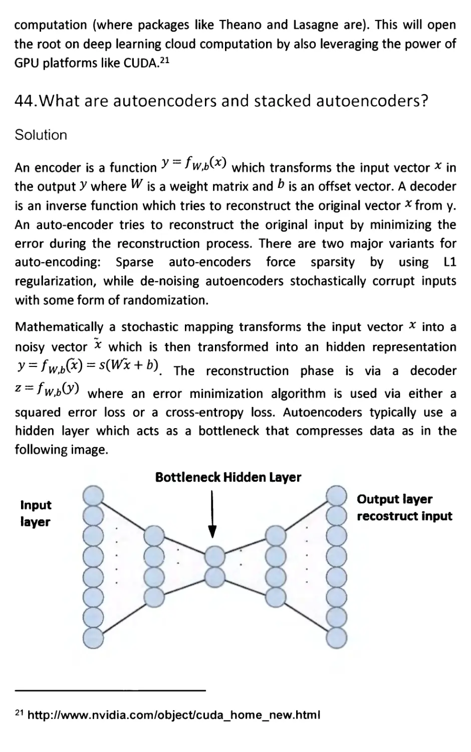
44. What are autoencoders and stacked autoencoders? 67
Solution 67
45. What are convolutional neural networks? 68
Solution 68
46. What are Restricted Boltzmann Machines, Deep Belief
Networks and Recurrent networks? 70
Solution 70
47. What is pre-training? 71
Solution 71
48. An example of Deep Learning with Nolearn and Lasagne
package 72
Solution 72
Code 73
Outcome 73
Code 74
49. Can you compute an embedding with Word2Vec? 75
Solution 75
Code 76
Code 76
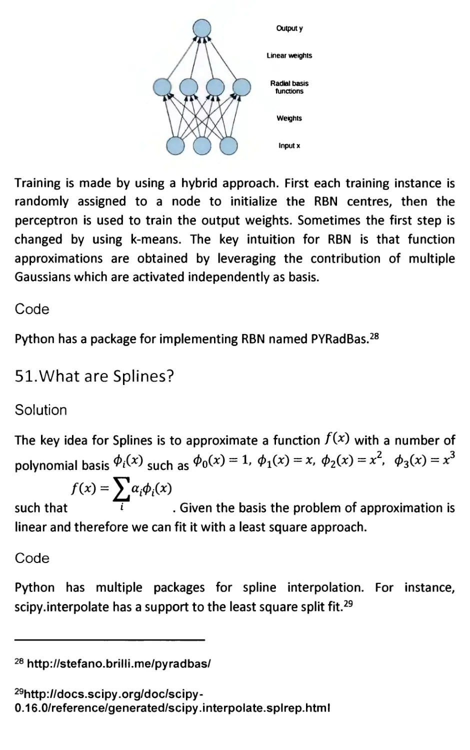
50. What are Radial Basis Networks? 77
Solution 77
Code 78
51. What are Splines? 78
Solution 78
Code 78
52. What are Self-Organized-Maps (SOMs)? 78
Solution 78
Code 79
53. What is Conjugate Gradient? 79
Solution 79
54. What is exploitation-exploration? And what is the armed
bandit method? 80
Solution 80
55. What is Simulated Annealing? 81
Solution 81
Code 81
56. What is a Monte Carlo experiment? 81
Solution 81
Code 82

57. What is a Markov Chain? 83
Solution 83
58. What is Gibbs sampling? 83
Solution 83
Code 84
59. What is Locality Sensitive Hashing (LSH)? 84
Solution 84
Code 85
60. What is minHash? 85
Solution 85
Code 86
61. What are Bloom Filters? 86
Solution 86
Code 87
62. What is Count Min Sketches? 87
Solution 87
Code 87
63. How to build a news clustering system 88
Solution 88
64. What is A/B testing? 89
Solution 89
65. What is Natural Language Processing? 90
Solution 90
Code 90
Outcome 92
66. Where to go from here 92
Appendix A 95
67. Ultra-Quick introduction to Python 95
68. Ultra-Quick introduction to Probabilities 96
69. Ultra-Quick introduction to Matrices and Vectors 97
70. Ultra-Quick summary of metrics 98
Classification Metrics 98
Clustering Metrics 99
Scoring Metrics 99
Rank Correlation Metrics 99
Probability Metrics 100
Ranking Models 100
71. Comparison of different machine learning techniques 101

Linear regression 101
Logistic regression 101
Support Vector Machines 101
Clustering 102
Decision Trees, Random Forests, and GBTs 102
Associative Rules 102
Neural Networks and Deep Learning 103

1. Why is Cross Validation important?
Solution
In machine learning it is important to assess how a model learned from
training data can be generalized on a new unseen data set. In particular a
problem of overfitting is observed when a model makes good predictions on
the training data but has poor performances on unknown data.
Cross-validation is frequently used for reducing the overfitting risk. This
methodology splits training data into two parts: one is the proper training set,
while the other part is the validation set which is used to check overfitting
and find the best partition according to some evaluation metric. There are
three commonly used options:
1. K-fold cross-validation: Data is divided into a train and a validation
set for k-times (called folds) and the minimizing combination is then
selected;
2. Leave one out validation: very similar to k-fold except that the folds
contain a single data point.
3. Stratified K-fold cross-validation, the folds are selected so that the
mean response is approximately the same in all the folds.
The first code fragment presents an example of cross-validation computed
with the scikit-leam toolkit on a toy dataset called diabetes. The size of the
test data is 20%, the machine learning classifier is based on a SVM, the
evaluation metric is accuracy and the number of folds is set to 4.
Code
import numpy as np
from sklearn import cross_validation
from sklearn import datasets
from sklearn import svm
diabets = datasets.load_diabetes()
X_train, X_test, y_train, y_test = \
cross_validation.train_test_split(
diabets.data, diabets.target, test_size=0.2,
random_state=0)
print X_train.shape, y_train.shape # test size 20^
print X_test.shape, y_test.shape
elf = svm.SVC(kernel=' i:.,.dr,/ C=l )
scores = cross validation.cross val score (

elf, diabets.data, diabets.target, cv=4) # 4-folds
print scores
print("-\:';r.-;.;y: . .z -''- .,;[;" % (scores .mean () ,
scores . std() ) )
2. Why is Grid Search important?
Solution
In machine learning it is important to assess which is the best configuration of
hyper-parameters for a learning algorithm. As usual the goal is to optimize
some well-defined evaluation metrics. Let us dig those aspects in more
details. First let us clarify that learning algorithms learn parameters in order
to create models based on input data. Second let us clarify that hyper-
parameters are then selected to ensure that a given model does not overfit
its training data.
Grid search is an exhaustive search procedure that explores a space of
manually defined hyper-parameters by testing all possible configurations and
by selecting the most effective one.
The first code example runs a cross-validation on a KNN classifier with 10
folds. The evaluation metric is accuracy. Then it performs a different grid
search on a parameter space defined in terms of number of neighbours to be
considered (from 1 to 10), in terms of weights (uniform or distance based)
and in terms of Power parameter for the Minkowski metric (when p = 1, this
is equivalent to a manhattan distance (II), or an euclidean distance (12) for p =
2). The whole grid consists in a space of 10 (neighbours) * 2 (weights) * 2
(distances) points which are exhaustively searched by the algorithm via
GridSearchCV. The best configuration (e.g. the one getting the best
accuracy) is then returned.
Code
from sklearn.cross_validation import cross_val_score
from sklearn.neighbors import KNeighborsClassifier
from sklearn.grid_search import GridSearchCV
import numpy as np
#load toydataset
boston = load boston()
12

X, y = boston.data, boston.target
yint = y[:].astype(int)
#grid = 20 x 2 x 3
classifier = KNeighborsClassifier(n_neighbors=5,
weights='un : i.'om', metric='~ir.-■.■: v;sk:_ ' , p=2)
grid ={ ' r. r.r-iahb■..:rr? ' : range (1,11) ,
'■>;e:.?:-s'~: ['uiiom', ' jil.st.ir. .::e ' ] ,
'p' : [1,2]}
print 'i as 1 ir.e . T-t ' \
% np.mean(cross_val_score(classifier, X, yint,
cv=10,
scoring=' a ::u^ :;.y ' , n_jobs=l))
search = GridSearchCV(estimator=classifier,
param_grid=grid,
scoring= ' ac :;j r-f-cy ' , n_jobs=l, refit=True,
cv=10)
search.fit(X, yint)
print 'r,e.-?:: ?a - arre ..-r r\? : s' % search. best_params_
print ' A^ol. racy 51 ' % search. best_score_
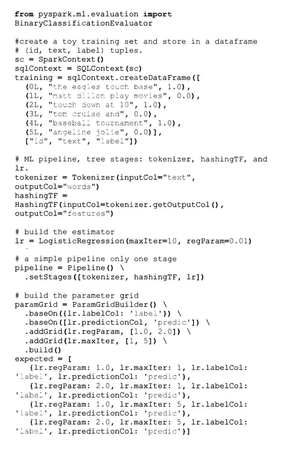
3. What are the new Spark DataFrame and the Spark
Pipeline? And how we can use the new ML library for
Grid Search
Solution
Spark has recently introduced DataFrames (previously called schemaRDD), a
new model for data representation which complements the traditional RDD.
A DataFrame can be seen as a table where the columns are explicitly
associated with names. As for RDD, Spark takes care of data distribution
across multiple nodes as well as marshalling/un-marshalling data operations.
Spark 1.2 has also introduced a new model for composing different machine
learning modules into a Pipeline where each component interacts with the
others via homogeneous APIs. Let's review the key concept introduced by the
Spark ML APIs:

1. ML Dataset: Spark ML uses DataFrames for holding a variety of data
types (columns can store text, features, true labels and predictions);
2. Transformer: A Transformer is an algorithm which can transform one
DataFrame into another DataFrame (for instance an ML model is a
Transformer which transforms a DataFrame with features into an
DataFrame with predictions);
3. Estimator: An Estimator is an algorithm which can be fit on a
DataFrame to produce a Transformer (for instance a learning
algorithm is an Estimator which trains on a training set and produces
a model);
4. Pipeline: A Pipeline chains multiple Transformers and Estimators
together to specify a machine learner workflow (for instance a whole
pipeline can be passed as a parameter to a function)
5. Param: All Transformers and Estimators now share a common
homogeneous API for specifying parameters.
In the code example below a dataframe with " ", " :-:-", "l r
columns has been defined. Then a pipeline is created. In particular a
Tokenizer is connected to a hashing term frequency module, that is in turn
connected to a linear regressor. The whole pipeline is a workflow which is
then passed as parameter to a cross validator. The cross-validator performs
an exhaustive grid search on a hyper-parameter space consisting in two
different regularization values and two different numbers of maximum
iterations. A BinaryClassif icationEvaluator is used for comparing
different configurations and this evaluator uses the areaUnderROC as a
default metric.
Code
from pyspark import SparkContext
from pyspark.sql import SQLContext
from pyspark.sql import Row
from pyspark.ml.feature import HashingTF, Tokenizer
from pyspark.ml.classification import
LogisticRegression
from pyspark.ml.tuning import ParamGridBuilder,
CrossValidator
from pyspark.ml import Pipeline
14

from pyspark.ml.evaluation import
BinaryClassificationEvaluator
(OL, '
(IL, '
(2L, '
(3L, '
(4L, '
(5L, '
#create a toy training set and store in a dataframe
# (id, text, label) tuples,
sc = SparkContext()
sqlContext = SQLContext(sc)
training = sqlContext.createDataFrame([
'"the eagles touch base", 1.0),
'natt dillen play movies", 0.0),
'touch down at 10", 1.0) ,
'ten cruise and", 0.0),
'baseball tournament", 1.0),
'angeiine joiie", 0.0)],
["id", "text", "label"])
# ML pipeline, tree stages: tokenizer, hashingTF, and
lr.
tokenizer = Tokenizer(inputCol="text",
outputCol="words")
hashingTF =
HashingTF(inputCol=tokenizer.getOutputCol(),
outputCol="features")
# build the estimator
lr = LogisticRegression(maxIter=10, regParam=0.01)
# a simple pipeline only one stage
pipeline = Pipeline() \
.setStages([tokenizer, hashingTF, lr])
# build the parameter grid
paramGrid = ParamGridBuilder() \
.baseOn({Ir.labelCol: 'label'}) \
.baseOn([lr.predictionCol, 'predic']) \
.addGrid(lr.regParam, [1.0, 2.0]) \
.addGrid(lr.maxlter, [1, 5]) \
.build()
expected = [
{lr.regParam: 1.0, lr.maxlter: 1, Ir.labelCol
'label', lr.predictionCol: 'predic'},
{lr.regParam: 2.0, lr.maxlter: 1, Ir.labelCol
'label', lr.predictionCol: 'predic'},
{lr.regParam: 1.0, lr.maxlter: 5, Ir.labelCol
'label', lr.predictionCol: 'predic'},
{lr.regParam: 2.0, lr.maxlter: 5, Ir.labelCol
'label', lr.predictionCol: 'predic'}]

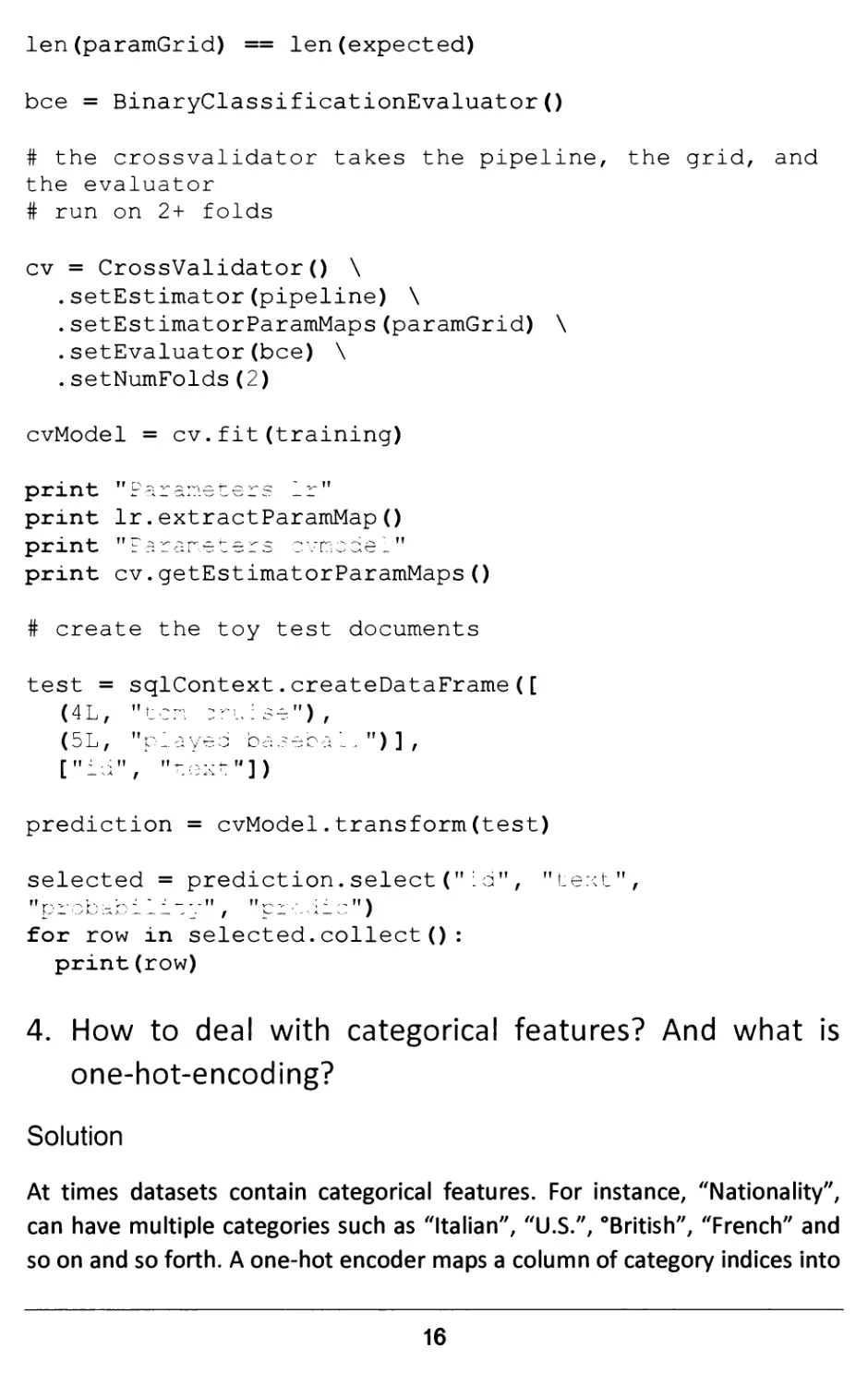
len(paramGrid) == len(expected)
bee = BinaryClassificationEvaluator()
# the crossvalidator takes the pipeline, the grid, and
the evaluator
# run on 2+ folds
cv = CrossValidator() \
.setEstimator(pipeline) \
.setEstimatorParamMaps(paramGrid) \
.setEvaluator(bee) \
.setNumFolds(2)
cvModel = cv.fit(training)
print raia^.L^ttr^ _r
print lr.extractParamMap()
print "Parameters cvncdel"
print cv.getEstimatorParamMaps()
# create the toy test documents
test = sqlContext.createDataFrame([
(4L, "ten --se"),
(5L, "played beeeoa 1 . ") ] ,
["id", "r.UXt"])
prediction = cvModel.transform(test)
selected = prediction.select("id", "text",
m ;,._>, - --•_.-?? m .. ; -; ft \
l" - J*-' ■■*x/ _■ f ^ - • - ■• * - - /
for row in selected.collect():
print(row)
4. How to deal with categorical features? And what is
one-hot-encoding?
Solution
At times datasets contain categorical features. For instance, "Nationality",
can have multiple categories such as "Italian", "U.S.", °British", "French" and
so on and so forth. A one-hot encoder maps a column of category indices into
16

a column of sparse binary vectors with at most one single one-value per row
that indicates the input category index. One-hot-encoding is very useful for
dealing with categorical features.
Indeed many learning algorithms learn one single weight per feature. For
instance, a linear classifier has the form wx + b > 0 anc| Wj|| |eam 0ne single
weight for the feature "Nationality". Sometimes this is a limit because we
might want to differentiate situations where people have more than one
nationality (e.g. "French" and "US" might be different from "Canadian" and
"US"). One-hot-encoding will naturally capture these types of interactions in
the data by blowing up the feature space where each choice of nationality
gets its own sparse representation.
In this code fragment a one hot encoding is computed on a toy example by
using the new ML Spark library.
Code
from pyspark.ml.feature import OneHotEncoder,
Stringlndexer
from pyspark import SparkContext
from pyspark.sql import SQLContext
sc = SparkContext()
sqlContext = SQLContext(sc)
df = sqlContext.createDataFrame([
::y"])
Stringlndexer (inputCol=" ;;ire:.;::: ~" ,
"I"-::. i:.-v")
model = stringlndexer.fit(df)
indexed = model.transform(df)
encoder = OneHotEncoder (inputCol="^::rv: ; ry^:. •.;>:",
outputCol=" y-r^.-rs \ry :.")
encoded = encoder.transform(indexed)
for e in encoded, select (". o " , ":••;'-: ") . take (1 ) :
(0 ,
(2,
(3 f
( 1
/ u,
(6
/ 7
M 11 \
M -, II \
II ^ II \
II IT \
M -I II \
II - " \
" -> " \
], [•
stringlndexer
outputCol="z~z

print e
5. What are generalized linear models and what is an R
Formula?
Solution
Generalized linear models unify various statistical models, such as linear and
logistic regression, through the specification of a model family and link
function. For instance, one formula could be y~/0 + /l meaning the
prediction for y is linearly modelled as function of the features /^and A.
More complex examples can be built by using R operators such as inclusion
(+), exclusion (-), inclusion all (.) and others.
In this code fragment Spark 1.5 supports Rformulas for predicting clicks based
on an extended linear model which is modelled as function of country and
hours. The model is then used to learn from the data via a fit operation.
This part is still experimental in Spark and will be further extended during the
next major releases.
Code
from pyspark.ml.feature import RFormula
from pyspark import SparkContext
from pyspark.sql import SQLContext
sc = SparkContext()
sqlContext = SQLContext(sc)
dataset
[
(5
(6
n
(S
(9
["-:
formula
fori
■Foa-t
= sqlConte
MM
r 1 ^ 1
M - ■- n - r\
r - t - - t
11 — - 11 i o
r / - ^ t
t -■•-■'- i
= RFormula
nula=":::i.:.>
xt
1
i
C
D
. . H
(
"—
. createDataFrame(
:),
.0),
• C),
• 0),
• 0)],
ii V, ... , -. v- m fi .., - - „ :^ f... ,
i"])
1
labelCol=" . -f-ii-f ")
output = formula.fit(dataset).transform(dataset)
18

output, select (" »■=■ . --", " '-: - ").show()
6. What are the Decision Trees?
Solution
Decision trees are a class of machine learning algorithms where the learned
model is represented by a tree. Each node represents a choice associated to
one input feature and the edge departing from that node represents the
potential outcomes for the choice. Tree models where the target variable can
take a finite set of values are called classification trees, while tree models
where the target variable can take continuous values are called regression
trees.
There is a vast literature for modelling Decision trees, however the most
common approach usually works recursively top-down, by choosing at each
step a variable that 'best' splits the feature space. Different metrics have
been proposed to define what is the 'best' choice. Let us review the most
popular ones:
• Gini impurity is the sum of the probabilities of each item being chosen,
multiplied by the probability of mistaken categorization
• Information gain is the difference between the entropy computed before
and after performing a split on a particular feature, where the entropy of
a random variable X is * ;
• Variance reduction is the difference between the variance computed
before and after performing a split on a particular feature.
In short the space of features is thus recursively explored: the feature
offering the 'best' choice is selected and the potential outcomes will generate
the children of the current node. The process is then recursively repeated on
the remaining features until the full tree is built or the maximum depth for
the tree is reached. Once the tree is available, it can be used for classification
and/or regression on new unseen data by navigating the three top-down
from the roof to a leaf. The prediction is the label of the final leaf. In this
image a decision tree for deciding whether today is a good day to play tennis
has been presented.

Humidity 1
^_ I Yes
High
/
No
Normal
\
Yes
Strong
/
No
Weak
\
Yes
Note that Decision Trees divide the feature space into axis-parallel rectangles
organized in a hierarchy and label each rectangle with one of the classes
corresponding to the leaf of the tree. Hence Decision Trees can deal with
non-linear separable data sets.
Decision trees show multiple advantages with respects to other learning
methods such as:
• It is easy to understand why a feature is recursively selected and it is
intuitive to understand the workflow represented once the tree is built;
• It is possible to handle both numerical and categorical data;
• It is possible to build trees for large datasets with reasonable robustness
for outliers
However there are also limitations:
• Learning an optimal decision tree is an NP-complete problem so
construction is based on heuristics which are frequently making locally-
optimal decisions at each node. Once a feature has been selected, the
decision cannot be reverted (however some extensions of Decision Trees
such Gradient Boosted, and Random Forests aim at circumventing this
limitation);
• Decision-trees can overfit training data and frequently do not generalize
well on new unseen data. Pruning and randomization are the techniques
adopted to minimize the impact of this problem.
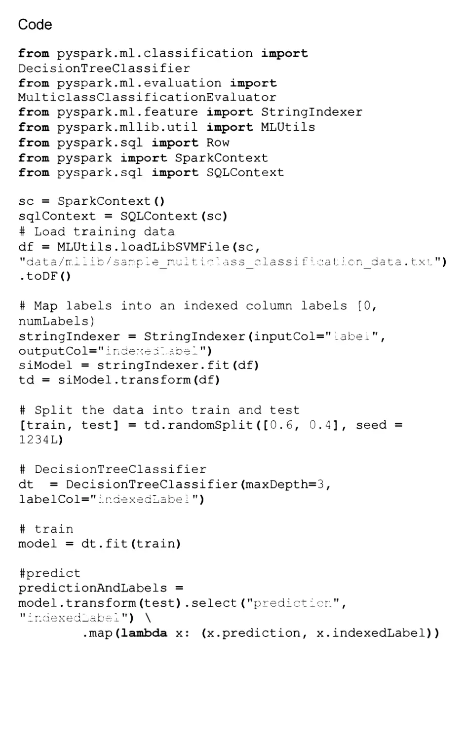
The code fragment reported below uses Decision Trees for Classification
based on the new DataFrame Spark representation. Training data is loaded
using the SVM file format natively supported by the library. Data is split into
training and test with a proportion of 60% and 40% respectively. Then a
decision tree is built by fitting the training data and by imposing a max depth
of 3. The default split criterion is Gini. Once the tree is available it can be used
to predict the outcomes for the test data.
20

Code
from pyspark.ml.classification import
DecisionTreeClassifier
from pyspark.ml.evaluation import
MulticlassClassificationEvaluator
from pyspark.ml.feature import Stringlndexer
from pyspark.mllib.util import MLUtils
from pyspark.sql import Row
from pyspark import SparkContext
from pyspark.sql import SQLContext
sc = SparkContext()
sqlContext = SQLContext(sc)
# Load training data
df = MLUtils.loadLibSVMFile(sc,
ffdata/ir.ilib/sa:r:ple_rnul t lclass_classiflea Licn_data . txi")
.toDF()
# Map labels into an indexed column labels [0,
numLabels)
stringlndexer = Stringlndexer(inputCol=Mlabel",
output Col=" i nciexell a bel")
siModel = stringlndexer.fit(df)
td = siModel.transform(df)
# Split the data into train and test
[train, test] = td.randomSplit([0.6, 0.4], seed =
1234L)
# DecisionTreeClassifier
dt = DecisionTreeClassifier(maxDepth=3,
labelCol="lnaexedLabel")
# train
model = dt.fit(train)
#predict
predictionAndLabels =
model. transform (test) . select ("prediction." ,
_ i - <1 cAca-ia JJ c; _l ) \
.map(lambda x: (x.prediction, x.indexedLabel))

7. What are the Ensembles?
Solution
The word "Ensemble" denotes a class of methods that generates multiple
hypothesis using the same base learner. The key intuition is that the
combination of multiple hypothesis learned from the data can indeed
generate a better prediction than the one generated with a single hypothesis.
There are multiple ways to combine base models.
• Bagging trains each model in the ensemble using a randomly drawn
subset of the training set. Then each model in the ensemble votes with
equal weigh;
• Boosting incrementally builds an ensemble by training each new model
instance in such a way that the training instances of that previously
misclassified models are thus emphasized.
• Stacking or Blending combines predictions built with multiple different
learning techniques. The combination is also learned with a special ad-
hoc learned model.
The winner of a Netflix competition combines different algorithms via
blending to provide a single rating that exploits the strengths of each model.
In the paper detailing their final solution the winners provide a description
using gradient boosted decision trees to combine over 500 different models
learned from data. (Lessons from the Netflix Prize Challenge. SIGKDD
Explorations, Volume 9, Issue 2, Robert M. Bell and Yehuda Koren.)
8. What is a Gradient Boosted Tree?
Solution
A gradient boosted decision tree (GBT) learning algorithm builds in sequence
a series of decision trees by fitting the models to the data. Each tree is
required to predict the error made by previous trees and then compares the
prediction with the true label. The dataset is re-labeled to put more emphasis
on training instances with poor predictions.
The key intuition is that each tree is specifically built for minimizing a loss
function representing the errors made in previous iterations. Typically the
22

loss function is either a log loss, a squared error or an absolute error. Log
losses can be used for classification, while squared errors and absolute errors
can be used for regression. In certain situations it has been observed that
training GBTs on a slight perturbated sample of the available data can
improve the performances achieved by the learner.
As a final note GBTs can handle categorical features and are able to capture
non-linearities and interactions in the feature space.
9. What is a Gradient Boosted Trees Regressor?
Solution
GBTs Regressors are gradient boosted trees used to deal with continuous
features. In the example below a Spark ML library is used and a training data
is converted into a suitable DataFrame format. The regressor runs for 50
iterations, which maximum depth is 5. Default loss function is the 12-norm. In
this case regression hasve been evaluated by means of three different
metrics: the square root of the mean squared error, the mean absolute error
or ll-norm, and the r2, a measure of variability for the regression model1.
Code
# gradient boosted regression
#
from pyspark import SparkContext
from pyspark.sql import SQLContext
from pyspark.sql import Row
from pyspark.mllib.util import MLUtils
from pyspark.ml.feature import Stringlndexer
from pyspark.ml.regression import GBTRegressor
from pyspark.mllib.evaluation import RegressionMetrics
sc = SparkContext()
sqlContext = SQLContext(sc)
#load a toy dataset with svm format
df = MLUtils.loadLibSVMFile(sc,
".:;-,- ,-:. :o/,r yrx. ~ . d-v. ") .toDF()
1 https://en.wikipedia.org/wiki/Coefficient_of_determination

# Map labels into an indexed column labels [0,
numLabels)
stringlndexer = Stringlndexer(inputCol="labol",
outputCol="indexedLabe:")
siModel = stringlndexer.fit(df)
td = siModel.transform(df)
# get the transformed model and split in train and test
[train, test] = td.randomSplit([0.7, 0.3])
# get the grandient boosted regressor
rf = GBTRegressor(maxlter=50, maxDepth=5,
labelCol=Mii:aexeal^be:M)
model = rf.fit(train)
# predict
predictionAndLabels =
model, transform (test) . select ("predict: i; i." ,
" : ndexedT.abei") \
.map(lambda x: (x.prediction, x.indexedLabel))
#compute metrics
metrics = RegressionMetrics(predictionAndLabels)
print ("rr;.;?e ■ . 3i" % metrics . rootMeanSquaredError)
print("r2 .3f" % metrics.r2)
print("mae . 3f" % metrics.meanAbsoluteError)
10.Gradient Boosted Trees Classification
Solution
GBTs Classifier are gradient boosted trees used to deal with categorical
features. In the example below the Spark ML library is used and a training
data is converted into a suitable DataFrame format. The classifier runs for 30
iterations, which maximum depth is 4. The default loss function is logistic. In
this case classification has been evaluated by means of the area under ROC
metric2.
Code
# gradient boosted classification
2 https://en.wikipedia.org/wiki/Receiver__operating__characteristic
24

#
from pyspark import SparkContext
from pyspark.sql import SQLContext
from pyspark.sql import Row
from pyspark.mllib.util import MLUtils
from pyspark.ml.feature import Stringlndexer
from pyspark.ml.classification import GBTClassifier
from pyspark.mllib.evaluation import
BinaryClassificationMetrics
sc = SparkContext()
sqlContext = SQLContext(sc)
#load a toy dataset with svm format
df = MLUtils.loadLibSVMFile(sc,
"data/mllib/sample_iibsvm_data.txt").toDF()
# Map labels into an indexed column labels [0,
numLabels)
stringlndexer = Stringlndexer (inputCol="i abe 1." ,
outputCol="indexealabel")
siModel = stringlndexer.fit(df)
td = siModel.transform(df)
# get the transformed model and split in train and test
[train, test] = td.randomSplit([0.7, 0.3])
# get the grandient boosted classifier
rf = GBTClassifier(maxlter=30, maxDepth=4,
labelCol="indexedLabei")
model = rf.fit (train)
# predict
predictionAndLabels =
model.transform(test).select("prediction",
"ir.dexeaLabel") \
.map(lambda x: (x.prediction, x.indexedLabel))
#compute metrics
metrics =
BinaryClassificationMetrics(predictionAndLabels)
print("AUG .3f" % metrics.areaUnderROC)

11.What is a Random Forest?
Solution
A random forest trains multiple decision trees in parallel by injecting some
randomness into the data, so each decision tree is slightly different from the
others. The randomness consists in subsampling the original dataset to get a
different training set (bootstrapping) and in subsampling different subsets of
the considered feature space in order to split at each tree node.
Once the forest is built, it can be used for classification or regression. In
classification each tree predicts a label and then the forest predicts the label
predicted by the majority of trees. In regression each tree predicts a
continuous value and the forest then predicts the average among those
values. In this example a RandomForestClassifier is built by using Gini as a
splitting criterion and the default number of trees is 20.
Code
from pyspark import SparkContext
from pyspark.sql import SQLContext
from pyspark.ml.feature import Stringlndexer
from pyspark.ml.classification import
RandomForestClassifier
from pyspark.ml import Pipeline
from pyspark.mllib.util import MLUtils
from pyspark.mllib.evaluation import
BinaryClassificationMetries
sc = SparkContext()
sqlContext = SQLContext(sc)
df = MLUtils.loadLibSVMFile(sc,
";;.- r _0-,3.'X-") .toDF()
# Map labels into an indexed column labels [0,
numLabels)
stringlndexer = Stringlndexer (inputCol="lar-:1" ,
outputCol=" : -.i-f-::^:.:",;^--:: ")
siModel = stringlndexer.fit(df)
td = siModel.transform(df)
26

# get the transformed model and split in train and test
[train, test] = td.randomSplit([0.7, .3])
rf = RandomForestClassif ier (numTrees=':, maxDepth=3 ,
labelCol=" : r-riexe:r.j;be ", impurity=" r. ", seed=42)
# train
model = rf.fit(train)
#predict
predictionAndLabels =
model. trans form (test) . select ("cro'ii.:- i :." ,
";rd,:^: ,::.• ") \
.map(lambda x: (x.prediction, x.indexedLabel))
tcompute metrics
metrics =
BinaryClassificationMetries(predictionAndLabels)
print(" " % metrics.areaUnderROC)
12.What is an AdaBoost classification algorithm?
Solution
Adaboost is one of the simplest yet effective classification algorithms. Its
name stands for Adaptive Boosting where a set t = {l, ...,T] 0f simple and
weak classifiers is used and the classifiers are also used in turn to boost
the mistake made by the previous classifier.
Mathematically at the very beginning all the weighs are set to 1/N , where N
are the datapoints. Then at each iteration a new classifier is trained on the
training set, with the weights that are modified according to how successful
each datapoint has been classified in the past epochs. In particular let us
at = log(—-
define \ t / where Ms the training error at iteration f, the weights
a.
at iteration t + 1 are boosted as wt + i = wt*e *I(yn*ht(xn» , where
l^n nt\xn)) is an indicator function which returns 1 if the output of the
base classifier at epoch t and for the data point%n is different from the
true label ^n, and it returns 0 otherwise. Therefore the key intuition is that it
is possible to decrease the weight of a correct classifier - because it has

already solved its task - and increase (e.g. boost) the weight of an incorrect
classifier because it still needs to solve the problem for that instance. This
boosting is repeated until 0<£t< 1/2.
At the end the classifier returns the sign of the weighted combination of basic
T
classifiers t = 1 ht\xrU). It should be noticed that the base classifiers can be
of any type including but not limited to Bayesian, Linear, Decision Trees,
Neural Networks and so on and so forth.
In Spark a good implementation of AdaBoost is available as external package
AdaBoost.MH, available inside the SparkPackages repository.3
13.What is a recommender system?
Solution
Recommender systems produce a list of recommendations such as news to
read, movies to see, music to listen, research articles to read, books to buy
and so on and so forth. The recommendations are generated through two
main approaches which are often combined:
• Collaborative filtering aims to learn a model from a user's past behaviour
(items previously purchased or clicked and/or numerical ratings
attributed to those items) as well as similar choices made by other users.
The learned model is then used to predict items (or ratings for items) that
the user may have an interest in. Note that in some situations rating and
choices can be explicitly made, while in other situations those are
implicitly inferred by users' actions. Collaborative filtering has two
variants:
■ User based collaborative filtering: the user's interest is taken into
account by looking for users who are somehow similar to him/her.
Each user is represented by a profile and different kinds of similarity
metrics can be defined. For instance a user can be represented by a
vector and the similarity could be the cosine similarity
3 http://spark-packages.org/package/tizfa/sparkboost
28

■ Item based collaborative filtering: the user's interest is directly
taken into account by aggregating similar classes of interest
• Content-based filtering aims to learn a model based on a series of
features related to an item in order to recommend additional items with
similar properties. For instance a content based filtering system can
recommend an article similar to other articles seen in the past, or it can
recommend a song with a sound similar to ones implicitly liked in the
past.
Recommenders have generally to deal with a bootstrap problem for
suggesting recommendations to new unseen users for whom very few
information about their tastes are available. In this case a solution could be to
cluster new users according to different criteria such us gender, age, location
and/or to leverage a complete set of signals such as time of the day, day of
the week, etc. One easy approach is to recommend what is popular, where
the definition of popularity could be either global or conditioned to a few and
simple criteria.
More sophisticate recommenders can also leverage additional structural
information. For instance an item can be referred by other items and those
can contribute to enrich the set of features. As an example, think about a
scientific publication which is referred by other scientific publications. In this
case the citation graph is a very useful source of information for
recommendations.
14.What is a collaborative filtering ALS algorithm?
Solution
An ALS algorithm is a collaborative filtering technique which models users
and items with a rating matrix ^ where the entry rv ~ r denotes that the user
i has expressed a rate rfor the item), either implicitly or explicitly. The
problem aims at predicting the missing entries in the matrix or, in other
words, it aims at predicting whether or not a user can be interested in a
particular item (a movie, a song, a book, a purchase etc.) that was never seen
before. This can be achieved by means of a mathematical technique called
matrix factorization. The key intuition is that users can be modelled via an
unknown latent matrix factor X (each user is a vector) and items can be

modelled via another different unknown latent matrix factor Y (each item is a
vector). Hence we have two unknown factors to learn and we can do this
iteratively. Y is first estimated using the available knowledge on X, and then
iteratively x is then estimated using the available knowledge on Ym The
alternate least square algorithm (ALS) aims at reaching convergence where
the matrices X and Y change very little after a certain number of iterations.
This is illustrated in the following image with R being the sparse matrix and X
and Y being the estimated vectors.
YT
R X
Mathematically, the problem can be seen as a minimization problem of the
following cost function
J(xi) = (rl-xiY)Wi(rl-xlYf + AxixiT
J(yi) = (rj - xyj)wj(rj - xyj?+tyy?
w..=\° ^=°
where lJ U otherwise anc| X control regularization. It can be shown that
the solution of the above equations is given by
xi = (YWy7 + XI) ~ 1YWiri
y} = (XTWjX + XI) ~ WWjTj
and those are the update rules iteratively adopted by the algorithm.
In this code fragment the new Spark ML library is used for providing
recommendations based on a user's x item matrix with explicit rating. Then a
new unseen user is provided with recommendations for available items.
There is a number of hyper-parameters which can be fine-tuned, including
the rank representing the number of columns in the user-feature and
product-features matrix, the iteration used during computation, the lambda
factor used for balancing overfitting with factorization's accuracy and alpha
30

which controls the weight of the observed and not observed user-product
interaction during the algorithm execution. Note that Spark implements ALS
also in the traditional MLlib library based on RDD. In that case ALS has two
different methods: one used for implicit ratings and the other one for explicit
ratings.
Code
from pyspark import SparkContext
from pyspark.sql import SQLContext
from pyspark.sql import Row
from pyspark.ml.recommendation import ALS
sc = SparkContext()
sqlContext = SQLContext(sc)
# create the dataframe (user x item x rating)
df = sqlContext.createDataFrame(
[(0, 0, 5.0), (0, I, 1.0) , (i, 1, 2.0) , C , 2,
3.0) , (2, 1, 3.0) , (2, 2, 6.0)] ,
["user", "i-::.", "r-i:. j"] )
als = ALS(rank=10, maxlter=8)
model = als.fit(df)
print "O^r. /. -i " % model, rank
test = sqlContext.createDataFrame([(0, 2), (1, 0) , (2,
0)], [":> r", "-::"])
predictions = sorted(model.transform(test).collect(),
key=lambda r: r[0])
for p in predictions: print p
If there is a need of pseudo-real time updates, then it could be convenient to
have a look to the project Oryx4, which implements the so-called Lambda
architecture, where a batch pipeline for bulk updates is used in parallel to
another pipeline allowing the faster updates as depicted in this image. Oryx
used Apache Kafka and Spark Streaming for input stream processing.
4 http://oryx.io/

Input
Input (Kafka topic)
Input
Recent
Input
, (r
input \U
Queries
X
7=\
/ Serving \
si Layer J
Speed
Layer
Spark
Streaming
Model
Updates
A A
Model
Model
Updates ^
Model
Models + Updates (Kafka topic)
Recent
Input
Batch
Layer
Spark
Streaming
Historical
Input
<
HDFS
Model
15.What is the DBSCAN clustering algorithm?
Solution
DBScan is a density based algorithm which groups together several closely
placed points in a vector space and marks outliers as stand-alone points. Two
hyper-parameters s and rninPoints should be provided as input. Points in the
feature space are then classified as it follows:
• A point P is a core point, if at least rninPoints points are within distance e
of it. Those points are marked as directly reachable from p;
• A point Q is reachable from P , if there is a path of points pl# •••# Pn with
pi = P and Pn = Q, where each Pl + 1 is directly reachable from P*;
• All non-reachable points from any other point are outliers.
At the end each cluster contains at least one core point with all reachable
points from it. It should be noticed that a DBScan does not require to
predefine the number of desired clusters but this is directly inferred from the
data.
In this code example a scikit-lean package has been used to cluster a set of
points contained in the diabetes toy dataset with the DBScan algorithm.
Spark does not contain yet a native implementation of DBSCAN but this will
be probably included in the next releases.5
32

Code
from sklearn.datasets import load_diabetes
from sklearn.cluster import DBSCAN
import pandas as pd
import matplotlib
import matplotlib.pyplot as pit
#load the data
diabetes = load_diabetes()
df = pd.DataFrame(diabetes.data)
texplore the data
print df.describe()
bp= df .plot (kind='r ::')
pit. show()
tperform the clustering
dbClustering = DBSCAN(eps=2.5, min_samples=2 5)
dbClustering.fit(diabetes.data)
print "c.-^SL-r-c r"
from collections import Counter
print Counter(dbClustering.labels_)
16.What is a Streaming K-Means?
Solution
A Streaming K-Means is a version of K-Means where it is assumed that the
points are continuously updated in a stream. For instance, we can decide to
cluster together new users who are using a mobile phone system and show
similar behaviours. In this case not all users are available before the clustering
itself because the dataset is continuously updated.
Therefore in the streaming environment data arrive in batches. The simplest
extension of the standard k-means algorithm would be to begin with cluster
centres and for each new batch of data points reapply the standard k-means
algorithm. This is pretty much equivalent to a well-known k-means extension
called mini-batch.
5 https://issues.apache.org/jira/browse/SPARK-5226

However two improvements might be used. First, we can introduce a hyper-
parameter called forgetfulness which might allow to control (reduce) the
importance of data observed long time ago. Second, we can introduce a
check to eliminate dying clusters e.g. those clusters which are not updated
since long time and probably represent a situation observed in old data.
In this code example the Streaming Support provided by Spark is leveraged
(see SparkStream6) and new data is processed as soon as it is produced into
an appropriate directory. Then each new point is associated with a given
cluster.
Code
from pyspark.mllib.clustering import StreamingKMeans
from pyspark.mllib.regression import LabeledPoint
from pyspark.mllib.linalg import Vectors
from pyspark import SparkContext
from pyspark.streaming import StreamingContext
# Create a local StreamingContext with two working
thread and batch interval of 1 second
sc = SparkContext ("I:: -:^1 ;Z" " , ":.' ■';■-■■/.■ -.ri-iW^rd Neurit-. ")
ssc = StreamingContext(sc, 1)
# continuous training
trainingData =
ssc.textFileStream(" ~
rse)
testData =
ssc . textFileStream( " '.
LabeledPoint.parse(s))
model = StreamingKMeans() \
.setK(3) \
.setDecayFactor(1.0) \
.setRandomCenters(dim=3, weight=0.0, seed=42)
model.trainOn(trainingData)
prediction = model.predictOnValues(testData)
print prediction
6 http://spark.apache.org/streaming/
:::").map(Vectors.pa
:").map(lambda s:
34

ssc.start()
ssc.awaitTermination()
17.What is Canopi Clusterting?
Solution
Canopy clustering algorithm is an unsupervised pre-clustering, often used as
preprocessing step for the K-means algorithm. The algorithm has two
T T
thresholds i and 2. These are the steps followed:
1. A random element is removed from the set of items and a new
'canopy' is created
2. For each point left in the set, assign the point to the new canopy if
T
the distance is less than the threshold i
T
3. If the distance is also less than 2 then remove the point from the
original set
4. Restart from 1 until there are no more data points to be clustered
Note that each point can belong to multiple clusters. In addition, each canopy
can be re-clustered with more accurate and computationally expensive
clustering algorithms. Moreover different levels of accuracy can be required
for the distance metrics used in 2 and 3. More details can be found
in "Efficient Clustering of High Dimensional Data Sets with
Application to Reference Matching, McCallum, A.; Nigam, K.; and
Ungar LH. (2000), Proceedings of the sixth ACM SIGKDD
international conference on Knowledge discovery and data
mining"
Spark's community is currently working for integrating Canopy in standard
MLLIB.7
18.What is Bisecting K-Means?
Solution
The bisecting k-means is an algorithm proposed to improve ^-means. The
algorithm uses the following steps:
7 https://issues.apache.org/jira/browse/SPARK-3439

1. Starts with all items belonging to the same cluster
2. While the number of clusters is less than *
a. For every cluster
i. measure the total error
ii. Run a k-means on the cluster with k=2
iii. Mesure the total error after the split generated by
k-means
b. Choose the cluster split that has minimized the total error
and commit this split.
The total error can be measured in different ways. For instance it could be
considered as the sum of squared error used by normal k-means to assign
certain items to the closest centroid.
Spark community is currently working on implementing Bisecting K-means
intoMLlib8
19.What is the PCA Dimensional reduction technique?
Solution
Dimensional reduction is a technique for compressing the feature space and
extracting latent features from raw data. The main goal is to maintain a
similar structure in the compressed space to the one observed in the full
space. The idea of the PCA is to find a rotation in the data, such as the first
coordinate has the largest variance possible. Then this coordinate is removed
from the data and the process is restarted with the remaining coordinates
which are required to be orthogonal to the preceding one. At the end the top
^ components are retained and, considering the principal coordinates, they
provide a compressed representation of the original data still presenting the
original structure.
Mathematically let us considerx as a data matrix where the sample mean of
each column has been shifted to zero. Then the transformation is defined by
a set of p-dimensional vectors that maps each row vector **of ^to a set of
new vectors of principal component scores k,i~xiwkt such as variable
8 https://issues.apache.org/jira/browse/SPARK-6517
36

t receiving the maximum possible variance from *. For the first component
we then have
Wi =
argmax > (t* ,)2 = argmax > (t+ ,)2 argmax > (x.w)2
||,v|| = l4j l'1 \\w\\ = l£j ' |H| = 1AJ
argmax 11Aw|| =
IMI = i
T T wTXTXw
argmax w X Xw = argmax
IMI = i IMI = l wTw
where we assume that the vectors w are unit vectors.
T
For a symmetric matrix X X it can shown that the maximum for
wTXTXw
argmax
IMI = i ww is obtained for the largest eigenvalue of the matrix, which
occurs when w is the largest eigenvector.
The problem of PCA computation is then equivalent to the problem of the
eigenvalue computation for the matrix^ Xm Once we have the first
component wi, we can transform the coordinates U ~ xiwi and repeat the
process for the remaining components after subtracting all previous ones.
This image provides an idea of what the first 2 components are for a
multivariate Gaussian distribution. The first component identifies the
direction of the largest variance in the data, while the second one is the
second largest variance in the data.
The following code fragment computes PCA using Spark with DataFrames.
The first 3 components are thus computed.

Code
from pyspark.ml.feature import PCA
from pyspark.mllib.linalg import Vectors
from pyspark import SparkContext
from pyspark.sql import SQLContext
sc = SparkContext()
sqlContext = SQLContext(sc)
data = [(Vectors.sparse(5, [(1, 1.0), (3, .3)]),),
(Vectors.dense([2.0, 0.0, 3.0, 4.0, 5.0]),),
(Vectors.dense([5.6, 3.0, 1.0, 6.4, 3.5]),),
(Vectors.dense([3.4, 5.3, 0.0, 5.5, 6.6]),),
(Vectors.dense([4.1, 3.1, 3.2, 9.1, ^.0]),),
(Vectors.dense([3.6, 4.1, 4.2, 6.3, 7.0]),),
]
df = sqlContext. createDataFrame (data, [" r'e.v .-■"])
pea = PCA(k=3, inputCol=" ';ea:u:es",
OUtpiltCol=": \--y s \~ V: ")
model = pea.fit(df)
result = model. transform (df) . select ("r,::j F- ■ L u :-.:.")
result.show(truncate=False)
20.What is the SVD Dimensional reduction technique?
Solution
SVD is another dimensional reduction technique based on eigenvalues
computation. The technique has a solid mathematical foundation which
factorizes a matrix ^ into three matrices V> %, V such that h=U%V . it can be
shown that ^ is an orthonormal matrix, the columns of which are left singular
vectors, while ^ is an orthonormal matrix, the columns of which are right
singular vectors, and ^ is a diagonal matrix with a non-negative diagonal
containing the singular values in descending order. Only the top k eigenvalues
and corresponding eigenvectors are retained.
Unfortunately pySpark does not support yet SVD computation while this is
available in Scala (October, 2015). Therefore the following code segment
shows how to compute SVD in Scala. The Python version is expected to be
included in Spark 1.6.X
38

Code
import org.apache.spark.mllib.linalg.Matrix
import org.apache.spark.mllib.linalg.distributed.RowMatrix
import
org.apache.spark.mllib.linalg.SingularvalueDecomposition
val mat: RowMatrix = ...
// Compute the top 20 eingenvalues and eingenvectors.
val svd: SingularValueDecomposition[RowMatrix, Matrix] =
mat.computeSVD(20, computeU = true)
val U: RowMatrix = svd.U
val s: Vector = svd.s
val V: Matrix = svd.V
21.What is a Latent Semantic Analysis (LSA)?
Solution
Latent Semantic Analysis (sometimes referred as latent semantic indexing) is
a natural language processing technique for analyzing documents and terms
contained within them. The idea is to build a matrix A where the columns
represent the paragraphs (or the documents) and the rows represent the
unique words contained in the collection of documents. Then SVD is used to
reduce the number of rows while preserving the structure of the columns.
Mathematically this process is referred as low rank approximation to the
term-document matrix. The original matrix A is generally sparse while the
low rank matrix is dense. The low rank matrix has multiple applications. For
instance a query term can be translated into the low-dimensional space and
related documents can be therefore retrieved. Also terms which are
semantically similar will be closer in the low-rank space and this can be used
for finding synonyms.
22.What is Parquet?
Solution
Parquet is a common tabular format for saving and retrieving data in Python.
Spark supports full integration with Parquet, while SPARK SQL allows to read
and write from Parquet files also supporting Parquet schemas. In addition to
that Parquet can be used by Spark to implement DataFrame abstractions.

In this code fragment Spark loads an example Parquet file and saves only few
fields from the original schema into a new parquet file.
Code
from pyspark import SparkContext
from pyspark.sql import SQLContext
sc = SparkContext()
sqlContext = SQLContext(sc)
df =
sqlContext. read, loadf" .y -;rr. _zr/rz ;/z.;-iz/rzecrr zzr /erzrr
df.select ("■ --" ,
"z riz "). write. save ("rriz-s^nrj'r-,-" 1 re
")
23.What is an Isotonic Regression?
Solution
An isotonic regression is similar to a linear regression with some additional
constrains. In particular this loss function has the following form:
n
(x,y,w) = ^wi(yi-xi)
; = i , where ^ represents the true labels and xi the
unknown values, with the constrains that *i - *2 - ••• - xn and wi > . The
main advantage of an isotonic fit is that the assumption of linear fitting,
typical of linear regressions, is relaxed as explained in the following image. In
practice the here present list of elements forms a function that is piecewise
linear.
40

J0 20 40 60 80 100
This code fragment computes an isotonic regression in Spark. This code is
very similar to a linear regression
Code
import math
from pyspark import SparkContext
from pyspark.mllib.regression import
IsotonicRegression, IsotonicRegressionModel
sc = SparkContext()
data =
sc. text File (" dzzz / r.iLlib / s.~nplo isotonic roarossicr: d-^ta
.txt")
# Create label, feature, weight (which defaults to 1.0)
parsedData = data.map(lambda line: tuple([float(x) for
x in line.split(',')]) + (1.0,))
# training (60%) and test (40%) sets.
training, test = parsedData.randomSplit([0.6, 0.4],
seed=42)
# training
model = IsotonicRegression.train(training)
# (predicted, true) labels.
predictionAndLabel = test.map(lambda p:
(model.predict(p[l]), p[0]))
# MSE

meanSquaredError = predictionAndLabel.map(lambda pi:
math.pow((pi[~] - pi [ 1]) , 2)).mean()
print(" : .: -. l j:i - " + str (meanSquaredError) )
24.What is LARS?
Solution
Lars (Least angle regression) is an algorithm for computing linear regression
with LI regularization (aka Lasso). It has been introduced in "Least Angle
Regression. Efron, Bradley; Hastie, Trevor; Johnstone, lain; Tibshirani, Robert
Annals of Statistics 32 (2): pp. 407-499" Lasso is a shrinkage and selection
method that minimizes the sum of squared errors, with a bound on the sum
of the coefficients absolute values. If the number of features is very high,
then LARS will produce an estimate of which variable to include and what are
the weights inferred during the training phase. Instead of providing one single
result, LARS can produce a curve explaining the solution for each different
choice of the hyper-parameter in LI which is very useful for cross-validation.
Mathematically: given a set of input measurements xvxi~-xp and an
outcome measurement)7, the lasso fits a linear model
n
«' = i with the goal of minimizing «' and under the
Y,\bi\<s
constrain i which generally produce a sparse vector of weights. The
key intuition of the algorithm is to increase a coefficient of each feature until
that feature is no longer correlated with the residual error. Mathematically
these are the steps followed:
• Start with all coefficients o equal to zero.
• Find the feature xi most correlated with V
• Increase the coefficient * in the direction of the sign of its
correlation withy. Take residuals r = y~y along the way. Stop
when some other feature XJ has as much correlation with r as xi
has.4
• Increase^ *' ^ in their joint least squares direction, until some other
predictorx™ has as much correlation with the residualr.
42

• if a non-zero coefficient hits zero, remove it from the active set of
features and recompute the joint direction.
• Continue until: all features are in the model
It can be shown that this algorithm gives the entire path of lasso solutions, as
5 is varied from 0 to infinity. In Python scikit-learn implements LARS. An
example of coefficients is provided in this image
V 500 1O00 1500 2CO0 2503 ttOO 3500
sum|bi|
25.What is GMLNET?
Solution
GMLNET is a very efficient algorithm for solving linear regression under the
ElasticNet coefficient constrains. It has been introduced in "Regularization
Paths for Generalized Linear Models via Coordinate Descent, Friedman,
Jerome; Trevor Hastie; Rob Tibshirani Journal of Statistical Software: 1-22."
ElasticNet combines LASSO constrains based on LI regularization with the
RIDGE constrains based on L2 regularization. The estimates of ElasticNet are
expressed as
l = *rgmxn(\\y-xb\\2 + X2\\b\\2 + X2\\b\\1
Spark implements GMLNET as an external package9
https://github.com/jakebelew/spark-glmnet

26.What is SVM with soft margins?
Solution
SVM allows classification with linear separable margins. However sometimes
it could be convenient to have soft-margins in such a way that few data
points are ignored and can be placed behind the supporting vectors.
Mathematically this is described by using a set of slack variables^ which
represent how far it is possible to go beyond the margins. The reg_param in
Spark class spark.mllib. classification. SVMWithSGD allows
to adjust the strength of constrains. Small values imply a soft margin, while
large values imply a hard margin. This image clarifies the use of soft margins
with support vectors.
27.What is the Expectation Maximization Clustering
algorithm?
Solution
Expectation Maximization is an iterative algorithm for finding the maximum a
posteriori estimated in a model, where the model depends on some hidden
latent variables. The algorithm iteratively repeats two steps until
convergence or until a maximum number of iterations has been reached:
• The expectation step (E) evaluates the expectation of the log-
likelihood using the current estimate of parameters;
• The maximization step (M) computes the parameters maximizing the
expected log-likelihood obtained during the previous E step.
44

For example suppose to have two biased coins, A and B, which return head
with an unknown bias ua*ub which we want to estimate. The experiment
consists in randomly choosing a coin and perform ten independent tosses for
six times (hence a total of 60 tosses). Suppose that during the experiment we
don't know the identity of the coins (either A or B) so that we have a hidden
unknown variable. The algorithm will iteratively start from some randomly
fit nt\
chosen initial parameters (A, bj in order to determine for each of the six
sets whether coin A or coin B was more likely to have generated the observed
flips with the current estimated parameter. Then assume these guessed coin
assignments to be correct and apply the maximum likelihood estimation
nt + i Qt + U
procedure to get ( a t u b )m Note that rather than picking the single most
likely completion of the missing coin assignments on each iteration, the EM
algorithm computes probabilities for each possible completion of the hidden
data. In this way it can express a confidence for each completion of the
hidden data.
Mathematically the likelihood function is represented by iP'&Z) = P(X,Z\0) /
where x represents the observed data, z the hidden latent data and 0 the
unknown parameters. The maximum likelihood estimate is obtained by
L(0;Z) = p(X\0) = J^(X,Z\0)
marginalizing onz as z . Iteratively we have that
the following:
Q(6\et) = E t[logL(0;X;Z)]
• E-step: z\x,e calculate the expected value
E L.1
z|^yL'"J of the conditional distribution of the hidden ^ given X
under the current estimation of 0
• M-step: find the parameter which maximizes
0t + 1 = argmax Q(e\6t)
e
EM typically converges to a local optimum and there is no bound on the
convergence rate in general. Note that EM should be seen as a framework
and specific applications have to be instanced for being applied.

28.What is a Gaussian Mixture?
Solution
A Gaussian Mixture Model is a composite distribution made by k Gaussian
sub-distributions each with its own probability represented by ^ J with
means ^ and variance \ A point of the model can be extracted by one of the
sub-distributions. Gaussian mixtures are frequently used to estimate the prior
K
distribution in a Bayesian classification as * = i with weights
^i. The posterior distribution can be also modelled as a Gaussian
K
i = i but with different values ^' ^' *.
A typical example of a Gaussian Mixture is topic modelling for documents
(also known as Gaussian Mixture Model, or GMM). The assumption is that a
document is made up of n words extracted from a vocabulary of size ^ where
each word can represent up to £ different topics. The distribution of the
words can be modelled as a mixture of £ categorical distributions, each of
which represents a topic.
This code fragment implements a Gaussian Mixture and it uses EM for
training the data. Note that the analytical definition of Q\? I ^ ) for Gaussian
mixtures goes beyond the scope of this introductive book. The interested
reader can refer to the here presented section10 for a complete discussion.
Code
from pyspark.mllib.clustering import GaussianMixture
from numpy import array
from pyspark import SparkContext
sc = SparkContext()
# Load
data = sc.textFile(" -;-;-..», -llic/j:::r. ri.»t h .->:". ")
10 https://en.wikipedia.org/wiki/Mixture_model
46

parsedData = data.map(lambda line: array([float(x) for
x in line.strip().split(' ')]))
k=3
# Build the model (cluster the data)
gmm = GaussianMixture.train(parsedData, k)
# output parameters of model
for i in range(k):
print ("v:-r' ", gmm. weights [i] , ""... ",
gmm.gaussians[i].mu,
"s:gi:,:i - ", gmm. gaussians [i] . sigma . toArray () )
29.What is the Latent Dirichlet Allocation topic model?
Solution
Latent Dirichlet Allocation (LDA) is a topic model for inferring topics given a
collection of textual documents. LDA computes several clusters where the
centres are the topics represented as bags of words and the documents are
assigned to the closer topics. LDA assumes that documents are generated
according to the following rules:
• First, decide on the number of words N in the complete document
and choose an initial topic mixture for the document itself (according
to a Dirichlet11 distribution over a fixed set of K topics).
• Then, generate each word w* in the document by:
o Picking a topic following the established distribution
o Using the topic to generate the word itself
Assuming this generative model for a collection of documents, LDA then
backtracks from it to discover a set of topics that are likely to have generated
the collection of textual documents itself. The mathematical foundation of
LDA is outside the scope of this introductory book but the interested reader
can refer to this link12 for a detailed explanation.
11 https://en.wikipedia.org/wiki/Dirichlet_distribution
2 https://en.wikipedia.org/wiki/Latent_Dirichlet_allocation

Spark supports two learners both based on Expectation Maximization (EM):
one is used for offline learning, while the second one for online with mini-
batches.
In this code example the data is represented by some word count vectors:
1 260231 1003
1 3013002001
14100490120
21 030050239
31193020013
4203451 1 140
21 030050229
11192120013
44034213000
28203020272
1 1 190220033
41004513010
Then LDA is used for inferring fc = 4 different topics, each one of which is
represented by the probability over the words distribution.
Code
from pyspark.mllib.clustering import LDA, LDAModel
from pyspark.mllib.linalg import Vectors
from pyspark import SparkContext
sc = SparkContext ()'
# Load data
data = sc.textFile("d^^--;/r.llir sa:*..r .:■::■_ 1 ±~ dat* . tr.r.")
parsedData = data.map(lambda line:
Vectors.dense([float(x) for x in line.strip().split('
')]))
# Index documents with unique IDs
corpus = parsedData.zipWithlndex().map(lambda x: [x[l],
x[0] ]) . cache ()
k=5
# Cluster the documents into three topics using LDA
IdaModel = LDA.train(corpus, k)
# Output topics. Each is a distribution over words
(matching word count vectors)
print ("7 rr: re;; :c ' xaa a ! str i buLlcr <? eve.- vocsb :?" "
+ str(IdaModel.vocabSize()) + " ras :")
topics = IdaModel.topicsMatrix()
for topic in range(k):
48

print ("~:r. . " + str (topic) + ":")
for word in range(0, IdaModel.vocabSize()):
print(" " + str(topics[word][topic]))
30.What is the Associative Rule Learning?
Solution
Associative Rule Learning is used to mine interesting relations between fields
in a large database of transactions. Originally it has been proposed as a tool
for basket analysis, where the goal was to report the likeness of buying an
item, if a set of items were already bought (For instance buying {coffee,
biscuits} will increase the probability of buying {milk}). Today Associative Rule
Learning is used in many online contexts such as Web usage mining, intrusion
detection bioinformatics and in many other scenarios where productivity
should be optimized.
Mathematically the problem is defined as it follows:
• Suppose to have a set of binary attributes representing the items
/ = {iv..., in} and a sext of transactions in the database D = ri'-' lrro
where each transaction has a unique id and contains a subset of
items.
• A rule has the form X=>Y , where X,Y — I and X n Y = 0 anc| where
both X and Y contain several items
• Let X be a set of items (the so called itemset), and let T be a set of
transactions in D and let us define
o The support SUPP(X) of X for T as the proportion of
transactions in the database, containing the itemset
o The confidence value of a rule X=>Y f Wjth respect to a set
of transactions T, is the proportion of the transactions
containing X and also Ym Mathematically
conf(X=>Y) = ——
supp(X)
The computation of the associative rules requires the user to define a
minimum support threshold for finding all the frequent itemsets being above
the threshold inside the database. In addition to that a minimum confidence
constrain is applied to the frequent items to form the rules.

Finding the frequent itemsets is computationally expensive because it
involves creating the set of the subsets of ', which is also known as the
powerset ofl.
However an efficient way to compute the frequent itemsets is based on a-
priori reasoning: a set of items is frequent, if and only if all its subsets are
frequent. So a-priori it is possible to start with sets providing k-1 items only
and verify, if they are above the support. If they are, the sets of
(& ~ 1) ~ items are combined in sets of K ~ items and the process is iteratively
repeated. If they are not, they are discarded thus effectively pruning the
powerset. In this example we can see an itemset and a set of frequent items
where the red line separates the frequent ones (above) from the remaining
ones (below).
Once the frequent items are available, the confidence threshold is
straightforwardly applied to derive the associative rules.
Multiple algorithms have been recently proposed to compute more
effectively the frequent itemsets. Sparks implements FP-Growth, a
compressed tree based algorithm.
50

31.WhatisFP-growth?
Solution
FP-Growth is an algorithm designed for efficiently computing frequent
itemsets by using a compressed Suffix Tree13 data structure for encoding the
transaction with no need of explicitly generate the candidates. Sparks
implements a distributed version of the algorithm. This code fragment is an
example of frequent itemsets in a distributed way
Code
from pyspark.mllib.fpm import FPGrowth
from pyspark import SparkContext
sc = SparkContext()
data = sc.textFile (",i ~r Winllib/sample ipjr:;v—.. ;")
transactions = data.map(lambda line:
line.strip() .split(' ') )
model = FPGrowth.train(transactions, minSupport=C.2,
numPartitions=10)
result = model.freqltemsets().collect()
for fi in result:
print(fi)
32.How to use the GraphX Library
Solution
GraphX14 is the Spark solution for dealing with large distributed graphs. This
kind of library supports direct, indirect graphs and multi-graphs with the
possibility of annotating both nodes and edges. Many graph algorithms are
already implemented in a very efficient way. For instance, computing Google
Pagerank on 3.7B edges for 20 iterations on a commodity cluster requires
13 https://en.wikipedia.org/wiki/Suffix_tree
14 http://spark.apache.org/graphx/

about 600 seconds, which is a timing competitive way with specific ad-hoc
solutions. Other already implemented algorithms include PageRank,
Connected Components, Label Propagation, SVD++, Strongly connected
Components and Triangle counts.
In short GraphX is more useful for machine learning because many problems
can be modelled as a large graph to mine. Unfortunately GraphX is not yet
available via Python binding, although a Minimum Viable Product is expected
to be available in Spark 1.6.0. In the meantime users can rely on GraphX via
the Scala APIs15.
33.What is PageRank? And how to compute it with
GraphX
Solution
PageRank is a ranking algorithm for web pages developed by Google. In this
context Web pages are represented as nodes in a direct graph and hyperlinks
as incoming edges in the graph. The key idea is that the importance of each
node is recursively split among all the cited nodes. Another way of describing
PageRank is in terms of 'random surfer', a model which represents the
likelihood that a person randomly clicking on links will arrive to any particular
page. This likelihood is expressed as a probability distribution and is
mathematically defined as
l-d ^ PR(pj)
PR(A)= + d > -
Pj£M(Pi) VHJJ
The probability of a random walk for node A is constituted by two
components. The first part accounts for pages with no outbound links, which
are assumed to link out to all other pages in the collection. Their PageRank
scores are therefore divided evenly among all other pages. This happens with
probability (l-d).
The second part recursively takes the sum of all the in-linking nodes denoted
by P; \Pj)t each of which is divided by the number of outbound links on
15 https://issues.apache.org/jira/browse/SPARK-3789
52

page v/. This happens with probability d which is denoted as the dumping
factor. It can be shown that PageRank computation is equivalent to the
computation of the eingenvalues and eingenvectors of a suitable matrix but
this advanced topic goes beyond the scope of this introductive book. The
interested reader can refer to "Fast PageRank Computation Via a Sparse
Linear System, Algorithms and Models for the Web-Graph Volume 3243 of the
series Lecture Notes in Computer Science pp 118-130,
Gianna M. Del Corso, Antonio Gulli, Francesco Romani"
The first code fragment computes PageRank with GraphX in Scala, while the
second one computes PageRank via native RDDs definition. The code is
included in the Spark distribution itself. The typical choice for a dumping
factor is d = °-85.
Code
val graph = GraphLoader.edgeListFile(sc,
"graphx/data/followers.txt" )
val ranks = graph.pageRank(0.0001).vertices
val users = sc.textFile("graphx/data/users.txt").map {
line =>
val fields = line.split {",")
(fields(0).toLong, fields(1)}
val ranksByUsername = users.join(ranks).map {
case (id, (username, rank)) => (username, rank)
}
printIn(ranksByUsername.collect().mkString("\n"))
Code
from future import print_function
import re
import sys
from operator import add
from pyspark import SparkContext
def :. v. r L; :~ (urls , rank) :
M M M , • .-_ . - ..^ _ "■ • - . 11 !! 11

num_urls = len(urls)
for url in urls:
yield (url, rank / num_urls)
def parseNeighbors(urls):
"""Parses a urls pair string into urls pair.
parts = re.split(r'\s^', urls)
return parts[0], parts[l]
if name == " main ":
if len(sys.argv) != 3:
print("Usage: pagerank <file> <iterations>",
file=sys.stderr)
exit(-1)
# Initialize the spark context.
sc = SparkContext(appName="PythonPageRank")
# Loads in input file. It should be in format of:
#
#
#
#
URL
URL
URL
neighbor URL
neighbor URL
neighbor URL
lines = sc.textFile(sys.argv[l], 1)
# Loads all URLs from input file
links = lines.map(lambda urls:
parseNeighbors(urls)).distinct().groupByKey().cache()
# Loads all URLs with other URL(s) link to from
input file and initialize ranks of them to one.
ranks = links.map(lambda url_neighbors:
(url_neighbors[0], 1.0))
# Calculates and updates URL ranks continuously
for iteration in range(int(sys.argv[2])):
# Calculates URL contribs to other URLs.
contribs = links.join(ranks).flatMap(
lambda url_urls_rank:
computeContribs(url_urls_rank[l][0],
url urls rank[l][1]))
54

# Re-calculates URL ranks based on neighbor
contributions.
ranks =
contribs.reduceByKey(add).mapValues(lambda rank: rank *
0.85 + 0.15)
# Collects all URL ranks and dump them to console.
for (link, rank) in ranks.collect():
print ("--s h^s -ar.k: a." % (link, rank))
sc.stop()
34.What is a Power Iteration Clustering?
Solution
A Power Iteration Clustering is a very fast Graph clustering algorithm
outperforming previous state-of-the-art clustering algorithms. PIC takes an
undirected graph with similarities defined at the edges and it outputs the
grouping assignment on nodes. PIC uses truncated power iterations16 to find
a very low-dimensional embedding of the nodes, but the full description of
the algorithm is outside the scope of this introductive book.
The following code fragment computes PIC with 2 clusters for a maximum
number of iterations equal to 100.
Code
from future import print_function
from pyspark.mllib.clustering import
PowerIterationClustering, PowerIterationClusteringModel
from pyspark import SparkContext
sc = SparkContext()
# Load and parse the data
data = sc. textFile ("data /n ; a ■ / 'c a ..a_aa .a, . •_: :•_ ")
similarities = data.map(lambda line: tuple ([float(x)
for x in line.split(' ')]))
numClusters = 2
maxlteration = 100
https://en.wikipedia.org/wiki/Power_iteration

# Cluster the data into two classes using
PowerIterationClustering
model = PowerlterationClustering.train(similarities,
numClusters, maxlteration)
model.assignments().foreach(lambda x: print(str(x.id) +
" -> " + str(x.cluster)))
35.What is a Perceptron?
Solution
A Perceptron is a binary classifier which allows linear separation of data. Like
many linear predictors it learns a set of weights w and the output /(*) is a
linear combination of the input x and the set of learned weights.
fM = (1 wx + b > 0
Mathematically this is defined as 1° °-w- , where * is the
intercept representing a bias in the decision which shifts the decision
boundary but not its direction.
XI
X2
X3
X4
Wl 1
W2 N.
W3 "VX
W4 ^f !
X5 W5
X6 W6
X7 W7
Learning the appropriate set of weights is very simple. At the beginning a
random positive choice is made wo, then- iteratively- the value ^ ~ J\wtx) \$
computed at step t and the weights are updated according to the rule
wt +1= wt+oc (" " Vt)x , where * >0 is a parameter known as the learning
rate and d \$ the expected true value in a supervised learning setting.
It can be shown that the perceptron converges to a local optimum if the data
is linearly separable. The interest for the Perceptron is historical because it
has been one of the first machine learning algorithms invented back in 50-ies
and, at that times, an ad-hoc computer was developed: the Mark I Perceptron
a two-layer perceptron still only able to separate linear data. However back in
1990, Hecht-Nielsen showed that a 3-layer perceptron was able to solve non
linear separation problems opening the route to modern Deep Learning, a
56

state-of-the-art learning technique used with success in many different
contexts. Perceptrons and the related artificial neural networks (ANN) were
not considered interesting for many years until the back-propagation
algorithm was presented in 1986 (actually re-discovered, because the original
proposal was in 1974). Back propagation is a form of gradient descent which
caused the initial big step for the rebirth of ANNs. The interested reader can
have a look to this paper "Learning representations by back-propagating
errors". Nature 323 (6088): 533-536, Ru met hart, David £.; Hinton, Geoffrey E.;
Williams, Ronald J. °.
36.What is an ANN (Artificial Neural Network)?
Solution
Artificial neural networks are machine learning techniques inspired by the
mammals' brain which is typically organized in multiple layers of neurons.
Each neuron has several input layers (with multiple axons), an intermediate
layer (synapse), and the output layer (with multiple dendrites). Synapses can
modify themselves according to the signal they receives as input. The total
input to a neuron is the sum of all the synaptic weighted inputs and the
neuron adopts a "all or nothing" firing scheme where the output is not
produced until a given threshold level has been reached. Once the neuron
has fired, a certain amount of time should be waited before the next fire will
happen. Our brain works by following this "simple" mechanism where billions
of neurons are working in parallel and continuously getting inputs from other
neurons and firing according to their internal state. At least this is what we
understood so far!
Now, Artificial Neural Networks follow a similar model where typically we
have three-four interconnected layers of artificial neurons. When there are
more than 10 layers, then the network is considered as a Deep Learning
network, a frequently used buzzword in these days. Each layer has an
activation function which can be linear or non linear. This image represents a
typical ANN with an input layer, an hidden intermediate layer, and an output
layer. Neural networks with multiple hidden layers are very common as we
will see in the next questions.

Hidden
Output
37.What are the activation functions?
Solution
Each internal node in an ANN behaves according to a pre-defined activation
function. There are linear and non-linear activation functions and all of them
fire after a given threshold level has been reached as described in this image
weights
y V \
v^v
transfer
function
activation
functon
net input
netj
t
<p
I
hreshol
> n;
' J
activation
d
. (1 I > 6,
<pO0 = L >
Stepwise activation function \y ow
Linear activation <P00 = wx + b
Non linear rectifier <P00 = maxS^O, x}
Log-sigmoid, the well-known continuous and non-linear function
1
(t)= Tpt
1 + e , with P as slope parameter. One advantage of a log-
do(t)
—K-L = o(t)(\-o(t))
sigmoid is that the derivative is easy to compute at
58

ec-e_t
<x(t) = tanh(t)=-
• Tan-sigmoid, defined as e + e _ /f can be proven that
^=l-tanh(t)2
dt
• Soft-max, a generalization of the logistic function which squashes a k-
dimensional vector z of real values into a k-dimensional vector °"(z) of
real values in the range (0,1). Mathematically, «
It can be proven that the derivative is easily computed as
dofz)
1 where (/ is the Kronecker Delta17
C =-^djlo£/IB(pj)
• Cross entropy is defined as j utiere ; represents the
target probability for output unit J and P; is the probability output for j
after applying the activation function.
38.How many types of Neural Networks are known?
ANNs have multiple basic shapes which can be combined to create
sophisticate models. Combining the basic shapes is an art which has been
subject of active research in the past years. Let's start from the simplest form
of ANN, the feed forward systems which are depicted in the image
Then there are recurrent systems where the output might be recursively
used as additional input. A typical model is shown in the image
https://en.wikipedia.org/wiki/Kronecker_delta

Many more models have been proposed including: Radial-basis, where the
activation function is typically a Gaussian Kernel, Hopfiled Networks, where
the activation function is a sigmoid and a concept of network energy is
adopted, Self-Organized Maps, where groups of neurons appear to organize
into specific regions, Competitive Models, where neurons compete to learn a
model and Bolzman Machines, where the input data distribution is compared
to the output data distribution.
39.How to train a Neural Network
Solution
Training an ANN can be performed in a supervised or unsupervised manner.
One common way is to use the Gradient Descent - frequently in its Stochastic
variant (SDG) - which has been revamped by Google for large distributed
dataset computations (Large Scale Distributed Deep Networks
Jeffrey Dean, Greg S. Corrado, Rajat Monga, Kai Chen, Matthieu Devin, Quoc
V. Le, Mark I. Mao, Marc'Aurelio Ranzato, Andrew Senior, Paul Tucker, Ke
Yang, and Andrew Y. Ng)
Another common variant is Back propagation (Backprop) which passes error
signals backwards through the network during training to update the weights
with the goal of minimizing a well-chosen error function. Backprop consists in
reality of two steps. First, the output is worked out considering the input and
the current weights in a feed-forward manner, and then the error is sent in
the opposite direction, thus realizing a proper backprop step. In this context
the learning rate is a training parameter that controls the size of weights and
the bias changes in learning. The momentum is another parameter which
simply adds a fraction of the previous weight update to the current one
during the training phase. The momentum parameter forces the search for
local optimum to take into account its movement from the previous iteration.
60

40.Which are the possible ANNs applications?
Solution
ANNs have been successfully used to tackle many learning problems including
but not limited to:
Data compression, where the complex representation of the input
layers is embedded in a more compact representation still preserving
the original structure to certain extents;
Patter Recognition with Optical Character Recognition (OCR),
intrusion detection for security, and fraudulent card transaction;
Function approximation, where ANNs are required to fit a given
analytical function;
Function optimization, where ANNs are required to minimize a given
analytical function;
Recommendation and Clustering with items recommendations and
self-organizing maps;
Feature detection in Image with face recognition and disease
detections with X-rays;
Series detection with prediction of temporal events such as the
future evolution of stock prices and many types of meteorological
events;
Classification and Regression, two typical machine learning classes
of application.
41.Can you code a simple ANNs in Python?
Solution
In this simple code fragment we are aiming at predicting the vector
out = [0, 0,1,1] given the three inputs in = {[0,0,1,1], [0,1,0,1], [1,1,1,1]}.
The network uses a nonlinear sigmoid function. At the beginning the weights
are assigned randomly. Then for 1000 iterations the output is updated in
forward propagation, followed by an evaluation of the error and by a
backprop step which updates the weights considering the slope of the
evaluated sigmoid at the error output times.

Code
import numpy as np
# sigmoid function
def sigmoid(x,deriv=False):
if(deriv==True):
return x*(1-x)
return 1/ (1+np.exp(-x))
# input
X = np.array([ [0,0,1],
[0,1,1],
[1,0,1],
[1,1,1] ])
# output
y = np.array([[0,0,1,1]]).T
np.random.seed(1)
# initialize weights randomly with mean 0
synO = 2*np.random.random((3,1)) - 1
10 = X
# for 1000 epochs .
for iter in xrange(1000):
# forward propagation
11 = sigmoid(np.dot(10,syn0))
# error
ll_error = y - 11
# multiply error by the
# slope of the sigmoid evaluated at 11
ll_delta = ll_error * sigmoid(11,True)
# update weights
synO += np.dot(10.T,ll_delta)
print "0u t pu t A f te r Training:"
print 11
62

42.What support has Spark for Neural Networks?
Solution
Spark is starting to provide support for ANNs and in particular the first
integration with Python is supposed to happen since version 1.6.018. In
particular the new ML library supports a Multilayer Perceptron used for
classification (MLPC). The shape of the network is such that each layer has a
sigmoid activation function and the output layer has a softmax activation
function.
The following code fragment works only on very recent Spark versions
(>1.6.X) and it is based on an internal distributed matrix computation on
DataFrames. MLPC uses backpropagation for learning the model together
with logistic losses and L-BFGS,19 an advanced function optimization method
outside the scope of this introductive book.
Code
# Multilayer perceptron for classification
# it workds with >1.6.X
from pyspark.mllib.linalg import Vectors
from pyspark import SparkContext
from pyspark.sql import SQLContext
sc = SparkContext()
sqlContext = SQLContext(sc)
df = sqlContext.createDataFrame([
(0.0, Vectors, dense ([CO, 0.0])),
(1.0, Vectors, dense ([CO, 1.0])),
(1.0, Vectors.dense([l.0, 0.0])),
(0.0, Vectors, dense ([1.0, 1.0]))], ["1-Or-l",
"i^turos"])
18 At the end of October 2016 it will be possible to play with "night builds":
https://cwiki.apache.org/confluence/display/SPARK/Useful+Developer+Tools
#UsefulDeveloperTools-NightlyBuilds and the related documentation available
online http://people.apache.org/-pwendell/spark-nightly/spark-master-
docs/latest/
19 https://en.wikipedia.org/wiki/Limited-memory_BFGS

mlp = MultilayerPerceptronClassifier(maxlter=l00,
layers=[2, :, 0], blockSize=l, seed=ll)
model = mlp.fit(df)
print model.layers
print model.weights.size
testDF = sqlContext.createDataFrame([
(Vectors.dense([l . 0, 0. ]) ,) ,
(Vectors, dense ([ . , .]),)], [": ^uui.s"])
model.transform(testDF).show()
43.What is Deep Learning?
Solution
Deep Learning is a buzzword which entered the mainstream thanks to some
recent results capturing the attention of a global audience. Google's Brain
project learns to find cats in videos, Facebook recognizes faces in images,
Baidu recognizes visual shapes and objects, and both Baidu and Microsoft use
deep learning for speech recognition. Apart from buzzwords, the most
prestigious minds are world-wide working in deep learning including Jeff
Dean (Google), Yann LeCun(Facebook), Andrew Ng(Baidu).
One very interesting progress made with Deep Learning is the possibility to
learn how to extract discriminative features in an automatic way. Traditional
machine learning requires a lot of human effort for hand-crafting features
and machine learning was essentially a way to learn weights for balancing
those features.
The automatic discovering of discriminative features is a big step forward
toward reasoning. Machines can now learn what is important and what is
not, while before humans had to pick features which were potentially
important and then let the machines weight them at the risk of missing
discriminative and fundamental information simply because it was not
considered.
In short we can say that now we have the so called Trainable Feature
Extractors and Trainable Learning while before we only had the former ones.
Auto-encoders are one tool used by Deep Learning for finding useful features
for representing an input distribution.
64

Another interesting characteristic of Deep Learning is the ability to learn from
mostly unlabelled data in a typical semi-supervised learning setting where a
very large number of training examples are not having complete and correct
true labels.
Yet another interesting trait of Deep Learning is the ability to learn how to
approximate highly varying functions, which happens when a piecewise
approximation (with constant or linear pieces) of a function requires a very
large number of pieces.
Deep learning uses a cascade of many layers of non-linear processing units,
which perform feature extraction and transformation. What is still required is
to manually compose the layers according the specific problem to be solved.
So the big next step would be to learn how to self-organize layers. Typically
Deep Learning composes many (recurrent) layers of ANNs with even more
sophisticated generative models such as Deep Belief Networks and Deep
Bolzmann Machines.
One fundamental assumption is that each following level will learn more
abstract concepts of the previous one. This concept is well explained in this
image where the first layer learns basic features, while the second layer
learns components of human face, and the third layer learns different types
of faces. Hence, the learning system is a high dimensional entity able to
discriminate many observed features that are related by unknown statistical
relations. Learning is thus distributed in the sense that knowledge itself is not
associated with one single neuron but it is the result of sharing information
within the network and the consequent activation of multiple neurons.

As shown in this image, features become more extended and complex the
deeper we go in the network. In addition to that multiple networks can be
specialized in different concepts and learn how faces, cars, elephants and
chairs are visualized.
FACES
CARS
ELEPHANTS
CHAIRS
•I
Improvements in hardware have also been an important enabling factor for
Deep Learning. In particular powerful graphics processing units (GPUs) are
highly suited for matrix and vector operations involved in machine learning
and GPUs can speed up training algorithms by orders of magnitude, bringing
running times of weeks back to few hours. This allows to increase the number
of layers in a deep network and therefore the level of sophistication in
representing models. This image gives another idea of how different levels
are progressively learning more and more complex visual features.
Layer 1
in i' i
1 j j i i
1 1 AMA f I
I -
Jl
w >
V
/ i
I A
Layer 2
- '.V
"1
(otfl
• t
I
Deep Learning networks are typically trained via backpropagation where
weights are updated via Stochastic Gradient Descent using an equation such
as
66

w
(t+1).
^+7?s
y
so that the weight between the units Uj is updated at time t+ 1 based on
the weight available at time t plus a fraction of the partial derivative of a
chosen cost function. V is the learning rate. Google built an Asynchronous
Distributed Stochastic Gradient Descent server where more than 16000 CPUs
independently update the gradient weights for learning the rather
sophisticate recognition of the concept of "cats" from a generic YouTube
video. Other types of training have been proposed including forward
propagation and forward-backward propagation for Restricted Bolzmann
Machines and for Recurrent Networks.
Another rather sophisticate approach uses Convolutional networks (networks
where the same weight is used in all the spatial locations in the layer) with 24
layers for annotating images with concepts showing an impressive 6.6% error
rate at top 5 results, which is a competitive result with the human brain
(ImageNet Classification with Deep Convolutional Neural Networks,
Krizhevsky, Alex)
** iv
mite
container sh p motor scooter
eopard
mite
black widow
cockroach
tick
starf sh
container ship |
lifeboat [
amphibian
fire boat
drilling pi tform
H
motor scooter
ok it |
moped t
bumper car I
go I fc art
leopard
gu
cheetah
snow leopard
Egyptian cat
' - ^
1
>
grille
£9S rtible
1
: 1
rillc
pickup
beach wagon
fir engine
mushroom
] agaric
j mushroom
j jelly fungus
gill fungus
ad-man's finger
- %
. fir *
■> «,, ■
cherr Madagascar cat
cUimat! n
grape
elderberry
ffordshir hulfterri r
currant
squirrel monkey
| p der m > key
1 titl
J indri
"f howler monkey

Embedding is another key concept introduced by Deep Learning. Embedding
is used to avoid the problems encountered by learning with sparse data. For
instance we can extract words from documents and then create "words
embeddings" where words are simply grouped together if they occur within a
chosen text window. A word embedding W.words^R : js a parameterized
function mapping words in some language to high-dimensional vectors
(perhaps 200 to 500 dimensions). Embedding vectors trained for language
modelling tasks have very interesting proprieties where it is possible to
express concepts and equivalences such as the relations between capitals and
countries, and the relation between the queen and the king, and the meaning
of superlative ("Efficient Estimation of Word Representations in Vector Space,
Tomas Mikolov)
E(Rome) - E(Italy) ^ E(berlin) - E(Germany)
E(hotter) - E(hot) + E(big) ^ E(bigger)
E(queeri) - E(womari) + E(mari) ^ E(king
This table describes a word embedding learned on a skip model trained on
783M words with 300 dimensionalities
Relationship
France - Paris
big - bigger
Miami - Florida
Einstein - scientist
Sarkozy - France
copper - Cu
Berlusconi - Silvio
Microsoft - Windows
Microsoft - Ballmer
Japan - sushi
Example 1
Italy: Rome
small: larger
Baltimore: Maryland
Messi: midfielder
Berlusconi: Italy
zinc: Zn
Sarkozy: Nicolas
Google: Android
Google: Yahoo
Germany: bratwurst
Example 2
Japan: Tokyo
cold: colder
Dallas: Texas
Mozart: violinist
Merkel: Germany
gold: Au
Putin: Medvedev
IBM: Linux
IBM: McNealy
France: tapas
Example 3
Florida: Tallahassee
quick: quicker
Kona: Hawaii
Picasso: painter
Koizumi: Japan
uranium: plutonium
Obama: Barack
Apple: iPhone
Apple: Jobs
USA: pizza
If you are interested in knowing more about Deep Learning, then it could be
worth having a look to a very exciting keynote by the way of Andrew Ng20.
The author of this book strongly believes that the next step for Deep Learning
is to integrate progress in HPC computation (where Spark is) with GPU
20 http://www.ustream.tv/recorded/60113824
68

computation (where packages like Theano and Lasagne are). This will open
the root on deep learning cloud computation by also leveraging the power of
GPU platforms like CUDA.21
44.What are autoencoders and stacked autoencoders?
Solution
An encoder is a function y ~ fw,bW which transforms the input vector x in
the output y where ^ is a weight matrix and b \s an offset vector. A decoder
is an inverse function which tries to reconstruct the original vector *from y.
An auto-encoder tries to reconstruct the original input by minimizing the
error during the reconstruction process. There are two major variants for
auto-encoding: Sparse auto-encoders force sparsity by using LI
regularization, while de-noising autoencoders stochastically corrupt inputs
with some form of randomization.
Mathematically a stochastic mapping transforms the input vector x into a
noisy vector x which is then transformed into an hidden representation
y-fw,b\x)-s(Wx + b). The reconstruction phase is via a decoder
z~Jw,b(y) where an error minimization algorithm is used via either a
squared error loss or a cross-entropy loss. Autoencoders typically use a
hidden layer which acts as a bottleneck that compresses data as in the
following image.
Bottleneck Hidden Layer
Input
layer
i-s-
i
Output layer
recostruct input
http://www.nvidia.com/object/cuda_home_new.html

In a deep learning context, multiple auto-encoders are stacked for producing
a final denoised output. The "magic" outcome of this combination is that
autoencoders learn how to extract meaningful features from noise data with
no need of a hand-craft features' selection.
There are also additional applications. For instance, deep autoencoders are
able to map images into compressed vectors with small dimensionality and
this can be useful for searching images by image similarity. Plus, Deep
autoencoders can map words into small dimension vectors and this is a useful
process in a distributed topic modellingacross a collection of documents.
45.What are convolutional neural networks?
Solution
Convolutional networks are typically used for multimedia processing and
consist in multiple layers of different types:
• Convolutional: convolutional layers consist in a rectangular grid of
neurons. Also the previous layer is required to be a rectangular grid
of neurons. Each neuron of the current layer takes the same weight
from the rectangular section of the previous layer. This process is
called image convolution. From the Latin convolvere, "to convolve"
means to roll together;
• Max-Pooling: max-pooling takes a rectangular block from the
convolution layer as an input and produces a single output either
computing the maximum, or via a learned linear combination;
• Fully connected: fully connected are typically the last stage of a
Convolutional Network where all the previous stages are connected
to a final neuron, which contains all the high-level "concepts"
learned so far.
This image represents a typical ConvNet with multiple layers
Input layer (SI) 4 feature maps
| | I ■ ' | (CI) 4 feature maps (S2) 6 feature maps (C2) 6 feature maps
convolution layer . sub-sampling layer i convolution layer ■ sub-sampling layer ■ fully connected ML? i
70

During 2014, Google presented GoogLeNet (Going Deeper with
Convolutions, Christian Szegedy et ol.) a convnet which won an international
competition for detecting and labeling photos. As discussed, GoogLeNet
scores a 6.65% error rate, which is close to the human labelling error rate.
The efficacy of convolutional nets in image recognition is one of the main
reasons why the world has shown interest to deep learning. They are driving
major innovations in machine vision, which has been used for self-driving
cars, drones, robotics and treatments for the visually impaired. The
interested reader can also take a look to this very interesting online course
from Stanford22 and an hands-on introduction to convnet presented here.23
46.What are Restricted Boltzmann Machines, Deep Belief
Networks and Recurrent networks?
Solution
Restricted Boltzmann Machine (RBMs) is a stochastic neural network, where
each neuron has some random behavior when activated. The machine
consists of one layer of visible neurons and one layer of hidden units. All
units in each layer have no connections among each other (as for the non-
restricted version) and are connected to all other units in other layer.
Connections are bidirectional and symmetric. During training and networks
usag, information flows in both directions with same weights in both
directions. Training is typically unsupervised, during one iteration the
weights are updated in the hidden units and then aiming at reconstructing
the visible units with maximum likelihood for training data.
22 https://cs231n.github.io
23 http://danielnouri.org/notes/2014/12/17/using-convolutional-neural-nets-to-
detect-facial-key points-tutorial/

A deep Belief Network is simply many RBMs stacked one on top of the
another. Each hidden layer has a double role: it works as hidden layer to the
nodes that come before it, and as input (or visible) layer to the nodes that
come after it.
Recently an unsupervised pre-training method gained popularity for
initializing deep neural networks with the weights of independent RBMs.
Recurrent networks include a feedback loop, where the output from step
n ~ 1 is fed back to the network itself so that this affects the outcome of
step n. In this way the network can learn a dynamic model depending on
the context of what learned so far.
47.What is pre-training?
Solution
Deep Learning has poor performances when trained on random initial
weights. In that case a pre-training step is typically adopted, in order to force
Deep Network to start in a region of the parameter space, which is close to
the zone when a solution is allowed. Pre-training was a key intuition to push
the renaissance of Neural Networks after 2006. Before that point the results
were very poor.
The key idea is to proceed incrementally. First the lower layers are trained
with an unsupervised learning algorithm (generally based on auto-encoders
or RBM): the output of each layer is used as pre-trained input for the
initialization of the weights of the next layer, one layer after another. Then
the whole neural network is fine-tuned by using supervised learning. This
two steps approach based on unsupervised training of layer after layer
followed by global supervised training has consistently shown to beat random
initialization on multiple application domains. There is no clear theoretical
72

explanation of why this happens, but it seems natural to think that the pre-
initialization facilitates the finding of a local optima with global supervised
techniques such as the Stochastic Gradient Descent.
48.An example of Deep Learning with Nolearn and
Lasagne package
Solution
Python has very good support for Deep Learning. In particular, Theano24 is a
Python library that lets you to define, optimize and evaluate mathematical
expressions. There are multiple cool features there supported including
transparent GPU support and symbolic differentiation, where Theano can
automatically build symbolic graphs for computing gradients. On the top of
Theano, there is a number of packages which offers Lego-like modules for
Deep Learning, including NoLearn25 and Lasagne26. At present these modules
are supposed to converge into one common library. Lasagne already supports
multiple Deep Learning layers including Input, Convolutional, Pooling,
Recurrent, Noise, Shape, Merge, Embedding and many others which emerged
in the last five years.
The following code takes a classical image dataset coming from MNIST27, it
splits it into training and test and then trains a Deep Belief Network (DBN)
with 784 input nodes - which is the size of a 28x28 grayscale image - , 300
RBN units and 10 output units for a maximum of 10 epochs, a learning rate of
0.3 and a decay of 0.9. Once the network is trained, it can be used for
predicting. In a pretty simple way, you just take your lego-like module from
Nolearn and train it! Just black magic art!
The second code fragment defines a ConvNet in Lasagne - with multiple
layers - it filters and optimizes parameters. Once the network is shaped,
training can happen by calling the//t method implemented in Lasagne.
24 http://deeplearning.net/software/theano/introduction.html#introduction
25 https://pythonhosted.org/nolearn/
26 http://lasagne.readthedocs.org/en/latest/
https://en.wikipedia.org/wiki/MNIST_database

Code
# import the necessary packages
from sklearn.cross_validation import train_test_split
from sklearn.metrics import classification_report
from sklearn import datasets
from nolearn.dbn import DBN
import numpy as np
# the MNIST dataset
print "[X] downloading data..."
dataset = datasets.fetch_mldata("MNIST Original")
(trainX, testX, trainY, testY) = train_test_split(
dataset.data / 255.0,
dataset.target.astype("intO"), test_size = 0.33)
# train the Deep Belief Network with 784 input units
(the flattened,
# 28x28 grayscale image), 300 hidden units, 10 output
units (one for
# each possible output classification, which are the
digits 1-10)
dbn = DBN(
[trainX.shape[1], 300, 10],
learn_rates = 0.3,
learn_rate_decays = 0.9,
epochs = 10,
verbose = 1)
dbn.fit(trainX, trainY)
# compute the predictions for the test data and show a
classification
# report
preds = dbn.predict(testX)
print classification_report(testY, preds)
Outcome
Epoch 9:
loss 0.0238578826697
err 0.00730020491803
(0:00:03)
100%
Epoch 10:
loss 0.0189791078394
err 0.00512295081967
74

(0:00:04)
0
1
2
3
4
5
6
7
8
9
avg / total
precision
0.98
0.98
0.97
0.98
0.97
0.98
0.98
0.98
0.98
0.98
0.98
recall
0.99
0.99
0.99
0.97
0.98
0.97
0.99
0.98
0.97
0.95
0.98
f1-score
0.99
0.99
0.98
0.98
0.97
0.97
0.99
0.98
0.97
0.96
0.98
support
2269
2623
2323
2354
2276
2004
2351
2374
2279
2247
23100
Code
net2 = NeuralNet(
layers = [
input r
conv _i_
pool!
pcol2
conv 3
poo_ j
?hiaaer:4!
'outout"
layers.InputLayer),
layers.Conv2DLayer),
layers.MaxPool2DLayer),
layers.Conv2DLayer),
layers.MaxPool2DLayer),
layers.Conv2DLayer),
layers.MaxPool2DLayer),
, layers.DenseLayer), -
layers.DenseLayer),
32, 32),
convl filter size
#layer parameters:
input_shape = (None, 1,
convl_num_filters = 16,
3), pooll_pool_size = (2,2),
conv2_num_filters = 32, conv2_filter_size =
2) , pool2_pool_size = (2,2),
conv3_num_filters = 64, conv3_filter_size =
2), pool3_pool_size = (2,2),
hidden4_num_units = 2 00,
output_nonlinearity = softmax,
output_num_units = 10,
#optimization parameters:
update = nesterov_momentum,
update_learning_rate = 0.015,
update_momentum = 0.9,
regression = False,
max epochs = 5,

verbose = ",
)
49.Can you compute an embedding with Word2Vec?
Solution
Word2Vec is a class of neural network models that produces one vector for
each word in a textual corpus, by encoding semantic information associated
to the word. The vectors can be used as features for NLP tasks such as
classification, entity detection and resolution, sentiment analysis and tagging.
In addition to that, vectors are used to find similar words by using cosine
similarity distance. The output of the Word2vec neural net is a vocabulary in
which each item has a vector attached to it, which can be served into a deep-
learning net or simply probed to detect relationships between words.
One interesting characteristic of word2vec is that this model trains words
against other words that are close inside the input text corpus. This is the so-
called context of a word. There are two variants of this idea. The first is called
continuous bag of words and it uses the context to predict a target word,
while the second one is called skip-gram, it is specular and uses a word for
predicting a target context. Spark uses the second model.
INPUT PROJECTION OUTPUT
INPUT PROJECTION OUTPUT
w(t-2)
w(t-1)
w(t-1)
w(t-2)
Ml)
w(t)
w<t-2)
wtt-1)
w{t-1)
w<t-2)
Continous Bag of Words Skip Gram Model
76

Mathematically the goal is to maximize the average log-likelihood
1 T k
t = y=-k for T training words in sequence wi>-~wt and a
training window of size k. In the skip-gram model each word has two vectors
that are in the representation uw and the context vw m while the probability
P(Wj | Wt) =
(uT' v )
v vv. vv/
e J c
V {uTv )
neL w/ wt
is expressed via softmax i = i , where V is the vocabulary
size. An important aspect of weor2vec is that semantically closer words are
mapped into close vectors in the word2vec vector space. In addition those
vectors reflect intuitive semantic composition properties as shown in this
image.
WOMAN
AUNT QUEENS
MAN
UNCLE K,NGS
QUEEN \ QUEEN
KING KING
In the first code example, a word2vec model is trained and then similar words
to word china are retrieved. In the second code example a DataFrame is
created containing the text and then a distributed vector representation is
computed. Each vector has 10 entries.
Code
from pyspark.mllib.feature import Word2Vec
sc = SparkContext()
inp = sc. textFile (" e :! -. ") .map (lambda row:
row.split (" "))
word2vec = Word2Vec()
model = word2vec.fit(inp)

synonyms = model, findSynonyms (' :.: ' sa ' , 4 0)
for word, cosine_distance in synonyms:
print(";}: ';".format(word, cosine_distance))
Code
from pyspark import SparkContext
from pyspark.sql import SQLContext
from pyspark.ml.feature import Word2Vec
sc = SparkContext()
sqlContext = SQLContext(sc)
df = sqlContext.createDataFrame([
i,::". split (" ") , ) ,
("so:.:--- or life is - c ::v - svi.r ". split ( " "),
),
("if s:s :;es ar; ,:.sl;- r--::::-; i i".split (" ") , ),
("chaL v::.t:h was r :se".split(" ") , )
], ["-e:-:-"])
# word2vec.
word2Vec = Word2Vec(vectorSize=10, minCount=0,
inputCol="-..e:;:-", outputCol=" -ess . :.")
model = word2Vec.fit(df)
result = model.transform(df)
for feature in result.select("rossin").take(4):
print(feature)
50.What are Radial Basis Networks?
Solution
Radial Basis networks are three-layer networks consisting of (a) input nodes
connected by weighted edges to (b) a set of proper RBF neurons which fire
proportionally to the distance of the input and the activation function and is
connected to (c) linear nodes. The activation function is typically a Gaussian
and the output layer is simply used to linearly combine all the results of each
RBF node. It can be shown that RBN can approximate non-linear functions.
78

Output y
Linear weights
Radial basis
functions
Weights
Input x
Training is made by using a hybrid approach. First each training instance is
randomly assigned to a node to initialize the RBN centres, then the
perceptron is used to train the output weights. Sometimes the first step is
changed by using k-means. The key intuition for RBN is that function
approximations are obtained by leveraging the contribution of multiple
Gaussians which are activated independently as basis.
Code
Python has a package for implementing RBN named PYRadBas.28
51.What are Splines?
Solution
The key idea for Splines is to approximate a function /(*) with a number of
polynomial basis **W such as *o(*) = L *i(*) = *. <l>2(*) = ^ *3(*) = *3
such that i . Given the basis the problem of approximation is
linear and therefore we can fit it with a least square approach.
Code
Python has multiple packages for spline interpolation. For instance,
scipy.interpolate has a support to the least square split fit.29
28 http://stefano.brilli.me/pyradbas/
29http://docs.scipy.org/doc/scipy-
0.16.0/reference/generated/scipy. interpolate.splrep.html

52.What are Self-Organized-Maps (SOMs)?
Solution
Self Organized Maps are two-layers networks. The input layer performs no
computation and the weights are used only for activation. The SOM layer is
fully connected in a square 2-d grid where each activated neuron changes
also the state of the other adjacent nodes.
\ T*
input vector
Mathematically all the neurons are randomly initialized. Then at iteration t
the neuron) minimizing the Euclidean distance between the input and the its
current weight is selected as winner. The weights of the winner are updated
as wt)1 = WJ + itf ~ *) where i? is the learning rate and * is the input. In
addition to that, the weights of the adjacent neurons in the grid map are
updated as »*¥= wtk + Ti*nbU.lc)(rf-x) where nb<j,k) ,s a neighbour
function which decides whether the neuron k \s near enough to the winning
neuron J in the map. Once the network is trained, a classification can be
performed by selecting the best neuron minimizing the Euclidean distance.
Code
Python has a package for implementing SOM named SOMPY.30
30 https://github.com/sevamoo/SOMPY
80

53.What is Conjugate Gradient?
Solution
The Conjugate Gradient (CG) is a method for finding the nearest local
minimum of a function of n variables with a known gradient. It uses
conjugate directions instead of the local gradient for descending. Frequently
the minimum is reached in less steps than one needed by a normal gradient
descent.
Suppose that a line minimization along the direction u has been just
completed. Then the gradient ^/at the current point is perpendicular to u,
because otherwise it would have been possible to move further along u.
Next it should be possible to move along a direction v. In steepest descent
this is achieved by letting v = ~Vf. In the conjugate gradient method
~ Vf is perturbed by adding a direction to it to become v. The key idea is
to choose v in such a way that it does not undo the minimization along u.
In other words, ^f is required to be perpendicular, at least locally to u,
before and after the algorithm moves along v.
In short CG is more expensive than the Gradient Descent but it will
generally converge to the local minimum in a faster way. This is
represented in the following image where the green line represents the
Gradient Descent and the red one the Conjugate Gradient.

54.What is exploitation-exploration? And what is the
armed bandit method?
Solution
Exploitation-Exploration is an adaptive method used for finding the optimal
solution in a search space. The idea is to combine an exploration phase where
new solutions are tested together with an exploitation phase where the
current best solution is used. One way to think about this approach is the so
called n-ormed bandit problem. Suppose to have a room with n armed bandit
slot machines. At the beginning the algorithm will explore the room trying to
find the machine which pays more -this is the so called exploration phase-
but after a while a phase of exploration will be alternated trying to maximize
the return on investment for the information acquired so far.
d-HQ-'L
5" ,
55.What is Simulated Annealing?
Solution
Simulated Annealing is an optimization method derived by Physics. The idea
is to describe the problem in terms of temperature T and energy state E. At
the beginning the system has an observed state < 0' o ^ . Then the state is
randomly perturbated to understand if energy will decrease. If energy is
lower, then the new state is accepted in a similar way to Gradient Descent. If
not, the new state is still accepted with probability e , where t is the
current iteration, which is a heuristic adopted solution to escape from local
minima. By every few iteration the annealing schedule is applied by reducing
82

temperature t + k c t where 0<c<l. jhe approach is repeated until
T > 0 or for a maximum number of iterations.
Code
Scipy has a good implementation of the simulated annealing31 method.
56. What is a Monte Carlo experiment?
Solution
Monte Carlo experiments are a class of algorithms relying on repeated
random sampling in order to obtain numerical results such as the estimation
of the probability distribution for a variable. For instance, Monte Carlo
simulators can be used to assess the risk of a given trading strategy with
options or stocks. The basic idea is that if many samples are drawn from a
distribution and a histogram is made, the histogram will be shaped similarly
the original distribution.
For instance, in a first experiment we simulate the failure rate of working
devices knowing that the probability of failure for each of them is
V - 0.000001. Let Us suppose that we have m - 1000 devices and we want
to know the number of still working devices after n = S years. The number of
failing devices follows a Poisson distribution that can be simulated with a
code fragment.
Let's see another example for estimating n. If we have a circle of radius r and
this is inscribed in a square with length 2r then the area of the circle is nr
and the area of the square is (2r) . Therefore the ratio of the area of the
n
circle to the area of the square will be 4. In other words, if we pick n random
n
n—
points, then approximately 4 will follow inside the circle and we can check if
a point (Xy)is inside the circle with x +y <r . If we count how many
times a point falls inside the circle ( say m), then we can approximate as
4ra
n = —
n
31 http://docs.scipy.org/doc/scipy-
0.15.1/reference/generated/scipy.optimize.anneal.html

Code
import numpy as np
n = 1000
m = 5
P - ^ . L1 / _ U v.; ,< .... .-
for _ in range(5 0):
failed = np.random.poisson(n * m * p)
print "L-si:.-.- i -i" %failed
import math
import random
maxlt = 1000000
ctr =
for i in range(maxlt):
if math.pow(random.random(), 2.0) +
math.pow(random.random(), 2.0) <= 1.0:
ctr += 1
print ".-_ = ", 4.0 * ctr / maxlt
57.What is a Markov Chain?
Solution
A Markov chain is a random process described by means of a direct graph
where nodes are states and edges represent the probability to move from
one state to another. Transitions are memory-less in the sense that the
transition from the current state only depends on that state and not on the
previous choices. The stationary distribution of a Markov Chain with
transition matrix P is a vector, *l>, such that *PP = *P. It can be shown that
PageRank computation is equivalent to finding the stationary distribution of a
suitable matrix.
84

58.What is Gibbs sampling?
Solution
When the conditional probability of each variable is known, it is possible to
use Gibbs sampling to infer the joint distribution. Gibbs sampling generates
an instance from each variable distribution conditioned in turn on the current
values of the other variables inside the distribution itself. It can be thus
shown that the stationary distribution of the generated Markov chain is the
joint distribution.
For instance, assume that we have pairs fay), where * represents the
outcome of a first die and V is the sum of the outcome of the first and second
die, Gibbs sampling works by starting with any valid value for x and V and
then repeatedly alternate replacing x with a random value conditioned to V
and y with a random value conditioned on *. After a certain number of
iterations x and V will represent a sample from the unconditioned
distribution. This code fragment in Python illustrates the method.
Code
def ():
return random.choice([1,2,3,4,5,6])
def (x):
return x+roll_a_die()
def (y):
if y<=^
return random.randomrange(1,y)
else
return random.randomrange(y-6,7)
def . (numlters=200) :
x=0,l

for _ in range(numlters):
x=random_x_given_y(y)
y=random_y_given_x(x)
return x, y
59. What is Locality Sensitive Hashing (LSH)?
Solution
Locality-sensitive hashing (LSH) reduces the dimensionality of high-
dimensional data. LSH hashes items so that similar items map to the same
hashed value with high probability. This is quite different from cryptographic
hashing, where the goal is to map objects to numbers with a low collision rate
and high randomness. In order to achieve this goal, there are multiple ways
to hash data and this subject is matter of intensive studies.
Here we propose only one approach and the interested reader can refer to
the link below32 for a more extensive discussion. The key idea is that without
losing in generality data can be represented by d-dimensional vectors in
{°* 1} . Then a random function simply selects a random bit from the input
point. More sophisticate hash functions can be also used.
Python has multiple packages for LSH computation. One of them is LSHash33,
which is very easy to use.
Code
from lshash import LSHash
lsh = LSHash(hash_size=5, input_dim=8)
lsh.index([1,2,3,4,3,6,~,8])
lsh.index([2,3,4,5,6,~,5, 9])
lsh.index([10,12,99,1,5,31,2,3
# returns the closer vectors in the hashed space
print lsh.query([1,2,3,4,5,6,7,7])
32 https://en.wikipedia.org/wiki/Locality-sensitive_hashing
33 https://github.com/kayzh/LSHash

60.What is minHash?
Solution
Min Hash permutation is a rather sophisticate hashing function which can be
used for LSH. The idea is that given a set of items s and a subset U and
supposing to use Jaccard index / as similarity function, it is possible to
compute /with minHash permutation. Given two sets 4# the
\AnB\
|i4u£|
, /
I A | AuB | B
h(A) = min {
Mathematically let n be a permutation of the index of s and let &£&
n(9)} be the minimum permutation for ^ - 5. It can be shown that with this
definition an important propriety will hold P[h(A) = K&)] =J(A,B)m |n other
words the min permutation allows us to compute efficiently the jaccard
similarity index between input data items.
Python has a nice implementation of minHash34 and the following code
fragment uses it.
Code
from hashlib import shal
from datasketch import MinHash
datal = ['minhash', 'is', 'a', 'probabilistic?, 'data',
'structure1, 'for1,
'estimating1, 'the1, 'similarity', 'between',
'datasets ' ]
data2 = ['minhash', 'is', 'a', 'probability', 'data',
'structure', 'for',
'estimating', 'the', 'similarity', 'between',
'documents']
https://github.com/ekzhu/datasketch

ml, m2 = MinHash(), MinHash()
for d in datal:
ml. digest (shal (d. encode (' u~ i ')))
for d in data2:
m2 .digest (shal (d. encode (' uL i"-:' ')))
print("-.3: :rrceo :--ccarc !:-r aaL-' -r-.ci d:U.v: i.s",
ml.jaccard(m2))
si = set(datal)
s2 = set(data2)
actual_jaccard =
float (len (si.intersection(s2)))/float(len(si.union(s2))
)
print (":,:-:-. , l-;:.:,: i:or cu t. 3 1 a:::; a^..a: : ;? " ,
actual_j accard)
61.What are Bloom Filters?
Solution
A Bloom filter is a probabilistic data structure that, given a set of elements s,
can be used to understand if an element is definitely not in s or if it's highly
probable to find it in the set. The key idea is that the Bloom filter is a compact
hashed data structure that allows to rapidly check if an element is not in s in
a deterministic way and at the same time it allows to rapidly check if an
element is in s with few cases of false positives.
Python has many modules for implementing Bloom Filters. For instance,
pybloom is used in the following code fragment.
Code
from pybloom import BloomFilter
f = BloomFilter(capacity=l0 00, error_rate=G.001)
[f.add(x) for x in range(10)]
[False, False, False, False, False, False, False,
False, False, False]
print all([(x in f) for x in range(10)])
88

62.What is Count Min Sketches?
Solution
Count Min Sketches is an efficient technique used for approximate counting
over a stream of data. (An improved data stream summary: the count-min
sketch and its applications in: Journal of Algorithms, 2005, pp. 58-75., "G.
Cormode and S. Muthukrisnan")
Suppose for instance that there is the need of counting the number of page
views that a web page receives over a stream that comprises many thousands
of URLs per second. Even simple operations such as maintaining counters can
be too expensive. In those situations count-min sketches can help because
computational requirements for counting are drastically reduced in exchange
of some accuracy.
Python has many packages for implementing count min sketches
Code
from countminsketch import CountMinSketch
sketch = CountMinSketch (lOOC, 1.0) # table size = 1000,
hash functions=10
sketch.add(" : i ")
sketch, add ("-.:.i.-:")
print sketch ["-:. ."]
63.How to build a news clustering system
Solution
News clustering is a hard problem to be solved. News articles are typically
arriving to our clustering engine in a continuous streaming fashion. Therefore
a plain vanilla batch approach is not feasible. For instance the simple idea of
using k-means cannot work for two reasons. First, it is not possible to know
the number of clusters a-priori because the topics are dynamically evolving.
Second, the articles themselves are not available a-priori. Therefore more
sophisticate strategies are required.
One initial idea is to split data in mini-batches (perhaps processed with Spark
Streaming) and to cluster the content of each mini-batch independently.
Then clusters of different epochs (e.g. mini-batches) can be chained together.

An additional intuition is to start with k-seeds and then extend those initial k-
clusters whenever a new article that is not similar enough to the initial groups
arrives. In this way new clusters are dynamically created when needed. In one
additional variant we could think about re-clustering all the articles after a
certain number of epochs under the assumption that this will improve our
target metric.
In addition to that we can have a look to data and perhaps notice that many
articles are near-duplicates. Hence we could aim at reducing the
computational complexity by applying pseudo-linear techniques such as
minHash shingling.
More sophisticate methods aim at ranking the articles by importance. This is
an even harder problem again because of the dynamic nature of the content
and the absence of links, which could have allowed PageRank-type
computations. If that is not possible, then a two-layer model could be
considered where the significance of a news article depends on the
importance of the originating news sources, which in turns depends on the
importance of the emitted articles. It can be proven that this recurrent
definition has a fixed-point solution (see Ranking a stream of news, WWW '05
Proceedings of the 14th international conference on World Wide Web, Gulli et
ai).
Even more sophisticate methods can aim at extracting entities from the
clusters and this is typically achieved by running a topic model detection on
the evolving mini-batches.
64.What is A/B testing?
Solution
A/B testing (sometimes called split testing) is comparing two versions of a
web page to see which one performs better. The key idea is to compare the
two web pages by showing the two variants (named A and B) to similar users
at the same time. The variant showing better impact in terms of metric is
considered the winner. In jargon the A/B test experiments are called 'flights'.
A certain number of aspects requires attention. First it is important to define
a target metric that is tracked for the flight. Then it is important to define
90

how much traffic the flight will receive, the so-called power of the flight (say
10% for A and 10% for B, and the remaining part is devoted to unchanged
experience). In addition to that it is important to compute how long the
experiment should run for having enough sensitiveness in moving the metric.
In turn this depends on the power of the flight and on the metric itself.
Moreover it is important to check the validity of the experiment by requiring
that the probability for a result to happen by chance is above a given
threshold called "significance level". Before the test is performed,
the significance level of the test (also known as p-value) is typically set at 5%
or 1% for all the modern lean online developments.
The key intuition behind the test is that we believe that our experiment is
good, if it is very unlikely that a naive model (also known as null hypothesis)
could perform as well as our experiment. The interested reader can find more
information including technical details like the confidence interval as well as
practical suggestions to run the experiments in the article: "Practical guide to
controlled experiments on the web, Proceedings of the 13th ACM SIGKDD
international conference on Knowledge discovery and data mining, Ron
Kohavietal"
65.What is Natural Language Processing?
Solution
Natural Language Processing (NLP) is a complex topic and there are books
devoted only to this subject. In this book an introductive survey will be
provided based on the NLTK, a Python Natural Language Toolkit. Let us start.
A text is made up of sentences and sentences are composed of words. So the
first step in NLP is frequently used to separate those basic units according to
the rules of the chosen language. Often very frequent words carry little
information and they should be filtered out as stopwords. The first code
fragment splits the text into sentences and then sentences into words, where
stop words are then removed.
In addition to that, it could be interesting to find out the meaning of words
and here Wordnet35 can help with its organization of terms into synsets,
which are organized into inheritance trees, where the most abstract terms
https://wordnet.princeton.edu/

are hypernyms and the more specific terms are hyponyms. Wordnet can also
help in finding synonyms and antonyms (opposite words) of a given term. The
code fragment finds the synonyms of the word love in English.
Moreover words can be stemmed and the rules for stemming are very
different from language to language. NLTK supports the SnowballStemmer
that supports multiple idioms. The code fragment finds the stem of the word
volvi in Spanish.
In certain situations it could be convenient to understand whether a word is a
noun, an adjective, a verb and so on. This is the process of part-of-speech
tagging and NLTK provides a convenient support for this type of analysis as
illustrated in the code fragment below.
Code
import nltk.data
text = "?c-;-tiy -■ re.;;:i- : b^-. ,:. i.dixiesi:
# download stopwords
#nltk.download("stopwords" )
from nltk.corpus import stopwords
stop = stopwords .words (' :.■:. jL ish ' )
# download the punkt package
#nltk.download('punkt' )
# load the sentences' tokenizer
tokenizer =
nltk.data, load (''. S-.er .:r.k,/e-; -r.r. c- e')
sentences = tokenizer.tokenize(text)
print sentences
# tokenize in words
from nltk.tokenize import WordPunctTokenizer
tokenizer = WordPunctTokenizer()
for sentence in sentences:
words = tokenizer.tokenize(sentence)
words = [w for w in words if w not in stop]
92

print words
#wordnet
#nltk.download("wordnet")
from nitk.corpus import wordnet
for i,j in enumerate(wordnet.synsets('love')) :
print "Synonyms:", ", ".join(j.lemma_names())
# SnowBallStemmer
from nltk.stem import SnowballStemmer
stemmer = SnowballStemmer('Spanish')
print "Spanish stonier"
print stemmer.stem('volver')
#tagger
#nltk.download('treebank')
from nitk.tag import UnigramTagger
from nltk.corpus import treebank
trainSenteces = treebank.tagged_sents()[:5000]
tagger = UnigramTagger(trainSenteces)
tagged = tagger.tag(words)
print tagged
Outcome
['Poetry is the record of the best and happiest moments
of the happiest and best minds.', 'Poetry is a sword of
lightning, ever unsh
eathed, which consumes the scabbard that would contain
it.']
['Poetry', 'record', 'best', 'happiest', 'moments',
'happiest', 'best', 'minds', '.']
['Poetry', 'sword', 'lightning', ',', 'ever',
'unsheathed', ',', 'consumes', 'scabbard', 'would',
'contain', '.']
Synonyms: love
Synonyms: love, passion
Synonyms: beloved, dear, dearest, honey, love
Synonyms: love, sexual_love, erotic_love
Synonyms: love
Synonyms: sexual_love, lovemaking, making_love, love,
love_life
Synonyms: love
Synonyms: love, enjoy
Synonyms: love

Synonyms: sleep_together, roll_in_the_hay, love,
make_out, make_love, sleep_with, get_laid, have_sex,
know, do_it, be_intimate, have
_intercourse, have_it_away, have_it_off, screw, fuck,
jazz, eff, hump, lie_with, bed, have_a_go_at_it, bang,
get_it_on, bonk
Spanish stemmer
volv
[('Poetry1, None), ('sword1, None), ('lightning',
None), (',', u','), ('ever', u'RB'), ('unsheathed',
None), (',', u','), ('consumes
', None), ('scabbard', None), ('would', u'MD'),
('contain', u'VB'), ('.', u'.')]
66.Where to go from here
The best next step is to start playing with real data and applying the
algorithms presented in this volume. Kaggle36 is a platform for data prediction
in competitions. Companies, organizations and researchers post their data
and have it scrutinized by the best experts worldwide. Therefore you can go
there and run few competitions for showcasing your value!
Remember: Every problem is represented by means of observed data. Data is
noisy. So you need to select the right summaries via feature engineering
along with the appropriate algorithm for learning. At the same time it is
certainly useful to provide a good mathematical formulation to the machine
learning problem. Then it is a matter of training (for supervised learning) and
evaluation. For supervised learning a good gold set can help. The process is
iterative: when you reach satisfying results or when you are stuck and do not
make any progress, that is exactly the right moment for iterating and
improving, trying to refine and frequently re-assess all the choices made so
far. After a few iterations you might be satisfied of your results and deploy
the model online for making forecasts on real unseen data. Users will provide
you with feedback (either explicit or implicit) and those are new signals that
you might want to collect for further refining your models.
Also remember: : great machine learning results can be achieved by finding
the right mix among the steps described in the image below.
36 https://www.kaggle.com/
94

i
\7
Problem
Observed
data
Feature
Engineerin
Algorithm
Selection
Mathematic
Formulation
w
Iterate &
improve
Train &
Evaluate
O
Gold Set
A great Data scientist always works in incremental and lean way!!!
Deploy
O
Real
unseen
data
I hope that this second volume provided you with some advanced tools for
machine learning and also reduced the halo of mystery surrounding the role
of Data science (after all it is all about data, math, coding and lots of
creativity!). Now you have a better understanding of multiple learning
techniques including linear learners, support vectors, different clustering
algorithms, decision trees, random forests, mars, gradient boosted trees,
ensembles, hyper-parameters searches, density estimations, expectation-
maximizations, dimensional reductions, bagging, recommendations, neural
networks, deep learning and associative rules. These are the ingredients of
you next machine learning recipe. Now it is up to you. Go and prepare your
next delicious machine learning dish!

Appendix A
67.Ultra-Quick introduction to Python
I assume that you are already familiar with programming languages and
hopefully you already have some experience with Python. However it is
useful to recall some peculiarities of the languages which are used in this
book.
Python does not use { } for delimiting code blocks but instead it uses
indentation, which can be confusing at the beginning if you are used to C/C++
programming. Importing a module and defining a function have a simple
syntax
import numpy as np
defdi.t(pO,pl):
return np.sum((p0-pl)**2)
Lists are defined with square brackets and slicing operations are easily
supported.
1=|1,2,3,4,5|
x|:3| #first three
x|3:| #three to end
x|2:4| #2nd, 3rd, 4th
y = x|:| #copy
List comprehension is useful for transforming a list into another list by
selecting some elements or by transforming other elements with a suitable
function. This example creates a list of 100 tuples [(0,0), (0,1),... (100,100)]
pairs = |(x, y) for x in range( 10) for y in range( 10)|
Python supports anonymous functions also known as lambda computation.
This is frequently used in Spark as reported in this example:
# map reduce
96

textFile.map(lambda line: len(line.split())).reduce(lambda a, b: a if (a > b) else b)
Numpy is a library for efficient linear algebra and numerical computation. In
this book we used numpy vectors intensively.
import numpy as np
defdi>i(pO,pl):
return np.sum((p0-pl)**2)
def kn n(training, trainingLabels, newPoint):
dists = np.array(|distanced, newPoint)| for t in training)
nearest = dists.argmin()
return trainingLabels|nearest]
Anaconda is a very convenient Python distribution for Data Science.37
68.Ultra-Quick introduction to Probabilities
Probabilities can be seen as a way to quantify uncertainty for an event E from
a universe of events. Mathematically this is denoted with p(E). Two events
E> F are independent, if the probability of having both of them happening is
P(E,F) = P(E)P(F)t if the events are not independent, then
(E, F) = P(E | F)P(F) t which means that the joint probability is equal to the
conditional probability of seeing E given F> times the probability of p.
The Bayes theorem is a powerful tool for learning because it allows to reverse
conditional probabilities. Mathematically the theorem states that:
P(E, F) = P(F I E)P(E)
P(E I F) =
P(F) Bayes P(F)
https://store.continuum.io/cshop/anaconda/

69.Ultra-Quick introduction to Matrices and Vectors
Vectors of length n represent points in an n-dimensional space. Vectors are
typically represented with the notation xi with * = l,...,n and sometimes with
bold letters * when there is no ambiguity. Matrices are tables with rows and
A
columns. They are typically represented as iJ and when there is no
ambiguity as A. The transpose of a matrix U is ti and it is denoted as ^ .
The transpose of a vector * of dimension n x l is the same vector 1 x n.
n 1
Given a vector x, we define the norm « = i and
||x||00 = max(|x1|,...Jxn|)
n
xy = YiXiyi
Given two vectors x> y, the inner product is * = 1 . Given the inner
cos (0) = =
product, we define the cosine similarity as (xx)(yy) ||x||||y|| f
where ^ is the angle between the vectors represented by * and V.
Given two vectors x, y, the outer product* ® yis equivalent to a matrix
multiplication*y , provided that* is represented as amxl column
vector and V as an n x l column vector.
a®b = abT -
rMi - aifoni
anbl '" anbn
Given a square matrix ^, a non-zero vector v is said eigenvector of ^ if the
following relation holds:
Av-Xv
For a given scalar ^ > °
98

70.Ultra-Quick summary of metrics
In this section a summary of the main metrics used in different machine
learning tasks is presented.
Classification Metrics
Name Formula
Accuracy
Precision
Recall
Specificity
Fl
ROC
(Receiver Operating Characteristic)
Used to summarize the bi-
dimensional ROC into a single value
represented by the area under the
ROC curve. The higher the value the
merrier
Recall-precision curve A plot representing the recall in the
y-axis and the precision in the x-asis
Where TP are true positives, TN are true negatives, FP are false positives , and
FN are false negatives. Note that the precision is the number of documents
that are relevant over the total number of relevant documents. Instead the
TP + TN
TP + TN + FN + FP
TP
TP + FP
TP
TP + FN
TN
TN + FP
2 * precision * recall
precision + recall
A plot representing the percentage
of true positives in the y-axis and
the percentage of true negatives in
the x-axis
AUC
(Area Under the Curve)

recall is the number of documents retrieved that are relevant over the total
number of retrieved documents.
Clustering Metrics
Name
Intra-cluster distance
Inter-cluster distance
Scoring Metrics
Name
Formula
Maximum distance between any
pair of elements in the cluster
Maximum distance between any
cluster
Formula
RMSE
MSE
R-squared
Mean Absolute
1
—\ (prediction,}- actual?)2
i = l
1 N
— / (prediction! - actual?)2
TV
1 - / (predictiont - actual?)2
i = l
— / (vredictiont - actual?)2
i = 1
1 N
— / \(predictiont - actual?)\
i = l
Rank Correlation Metrics
Name Formula
100

Kendall
Person
Spearman
T =
0.5n(n -1)
_ cov(x,y)
xy var(x)var(y)
where x> V are the ranks
\2
* [(number of concoi
p = l-
n(n2 -1)
where x> V are the ranks
Probability Metrics
Name
Formula
Log-likelihood
Entropy
Cross-Entropy
The likelihood of a set of parameter
values, 6, given outcomes x, is equal
to the probability of those observed
outcomes given those parameter
values. In short, W I x) = P{x I 9).
In many applications is more
convenient to use the logarithms
H(X)=-YP(xfrogP(x^
//(X,y)=-J]p(xl.)Zo^P(y,)
Ranking Models
Name
Formula
DCG (discounted cumulative gain)
rel
■+£
rel
lo(M(i) . rel-.
i = 2 * w, where '^is
the vote for position *

NDCG Sort the documents and produce
the maxium DCG till position V
(ideal DCG for position P, /DCGP)
DCGp
NDCG„ = P
p IDCGp
71.Comparison of different machine learning techniques
In this section some takeaways are summarized
Linear regression
• Linear regression is always the starting point for modelling quantities
• As the name says, this methodology is particularly useful for linear
separable datasets, which is frequently the case for very high
dimensions (e.g. when the number of features is very high).
• Regularization can provide sparse sets of weights and it is always
recommended to fine tune hyper-parameters related to Ll-norm, L2-
norm or ElasticNet.
• Training can be considered in terms of residuals. It starts with the
variable which best correlates with the error and then iteratively the
residuals are minimized.
• Linear regression is very efficient in providing the output, it simply
consists in a vector multiplication.
• Some forms of feature selection are always recommended as well as
combinations of multiple features and transformation.
• However linear regression does not work well when the data is not
linearly separable.
Logistic regression
• Logistic regression is the starting point for binary classification.
• Logistic regression can map real numbers into probabilities.
102

• However logistic regression might have problems with a very large
number of variables, or with categorical variables with a very large
number of outputs.
Support Vector Machines
• Support vectors can be used on linear separable data.
• Kernel methods can be used to map data into a space where data is
linearly separable (they can also be used in regression and in any
other linear method).
Clustering
• Clustering is an unsupervised learning technique about how to group
similar items together.
• Different types of similarity functions can be defined.
• Clustering might be used for data exploration, outliers detection or
for final products.
• However clustering is essentially based on heuristics and a rigorous
methodology for evaluation must be always provided.
Decision Trees, Random Forests, and GBTs
• Decision trees are the out-of-the box machine learning techniques.
• The models built by Decision Trees are very intuitive and simple to
understand.
• Decision trees typically work with categorical variables but can be
adopted to numerical ones.
• However, decision trees might overfit data and once a splitting
choice is made, it cannot be reverted.
• Bagging reduces variance and can reduce problems in generalization.
• Random forests use bagging to allow multiple choices when the
sequences of trees are built. Each tree improves the error observed
by the previous ones.
• However Random forests can be still overfit because are typically
deep and unpruned. Cross-validation might help as usual.
• Gradient boosted trees build multiple trees in parallel and multiple
splitting choices can be made in each different tree.
• All those methods work well with non-linearly separable data.

Associative Rules
• Associative rules are useful for finding correlations in data in which
items tends to occur together.
• However it is important to use modern methods for finding frequent
itemsets such as FP-Growth.
Neural Networks and Deep Learning
• Neural networks are popular for many learning tasks including
classification, compression and regression. Neural Networks have
multiple successful applications such as image processing, speech
recognition, npl and others.
• Recent algorithmic progress made possible to revamp the interest in
neural networks because it is now possible to train larger networks.
Also pre-training showed significant improvements in many
disciplines adopting Neural Networks.
• GPUs processing made possible to build deep networks made by
many more layers.
• Parallel computation and Spark-like frameworks made possible to
build very large scale platforms for Deep learning with dozens of
cpus.
• However, GPU and Parallel computation are still two separate fields
at the end of 2015
• Deep Learning made it possible to have Trainable feature extractors
in addition to Trainable learners. The latter are essentially learning
an optimal weight for manually handcrafted features. The former
can select the right weights on user's behalf.
• However the optimal composition of Neural network layers is still
requiring a lot of manual effort and it is more of less a black magic art
based on a lot of try-failure-success manual efforts.
• Learning how to compose the layers is most likely the Big step for
Datascience.
104

ABOUT THE AUTHOR
An experienced data mining engineer, passionate about technology and
innovation in consumers' space. Interested in search and machine learning on
massive dataset with a particular focus on query analysis, suggestions, entities,
personali2ation, freshness and universal ranking. Antonio Gulli has worked in
small startups, medium (Ask.com, Tiscali) and large corporations (Microsoft,
RELX). His carrier path is about mixing industry with academic experience.
Antonio holds a Master Degree in Computer Science and a Master Degree
in Engineering, and a Ph.D. in Computer Science. He founded two startups,
one of them was one of the earliest search engine in Europe back in 1998. He
filed more than 20 patents in search, machine learning and distributed system.
Antonio wrote several books on algorithms and currendy he serves as
(Senior) Program Committee member in many international conferences.
Antonio teaches also computer science and video game programming to
hundreds of youngsters on a voluntary basis.
"Nowadays, you must have a great combination of research skills and a
just-get-it-done attitude."
106

30704645R00061
Made in the USA
San Bernardino, CA
20 February 2016

V
"i\
\
ISBN 9781518678646
781518
678646