/


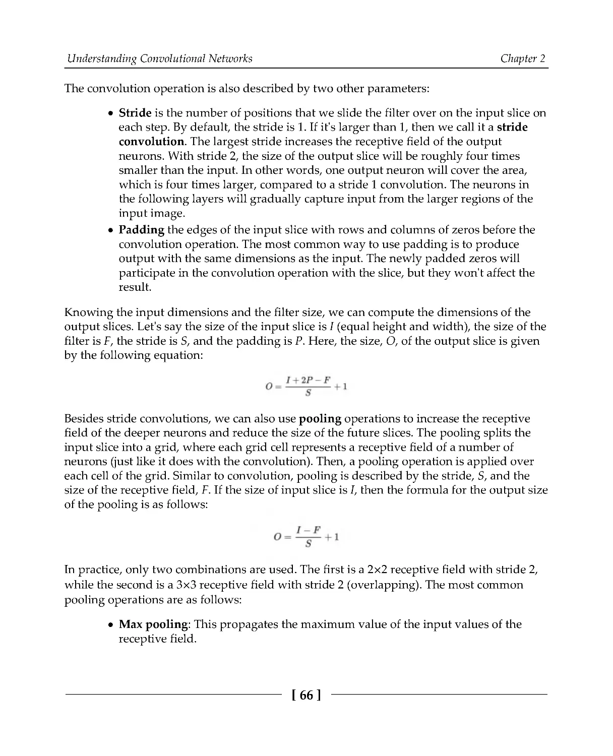


Author: Vasilev I.
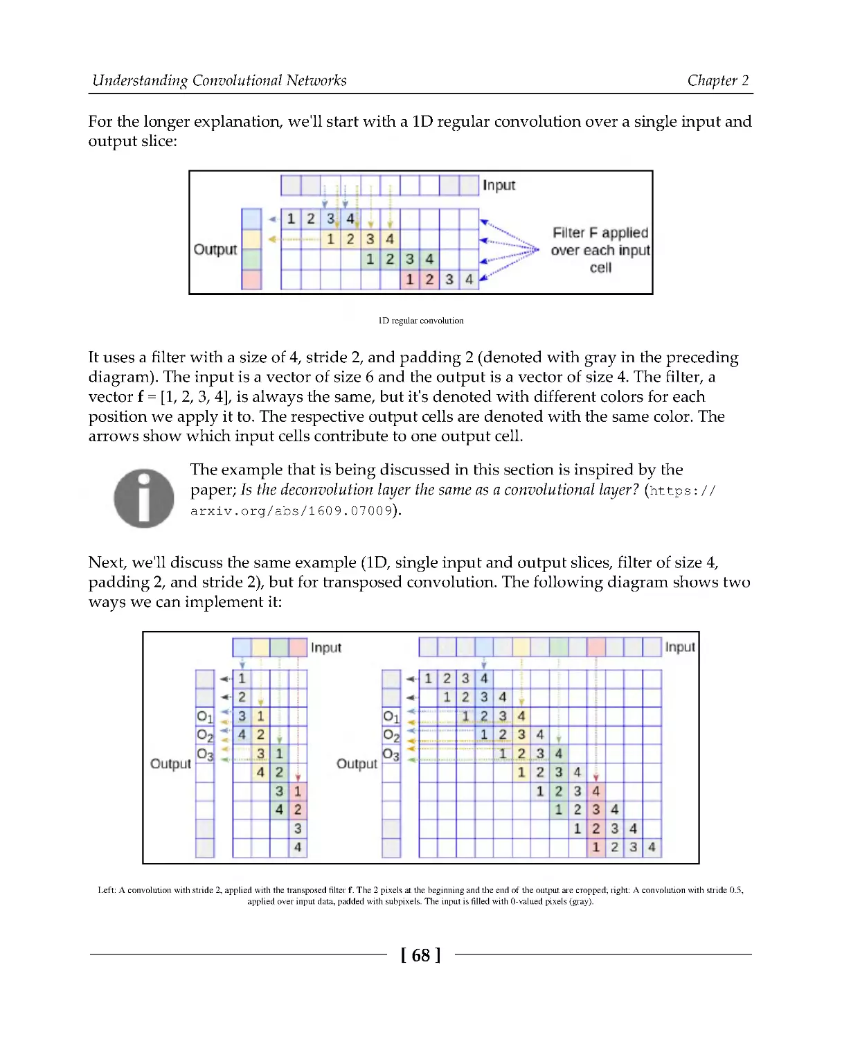
Tags: programming languages programming python packt publisher deep learning ai models
ISBN: 978-1-78995-617-7
Year: 2020


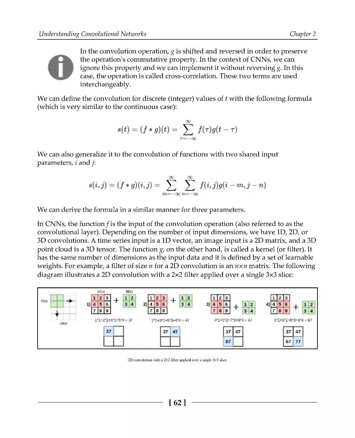
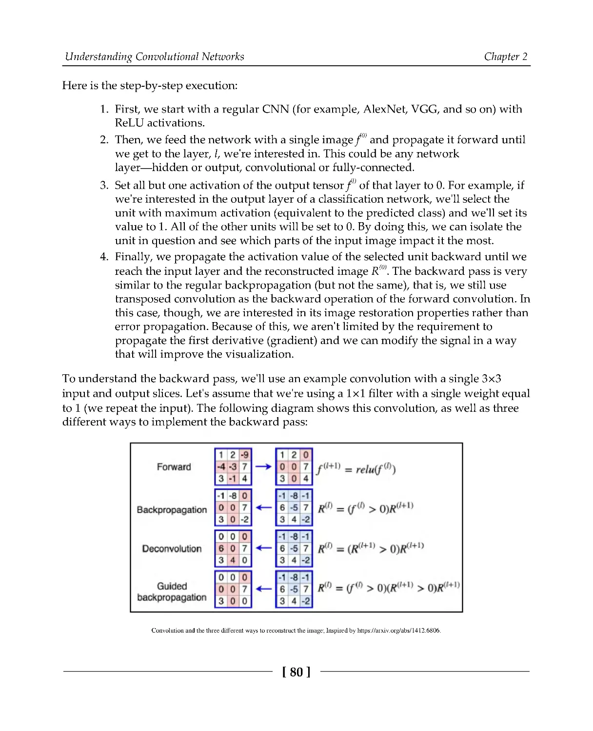
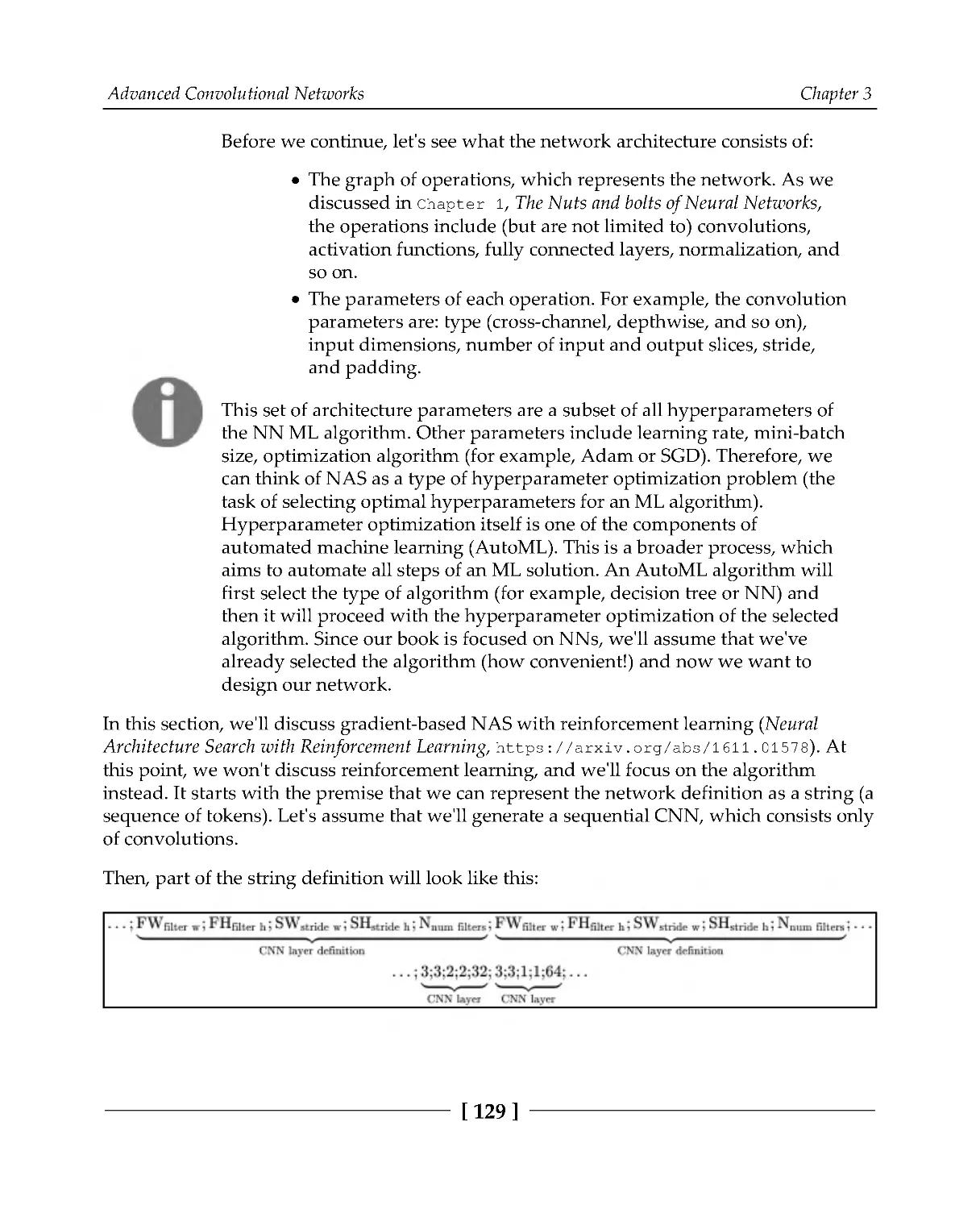
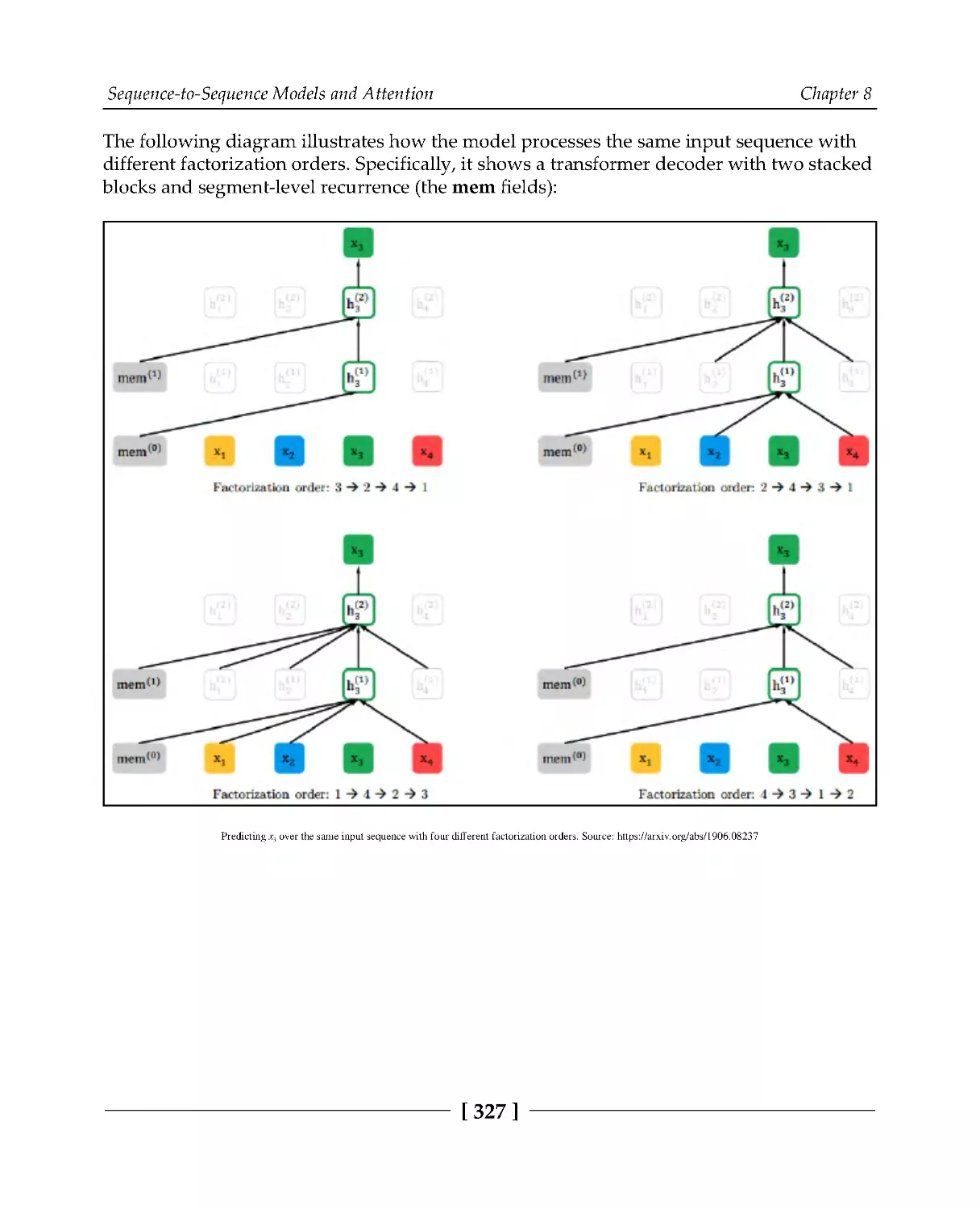
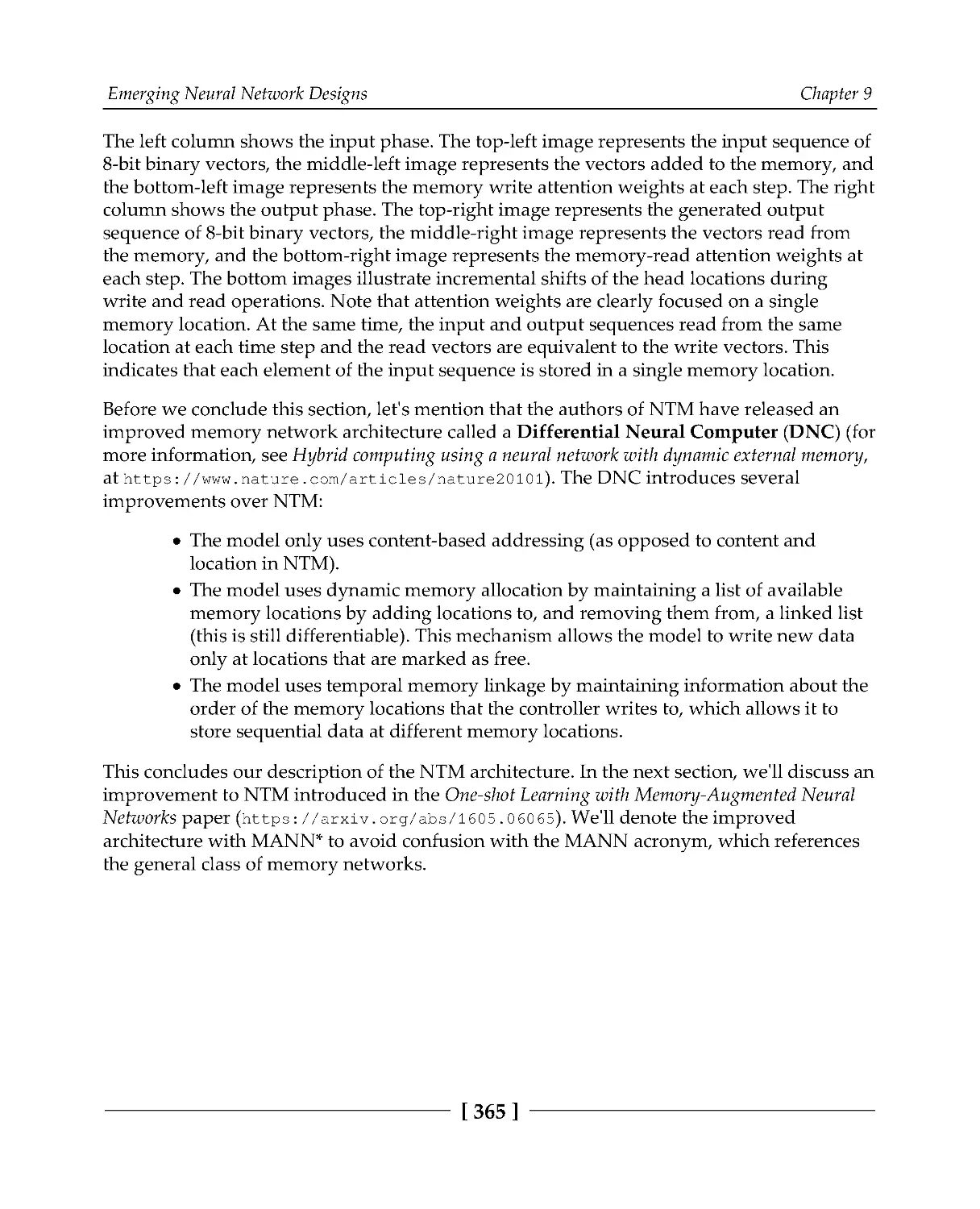
Text
Advanced Deep Learning with
Python
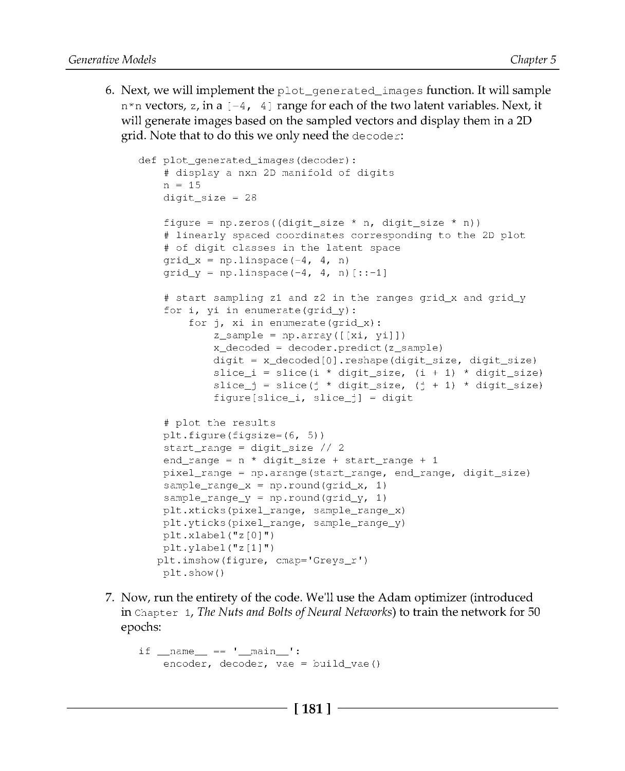
Design and implement advanced next-generation AI solutions
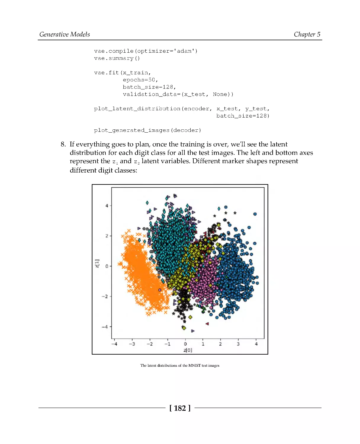
using TensorFlow and PyTorch
Ivan Vasilev
BIRMINGHAM - MUMBAI
Advanced Deep Learning with Python
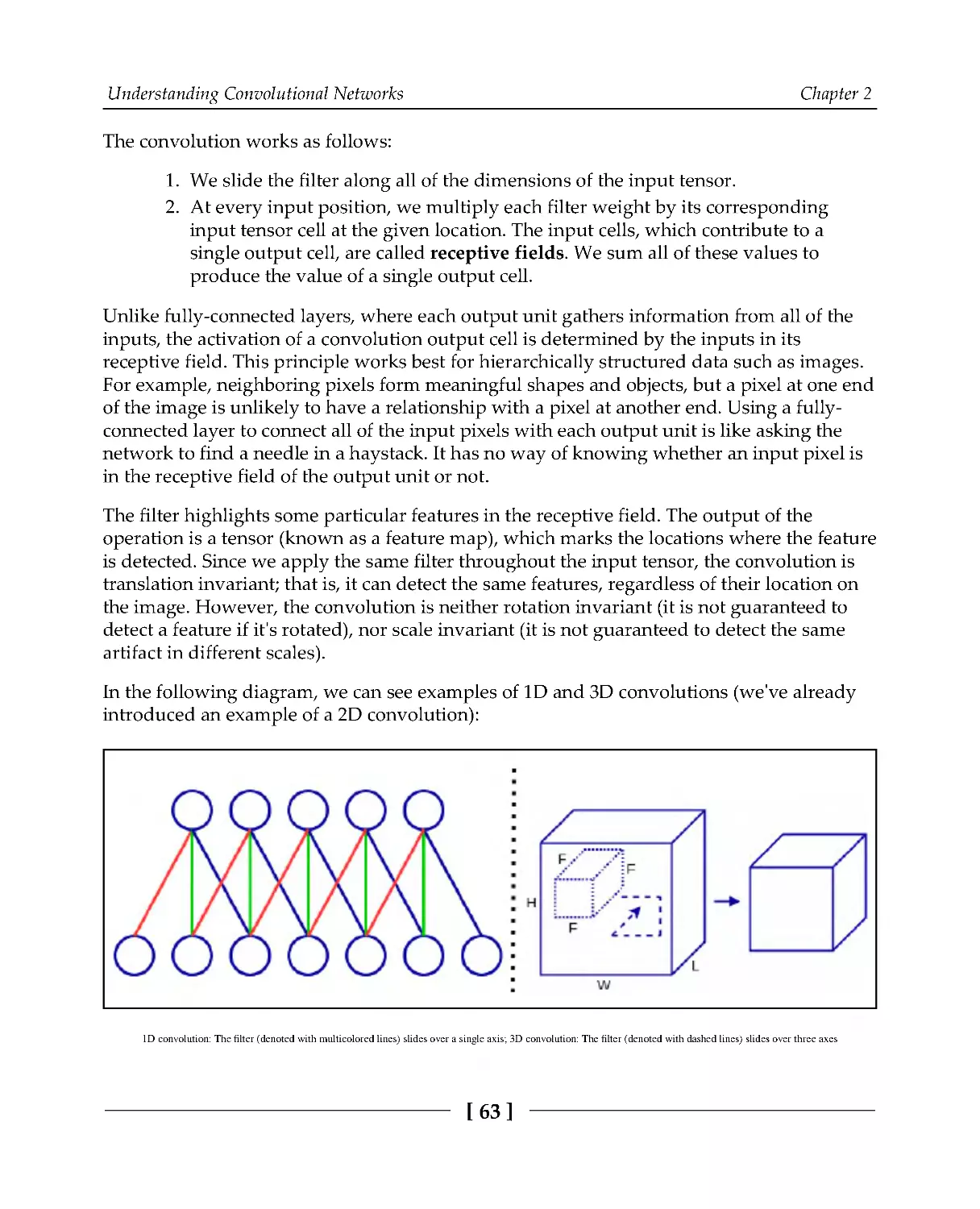
Copyright © 2019 Packt Publishing
All rights reserved. No part of this book may be reproduced, stored in a retrieval system, or transmitted in any form
or by any means, without the prior written permission of the publisher, except in the case of brief quotations
embedded in critical articles or reviews.
Every effort has been made in the preparation of this book to ensure the accuracy of the information presented.
However, the information contained in this book is sold without warranty, either express or implied. Neither the
author(s), nor Packt Publishing or its dealers and distributors, will be held liable for any damages caused or alleged
to have been caused directly or indirectly by this book.
Packt Publishing has endeavored to provide trademark information about all of the companies and products
mentioned in this book by the appropriate use of capitals. However, Packt Publishing cannot guarantee the accuracy
of this information.
Commissioning Editor: Pravin Dhandre
Acquisition Editor: Devika Battike
Content Development Editor: Nathanya Dias
Senior Editor: Ayaan Hoda
Technical Editor: Manikandan Kurup
Copy Editor: Safis Editing
Project Coordinator: Aishwarya Mohan
Proofreader: Safis Editing
Indexer: Tejal Daruwale Soni
Production Designer: Nilesh Mohite
First published: December 2019
Production reference: 1111219
Published by Packt Publishing Ltd.
Livery Place
35 Livery Street
Birmingham
B3 2PB, UK.
ISBN 978-1-78995-617-7
www.packt.com
Packt.com
Subscribe to our online digital library for full access to over 7,000 books and videos, as well
as industry leading tools to help you plan your personal development and advance your
career. For more information, please visit our website.
Why subscribe?
Spend less time learning and more time coding with practical eBooks and Videos
from over 4,000 industry professionals
Improve your learning with Skill Plans built especially for you
Get a free eBook or video every month
Fully searchable for easy access to vital information
Copy and paste, print, and bookmark content
Did you know that Packt offers eBook versions of every book published, with PDF and
ePub files available? You can upgrade to the eBook version at www.packt.com and as a print
book customer, you are entitled to a discount on the eBook copy. Get in touch with us at
customercare@packtpub.com for more details.
At www.packt.com, you can also read a collection of free technical articles, sign up for a
range of free newsletters, and receive exclusive discounts and offers on Packt books and
eBooks.
Contributors
About the author
Ivan Vasilev started working on the first open source Java deep learning library with GPU
support in 2013. The library was acquired by a German company, where he continued to
develop it. He has also worked as a machine learning engineer and researcher in the area of
medical image classification and segmentation with deep neural networks. Since 2017, he
has been focusing on financial machine learning. He is working on a Python-based
platform that provides the infrastructure to rapidly experiment with different machine
learning algorithms for algorithmic trading. Ivan holds an MSc degree in artificial
intelligence from the University of Sofia, St. Kliment Ohridski.
About the reviewer
Saibal Dutta has been working as an analytical consultant in SAS Research and
Development. He is also pursuing a PhD in data mining and machine learning from IIT,
Kharagpur. He holds an M.Tech in electronics and communication from the National
Institute of Technology, Rourkela. He has worked at TATA communications, Pune, and
HCL Technologies Limited, Noida, as a consultant. In his 7 years of consulting experience,
he has been associated with global players including IKEA (in Sweden) and Pearson (in the
US). His passion for entrepreneurship led him to create his own start-up in the field of data
analytics. His areas of expertise include data mining, artificial intelligence, machine
learning, image processing, and business consultation.
Packt is searching for authors like you
If you're interested in becoming an author for Packt, please visit authors.packtpub.com
and apply today. We have worked with thousands of developers and tech professionals,
just like you, to help them share their insight with the global tech community. You can
make a general application, apply for a specific hot topic that we are recruiting an author
for, or submit your own idea.
Table of Contents
Preface
1
Section 1: Core Concepts
Chapter 1: The Nuts and Bolts of Neural Networks
7
The mathematical apparatus of NNs
8
Linear algebra
8
Vector and matrix operations
10
Introduction to probability
14
Probability and sets
16
Conditional probability and the Bayes rule
18
Random variables and probability distributions
20
Probability distributions
23
Information theory
26
Differential calculus
29
A short introduction to NNs
32
Neurons
33
Layers as operations
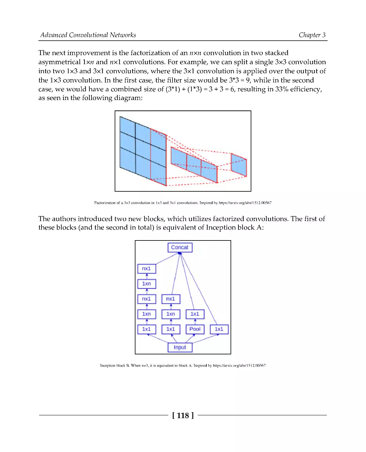
34
NNs
36
Activation functions
38
The universal approximation theorem
43
Training NNs
45
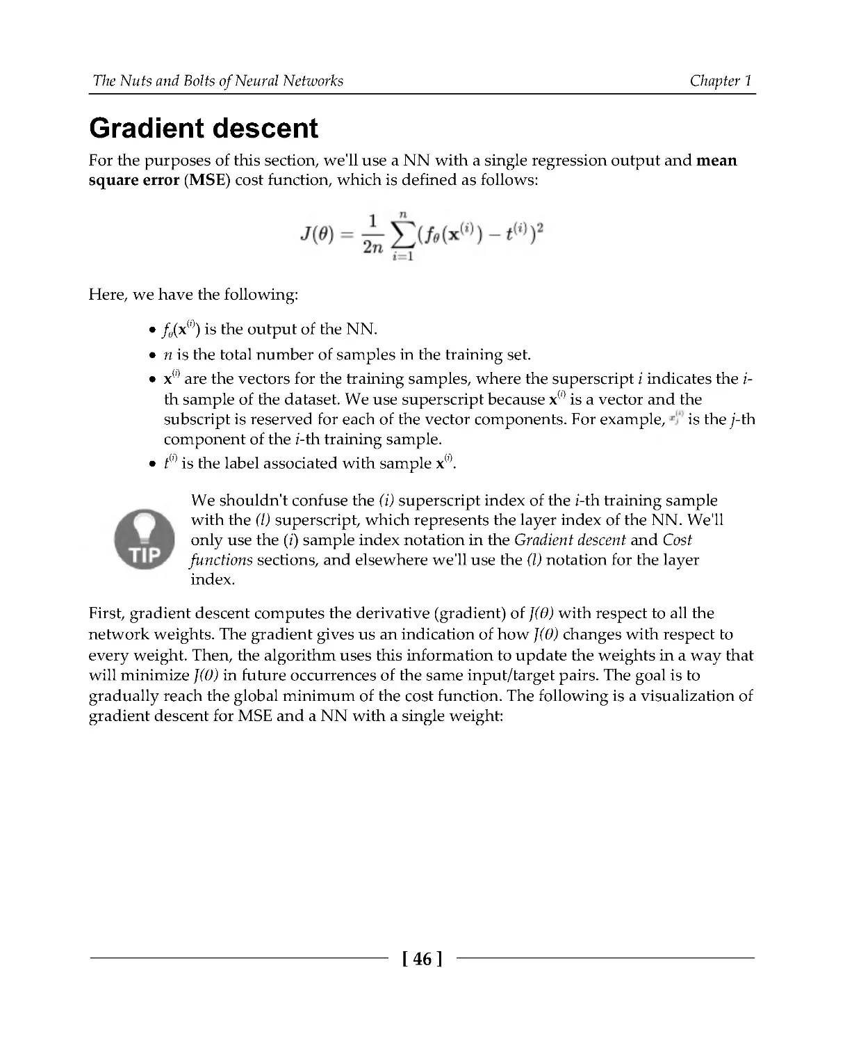
Gradient descent
46
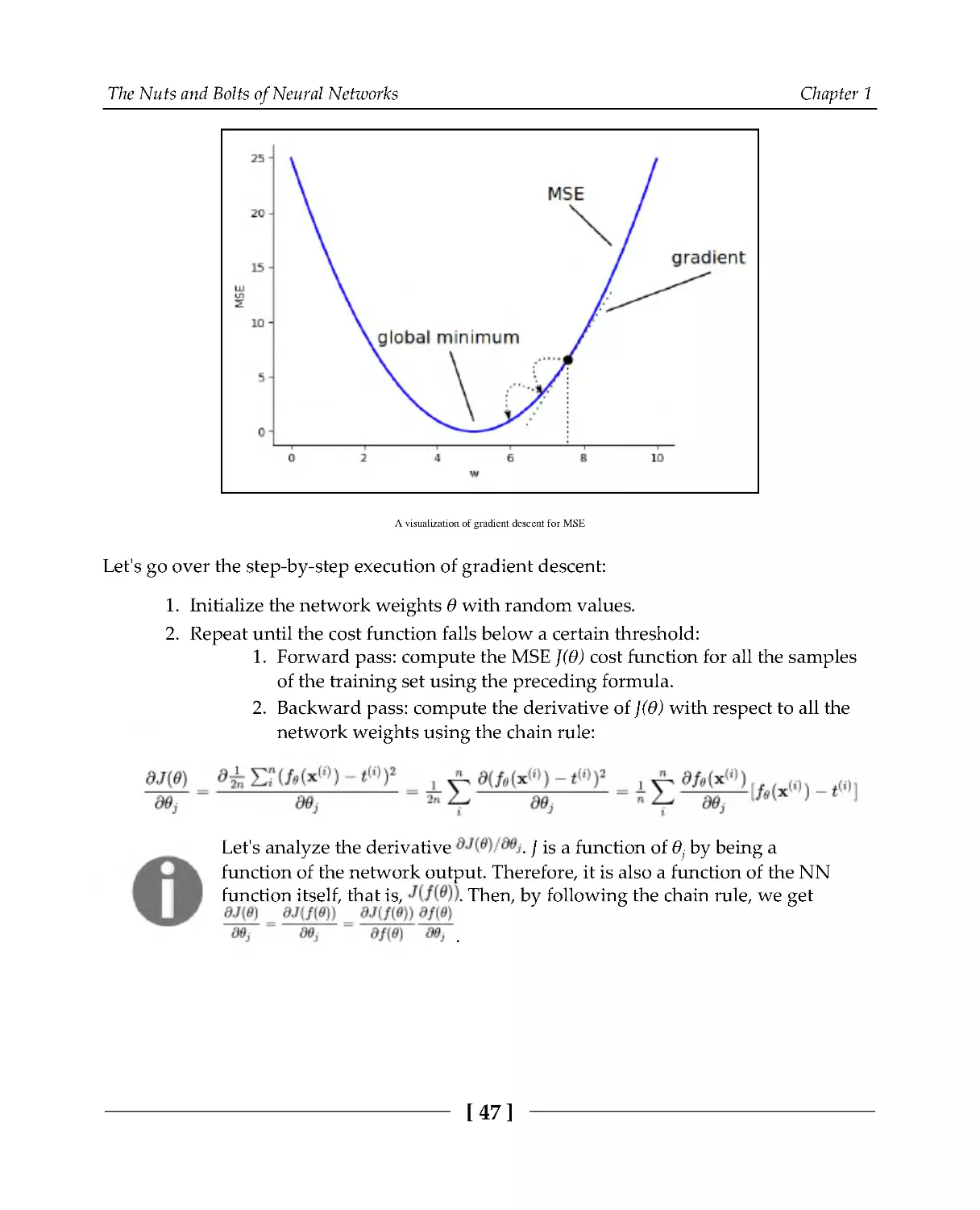
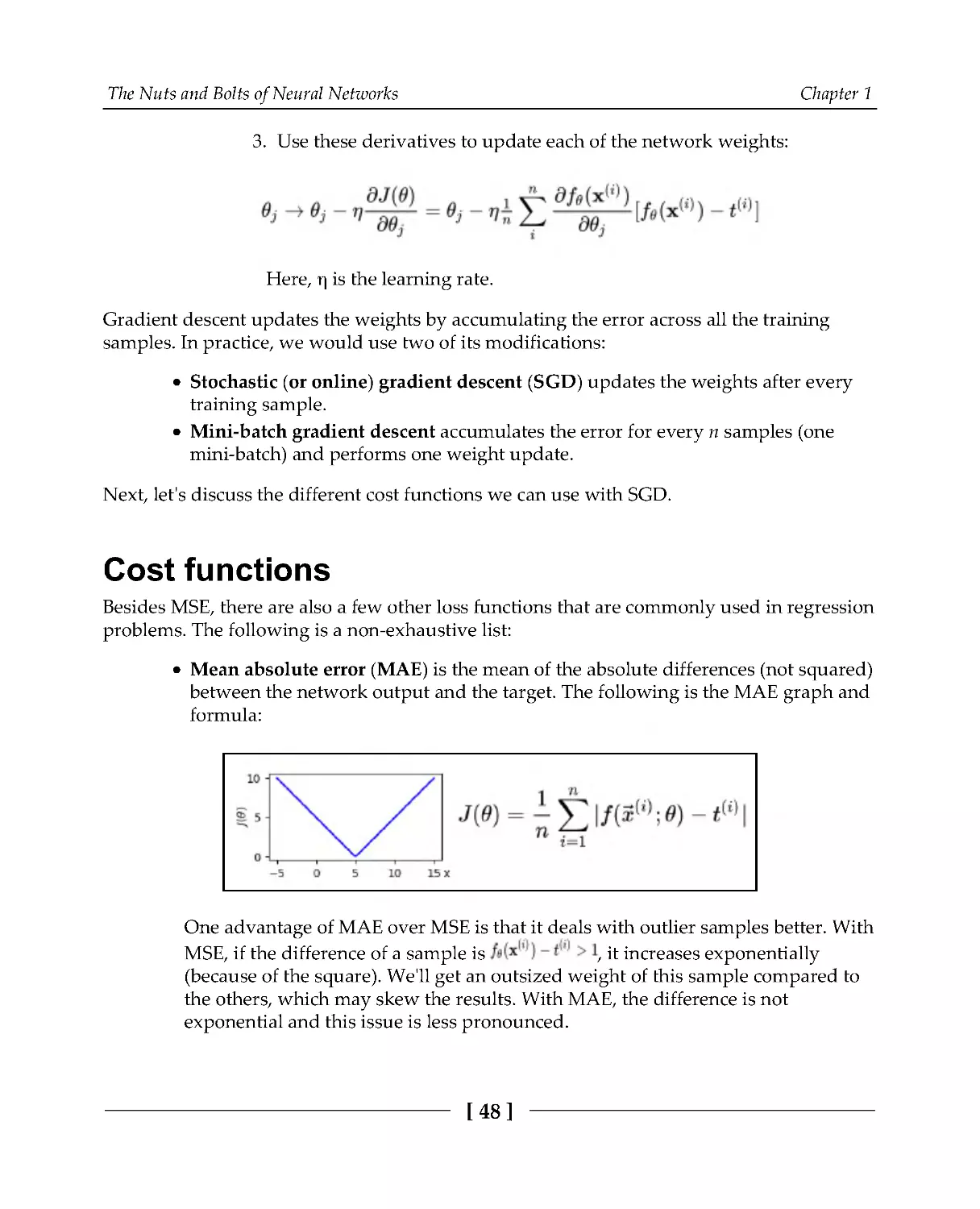
Cost functions
48
Backpropagation
50
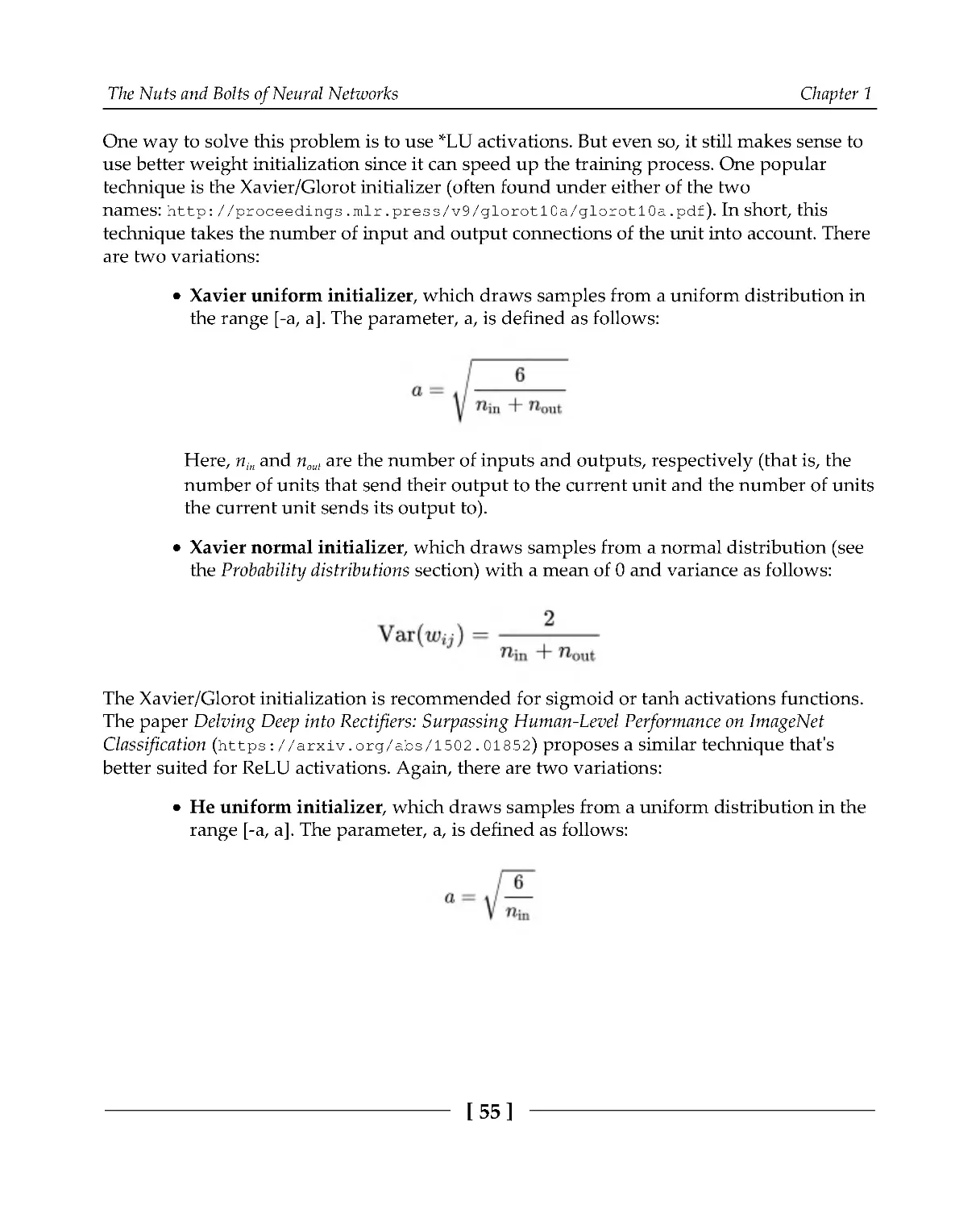
Weight initialization
54
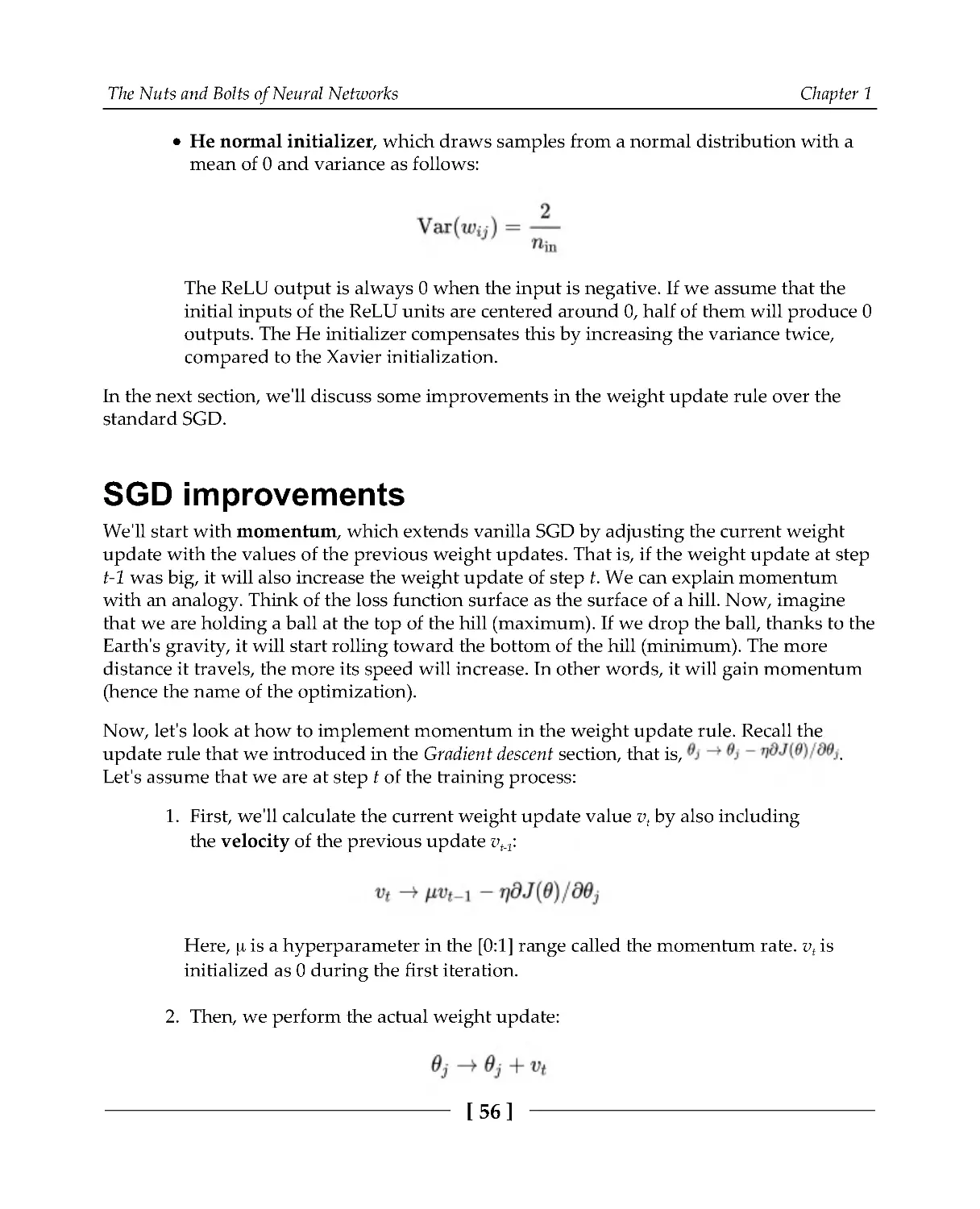
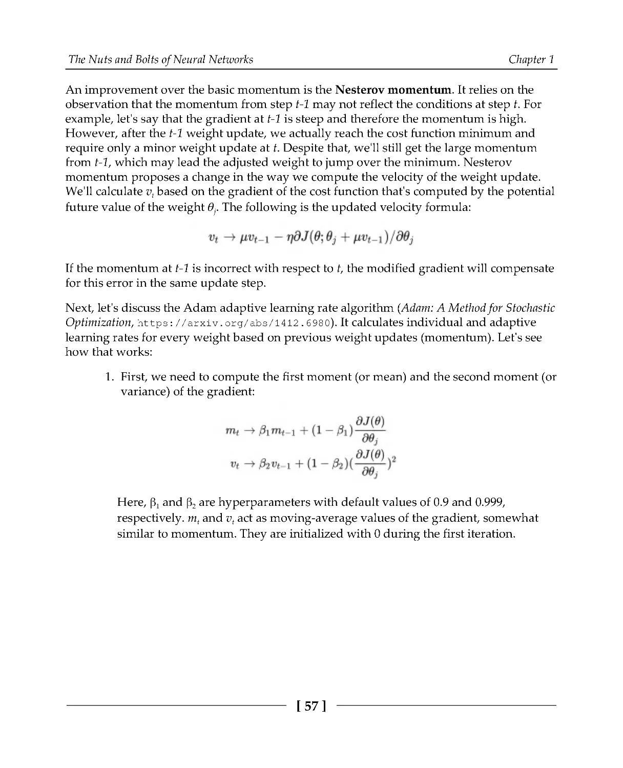
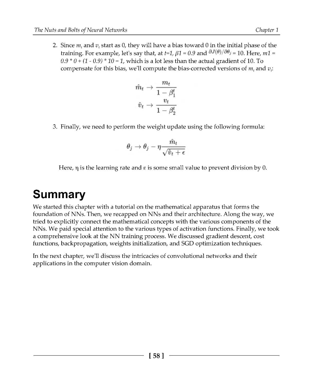
SGD improvements
56
Summary
58
Section 2: Computer Vision
Chapter 2: Understanding Convolutional Networks
60
Understanding CNNs
61
Types of convolutions
67
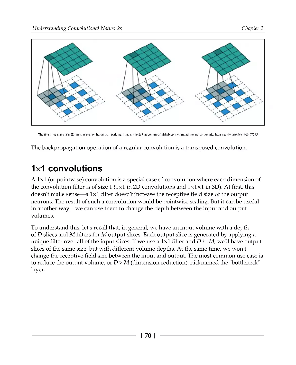
Transposed convolutions
67
1×1 convolutions
70
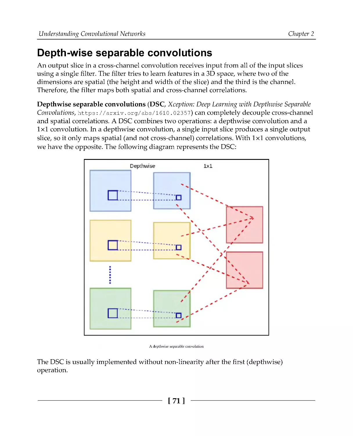
Depth-wise separable convolutions
71
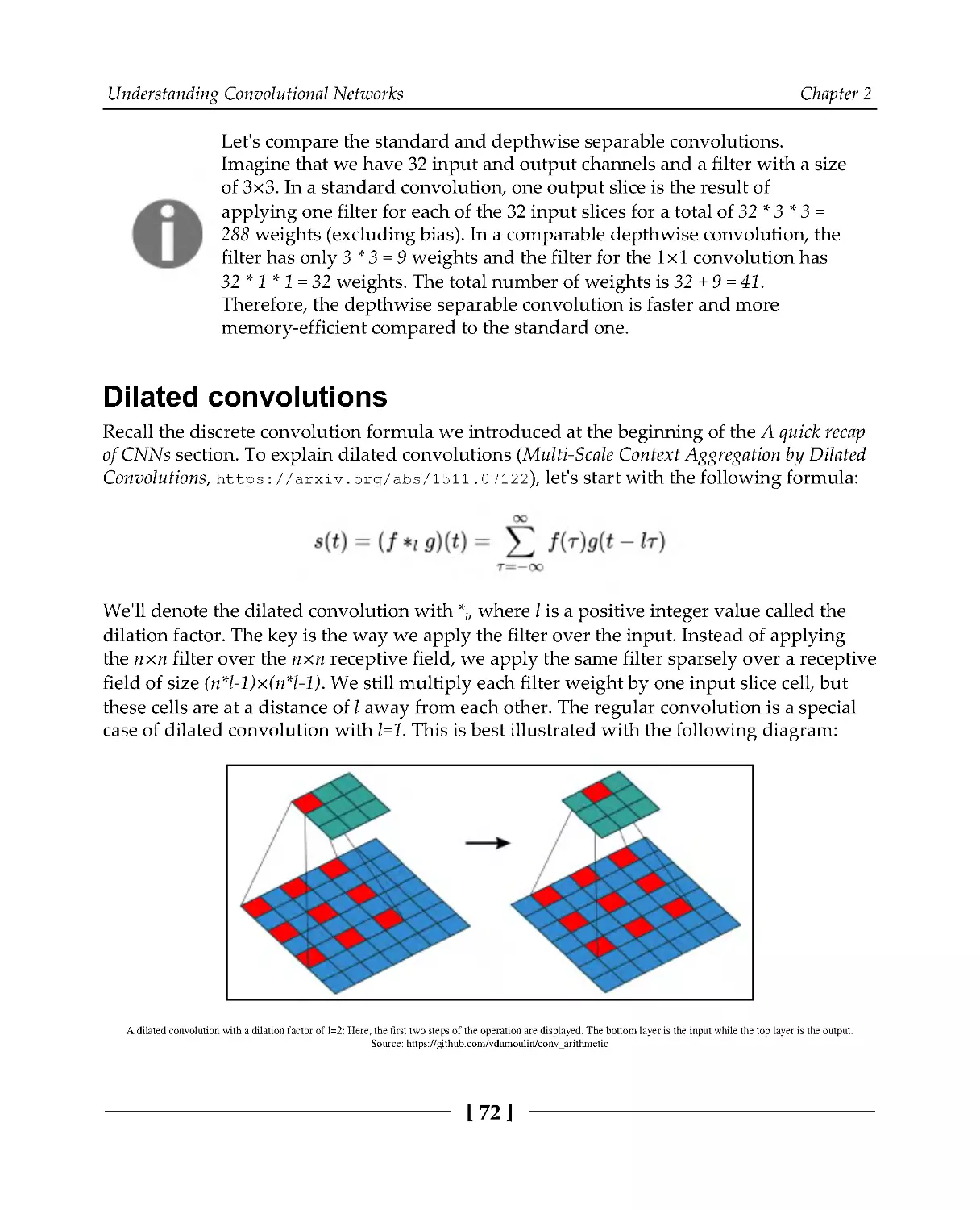
Dilated convolutions
72
Improving the efficiency of CNNs
73
Convolution as matrix multiplication
74
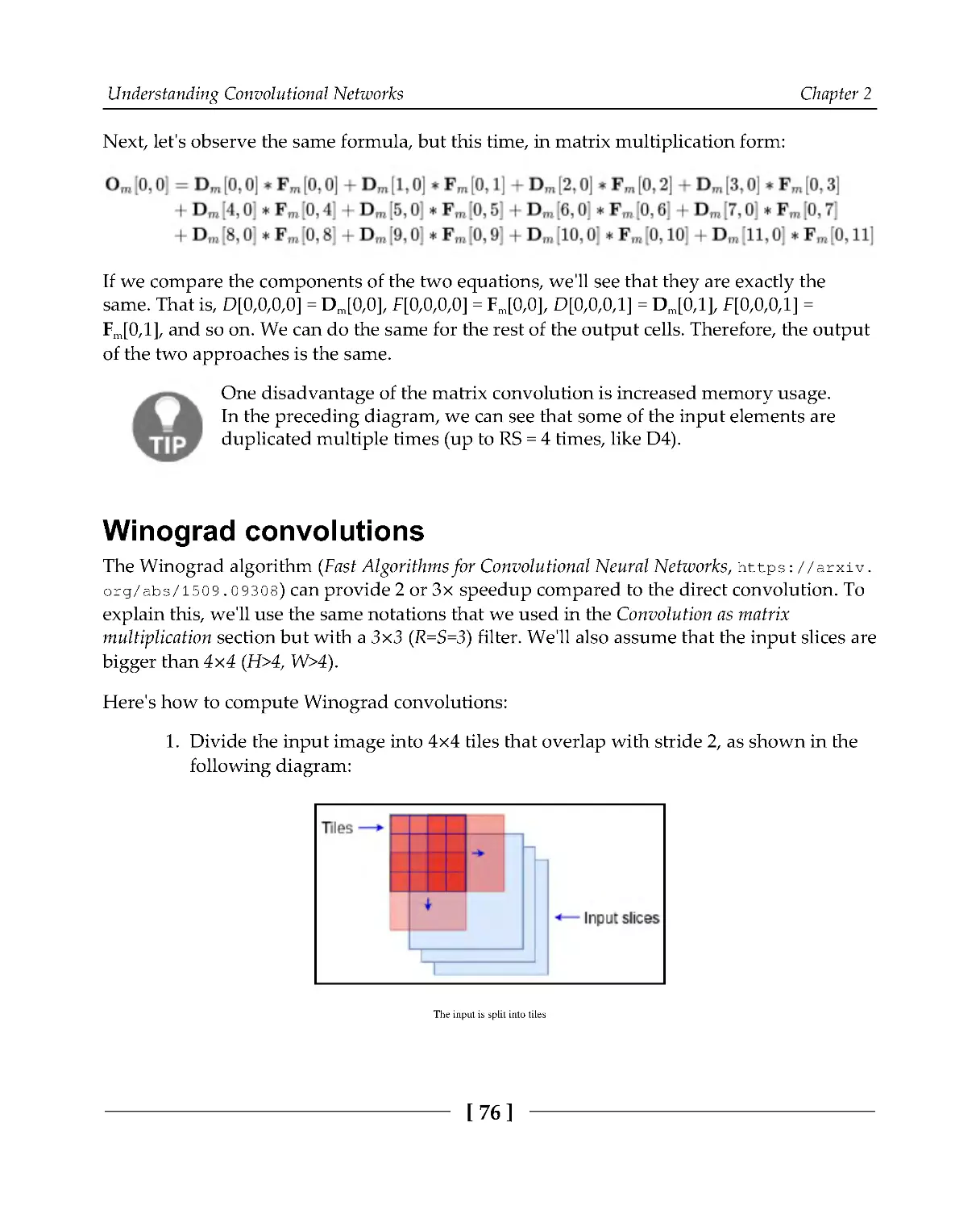
Winograd convolutions
76
Visualizing CNNs
79
Table of Contents
[ii]
Guided backpropagation
79
Gradient-weighted class activation mapping
82
CNN regularization
84
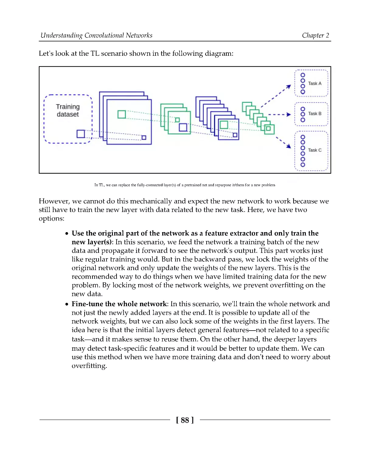
Introducing transfer learning
87
Implementing transfer learning with PyTorch
88
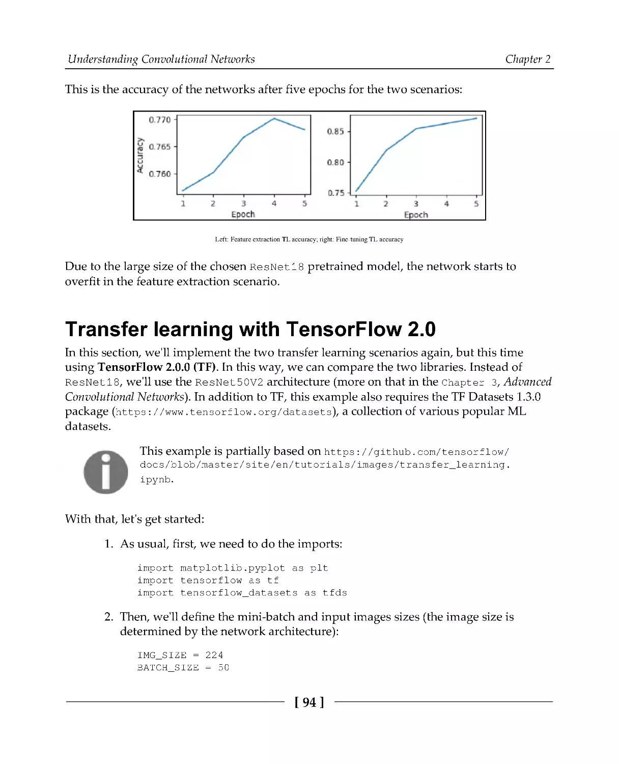
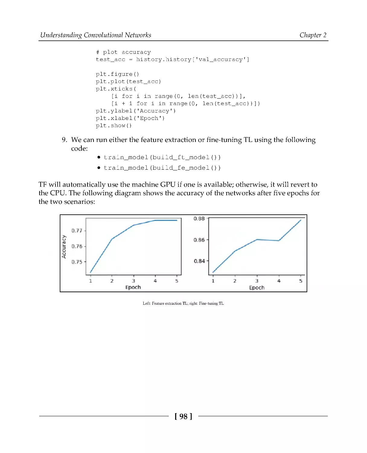
Transfer learning with TensorFlow 2.0
94
Summary
99
Chapter 3: Advanced Convolutional Networks
100
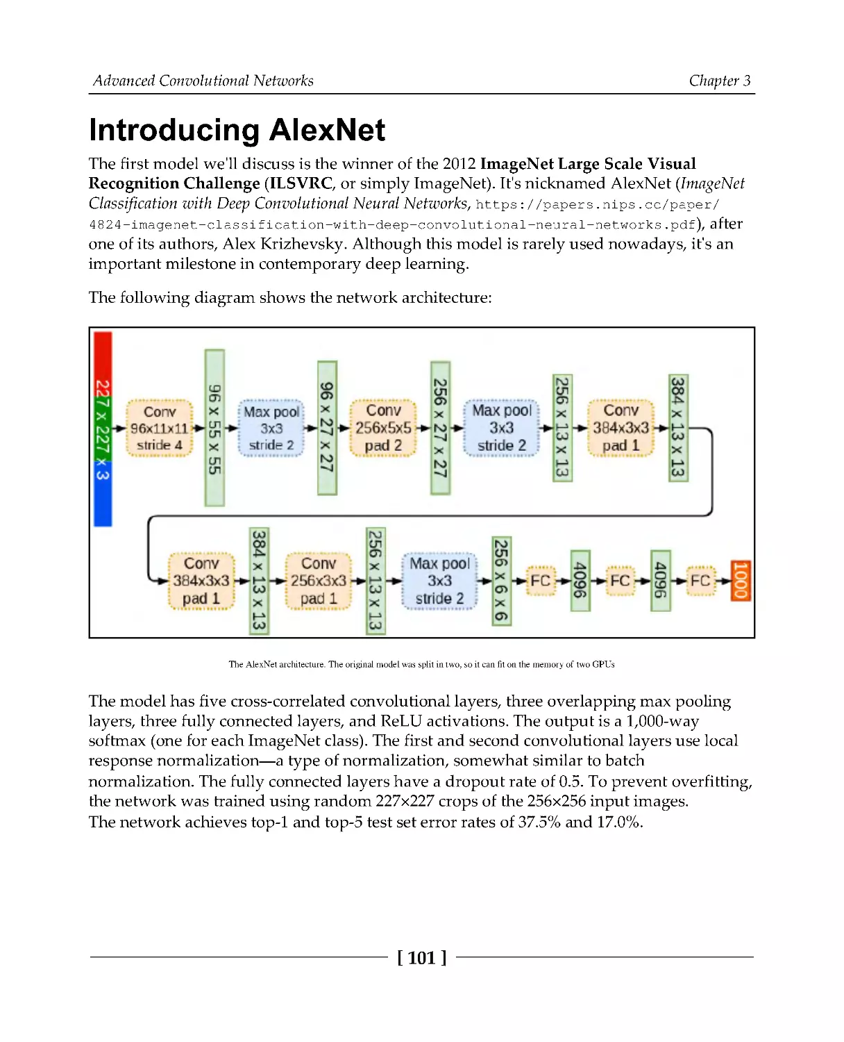
Introducing AlexNet
101
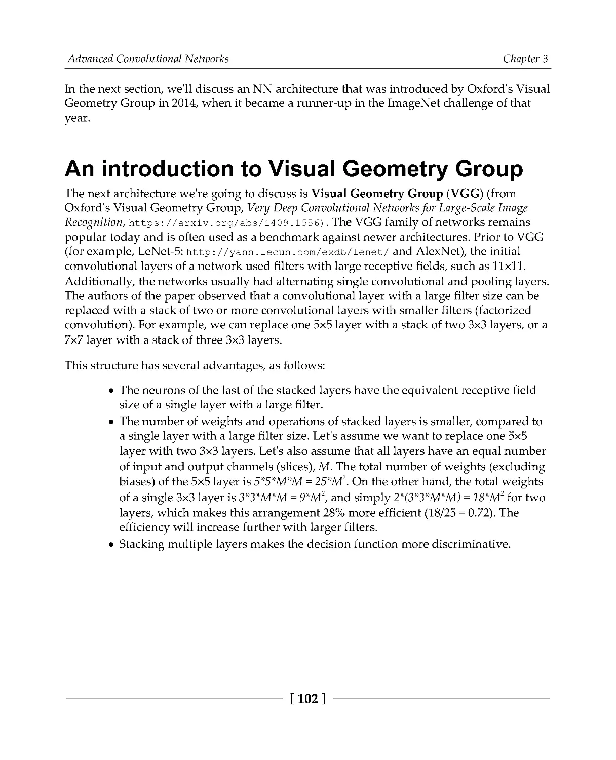
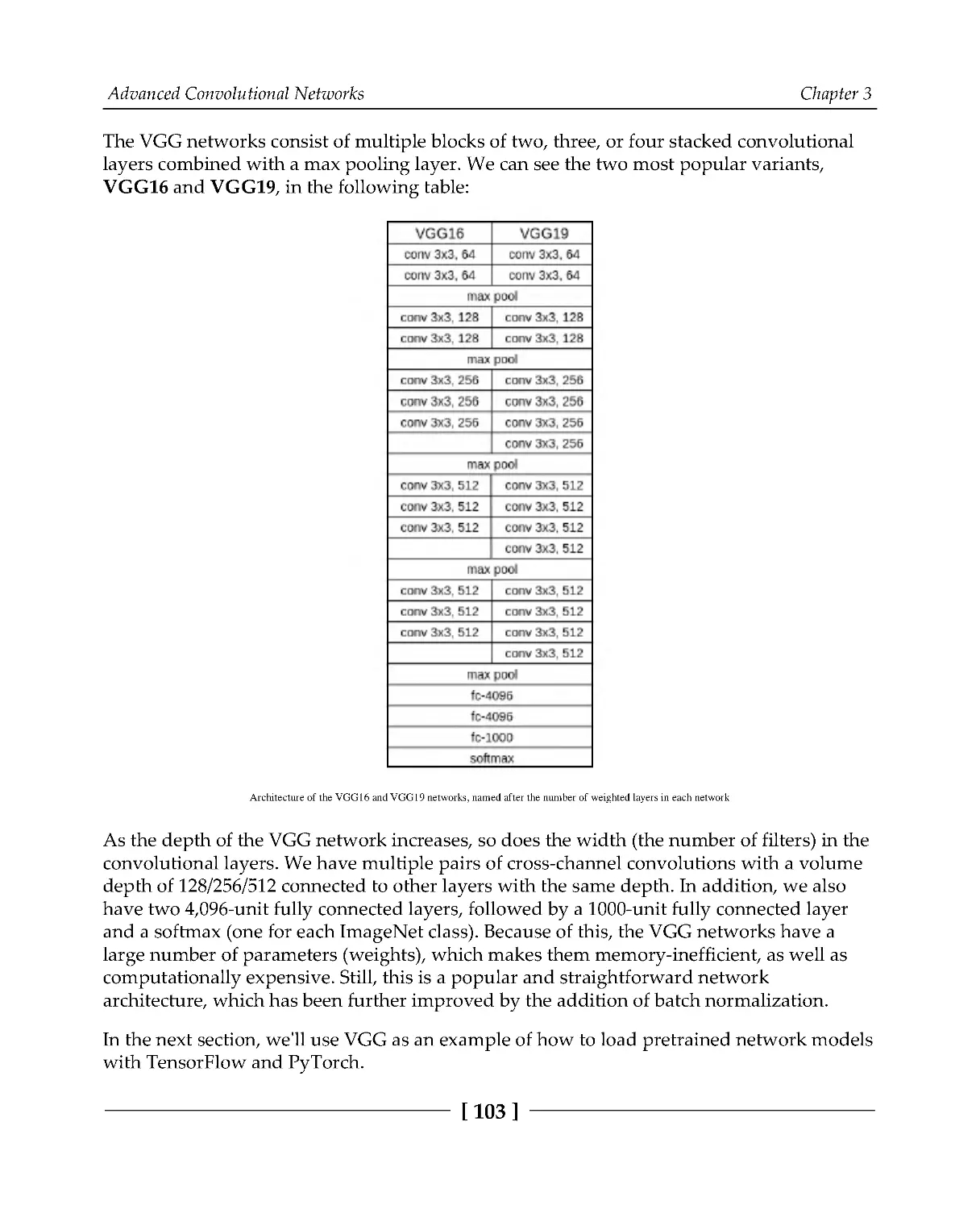
An introduction to Visual Geometry Group
102
VGG with PyTorch and TensorFlow
104
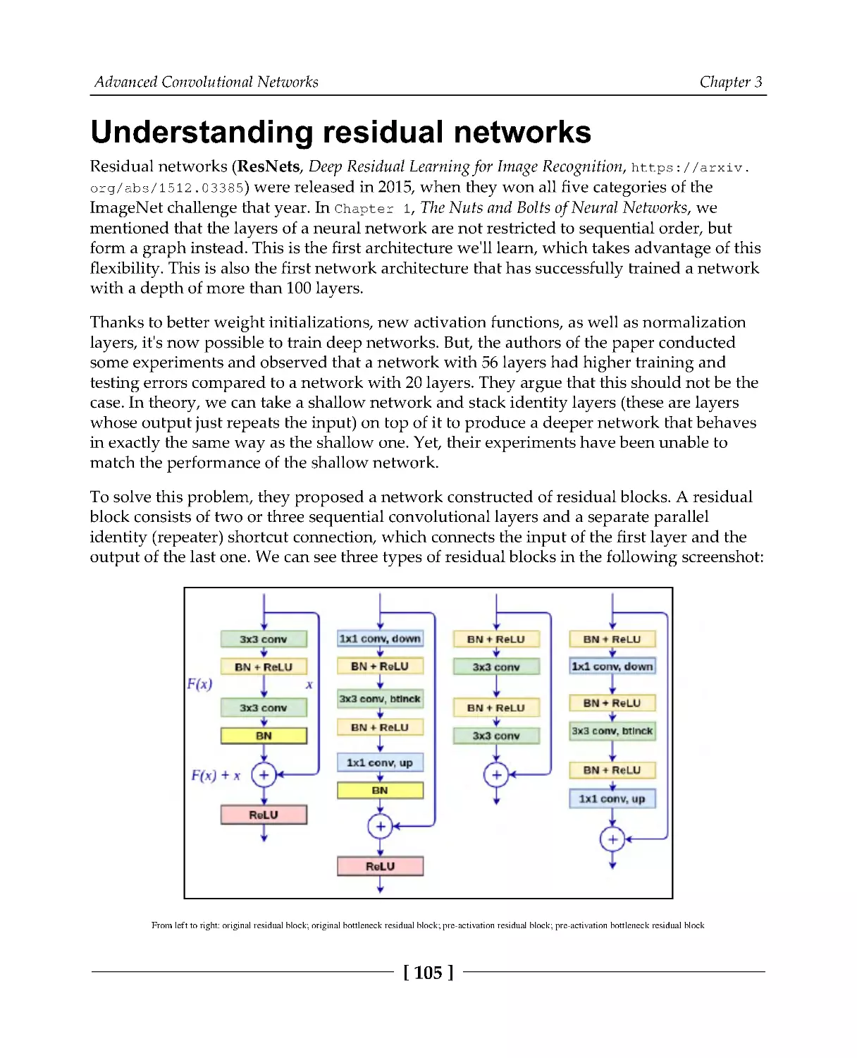
Understanding residual networks
105
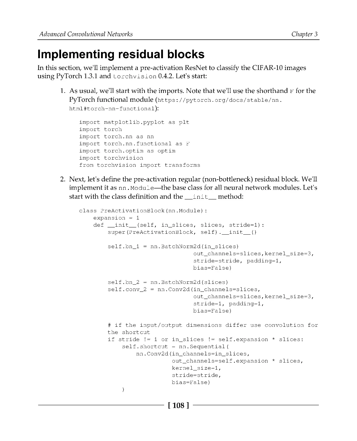
Implementing residual blocks
108
Understanding Inception networks
115
Inception v1
116
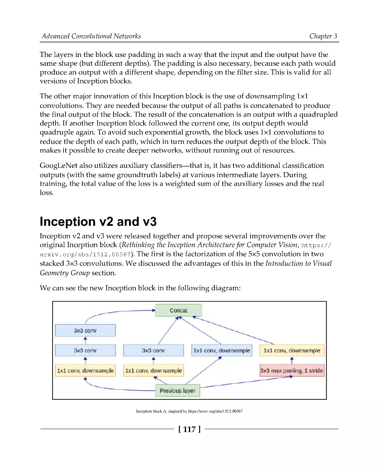
Inception v2 and v3
117
Inception v4 and Inception-ResNet
119
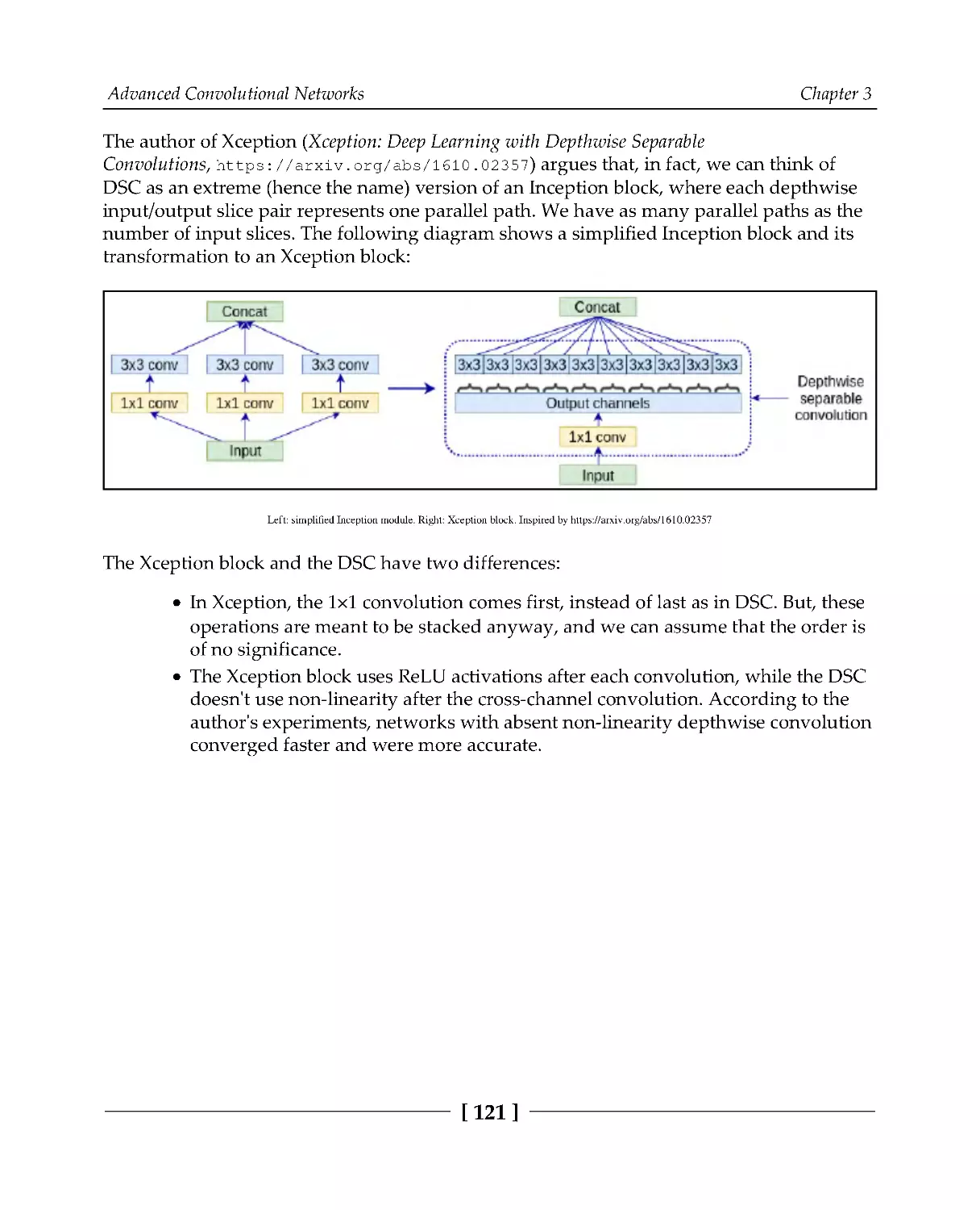
Introducing Xception
120
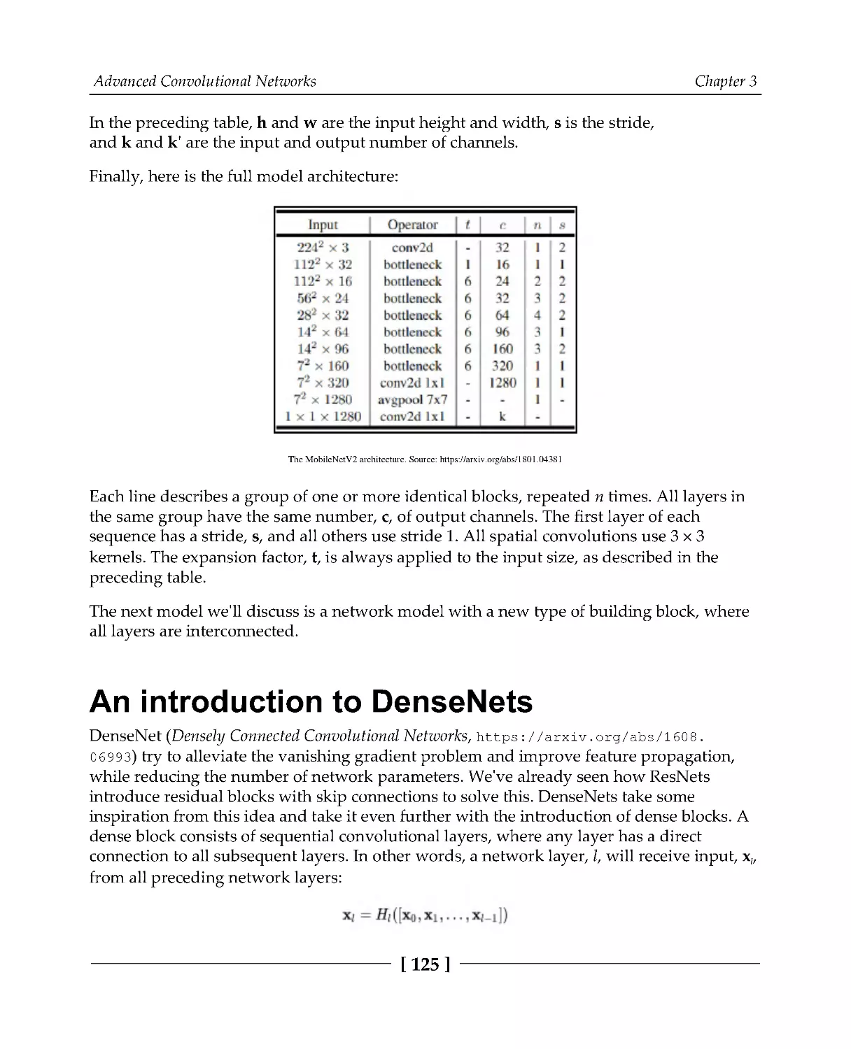
Introducing MobileNet
123
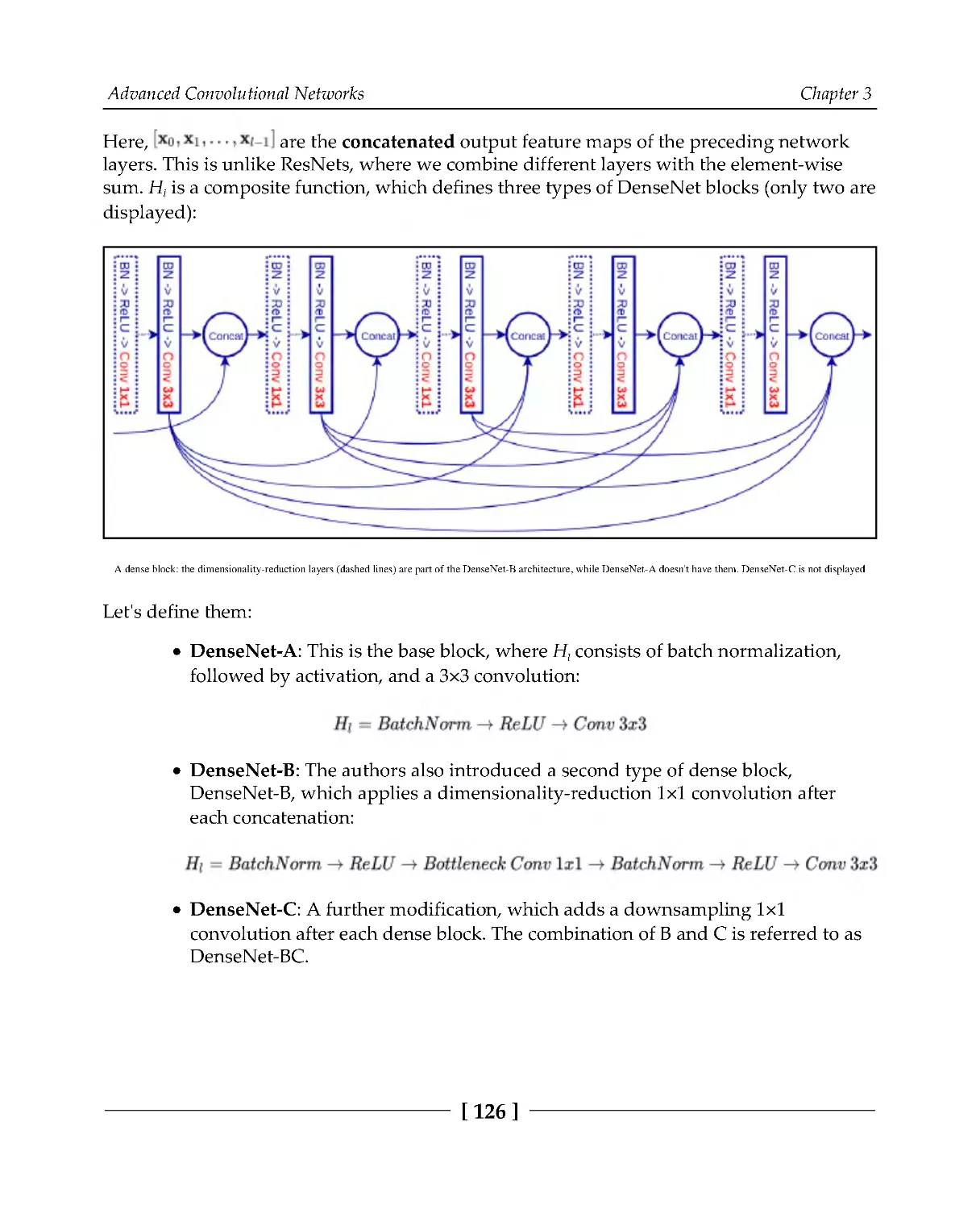
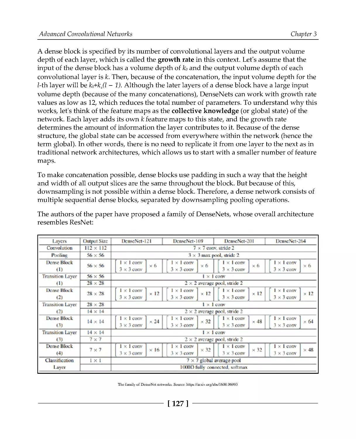
An introduction to DenseNets
125
The workings of neural architecture search
128
Introducing capsule networks
133
The limitations of convolutional networks
133
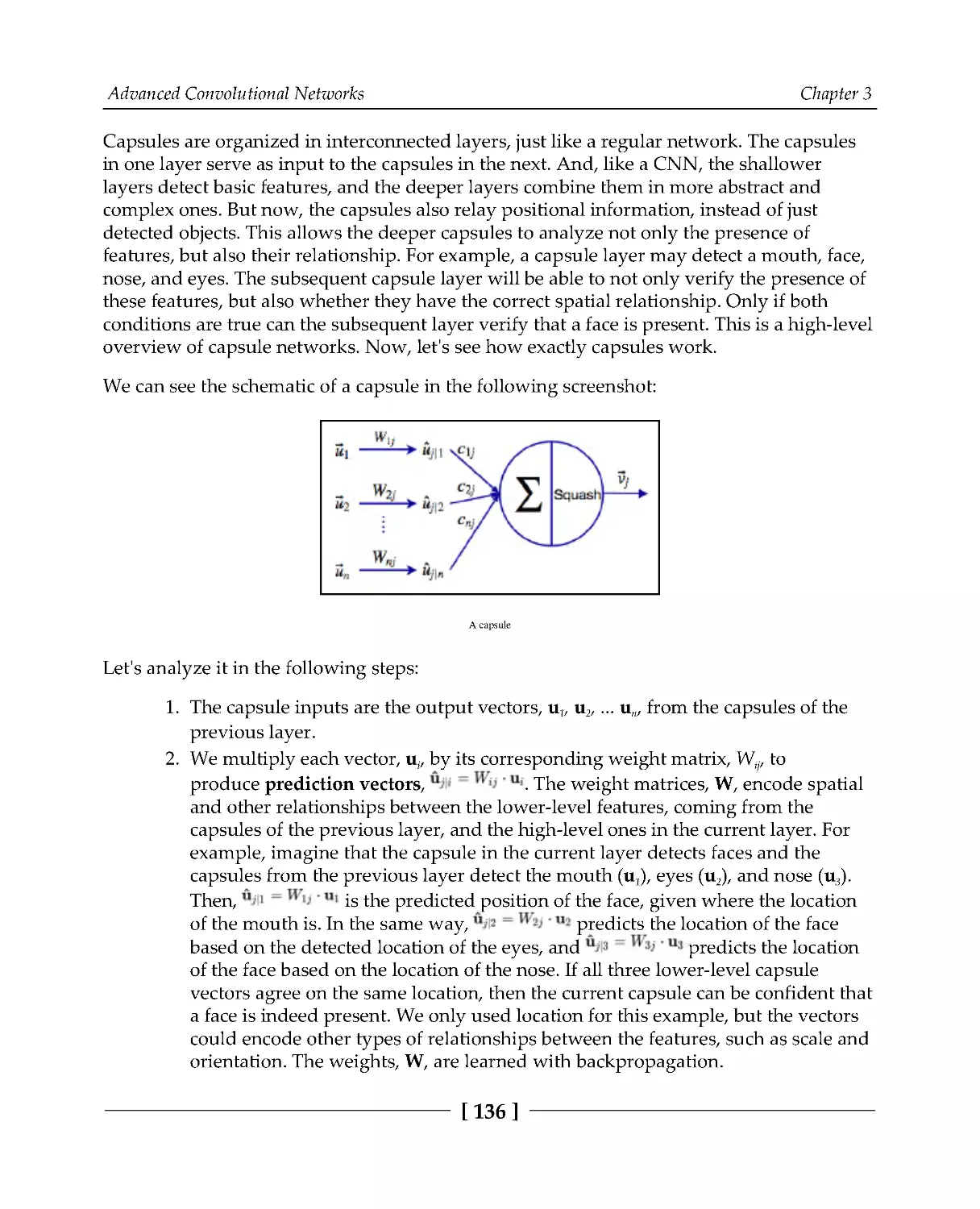
Capsules
135
Dynamic routing
137
The structure of the capsule network
139
Summary
140
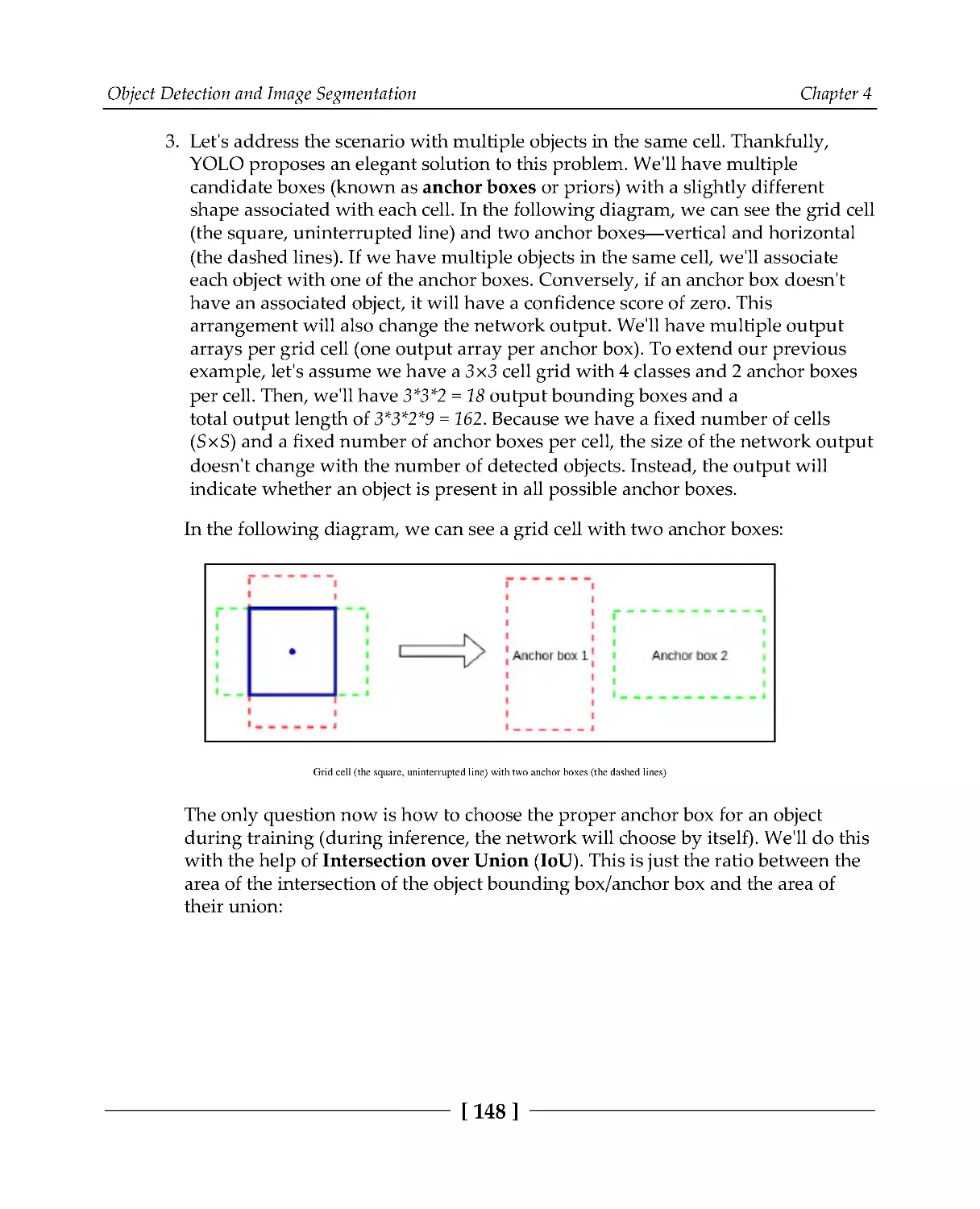
Chapter 4: Object Detection and Image Segmentation
141
Introduction to object detection
142
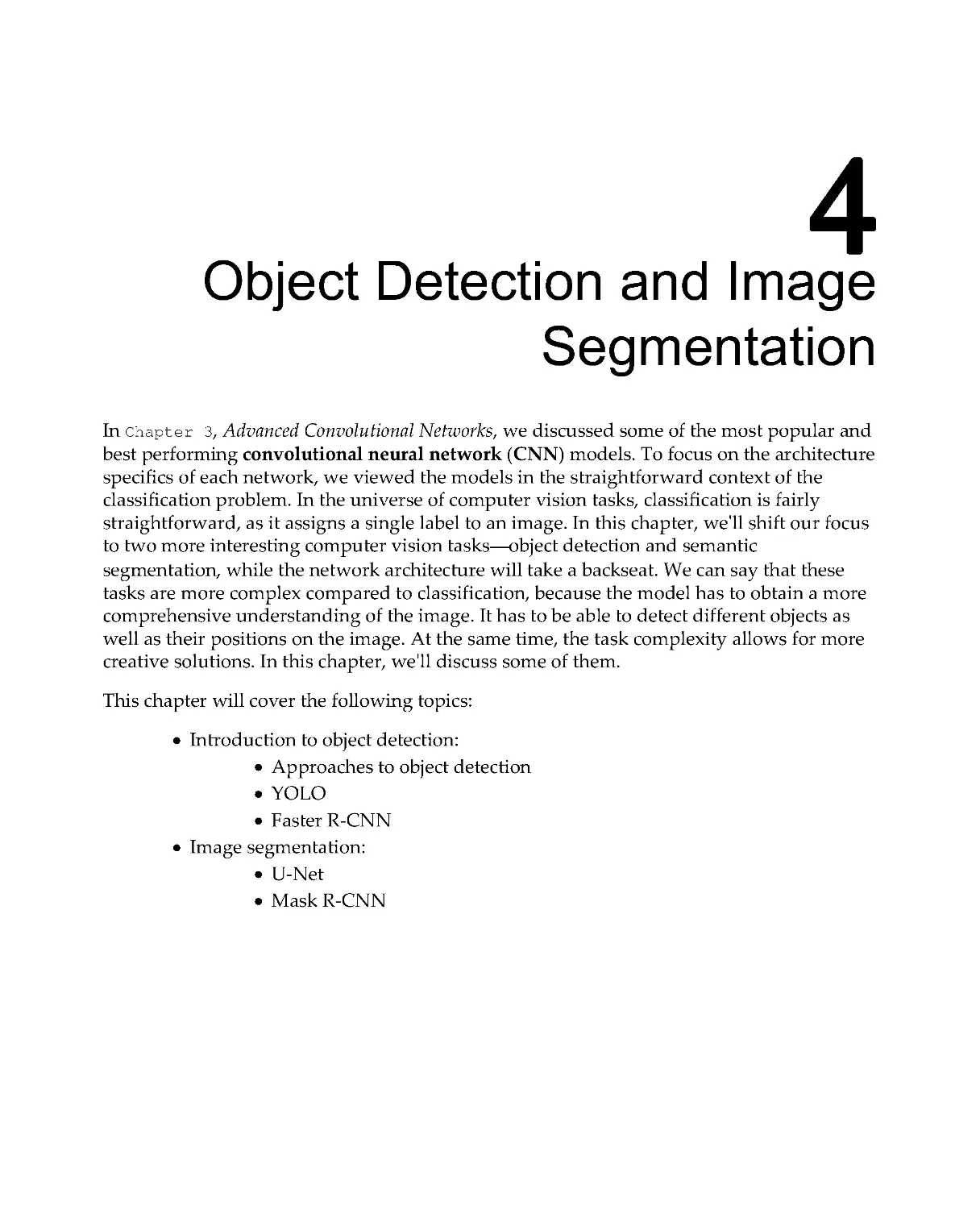
Approaches to object detection
143
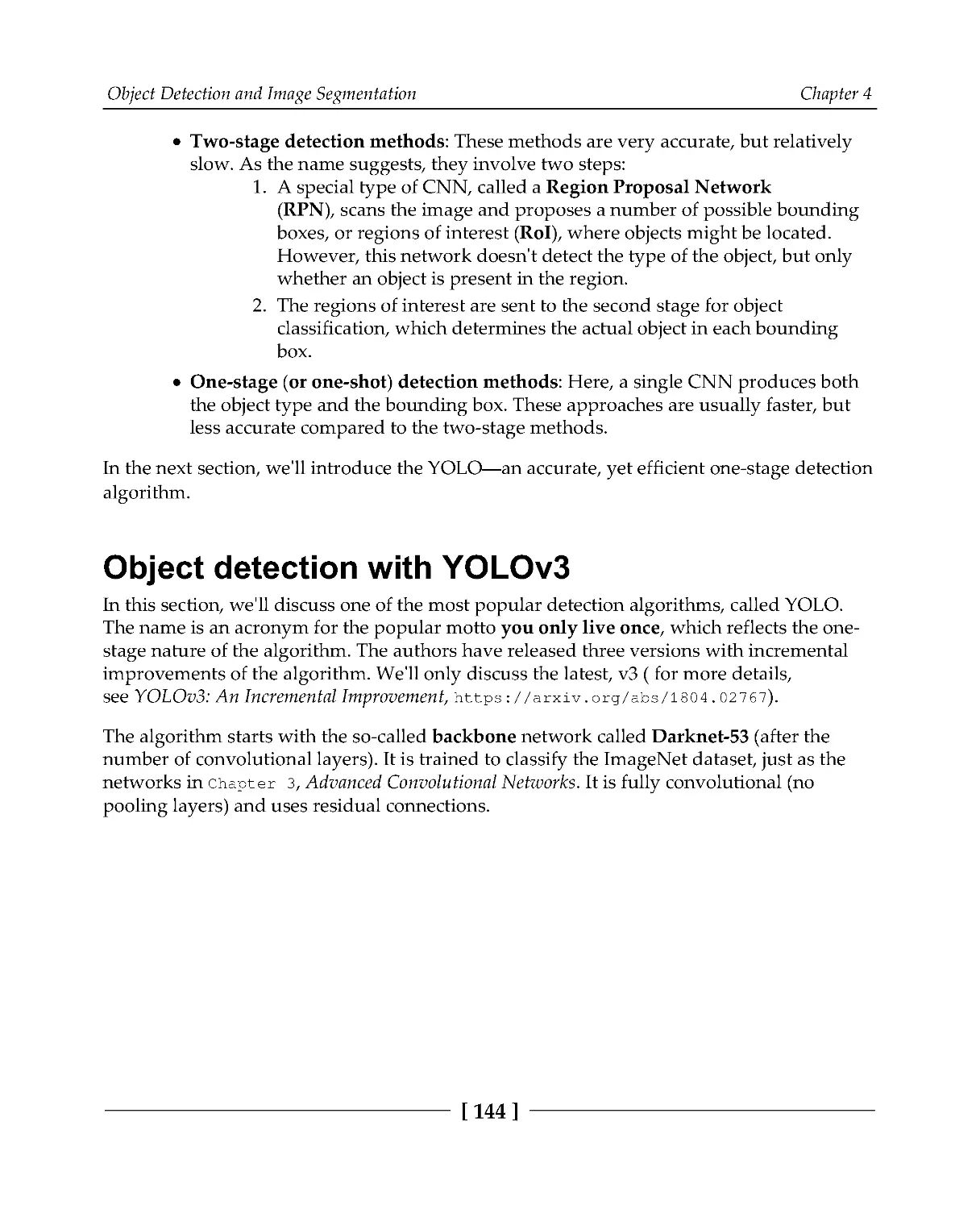
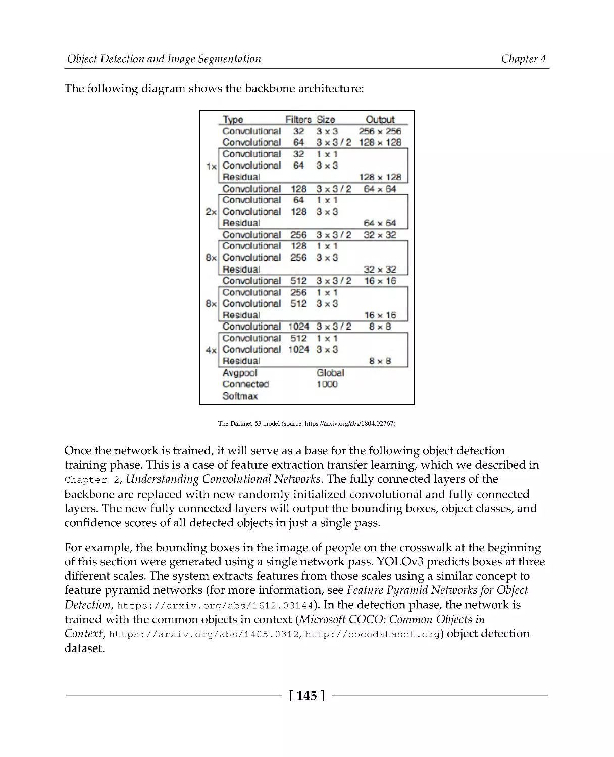
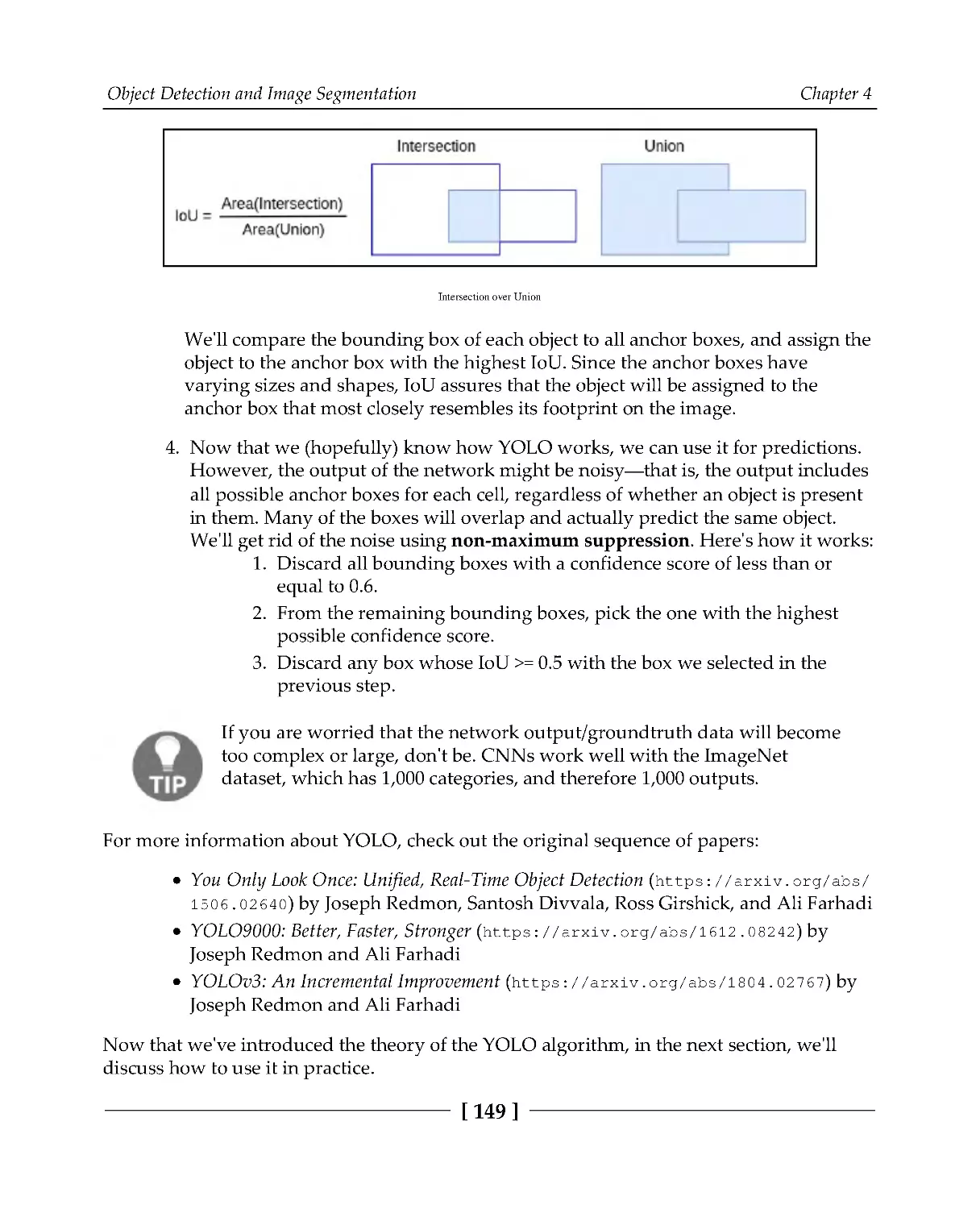
Object detection with YOLOv3
144
A code example of YOLOv3 with OpenCV
150
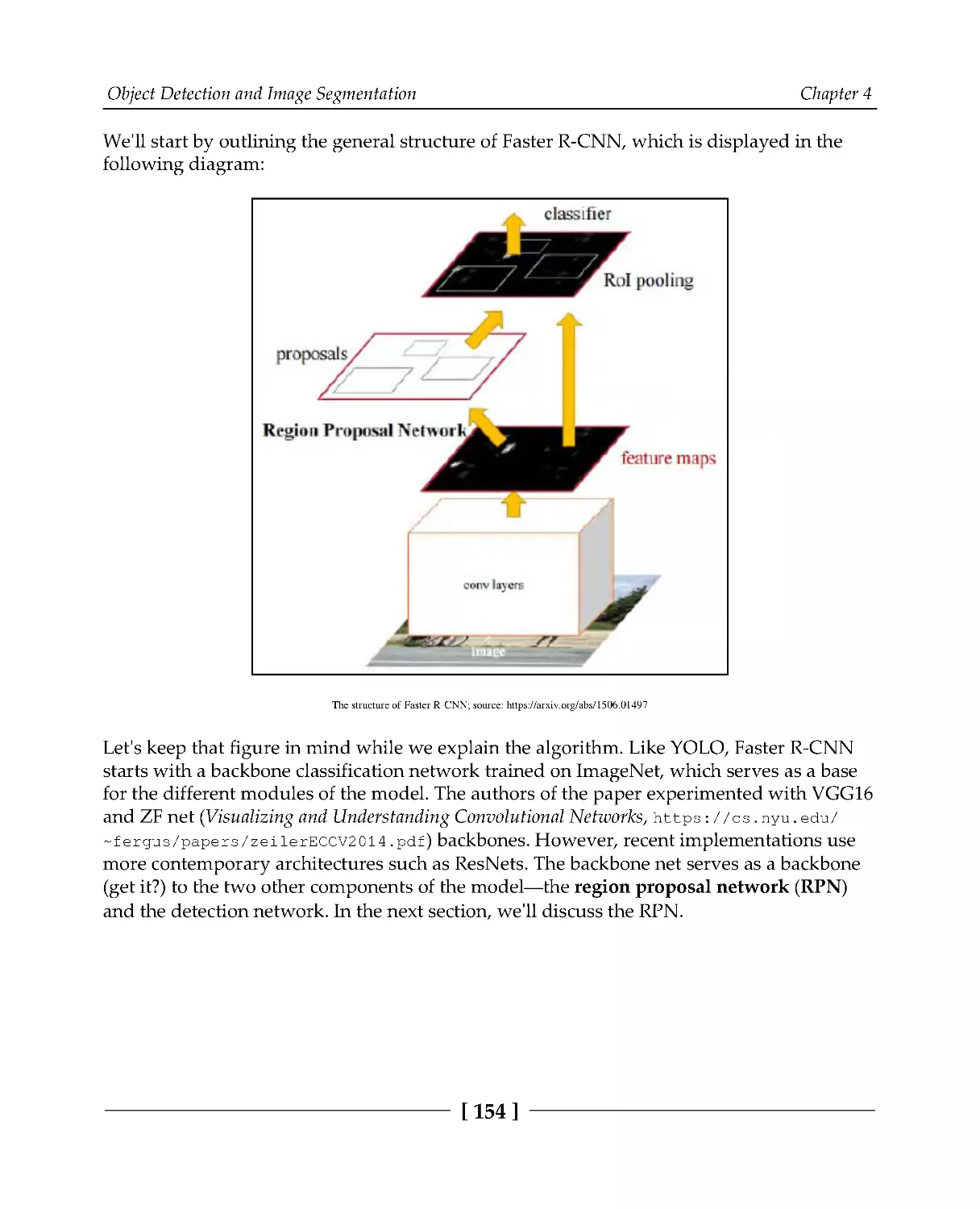
Object detection with Faster R-CNN
153
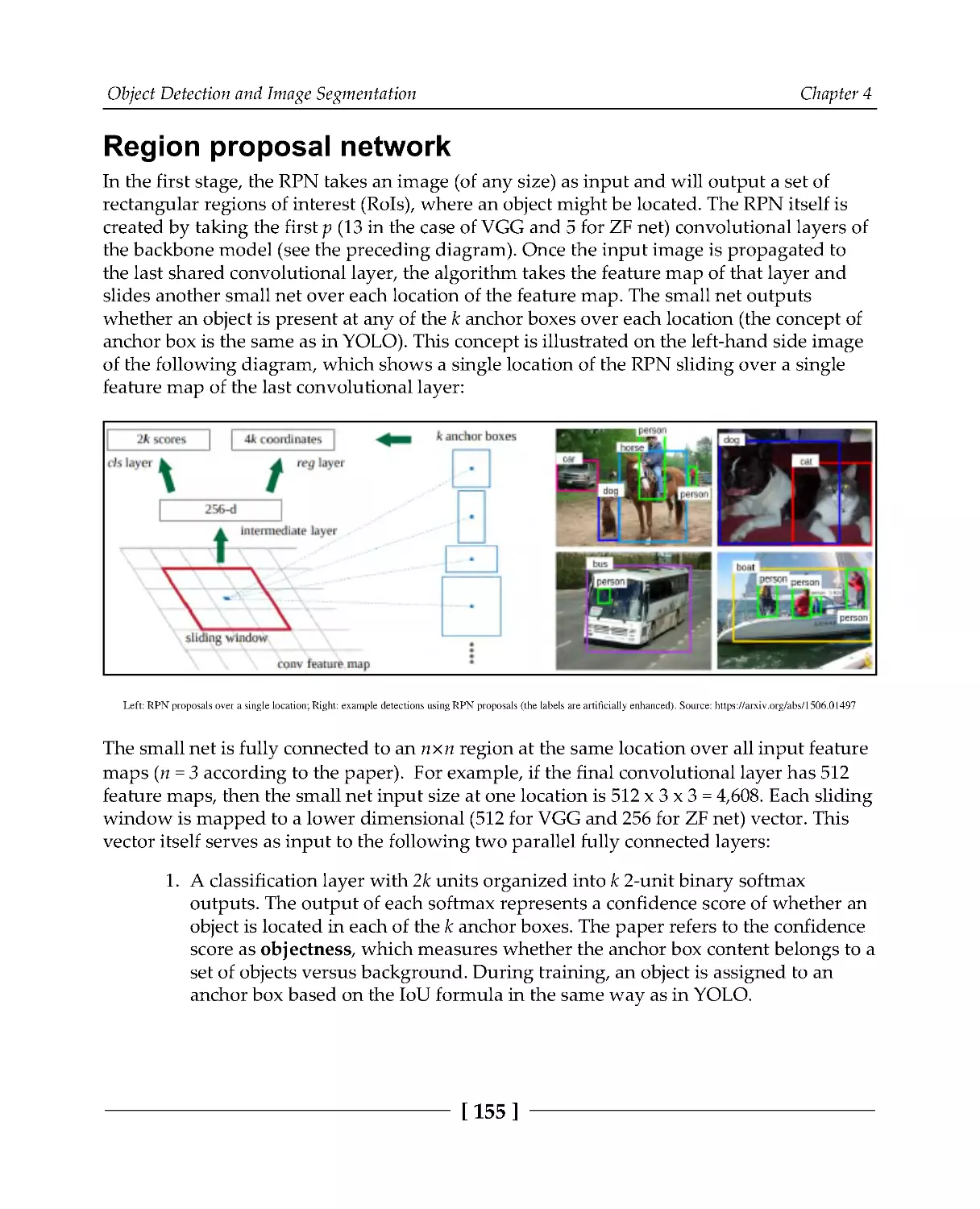
Region proposal network
155
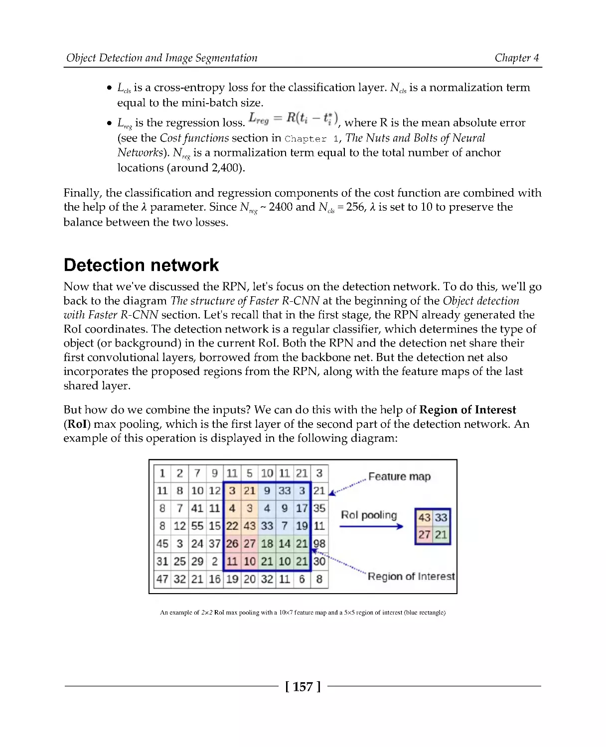
Detection network
157
Implementing Faster R-CNN with PyTorch
159
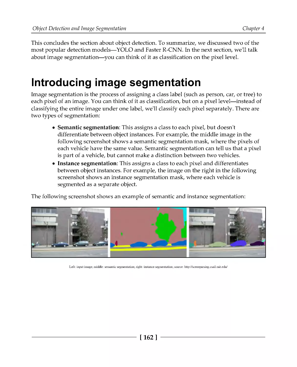
Introducing image segmentation
162
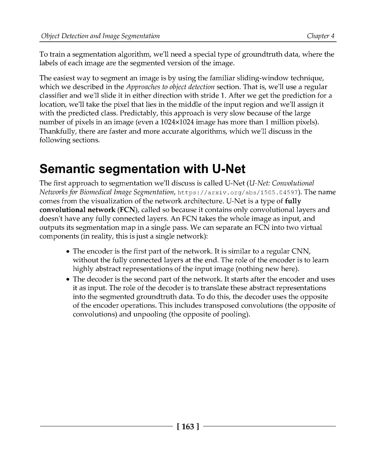
Semantic segmentation with U-Net
163
Instance segmentation with Mask R-CNN
166
Implementing Mask R-CNN with PyTorch
168
Summary
170
Chapter 5: Generative Models
171
Intuition and justification of generative models
171
Table of Contents
[iii]
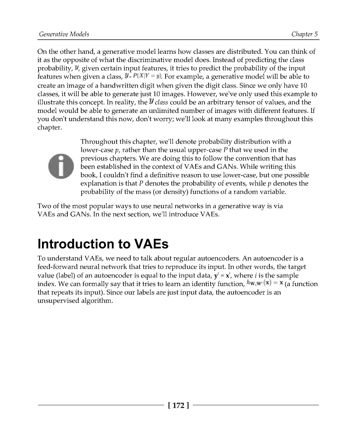
Introduction to VAEs
172
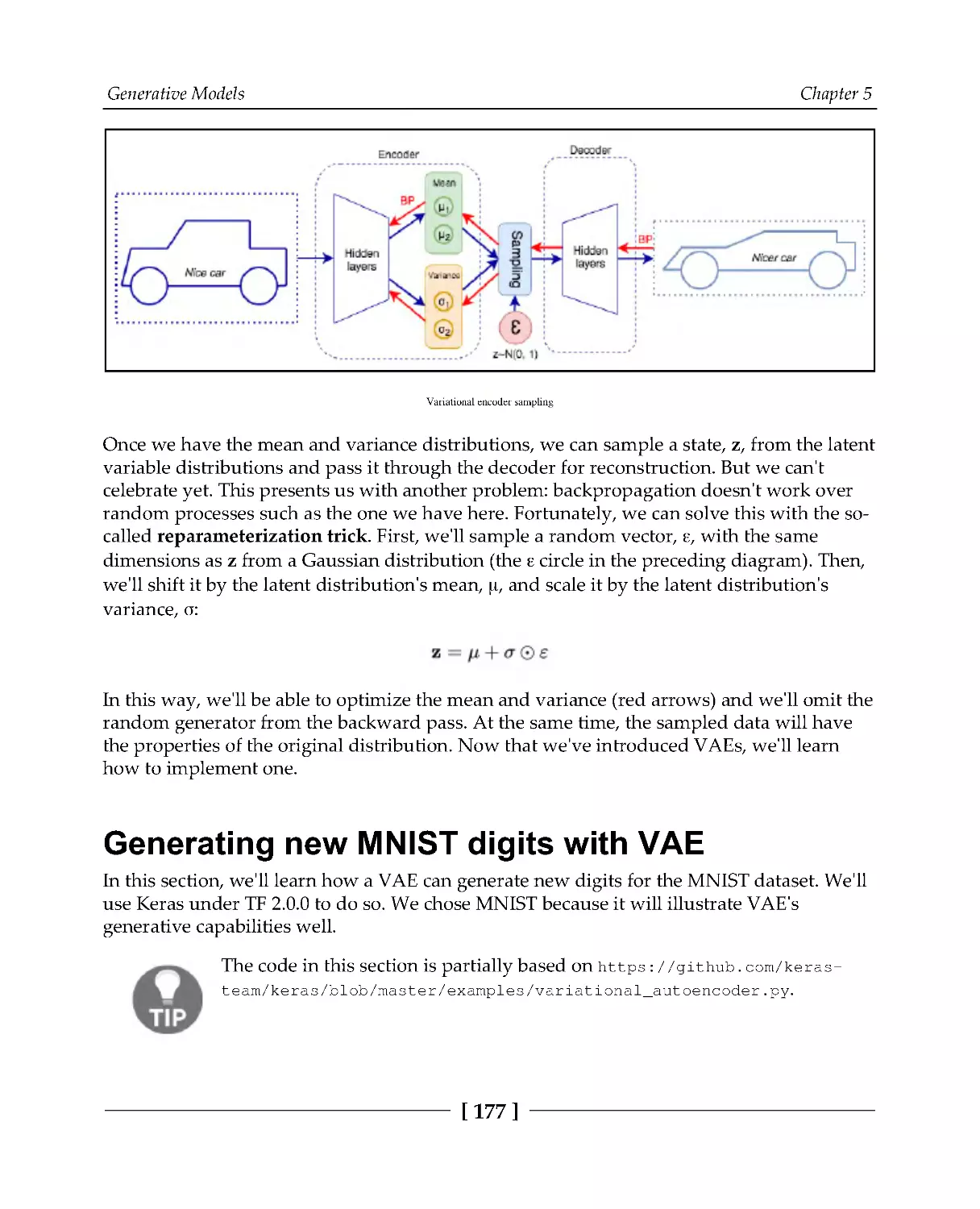
Generating new MNIST digits with VAE
177
Introduction to GANs
183
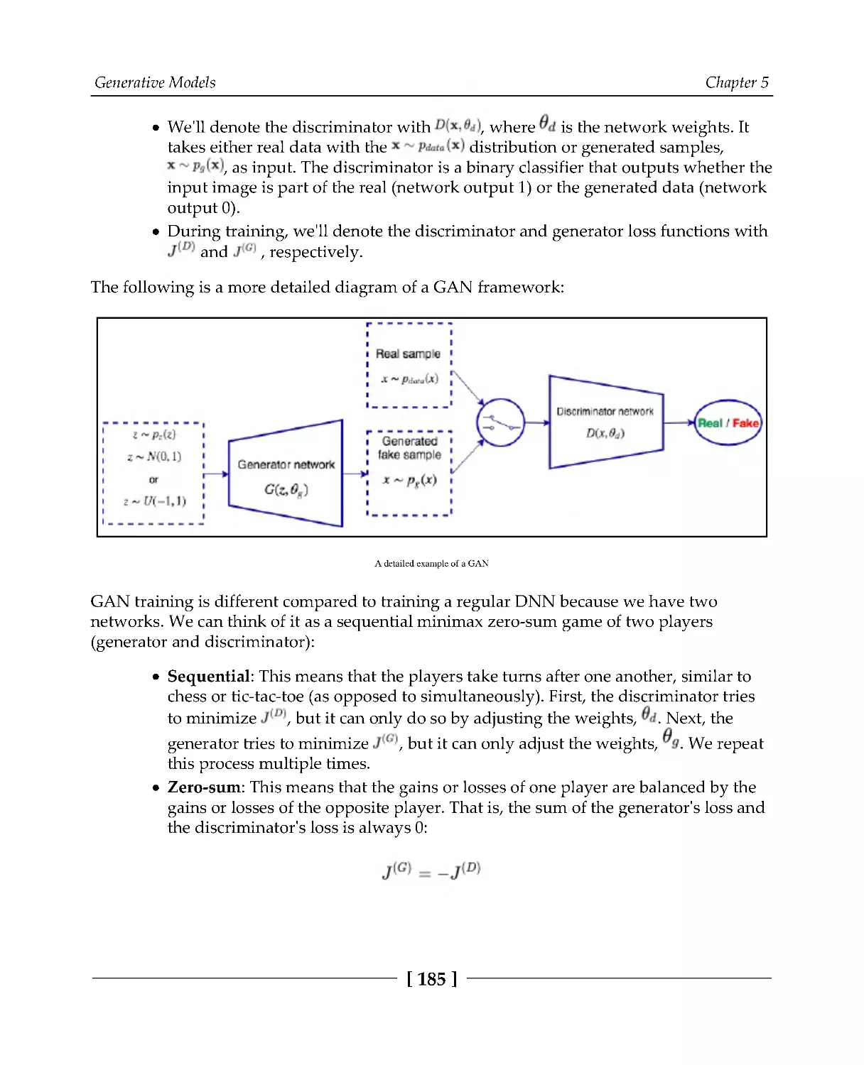
Training GANs
184
Training the discriminator
186
Training the generator
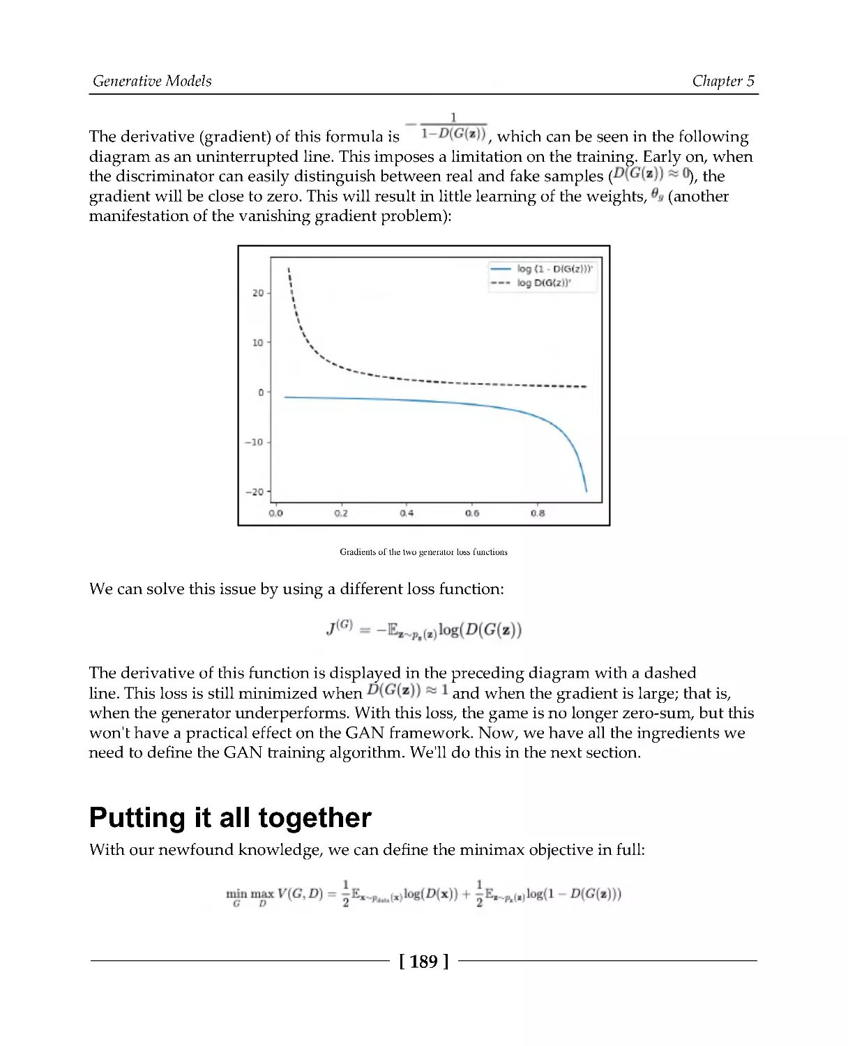
188
Putting it all together
189
Problems with training GANs
191
Types of GAN
192
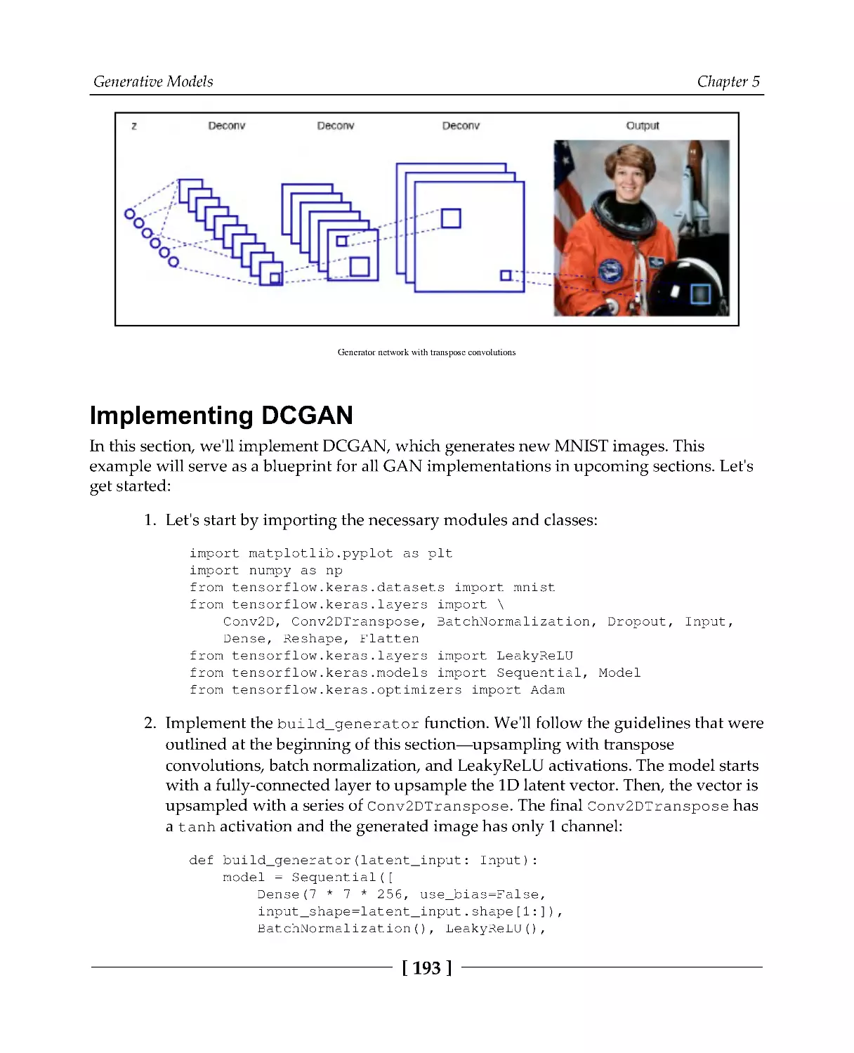
Deep Convolutional GAN
192
Implementing DCGAN
193
Conditional GAN
198
Implementing CGAN
199
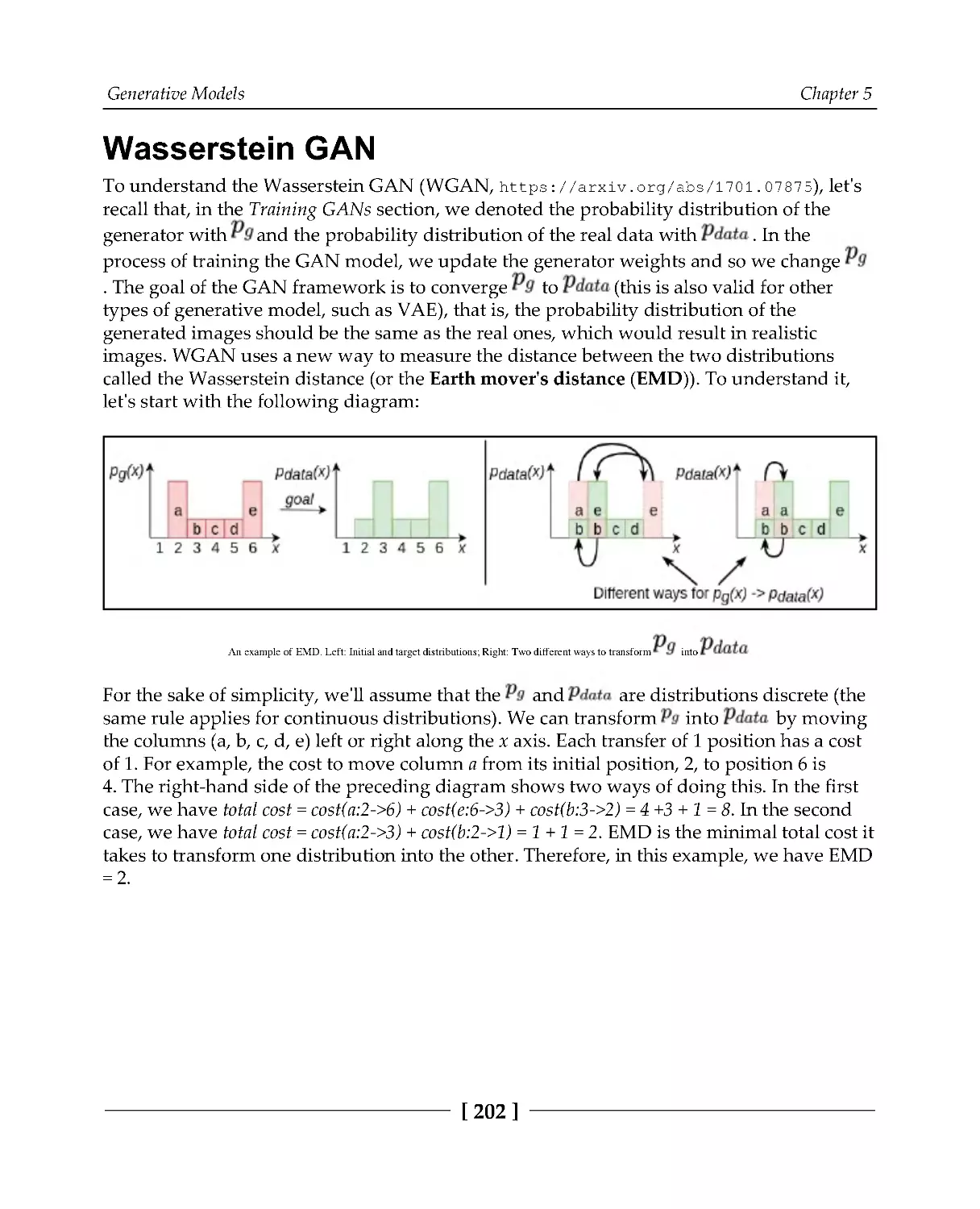
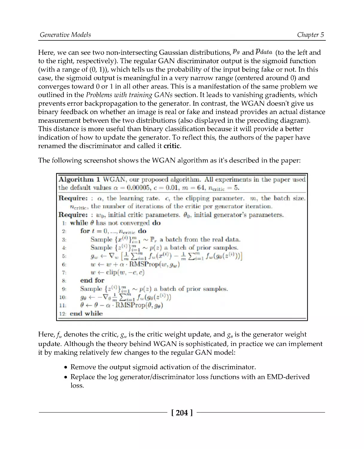
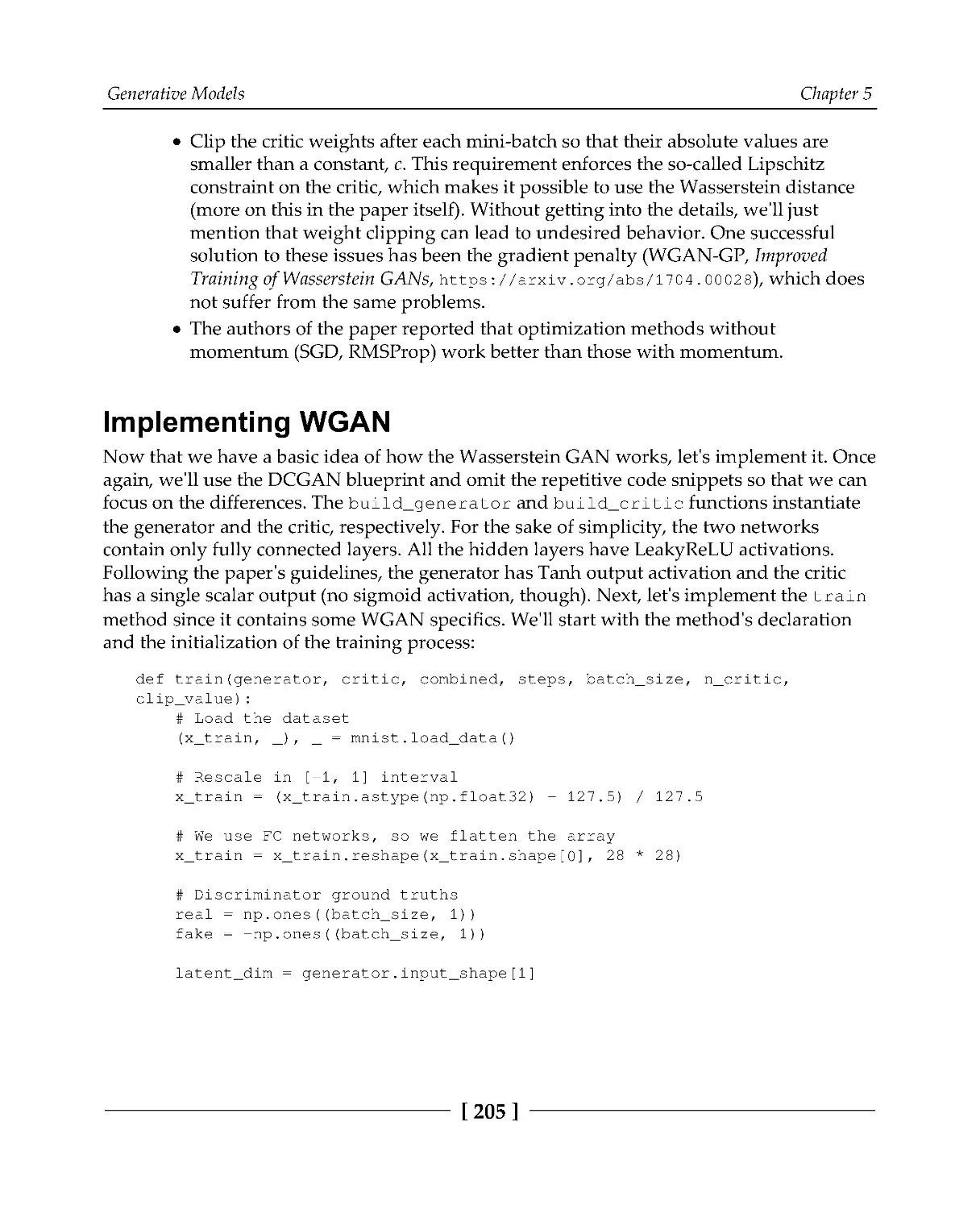
Wasserstein GAN
202
Implementing WGAN
205
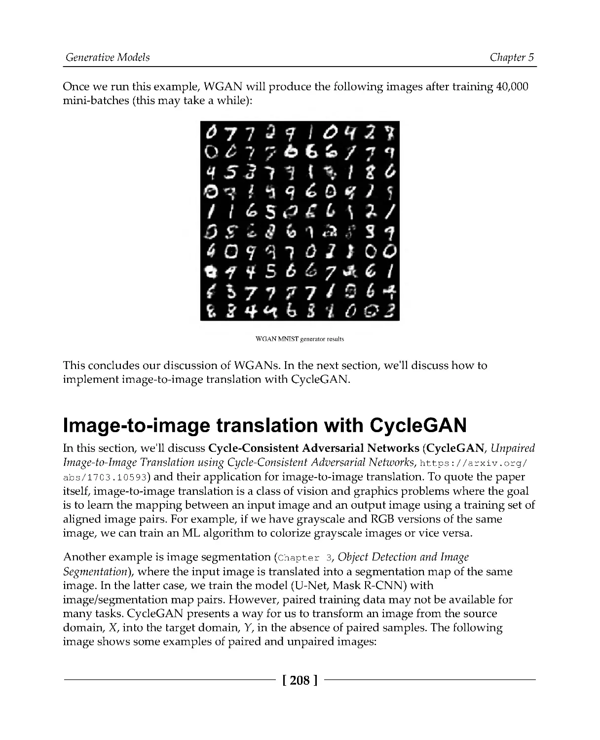
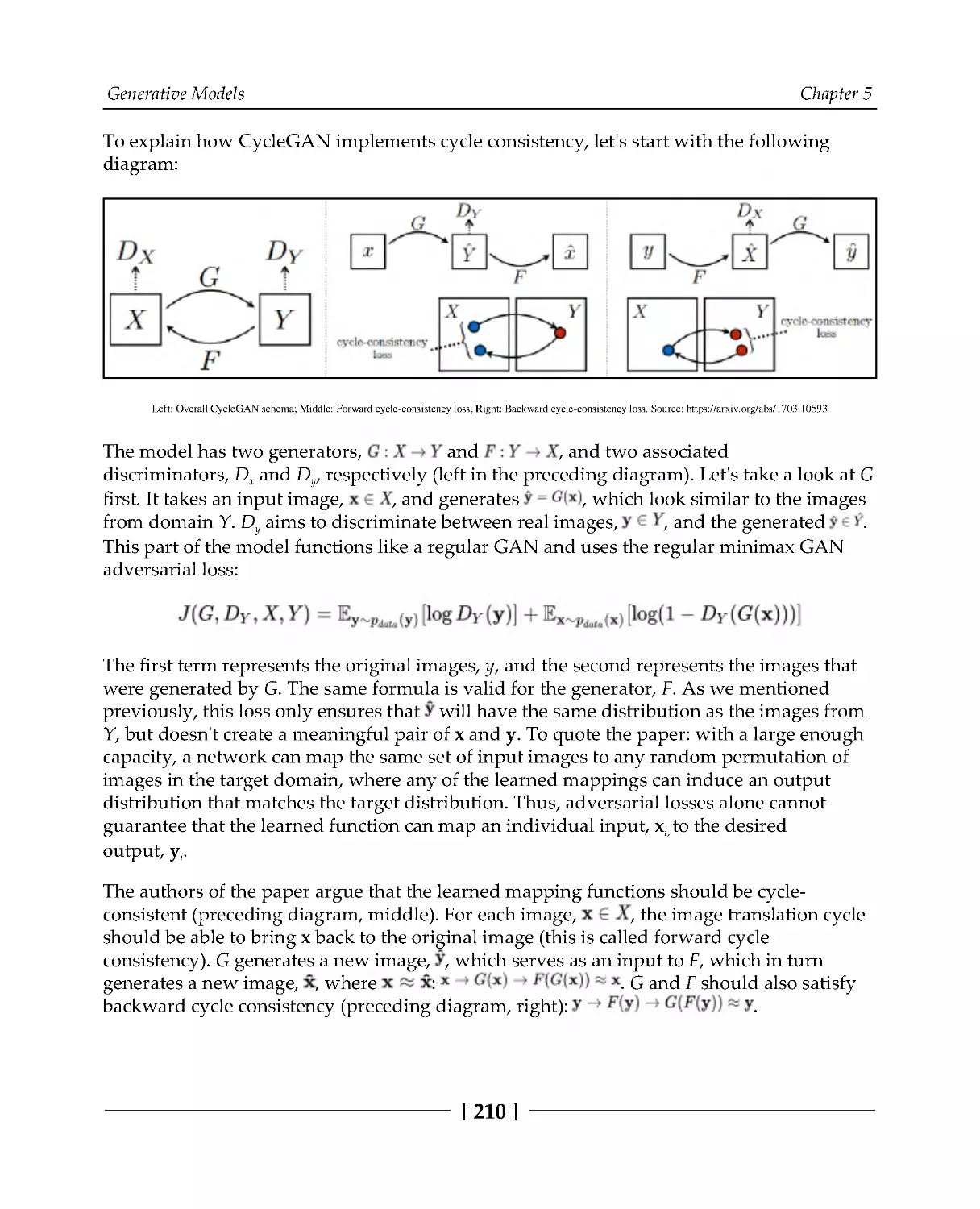
Image-to-image translation with CycleGAN
208
Implementing CycleGAN
211
Building the generator and discriminator
212
Putting it all together
214
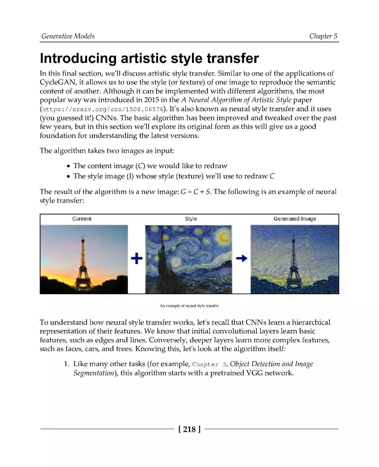
Introducing artistic style transfer
218
Summary
220
Section 3: Natural Language and Sequence
Processing
Chapter 6: Language Modeling
222
Understanding n-grams
223
Introducing neural language models
225
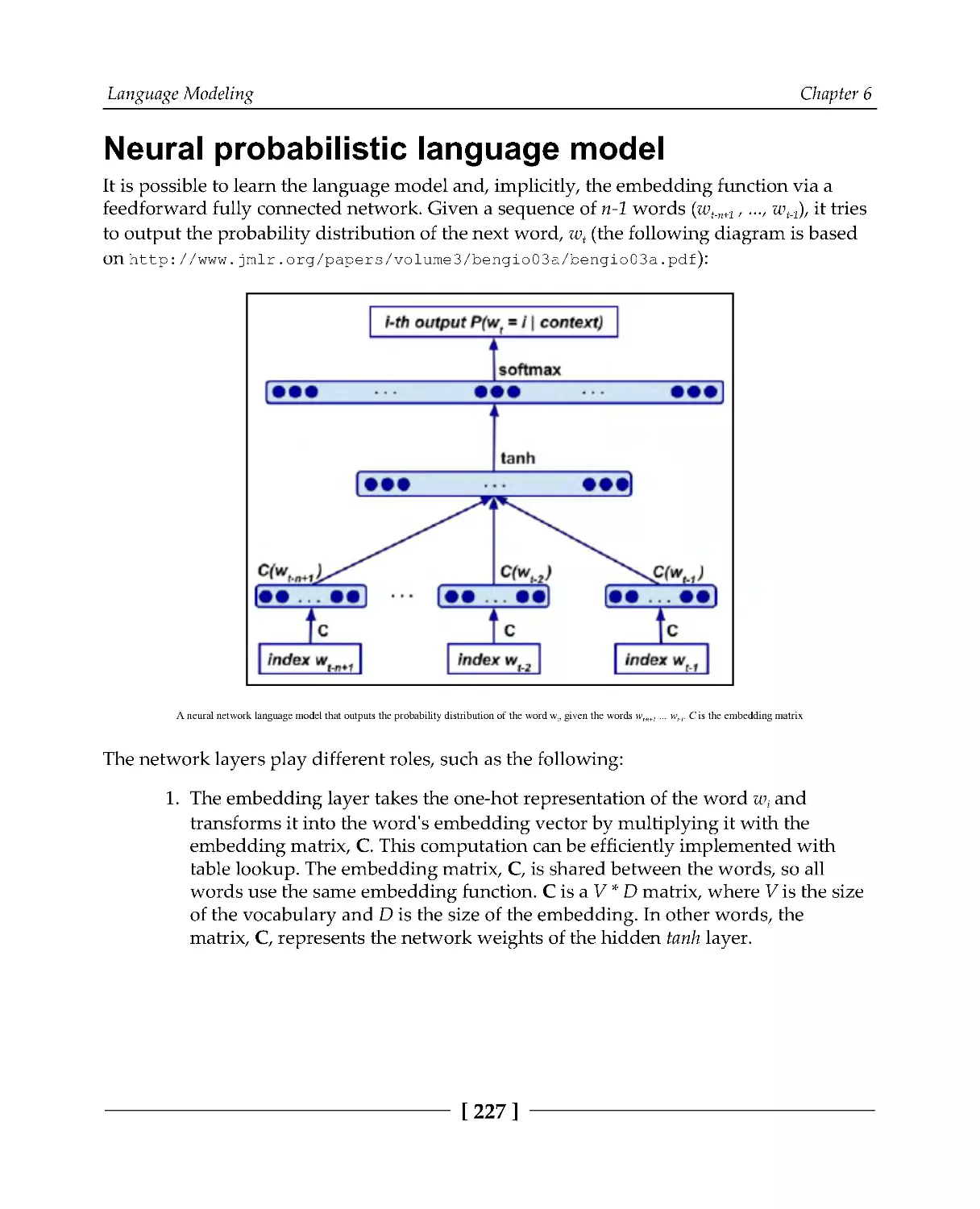
Neural probabilistic language model
227
Word2Vec
228
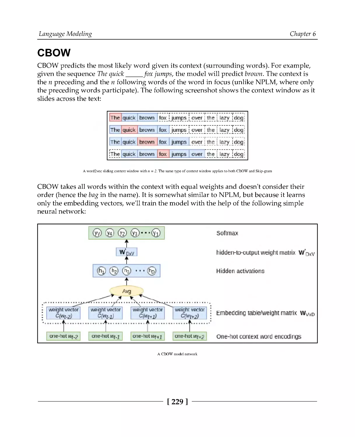
CBOW
229
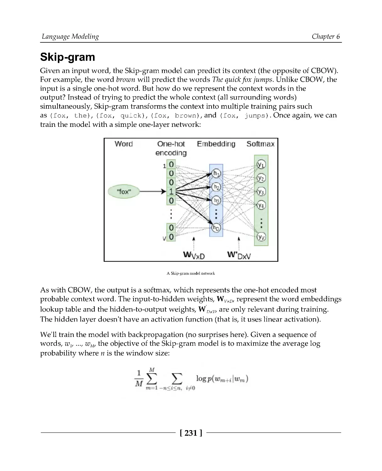
Skip-gram
231
fastText
233
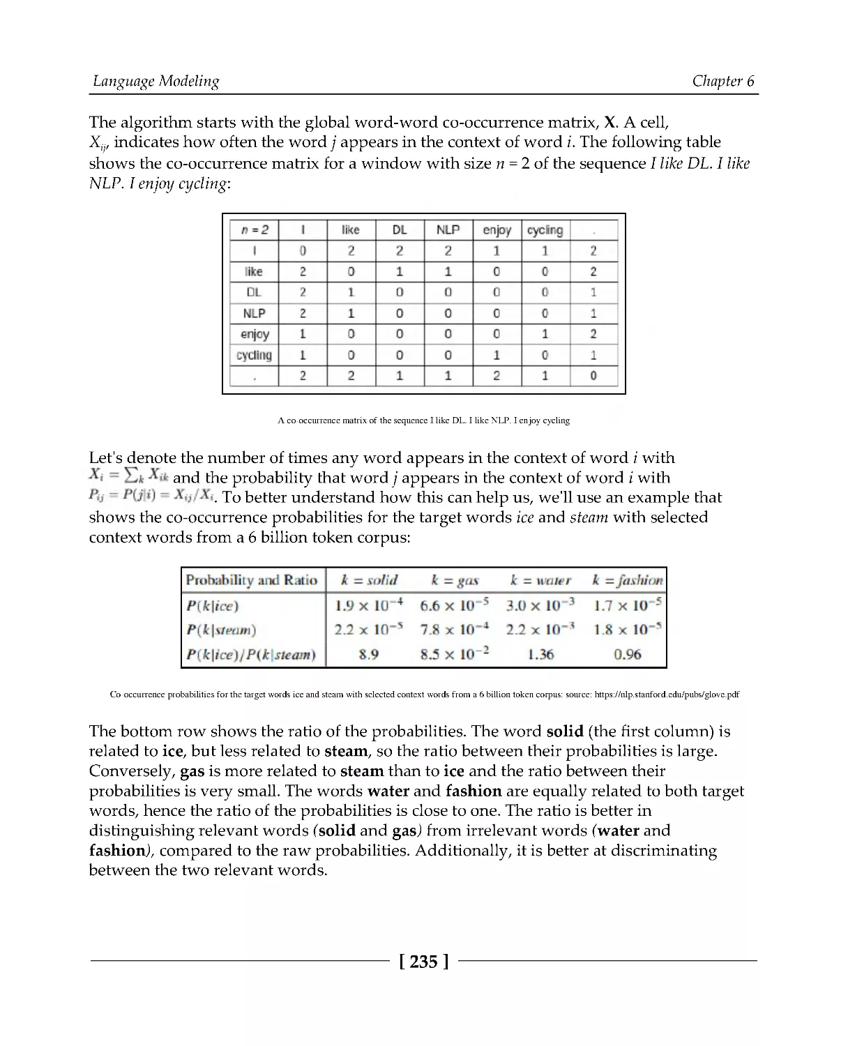
Global Vectors for Word Representation model
234
Implementing language models
238
Training the embedding model
238
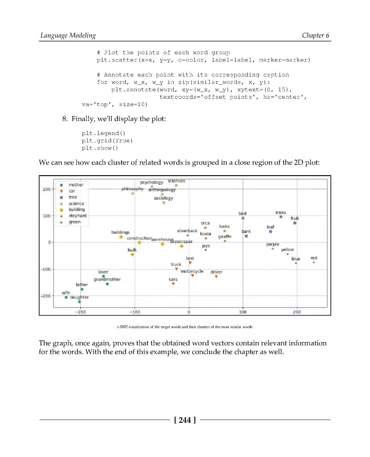
Visualizing embedding vectors
241
Summary
245
Chapter 7: Understanding Recurrent Networks
246
Introduction to RNNs
246
RNN implementation and training
251
Backpropagation through time
253
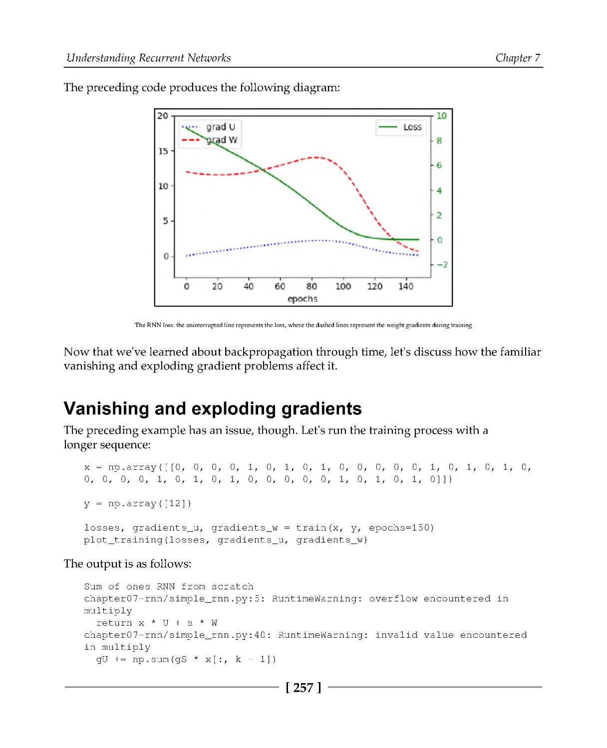
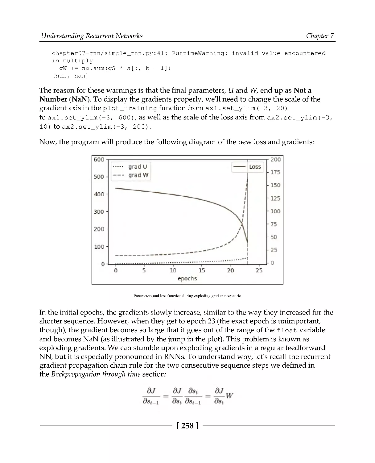
Vanishing and exploding gradients
257
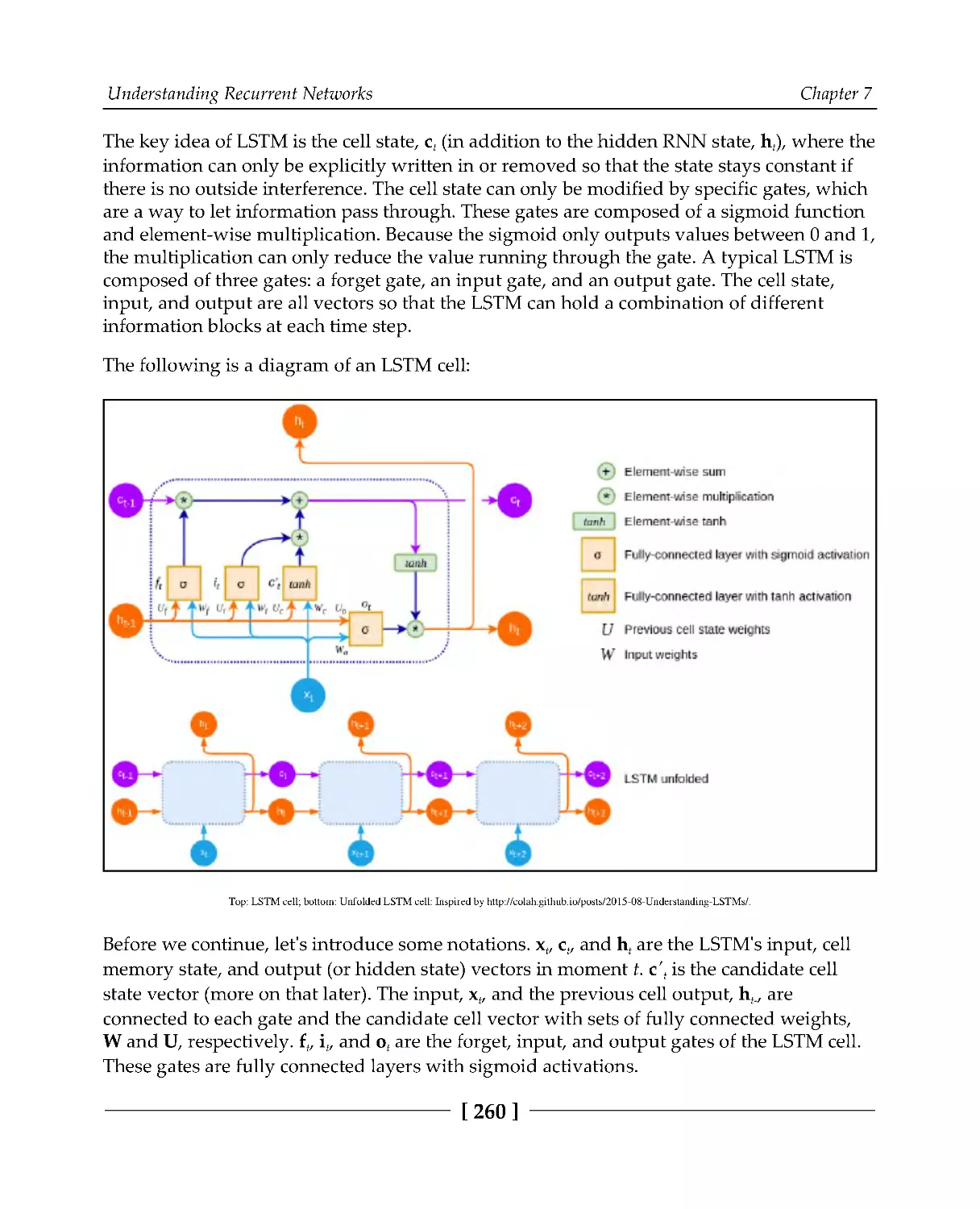
Introducing long short-term memory
259
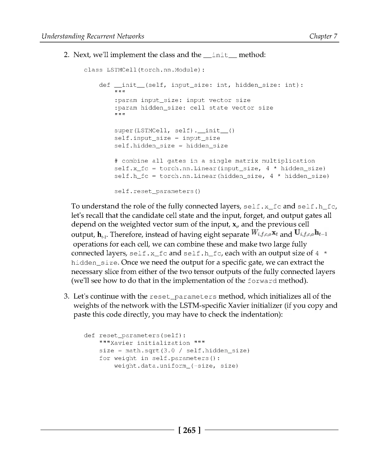
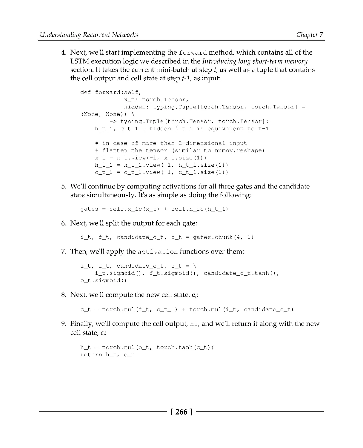
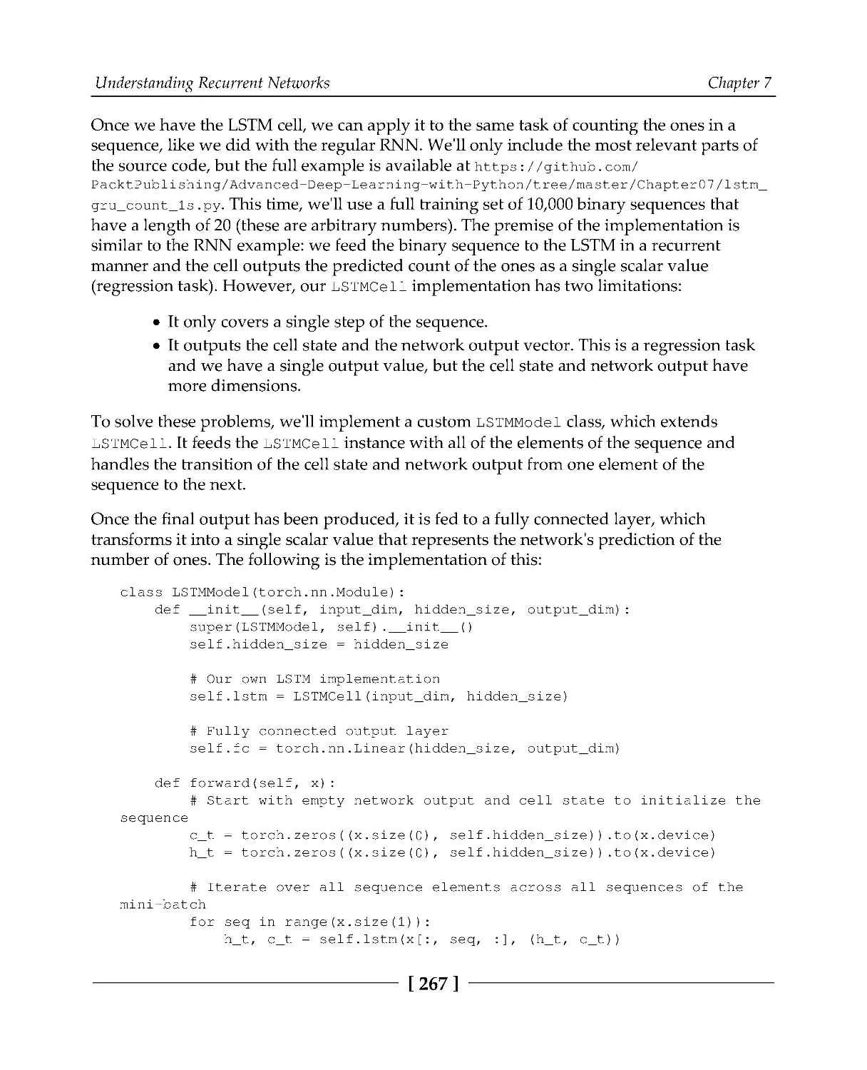
Implementing LSTM
264
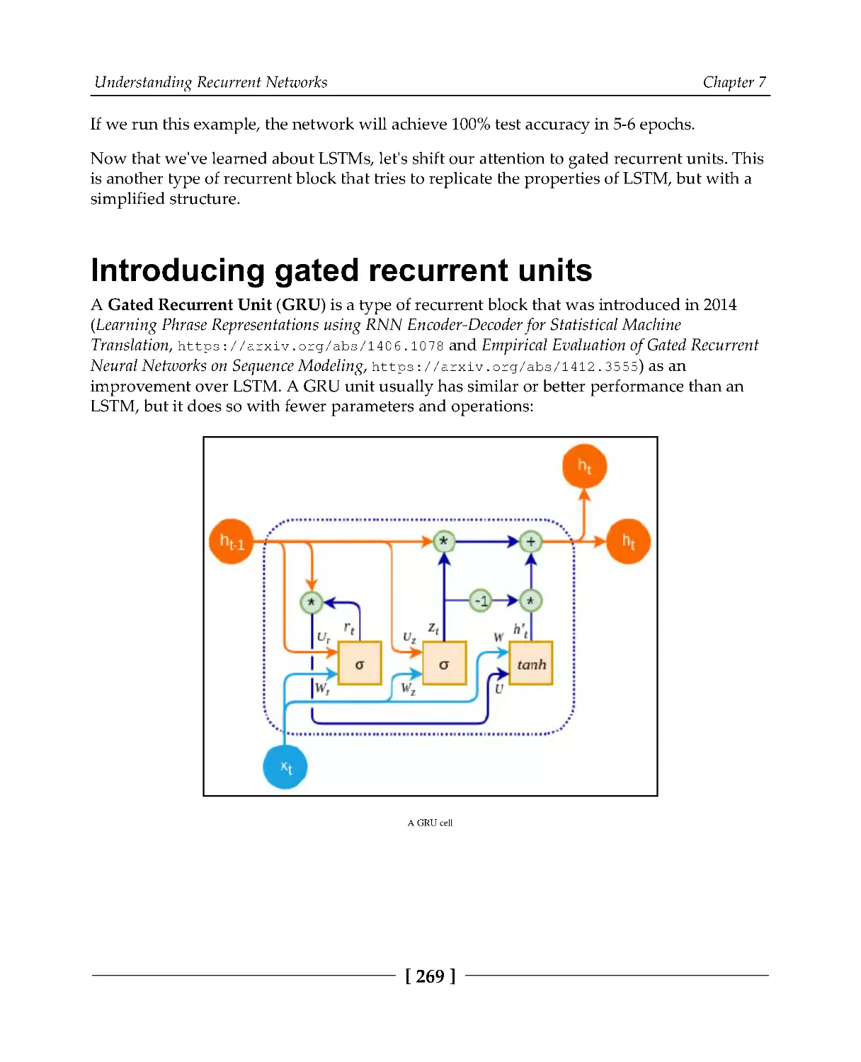
Introducing gated recurrent units
269
Table of Contents
[iv]
Implementing GRUs
270
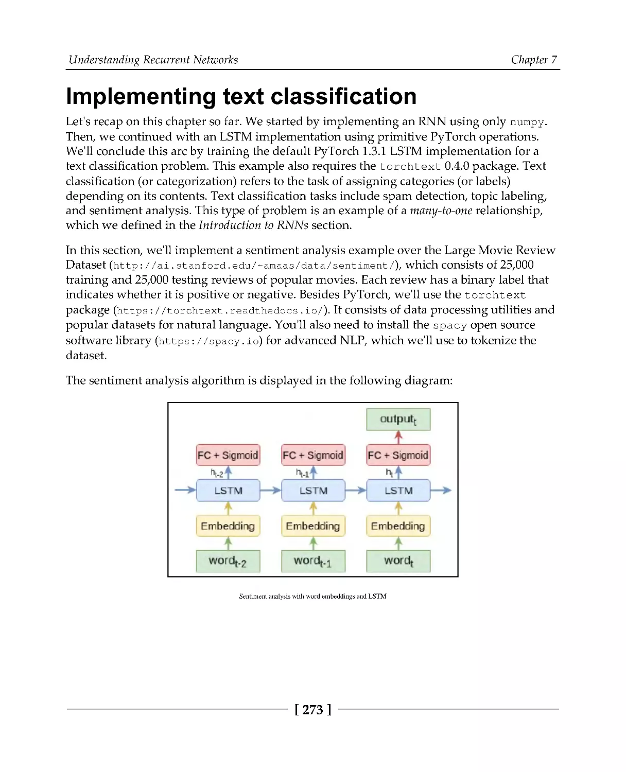
Implementing text classification
273
Summary
277
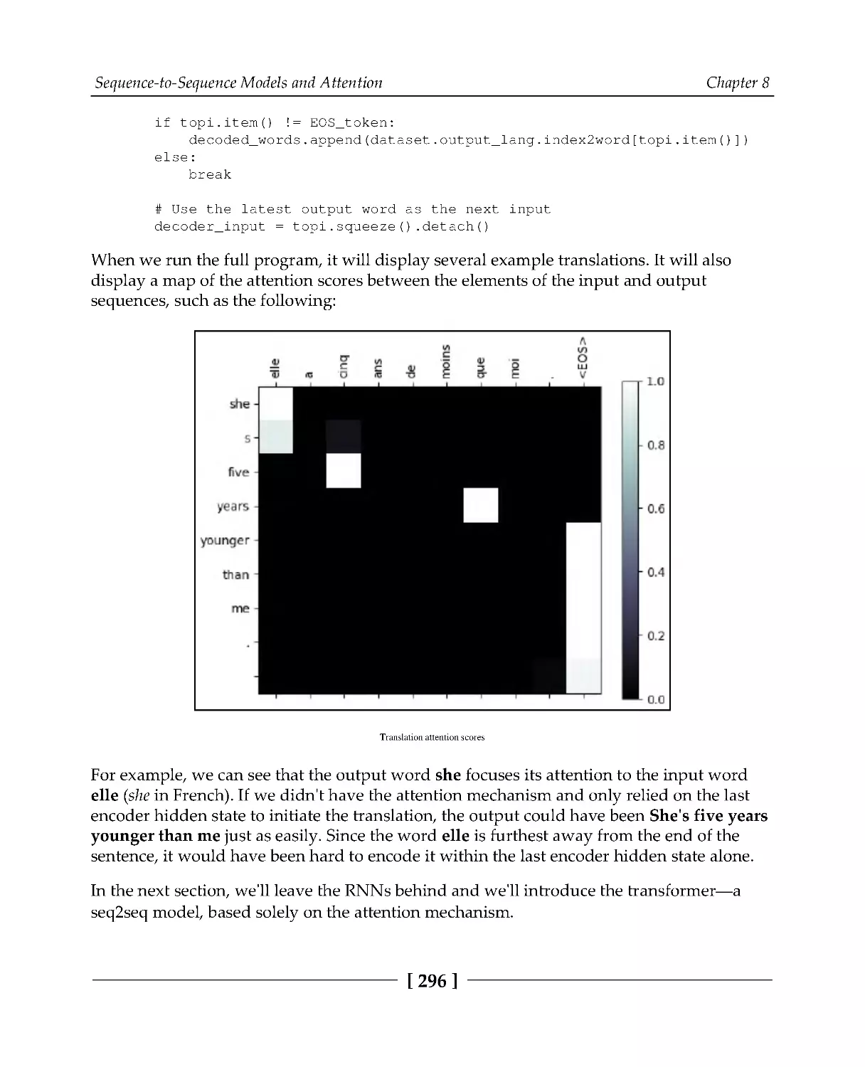
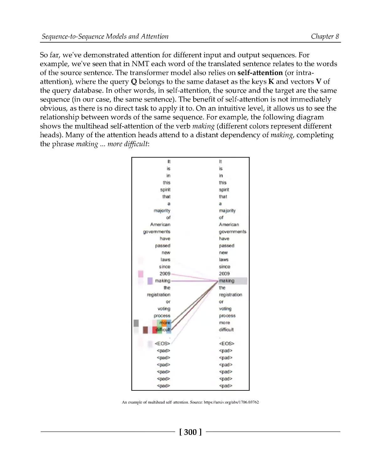
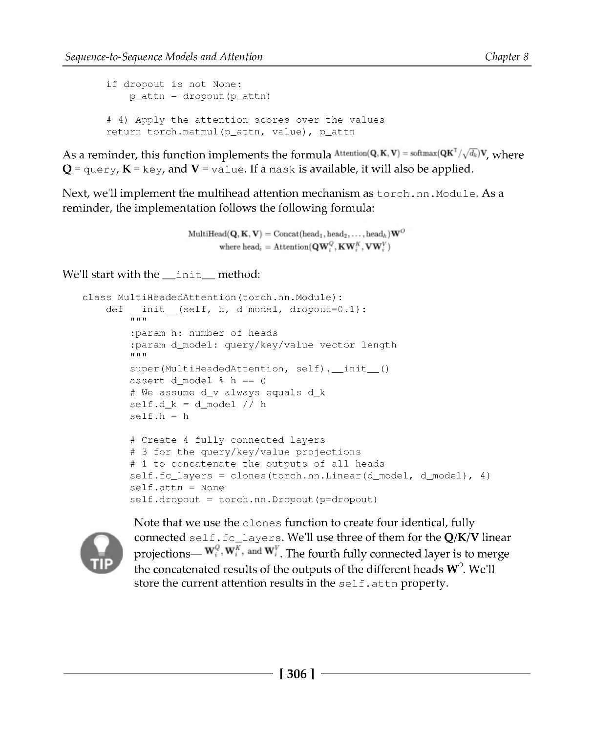
Chapter 8: Sequence-to-Sequence Models and Attention
278
Introducing seq2seq models
279
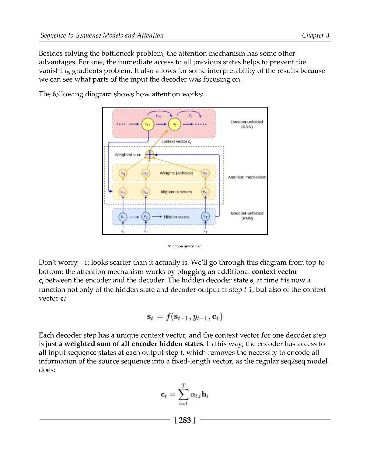
Seq2seq with attention
282
Bahdanau attention
282
Luong attention
285
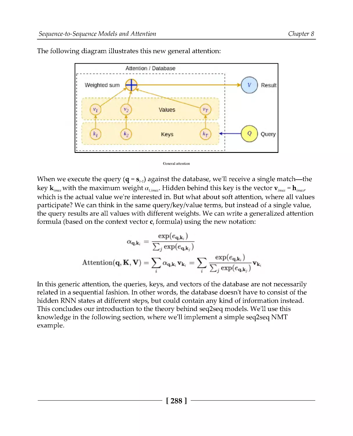
General attention
287
Implementing seq2seq with attention
289
Implementing the encoder
289
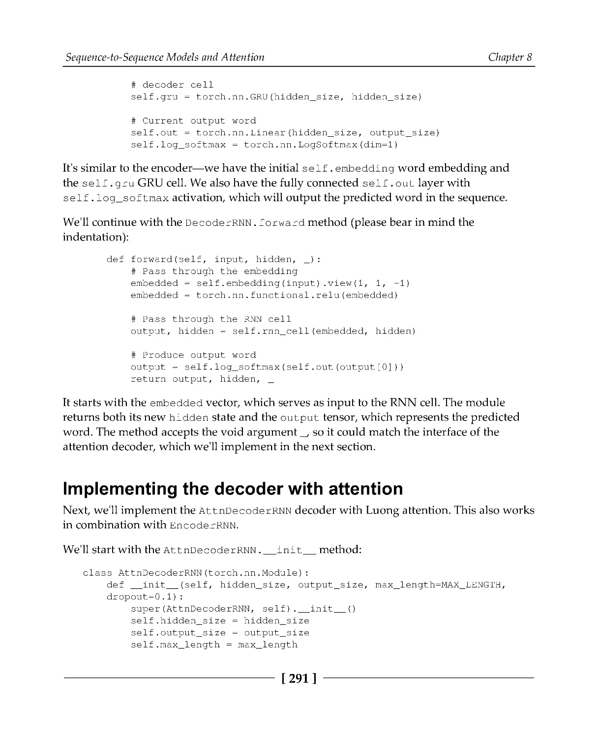
Implementing the decoder
290
Implementing the decoder with attention
291
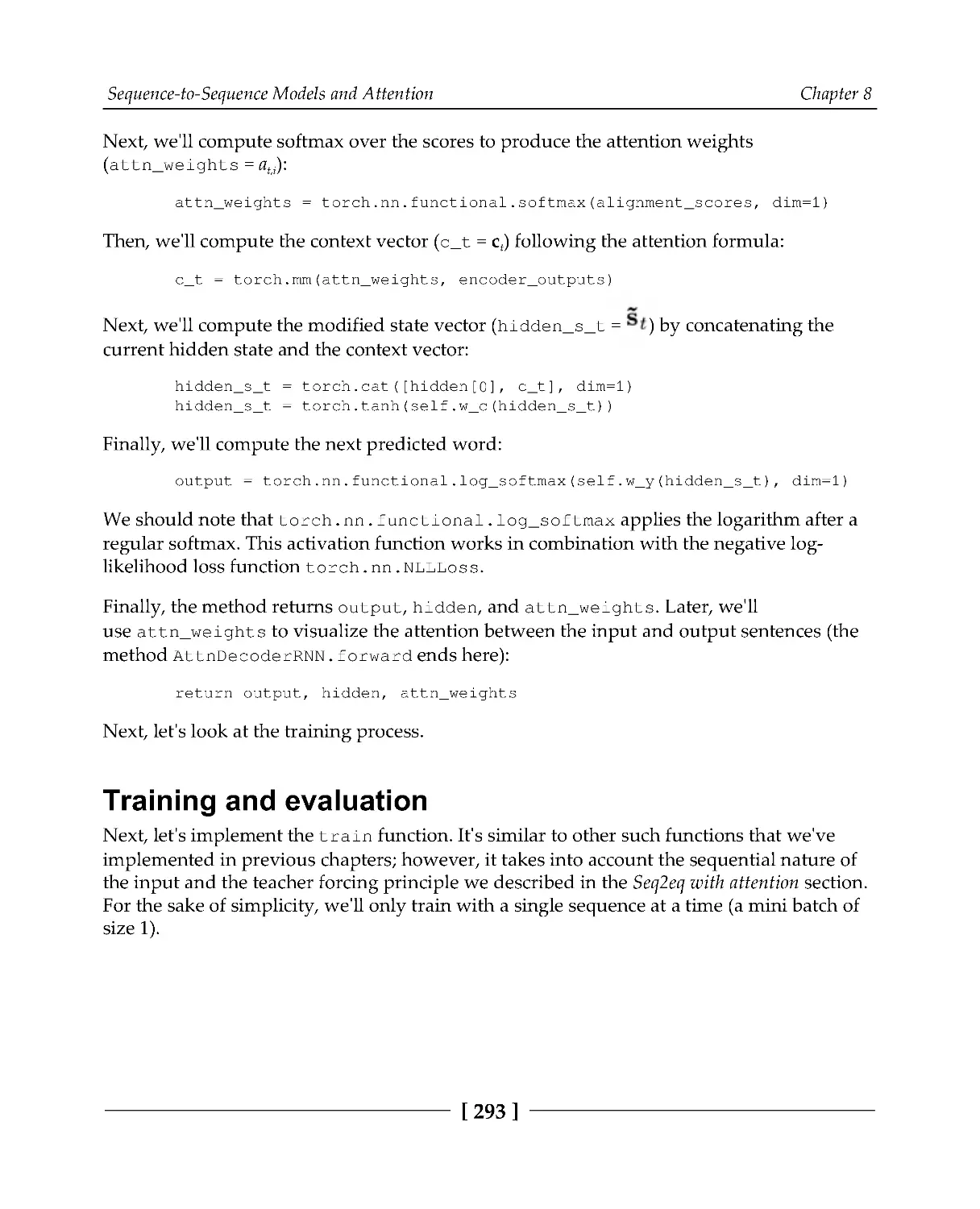
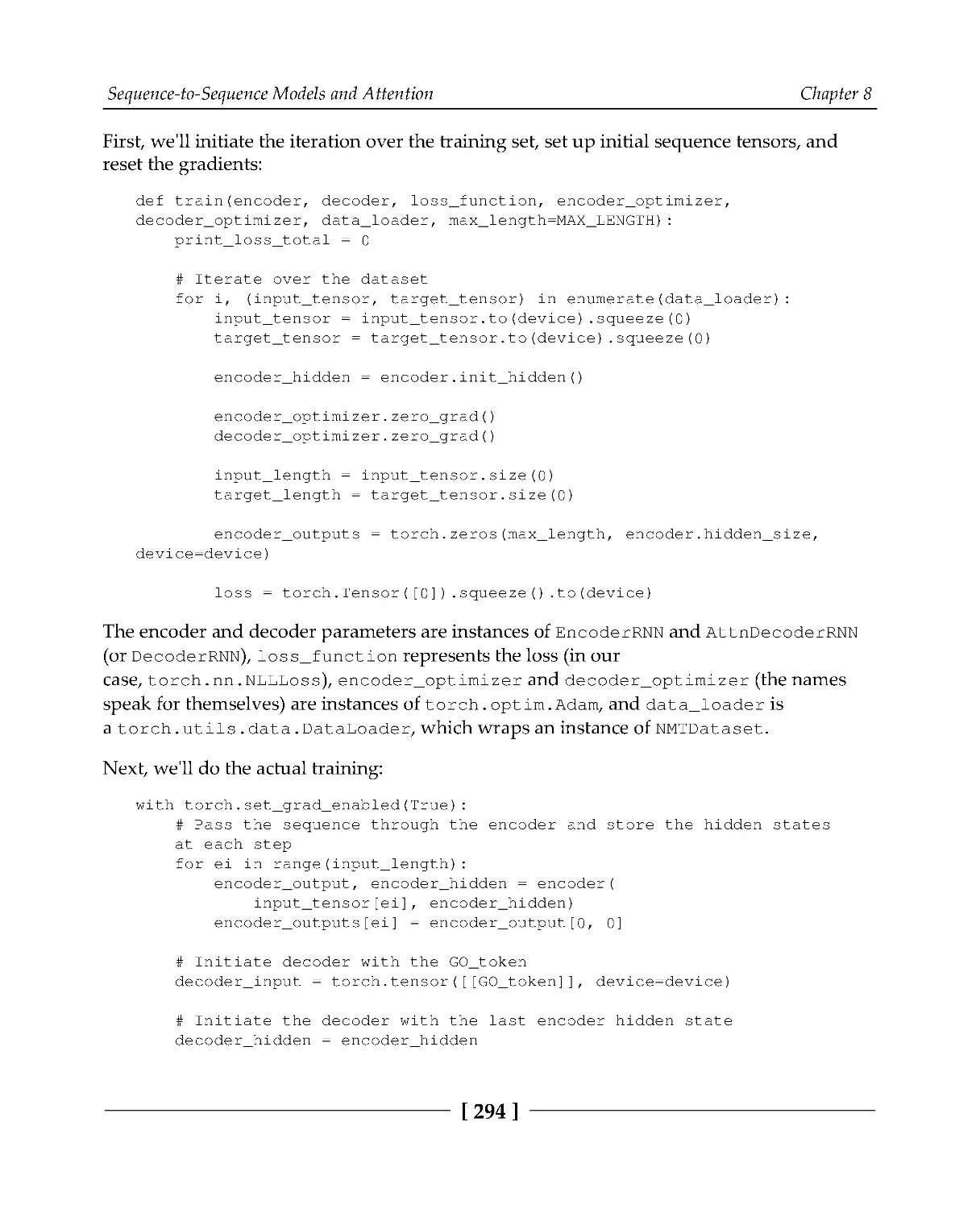
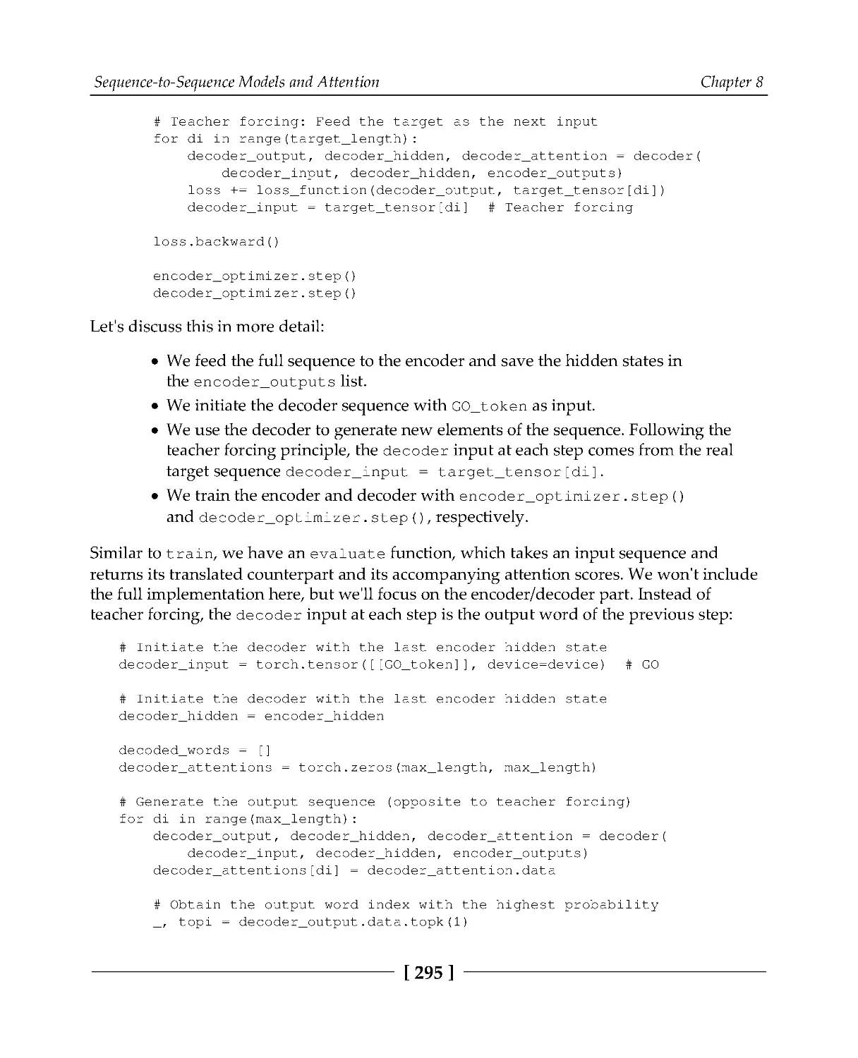
Training and evaluation
293
Understanding transformers
297
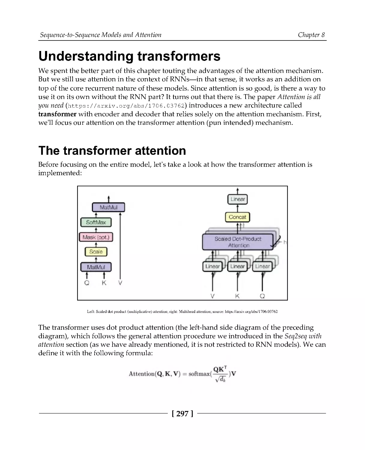
The transformer attention
297
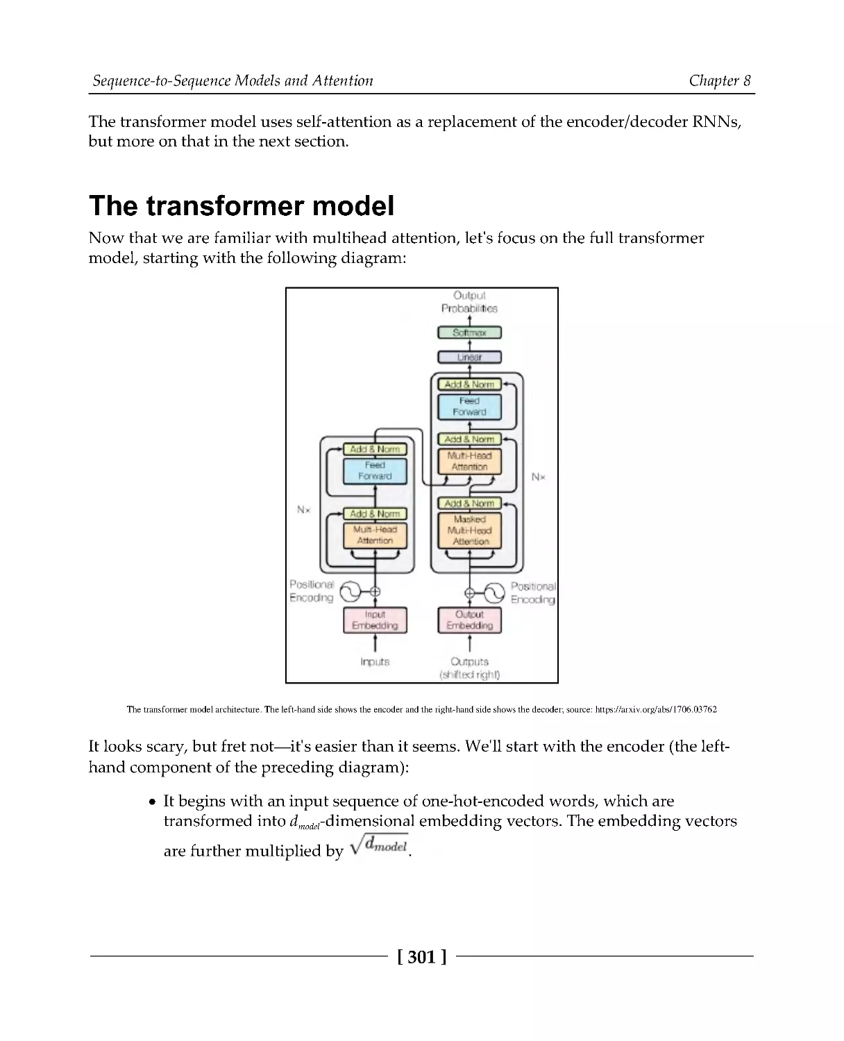
The transformer model
301
Implementing transformers
305
Multihead attention
305
Encoder
308
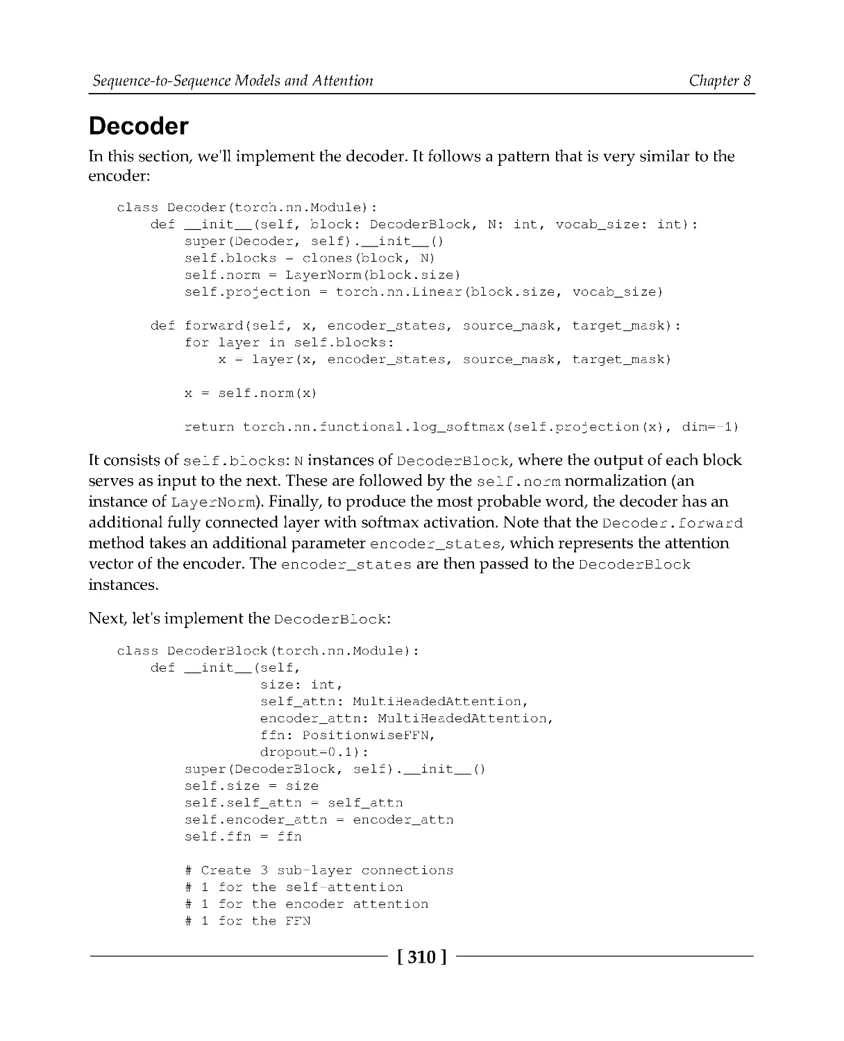
Decoder
310
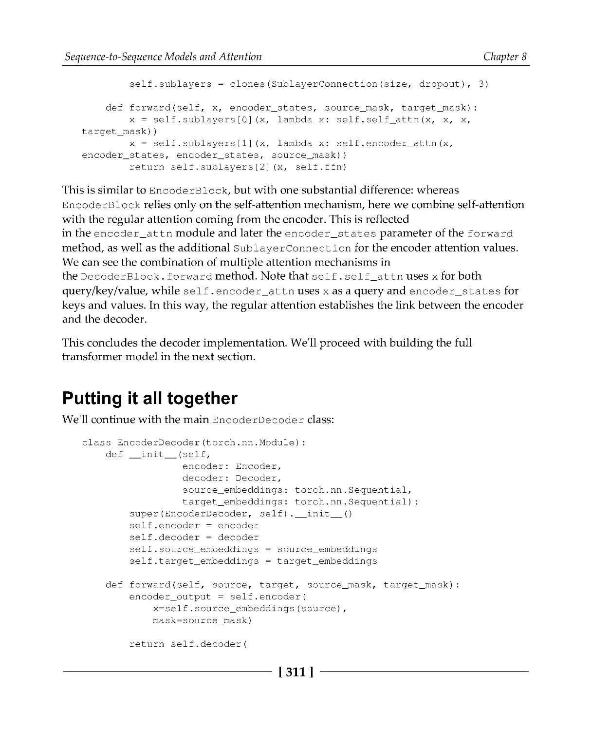
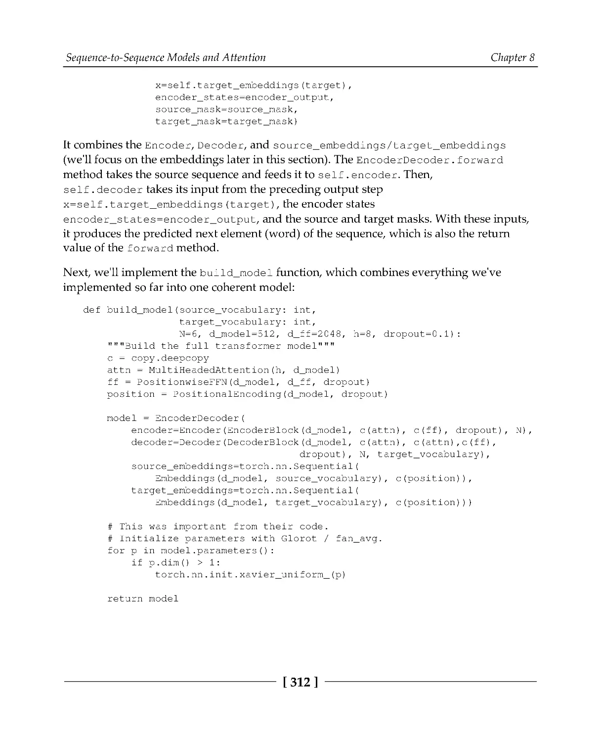
Putting it all together
311
Transformer language models
314
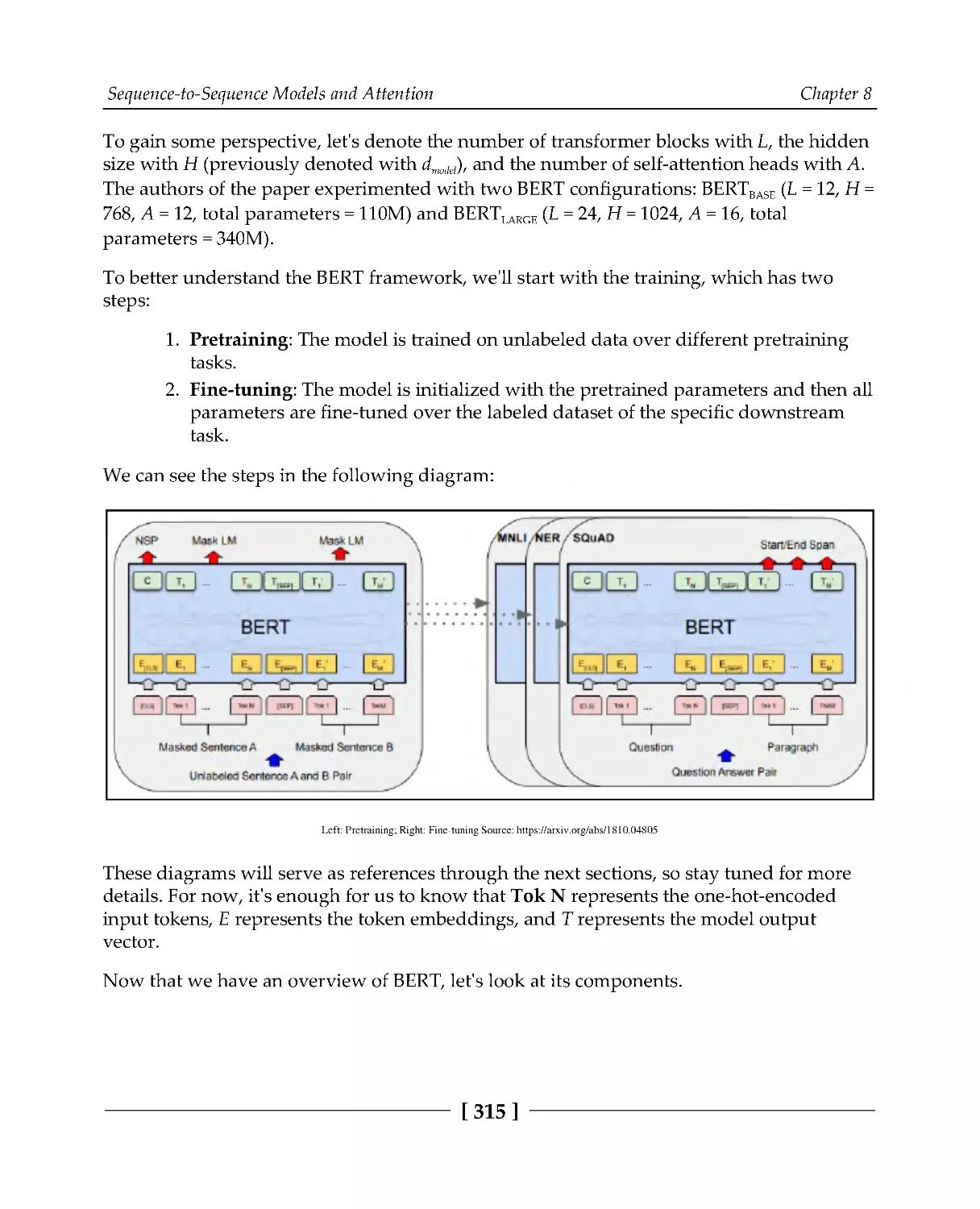
Bidirectional encoder representations from transformers
314
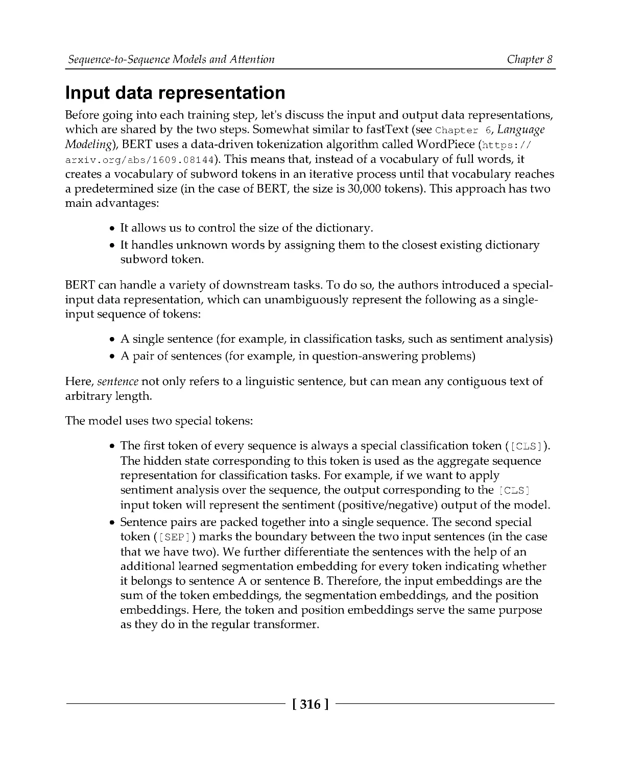
Input data representation
316
Pretraining
317
Fine-tuning
319
Transformer-XL
321
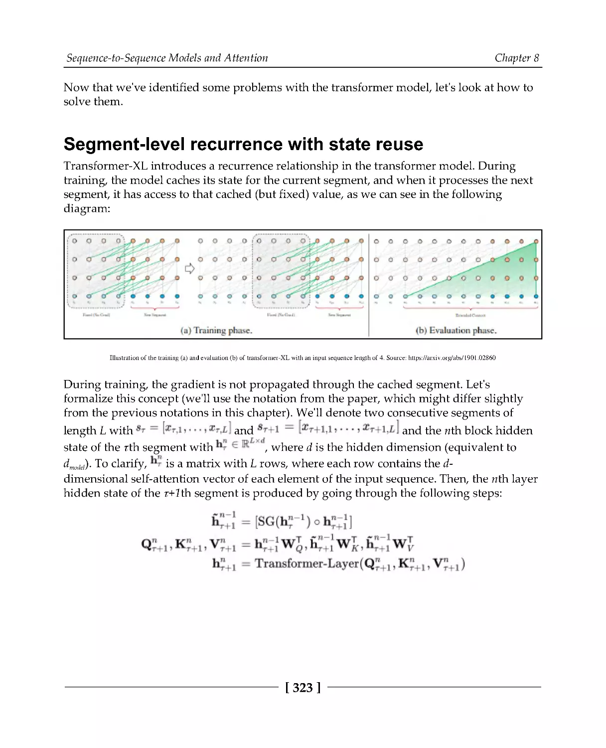
Segment-level recurrence with state reuse
323
Relative positional encodings
324
XLNet
326
Generating text with a transformer language model
330
Summary
332
Section 4: A Look to the Future
Chapter 9: Emerging Neural Network Designs
334
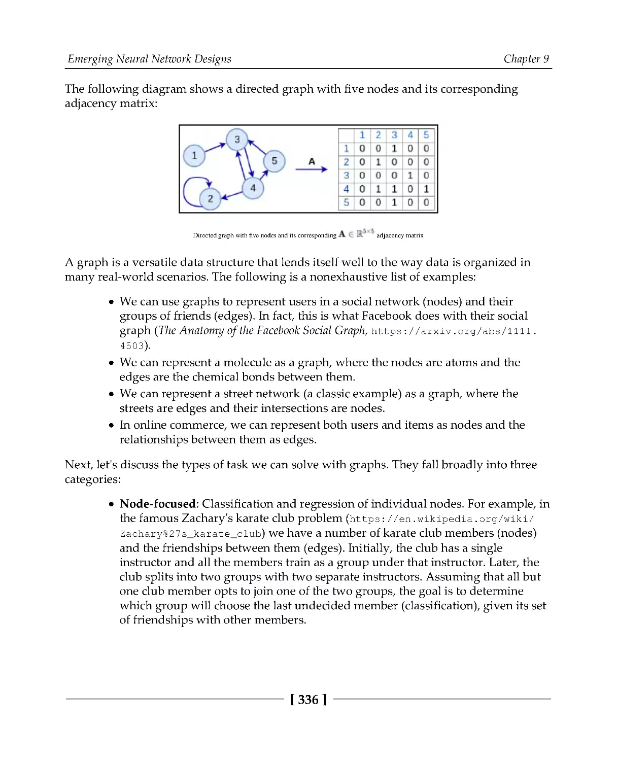
Introducing Graph NNs
335
Recurrent GNNs
338
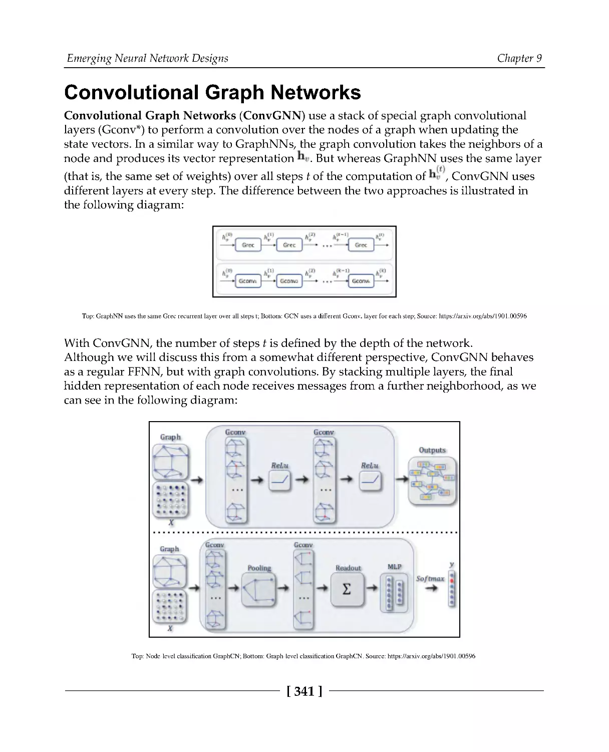
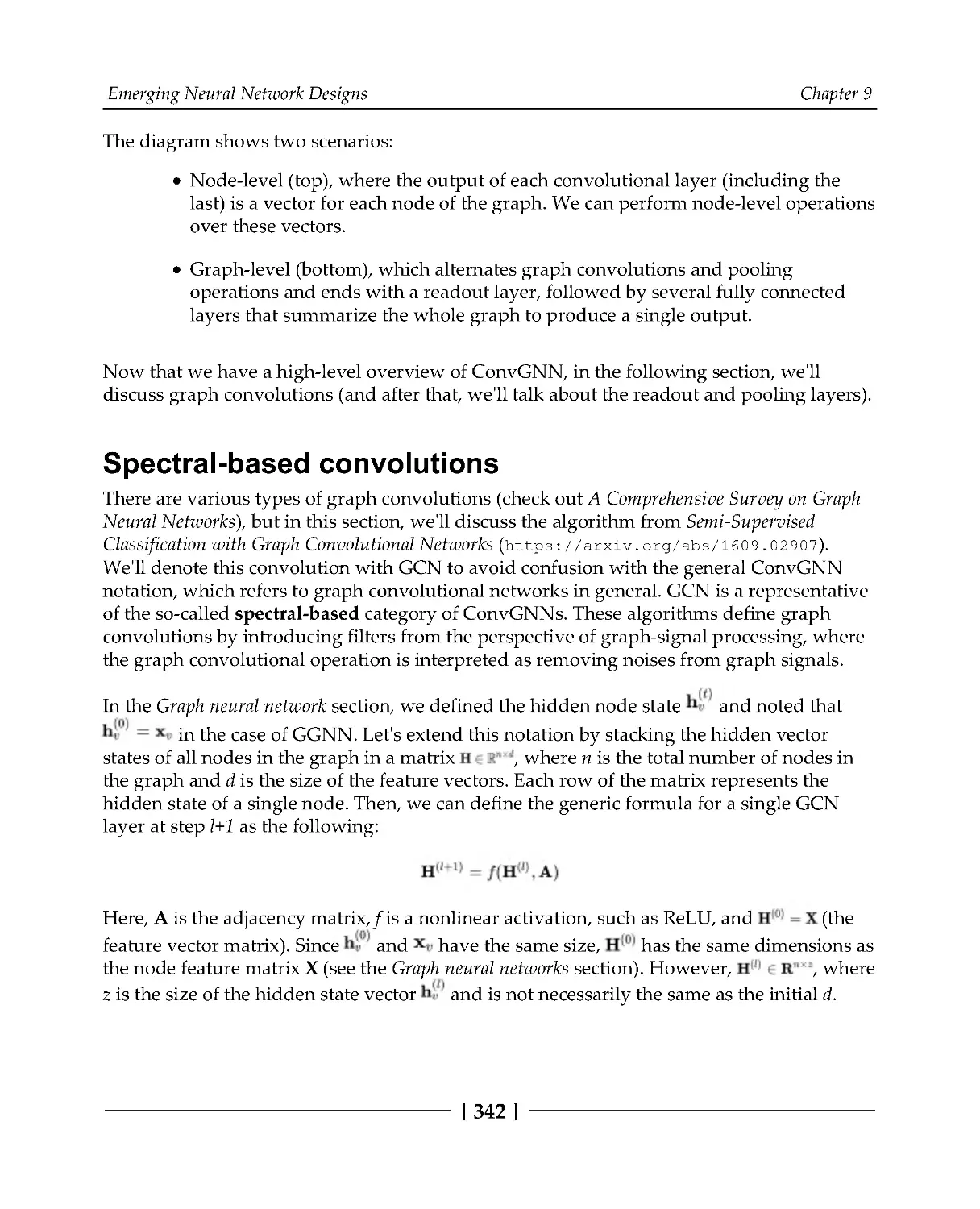
Convolutional Graph Networks
341
Spectral-based convolutions
342
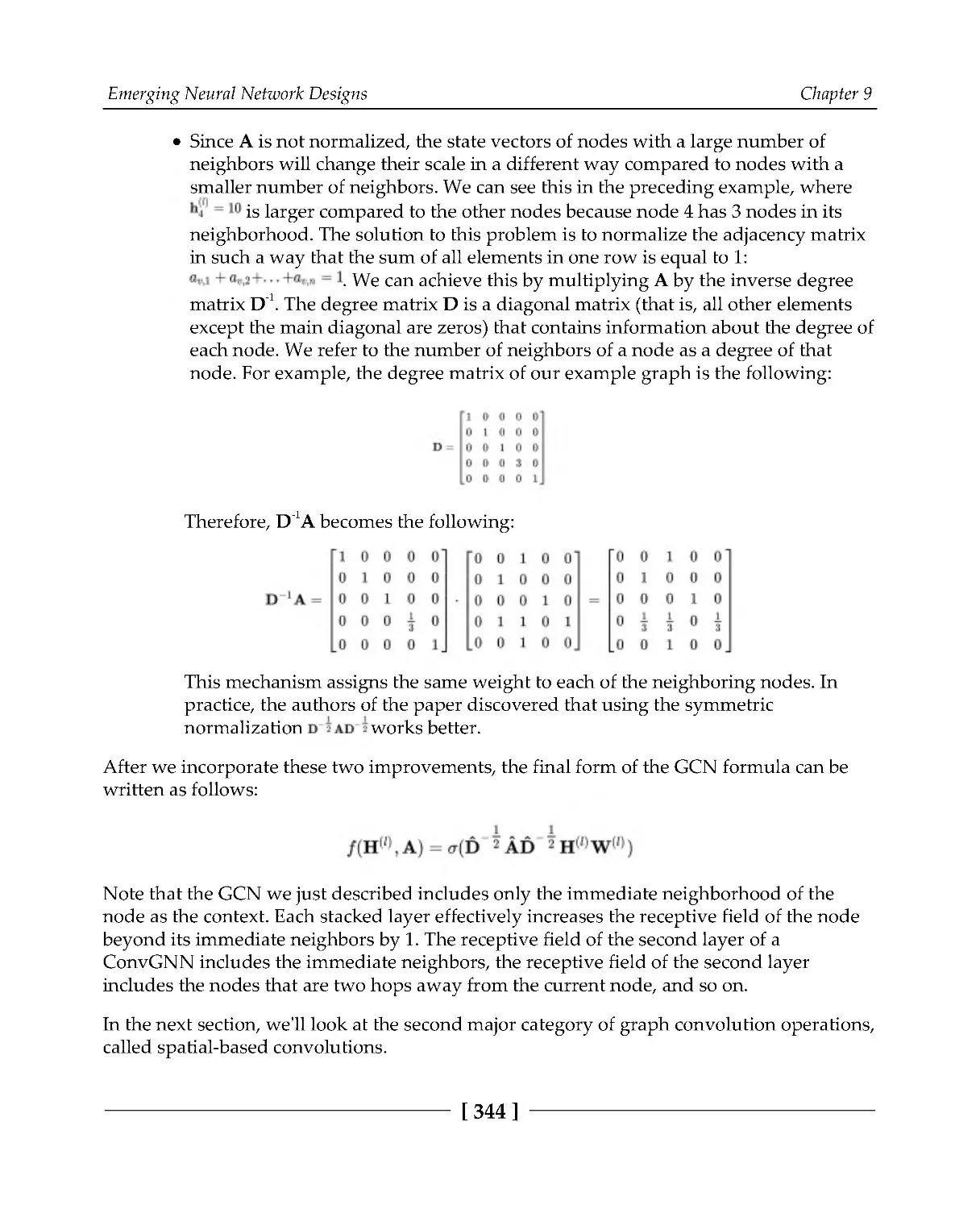
Spatial-based convolutions with attention
345
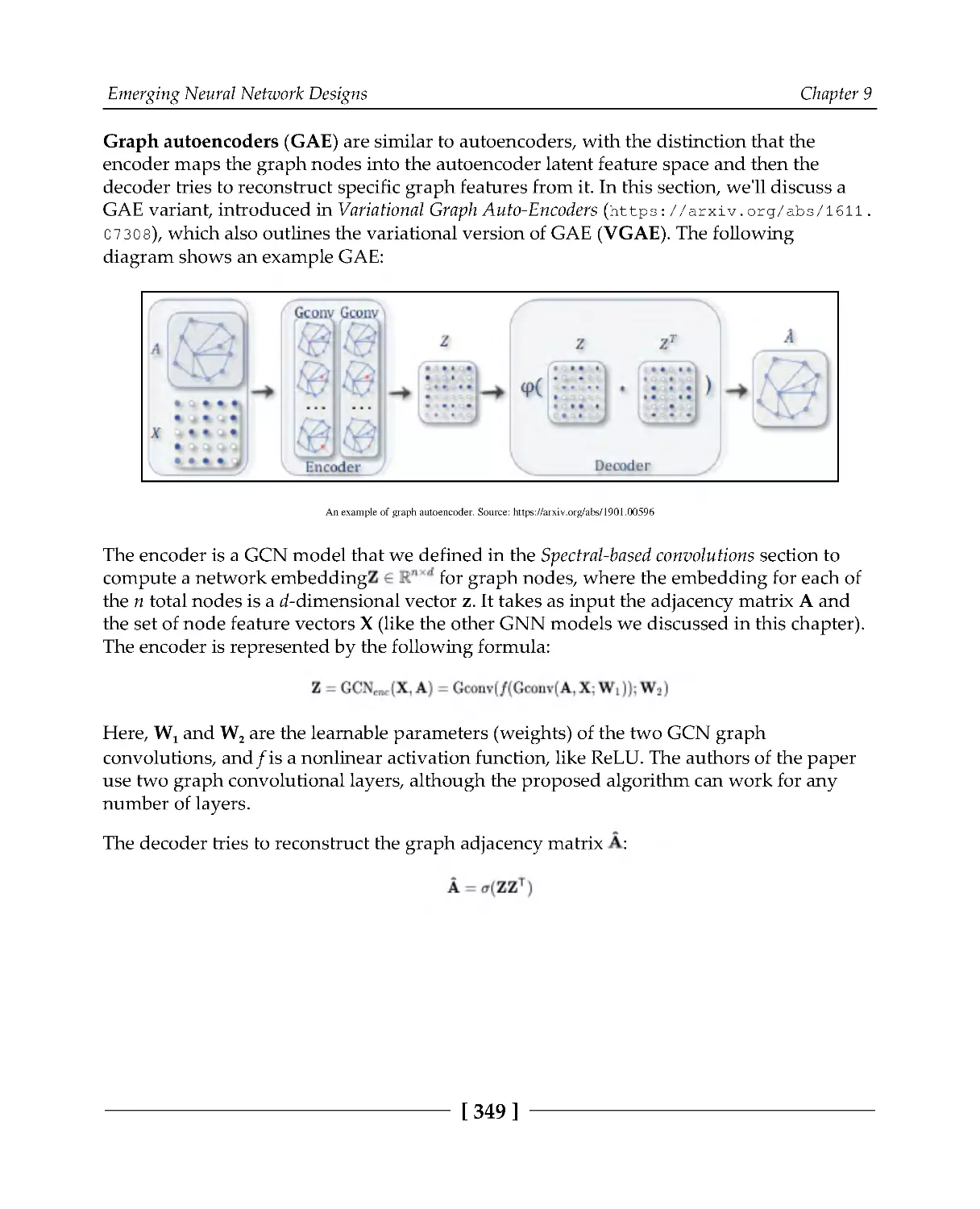
Graph autoencoders
348
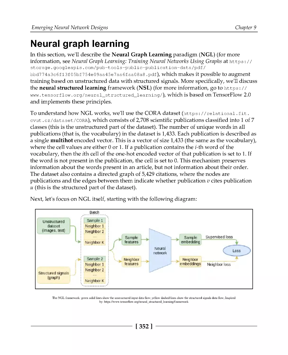
Neural graph learning
352
Implementing graph regularization
354
Introducing memory-augmented NNs
358
Table of Contents
[v]
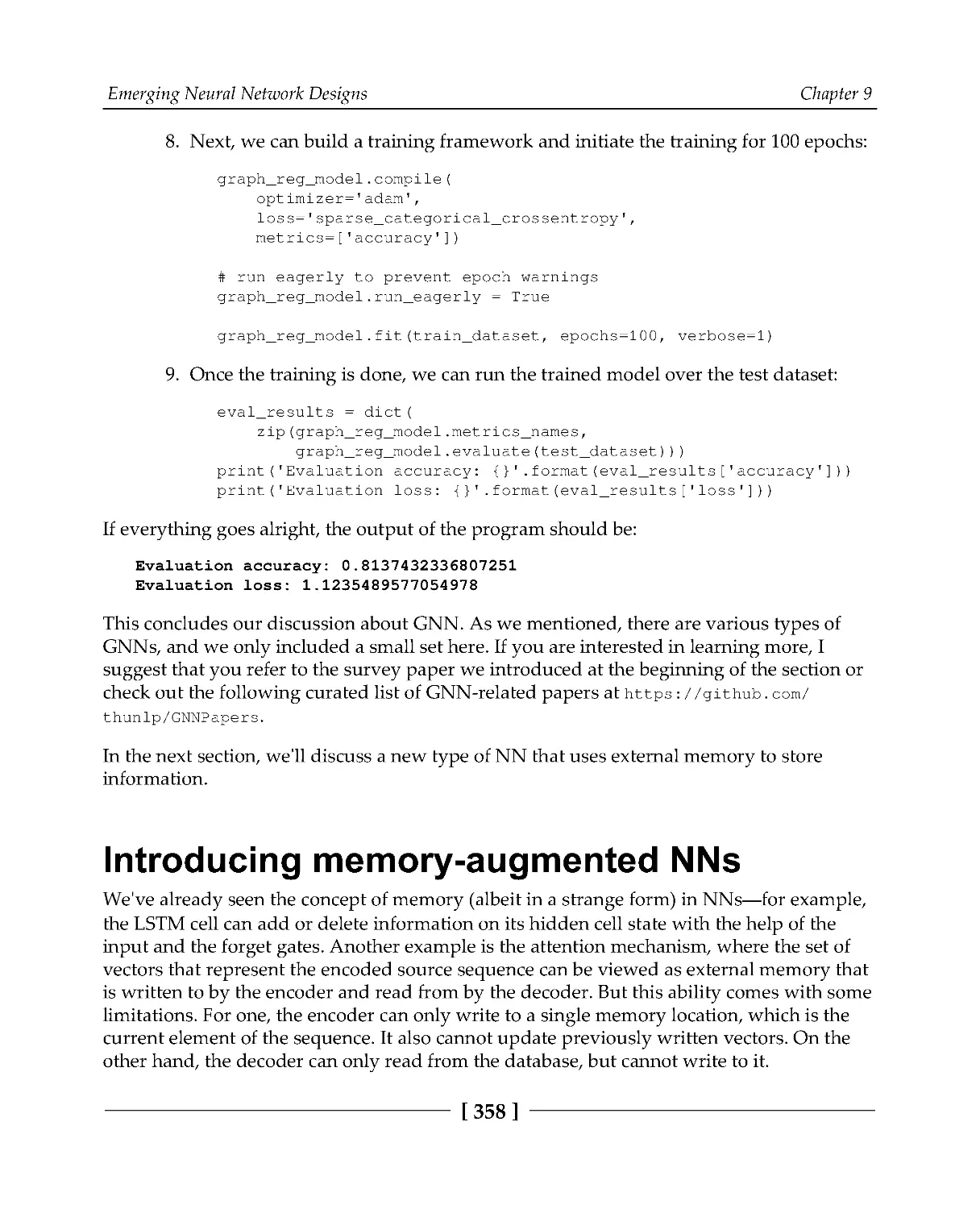
Neural Turing machines
359
MANN*
366
Summary
367
Chapter 10: Meta Learning
368
Introduction to meta learning
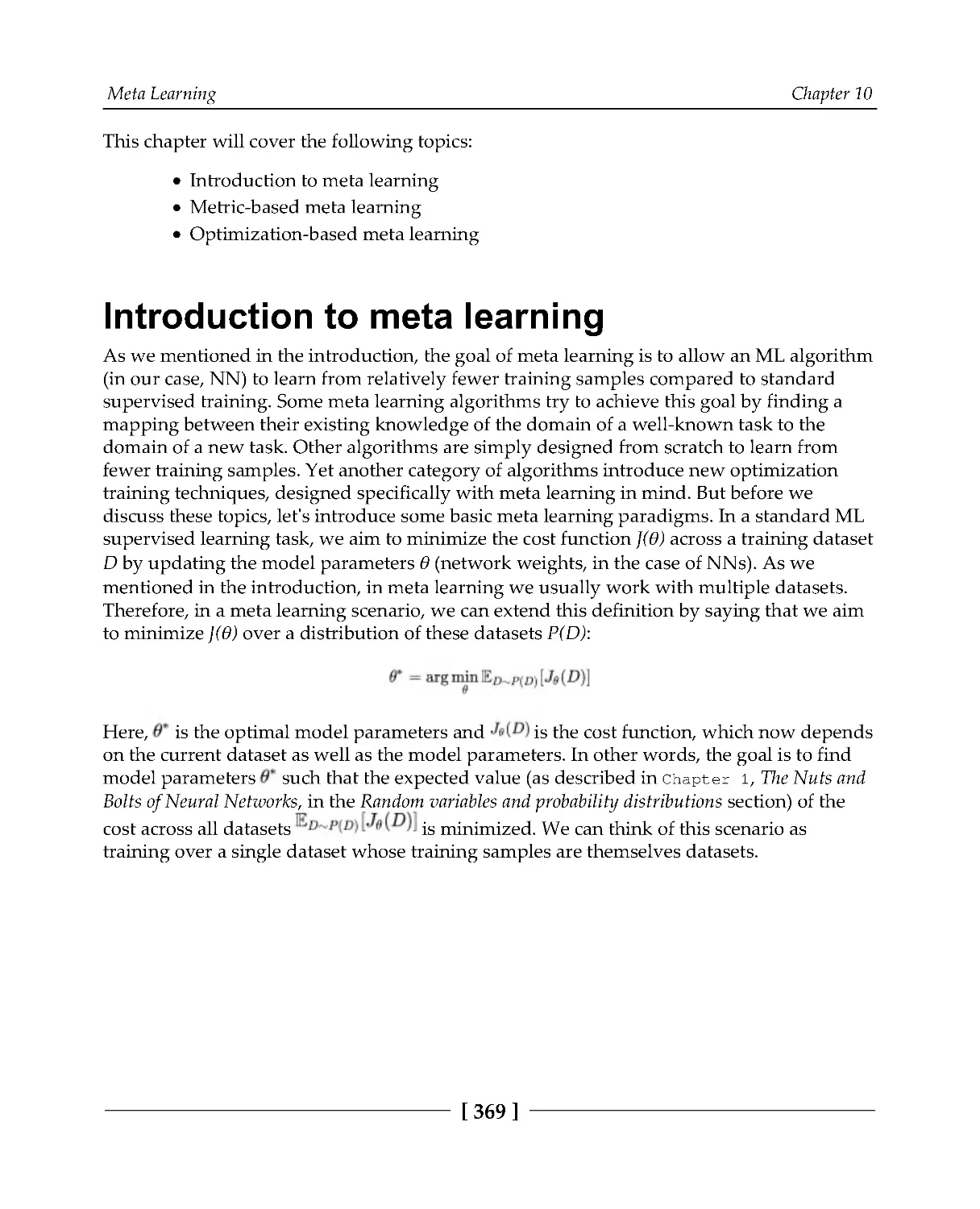
369
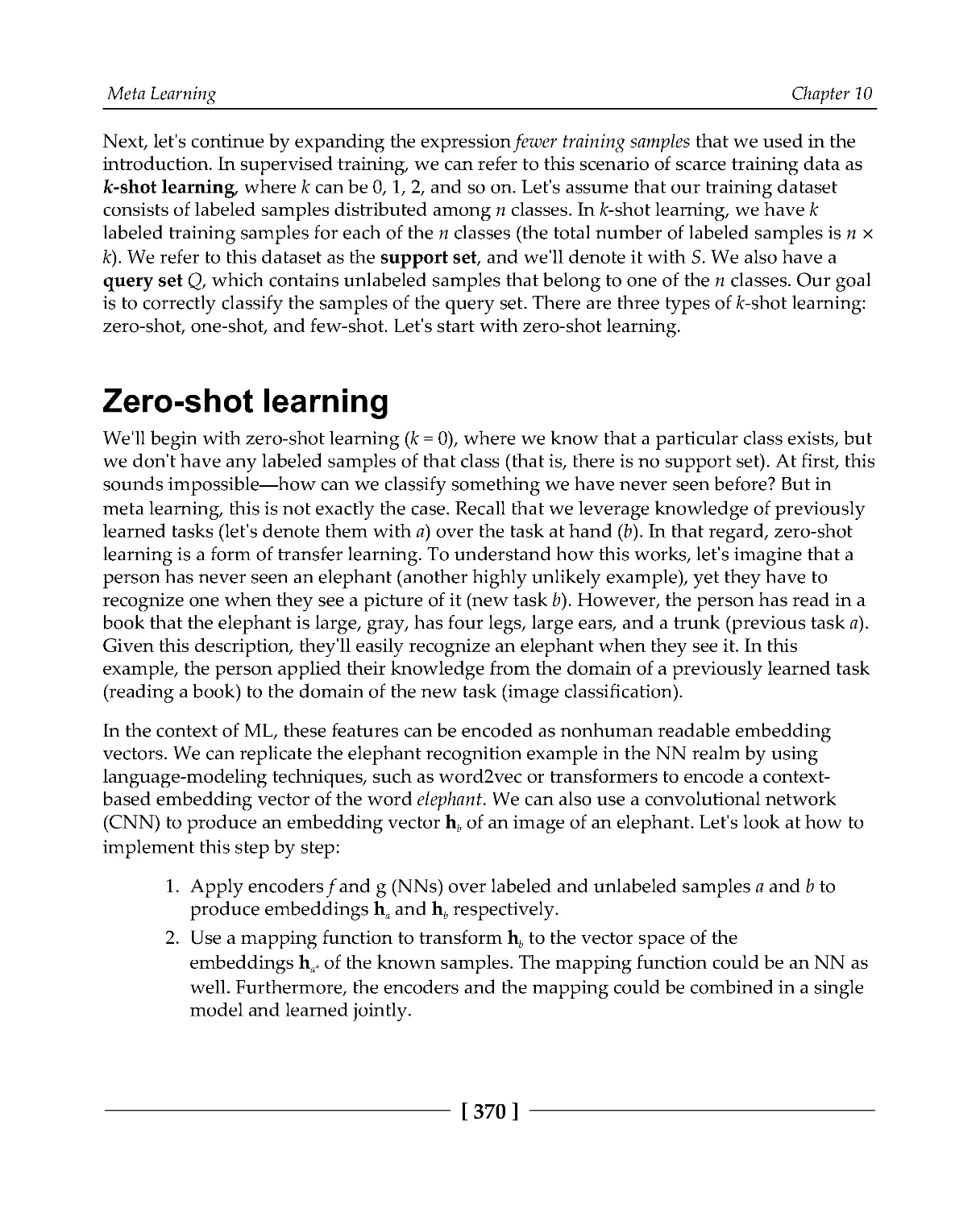
Zero-shot learning
370
One-shot learning
371
Meta-training and meta-testing
373
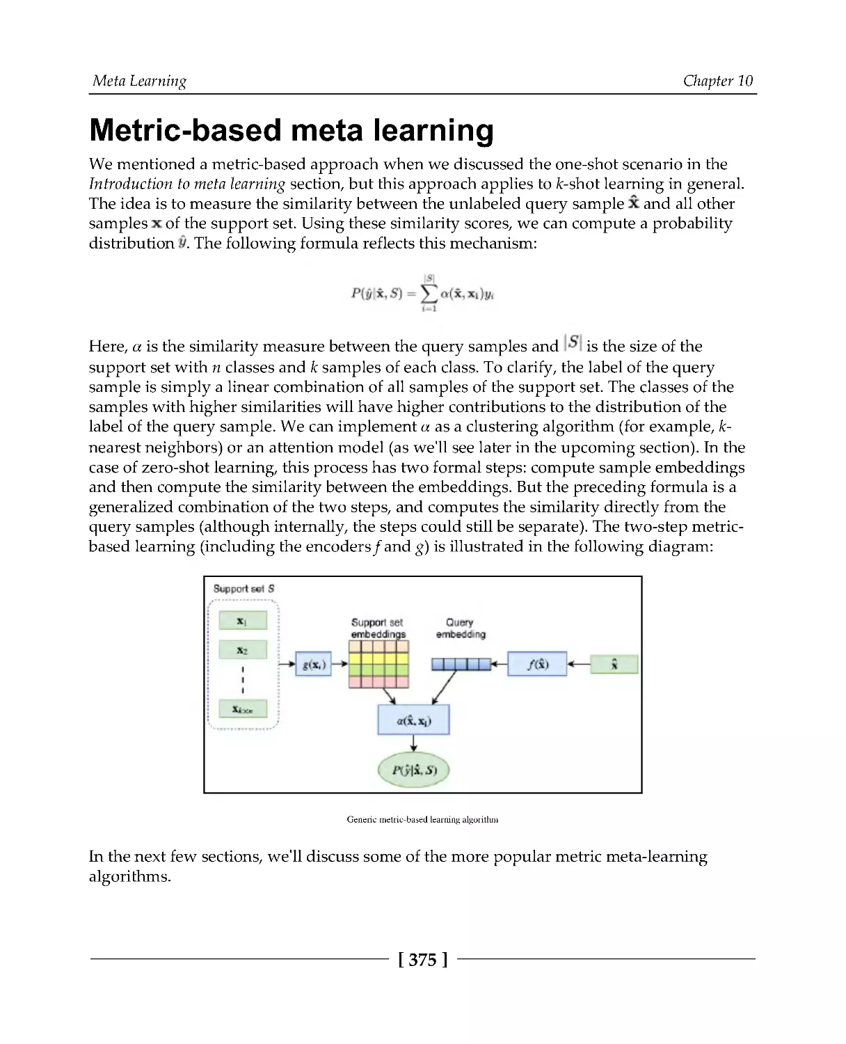
Metric-based meta learning
375
Matching networks for one-shot learning
375
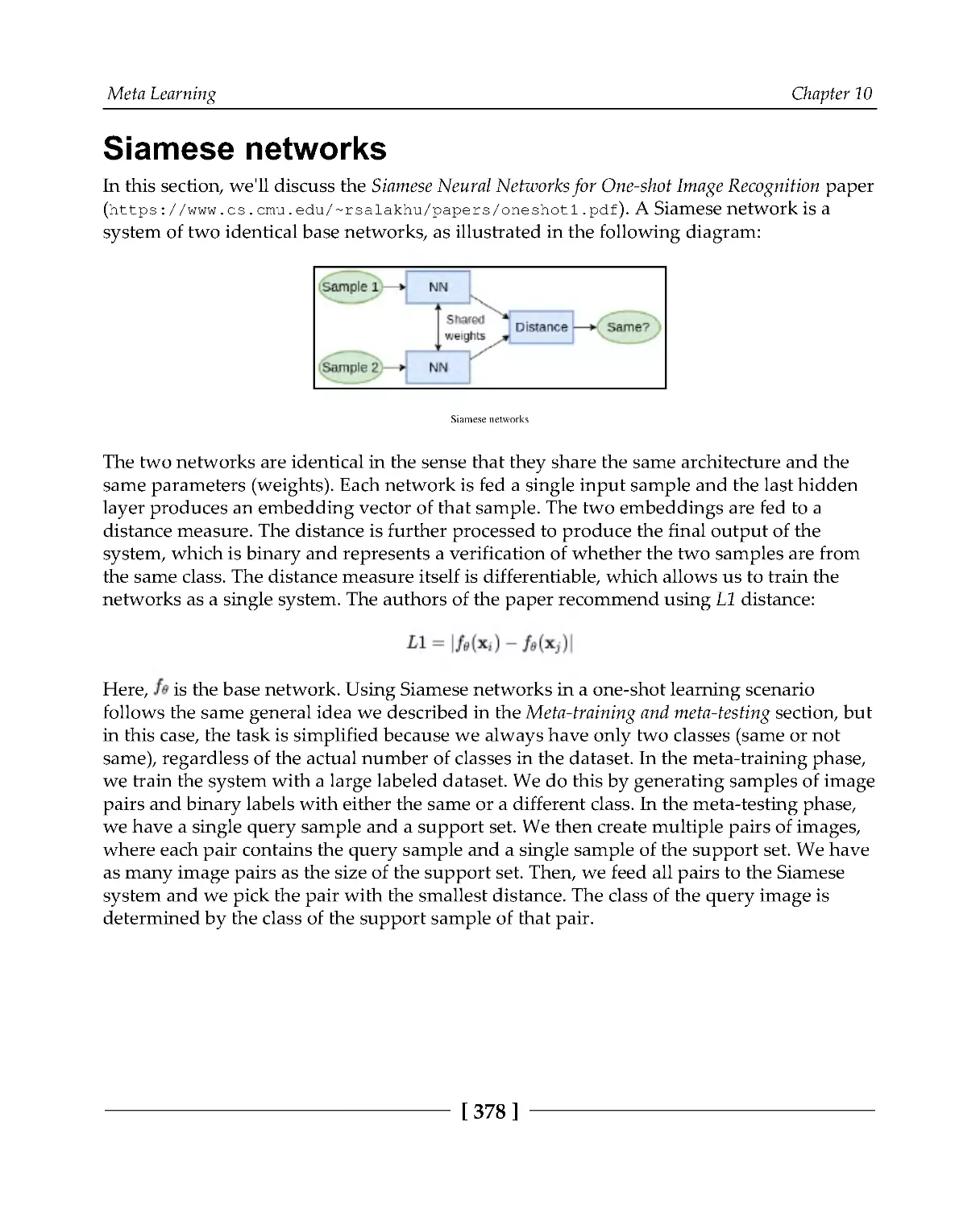
Siamese networks
378
Implementing Siamese networks
379
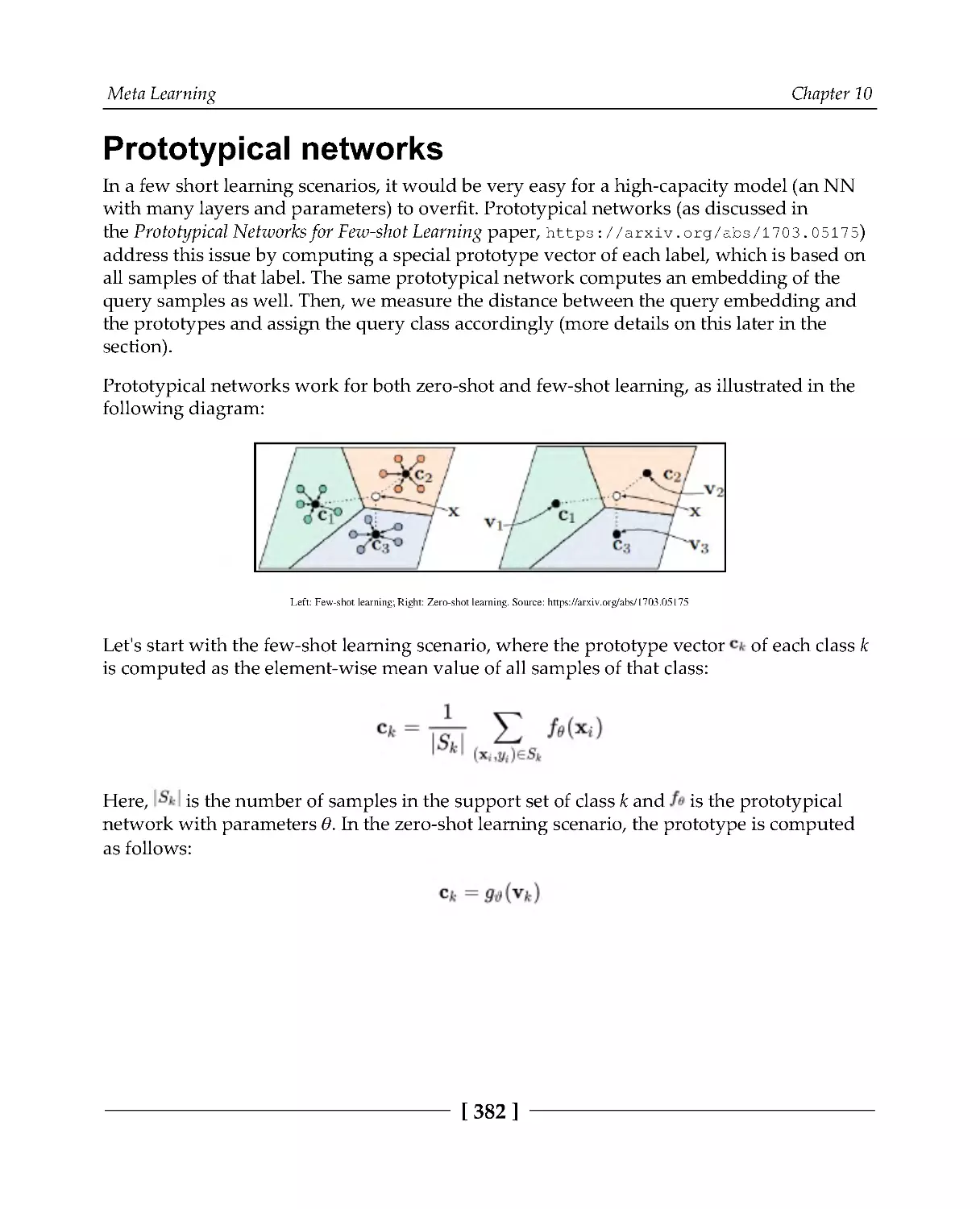
Prototypical networks
382
Optimization-based learning
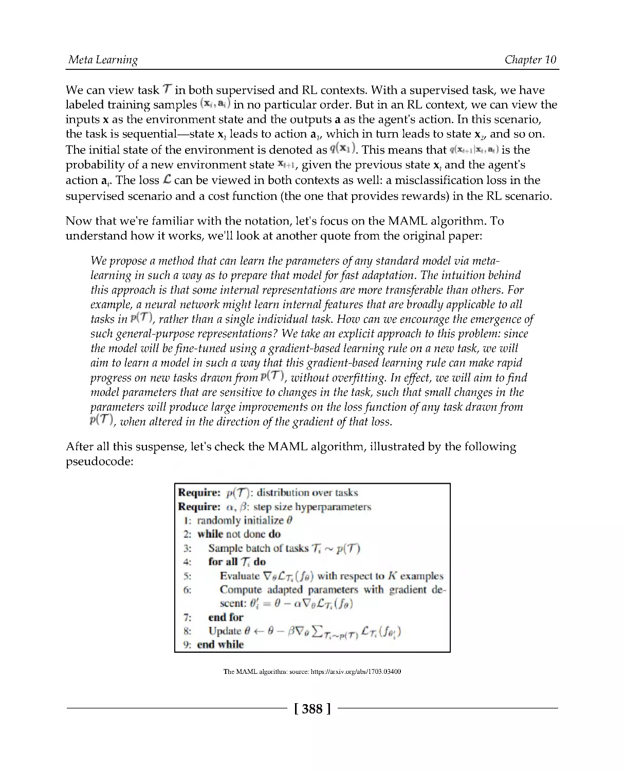
386
Summary
393
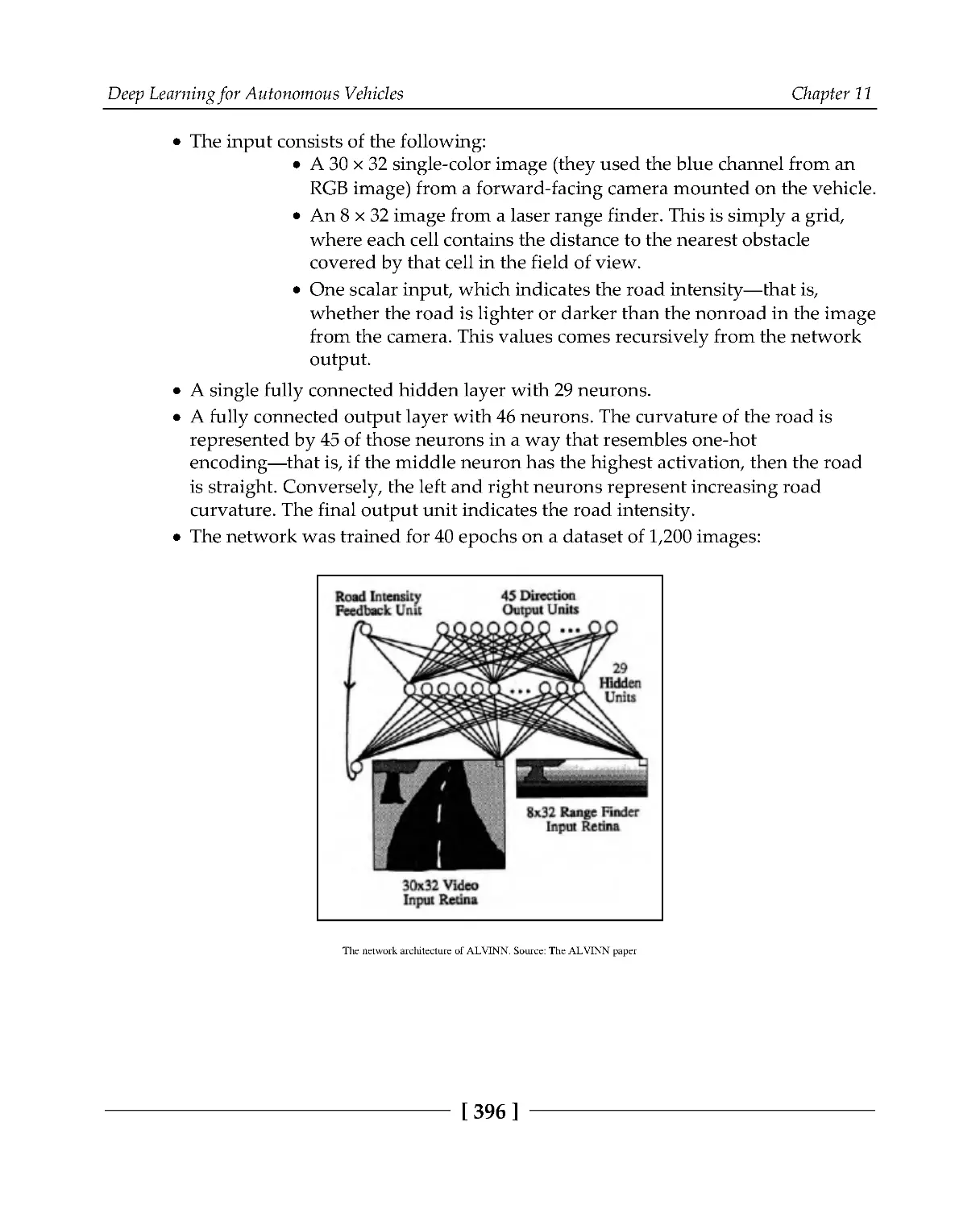
Chapter 11: Deep Learning for Autonomous Vehicles
394
Introduction to AVs
395
Brief history of AV research
395
Levels of automation
398
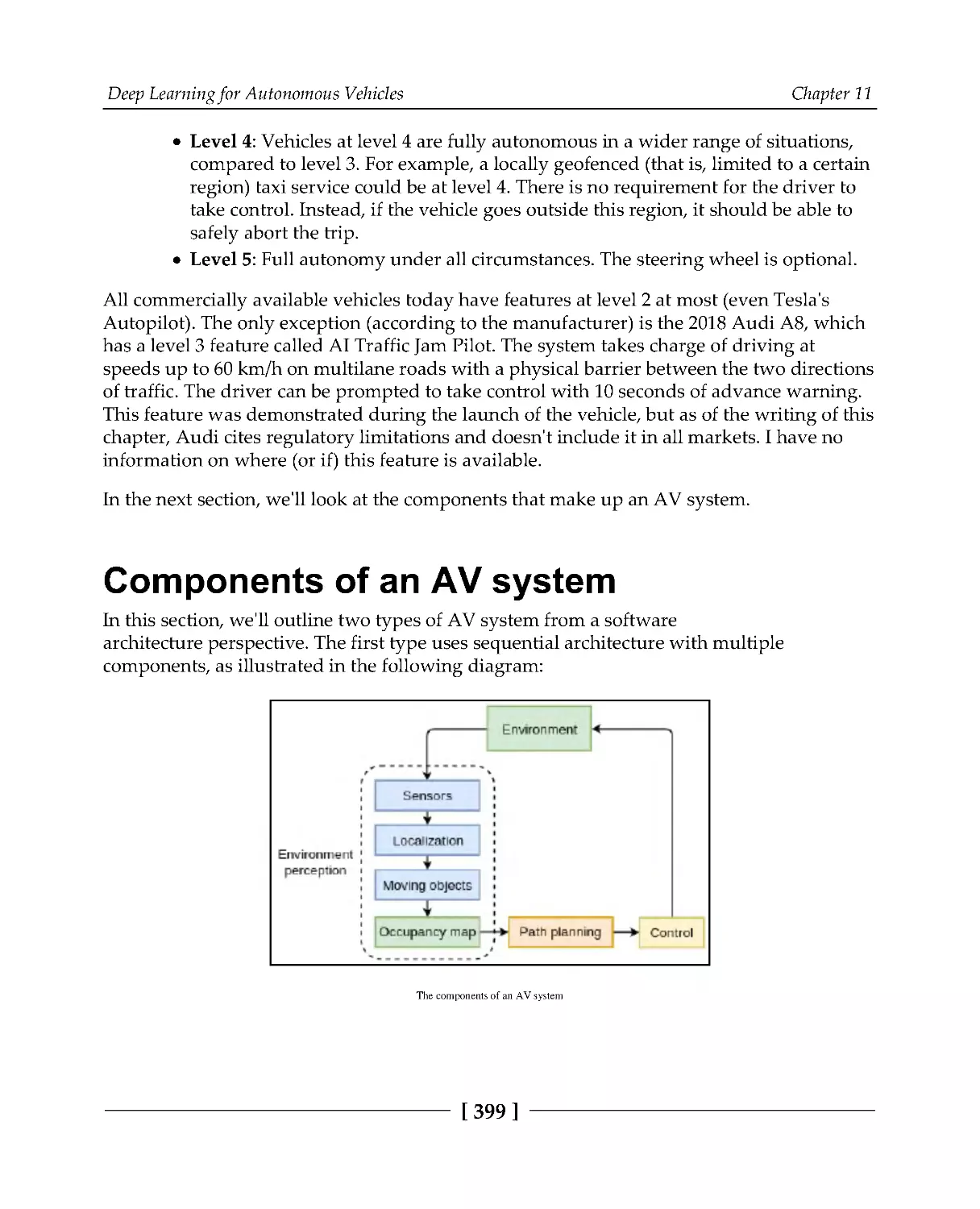
Components of an AV system
399
Environment perception
401
Sensing
402
Localization
404
Moving object detection and tracking
404
Path planning
405
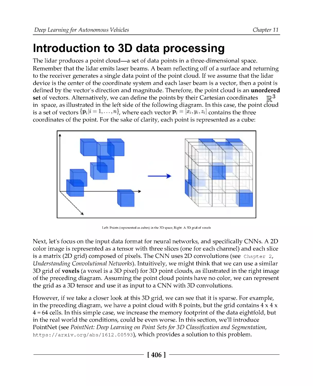
Introduction to 3D data processing
406
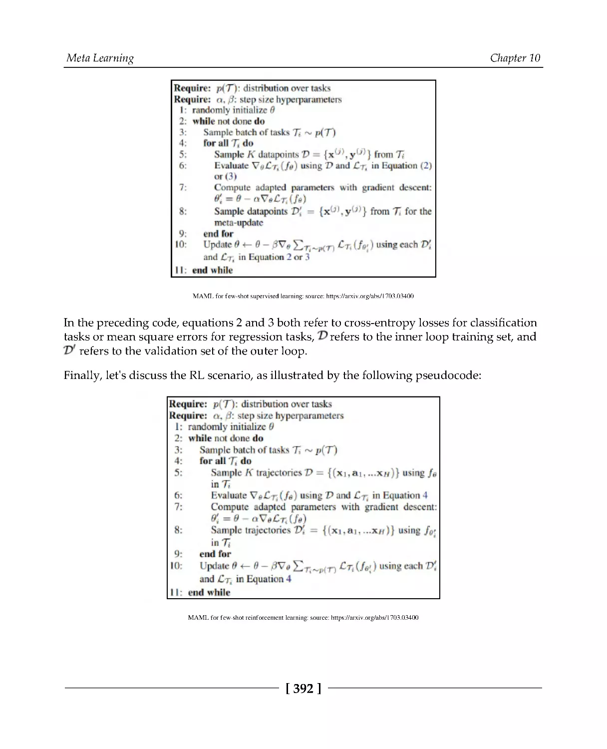
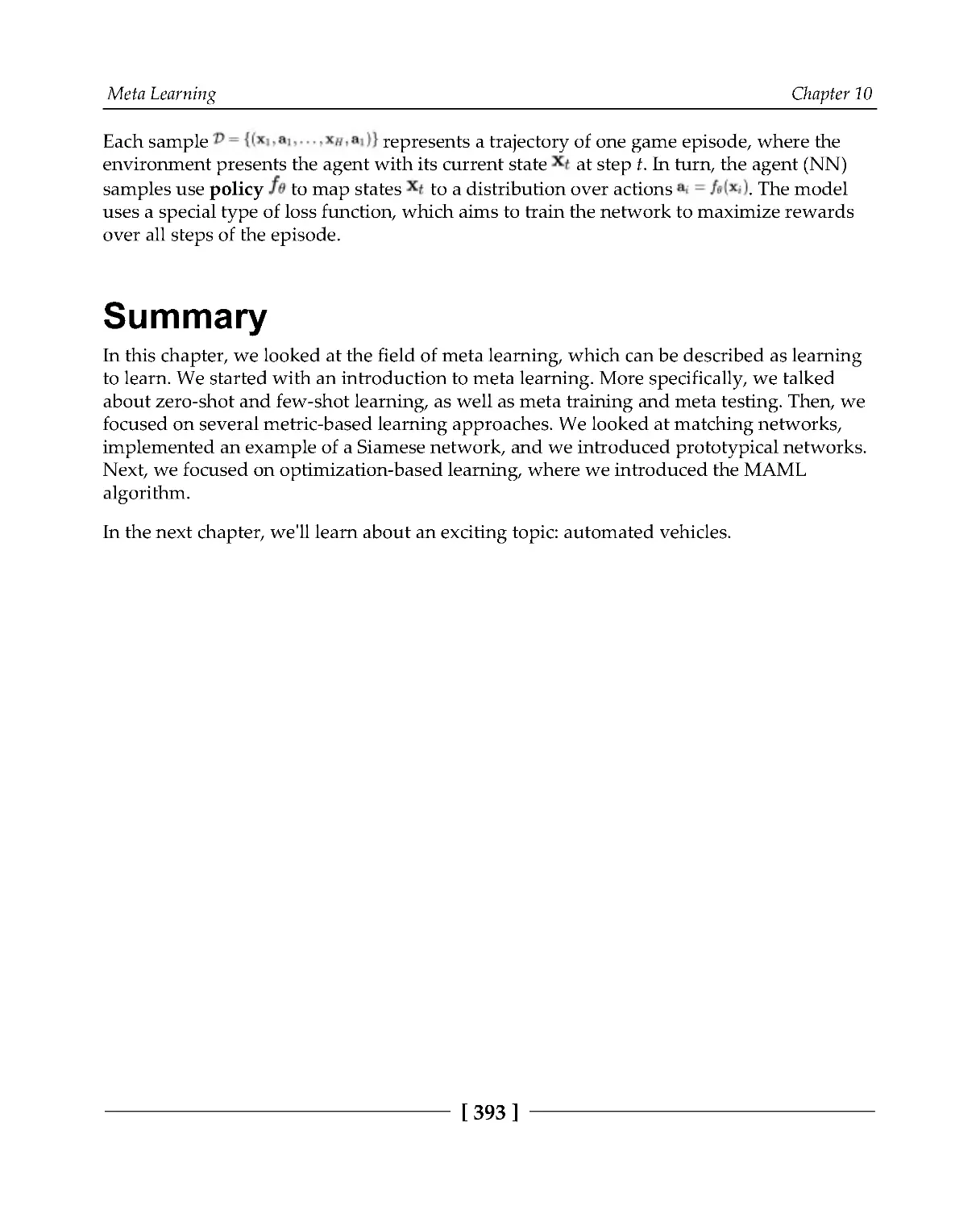
Imitation driving policy
410
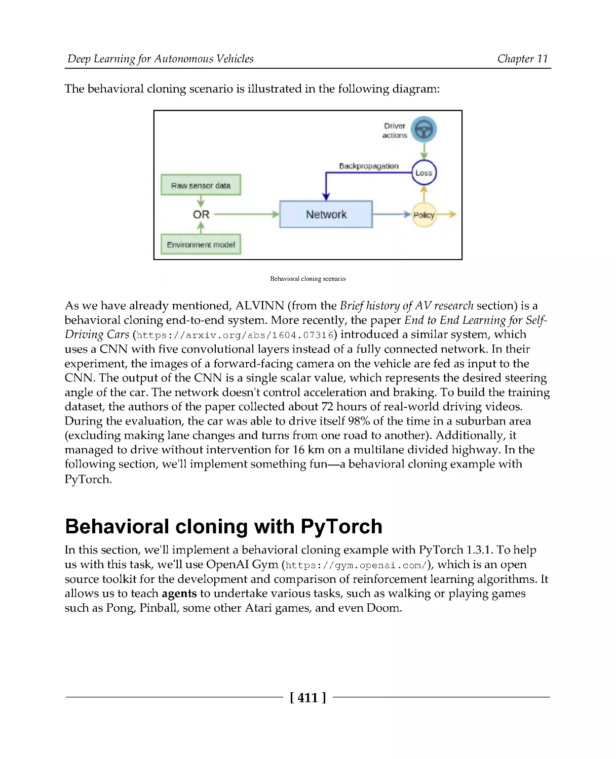
Behavioral cloning with PyTorch
411
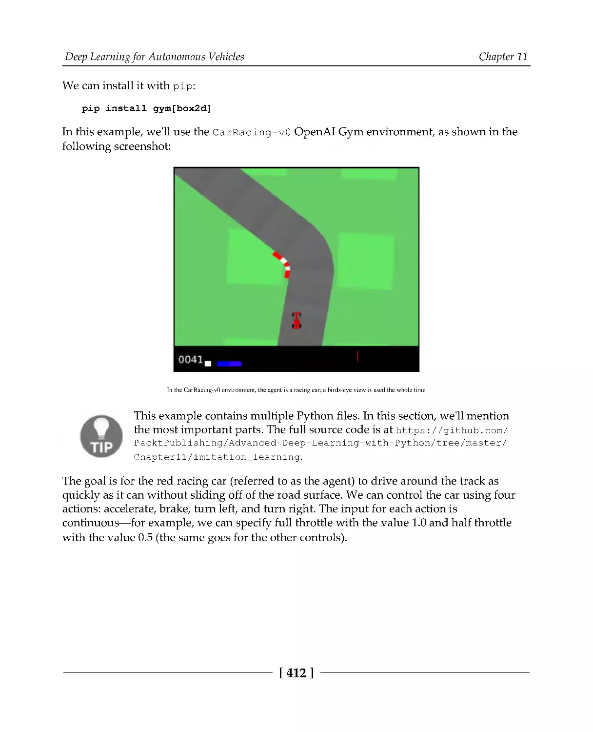
Generating the training dataset
414
Implementing the agent neural network
416
Training
417
Letting the agent drive
419
Putting it all together
420
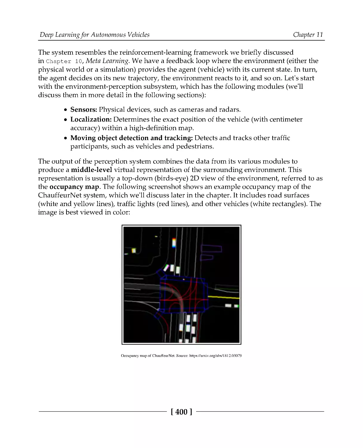
Driving policy with ChauffeurNet
422
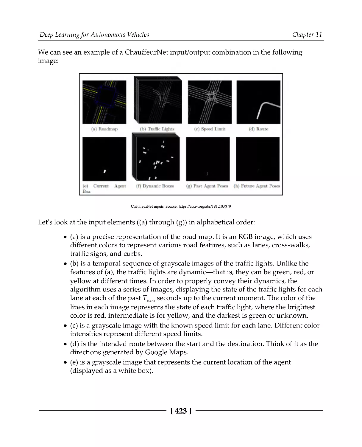
Input and output representations
422
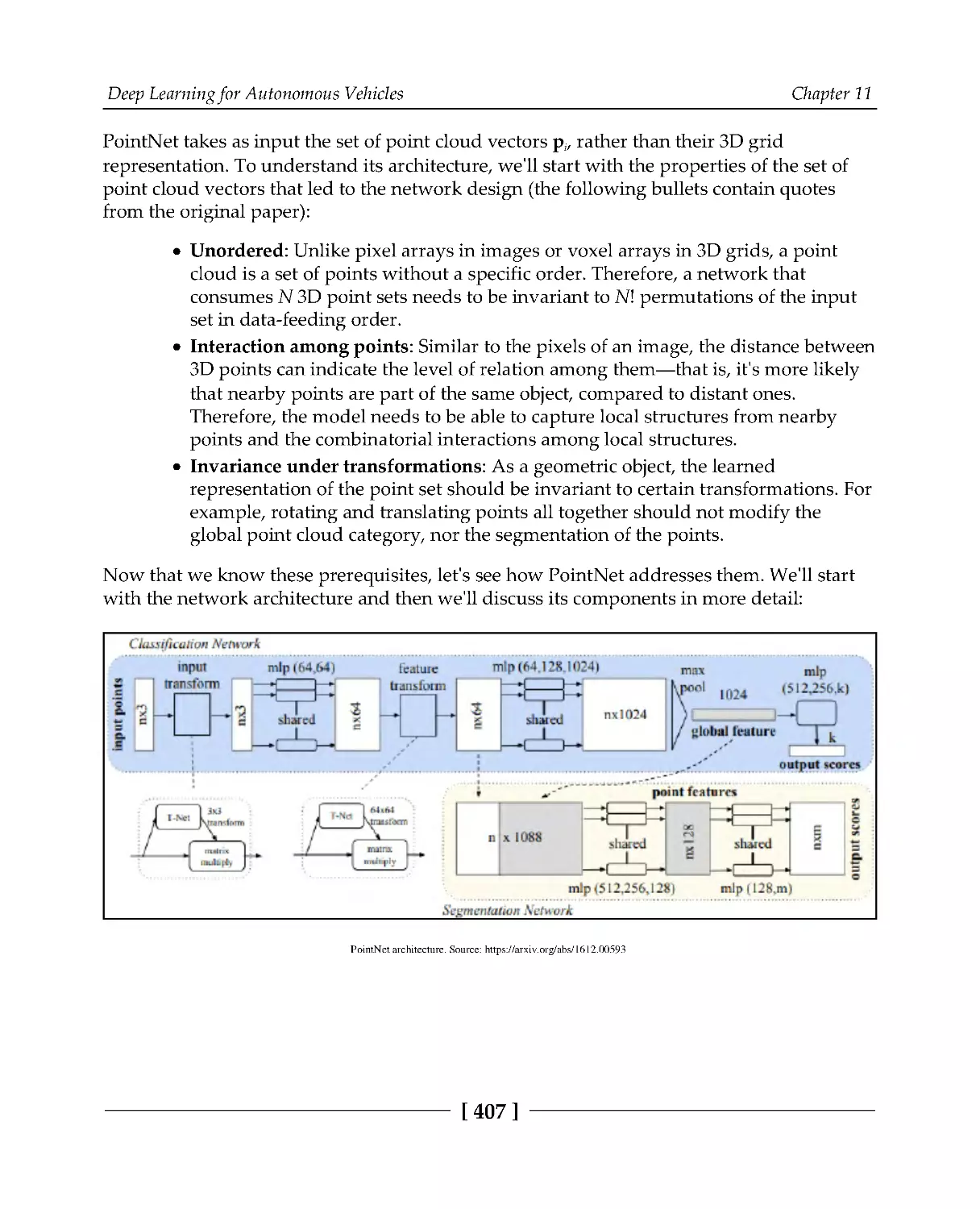
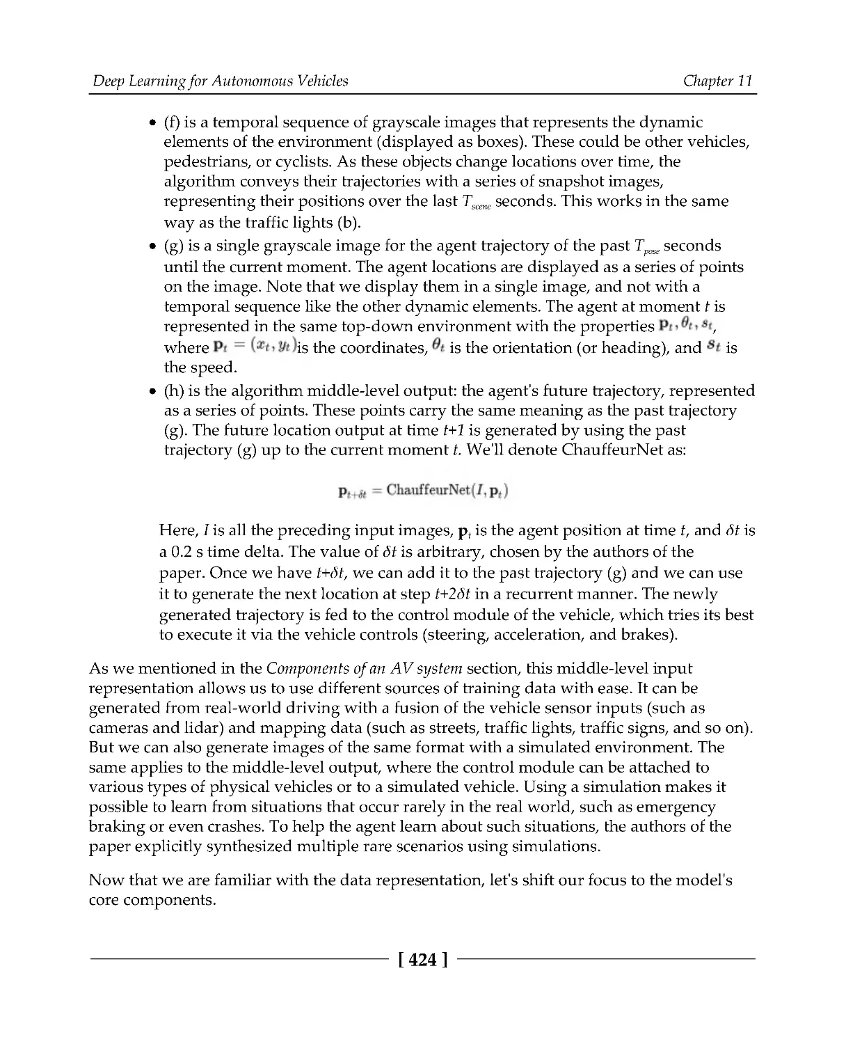
Model architecture
425
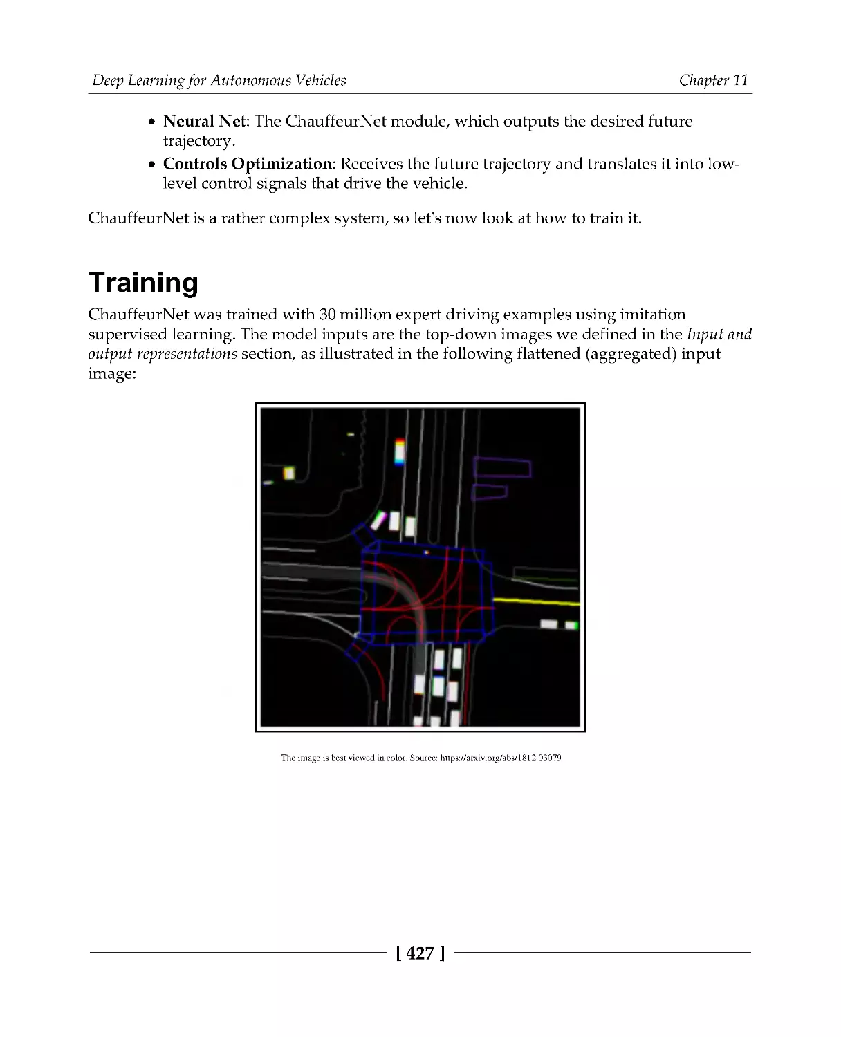
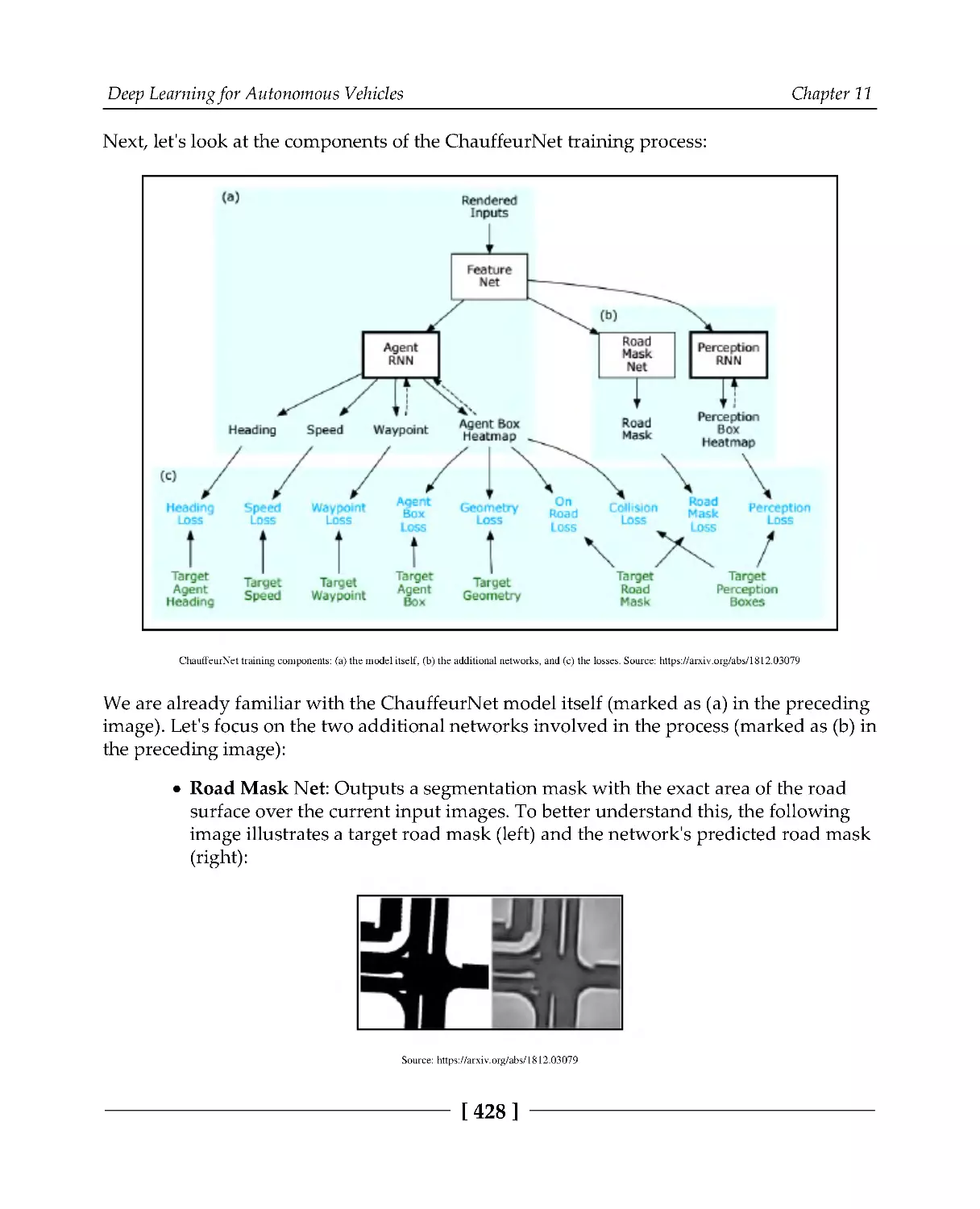
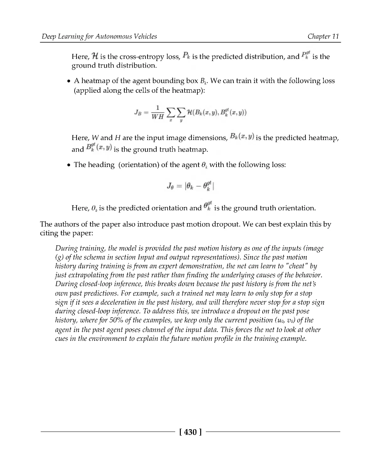
Training
427
Summary
432
Other Books You May Enjoy
433
Index
436
Preface
This book is a collection of newly evolved deep learning models, methodologies, and
implementations based on the areas of their application. In the first section of the book, you
will learn about the building blocks of deep learning and the math behind neural networks
(NNs). In the second section, you'll focus on convolutional neural networks (CNNs) and
their advanced applications in computer vision (CV). You'll learn to apply the most
popular CNN architectures in object detection and image segmentation. Finally, you'll
discuss variational autoencoders and generative adversarial networks.
In the third section, you'll focus on natural language and sequence processing. You'll use
NNs to extract sophisticated vector representations of words. You'll discuss various types
of recurrent networks, such as long short-term memory (LSTM) and gated recurrent unit
(GRU). Finally, you'll cover the attention mechanism to process sequential data without the
help of recurrent networks. In the final section, you'll learn how to use graph NNs to
process structured data. You'll cover meta-learning, which allows you to train an NN with
fewer training samples. And finally, you'll learn how to apply deep learning in autonomous
vehicles.
By the end of this book, you'll have gained mastery of the key concepts associated with
deep learning and evolutionary approaches to monitoring and managing deep learning
models.
Who this book is for
This book is for data scientists, deep learning engineers and researchers, and AI developers
who want to master deep learning and want to build innovative and unique deep learning
projects of their own. This book will also appeal to those who are looking to get well-versed
with advanced use cases and the methodologies adopted in the deep learning domain
using real-world examples. Basic conceptual understanding of deep learning and a working
knowledge of Python is assumed.
Preface
[2]
What this book covers
Chapter 1, The Nuts and Bolts of Neural Networks, will briefly introduce what deep learning
is and then discuss the mathematical underpinnings of NNs. This chapter will discuss NNs
as mathematical models. More specifically, we'll focus on vectors, matrices, and differential
calculus. We'll also discuss some gradient descent variations, such as Momentum, Adam,
and Adadelta, in depth. We will also discuss how to deal with imbalanced datasets.
Chapter 2, Understanding Convolutional Networks, will provide a short description of CNNs.
We'll discuss CNNs and their applications in CV
Chapter 3, Advanced Convolutional Networks, will discuss some advanced and widely used
NN architectures, including VGG, ResNet, MobileNets, GoogleNet, Inception, Xception,
and DenseNets. We'll also implement ResNet and Xception/MobileNets using PyTorch.
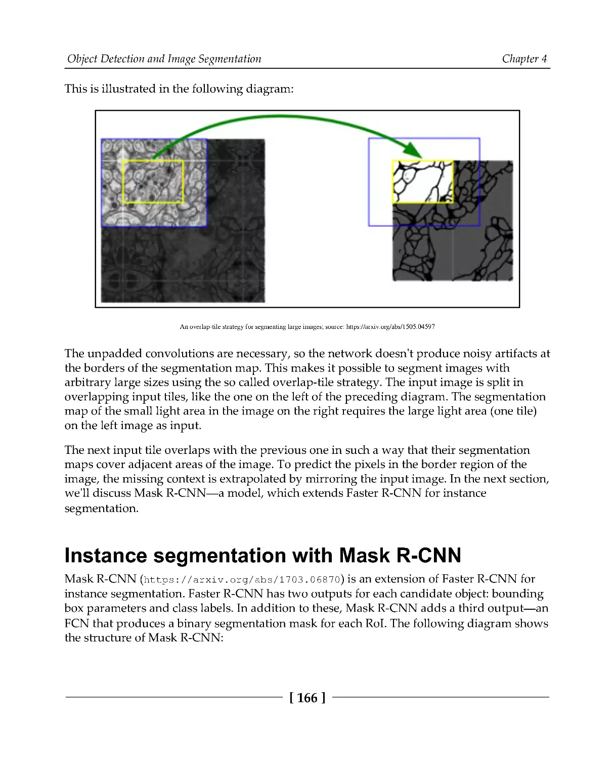
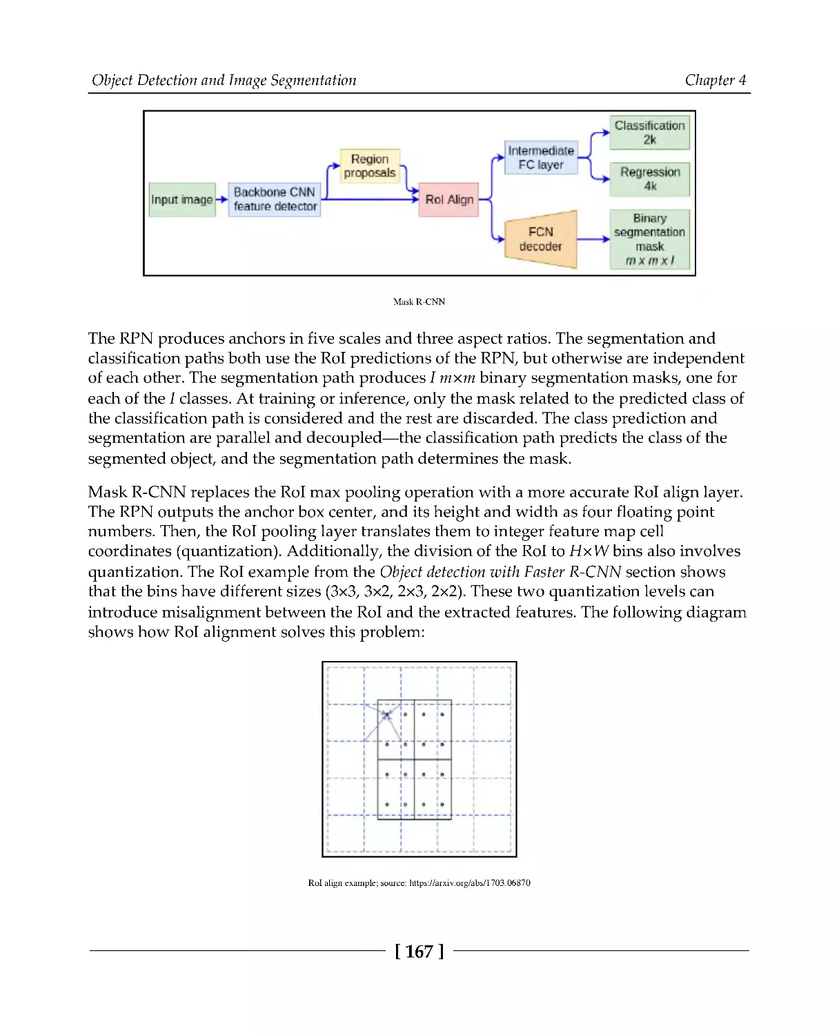
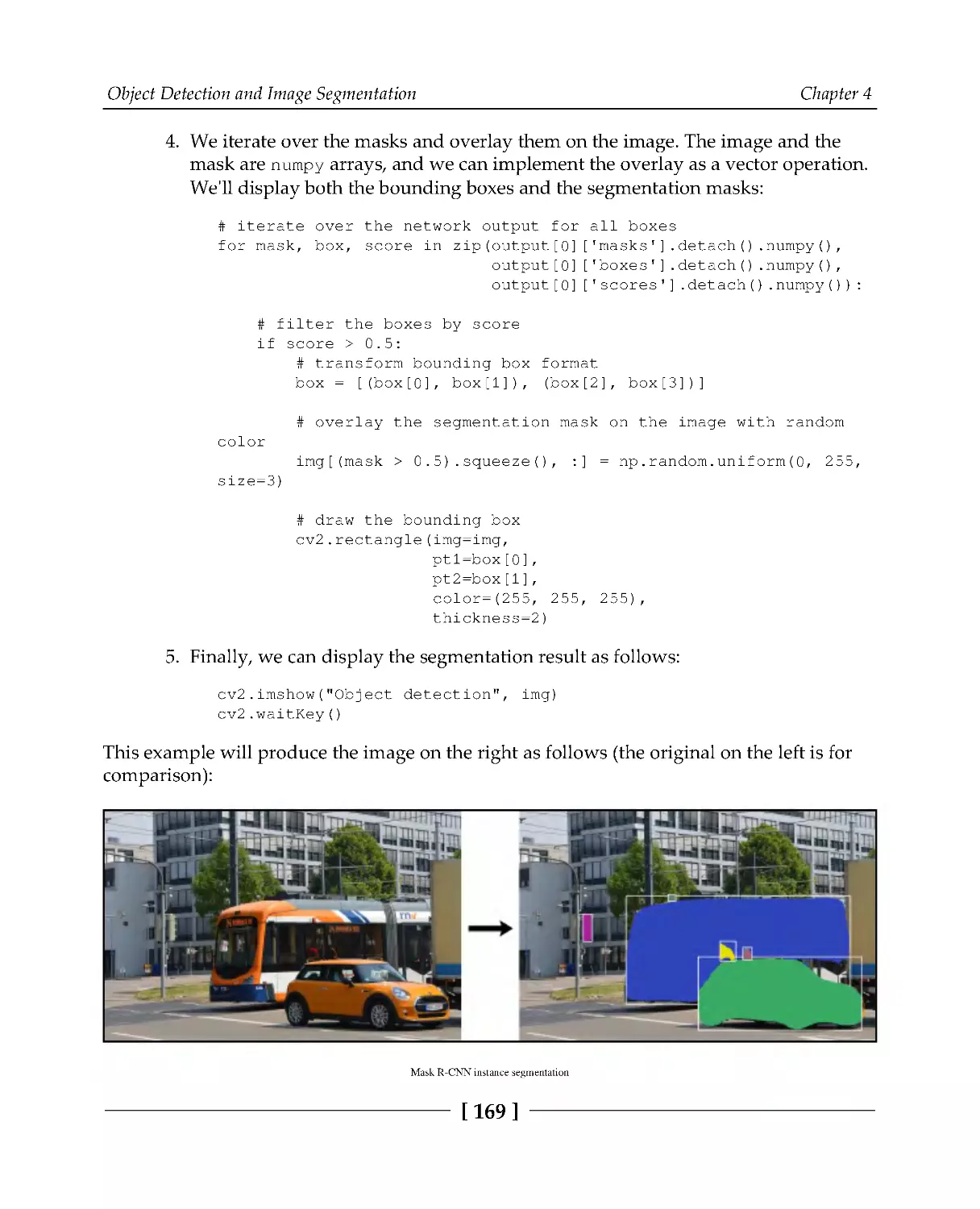
Chapter 4, Object Detection and Image Segmentation, will discuss two important vision tasks:
object detection and image segmentation. We'll provide implementations for both of them.
Chapter 5, Generative Models, will begin the discussion about generative models. In
particular, we'll talk about generative adversarial networks and neural style transfer. The
particular style transfer will be implemented later.
Chapter 6, Language Modeling, will introduce word and character-level language models.
We'll also talk about word vectors (word2vec, Glove, and fastText) and we'll use Gensim to
implement them. We'll also walk through the highly technical and complex process of
preparing text data for machine learning applications such as topic modeling and sentiment
modeling with the help of the Natural Language ToolKit's (NLTK) text processing
techniques.
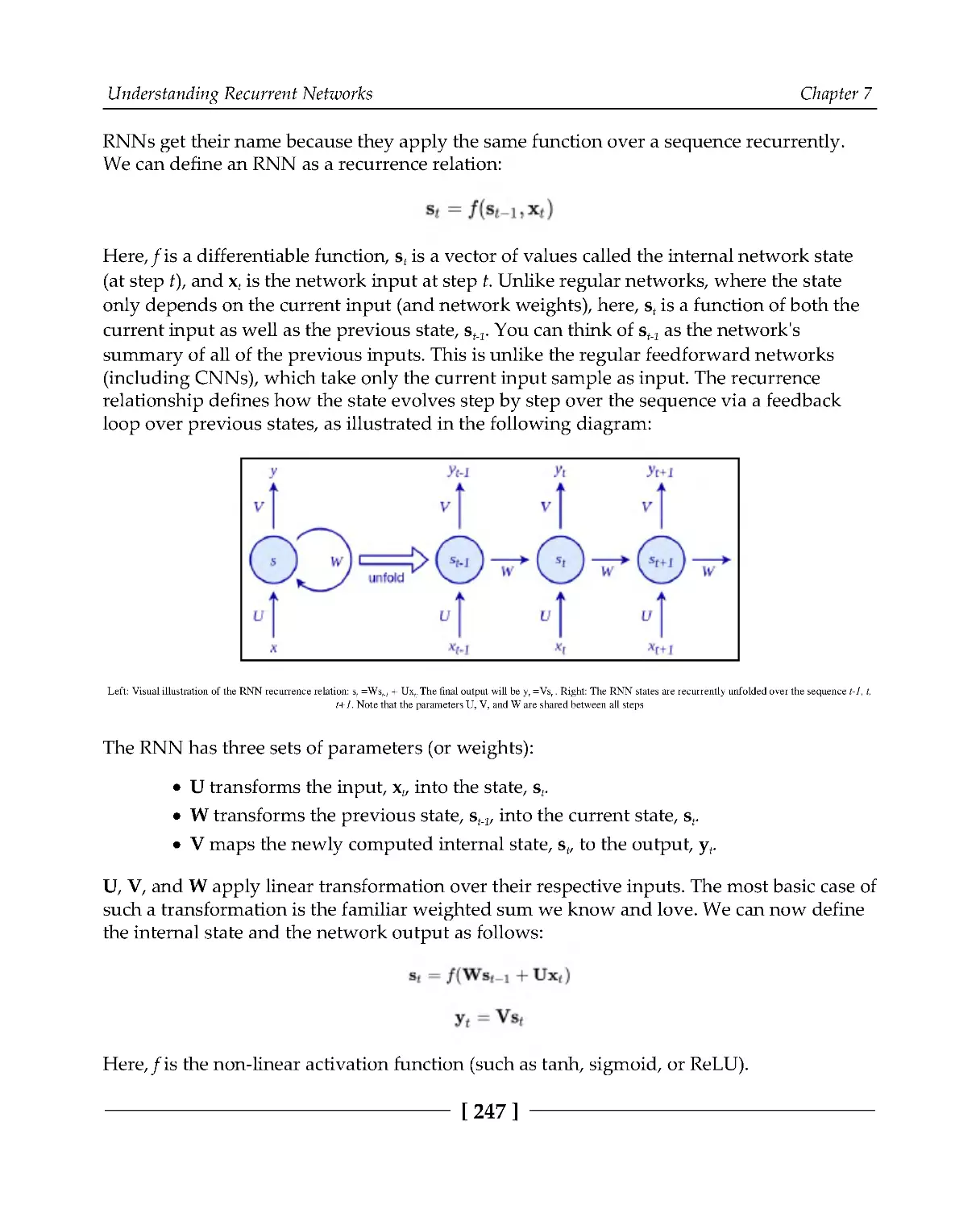
Chapter 7, Understanding Recurrent Networks, will discuss the basic recurrent networks,
LSTM, and GRU cells. We'll provide a detailed explanation and pure Python
implementations for all of the networks.
Chapter 8, Sequence-to-Sequence Models and Attention, will discuss sequence models and the
attention mechanism, including bidirectional LSTMs, and a new architecture called
transformer with encoders and decoders.
Chapter 9, Emerging Neural Network Designs, will discuss graph NNs and NNs with
memory, such as Neural Turing Machines (NTM), differentiable neural computers, and
MANN.
Preface
[3]
Chapter 10, Meta Learning, will discuss meta learning—the way to teach algorithms how to
learn. We'll also try to improve upon deep learning algorithms by giving them the ability to
learn more information using less training samples.
Chapter 11, Deep Learning for Autonomous Vehicles, will explore the applications of deep
learning in autonomous vehicles. We'll discuss how to use deep networks to help the
vehicle make sense of its surrounding environment.
To get the most out of this book
To get the most out of this book, you should be familiar with Python and have some
knowledge of machine learning. The book includes short introductions to the major types
of NNs, but it will help if you are already familiar with the basics of NNs.
Download the example code files
You can download the example code files for this book from your account at
www.packt.com. If you purchased this book elsewhere, you can visit
www.packtpub.com/support and register to have the files emailed directly to you.
You can download the code files by following these steps:
Log in or register at www.packt.com.
1.
Select the Support tab.
2.
Click on Code Downloads.
3.
Enter the name of the book in the Search box and follow the onscreen
4.
instructions.
Once the file is downloaded, please make sure that you unzip or extract the folder using the
latest version of:
WinRAR/7-Zip for Windows
Zipeg/iZip/UnRarX for Mac
7-Zip/PeaZip for Linux
The code bundle for the book is also hosted on GitHub at https:/
/
github.
com/
PacktPublishing/
Advanced-
Deep-
Learning-
with-
Python. In case there's an update to the
code, it will be updated on the existing GitHub repository.
We also have other code bundles from our rich catalog of books and videos available
at https:/
/
github.
com/
PacktPublishing/
. Check them out!
Preface
[4]
Download the color images
We also provide a PDF file that has color images of the screenshots/diagrams used in this
book. You can download it here: http:/
/
www.
packtpub.
com/
sites/
default/
files/
downloads/
9781789956177_
ColorImages.
pdf.
Conventions used
There are a number of text conventions used throughout this book.
CodeInText: Indicates code words in text, database table names, folder names, filenames,
file extensions, pathnames, dummy URLs, user input, and Twitter handles. Here is an
example: "Build the full GAN model by including the generator, discriminator, and
the combined network."
A block of code is set as follows:
import matplotlib.pyplot as plt
from matplotlib.markers import MarkerStyle
import numpy as np
import tensorflow as tf
from tensorflow.keras import backend as K
from tensorflow.keras.layers import Lambda, Input, Dense
Bold: Indicates a new term, an important word, or words that you see onscreen. For
example, words in menus or dialog boxes appear in the text like this. Here is an example:
"The collection of all possible outcomes (events) of an experiment is called, sample space."
Warnings or important notes appear like this.
Tips and tricks appear like this.
Preface
[5]
Get in touch
Feedback from our readers is always welcome.
General feedback: If you have questions about any aspect of this book, mention the book
title in the subject of your message and email us at customercare@packtpub.com.
Errata: Although we have taken every care to ensure the accuracy of our content, mistakes
do happen. If you have found a mistake in this book, we would be grateful if you would
report this to us. Please visit www.packtpub.com/support/errata, selecting your book,
clicking on the Errata Submission Form link, and entering the details.
Piracy: If you come across any illegal copies of our works in any form on the Internet, we
would be grateful if you would provide us with the location address or website name.
Please contact us at copyright@packt.com with a link to the material.
If you are interested in becoming an author: If there is a topic that you have expertise in
and you are interested in either writing or contributing to a book, please visit
authors.packtpub.com.
Reviews
Please leave a review. Once you have read and used this book, why not leave a review on
the site that you purchased it from? Potential readers can then see and use your unbiased
opinion to make purchase decisions, we at Packt can understand what you think about our
products, and our authors can see your feedback on their book. Thank you!
For more information about Packt, please visit packt.com.
1
Section 1: Core Concepts
This section will discuss some core Deep Learning (DL) concepts: what exactly DL is, the
mathematical underpinnings of DL algorithms, and the libraries and tools that make it
possible to develop DL algorithms rapidly.
This section contains the following chapter:
Chapter 1, The Nuts and Bolts of Neural Networks
1
The Nuts and Bolts of Neural
Networks
In this chapter, we'll discuss some of the intricacies of neural networks (NNs)—the
cornerstone of deep learning (DL). We'll talk about their mathematical apparatus,
structure, and training. Our main goal is to provide you with a systematic understanding of
NNs. Often, we approach them from a computer science perspective—as a machine
learning (ML) algorithm (or even a special entity) composed of a number of different
steps/components. We gain our intuition by thinking in terms of neurons, layers, and so on
(at least I did this when I first learned about this field). This is a perfectly valid way to do
things and we can still do impressive things at this level of understanding. Perhaps this is
not the correct approach, though.
NNs have solid mathematical foundations and if we approach them from this point of
view, we'll be able to define and understand them in a more fundamental and elegant way.
Therefore, in this chapter, we'll try to underscore the analogy between NNs from
mathematical and computer science points of view. If you are already familiar with these
topics, you can skip this chapter. Still, I hope that you'll find some interesting bits you
didn't know about already (we'll do our best to keep this chapter interesting!).
In this chapter, we will cover the following topics:
The mathematical apparatus of NNs
A short introduction to NNs
Training NNs
The Nuts and Bolts of Neural Networks
Chapter 1
[8]
The mathematical apparatus of NNs
In the next few sections, we'll discuss the mathematical branches related to NNs. Once
we've done this, we'll connect them to NNs themselves.
Linear algebra
Linear algebra deals with linear equations such as
and linear
transformations (or linear functions) and their representations, such as matrices and
vectors.
Linear algebra identifies the following mathematical objects:
Scalars: A single number.
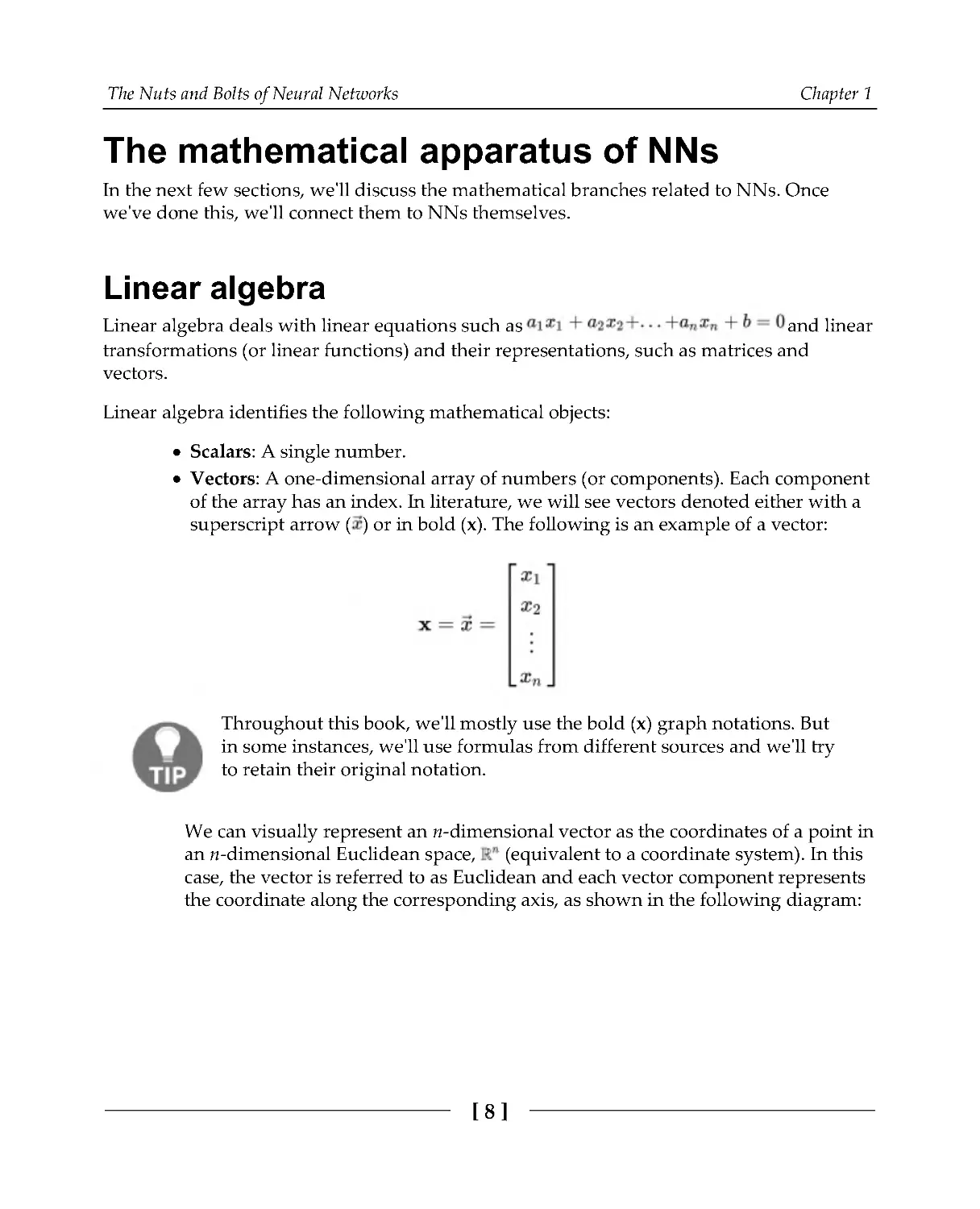
Vectors: A one-dimensional array of numbers (or components). Each component
of the array has an index. In literature, we will see vectors denoted either with a
superscript arrow ( ) or in bold (x). The following is an example of a vector:
Throughout this book, we'll mostly use the bold (x) graph notations. But
in some instances, we'll use formulas from different sources and we'll try
to retain their original notation.
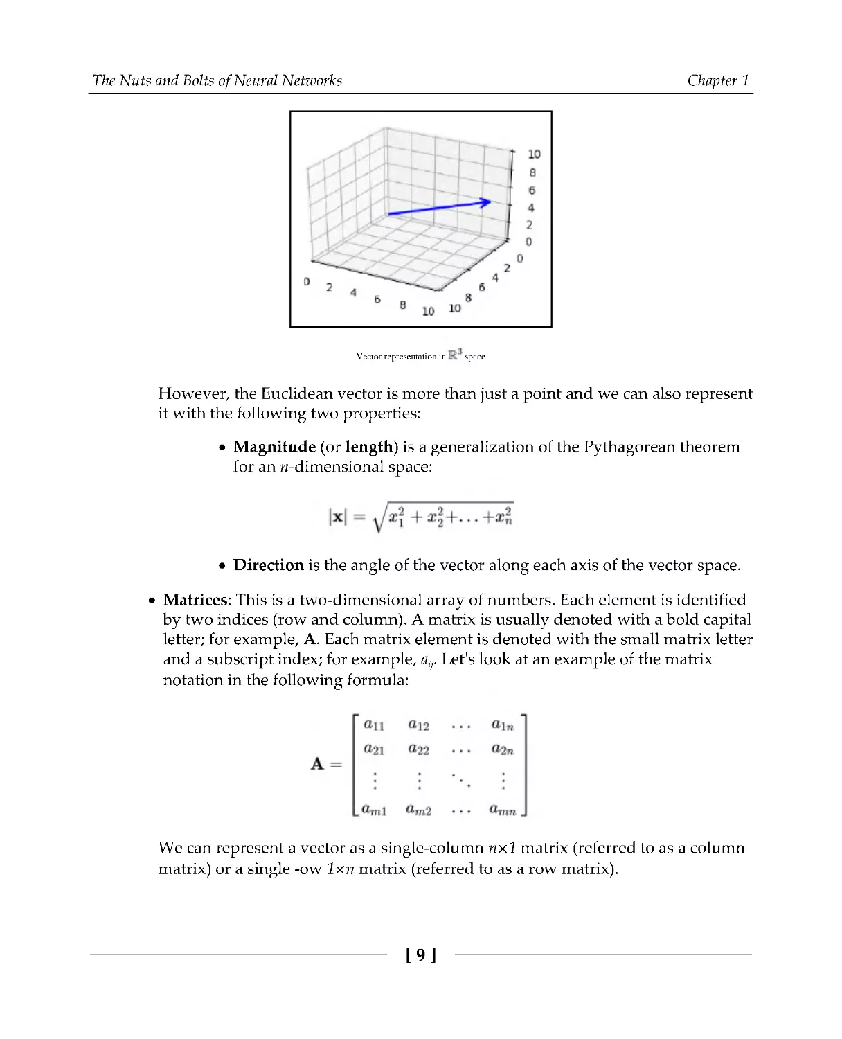
We can visually represent an n-dimensional vector as the coordinates of a point in
an n-dimensional Euclidean space, (equivalent to a coordinate system). In this
case, the vector is referred to as Euclidean and each vector component represents
the coordinate along the corresponding axis, as shown in the following diagram:
The Nuts and Bolts of Neural Networks
Chapter 1
[9]
Vector representation in
space
However, the Euclidean vector is more than just a point and we can also represent
it with the following two properties:
Magnitude (or length) is a generalization of the Pythagorean theorem
for an n-dimensional space:
Direction is the angle of the vector along each axis of the vector space.
Matrices: This is a two-dimensional array of numbers. Each element is identified
by two indices (row and column). A matrix is usually denoted with a bold capital
letter; for example, A. Each matrix element is denoted with the small matrix letter
and a subscript index; for example, aij. Let's look at an example of the matrix
notation in the following formula:
We can represent a vector as a single-column n×1 matrix (referred to as a column
matrix) or a single -ow 1×n matrix (referred to as a row matrix).
The Nuts and Bolts of Neural Networks
Chapter 1
[10]
Tensors: Before we explain them, we have to start with a disclaimer. Tensors
originally come from mathematics and physics, where they have existed long
before we started using them in ML. The tensor definition in these fields differs
from the ML one. For the purposes of this book, we'll only consider tensors in the
ML context. Here, a tensor is a multi-dimensional array with the following
properties:
Rank: Indicates the number of array dimensions. For example, a
tensor of rank 2 is a matrix, a tensor of rank 1 is a vector, and a
tensor of rank 0 is a scalar. However, the tensor has no limit on the
number of dimensions. Indeed, some types of NNs use tensors of
rank 4.
Shape: The size of each dimension.
The data type of the tensor elements. These can vary between
libraries, but typically include 16-, 32-, and 64-bit float and 8-, 16-,
32-, and 64-bit integers.
Contemporary DL libraries such as TensorFlow and PyTorch use tensors as their
main data structure.
You can find a thorough discussion on the nature of tensors here: https:/
/
stats.
stackexchange.
com/
questions/
198061/
why-
the-
sudden-
fascination-
with-
tensors. You can also check the TensorFlow (https:/
/
www.
tensorflow.
org/
guide/
tensors) and PyTorch (https:/
/
pytorch.
org/
docs/
stable/
tensors.
html) tensor definitions.
Now that we've introduced the types of objects in linear algebra, in the next section, we'll
discuss some operations that can be applied to them.
Vector and matrix operations
In this section, we'll discuss the vector and matrix operations that are relevant to NNs. Let's
start:
Vector addition is the operation of adding two or more vectors together into an
output vector sum. The output is another vector and is computed with the
following formula:
The Nuts and Bolts of Neural Networks
Chapter 1
[11]
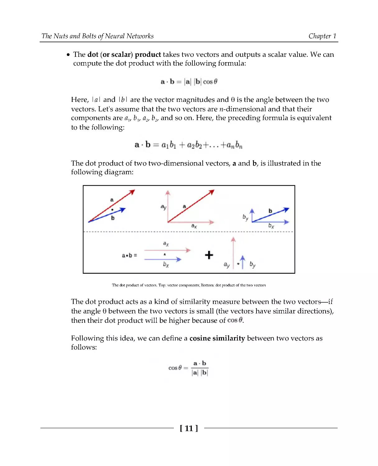
The dot (or scalar) product takes two vectors and outputs a scalar value. We can
compute the dot product with the following formula:
Here, |a| and |b| are the vector magnitudes and θ is the angle between the two
vectors. Let's assume that the two vectors are n-dimensional and that their
components are a1, b1, a2, b2, and so on. Here, the preceding formula is equivalent
to the following:
The dot product of two two-dimensional vectors, a and b, is illustrated in the
following diagram:
The dot product of vectors. Top: vector components; Bottom: dot product of the two vectors
The dot product acts as a kind of similarity measure between the two vectors—if
the angle θ between the two vectors is small (the vectors have similar directions),
then their dot product will be higher because of
.
Following this idea, we can define a cosine similarity between two vectors as
follows:
The Nuts and Bolts of Neural Networks
Chapter 1
[12]
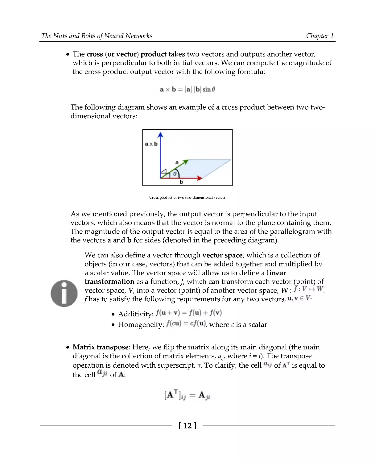
The cross (or vector) product takes two vectors and outputs another vector,
which is perpendicular to both initial vectors. We can compute the magnitude of
the cross product output vector with the following formula:
The following diagram shows an example of a cross product between two two-
dimensional vectors:
Cross product of two two-dimensional vectors
As we mentioned previously, the output vector is perpendicular to the input
vectors, which also means that the vector is normal to the plane containing them.
The magnitude of the output vector is equal to the area of the parallelogram with
the vectors a and b for sides (denoted in the preceding diagram).
We can also define a vector through vector space, which is a collection of
objects (in our case, vectors) that can be added together and multiplied by
a scalar value. The vector space will allow us to define a linear
transformation as a function, f, which can transform each vector (point) of
vector space, V, into a vector (point) of another vector space, W :
.
f has to satisfy the following requirements for any two vectors,
:
Additivity:
Homogeneity:
, where c is a scalar
Matrix transpose: Here, we flip the matrix along its main diagonal (the main
diagonal is the collection of matrix elements, aij, where i = j). The transpose
operation is denoted with superscript, . To clarify, the cell
of is equal to
the cell
of:
The Nuts and Bolts of Neural Networks
Chapter 1
[13]
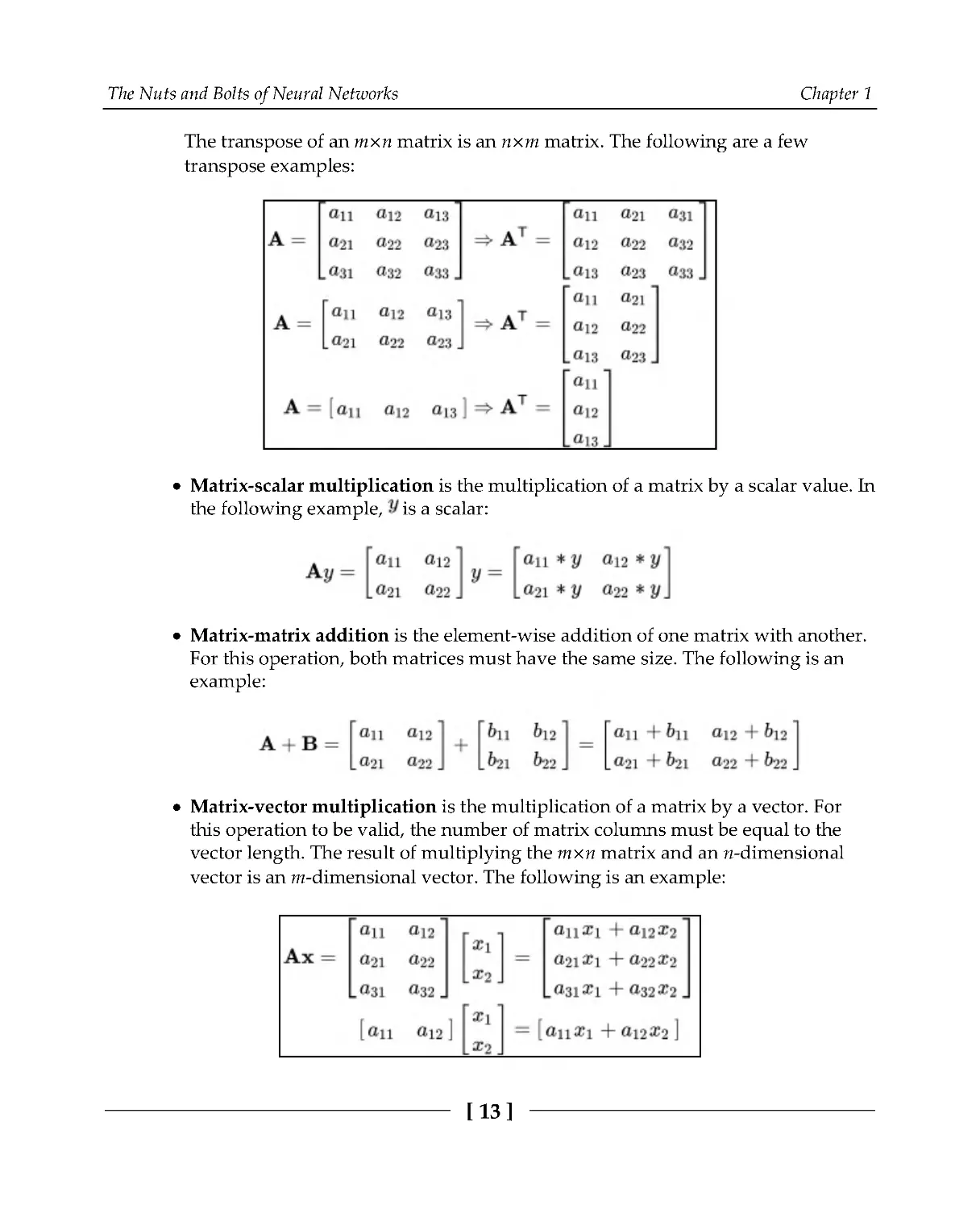
The transpose of an m×n matrix is an n×m matrix. The following are a few
transpose examples:
Matrix-scalar multiplication is the multiplication of a matrix by a scalar value. In
the following example, is a scalar:
Matrix-matrix addition is the element-wise addition of one matrix with another.
For this operation, both matrices must have the same size. The following is an
example:
Matrix-vector multiplication is the multiplication of a matrix by a vector. For
this operation to be valid, the number of matrix columns must be equal to the
vector length. The result of multiplying the m×n matrix and an n-dimensional
vector is an m-dimensional vector. The following is an example:
The Nuts and Bolts of Neural Networks
Chapter 1
[14]
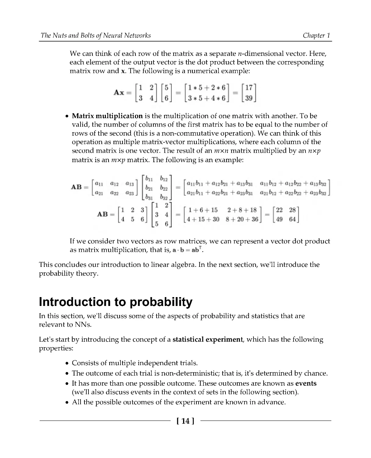
We can think of each row of the matrix as a separate n-dimensional vector. Here,
each element of the output vector is the dot product between the corresponding
matrix row and x. The following is a numerical example:
Matrix multiplication is the multiplication of one matrix with another. To be
valid, the number of columns of the first matrix has to be equal to the number of
rows of the second (this is a non-commutative operation). We can think of this
operation as multiple matrix-vector multiplications, where each column of the
second matrix is one vector. The result of an m×n matrix multiplied by an n×p
matrix is an m×p matrix. The following is an example:
If we consider two vectors as row matrices, we can represent a vector dot product
as matrix multiplication, that is,
.
This concludes our introduction to linear algebra. In the next section, we'll introduce the
probability theory.
Introduction to probability
In this section, we'll discuss some of the aspects of probability and statistics that are
relevant to NNs.
Let's start by introducing the concept of a statistical experiment, which has the following
properties:
Consists of multiple independent trials.
The outcome of each trial is non-deterministic; that is, it's determined by chance.
It has more than one possible outcome. These outcomes are known as events
(we'll also discuss events in the context of sets in the following section).
All the possible outcomes of the experiment are known in advance.
The Nuts and Bolts of Neural Networks
Chapter 1
[15]
One example of a statistical experiment is a coin toss, which has two possible
outcomes—heads or tails. Another example is a dice throw with six possible outcomes: 1, 2,
3,4,5,and6.
We'll define probability as the likelihood that some event, e, would occur and we'll denote
it with P(e). The probability is a number in the range of [0, 1], where 0 indicates that the
event cannot occur and 1 indicates that it will always occur. If P(e) = 0.5, there is a 50-50
chance the event would occur, and so on.
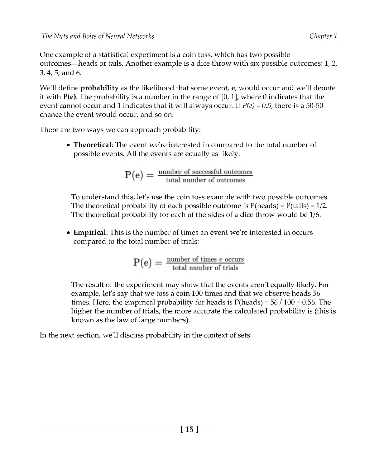
There are two ways we can approach probability:
Theoretical: The event we're interested in compared to the total number of
possible events. All the events are equally as likely:
To understand this, let's use the coin toss example with two possible outcomes.
The theoretical probability of each possible outcome is P(heads) = P(tails) = 1/2.
The theoretical probability for each of the sides of a dice throw would be 1/6.
Empirical: This is the number of times an event we're interested in occurs
compared to the total number of trials:
The result of the experiment may show that the events aren't equally likely. For
example, let's say that we toss a coin 100 times and that we observe heads 56
times. Here, the empirical probability for heads is P(heads) = 56 / 100 = 0.56 . The
higher the number of trials, the more accurate the calculated probability is (this is
known as the law of large numbers).
In the next section, we'll discuss probability in the context of sets.
The Nuts and Bolts of Neural Networks
Chapter 1
[16]
Probability and sets
The collection of all possible outcomes (events) of an experiment is called, sample space.
We can think of the sample space as a mathematical set. It is usually denoted with a capital
letter and we can list all the set outcomes with {} (the same as Python sets). For example, the
sample space of coin toss events is Sc = {heads, tails}, while for dice rows it's Sd = {1, 2, 3, 4, 5,
6}. A single outcome of the set (for example, heads) is called a sample point. An event is an
outcome (sample point) or a combination of outcomes (subset) of the sample space. An
example of a combined event is for the dice to land on an even number, that is, {2, 4, 6}.
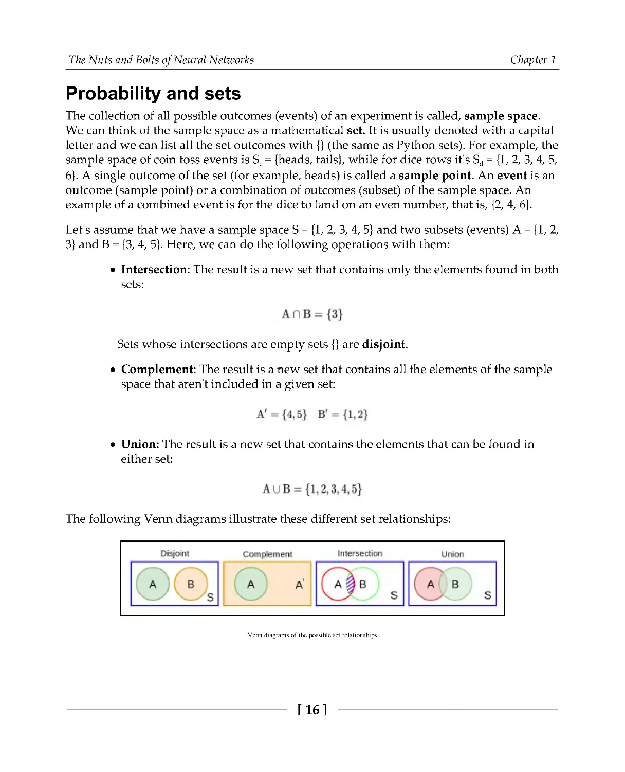
Let's assume that we have a sample space S = {1, 2, 3, 4, 5} and two subsets (events) A = {1, 2,
3} and B = {3, 4, 5}. Here, we can do the following operations with them:
Intersection: The result is a new set that contains only the elements found in both
sets:
Sets whose intersections are empty sets {} are disjoint.
Complement: The result is a new set that contains all the elements of the sample
space that aren't included in a given set:
Union: The result is a new set that contains the elements that can be found in
either set:
The following Venn diagrams illustrate these different set relationships:
Venn diagrams of the possible set relationships
The Nuts and Bolts of Neural Networks
Chapter 1
[17]
We can transfer the set properties to events and their probabilities. We'll assume that the
events are independent—the occurrence of one event doesn't affect the probability of the
occurrence of another. For example, the outcomes of the different coin tosses are
independent of one another. That being said, let's learn how to translate the set operations
in the events domain:
The intersection of two events is a subset of the outcomes, contained in both
events. The probability of the intersection is called joint probability and is
computed via the following formula:
Let's say that we want to compute the probability of a card being red (either
hearts or diamonds) and a Jack. The probability for red is P(red) = 26/52 = 1/2. The
probability for getting a Jack is P(Jack) = 4/52 = 1/13. Therefore, the joint
probability is P(red, Jack) = (1/2) * (1/13) = 1/26. In this example, we assumed that
the two events are independent. However, the two events occur at the same time
(we draw a single card). Had they occurred successively, for example, two card
draws, where one is a Jack and the other is red, we would enter the realm of
conditional probability. This joint probability is also denoted as P(A, B) or P(AB).
The probability of the occurrence of a single event P(A) is also known as marginal
probability (as opposed to joint probability).
Two events are disjoint (or mutually exclusive) if they don't share any outcomes.
That is, their respective sample space subsets are disjoint. For example, the
events of odd or even dice rows are disjoint. The following is true for the
probability of disjoint events:
The joint probability of disjoint events (the probability for these
events to occur simultaneously) is P(A∩B) = 0.
The sum of the probabilities of disjoint events is
.
If the subsets of multiple events contain the whole sample space between
themselves, they are jointly exhaustive. Events A and B from the preceding
example are jointly exhaustive because, together, they fill up the whole sample
space (1 through 5). The following is true for the probability of jointly exhaustive
events:
The Nuts and Bolts of Neural Networks
Chapter 1
[18]
If we only have two events that are disjoint and jointly exhaustive at the same
time, the events are complement. For example, odd and even dice throw events
are complement.
We'll refer to outcomes coming from either A or B (not necessarily in both) as the
union of A and B. The probability of this union is as follows:
So far, we've discussed independent events. In the next section, we'll focus on dependent
ones.
Conditional probability and the Bayes rule
If the occurrence of event A changes the probability of the occurrence of event B, where A
occurs before B, then the two are dependent. To illustrate this concept, let's imagine that we
draw multiple cards sequentially from the deck. When the deck is full, the probability to
draw hearts is P(hearts) = 13/52 = 0.25 . But once we've drawn the first card, the probability to
pick hearts on the second turn changes. Now, we only have 51 cards and one less heart.
We'll call the probability of the second draw conditional probability and we'll denote it
with P(B|A). This is the probability of event B (second draw), given that event A has
occurred (first draw). To continue with our example, the probability of picking hearts on
the second draw becomes P(hearts2|hearts1) = 12/51 = 0.235.
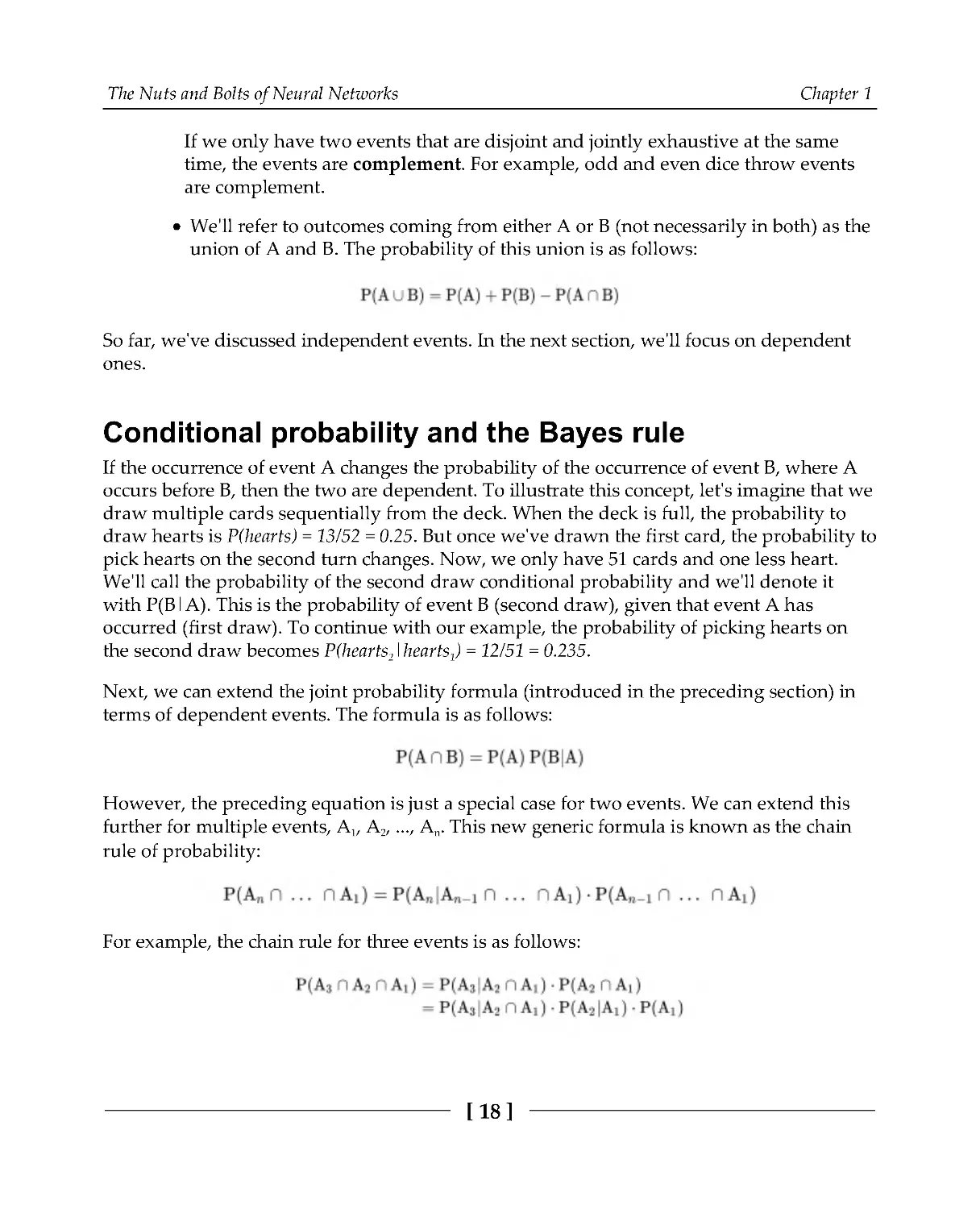
Next, we can extend the joint probability formula (introduced in the preceding section) in
terms of dependent events. The formula is as follows:
However, the preceding equation is just a special case for two events. We can extend this
further for multiple events, A1, A2, ..., An. This new generic formula is known as the chain
rule of probability:
For example, the chain rule for three events is as follows:
The Nuts and Bolts of Neural Networks
Chapter 1
[19]
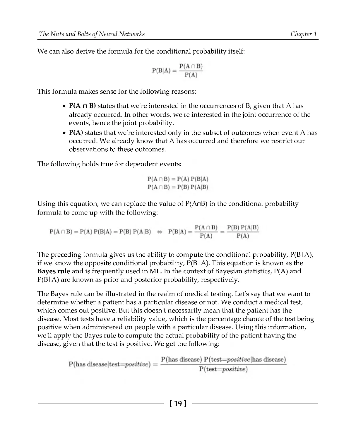
We can also derive the formula for the conditional probability itself:
This formula makes sense for the following reasons:
P(A ∩ B) states that we're interested in the occurrences of B, given that A has
already occurred. In other words, we're interested in the joint occurrence of the
events, hence the joint probability.
P(A) states that we're interested only in the subset of outcomes when event A has
occurred. We already know that A has occurred and therefore we restrict our
observations to these outcomes.
The following holds true for dependent events:
Using this equation, we can replace the value of P(A∩B) in the conditional probability
formula to come up with the following:
The preceding formula gives us the ability to compute the conditional probability, P(B|A),
if we know the opposite conditional probability, P(B|A). This equation is known as the
Bayes rule and is frequently used in ML. In the context of Bayesian statistics, P(A) and
P(B|A) are known as prior and posterior probability, respectively.
The Bayes rule can be illustrated in the realm of medical testing. Let's say that we want to
determine whether a patient has a particular disease or not. We conduct a medical test,
which comes out positive. But this doesn't necessarily mean that the patient has the
disease. Most tests have a reliability value, which is the percentage chance of the test being
positive when administered on people with a particular disease. Using this information,
we'll apply the Bayes rule to compute the actual probability of the patient having the
disease, given that the test is positive. We get the following:
The Nuts and Bolts of Neural Networks
Chapter 1
[20]
Here, P(has disease) is the general probability of the disease without any prior conditions.
Think of this as the probability of the disease in the general population.
Next, let's make some assumptions about the disease and the test's accuracy:
The test is 98% reliable, that is, if the test is positive, it will also be positive in 98%
of cases: P(test=positive|has disease) = 0.98 .
Only 2% of the people under 50 have this kind of disease: P(has disease) = 0.02.
The test that's administered on people under 50 is positive only for 3.9% of the
population: P(test=positive) = 0.039 .
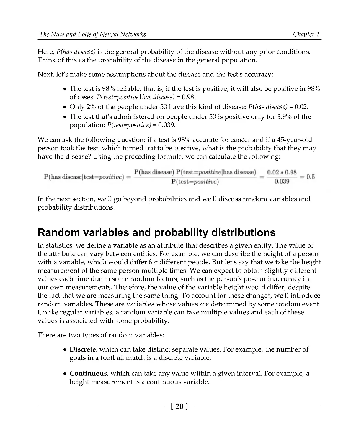
We can ask the following question: if a test is 98% accurate for cancer and if a 45-year-old
person took the test, which turned out to be positive, what is the probability that they may
have the disease? Using the preceding formula, we can calculate the following:
In the next section, we'll go beyond probabilities and we'll discuss random variables and
probability distributions.
Random variables and probability distributions
In statistics, we define a variable as an attribute that describes a given entity. The value of
the attribute can vary between entities. For example, we can describe the height of a person
with a variable, which would differ for different people. But let's say that we take the height
measurement of the same person multiple times. We can expect to obtain slightly different
values each time due to some random factors, such as the person's pose or inaccuracy in
our own measurements. Therefore, the value of the variable height would differ, despite
the fact that we are measuring the same thing. To account for these changes, we'll introduce
random variables. These are variables whose values are determined by some random event.
Unlike regular variables, a random variable can take multiple values and each of these
values is associated with some probability.
There are two types of random variables:
Discrete, which can take distinct separate values. For example, the number of
goals in a football match is a discrete variable.
Continuous, which can take any value within a given interval. For example, a
height measurement is a continuous variable.
The Nuts and Bolts of Neural Networks
Chapter 1
[21]
Random variables are denoted with capital letters and the probability of a certain value x
for random variable X is denoted with either P(X = x) or p(x). The collection of probabilities
for each possible value of a random variable is called the probability distribution.
Depending on the variable type, we have two types of probability distributions:
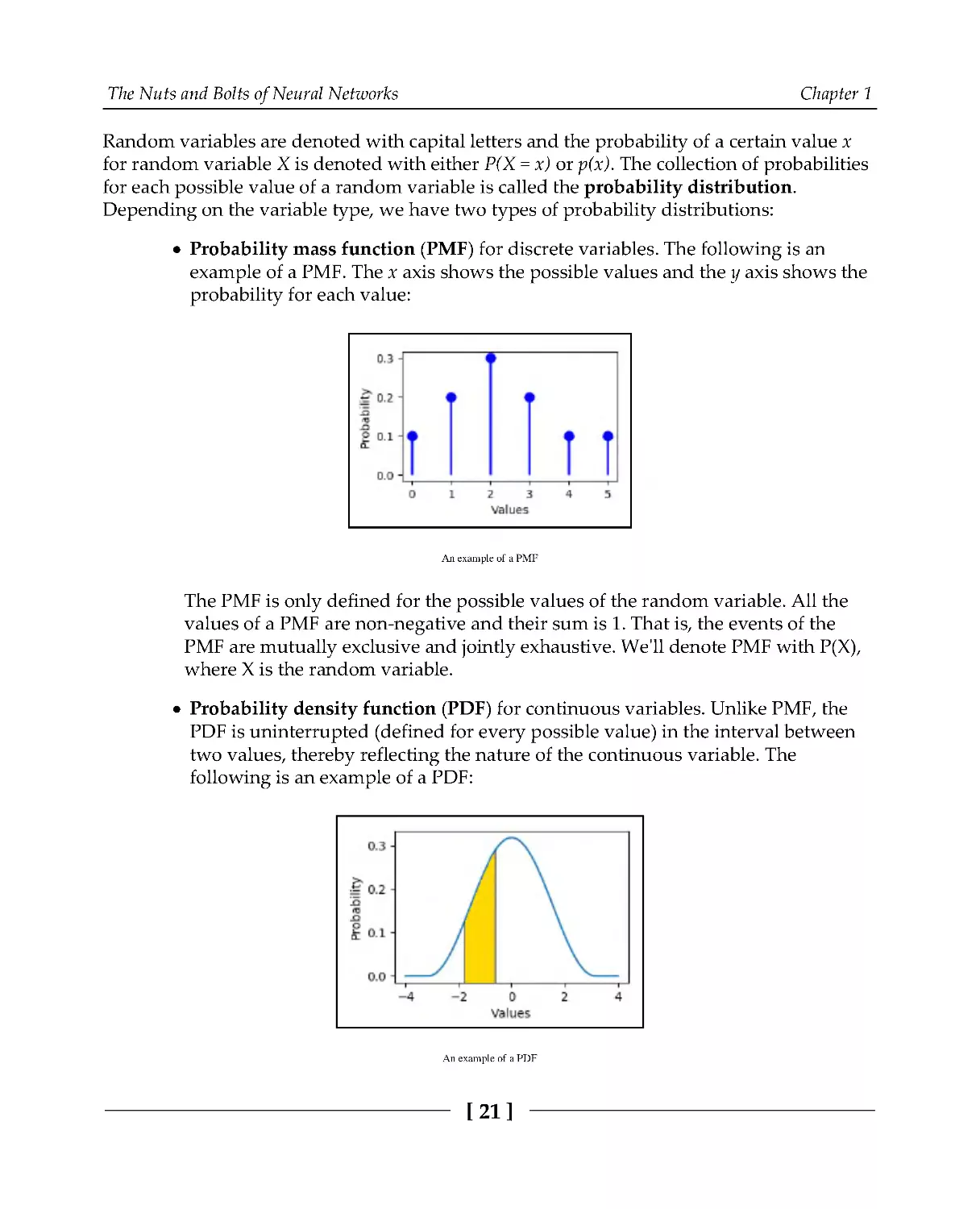
Probability mass function (PMF) for discrete variables. The following is an
example of a PMF. The x axis shows the possible values and the y axis shows the
probability for each value:
An example of a PMF
The PMF is only defined for the possible values of the random variable. All the
values of a PMF are non-negative and their sum is 1. That is, the events of the
PMF are mutually exclusive and jointly exhaustive. We'll denote PMF with P(X),
where X is the random variable.
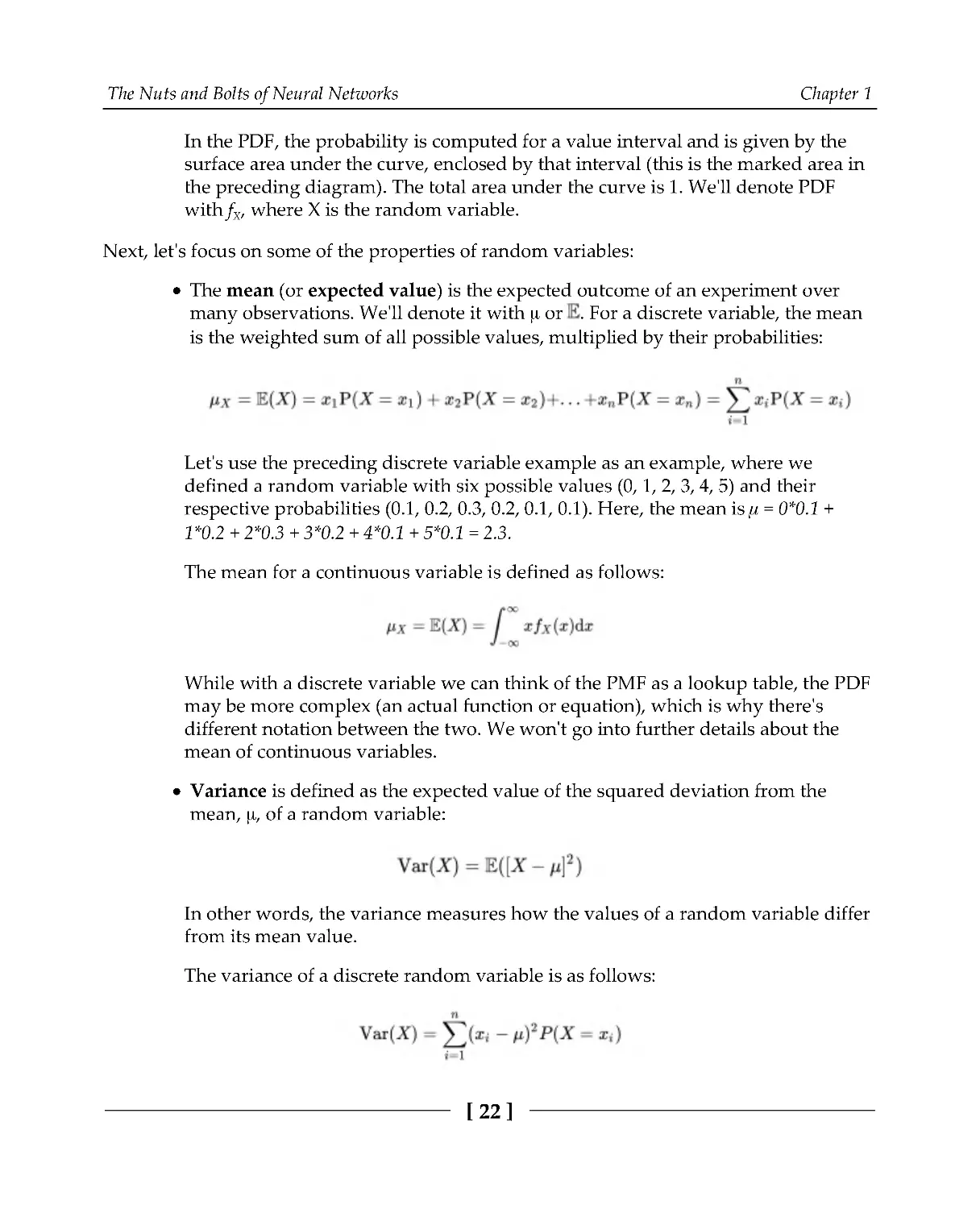
Probability density function (PDF) for continuous variables. Unlike PMF, the
PDF is uninterrupted (defined for every possible value) in the interval between
two values, thereby reflecting the nature of the continuous variable. The
following is an example of a PDF:
An example of a PDF
The Nuts and Bolts of Neural Networks
Chapter 1
[22]
In the PDF, the probability is computed for a value interval and is given by the
surface area under the curve, enclosed by that interval (this is the marked area in
the preceding diagram). The total area under the curve is 1. We'll denote PDF
with fX, where X is the random variable.
Next, let's focus on some of the properties of random variables:
The mean (or expected value) is the expected outcome of an experiment over
many observations. We'll denote it with μ or . For a discrete variable, the mean
is the weighted sum of all possible values, multiplied by their probabilities:
Let's use the preceding discrete variable example as an example, where we
defined a random variable with six possible values (0, 1, 2, 3, 4, 5) and their
respective probabilities (0.1, 0.2, 0.3, 0.2, 0.1, 0.1). Here, the mean is μ = 0*0.1 +
1*0.2 + 2*0.3 + 3*0.2 + 4*0.1 + 5*0.1 = 2.3.
The mean for a continuous variable is defined as follows:
While with a discrete variable we can think of the PMF as a lookup table, the PDF
may be more complex (an actual function or equation), which is why there's
different notation between the two. We won't go into further details about the
mean of continuous variables.
Variance is defined as the expected value of the squared deviation from the
mean, μ, of a random variable:
In other words, the variance measures how the values of a random variable differ
from its mean value.
The variance of a discrete random variable is as follows:
The Nuts and Bolts of Neural Networks
Chapter 1
[23]
Let's use the preceding example, where we calculated the mean value to be 2.3 .
The new variance would be Var(X) = (0 - 2 .3)2
*0+(1-2.3)2
*1+...+(5-2.3)2
*5=
2.01.
The variance of a continuous variable is defined as follows:
The standard deviation measures the degree to which the values of the random
variable differ from the expected value. If this definition sounds similar to
variance, it's because it is. In fact, the formula for standard deviation is as
follows:
We can also define the variance in terms of standard deviation:
The difference between standard deviation and variance is that the standard
deviation is expressed in the same units as the mean value, while the variance
uses squared units.
In this section, we defined what a probability distribution is. Next, let's discuss different
types of probability distributions.
Probability distributions
We'll start with the binomial distribution for discrete variables in binomial experiments. A
binomial experiment has only two possible outcomes: success or failure. It also satisfies the
following requirements:
Each trial is independent of the others.
The probability of success is always the same.
An example of a binomial experiment is the coin toss experiment.
The Nuts and Bolts of Neural Networks
Chapter 1
[24]
Now, let's assume that the experiment consists of n trials. x of them are successful, while
the probability of success at each trial is p. The formula for a binomial PMF of variable X
(not to be confused with x) is as follows:
Here,
is the binomial coefficient. This is the number of combinations of x
successful trials, which we can select from the n total trials. If n=1, then we have a special
case of binomial distribution called Bernoulli distribution.
Next, let's discuss the normal (or Gaussian) distribution for continuous variables, which
closely approximates many natural processes. The normal distribution is defined with the
following exponential PDF formula, known as normal equation (one of the most popular
notations):
Here, x is the value of the random variable, μ is the mean, σ is the standard deviation,
and σ
2
is the variance. The preceding equation produces a bell-shaped curve, which is
shown in the following diagram:
Normal distribution
The Nuts and Bolts of Neural Networks
Chapter 1
[25]
Let's discuss some of the properties of the normal distribution, in no particular order:
The curve is symmetric along its center, which is also the maximum value.
The shape and location of the curve are fully described by the mean and standard
deviation, where we have the following:
The center of the curve (and its maximum value) is equal to the
mean. That is, the mean determines the location of the curve along
the x axis.
The width of the curve is determined by the standard deviation.
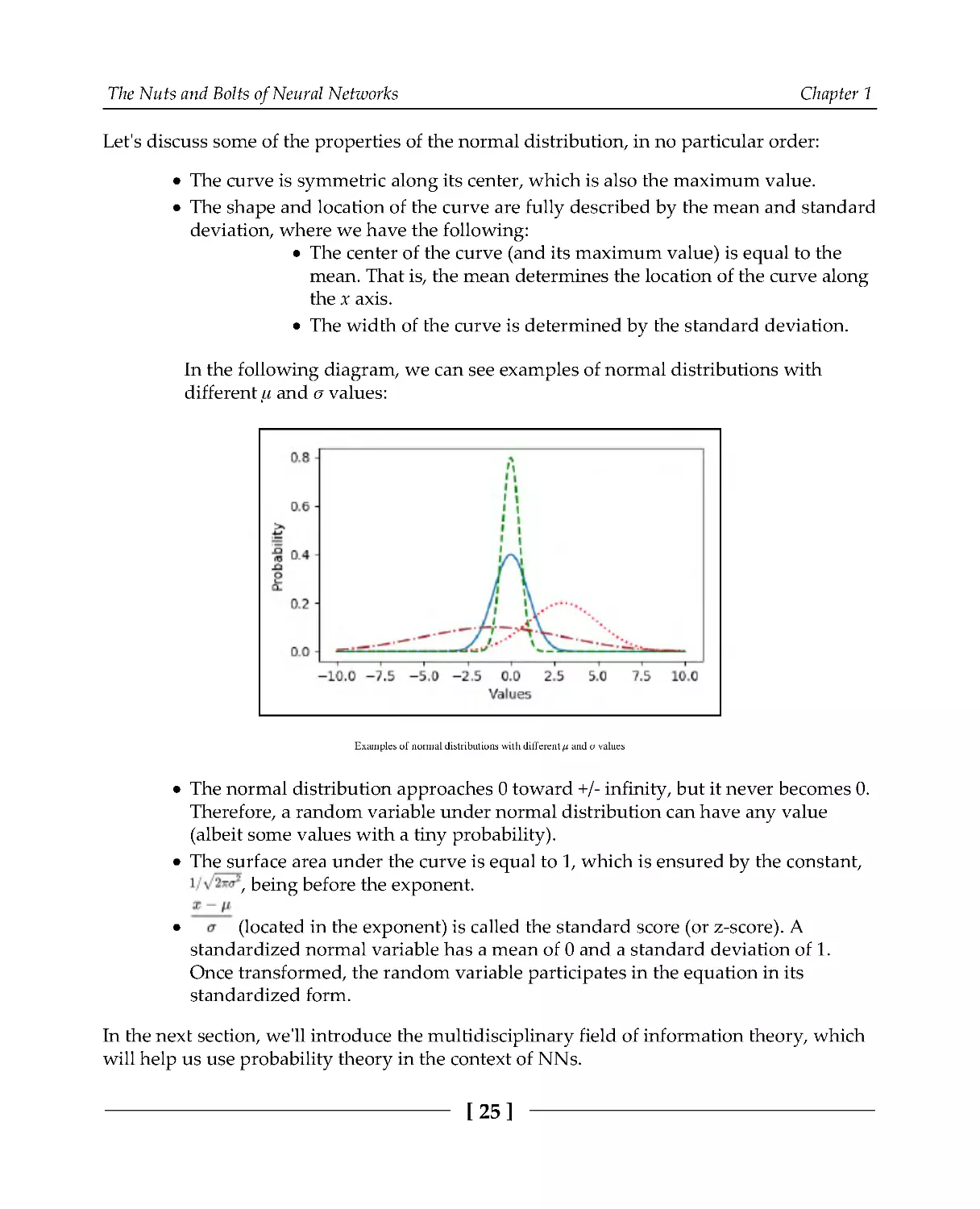
In the following diagram, we can see examples of normal distributions with
different μ and σ values:
Examples of normal distributions with different μ and σ values
The normal distribution approaches 0 toward +/- infinity, but it never becomes 0.
Therefore, a random variable under normal distribution can have any value
(albeit some values with a tiny probability).
The surface area under the curve is equal to 1, which is ensured by the constant,
, being before the exponent.
(located in the exponent) is called the standard score (or z-score). A
standardized normal variable has a mean of 0 and a standard deviation of 1.
Once transformed, the random variable participates in the equation in its
standardized form.
In the next section, we'll introduce the multidisciplinary field of information theory, which
will help us use probability theory in the context of NNs.
The Nuts and Bolts of Neural Networks
Chapter 1
[26]
Information theory
Information theory attempts to determine the amount of information an event has. The
amount of information is guided by the following principles:
The higher the probability of an event, the less informative the event is
considered. Conversely, if the probability is lower, the event carries more
informational content. For example, the outcome of a coin flip (with a probability
of 1/2) provides less information than the outcome of a dice throw (with a
probability of 1/6).
The information that's carried by independent events is the sum of their
individual information contents. For example, two dice rows that come up on the
same side of the dice (let's say, 4) are twice as informative as the individual rows.
We'll define the amount of information (or self-information) of event x as follows:
Here, log is the natural logarithm. For example, if the probability of event is P(x) = 0.8, then
I(x) = 0.22 . Alternatively, if P(x) = 0.2, then I(x) = 1.61. We can see that the event information
content is opposite to the event probability. The amount of self-information I(x) is
measured in natural units of information (nat). We can also compute I(x) with a base 2
logarithm
, in which case we measure it in bits. There is no principal
difference between the two versions. For the purposes of this book, we'll stick with the
natural logarithm version.
Let's discuss why we use logarithm in the preceding formula, even
though a negative probability would also satisfy the reciprocity between
self-information and probability. The main reason is the product and
division rules of logarithms:
Here, x1 and x2 are scalar values. Without going into too much detail, note
that these properties allow us to easily minimize the error function during
network training.
The Nuts and Bolts of Neural Networks
Chapter 1
[27]
So far, we've defined the information content of a single outcome. But what about other
outcomes? To measure them, we have to measure the amount of information over the
probability distribution of the random variable. Let's denote it with I(X), where X is a
random discrete variable (we'll focus on discrete variables here). Recall that, in the Random
variables and probability distributions section, we defined the mean (or expected value) of a
discrete random variable as the weighted sum of all possible values, multiplied by their
probabilities. We'll do something similar here, but we'll multiply the information content of
each event by the probability of that event.
This measure is called Shannon entropy (or just entropy) and is defined as follows:
Here, xi represents the discrete variable values. Events with higher probabilities will carry
more weight compared to low-probability ones. We can think of entropy as the expected
(mean) amount of information about the events (outcomes) of the probability distribution.
To understand this, let's try to compute the entropy of the familiar coin toss experiment.
We'll calculate two examples:
First, let's assume that P(heads) = P(tails) = 0.5. In this case, the entropy is as
follows:
Next, let's assume that, for some reason, the outcomes are not equally likely and
that the probability distribution is P(heads) = 0.2 and P(tails) = 0.8 . The entropy is
as follows:
The Nuts and Bolts of Neural Networks
Chapter 1
[28]
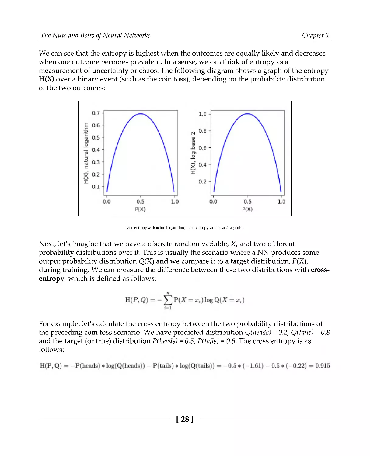
We can see that the entropy is highest when the outcomes are equally likely and decreases
when one outcome becomes prevalent. In a sense, we can think of entropy as a
measurement of uncertainty or chaos. The following diagram shows a graph of the entropy
H(X) over a binary event (such as the coin toss), depending on the probability distribution
of the two outcomes:
Left: entropy with natural logarithm; right: entropy with base 2 logarithm
Next, let's imagine that we have a discrete random variable, X, and two different
probability distributions over it. This is usually the scenario where a NN produces some
output probability distribution Q(X) and we compare it to a target distribution, P(X),
during training. We can measure the difference between these two distributions with cross-
entropy, which is defined as follows:
For example, let's calculate the cross entropy between the two probability distributions of
the preceding coin toss scenario. We have predicted distribution Q(heads) = 0.2, Q(tails) = 0.8
and the target (or true) distribution P(heads) = 0.5, P(tails) = 0.5. The cross entropy is as
follows:
The Nuts and Bolts of Neural Networks
Chapter 1
[29]
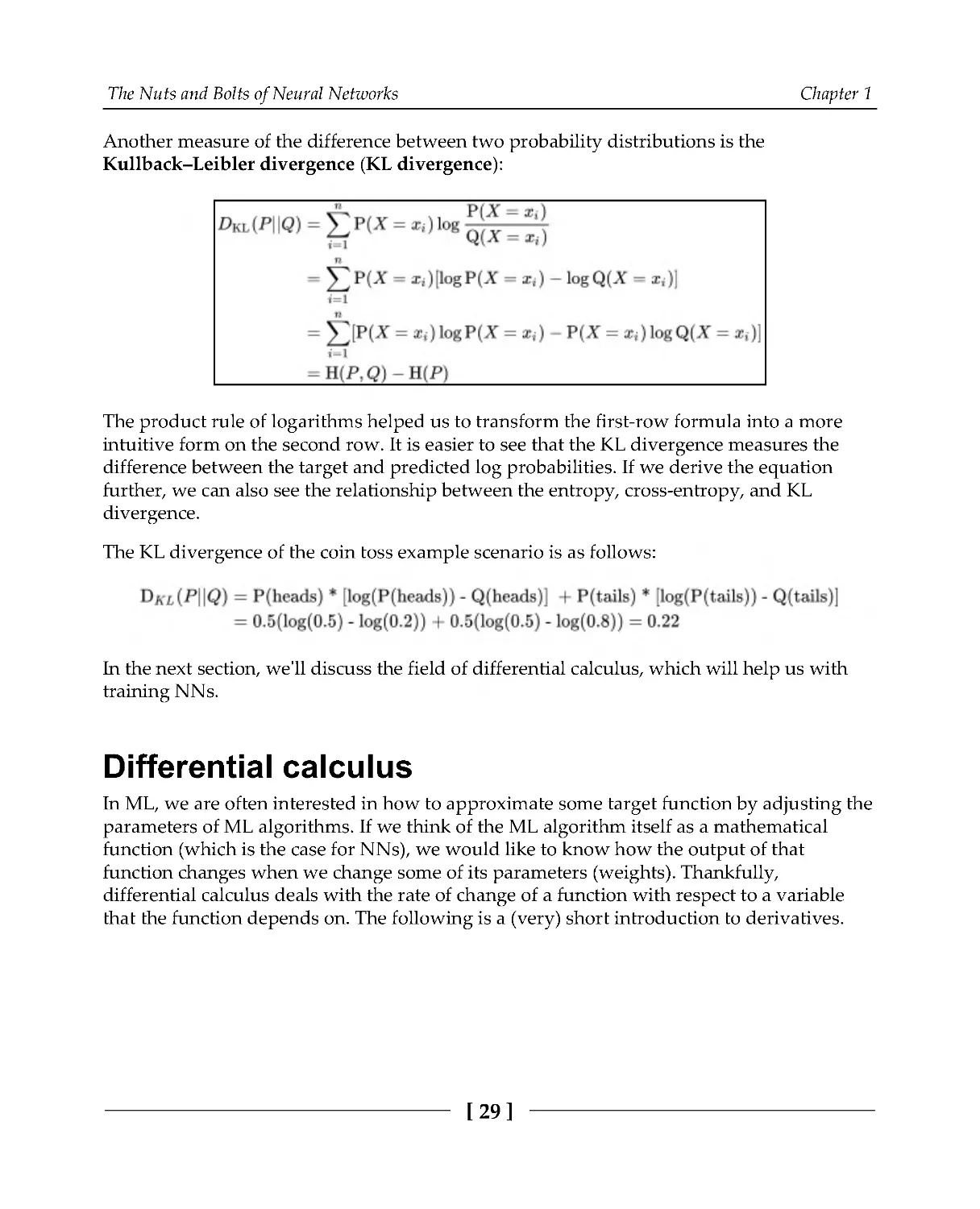
Another measure of the difference between two probability distributions is the
Kullback–Leibler divergence (KL divergence):
The product rule of logarithms helped us to transform the first-row formula into a more
intuitive form on the second row. It is easier to see that the KL divergence measures the
difference between the target and predicted log probabilities. If we derive the equation
further, we can also see the relationship between the entropy, cross-entropy, and KL
divergence.
The KL divergence of the coin toss example scenario is as follows:
In the next section, we'll discuss the field of differential calculus, which will help us with
training NNs.
Differential calculus
In ML, we are often interested in how to approximate some target function by adjusting the
parameters of ML algorithms. If we think of the ML algorithm itself as a mathematical
function (which is the case for NNs), we would like to know how the output of that
function changes when we change some of its parameters (weights). Thankfully,
differential calculus deals with the rate of change of a function with respect to a variable
that the function depends on. The following is a (very) short introduction to derivatives.
The Nuts and Bolts of Neural Networks
Chapter 1
[30]
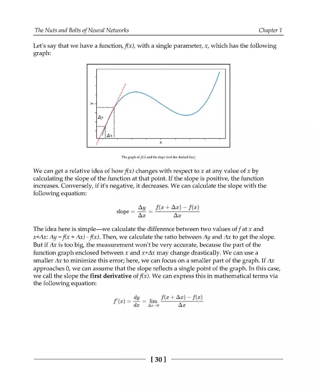
Let's say that we have a function, f(x), with a single parameter, x, which has the following
graph:
The graph of f(x) and the slope (red dot-dashed line)
We can get a relative idea of how f(x) changes with respect to x at any value of x by
calculating the slope of the function at that point. If the slope is positive, the function
increases. Conversely, if it's negative, it decreases. We can calculate the slope with the
following equation:
The idea here is simple—we calculate the difference between two values of f at x and
x+Δx: Δy = f(x + Δx) - f(x). Then, we calculate the ratio between Δy and Δx to get the slope.
But if Δx is too big, the measurement won't be very accurate, because the part of the
function graph enclosed between x and x+Δx may change drastically. We can use a
smaller Δx to minimize this error; here, we can focus on a smaller part of the graph. If Δx
approaches 0, we can assume that the slope reflects a single point of the graph. In this case,
we call the slope the first derivative of f(x). We can express this in mathematical terms via
the following equation:
The Nuts and Bolts of Neural Networks
Chapter 1
[31]
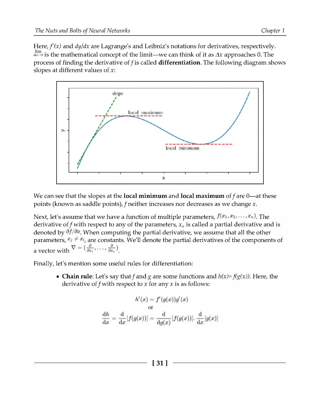
Here, f'(x) and dy/dx are Lagrange's and Leibniz's notations for derivatives, respectively.
is the mathematical concept of the limit—we can think of it as Δx approaches 0. The
process of finding the derivative of f is called differentiation. The following diagram shows
slopes at different values of x:
We can see that the slopes at the local minimum and local maximum of f are 0—at these
points (known as saddle points), f neither increases nor decreases as we change x.
Next, let's assume that we have a function of multiple parameters,
. The
derivative of f with respect to any of the parameters, xi, is called a partial derivative and is
denoted by
. When computing the partial derivative, we assume that all the other
parameters,
, are constants. We'll denote the partial derivatives of the components of
a vector with
.
Finally, let's mention some useful rules for differentiation:
Chain rule: Let's say that f and g are some functions and h(x)= f(g(x)). Here, the
derivative of f with respect to x for any x is as follows:
The Nuts and Bolts of Neural Networks
Chapter 1
[32]
Sum rule: Let's say that f and g are some functions and h(x) = f(x) + g(x). The sum
rule states the following:
Common functions:
x'=1
(ax)' = a, where a is scalar
a' = 0, where a is scalar
x
2
=2x
(e
x
)'=e
x
The mathematical apparatus of NNs and NNs themselves form a sort of knowledge
hierarchy. If we think of implementing a NN as building a house, then the mathematical
apparatus is like mixing concrete. We can learn how to mix the concrete independently of
how to build a house. In fact, we can mix concrete for a variety of purposes other than the
specific goal of building a house. However, we need to know how to mix concrete before
building the house. To continue with our analogy, now that we know how to mix concrete
(mathematical apparatus), we'll focus on actually building the house (NNs).
A short introduction to NNs
A NN is a function (let's denote it with f) that tries to approximate another target
function, g. We can describe this relationship with the following equation:
Here, x is the input data and θ are the NN parameters (weights). The goal is to find such
θ parameters with the best approximate, g. This generic definition applies for both
regression (approximating the exact value of g) and classification (assigning the input to
one of multiple possible classes) tasks. Alternatively, the NN function can be denoted as
.
We'll start our discussion from the smallest building block of the NN—the neuron.
The Nuts and Bolts of Neural Networks
Chapter 1
[33]
Neurons
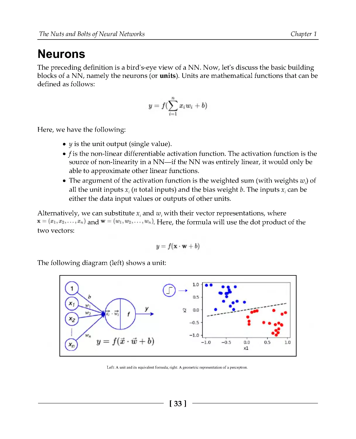
The preceding definition is a bird's-eye view of a NN. Now, let's discuss the basic building
blocks of a NN, namely the neurons (or units). Units are mathematical functions that can be
defined as follows:
Here, we have the following:
y is the unit output (single value).
f is the non-linear differentiable activation function. The activation function is the
source of non-linearity in a NN—if the NN was entirely linear, it would only be
able to approximate other linear functions.
The argument of the activation function is the weighted sum (with weights wi) of
all the unit inputs xi (n total inputs) and the bias weight b. The inputs xi can be
either the data input values or outputs of other units.
Alternatively, we can substitute xi and wi with their vector representations, where
and
. Here, the formula will use the dot product of the
two vectors:
The following diagram (left) shows a unit:
Left: A unit and its equivalent formula; right: A geometric representation of a perceptron.
The Nuts and Bolts of Neural Networks
Chapter 1
[34]
The input vector x will be perpendicular to the weight vector w if x• w = 0. Therefore, all
vectors x where x• w = 0 define a hyperplane in the vector space
, wherenisthe
dimension of x. In the case of two-dimensional input (x1, x2), we can represent the
hyperplane as a line. This could be illustrated with the perceptron (or binary classifier)—a
unit with a threshold activation function
that classifies its input in one of
the two classes. The geometric representation of the perceptron with two inputs (x1, x2) is a
line (or decision boundary) separating the two classes (to the right in the preceding
diagram). This imposes a serious limitation on the neuron because it cannot classify linearly
inseparable problems—even simple ones such as XOR.
A unit with an identity activation function (f(x) = x) is equivalent to multiple linear
regression, while a unit with a sigmoid activation function is equivalent to logistic
regression.
Next, let's learn how to organize the neurons in layers.
Layers as operations
The next level in the NN organizational structure is the layers of units, where we combine
the scalar outputs of multiple units in a single output vector. The units in a layer are not
connected to each other. This organizational structure makes sense for the following
reasons:
We can generalize multivariate regression to a layer, as opposed to only linear or
logistic regression for a single unit. In other words, we can approximate multiple
values with a layer as opposed to a single value with a unit. This happens in the
case of classification output, where each output unit represents the probability
the input belongs to a certain class.
A unit can convey limited information because its output is a scalar. By
combining the unit outputs, instead of a single activation, we can now consider
the vector in its entirety. In this way, we can convey a lot more information, not
only because the vector has multiple values, but also because the relative ratios
between them carry additional meaning.
Because the units in a layer have no connections to each other, we can parallelize
the computation of their outputs (thereby increasing the computational speed).
This ability is one of the major reasons for the success of DL in recent years.
The Nuts and Bolts of Neural Networks
Chapter 1
[35]
In classical NNs (that is, NNs before DL, when they were just one of many ML algorithms),
the primary type of layer is the fully connected (FC) layer. In this layer, every unit receives
weighted input from all the components of the input vector, x. Let's assume that the size of
the input vector is m and that the FC layer has n units and an activation function f, which is
the same for all the units. Each of the n units will have m weights: one for each of the m
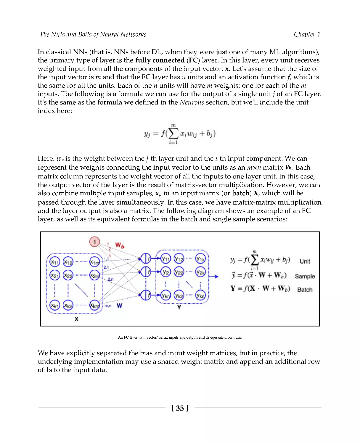
inputs. The following is a formula we can use for the output of a single unit j of an FC layer.
It's the same as the formula we defined in the Neurons section, but we'll include the unit
index here:
Here, wij is the weight between the j-th layer unit and the i-th input component. We can
represent the weights connecting the input vector to the units as an m×n matrix W. Each
matrix column represents the weight vector of all the inputs to one layer unit. In this case,
the output vector of the layer is the result of matrix-vector multiplication. However, we can
also combine multiple input samples, xi, in an input matrix (or batch) X, which will be
passed through the layer simultaneously. In this case, we have matrix-matrix multiplication
and the layer output is also a matrix. The following diagram shows an example of an FC
layer, as well as its equivalent formulas in the batch and single sample scenarios:
An FC layer with vector/matrix inputs and outputs and its equivalent formulas
We have explicitly separated the bias and input weight matrices, but in practice, the
underlying implementation may use a shared weight matrix and append an additional row
of 1s to the input data.
The Nuts and Bolts of Neural Networks
Chapter 1
[36]
Contemporary DL is not limited to FC layers. We have many other types, such as
convolutional, pooling, and so on. Some of the layers have trainable weights (FC,
convolutional), while others don't (pooling). We can also use the terms functions or
operations interchangeably with the layer. For example, in TensorFlow and PyTorch, the
FC layer we just described is a combination of two sequential operations. First, we perform
the weighted sum of the weights and inputs and then we feed the result as an input to the
activation function operation. In practice (that is, when working with DL libraries), the
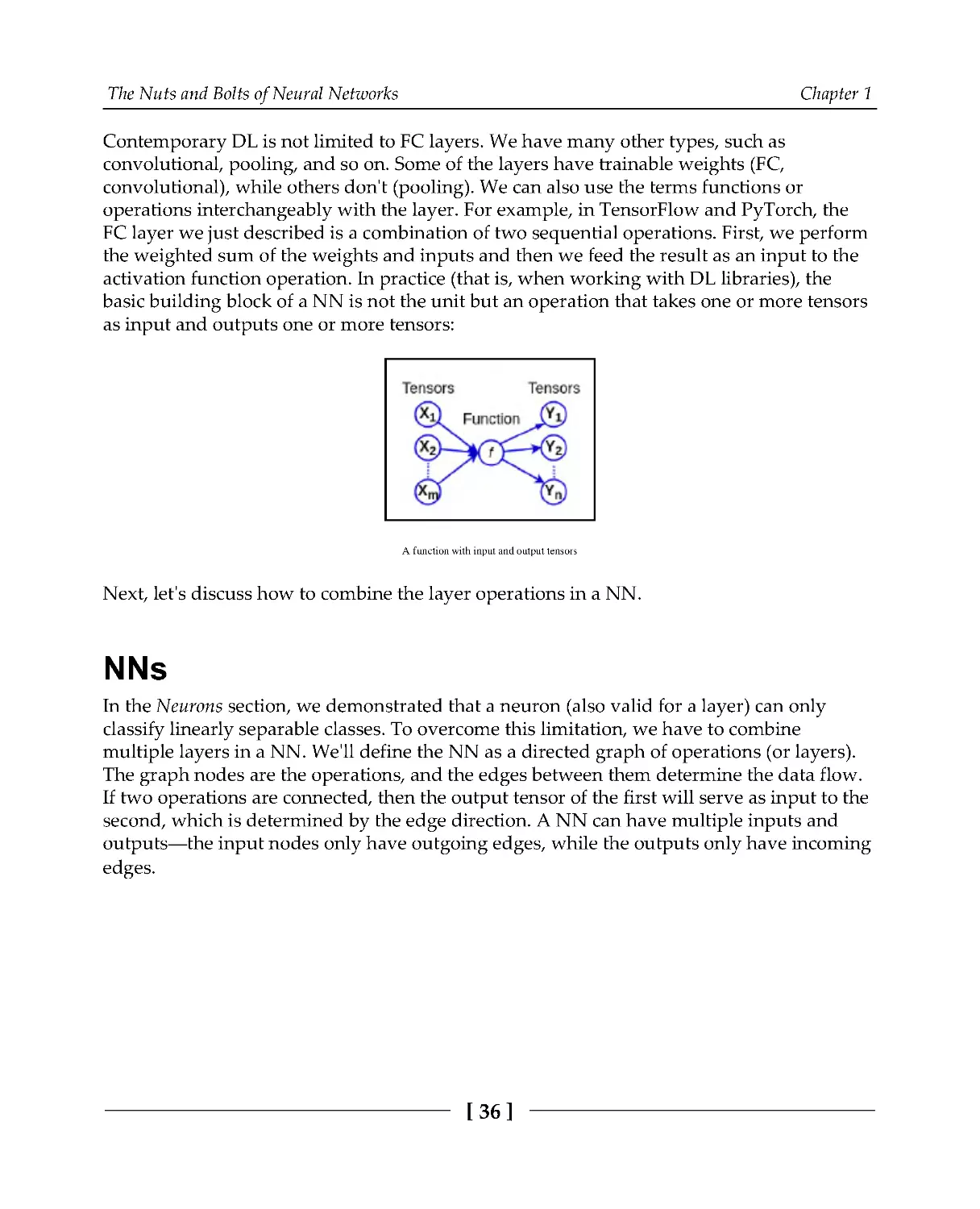
basic building block of a NN is not the unit but an operation that takes one or more tensors
as input and outputs one or more tensors:
A function with input and output tensors
Next, let's discuss how to combine the layer operations in a NN.
NNs
In the Neurons section, we demonstrated that a neuron (also valid for a layer) can only
classify linearly separable classes. To overcome this limitation, we have to combine
multiple layers in a NN. We'll define the NN as a directed graph of operations (or layers).
The graph nodes are the operations, and the edges between them determine the data flow.
If two operations are connected, then the output tensor of the first will serve as input to the
second, which is determined by the edge direction. A NN can have multiple inputs and
outputs—the input nodes only have outgoing edges, while the outputs only have incoming
edges.
The Nuts and Bolts of Neural Networks
Chapter 1
[37]
Based on this definition, we can identify two main types of NNs:
Feed-forward, which are represented by acyclic graphs.
Recurrent (RNN), which are represented by cyclic graphs. The recurrence is
temporal; the loop connection in the graph propagates the output of an operation
at moment t-1 and feeds it back into the network at the next moment, t. The RNN
maintains an internal state, which represents a kind of summary of all the
previous network inputs. This summary, along with the latest input, is fed to the
RNN. The network produces some output but also updates its internal state and
waits for the next input value. In this way, the RNN can take inputs with variable
lengths, such as text sequences or time series.
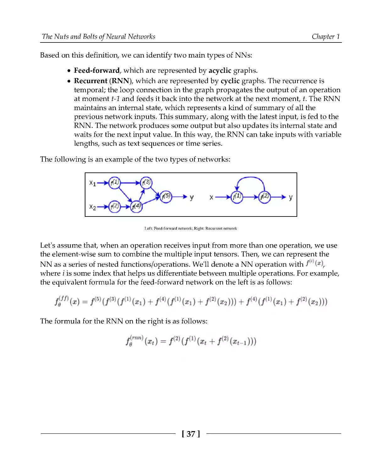
The following is an example of the two types of networks:
Left: Feed-forward network; Right: Recurrent network
Let's assume that, when an operation receives input from more than one operation, we use
the element-wise sum to combine the multiple input tensors. Then, we can represent the
NN as a series of nested functions/operations. We'll denote a NN operation with
,
where i is some index that helps us differentiate between multiple operations. For example,
the equivalent formula for the feed-forward network on the left is as follows:
The formula for the RNN on the right is as follows:
The Nuts and Bolts of Neural Networks
Chapter 1
[38]
We'll also denote the parameters (weights) of an operation with the same index as the
operation itself. Let's take an FC network layer with index l, which takes its input from a
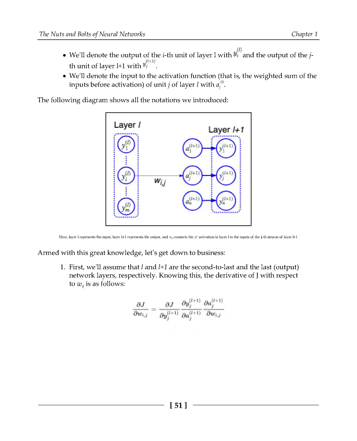
previous layer with index l-1. The following are the layer formulas for a single unit and
vector/matrix layer representations with layer indexes:
Now that we're familiar with the full NN architecture, let's discuss the different types of
activation functions.
Activation functions
Let's discuss the different types of activation functions, starting with the classics:
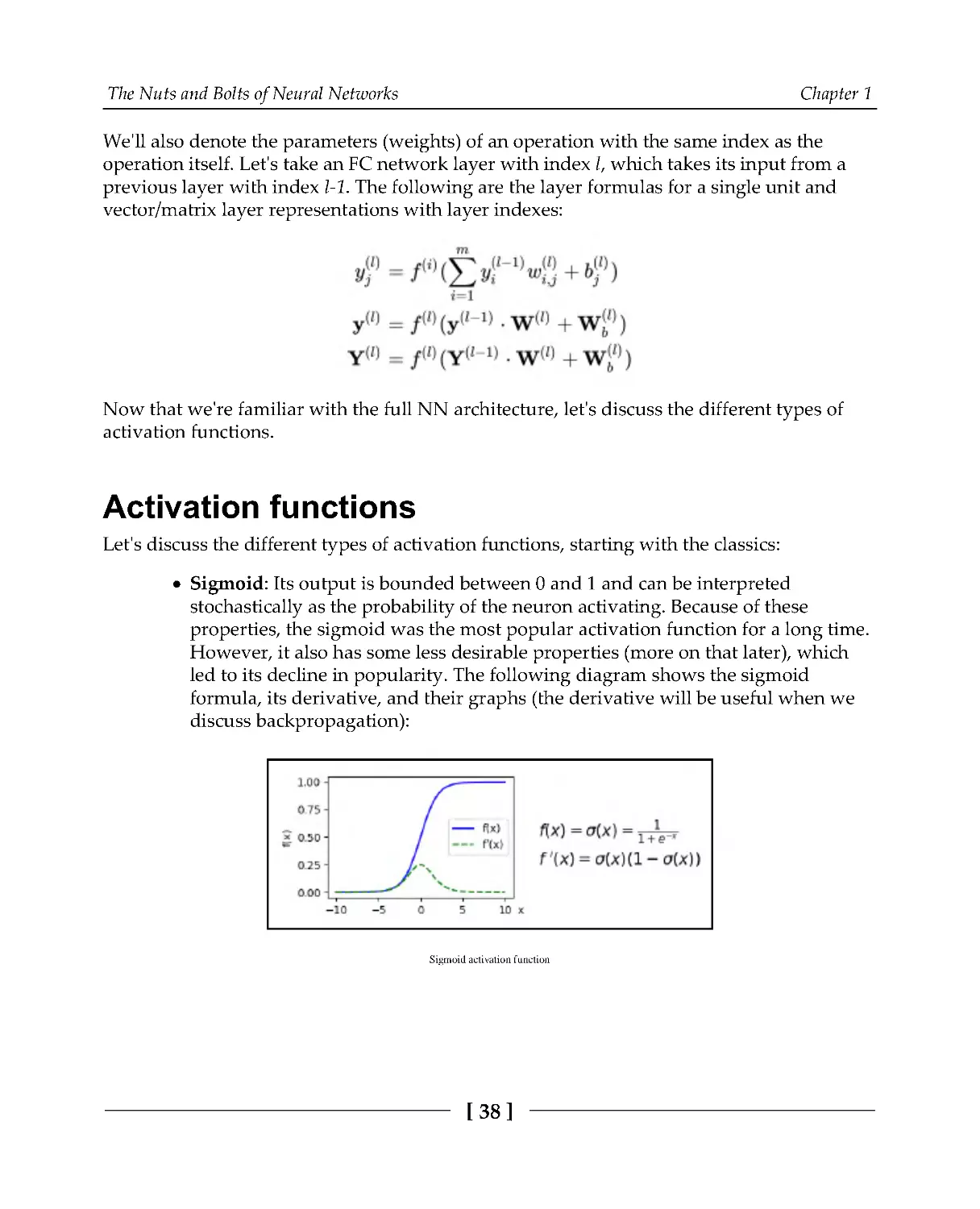
Sigmoid: Its output is bounded between 0 and 1 and can be interpreted
stochastically as the probability of the neuron activating. Because of these
properties, the sigmoid was the most popular activation function for a long time.
However, it also has some less desirable properties (more on that later), which
led to its decline in popularity. The following diagram shows the sigmoid
formula, its derivative, and their graphs (the derivative will be useful when we
discuss backpropagation):
Sigmoid activation function
The Nuts and Bolts of Neural Networks
Chapter 1
[39]
Hyperbolic tangent (tanh): The name speaks for itself. The principal difference
with the sigmoid is that the tanh is in the (-1, 1) range. The following diagram
shows the tanh formula, its derivative, and their graphs:
The hyperbolic tangent activation function
Next, let's focus on the new kids on the block—the *LU (LU stands for linear unit) family of
functions. We'll start with the rectified linear unit (ReLU), which was first successfully used
in 2011 (Deep Sparse Rectifier Neural Networks, http:/
/
proceedings.
mlr.
press/
v15/
glorot11a/
glorot11a.
pdf). The following diagram shows the ReLU formula, its
derivative, and their graphs:
ReLU activation function
As we can see, the ReLU repeats its input when x > 0 and stays at 0 otherwise. This
activation has several important advantages over sigmoid and tanh:
Its derivative helps prevent vanishing gradients (more on that in the Weights
initialization section). Strictly speaking, the derivative ReLU at value 0 is
undefined, which makes the ReLU only semi-differentiable (more information
about this can be found at https:/
/
en.
wikipedia.
org/
wiki/
Semi-
differentiability). But in practice, it works well enough.
The Nuts and Bolts of Neural Networks
Chapter 1
[40]
It's idempotent—if we pass a value through an arbitrary number of ReLU
activations, it will not change; for example, ReLU(2) = 2, ReLU(ReLU(2)) = 2, and
so on. This is not the case for a sigmoid, where the value is squashed on each pass:
σ(σ(2)) = 0.707. The following is an example of the activation of three consecutive
sigmoid activations:
Consecutive sigmoid activations "squash" the data
The idempotence of ReLU makes it theoretically possible to create networks with
more layers compared to the sigmoid.
It creates sparse activations—let's assume that the weights of the network are
initialized randomly through normal distribution. Here, there is a 0.5 chance that
the input for each ReLU unit is < 0. Therefore, the output of about half of all
activations will also be 0. The sparse activations have a number of advantages,
which we can roughly summarize as the Occam's razor in the context of
NNs—it's better to achieve the same result with a simpler data representation
than a complex one.
It's faster to compute in both the forward and backward passes.
However, during training, the network weights can be updated in such a way that some of
the ReLU units in a layer will always receive inputs smaller than 0, which in turn will cause
them to permanently output 0 as well. This phenomenon is known as dying ReLUs. To
solve this, a number of ReLU modifications have been proposed. The following is a non-
exhaustive list:
Leaky ReLU: When the input is larger than 0, leaky ReLU repeats its input in the
same way as the regular ReLU does. However, when x < 0, the leaky ReLU
outputs x multiplied by some constant α (0 < α < 1), instead of 0. The following
diagram shows the leaky ReLU formula, its derivative, and their graphs for
α=0.2:
The Nuts and Bolts of Neural Networks
Chapter 1
[41]
Leaky ReLU activation function
Parametric ReLU (PReLU, Delving Deep into Rectifiers: Surpassing Human-Level
Performance on ImageNet Classification, https:/
/
arxiv.
org/
abs/
1502.
01852): This
activation is the same as the leaky ReLU, but the parameter α is tunable and is
adjusted during training.
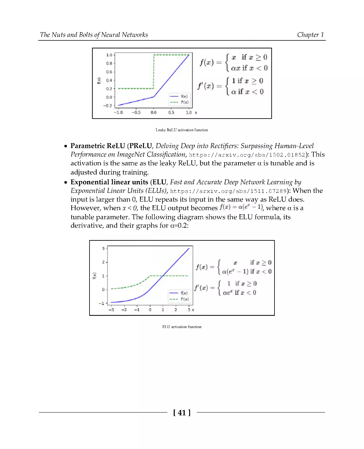
Exponential linear units (ELU, Fast and Accurate Deep Network Learning by
Exponential Linear Units (ELUs), https:/
/
arxiv.
org/
abs/
1511.
07289): When the
input is larger than 0, ELU repeats its input in the same way as ReLU does.
However, when x < 0, the ELU output becomes
,whereαisa
tunable parameter. The following diagram shows the ELU formula, its
derivative, and their graphs for α=0.2:
ELU activation function
The Nuts and Bolts of Neural Networks
Chapter 1
[42]
Scaled exponential linear units (SELU, Self-Normalizing Neural
Networks, https:/
/
arxiv.
org/
abs/
1706.
02515): This activation is similar to
ELU, except that the output (both smaller and larger than 0) is scaled with an
additional training parameter, λ. The SELU is part of a larger concept called self-
normalizing NNs (SNNs), which is described in the source paper. The following
is the SELU formula:
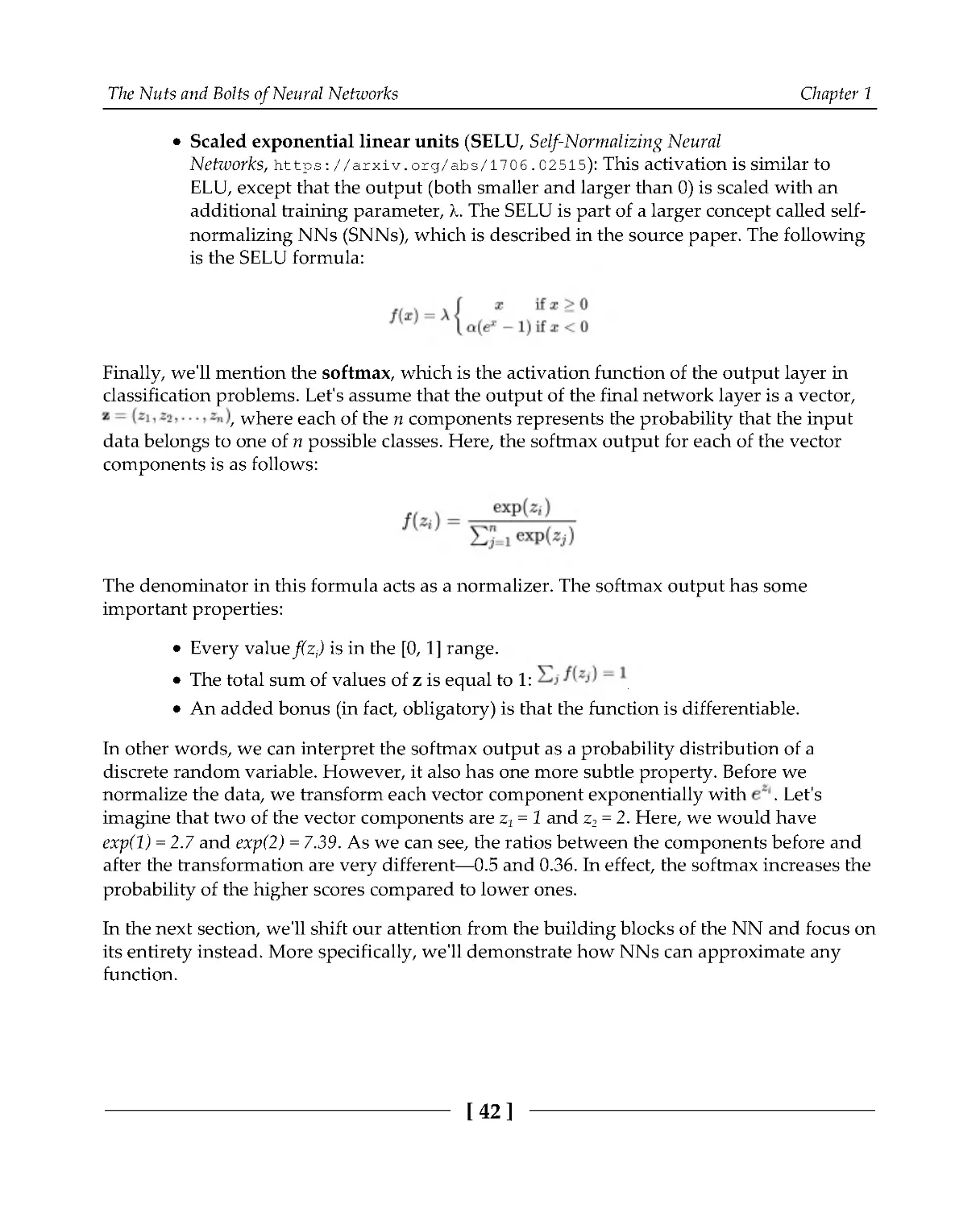
Finally, we'll mention the softmax, which is the activation function of the output layer in
classification problems. Let's assume that the output of the final network layer is a vector,
, where each of the n components represents the probability that the input
data belongs to one of n possible classes. Here, the softmax output for each of the vector
components is as follows:
The denominator in this formula acts as a normalizer. The softmax output has some
important properties:
Every value f(zi) is in the [0, 1] range.
The total sum of values of z is equal to 1:
.
An added bonus (in fact, obligatory) is that the function is differentiable.
In other words, we can interpret the softmax output as a probability distribution of a
discrete random variable. However, it also has one more subtle property. Before we
normalize the data, we transform each vector component exponentially with . Let's
imagine that two of the vector components are z1 = 1 and z2 = 2. Here, we would have
exp(1) = 2.7 and exp(2) = 7.39 . As we can see, the ratios between the components before and
after the transformation are very different—0 .5 and 0.36 . In effect, the softmax increases the
probability of the higher scores compared to lower ones.
In the next section, we'll shift our attention from the building blocks of the NN and focus on
its entirety instead. More specifically, we'll demonstrate how NNs can approximate any
function.
The Nuts and Bolts of Neural Networks
Chapter 1
[43]
The universal approximation theorem
The universal approximation theorem was first proved in 1989 for a NN with sigmoid
activation functions and then in 1991 for NNs with arbitrary non-linear activation
functions. It states that any continuous function on compact subsets of
can be
approximated to an arbitrary degree of accuracy by a feedforward NN with at least one
hidden layer with a finite number of units and a non-linear activation. Although a NN with
a single hidden layer won't perform well in many tasks, the theorem still tells us that there
are no theoretical insurmountable limitations in terms of NNs. The formal proof of the
theorem is too complex to be explained here, but we'll attempt to provide an intuitive
explanation using some basic mathematics.
The idea for the following example was inspired by Michael A. Nielsen's
book Neural Networks and Deep Learning (http:/
/
neuralnetworksanddeeplearning.
com/
).
We'll implement a NN that approximates the boxcar function (shown on the right in the
following diagram), which is a simple type of step function. Since a series of step functions
can approximate any continuous function on a compact subset of R, this will give us an
idea of why the universal approximation theorem holds:
The diagram on the left depicts continuous function approximation with a series of step functions, while the diagram on the right illustrates a single boxcar step
function.
To understand how this approximation works, we'll start with a single unit with a single
scalar input x and sigmoid activation. The following is a visualization of the unit and its
equivalent formula:
The Nuts and Bolts of Neural Networks
Chapter 1
[44]
In the following diagrams, we can see the graph of the formula for different values of b and
w for inputs in the range of [-10: 10]:
The neuron output based on different values of w and b. The network input x is represented on the x axis.
Upon closer inspection of the formula and the graph, we can see that the steepness of the
sigmoid function is determined by the weight, w. Also, the translation of the function along
the x axis is determined by the formula t = -b/w. Let's discuss the different scenarios in the
preceding diagram:
The top-left graph shows the regular sigmoid.
The top-right graph demonstrates that a large weight w amplifies the input x to a
point, where the unit output resembles threshold activation.
The bottom-left graph shows how the bias b translates the unit activation along
the x axis.
The bottom-right graph shows that we can simultaneously reverse the activation
with negative weight w and translate the activation along the x axis with the bias
b.
We can intuitively see that the preceding graphs contain all the ingredients of the box
function. We can combine the different scenarios with the help of a NN with one hidden
layer, which contains two of the aforementioned units. The following diagram shows the
network architecture, along with the weights and biases of the units, as well as the box
function that's produced by the network:
The Nuts and Bolts of Neural Networks
Chapter 1
[45]
Here's how it works:
First, the top unit activates for the upper step of the function and stays active.
The bottom unit activates afterward for the bottom step of the function and stays
active. The outputs of the hidden units cancel each other out because of the
weights in the output layer, which are the same but with opposite signs.
The weights of the output layer determine the height of the boxcar rectangle.
The output of this network isn't 0, but only in the (-5, 5) interval. Therefore, we can
approximate additional boxes by adding more units to the hidden layer in a similar
manner.
Now that we're familiar with the structure of a NN, let's focus on the training process.
Training NNs
In this section, we'll define training a NN as the process of adjusting its parameters
(weights) θ in a way that minimizes the cost function J(θ). The cost function is some
performance measurement over a training set that consists of multiple samples, represented
as vectors. Each vector has an associated label (supervised learning). Most commonly, the
cost function measures the difference between the network output and the label.
We'll start this section with a short recap of the gradient descent optimization algorithm. If
you're already familiar with it, you can skip this.
The Nuts and Bolts of Neural Networks
Chapter 1
[46]
Gradient descent
For the purposes of this section, we'll use a NN with a single regression output and mean
square error (MSE) cost function, which is defined as follows:
Here, we have the following:
fθ(x
(i)
) is the output of the NN.
n is the total number of samples in the training set.
x
(i)
are the vectors for the training samples, where the superscript i indicates the i-
th sample of the dataset. We use superscript because x
(i)
is a vector and the
subscript is reserved for each of the vector components. For example, is the j-th
component of the i-th training sample.
t(i)
is the label associated with sample x
(i)
.
We shouldn't confuse the (i) superscript index of the i-th training sample
with the (l) superscript, which represents the layer index of the NN. We'll
only use the (i) sample index notation in the Gradient descent and Cost
functions sections, and elsewhere we'll use the (l) notation for the layer
index.
First, gradient descent computes the derivative (gradient) of J(θ) with respect to all the
network weights. The gradient gives us an indication of how J(θ) changes with respect to
every weight. Then, the algorithm uses this information to update the weights in a way that
will minimize J(θ) in future occurrences of the same input/target pairs. The goal is to
gradually reach the global minimum of the cost function. The following is a visualization of
gradient descent for MSE and a NN with a single weight:
The Nuts and Bolts of Neural Networks
Chapter 1
[47]
A visualization of gradient descent for MSE
Let's go over the step-by-step execution of gradient descent:
Initialize the network weights θ with random values.
1.
Repeat until the cost function falls below a certain threshold:
2.
Forward pass: compute the MSE J(θ) cost function for all the samples
1.
of the training set using the preceding formula.
Backward pass: compute the derivative of J(θ) with respect to all the
2.
network weights using the chain rule:
Let's analyze the derivative
. Jisafunctionofθjbybeinga
function of the network output. Therefore, it is also a function of the NN
function itself, that is,
. Then, by following the chain rule, we get
.
The Nuts and Bolts of Neural Networks
Chapter 1
[48]
Use these derivatives to update each of the network weights:
3.
Here, η is the learning rate.
Gradient descent updates the weights by accumulating the error across all the training
samples. In practice, we would use two of its modifications:
Stochastic (or online) gradient descent (SGD) updates the weights after every
training sample.
Mini-batch gradient descent accumulates the error for every n samples (one
mini-batch) and performs one weight update.
Next, let's discuss the different cost functions we can use with SGD.
Cost functions
Besides MSE, there are also a few other loss functions that are commonly used in regression
problems. The following is a non-exhaustive list:
Mean absolute error (MAE) is the mean of the absolute differences (not squared)
between the network output and the target. The following is the MAE graph and
formula:
One advantage of MAE over MSE is that it deals with outlier samples better. With
MSE, if the difference of a sample is
, it increases exponentially
(because of the square). We'll get an outsized weight of this sample compared to
the others, which may skew the results. With MAE, the difference is not
exponential and this issue is less pronounced.
The Nuts and Bolts of Neural Networks
Chapter 1
[49]
On the other hand, the MAE gradient will have the same value until we reach the
minimum, where it will become 0 immediately. This makes it harder for the
algorithm to anticipate how close the cost function minimum is. Compare this to
MSE, where the slope gradually decreases as we get close to the cost minimum.
This makes MSE easier to optimize. In conclusion, unless the training data is
corrupted with outliers, it is usually recommended to use MSE over MAE.
Huber loss attempts to fix the problems of both MAE and MSE by combining
their properties. In short, when the absolute difference between the output and
the target data falls below the value of a fixed parameter, δ, the Huber loss
behaves like MSE. Conversely, when the difference is greater than δ, it resembles
MAE. In this way, it is less sensitive to outliers (when the difference is big) and at
the same time, the minimum of the function is properly differentiable. The
following is the Huber loss graph for three values of δ and its formula for a single
training sample, which reflects its dualistic nature:
Huber loss
Next, let's focus on cost functions for classification problems. The following is a non-
exhaustive list:
Cross-entropy loss: We have our work cut out for us here as we already defined
cross-entropy in the Information theory section. This loss is usually applied over
the output of a softmax function. The two work very well together. First, the
softmax converts the network output into a probability distribution. Then, cross-
entropy measures the difference between the network output (Q) and the true
distribution (P), which is provided as a training label. Another nice property is
that the derivative of H(P, Qsoftmax) is quite straightforward (although the
computation isn't):
Here, x
(i)
/t(i)
is the i-th input/label training pair.
The Nuts and Bolts of Neural Networks
Chapter 1
[50]
KL Divergence loss: Like cross-entropy loss, we already did the grunt work in
the Information theory section, where we derived the relationship between KL
divergence and cross-entropy loss. From their relationship, we can state that if
we use either of the two as a loss function, we implicitly use the other one as
well.
Sometimes, we may encounter the terms loss function and cost function
being used interchangeably. It is usually accepted that they differ slightly.
We'll refer to the loss function as the difference between the network
output and target data for a single sample of the training set. The cost
function is the same thing but is averaged (or summed) over multiple
samples (batch) of the training set.
Now that we have looked at different cost functions, let's focus on propagating the error
gradient through the network with backpropagation.
Backpropagation
In this section, we'll discuss how to update the network weights in order to minimize the
cost function. As we demonstrated in the Gradient descent section, this means finding the
derivative of the cost function J(θ) with respect to each network weight. We already took a
step in this direction with the help of the chain rule:
Here, f(θ) is the network output and θj is the j-th network weight. In this section, we'll push
the envelope further and we'll learn how to derive the NN function itself for all the network
weights (hint: chain rule). We'll do this by propagating the error gradient backward
through the network (hence the name). Let's start with a few assumptions:
For the sake of simplicity, we'll work with a sequential feed-forward NN.
Sequential means that each layer takes input from the preceding layer and sends
its output to the following layer.
We'll define wij as the weight between the i-th neuron of layer l and the j-th
neuron of layer l+1. In other words, we use subscripts i and j, where the element
with subscript i belongs to the preceding layer, which is the layer containing the
element with subscript j. In a multi-layer network, l and l+1 can be any two
consecutive layers, including input, hidden, and output layers.
The Nuts and Bolts of Neural Networks
Chapter 1
[51]
We'll denote the output of the i-th unit of layer l with and the output of the j-
th unit of layer l+1 with
.
We'll denote the input to the activation function (that is, the weighted sum of the
inputs before activation) of unit j of layer l with aj
(l)
.
The following diagram shows all the notations we introduced:
Here, layer l represents the input, layer l+1 represents the output, and wij connects the yi
(l)
activation in layer l to the inputs of the j-th neuron of layer l+1
Armed with this great knowledge, let's get down to business:
First, we'll assume that l and l+1 are the second-to-last and the last (output)
1.
network layers, respectively. Knowing this, the derivative of J with respect
to wij is as follows:
The Nuts and Bolts of Neural Networks
Chapter 1
[52]
Let's focus on
. Here, we compute the partial derivative of the
2.
weighted sum of the output of layer l with respect to one of the weights, wij. As
we discussed in the Differential calculus section, in partial derivatives, we'll
consider all the function parameters except wij constants. When we derive aj
(l+1)
,
they all become 0 and we're only left with
. Therefore, we get the
following:
The formula from point 1 holds for any two consecutive hidden layers, l and l+1,
3.
of the network. We know that
, and we also know that
is the derivative of the activation function, which we can calculate (see the
Activation functions section). All we need to do is calculate the derivative
(recall that, here, l+1 is some hidden layer). Let's note that this is the derivative of
the error with respect to the activation function in layer l+1. We can now
calculate all the derivatives, starting from the last layer and moving backward,
because the following apply:
We can calculate this derivative for the last layer.
We have a formula that allows us to calculate the derivative for one layer,
assuming that we can calculate the derivative for the next.
With these points in mind, we get the following equation by applying the chain
4.
rule:
The sum over j reflects the fact that, in the feedforward part of the network, the
output is fed to all the neurons in layer l+1. Therefore, they all contribute
to yi
(l)
when the error is propagated backward.
The Nuts and Bolts of Neural Networks
Chapter 1
[53]
Once again, we can calculate
. Following the same logic that we
followed in step 3, we can compute that
. Therefore, once we know
that
, we can calculate
. Since we can calculate
for the last
layer, we can move backward and calculate
for any layer, and therefore
for any layer.
To summarize, let's say we have a sequence of layers where the following
5.
applies:
Here, we have the following fundamental equations:
By using these two equations, we can calculate the derivatives for the cost with
respect to each layer.
If we set
, then δj
(l+1)
represents the variation in cost with
6.
respect to the activation value, and we can think of δj
(l+1)
as the error
at neuron yj
(l+1)
. We can rewrite these equations as follows:
Following this, we can write the following equation:
The Nuts and Bolts of Neural Networks
Chapter 1
[54]
These two equations provide us with an alternative view of backpropagation
since there is a variation in cost with respect to the activation value. They provide
us with a way to calculate the variation for any layer l once we know the variation
for the following layer, l+1.
We can combine these equations to show the following:
7.
The updated rule for the weights of each layer is given by the following equation:
8.
Now that we're familiar with backpropagation, let's discuss another component of the
training process: weight initialization.
Weight initialization
One key component of training deep networks is the random weight initialization. This
matters because some activation functions, such as sigmoid and ReLU, produce meaningful
outputs and gradients if their inputs are within a certain range.
A famous example is the vanishing gradient problem. To understand it, let's take an FC
layer with sigmoid activation (this example is also valid for tanh). We saw the sigmoid's
graph (blue) and its derivative (green) in the Activation functions section. If the weighted
sum of the inputs falls roughly outside the (-5, 5) range, the sigmoid activation will be
effectively 0 or 1. In essence, it saturates. This is visible during the backward pass where we
derive the sigmoid (the formula is σ' = σ(1 - σ)). We can see that the derivative is larger than
0 within the same (-5, 5) range of the input. Therefore, whatever error we try to propagate
back to the previous layers, it will vanish if the activation doesn't fall within this range
(hence the name).
Besides the tight meaningful range of the sigmoid derivative, let's note
that, even under the best conditions, its maximum value is 0.25. When we
propagate the gradient through the sigmoid derivative, it will be four
times smaller at best once it passes through. Because of this, the gradient
may vanish in just a few layers, even if we don't fall outside the desired
range. This is one of the major disadvantages of sigmoid over the *LU
family of functions, where the gradient is 1 in most cases.
The Nuts and Bolts of Neural Networks
Chapter 1
[55]
One way to solve this problem is to use *LU activations. But even so, it still makes sense to
use better weight initialization since it can speed up the training process. One popular
technique is the Xavier/Glorot initializer (often found under either of the two
names: http:/
/
proceedings.
mlr.
press/
v9/
glorot10a/
glorot10a.
pdf). In short, this
technique takes the number of input and output connections of the unit into account. There
are two variations:
Xavier uniform initializer, which draws samples from a uniform distribution in
the range [-a, a]. The parameter, a, is defined as follows:
Here, nin and nout are the number of inputs and outputs, respectively (that is, the
number of units that send their output to the current unit and the number of units
the current unit sends its output to).
Xavier normal initializer, which draws samples from a normal distribution (see
the Probability distributions section) with a mean of 0 and variance as follows:
The Xavier/Glorot initialization is recommended for sigmoid or tanh activations functions.
The paper Delving Deep into Rectifiers: Surpassing Human-Level Performance on ImageNet
Classification (https:/
/
arxiv.
org/
abs/
1502.
01852) proposes a similar technique that's
better suited for ReLU activations. Again, there are two variations:
He uniform initializer, which draws samples from a uniform distribution in the
range [-a, a]. The parameter, a, is defined as follows:
The Nuts and Bolts of Neural Networks
Chapter 1
[56]
He normal initializer, which draws samples from a normal distribution with a
mean of 0 and variance as follows:
The ReLU output is always 0 when the input is negative. If we assume that the
initial inputs of the ReLU units are centered around 0, half of them will produce 0
outputs. The He initializer compensates this by increasing the variance twice,
compared to the Xavier initialization.
In the next section, we'll discuss some improvements in the weight update rule over the
standard SGD.
SGD improvements
We'll start with momentum, which extends vanilla SGD by adjusting the current weight
update with the values of the previous weight updates. That is, if the weight update at step
t-1 was big, it will also increase the weight update of step t. We can explain momentum
with an analogy. Think of the loss function surface as the surface of a hill. Now, imagine
that we are holding a ball at the top of the hill (maximum). If we drop the ball, thanks to the
Earth's gravity, it will start rolling toward the bottom of the hill (minimum). The more
distance it travels, the more its speed will increase. In other words, it will gain momentum
(hence the name of the optimization).
Now, let's look at how to implement momentum in the weight update rule. Recall the
update rule that we introduced in the Gradient descent section, that is,
.
Let's assume that we are at step t of the training process:
First, we'll calculate the current weight update value vt by also including
1.
the velocity of the previous update vt-1:
Here, μ is a hyperparameter in the [0:1] range called the momentum rate. vt is
initialized as 0 during the first iteration.
Then, we perform the actual weight update:
2.
The Nuts and Bolts of Neural Networks
Chapter 1
[57]
An improvement over the basic momentum is the Nesterov momentum. It relies on the
observation that the momentum from step t-1 may not reflect the conditions at step t. For
example, let's say that the gradient at t-1 is steep and therefore the momentum is high.
However, after the t-1 weight update, we actually reach the cost function minimum and
require only a minor weight update at t. Despite that, we'll still get the large momentum
from t-1, which may lead the adjusted weight to jump over the minimum. Nesterov
momentum proposes a change in the way we compute the velocity of the weight update.
We'll calculate vt based on the gradient of the cost function that's computed by the potential
future value of the weight θj. The following is the updated velocity formula:
If the momentum at t-1 is incorrect with respect to t, the modified gradient will compensate
for this error in the same update step.
Next, let's discuss the Adam adaptive learning rate algorithm (Adam: A Method for Stochastic
Optimization, https:/
/
arxiv.
org/
abs/
1412.
6980). It calculates individual and adaptive
learning rates for every weight based on previous weight updates (momentum). Let's see
how that works:
First, we need to compute the first moment (or mean) and the second moment (or
1.
variance) of the gradient:
Here, β1 and β2 are hyperparameters with default values of 0.9 and 0.999,
respectively. mt and vt act as moving-average values of the gradient, somewhat
similar to momentum. They are initialized with 0 during the first iteration.
The Nuts and Bolts of Neural Networks
Chapter 1
[58]
Since mt and vt start as 0, they will have a bias toward 0 in the initial phase of the
2.
training. For example, let's say that, at t=1, β1 = 0.9 and
= 10.Here,m1=
0.9*0+(1-0.9)*10=1,whichisalotlessthantheactualgradientof10.To
compensate for this bias, we'll compute the bias-corrected versions of mt and vt:
Finally, we need to perform the weight update using the following formula:
3.
Here, η is the learning rate and ε is some small value to prevent division by 0.
Summary
We started this chapter with a tutorial on the mathematical apparatus that forms the
foundation of NNs. Then, we recapped on NNs and their architecture. Along the way, we
tried to explicitly connect the mathematical concepts with the various components of the
NNs. We paid special attention to the various types of activation functions. Finally, we took
a comprehensive look at the NN training process. We discussed gradient descent, cost
functions, backpropagation, weights initialization, and SGD optimization techniques.
In the next chapter, we'll discuss the intricacies of convolutional networks and their
applications in the computer vision domain.
2
Section 2: Computer Vision
This section will discuss Deep Learning (DL) applications in the computer vision domain.
We'll talk about convolutional networks, object detection and image segmentation,
generative models (GANs), and neural style transfer.
This section contains the following chapters:
Chapter 2, Understanding Convolutional Networks
Chapter 3, Advanced Convolutional Networks
Chapter 4, Object Detection and Image Segmentation
Chapter 5, Generative Models
2
Understanding Convolutional
Networks
In this chapter, we'll discuss Convolutional Neural Networks (CNNs) and their
applications in Computer Vision (CV). CNNs started the modern deep learning revolution.
They are at the base of virtually all recent CV advancements, including Generative
Adversarial Networks (GANs), object detection, image segmentation, neural style transfer,
and much more. For this reason, we believe CNNs deserve an in-depth look that's beyond
our basic understanding of them.
To do this, we'll start with a short recap of the CNN building blocks, that is, the
convolutional and pooling layers. We'll discuss the various types of convolutions in use
today since they are reflected in a large number of CNN applications. We'll also learn how
to visualize the internal state of CNNs. Then, we'll focus on regularization techniques and
implement a transfer learning example.
This chapter will cover the following topics:
Understanding CNNs
Introducing transfer learning
Understanding Convolutional Networks
Chapter 2
[61]
Understanding CNNs
In Chapter 1, The Nuts and Bolts of Neural Networks, we discussed that many NN operations
have solid mathematical foundations, and convolutions are no exception. Let's start by
defining the mathematical convolution:
Here, we have the following:
The convolution operation is denoted with *.
f and g are two functions with a common parameter, t.
The result of the convolution is a third function, s(t) (not just a single value).
The convolution of f and g at value t is the integral of the product of f(t) and the reversed
(mirrored) and shifted value of g(t-τ), where t-τ represents the shift. That is, for a single
value of f at time t, we shift g in the range
and we compute the product
f(t)g(t-τ) continuously because of the integral. The integral (and hence the convolution) is
equivalent to the area under the curve of the product of the two functions.
This is best illustrated in the following diagram:
Left: a convolution, where g is shifted and reversed; right: a step-by-step illustration of a convolution operation
Understanding Convolutional Networks
Chapter 2
[62]
In the convolution operation, g is shifted and reversed in order to preserve
the operation's commutative property. In the context of CNNs, we can
ignore this property and we can implement it without reversing g. In this
case, the operation is called cross-correlation. These two terms are used
interchangeably.
We can define the convolution for discrete (integer) values of t with the following formula
(which is very similar to the continuous case):
We can also generalize it to the convolution of functions with two shared input
parameters, i and j:
We can derive the formula in a similar manner for three parameters.
In CNNs, the function f is the input of the convolution operation (also referred to as the
convolutional layer). Depending on the number of input dimensions, we have 1D, 2D, or
3D convolutions. А time series input is a 1D vector, an image input is a 2D matrix, and a 3D
point cloud is a 3D tensor. The function g, on the other hand, is called a kernel (or filter). It
has the same number of dimensions as the input data and it is defined by a set of learnable
weights. For example, a filter of size n for a 2D convolution is an n×n matrix. The following
diagram illustrates a 2D convolution with a 2×2 filter applied over a single 3×3 slice:
2D convolution with a 2×2 filter applied over a single 3×3 slice
Understanding Convolutional Networks
Chapter 2
[63]
The convolution works as follows:
We slide the filter along all of the dimensions of the input tensor.
1.
At every input position, we multiply each filter weight by its corresponding
2.
input tensor cell at the given location. The input cells, which contribute to a
single output cell, are called receptive fields. We sum all of these values to
produce the value of a single output cell.
Unlike fully-connected layers, where each output unit gathers information from all of the
inputs, the activation of a convolution output cell is determined by the inputs in its
receptive field. This principle works best for hierarchically structured data such as images.
For example, neighboring pixels form meaningful shapes and objects, but a pixel at one end
of the image is unlikely to have a relationship with a pixel at another end. Using a fully-
connected layer to connect all of the input pixels with each output unit is like asking the
network to find a needle in a haystack. It has no way of knowing whether an input pixel is
in the receptive field of the output unit or not.
The filter highlights some particular features in the receptive field. The output of the
operation is a tensor (known as a feature map), which marks the locations where the feature
is detected. Since we apply the same filter throughout the input tensor, the convolution is
translation invariant; that is, it can detect the same features, regardless of their location on
the image. However, the convolution is neither rotation invariant (it is not guaranteed to
detect a feature if it's rotated), nor scale invariant (it is not guaranteed to detect the same
artifact in different scales).
In the following diagram, we can see examples of 1D and 3D convolutions (we've already
introduced an example of a 2D convolution):
1D convolution: The filter (denoted with multicolored lines) slides over a single axis; 3D convolution: The filter (denoted with dashed lines) slides over three axes
Understanding Convolutional Networks
Chapter 2
[64]
The CNN convolution can have multiple filters, highlighting different features, which
results in multiple output feature maps (one for each filter). It can also gather input from
multiple feature maps, for example, the output of a previous convolution. The combination
of feature maps (input or output) is called a volume. In this context, we can also refer to the
feature maps as slices. Although the two terms refer to the same thing, we can think of the
slice as part of the volume, whereas the feature map highlights its role as, well, a feature
map.
As we mentioned earlier in this section, each volume (as well as the filter) is represented by
a tensor. For example, a red, green, and blue (RGB) image is represented by a 3D tensor of
three 2D slices (one slice per color channel). But in the context of CNNs, we add one more
dimension for the sample index in the mini-batch. Here, a 1D convolution would have 3D
input and output tensors. Their axes can be in either NCW or NWC order, where N is the
index of the sample in the mini-batch, C is the index of the depth slice in the volume, and W
is the vector size of each sample. In the same way, a 2D convolution will be represented by
NCHW or NHWC tensors, where H and W are the height and width of the slices. A 3D
convolution will have an NCLHW or NLHWC order, where L stands for the depth of the
slice.
We use 2D convolutions to work with RGB images. However, we may
consider the three colors an additional dimension, hence making the RGB
image 3D. Why didn't we use 3D convolutions, then? The reason for this is
that, even though we can think of the input as 3D, the output is still a 2D
grid. Had we used 3D convolution, the output would also be 3D, which
doesn't carry any meaning in the case of 2D images.
Let's say we have n input and m output slices. In this case, we'll apply m filters across the
set of n input slices. Each filter will generate a unique output slice that highlights the
feature that was detected by the filter (n to m relationship).
Depending on the relationship of the input and output slice, we get cross-channel and
depth-wise convolutions, as illustrated in the following diagram:
Left: cross-channel convolution; right: depthwise convolution
Understanding Convolutional Networks
Chapter 2
[65]
Let's discuss their properties:
Cross-channel convolutions: One output slice receives input from all of the
input slices (n-to-one relationship). With multiple output slices, the relationship
becomes n-to-m. In other words, each input slice contributes to the output of each
output slice. Each pair of input/output slices uses a separate filter slice that's
unique to that pair. Let's denote the size of the filter (equal width and height)
with F, the depth of the input volume with Cin, and the depth of the output
volume with Cout. With this, we can compute the total number of weights, W, in a
2D convolution with the following equation:
Here, +1 represents the bias weight for each filter. Let's say we have three slices
and want to apply four 5×5 filters to them. If we did this, the convolution filter
would have a total of (3*5*5 + 1) * 4 = 304 weights, four output slices (output
volume with a depth of 4), and one bias per slice. The filter for each output slice
will have three 5×5 filter patches for each of the three input slices and one bias for
a total of 3*5*5 + 1 = 76 weights.
Depthwise convolutions: Each output slice receives input from a single input
slice. It's a kind of reversal of the previous case. In its most simple form, we
apply a filter over a single input slice to produce a single output slice. In this
case, the input and output volumes have the same depth, that is, C. We can also
specify a channel multiplier (an integer, m), where we apply m filters over a
single output slice to produce m output slices. This is a case of a one-to-m
relationship. In this case, the total number of output slices is n * m. We can
compute the number of weights, W, in a 2D depthwise convolution with the
following formula:
Here, m is the channel multiplier and +C represents the biases of each output slice.
Understanding Convolutional Networks
Chapter 2
[66]
The convolution operation is also described by two other parameters:
Stride is the number of positions that we slide the filter over on the input slice on
each step. By default, the stride is 1. If it's larger than 1, then we call it a stride
convolution. The largest stride increases the receptive field of the output
neurons. With stride 2, the size of the output slice will be roughly four times
smaller than the input. In other words, one output neuron will cover the area,
which is four times larger, compared to a stride 1 convolution. The neurons in
the following layers will gradually capture input from the larger regions of the
input image.
Padding the edges of the input slice with rows and columns of zeros before the
convolution operation. The most common way to use padding is to produce
output with the same dimensions as the input. The newly padded zeros will
participate in the convolution operation with the slice, but they won't affect the
result.
Knowing the input dimensions and the filter size, we can compute the dimensions of the
output slices. Let's say the size of the input slice is I (equal height and width), the size of the
filter is F, the stride is S, and the padding is P. Here, the size, O, of the output slice is given
by the following equation:
Besides stride convolutions, we can also use pooling operations to increase the receptive
field of the deeper neurons and reduce the size of the future slices. The pooling splits the
input slice into a grid, where each grid cell represents a receptive field of a number of
neurons (just like it does with the convolution). Then, a pooling operation is applied over
each cell of the grid. Similar to convolution, pooling is described by the stride, S, and the
size of the receptive field, F. If the size of input slice is I, then the formula for the output size
of the pooling is as follows:
In practice, only two combinations are used. The first is a 2×2 receptive field with stride 2,
while the second is a 3×3 receptive field with stride 2 (overlapping). The most common
pooling operations are as follows:
Max pooling: This propagates the maximum value of the input values of the
receptive field.
Understanding Convolutional Networks
Chapter 2
[67]
Average pooling: This propagates the average value of the inputs in the
receptive field.
Global Average Pooling (GAP): This is the same as average pooling, but the
pooling region has the same size as the feature map, I×I. GAP performs an
extreme type of dimensionality reduction: the output is a single scalar, which
represents the average value of the whole feature map.
Typically, we would alternate one or more convolutional layers with one pooling (or stride
convolution) layer. In this way, the convolutional layers can detect features at every level of
the receptive field size because the aggregated receptive field size of deeper layers is larger
than the ones at the beginning of the network. The deeper layers also have more filters
(hence, a higher volume depth) compared to the initial ones. The feature detector at the
beginning of the network works on a small receptive field. It can only detect a limited
number of features, such as edges or lines, that are shared among all classes.
On the other hand, a deeper layer would detect more complex and numerous features. For
example, if we have multiple classes, such as cars, trees, or people, each would have its own
set of features, such as tires, doors, leaves, and faces. This would require more feature
detectors. The output of the final convolution (or pooling) is "translated" to the target labels
by adding one or more fully connected layers.
Now that we have had an overview of convolutions, pooling operations, and CNNs, in the
next section, we'll focus on different types of convolution operations.
Types of convolutions
So far, we've discussed the most common type of convolution. In the upcoming sections,
we'll talk about a few of its variations.
Transposed convolutions
In the convolutional operations we've discussed so far, the output dimensions are either
equal or smaller than the input dimensions. In contrast, transposed convolutions (first
proposed in Deconvolutional Networks by Matthew D. Zeiler, Dilip Krishnan, Graham W.
Taylor, and Rob Fergus: https:/
/
www.
matthewzeiler.
com/
mattzeiler/
deconvolutionalnetworks.
pdf) allow us to upsample the input data (their output is larger
than the input). This operation is also known as deconvolution, fractionally strided
convolution, or sub-pixel convolution. These names can sometimes lead to confusion. To
clarify things, note that the transposed convolution is, in fact, a regular convolution with a
slightly modified input slice or convolutional filter.
Understanding Convolutional Networks
Chapter 2
[68]
For the longer explanation, we'll start with a 1D regular convolution over a single input and
output slice:
1D regular convolution
It uses a filter with a size of 4, stride 2, and padding 2 (denoted with gray in the preceding
diagram). The input is a vector of size 6 and the output is a vector of size 4. The filter, a
vector f = [1, 2, 3, 4], is always the same, but it's denoted with different colors for each
position we apply it to. The respective output cells are denoted with the same color. The
arrows show which input cells contribute to one output cell.
The example that is being discussed in this section is inspired by the
paper; Is the deconvolution layer the same as a convolutional layer? (https:/
/
arxiv.
org/
abs/
1609.
07009).
Next, we'll discuss the same example (1D, single input and output slices, filter of size 4,
padding 2, and stride 2), but for transposed convolution. The following diagram shows two
ways we can implement it:
Left: A convolution with stride 2, applied with the transposed filter f. The 2 pixels at the beginning and the end of the output are cropped; right: A convolution with stride 0.5,
applied over input data, padded with subpixels. The input is filled with 0-valued pixels (gray).
Understanding Convolutional Networks
Chapter 2
[69]
Let's discuss them in detail:
In the first case, we have a regular convolution with stride 2 and a
filter represented as transposed row matrix (equivalent to column matrix) with
size 4:
(shown in the preceding diagram, left). Note that the stride is
applied over the output layer as opposed to the regular convolution, where we
stride over the input. By setting the stride larger than 1, we can increase the
output size, compared to the input. Here, the size of the input slice is I, the size of
the filter is F, the stride is S, and the input padding is P. Due to this, the
size, O, of the output slice of a transposed convolution is given by the following
formula:
In this scenario, an input of size 4 produces an output of size 2*(4 - 1) + 4 - 2*2 =
6. We also crop the two cells at the beginning and the end of the output vector
because they only gather input from a single input cell.
In the second case, the input is filled with imaginary 0-valued subpixels between
the existing ones (shown in the preceding diagram, right). This is where the
name subpixel convolution comes from. Think of it as padding but within the
image itself and not only along the borders. Once the input has been transformed
in this way, a regular convolution is applied.
Let's compare the two output cells, o1 and o3, in both scenarios. As shown in the preceding
diagram, in either case, o1 receives input from the first and the second input cells and
o3 receives input from the second and third cells. In fact, the only difference between these
two cases is the index of the weight, which participates in the computation. However, the
weights are learned during training and, because of this, the index is not important.
Therefore, the two operations are equivalent.
Next, let's take a look at a 2D transposed convolution from a subpixel point of view (the
input is at the bottom). As with the 1D case, we insert 0-valued pixels and padding in the
input slice to achieve upsampling:
Understanding Convolutional Networks
Chapter 2
[70]
The first three steps of a 2D transpose convolution with padding 1 and stride 2: Source: https://github.com/vdumoulin/conv_arithmetic, https://arxiv.org/abs/1603.07285
The backpropagation operation of a regular convolution is a transposed convolution.
1×1 convolutions
A 1×1 (or pointwise) convolution is a special case of convolution where each dimension of
the convolution filter is of size 1 (1×1 in 2D convolutions and 1×1×1 in 3D). At first, this
doesn't make sense—a 1×1 filter doesn't increase the receptive field size of the output
neurons. The result of such a convolution would be pointwise scaling. But it can be useful
in another way—we can use them to change the depth between the input and output
volumes.
To understand this, let's recall that, in general, we have an input volume with a depth
of D slices and M filters for M output slices. Each output slice is generated by applying a
unique filter over all of the input slices. If we use a 1×1 filter and D != M, we'll have output
slices of the same size, but with different volume depths. At the same time, we won't
change the receptive field size between the input and output. The most common use case is
to reduce the output volume, or D > M (dimension reduction), nicknamed the "bottleneck"
layer.
Understanding Convolutional Networks
Chapter 2
[71]
Depth-wise separable convolutions
An output slice in a cross-channel convolution receives input from all of the input slices
using a single filter. The filter tries to learn features in a 3D space, where two of the
dimensions are spatial (the height and width of the slice) and the third is the channel.
Therefore, the filter maps both spatial and cross-channel correlations.
Depthwise separable convolutions (DSC, Xception: Deep Learning with Depthwise Separable
Convolutions, https:/
/
arxiv.
org/
abs/
1610.
02357) can completely decouple cross-channel
and spatial correlations. A DSC combines two operations: a depthwise convolution and a
1×1 convolution. In a depthwise convolution, a single input slice produces a single output
slice, so it only maps spatial (and not cross-channel) correlations. With 1×1 convolutions,
we have the opposite. The following diagram represents the DSC:
A depthwise separable convolution
The DSC is usually implemented without non-linearity after the first (depthwise)
operation.
Understanding Convolutional Networks
Chapter 2
[72]
Let's compare the standard and depthwise separable convolutions.
Imagine that we have 32 input and output channels and a filter with a size
of 3×3. In a standard convolution, one output slice is the result of
applying one filter for each of the 32 input slices for a total of 32 * 3 * 3 =
288 weights (excluding bias). In a comparable depthwise convolution, the
filter has only 3 * 3 = 9 weights and the filter for the 1×1 convolution has
32*1 *1=32weights.Thetotalnumberofweightsis32+9=41.
Therefore, the depthwise separable convolution is faster and more
memory-efficient compared to the standard one.
Dilated convolutions
Recall the discrete convolution formula we introduced at the beginning of the A quick recap
of CNNs section. To explain dilated convolutions (Multi-Scale Context Aggregation by Dilated
Convolutions, https:/
/
arxiv.
org/
abs/
1511.
07122), let's start with the following formula:
We'll denote the dilated convolution with *l, where l is a positive integer value called the
dilation factor. The key is the way we apply the filter over the input. Instead of applying
the n×n filter over the n×n receptive field, we apply the same filter sparsely over a receptive
field of size (n*l-1)×(n*l-1). We still multiply each filter weight by one input slice cell, but
these cells are at a distance of l away from each other. The regular convolution is a special
case of dilated convolution with l=1. This is best illustrated with the following diagram:
A dilated convolution with a dilation factor of l=2: Here, the first two steps of the operation are displayed. The bottom layer is the input while the top layer is the output.
Source: https://github.com/vdumoulin/conv_arithmetic
Understanding Convolutional Networks
Chapter 2
[73]
Dilated convolutions can increase the receptive field size exponentially without losing
resolution or coverage. We can also increase the receptive field with stride convolutions or
pooling but at the cost of resolution and/or coverage. To understand this, let's imagine that
we have a stride convolution with stride s>1. In this case, the output slice is s times smaller
than the input (loss of resolution). If we increase s>n further (n is the size of either the
pooling or convolutional kernel), we get loss of coverage because some of the areas of the
input slice will not participate in the output at all. Additionally, dilated convolutions don't
increase the computation and memory costs because the filter uses the same number of
weights as the regular convolution.
Improving the efficiency of CNNs
One of the main reasons for the advances in recent Deep Learning (DL) is its ability to run
Neural Networks (NNs) very fast. This is in large part because of the good match between
the nature of NN algorithms and the specifics of Graphical Processing Units (GPUs). In
Chapter 1, The Nuts and Bolts of Neural Networks, we underscored the importance of matrix
multiplication in NNs. As a testament to this, it is possible to transform the convolution
into a matrix multiplication as well. Matrix multiplication is embarrassingly parallel (trust
me, this is a term—you can Google it!). The computation of each output cell is not related to
the computation of any other output cell. Therefore, we can compute all of the outputs in
parallel.
Not coincidentally, GPUs are well suited for highly parallel operations like this. On the one
hand, a GPU has a high number of computational cores compared to a Central Processing
Unit (CPU). Even though a GPU core is faster than a CPU one, we can still compute a lot
more output cells in parallel. But what's even more important is that GPUs are
optimized for memory bandwidth, while CPUs are optimized for latency. This means that a
CPU can fetch small chunks of memory very quickly but will be slow when it comes to
fetching large chunks. The GPU does the opposite. Because of this, in tasks such as large
matrix multiplication for NNs, the GPU has an advantage.
Besides hardware specifics, we can optimize CNNs on the algorithmic side as well. The
majority of computational time in a CNN is devoted to the convolutions themselves.
Although the implementation of the convolution is straightforward enough, in practice,
there are more efficient algorithms to achieve the same result. Although contemporary DL
libraries such as TensorFlow or PyTorch shield the developer from such details, in this
book, we are aiming for a deeper (pun intended) understanding of DL.
Because of this, in the next section, we'll discuss two of the most popular fast convolution
algorithms.
Understanding Convolutional Networks
Chapter 2
[74]
Convolution as matrix multiplication
In this section, we'll describe the algorithm that we use to transform convolutions into
matrix multiplication, just like how it's implemented in the cuDNN library (cuDNN:
Efficient Primitives for Deep Learning, https:/
/
arxiv.
org/
abs/
1410.
0759). To understand
this, let's assume that we perform a cross-channel 2D convolution over an RGB input
image. Let's look at the following table for the parameters of the convolution:
Parameter
Notation
Value
Mini-batch size
N
1
Input feature maps (volume depth)
C
3 (one for each RGB channel)
Input image height
H
4
Input image width
W
4
Output feature maps (volume depth)
K
2
Filter height
R
2
Filter width
S
2
Output feature map height
P
2 (based on the input/filter sizes)
Output feature map width
Q
2 (based on the input/filter sizes)
For the sake of simplicity, we'll assume we have zero padding and stride 1. We'll denote the
input tensor with D and the convolution filter tensor with F. The matrix convolution works
in the following way:
We unfold the tensors, D and F, into the
and
matrices,
1.
respectively.
Then, we multiply the matrices to get the output matrix,
.
2.
Understanding Convolutional Networks
Chapter 2
[75]
We discussed matrix multiplication in Chapter 1, The Nuts and Bolts of Neural Networks.
Now, let's focus on the way we can unfold the tensors in matrices. The following diagram
shows how to do this:
Convolution as matrix multiplication; Inspired by https://arxiv.org/abs/1410.0759
Each feature map has a different color (R, G, B). In the regular convolution, the filter has a
square shape and we apply it over a square input region. In the transformation, we unfold
each possible square region of D into one column of Dm. Then, we unfold each square
component of F into one row of Fm. In this way, the input and filter data for each output cell
is situated in a single column/row of the matrices Dm and Fm. This makes it possible to
compute the output value as a matrix multiplication. The dimensions of the transformed
input/filter/output are as follows:
dim(Dm) = CRS×NPQ = 12×4
dim(Fm) = K×CRS = 2×12
dim(Om) = K×NPQ = 2×4
To understand this transformation, let's learn how to compute the first output cell with the
regular convolution algorithm:
Understanding Convolutional Networks
Chapter 2
[76]
Next, let's observe the same formula, but this time, in matrix multiplication form:
If we compare the components of the two equations, we'll see that they are exactly the
same. That is, D[0,0,0,0] = Dm[0,0], F[0,0,0,0] = Fm[0,0], D[0,0,0,1] = Dm[0,1], F[0,0,0,1] =
Fm[0,1], and so on. We can do the same for the rest of the output cells. Therefore, the output
of the two approaches is the same.
One disadvantage of the matrix convolution is increased memory usage.
In the preceding diagram, we can see that some of the input elements are
duplicated multiple times (up to RS = 4 times, like D4).
Winograd convolutions
The Winograd algorithm (Fast Algorithms for Convolutional Neural Networks, https:/
/
arxiv.
org/
abs/
1509.
09308) can provide 2 or 3× speedup compared to the direct convolution. To
explain this, we'll use the same notations that we used in the Convolution as matrix
multiplication section but with a 3×3 (R=S=3) filter. We'll also assume that the input slices are
bigger than 4×4 (H>4, W>4).
Here's how to compute Winograd convolutions:
Divide the input image into 4×4 tiles that overlap with stride 2, as shown in the
1.
following diagram:
The input is split into tiles
Understanding Convolutional Networks
Chapter 2
[77]
The tile size can vary, but for the sake of simplicity, we'll only focus on 4×4
tiles.
Transform each tile using the following two matrix multiplications:
2.
In the preceding formula, the matrix D is the input slice (the one with circle
values) while B is a special matrix, which results from the specifics of the
Winograd algorithm (you can find more information about them in the paper
linked at the beginning of this section).
Transform the filter using the following two matrix multiplications:
3.
In the preceding formula, the matrix F (the one with dot values) is the 3×3
convolution filter between one input and one output slice. G and its
transpose, , are, again, special matrices, which result from the specifics of the
Winograd algorithm. Note that the transformed filter matrix, Ft, has the same
dimensions as the input tile, Dt.
Compute the transformed output as an element-wise multiplication (the
4.
symbol) of the transformed input and filter:
Understanding Convolutional Networks
Chapter 2
[78]
Transform the output back into its original form:
5.
A is a transformation matrix, which makes it possible to transform
back
into the form, which would have resulted from a direct convolution. As shown in
the preceding formula and in the following diagram, the Winograd convolution
allows us to compute 2×2 output tile simultaneously (four output cells):
The Winograd convolution allows us to compute four output cells simultaneously
At first glance, it seems that the Winograd algorithm performs a lot more operations than
direct convolution. So, how is it faster, then? To find out, let's focus on the
transformation. The key here is that we have to perform
only once and then Dt can
participate in the outputs of all K (following the notation) output slices. Therefore,
is
amortized among all of the outputs and it doesn't affect the performance as much. Next,
let's take a look at the
transformation. This one is even better because, once we
compute Ft, we can apply it N×P×Q times (across all of the cells of the output slice and all
of the images in the batch). Therefore, the performance penalty for this transformation is
negligible. Similarly, the output transformation
is amortized over the number of
input channels C.
Understanding Convolutional Networks
Chapter 2
[79]
Finally, we'll discuss the element-wise multiplication,
, which is applied P×Q
times across all of the cells of the output slice and takes the bulk of the computational time.
It consists of 16 scalar multiply operations and allows us to compute 2×2 output tile, which
results in four multiplications for one output cell. Let's compare this with the direct
convolution, where we have to perform 3*3=9 scalar multiplications (each filter element is
multiplied by each receptive field input cell) for a single output. Therefore, the Winograd
convolution requires 9/4 = 2.25 fewer operations.
The Winograd convolution has the most benefits when working with
smaller filter sizes (for example, 3×3). Convolutions with larger filters (for
example, 11×11) can be efficiently implemented with Fast Fourier
Transform (FFT) convolutions, which are beyond the scope of this book.
In the next section, we'll try to understand the inner workings of CNNs by visualizing their
internal state.
Visualizing CNNs
One of the criticisms of NNs is that their results aren't interpretable. It's common to think of
a NN as a black box whose internal logic is hidden from us. This could be a serious
problem. On the one hand, it's less likely we trust an algorithm that works in a way we
don't understand, while on the other hand, it's hard to improve the accuracy of CNNs if we
don't know how they work. Because of this, in the upcoming sections, we'll discuss two
methods of visualizing the internal layers of a CNN, both of which will help us to gain
insight into the way they learn.
Guided backpropagation
Guided backpropagation (Striving for Simplicity: The All Convolutional Net, https:/
/
arxiv.
org/
abs/
1412.
6806) allows us to visualize the features that are learned by a single unit of
one layer of a CNN. The following diagram shows how the algorithm works:
Guided backpropagation visualization; Inspired by https://arxiv.org/abs/1412.6806.
Understanding Convolutional Networks
Chapter 2
[80]
Here is the step-by-step execution:
First, we start with a regular CNN (for example, AlexNet, VGG, and so on) with
1.
ReLU activations.
Then, we feed the network with a single image f
(0)
and propagate it forward until
2.
we get to the layer, l, we're interested in. This could be any network
layer—hidden or output, convolutional or fully-connected.
Set all but one activation of the output tensor f
(l)
of that layer to 0. For example, if
3.
we're interested in the output layer of a classification network, we'll select the
unit with maximum activation (equivalent to the predicted class) and we'll set its
value to 1. All of the other units will be set to 0. By doing this, we can isolate the
unit in question and see which parts of the input image impact it the most.
Finally, we propagate the activation value of the selected unit backward until we
4.
reach the input layer and the reconstructed image R
(0)
. The backward pass is very
similar to the regular backpropagation (but not the same), that is, we still use
transposed convolution as the backward operation of the forward convolution. In
this case, though, we are interested in its image restoration properties rather than
error propagation. Because of this, we aren't limited by the requirement to
propagate the first derivative (gradient) and we can modify the signal in a way
that will improve the visualization.
To understand the backward pass, we'll use an example convolution with a single 3×3
input and output slices. Let's assume that we're using a 1×1 filter with a single weight equal
to 1 (we repeat the input). The following diagram shows this convolution, as well as three
different ways to implement the backward pass:
Convolution and the three different ways to reconstruct the image; Inspired by https://arxiv.org/abs/1412.6806 .
Understanding Convolutional Networks
Chapter 2
[81]
Let's discuss these three different ways to implement the backward pass in detail:
Regular backpropagation: The backward signal is preconditioned on the input
image since it also depends on the forward activations (Chapter 1, The Nuts and
Bolts of Neural Networks, in the Backpropagation section). Our network uses a ReLU
activation function, so the signal will only pass through the units that had
positive activations in the forward pass.
Deconvolutional network (deconvnet, https:/
/
arxiv.
org/
abs/
1311.
2901): The
backward signal of layer l depends only on the backward signal of layer l+1. A
deconvnet will only route the positive values of l+1 to l, regardless of what the
forward activations are. Theoretically, the signal is not preconditioned on the
input image at all. In this case, the deconvnet tries to restore the image based on
its internal knowledge and the image class. However, this is not entirely true—if
the network contains max-pooling layers, the deconvnet will store the so-called
switches for each pooling layer. Each switch represents a map of the units with
max activations of the forward pass. This map determines how to route the
signal through the backward pass (you can read more about this in the source
paper).
Guided backpropagation: This is a combination of deconvnet and regular
backprop. It will only route signals that have positive forward activations in l
and positive backward activations in l+1. This adds additional guidance signal
(hence the name) from the higher layers to the regular backprop. In essence, this
step prevents negative gradients from flowing through the backward pass. The
rationale is that the units that act as suppressors of our starting unit will be
blocked and the reconstructed image will be free of their influence. Guided
backpropagation performs so well that it doesn't need to use deconvnet switches
and instead routes the signal to all the units in each pooling region.
The following screenshot shows a reconstructed image that was generated using guided
backpropagation and AlexNet:
From left to right: original image, color reconstruction, and grayscale reconstruction using guided backpropagation on AlexNet; these images were generated
using https://github.com/utkuozbulak/pytorch-cnn -visualizations.
Understanding Convolutional Networks
Chapter 2
[82]
Gradient-weighted class activation mapping
To understand gradient-weighted class activation mapping (Grad-CAM: Visual Explanations
from Deep Networks via Gradient-Based Localization, https:/
/
arxiv.
org/
abs/
1610.
02391),
let's quote the source paper itself:
"Grad-CAM uses the gradients of any target concept (say, the logits for 'dog' or even a
caption) flowing into the final convolutional layer to produce a coarse localization map
highlighting the important regions in the image for predicting the concept."
The following screenshot shows the Grad-CAM algorithm:
Grad-CAM schema; Source: https://arxiv.org/abs/1610.02391
Now, let's look at how it works:
First, you start with a classification CNN model (for example, VGG).
1.
Then, you feed the CNN with a single image and propagate it to the output layer.
2.
Like we did in guided backpropagation, we take the output unit with maximum
3.
activation (equivalent to the predicted class c), set its value to 1, and set all of the
other outputs to 0. In other words, create a one-hot encoded vector, y
c
, ofthe
prediction.
Understanding Convolutional Networks
Chapter 2
[83]
Next, compute the gradient of yc
with respect to the feature maps, A
k
, of the final
4.
convolutional layer,
, using backpropagation. i and j are the cell
coordinates in the feature map.
Then, compute the scalar weight, , which measures the "importance" of
5.
feature map k for the predicted class, c:
Finally, compute a weighted combination between the scalar weights and the
6.
forward activation feature maps of the final convolutional layer and follow this
with a ReLU:
Note that we multiply the scalar importance weight, , by the tensor feature
map, A
k
. The result is a heatmap with the same dimensions as the feature map
(14×14 in the case of VGG and AlexNet). It will highlight the areas of the feature
map with the highest importance to class c. The ReLU discards the negative
activations because we're only interested in the features that increase y
c
. Wecan
upsample this heatmap back to the size of the input image and then superimpose
it on it, as shown in the following screenshot:
Left to right: input image; upsampled heat-map; heat-map superimosed on the input (RGB); grayscale heat-map. The images were generated
using https://github.com/utkuozbulak/pytorch-cnn -visualizations.
Understanding Convolutional Networks
Chapter 2
[84]
One problem with Grad-CAM is upsampling the heatmap from 14×14 to 224×224 because
it doesn't provide a fine-grained perspective of the important features for each class. To
mitigate this problem, the authors of the paper proposed a combination of Grad-CAM and
guided backpropagation (displayed in the Grad-CAM schema at the beginning of this
section). We take the upsampled heatmap and combine it with the guided backprop
visualization with element-wise multiplication. The input image contains two objects: a dog
and a cat. Therefore, we can run Grad-CAM with both classes (the two rows of the
diagram). This example shows how different classes detect different relevant features in the
same image.
In the next section, we'll discuss how to optimize CNNs with the help of regularization.
CNN regularization
As we discussed in Chapter 1, The Nuts and Bolts of Neural Networks, a NN can approximate
any function. But with great power comes great responsibility. The NN may learn to
approximate the noise of the target function rather than its useful components. For
example, imagine that we are training a NN to classify whether an image contains a car or
not, but for some reason, the training set contains mostly red cars. It may turn out that the
NN will associate the color red with the car, rather than its shape. Now, if the network sees
a green car in inference mode, it may not recognize it as such because the color doesn't
match. This problem is referred to as overfitting and it is central in machine learning (and
even more so in deep networks). In this section, we'll discuss several ways to prevent it.
Such techniques are collectively known as regularization.
In the context of NNs, these regularization techniques usually impose some artificial
limitations or obstacles on the training process to prevent the network from approximating
the target function too closely. They try to guide the network to learn generic rather than
specific approximation of the target function in the hope that this representation will
generalize well on previously unseen examples of the test dataset. You may already
be familiar with many of these techniques, so we'll keep it short:
Input feature scaling:
. This operation scales all of the inputs in
the [0, 1] range. For example, a pixel with intensity 125 would have a scaled
value of
. Feature scaling is fast and easy to implement.
Understanding Convolutional Networks
Chapter 2
[85]
Input standard score:
. Here, μ and σ are the mean and standard
deviation of all of the training data. They are usually computed separately for
each input dimension. For example, in an RGB image, we would compute the
mean μ and σ for each channel. We should note that μ and σ have to be computed
on the training data and then applied to the test data. Alternatively, we can
compute μ and σ per sample if it's not practical to compute them over the entire
dataset.
Data augmentation: This is where we artificially increase the size of the training
set by applying random modifications (rotation, skew, scaling, and so on) on the
training samples before feeding them to the network.
L2 regularization (or weight decay): Here, we add a special regularization term
to the cost function. Let's assume that we're using MSE (Chapter 1, The Nuts and
Bolts of NNs, Gradient descent section). Here, the MSE + L2 regularization formula
is as follows:
Here, wj is one of k total network weights and λ is the weight decay coefficient.
The rationale is that if the network weights, wj, are large, then the cost function
will also increase. In effect, weight decay penalizes large weights (hence the
name). This prevents the network from relying too heavily on a few features
associated with these weights. There is less chance of overfitting when the
network is forced to work with multiple features. In practical terms, when we
compute the derivative of the weight decay cost function (the preceding formula)
with respect to each weight and then propagate it to the weights themselves, the
weight update rule changes from
to
.
Dropout: Here, we randomly and periodically remove some of the neurons
(along with their input and output connections) from the network. During a
training mini-batch, each neuron has a probability, p, of being stochastically
dropped. This is to ensure that no neuron ends up relying too much on other
neurons and "learns" something useful for the network instead.
Understanding Convolutional Networks
Chapter 2
[86]
Batch Normalization (BN, Batch Normalization: Accelerating Deep Network Training
by Reducing Internal Covariate Shift, https:/
/
arxiv.
org/
abs/
1502.
03167): This is
a way to apply data processing, similar to the standard score, for the hidden
layers of the network. It normalizes the outputs of the hidden layer for each mini-
batch (hence the name) in a way that maintains its mean activation value close to
0 and its standard deviation close to 1. Let's say
is a mini-
batch of size n. Each sample of D is a vector,
, and isacellwithanindexk
of that vector. For the sake of clarity, we'll omit the (k) superscript in the
following formulas; that is, we'll write xi, but we'll mean
. We can compute
BN for each activation, k, over the whole minibatch in the following way:
: This is the mini-batch mean. We compute μ separately
1.
for each location, k, over all samples.
: This is the mini-batch standard
2.
deviation. We compute σ separately for each location, k, over all
samples.
: We normalize each sample. ε is a constant that's added
3.
for numerical stability.
: γ and β are learnable parameters and we
4.
compute them over each location, k (γ(k)
and β(k)
), over all of the samples
of the mini-batch (the same applies for μ and σ). In convolutional
layers, each sample, x, is a tensor with multiple feature maps. To
preserve the convolutional property, we compute μ and σ per location
over all of the samples, but we use the same μ and σ in the matching
locations across all of the feature maps. On the other hand, we
compute γ and β per feature map, rather than per location.
Understanding Convolutional Networks
Chapter 2
[87]
This section concludes our analysis of the structure and inner workings of CNNs. At this
point, we would normally proceed with some sort of CNN coding example. But in this
book, we want to do things a little differently. Therefore, we won't implement a plain old
feed-forward CNN, which you may have already done before. Instead, in the next section,
you will be introduced to the technique of transfer learning—a way to use pretrained CNN
models for new tasks. But don't worry—we'll still implement a CNN from scratch. We'll do
this in Chapter 3, Advanced Convolutional Networks. In this way, we'll be able to create a
more complex network architecture using our knowledge from that chapter.
Introducing transfer learning
Let's say that we want to train a model on a task that doesn't have readily available labeled
training data like ImageNet does. Labeling training samples could be expensive, time-
consuming, and error-prone. So, what does a humble engineer do when they want to solve
a real ML problem with limited resources? Enter Transfer Learning (TL).
TL is the process of applying an existing trained ML model to a new, but related, problem.
For example, we can take a network trained on ImageNet and repurpose it to classify
grocery store items. Alternatively, we could use a driving simulator game to train a neural
network to drive a simulated car and then use the network to drive a real car (but don't try
this at home!). TL is a general ML concept that's applicable to all ML algorithms, but in this
context, we'll talk about CNNs. Here's how it works.
We start with an existing pretrained network. The most common scenario is to take a
pretrained network from ImageNet, but it could be any dataset. TensorFlow and PyTorch
both have popular ImageNet pretrained neural architectures that we can use. Alternatively,
we can train our own network with a dataset of our choice.
The fully-connected layers at the end of a CNN act as translators between the network's
language (the abstract feature representations learned during training) and our language,
which is the class of each sample. You can think of TL as a translation into another
language. We start with the network's features, which is the output of the last convolutional
or pooling layer. Then, we translate them into a different set of classes of the new task. We
can do this by removing the last fully-connected layer (or all the fully-connected layers) of
an existing pretrained network and replacing it with another layer, which represents the
classes of the new problem.
Understanding Convolutional Networks
Chapter 2
[88]
Let's look at the TL scenario shown in the following diagram:
In TL, we can replace the fully-connected layer(s) of a pretrained net and repurpose it/them for a new problem
However, we cannot do this mechanically and expect the new network to work because we
still have to train the new layer with data related to the new task. Here, we have two
options:
Use the original part of the network as a feature extractor and only train the
new layer(s): In this scenario, we feed the network a training batch of the new
data and propagate it forward to see the network's output. This part works just
like regular training would. But in the backward pass, we lock the weights of the
original network and only update the weights of the new layers. This is the
recommended way to do things when we have limited training data for the new
problem. By locking most of the network weights, we prevent overfitting on the
new data.
Fine-tune the whole network: In this scenario, we'll train the whole network and
not just the newly added layers at the end. It is possible to update all of the
network weights, but we can also lock some of the weights in the first layers. The
idea here is that the initial layers detect general features—not related to a specific
task—and it makes sense to reuse them. On the other hand, the deeper layers
may detect task-specific features and it would be better to update them. We can
use this method when we have more training data and don't need to worry about
overfitting.
Understanding Convolutional Networks
Chapter 2
[89]
Implementing transfer learning with PyTorch
Now that we know what TL is, let's look at whether it works in practice. In this section,
we'll apply an advanced ImageNet pretrained network on the CIFAR-10 images with
PyTorch 1.3 .1 and the torchvision 0.4 .2 package. We'll use both types of TL. It's
preferable to run this example on a GPU.
This example is partially based on https:/
/
github.
com/
pytorch/
tutorials/
blob/
master/
beginner_
source/
transfer_
learning_
tutorial.
py.
Let's get started:
Do the following imports:
1.
import torch
import torch.nn as nn
import torch.optim as optim
import torchvision
from torchvision import models, transforms
Define batch_size for convenience:
2.
batch_size = 50
Define the training dataset. We have to consider a few things:
3.
The CIFAR-10 images are 32×32, while the ImageNet network expects
224×224 input. Since we are using an ImageNet-based network, we'll
upsample the 32×32 CIFAR images to 224×224.
Standardize the CIFAR-10 data using the ImageNet mean and
standard deviation since this is what the network expects.
We'll also add some data augmentation in the form of random
horizontal or vertical flips:
# training data
train_data_transform = transforms.Compose([
transforms.Resize(224),
transforms.RandomHorizontalFlip(),
transforms.RandomVerticalFlip(),
transforms.ToTensor(),
transforms.Normalize((0.4914, 0.4821, 0.4465), (0.2470,
0.2435, 0.2616))
])
Understanding Convolutional Networks
Chapter 2
[90]
train_set = torchvision.datasets.CIFAR10(root='./data',
train=True, download=True,
transform=train_data_transform)
train_loader = torch.utils.data.DataLoader(train_set,
batch_size=batch_size,
shuffle=True, num_workers=2)
Follow the same steps with the validation/test data, but this time without
4.
augmentation:
val_data_transform = transforms.Compose([
transforms.Resize(224),
transforms.ToTensor(),
transforms.Normalize((0.4914, 0.4821, 0.4465), (0.2470, 0.2435,
0.2616))
])
val_set = torchvision.datasets.CIFAR10(root=' ./data',
train=False, download=True,
transform=val_data_transform)
val_order = torch.utils.data.DataLoader(val_set,
batch_size=batch_size,
shuffle=False, num_workers=2)
Choose device, preferably a GPU with a fallback on CPU:
5.
device = torch.device("cuda:0" if torch.cuda.is_available() else
"cpu")
Define the training of the model. Unlike TensorFlow, in PyTorch, we have to
6.
iterate over the training data manually. This method iterates once over the whole
training set (one epoch) and applies the optimizer after each forward pass:
def train_model(model, loss_function, optimizer, data_loader):
# set model to training mode
model.train()
current_loss = 0.0
current_acc = 0
# iterate over the training data
for i, (inputs, labels) in enumerate(data_loader):
# send the input/labels to the GPU
inputs = inputs.to(device)
labels = labels.to(device)
Understanding Convolutional Networks
Chapter 2
[91]
# zero the parameter gradients
optimizer.zero_grad()
with torch.set_grad_enabled(True):
# forward
outputs = model(inputs)
_ , predictions = torch.max(outputs, 1)
loss = loss_function(outputs, labels)
# backward
loss.backward()
optimizer.step()
# statistics
current_loss += loss.item() * inputs.size(0)
current_acc += torch.sum(predictions == labels.data)
total_loss = current_loss / len(data_loader.dataset)
total_acc = current_acc .double() / len(data_loader.dataset)
print('Train Loss: {:.4f}; Accuracy: {:.4f}'.format(total_loss,
total_acc))
Define the testing/validation of the model. This is very similar to the training
7.
phase, but we will skip the backpropagation part:
def test_model(model, loss_function, data_loader):
# set model in evaluation mode
model.eval()
current_loss = 0.0
current_acc = 0
# iterate over the validation data
for i, (inputs, labels) in enumerate(data_loader):
# send the input/labels to the GPU
inputs = inputs.to(device)
labels = labels.to(device)
# forward
with torch.set_grad_enabled(False):
outputs = model(inputs)
_ , predictions = torch.max(outputs, 1)
loss = loss_function(outputs, labels)
# statistics
current_loss += loss.item() * inputs.size(0)
current_acc += torch.sum(predictions == labels.data)
Understanding Convolutional Networks
Chapter 2
[92]
total_loss = current_loss / len(data_loader.dataset)
total_acc = current_acc .double() / len(data_loader.dataset)
print('Test Loss: {:.4f}; Accuracy: {:.4f}'.format(total_loss,
total_acc))
return total_loss, total_acc
Define the first TL scenario, where we use the pretrained network as a feature
8.
extractor:
We'll use a popular network known as ResNet-18. We'll talk about this
in detail in the Advanced network architectures section. PyTorch will
automatically download the pretrained weights.
Replace the last network layer with a new layer with 10 outputs (one
for each CIFAR-10 class).
Exclude the existing network layers from the backward pass and only
pass the newly added fully-connected layer to the Adam optimizer.
Run the training for epochs and evaluate the network accuracy after
each epoch.
Plot the test accuracy with the help of the plot_accuracy function. Its
definition is trivial and you can find it in this book's code repository.
The following is the tl_feature_extractor function, which implements all of
this:
def tl_feature_extractor(epochs=5):
# load the pretrained model
model = torchvision.models.resnet18(pretrained=True)
# exclude existing parameters from backward pass
# for performance
for param in model.parameters():
param.requires_grad = False
# newly constructed layers have requires_grad=True by default
num_features = model.fc.in_features
model.fc = nn .Linear(num_features, 10)
# transfer to GPU (if available)
model = model.to(device)
loss_function = nn.CrossEntropyLoss()
# only parameters of the final layer are being optimized
optimizer = optim.Adam(model.fc.parameters())
Understanding Convolutional Networks
Chapter 2
[93]
# train
test_acc = list() # collect accuracy for plotting
for epoch in range(epochs):
print('Epoch {}/{}'.format(epoch + 1, epochs))
train_model(model, loss_function, optimizer, train_loader)
_ , acc = test_model(model, loss_function, val_order)
test_acc.append(acc)
plot_accuracy(test_acc)
Implement the fine-tuning approach. This function is similar
9.
to tl_feature_extractor, but here, we're training the whole network:
def tl_fine_tuning(epochs=5):
# load the pretrained model
model = models.resnet18(pretrained=True)
# replace the last layer
num_features = model.fc.in_features
model.fc = nn .Linear(num_features, 10)
# transfer the model to the GPU
model = model.to(device)
# loss function
loss_function = nn.CrossEntropyLoss()
# We'll optimize all parameters
optimizer = optim.Adam(model.parameters())
# train
test_acc = list() # collect accuracy for plotting
for epoch in range(epochs):
print('Epoch {}/{}'.format(epoch + 1, epochs))
train_model(model, loss_function, optimizer, train_loader)
_ , acc = test_model(model, loss_function, val_order)
test_acc.append(acc)
plot_accuracy(test_acc)
Finally, we can run the whole thing in one of two ways:
10.
Call tl_fine_tuning() to use the fine-tuning TL approach for five
epochs.
Call tl_feature_extractor() to train the network with the feature
extractor approach for five epochs.
Understanding Convolutional Networks
Chapter 2
[94]
This is the accuracy of the networks after five epochs for the two scenarios:
Left: Feature extraction TL accuracy; right: Fine-tuning TL accuracy
Due to the large size of the chosen ResNet18 pretrained model, the network starts to
overfit in the feature extraction scenario.
Transfer learning with TensorFlow 2.0
In this section, we'll implement the two transfer learning scenarios again, but this time
using TensorFlow 2.0 .0 (TF). In this way, we can compare the two libraries. Instead of
ResNet18, we'll use the ResNet50V2 architecture (more on that in the Chapter 3, Advanced
Convolutional Networks). In addition to TF, this example also requires the TF Datasets 1.3 .0
package (https:/
/
www.
tensorflow.
org/
datasets), a collection of various popular ML
datasets.
This example is partially based on https:/
/
github.
com/
tensorflow/
docs/
blob/
master/
site/
en/
tutorials/
images/
transfer_
learning.
ipynb.
With that, let's get started:
As usual, first, we need to do the imports:
1.
import matplotlib.pyplot as plt
import tensorflow as tf
import tensorflow_datasets as tfds
Then, we'll define the mini-batch and input images sizes (the image size is
2.
determined by the network architecture):
IMG_SIZE = 224
BATCH_SIZE = 50
Understanding Convolutional Networks
Chapter 2
[95]
Next, we'll load the CIFAR-10 dataset with the help of TF datasets. The
3.
repeat() method allows us to reuse the dataset for multiple epochs:
data, metadata = tfds.load('cifar10', with_info=True,
as_supervised=True)
raw_train, raw_test = data['train'].repeat(), data['test'].repeat()
Then, we'll define the train_format_sample and test_format_sample
4.
functions, which will transform the input images into suitable CNN inputs.
These functions play the same roles that the transforms.Compose object plays,
which we defined in the Implementing transfer learning with PyTorch section. The
input is transformed as follows:
The images are resized to 96×96, which is the expected network input
size.
Each image is standardized by transforming its values so that it's in the
(-1; 1) interval.
The labels are transformed for one-hot encoding.
The training images are randomly flipped horizontally and vertically.
Let's look at the actual implementation:
def train_format_sample(image, label):
"""Transform data for training"""
image = tf.cast(image, tf.float32)
image = tf.image.resize(image, (IMG_SIZE, IMG_SIZE))
image = (image / 127.5) - 1
image = tf.image.random_flip_left_right(image)
image = tf.image.random_flip_up_down(image)
label = tf.one_hot(label,
metadata.features['label'].num_classes)
return image, label
def test_format_sample(image, label):
"""Transform data for testing"""
image = tf.cast(image, tf.float32)
image = tf.image.resize(image, (IMG_SIZE, IMG_SIZE))
image = (image / 127.5) - 1
label = tf.one_hot(label,
metadata.features['label'].num_classes)
return image, label
Understanding Convolutional Networks
Chapter 2
[96]
Next is some boilerplate code that assigns these transformers to the train/test
5.
datasets and splits them into mini-batches:
# assign transformers to raw data
train_data = raw_train.map(train_format_sample)
test_data = raw_test.map(test_format_sample)
# extract batches from the training set
train_batches = train_data.shuffle(1000).batch(BATCH_SIZE)
test_batches = test_data.batch(BATCH_SIZE)
Then, we need to define the feature extraction model:
6.
We'll use Keras for the pretrained network and model definition since
it is an integral part of TF 2.0 .
We load the ResNet50V2 pretrained net, excluding the final fully-
connected layers.
Then, we call base_model.trainable = False, which freezes all of
the network weights and prevents them from training.
Finally, we add a GlobalAveragePooling2D operation, followed by a
new and trainable fully-connected trainable layer at the end of the
network.
The following code implements this:
def build_fe_model():
# create the pretrained part of the network, excluding FC
layers
base_model =
tf.keras.applications.ResNet50V2(input_shape=(IMG_SIZE,
IMG_SIZE, 3), include_top=False, weights='imagenet')
# exclude all model layers from training
base_model.trainable = False
# create new model as a combination of the pretrained net
# and one fully connected layer at the top
return tf.keras.Sequential([
base_model,
tf.keras.layers.GlobalAveragePooling2D(),
tf.keras.layers.Dense(
metadata.features['label'].num_classes,
activation='softmax')
])
Understanding Convolutional Networks
Chapter 2
[97]
Next, we'll define the fine-tuning model. The only difference it has from the
7.
feature extraction is that we only freeze some of the bottom pretrained network
layers (as opposed to all of them). The following is the implementation:
def build_ft_model():
# create the pretrained part of the network, excluding FC
layers
base_model =
tf.keras.applications.ResNet50V2(input_shape=(IMG_SIZE,
IMG_SIZE, 3), include_top=False, weights='imagenet')
# Fine tune from this layer onwards
fine_tune_at = 100
# Freeze all the layers before the `fine_tune_at` layer
for layer in base_model.layers[:fine_tune_at]:
layer.trainable = False
# create new model as a combination of the pretrained net
# and one fully connected layer at the top
return tf.keras.Sequential([
base_model,
tf.keras.layers.GlobalAveragePooling2D(),
tf.keras.layers.Dense(
metadata.features['label'].num_classes,
activation='softmax')
])
Finally, we'll implement the train_model function, which trains and evaluates
8.
the models that are created by either the build_fe_model or build_ft_model
function:
def train_model(model, epochs=5):
# configure the model for training
model.compile(optimizer=tf.keras.optimizers.Adam(lr=0 .0001),
loss='categorical_crossentropy',
metrics=['accuracy'])
# train the model
history = model.fit(train_batches,
epochs=epochs,
steps_per_epoch=metadata.splits['train'].num_examples //
BATCH_SIZE,
validation_data=test_batches,
validation_steps=metadata.splits['test'].num_examples //
BATCH_SIZE,
workers=4)
Understanding Convolutional Networks
Chapter 2
[98]
# plot accuracy
test_acc = history.history['val_accuracy']
plt.figure()
plt.plot(test_acc)
plt.xticks(
[i for i in range(0, len(test_acc))],
[i + 1 for i in range(0, len(test_acc))])
plt.ylabel('Accuracy')
plt.xlabel('Epoch')
plt.show()
We can run either the feature extraction or fine-tuning TL using the following
9.
code:
train_model(build_ft_model())
train_model(build_fe_model())
TF will automatically use the machine GPU if one is available; otherwise, it will revert to
the CPU. The following diagram shows the accuracy of the networks after five epochs for
the two scenarios:
Left: Feature extraction TL; right: Fine-tuning TL
Understanding Convolutional Networks
Chapter 2
[99]
Summary
We started this chapter with a quick recap of CNNs and discussed transposed, depthwise
separable, and dilated convolutions. Next, we talked about improving the performance of
CNNs by representing the convolution as a matrix multiplication or with the Winograd
convolution algorithm. Then, we focused on visualizing CNNs with the help of guided
backpropagation and Grad-CAM. Next, we discussed the most popular regularization
techniques. Finally, we learned about transfer learning and implemented the same TL task
with both PyTorch and TF as a way to compare the two libraries.
In the next chapter, we'll discuss some of the most popular advanced CNN architectures.
3
Advanced Convolutional
Networks
In Chapter 2, Understanding Convolutional Networks, we discussed the building blocks of
convolutional neural networks (CNNs) and some of their properties. In this chapter, we'll
go a step further and talk about some of the most popular CNN architectures. These
networks usually combine multiple primitive convolution and/or pooling operations in a
novel building block that serves as a base for a complex architecture. This allows us to build
very deep (and sometimes wide) networks with high representational power that perform
well on complex tasks such as ImageNet classification, image segmentation, speech
recognition, and so on. Many of these models were first released as participants in the
ImageNet challenge, which they usually won. To simplify our task, we'll discuss all
architecture within the context of image classification. We'll still discuss more complex
tasks, but we'll do it in Chapter 4, Object Detection and Image Segmentation.
This chapter will cover the following topics:
Introducing AlexNet
An introduction to Visual Geometry Group
Understanding residual networks
Understanding Inception networks
Introducing Xception
Introducing MobileNet
An introduction to DenseNets
The workings of neural architecture search
Introducing capsule networks
Advanced Convolutional Networks
Chapter 3
[101]
Introducing AlexNet
The first model we'll discuss is the winner of the 2012 ImageNet Large Scale Visual
Recognition Challenge (ILSVRC, or simply ImageNet). It's nicknamed AlexNet (ImageNet
Classification with Deep Convolutional Neural Networks, https:/
/
papers.
nips.
cc/
paper/
4824-
imagenet-
classification-
with-
deep-
convolutional-
neural-
networks.
pdf), after
one of its authors, Alex Krizhevsky. Although this model is rarely used nowadays, it's an
important milestone in contemporary deep learning.
The following diagram shows the network architecture:
The AlexNet architecture. The original model was split in two, so it can fit on the memory of two GPUs
The model has five cross-correlated convolutional layers, three overlapping max pooling
layers, three fully connected layers, and ReLU activations. The output is a 1,000-way
softmax (one for each ImageNet class). The first and second convolutional layers use local
response normalization—a type of normalization, somewhat similar to batch
normalization. The fully connected layers have a dropout rate of 0.5 . To prevent overfitting,
the network was trained using random 227×227 crops of the 256×256 input images.
The network achieves top-1 and top-5 test set error rates of 37.5% and 17.0%.
Advanced Convolutional Networks
Chapter 3
[102]
In the next section, we'll discuss an NN architecture that was introduced by Oxford's Visual
Geometry Group in 2014, when it became a runner-up in the ImageNet challenge of that
year.
An introduction to Visual Geometry Group
The next architecture we're going to discuss is Visual Geometry Group (VGG) (from
Oxford's Visual Geometry Group, Very Deep Convolutional Networks for Large-Scale Image
Recognition, https:/
/
arxiv.
org/
abs/
1409.
1556). The VGG family of networks remains
popular today and is often used as a benchmark against newer architectures. Prior to VGG
(for example, LeNet-5: http:/
/
yann.
lecun.
com/
exdb/
lenet/
and AlexNet), the initial
convolutional layers of a network used filters with large receptive fields, such as 11×11.
Additionally, the networks usually had alternating single convolutional and pooling layers.
The authors of the paper observed that a convolutional layer with a large filter size can be
replaced with a stack of two or more convolutional layers with smaller filters (factorized
convolution). For example, we can replace one 5×5 layer with a stack of two 3×3 layers, or a
7×7 layer with a stack of three 3×3 layers.
This structure has several advantages, as follows:
The neurons of the last of the stacked layers have the equivalent receptive field
size of a single layer with a large filter.
The number of weights and operations of stacked layers is smaller, compared to
a single layer with a large filter size. Let's assume we want to replace one 5×5
layer with two 3×3 layers. Let's also assume that all layers have an equal number
of input and output channels (slices), M. The total number of weights (excluding
biases) of the 5×5 layer is 5*5*M*M = 25*M
2
. On the other hand, the total weights
of a single 3×3 layer is 3*3*M*M = 9*M
2
, and simply 2*(3*3*M*M) = 18*M
2
for two
layers, which makes this arrangement 28% more efficient (18/25 = 0.72). The
efficiency will increase further with larger filters.
Stacking multiple layers makes the decision function more discriminative.
Advanced Convolutional Networks
Chapter 3
[103]
The VGG networks consist of multiple blocks of two, three, or four stacked convolutional
layers combined with a max pooling layer. We can see the two most popular variants,
VGG16 and VGG19, in the following table:
Architecture of the VGG16 and VGG19 networks, named after the number of weighted layers in each network
As the depth of the VGG network increases, so does the width (the number of filters) in the
convolutional layers. We have multiple pairs of cross-channel convolutions with a volume
depth of 128/256/512 connected to other layers with the same depth. In addition, we also
have two 4,096-unit fully connected layers, followed by a 1000-unit fully connected layer
and a softmax (one for each ImageNet class). Because of this, the VGG networks have a
large number of parameters (weights), which makes them memory-inefficient, as well as
computationally expensive. Still, this is a popular and straightforward network
architecture, which has been further improved by the addition of batch normalization.
In the next section, we'll use VGG as an example of how to load pretrained network models
with TensorFlow and PyTorch.
Advanced Convolutional Networks
Chapter 3
[104]
VGG with PyTorch and TensorFlow
Both PyTorch and TensorFlow have pretrained VGG models. Let's see how to use them.
Keras is an official part of TensorFlow 2, therefore, we'll use it to load the model:
import tensorflow as tf
# VGG16
vgg16 = tf.keras.applications.vgg16.VGG16(include_top=True,
weights='imagenet',
input_tensor=None,
input_shape=None,
pooling=None,
classes=1000)
# VGG19
vgg19 = tf.keras.applications.vgg19.VGG19(include_top=True,
weights='imagenet',
input_tensor=None,
input_shape=None,
pooling=None,
classes=1000)
By setting the weights='imagenet' parameter, the network will be loaded with
pretrained ImageNet weights (they will be downloaded automatically). You can set
include_top to False, which will exclude the fully connected layers for a transfer
learning scenario. In this case, you can also use an arbitrary input size by setting a
tuple value to input_shape—the convolutional layers will automatically scale to match
the desired input shape. This is possible because the convolution filter is shared along the
whole feature map. Therefore, we can use the same filter on feature maps with different
sizes.
We'll continue with PyTorch, where you can choose whether you want to use a pretrained
model (again, with automatic download):
import torchvision.models as models
model = models.vgg16(pretrained=True)
You can try other pretrained models, using the same procedures we described. To avoid
repetition, we won't include the same code examples for the other architectures in this
section.
In the next section, we'll discuss one of the most popular CNN architectures, which was
released after VGG.
Advanced Convolutional Networks
Chapter 3
[105]
Understanding residual networks
Residual networks (ResNets, Deep Residual Learning for Image Recognition, https:/
/
arxiv.
org/
abs/
1512.
03385) were released in 2015, when they won all five categories of the
ImageNet challenge that year. In Chapter 1, The Nuts and Bolts of Neural Networks, we
mentioned that the layers of a neural network are not restricted to sequential order, but
form a graph instead. This is the first architecture we'll learn, which takes advantage of this
flexibility. This is also the first network architecture that has successfully trained a network
with a depth of more than 100 layers.
Thanks to better weight initializations, new activation functions, as well as normalization
layers, it's now possible to train deep networks. But, the authors of the paper conducted
some experiments and observed that a network with 56 layers had higher training and
testing errors compared to a network with 20 layers. They argue that this should not be the
case. In theory, we can take a shallow network and stack identity layers (these are layers
whose output just repeats the input) on top of it to produce a deeper network that behaves
in exactly the same way as the shallow one. Yet, their experiments have been unable to
match the performance of the shallow network.
To solve this problem, they proposed a network constructed of residual blocks. A residual
block consists of two or three sequential convolutional layers and a separate parallel
identity (repeater) shortcut connection, which connects the input of the first layer and the
output of the last one. We can see three types of residual blocks in the following screenshot:
From left to right: original residual block; original bottleneck residual block; pre-activation residual block; pre-activation bottleneck residual block
Advanced Convolutional Networks
Chapter 3
[106]
Each block has two parallel paths. The left-hand path is similar to the other networks we've
seen, and consists of sequential convolutional layers + batch normalization. The right path
contains the identity shortcut connection (also known as the skip connection). The two
paths are merged via an element-wise sum. That is, the left and right tensors have the same
shape and an element of the first tensor is added to the element in the same position in the
second tensor. The output is a single tensor with the same shape as the input. In effect, we
propagate forward the features learned by the block, but also the original unmodified
signal. In this way, we can get closer to the original scenario, as described by the authors.
The network can decide to skip some of the convolutional layers thanks to the skip
connections, in effect reducing its own depth. The residual blocks use padding in such a
way that the input and the output of the block have the same dimensions. Thanks to this,
we can stack any number of blocks for a network with an arbitrary depth.
And now, let's see how the blocks in the diagram differ:
The first block contains two 3×3 convolutional layers. This is the original residual
block, but if the layers are wide, stacking multiple blocks becomes
computationally expensive.
The second block is equivalent to the first, but it uses the so-called bottleneck
layer. First, we use a 1×1 convolution to downsample the input volume depth
(we discussed this in Chapter 2, Understanding Convolutional Networks). Then, we
apply a 3×3 (bottleneck) convolution to the reduced input. Finally, we expand the
output back to the desired depth with another 1×1 convolution. This layer is less
computationally expensive than the first.
The third block is the latest revision of the idea, published in 2016 by the same
authors (Identity Mappings in Deep Residual Networks, https:/
/
arxiv.
org/
abs/
1603.
05027). It uses pre-activations, and the batch normalization and the
activation function come before the convolutional layer. This may seem strange
at first, but thanks to this design, the skip connection path can run uninterrupted
throughout the network. This is contrary to the other residual blocks, where at
least one activation function is on the path of the skip connection. A combination
of stacked residual blocks still has the layers in the right order.
The fourth block is the bottleneck version of the third layer. It follows the same
principle as the bottleneck residual layer v1.
Advanced Convolutional Networks
Chapter 3
[107]
In the following table, we can see the family of networks proposed by the authors of the
paper:
The family of the most popular residual networks. The residual blocks are represented by rounded rectangles
Some of their properties are as follows:
They start with a 7×7 convolutional layer with stride 2, followed by 3×3 max-
pooling. This layer also serves as a downsampling step—the rest of the network
starts with a much smaller slice of 56×56, compared to 224×224 of the input.
Downsampling in the rest of the network is implemented with a modified
residual block with stride 2.
Average pooling downsamples the output after all residual blocks and before the
1,000-unit fully connected softmax layer.
The ResNet family of networks is popular not only because of their accuracy, but also
because of their relative simplicity and the versatility of the residual blocks. As we
mentioned, the input and output shape of the residual block can be the same due to the
padding. We can stack residual blocks in different configurations to solve various problems
with wide-ranging training set sizes and input dimensions. Because of this universality,
we'll implement an example of ResNet in the next section.
Advanced Convolutional Networks
Chapter 3
[108]
Implementing residual blocks
In this section, we'll implement a pre-activation ResNet to classify the CIFAR-10 images
using PyTorch 1.3 .1 and torchvision 0.4 .2 . Let's start:
As usual, we'll start with the imports. Note that we'll use the shorthand F for the
1.
PyTorch functional module (https:/
/
pytorch.
org/
docs/
stable/
nn.
html#torch-
nn-
functional):
import matplotlib.pyplot as plt
import torch
import torch.nn as nn
import torch.nn .functional as F
import torch.optim as optim
import torchvision
from torchvision import transforms
Next, let's define the pre-activation regular (non-bottleneck) residual block. We'll
2.
implement it as nn.Module—the base class for all neural network modules. Let's
start with the class definition and the __init__ method:
class PreActivationBlock(nn.Module):
expansion = 1
def __init__(self, in_slices, slices, stride=1):
super(PreActivationBlock, self)._ _init__()
self.bn_1 = nn.BatchNorm2d(in_slices)
out_channels=slices,kernel_size=3,
stride=stride, padding=1,
bias=False)
self.bn_2 = nn.BatchNorm2d(slices)
self.conv_2 = nn.Conv2d(in_channels=slices,
out_channels=slices,kernel_size=3,
stride=1, padding=1,
bias=False)
# if the input/output dimensions differ use convolution for
the shortcut
if stride != 1 or in_slices != self.expansion * slices:
self.shortcut = nn.Sequential(
nn.Conv2d(in_channels=in_slices,
out_channels=self.expansion * slices,
kernel_size=1,
stride=stride,
bias=False)
)
Advanced Convolutional Networks
Chapter 3
[109]
We will define only the learnable block components in the __init__
method—these include the convolution and batch normalization operations. Also,
note the way we implement the shortcut connection. If the input dimensions are
the same as the output dimensions, we can directly use the input tensor as the
shortcut. However, if the dimensions differ, we have to transform the input with
the help of a 1×1 convolution with the same stride and output channels as the one
in the main path. The dimensions may differ either by height/width (stride !=
1) or by depth (in_slices != self.expansion * slices). self.expansion
is a hyper-parameter, which was included in the original ResNet implementation.
It allows us to expand the output depth of the residual block.
The actual data propagation is implemented in the forward method (please
3.
mind the indentation, as it's a member of PreActivationBlock):
def forward(self, x):
out = F .relu(self.bn_1(x))
# reuse bn+relu in downsampling layers
shortcut = self.shortcut(out) if hasattr(self, 'shortcut')
else x
out = self.conv_1(out)
out = F .relu(self.bn_2(out))
out = self.conv_2(out)
out += shortcut
return out
We use the functional F.relu for the activation function, as it doesn't have
learnable parameters. Then, if the shortcut connection is a convolution and not an
identity (that is, the input/output dimensions of the block differ), we'll reuse
F.relu(self.bn_1(x)) to add non-linearity and batch normalization to the
shortcut. Otherwise, we'll just repeat the input.
Then, let's implement the bottleneck version of the residual block. We'll use the
4.
same blueprint as in the non-bottleneck implementation. We'll start with the class
definition and the __init__ method:
class PreActivationBottleneckBlock(nn.Module):
expansion = 4
def __init__(self, in_slices, slices, stride=1):
super(PreActivationBottleneckBlock, self)._ _init__()
Advanced Convolutional Networks
Chapter 3
[110]
self.bn_1 = nn.BatchNorm2d(in_slices)
self.conv_1 = nn.Conv2d(in_channels=in_slices,
out_channels=slices, kernel_size=1,
bias=False)
self.bn_2 = nn.BatchNorm2d(slices)
self.conv_2 = nn.Conv2d(in_channels=slices,
out_channels=slices, kernel_size=3,
stride=stride, padding=1,
bias=False)
self.bn_3 = nn.BatchNorm2d(slices)
self.conv_3 = nn.Conv2d(in_channels=slices,
out_channels=self.expansion *
slices,
kernel_size=1,
bias=False)
# if the input/output dimensions differ use convolution for
the shortcut
if stride != 1 or in_slices != self.expansion * slices:
self.shortcut = nn.Sequential(
nn.Conv2d(in_channels=in_slices,
out_channels=self.expansion * slices,
kernel_size=1, stride=stride,
bias=False)
)
The expansion parameter is 4 after the original implementation. The
self.conv_1 convolution operation represents the 1×1 downsampling
bottleneck connection, self.conv_2 is the actual convolution, and self.conv_3
is the upsampling 1×1 convolution. The shortcut mechanism follows the same
logic as in PreActivationBlock.
Next, let's implement the PreActivationBottleneckBlock.forward method.
5.
Once again, it follows the same logic as the one in PreActivationBlock:
def forward(self, x):
out = F .relu(self.bn_1(x))
# reuse bn+relu in downsampling layers
shortcut = self.shortcut(out) if hasattr(self, 'shortcut')
else x
out = self.conv_1(out)
out = F .relu(self.bn_2(out))
Advanced Convolutional Networks
Chapter 3
[111]
out = self.conv_2(out)
out = F .relu(self.bn_3(out))
out = self.conv_3(out)
out += shortcut
return out
Next, let's implement the residual network itself. We'll start with the class
6.
definition (it inherits nn.Module) and the __init__ method:
class PreActivationResNet(nn.Module):
def __init__(self, block, num_blocks, num_classes=10):
"""
:param block: type of residual block (regular or
bottleneck)
:param num_blocks: a list with 4 integer values.
Each value reflects the number of residual blocks in
the group
:param num_classes: number of output classes
"""
super(PreActivationResNet, self). __ init__()
self.in_slices = 64
self.conv_1 = nn.Conv2d(in_channels=3, out_channels=64,
kernel_size=3, stride=1, padding=1,
bias=False)
self.layer_1 = self._ make_group(block, 64, num_blocks[0],
stride=1)
self.layer_2 = self._ make_group(block, 128, num_blocks[1],
stride=2)
self.layer_3 = self._ make_group(block, 256, num_blocks[2],
stride=2)
self.layer_4 = self._ make_group(block, 512, num_blocks[3],
stride=2)
self.linear = nn.Linear(512 * block.expansion, num_classes)
The network contains four groups of residual blocks, just like the original
implementation. The number of blocks of each group is specified by the
num_blocks parameter. The initial convolution uses a 3×3 filter with stride 1, as
opposed to a 7×7 with stride 2 of the original implementation. This is because
the 32×32 CIFAR-10 images are much smaller than the 224×224 ImageNet ones,
and the downsampling is unnecessary.
Advanced Convolutional Networks
Chapter 3
[112]
Then, we'll implement the PreActivationResNet._make_group method,
7.
which creates one residual block group. All blocks in the group have stride 1,
except for the first, where stride is supplied as a parameter:
def _make_group(self, block, slices, num_blocks, stride):
"""Create one residual group"""
strides = [stride] + [1] * (num_blocks - 1)
layers = []
for stride in strides:
layers.append(block(self.in_slices, slices, stride))
self.in_slices = slices * block.expansion
return nn.Sequential(*layers)
Next, we'll implement the PreActivationResNet.forward method, which
8.
propagates the data through the network. We can see the downsampling average
pooling before the fully connected final layer:
def forward(self, x):
out = self.conv_1(x)
out = self.layer_1(out)
out = self.layer_2(out)
out = self.layer_3(out)
out = self.layer_4(out)
out = F .avg_pool2d(out, 4)
out = out.view(out.size(0), -1)
out = self.linear(out)
return out
Once we're done with the network, we can implement several ResNet
9.
configurations. The following is ResNet34 with 34 convolution layers, grouped
in [3, 4, 6, 3] non-bottleneck residual blocks:
def PreActivationResNet34():
return PreActivationResNet(block=PreActivationBlock,
num_blocks=[3, 4, 6, 3])
Advanced Convolutional Networks
Chapter 3
[113]
Finally, we can train the network. We'll start by defining the train and test
10.
datasets. We won't go into much detail about the implementation, as we've
already looked at a similar scenario, in Chapter 2, Understanding Convolutional
Networks. We'll augment the training set by padding the samples with four
pixels, and then we'll take random 32×32 crops out of it. The following is the
implementation:
# training data transformation
transform_train = transforms.Compose([
transforms.RandomCrop(32, padding=4),
transforms.RandomHorizontalFlip(),
transforms.ToTensor(),
transforms.Normalize((0.4914, 0.4821, 0.4465), (0.2470, 0.2435,
0.2616))
])
# training data loader
train_set = torchvision.datasets.CIFAR10(root=' ./data', train=True,
download=True,
transform=transform_train)
train_loader = torch.utils.data.DataLoader(dataset=train_set,
batch_size=100,
shuffle=True,
num_workers=2)
# test data transformation
transform_test = transforms.Compose([
transforms.ToTensor(),
transforms.Normalize((0.4914, 0.4821, 0.4465), (0.2470, 0.2435,
0.2616))
])
# test data loader
testset = torchvision.datasets.CIFAR10(root=' ./data', train=False,
download=True,
transform=transform_test)
test_loader = torch.utils.data.DataLoader(dataset=testset,
batch_size=100,
shuffle=False,
num_workers=2)
Advanced Convolutional Networks
Chapter 3
[114]
Then, we'll instantiate the network model and the training parameters—cross-
11.
entropy loss and the Adam optimizer:
# load the pretrained model
model = PreActivationResNet34()
# select gpu 0, if available
# otherwise fallback to cpu
device = torch.device("cuda:0" if torch.cuda.is_available() else
"cpu")
# transfer the model to the GPU
model = model.to(device)
# loss function
loss_function = nn.CrossEntropyLoss()
# We'll optimize all parameters
optimizer = optim.Adam(model.parameters())
We can now train the network for EPOCHS epochs. The train_model,
12.
test_model, and plot_accuracy functions are the same as the ones we defined
in the Implementing transfer learning with PyTorch section of Chapter 2,
Understanding Convolutional Networks, and we won't repeat their implementation
here. The following is the code:
# train
EPOCHS = 15
test_acc = list() # collect accuracy for plotting
for epoch in range(EPOCHS):
print('Epoch {}/{}'.format(epoch + 1, EPOCHS))
train_model(model, loss_function, optimizer, train_loader)
_ , acc = test_model(model, loss_function, test_loader)
test_acc.append(acc)
plot_accuracy(test_acc)
Advanced Convolutional Networks
Chapter 3
[115]
And, in the following graph, we can see the test accuracy in 15 iterations (the
training might take a while):
ResNet34 CIFAR accuracy in 15 epochs
The code in this section is partially based on the pre-activation ResNet
implementation in https:/
/
github.
com/
kuangliu/
pytorch-
cifar.
In this section, we discussed the various types of ResNets, and then we implemented one
with PyTorch. In the next section, we'll discuss Inception networks—yet another family of
networks, which elevate the use of parallel connections to a new level.
Understanding Inception networks
Inception networks (Going Deeper with Convolutions, https:/
/
arxiv.
org/
abs/
1409.
4842)
were introduced in 2014, when they won the ImageNet challenge of that year (there seems
to be a pattern here). Since then, the authors have released multiple improvements
(versions) of the architecture.
Fun fact: the name Inception comes in part from the We need to go deeper
internet meme, related to the movie Inception.
Advanced Convolutional Networks
Chapter 3
[116]
The idea behind Inception networks started from the basic premise that the objects in an
image have different scales. A distant object might take up a small region of the image, but
the same object, once nearer, might take up the majority of the image. This presents a
difficulty for standard CNNs, where the neurons in the different layers have a fixed
receptive field size as imposed on the input image. A regular network might be a good
detector of objects at a certain scale, but could miss them otherwise. To solve this
problem, the authors of the paper proposed a novel architecture: one composed of
Inception blocks. An Inception block starts with a common input, and then splits it into
different parallel paths (or towers). Each path contains either convolutional layers with a
different-sized filter, or a pooling layer. In this way, we apply different receptive fields on
the same input data. At the end of the Inception block, the outputs of the different paths are
concatenated. In the next few sections, we'll discuss the different variations of Inception
networks.
Inception v1
The following diagram shows the first version of the Inception block, part of the
GoogLeNet network architecture (https:/
/
arxiv.
org/
abs/
1409.
4842). GoogLeNet
contains nine such Inception blocks:
Inception v1 block, inspired by https://arxiv.org/abs/1409.4842
The v1 block has four paths:
1×1 convolution, which acts as a kind of repeater to the input
1×1 convolution, followed by a 3×3 convolution
1×1 convolution, followed by a 5×5 convolution
3×3 max pooling with stride 1
Advanced Convolutional Networks
Chapter 3
[117]
The layers in the block use padding in such a way that the input and the output have the
same shape (but different depths). The padding is also necessary, because each path would
produce an output with a different shape, depending on the filter size. This is valid for all
versions of Inception blocks.
The other major innovation of this Inception block is the use of downsampling 1×1
convolutions. They are needed because the output of all paths is concatenated to produce
the final output of the block. The result of the concatenation is an output with a quadrupled
depth. If another Inception block followed the current one, its output depth would
quadruple again. To avoid such exponential growth, the block uses 1×1 convolutions to
reduce the depth of each path, which in turn reduces the output depth of the block. This
makes it possible to create deeper networks, without running out of resources.
GoogLeNet also utilizes auxiliary classifiers—that is, it has two additional classification
outputs (with the same groundtruth labels) at various intermediate layers. During
training, the total value of the loss is a weighted sum of the auxiliary losses and the real
loss.
Inception v2 and v3
Inception v2 and v3 were released together and propose several improvements over the
original Inception block (Rethinking the Inception Architecture for Computer Vision, https:/
/
arxiv.
org/
abs/
1512.
00567). The first is the factorization of the 5×5 convolution in two
stacked 3×3 convolutions. We discussed the advantages of this in the Introduction to Visual
Geometry Group section.
We can see the new Inception block in the following diagram:
Inception block A, inspired by https://arxiv.org/abs/1512.00567
Advanced Convolutional Networks
Chapter 3
[118]
The next improvement is the factorization of an n×n convolution in two stacked
asymmetrical 1×n and n×1 convolutions. For example, we can split a single 3×3 convolution
into two 1×3 and 3×1 convolutions, where the 3×1 convolution is applied over the output of
the 1×3 convolution. In the first case, the filter size would be 3*3 = 9, while in the second
case, we would have a combined size of (3*1) + (1*3) = 3 + 3 = 6, resulting in 33% efficiency,
as seen in the following diagram:
Factorization of a 3×3 convolution in 1×3 and 3×1 convolutions. Inspired by https://arxiv.org/abs/1512.00567
The authors introduced two new blocks, which utilizes factorized convolutions. The first of
these blocks (and the second in total) is equivalent of Inception block A:
Inception block B. When n=3, it is equivalent to block A. Inspired by https://arxiv.org/abs/1512.00567
Advanced Convolutional Networks
Chapter 3
[119]
The second (third in total) block is similar, but the asymmetrical convolutions are parallel,
resulting in a higher output depth (more concatenated paths). The hypothesis here is that
the more features (different filters) the network has, the faster it learns (we also discussed
the need for more filters in Chapter 2, Understanding Convolutional Networks). On the other
hand, the wider layers take more memory and computation time. As a compromise, this
block is only used in the deeper part of the network, after the other blocks:
Inception block C, inspired by https://arxiv.org/abs/1512.00567
Using these new blocks, the authors proposed two new Inception networks: v2 and v3.
Another major improvement in this version is the use of batch normalization, which
was introduced by the same authors.
Inception v4 and Inception-ResNet
In the latest revision of Inception networks, the authors introduced three new streamlined
Inception blocks that build upon the idea of the previous versions (Inception-v4, Inception-
ResNet and the Impact of Residual Connections on Learning, https:/
/
arxiv.
org/
abs/
1602.
07261). They introduced 7×7 asymmetric factorized convolutions, and average pooling
instead of max pooling. More importantly, they created a residual/Inception hybrid
network known as Inception-ResNet, where the Inception blocks also include residual
connections. We can see the schematic of one such block in the following diagram:
Advanced Convolutional Networks
Chapter 3
[120]
An Inception block with a residual skip connection
In this section, we discussed different types of Inception networks and the different
principles used in the various Inception blocks. Next, we'll talk about a newer CNN
architecture, which takes the Inception concept to a new depth (or width, as it should be).
Introducing Xception
All Inception blocks so far start by splitting the input into several parallel paths. Each path
continues with a dimensionality-reduction 1×1 cross-channel convolution, followed by
regular cross-channel convolutions. On one hand, the 1×1 connection maps cross-channel
correlations, but not spatial ones (because of the 1×1 filter size). On the other hand, the
subsequent cross-channel convolutions map both types of correlations. Let's recall that
in Chapter 2, Understanding Convolutional Networks, we introduced depthwise separable
convolutions (DSC), which combine the following two operations:
A depthwise convolution: In a depthwise convolution, a single input slice
produces a single output slice, therefore it only maps spatial (and not cross-
channel) correlations.
A 1×1 cross-channel convolution: With 1×1 convolutions, we have the opposite,
that is, they only map cross-channel correlations.
Advanced Convolutional Networks
Chapter 3
[121]
The author of Xception (Xception: Deep Learning with Depthwise Separable
Convolutions, https:/
/
arxiv.
org/
abs/
1610.
02357) argues that, in fact, we can think of
DSC as an extreme (hence the name) version of an Inception block, where each depthwise
input/output slice pair represents one parallel path. We have as many parallel paths as the
number of input slices. The following diagram shows a simplified Inception block and its
transformation to an Xception block:
Left: simplified Inception module. Right: Xception block. Inspired by https://arxiv.org/abs/1610.02357
The Xception block and the DSC have two differences:
In Xception, the 1×1 convolution comes first, instead of last as in DSC. But, these
operations are meant to be stacked anyway, and we can assume that the order is
of no significance.
The Xception block uses ReLU activations after each convolution, while the DSC
doesn't use non-linearity after the cross-channel convolution. According to the
author's experiments, networks with absent non-linearity depthwise convolution
converged faster and were more accurate.
Advanced Convolutional Networks
Chapter 3
[122]
The following diagram depicts the architecture of the Xception network:
From left to right: Entry flow; Middle flow, repeated eight times; Exit flow. Source: https://arxiv.org/abs/1610.02357
It is built of linearly stacked DSCs and some of its properties are as follows:
The network contains 36 convolutional layers, structured into 14 modules, all of
which have linear residual connections around them, except for the first and last
modules. The modules are grouped in three sequential virtual flows—entry,
middle, and exit.
Downsampling with 3×3 max pooling in the entry and exit flows; no
downsampling in the middle flow; global average pooling before the fully
connected layers.
All convolutions and DSCs are followed by batch normalization.
All DSCs have a depth multiplier of 1 (no depth expansion).
This section concludes the series of Inception-based models. In the next section, we'll focus
on a special model, which prioritizes a small footprint and computational efficiency.
Advanced Convolutional Networks
Chapter 3
[123]
Introducing MobileNet
In this section, we'll discuss a lightweight CNN model called MobileNet (MobileNetV2:
Inverted Residuals and Linear Bottlenecks, https:/
/
arxiv.
org/
abs/
1801.
04381). We'll focus
on the second revision of this idea (MobileNetV1 was introduced in MobileNets: Efficient
Convolutional Neural Networks for Mobile Vision Applications, https:/
/
arxiv.
org/
abs/
1704.
04861).
MobileNet is aimed at devices with limited memory and computing power, such as mobile
phones (the name kind of gives it away). To reduce its footprint, the network uses DSC,
linear bottlenecks, and inverted residuals.
We are already familiar with DSC, so let's discuss the other two:
Linear bottlenecks: To understand this concept, we'll quote the paper:
"Consider a deep neural network consisting of n layers Li each of which has an
activation tensor of dimensions
. Throughout this section we will
be discussing the basic properties of these activation tensors, which we will treat
as containers of
"pixels" with di dimensions. Informally, for an input
set of real images, we say that the set of layer activations (for any layer Li) forms
a "manifold of interest". It has been long assumed that manifolds of interest in
neural networks could be embedded in low-dimensional subspaces. In other
words, when we look at all individual d-channel pixels of a deep convolutional
layer, the information encoded in those values actually lie in some manifold,
which can be embedded into a low-dimensional subspace."
One way to do this is with 1×1 bottleneck convolutions. But, the authors of the
paper argue that if this convolution is followed by non-linearity like ReLU, this
might lead to a loss of manifold information. If the ReLU input is larger than 0,
then the output of this unit is equivalent to the linear transformation of the input.
But, if the input is smaller, then the ReLU collapses and the information of that
unit is lost. Because of this, MobileNet uses 1×1 bottleneck convolution without
non-linear activation.
Advanced Convolutional Networks
Chapter 3
[124]
Inverted residuals: In the Residual networks section, we introduced the bottleneck
residual block, where the data flow in the non-shortcut path is input -> 1×1
bottleneck conv -> 3×3 conv -> 1×1 unsampling conv. In other words, it follows
a wide -> narrow -> wide data representation. The authors argue that the
bottlenecks actually contain all the necessary information, while an expansion layer acts
merely as an implementation detail that accompanies a non-linear transformation of the
tensor. Because of this, they propose having shortcut connections between the
bottleneck connections instead.
Based on these properties, the MobileNet model is composed of the following building
blocks:
Top: inverted residual block with stride 1. Bottom: stride 2 block
The model uses ReLU6 non-linearity: ReLU6 = min(max(input, 0),6). The maximum
activation value is limited to 6—in this way, the non-linearity is more robust in low-
precision floating-point computations. That's because 6 can take at most 3 bits, leaving the
rest for the floating-point portion of the number.
Besides stride, the blocks are described by an expansion factor, t, which determines the
expansion ratio of the bottleneck convolution.
The following table shows the relationship between the input and output dimensions of the
blocks:
The input and output dimensions relationship. Source: https://arxiv.org/abs/1801.04381
Advanced Convolutional Networks
Chapter 3
[125]
In the preceding table, h and w are the input height and width, s is the stride,
and k and k' are the input and output number of channels.
Finally, here is the full model architecture:
The MobileNetV2 architecture. Source: https://arxiv.org/abs/1801.04381
Each line describes a group of one or more identical blocks, repeated n times. All layers in
the same group have the same number, c, of output channels. The first layer of each
sequence has a stride, s, and all others use stride 1. All spatial convolutions use 3 × 3
kernels. The expansion factor, t, is always applied to the input size, as described in the
preceding table.
The next model we'll discuss is a network model with a new type of building block, where
all layers are interconnected.
An introduction to DenseNets
DenseNet (Densely Connected Convolutional Networks, https:/
/
arxiv.
org/
abs/
1608.
06993) try to alleviate the vanishing gradient problem and improve feature propagation,
while reducing the number of network parameters. We've already seen how ResNets
introduce residual blocks with skip connections to solve this. DenseNets take some
inspiration from this idea and take it even further with the introduction of dense blocks. A
dense block consists of sequential convolutional layers, where any layer has a direct
connection to all subsequent layers. In other words, a network layer, l, will receive input, xl,
from all preceding network layers:
Advanced Convolutional Networks
Chapter 3
[126]
Here,
are the concatenated output feature maps of the preceding network
layers. This is unlike ResNets, where we combine different layers with the element-wise
sum. Hl is a composite function, which defines three types of DenseNet blocks (only two are
displayed):
A dense block: the dimensionality-reduction layers (dashed lines) are part of the DenseNet-B architecture, while DenseNet-A doesn't have them. DenseNet-C is not displayed
Let's define them:
DenseNet-A: This is the base block, where Hl consists of batch normalization,
followed by activation, and a 3×3 convolution:
DenseNet-B: The authors also introduced a second type of dense block,
DenseNet-B, which applies a dimensionality-reduction 1×1 convolution after
each concatenation:
DenseNet-C: A further modification, which adds a downsampling 1×1
convolution after each dense block. The combination of B and C is referred to as
DenseNet-BC.
Advanced Convolutional Networks
Chapter 3
[127]
A dense block is specified by its number of convolutional layers and the output volume
depth of each layer, which is called the growth rate in this context. Let's assume that the
input of the dense block has a volume depth of k0 and the output volume depth of each
convolutional layer is k. Then, because of the concatenation, the input volume depth for the
l-th layer will be k0+kx(l − 1). Although the later layers of a dense block have a large input
volume depth (because of the many concatenations), DenseNets can work with growth rate
values as low as 12, which reduces the total number of parameters. To understand why this
works, let's think of the feature maps as the collective knowledge (or global state) of the
network. Each layer adds its own k feature maps to this state, and the growth rate
determines the amount of information the layer contributes to it. Because of the dense
structure, the global state can be accessed from everywhere within the network (hence the
term global). In other words, there is no need to replicate it from one layer to the next as in
traditional network architectures, which allows us to start with a smaller number of feature
maps.
To make concatenation possible, dense blocks use padding in such a way that the height
and width of all output slices are the same throughout the block. But because of this,
downsampling is not possible within a dense block. Therefore, a dense network consists of
multiple sequential dense blocks, separated by downsampling pooling operations.
The authors of the paper have proposed a family of DenseNets, whose overall architecture
resembles ResNet:
The family of DenseNet networks. Source: https://arxiv.org/abs/1608.06993
Advanced Convolutional Networks
Chapter 3
[128]
They have the following properties:
Start with a 7×7 stride 2 downsampling convolution.
A further downsampling 3×3 max pooling with stride 2.
Four groups of DenseNet-B blocks. The family of networks differs by the number
of dense blocks within each group.
Downsampling is handled by a transition layer of a 2×2 pooling operation with
stride 2 between the dense groups.
The transition layer contains a further 1×1 bottleneck convolution to reduce the
number of feature maps. The compression ratio of this convolution is specified
by a hyper-parameter, θ, where 0 < θ ≤ 1. If the number of input feature maps is
m, then the number of output feature maps is θm.
The dense blocks end up with a 7×7 global average pooling, followed by a 1,000-
unit fully connected softmax layer.
The authors of DenseNet have also released an improved DenseNet model called MSDNet
(Multi-Scale Dense Networks for Resource Efficient Image Classification, https:/
/
arxiv.
org/
abs/
1703.
09844), which (as the name suggests) uses multi-scale dense blocks.
With DenseNet, we conclude our discussion about conventional CNN architectures. In the
next section, we'll discuss whether it's possible to automate the process of finding the
optimal NN architecture.
The workings of neural architecture search
The NN models we've discussed so far were designed by their authors. But, what if we
could make the computer itself design the NN? Enter neural architecture search (NAS)—a
technique that automates the design of NNs.
Advanced Convolutional Networks
Chapter 3
[129]
Before we continue, let's see what the network architecture consists of:
The graph of operations, which represents the network. As we
discussed in Chapter 1, The Nuts and bolts of Neural Networks,
the operations include (but are not limited to) convolutions,
activation functions, fully connected layers, normalization, and
so on.
The parameters of each operation. For example, the convolution
parameters are: type (cross-channel, depthwise, and so on),
input dimensions, number of input and output slices, stride,
and padding.
This set of architecture parameters are a subset of all hyperparameters of
the NN ML algorithm. Other parameters include learning rate, mini-batch
size, optimization algorithm (for example, Adam or SGD). Therefore, we
can think of NAS as a type of hyperparameter optimization problem (the
task of selecting optimal hyperparameters for an ML algorithm).
Hyperparameter optimization itself is one of the components of
automated machine learning (AutoML). This is a broader process, which
aims to automate all steps of an ML solution. An AutoML algorithm will
first select the type of algorithm (for example, decision tree or NN) and
then it will proceed with the hyperparameter optimization of the selected
algorithm. Since our book is focused on NNs, we'll assume that we've
already selected the algorithm (how convenient!) and now we want to
design our network.
In this section, we'll discuss gradient-based NAS with reinforcement learning (Neural
Architecture Search with Reinforcement Learning, https:/
/
arxiv.
org/
abs/
1611.
01578). At
this point, we won't discuss reinforcement learning, and we'll focus on the algorithm
instead. It starts with the premise that we can represent the network definition as a string (a
sequence of tokens). Let's assume that we'll generate a sequential CNN, which consists only
of convolutions.
Then, part of the string definition will look like this:
Advanced Convolutional Networks
Chapter 3
[130]
We don't have to specify the layer type, because we only use convolutions. We exclude
padding for the sake of simplicity. The subscript text on the first line is included for clarity,
but won't be included in the algorithmic version.
We can see the algorithm overview in the following diagram:
NAS overview. Source: https://arxiv.org/abs/1611.01578
Let's start with the controller. It is an RNN, whose task is to generate new network
architectures. Although we haven't yet discussed RNNs (this honor won't come until
Chapter 7, Understanding Recurrent Networks), we'll try to explain how it works
nevertheless. In Chapter 1, The Nuts and Bolts of Neural Networks, we mentioned that an
RNN maintains an internal state—a summary of all its previous inputs. Based on that
internal state and the latest input sample, the network generates a new output, updates its
internal state, and waits for the next input.
Here, the controller will generate the string sequence, which describes the network
architecture. The controller output is a single token of the sequence. This could be filter
height/width, stride width/height, or the number of output filters. The type of token
depends on the length of the currently generated architecture. Once we have this token, we
feed it back to the RNN controller as input. Then, the network generates the next token of
the sequence.
Advanced Convolutional Networks
Chapter 3
[131]
This process is depicted in the following diagram:
Generating a network architecture with the RNN controller. The output token is fed back to the controller as input to generate the next token.
Source: https://arxiv.org/abs/1611.01578
The white vertical squares in the diagram represent the RNN controller, which consists of a
two-layer Long short-term memory (LSTM) cell (along the y-axis). Although the diagram
shows multiple instances of the RNN (along the x-axis), it is in fact the same network; it's
just unfolded in time, to represent the process of sequence generation. That is, each step
along the x-axis represents a single token of the network definition. A token prediction at
step t is carried out by a softmax classifier and then fed as controller input at step t+1. We
continue this process until the length of the generated network reaches a certain
value. Initially, this value is small (a short network), but it gradually increases (a longer
network) as the training progresses.
To better understand NAS, let's see a step-by-step execution of the algorithm:
The controller generates a new architecture, A.
1.
It builds and trains a new network with said architecture until it converges.
2.
It tests the new network on a withheld part of the training set and measures the
3.
error, R.
It uses this error to update the controller parameters, θc. As our controller is
4.
RNN, this means training the network and adjusting its weights. The model
parameters are updated in such a way as to reduce the error, R, of the future
architectures. This is made possible by a reinforcement learning algorithm called
REINFORCE, which is beyond the scope of this section.
It repeats these steps until the error, R, of the generated network falls below a
5.
certain threshold.
Advanced Convolutional Networks
Chapter 3
[132]
The controller can generate network architectures with some restrictions. As we mentioned
earlier in this section, the most severe is that the generated network only consists of
convolutional layers. To simplify things, each convolutional layer automatically includes
batch normalization and ReLU activation. But in theory, the controller could generate more
complex architectures with other layers such as pooling or normalization. We could
implement this by adding additional controller steps in the architecture sequence for the
layer type.
The authors of the paper implemented a technique that allows us to add residual skip
connections to the generated architecture. It works with a special type of controller step
called an anchor point. The anchor point at layer N has content-based sigmoids. The output
of a sigmoid j (j = 1, 2, 3, ..., N-1) represents the probability that the current layer has a
residual connection to layer j.
The modified controller is depicted in the following diagram:
RNN controller with anchor points for the residual connections. Source: https://arxiv.org/abs/1611.01578
If one layer has many input layers, all inputs are concatenated along the channel (depth)
dimension. Skip connections could create some issues in the network design:
The first hidden layer of the network (that is, the one not connected to any other
input layer) uses the input image as an input layer.
At the end of the network, all layer outputs that have not been connected are
concatenated in a final hidden state, which is sent to the classifier.
It may happen that the outputs to be concatenated have different sizes. In that
case, the smaller feature maps are padded with zeros to match the size of the
bigger ones.
Advanced Convolutional Networks
Chapter 3
[133]
In their experiment, the authors used a controller with a 2-layer LSTM cell with 35 units in
each layer. For every convolution, the controller has to select a filter height and width from
the values {1, 3, 5, 7}, and a number of filters to be one of {24, 36, 48, 64}. Additionally, they
performed 2 sets of experiments—one where the controller was allowed to select strides in
{1, 2, 3} and another with a fixed stride of 1.
Once the controller generates an architecture, the new network is trained for 50 epochs on
45,000 images of the CIFAR-10 dataset. The remaining 5,000 images are used for
validation. During training, the controller starts with an architecture depth of 6 layers and
then increases the depth by 2 layers on every 1,600 iterations. The best performing model
has a validation accuracy of 3.65%. It was discovered after 12,800 architectures using 800
GPUs (wow!). The reason for these steep computational requirements is that each new
network is trained from scratch just to produce one accuracy value, which can then be used
to train the controller. More recently, the new ENAS algorithm (Efficient Neural Architecture
Search via Parameter Sharing, https:/
/
arxiv.
org/
abs/
1802.
03268) has made it possible to
significantly reduce the computational resources of NAS by sharing the weights among the
generated models.
In the next section, we'll discuss a novel type of NN, which tries to overcome some of the
limitations of the CNNs we talked about so far.
Introducing capsule networks
Capsule networks (Dynamic Routing Between Capsules, https:/
/
arxiv.
org/
abs/
1710.
09829) were introduced as a way to overcome some of the limitations of standard CNNs.
To understand the idea behind capsule networks, we need to understand their limitations
first, which we will see in the next section.
The limitations of convolutional networks
Let's start with a quote from professor Hinton himself:
"The pooling operation used in convolutional neural networks is a big mistake and the fact
that it works so well is a disaster."
Advanced Convolutional Networks
Chapter 3
[134]
As we mentioned in Chapter 2, Understanding Convolutional Networks, CNNs are
translation-invariant. Let's imagine a picture with a face, located in the right half of the
picture. Translation invariance means that a CNN is very good at telling us that the picture
contains a face, but it cannot tell us whether the face is in the left or right part of the image.
The main culprit for this behavior is the pooling layers. Every pooling layer introduces a
little translation invariance. For example, the max pooling routes forward the activation of
only one of the input neurons, but the subsequent layers don't have any knowledge of
which neuron is routed.
By stacking multiple pooling layers, we gradually increase the receptive field size. But, the
detected object could be anywhere in the new receptive field, because none of the pooling
layers relay such information. Therefore, we also increase the translation invariance. At
first, this might seem to be a good thing, because the final labels have to be translation-
invariant. But, it poses a problem, as CNNs cannot identify the position of one object
relative to another. A CNN would identify both of the following images as a face, because
they both contain the components of a face (a nose, mouth, and eyes) regardless of their
relative positions to one another.
This is also known as the Picasso problem, as demonstrated in the following diagram:
A convolutional network would identify both of these images as a face
But, that's not all. A CNN would be confused even if the face had a different orientation,
for example, if it was turned upside down. One way to overcome this is with data
augmentation (rotation) during training. But, this only shows the limitations of the
network. We have to explicitly show the object in different orientations and tell the CNN
that this is, in fact, the same object.
Advanced Convolutional Networks
Chapter 3
[135]
So far, we've seen that a CNN discards the translation information (transitional invariance)
and doesn't understand the orientation of an object. In computer vision, the combination
of translation and orientation is known as the pose. The pose is enough to uniquely identify
the object's properties in the coordinate system. Let's use computer graphics to illustrate
this. A 3D object, say a cube, is entirely defined by its pose and the edge length. The process
of transforming the representation of a 3D object into an image on the screen is called
rendering. Knowing just its pose and the edge length of the cube, we can render it from any
point of view we like.
Therefore, if we can somehow train a network to understand these properties, we won't
have to feed it with multiple augmented versions of the same object. A CNN cannot do
that, because its internal data representation doesn't contain information about the object's
pose (only about its type). In contrast, capsule networks preserve information for both the
type and the pose of an object. Therefore, they can detect objects that can transform into
each other, which is known as equivariance. We can also think of this as reverse graphics,
that is, a reconstruction of the object's properties according to its rendered image.
To solve these problems, the authors of the paper propose a new type of network building
block, called a capsule, instead of the neuron. Let's discuss it in the next section.
Capsules
The output of a capsule is a vector, compared to the output of a neuron, which is a scalar
value. The capsule output vector carries the following meaning:
The elements of the vector represent the pose and other properties of the object.
The length of the vector is in the (0, 1) range and represents the probability of
detecting the feature at that location. As a reminder, the length of a vector is
, where vi are the vector elements.
Let's consider a capsule that detects faces. If we start moving a face across an image, the
values of the capsule vector will change to reflect the change in the position. However, its
length will always stay the same, because the probability of the face doesn't change with
the location.
Advanced Convolutional Networks
Chapter 3
[136]
Capsules are organized in interconnected layers, just like a regular network. The capsules
in one layer serve as input to the capsules in the next. And, like a CNN, the shallower
layers detect basic features, and the deeper layers combine them in more abstract and
complex ones. But now, the capsules also relay positional information, instead of just
detected objects. This allows the deeper capsules to analyze not only the presence of
features, but also their relationship. For example, a capsule layer may detect a mouth, face,
nose, and eyes. The subsequent capsule layer will be able to not only verify the presence of
these features, but also whether they have the correct spatial relationship. Only if both
conditions are true can the subsequent layer verify that a face is present. This is a high-level
overview of capsule networks. Now, let's see how exactly capsules work.
We can see the schematic of a capsule in the following screenshot:
A capsule
Let's analyze it in the following steps:
The capsule inputs are the output vectors, u1, u2, ... un, from the capsules of the
1.
previous layer.
We multiply each vector, ui, by its corresponding weight matrix, Wij, to
2.
produce prediction vectors,
. The weight matrices, W, encode spatial
and other relationships between the lower-level features, coming from the
capsules of the previous layer, and the high-level ones in the current layer. For
example, imagine that the capsule in the current layer detects faces and the
capsules from the previous layer detect the mouth (u1), eyes (u2), and nose (u3).
Then,
is the predicted position of the face, given where the location
of the mouth is. In the same way,
predicts the location of the face
based on the detected location of the eyes, and
predicts the location
of the face based on the location of the nose. If all three lower-level capsule
vectors agree on the same location, then the current capsule can be confident that
a face is indeed present. We only used location for this example, but the vectors
could encode other types of relationships between the features, such as scale and
orientation. The weights, W, are learned with backpropagation.
Advanced Convolutional Networks
Chapter 3
[137]
Next, we multiply the
vectors by the scalar coupling coefficients, cij. These
3.
coefficients are a separate set of parameters, apart from the weight matrices. They
exist between any two capsules, and indicate which high-level capsules will
receive input from a lower-level capsule. But, unlike weight matrices, which are
adjusted via backpropagation, coupling coefficients are computed on the fly
during the forward pass via a process called dynamic routing. We'll describe it in
the next section.
Then, we perform the sum of the weighted input vectors. This step is similar to
4.
the weighted sum in neurons, but with vectors:
Finally, we'll compute the output of the capsule, vj, by squashing the vector, sj. In
5.
this context, squashing means transforming the vector in such a way that its
length comes in the (0, 1) range, without changing its direction. As mentioned,
the length of the capsule vector represents the probability of the detected feature
and squashing it in the (0, 1) range reflects that. To do this, the authors propose a
novel formula:
Now that we know the structure of the capsules, in the following section, we'll describe the
algorithm to compute the coupling coefficients between capsules of different layers. That is,
the mechanism by which they relay signals between one another.
Dynamic routing
Let's describe the dynamic routing process to compute the coupling coefficients, cij,
displayed in the following diagram:
Advanced Convolutional Networks
Chapter 3
[138]
Dynamic routing example. The grouped dots indicate lower-level capsules that agree with each other
We have a lower-level capsule, I, that has to decide whether to send its output to one of two
higher-level capsules, J and K. The dark and light dots represent prediction vectors,
and
, which J and K have already received from other lower-level capsules. The arrows from
the I capsule to the J and K capsules point to the and
prediction vectors from I to J
and K. The clustered prediction vectors (lighter dots) indicate lower-level capsules that
agree with each other with regard to the high-level feature. For example, if the K capsule
describes a face, then the clustered predictions would indicate lower-level features, such as
a mouth, nose, and eyes. Conversely, the dispersed (darker) dots indicate disagreement. If
the I capsule predicts a vehicle tire, it would disagree with the clustered predictions in K.
However, if the clustered predictions in J represent features such as headlights, windshield,
or fenders, then the prediction of I would be in agreement with them. The lower-level
capsules have a way of determining whether they fall into the clustered or dispersed group
of each higher-level capsule. If they fall into the clustered group, they will increase the
corresponding coupling coefficient with that capsule and will route their vector in that
direction. Conversely, if they fall into the dispersed group, the coefficient will decrease.
Let's formalize this knowledge with a step-by-step algorithm, introduced by the authors:
For all i capsules in the l layer, and j capsules in the (l + 1) layer, we'll initialize
1.
, where bij is a temporary variable equivalent to cij. The vector
representation of all bij is bi. At the start of the algorithm, the i capsule has an
equal chance of routing its output to any of the capsules of the (l + 1) layer.
Advanced Convolutional Networks
Chapter 3
[139]
Repeat for r iterations, where r is a parameter:
2.
For all i capsules in the l layer:
. The sum of all outgoing
1.
coupling coefficients, ci, of a capsule amounts to 1 (they have a
probabilistic nature), hence the softmax.
For all j capsules in the (l + 1) layer:
. That is, we'll
2.
compute all non-squashed output vectors of the (l + 1) layer.
For all j capsules in the (l + 1) layer, we'll compute the squashed
3.
vectors:
.
For all i capsules in the l layer, and j capsules in the (l + 1) layer:
4.
. Here,
is the dot product of the prediction
vector of the low-level i capsule and the output vector of the high-
level j capsule vectors. If the dot product is high, then the i capsule is
in agreement with the other low-level capsules, which route their
output to the j capsule, and the coupling coefficient increases.
The authors have recently released an updated dynamic routing algorithm using a
clustering technique called expectation-maximization. You can read more about it in the
original paper, Matrix capsules with EM routing (https:/
/
ai.
google/
research/
pubs/
pub46653).
The structure of the capsule network
In this section, we'll describe the structure of the capsule network, which the authors used
to classify the MNIST dataset. The input of the network is the 28×28 MNIST grayscale
images, and the following are the steps:
We'll start with a single convolutional layer with 256 9×9 filters, stride 1, and
1.
ReLU activation. The shape of the output volume is (256, 20, 20).
We have another convolutional layer with 256 9×9 filters and stride 2. The shape
2.
of the output volume is (256, 6, 6).
Use the output of the layer as a foundation for the first capsule layer, called
3.
PrimaryCaps. Take the (256, 6, 6) output volume and split it into 32 separate (8,
6, 6) blocks. That is, each of the 32 blocks contains eight 6×6 slices. Take one
activation value with the same coordinates from each slice and combine these
values in a vector. For example, we can take activation (3, 7) of slice 1, (3, 7) of
slice 2, and so on and combine them in a vector with a length of 8. We'll have 36
of these vectors. Then, we'll transform each vector into a capsule for a total of 36
capsules. The shape of the output volume of the PrimaryCaps layer is (32, 8, 6,
6).
Advanced Convolutional Networks
Chapter 3
[140]
The second capsule layer is called DigitCaps. It contains 10 capsules (1 per
4.
digit), whose output is a vector with length 16. The shape of the output volume
of the DigitCaps layer is (10, 16). During inference, we compute the length of
each DigitCaps capsule vector. We then take the capsule with the longest vector
as the prediction result of the network.
During training, the network includes three additional, fully connected layers
5.
after DigitCaps, the last of which has 784 neurons (28×28). In the forward
training pass, the longest capsule vector serves as input to these layers. They try
to reconstruct the original image, starting from that vector. Then, the
reconstructed image is compared to the original one and the difference serves as
additional regularization loss for the backward pass.
Capsule networks are a new and promising approach to computer vision. However, they
are not widely adopted yet and don't have an official implementation in any of the deep
learning libraries discussed in this book, but you can find multiple third-party
implementations.
Summary
In this chapter, we discussed some popular CNN architectures: we started with the classics,
AlexNet and VGG. Then, we paid special attention to ResNets, as one of the most well-
known network architectures. We also discussed the various incarnations of Inception
networks and the Xception and MobileNetV2 models, which are related to them. We also
talked about the exciting new ML area of neural architecture search. Finally, we discussed
capsule networks—a new type of CV network, which tries to overcome some of the
inherent CNN limitations.
We've already seen how to apply these models in Chapter 2, Understanding Convolutional
Networks, where we employed ResNet and MobileNet in a transfer learning scenario for a
classification task. In the next chapter, we'll see how to apply some of them to more
complex tasks such as object detection and image segmentation.
4
Object Detection and Image
Segmentation
In Chapter 3, Advanced Convolutional Networks, we discussed some of the most popular and
best performing convolutional neural network (CNN) models. To focus on the architecture
specifics of each network, we viewed the models in the straightforward context of the
classification problem. In the universe of computer vision tasks, classification is fairly
straightforward, as it assigns a single label to an image. In this chapter, we'll shift our focus
to two more interesting computer vision tasks—object detection and semantic
segmentation, while the network architecture will take a backseat. We can say that these
tasks are more complex compared to classification, because the model has to obtain a more
comprehensive understanding of the image. It has to be able to detect different objects as
well as their positions on the image. At the same time, the task complexity allows for more
creative solutions. In this chapter, we'll discuss some of them.
This chapter will cover the following topics:
Introduction to object detection:
Approaches to object detection
YOLO
Faster R-CNN
Image segmentation:
U-Net
Mask R-CNN
Object Detection and Image Segmentation
Chapter 4
[142]
Introduction to object detection
Object detection is the process of finding object instances of a certain class, such as faces,
cars, and trees, in images or videos. Unlike classification, object detection can detect
multiple objects as well as their location in the image.
An object detector would return a list of detected objects with the following information for
each object:
The class of the object (person, car, tree, and so on).
Probability (or confidence score) in the [0, 1] range, which conveys how confident
the detector is that the object exists in that location. This is similar to the output
of a regular classifier.
The coordinates of the rectangular region of the image where the object is
located. This rectangle is called a bounding box.
We can see the typical output of an object-detection algorithm in the following photograph.
The object type and confidence score are above each bounding box:
The output of an object detector
Next, let's outline the different approaches to solving an object detection task.
Object Detection and Image Segmentation
Chapter 4
[143]
Approaches to object detection
In this section, we'll outline three approaches:
Classic sliding window: Here, we'll use a regular classification network
(classifier). This approach can work with any type of classification algorithm, but
it's relatively slow and error-prone:
Build an image pyramid: This is a combination of different scales of
1.
the same image (see the following photograph). For example, each
scaled image can be two times smaller than the previous one. In this
way, we'll be able to detect objects regardless of their size in the
original image.
Slide the classifier across the whole image: That is, we'll use each
2.
location of the image as an input to the classifier, and the result will
determine the type of object that is in the location. The bounding box
of the location is just the image region that we used as input.
We'll have multiple overlapping bounding boxes for each object: We'll
3.
use some heuristics to combine them in a single prediction.
Here is a diagram of the sliding window approach:
Sliding window plus image pyramid object detection
Object Detection and Image Segmentation
Chapter 4
[144]
Two-stage detection methods: These methods are very accurate, but relatively
slow. As the name suggests, they involve two steps:
A special type of CNN, called a Region Proposal Network
1.
(RPN), scans the image and proposes a number of possible bounding
boxes, or regions of interest (RoI), where objects might be located.
However, this network doesn't detect the type of the object, but only
whether an object is present in the region.
The regions of interest are sent to the second stage for object
2.
classification, which determines the actual object in each bounding
box.
One-stage (or one-shot) detection methods: Here, a single CNN produces both
the object type and the bounding box. These approaches are usually faster, but
less accurate compared to the two-stage methods.
In the next section, we'll introduce the YOLO—an accurate, yet efficient one-stage detection
algorithm.
Object detection with YOLOv3
In this section, we'll discuss one of the most popular detection algorithms, called YOLO.
The name is an acronym for the popular motto you only live once, which reflects the one-
stage nature of the algorithm. The authors have released three versions with incremental
improvements of the algorithm. We'll only discuss the latest, v3 ( for more details,
see YOLOv3: An Incremental Improvement, https:/
/
arxiv.
org/
abs/
1804.
02767).
The algorithm starts with the so-called backbone network called Darknet-53 (after the
number of convolutional layers). It is trained to classify the ImageNet dataset, just as the
networks in Chapter 3, Advanced Convolutional Networks. It is fully convolutional (no
pooling layers) and uses residual connections.
Object Detection and Image Segmentation
Chapter 4
[145]
The following diagram shows the backbone architecture:
The Darknet-53 model (source: https://arxiv.org/abs/1804.02767)
Once the network is trained, it will serve as a base for the following object detection
training phase. This is a case of feature extraction transfer learning, which we described in
Chapter 2, Understanding Convolutional Networks. The fully connected layers of the
backbone are replaced with new randomly initialized convolutional and fully connected
layers. The new fully connected layers will output the bounding boxes, object classes, and
confidence scores of all detected objects in just a single pass.
For example, the bounding boxes in the image of people on the crosswalk at the beginning
of this section were generated using a single network pass. YOLOv3 predicts boxes at three
different scales. The system extracts features from those scales using a similar concept to
feature pyramid networks (for more information, see Feature Pyramid Networks for Object
Detection, https:/
/
arxiv.
org/
abs/
1612.
03144). In the detection phase, the network is
trained with the common objects in context (Microsoft COCO: Common Objects in
Context, https:/
/
arxiv.
org/
abs/
1405.
0312, http:/
/
cocodataset.
org) object detection
dataset.
Object Detection and Image Segmentation
Chapter 4
[146]
Next, let's see how YOLO works:
Split the image into a grid of S×S cells (in the following diagram, we can see a
1.
3×3 grid):
The network treats the center of each grid cell as the center of the
region, where an object might be located.
An object might lie entirely within a cell. Then, its bounding box will
be smaller than the cell. Alternatively, it can span over multiple cells
and the bounding box will be larger. YOLO covers both cases.
The algorithm can detect multiple objects in a grid cell with the help
of anchor boxes (more on that later), but an object is associated with
one cell only (a one-to-n relation). That is, if the bounding box of the
object covers multiple cells, we'll associate the object with the cell,
where the center of the bounding box lies. For example, the two objects
in the following diagram span multiple cells, but they are both
assigned to the central cell, because their centers lie in it.
Some of the cells may contain an object and others might not. We are
only interested in the ones that do.
The following diagram shows a 3×3 cell grid with 2 objects and their bounding
boxes (dashed lines). Both objects are associated with the middle cell, because the
centers of their bounding boxes lie in that cell:
An object detection YOLO example with a 3x3 cell grid and 2 objects
Object Detection and Image Segmentation
Chapter 4
[147]
Тhe network will output multiple possible detected objects for each grid cell. For
2.
example, if the grid is 3×3, then the output will contain 9 possible detected
objects. For the sake of clarity, let's discuss the output data (and its
corresponding label) for a single grid cell/detected object. It is an array with
values, [bx, by, bh, bw, pc, c1, c2, ..., cn], where the values are as follows:
bx, by, bh, bw describes the object bounding box, if an object exists,
then bx and by are the coordinates of the center of the box. They are
normalized in the [0, 1] range with respect to the size of the image.
Thatis,iftheimageisofsize100x100andbx = 20andby=50,their
normalized values will be 0.2 and 0.5 . Basically, bh and bw represent the
box height and width. They are normalized with respect to the grid
cell. If the bounding box is larger than the cell, its value will be greater
than 1. Predicting the box parameters is a regression task.
pc is a confidence score in the [0, 1] range. The labels for the confidence
score are either 0 (not present) or 1 (present), making this part of the
output a classification task. If an object is not present, we can discard
the rest of the array values.
c1, c2, ..., cn is a one-hot encoding of the object class. For example, if we
have car, person, tree, cat, and dog classes, and the current object is of
the cat type, its encoding will be [0, 0, 0, 1, 0]. If we have n possible
classes, the size of the output array for one cell will be 5 + n (9 in our
example).
The network output/labels will contain S×S such arrays. For example, the length
of the YOLO output for a 3×3 cell grid and four classes would be 3*3*9 = 81.
Object Detection and Image Segmentation
Chapter 4
[148]
Let's address the scenario with multiple objects in the same cell. Thankfully,
3.
YOLO proposes an elegant solution to this problem. We'll have multiple
candidate boxes (known as anchor boxes or priors) with a slightly different
shape associated with each cell. In the following diagram, we can see the grid cell
(the square, uninterrupted line) and two anchor boxes—vertical and horizontal
(the dashed lines). If we have multiple objects in the same cell, we'll associate
each object with one of the anchor boxes. Conversely, if an anchor box doesn't
have an associated object, it will have a confidence score of zero. This
arrangement will also change the network output. We'll have multiple output
arrays per grid cell (one output array per anchor box). To extend our previous
example, let's assume we have a 3×3 cell grid with 4 classes and 2 anchor boxes
per cell. Then, we'll have 3*3*2 = 18 output bounding boxes and a
total output length of 3*3*2*9 = 162. Because we have a fixed number of cells
(S×S) and a fixed number of anchor boxes per cell, the size of the network output
doesn't change with the number of detected objects. Instead, the output will
indicate whether an object is present in all possible anchor boxes.
In the following diagram, we can see a grid cell with two anchor boxes:
Grid cell (the square, uninterrupted line) with two anchor boxes (the dashed lines)
The only question now is how to choose the proper anchor box for an object
during training (during inference, the network will choose by itself). We'll do this
with the help of Intersection over Union (IoU). This is just the ratio between the
area of the intersection of the object bounding box/anchor box and the area of
their union:
Object Detection and Image Segmentation
Chapter 4
[149]
Intersection over Union
We'll compare the bounding box of each object to all anchor boxes, and assign the
object to the anchor box with the highest IoU. Since the anchor boxes have
varying sizes and shapes, IoU assures that the object will be assigned to the
anchor box that most closely resembles its footprint on the image.
Now that we (hopefully) know how YOLO works, we can use it for predictions.
4.
However, the output of the network might be noisy—that is, the output includes
all possible anchor boxes for each cell, regardless of whether an object is present
in them. Many of the boxes will overlap and actually predict the same object.
We'll get rid of the noise using non-maximum suppression. Here's how it works:
Discard all bounding boxes with a confidence score of less than or
1.
equal to 0.6 .
From the remaining bounding boxes, pick the one with the highest
2.
possible confidence score.
Discard any box whose IoU >= 0.5 with the box we selected in the
3.
previous step.
If you are worried that the network output/groundtruth data will become
too complex or large, don't be. CNNs work well with the ImageNet
dataset, which has 1,000 categories, and therefore 1,000 outputs.
For more information about YOLO, check out the original sequence of papers:
You Only Look Once: Unified, Real-Time Object Detection (https:/
/
arxiv.
org/
abs/
1506.
02640) by Joseph Redmon, Santosh Divvala, Ross Girshick, and Ali Farhadi
YOLO9000: Better, Faster, Stronger (https:/
/
arxiv.
org/
abs/
1612.
08242) by
Joseph Redmon and Ali Farhadi
YOLOv3: An Incremental Improvement (https:/
/
arxiv.
org/
abs/
1804.
02767) by
Joseph Redmon and Ali Farhadi
Now that we've introduced the theory of the YOLO algorithm, in the next section, we'll
discuss how to use it in practice.
Object Detection and Image Segmentation
Chapter 4
[150]
A code example of YOLOv3 with OpenCV
In this section, we'll demonstrate how to use the YOLOv3 object detector with OpenCV. For
this example, you'll need opencv-python 4.1 .1 or higher, and 250 MB of disk space for the
pretrained YOLO network. Let's begin with the following steps:
Start with the imports:
1.
import os.path
import cv2 # opencv import
import numpy as np
import requests
Add some boilerplate code that downloads and stores several configuration and
2.
data files. We'll start with the YOLOv3 network configuration yolo_config and
weights, and we'll use them to initialize the net network. We'll use the YOLO
author's GitHub and personal website to do this:
# Download YOLO net config file
# We'll it from the YOLO author's github repo
yolo_config = 'yolov3.cfg'
if not os.path.isfile(yolo_config):
url =
'https://raw.githubusercontent.com/pjreddie/darknet/master/cfg/yolo
v3.cfg'
r = requests.get(url)
with open(yolo_config, 'wb') as f:
f.write(r.content)
# Download YOLO net weights
# We'll it from the YOLO author's website
yolo_weights = 'yolov3.weights'
if not os.path.isfile(yolo_weights):
url = 'https://pjreddie.com/media/files/yolov3.weights'
r = requests.get(url)
with open(yolo_weights, 'wb') as f:
f.write(r.content)
# load the network
net = cv2.dnn.readNet(yolo_weights, yolo_config)
Object Detection and Image Segmentation
Chapter 4
[151]
Next, we'll download the names of the COCO dataset classes that the network
3.
can detect. We'll also load them from the file. The dataset as presented in the
COCO paper contains 91 categories. However, the dataset on the website
contains only 80. YOLO uses the 80-category version:
# Download class names file
# Contains the names of the classes the network can detect
classes_file = 'coco.names'
if not os.path.isfile(classes_file):
url =
'https://raw.githubusercontent.com/pjreddie/darknet/master/data/coc
o.names'
r = requests.get(url)
with open(classes_file, 'wb') as f:
f.write(r.content)
# load class names
with open(classes_file, 'r') as f:
classes = [line.strip() for line in f.readlines()]
Then, download a test image from Wikipedia. We'll also load the image from the
4.
file in the blob variable:
# Download object detection image
image_file = 'source_1.png'
if not os.path.isfile(image_file):
url =
"https://github.com/ivan-vasilev/advanced-deep-learning-with-python
/blob/master/chapter04-detection-segmentation/source_1.png"
r = requests.get(url)
with open(image_file, 'wb') as f:
f.write(r.content)
# read and normalize image
image = cv2.imread(image_file)
blob = cv2.dnn.blobFromImage(image, 1 / 255, (416, 416), (0, 0, 0),
True, crop=False)
Object Detection and Image Segmentation
Chapter 4
[152]
Feed the image to the network and do the inference:
5.
# set as input to the net
net.setInput(blob)
# get network output layers
layer_names = net.getLayerNames()
output_layers = [layer_names[i[0] - 1] for i in
net.getUnconnectedOutLayers()]
# inference
# the network outputs multiple lists of anchor boxes,
# one for each detected class
outs = net.forward(output_layers)
Iterate over the classes and anchor boxes and prepare them for the next step:
6.
# extract bounding boxes
class_ids = list()
confidences = list()
boxes = list()
# iterate over all classes
for out in outs:
# iterate over the anchor boxes for each class
for detection in out:
# bounding box
center_x = int(detection[0] * image.shape[1])
center_y = int(detection[1] * image.shape[0])
w, h = int(detection[2] * image.shape[1]), int(detection[3]
* image.shape[0])
x, y = center_x
-
w // 2, center_y
-
h//2
boxes.append([x, y, w, h])
# confidence
confidences.append(float(detection[4]))
# class
class_ids.append(np.argmax(detection[5:]))
Remove the noise with non-max suppression. You can experiment with different
7.
values for score_threshold and nms_threshold to see how the detected
objects change:
# non-max suppression
ids = cv2.dnn.NMSBoxes(boxes, confidences, score_threshold=0.75,
nms_threshold=0 .5)
Object Detection and Image Segmentation
Chapter 4
[153]
Draw the bounding boxes and their captions on the image:
8.
for i in ids:
i=i[0]
x, y, w, h = boxes[i]
class_id = class_ids[i]
color = colors[class_id]
cv2.rectangle(img=image,
pt1=(round(x), round(y)),
pt2=(round(x + w), round(y + h)),
color=color,
thickness=3)
cv2.putText(img=image,
text=f"{classes[class_id]}: {confidences[i]:.2f}",
org=(x - 10, y - 10),
fontFace=cv2.FONT_HERSHEY_SIMPLEX,
fontScale=0 .8,
color=color,
thickness=2)
Finally, we can display the detected objects with the following code:
9.
cv2.imshow("Object detection", image)
cv2.waitKey()
If everything goes alright, this code block will produce the same image that we saw at
the beginning of the Introduction to object detection section.
This concludes our discussion about YOLO. In the next section, we'll introduce a two-stage
object detector called Faster R-CNN (R-CNN stands for Regions with CNN).
Object detection with Faster R-CNN
In this section, we'll discuss a two-stage object detection algorithm called Faster R-CNN
(Faster R-CNN: Towards Real-Time Object Detection with Region Proposal Networks, https:/
/
arxiv.
org/
abs/
1506.
01497). It is an evolution of the earlier two-stage detectors Fast R-
CNN (https:/
/
arxiv.
org/
abs/
1504.
08083) and R-CNN (Rich feature hierarchies for accurate
object detection and semantic segmentation, https:/
/
arxiv.
org/
abs/
1311.
2524).
Object Detection and Image Segmentation
Chapter 4
[154]
We'll start by outlining the general structure of Faster R-CNN, which is displayed in the
following diagram:
The structure of Faster R-CNN; source: https://arxiv.org/abs/1506.01497
Let's keep that figure in mind while we explain the algorithm. Like YOLO, Faster R-CNN
starts with a backbone classification network trained on ImageNet, which serves as a base
for the different modules of the model. The authors of the paper experimented with VGG16
and ZF net (Visualizing and Understanding Convolutional Networks, https:/
/
cs.
nyu.
edu/
~fergus/
papers/
zeilerECCV2014.
pdf) backbones. However, recent implementations use
more contemporary architectures such as ResNets. The backbone net serves as a backbone
(get it?) to the two other components of the model—the region proposal network (RPN)
and the detection network. In the next section, we'll discuss the RPN.
Object Detection and Image Segmentation
Chapter 4
[155]
Region proposal network
In the first stage, the RPN takes an image (of any size) as input and will output a set of
rectangular regions of interest (RoIs), where an object might be located. The RPN itself is
created by taking the first p (13 in the case of VGG and 5 for ZF net) convolutional layers of
the backbone model (see the preceding diagram). Once the input image is propagated to
the last shared convolutional layer, the algorithm takes the feature map of that layer and
slides another small net over each location of the feature map. The small net outputs
whether an object is present at any of the k anchor boxes over each location (the concept of
anchor box is the same as in YOLO). This concept is illustrated on the left-hand side image
of the following diagram, which shows a single location of the RPN sliding over a single
feature map of the last convolutional layer:
Left: RPN proposals over a single location; Right: example detections using RPN proposals (the labels are artificially enhanced). Source: https://arxiv.org/abs/1506.01497
The small net is fully connected to an n×n region at the same location over all input feature
maps (n = 3 according to the paper). For example, if the final convolutional layer has 512
feature maps, then the small net input size at one location is 512 x 3 x 3 = 4,608. Each sliding
window is mapped to a lower dimensional (512 for VGG and 256 for ZF net) vector. This
vector itself serves as input to the following two parallel fully connected layers:
A classification layer with 2k units organized into k 2-unit binary softmax
1.
outputs. The output of each softmax represents a confidence score of whether an
object is located in each of the k anchor boxes. The paper refers to the confidence
score as objectness, which measures whether the anchor box content belongs to a
set of objects versus background. During training, an object is assigned to an
anchor box based on the IoU formula in the same way as in YOLO.
Object Detection and Image Segmentation
Chapter 4
[156]
A regression layer with 4k units organized into k 4-unit RoI coordinates. 2 of the 4
2.
units represent the coordinates of the RoI center in the [0:1] range relative to the
whole image. The other two coordinates represent the height and width of the
region, relative to the whole image (again, similar to YOLO).
The authors of the paper experimented with three scales and three aspect ratios, resulting
in nine possible anchor boxes over each location. The typical H×W size of the final feature
map is around 2,400, which results in 2,400*9 = 21,600 anchor boxes.
In theory, we slide the small net over the feature map of the last
convolutional layer. However, the small net weights are shared along all
locations. Because of this, the sliding can be implemented as a cross-
channel convolution. Therefore, the network can produce output for all
anchor boxes in a single image pass. This is an improvement over Fast R-
CNN, which requires a separate network pass for each anchor box.
The RPN is trained with backpropagation and stochastic gradient descent (what a
surprise!). The shared convolutional layers are initialized with the weights of the backbone
net and the rest are initialized randomly. The samples of each mini-batch are extracted from
a single image, which contains many positive (objects) and negative (background) anchor
boxes. The sampling ratio between the two types is 1:1. Each anchor is assigned a binary
class label (of being an object or not). There are two kinds of anchors with positive labels:
the anchor/anchors with the highest IoU overlap with a groundtruth box or an anchor that
has an IoU overlap of higher than 0.7 with any groundtruth box. If the IoU ratio of an
anchor is lower than 0.3, the box is assigned a negative label. Anchors that are neither
positive nor negative do not participate in the training.
As the RPN has two output layers (classification and regression), the training uses the
following composite cost function:
Let's discuss it in detail:
i is the index of the anchor in the mini-batch.
pi is the classification output, which represents the predicted probability of
anchor i being an object. Note pi
*
is the target data for the same (0 or 1).
ti is the regression output vector of size 4, which represents the RoI parameters.
As in YOLO, the ti
*
is the target vector for the same.
Object Detection and Image Segmentation
Chapter 4
[157]
Lcls is a cross-entropy loss for the classification layer. Ncls is a normalization term
equal to the mini-batch size.
Lreg is the regression loss.
, where R is the mean absolute error
(see the Cost functions section in Chapter 1, The Nuts and Bolts of Neural
Networks). Nreg is a normalization term equal to the total number of anchor
locations (around 2,400).
Finally, the classification and regression components of the cost function are combined with
the help of the λ parameter. Since Nreg ~ 2400 and Ncls = 256, λ is set to 10 to preserve the
balance between the two losses.
Detection network
Now that we've discussed the RPN, let's focus on the detection network. To do this, we'll go
back to the diagram The structure of Faster R-CNN at the beginning of the Object detection
with Faster R-CNN section. Let's recall that in the first stage, the RPN already generated the
RoI coordinates. The detection network is a regular classifier, which determines the type of
object (or background) in the current RoI. Both the RPN and the detection net share their
first convolutional layers, borrowed from the backbone net. But the detection net also
incorporates the proposed regions from the RPN, along with the feature maps of the last
shared layer.
But how do we combine the inputs? We can do this with the help of Region of Interest
(RoI) max pooling, which is the first layer of the second part of the detection network. An
example of this operation is displayed in the following diagram:
An example of 2×2 RoI max pooling with a 10×7 feature map and a 5×5 region of interest (blue rectangle)
Object Detection and Image Segmentation
Chapter 4
[158]
For the sake of simplicity, we'll assume that we have a single 10×7 feature map and a single
RoI. As we learned in the Region proposal network section, the RoI is defined by its
coordinates, width, and height. The operation converts these parameters to actual
coordinates on the feature map. In this example, the region size is h×w = 5×5. The RoI max
pooling is further defined by its output height, H, and width, W. In this example, H×W
= 2×2, but in practice the values could be larger, such as 7×7. The operation splits
the h×w RoI into a grid with (h / H)×(w / W) subregions.
As we can see from the example, the subregions might have different sizes. Once this is
done, each subregion is downsampled to a single output cell by taking the maximum value
of that region. In other words, RoI pooling can transform inputs with arbitrary sizes into a
fixed-size output window. In this way, the transformed data can propagate through the
network in a consistent format.
As we mentioned in the Object detection with Faster R-CNN section, the RPN and the
detection network share their initial layers. However, they start their life as separate
networks. The training alternates between the two in a four-step process:
Train the RPN, which is initialized with the ImageNet weights of the backbone
1.
net.
Train the detection network, using the proposals from the freshly trained RPN
2.
from step 1. The training also starts with the weights of the ImageNet backbone
net. At this point, the two networks don't share weights.
Use the detection net shared layers to initialize the weights of the RPN. Then,
3.
train the RPN again, but freeze the shared layers and fine-tune the RPN-specific
layers only. The two networks share weights now.
Train the detection net by freezing the shared layers and fine-tuning the
4.
detection-net-specific layers only.
Now that we've introduced Faster R-CNN, in the next section, we'll discuss how to use it in
practice with the help of a pretrained PyTorch model.
Object Detection and Image Segmentation
Chapter 4
[159]
Implementing Faster R-CNN with PyTorch
In this section, we'll use a pretrained PyTorch Faster R-CNN with a ResNet50 backbone for
object detection. This example requires PyTorch 1.3.1, torchvision 0.4 .2, and python-
opencv 4.1 .1:
We'll start with the imports:
1.
import os.path
import cv2
import numpy as np
import requests
import torchvision
import torchvision.transforms as transforms
Next, we'll continue with downloading the input image, and we'll define the
2.
class names in the COCO dataset. This step is the same as the one we
implemented in the A code example of YOLOv3 with OpenCV section. The path to
the download image is stored in the image_file = 'source_2.png' variable,
and the class names are stored in the classes list. This implementation uses the
full 91 COCO categories.
We'll load the pretrained Faster R-CNN model, and we'll set it to evaluation
3.
mode:
# load the pytorch model
model =
torchvision.models.detection.fasterrcnn_resnet50_fpn(pretrained=Tru
e)
# set the model in evaluation mode
model.eval()
Then, we'll read the image file with OpenCV:
4.
img = cv2.imread(image_file)
Object Detection and Image Segmentation
Chapter 4
[160]
We'll define the PyTorch transform sequence, we'll transform the image to a
5.
PyTorch compatible tensor, and we'll feed it to the net. The network output is
stored in the output variable. As we discussed in the Region Proposal
Network section, output contains three components: boxes for the bounding box
parameters, classes for the object class, and scores for confidence scores. The
model applies NMS internally, and there is no need to do it in the code:
transform = transforms.Compose([transforms.ToPILImage(),
transforms.ToTensor()])
nn_input = transform(img)
output = model([nn_input])
Before we continue with displaying the detected objects, we'll define a set of
6.
random colors for each class of the COCO dataset:
colors = np.random.uniform(0, 255, size=(len(classes), 3))
We iterate over each bounding box and draw it on the image:
7.
# iterate over the network output for all boxes
for box, box_class, score in
zip(output[0]['boxes'].detach().numpy(),
output[0]['labels'].detach().numpy(),
output[0]['scores'].detach().numpy()):
# filter the boxes by score
if score > 0.5:
# transform bounding box format
box = [(box[0], box[1]), (box[2], box[3])]
# select class color
color = colors[box_class]
# extract class name
class_name = classes[box_class]
# draw the bounding box
cv2.rectangle(img=img, pt1=box[0], pt2=box[1], color=color,
thickness=2)
# display the box class label
cv2.putText(img=img, text=class_name, org=box[0],
fontFace=cv2.FONT_HERSHEY_SIMPLEX, fontScale=1,
color=color, thickness=2)
Object Detection and Image Segmentation
Chapter 4
[161]
Drawing the bounding boxes involves the following steps:
Filter the boxes with a confidence score of less than 0.5 to prevent noisy
detections.
The bounding box parameters (extracted from output['boxes'])
contain the top-left and bottom-right absolute (pixel) coordinates of the
bounding box on the image. They are only transformed in tuples to fit
the OpenCV format.
Extract the class name and the color for the bounding box.
Draw the bounding box and the class name.
Finally, we can display the detection result with the following code:
8.
cv2.imshow("Object detection", image)
cv2.waitKey()
This code will produce the following result (the passengers on the bus are also detected):
Faster R-CNN object detection
Object Detection and Image Segmentation
Chapter 4
[162]
This concludes the section about object detection. To summarize, we discussed two of the
most popular detection models—YOLO and Faster R-CNN. In the next section, we'll talk
about image segmentation—you can think of it as classification on the pixel level.
Introducing image segmentation
Image segmentation is the process of assigning a class label (such as person, car, or tree) to
each pixel of an image. You can think of it as classification, but on a pixel level—instead of
classifying the entire image under one label, we'll classify each pixel separately. There are
two types of segmentation:
Semantic segmentation: This assigns a class to each pixel, but doesn't
differentiate between object instances. For example, the middle image in the
following screenshot shows a semantic segmentation mask, where the pixels of
each vehicle have the same value. Semantic segmentation can tell us that a pixel
is part of a vehicle, but cannot make a distinction between two vehicles.
Instance segmentation: This assigns a class to each pixel and differentiates
between object instances. For example, the image on the right in the following
screenshot shows an instance segmentation mask, where each vehicle is
segmented as a separate object.
The following screenshot shows an example of semantic and instance segmentation:
Left: input image; middle: semantic segmentation; right: instance segmentation; source: http://sceneparsing.csail.mit.edu/
Object Detection and Image Segmentation
Chapter 4
[163]
To train a segmentation algorithm, we'll need a special type of groundtruth data, where the
labels of each image are the segmented version of the image.
The easiest way to segment an image is by using the familiar sliding-window technique,
which we described in the Approaches to object detection section. That is, we'll use a regular
classifier and we'll slide it in either direction with stride 1. After we get the prediction for a
location, we'll take the pixel that lies in the middle of the input region and we'll assign it
with the predicted class. Predictably, this approach is very slow because of the large
number of pixels in an image (even a 1024×1024 image has more than 1 million pixels).
Thankfully, there are faster and more accurate algorithms, which we'll discuss in the
following sections.
Semantic segmentation with U-Net
The first approach to segmentation we'll discuss is called U-Net (U-Net: Convolutional
Networks for Biomedical Image Segmentation, https:/
/
arxiv.
org/
abs/
1505.
04597). The name
comes from the visualization of the network architecture. U-Net is a type of fully
convolutional network (FCN), called so because it contains only convolutional layers and
doesn't have any fully connected layers. An FCN takes the whole image as input, and
outputs its segmentation map in a single pass. We can separate an FCN into two virtual
components (in reality, this is just a single network):
The encoder is the first part of the network. It is similar to a regular CNN,
without the fully connected layers at the end. The role of the encoder is to learn
highly abstract representations of the input image (nothing new here).
The decoder is the second part of the network. It starts after the encoder and uses
it as input. The role of the decoder is to translate these abstract representations
into the segmented groundtruth data. To do this, the decoder uses the opposite
of the encoder operations. This includes transposed convolutions (the opposite of
convolutions) and unpooling (the opposite of pooling).
Object Detection and Image Segmentation
Chapter 4
[164]
With that introduction, here is U-Net in all its glory:
The U-Net architecture; source: https://arxiv.org/abs/1505.04597
Each blue box corresponds to a multichannel feature map. The number of channels is
denoted on top of the box, and the feature map size is at the lower-left edge of the box.
White boxes represent copied feature maps. The arrows denote the different operations
(displayed on the legend as well). The left part of the U is the encoder, and the right part is
the decoder.
Object Detection and Image Segmentation
Chapter 4
[165]
Next, let's segment (get it?) the U-Net modules:
Encoder: the network takes as input a 572×572 RGB image. From there, it
continues like a regular CNN with alternating convolutional and max pooling
layers. The encoder consists of four blocks of the following layers.
Two consecutive cross-channel unpadded 3×3 convolutions with
stride 1.
A 2×2 max pooling layer.
ReLU activations.
Each downsampling step doubles the number of feature maps.
The final encoder convolution ends with 1,024 28×28 feature maps.
Decoder: This is symmetrical to the encoder. The decoder takes the innermost
28×28 feature maps and simultaneously upsamples and converts them to a
388×388 segmentation map. It contains four upsampling blocks:
The upsampling works with 2×2 transposed convolutions with
stride 2 (Chapter 2, Understanding Convolutional Networks),
denoted by green vertical arrows.
The output of each upsampling step is concatenated with the
cropped high-resolution feature maps of the corresponding
encoder step (grey horizontal arrows). The cropping is necessary
because of the loss of border pixels in every convolution.
Each transposed convolution is followed by two regular
convolutions to smooth the expanded image.
The upsampling steps halve the number of feature maps. The final
output uses a 1×1 bottleneck convolution to map the 64-component
feature map tensor to the desired number of classes. The authors of
the paper have demonstrated the binary segmentation of medical
images of cells.
The network output is a softmax over each pixel. That is, the
output contains as many independent softmax operations as the
number of pixels. The softmax output for one pixel determines the
pixel class. The U-Net is trained like a regular classification
network. However, the cost function is a combination of the cross-
entropy losses of the softmax outputs over all pixels.
We can see that because of the valid (unpadded) convolutions of the network, the output
segmentation map is smaller than the input image (388 versus 572). However, the output
map is not a rescaled version of the input image. Instead, it has a one-to-one scale
compared to the input, but only covers the central part of the input tile.
Object Detection and Image Segmentation
Chapter 4
[166]
This is illustrated in the following diagram:
An overlap-tile strategy for segmenting large images; source: https://arxiv.org/abs/1505.04597
The unpadded convolutions are necessary, so the network doesn't produce noisy artifacts at
the borders of the segmentation map. This makes it possible to segment images with
arbitrary large sizes using the so called overlap-tile strategy. The input image is split in
overlapping input tiles, like the one on the left of the preceding diagram. The segmentation
map of the small light area in the image on the right requires the large light area (one tile)
on the left image as input.
The next input tile overlaps with the previous one in such a way that their segmentation
maps cover adjacent areas of the image. To predict the pixels in the border region of the
image, the missing context is extrapolated by mirroring the input image. In the next section,
we'll discuss Mask R-CNN—a model, which extends Faster R-CNN for instance
segmentation.
Instance segmentation with Mask R-CNN
Mask R-CNN (https:/
/
arxiv.
org/
abs/
1703.
06870) is an extension of Faster R-CNN for
instance segmentation. Faster R-CNN has two outputs for each candidate object: bounding
box parameters and class labels. In addition to these, Mask R-CNN adds a third output—an
FCN that produces a binary segmentation mask for each RoI. The following diagram shows
the structure of Mask R-CNN:
Object Detection and Image Segmentation
Chapter 4
[167]
Mask R-CNN
The RPN produces anchors in five scales and three aspect ratios. The segmentation and
classification paths both use the RoI predictions of the RPN, but otherwise are independent
of each other. The segmentation path produces I m×m binary segmentation masks, one for
each of the I classes. At training or inference, only the mask related to the predicted class of
the classification path is considered and the rest are discarded. The class prediction and
segmentation are parallel and decoupled—the classification path predicts the class of the
segmented object, and the segmentation path determines the mask.
Mask R-CNN replaces the RoI max pooling operation with a more accurate RoI align layer.
The RPN outputs the anchor box center, and its height and width as four floating point
numbers. Then, the RoI pooling layer translates them to integer feature map cell
coordinates (quantization). Additionally, the division of the RoI to H×W bins also involves
quantization. The RoI example from the Object detection with Faster R-CNN section shows
that the bins have different sizes (3×3, 3×2, 2×3, 2×2). These two quantization levels can
introduce misalignment between the RoI and the extracted features. The following diagram
shows how RoI alignment solves this problem:
RoI align example; source: https://arxiv.org/abs/1703.06870
Object Detection and Image Segmentation
Chapter 4
[168]
The dashed lines represent the feature map cells. The region with solid lines in the middle
is a 2×2 RoI overlaid on the feature map. Note that it doesn't match the cells exactly.
Instead, it is located according to the RPN prediction without quantization. In the same
way, a cell of the RoI (the black dots) doesn't match one particular cell of the feature map.
The RoI align operation computes the value of an RoI cell with a bilinear interpolation of its
adjacent cells. In this way, RoI align is more accurate than RoI pooling.
At training, an RoI is assigned a positive label if it has IoU with a groundtruth box of at
least 0.5, and negative otherwise. The mask target is the intersection between an RoI and its
associated groundtruth mask. Only the positive RoIs participate in the segmentation path
training.
Implementing Mask R-CNN with PyTorch
In this section, we'll use a pretrained PyTorch Mask R-CNN with a ResNet50 backbone for
instance segmentation. This example requires PyTorch 1.1 .0, torchvision 0.3 .0, and OpenCV
3.4.2 . This example is very similar to the one we implemented in the Implementing Faster R-
CNN with PyTorch section. Because of this, we'll omit some parts of the code to avoid
repetition. Let's start:
The imports, classes, and image_file are the same as in the Faster R-CNN
1.
example.
The first difference between the two examples is that we'll load the Mask R-CNN
2.
pretrained model:
model =
torchvision.models.detection.maskrcnn_resnet50_fpn(pretrained=True)
model.eval()
We feed the input image to the network and obtain the output variable:
3.
# read the image file
img = cv2.imread(image_file)
# transform the input to tensor
transform = transforms.Compose([transforms.ToPILImage(),
transforms.ToTensor()])
nn_input = transform(img)
output = model([nn_input])
Besides boxes, classes, and scores, output contains an
additional masks component for the predicted segmentation masks.
Object Detection and Image Segmentation
Chapter 4
[169]
We iterate over the masks and overlay them on the image. The image and the
4.
mask are numpy arrays, and we can implement the overlay as a vector operation.
We'll display both the bounding boxes and the segmentation masks:
# iterate over the network output for all boxes
for mask, box, score in zip(output[0]['masks'].detach().numpy(),
output[0]['boxes'].detach().numpy(),
output[0]['scores'].detach().numpy()):
# filter the boxes by score
if score > 0.5:
# transform bounding box format
box = [(box[0], box[1]), (box[2], box[3])]
# overlay the segmentation mask on the image with random
color
img[(mask > 0.5).squeeze(), :] = np.random.uniform(0, 255,
size=3)
# draw the bounding box
cv2.rectangle(img=img,
pt1=box[0],
pt2=box[1],
color=(255, 255, 255),
thickness=2)
Finally, we can display the segmentation result as follows:
5.
cv2.imshow("Object detection", img)
cv2.waitKey()
This example will produce the image on the right as follows (the original on the left is for
comparison):
Mask R-CNN instance segmentation
Object Detection and Image Segmentation
Chapter 4
[170]
We can see that each segmentation mask is defined only within its bounding box, where all
values of the segmentation mask are greater than zero. To obtain the actual pixels that
belong to the object, we apply the mask only over the pixels, whose segmentation
confidence score is greater than 0.5 (this code snippet is part of step 4 of the Mask R-CNN
code example):
img[(mask > 0.5).squeeze(), :] = np.random.uniform(0, 255, size=3)
This concludes the section of the chapter devoted to image segmentation (in fact, it
concludes the chapter itself).
Summary
In this chapter, we discussed object detection and image segmentation. We started with the
one-shot detection algorithm, YOLO, and then we continued with the two-stage Faster R-
CNN algorithm. Next, we discussed the semantic segmentation network architecture, U-
Net. Finally, we talked about Mask R-CNN—an extension of Faster R-CNN for instance
segmentation.
In the next chapter, we'll explore new types of ML algorithms called generative models. We
can use them to generate new content, such as images. Stay tuned—it will be fun!
5
Generative Models
In the previous two chapters (Chapter 4, Advanced Convolutional Networks, and Chapter 5,
Object Detection and Image Segmentation), we focused on supervised computer vision
problems, such as classification and object detection. In this chapter, we'll discuss how to
create new images with the help of unsupervised neural networks. After all, it's a lot better
knowing that you don't need labeled data. More specifically, we'll talk about generative
models.
This chapter will cover the following topics:
Intuition and justification of generative models
Introduction to Variational Autoencoders (VAEs)
Introduction to Generative Adversarial Networks (GANs)
Types of GAN
Introducing to artistic style transfer
Intuition and justification of generative
models
So far, we've used neural networks as discriminative models. This simply means that,
given input data, a discriminative model will map it to a certain label (in other words, a
classification). A typical example is the classification of MNIST images in 1 of 10 digit
classes, where the neural network maps input data features (pixel intensities) to the digit
label. We can also say this in another way: a discriminative model gives us the probability
of (class), given (input). In the case of MNIST, this is the probability of the digit when
given the pixel intensities of the image.
Generative Models
Chapter 5
[172]
On the other hand, a generative model learns how classes are distributed. You can think of
it as the opposite of what the discriminative model does. Instead of predicting the class
probability, , given certain input features, it tries to predict the probability of the input
features when given a class,
-
. For example, a generative model will be able to
create an image of a handwritten digit when given the digit class. Since we only have 10
classes, it will be able to generate just 10 images. However, we've only used this example to
illustrate this concept. In reality, the class could be an arbitrary tensor of values, and the
model would be able to generate an unlimited number of images with different features. If
you don't understand this now, don't worry; we'll look at many examples throughout this
chapter.
Throughout this chapter, we'll denote probability distribution with a
lower-case p, rather than the usual upper-case P that we used in the
previous chapters. We are doing this to follow the convention that has
been established in the context of VAEs and GANs. While writing this
book, I couldn't find a definitive reason to use lower-case, but one possible
explanation is that P denotes the probability of events, while p denotes the
probability of the mass (or density) functions of a random variable.
Two of the most popular ways to use neural networks in a generative way is via
VAEs and GANs. In the next section, we'll introduce VAEs.
Introduction to VAEs
To understand VAEs, we need to talk about regular autoencoders. An autoencoder is a
feed-forward neural network that tries to reproduce its input. In other words, the target
value (label) of an autoencoder is equal to the input data, y
i
=x
i
, where i is the sample
index. We can formally say that it tries to learn an identity function,
(a function
that repeats its input). Since our labels are just input data, the autoencoder is an
unsupervised algorithm.
Generative Models
Chapter 5
[173]
The following diagram represents an autoencoder:
An autoencoder
An autoencoder consists of input, hidden (or bottleneck), and output layers. Similar to U-
Net (Chapter 4, Object Detection and Image Segmentation), we can think of the autoencoder as
a virtual composition of two components:
Encoder: Maps the input data to the network's internal representation. For the
sake of simplicity, in this example the encoder is a single, fully connected hidden
bottleneck layer. The internal state is just its activation vector. In general, the
encoder can have multiple hidden layers, including convolutional ones.
Decoder: Tries to reconstruct the input from the network's internal data
representation. The decoder can also have a complex structure that typically
mirrors the encoder. While U-Net tries to translate the input image into a target
image of some other domain (for example, a segmentation map), the autoencoder
simply tries to reconstruct its input.
Generative Models
Chapter 5
[174]
We can train the autoencoder by minimizing a loss function, which is known as the
reconstruction error,
. It measures the distance between the original input and its
reconstruction. We can minimize it in the usual way, that is, with gradient descent and
backpropagation. Depending on the approach we use, we can use either use mean square
error (MSE) or binary cross-entropy (such as cross-entropy, but with two classes) as
reconstruction errors.
At this point, you may be wondering what the point of the autoencoder is since it just
repeats its input. However, we aren't interested in the network output, but in its internal
data representation (which is also known as representation in the latent space). The latent
space contains hidden data features that are not directly observed but are inferred by the
algorithm instead. The key is that the bottleneck layer has fewer neurons than the
input/output ones. There are two main reasons for this:
Because the network tries to reconstruct its input from a smaller feature space, it
learns a compact representation of the data. You can think of this as compression
(but not lossless).
By using fewer neurons, the network is forced to learn only the most important
features of the data. To illustrate this concept, let's look at denoising
autoencoders, where we intentionally use corrupted input data, but non-
corrupted target data during training. For example, if we train a denoising
autoencoder to reconstruct MNIST images, we can introduce noise by setting the
max intensity (white) to random pixels of the image (as shown in the following
screenshot). To minimize the loss with the noiseless target, the autoencoder is
forced to look beyond the noise in the input and learn only the important
features of the data. However, if the network had more hidden neurons than
input, it might overfit on the noise. With the additional constraint of fewer
hidden neurons, it can only try to ignore the noise. Once trained, we can use a
denoising autoencoder to remove the noise from real images:
Denoising autoencoder input and target
Generative Models
Chapter 5
[175]
The encoder maps each input sample to the latent space, where each attribute of the latent
representation has a discrete value. This means that an input sample can have only one
latent representation. Therefore, the decoder can reconstruct the input in only one possible
way. In other words, we can generate a single reconstruction of one input sample. But we
don't want this. Instead, we want to generate new images that are different from the
original ones. VAEs are one possible solution to this task.
A VAE can describe a latent representation in probabilistic terms. That is, instead of
discrete values, we'll have a probability distribution for each latent attribute, making the
latent space continuous. This makes it easier for random sampling and interpolation. Let's
illustrate this with an example. Imagine that we are trying to encode an image of a vehicle
and our latent representation is a vector, z, with n elements (n neurons in the bottleneck
layer). Each element represents one vehicle property, such as length, height, and width (as
shown in the following diagram).
Say that the average vehicle length is four meters. Instead of the fixed value, the VAE can
decode this property as a normal distribution with a mean of 4 (the same applies for the
others). Then, the decoder can choose to sample a latent variable from the range of its
distribution. For example, it can reconstruct a longer and lower vehicle compared to the
input. By doing this, the VAE can generate an unlimited number of modified versions of
the input:
An example of a variational encoder sampling different values from the distribution ranges of the latent variables
Generative Models
Chapter 5
[176]
Let's formalize this:
The goal of the encoder is to approximate the real probability distribution,
,
where z is the latent space representation. However, it does so indirectly by
inferring from the conditional probability distribution of various samples,
, where x is the input data. In other words, the encoder tries to learn the
probability distribution of z, given the input data, x. We'll denote the encoder's
approximation of
with
, where φ are the weights of the network. The
encoder output is a probability distribution (for example, Gaussian) over the
possible values of z, which could have been generated by x. During training, we
continuously update the weights, φ, to bring
closer to the real
.
The goal of the decoder is to approximate the real probability
distribution, . In other words, the decoder tries to learn the conditional
probability distribution of the data, x, given the latent representation, z. We'll
denote the decoder's approximation of the real probability distribution with
, where θ is the decoder weights. The process starts by sampling z
stochastically (randomly) from the probability distribution (for example,
Gaussian). Then, z is sent through the decoder, whose output is a probability
distribution over the possible corresponding values of x. During training, we
continuously update the weights, θ, to bring
closer to the real
.
The VAE uses a special type of loss function with two terms:
The first is the Kullback-Leibler divergence (Chapter 1, The Nuts and Bolts of Neural
Networks) between the probability distribution,
, and the expected probability
distribution,
. In this context, it measures how much information is lost when we use
to represent
(in other words, how close the two distributions are). It encourages
the autoencoder to explore different reconstructions. The second is the reconstruction loss,
which measures the difference between the original input and its reconstruction. The more
they differ, the more it increases. Therefore, it encourages the autoencoder to reconstruct
data in a better way.
To implement this, the bottleneck layer won't directly output latent state variables. Instead,
it will output two vectors, which describe the mean and variance of the distribution of each
latent variable:
Generative Models
Chapter 5
[177]
Variational encoder sampling
Once we have the mean and variance distributions, we can sample a state, z, from the latent
variable distributions and pass it through the decoder for reconstruction. But we can't
celebrate yet. This presents us with another problem: backpropagation doesn't work over
random processes such as the one we have here. Fortunately, we can solve this with the so-
called reparameterization trick. First, we'll sample a random vector, ε, with the same
dimensions as z from a Gaussian distribution (the ε circle in the preceding diagram). Then,
we'll shift it by the latent distribution's mean, μ, and scale it by the latent distribution's
variance, σ:
In this way, we'll be able to optimize the mean and variance (red arrows) and we'll omit the
random generator from the backward pass. At the same time, the sampled data will have
the properties of the original distribution. Now that we've introduced VAEs, we'll learn
how to implement one.
Generating new MNIST digits with VAE
In this section, we'll learn how a VAE can generate new digits for the MNIST dataset. We'll
use Keras under TF 2.0.0 to do so. We chose MNIST because it will illustrate VAE's
generative capabilities well.
The code in this section is partially based on https:/
/
github.
com/
keras-
team/
keras/
blob/
master/
examples/
variational_
autoencoder.
py.
Generative Models
Chapter 5
[178]
Let's go through the implementation, step by step:
Let's start with the imports. We'll use the Keras module, which is integrated in
1.
TF:
import matplotlib.pyplot as plt
from matplotlib.markers import MarkerStyle
import numpy as np
import tensorflow as tf
from tensorflow.keras import backend as K
from tensorflow.keras.layers import Lambda, Input, Dense
from tensorflow.keras.losses import binary_crossentropy
from tensorflow.keras.models import Model
Now, we will instantiate the MNIST dataset. Recall that in Chapter 2,
2.
Understanding Convolutional Networks, we implemented a transfer learning
example with TF/Keras, where we used the tensorflow_datasets module to
load the CIFAR-10 dataset. In this example, we'll use the keras.datasets
module to load MNIST, which also works:
(x_train, y_train), (x_test, y_test) =
tf.keras.datasets.mnist.load_data()
image_size = x_train.shape[1] * x_train.shape[1]
x_train = np.reshape(x_train, [-1, image_size])
x_test = np.reshape(x_test, [-1, image_size])
x_train = x _train.astype('float32') / 255
x_test = x_test.astype('float32') / 255
Next, we'll implement the build_vae function, which will build the VAE:
3.
We'll have separate access to the encoder, decoder, and the full
network. The function will return them as a tuple.
The bottleneck layer will have only 2 neurons (that is, we'll have
only 2 latent variables). In this way, we'll be able to display the latent
distribution as a 2D plot.
The encoder/decoder will contain a single intermediate (hidden) fully-
connected layer with 512 neurons. This is not a convolutional network.
We'll use cross-entropy reconstruction loss and KL divergence.
The following shows how this is implemented globally:
def build_vae(intermediate_dim=512, latent_dim=2):
# encoder first
inputs = Input(shape=(image_size,), name='encoder_input')
Generative Models
Chapter 5
[179]
x = Dense(intermediate_dim, activation='relu')(inputs)
# latent mean and variance
z_mean = Dense(latent_dim, name='z_mean')(x)
z_log_var = Dense(latent_dim, name='z_log_var')(x)
# Reparameterization trick for random sampling
# Note the use of the Lambda layer
# At runtime, it will call the sampling function
z = Lambda(sampling, output_shape=(latent_dim,),
name='z')([z_mean, z_log_var])
# full encoder encoder model
encoder = Model(inputs, [z_mean, z_log_var, z], name='encoder')
encoder.summary()
# decoder
latent_inputs = Input(shape=(latent_dim,), name='z_sampling')
x = Dense(intermediate_dim, activation='relu')(latent_inputs)
outputs = Dense(image_size, activation='sigmoid')(x)
# full decoder model
decoder = Model(latent_inputs, outputs, name='decoder')
decoder.summary()
# VAE model
outputs = decoder(encoder(inputs)[2])
vae = Model(inputs, outputs, name='vae')
# Loss function
# we start with the reconstruction loss
reconstruction_loss = binary_crossentropy(inputs, outputs) *
image_size
# next is the KL divergence
kl_loss = 1 + z_log_var - K .square(z_mean) - K.exp(z_log_var)
kl_loss = K .sum(kl_loss, axis=- 1)
kl_loss *= -0 .5
# we combine them in a total loss
vae_loss = K.mean(reconstruction_loss + kl_loss)
vae.add_loss(vae_loss)
return encoder, decoder, vae
Generative Models
Chapter 5
[180]
Immediately tied to the network definition is the sampling function, which
4.
implements a random sampling of latent vectors z from the Gaussian unit (this is
the reparameterization trick we introduced in the Introduction to VAEs section):
def sampling(args: tuple):
"""
:param args: (tensor, tensor) mean and log of variance of
q(z|x)
"""
# unpack the input tuple
z_mean, z_log_var = args
# mini-batch size
mb_size = K .shape(z_mean)[0]
# latent space size
dim = K .int_shape(z_mean)[1]
# random normal vector with mean=0 and std=1.0
epsilon = K .random_normal(shape=(mb_size, dim))
return z_mean + K.exp(0.5 * z_log_var) * epsilon
Now, we need to implement the plot_latent_distribution function. It
5.
collects the latent representations of all the images in the test set and displays
them over a 2D plot. We can do this because our network has only two latent
variables (for the two axes of the plot). Note that to implement this we only need
the encoder:
def plot_latent_distribution(encoder, x_test, y_test,
batch_size=128):
z_mean, _,
_
= encoder.predict(x_test, batch_size=batch_size)
plt.figure(figsize=(6, 6))
markers = ('o', 'x', '^', '<', '>', '*', 'h', 'H', 'D', 'd',
'P', 'X', '8', 's', 'p')
for i in np.unique(y_test):
plt.scatter(z_mean[y_test == i, 0], z_mean[y_test == i, 1],
marker=MarkerStyle(markers[i],
fillstyle='none'),
edgecolors='black')
plt.xlabel("z[0]")
plt.ylabel("z[1]")
plt.show()
Generative Models
Chapter 5
[181]
Next, we will implement the plot_generated_images function. It will sample
6.
n*n vectors, z, in a [-4, 4] range for each of the two latent variables. Next, it
will generate images based on the sampled vectors and display them in a 2D
grid. Note that to do this we only need the decoder:
def plot_generated_images(decoder):
# display a nxn 2D manifold of digits
n=15
digit_size = 28
figure = np.zeros((digit_size * n, digit_size * n))
# linearly spaced coordinates corresponding to the 2D plot
# of digit classes in the latent space
grid_x = np.linspace(-4, 4, n)
grid_y = np.linspace(-4, 4, n)[::-1]
# start sampling z1 and z2 in the ranges grid_x and grid_y
for i, yi in enumerate(grid_y):
for j, xi in enumerate(grid_x):
z_sample = np.array([[xi, yi]])
x_decoded = decoder.predict(z_sample)
digit = x _decoded[0].reshape(digit_size, digit_size)
slice_i = slice(i * digit_size, (i + 1) * digit_size)
slice_j = slice(j * digit_size, (j + 1) * digit_size)
figure[slice_i, slice_j] = digit
# plot the results
plt.figure(figsize=(6, 5))
start_range = digit_size // 2
end_range = n * digit_size + start_range + 1
pixel_range = np.arange(start_range, end_range, digit_size)
sample_range_x = np.round(grid_x, 1)
sample_range_y = np.round(grid_y, 1)
plt.xticks(pixel_range, sample_range_x)
plt.yticks(pixel_range, sample_range_y)
plt.xlabel("z[0]")
plt.ylabel("z[1]")
plt.imshow(figure, cmap='Greys_r')
plt.show()
Now, run the entirety of the code. We'll use the Adam optimizer (introduced
7.
in Chapter 1, The Nuts and Bolts of Neural Networks) to train the network for 50
epochs:
if __name__ = = '_ _main__':
encoder, decoder, vae = build_vae()
Generative Models
Chapter 5
[182]
vae.compile(optimizer='adam')
vae.summary()
vae.fit(x_train,
epochs=50,
batch_size=128,
validation_data=(x_test, None))
plot_latent_distribution(encoder, x_test, y_test,
batch_size=128)
plot_generated_images(decoder)
If everything goes to plan, once the training is over, we'll see the latent
8.
distribution for each digit class for all the test images. The left and bottom axes
represent the z1 and z2 latent variables. Different marker shapes represent
different digit classes:
The latent distributions of the MNIST test images
Generative Models
Chapter 5
[183]
Next, we'll look at the images that were generated by plot_generated_images.
9.
The axes represent the particular latent distribution, z, that was used for each
image:
Images generated by the VAE
This concludes our description of VAEs. In the next section, we'll discuss GANs—arguably
the most popular family of generative models.
Introduction to GANs
In this section, we'll talk about arguably the most popular generative model today: the
GAN framework. It was first introduced in 2014 in the landmark paper Generative
Adversarial Nets (http:/
/
papers.
nips.
cc/
paper/
5423-
generative-
adversarial-
nets.
pdf). The GAN framework can work with any type of data, but its most popular application
by far is to generate images, and we'll discuss them in this context only. Let's see how it
works:
A GAN system
Generative Models
Chapter 5
[184]
A GAN is a system of two components (neural networks):
Generator: This is the generative model itself. It takes a probability distribution
(random noise) as input and tries to generate a realistic output image. Its purpose
is similar to the decoder part of the VAE.
Discriminator: This takes two alternating inputs: real images of the training
dataset or generated fake samples from the generator. It tries to determine
whether the input image comes from the real images or the generated ones.
The two networks are trained together as a system. On the one hand, the discriminator tries
to get better at distinguishing between real and fake images. On the other hand, the
generator tries to output more realistic images so that it can deceive the discriminator into
thinking that the generated images are real. To use the analogy in the original paper, you
can think of the generator as a team of counterfeiters, trying to produce fake currency.
Conversely, the discriminator acts as a police officer, trying to capture the fake money, and
the two are constantly trying to deceive each other (hence the name adversarial). The
ultimate goal of the system is to make the generator so good that the discriminator can't
distinguish between real and fake images. Even though the discriminator performs
classification, a GAN is still unsupervised, since we don't need labels for the images. In the
next section, we'll discuss the process of training in the context of the GAN framework.
Training GANs
Our main goal is for the generator to produce realistic images, and the GAN framework is a
vehicle for that goal. We'll train the generator and the discriminator separately and
sequentially (one after the other) and alternate between the two phases multiple times.
Before going into more detail, let's use the following diagram to introduce some notations:
We'll denote the generator with
, where is the network weights and z is
the latent vector, which serves as an input to the generator. Think of it as a
random seed value to kickstart the image-generation process. It is similar to the
latent vector in VAEs. z has a probability distribution,
, which is usually
random normal or random uniform. The generator outputs fake samples, x, with
a probability distribution of
. You can think of
as the probability
distribution of the real data according to the generator.
Generative Models
Chapter 5
[185]
We'll denote the discriminator with
, where is the network weights. It
takes either real data with the
distribution or generated samples,
, as input. The discriminator is a binary classifier that outputs whether the
input image is part of the real (network output 1) or the generated data (network
output 0).
During training, we'll denote the discriminator and generator loss functions with
and
, respectively.
The following is a more detailed diagram of a GAN framework:
A detailed example of a GAN
GAN training is different compared to training a regular DNN because we have two
networks. We can think of it as a sequential minimax zero-sum game of two players
(generator and discriminator):
Sequential: This means that the players take turns after one another, similar to
chess or tic-tac-toe (as opposed to simultaneously). First, the discriminator tries
to minimize
, but it can only do so by adjusting the weights,
. Next, the
generator tries to minimize
, but it can only adjust the weights,
. We repeat
this process multiple times.
Zero-sum: This means that the gains or losses of one player are balanced by the
gains or losses of the opposite player. That is, the sum of the generator's loss and
the discriminator's loss is always 0:
Generative Models
Chapter 5
[186]
Minimax: This means that the strategy of the first player (generator) is to
minimize the opponent's (discriminator) maximum score (hence the name).
When we train the discriminator, it becomes better at distinguishing between real
and fake samples (minimizing ). Next, when we train the generator, it tries to
step up to the level of the new and improved discriminator (we minimize
,
which is equivalent to maximizing ). The two networks are in constant
competition. We'll denote the minimax game with the following formula, where
is the loss function:
Let's assume that, after a number of training steps, both
and
will be at
some local minimum. Here, the solution to the minimax game is called the Nash
equilibrium. A Nash equilibrium happens when one of the actors doesn't change
its action, regardless of what the other actor may do. A Nash equilibrium in a
GAN framework happens when the generator becomes so good that the
discriminator is no longer able to distinguish between generated and real
samples. That is, the discriminator output will always be half, regardless of the
presented input.
Now that we have had an overview of GANs, let's discuss how to train them. We'll start
with the discriminator and then we'll continue with the generator.
Training the discriminator
The discriminator is a classification neural network and we can train it in the usual way,
that is, using gradient descent and backpropagation. However, the training set is composed
of real and generated samples. Let's learn how to incorporate that in the training process:
Depending on the input sample (real or fake), we have two paths:
1.
Select the sample from the real data,
, and use it to produce
.
Generate a fake sample,
. Here, the generator and discriminator
work as a single network. We start with a random vector, z, which we
use to produce the generated sample,
. Then, we use it as input to
the discriminator to produce the final output,
.
Next, we compute the loss function, which reflects the duality of the training
2.
data (more on that later).
Generative Models
Chapter 5
[187]
Finally, we backpropagate the error gradient and update the weights. Although
3.
the two networks work together, the generator weights, , will be locked and
we'll only update the discriminator weights,
. This ensures that we'll improve
the discriminatory performance by making it better, as opposed to making the
generator worse.
To understand discriminator loss, let's recall the formula for cross-entropy loss:
Here,
is the estimated probability of the output belonging to the i-th class (out of n total
classes) and
is the actual probability. For the sake of simplicity, we'll assume that we
apply the formula over a single training sample. In the case of binary classification, this
formula can be simplified, as follows:
When the target probabilities are
(one-hot-encoding), one of
the loss terms is always 0.
We can expand the formula for a mini-batch of m samples:
Knowing all this, let's define the discriminator loss:
Generative Models
Chapter 5
[188]
Although it seems complex, this is just cross-entropy loss for a binary classifier with some
GAN-specific bells and whistles. Let's discuss them:
The two components of the loss reflect the two possible classes (real or fake),
which are equal in number in the training set.
is the loss when the input is sampled from real data. Ideally,
in such cases, we'll have
.
In this context, the expectation term,
, implies that x is sampled from
. In essence, this part of the loss means that, when we sample x from
, we expect the discriminator output,
. Finally, 0.5
is the cumulative class probability of the real data,
, since it comprises
exactly half of the whole set.
is the loss when the input is sampled from generated data.
Here, we can make the same observations that we made with the real data
component. However, this term is maximized when
.
To summarize, the discriminator loss will be zero when
for all
and
for all generated
(or
).
Training the generator
We'll train the generator by making it better at deceiving the discriminator. To do this, we'll
need both networks, similar to the way we trained the discriminator with fake samples:
We start with a random latent vector, z, and feed it through both the generator
1.
and discriminator to produce the output,
.
The loss function is the same as the discriminator loss. However, our goal here is
2.
to maximize rather than minimize it, since we want to deceive the discriminator.
In the backward pass, the discriminator weights, , are locked and we can only
3.
adjust . This forces us to maximize the discriminator loss by making the
generator better, instead of making the discriminator worse.
You may have noticed that, in this phase, we only use generated data. Since the
discriminator weights are locked, we can ignore the part of the loss function that deals with
real data. Therefore, we can simplify it to the following:
Generative Models
Chapter 5
[189]
The derivative (gradient) of this formula is
, which can be seen in the following
diagram as an uninterrupted line. This imposes a limitation on the training. Early on, when
the discriminator can easily distinguish between real and fake samples (
), the
gradient will be close to zero. This will result in little learning of the weights, (another
manifestation of the vanishing gradient problem):
Gradients of the two generator loss functions
We can solve this issue by using a different loss function:
The derivative of this function is displayed in the preceding diagram with a dashed
line. This loss is still minimized when
and when the gradient is large; that is,
when the generator underperforms. With this loss, the game is no longer zero-sum, but this
won't have a practical effect on the GAN framework. Now, we have all the ingredients we
need to define the GAN training algorithm. We'll do this in the next section.
Putting it all together
With our newfound knowledge, we can define the minimax objective in full:
Generative Models
Chapter 5
[190]
In short, the generator tries to minimize the objective, while the discriminator tries to
maximize it. Note that, while the discriminator should minimize its loss, the minimax
objective is a negative of the discriminator loss, and therefore the discriminator has to
maximize it.
The following step-by-step training algorithm was introduced by the authors of the GAN
framework.
Repeat this for a number of iterations:
Repeat for k steps, where k is a hyperparameter:
1.
Sample a mini-batch of m random samples from the latent space,
Sample a mini-batch of m samples from the real data,
Update the discriminator weights, , by ascending the stochastic
gradient of its cost:
Sample a mini-batch of m random samples from the latent space,
2.
.
Update the generator by descending the stochastic gradient of its cost:
3.
Alternatively, we can use the updated cost function we introduced in the Training
the generator section:
Now that we know how to train GANs, let's discuss some of the problems we may face
while training them.
Generative Models
Chapter 5
[191]
Problems with training GANs
Training GAN models has some major pitfalls:
The gradient descent algorithm is designed to find the minimum of the loss
function, rather than the Nash equilibrium, which is not the same thing. As a
result, sometimes the training may fail to converge and could oscillate instead.
Recall that the discriminator output is a sigmoid function that represents the
probability of the example being real or fake. If the discriminator becomes too
good at this task, the probability output will converge to either 0 or 1 at every
training sample. This would mean that the error gradient will always be 0, which
will prevent the generator from learning anything. On the other hand, if the
discriminator is bad at recognizing fakes from real images, it will backpropagate
the wrong information to the generator. Therefore, the discriminator shouldn't be
either too good or too bad for the training to succeed. In practice, this means that
we cannot train it until convergence.
Mode collapse is a problem where the generator can generate a limited number
of images (or even just one), regardless of the latent input vector value. To
understand why this happens, let's focus on a single generator training episode
that tries to minimize
while the weights of the discriminator
are fixed. In other words, the generator tries to generate a fake image, x
*
, so that
. However, the loss function does not force the generator to
create a unique image, x
*
, for different values of the input latent vector. That is,
the training can modify the generator in a way where it completely decouples the
generated image, x
*
, from the latent vector value and, at the same time, still
minimize the loss function. For example, a GAN for generating new MNIST
images could only generate the number 4, regardless of the input. Once we
update the discriminator, the previous value, x
*
, may not be optimal anymore,
which would force the generator to generate new and different images.
Nevertheless, mode collapse may recur in different stages of the training process.
Now that we are familiar with the GAN framework, we'll discuss several different types of
GAN.
Generative Models
Chapter 5
[192]
Types of GAN
Since the GAN framework was first introduced, a lot of new variations have emerged. In
fact, there are so many new GANs now that, in order to stand out, the authors have come
up with creative GAN names, such as BicycleGAN, DiscoGAN, GANs for LIFE, and
ELEGANT. In the next few sections, we'll discuss some of them. All of the examples have
been implemented with TensorFlow 2.0 and Keras.
The code for DCGAN, CGAN, WGAN, and CycleGAN is partially
inspired by https:/
/
github.
com/
eriklindernoren/
Keras-
GAN. You can
find the full implementations of all the examples in this chapter
at https:/
/
github.
com/
PacktPublishing/
Advanced-
Deep-
Learning-
with-
Python/
tree/
master/
Chapter05.
Deep Convolutional GAN
In this section, we'll implement the Deep Convolutional GAN (DCGAN, Unsupervised
Representation Learning with Deep Convolutional Generative Adversarial Networks, https:/
/
arxiv.
rg/
abs/
1511.
06434). In the original GAN framework proposal, the authors
only used fully-connected networks. In contrast, in DCGANs both the generator and the
discriminator are CNNs. They have some constraints that help stabilize the training
process. You can think of these as general guidelines for GAN training and not just for
DCGANs:
The discriminator uses strided convolutions instead of pooling layers.
The generator uses transpose convolutions to upsample the latent vector, , to
the size of the generated image.
Both networks use batch normalization.
No fully-connected layers, with the exception of the last layer of the
discriminator.
LeakyReLU activations for all the layers of the generator and discriminator,
except their outputs. The generator output layer uses Tanh activation (which has
a range of (-1, 1)) to mimic the properties of real-world data. The discriminator
has a single sigmoid output (recall that it's in the range of (0, 1)) because it
measures the probability of the sample being real or fake.
In the following diagram, we can see a sample generator network in the DCGAN
framework:
Generative Models
Chapter 5
[193]
Generator network with transpose convolutions
Implementing DCGAN
In this section, we'll implement DCGAN, which generates new MNIST images. This
example will serve as a blueprint for all GAN implementations in upcoming sections. Let's
get started:
Let's start by importing the necessary modules and classes:
1.
import matplotlib.pyplot as plt
import numpy as np
from tensorflow.keras.datasets import mnist
from tensorflow.keras.layers import \
Conv2D, Conv2DTranspose, BatchNormalization, Dropout, Input,
Dense, Reshape, Flatten
from tensorflow.keras.layers import LeakyReLU
from tensorflow.keras.models import Sequential, Model
from tensorflow.keras.optimizers import Adam
Implement the build_generator function. We'll follow the guidelines that were
2.
outlined at the beginning of this section—upsampling with transpose
convolutions, batch normalization, and LeakyReLU activations. The model starts
with a fully-connected layer to upsample the 1D latent vector. Then, the vector is
upsampled with a series of Conv2DTranspose. The final Conv2DTranspose has
a tanh activation and the generated image has only 1 channel:
def build_generator(latent_input: Input):
model = Sequential([
Dense(7 * 7 * 256, use_bias=False,
input_shape=latent_input.shape[1:]),
BatchNormalization(), LeakyReLU(),
Generative Models
Chapter 5
[194]
Reshape((7, 7, 256)),
# expand the input with transposed convolutions
Conv2DTranspose(filters=128, kernel_size=(5, 5),
strides=(1, 1),
padding='same', use_bias=False),
BatchNormalization(), LeakyReLU(),
# gradually reduce the volume depth
Conv2DTranspose(filters=64, kernel_size=(5, 5),
strides=(2, 2),
padding='same', use_bias=False),
BatchNormalization(), LeakyReLU(),
Conv2DTranspose(filters=1, kernel_size=(5, 5),
strides=(2, 2), padding='same',
use_bias=False, activation='tanh'),
])
# this is forward phase
generated = model(latent_input)
return Model(z, generated)
Build the discriminator. Again, it's a simple CNN with stride convolutions:
3.
def build_discriminator():
model = Sequential([
Conv2D(filters=64, kernel_size=(5, 5), strides=(2, 2),
padding='same', input_shape=(28, 28, 1)),
LeakyReLU(), Dropout(0.3),
Conv2D(filters=128, kernel_size=(5, 5), strides=(2, 2),
padding='same'),
LeakyReLU(), Dropout(0.3),
Flatten(),
Dense(1, activation='sigmoid'),
])
image = Input(shape=(28, 28, 1))
output = model(image)
return Model(image, output)
Generative Models
Chapter 5
[195]
Implement the train function with the actual GAN training. This function
4.
implements the procedure that was outlined in the Putting it all together
subsection in the Training GANs section. We'll start with the function declaration
and the initialization of the variables:
def train(generator, discriminator, combined, steps, batch_size):
# Load the dataset
(x_train, _), _ = m nist.load_data()
# Rescale in [-1, 1] interval
x_train = (x_train.astype(np.float32) - 127 .5) / 127.5
x_train = np.expand_dims(x_train, axis= -1)
# Discriminator ground truths
real = np.ones((batch_size, 1))
fake = np.zeros((batch_size, 1))
latent_dim = generator.input_shape[1]
We'll continue with the training loop, where we alternate one discriminator
training episode with one generator training episode. First, we train the
discriminator on 1 batch of real_images and one batch of
generated_images. Then, we train the generator (which includes the
discriminator as well) on the same batch of generated_images. Note that we
label these images as real because we want to maximize the discriminator
loss. The following is the implementation (please note the indentation; this is still
part of the train function):
for step in range(steps):
# Train the discriminator
# Select a random batch of images
real_images = x _train[np.random.randint(0, x_train.shape[0],
batch_size)]
# Random batch of noise
noise = np.random.normal(0, 1, (batch_size, latent_dim))
# Generate a batch of new images
generated_images = generator.predict(noise)
# Train the discriminator
discriminator_real_loss = discriminator.train_on_batch
(real_images, real)
discriminator_fake_loss = discriminator.train_on_batch
(generated_images, fake)
Generative Models
Chapter 5
[196]
discriminator_loss = 0.5 * np.add(discriminator_real_loss,
discriminator_fake_loss)
# Train the generator
# random latent vector z
noise = np.random.normal(0, 1, (batch_size, latent_dim))
# Train the generator
# Note that we use the "valid" labels for the generated images
# That's because we try to maximize the discriminator loss
generator_loss = combined.train_on_batch(noise, real)
# Display progress
print("%d [Discriminator loss: %.4f%%, acc.: %.2f%%] [Generator
loss: %.4f%%]" % (step, discriminator_loss[0], 100 *
discriminator_loss[1], generator_loss))
Implement a boilerplate function, plot_generated_images, to display some
5.
generated images after the training is finished:
Create an nxn grid (the figure variable).
1.
Create nxn random latent vectors (the noise variable)—one for each
2.
generated image.
Generate the images and place them in the grid cells.
3.
Display the result.
4.
The following is the implementation:
def plot_generated_images(generator):
n=10
digit_size = 28
# big array containing all images
figure = np.zeros((digit_size * n, digit_size * n))
latent_dim = generator.input_shape[1]
# n*n random latent distributions
noise = np.random.normal(0, 1, (n * n, latent_dim))
# generate the images
generated_images = generator.predict(noise)
# fill the big array with images
for i in range(n):
for j in range(n):
slice_i = slice(i * digit_size, (i + 1) * digit_size)
Generative Models
Chapter 5
[197]
slice_j = slice(j * digit_size, (j + 1) * digit_size)
figure[slice_i, slice_j] = np.reshape
(generated_images[i * n + j], (28, 28))
# plot the results
plt.figure(figsize=(6, 5))
plt.axis('off')
plt.imshow(figure, cmap='Greys_r')
plt.show()
Build the full GAN model by including the generator, discriminator, and
6.
the combined network. We'll use the latent vector that's 64 in size (the
latent_dim variable) and we'll run the training for 50,000 batches using the
Adam optimizer (this may take a while). Then, we'll plot the results:
latent_dim = 64
# Build the generator
# Generator input z
z = Input(shape=(latent_dim,))
generator = build_generator(z)
generated_image = generator(z)
# we'll use Adam optimizer
optimizer = Adam(0.0002, 0.5)
# Build and compile the discriminator
discriminator = build_discriminator()
discriminator.compile(loss='binary_crossentropy',
optimizer=optimizer,
metrics=['accuracy'])
# Only train the generator for the combined model
discriminator.trainable = False
# The discriminator takes generated image as input and determines
validity
real_or_fake = discriminator(generated_image)
# Stack the generator and discriminator in a combined model
# Trains the generator to deceive the discriminator
combined = Model(z, real_or_fake)
combined.compile(loss='binary_crossentropy', optimizer=optimizer)
train(generator, discriminator, combined, steps=50000,
Generative Models
Chapter 5
[198]
batch_size=100)
plot_generated_images(generator)
If everything goes as planned, we should see something similar to the following:
Newly generated MNIST images
This concludes our discussion of DCGANs. In the next section, we'll discuss another type of
GAN model called the Conditional GAN.
Conditional GAN
The conditional GAN (CGAN, Conditional Generative Adversarial Nets, https:/
/
arxiv.
org/
abs/
1411.
1784) is an extension of the GAN model where both the generator and
discriminator receive some additional conditioning input information. This could be the
class of the current image or some other property:
Conditional GAN. Y represents the conditional input for the generator and discriminator
Generative Models
Chapter 5
[199]
For example, if we train a GAN to generate new MNIST images, we could add an
additional input layer with values of one-hot encoded image labels. CGANs have the
disadvantage that they are not strictly unsupervised and we need some kind of label for
them to work. However, they have some other advantages:
By using more well-structured information for training, the model can learn
better data representations and generate better samples.
In regular GANs, all the image information is stored in the latent vector, z. This
poses a problem: since can be complex, we don't have much control over the
properties of the generated image. For example, suppose that we want our
MNIST GAN to generate a certain digit; say, 7. We would have to experiment
with different latent vectors until we reach the desired output. But with CGAN,
we could simply combine the one-hot vector of 7 with some random z and the
network will generate the correct digit. We could still try different values for
z and the model would generate different versions of the digit, that is, 7. In short,
CGAN provides a way for us to control (condition) the generator output.
Because of the conditional input, we'll modify the minimax objective to include the
condition, y, as well:
Implementing CGAN
The blueprint for the CGAN implementation is very similar to the DCGAN example in
the Implementing DCGAN section. That is, we'll implement CGAN in order to generate new
images of the MNIST dataset. For the sake of simplicity (and diversity), we'll use fully
connected generators and discriminators. To avoid repetition, we'll only show modified
sections of the code compared to DCGAN. You can find the full example in this book's
GitHub repository.
The first significant difference is the definition of the generator:
def build_generator(z_input: Input, label_input: Input):
model = Sequential([
Dense(128, input_dim=latent_dim),
LeakyReLU(alpha=0.2), BatchNormalization(momentum=0.8),
Dense(256),
LeakyReLU(alpha=0.2), BatchNormalization(momentum=0.8),
Dense(512),
LeakyReLU(alpha=0.2), BatchNormalization(momentum=0.8),
Dense(np.prod((28, 28, 1)), activation='tanh'),
Generative Models
Chapter 5
[200]
# reshape to MNIST image size
Reshape((28, 28, 1))
])
model.summary()
# the latent input vector z
label_embedding = Embedding(input_dim=10,
output_dim=latent_dim)(label_input)
flat_embedding = Flatten()(label_embedding)
# combine the noise and label by element-wise multiplication
model_input = multiply([z_input, flat_embedding])
image = model(model_input)
return Model([z_input, label_input], image)
Although it's a fully-connected network, we still follow the GAN network design
guidelines that were defined in the Deep Convolutional GANs section. Let's discuss the way
we combine the latent vector, z_input, with the conditional label, label_input (an
integer with values from 0 to 9). We can see that label_input is transformed with
an Embedding layer. This layer does two things:
Converts the integer value, label_input, into a one-hot representation with a
length of input_dim
Uses the one-hot representation as an input for a fully-connected layer with the
size of output_dim
The embedding layer allows us to obtain unique vector representations for each possible
input value. In this case, the output of label_embedding has the same dimensions as the
size of the latent vector and z_input. label_embedding is combined with the latent
vector, z_input, with the help of element-wise multiplication in the model_input
variable, which serves as an input for the rest of the network.
Next, we'll focus on the discriminator, which is also a fully-connected network and uses the
same embedding mechanism as the generator. This time, the embedding output size is
np.prod((28, 28, 1)), which is equal to 784 (the size of the MNIST images):
def build_discriminator():
model = Sequential([
Flatten(input_shape=(28, 28, 1)),
Dense(256),
LeakyReLU(alpha=0.2),
Dense(128),
LeakyReLU(alpha=0.2),
Dense(1, activation='sigmoid'),
Generative Models
Chapter 5
[201]
], name='discriminator')
model.summary()
image = Input(shape=(28, 28, 1))
flat_img = Flatten()(image)
label_input = Input(shape=(1,), dtype='int32')
label_embedding = Embedding(input_dim=10, output_dim=np.prod(
(28, 28, 1)))(label_input)
flat_embedding = Flatten()(label_embedding)
# combine the noise and label by element-wise multiplication
model_input = multiply([flat_img, flat_embedding])
validity = model(model_input)
return Model([image, label_input], validity)
The rest of the example code is very similar to the DCGAN example. The only other
differences are trivial—they account for the multiple inputs (latent vector and embedding)
for the networks. The plot_generated_images function has an additional parameter,
which allows it to generate images for random latent vectors and a specific conditional
label (in this case, a digit). In the following, we can see the newly generated images for
conditional labels 3, 8, and 9:
CGAN for conditional labels 3, 8, and 9
This concludes our discussion of CGANs. In the next section, we'll discuss another type of
GAN model called the Wasserstein GAN.
Generative Models
Chapter 5
[202]
Wasserstein GAN
To understand the Wasserstein GAN (WGAN, https:/
/
arxiv.
org/
abs/
1701.
07875), let's
recall that, in the Training GANs section, we denoted the probability distribution of the
generator with and the probability distribution of the real data with
. Inthe
process of training the GAN model, we update the generator weights and so we change
. The goal of the GAN framework is to converge to
(this is also valid for other
types of generative model, such as VAE), that is, the probability distribution of the
generated images should be the same as the real ones, which would result in realistic
images. WGAN uses a new way to measure the distance between the two distributions
called the Wasserstein distance (or the Earth mover's distance (EMD)). To understand it,
let's start with the following diagram:
An example of EMD. Left: Initial and target distributions; Right: Two different ways to transform
into
For the sake of simplicity, we'll assume that the and
are distributions discrete (the
same rule applies for continuous distributions). We can transform into
by moving
the columns (a, b, c, d, e) left or right along the x axis. Each transfer of 1 position has a cost
of 1. For example, the cost to move column a from its initial position, 2, to position 6 is
4. The right-hand side of the preceding diagram shows two ways of doing this. In the first
case, we have total cost = cost(a:2->6) + cost(e:6->3) + cost(b:3->2) = 4 +3 + 1 = 8. In the second
case, we have total cost = cost(a:2->3) + cost(b:2->1) = 1 + 1 = 2. EMD is the minimal total cost it
takes to transform one distribution into the other. Therefore, in this example, we have EMD
=2.
Generative Models
Chapter 5
[203]
We now have a basic idea of what EMD is, but we still don't know why it's necessary to use
this metric in the GAN model. The WGAN paper provides an elaborate but somewhat
complex answer to this question. In this section, we'll try to explain it. To start, let's note
that the generator starts with a low-dimensional latent vector, , and then transforms it into
a high-dimensional generated image (for example, 784, in the case of MNIST). The output
size of the image also implies a high-dimensional distribution of the generated data,
.
However, its intrinsic dimensions (the latent vector, ) are much lower. Because of this
will be excluded from big sections of the high-dimensional feature space. On the other
hand,
is truly high dimensional because it doesn't start from a latent vector; instead, it
represents the real data with its full richness. Therefore, it's very likely that and
don't intersect anywhere in the feature space.
To understand why this matters, let's note that we can transform the generator and
discriminator cost functions (see the Training GANs section) into functions of the KL and
the Jensen–Shannon (JS, https:/
/
en.
wikipedia.
org/
wiki/
Jensen%E2%80%93Shannon_
divergence) divergence. The problem with these metrics is that they provide a zero
gradient when the two distributions don't intersect. That is, no matter what the distance
between the two distributions is (small or large), if they don't intersect, the metrics won't
provide any information about the actual difference between them. However, as we just
explained, it's very likely that the distributions won't intersect. Contrary to this, the
Wasserstein distance works regardless of whether the distributions intersect or not, which
makes it a better candidate for the GAN model. We can illustrate this issue visually with
the following diagram:
The advantage of the Wasserstein distance over the regular GAN discriminator. Source: https://arxiv.org/abs/1701.07875
Generative Models
Chapter 5
[204]
Here, we can see two non-intersecting Gaussian distributions, and
(to the left and
to the right, respectively). The regular GAN discriminator output is the sigmoid function
(with a range of (0, 1)), which tells us the probability of the input being fake or not. In this
case, the sigmoid output is meaningful in a very narrow range (centered around 0) and
converges toward 0 or 1 in all other areas. This is a manifestation of the same problem we
outlined in the Problems with training GANs section. It leads to vanishing gradients, which
prevents error backpropagation to the generator. In contrast, the WGAN doesn't give us
binary feedback on whether an image is real or fake and instead provides an actual distance
measurement between the two distributions (also displayed in the preceding diagram).
This distance is more useful than binary classification because it will provide a better
indication of how to update the generator. To reflect this, the authors of the paper have
renamed the discriminator and called it critic.
The following screenshot shows the WGAN algorithm as it's described in the paper:
Here, fw denotes the critic, gw is the critic weight update, and gθ is the generator weight
update. Although the theory behind WGAN is sophisticated, in practice we can implement
it by making relatively few changes to the regular GAN model:
Remove the output sigmoid activation of the discriminator.
Replace the log generator/discriminator loss functions with an EMD-derived
loss.
Generative Models
Chapter 5
[205]
Clip the critic weights after each mini-batch so that their absolute values are
smaller than a constant, c. This requirement enforces the so-called Lipschitz
constraint on the critic, which makes it possible to use the Wasserstein distance
(more on this in the paper itself). Without getting into the details, we'll just
mention that weight clipping can lead to undesired behavior. One successful
solution to these issues has been the gradient penalty (WGAN-GP, Improved
Training of Wasserstein GANs, https:/
/
arxiv.
org/
abs/
1704.
00028), which does
not suffer from the same problems.
The authors of the paper reported that optimization methods without
momentum (SGD, RMSProp) work better than those with momentum.
Implementing WGAN
Now that we have a basic idea of how the Wasserstein GAN works, let's implement it. Once
again, we'll use the DCGAN blueprint and omit the repetitive code snippets so that we can
focus on the differences. The build_generator and build_critic functions instantiate
the generator and the critic, respectively. For the sake of simplicity, the two networks
contain only fully connected layers. All the hidden layers have LeakyReLU activations.
Following the paper's guidelines, the generator has Tanh output activation and the critic
has a single scalar output (no sigmoid activation, though). Next, let's implement the train
method since it contains some WGAN specifics. We'll start with the method's declaration
and the initialization of the training process:
def train(generator, critic, combined, steps, batch_size, n_critic,
clip_value):
# Load the dataset
(x_train, _), _ = mnist.load_data()
# Rescale in [-1, 1] interval
x_train = (x_train.astype(np.float32) - 127.5) / 127.5
# We use FC networks, so we flatten the array
x_train = x_train.reshape(x_train.shape[0], 28 * 28)
# Discriminator ground truths
real = np.ones((batch_size, 1))
fake = - np.ones((batch_size, 1))
latent_dim = generator.input_shape[1]
Generative Models
Chapter 5
[206]
Then, we'll continue with the training loop, which follows the steps of the WGAN
algorithm we described earlier in this section. The inner loop trains the critic n_critic
steps for each training step of the generator. In fact, this is the main difference between
training the critic and training the discriminator in the train function of the
Implementing DCGAN section, where the discriminator and the generator alternate at each
step. Additionally, the weights critic is clipped after each mini-batch. The following is the
implementation (please note the indentation; this code is part of the train function):
for step in range(steps):
# Train the critic first for n_critic steps
for _ in range(n_critic):
# Select a random batch of images
real_images = x_train[np.random.randint(0, x_train.shape[0],
batch_size)]
# Sample noise as generator input
noise = np.random.normal(0, 1, (batch_size, latent_dim))
# Generate a batch of new images
generated_images = generator.predict(noise)
# Train the critic
critic_real_loss = critic.train_on_batch(real_images, real)
critic_fake_loss = critic.train_on_batch(generated_images,
fake)
critic_loss = 0.5 * np.add(critic_real_loss, critic_fake_loss)
# Clip critic weights
for l in critic.layers:
weights = l.get_weights()
weights = [np.clip(w, -clip_value, clip_value) for w in
weights]
l.set_weights(weights)
# Train the generator
# Note that we use the "valid" labels for the generated images
# That's because we try to maximize the discriminator loss
generator_loss = combined.train_on_batch(noise, real)
# Display progress
print("%d [Critic loss: %.4f%%] [Generator loss: %.4f%%]" %
(step, critic_loss[0], generator_loss))
Generative Models
Chapter 5
[207]
Next, we'll implement the derivative of the Wasserstein loss itself. It is a TF operation that
represents the mean value of the product of the network output and the labels (real or
fake):
def wasserstein_loss(y_true, y_pred):
"""The Wasserstein loss implementation"""
return tensorflow.keras.backend.mean(y_true * y_pred)
Now, we can build the full GAN model. This step is similar to the other GAN models:
latent_dim = 100
# Build the generator
# Generator input z
z = Input(shape=(latent_dim,))
generator = build_generator(z)
generated_image = generator(z)
# we'll use RMSprop optimizer
optimizer = RMSprop(lr=0 .00005)
# Build and compile the discriminator
critic = build_critic()
critic.compile(optimizer, wasserstein_loss,
metrics=['accuracy'])
# The discriminator takes generated image as input and determines validity
real_or_fake = critic(generated_image)
# Only train the generator for the combined model
critic.trainable = False
# Stack the generator and discriminator in a combined model
# Trains the generator to deceive the discriminator
combined = Model(z, real_or_fake)
combined.compile(loss=wasserstein_loss, optimizer=optimizer)
Finally, let's initiate training and evaluation:
# train the GAN system
train(generator, critic, combined,
steps=40000, batch_size=100, n_critic=5, clip_value=0.01)
# display some random generated images
plot_generated_images(generator)
Generative Models
Chapter 5
[208]
Once we run this example, WGAN will produce the following images after training 40,000
mini-batches (this may take a while):
WGAN MNIST generator results
This concludes our discussion of WGANs. In the next section, we'll discuss how to
implement image-to-image translation with CycleGAN.
Image-to-image translation with CycleGAN
In this section, we'll discuss Cycle-Consistent Adversarial Networks (CycleGAN, Unpaired
Image-to-Image Translation using Cycle-Consistent Adversarial Networks, https:/
/
arxiv.
org/
abs/
1703.
10593) and their application for image-to-image translation. To quote the paper
itself, image-to-image translation is a class of vision and graphics problems where the goal
is to learn the mapping between an input image and an output image using a training set of
aligned image pairs. For example, if we have grayscale and RGB versions of the same
image, we can train an ML algorithm to colorize grayscale images or vice versa.
Another example is image segmentation (Chapter 3, Object Detection and Image
Segmentation), where the input image is translated into a segmentation map of the same
image. In the latter case, we train the model (U-Net, Mask R-CNN) with
image/segmentation map pairs. However, paired training data may not be available for
many tasks. CycleGAN presents a way for us to transform an image from the source
domain, X, into the target domain, Y, in the absence of paired samples. The following
image shows some examples of paired and unpaired images:
Generative Models
Chapter 5
[209]
Left: Paired training samples with the corresponding source and target images; Right: Unpaired training samples, where the source and target images don't correspond.
Source: https://arxiv.org/abs/1703.10593
The Image-to-Image Translation with Conditional Adversarial Networks
(known as Pix2Pix, https:/
/
arxiv.
org/
abs/
1611.
07004) paper from the
same team also does image-to-image translation for paired training data.
But how does CycleGAN do this? First, the algorithm assumes that, although there are no
direct pairs in the two sets, there is still some relationship between the two domains. For
example, these could be photographs of the same scene but from different angles.
CycleGAN aims to learn this set-level relationship, rather than the relationships between
distinct pairs. In theory, the GAN model lends itself to this task well. We can train a
generator that maps
, which produces an image,
, that a discriminator
cannot distinguish from the target images,
. More specifically, the optimal G should
translate the domain, X, into a domain, , with an identical distribution to domain Y. In
practice, the authors of the paper discovered that such a translation does not guarantee that
an individual input, x, and output, y, are paired up in a meaningful way—there are
infinitely many mappings, G, that will create the same distribution over . They also found
that this GAN model suffers from the familiar mode collapse problem.
CycleGAN tries to solve these issues with the so-called cycle consistency. To understand
what this is, let's say that we translate a sentence from English into German. The translation
will be cycle-consistent if we translate the sentence back from German into English and we
arrive at the original sentence we started with. In a mathematical context, if we have a
translator,
, and another translator,
, the two should be inverses of each
other.
Generative Models
Chapter 5
[210]
To explain how CycleGAN implements cycle consistency, let's start with the following
diagram:
Left: Overall CycleGAN schema; Middle: Forward cycle-consistency loss; Right: Backward cycle-consistency loss. Source: https://arxiv.org/abs/1703.10593
The model has two generators,
and
, and two associated
discriminators, Dx and Dy, respectively (left in the preceding diagram). Let's take a look at G
first. It takes an input image,
, and generates
, which look similar to the images
from domain Y. Dy aims to discriminate between real images,
, and the generated
.
This part of the model functions like a regular GAN and uses the regular minimax GAN
adversarial loss:
The first term represents the original images, y, and the second represents the images that
were generated by G. The same formula is valid for the generator, F. As we mentioned
previously, this loss only ensures that will have the same distribution as the images from
Y, but doesn't create a meaningful pair of x and y. To quote the paper: with a large enough
capacity, a network can map the same set of input images to any random permutation of
images in the target domain, where any of the learned mappings can induce an output
distribution that matches the target distribution. Thus, adversarial losses alone cannot
guarantee that the learned function can map an individual input, xi, to the desired
output, yi.
The authors of the paper argue that the learned mapping functions should be cycle-
consistent (preceding diagram, middle). For each image,
, the image translation cycle
should be able to bring x back to the original image (this is called forward cycle
consistency). G generates a new image, , which serves as an input to F, which in turn
generates a new image, , where
:
. G and F should also satisfy
backward cycle consistency (preceding diagram, right):
.
Generative Models
Chapter 5
[211]
This new path creates an additional cycle-consistency loss term:
This measures the absolute difference between the original images, that is, x and y, and
their generated counterparts, and . Note that these paths can be viewed as jointly
training two autoencoders,
and
. Each autoencoder has a special
internal structure: it maps an image to itself with the help of an intermediate representation
–
the translation of the image into another domain.
The full CycleGAN objective is a combination of the cycle consistency loss and the
adversarial losses of F and G:
Here, the coefficient, λ, controls the relative importance between the two losses. CycleGAN
aims to solve the following minimax objective:
Implementing CycleGAN
This example contains several source files located at https:/
/
github.
com/
PacktPublishing/
Advanced-
Deep-
Learning-
with-
Python/
tree/
master/
Chapter05/
cyclegan. Besides TF, the code also depends on tensorflow_addons and imageio
packages. You can install them with the pip package installer. We'll implement CycleGAN
for multiple training datasets, all of which were provided by the authors of the paper.
Before you run the example, you have to download the relevant dataset with the help of
the download_dataset.sh executable script, which uses the dataset name as an
argument. The list of available datasets is included in the file. Once you've downloaded
this, you can access the images with the help of the DataLoader class, which is located in
the data_loader.py module (we won't include its source code here). Suffice to say that
the class can load mini-batches and whole datasets of normalized images as numpy
arrays. We'll also omit the usual imports.
Generative Models
Chapter 5
[212]
Building the generator and discriminator
First, we'll implement the build_generator function. The GAN models we've looked at
so far started with some sort of latent vector. But here, the generator input is an image from
one of the domains and the output is an image from the opposite domain. Following the
paper's guidelines, the generator is a U-Net style network. It has a downsampling encoder,
an upsampling decoder, and shortcut connections between the corresponding
encoder/decoder blocks. We'll start with the build_generator definition:
def build_generator(img: Input) -> Model:
The U-Net downsampling encoder consists of a number of convolutional layers with
LeakyReLU activations, followed by InstanceNormalization. The difference between
batch and instance normalization is that batch normalization computes its parameters
across the whole mini-batch, while instance normalization computes them separately for
each image of the mini-batch. For clarity, we'll implement a separate subroutine called
downsampling2d, which defines one such layer. We'll use this function to build the
necessary number of layers when we build the network encoder (please note the
indentation here; downsampling2d is a subroutine defined within build_generator):
def downsampling2d(layer_input, filters: int):
"""Layers used in the encoder"""
d = Conv2D(filters=filters,
kernel_size=4,
strides=2,
padding='same')(layer_input)
d = LeakyReLU(alpha=0.2)(d)
d = InstanceNormalization()(d)
return d
Next, let's focus on the decoder, which isn't implemented with transpose convolutions.
Instead, the input data is upsampled with the UpSampling2D operation, which simply
duplicates each input pixel as a 2×2 patch. This is followed by a regular convolution to
smooth out the patches. This smoothed output is concatenated with the shortcut (or
skip_input) connection from the corresponding encoder block. The decoder consists of a
number of such upsampling blocks. For clarity, we'll implement a separate
subroutine called upsampling2d, which defines one such block. We'll use it to build the
necessary number of blocks for the network decoder (please note the indentation here;
upsampling2d is a subroutine defined within build_generator):
def upsampling2d(layer_input, skip_input, filters: int):
"""
Layers used in the decoder
:param layer_input: input layer
:param skip_input: another input from the corresponding encoder
Generative Models
Chapter 5
[213]
block
:param filters: number of filters
"""
u = UpSampling2D(size=2)(layer_input)
u = Conv2D(filters=filters,
kernel_size=4,
strides=1,
padding='same',
activation='relu')(u)
u = InstanceNormalization()(u)
u = Concatenate()([u, skip_input])
return u
Next, we'll implement the full definition of the U-Net using the subroutines we just
defined (please note the indentation here; the code is part of build_generator):
# Encoder
gf=32
d1 = downsampling2d(img, gf)
d2 = downsampling2d(d1, gf * 2)
d3 = downsampling2d(d2, gf * 4)
d4 = downsampling2d(d3, gf * 8)
# Decoder
# Note that we concatenate each upsampling2d block with
# its corresponding downsampling2d block, as per U-Net
u1 = upsampling2d(d4, d3, gf * 4)
u2 = upsampling2d(u1, d2, gf * 2)
u3 = upsampling2d(u2, d1, gf)
u4 = UpSampling2D(size=2)(u3)
output_img = Conv2D(3, kernel_size=4, strides=1, padding='same',
activation='tanh')(u4)
model = Model(img, output_img)
model.summary()
return model
Then, we should implement the build_discriminator function. We'll omit the
implementation here because it is a fairly straightforward CNN, similar to those shown in
the previous examples (you can find this in the book's GitHub repository). The only
difference is that, instead of using batch normalization, it uses instance normalization.
Generative Models
Chapter 5
[214]
Putting it all together
At this point, we usually implement the train method, but because CycleGAN has more
components, we'll show you how to build the entire model. First, we instantiate the
data_loader object, where you can specify the name of the training set (feel free to
experiment with the different datasets). All the images will be resized to
img_res=(IMG_SIZE, IMG_SIZE) for the network input, where IMG_SIZE = 256 (you
can also try 128 to speed up the training process):
# Input shape
img_shape = (IMG_SIZE, IMG_SIZE, 3)
# Configure data loader
data_loader = DataLoader(dataset_name='facades',
img_res=(IMG_SIZE, IMG_SIZE))
Then, we'll define the optimizer and the loss weights:
lambda_cycle = 10.0 # Cycle-consistency loss
lambda_id = 0.1 * lambda_cycle # Identity loss
optimizer = Adam(0.0002, 0.5)
Next, we'll create the two generators, g_XY and g_YX, and their corresponding
discriminators, d_Y and d_X. We'll also create the combined model to train both generators
simultaneously. Then, we'll create the composite loss function, which contains an
additional identity mapping term. You can read more about it in the respective paper, but
in short, it helps preserve color composition between the input and the output when
translating images from the painting domain to the photo domain:
# Build and compile the discriminators
d_X = build_discriminator(Input(shape=img_shape))
d_Y = build_discriminator(Input(shape=img_shape))
d_X.compile(loss='mse', optimizer=optimizer, metrics=['accuracy'])
d_Y.compile(loss='mse', optimizer=optimizer, metrics=['accuracy'])
# Build the generators
img_X = Input(shape=img_shape)
g_XY = build_generator(img_X)
img_Y = Input(shape=img_shape)
g_YX = build_generator(img_Y)
# Translate images to the other domain
fake_Y = g _XY(img_X)
fake_X = g _YX(img_Y)
Generative Models
Chapter 5
[215]
# Translate images back to original domain
reconstr_X = g _YX(fake_Y)
reconstr_Y = g _XY(fake_X)
# Identity mapping of images
img_X_id = g _YX(img_X)
img_Y_id = g _XY(img_Y)
# For the combined model we will only train the generators
d_X.trainable = False
d_Y.trainable = False
# Discriminators determines validity of translated images
valid_X = d_X(fake_X)
valid_Y = d_Y(fake_Y)
# Combined model trains both generators to fool the two discriminators
combined = Model(inputs=[img_X, img_Y],
outputs=[valid_X, valid_Y,
reconstr_X, reconstr_Y,
img_X_id, img_Y_id])
Next, let's configure the combined model for training:
combined.compile(loss=['mse', 'mse',
'mae', 'mae',
'mae', 'mae'],
loss_weights=[1, 1,
lambda_cycle, lambda_cycle,
lambda_id, lambda_id],
optimizer=optimizer)
Once the model is ready, we initiate the training process with the train function. In line
with the paper's guidelines, we will use a mini-batch of size 1:
train(epochs=200, batch_size=1, data_loader=data_loader,
g_XY =g _XY,
g_YX =g _YX,
d_X=d_X,
d_Y=d_Y,
combined=combined,
sample_interval=200)
Generative Models
Chapter 5
[216]
Finally, we'll implement the train function. It is somewhat similar to the previous GAN
models, but it also takes the two pairs of generators and discriminators into account:
def train(epochs: int, data_loader: DataLoader,
g_XY: Model, g_YX: Model, d_X: Model, d_Y: Model,
combined:Model, batch_size=1, sample_interval=50):
start_time = datetime.datetime.now()
# Calculate output shape of D (PatchGAN)
patch = int(IMG_SIZE / 2 ** 4)
disc_patch = (patch, patch, 1)
# GAN loss ground truths
valid = np.ones((batch_size,) + disc_patch)
fake = np.zeros((batch_size,) + disc_patch)
for epoch in range(epochs):
for batch_i, (imgs_X, imgs_Y) in
enumerate(data_loader.load_batch(batch_size)):
# Train the discriminators
# Translate images to opposite domain
fake_Y = g _XY.predict(imgs_X)
fake_X = g _YX.predict(imgs_Y)
# Train the discriminators (original images = real /
translated = Fake)
dX_loss_real = d _X .train_on_batch(imgs_X, valid)
dX_loss_fake = d _X .train_on_batch(fake_X, fake)
dX_loss = 0.5 * np.add(dX_loss_real, dX_loss_fake)
dY_loss_real = d _Y .train_on_batch(imgs_Y, valid)
dY_loss_fake = d _Y .train_on_batch(fake_Y, fake)
dY_loss = 0.5 * np.add(dY_loss_real, dY_loss_fake)
# Total discriminator loss
d_loss = 0 .5 * np.add(dX_loss, dY_loss)
# Train the generators
g_loss = combined.train_on_batch([imgs_X, imgs_Y],
[valid, valid,
imgs_X, imgs_Y,
imgs_X, imgs_Y])
elapsed_time = datetime.datetime.now() - start_time
# Plot the progress
print("[Epoch %d/%d] [Batch %d/%d] [D loss: %f, acc: %3d%%]
Generative Models
Chapter 5
[217]
[G loss: %05f, adv: %05f, recon: %05f, id: %05f] time: %s " \
% (epoch, epochs, batch_i, data_loader.n _batches, d_loss[0],
100 * d_loss[1], g_loss[0], np.mean(g_loss[1:3]),
np.mean(g_loss[3:5]), np.mean(g_loss[5:6]), elapsed_time))
# If at save interval => save generated image samples
if batch_i % sample_interval == 0:
sample_images(epoch, batch_i, g_XY, g_YX, data_loader)
The training may take a while to finish, but the process will generate images after each
sample_interval batch. The following shows some examples of the images that were
generated by the Center for Machine Perception facade database (http:/
/
cmp.
felk.
cvut.
cz/
~ tylecr1/
facade/
). It contains building facades, where each pixel is labeled as one of
multiple facade-related categories, such as windows, doors, balconies, and so on:
An example of CycleGAN image-to-image translation
This concludes our discussion of GANs. Next, we'll focus on a different type of generative
model called artistic style transfer.
Generative Models
Chapter 5
[218]
Introducing artistic style transfer
In this final section, we'll discuss artistic style transfer. Similar to one of the applications of
CycleGAN, it allows us to use the style (or texture) of one image to reproduce the semantic
content of another. Although it can be implemented with different algorithms, the most
popular way was introduced in 2015 in the A Neural Algorithm of Artistic Style paper
(https:/
/
arxiv.
org/
abs/
1508.
06576). It's also known as neural style transfer and it uses
(you guessed it!) CNNs. The basic algorithm has been improved and tweaked over the past
few years, but in this section we'll explore its original form as this will give us a good
foundation for understanding the latest versions.
The algorithm takes two images as input:
The content image (C) we would like to redraw
The style image (I) whose style (texture) we'll use to redraw C
The result of the algorithm is a new image: G = C + S. The following is an example of neural
style transfer:
An example of neural style transfer
To understand how neural style transfer works, let's recall that CNNs learn a hierarchical
representation of their features. We know that initial convolutional layers learn basic
features, such as edges and lines. Conversely, deeper layers learn more complex features,
such as faces, cars, and trees. Knowing this, let's look at the algorithm itself:
Like many other tasks (for example, Chapter 3, Object Detection and Image
1.
Segmentation), this algorithm starts with a pretrained VGG network.
Generative Models
Chapter 5
[219]
Feed the network with the content image, C. Extract and store the output
2.
activations (or feature maps or slices) of one or more of the hidden convolutional
layers in the middle of the network. Let's denote these activations with Ac
l
,
where l is the index of the layer. We're interested in the middle layers because the
level of feature abstraction encoded in them is best suited for this task.
Do the same with the style image, S. This time, denote the style activations of
3.
the l layer with As
l
. The layers we choose for the content and style are not
necessarily the same.
Generate a single random image (white noise), G. This random image will
4.
gradually turn into the end result of the algorithm. We'll repeat this for a number
of iterations:
Propagate G through the network. This is the only image we'll use
1.
throughout the whole process. Like we did previously, we'll store the
activations for all the l layers (here, l is a combination of all layers we
used for the content and style images). Let's denote these activations
with Ag
l
.
Compute the difference between the random noise activations, Ag
l
,on
2.
one hand and Ac
l
and As
l
on the other. These will be the
two components of our loss function:
, known as the content loss:
This is just the MSE over the element-wise difference
between the two activations of all l layers.
, known as the style loss: This is similar to the
content loss, but instead of raw activations we'll compare
their gram matrices (we won't go into this in any detail).
Use the content and style losses to compute the total loss,
3.
, which is just a weighted sum of the two.
The α and β coefficients determine which of the components will carry
more weight.
Backpropagate the gradients to the start of the network and update the
4.
generated image,
. In this way, we make G more similar
to both the content and style images since the loss function is a
combination of both.
This algorithm makes it possible for us to harness the powerful representational power of
CNNs for artistic style transfer. It does this with a novel loss function and the smart use of
backpropagation.
Generative Models
Chapter 5
[220]
If you are interested in implementing neural style transfer, check out the official PyTorch
tutorial at https:/
/
pytorch.
org/
tutorials/
advanced/
neural_
style_
tutorial.
html.
Alternatively, go to https:/
/
www.
tensorflow.
org/
beta/
tutorials/
generative/
style_
transfer for the TF 2.0 implementation.
One shortcoming of this algorithm is that it's relatively slow. Typically, we have to repeat
this pseudo-training procedure for a couple of hundred iterations to produce a visually
appealing result. Fortunately, the paper Perceptual Losses for Real-Time Style Transfer and
Super-Resolution (https:/
/
arxiv.
org/
abs/
1603.
08155) builds on top of the original
algorithm to provide a solution, which is three orders of magnitude faster.
Summary
In this chapter, we discussed how to create new images with generative models, which is
one of the most exciting deep learning areas at the moment. We learned about the
theoretical foundations of VAEs and then we implemented a simple VAE to generate
new MNIST digits. Then, we described the GAN framework and we discussed and
implemented multiple types of GAN, including DCGAN, CGAN, WGAN, and CycleGAN.
Finally, we mentioned the neural style transfer algorithm. This chapter concludes a series of
four chapters dedicated to computer vision and I really hope you've enjoyed them.
In the next few chapters, we'll talk about Natural Language Processing and recurrent
networks.
3
Section 3: Natural Language
and Sequence Processing
In this section, we'll discuss recurrent networks, natural language, and sequence
processing. We'll talk about the state-of-the art techniques in natural language processing,
such as sequence and attention models, as well as Google's BERT.
This section contains the following chapters:
Chapter 6, Language Modeling
Chapter 7, Understanding Recurrent Networks
Chapter 8, Sequence-to-Sequence Models and Attention
6
Language Modeling
This chapter is the first of several in which we'll discuss different neural network
algorithms in the context of natural language processing (NLP). NLP teaches computers to
process and analyze natural language data in order to perform tasks such as machine
translation, sentiment analysis, natural language generation, and so on. But to successfully
solve such complex problems, we have to represent the natural language in a way that the
computer can understand, and this is not a trivial task.
To understand why, let's go back to image recognition. The neural network input is fairly
intuitive—a 2D tensor with preprocessed pixel intensities, which preserves the spatial
features of the image. Let's take a 28 x 28 MNIST image, which contains 784 pixels. All the
information about the digit in the image is contained within these pixels only and we don't
need any external information to classify the image. We can also safely assume that each
pixel (perhaps excluding the ones near the image borders) carries the same information
weight. Therefore, we feed them all to the network to do its magic and we let the results
speak for themselves.
Now, let's focus on text data. Unlike an image, we have 1D (as opposed to 2D) data—a
single long sequence of words. A general rule of thumb is that a single-spaced A4 page
contains 500 words. To feed a network (or any ML algorithm) the informational equivalent
of a single MNIST image, we need 1.5 pages of text. The text structure has several
hierarchical levels; starting from characters, then words, sentences, and paragraphs, all of
which can fit within 1.5 pages of text. All the pixels of the image relate to one digit;
however, we don't know whether all the words relate to the same subject. To avoid this
complexity, NLP algorithms usually work with shorter sequences. Even though some
algorithms use recurrent neural networks (RNNs), which take into account all previous
inputs, in practice, they are still limited to a relatively short window of the immediately
preceding words. Therefore, an NLP algorithm has to do more (perform well) with less (a
smaller amount of input information).
Language Modeling
Chapter 6
[223]
To help us with this, we'll use a special type of vector word representation (language
model). The language models we'll discuss use the context of a word (its surrounding
words) to create a unique embedding vector associated with that word. These vectors carry
more information about the word, compared to, say, one-hot encoding. They serve as a base
for various NLP tasks.
In this chapter, we will cover the following topics:
Understanding n-grams
Introducing neural language models:
Neural probabilistic language model
Word2Vec and fastText
Global Vectors for Word Representation
Implementing language models
Understanding n-grams
A word-based language model defines a probability distribution over sequences of words.
Given a sequence of words of length m (for example, a sentence), it assigns a probability
P(w1, ... , wm) to the full sequence of words. We can use these probabilities as follows:
To estimate the likelihood of different phrases in NLP applications.
As a generative model to create new text. A word-based language model can
compute the likelihood of a given word following a sequence of words.
The inference of the probability of a long sequence, say w1, ..., wm, is typically infeasible. We
can calculate the joint probability of P(w1, ... , wm) with the chain rule of joint probability
(Chapter 1, The Nuts and Bolts of Neural Networks):
The probability of the later words given the earlier words would be especially difficult to
estimate from the data. That's why this joint probability is typically approximated by an
independence assumption that the i-th word is only dependent on the n-1 previous words.
We'll only model the joint probabilities of combinations of n sequential words, called n-
grams. For example, in the phrase the quick brown fox, we have the following n-grams:
1-gram: The, quick, brown, and fox (also known as a unigram).
2-grams: The quick, quick brown, and brown fox (also known as a bigram).
Language Modeling
Chapter 6
[224]
3-grams: The quick brown and quick brown fox (also known as a trigram).
4-grams: The quick brown fox.
The inference of the joint distribution is approximated with the help of n-gram models that
split the joint distribution into multiple independent parts.
The term n-grams can refer to other types of sequences of length n, such
as n characters.
If we have a large corpus of text, we can find all the n-grams up until a certain n (typically 2
to 4) and count the occurrence of each n-gram in that corpus. From these counts, we can
estimate the probabilities of the last word of each n-gram, given the previous n-1 words:
1-gram:
2-gram:
N-gram:
The independent assumption that the i-th word is only dependent on the previous n-1
words can now be used to approximate the joint distribution.
For example, for a unigram, we can approximate the joint distribution by using the
following formula:
For a trigram, we can approximate the joint distribution by using the following formula:
Language Modeling
Chapter 6
[225]
We can see that, based on the vocabulary size, the number of n-grams grows exponentially
with n. For example, if a small vocabulary contains 100 words, then the number of possible
5-grams would be 1005
= 10,000,000,000 different 5-grams. In comparison, the entire works
of Shakespeare contain around 30,000 different words, illustrating the infeasibility of using
n-grams with a large n. Not only is there the issue of storing all the probabilities, but we
would also need a very large text corpus to create decent n-gram probability estimations for
larger values of n.
This problem is known as the curse of dimensionality. When the number of possible input
variables (words) increases, the number of different combinations of these input values
increases exponentially. The curse of dimensionality arises when the learning algorithm
needs at least one example per relevant combination of values, which is the case in n-gram
modeling. The larger our n, the better we can approximate the original distribution and the
more data we would need to make good estimations of the n-gram probabilities.
Now that we are familiar with the n-gram model and the curse of dimensionality, let's
discuss how to solve it with the help of neural language models.
Introducing neural language models
One way to overcome the curse of dimensionality is by learning a lower-dimensional,
distributed representation of the words (A Neural Probabilistic Language Model, http:/
/
www.
jmlr.
org/
papers/
volume3/
bengio03a/
bengio03a.
pdf). This distributed representation is
created by learning an embedding function that transforms the space of words into a lower-
dimensional space of word embeddings as follows:
Words -> one-hot encoding -> word embedding vectors
Language Modeling
Chapter 6
[226]
Words from the vocabulary with size V are transformed into one-hot encoding vectors of
size V (each word is encoded uniquely). Then, the embedding function transforms this V-
dimensional space into a distributed representation of size D (here, D=4).
The idea is that the embedding function learns semantic information about the words. It
associates each word in the vocabulary with a continuous-valued vector representation,
that is, the word embedding. Each word corresponds to a point in this embedding space,
and different dimensions correspond to the grammatical or semantic properties of these
words.
The goal is to ensure that the words close to each other in the embedding space have
similar meanings. In this way, the information that some words are semantically similar
can be exploited by the language model. For example, it might learn that fox and cat are
semantically related and that both the quick brown fox and the quick brown cat are valid
phrases. A sequence of words can then be replaced with a sequence of embedding vectors
that capture the characteristics of these words. We can use this sequence as a base for
various NLP tasks. For example, a classifier trying to classify the sentiment of an article
might be trained on using previously learned word embeddings, instead of one-hot
encoding vectors. In this way, the semantic information of the words becomes readily
available for the sentiment classifier.
Word embeddings are one of the central paradigms when solving NLP tasks. We can use
them to improve the performance of other tasks where there might not be a lot of labeled
data available. Next, we'll discuss the first neural language model that was introduced in
2001 (which serves as an example that many of the concepts in deep learning are not new).
We usually denote vectors with bold non-italic lowercase letters, such as
w. But the convention in neural language models is to use italic lowercase,
such as w. In this chapter, we'll use this convention.
In the next section, we will take a look at the neural probabilistic language model (NPLM).
Language Modeling
Chapter 6
[227]
Neural probabilistic language model
It is possible to learn the language model and, implicitly, the embedding function via a
feedforward fully connected network. Given a sequence of n-1 words (wt-n+1 , ..., wt-1), it tries
to output the probability distribution of the next word, wt (the following diagram is based
on http:/
/
www.
jmlr.
org/
papers/
volume3/
bengio03a/
bengio03a.
pdf):
A neural network language model that outputs the probability distribution of the word wt, given the words wt-n+1 ... wt-1
. C is the embedding matrix
The network layers play different roles, such as the following:
The embedding layer takes the one-hot representation of the word wi and
1.
transforms it into the word's embedding vector by multiplying it with the
embedding matrix, C. This computation can be efficiently implemented with
table lookup. The embedding matrix, C, is shared between the words, so all
words use the same embedding function. C is a V * D matrix, where V is the size
of the vocabulary and D is the size of the embedding. In other words, the
matrix, C, represents the network weights of the hidden tanh layer.
Language Modeling
Chapter 6
[228]
The resulting embeddings are concatenated and serve as an input to the hidden
2.
layer, which uses tanh activation. The output of the hidden layer is thus
represented by the
function,
where H represents the embedding to hidden layer weights and d represents the
hidden biases.
Finally, we have the output layer with weights, U, bias, b, and softmax activation,
3.
which map the hidden layer to the word space probability distribution:
.
This model simultaneously learns an embedding of all the words in the vocabulary
(embedding layer) and a model of the probability function for sequences of words (network
output). It is able to generalize this probability function to sequences of words that were not
seen during training. A specific combination of words in the test set might not be seen in
the training set, but a sequence with similar embedding features is much more likely to be
seen during training. Since we can construct the training data and labels based on the
positions of the words (which already exist in the text), training this model is an
unsupervised learning task. Next, we'll discuss the word2vec language model, which was
introduced in 2013 and sparked an interest in the field of NLP in the context of neural
networks.
Word2Vec
A lot of research has gone into creating better word embedding models, in particular by
omitting learning the probability function over sequences of words. One of the most
popular ways to do this is with word2vec (http:/
/
papers.
nips.
cc/
paper/
5021-
distributed-
representations-
of-
words-
and-
phrases-
and-
their-
compositionality.
pdf and https:/
/
arxiv.
org/
abs/
1301.
3781, https:/
/
arxiv.
org/
abs/
1310.
4546). Similar
to NPLM, word2vec creates embedding vectors based on the context (surrounding words)
of the word in focus. It comes in two flavors: continuous bag of words (CBOW) and Skip-
gram. We'll start with CBOW and then we'll discuss Skip-gram.
Language Modeling
Chapter 6
[229]
CBOW
CBOW predicts the most likely word given its context (surrounding words). For example,
given the sequence The quick _____ fox jumps, the model will predict brown. The context is
the n preceding and the n following words of the word in focus (unlike NPLM, where only
the preceding words participate). The following screenshot shows the context window as it
slides across the text:
A word2vec sliding context window with n = 2. The same type of context window applies to both CBOW and Skip-gram
CBOW takes all words within the context with equal weights and doesn't consider their
order (hence the bag in the name). It is somewhat similar to NPLM, but because it learns
only the embedding vectors, we'll train the model with the help of the following simple
neural network:
A CBOW model network
Language Modeling
Chapter 6
[230]
Here's how it works:
The network has input, hidden, and output layers.
The input is the one-hot encoded word representations. The one-hot encoded
vector size of each word is equal to the size of the vocabulary, V.
The embedding vectors are represented by the input-to-hidden weights, WV×D, of
the network. They are V × D-shaped matrix, where D is the length of the
embedding vector (which is the same as the number of units in the hidden layer).
As in NPLM, we can think of the weights as a lookup table, where each row
represents one word embedding vector. Because each input word is one-hot
encoded, it will always activate a single row of the weights. That is, for each
input sample (word), only the word's own embedding vector will participate.
The embedding vectors of all context words are averaged to produce the output
of the hidden network layer (there is no activation function).
The hidden activations serve as input to the output softmax layer of size V (with
the weight vector W
'
D×V), which predicts the most likely word to be found in the
context (proximity) of the input words. The index with the highest activation
represents the one-hot encoded related word.
We'll train the network with gradient descent and backpropagation. The training set
consists of (context and label) one-hot encoded pairs of words, appearing in close proximity
to each other in the text. For example, if part of the text is the sequence [the, quick,
brown, fox, jumps] and n = 2, the training tuples will include ([quick, brown],
the), ([the, brown, fox], quick), ([the, quick, fox jumps], brown), and so
on. Since we are only interested in the embeddings, WV×D, we'll discard the rest of the
network weights, W
'
V×D, when the training is finished.
CBOW will tell us which word is most likely to appear in a given context. This could be a
problem for rare words. For example, given the context The weather today is really ____, the
model will predict the word beautiful rather than fabulous (hey, it's just an example). CBOW
is several times faster to train than the Skip-gram and achieves slightly better accuracy for
frequent words.
Language Modeling
Chapter 6
[231]
Skip-gram
Given an input word, the Skip-gram model can predict its context (the opposite of CBOW).
For example, the word brown will predict the words The quick fox jumps. Unlike CBOW, the
input is a single one-hot word. But how do we represent the context words in the
output? Instead of trying to predict the whole context (all surrounding words)
simultaneously, Skip-gram transforms the context into multiple training pairs such
as (fox, the), (fox, quick), (fox, brown), and (fox, jumps). Once again, we can
train the model with a simple one-layer network:
A Skip-gram model network
As with CBOW, the output is a softmax, which represents the one-hot encoded most
probable context word. The input-to-hidden weights, WV×D, represent the word embeddings
lookup table and the hidden-to-output weights, W
'
D×V, are only relevant during training.
The hidden layer doesn't have an activation function (that is, it uses linear activation).
We'll train the model with backpropagation (no surprises here). Given a sequence of
words, w1, ..., wM, the objective of the Skip-gram model is to maximize the average log
probability where n is the window size:
Language Modeling
Chapter 6
[232]
The model defines the probability,
,
as the following:
In this example, wI and wO are the input and output words and vw and v
'
w are the
corresponding word vectors in the input and output weights WV×D and W'
D×V, respectively
(we keep the original notation of the paper). Since the net doesn't have a hidden activation
function, its output value for one input/output word pair is simply the multiplication of the
input word vector,
,
and the output word vector,
(hence the transpose operation).
The authors of the word2vec paper note that word representations cannot represent
idiomatic phrases that are not compositions of the individual words. For example, New York
Times is a newspaper, and not just a natural combination of the meanings of New, York, and
Times. To overcome this, the model can be extended to include whole phrases. However,
this significantly increases the vocabulary size. And, as we can see from the preceding
formula, the softmax denominator needs to compute the output vectors for all words of the
vocabulary. Additionally, every weight of the W
'
D×V matrix is updated on every training
step, which slows the training.
To solve this, we can replace the softmax with the so-called negative sampling (NEG). For
each training sample, we'll take the positive training pair (for example, (fox, brown)), as
well as k additional negative pairs (for example, (fox, puzzle)), where k is usually in the
range of [5,20]. Instead of predicting the word that best matches the input word (softmax),
we'll simply predict whether the current pair of words is true or not. In effect, we convert
the multinomial classification problem (classify as one of many classes) to a binary logistic
regression (or binary classification) problem. By learning the distinction between positive
and negative pairs, the classifier will eventually learn the word vectors in the same way, as
with multinomial classification. In word2vec, the words for the negative pairs are drawn
from a special distribution, which draws less frequent words more often, compared to more
frequent ones.
Language Modeling
Chapter 6
[233]
Some of the most frequent words to occur carry less information value compared to the rare
words. Examples of such words are the definite and indefinite articles a, an, and the. The
model will benefit more from observing the pairs London and city compared to the and
city because almost all words co-occur frequently with the. The opposite is also true—the
vector representations of frequent words do not change significantly after training on a
large number of examples. To counter the imbalance between the rare and frequent words,
the authors of the paper propose a subsampling approach, where each word, wi, of the
training set is discarded with some probability, computed by the heuristic formula
where f(wi) is the frequency of word wi and t is a threshold (usually around 10-5
):
It aggressively subsamples words with a frequency of greater than t, but also preserves the
ranking of the frequencies.
In conclusion, we can say that, in general, Skip-gram performs better on rare words
compared to CBOW, but it takes longer to train.
fastText
fastText (https:/
/
fasttext.
cc/
) is a library for learning word embeddings and text
classification created by the Facebook AI Research (FAIR) group. Word2Vec treats each
word in the corpus as an atomic entity and generates a vector for each word, but this
approach ignores the internal structure of the words. In contrast, fastText decomposes each
word, w, to a bag of character n-grams. For example, if n = 3, we can decompose the word
there to the character 3-grams and the special sequence <there> for the whole word:
<th, the, her, ere, re>
Note the use of the special characters < and > to indicate the start and the end of the word.
This is necessary to avoid mismatching between n-grams from different words. For
example, the word her will be represented as <her> and it will not be mistaken for the n-
gram her from the word there. The authors of fastText suggest 3 ≤ n ≤ 6.
Language Modeling
Chapter 6
[234]
Recall the softmax formula we introduced in the Skip-gram section. Let's generalize it by
replacing the vector multiplication operation of the word2vec network with a generic
scoring function, s, where wt is the input word and wc is the context word:
In the case of fastText, we'll represent a word with the sum of the vector representations of
its n-grams. Let's denote the set of n-grams that appear in word w with Gw = {1 ... G}, the
vector representation of an n-gram, g, with vg, and the potential vector of the context
word, c, with v'c. Then, the scoring function defined by fastText becomes the following:
In effect, we train the fastText model with Skip-gram type word pairs, but the input word is
represented as a bag of n-grams.
Using character n-grams has several advantages over the traditional word2vec model:
It can classify unknown or misspelled words if they share n-grams with other
words familiar to the model.
It can generate better word embeddings for rare words. Even if a word is rare, its
character n-grams are still shared with other words, so the embeddings can still
be good.
Now that we are familiar with word2vec, we'll introduce the Global Vectors for Word
Representation language model, which improves some word2vec deficiencies.
Global Vectors for Word Representation model
One disadvantage of word2vec is that it only uses the local context of words and doesn't
consider their global co-occurrences. In this way, the model loses a readily available,
valuable source of information. As the name suggests, the Global Vectors for Word
Representation (GloVe) model tries to solve this (https:/
/
nlp.
stanford.
edu/
pubs/
glove.
pdf).
Language Modeling
Chapter 6
[235]
The algorithm starts with the global word-word co-occurrence matrix, X. A cell,
Xij, indicates how often the word j appears in the context of word i. The following table
shows the co-occurrence matrix for a window with size n = 2 of the sequence I like DL. I like
NLP. I enjoy cycling:
A co-occurrence matrix of the sequence I like DL. I like NLP. I enjoy cycling
Let's denote the number of times any word appears in the context of word i with
and the probability that word j appears in the context of word i with
. To better understand how this can help us, we'll use an example that
shows the co-occurrence probabilities for the target words ice and steam with selected
context words from a 6 billion token corpus:
Co-occurrence probabilities for the target words ice and steam with selected context words from a 6 billion token corpus: source: https://nlp.stanford.edu/pubs/glove.pdf
The bottom row shows the ratio of the probabilities. The word solid (the first column) is
related to ice, but less related to steam, so the ratio between their probabilities is large.
Conversely, gas is more related to steam than to ice and the ratio between their
probabilities is very small. The words water and fashion are equally related to both target
words, hence the ratio of the probabilities is close to one. The ratio is better in
distinguishing relevant words (solid and gas) from irrelevant words (water and
fashion), compared to the raw probabilities. Additionally, it is better at discriminating
between the two relevant words.
Language Modeling
Chapter 6
[236]
With the previous argument, the authors of GloVe propose starting the word vector
learning with the ratios of co-occurrence probabilities, rather than the probabilities
themselves. With that starting point, and keeping in mind that the ratio
depends on
three words—i, j, and k—we can define the most general form of the GloVe model as
follows, where
are the word vectors and
is a special context vector, which
we'll discuss later ( is the D-dimensional vector space of real numbers):
In other words, F is such a function that, when computed with these three specific vectors
(we assume that we already know them), will output the ratio of probabilities.
Furthermore, F should encode the information of the probabilities ratio because we've
already identified its importance. Since vector spaces are inherently linear, one way to
encode this information is with the vector difference of the two target words. Therefore, the
function becomes the following:
Next, let's note that the function arguments are vectors, but the ratio of probabilities is
scalar. To solve this issue, we can take the dot product of the arguments:
Then, let's observe that the distinction between a word and its context word is arbitrary and
we can freely exchange the two roles. Therefore, we should have
, but the preceding equation doesn't satisfy this condition. Long
story short (there is a more detailed explanation in the paper), to satisfy this condition, we
need to introduce another restriction in the form of the following equation where, and
are bias scalar values:
Language Modeling
Chapter 6
[237]
One issue with this formula is that log(0) is undefined, but the majority of the Xik entries will
be 0. Additionally, it takes all co-occurrences with the same weight, but rare co-occurrences
are noisy and carry less information than the more frequent ones. To solve all these issues,
the authors propose a least squares regression model with a weighting function, f(Xij), for
each co-occurrence. The model has the following cost function:
Finally, the weighting function, f, should satisfy several properties. First, f(0) = 0. Then, f(x)
should be non-decreasing so that rare co-occurrences are not overweighted. And finally,
f(x) should be relatively small for large values of x, so that frequent co-occurrences are not
overweighted. Based on these properties and their experiments, the authors propose the
following function:
The following graph shows f(x):
Weighting function f(Xij) with a cut-off value of xmax= 100 and α = 3/4. The authors' experiments show that these parameters work best;
source: https://nlp.stanford.edu/pubs/glove.pdf
The model generates two sets of word vectors: W and . When X is symmetric, W and
are equivalent and differ only as a result of their random initializations. But the authors
note that training an ensemble of networks and averaging their results usually helps to
prevent overfitting. To mimic this behavior, they choose to use the sum
as the final
word vectors, observing a small increase in the performance.
Language Modeling
Chapter 6
[238]
This concludes our discussion about neural language models. In the next section, we'll see
how to train and visualize a word2vec model.
Implementing language models
In this section, we'll implement a short pipeline for preprocessing text sequences and
training a word2vec model with the processed data. We'll also implement another example
to visualize embedding vectors and check some of their interesting properties.
The code in this section requires the following Python packages:
Gensim (version 3.80, https:/
/
radimrehurek.
com/
gensim/
) is an open source
Python library for unsupervised topic modeling and NLP. It supports all three
models that we have discussed so far (word2vec, GloVe, and fastText).
The Natural Language Toolkit (NLTK, https:/
/
www.
nltk.
org/
, ver 3.4.4) is a
Python suite of libraries and programs for symbolic and statistical NLP.
Scikit-learn (ver 0.19.1, https:/
/
scikit-
learn.
org/
) is an open source Python
ML library with various classification, regression, and clustering algorithms.
More specifically, we'll use t-Distributed Stochastic Neighbor Embedding (t-
SNE, https:/
/
lvdmaaten.
github.
io/
tsne/
) to visualize high-dimensional
embedding vectors (more on that later).
With this introduction, let's continue with training the language model.
Training the embedding model
In the first example, we'll train a word2vec model on the classic novel War and Peace by Leo
Tolstoy. The novel is stored as a regular text file in the code repository. Let's start:
As the tradition goes, we'll do the imports:
1.
import logging
import pprint # beautify prints
import gensim
import nltk
Then, we'll set the logging level to INFO so we can track the training progress:
2.
logging.basicConfig(level=logging.INFO)
Language Modeling
Chapter 6
[239]
Next, we'll implement the text tokenization pipeline. Tokenization refers to the
3.
breaking up of a text sequence into pieces (or tokens) such as words, keywords,
phrases, symbols, and other elements. Tokens can be individual words, phrases,
or even whole sentences. We'll implement two-level tokenization; first, we'll split
the text into sentences and then we'll split each sentence into individual words:
class TokenizedSentences:
"""Split text to sentences and tokenize them"""
def __init__(self, filename: str):
self.filename = filename
def __iter__(self):
with open(self.filename) as f:
corpus = f.read()
raw_sentences = nltk.tokenize.sent_tokenize(corpus)
for sentence in raw_sentences:
if len(sentence) > 0:
yield gensim.utils.simple_preprocess(sentence,
min_len=2, max_len=15)
The TokenizedSentences iterator takes as an argument the text filename, where
the novel is located. Here's how the rest of it works:
The iteration starts by reading the full contents of the file in the corpus
1.
variable.
The raw text is split into a list of sentences (the raw_sentences
2.
variable) with the help of
NLTK's nltk.tokenize.sent_tokenize(corpus) function. For
example, it will return a ['I like DL.', 'I like NLP.', 'I
enjoy cycling.'] for input list 'I like DL. I like NLP. I
enjoy cycling.'.
Next, each sentence is preprocessed with the
3.
gensim.utils.simple_preprocess(sentence, min_len=2,
max_len=15) function. It converts a document into a list of lowercase
tokens, ignoring tokens that are too short or too long. For example,
the 'I like DL' sentence will be tokenized to the ['like', 'dl']
list. The punctuation characters are also removed. The tokenized
sentence is yielded as the final result.
Then, we'll instantiate TokenizedSentences:
4.
sentences = TokenizedSentences('war_and_peace.txt')
Language Modeling
Chapter 6
[240]
Next, we'll instantiate Gensim's word2vec training model:
5.
model = gensim.models.word2vec. \
Word2Vec(sentences=sentences,
sg=1, # 0 for CBOW and 1 for Skip-gram
window=5, # the size of the context window
negative=5, # negative sampling word count
min_count=5, # minimal word occurrences to include
iter=5, # number of epochs
)
The model takes sentences as a training dataset. Word2Vec supports all
parameters and variants of the model that we've discussed in this chapter. For
example, you can switch between CBOW or Skip-gram with the sg parameter.
You can also set the context window size, negative sampling count, number of
epochs, and other things. You can explore all parameters in the code itself.
Alternatively, you can use the fastText model by replacing
gensim.models.word2vec.Word2Vec
with gensim.models.fasttext.FastText (it works with the same
input parameters).
The Word2Vec constructor also initiates the training. After a short time (you
6.
don't need the GPU, as the training dataset is small), the generated embedding
vectors are stored in the model.wv object. On one hand, it acts like a dictionary
and you can access the vector for each word with
model.wv['WORD_GOES_HERE'], however, it also supports some other
interesting functionality. You can measure the similarity between different words
based on the difference of their word vectors with the model.wv.most_similar
method. First, it converts each word vector to a unit vector (a vector with a
length of one). Then, it computes the dot product between the unit vector of the
target word and the unit vectors of all other words. The higher the dot product
between two vectors, the more similar they are. For example,
pprint.pprint(model.wv.most_similar(positive='mother', topn=5))
will output the five most similar words to the word 'mother' and their dot
products:
[('sister', 0.9024157524108887),
('daughter', 0.8976515531539917),
('brother', 0.8965438008308411),
('father', 0.8935455679893494),
('husband', 0.8779271245002747)]
Language Modeling
Chapter 6
[241]
The result serves as a kind of proof that the word vectors correctly encode the
meaning of the words. The word 'mother' is indeed related by meaning to
'sister', 'daughter', and so on.
We can also find the most similar words to a combination of target words. For
example, model.wv.most_similar(positive=['woman', 'king'],
topn=5) will take the mean of the word vectors of 'woman' and 'king' and
then it will find the words with the most similar vectors to the new mean value:
[('heiress', 0.9176832437515259), ('admirable',
0.9104862213134766), ('honorable', 0.9047746658325195),
('creature', 0.9040032625198364), ('depraved', 0.9013445973396301)]
We can see that some of the words are relevant ('heiress'), but most aren't ('creature',
'admirable'). Perhaps our training dataset is too small to capture more complex relations
like these.
Visualizing embedding vectors
To obtain better word vectors, compared to the ones in the Training embedding model section,
we'll train another word2vec model. However, this time, we will use a larger corpus—the
text8 dataset, which consists of the first 100,000,000 bytes of plain text from Wikipedia.
The dataset is included in Gensim and it's tokenized as a single long list of words. With
that, let's start:
As usual, the imports are first. We'll also set the logging to INFO for good
1.
measure:
import logging
import pprint # beautify prints
import gensim.downloader as gensim_downloader
import matplotlib.pyplot as plt
import numpy as np
from gensim.models.word2vec import Word2Vec
from sklearn.manifold import TSNE
logging.basicConfig(level=logging.INFO)
Language Modeling
Chapter 6
[242]
Next, we'll train the Word2vec model. This time, we'll use CBOW for faster
2.
training. We'll load the dataset with gensim_downloader.load('text8'):
model = Word2Vec(
sentences=gensim_downloader.load('text8'), # download and load
the text8 dataset
sg=0, size=100, window=5, negative=5, min_count=5, iter=5)
To see if this model is better, we can try to find the words most similar to
3.
'woman' and 'king', but most dissimilar to 'man'. Ideally, one of the words
would be 'queen'. We can do this with the expression
pprint.pprint(model.wv.most_similar(positive=['woman', 'king'],
negative=['man'])). The output is as follows:
[('queen', 0.6532326936721802), ('prince', 0.6139929294586182),
('empress', 0.6126195192337036), ('princess', 0.6075714230537415),
('elizabeth', 0.588543176651001), ('throne', 0.5846244692802429),
('daughter', 0.5667101144790649), ('son', 0.5659586191177368),
('isabella', 0.5611927509307861), ('scots', 0.5606790781021118)]
Indeed, the most similar word is 'queen', but the rest of the words are relevant
as well.
Next, we'll display the words in a 2D plot with the help of a t-SNE visualization
4.
model on the collected word vectors. The t-SNE models each high-dimensional
embedding vector on a two- or three-dimensional point in a way where similar
objects are modeled on nearby points and dissimilar objects are modeled on
distant points with a high probability. We'll start with several
target_words and then we'll collect clusters of the n most similar words (and
their vectors) to each target word. The following is the code that does this:
target_words = ['mother', 'car', 'tree', 'science', 'building',
'elephant', 'green']
word_groups, embedding_groups = list(), list()
for word in target_words:
words = [w for w, _ in model.most_similar(word, topn=5)]
word_groups.append(words)
embedding_groups.append([model.wv[w] for w in words])
Language Modeling
Chapter 6
[243]
Then, we'll train a t-SNE visualization model on the collected clusters with the
5.
following parameters:
perplexity is loosely related to the number of nearest neighbors
considered when matching the original and the reduced vectors for
each point. In other words, it determines whether the algorithm will
focus on the local or the global properties of the data.
n_components=2 specifies the number of output vector dimensions.
n_iter=5000 is the number of training iterations.
init='pca' to use principal component analysis (PCA)-based
initialization.
The model takes the embedding_groups clusters as input and outputs the
embeddings_2d array with 2D embedding vectors. The following is the
implementation:
# Train the t-SNE algorithm
embedding_groups = np.array(embedding_groups)
m, n, vector_size = embedding_groups.shape
tsne_model = TSNE(perplexity=8, n_components=2, init='pca',
n_iter=5000)
# generate 2d embeddings from the original 100d ones
embeddings_2d = tsne_model.fit_transform(embedding_groups.reshape(m
* n, vector_size))
embeddings_2d = np.array(embeddings_2d).reshape(m, n, 2)
Next, we'll display the new 2D embeddings. To do this, we'll initialize the plot
6.
and some of its properties for better visibility:
# Plot the results
plt.figure(figsize=(16, 9))
# Different color and marker for each group of similar words
color_map = plt.get_cmap('Dark2')(np.linspace(0, 1,
len(target_words)))
markers = ['o', 'v', 's', 'x', 'D', '*', '+']
Then, we'll iterate over each similar_words cluster and we'll display its words
7.
on a scatter plot as points. We'll use a unique marker for each cluster. The points
will be annotated with their corresponding words:
# Iterate over all groups
for label, similar_words, emb, color, marker in \
zip(target_words, word_groups, embeddings_2d, color_map,
markers):
x, y = emb[:, 0], emb[:, 1]
Language Modeling
Chapter 6
[244]
# Plot the points of each word group
plt.scatter(x=x, y=y, c=color, label=label, marker=marker)
# Annotate each point with its corresponding caption
for word, w_x, w_y in zip(similar_words, x, y):
plt.annotate(word, xy=(w_x, w_y), xytext=(0, 15),
textcoords='offset points', ha='center',
va='top', size=10)
Finally, we'll display the plot:
8.
plt.legend()
plt.grid(True)
plt.show()
We can see how each cluster of related words is grouped in a close region of the 2D plot:
t-SNE visualization of the target words and their clusters of the most similar words
The graph, once again, proves that the obtained word vectors contain relevant information
for the words. With the end of this example, we conclude the chapter as well.
Language Modeling
Chapter 6
[245]
Summary
This was the first chapter devoted to NLP. Appropriately, we started with the basic
building blocks of most NLP algorithms today—the words and their context-based vector
representations. We started with n-grams and the need to represent words as vectors. Then,
we discussed the word2vec, fastText, and GloVe models. Finally, we implemented a simple
pipeline to train an embedding model and we visualized word vectors with t-SNE.
In the next chapter, we'll discuss RNNs—a neural network architecture that naturally lends
itself to NLP tasks.
7
Understanding Recurrent
Networks
In Chapter 1, The Nuts and Bolts of Neural Networks, and Chapter 2, Understanding
Convolutional Networks, we took an in-depth look at the properties of general feedforward
networks and their specialized incarnation, Convolutional Neural Networks (CNNs). In
this chapter, we'll close this story arc with Recurrent Neural Networks (RNNs). The NN
architectures we discussed in the previous chapters take in a fixed-sized input and provide
a fixed-sized output. RNNs lift this constraint with their ability to process input sequences
of a variable length by defining a recurrent relationship over these sequences (hence the
name). If you are familiar with some of the topics that will be discussed in this chapter, you
can skip them.
In this chapter, we will cover the following topics:
Introduction to RNNs
Introducing long short-term memory
Introducing gated recurrent units
Implementing text classification
Introduction to RNNs
RNNs are neural networks that can process sequential data with a variable length.
Examples of such data include the words of a sentence or the price of stock at various
moments in time. By using the word sequential, we imply that the elements of the sequence
are related to each other and that their order matters. For example, if we take a book and
randomly shuffle all of the words in it, the text will lose its meaning, even though we'll still
know the individual words. Naturally, we can use RNNs to solve tasks that relate to
sequential data. Examples of such tasks are language translation, speech recognition,
predicting the next element of a time series, and so on.
Understanding Recurrent Networks
Chapter 7
[247]
RNNs get their name because they apply the same function over a sequence recurrently.
We can define an RNN as a recurrence relation:
Here, f is a differentiable function, st is a vector of values called the internal network state
(at step t), and xt is the network input at step t. Unlike regular networks, where the state
only depends on the current input (and network weights), here, st is a function of both the
current input as well as the previous state, st-1
. You can think of st-1 as the network's
summary of all of the previous inputs. This is unlike the regular feedforward networks
(including CNNs), which take only the current input sample as input. The recurrence
relationship defines how the state evolves step by step over the sequence via a feedback
loop over previous states, as illustrated in the following diagram:
Left: Visual illustration of the RNN recurrence relation: st =Wst-1 + Uxt; The final output will be yt =Vst . Right: The RNN states are recurrently unfolded over the sequence t-1, t,
t+1. Note that the parameters U, V, and W are shared between all steps
The RNN has three sets of parameters (or weights):
U transforms the input, xt, into the state, st.
W transforms the previous state, st-1, into the current state, st.
V maps the newly computed internal state, st, to the output, yt.
U, V, and W apply linear transformation over their respective inputs. The most basic case of
such a transformation is the familiar weighted sum we know and love. We can now define
the internal state and the network output as follows:
Here, f is the non-linear activation function (such as tanh, sigmoid, or ReLU).
Understanding Recurrent Networks
Chapter 7
[248]
For example, in a word-level language model, the input, x, will be a sequence of words
encoded in input vectors (x1 ... xt ...). The state, s, will be a sequence of state vectors (s1 ... st ...
). Finally, the output, y, will be a sequence of probability vectors (y1 ... yt ... ) of the next
words in the sequence.
Note that, in an RNN, each state is dependent on all of the previous computations through
this recurrence relation. An important implication of this is that RNNs have memory over
time because the states, s, contain information based on the previous steps. In theory, RNNs
can remember information for an arbitrarily long period of time, but in practice, they are
limited to looking back only a few steps. We will address this issue in more detail in
the Vanishing and exploding gradients section.
The RNN we described here is somewhat equivalent to a single layer regular neural
network (with an additional recurrence relationship). As we now know from Chapter 1,
The Nuts and Bolts of Neural Networks, a network with a single layer has some serious
limitations. Fear not! As with regular networks, we can stack multiple RNNs to form
a stacked RNN. The cell state, s
l
t, of an RNN cell at level l at time t will take the output, yt
l-1
,
of the RNN cell from level l-1 and the previous cell state, s
l
t-1, of the cell at the same
level, l, as the input:
In the following diagram, we can see an unfolded, stacked RNN:
Stacked RNN
Understanding Recurrent Networks
Chapter 7
[249]
The RNN we've discussed so far takes the preceding elements of the sequence to produce
an output. This makes sense for tasks such as time series prediction, where we want to
predict the next element of the series based on the previous elements. But it also imposes
unnecessary limitations on other tasks, such as the ones from the NLP domain. As we saw
in Chapter 6, Language Modeling, we can obtain a lot of information about a word by its
context and it makes sense to extract that context from both the preceding and succeeding
words.
We can extend the regular RNN to the so-called bidirectional RNN to cover this scenario,
as shown in the following diagram:
Bidirectional RNN
This network has two propagation loops working in both directions, that is, left to right
from steps t to t+1 and right to left from steps t+1 to t. We'll denote the right to left
propagation related notations with the prim symbol (not to be confused with derivatives).
At each time step, t, the network maintains two internal state vectors: st for the left to right
propagation and s't for the right to left propagation. The right to left phase has its own set
of input weights, U' and W' , mirroring the weights, U and W, for the left to right phase.
The formula for the right to left hidden state vector is as follows:
The output of the network, yt, is a combination of the internal states, st and st+1. One way to
combine them is with concatenation. In this case, we'll denote the weight matrix of the
concatenated states to the output with V. Here, the formula for the output is as follows:
Understanding Recurrent Networks
Chapter 7
[250]
Alternatively, we can simply sum the two state vectors:
Because RNNs are not limited to processing fixed-size inputs, they really expand the
possibilities of what we can compute with neural networks, such as sequences of different
lengths or images of varied sizes.
Let's go over some different combinations:
One-to-one: This is non-sequential processing, such as feedforward neural
networks and CNNs. Note that, there isn't much difference between a
feedforward network and applying an RNN to a single time step. An example of
one-to-one processing is image classification, which we looked at in Chapter 2,
Understanding Convolutional Networks, and Chapter 3, Advanced Convolutional
Networks.
One-to-many: This processing generates a sequence based on a single input, for
example, caption generation from an image (Show and Tell: A Neural Image Caption
Generator, https:/
/
arxiv.
org/
abs/
1411.
4555).
Many-to-one: This processing outputs a single result based on a sequence, for
example, sentiment classification of text.
Many-to-many indirect: A sequence is encoded into a state vector,
after which this state vector is decoded into a new sequence, for example,
language translation (Learning Phrase Representations using RNN Encoder-Decoder
for Statistical Machine Translation, https:/
/
arxiv.
org/
abs/
1406.
1078 and Sequence to Sequence Learning with Neural Networks, http:/
/
papers.
nips.
cc/
paper/
5346-
sequence-
to-
sequence-
learning-
with-
neural-
networks.
pdf).
Many-to-many direct: This outputs a result for each input step, for example,
frame phoneme labeling in speech recognition.
The many-to-many models are often referred to as sequence-to-sequence
(seq2seq) models.
Understanding Recurrent Networks
Chapter 7
[251]
The following is a graphical representation of the preceding input-output combinations:
RNN input-output combinations: Inspired by http://karpathy.github.io/2015/05/21/rnn-effectiveness/.
Now that we've introduced RNNs, in the next section, we'll implement a simple RNN
example from scratch to improve our knowledge.
RNN implementation and training
In the preceding section, we briefly discussed what RNNs are and what problems
they can solve. Let's dive into the details of an RNN and how to train it with a very simple
toy example: counting ones in a sequence.
In this problem, we will teach a basic RNN how to count the number of ones in the input
and then output the result at the end of the sequence. This is an example of a many-to-one
relationship, which we defined in the previous section.
We'll implement this example with Python (no DL libraries) and NumPy. An example of
the input and output is as follows:
In:(0,0,0,0,1,0,1,0,1,0)
Out: 3
Understanding Recurrent Networks
Chapter 7
[252]
The RNN we'll use is illustrated in the following diagram:
Basic RNN for counting ones in the input
The network will have only two parameters: an input weight, U, and a recurrence
weight, W. The output weight, V, is set to 1 so that we just read out the last state as the
output, y.
Since st, xt, U, and W are scalar values, we won't use the matrix notation
(bold capital letters) in the RNN implementation and training section and its
subsections. However, note that the generic versions of these formulas use
matrix and vector parameters.
Before we continue, let's add some code so that our example can be executed. We'll
import numpy and define our training and data, x, and labels, y. x is two-dimensional since
the first dimension represents the sample in the mini-batch. For the sake of simplicity, we'll
use a mini-batch with a single sample:
import numpy as np
# The first dimension represents the mini-batch
x = np.array([[0, 0, 0, 0, 1, 0, 1, 0, 1, 0]])
y = np.array([3])
The recurrence relation defined by this network is
. Note that this is a
linear model since we don't apply a non-linear function in this formula. We can implement
a recurrence relationship as follows:
def step(s, x, U, W):
returnx*U+s*W
Understanding Recurrent Networks
Chapter 7
[253]
The states, st, and the weights, W and U, are single scalar values. A good solution to this is
to just get the sum of the inputs across the sequence. If we set U=1, then whenever input is
received, we will get its full value. If we set W=1, then the value we would accumulate
would never decay. So, for this example, we would get the desired output: 3.
Nevertheless, let's use this simple example to network the training and implementation of
this neural network. This will be interesting, as we will see in the rest of this section. First,
let's look at how we can get this result through backpropagation.
Backpropagation through time
Backpropagation through time is the typical algorithm we use to train recurrent networks
(Backpropagation Through Time: What It Does and How to Do It, http:/
/
axon.
cs.
byu.
edu/
~martinez/
classes/
678/
Papers/
Werbos_
BPTT.
pdf). As the name suggests, it's based on the
backpropagation algorithm we discussed in Chapter 1, The Nuts and Bolts of Neural
Networks.
The main difference between regular backpropagation and backpropagation through time
is that the recurrent network is unfolded through time for a certain number of time steps
(as illustrated in the preceding diagram). Once the unfolding is complete, we end up with a
model that is quite similar to a regular multi-layer feedforward network, that is, one hidden
layer of that network represents one step through time. The only differences are that each
layer has multiple inputs: the previous state, st-1, and the current input, xt. The
parameters U and W are shared between all of the hidden layers.
The forward pass unwraps the RNN along the sequence and builds a stack of states for
each step. In the following code block, we can see an implementation of the forward pass,
which returns the activation, s, for each recurrent step and each sample in the batch:
def forward(x, U, W):
# Number of samples in the mini-batch
number_of_samples = len(x)
# Length of each sample
sequence_length = len(x[0])
# Initialize the state activation for each sample along the sequence
s = np.zeros((number_of_samples, sequence_length + 1))
# Update the states over the sequence
for t in range(0, sequence_length):
s[:, t + 1] = step(s[:, t], x[:, t], U, W) # step function
return s
Understanding Recurrent Networks
Chapter 7
[254]
Now that we have our forward step and loss function, we can define how the gradient is
propagated backward. Since the unfolded RNN is equivalent to a regular feedforward
network, we can use the backpropagation chain rule we introduced in Chapter 1, The Nuts
and Bolts of Neural Networks.
Because the weights, W and U, are shared across the layers, we'll accumulate the error
derivatives for each recurrent step, and in the end, we'll update the weights with the
accumulated value.
First, we need to get the gradient of the output, st, with respect to the loss function (∂J/∂s).
Once we have it, we'll propagate it backward through the stack of activities we built during
the forward step. This backward pass pops activities off of the stack to accumulate their
error derivatives at each time step. The recurrence relation to propagate this gradient
through the network can be written as follows (chain rule):
Here, J is the loss function.
The gradients of the weights, U and W, are accumulated as follows:
The following is an implementation of the backward pass:
The gradients for U and W are accumulated in gU and gW, respectively:
1.
def backward(x, s, y, W):
sequence_length = len(x[0])
# The network output is just the last activation of sequence
s_t = s[:, -1]
# Compute the gradient of the output w.r.t. MSE loss function
at final state
gS=2*(s_t
-
y)
# Set the gradient accumulations to 0
Understanding Recurrent Networks
Chapter 7
[255]
gU,gW=0,0
# Accumulate gradients backwards
for k in range(sequence_length, 0, -1):
# Compute the parameter gradients and accumulate the
results
gU += np.sum(gS * x[:, k - 1])
gW += np.sum(gS * s[:, k - 1])
# Compute the gradient at the output of the previous layer
gS=gS*W
return gU, gW
We can now try to use gradient descent to optimize our network. We
2.
compute gradients (using mean square error) with the help of the backward
function and we use them to update the weights value:
def train(x, y, epochs, learning_rate=0 .0005):
"""Train the network"""
# Set initial parameters
weights = (-2, 0) # (U, W)
# Accumulate the losses and their respective weights
losses = list()
gradients_u = list()
gradients_w = list()
# Perform iterative gradient descent
for i in range(epochs):
# Perform forward and backward pass to get the gradients
s = forward(x, weights[0], weights[1])
# Compute the loss
loss = (y[0] - s[-1, -1]) ** 2
# Store the loss and weights values for later display
losses.append(loss)
gradients = backward(x, s, y, weights[1])
gradients_u .append(gradients[0])
gradients_w .append(gradients[1])
# Update each parameter `p` by p = p - (gradient *
learning_rate).
# `gp ` is the gradient of parameter `p`
weights = tuple((p - gp * learning_rate) for p, gp in
Understanding Recurrent Networks
Chapter 7
[256]
zip(weights, gradients))
print(weights)
return np.array(losses), np.array(gradients_u),
np.array(gradients_w)
Next, we'll implement the related plot_training function, which displays
3.
the loss function and the gradients for each weight over the epochs:
def plot_training(losses, gradients_u, gradients_w):
import matplotlib.pyplot as plt
# remove nan and inf values
losses = losses[~np.isnan(losses)][:-1]
gradients_u = gradients_u[~np.isnan(gradients_u)][:-1]
gradients_w = gradients_w[~np.isnan(gradients_w)][:-1]
# plot the weights U and W
fig, ax1 = plt.subplots(figsize=(5, 3.4))
ax1.set_ylim(-3, 20)
ax1.set_xlabel('epochs')
ax1.plot(gradients_u, label='grad U', color='blue',
linestyle=':')
ax1.plot(gradients_w, label='grad W', color='red', linestyle='-
-
')
ax1.legend(loc='upper left')
# instantiate a second axis that shares the same x-axis
# plot the loss on the second axis
ax2 = ax1.twinx()
# uncomment to plot exploding gradients
ax2.set_ylim(-3, 10)
ax2.plot(losses, label='Loss', color='green')
ax2.tick_params(axis='y', labelcolor='green')
ax2.legend(loc='upper right')
fig.tight_layout()
plt.show()
Finally, we can run this code:
4.
losses, gradients_u, gradients_w = train(x, y, epochs=150)
plot_training(losses, gradients_u, gradients_w)
Understanding Recurrent Networks
Chapter 7
[257]
The preceding code produces the following diagram:
The RNN loss: the uninterrupted line represents the loss, where the dashed lines represent the weight gradients during training
Now that we've learned about backpropagation through time, let's discuss how the familiar
vanishing and exploding gradient problems affect it.
Vanishing and exploding gradients
The preceding example has an issue, though. Let's run the training process with a
longer sequence:
x=np.array([[0,0,0,0,1,0,1,0,1,0,0,0,0,0,1,0,1,0,1,0,
0,0,0,0,1,0,1,0,1,0,0,0,0,0,1,0,1,0,1,0]])
y = np.array([12])
losses, gradients_u, gradients_w = train(x, y, epochs=150)
plot_training(losses, gradients_u, gradients_w)
The output is as follows:
Sum of ones RNN from scratch
chapter07-rnn/simple_rnn .py:5: RuntimeWarning: overflow encountered in
multiply
returnx*U+s*W
chapter07-rnn/simple_rnn .py:40: RuntimeWarning: invalid value encountered
in multiply
gU += np.sum(gS * x[:, k - 1])
Understanding Recurrent Networks
Chapter 7
[258]
chapter07-rnn/simple_rnn .py:41: RuntimeWarning: invalid value encountered
in multiply
gW += np.sum(gS * s[:, k - 1])
(nan, nan)
The reason for these warnings is that the final parameters, U and W, end up as Not a
Number (NaN). To display the gradients properly, we'll need to change the scale of the
gradient axis in the plot_training function from ax1.set_ylim(-3, 20)
to ax1.set_ylim(-3, 600), as well as the scale of the loss axis from ax2.set_ylim(-3,
10) to ax2.set_ylim(-3, 200).
Now, the program will produce the following diagram of the new loss and gradients:
Parameters and loss function during exploding gradients scenario
In the initial epochs, the gradients slowly increase, similar to the way they increased for the
shorter sequence. However, when they get to epoch 23 (the exact epoch is unimportant,
though), the gradient becomes so large that it goes out of the range of the float variable
and becomes NaN (as illustrated by the jump in the plot). This problem is known as
exploding gradients. We can stumble upon exploding gradients in a regular feedforward
NN, but it is especially pronounced in RNNs. To understand why, let's recall the recurrent
gradient propagation chain rule for the two consecutive sequence steps we defined in
the Backpropagation through time section:
Understanding Recurrent Networks
Chapter 7
[259]
Depending on the sequence's length, an unfolded RNN can be much deeper compared to a
regular network. At the same time, the weights, W, of an RNN are shared across all of the
steps. Therefore, we can generalize this formula to compute the gradient between two non-
consecutive steps of the sequence. Because W is shared, the equation forms a geometric
progression:
In our simple linear RNN, the gradient grows exponentially if |W| > 1 (exploding
gradient), where W is a single scalar weight, for example, 50 time steps over W=1.5 is W
50
≈ 637621500. The gradient shrinks exponentially if |W| <1 (vanishing gradient), for
example, 10 time steps over W=0.6 is W
20
= 0.00097. If the weight parameter, W, is a matrix
instead of a scalar, this exploding or vanishing gradient is related to the largest eigenvalue
(ρ) of W (also known as a spectral radius). It is sufficient for ρ < 1 for the gradients to
vanish, and it is necessary for ρ > 1 for them to explode.
The vanishing gradients problem, which we first mentioned in Chapter 1, The Nuts and
Bolts of Neural Networks, has another more subtle effect in RNNs. The gradient decays
exponentially over the number of steps to a point where it becomes extremely small in
the earlier states. In effect, they are overshadowed by the larger gradients from more recent
time steps, and the network's ability to retain the history of these earlier states
vanishes. This problem is harder to detect because the training will still work and the
network will produce valid outputs (unlike with exploding gradients). It just won't be able
to learn long-term dependencies.
Now, we are familiar with some of the problems of RNNs. This knowledge will serve us
well because, in the next section, we'll discuss how to solve these problems with the help of
a special type of RNN.
Introducing long short-term memory
Hochreiter and Schmidhuber studied the problems of vanishing and exploding gradients
extensively and came up with a solution called Long Short-Term Memory (LSTM, https:/
/
www.
bioinf.
jku.
at/
publications/
older/
2604.
pdf). LSTMs can handle long-term
dependencies due to a specially crafted memory cell. In fact, they work so well that most of
the current accomplishments in training RNNs on a variety of problems are due to the use
of LSTMs. In this section, we'll explore how this memory cell works and how it solves the
vanishing gradients issue.
Understanding Recurrent Networks
Chapter 7
[260]
The key idea of LSTM is the cell state, ct (in addition to the hidden RNN state, ht), where the
information can only be explicitly written in or removed so that the state stays constant if
there is no outside interference. The cell state can only be modified by specific gates, which
are a way to let information pass through. These gates are composed of a sigmoid function
and element-wise multiplication. Because the sigmoid only outputs values between 0 and 1,
the multiplication can only reduce the value running through the gate. A typical LSTM is
composed of three gates: a forget gate, an input gate, and an output gate. The cell state,
input, and output are all vectors so that the LSTM can hold a combination of different
information blocks at each time step.
The following is a diagram of an LSTM cell:
Top: LSTM cell; bottom: Unfolded LSTM cell: Inspired by http://colah.github.io/posts/2015-08-Understanding-LSTMs/.
Before we continue, let's introduce some notations. xt, ct, and ht are the LSTM's input, cell
memory state, and output (or hidden state) vectors in moment t. c't is the candidate cell
state vector (more on that later). The input, xt, and the previous cell output, ht-, are
connected to each gate and the candidate cell vector with sets of fully connected weights,
W and U, respectively. ft, it, and ot are the forget, input, and output gates of the LSTM cell.
These gates are fully connected layers with sigmoid activations.
Understanding Recurrent Networks
Chapter 7
[261]
Let's start with the forget gate, ft. As the name suggests, it decides whether we want to
erase parts of the existing cell state or not. It bases its decision on the weighted vector sum
of the output of the previous cell, ht-1, and the current input, xt:
From the preceding diagram, we can see that the forget gate applies element-wise sigmoid
activations on each element of the previous state vector, ct-1: ft * ct-1
. Again, note that because
the operation is element-wise, the values of this vector are squashed in the [0, 1] range. An
output of 0 erases a specific ct-1 cell block completely and an output of 1 allows the
information in that cell block to pass through. This means that the LSTM can get rid of
irrelevant information in its cell state vector.
The forget gate was not in the original LSTM that was proposed by
Hochreiter. Instead, it was proposed in Learning to Forget: Continual
Prediction with LSTM
(http://citeseerx.ist.psu.edu/viewdoc/download?doi=10.1 .1 .55.570
9&rep=rep1&type=pdf).
The input gate, it, decides what new information is going to be added to the memory cell in
a multi-step process. The first step determines whether any information is going to be
added. As in the forget gate, it bases its decision on ht-1 and xt: it outputs 0 or 1 through the
sigmoid function for each cell of the candidate state vector. An output of 0 means that no
information is added to that cell block's memory. As a result, the LSTM can store specific
pieces of information in its cell state vector:
In the next step, we compute the new candidate cell state, c't
. It is based on the previous
output, ht-1, and the current input, xt, and is transformed via a tanh function:
Next, c't is combined with the sigmoid outputs of the input gate via element-wise
multiplication,
.
To recap, the forget and input gates decide what information to forget and include from the
previous and candidate cell states, respectively. The final version of the new cell state, ct, is
just an element-wise sum between these two components:
Understanding Recurrent Networks
Chapter 7
[262]
Next, let's focus on the output gate, which decides what the total cell output is going to be.
It takes ht-1 and xt as inputs and outputs, that is, 0 or 1 (via the sigmoid function), for each
block of the cell's memory. Like before, 0 means that the block doesn't output any
information and 1 means that the block can pass through as a cell's output. Therefore, the
LSTM can output specific blocks of information from its cell state vector:
Finally, the LSTM cell output is transferred by a tanh function:
Because all of these formulas are derivable, we can chain LSTM cells together, just like
when we chain simple RNN states together and train the network via backpropagation
through time.
But how does the LSTM protect us from vanishing gradients? Let's start with the forward
phase. Notice that the cell state is copied identically from step to step if the forget gate is 1
and the input gate is 0:
. Only the forget gate
can completely erase the cell's memory. As a result, the memory can remain unchanged
over a long period of time. Also, note that the input is a tanh activation that's been added to
the current cell's memory. This means that the cell's memory doesn't blow up and is quite
stable.
Let's use an example to demonstrate how a LSTM cell is unfolded. For the sake of
simplicity, we'll assume that it has one-dimensional (single scalar value) input, state, and
output vectors. Because the values are scalar, we won't use vector notation for the rest of
this example:
Unrolling an LSTM through time: Inspired by http://nikhilbuduma.com/2015/01/11/a-deep-dive-into-recurrent-neural-networks/.
Understanding Recurrent Networks
Chapter 7
[263]
The process is as follows:
First, we have a value of 3 as a candidate state. The input gate is set to fi = 1 and
1.
the forget gate is set to ft = 0. This means that the previous state, ct-1
= N, is erased
and is replaced with the new state,
.
For the next two time steps, the forget gate is set to 1, while the input gate is set
2.
to 0. By doing this, all of the information is kept throughout these steps and no
new information is added because the input gate is set to 0:
.
Finally, the output gate is set to ot = 1 and 3 is output and remains unchanged.
3.
We have successfully demonstrated how the internal state is stored across
multiple steps.
Next, let's focus on the backward phase. The cell state, ct, can mitigate the vanishing/
exploding gradients as well with the help of the forget gate, ft. Like the regular RNN, we
can use the chain rule to compute the partial derivative,
, for two consecutive
steps. Following the formula
and without going into details, its partial
derivative is as follows:
We can generalize this to non-consecutive steps as well:
If the forget gate values are close to 1, gradient information can pass back through the
network states almost unchanged. This is because ft uses sigmoid activation and
information flow is still subject to the vanishing gradient that's specific to sigmoid
activations (Chapter 1, The Nuts and Bolts of Neural Networks). But unlike the gradients in
the regular RNN, ft has a different value at each time step. Therefore, this is not a geometric
progression and the vanishing gradient effect is less pronounced.
We can stack LSTM cells in the same way as we stack regular RNNs, with the exception
that a cell state of step t at one level serves as an input to the cell state of the same level at
step t+1. The following diagram shows an unfolded stacked LSTM:
Understanding Recurrent Networks
Chapter 7
[264]
Stacked LSTM
Now that we've introduced LSTM, let's solidify our knowledge by implementing it in the
next section.
Implementing LSTM
In this section, we'll implement an LSTM cell with PyTorch 1.3 .1 . First, let's note that
PyTorch already has an LSTM implementation, which is available at torch.nn.LSTM.
However, our goal is to understand how the LSTM cell works, so we'll implement our own
version from scratch instead. The cell will be a subclass of torch.nn.Module and we'll use
it as a building block for larger models. The source code for this example is available at
https:/
/
github.
com/
PacktPublishing/
Advanced-
Deep-
Learning-
with-
Python/
tree/
master/
Chapter07/
lstm_
cell.
py. Let's get started:
First, we'll do the imports:
1.
import math
import typing
import torch
Understanding Recurrent Networks
Chapter 7
[265]
Next, we'll implement the class and the __init__ method:
2.
class LSTMCell(torch.nn .Module):
def __init__(self, input_size: int, hidden_size: int):
"""
:param input_size: input vector size
:param hidden_size: cell state vector size
"""
super(LSTMCell, self)._ _init__()
self.input_size = input_size
self.hidden_size = hidden_size
# combine all gates in a single matrix multiplication
self.x_fc = torch.nn.Linear(input_size, 4 * hidden_size)
self.h_fc = torch.nn.Linear(hidden_size, 4 * hidden_size)
self.reset_parameters()
To understand the role of the fully connected layers, self.x_fc and self.h_fc,
let's recall that the candidate cell state and the input, forget, and output gates all
depend on the weighted vector sum of the input, xt, and the previous cell
output, ht-1
. Therefore, instead of having eight separate
and
operations for each cell, we can combine these and make two large fully
connected layers, self.x_fc and self.h_fc, each with an output size of 4 *
hidden_size. Once we need the output for a specific gate, we can extract the
necessary slice from either of the two tensor outputs of the fully connected layers
(we'll see how to do that in the implementation of the forward method).
Let's continue with the reset_parameters method, which initializes all of the
3.
weights of the network with the LSTM-specific Xavier initializer (if you copy and
paste this code directly, you may have to check the indentation):
def reset_parameters(self):
"""Xavier initialization """
size = math.sqrt(3.0 / self.hidden_size)
for weight in self.parameters():
weight.data.uniform_( -size, size)
Understanding Recurrent Networks
Chapter 7
[266]
Next, we'll start implementing the forward method, which contains all of the
4.
LSTM execution logic we described in the Introducing long short-term memory
section. It takes the current mini-batch at step t, as well as a tuple that contains
the cell output and cell state at step t-1, as input:
def forward(self,
x_t: torch.Tensor,
hidden: typing.Tuple[torch.Tensor, torch.Tensor] =
(None, None)) \
- > typing.Tuple[torch.Tensor, torch.Tensor]:
h_t _1, c_t_1 = hidden # t_1 is equivalent to t-1
# in case of more than 2-dimensional input
# flatten the tensor (similar to numpy.reshape)
x_t = x _t .view(-1, x_t.size(1))
h_t _1 = h _t _1 .view(-1, h_t_1.size(1))
c_t _1 = c _t _1 .view(-1, c_t_1.size(1))
We'll continue by computing activations for all three gates and the candidate
5.
state simultaneously. It's as simple as doing the following:
gates = self.x_fc(x_t) + self.h _fc(h_t_1)
Next, we'll split the output for each gate:
6.
i_t, f_t, candidate_c _t, o_t = gates.chunk(4, 1)
Then, we'll apply the activation functions over them:
7.
i_t, f_t, candidate_c _t, o_t = \
i_t .sigmoid(), f_t.sigmoid(), candidate_c _t .tanh(),
o_t .sigmoid()
Next, we'll compute the new cell state, ct:
8.
c_t = torch.mul(f_t, c_t_1) + torch.mul(i_t, candidate_c_t)
Finally, we'll compute the cell output, ht, and we'll return it along with the new
9.
cell state, ct:
h_t = torch.mul(o_t, torch.tanh(c_t))
return h_t, c_t
Understanding Recurrent Networks
Chapter 7
[267]
Once we have the LSTM cell, we can apply it to the same task of counting the ones in a
sequence, like we did with the regular RNN. We'll only include the most relevant parts of
the source code, but the full example is available at https:/
/
github.
com/
PacktPublishing/
Advanced-
Deep-
Learning-
with-
Python/
tree/
master/
Chapter07/
lstm_
gru_
count_
1s.
py. This time, we'll use a full training set of 10,000 binary sequences that
have a length of 20 (these are arbitrary numbers). The premise of the implementation is
similar to the RNN example: we feed the binary sequence to the LSTM in a recurrent
manner and the cell outputs the predicted count of the ones as a single scalar value
(regression task). However, our LSTMCell implementation has two limitations:
It only covers a single step of the sequence.
It outputs the cell state and the network output vector. This is a regression task
and we have a single output value, but the cell state and network output have
more dimensions.
To solve these problems, we'll implement a custom LSTMModel class, which extends
LSTMCell. It feeds the LSTMCell instance with all of the elements of the sequence and
handles the transition of the cell state and network output from one element of the
sequence to the next.
Once the final output has been produced, it is fed to a fully connected layer, which
transforms it into a single scalar value that represents the network's prediction of the
number of ones. The following is the implementation of this:
class LSTMModel(torch.nn .Module):
def __init__(self, input_dim, hidden_size, output_dim):
super(LSTMModel, self)._ _init__()
self.hidden_size = hidden_size
# Our own LSTM implementation
self.lstm = LSTMCell(input_dim, hidden_size)
# Fully connected output layer
self.fc = torch.nn .Linear(hidden_size, output_dim)
def forward(self, x):
# Start with empty network output and cell state to initialize the
sequence
c_t = torch.zeros((x.size(0), self.hidden_size)).to(x.device)
h_t = torch.zeros((x.size(0), self.hidden_size)).to(x.device)
# Iterate over all sequence elements across all sequences of the
mini-batch
for seq in range(x.size(1)):
h_t, c_t = self.lstm(x[:, seq, :], (h_t, c_t))
Understanding Recurrent Networks
Chapter 7
[268]
# Final output layer
return self.fc(h_t)
Now, we'll jump straight to the train/test setup stage (recall that this is just a snippet of the
full source code):
First, we'll generate the training and testing datasets. The generate_dataset
1.
function returns an instance of torch.utils.data.TensorDataset. It contains
TRAINING_SAMPLES = 10000 two-dimensional tensors of binary sequences
with a length of SEQUENCE_LENGTH = 20 and scalar value labels for the number
of ones in each sequence:
train = generate_dataset(SEQUENCE_LENGTH, TRAINING_SAMPLES)
train_loader = torch.utils.data.DataLoader(train,
batch_size=BATCH_SIZE, shuffle=True)
test = generate_dataset(SEQUENCE_LENGTH, TEST_SAMPLES)
test_loader = torch.utils.data.DataLoader(test,
batch_size=BATCH_SIZE, shuffle=True)
We'll instantiate the model with HIDDEN_UNITS = 20. The model takes a single
2.
input (each sequence element) and outputs a single value (number of ones):
model = LSTMModel(input_size=1, hidden_size=HIDDEN_UNITS,
output_size=1)
Next, we'll instantiate the MSELoss function (because of the regression) and the
3.
Adam optimizer:
loss_function = torch.nn.MSELoss()
optimizer = torch.optim.Adam(model.parameters())
Finally, we can run the training/testing cycle for EPOCHS = 10. The
4.
train_model and test_model functions are the same as the ones we
implemented in the Implementing transfer learning with PyTorch section of Chapter
2, Understanding Convolutional Networks:
for epoch in range(EPOCHS):
print('Epoch {}/{}'.format(epoch + 1, EPOCHS))
train_model(model, loss_function, optimizer, train_loader)
test_model(model, loss_function, test_loader)
Understanding Recurrent Networks
Chapter 7
[269]
If we run this example, the network will achieve 100% test accuracy in 5-6 epochs.
Now that we've learned about LSTMs, let's shift our attention to gated recurrent units. This
is another type of recurrent block that tries to replicate the properties of LSTM, but with a
simplified structure.
Introducing gated recurrent units
A Gated Recurrent Unit (GRU) is a type of recurrent block that was introduced in 2014
(Learning Phrase Representations using RNN Encoder-Decoder for Statistical Machine
Translation, https:/
/
arxiv.
org/
abs/
1406.
1078 and Empirical Evaluation of Gated Recurrent
Neural Networks on Sequence Modeling, https:/
/
arxiv.
org/
abs/
1412.
3555) as an
improvement over LSTM. A GRU unit usually has similar or better performance than an
LSTM, but it does so with fewer parameters and operations:
A GRU cell
Understanding Recurrent Networks
Chapter 7
[270]
Similar to the classic RNN, a GRU cell has a single hidden state, ht. You can think of it as a
combination of the hidden and cell states of an LSTM. The GRU cell has two gates:
An update gate, zt, which combines the input and forget LSTM gates. It decides
what information to discard and what new information to include in its place,
based on the network input, xt, and the previous cell hidden state, ht-1
.By
combining the two gates, we can ensure that the cell will forget information, but
only when we are going to include new information in its place:
A reset gate, rt, which uses the previous cell state, ht-1, and the network input, xt,
to decide how much of the previous state to pass through:
Next, we have the candidate state, h't:
Finally, the GRU output, ht, at time t is an element-wise sum between the previous
output, ht−1, and the candidate output, h't:
Since the update gate allows us to both forget and store data, it is directly applied over the
previous output, ht−1, and applied over the candidate output, h't
.
Implementing GRUs
In this section, we'll implement a GRU cell with PyTorch 1.3 .1 by following the blueprint
from the Implementing LSTM section. Let's get started:
First, we'll do the imports:
1.
import math
import torch
Understanding Recurrent Networks
Chapter 7
[271]
Next, we'll write the class definition and the init method. In LSTM, we were
2.
able to create a shared fully connected layer for all gates, because each gate
required the same input combination of xt and ht-1
. The GRU gates use different
inputs, so we'll create separate fully connected operations for each GRU gate:
class GRUCell(torch.nn.Module):
def __init__(self, input_size: int, hidden_size: int):
"""
:param input_size: input vector size
:param hidden_size: cell state vector size
"""
super(GRUCell, self). __ init__()
self.input_size = input_size
self.hidden_size = hidden_size
#xtoresetgater
self.x_r_fc = torch.nn.Linear(input_size, hidden_size)
#xtoupdategatez
self.x_z_fc = torch.nn.Linear(input_size, hidden_size)
# x to candidate state h'(t)
self.x_h_fc = torch.nn.Linear(input_size, hidden_size)
# network output/state h(t-1) to reset gate r
self.h_r_fc = torch.nn.Linear(hidden_size, hidden_size)
# network output/state h(t-1) to update gate z
self.h_z_fc = torch.nn.Linear(hidden_size, hidden_size)
# network state h(t-1) passed through the reset gate r
towards candidate state h(t)
self.hr_h _fc = torch.nn .Linear(hidden_size, hidden_size)
We'll omit the definition of reset_parameters because it's the same as it is in
LSTMCell.
Understanding Recurrent Networks
Chapter 7
[272]
Then, we'll implement the forward method with the cell by following the steps
3.
we described in the Gated recurrent units section. The method takes the current
input vector, xt, and the previous cell state/output, ht-1, as input. First, we'll
compute the forget and update gates, similar to how we computed the gates in
the LSTM cell:
def forward(self,
x_t: torch.Tensor,
h_t _1: torch.Tensor = None) \
- > torch.Tensor:
# compute update gate vector
z_t = torch.sigmoid(self.x_z_fc(x_t) + self.h _z _fc(h_t_1))
# compute reset gate vector
r_t = torch.sigmoid(self.x_r_fc(x_t) + self.h _r _fc(h_t_1))
Next, we'll compute the new candidate state/output, which uses the reset gate:
4.
candidate_h _t = torch.tanh(self.x _h _fc(x_t) +
self.hr_h _fc(torch.mul(r_t, h_t _1)))
Finally, we'll compute the new output based on the candidate state and the
5.
update gate:
h_t = torch.mul(z_t, h_t_1) + torch.mul(1 - z _t, candidate_h_t)
We can implement the counting of ones task with a GRU cell in the same way that we did
with LSTM. To avoid repetition, we won't include the implementation here, but it is
available at https:/
/
github.
com/
PacktPublishing/
Advanced-
Deep-
Learning-
with-
Python/
tree/
master/
Chapter07/
lstm_
gru_
count_
1s.
py.
This concludes our discussion about various types of RNNs. Next, we'll channel this
knowledge by implementing a text sentiment analysis example.
Understanding Recurrent Networks
Chapter 7
[273]
Implementing text classification
Let's recap on this chapter so far. We started by implementing an RNN using only numpy.
Then, we continued with an LSTM implementation using primitive PyTorch operations.
We'll conclude this arc by training the default PyTorch 1.3 .1 LSTM implementation for a
text classification problem. This example also requires the torchtext 0.4 .0 package. Text
classification (or categorization) refers to the task of assigning categories (or labels)
depending on its contents. Text classification tasks include spam detection, topic labeling,
and sentiment analysis. This type of problem is an example of a many-to-one relationship,
which we defined in the Introduction to RNNs section.
In this section, we'll implement a sentiment analysis example over the Large Movie Review
Dataset (http:/
/
ai.
stanford.
edu/
~ amaas/
data/
sentiment/
), which consists of 25,000
training and 25,000 testing reviews of popular movies. Each review has a binary label that
indicates whether it is positive or negative. Besides PyTorch, we'll use the torchtext
package (https:/
/
torchtext.
readthedocs.
io/
). It consists of data processing utilities and
popular datasets for natural language. You'll also need to install the spacy open source
software library (https:/
/
spacy.
io) for advanced NLP, which we'll use to tokenize the
dataset.
The sentiment analysis algorithm is displayed in the following diagram:
Sentiment analysis with word embeddings and LSTM
Understanding Recurrent Networks
Chapter 7
[274]
Let's describe the algorithm steps (these are valid for any text classification algorithm):
Each word of the sequence is replaced with its embedding vector (Chapter 6,
1.
Language Modeling). These embeddings can be produced with word2vec, fastText,
GloVe, and so on.
The word embedding is fed as input to the LSTM cell.
2.
The cell output, ht, serves as input to a fully connected layer with a single output
3.
unit. The unit uses sigmoid activation, which represents the probability of the
review to be positive (1) or negative (0). If the problem is multinomial (and not
binary), we can replace the sigmoid with softmax.
The network output for the final element of the sequence is taken as a result for
4.
the whole sequence.
Now that we have provided an overview of the algorithm, let's implement it. We'll only
include the interesting portions of the code, but the full implementation is available at
https:/
/
github.
com/
PacktPublishing/
Advanced-
Deep-
Learning-
with-
Python/
tree/
master/
Chapter07/
sentiment_
analysis.
py.
This example is partially based on https:/
/
github.
com/
bentrevett/
pytorch-
sentiment-
analysis.
Let's get started:
First, we'll add the imports:
1.
import torch
import torchtext
Next, we'll instantiate a torchtext.data.Field object:
2.
TEXT = torchtext.data.Field(
tokenize='spacy',
# use SpaCy tokenizer
lower=True, # convert all letters to lower case
include_lengths=True, # include the length of the movie review
)
This object declares a text processing pipeline, which starts with the raw text and
outputs a tensor representation of the text. More specifically, it uses the spacy
tokenizer, converts all of the letters into lowercase, and includes the length (in
words) of each movie review.
Understanding Recurrent Networks
Chapter 7
[275]
Then, we'll do the same for the labels (positive or negative):
3.
LABEL = torchtext.data.LabelField(dtype=torch.float)
Next, we'll instantiate the training and testing dataset splits:
4.
train, test = torchtext.datasets.IMDB .splits(TEXT, LABEL)
The movie review dataset is included in torchtext and we don't need to do any
additional work. The splits method takes the TEXT and LABEL fields as
parameters. By doing this, the specified pipelines are applied over the selected
dataset.
Then, we'll instantiate the vocabulary:
5.
TEXT.build_vocab(train, vectors=torchtext.vocab.GloVe(name='6B',
dim=100))
LABEL.build_vocab(train)
The vocabulary presents a mechanism for the numerical representation of the
words. In this case, the numerical representation of the TEXT field is a pretrained
100d GloVe vector. On the other hand, the labels in the dataset have a string value
of either pos or neg. The role of the vocabulary here is to assign numbers (0 and
1) to these two labels.
Next, we'll define iterators for the training and testing datasets, where device
6.
represents either GPU or CPU. The iterators will return one mini-batch at each
call:
train_iter, test_iter = torchtext.data.BucketIterator.splits(
(train, test), sort_within_batch=True, batch_size=64,
device=device)
We'll proceed by implementing and instantiating the LSTMModel class. This is at
7.
the core of the program, which implements the algorithm steps we defined in the
diagram at the beginning of this section:
class LSTMModel(torch.nn.Module):
def __init__(self, vocab_size, embedding_size, hidden_size,
output_size, pad_idx):
super()._ _init__()
# Embedding field
self.embedding=torch.nn .Embedding(num_embeddings=vocab_size,
embedding_dim=embedding_size,padding_idx=pad_idx)
Understanding Recurrent Networks
Chapter 7
[276]
# LSTM cell
self.rnn = torch.nn .LSTM(input_size=embedding_size,
hidden_size=hidden_size)
# Fully connected output
self.fc = torch.nn.Linear(hidden_size, output_size)
def forward(self, text_sequence, text_lengths):
# Extract embedding vectors
embeddings = self.embedding(text_sequence)
# Pad the sequences to equal length
packed_sequence =torch.nn .utils.rnn .pack_padded_sequence
(embeddings, text_lengths)
packed_output, (hidden, cell) = self.rnn(packed_sequence)
return self.fc(hidden)
model = LSTMModel(vocab_size=len(TEXT.vocab),
embedding_size=EMBEDDING_SIZE,
hidden_size=HIDDEN_SIZE,
output_size=1,
pad_idx=TEXT.vocab.stoi[TEXT.pad_token])
LSTMModel processes a mini-batch of sequences (in this case, movie reviews) with
varying lengths. However, the mini-batch is a tensor, which assigns slices with
equal length for each sequence. Because of this, all of the sequences are padded in
advance with a special symbol to reach the length of the longest sequence in the
batch. The padding_idx parameter in the constructor of torch.nn.Embedding
represents the index of the padding symbol in the vocabulary. But using
sequences with padding will lead to unnecessary calculations for the padded
portions. Because of this, the forward propagation of the model takes both
the text mini-batch and text_lengths of each sequence as parameters. They
are fed to the pack_padded_sequence function, which transforms them into a
packed_sequence object. We do all of this because the self.rnn object (the
instance of torch.nn.LSTM) has a special routine for processing packed
sequences, which optimizes the computation with respect to the padding.
Next, we'll copy the GloVe word embedding vectors to the embedding layer
8.
of the model:
model.embedding.weight.data.copy_(TEXT.vocab.vectors)
Understanding Recurrent Networks
Chapter 7
[277]
Then, we'll set the embedding entries for the padding and unknown tokens to
9.
zeros so that they don't influence the propagation:
model.embedding.weight.data[TEXT.vocab.stoi[TEXT.unk_token]] =
torch.zeros(EMBEDDING_SIZE)
model.embedding.weight.data[TEXT.vocab.stoi[TEXT.pad_token]] =
torch.zeros(EMBEDDING_SIZE)
Finally, we can run the whole thing with the following code (the train_model
10.
and test_model functions are the same as they were previously):
optimizer = torch.optim.Adam(model.parameters())
loss_function = torch.nn.BCEWithLogitsLoss().to(device)
model = model.to(device)
for epoch in range(5):
print(f"Epoch {epoch + 1}/5")
train_model(model, loss_function, optimizer, train_iter)
test_model(model, loss_function, test_iter)
If everything works as intended, the model will achieve a test accuracy of around 88%.
Summary
In this chapter, we discussed RNNs. First, we started with the RNN and backpropagation
through time theory. Then, we implemented an RNN from scratch to solidify our
knowledge on the subject. Next, we moved on to more complex LSTM and GRU cells using
the same pattern: a theoretical explanation, followed by a practical PyTorch
implementation. Finally, we combined our knowledge from Chapter 6, Language Modeling,
with the new material from this chapter for a full-featured sentiment analysis task
implementation.
In the next chapter, we'll discuss seq2seq models and their variations—an exciting new
development in sequence processing.
8
Sequence-to-Sequence Models
and Attention
In Chapter 7, Understanding Recurrent Networks, we outlined several types of recurrent
models, depending on the input-output combinations. One of them is indirect many-to-
many or sequence-to-sequence (seq2seq), where an input sequence is transformed into
another, different output sequence, not necessarily with the same length as the
input. Machine translation is the most popular type of seq2seq task. The input sequences
are the words of a sentence in one language and the output sequences are the words of the
same sentence translated into another language. For example, we can translate the English
sequence tourist attraction to the German touristenattraktion. Not only is the output
sentence a different length, but there is no direct correspondence between the elements of
the input and output sequences. In particular, one output element corresponds to a
combination of two input elements.
Machine translation that's implemented with a single neural network is called neural
machine translation (NMT). Other types of indirect many-to-many tasks include speech
recognition, where we take different time frames of an audio input and convert them into a
text transcript, question-answering chatbots, where the input sequences are the words of a
textual question and the output sequence is the answer to that question, and text
summarization, where the input is a text document and the output is a short summary of
the text's contents.
Sequence-to-Sequence Models and Attention
Chapter 8
[279]
In this chapter, we'll introduce the attention mechanism—a new type of algorithm for
seq2seq tasks. It allows direct access to any element of the input sequence. This is unlike a
recurrent neural network (RNN), which summarizes the whole sequence in a single
hidden state vector and prioritizes recent sequence elements over older ones.
This chapter will cover the following topics:
Introducing seq2seq models
Seq2seq with attention
Understanding transformers
Transformer language models:
Bidirectional encoder representations from transformers
Transformer-XL
XLNet
Introducing seq2seq models
Seq2seq, or encoder-decoder (see Sequence to Sequence Learning with Neural
Networks at https:/
/
arxiv.
org/
abs/
1409.
3215), models use RNNs in a way that's
especially suited for solving tasks with indirect many-to-many relationships between the
input and the output. A similar model was also proposed in another pioneering
paper, Learning Phrase Representations using RNN Encoder-Decoder for Statistical Machine
Translation (go to https:/
/
arxiv.
org/
abs/
1406.
1078 for more information). The following
is a diagram of the seq2seq model. The input sequence [A, B, C, <EOS>] is decoded into the
output sequence [W, X, Y, Z, <EOS>]:
A seq2seq model case by https://arxiv.org/abs/1409.3215
Sequence-to-Sequence Models and Attention
Chapter 8
[280]
The model consists of two parts: an encoder and a decoder. Here's how the inference part
works:
The encoder is an RNN. The original paper uses LSTM, but GRU or other types
would also work. Taken by itself, the encoder works in the usual way—it reads
the input sequence, one step at a time, and updates its internal state after each
step. The encoder will stop reading the input sequence once a special
<EOS>—end of sequence—symbol is reached. If we assume that we use a textual
sequence, we'll use word-embedding vectors as the encoder input at each step,
and the <EOS> symbol signals the end of a sentence. The encoder output is
discarded and has no role in the seq2seq model, as we're only interested in the
hidden encoder state.
Once the encoder is finished, we'll signal the decoder so that it can start
generating the output sequence with a special <GO> input signal. The encoder is
also an RNN (LSTM or GRU). The link between the encoder and the decoder is
the most recent encoder internal state vector ht (also known as the thought
vector), which is fed as the recurrence relation at the first decoder step. The
decoder output yt+1 at step t+1 is one element of the output sequence. We'll use it
as an input at step t+2, then we'll generate new output, and so on (this type of
model is called autoregressive). In the case of textual sequences, the decoder
output is a softmax over all the words in the vocabulary. At each step, we take
the word with the highest probability and we feed it as input to the next step.
Once <EOS> becomes the most probable symbol, the decoding is finished.
The training of the model is supervised, and the model needs to know both the input
sequence and its corresponding target output sequence (for example, the same text in
multiple languages). We feed the input sequence to the decoder, generate the thought
vector ht, and use it to initiate the output sequence generation from the decoder. However,
the decoder uses a process called teacher forcing—the decoder input at step t is not the
decoder output of step t-1. Instead, the input at step t is always the correct character from
the target sequence at step t-1. For example, let's say that the correct target sequence until
step t is [W, X, Y], but the current decoder-generated output sequence is [W, X, Z]. With
teacher forcing, the decoder input at step t+1 will be Y instead of Z. In other words, the
decoder learns to generate target values [t+1, ...] given target values [..., t]. We can think of
this in the following way: the decoder input is the target sequence, while its output (target
values) is the same sequence, but shifted one position to the right.
Sequence-to-Sequence Models and Attention
Chapter 8
[281]
To summarize, the seq2seq model solves the problem of varying input/output sequence
lengths by encoding the input sequence in a fixed-length state vector and then using this
vector as a base to generate the output sequence. We can formalize this by saying that it
tries to maximize the following probability:
This is equivalent to the following:
Let's look at the elements of this formula in more detail:
is the conditional probability where
is the input
sequence with length T and
is the output sequence with length T'.
The element v is the fixed-length encoding of the input sequence (the thought
vector).
is the probability of an output word yT' given prior words y, as
well as the vector v.
The original seq2seq paper introduces a few tricks to enhance the training and performance
of the model:
The encoder and decoder are two separate LSTMs. In the case of NMTs, this
makes it possible to train different decoders with the same encoder.
The experiments of the authors of the paper demonstrated that stacked LSTMs
perform better than the ones with a single layer.
The input sequence is fed to the decoder in reverse. For example, ABC -> WXYZ
would become CBA -> WXYZ. There is no clear explanation of why this works,
but the authors have shared their intuition: since this is a step-by-step model, if
the sequences were in normal order, each source word in the source sentence
would be far from its corresponding word in the output sentence. If we reverse
the input sequence, the average distance between input/output words won't
change, but the first input words will be very close to the first output words. This
will help the model to establish better communication between the input and
output sequences.
Sequence-to-Sequence Models and Attention
Chapter 8
[282]
Besides <EOS> and <GO>, the model also uses the following two special symbols
(we've already encountered them in the Implementing text classification section
of Chapter 7, Understanding Recurrent Networks):
<UNK>—unknown: This is used to replace rare words so that the
vocabulary size doesn't grow too large.
<PAD>: For performance reasons, we have to train the model with
sequences of a fixed length. However, this contradicts the real-
world training data, where the sequences can have arbitrary
lengths. To solve this, shorter sequences are filled with the special
<PAD> symbol.
Now that we've introduced the base seq2seq model architecture, we'll learn how to extend
it with the attention mechanism.
Seq2seq with attention
The decoder has to generate the entire output sequence based solely on the thought vector.
For this to work, the thought vector has to encode all of the information of the input
sequence; however, the encoder is an RNN, and we can expect that its hidden state will
carry more information about the latest sequence elements than the earliest. Using LSTM
cells and reversing the input helps, but cannot prevent it entirely. Because of this, the
thought vector becomes something of a bottleneck. As a result, the seq2seq model works
well for short sentences, but the performance deteriorates for longer ones.
Bahdanau attention
We can solve this problem with the help of the attention mechanism (see Neural Machine
Translation by Jointly Learning to Align and Translate at https:/
/
arxiv.
org/
abs/
1409.
0473),
an extension of the seq2seq model, that provides a way for the decoder to work with all
encoder hidden states, not just the last one.
The type of attention mechanism in this section is called Bahdanau
attention, after the author of the original paper.
Sequence-to-Sequence Models and Attention
Chapter 8
[283]
Besides solving the bottleneck problem, the attention mechanism has some other
advantages. For one, the immediate access to all previous states helps to prevent the
vanishing gradients problem. It also allows for some interpretability of the results because
we can see what parts of the input the decoder was focusing on.
The following diagram shows how attention works:
Attention mechanism
Don't worry—it looks scarier than it actually is. We'll go through this diagram from top to
bottom: the attention mechanism works by plugging an additional context vector
ct between the encoder and the decoder. The hidden decoder state st at time t is now a
function not only of the hidden state and decoder output at step t-1, but also of the context
vector ct:
Each decoder step has a unique context vector, and the context vector for one decoder step
is just a weighted sum of all encoder hidden states. In this way, the encoder has access to
all input sequence states at each output step t, which removes the necessity to encode all
information of the source sequence into a fixed-length vector, as the regular seq2seq model
does:
Sequence-to-Sequence Models and Attention
Chapter 8
[284]
Let's discuss this formula in more detail:
ct is the context vector for a decoder output step t out of T', the total output.
hi is the hidden state of encoder step i out of T total input steps.
αt,i is the scalar weight associated with hi in the context of the current decoder
step t.
Note that αt,i is unique for both the encoder and decoder steps—that is, the input sequence
states will have different weights depending on the current output step. For example, if the
input and output sequences have lengths of 10, then the weights will be represented by a 10
× 10 matrix for a total of 100 weights. This means that the attention mechanism will focus
the attention (get it?) of the decoder on different parts of the input sequence, depending on
the current state of the output sequence. If αt,i is large, then the decoder will pay a lot of
attention to hi at step t.
But how do we compute the weights αt,i? First, we should mention that the sum of all αt,i for
a decoder at step t is 1. We can implement this with a softmax operation on top of the
attention mechanism:
Here, et,k is an alignment model, which indicates how well the input sequence elements
around position k match (or align with) the output at position t. This score (represented by
the weight αt,i) is based on the previous decoder state st-1 (we use st-1 because we have not
computed st yet), as well as the encoder state hi:
Here, a (and not alpha) is a differentiable function, which is trained with backpropagation
together with the rest of the system. Different functions satisfy these requirements, but the
authors of the paper chose the so-called additive attention, which combines st-1 and hi with
the help of addition. It exists in two flavors:
Sequence-to-Sequence Models and Attention
Chapter 8
[285]
In the first formula, W is a weight matrix, applied over the concatenated vectors st-1 and hi,
and v is a weight vector. The second formula is similar, but this time we have separate fully
connected layers (the weight matrices W1 and W2) and we sum st-1 and hi. In both cases, the
alignment model can be represented as a simple feed-forward network with one hidden
layer.
Now that we know the formulas for ct and αt,i, let's replace the latter in the former:
As a conclusion, let's summarize the attention algorithm in a step-by-step manner as
follows:
Feed the encoder with the input sequence and compute the set of hidden states
1.
.
Compute the alignment scores
, which use the decoder state from
2.
the preceding step st-1
. If t = 1, we'll use the last encoder state hT as the initial
hidden state.
Compute the weights
.
3.
Compute the context vector
.
4.
Compute the hidden state
, based on the
5.
concatenated vectors st-1 and ct and the previous decoder output yt-1
. At this point,
we can compute the final output yt. In the case where we need to classify the next
word, we'll use the softmax output
, where Wy is a weight
matrix.
Repeat steps 2–6 until the end of the sequence.
6.
Next, we'll introduce a slightly improved attention mechanism called Luong attention.
Luong attention
Luong attention (see Effective Approaches to Attention-based Neural Machine Translation
at https:/
/
arxiv.
org/
abs/
1508.
04025) introduces several improvements over Bahdanau
attention. Most notably, the alignment scores et depend on the decoder hidden state st, as
opposed to st-1 in Bahdanau attention. To better understand this, let's compare the two
algorithms:
Sequence-to-Sequence Models and Attention
Chapter 8
[286]
Left: Bahdanau attention; right: Luong attention
Let's go through a step-by-step execution of Luong attention:
Feed the encoder with the input sequence and compute the set of encoder hidden
1.
states
.
Compute the decoder hidden state
based on the previous
2.
decoder hidden state st-1 and the previous decoder output yt-1 (not the context
vector, though).
Compute the alignment scores
, which use the decoder state from the
3.
current step st. Besides additive attention, the Luong attention paper also
proposes two types of multiplicative attention:
: The basic dot product without any parameters. In this case,
the vectors s and h need to have the same sizes.
: Here, Wm is a trainable weight matrix of the attention
layer.
The multiplication of the vectors as an alignment score measurement has an
intuitive explanation—as we mentioned in Chapter 1, The Nuts and Bolts of Neural
Networks, the dot product acts as a similarity measure between vectors. Therefore,
if the vectors are similar (that is, aligned), the result of the multiplication will be a
large value and the attention will be focused on the current t,i relationship.
Compute the weights
.
4.
Compute the context vector
.
5.
Compute the vector
based on the concatenated vectors ct
6.
and st. At this point, we can compute the final output yt. In the case of
classification, we'll use softmax
, where Wy is a weight matrix.
Repeat steps 2–7 until the end of the sequence.
7.
Sequence-to-Sequence Models and Attention
Chapter 8
[287]
Next, let's discuss some more attention variants. We'll start with hard and soft attention,
which relates to the way we compute the context vector ct. So far, we've described soft
attention, where ct is a weighted sum of all hidden states of the input sequence. With hard
attention, we still compute the weights αt,i, but we only take the hidden state himax with the
maximum associated weight αt,imax. Then, the selected state himax serves as the context vector.
At first, hard attention seems a little counter-intuitive—after all this effort to enable the
decoder to have access to all input states, why limit it to a single state again? However,
hard attention was first introduced in the context of image-recognition tasks, where the
input sequence represents different regions of the same image. In such cases, it makes more
sense to choose between multiple regions or a single region. Unlike soft attention, hard
attention is a stochastic process, which is nondifferentiable. Therefore, the backward phase
uses some tricks to work (this goes beyond the scope of this book).
Local attention represents a compromise between soft and hard attention. Whereas these
mechanisms take into account either all input hidden vectors (global) or just a single input
vector, local attention takes a window of vectors, surrounding a given input sequence
location, and then applies soft attention over this window only. But how do we determine
the center of the window pt (known as the aligned position), based on the current output
step t? The easiest way is to assume that the source and target sequences are roughly
monotonically aligned—that is, to set pt = t—following the logic that the input and output
sequence positions relate to the same thing.
Next, we'll summarize what we have learned so far by introducing a general form of the
attention mechanism.
General attention
Although we've discussed the attention mechanism in the context of NMT, it is a general
deep-learning technique that can be applied to any seq2seq task. Let's assume that we are
working with hard attention. In this case, we can think of the vector st-1 as a query executed
against a database of key-value pairs, where the keys are vectors and the hidden
states hi are the values. These are often abbreviated as Q, K, and V, and you can think of
them as matrices of vectors. The keys Q and the values V of Luong and Bahdanau attention
are the same vector—that is, these attention models are more like Q/V, rather than Q/K/V.
The general attention mechanism uses all three components.
Sequence-to-Sequence Models and Attention
Chapter 8
[288]
The following diagram illustrates this new general attention:
General attention
When we execute the query (q = st-1) against the database, we'll receive a single match—the
key kimax with the maximum weight αt,imax. Hidden behind this key is the vector vimax = himax,
which is the actual value we're interested in. But what about soft attention, where all values
participate? We can think in the same query/key/value terms, but instead of a single value,
the query results are all values with different weights. We can write a generalized attention
formula (based on the context vector ct formula) using the new notation:
In this generic attention, the queries, keys, and vectors of the database are not necessarily
related in a sequential fashion. In other words, the database doesn't have to consist of the
hidden RNN states at different steps, but could contain any kind of information instead.
This concludes our introduction to the theory behind seq2seq models. We'll use this
knowledge in the following section, where we'll implement a simple seq2seq NMT
example.
Sequence-to-Sequence Models and Attention
Chapter 8
[289]
Implementing seq2seq with attention
In this section, we'll use PyTorch 1.3 .1 to implement a simple NMT example with the help
of a seq2seq attention model. To clarify, we'll implement a seq2seq attention model, like the
one we introduced in the Introducing seq2seq models section, and we'll extend it with Luong
attention. The model encoder will take as input a text sequence (sentence) in one language
and the decoder will output the corresponding sequence translated into another language.
We'll only show the most relevant parts of the code, but the full example
is available at https:/
/
github.
com/
PacktPublishing/
Advanced-
Deep-
Learning-
with-
Python/
tree/
master/
Chapter08/
nmt_
rnn_
attention. This example is partially based on the PyTorch tutorial
at https:/
/
github.
com/
pytorch/
tutorials/
blob/
master/
intermediate_
source/
seq2seq_
translation_
tutorial.
py.
Let's start with the training set. It consists of a large list of sentences in both French and
English, stored in a text file. The NMTDataset class (a subclass of
torch.utils.data.Dataset) implements the necessary data preprocessing. It creates a
vocabulary with integer indexes of all possible words in the dataset. For the sake of
simplicity, we won't use embedding vectors, and we'll feed the words to the network with
their numerical representation. Also, we won't split the dataset into training and testing
parts, as our goal is to demonstrate the work of the seq2seq model. The NMTDataset class
outputs source-target tuple sentences, where each sentence is represented by a 1D tensor of
indexes of the words in that sentence.
Implementing the encoder
Next, let's continue with implementing the encoder.
We'll start with the constructor:
class EncoderRNN(torch.nn.Module):
def __init__(self, input_size, hidden_size):
super(EncoderRNN, self). __ init__()
self.input_size = input_size
self.hidden_size = hidden_size
# Embedding for the input words
self.embedding = torch.nn.Embedding(input_size, hidden_size)
# The actual rnn sell
self.rnn _cell = torch.nn .GRU(hidden_size, hidden_size)
Sequence-to-Sequence Models and Attention
Chapter 8
[290]
The entry point is the self.embedding module. It will take the index of each word and it
will return its assigned embedding vector. We will not use pretrained word vectors (such as
GloVe), but nevertheless, the concept of embedding vectors is the same—it's just that we'll
initialize them with random values and we'll train them along the way with the rest of the
model. Then, we have the torch.nn.GRU RNN cell itself.
Next, let's implement the EncoderRNN.forward method (please bear in mind the
indentation):
def forward(self, input, hidden):
# Pass through the embedding
embedded = self.embedding(input).view(1, 1, -1)
output = embedded
# Pass through the RNN
output, hidden = self.rnn_cell(output, hidden)
return output, hidden
It represents the processing of a sequence element. First, we obtain the embedded word
vector and then we feed it to the RNN cell.
We'll also implement the EncoderRNN.init_hidden method, which creates an empty
tensor with the same size as the hidden RNN state. This tensor serves as the first RNN
hidden state at the beginning of the sequence (please bear in mind the indentation):
def init_hidden(self):
return torch.zeros(1, 1, self.hidden_size, device=device)
Now that we've implemented the encoder, let's continue with the decoder implementation.
Implementing the decoder
Let's implement the DecoderRNN class—a basic decoder without attention. Again, we'll
start with the constructor:
class DecoderRNN(torch.nn.Module):
def __init__(self, hidden_size, output_size):
super(DecoderRNN, self). __ init__()
self.hidden_size = hidden_size
self.output_size = output_size
# Embedding for the current input word
self.embedding = torch.nn.Embedding(output_size, hidden_size)
Sequence-to-Sequence Models and Attention
Chapter 8
[291]
# decoder cell
self.gru = torch.nn.GRU(hidden_size, hidden_size)
# Current output word
self.out = torch.nn.Linear(hidden_size, output_size)
self.log_softmax = torch.nn.LogSoftmax(dim=1)
It's similar to the encoder—we have the initial self.embedding word embedding and
the self.gru GRU cell. We also have the fully connected self.out layer with
self.log_softmax activation, which will output the predicted word in the sequence.
We'll continue with the DecoderRNN.forward method (please bear in mind the
indentation):
def forward(self, input, hidden, _):
# Pass through the embedding
embedded = self.embedding(input).view(1, 1, -1)
embedded = torch.nn.functional.relu(embedded)
# Pass through the RNN cell
output, hidden = self.rnn_cell(embedded, hidden)
# Produce output word
output = self.log_softmax(self.out(output[0]))
return output, hidden, _
It starts with the embedded vector, which serves as input to the RNN cell. The module
returns both its new hidden state and the output tensor, which represents the predicted
word. The method accepts the void argument _, so it could match the interface of the
attention decoder, which we'll implement in the next section.
Implementing the decoder with attention
Next, we'll implement the AttnDecoderRNN decoder with Luong attention. This also works
in combination with EncoderRNN.
We'll start with the AttnDecoderRNN.__init__ method:
class AttnDecoderRNN(torch.nn.Module):
def __init__(self, hidden_size, output_size, max_length=MAX_LENGTH,
dropout=0.1):
super(AttnDecoderRNN, self). __ init__()
self.hidden_size = hidden_size
self.output_size = output_size
self.max_length = max_length
Sequence-to-Sequence Models and Attention
Chapter 8
[292]
# Embedding for the input word
self.embedding = torch.nn.Embedding(self.output_size,
self.hidden_size)
self.dropout = torch.nn.Dropout(dropout)
# Attention portion
self.attn = torch.nn .Linear(in_features=self.hidden_size,
out_features=self.hidden_size)
self.w _c = torch.nn.Linear(in_features=self.hidden_size * 2,
out_features=self.hidden_size)
# RNN
self.rnn _cell = torch.nn .GRU(input_size=self.hidden_size,
hidden_size=self.hidden_size)
# Output word
self.w _y = torch.nn.Linear(in_features=self.hidden_size,
out_features=self.output_size)
As usual, we have self.embedding, but this time, we'll also add self.dropout to
prevent overfitting. The fully connected self.attn and self.w_c layers relate to the
attention mechanism, and we'll learn how to use them when we look at
the AttnDecoderRNN.forward method, which comes next. AttnDecoderRNN.forward
implements the Luong attention algorithm we described in the Seq2seq with
attention section. Let's start with the method declaration and parameter preprocessing:
def forward(self, input, hidden, encoder_outputs):
embedded = self.embedding(input).view(1, 1, -1)
embedded = self.dropout(embedded)
Next, we'll compute the current hidden state (hidden = st). Please bear in mind the
indentation, as this code is still part of the AttnDecoderRNN.forward method:
rnn_out, hidden = self.rnn _cell(embedded, hidden)
Then, we'll compute the alignment scores (alignment_scores = et,i), following the
multiplicative attention formula. Here, torch.mm is the matrix multiplication and
encoder_outputs is the encoder outputs (surprise!):
alignment_scores = torch.mm(self.attn(hidden)[0], encoder_outputs.t())
Sequence-to-Sequence Models and Attention
Chapter 8
[293]
Next, we'll compute softmax over the scores to produce the attention weights
(attn_weights = at,i):
attn_weights = torch.nn.functional.softmax(alignment_scores, dim=1)
Then, we'll compute the context vector (c_t = ct) following the attention formula:
c_t = torch.mm(attn_weights, encoder_outputs)
Next, we'll compute the modified state vector (hidden_s_t = ) by concatenating the
current hidden state and the context vector:
hidden_s _t = torch.cat([hidden[0], c_t], dim=1)
hidden_s _t = torch.tanh(self.w _c(hidden_s_t))
Finally, we'll compute the next predicted word:
output = torch.nn.functional.log_softmax(self.w_y(hidden_s _t), dim=1)
We should note that torch.nn.functional.log_softmax applies the logarithm after a
regular softmax. This activation function works in combination with the negative log-
likelihood loss function torch.nn.NLLLoss.
Finally, the method returns output, hidden, and attn_weights. Later, we'll
use attn_weights to visualize the attention between the input and output sentences (the
method AttnDecoderRNN.forward ends here):
return output, hidden, attn_weights
Next, let's look at the training process.
Training and evaluation
Next, let's implement the train function. It's similar to other such functions that we've
implemented in previous chapters; however, it takes into account the sequential nature of
the input and the teacher forcing principle we described in the Seq2eq with attention section.
For the sake of simplicity, we'll only train with a single sequence at a time (a mini batch of
size 1).
Sequence-to-Sequence Models and Attention
Chapter 8
[294]
First, we'll initiate the iteration over the training set, set up initial sequence tensors, and
reset the gradients:
def train(encoder, decoder, loss_function, encoder_optimizer,
decoder_optimizer, data_loader, max_length=MAX _LENGTH):
print_loss_total = 0
# Iterate over the dataset
for i, (input_tensor, target_tensor) in enumerate(data_loader):
input_tensor = input_tensor.to(device).squeeze(0)
target_tensor = target_tensor.to(device).squeeze(0)
encoder_hidden = encoder.init_hidden()
encoder_optimizer.zero_grad()
decoder_optimizer.zero_grad()
input_length = input_tensor.size(0)
target_length = target_tensor.size(0)
encoder_outputs = torch.zeros(max_length, encoder.hidden_size,
device=device)
loss = torch.Tensor([0]).squeeze().to(device)
The encoder and decoder parameters are instances of EncoderRNN and AttnDecoderRNN
(or DecoderRNN), loss_function represents the loss (in our
case, torch.nn.NLLLoss), encoder_optimizer and decoder_optimizer (the names
speak for themselves) are instances of torch.optim.Adam, and data_loader is
a torch.utils.data.DataLoader, which wraps an instance of NMTDataset.
Next, we'll do the actual training:
with torch.set_grad_enabled(True):
# Pass the sequence through the encoder and store the hidden states
at each step
for ei in range(input_length):
encoder_output, encoder_hidden = encoder(
input_tensor[ei], encoder_hidden)
encoder_outputs[ei] = encoder_output[0, 0]
# Initiate decoder with the GO_token
decoder_input = torch.tensor([[GO_token]], device=device)
# Initiate the decoder with the last encoder hidden state
decoder_hidden = encoder_hidden
Sequence-to-Sequence Models and Attention
Chapter 8
[295]
# Teacher forcing: Feed the target as the next input
for di in range(target_length):
decoder_output, decoder_hidden, decoder_attention = decoder(
decoder_input, decoder_hidden, encoder_outputs)
loss += loss_function(decoder_output, target_tensor[di])
decoder_input = target_tensor[di] # Teacher forcing
loss.backward()
encoder_optimizer.step()
decoder_optimizer.step()
Let's discuss this in more detail:
We feed the full sequence to the encoder and save the hidden states in
the encoder_outputs list.
We initiate the decoder sequence with GO_token as input.
We use the decoder to generate new elements of the sequence. Following the
teacher forcing principle, the decoder input at each step comes from the real
target sequence decoder_input = target_tensor[di].
We train the encoder and decoder with encoder_optimizer.step()
and decoder_optimizer.step(), respectively.
Similar to train, we have an evaluate function, which takes an input sequence and
returns its translated counterpart and its accompanying attention scores. We won't include
the full implementation here, but we'll focus on the encoder/decoder part. Instead of
teacher forcing, the decoder input at each step is the output word of the previous step:
# Initiate the decoder with the last encoder hidden state
decoder_input = torch.tensor([[GO_token]], device=device) # GO
# Initiate the decoder with the last encoder hidden state
decoder_hidden = encoder_hidden
decoded_words = []
decoder_attentions = torch.zeros(max_length, max_length)
# Generate the output sequence (opposite to teacher forcing)
for di in range(max_length):
decoder_output, decoder_hidden, decoder_attention = decoder(
decoder_input, decoder_hidden, encoder_outputs)
decoder_attentions[di] = decoder_attention.data
# Obtain the output word index with the highest probability
_, topi = decoder_output.data.topk(1)
Sequence-to-Sequence Models and Attention
Chapter 8
[296]
if topi.item() != EOS_token:
decoded_words.append(dataset.output_lang.index2word[topi.item()])
else:
break
# Use the latest output word as the next input
decoder_input = topi.squeeze().detach()
When we run the full program, it will display several example translations. It will also
display a map of the attention scores between the elements of the input and output
sequences, such as the following:
Translation attention scores
For example, we can see that the output word she focuses its attention to the input word
elle (she in French). If we didn't have the attention mechanism and only relied on the last
encoder hidden state to initiate the translation, the output could have been She's five years
younger than me just as easily. Since the word elle is furthest away from the end of the
sentence, it would have been hard to encode it within the last encoder hidden state alone.
In the next section, we'll leave the RNNs behind and we'll introduce the transformer—a
seq2seq model, based solely on the attention mechanism.
Sequence-to-Sequence Models and Attention
Chapter 8
[297]
Understanding transformers
We spent the better part of this chapter touting the advantages of the attention mechanism.
But we still use attention in the context of RNNs—in that sense, it works as an addition on
top of the core recurrent nature of these models. Since attention is so good, is there a way to
use it on its own without the RNN part? It turns out that there is. The paper Attention is all
you need (https:/
/
arxiv.
org/
abs/
1706.
03762) introduces a new architecture called
transformer with encoder and decoder that relies solely on the attention mechanism. First,
we'll focus our attention on the transformer attention (pun intended) mechanism.
The transformer attention
Before focusing on the entire model, let's take a look at how the transformer attention is
implemented:
Left: Scaled dot product (multiplicative) attention; right: Multihead attention; source: https://arxiv.org/abs/1706.03762
The transformer uses dot product attention (the left-hand side diagram of the preceding
diagram), which follows the general attention procedure we introduced in the Seq2seq with
attention section (as we have already mentioned, it is not restricted to RNN models). We can
define it with the following formula:
Sequence-to-Sequence Models and Attention
Chapter 8
[298]
In practice, we'll compute the attention function over a set of queries simultaneously,
packed in a matrix Q. In this scenario, the keys K, the values V, and the result are also
matrices. Let's discuss the steps of the formula in more detail:
Match the query Q and the database (keys K) with matrix multiplication to
1.
produce the alignment scores
. Let's assume that we want to match m
different queries to a database of n values and the query-key vector length is dk.
Then, we have the matrix
with one dk-dimensional query per row for m
total rows. Similarly, we have the matrix
with one dk-dimensional key
per row for n total rows. Then, the output matrix will have
, where
one row contains the alignment scores of a single query over all keys of the
database:
In other words, we can match multiple queries against multiple database keys in
a single matrix-matrix multiplication. In the context of NMT, we can compute the
alignment scores of all words of the target sentence over all words of the source
sentence in the same way.
Scale the alignment scores with
, where dk is the vector size of the key
2.
vectors in the matrix K, which is also equal to the size of the query vectors in Q
(analogously, dv is the vector size of the key vectors V). The authors of the paper
suspect that for large values of dk, the dot product grows large in magnitude and
pushes the softmax in regions with extremely small gradients, which leads to the
infamous vanishing gradients problem, hence the need to scale the results.
Compute the attention scores with the softmax operation along the rows of the
3.
matrix (we'll talk about the mask operation later):
Sequence-to-Sequence Models and Attention
Chapter 8
[299]
Compute the final attention vector by multiplying the attention scores with the
4.
values V:
We can adapt this mechanism to work with both hard and soft attention.
The authors also propose multihead attention (see the right-hand side diagram of
the preceding diagram). Instead of a single attention function with dmodel-dimensional keys,
we linearly project the keys, queries, and values h times to produce h different dk-, dk-, and
dv-dimensional projections of these values. Then, we apply separate parallel attention
functions (or heads) over the newly created vectors, which yield a single dv-dimensional
output for each head. Finally, we concatenate the head outputs to produce the final
attention result. Multihead attention allows each head to attend to different elements of the
sequence. At the same time, the model combines the outputs of the heads in a single
cohesive representation. More precisely, we can define this with the following formula:
Let's look at this in more detail, starting with the heads:
Each head receives the linearly projected versions of the initial Q, K, and V. The
1.
projections are computed with the learnable weight matrices Wi
Q
,Wi
K
, andWi
V
respectively. Note that we have a separate set of weights for each component (Q,
K, V) and for each head i. To satisfy the transformation from dmodel to
and dk and dv, the dimensions of these matrices are
,
, and
.
Once Q, K, and V are transformed, we can compute the attention of each head
2.
using the regular attention model we described at the beginning of this section.
The final attention result is the linear projection (the weight matrix W
O
of
3.
learnable weights) over the concatenated head outputs headi.
Sequence-to-Sequence Models and Attention
Chapter 8
[300]
So far, we've demonstrated attention for different input and output sequences. For
example, we've seen that in NMT each word of the translated sentence relates to the words
of the source sentence. The transformer model also relies on self-attention (or intra-
attention), where the query Q belongs to the same dataset as the keys K and vectors V of
the query database. In other words, in self-attention, the source and the target are the same
sequence (in our case, the same sentence). The benefit of self-attention is not immediately
obvious, as there is no direct task to apply it to. On an intuitive level, it allows us to see the
relationship between words of the same sequence. For example, the following diagram
shows the multihead self-attention of the verb making (different colors represent different
heads). Many of the attention heads attend to a distant dependency of making, completing
the phrase making ... more difficult:
An example of multihead self-attention. Source: https://arxiv.org/abs/1706.03762
Sequence-to-Sequence Models and Attention
Chapter 8
[301]
The transformer model uses self-attention as a replacement of the encoder/decoder RNNs,
but more on that in the next section.
The transformer model
Now that we are familiar with multihead attention, let's focus on the full transformer
model, starting with the following diagram:
The transformer model architecture. The left-hand side shows the encoder and the right-hand side shows the decoder; source: https://arxiv.org/abs/1706.03762
It looks scary, but fret not—it's easier than it seems. We'll start with the encoder (the left-
hand component of the preceding diagram):
It begins with an input sequence of one-hot-encoded words, which are
transformed into dmodel-dimensional embedding vectors. The embedding vectors
are further multiplied by
.
Sequence-to-Sequence Models and Attention
Chapter 8
[302]
The transformer doesn't use RNNs, and therefore, it has to convey the positional
information of each sequence element in some other way. We can do this
explicitly by augmenting each embedding vector with positional encoding. In
short, the positional encoding is a vector with the same length dmodel as the
embedding vector. The positional vector is added (elementwise) to the
embedding vector and the result is propagated further in the encoder. The
authors of the paper introduce the following function for each element i of the
positional vector, when the current word has the position pos in the sequence:
Each dimension of the positional encoding corresponds to a sinusoid. The
wavelengths form a geometric progression from 2π to 10000 · 2π. The authors
hypothesize that this function would allow the model to easily learn to attend by
relative positions, since, for any fixed offset k, PEpos+k can be represented as a linear
function of PEpos.
The rest of the encoder is composed of a stack of N = 6 identical blocks. Each
block has two sublayers:
A multihead self-attention mechanism, like the one we described
in the section titled The transformer attention. Since the self-attention
mechanism works across the whole input sequence, the encoder is
bidirectional by design. Some algorithms use only the encoder
transformer part and are referred to as transformer encoder.
A simple, fully connected, feed-forward network, which is defined
by the following formula:
The network is applied to each sequence element x separately. It
uses the same set of parameters (W1, W2, b1, and b2) across different
positions, but different parameters across the different encoder
blocks.
Sequence-to-Sequence Models and Attention
Chapter 8
[303]
Each sublayer (both the multihead attention and feed-forward network) has a
residual connection around itself and ends with normalization over the sum of
that connection and its own output and the residual connection. Therefore, the
output of each sublayer is as follows:
The normalization technique is described in the paper Layer Normalization
(https:/
/
arxiv.
org/
abs/
1607.
06450).
Next, let's look at the decoder, which is somewhat similar to the encoder:
The input at step t is the decoder's own predicted output word at step t-1 . The
input word uses the same embedding vectors and positional encoding as the
encoder.
The decoder continues with a stack of N = 6 identical blocks, which are somewhat
similar to the encoder blocks. Each block consists of three sublayers and each
sublayer employs residual connections and normalization. The sublayers are:
A multihead self-attention mechanism. The encoder self-attention
can attend to all elements of the sequence, regardless of whether
they come before or after the target element. But the decoder has
only a partially generated target sequence. Therefore, the self-
attention here can only attend to the preceding sequence
elements. This is implemented by masking out (setting to −∞) all
values in the input of the softmax, which correspond to illegal
connections:
The masking makes the decoder unidirectional (unlike the
bidirectional encoder). Algorithms that work with the decoder are
referred to as transformer decoder algorithms.
Sequence-to-Sequence Models and Attention
Chapter 8
[304]
A regular attention mechanism, where the queries come from the
previous decoder layer, and the keys and values come from the
previous sublayer, which represents the processed decoder output
at step t-1 . This allows every position in the decoder to attend over
all positions in the input sequence. This mimics the typical
encoder-decoder attention mechanisms, which we discussed in
the Seq2seq with attention section.
A feed-forward network, which is similar to the one in the
encoder.
The decoder ends with a fully connected layer, followed by a softmax, which
produces the most probable next word of the sentence.
The transformer uses dropout as a regularization technique. It adds dropout to the output
of each sublayer before it is added to the sublayer input and normalized. It also applies
dropout to the sums of the embeddings and the positional encodings in both the encoder
and decoder stacks.
Finally, let's summarize the benefits of self-attention over the RNN attention models we
discussed in the Seq2seq with attention section. The key advantage of the self-attention
mechanism is the immediate access to all elements of the input sequence, as opposed to the
bottleneck thought vector of the RNN models. Additionally—the following is a direct quote
from the paper—a self-attention layer connects all positions with a constant number of
sequentially executed operations, whereas a recurrent layer requires O(n) sequential
operations.
In terms of computational complexity, self-attention layers are faster than recurrent layers
when the sequence length n is smaller than the representation dimensionality d, which is
most often the case with sentence representations used by state-of-the-art models in
machine translations, such as word-piece (see Google's Neural Machine Translation System:
Bridging the Gap between Human and Machine Translation at https:/
/
arxiv.
org/
abs/
1609.
08144) and byte-pair (see Neural Machine Translation of Rare Words with Subword Units
at https:/
/
arxiv.
org/
abs/
1508.
07909) representations. To improve computational
performance for tasks involving very long sequences, self-attention could be restricted to
considering only a neighborhood of size r in the input sequence centered around the
respective output position.
This concludes our theoretical description of transformers. In the next section, we'll
implement a transformer from scratch.
Sequence-to-Sequence Models and Attention
Chapter 8
[305]
Implementing transformers
In this section, we'll implement the transformer model with the help of PyTorch 1.3.1 . As
the example is relatively complex, we'll simplify it by using a basic training dataset: we'll
train the model to copy a randomly generated sequence of integer values—that is, the
source and the target sequence are the same and the transformer will learn to replicate the
input sequence as the output. We won't include the full source code, but you can find it at
https:/
/
github.
com/
PacktPublishing/
Advanced-
Deep-
Learning-
with-
Python/
tree/
master/
Chapter08/
transformer.
py.
This example is based on https:/
/
github.
com/
harvardnlp/
annotated-
transformer. Let's also note that PyTorch 1.2 has introduced native
transformer modules (the documentation is available at https:/
/
pytorch.
org/
docs/
master/
nn.
html#transformer-
layers). Still, in this
section we'll implement the transformer from scratch to understand it
better.
First, we'll start with the utility function clone, which takes an instance of
torch.nn.Module and produces n identical deep copies of the same module (excluding
the original source instance):
def clones(module: torch.nn.Module, n: int):
return torch.nn.ModuleList([copy.deepcopy(module) for _ in range(n)])
With this short introduction, let's continue with the implementation of multihead attention.
Multihead attention
In this section, we'll implement multihead attention by following the definitions from
the The transformer attention section. We'll start with the implementation of the regular
scaled dot product attention:
def attention(query, key, value, mask=None, dropout=None):
"""Scaled Dot Product Attention"""
d_k = query.size(-1)
# 1) and 2) Compute the alignment scores with scaling
scores = torch.matmul(query, key.transpose(-2, -1)) / math.sqrt(d_k)
if mask is not None:
scores = scores.masked_fill(mask == 0, -1e9)
# 3) Compute the attention scores (softmax)
p_attn = torch.nn.functional.softmax(scores, dim=- 1)
Sequence-to-Sequence Models and Attention
Chapter 8
[306]
if dropout is not None:
p_attn = dropout(p_attn)
# 4) Apply the attention scores over the values
return torch.matmul(p_attn, value), p_attn
As a reminder, this function implements the formula
, where
Q = query, K = key, and V = value. If a mask is available, it will also be applied.
Next, we'll implement the multihead attention mechanism as torch.nn.Module. As a
reminder, the implementation follows the following formula:
We'll start with the __init__ method:
class MultiHeadedAttention(torch.nn.Module):
def __init__(self, h, d_model, dropout=0 .1):
"""
:param h: number of heads
:param d_model: query/key/value vector length
"""
super(MultiHeadedAttention, self). __ init__()
assert d_model % h == 0
# We assume d_v always equals d_k
self.d _k = d _model // h
self.h = h
# Create 4 fully connected layers
# 3 for the query/key/value projections
# 1 to concatenate the outputs of all heads
self.fc_layers = clones(torch.nn .Linear(d_model, d_model), 4)
self.attn = None
self.dropout = torch.nn.Dropout(p=dropout)
Note that we use the clones function to create four identical, fully
connected self.fc_layers. We'll use three of them for the Q/K/V linear
projections—
. The fourth fully connected layer is to merge
the concatenated results of the outputs of the different heads W
O
. We'll
store the current attention results in the self.attn property.
Sequence-to-Sequence Models and Attention
Chapter 8
[307]
Next, let's implement the MultiHeadedAttention.forward method (please bear in mind
the indentation):
def forward(self, query, key, value, mask=None):
if mask is not None:
# Same mask applied to all h heads.
mask = mask.unsqueeze(1)
batch_samples = query.size(0)
# 1) Do all the linear projections in batch from d_model => h x d_k
projections = list()
for l, x in zip(self.fc_layers, (query, key, value)):
projections.append(
l(x).view(batch_samples, -1, self.h, self.d_k).transpose(1, 2)
)
query, key, value = projections
# 2) Apply attention on all the projected vectors in batch.
x, self.attn = attention(query, key, value,
mask=mask,
dropout=self.dropout)
# 3) "Concat" using a view and apply a final linear.
x = x.transpose(1, 2).contiguous() \
.view(batch_samples, -1, self.h * self.d _k)
return self.fc_layers[-1](x)
We iterate over the Q/K/V vectors and their reference projection self.fc_layers and
produce the Q/K/V projections with the following snippet:
l(x).view(batch_samples, -1, self.h, self.d_k).transpose(1, 2)
Then, we apply the regular attention over the projections using the attention function we
first defined, and finally, we concatenate the outputs of multiple heads and return the
results. Now that we've implemented multihead attention, let's continue by implementing
the encoder.
Sequence-to-Sequence Models and Attention
Chapter 8
[308]
Encoder
In this section, we'll implement the encoder, which is composed of several different
subcomponents. Let's start with the main definition and then dive into more details:
class Encoder(torch.nn .Module):
def __init__(self, block: EncoderBlock, N: int):
super(Encoder, self)._ _init__()
self.blocks = clones(block, N)
self.norm = LayerNorm(block.size)
def forward(self, x, mask):
"""Iterate over all blocks and normalize"""
for layer in self.blocks:
x = layer(x, mask)
return self.norm(x)
It is fairly straightforward: the encoder is composed of self.blocks: N stacked instances
of EncoderBlock, where each serves as input for the next. They are followed
by LayerNorm normalization self.norm (we discussed these concepts in the The
transformer model section). The forward method takes as input the data tensor x and an
instance of mask, which blocks some of the input sequence elements. As we discussed in
the The transformer model section, the mask is only relevant to the decoder part of the model,
where the future elements of the sequence are not available yet. In the encoder, the mask
exists only as a placeholder.
We'll omit the definition of LayerNorm (it's enough to know that it's a normalization at the
end of the encoder) and we'll focus on EncoderBlock instead:
class EncoderBlock(torch.nn.Module):
def __init__(self,
size: int,
self_attn: MultiHeadedAttention,
ffn: PositionwiseFFN,
dropout=0 .1):
super(EncoderBlock, self). __ init__()
self.self_attn = self_attn
self.ffn = ffn
# Create 2 sub-layer connections
# 1 for the self-attention
#1fortheFFN
self.sublayers = clones(SublayerConnection(size, dropout), 2)
self.size = size
Sequence-to-Sequence Models and Attention
Chapter 8
[309]
def forward(self, x, mask):
x = self.sublayers[0](x, lambda x: self.self_attn(x, x, x, mask))
return self.sublayers[1](x, self.ffn)
As a reminder, each encoder block consists of two sublayers (self.sublayers instantiated
with the familiar clones function): a multihead self-attention self_attn (an instance of
MultiHeadedAttention), followed by a simple fully connected network ffn (an instance
of PositionwiseFFN). Each sublayer is wrapped by its residual connection, which is
implemented with the SublayerConnection class:
class SublayerConnection(torch.nn.Module):
def __init__(self, size, dropout):
super(SublayerConnection, self). __ init__()
self.norm = LayerNorm(size)
self.dropout = torch.nn.Dropout(dropout)
def forward(self, x, sublayer):
return x + self.dropout(sublayer(self.norm(x)))
The residual connection also includes normalization and dropout (according to the
definition). As a reminder, it follows the formula
, but for
code simplicity, the self.norm comes first rather than last. The
SublayerConnection.forward phrase takes as input the data tensor x and sublayer,
which is an instance of either MultiHeadedAttention or PositionwiseFFN. We can see
this dynamic in the EncoderBlock.forward method.
The only component we haven't defined yet is PositionwiseFFN, which implements the
formula
. Let's add this missing piece:
class PositionwiseFFN(torch.nn .Module):
def __init__(self, d_model: int, d_ff: int, dropout=0.1):
super(PositionwiseFFN, self)._ _init__()
self.w _1 = torch.nn.Linear(d_model, d_ff)
self.w _2 = torch.nn.Linear(d_ff, d_model)
self.dropout = torch.nn.Dropout(dropout)
def forward(self, x):
return
self.w _2(self.dropout(torch.nn .functional.relu(self.w_1(x))))
We have now implemented the encoder and all its building blocks. In the next section, we'll
continue with the decoder definition.
Sequence-to-Sequence Models and Attention
Chapter 8
[310]
Decoder
In this section, we'll implement the decoder. It follows a pattern that is very similar to the
encoder:
class Decoder(torch.nn .Module):
def __init__(self, block: DecoderBlock, N: int, vocab_size: int):
super(Decoder, self)._ _init__()
self.blocks = clones(block, N)
self.norm = LayerNorm(block.size)
self.projection = torch.nn .Linear(block.size, vocab_size)
def forward(self, x, encoder_states, source_mask, target_mask):
for layer in self.blocks:
x = layer(x, encoder_states, source_mask, target_mask)
x = self.norm(x)
return torch.nn.functional.log_softmax(self.projection(x), dim=- 1)
It consists of self.blocks: N instances of DecoderBlock, where the output of each block
serves as input to the next. These are followed by the self.norm normalization (an
instance of LayerNorm). Finally, to produce the most probable word, the decoder has an
additional fully connected layer with softmax activation. Note that the Decoder.forward
method takes an additional parameter encoder_states, which represents the attention
vector of the encoder. The encoder_states are then passed to the DecoderBlock
instances.
Next, let's implement the DecoderBlock:
class DecoderBlock(torch.nn.Module):
def __init__(self,
size: int,
self_attn: MultiHeadedAttention,
encoder_attn: MultiHeadedAttention,
ffn: PositionwiseFFN,
dropout=0 .1):
super(DecoderBlock, self). __ init__()
self.size = size
self.self_attn = self_attn
self.encoder_attn = encoder_attn
self.ffn = ffn
# Create 3 sub-layer connections
# 1 for the self-attention
# 1 for the encoder attention
#1fortheFFN
Sequence-to-Sequence Models and Attention
Chapter 8
[311]
self.sublayers = clones(SublayerConnection(size, dropout), 3)
def forward(self, x, encoder_states, source_mask, target_mask):
x = self.sublayers[0](x, lambda x: self.self_attn(x, x, x,
target_mask))
x = self.sublayers[1](x, lambda x: self.encoder_attn(x,
encoder_states, encoder_states, source_mask))
return self.sublayers[2](x, self.ffn)
This is similar to EncoderBlock, but with one substantial difference: whereas
EncoderBlock relies only on the self-attention mechanism, here we combine self-attention
with the regular attention coming from the encoder. This is reflected
in the encoder_attn module and later the encoder_states parameter of the forward
method, as well as the additional SublayerConnection for the encoder attention values.
We can see the combination of multiple attention mechanisms in
the DecoderBlock.forward method. Note that self.self_attn uses x for both
query/key/value, while self.encoder_attn uses x as a query and encoder_states for
keys and values. In this way, the regular attention establishes the link between the encoder
and the decoder.
This concludes the decoder implementation. We'll proceed with building the full
transformer model in the next section.
Putting it all together
We'll continue with the main EncoderDecoder class:
class EncoderDecoder(torch.nn.Module):
def __init__(self,
encoder: Encoder,
decoder: Decoder,
source_embeddings: torch.nn .Sequential,
target_embeddings: torch.nn .Sequential):
super(EncoderDecoder, self). __ init__()
self.encoder = encoder
self.decoder = decoder
self.source_embeddings = source_embeddings
self.target_embeddings = target_embeddings
def forward(self, source, target, source_mask, target_mask):
encoder_output = self.encoder(
x=self.source_embeddings(source),
mask=source_mask)
return self.decoder(
Sequence-to-Sequence Models and Attention
Chapter 8
[312]
x=self.target_embeddings(target),
encoder_states=encoder_output,
source_mask=source_mask,
target_mask=target_mask)
It combines the Encoder, Decoder, and source_embeddings/target_embeddings
(we'll focus on the embeddings later in this section). The EncoderDecoder.forward
method takes the source sequence and feeds it to self.encoder. Then,
self.decoder takes its input from the preceding output step
x=self.target_embeddings(target), the encoder states
encoder_states=encoder_output, and the source and target masks. With these inputs,
it produces the predicted next element (word) of the sequence, which is also the return
value of the forward method.
Next, we'll implement the build_model function, which combines everything we've
implemented so far into one coherent model:
def build_model(source_vocabulary: int,
target_vocabulary: int,
N=6, d_model=512, d_ff =2048, h=8, dropout=0.1):
"""Build the full transformer model"""
c = copy.deepcopy
attn = MultiHeadedAttention(h, d_model)
ff = PositionwiseFFN(d_model, d_ff, dropout)
position = PositionalEncoding(d_model, dropout)
model = EncoderDecoder(
encoder=Encoder(EncoderBlock(d_model, c(attn), c(ff), dropout), N),
decoder=Decoder(DecoderBlock(d_model, c(attn), c(attn),c(ff),
dropout), N, target_vocabulary),
source_embeddings=torch.nn .Sequential(
Embeddings(d_model, source_vocabulary), c(position)),
target_embeddings=torch.nn .Sequential(
Embeddings(d_model, target_vocabulary), c(position)))
# This was important from their code.
# Initialize parameters with Glorot / fan_avg.
for p in model.parameters():
if p.dim() > 1:
torch.nn .init.xavier_uniform_(p)
return model
Sequence-to-Sequence Models and Attention
Chapter 8
[313]
Besides the familiar MultiHeadedAttention and PositionwiseFFN, we also create
the position variable (an instance of the PositionalEncoding class). This class
implements the sinusoidal positional encoding we described in the The transformer model
section (we won't include the full implementation here). Now let's focus on
the EncoderDecoder instantiation: we are already familiar with the encoder and the
decoder, so there are no surprises there. But the embeddings are a tad more interesting. The
following code instantiates the source embeddings (but this is also valid for the target
ones):
source_embeddings=torch.nn .Sequential(Embeddings(d_model,
source_vocabulary), c(position))
We can see that they are a sequential list of two components:
An instance of the Embeddings class, which is simply a combination
of torch.nn.Embedding further multiplied by
(we'll omit the class
definition here)
Positional encoding c(position), which adds the positional sinusoidal data to
the embedding vector
Once we have the input data preprocessed in this way, it can serve as input to the core part
of the encoder/decoder.
This concludes our implementation of the transformer. Our goal with this example was to
provide a supplement to the theoretical base of the sections called The transformer
attention and The transformer model. Therefore, we have focused on the most relevant parts
of the code and omitted a few ordinary code sections, chief among them the
RandomDataset data generator for random numerical sequences and the train_model
function, which implements the training. Nevertheless, I would encourage the reader to run
through the full example step by step so that they can gain a better understanding of the
way the transformer works.
In the next section, we'll talk about some of the state-of-the-art language models based on
the attention mechanisms we have introduced so far.
Sequence-to-Sequence Models and Attention
Chapter 8
[314]
Transformer language models
In Chapter 6, Language Modeling, we introduced several different language models
(word2vec, GloVe, and fastText) that use the context of a word (its surrounding words) to
create word vectors (embeddings). These models share some common properties:
They are context-free (I know it contradicts the previous statement) because they
create a single global word vector of each word based on all its occurrences in the
training text. For example, lead can have completely different meanings in the
phrases lead the way and lead atom, yet the model will try to embed both meanings
in the same word vector.
They are position-free because they don't take into account the order of the
contextual words when training for the embedding vectors.
In contrast, it's possible to create transformer-based language models, which are both
context- and position-dependent. These models will produce different word vectors for
each unique context of the word, taking into account both the current context words and
their positions. This leads to a conceptual difference between the classic and transformer-
based models. Since a model such as word2vec creates static context- and position-free
embedding vectors, we can discard the model and only use the vectors in subsequent
downstream tasks. But the transformer model creates dynamic vectors based on the
context, and therefore, we have to include it as part of the task pipeline.
In the following sections, we'll discuss some of the most recent transformer-based models.
Bidirectional encoder representations from
transformers
The bidirectional encoder representations from transformers (BERT) (see BERT: Pre-
training of Deep Bidirectional Transformers for Language Understanding at https:/
/
arxiv.
org/
abs/
1810.
04805) model has a very descriptive name. Let's look at some of the elements that
are mentioned:
Encoder representations: This model uses only the output of the multilayer
encoder part of the transformer architecture we described in the The transformer
model section.
Bidirectional: The encoder has an inherent bidirectional nature.
Sequence-to-Sequence Models and Attention
Chapter 8
[315]
To gain some perspective, let's denote the number of transformer blocks with L, the hidden
size with H (previously denoted with dmodel), and the number of self-attention heads with A.
The authors of the paper experimented with two BERT configurations: BERTBASE (L = 12, H =
768, A = 12, total parameters = 110M) and BERTLARGE (L = 24, H = 1024, A = 16, total
parameters = 340M).
To better understand the BERT framework, we'll start with the training, which has two
steps:
Pretraining: The model is trained on unlabeled data over different pretraining
1.
tasks.
Fine-tuning: The model is initialized with the pretrained parameters and then all
2.
parameters are fine-tuned over the labeled dataset of the specific downstream
task.
We can see the steps in the following diagram:
Left: Pretraining; Right: Fine-tuning Source: https://arxiv.org/abs/1810.04805
These diagrams will serve as references through the next sections, so stay tuned for more
details. For now, it's enough for us to know that Tok N represents the one-hot-encoded
input tokens, E represents the token embeddings, and T represents the model output
vector.
Now that we have an overview of BERT, let's look at its components.
Sequence-to-Sequence Models and Attention
Chapter 8
[316]
Input data representation
Before going into each training step, let's discuss the input and output data representations,
which are shared by the two steps. Somewhat similar to fastText (see Chapter 6, Language
Modeling), BERT uses a data-driven tokenization algorithm called WordPiece (https:/
/
arxiv.
org/
abs/
1609.
08144). This means that, instead of a vocabulary of full words, it
creates a vocabulary of subword tokens in an iterative process until that vocabulary reaches
a predetermined size (in the case of BERT, the size is 30,000 tokens). This approach has two
main advantages:
It allows us to control the size of the dictionary.
It handles unknown words by assigning them to the closest existing dictionary
subword token.
BERT can handle a variety of downstream tasks. To do so, the authors introduced a special-
input data representation, which can unambiguously represent the following as a single-
input sequence of tokens:
A single sentence (for example, in classification tasks, such as sentiment analysis)
A pair of sentences (for example, in question-answering problems)
Here, sentence not only refers to a linguistic sentence, but can mean any contiguous text of
arbitrary length.
The model uses two special tokens:
The first token of every sequence is always a special classification token ([CLS]).
The hidden state corresponding to this token is used as the aggregate sequence
representation for classification tasks. For example, if we want to apply
sentiment analysis over the sequence, the output corresponding to the [CLS]
input token will represent the sentiment (positive/negative) output of the model.
Sentence pairs are packed together into a single sequence. The second special
token ([SEP]) marks the boundary between the two input sentences (in the case
that we have two). We further differentiate the sentences with the help of an
additional learned segmentation embedding for every token indicating whether
it belongs to sentence A or sentence B. Therefore, the input embeddings are the
sum of the token embeddings, the segmentation embeddings, and the position
embeddings. Here, the token and position embeddings serve the same purpose
as they do in the regular transformer.
Sequence-to-Sequence Models and Attention
Chapter 8
[317]
The following diagram displays the special tokens, as well as the input embeddings:
BERT input representation; the input embeddings are the sum of the token embeddings, the segmentation embeddings, and the position
embeddings. Source: https://arxiv.org/abs/1810.04805
Now that we know how the input is processed, let's look at the pretraining step.
Pretraining
The pretraining step is illustrated on the left-hand side of the diagram in the Bidirectional
encoder representations from transformers section. The authors of the paper trained the BERT
model using two unsupervised training tasks: masked language modeling (MLM) and
next sentence prediction (NSP).
We'll start with MLM, where the model is presented with an input sequence and its goal is
to predict a missing word in that sequence. In this case, BERT acts as a denoising
autoencoder in the sense that it tries to reconstruct its intentionally corrupted input. MLM
is similar in nature to the CBOW objective of the word2vec model (see Chapter 6, Language
Modeling). To solve this task, the BERT encoder output is extended with a fully connected
layer with softmax activation to produce the most probable word, given the input
sequence. Each input sequence is modified by randomly masking 15% (according to the
paper) of the WordPiece tokens. To better understand this, we'll use an example from the
paper itself: assuming that the unlabeled sentence is my dog is hairy, and that, during the
random masking procedure, we chose the fourth token (which corresponds to hairy), our
masking procedure can be further illustrated by the following points:
80% of the time: Replace the word with the [MASK] token—for example, my dog
is hairy → my dog is [MASK].
10% of the time: Replace the word with a random word—for example, my dog is
hairy → my dog is apple.
Sequence-to-Sequence Models and Attention
Chapter 8
[318]
10% of the time: Keep the word unchanged my dog is hairy → my dog is hairy. The
purpose of this is to bias the representation toward the actual observed word.
Because the model is bidirectional, the [MASK] token can appear at any
position in the input sequence. At the same time, the model will use the
full sequence to predict the missing word. This is opposed to
unidirectional autoregressive models (we'll discuss these in the following
sections), which always try to predict the next word from all preceding
words, thereby avoiding the need to have [MASK] tokens.
There are two main reasons why we need this 80/10/10 distribution:
The [MASK] token creates a mismatch between pretraining and fine-tuning (we'll
discuss this in the next section), since it only appears in the former but not in the
latter—that is, the fine-tuning task will present the model with input sequences
without the [MASK] token. Yet, the model was pretrained to expect sequences
with [MASK], which might lead to undefined behavior.
BERT assumes that the predicted tokens are independent of each other. To
understand this, let's imagine that the model tries to reconstruct the input
sequence I went [MASK] with my [MASK]. BERT can predict the sentence I went
cycling with my bicycle, which is a valid sentence. But because the model does not
relate the two masked words, nothing prevents it from predicting I went
swimming with my bicycle, which is not valid.
With the 80/10/10 distribution, the transformer encoder does not know which words it
will be asked to predict or which have been replaced by random words, so it is forced to
keep a distributional contextual representation of every input token. Additionally, because
random replacement only occurs for 1.5% of all tokens (that is, 10% of 15%), this does not
seem to harm the model's language-understanding ability.
One disadvantage of MLM is that, because the model only predicts 15% of the words in
each batch, it might converge more slowly than pretraining models that use all words.
Next, let's continue with NSP. The authors argue that many important downstream tasks,
such as question answering (QA) and natural language inference (NLI), are based on
understanding the relationship between two sentences, which is not directly captured by
language modeling.
Sequence-to-Sequence Models and Attention
Chapter 8
[319]
Natural language inference determines whether a sentence, which represents
a hypothesis, is either true (entailment), false (contradiction), or
undetermined (neutral) given another sentence, called a premise. The
following table shows some examples:
Premise
Hypothesis
Label
I am running
I am sleeping
contradiction
I am running
I am listening to music
neutral
I am running
I am training
entailment
In order to train a model that understands sentence relationships, we pretrain for a next-
sentence prediction task that can be trivially generated from any monolingual corpus.
Specifically, each input sequence consists of a starting [CLS] token, followed by two
concatenated sentences, A and B, which are separated by the [SEP] token (see the diagram
in the Bidirectional encoder representations from transformers section). When choosing the
sentences A and B for each pretraining example, 50% of the time, B is the actual next
sentence that follows A (labeled as IsNext), and 50% of the time, it is a random sentence
from the corpus (labeled as NotNext). As we mentioned, the model outputs the
IsNext/NotNext labels on the [CLS] corresponding input.
The NSP task is illustrated using the following example:
[CLS] the man went to [MASK] store [SEP] he bought a gallon [MASK] milk [SEP]
with the label IsNext.
[CLS] the man [MASK] to the store [SEP] penguins [MASK] are flight ##less birds
[SEP] with the label NotNext. Note the use of the ##less token, which is the
result of the WordPiece tokenization algorithm.
Next, let's look at the fine-tuning step.
Fine-tuning
The fine-tuning task follows the pretraining task, and apart from the input preprocessing,
the two steps are very similar. Instead of creating a masked sequence, we simply feed the
BERT model with the task-specific unmodified input and output and fine-tune all the
parameters in an end-to-end fashion. Therefore, the model that we use in the fine-tuning
phase is the same model that we'll use in the actual production environment.
Sequence-to-Sequence Models and Attention
Chapter 8
[320]
The following diagram shows how to solve several different types of task with BERT:
BERT applications for different tasks; source: https://arxiv.org/abs/1810.04805
Let's discuss them:
The top-left scenario illustrates how to use BERT for sentence-pair classification
tasks, such as NLI. In short, we feed the model with two concatenated sentences
and only look at the [CLS] token output classification, which will output the
model result. For example, in an NLI task, the goal is to predict whether the
second sentence is an entailment, a contradiction, or neutral with respect to the
first one.
Sequence-to-Sequence Models and Attention
Chapter 8
[321]
The top-right scenario illustrates how to use BERT for single-sentence
classification tasks, such as sentiment analysis. This is very similar to the
sentence-pair classification.
The bottom-left scenario illustrates how to use BERT on the Stanford Question
Answering Dataset (SQuAD v1.1, https:/
/
rajpurkar.
github.
io/
SQuAD-
explorer/
explore/
1.
1/
dev/
). Given that sequence A is a question and sequence
B is a passage from Wikipedia, which contains the answer, the goal is to predict
the text span (start and end) of the answer within this passage. We introduce two
new vectors: a start vector
and an end vector
, whereHisthe
hidden size of the model. The probability of each word i as being the start (or
end) of the answer span is computed as a dot product between its output vector
Ti and S (or E), followed by a softmax over all the words of the sequence B:
. The score of a candidate span starting from position i and spanning to
j is computed as
. The output candidate is the one with the maximum
score, where
.
The bottom-right scenario illustrates how to use BERT for named entity
recognition (NER), where each input token is classified as some type of entity.
This concludes our section dedicated to the BERT model. As a reminder, it is based on the
transformer encoder. In the next section, we'll discuss transformer decoder models.
Transformer-XL
In this section, we'll talk about an improvement over the vanilla transformer, called
transformer-XL, where XL stands for extra long (see Transformer-XL: Attentive Language
Models Beyond a Fixed-Length Context at https:/
/
arxiv.
org/
abs/
1901.
02860). To
understand the need to improve the regular transformer, let's discuss some of its
limitations, one of which comes from the nature of the transformer itself. An RNN-based
model has the (at least theoretical) ability to convey information about sequences of
arbitrary length, because the internal RNN state is adjusted based on all previous inputs.
But the transformer's self-attention doesn't have such a recurrent component, and is
restricted entirely within the bounds of the current input sequence. If we had infinite
memory and computation, a simple solution would be to process the entire context
sequence. But in practice, we have limited resources, and so we split the entire text into
smaller segments and train the model only within each segment, as image (a) in the
following diagram shows:
Sequence-to-Sequence Models and Attention
Chapter 8
[322]
Illustration of the training (a) and evaluation (b) of a regular transformer with an input sequence of length 4; note the use of the unidirectional transformer
decoder. Source: https://arxiv.org/abs/1901.02860
The horizontal axis represents the input sequence [x1,..., x4] and the vertical axis represents
the stacked decoder blocks. Note that element xi can only attend to the elements
.
That's because transformer-XL is based on the transformer decoder (and doesn't include the
encoder), unlike BERT, which is based on the encoder. Therefore, the transformer-XL
decoder is not the same as the decoder in the full encoder-decoder transformer, because it
doesn't have access to the encoder state, as the regular decoder does. In that sense, the
transformer-XL decoder is very similar to a general transformer encoder, with the exception
that it's unidirectional, because of the input sequence mask. Transformer-XL is an example
of an autoregressive model.
As the preceding diagram demonstrates, the largest possible dependency length is upper-
bounded by the segment length, and although the attention mechanism helps prevent
vanishing gradients by allowing immediate access to all elements of the sequence, the
transformer cannot fully exploit this advantage, because of the limited input segment.
Furthermore, the text is usually split by selecting a consecutive chunk of symbols without
respecting the sentence or any other semantic boundary, which the authors of the paper
refer to as context fragmentation. To quote the paper itself, the model lacks the contextual
information needed to well predict the first few symbols, leading to inefficient optimization
and inferior performance.
Another issue of the vanilla transformer is manifested during evaluation, as shown on the
right-hand side of the preceding diagram. At each step, the model takes the full sequence as
input, but only makes a single prediction. To predict the next output, the transformer is
shifted right with a single position, yet the new segment (which is the same as the last
segment, except for the last value) has to be processed from scratch over the full input
sequence.
Sequence-to-Sequence Models and Attention
Chapter 8
[323]
Now that we've identified some problems with the transformer model, let's look at how to
solve them.
Segment-level recurrence with state reuse
Transformer-XL introduces a recurrence relationship in the transformer model. During
training, the model caches its state for the current segment, and when it processes the next
segment, it has access to that cached (but fixed) value, as we can see in the following
diagram:
Illustration of the training (a) and evaluation (b) of transformer-XL with an input sequence length of 4. Source: https://arxiv.org/abs/1901.02860
During training, the gradient is not propagated through the cached segment. Let's
formalize this concept (we'll use the notation from the paper, which might differ slightly
from the previous notations in this chapter). We'll denote two consecutive segments of
length L with
and
and the nth block hidden
state of the τth segment with
, where d is the hidden dimension (equivalent to
dmodel). To clarify, is a matrix with L rows, where each row contains the d-
dimensional self-attention vector of each element of the input sequence. Then, the nth layer
hidden state of the τ+1th segment is produced by going through the following steps:
Sequence-to-Sequence Models and Attention
Chapter 8
[324]
Here,
refers to the stop gradient, W* refers to the model parameters (previously
denoted with W*), and
refers to the concatenation of the two hidden
sequences along the length dimension. To clarify, the concatenated hidden sequences is a
matrix with 2L rows, where each row contains the d-dimensional self-attention vector of
one element of the combined input sequences τ and τ+1. The paper does a great job of
explaining the intricacies of the preceding formulas, so the following explanation contains
some direct quotes. Compared to the standard transformer, the critical difference lies in
that the key
and value
are conditioned on the extended context
,andso
is cached from the previous segment (shown with the green paths in the preceding
diagram). With this recurrence mechanism applied to every two consecutive segments of a
corpus, it essentially creates a segment-level recurrence in the hidden states. As a result, the
effective context that is utilized can go way beyond just two segments. However, note that
the recurrent dependency between
and
shifts one layer downward per segment.
Consequently, the largest possible dependency length grows linearly with respect to the
number of layers as well as the segment length—that is, O(N × L), as visualized by the
shaded area of the preceding diagram.
Besides achieving extra-long context and resolving fragmentation, another benefit that
comes with the recurrence scheme is significantly faster evaluation. Specifically, during
evaluation, the representations from the previous segments can be reused instead of being
computed from scratch, as in the case of the vanilla model.
Finally, note that the recurrence scheme does not need to be restricted to only the previous
segment. In theory, we can cache as many previous segments as the GPU memory allows
and reuse all of them as the extra context when processing the current segment.
The recurrence scheme will require a new way to encode the positions of the sequence
elements. Let's look at this topic next.
Relative positional encodings
The vanilla transformer input is augmented with sinusoidal positional encodings (see
the The transformer model section), which are relevant only within the current segment. The
following formula shows how to schematically compute the states and
with the
current positional encodings:
Sequence-to-Sequence Models and Attention
Chapter 8
[325]
Here,
is the word-embedding sequence of sτ, and f is the transformation function.
We can see that we use the same positional encoding for both and
. Because of
this, the model cannot distinguish between the positions of two elements of the same
position within the different sequences
and
. To avoid this, the authors of the
paper propose a new type of relative positional encoding scheme. They made the
observation that when a query vector (or matrix of queries)
attends to key vectors
,
it does not need to know the absolute position of each key vector to identify the temporal
order of the segment. Instead, it is enough to know the relative distance between each key
vector
and itself
—that is i−j.
The proposed solution is to create a set of relative positional encodings
, where
each cell of the ith row indicates the relative distance between the ith element and the rest
of the elements of the sequence. R uses the same sinusoidal formula as before, but this time,
with relative instead of absolute positions. This relative distance is injected dynamically (as
opposed to being part of the input preprocessing), which makes it possible for the query
vector to distinguish between the positions of
and
. To understand this, let's start
with the product absolute position attention formula from the The transformer
attention section, which can be decomposed as follows:
Let's discuss the components of this formula:
Indicates how much word i attends to word j, regardless of their current position
1.
(content-based addressing)—for example, how much the word tire relates to the
word car.
Reflects how much word i attends to the word in position j, regardless of what
2.
that word is (content-dependent positional bias)—for example, if the word i is
cream, we may want to check the probability that word j = i - 1 is ice.
This step is the opposite of step 2.
3.
Indicates how much a word in position i should attend to a word in position j,
4.
regardless of what the two words are (global-positioning bias)—for example, this
value could be low for positions that are far apart.
Sequence-to-Sequence Models and Attention
Chapter 8
[326]
In transformer-XL, this formula is modified to include the relative positional embeddings:
Let's outline the changes with respect to the absolute position formula:
Replace all appearances of the absolute positional embedding Uj for computing
key vectors in terms (2) and (4) with its relative counterpart Ri−j
.
Replace the query
in term (3) with a trainable parameter
. The
reasoning behind this is that the query vector is the same for all query positions;
therefore, the attentive bias toward different words should remain the same
regardless of the query position. Similarly, a trainable parameter
substitutes
in term (4).
Separate WK into two weight matrices WK,E and WK,R to produce separate content-
based and position-based key vectors.
To recap, the segment-level recurrence and relative positional encodings are the main
improvements of transformer-XL over the vanilla transformer. In the next section, we'll
look at yet another improvement of transformer-XL .
XLNet
The authors note that bidirectional models with denoising autoencoding pretraining (such
as BERT) achieve better performance compared to unidirectional autoregressive models
(such as transformer-XL). But as we mentioned in the Pretraining subsection of the
Bidirectional encoder representations from transformers section, the [MASK] token introduces a
discrepancy between the pretraining and fine-tuning steps. To overcome these limitations,
the authors of transformer-XL propose XLNet (see XLNet: Generalized Autoregressive
Pretraining for Language Understanding at https:/
/
arxiv.
org/
abs/
1906.
08237): a
generalized autoregressive pretraining mechanism that enables learning bidirectional
contexts by maximizing the expected likelihood over all permutations of the factorization
order. To clarify, XLNet builds upon the transformer decoder model of transformer-XL and
introduces a smart permutation-based mechanism for bidirectional context flow within the
autoregressive pretraining step.
Sequence-to-Sequence Models and Attention
Chapter 8
[327]
The following diagram illustrates how the model processes the same input sequence with
different factorization orders. Specifically, it shows a transformer decoder with two stacked
blocks and segment-level recurrence (the mem fields):
Predicting x3 over the same input sequence with four different factorization orders. Source: https://arxiv.org/abs/1906.08237
Sequence-to-Sequence Models and Attention
Chapter 8
[328]
There are T! different orders to perform a valid autoregressive factorization over a sequence
of length T. Let's assume that we have an input sequence of [x1, x2, x3, x4] with length 4. The
diagram shows four of the possible 4! = 24 factorization orders of that sequence (starting
clockwise from the top-left corner): [x3, x2, x4, x1], [x2, x4, x3, x1], [x4, x3, x1, x2], and [x1, x4, x2, x3].
Remember that the autoregressive model allows the current element to attend only to the
preceding elements of the sequence. Therefore, under normal circumstances, x3 would be
able to attend only to x1 and x2. But the XLNet algorithm trains the model not only with the
regular sequence, but also with different factorization orders of that sequence. Therefore,
the model will see all four factorization orders as well as the original input. For example,
with [x3, x2, x4, x1], x3 will not be able to attend to any of the other elements, because it's the
first one. Alternatively, with [x2, x4, x3, x1], x3 will be able to attend to x2 and x4. Under the
previous circumstances, x4 would have been inaccessible. The black arrows in the diagram
indicate the elements that x3 can attend to, depending on the factorization order (the
unavailable elements have no arrows).
But how can this work, and what is the point of the training when the sequence will lose its
meaning if it's not in its natural order? To answer this, let's remember that the transformer
has no implicit recurrent mechanism, and instead, we convey the position of the elements
with the explicit positional encodings. Let's also remember that in the regular transformer
decoder, we use the self-attention mask to limit the access to the sequence elements
following the current one. When we feed a sequence with another factorization order,
say [x2, x4, x3, x1], the elements of the sequence will maintain their original positional
encoding and the transformer will not lose their correct order. In fact, the input is still the
original sequence [x1, x2, x3, x4], but with an altered attention mask to provide access only to
elements x2 and x4.
To formalize this concept, let's introduce some notations:
is the set of all possible
permutations of the length-T index sequence [1, 2, . . . , T];
is one permutation
of ; is the tth element of that permutation;
are the first t-1 elements of that permutation,
and
is the probability distribution of the next word
, given the current
permutation
(the autoregressive task, which is the output of the model), where θ are
the model parameters. Then, the permutation language modeling objective is as follows:
Sequence-to-Sequence Models and Attention
Chapter 8
[329]
It samples different factorization orders of the input sequence one at a time and attempts to
maximize the probability —that is, to increase the chance of the model to predict the
correct word. The parameters θ are shared across all factorization orders; therefore, the
model will be able to see every possible element
, thereby emulating bidirectional
context. At the same time, this is still an autoregressive function, which doesn't need
[MASK] tokens.
We need one more piece to fully utilize the permutation-based pretraining. We'll start by
defining the probability distribution of the next word
, given the current permutation
(the autoregressive task, which is the output of the model)
, which is simply
the softmax output of the model:
Here,
acts as the query and
is the hidden representation produced by the
transformer after the proper masking, which acts as the key-value database.
Next, let's assume that we have two factorization orders
and
, where the first two elements are the same and the second two are
swapped. Let's also assume that t = 3—that is, the model has to predict the third element of
the sequence. Since
, we can see that
will be the same in both cases.
Therefore,
. But this is not a valid result, because in the first case,
the model should predict x4 and in the second, x1. Let's remember that although we
predict x1 and x4 in position 3, they still maintain their original positional encodings.
Therefore, we can alter the current formula to include the positional information for the
predicted element (which will be different for x1 and x4), but exclude the actual word. In
other words, we can modify the task of the model from predict the next word to predict the
next word, given that we know its position. In this way, the formula for the two-sample
factorization orders will be different. The modified formula is as follows:
Sequence-to-Sequence Models and Attention
Chapter 8
[330]
Here, is the new transformer function, which also includes the positional information
. The authors of the paper propose a special mechanism called two-stream self-attention to
solve this. As the name suggests, it consists of two combined attention mechanisms:
Content representation
, which is the attention mechanism we are already
familiar with. This representation encodes both the context and the content
itself.
Query representation
, which only has access to the contextual
information
and the position , but not the content , as we mentioned
previously.
I would encourage you to check the original paper for more details. In the next section,
we'll implement a basic example of a transformer language model.
Generating text with a transformer language
model
In this section, we'll implement a basic text-generation example with the help of the
transformers 2.1 .1 library (https:/
/
huggingface.
co/
transformers/
), released by
Hugging Face. This is a well-maintained and popular open source package that implements
different transformer language models, including BERT, transformer-XL, XLNet, OpenAI
GPT, GPT-2, and others. We'll use a pretrained transformer-XL model to generate new text
based on an initial input sequence. The goal is to give you a brief taste of the library:
Let's start with the imports:
1.
import torch
from transformers import TransfoXLLMHeadModel, TransfoXLTokenizer
The TransfoXLLMHeadModel and TransfoXLTokenizer phrases are the
implementations of the transformer-XL language model and its corresponding
tokenizer.
Next, we'll initialize the device and instantiate the model and the tokenizer.
2.
Note that we'll use the transfo-xl-wt103 pretrained set of parameters,
available in the library:
device = torch.device("cuda:0" if torch.cuda.is_available() else
"cpu")
# Instantiate pre-trained model-specific tokenizer and the model
itself
Sequence-to-Sequence Models and Attention
Chapter 8
[331]
tokenizer = TransfoXLTokenizer.from_pretrained('transfo-xl-wt103')
model = TransfoXLLMHeadModel.from_pretrained('transfo-xl-
wt103').to(device)
Then, we'll specify the initial sequence, tokenize it, and turn it into a model-
3.
compatible input tokens_tensor, which contains a list of tokens:
text = "The company was founded in"
tokens_tensor = \
torch.tensor(tokenizer.encode(text)) \
. unsqueeze(0) \
. to(device)
Next, we'll use this token to initiate a loop, where the model will generate new
4.
tokens of the sequence:
mems = None # recurrence mechanism
predicted_tokens = list()
for i in range(50): # stop at 50 predicted tokens
# Generate predictions
predictions, mems = model(tokens_tensor, mems=mems)
# Get most probable word index
predicted_index = torch.topk(predictions[0, -1, :], 1)[1]
# Extract the word from the index
predicted_token = tokenizer.decode(predicted_index)
# break if [EOS] reached
if predicted_token == tokenizer.eos _token:
break
# Store the current token
predicted_tokens.append(predicted_token)
# Append new token to the existing sequence
tokens_tensor = torch.cat((tokens_tensor,
predicted_index.unsqueeze(1)), dim=1)
Sequence-to-Sequence Models and Attention
Chapter 8
[332]
We start the loop with the initial sequence of tokens tokens_tensor. The model
uses this to generate the predictions (a softmax over all tokens of the
vocabulary) and mems (a variable that stores the previous hidden decoder state for
the recurrence relation). We extract the index of the most probable word
predicted_index and we convert it to a vocabulary token predicted_token.
Then, we append it to the existing tokens_tensor and initiate the loop again
with the new sequence. The loop ends either after 50 tokens or when the special
[EOS] token is reached.
Finally, we'll display the result:
5.
print('Initial sequence: ' + text)
print('Predicted output: ' + " ".join(predicted_tokens))
The output of the program is as follows:
Initial sequence: The company was founded in
Predicted output: the United States .
With this example, we conclude a long chapter about attention models.
Summary
In this chapter, we focused on seq2seq models and the attention mechanism. First, we
discussed and implemented a regular recurrent encoder-decoder seq2seq model and
learned how to complement it with the attention mechanism. Then, we talked about and
implemented a purely attention-based type of model called a transformer. We also defined
multihead attention in their context. Next, we discussed transformer language models
(such as BERT, transformerXL, and XLNet). Finally, we implemented a simple text-
generation example using the transformers library.
This chapter concludes our series of chapters with a focus on natural language processing.
In the next chapter, we'll talk about some new trends in deep learning that aren't fully
matured yet but hold great potential for the future.
4
Section 4: A Look to the Future
In this section, we'll discuss some recent DL techniques that have not reached widespread
adoption yet, but are nevertheless promising.
This section contains the following chapters:
Chapter 9, Emerging Neural Network Designs
Chapter 10, Meta Learning
Chapter 11, Deep Learning for Autonomous Vehicles
9
Emerging Neural Network
Designs
In this chapter, we'll look at some emerging Neural Network (NN) designs. They haven't
reached maturity yet, but hold potential for the future because they try to address
fundamental limitations in existing DL algorithms. If one day any of these technologies
prove successful and useful for practical applications, we might get one step closer to
artificial general intelligence.
One thing that we need to bear in mind is the nature of structured data. So far in this book,
we've focused on processing either images or text—in other words, unstructured data. This
is not a coincidence, because NNs excel in the seemingly complex task of finding structure
in combinations of pixels or text sequences. On the other hand, ML algorithms, such as
gradient boosted trees or random forests, seem to perform on a par with, or better than,
NNs when it comes to structured data, such as social-network graphs or brain connections.
In this chapter, we'll introduce graph NNs to deal with arbitrary structured graphs.
Another NN limitation manifests itself with Recurrent Networks (RNNs). In theory, these
are one of the most powerful NN models because they are Turing-complete, which means
that an RNN can theoretically solve any computational problem. This is often not the case
in practice. RNNs (even Long Short-Term Memory (LSTM)) can struggle to carry
information over extended periods of time. One possible solution is to extend the RNN
with an external addressable memory. We'll look at how to do this in this chapter.
The topics in this chapter are not detached from the rest of the topics in this book. In fact,
we'll see that the new network architectures that we'll look at are based on many of the
algorithms that we've already covered. These include convolutions, RNNs, and attention
models, as well as others.
Emerging Neural Network Designs
Chapter 9
[335]
This chapter will cover the following topics:
Introducing graph NNs
Introducing memory-augmented NNs
Introducing Graph NNs
Before learning about graph NNs (GNNs), let's look at why we need graph networks in the
first place. We'll start by defining a graph, which is a set of objects (also known as nodes or
vertices) where some pairs of objects have connections (or edges) between them.
In this section, we'll use several survey papers as resources, most notably
A Comprehensive Survey on Graph Neural Networks (https:/
/
arxiv.
org/
abs/
1901.
00596), which contains some quotes and images.
A graph has the following properties:
We'll represent the graph as
, whereVisthesetofnodesandEistheset
of edges.
The expression
describes an edge between two nodes,
.
An adjacency matrix,
, where n is the number of graph nodes. This is
written as
if an edge
exists and
if it doesn't.
Graphs can be directed when the edges have a direction and undirected when
they don't. The adjacency matrix of an undirected graph is symmetric—that is
. The adjacency matrix of a directed graph is asymmetric—that is
.
Graphs can be cyclic or acyclic. As the name suggests, a cyclic graph contains at
least one cycle, which is a non-empty path of nodes where only the first and the
last node are the same. Acyclic graphs don't contain cycles.
Both graph edges and nodes can have associated attributes, known as feature
vectors. We'll denote the d-dimensional feature vector of node v with
. Ifa
graph has n nodes, we can represent them as a matrix
. Analogously,
each edge attribute is a c-dimensional feature vector, expressed as
, where
v and u are nodes. We can represent the set of edge attributes of a graph as a
matrix
.
Emerging Neural Network Designs
Chapter 9
[336]
The following diagram shows a directed graph with five nodes and its corresponding
adjacency matrix:
Directed graph with five nodes and its corresponding
adjacency matrix
A graph is a versatile data structure that lends itself well to the way data is organized in
many real-world scenarios. The following is a nonexhaustive list of examples:
We can use graphs to represent users in a social network (nodes) and their
groups of friends (edges). In fact, this is what Facebook does with their social
graph (The Anatomy of the Facebook Social Graph, https:/
/
arxiv.
org/
abs/
1111.
4503).
We can represent a molecule as a graph, where the nodes are atoms and the
edges are the chemical bonds between them.
We can represent a street network (a classic example) as a graph, where the
streets are edges and their intersections are nodes.
In online commerce, we can represent both users and items as nodes and the
relationships between them as edges.
Next, let's discuss the types of task we can solve with graphs. They fall broadly into three
categories:
Node-focused: Classification and regression of individual nodes. For example, in
the famous Zachary's karate club problem (https:/
/
en.
wikipedia.
org/
wiki/
Zachary%27s_
karate_
club) we have a number of karate club members (nodes)
and the friendships between them (edges). Initially, the club has a single
instructor and all the members train as a group under that instructor. Later, the
club splits into two groups with two separate instructors. Assuming that all but
one club member opts to join one of the two groups, the goal is to determine
which group will choose the last undecided member (classification), given its set
of friendships with other members.
Emerging Neural Network Designs
Chapter 9
[337]
Edge-focused: Classification and regression of individual edges of the graph. For
example, we can predict how likely it is that two people in a social network know
each other. In other words, the task is to determine whether an edge exists
between two graph nodes.
Graph-focused: Classification and regression of full graphs. For example, given a
molecule represented as a graph, we can predict whether the molecule is toxic.
Next, let's outline the main training frameworks of GNNs:
Supervised: All training data is labeled. We can apply supervised learning at
node, edge, and graph level.
Unsupervised: The goal here is to learn some form of graph embedding—for
example, using autoencoders (we'll discuss this scenario later in the chapter). We
can apply unsupervised learning at node, edge, and graph level.
Semi-supervised: This is usually applied at node level, where some graph nodes
are labeled and some aren't. Semi-supervised learning is especially suited for
graphs because we can make the simple (but often true) assumption that
neighboring nodes are likely to have the same labels. For example, say that we
have two neighboring connected nodes. One of them contains an image of a car
and the other contains an image of a truck. Let's assume that the truck node is
labeled as a vehicle while the car node is unlabeled. We can safely assume that
the car node is also a vehicle because of its proximity to another vehicle node (the
truck). There are multiple ways we can utilize this graph property in GNNs.
We'll outline two of them (they are not mutually exclusive):
Use this property implicitly by feeding the adjacency matrix of the
graph as input to the network. The network will do its magic and
hopefully infer that neighboring nodes are likely to have the same
labels, thereby increasing the accuracy of the predictions thanks to
the additional information. Most GNNs we'll discuss in this
chapter use this mechanism.
Label propagation, where we can use labeled nodes as a seed for
assigning labels to unlabeled ones based on their proximity to the
labeled. We can do this in an iterative way as far as convergence by
going through the following steps:
Start with the seed labels.
1.
For all graph nodes (except the seed), assign a label
2.
based on the labels of their neighboring nodes. This step
creates a new label configuration for the whole graph,
where some of the nodes might need a new label, based
on the modified neighbors' labels.
Emerging Neural Network Designs
Chapter 9
[338]
Stop label propagation if a convergence criterion is met;
3.
otherwise, repeat step 2.
We'll use this short introduction to graphs as a base for the next few sections, where we'll
discuss various types of graph-focused NN model. The GNN arena is relatively new, and
there is no outright perfect model resembling convolutional networks (CNNs) in computer
vision. Instead, we have different models with various properties. Most of them fall into a
few general categories, and there are attempts to create a framework that is generic enough
to combine them all. This book doesn't aim to invent new models or model taxonomies but;
instead, we'll introduce you to some existing ones.
Recurrent GNNs
We'll start this section by looking at graph neural networks (GraphNNs; see The Graph
Neural Network Model, https:/
/
ieeexplore.
ieee.
org/
document/
4700287). Although the
authors of the paper abbreviated the model to GNN, we'll refer to it with the GraphNN
acronym to avoid conflict with the GNN abbreviation, which is reserved for the general
class of graph networks. This is one of the first GNN models to be proposed. It extends
existing NNs to process graph-structured data. In the same way that we used the context of
a word (that is, its surrounding words) to create embedding vectors (Chapter 6, Language
Modeling), we can use the neighboring graph nodes of a node to do the same. GraphNNs
aim to create an s-dimensional vector state
of a node v based on the neighborhood of
that node. In a similar way to language modeling, the vector state can serve as the input for
other tasks, such as node classification.
The state of a node is updated by exchanging neighborhood information recurrently until a
stable equilibrium is reached. Let's denote the set of neighborhood nodes v with and a
single node of that neighborhood with u. The hidden state of a node is recurrently updated
using the following formula:
Emerging Neural Network Designs
Chapter 9
[339]
Here, f is a parametric function (for example, a feed-forward NN (FFNN)) and each state
is initialized randomly. The parametric function f takes as inputs the feature vector of
v , the feature vector
of its neighbor u, the feature vector
of the edge connecting u
and v, and the state vector
of u at step t-1. In other words, f uses all known information
about the neighborhood of v. The expression
is a sum of the f applied over all
neighboring nodes, which allows GraphNN to be independent of the number of neighbors
and their ordering. The function f is the same (that is, has the same weights) for all steps of
the process.
Note that we have an iterative (or recurrent) process, where the states at step t are based on
the number of steps up to t-1, as follows:
The recurrent process of updating the feature vector states; the Grec recurrent layer is the same (that is, has the same weights) for all
steps; Source: https://arxiv.org/abs/1901.00596
The process continues until a stable equilibrium is reached. For this to work, the function f
must be a contraction mapping. Let's clarify this: when applied to any two points (or
values) A and B, a contraction mapping function f satisfies the condition
, where γ is a scalar value and
. In other words, the
contraction mapping shrinks the distance between two points after mapping. This ensures
that the system will converge (exponentially quickly) to the equilibrium state vector for
any initial value
. We can modify an NN to be a contracting function, but this goes
beyond the scope of this book.
Now that we have the hidden state, we can use it for tasks such as node classification. We
can express this with the following formula:
In this equation,
is the state once an equilibrium is reached and g is a parametric
function—for example, a fully connected layer with softmax activation for classification
tasks.
Emerging Neural Network Designs
Chapter 9
[340]
Next, let's look at how to train the GraphNN, given a set of training labels ti for some or all
graph nodes and a mini-batch of size m. To train the GraphNN, go through the following
steps:
Compute and ov for all m nodes, following the recurrent process we just
1.
described.
Compute the cost function (ti is the label of node i):
2.
Propagate the cost backward. Note that alternating the node state update of step
3.
1 with the gradient propagation of the current step allows GraphNN to process
cyclic graphs.
Update the weights of the combined network g(f).
4.
GraphNN has several limitations, one of which is that computing the equilibrium state
vector is not efficient. Furthermore, as we mentioned previously in this section,
GraphNN uses the same parameters (weights) to update over all steps t. In contrast,
other NN models can use multiple stacked layers with different sets of weights, which
makes it possible for us to capture the hierarchical structure of the data. It also allows us to
compute in a single forward pass. Finally, it's worth mentioning that, although
computing is a recurrent process, GraphNN isn't a recurrent network.
The Gated Graph NN model (GGNN, https:/
/
arxiv.
org/
abs/
1511.
05493) tries to
overcome these limitations with the help of Gated Recurrent Unit cells (or GRU; for more
information, see Chapter 7, Understanding Recurrent Networks) as a recurrent function. We
can define GGNN as the following:
In the preceding formula,
. To clarify, GGNN updates the state based on its
neighboring states
of the same step t and its previous hidden state
.
From a historical perspective, GraphNNs were one of the first GNN models. But as we
mentioned, they have some limitations. In the next section, we'll discuss Convolutional
Graph Networks, which are a more recent development.
Emerging Neural Network Designs
Chapter 9
[341]
Convolutional Graph Networks
Convolutional Graph Networks (ConvGNN) use a stack of special graph convolutional
layers (Gconv*) to perform a convolution over the nodes of a graph when updating the
state vectors. In a similar way to GraphNNs, the graph convolution takes the neighbors of a
node and produces its vector representation . But whereas GraphNN uses the same layer
(that is, the same set of weights) over all steps t of the computation of
, ConvGNN uses
different layers at every step. The difference between the two approaches is illustrated in
the following diagram:
Top: GraphNN uses the same Grec recurrent layer over all steps t; Bottom: GCN uses a different Gconv* layer for each step; Source: https://arxiv.org/abs/1901.00596
With ConvGNN, the number of steps t is defined by the depth of the network.
Although we will discuss this from a somewhat different perspective, ConvGNN behaves
as a regular FFNN, but with graph convolutions. By stacking multiple layers, the final
hidden representation of each node receives messages from a further neighborhood, as we
can see in the following diagram:
Top: Node-level classification GraphCN; Bottom: Graph-level classification GraphCN. Source: https://arxiv.org/abs/1901.00596
Emerging Neural Network Designs
Chapter 9
[342]
The diagram shows two scenarios:
Node-level (top), where the output of each convolutional layer (including the
last) is a vector for each node of the graph. We can perform node-level operations
over these vectors.
Graph-level (bottom), which alternates graph convolutions and pooling
operations and ends with a readout layer, followed by several fully connected
layers that summarize the whole graph to produce a single output.
Now that we have a high-level overview of ConvGNN, in the following section, we'll
discuss graph convolutions (and after that, we'll talk about the readout and pooling layers).
Spectral-based convolutions
There are various types of graph convolutions (check out A Comprehensive Survey on Graph
Neural Networks), but in this section, we'll discuss the algorithm from Semi-Supervised
Classification with Graph Convolutional Networks (https:/
/
arxiv.
org/
abs/
1609.
02907).
We'll denote this convolution with GCN to avoid confusion with the general ConvGNN
notation, which refers to graph convolutional networks in general. GCN is a representative
of the so-called spectral-based category of ConvGNNs. These algorithms define graph
convolutions by introducing filters from the perspective of graph-signal processing, where
the graph convolutional operation is interpreted as removing noises from graph signals.
In the Graph neural network section, we defined the hidden node state
and noted that
in the case of GGNN. Let's extend this notation by stacking the hidden vector
states of all nodes in the graph in a matrix
, where n is the total number of nodes in
the graph and d is the size of the feature vectors. Each row of the matrix represents the
hidden state of a single node. Then, we can define the generic formula for a single GCN
layer at step l+1 as the following:
Here, A is the adjacency matrix, f is a nonlinear activation, such as ReLU, and
(the
feature vector matrix). Since
and have the same size,
has the same dimensions as
the node feature matrix X (see the Graph neural networks section). However,
, where
z is the size of the hidden state vector
and is not necessarily the same as the initial d.
Emerging Neural Network Designs
Chapter 9
[343]
Let's continue with a simplified but concrete version of the GCN:
Here,
is a weight matrix and σ is the sigmoid function. Since the adjacency
matrix A represents the graph in matrix form, we can compute the output of the layer in a
single operation. The
operation allows each node to receive input from its neighboring
nodes (it also allows GCN to work with both directed and undirected graphs). Let's see
how this works with an example. We'll use the five-node graph that we introduced in the
Graph neural networks section. For the sake of readability, we'll assign a one-dimensional
vector hidden state for each node with a value equal to the node number
. Then we can compute the example with the following
formula:
We can see how
because it receives input from nodes 2, 3, and 5. If had more
dimensions, then each cell of the output vector would be a sum of the corresponding cells
of the state vectors of the input nodes:
Here,
are the cells of the adjacency matrix.
Although this solution is elegant, it has two limitations:
Not all nodes receive input from their own previous state. In the preceding
example, only node 2 takes input from itself because it has a loop edge (this is the
edge that connects the node to itself). The solution to this problem is to artificially
create loop edges for all nodes by setting all values along the main diagonal of
the adjacency matrix to ones:
. In this equation, I is the identity matrix,
which has ones along the main diagonal and zeros in all other cells.
Emerging Neural Network Designs
Chapter 9
[344]
Since A is not normalized, the state vectors of nodes with a large number of
neighbors will change their scale in a different way compared to nodes with a
smaller number of neighbors. We can see this in the preceding example, where
is larger compared to the other nodes because node 4 has 3 nodes in its
neighborhood. The solution to this problem is to normalize the adjacency matrix
in such a way that the sum of all elements in one row is equal to 1:
. We can achieve this by multiplying A by the inverse degree
matrix D
-1
. The degree matrix D is a diagonal matrix (that is, all other elements
except the main diagonal are zeros) that contains information about the degree of
each node. We refer to the number of neighbors of a node as a degree of that
node. For example, the degree matrix of our example graph is the following:
Therefore, D
-1
A becomes the following:
This mechanism assigns the same weight to each of the neighboring nodes. In
practice, the authors of the paper discovered that using the symmetric
normalization
works better.
After we incorporate these two improvements, the final form of the GCN formula can be
written as follows:
Note that the GCN we just described includes only the immediate neighborhood of the
node as the context. Each stacked layer effectively increases the receptive field of the node
beyond its immediate neighbors by 1. The receptive field of the second layer of a
ConvGNN includes the immediate neighbors, the receptive field of the second layer
includes the nodes that are two hops away from the current node, and so on.
In the next section, we'll look at the second major category of graph convolution operations,
called spatial-based convolutions.
Emerging Neural Network Designs
Chapter 9
[345]
Spatial-based convolutions with attention
The second ConvGNN category is spatial-based methods, which take inspiration from the
computer vision convolution (Chapter 2, Understanding Convolutional Networks). We can
think of an image as a graph, where each pixel is a node, directly connected to its
neighboring pixels (the left-hand image in the following diagram). For example, if we use 3
× 3 as a filter, the neighborhood of each pixel consists of eight pixels. In the image
convolution, this 3 × 3 weighted filter is applied over the 3 × 3 patch and the result is a
weighted sum of the intensities of all nine pixels. Similarly, the spatial-based graph
convolution convolves the representation of the central node with the representations of its
neighbors to derive an updated representation for the central node, as illustrated in the
right-hand image in the following diagram:
Left: 2D convolution over a pixel grid; Right: Spatial graph convolution. Source: https://arxiv.org/abs/1901.00596
The generic spatial-based convolution is somewhat similar to the GCN in the sense that
both operations rely on graph neighbors. The GCN uses the inverse degree matrix to assign
weights to each neighbor. Spatial convolutions use the convolution filter for the same
purpose. The main difference between the two is that in the case of GCNs, the weights are
fixed and normalized, whereas the filter weights of the spatial convolution are learnable
and not normalized. In some sense, we can think of the GCN as a spatial-based approach as
well.
We'll continue this section with a specific type of spatial-based model called the Graph
Attention Network (GAT) (for more information, go to https:/
/
arxiv.
org/
abs/
1710.
10903), which implements graph convolutions with a special graph self-attention layer.
Instead of learning a convolutional filter or using the averaged adjacency matrix as a GCN,
GAT uses the attention scores of the self-attention mechanism to assign weights to each of
the neighboring nodes. The GAT layer is the main building block of graph attention
networks, which consist of multiple stacked GAT layers. As with GCN, each additional
layer increases the receptive field of the target node.
Emerging Neural Network Designs
Chapter 9
[346]
Similar to GCN, the GAT layer takes as input a set of node feature vectors
and
outputs a different set of feature vectors
, not necessarily of the same
cardinality. Following the procedure we outlined in Chapter 8, Sequence-to-Sequence Models
and Attention, the operation starts by computing the alignment scores between the feature
vectors
and
of each two nodes of the neighborhood:
Here,
is a weight matrix that transforms the input vectors to the cardinality of
the output vectors and provides the necessary learnable parameters. The fa expression is a
simple FFN with a single layer and LeakyReLU activation, which is parameterized by a
weight vector
and implements the additive attention mechanism:
Here,
represents concatenation. If we don't impose any restrictions, each node
will be able to attend to all other nodes of the graph, regardless of their proximity to the
target node; however, we're only interested in the neighboring nodes. The authors of GAT
propose to solve this by using masked attention, where the mask covers all nodes that are
not immediate neighbors of the target node. We'll denote the immediate neighbors of node i
with .
Next, we compute attention scores by using softmax. The following are the generic formula
and the formula with fa (applied only over the immediate neighbors):
Once we have the attention scores, we can use them to compute the final output feature
vector of each node (we referred to this as the context vector in Chapter 8, Sequence-to-
Sequence Models and Attention), which is a weighted combination of the input feature vectors
of all neighbors:
Emerging Neural Network Designs
Chapter 9
[347]
Here, σ is the sigmoid function. The authors of the paper also found multihead attention to
be beneficial to the performance of the model:
Here, k is the index of each head (for a total of K heads),
are the attention scores for each
attention head, and
is the weight matrix of each attention head. Since
is a result
of concatenation, its cardinality will be k × zl+1. Because of this, concatenation is not possible
in the final attention layer of the network. To solve this, the authors of the paper suggest
that you should average the outputs of the attention heads in the final layer (denoted with
index L):
The following diagram shows a comparison between regular and multihead attention in the
GAT context. In the left image, we can see the regular attention mechanism, applied
between two nodes and i and j. In the right image, we can see the multihead attention
with k = 3 heads of node 1 with its neighborhood. The aggregated features are either
concatenated (for all hidden GAT layers) or averaged (for the final GAT layer):
Left: Regular attention over two nodes; Right: Multihead attention of node 1 with its neighborhood. Source: https://arxiv.org/abs/1710.10903
Once we have the output of the final GAT layer, we can use it as input to the next task-
specific layers. For example, this could be a fully connected layer with softmax activation
for node classification.
Emerging Neural Network Designs
Chapter 9
[348]
Before we conclude this section devoted to ConvGNNs, let's discuss two final components
that we haven't addressed yet. The first is the readout layer that we introduced in the
graph-level classification example at the beginning of the Convolutional Graph Networks
section. It takes as input all the node states of the last graph convolutional layer H
(L)
and
outputs a single vector that summarizes the whole graph. We can define it formally as the
following:
Here, G represents the set of graph nodes and R is the readout function. There are various
ways to implement it, but the simplest is to take the element-wise sum or mean of all node
states.
The next (and final) ConvGNN component we'll look at is the pooling operation. Once
again, there are various ways to use this, but one of the simplest is to use the same
max/average pooling operations as we did in the computer vision convolutions:
Here, p indicates the size of the pooling window. If the pooling window contains the whole
graph, the pooling becomes similar to the readout.
This concludes our discussion about ConvGNNs. In the next section, we'll discuss graph
autoencoders, which provide a way to generate new graphs.
Graph autoencoders
Let's have a quick recap of autoencoders, which we first introduced in Chapter
5, Generative Models. An autoencoder is an FFN that tries to reproduce its input (more
accurately, it tries to learn an identity function,
). We can think of the
autoencoder as a virtual composition of two components—the encoder, which maps the
input data to the network's internal latent feature space (represented as vector z), and
the decoder, which tries to reconstruct the input from the network's internal data
representation. We can train the autoencoder in an unsupervised way by minimizing a loss
function (known as a reconstruction error), which measures the distance between the
original input and its reconstruction.
Emerging Neural Network Designs
Chapter 9
[349]
Graph autoencoders (GAE) are similar to autoencoders, with the distinction that the
encoder maps the graph nodes into the autoencoder latent feature space and then the
decoder tries to reconstruct specific graph features from it. In this section, we'll discuss a
GAE variant, introduced in Variational Graph Auto-Encoders (https:/
/
arxiv.
org/
abs/
1611.
07308), which also outlines the variational version of GAE (VGAE). The following
diagram shows an example GAE:
An example of graph autoencoder. Source: https://arxiv.org/abs/1901.00596
The encoder is a GCN model that we defined in the Spectral-based convolutions section to
compute a network embedding
for graph nodes, where the embedding for each of
the n total nodes is a d-dimensional vector z. It takes as input the adjacency matrix A and
the set of node feature vectors X (like the other GNN models we discussed in this chapter).
The encoder is represented by the following formula:
Here, W1 and W2 are the learnable parameters (weights) of the two GCN graph
convolutions, and f is a nonlinear activation function, like ReLU. The authors of the paper
use two graph convolutional layers, although the proposed algorithm can work for any
number of layers.
The decoder tries to reconstruct the graph adjacency matrix :
Emerging Neural Network Designs
Chapter 9
[350]
Here, σ is the sigmoid function. It first computes the dot (or inner) product between Z and
its transpose:
. To clarify, this operation computes a dot product of the vector
embedding zi of each node i and the vector embedding zj of every other node j of the graph,
as shown in the following example:
As we mentioned in Chapter 1, The Nuts and Bolts of Neural Networks, we can think of the
dot product as a similarity measure between vectors. Therefore,
measures the distance
between every possible pair of nodes. These distances serve as a base for the reconstruction
effort. After this, the decoder applies a nonlinear activation function and proceeds to
reconstruct the graph adjacency matrix. We can train the GAE by minimizing the
discrepancy between the real reconstructed adjacency matrices.
Next, let's focus on Variational Graph Autoencoders (VGAE). Much like the Variational
Autoencoders (VAE) we discussed in Chapter 5, Generative Models, the VGAE is a
generative model that can generate new graphs (more specifically, new adjacency matrices).
To understand this, let's start with a short recap of VAEs. Unlike regular autoencoders, the
VAE bottleneck layer won't directly output latent state vectors. Instead, it will output two
vectors, which describe the mean μ and the variance σ of the distribution of the latent
vector z. We'll use them to sample a random vector ε with the same dimensions as z from
a Gaussian distribution. More specifically, we'll shift ε by the latent distribution's
mean μ and scale it by the latent distribution's variance σ:
This technique is known as the reparameterization trick, and it allows the random vector to
have the same mean and variance as the original dataset.
We can think of VGAE as a combination of GAE and VAE in the sense that it works with
graph inputs (such as GAE) and follows the same principles to generate new data (like
VAE). First, let's focus on the encoder, which is split into two paths:
Emerging Neural Network Designs
Chapter 9
[351]
Here, the weights W0 are shared between the paths, is the symmetrically normalized
adjacency matrix, μ is the matrix of mean vectors μi, and σ is the matrix of variances σi of
each graph node. Then, the encoder inference step for the full graph is defined as the inner
product of the latent representations of all graph nodes i:
In this formula, n is the number of nodes in the graph and
represents the encoder
approximation of the real probability distribution
, where φ is the network
parameters (here, we have preserved the notation of Chapter 5, Generative Models). The
approximation is a Gaussian distribution with node-specific mean μi and diagonal
covariance values :
Next, we define the generative step, which creates the new adjacency matrix. It is an inner
product of the random latent vectors:
Here,
indicates whether an edge exists between two nodes i and j, and
represents the decoder approximation of the real probability
. We can train the
VGAE using the already familiar VAE cost:
Here, the first term is the Kullback–Leibler divergence and the second is the reconstruction
cost.
This concludes our description of GAE and VGAE. In the next section, we'll discuss yet
another graph-learning paradigm, which makes it possible to mix structured and
unstructured data as network inputs.
Emerging Neural Network Designs
Chapter 9
[352]
Neural graph learning
In this section, we'll describe the Neural Graph Learning paradigm (NGL) (for more
information, see Neural Graph Learning: Training Neural Networks Using Graphs at https:/
/
storage.
googleapis.
com/
pub-
tools-
public-
publication-
data/
pdf/
bbd774a3c6f13f05bf754e09aa45e7aa6faa08a8.
pdf), which makes it possible to augment
training based on unstructured data with structured signals. More specifically, we'll discuss
the neural structured learning framework (NSL) (for more information, go to https:/
/
www.
tensorflow.
org/
neural_
structured_
learning/
), which is based on TensorFlow 2.0
and implements these principles.
To understand how NGL works, we'll use the CORA dataset (https:/
/
relational.
fit.
cvut.
cz/
dataset/
CORA), which consists of 2,708 scientific publications classified into 1 of 7
classes (this is the unstructured part of the dataset). The number of unique words in all
publications (that is, the vocabulary) in the dataset is 1,433. Each publication is described as
a single multihot encoded vector. This is a vector of size 1,433 (the same as the vocabulary),
where the cell values are either 0 or 1. If a publication contains the i-th word of the
vocabulary, then the ith cell of the one-hot encoded vector of that publication is set to 1. If
the word is not present in the publication, the cell is set to 0. This mechanism preserves
information about the words present in an article, but not information about their order.
The dataset also contains a directed graph of 5,429 citations, where the nodes are
publications and the edges between them indicate whether publication v cites publication
u (this is the structured part of the dataset).
Next, let's focus on NGL itself, starting with the following diagram:
The NGL framework: green solid lines show the unstructured input data flow; yellow dashed lines show the structured signals data flow; Inspired
by: https://www.tensorflow.org/neural_structured_learning/framework
Emerging Neural Network Designs
Chapter 9
[353]
It acts as a kind of wrapper over the regular NN training framework, and it can be applied
over any type of network, including FFN and RNN. For example, we can have a regular
FFN, which takes as input the multihot encoded publication vector and tries to classify it to
one of the 7 classes, using softmax output, as illustrated in the preceding diagram with
green uninterrupted lines. NGL allows us to extend this network with structured data,
offered by the citations, as illustrated by the yellow dashed lines.
Let's look at how this works. We start with the assumption that neighboring nodes in the
graph are somewhat similar. We can transfer this assumption to the NN domain by saying
that the embedding vector produced by the NN (the embedding is the output of the last
hidden layer) of sample i should be somewhat similar to the embedding of sample j,
provided that the two samples are neighbors in the associated graph. In our example, we
can assume that the embedding vector of publication i should be similar to the embedding
of publication j, provided that one of them cites the other (that is, they are neighbors in the
graph of citations). In practice, we can implement this with the following steps:
Start with a dataset that contains both unstructured data (multihot-encoded
1.
publications) and structured data (the graph of citations).
Build special types of composite training samples (organized in batches), where
2.
each composite sample consists of a single regular input sample (one multihot-
encoded publication) and K of its neighboring samples (the multihot-encoded
publications that cite or are cited by the initial sample).
Feed the composite sample to the NN and produce embeddings for both the
3.
initial sample and its neighbors. Although the preceding diagram shows the two
paths running in parallel, this is not the case. The diagram aims to illustrate that
the network processes both the central sample and its neighbors, but the actual
NN is not privy to this arrangement—it just takes all of the multihot-encoded
inputs as part of a single batch and processes them. Instead, the NSL portion on
top of the regular NN differentiates the two components.
Compute a special type of composite loss function composed of two parts:
4.
regular supervised loss and regularization neighbor loss, which uses a metric to
measure the distance between the initial sample embedding and the embedding
of its neighbors. The neighbor loss is the mechanism that allows us to augment
unstructured training data with structured signals. The composite loss is defined
as follows:
Emerging Neural Network Designs
Chapter 9
[354]
This formula has the following features:
n is the number of composite samples in the mini-batch.
is the supervised loss function.
fθ is the NN function with weights θ.
α is a scalar parameter that determines the relative weight between the two loss
components.
is the set of graph neighbors of sample xi. Note that the neighbor loss
iterates over all neighbors of all nodes of the graph (two sums).
is the weight of the graph edge between samples i and j. If the task doesn't
have a notion of weights, we can assume that all weights are 1.
is the distance metric between the embedding vectors of samples i and j.
Because of the regularization nature of the neighbor loss, NGL is also referred to
as graph regularization.
Propagate the error backward and update the network weights θ.
5.
Now that we have an overview of graph regularization, let's implement it.
Implementing graph regularization
In this section, we'll implement graph regularization over the Cora dataset with the help of
the NSL framework. This example is based on the tutorial available at https:/
/
www.
tensorflow.
org/
neural_
structured_
learning/
tutorials/
graph_
keras_
mlp_
cora. Before
we proceed with the implementation, we have to satisfy some prerequisites. First, we need
TensorFlow 2.0 and the neural-structured-learning 1.1 .0 package (available via pip).
Once we satisfy these requirements, we can proceed with the implementation:
We'll start with the package imports:
1.
import neural_structured_learning as nsl
import tensorflow as tf
We'll continue with some constant parameters of the program (hopefully the
2.
constant names and the comments speak for themselves):
# Cora dataset path
TRAIN_DATA_PATH = 'data/train_merged_examples.tfr'
TEST_DATA _PATH = 'data/test_examples.tfr'
# Constants used to identify neighbor features in the input.
Emerging Neural Network Designs
Chapter 9
[355]
NBR_FEATURE_PREFIX = 'NL_nbr_'
NBR_WEIGHT_SUFFIX = ' _weight'
# Dataset parameters
NUM_CLASSES = 7
MAX_SEQ_LENGTH = 1433
# Number of neighbors to consider in the composite loss function
NUM_NEIGHBORS = 1
# Training parameters
BATCH_SIZE = 128
The files under TRAIN_DATA_PATH and TEST_DATA_PATH contain the Cora
dataset and labels, preprocessed in a TensorFlow-friendly format.
Next, let's load the dataset. This process is implemented by using two
3.
functions: make_dataset, which builds the whole dataset, and parse_example,
which parses a single composite sample (make_dataset uses parse_example
internally). We'll start with make_dataset:
def make_dataset(file_path: str, training=False) ->
tf.data.TFRecordDataset:
dataset = tf.data.TFRecordDataset([file_path])
if training:
dataset = dataset.shuffle(10000)
dataset = dataset.map(parse_example).batch(BATCH_SIZE)
return dataset
Note that dataset.map(parse_example) internally applies parse_example
over all samples of the dataset. Let's continue with the definition
of parse_example , starting from the declaration:
def parse_example(example_proto: tf.train.Example) -> tuple:
The function creates the feature_spec dictionary that represents a kind of
template for a single composite sample, which is later filled with actual data from
the dataset. First, we fill feature_spec with the placeholder instances of
tf.io.FixedLenFeature for 'words', which represents a multihot-encoded
publication, and 'label', which represents the class of the publication (please
bear in mind the indentation as this code is still part of parse_example):
feature_spec = {
'words':
tf.io.FixedLenFeature(shape=[MAX_SEQ_LENGTH],
dtype=tf.int64,
default_value=tf.constant(
value=0,
Emerging Neural Network Designs
Chapter 9
[356]
dtype=tf.int64,
shape=[MAX_SEQ_LENGTH])),
'label':
tf.io.FixedLenFeature((), tf.int64, default_value=- 1),
}
Then, we iterate over the first NUM_NEIGHBORS neighbors and add their multihot
vectors and edge weights to feature_spec under the nbr_feature_key and
nbr_weight_key keys respectively:
for i in range(NUM_NEIGHBORS):
nbr_feature_key = '{}{}_{}'.format(NBR_FEATURE_PREFIX, i,
'words')
nbr_weight_key = '{}{}{}'.format(NBR_FEATURE_PREFIX, i,
NBR_WEIGHT_SUFFIX)
feature_spec[nbr_feature_key] = tf.io.FixedLenFeature(
shape=[MAX_SEQ_LENGTH],
dtype=tf.int64,
default_value=tf.constant(
value=0, dtype=tf.int64, shape=[MAX_SEQ_LENGTH]))
feature_spec[nbr_weight_key] = tf.io.FixedLenFeature(
shape=[1], dtype=tf.float32,
default_value=tf.constant([0.0]))
features = tf.io.parse_single_example(example_proto,
feature_spec)
labels = features.pop('label')
return features, labels
Note that we populate the template with a real sample from the dataset with the
following code snippet:
features = tf.io.parse_single_example(example_proto,
feature_spec)
Now, we can instantiate the training and testing datasets:
4.
train_dataset = make_dataset(TRAIN_DATA _PATH, training=True)
test_dataset = make_dataset(TEST_DATA _PATH)
Emerging Neural Network Designs
Chapter 9
[357]
Next, let's implement the model, which is a simple FFN with two hidden layers
5.
and softmax as output. The model takes the multihot-encoded publication vector
as input and outputs the publication class. It is independent of NSL and can be
trained, in a simple supervised way, as a classification:
def build_model(dropout_rate):
"""Creates a sequential multi-layer perceptron model."""
return tf.keras.Sequential([
# one-hot encoded input.
tf.keras.layers.InputLayer(
input_shape=(MAX_SEQ_LENGTH,), name='words'),
# 2 fully connected layers + dropout
tf.keras.layers.Dense(64, activation='relu'),
tf.keras.layers.Dropout(dropout_rate),
tf.keras.layers.Dense(64, activation='relu'),
tf.keras.layers.Dropout(dropout_rate),
# Softmax output
tf.keras.layers.Dense(NUM_CLASSES, activation='softmax')
])
Next, let's instantiate the model:
6.
model = build_model(dropout_rate=0.5)
We have all the ingredients that we need to use graph regularization. We'll start
7.
by wrapping the model with the NSL wrapper:
graph_reg_config = nsl.configs.make_graph_reg_config(
max_neighbors=NUM_NEIGHBORS,
multiplier=0.1,
distance_type=nsl.configs.DistanceType.L2,
sum_over_axis=- 1)
graph_reg_model = nsl.keras.GraphRegularization(model,
graph_reg_config)
We instantiate the graph_reg_config object (an instance of
nsl.configs.GraphRegConfig) with the graph regularization parameters:
max_neighbors=NUM_NEIGHBORS is the number of neighbors to use,
multiplier=0.1 is equivalent to the parameter α of the composite loss we
introduced in the Neural structured learning section, and
distance_type=nsl.configs.DistanceType.L2 is the distance metric
between the neighboring node embeddings.
Emerging Neural Network Designs
Chapter 9
[358]
Next, we can build a training framework and initiate the training for 100 epochs:
8.
graph_reg_model.compile(
optimizer='adam',
loss='sparse_categorical_crossentropy',
metrics=['accuracy'])
# run eagerly to prevent epoch warnings
graph_reg_model.run_eagerly = True
graph_reg_model.fit(train_dataset, epochs=100, verbose=1)
Once the training is done, we can run the trained model over the test dataset:
9.
eval_results = dict(
zip(graph_reg_model.metrics_names,
graph_reg_model.evaluate(test_dataset)))
print('Evaluation accuracy: {}'.format(eval_results['accuracy']))
print('Evaluation loss: {}'.format(eval_results['loss']))
If everything goes alright, the output of the program should be:
Evaluation accuracy: 0.8137432336807251
Evaluation loss: 1.1235489577054978
This concludes our discussion about GNN. As we mentioned, there are various types of
GNNs, and we only included a small set here. If you are interested in learning more, I
suggest that you refer to the survey paper we introduced at the beginning of the section or
check out the following curated list of GNN-related papers at https:/
/
github.
com/
thunlp/
GNNPapers.
In the next section, we'll discuss a new type of NN that uses external memory to store
information.
Introducing memory-augmented NNs
We've already seen the concept of memory (albeit in a strange form) in NNs—for example,
the LSTM cell can add or delete information on its hidden cell state with the help of the
input and the forget gates. Another example is the attention mechanism, where the set of
vectors that represent the encoded source sequence can be viewed as external memory that
is written to by the encoder and read from by the decoder. But this ability comes with some
limitations. For one, the encoder can only write to a single memory location, which is the
current element of the sequence. It also cannot update previously written vectors. On the
other hand, the decoder can only read from the database, but cannot write to it.
Emerging Neural Network Designs
Chapter 9
[359]
In this section, we'll take the concept of memory one step further and look at Memory-
Augmented NNs (MANNs), which resolve these limitations. This is a new class of
algorithm and is still in its early stages, unlike the more mainstream types of NN, such as
convolutional and RNNs, which have been around for decades. The first MANN network
we'll discuss is the neural Turing machine.
Neural Turing machines
The concept of MANNs was first introduced with the concept of the neural Turing
machine (NTM) (for more information, go to https:/
/
arxiv.
org/
abs/
1410.
5401). The
NTM has two components:
A NN controller.
An external memory, represented as a matrix
. The matrix contains n
rows of d-dimensional vectors.
The following diagram provides an overview of the NTM architecture:
NTM Source: https://arxiv.org/abs/1410.5401
An NTM works in a sequential fashion (like an RNN), where the controller takes input
vectors and produces output vectors in response. It also reads and writes to memory with
the help of multiple parallel read/write heads.
Emerging Neural Network Designs
Chapter 9
[360]
Let's focus on the reading operation, which is very similar to the attention mechanism we
looked at in Chapter 8, Sequence-to-Sequence Models and Attention. A read head always reads
the full memory matrix, but it does so by attending to different memory vectors with
different intensities. To do this, the read head emits an n-dimensional vector
(at step t)
with the following constraints:
The implements an attention mechanism, where each cell i of the vector indicates the
weight of the ith memory vector (that is, the ith row of the matrix M) in forming the output.
The output of a read operation at step t is a d-dimensional vector rt, defined as the weighted
sum of all memory vectors:
This operation is similar to the soft attention mechanism we discussed in Chapter
8, Sequence-to-Sequence Models and Attention. Soft attention (unlike hard attention) is
differentiable, and this also true of this operation. In this way, the whole NTM (controller
and memory) is a single differentiable system, which makes it possible to train it with
gradient descent and backpropagation.
Next, let's focus on the writing operation, which is composed of two steps: erase followed
by an add. The write head emits the same type of attention vector
as the reading heads.
It also emits another erase vector
, whose values are all within the (0, 1) range. We
can define the erase operation at step t over a single row i of the memory as a function of
these two vectors and the memory state at step t-1,
:
Here, 1 is a d-dimensional vector of ones and the multiplication between
and the
erase component is element-based. According to this formula, a memory location can be
erased only if both the weight
and et are nonzero. This mechanism can work with
multiple attention heads writing in an arbitrary order, because multiplication is
commutative.
Emerging Neural Network Designs
Chapter 9
[361]
The erase operation is followed by the add operation. The write head produces an add
vector
, which is added to the memory after the erase to produce the final memory
state at step t:
We are now familiar with read and write operations, but we still don't know how to
produce attention vectors (we'll omit the superscript index, because the following
descriptions apply for both read and write heads). NTM uses two complementary
addressing mechanisms to do this: content-based and location-based.
We'll start with content-based addressing, where each head (both reading and writing)
emits a key vector
. This vector is compared to each memory vector
using the
similarity measure
. The NTM authors propose using cosine similarity, defined as
follows:
Then, we define a single cell of the content-based addressing vector as a softmax over the
similarity results of all memory vectors:
Here, is a scalar value key strength, which widens or narrows the scope of the focus. For
small values of , the attention will diffuse over all memory vectors, and for large , the
attention will focus only on the most similar memory vectors.
The authors of NTM argue that in some problems, content-based attention is not enough,
because the content of a variable can be arbitrary but its address has to be recognizable.
They cite arithmetic problems as one such problem: two variables, x and y, can take on any
two values, but the procedure f(x, y) = x × y should still be defined. A controller for this task
could take the values of the variables x and y, store them in different addresses, then
retrieve them and perform a multiplication algorithm. In this case, the variables are
addressed by location, not by content, which brings us to the location-based addressing
mechanism. It works with both random-access memory jumps and simple iterations across
locations. It does this by shifting the attention weights one step forward or backward.
Emerging Neural Network Designs
Chapter 9
[362]
For example, if the current weighting focuses entirely on a single location, a rotation of 1
would shift the focus to the next location. A negative shift would move the weighting in the
opposite direction.
Content and location addressing work in combination, as shown in the following diagram:
Flow diagram of the addressing mechanism. Source: https://arxiv.org/abs/1410.5401
Let's see how it works step by step:
Content addressing produces the content addressing vector , based on the
1.
memory
, the key vector , and the key strength .
Interpolation is the first of three steps in the location addressing mechanism, and
2.
it comes before the actual weight shifting. Each head (read or write) emits a
scalar interpolation gate gt in the (0, 1) range. The gt dictates whether to preserve
the weight
produced by the head at step t-1 or replace it with the content-
based weight of the current step t. The interpolation is defined as follows:
If gt = 0, then we'll preserve the previous addressing vector completely.
Alternatively, if gt = 1, we'll only use the content-based addressing vector.
Emerging Neural Network Designs
Chapter 9
[363]
The next step is the convolutional shift, which takes interpolation attention
3.
and determines how to shift it. Let's assume that the head attention can shift
forward (+1), backward (-1), or stay the same (0). Each head emits a shift
weighting st that defines a normalized distribution over the allowed shifts. In this
case, st will have three elements, which indicate the degree to which shifts of -1, 0,
and 1 are performed. If we assume that the memory vector indices are 0-based
(from 0 to n-1), then we can define the rotation of by st as a circular
convolution:
Note that, although we iterate over all memory indices, st will have nonzero
values only at the allowed positions.
The final addressing step is the sharpening step. One side, effect of the ability to
4.
simultaneously shift with different degrees over multiple directions is that the
attention might blur. For example, let's say that we shift forward (+1) with a
probability of 0.6, shift backward (-1) with a probability of 0.2, and don't shift (0)
with a probability of 0.2 . When we apply the shifting, the original focused
attention will blur between the three locations. To solve this, the authors of NTM
suggest that you modify each head to emit another scalar
, which will
sharpen the final results using the following formula:
Now that we know how addressing works, let's focus on the controller, where we can use
either RNN (for example, LSTM) or FFN. The authors of NTM argue that an LSTM
controller has internal memory, which is complementary to the external memory and also
allows the controller to mix information from multiple time steps. However, in the context
of NTM, an FFN controller can mimic an RNN one by reading and writing at the same
memory location at every step. Additionally, the FFN is more transparent because its
read/write pattern is easier to interpret than the internal RNN state.
Emerging Neural Network Designs
Chapter 9
[364]
The authors of the paper illustrate how NTM works with several tasks, one of which is a
copy operation where the NTM has to replicate the input sequence as output. The task
illustrates the model's ability to store and access information over long periods of time. The
input sequence has a random length between 1 and 20. Each element of the sequence is a
vector with eight binary elements (representing a single byte). First, the model takes the
input sequence step by step until a special delimiter is reached. Then, it starts to generate
the output sequence. No additional inputs are presented during the generation phase to
ensure that the model can generate the entire sequence without intermediate assistance.
The authors compare the performance of NTM- and LSTM-based models and note that
NTM converges faster during training and can replicate longer sequences compared to
LSTM. Based on these results, and after examining the interactions of the controller and the
memory, they conclude that NTM doesn't simply memorize the input sequence; instead, it
learns a type of copy algorithm. We can describe the sequence of operations for the
algorithm with the following pseudocode:
The NTM model learns a form of copy algorithm: source: https://arxiv.org/abs/1410.5401
Next, let's focus on the copy algorithm from the perspective of the interaction between the
controller and the memory, as illustrated in the following image:
The controller/memory interaction during the copy algorithm; Source: https://arxiv.org/abs/1410.5401
Emerging Neural Network Designs
Chapter 9
[365]
The left column shows the input phase. The top-left image represents the input sequence of
8-bit binary vectors, the middle-left image represents the vectors added to the memory, and
the bottom-left image represents the memory write attention weights at each step. The right
column shows the output phase. The top-right image represents the generated output
sequence of 8-bit binary vectors, the middle-right image represents the vectors read from
the memory, and the bottom-right image represents the memory-read attention weights at
each step. The bottom images illustrate incremental shifts of the head locations during
write and read operations. Note that attention weights are clearly focused on a single
memory location. At the same time, the input and output sequences read from the same
location at each time step and the read vectors are equivalent to the write vectors. This
indicates that each element of the input sequence is stored in a single memory location.
Before we conclude this section, let's mention that the authors of NTM have released an
improved memory network architecture called a Differential Neural Computer (DNC) (for
more information, see Hybrid computing using a neural network with dynamic external memory,
at https:/
/
www.
nature.
com/
articles/
nature20101). The DNC introduces several
improvements over NTM:
The model only uses content-based addressing (as opposed to content and
location in NTM).
The model uses dynamic memory allocation by maintaining a list of available
memory locations by adding locations to, and removing them from, a linked list
(this is still differentiable). This mechanism allows the model to write new data
only at locations that are marked as free.
The model uses temporal memory linkage by maintaining information about the
order of the memory locations that the controller writes to, which allows it to
store sequential data at different memory locations.
This concludes our description of the NTM architecture. In the next section, we'll discuss an
improvement to NTM introduced in the One-shot Learning with Memory-Augmented Neural
Networks paper (https:/
/
arxiv.
org/
abs/
1605.
06065). We'll denote the improved
architecture with MANN* to avoid confusion with the MANN acronym, which references
the general class of memory networks.
Emerging Neural Network Designs
Chapter 9
[366]
MANN*
The MANN* read operation is very similar to the NTM read operation, with the exception
that it doesn't include the key strength parameter . On the other hand, MANN*
introduces a new content-based write addressing mechanism called Least Recently Used
Access (LRUA) as a replacement for the combined content/location NTM addressing
mechanism. The LRUA write operation writes to either the least-used memory location or
the most recently used one. There are two reasons for implementing this: to preserve
recently stored information by writing new memories to the most rarely-used locations,
and by writing new data to the last used location, the new information serves as a kind of
update to the previously written state. But how does the model know which of the two
options to use? The MANN* addressing mechanism interpolates between the two options
by introducing a vector of usage weights
. These weights are updated at each time
step by adding the usage weights
at step t-1 with the current read and write attention
weights:
Here, the scalar γ is a decay parameter, which determines the balance between the two
components of the equation. MANN* also introduces the least recently used weights vector
, where each element of the vector is defined as follows:
Here,
is the nth smallest element of the vector
and n is equal to the number of
memory reads. At this point, we can compute the write weights, which are an interpolation
between the read weights and the least-recently used weights at step t-1:
Here, σ is the sigmoid function and α is a learnable scalar parameter, which indicates how
to balance between the 2 input weights. Now, we can write new data to the memory, which
is done in 2 steps: the first is for computing the least recently used location using the
weights
. The second step is the actual writing:
Here, is the key vector we defined when we discussed NTM.
Emerging Neural Network Designs
Chapter 9
[367]
The MANN* paper goes into a bit more detail (compared to the original NTM paper) about
the way the controller interacts with the input data and the read/write heads. The authors
of the paper noted that their best performing models use LSTM (see Chapter 7,
Understanding Recurrent Networks) controllers. So the following is how the LSTM controller
plugs into the MANN* system:
The controller inputs at step t are the concatenated vectors
, where is the
input data and
is the system's output at step t-1 . In classification tasks, the
outputs are one-hot encoded class representations.
The controller outputs at step t are the concatenated
, where is the
LSTM cell hidden state and is a result of the read operation. For classification
tasks, we can use as an input for a fully connected layer with softmax output,
resulting in the expression
, where
is the fully connected layer
weights.
The key vector , which serves as a base for the attention weights of the
read/write operations, is the LSTM cell state .
This concludes our discussion of MANNs and, indeed, the chapter.
Summary
In this chapter, we covered two categories of emerging NN models—GNNs and MANNs.
We started with a short introduction to graphs and then we looked at several different
types of GNN, including GraphNN, graph convolutional networks, graph attention
networks, and graph autoencoders. We concluded the graph section by looking at the NGL
and we implemented an NGL example using the TensorFlow-based NSL framework. Then
we focused on memory-augmented networks, where we looked at the NTM and MANN*
architectures.
In the next chapter, we'll look at the emerging field of meta learning, which involves
making ML algorithms learn to learn.
10
Meta Learning
In Chapter 9, Emerging Neural Network Designs, we introduced new neural network
(NN) architectures to tackle some of the limitations of existing deep learning (DL)
algorithms. We discussed graph neural networks that are used to process structured
data, represented as graphs. We also introduced memory augmented neural networks,
which allow networks to use external memory. In this chapter, we'll look at how to
improve DL algorithms by giving them the ability to learn more information using
fewer training samples.
Let's illustrate this problem with an example. Imagine that a person has never seen a
certain type of object, say a car (I know—highly unlikely). They will only need to see a
car once to be able to recognize other cars as well. But this is not the case with DL
algorithms. A DNN needs a lot of training samples (and sometimes data augmentation
as well), to be able to recognize a certain class of object. Even the relatively
small CIFAR-10 (https:/
/
www.
cs.
toronto.
edu/
~kriz/
cifar.
html) dataset contains
50,000 training images for only 10 classes of objects, the equivalent of 5,000 images per
class.
Meta learning, also referred to as learning to learn, allows machine learning (ML)
algorithms to leverage and channel knowledge, gained over multiple training tasks, to
improve its training efficiency over a new task. Hopefully, in this way, the algorithm
will require fewer training samples to learn the new task. The ability to train with
fewer samples has two advantages: reduced training time and good performance
when there is not enough training data. In that regard, the goals of meta learning are
similar to the transfer learning mechanism that we introduced in Chapter
2, Understanding Convolutional Networks. In fact, we can think of transfer learning as a
meta learning algorithm. But there are multiple approaches to meta learning. In this
chapter, we'll discuss some of them.
Meta Learning
Chapter 10
[369]
This chapter will cover the following topics:
Introduction to meta learning
Metric-based meta learning
Optimization-based meta learning
Introduction to meta learning
As we mentioned in the introduction, the goal of meta learning is to allow an ML algorithm
(in our case, NN) to learn from relatively fewer training samples compared to standard
supervised training. Some meta learning algorithms try to achieve this goal by finding a
mapping between their existing knowledge of the domain of a well-known task to the
domain of a new task. Other algorithms are simply designed from scratch to learn from
fewer training samples. Yet another category of algorithms introduce new optimization
training techniques, designed specifically with meta learning in mind. But before we
discuss these topics, let's introduce some basic meta learning paradigms. In a standard ML
supervised learning task, we aim to minimize the cost function J(θ) across a training dataset
D by updating the model parameters θ (network weights, in the case of NNs). As we
mentioned in the introduction, in meta learning we usually work with multiple datasets.
Therefore, in a meta learning scenario, we can extend this definition by saying that we aim
to minimize J(θ) over a distribution of these datasets P(D):
Here, is the optimal model parameters and
is the cost function, which now depends
on the current dataset as well as the model parameters. In other words, the goal is to find
model parameters such that the expected value (as described in Chapter 1, The Nuts and
Bolts of Neural Networks, in the Random variables and probability distributions section) of the
cost across all datasets
is minimized. We can think of this scenario as
training over a single dataset whose training samples are themselves datasets.
Meta Learning
Chapter 10
[370]
Next, let's continue by expanding the expression fewer training samples that we used in the
introduction. In supervised training, we can refer to this scenario of scarce training data as
k-shot learning, where k can be 0, 1, 2, and so on. Let's assume that our training dataset
consists of labeled samples distributed among n classes. In k-shot learning, we have k
labeled training samples for each of the n classes (the total number of labeled samples is n ×
k). We refer to this dataset as the support set, and we'll denote it with S. We also have a
query set Q, which contains unlabeled samples that belong to one of the n classes. Our goal
is to correctly classify the samples of the query set. There are three types of k-shot learning:
zero-shot, one-shot, and few-shot. Let's start with zero-shot learning.
Zero-shot learning
We'll begin with zero-shot learning (k = 0), where we know that a particular class exists, but
we don't have any labeled samples of that class (that is, there is no support set). At first, this
sounds impossible—how can we classify something we have never seen before? But in
meta learning, this is not exactly the case. Recall that we leverage knowledge of previously
learned tasks (let's denote them with a) over the task at hand (b). In that regard, zero-shot
learning is a form of transfer learning. To understand how this works, let's imagine that a
person has never seen an elephant (another highly unlikely example), yet they have to
recognize one when they see a picture of it (new task b). However, the person has read in a
book that the elephant is large, gray, has four legs, large ears, and a trunk (previous task a).
Given this description, they'll easily recognize an elephant when they see it. In this
example, the person applied their knowledge from the domain of a previously learned task
(reading a book) to the domain of the new task (image classification).
In the context of ML, these features can be encoded as nonhuman readable embedding
vectors. We can replicate the elephant recognition example in the NN realm by using
language-modeling techniques, such as word2vec or transformers to encode a context-
based embedding vector of the word elephant. We can also use a convolutional network
(CNN) to produce an embedding vector hb of an image of an elephant. Let's look at how to
implement this step by step:
Apply encoders f and g (NNs) over labeled and unlabeled samples a and b to
1.
produce embeddings ha and hb respectively.
Use a mapping function to transform hb to the vector space of the
2.
embeddings ha* of the known samples. The mapping function could be an NN as
well. Furthermore, the encoders and the mapping could be combined in a single
model and learned jointly.
Meta Learning
Chapter 10
[371]
Once we have the transformed representation of the query sample, we can
3.
compare it to all representations ha* using a similarity measure (for example,
cosine similarity). We then assume that the query sample's class is the same as
the class of the support sample most closely related to the query. The following
diagram illustrates this scenario:
Zero-shot learning is possible thanks to transfer learning. Inspired by Chapter 15 of http://www.deeplearningbook.org/
Let's formalize the zero-shot learning scenario. In a traditional classification task with a
single dataset, the NN represents the conditional probability
, where y is the label of
input sample x and θ is the model parameters. In meta learning, x and y belong to the
traditional dataset, but we introduce a random variable T that describes the new task we're
interested in. In our example, x would be the context (surrounding words) of the word
elephant, and the label y is a one-hot encoding of the class elephant. On the other hand, T
will be an image we're interested in; therefore, the meta learning model represents a new
conditional probability
. The zero-shot scenario we just described is part of so-
called metric-based meta learning (we'll see more examples of this later in the chapter). For
now, let's move on to one-shot learning.
One-shot learning
In this section, we'll be looking at one-shot learning (k = 1) and its generalization few-shot
learning (k > 1). In this case, the support set is not empty and we have one or more labeled
samples of each class. This is an advantage over the zero-shot scenario because we can rely
on labeled samples from the same domain instead of using a mapping from the labeled
samples of another domain. Therefore, we have a single encoder f and no need for
additional mapping.
Meta Learning
Chapter 10
[372]
An example of a one-shot learning task is a company's facial recognition system. This
system should be able to recognize the identity of an employee based on a single photo. It
should be possible to add new employees with a single photo as well. Let's note that in this
scenario, adding a new employee is equivalent to adding a new class that has already been
seen (the photo itself), but which is otherwise unknown. This is in contrast to zero-shot
learning, where we had unseen, but known classes. A naive way to solve this task is with a
classification feed-forward network (FFN), which takes the photo as input and ends with a
softmax output, where each class represents one employee. This system will have two
major disadvantages. First, every time we add a new employee, we have to retrain the
whole model using the full dataset of employees. And second, we need multiple images per
employee to train the model.
The following description is based on the method introduced in Matching
Networks for One Shot Learning (https:/
/
arxiv.
org/
abs/
1606.
04080). The
paper has two major contributions: a novel one-shot training procedure
and a special network architecture. In this section, we'll discuss the
training procedure and we'll describe the network architecture in
the Matching networks section.
We can also solve this task within the one-shot learning framework. The first thing we'll
need is a pretrained network that can produce embedding vectors of the employee images.
We'll assume that the pretraining allows the network to produce a sufficiently unique
embedding h for each photo. We'll also store all employee photos in some external
database. For performance reasons, we can apply the network to all photos and then store
the embedding of each image as well. Let's focus on the use case where the system has to
identify an existing employee when he or she tries to authenticate with a new photo. We'll
use the network to produce an embedding of that photo and then we'll compare it to the
embeddings in the database. We'll identify the employee by taking the database embedding
that most closely matches the embedding of the current photo.
Next, let's look at the use case when a new employee is added to the system. Here, we'll
simply take a photo of that employee and store it in the database. In this way, every time
the employee tries to authenticate, their current photo will be compared to the initial one
(along with all other photos). In this way, we have added a new class (the employee)
without any changes to the network. We can think of the employee photo/identification
database as a support set
. The goal of the task is to map this
support set to a classifier
, which outputs a probability distribution over the labels ,
given a previously unseen query sample . In our case, the
pairs represent new
employees (that is, new query samples and new classes) that were not part of the system
before.
Meta Learning
Chapter 10
[373]
In other words, we want to be able to predict never before seen classes with the help of the
existing support set. We'll define the mapping
as a conditional probability
,
implemented by a neural network with weights θ. Additionally, we can also plug a new
support set into the same network, which would lead to a new probability distribution
. In this way, we can condition the outputs over the new training data without
changing the network weights θ.
Now that we are familiar with k-shot learning, let's look at how to train an algorithm with
few-shot datasets.
Meta-training and meta-testing
The scenarios we described in the Zero-shot learning and One-shot learning sections are
referred to as meta-testing phases. In this phase, we leverage the knowledge of a
pretrained network and apply it to predict previously unseen labels with the help of only a
small support set (or no support set at all). We also have a meta-training phase, where we
train a network from scratch in a few-shot context. The authors of Matching Networks for
One Shot Learning introduce a meta-training algorithm that closely matches the meta-
testing. This is necessary so that we can train the model under the same conditions that we
expect it to work in the testing phase. Since we train the network from scratch, the training
set (denoted with D) is not a few-shot dataset, and instead contains a sufficient number of
labeled examples of each class. Nevertheless, the training process simulates a few-shot
dataset.
Here's how it works:
Sample a set of labels
, where T is the set of all labels in D. To clarify, L
1.
contains only part of all labels T. In this way, the training mimics the testing
when the model sees just a couple of samples. For example, adding a new
employee to the facial recognition system requires a single image and a label.
Sample a support set
, where the labels of all samples in are only part of
2.
L
. The support set contains k samples of each label.
Sample a training batch
, where
(the same as the support set). The
3.
combination of and
represents one training episode. We can think of the
episode as a separate learning task with its corresponding dataset. Alternatively,
in supervised learning, one episode is simply a single training sample.
Meta Learning
Chapter 10
[374]
Optimize the network weights over the episode. The network represents the
4.
probability
and uses both and
as inputs. To clarify, the
set consists of the
tuples, conditioned on the support set . This is the
"meta" part of the training process, because the model learns to learn from a
support set to minimize the loss over the full batch. The model uses the following
cross-entropy objective:
Here,
and
reflect the sampling of labels and examples respectively.
Let's compare this to the same task, but in a classic supervised learning scenario.
In this case, we sample mini batches B from the dataset D and there is no support
set. The sampling is random and doesn't depend on the labels. Then, the
preceding formula would transform to the following:
Meta learning algorithms can be classified into three main categories: metric-based, model-
based, and optimization-based. In this chapter, we'll focus on the metric- and optimization-
based approaches (excluding model-based). Model-based meta learning algorithms don't
impose any restrictions on the type of ML algorithm that implements the probability
. That is, there is no requirement for encoder and mapping functions. Instead, they
rely on network architectures specifically adapted to work with a small number of labeled
samples. You may recall that in Chapter 9, Emerging Neural Network Designs, we introduced
one such model when we looked at the One-shot Learning with Memory-Augmented Neural
Networks paper(https:/
/
arxiv.
org/
abs/
1605.
06065). As the name suggests, the paper
demonstrates the use of memory-augmented neural networks in a one-shot learning
framework. Since we have already discussed the network architecture, and the training
process is similar to the one we described in this section, we won't include another model-
based example in this chapter.
Now that we've introduced the basics of meta learning, in the following section we'll focus
on metric-based learning algorithms.
Meta Learning
Chapter 10
[375]
Metric-based meta learning
We mentioned a metric-based approach when we discussed the one-shot scenario in the
Introduction to meta learning section, but this approach applies to k-shot learning in general.
The idea is to measure the similarity between the unlabeled query sample and all other
samples of the support set. Using these similarity scores, we can compute a probability
distribution . The following formula reflects this mechanism:
Here, α is the similarity measure between the query samples and is the size of the
support set with n classes and k samples of each class. To clarify, the label of the query
sample is simply a linear combination of all samples of the support set. The classes of the
samples with higher similarities will have higher contributions to the distribution of the
label of the query sample. We can implement α as a clustering algorithm (for example, k-
nearest neighbors) or an attention model (as we'll see later in the upcoming section). In the
case of zero-shot learning, this process has two formal steps: compute sample embeddings
and then compute the similarity between the embeddings. But the preceding formula is a
generalized combination of the two steps, and computes the similarity directly from the
query samples (although internally, the steps could still be separate). The two-step metric-
based learning (including the encoders f and g) is illustrated in the following diagram:
Generic metric-based learning algorithm
In the next few sections, we'll discuss some of the more popular metric meta-learning
algorithms.
Meta Learning
Chapter 10
[376]
Matching networks for one-shot learning
We already discussed the training procedure that was introduced alongside matching
networks in the Introduction to meta learning section. Now, let's focus on the actual model,
starting with the similarity measure, which we outlined in the Metric-based meta
learning section. One way to implement this is with cosine similarity (denoted with c),
followed by softmax:
Here, f and g are encoders of the samples of the new task and the support set respectively
(as we discussed, it's possible that f and g are the same function). The encoders could be
CNNs for image inputs or word embeddings, such as word2vec in the case of natural
language processing tasks. This formula is very similar to the attention mechanism that we
introduced in Chapter 8, Sequence-to-Sequence Models and Attention.
With the current definition, the encoder g only encodes one support sample at a time,
independently of the other samples of the support set. However, it's possible that the
embeddings
and
of two samples i and j are very close in the embedding feature
space, but that the two samples have different labels. The authors of the paper propose
modifying g to take the whole support set S as additional input:
. In this way, the
encoder could condition the embedding vector of on S and avoid this problem. We can
apply similar logic to the encoder f as well. The paper refers to new embedding functions
as full context embeddings.
Let's look at how to implement full context embeddings over f. First, we'll introduce a new
function
, which is similar to the old encoder (before including S as input)—that is, f'
could be a CNN or word-embedding model, which creates sample embedding,
independently of the support set. The result of
will serve as the input for the full
embedding function
. We'll treat the support set as a sequence, which allows us to
embed it using long short-term memory (LSTM). Because of this, computing the
embedding vector is a sequential process of multiple steps.
However, S is a set, which implies that the order of samples in the sequence is not relevant.
To reflect this, the algorithm also uses a special attention mechanism over the elements of
the support set. In this way, the embedding function can attend to all previous elements of
the sequence, regardless of their order.
Meta Learning
Chapter 10
[377]
Let's see how one step of the encoder works:
, where t is the current element of the input
1.
sequence, is an intermediate hidden state,
is the hidden state at step t-1, and
is the cell state. The attention mechanism is implemented with a vector
,
which is concatenated to the hidden state
.
, where is the final hidden state at step t.
2.
, where is the size of the support set, g is an embedding
3.
function for the support set, and α is a similarity measure, which is defined as
multiplicative attention, followed by a softmax:
The process continues for T steps (T is a parameter). We can summarize it with the
following formula:
Next, let's focus on the full context embeddings of g. Like f, we'll introduce a new function,
, which is similar to the old encoder (before including S as input). The authors propose
to use a bidirectional LSTM encoder, defined as follows:
Here,
and
are the cell hidden states in both directions. We can define them as
follows:
In the next section, we'll discuss another metric-based learning approach called Siamese
networks.
Meta Learning
Chapter 10
[378]
Siamese networks
In this section, we'll discuss the Siamese Neural Networks for One-shot Image Recognition paper
(https:/
/
www.
cs.
cmu.
edu/
~rsalakhu/
papers/
oneshot1.
pdf). A Siamese network is a
system of two identical base networks, as illustrated in the following diagram:
Siamese networks
The two networks are identical in the sense that they share the same architecture and the
same parameters (weights). Each network is fed a single input sample and the last hidden
layer produces an embedding vector of that sample. The two embeddings are fed to a
distance measure. The distance is further processed to produce the final output of the
system, which is binary and represents a verification of whether the two samples are from
the same class. The distance measure itself is differentiable, which allows us to train the
networks as a single system. The authors of the paper recommend using L1 distance:
Here, is the base network. Using Siamese networks in a one-shot learning scenario
follows the same general idea we described in the Meta-training and meta-testing section, but
in this case, the task is simplified because we always have only two classes (same or not
same), regardless of the actual number of classes in the dataset. In the meta-training phase,
we train the system with a large labeled dataset. We do this by generating samples of image
pairs and binary labels with either the same or a different class. In the meta-testing phase,
we have a single query sample and a support set. We then create multiple pairs of images,
where each pair contains the query sample and a single sample of the support set. We have
as many image pairs as the size of the support set. Then, we feed all pairs to the Siamese
system and we pick the pair with the smallest distance. The class of the query image is
determined by the class of the support sample of that pair.
Meta Learning
Chapter 10
[379]
Implementing Siamese networks
In this section, we'll use Keras to implement a simple example of Siamese networks, which
will verify whether two MNIST images are from the same class or not. It is partially based
on https:/
/
github.
com/
keras-
team/
keras/
blob/
master/
examples/
mnist_
siamese.
py.
Let's look at how to do this step by step:
We'll start with the import statements:
1.
import random
import numpy as np
import tensorflow as tf
Next, we'll implement the create_pairs function to create the train/test dataset
2.
(both for training and testing):
def create_pairs(inputs: np.ndarray, labels: np.ndarray):
num_classes = 10
digit_indices = [np.where(labels == i)[0] for i in
range(num_classes)]
pairs = list()
labels = list()
n = min([len(digit_indices[d]) for d in range(num_classes)]) -
1
for d in range(num_classes):
for i in range(n):
z1, z2 = digit_indices[d][i], digit_indices[d][i + 1]
pairs += [[inputs[z1], inputs[z2]]]
inc = random.randrange(1, num_classes)
dn = (d + inc) % num_classes
z1, z2 = digit_indices[d][i], digit_indices[dn][i]
pairs += [[inputs[z1], inputs[z2]]]
labels += [1, 0]
return np.array(pairs), np.array(labels, dtype=np.float32)
Each dataset sample consists of an input pair of two MNIST images and a binary
label, which indicates whether they are from the same class. The function creates
an equal number of true/false samples distributed over all classes (digits).
Meta Learning
Chapter 10
[380]
Next, let's implement the create_base_network function, which defines one
3.
branch of the Siamese network:
def create_base_network():
return tf.keras.models.Sequential([
tf.keras.layers.Flatten(),
tf.keras.layers.Dense(128, activation='relu'),
tf.keras.layers.Dropout(0.1),
tf.keras.layers.Dense(128, activation='relu'),
tf.keras.layers.Dropout(0.1),
tf.keras.layers.Dense(64, activation='relu'),
])
The branch represents the base network that starts from the input and goes to the
last hidden layer, before the distance measure. We'll use a simple NN of three
fully connected layers.
Next, let's build the whole training system, starting from the MNIST dataset:
4.
(x_train, y_train), (x_test, y_test) =
tf.keras.datasets.mnist.load_data()
x_train = x _train.astype(np.float32)
x_test = x_test.astype(np.float32)
x_train /= 255
x_test /= 255
input_shape = x _train.shape[1:]
We'll use the raw dataset to create the actual train and test verification datasets:
5.
train_pairs, tr_labels = create_pairs(x_train, y_train)
test_pairs, test_labels = create_pairs(x_test, y_test)
Then, we'll build the base portion of the Siamese network:
6.
base_network = create_base_network()
The base_network object is shared between the two forks of the Siamese system.
In this way, we ensure that the weights are the same in the two branches.
Meta Learning
Chapter 10
[381]
Next, let's create the two branches:
7.
# Create first half of the siamese system
input_a = tf.keras.layers.Input(shape=input_shape)
# Note how we reuse the base_network in both halfs
encoder_a = base_network(input_a)
# Create the second half of the siamese system
input_b = tf.keras.layers.Input(shape=input_shape)
encoder_b = base_network(input_b)
Next, we'll create the L1 distance, which uses the outputs of encoder_a
8.
and encoder_b. It is implemented as a tf.keras.layers.Lambda layer:
l1_dist = tf.keras.layers.Lambda(
lambda embeddings: tf.keras.backend.abs(embeddings[0] -
embeddings[1])) \
([encoder_a, encoder_b])
Then, we'll create the final fully connected layer, which takes the output of the
9.
distance and compresses it to a single sigmoid output:
flattened_weighted_distance = tf.keras.layers.Dense(1,
activation='sigmoid') \
(l1_dist)
Finally, we can build the model and initiate the training for 20 epochs:
10.
# Build the model
model = tf.keras.models.Model([input_a, input_b],
flattened_weighted_distance)
# Train
model.compile(loss='binary_crossentropy',
optimizer=tf.keras.optimizers.Adam(),
metrics=['accuracy'])
model.fit([train_pairs[:, 0], train_pairs[:, 1]], tr_labels,
batch_size=128,
epochs=20,
validation_data=([test_pairs[:, 0], test_pairs[:, 1]],
test_labels))
If everything goes alright, the model will achieve around 98% accuracy.
Next, we'll discuss yet another metric learning method called prototypical networks.
Meta Learning
Chapter 10
[382]
Prototypical networks
In a few short learning scenarios, it would be very easy for a high-capacity model (an NN
with many layers and parameters) to overfit. Prototypical networks (as discussed in
the Prototypical Networks for Few-shot Learning paper, https:/
/
arxiv.
org/
abs/
1703.
05175)
address this issue by computing a special prototype vector of each label, which is based on
all samples of that label. The same prototypical network computes an embedding of the
query samples as well. Then, we measure the distance between the query embedding and
the prototypes and assign the query class accordingly (more details on this later in the
section).
Prototypical networks work for both zero-shot and few-shot learning, as illustrated in the
following diagram:
Left: Few-shot learning; Right: Zero-shot learning. Source: https://arxiv.org/abs/1703.05175
Let's start with the few-shot learning scenario, where the prototype vector of each class k
is computed as the element-wise mean value of all samples of that class:
Here,
is the number of samples in the support set of class k and is the prototypical
network with parameters θ. In the zero-shot learning scenario, the prototype is computed
as follows:
Meta Learning
Chapter 10
[383]
Here, is a metadata vector, which gives a high-level description of the label, and is
the embedding function (encoder) of that vector. The metadata vectors could be given in
advance or computed.
Each new query sample is classified as a softmax over the distance between the sample
embedding and all prototypes:
Here, d is a distance measure (for example, the linear Euclidean distance).
Now that we have an overview of the main idea behind prototype networks, let's focus on
how to train them (the procedure is similar to the training we outlined in the Introduction to
meta learning section).
Before we start, we'll introduce some notations:
D is the few-shot training set.
Dk is the training samples of D of class k.
T is the total number of classes in the dataset.
is the subset of labels, selected for each training episode.
NS is the number of support samples per class per episode.
NQ is the number of query samples per episode.
The algorithm starts with the training set D and outputs the result of the cost function J.
Let's look at how it works step by step:
Sample a set of labels
.
1.
Meta Learning
Chapter 10
[384]
For each class k in L, do the following:
2.
Sample support set
, where
.
1.
Sample query set
, where
.
2.
Compute the class prototype from the support set:
3.
Initialize the cost function
.
3.
For each class k in L, do the following:
4.
For each query sample
, update the cost function as follows:
1.
Intuitively, the first component (in the square braces) minimizes the
distance between the query and its corresponding prototype of the same
class. The second term maximizes the sum of the distance between the
query and the prototypes of the other classes.
The authors of the paper demonstrated their work on the Omniglot dataset (https:/
/
github.
com/
brendenlake/
omniglot), which contains 1,623 images of handwritten
characters collected from 50 alphabets. There are 20 examples associated with each
character, where each example is drawn by a different human subject. The goal is to classify
a new character as one of the 1,623 classes. They trained prototypical networks using
Euclidean distance, one-shot, and five-shot scenarios, and training episodes with 60 classes
and 5 query points per class. The following screenshot shows a t-SNE (https:/
/
lvdmaaten.
github.
io/
tsne/
) visualization of the embeddings of a subset of similar (but not the same)
characters of the same alphabet, learned by the prototypical network.
Meta Learning
Chapter 10
[385]
Even though the visualized characters are minor variations of each other, the network is
able to cluster the hand-drawn characters closely around the class prototypes. Several
misclassified characters are highlighted in rectangles, along with arrows pointing to the
correct prototype:
A t-SNE visualization of the embeddings of a subset of similar characters, learned by the network; source: https://arxiv.org/abs/1703.05175
This concludes our description of prototypical networks and metric-based meta learning as
well. Next, we'll focus on model-based methods.
Meta Learning
Chapter 10
[386]
Optimization-based learning
So far, we have discussed metric-based learning, which uses a special similarity measure
(which is hard to overfit) to adapt the representational power of NNs with the ability to
learn from datasets with few training samples. Alternatively, model-based approaches rely
on improved network architectures (for example, memory augmented networks) to solve
the same issue. In this section, we'll discuss optimization-based approaches, which adjust
the training framework to adapt to the few-shot learning requirements. More specifically,
we'll focus on a particular algorithm called model-agnostic meta learning (MAML; Model-
Agnostic Meta-Learning for Fast Adaptation of Deep Networks, https:/
/
arxiv.
org/
abs/
1703.
03400). As the name suggests, MAML can be applied over any learning problem and model
that is trained with gradient descent.
To quote the original paper:
The key idea underlying our method is to train the model’s initial parameters such that the
model has maximal performance on a new task after the parameters have been updated
through one or more gradient steps computed with a small amount of data from that new
task.
...
The process of training a model’s parameters such that a few gradient steps, or even a
single gradient step, can produce good results on a new task can be viewed from a feature
learning standpoint as building an internal representation that is broadly suitable for
many tasks. If the internal representation is suitable to many tasks, simply fine-tuning the
parameters slightly (e.g . by primarily modifying the top layer weights in a feedforward
model) can produce good results. In effect, our procedure optimizes for models that are
easy and fast to fine-tune, allowing the adaptation to happen in the right space for fast
learning. From a dynamical systems standpoint, our learning process can be viewed as
maximizing the sensitivity of the loss functions of new tasks with respect to the
parameters: when the sensitivity is high, small local changes to the parameters can lead to
large improvements in the task loss.
The primary contribution of this work is a simple model and task-agnostic algorithm for
meta-learning that trains a model’s parameters such that a small number of gradient
updates will lead to fast learning on a new task. We demonstrate the algorithm on different
model types, including fully connected and convolutional networks, and in several distinct
domains, including few-shot regression, image classification, and reinforcement learning.
Our evaluation shows that our meta-learning algorithm compares favorably to state-of-
the-art one-shot learning methods designed specifically for supervised classification, while
using fewer parameters, but that it can also be readily applied to regression and can
accelerate reinforcement learning in the presence of task variability, substantially
outperforming direct pretraining as initialization.
Meta Learning
Chapter 10
[387]
To understand MAML, we'll introduce some paper-specific notations (some of them
overlap with notations from the preceding sections, but I prefer to preserve the originals
from the paper):
We'll denote the model (neural network) with , which maps inputs x to
outputs a.
We'll denote the full training set with (equivalent to the dataset D). Similar to
the meta-training of the Meta-training and meta-testing section, we sample tasks
(equivalent to episodes) from during training. This process is defined as a
distribution over tasks
.
We'll denote one task (an episode) with
.It
is defined by a loss function
(equivalent to the loss J), a
distribution over the initial observations
, a transition distribution
, and length H.
To understand some components of the MAML task definition, let's note that besides
supervised problems, MAML can be applied to reinforcement learning (RL) tasks as well.
In the RL framework, we have an environment and an agent, which continuously interact
with each other. At each step, the agent takes an action (from a number of possible actions)
and the environment provides it with feedback. The feedback consists of a reward (which
could be negative) and the new state of the environment after the agent's action. Then the
agent takes a new action, and so on, as illustrated in the following diagram:
The RL framework
Many real-world tasks can be represented as RL problems, including games, where the
agent is the player and the environment is the game universe.
Meta Learning
Chapter 10
[388]
We can view task in both supervised and RL contexts. With a supervised task, we have
labeled training samples
in no particular order. But in an RL context, we can view the
inputs x as the environment state and the outputs a as the agent's action. In this scenario,
the task is sequential—state x1 leads to action a1, which in turn leads to state x2, and so on.
The initial state of the environment is denoted as
. This means that
is the
probability of a new environment state
, given the previous state xt and the agent's
action at. The loss can be viewed in both contexts as well: a misclassification loss in the
supervised scenario and a cost function (the one that provides rewards) in the RL scenario.
Now that we're familiar with the notation, let's focus on the MAML algorithm. To
understand how it works, we'll look at another quote from the original paper:
We propose a method that can learn the parameters of any standard model via meta-
learning in such a way as to prepare that model for fast adaptation. The intuition behind
this approach is that some internal representations are more transferable than others. For
example, a neural network might learn internal features that are broadly applicable to all
tasks in
, rather than a single individual task. How can we encourage the emergence of
such general-purpose representations? We take an explicit approach to this problem: since
the model will be fine-tuned using a gradient-based learning rule on a new task, we will
aim to learn a model in such a way that this gradient-based learning rule can make rapid
progress on new tasks drawn from
, without overfitting. In effect, we will aim to find
model parameters that are sensitive to changes in the task, such that small changes in the
parameters will produce large improvements on the loss function of any task drawn from
, when altered in the direction of the gradient of that loss.
After all this suspense, let's check the MAML algorithm, illustrated by the following
pseudocode:
The MAML algorithm: source: https://arxiv.org/abs/1703.03400
Meta Learning
Chapter 10
[389]
The algorithm has an outer (line 2) and an inner loop (line 4). We'll start with the inner
loop, which iterates over a number of tasks, sampled from the task distribution
. Let's
focus on a single loop iteration, which handles a single task with training samples,
where is the support set of the task. The training samples are processed as batches in the
following steps (lines 4 through 7 in the preceding screenshot):
Propagate the samples through the model and compute the loss
.
1.
Compute the error gradient
with respect to the initial parameters θ.
2.
Propagate the gradient backward and compute the updated model parameters
3.
, where α is the learning rate. Note that the parameters are
auxiliary and are specific for each task. To clarify, whenever the inner loop starts
a new iteration for a new task
, the model always starts with the same initial
parameters θ. At the same time, each task stores its updated weights as an
additional variable without actually modifying the initial parameters θ (we'll
update the original model in the outer loop).
We can perform such gradient updates multiple times over the same task. Think
4.
of it as training over multiple batches, implemented with an additional nested
loop in the inner loop. In this scenario, the algorithm starts each iteration i with
the weights
of the last iteration and not with the initial parameters θ, as
shown in the following formula:
In the case of multiple iterations, only the latest weights are preserved.
Only after the inner loop is done can we proceed to update the initial parameters θ of
the original model, based on the feedback of all tasks . To understand why this is
necessary, let's take a look at the following diagram:
Meta Learning
Chapter 10
[390]
MAML that optimizes for parameters θ that can quickly adapt to new tasks: source: https://arxiv.org/abs/1703.03400
It shows the error gradients of three tasks
along the global error gradient.
Let's assume that, instead of an inner/outer loop mechanism, we iterate sequentially over
each task and simply update the original model parameters θ after each mini batch. We can
see that the gradients of the different loss functions would push the model in completely
different directions; for example, the error gradient of task 2 will contradict the gradient of
task 1. MAML solves this problem by aggregating (but not applying) the updated weights
for each task from the inner loop (the auxiliary parameters ). Then, we can compute the
outer loop cost function (referred to as the meta-objective), combining the updated weights
of all tasks all at once (this is a meta optimization across all tasks):
We use the following formula for the weight update of the main model parameters:
Here, β is the learning rate. The outer loop tasks (line 8 of the MAML pseudocode
program) are not the same as the ones from the inner loop (line 3). We can think of inner
loop tasks as the training set and the tasks of the outer loop as the validation set. Note that
we use task-specific parameters to compute the losses, but we compute the loss gradient
with respect to the initial parameters θ. To clarify, this means that we backpropagate
through the outer loop and the inner loop as well. This is referred to as a second-order
gradient, because we compute a gradient over the gradient (second derivative). This makes
it possible to learn parameter that can generalize over a task even after a number of
updates.
Meta Learning
Chapter 10
[391]
One disadvantage of MAML is that backpropagation through the full computational graph
(the outer loop and inner loop) is computationally expensive. In addition, because of the
large number of backpropagation steps, it can suffer from vanishing or exploding
gradients. To better understand this, let's assume that we have a single task (we'll omit it
from the formulas); we perform a single gradient step (one inner loop iteration) for that
task, and the inner loop's updated parameters are . That is, we change the notation of the
loss function from
to
. Then, the parameter update rule of the outer loop
becomes the following:
We can compute the gradient of the loss with respect to the initial parameters θ with the
help of the chain rule (see Chapter 1, The Nuts and Bolts Of Neural Networks):
We can see that the formula includes second-degree derivative
. The authors
of MAML have proposed the so-called first-order MAML (FOMAML), which simply
ignores the term
. With this, we have
and the FOMAML gradient becomes:
This simplified formula excludes the computationally expensive second-order gradient.
So far, we have looked at the generic MAML algorithm, which applies for both supervised
and RL settings. Next, let's focus on the supervised version. Let's recall that in the
supervised case, each task is a list of unrelated input/label pairs and the episode length H
is 1. We can see the MAML algorithm for few-shot supervised learning in the following
pseudocode (it's similar to the generic algorithm):
Meta Learning
Chapter 10
[392]
MAML for few-shot supervised learning: source: https://arxiv.org/abs/1703.03400
In the preceding code, equations 2 and 3 both refer to cross-entropy losses for classification
tasks or mean square errors for regression tasks, refers to the inner loop training set, and
refers to the validation set of the outer loop.
Finally, let's discuss the RL scenario, as illustrated by the following pseudocode:
MAML for few-shot reinforcement learning: source: https://arxiv.org/abs/1703.03400
Meta Learning
Chapter 10
[393]
Each sample
represents a trajectory of one game episode, where the
environment presents the agent with its current state at step t. In turn, the agent (NN)
samples use policy to map states to a distribution over actions
. The model
uses a special type of loss function, which aims to train the network to maximize rewards
over all steps of the episode.
Summary
In this chapter, we looked at the field of meta learning, which can be described as learning
to learn. We started with an introduction to meta learning. More specifically, we talked
about zero-shot and few-shot learning, as well as meta training and meta testing. Then, we
focused on several metric-based learning approaches. We looked at matching networks,
implemented an example of a Siamese network, and we introduced prototypical networks.
Next, we focused on optimization-based learning, where we introduced the MAML
algorithm.
In the next chapter, we'll learn about an exciting topic: automated vehicles.
11
Deep Learning for Autonomous
Vehicles
Let's think about how autonomous vehicles (AVs) will affect our lives. For one thing,
instead of focusing our attention on driving, we'll be able to do something else during our
trip. Catering to the needs of such travelers could probably spawn a whole industry in
itself. But that's just an added bonus. If we can be more productive or just relax during our
travels, it is likely that we'll start traveling more, not to mention the benefits for people with
limited ability to drive themselves. Making such an essential and basic commodity as
transportation more accessible has the potential to transform our lives. And that's just the
effect on us as individuals—AVs can have profound effects on the economy too, starting
from delivery services to just-in-time manufacturing. In short, making AVs work is a very
high-stakes game. No wonder, then, that in recent years the research in this area has moved
from the academic world to the real economy. Companies from Waymo, Uber, and
NVIDIA to virtually all major vehicle manufacturers are rushing to develop AVs.
However, we are not there just yet. One of the reasons for this is that self-driving is a
complex task, composed of multiple subproblems, each a major task in its own right. To
navigate successfully, the vehicle's program needs an accurate 3D model of the
environment. The way to construct such a model is to combine the signals coming from
multiple sensors. Once we have the model, we still need to solve the actual driving task.
Think about the many unexpected and unique situations a driver has to overcome without
crashing. But even if we create a driving policy, it needs to be accurate almost 100% of the
time. Say that our AV will successfully stop at 99 out of 100 red traffic lights. 99% accuracy
is a great success for any other machine learning (ML) task; not so for autonomous driving,
where even a single mistake can lead to a crash.
In this chapter, we'll explore the applications of deep learning in AVs. We'll look at how to
use deep networks to help the vehicle make sense of its surrounding environment. We'll
also see how to use them in actually controlling the vehicle.
Deep Learning for Autonomous Vehicles
Chapter 11
[395]
This chapter will cover the following topics:
Introduction to AVs
Components of an AV system
Introduction to 3D data processing
Imitation driving policy
Driving policy with ChauffeurNet
Introduction to AVs
We'll start this section with a brief history of AV research (which started surprisingly long
ago). We'll also try to define the different levels of AV automation according to the Society
of Automotive Engineers (SAE).
Brief history of AV research
The first serious attempts to implement self-driving cars began in the 1980s in Europe and
the USA. Since the mid 2000s, progress has rapidly accelerated. The first major effort in the
area was the Eureka Prometheus Project (https:/
/
en.
wikipedia.
org/
wiki/
Eureka_
Prometheus_
Project), which lasted from 1987 to 1995. It culminated in 1995, when an
autonomous Mercedes-Benz S-Class took a 1,600 km trip from Munich to Copenhagen and
back using computer vision. At some points, the car achieved speeds of up to 175 km/h on
the German Autobahn (fun fact: some sections of the Autobahn don't have speed
restrictions). The car was able to overtake other cars on its own. The average distance
between human interventions was 9 km, and at one point it drove 158 km without
interventions.
In 1989, Dean Pomerleau from Carnegie Mellon University published ALVINN: An
Autonomous Land Vehicle in a Neural Network (https:/
/
papers.
nips.
cc/
paper/
95-
alvinn-
an-
autonomous-
land-
vehicle-
in-
a-
neural-
network.
pdf), a pioneering paper on the use
of neural networks for AVs. This work is especially interesting, as it applied many of the
topics we've discussed in this book in AVs 30 years ago. Let's look at the most
important properties of ALVINN:
It uses a simple neural network to decide the steering angle of a vehicle (it
doesn't control the acceleration and the brakes).
The network is fully connected with one input layer, one hidden layer, and one
output layer.
Deep Learning for Autonomous Vehicles
Chapter 11
[396]
The input consists of the following:
A 30 × 32 single-color image (they used the blue channel from an
RGB image) from a forward-facing camera mounted on the vehicle.
An 8 × 32 image from a laser range finder. This is simply a grid,
where each cell contains the distance to the nearest obstacle
covered by that cell in the field of view.
One scalar input, which indicates the road intensity—that is,
whether the road is lighter or darker than the nonroad in the image
from the camera. This values comes recursively from the network
output.
A single fully connected hidden layer with 29 neurons.
A fully connected output layer with 46 neurons. The curvature of the road is
represented by 45 of those neurons in a way that resembles one-hot
encoding—that is, if the middle neuron has the highest activation, then the road
is straight. Conversely, the left and right neurons represent increasing road
curvature. The final output unit indicates the road intensity.
The network was trained for 40 epochs on a dataset of 1,200 images:
The network architecture of ALVINN. Source: The ALVINN paper
Deep Learning for Autonomous Vehicles
Chapter 11
[397]
Next, let's take a look at the more recent timeline of (mostly) commercial AV progress:
The DARPA Grand Challenge (https:/
/
en.
wikipedia.
org/
wiki/
DARPA_
Grand_
Challenge) was organized in 2004, 2005, and 2007. In the first year, the
participating teams' AVs had to navigate a 240 km route in the Mojave Desert.
The best-performing AV managed just 11.78 km of that route, before getting
hung up on a rock. In 2005, the teams had to overcome a 212 km off-road course
in California and Nevada. This time, five vehicles managed to drive the whole
route. The 2007 challenge was to navigate a mock urban environment, built in an
air force base. The total route length was 89 km and the participants had to obey
the traffic rules. Six vehicles finished the whole course.
In 2009, Google started developing self-driving technology. This effort led to the
creation of Alphabet's (Google's parent company) subsidiary Waymo (https:/
/
waymo.
com/
). In December 2018, they launched the first commercial on-demand
ride-hailing service with AVs in Phoenix, Arizona. In October 2019, Waymo
announced the start of the first truly driverless cars as part of their robotaxi
service (previously, a safety driver had always been present).
Mobileye (https:/
/
www.
mobileye.
com/
) uses deep neural networks to provide
driver-assistance systems (for example, lane-keeping assistance). The company
has developed a series of system-on-chip (SOC) devices, specifically optimized
to run neural networks with low energy consumption, required for automotive
use. Its products are used by many of the major vehicle manufacturers. In 2017,
Mobileye was acquired by Intel for $15.3 billion. Since then, BMW, Intel, Fiat-
Chrysler, SAIC, Volkswagen, NIO, and the automotive supplier Delphi (now
Aptiv) have cooperated on the joint development of self-driving technology. In
the first three quarters of 2019, the total sales of Mobileye were $822 million,
compared to $358 million in all four quarters of 2016.
In 2016, General Motors acquired Cruise Automation (https:/
/
getcruise.
com/
),
a developer of self-driving technology, for more than $500 million (the exact
figure is unknown). Since then, Cruise Automation has tested and demonstrated
multiple AV prototypes, driving in San Francisco. In October 2018, it was
announced that Honda will also participate in the venture by investing $750
million in return for a 5.7% stake. In May 2019, Cruise secured $1.15 billion
additional investment from a group of new and existing investors.
In 2017, Ford Motor Co. acquired majority ownership of the self-driving startup
Argo AI. In 2019, Volkswagen announced that it will invest $2.6 billion in Argo
AI as part of a larger deal with Ford. Volkswagen would contribute $1 billion in
funding and its $1.6 billion Autonomous Intelligence Driving subsidiary with
more than 150 employees, based in Munich.
Deep Learning for Autonomous Vehicles
Chapter 11
[398]
Levels of automation
When we talk about AVs, we usually imagine fully driverless vehicles. But in reality, we
have cars that require a driver, but still provide some automated features.
The SAE has developed a scale of six levels of automation:
Level 0: The driver handles the steering, acceleration, and braking of the vehicle.
The features at this level can only provide warnings and immediate assistance to
the driver's actions. Examples of features of this level include the following:
A lane-departure warning simply warns the driver when the
vehicle has crossed one of the lane markings.
A blind-spot warning warns the driver when another vehicle is
located in the blind spot area of the car (the area immediately left
or right of the rear end of the vehicle).
Level 1: Features that provide either steering or acceleration/braking assistance to
the driver. The most popular of these features in vehicles today are the following:
Lane-keeping assist (LKA): The vehicle can detect the lane
markings and use the steering to keep itself centered in the lane.
Adaptive cruise control (ACC): The vehicle can
detect other vehicles and use brakes and acceleration to maintain a
preset speed or reduce it, depending on the circumstances.
Automatic emergency braking (AEB): The vehicle
can stop automatically if it detects an obstacle and the driver
doesn't react.
Level 2: Features that provide both steering and brake/acceleration assistance to
the driver. One such feature is a combination of LKA and adaptive cruise control.
At this level, the car can return control to the driver without advance warning at
any moment. Therefore, he or she has to maintain a constant focus on the road
situation. For example, if the lane markings suddenly disappear, the LKA system
can prompt the driver to take control of the steering immediately.
Level 3: This is the first level where we can talk about real autonomy. It is similar
to level 2 in the sense that the car can drive itself under certain limited conditions
and can prompt the driver to take control; however, this is guaranteed to happen
in advance with sufficient time to allow an inattentive person to familiarize
themselves with the road conditions. For example, say that the car drives itself on
the highway, but the cloud-connected navigation obtains information about
construction works on the road ahead. The driver will be prompted to take
control well in advance of reaching the construction area.
Deep Learning for Autonomous Vehicles
Chapter 11
[399]
Level 4: Vehicles at level 4 are fully autonomous in a wider range of situations,
compared to level 3. For example, a locally geofenced (that is, limited to a certain
region) taxi service could be at level 4. There is no requirement for the driver to
take control. Instead, if the vehicle goes outside this region, it should be able to
safely abort the trip.
Level 5: Full autonomy under all circumstances. The steering wheel is optional.
All commercially available vehicles today have features at level 2 at most (even Tesla's
Autopilot). The only exception (according to the manufacturer) is the 2018 Audi A8, which
has a level 3 feature called AI Traffic Jam Pilot. The system takes charge of driving at
speeds up to 60 km/h on multilane roads with a physical barrier between the two directions
of traffic. The driver can be prompted to take control with 10 seconds of advance warning.
This feature was demonstrated during the launch of the vehicle, but as of the writing of this
chapter, Audi cites regulatory limitations and doesn't include it in all markets. I have no
information on where (or if) this feature is available.
In the next section, we'll look at the components that make up an AV system.
Components of an AV system
In this section, we'll outline two types of AV system from a software
architecture perspective. The first type uses sequential architecture with multiple
components, as illustrated in the following diagram:
The components of an AV system
Deep Learning for Autonomous Vehicles
Chapter 11
[400]
The system resembles the reinforcement-learning framework we briefly discussed
in Chapter 10, Meta Learning. We have a feedback loop where the environment (either the
physical world or a simulation) provides the agent (vehicle) with its current state. In turn,
the agent decides on its new trajectory, the environment reacts to it, and so on. Let's start
with the environment-perception subsystem, which has the following modules (we'll
discuss them in more detail in the following sections):
Sensors: Physical devices, such as cameras and radars.
Localization: Determines the exact position of the vehicle (with centimeter
accuracy) within a high-definition map.
Moving object detection and tracking: Detects and tracks other traffic
participants, such as vehicles and pedestrians.
The output of the perception system combines the data from its various modules to
produce a middle-level virtual representation of the surrounding environment. This
representation is usually a top-down (birds-eye) 2D view of the environment, referred to as
the occupancy map. The following screenshot shows an example occupancy map of the
ChauffeurNet system, which we'll discuss later in the chapter. It includes road surfaces
(white and yellow lines), traffic lights (red lines), and other vehicles (white rectangles). The
image is best viewed in color:
Occupancy map of ChauffeurNet. Source: https://arxiv.org/abs/1812.03079
Deep Learning for Autonomous Vehicles
Chapter 11
[401]
The occupancy map serves as input for the path-planning module, which uses it to
determine the future trajectory of the vehicle. The control module takes the desired
trajectory and translates it to low-level control inputs to the vehicle.
The middle-level representation approach has several advantages. Firstly, it is well-suited
for the functions of the path-planning and control modules. Also, instead of using the
sensor data to create the top-down image, we can produce it with a simulator. In this way,
it will be easier to collect training data, as we won't have to drive a real car. Even more
important is that we'll be able to simulate situations that rarely occur in the real world. For
example, our AV has to avoid crashes at any cost, yet real-world training data will have
very few, if any, crashes. If we only use real sensor data, one of the most important driving
situations will be severely underrepresented.
The second type of AV system uses a single end-to-end component, which takes the raw
sensor data as input and produces driving policy in the form of steering controls, as shown
in the following diagram:
End-to-end AV system
In fact, we already mentioned an end-to-end system when we discussed ALVINN (in the
Brief history of AV research section). Next, we'll focus on the different modules of the
sequential system. We'll cover the end-to-end system in more detail later in the chapter.
Environment perception
For any automation feature to work, the vehicle needs a good perception of its surrounding
environment. The environment-perception system has to identify the exact position,
distance, and direction of moving objects, such as pedestrians, cyclists, and other vehicles.
Additionally, it has to create a precise mapping of the road surface and the exact position of
the vehicle on that surface and in the environment as a whole. Let's discuss the hardware
and software components that help the AV create this virtual model of the environment.
Deep Learning for Autonomous Vehicles
Chapter 11
[402]
Sensing
The key to building a good environment model is the vehicle sensors. The following is a list
of the most important sensors:
Camera: Its images are used to detect the road surface, lane markings,
pedestrians, cyclists, other vehicles, and so on. An important camera property in
the automotive context (besides the resolution) is the field of view. It measures
how much of the observable world the camera sees at any given moment. For
example, with a 180o field of view, it can see everything in front of it and nothing
behind. With a 360
o
field of view, it can see everything in front of it and
everything behind the vehicle (full observation). The following different types of
camera systems exist:
Mono camera: Uses a single forward-facing camera, usually
mounted on the top of the windshield. Most automation features
rely on this type of camera to work. A typical field of view for the
mono camera is 125o
.
Stereo camera: A system of two forward-facing cameras, slightly
removed from each other. The distance between the cameras
allows them to capture the same picture from a slightly different
angle and combine them into a 3D image (in the same way we use
our eyes). A stereo system can measure the distance to some of the
objects in the image, while a mono camera relies only on heuristics
to do this.
360o
surrounding view of the environment: some vehicles have a
system of four cameras (front, back, left, and right).
Night vision camera: a system, where the vehicle includes a
special type of headlight, which emits light in the infrared
spectrum in addition to its regular function. The light is recorded
from infrared cameras, which can display an enhanced image to
the driver and detect obstacles during the night.
Deep Learning for Autonomous Vehicles
Chapter 11
[403]
Radar: A system that uses a transmitter to emit electromagnetic waves (in the
radio or microwave spectrum) in different directions. When the waves reach an
object, they are usually reflected, some of them in the direction of the radar itself.
The radar can detect them with a special receiver antenna. Since we know that
radio waves travel at the speed of light, we can calculate the distance to the
reflected object by measuring how much time has passed between emitting and
receiving the signal. We can also calculate the speed of an object (for example,
another vehicle) by measuring the difference between the frequencies of the
outgoing and incoming waves (Doppler effect). The "image" of the radar is
noisier, narrower, and with lower resolution, compared to a camera image. For
example, a long-range radar can detect objects at a distance of 160 m, but in a
narrow 12
o
field of view. The radar can detect other vehicles and pedestrians, but
it won't be able to detect the road surface or lane markings. It is usually used for
ACC and AEB, while the LKA system uses a camera. Most vehicles have one or
two front-facing radars and, on rare occasions, a rear-facing radar.
Lidar (light detection and ranging): This sensor is somewhat similar to radar,
but instead of radio waves, it emits laser beams in the near-infrared spectrum.
Because of this, one emitted pulse can accurately measure the distance to a single
point. Lidar emits multiple signals very fast in a pattern, which creates a 3D point
cloud of the environment (the sensor can rotate very fast). The following is a
diagram of how a vehicle would see the world with a lidar:
A diagram of how a vehicle sees the world through lidar
Sonar (sound navigation ranging): This sensor emits pulses of ultrasonic waves
and maps the environment by listening to the echos of the waves, reflected by the
surrounding objects. Sonar is inexpensive compared to radar, but has a limited
effective range of detection. Because of this, they are usually used in parking
assistance features.
The data from multiple sensors can be merged into a single environment model with a
process called sensor fusion. Sensor fusion is usually implemented using Kalman filters
(https:/
/
en.
wikipedia.
org/
wiki/
Kalman_
filter).
Deep Learning for Autonomous Vehicles
Chapter 11
[404]
Localization
Localization is the process of determining the exact position of the vehicle on the map.
Why is this important? Companies such as HERE (https:/
/
www.
here.
com/
) specialize in
creating extremely accurate road maps, where the entire area of the road surface is known
to within a few centimeters. These maps could also include information about static objects
of interest, such as lane markings, traffic signs, traffic lights, speed restrictions, zebra
crossings, speed bumps, and so on. Therefore, if we know the exact position of the vehicle
on the road, it won't be hard to calculate the optimal trajectory.
One obvious solution is to use GPS; however, GPS can be accurate to within 1-2 meters
under perfect conditions. In areas with high-rise buildings or mountains, the accuracy can
suffer because the GPS receiver won't be able to get a signal from a sufficient number of
satellites. One way to solve this problem is with simultaneous localization and
mapping (SLAM) algorithms. These algorithms are beyond the scope of this book, but I
encourage you to do your own research on the topic.
Moving object detection and tracking
We now have an idea of what sensors the vehicle uses, and we have briefly mentioned the
importance of knowing its exact location on the map. With this knowledge, the vehicle
could theoretically navigate to its destination by simply following a breadcrumb trail of
fine-grained points. However, the task of autonomous driving isn't that simple, because the
environment is dynamic, as it includes moving objects such as vehicles, pedestrians,
cyclists, and so on. An autonomous vehicle must constantly know the positions of the
moving objects and track them as it plans its trajectory. This is one area where we can apply
deep-learning algorithms to the raw sensor data. First, we'll do this for the camera. In
Chapter 5, Object Detection and Image Segmentation, we discussed how to use convolutional
networks (CNNs) in two advanced vision tasks—object detection and semantic
segmentation.
To recap, object detection creates a bounding box around different classes of objects
detected in the image. Semantic segmentation assigns a class label to every pixel of the
image. We can use segmentation to detect the exact shape of the road surface and the lane
markings on the camera image. We can use object detection to classify and localize the
moving objects of interest in the environment; however, we have already covered these
topics in Chapter 5, Object Detection and Image Segmentation. In this chapter, we'll focus on
the lidar sensor and we'll discuss how to apply CNNs over the 3D point cloud this sensor
produces.
Deep Learning for Autonomous Vehicles
Chapter 11
[405]
Now that we've outlined the perception subsystem components, in the next section, we'll
introduce the path planning subsystem.
Path planning
Path planning (or driving policy) is the process of calculating the vehicle trajectory and
speed. Although we might have an accurate map and exact location of the vehicle, we still
need to keep in mind the dynamics of the environment. The car is surrounded by other
moving vehicles, pedestrians, traffic lights, and so on. What happens if the vehicle in front
stops suddenly? Or if it's moving too slow? Our AV has to make the decision to overtake
and then execute the maneuver. This is an area where ML and DL in particular can be
especially useful, and we'll discuss two ways to implement these in this chapter. More
specifically, we'll discuss using an imitation driving policy in an end-to-end learning
system, as well as a driving policy algorithm called ChauffeurNet, which was developed by
Waymo.
One obstacle in AV research is that building an AV and obtaining the necessary permits to
test it is very expensive and time-consuming. Thankfully, we can still train our algorithms
with the help of AV simulators.
Some of the most popular simulators are the following:
Microsoft AirSim, built on the Unreal Engine (https:/
/
github.
com/
Microsoft/
AirSim/
)
CARLA, built on the Unreal Engine (https:/
/
github.
com/
carla-
simulator/
carla)
Udacity's Self-Driving Car Simulator, built with Unity (https:/
/
github.
com/
udacity/
self-
driving-
car-
sim)
OpenAI Gym's CarRacing-v0 environment (we'll see an example of this in the
Imitation driving policy section)
This concludes our description of the components of an AV system. Next, we'll discuss how
to process 3D spatial data.
Deep Learning for Autonomous Vehicles
Chapter 11
[406]
Introduction to 3D data processing
The lidar produces a point cloud—a set of data points in a three-dimensional space.
Remember that the lidar emits laser beams. A beam reflecting off of a surface and returning
to the receiver generates a single data point of the point cloud. If we assume that the lidar
device is the center of the coordinate system and each laser beam is a vector, then a point is
defined by the vector's direction and magnitude. Therefore, the point cloud is an unordered
set of vectors. Alternatively, we can define the points by their Cartesian coordinates
in space, as illustrated in the left side of the following diagram. In this case, the point cloud
is a set of vectors
, where each vector
contains the three
coordinates of the point. For the sake of clarity, each point is represented as a cube:
Left: Points (represented as cubes) in the 3D space; Right: A 3D grid of voxels
Next, let's focus on the input data format for neural networks, and specifically CNNs. A 2D
color image is represented as a tensor with three slices (one for each channel) and each slice
is a matrix (2D grid) composed of pixels. The CNN uses 2D convolutions (see Chapter 2,
Understanding Convolutional Networks). Intuitively, we might think that we can use a similar
3D grid of voxels (a voxel is a 3D pixel) for 3D point clouds, as illustrated in the right image
of the preceding diagram. Assuming the point cloud points have no color, we can represent
the grid as a 3D tensor and use it as input to a CNN with 3D convolutions.
However, if we take a closer look at this 3D grid, we can see that it is sparse. For example,
in the preceding diagram, we have a point cloud with 8 points, but the grid contains 4 x 4 x
4 = 64 cells. In this simple case, we increase the memory footprint of the data eightfold, but
in the real world the conditions, could be even worse. In this section, we'll introduce
PointNet (see PointNet: Deep Learning on Point Sets for 3D Classification and Segmentation,
https:/
/
arxiv.
org/
abs/
1612.
00593), which provides a solution to this problem.
Deep Learning for Autonomous Vehicles
Chapter 11
[407]
PointNet takes as input the set of point cloud vectors pi, rather than their 3D grid
representation. To understand its architecture, we'll start with the properties of the set of
point cloud vectors that led to the network design (the following bullets contain quotes
from the original paper):
Unordered: Unlike pixel arrays in images or voxel arrays in 3D grids, a point
cloud is a set of points without a specific order. Therefore, a network that
consumes N 3D point sets needs to be invariant to N! permutations of the input
set in data-feeding order.
Interaction among points: Similar to the pixels of an image, the distance between
3D points can indicate the level of relation among them—that is, it's more likely
that nearby points are part of the same object, compared to distant ones.
Therefore, the model needs to be able to capture local structures from nearby
points and the combinatorial interactions among local structures.
Invariance under transformations: As a geometric object, the learned
representation of the point set should be invariant to certain transformations. For
example, rotating and translating points all together should not modify the
global point cloud category, nor the segmentation of the points.
Now that we know these prerequisites, let's see how PointNet addresses them. We'll start
with the network architecture and then we'll discuss its components in more detail:
PointNet architecture. Source: https://arxiv.org/abs/1612.00593
Deep Learning for Autonomous Vehicles
Chapter 11
[408]
PointNet is a multilayer perceptron (MLP). This is a feed-forward network that consists
only of fully connected layers (and max pooling, but more on that later). As we mentioned,
the set of input point cloud vectors pi is represented as an n × 3 tensor. It is important to
note that the network (up until the max pooling layer) is shared among all points of the set.
That is, although the input size is n × 3, we can think of PointNet as applying the same
network n times over n input vectors of size 1 × 3. In other words, the network weights are
shared among all points of the point cloud. This sequential arrangement also allows for an
arbitrary number of input points.
The input passes through the input transform (we'll look at this in more detail later), which
outputs another n × 3 tensor, where each of the n points is defined by three components
(similar to the input tensor). This tensor is fed to an upsampling fully connected layer,
which encodes each point to a 64-dimensional vector for n × 64 output. The network
continues with another transformation, similar to the input transform. The result is then
gradually upsampled with 64, then 128, and finally 1,024 fully connected layers to produce
the final n × 1024 output. This tensor serves as input to a max pooling layer, which takes the
maximum element of the same location among all n points and produces a 1,024-
dimensional output vector. This vector is an aggregated representation of the whole set of
points.
But why use max pooling in the first place? Remember that max pooling is a symmetric
operation—that is, it will produce the same output regardless of the order of the inputs. At
the same time, the set of points is unordered as well. Using max pooling ensures that the
network will produce the same result regardless of the order of the points. The authors of
the paper chose max pooling over other symmetric functions, such as average pooling and
sum, because max pooling demonstrated the highest accuracy in the benchmark datasets.
After the max pooling, the network splits into two networks, depending on the type of task
(see the preceding diagram):
Classification: The 1024D aggregate vector serves as input to several fully
connected layers, which end with k-way softmax, where k is the number of
classes. This is a standard classification pipeline.
Segmentation: This assigns a class to each point of the set. An extension of the
classification net, this task requires a combination of local and global knowledge.
As the diagram illustrates, we concatenate each of the n 64D intermediate point
representations with the global 1024D vector for a combined n × 1088 tensor. Like
the initial segment of the network, this path is also shared among all points. The
vector of each point is downsampled to 128D with a series (1088 to 512, then to
256, and finally, to 128) fully connected layers. The final fully connected layer has
m units (one for each class) and softmax activation.
Deep Learning for Autonomous Vehicles
Chapter 11
[409]
So far, we have explicitly addressed the unordered nature of the input data with the max
pooling operation, but we still have to address the invariance and interaction among points.
This is where the input and feature transforms will help. Let's start with the input
transform (in the preceding diagram, this is T-net). T -net is an MLP, which is similar to the
full PointNet (it is referred to as a mini-PointNet), as illustrated in the following diagram:
Input (and feature) transform T-nets
The input transform T-net takes as input the n × 3 set of points (the same input as the full
network). Like the full PointNet, T-net is shared among all points. First, the input is
upsampled to n × 1024 with 64-, then 128-, and finally, 1024-unit fully connected layers. The
upsampled output is fed to a max pooling operation, which outputs 1 × 1024 vector. Then,
the vector is downsampled to 1 × 256 using two 512- and 256-unit fully connected layers.
The 1 × 256 vector is multiplied by a 256 × 9 matrix of global (shared) learnable weights.
The result is reshaped as a 3 × 3 matrix, which is multiplied by the original input
point pi over all points to produce the final n × 3 output tensor. The intermediate 3 × 3
matrix acts as a type of learnable affine transformation matrix over the set of points. In this
way, the points are normalized into a familiar perspective with respect to the
network—that is, the network becomes invariant under transformations. The second T-net
(feature transform) is almost identical to the first, with the exception that the input tensor
is n × 64, which results in a 64 × 64 matrix.
Although the global max pooling layer ensures that the network is not influenced by the
order of the data, it has another disadvantage, because it creates a single representation of
the whole input set of points; however, these points might belong to different objects (for
example, vehicles and pedestrians). In situations like this, the global aggregation could be
problematic. To solve this, the authors of PointNet introduced PointNet++ (see PointNet++:
Deep Hierarchical Feature Learning on Point Sets in a Metric Space at https:/
/
arxiv.
org/
abs/
1706.
02413), which is a hierarchical neural network that applies PointNet recursively on a
nested partitioning of the input point set.
In this section, we looked at 3D data processing in the context of the AV environment-
perception system. In the next section, we'll shift our attention to the path-planning system
with an imitation driving policy.
Deep Learning for Autonomous Vehicles
Chapter 11
[410]
Imitation driving policy
In the Components of an AV system section, we outlined several modules that were necessary
for a self-driving system. In this section, we'll look at how to implement one of them—the
driving policy—with the help of DL. One way to do this is with RL, where the car is the
agent and the environment is, well, the environment. Another popular approach
is imitation learning, where the model (network) learns to imitate the actions of an expert
(human). Let's look at the properties of imitation learning in the AV scenario:
We'll use a type of imitation learning, known as behavioral cloning. This simply
means that we'll train our network in a supervised way. Alternatively, we could
use imitation learning in a reinforcement learning (RL) scenario, which is known
as inverse RL.
The output of the network is the driving policy, represented by the desired
steering angle and/or acceleration or braking. For example, we can have one
regression output neuron for the steering angle and one neuron for acceleration
or braking (as we cannot have both at the same time).
The network input can be either of the following:
Raw sensor data for end-to-end systems—for example, an image
from the forward-facing camera. AV systems, where a single
model uses raw sensor inputs and outputs a driving policy, are
referred to as end-to-end.
Middle-level environment representation for sequential composite
systems.
We'll create the training dataset with the help of an expert. We'll let the expert
drive the vehicle manually, either in the real world or in a simulator. At each step
of the journey, we'll record the following:
The current state of the environment. This could be the raw sensor
data or the top-down view representation. We'll use the current
state as input for the model.
The actions of the expert in the current state of the environment
(steering angle and braking/acceleration). This will be the target
data for the network. During training, we'll simply minimize the
error between the network predictions and the driver actions using
the familiar gradient descent. In this way, we'll teach the network
to imitate the driver.
Deep Learning for Autonomous Vehicles
Chapter 11
[411]
The behavioral cloning scenario is illustrated in the following diagram:
Behavioral cloning scenario
As we have already mentioned, ALVINN (from the Brief history of AV research section) is a
behavioral cloning end-to-end system. More recently, the paper End to End Learning for Self-
Driving Cars (https:/
/
arxiv.
org/
abs/
1604.
07316) introduced a similar system, which
uses a CNN with five convolutional layers instead of a fully connected network. In their
experiment, the images of a forward-facing camera on the vehicle are fed as input to the
CNN. The output of the CNN is a single scalar value, which represents the desired steering
angle of the car. The network doesn't control acceleration and braking. To build the training
dataset, the authors of the paper collected about 72 hours of real-world driving videos.
During the evaluation, the car was able to drive itself 98% of the time in a suburban area
(excluding making lane changes and turns from one road to another). Additionally, it
managed to drive without intervention for 16 km on a multilane divided highway. In the
following section, we'll implement something fun—a behavioral cloning example with
PyTorch.
Behavioral cloning with PyTorch
In this section, we'll implement a behavioral cloning example with PyTorch 1.3 .1 . To help
us with this task, we'll use OpenAI Gym (https:/
/
gym.
openai.
com/
), which is an open
source toolkit for the development and comparison of reinforcement learning algorithms. It
allows us to teach agents to undertake various tasks, such as walking or playing games
such as Pong, Pinball, some other Atari games, and even Doom.
Deep Learning for Autonomous Vehicles
Chapter 11
[412]
We can install it with pip:
pip install gym[box2d]
In this example, we'll use the CarRacing-v0 OpenAI Gym environment, as shown in the
following screenshot:
In the CarRacing-v0 environment, the agent is a racing car; a birds-eye view is used the whole time
This example contains multiple Python files. In this section, we'll mention
the most important parts. The full source code is at https:/
/
github.
com/
PacktPublishing/
Advanced-
Deep-
Learning-
with-
Python/
tree/
master/
Chapter11/
imitation_
learning.
The goal is for the red racing car (referred to as the agent) to drive around the track as
quickly as it can without sliding off of the road surface. We can control the car using four
actions: accelerate, brake, turn left, and turn right. The input for each action is
continuous—for example, we can specify full throttle with the value 1.0 and half throttle
with the value 0.5 (the same goes for the other controls).
Deep Learning for Autonomous Vehicles
Chapter 11
[413]
For the sake of simplicity, we'll assume that we can only specify two discrete action values:
0 for no action and 1 for full action. Since, originally, this was an RL environment, the agent
will receive an award at each step as it progresses along the track; however, we'll not use it,
since the agent will learn directly from our actions. We'll perform the following steps:
Create a training dataset by driving the car around the track ourselves (we'll
1.
control it with the keyboard arrows). In other words, we'll be the expert that the
agent tries to imitate. At every step of the episode, we'll record the current game
frame (state) and the currently pressed keys, and we'll store them in a file. The
full code for this step is available at https:/
/
github.
com/
PacktPublishing/
Advanced-
Deep-
Learning-
with-
Python/
blob/
master/
Chapter11/
imitation_
learning/
keyboard_
agent.
py. All you have to do is run the file and the game
will start. As you play, the episodes will be recorded (once every five episodes)
in the imitation_learning/data/data.gzip file. If you want to start over,
you can simply delete it. You can exit the game by pressing Escape and pause the
game using the Spacebar. You can also start a new episode by pressing Enter. In
this case, the current episode will be discarded and its sequence will not be
stored. We suggest that you play at least 20 episodes for a sufficient size of the
training dataset. It would be good to use the brake more often because otherwise,
the dataset will become too imbalanced. In normal play, acceleration is used
much more frequently than the brake or the steering. Alternatively, if you don't
want to play, the GitHub repository already includes an existing data file.
The agent is represented by a CNN. We'll train it in a supervised manner using
2.
the dataset we just generated. The input will be a single game frame and the
output will be a combination of steering direction and brake/acceleration. The
target (labels) will be the action recorded for the human operator. If you want to
omit this step, the repository already has a trained PyTorch network located at
https:/
/
github.
com/
PacktPublishing/
Advanced-
Deep-
Learning-
with-
Python/
tree/
master/
Chapter11/
imitation_
learning/
data/
model.
pt.
Let the CNN agent play by using the network output to determine the next
3.
action to send to the environment. You can do this by simply running
the https:/
/
github.
com/
PacktPublishing/
Advanced-
Deep-
Learning-
with-
Python/
blob/
master/
Chapter11/
imitation_
learning/
nn_
agent.
py file. If
you haven't performed any of the previous two steps, this file will
use the existing agent.
With that introduction, let's continue by preparing the training dataset.
Deep Learning for Autonomous Vehicles
Chapter 11
[414]
Generating the training dataset
In this section, we'll look at how to generate a training dataset and load it as an instance of
PyTorch's torch.utils.data.DataLoader class. We'll highlight the most relevant parts
of the code, but the full source code is located at https:/
/
github.
com/
PacktPublishing/
Advanced-
Deep-
Learning-
with-
Python/
blob/
master/
Chapter11/
imitation_
learning/
train.
py.
We'll create the training dataset in several steps:
The read_data function reads imitation_learning/data/data.gzip in
1.
two numpy arrays: one for the game frames and the other for the keyboard
combinations associated with them.
The environment accepts actions, composed of a three-element array, where the
2.
following are true:
The first element has a value in the range [-1, 1] and represents the
steering angle (-1 for right, 1 for left).
The second element is in the [0, 1] range and represents the throttle.
The third element is in the [0, 1] range and represents the brake
power.
We'll use the seven most common key combinations: [0, 0, 0] for no action
3.
(the car is coasting), [0, 1, 0] for acceleration, [0, 0, 1] for brake, [-1, 0,
0] for left, [-1, 0, 1] for a combination of left and brake, [1, 0, 0] for right,
and [1, 0, 1] for the right and brake combination. We have deliberately
prevented the simultaneous use of acceleration and left or right, as the car
becomes very unstable. The rest of the combinations are implausible.
The read_data phrase will convert these arrays to a single class label from 0 to
6. In this way, we'll simply solve a classification problem with seven classes.
The read_data function will also balance the dataset. As we mentioned,
4.
acceleration is the most common key combination, while some of the others, such
as brake, are the rarest. Therefore, we'll remove some of the acceleration samples
and we'll multiply some of the braking (and left/right + brake). However, the
author did this in a heuristic way by trying multiple combinations of
deletion/multiplication ratios and selected the ones that work best. If you record
your own dataset, your driving style may differ, and you may want to modify
these ratios.
Deep Learning for Autonomous Vehicles
Chapter 11
[415]
Once we have the numpy arrays of the training samples, we'll use the create_datasets
function to convert them to torch.utils.data.DataLoader instances. These classes
simply allow us to extract the data in mini batches and apply data augmentation.
But first, let's implement the data_transform list of transformations, which modify the
image before feeding it to the network. The full implementation is available at https:/
/
github.
com/
PacktPublishing/
Advanced-
Deep-
Learning-
with-
Python/
blob/
master/
Chapter11/
imitation_
learning/
util.
py. We'll convert the image to grayscale, normalize
the color values in the [0, 1] range, and crop the bottom part of the frame (the black
rectangle, which shows the rewards and other information). The implementation is as
follows:
data_transform = torchvision.transforms.Compose([
torchvision.transforms.ToPILImage(),
torchvision.transforms.Grayscale(1),
torchvision.transforms.Pad((12, 12, 12, 0)),
torchvision.transforms.CenterCrop(84),
torchvision.transforms.ToTensor(),
torchvision.transforms.Normalize((0,), (1,)),
])
Next, let's shift our attention back to the create_datasets function. We'll start with
the declaration:
def create_datasets():
Then, we'll implement the TensorDatasetTransforms helper class to be able to apply
the data_transform transformations over the input image. The implementation is as
follows (please bear in mind the indentation, as this code is still part of
the create_datasets function):
class TensorDatasetTransforms(torch.utils.data.TensorDataset):
def __init__(self, x, y):
super(). __ init__(x, y)
def __getitem__(self, index):
tensor = data_transform(self.tensors[0][index])
return (tensor,) + tuple(t[index] for t in self.tensors[1:])
Next, we'll read the previously generated dataset in full:
x, y = read_data()
x = np.moveaxis(x, 3, 1) # channel first (torch requirement)
Deep Learning for Autonomous Vehicles
Chapter 11
[416]
Then, we'll create the training and validation data loaders (train_loader
and val_loader). Finally, we'll return them as the result of the create_datasets
function:
# train dataset
x_train = x[:int(len(x) * TRAIN_VAL_SPLIT)]
y_train = y[:int(len(y) * TRAIN_VAL_SPLIT)]
train_set = TensorDatasetTransforms(torch.tensor(x_train),
torch.tensor(y_train))
train_loader = torch.utils.data.DataLoader(train_set,
batch_size=BATCH_SIZE,
shuffle=True, num_workers=2)
# test dataset
x_val, y_val = x[int(len(x_train)):], y[int(len(y_train)):]
val_set = TensorDatasetTransforms(torch.tensor(x_val),
torch.tensor(y_val))
val_loader = torch.utils.data.DataLoader(val_set,
batch_size=BATCH_SIZE,
shuffle=False, num_workers=2)
return train_loader, val_loader
Next, let's focus on the agent NN architecture.
Implementing the agent neural network
The agent is represented by a CNN with the following properties:
A single-input 84 × 84 slice.
Three convolutional layers with striding for downsampling.
ELU activations.
Two fully connected layers.
Seven output neurons (one for each neuron).
Batch normalization and dropout, applied after each layer (even the
convolutional) to prevent overfitting. Overfitting in this task is particularly
exaggerated because we cannot use any meaningful data augmentation
techniques. For example, say that we randomly flipped the image horizontally. In
this case, we would have to also alter the label to reverse the steering value.
Therefore, we'll rely on regularization as much as we can.
Deep Learning for Autonomous Vehicles
Chapter 11
[417]
The following code block shows the network implementation:
def build_network():
return torch.nn.Sequential(
torch.nn .Conv2d(1, 32, 8, 4),
torch.nn .BatchNorm2d(32),
torch.nn .ELU(),
torch.nn .Dropout2d(0.5),
torch.nn .Conv2d(32, 64, 4, 2),
torch.nn .BatchNorm2d(64),
torch.nn .ELU(),
torch.nn .Dropout2d(0.5),
torch.nn .Conv2d(64, 64, 3, 1),
torch.nn .ELU(),
torch.nn .Flatten(),
torch.nn .BatchNorm1d(64 * 7 * 7),
torch.nn .Dropout(),
torch.nn .Linear(64 * 7 * 7, 120),
torch.nn .ELU(),
torch.nn .BatchNorm1d(120),
torch.nn .Dropout(),
torch.nn .Linear(120, len(available_actions)),
)
Having implemented the training dataset and the agent, we can proceed with the training.
Training
We'll implement the training itself with the help of the train function, which takes the
network and the cuda device as parameters. We'll use cross-entropy loss and the Adam
optimizer (the usual combination for classification tasks). The function simply
iterates EPOCHS times and calls the train_epoch and test functions for each epoch. The
following is the implementation:
def train(model: torch.nn.Module, device: torch.device):
loss_function = torch.nn .CrossEntropyLoss()
optimizer = torch.optim.Adam(model.parameters())
train_loader, val_order = create_datasets() # read datasets
# train
for epoch in range(EPOCHS):
print('Epoch {}/{}'.format(epoch + 1, EPOCHS))
train_epoch(model, device, loss_function, optimizer, train_loader)
Deep Learning for Autonomous Vehicles
Chapter 11
[418]
test(model, device, loss_function, val_order)
# save model
model_path = os.path.join(DATA_DIR, MODEL_FILE)
torch.save(model.state_dict(), model_path)
Then, we'll implement the train_epoch for a single epoch training. This function iterates
over all mini batches and performs forward and backward passes for each one. The
following is the implementation:
def train_epoch(model, device, loss_function, optimizer, data_loader):
model.train() # set model to training mode
current_loss, current_acc = 0.0, 0.0
for i, (inputs, labels) in enumerate(data_loader):
inputs, labels = inputs.to(device), labels.to(device) # send to
device
optimizer.zero_grad() # zero the parameter gradients
with torch.set_grad_enabled(True):
outputs = model(inputs) # forward
_, predictions = torch.max(outputs, 1)
loss = loss_function(outputs, labels)
loss.backward() # backward
optimizer.step()
current_loss += loss.item() * inputs.size(0) # statistics
current_acc += torch.sum(predictions == labels.data)
total_loss = current_loss / len(data_loader.dataset)
total_acc = current_acc / len(data_loader.dataset)
print('Train Loss: {:.4f}; Accuracy: {:.4f}'.format(total_loss,
total_acc))
The train_epoch and test functions are similar to the ones we
implemented for the transfer learning code example in Chapter
2, Understanding Convolutional Networks. To avoid repetition, we won't
implement the test function here, although it's available in the GitHub
repository.
Deep Learning for Autonomous Vehicles
Chapter 11
[419]
We'll run the training for around 100 epochs, but you can shorten this to 20 or 30 epochs for
rapid experiments. One epoch usually takes less than a minute using the default training
set. Now that we are familiar with the training, let's see how to use the agent NN to drive
the race car in our simulated environment.
Letting the agent drive
We'll start by implementing the nn_agent_drive function, which allows the agent to play
the game (defined in https:/
/
github.
com/
PacktPublishing/
Advanced-
Deep-
Learning-
with-
Python/
blob/
master/
Chapter11/
imitation_
learning/
nn_
agent.
py).
The function will start the env environment with an initial state (game frame). We'll use it
as an input to the network. Then, we'll convert the softmax network output from one-hot
encoding to an array-based action and we'll send it to the environment to make the next
step. We'll repeat these steps until the episode ends. The nn_agent_drive function also
allows the user to exit by pressing Escape. Note that we still use the
same data_transform transformations as we did for the training.
First, we'll implement the initialization part, which binds the Esc key and initializes the
environment:
def nn_agent_drive(model: torch.nn .Module, device: torch.device):
env = gym.make('CarRacing-v0')
global human_wants_exit # use ESC to exit
human_wants_exit = False
def key_press(key, mod):
"""Capture ESC key"""
global human_wants_exit
if key == 0xff1b: # escape
human_wants_exit = True
state = env.reset() # initialize environment
env.unwrapped.viewer.window.on_key_press = key_press
Deep Learning for Autonomous Vehicles
Chapter 11
[420]
Next, we'll implement the main loop, where the agent (vehicle) takes an action, the
environment returns the new state, and so on. This dynamic is reflected in the infinite
while loop (please mind the indentation, as this code is still part of nn_agent_play):
while 1:
env.render()
state = np.moveaxis(state, 2, 0) # channel first image
state = torch.from_numpy(np.flip(state, axis=0).copy()) # np to
tensor
state = data_transform(state).unsqueeze(0) # apply transformations
state = state.to(device) # add additional dimension
with torch.set_grad_enabled(False): # forward
outputs = model(state)
normalized = torch.nn.functional.softmax(outputs, dim=1)
# translate from net output to env action
max_action = np.argmax(normalized.cpu().numpy()[0])
action = available_actions[max_action]
action[2] = 0.3 if action[2] != 0 else 0 # adjust brake power
state, _, terminal, _ = env.step(action) # one step
if terminal:
state = env.reset()
if human_wants_exit:
env.close()
return
We now have all the ingredients to run the program, which we will do in the following
section.
Putting it all together
Finally, we can run the whole thing. The full code for this is available at https:/
/
github.
com/
PacktPublishing/
Advanced-
Deep-
Learning-
with-
Python/
blob/
master/
Chapter11/
imitation_
learning/
main.
py.
Deep Learning for Autonomous Vehicles
Chapter 11
[421]
The following snippet builds and restores (if available) the network, runs the training, and
evaluates the network:
# create cuda device
dev = torch.device("cuda:0" if torch.cuda.is_available() else "cpu")
# create the network
model = build_network()
# if true, try to restore the network from the data file
restore = False
if restore:
model_path = os.path.join(DATA_DIR, MODEL_FILE)
model.load_state_dict(torch.load(model_path))
# set the model to evaluation (and not training) mode
model.eval()
# transfer to the gpu
model = model.to(dev)
# train
train(model, dev)
# agent play
nn_agent_drive(model, dev)
Although we cannot show the agent in action here, you can easily see it in action by
following the instructions in this section. Still, we can say that it learns well and is able to
make full laps of the racing track on a regular basis (but not always). Interestingly, the
network's driving style strongly resembles the style of the operator who generated the
dataset. The example also goes to show that we shouldn't underestimate supervised
learning. We were able to create a decently performing agent with a small dataset, and in a
relatively short training time.
With this, we conclude our imitation learning example. Next, we'll discuss a much more
sophisticated driving policy algorithm called ChauffeurNet.
Deep Learning for Autonomous Vehicles
Chapter 11
[422]
Driving policy with ChauffeurNet
In this section, we'll discuss a recent paper called ChauffeurNet: Learning to Drive by Imitating
the Best and Synthesizing the Worst (https:/
/
arxiv.
org/
abs/
1812.
03079). It was released in
December 2018 by Waymo, one of the leaders in the field of AV. Let's look at some of the
properties of the ChaffeurNet model:
It is a combination of two interconnected networks. The first is a CNN called
FeatureNet, which extracts features from the environment. These features are fed
as inputs to a second, recurrent network called AgentRNN, which determines the
driving policy.
It uses imitation supervised learning in a similar way to the algorithms we
described in the Imitation driving policy section. The training set is generated
based on records of real-world driving episodes. ChauffeurNet can handle
complex driving situations, such as lane changes, traffic lights, traffic signs,
changing from one street to another, and so on.
This paper is published by Waymo on arxiv.org and is used here for
referential purposes only. Waymo and arxiv.org are not affiliated, and do
not endorse this book, or the authors.
We'll start our discussion about ChauffeurNet with the input and output data
representations.
Input and output representations
The end-to-end approach feeds raw sensor data (for example, camera images) to the ML
algorithm (NN), which in turn produces the driving policy (steering angle and
acceleration). In contrast, ChauffeurNet uses the middle-level input and output that we
introduced in the Components of an AV system section. Let's look at the input to the ML
algorithm first. This is a series of top-down (birds-eye) view 400 × 400 images, similar to the
images of the CarRacing-v0 environment, but much more complex. One moment of time t
is represented by multiple images, where each one contains different elements of the
environment.
Deep Learning for Autonomous Vehicles
Chapter 11
[423]
We can see an example of a ChauffeurNet input/output combination in the following
image:
ChauffeurNet inputs. Source: https://arxiv.org/abs/1812.03079
Let's look at the input elements ((a) through (g)) in alphabetical order:
(a) is a precise representation of the road map. It is an RGB image, which uses
different colors to represent various road features, such as lanes, cross-walks,
traffic signs, and curbs.
(b) is a temporal sequence of grayscale images of the traffic lights. Unlike the
features of (a), the traffic lights are dynamic—that is, they can be green, red, or
yellow at different times. In order to properly convey their dynamics, the
algorithm uses a series of images, displaying the state of the traffic lights for each
lane at each of the past Tscene seconds up to the current moment. The color of the
lines in each image represents the state of each traffic light, where the brightest
color is red, intermediate is for yellow, and the darkest is green or unknown.
(c) is a grayscale image with the known speed limit for each lane. Different color
intensities represent different speed limits.
(d) is the intended route between the start and the destination. Think of it as the
directions generated by Google Maps.
(e) is a grayscale image that represents the current location of the agent
(displayed as a white box).
Deep Learning for Autonomous Vehicles
Chapter 11
[424]
(f) is a temporal sequence of grayscale images that represents the dynamic
elements of the environment (displayed as boxes). These could be other vehicles,
pedestrians, or cyclists. As these objects change locations over time, the
algorithm conveys their trajectories with a series of snapshot images,
representing their positions over the last Tscene seconds. This works in the same
way as the traffic lights (b).
(g) is a single grayscale image for the agent trajectory of the past Tpose seconds
until the current moment. The agent locations are displayed as a series of points
on the image. Note that we display them in a single image, and not with a
temporal sequence like the other dynamic elements. The agent at moment t is
represented in the same top-down environment with the properties
,
where
is the coordinates, is the orientation (or heading), and is
the speed.
(h) is the algorithm middle-level output: the agent's future trajectory, represented
as a series of points. These points carry the same meaning as the past trajectory
(g). The future location output at time t+1 is generated by using the past
trajectory (g) up to the current moment t. We'll denote ChauffeurNet as:
Here, I is all the preceding input images, pt is the agent position at time t, and δt is
a 0.2 s time delta. The value of δt is arbitrary, chosen by the authors of the
paper. Once we have t+δt, we can add it to the past trajectory (g) and we can use
it to generate the next location at step t+2δt in a recurrent manner. The newly
generated trajectory is fed to the control module of the vehicle, which tries its best
to execute it via the vehicle controls (steering, acceleration, and brakes).
As we mentioned in the Components of an AV system section, this middle-level input
representation allows us to use different sources of training data with ease. It can be
generated from real-world driving with a fusion of the vehicle sensor inputs (such as
cameras and lidar) and mapping data (such as streets, traffic lights, traffic signs, and so on).
But we can also generate images of the same format with a simulated environment. The
same applies to the middle-level output, where the control module can be attached to
various types of physical vehicles or to a simulated vehicle. Using a simulation makes it
possible to learn from situations that occur rarely in the real world, such as emergency
braking or even crashes. To help the agent learn about such situations, the authors of the
paper explicitly synthesized multiple rare scenarios using simulations.
Now that we are familiar with the data representation, let's shift our focus to the model's
core components.
Deep Learning for Autonomous Vehicles
Chapter 11
[425]
Model architecture
The following diagram illustrates the ChauffeurNet model architecture:
(a) ChauffeurNet architecture and (b) the memory updates over the iterations Source: https://arxiv.org/abs/1812.03079
First, we have FeatureNet (in the preceding diagram, this is marked by (a)). This is a CNN
with residual connections, whose inputs are the top-down images we looked at in the Input
and output representations section. The output of FeatureNet is a feature vector F which
represents the synthesized network's understanding of the current environment. This
vector serves as one of the inputs to the recurrent network AgentRNN, which predicts
successive points in the driving trajectory iteratively. Let's say that we want to predict the
next point of the agent's trajectory at step k. In this case, AgentRNN has the following
outputs:
pk is the predicted next point of the driving trajectory at that step. As we can see
from the diagram, the output of AgentRNN is actually a heatmap with the same
dimensions as the input images. It represents a probability distribution Pk(x, y)
over the spatial coordinates, which indicates the probability of the next waypoint
over each cell (pixel) of the heatmap. We use the arg-max operation to obtain the
coarse pose prediction pk from this heatmap.
Deep Learning for Autonomous Vehicles
Chapter 11
[426]
Bk is the predicted bounding box of the agent at step k. Like the waypoint
output, Bk is a heatmap, but, here, each cell uses sigmoid activation and
represents the probability that the agent occupies that particular pixel.
There are also two additional outputs that are not displayed in the
diagram: θk for the heading (or orientation) of the agent and sk for the desired
speed.
ChauffeurNet also includes an additive memory, denoted by M (in the preceding diagram,
this is marked by (b)). M is the single-channel input image (g) that we defined in the Input
and output representations section. It represents the waypoint predictions (pk, pk-1, ...., p0) of the
past steps k. The current waypoint pk is added to the memory at each step, as displayed in
the preceding diagram.
The outputs pk and Bk are fed back recursively as inputs to AgentRNN for the next step k+1.
The formula for the AgentRNN output is as follows:
Next, let's check how ChauffeurNet integrates within the sequential AV pipeline:
ChauffeurNet within the full end-to-end driving pipeline. Source: https://arxiv.org/abs/1812.03079
The system resembles the feedback loop that we introduced in the Components of an AV
system section. Let's look at its components:
Data Renderer: Receives input from both the environment and the dynamic
router. Its role is to transform these signals into the top-down input images we
defined in the Input and output representations section.
Dynamic Router: Provides the intended route, which is dynamically updated,
based on whether the agent was able to reach the previous target coordinates.
Think of it as a navigation system, where you input a destination and it provides
you with a route to the target. You start navigating this route and, if you stray
from it, the system will calculate a new route dynamically based on your current
location and your destination.
Deep Learning for Autonomous Vehicles
Chapter 11
[427]
Neural Net: The ChauffeurNet module, which outputs the desired future
trajectory.
Controls Optimization: Receives the future trajectory and translates it into low-
level control signals that drive the vehicle.
ChauffeurNet is a rather complex system, so let's now look at how to train it.
Training
ChauffeurNet was trained with 30 million expert driving examples using imitation
supervised learning. The model inputs are the top-down images we defined in the Input and
output representations section, as illustrated in the following flattened (aggregated) input
image:
The image is best viewed in color. Source: https://arxiv.org/abs/1812.03079
Deep Learning for Autonomous Vehicles
Chapter 11
[428]
Next, let's look at the components of the ChauffeurNet training process:
ChauffeurNet training components: (a) the model itself, (b) the additional networks, and (c) the losses. Source: https://arxiv.org/abs/1812.03079
We are already familiar with the ChauffeurNet model itself (marked as (a) in the preceding
image). Let's focus on the two additional networks involved in the process (marked as (b) in
the preceding image):
Road Mask Net: Outputs a segmentation mask with the exact area of the road
surface over the current input images. To better understand this, the following
image illustrates a target road mask (left) and the network's predicted road mask
(right):
Source: https://arxiv.org/abs/1812.03079
Deep Learning for Autonomous Vehicles
Chapter 11
[429]
PerceptionRNN: Outputs a segmentation mask with the predicted future
locations of every other dynamic object in the environment (vehicles, cyclists,
pedestrians, and so on). The output of PerceptionRNN is illustrated in the
following diagram, which shows the predicted location of other vehicles (the
light rectangles):
Source: https://arxiv.org/abs/1812.03079
These networks don't participate in the final vehicle control and are used only during
training. The goal behind their use is that the FeatureNet network will learn better
representations if it receives feedback from the tree tasks (AgentRNN, Road Mask Net, and
PerceptionRNN), compared to simply getting feedback from AgentRNN.
Now, let's focus on the various loss functions (the bottom section (c) of the ChauffeurNet
schema). We'll start with the imitation losses, which reflect how the model prediction of the
future agent position differs from the human expert ground truth. The following list shows
the AgentRNN outputs with their corresponding loss functions:
A probability distribution Pk(x, y) over the spatial coordinates of the predicted
waypoint pk. We'll train this component with the following loss:
Deep Learning for Autonomous Vehicles
Chapter 11
[430]
Here, is the cross-entropy loss,
is the predicted distribution, and is the
ground truth distribution.
A heatmap of the agent bounding box Bk. We can train it with the following loss
(applied along the cells of the heatmap):
Here, W and H are the input image dimensions,
is the predicted heatmap,
and
is the ground truth heatmap.
The heading (orientation) of the agent θk with the following loss:
Here, θk is the predicted orientation and is the ground truth orientation.
The authors of the paper also introduce past motion dropout. We can best explain this by
citing the paper:
During training, the model is provided the past motion history as one of the inputs (image
(g) of the schema in section Input and output representations). Since the past motion
history during training is from an expert demonstration, the net can learn to "cheat" by
just extrapolating from the past rather than finding the underlying causes of the behavior.
During closed-loop inference, this breaks down because the past history is from the net’s
own past predictions. For example, such a trained net may learn to only stop for a stop
sign if it sees a deceleration in the past history, and will therefore never stop for a stop sign
during closed-loop inference. To address this, we introduce a dropout on the past pose
history, where for 50% of the examples, we keep only the current position (u0, v0) of the
agent in the past agent poses channel of the input data. This forces the net to look at other
cues in the environment to explain the future motion profile in the training example.
Deep Learning for Autonomous Vehicles
Chapter 11
[431]
They also observed that the imitation learning approach works well when the driving
situation does not differ significantly from the expert driving training data. However, the
agent has to be prepared for many driving situations that are not part of the training, such
as collisions. If the agent only relies on the training data, it will have to learn about
collisions implicitly, which is not easy. To solve this problem, the paper proposes explicit
loss functions for the most important situations. These include the following:
Waypoint loss: The error between the ground truth and the predicted agent
future position pk.
Speed loss: The error between the ground truth and the predicted agent future
speed sk.
Heading loss: The error between the ground truth and the predicted agent future
direction θk.
Agent-box loss: The error between the ground truth and the predicted agent
bounding box Bk.
Geometry loss: Force the agent to explicitly follow the target trajectory,
independent of the speed profile.
On-road loss: Force the agent to navigate only over the road surface area and
avoid the nonroad areas of the environment. This loss will increase if the
predicted bounding box of the agent overlaps with the nonroad area of the
image, predicted by the road mask network.
Collision loss: Explicitly force the agent to avoid collisions. This loss will
increase if the agent's predicted bounding box overlaps with the bounding boxes
of any of the other dynamic objects of the environment.
ChauffeurNet performed well in various real-world driving situations.
You can see some of the results at https:/
/
medium.
com/
waymo/
learning-
to-
drive-
beyond-
pure-
imitation-
465499f8bcb2.
Deep Learning for Autonomous Vehicles
Chapter 11
[432]
Summary
In this chapter, we explored the applications of deep learning in AVs. We started with a
brief historical overview of AV research and we discussed the different levels of autonomy.
Then we described the components of the AV system and identified when it's appropriate
to use DL techniques. Next, we looked at 3D-data processing and PointNet. Then we
introduced the topic of implementing driving policies using behavioral cloning, and we
implemented an imitation learning example with PyTorch. Finally, we looked at Waymo's
ChauffeurNet system.
This chapter concludes our book. I hope you enjoyed the read!
Other Books You May Enjoy
If you enjoyed this book, you may be interested in these other books by Packt:
Hands-On Deep Learning Architectures with Python
Yuxi (Hayden) Liu, Saransh Mehta
ISBN: 978-1-78899-808-6
Implement CNNs, RNNs, and other commonly used architectures with Python
Explore architectures such as VGGNet, AlexNet, and GoogLeNet
Build deep learning architectures for AI applications such as face and image
recognition, fraud detection, and many more
Understand the architectures and applications of Boltzmann machines and
autoencoders with concrete examples
Master artificial intelligence and neural network concepts and apply them to
your architecture
Understand deep learning architectures for mobile and embedded systems
Other Books You May Enjoy
[434]
Hands-On Deep Learning Algorithms with Python
Sudharsan Ravichandiran
ISBN: 978-1-78934-415-8
Implement basic-to-advanced deep learning algorithms
Master the mathematics behind deep learning algorithms
Become familiar with gradient descent and its variants, such as AMSGrad,
AdaDelta, Adam, and Nadam
Implement recurrent networks, such as RNN, LSTM, GRU, and seq2seq models
Understand how machines interpret images using CNN and capsule networks
Implement different types of generative adversarial network, such as CGAN,
CycleGAN, and StackGAN
Explore various types of autoencoder, such as Sparse autoencoders, DAE, CAE,
and VAE
Other Books You May Enjoy
[435]
Leave a review - let other readers know what
you think
Please share your thoughts on this book with others by leaving a review on the site that you
bought it from. If you purchased the book from Amazon, please leave us an honest review
on this book's Amazon page. This is vital so that other potential readers can see and use
your unbiased opinion to make purchasing decisions, we can understand what our
customers think about our products, and our authors can see your feedback on the title that
they have worked with Packt to create. It will only take a few minutes of your time, but is
valuable to other potential customers, our authors, and Packt. Thank you!
Index
1
1-gram 223
1×1 convolutions 70
1×1 cross-channel convolution 120
2
2-grams 223
3
3-grams 223
3D data processing 406, 407, 408, 409
4
4-grams 223
A
activation functions
about 38
hyperbolic tangent (tanh) 39
sigmoid 38
acyclic graph 37
adaptive cruise control (ACC) 398
additive attention 284
AlexNet
about 101
architecture 101
aligned position 287
ALVINN
properties 395, 396
anchor boxes 146, 148
artistic style transfer 218
attention mechanism 282
autoencoder 172, 173, 348
automatic emergency braking (AEB) 398
autonomous vehicles (AVs)
research history 395, 397
autoregressive model 280, 322
AV system, components
about 399, 401
environment-perception system 401
path planning process 405
vehicle localization 404
average pooling 67
B
backbone network 144
backpropagation 50, 51, 52, 53, 54
backpropagation through time 253, 254, 257
Bahdanau attention 282, 283, 284, 285
batch normalization (BN) 86
Bayes rule 18, 19, 20
behavioral cloning implementation, with PyTorch
about 411, 413
agent neural network, implementing 416, 417
implementing 420, 421
nn_agent_drive function, implementing 419, 420
training dataset, generating 414, 416
training, implementing 417, 418, 419
behavioral cloning
about 410
using, with PyTorch 411
Bernoulli distribution 24
bidirectional encoder representations from
transformers (BERT)
about 314, 315
fine-tuning 319, 320, 321
input data representation 316, 317
pretraining 317, 318, 319
bidirectional RNN 249
bigram 223
binomial distribution 23
bounding box 142
[437]
C
camera
360 degree surrounding view of environment
402
about 402
mono camera 402
night vision camera 403
stereo camera 402
capsule network
about 133
structure 139, 140
capsules 135, 136, 137
CARLA
reference link 405
Central Processing Unit (CPU) 73
ChaffeurNet model
architecture 425, 426
Controls Optimization 427
Data Renderer 426
Dynamic Router 426
input and output representations 422, 423, 424
Neural Net 427
PerceptionRNN 429
properties 422
reference link 431
Road Mask Net 428
training 429
training process 427, 428, 430, 431
channel multiplier 65
classic sliding window 143
CNN regularization 84
components, loss function
content loss 219
style loss 219
conditional GAN (CGAN)
about 198
advantages 199
implementing 199, 200, 201
conditional probability 18, 19, 20
content loss 219
Continual Prediction, with LSTM
reference link 261
continuous bag of words (CBOW) 229, 230
control module 401
convolutional graph networks (ConvGNN)
about 341, 342
spatial-based convolutions 345, 346, 347, 348
spectral-based convolutions 342, 343, 344
convolutional networks (CNNs)
about 61, 62, 63, 64, 338, 404
efficiency, improving 73
guided backpropagation 79
limitations 133
visualizing 79
convolutions
1×1 convolutions 70
as matrix multiplication 74, 75
depth-wise separable convolutions 71
dilated convolutions 72, 73
transposed convolutions 67
types 67
Winograd convolutions 76, 77, 78, 79
working 63
CORA dataset
reference link 352
cosine similarity 11
cost functions
about 48
cross-entropy loss 49
KL Divergence loss 50
critic 204
cross product 12
cross-channel convolutions 65
cross-correlation 62
cross-entropy 28
cross-entropy loss 49
Cruise Automation
URL 397
cycle consistency 209
Cycle-Consistent Adversarial Networks (CycleGAN)
about 208
discriminator, building 212
generator, building 212
implementing 211
used, for image-to-image translation 208, 210
CycleGAN image-to-image translation
example 214, 216
cyclic graph 37
[438]
D
Darknet-53 144
DARPA Grand Challenge
reference link 397
data augmentation 85
decoder 165, 173, 176, 348
deconvolution 67
deconvolutional network 81
Deep Convolutional GAN (DCGAN)
about 192
implementing 193, 194, 195, 196, 198
deep learning (DL) 73
Deep Residual Learning for Image Recognition
reference link 105
denoising autoencoders 174
Densely Connected Convolutional Networks
reference link 125
DenseNets
about 125
properties 128
depth-wise separable convolutions 71
depthwise convolution 65, 120
depthwise separable convolutions (DSC) 120
detection network 157, 158
differential calculus 29, 30, 31
differential neural computer (DNC) 365
differentiation 31
differentiation, rules
chain rule 31
sum rule 32
dilated convolutions 72, 73
direction 9
discriminative models 171
disjoint 16
dot product 11
dropout 85
dying ReLUs 40
dynamic routing 137, 138
E
Earth mover's distance (EMD) 202
edges 335
embedding model
training 238, 239, 240
embedding vectors
visualizing 241, 242, 244
encoder 165, 173, 176, 348
end-to-end policy 410
environment-perception system
building 401
localization 404
moving object detection 404
moving object tracking 404
vehicle sensors 402
Eureka Prometheus Project
reference 395
event 14, 16
explicit loss functions
agent-box loss 431
collision loss 431
geometry loss 431
heading loss 431
on-road loss 431
speed loss 431
waypoint loss 431
exponential linear units (ELU) 41
F
Facebook AI Research (FAIR) group 233
Faster R-CNN
implementing, with PyTorch 159, 160, 161
reference link 153
using, for object detection 153, 154
fastText
reference link 233
feed-forward network (FFN) 372
feed-forward neural network (FFNN) 339
few-shot learning 371
first-order MAML (FOMAML) 391
fractionally strided convolution 67
frameworks, graph NNs
label propagation 337
semi-supervised learning 337
supervised learning 337
full context embeddings 376
fully connected (FC) 35
fully convolutional network (FCN) 163
[439]
G
GAN models
training, pitfalls 191
gated graph neural network model (GGNN) 340
gated recurrent unit (GRU)
about 269, 270, 340
implementing 270, 271, 272
reset gate 270
update gate 270
general attention 287, 288
Generative Adversarial Nets
reference link 183
Generative Adversarial Networks (GANs)
about 183
conditional GAN (CGAN) 198
Deep Convolutional GAN (DCGAN) 192
discriminator 184
discriminator, training 186, 187, 188
generator 184
generator, training 188, 189
image-to-image translation, with CycleGAN 208,
210
implementing 189
minimax 186
sequential 185
training 184, 185
types 192
Wasserstein GAN 202, 204
zero-sum 185
generative models 171, 172
Gensim
reference link 238
global average pooling (GAP) 67
Global Vectors for Word Representation (GloVe)
about 236, 237
reference link 234
gradient descent 46, 47, 48
gradient-weighted class activation mapping 82, 83,
84
gram matrices 219
graph attention network (GAT) 345
graph autoencoders (GAE) 348, 349, 350, 351
graph neural networks (GraphNNs), training
frameworks
unsupervised learning 337
graph NNs 335
graph NNs, tasks
edge-focused 337
graph-focused 337
graph regularization
about 354
implementing 354, 355, 356, 357, 358
graph
about 336
properties 335
Graphical Processing Units (GPUs) 73
growth rate 127
guided backpropagation 79, 80, 81
H
hard attention 287
He uniform initializer 55
Huber loss 49
hyperbolic tangent (tanh) function 39
I
image-to-image translation
with CycleGAN 208, 210
ImageNet Classification with Deep Convolutional
Neural Networks
reference link 101
ImageNet Large Scale Visual Recognition
Challenge (ILSVRC) 101
imitation driving policy 410, 411
imitation learning
properties, in AV scenario 410
Inception networks 115, 116
Inception v1 116, 117
Inception v2 117
Inception v3 118, 119
Inception v4 119
Inception-ResNet 119
independent events 17
information theory 26, 27, 28, 29
input feature scaling 84
input standard score 85
instance segmentation
about 162
with Mask R-CNN 166, 167, 168
intersection operation 16
[440]
Intersection over Union (IoU) 148
inverted residuals 124
J
Jensen–Shannon (JS)
reference link 203
joint probability 17
jointly exhaustive 17
K
k-shot learning 370
Kalman filters
reference link 403
Keras-GAN
reference link 192
kernel 62
KL Divergence loss 50
Kullback–Leibler divergence (KL divergence) 29,
176
L
L2 regularization 85
language modeling
word-based models 223
language models
implementing 238
latent space 174
leaky ReLU 40
least recently used access (LRUA) 366
LeNet-5
reference link 102
linear algebra
about 8
magnitude 9
matrices 9
scalars 8
tensors 10
vectors 8
linear bottlenecks 123
linear transformation 12
local attention 287
long short-term memory (LSTM)
about 131, 259, 261, 262, 263
implementing 264, 265, 266, 267, 268
reference link 259
LSTM cell
reference link 260
Luong attention 285, 286, 287
M
magnitude 9
MANN* read operation 366, 367
marginal probability 17
Mask R-CNN
implementing, with PyTorch 168, 169, 170
reference link 166
using, for instance segmentation 166, 167, 168
masked language modeling (MLM) 317
mathematical convolution 61
matrices 9
matrix multiplication 14
matrix operations 10
matrix transpose 12
matrix-matrix addition 13
matrix-scalar multiplication 13
matrix-vector multiplication 13
max pooling 66
mean 176
mean absolute error (MAE) 48, 49
mean square error (MSE) 46, 174
mean value 22
memory-augmented neural networks (MANNs)
358, 359
neural Turing machine (NTM) 359, 360, 361,
363, 365
meta learning 369, 370
meta-testing phases 373, 374
meta-training phase 373, 374
metric meta-learning algorithms
networks, matching for one-shot learning 376,
377
prototypical networks 382, 383, 384, 385
Siamese networks 378
metric-based meta learning 375
Microsoft AirSim
reference link 405
mini-batch gradient descent 48
MNIST digits
generating, with VAEs 177, 178, 180, 181, 183
MobileNet 123, 124
[441]
Mobileye
URL 397
mode collapse 191
modules, environment-perception subsystem
localization 400
moving object detection 400
moving object tracking 400
sensors 400
momentum 56
multihead attention 299
multilayer perceptron (MLP) 408
multiplicative attention 286
mutually exclusive 17
N
n-grams 223, 224
named entity recognition (NER) 321
natural language inference (NLI) 318
Natural Language Toolkit (NLTK)
reference link 238
negative sampling (NEG) 232
Nesterov momentum 57
Neural Algorithm, of Artistic Style
reference link 218
neural architecture search (NAS)
about 128
working 129, 130, 132, 133
neural graph learning (NGL)
about 352, 353, 354
graph regularization, implementing 354, 355,
356, 357, 358
neural language models
about 225, 226
Global Vectors for Word Representation (GloVe)
234, 235, 237
neural probabilistic language model 227
Word2Vec 228
neural networks (NNs), training process
SGD, improvements 56, 57, 58
weight initialization 55, 56
neural networks (NNs)
about 8, 32, 36, 37, 73
activation functions 38
backpropagation 50, 51, 52, 53, 54
cost functions 48
differential calculus 29, 30, 31
feed-forward 37
gradient descent 46
layers, as operations 34, 35, 36
linear algebra 8
neuron 33, 34
probability 14
recurrent (RNN) 37
training 45
universal approximation theorem 43, 44, 45
weight initialization 54
Neural Networks and Deep Learning
URL 43
neural probabilistic language model 227, 228
neural structured learning (NSL) 352
neural style transfer 218
neural style transfer, with PyTorch
reference link 220
neural Turing machine (NTM) 359, 360, 361, 363,
365
neuron 33, 34
next sentence prediction (NSP) 317
nodes 335
non-maximum suppression 149
not a number (NaN) 258
O
object detection, approaches
classic sliding window 143
one-stage detection methods 144
two-stage detection methods 144
object detection, with Faster R-CNN
about 153, 154
detection network 157, 158
region proposal network (RPN) 155, 156
object detection
about 142
with YOLOv3 144, 145
object detector 142
occupancy map 400
Omniglot dataset
reference link 384
one-shot learning
about 371, 372, 373
networks, matching 376, 377
[442]
one-stage detection methods 144
OpenAI Gym
reference link 411
optimization-based learning 386, 387, 388, 389,
390, 391, 392, 393
P
padding 66
parametric ReLU (PReLU) 41
path-planning module 401
Perceptual Losses, for Real-Time Style Transfer
and Super-Resolution
reference link 220
Picasso problem 134
PointNet 408
pooling operations 66
principal component analysis (PCA) 243
probability density function (PDF) 21
probability distributions 20, 21, 23, 24, 25
probability mass function (PMF) 21
probability
about 14, 15
conditional probability 18
empirical 15
theoretical 15
prototypical networks 382, 383, 384, 385
PyTorch 1.3 .1 89
PyTorch
Faster R-CNN, implementing with 159, 160, 161
Mask R-CNN, implementing with 168, 169, 170
reference link 10
transfer learning, implementing 89, 90, 91, 93,
94
used, for behavioral cloning implementation 411
Q
query set 370
question answering (QA) 318
R
random variables
about 20, 21
continuous 20
discrete 20
properties 22, 23
receptive fields 63
reconstruction error 174, 348
reconstruction loss 176
rectified linear unit (ReLU)
about 39, 40
exponential linear units (ELU) 41
leaky ReLU 40
parametric ReLU (PReLU) 41
recurrent GNNs 338, 339, 340
recurrent neural networks (RNNs)
about 246, 247, 248, 249
backpropagation through time 253, 254, 255,
256
gradients, exploding 257, 259
gradients, vanishing 257, 259
implementing 251, 252, 253
many-to-many direct 250
many-to-many indirect 250
many-to-one 250
one-to-many 250
one-to-one 250
parameters 247
training 251, 252, 253
Region of Interest (RoI) 157
Region Proposal Network (RPN) 144
region proposal network (RPN) 155, 156
regions of interest (RoI) 144
regular backpropagation 81
regularization 84
reinforcement learning (RL) 387
reparameterization 350
reparameterization trick 177
residual blocks
implementing 108, 109, 110, 112, 114
residual networks 105, 106
ResNets 105
S
sample point 16
sample space 16
scalars 8
scaled exponential linear units (SELU) 42
scikit-learn
reference link 238
segmentation 408
[443]
Self-Driving Car Simulator
reference link 405
semantic segmentation
about 162
approaches 163
with U-net 163, 164
semi-differentiability
reference link 39
sensor fusion 403
sentiment analysis
reference link 273
seq2seq model
about 279, 280, 281
decoder 280
encoder 280
seq2seq with attention
about 282
Bahdanau attention 282, 283, 284, 285
decoder, implementing 290, 291
decoder, implementing with attention 291, 292,
293
encoder, implementing 289, 290
evaluation 293, 295, 296
general attention 287, 288
implementing 289
Luong attention 285, 287
training 293, 295, 296
set, operations
complement 16, 18
intersection 16, 17
union 16
sets 16
Siamese networks
about 378
implementing 379, 380, 381
sigmoid function 38
simultaneous localization and mapping (SLAM)
404
Skip-gram model 231, 232
Society of Automotive Engineers (SAE)
about 395
automation levels 398, 399
soft attention 287
softmax 42
spacy
URL 273
spatial-based convolutions 345, 346, 347, 348
spectral radius 259
spectral-based convolutions 342, 343, 344
stacked RNN 248
standard classification pipeline 408
standard deviation 23
Stanford Question Answering Dataset (SQuAD)
321
statistical experiment 14
stochastic gradient descent (SGD)
about 48
improvement 56, 57, 58
Stochastic Neighbor Embedding (t-SNE)
reference link 238
stride 66
stride convolution 66
style loss 219
sub-pixel convolution 67
support set 370
system-on -chip (SOC) 397
T
t-SNE
reference link 384
tasks, graph NNs
node-focused 336
teacher forcing process 280
TensorFlow 2.0
transfer learning 94, 96, 97, 98
TensorFlow
reference link 10
tensors
about 10
data type 10
rank 10
reference link 10
shape 10
text classification
implementing 273, 274, 275, 276
text
generating, with transformer language model
330, 332
TF 2.0 implementation
reference link 220
[444]
tokens 239
torchtext package
reference link 273
transfer learning (TL)
about 88
implementing, with PyTorch 89, 90, 91, 93, 94
with TensorFlow 2.0 94, 96, 97, 98
transformer attention 297, 298, 299, 300, 301
transformer decoder algorithms 303
transformer encoder 302
transformer language model
about 314
used, for generating text 330, 332
transformer model 301, 302, 303, 304
transformer-XL
about 321, 322
relative positional encodings 324, 325, 326
segment-level recurrence, with state reuse 323,
324
transformers
about 297
decoder, implementing 310, 311
encoder, implementing 308, 309
implementing 305, 311, 312, 313
multihead attention, implementing 305, 306, 307
transposed convolutions 67, 68, 69
trigram 224
two-stage detection methods 144
U
U-net
using, for semantic segmentation 163, 164
unigram 223
universal approximation theorem 43, 44, 45
V
vanishing gradient problem 259
variance 22, 176
variational autoencoders (VAEs)
about 172, 175, 177, 350
used, for generating MNIST digits 177, 178,
180, 181, 183
variational graph autoencoders (VGAE) 350
vector addition 10
vector operations 10
vector space 12
vectors 8
vehicle sensors
camera 402
Lidar (light detection and ranging) 403
radar 403
Sonar (sound navigation ranging) 403
velocity 56
Venn diagrams 16
vertices 335
Very Deep Convolutional Networks for Large-Scale
Image Recognition
reference link 102
VGG16 103
VGG19 103
Visual Geometry Group (VGG)
about 102
advantages 102
with PyTorch 104
with TensorFlow 104
voxels 406
W
Wasserstein distance 202
Wasserstein GAN
about 202, 204
implementing 205, 206, 207, 208
reference link 202, 205
Waymo
URL 397
weight decay 85
weight initialization 54
Winograd convolutions 76, 77, 78, 79
Word2Vec
about 228
CBOW 229, 230
fastText 233
Skip-gram model 231, 232
X
Xavier normal initializer 55
Xavier uniform initializer 55
Xavier/Glorot initializer
reference link 55
Xception
about 120, 121
architecture 122
properties 122
XLNet 326, 328, 329
Y
YOLO
about 144
references 149
working 146, 147, 148, 149
YOLOv3, with OpenCV
code example 150, 151, 152, 153
YOLOv3
using, for object detection 144, 145
Z
Zachary's karate club problem
reference link 336
zero-shot learning 370, 371