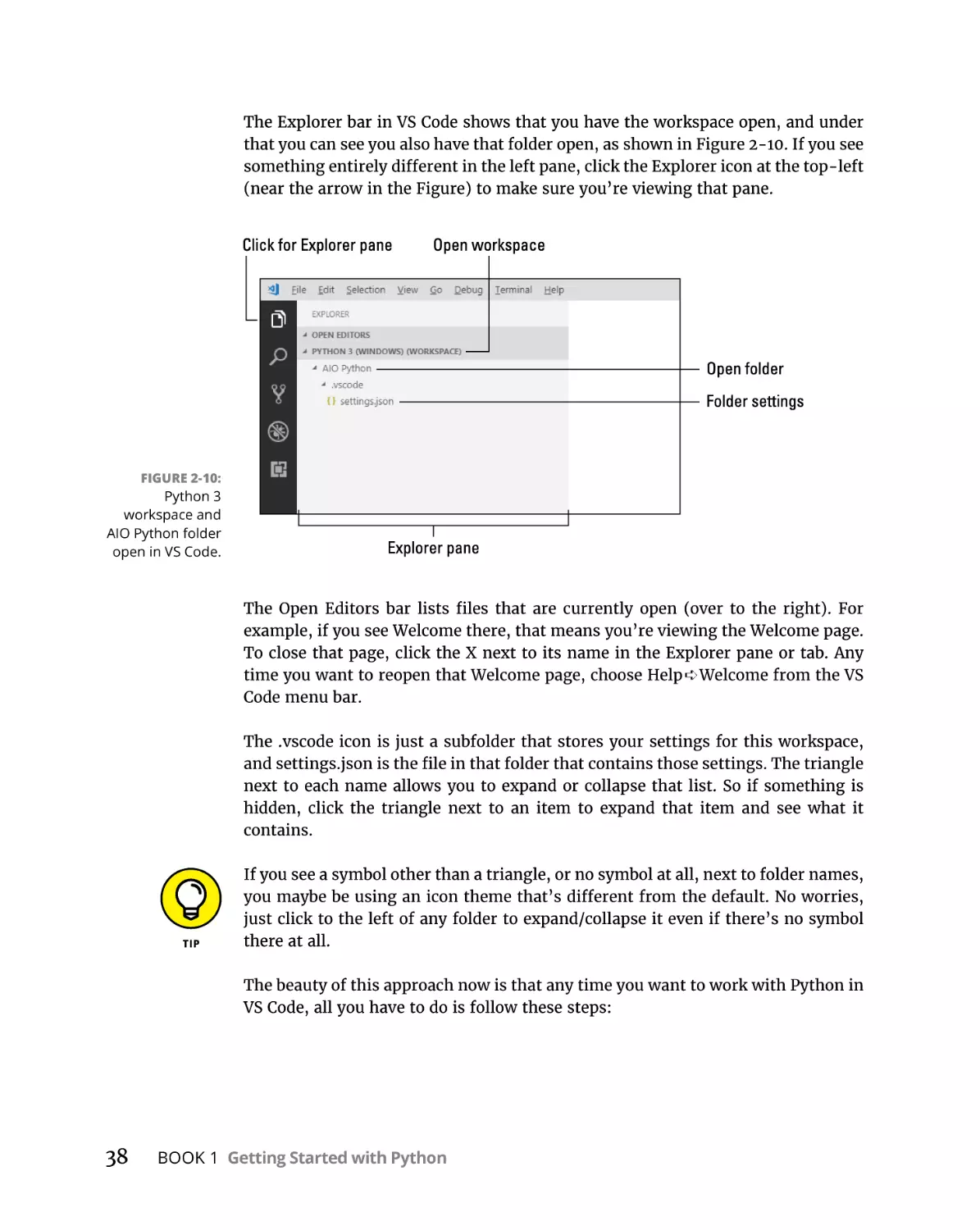
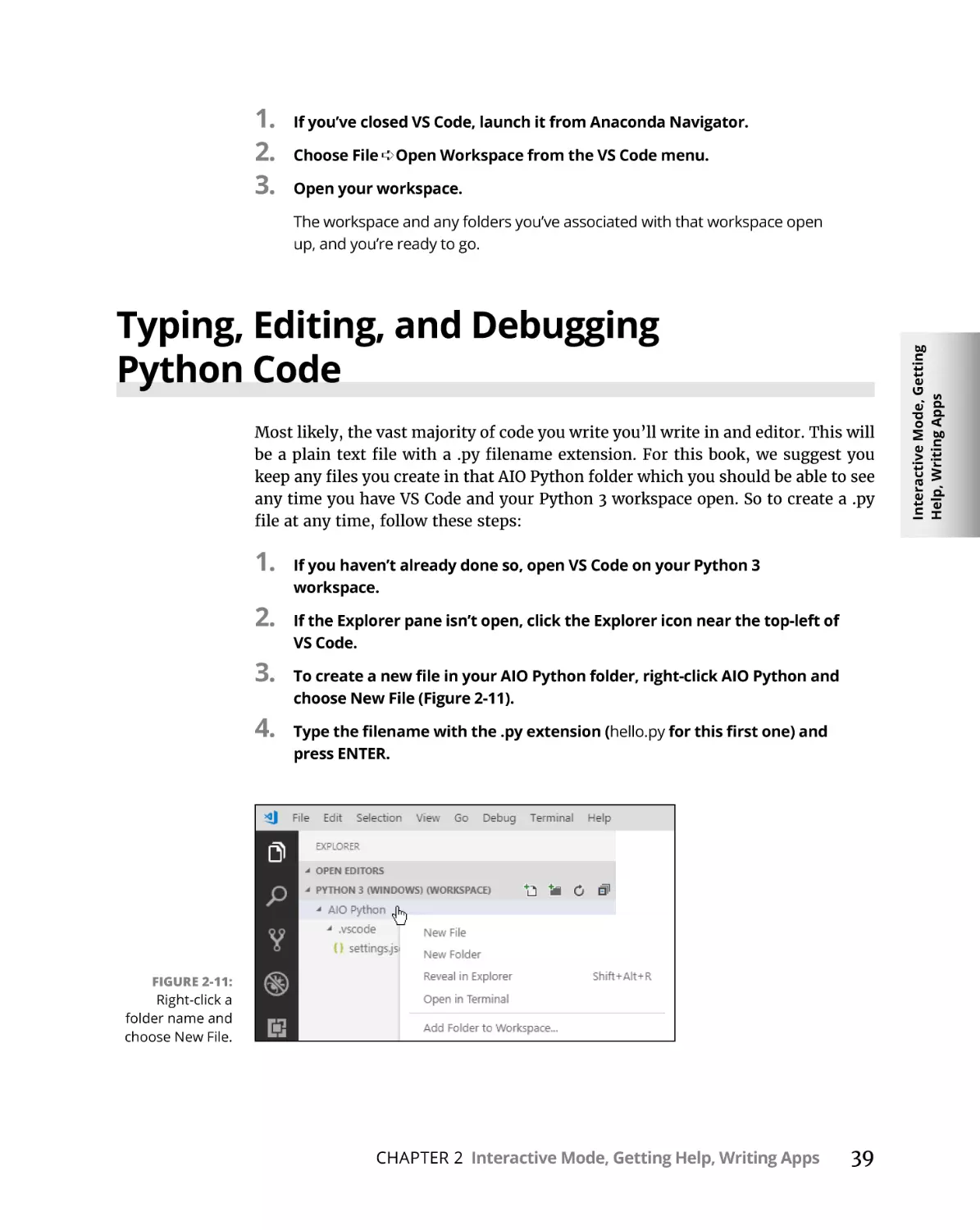
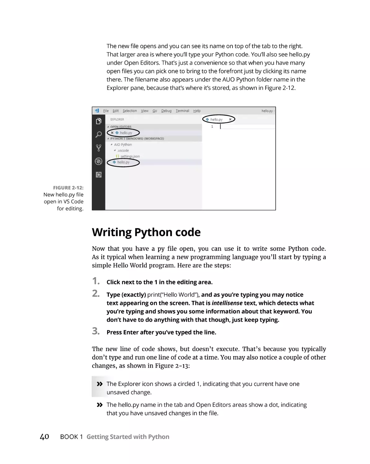
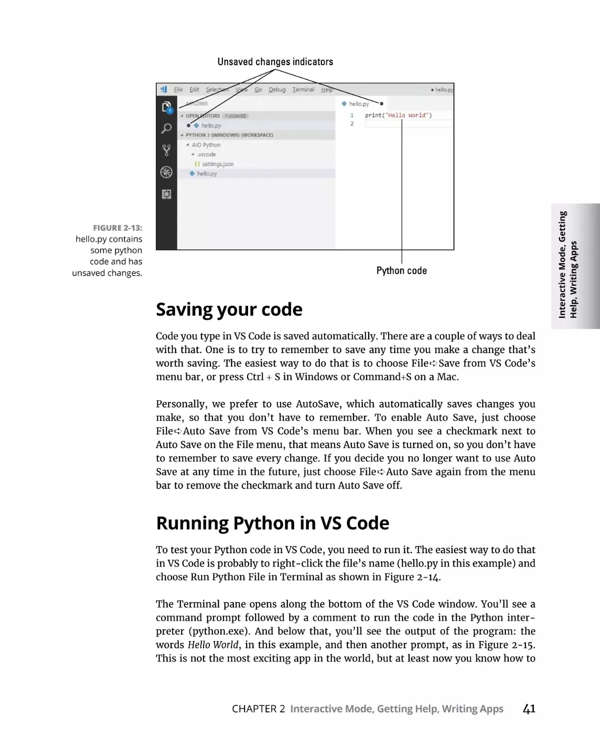
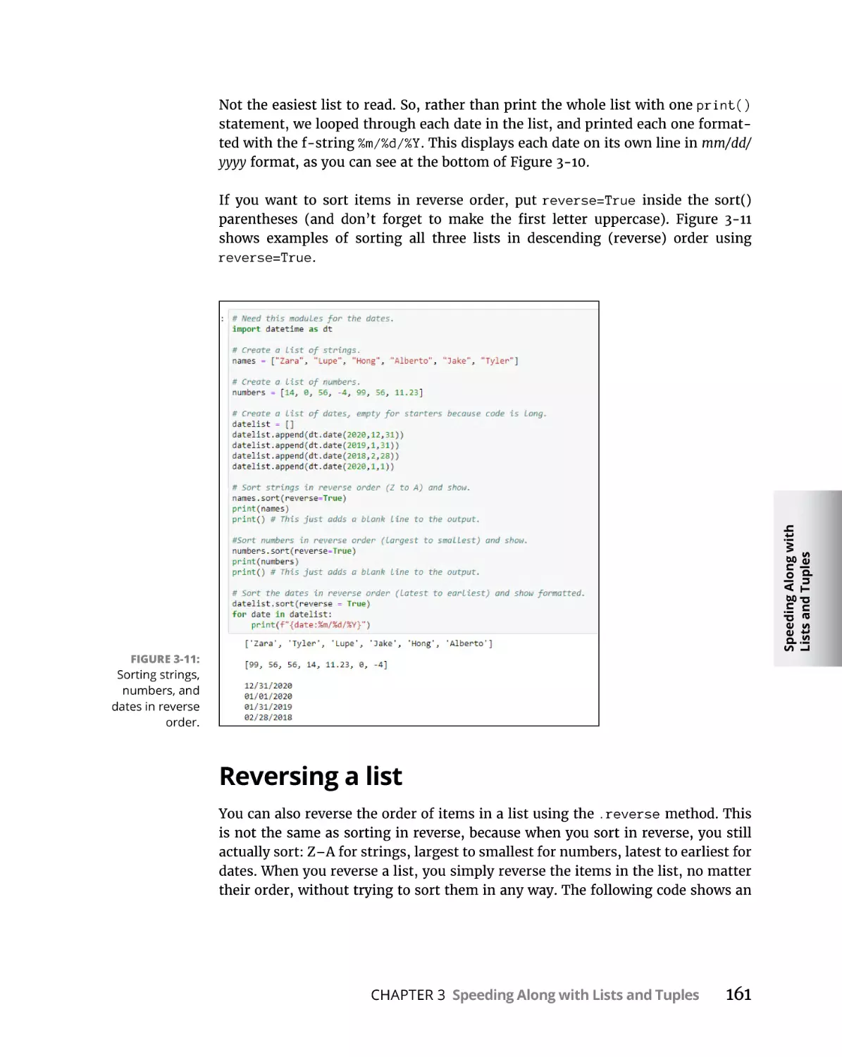
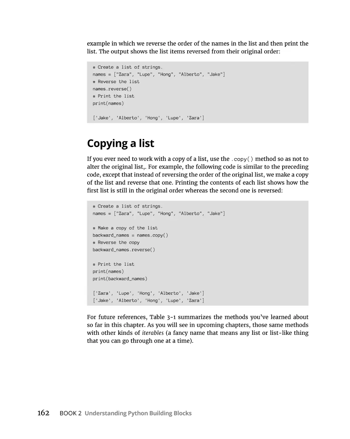
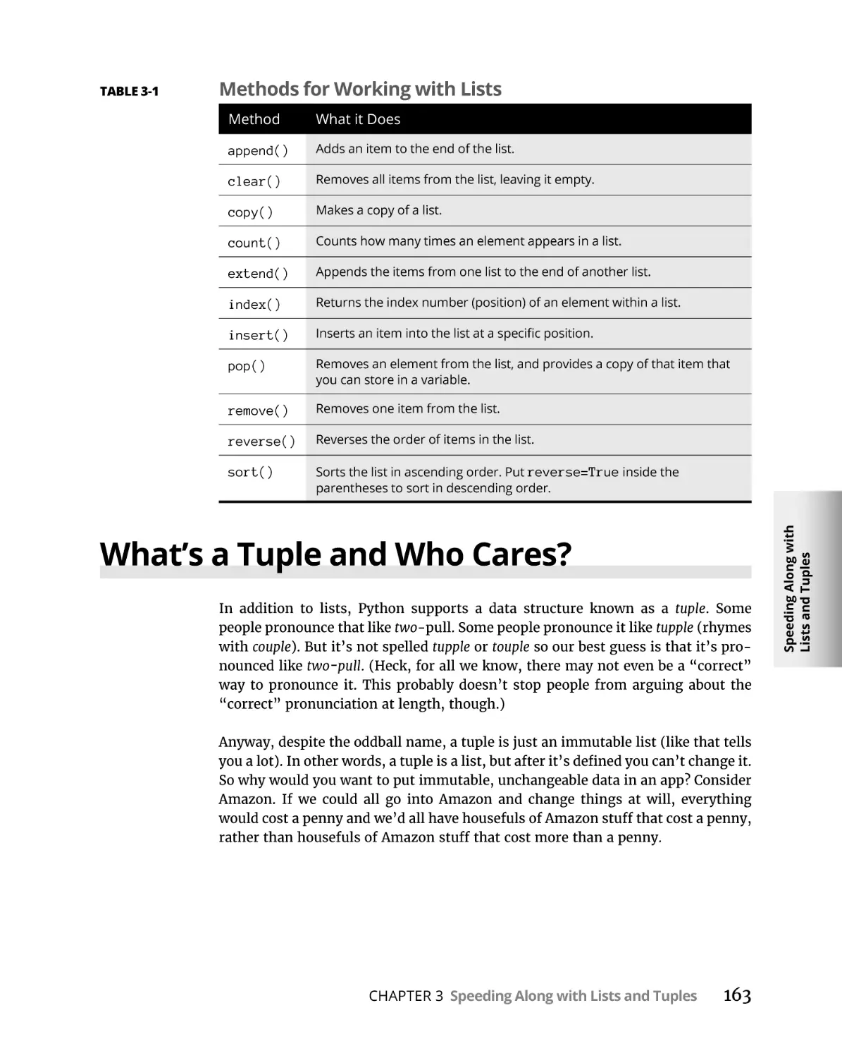
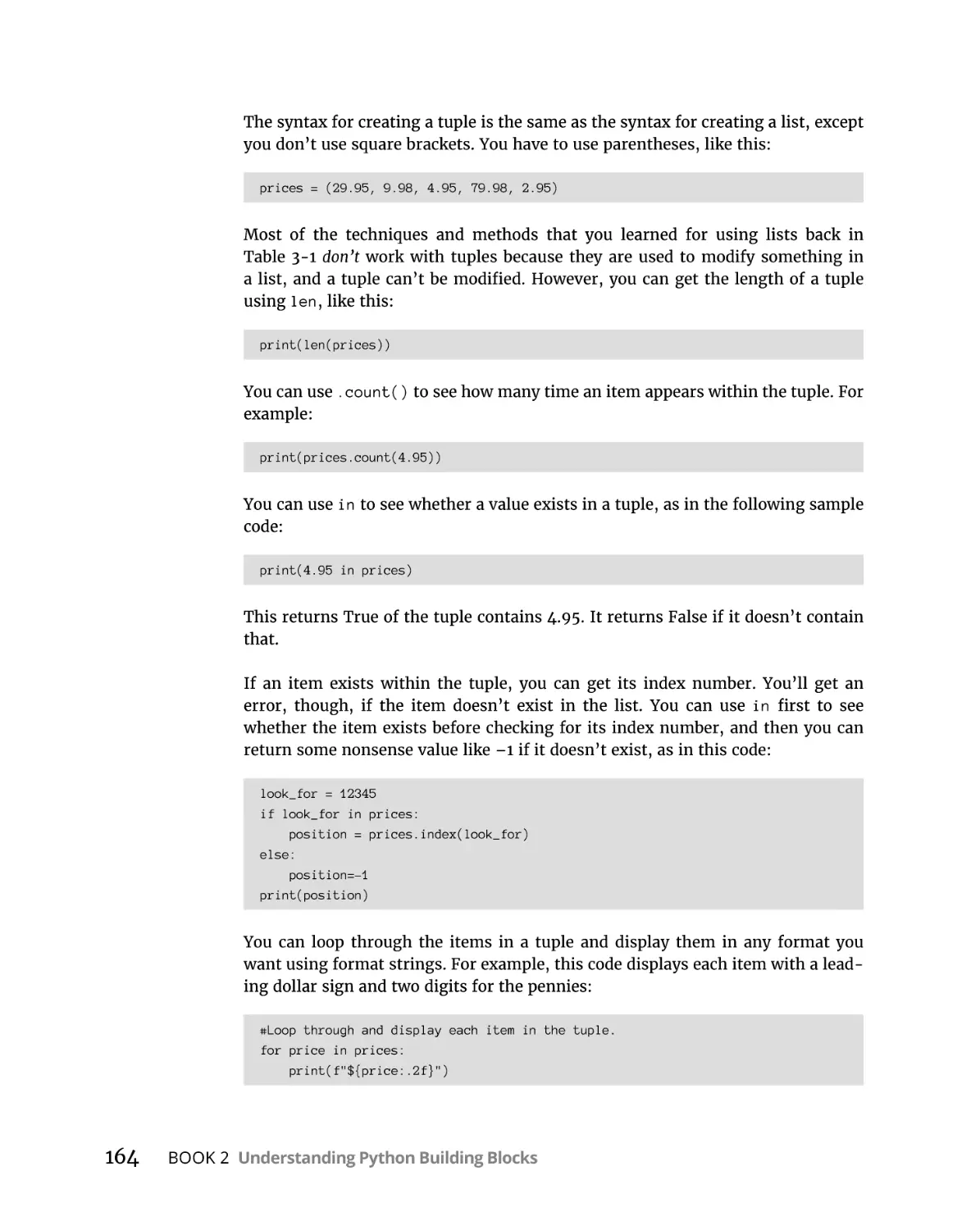
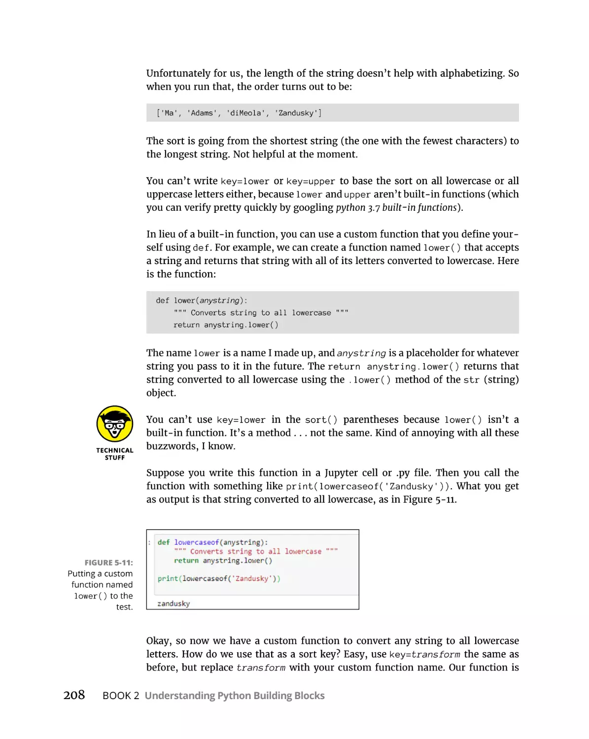
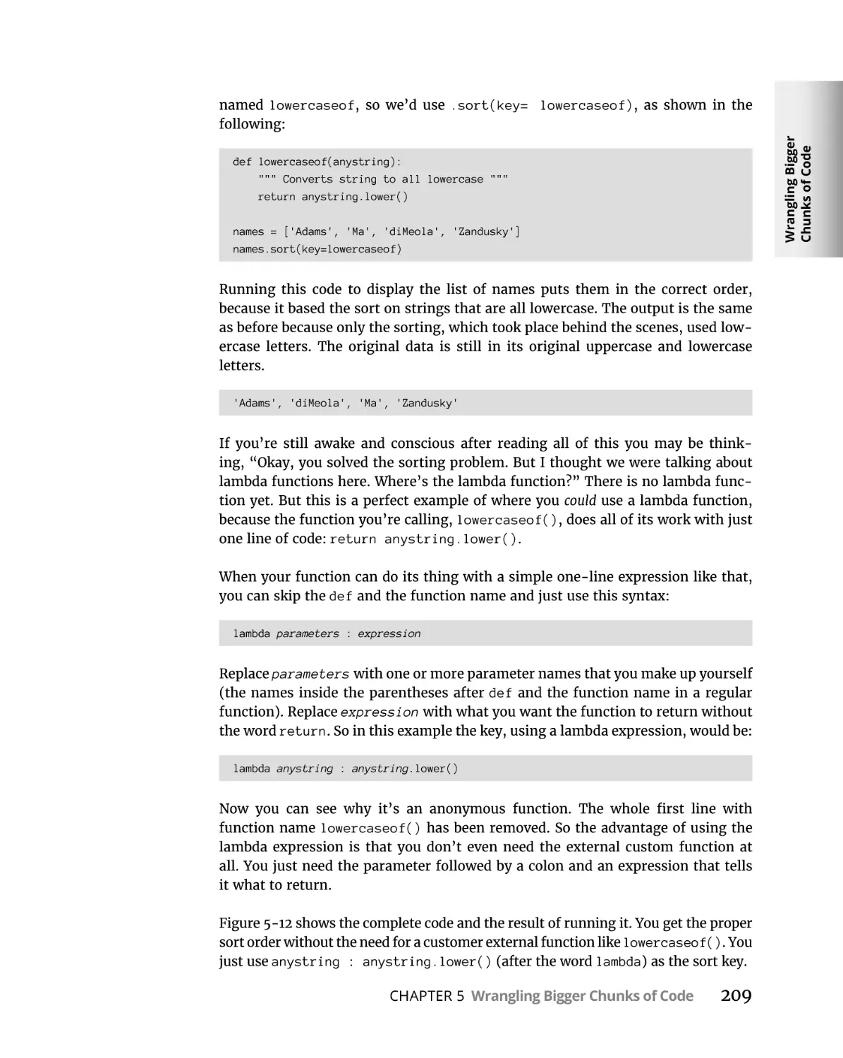
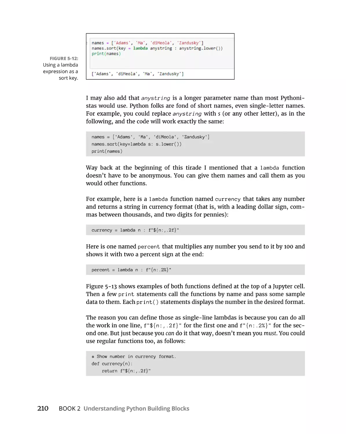
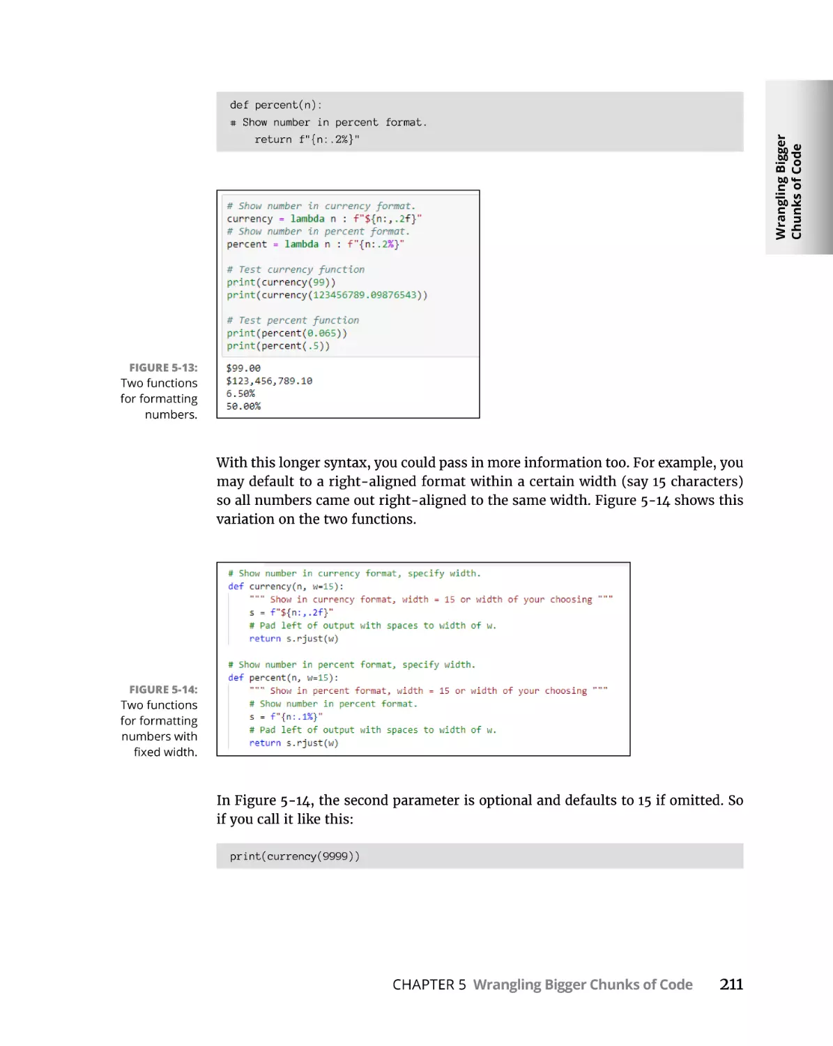
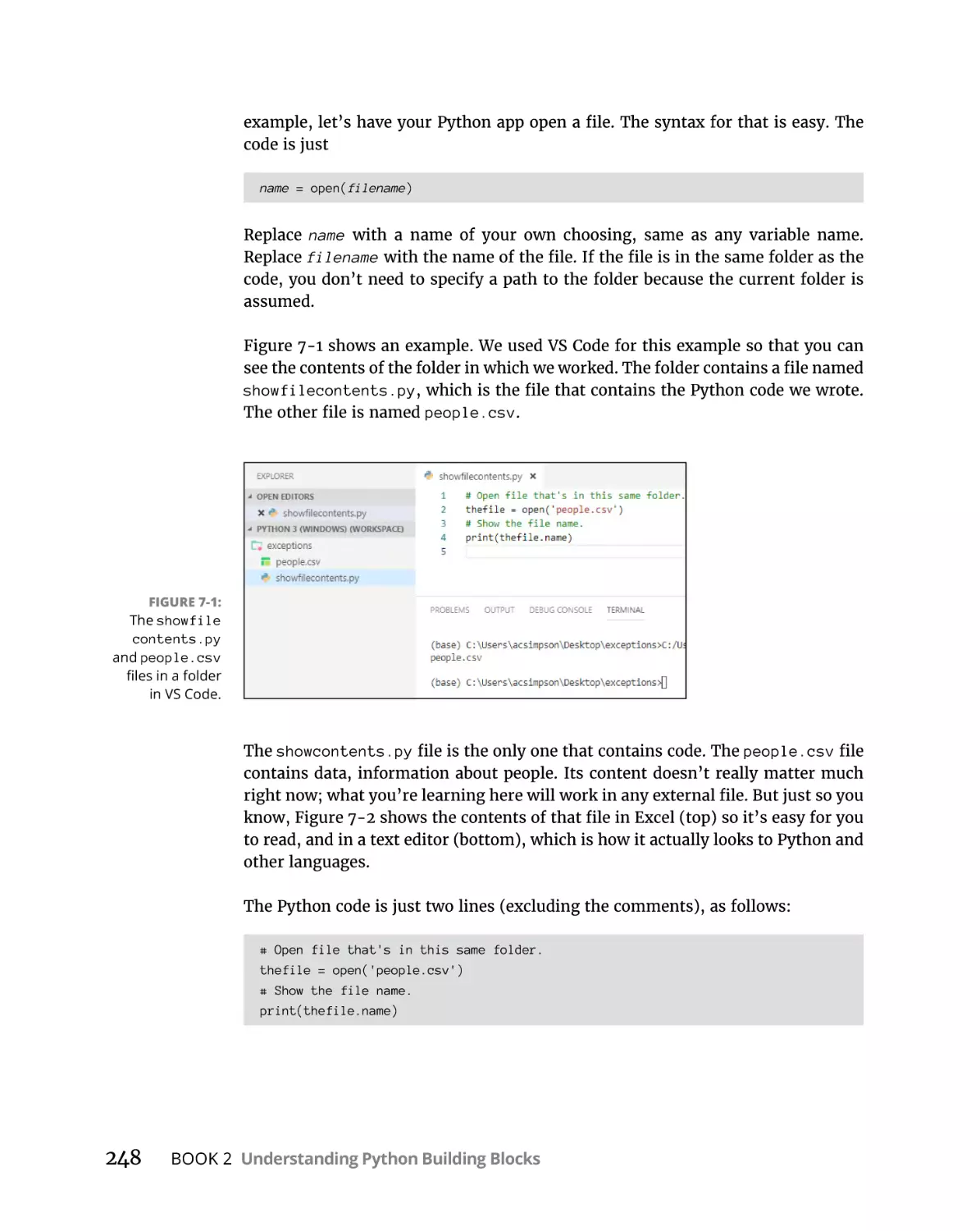
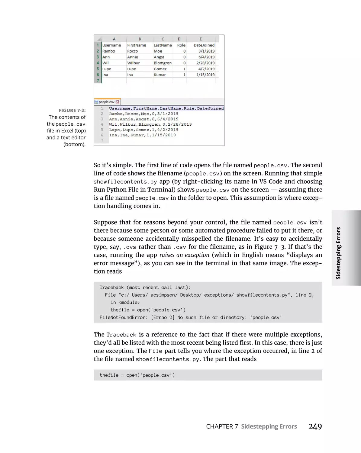
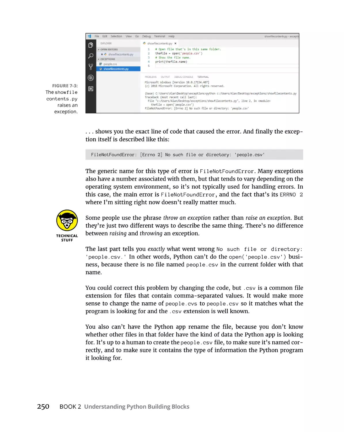
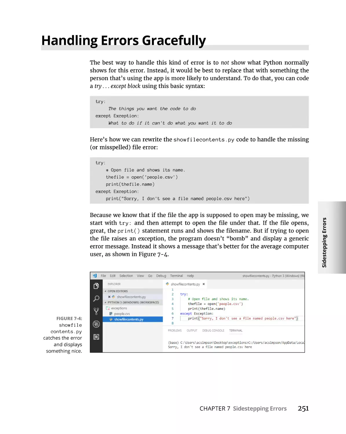
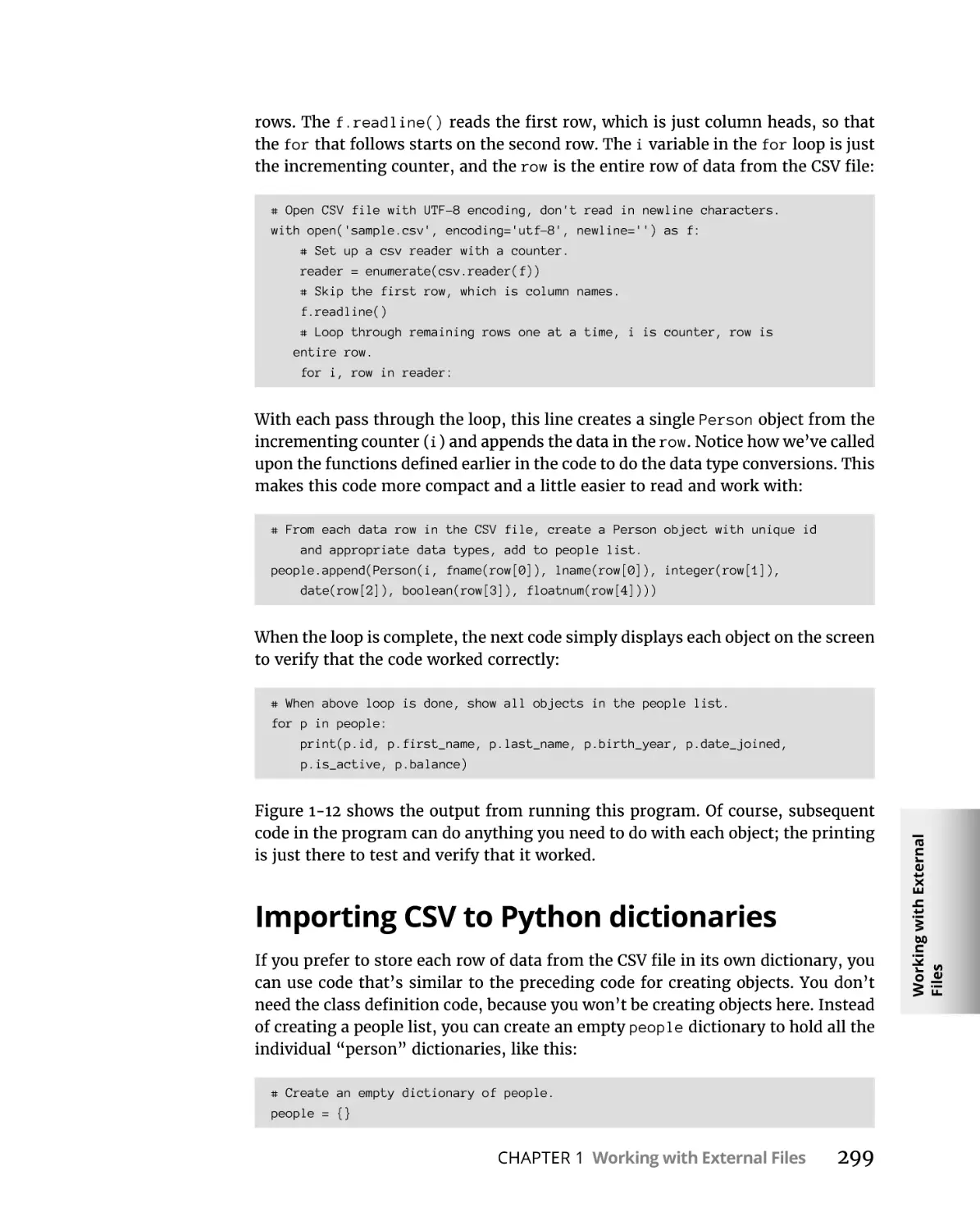
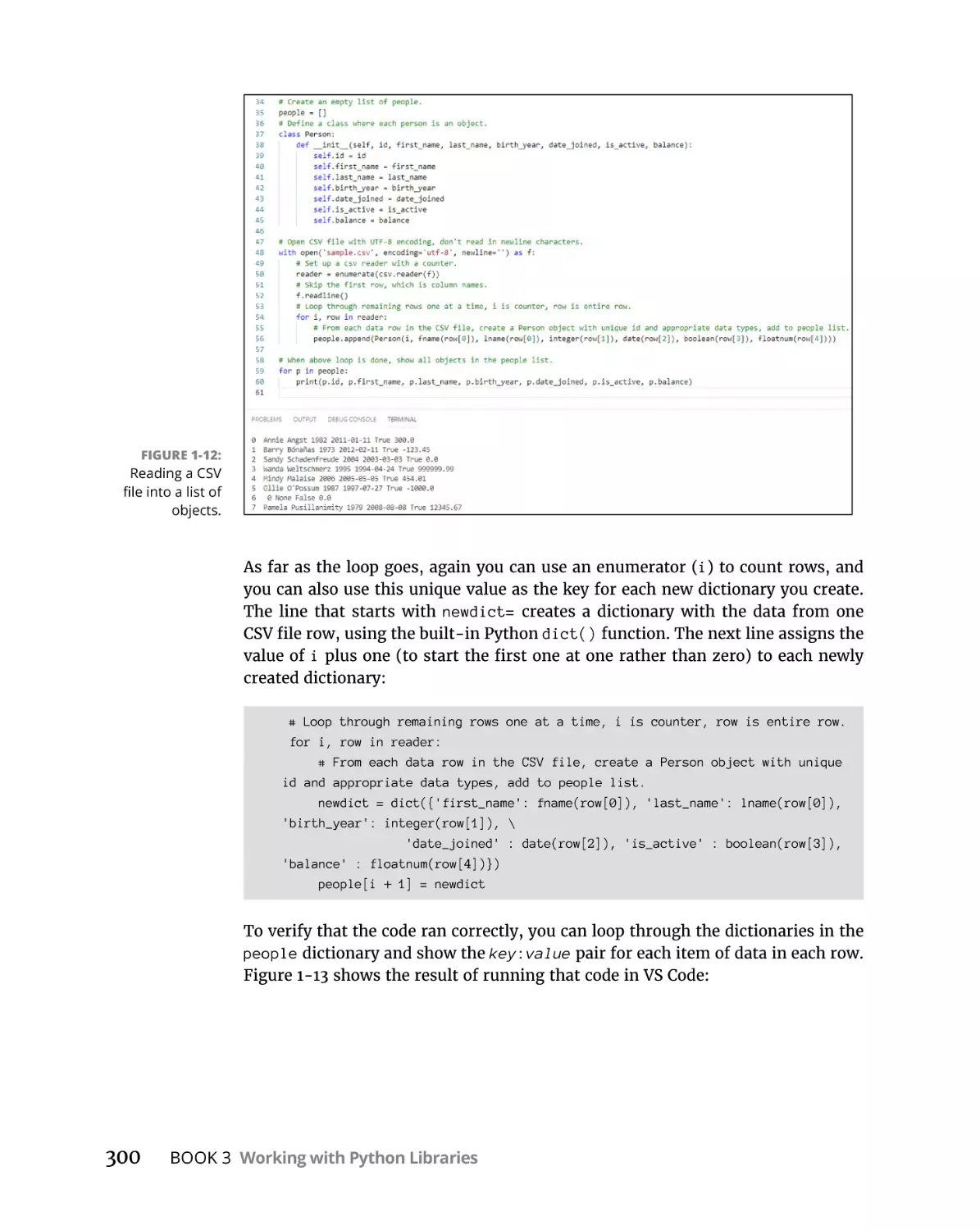
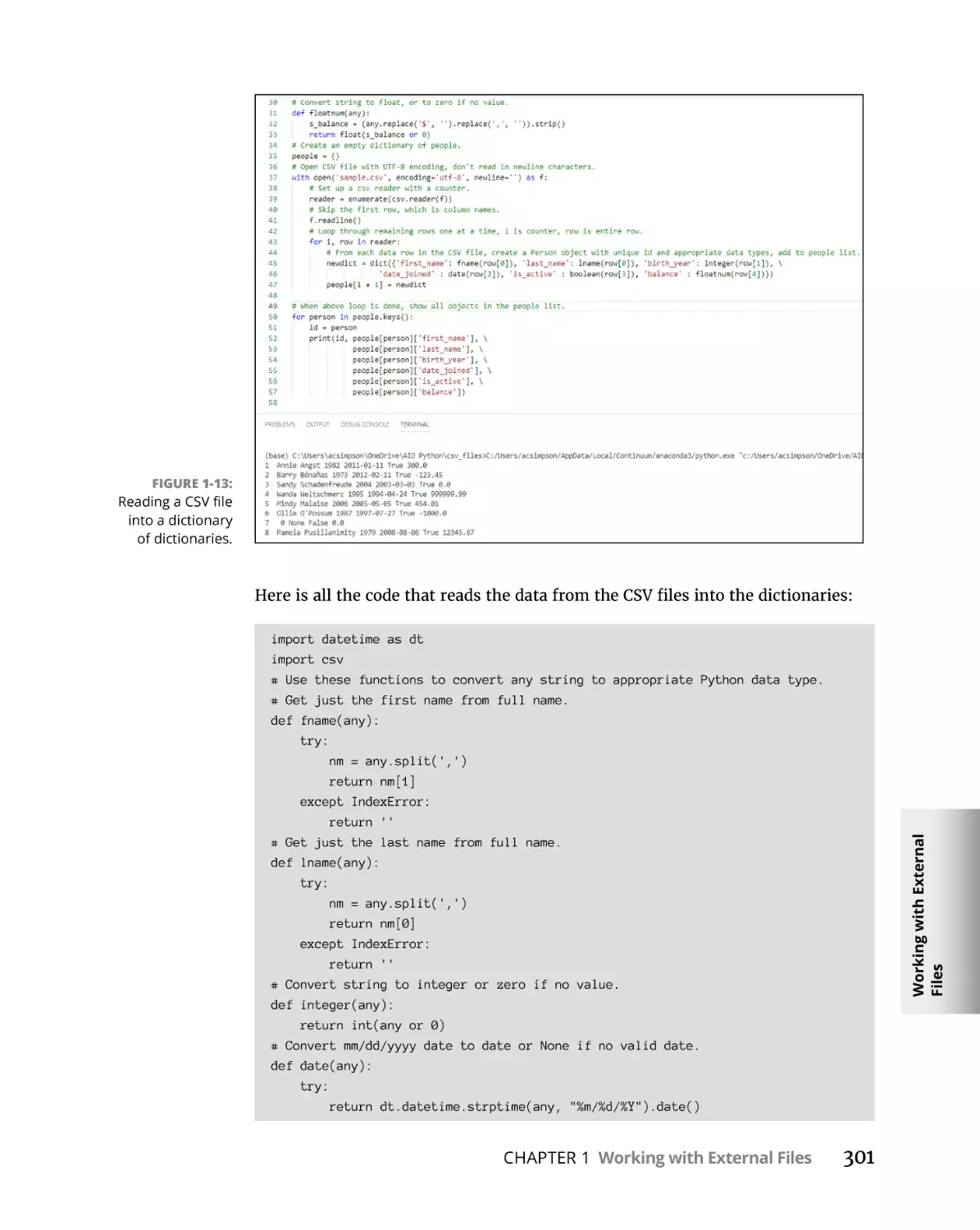
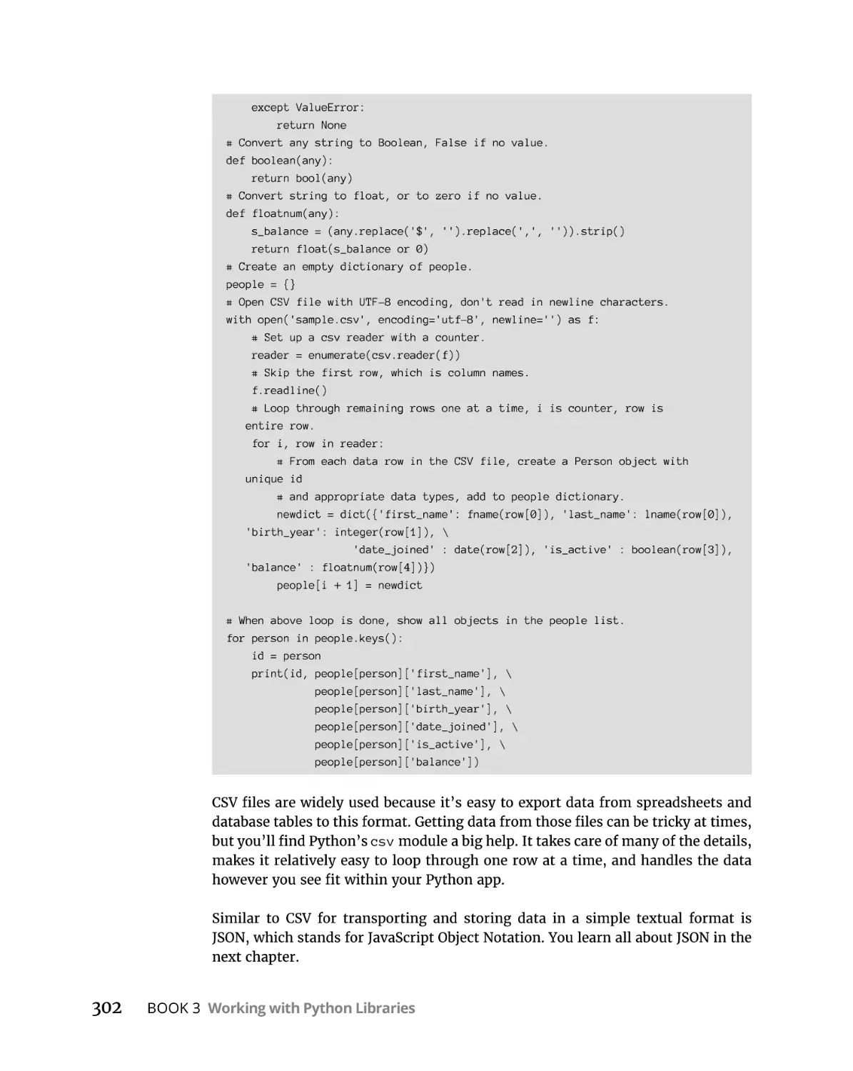
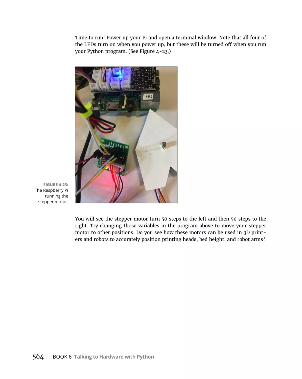
/


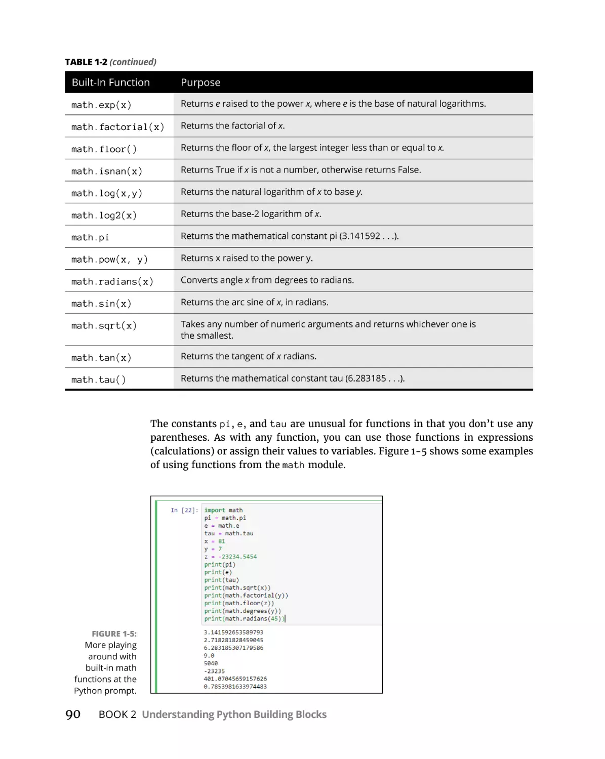


Author: Shovic J. Simpson A.
Tags: programming python programming language
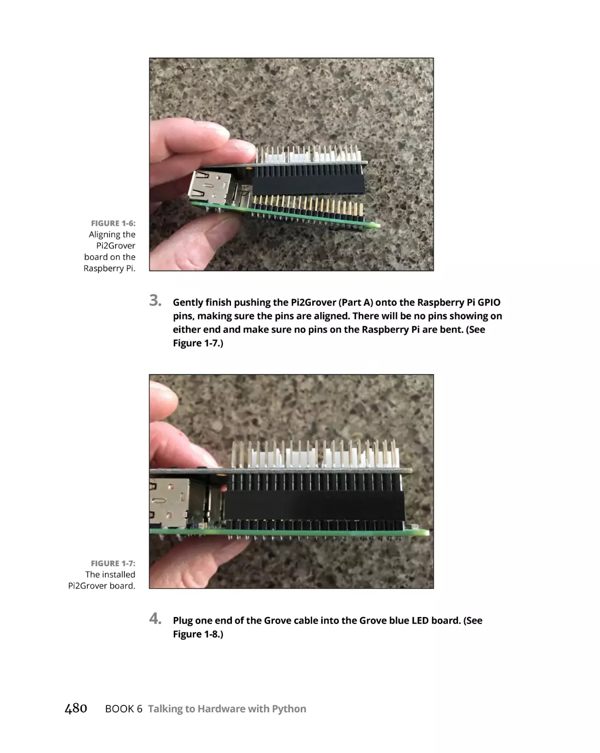
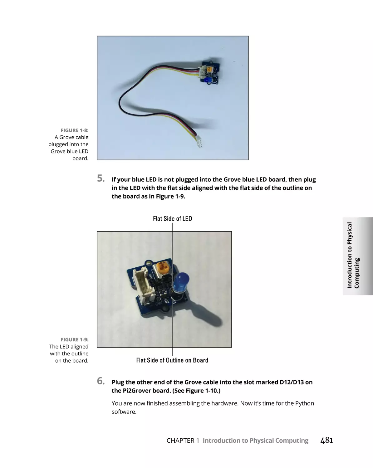
ISBN: 978-1-119-55759-3
Year: 2019

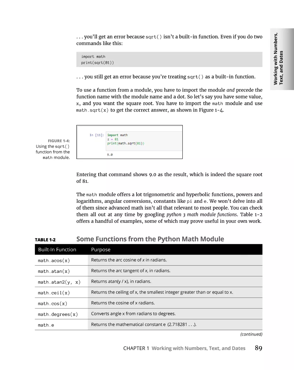
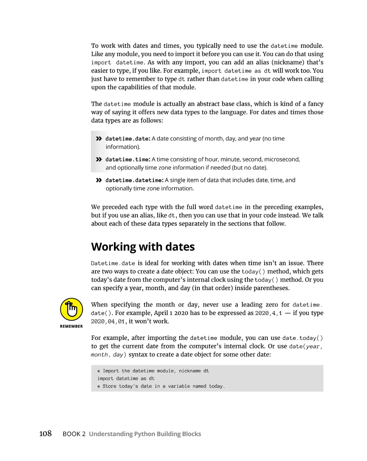
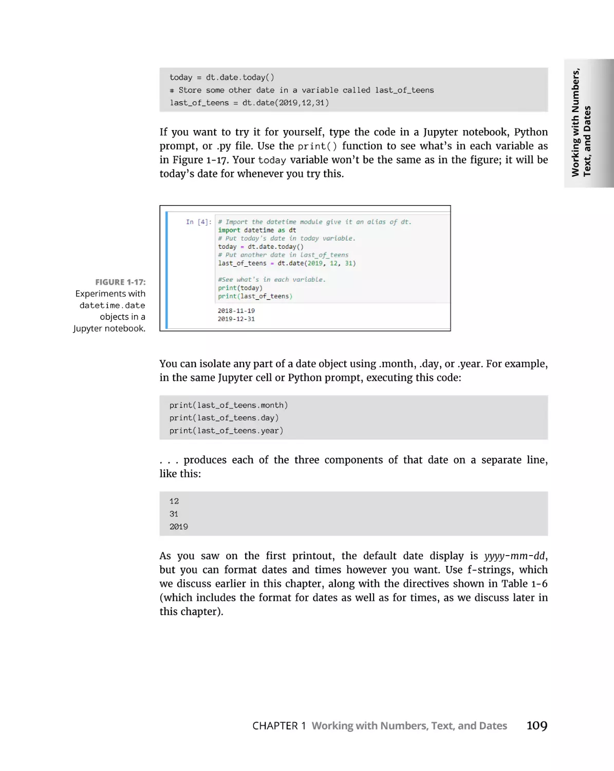
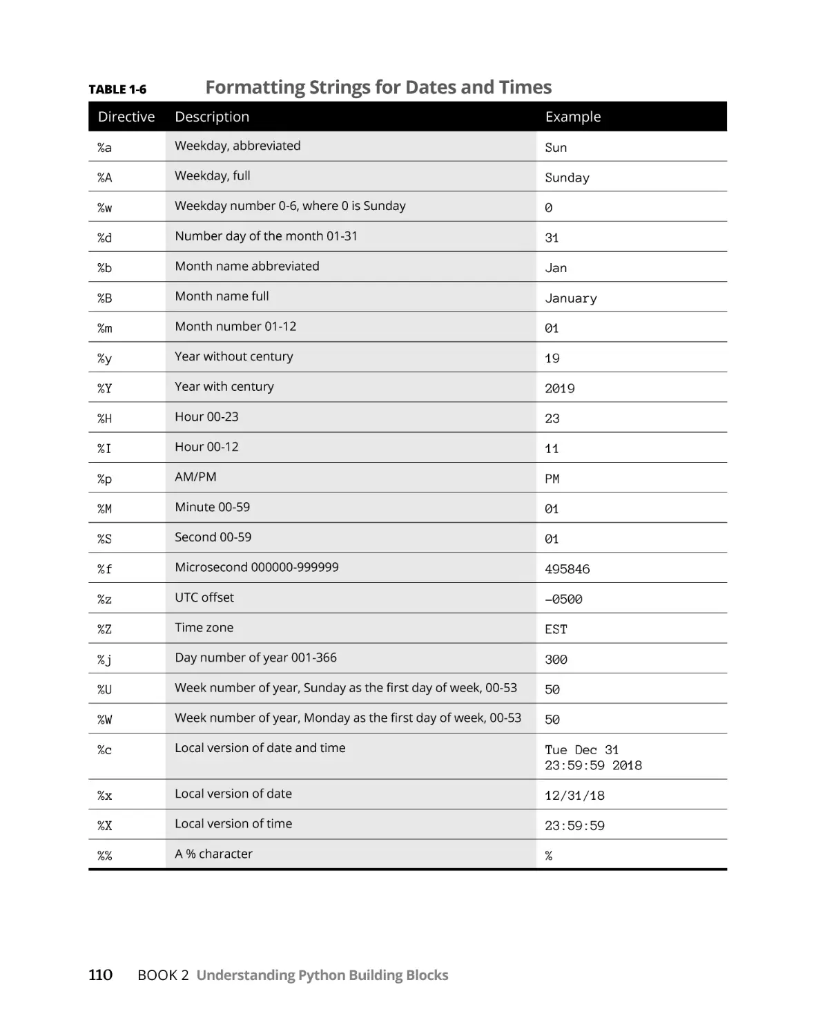
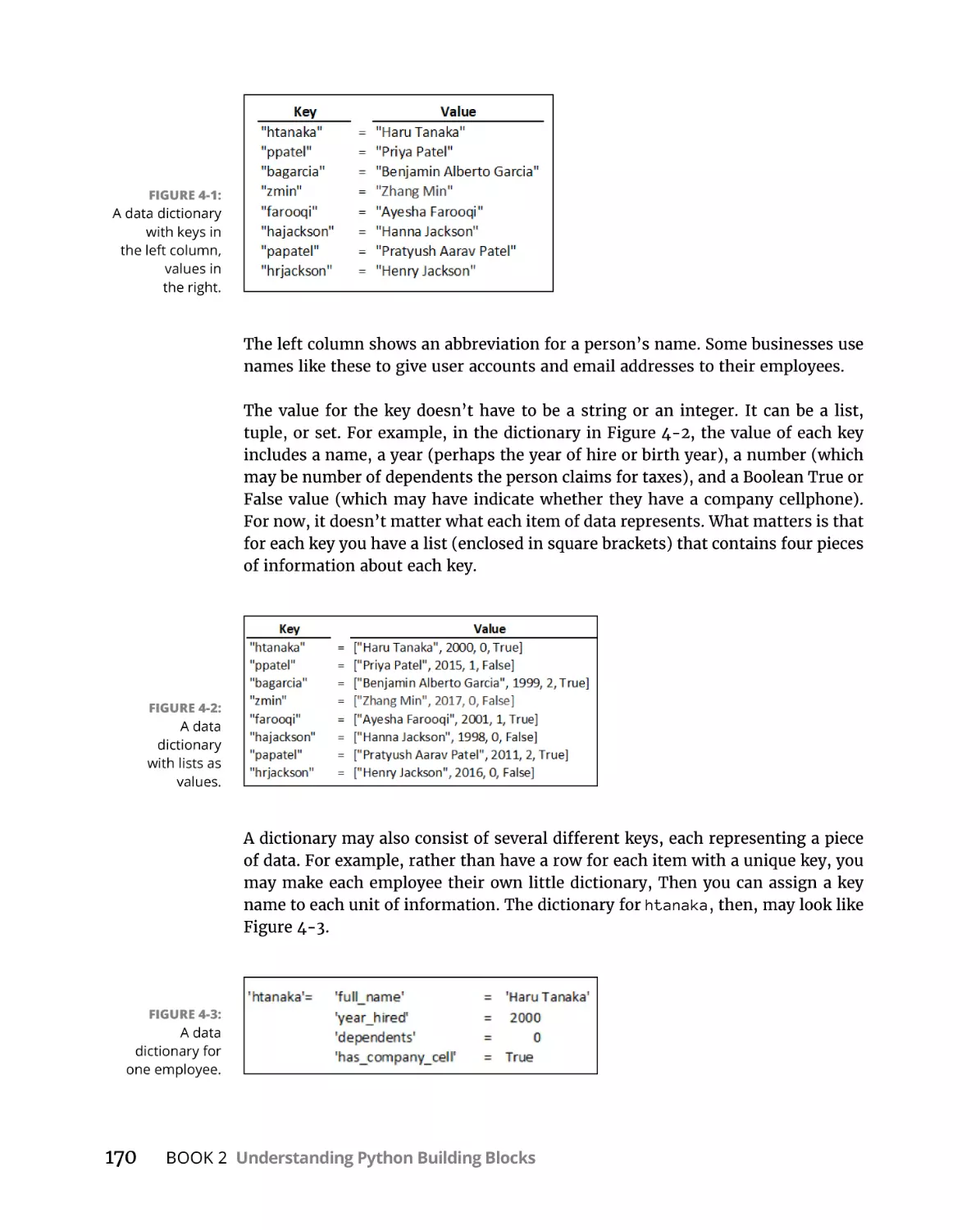
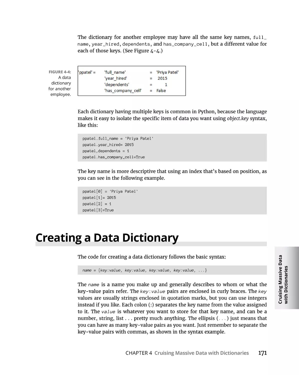
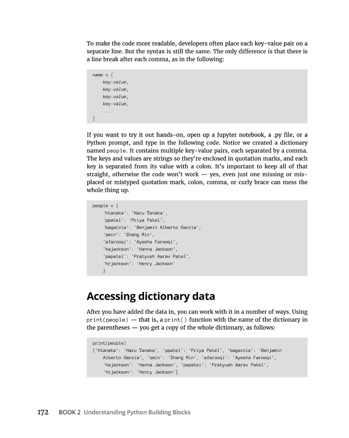
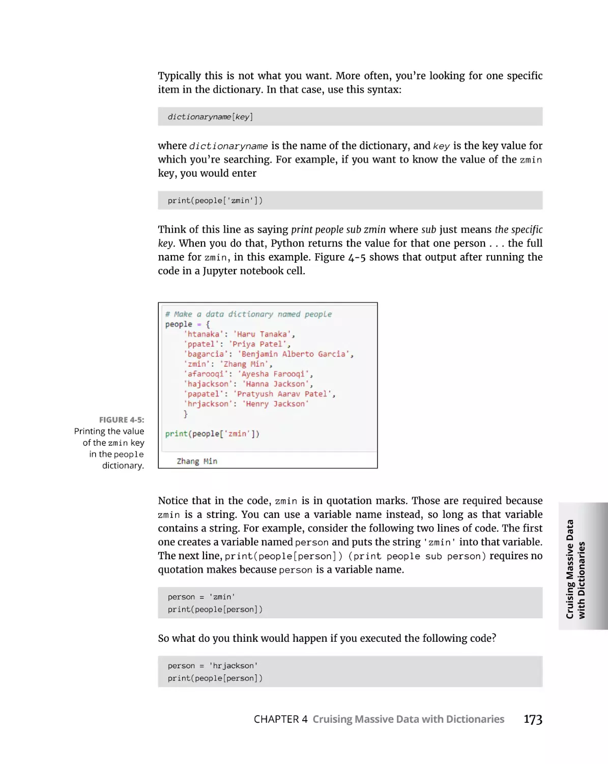
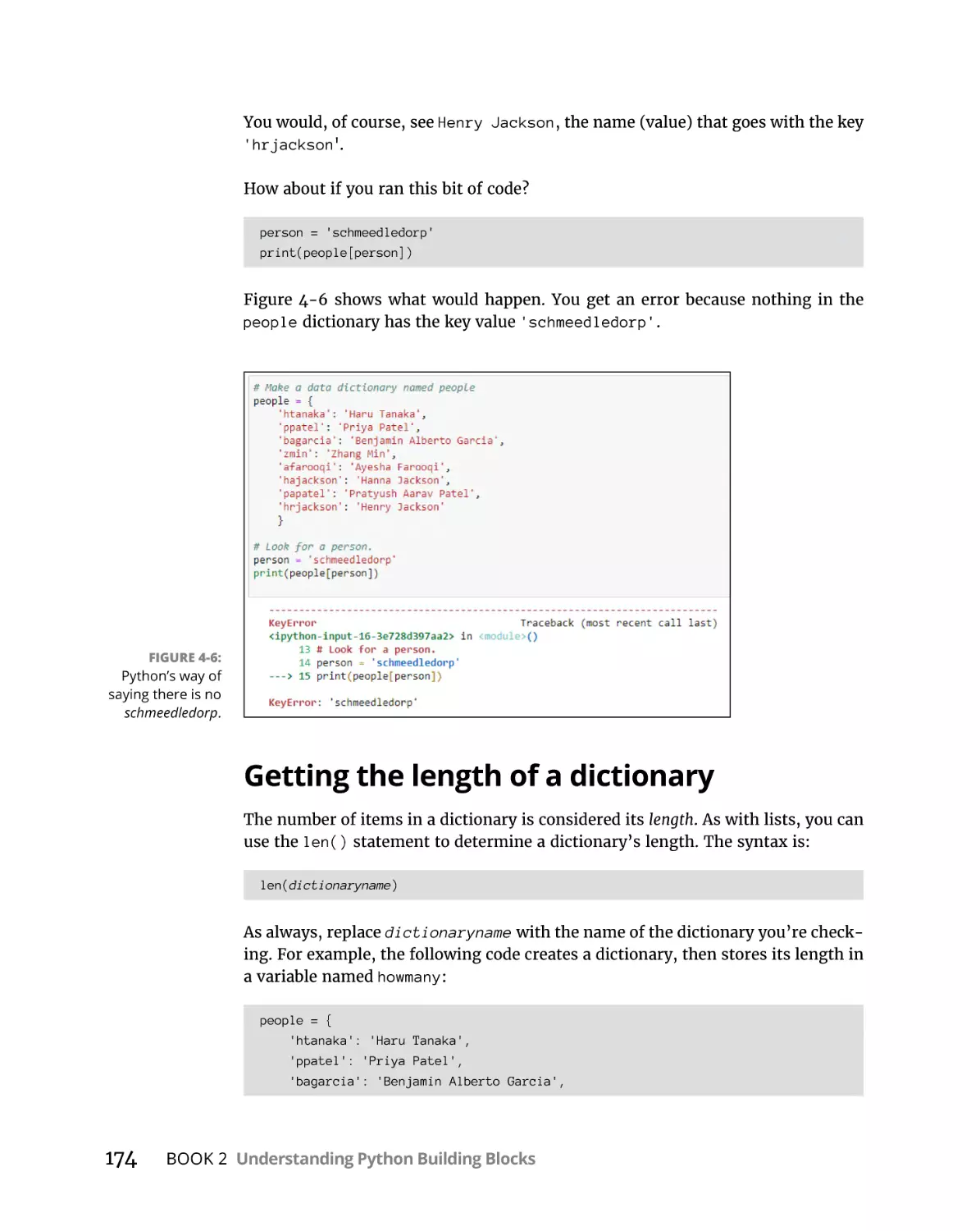
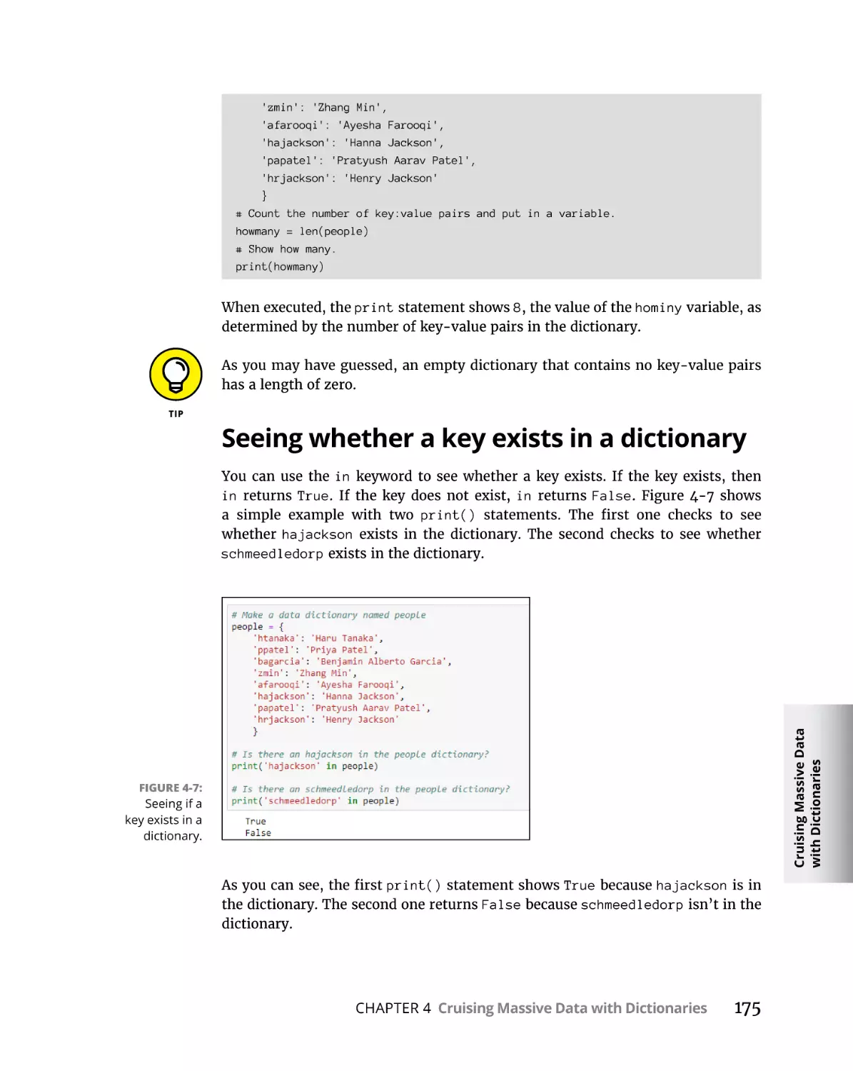
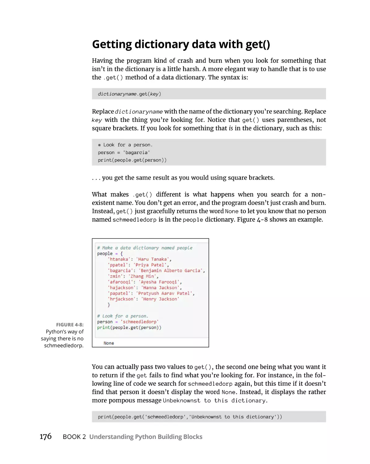
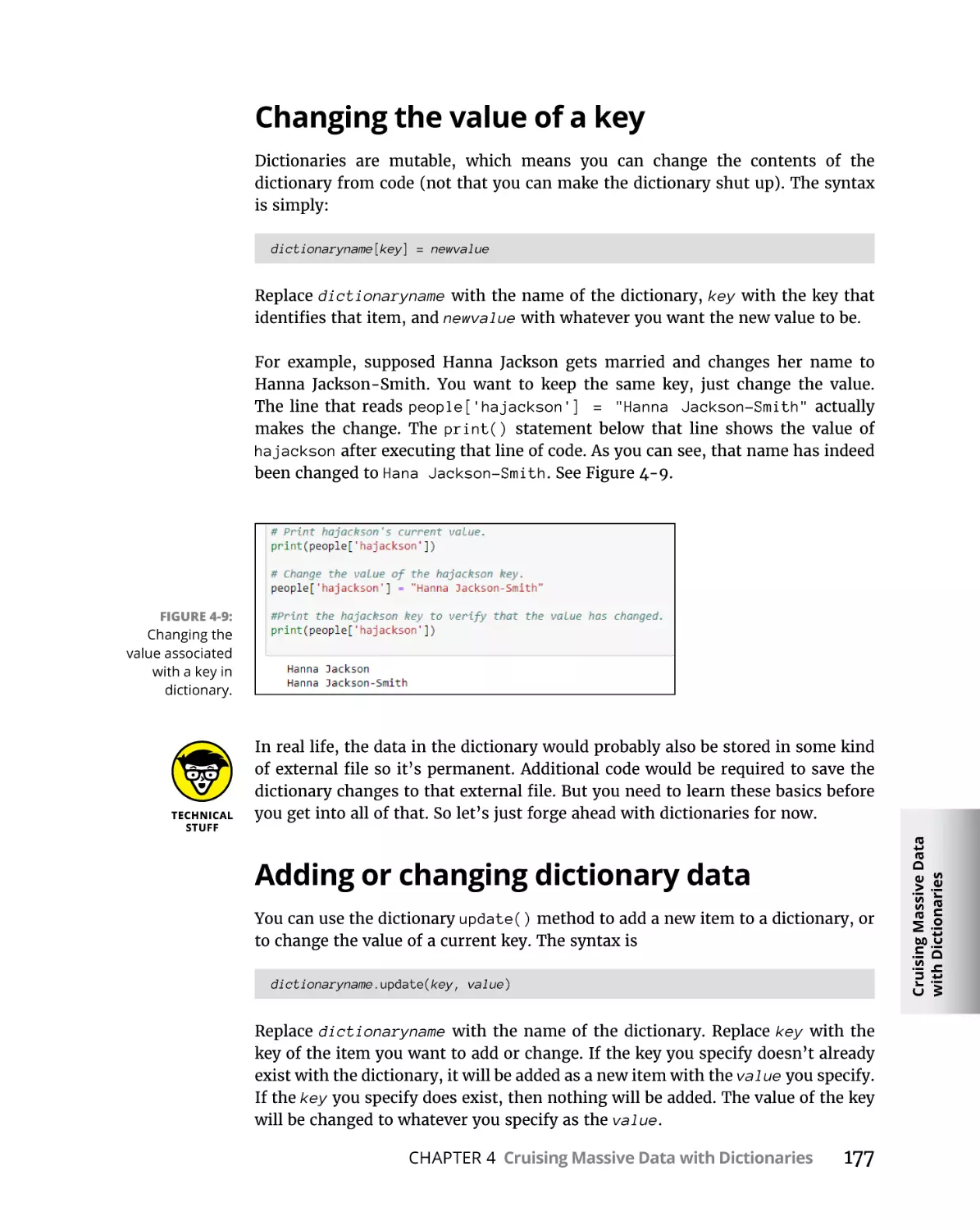
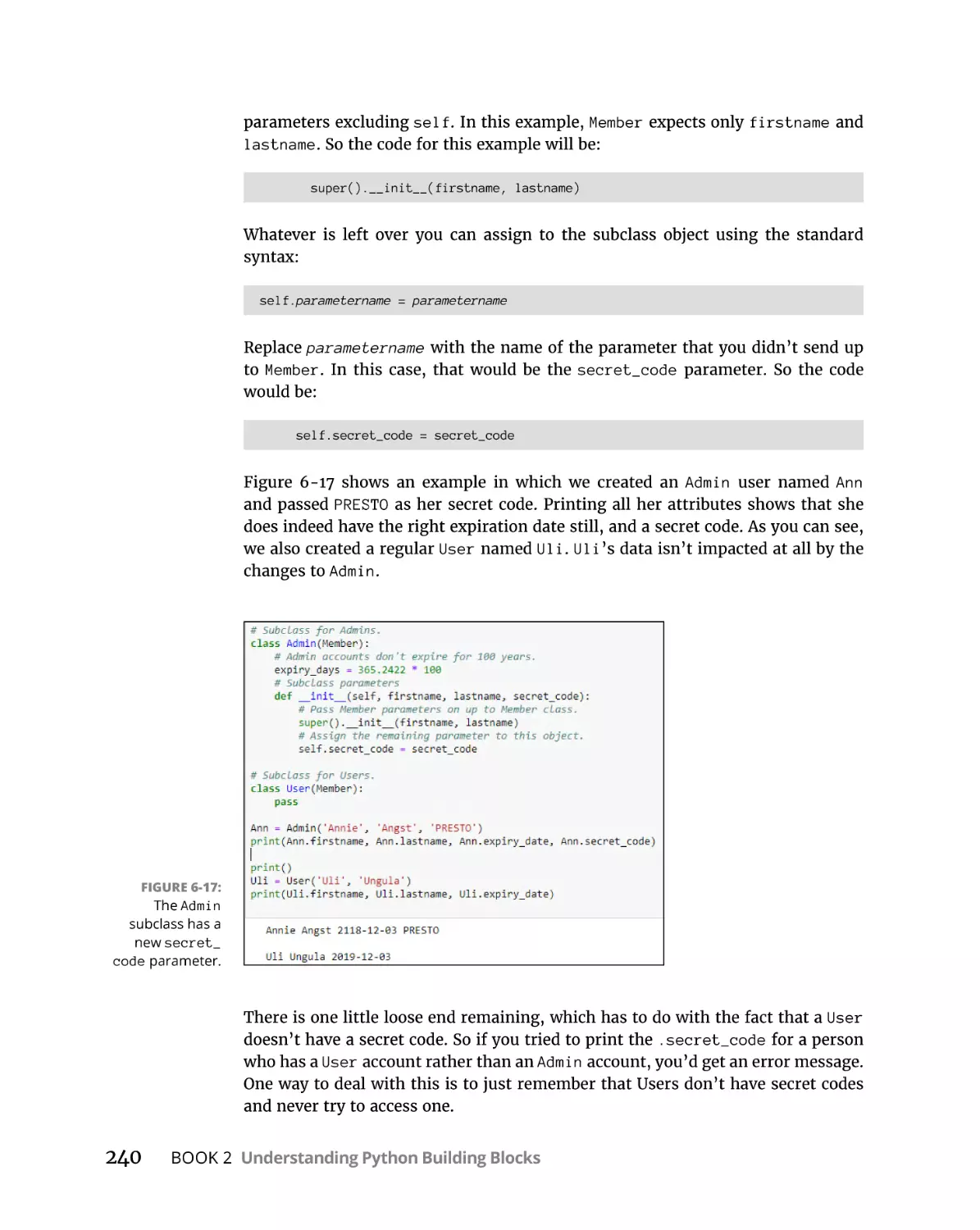
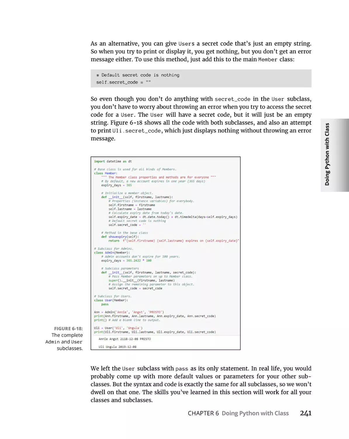
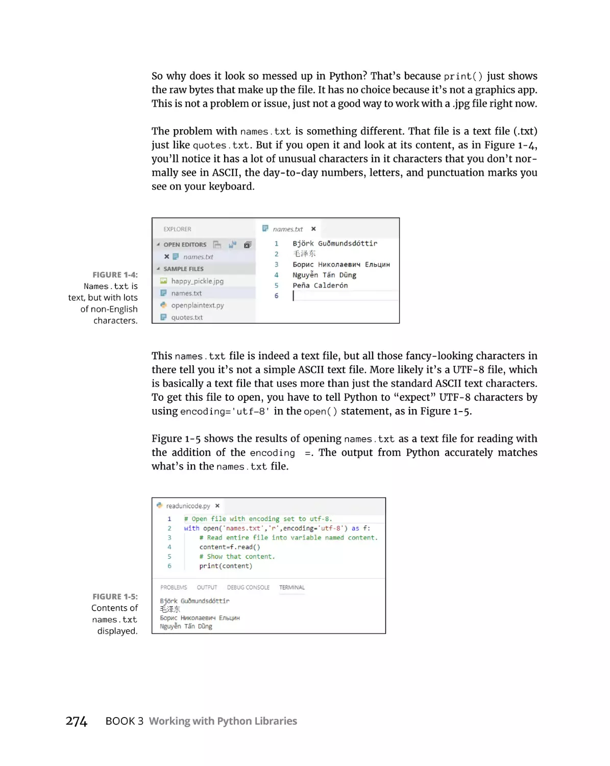
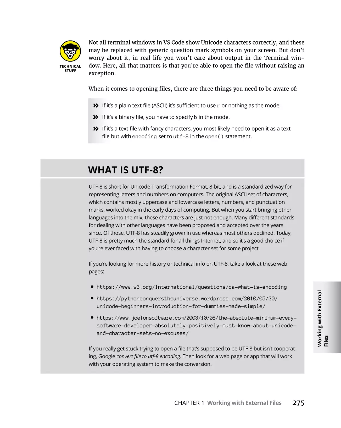
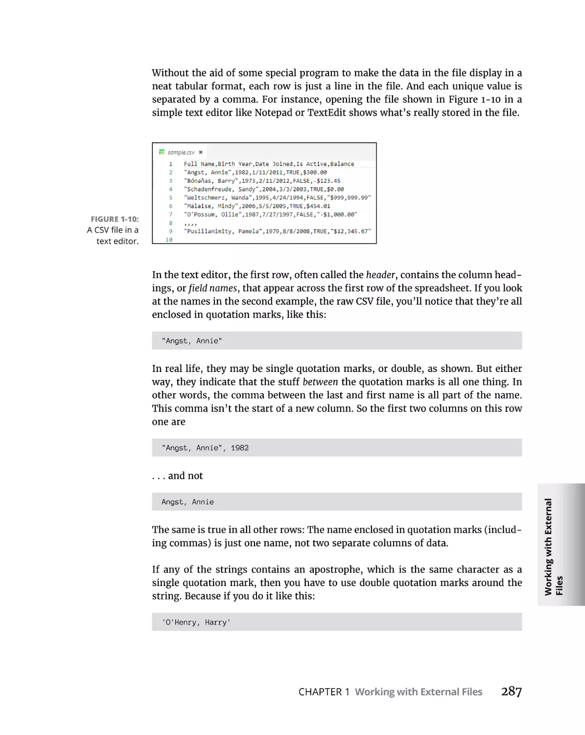
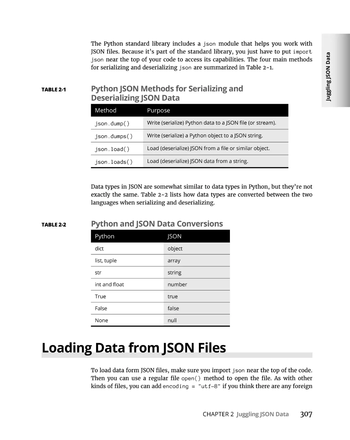
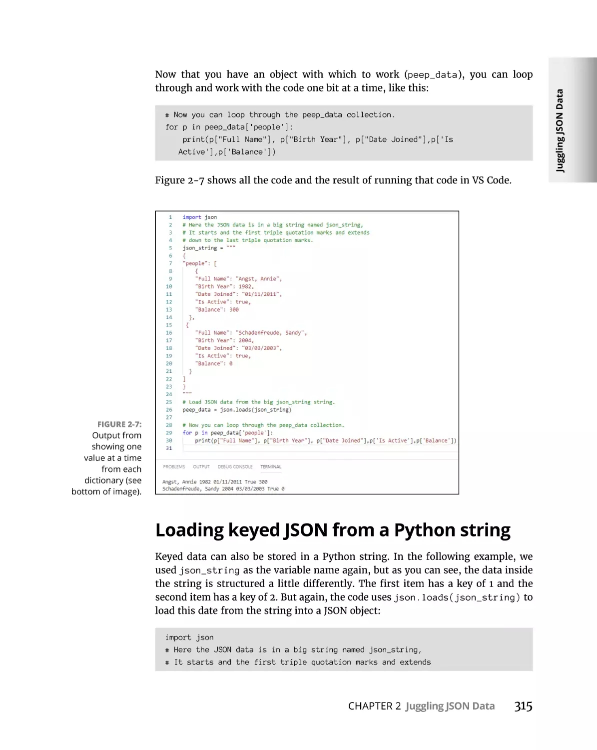
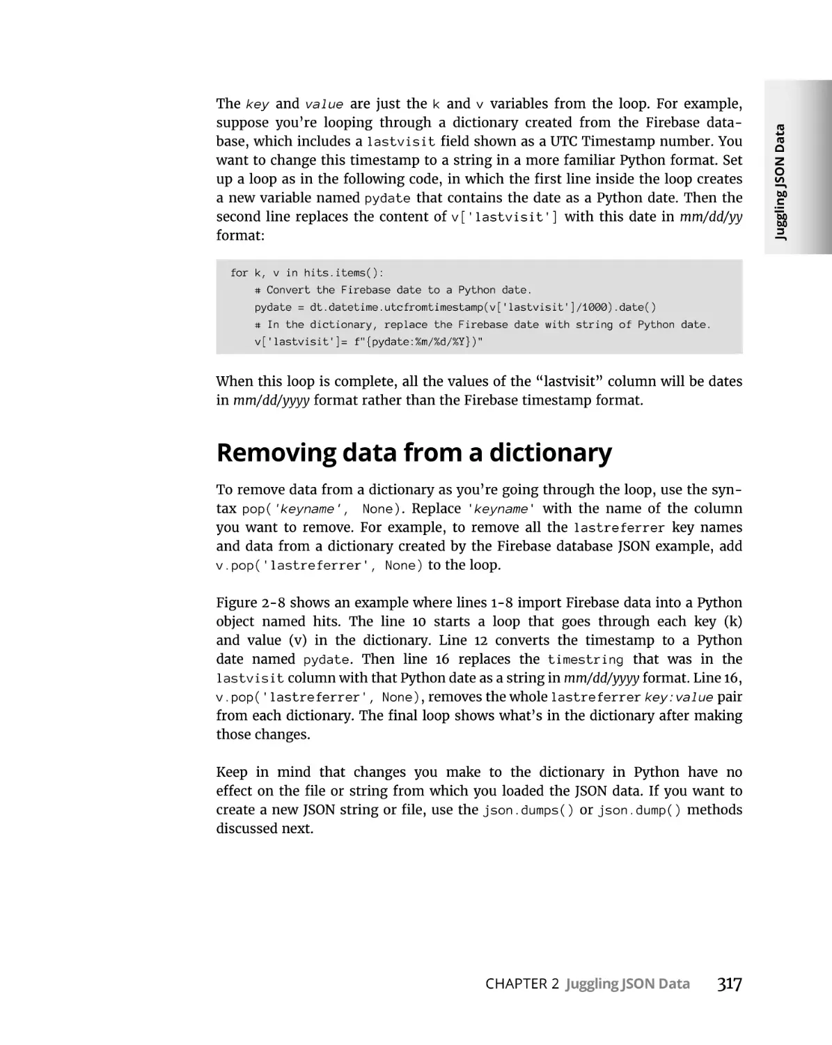
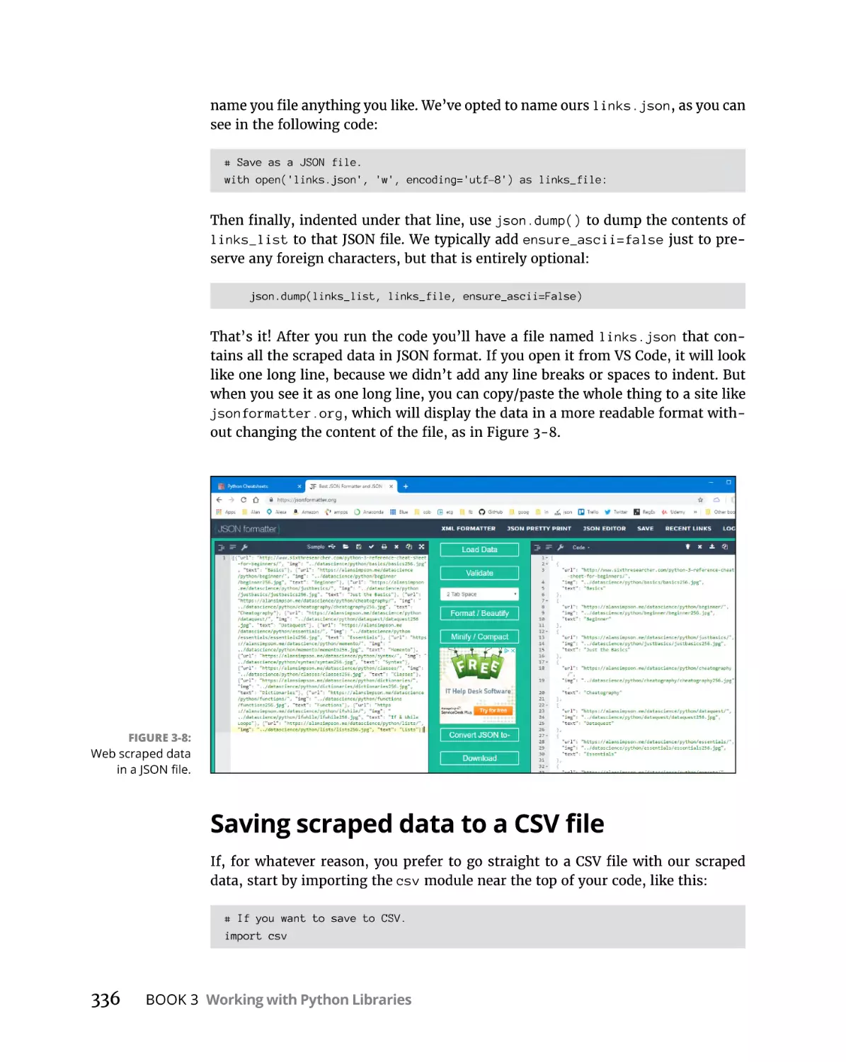
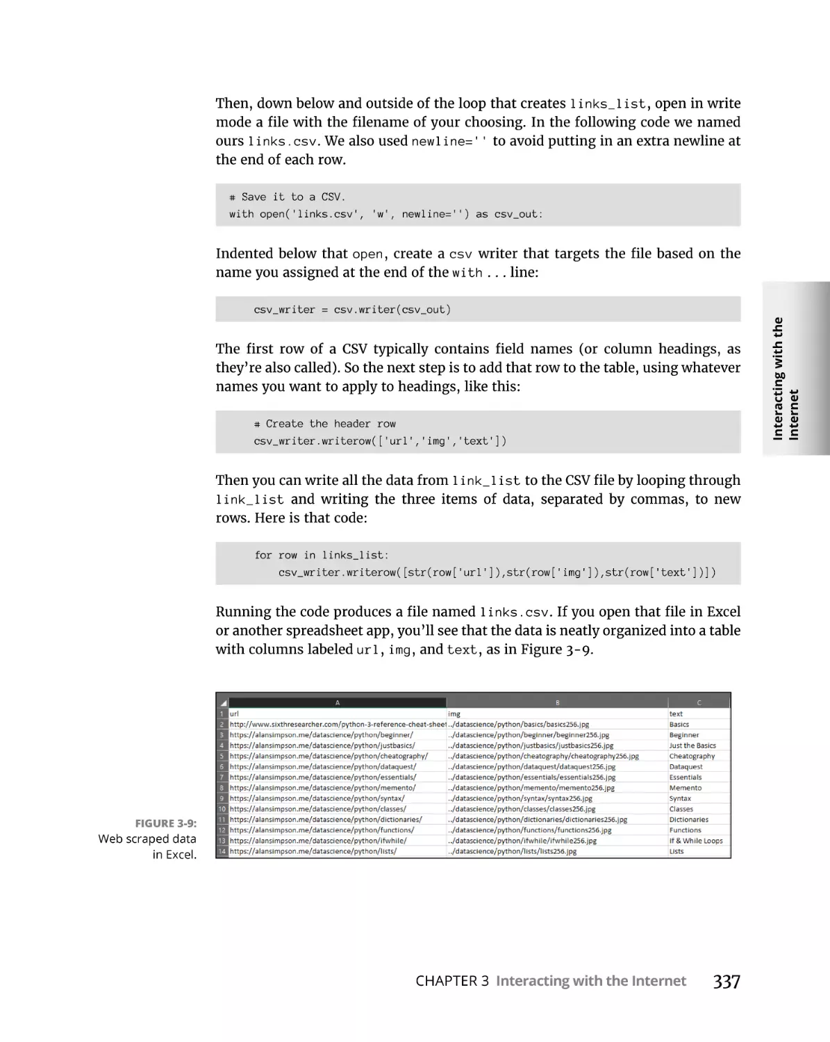
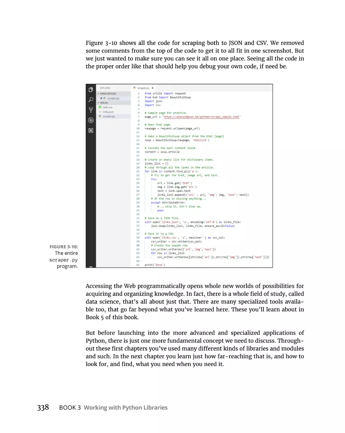
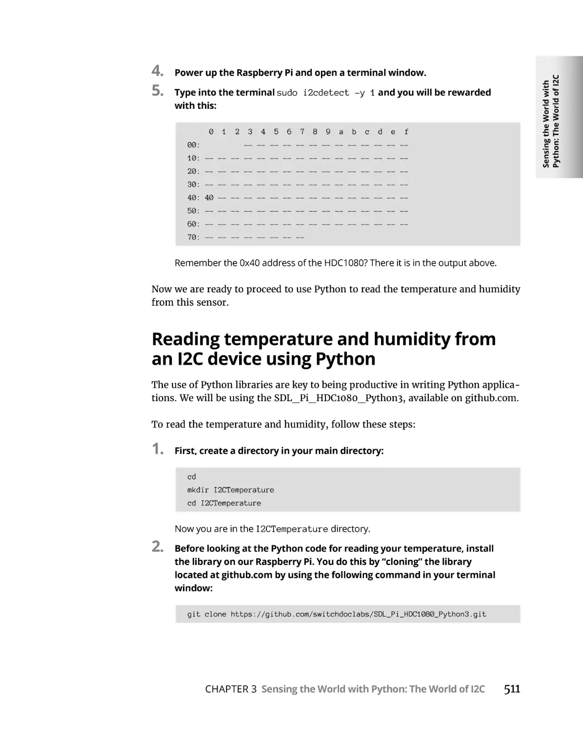
Text
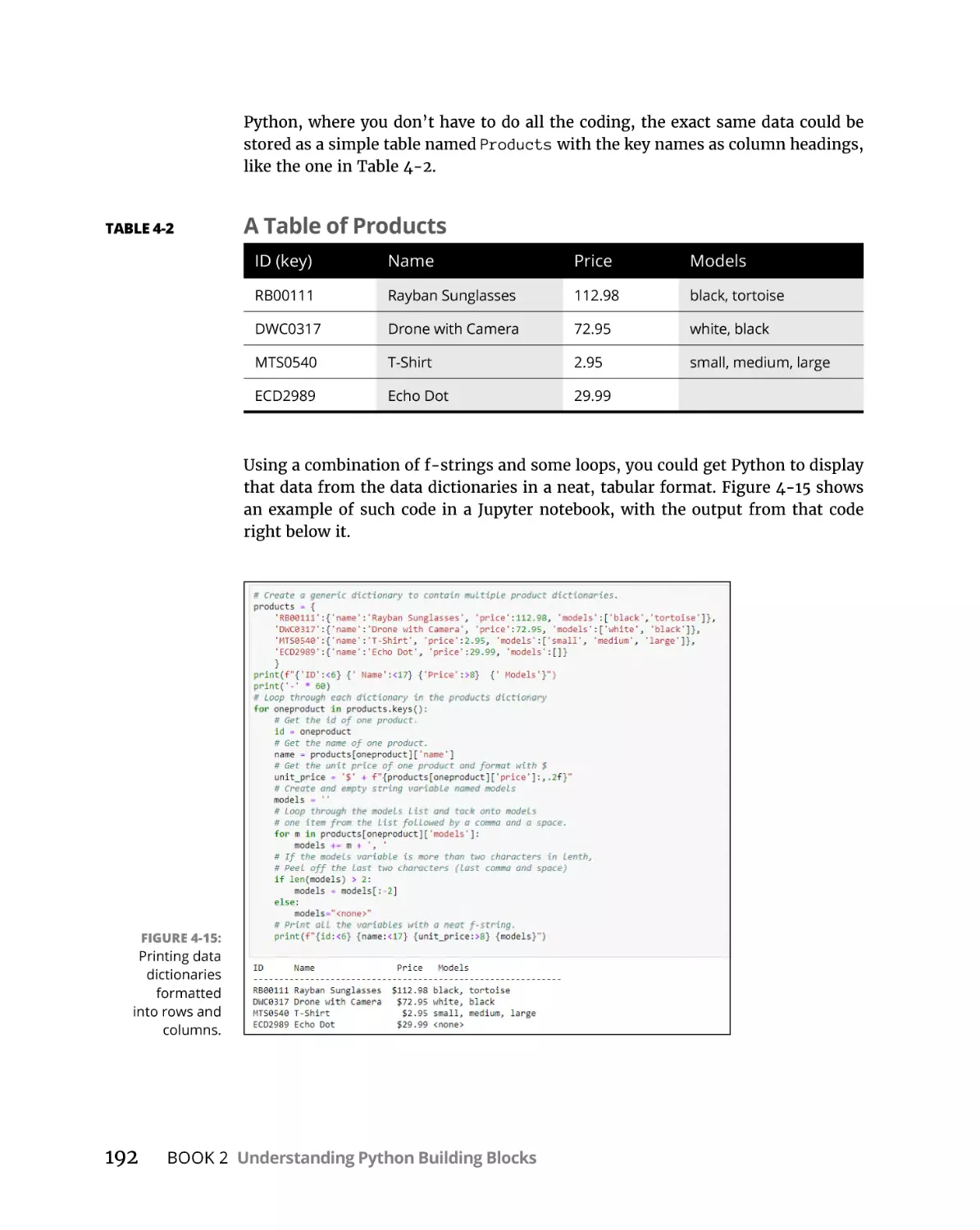
Python
ALL-IN-ONE
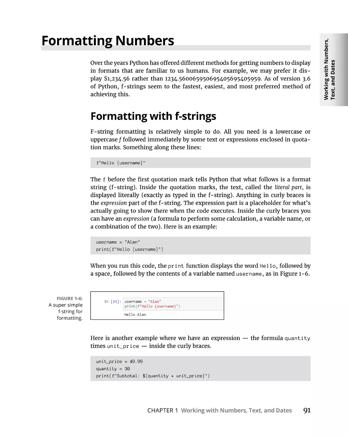
by John Shovic and Alan Simpson
Python All-in-One For Dummies®
Published by: John Wiley & Sons, Inc., 111 River Street, Hoboken, NJ 07030-5774, www.wiley.com
Copyright © 2019 by John Wiley & Sons, Inc., Hoboken, New Jersey
Published simultaneously in Canada
No part of this publication may be reproduced, stored in a retrieval system or transmitted in any form or by any
means, electronic, mechanical, photocopying, recording, scanning or otherwise, except as permitted under Sections
107 or 108 of the 1976 United States Copyright Act, without the prior written permission of the Publisher. Requests to
the Publisher for permission should be addressed to the Permissions Department, John Wiley & Sons, Inc., 111 River
Street, Hoboken, NJ 07030, (201) 748-6011, fax (201) 748-6008, or online at www.wiley.com/go/permissions.
Trademarks: Wiley, For Dummies, the Dummies Man logo, Dummies.com, Making Everything Easier, and related
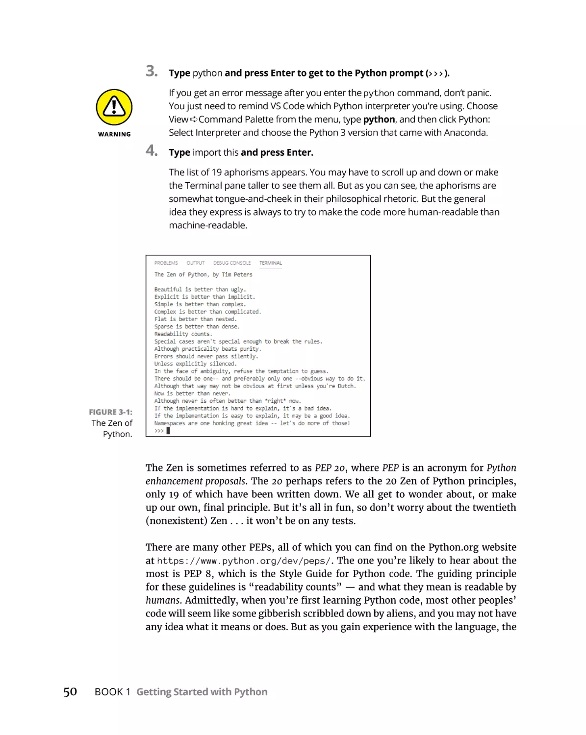
trade dress are trademarks or registered trademarks of John Wiley & Sons, Inc. and may not be used without written
permission. All other trademarks are the property of their respective owners. John Wiley & Sons, Inc. is not associated
with any product or vendor mentioned in this book.
LIMIT OF LIABILITY/DISCLAIMER OF WARRANTY: THE PUBLISHER AND THE AUTHOR MAKE NO
REPRESENTATIONS OR WARRANTIES WITH RESPECT TO THE ACCURACY OR COMPLETENESS OF THE CONTENTS
OF THIS WORK AND SPECIFICALLY DISCLAIM ALL WARRANTIES, INCLUDING WITHOUT LIMITATION WARRANTIES
OF FITNESS FOR A PARTICULAR PURPOSE. NO WARRANTY MAY BE CREATED OR EXTENDED BY SALES OR
PROMOTIONAL MATERIALS. THE ADVICE AND STRATEGIES CONTAINED HEREIN MAY NOT BE SUITABLE FOR
EVERY SITUATION. THIS WORK IS SOLD WITH THE UNDERSTANDING THAT THE PUBLISHER IS NOT ENGAGED
IN RENDERING LEGAL, ACCOUNTING, OR OTHER PROFESSIONAL SERVICES. IF PROFESSIONAL ASSISTANCE
IS REQUIRED, THE SERVICES OF A COMPETENT PROFESSIONAL PERSON SHOULD BE SOUGHT. NEITHER THE
PUBLISHER NOR THE AUTHOR SHALL BE LIABLE FOR DAMAGES ARISING HEREFROM. THE FACT THAT AN
ORGANIZATION OR WEBSITE IS REFERRED TO IN THIS WORK AS A CITATION AND/OR A POTENTIAL SOURCE OF
FURTHER INFORMATION DOES NOT MEAN THAT THE AUTHOR OR THE PUBLISHER ENDORSES THE INFORMATION
THE ORGANIZATION OR WEBSITE MAY PROVIDE OR RECOMMENDATIONS IT MAY MAKE. FURTHER, READERS
SHOULD BE AWARE THAT INTERNET WEBSITES LISTED IN THIS WORK MAY HAVE CHANGED OR DISAPPEARED
BETWEEN WHEN THIS WORK WAS WRITTEN AND WHEN IT IS READ.
For general information on our other products and services, please contact our Customer Care Department within
the U.S. at 877-762-2974, outside the U.S. at 317-572-3993, or fax 317-572-4002. For technical support, please visit
https://hub.wiley.com/community/support/dummies.
Wiley publishes in a variety of print and electronic formats and by print-on-demand. Some material included with
standard print versions of this book may not be included in e-books or in print-on-demand. If this book refers to
media such as a CD or DVD that is not included in the version you purchased, you may download this material at
http://booksupport.wiley.com. For more information about Wiley products, visit www.wiley.com.
Library of Congress Control Number: 2019937504
ISBN 978-1-119-55759-3 (pbk); ISBN 978-1-119-55767-8 (ebk); ISBN 978-1-119-55761-6 (ebk)
Manufactured in the United States of America
10 9 8 7 6 5 4 3 2 1
Contents at a Glance
Introduction. . . . . . . . . . . . . . . . . . . . . . . . . . . . . . . . . . . . . . . . . . . . . . . . . . . . . . . . . 1
Book 1: Getting Started with Python. . . . . . . . . . . . . . . . . . . . . . . . . . . . 5
CHAPTER 1:
CHAPTER 2:
CHAPTER 3:
CHAPTER 4:
Starting with Python. . . . . . . . . . . . . . . . . . . . . . . . . . . . . . . . . . . . . . . . . . . . . . 7
Interactive Mode, Getting Help, Writing Apps. . . . . . . . . . . . . . . . . . . . . . . 27
Python Elements and Syntax. . . . . . . . . . . . . . . . . . . . . . . . . . . . . . . . . . . . . 49
Building Your First Python Application. . . . . . . . . . . . . . . . . . . . . . . . . . . . . 61
Book 2: Understanding Python Building Blocks. . . . . . . . . . . . . . 83
CHAPTER 1:
CHAPTER 2:
CHAPTER 3:
CHAPTER 4:
CHAPTER 5:
CHAPTER 6:
CHAPTER 7:
Working with Numbers, Text, and Dates. . . . . . . . . . . . . . . . . . . . . . . . . . . 85
Controlling the Action . . . . . . . . . . . . . . . . . . . . . . . . . . . . . . . . . . . . . . . . . 125
Speeding Along with Lists and Tuples. . . . . . . . . . . . . . . . . . . . . . . . . . . . 147
Cruising Massive Data with Dictionaries . . . . . . . . . . . . . . . . . . . . . . . . . 169
Wrangling Bigger Chunks of Code. . . . . . . . . . . . . . . . . . . . . . . . . . . . . . . 193
Doing Python with Class. . . . . . . . . . . . . . . . . . . . . . . . . . . . . . . . . . . . . . . 213
Sidestepping Errors. . . . . . . . . . . . . . . . . . . . . . . . . . . . . . . . . . . . . . . . . . . 247
Book 3: Working with Python Libraries. . . . . . . . . . . . . . . . . . . . . .
265
Working with External Files. . . . . . . . . . . . . . . . . . . . . . . . . . . . . . . . . . . . .
Juggling JSON Data. . . . . . . . . . . . . . . . . . . . . . . . . . . . . . . . . . . . . . . . . . . .
Interacting with the Internet. . . . . . . . . . . . . . . . . . . . . . . . . . . . . . . . . . . .
Libraries, Packages, and Modules. . . . . . . . . . . . . . . . . . . . . . . . . . . . . . .
267
303
323
339
CHAPTER 1:
CHAPTER 2:
CHAPTER 3:
CHAPTER 4:
Book 4: Using Artificial Intelligence in Python . . . . . . . . . . . . .
353
Exploring Artificial Intelligence. . . . . . . . . . . . . . . . . . . . . . . . . . . . . . . . . .
Building a Neural Network in Python. . . . . . . . . . . . . . . . . . . . . . . . . . . .
Doing Machine Learning in Python. . . . . . . . . . . . . . . . . . . . . . . . . . . . . .
Exploring More AI in Python. . . . . . . . . . . . . . . . . . . . . . . . . . . . . . . . . . . .
355
365
393
415
Book 5: Doing Data Science with Python. . . . . . . . . . . . . . . . . . . .
427
CHAPTER 1:
CHAPTER 2:
CHAPTER 3:
CHAPTER 4:
CHAPTER 1:
CHAPTER 2:
CHAPTER 3:
The Five Areas of Data Science. . . . . . . . . . . . . . . . . . . . . . . . . . . . . . . . . . 429
Exploring Big Data with Python. . . . . . . . . . . . . . . . . . . . . . . . . . . . . . . . . 437
Using Big Data from the Google Cloud. . . . . . . . . . . . . . . . . . . . . . . . . . . 451
Book 6: Talking to Hardware with Python . . . . . . . . . . . . . . . . . .
469
Introduction to Physical Computing. . . . . . . . . . . . . . . . . . . . . . . . . . . . .
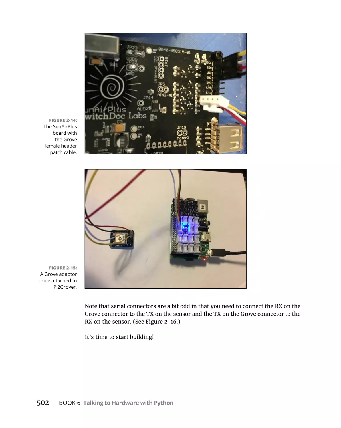
No Soldering! Grove Connectors for Building Things . . . . . . . . . . . . . .
Sensing the World with Python: The World of I2C. . . . . . . . . . . . . . . . .
Making Things Move with Python. . . . . . . . . . . . . . . . . . . . . . . . . . . . . . .
471
487
505
537
Book 7: Building Robots with Python . . . . . . . . . . . . . . . . . . . . . . . .
565
Introduction to Robotics. . . . . . . . . . . . . . . . . . . . . . . . . . . . . . . . . . . . . . .
Building Your First Python Robot. . . . . . . . . . . . . . . . . . . . . . . . . . . . . . . .
Programming Your Robot Rover in Python. . . . . . . . . . . . . . . . . . . . . . .
Using Artificial Intelligence in Robotics. . . . . . . . . . . . . . . . . . . . . . . . . . .
567
575
595
623
Index. . . . . . . . . . . . . . . . . . . . . . . . . . . . . . . . . . . . . . . . . . . . . . . . . . . . . . . . . . . . . . .
647
CHAPTER 1:
CHAPTER 2:
CHAPTER 3:
CHAPTER 4:
CHAPTER 1:
CHAPTER 2:
CHAPTER 3:
CHAPTER 4:
Table of Contents
INTRODUCTION . . . . . . . . . . . . . . . . . . . . . . . . . . . . . . . . . . . . . . . . . . . . . . . . . . . . 1
About This Book. . . . . . . . . . . . . . . . . . . . . . . . . . . . . . . . . . . . . . . . . . . . . . .
Foolish Assumptions. . . . . . . . . . . . . . . . . . . . . . . . . . . . . . . . . . . . . . . . . . .
Icons Used in This Book. . . . . . . . . . . . . . . . . . . . . . . . . . . . . . . . . . . . . . . .
Beyond the Book. . . . . . . . . . . . . . . . . . . . . . . . . . . . . . . . . . . . . . . . . . . . . .
Where to Go from Here . . . . . . . . . . . . . . . . . . . . . . . . . . . . . . . . . . . . . . . .
1
2
2
3
3
BOOK 1: GETTING STARTED WITH PYTHON. . . . . . . . . . . . . . . . . . . 5
CHAPTER 1:
Starting with Python. . . . . . . . . . . . . . . . . . . . . . . . . . . . . . . . . . . . . . 7
Why Python Is Hot. . . . . . . . . . . . . . . . . . . . . . . . . . . . . . . . . . . . . . . . . . . . . 8
Choosing the Right Python. . . . . . . . . . . . . . . . . . . . . . . . . . . . . . . . . . . . . . 9
Tools for Success. . . . . . . . . . . . . . . . . . . . . . . . . . . . . . . . . . . . . . . . . . . . . 11
An excellent, free learning environment . . . . . . . . . . . . . . . . . . . . . . 12
Installing Anaconda and VS Code. . . . . . . . . . . . . . . . . . . . . . . . . . . . 13
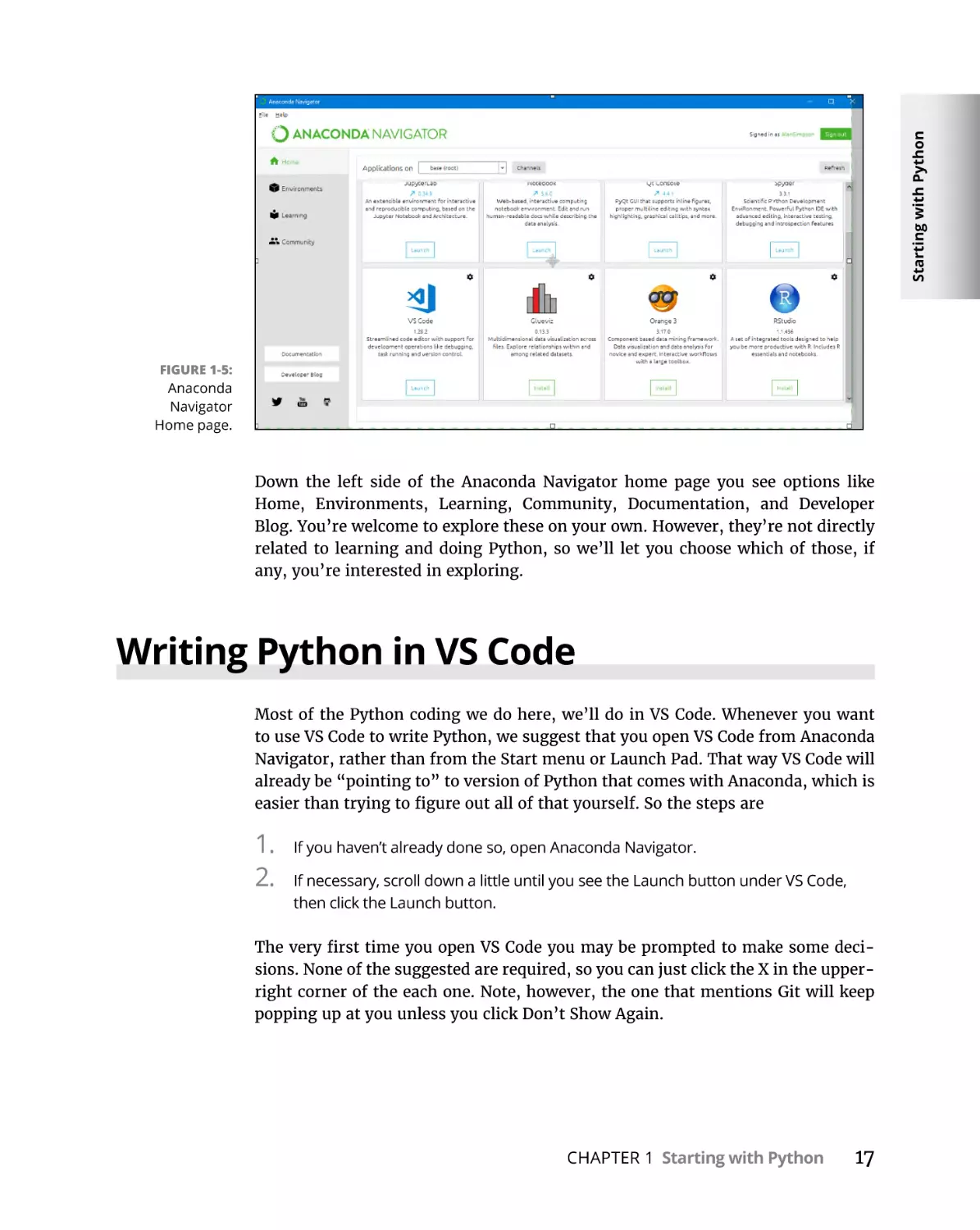
Writing Python in VS Code. . . . . . . . . . . . . . . . . . . . . . . . . . . . . . . . . . . . . 17
Choosing your Python interpreter . . . . . . . . . . . . . . . . . . . . . . . . . . . 19
Writing some Python code. . . . . . . . . . . . . . . . . . . . . . . . . . . . . . . . . . 20
Getting back to VS Code Python . . . . . . . . . . . . . . . . . . . . . . . . . . . . . 21
Using Jupyter Notebook for Coding . . . . . . . . . . . . . . . . . . . . . . . . . . . . . 21
CHAPTER 2:
Interactive Mode, Getting Help, Writing Apps. . . . . . . 27
Using Python Interactive Mode. . . . . . . . . . . . . . . . . . . . . . . . . . . . . . . . .
Opening Terminal . . . . . . . . . . . . . . . . . . . . . . . . . . . . . . . . . . . . . . . . .
Getting your Python version . . . . . . . . . . . . . . . . . . . . . . . . . . . . . . . .
Going into the Python Interpreter . . . . . . . . . . . . . . . . . . . . . . . . . . .
Entering commands . . . . . . . . . . . . . . . . . . . . . . . . . . . . . . . . . . . . . . .
Using Python’s built-in help. . . . . . . . . . . . . . . . . . . . . . . . . . . . . . . . .
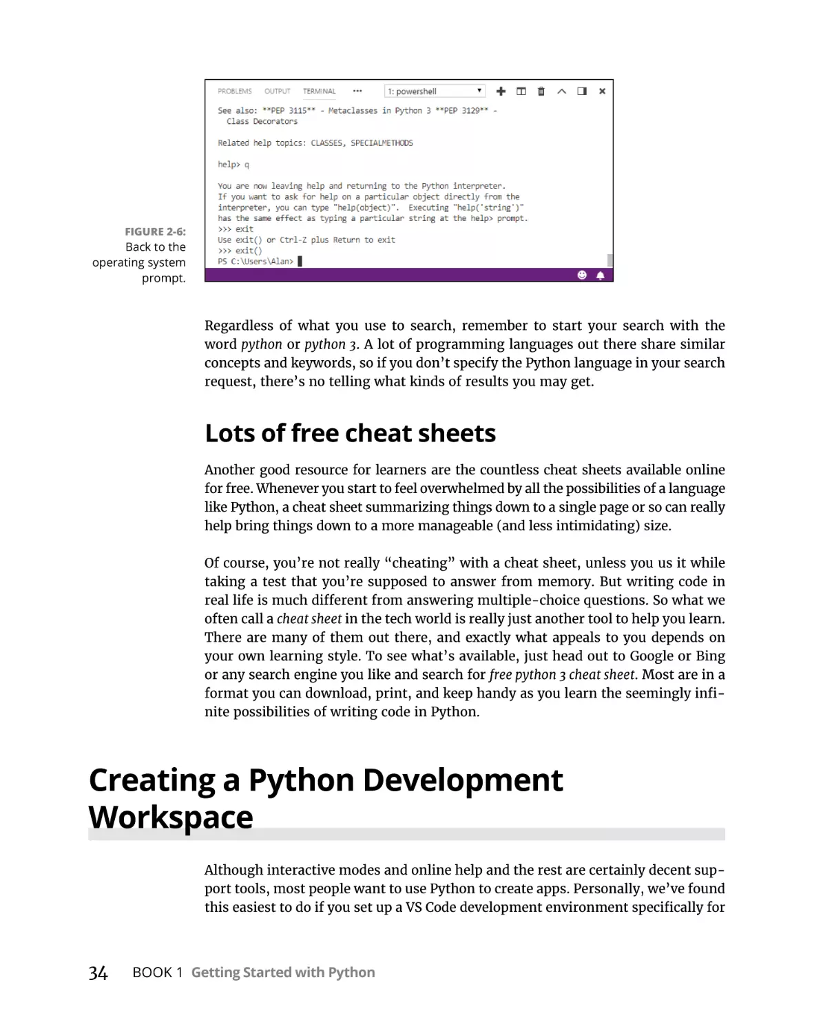
Exiting interactive help. . . . . . . . . . . . . . . . . . . . . . . . . . . . . . . . . . . . .
Searching for specific help topics online . . . . . . . . . . . . . . . . . . . . . .
Lots of free cheat sheets . . . . . . . . . . . . . . . . . . . . . . . . . . . . . . . . . . .
Creating a Python Development Workspace. . . . . . . . . . . . . . . . . . . . . .
Creating a Folder for your Python Code . . . . . . . . . . . . . . . . . . . . . . . . .
Typing, Editing, and Debugging Python Code. . . . . . . . . . . . . . . . . . . . .
Writing Python code . . . . . . . . . . . . . . . . . . . . . . . . . . . . . . . . . . . . . . .
Saving your code. . . . . . . . . . . . . . . . . . . . . . . . . . . . . . . . . . . . . . . . . .
Running Python in VS Code. . . . . . . . . . . . . . . . . . . . . . . . . . . . . . . . .
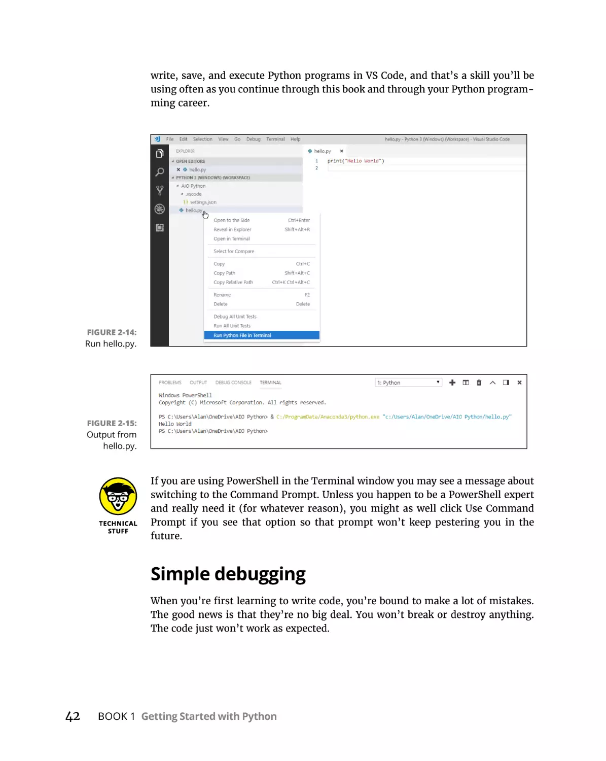
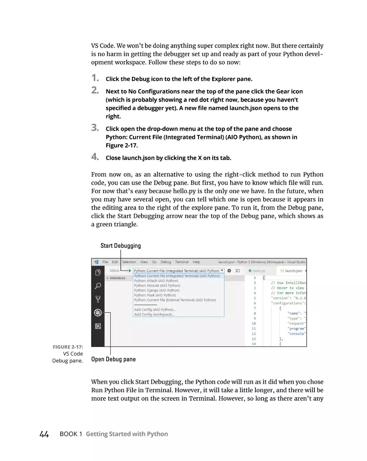
Simple debugging . . . . . . . . . . . . . . . . . . . . . . . . . . . . . . . . . . . . . . . . .
The VS Code Python debugger . . . . . . . . . . . . . . . . . . . . . . . . . . . . . .
Table of Contents
27
28
28
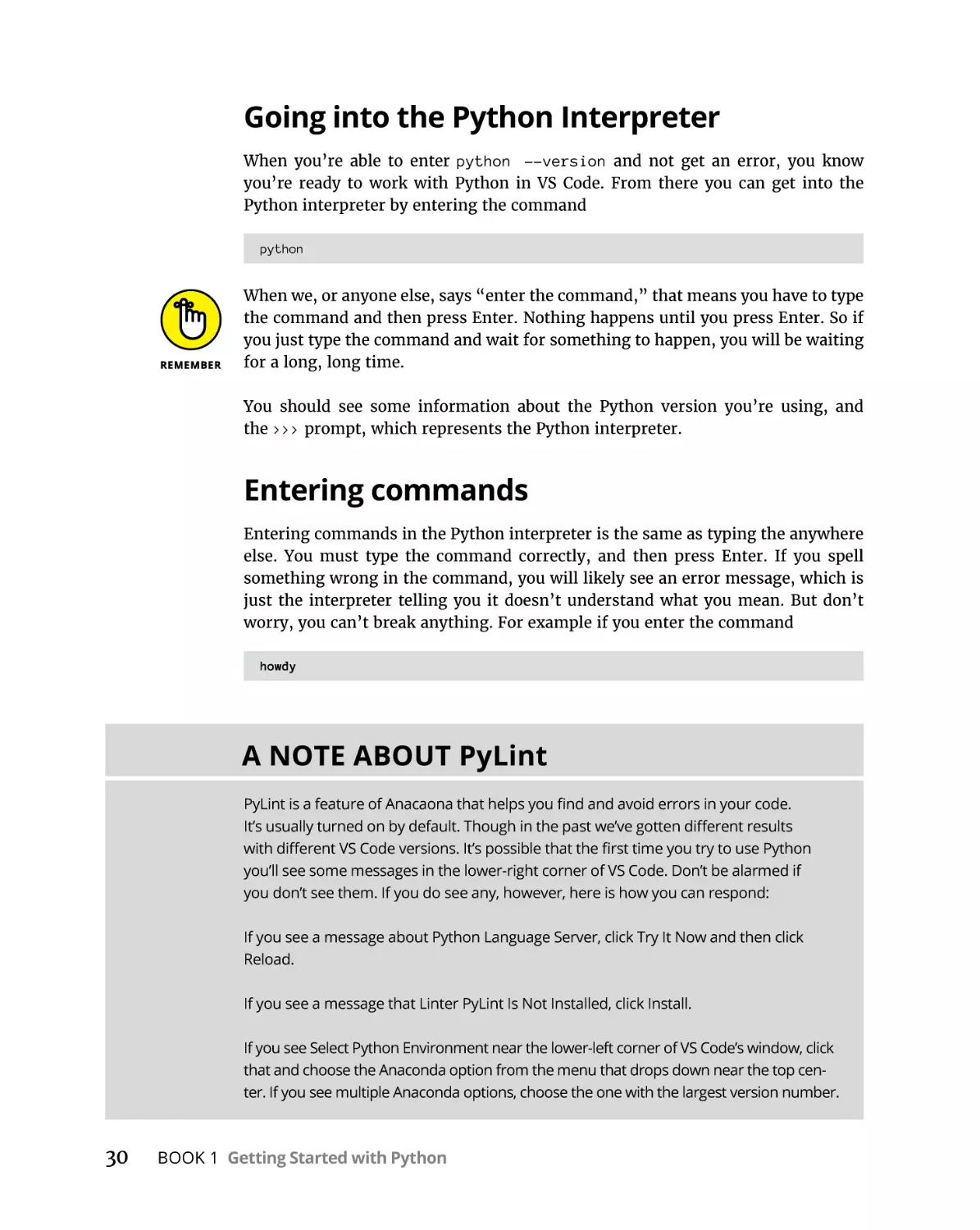
30
30
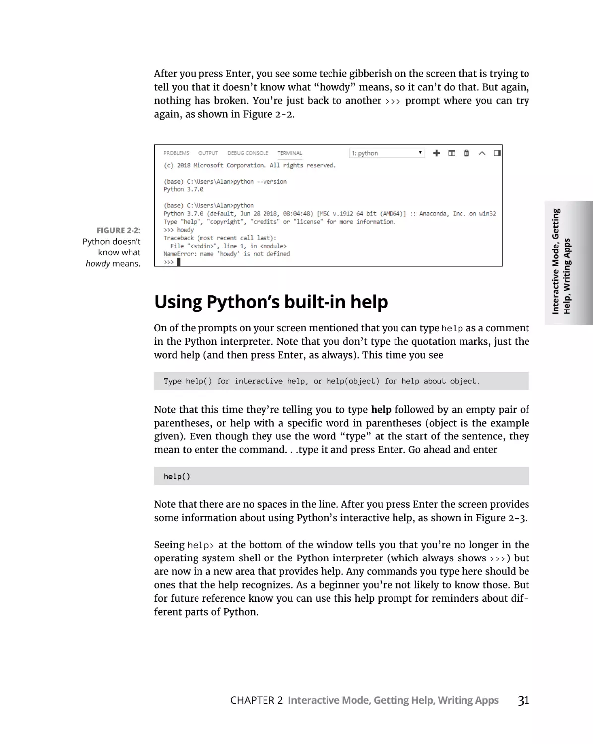
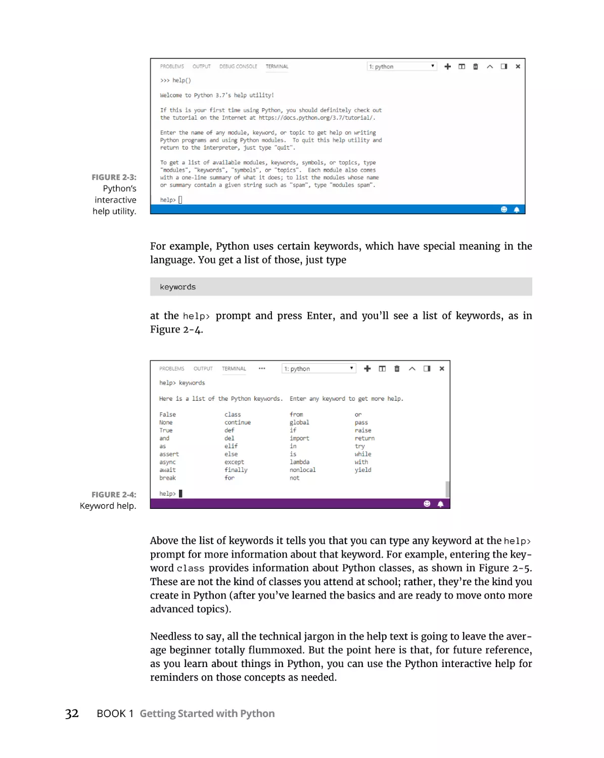
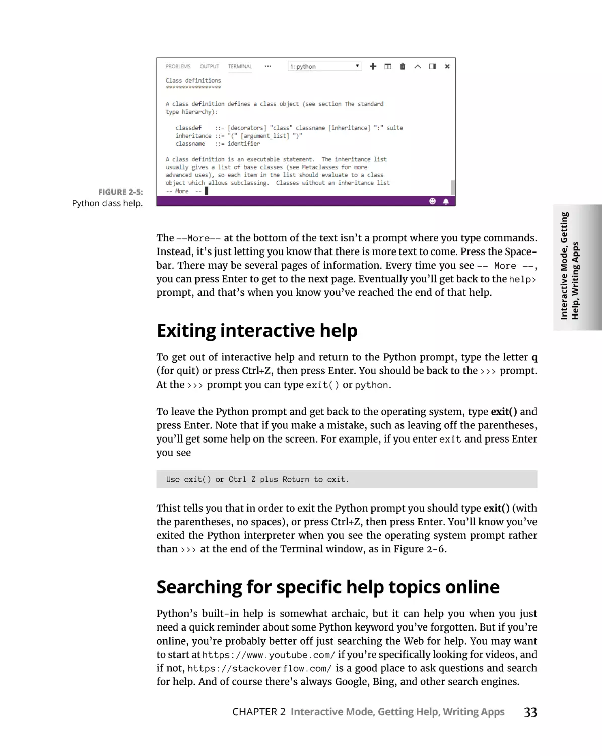
31
33
33
34
34
37
39
40
41
41
42
43
v
Writing Code in a Jupyter Notebook. . . . . . . . . . . . . . . . . . . . . . . . . . . . .
Creating a folder for Jupyter Notebook . . . . . . . . . . . . . . . . . . . . . . .
Creating and saving a Jupyter notebook . . . . . . . . . . . . . . . . . . . . . .
Typing and running code in a notebook . . . . . . . . . . . . . . . . . . . . . .
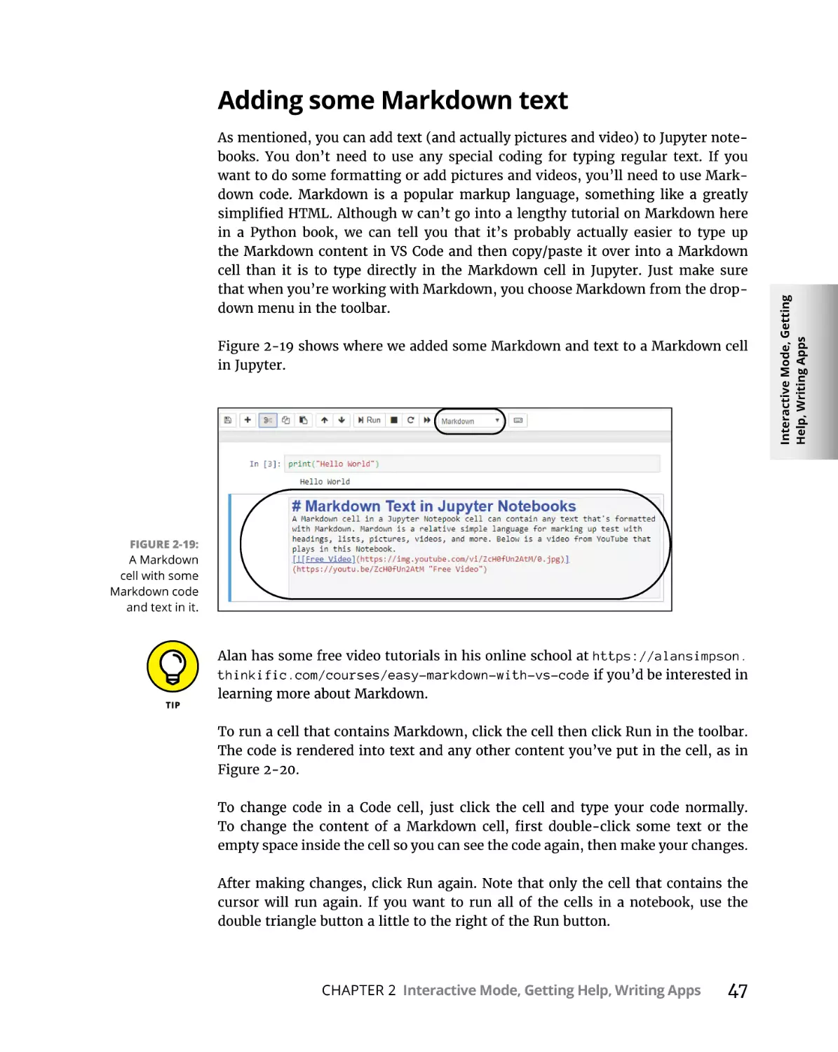
Adding some Markdown text. . . . . . . . . . . . . . . . . . . . . . . . . . . . . . . .
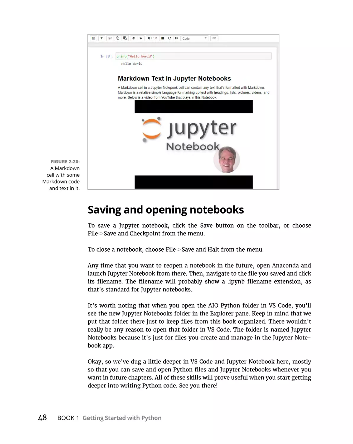
Saving and opening notebooks. . . . . . . . . . . . . . . . . . . . . . . . . . . . . .
CHAPTER 3:
Python Elements and Syntax. . . . . . . . . . . . . . . . . . . . . . . . . . . 49
The Zen of Python. . . . . . . . . . . . . . . . . . . . . . . . . . . . . . . . . . . . . . . . . . . .
Object-Oriented Programming . . . . . . . . . . . . . . . . . . . . . . . . . . . . . . . . .
Indentations Count, Big Time . . . . . . . . . . . . . . . . . . . . . . . . . . . . . . . . . .
Using Python Modules . . . . . . . . . . . . . . . . . . . . . . . . . . . . . . . . . . . . . . . .
Syntax for importing modules. . . . . . . . . . . . . . . . . . . . . . . . . . . . . . .
Using an alias with modules . . . . . . . . . . . . . . . . . . . . . . . . . . . . . . . .
CHAPTER 4:
45
45
46
46
47
48
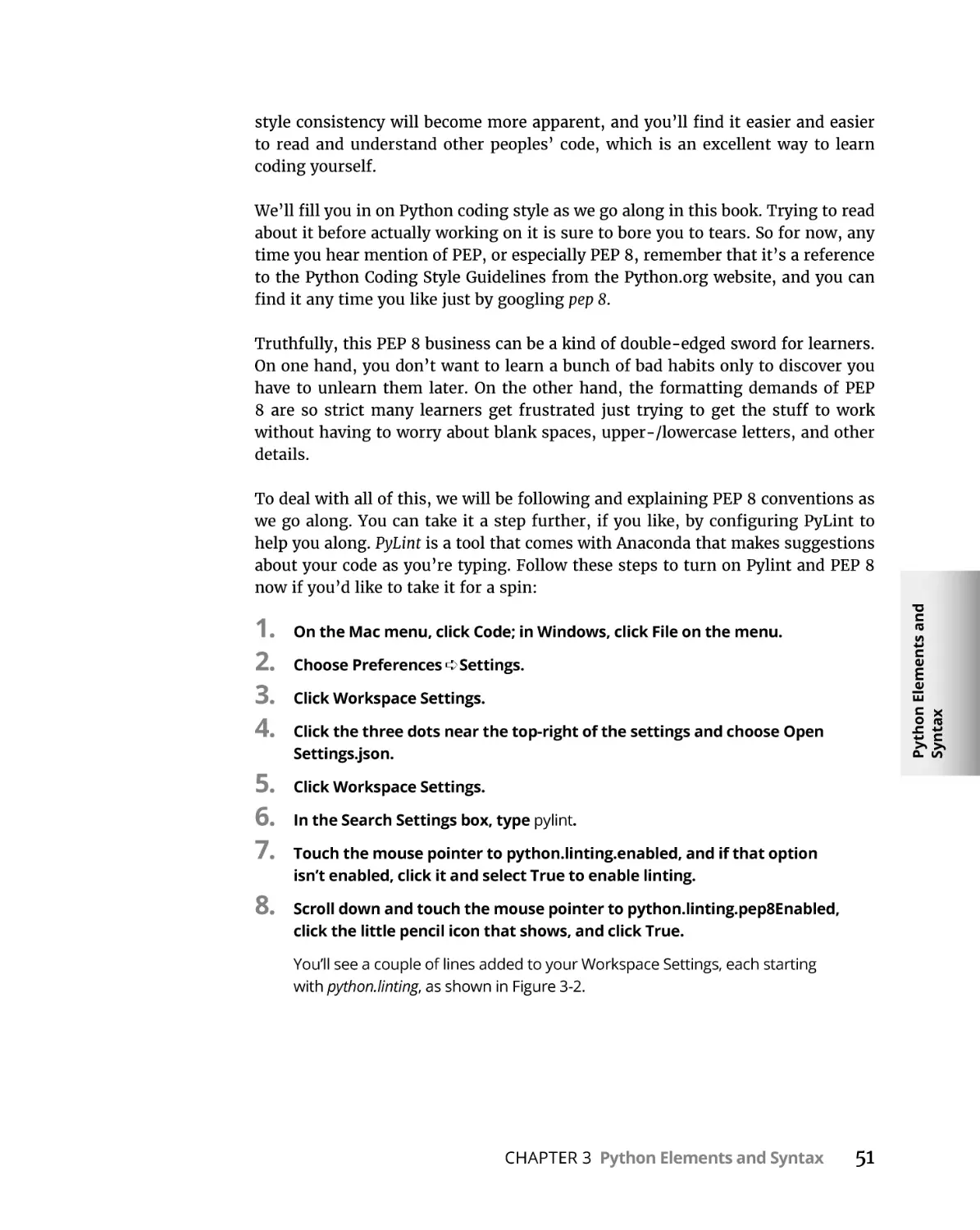
49
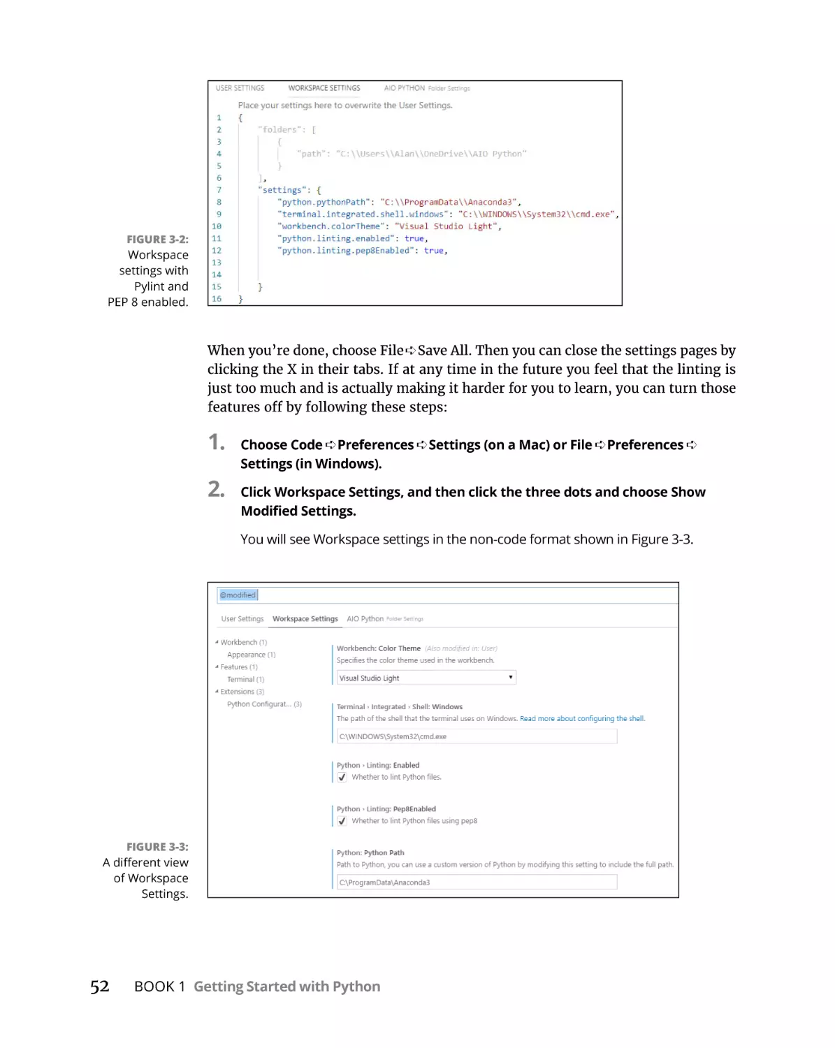
53
54
56
58
59
Building Your First Python Application. . . . . . . . . . . . . . . 61
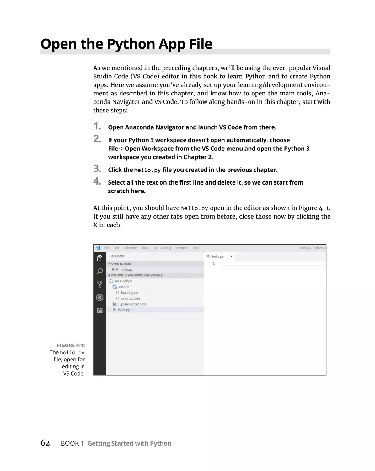
Open the Python App File . . . . . . . . . . . . . . . . . . . . . . . . . . . . . . . . . . . . .
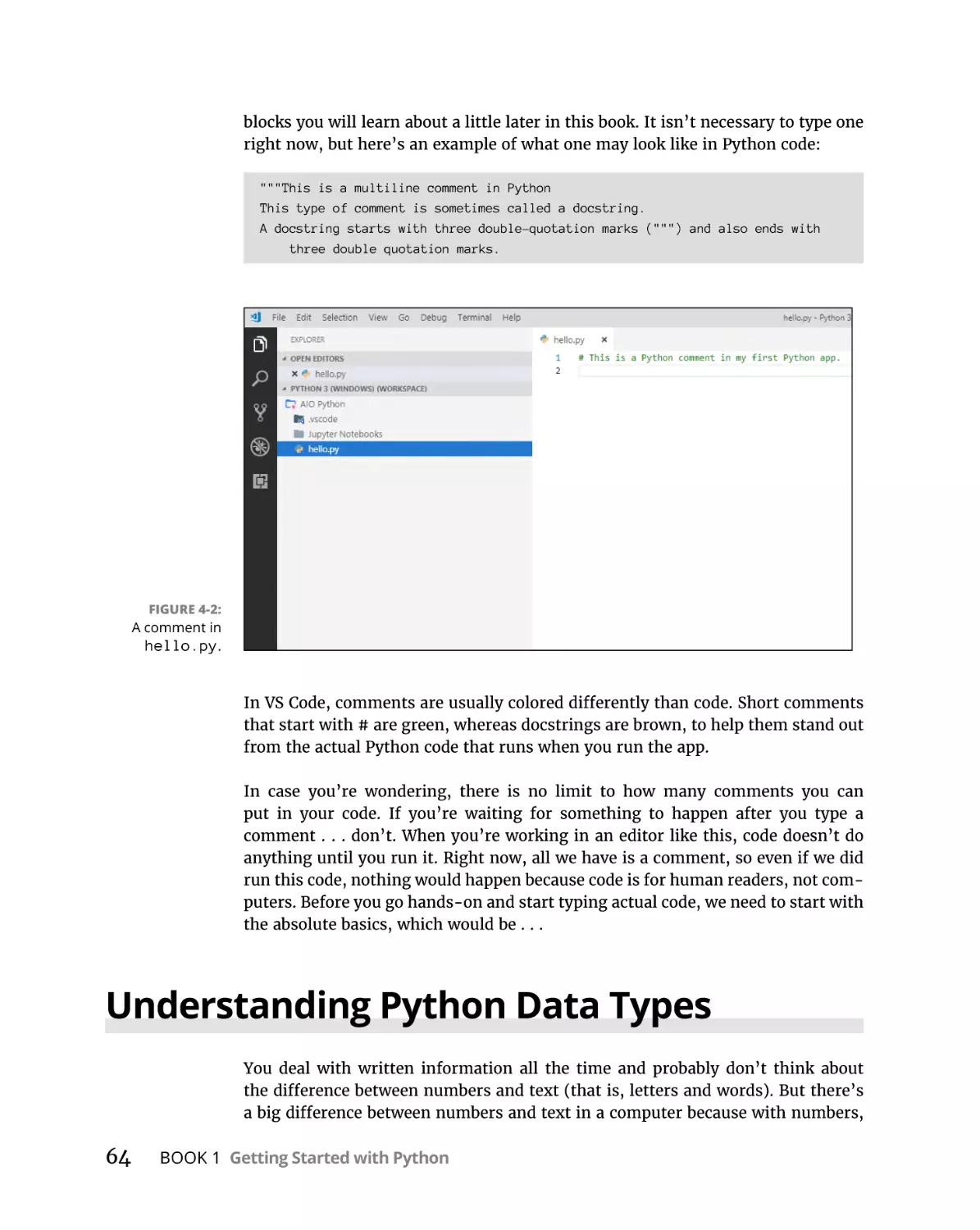
Typing and Using Python Comments. . . . . . . . . . . . . . . . . . . . . . . . . . . .
Understanding Python Data Types. . . . . . . . . . . . . . . . . . . . . . . . . . . . . .
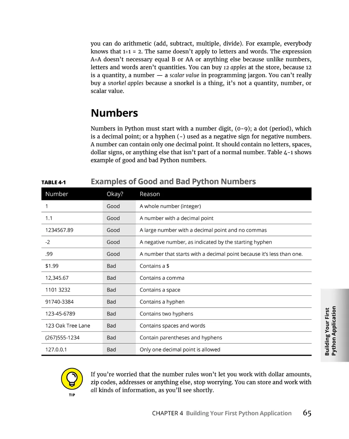
Numbers. . . . . . . . . . . . . . . . . . . . . . . . . . . . . . . . . . . . . . . . . . . . . . . . .
Words (strings). . . . . . . . . . . . . . . . . . . . . . . . . . . . . . . . . . . . . . . . . . . .
True/false Booleans . . . . . . . . . . . . . . . . . . . . . . . . . . . . . . . . . . . . . . .
Doing Work with Python Operators. . . . . . . . . . . . . . . . . . . . . . . . . . . . .
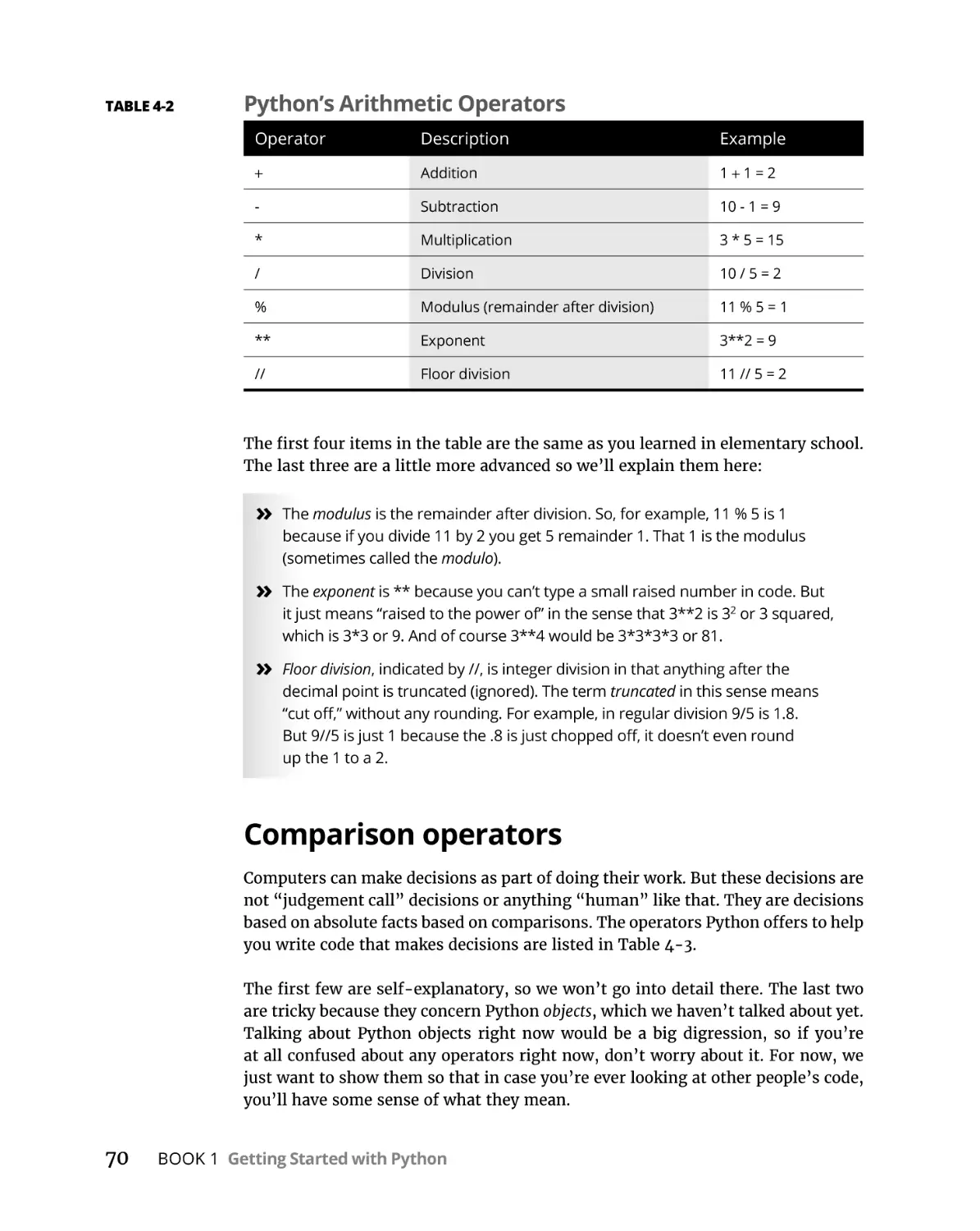
Arithmetic operators. . . . . . . . . . . . . . . . . . . . . . . . . . . . . . . . . . . . . . .
Comparison operators. . . . . . . . . . . . . . . . . . . . . . . . . . . . . . . . . . . . .
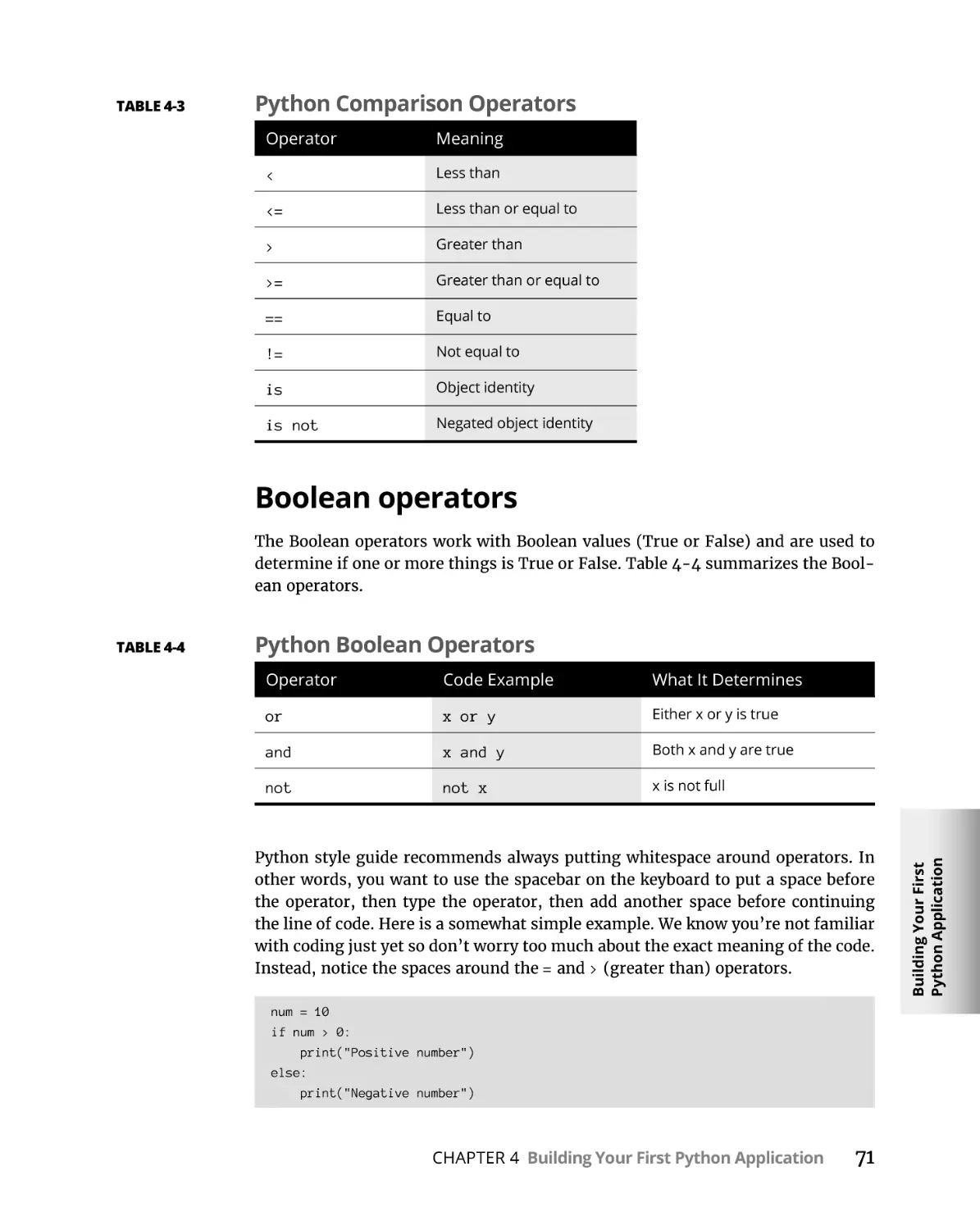
Boolean operators. . . . . . . . . . . . . . . . . . . . . . . . . . . . . . . . . . . . . . . . .
Creating and Using Variables. . . . . . . . . . . . . . . . . . . . . . . . . . . . . . . . . . .
Creating valid variable names. . . . . . . . . . . . . . . . . . . . . . . . . . . . . . .
Creating variables in code . . . . . . . . . . . . . . . . . . . . . . . . . . . . . . . . . .
Manipulating variables. . . . . . . . . . . . . . . . . . . . . . . . . . . . . . . . . . . . .
Saving your work. . . . . . . . . . . . . . . . . . . . . . . . . . . . . . . . . . . . . . . . . .
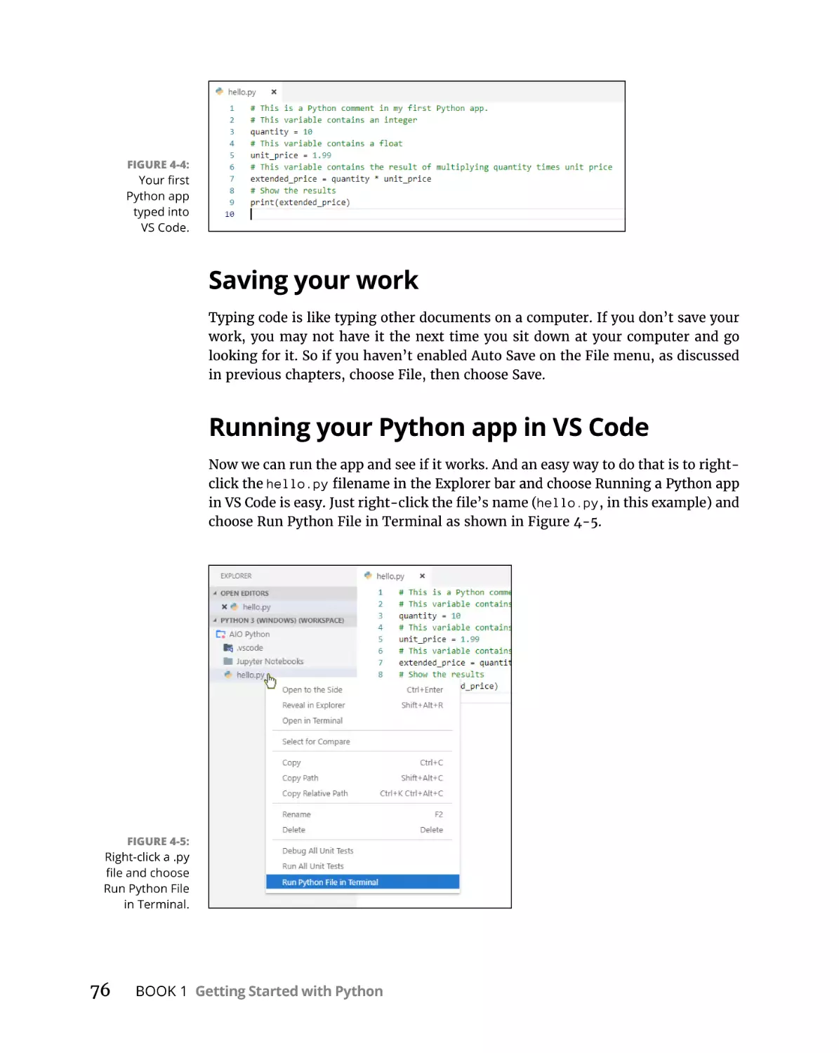
Running your Python app in VS Code. . . . . . . . . . . . . . . . . . . . . . . . .
What Syntax Is and Why It Matters. . . . . . . . . . . . . . . . . . . . . . . . . . . . . .
Putting Code Together . . . . . . . . . . . . . . . . . . . . . . . . . . . . . . . . . . . . . . . .
62
63
64
65
66
68
69
69
70
71
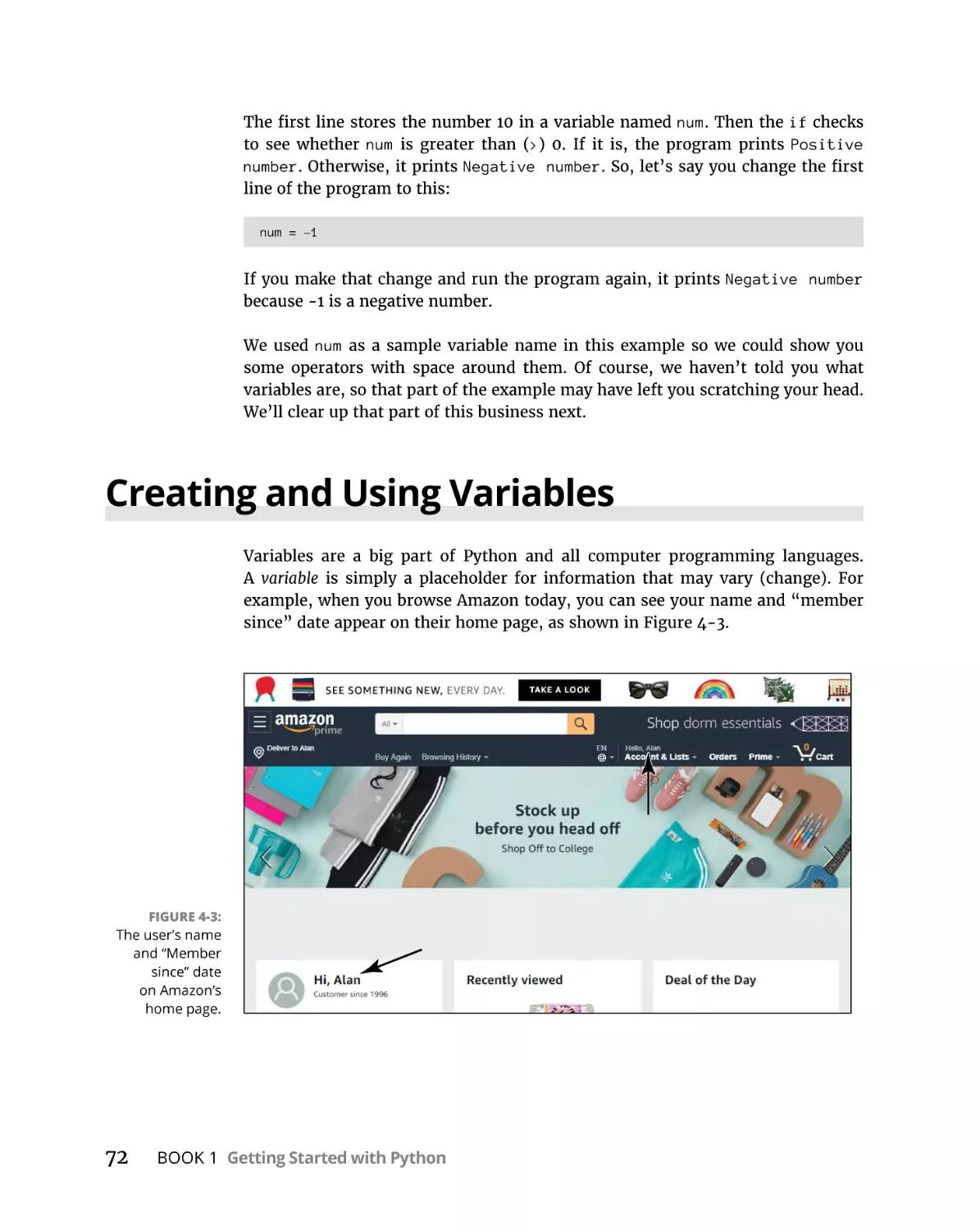
72
73
74
75
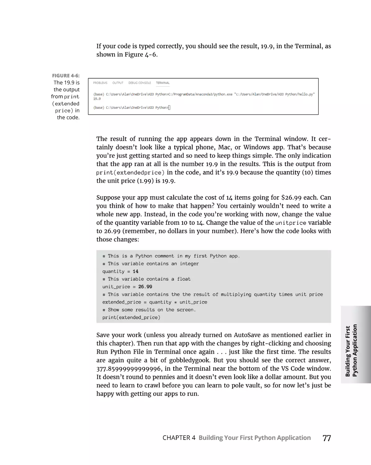
76
76
78
82
BOOK 2: UNDERSTANDING PYTHON
BUILDING BLOCKS . . . . . . . . . . . . . . . . . . . . . . . . . . . . . . . . . . . . . . . . . . . . . . . . 83
CHAPTER 1:
Working with Numbers, Text, and Dates. . . . . . . . . . . . . 85
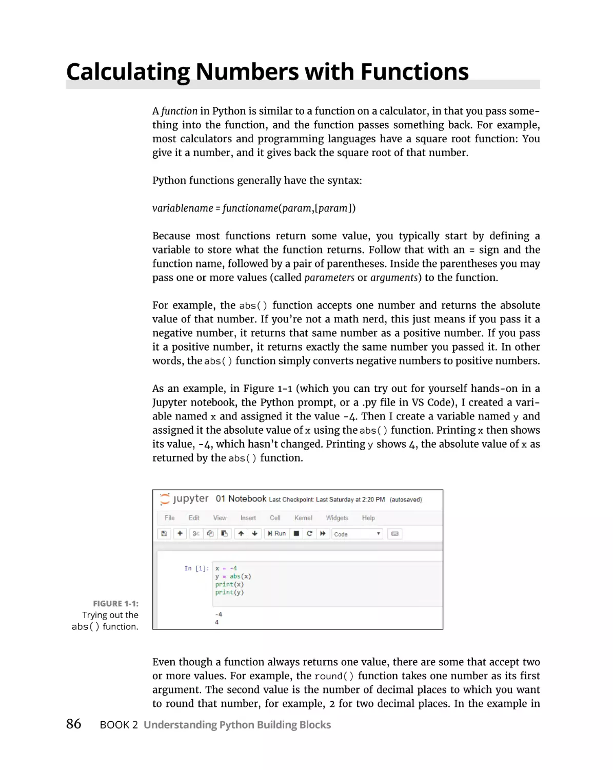
Calculating Numbers with Functions . . . . . . . . . . . . . . . . . . . . . . . . . . . .
Still More Math Functions . . . . . . . . . . . . . . . . . . . . . . . . . . . . . . . . . . . . .
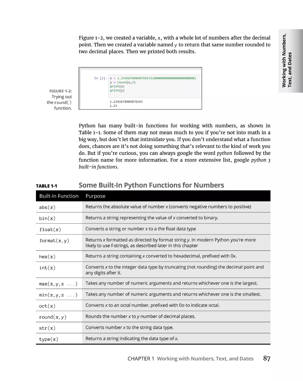
Formatting Numbers . . . . . . . . . . . . . . . . . . . . . . . . . . . . . . . . . . . . . . . . .
Formatting with f-strings . . . . . . . . . . . . . . . . . . . . . . . . . . . . . . . . . . .
Showing dollar amounts. . . . . . . . . . . . . . . . . . . . . . . . . . . . . . . . . . . .
Formatting percent numbers . . . . . . . . . . . . . . . . . . . . . . . . . . . . . . .
vi
Python All-in-One For Dummies
86
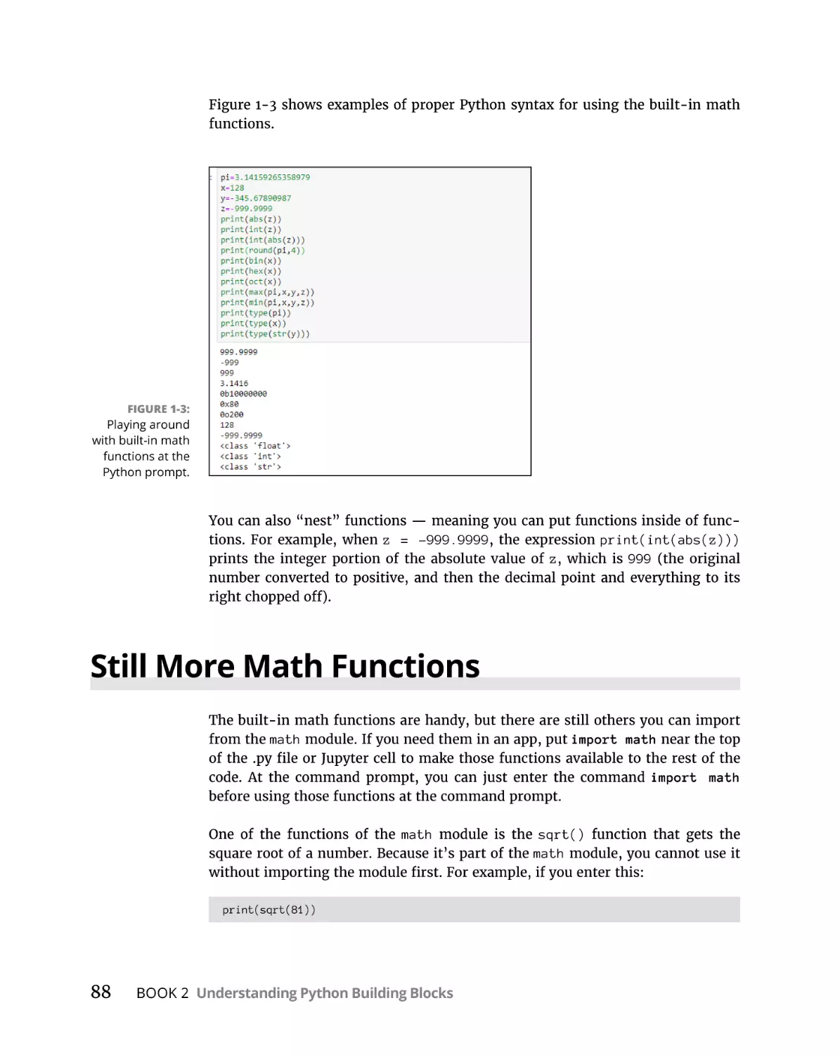
88
91
91
92
93
Making multiline format strings . . . . . . . . . . . . . . . . . . . . . . . . . . . . . 95
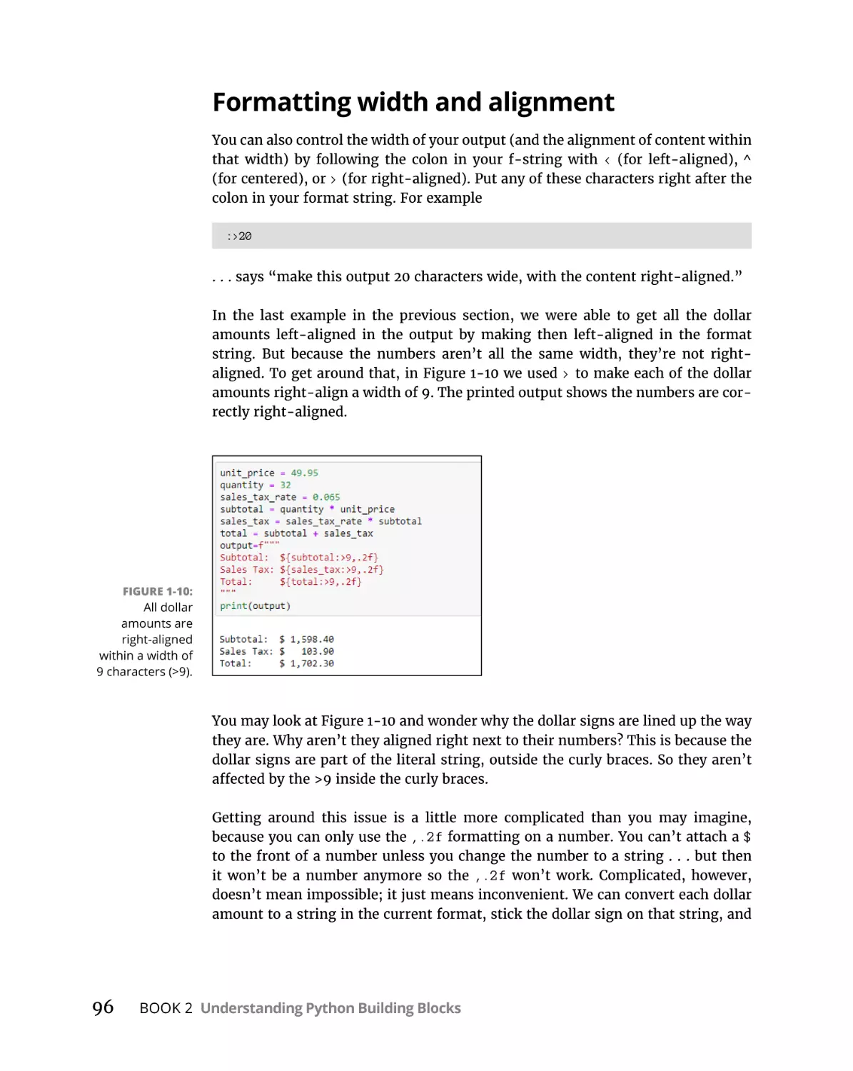
Formatting width and alignment. . . . . . . . . . . . . . . . . . . . . . . . . . . . . 96
Grappling with Weirder Numbers. . . . . . . . . . . . . . . . . . . . . . . . . . . . . . . 98
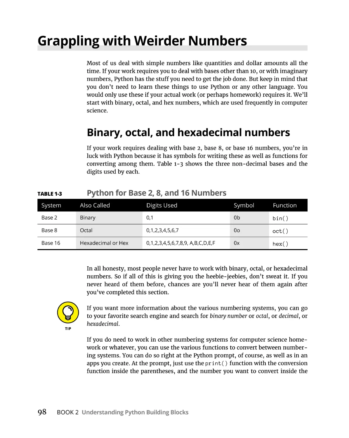
Binary, octal, and hexadecimal numbers. . . . . . . . . . . . . . . . . . . . . . 98
Complex numbers. . . . . . . . . . . . . . . . . . . . . . . . . . . . . . . . . . . . . . . . . 99
Manipulating Strings. . . . . . . . . . . . . . . . . . . . . . . . . . . . . . . . . . . . . . . . . 100
Concatenating strings. . . . . . . . . . . . . . . . . . . . . . . . . . . . . . . . . . . . . 101
Getting the length of a string. . . . . . . . . . . . . . . . . . . . . . . . . . . . . . . 102
Working with common string operators . . . . . . . . . . . . . . . . . . . . . 102
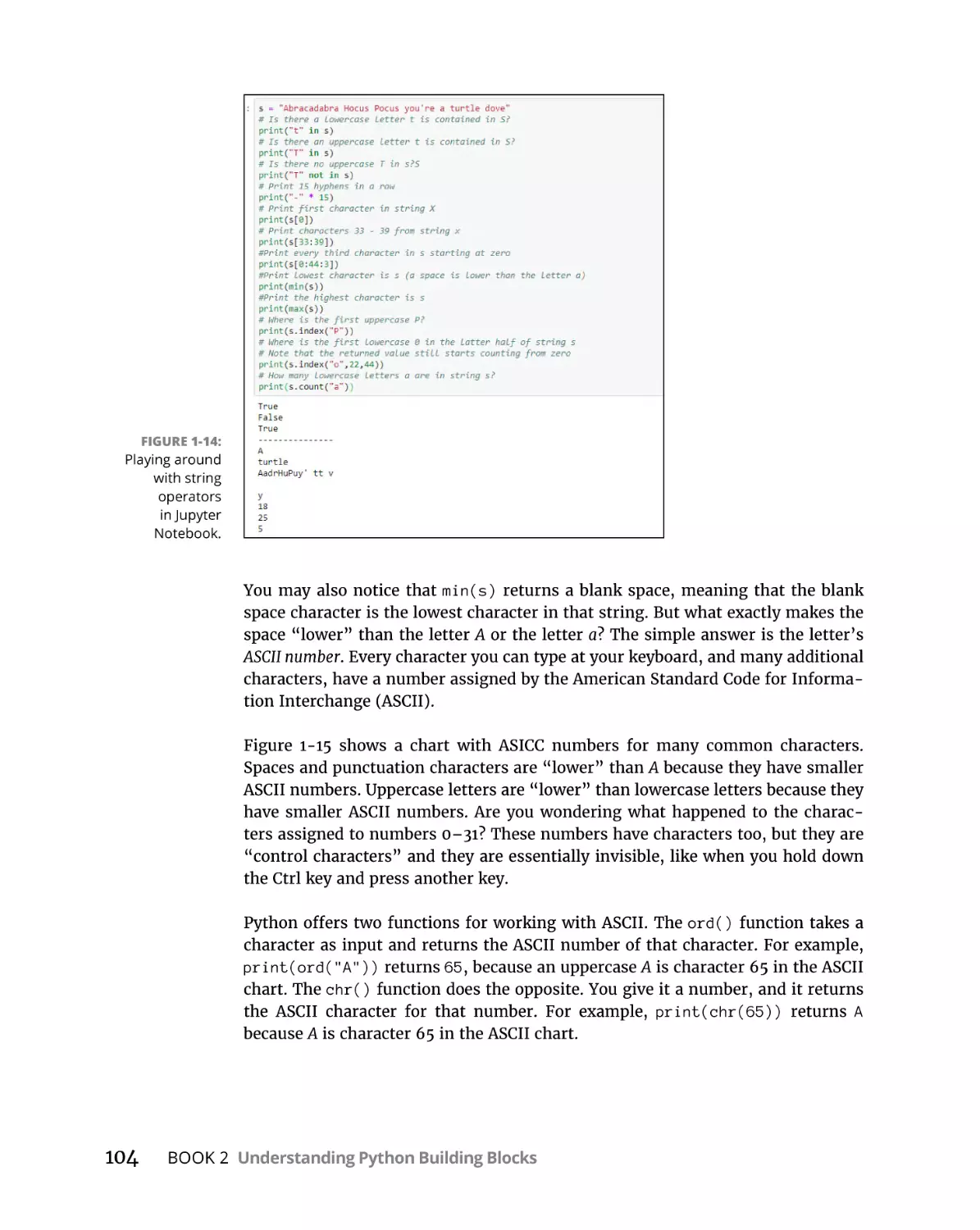
Manipulating strings with methods . . . . . . . . . . . . . . . . . . . . . . . . . 105
Uncovering Dates and Times. . . . . . . . . . . . . . . . . . . . . . . . . . . . . . . . . . 107
Working with dates. . . . . . . . . . . . . . . . . . . . . . . . . . . . . . . . . . . . . . . 108
Working with times. . . . . . . . . . . . . . . . . . . . . . . . . . . . . . . . . . . . . . . 112
Calculating timespans. . . . . . . . . . . . . . . . . . . . . . . . . . . . . . . . . . . . . 114
Accounting for Time Zones . . . . . . . . . . . . . . . . . . . . . . . . . . . . . . . . . . . 118
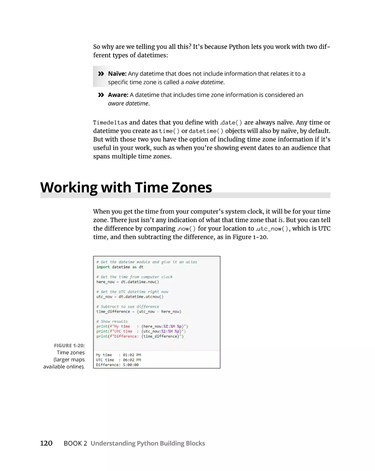
Working with Time Zones. . . . . . . . . . . . . . . . . . . . . . . . . . . . . . . . . . . . . 120
CHAPTER 2:
CHAPTER 3:
Controlling the Action . . . . . . . . . . . . . . . . . . . . . . . . . . . . . . . . .
125
Main Operators for Controlling the Action . . . . . . . . . . . . . . . . . . . . . .
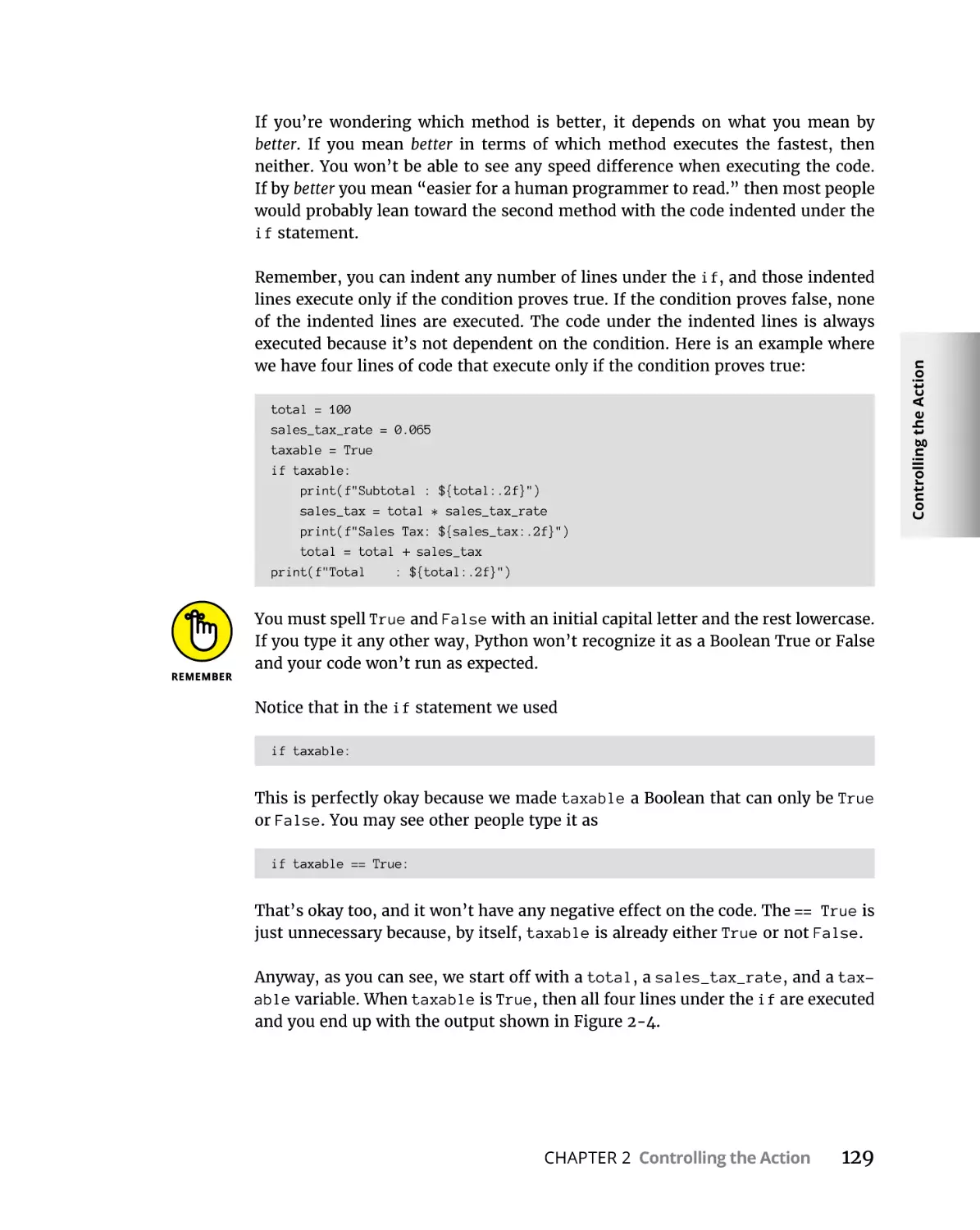
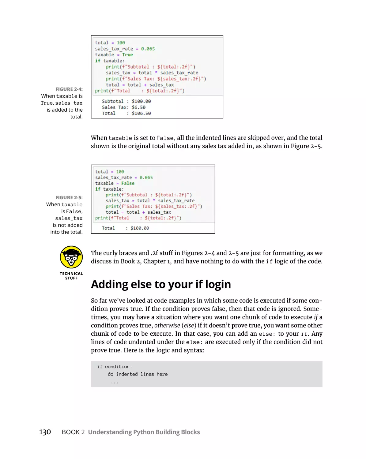
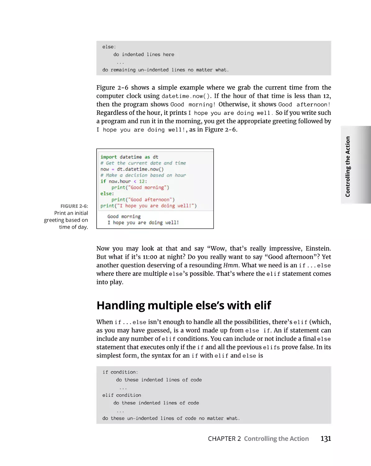
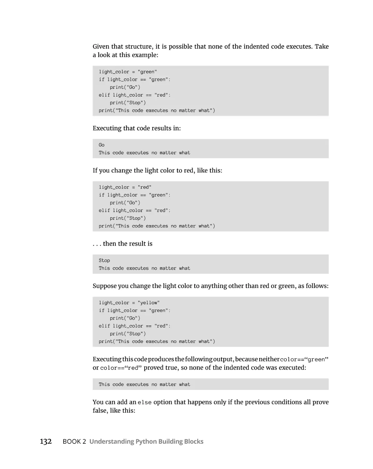
Making Decisions with if. . . . . . . . . . . . . . . . . . . . . . . . . . . . . . . . . . . . . .
Adding else to your if login. . . . . . . . . . . . . . . . . . . . . . . . . . . . . . . . .
Handling multiple else’s with elif. . . . . . . . . . . . . . . . . . . . . . . . . . . .
Ternary operations . . . . . . . . . . . . . . . . . . . . . . . . . . . . . . . . . . . . . . .
Repeating a Process with for. . . . . . . . . . . . . . . . . . . . . . . . . . . . . . . . . .
Looping through numbers in a range . . . . . . . . . . . . . . . . . . . . . . .
Looping through a string . . . . . . . . . . . . . . . . . . . . . . . . . . . . . . . . . .
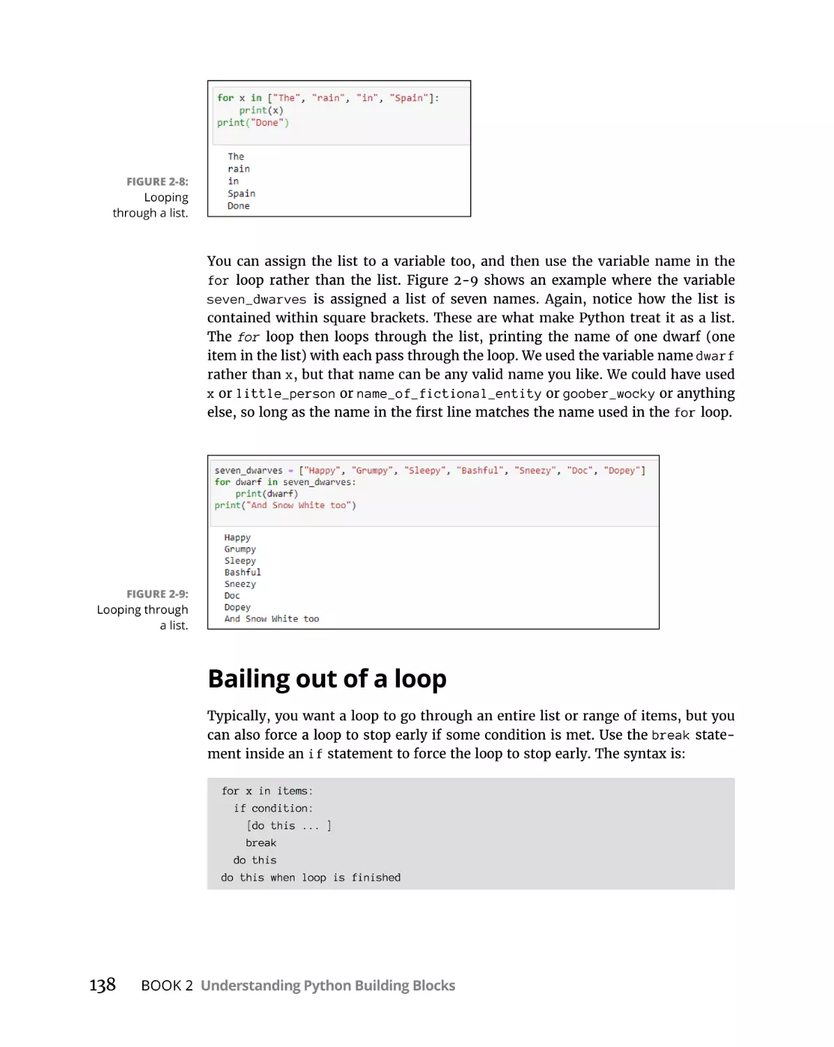
Looping through a list. . . . . . . . . . . . . . . . . . . . . . . . . . . . . . . . . . . . .
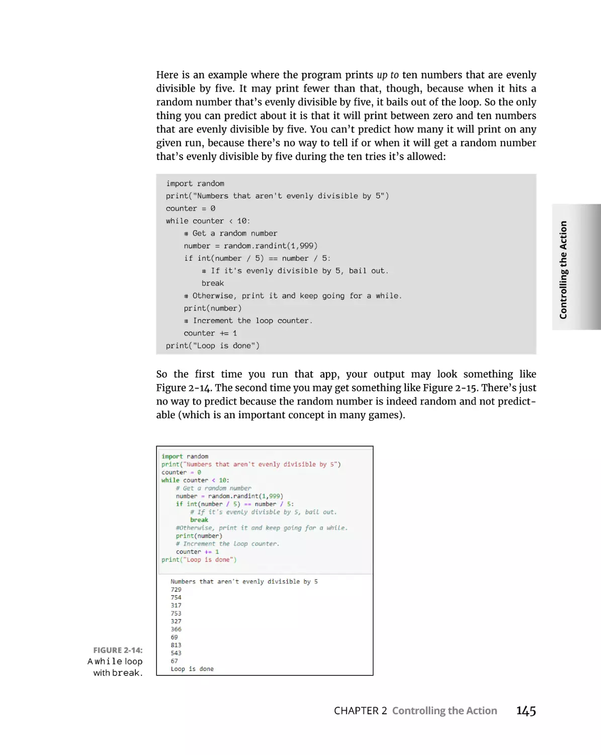
Bailing out of a loop . . . . . . . . . . . . . . . . . . . . . . . . . . . . . . . . . . . . . .
Looping with continue . . . . . . . . . . . . . . . . . . . . . . . . . . . . . . . . . . . .
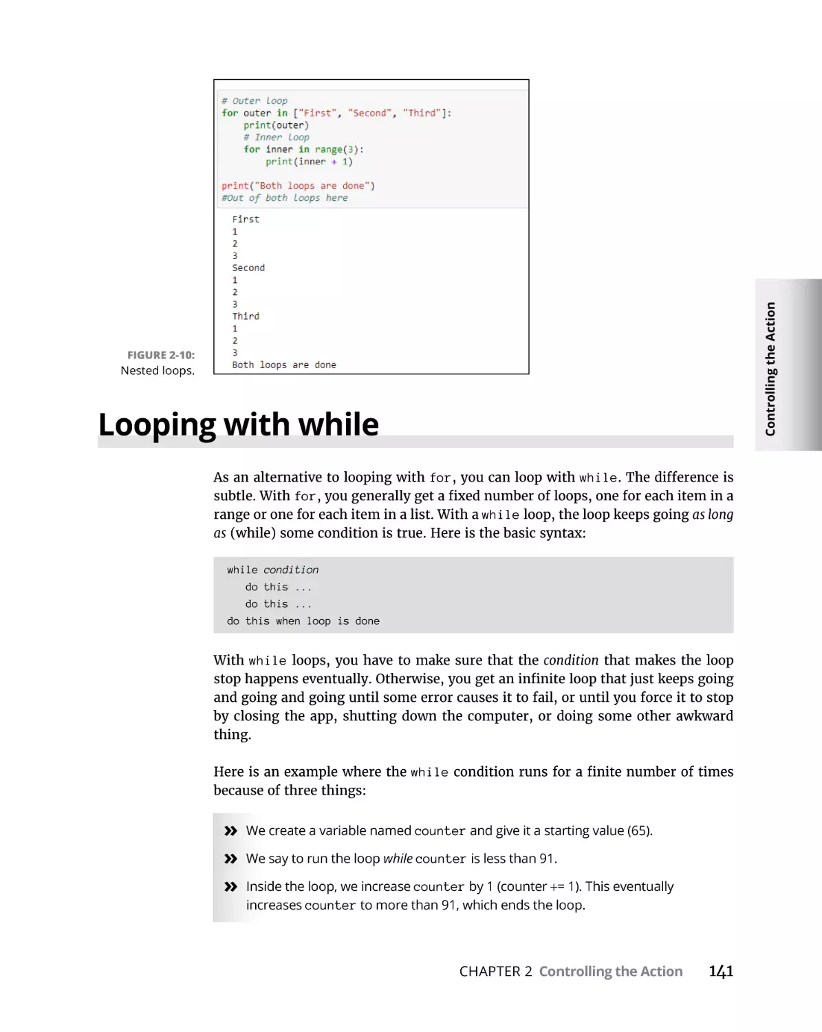
Nesting loops. . . . . . . . . . . . . . . . . . . . . . . . . . . . . . . . . . . . . . . . . . . .
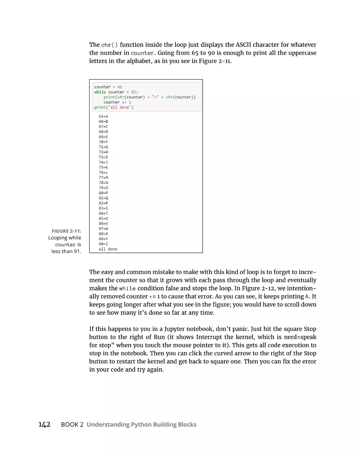
Looping with while . . . . . . . . . . . . . . . . . . . . . . . . . . . . . . . . . . . . . . . . . .
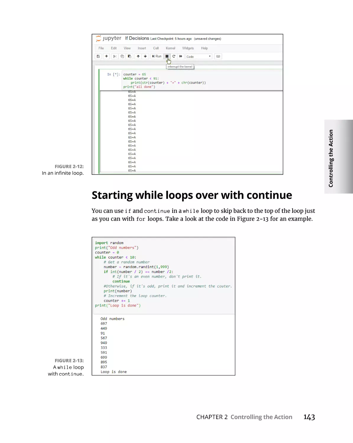
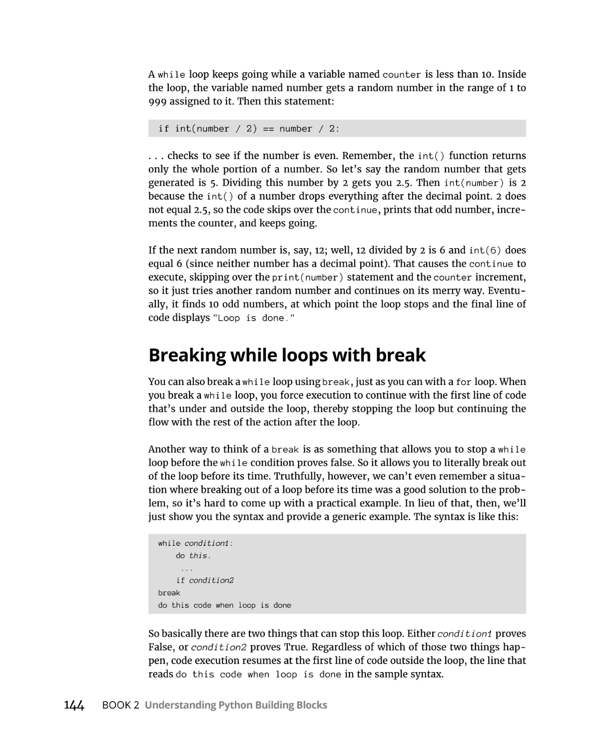
Starting while loops over with continue. . . . . . . . . . . . . . . . . . . . . .
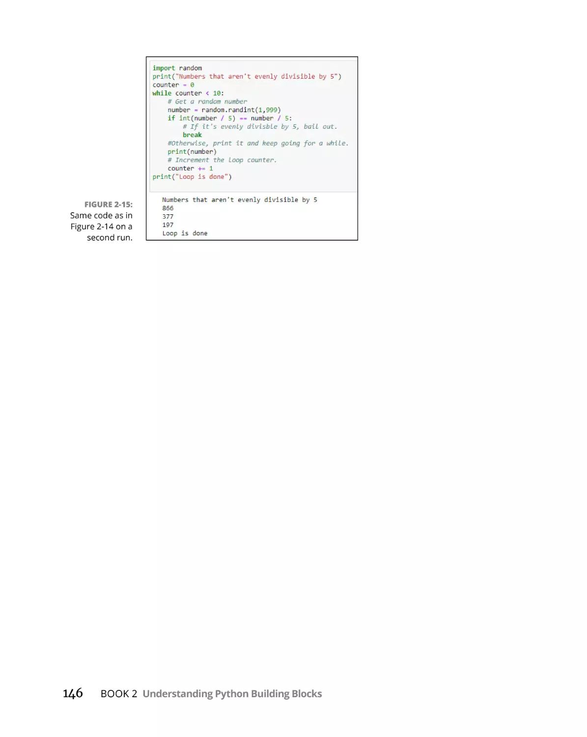
Breaking while loops with break. . . . . . . . . . . . . . . . . . . . . . . . . . . .
125
126
130
131
133
134
134
136
137
138
140
140
141
143
144
Speeding Along with Lists and Tuples. . . . . . . . . . . . . . .
147
Defining and Using Lists. . . . . . . . . . . . . . . . . . . . . . . . . . . . . . . . . . . . . . 147
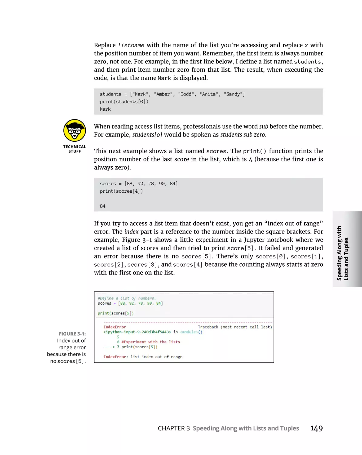
Referencing list items by position. . . . . . . . . . . . . . . . . . . . . . . . . . . 148
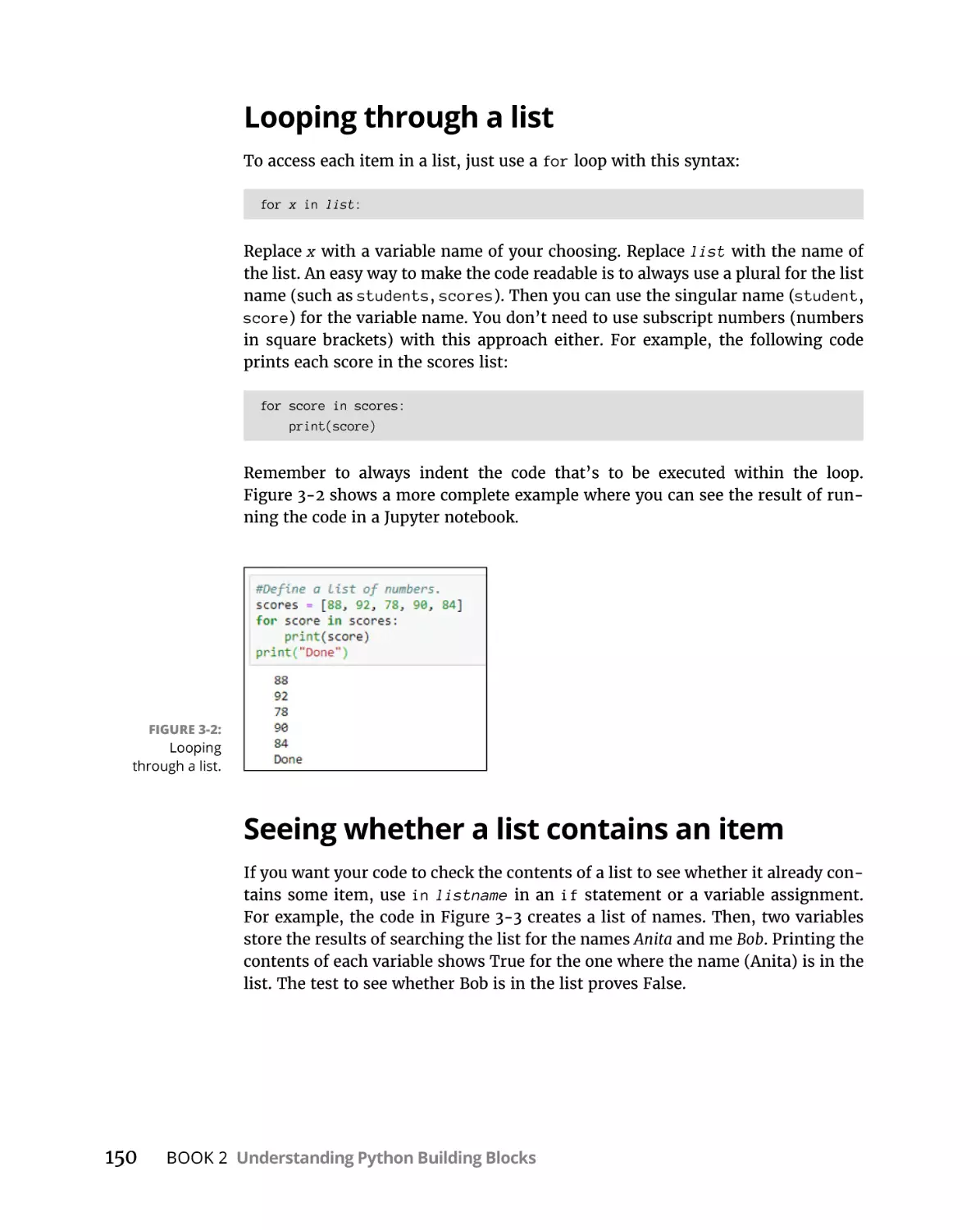
Looping through a list. . . . . . . . . . . . . . . . . . . . . . . . . . . . . . . . . . . . . 150
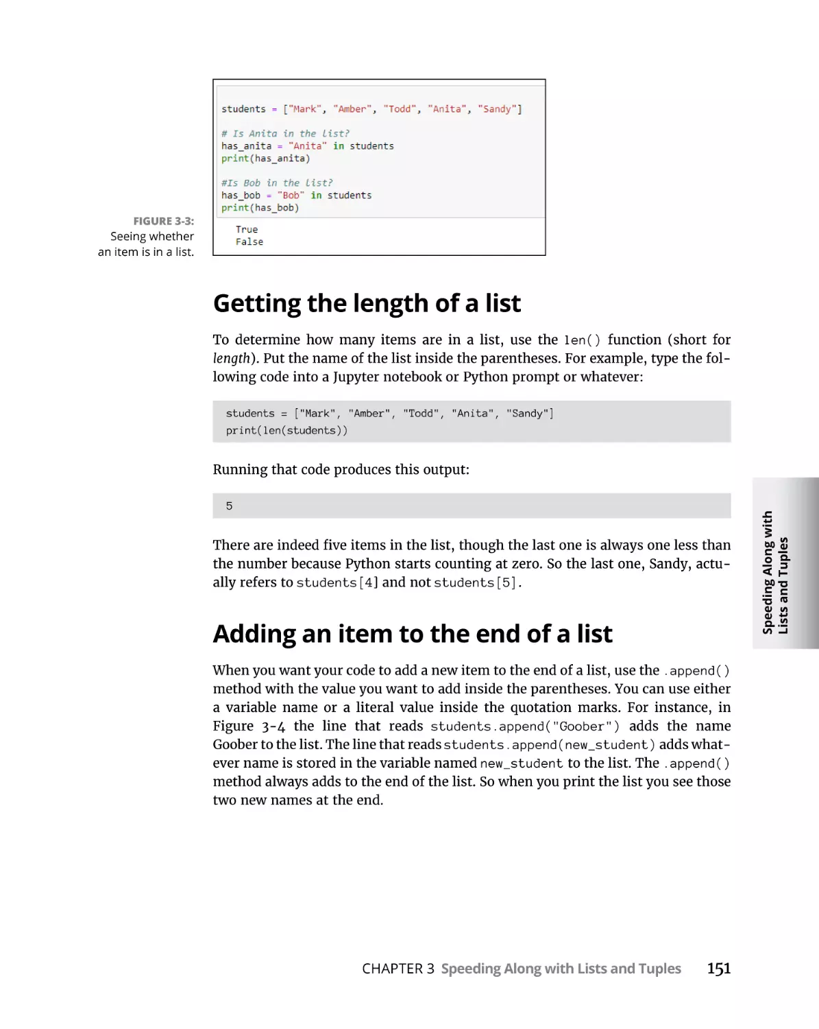
Seeing whether a list contains an item. . . . . . . . . . . . . . . . . . . . . . .150
Getting the length of a list . . . . . . . . . . . . . . . . . . . . . . . . . . . . . . . . . 151
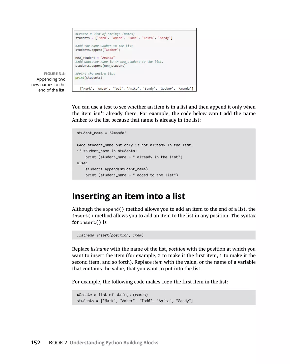
Adding an item to the end of a list . . . . . . . . . . . . . . . . . . . . . . . . . . 151
Inserting an item into a list . . . . . . . . . . . . . . . . . . . . . . . . . . . . . . . . 152
Changing an item in a list. . . . . . . . . . . . . . . . . . . . . . . . . . . . . . . . . . 153
Combining lists . . . . . . . . . . . . . . . . . . . . . . . . . . . . . . . . . . . . . . . . . . 153
Table of Contents
vii
Removing list items. . . . . . . . . . . . . . . . . . . . . . . . . . . . . . . . . . . . . . . 154
Clearing out a list. . . . . . . . . . . . . . . . . . . . . . . . . . . . . . . . . . . . . . . . . 156
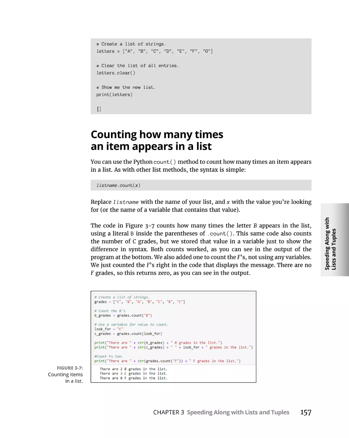
Counting how many times an item appears in a list . . . . . . . . . . . 157
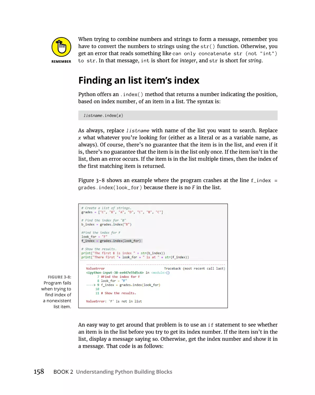
Finding an list item’s index. . . . . . . . . . . . . . . . . . . . . . . . . . . . . . . . . 158
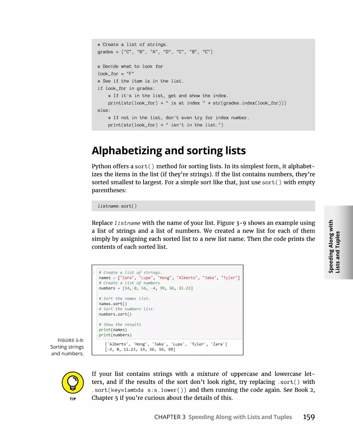
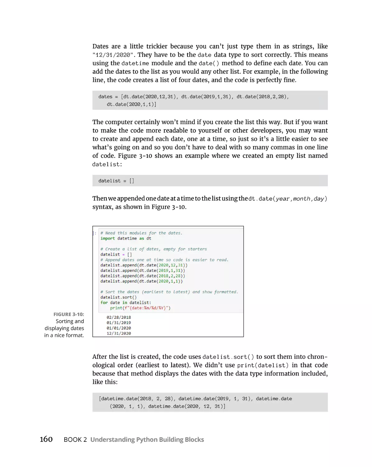
Alphabetizing and sorting lists. . . . . . . . . . . . . . . . . . . . . . . . . . . . . .159
Reversing a list. . . . . . . . . . . . . . . . . . . . . . . . . . . . . . . . . . . . . . . . . . . 161
Copying a list . . . . . . . . . . . . . . . . . . . . . . . . . . . . . . . . . . . . . . . . . . . . 162
What’s a Tuple and Who Cares? . . . . . . . . . . . . . . . . . . . . . . . . . . . . . . . 163
Working with Sets. . . . . . . . . . . . . . . . . . . . . . . . . . . . . . . . . . . . . . . . . . . 165
CHAPTER 4:
CHAPTER 5:
CHAPTER 6:
Cruising Massive Data with Dictionaries. . . . . . . . . . .
169
Creating a Data Dictionary. . . . . . . . . . . . . . . . . . . . . . . . . . . . . . . . . . . .
Accessing dictionary data. . . . . . . . . . . . . . . . . . . . . . . . . . . . . . . . . .
Getting the length of a dictionary. . . . . . . . . . . . . . . . . . . . . . . . . . .
Seeing whether a key exists in a dictionary. . . . . . . . . . . . . . . . . . .
Getting dictionary data with get() . . . . . . . . . . . . . . . . . . . . . . . . . . .
Changing the value of a key. . . . . . . . . . . . . . . . . . . . . . . . . . . . . . . .
Adding or changing dictionary data . . . . . . . . . . . . . . . . . . . . . . . . .
Looping through a Dictionary . . . . . . . . . . . . . . . . . . . . . . . . . . . . . . . . .
Data Dictionary Methods. . . . . . . . . . . . . . . . . . . . . . . . . . . . . . . . . . . . .
Copying a Dictionary. . . . . . . . . . . . . . . . . . . . . . . . . . . . . . . . . . . . . . . . .
Deleting Dictionary Items. . . . . . . . . . . . . . . . . . . . . . . . . . . . . . . . . . . . .
Using pop() with Data Dictionaries. . . . . . . . . . . . . . . . . . . . . . . . . .
Fun with Multi-Key Dictionaries. . . . . . . . . . . . . . . . . . . . . . . . . . . . . . . .
Using the mysterious fromkeys and setdefault methods. . . . . . .
Nesting Dictionaries . . . . . . . . . . . . . . . . . . . . . . . . . . . . . . . . . . . . . .
171
172
174
175
176
177
177
179
181
182
182
184
186
188
190
Wrangling Bigger Chunks of Code . . . . . . . . . . . . . . . . . . .
193
Creating a Function. . . . . . . . . . . . . . . . . . . . . . . . . . . . . . . . . . . . . . . . . .
Commenting a Function. . . . . . . . . . . . . . . . . . . . . . . . . . . . . . . . . . . . . .
Passing Information to a Function . . . . . . . . . . . . . . . . . . . . . . . . . . . . .
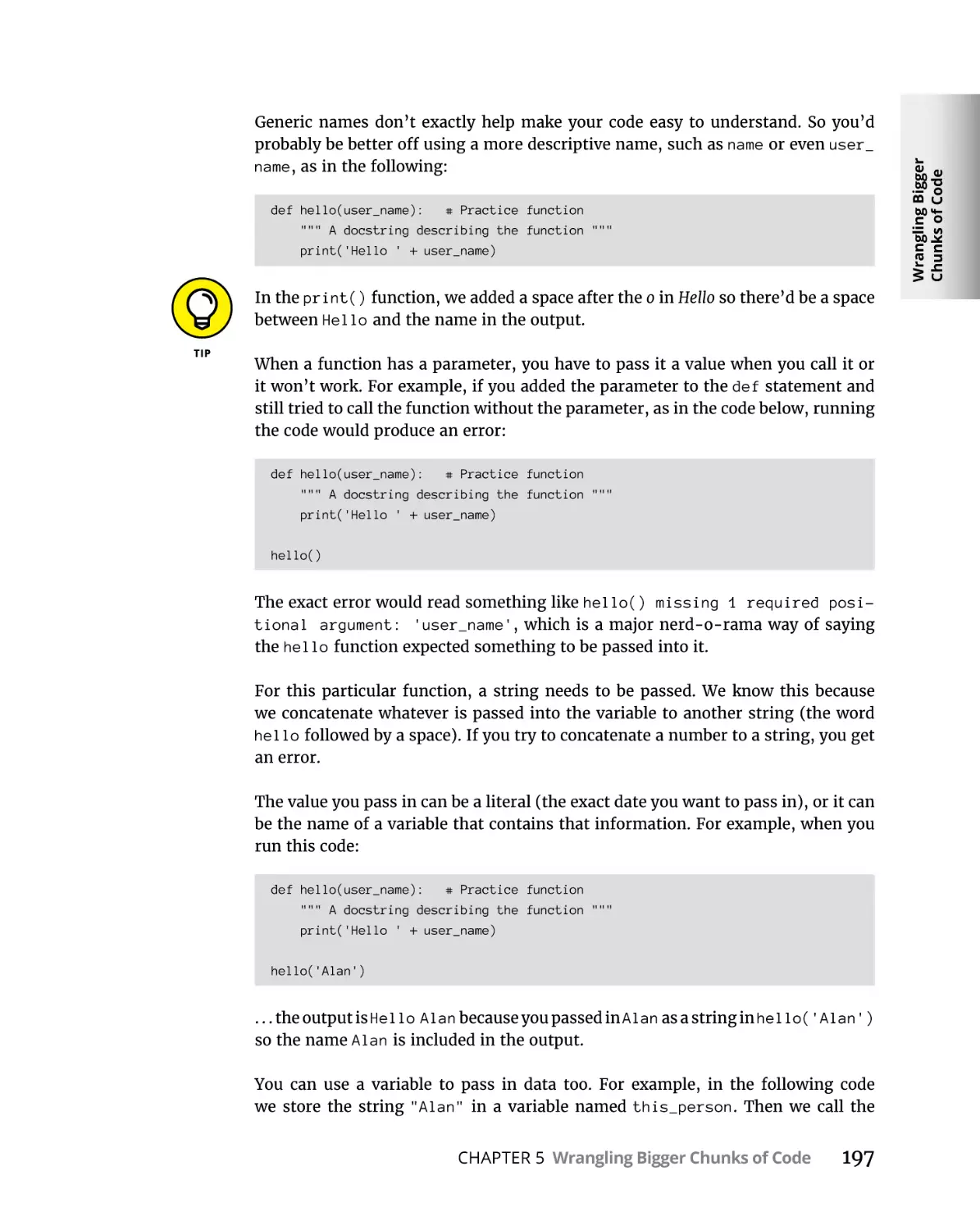
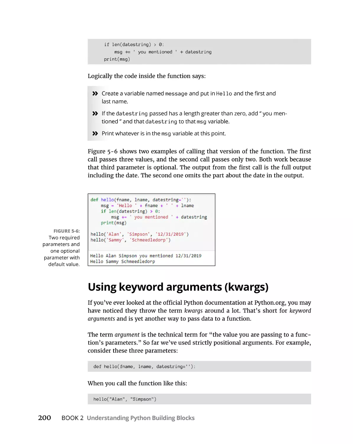
Defining optional parameters with defaults. . . . . . . . . . . . . . . . . .
Passing multiple values to a function. . . . . . . . . . . . . . . . . . . . . . . .
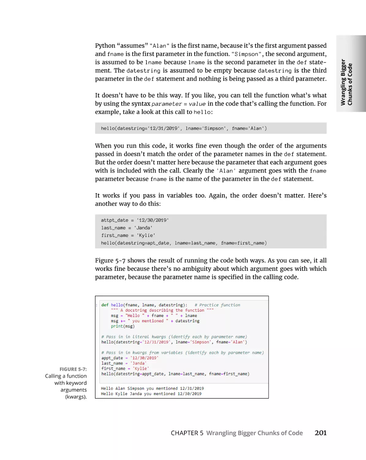
Using keyword arguments (kwargs). . . . . . . . . . . . . . . . . . . . . . . . .
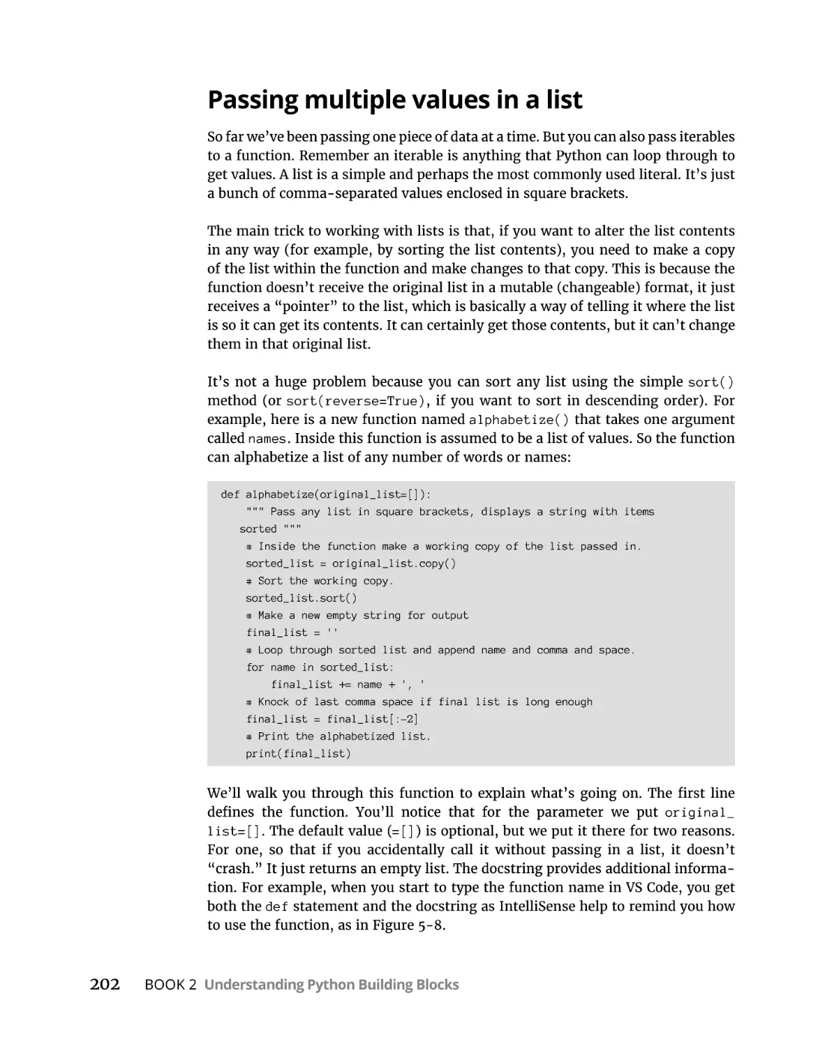
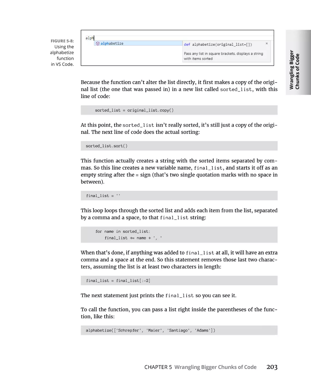
Passing multiple values in a list. . . . . . . . . . . . . . . . . . . . . . . . . . . . .
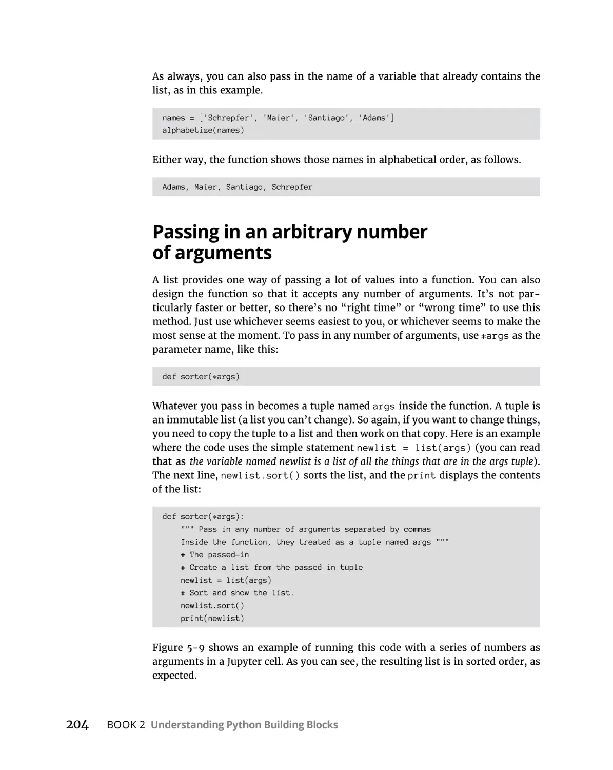
Passing in an arbitrary number of arguments . . . . . . . . . . . . . . . .
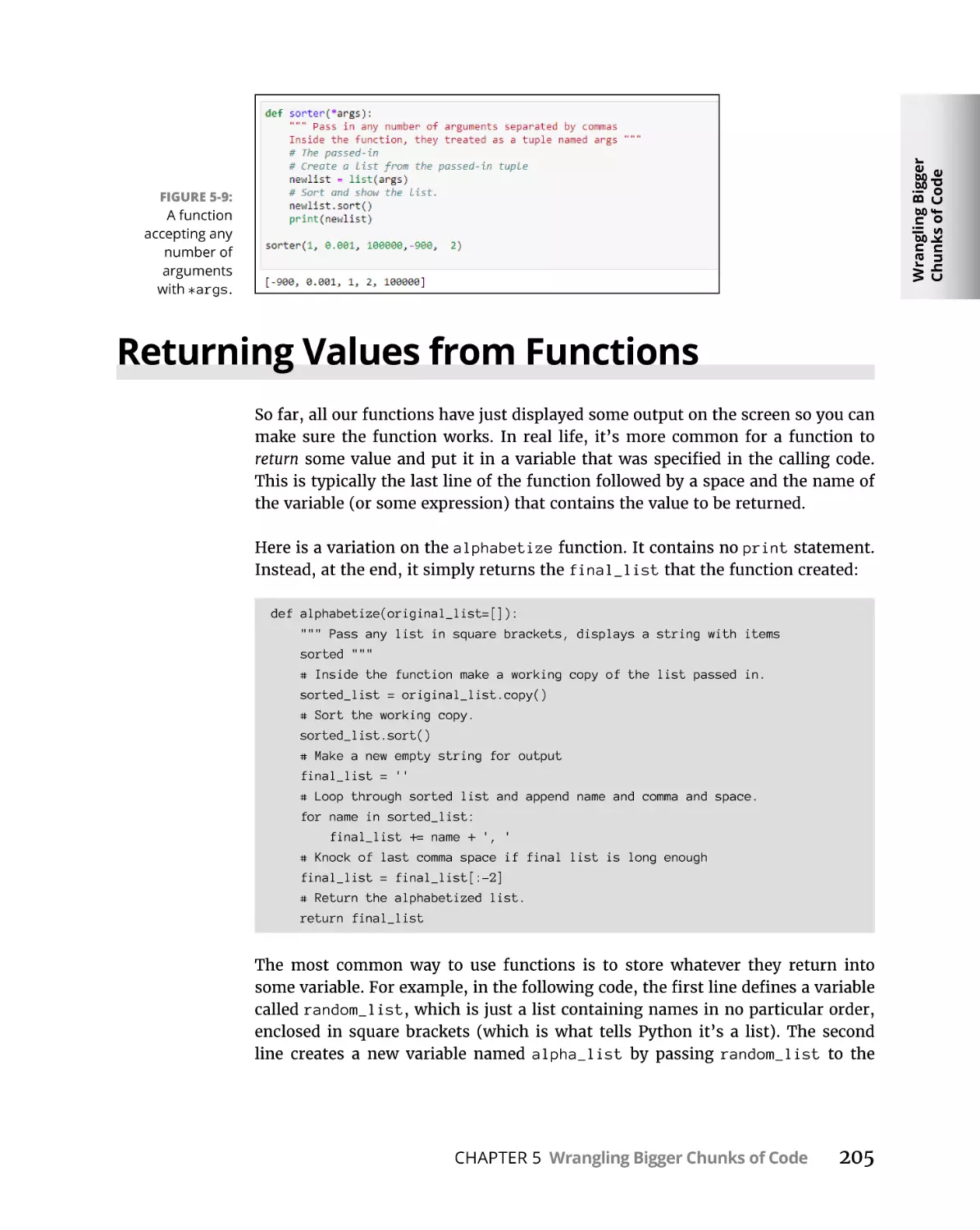
Returning Values from Functions. . . . . . . . . . . . . . . . . . . . . . . . . . . . . .
Unmasking Anonymous Functions. . . . . . . . . . . . . . . . . . . . . . . . . . . . .
194
195
196
198
199
200
202
204
205
206
Doing Python with Class. . . . . . . . . . . . . . . . . . . . . . . . . . . . . . .
213
Mastering Classes and Objects. . . . . . . . . . . . . . . . . . . . . . . . . . . . . . . . 213
Creating a Class. . . . . . . . . . . . . . . . . . . . . . . . . . . . . . . . . . . . . . . . . . . . . 216
How a Class Creates an Instance . . . . . . . . . . . . . . . . . . . . . . . . . . . . . . 217
viii
Python All-in-One For Dummies
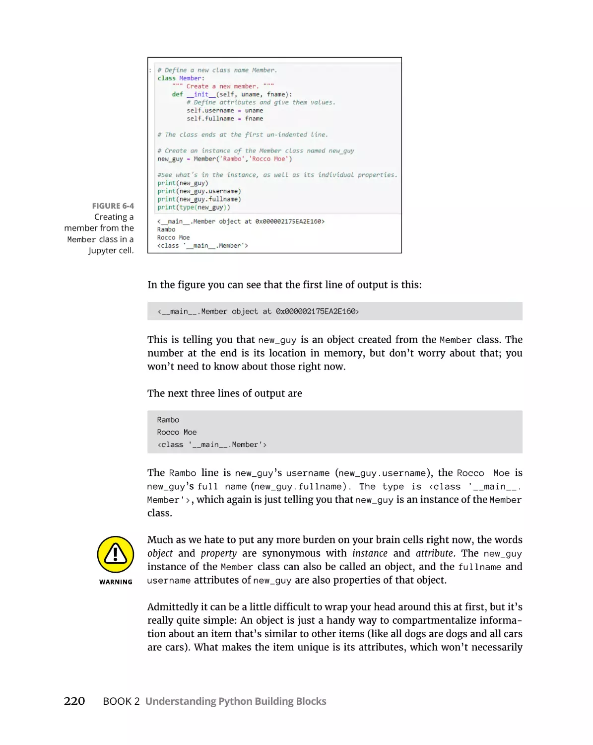
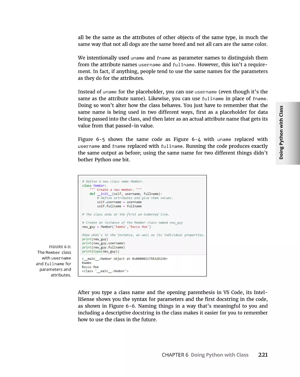
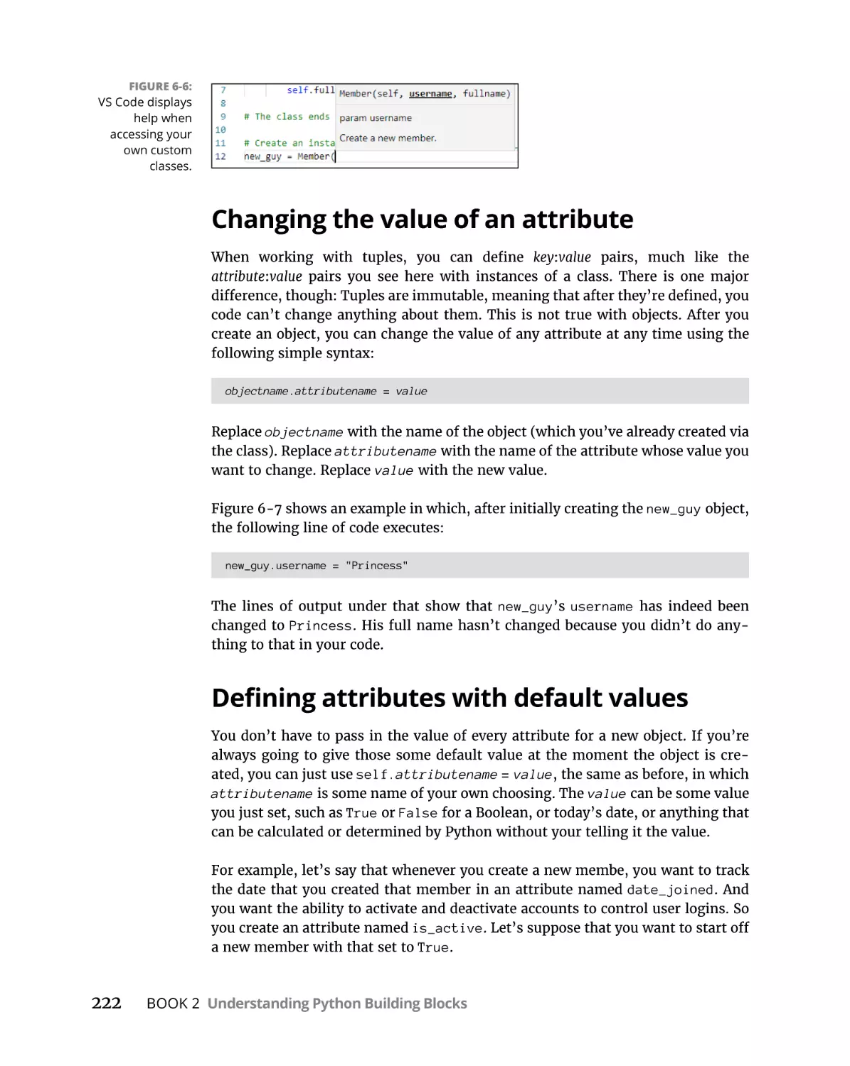
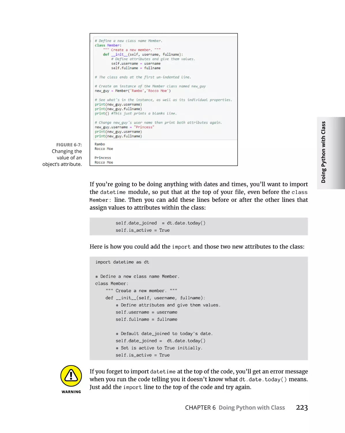
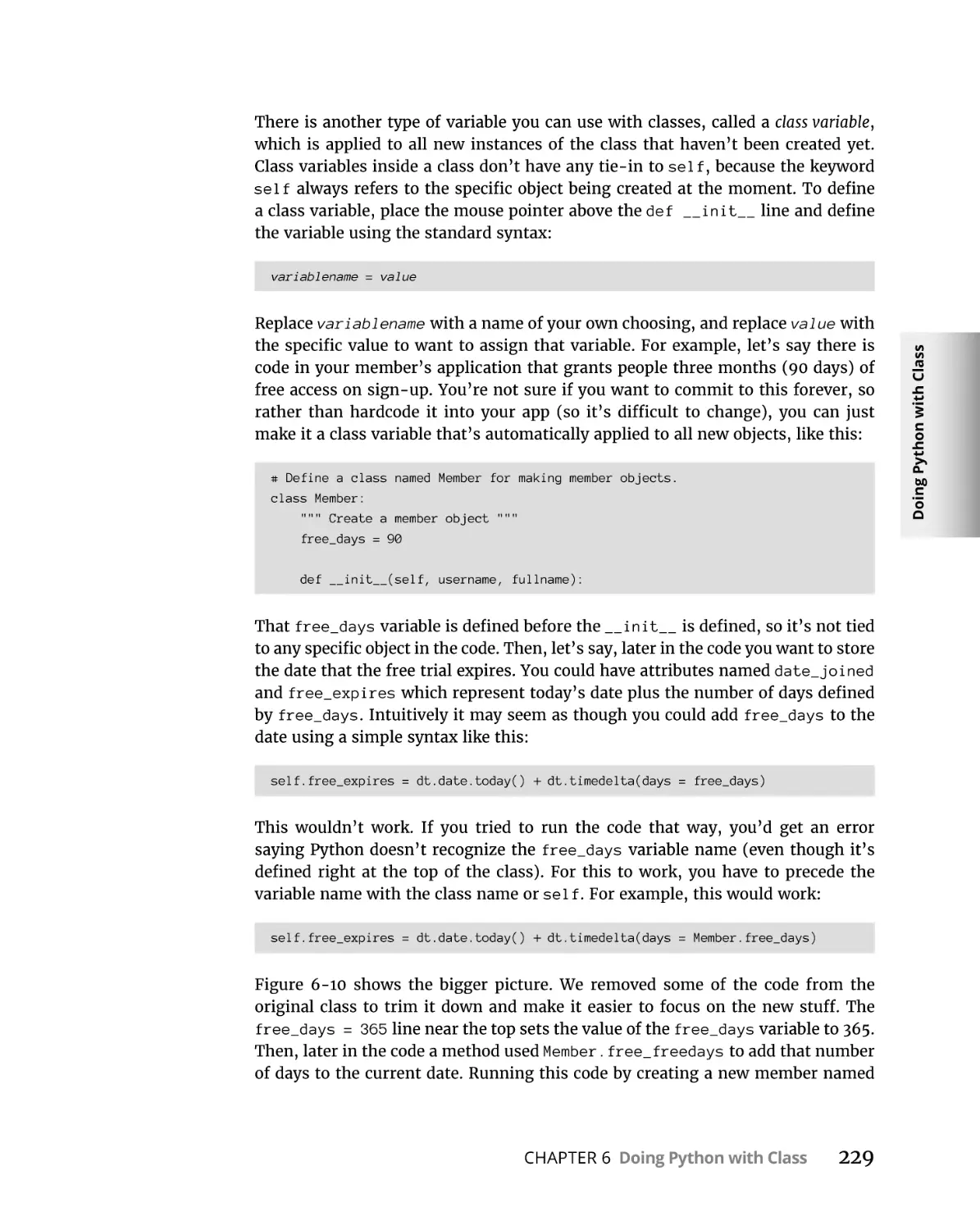
Giving an Object Its Attributes. . . . . . . . . . . . . . . . . . . . . . . . . . . . . . . . .
Creating an instance from a class. . . . . . . . . . . . . . . . . . . . . . . . . . .
Changing the value of an attribute. . . . . . . . . . . . . . . . . . . . . . . . . .
Defining attributes with default values . . . . . . . . . . . . . . . . . . . . . .
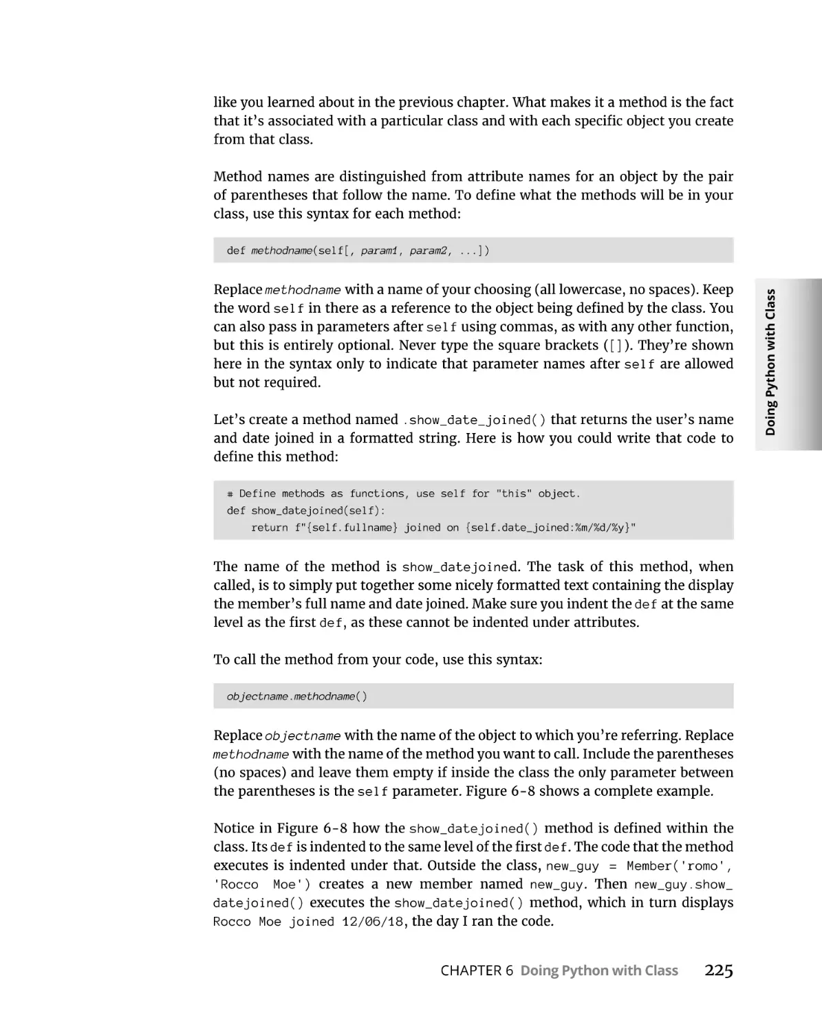
Giving a Class Methods. . . . . . . . . . . . . . . . . . . . . . . . . . . . . . . . . . . . . . .
Passing parameters to methods. . . . . . . . . . . . . . . . . . . . . . . . . . . .
Calling a class method by class name . . . . . . . . . . . . . . . . . . . . . . .
Using class variables. . . . . . . . . . . . . . . . . . . . . . . . . . . . . . . . . . . . . .
Using class methods. . . . . . . . . . . . . . . . . . . . . . . . . . . . . . . . . . . . . .
Using static methods . . . . . . . . . . . . . . . . . . . . . . . . . . . . . . . . . . . . .
Understanding Class Inheritance . . . . . . . . . . . . . . . . . . . . . . . . . . . . . .
Creating the base (main) class. . . . . . . . . . . . . . . . . . . . . . . . . . . . . .
Defining a subclass. . . . . . . . . . . . . . . . . . . . . . . . . . . . . . . . . . . . . . .
Overriding a default value from a subclass. . . . . . . . . . . . . . . . . . .
Adding extra parameters from a subclass. . . . . . . . . . . . . . . . . . . .
Calling a base class method. . . . . . . . . . . . . . . . . . . . . . . . . . . . . . . .
Using the same name twice. . . . . . . . . . . . . . . . . . . . . . . . . . . . . . . .
218
219
222
222
224
226
227
228
230
232
234
236
237
239
239
242
243
Sidestepping Errors . . . . . . . . . . . . . . . . . . . . . . . . . . . . . . . . . . . .
247
Understanding Exceptions. . . . . . . . . . . . . . . . . . . . . . . . . . . . . . . . . . . .
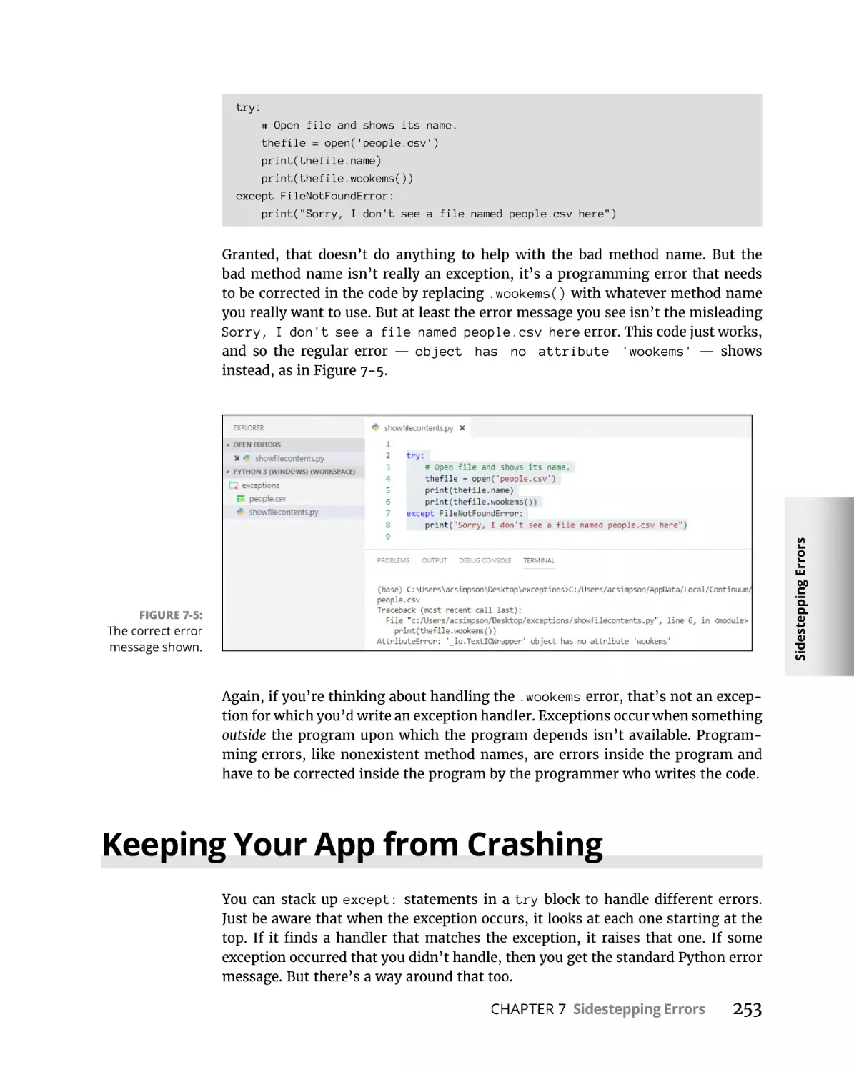
Handling Errors Gracefully. . . . . . . . . . . . . . . . . . . . . . . . . . . . . . . . . . . .
Being Specific about Exceptions. . . . . . . . . . . . . . . . . . . . . . . . . . . . . . .
Keeping Your App from Crashing. . . . . . . . . . . . . . . . . . . . . . . . . . . . . .
Adding an else to the Mix. . . . . . . . . . . . . . . . . . . . . . . . . . . . . . . . . . . . .
Using try . . . except . . . else . . . finally. . . . . . . . . . . . . . . . . . . . . . . . . .
Raising Your Own Errors . . . . . . . . . . . . . . . . . . . . . . . . . . . . . . . . . . . . .
247
251
252
253
255
257
259
BOOK 3: WORKING WITH PYTHON LIBRARIES . . . . . . . . . . . .
265
CHAPTER 7:
CHAPTER 1:
Working with External Files . . . . . . . . . . . . . . . . . . . . . . . . . .
267
Understanding Text and Binary Files. . . . . . . . . . . . . . . . . . . . . . . . . . .
Opening and Closing Files . . . . . . . . . . . . . . . . . . . . . . . . . . . . . . . . . . . .
Reading a File’s Contents . . . . . . . . . . . . . . . . . . . . . . . . . . . . . . . . . . . . .
Looping through a File . . . . . . . . . . . . . . . . . . . . . . . . . . . . . . . . . . . . . . .
Looping with readlines(). . . . . . . . . . . . . . . . . . . . . . . . . . . . . . . . . . .
Looping with readline(). . . . . . . . . . . . . . . . . . . . . . . . . . . . . . . . . . . .
Appending versus overwriting files. . . . . . . . . . . . . . . . . . . . . . . . . .
Using tell() to determine the pointer location. . . . . . . . . . . . . . . . .
Moving the pointer with seek() . . . . . . . . . . . . . . . . . . . . . . . . . . . . .
Reading and Copying a Binary File . . . . . . . . . . . . . . . . . . . . . . . . . . . . .
Conquering CSV Files . . . . . . . . . . . . . . . . . . . . . . . . . . . . . . . . . . . . . . . .
Opening a CSV file. . . . . . . . . . . . . . . . . . . . . . . . . . . . . . . . . . . . . . . .
Converting strings. . . . . . . . . . . . . . . . . . . . . . . . . . . . . . . . . . . . . . . .
267
269
276
277
277
279
280
281
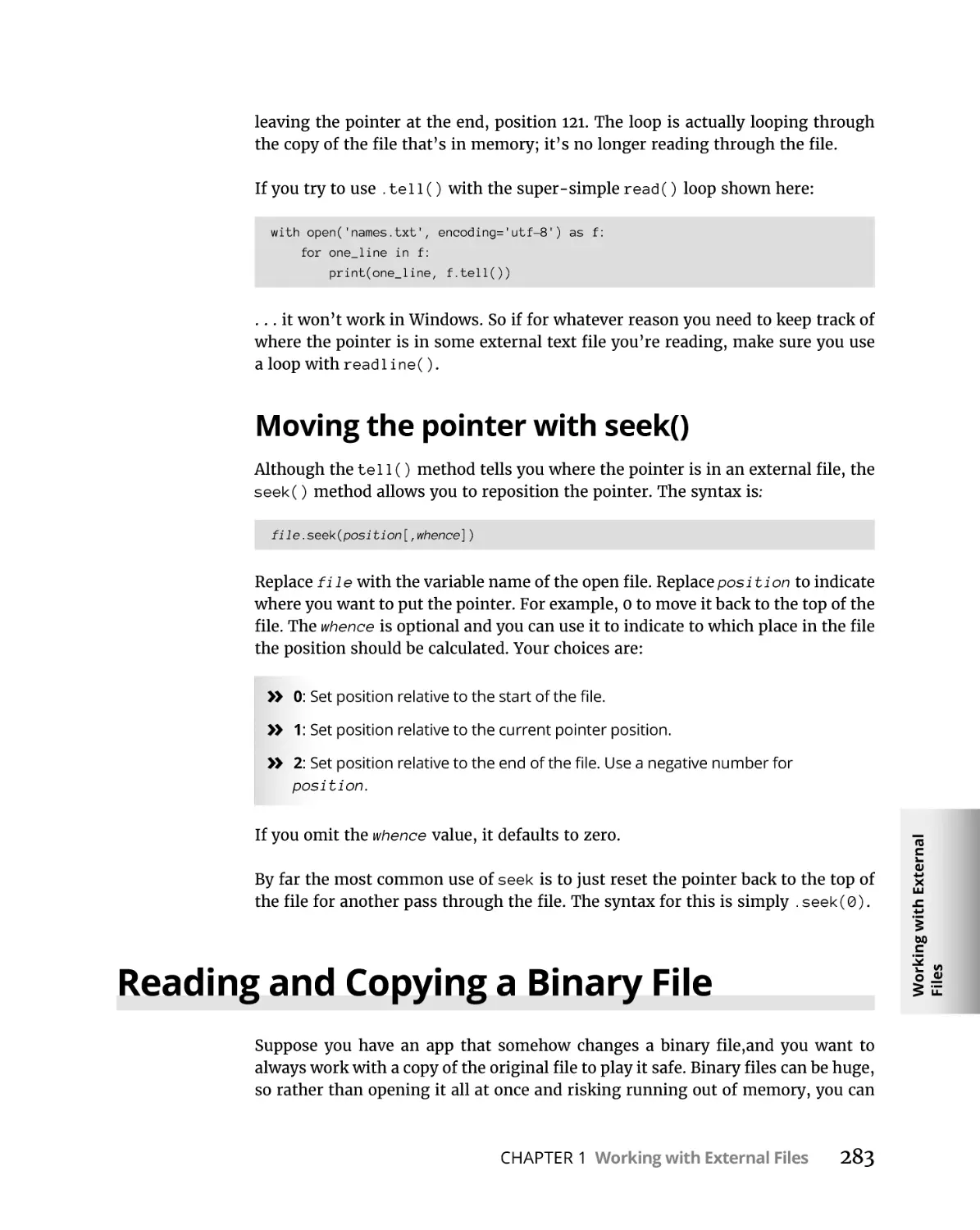
283
283
286
288
290
Table of Contents
ix
CHAPTER 2:
CHAPTER 3:
CHAPTER 4:
x
Converting to integers . . . . . . . . . . . . . . . . . . . . . . . . . . . . . . . . . . . .
Converting to date. . . . . . . . . . . . . . . . . . . . . . . . . . . . . . . . . . . . . . . .
Converting to Boolean . . . . . . . . . . . . . . . . . . . . . . . . . . . . . . . . . . . .
Converting to floats. . . . . . . . . . . . . . . . . . . . . . . . . . . . . . . . . . . . . . .
From CSV to Objects and Dictionaries . . . . . . . . . . . . . . . . . . . . . . . . . .
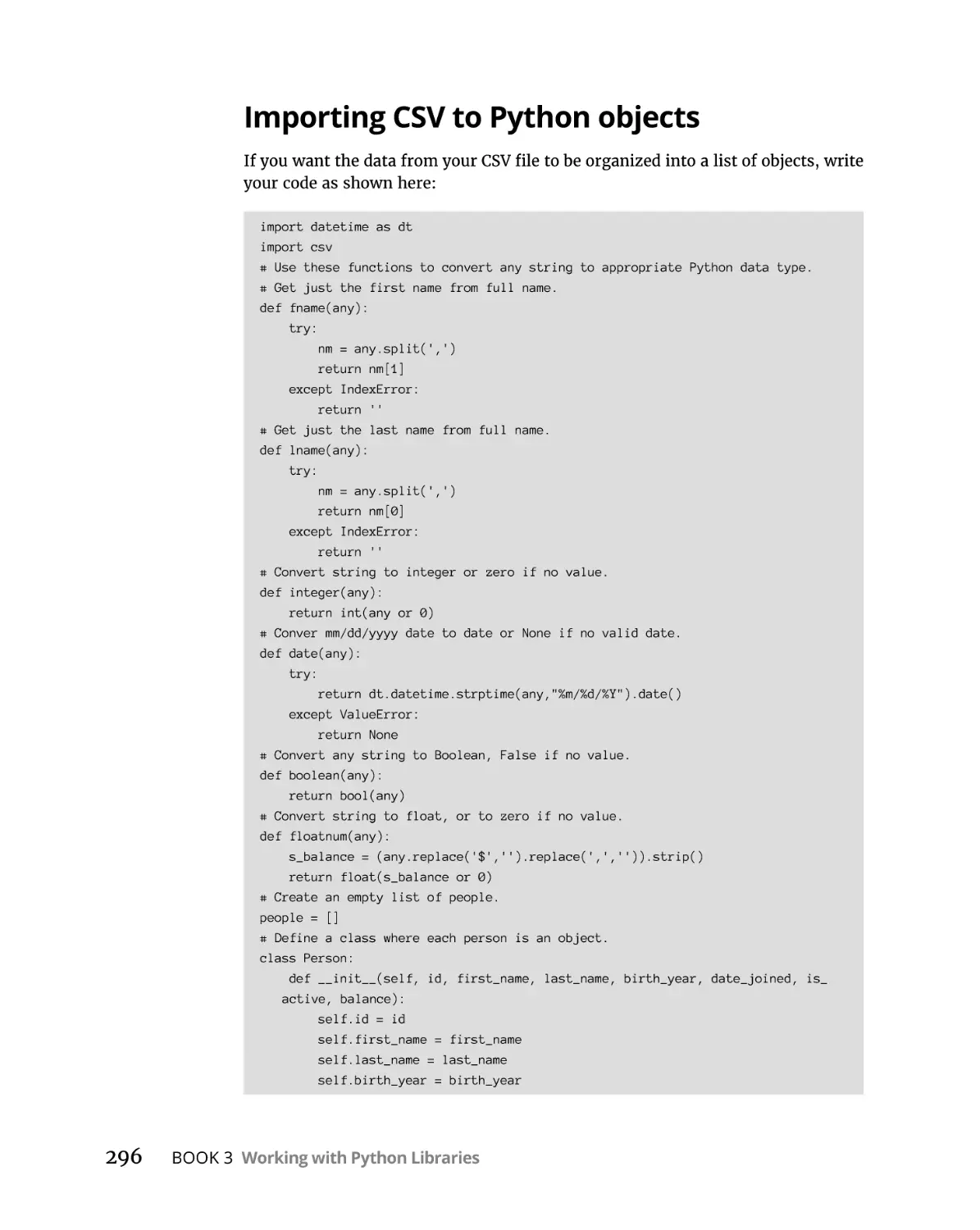
Importing CSV to Python objects. . . . . . . . . . . . . . . . . . . . . . . . . . . .
Importing CSV to Python dictionaries. . . . . . . . . . . . . . . . . . . . . . . .
291
292
293
293
295
296
299
Juggling JSON Data . . . . . . . . . . . . . . . . . . . . . . . . . . . . . . . . . . . . .
303
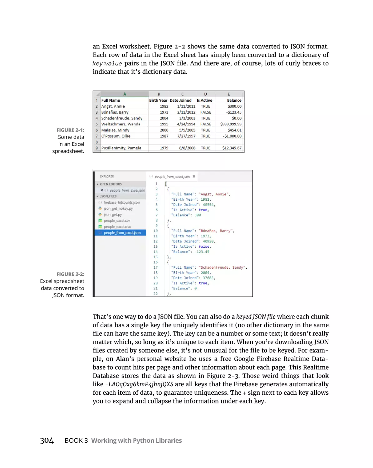
Organizing JSON Data. . . . . . . . . . . . . . . . . . . . . . . . . . . . . . . . . . . . . . . .
Understanding Serialization . . . . . . . . . . . . . . . . . . . . . . . . . . . . . . . . . .
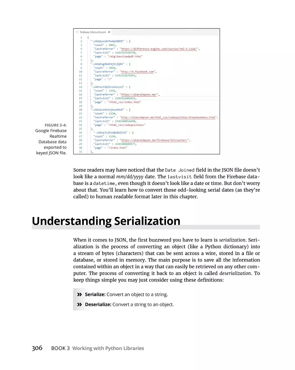
Loading Data from JSON Files . . . . . . . . . . . . . . . . . . . . . . . . . . . . . . . . .
Converting an Excel date to a JSON date. . . . . . . . . . . . . . . . . . . . .
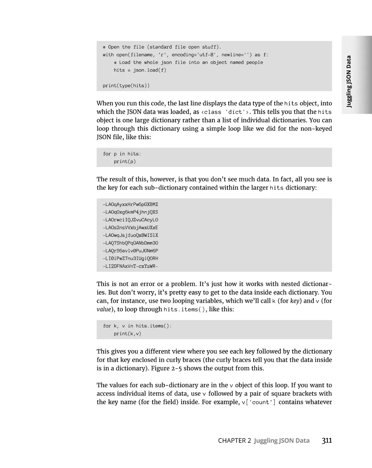
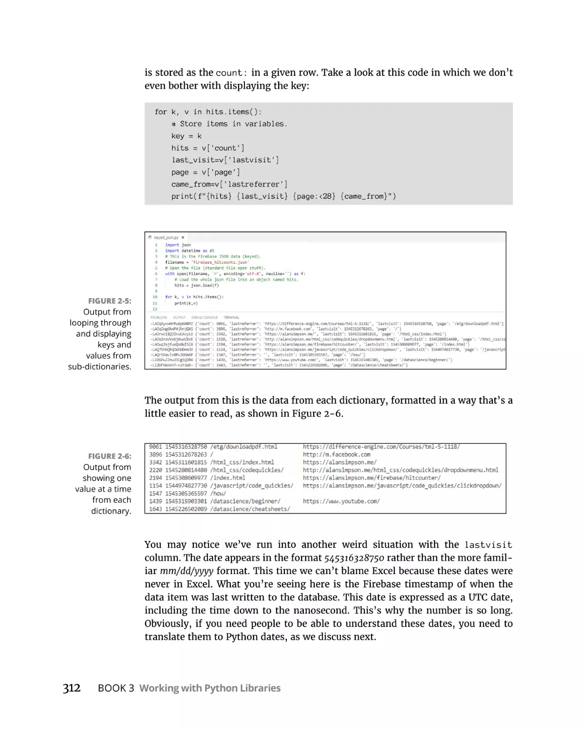
Looping through a keyed JSON file. . . . . . . . . . . . . . . . . . . . . . . . . .
Converting firebase timestamps to Python dates . . . . . . . . . . . . .
Loading unkeyed JSON from a Python string . . . . . . . . . . . . . . . . .
Loading keyed JSON from a Python string. . . . . . . . . . . . . . . . . . . .
Changing JSON data . . . . . . . . . . . . . . . . . . . . . . . . . . . . . . . . . . . . . .
Removing data from a dictionary . . . . . . . . . . . . . . . . . . . . . . . . . . .
Dumping Python Data to JSON . . . . . . . . . . . . . . . . . . . . . . . . . . . . . . . .
303
306
307
309
310
313
314
315
316
317
318
Interacting with the Internet. . . . . . . . . . . . . . . . . . . . . . . . .
323
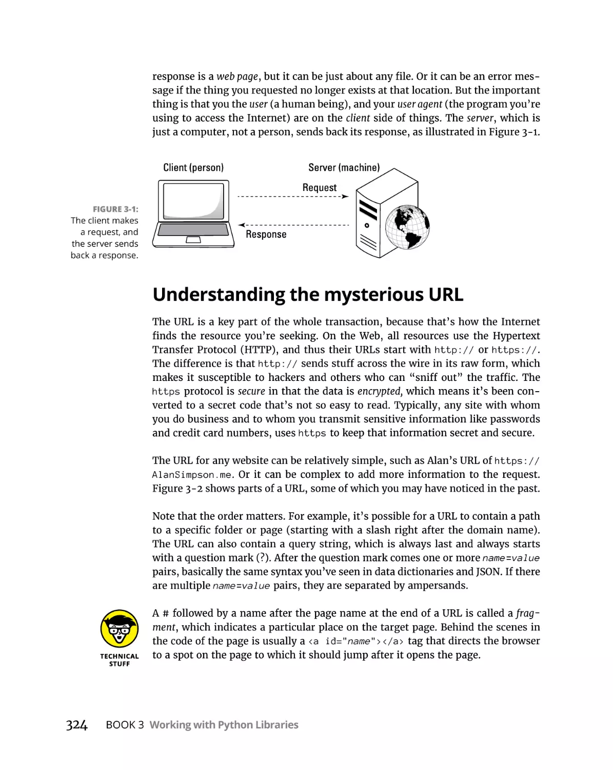
How the Web Works. . . . . . . . . . . . . . . . . . . . . . . . . . . . . . . . . . . . . . . . .
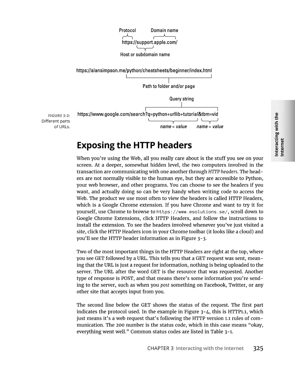
Understanding the mysterious URL. . . . . . . . . . . . . . . . . . . . . . . . .
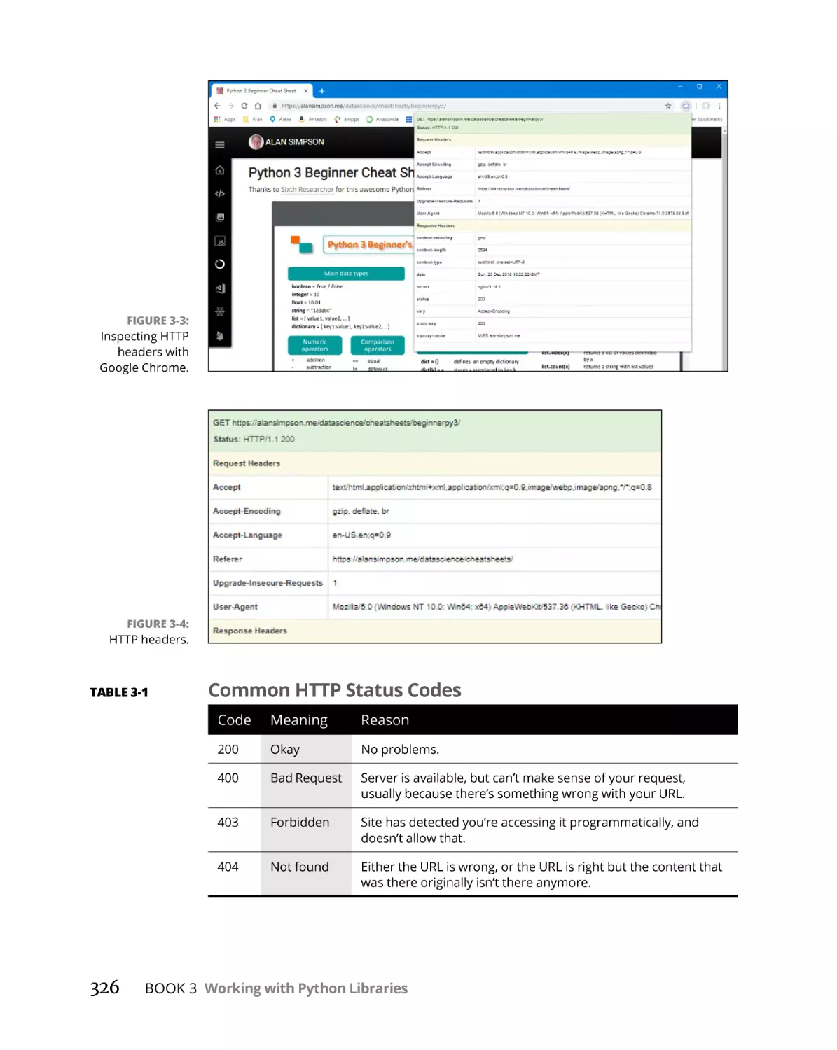
Exposing the HTTP headers. . . . . . . . . . . . . . . . . . . . . . . . . . . . . . . .
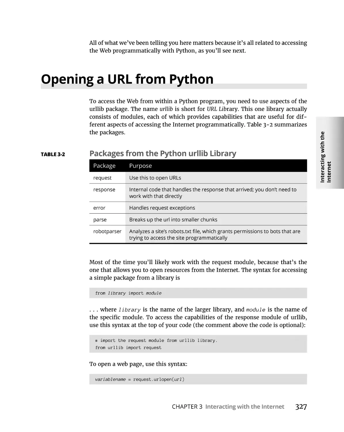
Opening a URL from Python . . . . . . . . . . . . . . . . . . . . . . . . . . . . . . . . . .
Posting to the Web with Python . . . . . . . . . . . . . . . . . . . . . . . . . . . . . . .
Scraping the Web with Python . . . . . . . . . . . . . . . . . . . . . . . . . . . . . . . .
Parsing part of a page. . . . . . . . . . . . . . . . . . . . . . . . . . . . . . . . . . . . .
Storing the parsed content . . . . . . . . . . . . . . . . . . . . . . . . . . . . . . . .
Saving scraped data to a JSON file . . . . . . . . . . . . . . . . . . . . . . . . . .
Saving scraped data to a CSV file . . . . . . . . . . . . . . . . . . . . . . . . . . .
323
324
325
327
328
330
333
333
335
336
Libraries, Packages, and Modules . . . . . . . . . . . . . . . . . . .
339
Understanding the Python Standard Library . . . . . . . . . . . . . . . . . . . .
Using the dir() function. . . . . . . . . . . . . . . . . . . . . . . . . . . . . . . . . . . .
Using the help() function . . . . . . . . . . . . . . . . . . . . . . . . . . . . . . . . . .
Exploring built-in functions . . . . . . . . . . . . . . . . . . . . . . . . . . . . . . . .
Exploring Python Packages . . . . . . . . . . . . . . . . . . . . . . . . . . . . . . . . . . .
Importing Python Modules . . . . . . . . . . . . . . . . . . . . . . . . . . . . . . . . . . .
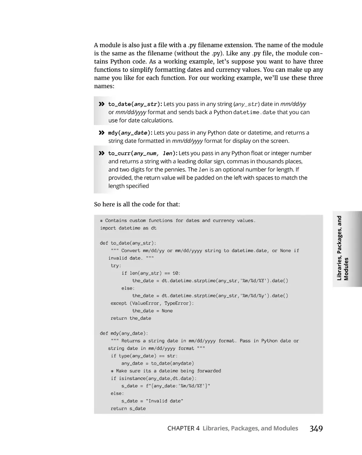
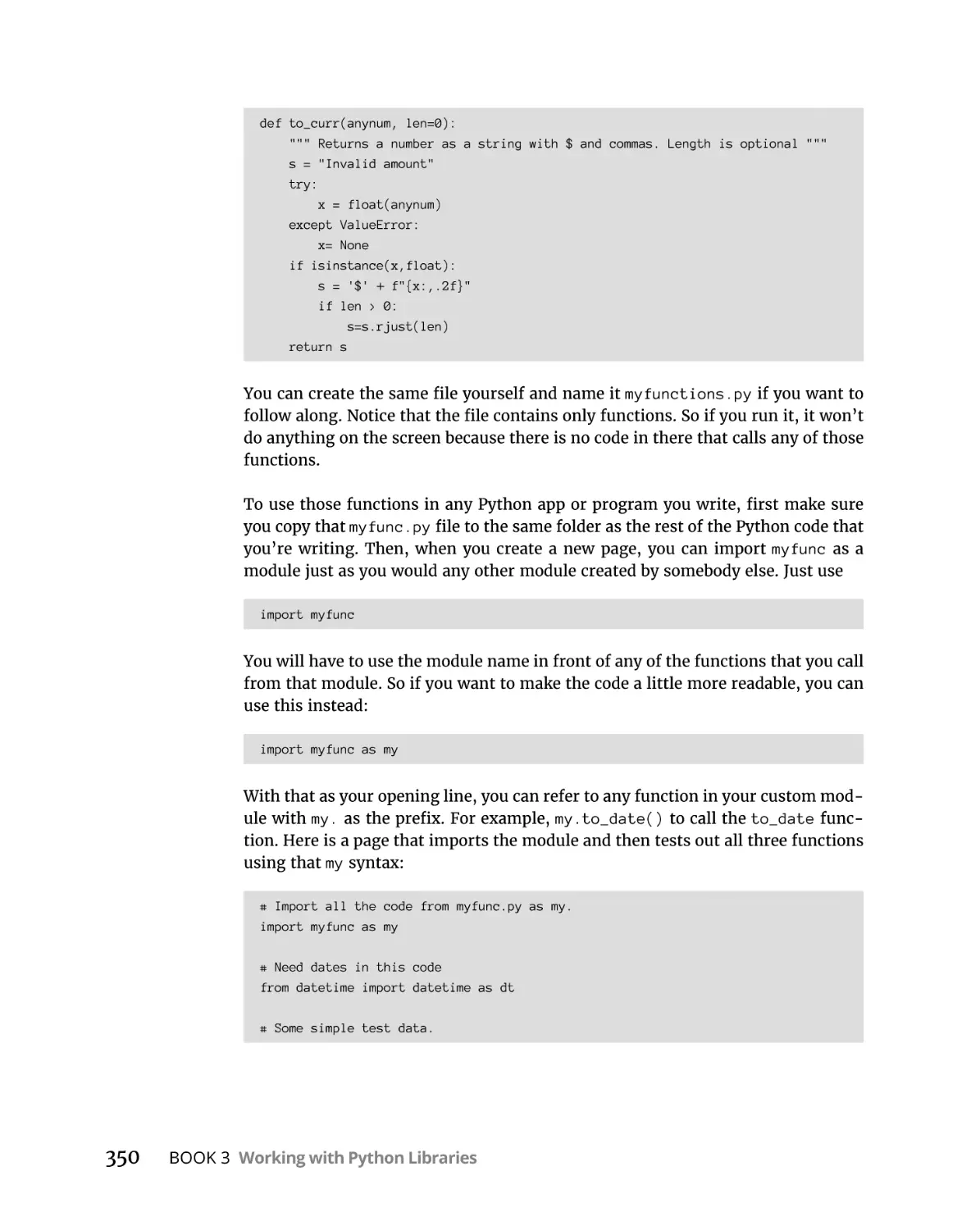
Making Your Own Modules . . . . . . . . . . . . . . . . . . . . . . . . . . . . . . . . . . .
339
340
341
343
343
345
348
Python All-in-One For Dummies
BOOK 4: USING ARTIFICIAL INTELLIGENCE
IN PYTHON . . . . . . . . . . . . . . . . . . . . . . . . . . . . . . . . . . . . . . . . . . . . . . . . . . . . . . .
353
Exploring Artificial Intelligence . . . . . . . . . . . . . . . . . . . . . .
355
AI Is a Collection of Techniques. . . . . . . . . . . . . . . . . . . . . . . . . . . . . . . .
Neural networks . . . . . . . . . . . . . . . . . . . . . . . . . . . . . . . . . . . . . . . . .
Machine learning. . . . . . . . . . . . . . . . . . . . . . . . . . . . . . . . . . . . . . . . .
TensorFlow — A framework for deep learning. . . . . . . . . . . . . . . .
Current Limitations of AI . . . . . . . . . . . . . . . . . . . . . . . . . . . . . . . . . . . . .
356
356
359
361
363
Building a Neural Network in Python. . . . . . . . . . . . . . .
365
CHAPTER 1:
CHAPTER 2:
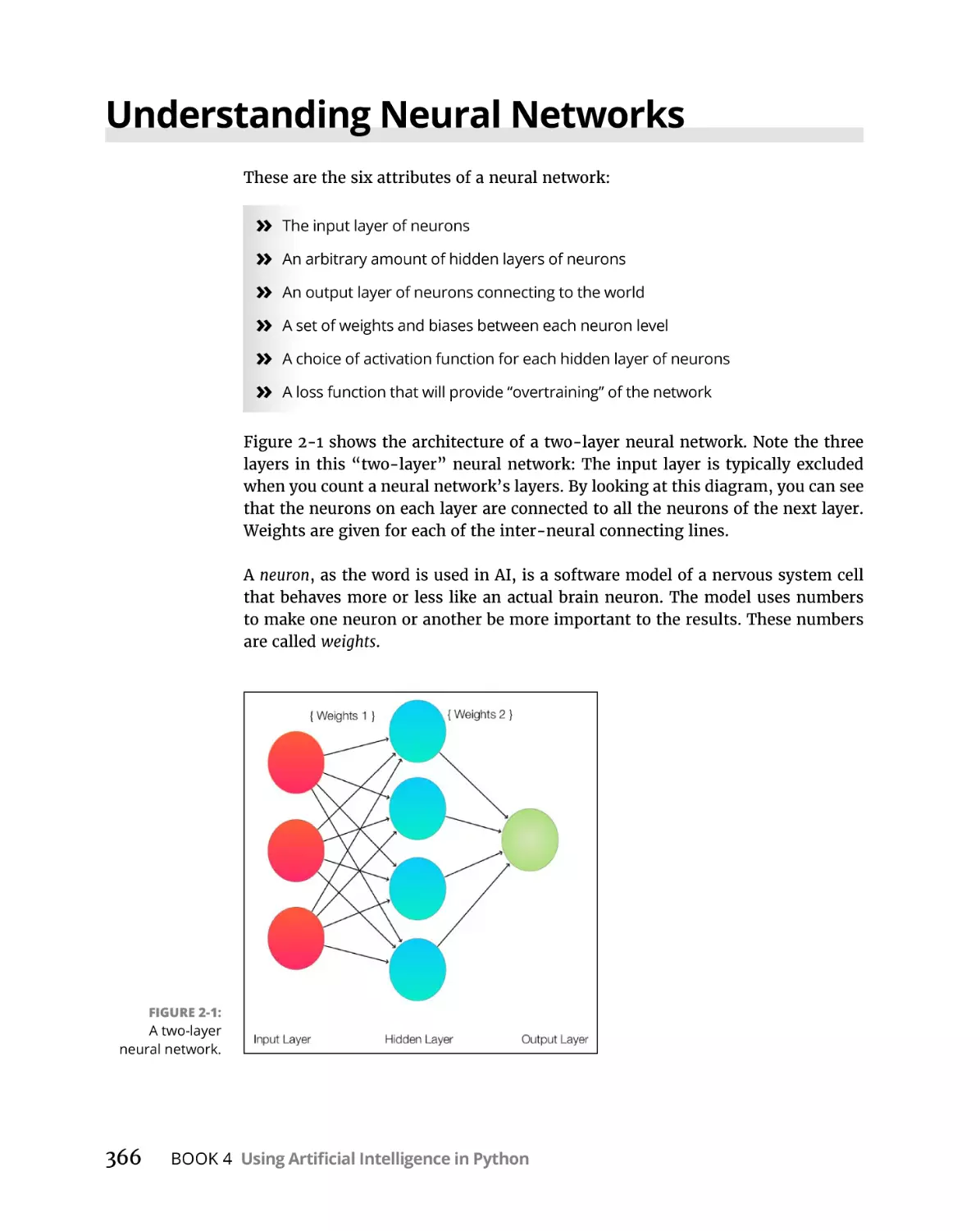
Understanding Neural Networks . . . . . . . . . . . . . . . . . . . . . . . . . . . . . . 366
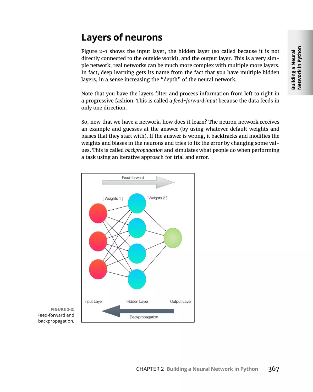
Layers of neurons . . . . . . . . . . . . . . . . . . . . . . . . . . . . . . . . . . . . . . . . 367
Weights and biases. . . . . . . . . . . . . . . . . . . . . . . . . . . . . . . . . . . . . . . 368
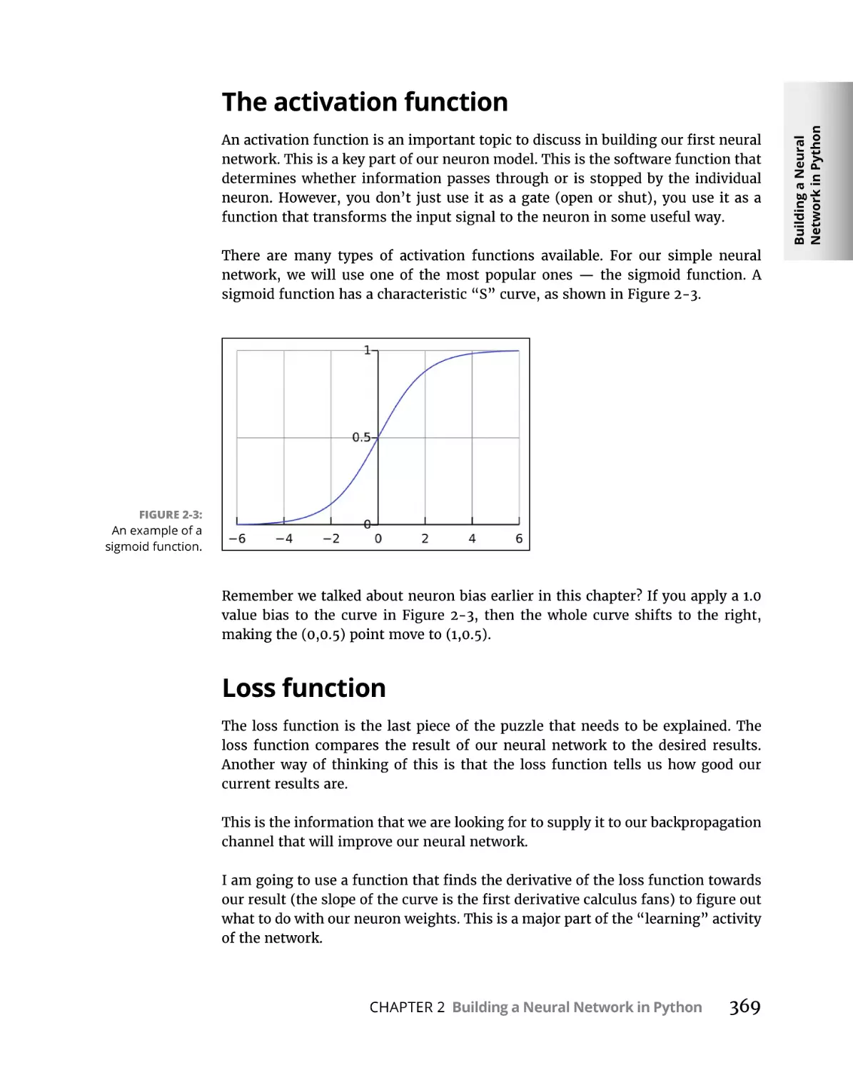
The activation function. . . . . . . . . . . . . . . . . . . . . . . . . . . . . . . . . . . . 369
Loss function . . . . . . . . . . . . . . . . . . . . . . . . . . . . . . . . . . . . . . . . . . . . 369
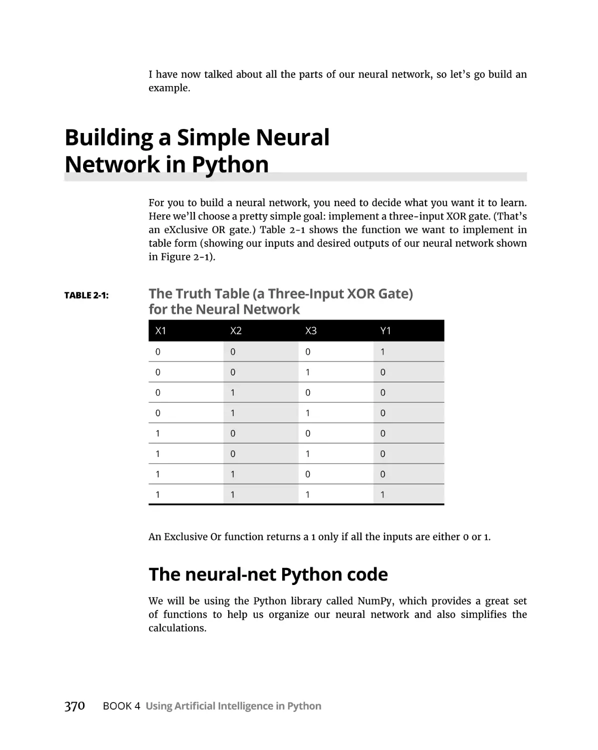
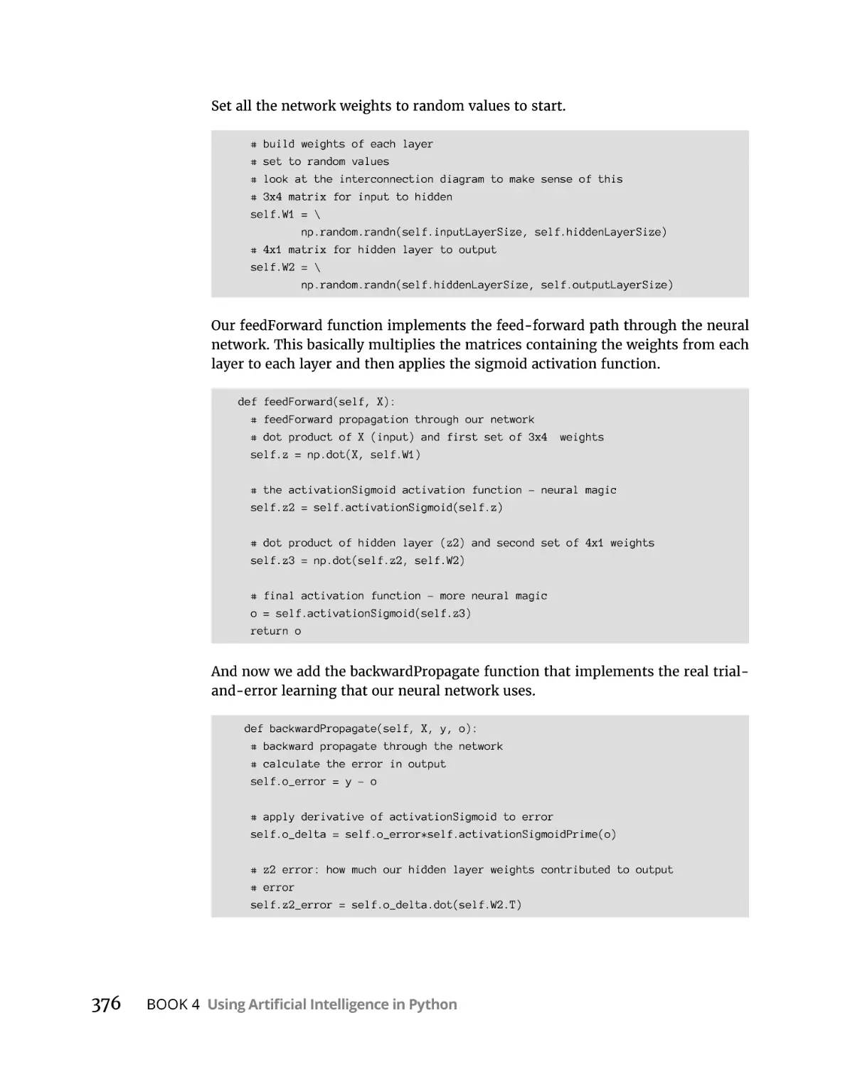
Building a Simple Neural Network in Python . . . . . . . . . . . . . . . . . . . . 370
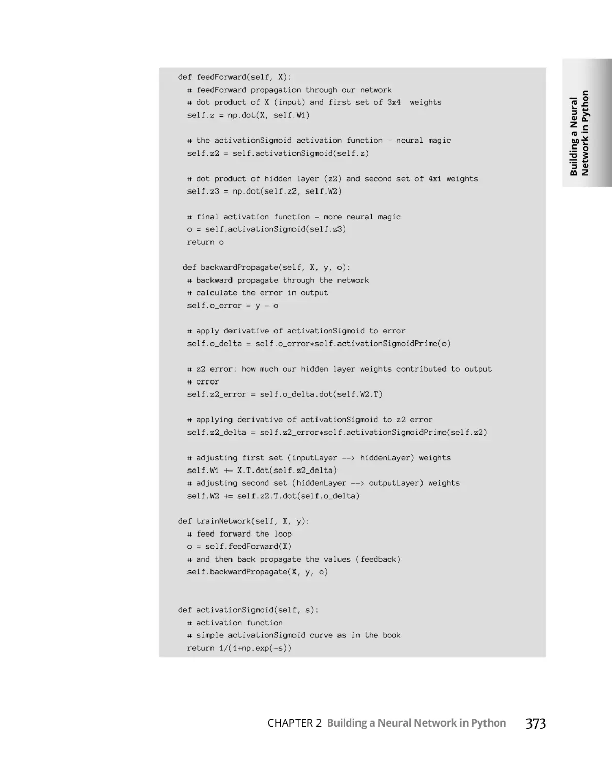
The neural-net Python code. . . . . . . . . . . . . . . . . . . . . . . . . . . . . . . .370
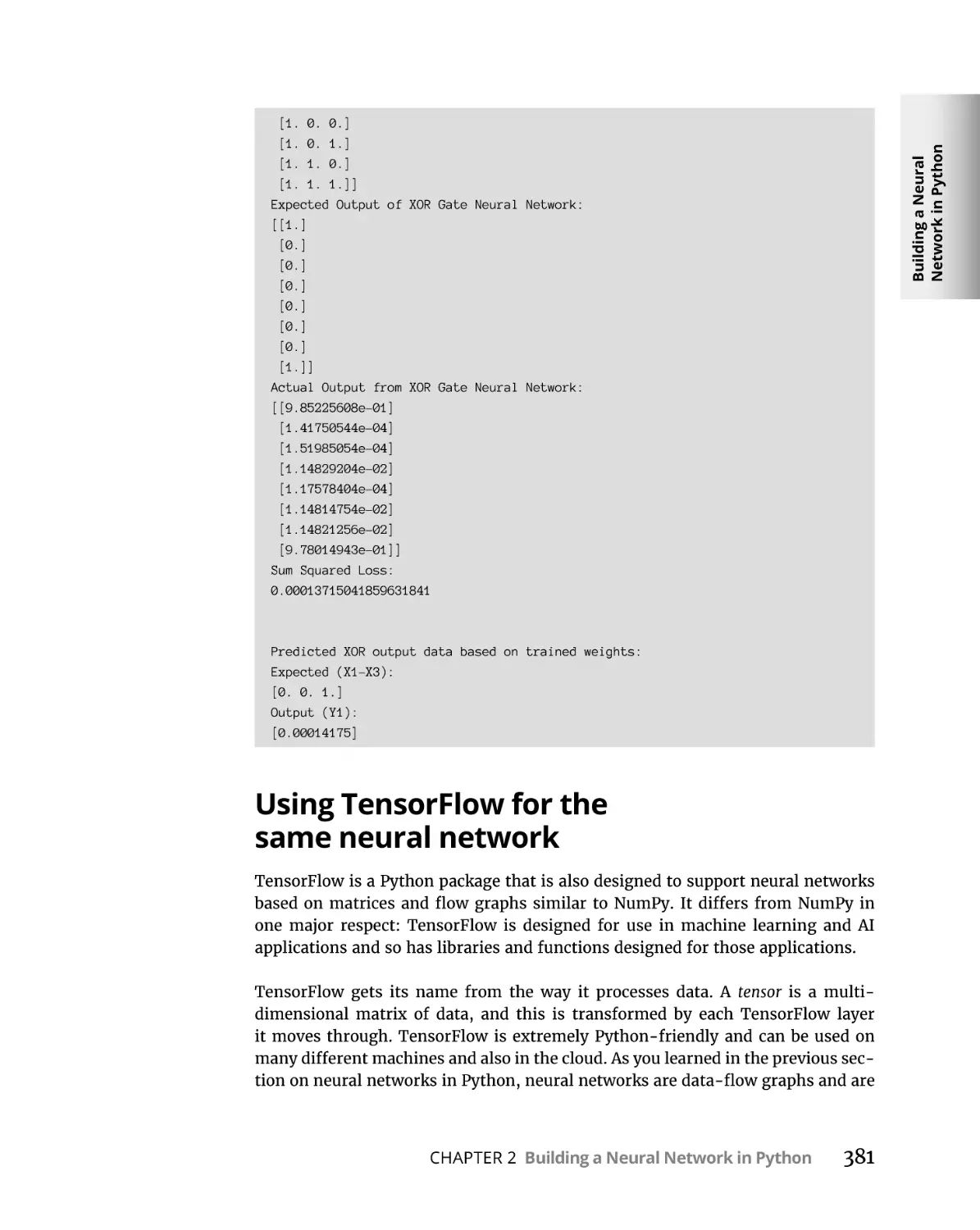
Using TensorFlow for the same neural network. . . . . . . . . . . . . . . 381
Installing the TensorFlow Python library. . . . . . . . . . . . . . . . . . . . . 382
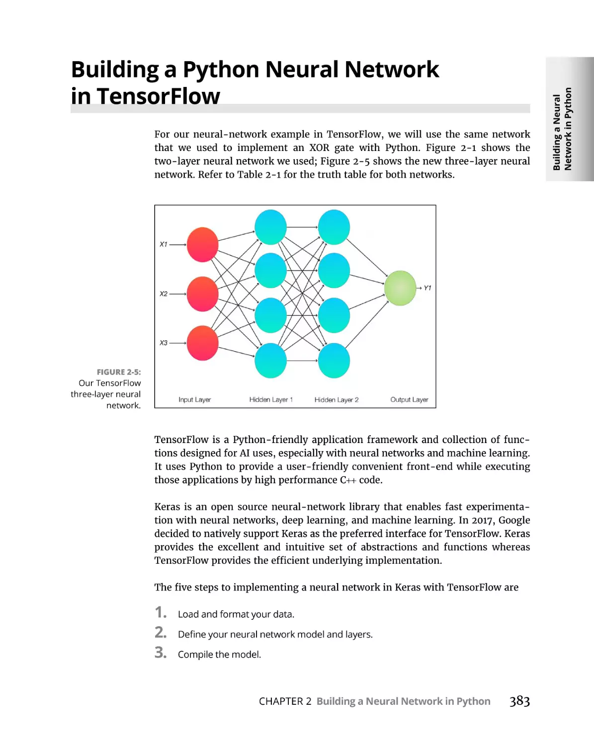
Building a Python Neural Network in TensorFlow . . . . . . . . . . . . . . . . 383
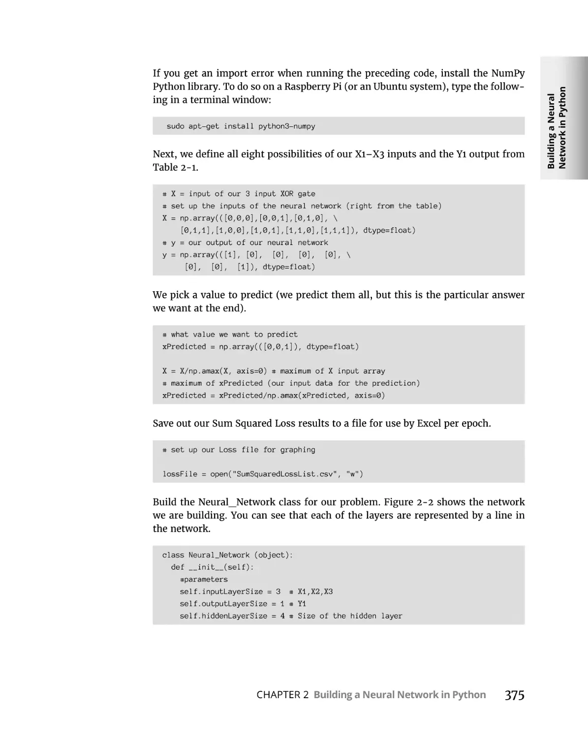
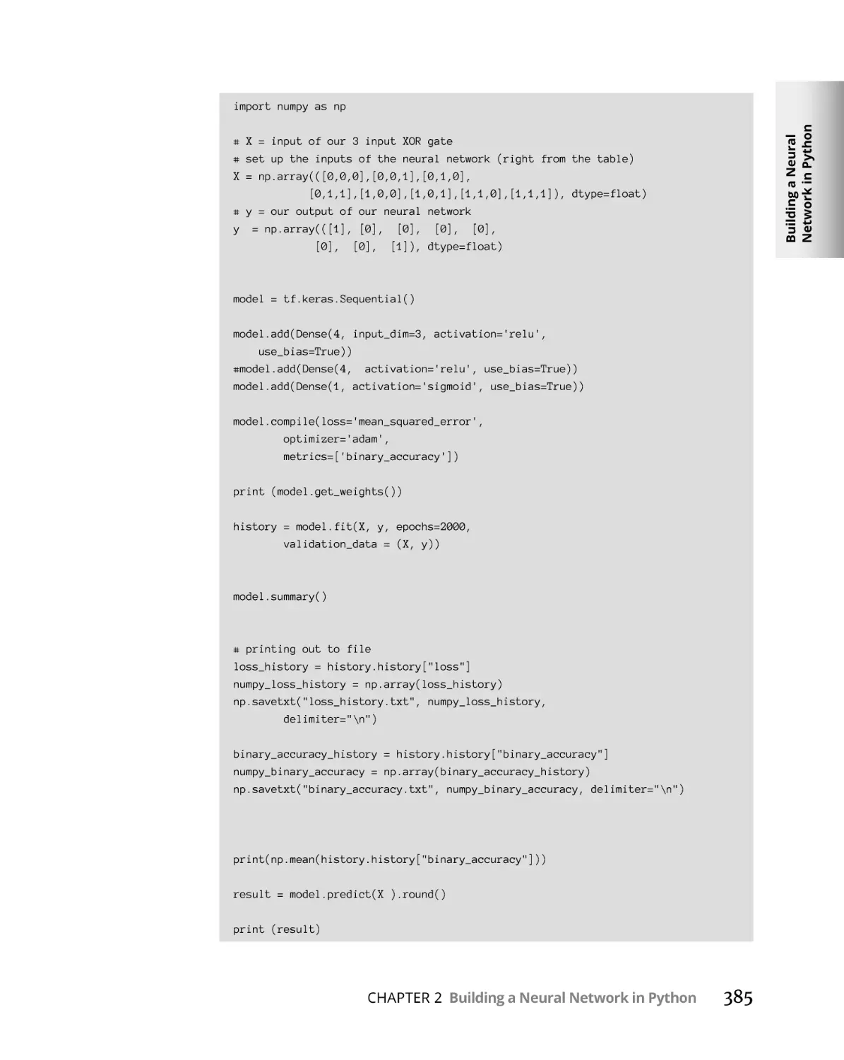
Loading your data. . . . . . . . . . . . . . . . . . . . . . . . . . . . . . . . . . . . . . . . 384
Defining your neural-network model and layers . . . . . . . . . . . . . . 384
Compiling your model . . . . . . . . . . . . . . . . . . . . . . . . . . . . . . . . . . . . 384
Fitting and training your model. . . . . . . . . . . . . . . . . . . . . . . . . . . . . 384
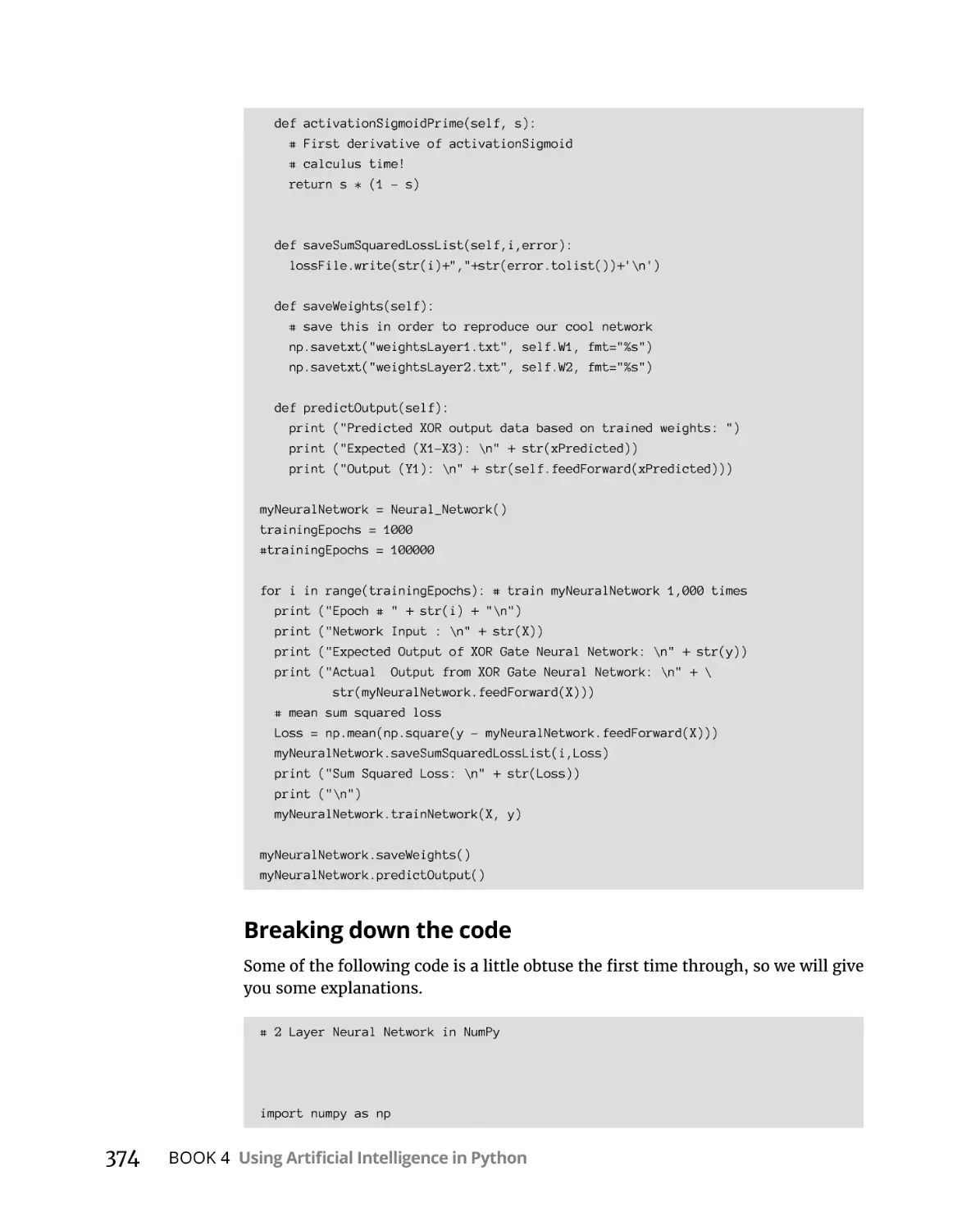
Breaking down the code. . . . . . . . . . . . . . . . . . . . . . . . . . . . . . . . . . . 386
Evaluating the model . . . . . . . . . . . . . . . . . . . . . . . . . . . . . . . . . . . . . 388
Changing to a three-layer neural network in
TensorFlow/Keras . . . . . . . . . . . . . . . . . . . . . . . . . . . . . . . . . . . . . . . . 390
CHAPTER 3:
Doing Machine Learning in Python. . . . . . . . . . . . . . . . . .
393
Learning by Looking for Solutions in All the Wrong Places. . . . . . . . .
Classifying Clothes with Machine Learning. . . . . . . . . . . . . . . . . . . . . .
Training and Learning with TensorFlow. . . . . . . . . . . . . . . . . . . . . . . . .
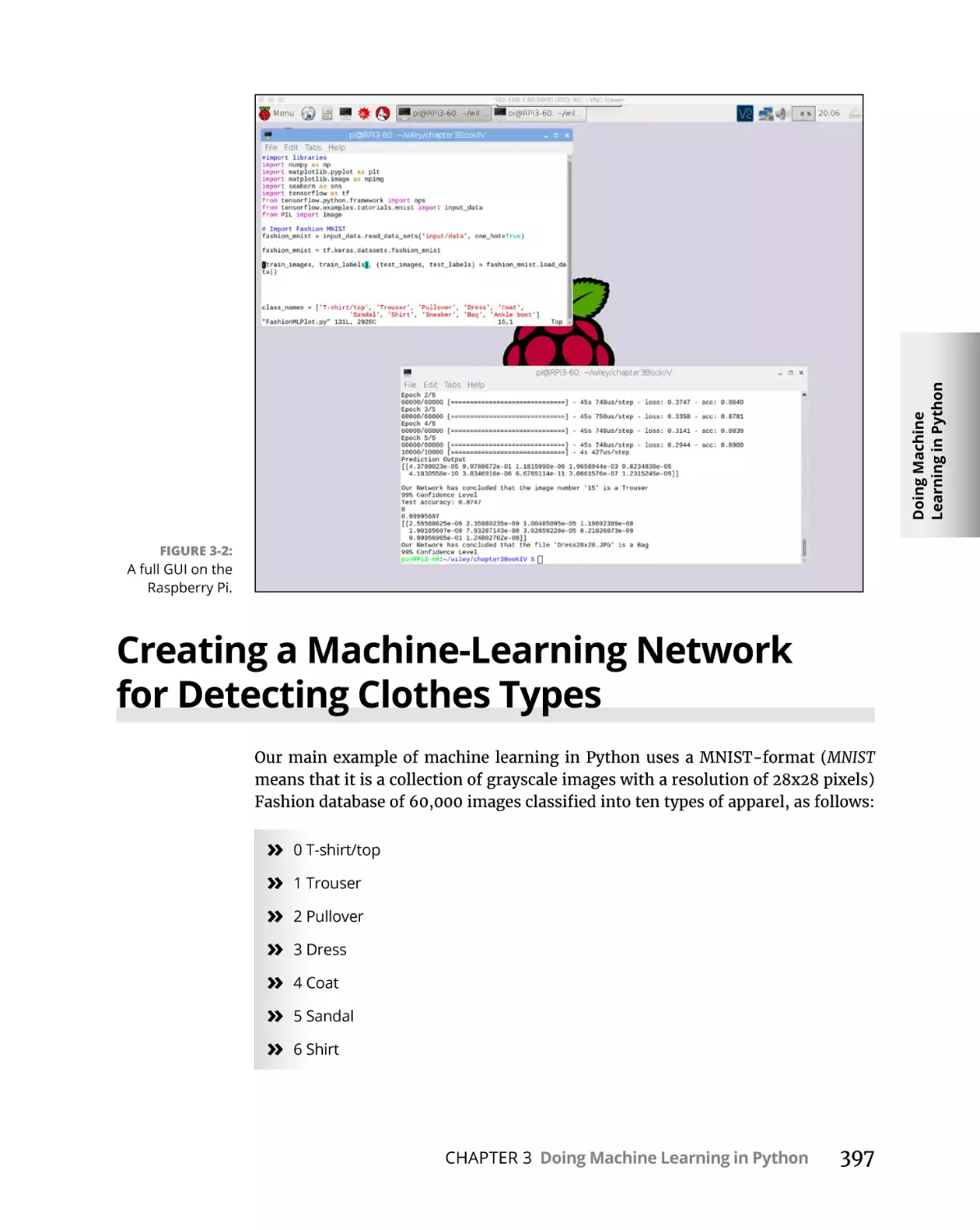
Setting Up the Software Environment for this Chapter. . . . . . . . . . . .
Creating a Machine-Learning Network for Detecting
Clothes Types. . . . . . . . . . . . . . . . . . . . . . . . . . . . . . . . . . . . . . . . . . . . . . .
Getting the data — The Fashion-MNIST dataset. . . . . . . . . . . . . . .
Training the network. . . . . . . . . . . . . . . . . . . . . . . . . . . . . . . . . . . . . .
Testing our network . . . . . . . . . . . . . . . . . . . . . . . . . . . . . . . . . . . . . .
Breaking down the code. . . . . . . . . . . . . . . . . . . . . . . . . . . . . . . . . . .
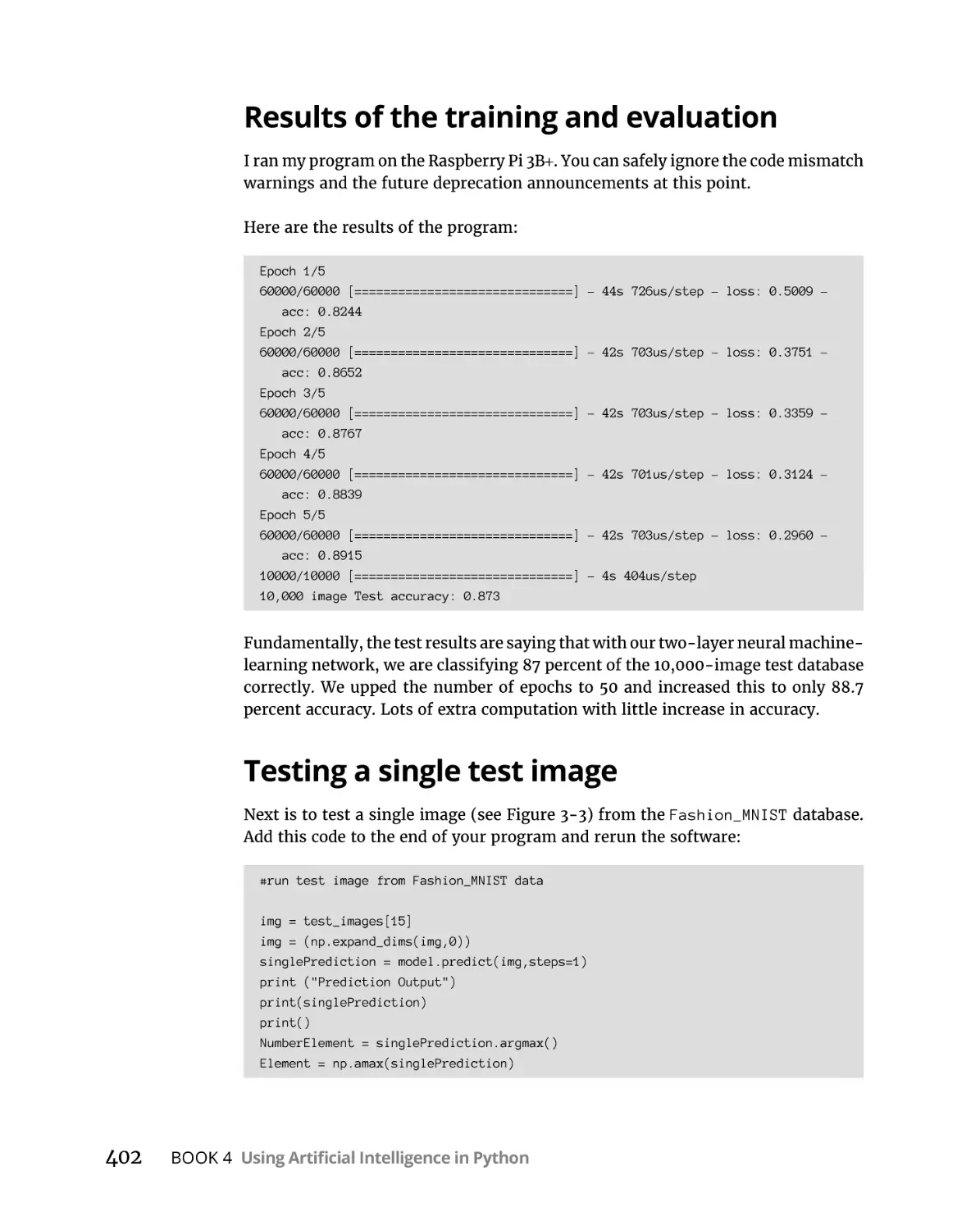
Results of the training and evaluation. . . . . . . . . . . . . . . . . . . . . . .
Testing a single test image. . . . . . . . . . . . . . . . . . . . . . . . . . . . . . . . .
394
395
395
396
Table of Contents
397
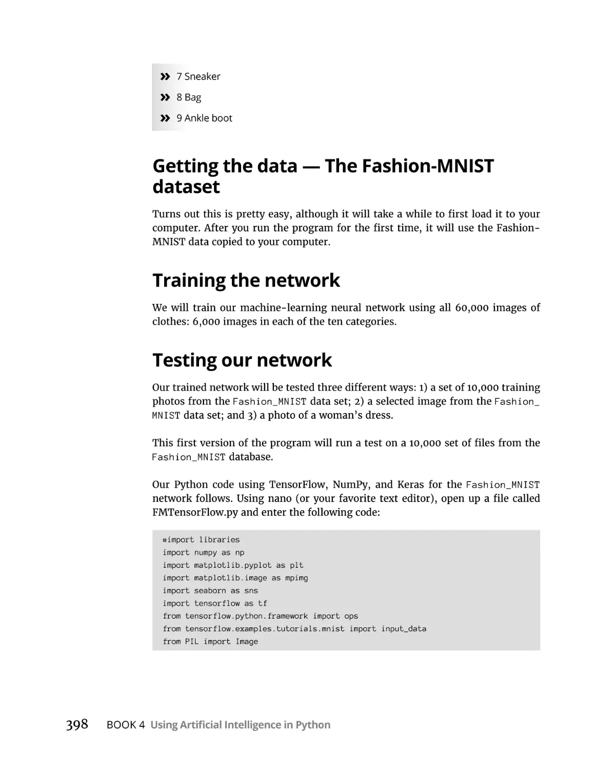
398
398
398
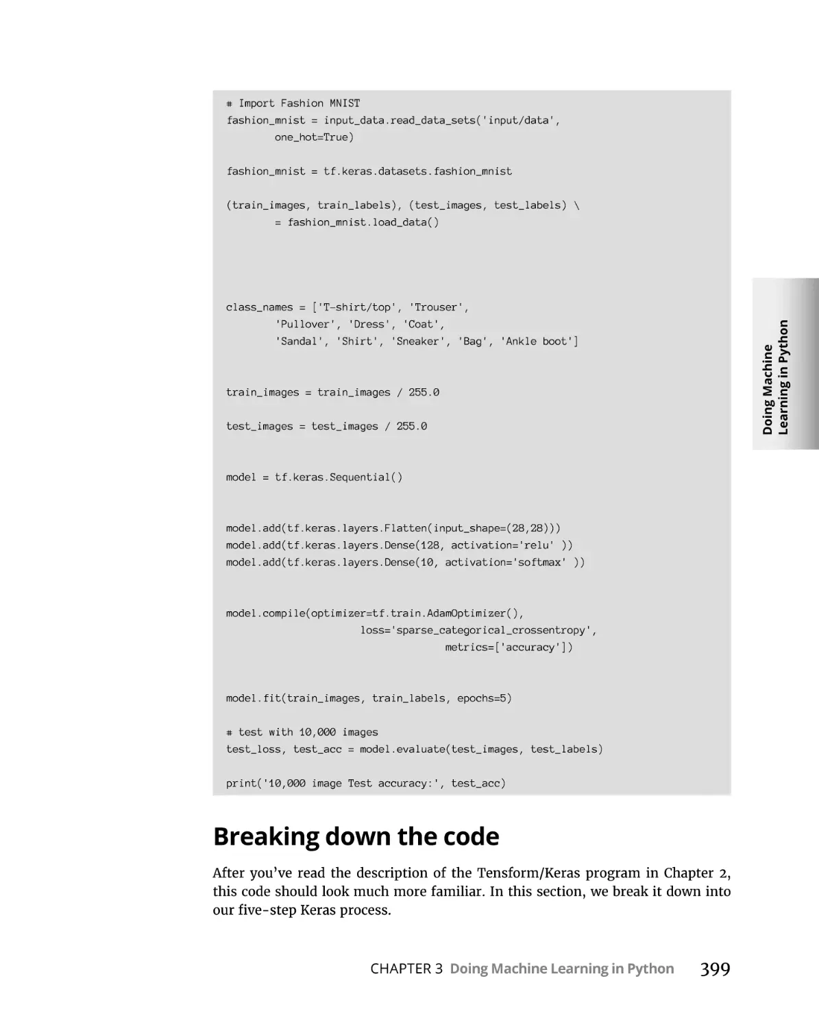
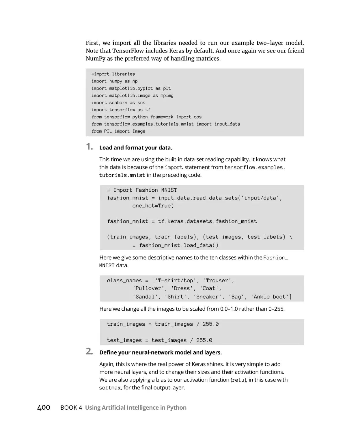
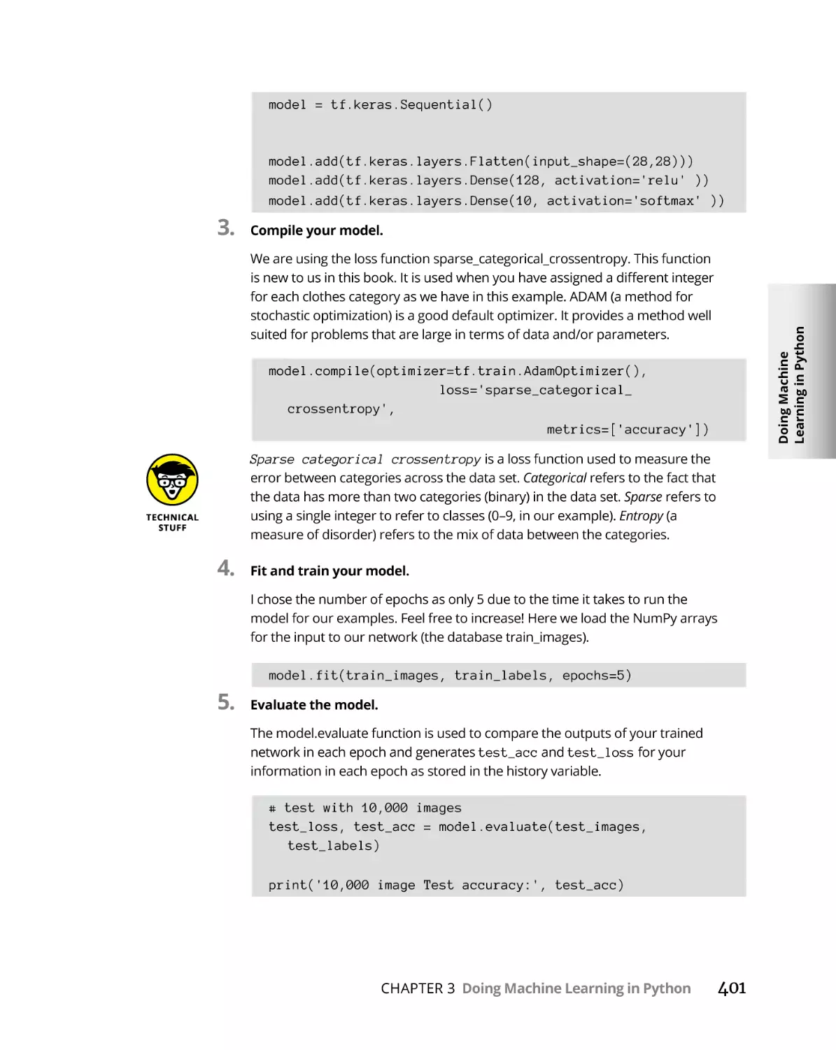
399
402
402
xi
Testing on external pictures . . . . . . . . . . . . . . . . . . . . . . . . . . . . . . .
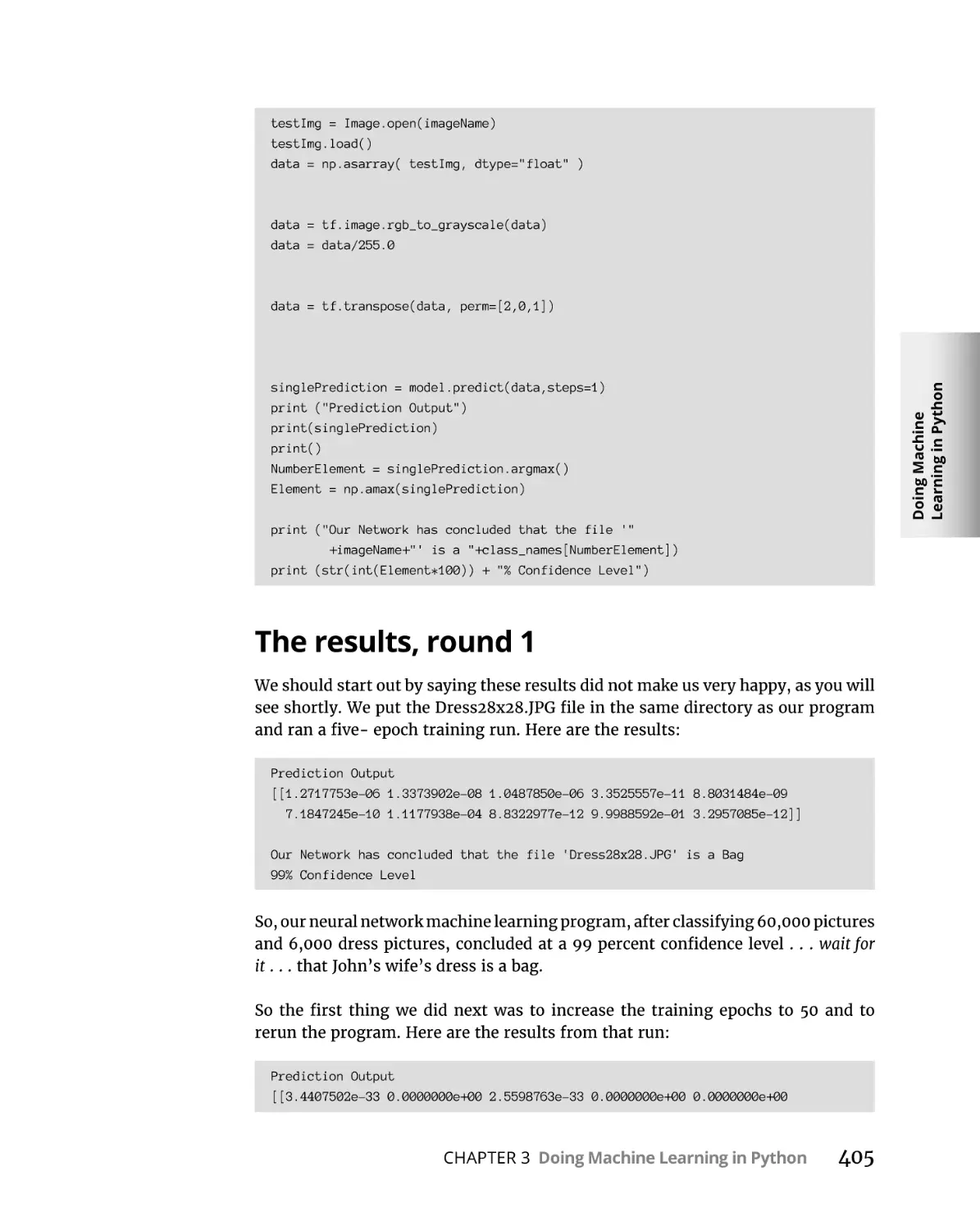
The results, round 1 . . . . . . . . . . . . . . . . . . . . . . . . . . . . . . . . . . . . . .
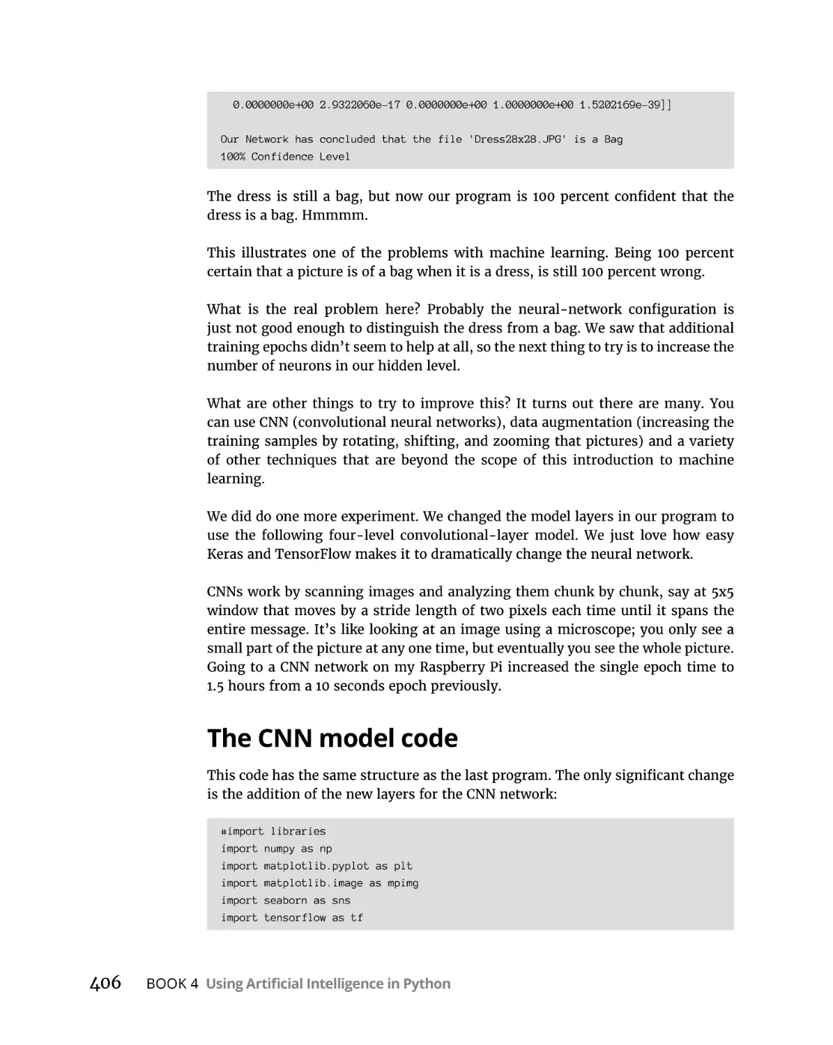
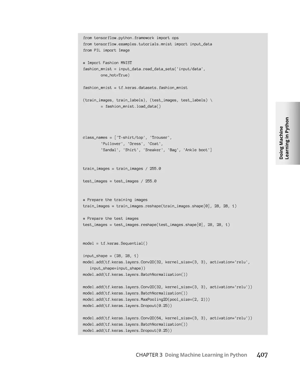
The CNN model code . . . . . . . . . . . . . . . . . . . . . . . . . . . . . . . . . . . . .
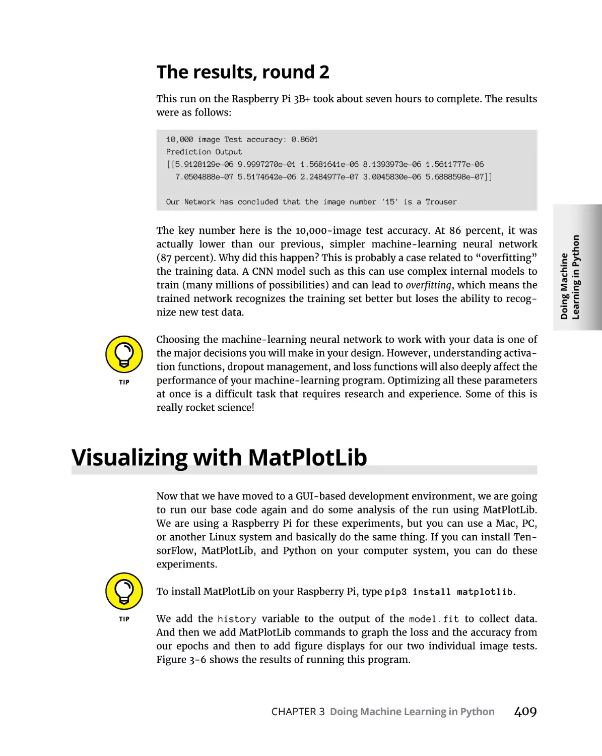
The results, round 2 . . . . . . . . . . . . . . . . . . . . . . . . . . . . . . . . . . . . . .
Visualizing with MatPlotLib . . . . . . . . . . . . . . . . . . . . . . . . . . . . . . . . . . .
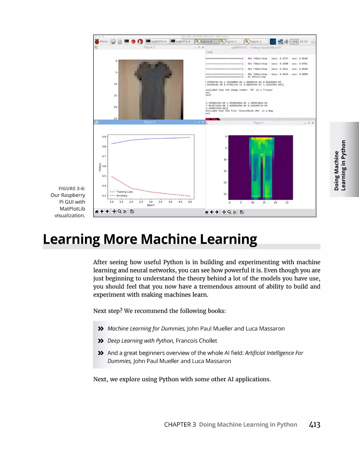
Learning More Machine Learning. . . . . . . . . . . . . . . . . . . . . . . . . . . . . .
403
405
406
409
409
413
Exploring More AI in Python. . . . . . . . . . . . . . . . . . . . . . . . . .
415
Limitations of the Raspberry Pi and AI. . . . . . . . . . . . . . . . . . . . . . . . . .
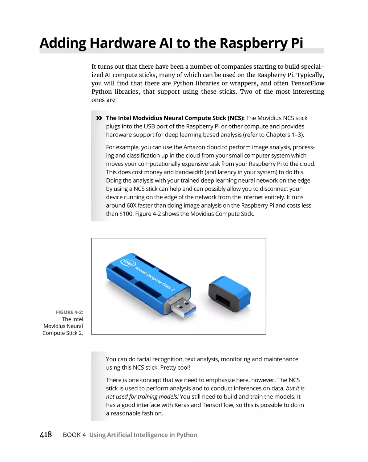
Adding Hardware AI to the Raspberry Pi. . . . . . . . . . . . . . . . . . . . . . . .
AI in the Cloud. . . . . . . . . . . . . . . . . . . . . . . . . . . . . . . . . . . . . . . . . . . . . .
Google cloud . . . . . . . . . . . . . . . . . . . . . . . . . . . . . . . . . . . . . . . . . . . .
Amazon Web Services. . . . . . . . . . . . . . . . . . . . . . . . . . . . . . . . . . . . .
IBM cloud . . . . . . . . . . . . . . . . . . . . . . . . . . . . . . . . . . . . . . . . . . . . . . .
Microsoft Azure. . . . . . . . . . . . . . . . . . . . . . . . . . . . . . . . . . . . . . . . . .
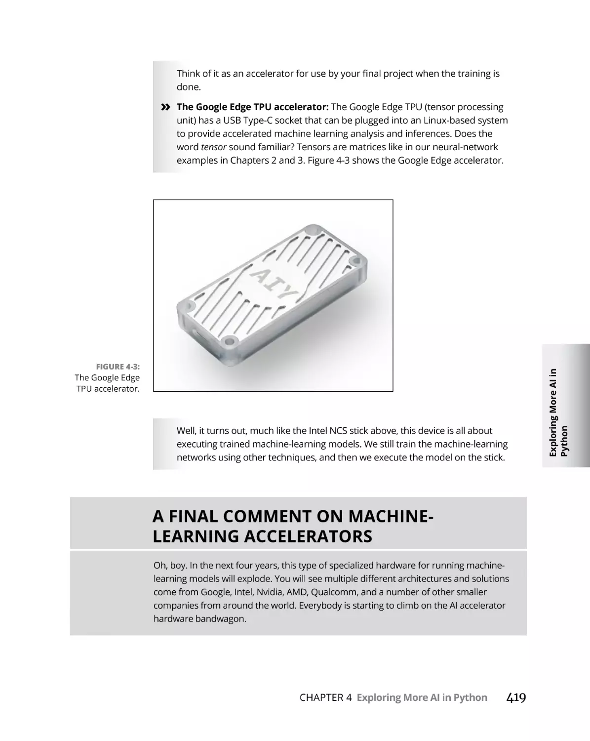
AI on a Graphics Card. . . . . . . . . . . . . . . . . . . . . . . . . . . . . . . . . . . . . . . .
Where to Go for More AI Fun in Python. . . . . . . . . . . . . . . . . . . . . . . . .
415
418
420
421
421
422
422
423
424
BOOK 5: DOING DATA SCIENCE WITH PYTHON. . . . . . . . . . .
427
CHAPTER 4:
CHAPTER 1:
CHAPTER 2:
CHAPTER 3:
xii
The Five Areas of Data Science. . . . . . . . . . . . . . . . . . . . . . .
429
Working with Big, Big Data. . . . . . . . . . . . . . . . . . . . . . . . . . . . . . . . . . . .
Volume . . . . . . . . . . . . . . . . . . . . . . . . . . . . . . . . . . . . . . . . . . . . . . . . .
Variety. . . . . . . . . . . . . . . . . . . . . . . . . . . . . . . . . . . . . . . . . . . . . . . . . .
Velocity . . . . . . . . . . . . . . . . . . . . . . . . . . . . . . . . . . . . . . . . . . . . . . . . .
Managing volume, variety, and velocity. . . . . . . . . . . . . . . . . . . . . .
Cooking with Gas: The Five Step Process of Data Science. . . . . . . . . .
Capturing the data . . . . . . . . . . . . . . . . . . . . . . . . . . . . . . . . . . . . . . .
Processing the data. . . . . . . . . . . . . . . . . . . . . . . . . . . . . . . . . . . . . . .
Analyzing the data. . . . . . . . . . . . . . . . . . . . . . . . . . . . . . . . . . . . . . . .
Communicating the results . . . . . . . . . . . . . . . . . . . . . . . . . . . . . . . .
Maintaining the data. . . . . . . . . . . . . . . . . . . . . . . . . . . . . . . . . . . . . .
430
430
431
431
432
432
433
433
434
434
435
Exploring Big Data with Python. . . . . . . . . . . . . . . . . . . . . .
437
Introducing NumPy, Pandas, and MatPlotLib. . . . . . . . . . . . . . . . .
Doing Your First Data Science Project . . . . . . . . . . . . . . . . . . . . . . . . . .
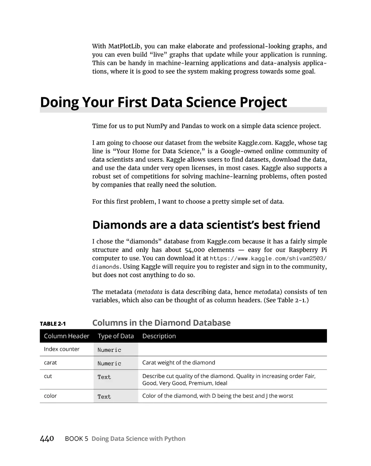
Diamonds are a data scientist’s best friend . . . . . . . . . . . . . . . . . .
Breaking down the code. . . . . . . . . . . . . . . . . . . . . . . . . . . . . . . . . . .
Visualizing the data with MatPlotLib. . . . . . . . . . . . . . . . . . . . . . . . .
438
440
440
443
444
Using Big Data from the Google Cloud. . . . . . . . . . . . . .
451
What Is Big Data?. . . . . . . . . . . . . . . . . . . . . . . . . . . . . . . . . . . . . . . . . . . .
Understanding the Google Cloud and BigQuery . . . . . . . . . . . . . . . . .
The Google Cloud Platform . . . . . . . . . . . . . . . . . . . . . . . . . . . . . . . .
BigQuery from Google . . . . . . . . . . . . . . . . . . . . . . . . . . . . . . . . . . . .
451
452
452
452
Python All-in-One For Dummies
Computer security on the cloud . . . . . . . . . . . . . . . . . . . . . . . . . . . .
Signing up on Google for BigQuery . . . . . . . . . . . . . . . . . . . . . . . . .
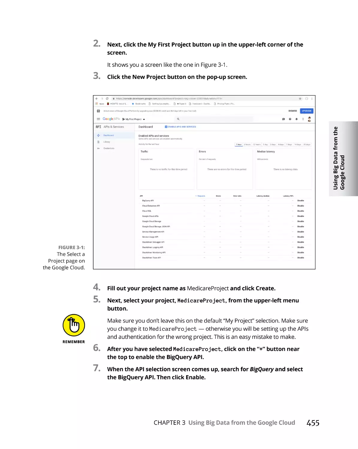
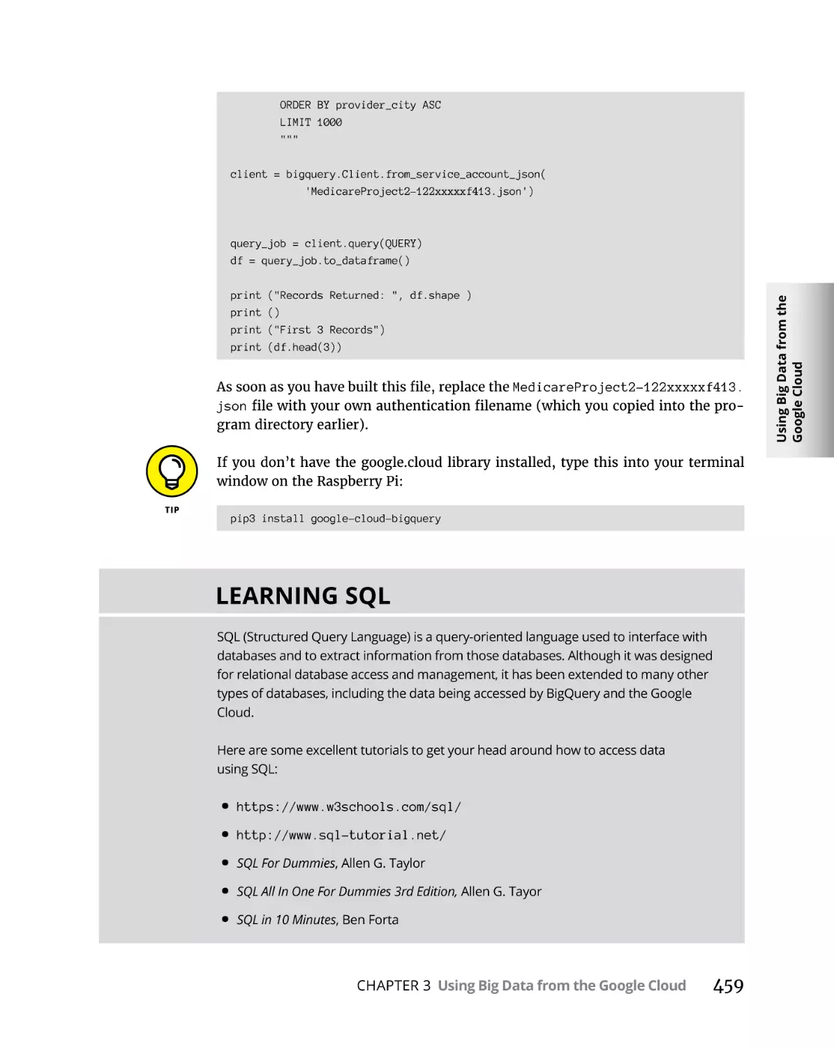
Reading the Medicare Big Data. . . . . . . . . . . . . . . . . . . . . . . . . . . . . . . .
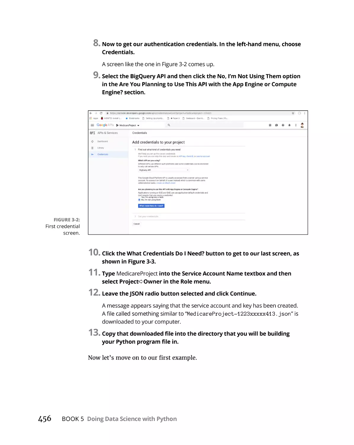
Setting up your project and authentication. . . . . . . . . . . . . . . . . . .
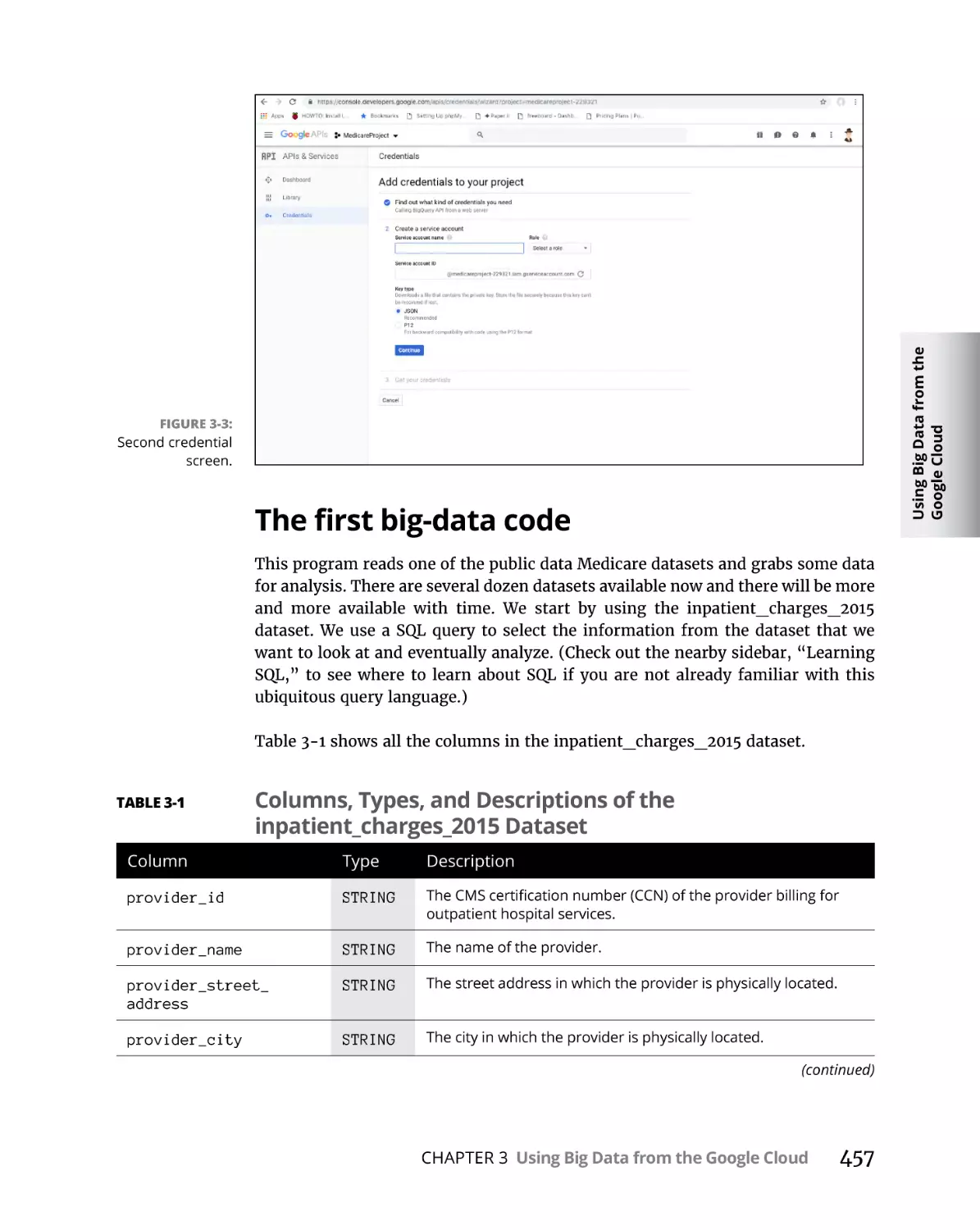
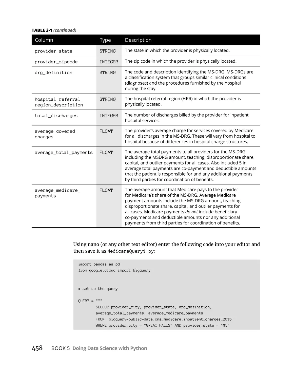
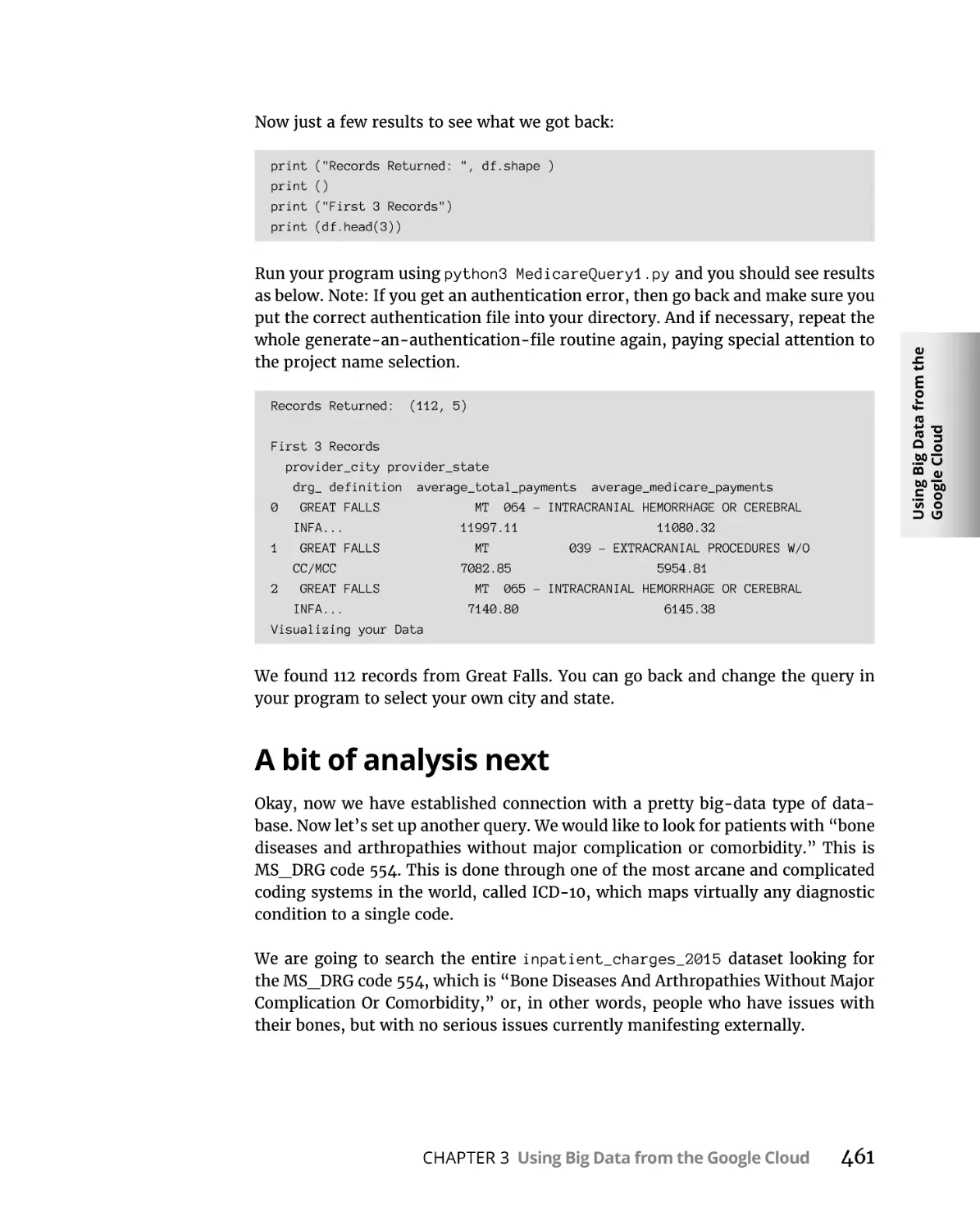
The first big-data code . . . . . . . . . . . . . . . . . . . . . . . . . . . . . . . . . . . .
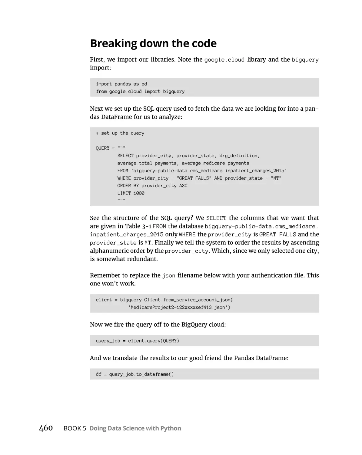
Breaking down the code. . . . . . . . . . . . . . . . . . . . . . . . . . . . . . . . . . .
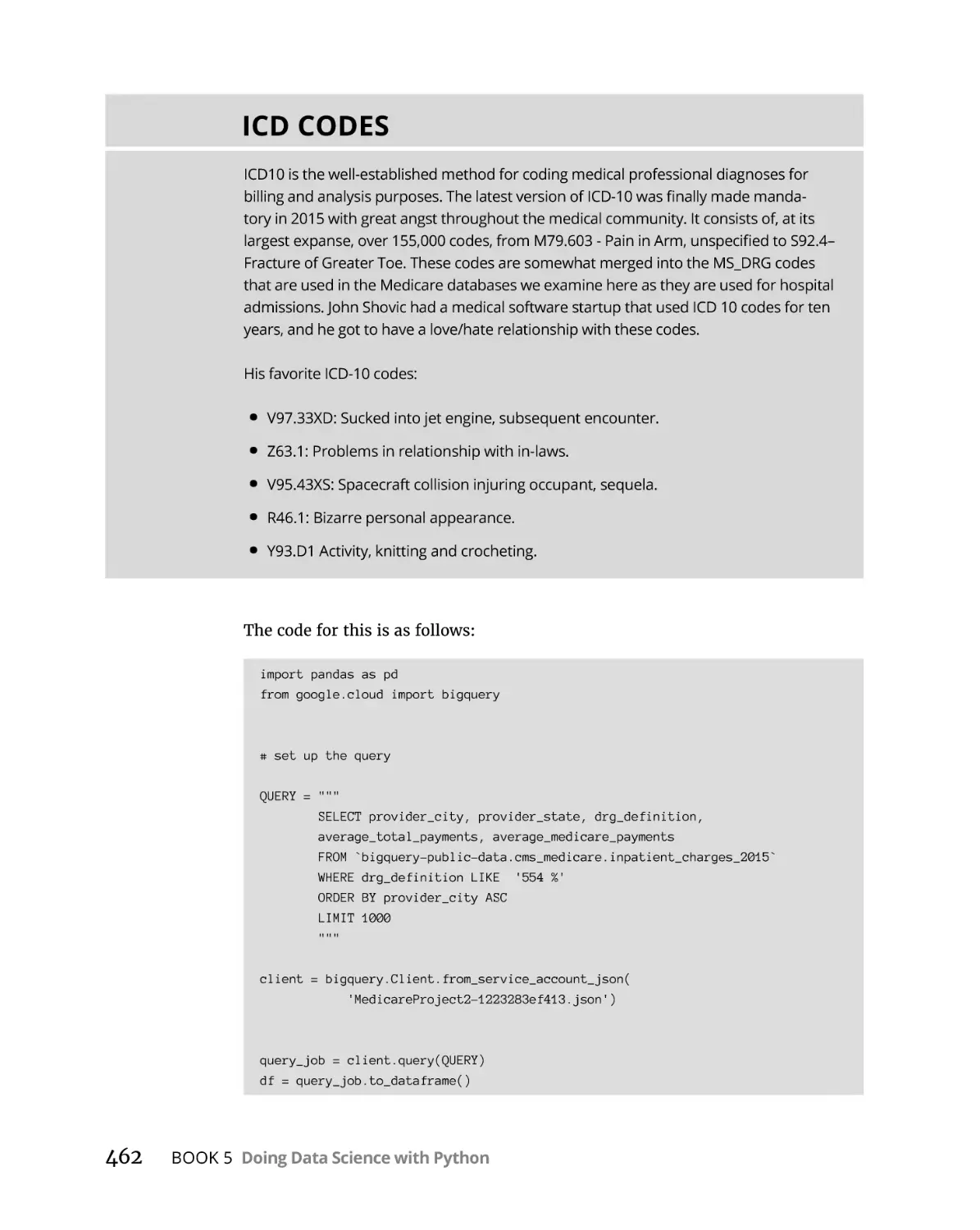
A bit of analysis next. . . . . . . . . . . . . . . . . . . . . . . . . . . . . . . . . . . . . .
Payment percent by state . . . . . . . . . . . . . . . . . . . . . . . . . . . . . . . . .
And now some visualization . . . . . . . . . . . . . . . . . . . . . . . . . . . . . . .
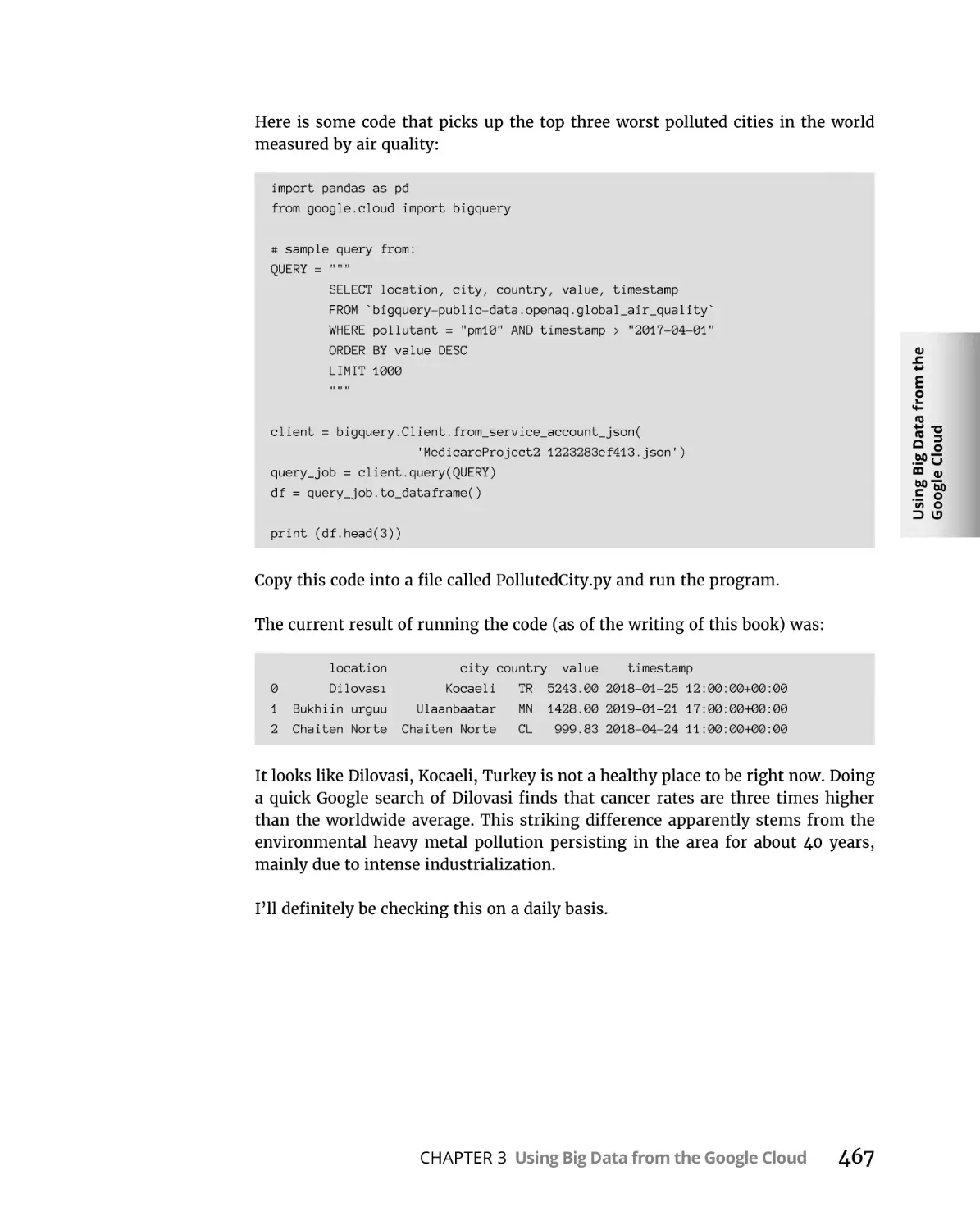
Looking for the Most Polluted City in the World on
an Hourly Basis . . . . . . . . . . . . . . . . . . . . . . . . . . . . . . . . . . . . . . . . . . . . .
453
454
454
454
457
460
461
464
465
BOOK 6: TALKING TO HARDWARE WITH PYTHON. . . . . . . .
469
Introduction to Physical Computing. . . . . . . . . . . . . . . .
471
Physical Computing Is Fun. . . . . . . . . . . . . . . . . . . . . . . . . . . . . . . . . . . .
What Is a Raspberry Pi? . . . . . . . . . . . . . . . . . . . . . . . . . . . . . . . . . . . . . .
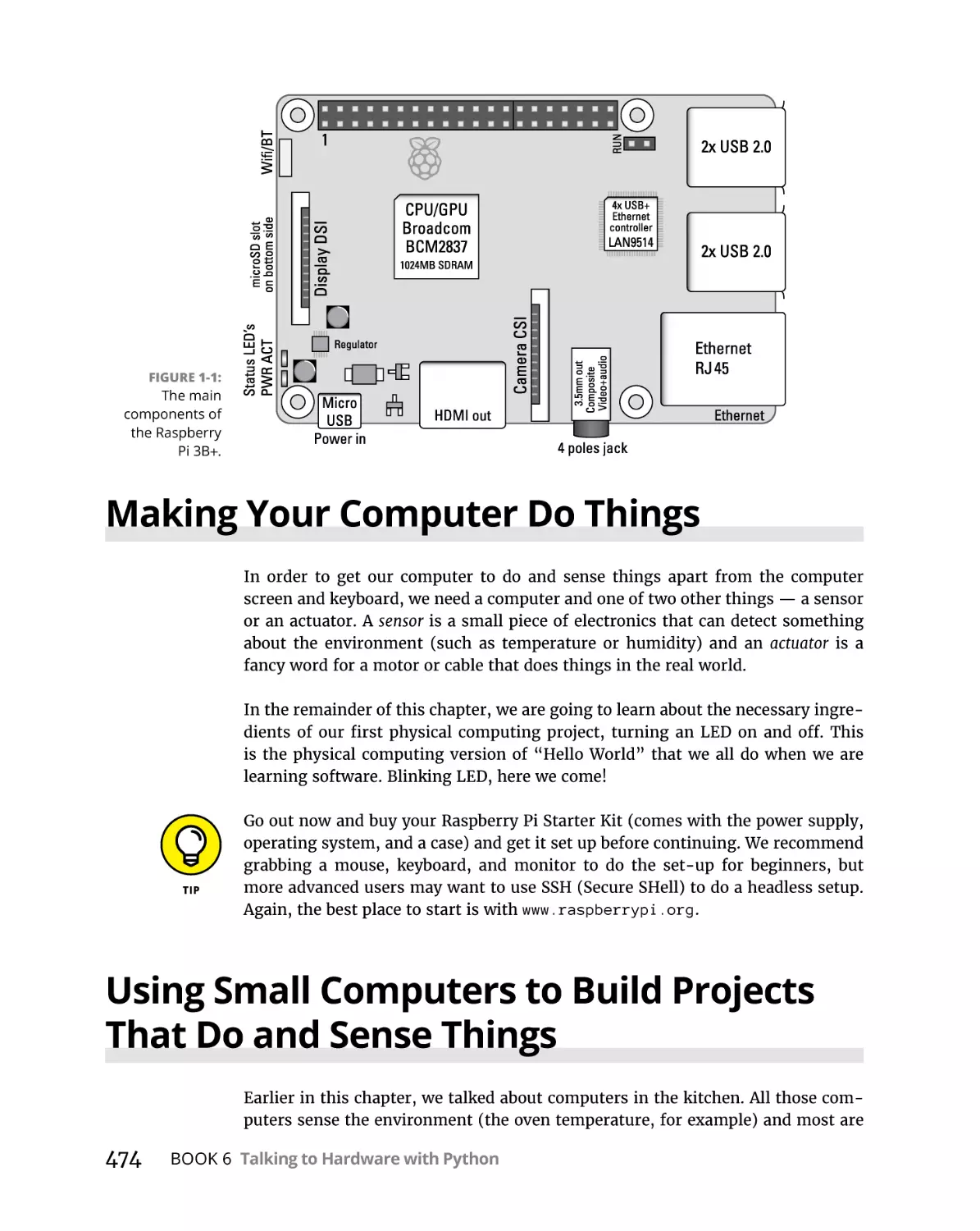
Making Your Computer Do Things . . . . . . . . . . . . . . . . . . . . . . . . . . . . .
Using Small Computers to Build Projects That Do
and Sense Things. . . . . . . . . . . . . . . . . . . . . . . . . . . . . . . . . . . . . . . . . . . .
The Raspberry Pi: A Perfect Platform for Physical
Computing in Python . . . . . . . . . . . . . . . . . . . . . . . . . . . . . . . . . . . . . . . .
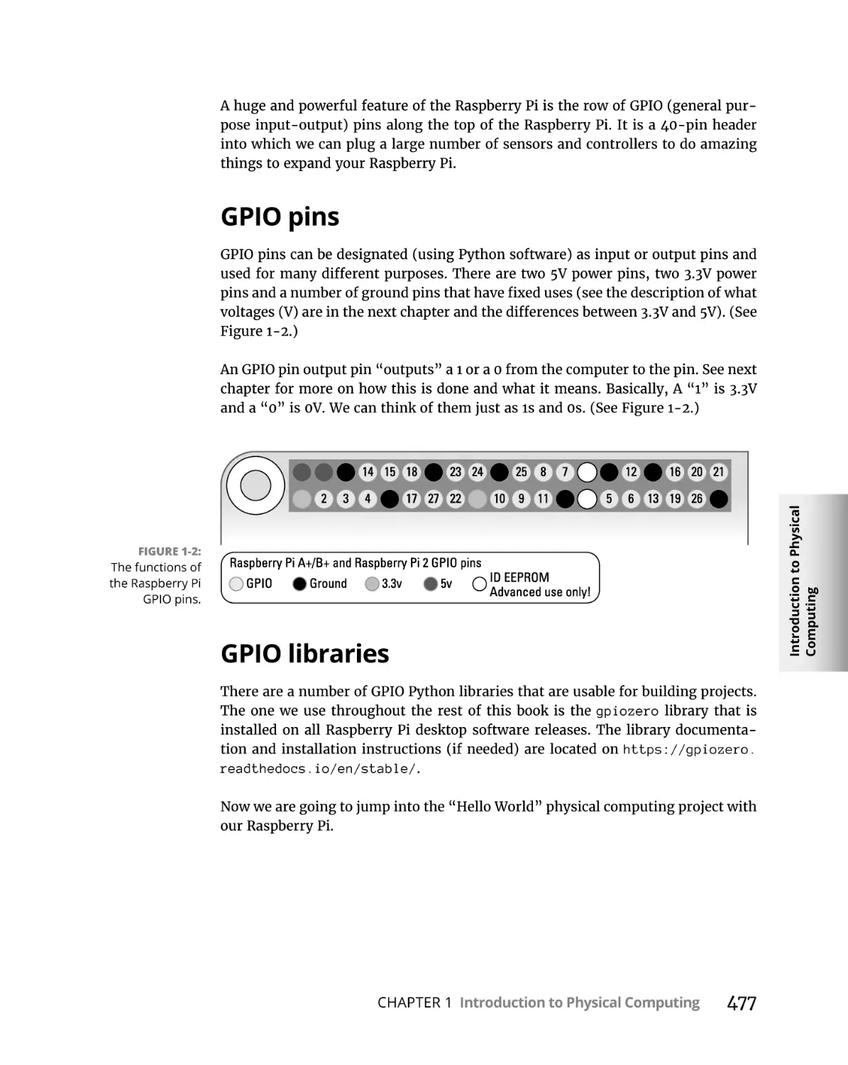
GPIO pins . . . . . . . . . . . . . . . . . . . . . . . . . . . . . . . . . . . . . . . . . . . . . . .
GPIO libraries. . . . . . . . . . . . . . . . . . . . . . . . . . . . . . . . . . . . . . . . . . . .
The hardware for “Hello World” . . . . . . . . . . . . . . . . . . . . . . . . . . . .
Assembling the hardware . . . . . . . . . . . . . . . . . . . . . . . . . . . . . . . . .
Controlling the LED with Python on the Raspberry Pi. . . . . . . . . . . . .
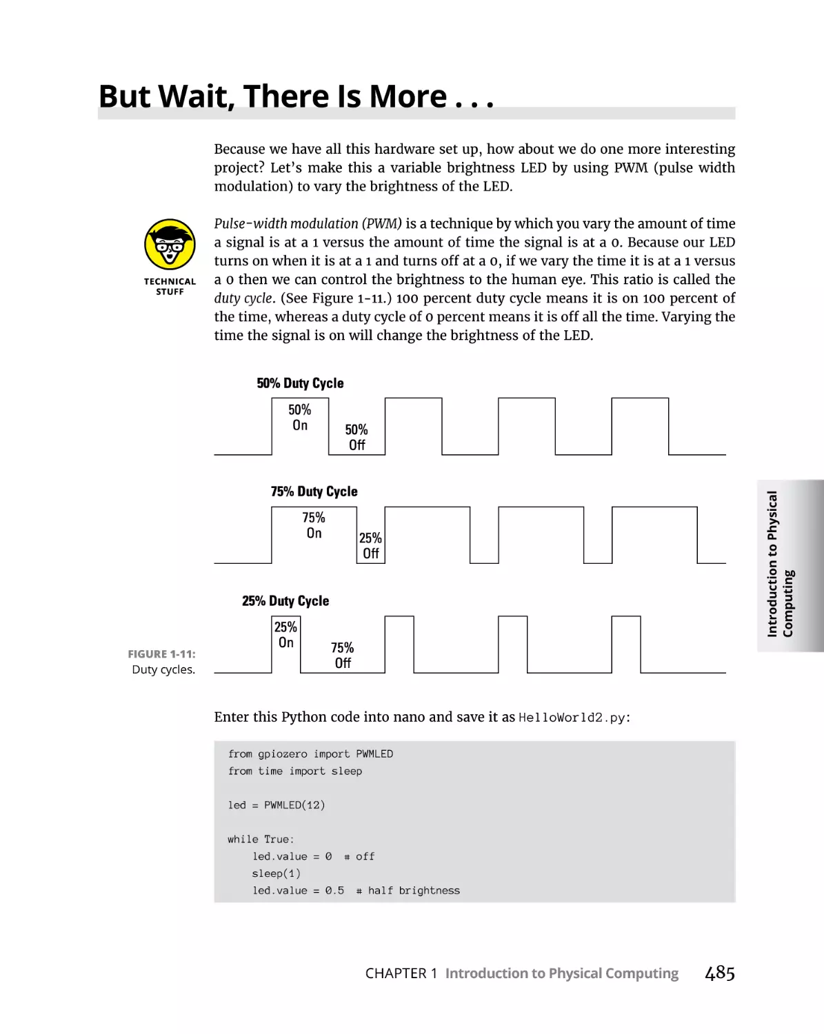
But Wait, There Is More . . . . . . . . . . . . . . . . . . . . . . . . . . . . . . . . . . . . . .
472
472
474
CHAPTER 1:
CHAPTER 2:
466
474
476
477
477
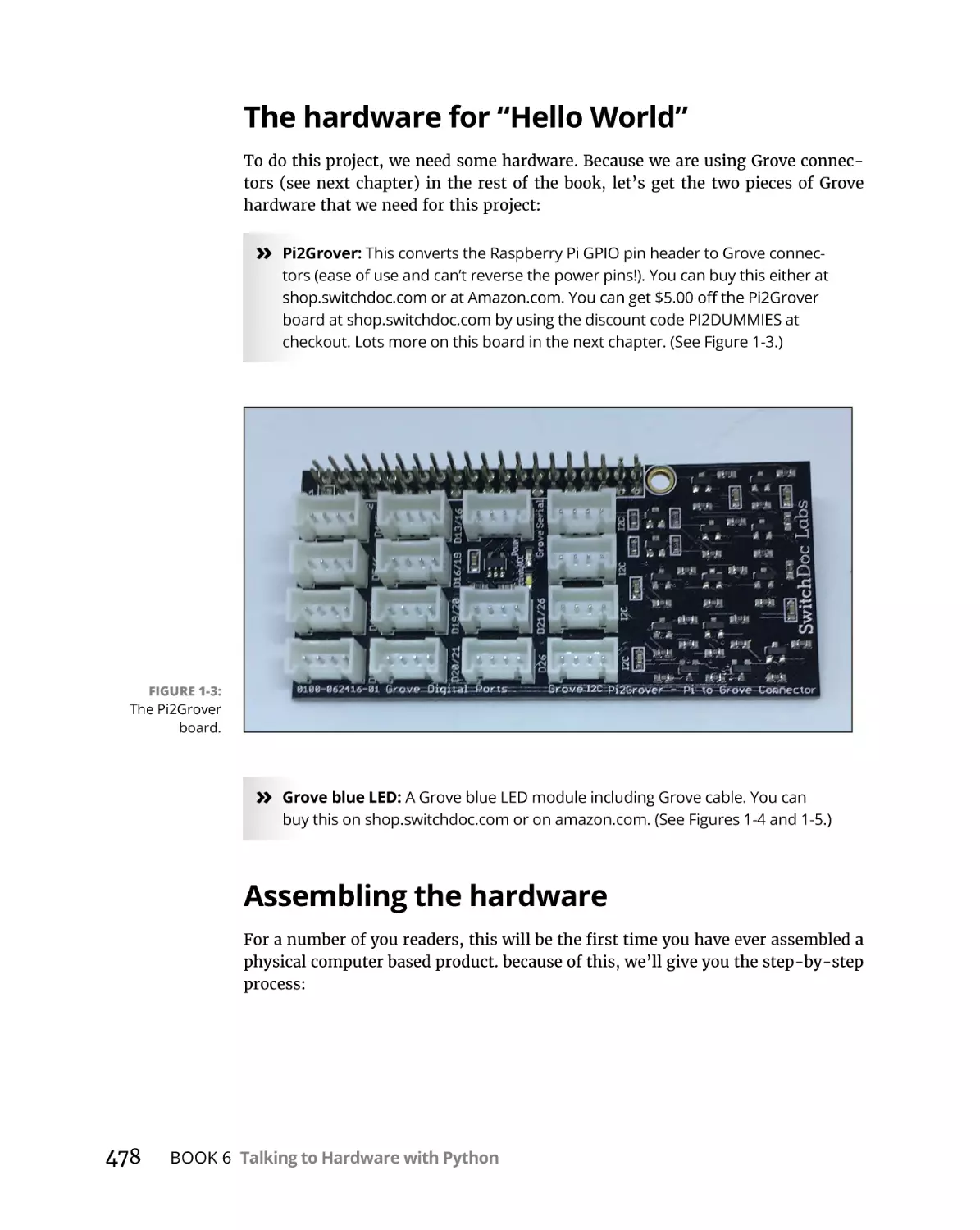
478
478
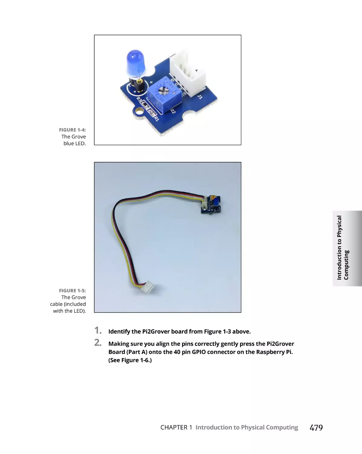
482
485
No Soldering! Grove Connectors
for Building Things . . . . . . . . . . . . . . . . . . . . . . . . . . . . . . . . . . . . .
487
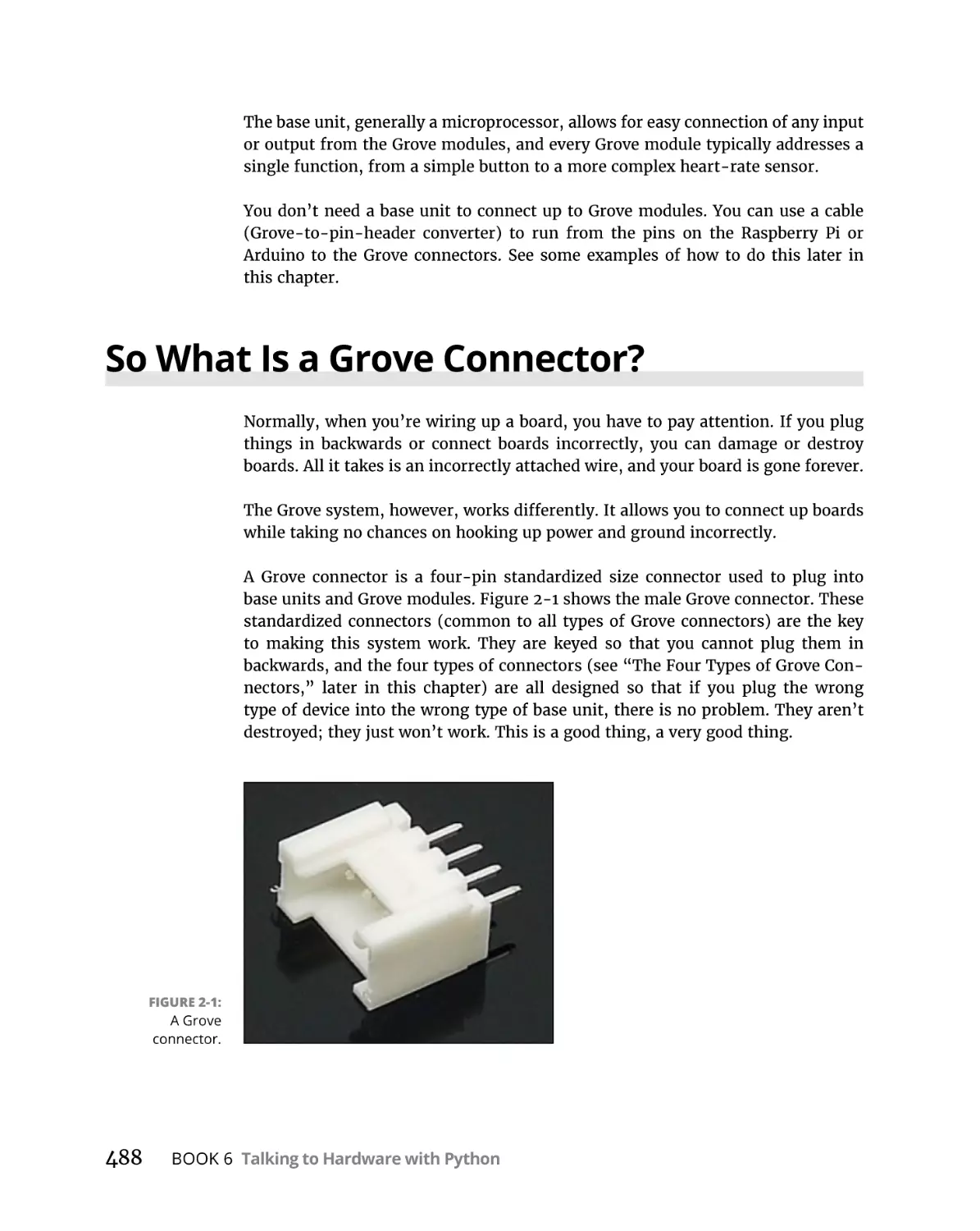
So What Is a Grove Connector?. . . . . . . . . . . . . . . . . . . . . . . . . . . . . . . .
Selecting Grove Base Units . . . . . . . . . . . . . . . . . . . . . . . . . . . . . . . . . . .
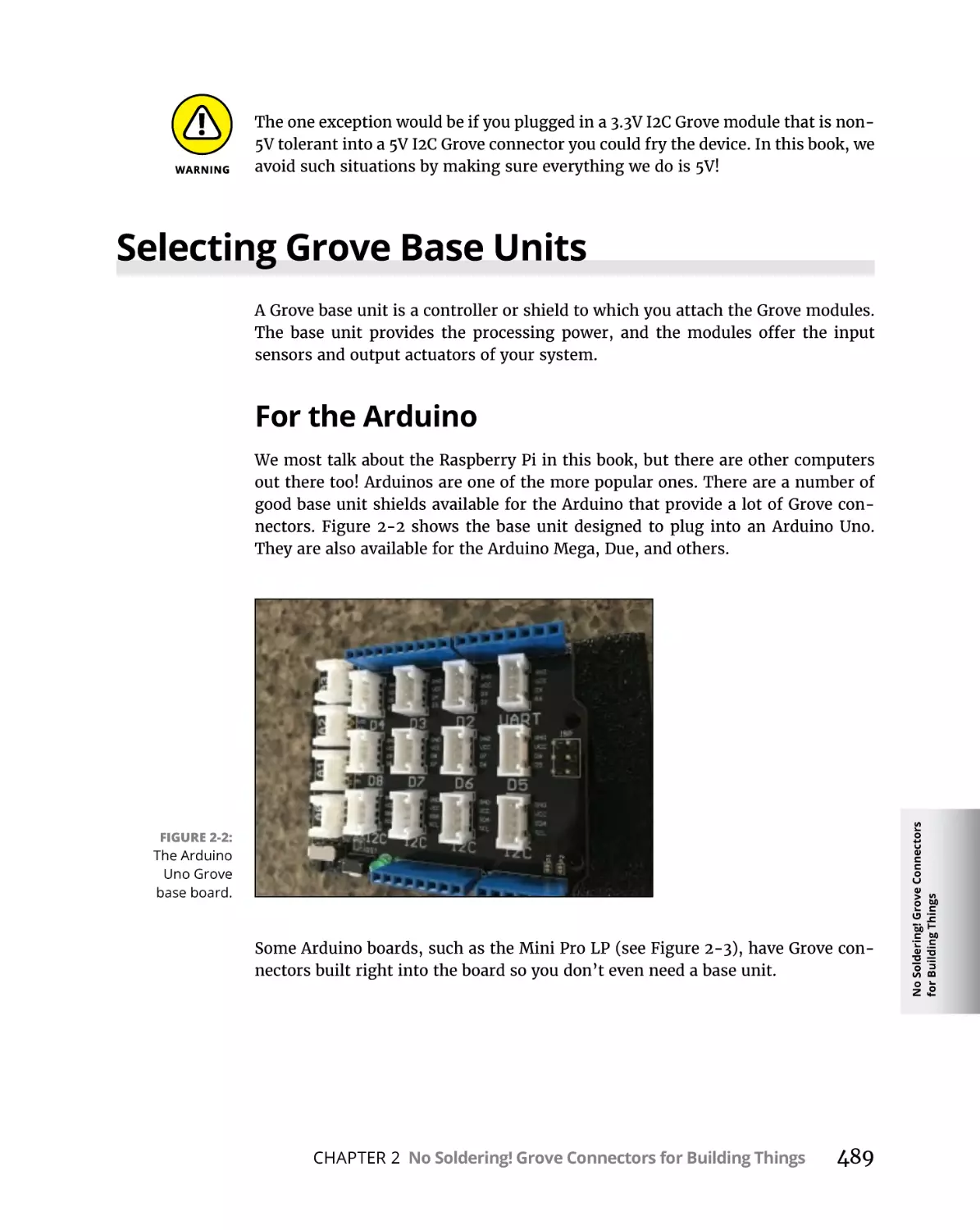
For the Arduino . . . . . . . . . . . . . . . . . . . . . . . . . . . . . . . . . . . . . . . . . .
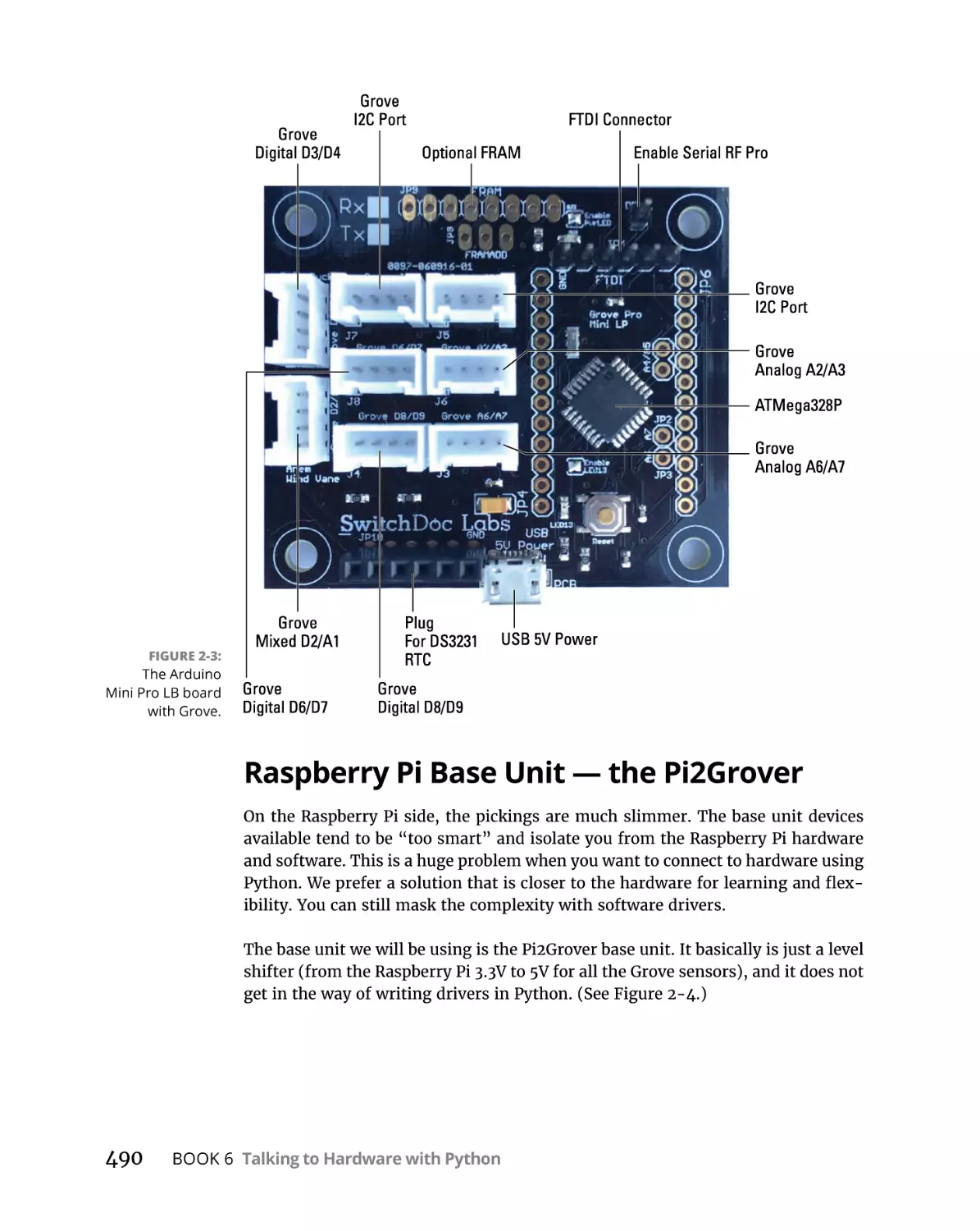
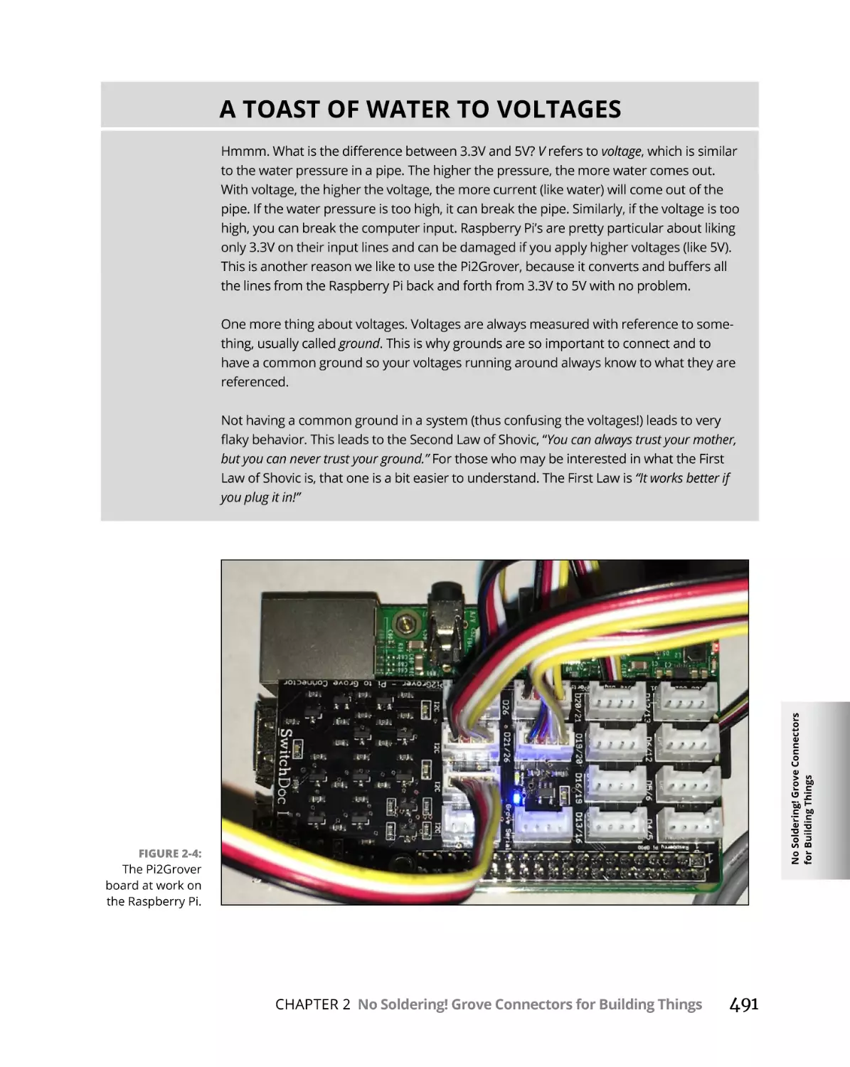
Raspberry Pi Base Unit — the Pi2Grover. . . . . . . . . . . . . . . . . . . . .
The Four Types of Grove Connectors. . . . . . . . . . . . . . . . . . . . . . . . . . .
The Four Types of Grove Signals. . . . . . . . . . . . . . . . . . . . . . . . . . . . . . .
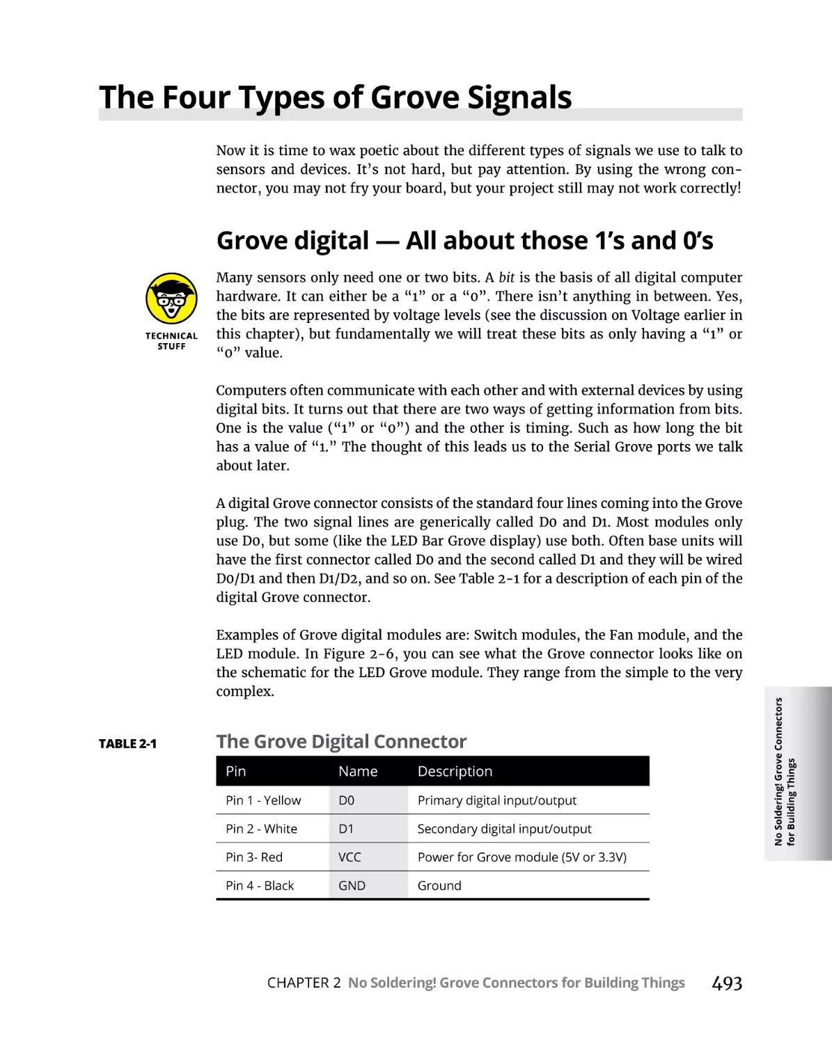
Grove digital — All about those 1’s and 0’s . . . . . . . . . . . . . . . . . . .
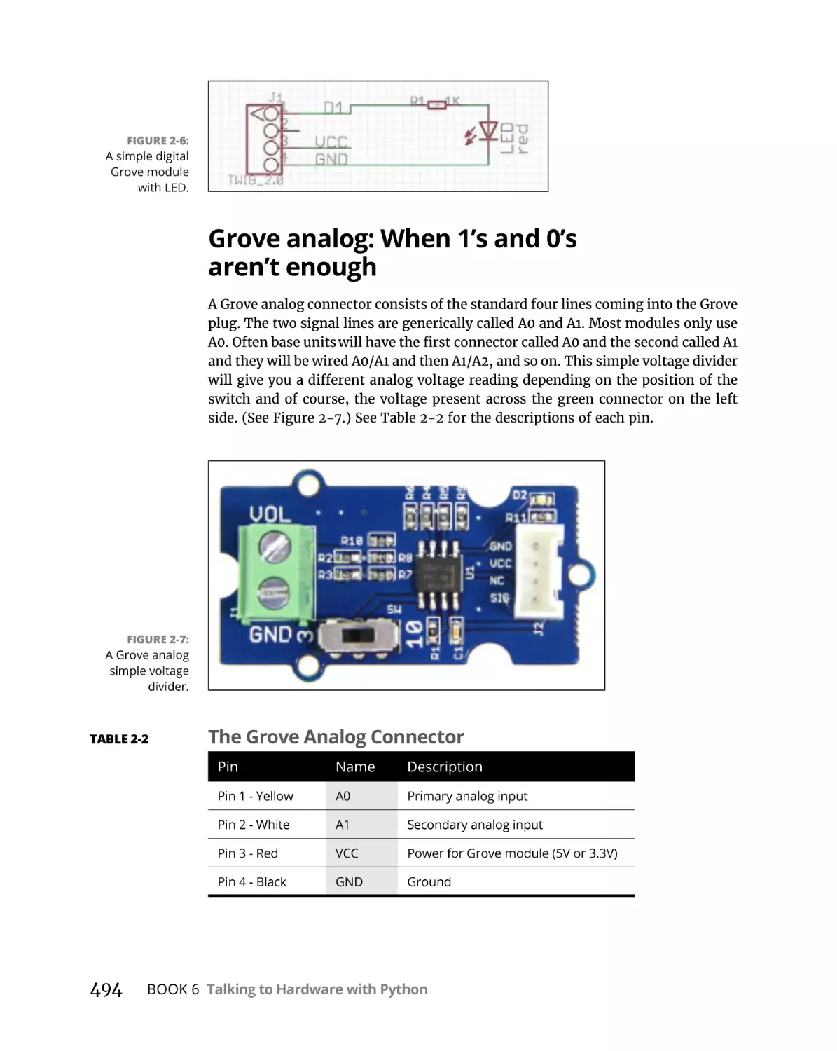
Grove analog: When 1’s and 0’s aren’t enough. . . . . . . . . . . . . . . .
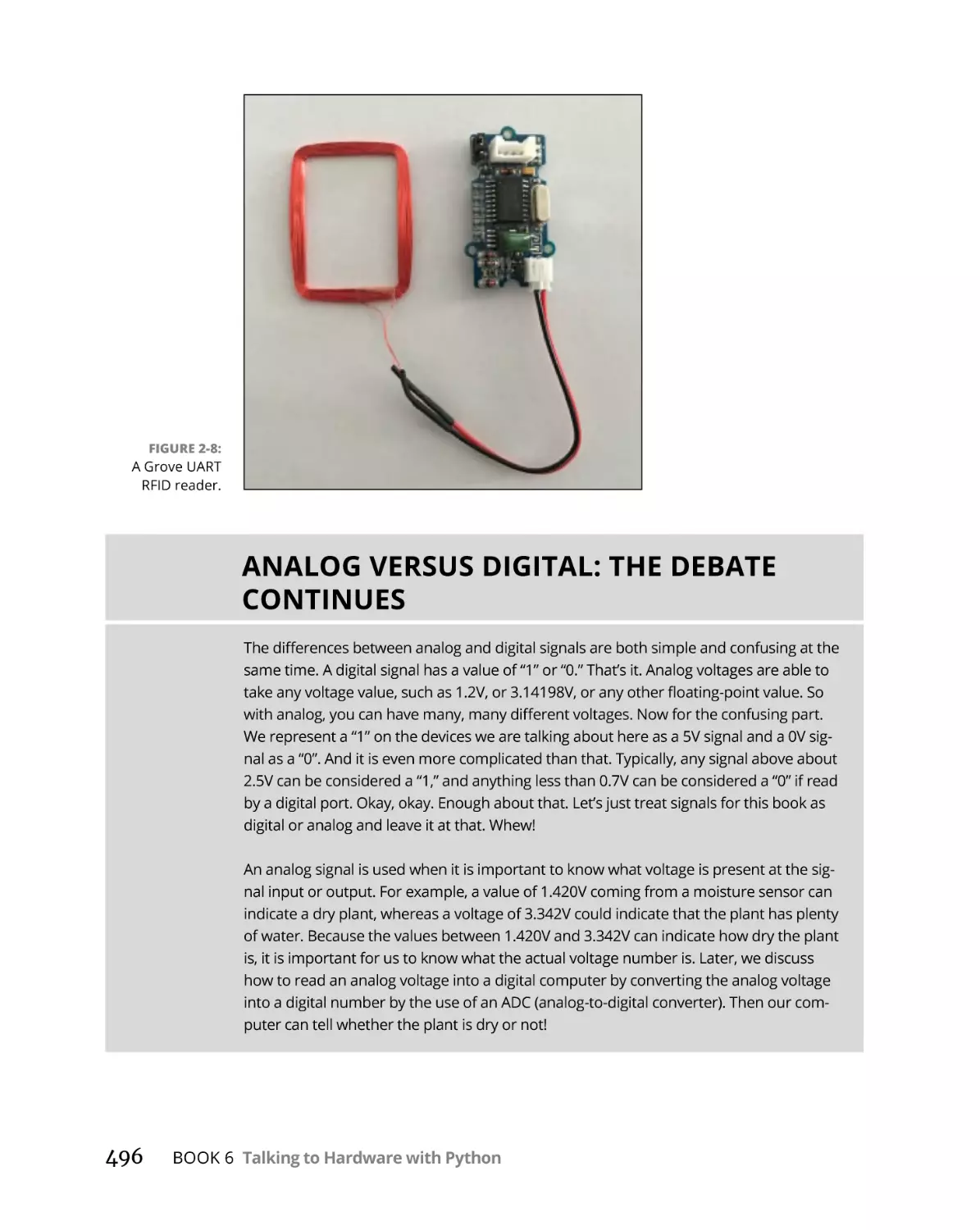
Grove UART (or serial) — Bit by bit transmission. . . . . . . . . . . . . .
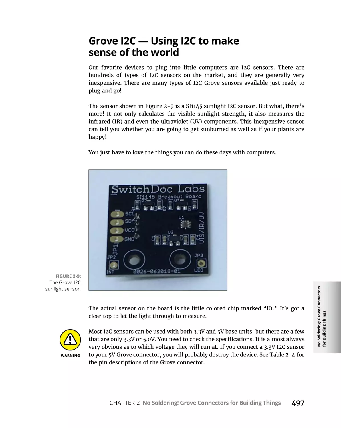
Grove I2C — Using I2C to make sense of the world. . . . . . . . . . . .
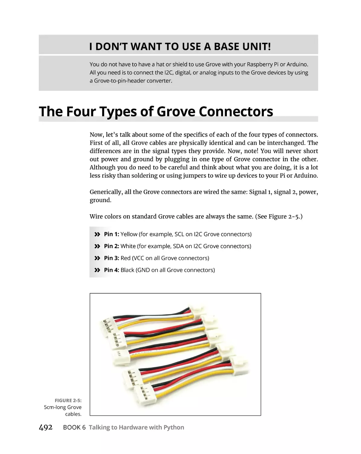
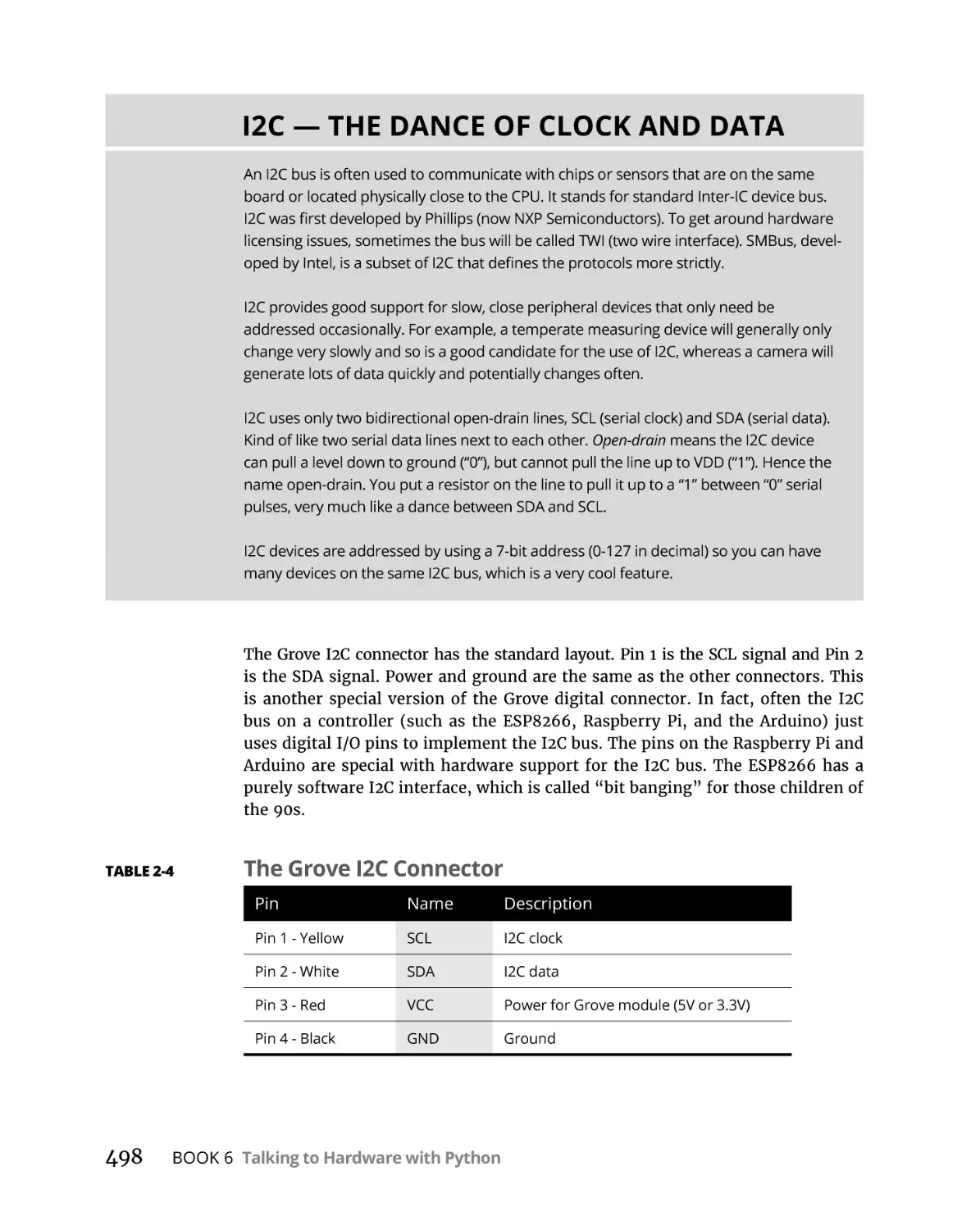
Using Grove Cables to Get Connected. . . . . . . . . . . . . . . . . . . . . . . . . .
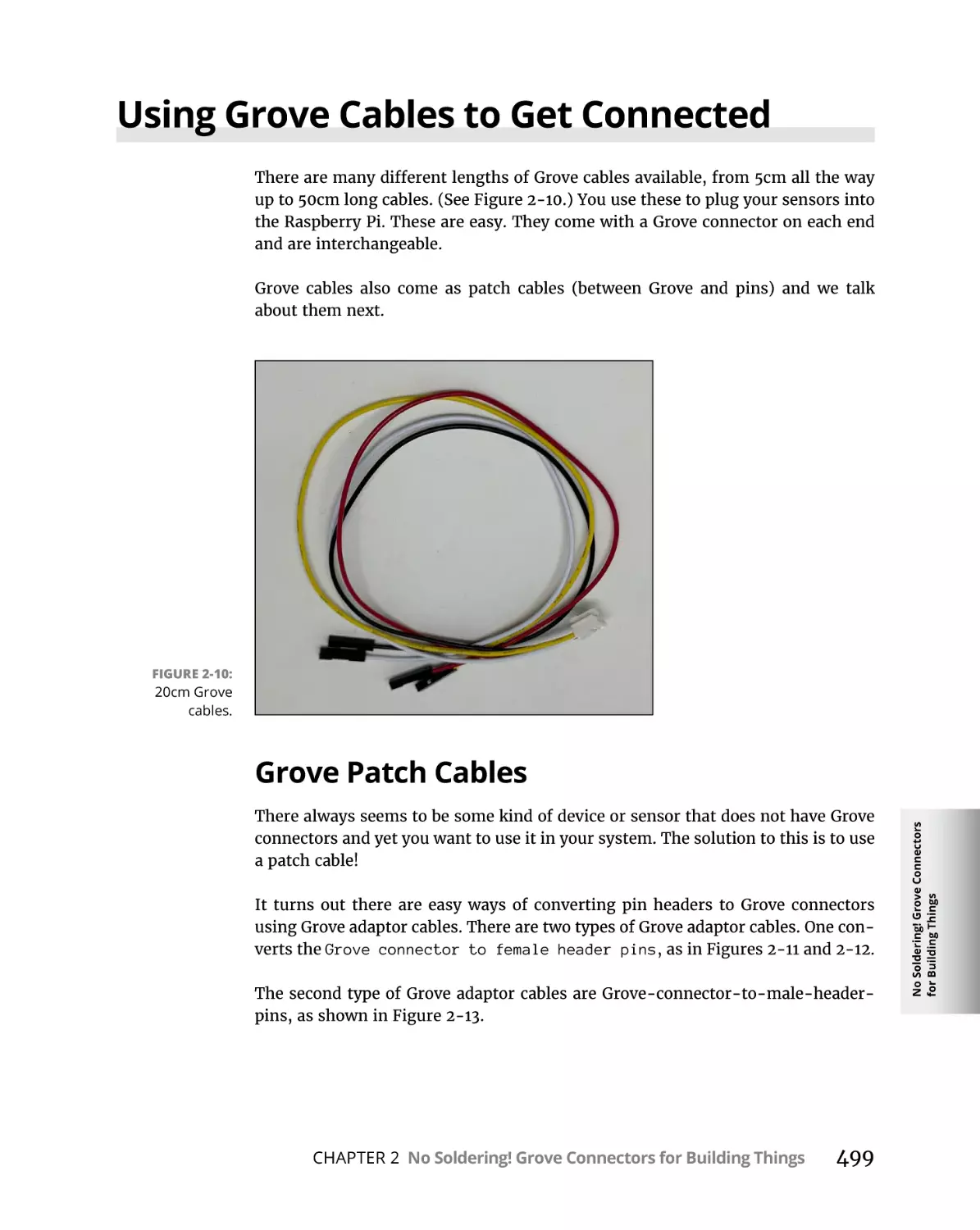
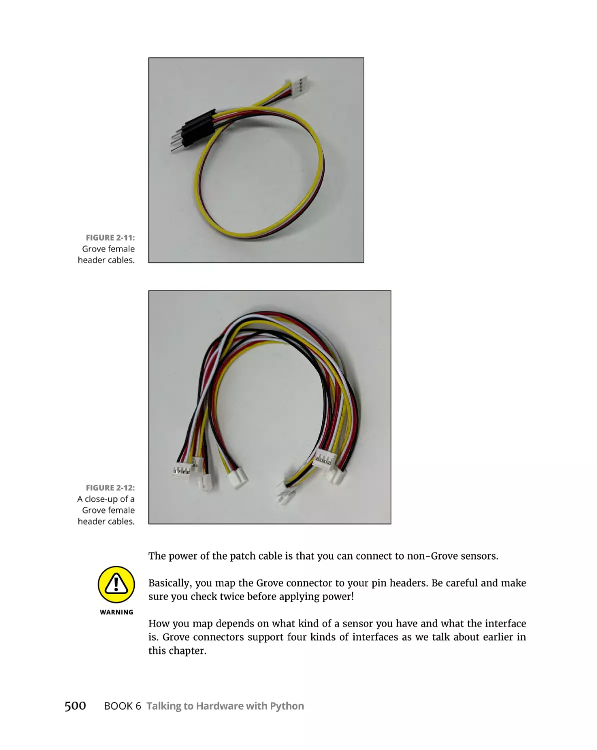
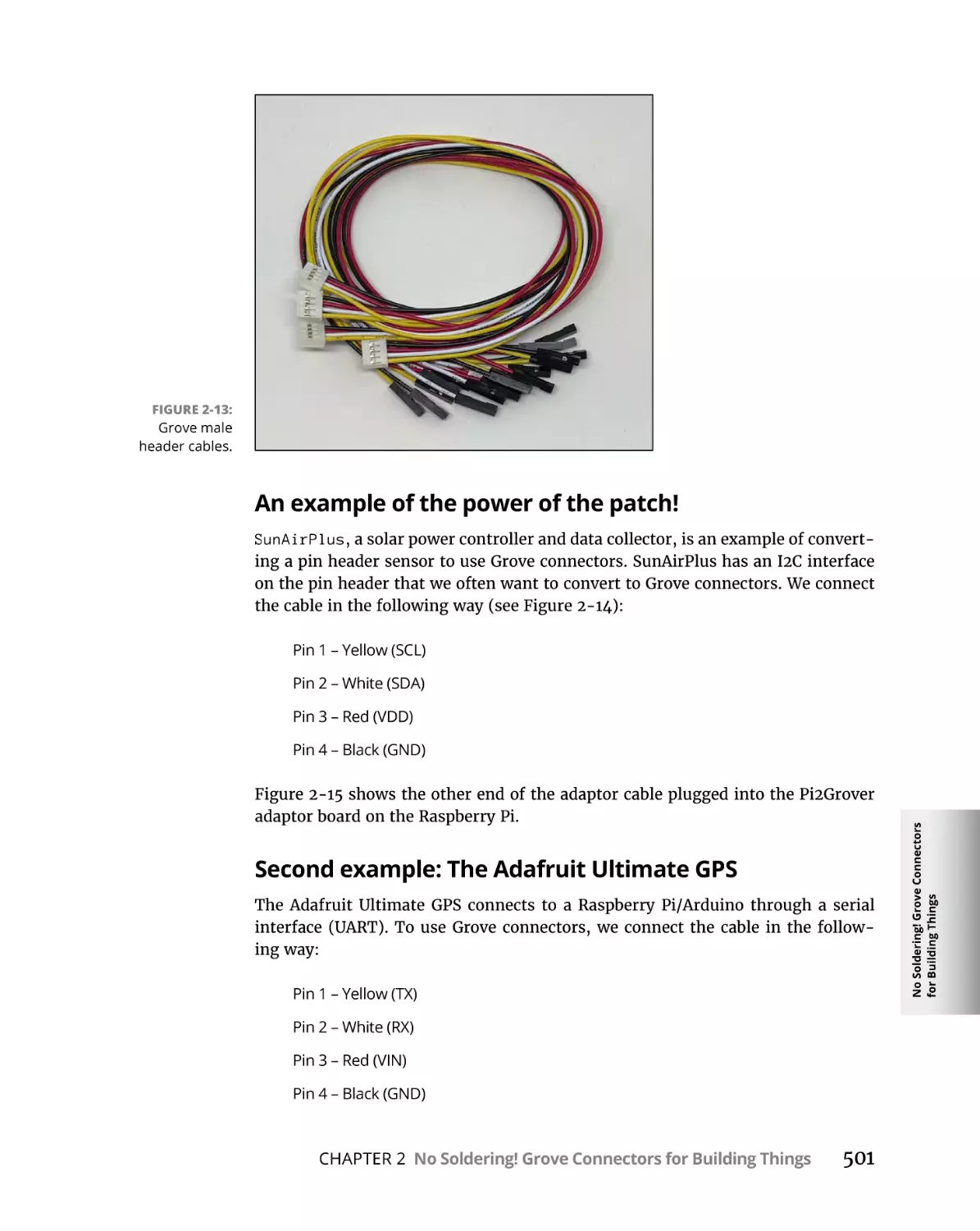
Grove Patch Cables. . . . . . . . . . . . . . . . . . . . . . . . . . . . . . . . . . . . . . .
488
489
489
490
492
493
493
494
495
497
499
499
Table of Contents
xiii
CHAPTER 3:
505
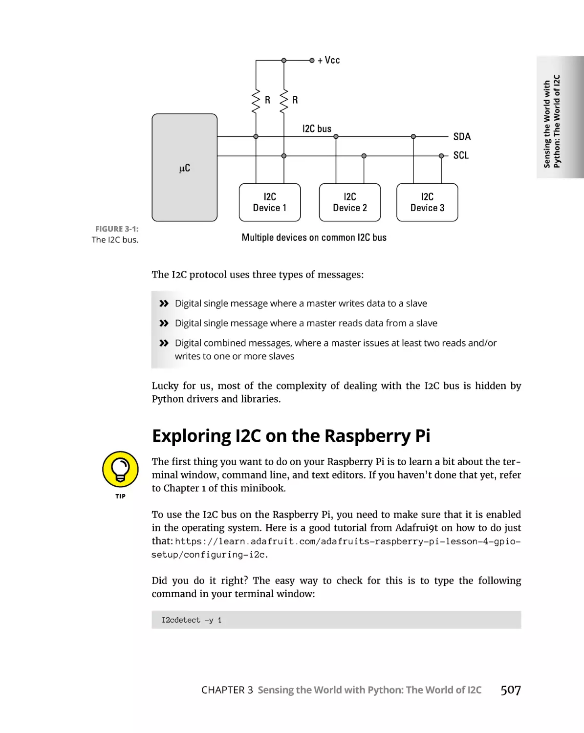
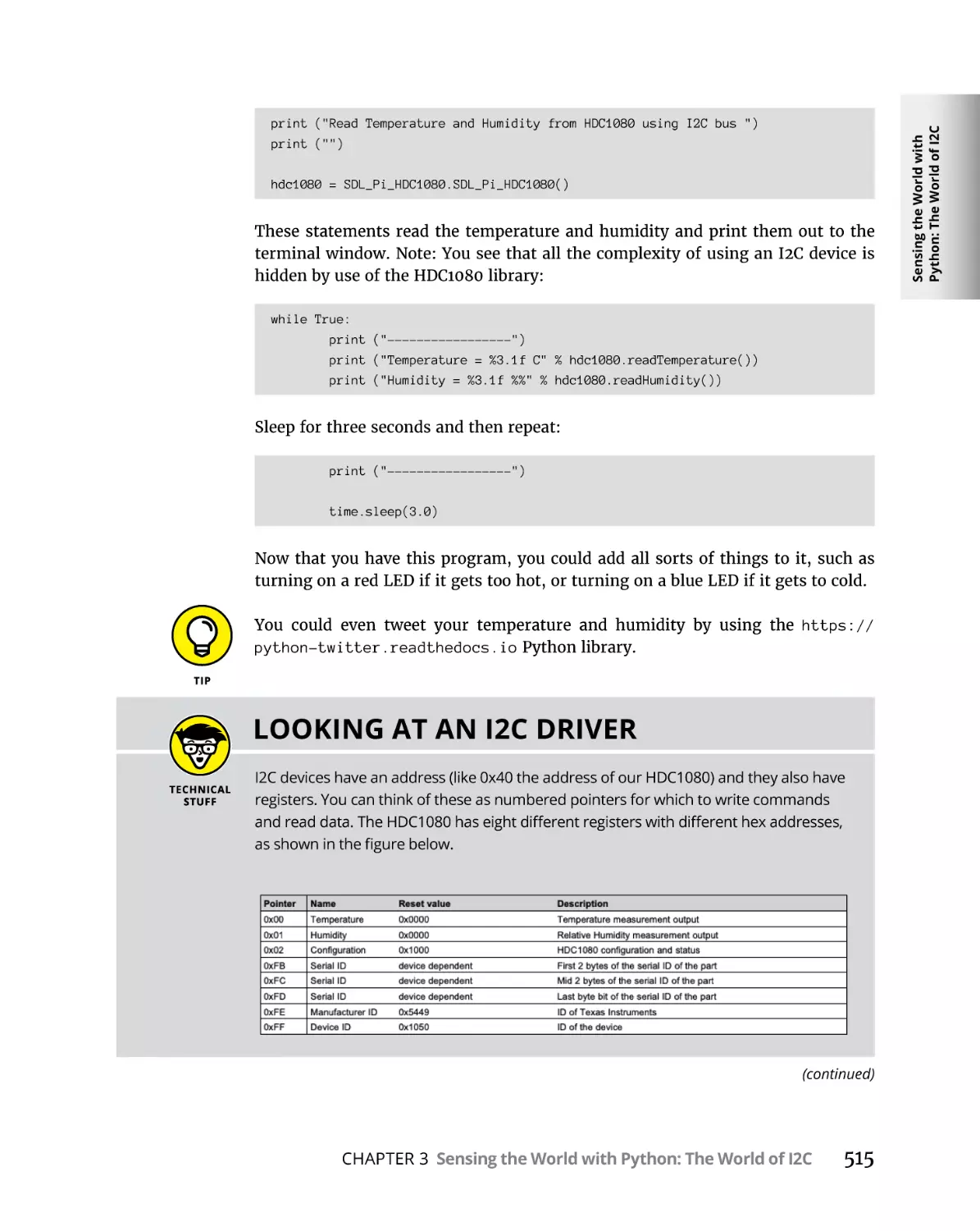
Understanding I2C . . . . . . . . . . . . . . . . . . . . . . . . . . . . . . . . . . . . . . . . . .
Exploring I2C on the Raspberry Pi. . . . . . . . . . . . . . . . . . . . . . . . . . .
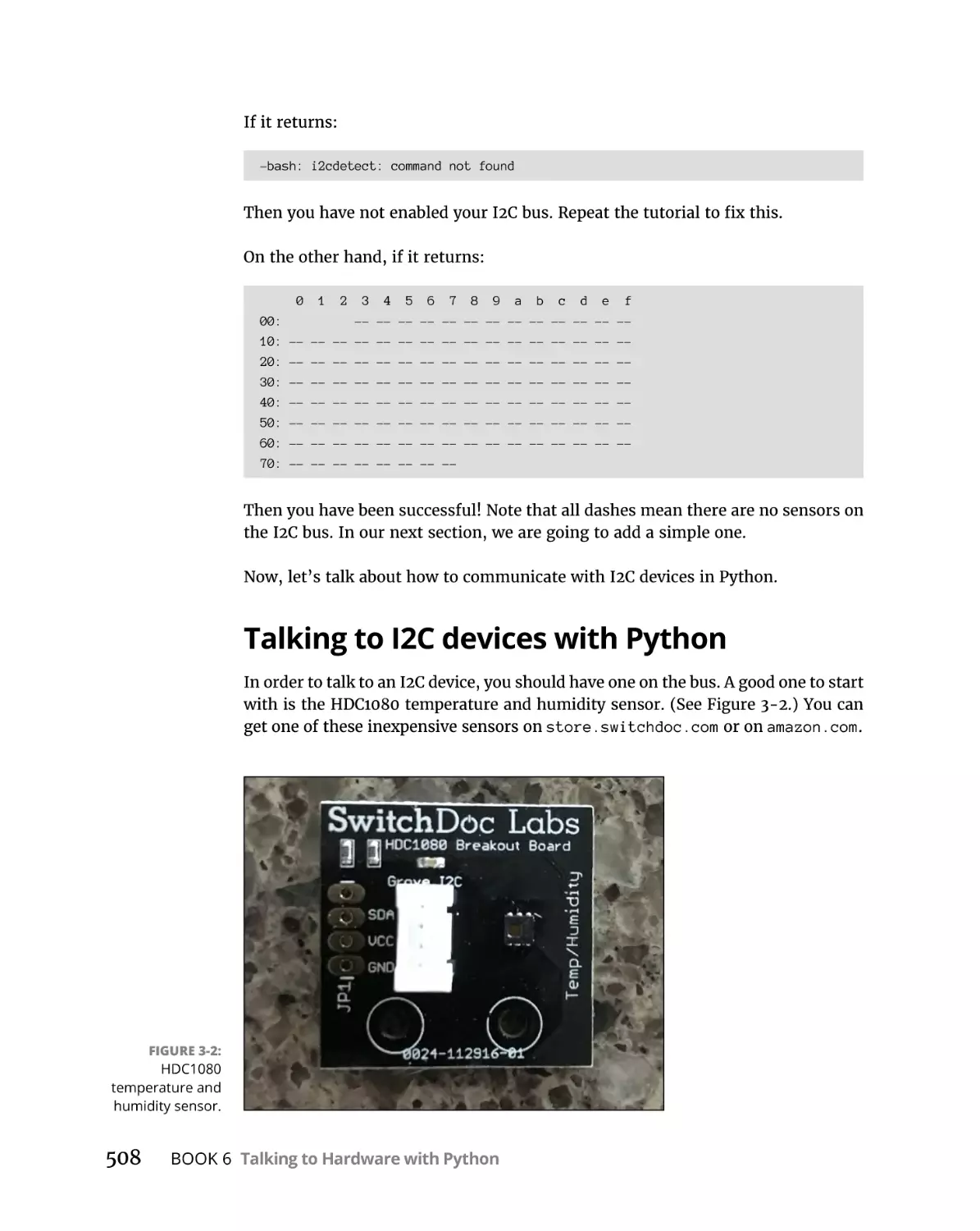
Talking to I2C devices with Python. . . . . . . . . . . . . . . . . . . . . . . . . .
Reading temperature and humidity from an I2C
device using Python . . . . . . . . . . . . . . . . . . . . . . . . . . . . . . . . . . . . . .
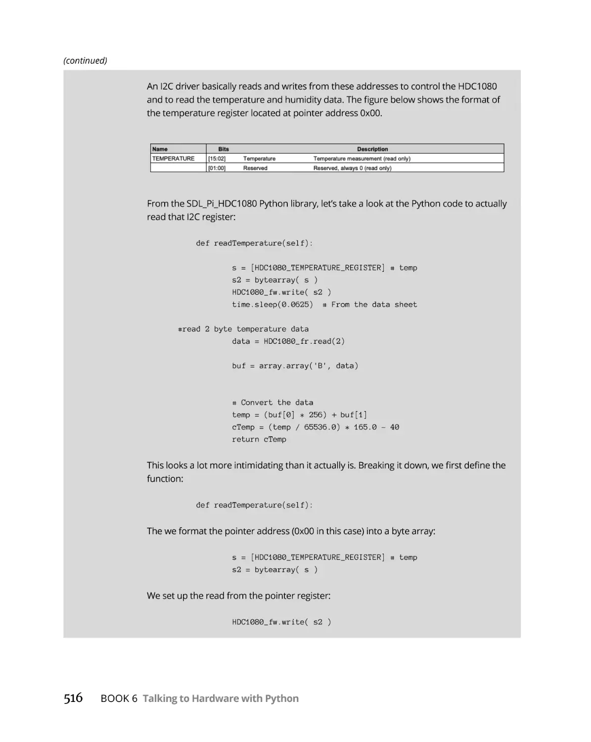
Breaking down the program . . . . . . . . . . . . . . . . . . . . . . . . . . . . . . .
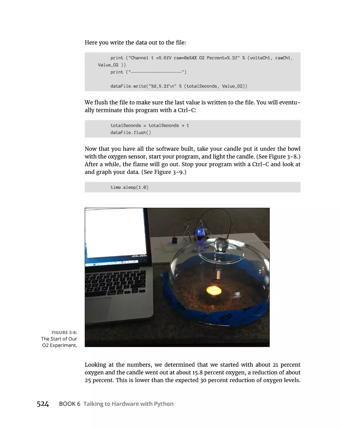
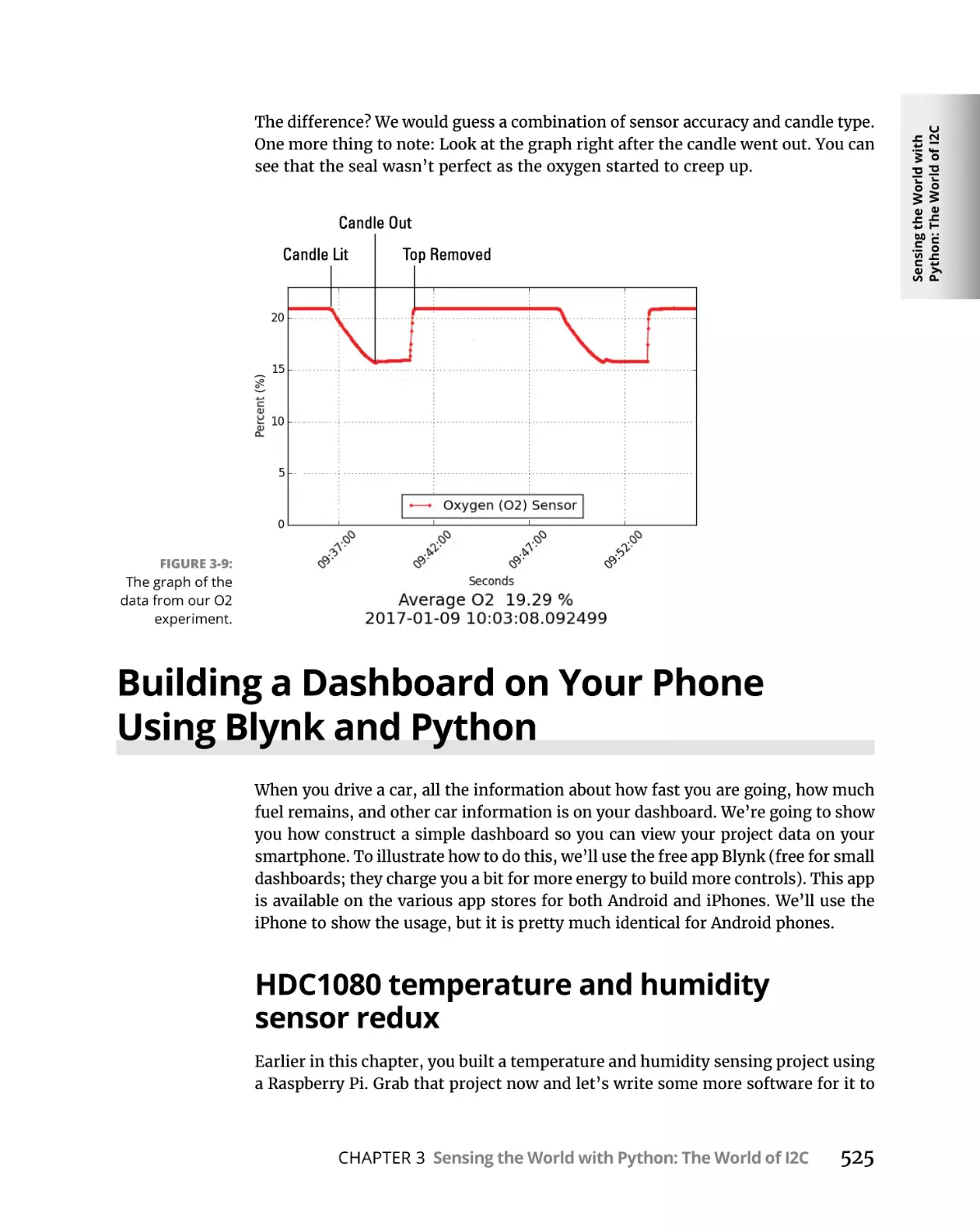
A Fun Experiment for Measuring Oxygen and a Flame. . . . . . . . . . . .
Analog-to-digital converters (ADC) . . . . . . . . . . . . . . . . . . . . . . . . . .
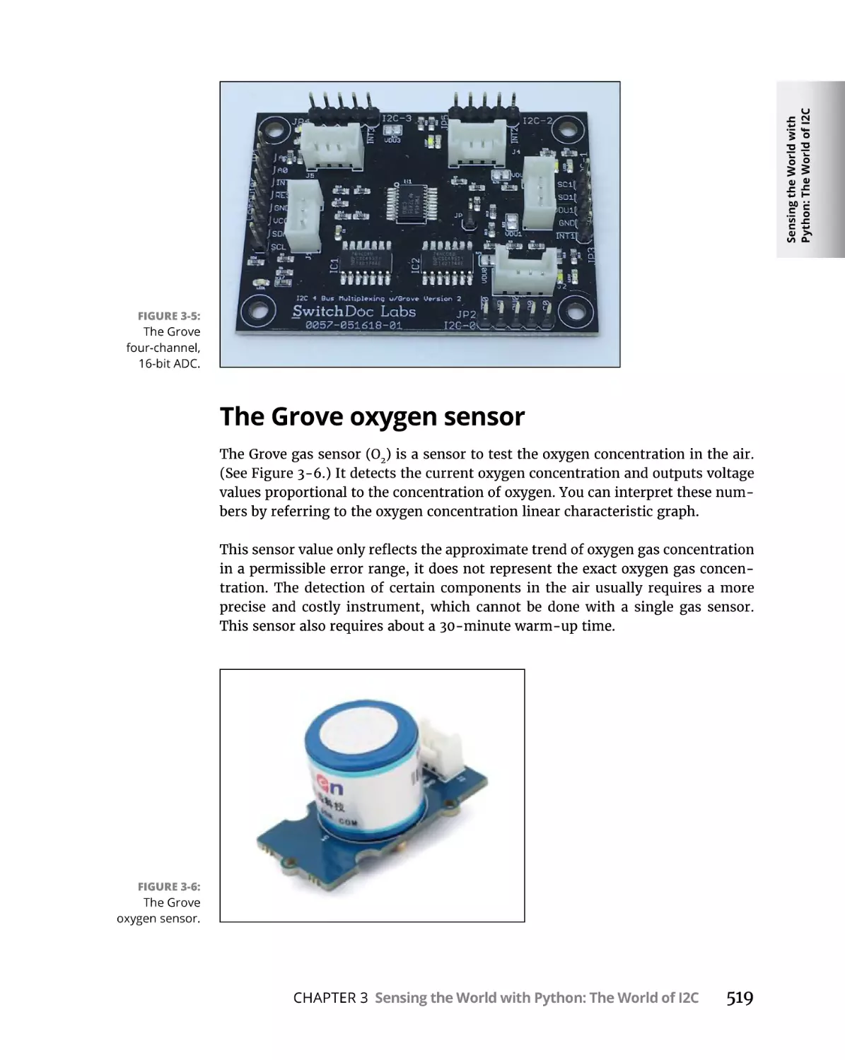
The Grove oxygen sensor. . . . . . . . . . . . . . . . . . . . . . . . . . . . . . . . . .
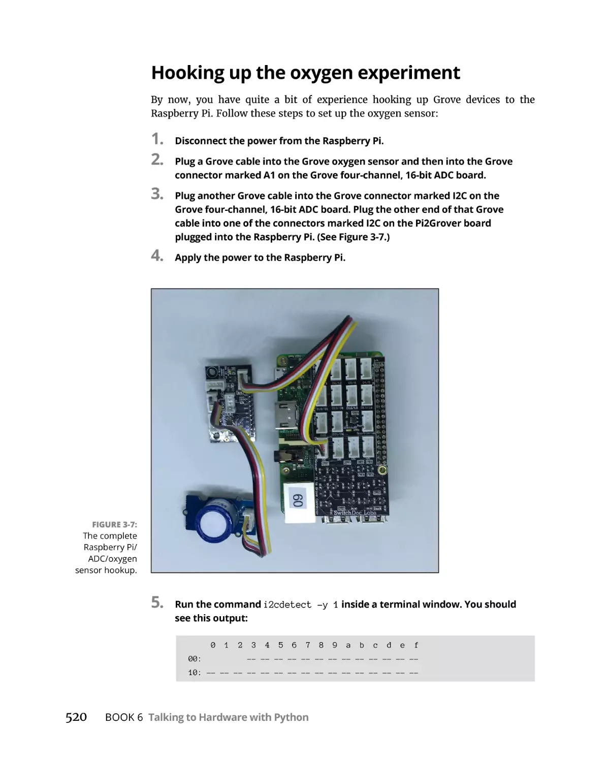
Hooking up the oxygen experiment. . . . . . . . . . . . . . . . . . . . . . . . .
Breaking down the code. . . . . . . . . . . . . . . . . . . . . . . . . . . . . . . . . . .
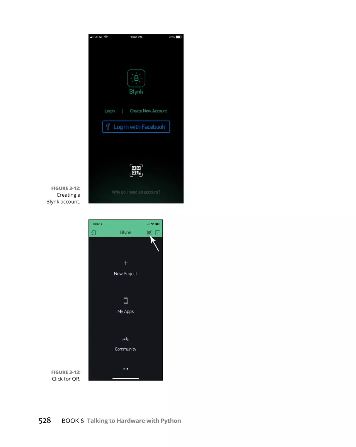
Building a Dashboard on Your Phone Using Blynk and Python. . . . .
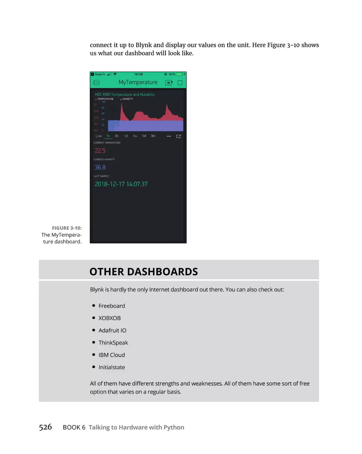
HDC1080 temperature and humidity sensor redux. . . . . . . . . . . .
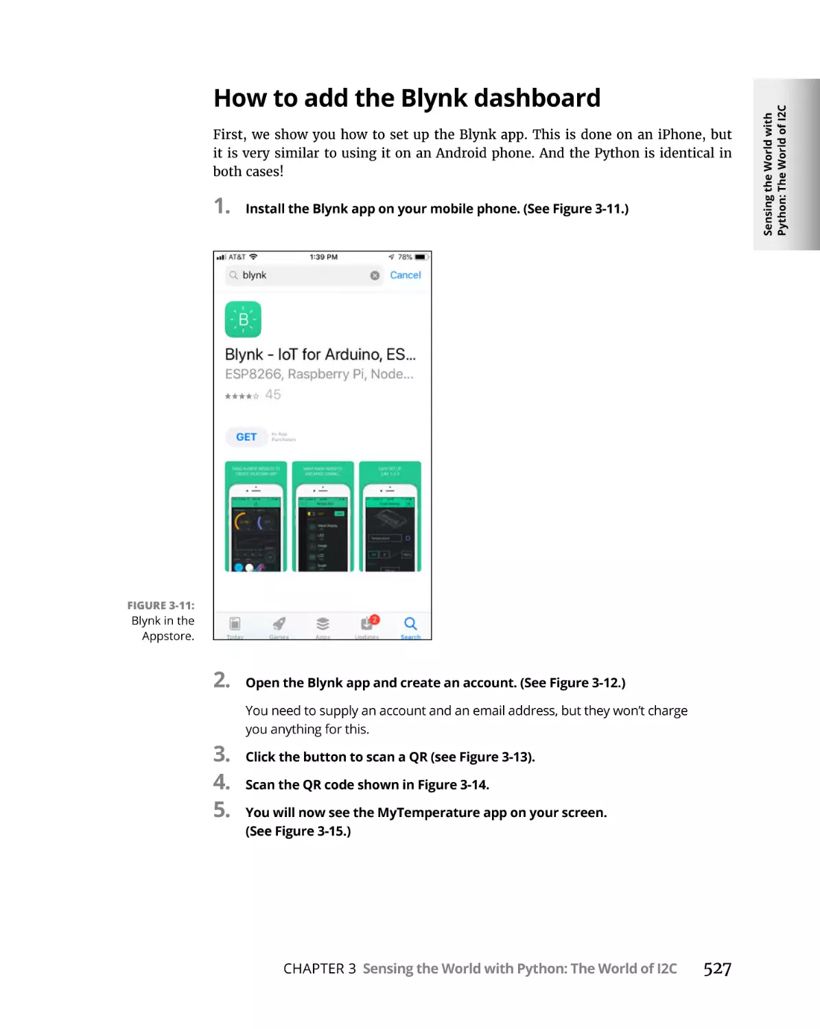
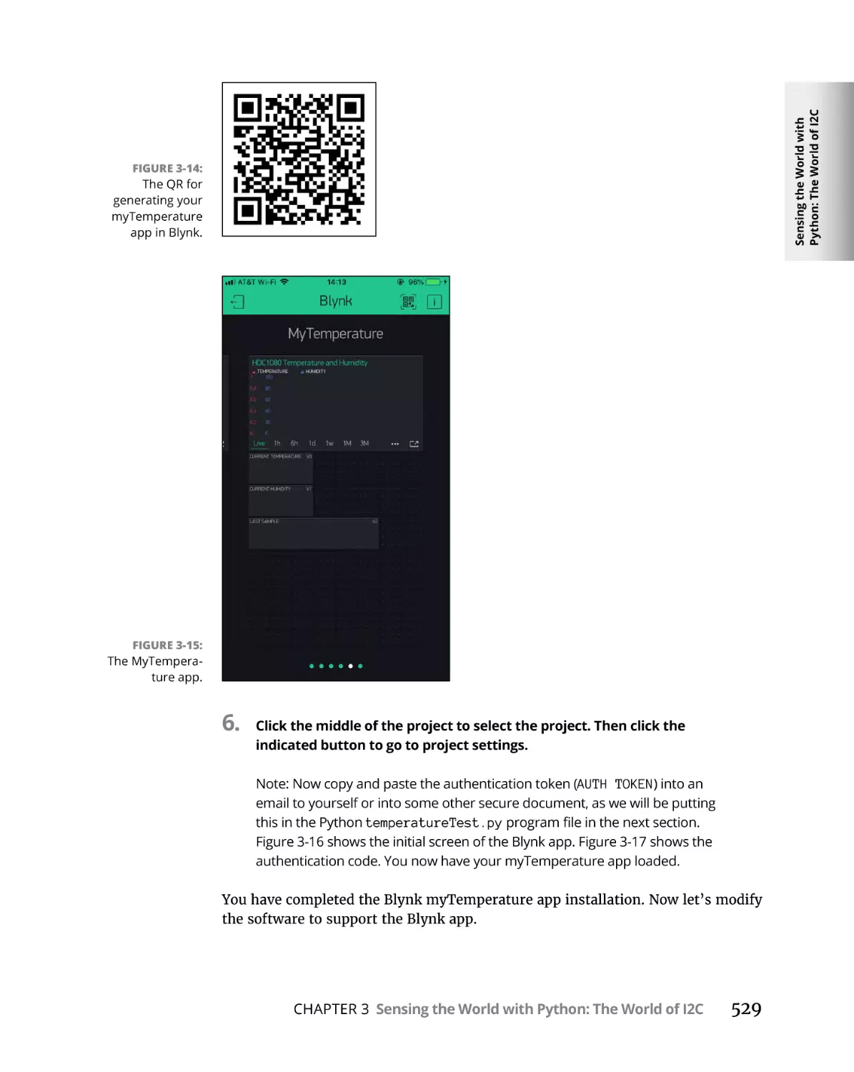
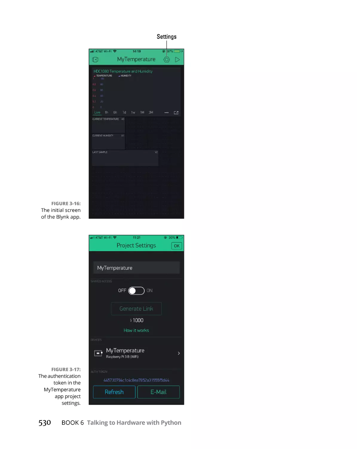
How to add the Blynk dashboard. . . . . . . . . . . . . . . . . . . . . . . . . . .
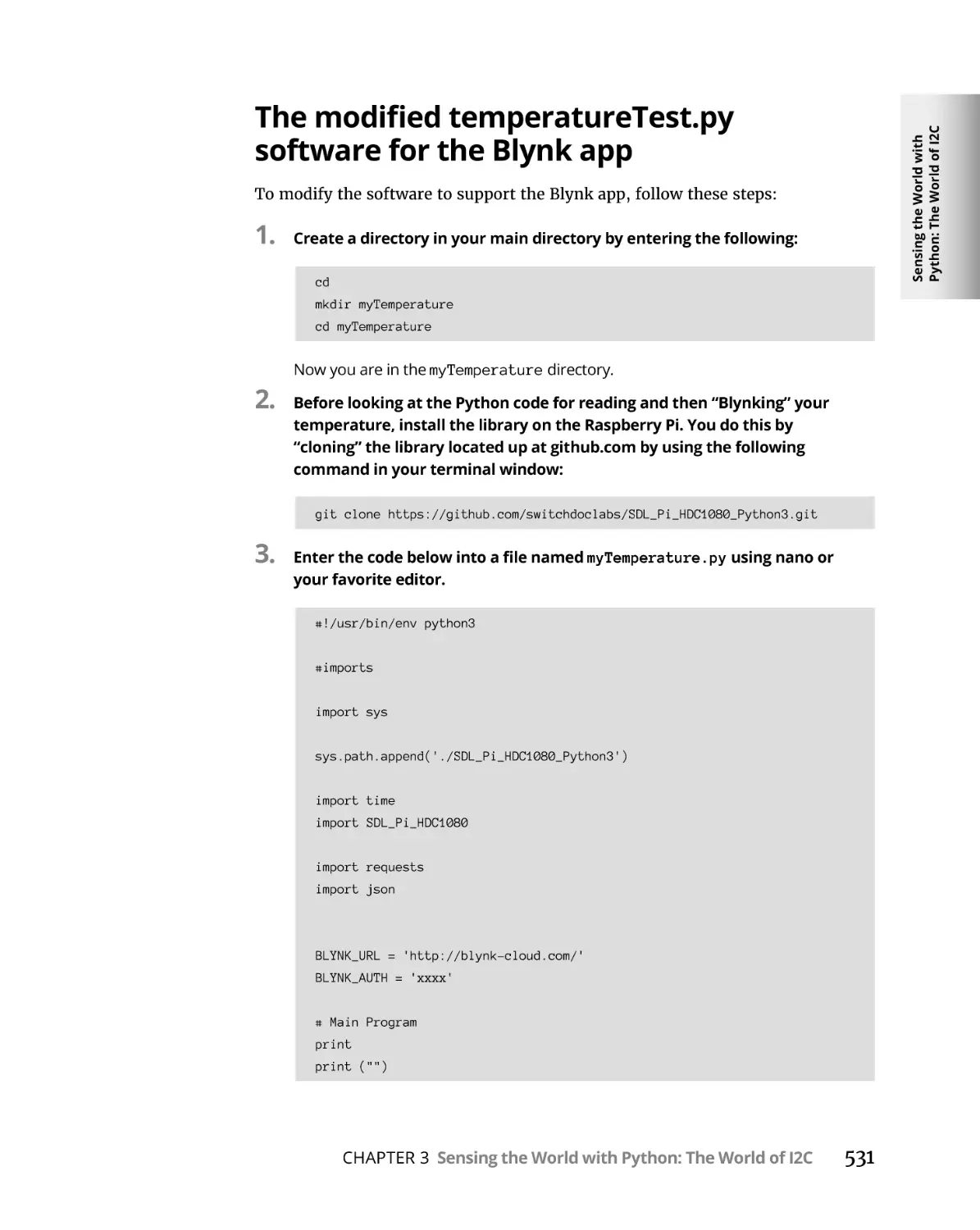
The modified temperatureTest.py software for the
Blynk app . . . . . . . . . . . . . . . . . . . . . . . . . . . . . . . . . . . . . . . . . . . . . . .
Breaking down the code. . . . . . . . . . . . . . . . . . . . . . . . . . . . . . . . . . .
Where to Go from Here . . . . . . . . . . . . . . . . . . . . . . . . . . . . . . . . . . .
531
533
536
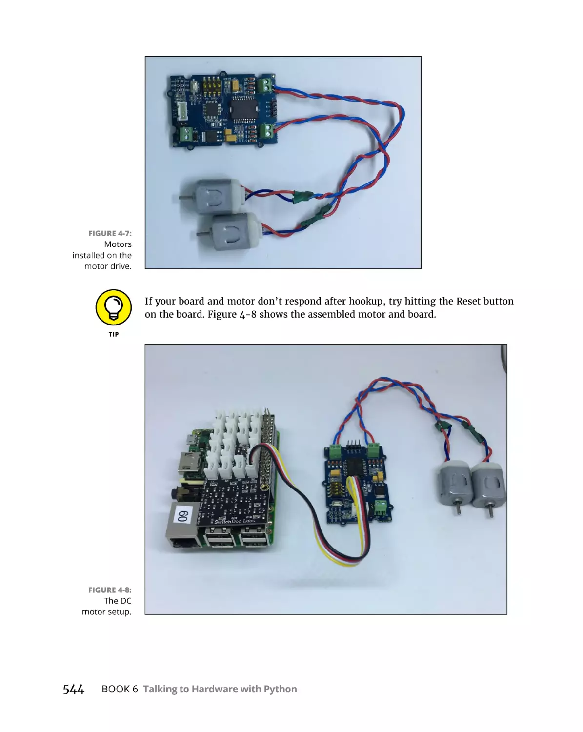
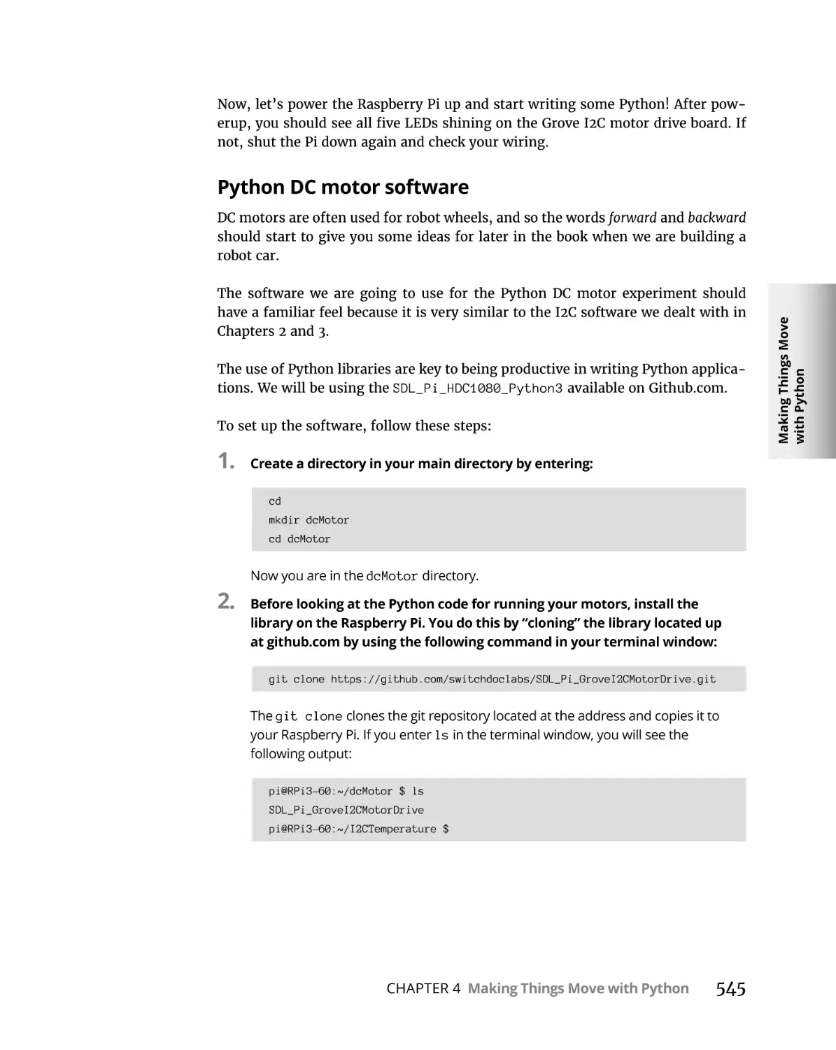
Making Things Move with Python. . . . . . . . . . . . . . . . . . .
537
Exploring Electric Motors. . . . . . . . . . . . . . . . . . . . . . . . . . . . . . . . . . . . .
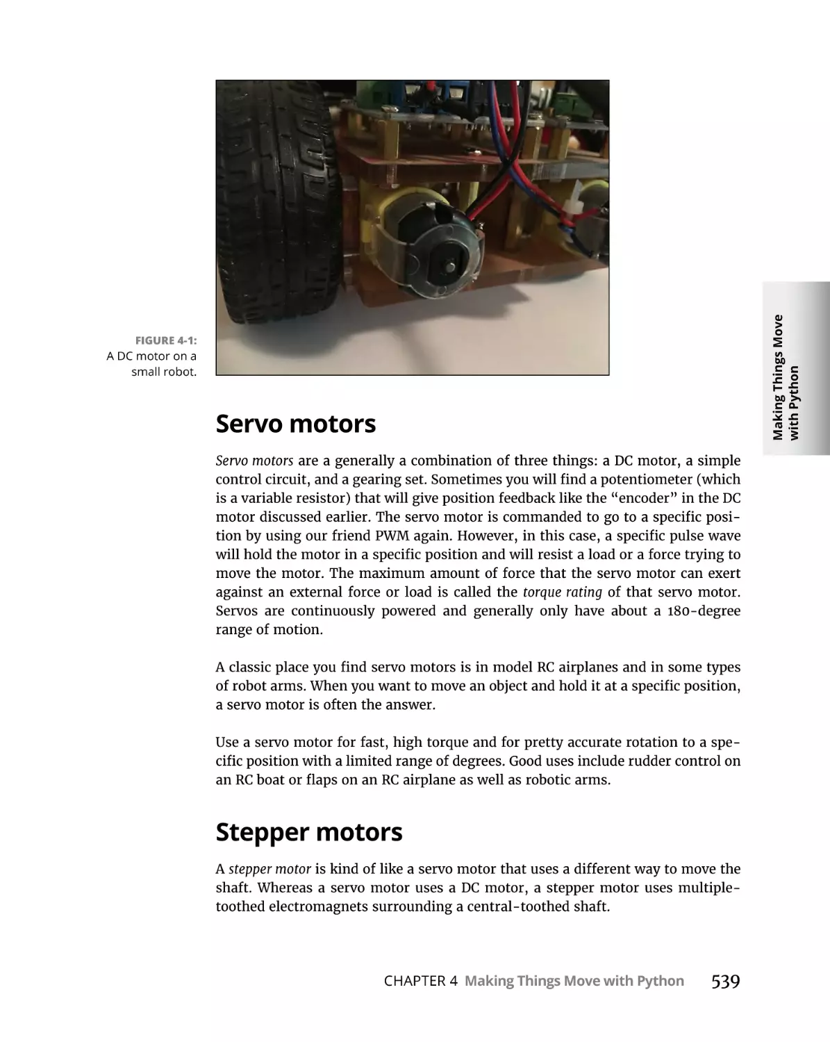
Small DC motors . . . . . . . . . . . . . . . . . . . . . . . . . . . . . . . . . . . . . . . . .
Servo motors. . . . . . . . . . . . . . . . . . . . . . . . . . . . . . . . . . . . . . . . . . . .
Stepper motors. . . . . . . . . . . . . . . . . . . . . . . . . . . . . . . . . . . . . . . . . .
Controlling Motors with a Computer . . . . . . . . . . . . . . . . . . . . . . . . . . .
Python and DC Motors. . . . . . . . . . . . . . . . . . . . . . . . . . . . . . . . . . . .
Python and running a servo motor. . . . . . . . . . . . . . . . . . . . . . . . . .
Python and making a stepper motor step. . . . . . . . . . . . . . . . . . . .
538
538
539
539
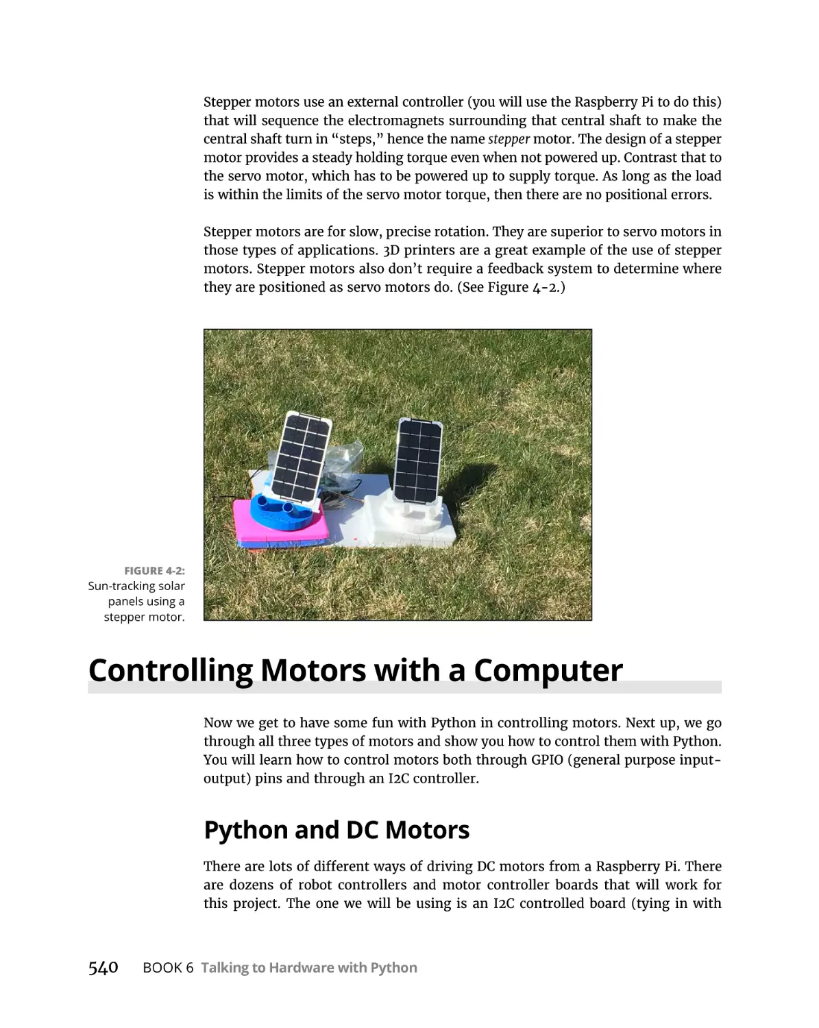
540
540
548
554
BOOK 7: BUILDING ROBOTS WITH PYTHON. . . . . . . . . . . . . . .
565
CHAPTER 4:
CHAPTER 1:
xiv
Sensing the World with Python:
The World of I2C . . . . . . . . . . . . . . . . . . . . . . . . . . . . . . . . . . . . . . . .
506
507
508
511
514
517
518
519
520
522
525
525
527
Introduction to Robotics . . . . . . . . . . . . . . . . . . . . . . . . . . . . . .
567
A Robot Is Not Always like a Human. . . . . . . . . . . . . . . . . . . . . . . . . . . .
Not Every Robot Has Arms or Wheels . . . . . . . . . . . . . . . . . . . . . . . . . .
The Wilkinson Bread-Making Robot. . . . . . . . . . . . . . . . . . . . . . . . .
Baxter the Coffee-Making Robot. . . . . . . . . . . . . . . . . . . . . . . . . . . .
The Griffin Bluetooth-enabled toaster. . . . . . . . . . . . . . . . . . . . . . .
Understanding the Main Parts of a Robot. . . . . . . . . . . . . . . . . . . . . . .
Computers. . . . . . . . . . . . . . . . . . . . . . . . . . . . . . . . . . . . . . . . . . . . . .
Motors and actuators. . . . . . . . . . . . . . . . . . . . . . . . . . . . . . . . . . . . .
Communications. . . . . . . . . . . . . . . . . . . . . . . . . . . . . . . . . . . . . . . . .
Sensors. . . . . . . . . . . . . . . . . . . . . . . . . . . . . . . . . . . . . . . . . . . . . . . . .
Programming Robots . . . . . . . . . . . . . . . . . . . . . . . . . . . . . . . . . . . . . . . .
567
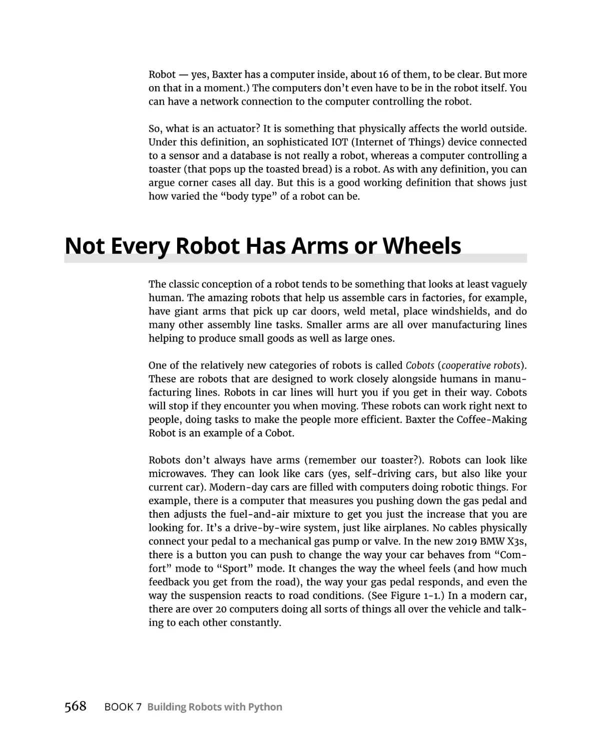
568
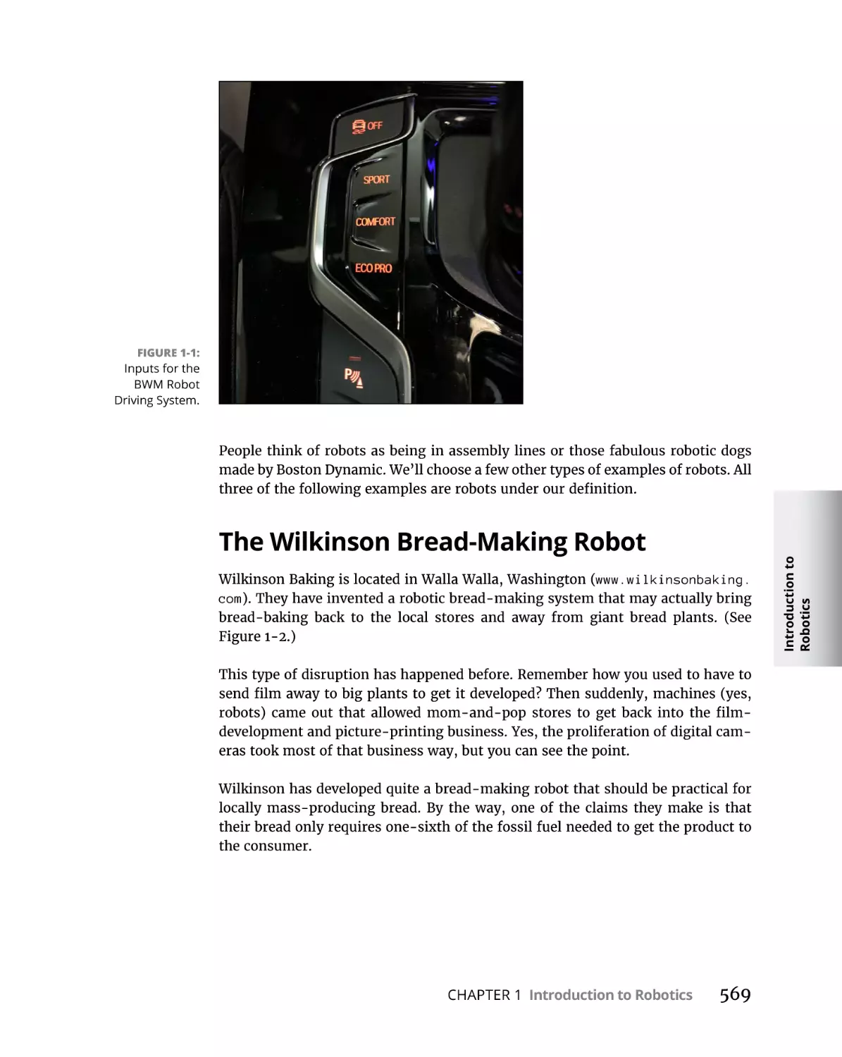
569
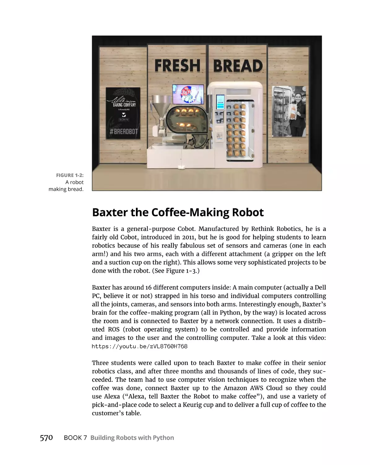
570
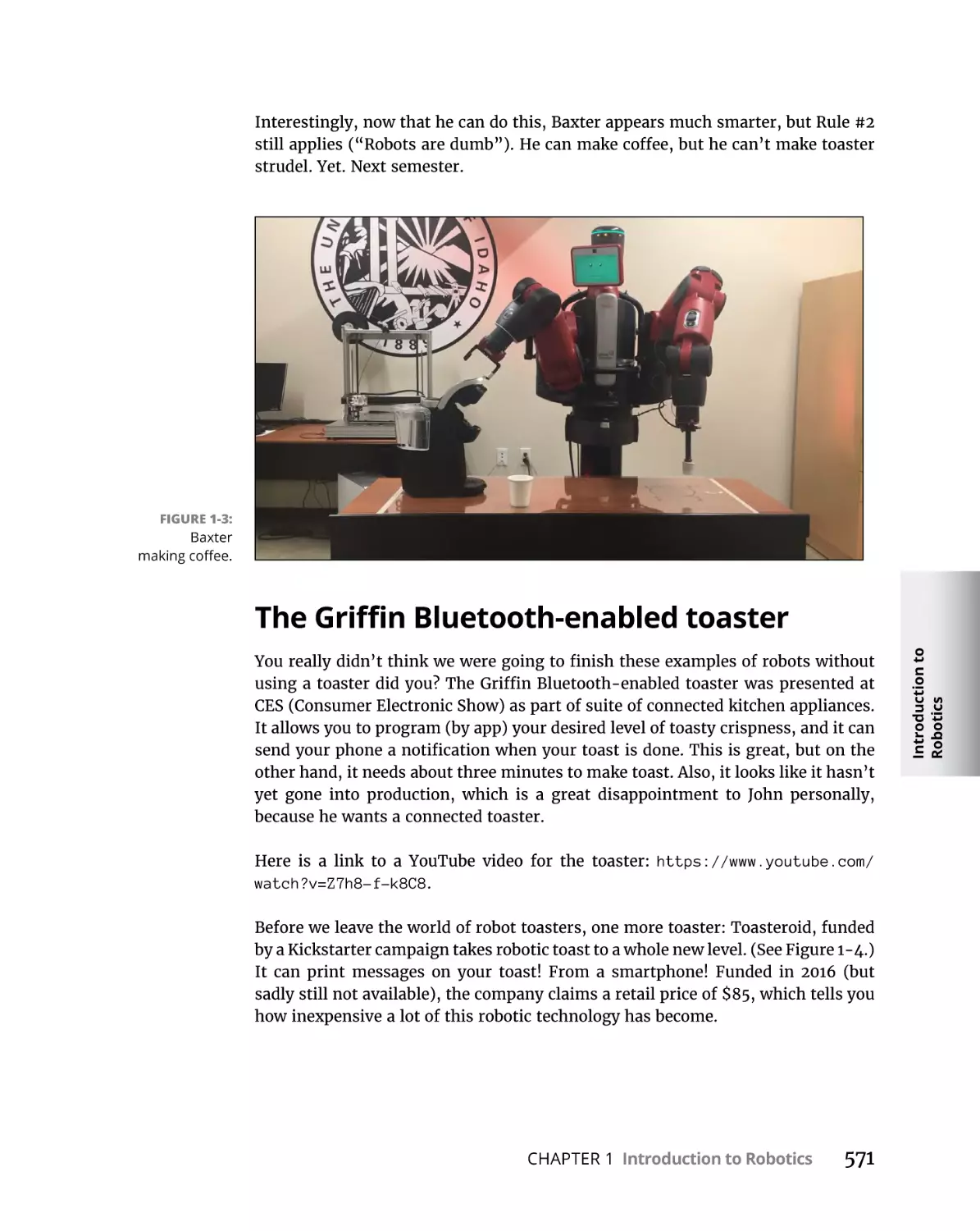
571
572
572
573
573
573
574
Python All-in-One For Dummies
CHAPTER 2:
Building Your First Python Robot. . . . . . . . . . . . . . . . . . . .
575
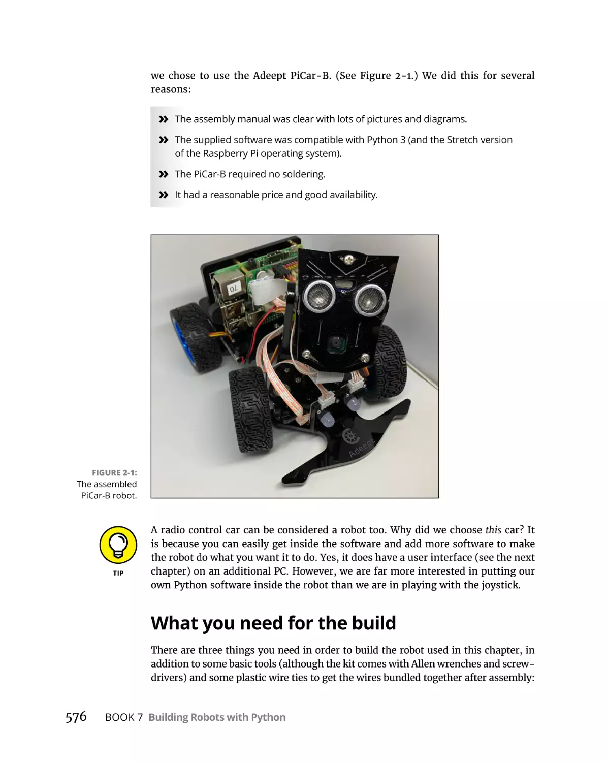
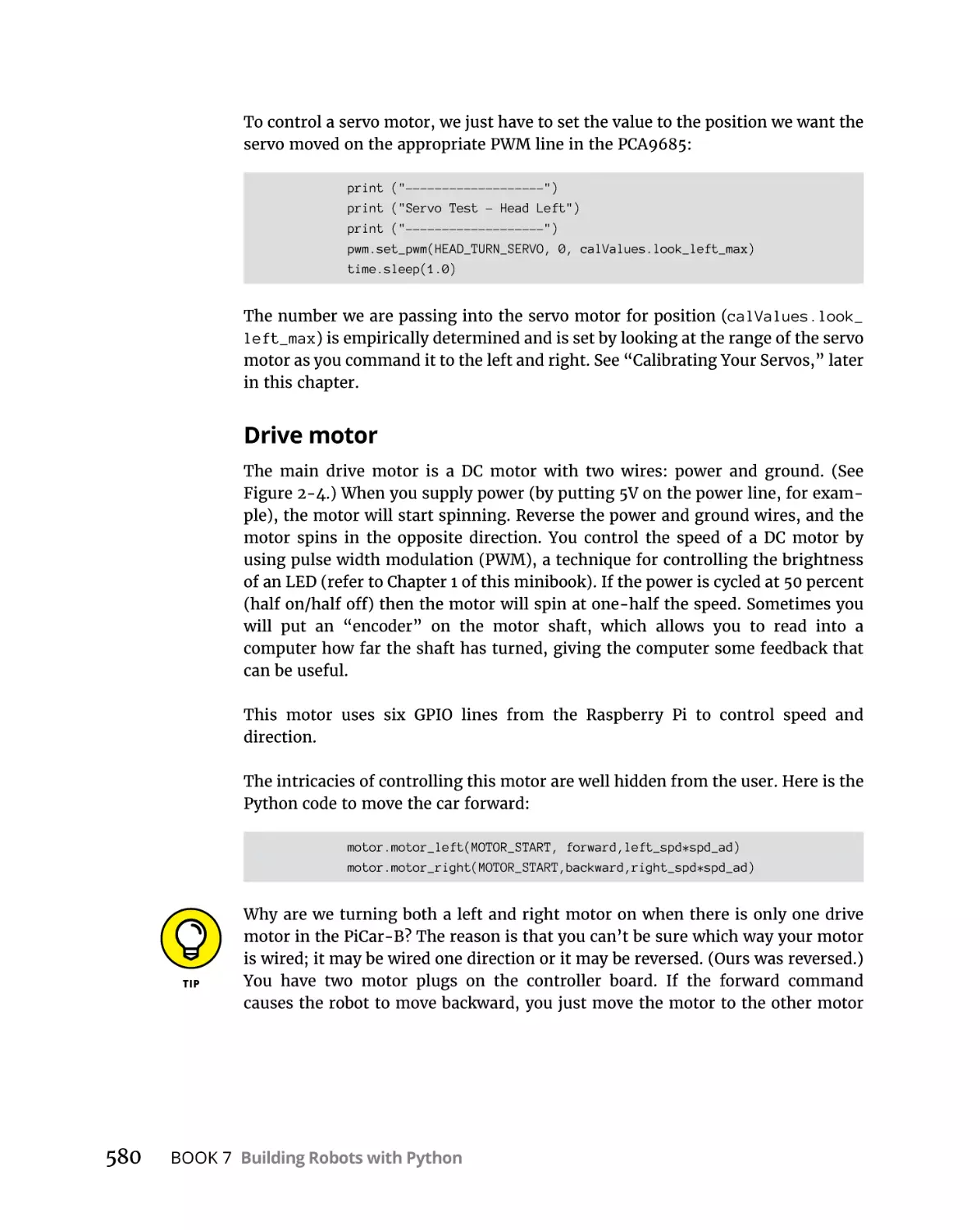
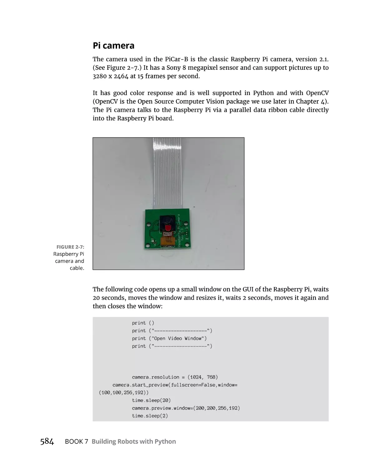
Introducing the Mars Rover PiCar-B. . . . . . . . . . . . . . . . . . . . . . . . . . . . 575
What you need for the build . . . . . . . . . . . . . . . . . . . . . . . . . . . . . . . 576
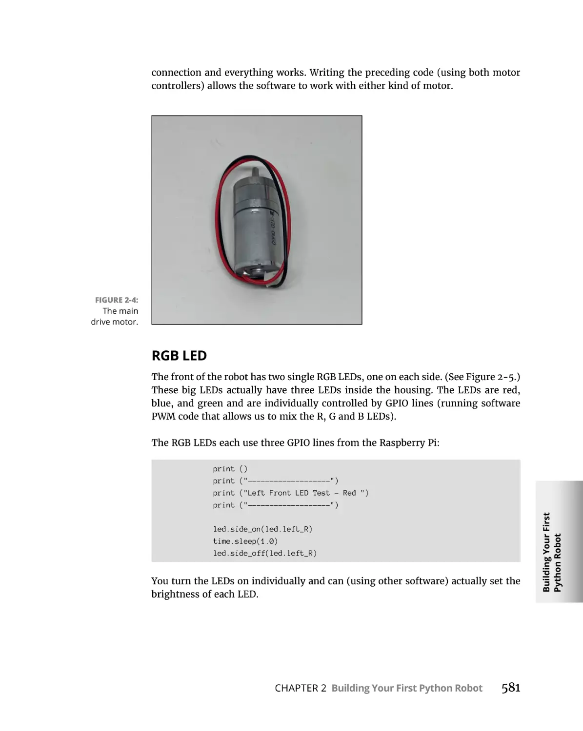
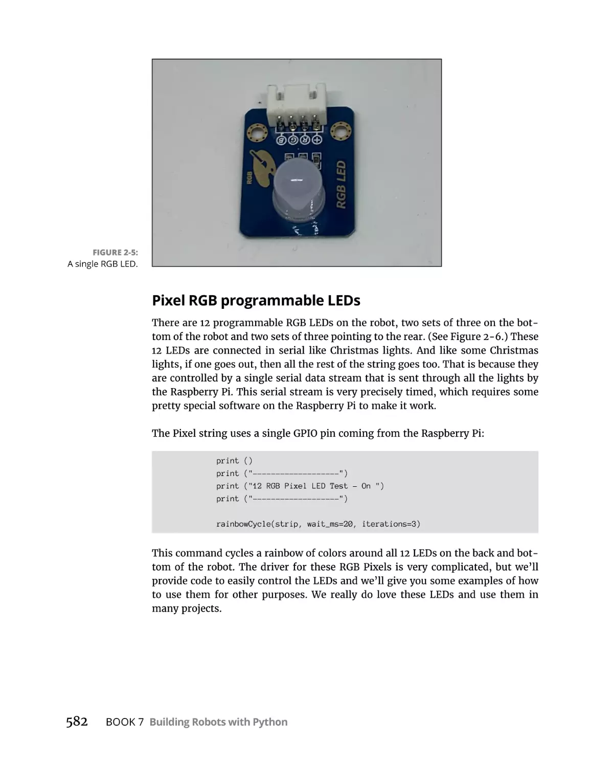
Understanding the robot components . . . . . . . . . . . . . . . . . . . . . . 577
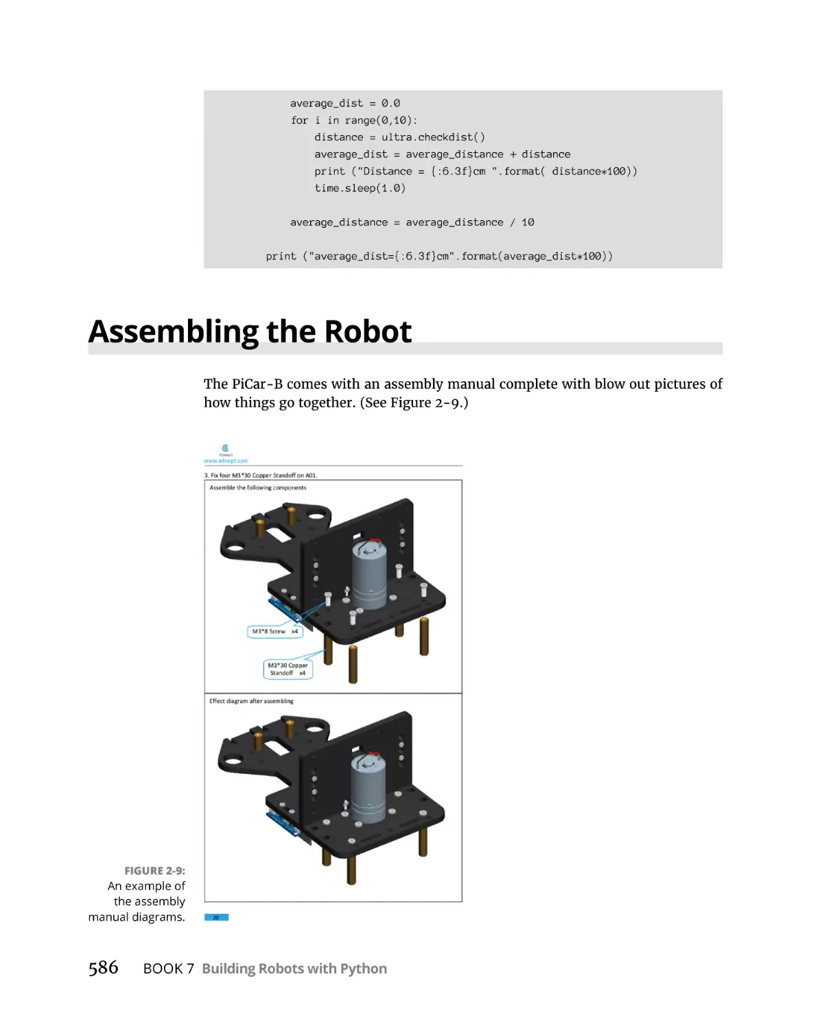
Assembling the Robot. . . . . . . . . . . . . . . . . . . . . . . . . . . . . . . . . . . . . . . . 586
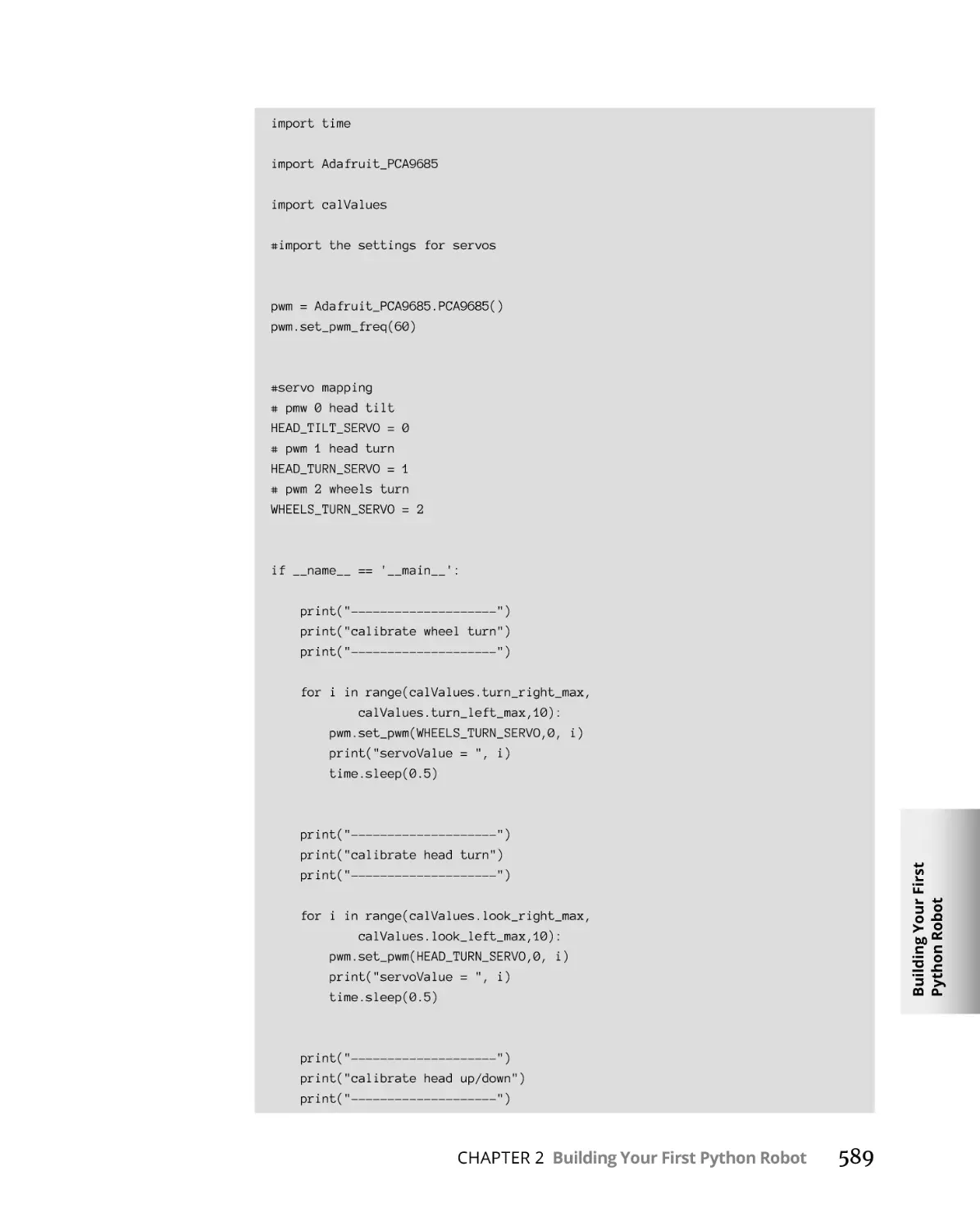
Calibrating your servos. . . . . . . . . . . . . . . . . . . . . . . . . . . . . . . . . . . . 588
Running tests on your rover in Python. . . . . . . . . . . . . . . . . . . . . . .591
Installing software for the CarPi-B Python test. . . . . . . . . . . . . . . . 591
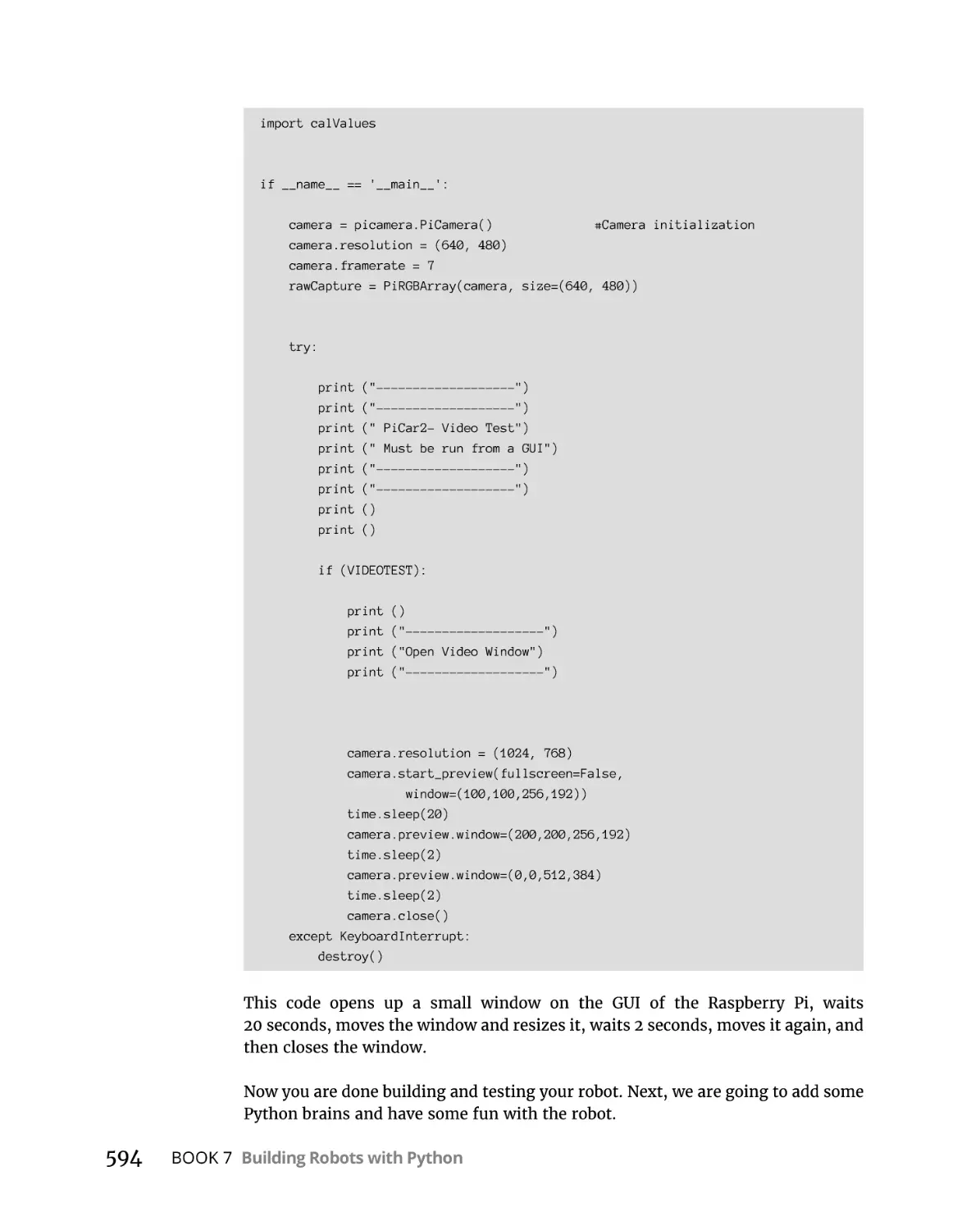
The PiCar-B Python test code . . . . . . . . . . . . . . . . . . . . . . . . . . . . . . 592
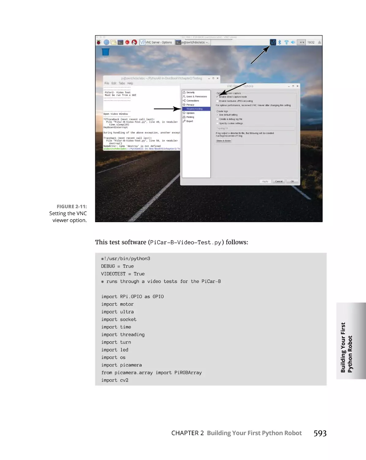
Pi camera video testing . . . . . . . . . . . . . . . . . . . . . . . . . . . . . . . . . . . 592
CHAPTER 3:
Programming Your Robot Rover in Python. . . . . . . .
595
Building a Simple High-Level Python Interface. . . . . . . . . . . . . . . . . . . 595
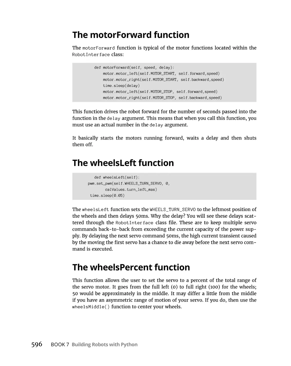
The motorForward function. . . . . . . . . . . . . . . . . . . . . . . . . . . . . . . . 596
The wheelsLeft function. . . . . . . . . . . . . . . . . . . . . . . . . . . . . . . . . . . 596
The wheelsPercent function . . . . . . . . . . . . . . . . . . . . . . . . . . . . . . . 596
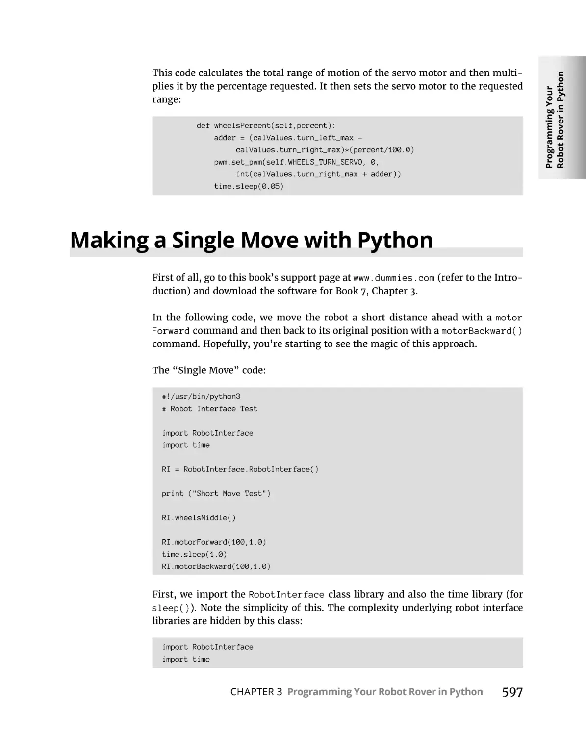
Making a Single Move with Python. . . . . . . . . . . . . . . . . . . . . . . . . . . . . 597
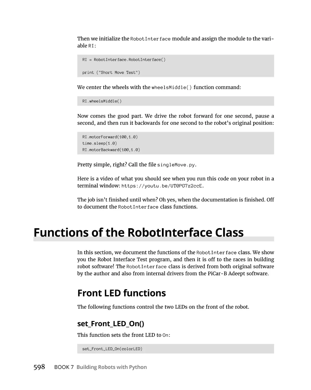
Functions of the RobotInterface Class. . . . . . . . . . . . . . . . . . . . . . . . . . 598
Front LED functions. . . . . . . . . . . . . . . . . . . . . . . . . . . . . . . . . . . . . . . 598
Pixel strip functions. . . . . . . . . . . . . . . . . . . . . . . . . . . . . . . . . . . . . . . 600
Ultrasonic distance sensor function. . . . . . . . . . . . . . . . . . . . . . . . . 601
Main motor functions. . . . . . . . . . . . . . . . . . . . . . . . . . . . . . . . . . . . . 602
Servo functions . . . . . . . . . . . . . . . . . . . . . . . . . . . . . . . . . . . . . . . . . . 603
General servo function. . . . . . . . . . . . . . . . . . . . . . . . . . . . . . . . . . . . 606
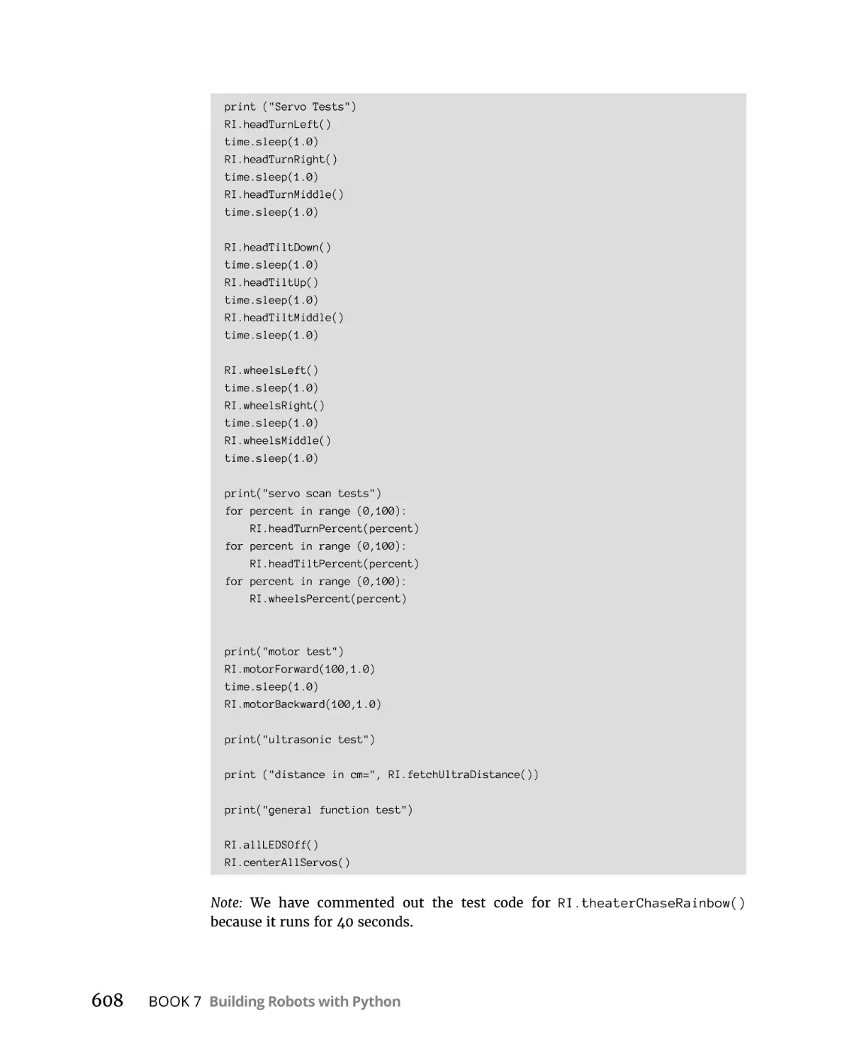
The Python Robot Interface Test. . . . . . . . . . . . . . . . . . . . . . . . . . . . 606
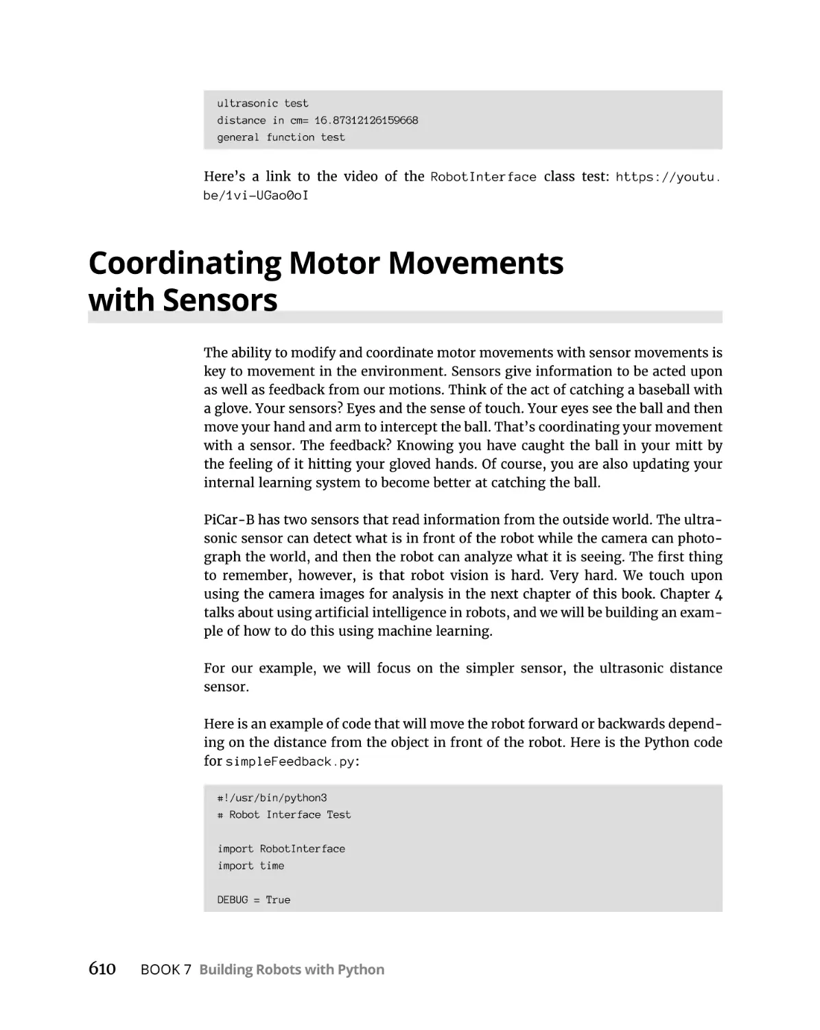
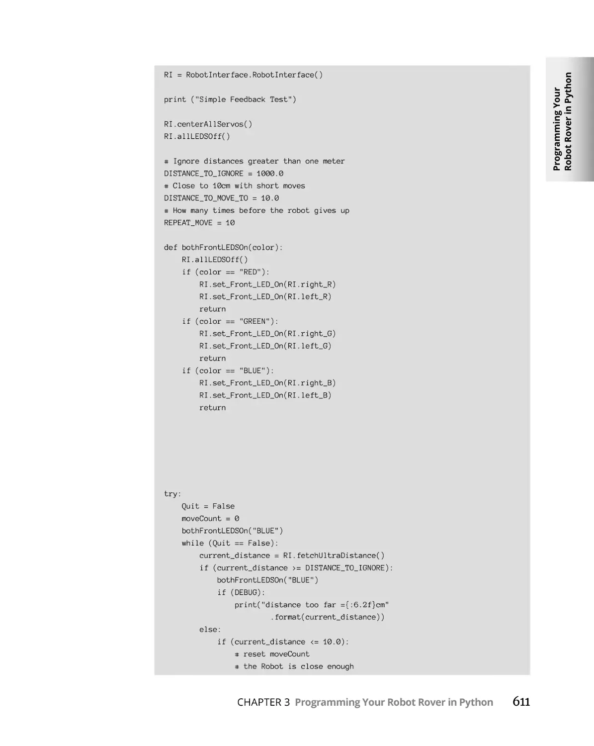
Coordinating Motor Movements with Sensors. . . . . . . . . . . . . . . . . . . 610
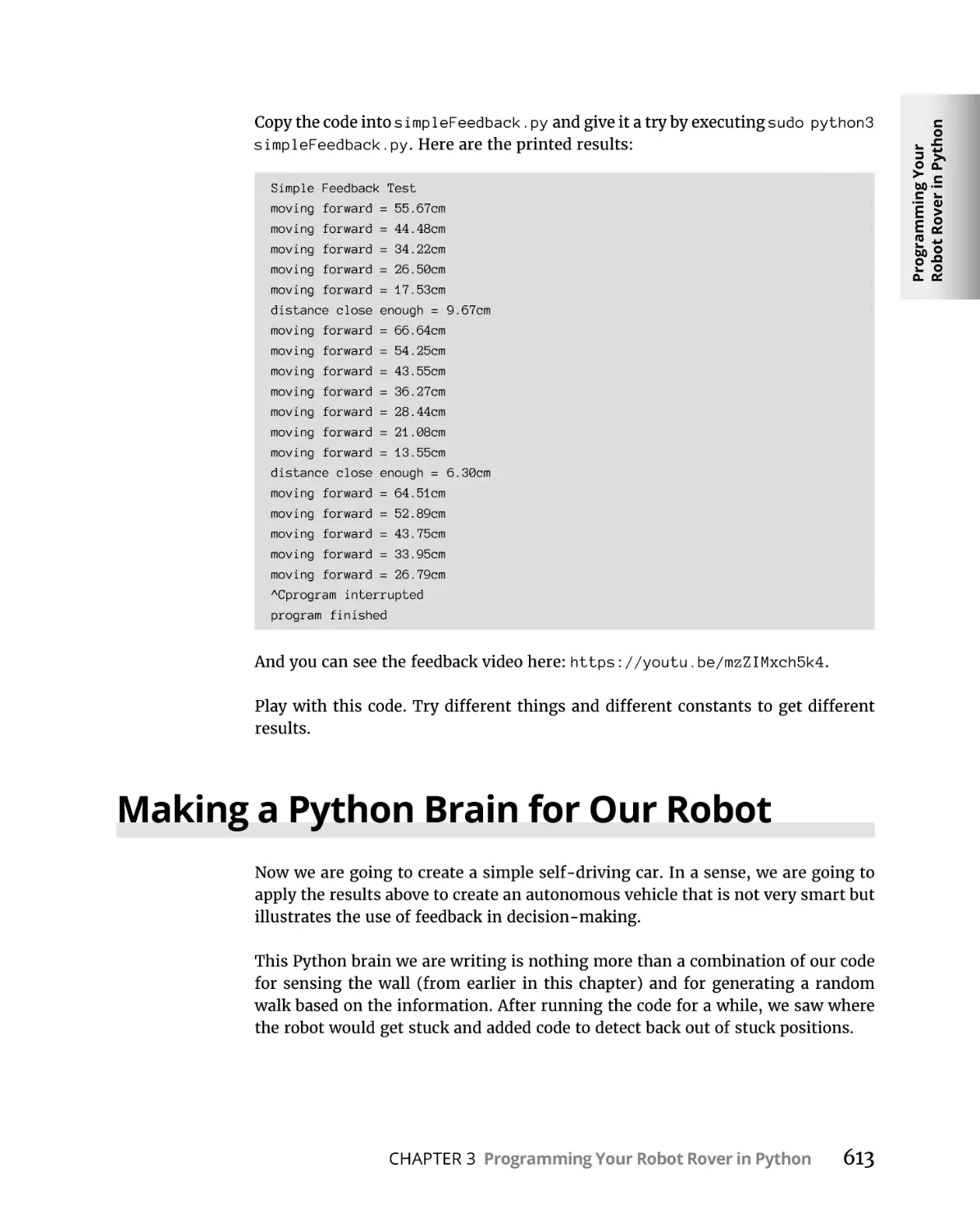
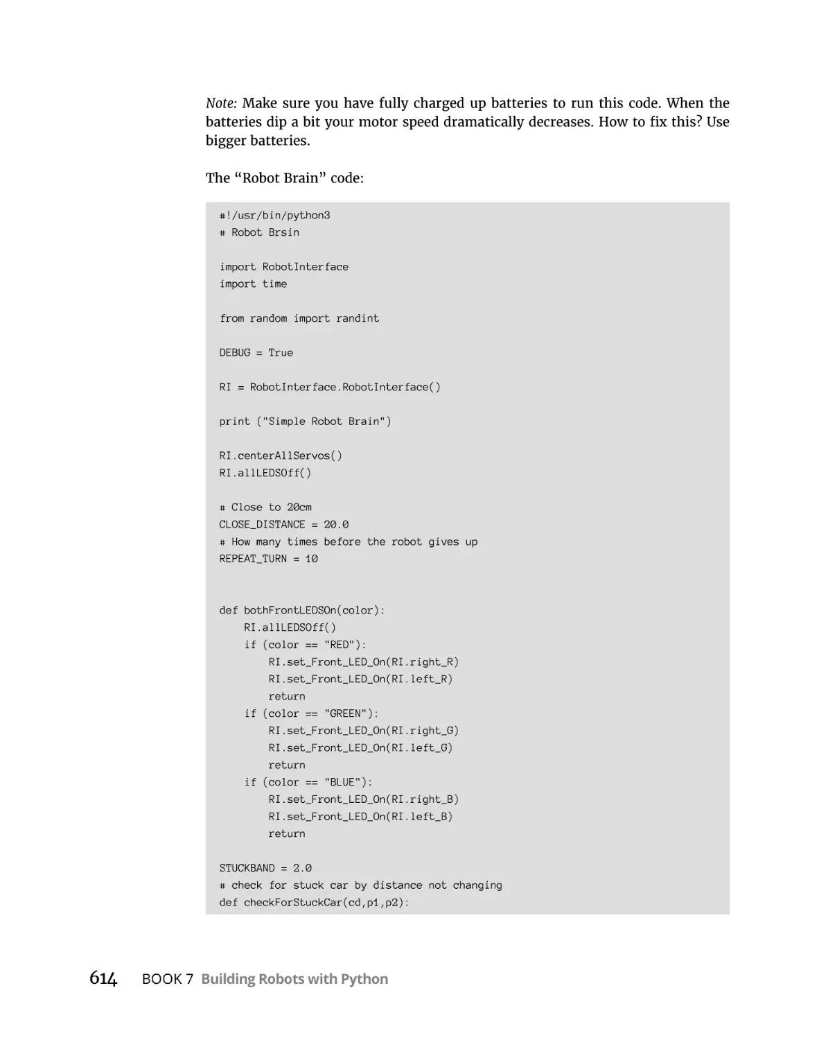
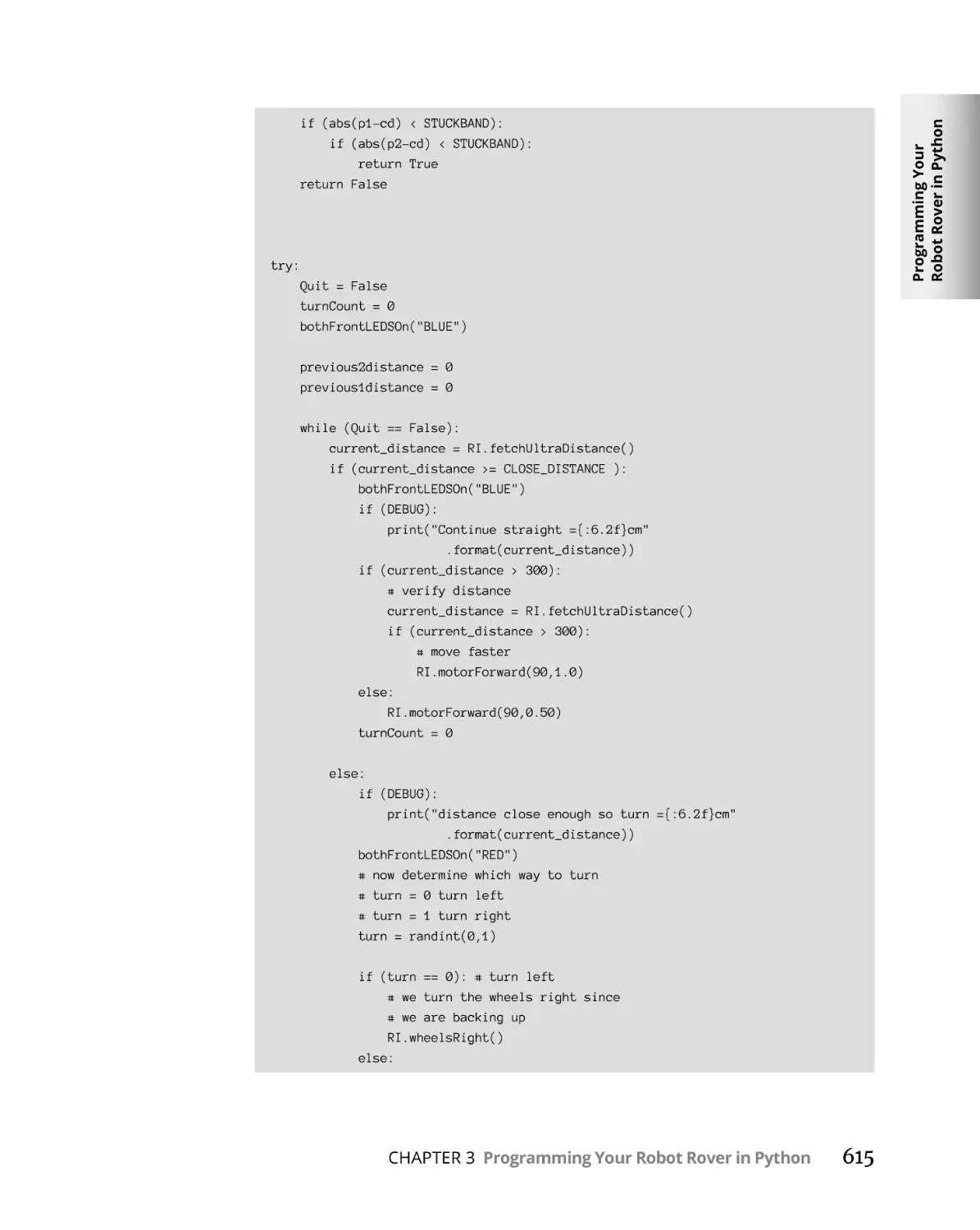
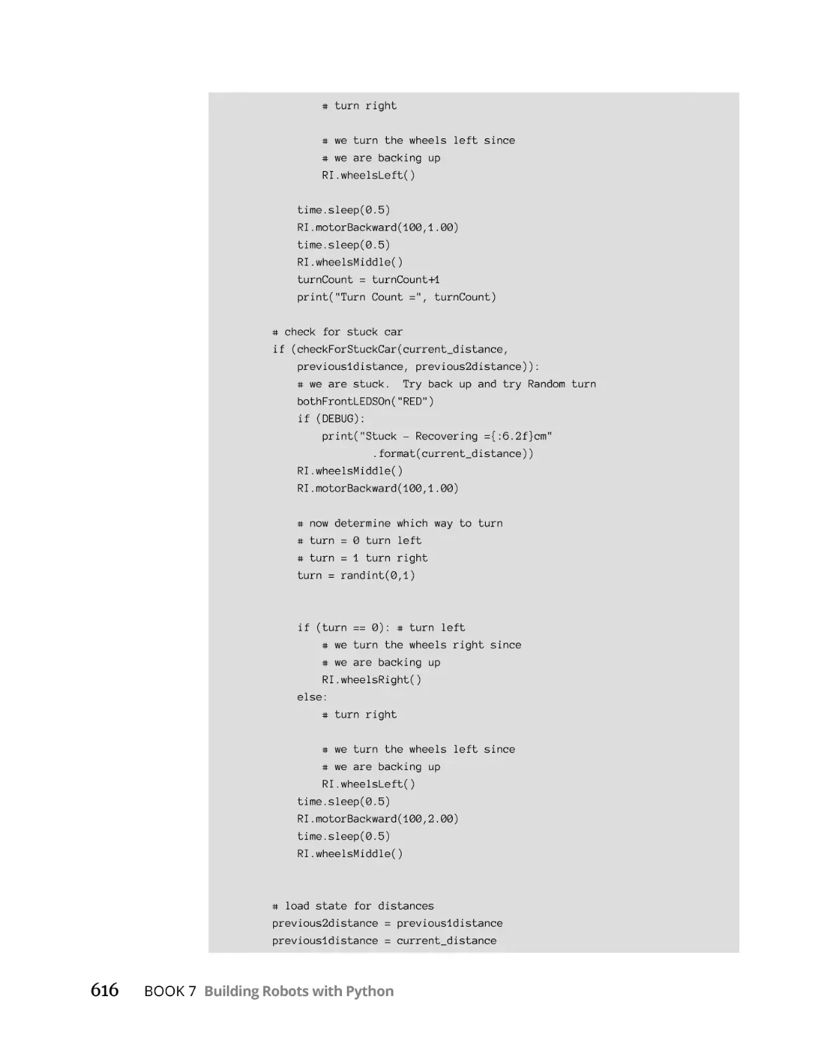
Making a Python Brain for Our Robot . . . . . . . . . . . . . . . . . . . . . . . . . . 613
A Better Robot Brain Architecture. . . . . . . . . . . . . . . . . . . . . . . . . . .620
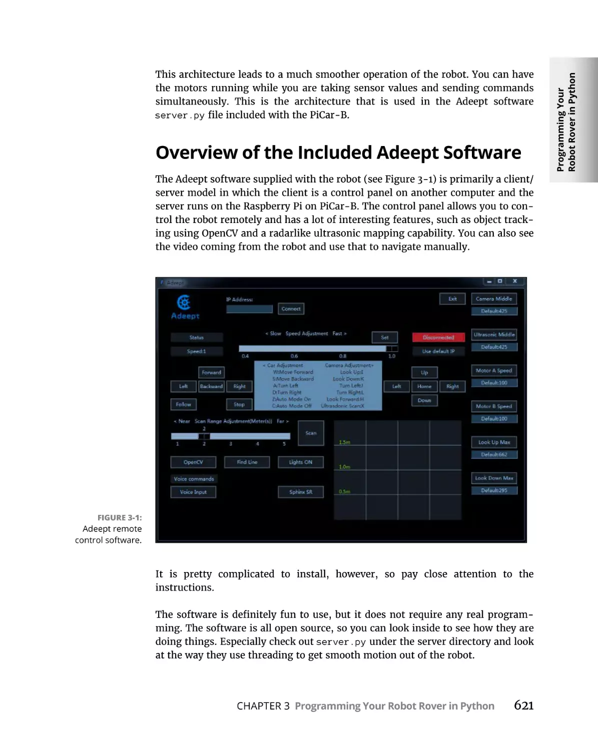
Overview of the Included Adeept Software. . . . . . . . . . . . . . . . . . . 621
Where to Go from Here? . . . . . . . . . . . . . . . . . . . . . . . . . . . . . . . . . . 622
CHAPTER 4:
Using Artificial Intelligence in Robotics. . . . . . . . . . . . . 623
This Chapter’s Project: Going to the Dogs. . . . . . . . . . . . . . . . . . . . . . .
Setting Up the Project. . . . . . . . . . . . . . . . . . . . . . . . . . . . . . . . . . . . . . . .
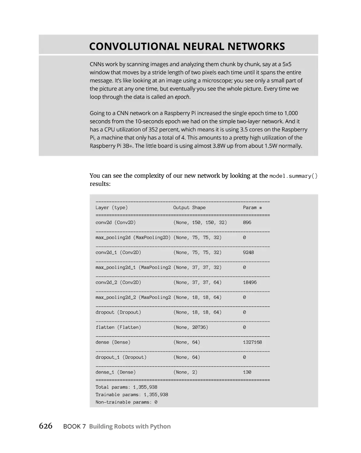
Machine Learning Using TensorFlow. . . . . . . . . . . . . . . . . . . . . . . . . . .
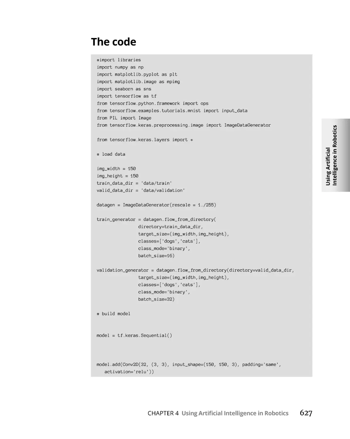
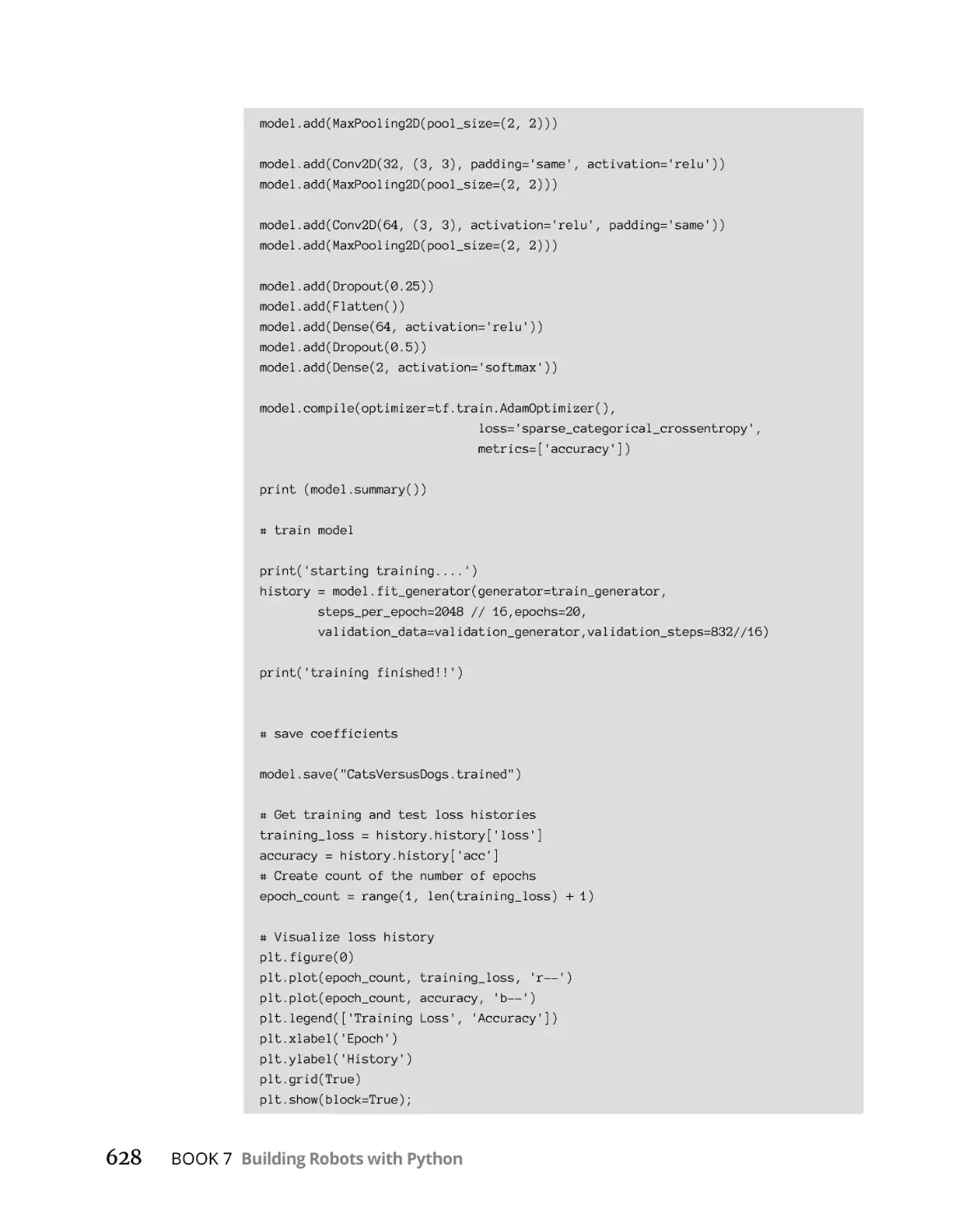
The code. . . . . . . . . . . . . . . . . . . . . . . . . . . . . . . . . . . . . . . . . . . . . . . .
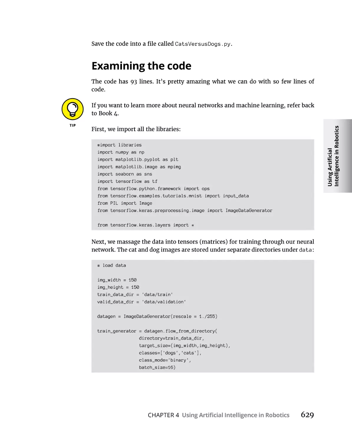
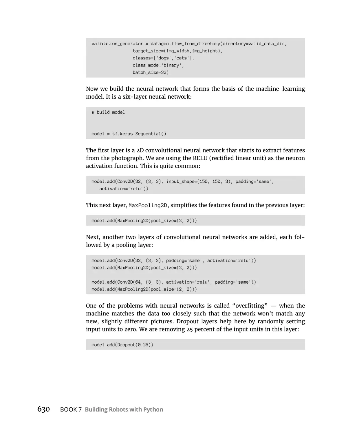
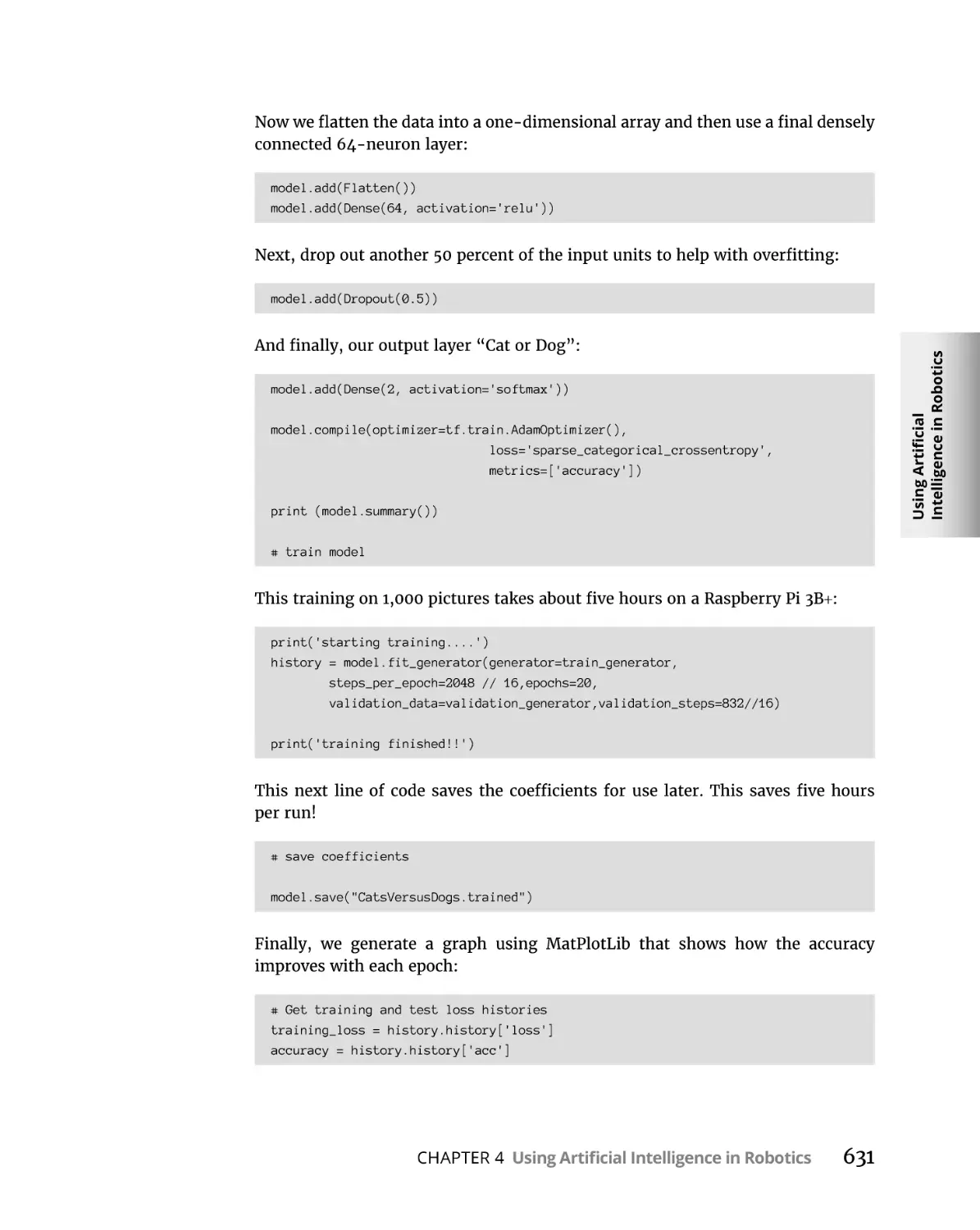
Examining the code. . . . . . . . . . . . . . . . . . . . . . . . . . . . . . . . . . . . . . .
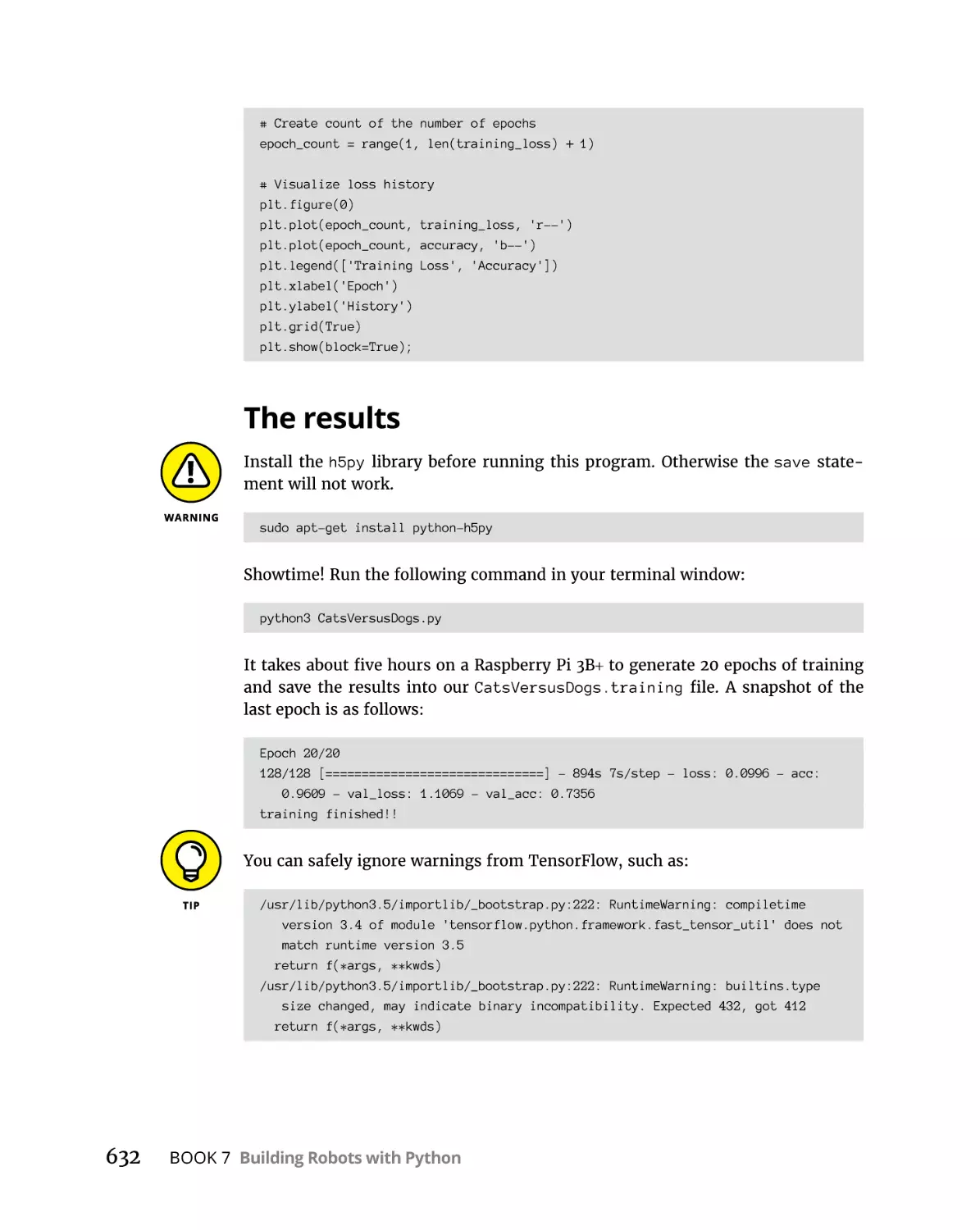
The results . . . . . . . . . . . . . . . . . . . . . . . . . . . . . . . . . . . . . . . . . . . . . .
Testing the Trained Network. . . . . . . . . . . . . . . . . . . . . . . . . . . . . . . . . .
The code. . . . . . . . . . . . . . . . . . . . . . . . . . . . . . . . . . . . . . . . . . . . . . . .
Explaining the code. . . . . . . . . . . . . . . . . . . . . . . . . . . . . . . . . . . . . . .
The results . . . . . . . . . . . . . . . . . . . . . . . . . . . . . . . . . . . . . . . . . . . . . .
Table of Contents
624
624
625
627
629
632
633
634
636
637
xv
Taking Cats and Dogs to Our Robot. . . . . . . . . . . . . . . . . . . . . . . . . . . .
The code. . . . . . . . . . . . . . . . . . . . . . . . . . . . . . . . . . . . . . . . . . . . . . . .
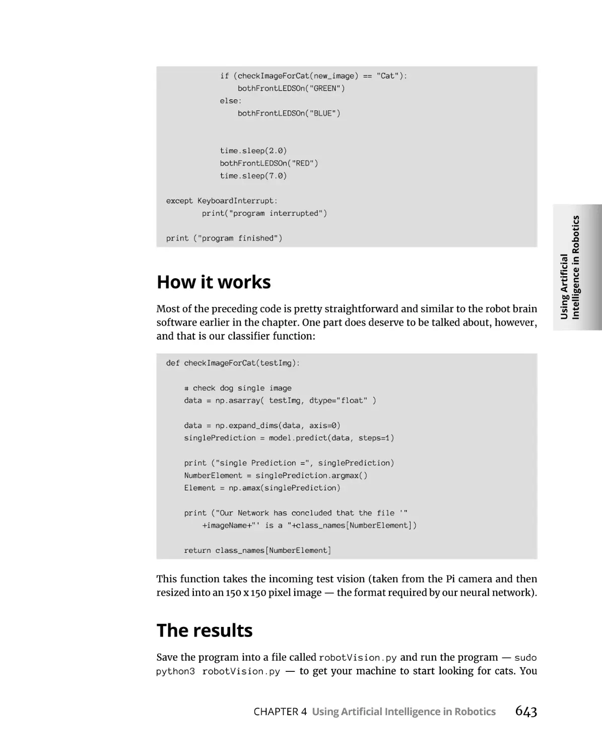
How it works. . . . . . . . . . . . . . . . . . . . . . . . . . . . . . . . . . . . . . . . . . . . .
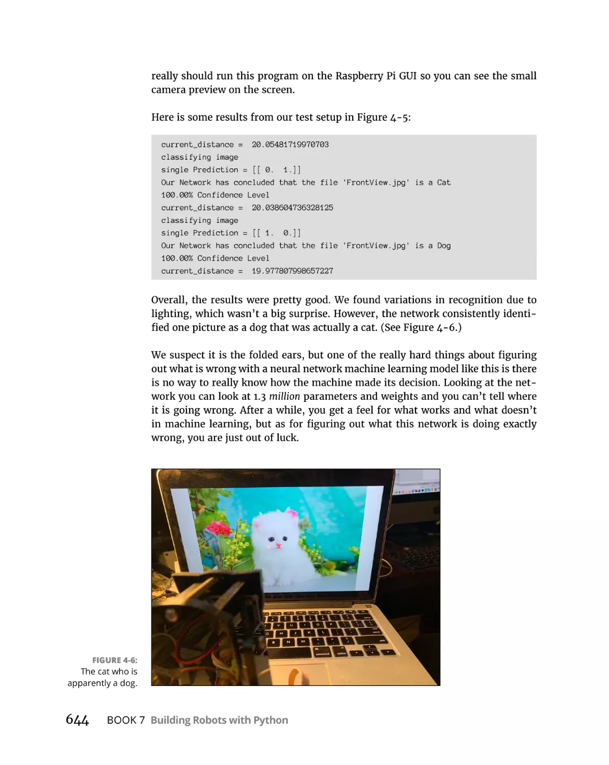
The results . . . . . . . . . . . . . . . . . . . . . . . . . . . . . . . . . . . . . . . . . . . . . .
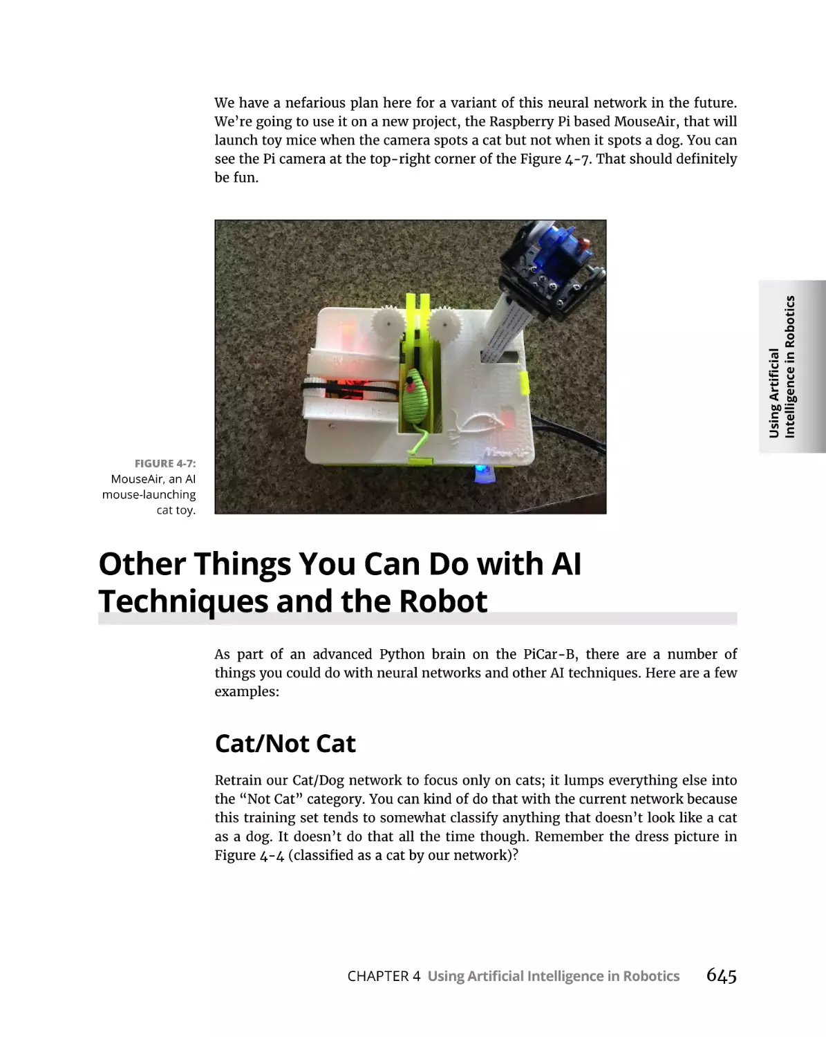
Other Things You Can Do with AI Techniques and the Robot . . . . . .
Cat/Not Cat. . . . . . . . . . . . . . . . . . . . . . . . . . . . . . . . . . . . . . . . . . . . . .
Santa/Not Santa. . . . . . . . . . . . . . . . . . . . . . . . . . . . . . . . . . . . . . . . . .
Follow the ball . . . . . . . . . . . . . . . . . . . . . . . . . . . . . . . . . . . . . . . . . . .
Using Alexa to control your robot. . . . . . . . . . . . . . . . . . . . . . . . . . .
AI and the Future of Robotics . . . . . . . . . . . . . . . . . . . . . . . . . . . . . . . . .
INDEX
xvi
640
640
643
643
645
645
646
646
646
646
. . . . . . . . . . . . . . . . . . . . . . . . . . . . . . . . . . . . . . . . . . . . . . . . . . . . . . . . . . . . . 647
Python All-in-One For Dummies
Introduction
T
he power of Python. The Python language is becoming more and more popular, and in 2017 it became the most popular language in the world according to IEEE Spectrum. The power of Python is real.
Why is Python the number one language? Because it is incredibly easy to learn
and use. Part of it is its simplified syntax and its natural-language flow, but a lot
of it has to do with the amazing user community and the breadth of applications
available.
About This Book
This book is a reference manual to guide you through the process of learning
Python and how to use it in modern computer applications, such as data science,
artificial intelligence, physical computing, and robotics. If you are looking to learn
a little about a lot of exciting things, then this is the book for you. It gives you an
introduction to the topics that you will need to go deeper into any of these areas
of technology.
This book guides you through the Python language and then it takes you on a tour
through some really cool libraries and technologies (the Raspberry Pi, robotics, AI,
data science, and so on) all revolving around the Python language. When you work
on new projects and new technologies, Python is there for you with an incredibly
diverse number of libraries just waiting for you to use.
This is a hands-on book. There are examples and code all throughout the book.
You are expected to take the code, run it, and then modify it to do what you want.
You don’t just buy a robot, you build it so you can understand all the pieces and
can make sense of the way Python works with the robot to control all the motors
and sensors. Artificial intelligence is complicated, but Python helps make a significant part of it accessible. Data science is complicated, but Python helps you do
data science more easily. Robotics is complicated, but Python gives you the code
that controls the robot. And Python even allows us to tie these pieces together and
use, say, AI in robotics.
In this book, we take you through the basics of the Python language in small,
easy-to-understand steps. After we have introduced you to the language, then we
Introduction
1
step into the world of Python and artificial intelligence, exploring programming
in machine learning and neural networks using Python and TensorFlow and actually working on real problems and real software, not just toy applications.
After that, we’re off to the exciting world of Big Data and data science with Python.
We look at big public data sets such as medical and environmental data all using
Python.
Finally, you get to experience the magic of what I call “physical computing.”
Using the small, inexpensive Raspberry Pi computer (it’s small, but incredibly
popular) we show you how to use Python to control motors and read sensors. This
is a lead-up to our final book, “Python and Robotics.” Here you learn how to build
a robot and how to control that robot with Python and your own programs, even
using artificial intelligence.
This is not your mother’s RC car.
Python data science, robotics, AI, and fun all in the same book.
This book won’t make you understand everything about these fields, but it will
give you a great introduction to the terminology and the power of Python in all
these fields. Enjoy the book and go forth and learn more afterwards.
Foolish Assumptions
We assume you know how to use a computer in a very basic way. If you can turn on
the computer and use a mouse, you’re ready for this book. We assume you don’t
know how to program yet, although you will have some skills in programming
by the end of the book. If we’re wrong and you do already know Python (or some
other computer language), jump ahead to minibook 4 and dig right into learning
something new. Our intent is to guide you through the language of Python and
then through some of the amazing technologies and devices that use Python. We
provide complete examples. If you get stuck on something, look it up on the web,
read a tutorial, and then come back to it.
Icons Used in This Book
What’s a For Dummies book without icons pointing you in the direction of truly
helpful information that’s sure to speed you along your way? Here we briefly
describe each icon we use in this book.
2
Python All-in-One For Dummies
The Tip icon points out helpful information that’s likely to make your job easier.
This icon marks a generally interesting and useful fact — something you may
want to remember for later use.
The Warning icon highlights lurking danger. When we use this icon, we’re telling
you to pay attention and proceed with caution.
When you see this icon, you know that there’s techie-type material nearby. If
you’re not feeling technical-minded, you can skip this information.
Beyond the Book
In addition to the material in the print or ebook you’re reading right now, this
product also comes with some access-anywhere goodies on the web. No matter
how well you understand Python concepts, you’ll likely come across a few questions where you don’t have a clue. To get this material, simply go to www.dummies.
com and search for “Python All-in-One For Dummies Cheat Sheet” in the Search box.
Where to Go from Here
Python All-in-One For Dummies is designed so that you can read a chapter or section out of order, depending on what subjects you’re most interested in. Where
you go from here is entirely up to you!
Book 1 is a great place to start reading if you’ve never used Python before. Discovering the basics and common terminology can be quite helpful for later chapters
that use the terms and commands regularly!
Occasionally, we have updates to our technology books. If this book does have any
technical updates, they’ll be posted at www.dummies.com/go/pythonaiofdupdates.
Introduction
3
1
Getting Started
with Python
Contents at a Glance
CHAPTER 1:
Starting with Python. . . . . . . . . . . . . . . . . . . . . . . . . . . . . . . . . . 7
Why Python Is Hot. . . . . . . . . . . . . . . . . . . . . . . . . . . . . . . . . . . . . . . . . . . 8
Choosing the Right Python. . . . . . . . . . . . . . . . . . . . . . . . . . . . . . . . . . . . 9
Tools for Success. . . . . . . . . . . . . . . . . . . . . . . . . . . . . . . . . . . . . . . . . . . 11
Writing Python in VS Code. . . . . . . . . . . . . . . . . . . . . . . . . . . . . . . . . . . 17
Using Jupyter Notebook for Coding . . . . . . . . . . . . . . . . . . . . . . . . . . . 21
CHAPTER 2:
Interactive Mode, Getting Help, Writing Apps. . . . 27
Using Python Interactive Mode. . . . . . . . . . . . . . . . . . . . . . . . . . . . . . .
Creating a Python Development Workspace. . . . . . . . . . . . . . . . . . . .
Creating a Folder for your Python Code . . . . . . . . . . . . . . . . . . . . . . .
Typing, Editing, and Debugging Python Code. . . . . . . . . . . . . . . . . . .
Writing Code in a Jupyter Notebook. . . . . . . . . . . . . . . . . . . . . . . . . . .
CHAPTER 3:
Python Elements and Syntax . . . . . . . . . . . . . . . . . . . . . . . 49
The Zen of Python. . . . . . . . . . . . . . . . . . . . . . . . . . . . . . . . . . . . . . . . . .
Object-Oriented Programming . . . . . . . . . . . . . . . . . . . . . . . . . . . . . . .
Indentations Count, Big Time . . . . . . . . . . . . . . . . . . . . . . . . . . . . . . . .
Using Python Modules . . . . . . . . . . . . . . . . . . . . . . . . . . . . . . . . . . . . . .
CHAPTER 4:
27
34
37
39
45
49
53
54
56
Building Your First Python Application. . . . . . . . . . . . 61
Open the Python App File . . . . . . . . . . . . . . . . . . . . . . . . . . . . . . . . . . .
Typing and Using Python Comments. . . . . . . . . . . . . . . . . . . . . . . . . .
Understanding Python Data Types. . . . . . . . . . . . . . . . . . . . . . . . . . . .
Doing Work with Python Operators. . . . . . . . . . . . . . . . . . . . . . . . . . .
Creating and Using Variables. . . . . . . . . . . . . . . . . . . . . . . . . . . . . . . . .
What Syntax Is and Why It Matters. . . . . . . . . . . . . . . . . . . . . . . . . . . .
Putting Code Together . . . . . . . . . . . . . . . . . . . . . . . . . . . . . . . . . . . . . .
62
63
64
69
72
78
82
IN THE CHAPTER
»» Why Python is hot
»» Tools for success
»» Writing Python in VS Code
»» Writing Python in Jupyter notebooks
Chapter
1
Starting with Python
T
he fact that you’re reading this implies you know that Python is a great
thing to know if you’re looking for a good job in programming. It’s also
good to know if you’re looking to expand your existing programming skills
into exciting cutting-edge technologies like artificial intelligence (AI), machine
learning (ML), data science, or robotics, or even if you’re just building apps in
general. So we’re not going to try to sell you on Python. It sells itself.
Our approach, especially in this book, leans heavily toward the hands-on. A common failure in many tutorials is that they already assume you’re a professional
programmer in Python or some other language, and they skip over things they
assume you already know.
This book is different in that we don’t assume you’re already programming in
Python or some other language. We assume you can use a computer and understand basics like files and folders. But that’s about it for assumptions.
We also assume you’re not up for settling down in an easy chair in front of the
fireplace to read page after page of theoretical stuff “about” Python, like some
kind of novel. You don’t have that much free time to kill. So we’re going to get
right into it and focus on doing, hands-on, because that’s the only way most of us
learn. Personally, we’ve never seen anybody read a book “about” Python and then
sit at a computer and write Python like a pro. Human brains don’t work that way.
We learn through practice and repetition, and that requires hands-on.
CHAPTER 1 Starting with Python
7
Why Python Is Hot
We promised we weren’t going to spend a bunch of time trying to “sell” you on
Python, and that’s not our intent here. Python is hot — that’s probably why you want
to learn it, and that’s good. But we would like to talk briefly about why it’s so hot.
Python is hot primarily because it has all the right stuff for the kind of software development that’s really driving the whole software development world
these days. Machine learning, robotics, artificial intelligence, and data science are
the leading technologies today and for the foreseeable future. Python is popular
mainly because it already has lots of capabilities in those areas, while many older
languages lag behind in these technologies.
If you’re not familiar with programming languages like C and Java, feel free to
skip to the next section, “Python versions,” as this information is only for people
who wonder about differences among the languages. But in case you’re wondering, just as there are different brands of toothpaste, shampoo, cars, and just about
every other product you can buy, there are different “brands” of programming
languages with names like Java, C, C++ (pronounced C plus plus), and C# (pronounced
C sharp). They’re all programming languages, just like all brands of toothpaste are
toothpaste. The main reasons cited for Python’s current popularity are
»» Python is relatively easy to learn.
»» Everything you need to learn (and do) Python is free.
»» Python offers more readymade tools for current hot technologies like data
science, machine learning, artificial intelligence, and robotics than most other
languages.
HTML, CSS, AND JavaScript
Some of you may have heard of languages like HTML, CSS and JavaScript. Those aren’t
traditional programming languages for developing apps or other generic software.
HTML and CSS are specialized for developing Web pages. JavaScript is a programming
language; however, it too is heavily geared to Website development and isn’t quite in
the same category of general programming languages like Python and Java.
Another way to look at it is, you wouldn’t learn HTML, CSS, and JavaScript instead of
Python, as there is too little overlap to justify it. If you specifically want to design and
create websites, you have to learn HTML, CSS, and JavaScript whether you’re already
familiar with Python or some other programming language.
8
BOOK 1 Getting Started with Python
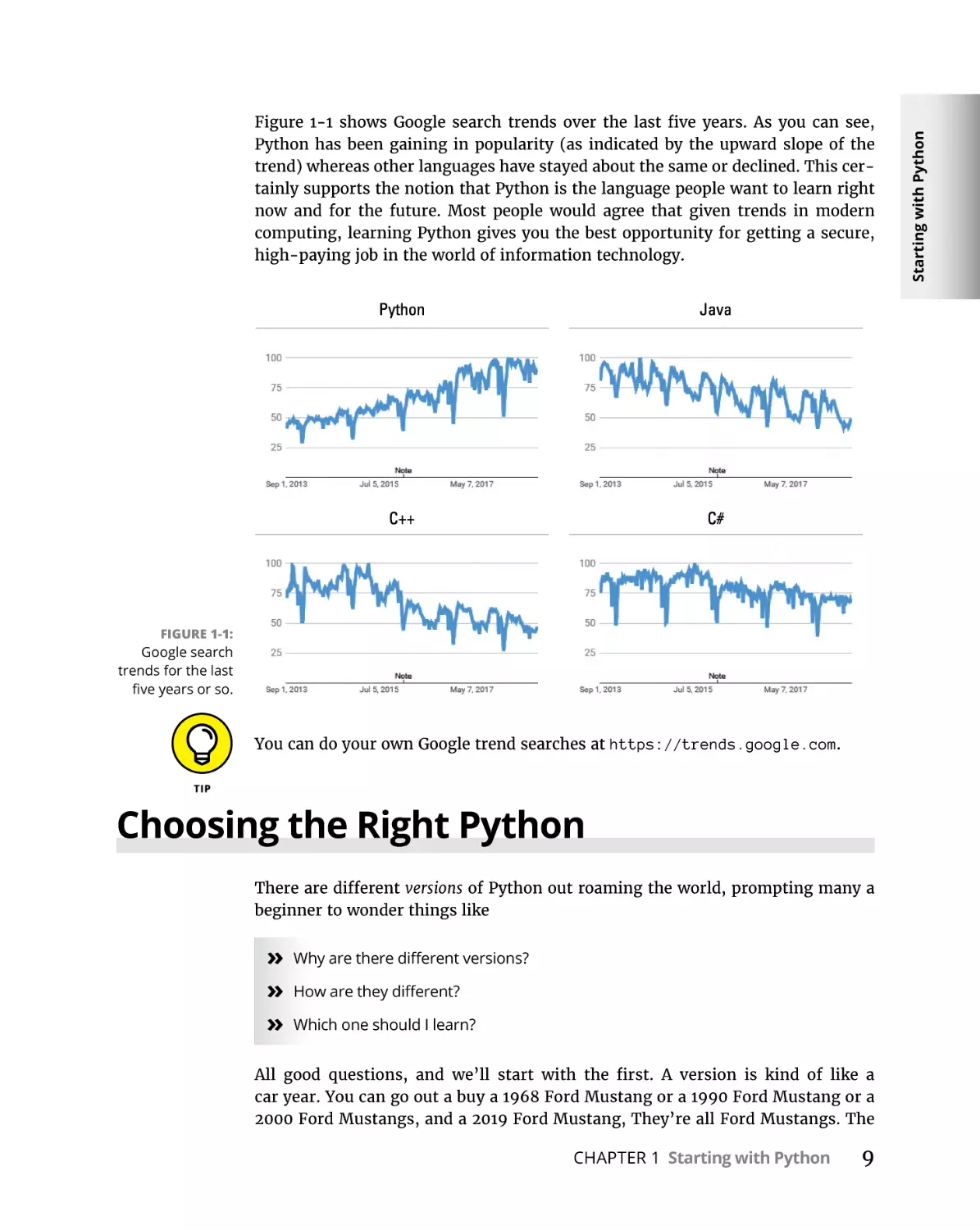
FIGURE 1-1:
Google search
trends for the last
five years or so.
You can do your own Google trend searches at https://trends.google.com.
Choosing the Right Python
There are different versions of Python out roaming the world, prompting many a
beginner to wonder things like
»» Why are there different versions?
»» How are they different?
»» Which one should I learn?
All good questions, and we’ll start with the first. A version is kind of like a
car year. You can go out a buy a 1968 Ford Mustang or a 1990 Ford Mustang or a
2000 Ford Mustangs, and a 2019 Ford Mustang, They’re all Ford Mustangs. The
CHAPTER 1 Starting with Python
9
Starting with Python
Figure 1-1 shows Google search trends over the last five years. As you can see,
Python has been gaining in popularity (as indicated by the upward slope of the
trend) whereas other languages have stayed about the same or declined. This certainly supports the notion that Python is the language people want to learn right
now and for the future. Most people would agree that given trends in modern
computing, learning Python gives you the best opportunity for getting a secure,
high-paying job in the world of information technology.
only difference is that the one with the highest year number is the most “current” Ford Mustang. That Mustang is different from the older models in that
it has some improvements based on experience with earlier models, as well as
features that are current with the times.
Programming languages (and most other software products) work the same way.
But as a rule we don’t ascribe year numbers to them, because they’re not released
on a yearly basis. They’re released whenever they’re released. But the principle
is the same. The version with the highest number us the newest, most recent
“model,” sporting improvements based on experience with earlier versions, as
well as features that are relevant to the current times.
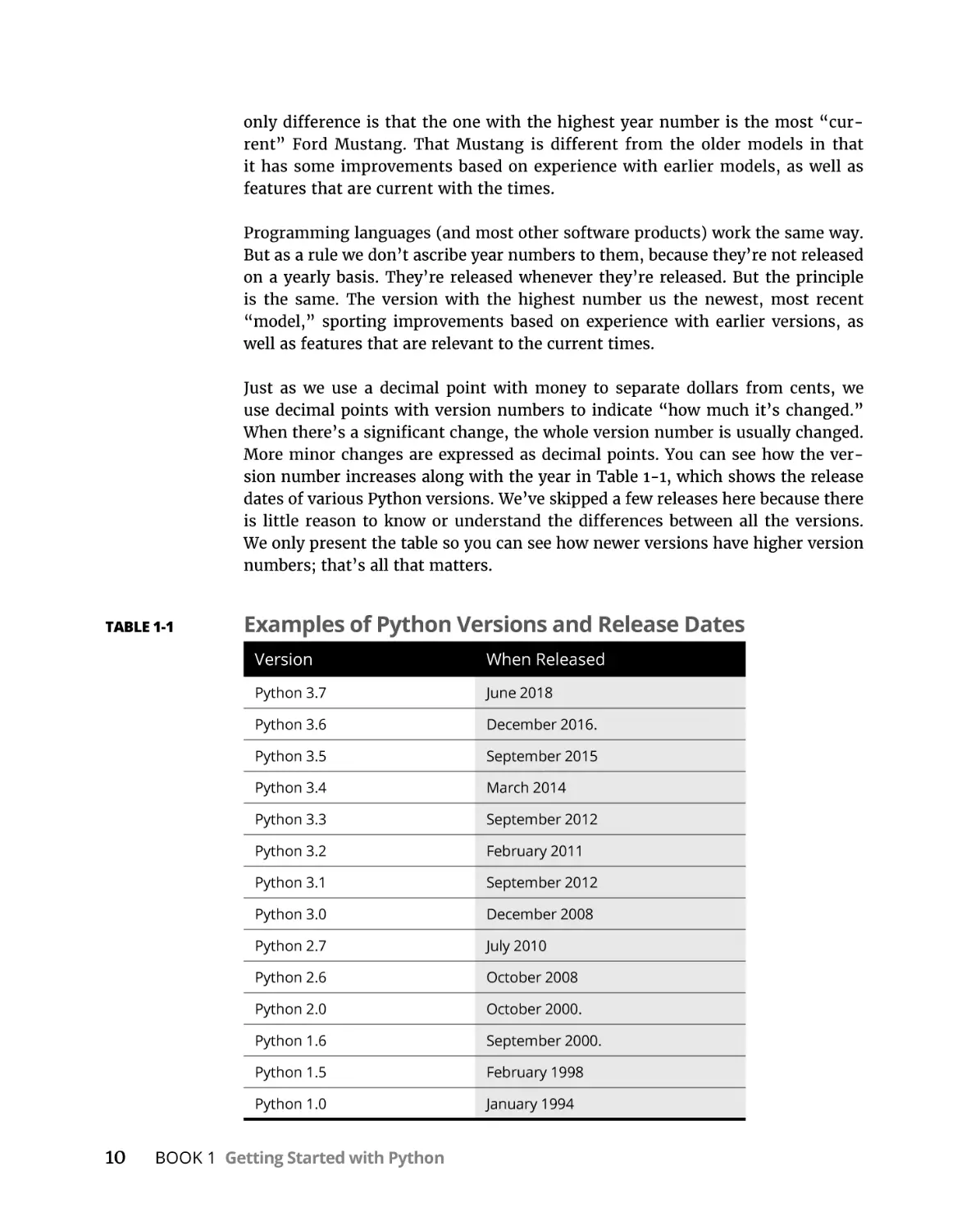
Just as we use a decimal point with money to separate dollars from cents, we
use decimal points with version numbers to indicate “how much it’s changed.”
When there’s a significant change, the whole version number is usually changed.
More minor changes are expressed as decimal points. You can see how the version number increases along with the year in Table 1-1, which shows the release
dates of various Python versions. We’ve skipped a few releases here because there
is little reason to know or understand the differences between all the versions.
We only present the table so you can see how newer versions have higher version
numbers; that’s all that matters.
TABLE 1-1
10
Examples of Python Versions and Release Dates
Version
When Released
Python 3.7
June 2018
Python 3.6
December 2016.
Python 3.5
September 2015
Python 3.4
March 2014
Python 3.3
September 2012
Python 3.2
February 2011
Python 3.1
September 2012
Python 3.0
December 2008
Python 2.7
July 2010
Python 2.6
October 2008
Python 2.0
October 2000.
Python 1.6
September 2000.
Python 1.5
February 1998
Python 1.0
January 1994
BOOK 1 Getting Started with Python
The car years analogy is just an analogy indicating that the larger the number,
the more recent the version. But in Python it’s the most recent within the main
Python version. When the first number changes, that’s usually a change that’s so
significant, software written in prior versions may not even work in that version.
If you happen to be a software company with a product, written in Python 2, on
the market, and have millions of dollars invested in that product, you may not
be too thrilled to have to start over from scratch to go with the current version.
So “older versions” often continue to be supported and evolve, independent of the
most recent version, to support developers and businesses that are already heavily
invested in the previous version.
The biggest question on most beginners minds is “what version should I learn?”
The answer to that is simple . . . whatever is the most current version. You’ll know
what that is because when you go to the Python.org website to download Python,
they will tell you what the most current stable build (version) is. That’s the one
they’ll recommend, and that’s the one you should use.
The only reason to learn something like Version 2 or 2.7 or something else older
would be if you’ve already been hired to work on some project, and that company
requires you to learn and use a specific version. That sort of thing is rare, because
as a beginner you’re not likely to already have a full-time job as a programmer.
But in the messy real world there are companies heavily invested in some earlier
version of a product, so when hiring, they’ll be looking for people with knowledge
of that version.
In this book, we focus on versions of Python that are current in late 2018 and early
2019, from Python 3.7 and above. Don’t worry about version differences after the
first and second digits. Version 3.7.2 is similar enough go version 3.7.1 that it’s
not important, especially to a beginner. Likewise, Version 3.8 isn’t that big a jump
from 3.7. So don’t worry about these miner version differences when first learning. Most of what’s in Python is the across all versions. So you need not worry
about investing time in learning a version that’s obsolete or soon will be — unless
you happen to be learning from a very old book.
Tools for Success
Now, we need to start getting your computer set up so you can learn, and do,
Python hands-on. For one, you’ll need a good Python interpreter and editor. The
editor lets you type the code, the interpreter lets you run that code. When you run
CHAPTER 1 Starting with Python
11
Starting with Python
If you paid close attention you may notice that Version 3.0 starts in December
2008, but Version 2.7 extends into 2010. So if versions are like car years, why the
overlap?
(or execute) code, you’re telling the computer to “do whatever my code tells you
to do.”
The term code refers to anything written in a programming language to provide
instructions to a computer. The term coding is often used to describe the act or
writing code. A code editor is an app that lets you type code, in much the same way
an app like Word or Pages helps you type regular plain-English text.
Just as there are many brands of toothpaste, soap, and shampoo in the worlds,
there are many “brands” of code editors that work well with Python. There isn’t
a right one or wrong one, a good one or bad one, a best one or worst one. Just a
lot of different products that basically do the same thing but vary slightly in their
approach and what that editor’s creators thing is “good.”
If you already started learning Python on your own before this book, and are
happy with whatever you’ve been using, you’re welcome to continue using that
and ignore our suggestions. If you’re just getting started with this stuff, we suggest you use VS Code, because it is . . .
An excellent, free learning environment
The editor we recommend, and will be using in this book, is called Visual Studio
Code, officially. But most often you hear is spoken or written as VS Code. The main
reasons it’s our own favorite are as follows:
»» It is an excellent editor for learning coding.
»» It is an excellent editor for writing code professionally, and is in fact used by
millions or professional programmers and developers.
»» It’s relatively easy to learn and use.
»» It works pretty much the same on Windows, Mac, and Linux.
»» It’s free.
The editor is an important part of learning and doing Python code. But you also
need the Python interpreter. Chances are, you’re also going to want some Python
packages, too. The packages are simply code already written by someone else to do
common tasks so that you don’t have to start from scratch and reinvent the wheel
every time you want to perform one of those tasks.
Python packages are not a “crutch” for beginners. They are major components
of the entire Python development environment and are used by seasoned professionals as much as they are used by beginners.
12
BOOK 1 Getting Started with Python
An excellent alternative to the old command-line driven ways of doing thing is to
use a more complete Python development environment with a more intuitive and
more easily managed graphic user interface, as on a Mac or Windows or any phone
or tablet. The one we recommend is called Anaconda. It is free, and it is excellent. If you’ve never heard of it and aren’t so sure about downloading something
you’ve never heard of, you can explore what it’s all about at the Anaconda website
at https://www.anaconda.com/.
Anaconda is often referred to as a data science platform because many of the
packages that come with it are data-science–oriented. But don’t let that worry
you if you’re interested in doing other things with Python. Anaconda is excellent
for learning and doing all kinds of things with Python. And it also comes with
VS Code, our personal favorite coding editor, as well as Jupyter Notebook, which
provides another excellent means of coding with Python. And best of all, it’s 100
percent free, so it’s well worth the effort of downloading and installing it.
We can’t really take you step-by-step through every part of downloading and
installing Anaconda because it’s distributed from the a website, and people change
their websites whenever they feel like it. But we can certainly give you the broad
strokes. You should be able to follow along, using Mac, Windows, or Linux. You
just have to keep an eye on your screen as you go along, and follow any onscreen
instructions as they arise, while following the steps.
Installing Anaconda and VS Code
To download and install Anaconda, and VS Code you’ll need to connect to the
Internet and use a web browser. Any Web browser should do, be in Google Chrome,
Firefox, Safari, Edge, Internet Explorer, or whatever. Fire up whatever browser
you normally use to browse the Web, then follow these steps:
1.
2.
Browse to https://www.anaconda.com/download/ to get to a page that
looks something like this (don’t worry about version numbers or dates,
just download whatever they recommend when you get there).
Scroll down a little and you should see some download options that look
something like the example shown in Figure 1-2.
We used a Windows computer for that screenshot, but Mac and Linux users
will see something similar.
CHAPTER 1 Starting with Python
13
Starting with Python
Historically, managing Python, the packages, and the editor was a somewhat laborious task involving typing cryptic commands at a command prompt. Although
that’s not a particularly “bad” thing, it certainly isn’t the most efficient way to do
things, especially when you’re first getting started. You end up spending most of
your time upfront trying to learn and type awkward commands just to get Python
to work on your computer, rather than actually learning Python itself.
FIGURE 1-2:
Click Download
under the largest
version number.
3.
Click Download under whichever version number is the highest on your
screen.
For me, right now, it’s version 3.7 but a higher-numbered version may be
available when you get there. Don’t worry about that.
Jot down the Python version number you’re downloading for future reference
a little later in this chapter. You can also click How to Install ANACONDA on the
download page if you’d like to see the instructions from the Anaconda team.
4.
5.
6.
7.
If prompted for your email address, either provide it or click the X in the
pop-up window’s upper-right corner to close the prompt without entering
your email address.
If you see Keep/Discard options in the lower-left corner of your screen,
click Keep.
When the download is complete, open your Downloads folder (or
whichever folder to which you downloaded the file).
If you’re using Mac or Linux, double-click the file you downloaded. If
you’re using Windows, right-click that file and choose Run as
Administrator, as shown in Figure 1-3.
The Run-As-Administrator business in Windows ensures that you can install
everything. If that option isn’t available to you, double-clicking the file’s icon
should be sufficient.
8.
14
Click Next, Continue, Agree, or I Agree on the first installation pages until
you get to one of the pages shown in Figures 1-4 (Mac will be on the one
on the left, Windows the one on the right).
BOOK 1 Getting Started with Python
Starting with Python
FIGURE 1-3:
In Windows,
right-click and
choose Run As
Administrator.
FIGURE 1-4:
Choose how to
install Anaconda.
9. Choose whichever option makes sense to you. Or, if in double, choose
Install on a specific disk (for Mac), and then Macintosh HD, or choose
Install for All Users (if on Windows using Administrator privileges. If the
option we suggested isn’t available to you, click the one closest to it.
10. Click Continue or Next and follow the onscreen instructions. If you’re
unsure about what options to choose on any page, don’t choose any. Just
accept the default suggestions.
11. It may take several minutes, but eventually you’ll come to a page where
it asks if you want to installed Microsoft VS Code. Click Install Microsoft
VS Code (or whatever option on your screen indicates that you want to
install VS Code).
If VS Code is already installed on your computer, no worries. The Anaconda
installer will just tell you that, or perhaps update your version to the more
current version.
12. Continue to follow any onscreen instructions, click Continue or Next to
proceed through the installation steps, then click Close or Finish on the
last page.
CHAPTER 1 Starting with Python
15
You may be prompted to sign up with Anaconda Cloud. Doing so is free, but not
required. So you can decide for yourself if that’s something you want to do.
Opening Anaconda (Mac)
After it’s installed on your Mac, you can open Anaconda as you would any other
app. Use whichever of the following methods appeals to you:
»» Open Launchpad and open Anaconda Navigator.
»» Or click the Spotlight magnifying glass, start typing Anaconda, and then
double-click Anaconda Navigator.
»» Or open Finder and your Applications folder and double-click the AnacondaNavigator icon there.
After Anaconda Navigator opens, right-click its icon in the Dock and choose Keep
in Dock to keep its icon visible in the Dock at all times so it’s easy to find when
you need it.
Opening Anaconda (Windows)
After Anaconda is installed in Windows, you can start it as you would any other
app. Although there are some differences among different versions of Windows,
you should be able to use just about any of these options:
»» Click the Start button then click Anaconda Navigator on the Start menu.
»» Or click the Start button, start typing Anaconda, then click AnacondaNavigator on the Start menu once you see it there.
On the Start menu you can right-click Anaconda-Navigator and choose Pin to
Start or right-click and choose More ➪ Pin to Taskbar to make the icon easy to
find in the future.
Using Anaconda Navigator
Anaconda Navigator, as the name implies, is the component of the Anaconda
environment that lets you navigate around through different features of the app
and choose what you want to run. When you first start it, it open to the Anaconda
Navigator home page, which should look something like Figure 1-5.
If you see a prompt for getting an updated version when you open Anaconda, it’s
okay to install the update. It won’t cost anything or affect your ability to follow
along in this book.
16
BOOK 1 Getting Started with Python
Starting with Python
FIGURE 1-5:
Anaconda
Navigator
Home page.
Down the left side of the Anaconda Navigator home page you see options like
Home, Environments, Learning, Community, Documentation, and Developer
Blog. You’re welcome to explore these on your own. However, they’re not directly
related to learning and doing Python, so we’ll let you choose which of those, if
any, you’re interested in exploring.
Writing Python in VS Code
Most of the Python coding we do here, we’ll do in VS Code. Whenever you want
to use VS Code to write Python, we suggest that you open VS Code from Anaconda
Navigator, rather than from the Start menu or Launch Pad. That way VS Code will
already be “pointing to” to version of Python that comes with Anaconda, which is
easier than trying to figure out all of that yourself. So the steps are
1.
2.
If you haven’t already done so, open Anaconda Navigator.
If necessary, scroll down a little until you see the Launch button under VS Code,
then click the Launch button.
The very first time you open VS Code you may be prompted to make some decisions. None of the suggested are required, so you can just click the X in the upperright corner of the each one. Note, however, the one that mentions Git will keep
popping up at you unless you click Don’t Show Again.
CHAPTER 1 Starting with Python
17
ABOUT GIT
Git is a popular means of storing backups of your coding projects, and sharing coding
projects with other developers or team members. It’s popular with professional programmers and VS Code has built-in support for it. But Git is entirely optional and not
directly related to learning or doing Python coding. So it’s perfectly okay to choose Don’t
Show Again to bypass that offer when it arrives. You can install Git at any time in the
future if you later decide to learn about it.
When you’re finished, the VS Code window will look something like Figure 1-6.
If you don’t see quite that many options on your screen, choose Help ➪ Welcome
from the menu bar.
FIGURE 1-6:
VS Code editor
with welcome
screen.
Your screen will likely be black with white and colored text. In this book, we show
everything as white with black text because it’s easier to read on paper that way.
You can keep the dark background if you like. If you would rather have a light
background, on a Mac click Code on the menu and choose Preferences ➪ Color
Theme. In Windows, choose File ➪ Preferences ➪ Color Theme. Then choose a
lighter color theme, like Light (Visual Studio) and your VS Code screens will look
more like the ones in this book.
18
BOOK 1 Getting Started with Python
FIGURE 1-7:
VS Code
xtensions
e
for Python.
Choosing your Python interpreter
Before you start doing any Python coding in VS Code, you want to make sure
you’re using the correct Python interpreter. Do to so, follow these steps:
1.
2.
Choose View ➪ Command Palette from VS Code’s menu.
Type python and then click Python: Select Interpreter.
Choose the Python version number that matches your download (the one you
jotted down while first downloading Anaconda). If you have multiple options
with the same version number, choose the one that includes the names base
and conda, as in Figure 1-8.
FIGURE 1-8:
Choose
your Python
interpreter
(usually the
highest version
number).
CHAPTER 1 Starting with Python
19
Starting with Python
To make sure you’re ready to do Python coding, click the Extensions icons in the
left pane (it looks like a puzzle piece). You should see at least three extensions
listed, Anaconda Extension Pack, Python, and YAML, as shown in Figure 1-7.
Writing some Python code
To test everything to make sure it’s going to work, follow these steps:
1.
In VS Code, choose View ➪ Terminal from the VS Code menu.
You should see a pane along the bottom-right that looks like one of those
shown in Figure 1-9.
FIGURE 1-9:
Terminal in VS
Code (Windows
and Mac).
2.
In the Terminal, type python and press Enter.
You should see some information about Python followed by a >>> prompt.
That >>> prompt is your Python interpreter; if you type Python code there and
press Enter, the code will execute.
3.
Type 1+1 and press Enter.
You should now see 2 (the sum of one plus one), followed by another Python
prompt, as shown in Figure 1-10.
FIGURE 1-10:
Python shows
the sum of one
plus one.
20
BOOK 1 Getting Started with Python
1.
2.
3.
In the VS Code Terminal pane, press CTRL+D or type exit() and press Enter.
The last prompt at the bottom of the terminal window should now be
whatever it was before you went to the Python prompt, indicating that
you’re no longer in the Interpreter.
To close VS Code in Windows, click the Close (X) button in the upper-right
corner or choose View ➪ Exit from the menu. On a Mac, click the round
red dot in the upper-left corner, or choose Code ➪ Quit Visual Studio Code
from the menu.
You can also close Anaconda Navigator using similar techniques: click the
X in the upper-right corner or choose File ➪ Quit from the menu bar in
Windows. Or click the red dot or go to Anaconda Navigator in the menu
and choose Quit Anaconda-Navigator.
Getting back to VS Code Python
In the future, any time you want to work in Python in VS Code, we suggest you
open Anaconda Navigator and then Launch VS Code from there. You’ll be ready to
roll and do any of the hands-on exercises presented in future chapters.
Using Jupyter Notebook for Coding
Jupyter Notebook is another popular tool for writing Python code. The name Jupyter comes from the fact that it supports writing code in three popular languages:
Julia
Python
R
Julia and R are popular for data science, Python is of course, a more generic programming language that happens to be popular in data science as well, though
Python is good for all kinds of development, not just data science.
CHAPTER 1 Starting with Python
21
Starting with Python
The 1+1 exercise is about as simple an exercise as you can do. However, all we care
about right now is that you saw the 2, because that means your Python development environment is all set up and ready to go. You won’t have to repeat any of
these steps in the future. Now let me show you how to exit out of Python and VS
Code. Here are the steps:
People often use Jupyter to share code on the Internet. It’s free, and comes with
Anaconda. So if you’re installed Anaconda, you already have it and can open it at
any time by following these simple steps:
1.
2.
Open Anaconda as discussed earlier in this chapter
Click Launch under Jupyter Notebook (shown in Figure 1-11).
FIGURE 1-11:
Launch Jupyter
Notebook from
Anaconda’s home
page.
Jupyter notebooks are web-based, meaning that when Jupyter opens, it does
so in your default Web browser, which may be Safari, Google Chrome, Edge,
or Internet Explorer. At first, it doesn’t look like it has much to do with coding,
because it just shows an alphabetized list of folder (directory) names to which
it has access, as shown in Figure 1-12. (Of course, the names you see may
different from those in the figure, because those folder names are from my
computer, not yours.)
3.
4.
Click a folder name of your choosing (the Desktop is fine, we’re not
making any commitment here).
Click New, and then choose Python 3 under Notebook, as shown in
Figure 1-13.
A new, empty notebook named Untitled opens. You should see a rectangle
with In []: at the left side. That’s called a cell, and a cell can contain either
code (words written in the Python language) or just regular text and pictures. If
you want to write Code, make sure the drop-down menu in the toolbar shows
the word Code. You can change that to Markdown if you want to write regular
text rather than Python code.
22
BOOK 1 Getting Started with Python
Starting with Python
FIGURE 1-12:
Jupyter Notebook
opening page.
FIGURE 1-13:
Creating a new
Jupyter notebook.
Markdown is a language for writing text that uses fonts, pictures, and such. We’ll
talk more about that in the next chapter. For now, let’s just stay focused on Python
code, since that what this book is all about.
A cell is not like the Python interpreter, where your code executes immediately.
You have to type some code first (any amount), and then run that code using the
Run button in the toolbar. To see for yourself, follow these steps:
1.
2.
3.
Click inside the code cell.
Type 1+1.
Press Enter.
You see the 1+1 in the cell, but not result, 2. To get the result, click Run in the
toolbar or put the mouse pointer into the cell and click the Run icon at the left
side of the cell, as shown in Figure 1-14.
CHAPTER 1 Starting with Python
23
FIGURE 1-14:
Two ways to
run code in a
Jupyter cell.
You’ll see the number 2 to the right of Out[1], as in Figure 1-15. The Out
indicates that you’re seeing the output from executing the code in the cell,
which of course is 2 because one plus one is two.
FIGURE 1-15:
Result of running
code in a Jupyter
Notebook cell.
To close a notebook, you can used either of these methods:
»» Close the tab in the browser that’s showing the cell.
»» Or, choose File ➪ Close and Halt from the toolbar above the cells.
Figure 1-15 shows an example using Chrome as the browser. Your tabs may look
different if you’re using a different browser. You may be prompted to save your
work. For now, you don’t need to save because we’re just focused on the absolute
24
BOOK 1 Getting Started with Python
Even if you don’t specifically save a notebook, you will see an icon for it in the
folder in which you created the notebook. Its name will be Untitled, and if you
have filename extensions visible, you’ll see a .ipynb filename extension. The pynb
part is short for Python notebook. The i in that extension, in case you’re wondering, comes from iPython, which is the name of the app from which Jupyter Notebook was created, and is short for “interactive.”
You can delete a notebook file if you are just practicing and don’t want to keep it.
Just make sure you close the notebook in the web browser (or just close the whole
browser first) — otherwise, you may get an error message stating that you can’t
delete the file while it’s open.
So now you are ready to go. You have great set of tools set up for learning Python.
The simple skills you’ve learned in this chapter will serve you well through your
learning process, as well as you professional programming after you’ve mastered
the basics. Come on over to Chapter 2 in this minibook now and we’ll get a bit
deeper into Python and using the tools you now have available on your computer.
CHAPTER 1 Starting with Python
25
Starting with Python
basics . . . the thing you may be doing every time you want to run some Python
code.
IN THIS CHAPTER
»» Using the Python interactive mode
»» Creating a Python development
workspace
»» Create a folder for your Python code
»» Typing, editing, and debugging
Python code
»» Writing code in a Jupyter notebook
Chapter
2
Interactive Mode,
Getting Help,
Writing Apps
N
ow that you have Anaconda and VS Code installed, you’re ready to start
digging deeper into writing Python code. In this chapter we take you
briefly through the interactive, help, and code editing features of VS Code
and Jupyter Notebook to build on what you’ve learned so far. Most of you are
probably anxious to get started on more advanced topics like data science, artificial intelligence, robotics, or whatever. But learning that will be easier if you have
a good understand of the many tools available to you, and the skills to use them.
Using Python Interactive Mode
Many teachers and authors will suggest you try things hands-on at the Python
prompt, and assume you already know how to get there. We’ve seen many frustrated beginners complain that trying activities recommended in some tutorial
CHAPTER 2 Interactive Mode, Getting Help, Writing Apps
27
never work for them. The frustration often steps from the fact that they’re typing
and executing the code in the wrong place. With Anaconda, the Terminal in VS
Code is a great place to type Python code. So in this chapter we’ll start with that.
Opening Terminal
To use Python interactively with Anaconda, we suggest you follow these steps:
1.
2.
3.
Open Anaconda Navigator, then open VS Code by clicking its Launch
button on the Anaconda home page.
If you don’t see the Terminal pane at the bottom of the VS Code window,
choose View ➪ Terminal from the VS Code menu bar.
If the words Terminal isn’t highlighted at the top of the pane, click
Terminal (circled in Figure 2-1).
FIGURE 2-1:
Terminal pane
in VS Code.
The very first prompt you see is typically for your computer’s operating system,
and likely shows the user name of the account you’re in. For example, on a Mac it
may look like Alans-Air:~ alan$ but with the name of your computer in place of
Alans-Air. In Windows it would likely be C:\Users\Alan> with your user name in
place of Alan, and possibly a path that’s different from C:\Users.
Getting your Python version
At the operating system command prompt, you can type this and press Enter to
see what version of Python you’re using. Note that there is a space before the first
hyphen, and no other spaces.
python --version
28
BOOK 1 Getting Started with Python
COLORS AND ICONS IN VS CODE
By default, the VS Code terminal displays white text against a black background. We will
be reversing those colors in this book, just because we think the dark against light works
better for print like this. You’re welcome to use any color scheme you like. If you just
want to switch to black on white, as shown in this book, use either of these methods:
On a Mac choose Code ➪ Preferences ➪ Color Theme ➪ Light (Visual Studio).
Interactive Mode, Getting
Help, Writing Apps
In Windows choose File ➪ Preferences ➪ Color Theme ➪ Light (Visual Studio).
If you want your icons in VS Code to match the ones we’re using, you’ll need to download and install the Material Icon Theme. You may also want to download the Material
color theme and try it out. We won’t be using it for the book because it doesn’t play well
when printed on paper. But you may want to take it for a spin. Follow these steps:
1. Click Extensions in the left pane.
2. Type material, look for Material Icon Theme, and click its Install option.
3. Click Reload on any selected extension to install both extensions. If you
see a prompt at bottom right asking if you want to activate the icons,
click Activate.
4. Choose File (in Windows) or Code (on a Mac) then Preferences ➪ File Icon
Theme then click Material Icon Theme.
5. If you’d like to try out the color theme, open File (in Windows) or Code
(on a Mac) and then choose Preferences ➪ Color Theme and click Material
Icon Theme.
If at any time you change your mind about the color theme, repeat step 5 above and
choose something other than Material Icon Theme.
You should see something like Python 3.x.x (where the x’s are numbers representing the version of Python you’re using. If instead you see an error message, you’re not quite where you need to be. You want to make sure you start VS
Code from within Anaconda, not just from Launchpad or your Start menu. Type
python --version in the VS Code Terminal pane, and press Enter again. If it still
doesn’t work, choose View ➪ Command Palette from the VS Code menu bar, type
python, choose Python: Select Interpreter, and then choose the Python interpreter
you downloaded with Anaconda.
CHAPTER 2 Interactive Mode, Getting Help, Writing Apps
29
Going into the Python Interpreter
When you’re able to enter python --version and not get an error, you know
you’re ready to work with Python in VS Code. From there you can get into the
Python interpreter by entering the command
python
When we, or anyone else, says “enter the command,” that means you have to type
the command and then press Enter. Nothing happens until you press Enter. So if
you just type the command and wait for something to happen, you will be waiting
for a long, long time.
You should see some information about the Python version you’re using, and
the >>> prompt, which represents the Python interpreter.
Entering commands
Entering commands in the Python interpreter is the same as typing the anywhere
else. You must type the command correctly, and then press Enter. If you spell
something wrong in the command, you will likely see an error message, which is
just the interpreter telling you it doesn’t understand what you mean. But don’t
worry, you can’t break anything. For example if you enter the command
howdy
A NOTE ABOUT PyLint
PyLint is a feature of Anacaona that helps you find and avoid errors in your code.
It’s usually turned on by default. Though in the past we’ve gotten different results
with different VS Code versions. It’s possible that the first time you try to use Python
you’ll see some messages in the lower-right corner of VS Code. Don’t be alarmed if
you don’t see them. If you do see any, however, here is how you can respond:
If you see a message about Python Language Server, click Try It Now and then click
Reload.
If you see a message that Linter PyLint Is Not Installed, click Install.
If you see Select Python Environment near the lower-left corner of VS Code’s window, click
that and choose the Anaconda option from the menu that drops down near the top center. If you see multiple Anaconda options, choose the one with the largest v ersion number.
30
BOOK 1 Getting Started with Python
Interactive Mode, Getting
Help, Writing Apps
After you press Enter, you see some techie gibberish on the screen that is trying to
tell you that it doesn’t know what “howdy” means, so it can’t do that. But again,
nothing has broken. You’re just back to another >>> prompt where you can try
again, as shown in Figure 2-2.
FIGURE 2-2:
Python doesn’t
know what
howdy means.
Using Python’s built-in help
On of the prompts on your screen mentioned that you can type help as a comment
in the Python interpreter. Note that you don’t type the quotation marks, just the
word help (and then press Enter, as always). This time you see
Type help() for interactive help, or help(object) for help about object.
Note that this time they’re telling you to type help followed by an empty pair of
parentheses, or help with a specific word in parentheses (object is the example
given). Even though they use the word “type” at the start of the sentence, they
mean to enter the command. . .type it and press Enter. Go ahead and enter
help()
Note that there are no spaces in the line. After you press Enter the screen provides
some information about using Python’s interactive help, as shown in Figure 2-3.
Seeing help> at the bottom of the window tells you that you’re no longer in the
operating system shell or the Python interpreter (which always shows >>>) but
are now in a new area that provides help. Any commands you type here should be
ones that the help recognizes. As a beginner you’re not likely to know those. But
for future reference know you can use this help prompt for reminders about different parts of Python.
CHAPTER 2 Interactive Mode, Getting Help, Writing Apps
31
FIGURE 2-3:
Python’s
interactive
help utility.
For example, Python uses certain keywords, which have special meaning in the
language. You get a list of those, just type
keywords
at the help> prompt and press Enter, and you’ll see a list of keywords, as in
Figure 2-4.
FIGURE 2-4:
Keyword help.
Above the list of keywords it tells you that you can type any keyword at the help>
prompt for more information about that keyword. For example, entering the keyword class provides information about Python classes, as shown in Figure 2-5.
These are not the kind of classes you attend at school; rather, they’re the kind you
create in Python (after you’ve learned the basics and are ready to move onto more
advanced topics).
Needless to say, all the technical jargon in the help text is going to leave the average beginner totally flummoxed. But the point here is that, for future reference,
as you learn about things in Python, you can use the Python interactive help for
reminders on those concepts as needed.
32
BOOK 1 Getting Started with Python
FIGURE 2-5:
The --More-- at the bottom of the text isn’t a prompt where you type commands.
Instead, it’s just letting you know that there is more text to come. Press the Spacebar. There may be several pages of information. Every time you see -- More --,
you can press Enter to get to the next page. Eventually you’ll get back to the help>
prompt, and that’s when you know you’ve reached the end of that help.
Exiting interactive help
To get out of interactive help and return to the Python prompt, type the letter q
(for quit) or press Ctrl+Z, then press Enter. You should be back to the >>> prompt.
At the >>> prompt you can type exit() or python.
To leave the Python prompt and get back to the operating system, type exit() and
press Enter. Note that if you make a mistake, such as leaving off the parentheses,
you’ll get some help on the screen. For example, if you enter exit and press Enter
you see
Use exit() or Ctrl-Z plus Return to exit.
Thist tells you that in order to exit the Python prompt you should type exit() (with
the parentheses, no spaces), or press Ctrl+Z, then press Enter. You’ll know you’ve
exited the Python interpreter when you see the operating system prompt rather
than >>> at the end of the Terminal window, as in Figure 2-6.
Searching for specific help topics online
Python’s built-in help is somewhat archaic, but it can help you when you just
need a quick reminder about some Python keyword you’ve forgotten. But if you’re
online, you’re probably better off just searching the Web for help. You may want
to start at https://www.youtube.com/ if you’re specifically looking for videos, and
if not, https://stackoverflow.com/ is a good place to ask questions and search
for help. And of course there’s always Google, Bing, and other search engines.
CHAPTER 2 Interactive Mode, Getting Help, Writing Apps
33
Interactive Mode, Getting
Help, Writing Apps
Python class help.
FIGURE 2-6:
Back to the
operating system
prompt.
Regardless of what you use to search, remember to start your search with the
word python or python 3. A lot of programming languages out there share similar
concepts and keywords, so if you don’t specify the Python language in your search
request, there’s no telling what kinds of results you may get.
Lots of free cheat sheets
Another good resource for learners are the countless cheat sheets available online
for free. Whenever you start to feel overwhelmed by all the possibilities of a language
like Python, a cheat sheet summarizing things down to a single page or so can really
help bring things down to a more manageable (and less intimidating) size.
Of course, you’re not really “cheating” with a cheat sheet, unless you us it while
taking a test that you’re supposed to answer from memory. But writing code in
real life is much different from answering multiple-choice questions. So what we
often call a cheat sheet in the tech world is really just another tool to help you learn.
There are many of them out there, and exactly what appeals to you depends on
your own learning style. To see what’s available, just head out to Google or Bing
or any search engine you like and search for free python 3 cheat sheet. Most are in a
format you can download, print, and keep handy as you learn the seemingly infinite possibilities of writing code in Python.
Creating a Python Development
Workspace
Although interactive modes and online help and the rest are certainly decent support tools, most people want to use Python to create apps. Personally, we’ve found
this easiest to do if you set up a VS Code development environment specifically for
34
BOOK 1 Getting Started with Python
learning and doing Python. You can set up other development environments for
other types of coding, such as HTML, CSS, and JavaScript for the Web, fine-tuning
each as you go along to best support whatever language you’re working in.
In VS Code, they use the term workspace to define what we call a development
environment. It’s basically the specific Python interpreter you’re using plus any
additional extensions you gather along to the way to make learning and doing
easier.
To make it easy to get to these workspaces from any Internet-connected computer
in the world, Alan has a folder on a cloud drive (OneDrive) named VS Code Workspaces. However, you can store your workspaces anyplace you like — even on your
own computer, if you don’t have or don’t want to use a cloud drive. But if you do
want to create a folder for storing workspaces, do so now, before proceeding with
the following steps. Then
1.
2.
3.
4.
5.
6.
If VS Code isn’t already open, open launch it from Anaconda.
Choose File ➪ Save Workspace As.
Navigate to the folder in which you want to save the workspace settings.
Type a name for the workspace. Alan uses Python 3 followed by Mac or
Windows depending on which type of machine he’s on, as shown in
Figure 2-7.
•
•
On a Mac, choose Code ➪ Preferences ➪ Settings.
In Windows, choose File ➪ Preferences ➪ Settings.
If you see a page like the one in Figure 2-7, click the three dots near the
top-right corner and choose Open Settings.json, as shown in Figure 2-8.
In the next window, select the entire line of code that starts with python.
pythonpath (this tells VS Code where to find the Python interpreter on
your computer). You can also select any other command lines that you’d
like to make part of the workspace, but don’t select the curly braces.
7.
Click Workspace Settings above the code you just selected.
CHAPTER 2 Interactive Mode, Getting Help, Writing Apps
35
Interactive Mode, Getting
Help, Writing Apps
We often switch between Mac and Windows computers, and so we actually have
one dev environment for each. Alan keep his in a OneDrive folder so he can get to
them from anywhere. Although this is certainly not a requirement, it sure comes
in handy. But if you’ll be working strictly from one computer, you can put your
environment on your computer’s hard drive rather than out on a cloud drive.
FIGURE 2-7:
Saving c urrent
settings as
workspace
settings.
FIGURE 2-8:
VS Code Settings.
8.
Click between the setting’s curly braces and paste in the lines of code
there, as shown in Figure 2-9. Keep in mind that your python path may
not look like the one in the image.
FIGURE 2-9:
Python path
moved to
workspace
settings.
36
BOOK 1 Getting Started with Python
9. Choose File ➪ Save from the VS Code menu.
10. Close the Settings and User Settings tabs by clicking the X on the right
side of each tab.
11. Close VS Code.
12. Close Anaconda.
Creating a Folder for your Python Code
Next, we create a folder in which to store all the Python code that you write in
this book, so it’s all together in one place and easy to find when you need it. You
can put this folder anywhere you like. Alan again will use a cloud drive (OneDrive)
so he can get to it from any computer. But you can put yours wherever you like.
He’ll name his folder AIO Python (for All-In-One Python), but you can name yours
whatever you like.
The steps are the same as for any other folder, there’s nothing special about the
folder. In Windows you can navigate to the folder which will contain the new
folder (Alan would use OneDrive, but you can use your Desktop, Documents, or
any other folder). On a Mac, right-click some empty place in the folder and choose
New Folder. In Windows, right-click an empty spot in the folder and choose
New ➪ Folder. Type the folder name (AIO Python, in our example) and press Enter.
Last but not least, you want to associate the code folder you just created with the
VS Code workspace you just created, so that any time you work in the AIO Python
folder you’re using the correct Python interpreter and other Python-related settings you choose over time with the files in the code folder. Here’s how:
1.
2.
3.
4.
5.
Open Anaconda and launch VS Code from there.
From the VS Code menu choose File ➪ Open Workspace.
Navigate to the folder where you saved your workspace and open the
workspace from there.
Choose File ➪ Add Folder to Workspace.
Navigate to the folder in which you created the AIO Python folder, click
that folder’s icon, and choose Add.
CHAPTER 2 Interactive Mode, Getting Help, Writing Apps
37
Interactive Mode, Getting
Help, Writing Apps
You’ll see how to take advantage of the new workspace settings in a moment.
But first, you’d be wise to create a directory (folder) to store all the code you’ll be
writing in this book so it’s easy to find when you want to review.
The Explorer bar in VS Code shows that you have the workspace open, and under
that you can see you also have that folder open, as shown in Figure 2-10. If you see
something entirely different in the left pane, click the Explorer icon at the top-left
(near the arrow in the Figure) to make sure you’re viewing that pane.
FIGURE 2-10:
Python 3
orkspace and
w
AIO Python folder
open in VS Code.
The Open Editors bar lists files that are currently open (over to the right). For
example, if you see Welcome there, that means you’re viewing the Welcome page.
To close that page, click the X next to its name in the Explorer pane or tab. Any
time you want to reopen that Welcome page, choose Help ➪ Welcome from the VS
Code menu bar.
The .vscode icon is just a subfolder that stores your settings for this workspace,
and settings.json is the file in that folder that contains those settings. The triangle
next to each name allows you to expand or collapse that list. So if something is
hidden, click the triangle next to an item to expand that item and see what it
contains.
If you see a symbol other than a triangle, or no symbol at all, next to folder names,
you maybe be using an icon theme that’s different from the default. No worries,
just click to the left of any folder to expand/collapse it even if there’s no symbol
there at all.
The beauty of this approach now is that any time you want to work with Python in
VS Code, all you have to do is follow these steps:
38
BOOK 1 Getting Started with Python
1.
2.
3.
If you’ve closed VS Code, launch it from Anaconda Navigator.
Choose File ➪ Open Workspace from the VS Code menu.
Open your workspace.
Typing, Editing, and Debugging
Python Code
Most likely, the vast majority of code you write you’ll write in and editor. This will
be a plain text file with a .py filename extension. For this book, we suggest you
keep any files you create in that AIO Python folder which you should be able to see
any time you have VS Code and your Python 3 workspace open. So to create a .py
file at any time, follow these steps:
1.
2.
3.
4.
If you haven’t already done so, open VS Code on your Python 3
workspace.
If the Explorer pane isn’t open, click the Explorer icon near the top-left of
VS Code.
To create a new file in your AIO Python folder, right-click AIO Python and
choose New File (Figure 2-11).
Type the filename with the .py extension (hello.py for this first one) and
press ENTER.
FIGURE 2-11:
Right-click a
folder name and
choose New File.
CHAPTER 2 Interactive Mode, Getting Help, Writing Apps
39
Interactive Mode, Getting
Help, Writing Apps
The workspace and any folders you’ve associated with that workspace open
up, and you’re ready to go.
The new file opens and you can see its name on top of the tab to the right.
That larger area is where you’ll type your Python code. You’ll also see hello.py
under Open Editors. That’s just a convenience so that when you have many
open files you can pick one to bring to the forefront just by clicking its name
there. The filename also appears under the AUO Python folder name in the
Explorer pane, because that’s where it’s stored, as shown in Figure 2-12.
FIGURE 2-12:
New hello.py file
open in VS Code
for editing.
Writing Python code
Now that you have a py file open, you can use it to write some Python code.
As it typical when learning a new programming language you’ll start by typing a
simple Hello World program. Here are the steps:
1.
2.
3.
Click next to the 1 in the editing area.
Type (exactly) print(“Hello World”), and as you’re typing you may notice
text appearing on the screen. That is intellisense text, which detects what
you’re typing and shows you some information about that keyword. You
don’t have to do anything with that though, just keep typing.
Press Enter after you’ve typed the line.
The new line of code shows, but doesn’t execute. That’s because you typically
don’t type and run one line of code at a time. You may also notice a couple of other
changes, as shown in Figure 2-13:
»» The Explorer icon shows a circled 1, indicating that you current have one
unsaved change.
»» The hello.py name in the tab and Open Editors areas show a dot, indicating
that you have unsaved changes in the file.
40
BOOK 1 Getting Started with Python
Interactive Mode, Getting
Help, Writing Apps
FIGURE 2-13:
hello.py contains
some python
code and has
unsaved changes.
Saving your code
Code you type in VS Code is saved automatically. There are a couple of ways to deal
with that. One is to try to remember to save any time you make a change that’s
worth saving. The easiest way to do that is to choose File ➪ Save from VS Code’s
menu bar, or press Ctrl + S in Windows or Command+S on a Mac.
Personally, we prefer to use AutoSave, which automatically saves changes you
make, so that you don’t have to remember. To enable Auto Save, just choose
File ➪ Auto Save from VS Code’s menu bar. When you see a checkmark next to
Auto Save on the File menu, that means Auto Save is turned on, so you don’t have
to remember to save every change. If you decide you no longer want to use Auto
Save at any time in the future, just choose File ➪ Auto Save again from the menu
bar to remove the checkmark and turn Auto Save off.
Running Python in VS Code
To test your Python code in VS Code, you need to run it. The easiest way to do that
in VS Code is probably to right-click the file’s name (hello.py in this example) and
choose Run Python File in Terminal as shown in Figure 2-14.
The Terminal pane opens along the bottom of the VS Code window. You’ll see a
command prompt followed by a comment to run the code in the Python interpreter (python.exe). And below that, you’ll see the output of the program: the
words Hello World, in this example, and then another prompt, as in Figure 2-15.
This is not the most exciting app in the world, but at least now you know how to
CHAPTER 2 Interactive Mode, Getting Help, Writing Apps
41
write, save, and execute Python programs in VS Code, and that’s a skill you’ll be
using often as you continue through this book and through your Python programming career.
FIGURE 2-14:
Run hello.py.
FIGURE 2-15:
Output from
hello.py.
If you are using PowerShell in the Terminal window you may see a message about
switching to the Command Prompt. Unless you happen to be a PowerShell expert
and really need it (for whatever reason), you might as well click Use Command
Prompt if you see that option so that prompt won’t keep pestering you in the
future.
Simple debugging
When you’re first learning to write code, you’re bound to make a lot of mistakes.
The good news is that they’re no big deal. You won’t break or destroy anything.
The code just won’t work as expected.
42
BOOK 1 Getting Started with Python
Before you even attempt to run some code, you may see several indicators on the
screen indicating that there is an error in your code:
»» The name of the folder and file that contain the error will be red in the
Explorer pane.
»» The number of errors in the file will show in red next to the filename in the
Explorer bar.
»» The total number of errors will show next to the circled X at the bottom left
»» The bad code will likely have a wave red underline beneath it.
Figure 2-16 shows an example where we typed PRINT in all uppercase, which is
not allowed in Python. Python is case sensitive, so when we show a command to
type in lowercase, that means you have to type it in lowercase, too.
FIGURE 2-16:
PRINT is typed
incorrectly in
hello.py.
To run the file in Terminal, you’ll have to fix the error. Touching the mouse
pointer to the word with the red wavy line below will give you a brief (though
highly technical) description of the problem. In the example shown in the image,
we just typed PRINT (uppercase) rather than print (lowercase). So, to fix the error
we would just replace PRINT with print and then save the change (unless you’ve
turned on Auto Save). Then you can right-click and choose Run Python File in
Terminal to run the corrected code.
The VS Code Python debugger
VS Code also has a built-in debugger that can help when working with more complex programs and also provides another means of running Python programs in
CHAPTER 2 Interactive Mode, Getting Help, Writing Apps
43
Interactive Mode, Getting
Help, Writing Apps
corner of the CS Code window.
VS Code. We won’t be doing anything super complex right now. But there certainly
is no harm in getting the debugger set up and ready as part of your Python development workspace. Follow these steps to do so now:
1.
2.
3.
4.
Click the Debug icon to the left of the Explorer pane.
Next to No Configurations near the top of the pane click the Gear icon
(which is probably showing a red dot right now, because you haven’t
specified a debugger yet). A new file named launch.json opens to the
right.
Click open the drop-down menu at the top of the pane and choose
Python: Current File (Integrated Terminal) (AIO Python), as shown in
Figure 2-17.
Close launch.json by clicking the X on its tab.
From now on, as an alternative to using the right-click method to run Python
code, you can use the Debug pane. But first, you have to know which file will run.
For now that’s easy because hello.py is the only one we have. In the future, when
you may have several open, you can tell which one is open because it appears in
the editing area to the right of the explore pane. To run it, from the Debug pane,
click the Start Debugging arrow near the top of the Debug pane, which shows as
a green triangle.
FIGURE 2-17:
VS Code
Debug pane.
When you click Start Debugging, the Python code will run as it did when you chose
Run Python File in Terminal. However, it will take a little longer, and there will be
more text output on the screen in Terminal. However, so long as there aren’t any
44
BOOK 1 Getting Started with Python
actual errors, you should see the output under all of that (Hello World) followed
by the command prompt for your operating system.
If that seems like a lot to remember, for now all you have to do is remember that
whenever you want to run the some Python code in VS Code, you can do either of
the following, whichever is most convenient for you at the moment:
then click Start Debugging at the top of the Debug pane.
If you can remember those two things, you’re well on your way to learning Python,
and you have a good environment in which to work.
Writing Code in a Jupyter Notebook
In Chapter 1 you learned about Jupyter notebooks as another way to write and
run Python code. In this chapter, we’d like to build on what you learned there by
showing you how to create, save, and open Jupyter notebooks. You can, of course,
save your Jupyter notebooks wherever you want using any filenames you want.
For our working example here we’ll create subfolder named Jupyter Notebooks
inside your AIO Python folder just to keep everything together.
Creating a folder for Jupyter Notebook
A Jupyter Notebooks folder is no different from any other, so you can create it
using whatever method you normally use in your operating system. We’ll put ours
in the AIO Python folder we created, again just to keep all the files for this book in
one place. The steps to do this are as follows:
1.
2.
3.
Open your AIO Python folder in Finder (Mac) or Explorer (Windows).
Right-click an empty spot in that folder and choose New ➪ Folder (in
Windows) or New Folder on a Mac.
Type Jupyter Notebooks as the folder name and press Enter.
Now that you have a folder in which to save Jupyter notebooks, you can create a
notebook, as discussed next.
CHAPTER 2 Interactive Mode, Getting Help, Writing Apps
45
Interactive Mode, Getting
Help, Writing Apps
»» Right-click the .py file’s name and choose Run File in Terminal.
»» Click the .py file’s name in the Explorer bar to select that file, click Debug, and
Creating and saving a Jupyter notebook
To create a Jupyter notebook and save it in a folder, follow these steps:
1.
2.
3.
4.
Open Anaconda (if it isn’t already open) and launch Jupyter Notebooks
from there.
On the first page, navigate to the Jupyter Notebooks folder you created
in the previous section. You should see something like The notebook list is
empty because the folder is empty.
Click New and choose Python 3.
Near the top of the new notebook that opened click Untitled, type in the
new name 01 Notebook, and click Rename.
That’s it, the notebook is created and saved in your AIO Python folder as shown
in Figure 2-18.
FIGURE 2-18:
01 Notebook
created in Jupyter
Notebook.
Typing and running code in a notebook
When your notebook is open, you can type Python code into any Code cell and text
into any Markdown cell. When you see the word Code in the drop-down menu in
the toolbar below the menu bar, the active cell is for typing code. To take it for a
spin, follow these steps:
1.
2.
Click in the Code cell (to the right of In [ ]: and type print(“Hello World”) and
don’t forget to use lowercase letters for the word print.
To run the code, hold down the Alt key (in Windows) or the Option key
(on a Mac) and press Enter, or click the Play triangle to the left of the
word In.
The output from the code appears below the cell, and another cell opens
below.
46
BOOK 1 Getting Started with Python
As mentioned, you can add text (and actually pictures and video) to Jupyter notebooks. You don’t need to use any special coding for typing regular text. If you
want to do some formatting or add pictures and videos, you’ll need to use Markdown code. Markdown is a popular markup language, something like a greatly
simplified HTML. Although w can’t go into a lengthy tutorial on Markdown here
in a Python book, we can tell you that it’s probably actually easier to type up
the Markdown content in VS Code and then copy/paste it over into a Markdown
cell than it is to type directly in the Markdown cell in Jupyter. Just make sure
that when you’re working with Markdown, you choose Markdown from the dropdown menu in the toolbar.
Figure 2-19 shows where we added some Markdown and text to a Markdown cell
in Jupyter.
FIGURE 2-19:
A Markdown
cell with some
Markdown code
and text in it.
Alan has some free video tutorials in his online school at https://alansimpson.
thinkific.com/courses/easy-markdown-with-vs-code if you’d be interested in
learning more about Markdown.
To run a cell that contains Markdown, click the cell then click Run in the toolbar.
The code is rendered into text and any other content you’ve put in the cell, as in
Figure 2-20.
To change code in a Code cell, just click the cell and type your code normally.
To change the content of a Markdown cell, first double-click some text or the
empty space inside the cell so you can see the code again, then make your changes.
After making changes, click Run again. Note that only the cell that contains the
cursor will run again. If you want to run all of the cells in a notebook, use the
double triangle button a little to the right of the Run button.
CHAPTER 2 Interactive Mode, Getting Help, Writing Apps
47
Interactive Mode, Getting
Help, Writing Apps
Adding some Markdown text
FIGURE 2-20:
A Markdown
cell with some
Markdown code
and text in it.
Saving and opening notebooks
To save a Jupyter notebook, click the Save button on the toolbar, or choose
File ➪ Save and Checkpoint from the menu.
To close a notebook, choose File ➪ Save and Halt from the menu.
Any time that you want to reopen a notebook in the future, open Anaconda and
launch Jupyter Notebook from there. Then, navigate to the file you saved and click
its filename. The filename will probably show a .ipynb filename extension, as
that’s standard for Jupyter notebooks.
It’s worth noting that when you open the AIO Python folder in VS Code, you’ll
see the new Jupyter Notebooks folder in the Explorer pane. Keep in mind that we
put that folder there just to keep files from this book organized. There wouldn’t
really be any reason to open that folder in VS Code. The folder is named Jupyter
Notebooks because it’s just for files you create and manage in the Jupyter Notebook app.
Okay, so we’ve dug a little deeper in VS Code and Jupyter Notebook here, mostly
so that you can save and open Python files and Jupyter Notebooks whenever you
want in future chapters. All of these skills will prove useful when you start getting
deeper into writing Python code. See you there!
48
BOOK 1 Getting Started with Python
IN THIS CHAPTER
»» The Zen of Python
»» Understanding object-oriented
programming
»» Indentations count, big time
»» Using Python modules
Chapter
3
Python Elements
and Syntax
M
any programming languages focus on things that the computer does and
how it does them rather than on the way humans think and work. This
one simple fact makes most programming languages difficult for most
people to learn. Python is different in that’s is based on the philosophy that a
programming language should be geared more toward how humans think, work,
and communicate than what happens inside the computer. The Zen of Python is
the perfect example of that human orientation, so we start this chapter with that.
The Zen of Python
The Zen of Python is a list of guiding principles for the design of the Python
language. (See Figure 3-1.) These principles are actually hidden in an Easter egg
(a slang term for something in a programming language or app that’s not easy to
find and that serves as a bit of an inside joke to people who have learned enough
Python to be able to find it). To get to the Easter egg, follow these steps:
1.
2.
Launch VS Code from Anaconda Navigator and open your Python 3
workspace.
If the Terminal pane isn’t open, choose View ➪ Terminal from the VS Code
menu bar.
CHAPTER 3 Python Elements and Syntax
49
3.
Type python and press Enter to get to the Python prompt (>>>).
If you get an error message after you enter the python command, don’t panic.
You just need to remind VS Code which Python interpreter you’re using. Choose
View ➪ Command Palette from the menu, type python, and then click Python:
Select Interpreter and choose the Python 3 version that came with Anaconda.
4.
Type import this and press Enter.
The list of 19 aphorisms appears. You may have to scroll up and down or make
the Terminal pane taller to see them all. But as you can see, the aphorisms are
somewhat tongue-and-cheek in their philosophical rhetoric. But the general
idea they express is always to try to make the code more human-readable than
machine-readable.
FIGURE 3-1:
The Zen of
Python.
The Zen is sometimes referred to as PEP 20, where PEP is an acronym for Python
enhancement proposals. The 20 perhaps refers to the 20 Zen of Python principles,
only 19 of which have been written down. We all get to wonder about, or make
up our own, final principle. But it’s all in fun, so don’t worry about the twentieth
(nonexistent) Zen . . . it won’t be on any tests.
There are many other PEPs, all of which you can find on the Python.org website
at https://www.python.org/dev/peps/. The one you’re likely to hear about the
most is PEP 8, which is the Style Guide for Python code. The guiding principle
for these guidelines is “readability counts” — and what they mean is readable by
humans. Admittedly, when you’re first learning Python code, most other peoples’
code will seem like some gibberish scribbled down by aliens, and you may not have
any idea what it means or does. But as you gain experience with the language, the
50
BOOK 1 Getting Started with Python
style consistency will become more apparent, and you’ll find it easier and easier
to read and understand other peoples’ code, which is an excellent way to learn
coding yourself.
We’ll fill you in on Python coding style as we go along in this book. Trying to read
about it before actually working on it is sure to bore you to tears. So for now, any
time you hear mention of PEP, or especially PEP 8, remember that it’s a reference
to the Python Coding Style Guidelines from the Python.org website, and you can
find it any time you like just by googling pep 8.
Truthfully, this PEP 8 business can be a kind of double-edged sword for learners.
On one hand, you don’t want to learn a bunch of bad habits only to discover you
have to unlearn them later. On the other hand, the formatting demands of PEP
8 are so strict many learners get frustrated just trying to get the stuff to work
without having to worry about blank spaces, upper-/lowercase letters, and other
details.
1.
2.
3.
4.
5.
6.
7.
8.
Python Elements and
Syntax
To deal with all of this, we will be following and explaining PEP 8 conventions as
we go along. You can take it a step further, if you like, by configuring PyLint to
help you along. PyLint is a tool that comes with Anaconda that makes suggestions
about your code as you’re typing. Follow these steps to turn on Pylint and PEP 8
now if you’d like to take it for a spin:
On the Mac menu, click Code; in Windows, click File on the menu.
Choose Preferences ➪ Settings.
Click Workspace Settings.
Click the three dots near the top-right of the settings and choose Open
Settings.json.
Click Workspace Settings.
In the Search Settings box, type pylint.
Touch the mouse pointer to python.linting.enabled, and if that option
isn’t enabled, click it and select True to enable linting.
Scroll down and touch the mouse pointer to python.linting.pep8Enabled,
click the little pencil icon that shows, and click True.
You’ll see a couple of lines added to your Workspace Settings, each starting
with python.linting, as shown in Figure 3-2.
CHAPTER 3 Python Elements and Syntax
51
FIGURE 3-2:
Workspace
settings with
Pylint and
PEP 8 enabled.
When you’re done, choose File ➪ Save All. Then you can close the settings pages by
clicking the X in their tabs. If at any time in the future you feel that the linting is
just too much and is actually making it harder for you to learn, you can turn those
features off by following these steps:
1.
2.
Choose Code ➪ Preferences ➪ Settings (on a Mac) or File ➪ Preferences ➪
Settings (in Windows).
Click Workspace Settings, and then click the three dots and choose Show
Modified Settings.
You will see Workspace settings in the non-code format shown in Figure 3-3.
FIGURE 3-3:
A different view
of Workspace
Settings.
52
BOOK 1 Getting Started with Python
3.
If you want to disable just PEP 8 (which is the one that drives most
beginners a little crazy), click the checkmark for Python ➪ Linting:
Pep8Enabled.
Try things with PEP 8 disabled. If the linting still feels like it’s too much, you can
repeat the steps and clear the checkmark next to Python ➪ Linting:Enabled.
Object-Oriented Programming
Take a car, for example. Any one car is an object. Not all cars are exactly the same.
Different cars have different properties, such as make, model, year, color, size,
and so forth that make them different from one another. And yet, they all serve
the same basic purpose . . . to get us from point A to point B without having to walk
or use some other mode of transportation.
All cars have certain methods (things they can do) in common. We can drive them,
steer them, speed them up, slow them down, control the inside temperature, and
more using controls within the car that we can manipulate with our hands.
An object in an object-oriented programming language isn’t a physical thing, like
a car, because it exists only inside a computer. However, you can have a class
(which you can think as an object creator, such as a car factory) that can produce many different kinds of objects (cars) for varying purposes (sporty, off-road,
sedan). All these objects can be controlled through the controls that all have in
common, much as all cars are controlled by the steering wheel, brakes, accelerator, and gearshift.
Python is very much an object-oriented language. This may not be readily apparent when you first start learning because the core language consists of “controls”
(in the form of words) that allow you to control all different kinds of objects. You
need to learn the core language first so that when you’re ready to start using other
peoples’ objects, you know how to do so. This is sort of like, once you know how
to drive one car, you pretty much know how to drive them all. You don’t have to
worry about renting a car only to discover that the accelerator is on the roof, the
steering wheel on the floor, and you have to use voice commands rather than a
brake to slow it down. The basic skill of “driving” applies to all cars.
CHAPTER 3 Python Elements and Syntax
53
Python Elements and
Syntax
At the risk of getting too technical/computer science-y, we should mention that
there are different kinds of languages and different approaches to designing
languages. Perhaps the most successful and widely used model is what’s called
object-oriented programming, or OOP for short. It’s a design philosophy that tries
to mimic the real world in the sense that it consists of objects, with properties,
and methods (actions) that those objects perform.
Indentations Count, Big Time
In terms of the basic style of writing code, the one thing that really makes Python
different from other languages is that it uses indentations rather than parentheses and curly braces and such, to indicate “blocks” or “chunks” of code. In this
book, we don’t assume you’re familiar with other languages, so don’t worry if
that means nothing to you. But if you do happen to have some familiarity with
a language like JavaScript, you know that there’s quite a bit of wrangling with
parentheses and such to control “what’s inside of what.” For example, here’s
some JavaScript code. If you’re familiar with the Magic 8 Ball toy, you may have a
sense of what this program is doing. But that’s not what’s important. Just notice
that there are a lot of parentheses, curly braces, and semicolons in there:
document.addEventListener("DOMContentLoaded", function () {var question =
prompt("Ask magic 8 ball a question");var answer = Math.floor(Math.random()
* 8) + 1; if (answer == 1) {alert("It is certain");} else if (answer == 2)
{alert("Outlook good");} else if (answer == 3) {alert("You may rely on
it");} else if (answer == 4) {alert("Ask again later");} else if (answer ==
5) {alert("Concentrate and ask again");} else if (answer == 6) {alert
("Reply hazy, try again");} else if (answer == 7) {alert("My reply is
no");} else if (answer == 8) {alert("My sources say no")} else {alert
("That's not a question");}alert("The end");})
That code is a mess and not fun to read. We can make reading it a little easier by
breaking it into multiple lines and indenting some of those lines. Doing so isn’t
required in JavaScript, but it can be done to make the code a little easier for a
human to read, as shown below:
document.addEventListener("DOMContentLoaded", function () {
var question = prompt("Ask magic 8 ball a question");
var answer = Math.floor(Math.random() * 8) + 1;
if (answer == 1) {
alert("It is certain");
} else if (answer == 2) {
alert("Outlook good");
} else if (answer == 3) {
alert("You may rely on it");
} else if (answer == 4) {
alert("Ask again later");
} else if (answer == 5) {
alert("Concentrate and ask again");
} else if (answer == 6) {
alert("Reply hazy, try again");
} else if (answer == 7) {
alert("My reply is no");
54
BOOK 1 Getting Started with Python
} else if (answer == 8) {
alert("My sources say no")
} else {
alert("That's not a question");}
alert("The end");
})
In JavaScript, all the parentheses and curly braces are required because they identify where chunks of code begin and end. The indentations for readability are
optional.
Things are quite the opposite in Python because Python doesn’t use curly braces
or any other special characters to mark the beginnings and ends of blocks of
code. The indentations themselves mark those. So those indentations aren’t at all
optional — they are in fact required, and they have a considerable impact on how
the code runs. But the upside is, when you read the code, (as a human, not as a
computer), it’s relatively easy to see what’s going on, and you’re not distracted
by a ton of extra quotation marks. Here is that JavaScript code written in Python:
Python Elements and
Syntax
import random
question = input("Ask magic 8 ball a question")
answer = random.randint(1,8)
if answer == 1:
print("It is certain")
elif answer == 2:
print("Outlook good")
elif answer == 3:
print("You may rely on it")
elif answer == 4:
print("Ask again later")
elif answer == 5:
print("Concentrate and ask again")
elif answer == 6:
print("Reply hazy, try again")
elif answer == 7:
print ("My reply is no")
elif answer == 8:
print ("My sources say no")
else:
print("That's not a question")
print ("The end")
You may notice at the top of the Python code there is a line that starts with the
word import. Those are very common in Python, and you’ll see why in the next
section.
CHAPTER 3 Python Elements and Syntax
55
Using Python Modules
One of the secrets to Python’s success is that it’s comprised of a relatively simple,
clean, core language. That’s the part you really need to learn first. In addition to
that core language, there are many, many modules out there that you can grab for
free and access from your own code. These modules are also written in the core
language, but you don’t really need to see that or even know it, because you can
access all the power of the modules from the basic core language.
Most modules are for some kind of specific application like science or numbers or
artificial intelligence or working with dates and time or . . . whatever. The beauty
of it is that somebody else (probably a lot of people) spent a lot of time creating, testing, and fine-tuning that module so you don’t have to. You just have to
import whichever modules you want into your own .py file, and use the modules’
capabilities as instructed in the documentation that’s available for each module.
The preceding sample Magic 8 Ball program starts with this line:
import random
As it turns out, the core Python language has nothing built into it to generate a
random number. Although we could probably figure out some way to make one,
there’s no need to because somebody else has already figured out how to do this
and made the code freely available. Starting our program with import random tells
the program we want to use the capabilities of that module to generate a random
number. Then, later in the program, we generate a random number between 1 and
8 with this specific line of code:
answer = random.randint(1,8)
Using the existing module saves me from having to reinvent the wheel trying
to figure out how to make a random number from the core language. And there
are literally hundreds of free modules for Python, which means you pretty much
never have to reinvent any wheels. You just need to know which module to import
into your program.
Now, you may be wondering where all the modules are located and where you can
get them. Well, truthfully, they’re all over the place online. But chances are, you will
never need to go and download one because you already have all the most widely
used modules in the world. You have them because they came along with Anaconda
when you downloaded and installed that. To see for yourself, follow these steps:
1.
2.
56
Open Anaconda in the usual manner on your computer.
Click Environments in the left column.
BOOK 1 Getting Started with Python
Those things you see to the right are actually Python modules that are already
installed on your computer and ready for you to import and use as needed. (See
Figure 3-4.) As you scroll down through the names, you’ll see that you already
have a ton of them. In the right column, you even get to see which version of the
module you have.
FIGURE 3-4:
You may also notice that some of the version numbers in the right column are colored and have an arrow showing. These represent modules that may have a more
recent version available for you to download. As with programming languages,
modules evolve over time and version as their authors improve things and add
new capabilities. You’re not required to always have the latest version, though. If
the version you have is working, you can stick with that.
One of many nice things about Anaconda is that in order to get the latest version,
you don’t have to do any weird pip commands, as many older Python tutorials
tell you to do. Instead, just click the arrow or version number of the module you
want to download. In fact, you can click as many as you want. Then click Apply at
the bottom-right. Anaconda does all the dirty work of finding the current module,
determining whether there actually is a newer version available, and then downloading that version, if it’s available.
When all the downloads are done, you’ll see a dialog box like the one shown in
Figure 3-5. If no names are listed, then that means all the selected modules are
actually up-to-date so you can just click Cancel and then click Home in the left
pane to return to Anaconda’s home page. If, on the other hand, you do see some
names listed under The Following Packages Will Be Modified, click Apply to install
the latest versions.
CHAPTER 3 Python Elements and Syntax
57
Python Elements and
Syntax
Installed
modules.
FIGURE 3-5:
All our packages
are installed and
up-to-date.
Syntax for importing modules
As we already mentioned, in your own Python code, you must import a module
before you can access its capabilities. The syntax for doing so is
import modulename [as alias]
When you see such a chart, always remember four things:
»» The code is case-sensitive, meaning you must type import and as using all
lowercase letters, as shown. It won’t work if you use uppercase letters.
»» Anything in italics is a placeholder for specific information that you’ll supply
in your own code. For example, there are dozens of modules available to you.
In your code, you must replace modulename with the exact name of the
module you want to import.
»» Anything in square brackets is optional, meaning you can type the command
with or without that part.
»» You never type the square brackets in your code because they are not part
of the Python language. They are used only to indicate optional parts in the
syntax.
You can type the import any place you type Python code: the Python command
prompt (>>>), in a .py file, or in a Jupyter notebook. In a .py file you should always
put the import statements first, so their capabilities are available to the rest of
the code.
58
BOOK 1 Getting Started with Python
Using an alias with modules
As mentioned in the previous section, you can assign an alias, a “nickname,” to
any module you import just by following the module name with a space, the word
as, and then a name of your own choosing. This is usually a short name that’s
easy to type and remember, so you don’t have to type the long name every time
you want to access the module’s capabilities.
For example, instead of typing import random to import that module, we could
import it and give it a nickname like rnd, which is shorter:
import random as rnd
Then, in subsequent code, you wouldn’t use the full name, random, to refer to the
module. Instead, you’d use the short name, rnd, as in the example below:
answer = rnd.randint(1,8)
In previous chapters, we promised lots of hands-on in this book. Telling you all
these facts without a lot of guided hands-on practice amounts may seem like
cheating, then. We’ve done so, however, because these bits of background knowledge will help you make sense of things as you learn Python, and should help with
seeing the big picture and remembering things. But now, without any further ado,
it’s time to really apply all you’ve learned so far and start getting your hands dirty
with some real Python code. See you in the next chapter.
CHAPTER 3 Python Elements and Syntax
59
Python Elements and
Syntax
It may not seem like a big deal in this short example. But you may come across
some modules that have lengthy names, and your code requires referring to that
module in many different places. Having the alias name available lets you type
just that short name, you don’t need to type the full name.
IN THIS CHAPTER
»» Open the Python app file
»» Typing and using Python comments
»» Understanding Python data types
»» Doing work with Python operators
»» Creating and using variables
»» What syntax is and why it matters
»» Putting code together
Chapter
4
Building Your First
Python Application
S
o you want to build an application in Python, huh? Whether you want to code
a website, analyze data, or create a script for automating something, this
chapter gives you all the basics you need to get started on your journey. Most
people use programming languages like Python to create application programs,
which are often referred to as just applications or just programs or even apps for
short. To create apps, you need to know how to write code inside a code editor.
You also need to start learning the language (Python, in this book) in which you’ll
be creating those apps.
Like any language, you need to understand the individual words so that you can
start building sentences and, finally, the blocks of code that will enable your app
to work. First, we walk you through creating an app file in which you create your
code. You then learn all about the various data types, operators, and variables that
are the words of the Python language, and then Python syntax. Along the way, you
see how to save your app, catch mistakes with linting, and even how to comment
your code so that you and others can understand how you built it and why.
Are you ready?
CHAPTER 4 Building Your First Python Application
61
Open the Python App File
As we mentioned in the preceding chapters, we’ll be using the ever-popular Visual
Studio Code (VS Code) editor in this book to learn Python and to create Python
apps. Here we assume you’ve already set up your learning/development environment as described in this chapter, and know how to open the main tools, Anaconda Navigator and VS Code. To follow along hands-on in this chapter, start with
these steps:
1.
2.
3.
4.
Open Anaconda Navigator and launch VS Code from there.
If your Python 3 workspace doesn’t open automatically, choose
File ➪ Open Workspace from the VS Code menu and open the Python 3
workspace you created in Chapter 2.
Click the hello.py file you created in the previous chapter.
Select all the text on the first line and delete it, so we can start from
scratch here.
At this point, you should have hello.py open in the editor as shown in Figure 4-1.
If you still have any other tabs open from before, close those now by clicking the
X in each.
FIGURE 4-1:
The hello.py
file, open for
editing in
VS Code.
62
BOOK 1 Getting Started with Python
Typing and Using Python Comments
Before you type any code, let’s start with a programmer’s comment. A programmer’s comment (usually called a comment for short) is text in the program that
does nothing. Which brings up the question . . .” If it doesn’t do anything, then
why type it in?” As a learner, you can use comments in your code as notes to yourself about what the code is doing. These can help a lot when you’re first learning.
Comments in code aren’t strictly for beginners. When working in teams, professionals often use comments to explain to team members what their code is doing.
Developers will also put comments in their code as notes to themselves, so that if
they review the code in the future, they can refer to their own notes for reminders on why they did something in the code. Because a comment isn’t code, your
wording can be anything you want. However, to be identified as a comment, the
text must
»» Start with a pound sign
»» Or be enclosed in triple quotation marks
If it’s a short comment (if it doesn’t extend to two or more lines), the leading
pound sign is sufficient. Often you’ll see that pound sign followed by a space, as
in the example below, but that space is optional:
# This is a Python comment
To type a Python comment into your own code
2.
Click next to the 1 in VS Code under the hello.py tab and type # This is a
Python comment in my first Python app.
Press Enter.
The comment you typed appears on line 1 as in Figure 4-2. The comment text
will be green if you’re using the default color theme. You’ll notice that the
blinking cursor is now on line 2.
Although you won’t use multiline comments just yet, be aware that you can type
longer multiline comments in Python by enclosing them in triple quotation marks.
These larger comments are sometimes called docstrings and often appear at the top
of a Python module, function class, or method definition, which are app building
CHAPTER 4 Building Your First Python Application
63
Building Your First
Python Application
1.
blocks you will learn about a little later in this book. It isn’t necessary to type one
right now, but here’s an example of what one may look like in Python code:
"""This is a multiline comment in Python
This type of comment is sometimes called a docstring.
A docstring starts with three double-quotation marks (""") and also ends with
three double quotation marks.
FIGURE 4-2:
A comment in
hello.py.
In VS Code, comments are usually colored differently than code. Short comments
that start with # are green, whereas docstrings are brown, to help them stand out
from the actual Python code that runs when you run the app.
In case you’re wondering, there is no limit to how many comments you can
put in your code. If you’re waiting for something to happen after you type a
comment . . . don’t. When you’re working in an editor like this, code doesn’t do
anything until you run it. Right now, all we have is a comment, so even if we did
run this code, nothing would happen because code is for human readers, not computers. Before you go hands-on and start typing actual code, we need to start with
the absolute basics, which would be . . .
Understanding Python Data Types
You deal with written information all the time and probably don’t think about
the difference between numbers and text (that is, letters and words). But there’s
a big difference between numbers and text in a computer because with numbers,
64
BOOK 1 Getting Started with Python
you can do arithmetic (add, subtract, multiple, divide). For example, everybody
knows that 1+1 = 2. The same doesn’t apply to letters and words. The expression
A+A doesn’t necessary equal B or AA or anything else because unlike numbers,
letters and words aren’t quantities. You can buy 12 apples at the store, because 12
is a quantity, a number — a scalar value in programming jargon. You can’t really
buy a snorkel apples because a snorkel is a thing, it’s not a quantity, number, or
scalar value.
Numbers
Numbers in Python must start with a number digit, (0-9); a dot (period), which
is a decimal point; or a hyphen (-) used as a negative sign for negative numbers.
A number can contain only one decimal point. It should contain no letters, spaces,
dollar signs, or anything else that isn’t part of a normal number. Table 4-1 shows
example of good and bad Python numbers.
TABLE 4-1
Examples of Good and Bad Python Numbers
Okay?
Reason
1
Good
A whole number (integer)
1.1
Good
A number with a decimal point
1234567.89
Good
A large number with a decimal point and no commas
-2
Good
A negative number, as indicated by the starting hyphen
.99
Good
A number that starts with a decimal point because it’s less than one.
$1.99
Bad
Contains a $
12,345.67
Bad
Contains a comma
1101 3232
Bad
Contains a space
91740-3384
Bad
Contains a hyphen
123-45-6789
Bad
Contains two hyphens
123 Oak Tree Lane
Bad
Contains spaces and words
(267)555-1234
Bad
Contain parentheses and hyphens
127.0.0.1
Bad
Only one decimal point is allowed
Building Your First
Python Application
Number
If you’re worried that the number rules won’t let you work with dollar amounts,
zip codes, addresses or anything else, stop worrying. You can store and work with
all kinds of information, as you’ll see shortly.
CHAPTER 4 Building Your First Python Application
65
The vast majority of numbers you use will probably match one of the first four
examples of good numbers. However, if you happen to be looking at code used for
more advanced scientific or mathematical applications, you may occasionally see
numbers that contain the letter e or the letter j. That’s because Python actually
supports three different types of numbers, as discussed in the sections that follow.
Integers
An integer is any whole number, positive or negative. There is no limit to its size.
Numbers like 0, -1, and 999999999999999 are all perfectly valid integers. From
your perspective, an integer is just any valid number that doesn’t contain a decimal point.
Floats
A floating point number, often called a float for short, is just any valid number that contains a decimal point. Again, there is no size limit, 1.1 and -1.1 and
123456.789012345 are all perfectly valid floats.
If you happen to work with very large scientific numbers, you can put an e in a
number to indicate the power of 10. For example, 234e1000 is a valid number, and
will be treated as a float even if there’s no decimal point. If you’re familiar with
scientific notation, you know 234e3 is 234,000 (replace the e3 with 3 zeroes). If
you’re not familiar with scientific notation, don’t worry about it. If you’re not
using it in your day-to-day work now, chances are you’ll never need it in Python
either.
Complex numbers
Just about any kind of number can be expressed as an integer or float, so being
familiar with those is sufficient for just about everyone. Though in the interest
of being accurate we should point out that Python also supports complex numbers.
These bizarre little charmers always end with the letter j, which is the imaginary
part of the number. If you have absolutely no idea what we’re talking about, then
you’re a normal person because only people who are really “out there” in math
land care about these. If you’ve never heard of them before now, chances are you
won’t be using them in your computer work or Python programming.
Words (strings)
Strings are sort of the opposite of numbers. With numbers, you can add, subtract,
multiply, and divide because the numbers represent quantities. Strings are for
just about everything else. Names, addresses, and all other kinds of text you see
every day would be a string in Python (and for computers in general). It’s called
a string because it’s a string of characters (letters, spaces, punctuation marks,
66
BOOK 1 Getting Started with Python
maybe some numbers). To us, a string usually has some meaning, like a person’s
name or address, but computers don’t have eyes to see with or brains to think
with or any awareness that humans even exist, so if it’s not something on which
you can do arithmetic, it’s just a string of characters.
Unlike numbers, a string must always be enclosed in quotation marks. You can use
either double quotation marks (“) or singles (‘). All the following are valid strings:
"Hi there, I am a string"
'Hello world'
"123 Oak Tree Lane"
"(267)555-1234"
"18901-3384"
Notice that it’s perfectly fine to use numeric characters (0-9) as well as hyphens
and dots in strings. Each is still a string because it’s enclosed in quotation marks.
A word of caution. If a string contains an apostrophe (single quote), then the
whole string should be enclosed in double quotation marks like this:
"Mary's dog said Woof"
The double quotation marks are necessary because there’s no confusion about
where the string starts and ends. If you instead used single quotes, like this:
'Mary's dog said Woof'
Similarly, if the string contains double-quotation makes, then the whole thing
should be enclosed in single quotation marks to avoid confusion. For example:
'The dog of Mary said "Woof".'
So the first single quotation mark starts the string, the second one ends it, and
the double quotation marks cause no confusion because they’re inside that string.
So what if we have a string that contains both single and double quotation marks,
like this?:
Mary's dog said "Woof".
CHAPTER 4 Building Your First Python Application
67
Building Your First
Python Application
. . . the computer would be too dumb to get that right. It would see the first single
quote as the start of the string, the second one (after Mary) as the end of the
string, and then it wouldn’t know what to do with the rest of the stuff, and your
app wouldn’t run correctly.
This deserves a resounding hmm. Fortunately, the creators of Python realized this
sort of thing can happen, so they came up with an escape. In fact, the things you
use are called escape characters because, in a sense, they allow you to escape (avoid)
the “special meaning” of a character like a single or double quotation mark. To
escape a character, just precede it with a backslash (\). Make sure you use a backslash (the one that leans back toward the previous character, like this \) or it won’t
work right.
Using that last example, we could enclose the whole thing in single quotation
marks, and then escape the apostrophe (which is the same character) by preceding it with a backslash, like this:
'Mary\'s dog said "Woof".'
Or, we could enclose the whole thing in double quotation marks, and escape the
quotation marks embedded with the string, like this:
"Mary's dog said \"Woof\"."
Another common use of the backslash is to add a line break to end a line, on the
screen where a user is viewing it (the user being anybody who uses some app you
wrote). For example, this string
"The old pond\nA frog jumped in,\nKerplunk!"
. . . would look like this when displayed to a user:
The old pond
A frog jumped in,
Kerplunk!
. . . because each \n would be converted to a line break, ending the line there:
True/false Booleans
There is a third data type in Python that isn’t exactly a number, or a string. It’s
called a Boolean (named after a mathematician named George Boole), and it can
be one of two values: either True or False. It may seem a little odd to have a data
type for something that can only be True or False. However, because of the way
computers do their work, it’s actually efficient to make True/False its own data
68
BOOK 1 Getting Started with Python
type. A single bit, which is the smallest unit of storage in a computer, is all that’s
required to store a value that can only be True or False.
In Python code, people store True or False values in variables (placeholders in code
that we discuss later in this chapter) using a format similar to this:
x = True
. . . or perhaps this:
X = False
You know True and False are Boolean here because they’re not enclosed in quotation marks (as a string would be), and they’re not numbers. Also, the initial cap is
required. In other words, the first letter has to be capitalized and all the remaining
letters after that have to be lowercase.
Doing Work with Python Operators
Python offers many different operators for working with and comparing types of
information. Here we just summarize them all for future reference, without going
into great detail. Whether you use an operator in your own work depends on the
types of apps you develop. For now, it’s sufficient just to be aware that they’re
available.
Arithmetic operators
As the name implies, arithmetic operators are for doing arithmetic; addition, subtraction, multiplication, division, and others. Table 4-2 lists Python’s arithmetic
operators.
CHAPTER 4 Building Your First Python Application
69
Building Your First
Python Application
You use computers in a couple of ways. One way is to simply store information, like
a file cabinet but without any paper. As we discussed in the previous section, with
Python and for computers in general it helps to think of information as being one
of the following data types: number, string, or Boolean. You also use computers
to operate on that information, meaning to do any necessary math or comparisons
or searches or whatever to help you find information and organize it in a way that
makes sense to you.
TABLE 4-2
Python’s Arithmetic Operators
Operator
Description
Example
+
Addition
1+1=2
-
Subtraction
10 - 1 = 9
*
Multiplication
3 * 5 = 15
/
Division
10 / 5 = 2
%
Modulus (remainder after division)
11 % 5 = 1
**
Exponent
3**2 = 9
//
Floor division
11 // 5 = 2
The first four items in the table are the same as you learned in elementary school.
The last three are a little more advanced so we’ll explain them here:
»» The modulus is the remainder after division. So, for example, 11 % 5 is 1
because if you divide 11 by 2 you get 5 remainder 1. That 1 is the modulus
(sometimes called the modulo).
»» The exponent is ** because you can’t type a small raised number in code. But
it just means “raised to the power of” in the sense that 3**2 is 32 or 3 squared,
which is 3*3 or 9. And of course 3**4 would be 3*3*3*3 or 81.
»» Floor division, indicated by //, is integer division in that anything after the
decimal point is truncated (ignored). The term truncated in this sense means
“cut off,” without any rounding. For example, in regular division 9/5 is 1.8.
But 9//5 is just 1 because the .8 is just chopped off, it doesn’t even round
up the 1 to a 2.
Comparison operators
Computers can make decisions as part of doing their work. But these decisions are
not “judgement call” decisions or anything “human” like that. They are decisions
based on absolute facts based on comparisons. The operators Python offers to help
you write code that makes decisions are listed in Table 4-3.
The first few are self-explanatory, so we won’t go into detail there. The last two
are tricky because they concern Python objects, which we haven’t talked about yet.
Talking about Python objects right now would be a big digression, so if you’re
at all confused about any operators right now, don’t worry about it. For now, we
just want to show them so that in case you’re ever looking at other people’s code,
you’ll have some sense of what they mean.
70
BOOK 1 Getting Started with Python
TABLE 4-3
Python Comparison Operators
Operator
Meaning
<
Less than
<=
Less than or equal to
>
Greater than
>=
Greater than or equal to
==
Equal to
!=
Not equal to
is
Object identity
is not
Negated object identity
Boolean operators
The Boolean operators work with Boolean values (True or False) and are used to
determine if one or more things is True or False. Table 4-4 summarizes the Boolean operators.
Python Boolean Operators
Operator
Code Example
What It Determines
or
x or y
Either x or y is true
and
x and y
Both x and y are true
not
not x
x is not full
Python style guide recommends always putting whitespace around operators. In
other words, you want to use the spacebar on the keyboard to put a space before
the operator, then type the operator, then add another space before continuing
the line of code. Here is a somewhat simple example. We know you’re not familiar
with coding just yet so don’t worry too much about the exact meaning of the code.
Instead, notice the spaces around the = and > (greater than) operators.
num = 10
if num > 0:
print("Positive number")
else:
print("Negative number")
CHAPTER 4 Building Your First Python Application
71
Building Your First
Python Application
TABLE 4-4
The first line stores the number 10 in a variable named num. Then the if checks
to see whether num is greater than (>) 0. If it is, the program prints Positive
number. Otherwise, it prints Negative number. So, let’s say you change the first
line of the program to this:
num = -1
If you make that change and run the program again, it prints Negative number
because -1 is a negative number.
We used num as a sample variable name in this example so we could show you
some operators with space around them. Of course, we haven’t told you what
variables are, so that part of the example may have left you scratching your head.
We’ll clear up that part of this business next.
Creating and Using Variables
Variables are a big part of Python and all computer programming languages.
A variable is simply a placeholder for information that may vary (change). For
example, when you browse Amazon today, you can see your name and “member
since” date appear on their home page, as shown in Figure 4-3.
FIGURE 4-3:
The user’s name
and “Member
since” date
on Amazon’s
home page.
72
BOOK 1 Getting Started with Python
Certainly not everyone who goes to Amazon that day is named Alan and has been
a member since 1996. Other people must be seeing other stuff there. But Amazon
certainly can’t make a custom home page for every one of its millions of users. So
most of what’s on that page is probably literal — meaning everybody who views
the page sees the same stuff. Only the information that changes depending on
who is viewing the page is stored as a variable (that is, only the information that
is variable). A variable, in Python, is simply a storage place for information that
can change at any time. But in your code it’s represented by a variable name rather
than a place.
Here is another way to think of it. Anytime you buy one or more of some product,
the extended price is the unit price times the number of items you bought. In other
words
Quantity * Unit Price = Extended Price
You can consider Quantity and Unit Price to be variables, because no matter what
numbers you plug in for Quantity and Unit Price, you get the correct extended
price. For example, if you buy 3 turtle doves for $1.00 apiece, your extended price
is $3.00 (3 * $1.00). If you buy two dozen roses for $1.50 apiece, the extended price
is $36 because 1.5 * 24 is 36.
So, if you consider Quantity and Unit Price to be variables in which you can store
numbers, you get the correct extended price when you multiple those two numbers no matter what numbers you use to replace Quantity and Unit Price.
In our explanation of what a variable is we used names like Quantity and Unit
Price, and this is certainly fine for a general example. Those are names we just
made up. In Python, you can also make up your own variable names. But the rules
are more stringent than when making them up in plain English. Python variable
names have to conform to certain rules to be recognized as variable names. The
rules are
»» The variable name must start with a letter or underscore (_).
»» After the first letter you can use letters, numbers, or underscores.
»» Variable names are case-sensitive, so once you make up a name, any other
reference to that variable must use the same uppercase and lowercase letters
as the name you originally made up.
»» Variable names cannot be enclosed in, or contain, single or double quotation
marks.
CHAPTER 4 Building Your First Python Application
73
Building Your First
Python Application
Creating valid variable names
»» PEP 8 style conventions recommend using only lowercase letters in variable
names, use an underscore to separate multiple words in the variable name.
PEP 8, which we mentioned in previous chapters, is a style guide for writing code,
rather than strict must-follow rules. So you often see variable names that don’t
conform to that last style. Camel caps formatting — whereby the first letter is
made lowercase and new words are capitalized instead of separated by spaces — is
pretty common, even in Python. For example, extendedPrice or unitPrice are
Camel caps terms that are both technically valid and will not make your program
fail. But experienced Python purists sometimes get that “disgusted” look on their
face when they see names like these in you code. They would prefer you stick
with the PEP 8 style guidelines, which recommend using extended_price and
unit_price as your variable names, on the grounds that the PEP 8 syntax is more
readable for human programmers.
Creating variables in code
To create a variable, you use the syntax (order of things) as follows:
variablename = value
As mentioned, the variablename is the name you make up. You can use x or y,
like people often do in math, but in larger programs, it’s a good idea to give your
variables more meaningful names, like quantity or unit_price or sales_tax or
user_name, so that you can always remember what you’re storing in the variable.
The value is whatever you want to store in the variable. It can be a number, a
string, or a Boolean True or False value.
The = sign in the assignment operator is so named because it assigns the value (on
the right) to the variable (on the left). For example, here . . .
x = 10
. . . we are storing the number 10 in a variable named x. Or, in other words, we’re
assigning the value 10 to the variable named x.
Here . . .
user_name = "Alan"
We’re putting the string Alan in a variable named username.
74
BOOK 1 Getting Started with Python
Manipulating variables
Much of computer programming revolves around storing values in variables and
manipulating that information with operators. Let’s go hands-on and try some
simple examples just to get the hang of it. If you still have VS Code open with that
one comment showing, follow these steps in the VS Code editor:
1.
2.
3.
4.
5.
6.
7.
8.
Under the line that reads # This is a Python comment in my first Python
app., type this comment # This variable contains an integer.
Press Enter, type quantity = 10 (don’t forget to put a space before and
after the = sign), and press Enter.
Type # This variable contains a float and press Enter again.
Type unit_price = 1.99 and press Enter again (don’t type a dollar sign!).
Type # This variable contains the result of multiplying quantity times unit price
and press Enter.
Type extended_price = quantity * unit_price (again with spaces around the
operators) and press Enter.
Type # Show the results and press Enter.
Type print(extended_price) and press Enter.
Figure 4-4 shows how things should look now. If you made any errors, you may
see some red wavy lines near where there is an error, or possibly green wavy lines
if it’s just a stylistic error such as an extra space or an omitted Enter at the end of
a line. If yours does have errors, make sure that you understand that when typing
code, you have to be accurate. You can’t type something that looks sorta like what
you were supposed to type. When texting to humans, you can make all kinds of
typographical errors and your human recipient can usually figure out what you
meant based on the context of the message. But computers don’t have eyes or
brains or any concept of “context,” and so they will generally just not work properly if there are errors in your code.
In other words, if the code is wrong, it won’t work when you run it. It’s as simple
as that, no exception.
CHAPTER 4 Building Your First Python Application
75
Building Your First
Python Application
Your Python app creates some variables, stores some value in them, and even calculates a new value, extended_price, based on the contents of the quantity and
unit_price variables. The very last line displays the contents of the extendedprice variable on the screen. Remember, the comments don’t actually do anything
in the program as it’s running. The comments are just notes to yourself about
what’s going on in the program.
FIGURE 4-4:
Your first
Python app
typed into
VS Code.
Saving your work
Typing code is like typing other documents on a computer. If you don’t save your
work, you may not have it the next time you sit down at your computer and go
looking for it. So if you haven’t enabled Auto Save on the File menu, as discussed
in previous chapters, choose File, then choose Save.
Running your Python app in VS Code
Now we can run the app and see if it works. And an easy way to do that is to rightclick the hello.py filename in the Explorer bar and choose Running a Python app
in VS Code is easy. Just right-click the file’s name (hello.py, in this example) and
choose Run Python File in Terminal as shown in Figure 4-5.
FIGURE 4-5:
Right-click a .py
file and choose
Run Python File
in Terminal.
76
BOOK 1 Getting Started with Python
If your code is typed correctly, you should see the result, 19.9, in the Terminal, as
shown in Figure 4-6.
FIGURE 4-6:
The 19.9 is
the output
from print
(extended
price) in
the code.
The result of running the app appears down in the Terminal window. It certainly doesn’t look like a typical phone, Mac, or Windows app. That’s because
you’re just getting started and so need to keep things simple. The only indication
that the app ran at all is the number 19.9 in the results. This is the output from
print(extendedprice) in the code, and it’s 19.9 because the quantity (10) times
the unit price (1.99) is 19.9.
Suppose your app must calculate the cost of 14 items going for $26.99 each. Can
you think of how to make that happen? You certainly wouldn’t need to write a
whole new app. Instead, in the code you’re working with now, change the value
of the quantity variable from 10 to 14. Change the value of the unitprice variable
to 26.99 (remember, no dollars in your number). Here’s how the code looks with
those changes:
Save your work (unless you already turned on AutoSave as mentioned earlier in
this chapter). Then run that app with the changes by right-clicking and choosing
Run Python File in Terminal once again . . . just like the first time. The results
are again quite a bit of gobbledygook. But you should see the correct answer,
377.85999999999996, in the Terminal near the bottom of the VS Code window.
It doesn’t round to pennies and it doesn’t even look like a dollar amount. But you
need to learn to crawl before you can learn to pole vault, so for now let’s just be
happy with getting our apps to run.
CHAPTER 4 Building Your First Python Application
77
Building Your First
Python Application
# This is a Python comment in my first Python app.
# This variable contains an integer
quantity = 14
# This variable contains a float
unit_price = 26.99
# This variable contains the the result of multiplying quantity times unit price
extended_price = quantity * unit_price
# Show some results on the screen.
print(extended_price)
What Syntax Is and Why It Matters
If you look up the word syntax in the dictionary, you’ll probably see it defined as
something like “the arrangement of words and phrases to create well-formed
sentences in a language.” In programming languages like Python, there really is
no such thing as a well-formed sentence. With code, we generally refer to each
line of code a statement or a line (of code). But the order of words is important, and
there are “words” in the sense that you need a space between each word, just as
you do when typing regular text like this.
Syntax is important in human languages because the order contributes much to
the meaning. For example, compare these three short sentences:
Mary kissed John.
John kissed Mary.
Kissed Mary John.
All three sentences contain the same exact words. But the meanings are very
different. The first two make it clear who kissed whom, and the last one is a little
hard to interpret. Even though they all contain exactly the same words.
Proper syntax in programming languages is every bit as important as it is in
human languages — even more so, in some ways, because when you make a
mistake speaking or writing to someone, that other person can usually figure out
what you meant by the context of your words. But computers aren’t nearly that
smart. Computers don’t have brains, can’t “guess your actual meaning” based on
context, and in fact the whole concept of “context” doesn’t even exist for computers. So syntax matters even more when writing code to tell a computer what to
do than it does for human languages.
Looking back at our earliest code, notice that all the lines of actual code (not the
comments, which start with #) follow the syntax . . .
variablename = value
. . . where variablename is some name we made up, and value is something we
are storing in that variable. It works because it’s the proper syntax. If you try to
do it like this . . .
value = variablename
78
BOOK 1 Getting Started with Python
. . . it won’t work. For example, this is the correct way to store the value 10 in a
variable named x:
x = 10
It may seem you could also do it this way . . .
10 = x
. . . but that won’t work in Python. If you run the app with that line in it, nothing
terrible will happen . . . you won’t break anything. But you will get an error message that looks something like this:
File ".../AIO Python/hello.py", line 10
10=x
^
SyntaxError: can't assign to literal
The SyntaxError part tells you that Python doesn’t know what to do with that
line of code because you didn’t follow the proper syntax. To fix the error, just
rewrite the line as
x = 10
The Python language consists of lines of code, each one ending with a line break
or semicolon. In other words, this is three lines of Python code:
first_name="Alan"
last_name="Simpson"
print(first_name,last_name)
Building Your First
Python Application
It would also be perfectly acceptable to us a semicolon wherever instead of a line
break, as below.
first_name="Alan"; last_name="Simpson"
print(first_name,last_name)
Or, if you prefer:
first_name="Alan"; last_name="Simpson"; print(first_name,last_name)
Note that there is no advantage or disadvantage to doing so in terms of how the
code runs. The code runs exactly the same either way. The semicolons are just an
alternative to line breaks that you can use if, for whatever reason, you want to put
a lot of code alone one physical line in your editor.
CHAPTER 4 Building Your First Python Application
79
Note how our variables’ names are all lowercase, and the words are separated by
an underscore:
first_name
last_name
This is a naming convention used in Python — to use all lowercase letters for variable names with words separated by underscores. But note that a convention is not
the same as a syntax rule. You could name the variables as
FirstName
LastName
This is perfectly okay in Python and doesn’t break any syntax rules. The naming
convention is just there to try to get programmers to follow some basic stylistic
rules that make the code more readable to other programs, which is especially
important when working in programming teams or groups.
So far we’re looked at lines of code. There are also blocks of code or code blocks
where two or more lines of code work together in some manner. Here is an
example:
x = 10
if x == 0:
print("x is zero")
else:
print("x is ",x)
print("All done")
The == (two equal signs) means “is equal to” in Python and is used to compare
values to one another to see if they’re equal. That’s different from just = (one
equal sign), which is the assignment operator for assigning variables.
The first line, x=10, is just a line of code. Next, the if x == 0 tests to see whether
the x variable contains the number zero. If x does contain zero, then the indented
line (print("x is zero") executes and that’s what you see on the screen. However,
if x does not contain zero, then that indented line is skipped over and the else:
statement executes. The indented line under else: print("x is ",x) executes,
but only if the x doesn’t contain zero. The last line, print("All done!"), executes
no matter what, since it’s not indented.
So, in other words, indentations matter a lot in Python, since only one of the
indented lines above will execute depending on the value in x. We’ll get into the
specifics of using indentations in your code as we progress through the book. For
now, just try to remember that syntax, and indentations are important in Python,
so you must type carefully when writing code.
80
BOOK 1 Getting Started with Python
Next time you run the app, it will run and you won’t get a syntax error for that
line.
If you have linting and PEP 8 enabled in your Workspace settings, as described
in Chapter 3, then you may see red wavy underlines or green wavy underlines on
code that appears to be perfectly okay. Touching the mouse pointer to such an
underline will usually show a message at the mouse pointer indicating what the
problem is, as in Figure 4-7.
FIGURE 4-7:
Touched the
mouse pointer
to a red wavy
underline.
The first part of the message reads:
[pep8] missing whitespace around operator
That’s telling you that this particular error is related to Pep 8 syntax, which says
you should put whitespace around operators.
The second part just tells you that the variable named quantity contains an integer (int), a whole number. That’s not an error, just information.
Now let’s suppose you fix that spacing issue but still see a green wavy underline
under the 14. What’s up with that? Well, to find out, simply click the green wavy
underline and leave the mouse pointer sitting right there until you see an explanation, as in Figure 4-8.
FIGURE 4-8:
Touching the
mouse pointer
to a green wavy
underline.
CHAPTER 4 Building Your First Python Application
81
Building Your First
Python Application
To fix the error, put whitespace around the = sign. In other words, us the spacebar
on your keyboard to put a space before the = sign, and then another space after
the = sign.
This time, the top message shows [pep8] trailing whitespace on top, and 14: int on
the bottom. Again, the bottom part is just informational, telling you that the 14
is stored as an integer. The error is the trailing whitespace. What this means is
that, for whatever reason, there happens to be a blank space after the 14 on that
line. You can’t see it, because it’s just a space. But if you click the end of that line
and press Backspace until the cursor is right up to the 4 in 14, then you will have
eliminated any trailing spaces, and that should clear that error.
Keep in mind that not all red errors are the same and not all green errors are the
same. So don’t make any assumptions. In general, red errors are likely to prevent
the app from running correctly, while green errors are just stylistic errors. But you
won’t know, specifically, what the error is unless you click the wavy underline and
leave the mouse pointer there until you see the message. And the error won’t go
away until you take whatever action is required to fix that error.
If the PeP 8 errors really drive you nuts when trying to learn, remember you
can go into the VS Code Workspace Settings and turn off the Python ➪ Linting:
Pep8Enabled setting so it doesn’t check your code so aggressively.
Putting Code Together
The exercises you’ve just completed explain how to type, save, run, change,
and save again, run an app again after making your changes. All those different
things define what you’ll be doing with any kind of software development in any
language. So you want to practice them often until they become second nature to
you. But don’t worry, that doesn’t mean you have to do this one chapter over and
over again to get the hang of it. You’ll be using all these same skills throughout
this book as you work your way from absolute beginner to hot-shot twenty-first
century Python developer.
82
BOOK 1 Getting Started with Python
2
Understanding
Python Building
Blocks
Contents at a Glance
CHAPTER 1:
Working with Numbers, Text, and Dates. . . . . . . . . . . . . 85
Calculating Numbers with Functions . . . . . . . . . . . . . . . . . . . . . . . . . . . . . . . . . . . . . . . . . . . 86
Still More Math Functions . . . . . . . . . . . . . . . . . . . . . . . . . . . . . . . . . . . . . . . . . . . . . . . . . . . . 88
Formatting Numbers . . . . . . . . . . . . . . . . . . . . . . . . . . . . . . . . . . . . . . . . . . . . . . . . . . . . . . . . 91
Grappling with Weirder Numbers. . . . . . . . . . . . . . . . . . . . . . . . . . . . . . . . . . . . . . . . . . . . . . 98
Manipulating Strings. . . . . . . . . . . . . . . . . . . . . . . . . . . . . . . . . . . . . . . . . . . . . . . . . . . . . . . . 100
Uncovering Dates and Times. . . . . . . . . . . . . . . . . . . . . . . . . . . . . . . . . . . . . . . . . . . . . . . . . 107
Accounting for Time Zones . . . . . . . . . . . . . . . . . . . . . . . . . . . . . . . . . . . . . . . . . . . . . . . . . . 118
Working with Time Zones. . . . . . . . . . . . . . . . . . . . . . . . . . . . . . . . . . . . . . . . . . . . . . . . . . . . 120
CHAPTER 2:
Controlling the Action. . . . . . . . . . . . . . . . . . . . . . . . . . . . . . . . . . . . . . . . 125
Main Operators for Controlling the Action . . . . . . . . . . . . . . . . . . . . . . . . . . . . . . . . . . . . .
Making Decisions with if. . . . . . . . . . . . . . . . . . . . . . . . . . . . . . . . . . . . . . . . . . . . . . . . . . . . .
Repeating a Process with for. . . . . . . . . . . . . . . . . . . . . . . . . . . . . . . . . . . . . . . . . . . . . . . . .
Looping with while . . . . . . . . . . . . . . . . . . . . . . . . . . . . . . . . . . . . . . . . . . . . . . . . . . . . . . . . .
CHAPTER 3:
125
126
134
141
Speeding Along with Lists and Tuples . . . . . . . . . . . . . . . . 147
Defining and Using Lists. . . . . . . . . . . . . . . . . . . . . . . . . . . . . . . . . . . . . . . . . . . . . . . . . . . . . 147
What’s a Tuple and Who Cares? . . . . . . . . . . . . . . . . . . . . . . . . . . . . . . . . . . . . . . . . . . . . . . 163
Working with Sets . . . . . . . . . . . . . . . . . . . . . . . . . . . . . . . . . . . . . . . . . . . . . . . . . . . . . . . . . . 165
CHAPTER 4:
Cruising Massive Data with Dictionaries. . . . . . . . . . . . 169
Creating a Data Dictionary. . . . . . . . . . . . . . . . . . . . . . . . . . . . . . . . . . . . . . . . . . . . . . . . . . .
Looping through a Dictionary . . . . . . . . . . . . . . . . . . . . . . . . . . . . . . . . . . . . . . . . . . . . . . . .
Data Dictionary Methods. . . . . . . . . . . . . . . . . . . . . . . . . . . . . . . . . . . . . . . . . . . . . . . . . . . .
Copying a Dictionary. . . . . . . . . . . . . . . . . . . . . . . . . . . . . . . . . . . . . . . . . . . . . . . . . . . . . . . .
Deleting Dictionary Items. . . . . . . . . . . . . . . . . . . . . . . . . . . . . . . . . . . . . . . . . . . . . . . . . . . .
Fun with Multi-Key Dictionaries. . . . . . . . . . . . . . . . . . . . . . . . . . . . . . . . . . . . . . . . . . . . . . .
CHAPTER 5:
Wrangling Bigger Chunks of Code . . . . . . . . . . . . . . . . . . . . . . 193
Creating a Function. . . . . . . . . . . . . . . . . . . . . . . . . . . . . . . . . . . . . . . . . . . . . . . . . . . . . . . . .
Commenting a Function. . . . . . . . . . . . . . . . . . . . . . . . . . . . . . . . . . . . . . . . . . . . . . . . . . . . .
Passing Information to a Function . . . . . . . . . . . . . . . . . . . . . . . . . . . . . . . . . . . . . . . . . . . .
Returning Values from Functions. . . . . . . . . . . . . . . . . . . . . . . . . . . . . . . . . . . . . . . . . . . . .
Unmasking Anonymous Functions. . . . . . . . . . . . . . . . . . . . . . . . . . . . . . . . . . . . . . . . . . . .
CHAPTER 6:
194
195
196
205
206
Doing Python with Class . . . . . . . . . . . . . . . . . . . . . . . . . . . . . . . . . . . . 213
Mastering Classes and Objects. . . . . . . . . . . . . . . . . . . . . . . . . . . . . . . . . . . . . . . . . . . . . . .
Creating a Class. . . . . . . . . . . . . . . . . . . . . . . . . . . . . . . . . . . . . . . . . . . . . . . . . . . . . . . . . . . .
How a Class Creates an Instance . . . . . . . . . . . . . . . . . . . . . . . . . . . . . . . . . . . . . . . . . . . . .
Giving an Object Its Attributes. . . . . . . . . . . . . . . . . . . . . . . . . . . . . . . . . . . . . . . . . . . . . . . .
Giving a Class Methods. . . . . . . . . . . . . . . . . . . . . . . . . . . . . . . . . . . . . . . . . . . . . . . . . . . . . .
Understanding Class Inheritance . . . . . . . . . . . . . . . . . . . . . . . . . . . . . . . . . . . . . . . . . . . . .
CHAPTER 7:
171
179
181
182
182
186
213
216
217
218
224
234
Sidestepping Errors. . . . . . . . . . . . . . . . . . . . . . . . . . . . . . . . . . . . . . . . . . . . 247
Understanding Exceptions. . . . . . . . . . . . . . . . . . . . . . . . . . . . . . . . . . . . . . . . . . . . . . . . . . .
Handling Errors Gracefully. . . . . . . . . . . . . . . . . . . . . . . . . . . . . . . . . . . . . . . . . . . . . . . . . . .
Being Specific about Exceptions. . . . . . . . . . . . . . . . . . . . . . . . . . . . . . . . . . . . . . . . . . . . . .
Keeping Your App from Crashing. . . . . . . . . . . . . . . . . . . . . . . . . . . . . . . . . . . . . . . . . . . . .
Adding an else to the Mix. . . . . . . . . . . . . . . . . . . . . . . . . . . . . . . . . . . . . . . . . . . . . . . . . . . .
Using try . . . except . . . else . . . finally. . . . . . . . . . . . . . . . . . . . . . . . . . . . . . . . . . . . . . . . .
Raising Your Own Errors . . . . . . . . . . . . . . . . . . . . . . . . . . . . . . . . . . . . . . . . . . . . . . . . . . . .
247
251
252
253
255
257
259
IN THIS CHAPTER
»» Mastering whole numbers
»» Juggling numbers with decimal points
»» Simplifying strings
»» Conquering Boolean true/false
»» Uncovering dates and times
Chapter
1
Working with Numbers,
Text, and Dates
C
omputers in general, and certainly Python, deal with information in
ways that are different from what you may be used to in your everyday
life. This takes some getting used to. In the computer world, numbers are
numbers you can add, subtract, multiply, and divide. Python also differentiates
between whole numbers (called integers) and numbers that contain a decimal
point (called floats). Words (textual information like names and addresses) are
stored as strings, which is short for “a string of characters.”
In addition to numbers and strings, there are Boolean values, which can be either
True or False, but nothing else. In real life, we also have to deal with dates and
times, which are yet another type of information. Python doesn’t actually have
any built-in data type for dates and times, but thankfully, a free module you can
import any time works with such information. This chapter is all about taking full
advantage of the various Python data types.
CHAPTER 1 Working with Numbers, Text, and Dates
85
Calculating Numbers with Functions
A function in Python is similar to a function on a calculator, in that you pass something into the function, and the function passes something back. For example,
most calculators and programming languages have a square root function: You
give it a number, and it gives back the square root of that number.
Python functions generally have the syntax:
variablename = functioname(param,[param])
Because most functions return some value, you typically start by defining a
variable to store what the function returns. Follow that with an = sign and the
function name, followed by a pair of parentheses. Inside the parentheses you may
pass one or more values (called parameters or arguments) to the function.
For example, the abs() function accepts one number and returns the absolute
value of that number. If you’re not a math nerd, this just means if you pass it a
negative number, it returns that same number as a positive number. If you pass
it a positive number, it returns exactly the same number you passed it. In other
words, the abs() function simply converts negative numbers to positive numbers.
As an example, in Figure 1-1 (which you can try out for yourself hands-on in a
Jupyter notebook, the Python prompt, or a .py file in VS Code), I created a variable named x and assigned it the value -4. Then I create a variable named y and
assigned it the absolute value of x using the abs() function. Printing x then shows
its value, -4, which hasn’t changed. Printing y shows 4, the absolute value of x as
returned by the abs() function.
FIGURE 1-1:
Trying out the
abs() function.
Even though a function always returns one value, there are some that accept two
or more values. For example, the round() function takes one number as its first
argument. The second value is the number of decimal places to which you want
to round that number, for example, 2 for two decimal places. In the example in
86
BOOK 2 Understanding Python Building Blocks
FIGURE 1-2:
Trying out
the round()
function.
Python has many built-in functions for working with numbers, as shown in
Table 1-1. Some of them may not mean much to you if you’re not into math in a
big way, but don’t let that intimidate you. If you don’t understand what a function
does, chances are it’s not doing something that’s relevant to the kind of work you
do. But if you’re curious, you can always google the word python followed by the
function name for more information. For a more extensive list, google python 3
built-in functions.
TABLE 1-1
Some Built-In Python Functions for Numbers
Built-In Function
Purpose
abs(x)
Returns the absolute value of number x (converts negative numbers to positive)
bin(x)
Returns a string representing the value of x converted to binary.
float(x)
Converts a string or number x to a the float data type
format(x,y)
Returns x formatted as directed by format string y. In modern Python you’re more
likely to use f-strings, as described later in this chapter
hex(x)
Returns a string containing x converted to hexadecimal, prefixed with 0x.
int(x)
Converts x to the integer data type by truncating (not rounding) the decimal point and
any digits after it.
max(x,y,z ...)
Takes any number of numeric arguments and returns whichever one is the largest.
min(x,y,z ...)
Takes any number of numeric arguments and returns whichever one is the smallest.
oct(x)
Converts x to an octal number, prefixed with 0o to indicate octal.
round(x,y)
Rounds the number x to y number of decimal places.
str(x)
Converts number x to the string data type.
type(x)
Returns a string indicating the data type of x.
CHAPTER 1 Working with Numbers, Text, and Dates
87
Working with Numbers,
Text, and Dates
Figure 1-2, we created a variable, x, with a whole lot of numbers after the decimal
point. Then we created a variable named y to return that same number rounded to
two decimal places. Then we printed both results.
Figure 1-3 shows examples of proper Python syntax for using the built-in math
functions.
FIGURE 1-3:
Playing around
with built-in math
functions at the
Python prompt.
You can also “nest” functions — meaning you can put functions inside of functions. For example, when z = -999.9999, the expression print(int(abs(z)))
prints the integer portion of the absolute value of z, which is 999 (the original
number converted to positive, and then the decimal point and everything to its
right chopped off).
Still More Math Functions
The built-in math functions are handy, but there are still others you can import
from the math module. If you need them in an app, put import math near the top
of the .py file or Jupyter cell to make those functions available to the rest of the
code. At the command prompt, you can just enter the command import math
before using those functions at the command prompt.
One of the functions of the math module is the sqrt() function that gets the
square root of a number. Because it’s part of the math module, you cannot use it
without importing the module first. For example, if you enter this:
print(sqrt(81))
88
BOOK 2 Understanding Python Building Blocks
import math
print(sqrt(81))
. . . you still get an error because you’re treating sqrt() as a built-in function.
To use a function from a module, you have to import the module and precede the
function name with the module name and a dot. So let’s say you have some value,
x, and you want the square root. You have to import the math module and use
math.sqrt(x) to get the correct answer, as shown in Figure 1-4.
FIGURE 1-4:
Using the sqrt()
function from the
math module.
Entering that command shows 9.0 as the result, which is indeed the square root
of 81.
The math module offers a lot trigonometric and hyperbolic functions, powers and
logarithms, angular conversions, constants like pi and e. We won’t delve into all
of them since advanced math isn’t all that relevant to most people. You can check
them all out at any time by googling python 3 math module functions. Table 1-2
offers a handful of examples, some of which may prove useful in your own work.
TABLE 1-2
Some Functions from the Python Math Module
Built-In Function
Purpose
math.acos(x)
Returns the arc cosine of x in radians.
math.atan(x)
Returns the arc tangent of x, in radians.
math.atan2(y, x)
Returns atan(y / x), in radians.
math.ceil(x)
Returns the ceiling of x, the smallest integer greater than or equal to x.
math.cos(x)
Returns the cosine of x radians.
math.degrees(x)
Converts angle x from radians to degrees.
math.e
Returns the mathematical constant e (2.718281 . . .).
(continued)
CHAPTER 1 Working with Numbers, Text, and Dates
89
Working with Numbers,
Text, and Dates
. . . you’ll get an error because sqrt() isn’t a built-in function. Even if you do two
commands like this:
TABLE 1-2 (continued)
Built-In Function
Purpose
math.exp(x)
Returns e raised to the power x, where e is the base of natural logarithms.
math.factorial(x)
Returns the factorial of x.
math.floor()
Returns the floor of x, the largest integer less than or equal to x.
math.isnan(x)
Returns True if x is not a number, otherwise returns False.
math.log(x,y)
Returns the natural logarithm of x to base y.
math.log2(x)
Returns the base-2 logarithm of x.
math.pi
Returns the mathematical constant pi (3.141592 . . .).
math.pow(x, y)
Returns x raised to the power y.
math.radians(x)
Converts angle x from degrees to radians.
math.sin(x)
Returns the arc sine of x, in radians.
math.sqrt(x)
Takes any number of numeric arguments and returns whichever one is
the smallest.
math.tan(x)
Returns the tangent of x radians.
math.tau()
Returns the mathematical constant tau (6.283185 . . .).
The constants pi, e, and tau are unusual for functions in that you don’t use any
parentheses. As with any function, you can use those functions in expressions
(calculations) or assign their values to variables. Figure 1-5 shows some examples
of using functions from the math module.
FIGURE 1-5:
More playing
around with
built-in math
functions at the
Python prompt.
90
BOOK 2 Understanding Python Building Blocks
Over the years Python has offered different methods for getting numbers to display
in formats that are familiar to us humans. For example, we may prefer it display $1,234.56 rather than 1234.560065950695405695405959. As of version 3.6
of Python, f-strings seem to the fastest, easiest, and most preferred method of
achieving this.
Formatting with f-strings
F-string formatting is relatively simple to do. All you need is a lowercase or
uppercase f followed immediately by some text or expressions enclosed in quotation marks. Something along these lines:
f"Hello {username}"
The f before the first quotation mark tells Python that what follows is a format
string (f-string). Inside the quotation marks, the text, called the literal part, is
displayed literally (exactly as typed in the f-string). Anything in curly braces is
the expression part of the f-string. The expression part is a placeholder for what’s
actually going to show there when the code executes. Inside the curly braces you
can have an expression (a formula to perform some calculation, a variable name, or
a combination of the two). Here is an example:
username = "Alan"
print(f"Hello {username}")
When you run this code, the print function displays the word Hello, followed by
a space, followed by the contents of a variable named username, as in Figure 1-6.
FIGURE 1-6:
A super simple
f-string for
formatting.
Here is another example where we have an expression — the formula quantity
times unit_price — inside the curly braces.
unit_price = 49.99
quantity = 30
print(f"Subtotal: ${quantity * unit_price}")
CHAPTER 1 Working with Numbers, Text, and Dates
91
Working with Numbers,
Text, and Dates
Formatting Numbers
The output from that, when executed, is:
Subtotal: $1499.7
That $1499.7 isn’t really an ideal way to show dollar amounts. Typically we like
to use commas in the thousands places, and two digits for the pennies, as in the
example below:
Subtotal: $1,499.70
Fortunately, f-strings provide you with the means to do this, as you learn next.
Showing dollar amounts
To get a comma to show in the dollar amount and the pennies to be two digits, you
can use a format string inside the curly braces of an expression in an f-string. The
format string starts with a colon and needs to be placed inside the closing curly
brace, right up against the variable name or the value being shown.
To show commas in thousands places, use a comma in your format string right
after the colon, like this:
:,
Using our current example, this would be:
print(f"Subtotal: ${quantity * unit_price:,}")
Executing this statement produced this output:
Subtotal: $1,499.7
To get the pennies to show as two digits, follow the comma with
.2f
The .2f means “two decimal places, fixed” (never any more or less than two
decimal places). So here’s how the code looks to show the number with commas
and two decimal places:
print(f"Subtotal: ${quantity * unit_price:,.2f}")
92
BOOK 2 Understanding Python Building Blocks
Subtotal: $1,499.70
Perfect! That’s exactly the format we want. So any time you want to show a number with commas in the thousands places and exactly two digits after the decimal
point, use an f-string with the format string ,.2f.
Formatting percent numbers
Now, suppose your app applies sales tax. This app needs to know the sales tax
rate, which should be expressed as a decimal number. So if the sales tax rate is
6.5 percent, then it has to be written as 0.065 (or .065, if you prefer) in your code,
like this:
sales_tax_rate = 0.065
It’s the same amount with or without the leading zero, so just use whichever format works for you.
This number format is ideal for Python, and you wouldn’t want to mess with
that. But if you want to show that number to a human, simply displaying it with a
print() function shows it exactly as Python stores it:
sales_tax_rate = 0.065
print(f"Sales Tax Rate {sales_tax_rate}")
Sales Tax Rate 0.065
When displaying the sales tax rate for people to read, you’ll probably want to use
the more familiar 6.5% format rather than .065. You can use the same idea as
with fixed numbers (.2f); however, don’t use the f for “fixed numbers.” Instead
replace that with a % sign, like this:
print(f"Sales Tax Rate {sales_tax_rate:.2%}")
Running this code multiples the sales tax rate by 100 and follows it with a % sign,
as you can see in Figure 1-7.
In both of the preceding examples, we used 2 for the number of digits. But of
course you can display any number of digits you want, from zero (none) to whatever level of precision you need. For example, using 1.%, as in the following:
print(f"Sales Tax Rate {sales_tax_rate:.1%}")
CHAPTER 1 Working with Numbers, Text, and Dates
93
Working with Numbers,
Text, and Dates
Here is how this code looks when executed:
FIGURE 1-7:
Formatting a
percentage
number
with .2%.
. . . shows this output when executed:
Sales Tax Rate 6.5%
Replacing that 1 with a 9, like this
print(f"Sales Tax Rate {sales_tax_rate:.9%}")
. . . displays the percentage with nine digits after the decimal point.
Sales Tax Rate 6.500000000%
Your format string doesn’t have to be one short thing inside the parentheses of a
print() function. You can store it to a variable too, then print the variable. The
format string itself is like any other string in that it must be enclosed in single,
double, or triple quotation marks. It doesn’t matter which you use as the outermost quotation marks on the format string, the output is the same regardless, as
you can see in the example shown in Figure 1-8.
FIGURE 1-8:
An f-string can be
encased in single,
double, or triple
quotation marks.
For single and double quotation marks, use the ones on the keyboard key that
shows both kinds of quotation marks. For triple quotation marks, you can use
three of either. Make sure you end the string with exactly the same characters you
used to start the string. For example, all the strings in Figure 1-8 are perfectly
valid code, and they will all be treated the same.
94
BOOK 2 Understanding Python Building Blocks
If you want to have line breaks in your format strings for multiline output, you
have a couple of choices:
»» Use /n: You can use a single-line format string with \n any place you want a
line break. Just make sure you put the \n in the literal portion of the format
string, not inside any curly braces. For example:
user1 = "Alberto"
user2 = "Babs"
user3 = "Carlos"
output=f"{user1} \n{user2} \n{user3}"
print(output)
When executed, this code displays:
Alberto
Babs
Carlos
»» Use triple quotation marks: If you use triple quotation marks around your
format string, then you don’t need to use \n. You can just break the line in the
format string wherever you want it to break in the output. For example, look
at the code in Figure 1-9. The format string is in triple quotation marks and
contains multiple line breaks. The output from running the code has line
breaks in all the same places.
As you can see, the output honors the line breaks and even the blank spaces
in the format string. Unfortunately it’s not perfect — in real life, we would
right-align all the numbers so all the decimal points line up. All is not lost,
though, because with format strings you can also control the width and
alignments of your output.
FIGURE 1-9:
A multiline
f-string
enclosed in
triple
quotation
marks.
CHAPTER 1 Working with Numbers, Text, and Dates
95
Working with Numbers,
Text, and Dates
Making multiline format strings
Formatting width and alignment
You can also control the width of your output (and the alignment of content within
that width) by following the colon in your f-string with < (for left-aligned), ^
(for centered), or > (for right-aligned). Put any of these characters right after the
colon in your format string. For example
:>20
. . . says “make this output 20 characters wide, with the content right-aligned.”
In the last example in the previous section, we were able to get all the dollar
amounts left-aligned in the output by making then left-aligned in the format
string. But because the numbers aren’t all the same width, they’re not rightaligned. To get around that, in Figure 1-10 we used > to make each of the dollar
amounts right-align a width of 9. The printed output shows the numbers are correctly right-aligned.
FIGURE 1-10:
All dollar
amounts are
right-aligned
within a width of
9 characters (>9).
You may look at Figure 1-10 and wonder why the dollar signs are lined up the way
they are. Why aren’t they aligned right next to their numbers? This is because the
dollar signs are part of the literal string, outside the curly braces. So they aren’t
affected by the >9 inside the curly braces.
Getting around this issue is a little more complicated than you may imagine,
because you can only use the ,.2f formatting on a number. You can’t attach a $
to the front of a number unless you change the number to a string . . . but then
it won’t be a number anymore so the ,.2f won’t work. Complicated, however,
doesn’t mean impossible; it just means inconvenient. We can convert each dollar
amount to a string in the current format, stick the dollar sign on that string, and
96
BOOK 2 Understanding Python Building Blocks
s_subtotal = "$" + f"{subtotal:,.2f}"
The subtotal is a number calculated by multiplying the quantity times the
unit_price. The s"{subtotal:,2f}" formats that number in the fixed twodecimal-places format with commas in the thousands places, like this:
1,598.40
This is a string rather than a number, because an f-string always produces a
string. The app sticks a dollar sign on the front of that string using "$"+. So you
end up with a string that looks like $1,598.40. We put this in a new variable
named s_subtotal. (We added the leading s_ to remind us that this is the string
equivalent of the subtotal number, not the original number.) Later in the format
string we just give this a width and right-align it to that width using >9, like this:
Subtotal:
{s_subtotal:>9}
When you use + with strings you concatenate (join together) the two strings. The +
only does addition with numbers, not strings.
Figure 1-11 shows the whole kit-and-caboodle, including the output from running the code. All the numbers are right-aligned with the dollar signs in the usual
place.
FIGURE 1-11:
All the dollar
amounts neatly
aligned.
CHAPTER 1 Working with Numbers, Text, and Dates
97
Working with Numbers,
Text, and Dates
then format the width and alignment on this string. For example, here is how we
could do the subtotal variable:
Grappling with Weirder Numbers
Most of us deal with simple numbers like quantities and dollar amounts all the
time. If your work requires you to deal with bases other than 10, or with imaginary
numbers, Python has the stuff you need to get the job done. But keep in mind that
you don’t need to learn these things to use Python or any other language. You
would only use these if your actual work (or perhaps homework) requires it. We’ll
start with binary, octal, and hex numbers, which are used frequently in computer
science.
Binary, octal, and hexadecimal numbers
If your work requires dealing with base 2, base 8, or base 16 numbers, you’re in
luck with Python because it has symbols for writing these as well as functions for
converting among them. Table 1-3 shows the three non-decimal bases and the
digits used by each.
TABLE 1-3
Python for Base 2, 8, and 16 Numbers
System
Also Called
Digits Used
Symbol
Function
Base 2
Binary
0,1
0b
bin()
Base 8
Octal
0,1,2,3,4,5,6,7
0o
oct()
Base 16
Hexadecimal or Hex
0,1,2,3,4,5,6,7,8,9, A,B,C,D,E,F
0x
hex()
In all honesty, most people never have to work with binary, octal, or hexadecimal
numbers. So if all of this is giving you the heebie-jeebies, don’t sweat it. If you
never heard of them before, chances are you’ll never hear of them again after
you’ve completed this section.
If you want more information about the various numbering systems, you can go
to your favorite search engine and search for binary number or octal, or decimal, or
hexadecimal.
If you do need to work in other numbering systems for computer science homework or whatever, you can use the various functions to convert between numbering systems. You can do so right at the Python prompt, of course, as well as in an
apps you create. At the prompt, just use the print() function with the conversion
function inside the parentheses, and the number you want to convert inside the
98
BOOK 2 Understanding Python Building Blocks
print(hex(255))
The result is 0xff, where the 0x is there just to indicate that the number that follows is expressed in hex, and ff is the hexadecimal equivalent of 255.
To convert from binary, octal, or hex to decimal, you don’t need to use a function.
Just use print() with the number you want to convert inside the parentheses. For
example, print(0xff) displays 255, the decimal equivalent of hex ff. Figure 1-12
shows some more examples you can try at the Python prompt.
FIGURE 1-12:
Messing about
with binary, octal,
and hex.
In case you’re wondering about the print("\n") in Figure 1-12, it displays a line
break, which produces the blank line you see in the output.
Complex numbers
Complex numbers are another one of those weird numbering things you may
never have to deal with unless you happen to be into electrical engineering, higher
math, or a branch of science that uses them. A complex number is one that can be
expressed as a+bi where a and b are real numbers, and i represents the imaginary number satisfied by the equation x2=–1. There is no number x whose square
equals –1, so that’s why it’s called an imaginary number.
Some branches of math actually use the lowercase letter i to indicate an imaginary number. But Python uses j, as does electrical engineering, where i is used
to indicate current. Anyway, if your application requires working with complex
CHAPTER 1 Working with Numbers, Text, and Dates
99
Working with Numbers,
Text, and Dates
innermost parentheses. For example, this gets you the hexadecimal equivalent of
the number 255:
numbers, you can use the complex() function to generate an imaginary number,
using the syntax:
complex(real,imaginary)
Replace real with the real part of the complex number, replace imaginary with
the imaginary number. For example, in code or the command prompt try this:
z = complex(2,-3)
The variable z gets the imaginary number 2–3j. Using a print() function to display the contents of z, like this:
print(z)
. . . displays the imaginary number (2-3j).
You can tack .real or .imag into an imaginary number to get the real or imaginary part. For example,
print(z.real)
. . . produces 2.0, which is the real part of the number z, and
print(z.imag)
. . . returns –3.0, which is the imaginary part of z.
Once again, if none this makes any sense to you, don’t worry about it. It’s not
required for learning or doing Python. Python simply offers complex numbers and
those functions for people who happen to require the use of such numbers.
If your work requires working with complex numbers, google python cmath to learn
about Python’s cmath module, which provides functions for complex numbers.
Manipulating Strings
In Python and other programming languages, we refer to words and chunks of
text as strings, short for “a string of characters,” which has no numeric meaning
or value. (We discuss the basics of strings in Book 1, Chapter 4.)
100
BOOK 2 Understanding Python Building Blocks
You can join strings together using a + sign. This is commonly called string concatenation in nerd-o-rama world. One thing that often catches beginners off-guard
is the fact that the computer doesn’t know a “word” from a bologna sandwich. So
when you join strings together, it doesn’t automatically put spaces where you’d
expect them. For example, in the following code, the full_name is a concatenation
of the first three strings.
first_name = "Alan"
middle_init = "C"
last_name = "Simpson"
full_name = first_name+middle_init+last_name
print(full_name)
Running this code to print the contents of the full_name variable reveals that
Python did indeed join them together in one long string:
AlanCSimpson
There is nothing “wrong” with this output, per se, except that we usually put
spaces between words and between parts of a person’s name.
Because Python won’t automatically put in spaces where you think they should
go, you’ll have to put them in yourself. The easiest way to represent a single space
is by using a pair of quotation marks with one space between them, like this:
" "
If you forget to put the space between the quotation marks, like this:
""
. . . you won’t get a space in your string either. You can, of course, put multiple
spaces between the quotation marks if you want multiple spaces in your output, but typically one space is enough. In the following example we put a space
between first_name and last_name. We also stuck a period and space after middle_init. When we display the contents of that full_name variable, it looks more
like the kind of name we’re used to seeing.
first_name = "Alan"
middle_init = "C"
last_name = "Simpson"
full_name = first_name + " " + middle_init + ". " + last_name
print(full_name)
CHAPTER 1 Working with Numbers, Text, and Dates
101
Working with Numbers,
Text, and Dates
Concatenating strings
The output of that code is:
Alan C. Simpson
Getting the length of a string
To determine how many characters are in a string, use the built-in len() function
(short for length). The length includes spaces because spaces are characters, each
one having a length of one. An empty string — that is, a string with nothing in it,
not even a space — has a length of zero.
Here are some examples. In the first line we define a variable named s1 and put
an empty string in it (a pair of quotation marks with nothing in between). The
s2 variable gets a space (a pair of quotation marks with a space between). The s3
variable gets a string with some letters and spaces. Then, three print() functions
display the length of each string:
s1 = ""
s2 = " "
s3 = "A B C"
print(len(s1))
print(len(s2))
print(len(s3))
Here is the output from that code, when executed, which makes perfect sense
when you understand how len() measures the length of strings as the number of
characters (including spaces) contained within the string:
0
1
5
Working with common string operators
Python offers several operators for working with sequences of data. One weird
thing about strings in Python (and in most other programming languages) is that
when you’re counting characters, the first character counts as zero, not one.
This makes no sense to us humans. But the reasons for doing it that way have to
do with what’s most efficient for the way computers work. So even though the
string in Figure 1-13 is five characters long, the last character in that string is the
number 4, because the first character is number 0. Go figure.
102
BOOK 2 Understanding Python Building Blocks
Character
positions within
a string start at
zero, not one.
Table 1-4 summarizes the Python 3 operators for working with strings.
Figure 1-14 shows examples of trying things out, just playing around with them
in Jupyter Notebook.
TABLE 1-4
Python Sequence Operators That Work with Strings
Operator
Purpose
x in s
Returns True if x exists somewhere in string s.
x not in s
Returns True if x is not contained within string s.
s * n or n * s
Repeats string s n times.
s[i]
The ith item of string s where the first character is 0.
s[i:j]
A slice from string x beginning with the character at position i through to the
character at position j.
s[i:j:k]
A slice of s from i to j with step k.
min(s)
The smallest (lowest) item of string s.
max(s)
The largest (highest) item of string s.
s.index(x[, i[, j]])
The numeric position of the first occurrence of x in string s. The optional i and
j let you limit the search to the characters from i to j.
s.count(x)
The total number of times string x appears in larger string s.
Figure 1-14 shows examples or using the string operators. When the output of a
print() function doesn’t look right, keep in mind two very important facts about
strings in Python:
»» The first character is always number 0.
»» Every space counts as one character, so don’t skip over spaces when counting.
CHAPTER 1 Working with Numbers, Text, and Dates
103
Working with Numbers,
Text, and Dates
FIGURE 1-13:
FIGURE 1-14:
Playing around
with string
operators
in Jupyter
Notebook.
You may also notice that min(s) returns a blank space, meaning that the blank
space character is the lowest character in that string. But what exactly makes the
space “lower” than the letter A or the letter a? The simple answer is the letter’s
ASCII number. Every character you can type at your keyboard, and many additional
characters, have a number assigned by the American Standard Code for Information Interchange (ASCII).
Figure 1-15 shows a chart with ASICC numbers for many common characters.
Spaces and punctuation characters are “lower” than A because they have smaller
ASCII numbers. Uppercase letters are “lower” than lowercase letters because they
have smaller ASCII numbers. Are you wondering what happened to the characters assigned to numbers 0–31? These numbers have characters too, but they are
“control characters” and they are essentially invisible, like when you hold down
the Ctrl key and press another key.
Python offers two functions for working with ASCII. The ord() function takes a
character as input and returns the ASCII number of that character. For example,
print(ord("A")) returns 65, because an uppercase A is character 65 in the ASCII
chart. The chr() function does the opposite. You give it a number, and it returns
the ASCII character for that number. For example, print(chr(65)) returns A
because A is character 65 in the ASCII chart.
104
BOOK 2 Understanding Python Building Blocks
Working with Numbers,
Text, and Dates
FIGURE 1-15:
ASCII numbers
for common
characters.
Manipulating strings with methods
Every string in Python 3 is considered a str object. Yes, that’s pronounced like string
object; the str is there to distinguish it as the current, new way of doing things, as
opposed to the older method called the string object. It’s just another of those crazy
things that seem deliberately confusing. Just remember that in Python 3, str is all
about strings of characters.
The str methods (also called string methods) are different from functions in that
the syntax is:
string.methodname(params)
where string is the string you’re analyzing, methodname is the name of a method
from Table 1-5, and params refers to any parameters (if required) that you need
to pass to the method. The leading s in the first column of Table 1-5 means “any
string,” be it a literal string enclosed in quotation marks or the name of a variable
that contains a string.
CHAPTER 1 Working with Numbers, Text, and Dates
105
TABLE 1-5
Built-In Methods for Python 3 Strings
Method
Purpose
s.capitalize()
Returns a string with the first letter capitalized, the rest lowercase.
s.count(x,[y.z])
Returns the number of times string x appears in string s. Optionally you can add y as
a starting point and z as an ending point to search only a portion of the string.
s.find(x,[y.z])
Returns a number indicating the first position at which string x can be found in string
s. Optional y and z parameters allow you to limit the search to a portion of the
string. Returns –1 if none found.
s.index(x,[y.z])
Similar to find but returns a “substring not found” error if string x can’t be found
in string y.
s.isalpha()
Returns True if s is at least one character long and contains only letters (A-Z or a-z).
s.isdecimal()
Returns True if s is at least one character long and contains only numeric
characters (0-9).
s.islower()
Returns True if s contains letters and all those letters are lowercase.
s.isnumeric()
Returns True if s is at least one character long and contains only numeric
characters (0-9).
s.isprintable()
Returns True if string s contains only printable characters.
s.istitle()
Returns True if string s contains letters and the first letter of each word is uppercase
followed by lowercase letters.
s.isupper()
Returns True if all letters in the string are uppercase.
s.lower()
Returns s with all letters converted to lowercase.
s.lstrip()
Returns s with any leading spaces removed.
s.replace(x,y)
Returns a copy of string s with all characters x replaced by character y.
s.rfind(x,[y,z])
Similar to find but searches backwards from the start of the string. If y and z are
provided, searches backwards from position z to position y. Returns –1 if string x
not found.
s.rindex()
Same as .rfind but returns an error if the substring isn’t found.
s.rstrip()
Returns string x with any trailing spaces removed.
s.strip()
Returns string x with leading and trailing spaces removed.
s.swapcase()
Returns string s with uppercase letters converted to lowercase and lowercase letters
converted to uppercase.
s.title()
Returns string s with the first letter of every word capitalized and all other letters
lowercase.
s.upper()
Returns string s with all letters converted to uppercase.
106
BOOK 2 Understanding Python Building Blocks
Don’t bother trying to memorize or even make sense of every string method.
Remember instead that if you need to operate on a string in Python, you can
google python 3 string methods to find out what’s available.
FIGURE 1-16:
Playing around
with Python 3
string functions.
Uncovering Dates and Times
In the world of computers, we often use dates and times for scheduling, or for
calculating when something is due or how many days it’s past due. We sometimes
use timestamps to record exactly when some user did something or when some
event occurred. There are lots of reasons for using dates and times in Python,
but perhaps surprisingly, no built-in data type for them exists like the ones for
strings and numbers.
CHAPTER 1 Working with Numbers, Text, and Dates
107
Working with Numbers,
Text, and Dates
You can certainly play around with these methods in a Jupyter Notebook, the
Python prompt, or a .py file. Figure 1-16 shows some examples in a Jupyter
Notebook using three variables named s1, s2, and s3 as strings to experiment
with. The result of running the code appears below the code.
To work with dates and times, you typically need to use the datetime module.
Like any module, you need to import it before you can use it. You can do that using
import datetime. As with any import, you can add an alias (nickname) that’s
easier to type, if you like. For example, import datetime as dt will work too. You
just have to remember to type dt rather than datetime in your code when calling
upon the capabilities of that module.
The datetime module is actually an abstract base class, which is kind of a fancy
way of saying it offers new data types to the language. For dates and times those
data types are as follows:
»» datetime.date: A date consisting of month, day, and year (no time
information).
»» datetime.time: A time consisting of hour, minute, second, microsecond,
and optionally time zone information if needed (but no date).
»» datetime.datetime: A single item of data that includes date, time, and
optionally time zone information.
We preceded each type with the full word datetime in the preceding examples,
but if you use an alias, like dt, then you can use that in your code instead. We talk
about each of these data types separately in the sections that follow.
Working with dates
Datetime.date is ideal for working with dates when time isn’t an issue. There
are two ways to create a date object: You can use the today() method, which gets
today’s date from the computer’s internal clock using the today() method. Or you
can specify a year, month, and day (in that order) inside parentheses.
When specifying the month or day, never use a leading zero for datetime.
date(). For example, April 1 2020 has to be expressed as 2020,4,1 — if you type
2020,04,01, it won’t work.
For example, after importing the datetime module, you can use date.today()
to get the current date from the computer’s internal clock. Or use date(year,
month, day) syntax to create a date object for some other date:
# Import the datetime module, nickname dt
import datetime as dt
# Store today's date in a variable named today.
108
BOOK 2 Understanding Python Building Blocks
If you want to try it for yourself, type the code in a Jupyter notebook, Python
prompt, or .py file. Use the print() function to see what’s in each variable as
in Figure 1-17. Your today variable won’t be the same as in the figure; it will be
today’s date for whenever you try this.
FIGURE 1-17:
Experiments with
datetime.date
objects in a
Jupyter notebook.
You can isolate any part of a date object using .month, .day, or .year. For example,
in the same Jupyter cell or Python prompt, executing this code:
print(last_of_teens.month)
print(last_of_teens.day)
print(last_of_teens.year)
. . . produces each of the three components of that date on a separate line,
like this:
12
31
2019
As you saw on the first printout, the default date display is yyyy-mm-dd,
but you can format dates and times however you want. Use f-strings, which
we discuss earlier in this chapter, along with the directives shown in Table 1-6
(which includes the format for dates as well as for times, as we discuss later in
this chapter).
CHAPTER 1 Working with Numbers, Text, and Dates
109
Working with Numbers,
Text, and Dates
today = dt.date.today()
# Store some other date in a variable called last_of_teens
last_of_teens = dt.date(2019,12,31)
TABLE 1-6
Formatting Strings for Dates and Times
Directive
Description
Example
%a
Weekday, abbreviated
Sun
%A
Weekday, full
Sunday
%w
Weekday number 0-6, where 0 is Sunday
0
%d
Number day of the month 01-31
31
%b
Month name abbreviated
Jan
%B
Month name full
January
%m
Month number 01-12
01
%y
Year without century
19
%Y
Year with century
2019
%H
Hour 00-23
23
%I
Hour 00-12
11
%p
AM/PM
PM
%M
Minute 00-59
01
%S
Second 00-59
01
%f
Microsecond 000000-999999
495846
%z
UTC offset
-0500
%Z
Time zone
EST
%j
Day number of year 001-366
300
%U
Week number of year, Sunday as the first day of week, 00-53
50
%W
Week number of year, Monday as the first day of week, 00-53
50
%c
Local version of date and time
Tue Dec 31
23:59:59 2018
%x
Local version of date
12/31/18
%X
Local version of time
23:59:59
%%
A % character
%
110
BOOK 2 Understanding Python Building Blocks
When using format strings, make sure you put spaces, slashes, and anything else
you want between directives where you want those to appear in the output. For
example, this line:
print(f"{last_of_teens:%A, %B %d, %Y}")
. . . when executed, shows this:
Tuesday, December 31, 2019
To show the date in the mm/dd/yyyy format, use %m/%d/%Y, like this:
todays_date = f"{today:%m/%d/%Y}"
The output will be the current date for you when you try it, but the format should
be like this:
11/19/2018
Table 1-7 shows a few more examples you can try out with different dates.
TABLE 1-7
Sample Date Format Strings
Format String
Example
%a, %b %d %Y
Sat, Jun 01 2019
%x
06/01/19
%m-%d-%y
06-01-19
This %A %B %d
This Saturday June 01
%A %B %d is day
number %j of %Y
Saturday June 01 is day number
152 of 2019
CHAPTER 1 Working with Numbers, Text, and Dates
111
Working with Numbers,
Text, and Dates
Some tutorials tell you to use strftime rather than f-strings for formatting dates
and times, and that’s certainly a valid way to do it. We’re sticking with the newer
f-strings here, however, because we think they’ll be preferred over strftime in
the future.
YOUR COMPUTER DATE AND TIME
If your computer is connected to the Internet, its internal date and time should be
accurate. That’s because it gets that information from NNTP (Network News Transfer
Protocol), a standard time that any computer or app can get from the Internet.
The date-time information is tailored to your time zone and takes into account the
daylight savings time of your location (if it uses daylight savings time). So in other words,
the date and time shown on your computer screen should match what the calendar
and the clock on your wall say.
Working with times
If you want to work strictly with time data, use the datetime.time class. The
basic syntax for defining a time object using the time class is
variable = datetime.time([hour,[minute,[second,[microsecond]]]])
Notice how all the arguments are optional. For example, using no arguments like
this:
midnight = dt.time()
print(midnight)
. . . stores the time as 00:00:00, which is exactly midnight. To verify that it’s really
a time, entering print(type(midnight)) shows
00:00:00
<class 'datetime.time'>
That second line tells you that the 00:00:00 number is a time object from the
datetime class.
The fourth optional value you can pass to time() is microseconds (millionths
of a second). For example, the following code puts a time that’s a millionth of a
second before midnight in a variable named almost_midnight and then displays
that time onscreen with a print() function.
almost_midnight = dt.time(23,59,59,999999)
print(almost_midnight)
23:59:59.999999
112
BOOK 2 Understanding Python Building Blocks
TABLE 1-8
Sample Date Format Strings
Format String
Example
%I:%M %p
11:59 PM
%H:%M:%S and %f microseconds
23:59:59 and 999999 microseconds
%X
23:59:59
Sometimes you want to just work with dates, and sometimes you want to just
work with times. Often you want to pinpoint a moment in time using both date
and time. For that, use the datetime class of the datetime module. This class
supports a now() method that can grab the current date and time from the computer clock, as follows:
import datetime as dt
right_now = dt.datetime.now()
print(right_now)
Exactly what you see on the screen from the print() function depends on when
you execute this code. But the format of the datetime value will be like this:
2019-11-19 14:03:07.525975
This means November 19, 2019 at 2:03 PM (with 7.525975 seconds tacked on).
You can also define a datetime using any the parameters shown below. The month,
day, and year are required. The rest are optional and set to zero in the time if you
omit them.
datetime(year, month, day, hour, [minute, [second, [microsecond]]])
Here is an example using 11:59 PM on December 31 2019:
import datetime as dt
new_years_eve = dt.datetime(2019,12,31,23,59)
print(new_years_eve)
CHAPTER 1 Working with Numbers, Text, and Dates
113
Working with Numbers,
Text, and Dates
You can use format strings with the time directives from Table 1-6 to control the
format of the time. Table 1-8 shows some examples using 23:59:59:999999 as the
sample time.
Here is the output of that print() statement with no formatting:
2019-12-31 23:59:00
Table 1-9 shows examples of formatting the datetime using directives shown back
in Table 1-6.
TABLE 1-9
Sample Datetime Format Strings
Format String
Example
%A, %B %d at %I:%M%p
Tuesday, December 31 at 11:59PM
%m/%d/%y at %H:%M%p
12/31/19 at 23:59
%I:%M %p on %b %d
11:59 PM on Dec 31
%x
12/31/19
%c
Tue Dec 31 23:59:00 2019
%m/%d/%y at %I:%M %p
12/31/19 at 11:59 PM
%I:%M %p on %m/%d/%y
1:59 PM on 12/31/2019
Calculating timespans
Sometimes just knowing the date or time isn’t enough. Sometimes you need to
know the duration or timespan as it’s typically called in the computer world. In
other words, not the date, not the o’clock, but the “how long” in terms of years,
months, weeks, days, hours, minutes, or whatever. For timespans, the Python
datetime module includes the datetime.timedelta class.
A timedelta object is created automatically whenever you subtract two dates,
times, or datetimes to determine the duration between them. For example, suppose you create a couple of variables to store dates, perhaps one for New Year’s
Day, another for Memorial Day. Then you create a third variable named days_
between and put in it the difference you get by subtracting the earlier date from
the later date, as follows:
import datetime as dt
new_years_day = dt.date(2019,1,1)
memorial_day = dt.date(2019,5,27)
days_between = memorial_day - new_years_day
114
BOOK 2 Understanding Python Building Blocks
146 days, 0:00:00
<class 'datetime.timedelta'>
The timedelta happens automatically when you subtract one date from another
to get the time between. You can also define any timedelta (duration) using this
syntax:
datetime.timedelta(days=, seconds=, microseconds=, milliseconds=, minutes=,
hours=, weeks=)
If you provide an argument, you must include a number after the = sign. If you
omit an argument, its value is set to zero.
To get an understanding of how this works, try out the following code. After
importing the datetime module, create a date using .date(). Then create a timedelta using .timedelta. If you add the date and timedelta, you get a new date —
in this case, a date that’s 146 days after 1/1/2019.
import datetime as dt
new_years_day = dt.date(2019,1,1)
duration = dt.timedelta(days=146)
print(new_years_day + duration)
2019-05-27
Of course, you can subtract too. For example, if you start off with a date of
5/27/2019 and subtract 146 days, you get 1/1/2019, as shown here:
import datetime as dt
memorial_day = dt.date(2019,5,27)
duration = dt.timedelta(days=146)
print(memorial_day - duration)
2019-01-01
CHAPTER 1 Working with Numbers, Text, and Dates
115
Working with Numbers,
Text, and Dates
So what exactly is days_between in terms of a data type? If you print its value, you
get 146 days, 0:00:00. In other words, there is 146 days between those dates;
the 0:00:00 is time but because we didn’t specify a time of day in either date,
these are all just set to zero. If you use the Python type() function to determine
the data type of days_between, you see it’s a timedelta object from the datetime
class, as follows:
It works with datetimes too. If you’re looking for a duration that’s less than a day,
just give both times the same date. For example, consider the following code and
the results of the subtraction:
import datetime as dt
start_time = dt.datetime(2019, 3, 31, 8, 0, 0)
finish_time = dt.datetime(2019, 3, 31, 14, 34, 45)
time_between = finish_time - start_time
print(time_between)
print(type(time_between))
6:34:45
<class 'datetime.timedelta'>
We know that 6:34:45 is a time duration of 6 hours 34 minutes and 45 seconds
because, for one thing, it’s the result of subtracting one moment of time from
another. Also, printing the type() of that data type tells us it’s a timedelta (a
duration), not an o’clock time.
Here is another example using datetimes with different dates, one being the current datetime, the other being a date of birth with the time down to the minute
(March 31 1995 at 8:26 AM). To calculate age, subtract the birthdate from the now
time:
import datetime as dt
now = dt.datetime.now()
birthdatetime = dt.datetime(1995, 3, 31, 8, 26)
age = now - birthdatetime
print(age)
print(type(age))
8634 days, 7:55:07.739804
<class 'datetime.timedelta'>
The result is expressed as 8634 days, 7 hours, 52 minutes, and 1.967031
seconds (the tiny seconds value stems from the fact that datetime.now grabs the
date and time from the computer’s clock down to the microsecond).
You don’t always need microseconds or even seconds in your timedelta. For
example, say you’re trying to determine somebody’s age. You could start
by creating two dates, one named today for today’s date and another named
birthdate that contains the birthdate. The following example uses the birthdate
of Jan 31, 2000:
116
BOOK 2 Understanding Python Building Blocks
The last two lines create a variable named delta_age and prints what’s in the
variable. If you actually run this code yourself, you’ll see something like the following output (but it won’t be exactly that because your “today” date will be
whatever today’s date is when you run the app).
6533 days, 0:00:00
Let’s say what we really want is the age in years. You can convert the timedelta to
a number of days by tacking .days onto the timedelta. You can put that in another
variable called days_old. Printing days_old and its type shows you that days_old
is an int, a regular old integer you can do math with:
delta_age = (today - birthdate)
days_old = delta_age.days
print(days_old, type(days_old))
6533 <class 'int'>
To get the number of years, divide the number of days by 365. If you want just
the number of years as an integer, use the floor division operator (//) rather than
regular division (/). Put that in a variable named years_old and print that value,
as follows:
years_old = days_old // 365
print(years_old)
18
So there you have the age, in years, as 18. If you want the number of months too,
you can ballpark that just by taking the remainder of dividing the days by 365 to
get the number of days left over. Then floor divide that value by 30 (because on
average each month has about 30 days) to get a good approximation of the number of months. Use % for division rather than / to get just the remainder after the
division. Figure 1-18 shows the whole sequence of events in a Jupyter notebook,
with comments to explain what’s going on.
CHAPTER 1 Working with Numbers, Text, and Dates
117
Working with Numbers,
Text, and Dates
import datetime as dt
today = dt.date.today()
birthdate = dt.date(2000, 12, 31)
delta_age = (today - birthdate)
print(delta_age)
FIGURE 1-18:
Calculating age
in years and
months from a
timedelta.
Accounting for Time Zones
As you may know, just because it’s noon, or whatever, in your neighborhood
doesn’t mean its noon everywhere. This is because the earth is divided into time
zones so that “noon” means roughly “middle of the day” no matter where you
happen to be on earth.
Figure 1-19 shows a map of all the time zones. It’s not easy to see in this book,
but you can easily find a larger version just by googling time zone map if you want
a closer look.
FIGURE 1-19:
Time zones
(larger maps
available online).
118
BOOK 2 Understanding Python Building Blocks
These days, most people rely on the Olson Database as the primary source of information about time zones. It lists all the current time zones and locations. Feel
free to Google Olson database or tz database if you’re interested in all the details.
There are too many time zone names to list here, but Table 1-10 shows some
examples of American time zones. The left column is the “official name” from
the database. The second column shows the more familiar name. The last two
columns show the offset from UTC for standard time and daylight savings time.
TABLE 1-10
Sample Time Zones from the Olson Database
Time Zone
Common Name
UTC Offset
UTC DST Offset
Etc/UCT
UCT
+00:00
+00:00
Etc/UTC
Universal
+00:00
+00:00
America/Anchorage
US/Alaska
−09:00
−08:00
America/Adak
US/Aleutian
−10:00
−09:00
America/Phoenix
US/Arizona
−07:00
−07:00
America/Chicago
US/Central
−06:00
−05:00
America/New_York
US/Eastern
−05:00
−04:00
America/Indiana/Indianapolis
US/East-Indiana
−05:00
−04:00
Pacific/Honolulu
US/Hawaii
−10:00
−10:00
America/Indiana/Knox
US/Indiana-Starke
−06:00
−05:00
America/Detroit
US/Michigan
−05:00
−04:00
America/Denver
US/Mountain
−07:00
−06:00
America/Los_Angeles
US/Pacific
−08:00
−07:00
Pacific/Pago_Pago
US/Samoa
−11:00
−11:00
Etc/UTC
UTC
+00:00
+00:00
Etc/UTC
Zulu
+00:00
+00:00
CHAPTER 1 Working with Numbers, Text, and Dates
119
Working with Numbers,
Text, and Dates
Figure 1-19 shows how at any given moment, it’s a different day and time of day
depending on where you happen to be on the globe. There is a universal time,
called the Coordinated Universal Time or Universal Time Coordinated (UTC). You
may have heard of Greenwich Mean Time (GMT) or Zulu time used by the military,
which is the same idea. It’s the time at the Prime Meridian on Earth, or 0 degrees
longitude, smack dab in the middle of the time zone map in Figure 1-19.
So why are we telling you all this? It’s because Python lets you work with two different types of datetimes:
»» Naïve: Any datetime that does not include information that relates it to a
specific time zone is called a naïve datetime.
»» Aware: A datetime that includes time zone information is considered an
aware datetime.
Timedeltas and dates that you define with .date() are always naïve. Any time or
datetime you create as time() or datetime() objects will also by naïve, by default.
But with those two you have the option of including time zone information if it’s
useful in your work, such as when you’re showing event dates to an audience that
spans multiple time zones.
Working with Time Zones
When you get the time from your computer’s system clock, it will be for your time
zone. There just isn’t any indication of what that time zone that is. But you can tell
the difference by comparing .now() for your location to .utc_now(), which is UTC
time, and then subtracting the difference, as in Figure 1-20.
FIGURE 1-20:
Time zones
(larger maps
available online).
120
BOOK 2 Understanding Python Building Blocks
Not that if you subtract the earlier time from the later time you get a negative
number, which can be misleading, as follows:
time_difference = (here_now - utc_now)
Difference: -1 day, 19:00:00
That’s still five hours, really, because if you subtract 1 day and 19 hours from
24 hours (one day), you still get 5 hours. Tricky business. But keep in mind the left
side of the time zone map is east, and the sun rises in the east in each time zone.
So when it’s rising in your time zone, it’s already risen in time zones to the right,
and hasn’t yet risen in time zones to your left.
If you want to work directly with time zone names, you’ll need to import some
dateutils. In particular, you need gettz (short for get timezone) from the tz class
of dateutil. So in your code, right after the line where you import datetime, use
from dateutil.tz import gettz like this:
# import datetime and dateutil tz
import datetime as dt
from dateutil.tz import gettz
Afterwards, you can use gettz('name') to get time zone information for any time
zone. Replace name with the name of the time zone from the Olson database. For
example, America/New_York for USA Eastern Time, or Etc_UTC for UTC Time.
Figure 1-21 shows an example where we get the current date and time using
datetime.now() with five different time zones — UTC and four USA time zones.
All the USA times are standard time because nobody in the USA is on daylight
savings time (DST) in November. Let’s see if it’s smart enough to figure out daylight savings time if we schedule an event for some time in July, when the USA is
on back on daylight savings time.
In this code (see Figure 1-22), we import datetime and gettx from dateutil, as
we did in the previous example. But we’re not concerned about the current time.
We’re concerned about an event scheduled for date and time of July 4, 2020 at
7:00 PM in our local time zone. So we define that using the following:
event = dt.datetime(2020,7,4,19,0,0)
CHAPTER 1 Working with Numbers, Text, and Dates
121
Working with Numbers,
Text, and Dates
When we ran that code, the current time was 1:02PM and the UTC time was 6:02PM.
The difference is 5:00:00, which means five hours (no minutes or seconds). Our
time is earlier, so our time zone is really UTC – 5 hours.
FIGURE 1-21:
The current
date and time
for five different
time zones.
We didn’t say anything about time zone in that date time, so it will automatically
be for our time zone. That datetime is stored in a variable named event.
FIGURE 1-22:
Date and time
for a scheduled
event in multiple
time zones.
122
BOOK 2 Understanding Python Building Blocks
# Show local date and time
print("Local: " + f"{event:%D %I:%M %p %Z}" + "\n")
When the app runs, it displays this output based on the datetime and our format
string:
Local: 07/04/20 07:00 PM
The remaining code calculates the correct datetime for each of five time zones
using this code:
name = event.astimezone(gettz("tzname"))
The first name is just a variable name we made up, and it could be any valid variable name. In event.astimezone(), the name event refers to the initial event
time defined in a previous line. The astimezone() is a built-in dateutil function
that uses the following syntax:
.astimezone(gettz("tzname"))
In each line of code that calculates the date and time for a time zone, we replace
tzname with the name of the time zone from the Olson database. As you can see
in the output, the datetime of the event for five different time zones is displayed.
Note that the USA time zones are daylight savings time (such as EDT). Because we
happen to be on the USA east coast, and because the event in question is in July,
the correct local time zone is Eastern Daylight Time. When you look at the output
of the dates, the first one matches our time zone, as it should, and the times for
the remaining dates are adjusted for different time zones.
If you’re thinking “Eek, what a complicated mess,” you won’t get any argument
from us. None of this strikes us as intuitive, easy, or in even in the general ballpark of “fun.” But if you’re in a pinch and really need some time zone information
for your data, this shows you how to get it.
If you research Python time zones online, you’ll probably find that many people
recommend using the arrow module rather than the dateutil module to make
everything easier. We won’t get into all of that here, because arrow isn’t part of
your initial Python installation and this book is hefty enough. (If we tried to cover
literally everything, you’d need a wheelbarrow to carry it around.)
CHAPTER 1 Working with Numbers, Text, and Dates
123
Working with Numbers,
Text, and Dates
This line of code shows the date and time, again local, since we didn’t say anything about time zone. We added the word "Local:" to the start of the text, and
put a line break at the end with \n to visually separate it a little from the rest of
the output:
IN THIS CHAPTER
»» Making decisions with if
»» Repeating a process with for
»» Looping with while
»» Protecting your users from errors
»» Understanding contextual coding
Chapter
2
Controlling the Action
S
o far in this book we’ve talked a lot about storing information in computers,
mostly in variables that Python and your computer can work with. Having
the information there in a form that the computer can work with is c
ertainly
critical to getting a computer to do anything. Think of this as the “having” part —
having some information with which to work. But now we need to turn our attention to the “doing” part . . . actually working with that information to create
something useful or entertaining. In this chapter, we cover the most important
and the most commonly used operations for making the computer do stuff. We
start with something that computers do well, do quickly, and do a lot — make
decisions.
Main Operators for Controlling the Action
You control what your program (and the computer) does by making decisions,
which often involves making comparisons. We use operators, such as those in
Table 2-1 to make comparisons. These are often referred to as relational operators
or comparison operators because by comparing items the computer is determining
how two items are related.
CHAPTER 2 Controlling the Action
125
TABLE 2-1
Python Comparison Operators for Decision-Making
Operator
Meaning
==
is equal to
!=
is not equal to
<
is less than
>
is greater than
<=
is less than or equal to
>=
is greater than or equal to
Python also offers three logical operators, also called Boolean operators that can
allow you assess multiple comparisons before making a final decision. Those
operators use the English word for, well, basically what they mean, as shown in
Table 2-2.
TABLE 2-2
Python Logical Operators
Operator
Meaning
and
both are true
or
one or the other is true
not
is not true
In case you’re wondering about that Boolean word, it’s a reference to a guy named
George Boole who, in the mid-1800s, helped establish the algebra of logic, which
pretty much laid the foundation for today’s computers. Feel free to google his
name to learn more if you’re interested.
All these operators are often used in conjunction with if ... then ... else type
decisions to control exactly what an app or program does. To make such decisions,
you use the Python if statements.
Making Decisions with if
The word if is used a lot in all apps and computer programs to make decisions. The
simplest syntax for if is:
126
BOOK 2 Understanding Python Building Blocks
if condition: do this
do this no matter what
Figure 2-1 shows a simple example where the variable named sun receives the
string "down." Then an if statement checks to see whether the variable sun contains the word down and, if it does, prints "Good night!" Then it just continues
on normally to print I am here. You can see in the output that the result is that
both lines are displayed.
FIGURE 2-1:
The result of a
simple if when
the condition
proves true.
Make sure you always use two equal signs with no space between (==) to test
equality. It’s easy to forget that. If you type it wrong, it won’t work as expected.
If you run the same code with some word other than down in the sun variable, then
the first print is ignored, but the next line is still executed normally because it’s
not dependent on the condition being true, as shown in Figure 2-2.
FIGURE 2-2:
Result of simple
“if” when the
condition
proves false.
In the second example, it’s not true that the variable named sun contains True,
therefore the rest of that line is ignored and only the next line is executed.
That syntax, where the code to be executed when the condition proves true is on
the same line as the if works, but often you want to do more than one thing when
the condition proves true. For that, you’ll need to indent each line to be executed
only if the condition proves true. And code that’s not indented below the if is
CHAPTER 2 Controlling the Action
127
Controlling the Action
So the first do this line is executed only if the condition is true. If the condition
is false, that first do this is ignored. Regardless of what the condition turns out
to be, the second line is executed next. Notice that neither line is indented. This
means a lot in Python, as you’ll see shortly. But first, let’s do a couple of simple
examples with this simple syntax. You can try it for yourself in a Jupyter notebook
or .py file if you want to follow along.
executed whether the condition proves true or not. The recommendation is to
indent by four spaces, but that’s not a hard and fast rule. You just have to remember that each line has to be indented the same amount.
Also, you can use the “indented” syntax even if only one line of code is to be
executed should the condition prove true. In fact, that’s the most common way to
write an if in Python because most people agree it makes the code more “readable” from a human perspective. So really the syntax is
if condition:
do this
...
do this no matter what
So if the condition proves true, the do this line is executed as are any other lines
that are indented equally to that one. The first un-indented line under the if is
executed no matter what. So you could write the simple sun example like this:
sun = "down"
if sun == "down":
print("Good night!")
print("I am here")
As you can see in Figure 2-3, the code works exactly the same as putting the code
on one line. If sun is down, then Good night! prints before the second print is
executed. If sun doesn’t contain down, then the print statement for Good night!
is skipped over and ignored.
FIGURE 2-3:
Result of simple
if when the
condition
proves false.
128
BOOK 2 Understanding Python Building Blocks
Remember, you can indent any number of lines under the if, and those indented
lines execute only if the condition proves true. If the condition proves false, none
of the indented lines are executed. The code under the indented lines is always
executed because it’s not dependent on the condition. Here is an example where
we have four lines of code that execute only if the condition proves true:
total = 100
sales_tax_rate = 0.065
taxable = True
if taxable:
print(f"Subtotal : ${total:.2f}")
sales_tax = total * sales_tax_rate
print(f"Sales Tax: ${sales_tax:.2f}")
total = total + sales_tax
print(f"Total
: ${total:.2f}")
You must spell True and False with an initial capital letter and the rest lowercase.
If you type it any other way, Python won’t recognize it as a Boolean True or False
and your code won’t run as expected.
Notice that in the if statement we used
if taxable:
This is perfectly okay because we made taxable a Boolean that can only be True
or False. You may see other people type it as
if taxable == True:
That’s okay too, and it won’t have any negative effect on the code. The == True is
just unnecessary because, by itself, taxable is already either True or not False.
Anyway, as you can see, we start off with a total, a sales_tax_rate, and a taxable variable. When taxable is True, then all four lines under the if are executed
and you end up with the output shown in Figure 2-4.
CHAPTER 2 Controlling the Action
129
Controlling the Action
If you’re wondering which method is better, it depends on what you mean by
better. If you mean better in terms of which method executes the fastest, then
neither. You won’t be able to see any speed difference when executing the code.
If by better you mean “easier for a human programmer to read.” then most people
would probably lean toward the second method with the code indented under the
if statement.
FIGURE 2-4:
When taxable is
True, sales_tax
is added to the
total.
When taxable is set to False, all the indented lines are skipped over, and the total
shown is the original total without any sales tax added in, as shown in Figure 2-5.
FIGURE 2-5:
When taxable
is False,
sales_tax
is not added
into the total.
The curly braces and .2f stuff in Figures 2-4 and 2-5 are just for formatting, as we
discuss in Book 2, Chapter 1, and have nothing to do with the if logic of the code.
Adding else to your if login
So far we’ve looked at code examples in which some code is executed if some condition proves true. If the condition proves false, then that code is ignored. Sometimes, you may have a situation where you want one chunk of code to execute if a
condition proves true, otherwise (else) if it doesn’t prove true, you want some other
chunk of code to be execute. In that case, you can add an else: to your if. Any
lines of code undented under the else: are executed only if the condition did not
prove true. Here is the logic and syntax:
if condition:
do indented lines here
...
130
BOOK 2 Understanding Python Building Blocks
else:
do indented lines here
...
do remaining un-indented lines no matter what.
Controlling the Action
Figure 2-6 shows a simple example where we grab the current time from the
computer clock using datetime.now(). If the hour of that time is less than 12,
then the program shows Good morning! Otherwise, it shows Good afternoon!
Regardless of the hour, it prints I hope you are doing well. So if you write such
a program and run it in the morning, you get the appropriate greeting followed by
I hope you are doing well!, as in Figure 2-6.
FIGURE 2-6:
Print an initial
greeting based on
time of day.
Now you may look at that and say “Wow, that’s really impressive, Einstein.
But what if it’s 11:00 at night? Do you really want to say “Good afternoon”? Yet
another question deserving of a resounding Hmm. What we need is an if . . . else
where there are multiple else’s possible. That’s where the elif statement comes
into play.
Handling multiple else’s with elif
When if . . . else isn’t enough to handle all the possibilities, there’s elif (which,
as you may have guessed, is a word made up from else if. An if statement can
include any number of elif conditions. You can include or not include a final else
statement that executes only if the if and all the previous elifs prove false. In its
simplest form, the syntax for an if with elif and else is
if condition:
do these indented lines of code
...
elif condition
do these indented lines of code
...
do these un-indented lines of code no matter what.
CHAPTER 2 Controlling the Action
131
Given that structure, it is possible that none of the indented code executes. Take
a look at this example:
light_color = "green"
if light_color == "green":
print("Go")
elif light_color == "red":
print("Stop")
print("This code executes no matter what")
Executing that code results in:
Go
This code executes no matter what
If you change the light color to red, like this:
light_color = "red"
if light_color == "green":
print("Go")
elif light_color == "red":
print("Stop")
print("This code executes no matter what")
. . . then the result is
Stop
This code executes no matter what
Suppose you change the light color to anything other than red or green, as follows:
light_color = "yellow"
if light_color == "green":
print("Go")
elif light_color == "red":
print("Stop")
print("This code executes no matter what")
Executing this code produces the following output, because neither color==“green”
or color==“red” proved true, so none of the indented code was executed:
This code executes no matter what
You can add an else option that happens only if the previous conditions all prove
false, like this:
132
BOOK 2 Understanding Python Building Blocks
light_color = "yellow"
if light_color == "green":
print("Go")
elif light_color == "red":
print("Stop")
else:
print("Proceed with caution")
print("This code executes no matter what")
Proceed with caution
This code executes no matter what
The fact that the light_color is yellow prevents the first two if conditions from
proving true, so only the else code is executed. And that’s true for anything you
put into the light_color variable because the else isn’t looking for a specific
condition. It’s just playing an “if all else fails, do this” kind of role in the logic.
Ternary operations
In this book, we don’t assume you’re familiar with other programming languages,
but we need to mention this for those readers who are familiar with other languages. Many languages have a shorthand way of doing if . . . else all on one line
of code. For example, consider the following JavaScript code:
//JavaScript code example, won't work in Python
age=14;
beverage = (age > 20) ? "beer" : "milk";
alert("Have a " + beverage);
The third line is a shorthand way of saying “Put into the beverage variable beer
or milk depending on the contents of the age variable” In Python you may write
that as something like this:
age = 31
if age < 21:
beverage =
elif age >= 21
beverage =
else:
beverage =
"milk"
and age < 80:
"beer"
"prune juice"
print("Have a " + beverage)
CHAPTER 2 Controlling the Action
133
Controlling the Action
The output is:
The code is longer and more wordy, but easier to understand. Adding comments,
which is always an option, helps a lot too, as follows:
age = 31
if age < 21:
# If under 21, no alcohol
beverage = "milk"
elif age >= 21 and age < 80:
# Ages 21 - 79, suggest beer
beverage = "beer"
else:
# If 80 or older, prune juice might be a good choice.
beverage = "prune juice"
print("Have a " + beverage)
If you’re wondering what the rule is for indenting comments, there is no rule.
Comments are just notes to yourself, they are not executable code. So they are
never executed like code, no matter what their level indentation.
Repeating a Process with for
Decision-making is a big part of writing all kinds of apps, be it games, artificial
intelligence, robotics . . . whatever. But there are also cases where you need to
count or perform some task over and over. A for loop is one way to do that. It
allows you to repeat a line of code, or several lines of code, as many times as you
like.
Looping through numbers in a range
If you know how many times you want a loop to repeat, using this syntax may
be easiest:
for x in range(y):
do this
do this
...
un-indented code is executed after the loop
Replace x with any variable name of your choosing. Replace y with any number
or range of numbers. If you specify one number, the range will be from zero to
134
BOOK 2 Understanding Python Building Blocks
one less than the final number. For example, run this code in a Jupyter notebook
or .py file:
for x in range(7):
print(x)
print("All done")
The output is the result of executing print(x) once for each pass through the
loop, with x starting at zero. The final line, which isn’t indented, executes after
the loop has finished looping. So the output is:
Controlling the Action
0
1
2
3
4
5
6
All done
If you find this a bit annoying because the loop doesn’t do what you meant, you
can put two numbers, separated by a comma, as the range. The first number is
where the counting for the loop starts. The second number is one greater than
where the loop stops (which is unfortunate for readability but such is life). For
example, here is a for loop with two numbers in the range:
for x in range(1, 10):
print(x)
print("All done")
When you run that code, the counter starts at 1, and as indicated, it stops short of
the last number:
1
2
3
4
5
6
7
8
9
All done
CHAPTER 2 Controlling the Action
135
If you really want the loop to count from 1 to 10, the range will have to be 1,11.
This won’t make your brain cells any happier, but at least it gets the desired goal
of 1 to 10, as shown in Figure 2-7.
FIGURE 2-7:
A loop that
counts
from 1 to 10.
Looping through a string
Using range() in a for loop is optional. You can replace range with a string, and
the loop repeats once for each character in the string. The variable x (or whatever
you name the variable) contains one character from the string with each pass
through the loop, going from left to right. The syntax here is:
for x in string
do this
do this
...
Do this when the loop is done
As usual, replace x with any variable name you like. The string should be text
enclosed in quotation marks, or it should be the name of a variable that contains a
string. For example, type this code into a Jupyter notebook or .py file:
for x in "snorkel":
print(x)
print("Done")
When you run this code, you get the following output. The loop printed one letter
from the word "snorkel" with each pass through the loop. When the looping was
finished, execution fell to the first un-indented line outside the loop.
136
BOOK 2 Understanding Python Building Blocks
s
n
o
r
k
e
l
Done
my_word = "snorkel"
for x in my_word:
print(x)
print("Done")
The result is exactly the same. The only difference is we used a variable name
rather than a string in the for loop. But it “knew” that you meant the content of
my_word, because my_word isn’t enclosed in quotation marks.
s
n
o
r
k
e
l
Done
Looping through a list
A list, in Python, is basically any group of items, separated by commas, inside
square brackets. You can loop through such a list either directly in the for loop or
through a variable that contains the list. Here is an example of looping through
the list with no variable:
for x in ["The", "rain", "in", "Spain"]:
print(x)
print("Done")
This kind of loop repeats once for each item in the list. The variable (x in the preceding example) gets its value from one item in the list, going from left to right.
So, running the preceding code produces the output you see in Figure 2-8.
CHAPTER 2 Controlling the Action
137
Controlling the Action
The string doesn’t have to be a literal string. It can be the name of any variable
that contains a string. For example, try this code:
FIGURE 2-8:
Looping
through a list.
You can assign the list to a variable too, and then use the variable name in the
for loop rather than the list. Figure 2-9 shows an example where the variable
seven_dwarves is assigned a list of seven names. Again, notice how the list is
contained within square brackets. These are what make Python treat it as a list.
The for loop then loops through the list, printing the name of one dwarf (one
item in the list) with each pass through the loop. We used the variable name dwarf
rather than x, but that name can be any valid name you like. We could have used
x or little_person or name_of_fictional_entity or goober_wocky or anything
else, so long as the name in the first line matches the name used in the for loop.
FIGURE 2-9:
Looping through
a list.
Bailing out of a loop
Typically, you want a loop to go through an entire list or range of items, but you
can also force a loop to stop early if some condition is met. Use the break statement inside an if statement to force the loop to stop early. The syntax is:
for x in items:
if condition:
[do this ... ]
break
do this
do this when loop is finished
138
BOOK 2 Understanding Python Building Blocks
We put the [do this ... ] in square brackets because putting code above the
continue is optional, not required. So let’s say someone took an exam and we
want to loop through their answers. But we have a rule that says if they leave an
answer empty, then we mark it Incomplete and ignore the rest of the items in the
list. Here is one where all items are answered (no blanks):
Controlling the Action
answers = ["A", "C", "B", "D"]
for answer in answers:
if answer == "":
print("Incomplete")
break
print(answer)
print("Loop is done")
In the result, all four answers are printed:
A
C
B
D
Loop is done
Here is the same code, but the third item in the list is blank, as indicated by the
empty string "".
answers = ["A", "C", "", "D"]
for answer in answers:
if answer == "":
print("Incomplete")
break
print(answer)
print("Loop is done")
Here is the output of running that code:
A
C
Incomplete
Loop is done
So the logic is, as long as there is some answer provided, the if code is not executed and the loop runs to completion. However, if the loop encounters a blank
answer, it prints Incomplete and also “breaks” the loop, jumping down to the
first statement outside the loop (the final un-indented code), which says Loop is
done.
CHAPTER 2 Controlling the Action
139
Looping with continue
You can also use a continue statement in a loop, which is kind of the opposite of
break. Whereas break makes code execution jump past the end of the loop and
stop looping, continue makes it jump back to the top of the loop and continue
with the next item (that is, after the item that triggered the continue). So here is
the same code as the previous example, but instead of executing a break when it
hits a blank answer, it continues with the next item in the list:
answers = ["A", "C", "", "D"]
for answer in answers:
if answer == "":
print("Incomplete")
continue
print(answer)
print("Loop is done")
The output of that code is as follows. It doesn’t print the blank answer, it prints
Incomplete, but then it goes back and continues looping through the rest of the
items:
A
C
Incomplete
D
Loop is done
Nesting loops
It’s perfectly okay to nest loops . . . that is, to put loops inside of loops. Just make
sure you get your indentations right because only the indentations determine
which loop, if any, a line of code is located within. For example, in Figure 1-10
an outer loop loops through the words First, Second, and Third. With each pass
through the loop, it prints a word, then it prints the numbers 1–3 (by looping
through a range and adding 1 to each range value).
So you can see, the loops work because we see each word in the outer list followed
by the numbers 1–3. The end of the loop is the first un-indented line at the bottom, which doesn’t print until the outer loop has completed its process.
140
BOOK 2 Understanding Python Building Blocks
Controlling the Action
FIGURE 2-10:
Nested loops.
Looping with while
As an alternative to looping with for, you can loop with while. The difference is
subtle. With for, you generally get a fixed number of loops, one for each item in a
range or one for each item in a list. With a while loop, the loop keeps going as long
as (while) some condition is true. Here is the basic syntax:
while condition
do this ...
do this ...
do this when loop is done
With while loops, you have to make sure that the condition that makes the loop
stop happens eventually. Otherwise, you get an infinite loop that just keeps going
and going and going until some error causes it to fail, or until you force it to stop
by closing the app, shutting down the computer, or doing some other awkward
thing.
Here is an example where the while condition runs for a finite number of times
because of three things:
»» We create a variable named counter and give it a starting value (65).
»» We say to run the loop while counter is less than 91.
»» Inside the loop, we increase counter by 1 (counter += 1). This eventually
increases counter to more than 91, which ends the loop.
CHAPTER 2 Controlling the Action
141
The chr() function inside the loop just displays the ASCII character for whatever
the number in counter. Going from 65 to 90 is enough to print all the uppercase
letters in the alphabet, as in you see in Figure 2-11.
FIGURE 2-11:
Looping while
counter is
less than 91.
The easy and common mistake to make with this kind of loop is to forget to increment the counter so that it grows with each pass through the loop and eventually
makes the while condition false and stops the loop. In Figure 2-12, we intentionally removed counter += 1 to cause that error. As you can see, it keeps printing A. It
keeps going longer after what you see in the figure; you would have to scroll down
to see how many it’s done so far at any time.
If this happens to you in a Jupyter notebook, don’t panic. Just hit the square Stop
button to the right of Run (it shows Interrupt the kernel, which is nerd=speak
for stop” when you touch the mouse pointer to it). This gets all code execution to
stop in the notebook. Then you can click the curved arrow to the right of the Stop
button to restart the kernel and get back to square one. Then you can fix the error
in your code and try again.
142
BOOK 2 Understanding Python Building Blocks
Controlling the Action
FIGURE 2-12:
In an infinite loop.
Starting while loops over with continue
You can use if and continue in a while loop to skip back to the top of the loop just
as you can with for loops. Take a look at the code in Figure 2-13 for an example.
FIGURE 2-13:
A while loop
with continue.
CHAPTER 2 Controlling the Action
143
A while loop keeps going while a variable named counter is less than 10. Inside
the loop, the variable named number gets a random number in the range of 1 to
999 assigned to it. Then this statement:
if int(number / 2) == number / 2:
. . . checks to see if the number is even. Remember, the int() function returns
only the whole portion of a number. So let’s say the random number that gets
generated is 5. Dividing this number by 2 gets you 2.5. Then int(number) is 2
because the int() of a number drops everything after the decimal point. 2 does
not equal 2.5, so the code skips over the continue, prints that odd number, increments the counter, and keeps going.
If the next random number is, say, 12; well, 12 divided by 2 is 6 and int(6) does
equal 6 (since neither number has a decimal point). That causes the continue to
execute, skipping over the print(number) statement and the counter increment,
so it just tries another random number and continues on its merry way. Eventually, it finds 10 odd numbers, at which point the loop stops and the final line of
code displays "Loop is done."
Breaking while loops with break
You can also break a while loop using break, just as you can with a for loop. When
you break a while loop, you force execution to continue with the first line of code
that’s under and outside the loop, thereby stopping the loop but continuing the
flow with the rest of the action after the loop.
Another way to think of a break is as something that allows you to stop a while
loop before the while condition proves false. So it allows you to literally break out
of the loop before its time. Truthfully, however, we can’t even remember a situation where breaking out of a loop before its time was a good solution to the problem, so it’s hard to come up with a practical example. In lieu of that, then, we’ll
just show you the syntax and provide a generic example. The syntax is like this:
while condition1:
do this.
...
if condition2
break
do this code when loop is done
So basically there are two things that can stop this loop. Either condition1 proves
False, or condition2 proves True. Regardless of which of those two things happen, code execution resumes at the first line of code outside the loop, the line that
reads do this code when loop is done in the sample syntax.
144
BOOK 2 Understanding Python Building Blocks
Here is an example where the program prints up to ten numbers that are evenly
divisible by five. It may print fewer than that, though, because when it hits a
random number that’s evenly divisible by five, it bails out of the loop. So the only
thing you can predict about it is that it will print between zero and ten numbers
that are evenly divisible by five. You can’t predict how many it will print on any
given run, because there’s no way to tell if or when it will get a random number
that’s evenly divisible by five during the ten tries it’s allowed:
Controlling the Action
import random
print("Numbers that aren't evenly divisible by 5")
counter = 0
while counter < 10:
# Get a random number
number = random.randint(1,999)
if int(number / 5) == number / 5:
# If it's evenly divisible by 5, bail out.
break
# Otherwise, print it and keep going for a while.
print(number)
# Increment the loop counter.
counter += 1
print("Loop is done")
So the first time you run that app, your output may look something like
Figure 2-14. The second time you may get something like Figure 2-15. There’s just
no way to predict because the random number is indeed random and not predictable (which is an important concept in many games).
FIGURE 2-14:
A while loop
with break.
CHAPTER 2 Controlling the Action
145
FIGURE 2-15:
Same code as in
Figure 2-14 on a
second run.
146
BOOK 2 Understanding Python Building Blocks
IN THIS CHAPTER
»» Defining and using lists
»» Working with sets of information
»» What’s a tuple and who cares?
»» When tuples are ideal
»» How to make a tuple
»» Accessing a tuple’s data
Chapter
3
Speeding Along with
Lists and Tuples
S
ometimes in code you work with one item of data at a time, such as a
person’s name or a unit price or a username. There are also plenty of times
where you work with larger sets of data, like a list of people’s names or a
list of products and their prices. These sets of data are often referred to as lists or
arrays in most programming languages.
Python has lots of really great ways for dealing with all kinds of data collections
in easy, fast, and efficient ways. You learn about those in this chapter. As always,
I encourage you to follow along hands-on in a Jupyter notebook or .py file as you
read this chapter. The “doing” really helps with the “understanding” part, and
helps it all to sink in better.
Defining and Using Lists
The simplest data collection in Python is a list. We provided examples of these in
the previous chapter. A list is any list of data items, separated by commas, inside
square brackets. Typically, you assign a name to the list using an = sign, just as
CHAPTER 3 Speeding Along with Lists and Tuples
147
you would with variables. If the list contains numbers, then don’t use quotation
marks around them. For example, here is a list of test scores:
scores = [88, 92, 78, 90, 98, 84]
If the list contains strings then, as always, those strings should be enclosed in
single or double quotation marks, as in this example:
students = ["Mark", "Amber", "Todd", "Anita", "Sandy"]
To display the contents of a list on the screen, you can print it just as you would
print any regular variable. For example, executing print(students) in your code
after defining that list shows this on the screen.
['Mark', 'Amber', 'Todd', 'Anita', 'Sandy']
This may not be exactly what you had in mind. But don’t worry, Python offers lots
of great ways to access data in lists and display it however you like.
Referencing list items by position
Each item in a list has a position number, starting with zero, even though you
don’t see any numbers. You can refer to any item in the list by its number using
the name for the list followed by a number in square brackets. In other words, use
this syntax:
listname[x]
REALLY, REALLY LONG LISTS
All the lists in this chapter are short to make the examples easy and manageable. In real
life, however, you may have lists containing hundreds or even thousands of items that
change frequently. These kinds of lists you wouldn’t type into the code directly because
doing so makes the code difficult to work with. You’ll more likely store such lists in an
external file or external database where everything is easier to manage.
All the techniques you learn in this chapter apply to lists that are stored in external files.
The only difference is that you have to write code to pull the data into the list first. This
is a lot easier than trying to type every list directly into the code. But before you start
tackling those really huge lists, you need to know all the techniques for working with
them. So stick with this chapter before you try moving on to managing external data.
You’ll be glad you did.
148
BOOK 2 Understanding Python Building Blocks
Replace listname with the name of the list you’re accessing and replace x with
the position number of item you want. Remember, the first item is always number
zero, not one. For example, in the first line below, I define a list named students,
and then print item number zero from that list. The result, when executing the
code, is that the name Mark is displayed.
students = ["Mark", "Amber", "Todd", "Anita", "Sandy"]
print(students[0])
Mark
When reading access list items, professionals use the word sub before the number.
For example, students[0] would be spoken as students sub zero.
This next example shows a list named scores. The print() function prints the
position number of the last score in the list, which is 4 (because the first one is
always zero).
scores = [88, 92, 78, 90, 84]
print(scores[4])
If you try to access a list item that doesn’t exist, you get an “index out of range”
error. The index part is a reference to the number inside the square brackets. For
example, Figure 3-1 shows a little experiment in a Jupyter notebook where we
created a list of scores and then tried to print score[5]. It failed and generated
an error because there is no scores[5]. There’s only scores[0], scores[1],
scores[2], scores[3], and scores[4] because the counting always starts at zero
with the first one on the list.
FIGURE 3-1:
Index out of
range error
because there is
no scores[5].
CHAPTER 3 Speeding Along with Lists and Tuples
149
Speeding Along with
Lists and Tuples
84
Looping through a list
To access each item in a list, just use a for loop with this syntax:
for x in list:
Replace x with a variable name of your choosing. Replace list with the name of
the list. An easy way to make the code readable is to always use a plural for the list
name (such as students, scores). Then you can use the singular name (student,
score) for the variable name. You don’t need to use subscript numbers (numbers
in square brackets) with this approach either. For example, the following code
prints each score in the scores list:
for score in scores:
print(score)
Remember to always indent the code that’s to be executed within the loop.
Figure 3-2 shows a more complete example where you can see the result of running the code in a Jupyter notebook.
FIGURE 3-2:
Looping
through a list.
Seeing whether a list contains an item
If you want your code to check the contents of a list to see whether it already contains some item, use in listname in an if statement or a variable assignment.
For example, the code in Figure 3-3 creates a list of names. Then, two variables
store the results of searching the list for the names Anita and me Bob. Printing the
contents of each variable shows True for the one where the name (Anita) is in the
list. The test to see whether Bob is in the list proves False.
150
BOOK 2 Understanding Python Building Blocks
FIGURE 3-3:
Seeing whether
an item is in a list.
Getting the length of a list
To determine how many items are in a list, use the len() function (short for
length). Put the name of the list inside the parentheses. For example, type the following code into a Jupyter notebook or Python prompt or whatever:
students = ["Mark", "Amber", "Todd", "Anita", "Sandy"]
print(len(students))
5
There are indeed five items in the list, though the last one is always one less than
the number because Python starts counting at zero. So the last one, Sandy, actually refers to students[4] and not students[5].
Adding an item to the end of a list
When you want your code to add a new item to the end of a list, use the .append()
method with the value you want to add inside the parentheses. You can use either
a variable name or a literal value inside the quotation marks. For instance, in
Figure 3-4 the line that reads students.append("Goober") adds the name
Goober to the list. The line that reads students.append(new_student) adds whatever name is stored in the variable named new_student to the list. The .append()
method always adds to the end of the list. So when you print the list you see those
two new names at the end.
CHAPTER 3 Speeding Along with Lists and Tuples
151
Speeding Along with
Lists and Tuples
Running that code produces this output:
FIGURE 3-4:
Appending two
new names to the
end of the list.
You can use a test to see whether an item is in a list and then append it only when
the item isn’t already there. For example, the code below won’t add the name
Amber to the list because that name is already in the list:
student_name = "Amanda"
#Add student_name but only if not already in the list.
if student_name in students:
print (student_name + " already in the list")
else:
students.append(student_name)
print (student_name + " added to the list")
Inserting an item into a list
Although the append() method allows you to add an item to the end of a list, the
insert() method allows you to add an item to the list in any position. The syntax
for insert() is
listname.insert(position, item)
Replace listname with the name of the list, position with the position at which you
want to insert the item (for example, 0 to make it the first item, 1 to make it the
second item, and so forth). Replace item with the value, or the name of a variable
that contains the value, that you want to put into the list.
For example, the following code makes Lupe the first item in the list:
#Create a list of strings (names).
students = ["Mark", "Amber", "Todd", "Anita", "Sandy"]
152
BOOK 2 Understanding Python Building Blocks
student_name = "Lupe"
# Add student name to front of the list.
students.insert(0,student_name)
#Show me the new list.
print(students)
If you run the code, print(students) will show the list after the new name has
been inserted, as follows:
['Lupe', 'Mark', 'Amber', 'Todd', 'Anita', 'Sandy']
Changing an item in a list
You can change an item in a list using the = assignment operator just like you do
with variables. Just make sure you include the index number in square brackets of
the item you want to change. The syntax is:
Replace listname with the name of the list; replace index with the subscript
(index number) of the item you want to change; and replace newvalue with whatever you want to put in the list item. For example, take a look at this code:
#Create a list of strings (names).
students = ["Mark", "Amber", "Todd", "Anita", "Sandy"]
students[3] = "Hobart"
print(students)
When you run this code, the output is as follows, because Anita’s name has been
changed to Hobart.
['Mark', 'Amber', 'Todd', 'Hobart', 'Sandy']
Combining lists
If you have two lists that you want to combine into a single list, use the extend()
function with the syntax:
original_list.extend(additional_items_list)
CHAPTER 3 Speeding Along with Lists and Tuples
153
Speeding Along with
Lists and Tuples
listname[index]=newvalue
In your code, replace original_list with the name of the list to which you’ll be
adding new list items. Replace additional_items_list with the name of the list that
contains the items you want to add to the first list. Here is a simple example using
lists named list1 and list2. After executing list1.extend(list2), the first list
contains the items from both lists, as you can see in the output of the print()
statement at the end.
# Create two lists of Names.
list1 = ["Zara", "Lupe", "Hong", "Alberto", "Jake"]
list2 = ["Huey", "Dewey", "Louie", "Nader", "Bubba"]
# Add list2 names to list1.
list1.extend(list2)
# Print list 1.
print(list1)
['Zara', 'Lupe', 'Hong', 'Alberto', 'Jake', 'Huey', 'Dewey', 'Louie', 'Nader',
'Bubba']
Easy Parcheesi, no?
Removing list items
Python offers a remove() method so you can remove any value from the list.
If the item is in the list multiple times, only the first occurrence is removed. For
example, the following code shows a list of letters with the letter C repeated a few
times. Then the code uses letters.remove("C") to remove the letter C from the list:
#Create a list of strings.
letters = ["A", "B", "C", "D", "C", "E", "C"]
# Remove "C" from the list.
letters.remove("C")
#Show me the new list.
print(letters)
When you actually execute this code and then print the list, you’ll see that only the
first letter C has been removed:
['A', 'B', 'D', 'C', 'E', 'C']
154
BOOK 2 Understanding Python Building Blocks
If you need to remove all of an item, you can use a while loop to repeat the
.remove as long as the item still remains in the list. For example, this code
repeats the .remove as long as the “C” is still in the list.
#Create a list of strings.
letters = ["A", "B", "C", "D", "C", "E", "C"]
If you want to remove an item based on its position in the list, use pop() with an
index number rather than remove() with a value. If you want to remove the last
item from the list, use pop() without an index number. For example, the following code creates a list, one line removes the first item (0), and another removes
the last item (pop() with nothing in the parentheses). Printing the list shows
those two items have been removed:
#Create a list of strings.
letters = ["A", "B", "C", "D", "E", "F", "G"]
#Show me the new list.
print(letters)
Running the code shows that the popping the first and last items did, indeed,
work:
['B', 'C', 'D', 'E', 'F']
When you pop() an item off the list, you can store a copy of that value in some
variable. For example Figure 3-5 shows the same code as above. However, it stores
copies of what’s been removed in variables named first_removed and last_
removed. At the end it prints the list, and also shows which letters were removed.
FIGURE 3-5:
Removing
list items
with pop().
CHAPTER 3 Speeding Along with Lists and Tuples
155
Speeding Along with
Lists and Tuples
#Remove the first item.
letters.pop(0)
#Remove the last item.
letters.pop()
Python also offers a del (short for delete) command that deletes any item from
a list based on its index number (position). But again, you have to remember
that the first item is zero. So, let’s say you run the following code to delete item
number 2 from the list:
# Create a list of strings.
letters = ["A", "B", "C", "D", "E", "F", "G"]
# Remove item sub 2.
del letters[2]
print(letters)
Running that code shows the list again, as follows. The letter C has been deleted,
which is the correct item to delete because letters are numbered 0, 1, 2, 3, and so
forth.
['A', 'B', 'D', 'E', 'F', 'G']
You can also use del to delete an entire list. Just don’t use the square brackets
and the index number. For example, the code in Figure 3-6 creates a list then
deletes it. Trying to print the list after the deletion causes an error, because the
list no longer exists when the print() statement is executed.
FIGURE 3-6:
Deleting a
list and then
trying to print it
causes an error.
Clearing out a list
If you want to delete the contents of a list but not the list itself, use .clear(). The
list still exists; however, it contains no items. In other words, it’s an empty list.
The following code shows how you could test this. Running the code displays [] at
the end, which lets you know the list is empty:
156
BOOK 2 Understanding Python Building Blocks
# Create a list of strings.
letters = ["A", "B", "C", "D", "E", "F", "G"]
# Clear the list of all entries.
letters.clear()
# Show me the new list.
print(letters)
[]
Counting how many times
an item appears in a list
You can use the Python count() method to count how many times an item appears
in a list. As with other list methods, the syntax is simple:
listname.count(x)
The code in Figure 3-7 counts how many times the letter B appears in the list,
using a literal B inside the parentheses of .count(). This same code also counts
the number of C grades, but we stored that value in a variable just to show the
difference in syntax. Both counts worked, as you can see in the output of the
program at the bottom. We also added one to count the F’s, not using any variables.
We just counted the F’s right in the code that displays the message. There are no
F grades, so this returns zero, as you can see in the output.
FIGURE 3-7:
Counting items
in a list.
CHAPTER 3 Speeding Along with Lists and Tuples
157
Speeding Along with
Lists and Tuples
Replace listname with the name of your list, and x with the value you’re looking
for (or the name of a variable that contains that value).
When trying to combine numbers and strings to form a message, remember you
have to convert the numbers to strings using the str() function. Otherwise, you
get an error that reads something like can only concatenate str (not "int")
to str. In that message, int is short for integer, and str is short for string.
Finding an list item’s index
Python offers an .index() method that returns a number indicating the position,
based on index number, of an item in a list. The syntax is:
listname.index(x)
As always, replace listname with name of the list you want to search. Replace
x what whatever you’re looking for (either as a literal or as a variable name, as
always). Of course, there’s no guarantee that the item is in the list, and even if it
is, there’s no guarantee that the item is in the list only once. If the item isn’t in the
list, then an error occurs. If the item is in the list multiple times, then the index of
the first matching item is returned.
Figure 3-8 shows an example where the program crashes at the line f_index =
grades.index(look_for) because there is no F in the list.
FIGURE 3-8:
Program fails
when trying to
find index of
a nonexistent
list item.
An easy way to get around that problem is to use an if statement to see whether
an item is in the list before you try to get its index number. If the item isn’t in the
list, display a message saying so. Otherwise, get the index number and show it in
a message. That code is as follows:
158
BOOK 2 Understanding Python Building Blocks
# Create a list of strings.
grades = ["C", "B", "A", "D", "C", "B", "C"]
# Decide what to look for
look_for = "F"
# See if the item is in the list.
if look_for in grades:
# If it's in the list, get and show the index.
print(str(look_for) + " is at index " + str(grades.index(look_for)))
else:
# If not in the list, don't even try for index number.
print(str(look_for) + " isn't in the list.")
Alphabetizing and sorting lists
Python offers a sort() method for sorting lists. In its simplest form, it alphabetizes the items in the list (if they’re strings). If the list contains numbers, they’re
sorted smallest to largest. For a simple sort like that, just use sort() with empty
parentheses:
Replace listname with the name of your list. Figure 3-9 shows an example using
a list of strings and a list of numbers. We created a new list for each of them
simply by assigning each sorted list to a new list name. Then the code prints the
contents of each sorted list.
FIGURE 3-9:
Sorting strings
and numbers.
If your list contains strings with a mixture of uppercase and lowercase letters, and if the results of the sort don’t look right, try replacing .sort() with
.sort(key=lambda s:s.lower()) and then running the code again. See Book 2,
Chapter 5 if you’re curious about the details of this.
CHAPTER 3 Speeding Along with Lists and Tuples
159
Speeding Along with
Lists and Tuples
listname.sort()
Dates are a little trickier because you can’t just type them in as strings, like
"12/31/2020". They have to be the date data type to sort correctly. This means
using the datetime module and the date() method to define each date. You can
add the dates to the list as you would any other list. For example, in the following
line, the code creates a list of four dates, and the code is perfectly fine.
dates = [dt.date(2020,12,31), dt.date(2019,1,31), dt.date(2018,2,28),
dt.date(2020,1,1)]
The computer certainly won’t mind if you create the list this way. But if you want
to make the code more readable to yourself or other developers, you may want
to create and append each date, one at a time, so just so it’s a little easier to see
what’s going on and so you don’t have to deal with so many commas in one line
of code. Figure 3-10 shows an example where we created an empty list named
datelist:
datelist = []
Then we appended one date at a time to the list using the dt.date(year,month,day)
syntax, as shown in Figure 3-10.
FIGURE 3-10:
Sorting and
isplaying dates
d
in a nice format.
After the list is created, the code uses datelist.sort() to sort them into chronological order (earliest to latest). We didn’t use print(datelist) in that code
because that method displays the dates with the data type information included,
like this:
[datetime.date(2018, 2, 28), datetime.date(2019, 1, 31), datetime.date
(2020, 1, 1), datetime.date(2020, 12, 31)]
160
BOOK 2 Understanding Python Building Blocks
Not the easiest list to read. So, rather than print the whole list with one print()
statement, we looped through each date in the list, and printed each one formatted with the f-string %m/%d/%Y. This displays each date on its own line in mm/dd/
yyyy format, as you can see at the bottom of Figure 3-10.
Speeding Along with
Lists and Tuples
If you want to sort items in reverse order, put reverse=True inside the sort()
parentheses (and don’t forget to make the first letter uppercase). Figure 3-11
shows examples of sorting all three lists in descending (reverse) order using
reverse=True.
FIGURE 3-11:
Sorting strings,
numbers, and
dates in reverse
order.
Reversing a list
You can also reverse the order of items in a list using the .reverse method. This
is not the same as sorting in reverse, because when you sort in reverse, you still
actually sort: Z–A for strings, largest to smallest for numbers, latest to earliest for
dates. When you reverse a list, you simply reverse the items in the list, no matter
their order, without trying to sort them in any way. The following code shows an
CHAPTER 3 Speeding Along with Lists and Tuples
161
example in which we reverse the order of the names in the list and then print the
list. The output shows the list items reversed from their original order:
# Create a list of strings.
names = ["Zara", "Lupe", "Hong", "Alberto", "Jake"]
# Reverse the list
names.reverse()
# Print the list
print(names)
['Jake', 'Alberto', 'Hong', 'Lupe', 'Zara']
Copying a list
If you ever need to work with a copy of a list, use the .copy() method so as not to
alter the original list,. For example, the following code is similar to the preceding
code, except that instead of reversing the order of the original list, we make a copy
of the list and reverse that one. Printing the contents of each list shows how the
first list is still in the original order whereas the second one is reversed:
# Create a list of strings.
names = ["Zara", "Lupe", "Hong", "Alberto", "Jake"]
# Make a copy of the list
backward_names = names.copy()
# Reverse the copy
backward_names.reverse()
# Print the list
print(names)
print(backward_names)
['Zara', 'Lupe', 'Hong', 'Alberto', 'Jake']
['Jake', 'Alberto', 'Hong', 'Lupe', 'Zara']
For future references, Table 3-1 summarizes the methods you’ve learned about
so far in this chapter. As you will see in upcoming chapters, those same methods
with other kinds of iterables (a fancy name that means any list or list-like thing
that you can go through one at a time).
162
BOOK 2 Understanding Python Building Blocks
Methods for Working with Lists
Method
What it Does
append()
Adds an item to the end of the list.
clear()
Removes all items from the list, leaving it empty.
copy()
Makes a copy of a list.
count()
Counts how many times an element appears in a list.
extend()
Appends the items from one list to the end of another list.
index()
Returns the index number (position) of an element within a list.
insert()
Inserts an item into the list at a specific position.
pop()
Removes an element from the list, and provides a copy of that item that
you can store in a variable.
remove()
Removes one item from the list.
reverse()
Reverses the order of items in the list.
sort()
Sorts the list in ascending order. Put reverse=True inside the
parentheses to sort in descending order.
What’s a Tuple and Who Cares?
In addition to lists, Python supports a data structure known as a tuple. Some
people pronounce that like two-pull. Some people pronounce it like tupple (rhymes
with couple). But it’s not spelled tupple or touple so our best guess is that it’s pronounced like two-pull. (Heck, for all we know, there may not even be a “correct”
way to pronounce it. This probably doesn’t stop people from arguing about the
“correct” pronunciation at length, though.)
Anyway, despite the oddball name, a tuple is just an immutable list (like that tells
you a lot). In other words, a tuple is a list, but after it’s defined you can’t change it.
So why would you want to put immutable, unchangeable data in an app? Consider
Amazon. If we could all go into Amazon and change things at will, everything
would cost a penny and we’d all have housefuls of Amazon stuff that cost a penny,
rather than housefuls of Amazon stuff that cost more than a penny.
CHAPTER 3 Speeding Along with Lists and Tuples
163
Speeding Along with
Lists and Tuples
TABLE 3-1
The syntax for creating a tuple is the same as the syntax for creating a list, except
you don’t use square brackets. You have to use parentheses, like this:
prices = (29.95, 9.98, 4.95, 79.98, 2.95)
Most of the techniques and methods that you learned for using lists back in
Table 3-1 don’t work with tuples because they are used to modify something in
a list, and a tuple can’t be modified. However, you can get the length of a tuple
using len, like this:
print(len(prices))
You can use .count() to see how many time an item appears within the tuple. For
example:
print(prices.count(4.95))
You can use in to see whether a value exists in a tuple, as in the following sample
code:
print(4.95 in prices)
This returns True of the tuple contains 4.95. It returns False if it doesn’t contain
that.
If an item exists within the tuple, you can get its index number. You’ll get an
error, though, if the item doesn’t exist in the list. You can use in first to see
whether the item exists before checking for its index number, and then you can
return some nonsense value like –1 if it doesn’t exist, as in this code:
look_for = 12345
if look_for in prices:
position = prices.index(look_for)
else:
position=-1
print(position)
You can loop through the items in a tuple and display them in any format you
want using format strings. For example, this code displays each item with a leading dollar sign and two digits for the pennies:
#Loop through and display each item in the tuple.
for price in prices:
print(f"${price:.2f}")
164
BOOK 2 Understanding Python Building Blocks
The output from running this code with the sample tuple is as follows:
$29.95
$9.98
$4.95
$79.98
$2.95
You cannot change the value of an item in a tuple using this kind of syntax:
prices[1] = 234.56
If you try that, you’ll get an error message that reads TypeError: 'tuple' object
does not support item assignment. This is telling you that you can’t use the
assignment operator, =, to change the value of an item in a tuple because a tuple
is immutable, meaning its content cannot be changed.
Working with Sets
Python also offers sets as a means of organizing data. The difference between a
set and a list is that the items in set have no specific order. Even though you may
define the set with the items in a certain order, none of the items get index numbers to identify their positions.
To define a set, use curly braces where you would have used square brackets for
a list and parentheses for a tuple. For example, here’s a set with some numbers
in it:
sample_set = {1.98, 98.9, 74.95, 2.5, 1, 16.3}
Sets are similar to lists and tuples in a few ways. You can use len() to determine
how many items are in a set. Use in to determine whether an item is in a set. But
you cannot get an item in a set based on its index number. Nor can you change an
item that is already in the set.
CHAPTER 3 Speeding Along with Lists and Tuples
165
Speeding Along with
Lists and Tuples
Any of the methods that alter data, or even just copy data, from a list cause an
error when you try them with a tuple. This incudes .append(), .clear(), .copy(),
.extend(), .insert(), .pop(), .remove(), .reverse(), and .sort(). In short,
a tuple makes sense if you want to show data to users without giving them any
means to change any of the information.
You can’t change the order of items in a set either. So you cannot use .sort() to
sort the set or .reverse() to reverse its order.
You can add a single new item to a set using .add(), as in the following example:
sample_set.add(11.23)
You can also add multiple items to a set using .update(). But the items you’re
adding should be defined as a list in square brackets, as in the following example:
sample_set.update([88, 123.45, 2.98])
You can copy a set. However, because the set has no defined order, when you display the copy, its items may not be in the same order as the original set, as shown
in this code and its output:
# Define a set named sample_set.
sample_set = {1.98, 98.9, 74.95, 2.5, 1, 16.3}
# Show the whole set
print(sample_set)
# Make a copy and shoe the copy.
ss2 = sample_set.copy()
print(ss2)
{1.98, 98.9, 2.5, 1, 74.95, 16.3}
{16.3, 1.98, 98.9, 2.5, 1, 74.95}
You can loop through a set and display its contents formatted with f-strings. The
last couple of code lines in Figure 3-12 show a loop that uses >6.2f to format all
the prices right-aligned within a width of six characters. The output from that
code is shown at the bottom of the figure. You can see the output from the first
few print statements. The list at the end is output from the loop that prints each
value right-aligned.
Lists and tuples are two of the most commonly-used Python data structures. Sets
don’t seem to get as much play as the other two, but it’s good to know about them.
A fourth, and very widely-used Python data structure is the data dictionary, which
you will learn about in the next chapter.
166
BOOK 2 Understanding Python Building Blocks
FIGURE 3-12:
Speeding Along with
Lists and Tuples
Playing about
with Python sets.
CHAPTER 3 Speeding Along with Lists and Tuples
167
IN THIS CHAPTER
»» Why use data dictionaries?
»» Creating a data dictionary
»» Looping through a dictionary
»» Data dictionary methods
Chapter
4
Cruising Massive Data
with Dictionaries
D
ata dictionaries, also called associative arrays in some languages, are kind of
like lists, which we discuss in Chapter 3. But instead of each item in the list
being identified by its position in the list, each item is uniquely identified
by a key. You can define the key, which can be a string or a number, yourself. All
that matters is that it be unique to each item in the dictionary.
To understand why uniqueness matters, think about phone numbers, email
addresses, and Social Security numbers. If two or more people had the same phone
number, then whenever someone called that number, all those people would get
the call. If two or more people had the same email address, then all those people
would get the same email messages. If two or more people had the same Social
Security number, and one of those people was a million dollars behind in their
taxes, you better hope you can convince the tax folks you’re not the one who owes
a million dollars, even though your Social Security number is on the past-due bill.
The key in a dictionary represents one unique thing, and you can associate a value
with that key. The value can be a number, string, list, tuple — just about anything,
really. So you can think of a data dictionary as being kind of like a table where the
first column contains a single item of information that’s unique to that item and
the second column, the value, contains information that’s relevant to, and perhaps
unique to, that key. In the example in Figure 4-1, the left column contains a key
that’s unique to each row. The second column is the value assigned to each key.
CHAPTER 4 Cruising Massive Data with Dictionaries
169
FIGURE 4-1:
A data d
ictionary
with keys in
the left c olumn,
values in
the right.
The left column shows an abbreviation for a person’s name. Some businesses use
names like these to give user accounts and email addresses to their employees.
The value for the key doesn’t have to be a string or an integer. It can be a list,
tuple, or set. For example, in the dictionary in Figure 4-2, the value of each key
includes a name, a year (perhaps the year of hire or birth year), a number (which
may be number of dependents the person claims for taxes), and a Boolean True or
False value (which may have indicate whether they have a company cellphone).
For now, it doesn’t matter what each item of data represents. What matters is that
for each key you have a list (enclosed in square brackets) that contains four pieces
of information about each key.
FIGURE 4-2:
A data
dictionary
with lists as
values.
A dictionary may also consist of several different keys, each representing a piece
of data. For example, rather than have a row for each item with a unique key, you
may make each employee their own little dictionary, Then you can assign a key
name to each unit of information. The dictionary for htanaka, then, may look like
Figure 4-3.
FIGURE 4-3:
A data
dictionary for
one employee.
170
BOOK 2 Understanding Python Building Blocks
The dictionary for another employee may have all the same key names, full_
name, year_hired, dependents, and has_company_cell, but a different value for
each of those keys. (See Figure 4-4.)
FIGURE 4-4:
A data
dictionary
for another
employee.
Each dictionary having multiple keys is common in Python, because the language
makes it easy to isolate the specific item of data you want using object.key syntax,
like this:
ppatel.full_name = 'Priya Patel'
ppatel.year_hired= 2015
ppatel,dependents = 1
ppatel.has_company_cell=True
The key name is more descriptive that using an index that’s based on position, as
you can see in the following example.
ppatel[0] = 'Priya Patel'
ppatel[1]= 2015
ppatel[2] = 1
ppatel[3]=True
The code for creating a data dictionary follows the basic syntax:
name = {key:value, key:value, key:value, key:value, ...}
The name is a name you make up and generally describes to whom or what the
key-value pairs refer. The key:value pairs are enclosed in curly braces. The key
values are usually strings enclosed in quotation marks, but you can use integers
instead if you like. Each colon (:) separates the key name from the value assigned
to it. The value is whatever you want to store for that key name, and can be a
number, string, list . . . pretty much anything. The ellipsis (...) just means that
you can have as many key-value pairs as you want. Just remember to separate the
key-value pairs with commas, as shown in the syntax example.
CHAPTER 4 Cruising Massive Data with Dictionaries
171
Cruising Massive Data
with Dictionaries
Creating a Data Dictionary
To make the code more readable, developers often place each key-value pair on a
separate line. But the syntax is still the same. The only difference is that there is
a line break after each comma, as in the following:
name = {
key:value,
key:value,
key:value,
key:value,
...
}
If you want to try it out hands-on, open up a Jupyter notebook, a .py file, or a
Python prompt, and type in the following code. Notice we created a dictionary
named people. It contains multiple key-value pairs, each separated by a comma.
The keys and values are strings so they’re enclosed in quotation marks, and each
key is separated from its value with a colon. It’s important to keep all of that
straight, otherwise the code won’t work — yes, even just one missing or misplaced or mistyped quotation mark, colon, comma, or curly brace can mess the
whole thing up.
people = {
'htanaka': 'Haru Tanaka',
'ppatel': 'Priya Patel',
'bagarcia': 'Benjamin Alberto Garcia',
'zmin': 'Zhang Min',
'afarooqi': 'Ayesha Farooqi',
'hajackson': 'Hanna Jackson',
'papatel': 'Pratyush Aarav Patel',
'hrjackson': 'Henry Jackson'
}
Accessing dictionary data
After you have added the data in, you can work with it in a number of ways. Using
print(people) — that is, a print() function with the name of the dictionary in
the parentheses — you get a copy of the whole dictionary, as follows:
print(people)
{'htanaka': 'Haru Tanaka', 'ppatel': 'Priya Patel', 'bagarcia': 'Benjamin
Alberto Garcia', 'zmin': 'Zhang Min', 'afarooqi': 'Ayesha Farooqi',
'hajackson': 'Hanna Jackson', 'papatel': 'Pratyush Aarav Patel',
'hrjackson': 'Henry Jackson'}
172
BOOK 2 Understanding Python Building Blocks
Typically this is not what you want. More often, you’re looking for one specific
item in the dictionary. In that case, use this syntax:
dictionaryname[key]
where dictionaryname is the name of the dictionary, and key is the key value for
which you’re searching. For example, if you want to know the value of the zmin
key, you would enter
print(people['zmin'])
Think of this line as saying print people sub zmin where sub just means the specific
key. When you do that, Python returns the value for that one person . . . the full
name for zmin, in this example. Figure 4-5 shows that output after running the
code in a Jupyter notebook cell.
FIGURE 4-5:
Notice that in the code, zmin is in quotation marks. Those are required because
zmin is a string. You can use a variable name instead, so long as that variable
contains a string. For example, consider the following two lines of code. The first
one creates a variable named person and puts the string 'zmin' into that variable.
The next line, print(people[person]) (print people sub person) requires no
quotation makes because person is a variable name.
person = 'zmin'
print(people[person])
So what do you think would happen if you executed the following code?
person = 'hrjackson'
print(people[person])
CHAPTER 4 Cruising Massive Data with Dictionaries
173
Cruising Massive Data
with Dictionaries
Printing the value
of the zmin key
in the people
dictionary.
You would, of course, see Henry Jackson, the name (value) that goes with the key
'hrjackson'.
How about if you ran this bit of code?
person = 'schmeedledorp'
print(people[person])
Figure 4-6 shows what would happen. You get an error because nothing in the
people dictionary has the key value 'schmeedledorp'.
FIGURE 4-6:
Python’s way of
saying there is no
schmeedledorp.
Getting the length of a dictionary
The number of items in a dictionary is considered its length. As with lists, you can
use the len() statement to determine a dictionary’s length. The syntax is:
len(dictionaryname)
As always, replace dictionaryname with the name of the dictionary you’re checking. For example, the following code creates a dictionary, then stores its length in
a variable named howmany:
people = {
'htanaka': 'Haru Tanaka',
'ppatel': 'Priya Patel',
'bagarcia': 'Benjamin Alberto Garcia',
174
BOOK 2 Understanding Python Building Blocks
'zmin': 'Zhang Min',
'afarooqi': 'Ayesha Farooqi',
'hajackson': 'Hanna Jackson',
'papatel': 'Pratyush Aarav Patel',
'hrjackson': 'Henry Jackson'
}
# Count the number of key:value pairs and put in a variable.
howmany = len(people)
# Show how many.
print(howmany)
When executed, the print statement shows 8, the value of the hominy variable, as
determined by the number of key-value pairs in the dictionary.
As you may have guessed, an empty dictionary that contains no key-value pairs
has a length of zero.
Seeing whether a key exists in a dictionary
Cruising Massive Data
with Dictionaries
You can use the in keyword to see whether a key exists. If the key exists, then
in returns True. If the key does not exist, in returns False. Figure 4-7 shows
a simple example with two print() statements. The first one checks to see
whether hajackson exists in the dictionary. The second checks to see whether
schmeedledorp exists in the dictionary.
FIGURE 4-7:
Seeing if a
key exists in a
dictionary.
As you can see, the first print() statement shows True because hajackson is in
the dictionary. The second one returns False because schmeedledorp isn’t in the
dictionary.
CHAPTER 4 Cruising Massive Data with Dictionaries
175
Getting dictionary data with get()
Having the program kind of crash and burn when you look for something that
isn’t in the dictionary is a little harsh. A more elegant way to handle that is to use
the .get() method of a data dictionary. The syntax is:
dictionaryname.get(key)
Replace dictionaryname with the name of the dictionary you’re searching. Replace
key with the thing you’re looking for. Notice that get() uses parentheses, not
square brackets. If you look for something that is in the dictionary, such as this:
# Look for a person.
person = 'bagarcia'
print(people.get(person))
. . . you get the same result as you would using square brackets.
What makes .get() different is what happens when you search for a nonexistent name. You don’t get an error, and the program doesn’t just crash and burn.
Instead, get() just gracefully returns the word None to let you know that no person
named schmeedledorp is in the people dictionary. Figure 4-8 shows an example.
FIGURE 4-8:
Python’s way of
saying there is no
schmeedledorp.
You can actually pass two values to get(), the second one being what you want it
to return if the get fails to find what you’re looking for. For instance, in the following line of code we search for schmeedledorp again, but this time if it doesn’t
find that person it doesn’t display the word None. Instead, it displays the rather
more pompous message Unbeknownst to this dictionary.
print(people.get('schmeedledorp','Unbeknownst to this dictionary'))
176
BOOK 2 Understanding Python Building Blocks
Changing the value of a key
Dictionaries are mutable, which means you can change the contents of the
dictionary from code (not that you can make the dictionary shut up). The syntax
is simply:
dictionaryname[key] = newvalue
Replace dictionaryname with the name of the dictionary, key with the key that
identifies that item, and newvalue with whatever you want the new value to be.
For example, supposed Hanna Jackson gets married and changes her name to
Hanna Jackson-Smith. You want to keep the same key, just change the value.
The line that reads people['hajackson'] = "Hanna Jackson-Smith" actually
makes the change. The print() statement below that line shows the value of
hajackson after executing that line of code. As you can see, that name has indeed
been changed to Hana Jackson-Smith. See Figure 4-9.
FIGURE 4-9:
Changing the
value associated
with a key in
dictionary.
Adding or changing dictionary data
You can use the dictionary update() method to add a new item to a dictionary, or
to change the value of a current key. The syntax is
dictionaryname.update(key, value)
Replace dictionaryname with the name of the dictionary. Replace key with the
key of the item you want to add or change. If the key you specify doesn’t already
exist with the dictionary, it will be added as a new item with the value you specify.
If the key you specify does exist, then nothing will be added. The value of the key
will be changed to whatever you specify as the value.
CHAPTER 4 Cruising Massive Data with Dictionaries
177
Cruising Massive Data
with Dictionaries
In real life, the data in the dictionary would probably also be stored in some kind
of external file so it’s permanent. Additional code would be required to save the
dictionary changes to that external file. But you need to learn these basics before
you get into all of that. So let’s just forge ahead with dictionaries for now.
For example, consider the following Python code that creates a data dictionary
named people and put two peoples’ names into it:
# Make a data dictionary named people.
people = {
'papatel': 'Pratyush Aarav Patel',
'hrjackson': 'Henry Jackson'
}
# Change the value of the hrjackson key.
people.update({'hrjackson':'Henrietta Jackson'})
print(people)
# Update the dictionary with a new property:value pair.
people.update({'wwiggins':'Wanda Wiggins'})
The first update line, shown below. . .
people.update({'hrjackson':'Henrietta Jackson'})
. . . changes the value for hrjackson from Henry Jackson to ’Henrietta Jackson. It
changes the existing name because the key hrjackson already exists in the data
dictionary.
The second update() reads as follows:
people.update({'wwiggins':'Wanda Wiggins'})
There is no key wwiggins in the dictionary. So update() can’t change the name for
wwiggins. So instead that line adds a new key-value pair to the dictionary with
wwigins as the key and Wanda Wiggins as the value.
The code doesn’t specify whether to change or add the value. It doesn’t need to
because the decision is made automatically. Each key in a dictionary must be unique;
you can’t have two or more rows with the same key. So when you do an update(), it
first checks to see whether the key already exists. If it does, then only the value of that
key is modified; nothing new is added. If the key does not already exist in the dictionary, then there is nothing to modify so the whole new key-value is added to the dictionary. That’s automatic, and the decision about which action to perform is simple:
»» If the key already exists in the dictionary, then its value is updated, because no
two items in a dictionary are allowed to have the same key.
178
BOOK 2 Understanding Python Building Blocks
»» If the key does not already exist, then the key-value pair is added because
there is nothing in the dictionary that already has that key, so the only choice
is to add it.
After running the code above, the dictionary contains three items, paptel,
hrjackson (with the new name), and wwiggins. Adding the following lines to the
end of that code displays everything in the dictionary:
# Show what's in the data dictionary now.
for person in people.keys():
print(person + "=" + people[person])
If you add that code and run it again, you get the output below, which shows the
complete contents of the data dictionary at the end of that program:
papatel = Pratyush Aarav Patel
hrjackson = Henrietta Jackson
wwiggins = Wanda Wiggins
As you may have guessed, you can loop through a dictionary in much the same
way you loop through lists, tuples, and sets. But there are some extra things you
can do with dictionaries, so let’s take a look at those next.
Looping through a Dictionary
You can loop through each item in a dictionary in much the same way you can loop
through lists and tuples. But you have some extra options. If you just specify the
dictionary name in the for loop, you get all the keys, as follows:
Cruising Massive Data
with Dictionaries
for person in people:
print(person)
htanaka
ppatel
bagarcia
zmin
afarooqi
hajackson
papatel
hrjackson
CHAPTER 4 Cruising Massive Data with Dictionaries
179
If you want to see the value of each item, keep the for loop the same, but print
dictionaryname[key] where dictionary name is the name of the dictionary
(people in our example) and key is whatever name you use right after the for in
the loop (person, in the following example).
for person in people:
print(people[person])
Running this code against the sample people dictionary lists all the names, as
follows:
Haru Tanaka
Priya Patel
Benjamin Alberto Garcia
Zhang Min
Ayesha Farooqi
Hanna Jackson
Pratyush Aarav Patel
Henry Jackson
You can also get all the names just by using a slightly different syntax in the for
loop: . . . add .values() to the dictionary name as in the following. Then you can
just print the variable name (person), and you will still see the value before you’re
looping through the values.
for person in people.values():
print(person)
Lastly, you can loop through the keys and values at the same time by using
.items() after the dictionary name in the for loop. But you will need two variables after the for as well, one to reference the key, the other to reference the
value. If you want so see both as you’re looking through, then you’ll need to use
those same names inside the parentheses of the print.
For example, the loop in Figure 4-10 uses two variable names, key and value
(although they could be x and y or anything else) to loop through people.items().
The print statement displays both the key and the value with each pass through
the loop. In that example, the print() also has a literal equal sign (enclosed in
quotation marks) to separate the key from the value. As you can see in the output,
you get a list of all the keys followed by an equal sign and the value assigned to
that key.
180
BOOK 2 Understanding Python Building Blocks
FIGURE 4-10:
Looping through
a dictionary with
items() and two
variable names.
Data Dictionary Methods
If you’ve been diligently following along chapter to chapter, you may have noticed
that some of the methods for data dictionaries look similar to those for lists,
tuples, and sets. So maybe now would be a good time to list all the methods that
dictionaries offer for future reference. (See Table 4-1.) You’ve already seen some
put to use in this chapter. We get to the others a little later.
Data Dictionary Methods
Method
What it Does
clear()
Empties the dictionary by remove all keys and values.
copy()
Returns a copy of the dictionary.
fromkeys()
Returns a new copy of the dictionary but with only specified keys
and values.
get()
Returns the value of the specified key, or None if it doesn’t exist.
items()
Returns a list of items as a tuple for each key-value pair.
keys()
Returns a list of all the keys in a dictionary.
pop()
Removes the item specified by the key from the dictionary, and stores
it in a variable.
popitem()
Removes the last key-value pair.
Cruising Massive Data
with Dictionaries
TABLE 4-1
(continued)
CHAPTER 4 Cruising Massive Data with Dictionaries
181
TABLE 4-1 (continued)
Method
What it Does
setdefault()
Returns the value of the specified key. If the key does not exist: insert
the key, with the specified value.
update()
Updates the value of an existing key, or adds a new key-value pair if
the specified key isn’t already in the dictionary.
values()
Returns a list of all the values in the dictionary.
Copying a Dictionary
If you need to make a copy of a data dictionary to work with, use this syntax:
newdictionaryname = dictionaryname.copy()
Replace newdictionaryname with whatever you want to name the new dictionary.
Replace dictionaryname with the name of the existing dictionary that you want
to copy.
Figure 4-11 shows a simple example in which we created a dictionary named
people. Then we create another dictionary named peeps2 as a copy of that people
dictionary. Printing the contents of each dictionary shows that they are indeed
identical.
FIGURE 4-11:
Copying a
dictionary.
Deleting Dictionary Items
There are several ways to remove data from data dictionaries. The del keyword
(short for delete) can remove any item based on its key. The syntax is as follows:
182
BOOK 2 Understanding Python Building Blocks
del dictionaryname[key]
For example, the following code creates a dictionary named people. Then it uses
del people["zmin"] to remove the item that has zmin as its key. Printing the contents of the dictionary afterwards shows that zmin is no longer in that dictionary.
# Define a dictionary named people.
people = {
'htanaka': 'Haru Tanaka',
'zmin': 'Zhang Min',
'afarooqi': 'Ayesha Farooqi',
}
# Show original people dictionary.
print(people)
# Remove zmin from the dictionary.
del people["zmin"]
#Show what's in people now.
print(people)
Here is the output of that program:
{'htanaka': 'Haru Tanaka', 'zmin': 'Zhang Min', 'afarooqi': 'Ayesha Farooqi'}
{'htanaka': 'Haru Tanaka', 'afarooqi': 'Ayesha Farooqi'}
Cruising Massive Data
with Dictionaries
If you forget to include a specific key with the del keyword, and specify only the
dictionary name, then the entire dictionary is deleted, even its name. For example,
if you executed del people instead of using del people["zmin"] in the preceding code, the output of the second print(people) would be an error, as in the
following, because after it’s deleted the people dictionary no longer exists and its
content cannot be displayed.
{'htanaka': 'Haru Tanaka', 'zmin': 'Zhang Min', 'afarooqi': 'Ayesha Farooqi'}
---------------------------------------------------------NameError
Traceback (most recent call last)
<ipython-input-32-24401f5e8cf0> in <module>()
13
14 #Show what's in people now.
---> 15 print(people)
NameError: name 'people' is not defined
CHAPTER 4 Cruising Massive Data with Dictionaries
183
To remove all key-value pairs from a dictionary without deleting the entire
dictionary, use the clear method with this syntax:
dictionaryname.clear()
The following code creates a dictionary named people, puts some key-value pairs
in it, and then prints that dictionary so you can see its content. Then, people.
clear() empties out all the data.
# Define a dictionary named people.
people = {
'htanaka': 'Haru Tanaka',
'zmin': 'Zhang Min',
'afarooqi': 'Ayesha Farooqi',
}
# Show original people dictionary.
print(people)
# Remove all data from the dictionary.
people.clear()
#Show what's in people now.
print(people)
The output of running this code shows that initially the people data dictionary
contains three property:value pairs. After using people.clear() to wipe it
clear, printing the people dictionary displays {}, which is Python’s way of telling
you that the dictionary is empty.
{'htanaka': 'Haru Tanaka', 'zmin': 'Zhang Min', 'afarooqi': 'Ayesha Farooqi'}
{}
Using pop() with Data Dictionaries
The pop() method offers another way to remove data from a data dictionary.
It actually does two things:
»» If you store the results of the pop() to a variable, that variable gets the value
of the popped key.
»» Regardless of whether you store the result of the pop in a variable, the
specified key is removed from the dictionary.
184
BOOK 2 Understanding Python Building Blocks
Figure 4-12 shows an example where in the output, you first see the entire dictionary. Then adios = people.pop("zmin") is executed, putting the value of the
zmin key into a variable named adios. Printing the variable (adios) shows that
the adios variable does indeed contain Zhang Min, the value of the zmin variable.
Printing the entire people dictionary again proves that zmin has been removed
from the dictionary.
FIGURE 4-12:
Popping an item
from a dictionary.
Data dictionaries offer a variation on pop() that uses this syntax:
dictionaryname = popitem()
If you store the results of popitem to a variable, you don’t get that item’s value,
which is different from the way pop() works. Instead, you get both the key and its
value. The dictionary no longer contains that key-value pair. So, in other words, if
you replace adios = people.pop("zmin") in Figure 4-12 with adios = people.
popitem(), the output is as follows:
{'htanaka': 'Haru Tanaka', 'zmin': 'Zhang Min', 'afarooqi': 'Ayesha Farooqi'}
('afarooqi', 'Ayesha Farooqi')
{'htanaka': 'Haru Tanaka', 'zmin': 'Zhang Min'}
CHAPTER 4 Cruising Massive Data with Dictionaries
185
Cruising Massive Data
with Dictionaries
This one is tricky because in some earlier versions of Python it would remove some
item at random. That’s kind of weird unless you’re writing a game or something
and you do indeed want to remove things at random. But as of Python version 3.7
(the version used in this book), popitem() always removes the very last key-value
pair.
Fun with Multi-Key Dictionaries
So far you’ve worked with a dictionary that has one value (a person’s name) for
each key (an abbreviation of that person’s name). But it’s not at all unusual for a
dictionary to have multiple key-value pairs for one item of data.
For example, suppose that just knowing the person’s full name isn’t enough. You
want to also know the year they were hired, their date of birth, and whether or
not that employee has been issued a company laptop. The dictionary for any one
person may look more like this:
employee = {
'name' : 'Haru Tanaka',
'year_hired' : 2005,
'dob' : '11/23/1987',
'has_laptop' : False
}
Suppose you need a dictionary of products that you sell. For each product you
want to know its name, its unit price, whether or not it’s taxable, and how many
you currently have in stock. The dictionary may look something like this (for one
product):
product = {
'name' : 'Ray-Ban Wayfarer Sunglasses',
'unit_price' : 112.99,
'taxable' : True,
'in_stock' : 10
}
Notice that in each example, the key name is always enclosed in quotation marks.
We even enclosed the date in dob (date of birth) in quotation marks. If you don’t, it
may be treated as a set of numbers, as in “11 divided by 23 divided by 1987” which
isn’t useful information. Booleans are either True or False (initial caps) with no
quotation marks. Integers (2005, 10) and floats (112.99) are not enclosed in quotation marks either. It’s important to make sure you always do these correctly, as
shown in the examples above.
The value for a property can be a list, tuple, or set; it doesn’t have to be a single value. For example, for the sunglasses product, maybe you offer two models
(color), black and tortoise. You could add a colors or model key and list the items
as a comma-separated list in square brackets like this:
186
BOOK 2 Understanding Python Building Blocks
product = {
'name' : 'Ray-Ban Wayfarer Sunglasses',
'unit_price' : 112.99,
'taxable' : True,
'in_stock' : 10,
'models' : ['Black', 'Tortoise']
}
Next let’s look at how you may display the dictionary data. You can use the simple
dictionaryname[key] syntax to print just the value of each key. For example,
using that last product example, the output of this code:
print(product['name'])
print(product['unit_price'])
print(product['taxable'])
print(product['in_stock'])
print(product['models'])
. . . would be:
Ray-Ban Wayfarer Sunglasses
112.99
True
10
['Black', 'Tortoise']
You could fancy it up by adding some descriptive text to each print statement,
followed by a comma and the code. You could also loop through the list to print
each model on a separate line. And you can use an f-string to format any data if
you like. For example, here is a variation on the print() statements shown above:
CHAPTER 4 Cruising Massive Data with Dictionaries
Cruising Massive Data
with Dictionaries
product = {
'name' : 'Ray-Ban Wayfarer Sunglasses',
'unit_price' : 112.99,
'taxable' : True,
'in_stock' : 10,
'models' : ['Black', 'Tortoise']
}
print('Name:
', product['name'])
print('Price:
',f"${product['unit_price']:.2f}")
print('Taxable: ',product['taxable'])
print('In Stock:',product['in_stock'])
print('Models:')
for model in product['models']:
print(" " * 10 + model)
187
Here is the output of that code:
Name:
Price:
Taxable:
In Stock:
Models:
Ray-Ban Wayfarer Sunglasses
$112.99
True
10
Black
Tortoise
The " " * 10 on the last line of code says to print a space (“ ”) ten times. In other
words, indent ten spaces. If you don’t put exactly one space between those quotation marks, you won’t get 10 spaces. You’ll get 10 of whatever is between the
quotation marks, which also means you’ll get nothing if you don’t put anything
between the quotation marks.
Using the mysterious fromkeys
and setdefault methods
Data dictionaries in Python offer two methods, named fromkeys() and
setdefault(), which are the cause of much head-scratching among Python
learners — and rightly so because it’s not easy to find practical applications for
their use. But we’ll take a shot at it and at least show you exactly what to expect if
you ever use these methods in your code.
The fromkeys() method uses this syntax:
newdictionaryname = dict(iterable[,value])
Replace newdictionary name with whatever you want to name the new dictionary. It doesn’t have to be a generic name like product. It can be something that
uniquely identifies the product, such as a UPC (Universal Product Code) or SKU
(Stock Keeping Unit) that’s specific to your own business.
Replace the iterable part with any iterable — meaning, something the code can
loop through; a simple list will do. The value part is optional. If omitted, each key
in the dictionary gets a value of None, which is simply Python’s way of saying no
value has been assigned to this key in this dictionary yet.
Here is an example in which we created a new dictionary DWC001 (pretend this is
an SKU for some product in our inventory). We gave it a list of key names enclosed
in square brackets and separated by commas, which makes it a properly defined
list for Python. We provided nothing for value. The code then prints the new
188
BOOK 2 Understanding Python Building Blocks
dictionary. As you can see, the last line of code prints the dictionary, which contains the specified key names with each key having a value of None.
DWC001 = dict.fromkeys(['name', 'unit_price', 'taxable', 'in_stock', 'models'])
print(DWC001)
{'name': None, 'unit_price': None, 'taxable': None, 'in_stock': None, 'models':
None}
Now, let’s say you don’t want to type out all those key names. You just want
to use the same keys you’re using in other dictionaries. In that case, you can
use dictionary.keys() for your iterable list of key names, so long as dictionary refers to another dictionary that already exists in the program. For example, in the following code, we created a dictionary named product that has some
key names and nothing specific for the values. Then we used DWC001 = dict.
fromkeys(product.keys()) to create a new dictionary with the specific name
DWC001 that has the same keys as the generic product dictionary. We didn’t specify
any values in the dict.fromkeys(product.keys()) line, so each of those keys in
the new dictionary will have values set to None.
# Create a generic dictionary for products name product.
product = {
'name': '',
'unit_price': 0,
'taxable': True,
'in_stock': 0,
'models': []
}
# Create a dictionary names DWC001 that has the same keys as product.
DWC001 = dict.fromkeys(product.keys())
The final print() statement shows what’s in the new dictionary. You can see it
has all the same keys as the product dictionary, with each value set to None.
{'name': None, 'unit_price': None, 'taxable': None, 'in_stock': None, 'models':
None}
The .setdefault() value lets you add a new key to a dictionary, with a predefined value. It only adds a new key and value, though. It will not alter the value
for an existing key, even if that key’s value is None. So it could come in handy
after the fact if you defined dictionaries and then later wanted to add a another
property:value pair, but only to dictionaries that don’t already have that property in them.
CHAPTER 4 Cruising Massive Data with Dictionaries
189
Cruising Massive Data
with Dictionaries
#Show what's in the new dictionary.
print(DWC001)
Figure 4-13 shows an example in which we created the DWC001 dictionary
using the same keys as the product dictionary. After the dictionary is created,
setdefault('taxable',True) adds a key named taxable and sets its value to
True — but only if that dictionary doesn’t already have a key named taxable. It
also adds a key named reorder_point and sets its value to 10, but again, only if
that key doesn’t already exist.
As you can see in the output from the code, after the fromkeys and setdefault
operations, the new dictionary has all the same keys as the product dictionary
plus a new key-value pair, reorder_point:10, which was added by the second
setdefault. The taxable key in that output, though, is still None, because
setdefault won’t change the value of an existing key. It only adds a new key with
the default value to a dictionary that doesn’t already have that key.
FIGURE 4-13:
Experimenting
with fromkeys
and setdefault.
So what if you really did want to set the default of taxable to True, rather than none.
The simple solution there would be to use the standard syntax, dictionaryname
[key] = newvalue to change the value of the extant taxable key from None to True.
The second output in Figure 4-13 proves that changing the value of the key in that
manner did work.
Nesting Dictionaries
By now it may have occurred to you that any given program you write may require
several dictionaries, each with a unique name. But if you just define a bunch of
dictionaries with names, how could you loop through the whole kit-and-caboodle
190
BOOK 2 Understanding Python Building Blocks
without specifically accessing each dictionary by name? The answer is, make each
of those dictionaries a key-value pair in some containing dictionary, where the
key is the unique identifier for each dictionary (for example, a UPC or SKU for each
product). The value for each key would then be a dictionary of all the key-value
pairs for that dictionary. So the syntax would be:
containingdictionaryname = {
key : {dictionary},
key : {dictionary},
key : {dictionary},
...
}
That’s just the syntax for the dictionary of dictionaries. You have to replace all the
italicized placeholder names as follows:
»» containingdictionaryname: This is the name assigned to the dictionary
as a whole. It can be any name you like, but should describe what the
dictionary contains.
»» key: Each key value must be unique, such as the UPC or SKU for a product,
or the username for people, or even just some sequential number, so long as
it’s never repeated.
»» {dictionary} Enclose all the key-value pairs for that one dictionary item in
Figure 4-14 shows an example in which we have a dictionary named products
(plural, because it contains many products). This dictionary in turn contains
four individual products. Each of those products has a unique key, like RB0011,
DWC0317, and so forth, which are perhaps in-house SKU numbers that the business uses to manage its own inventory. Each of those four products in turn has
name, price, and models keys.
FIGURE 4-14:
Multiple product
dictionaries
contained within
a larger products
dictionary.
The complex syntax with all the curly braces, commas, and colons makes it hard
to see what’s really going on there (not to mention hard to type). But outside of
CHAPTER 4 Cruising Massive Data with Dictionaries
191
Cruising Massive Data
with Dictionaries
curly braces, and follow that whole thing with a comma if another dictionary
follows.
Python, where you don’t have to do all the coding, the exact same data could be
stored as a simple table named Products with the key names as column headings,
like the one in Table 4-2.
TABLE 4-2
A Table of Products
ID (key)
Name
Price
Models
RB00111
Rayban Sunglasses
112.98
black, tortoise
DWC0317
Drone with Camera
72.95
white, black
MTS0540
T-Shirt
2.95
small, medium, large
ECD2989
Echo Dot
29.99
Using a combination of f-strings and some loops, you could get Python to display
that data from the data dictionaries in a neat, tabular format. Figure 4-15 shows
an example of such code in a Jupyter notebook, with the output from that code
right below it.
FIGURE 4-15:
Printing data
dictionaries
formatted
into rows and
columns.
192
BOOK 2 Understanding Python Building Blocks
IN THIS CHAPTER
»» Creating a function
»» Commenting a function
»» Passing information to a function
»» Returning values from functions
»» Unmasking anonymous functions
Chapter
5
Wrangling Bigger
Chunks of Code
I
n this chapter you learn how to better manage larger code projects by creating
your own functions. Functions provide a way to compartmentalize your code
into small tasks that can be called from multiple places within an app. For
example, if something you need to access throughout the app requires a dozen
lines of code, chances are you don’t want to repeat that code over and over again
every time you need it. Doing so just makes the code larger than it needs to be.
Also, if you want to change something, or if you have to fix an error in that code,
you don’t want to have to do it repeatedly in a bunch of different places. If all that
code were contained in a function, you would just have to change or fix it in that
one location.
To access the task that the function performs, you just call the function from your
code. You do this in exactly the same way you call a built-in function like print:
You just type the name into your code. You can make up your own function names
too. So, think of functions as a way to personalize the Python language so its commands fit what you need in your application.
CHAPTER 5 Wrangling Bigger Chunks of Code
193
Creating a Function
Creating a function is easy. In fact, feel free to follow along here in a Jupyter notebook cell or .py file if you want to get some hands-on experience. Going hands-on
really helps with the understanding and remembering things.
To create a function, start a new line with def (short for definition) followed by a
space, and then a name of your own choosing followed by a pair of parentheses
with no spaces before or inside. Then put a colon at the end of that line. For example, to create a simple function named hello(), type:
def hello():
This is a function. However, it doesn’t do anything. To make the function do
something, you have to write the Python code that tells it what to do on subsequent lines. To ensure that the new code is “inside” the function, indent each of
those lines.
Indentations count big time in Python. There is no command that marks the end
of a function. All indented lines below the def line are part of that function. The
first un-indented line (indented as far out as the def line) is outside the function.
To make this function do something, you need to put an indented line of code
under the def. We’ll start easy by just having the function say hello. So, type
print('Hello') indented under the def line. Now your code looks like this:
def hello():
print('Hello')
If you run the code now, nothing will happen. That’s okay. Nothing should happen
because the code inside a function isn’t executed until the functioned is called. You
call your own functions the same way you call built-in functions, by writing code
that calls the function by name, including the parentheses at the end.
For example, if you’re following along, press Enter to add a blank line and then
type hello() (no spaces in there) and make sure it’s not indented. (You don’t
want this code to be indented because it’s calling the function to execute its code;
it’s not part of the function.) So it looks like this:
def hello():
print('Hello')
hello()
194
BOOK 2 Understanding Python Building Blocks
FIGURE 5-1:
Writing, and
calling, a simple
function named
hello().
Commenting a Function
Comments are always optional in code. But it’s somewhat customary to make the
first line under the def statement a docstring (text enclosed in triple quotation
marks) that describes what the function does. It’s also fairly common to put a
comment, preceded by a # sign, to the right of the parentheses in the first line.
Here’s an example using the simple hello() function:
def hello():
# Practice function
""" A docstring describing the function """
print('Hello')
Because they’re just comments, they don’t have any effect on what the code does.
Running the code again displays exactly the same results. This is because comments are just notes to yourself or to programming team members describing
what the code is about.
As an added bonus for VS Code users, when you start typing the function name,
VS Code’s IntelliSense help shows the def statement for your custom function as
well as the docstring you typed for it, as in Figure 5-2. So you get to create your
own custom help for your own custom functions.
FIGURE 5-2:
The docstring
comment for
your functions
appears in
VS Code
IntelliSense help.
CHAPTER 5 Wrangling Bigger Chunks of Code
195
Wrangling Bigger
Chunks of Code
Still, nothing happens if you’re in a Jupyter cell or a .py file because you’ve only
typed in the code so far. For anything to happen, you have to run the code in the
usual way in Jupyter or VS Code (if you’re using a .py file in VS Code). When the
code executes, you should see the output, which is just the word Hello, as shown
in Figure 5-1.
Passing Information to a Function
You can pass information to functions for them to work on. To do so, enter a
parameter name for each piece of information you’ll be passing into the function.
A parameter name is the same as a variable name. You can make it up yourself.
Use lowercase letters, no spaces or punctuation. Ideally, the parameter should
describe what’s being passed in, for code readability, but you can use generic
names like x and y, if you prefer.
Any name you provide as a parameter is local only to that function. For example,
if you have a variable named x outside the function, and another variable named
x that’s inside the function, and changes you make to x inside the function won’t
affect the variable named x that’s outside the function.
The technical term for the way variables work inside functions is local scope, meaning the scope of the variables’ existence and influence stays inside the function
and extends out no further. Variables that are created and modified inside a function literally cease to exist the moment the function stops running, and any variables that were defined outside to the function are unaffected by the goings-on
inside the function. This is a good thing, because when you’re writing a function,
you don’t have to worry about accidentally changing a variable outside the function that happens to have the same name.
A function can return a value, and that returned value is visible outside the function. More on how all that works in a moment.
As an example, let’s say you want the hello function to say hello to whoever is
using the app (and you have access to that information in some variable). To pass
the information into the function and use it there:
»» Put a name inside the function’s parentheses to act as a placeholder for the
incoming information.
»» Inside the function, use that exact same name to work with the information
that’s passed in.
For example, suppose you want to pass a person’s name into the hello function,
and then use it in the print() statement. You could use any generic name for
both, like this:
def hello(x):
# Practice function
""" A docstring describing the function """
print('Hello ' + x)
196
BOOK 2 Understanding Python Building Blocks
def hello(user_name):
# Practice function
""" A docstring describing the function """
print('Hello ' + user_name)
In the print() function, we added a space after the o in Hello so there’d be a space
between Hello and the name in the output.
When a function has a parameter, you have to pass it a value when you call it or
it won’t work. For example, if you added the parameter to the def statement and
still tried to call the function without the parameter, as in the code below, running
the code would produce an error:
def hello(user_name):
# Practice function
""" A docstring describing the function """
print('Hello ' + user_name)
hello()
The exact error would read something like hello() missing 1 required positional argument: 'user_name', which is a major nerd-o-rama way of saying
the hello function expected something to be passed into it.
For this particular function, a string needs to be passed. We know this because
we concatenate whatever is passed into the variable to another string (the word
hello followed by a space). If you try to concatenate a number to a string, you get
an error.
The value you pass in can be a literal (the exact date you want to pass in), or it can
be the name of a variable that contains that information. For example, when you
run this code:
def hello(user_name):
# Practice function
""" A docstring describing the function """
print('Hello ' + user_name)
hello('Alan')
. . . the output is Hello Alan because you passed in Alan as a string in hello('Alan')
so the name Alan is included in the output.
You can use a variable to pass in data too. For example, in the following code
we store the string "Alan" in a variable named this_person. Then we call the
CHAPTER 5 Wrangling Bigger Chunks of Code
197
Wrangling Bigger
Chunks of Code
Generic names don’t exactly help make your code easy to understand. So you’d
probably be better off using a more descriptive name, such as name or even user_
name, as in the following:
function using that variable name. So running that code produces Hello Alan, as
shown in Figure 5-3.
FIGURE 5-3:
Passing data to
a function via a
variable.
Defining optional parameters with defaults
In the previous section we mention that when you call a function that “expects”
parameters without passing in those parameters, you get an error. That’s was a
little bit of a lie. You can write a function so that passing in a parameter is optional,
but you have to tell it what to use if nothing gets passed in. The syntax for that is:
def functioname(paremetername = defaultvalue):
The only thing that’s really different is the = defaultvalue part after the parameter name. For example, you could rewrite our sample hello() function with a
default value, like this:
def hello(user_name = 'nobody'):
# Practice function
""" A docstring describing the function """
print('Hello ' + user_name)
Figure 5-4 shows the function after making that change. That code also called the
function, both with a parameter and without. As you can see in the output, there’s
no error. The first call displays hello followed by the passed-in name. The empty
hello() call to the functions executes the function with the default user name,
nobody, so the output is Hello nobody.
FIGURE 5-4:
An optional
parameter
with a default
value added to
the hello()
function.
198
BOOK 2 Understanding Python Building Blocks
So far in all our examples we’ve passed just one value to the function. But you can
pass as many values as you want. Just provide a parameter name for each value,
and separate the names with commas.
For example, suppose you want to pass the user’s first name, last name, and
maybe a date into the function. You could define those three parameters like this:
def hello(fname, lname, datestring):
# Practice function
""" A docstring describing the function """
print('Hello ' + fname + ' ' + lname)
print('The date is ' + datestring)
Notice that none of the parameters is optional. So when calling the function, you
need to pass in three values, like this:
hello('Alan', 'Simpson', '12/31/2019')
Figure 5-5 shows this code and the output from passing in three values.
FIGURE 5-5:
The hello
function
with three
parameters.
If you want to use some (but not all) optional parameters with multiple parameters, make sure the optional ones are the last ones entered. For example, consider
the following, which would not work right:
def hello(fname, lname='unknown', datestring):
If you try to run this code with that arrangement, you get an error that reads
something along the lines of SyntaxError: non-default argument follows
default argument. This is trying to tell you that if you want to list both required
parameters and optional parameters in a function, you have to put in all the
required ones first (in any order). Then the optional parameters can be listed after
that with their = signs (in any order). So this would work fine:
def hello(fname, lname, datestring=''):
msg = 'Hello ' + fname + ' ' + lname
CHAPTER 5 Wrangling Bigger Chunks of Code
199
Wrangling Bigger
Chunks of Code
Passing multiple values to a function
if len(datestring) > 0:
msg += ' you mentioned ' + datestring
print(msg)
Logically the code inside the function says:
»» Create a variable named message and put in Hello and the first and
last name.
»» If the datestring passed has a length greater than zero, add “ you mentioned ” and that datestring to that msg variable.
»» Print whatever is in the msg variable at this point.
Figure 5-6 shows two examples of calling that version of the function. The first
call passes three values, and the second call passes only two. Both work because
that third parameter is optional. The output from the first call is the full output
including the date. The second one omits the part about the date in the output.
FIGURE 5-6:
Two required
parameters and
one optional
parameter with
default value.
Using keyword arguments (kwargs)
If you’ve ever looked at the official Python documentation at Python.org, you may
have noticed they throw the term kwargs around a lot. That’s short for keyword
arguments and is yet another way to pass data to a function.
The term argument is the technical term for “the value you are passing to a function’s parameters.” So far we’ve used strictly positional arguments. For example,
consider these three parameters:
def hello(fname, lname, datestring=''):
When you call the function like this:
hello("Alan", "Simpson")
200
BOOK 2 Understanding Python Building Blocks
It doesn’t have to be this way. If you like, you can tell the function what’s what
by using the syntax parameter = value in the code that’s calling the function. For
example, take a look at this call to hello:
hello(datestring='12/31/2019', lname='Simpson', fname='Alan')
When you run this code, it works fine even though the order of the arguments
passed in doesn’t match the order of the parameter names in the def statement.
But the order doesn’t matter here because the parameter that each argument goes
with is included with the call. Clearly the 'Alan' argument goes with the fname
parameter because fname is the name of the parameter in the def statement.
It works if you pass in variables too. Again, the order doesn’t matter. Here’s
another way to do this:
attpt_date = '12/30/2019'
last_name = 'Janda'
first_name = 'Kylie'
hello(datestring=apt_date, lname=last_name, fname=first_name)
Figure 5-7 shows the result of running the code both ways. As you can see, it all
works fine because there’s no ambiguity about which argument goes with which
parameter, because the parameter name is specified in the calling code.
FIGURE 5-7:
Calling a function
with keyword
arguments
(kwargs).
CHAPTER 5 Wrangling Bigger Chunks of Code
201
Wrangling Bigger
Chunks of Code
Python “assumes” "Alan" is the first name, because it’s the first argument passed
and fname is the first parameter in the function. "Simpson", the second argument,
is assumed to be lname because lname is the second parameter in the def statement. The datestring is assumed to be empty because datestring is the third
parameter in the def statement and nothing is being passed as a third parameter.
Passing multiple values in a list
So far we’ve been passing one piece of data at a time. But you can also pass iterables
to a function. Remember an iterable is anything that Python can loop through to
get values. A list is a simple and perhaps the most commonly used literal. It’s just
a bunch of comma-separated values enclosed in square brackets.
The main trick to working with lists is that, if you want to alter the list contents
in any way (for example, by sorting the list contents), you need to make a copy
of the list within the function and make changes to that copy. This is because the
function doesn’t receive the original list in a mutable (changeable) format, it just
receives a “pointer” to the list, which is basically a way of telling it where the list
is so it can get its contents. It can certainly get those contents, but it can’t change
them in that original list.
It’s not a huge problem because you can sort any list using the simple sort()
method (or sort(reverse=True), if you want to sort in descending order). For
example, here is a new function named alphabetize() that takes one argument
called names. Inside this function is assumed to be a list of values. So the function
can alphabetize a list of any number of words or names:
def alphabetize(original_list=[]):
""" Pass any list in square brackets, displays a string with items
sorted """
# Inside the function make a working copy of the list passed in.
sorted_list = original_list.copy()
# Sort the working copy.
sorted_list.sort()
# Make a new empty string for output
final_list = ''
# Loop through sorted list and append name and comma and space.
for name in sorted_list:
final_list += name + ', '
# Knock of last comma space if final list is long enough
final_list = final_list[:-2]
# Print the alphabetized list.
print(final_list)
We’ll walk you through this function to explain what’s going on. The first line
defines the function. You’ll notice that for the parameter we put original_
list=[]. The default value (=[]) is optional, but we put it there for two reasons.
For one, so that if you accidentally call it without passing in a list, it doesn’t
“crash.” It just returns an empty list. The docstring provides additional information. For example, when you start to type the function name in VS Code, you get
both the def statement and the docstring as IntelliSense help to remind you how
to use the function, as in Figure 5-8.
202
BOOK 2 Understanding Python Building Blocks
Using the
alphabetize
function
in VS Code.
Because the function can’t alter the list directly, it first makes a copy of the original list (the one that was passed in) in a new list called sorted_list, with this
line of code:
sorted_list = original_list.copy()
At this point, the sorted_list isn’t really sorted, it’s still just a copy of the original. The next line of code does the actual sorting:
sorted_list.sort()
This function actually creates a string with the sorted items separated by commas. So this line creates a new variable name, final_list, and starts it off as an
empty string after the = sign (that’s two single quotation marks with no space in
between).
final_list = ''
This loop loops through the sorted list and adds each item from the list, separated
by a comma and a space, to that final_list string:
for name in sorted_list:
final_list += name + ', '
When that’s done, if anything was added to final_list at all, it will have an extra
comma and a space at the end. So this statement removes those last two characters, assuming the list is at least two characters in length:
final_list = final_list[:-2]
The next statement just prints the final_list so you can see it.
To call the function, you can pass a list right inside the parentheses of the function, like this:
alphabetize(['Schrepfer', 'Maier', 'Santiago', 'Adams'])
CHAPTER 5 Wrangling Bigger Chunks of Code
203
Wrangling Bigger
Chunks of Code
FIGURE 5-8:
As always, you can also pass in the name of a variable that already contains the
list, as in this example.
names = ['Schrepfer', 'Maier', 'Santiago', 'Adams']
alphabetize(names)
Either way, the function shows those names in alphabetical order, as follows.
Adams, Maier, Santiago, Schrepfer
Passing in an arbitrary number
of arguments
A list provides one way of passing a lot of values into a function. You can also
design the function so that it accepts any number of arguments. It’s not particularly faster or better, so there’s no “right time” or “wrong time” to use this
method. Just use whichever seems easiest to you, or whichever seems to make the
most sense at the moment. To pass in any number of arguments, use *args as the
parameter name, like this:
def sorter(*args)
Whatever you pass in becomes a tuple named args inside the function. A tuple is
an immutable list (a list you can’t change). So again, if you want to change things,
you need to copy the tuple to a list and then work on that copy. Here is an example
where the code uses the simple statement newlist = list(args) (you can read
that as the variable named newlist is a list of all the things that are in the args tuple).
The next line, newlist.sort() sorts the list, and the print displays the contents
of the list:
def sorter(*args):
""" Pass in any number of arguments separated by commas
Inside the function, they treated as a tuple named args """
# The passed-in
# Create a list from the passed-in tuple
newlist = list(args)
# Sort and show the list.
newlist.sort()
print(newlist)
Figure 5-9 shows an example of running this code with a series of numbers as
arguments in a Jupyter cell. As you can see, the resulting list is in sorted order, as
expected.
204
BOOK 2 Understanding Python Building Blocks
Wrangling Bigger
Chunks of Code
FIGURE 5-9:
A function
accepting any
number of
arguments
with *args.
Returning Values from Functions
So far, all our functions have just displayed some output on the screen so you can
make sure the function works. In real life, it’s more common for a function to
return some value and put it in a variable that was specified in the calling code.
This is typically the last line of the function followed by a space and the name of
the variable (or some expression) that contains the value to be returned.
Here is a variation on the alphabetize function. It contains no print statement.
Instead, at the end, it simply returns the final_list that the function created:
def alphabetize(original_list=[]):
""" Pass any list in square brackets, displays a string with items
sorted """
# Inside the function make a working copy of the list passed in.
sorted_list = original_list.copy()
# Sort the working copy.
sorted_list.sort()
# Make a new empty string for output
final_list = ''
# Loop through sorted list and append name and comma and space.
for name in sorted_list:
final_list += name + ', '
# Knock of last comma space if final list is long enough
final_list = final_list[:-2]
# Return the alphabetized list.
return final_list
The most common way to use functions is to store whatever they return into
some variable. For example, in the following code, the first line defines a variable
called random_list, which is just a list containing names in no particular order,
enclosed in square brackets (which is what tells Python it’s a list). The second
line creates a new variable named alpha_list by passing random_list to the
CHAPTER 5 Wrangling Bigger Chunks of Code
205
alphabetize() function and storing whatever that function returns. The final
print statement displays whatever is in the alpha_list variable:
random_list = ['McMullen', 'Keaser', 'Maier', 'Wilson', 'Yudt', 'Gallagher',
'Jacobs']
alpha_list = alphabetize(random_list)
print(alpha_list)
Figure 5-10 shows the result of running the whole kit-and-caboodle in a Jupyter cell.
FIGURE 5-10:
Printing a string
returned by the
alphabetize()
function.
Unmasking Anonymous Functions
Python supports the concept of anonymous functions, also called lambda functions.
The anonymous part of the name is based on the fact that the function doesn’t
need to have a name (but can have one if you want it to). The lambda part is based
on the use of the keyword lambda to define them in Python. Lambda is also the 11th
letter of the Greek alphabet. But the main reason that the name is used in Python
is because the term lambda is used to describe anonymous functions in calculus.
Now that we’ve cleared that up, you can use this info to spark enthralling conversation at office parties.
The minimal syntax for defining a lambda expression (with no name) is:
Lambda arguments : expression
206
BOOK 2 Understanding Python Building Blocks
»» Replace arguments with data being passed into the expression.
»» Replace expression with an expression (formula) that defines what you want
the lambda to return.
A fairly common example of using that syntax is when you’re trying to sort strings
of text where some of the names start with uppercase letters and some start with
lowercase letters, as in these names:
Adams, Ma, diMeola, Zandusky
Suppose you write the following code to put the names into a list, sort it, and then
print the list, like this:
names = ['Adams', 'Ma', 'diMeola', 'Zandusky']
names.sort()
print(names)
That output from this is:
['Adams', 'Ma', 'Zandusky', 'diMeola']
Having diMeola come after Zandusky seems wrong to me, and probably to you.
But computers don’t always see things the way we do. (Actually, they don’t “see”
anything because they don’t have eyes or brains . . . but that’s beside the point.)
The reason diMeola comes after Zandusky is because the sort is based on ASCII,
which is a system in which each character is represented by a number. All the
lowercase letters have numbers that are higher than uppercase numbers. So, when
sorting, all the words starting with lowercase letters come after the words that
start with an uppercase letter. If nothing else, it at least warrants a minor hmm.
To help with these matters, the Python sort() method lets you include a key=
expression inside the parentheses, where you can tell it how to sort. The syntax is:
.sort(key = transform)
The transform part is some variation on the data being sorted. If you’re lucky and
one of the built-in functions like len (for length) will work for you, then you can
just use that in place of transform, like this:
names.sort(key=len)
CHAPTER 5 Wrangling Bigger Chunks of Code
207
Wrangling Bigger
Chunks of Code
When using it:
Unfortunately for us, the length of the string doesn’t help with alphabetizing. So
when you run that, the order turns out to be:
['Ma', 'Adams', 'diMeola', 'Zandusky']
The sort is going from the shortest string (the one with the fewest characters) to
the longest string. Not helpful at the moment.
You can’t write key=lower or key=upper to base the sort on all lowercase or all
uppercase letters either, because lower and upper aren’t built-in functions (which
you can verify pretty quickly by googling python 3.7 built-in functions).
In lieu of a built-in function, you can use a custom function that you define yourself using def. For example, we can create a function named lower() that accepts
a string and returns that string with all of its letters converted to lowercase. Here
is the function:
def lower(anystring):
""" Converts string to all lowercase """
return anystring.lower()
The name lower is a name I made up, and anystring is a placeholder for whatever
string you pass to it in the future. The return anystring.lower() returns that
string converted to all lowercase using the .lower() method of the str (string)
object.
You can’t use key=lower in the sort() parentheses because lower() isn’t a
built-in function. It’s a method . . . not the same. Kind of annoying with all these
buzzwords, I know.
Suppose you write this function in a Jupyter cell or .py file. Then you call the
function with something like print(lowercaseof('Zandusky')). What you get
as output is that string converted to all lowercase, as in Figure 5-11.
FIGURE 5-11:
Putting a custom
function named
lower() to the
test.
Okay, so now we have a custom function to convert any string to all lowercase
letters. How do we use that as a sort key? Easy, use key=transform the same as
before, but replace transform with your custom function name. Our function is
208
BOOK 2 Understanding Python Building Blocks
Wrangling Bigger
Chunks of Code
named lowercaseof, so we’d use .sort(key= lowercaseof), as shown in the
following:
def lowercaseof(anystring):
""" Converts string to all lowercase """
return anystring.lower()
names = ['Adams', 'Ma', 'diMeola', 'Zandusky']
names.sort(key=lowercaseof)
Running this code to display the list of names puts them in the correct order,
because it based the sort on strings that are all lowercase. The output is the same
as before because only the sorting, which took place behind the scenes, used lowercase letters. The original data is still in its original uppercase and lowercase
letters.
'Adams', 'diMeola', 'Ma', 'Zandusky'
If you’re still awake and conscious after reading all of this you may be thinking, “Okay, you solved the sorting problem. But I thought we were talking about
lambda functions here. Where’s the lambda function?” There is no lambda function yet. But this is a perfect example of where you could use a lambda function,
because the function you’re calling, lowercaseof(), does all of its work with just
one line of code: return anystring.lower().
When your function can do its thing with a simple one-line expression like that,
you can skip the def and the function name and just use this syntax:
lambda parameters : expression
Replace parameters with one or more parameter names that you make up yourself
(the names inside the parentheses after def and the function name in a regular
function). Replace expression with what you want the function to return without
the word return. So in this example the key, using a lambda expression, would be:
lambda anystring : anystring.lower()
Now you can see why it’s an anonymous function. The whole first line with
function name lowercaseof() has been removed. So the advantage of using the
lambda expression is that you don’t even need the external custom function at
all. You just need the parameter followed by a colon and an expression that tells
it what to return.
Figure 5-12 shows the complete code and the result of running it. You get the proper
sort order without the need for a customer external function like lowercaseof(). You
just use anystring : anystring.lower() (after the word lambda) as the sort key.
CHAPTER 5 Wrangling Bigger Chunks of Code
209
FIGURE 5-12:
Using a lambda
expression as a
sort key.
I may also add that anystring is a longer parameter name than most Pythonistas would use. Python folks are fond of short names, even single-letter names.
For example, you could replace anystring with s (or any other letter), as in the
following, and the code will work exactly the same:
names = ['Adams', 'Ma', 'diMeola', 'Zandusky']
names.sort(key=lambda s: s.lower())
print(names)
Way back at the beginning of this tirade I mentioned that a lambda function
doesn’t have to be anonymous. You can give them names and call them as you
would other functions.
For example, here is a lambda function named currency that takes any number
and returns a string in currency format (that is, with a leading dollar sign, commas between thousands, and two digits for pennies):
currency = lambda n : f"${n:,.2f}"
Here is one named percent that multiplies any number you send to it by 100 and
shows it with two a percent sign at the end:
percent = lambda n : f"{n:.2%}"
Figure 5-13 shows examples of both functions defined at the top of a Jupyter cell.
Then a few print statements call the functions by name and pass some sample
data to them. Each print() statements displays the number in the desired format.
The reason you can define those as single-line lambdas is because you can do all
the work in one line, f"${n:,.2f}" for the first one and f"{n:.2%}" for the second one. But just because you can do it that way, doesn’t mean you must. You could
use regular functions too, as follows:
# Show number in currency format.
def currency(n):
return f"${n:,.2f}"
210
BOOK 2 Understanding Python Building Blocks
Wrangling Bigger
Chunks of Code
def percent(n):
# Show number in percent format.
return f"{n:.2%}"
FIGURE 5-13:
Two functions
for formatting
numbers.
With this longer syntax, you could pass in more information too. For example, you
may default to a right-aligned format within a certain width (say 15 characters)
so all numbers came out right-aligned to the same width. Figure 5-14 shows this
variation on the two functions.
FIGURE 5-14:
Two functions
for formatting
numbers with
fixed width.
In Figure 5-14, the second parameter is optional and defaults to 15 if omitted. So
if you call it like this:
print(currency(9999))
CHAPTER 5 Wrangling Bigger Chunks of Code
211
. . . you get $9,999.00 padding with enough spaces on the left to make it 15 characters wide. If you call it like this instead:
print(currency(9999,20)
. . . you still get $9,999.00 but padded with enough spaces on the left to make it
20 characters wide.
The .ljust() used in Figure 5-14 is a Python built-in string method that pads the
left side of a string with sufficient spaces to make it the specified width. There’s
also an rjust() method to pad the right side. You can also specify a character
other than a space. Google python 3 ljust rjust if you need more info.
So there you have it, the ability to create your own custom functions in Python.
In real life, what you want to do is, any time you find that you need access to the
same chunk of code — the same bit of login — over and over again in your app,
don’t simply copy/paste that chunk of code over and over again. Instead, put all
that code in a function that you can call by name. That way, if you decide to change
the code, you don’t have to go digging through your app to find all the places that
need changing. Just change it in the function where it’s all defined in one place.
212
BOOK 2 Understanding Python Building Blocks
IN THIS CHAPTER
»» Mastering classes and objects
»» Creating a class
»» Initializing an object in a class
»» Populating an object’s attributes
»» Giving a class methods
»» Understanding class inheritance
Chapter
6
Doing Python with Class
I
n the previous chapter, we talk about functions, which allow you to compartmentalize chunks of code that do specific tasks. In this chapter, you learn about
classes, which allow you to compartmentalize code and data. You discover all
the wonder, majesty, and beauty of classes and objects (okay, maybe we oversold
things a little there). But classes have become a defining characteristic of modern
object-oriented programming languages like Python.
We’re aware we threw a whole lot of techno jargon your way in the previous
chapters. Don’t worry. For the rest of this chapter we start off assuming that —
like 99.9 percent of people in this world — you don’t know a class from an object
from a pastrami sandwich.
Mastering Classes and Objects
Object-oriented programming (OOP) has been a major buzzword in the computer
world for at least a couple decades now. The term object stems from the fact that
the model resembles objects in the real word in that each object is a thing that has
certain attributes and characteristics that make it unique. For example, a chair is
an object. In the world, there are lots of different chairs that differ in size, shape,
color, and material. But they’re all still chairs.
CHAPTER 6 Doing Python with Class
213
How about cars? We all recognize a car when we see one. (Well, usually.) Even
though cars aren’t all exactly the same, they all have certain attributes (year,
make, model, color) that make each unique. They have certain methods in common, where a method is an action or a thing the car can do. For example, cars all
have go, stop, and turn actions you can control pretty much the same in each one.
Figure 6-1 shows the concept where all cars (although not identical) have certain attributes and methods in common. In this case, you can think of the class
“cars” as being sort of a factory that creates all cars. After it’s created, each car
is an independent object. Changing one car has no effect on the other cars or the
Car class.
FIGURE 6-1:
Different car
objects.
If the factory idea doesn’t work for you, think of a class as type of blueprint. For
instance, take dogs. No, there is no physical blueprint for creating dogs. But there
is some dog DNA that pretty much does the same thing. The dog DNA can be
considered a type of blueprint (like a Python class) from which all dogs are created. Dogs vary in the attributes like breed, color, and size, but they share certain
behaviors (methods) like “eat” and “sleep.” Figure 6-2 shows an example where
there is a class of animal called Dog from which all dogs originate.
Even people can easily be viewed as objects in this manner. In your code, you
could create a Member class with which you manage your site members. Each
member would have certain attributes, such as a username, full name, and so
forth. You could also have methods such as .archive() to deactivate an account
and .restore() to reactivate an account. The .archive() and .restore()
214
BOOK 2 Understanding Python Building Blocks
Doing Python with Class
methods are behaviors that let you control membership, in much the same way the
accelerator, brake, and steering wheel allow you to control a car. Figure 6-3 shows
the concept.
FIGURE 6-2:
The Dog class
creates many
unique dogs.
FIGURE 6-3:
The Member class
and member
instances.
The main point is that each instance of a class is its own independent object with
which you can work. Changing one instance of a class has no effect on the class or
on other instances, just as painting one car a different color has no effect on the
car factory or on any other cars produced by that factory.
CHAPTER 6 Doing Python with Class
215
All this business of classes and instances stems from a type of programming
called object-oriented programming (OOP for short). It’s been a major concept
in the biz for a few decades now. Python, like any significant, serious, modern
programming language is object-oriented. The main buzzwords you need to get
comfortable with are the ones I’ve harped on in the last few paragraphs:
»» Class: A piece of code from which you can generate a unique object, where
each object is a single instance of the class. Think of it as a blueprint or factory
from which you can create individual objects.
»» Instance: One unit of data plus code generated from a class as an instance
of that class. Each instance of a class is also called an object just like all the
different cars are objects, all created by some car factory (class).
»» Attribute: A characteristic of an object that contains information about the
object. Also called a property of the object. An attribute name is preceded by
dot, as in member.username which may contain the username for one site
member.
»» Method: A Python function that’s associated with the class. It defines an
action that object can perform. In an object, you call a method by preceding
the method name with a dot, and following it with a pair of parentheses. For
example member.archive() may be a method that archives (deactivates) the
member’s account.
Creating a Class
You create your own classes like you create your own functions. You are free to
name the class whatever you want, so long as it’s a legitimate name that starts
with a letter and contains no spaces or punctuation. It’s customary to start a class
name with an uppercase letter to help distinguish classes from variables. To get
started, all you need is the word class followed by a space, a class name of your
choosing, and a colon. For example, to create a new class named Member, use
class Member:
To make your code more descriptive, feel free to put a comment above the class
definition. You can also put a docstring below the class line, which will show up
whenever you type the class name in VS Code. For example, to add comments for
your new Member class, you might type up the code like this:
# Define a new class name Member.
class Member:
""" Create a new member. """
216
BOOK 2 Understanding Python Building Blocks
EMPTY CLASSES
If you start a class with class name: and then run your code before finishing the class,
you’ll actually get an error. To get around that, you can tell Python that you’re just not
quite ready to finish writing the class by putting the keyword pass below the definition,
as in the following code:
In essence, what you’re doing there is telling Python “Hey I know this class doesn’t really
work yet, but just let it pass and don’t throw an error message telling me about it.”
That’s it for defining a new class. However, it isn’t useful until you specify what
attributes you want each object that you create from this class to inherit from the
class.
How a Class Creates an Instance
To grant to your class the ability to create instances (objects) for you, you give
the class an init method. The word init is short for initialize. As a method, it’s
really just a function that’s defined inside of a class. But it must have the specific
name __init__ — that’s two underscores followed by init followed by two more
underscores.
That __init__ is sometimes spoken as “dunder init.” The dunder part is short for
double underline.
The syntax for creating an init method is:
def __init__(self[, suppliedprop1, suppliedprop2,...])
The def is short for define, and __init__ is the name of a built-in Python method
that’s capable of creating objects from within a class. The self part is just a variable name, and it is used to refer to the object being created at the moment. You
can use the name of your own choosing instead of self. But self would be considered by most a good “best practice” since it’s explanatory and customary.
CHAPTER 6 Doing Python with Class
217
Doing Python with Class
# Define a new class name Member.
class Member:
pass
This whole businesses of classes is easier to learn and understand if you start off
simply. So, for a working example, let’s create a class named Member, into which
you will pass a username (uname) and full name (fname) whenever you want to
create a member. As always, you can precede the code with a comment. You can
also put a docstring (in triple quotation marks) under the first line both as a comment but also as an IntelliSense reminder when typing code in VS Code:
# Define a class named Member for making member objects.
class Member:
""" Create a member from uname and fname """
def __init__(self, uname, fname):
When that def __init__ line executes, you have an empty object, named self,
inside of the class. The uname and fname parameters just hold whatever data you
pass in, and you’ll see how that works in a moment.
An empty object with no data doesn’t do you much good. What makes an object
useful is the information it contains that’s unique to that object (its attributes).
So, in your class, the next step is to assign a value to each of the object’s attributes.
Giving an Object Its Attributes
Now that you have a new, empty Member object, you can start giving it attributes
and populate (store values in) those attributes. For example, let’s say you want
each member to have a .username attribute that contains the user’s username
(perhaps for logging in). You have a second attribute named fullname, which is
the member’s full name. To define and populate those attributes use
self.username = uname
self.fullname = fname
The first line creates an attribute named username for the new instance (self)
and puts into it whatever was passed into the uname attribute when the class was
called. The second line creates an attribute named fullname for the new self
object, and puts into it whatever was passed in as the fname variable. Add in a
comment and the whole class may look like this:
# Define a new class name Member.
class Member:
""" Create a new member. """
def __init__(self, uname, fname):
# Define attributes and give them values.
218
BOOK 2 Understanding Python Building Blocks
self.username = uname
self.fullname = fname
The convention for naming things in classes suggests using an initial cap for the
class name, but attributes should follow the standard for variables, being all
lowercase with an underscore to separate words within the name.
Creating an instance from a class
When you have created the class, you can create instances (objects) from it using
this simple syntax:
this_instance_name = Member('uname', 'fname')
Replace this_instance_name with a name of your own choosing (in much the
same way you may name a dog, who is an instance of the dog class). Replace
uname and fname with the username and full name you want to put into the object
that will be created. Make sure you don’t indent that code; otherwise, Python will
think that new code still belongs to the class’s code. It doesn’t. It’s new code to
test the class.
So, for the sake of example, let’s say you want to create a member named new_guy
with the username Rambo and the full name Rocco Moe. Here’s the code for that:
new_guy = Member('Rambo','Rocco Moe')
If you run this code and don’t get any error messages, then you know it at least
ran. But to make sure, you can print the object or its attributes. So to see what’s
really in the new_guy instance of Members, you can print it as a whole. You can also
print just its attributes, new_guy.username and new_guy.fullname. You can also
print type(new_guy) to ask Python what “type” new_guy is. Here is that code:
print(new_guy)
print(new_guy.username)
print(new_guy.fullname)
print(type(new_guy))
Figure 6-4 shows all the code and the result of running it in a Jupyter cell.
CHAPTER 6 Doing Python with Class
219
Doing Python with Class
So do you see what’s happening there? The __init__ line creates a new empty
object named self. Then the self.username = uname line adds an attribute
named username to that empty object, and puts into that attribute whatever was
passed in as uname. Then the self.fullname = fname line does the same thing for
the fullname attribute and the fname value that was passed in.
FIGURE 6-4
Creating a
member from the
Member class in a
Jupyter cell.
In the figure you can see that the first line of output is this:
<__main__.Member object at 0x000002175EA2E160>
This is telling you that new_guy is an object created from the Member class. The
number at the end is its location in memory, but don’t worry about that; you
won’t need to know about those right now.
The next three lines of output are
Rambo
Rocco Moe
<class '__main__.Member'>
The Rambo line is new_guy’s username (new_guy.username), the Rocco Moe is
new_guy’s full name (new_guy.fullname). The type is <class '__main__.
Member'>, which again is just telling you that new_guy is an instance of the Member
class.
Much as we hate to put any more burden on your brain cells right now, the words
object and property are synonymous with instance and attribute. The new_guy
instance of the Member class can also be called an object, and the fullname and
username attributes of new_guy are also properties of that object.
Admittedly it can be a little difficult to wrap your head around this at first, but it’s
really quite simple: An object is just a handy way to compartmentalize information about an item that’s similar to other items (like all dogs are dogs and all cars
are cars). What makes the item unique is its attributes, which won’t necessarily
220
BOOK 2 Understanding Python Building Blocks
all be the same as the attributes of other objects of the same type, in much the
same way that not all dogs are the same breed and not all cars are the same color.
Instead of uname for the placeholder, you can use username (even though it’s the
same as the attribute name). Likewise, you can use fullname in place of fname.
Doing so won’t alter how the class behaves. You just have to remember that the
same name is being used in two different ways, first as a placeholder for data
being passed into the class, and then later as an actual attribute name that gets its
value from that passed-in value.
Figure 6-5 shows the same code as Figure 6-4 with uname replaced with
username and fname replaced with fullname. Running the code produces exactly
the same output as before; using the same name for two different things didn’t
bother Python one bit.
FIGURE 6-5:
The Member class
with username
and fullname for
parameters and
attributes.
After you type a class name and the opening parenthesis in VS Code, its IntelliSense shows you the syntax for parameters and the first docstring in the code,
as shown in Figure 6-6. Naming things in a way that’s meaningful to you and
including a descriptive docstring in the class makes it easier for you to remember
how to use the class in the future.
CHAPTER 6 Doing Python with Class
221
Doing Python with Class
We intentionally used uname and fname as parameter names to distinguish them
from the attribute names username and fullname. However, this isn’t a requirement. In fact, if anything, people tend to use the same names for the parameters
as they do for the attributes.
FIGURE 6-6:
VS Code displays
help when
accessing your
own custom
classes.
Changing the value of an attribute
When working with tuples, you can define key:value pairs, much like the
attribute:value pairs you see here with instances of a class. There is one major
difference, though: Tuples are immutable, meaning that after they’re defined, you
code can’t change anything about them. This is not true with objects. After you
create an object, you can change the value of any attribute at any time using the
following simple syntax:
objectname.attributename = value
Replace objectname with the name of the object (which you’ve already created via
the class). Replace attributename with the name of the attribute whose value you
want to change. Replace value with the new value.
Figure 6-7 shows an example in which, after initially creating the new_guy object,
the following line of code executes:
new_guy.username = "Princess"
The lines of output under that show that new_guy’s username has indeed been
changed to Princess. His full name hasn’t changed because you didn’t do anything to that in your code.
Defining attributes with default values
You don’t have to pass in the value of every attribute for a new object. If you’re
always going to give those some default value at the moment the object is created, you can just use self.attributename = value, the same as before, in which
attributename is some name of your own choosing. The value can be some value
you just set, such as True or False for a Boolean, or today’s date, or anything that
can be calculated or determined by Python without your telling it the value.
For example, let’s say that whenever you create a new membe, you want to track
the date that you created that member in an attribute named date_joined. And
you want the ability to activate and deactivate accounts to control user logins. So
you create an attribute named is_active. Let’s suppose that you want to start off
a new member with that set to True.
222
BOOK 2 Understanding Python Building Blocks
If you’re going to be doing anything with dates and times, you’ll want to import
the datetime module, so put that at the top of your file, even before the class
Member: line. Then you can add these lines before or after the other lines that
assign values to attributes within the class:
self.date_joined = dt.date.today()
self.is_active = True
Here is how you could add the import and those two new attributes to the class:
import datetime as dt
# Define a new class name Member.
class Member:
""" Create a new member. """
def __init__(self, username, fullname):
# Define attributes and give them values.
self.username = username
self.fullname = fullname
# Default date_joined to today's date.
self.date_joined = dt.date.today()
# Set is active to True initially.
self.is_active = True
If you forget to import datetime at the top of the code, you’ll get an error message
when you run the code telling you it doesn’t know what dt.date.today() means.
Just add the import line to the top of the code and try again.
CHAPTER 6 Doing Python with Class
223
Doing Python with Class
FIGURE 6-7:
Changing the
value of an
object’s attribute.
PERSISTING CHANGES TO DATA
Maybe you’re wondering what the point is of creating all these different classes and
objects if everything just ceases to exist the moment the program ends. What does it
mean to create a “member” if you can’t store that information “forever” and use it to
control members logging into a website or whatever?
Truthfully, it doesn’t do you any good . . . by itself. However, all the data you create
and manage with classes and objects can be persisted (retained indefinitely) and be at
your disposal at any time by storing that data in some kind of external file, usually a
database.
We get to that business of persisting data in Book 3 of this book. But first you really
need to learn the core Python basics because it’s pretty much impossible to understand
how any of that works if you don’t already understand how all of this (the stuff we’re
talking about in this book) works.
There is no need to pass any new data into the class for the date_joined and
is_active attributes, because those can be determined by the code.
Note that a default value is just that: It’s a value that gets assigned automatically
when you first create the object. But that doesn’t mean it can’t be changed. You
can change those values the same as you would change any other attribute’s value
using the syntax
objectname.attributename = value
For example, suppose you use the is_active attribute to determine whether a
user is active and can log into your site. If a member turns out to be an obnoxious troll and you don’t want him logging in anymore, you could just change the
is_active attribute to False like this:
newmember.is_active = False
Giving a Class Methods
Any object you define can have any number of attributes, each given any name you
like, in order to store information about the object, like a dog’s breed and color
or a car’s make and model. You can also define you own methods for any object,
which are more like behaviors than facts about the object. For example, a dog can
eat, sleep, and bark. A car can go, stop, and turn. A method is really just a function,
224
BOOK 2 Understanding Python Building Blocks
like you learned about in the previous chapter. What makes it a method is the fact
that it’s associated with a particular class and with each specific object you create
from that class.
Method names are distinguished from attribute names for an object by the pair
of parentheses that follow the name. To define what the methods will be in your
class, use this syntax for each method:
Replace methodname with a name of your choosing (all lowercase, no spaces). Keep
the word self in there as a reference to the object being defined by the class. You
can also pass in parameters after self using commas, as with any other function,
but this is entirely optional. Never type the square brackets ([]). They’re shown
here in the syntax only to indicate that parameter names after self are allowed
but not required.
Let’s create a method named .show_date_joined() that returns the user’s name
and date joined in a formatted string. Here is how you could write that code to
define this method:
# Define methods as functions, use self for "this" object.
def show_datejoined(self):
return f"{self.fullname} joined on {self.date_joined:%m/%d/%y}"
The name of the method is show_datejoined. The task of this method, when
called, is to simply put together some nicely formatted text containing the display
the member’s full name and date joined. Make sure you indent the def at the same
level as the first def, as these cannot be indented under attributes.
To call the method from your code, use this syntax:
objectname.methodname()
Replace objectname with the name of the object to which you’re referring. Replace
methodname with the name of the method you want to call. Include the parentheses
(no spaces) and leave them empty if inside the class the only parameter between
the parentheses is the self parameter. Figure 6-8 shows a complete example.
Notice in Figure 6-8 how the show_datejoined() method is defined within the
class. Its def is indented to the same level of the first def. The code that the method
executes is indented under that. Outside the class, new_guy = Member('romo',
'Rocco Moe') creates a new member named new_guy. Then new_guy.show_
datejoined() executes the show_datejoined() method, which in turn displays
Rocco Moe joined 12/06/18, the day I ran the code.
CHAPTER 6 Doing Python with Class
225
Doing Python with Class
def methodname(self[, param1, param2, ...])
FIGURE 6-8:
Changing
the value of
an object’s
attributes.
Passing parameters to methods
You can pass data into methods in the same way you do functions, by using
parameter names inside the parentheses. However, keep in mind that self always
appears there first, and it never receives data from the outside. For example, let’s
say you want to create a method called .activate() and set it to True if the user
is allowed to log in, False when the user isn’t. Whatever you pass in is assigned to
the .is_active attribute. Here is how to define that method in your code:
# Method to activate (True) or deactivate (False) account.
def activate(self, yesno):
""" True for active, False to make inactive """
self.is_active = yesno
The docstring we put in there is optional. But it does appear on the screen when
you’re typing relevant code in VS Code, so it serves as a good reminder about
what you can pass in. When executed, this method doesn’t show anything on the
screen, it just changes the is_active attribute for that member to whatever you
passed in as the yesno parameter.
It helps to understand that a method is really just a function. What makes a method
different from a generic function is the fact that a method is always associated
with some class. So it’s not as generic as a function.
226
BOOK 2 Understanding Python Building Blocks
Doing Python with Class
Figure 6-9 shows the whole class followed by some code to test it. The line
new_guy = Member('romo', 'Rocco Moe') creates a new member object named
new_guy. Then, print(new_guy.is_active) displays the value of the is_active
attribute, which is True because that’s the default for all new members.
FIGURE 6-9
Adding and
testing an
.activate()
method.
The line new_guy.activate(False) calls the activate() method for that object
and passes to it a Boolean False. Then print(new_guy.is_active) proves that
the call to activate did indeed change the is_active attribute for new_guy from
True to False.
Calling a class method by class name
As you’ve seen, you can call a class’s method using the syntax
specificobject.method()
An alternative is to use the specific class name, which can help make the code a
little easier to understand for a human. There’s no right or wrong way, no best
CHAPTER 6 Doing Python with Class
227
practice or worst practice, to do this. There’s just two different ways to achieve a
goal, and you can use whichever you prefer. Anyway, that alternative syntax is:
Classname.method(specificobject)
Replace Classname with the name of the class (which we typically define starting with a capital letter), followed by the method name, and then put the specific
object (which you’ve presumably already created) inside the parentheses.
For example, suppose we create a new member named Wilbur using the Member
class and this code:
wilbur = Member('wblomgren', 'Wilbur Blomgren')
Here, wilbur is the specific object we created from the Member class. We can call
the show_datejoined() method on that object using the syntax you’ve already
seen, like this:
print(wilbur.show_datejoined())
The alternative is to call the show_datejoined() method of the Member class and
pass to it that specific object, wilbur, like this:
print(Member.show_datejoined(wilbur))
The output from both methods is exactly the same, as in the following (but with
the date on which you ran the code):
Wilbur Blomgren joined on 12/06/18
Again, the latter method isn’t faster, slower, better, worse, or anything like that.
It’s just an alternative syntax you can use, and some people prefer it because
starting the line with Member makes it clear to which class the show_datejoined()
method belongs. This in turn can make the code more readable by other programmers, or by yourself a year from now when you don’t remember any of the things
you originally wrote in this app.
Using class variables
So far you’ve seen examples of attributes, which are sometimes called instance
variables, because they’re placeholders that contain information that varies from
one instance of the class to another. For example, in a dog class, dog.breed may
be Poodle for one dog, Schnauzer for another dog.
228
BOOK 2 Understanding Python Building Blocks
There is another type of variable you can use with classes, called a class variable,
which is applied to all new instances of the class that haven’t been created yet.
Class variables inside a class don’t have any tie-in to self, because the keyword
self always refers to the specific object being created at the moment. To define
a class variable, place the mouse pointer above the def __init__ line and define
the variable using the standard syntax:
Replace variablename with a name of your own choosing, and replace value with
the specific value to want to assign that variable. For example, let’s say there is
code in your member’s application that grants people three months (90 days) of
free access on sign-up. You’re not sure if you want to commit to this forever, so
rather than hardcode it into your app (so it’s difficult to change), you can just
make it a class variable that’s automatically applied to all new objects, like this:
# Define a class named Member for making member objects.
class Member:
""" Create a member object """
free_days = 90
def __init__(self, username, fullname):
That free_days variable is defined before the __init__ is defined, so it’s not tied
to any specific object in the code. Then, let’s say, later in the code you want to store
the date that the free trial expires. You could have attributes named date_joined
and free_expires which represent today’s date plus the number of days defined
by free_days. Intuitively it may seem as though you could add free_days to the
date using a simple syntax like this:
self.free_expires = dt.date.today() + dt.timedelta(days = free_days)
This wouldn’t work. If you tried to run the code that way, you’d get an error
saying Python doesn’t recognize the free_days variable name (even though it’s
defined right at the top of the class). For this to work, you have to precede the
variable name with the class name or self. For example, this would work:
self.free_expires = dt.date.today() + dt.timedelta(days = Member.free_days)
Figure 6-10 shows the bigger picture. We removed some of the code from the
original class to trim it down and make it easier to focus on the new stuff. The
free_days = 365 line near the top sets the value of the free_days variable to 365.
Then, later in the code a method used Member.free_freedays to add that number
of days to the current date. Running this code by creating a new member named
CHAPTER 6 Doing Python with Class
229
Doing Python with Class
variablename = value
wilbur and viewing his date_joined and free_expires attributes shows the current date (whatever that is where you’re sitting when you run the code), and the
date 365 days after that.
FIGURE 6-10:
The variable
free_days is a
class variable in
this class.
So, what if later down the road you decide giving people 90 free days is plenty. You
could just change that in the class directly, but since it’s a variable, you can do it
on-the-fly, like this, outside the class:
#Set a default for free days.
Member.free_days = 90
When you run this code, you still create a user named wilbur with date_joined
and free_days variables. But this time, wilbur.free_expires will be 90 days
after the datejoined, not 365 days
Using class methods
Recall that a method is a function that’s tied to a particular class. So far, the methods you’ve used, like .show_datejoined() and .activate() have been instance
methods, because you always use them with a specific object . . . a specific instance
of the class. With Python, you can also create class methods.
As the name implies, a class method is a method that is associated with the class
as a whole, not specific instances of the class. In other words, class methods are
similar in scope to class variables in that they apply to the whole class and not just
individual instances of the class.
230
BOOK 2 Understanding Python Building Blocks
As with class variables, you don’t need the self keyword with class methods,
because that keyword always refers to the specific object being created at the
moment, not to all objects created by the class. So for starters, if you want a
method to do something to the class as a whole, don’t use def name(self) because
the self immediately ties the method to one object.
It would be nice if all you had to do to create class methods is exclude the word
self, but unfortunately it doesn’t work that way. To define a class method, you
@classmethod
The @ at the start of this defines it as a decorator — yep, yet another buzzword to
add to your ever-growing list of nerd-o-rama buzzwords. A decorator is generally
something that alters or extends the functionality of that to which it is applied.
Underneath that line, define your class method using this syntax:
def methodname(cls,x):
Replace methodname with whatever name you want to give you method. Leave
the cls as-is because that’s a reference to the class as a whole (because the
@classmethod decorator defined it as such behind-the-scenes). After the cls,
you can have commas and the names of parameters that you want to pass to the
method, just as you can with regular instance methods.
For example, suppose you want to define a method that sets the number of free
days just before you start creating objects, so all objects get that same free_days
amount. The code below accomplishes that by first defining a class variable
named free_days that has a given default value of zero (the default value can be
anything).
Further down in the class is this class method:
# Class methods follow @classmethods and use cls rather then self.
@classmethod
def setfreedays(cls,days):
cls.free_days = days
This code tells Python that when someone calls the setfreedays() method on
this class, it should set the value of cls.free_days (the free_days class variable for this class) to whatever number of days they passed in. Figure 6-11 shows
a complete example in a Jupyter cell (which you can certainly type in and try for
yourself), and the results of running that code.
CHAPTER 6 Doing Python with Class
231
Doing Python with Class
first need to type this into your code:
FIGURE 6-11:
The set
freedays()
method is a
class method
in this class.
So let’s see what happens when you run this code. This line:
Member.setfreedays(30)
. . . tells Python to call the setfreedays() method of the Python class and to pass
to it the number 30. So, inside the class, the free_days = 0 variable receives a
new value of 30, overriding the original 0.
It’s easy to forget that upper- and lowercase letters matter a lot in Python, especially since it seems you’re using lowercase 99.9 percent of the time. But as a rule,
class names start with an initial cap, so any call to the class name must also start
with an initial cap.
Next, the code creates a member named wilbur, and then prints the values of his
date_joined and free_expires attributes:
wilbur = Member('wblomgren', 'Wilbur Blomgren')
print(wilbur.date_joined )
print(wilbur.free_expires)
The exact output of this depends on the date of the day when you run this code.
But the first date should be today’s date, whereas the free_expires date should
be 30 days later (or whatever number of days you specified in the Member.
setfreedays(30) line).
Using static methods
Just when you thought you may finally be done learning about classes, it turns out
there is another kind of method you can create in a Python class. It’s called a static
method and it starts with this decorator: @staticmethod.
So at least that part is easy. What makes a static method different from instance
and class methods is that a static method doesn’t relate specifically to an instance
232
BOOK 2 Understanding Python Building Blocks
of an object, or even to the class as a whole. It really is generic function, and really
the only reason to define it as part of a class would be that you wanted to use that
same name elsewhere for something else in your code. In other words, it’s strictly
an organizational thing to keep together code that goes together so it’s easy to
find when you’re looking through your code to change or embellish things.
@staticmethod
def currenttime():
now = dt.datetime.now()
return f"{now:%I:%M %p}"
So we have a method called currenttime() that isn’t expecting any data to be
passed in, and doesn’t even care about that object you’re working with, or even
the class; it just gets the current datetime using now = dt.datetime.now() and
then returns that information in a nice 12:00 PM type format.
Figure 6-12 shows a complete example in which you can see the static method
properly indented and typed near the end of the class. When code outside the
class calls Member.currenttime(), it dutifully returns whatever the time is at the
moment, even without your saying anything about a specific object from that class.
FIGURE 6-12:
The Member class
now has a static
method named
currenttime().
CHAPTER 6 Doing Python with Class
233
Doing Python with Class
Anyway, underneath that @staticmethod line you define your static method the
same as any other method, but you don’t use self and you don’t use cls. Because
a static method isn’t strictly tied to a class or object, except to the extent you want
to keep it there for organizing your code. Here’s an example:
Understanding Class Inheritance
People who are really into object-oriented programming live to talk about class
inheritance and subclasses and so on, stuff that means little or nothing to the
average Joe or Josephine on the street. Still, what they’re talking about as a Python
concept is actually something you see in real life all the time.
As mentioned earlier, if we consider dog DNA to be a kind of “factory” or Python
class, we can lump all dogs together as members of class of animals we call dogs.
Even though each dog is unique, all dogs are still dogs because they are members
of the class we call dogs, and we can illustrate that, as in Figure 6-13.
FIGURE 6-13:
Dogs as “objects”
of the class dogs.
So each dog is unique (although no other dog is as good as yours), but what makes
dogs similar to each another are the characteristics that they inherit from the class
of dogs.
The notions of class and class inheritance that Python and other object-oriented
languages offer didn’t materialize out of the clear blue sky just to make it harder
and more annoying to learn this stuff. Much of the world’s information can best
be stored, categorized, and understood by using classes and subclasses and subsubclasses, on down to individuals.
For example, you may have noticed that there are other dog-like creatures roaming the planet (although they’re probably not the kind you’d like to keep around
the house as pets). Wolves, coyotes, and jackals come to mind. They are similar to
dogs in that they all inherit their dogginess from a higher level class we could call
canines, as shown in Figure 6-14.
Using our dog analogy, we certainly don’t need to stop at canines on the way
up. We can put mammals above that, because all canines are mammals. We can
put animals above that, because all mammals are animals. And we can put living
things above that, because all animals are living things. So basically all the things
234
BOOK 2 Understanding Python Building Blocks
Doing Python with Class
that make a dog a dog stem from the fact that each one inherits certain characteristics from numerous “classes” or critters that preceded it.
FIGURE 6-14:
Several different
kinds of animals
are similar to
dogs.
To the biology brainiacs out there, yes I know that Mammalia is a class, Canis is
a genus, and below that are species. So you don’t need to email or message me on
that. I’m using class and subclass terms here just to relate the concept to classes,
subclasses, and objects in Python.
Obviously the concept doesn’t just apply to dogs. There are lots of different cats in
the world too. There’s cute little Bootsy, with whom you’d be happy to share your
bed, and plenty of other felines, such as lions, tigers, and jaguars, with whom you
probably wouldn’t.
If you google living things hierarchy and click Images, you’ll see just how many
ways there are to classify all living things, and how inheritance works its way
down from the general to the specific living thing.
Even our car analogy can follow along with this. At the top, we have transportation vehicles. Under that, perhaps boats, planes, and automobiles. Under automobiles we have cars, trucks, vans, and so forth and so on, down to any one specific
car. So classes and subclasses are nothing new. What’s new is simply thinking
about representing those things to mindless machines that we call computers. So
let’s see how you would do that.
From a coding perspective, the easiest way to do inheritance is by creating subclasses within a class. The class defines things that apply to all instances of that
class. Each subclass defines things that are relevant only to the subclass without
replacing anything that’s coming from the generic “parent” class.
CHAPTER 6 Doing Python with Class
235
Creating the base (main) class
Subclasses inherit all the attributes and methods of some higher-level main class,
or parent class, which is usually referred to as the base class. This class is just
any class, no different from what you’ve seen in this chapter so far. We’ll use a
Members class again, but we’ll whittle it down to some bare essentials that have
nothing to do with subclasses, so you don’t have all the extra irrelevant code to dig
through. Here is the basic class:
import datetime as dt
# Class is used for all kinds of people.
import datetime as dt
# Base class is used for all kinds of Members.
class Member:
""" The Member class attributes and methods are for everyone """
# By default, a new account expires in one year (365 days)
expiry_days = 365
# Initialize a member object.
def __init__(self, firstname, lastname):
# Attributes (instance variables) for everybody.
self.firstname = firstname
self.lastname = lastname
# Calculate expiry date from today's date.
self.expiry_date = dt.date.today() + dt.timedelta(days=self.expiry_days)
By default, new accounts expire in one year. So this class first sets a class variable name expiry_days to 365 to be used in later code to calculate the expiration
date from today’s date. As you’ll see later, we used a class variable to define that,
because we can give it a new value from a subclass.
To keep the code example simple and uncluttered, this version of the Member class
accepts only two parameters, firstname and lastname.
Figure 6-15 shows an example of testing the code with a hypothetical member
named Joe. Printing Joe’s firstname, lastname, and expiry_date shows what you
would expect the class to do when passing the firstname Joe and the lastname
Anybody. When you run the code, the expiry_date should be one year from whatever date it us when you run the code.
Now suppose our real intent is to make two different kinds of users, Admins and
Users. Both types of users will have the attributes that the Member class offers. So
by defining those types of users as subclasses of Member, they will automatically
get the same attributes (and methods, if any).
236
BOOK 2 Understanding Python Building Blocks
Doing Python with Class
FIGURE 6-15:
A simplified
Member class.
Defining a subclass
To define a subclass, make sure you get the cursor below the base class, and back
to no indentation, because the subclass isn’t a part of, or contained within, the
base class. To define a subclass, use this syntax:
class subclassname(mainclassname):
Replace subclassname with whatever you want to name this subclass. Replace
mainclassname with the name of the base class, as defined at the top of the base
class. For example, to make a subclass of Member named Admin, use:
class Admin(Person):
To create another subclass named User, add this code:
class User(Person):
If you leave the classes empty, you won’t be able to test because you’ll get an error
message telling you the class is empty. But you can put the word pass as the first
command in each one. This is your way of telling Python “Yes I know these classes
are empty, but let it pass, don’t throw an error message”). You can put a comment
above each one to remind you of what each one is for, as in the following:
# Subclass for Admins.
class Admin(Member):
pass
CHAPTER 6 Doing Python with Class
237
# Subclass for Users.
class User(Member):
pass
When you use the subclasses, you don’t have to make any direct reference to the
Member class. The Admins and Users will both inherit all the Member stuff automatically. So, for example, to create an Admin named Annie, you’d use this syntax:
Ann = Admin('Annie', 'Angst')
To create a User, do the same thing with the User class and a name for the user.
For example:
Uli = User('Uli', 'Ungula')
To see if this code works, you can do the same thing you did for Member Joe.
After you create the two accounts, use print() statements to see what’s in them.
Figure 6-16 shows the results of creating the two users. Ann is an Admin, and
Uli us a User, but both of them automatically get all the attributes (attributes)
assigned to members. (The Member class is directly above the code shown in the
image. I left that out because it hasn’t changed).
FIGURE 6-16:
Creating and
testing a Person
subclass.
So what you’ve learned here is that the subclass accepts all the different
parameters that the base class accepts and assigns them to attributes, same as
the Person class. But so far Admin and User are just members with no unique
characteristics. In real life, there will probably be some differences between
these two types of users. In the next sections you learn different ways to make
these differences happen.
238
BOOK 2 Understanding Python Building Blocks
Overriding a default value from a subclass
# Subclass for Admins.
class Admin(Member):
# Admin accounts don't expire for 100 years.
expiry_days = 365.2422 * 100
Whatever value you pass will override the default set near the top of the Member
class, and will be used to calculate the Admin’s expiration date.
Adding extra parameters from a subclass
Sometimes, members of a subclass have some parameter value that other members don’t. In that case, you may want to pass a parameter from the subclass that
doesn’t even exist in the base class. Doing so is a little more complicated than
just changing a default value, but it’s a fairly common technique so you should be
aware of it. Let’s work through an example.
For starters, your subclass will need its own def __init__ line that contains
everything that’s in the base class’s __init__, plus any extra stuff you want to
pass. For example, let’s say admins have some secret code and you want to pass
that from the Admin subclass. You still have to pass the first and last name, so your
def __init__ line in the Admin subclass will look like this:
def __init__(self, firstname, lastname, secret_code):
The indentation level will be the same as the lines above it.
Next, any parameters that belong to the base class, Member, need to be passed up
there using this rather odd-looking syntax:
super().__init__(param1, param2,...)
Replace param1, param2, and so forth with the names of parameters you want
to send to the base class. This should be everything that’s already in the Member
CHAPTER 6 Doing Python with Class
239
Doing Python with Class
One of the simplest things you can do with a subclass is give an attribute that has
a default value in the base class some other value. For example, in the Member class
we created a variable named expiry_days to be used later in the class to calculate an expiration date. But suppose you want Admin accounts to never expire (or
to expire after some ridiculous duration so there’s still some date there). All you
have to do is set the new expiry_date in the Admin class (and you can remove the
pass line since the class won’t be empty anymore). Here’s how this may look in
your Admin subclass:
parameters excluding self. In this example, Member expects only firstname and
lastname. So the code for this example will be:
super().__init__(firstname, lastname)
Whatever is left over you can assign to the subclass object using the standard
syntax:
self.parametername = parametername
Replace parametername with the name of the parameter that you didn’t send up
to Member. In this case, that would be the secret_code parameter. So the code
would be:
self.secret_code = secret_code
Figure 6-17 shows an example in which we created an Admin user named Ann
and passed PRESTO as her secret code. Printing all her attributes shows that she
does indeed have the right expiration date still, and a secret code. As you can see,
we also created a regular User named Uli. Uli’s data isn’t impacted at all by the
changes to Admin.
FIGURE 6-17:
The Admin
subclass has a
new secret_
code parameter.
There is one little loose end remaining, which has to do with the fact that a User
doesn’t have a secret code. So if you tried to print the .secret_code for a person
who has a User account rather than an Admin account, you’d get an error message.
One way to deal with this is to just remember that Users don’t have secret codes
and never try to access one.
240
BOOK 2 Understanding Python Building Blocks
As an alternative, you can give Users a secret code that’s just an empty string.
So when you try to print or display it, you get nothing, but you don’t get an error
message either. To use this method, just add this to the main Member class:
So even though you don’t do anything with secret_code in the User subclass,
you don’t have to worry about throwing an error when you try to access the secret
code for a User. The User will have a secret code, but it will just be an empty
string. Figure 6-18 shows all the code with both subclasses, and also an attempt
to print Uli.secret_code, which just displays nothing without throwing an error
message.
FIGURE 6-18:
The complete
Admin and User
subclasses.
We left the User subclass with pass as its only statement. In real life, you would
probably come up with more default values or parameters for your other subclasses. But the syntax and code is exactly the same for all subclasses, so we won’t
dwell on that one. The skills you’ve learned in this section will work for all your
classes and subclasses.
CHAPTER 6 Doing Python with Class
241
Doing Python with Class
# Default secret code is nothing
self.secret_code = ""
Calling a base class method
Methods in the base class work the same for subclasses as they do for the base
class. To try it out, add a new method called showexpire(self) to the bottom of
the base class, as follows:
class Member:
""" The Member class attributes and methods are for everyone """
# By default, a new account expires in one year (365 days)
expiry_days = 365
# Initialize a member object.
def __init__(self, firstname, lastname):
# Attributes (instance variables) for everybody.
self.firstname = firstname
self.lastname = lastname
# Calculate expiry date from today's date.
self.expiry_date = dt.date.today() + dt.timedelta(days=self.expiry_days)
# Default secret code is nothing
self.secret_code = ''
# Method in the base class
def showexpiry(self):
return f"{self.firstname} {self.lastname} expires on {self.
expiry_date}"
The showexpiry() method, when called, returns a formatted string containing the
user’s first and last name and expiration date. Leaving the subclasses untouched
and executing the code displays the names and expiry dates of Ann and Uli:
Ann = Admin('Annie', 'Angst', 'PRESTO')
print(Ann.showexpiry())
Uli = User('Uli', 'Ungula')
print(Uli.showexpiry())
Here is that output, although your dates will differ based on the date that you ran
the code:
Annie Angst expires on 2118-12-04
Uli Ungula expires on 2019-12-04
242
BOOK 2 Understanding Python Building Blocks
Using the same name twice
The one loose end you may be wondering about is what happens when you use the
same name more than once? Python will always opt for the most specific one,
the one that’s tied to the subclass. It will only use the more generic method from
the base class if there is nothing in the subclass that has that method name.
Doing Python with Class
To illustrate, here’s some code that whittles the Member class down to just a couple
of attributes and methods, to get any irrelevant code out of the way. Comments in
the code describe what’s going on in the code:
class Member:
""" The Member class attributes and methods """
# Initialize a member object.
def __init__(self, firstname, lastname):
# Attributes (instance variables) for everybody.
self.firstname = firstname
self.lastname = lastname
# Method in the base class
def get_status(self):
return f"{self.firstname} is a Member."
# Subclass for Administrators
class Admin(Member):
def get_status(self):
return f"{self.firstname} is an Admin."
# Subclass for regular Users
class User(Member):
def get_status(self):
return f"{self.firstname} is a regular User."
The Member class, and both the Admin and User classes have a method named
get_status(), which shows the member’s first name and status. Figure 6-19
shows the result of running that code with an Admin, a User, and a Member who is
neither an Admin nor a User. As you can see, the get_status called in each case is
the get_status() that’s associated with the user’s subclass (or base class in the
case of the person who is a Member, neither an Admin or User).
Python has a built-in help() method that you can use with any class to get more
information about that class. For example, at the bottom of the code in Figure 6-19,
add this line:
help(Admin)
CHAPTER 6 Doing Python with Class
243
When you run the code again, you’ll see some information about that Admin class,
as you can see in Figure 6-20.
FIGURE 6-19:
Three methods
with the
same name,
get_status().
FIGURE 6-20:
Output from
help(Admin).
244
BOOK 2 Understanding Python Building Blocks
You don’t really need to worry about all the details of that figure right now, so
don’t worry if it’s a little intimidating. For now, the most important thing is the
section titled Method Resolution Order, which looks like this:
What the method resolution order tells you is that if a class (and its subclasses)
all have methods with the same name (like get_status), then a call to get_
status() from an Admin user will cause Python to look in Admin for that method
and to use that one, if it exists. If no get_status() method was defined in the
Admin subclass, then it looks in the Member class and uses that one, if found. If
neither of those had a get_status method, it looks in builtins.object, which
is a reference to certain built_in methods that all classes and subclasses share.
So the bottom line is, if you do store your data in hierarchies of classes and subclasses, and you call a method on a subclass, it will use that subclass method if
it exists. If not, it will use the base class method, if it exists. If that also doesn’t
exist, it will try the built-in methods. And if all else fails, it will throw an error
because it can’t find the method your code is trying to call. Usually the main reason for this type of error is that you simply misspelled the method name in your
code, so Python can’t find it.
An example of a built-in method is __dict__. The dict is short for dictionary,
and those are double-underscores surrounding the abbreviation. Referring back
to Figure 6-20, executing the command
print(Admin.__dict__)
. . . doesn’t cause an error, even though we’ve never defined a method named
__dict__. That’s because there is a built-in method with that name, and when
called with print(), it shows a dictionary of methods (both yours and built-in
ones) for that object. It’s not really something you have to get too involved with
this early in the learning curve. Just be aware that if you try to call a method that
doesn’t exist at any of those three levels, such as this:
print(Admin.snookums())
. . . you get an error that looks something like this:
--->
print(Admin.snookums())
AttributeError: type object 'Admin' has no attribute 'snookums'
CHAPTER 6 Doing Python with Class
245
Doing Python with Class
Method resolution order:
Admin
Member
builtins.object
This is telling you that Python has no idea what snookums() is about, so it can
only throw an error. In real life, this kind of error is usually caused simply by misspelling the method name in your code.
Classes (and to some extent, subclasses) are pretty heavily used in the Python
world, and what you’ve learned here should make it relatively easy to write your
own classes, as well as to understand classes written by others. There is on more
“core” Python concept you’ll want to learn about before we finish this book, and
that’s how Python handles errors, and things you can do in your own code to better handle errors.
246
BOOK 2 Understanding Python Building Blocks
IN THIS CHAPTER
»» Understanding exceptions
»» Handling errors gracefully
»» Keeping your app from crashing
»» Using try . . . except . . . else . . .
finally
»» Raising your own exceptions
Chapter
7
Sidestepping Errors
W
e all want our programs to run perfectly all the time. But sometimes
there are situations out there in the real world that won’t let that happen. This is no fault of yours or your program’s. It’s usually something the person using the program did wrong. Error handling is all about trying
to anticipate what those problems may be, and then “catching” the error and
informing the user of the problem so they can fix it.
It’s important to keep in mind the techniques here aren’t for fixing bugs in your
code. Those kinds of errors you have to fix yourself. We’re talking strictly about
errors in the environment in which the program is running, over which you have
no control. Handling the error is simply a way of replacing the tech-speak error
message that Python normally displays, which is meaningless to most people,
with a message that tells them in plain English what’s wrong and, ideally, how
to fix it.
Again, the user will be fixing the environment in which the program is running . . .
they won’t be fixing your code.
Understanding Exceptions
In Python (and all other programing languages) the term exception refers
to an error that isn’t due to a programming error. Rather it’s an error out in
the real world that prevents the program from running properly. As simple
CHAPTER 7 Sidestepping Errors
247
example, let’s have your Python app open a file. The syntax for that is easy. The
code is just
name = open(filename)
Replace name with a name of your own choosing, same as any variable name.
Replace filename with the name of the file. If the file is in the same folder as the
code, you don’t need to specify a path to the folder because the current folder is
assumed.
Figure 7-1 shows an example. We used VS Code for this example so that you can
see the contents of the folder in which we worked. The folder contains a file named
showfilecontents.py, which is the file that contains the Python code we wrote.
The other file is named people.csv.
FIGURE 7-1:
The showfile
contents.py
and people.csv
files in a folder
in VS Code.
The showcontents.py file is the only one that contains code. The people.csv file
contains data, information about people. Its content doesn’t really matter much
right now; what you’re learning here will work in any external file. But just so you
know, Figure 7-2 shows the contents of that file in Excel (top) so it’s easy for you
to read, and in a text editor (bottom), which is how it actually looks to Python and
other languages.
The Python code is just two lines (excluding the comments), as follows:
# Open file that's in this same folder.
thefile = open('people.csv')
# Show the file name.
print(thefile.name)
248
BOOK 2 Understanding Python Building Blocks
FIGURE 7-2:
The contents of
the people.csv
file in Excel (top)
and a text editor
(bottom).
Suppose that for reasons beyond your control, the file named people.csv isn’t
there because some person or some automated procedure failed to put it there, or
because someone accidentally misspelled the filename. It’s easy to accidentally
type, say, .cvs rather than .csv for the filename, as in Figure 7-3. If that’s the
case, running the app raises an exception (which in English means “displays an
error message”), as you can see in the terminal in that same image. The exception reads
Traceback (most recent call last):
File "c:/ Users/ acsimpson/ Desktop/ exceptions/ showfilecontents.py", line 2,
in <module>
thefile = open('people.csv')
FileNotFoundError: [Errno 2] No such file or directory: 'people.csv'
The Traceback is a reference to the fact that if there were multiple exceptions,
they’d all be listed with the most recent being listed first. In this case, there is just
one exception. The File part tells you where the exception occurred, in line 2 of
the file named showfilecontents.py. The part that reads
thefile = open('people.csv')
CHAPTER 7 Sidestepping Errors
249
Sidestepping Errors
So it’s simple. The first line of code opens the file named people.csv. The second
line of code shows the filename (people.csv) on the screen. Running that simple
showfilecontents.py app (by right-clicking its name in VS Code and choosing
Run Python File in Terminal) shows people.csv on the screen — assuming there
is a file named people.csv in the folder to open. This assumption is where exception handling comes in.
FIGURE 7-3:
The showfile
contents.py
raises an
exception.
. . . shows you the exact line of code that caused the error. And finally the exception itself is described like this:
FileNotFoundError: [Errno 2] No such file or directory: 'people.csv'
The generic name for this type of error is FileNotFoundError. Many exceptions
also have a number associated with them, but that tends to vary depending on the
operating system environment, so it’s not typically used for handling errors. In
this case, the main error is FileNotFoundError, and the fact that’s its ERRNO 2
where I’m sitting right now doesn’t really matter much.
Some people use the phrase throw an exception rather than raise an exception. But
they’re just two different ways to describe the same thing. There’s no difference
between raising and throwing an exception.
The last part tells you exactly what went wrong No such file or directory:
'people.csv.' In other words, Python can’t do the open('people.csv') business, because there is no file named people.csv in the current folder with that
name.
You could correct this problem by changing the code, but .csv is a common file
extension for files that contain comma-separated values. It would make more
sense to change the name of people.cvs to people.csv so it matches what the
program is looking for and the .csv extension is well known.
You also can’t have the Python app rename the file, because you don’t know
whether other files in that folder have the kind of data the Python app is looking
for. It’s up to a human to create the people.csv file, to make sure it’s named correctly, and to make sure it contains the type of information the Python program
it looking for.
250
BOOK 2 Understanding Python Building Blocks
Handling Errors Gracefully
The best way to handle this kind of error is to not show what Python normally
shows for this error. Instead, it would be best to replace that with something the
person that’s using the app is more likely to understand. To do that, you can code
a try . . . except block using this basic syntax:
try:
The things you want the code to do
except Exception:
What to do if it can't do what you want it to do
Here’s how we can rewrite the showfilecontents.py code to handle the missing
(or misspelled) file error:
Because we know that if the file the app is supposed to open may be missing, we
start with try: and then attempt to open the file under that. If the file opens,
great, the print() statement runs and shows the filename. But if trying to open
the file raises an exception, the program doesn’t “bomb” and display a generic
error message. Instead it shows a message that’s better for the average computer
user, as shown in Figure 7-4.
FIGURE 7-4:
showfile
contents.py
catches the error
and displays
something nice.
CHAPTER 7 Sidestepping Errors
251
Sidestepping Errors
try:
# Open file and shows its name.
thefile = open('people.csv')
print(thefile.name)
except Exception:
print("Sorry, I don't see a file named people.csv here")
Being Specific about Exceptions
The preceding syntax handled the “file not found” error gracefully. But it could be
more graceful. For example, if you rename people.cvs to people.csv and run the
app again, you see the filename on the screen. No error.
Now suppose you add another line of code under the print statement, something
along these lines:
try:
# Open file and shows its name.
thefile = open('people.csv')
print(thefile.name)
print(thefile.wookems())
except Exception:
print("Sorry, I don't see a file named people.csv here")
Running this code displays the following:
people.csv
Sorry, I don't see a file named people.csv here
It must have found the file in order to print the filename (which it does). But then
it says it can’t find the file. So what gives?
The problem is in the line except Exception: What that says is “if any exception
is raised in this try block, do the code under the except line.” Hmmm, this is not
good because the error is actually caused by the line that reads
print(thefile.wookems())
This line raises an exception because there is no property named wookems() in
Python.
To clean this up, you want to replace Exception: with the specific exception you
want it to catch. But how do you know what that specific exception is? Easy. The
exception that gets raised with no exceptions handing is:
FileNotFoundError: [Errno 2] No such file or directory: 'people.csv'
That very first word is the name of the exception that you can use in place of the
generic Exception name, like this:
252
BOOK 2 Understanding Python Building Blocks
try:
# Open file and shows its name.
thefile = open('people.csv')
print(thefile.name)
print(thefile.wookems())
except FileNotFoundError:
print("Sorry, I don't see a file named people.csv here")
Sidestepping Errors
Granted, that doesn’t do anything to help with the bad method name. But the
bad method name isn’t really an exception, it’s a programming error that needs
to be corrected in the code by replacing .wookems() with whatever method name
you really want to use. But at least the error message you see isn’t the misleading
Sorry, I don't see a file named people.csv here error. This code just works,
and so the regular error — object has no attribute 'wookems' — shows
instead, as in Figure 7-5.
FIGURE 7-5:
The correct error
message shown.
Again, if you’re thinking about handling the .wookems error, that’s not an exception for which you’d write an exception handler. Exceptions occur when something
outside the program upon which the program depends isn’t available. Programming errors, like nonexistent method names, are errors inside the program and
have to be corrected inside the program by the programmer who writes the code.
Keeping Your App from Crashing
You can stack up except: statements in a try block to handle different errors.
Just be aware that when the exception occurs, it looks at each one starting at the
top. If it finds a handler that matches the exception, it raises that one. If some
exception occurred that you didn’t handle, then you get the standard Python error
message. But there’s a way around that too.
CHAPTER 7 Sidestepping Errors
253
If you want to avoid all Python error messages, you can just make the last one
except Exception: so that it catches any exception that hasn’t already be caught
by any preceding except: in the code. For example, here we just have two handlers, one for FileNotFound, and one for everything else:
I know you haven’t learned about open and readline and close, but don’t worry
about that. All we care about here is the exception handling, which is the try: and
except: portions of the code — for now.
try:
# Open file and shows its name.
thefile = open('people.csv')
# Print a couple blank lines then the first line from the file.
print('\n\n', thefile.readline())
# Close the file.
thefile.closed()
except FileNotFoundError:
print("Sorry, I don't see a file named people.csv here")
except Exception:
print("Sorry, something else went wrong")
Running this code produces the following output:
Username,FirstName,LastName,Role,DateJoined
Sorry, something else went wrong
The first line shows the first line of text from the people.csv file. The second
line is the output from the second except: statement, which reads Sorry,
something else went wrong. This message is vague and doesn’t really help
you find the problem.
Rather than just print some generic message for an unknown exception, you can
capture the error message in a variable and then display the contents of that variable to see the message. As usual, you can name that variable anything you like,
though a lot of people use e or err as an abbreviation for error.
For example, consider the following rewrite of the preceding code. The generic
handler, except Exception now has an as e at the end, which means “whatever
exception gets caught here, put the error message in a variable named e.” Then
the next line uses print(e) to display whatever is in that e variable:
try:
# Open file and shows its name.
thefile = open('people.csv')
254
BOOK 2 Understanding Python Building Blocks
# Print a couple blank lines then the first line from the file.
print('\n\n', thefile.readline())
thefile.wigwam()
except FileNotFoundError:
print("Sorry, I don't see a file named people.csv here")
except Exception as e:
print(e)
Running this code displays the following:
Username,FirstName,LastName,Role,DateJoined
'_io.TextIOWrapper' object has no attribute 'wigwam'
The first line with Username, Firstname and so forth is just the first line of text
from the people.csv file. There’s no error in the code, and that file is there, so
that all went well. The second line is this:
This is certainly not plain English. But it’s better than “Something else went
wrong.” At least the part that reads object has no attribute 'wigwam' lets
you know that the problem has something to do with the word wigwam. So you
still handled the error gracefully, and the app didn’t “crash.” And you at least got
some information about the error that should be helpful to you, even though it
may not be so helpful to people who are using the app with no knowledge of its
inner workings.
Adding an else to the Mix
If you look at code written by professional Python programmers, they usually
don’t have a whole lot of code under the try:. This is because you want your
catch: blocks to catch certain possible errors and top processing with an error
message should the error occur. Otherwise, you want it to just continue on with
the rest of the code (which may also contain situations that generate other types
of exceptions).
A more elegant way to deal with the problem uses this syntax:
try:
The thing that might cause an exception
CHAPTER 7 Sidestepping Errors
255
Sidestepping Errors
'_io.TextIOWrapper' object has no attribute 'wigwam'
catch (a common exception):
Explain the problem
catch Exception as e:
Show the generic error message
else:
Continue on here only if no exceptions raised
So the logic with this flow is
Try to open the file...
If the file isn't there, tell them and stop.
If the file isn't there, show error and stop
Otherwise...
Go on with the rest of the code.
By limiting the try: to the one thing that’s most likely to raise an exception,
we can stop the code dead in its tracks before it tries to go any further. But if no
exception is raised, then it continues on normally, below the else, where the
previous exception handlers don’t matter anymore. Here is all the code with comments explaining what’s going on:
try:
# Open the file name people.csv
thefile = open('people.csv')
# Watch for common error and stop program if it happens.
except FileNotFoundError:
print("Sorry, I don't see a file named people.csv here")
# Catch any unexpected error and stop program if one happens.
except Exception as err:
print(err)
# Otherwise, if nothing bad has happened by now, just keep going.
else:
# File must be open by now if we got here.
print('\n') # Print a blank line.
# Print each line from the file.
for one_line in thefile:
print(one_line)
thefile.close()
print("Success!")
As always with Python, indentations matter a lot. Make sure you indent your own
code as shown in this chapter or your code may not work right.
Figure 7-6 also shows all the code and the results of running that code in
VS Code.
256
BOOK 2 Understanding Python Building Blocks
FIGURE 7-6:
Code with
try, exception
handlers, and
an else for when
there are no
exceptions.
If you look at the complete syntax for Python exception handling, you’ll see there
is one more option at the end, like this:
try:
try to do this
except:
if x happens, stop here
except Exception as e:
if something else bad happens, stop here
else:
if no exceptions, continue on normally here
finally:
do this code no matter what happened above
The finally: block, if included, is the code that runs whether an exception occurs
or not. This pattern tends to be used in more complex apps, such as those in which
a new chunk of code that’s dependent on the availability of some external resource
is called after some series of events is carried out. If the resource is available, the
code plays out, but if the resource isn’t available, some other code executes.
CHAPTER 7 Sidestepping Errors
257
Sidestepping Errors
Using try . . . except . . . else . . . finally
To illustrate, here is some code that expects to find an external resource named
people.csv to be available to the code.
print('Do this first')
try:
open('people.csv')
except FileNotFoundError:
print('Cannot find file named people.csv')
except Exception as e:
print('e')
else:
print('Show this if no exception.')
finally:
print('This is in the finally block')
print("This is outside the try...except...else...finally")
When you run this code with a file named people.csv in the folder, you get this
output:
Do this first
Show this if no exception.
This is in the finally block
This is outside the try...except...else...finally
None of the exception-reporting code executed because the open() statement was
able to open the file named people.csv.
Run this same code without a file named people.csv in the same folder, you get
the following result. This time the code reports that it cannot fine a file named
people.csv. But the app doesn’t “crash”. Rather, it just keeps on executing the rest
of the code.
Do this first
Cannot find file named people.csv
This is in the finally block
This is outside the try...except...else...finally
What these examples show you is that you can control exactly what happens in
some small part of a program that’s vulnerable to user errors or other “outside”
exceptions, while still allowing other code to run normally.
258
BOOK 2 Understanding Python Building Blocks
Raising Your Own Errors
Python has lots of built-in exceptions for recognizing and identifying errors, as
you’ll see while writing and testing code, especially when you’re first learning.
However, you aren’t limited to those. If your app has some vulnerability that isn’t
covered by the built-in exceptions, you can invent your own.
For a detailed list of all the different exceptions that Python can catch, take a
look at https://docs.python.org/3/library/exceptions.html in the Python.
org documentation.
The general syntax for raising your own error is:
raise error
Replace error with the wording of the known error that you want to raise (such
as FileNotFoundError). Or, if the error isn’t covered by one of those built-in
errors, you can just raise Exception and that will execute whatever is under catch
Exception: in your code.
Sidestepping Errors
As a working example, let’s say you want two conditions to be met for the program to run successfully:
»» The people.csv file must exist so you can open it.
»» The people.csv file must contain more than one row of data (the first row is
just column names, not data, but if it has only column headings we want to
consider it empty.
Here is an example of how you may handle that situation, just looking at the
exception handling part:
try:
# Open the file (no error check for this example).
thefile = open('people.csv')
# Count the number of lines in file.
line_count = len(thefile.readlines())
# If there is fewer than 2 lines, raise exception.
if line_count < 2:
raise Exception
# Handles missing file error.
except FileNotFoundError:
print('\nThere is no people.csv file here')
CHAPTER 7 Sidestepping Errors
259
# Handles all other exceptions
except Exception as e:
# Show the error.
print('\n\nFailed: The error was ' + str(e))
# Close the file.
thefile.close()
So let’s step through it. The first lines try to open the people.csv file:
try:
# Open the file (no error check for this example).
thefile = open('people.csv')
We know that if the people.csv file doesn’t exist, execution will jump to this
exception handler, which tells the user the file isn’t there:
except FileNotFoundError:
print('\nThere is no people.csv file here')
Assuming that didn’t happen and the file is now open, this next line counts how
many lines are in the file:
line_count = len(thefile.readlines())
If the file is empty, the line count will be 0. If the file contains only column headings, like this:
Username,FirstName,LastName,DateJoined
. . . then the length will be 1. We want the rest of the code to run only if the
length of the file is 2 or more. So if the line count is less than 2 the code can raise
an exception. You may not know what that exception is, so you tell it to raise a
generic exception, like this:
if line_count < 2:
raise Exception
The exception handler in the code for general exceptions looks like this:
# Handles all other exceptions
except Exception as e:
# Show the error.
print('\n\nFailed: The error was ' + str(e))
260
BOOK 2 Understanding Python Building Blocks
# Close the file.
thefile.close()
The e grabs the actual exception, and then the next print statement shows
what that was. So, let’s say you run that code and people.csv is empty or incomplete. The output will be:
Failed: The error was
Notice there is no explanation of the error. That’s because error that Python
can recognize on its own was found. You could raise a known exception instead.
For example, rather than raising a general Exception, you can raise a File
NotFoundError, like this:
if line_count < 2:
raise FileNotFoundError
But if you do that, the FileNotFoundError handler is called and displays There
is no people.csv file, which isn’t really true in this case, and it’s not the
cause of the problem. There is a people.csv file; it just doesn’t have any data to
All exceptions in Python are actually objects, instances of the built-in class named
Errors in Python. To create your own exception, you first have to import the
Errors class to use as a base class (much like the Member class was a base class for
different types of users). Then, under that, you define your own error as a subclass
of that. This code goes up at the top of the file so it’s executed before any other
code tries to use the custom exception:
# define Python user-defined exceptions
class Error(Exception):
"""Base class for other exceptions"""
pass
# Your custom error (inherits from Error)
class EmptyFileError(Error):
pass
As before, the word pass in each class just tells Python “I know this class has
no code in it, and that’s okay here. You don’t need to raise an exception to tell me
that.”
CHAPTER 7 Sidestepping Errors
261
Sidestepping Errors
loop through. What you need is your own custom exception and handler for that
exception.
Now that there exists an exception called EmptyFileError, you can raise that
exception when the file has insufficient content. Then write a handler to handle
that exception. Here’s that code:
# If there is fewer than 2 lines, raise exception.
if line_count < 2:
raise EmptyFileError
# Handles my custom error for too few rows.
except EmptyFileError:
print("\nYour people.csv file doesn't have enough stuff.")
Figure 7-7 shows all the code.
FIGURE 7-7:
Custom
EmptyFileError
added for
exception
handling.
So here is how things will play out when the code runs. If there is no people.csv
file at all, this error shows:
There is no people.csv file here.
262
BOOK 2 Understanding Python Building Blocks
If there is a people.csv file but it’s empty or contains only column headings, this
is all the program shows:
Your people.csv file doesn't have enough stuff.
Assuming neither error happened, then the code under the else: runs and shows
whatever is in the file on the screen.
So as you can see, exception handling lets you plan ahead for errors caused by vulnerabilities in your code. We’re not taking about bugs in your code or coding errors
here. We’re generally talking about outside resources that the program needs to
run correctly.
Sidestepping Errors
When those outside resources are missing or insufficient, you don’t have to let the
program just “crash” and display any nerd-o-rama error message on the screen
to baffle your users. Instead, you can catch the exception and show them some
text that tells them exactly what’s wrong, which will, in turn, help them fix that
problem and run the program again, successfully this time. That’s what exception
handling is all about.
CHAPTER 7 Sidestepping Errors
263
3
Working with
Python Libraries
Contents at a Glance
CHAPTER 1:
Working with External Files. . . . . . . . . . . . . . . . . . . . . . . . 267
Understanding Text and Binary Files. . . . . . . . . . . . . . . . . . . . . . . . . 267
Opening and Closing Files . . . . . . . . . . . . . . . . . . . . . . . . . . . . . . . . . . 269
Reading a File’s Contents . . . . . . . . . . . . . . . . . . . . . . . . . . . . . . . . . . . 276
Looping through a File . . . . . . . . . . . . . . . . . . . . . . . . . . . . . . . . . . . . . 277
Reading and Copying a Binary File . . . . . . . . . . . . . . . . . . . . . . . . . . . 283
Conquering CSV Files . . . . . . . . . . . . . . . . . . . . . . . . . . . . . . . . . . . . . . 286
From CSV to Objects and Dictionaries . . . . . . . . . . . . . . . . . . . . . . . . 295
CHAPTER 2:
Juggling JSON Data . . . . . . . . . . . . . . . . . . . . . . . . . . . . . . . . . . 303
Organizing JSON Data. . . . . . . . . . . . . . . . . . . . . . . . . . . . . . . . . . . . . . 303
Understanding Serialization . . . . . . . . . . . . . . . . . . . . . . . . . . . . . . . . 306
Loading Data from JSON Files . . . . . . . . . . . . . . . . . . . . . . . . . . . . . . . 307
Dumping Python Data to JSON . . . . . . . . . . . . . . . . . . . . . . . . . . . . . . 318
CHAPTER 3:
Interacting with the Internet. . . . . . . . . . . . . . . . . . . . . . 323
How the Web Works. . . . . . . . . . . . . . . . . . . . . . . . . . . . . . . . . . . . . . . 323
Opening a URL from Python . . . . . . . . . . . . . . . . . . . . . . . . . . . . . . . . 327
Posting to the Web with Python . . . . . . . . . . . . . . . . . . . . . . . . . . . . . 328
Scraping the Web with Python . . . . . . . . . . . . . . . . . . . . . . . . . . . . . . 330
CHAPTER 4:
Libraries, Packages, and Modules. . . . . . . . . . . . . . . . . 339
Understanding the Python Standard Library . . . . . . . . . . . . . . . . . . 339
Exploring Python Packages . . . . . . . . . . . . . . . . . . . . . . . . . . . . . . . . . 343
Importing Python Modules . . . . . . . . . . . . . . . . . . . . . . . . . . . . . . . . . 345
Making Your Own Modules . . . . . . . . . . . . . . . . . . . . . . . . . . . . . . . . . 348
IN THIS CHAPTER
»» Understanding text and binary files
»» Opening and closing files
»» Reading a file’s contents
»» Looping through a file
»» Reading and copying binary files
»» Conquering with CSV files
»» From CSV to dictionaries and objects
Chapter
1
Working with
External Files
P
retty much everything that’s stored in your computer, be it a document, program, movie, photograph . . . whatever, is stored in a file. Most files are organized info folders (also called directories). On a Mac you can use Finder to browse
around through folders and files. In Windows you use File Explorer or Windows
Explorer (but not Internet Explorer) to browse around through folders and files.
Python offers many tools for creating, reading from, and writing to many different kinds of files. In this chapter, you learn all the most important skills for
working with files using Python code.
Understanding Text and Binary Files
There are basically two types of files:
»» Text files: Text files contain plain text characters. When you open these in a
text editor, they show human-readable content. The text may not be in a
CHAPTER 1 Working with External Files
267
language you know or understand, but you will see mostly normal characters
that you can type at any keyboard.
»» Binary files: A binary file stores information in bytes that aren’t quite so
humanly readable. We don’t recommend you do this, but if you open the
binary file in a text editor, what you see may resemble Figure 1-1.
FIGURE 1-1:
How a binary
files looks in
a program for
diting text files.
e
If you do ever open a binary file in a text editor and see this gobbledygook, don’t
panic. Just close the file or program and choose No if asked to save it. The file will
be fine, so long as you don’t save it.
Figure 1-2 lists examples of different kinds of text and binary files, some of which
you may have worked with in the past. There are other files types, of course, but
these are among the most widely used.
FIGURE 1-2:
Common text
and binary files.
268
BOOK 3 Working with Python Libraries
As with any Python code, you can use a Jupyter notebook, VS Code, or virtually any
coding editor to write your Python code. In this chapter, we use VS Code simply
because its Explorer bar (on the left, when it’s open) displays the contents of the
folder in which you’re currently working.
Opening and Closing Files
To open a file from within a Python app, use the syntax:
open(filename.ext[,mode])
Replace filename.ext with the filename of the file you want to open. If the file is
not in the same directory as the Python code, you need to specify a path to the file.
Use forward slashes, even if you’re working in Windows. For example, if the file
you want to open is foo.txt on your desktop, and your user account name is Alan,
you’d use the path C:/Users/Alan/Desktop/foo.txt rather than the more common Windows syntax with backslashes like C:\Users\Alan\Desktop\foo.txt.
The [,mode] is optional (as indicated by the square brackets). Use it to specify
what kind of access you want your app to have, using the following singlecharacter abbreviations:
»» r: (Read): Allows Python to open the file but not make any changes. This is the
default if you don’t specify a mode. If the file doesn’t exist, Python raises a
FileNotFoundError exception.
of the file but not to change existing content. If the file doesn’t exist, this mode
creates the file.
»» w: (Write): Opens the file and allows Python to make changes to the file.
Creates the file if it doesn’t exist.
»» x: (Create): Creates the file if it doesn’t already exist. If the file does exist, it
raises a FileExistsError exception.
For more information on exceptions, see Book 2, Chapter 7.
CHAPTER 1 Working with External Files
269
Working with External
Files
»» r+: (Read/Write): Allows Python to read and write to the file.
»» a: (Append): Opens the file and allows Python to add new content to the end
You can also specify what type of file you’re opening (or creating). If you already
specified one of the above modes, just add this as another letter. If you use just one
of the letters below on its own, the file opens in Read mode.
»» t: (Text): Open as a text file, read and write text.
»» b: (Binary): Open as a binary file, read and write bytes.
There are basically two ways to use the open method. With one syntax you assign
a variable name to the file, and use this variable name in later code to refer to the
file. That syntax is:
var = open(filename.ext[,mode])
Replace var with a name of your choosing (though it’s very common in Python
to use just the letter f as the name). Although this method does work, it’s not
ideal because, after it’s opened, the file remains open until you specifically close
it using the close() method. Forgetting to close files can cause the problem of
having too many files open at the same time, which can corrupt the contents of a
file or cause your app to raise and exception and crash.
After the file is open, there are a few ways to access its content, as we discuss a
little later in this chapter. For now, we simply copy everything that’s in the file to
a variable named filecontents in Python, and then we display this content using
a simple print() function. So to open quotes.txt, read in all its content, and
display that content on the screen, use this code:
f = open('quotes.txt')
filecontents = f.read()
print(filecontents)
With this method, the file remains open until you specifically close it using the file
variable name and the .close() method, like this:
f.close()
It’s important for your apps to close any files it no longer needs open. Failure to
do so allows open file handlers to accumulate, which can eventually cause the app
to throw an exception and crash, perhaps even corrupting some of the open files
along the way.
Getting back to the act of actually opening the file, though: another way to do this
is by using a context manager or by using contextual coding. This method starts with
the word with. You still assign a variable name. But you do so near the end of the
270
BOOK 3 Working with Python Libraries
line. The very last thing on the line is a colon which marks the beginning of the
with block. All indented code below that is assumed to be relevant to the context
of the open file (like code indented inside a loop). At the end of this you don’t need
to specifically close the file; Python does it automatically:
# ---------------- Contextual syntax
with open('quotes.txt') as f:
filecontents = f.read()
print(filecontents)
# The unindented line below is outside the with... block;
print('File is closed: ', f.closed)
The following code shows a single app that opens quotes.txt, reads and displays
its content, and then closes the file. With the first method you have to specifically
use .close() to close the file. With the second, the file closes automatically, so no
.close() is required:
# - Basic syntax to open, read, and display file contents.
f = open('quotes.txt')
filecontents = f.read()
print(filecontents)
# Returns True if the file is closed, otherwise alse.
print('File is closed: ', f.closed)
# Closes the file.
f.close() #Close the file.
print() # Print a blank line.
# The unindented line below is outside the with... block;
print('File is closed: ', f.closed)
The output of this app is as follows. At the end of the first output, .closed is
False because it’s tested before the close() actually closes the file. At the end of
the second output, .closed is True, without executing a .close(), because leaving the code that’s indented under the with: line closes the file automatically.
I've had a perfectly wonderful evening, but this wasn't it.
Groucho Marx
The difference between stupidity and genius is that genius has its limits.
Albert Einstein
CHAPTER 1 Working with External Files
271
Working with External
Files
# ---------------- Contextual syntax
with open('quotes.txt') as f:
filecontents = f.read()
print(filecontents)
We are all here on earth to help others; what on earth the others are here for,
I have no idea.
W. H. Auden
Ending a sentence with a preposition is something up with I will not put.
Winston Churchill
File is closed:
False
I've had a perfectly wonderful evening, but this wasn't it.
Groucho Marx
The difference between stupidity and genius is that genius has its limits.
Albert Einstein
We are all here on earth to help others; what on earth the others are here for,
I have no idea.
W. H. Auden
Ending a sentence with a preposition is something up with I will not put.
Winston Churchill
File is closed:
True
For the rest of this chapter we stick with the contextual syntax because it’s generally the preferred and recommended syntax, and a good habit to acquire right
from the start.
The previous example works fine because quotes.txt is a really simple text file
that contains only ASCII characters — the kinds of letters, numbers, and punctuation marks that you can type from a standard keyboard for the English language.
with open('happy_pickle.jpg') as f:
filecontents = f.read()
print(filecontents)
Attempting to run this code results in the following error:
UnicodeDecodeError: 'charmap' codec can't decode byte 0x90 in position 40:
character maps to <undefined>
This isn’t the most helpful message in the world. Suppose you try to open names.
txt, which (one would assume) is a text file like quotes.txt, using this code:
with open('names.txt') as f:
filecontents = f.read()
print(filecontents)
272
BOOK 3 Working with Python Libraries
You run this code, and again you get a strange error message, like this:
UnicodeDecodeError: 'charmap' codec can't decode byte 0x81 in position 45:
character maps to <undefined>
So what the heck is going on here?
The first problem is caused by the fact that the file is a .jpg, a graphic image,
which means it’s a binary file, not a text file. So to open this one, you need a b in
the mode. Or use rb, which means read binary, like this:
with open('happy_pickle.jpg', 'rb') as f:
filecontents = f.read()
print(filecontents)
Running this code doesn’t generate an error. But what it does show doesn’t look
anything like the actual picture. The output from this code is a lot of stuff that
looks something like this:
\x07~}\xba\xe7\xd2\x8c\x00\x0e|\xbd\xa8\x12l+\xca\xf7\xae\xa5\x9e^\x8d\x89
\x7f\xde\xb4f>\x98\xc7\xfc\xcf46d\xcf\x1c\xd0\xa6\x98m$\xb6(U\x8c\xa6\x83
\x19\x17\xa6>\xe6\x94\x96|g\'4\xab\xdd\xb8\xc8=\xa9[\x8b\xcc`\x0e8\xa3
\xb0;\xc6\xe6\xbb(I.\xa3\xda\x91\xb8\xbd\xf2\x97\xdf\xc1\xf4\xefI\xcdy
\x97d\x1e`;\xf64\x94\xd7\x03
Working with External
Files
If we open happy_pickle.jpg in a graphics app or in VS Code, it looks nothing like
that gibberish. Instead, it looks like Figure 1-3.
FIGURE 1-3:
How happy_
pickle.jpg is
supposed to look.
CHAPTER 1 Working with External Files
273
So why does it look so messed up in Python? That’s because print() just shows
the raw bytes that make up the file. It has no choice because it’s not a graphics app.
This is not a problem or issue, just not a good way to work with a .jpg file right now.
The problem with names.txt is something different. That file is a text file (.txt)
just like quotes.txt. But if you open it and look at its content, as in Figure 1-4,
you’ll notice it has a lot of unusual characters in it characters that you don’t normally see in ASCII, the day-to-day numbers, letters, and punctuation marks you
see on your keyboard.
FIGURE 1-4:
Names.txt is
text, but with lots
of non-English
characters.
This names.txt file is indeed a text file, but all those fancy-looking characters in
there tell you it’s not a simple ASCII text file. More likely it’s a UTF-8 file, which
is basically a text file that uses more than just the standard ASCII text characters.
To get this file to open, you have to tell Python to “expect” UTF-8 characters by
using encoding='utf-8' in the open() statement, as in Figure 1-5.
Figure 1-5 shows the results of opening names.txt as a text file for reading with
the addition of the encoding =. The output from Python accurately matches
what’s in the names.txt file.
FIGURE 1-5:
Contents of
names.txt
displayed.
274
BOOK 3 Working with Python Libraries
Not all terminal windows in VS Code show Unicode characters correctly, and these
may be replaced with generic question mark symbols on your screen. But don’t
worry about it, in real life you won’t care about output in the Terminal window. Here, all that matters is that you’re able to open the file without raising an
exception.
When it comes to opening files, there are three things you need to be aware of:
»» If it’s a plain text file (ASCII) it’s sufficient to use r or nothing as the mode.
»» If it’s a binary file, you have to specify b in the mode.
»» If it’s a text file with fancy characters, you most likely need to open it as a text
file but with encoding set to utf-8 in the open() statement.
WHAT IS UTF-8?
UTF-8 is short for Unicode Transformation Format, 8-bit, and is a standardized way for
representing letters and numbers on computers. The original ASCII set of characters,
which contains mostly uppercase and lowercase letters, numbers, and punctuation
marks, worked okay in the early days of computing. But when you start bringing other
languages into the mix, these characters are just not enough. Many different standards
for dealing with other languages have been proposed and accepted over the years
since. Of those, UTF-8 has steadily grown in use whereas most others declined. Today,
UTF-8 is pretty much the standard for all things Internet, and so it’s a good choice if
you’re ever faced with having to choose a character set for some project.
•
•
https://www.w3.org/International/questions/qa-what-is-encoding
•
https://www.joelonsoftware.com/2003/10/08/the-absolute-minimum-everysoftware-developer-absolutely-positively-must-know-about-unicodeand-character-sets-no-excuses/
https://pythonconquerstheuniverse.wordpress.com/2010/05/30/
unicode-beginners-introduction-for-dummies-made-simple/
If you really get stuck trying to open a file that’s supposed to be UTF-8 but isn’t cooperating, Google convert file to utf-8 encoding. Then look for a web page or app that will work
with your operating system to make the conversion.
CHAPTER 1 Working with External Files
275
Working with External
Files
If you’re looking for more history or technical info on UTF-8, take a look at these web
pages:
Reading a File’s Contents
Earlier in this chapter, you saw how you can read all of an open file’s contents
using .read(). But that’s not the only way to do it. You actually have three choices:
»» read([size]): Reads in the entire file if you leave the parentheses empty.
If you specify a size inside the parentheses, it reads that many characters
(for a text file) or that many bytes (for a binary file).
»» readline(): Reads one line of content from a text file (the line ends wherever
there’s a newline character).
»» readlines(): Reads all the lines of a text file into a list.
People don’t type binary files, so any newline characters that happen to be in
there would be arbitrary. Therefore, readline() and readlines() are useful only
for text files.
Both the read() and readline() methods read in the entire file at once. The
only real difference is that read reads it in as one big chunk of data, whereas
readlines() reads it in one line at a time and stores each line as an item in a list.
For example, the following code opens quotes.txt, reads in all the content, and
then displays it
with open('quotes.txt') as f:
# Read in entire file
content = f.read()
print(content)
The content variable ends up storing a copy of everything that’s in the CSV file.
Printing this variable shows the contents. It’s broken into multiple lines exactly as
the original file is because the newline character at the end of each line in the file
also starts a new line on the screen when printing the content.
Here is the same code using readlines() rather than read:
with open('quotes.txt') as f:
content = f.readlines()
print(content)
The output from this code is
["I've had a perfectly wonderful evening, but this wasn't it.\n", 'Groucho
Marx\n', 'The difference between stupidity and genius is that genius has its
limits.\n', 'Albert Einstein\n', 'We are all here on earth to help others;
276
BOOK 3 Working with Python Libraries
what on earth the others are here for, I have no idea.\n', 'W. H. Auden\n',
'Ending a sentence with a preposition is something up with I will not put.\n',
'Winston Churchill\n']
The square brackets surrounding the output tell you that it’s a list. Each item in
the list is surrounded by quotation marks and separated by commas. The \n at the
end of each item is the newline character that ends the line in the file.
Unlike readlines() (plural), readline() reads just one line from the file. The
line extends from the beginning of the file to just after the first newline character.
Executing another readline() reads the next line in the file, and so forth. For
example, suppose you run this code:
with open('quotes.txt') as f:
content = f.readline()
print(content)
The output is
I've had a perfectly wonderful evening, but this wasn't it.
Executing another readline() after this would read the next line. As you may
guess, when it comes to readline() and readlines(), you’re likely to want to
use some loops to access all the data in a way where you have some more control.
You can loop through a file using either readlines() or readline(). The readlines()
method always reads in the file as a whole. Which means if the file is very large,
you may run out of memory (RAM) before the file has been read in. But if you
know the size of the file and it’s relative small (maybe a few hundred rows of data
or less), readlines() is a speedy way to get all the data. Those data will be in a list.
So you will then loop through the list rather than a file. You can also loop through
binary files, but they don’t have lines of text like text files do. So those you read in
“chunks” as you’ll see at the end of this ection.
Looping with readlines()
When you read a file with readlines(), you read the entire file in one fell swoop
as a list. So you don’t really loop through the file one row at a time. Rather, you
CHAPTER 1 Working with External Files
277
Working with External
Files
Looping through a File
loop through the list of items that readlines() stores in memory. The code to do
so looks like this:
with open('quotes.txt') as f:
# Reads in all lines first, then loops through.
for one_line in f.readlines():
print(one_line)
If you run this code, the output will be double-spaced because each list item
ends with a newline, and then print always adds its own newline with each pass
through the loop. If you want to retain the single spacing, add end='' to the print
statement (make sure you use two single or double quotation marks with nothing
in between after the =). Here’s an example:
with open('quotes.txt') as f:
# Reads in all lines first, then loops through.
for one_line in f.readlines():
print(one_line, end='')
The output from this code is:
I've had a perfectly wonderful evening, but this wasn't it.
Groucho Marx
The difference between stupidity and genius is that genius has its limits.
Albert Einstein
We are all here on earth to help others; what on earth the others are here for,
I have no idea.
W. H. Auden
Ending a sentence with a preposition is something up with I will not put.
Winston Churchill
Let’s say you’re pretty good with this, except that if the line to be printed is a
name, you want to indent the name by a space and put an extra blank line beneath
it. How could you do that? Well, Python has a built-in enumerate() function that,
when used with a list, counts the number of passes through the loop, starting at
zero. So instead of the for: loop shown in the previous example, you write it as
for one_line in enumerate(f.readlines()):. With each pass through the loop
one_line[0] contains the number of that line, whereas one_line[1] contains
its content . . . the text of the line. With each pass through the loop, you can see
whether the counter is an even number (that number % 2 will be zero for even
numbers, because % returns the remainder after division). So you could write the
code this way:
with open('quotes.txt') as f:
# Reads in all lines first, then loops through.
# Count each line starting at zero.
278
BOOK 3 Working with Python Libraries
for one_line in enumerate(f.readlines()):
# If counter is even number, print with no extra newline
if one_line[0] % 2 == 0:
print(one_line[1], end='')
# Otherwise print a couple spaces and an extra newline.
else:
print(' ' + one_line[1])
The output from this will be as follows:
I've had a perfectly wonderful evening, but this wasn't it.
Groucho Marx
The difference between stupidity and genius is that genius has its limits.
Albert Einstein
We are all here on earth to help others; what on earth the others are here for,
I have no idea.
W. H. Auden
Ending a sentence with a preposition is something up with I will not put.
Winston Churchill
If you aren’t too sure about the size of the file you’re reading, or the amount of
RAM in the computer running your app, using readlines() to read in an entire
file can be risky. Because if there isn’t enough memory to hold the entire file, the
app will crash when it runs out of memory. To play it safe, you can loop through
the file one line at a time so only one line of content from the file is in memory at
any given time. To use this method you can open the file, read one line and put it
in a variable. Then loop through the file as long as (while) the variable isn’t empty.
Because each line in the file contains some text, the variable won’t be empty until
after the very last line is read. Here is the code for this approach to looping:
with open('quotes.txt') as f:
one_line = f.readline()
while one_line:
print(one_line, end='')
one_line = f.readline()
For larger files this would be the way to go because at no point are you reading in the entire file. The only danger there is forgetting to do the .readline()
inside the loop to advance to the next pointer. Failure to do this creates in infinite
loop that prints the first line over and over again. If you ever find yourself in this
CHAPTER 1 Working with External Files
279
Working with External
Files
Looping with readline()
situation, pressing Ctrl+C in the terminal window where the code us running will
stop the loop.
So what about if you want to do a thing like in readlines() where you indent and
print an extra blank line after peoples’ names? In this example, you really can’t
use enumerate with the while loop. But you could set up a simple counter yourself, starting at 1 if you like, and increment it by 1 with each pass through the loop.
Indent and do the extra space on even-numbered lines like this:
# Store a number to use as a loop counter.
counter = 1
# Open the file.
with open('quotes.txt') as f:
# Read one line from the file.
one_line = f.readline()
# As long as there are lines to read...
while one_line:
# If the counter is an even number, print a couple spaces.
if counter % 2 == 0:
print(' ' + one_line)
# Otherwise print with no newline at the end.
else:
print(one_line,end='')
# Increment the counter
counter += 1
# Read the next line.
one_line = f.readline()
The output from this loop is the same as for the second readlines() loop in
which each author’s name is indented and followed by an extra blank line caused
by using print() without the end=''.
Appending versus overwriting files
Any time you work with files it’s important to understand the difference between
write and append. If a file contains information already, and you open it in write
mode, then write more to it, your new content will actually overwrite (replace)
whatever is already in the file. There is no undo for this. So if the content of the
file is important, you want to make sure you don’t make that mistake. To add content to a file, open the file in append (a) mode, then use .write to write to a file.
As a working example, suppose you want to add the name Peña Calderón to the
names.txt file used in the previous section. This name, as well as the names that
are already in this file, use special characters beyond the English alphabet, which
tells you to make sure you set the encoding to UTF-8. Also, if you want each name
280
BOOK 3 Working with Python Libraries
in the file on a separate line, you should add a \n (newline) to the end of whatever
name you’re adding. So your code should look like this:
# New name to add with \n to mark end of line.
new_name = 'Peña Calderón\n'
# Open names.txt in append mode with encoding.
with open('names.txt', 'a', encoding='utf-8') as f:
f.write(new_name)
To verify that it worked, start a new block of code, with no indents, so names.
txt file closes automatically. Then open this same file in read (r) mode and view
its contents. Figure 1-6 shows all the code to add the new name and the code to
display the names.txt file after adding this name.
FIGURE 1-6:
Typing special characters like ñ and ó usually involves holding down the Alt key
and typing 3 or 4 numeric digit; for example, Alt+164 for ñ or Alt+0243 for ó.
Exactly how you do this depends on the operating system and editor you’re using.
But as a rule you can google a phrase like type tilde n on Windows or type accented o
on Mac and so on to find out exactly what you need to do to type a special character.
Using tell() to determine
the pointer location
Whenever you loop through a file, its contents are read top-to-bottom, left-toright. Python maintains an invisible pointer to keep track of where it is in the
file. When you’re reading a text file with readline(), this is always the character
position of the next line in the file.
CHAPTER 1 Working with External Files
281
Working with External
Files
A new name
appended to
the end of the
names.txt file.
If all you’ve done so far is open the file, the character position will be zero, the
very start of the file. Each time you execute a readline(), the pointer advances
to the start of the next row. Here is some code to illustrate; its output is below the
code:
with open('names.txt', encoding='utf-8') as f:
# Read first line to get started.
print(f.tell())
one_line = f.readline()
# Keep reading one line at a time until there are no more.
while one_line:
print(one_line[:-1], f.tell())
one_line = f.readline()
0
Björk Guðmundsdóttir 25
毛泽东 36
Бopиc Hикoлaeвич Eльцин 82
Nguyễn Tấn Dũng 104
Peña Calderón 121
The first zero is the position of the pointer right after the file is opened. The 25
at the end of the next line is the position of the pointer after reading this first line.
The 36 at the end of the next line is the pointer position at the end of the second
line, and so forth, until the 121 at the end, when the pointer is at the very end of
the file.
If you try to do this with readlines() you get a very different result. Here is the
code:
with open('names.txt', encoding='utf-8') as f:
print(f.tell())
# Reads in all lines first, then loops through.
for one_line in f.readlines():
print(one_line[:-1],f.tell())
Here is the output:
0
Björk Guðmundsdóttir 121
毛泽东 121
Бopиc Hикoлaeвич Eльцин 121
Nguyễn Tấn Dũng 121
Peña Calderón 121
The pointer starts out at position zero, as expected. But each line shows a 121
at the end. This is because readlines() reads in the entire file when executed,
282
BOOK 3 Working with Python Libraries
leaving the pointer at the end, position 121. The loop is actually looping through
the copy of the file that’s in memory; it’s no longer reading through the file.
If you try to use .tell() with the super-simple read() loop shown here:
with open('names.txt', encoding='utf-8') as f:
for one_line in f:
print(one_line, f.tell())
. . . it won’t work in Windows. So if for whatever reason you need to keep track of
where the pointer is in some external text file you’re reading, make sure you use
a loop with readline().
Moving the pointer with seek()
Although the tell() method tells you where the pointer is in an external file, the
seek() method allows you to reposition the pointer. The syntax is:
file.seek(position[,whence])
Replace file with the variable name of the open file. Replace position to indicate
where you want to put the pointer. For example, 0 to move it back to the top of the
file. The whence is optional and you can use it to indicate to which place in the file
the position should be calculated. Your choices are:
»» 0: Set position relative to the start of the file.
»» 1: Set position relative to the current pointer position.
»» 2: Set position relative to the end of the file. Use a negative number for
If you omit the whence value, it defaults to zero.
By far the most common use of seek is to just reset the pointer back to the top of
the file for another pass through the file. The syntax for this is simply .seek(0).
Reading and Copying a Binary File
Suppose you have an app that somehow changes a binary file,and you want to
always work with a copy of the original file to play it safe. Binary files can be huge,
so rather than opening it all at once and risking running out of memory, you can
CHAPTER 1 Working with External Files
283
Working with External
Files
position.
read it in chunks and write it out in chunks. Binary files have no human-readable
content in them. Nor do they have lines of text. So readline() and readlines()
aren’t a good choice for looping through binary files. But you can use .read()
with a specified size to achieve a similar result with binary files.
Figure 1-7 shows a file named binarycopy.py that will make a copy of any binary
file. We’ll take you through it step-by-step so you can understand how it works.
FIGURE 1-7:
The binarycopy.
py file copies any
binary file.
The first step is to specify the file you want to copy. We chose happy_pickle.jpg,
which, as you can see in the figure, is in the same folder as the binarycopy.py
folder:
# Specify the file to copy.
file_to_copy = 'happy_pickle.jpg'
To make an empty file to copy into, you first need a filename for the file. The following code takes care of that:
# Create new file name with _copy before the extension.
name_parts = file_to_copy.split('.')
new_file = name_parts[0] + '_copy.' + name_parts[1]
The first line after the copy splits the existing filename in two at the dot, so name_
parts[0] contains happy_pickle and name_parts[1] contains png. Then the
new_file variable gets a value consisting of the first part of the name with _copy
and a dot attached, and then the last part of the name. So after this line executes,
the new_file variable contains happy_pickle_copy.png.
284
BOOK 3 Working with Python Libraries
In order to make the copy, you can open the original file in rb mode (read, binary
file). The open the file into which you want to copy the original file in wb mode
(write, binary). With write, Python creates a file of this name if the file doesn’t
already exist. If the file does exist, then Python opens it with the pointer set at 0,
so anything that you write into the file will replace (not add to) the existing file.
In the code you can see that we used original_file as the variable name from
which to copy, and copy_to as the variable name of the file into which you copy
data. Indentations, as always, are critical:
# Open the original file as read-only binary.
with open(file_to_copy,'rb') as original_file:
# Create or open file to copy into.
with open(new_file,'wb') as copy_to:
If you use .read() to read in the entire binary file, you run the risk of it being so
large that it overwhelms the computer’s RAM and crashes the program. To avoid
this, we’ve written this program to read in a modest 4MB (4,096 kilobytes) of data
at a time. This 4MB chunk is stored in a variable named chunk:
# Grab a chunk of original file (4MB).
chunk = original_file.read(4096)
The next line sets up a loop that keeps reading one chunk at a time. The pointer
is automatically positioned to the next chunk with each pass through the loop.
Eventually, it will hit the end of the file where it can’t read anymore. When this
happens, chunk will be empty, meaning it has a length of 0. So this loop keeps
going through the file until it gets to the end:
Within the loop, the first line copies the last-read chunk into the copy_to file. The
second line reads the next 4MB chunk from the original file. And so it goes until
everything from original_file has been copied to the new file:
copy_to.write(chunk)
# Make sure you read in the next chunk in this loop.
chunk = original_file.read(4096)
All the indentations stop after this line. So when the loop is done, the files close
automatically, and the last line just shows the word Done!
print('Done!')
CHAPTER 1 Working with External Files
285
Working with External
Files
#Loop through until no more chunks.
while len(chunk) > 0:
Figure 1-8 shows the results of running the code. The terminal pane simply shows
Done!. But as you can see, there’s now a file named happy_pickle_copy.jpg in
the folder. Opening this file will prove that it is an exact copy of the original file.
FIGURE 1-8:
Running
binarycopy.py
added happy_
pickle_copy.
jpg to the folder.
Conquering CSV Files
CSV (short for comma separated values) is a widely used format for storing and
transporting tabular data. Tabular means that it can generally be displayed in a
table format consisting of rows and columns. In a spreadsheet app like Microsoft
Excel, Apple Numbers, or Google Sheets, the tabular format is pretty obvious, as
shown in Figure 1-9.
FIGURE 1-9:
A CSV file in
Microsoft Excel.
286
BOOK 3 Working with Python Libraries
Without the aid of some special program to make the data in the file display in a
neat tabular format, each row is just a line in the file. And each unique value is
separated by a comma. For instance, opening the file shown in Figure 1-10 in a
simple text editor like Notepad or TextEdit shows what’s really stored in the file.
FIGURE 1-10:
A CSV file in a
text editor.
In the text editor, the first row, often called the header, contains the column headings, or field names, that appear across the first row of the spreadsheet. If you look
at the names in the second example, the raw CSV file, you’ll notice that they’re all
enclosed in quotation marks, like this:
"Angst, Annie"
In real life, they may be single quotation marks, or double, as shown. But either
way, they indicate that the stuff between the quotation marks is all one thing. In
other words, the comma between the last and first name is all part of the name.
This comma isn’t the start of a new column. So the first two columns on this row
one are
"Angst, Annie", 1982
Angst, Annie
The same is true in all other rows: The name enclosed in quotation marks (including commas) is just one name, not two separate columns of data.
If any of the strings contains an apostrophe, which is the same character as a
single quotation mark, then you have to use double quotation marks around the
string. Because if you do it like this:
'O'Henry, Harry'
CHAPTER 1 Working with External Files
287
Working with External
Files
. . . and not
The first part of the string looks like 'O' and then Python won’t know what to
do with the text after the second single quotation mark. Using double-quotation
marks alleviates any confusion because there are no other double quotation marks
contained within the name:
“O’Henry, Harry”
Figure 1-10 also contains a few other problems that you may encounter when
working with CSV files on your own. For example, the Bónañas, Barry name contains some non-ASCII characters. The second-to-last row just contains a bunch of
commas. If in a CSV file a cell is missing its data, you just put the comma that ends
this cell with nothing to its left. The Balance column has dollar signs and commas
in the numbers, which don’t work with the Python float data type. We talk about
how to deal with all of this in the sections to follow.
Although it would certainly be possible to work with CSV files using just what
you’ve learned so far, it’s a lot quicker and easier if you use the csv module, which
you already have. To use it, just put this near the top of your program:
import csv
Remember, this doesn’t bring in a CSV file. It just brings in the pre-written code
that makes it easier for you to work with CSV files in your own Python code.
Opening a CSV file
Opening a CSV file is really no different from opening any other file. Just
remember that if the file contains special characters, you need to include the
encoding='utf-8' to avoid an error message. Optionally, when importing data,
you probably don’t want to read in the newline character at the end of each row,
so you can add newline='' to the open() statement. Here is how you might comment and code this, except you’d replace sample.csv with the path to the CSV file
you want to open:
# Open CSV file with UTF-8 encoding, don't read in newline characters.
with open('sample.csv', encoding='utf-8', newline='') as f:
To loop through a CSV file, you can use the built-in reader function, which reads
one row with execution. Again, the syntax is pretty simple, as shown in the following code. Replace f with whatever name you used at the end of your open
statement (without the colon at the very end).
reader = csv.reader(f)
288
BOOK 3 Working with Python Libraries
Although it’s entirely optional, you can also count rows as you go. Just put everything to the right of the = in an enumerate(), as shown in the following (where
we’ve also added a comment above the code):
# Create a CVS row counter and row reader.
reader = enumerate(csv.reader(f))
Next, you can set up your loop to read one row at a time. Because you put an enumerator on it, you can use two variable names in your for: the first one (which
we’ll call i) will keep track of the counter (which starts at zero and increases by 1
with each pass through the loop). The second variable, row, will contain the entire
row of data from the CSV file:
# Loop through one row at a time, i is counter, row is entire row.
for i, row in reader:
You could start with this followed by a print() function to print the value of i and
row with each pass through the loop, like this:
import csv
# Open CSV file with UTF-8 encoding, don't read in newline characters.
with open('sample.csv', encoding='utf-8', newline='') as f:
# # Create a CVS row counter and row reader.
reader = enumerate(csv.reader(f))
# Loop through one row at a time, i is counter, row is entire row.
for i, row in reader:
print(i, row)
print('Done')
The output from this, using the sample.csv file described earlier as input is as
follows:
['\ufeffFull Name', 'Birth Year', 'Date Joined', 'Is Active', 'Balance']
['Angst, Annie', '1982', '1/11/2011', 'TRUE', '$300.00']
['Bónañas, Barry', '1973', '2/11/2012', 'FALSE', '-$123.45']
['Schadenfreude, Sandy', '2004', '3/3/2003', 'TRUE', '$0.00']
['Weltschmerz, Wanda', '1995', '4/24/1994', 'FALSE', '$999,999.99']
['Malaise, Mindy', '2006', '5/5/2005', 'TRUE', '$454.01']
["O'Possum, Ollie", '1987', '7/27/1997', 'FALSE', '-$1,000.00']
['', '', '', '', '']
['Pusillanimity, Pamela', '1979', '8/8/2008', 'TRUE', '$12,345.67']
Working with External
Files
0
1
2
3
4
5
6
7
8
Notice how the row of column names is row zero. The weird \ufeff before Full
Name in that row is called the Byte Order Mark (BOM) and it’s just something
Excel sticks in there. Typically you don’t care what’s in that first row because the
real data doesn’t start until the next row down. So don’t give the BOM a second
thought, it’s of no value to you, nor is it doing any harm.
CHAPTER 1 Working with External Files
289
Notice how each row is actually a list of five items separated by commas. In your
code you can refer to each column by its position. For example, row[0] is the first
column in the row (the person’s name). Then, row[1] is the birth year, row[2]
is date joined, row[3] is whether the person is active, and row[4] is the balance.
All the data in the CSV file are strings — even if they don’t look like strings. But
anything and everything coming from a CSV file is a string because a CSV file is a
type of text file, and a text file contains only strings (text), and no integers, dates,
Booleans, or floats.
In your app, it’s likely that you will want to convert the incoming data to Python
data types, so you can work with them more effectively, or perhaps even transfer
them to a database. In the next sections, we look at how to do the conversion for
each data type.
Converting strings
Technically, you don’t have to convert anything from the CSV file to a string. But
you may want to chop it up a bit, or deal with empty strings in some way, so there
are some things you can do. First, as we mentioned earlier, we care only about the
data here, not that first row. So inside the loop you can start with an if that doesn’t
do anything if the current row is row zero. Replace the print(i,row) like this:
# Row 0 is just column headings, ignore it.
if i > 0:
full_name = row[0].split(',')
last_name=full_name[0].strip()
first_name=full_name[1].strip()
This code says “So long as we’re not looking at the first row, create a variable
named fullname and store in it whatever is in the first column split into two
separate values at the comma.” After that line executes, full_name[0] contains
the person’s last name, which we then put into a variable named first_name,
and full_name[1] contains the person’s first name, which we put into a variable
named first_name. But if you run the code that way, it will bomb, because row 7
doesn’t have a name, and Python can’t split an empty string at a comma (because
the empty string contains no comma).
To get around this, you can tell Python to try to split the name at the comma, if it
can. But if it bombs out when trying, just store and empty string in the full_name,
last_name, and first_name variables. Here’s that code with some extra comments thrown in to explain all that’s going on. Instead of printing i and the whole
row, the code just prints the first name and last name (and nothing for the row
whose information is missing). You can see the output below the code below.
290
BOOK 3 Working with Python Libraries
import csv
# Open CSV file with UTF-8 encoding, don't read in newline characters.
with open('sample.csv', encoding='utf-8', newline='') as f:
# # Create a CVS row counter and row reader.
reader = enumerate(csv.reader(f))
# Loop through one row at a time, i is counter, row is entire row.
for i, row in reader:
# Row 0 is just column headings, ignore it.
if i > 0:
# Whole name split into two at comma.
try:
full_name = row[0].split(',')
# Last name, strip extra spaces.
last_name=full_name[0].strip()
# First name, strip extra spaces.
first_name=full_name[1].strip()
except IndexError:
full_name = last_name = first_name = ""
print(first_name, last_name)
print('Done!')
Annie
Barry
Sandy
Wanda
Mindy
Ollie
Angst
Bónañas
Schadenfreude
Weltschmerz
Malaise
O'Possum
Pamela Pusillanimity
Done!
The second column in each row, row[1], is the birth year. So long as the string
contains something that can be converted to a number, you can use the simple
built-in int() function to convert it to an integer. We do have a problem in row 7
though, which is empty. Python won’t automatically convert this to a zero, you
have to help it along a bit. Here is the code for that:
# Birth year integer, zero for empty string.
birth_year= int(row[1] or 0)
The code looks surprisingly simple, but this is the beauty of Python: It is surprisingly simple. This line of code says “create a variable named birth_year and put
in it the second column value, if you can, or if there is nothing to convert to an
integer, then just put in a zero.”
CHAPTER 1 Working with External Files
291
Working with External
Files
Converting to integers
Converting to date
The third column in our CSV file, row[2], is the date joined, and it appears to have
a reasonable date in each row (except the row whose data is missing). To convert
this to a date, you first need to import the datetime module by adding import
datetime as dt up near the top of the program. Then the simple conversion is
just:
date_joined = dt.datetime.strptime(row[2],"%m/%d/%Y").date()
There’s a lot going on there, so let us unpack it a bit. First, you create a variable named date_joined. The strptime means “string parse for date time.” The
[row,2] means the third column (because the first column is always column 0).
The "%m/%d/%Y" tells strptime that the string date contains the month, followed
by a slash, the day of the month, followed by a slash, and then the four-digit year
(uppercase %Y). The .date() at the very end means “just the date; there is no time
here to parse.”
One small problem. When it gets to the row whose date is missing, this will bomb.
So once again we’ll use a try ... to do the date, and if it can’t come up with a
date, then put in the value None, which is Python’s word for an empty object.
In Python, datetime is a class, so any date and time you create is actually an
object (of the datetime type). You don’t use '' for an empty object, '' is for an
empty string. Python uses the word None for an empty object.
Here is the code as it stands now with the import up top for the datetime, and
try ... except for converting the string date to a Python date:
import csv
import datetime as dt
# Open CSV file with UTF-8 encoding, don't read in newline characters.
with open('sample.csv', encoding='utf-8', newline='') as f:
# # Create a CVS row counter and row reader.
reader = enumerate(csv.reader(f))
# Loop through one row at a time, i is counter, row is entire row.
for i, row in reader:
# Row 0 is just column headings, ignore it.
if i > 0:
# Whole name split into two at comma.
try:
full_name = row[0].split(',')
# Last name, strip extra spaces.
last_name = full_name[0].strip()
# First name, strip extra spaces.
first_name = full_name[1].strip()
292
BOOK 3 Working with Python Libraries
except IndexError:
full_name = last_name = first_name = ""
# Birth year integer, zero for empty string.
birth_year = int(row[1] or 0)
# Date_joined is a date.
try:
date_joined = dt.datetime.strptime(row[2], "%m/%d/%Y").date()
except ValueError:
date_joined = None
print(first_name, last_name, birth_year, date_joined)
print('Done!')
Here is the output from this code, which now prints first_name, last_name,
birth_year, and date_joined with each pass through the data rows in the table:
Annie Angst 1982 2011-01-11
Barry Bónañas 1973 2012-02-11
Sandy Schadenfreude 2004 2003-03-03
Wanda Weltschmerz 1995 1994-04-24
Mindy Malaise 2006 2005-05-05
Ollie O'Possum 1987 1997-07-27
0 None
Pamela Pusillanimity 1979 2008-08-08
Done!
The fourth column, row[3] in each row contains TRUE or FALSE. Excel uses all
uppercase letters like this, and that is automatically carried over to the CSV file
when saving as CSV in Excel. Python uses initial caps, True and False. Python has
a simple bool() function for making this conversion. And it won’t bomb out when
it hits an empty cell . . . it just considers that cell False. So this conversion can be
as simple as this:
# is_active is a Boolean, automatically False for empty string.
is_active=bool(row[3])
Converting to floats
The fifth column in each row contains the balance, which is a dollar amount. In
Python, you want this to be a float. But there’s a problem right off the bat. Python
floats can’t contain a dollar sign ($) or a comma (,). So the first thing you need to
do is remove those from the string. Also, you can’t have any accidental leading or
CHAPTER 1 Working with External Files
293
Working with External
Files
Converting to Boolean
trailing spaces. These you can easily remove with the strip() method. This line
creates a variable named str_balance (which is still a string), but with the dollar
sign, comma, and any trailing leading spaces removed:
# Remove $, commas, leading trailing spaces.
str_balance = (row[4].replace('$','').replace(',','')).strip()
You can read this second line as “the new string named balance consists of whatever is in the fifth column after replacing any dollar signs with nothing, and
replacing any commas with nothing, and stripping off all leading and trailing
spaces.” Below that line, you can add a comma and then another line to create
a float named balance that uses the built-in float() method to convert the
str_balance string into a float. Like int(), float() has its own built-in exception handler, which, if it can’t make sense of the thing it’s trying to convert to a
float, stores a zero as the value of the float. The code in Figure 1-11 shows everything in place, including a print() line that displays the values of all five columns
after conversion.
FIGURE 1-11:
Reading a CSV file
and converting
to Python data
types.
294
BOOK 3 Working with Python Libraries
USING REGULAR EXPRESSIONS IN PYTHON
Even though this book assumes you’re not already familiar with other programming
languages, some readers inevitably will be, and some of those are likely to ask why we
didn’t use a regular expression to remove the dollar sign and comma from the balance
instead of the replace() method. The answer to this would be, “Because you’re not
required to do it that way, and not everyone reading this book is aware that a thing
called regular expressions is available in most programming languages.”
But if you happen to be a person who was thinking of asking this question, the first
thing to know is that regular expressions aren’t built-in to Python. So if you want to use
them, you need to put an import re at the top of your code. In this particular example,
which just uses the substitution capabilities of regular expressions, you’d need this near
the top of your code:
from re import sub.
Later in the code, you can remove the
str_balance = (row[4].replace('$','').replace(',','')).strip()
line completely and replace it with
str_balance = (sub(r'[\s\$,]','',row[4])).strip()
This line does exactly the same thing as the original line. It removes the dollar sign, commas, and any leading and trailing spaces from the fifth column value.
You’ve seen how you can read in data from any CSV file, and how to convert that
data from the default string data type to an appropriate Python data type. Chances
are, in addition to all of this, you may want to organize the data into a group of
objects, all generated from the same class, or perhaps into a set of dictionaries
inside a larger dictionary. All the code you’ve learned far will be useful, because
it’s all necessary to get the job done. To reduce the code clutter in these examples,
we’ve taken the various bits of code for converting the data and put them into
their own functions. This allows you to convert a data item just using the function
name with the value to convert in parentheses, like this: balance(row[4]).
CHAPTER 1 Working with External Files
295
Working with External
Files
From CSV to Objects and Dictionaries
Importing CSV to Python objects
If you want the data from your CSV file to be organized into a list of objects, write
your code as shown here:
import datetime as dt
import csv
# Use these functions to convert any string to appropriate Python data type.
# Get just the first name from full name.
def fname(any):
try:
nm = any.split(',')
return nm[1]
except IndexError:
return ''
# Get just the last name from full name.
def lname(any):
try:
nm = any.split(',')
return nm[0]
except IndexError:
return ''
# Convert string to integer or zero if no value.
def integer(any):
return int(any or 0)
# Conver mm/dd/yyyy date to date or None if no valid date.
def date(any):
try:
return dt.datetime.strptime(any,"%m/%d/%Y").date()
except ValueError:
return None
# Convert any string to Boolean, False if no value.
def boolean(any):
return bool(any)
# Convert string to float, or to zero if no value.
def floatnum(any):
s_balance = (any.replace('$','').replace(',','')).strip()
return float(s_balance or 0)
# Create an empty list of people.
people = []
# Define a class where each person is an object.
class Person:
def __init__(self, id, first_name, last_name, birth_year, date_joined, is_
active, balance):
self.id = id
self.first_name = first_name
self.last_name = last_name
self.birth_year = birth_year
296
BOOK 3 Working with Python Libraries
self.date_joined = date_joined
self.is_active = is_active
self.balance = balance
# Open CSV file with UTF-8 encoding, don't read in newline characters.
with open('sample.csv', encoding='utf-8', newline='') as f:
# Set up a csv reader with a counter.
reader = enumerate(csv.reader(f))
# Skip the first row, which is column names.
f.readline()
# Loop through remaining rows one at a time, i is counter, row is
entire row.
for i, row in reader:
# From each data row in the CSV file, create a Person object with unique
id and appropriate data types, add to people list.
people.append(Person(i, fname(row[0]), lname(row[0]), integer(row[1]),
date(row[2]), boolean(row[3]), floatnum(row[4])))
# When above loop is done, show all objects in the people list.
for p in people:
print(p.id, p.first_name, p.last_name, p.birth_year, p.date_joined, p.is_
active, p.balance)
Here’s how the code works: The first couple of lines are the required imports, followed by a number of functions to convert the incoming string data to Python data
types. This code is similar to previous examples in this chapter. We just separated
the conversion code out into separate functions to compartmentalize everything
a bit:
Working with External
Files
import datetime as dt
import csv
# Use these functions to convert any string to appropriate Python data type.
# Get just the first name from full name.
def fname(any):
try:
nm = any.split(',')
return nm[1]
except IndexError:
return ''
# Get just the last name from full name.
def lname(any):
try:
nm = any.split(',')
return nm[0]
except IndexError:
return ''
CHAPTER 1 Working with External Files
297
# Convert string to integer or zero if no value.
def integer(any):
return int(any or 0)
# Conver mm/dd/yyyy date to date or None if no valid date.
def date(any):
try:
return dt.datetime.strptime(any,"%m/%d/%Y").date()
except ValueError:
return None
# Convert any string to Boolean, False if no value.
def boolean(any):
return bool(any)
# Convert string to float, or to zero if no value.
def floatnum(any):
s_balance = (any.replace('$','').replace(',','')).strip()
return float(s_balance or 0)
This next line creates an empty list named people. This just provides a place to
store the objects that the program will create from the CSV file:
# Create an empty list of people.
people = []
Next, the code defines a class that will be used to generate each Person object
from the CSV file:
# Define a class where each person is an object.
class Person:
def __init__(self, id, first_name, last_name, birth_year, date_joined, is_
active, balance):
self.id = id
self.first_name = first_name
self.last_name = last_name
self.birth_year = birth_year
self.date_joined = date_joined
self.is_active = is_active
self.balance = balance
The actual reading of the CSV file starts in the next lines. Notice how the code
opens the sample.csv file with encoding. The newline='' just prevents it from
sticking the newline character that’s at the end of each row to the last item of data
in each row. The reader uses an enumerator to keep a count while reading the
298
BOOK 3 Working with Python Libraries
rows. The f.readline() reads the first row, which is just column heads, so that
the for that follows starts on the second row. The i variable in the for loop is just
the incrementing counter, and the row is the entire row of data from the CSV file:
# Open CSV file with UTF-8 encoding, don't read in newline characters.
with open('sample.csv', encoding='utf-8', newline='') as f:
# Set up a csv reader with a counter.
reader = enumerate(csv.reader(f))
# Skip the first row, which is column names.
f.readline()
# Loop through remaining rows one at a time, i is counter, row is
entire row.
for i, row in reader:
With each pass through the loop, this line creates a single Person object from the
incrementing counter (i) and appends the data in the row. Notice how we’ve called
upon the functions defined earlier in the code to do the data type conversions. This
makes this code more compact and a little easier to read and work with:
# From each data row in the CSV file, create a Person object with unique id
and appropriate data types, add to people list.
people.append(Person(i, fname(row[0]), lname(row[0]), integer(row[1]),
date(row[2]), boolean(row[3]), floatnum(row[4])))
When the loop is complete, the next code simply displays each object on the screen
to verify that the code worked correctly:
Figure 1-12 shows the output from running this program. Of course, subsequent
code in the program can do anything you need to do with each object; the printing
is just there to test and verify that it worked.
Importing CSV to Python dictionaries
If you prefer to store each row of data from the CSV file in its own dictionary, you
can use code that’s similar to the preceding code for creating objects. You don’t
need the class definition code, because you won’t be creating objects here. Instead
of creating a people list, you can create an empty people dictionary to hold all the
individual “person” dictionaries, like this:
# Create an empty dictionary of people.
people = {}
CHAPTER 1 Working with External Files
299
Working with External
Files
# When above loop is done, show all objects in the people list.
for p in people:
print(p.id, p.first_name, p.last_name, p.birth_year, p.date_joined,
p.is_active, p.balance)
FIGURE 1-12:
Reading a CSV
file into a list of
objects.
As far as the loop goes, again you can use an enumerator (i) to count rows, and
you can also use this unique value as the key for each new dictionary you create.
The line that starts with newdict= creates a dictionary with the data from one
CSV file row, using the built-in Python dict() function. The next line assigns the
value of i plus one (to start the first one at one rather than zero) to each newly
created dictionary:
# Loop through remaining rows one at a time, i is counter, row is entire row.
for i, row in reader:
# From each data row in the CSV file, create a Person object with unique
id and appropriate data types, add to people list.
newdict = dict({'first_name': fname(row[0]), 'last_name': lname(row[0]),
'birth_year': integer(row[1]), \
'date_joined' : date(row[2]), 'is_active' : boolean(row[3]),
'balance' : floatnum(row[4])})
people[i + 1] = newdict
To verify that the code ran correctly, you can loop through the dictionaries in the
people dictionary and show the key:value pair for each item of data in each row.
Figure 1-13 shows the result of running that code in VS Code:
300
BOOK 3 Working with Python Libraries
FIGURE 1-13:
Reading a CSV file
into a dictionary
of dictionaries.
Here is all the code that reads the data from the CSV files into the dictionaries:
CHAPTER 1 Working with External Files
Working with External
Files
import datetime as dt
import csv
# Use these functions to convert any string to appropriate Python data type.
# Get just the first name from full name.
def fname(any):
try:
nm = any.split(',')
return nm[1]
except IndexError:
return ''
# Get just the last name from full name.
def lname(any):
try:
nm = any.split(',')
return nm[0]
except IndexError:
return ''
# Convert string to integer or zero if no value.
def integer(any):
return int(any or 0)
# Convert mm/dd/yyyy date to date or None if no valid date.
def date(any):
try:
return dt.datetime.strptime(any, "%m/%d/%Y").date()
301
except ValueError:
return None
# Convert any string to Boolean, False if no value.
def boolean(any):
return bool(any)
# Convert string to float, or to zero if no value.
def floatnum(any):
s_balance = (any.replace('$', '').replace(',', '')).strip()
return float(s_balance or 0)
# Create an empty dictionary of people.
people = {}
# Open CSV file with UTF-8 encoding, don't read in newline characters.
with open('sample.csv', encoding='utf-8', newline='') as f:
# Set up a csv reader with a counter.
reader = enumerate(csv.reader(f))
# Skip the first row, which is column names.
f.readline()
# Loop through remaining rows one at a time, i is counter, row is
entire row.
for i, row in reader:
# From each data row in the CSV file, create a Person object with
unique id
# and appropriate data types, add to people dictionary.
newdict = dict({'first_name': fname(row[0]), 'last_name': lname(row[0]),
'birth_year': integer(row[1]), \
'date_joined' : date(row[2]), 'is_active' : boolean(row[3]),
'balance' : floatnum(row[4])})
people[i + 1] = newdict
# When above loop is done, show all objects in the people list.
for person in people.keys():
id = person
print(id, people[person]['first_name'], \
people[person]['last_name'], \
people[person]['birth_year'], \
people[person]['date_joined'], \
people[person]['is_active'], \
people[person]['balance'])
CSV files are widely used because it’s easy to export data from spreadsheets and
database tables to this format. Getting data from those files can be tricky at times,
but you’ll find Python’s csv module a big help. It takes care of many of the details,
makes it relatively easy to loop through one row at a time, and handles the data
however you see fit within your Python app.
Similar to CSV for transporting and storing data in a simple textual format is
JSON, which stands for JavaScript Object Notation. You learn all about JSON in the
next chapter.
302
BOOK 3 Working with Python Libraries
IN THIS CHAPTER
»» Organizing JSON data
»» Understanding serialization
»» Loading data from JSON files
»» Dumping Python data to JSON
Chapter
2
Juggling JSON Data
J
SON (JavaScript Object Notation) is a common marshalling format for objectoriented data. That term, marshalling format, generally means a format used
to send the data from one computer to another. However, some databases,
such as the free Realtime Database at Google’s Firebase, actually store the data in
JSON format as well. The name JavaScript at the front sometimes throws people off
a bit, especially when you’re using Python, not JavaScript, to write your code. But
don’t worry about that. The format just got its start in the JavaScript world. It’s
now a widely known general purpose format used with all kinds of computers and
programming languages.
In this chapter you learn exactly what JSON is, as well as how to export and import
data to and from JSON. If you find that all the buzzwords surrounding JSON make
you uncomfortable, don’t worry. We’ll get through all the jargon first. As you’ll
see, JSON data is formatted almost the same way as Python data dictionaries. So
there won’t be a huge amount of new stuff to learn. Also, you already have the free
Python JSON module, which makes it even easier to work with JSON data.
Organizing JSON Data
JSON data is roughly the equivalent of a data dictionary in Python, which makes
JSON files fairly easy to work with. It’s probably easiest to understand when it’s
compared to tabular data. For instance, Figure 2-1 shows some tabular data in
CHAPTER 2 Juggling JSON Data
303
an Excel worksheet. Figure 2-2 shows the same data converted to JSON format.
Each row of data in the Excel sheet has simply been converted to a dictionary of
key:value pairs in the JSON file. And there are, of course, lots of curly braces to
indicate that it’s dictionary data.
FIGURE 2-1:
Some data
in an Excel
spreadsheet.
FIGURE 2-2:
Excel spreadsheet
data converted to
JSON format.
That’s one way to do a JSON file. You can also do a keyed JSON file where each chunk
of data has a single key the uniquely identifies it (no other dictionary in the same
file can have the same key). The key can be a number or some text; it doesn’t really
matter which, so long as it’s unique to each item. When you’re downloading JSON
files created by someone else, it’s not unusual for the file to be keyed. For example, on Alan’s personal website he uses a free Google Firebase Realtime Database to count hits per page and other information about each page. This Realtime
Database stores the data as shown in Figure 2-3. Those weird things that look
like -LAOqOxg6kmP4jhnjQXS are all keys that the Firebase generates automatically
for each item of data, to guarantee uniqueness. The + sign next to each key allows
you to expand and collapse the information under each key.
304
BOOK 3 Working with Python Libraries
Juggling JSON Data
CONVERTING EXCEL TO JSON
In case you’re wondering, to convert that sample Excel spreadsheet to JSON, set your
browser to www.convertcsv.com/csv-to-json.htm and follow these steps:
1. In Step 1, open the Choose File tab, set the Encoding to UTF-8, click the Browse
button, select your Excel file, and click Open.
2. In Step 2, make sure the First Row Is Column Names option is checked and set
Skip # of Lines to 1 to skip the column headings row.
3. In Step 5, click the CSV to JSON button.
4. Next to Save Your Result, type a filename then click the Download Result button.
The file should end up in your Downloads folder (or to whatever location you normally
download) with a .json extension. It’s a plain text file so you can open it with any text
editor, or a code editor like VS Code. The converter automatically skips empty rows in
Excel files, so your JSON file won’t contain any data for empty rows in a spreadsheet.
If you often work with Excel, CSV, JSON, and similar types of data, you may want to
spend some time exploring the many tools and capabilities of that http://www.
convertcsv.com/ website.
FIGURE 2-3:
Some data in a
Google Firebase
Realtime
Database.
As you can see in the image, Firebase also has an Export JSON option that downloads
the data to a JSON file to your computer. We did this. Figure 2-4 shows how the data
looks in that downloaded file. You can tell that one is a keyed JSON file because each
chunk of data is preceded by a unique key, like -LAOqAyxxHrPw6pGXBMZ followed by
a colon. You can work with both keyed and un-keyed JSON files in Python.
CHAPTER 2 Juggling JSON Data
305
FIGURE 2-4:
Google Firebase
Realtime
Database data
exported to
keyed JSON file.
Some readers may have noticed that the Date Joined field in the JSON file doesn’t
look like a normal mm/dd/yyyy date. The lastvisit field from the Firebase database is a datetime, even though it doesn’t look like a date or time. But don’t worry
about that. You’ll learn how to convert those odd-looking serial dates (as they’re
called) to human readable format later in this chapter.
Understanding Serialization
When it comes to JSON, the first buzzword you have to learn is serialization. Serialization is the process of converting an object (like a Python dictionary) into
a stream of bytes (characters) that can be sent across a wire, stored in a file or
database, or stored in memory. The main purpose is to save all the information
contained within an object in a way that can easily be retrieved on any other computer. The process of converting it back to an object is called deserialization. To
keep things simple you may just consider using these definitions:
»» Serialize: Convert an object to a string.
»» Deserialize: Convert a string to an object.
306
BOOK 3 Working with Python Libraries
TABLE 2-1
Python JSON Methods for Serializing and
Deserializing JSON Data
Method
Purpose
json.dump()
Write (serialize) Python data to a JSON file (or stream).
json.dumps()
Write (serialize) a Python object to a JSON string.
json.load()
Load (deserialize) JSON from a file or similar object.
json.loads()
Load (deserialize) JSON data from a string.
Data types in JSON are somewhat similar to data types in Python, but they’re not
exactly the same. Table 2-2 lists how data types are converted between the two
languages when serializing and deserializing.
TABLE 2-2
Python and JSON Data Conversions
Python
JSON
dict
object
list, tuple
array
str
string
int and float
number
True
true
False
false
None
null
Loading Data from JSON Files
To load data form JSON files, make sure you import json near the top of the code.
Then you can use a regular file open() method to open the file. As with other
kinds of files, you can add encoding = "utf-8" if you think there are any foreign
CHAPTER 2 Juggling JSON Data
307
Juggling JSON Data
The Python standard library includes a json module that helps you work with
JSON files. Because it’s part of the standard library, you just have to put import
json near the top of your code to access its capabilities. The four main methods
for serializing and deserializing json are summarized in Table 2-1.
characters in the data to preserve. You can also use newline="" to avoid bringing
in the newline character at the end of each row, which isn’t really part of the data.
It’s just a hidden character to end the line when displaying the data on the screen.
To load the JSON data into Python, come up with a variable name to hold the data
(we’ll use people) and then use json.load() to load the file contents into the
variable, like this:
import json
# This is the Excel data (no keys)
filename = 'people_from_excel.json'
# Open the file (standard file open stuff)
with open(filename, 'r', encoding='utf-8', newline='') as f:
# Load the whole json file into an object named people
people = json.load(f)
Running this code doesn’t display anything on the screen. However, you can
explore the people object in a number of ways using print() un-indented print
statements below this last line. For example this
print(people)
. . . displays everything that’s in the p variable. In the output, you can see it starts
and ends with square brackets ([]), which tells you that people is a list. To verify
this, you can run this line of code:
print(type(people))
When you do, Python displays <class 'list'>, which tells you that the object
is an instance of the list class. In other words, it’s a list object, although most
people would just call it a list.
<class 'list'>
Because it’s a list, you can loop through it. Within the loop you can display the
type of each item, like this:
for p in people:
print(type(p))
The output from this is:
<class 'dict'>
<class 'dict'>
<class 'dict'>
308
BOOK 3 Working with Python Libraries
'dict'>
'dict'>
'dict'>
'dict'>
This’s useful information because it tells you that each of the “people” (which
we’ve abbreviated p in that code) in the list is a Python dictionary. So within the
loop, you can isolate each value by its key. For example, take a look at this code:
for p in people:
print(p['Full Name'], p['Birth Year'], p['Date Joined'], p['Is Active'],
p['Balance'])
Running this code displays all the data in the JSON file, as in the following. Those
data came from the Excel spreadsheet shown back in Figure 2-1.
Angst, Annie 1982 40554 True 300
Bónañas, Barry 1973 40950 False -123.45
Schadenfreude, Sandy 2004 37683 True 0
Weltschmerz, Wanda 1995 34448 False 999999.99
Malaise, Mindy 2006 38477 True 454.01
O'Possum, Ollie 1987 35638 True -1000
Pusillanimity, Pamela 1979 39668 True 12345.67
Converting an Excel date to a JSON date
You may be thinking “Hey, waitaminit . . . what’s with those 40554, 40950, 37683
numbers in the Date Joined column?” Well, those are serial dates, but you can certainly convert them to Python dates. You’ll need to import the xlrd (Excel reader)
and datetime modules. Then, to convert that integer in the p['Date Joined']
column to a Python date, use this code:
y, m, d, h, i, s = xlrd.xldate_as_tuple(p['Date Joined'],0)
joined = dt.date(y, m, d)
To display this date in a familiar format, you can use an f-string like this:
print(f"{joined:%m/%d/%Y}")
Here is all the code, including the necessary imports at the top of the file:
import json, xlrd
import datetime as dt
# This is the Excel data (no keys)
filename = 'people_from_excel.json'
CHAPTER 2 Juggling JSON Data
309
Juggling JSON Data
<class
<class
<class
<class
# Open the file (standard file open stuff)
with open(filename, 'r', encoding='utf-8', newline='') as f:
# Load the whole json file into an object named people
people = json.load(f)
# Dictionaries are in a list, loop through and display each dictionary.
for p in people:
name=p['Full Name']
byear = p['Birth Year']
# Excel date pretty tricky, use xlrd module.
y, m, d, h, i, s = xlrd.xldate_as_tuple(p['Date Joined'],0)
joined = dt.date(y, m, d)
balance = '$' + f"{p['Balance']:,.2f}"
print(f"{name:<22} {byear} {joined:%m/%d/%Y} {balance:>12}")
Here is the output of this code, which, you can see, is fairly neatly formatted and
looks more like the original Excel data than the JSON data. If you need to display the data in dd/mm/yyyy format just changes the pattern in the last line to
%d/%m/%Y.
Angst, Annie
Bónañas, Barry
Schadenfreude, Sandy
Weltschmerz, Wanda
Malaise, Mindy
O'Possum, Ollie
Pusillanimity, Pamela
1982
1973
2004
1995
2006
1987
1979
01/11/2011
02/11/2012
03/03/2003
04/24/1994
05/05/2005
07/27/1997
08/08/2008
$300.00
$-123.45
$0.00
$999,999.99
$454.01
$-1,000.00
$12,345.67
Looping through a keyed JSON file
Opening and loading a keyed JSON file is the same as opening a non-keyed file.
However, after it’s loaded, the data tends to be a single dictionary rather than
a list of dictionaries. For example, here is the code to open and load the data
we exported from Firebase (the original is shown back in Figure 3-4). This data
contains hit counts for pages in a website, including the page name, the number
of hits to date, the last referred (the last page that sent someone to that page),
and the date and time of the last visit. As you can see, the code for opening and
loading the JSON data is basically the same. The JSON data loads to an object we
named hits:
import json
import datetime as dt
# This is the Firebase JSON data (keyed).
filename = 'firebase_hitcounts.json'
310
BOOK 3 Working with Python Libraries
print(type(hits))
When you run this code, the last line displays the data type of the hits object, into
which the JSON data was loaded, as <class 'dict'>. This tells you that the hits
object is one large dictionary rather than a list of individual dictionaries. You can
loop through this dictionary using a simple loop like we did for the non-keyed
JSON file, like this:
for p in hits:
print(p)
The result of this, however, is that you don’t see much data. In fact, all you see is
the key for each sub-dictionary contained within the larger hits dictionary:
-LAOqAyxxHrPw6pGXBMZ
-LAOqOxg6kmP4jhnjQXS
-LAOrwciIQJZvuCAcyLO
-LAOs2nsVVxbjAwxUXxE
-LAOwqJsjfuoQx8WISlX
-LAQ7ShbQPqOANbDmm3O
-LAQrS6avlv0PuJGNm6P
-LI0iPwZ7nu3IUgiQORH
-LI2DFNAxVnT-cxYzWR-
This is not an error or a problem. It’s just how it works with nested dictionaries. But don’t worry, it’s pretty easy to get to the data inside each dictionary. You
can, for instance, use two looping variables, which we’ll call k (for key) and v (for
value), to loop through hits.items(), like this:
for k, v in hits.items():
print(k,v)
This gives you a different view where you see each key followed by the dictionary
for that key enclosed in curly braces (the curly braces tell you that the data inside
is in a dictionary). Figure 2-5 shows the output from this.
The values for each sub-dictionary are in the v object of this loop. If you want to
access individual items of data, use v followed by a pair of square brackets with
the key name (for the field) inside. For example, v['count'] contains whatever
CHAPTER 2 Juggling JSON Data
311
Juggling JSON Data
# Open the file (standard file open stuff).
with open(filename, 'r', encoding='utf-8', newline='') as f:
# Load the whole json file into an object named people
hits = json.load(f)
is stored as the count: in a given row. Take a look at this code in which we don’t
even bother with displaying the key:
for k, v in hits.items():
# Store items in variables.
key = k
hits = v['count']
last_visit=v['lastvisit']
page = v['page']
came_from=v['lastreferrer']
print(f"{hits} {last_visit} {page:<28} {came_from}")
FIGURE 2-5:
Output from
looping through
and displaying
keys and
values from
sub-dictionaries.
The output from this is the data from each dictionary, formatted in a way that’s a
little easier to read, as shown in Figure 2-6.
FIGURE 2-6:
Output from
showing one
value at a time
from each
dictionary.
You may notice we’ve run into another weird situation with the lastvisit
column. The date appears in the format 545316328750 rather than the more familiar mm/dd/yyyy format. This time we can’t blame Excel because these dates were
never in Excel. What you’re seeing here is the Firebase timestamp of when the
data item was last written to the database. This date is expressed as a UTC date,
including the time down to the nanosecond. This’s why the number is so long.
Obviously, if you need people to be able to understand these dates, you need to
translate them to Python dates, as we discuss next.
312
BOOK 3 Working with Python Libraries
As always, the first thing you need to do when working with dates and times in
a Python app is to make sure you’ve imported the datetime module, which we
usually do using the code import datetime as dt, in which the dt is an optional
alias (a nickname that easier to type than the full name).
Because we know that the Firebase datetime is UTC-based, we know that we can
use the datetime .utcfromtimestamp() method to convert it to Python time. But
there is a catch. If you went strictly by the documentation you would expect this
to work:
last_visit = dt.datetime.utcfromtimestamp(v['lastvisit'])
However, in Windows, apparently that nanosecond resolution is a bit much and
this code raises an OS Error exception. Fortunately, there’s an easy workaround.
Dividing that lastvisit number by 1,000 trims off the last few digits, which gets
the number into a lower-resolution datetime that Windows can stomach. All we
really care about in this application is the date of the last visit; we don’t care at
all about the time. So you can grab just the date and get past the error by writing
the code like this:
last_visit = dt.datetime.utcfromtimestamp(v['lastvisit']/1000).date()
What you end up with, then, in the last_visit variable is a simple Python date.
So you can use a standard f-string to format the date however you like. For example, use this in your f-string to display that date:
{last_visit: %m/%d/%Y}
The dates will be in mm/dd/yyyy format in the output, like this:
12/20/2018
12/19/2018
12/17/2018
12/20/2018
11/30/2018
12/16/2018
12/20/2018
12/20/2018
12/19/2018
CHAPTER 2 Juggling JSON Data
313
Juggling JSON Data
Converting firebase timestamps
to Python dates
Loading unkeyed JSON
from a Python string
The load() method we used in the previous examples loaded the JSON data from a
file. However, JSON data is always delivered in a text file, thus you can copy/paste
the whole thing into a Python string. Typically you give the whole string a variable
name and set it equal to some docstring that starts and ends with triple quotation
marks. Put all the JSON data inside the triple quotation marks as in the following
code. (To keep the code short, we’ve included data for only a couple of people, but
at least you can see how the data is structured.)
import json
# Here the JSON data is in a big string named json_string.
# It starts and the first triple quotation marks and extends
# down to the last triple quotation marks.
json_string = """
{
"people": [
{
"Full Name": "Angst, Annie",
"Birth Year": 1982,
"Date Joined": "01/11/2011",
"Is Active": true,
"Balance": 300
},
{
"Full Name": "Schadenfreude, Sandy",
"Birth Year": 2004,
"Date Joined": "03/03/2003",
"Is Active": true,
"Balance": 0
}
]
}
"""
Although it may be nice to be able to see all the data from within your code like
that, there is one big disadvantage: You can’t loop through a string to get to individual items of data. If you want to loop through, you need to load the JSON data
from the string into some kind of object. To do this, use json.loads() (where the
s is short for from string), as in the following code. As usual, peep_data is just a
name we made up to differentiate the loaded JSON data from the data in the string:
# Load JSON data from the big json_string string.
peep_data = json.loads(json_string)
314
BOOK 3 Working with Python Libraries
# Now you can loop through the peep_data collection.
for p in peep_data['people']:
print(p["Full Name"], p["Birth Year"], p["Date Joined"],p['Is
Active'],p['Balance'])
Figure 2-7 shows all the code and the result of running that code in VS Code.
FIGURE 2-7:
Output from
showing one
value at a time
from each
dictionary (see
bottom of image).
Loading keyed JSON from a Python string
Keyed data can also be stored in a Python string. In the following example, we
used json_string as the variable name again, but as you can see, the data inside
the string is structured a little differently. The first item has a key of 1 and the
second item has a key of 2. But again, the code uses json.loads(json_string) to
load this date from the string into a JSON object:
import json
# Here the JSON data is in a big string named json_string,
# It starts and the first triple quotation marks and extends
CHAPTER 2 Juggling JSON Data
315
Juggling JSON Data
Now that you have an object with which to work (peep_data), you can loop
through and work with the code one bit at a time, like this:
# down to the last triple quotation marks.
json_string = """
{
"1": {
"count": 9061,
"lastreferrer": "https://difference-engine.com/Courses/tml-5-1118/",
"lastvisit": "12/20/2018",
"page": "/etg/downloadpdf.html"
},
"2": {
"count" : 3342,
"lastreferrer" : "https://alansimpson.me/",
"lastvisit" : "12/19/2018",
"page" : "/html_css/index.html"
}
}
"""
# Load JSON data from the big json_string string.
hits_data = json.loads(json_string)
# Now you can loop through the hits_data collection.
for k, v in hits_data.items():
print(f"{k}. {v['count']:>5} - {v['page']}")
The loop at the end prints the key, hit count, and page name from each item in
the format shown in the following code. Note that this loop uses the two variables
named k and v to loop through hits_data.items(), which is the standard syntax
for looping through a dictionary of dictionaries:
1.
2.
9061 - /etg/downloadpdf.html
3342 - /html_css/index.html
Changing JSON data
When you have JSON data in a data dictionary, you can use standard dictionary
procedures (originally presented in Book 2, Chapter 4) to manipulate the data
in the dictionary. As you’re looping through the data dictionary with key, value
variables, you can change the value of any key:value pair using the relatively
simple syntax:
value['key'] = newdata
316
BOOK 3 Working with Python Libraries
for k, v in hits.items():
# Convert the Firebase date to a Python date.
pydate = dt.datetime.utcfromtimestamp(v['lastvisit']/1000).date()
# In the dictionary, replace the Firebase date with string of Python date.
v['lastvisit']= f"{pydate:%m/%d/%Y})"
When this loop is complete, all the values of the “lastvisit” column will be dates
in mm/dd/yyyy format rather than the Firebase timestamp format.
Removing data from a dictionary
To remove data from a dictionary as you’re going through the loop, use the syntax pop('keyname', None). Replace 'keyname' with the name of the column
you want to remove. For example, to remove all the lastreferrer key names
and data from a dictionary created by the Firebase database JSON example, add
v.pop('lastreferrer', None) to the loop.
Figure 2-8 shows an example where lines 1-8 import Firebase data into a Python
object named hits. The line 10 starts a loop that goes through each key (k)
and value (v) in the dictionary. Line 12 converts the timestamp to a Python
date named pydate. Then line 16 replaces the timestring that was in the
lastvisit column with that Python date as a string in mm/dd/yyyy format. Line 16,
v.pop('lastreferrer', None), removes the whole lastreferrer key:value pair
from each dictionary. The final loop shows what’s in the dictionary after making
those changes.
Keep in mind that changes you make to the dictionary in Python have no
effect on the file or string from which you loaded the JSON data. If you want to
create a new JSON string or file, use the json.dumps() or json.dump() methods
discussed next.
CHAPTER 2 Juggling JSON Data
317
Juggling JSON Data
The key and value are just the k and v variables from the loop. For example,
suppose you’re looping through a dictionary created from the Firebase database, which includes a lastvisit field shown as a UTC Timestamp number. You
want to change this timestamp to a string in a more familiar Python format. Set
up a loop as in the following code, in which the first line inside the loop creates
a new variable named pydate that contains the date as a Python date. Then the
second line replaces the content of v['lastvisit'] with this date in mm/dd/yy
format:
FIGURE 2-8:
Changing the
value of one
key in each
dictionary, and
removing an
entire key:value
pair from the
dictionary.
Dumping Python Data to JSON
So far we’ve talked about bringing JSON data from the outside world into your app
so Python can use its data. There may be times where you want to go the opposite direction, to take some data that’s already in your app in a dictionary format
and export it out to JSON to pass to another app, the public at large, or whatever.
This is where the json.dump() and json.dumps() methods come into play. The
dumps() method creates a JSON string of the data, which is still in memory where
you can print() it to see it. For example, the previous code examples imported
a Firebase database to a Python dictionary, then looped through that dictionary changing all the timestamps to mm/dd/yyyy dates, and also removing all the
lastreferrer key:value pairs. So let’s say you want to create a JSON string
of this new dictionary. You could use dumps like this to create a string named
new_dict, and you could also print that string to the console. The last two lines of
code outside the loop would be:
#Looping is done, copy new dictionary to JSON string.
new_dict = json.dumps(hits)
print(new_dict)
The new_dict string would show in its native, not-very-readable format, which
would look something like this:
318
BOOK 3 Working with Python Libraries
Wee replaced some of the data with ... because you don’t need to see all the items
to see how unreadable it looks.
Fortunately, the .dumps() method supports an indent= option in which you can
specify how you want to indent the JSON data to make it more readable. Two spaces
is usually sufficient. For example, add indent=2 to the code above as follows:
#Looping is done, copy new dictionary to JSON string.
new_dict = json.dumps(hits, indent=2)
print(new_dict)
The output from this print() shows the JSON data in a much more readable format, as shown here:
{
"-LAOqAyxxHrPw6pGXBMZ": {
"count": 9061,
"lastvisit": "12/20/2018)",
"page": "/etg/downloadpdf.html"
},
"-LAOqOxg6kmP4jhnjQXS": {
"count": 3896,
"lastvisit": "12/20/2018)",
"page": "/"
},
...
}
If you use foreign or special characters in your data dictionary and you want to
preserve them, add ensure_ascii=False to your code as follows:
new_dict = json.dumps(hits, indent=2, ensure_ascii=False)
In our example, the key names in each dictionary are already in alphabetical order
(count, lastvisit, page), so we wouldn’t need to do anything to put them that
way. But in your own code, if you want to ensure the keys in each dictionary are in
alphabetical order, add sortkeys=True to your .dumps method as follows:
new_dict = json.dumps(hits, indent=2, ensure_ascii=False, sort_keys=True)
CHAPTER 2 Juggling JSON Data
319
Juggling JSON Data
{"-LAOqAyxxHrPw6pGXBMZ": {"count": 9061, "lastvisit": "12/20/2018)", "page":
"/etg/downloadpdf.html"}, "-LAOqOxg6kmP4jhnjQXS": {"count": 3896,
"lastvisit": "12/20/2018)", "page": "/"}, "-LAOrwciIQJZvuCAcyLO":
{"count": 3342, "lastvisit": "12/20/2018)", "page":
"/html_css/index.html"}, ... }}
If you want to output your JSON to a file, use json.dump() rather than json.
dumps(). You can use ensure_ascii=False to maintain foreign characters, and
sort_keys = True to alphabetize key names. You can also include an indent=
option, although that would make the file larger and typically you want to keep
files small to conserve space and minimize download time.
As an example, suppose you want to create a file named hitcounts_new.json (or
if it already exists, open it to overwrite its content). You want to retain any foreign
characters that you write to the file. Here’s the code for that; the 'w' is required
to make sure the file opens for writing data into it:
with open('hitcounts_new.json', 'w', encoding='utf-8') as out_file:
Then, to copy the dictionary named hits as JSON into this file, use the name you
assigned at the end of the code in the line above. Again, to retain any foreign
characters and perhaps to alphabetize the key names in each dictionary, follow
that line with this one, making sure this one is indented to be contained within
the with block:
json.dump(hits, out_file, ensure_ascii=False, sort_keys=True)
Figure 2-9 shows all the code starting with the data that was exported from
Firebase, looping through the dictionary that the import created, changing and
removing some content, and then writing the new dictionary out to a new JSON
file named hitcounts_new.json.
FIGURE 2-9:
Writing m
odified
Firebase data
to a new JSON
file named
hitcounts_
new.json.
320
BOOK 3 Working with Python Libraries
FIGURE 2-10:
Writing modified
Firebase data
to a new JSON
file named
hitcounts_
new.json.
JSON is a very widely used format for storing and sharing data. Luckily Python
has lots of built-in tools for consuming and creating JSON data. We’ve covered
the most important capabilities here. But don’t be shy about searching Google or
YouTube for python json if you want to explore more.
CHAPTER 2 Juggling JSON Data
321
Juggling JSON Data
Figure 2-10 shows the contents of the hitcounts_new.json file after running the
app. We didn’t indent the JSON because files are really for storing or sharing, not
for looking at, but you can still see the datevisited values are in the mm/dd/yyyy
format and the lastreferrer key:value pair isn’t in there, because earlier code
removed that key:value pair.
IN THIS CHAPTER
»» How the Web works
»» Opening web pages from Python
»» Posting to the Web with Python
»» Web scraping with Python
Chapter
3
Interacting with
the Internet
A
s you probably know, the Internet is home to virtually all the world’s
knowledge. Most of us use the World Wide Web (a.k.a. the Web) to find
information all the time. We do so using a web browser like Safari, Google
Chrome, Firefox, Opera, Internet Explorer, or Edge. To visit a website, you type a
URL (uniform resource locator) into your browser’s Address bar and press Enter,
or you click a link that sends you to the page automatically.
As an alternative to browsing the Web with your web browser, you can access its
content programmatically. In other words, you can use a programming language like
Python to post information to the Web, as well as to access web information. In a
sense, you make the Web your personal database of knowledge from which your apps
can pluck information at will. In this chapter you learn about the two main modules
for access the Web programmatically with Python: urllib and Beautiful Soup.
How the Web Works
When you open up your web browser and type in a URL or click a link, that action
sends a request to the Internet. The Internet directs your request to the appropriate
web server, which in turn sends a response back to your computer. Typically that
CHAPTER 3 Interacting with the Internet
323
response is a web page, but it can be just about any file. Or it can be an error message if the thing you requested no longer exists at that location. But the important
thing is that you the user (a human being), and your user agent (the program you’re
using to access the Internet) are on the client side of things. The server, which is
just a computer, not a person, sends back its response, as illustrated in Figure 3-1.
FIGURE 3-1:
The client makes
a request, and
the server sends
back a response.
Understanding the mysterious URL
The URL is a key part of the whole transaction, because that’s how the Internet
finds the resource you’re seeking. On the Web, all resources use the Hypertext
Transfer Protocol (HTTP), and thus their URLs start with http:// or https://.
The difference is that http:// sends stuff across the wire in its raw form, which
makes it susceptible to hackers and others who can “sniff out” the traffic. The
https protocol is secure in that the data is encrypted, which means it’s been converted to a secret code that’s not so easy to read. Typically, any site with whom
you do business and to whom you transmit sensitive information like passwords
and credit card numbers, uses https to keep that information secret and secure.
The URL for any website can be relatively simple, such as Alan’s URL of https://
AlanSimpson.me. Or it can be complex to add more information to the request.
Figure 3-2 shows parts of a URL, some of which you may have noticed in the past.
Note that the order matters. For example, it’s possible for a URL to contain a path
to a specific folder or page (starting with a slash right after the domain name).
The URL can also contain a query string, which is always last and always starts
with a question mark (?). After the question mark comes one or more name=value
pairs, basically the same syntax you’ve seen in data dictionaries and JSON. If there
are multiple name=value pairs, they are separated by ampersands.
A # followed by a name after the page name at the end of a URL is called a fragment, which indicates a particular place on the target page. Behind the scenes in
the code of the page is usually a <a id="name"></a> tag that directs the browser
to a spot on the page to which it should jump after it opens the page.
324
BOOK 3 Working with Python Libraries
Exposing the HTTP headers
When you’re using the Web, all you really care about is the stuff you see on your
screen. At a deeper, somewhat hidden level, the two computers involved in the
transaction are communicating with one another through HTTP headers. The headers are not normally visible to the human eye, but they are accessible to Python,
your web browser, and other programs. You can choose to see the headers if you
want, and actually doing so can be very handy when writing code to access the
Web. The product we use most often to view the headers is called HTTP Headers,
which is a Google Chrome extension. If you have Chrome and want to try it for
yourself, use Chrome to browse to https://www.esolutions.se/, scroll down to
Google Chrome Extensions, click HTTP Headers, and follow the instructions to
install the extension. To see the headers involved whenever you’ve just visited a
site, click the HTTP Headers icon in your Chrome toolbar (it looks like a cloud) and
you’ll see the HTTP header information as in Figure 3-3.
Two of the most important things in the HTTP Headers are right at the top, where
you see GET followed by a URL. This tells you that a GET request was sent, meaning that the URL is just a request for information, nothing is being uploaded to the
server. The URL after the word GET is the resource that was requested. Another
type of response is POST, and that means there’s some information you’re sending to the server, such as when you post something on Facebook, Twitter, or any
other site that accepts input from you.
The second line below the GET shows the status of the request. The first part
indicates the protocol used. In the example in Figure 3-4, this is HTTP1.1, which
just means it’s a web request that’s following the HTTP version 1.1 rules of communication. The 200 number is the status code, which in this case means “okay,
everything went well.” Common status codes are listed in Table 3-1.
CHAPTER 3 Interacting with the Internet
325
Interacting with the
Internet
FIGURE 3-2:
Different parts
of URLs.
FIGURE 3-3:
Inspecting HTTP
headers with
Google Chrome.
FIGURE 3-4:
HTTP headers.
TABLE 3-1
326
Common HTTP Status Codes
Code
Meaning
Reason
200
Okay
No problems.
400
Bad Request
Server is available, but can’t make sense of your request,
usually because there’s something wrong with your URL.
403
Forbidden
Site has detected you’re accessing it programmatically, and
doesn’t allow that.
404
Not found
Either the URL is wrong, or the URL is right but the content that
was there originally isn’t there anymore.
BOOK 3 Working with Python Libraries
All of what we’ve been telling you here matters because it’s all related to accessing
the Web programmatically with Python, as you’ll see next.
To access the Web from within a Python program, you need to use aspects of the
urllib package. The name urllib is short for URL Library. This one library actually
consists of modules, each of which provides capabilities that are useful for different aspects of accessing the Internet programmatically. Table 3-2 summarizes
the packages.
TABLE 3-2
Packages from the Python urllib Library
Package
Purpose
request
Use this to open URLs
response
Internal code that handles the response that arrived; you don’t need to
work with that directly
error
Handles request exceptions
parse
Breaks up the url into smaller chunks
robotparser
Analyzes a site’s robots.txt file, which grants permissions to bots that are
trying to access the site programmatically
Most of the time you’ll likely work with the request module, because that’s the
one that allows you to open resources from the Internet. The syntax for accessing
a simple package from a library is
from library import module
. . . where library is the name of the larger library, and module is the name of
the specific module. To access the capabilities of the response module of urllib,
use this syntax at the top of your code (the comment above the code is optional):
# import the request module from urllib library.
from urllib import request
To open a web page, use this syntax:
variablename = request.urlopen(url)
CHAPTER 3 Interacting with the Internet
327
Interacting with the
Internet
Opening a URL from Python
Replace variablename with any variable name of your own choosing. Request url
with the URL of the resource you want to access. You must enclose it in singleor double-quotation marks unless it’s stored in a variable. If the URL is already
stored in some variable, then just the variable name without quotation marks will
work.
When running the code, the result will be an HTTPResponse object.
As an example, here is some code you can run in a Jupyter notebook or any .py file
to access a sample HTML page Alan added to his own site just for this purpose:
# import the request module from urllib library.
from urllib import request
# URL (address) of the desired page.
sample_url = 'https://AlanSimpson.me/python/sample.html'
# Request the page and put it in a variables named the page.
thepage = request.urlopen(sample_url)
# Put the response code in a variable named status.
status = thepage.code
# What is the data type of the page?
print(type(thepage))
# What is the status code?
print(status)
Running this code displays this output:
<class 'http.client.HTTPResponse'>
200
This is telling you that the variable named thepage contains an http.client.
HTTPResponse object . . . which is everything the server sent back in response to
the request. The 200 is the status code that’s telling you all went well.
Posting to the Web with Python
Not all attempts to access web resources will go as smoothly as the previous example. For example, type this URL into your browser’s Address bar, and press Enter:
https://www.google.com/search?q=python web scraping tutorial
Google returns a search result of many pages and videos that contain the words
python web scraping tutorial. If you look at the Address bar, you may notice that the
328
BOOK 3 Working with Python Libraries
URL you typed has changed slightly and that blank spaces have all be replaced
with %20, as in the following line of code:
https://www.google.com/search?q=python%20web%20scraping%20tutorial
That %20 is the ASCII code, in hex, for a space, and the browser just does that to
avoid sending the actual spaces in the URL. Not a big deal.
So now, let’s see what happens if you run the same code as above but with the
Google URL rather than the original URL. Here is that code:
Interacting with the
Internet
from urllib import request
# URL (address) of the desired page.
sample_url = ' https://www.google.com/search?q=python%20web%20scraping%20
tutorial'
# Request the page and put it in a variables named the page.
thepage = request.urlopen(sample_url)
# Put the response code in a variable named status.
status = thepage.code
# What is the data type of the page?
print(type(thepage))
# What is the status code?
print(status)
When you run this code, things don’t go so smoothly. You may see several error
messages, but the most important one is the one that usually reads something
like this:
HTTPError: HTTP Error 403: Forbidden
The “error” isn’t with your coding. Rather, it’s an HTTP error. Specifically, it’s
error number 403 for “Forbidden.” Basically your code worked. That is, the URL
was sent to Google. But Google replied with “Sorry, you can search our site from
your browser, but not from Python code like that.” Google isn’t the only site that
does that. Many big sites reject attempts to access their content programmatically, in part to protect their rights to their own content, and in part to have some
control over the incoming traffic.
The good news is, sites that don’t allow you to post directly using Python or some
other programming language often do allow you to post content. But you have to
do so through their API (application programming interface). You can still use
Python as your programming language. You just have to abide by their rules when
doing so.
CHAPTER 3 Interacting with the Internet
329
An easy way to find out whether a site has such an API is to simply Google your
intention and language. For example, post to facebook with python or post to twitter
with python or something like that. We won’t attempt to provide an example here
of actually doing such a thing, because they tend to change the rules often and
anything we say may be outdated by the time you read this. But a Google search
should get you want you need to know. If you get lots of results, focus on the ones
that were posted most recently.
Scraping the Web with Python
Whenever you request a page from the Web, it’s delivered to you as a web page
usually consisting of HTML and content. The HTML is markup code that, in conjunction with another language called CSS, tells the browser how to display the
content in terms of size, position, font, images, and all other such visual, stylistic
matters. In our web browser, you don’t see that HTML or CSS code. You see only
the content, which is generally contained within blocks of HTML code in the page.
As a working example we’re going to use the relatively simple page shown in
Figure 3-5.
FIGURE 3-5:
Sample page
used for web
scraping.
The code that tells the browser how to display that page’s content isn’t visible in
the browser, unless you view the source code. In most browsers, you can do that by
pressing the F12 key or by right-clicking an empty spot on the page and choosing
View Source or Inspect or some other such option, depending on the brand and
330
BOOK 3 Working with Python Libraries
version you’re using. In most web pages, the real content — the stuff you see
in the browser — is between the <body> ... </body> tags. Within the body of
the page, there may be sections for a header, navigation bar footer, perhaps ads,
or whatever. In that particular page, the real “meat” of the content is between
<article> ... </article> tags. Each card that you see in the browser is defined
as a link in <a> ... </a> tags.
Interacting with the
Internet
Figure 3-6 shows some of the HTML code for the page in Figure 3-3. We’re only
showing code for the first two links in the page, but all the links follow the same
structure. And they are all contained within the section denoted by a pair of
<article> ... </article> tags.
FIGURE 3-6:
Some of the code
from the sample
page for web
scraping.
Notice that each link consists of several tags, as summarized here:
»» <a>
... </a>: The a (sometimes called anchor) tags define where the
browser should take the user when they click the link. The href= part of the
<a> tag is the exact URL of the page to which the user should be taken.
»» <img>: The img tag defines the image that shows for each link. The src=
attribute in that tag defines the source of the image — in other words, the
exact location and filename to show for that link.
»» <span>
... </span>: At the bottom of the link is some text enclosed in
<span> ... </span> tags. That text appears at the bottom of each link as
white text against a black background.
The term web scraping refers to opening a web page, in order to pick its information apart programmatically for use in some other manner. Python has great web
scraping capabilities, and this is a hot topic most people want to learn about. So
for the first parts of this chapter we’ll focus on that, using the sample page we just
showed you as our working example.
The term screen scraping is also used as a synonym for web scraping. Though, as
you’ll see here, you’re not actually scraping content from the computer screen.
You’re scraping it from the file that gets sent to the browser so that the browser
can display the information on your screen.
CHAPTER 3 Interacting with the Internet
331
In the Python code, you’ll need to import two modules, both of which come with
Anaconda so you should already have them. One of them is the request module
from urllib (short for URL Library), which allows you to send a request out to the
Web for a resource and to read what the Web serves back. The second is called
BeautifulSoup, from a song in the book Alice in Wonderland. That one provides
tools for parsing the web page that you’ve retrieved for specific items of data in
which you’re interested. So to get started, open up a Jupyter notebook or create a
.py file in VS Code and type the first two lines as follows:
# Get request module from url library.
from urllib import request
# This one has handy tools for scraping a web page.
from bs4 import BeautifulSoup
Next, you need to tell Python where the page of interest is located on the Internet.
In this case, the URL is
https://alansimpson.me/python/scrape_sample.html
You can verify this by typing the URL into the Address bar of your browser and
pressing Enter. But to scrape the page, you’ll need to put that URL in your Python
code. You can give it a short name, like page_url, by assigning it to a variable like
this:
# Sample page for practice.
page_url = 'https://alansimpson.me/python/scrape_sample.html'
To get the web page at that location into your Python app, create another variable,
which we’ll call rawpage, and use the urlopen method of the request module to
read in the page. Here is how that code looks:
# Open that page.
rawpage = request.urlopen(page_url)
To make it relatively easy to parse that page in subsequent code, copy it over a
BeautifulSoup object. We’ll name the object soup in our code. You’ll also have to
tell BeautifulSoup how you want the page parsed. You can use html5lib, which
also comes with Anaconda. So just add these lines:
# Make a BeautifulSoup object from the html page.
soup = BeautifulSoup(rawpage, 'html5lib')
332
BOOK 3 Working with Python Libraries
Parsing part of a page
# Isolate the main content block.
content = soup.article
Storing the parsed content
You goal, when scraping a web page, is typically to collect just specific data of
interest. In this case, we just want the URL, image source, and text for a number
of links. We know there will be more than one line. An easy way to store these, for
starters, would be to put them in a list. In this code we create an empty list named
links_list for that purpose using this code:
# Create an empty list for dictionary items.
links_list = []
Next the code needs to loop through each link tag in the page content. Each of those
starts and ends with an <a> tag. To tell Python to loop through each link individually, use the find_all method of BeautifulSoup in a loop. In the code below, as
we loop through the links, we assign the current link to a variable named link:
# Loop through all the links in the article.
for link in content.find_all('a'):
Each link’s code will look something like this, though each will have a unique URL,
image source, and text:
<a href="https://alansimpson.me/datascience/python/lists/">
<img src="../datascience/python/lists/lists256.jpg" alt="Python lists">
<span>Lists</span>
</a>
The three items of data we want are:
»» The link url, which is enclosed in quotation marks after the href= in
the <a> tag.
CHAPTER 3 Interacting with the Internet
333
Interacting with the
Internet
Most web pages contain lots of code for content in the header, footer, sidebars,
ads, and whatever else is going on in the page. The main content is often just in
one section. If you can identify just that section, your parsing code will run more
quickly. In this example, in which we created the web page ourselves, we put all
the main content between a pair of <article> ... </article> tags. In the following code, we assign that block of code to a variable named content. Later code
in the page will parse only that part of the page, which can help improve speed
and accuracy.
»» The image source, which is enclosed in quotation marks after src= in the
img tag.
»» The link text, which is enclosed in <span>
... </span> tags.
The following code teases out each of those components by using the .get()
method on BeautifulSoup to isolate something inside the link (that is, in between
the <a> and </a> tags that mark the beginning and end of each link). To get the
URL portion of the link and put it in a variable named url, we use this code:
url = link.get('href')
You have to make sure to indent that under the loop so it’s executed for each link.
To get the image source and put it in a variable named img we used this code:
img = link.img.get('src')
The text is between <span> ... </span> text near the bottom of the link. To grab
that and put it into a variable named text, add this line of code:
text = link.span.text
You don’t have to use .get() for that because the text isn’t in an HTML attribute
like href= or src=. It’s just text between <span> ... </span> tags.
Finally, you need to save all that before going to the next link in the page. An easy
way to do that is to append all three items of data to the links_list using this
code:
links_list.append({'url' : url, 'img': img, 'text': text})
That’s it for storing all the data for one link with each pass through the loop.
There is one other caveat, though. Web browsers are very forgiving of errors in
HTML code. So it’s possible there will be mistyped code or missing code here
and there that could cause the loop to fail. Typically this will be in the form of an
attribute error, where Python can’t find some attribute. If there’s data missing,
we prefer that the Python just skip the bad line and then keep going, rather then
crash-and-burn leaving us with no data at all. So we should put the whole business of grabbing the parts in a try: block, which, if it fails, allows Python to just
skip that one link and move onto the next. The code for that looks like this:
# Try to get the href, image url, and text.
try:
url = link.get('href')
img = link.img.get('src')
334
BOOK 3 Working with Python Libraries
Figure 3-7 shows all the code as it stands right now. If you run it like that, you’d
end up with the link_list being filled with all the data you scraped. But that
doesn’t do you much good. Chances are, you’re going to want to save it as data to
use elsewhere. You can do so by saving the data to a JSON file, a CSV file, or both,
whatever is most convenient for you. In the sections that follow we show you how
to do both.
FIGURE 3-7:
Web scraping
code complete.
Saving scraped data to a JSON file
To save the scraped data to a JSON file, first import the json module near the top
of your code, like this:
# If you want to dump data to json file.
import json
Then, below the loop (not indented, because you don’t want to repeat the code for
each pass through the loop), first open a file, for writing, using this code. You can
CHAPTER 3 Interacting with the Internet
335
Interacting with the
Internet
text = link.span.text
links_list.append({'url' : url, 'img': img, 'text': text})
# If the row is missing anything...
except AttributeError:
#... skip it, don't blow up.
pass
name you file anything you like. We’ve opted to name ours links.json, as you can
see in the following code:
# Save as a JSON file.
with open('links.json', 'w', encoding='utf-8') as links_file:
Then finally, indented under that line, use json.dump() to dump the contents of
links_list to that JSON file. We typically add ensure_ascii=false just to preserve any foreign characters, but that is entirely optional:
json.dump(links_list, links_file, ensure_ascii=False)
That’s it! After you run the code you’ll have a file named links.json that contains all the scraped data in JSON format. If you open it from VS Code, it will look
like one long line, because we didn’t add any line breaks or spaces to indent. But
when you see it as one long line, you can copy/paste the whole thing to a site like
jsonformatter.org, which will display the data in a more readable format without changing the content of the file, as in Figure 3-8.
FIGURE 3-8:
Web scraped data
in a JSON file.
Saving scraped data to a CSV file
If, for whatever reason, you prefer to go straight to a CSV file with our scraped
data, start by importing the csv module near the top of your code, like this:
# If you want to save to CSV.
import csv
336
BOOK 3 Working with Python Libraries
Then, down below and outside of the loop that creates links_list, open in write
mode a file with the filename of your choosing. In the following code we named
ours links.csv. We also used newline='' to avoid putting in an extra newline at
the end of each row.
# Save it to a CSV.
with open('links.csv', 'w', newline='') as csv_out:
Indented below that open, create a csv writer that targets the file based on the
name you assigned at the end of the with . . . line:
The first row of a CSV typically contains field names (or column headings, as
they’re also called). So the next step is to add that row to the table, using whatever
names you want to apply to headings, like this:
# Create the header row
csv_writer.writerow(['url','img','text'])
Then you can write all the data from link_list to the CSV file by looping through
link_list and writing the three items of data, separated by commas, to new
rows. Here is that code:
for row in links_list:
csv_writer.writerow([str(row['url']),str(row['img']),str(row['text'])])
Running the code produces a file named links.csv. If you open that file in Excel
or another spreadsheet app, you’ll see that the data is neatly organized into a table
with columns labeled url, img, and text, as in Figure 3-9.
FIGURE 3-9:
Web scraped data
in Excel.
CHAPTER 3 Interacting with the Internet
337
Interacting with the
Internet
csv_writer = csv.writer(csv_out)
Figure 3-10 shows all the code for scraping both to JSON and CSV. We removed
some comments from the top of the code to get it to all fit in one screenshot. But
we just wanted to make sure you can see it all on one place. Seeing all the code in
the proper order like that should help you debug your own code, if need be.
FIGURE 3-10:
The entire
scraper.py
program.
Accessing the Web programmatically opens whole new worlds of possibilities for
acquiring and organizing knowledge. In fact, there is a whole field of study, called
data science, that’s all about just that. There are many specialized tools available too, that go far beyond what you’ve learned here. These you’ll learn about in
Book 5 of this book.
But before launching into the more advanced and specialized applications of
Python, there is just one more fundamental concept we need to discuss. Throughout these first chapters you’ve used many different kinds of libraries and modules
and such. In the next chapter you learn just how far-reaching that is, and how to
look for, and find, what you need when you need it.
338
BOOK 3 Working with Python Libraries
IN THIS CHAPTER
»» Understanding the standard library
»» Exploring Python packages
»» Importing Python modules
»» Creating your own Python modules
Chapter
4
Libraries, Packages,
and Modules
F
or the most part, all the chapters leading up to this one have focused on the
core Python language, the elements of the language you’ll need no matter how you intend to use Python in the future. But as you’ve seen, many
programs start by importing one or more modules. Each module is essentially a
collection of pre-written code that you can use in your own code without having
to reinvent that wheel. The granddaddy of all this pre-written specialized code is
called the Python standard library.
Understanding the Python
Standard Library
The Python standard library is basically all the stuff you get when you get the
Python languages. That includes all the Python data types like string, integer,
float, and Boolean. Every instance of those data types is actually an instance of a
class defined in the standard library. For this reason, the terms type, instance,
and object are often used interchangeably. An integer is a whole number; it’s also
a data type in Python. But it exists because the standard library contains a class
for integers, and every integer you create is actually an instance of that class and
hence an object (because classes are the templates for things called objects).
CHAPTER 4 Libraries, Packages, and Modules
339
The type() function in Python usually identifies the type of a piece of data. For
example, run these two lines of code at a Python prompt, in a Jupyter notebook
or a .py file:
x = 3
print(type(x))
The output is:
<class 'int'>
This is telling you that x is an integer, and also that it’s an instance of the int
class from the standard library. Running this code:
x = 'howdy'
print(type(x))
Produces this output:
<class 'str'>
That is, x contains data that’s the string data type, created by the Python str
class. The same thing works for a float (a numeric value with a decimal point,
like 3.14) and for Booleans (True or False).
Using the dir() function
The Python standard library offers a dir() method that displays a list of all the
attributes associated with a type. For example, in the previous example the result
<class 'str'> tells you that the data is the str data type. So you know that’s a
type, and thus in instance of a class called str (short for string). Entering this
command:
dir(str)
Displays something like this:
['__add__', '__class__', '__contains__', '__delattr__', '__dir__', '__doc__',
'__eq__', '__format__', '__ge__', '__getattribute__', '__getitem__',
'__getnewargs__', '__gt__', '__hash__', '__init__','__init_subclass__',
'__iter__', '__le__', '__len__', '__lt__', '__mod__', '__mul__', '__ne__',
'__new__', '__reduce__', '__reduce_ex__', '__repr__', '__rmod__', '__rmul__',
'__setattr__', '__sizeof__', '__str__', '__subclasshook__', 'capitalize',
'casefold', 'center', 'count', 'encode', 'endswith', 'expandtabs', 'find',
340
BOOK 3 Working with Python Libraries
'format', 'format_map', 'index', 'isalnum', 'isalpha', 'isascii',
'isdecimal', 'isdigit', 'isidentifier', 'islower', 'isnumeric',
'isprintable', 'isspace', 'istitle', 'isupper', 'join', 'ljust', 'lower',
'lstrip', 'maketrans', 'partition', 'replace', 'rfind', 'rindex', 'rjust',
'rpartition', 'rsplit', 'rstrip', 'split', 'splitlines', 'startswith',
'strip', 'swapcase', 'title', 'translate', 'upper', 'zfill']
The dunder named items (the names surrounded by double-underlines) usually
represent something that’s built into Python and that plays some role in the language that you don’t necessarily access directly. These are often referred to as
special variables or magic methods. For example, there’s an __add__ method that’s
actually invoked by using the + (addition) operator to add two numbers or join
together two strings.
The regular functions don’t have the double underscores and are typically followed by parentheses. For example, take a look at these lines of code:
x = "Howdy"
print(type(x), x.isalpha(), x.upper())
<class 'str'> True HOWDY
The first part, <class 'str'> tells you that x contains a string. As such, you
can use any of the attributes shown in the output of dir(str) on it. For example, the True is the output from x.isalpha() because x does contain alphabetic
characters. The HOWDY is the output of x.upper(), which converts the string to all
uppercase letters.
Beginners often wonder what good seeing a bunch of names like 'capitalize',
'casefold', 'center', 'count', 'encode', 'endswith', 'expandtabs', 'find',
'format', and so forth does for you when you don’t know what the names mean
or how to use them. Well, they don’t really help you much if you don’t pursue it
any further. You can get some more detailed information by using help() rather
than dir.
Using the help() function
The Python prompt also offers a help() function with the syntax:
help(object)
CHAPTER 4 Libraries, Packages, and Modules
341
Libraries, Packages, and
Modules
The output from that code is:
To use it, replace object with the object type with which you’re seeking help. For
example, to get help with str objects (strings, which come from the str class)
enter this command at the Python prompt:
help(str)
The output will be more substantial information about the topic in the parentheses. For example, where dir(str) lists the names of attributes of that type,
help(dir) provides more detail about each item. For example, whereas dir(str)
tells you that there’s a thing called capitalize in the str class, help tells you a
bit more about it, as follows:
capitalize(self, /)
Return a capitalized version of the string.
More specifically, make the first character have upper case and the rest lower
case.
The word self there just means that whatever word you pass to capitalize is
what gets capitalized. The / at the end marks the end of positional-only parameters, meaning that you can’t use keywords with parameters after that like you
can when defining your own functions. What usually works best for most people
is a more in-depth explanation and one or more examples. For those, Google or
a similar search engine is usually your best bet. Start the search with the word
Python (so it knows what the search is in reference too) followed by the exact word
with which your seeking assistance. For example, searching Google for
python capitalize
. . . provides links to lots of different resources for learning about the capitalize
attribute of the str object, including examples of its use.
If you get tired of pressing any key to get past More . . . at the end of every page in
help, just press Ctrl+C. This gets you back to the Python prompt.
Of course, a really good (albeit technical) resource for the Python standard library
is the standard library documentation itself. This is always available at https://
docs.python.org/ usually under the link Library Reference. But even that
wording may change, so if in doubt, just google python standard library. Just be
forewarned that it is huge and very technical. So don’t expect to memorize or even
understand it all right off the bat. Use it as an ongoing resource to learn about
things that interest you as your knowledge of Python develops.
342
BOOK 3 Working with Python Libraries
The documentation that appears at docs.python.org will generally be for the
current stable version. Links to older versions, and to any newer versions that
may be in the works when you visit, are available from links at the left side of
the page.
Exploring built-in functions
Libraries, Packages, and
Modules
Both dir() and help() are examples of Python built-in functions. These are
functions that are always available to you in Python, in any app you’re creating as
well as at the Python command prompt. These built-in functions are also a part
of the standard library. In fact, if you google Python built-in functions, some of the
search results will point directly to the Python documentation. Clicking that link
will open that section of the standard library documentation and displays a table
of all the built-in functions, as in Figure 4-1. On that page, you can click the name
of any function to learn more about it.
FIGURE 4-1:
Python’s built-in
functions.
Exploring Python Packages
The Python language supports modular programming, where the idea is that there’s
no need for every individual programmer to reinvent everything herself. Even the
largest projects can be broken down into smaller, more manageable components
or modules. And in fact, a large project may actually require some components
that already exist out there in the world somewhere, because somebody already
needed the functionality and spent the time to create, test, and debug it.
CHAPTER 4 Libraries, Packages, and Modules
343
Any large project, whether you’re working alone or as a team member, can simplified and streamlined if some components can use tried-and-true code that’s
already been written, tested, debugged, and deemed reliable by members of the
Python programming community. The packages you hear about in relation to
Python are exactly that kind of code — code that’s been developed and nurtured,
is trustworthy, and generic enough that it can be used as a component of some
large project that you’re working on.
There are literally thousands of packages available for Python. A good resource
for finding packages is PyPi, a clever name that’s easy to remember and short for
Python Package Index. You can check it out at any time using any browser and
the URL https://pypi.org/. There is also a program named pip, another clever
name, which stands for Pip Installs Packages. It’s commonly referred to as a package manager because you can also use it to explore, update, and remove existing
packages.
To use pip, you have to get to your operating system’s command prompt, which
is Terminal on a Mac, or cmd.exe or Powershell in Windows. If you’re using VS
Code, the simplest way to get there is to open VS Code and choose View➪ Terminal
from its menu bar.
If you already have pip, typing this command at a command prompt will tell you
which version of pip is currently installed:
pip --version
The result will likely look something like this (but with your version’s numbers
and names):
pip 18.1 from C:\Users\...\AppData\Local\Continuum\anaconda3\lib\site-packages\
pip (python 3.7)
To see what packages you already have installed, enter this at the operating system command prompt:
pip list
Most people are surprised at how many packages they already have installed. It’s
a very lengthy list, and you have to scroll up and down quite a bit to see all the
names. However, one of the advantages of installing Python with Anaconda is
that you get lots of great packages in the mix. And you don’t have to rely on pip
list to find their names. Instead, just open Anaconda Navigator and click Environments in the left column. You’ll see a list of all your installed packages, along
with a brief description and version number for each, as shown in the example in
Figure 4-2.
344
BOOK 3 Working with Python Libraries
FIGURE 4-2:
Installed
packages as
viewed in
Anaconda.
Although it’s perfectly okay to use pip to install any packages that you don’t
already have, the one disadvantage is that those packages may not show up in
Anaconda Navigator’s list of installed packages. To get around that, any time you
see an instruction to pip something to install it, you can try replacing the word pip
with the word conda (short for Anaconda). This adds the package to your collection, so it will show up both when you do pip list and when you look at the list
in Anaconda Navigator.
Importing Python Modules
You’ll hear the word module used in conjunction with Python all the time. If you
think of the standard library as an actual physical library, and a package as being,
perhaps, one book in that library, then you can think of a module as being one
chapter in one book. In other words, a package may contain many modules,
and a library may contain many packages. The module is a big part of what
makes Python a modular language, because code is grouped together according
to function. So in the one hand, you don’t have to import everything including
the kitchen sink to use some code. By the same token, if you need to use several
related things, such as functions for working with dates and times, you don’t have
to import them all one at a time. Typically, importing just the whole module will
get you what you need. For example, to work with dates and times, you don’t have
CHAPTER 4 Libraries, Packages, and Modules
345
Libraries, Packages, and
Modules
See Book 1 for more information on installing and using Anaconda.
to import every Python module out there. Nor do you need to import every possible little function and object one at a time. You just import the whole module, like
datetime, to get lots of handy things for working with dates and times.
There are actually a few ways to import functionality from modules. One of the
most common is to simply import the whole module. To do that, you just follow
the import command with the name of the module you want to import. For example, this imports the entire math module, which has lots of functions and stuff for
doing math:
import math
After you import a module, the dir() and help() functions work on that too. For
example, if you tried doing dir(math) or help(math) before import math, you’d
get an error. That’s because that math package isn’t part of the standard library.
However, if you do import math first, and then help(math), then it all works.
There may be times where you don’t really need the whole kit-and-caboodle. In
those cases, you can import just what you need using a syntax like this:
from math import pi
In this example, you’re just importing one thing (pi), so you’re not bringing in
unnecessary stuff. The second example is also handy because in your code you can
refer to pi as just pi, you don’t have to use math.pi. Here is some stuff you can try
at the Python prompt, such as in a VS Code Terminal window, to see for yourself:
Enter the command print(pi) and press Enter. Most likely you’ll get an error
that reads:
NameError: name 'pi' is not defined
In other words, pi isn’t part of the standard library that’s always available to your
Python code. To use it, you have to import the math module. There are two ways
to do that. You can import the whole thing by typing this at the Python prompt:
import math
But if you do that and then enter
print(pi)
. . . you’ll get the same error again, even though you imported the math package.
The reason for that is when you import an entire module and you want to use a
346
BOOK 3 Working with Python Libraries
part of it, you have to precede the part you want to use with the name of the module and a dot. For example, if you enter this command:
print(math.pi)
. . . you get the correct answer:
3.141592653589793
Usually help() and dir() are just things you use at the Python prompt for a quick
lookup. They’re not the kinds of things you’re likely to use when actually writing
an app. So using from rather than import is actually more efficient because you’re
only bringing in what you need. As an added bonus, you don’t have to precede the
function name with the module name and a dot. For example, when you import
only pi from the math module, like this:
from math import pi
Then you can refer to pi in your code is simply pi, not math.pi. In other words,
if you execute this function:
print(pi)
. . . you’ll get the right answer:
3.141592653589793
This is because Python now “knows” of pi as being the thing named pi from the
math module; you don’t have to specifically tell it to use math.pi.
You can also import multiple items from a package by listing their names, separated by commas, at the end of the from ... command. For example, suppose you
need pi and square roots in your app. You could import just those into your app
using this syntax:
from math import pi, sqrt
CHAPTER 4 Libraries, Packages, and Modules
347
Libraries, Packages, and
Modules
Be aware that when you import just part of a module, the help() and dir() functions for the whole module won’t work. For example, if you’ve only executed
from math import pi in your code and you attempt to execute a dir(math)
or help(math) function, it won’t work, because Python doesn’t have the entire
module at its disposal. It only has at its disposal that which you imported, pi in
this example.
Once again, because you used the from syntax for the import, you can refer to pi
and sqrt() in your code by name without the leading module name. For example,
after executing that from statement, this code:
print(sqrt(pi))
. . . displays
1.7724538509055159
. . . which, as you may have guessed, is the square root of the number pi.
You may also notice people importing a module like this:
from math import *
The asterisk is short for “everything.” So in essence, that command is exactly
the same as import math, which also imports the entire math module. But this
is a subtle difference: When you do from math import * you associate the name
of everything in the math module with that module. So you can use those names
without the math. prefix. In other words, after you execute this:
from math import *
. . . you can do a command like print(pi) and it will work, even without using
print(math.pi). Although it does seem like a smart and convenient thing to do,
we should point out that many programmers think that sort of thing isn’t very
Pythonic. If you’re importing lots of modules and using lots of different pieces of
each, avoiding module names in code can make it harder for other programmers
to read and make sense of that code. So although in a Zen of Python sense it may
be frowned upon, technically it works and is an option for you.
Making Your Own Modules
For all the hoopla about modules, a module is actually a pretty simple thing.
In fact, it’s just a file with a .py extension that contains Python code. That’s it.
So any time you write Python code and save it in a .py file, you’ve basically created
a module. That’s not to say you always have to use that code as a module. It can
certainly be treated as a standalone app. But if you wanted to create your own
module, with just code that you need often in your own work, you could certainly
do so. We explain the whole process in this section.
348
BOOK 3 Working with Python Libraries
A module is also just a file with a .py filename extension. The name of the module
is the same as the filename (without the .py). Like any .py file, the module contains Python code. As a working example, let’s suppose you want to have three
functions to simplify formatting dates and currency values. You can make up any
name you like for each function. For our working example, we’ll use these three
names:
»» to_date(any_str): Lets you pass in any string (any_str) date in mm/dd/yy
or mm/dd/yyyy format and sends back a Python datetime.date that you can
use for date calculations.
»» mdy(any_date): Lets you pass in any Python date or datetime, and returns a
string date formatted in mm/dd/yyyy format for display on the screen.
»» to_curr(any_num,
len): Lets you pass in any Python float or integer number
and returns a string with a leading dollar sign, commas in thousands places,
and two digits for the pennies. The len is an optional number for length. If
provided, the return value will be padded on the left with spaces to match the
length specified
Libraries, Packages, and
Modules
So here is all the code for that:
# Contains custom functions for dates and currency values.
import datetime as dt
def to_date(any_str):
""" Convert mm/dd/yy or mm/dd/yyyy string to datetime.date, or None if
invalid date. """
try:
if len(any_str) == 10:
the_date = dt.datetime.strptime(any_str,'%m/%d/%Y').date()
else:
the_date = dt.datetime.strptime(any_str,'%m/%d/%y').date()
except (ValueError, TypeError):
the_date = None
return the_date
def mdy(any_date):
""" Returns a string date in mm/dd/yyyy format. Pass in Python date or
string date in mm/dd/yyyy format """
if type(any_date) == str:
any_date = to_date(anydate)
# Make sure its a dateime being forwarded
if isinstance(any_date,dt.date):
s_date = f"{any_date:'%m/%d/%Y'}"
else:
s_date = "Invalid date"
return s_date
CHAPTER 4 Libraries, Packages, and Modules
349
def to_curr(anynum, len=0):
""" Returns a number as a string with $ and commas. Length is optional """
s = "Invalid amount"
try:
x = float(anynum)
except ValueError:
x= None
if isinstance(x,float):
s = '$' + f"{x:,.2f}"
if len > 0:
s=s.rjust(len)
return s
You can create the same file yourself and name it myfunctions.py if you want to
follow along. Notice that the file contains only functions. So if you run it, it won’t
do anything on the screen because there is no code in there that calls any of those
functions.
To use those functions in any Python app or program you write, first make sure
you copy that myfunc.py file to the same folder as the rest of the Python code that
you’re writing. Then, when you create a new page, you can import myfunc as a
module just as you would any other module created by somebody else. Just use
import myfunc
You will have to use the module name in front of any of the functions that you call
from that module. So if you want to make the code a little more readable, you can
use this instead:
import myfunc as my
With that as your opening line, you can refer to any function in your custom module with my. as the prefix. For example, my.to_date() to call the to_date function. Here is a page that imports the module and then tests out all three functions
using that my syntax:
# Import all the code from myfunc.py as my.
import myfunc as my
# Need dates in this code
from datetime import datetime as dt
# Some simple test data.
350
BOOK 3 Working with Python Libraries
string_date="12/31/2019"
# Convert string date to datetime.date
print(my.to_date(string_date))
today = dt.today()
# Show today's date in mm/dd/yyyy format.
print(my.mdy(today))
dollar_amt=12345.678
# Show this big number in currency format.
print(my.to_curr(dollar_amt))
When you run this code, assuming it’s all typed correctly with no errors, the output should look like this:
2019-12-31
'12/27/2018'
$12,345.68
from myfunc import to_date, mdy, to_curr
The rest of the code would be the same as in the previous example, except you can
leave off the my. prefixes as in the following code:
# Import all the code from myfunc.py by name.
from myfunc import to_date, mdy, to_curr
# Need dates in this code
from datetime import datetime as dt
# Some simple test data.
string_date="12/31/2019"
# Convert string date to datetime.date
print(to_date(string_date))
today = dt.today()
# Show today's date in mm/dd/yyyy format.
print(mdy(today))
dollar_amt=12345.678
# Show this big number in currency format.
print(to_curr(dollar_amt))
CHAPTER 4 Libraries, Packages, and Modules
351
Libraries, Packages, and
Modules
We also mentioned earlier that you can skip using the prefix if you import items
by name. In this case, that means you could call to_date() and mdy() and to_
curr() without using the my. prefix. The first line of code would need to be
So that’s it for Python libraries, packages, and modules. The whole business can
be pretty confusing because people tend to use the terms interchangeably. And
that’s because they all represent code written by others that you’re allowed to use
in any Python code you write yourself. The only real difference is in size. A library
may contain several packages. A package may contain several modules. The modules themselves will usually contain functions, classes, or some other pre-written
chunks of code that you’re free to use.
In the books and chapters to follow, you’ll see lots of modules and classes because
it’s those things that make Python so modular and so applicable to many different
types of work and study. But keep in mind that the core principles of the Python
language that you’ve learned in these first three books apply everywhere, whether
you’re doing data science or AI or robotics. You’ll just be using that core language
to work with code that others have already written for that one specialized area.
352
BOOK 3 Working with Python Libraries
4
Using Artificial
Intelligence in
Python
Contents at a Glance
CHAPTER 1:
Exploring Artificial Intelligence. . . . . . . . . . . . . . . . . . . . 355
AI Is a Collection of Techniques. . . . . . . . . . . . . . . . . . . . . . . . . . . . . . 356
Current Limitations of AI . . . . . . . . . . . . . . . . . . . . . . . . . . . . . . . . . . . 363
CHAPTER 2:
Building a Neural Network in Python . . . . . . . . . . . . 365
Understanding Neural Networks . . . . . . . . . . . . . . . . . . . . . . . . . . . . 366
Building a Simple Neural Network in Python . . . . . . . . . . . . . . . . . . 370
Building a Python Neural Network in TensorFlow . . . . . . . . . . . . . . 383
CHAPTER 3:
Doing Machine Learning in Python . . . . . . . . . . . . . . . 393
Learning by Looking for Solutions in All the Wrong Places. . . . . . . 394
Classifying Clothes with Machine Learning. . . . . . . . . . . . . . . . . . . . 395
Training and Learning with TensorFlow. . . . . . . . . . . . . . . . . . . . . . . 395
Setting Up the Software Environment for this Chapter. . . . . . . . . . 396
Creating a Machine-Learning Network for
Detecting Clothes Types. . . . . . . . . . . . . . . . . . . . . . . . . . . . . . . . . . . . 397
Visualizing with MatPlotLib . . . . . . . . . . . . . . . . . . . . . . . . . . . . . . . . . 409
Learning More Machine Learning. . . . . . . . . . . . . . . . . . . . . . . . . . . . 413
CHAPTER 4:
Exploring More AI in Python . . . . . . . . . . . . . . . . . . . . . . . 415
Limitations of the Raspberry Pi and AI. . . . . . . . . . . . . . . . . . . . . . . . 415
Adding Hardware AI to the Raspberry Pi. . . . . . . . . . . . . . . . . . . . . . 418
AI in the Cloud. . . . . . . . . . . . . . . . . . . . . . . . . . . . . . . . . . . . . . . . . . . . 420
AI on a Graphics Card. . . . . . . . . . . . . . . . . . . . . . . . . . . . . . . . . . . . . . 423
Where to Go for More AI Fun in Python. . . . . . . . . . . . . . . . . . . . . . . 424
IN THIS CHAPTER
»» Understanding the concepts of AI
»» Learning not to fear AI
»» Understanding AI techniques
»» Neural networks are your friends
Chapter
1
Exploring Artificial
Intelligence
A
rtificial intelligence (AI) has been a much-maligned set of words over the
past few years. The popular news media tends to take any small advance
in AI out of context and proclaims “smart computers are here!” A simple
example will suffice to show this point.
In 2017, Facebook engineers programmed two programs to value certain objects
more than others (balls, blocks, and such) and then had the two programs, thorough a rules set and a language like English, negotiate with each other to maximize the acquisition of objects that the programs valued. The programs did not
have a “language syntax checker” and because of the way the programs learned
(a machine learning technique), the communication between the programs
soon became syntactically incorrect English (a good example is when a program
wanted something, it would say “I want” and the program logic decided that if
one “I want” is good, then saying many “I want I want I want” should be better).
Of course, the news media reported this as a new language (it wasn’t) and later,
when the programs were shut down (because the experiment was finished, a
normal thing to do), some pundit decided that the Facebook engineers had shut
the programs down right before they had become sentient. Needless to say, this
wasn’t the case. Interestingly enough, all these programs are available to download for free, so we better hope that everybody shuts them down before they
become sentient.
CHAPTER 1 Exploring Artificial Intelligence
355
This chapter introduces you to the concept of AI and describes its limitations. We
explore different AI techniques and then give a bit of history to put the current AI
revolution in context.
From Dictionary.com, “Artificial intelligence is the theory and development of
computer systems able to perform tasks that normally require human intelligence,
such as visual perception, speech recognition, decision-making, and translation
between languages.”
AI Is a Collection of Techniques
The point of this chapter is to demystify AI and to start to understand just how
useful and cool these new AI techniques are. Note that we said “AI techniques”
and not just “AI.” General “AI,” in the sense of how intelligent a person is, does
not exist, but we do have a bunch of different algorithms, statistical techniques,
and tools that can do some pretty impressive “humanlike” things, such as learning and adapting to the environment.
In this chapter, we show you three of these AI techniques. These are
»» Neural networks
»» Machine learning
»» A TensorFlow classifier with Python
After this, you will become sentient. Oh wait, if you have bought this book, you are
already over that threshold. Then, on to Python and AI.
Next, we briefly describe each of the major AI techniques and programs that we go
through in the next three chapters.
Neural networks
Just by the name neural networks, you know we’re going to be talking about brain
cells. Human brains have billions of neurons (approximately 80 billion by some
counts) and have roughly 10 times the amount of glial cells (which help neurons
communicate and play a role in neuron placement). A real key to understanding how the brain works is connections. Each neuron has many connections with
other neurons (up to 200,000 connections for some neurons in the brain), so it
is not just the neurons that make people intelligent, it’s how they are connected.
356
BOOK 4 Using Artificial Intelligence in Python
ARTIFICIAL INTELLIGENCE IS THE
TECHNOLOGY OF THE FUTURE . . .
AND ALWAYS WILL BE . . .
“What magical trick makes us intelligent? The trick is that there is no
trick. The power of intelligence stems from our vast diversity, not from
any single, perfect principle.”
—MARVIN MINSKY, THE SOCIETY OF MIND (1987)
John Shovic: I had the honor of having lunch and spending an afternoon with Dr. Minsky
in 1983 in Pocatello, Idaho. I was working as a VLSI (very large scale integrated circuit)
design engineer at American Micro Systems, a company located in Pocatello, and I had
just started my Ph.D. work part-time at the University of Idaho. My first AI class was
under my belt, and I was beside myself that Dr. Marvin Minsky from the AI Lab at MIT
was coming to Pocatello. I made a few phone calls and managed to get him to meet
with two of us who had been in the AI class, for lunch and then an afternoon meeting.
Looking back, I am amazed that he would take this kind of time for us, but that was the
kind of guy he was.
It was like we were Rolling Stones fans and Mick Jagger was coming to town to spend
time with us. Honestly, much as I would like to spend an afternoon with Mick Jagger, I
would rather have Dr. Minsky.
Well, I remember thinking about that day 20 years later, in 2003, and realizing we still
weren’t there. At that point, I started wondering whether AI is the technology of the
future and always will be. Here I am in 2019, another 16 years later, and we still don’t
have general AI. But one thing has changed in those 16 years. We now have a bunch of
AI techniques, learning and searching techniques, that can do some pretty impressive
things and may someday lead to that general AI that Dr. Minsky was talking about. Who
knows? It may even take less than 20 years!
CHAPTER 1 Exploring Artificial Intelligence
357
Exploring Artificial
Intelligence
I had just finished his book, Artificial Intelligence, and I was bursting with questions
about his work. He was very interested in what we had learned from our AI class at the
University of Idaho and he was quite complimentary about Dr. John Dickinson, the professor of the AI course, and his choice of subjects. I had a lot of enthusiasm about the
topic and was thinking that I might make a career of it. Of all we talked about, I remember one thing clearly. He said (and this is paraphrased), “I started in AI about 20 years
ago and I was convinced then that 20 years later we would have true AI. I now think we
are still about 20 years off from having true AI.”
Elephants have over 270 billion neurons, but they aren’t nearly as densely connected as human neurons. Robert Metcalf, the founder of 3Com and an entrepreneur professor at the University of Texas, famously said (referring to Ethernet)
that “the value of a telecommunications network is proportional to the square of
the number of connected users of the system.” With that squared value of connections coming in, we make up for those missing 200 or so billion elephant neurons
by having ours much more densely connected.
However, is it any surprise that elephants have good memories and a complex
social system?
AI researchers thought (and were right) that if we could reverse engineer neurons
and their connections then we could use this information to construct computer
models that could be used to make smarter programs. However, the limitations of
the first popular model (Preceptrons) quickly led to general disappointment and
the first “AI Winter” (see sidebar).
Over the past 30 years, however, much more information has gone into the development of neural networks and now they are quite useful in a number of ways,
including convolutional neural networks and deep learning architectures.
THE AI WINTER
The term AI Winter was first discussed at the 1984 meeting of the American Association
of Artificial Intelligence. Our friend from another sidebar, Dr. Marvin Minsky, warned
the business community that enthusiasm for AI had spiraled out of control in the
1980s and that disappointment would certainly follow. Three years after he said that,
the multi-billion dollar AI business collapsed. An AI Winter refers to the moment that
investment and research dollars dry up. In economic terms, this is called a bubble,
much like the dot-com bubble in 1999, the real estate bubble that collapsed in 2007,
and the Dutch tulip bulb market bubble in Holland in 1637. Overhype leads to overexpectations, which lead to inevitable disappointment.
This happened in the 2000s again (partially because of the dot-com bubble) and
researchers went to great lengths to avoid using the AI term in their proposals and
papers. It seems to me that we are again approaching such a bubble, but none of us
are anywhere near smart enough to know when winter is coming (pardon this, Game
of Thrones fans). One of the big differences is that a number of AI techniques have
moved into the mainstream (read consumer), such as Amazon Alexa and Google Home.
So there’s no doubt that some of the current exuberance and investment in AI is irrational, but we have gotten a lot of good tools out of it this time that we can continue to
use even when the bubble pops.
358
BOOK 4 Using Artificial Intelligence in Python
Neural networks are good models for how brains learn and classify data. Given
that, it is no surprise that neural networks show up in machine learning and other
AI techniques.
A neural network consists of the following parts:
»» The input layer of neurons
»» An arbitrary amount of hidden layers of neurons
»» An output layer of neurons connecting to the world
»» A set of weights and biases between each neuron level
»» A choice of activation function for each hidden layer of neurons
When you set up a network of neurons (and you do define the architecture and
layout — creating an arbitrary network of connections has turned into what we
call “evolutionary computing” — see sidebar) one of the most important choices
you make is the activation function (sometimes known as the threshold for the
neuron to fire). This activation function is one of the key things you define when
you build your Python models of neurons in the next chapter.
Machine learning
Learning is the classic example of what it means to be human. We learn. We adapt.
DEEP LEARNING
Deep learning has a pretty loose definition. The deep refers to the use of a number of
layers of different learning to produce the desired result. It also generally uses neural
networks at one level or another, or sometimes even multiple layers of networks.
The general idea is that one layer feeds the output to the next layer and so on. Each
layer transforms the data into more abstract information. An example of this might be
a picture of blocks being broken down by pixels, analyzed by a neural network and the
resulting x, y coordinates of objects are passed down to another layer in the deep learning stack to do more processing for color.
CHAPTER 1 Exploring Artificial Intelligence
359
Exploring Artificial
Intelligence
Today, our AI researchers have brought quasi-human–level learning to computers in specific tasks, such as image recognition or sound processing (“Alexa, find
me a new brain”), and there is hope to get to a level of similar learning in other
tasks, like driving a car.
Machine learning isn’t fully automated. You can’t say, “Computer, read this book”
and expect it understand what it is reading. Currently using machine learning
techniques require large amounts of human-classified and -selected data, data
analysis, and training.
There are many different techniques used for machine learning. Some of these are
»» Statistical analysis
»» Neural networks
»» Decision trees
»» Evolutionary algorithms
Neural networks have many uses both in classification and in machine learning.
Machine learning really refers to the different ways of using these techniques
expert systems that ruled AI in the 1980s. In the late 1980s, John wrote his Ph.D.
dissertation on how to build a deeply pipelined machine to speed up the evaluation
of expert systems. Hardware acceleration of machine learning is an active area of
research today.
In the following chapter, we show you how to use Python to build machines that
demonstrate all the important tasks of machine learning.
AI IN SMARTPHONES
The current AI revolution is making its way into the handhelds. Both Samsung and
Apple are racing to add these features to their phones. As of the writing of this book,
the Samsung product requires processing off the phone and in the cloud. The A12 chip
in the latest Apple smartphones is pretty impressive. It features a four core CPU (central
processing units) and a six core GPU (graphics processing unit — a specialized CPU for
AI and graphics techniques). It is a processor chip that is dedicated for AI applications,
such as facial ID-recognition software. It also has a specialized neural network for a variety of applications.
The AI is capable of performing over 5 trillion operations per second. Take that, Animojis
in your text messages.
Samsung is touting that they will have an even more advanced AI chip in their upcoming
phones.
360
BOOK 4 Using Artificial Intelligence in Python
TensorFlow — A framework
for deep learning
TensorFlow is an open-source, multi-machine set of API (application programming interfaces) used for building, learning, and doing research on deep learning.
It hides a lot of the complexity of deep learning behind the curtain and makes the
technology more accessible.
EVOLUTIONARY COMPUTING
Evolutionary computing is a set of computational algorithms and heuristics (a fancy
word for rules of thumb) for global optimization that are inspired by biological evolution. It is derived from machine learning techniques but it differs in that evolutionary
computing is generally used to solve problems whose solution is not known (machine
learning programs are taught what they are looking for) by the programmer beforehand.
By using evolutionary computing algorithms, you can find exuberant but guided solutions to problems in a design space. It has been used to create solutions as diverse as
better spacecraft antennas and improved bus routing. It uses very computationally
intensive algorithms to search a problem space for solutions. It’s very computationally
intensive because you have a “population” of solutions that you have look at to see what
is doing well and then select the new ones to move to the next generation. Survival of
the fittest, in a real sense.
I had a student in my graduate Advanced Robotics class at the University of Idaho use
evolutionary computing to allow a robot named Baxter to pick out red or yellow blocks
from one box and move them to another box. He used photos from the robot and
evolutionary computing to try to find an algorithm to identify and locate these blocks
so Baxter could find them. In the picture you can see the two boxes whose blocks
Baxter was to move. He did not succeed using evolutionary computing algorithms to
find a solution. Why? Using evolutionary computing techniques to find a solution to
an ill-defined and unconstrained problem requires exponentially greater computing
(continued)
CHAPTER 1 Exploring Artificial Intelligence
361
Exploring Artificial
Intelligence
All these population evaluations are difficult for computers to process, which is why so
many of the evolution algorithms really require massive parallel computing.
(continued)
resources, and even these still might not come up with a solution. Smaller, constrained
problems are a better match for evolutionary techniques.
362
BOOK 4 Using Artificial Intelligence in Python
TensorFlow started in 2011 as a proprietary AI environment in the Google Brain
group. It has been extensively used within Google and, when it was released to
open source, it was embraced by the AI community immediately. Of over 1,500
GitHub source repositories using TensorFlow, only five are from Google. Why is
this significant? It shows just how well TensorFlow has been welcomed by the
user community. GitHub is a popular website where people place their code for
applications and projects in a way that other people can use and learn from them.
TensorFlow gets its name from the way the data is processed. A tensor is a
multidimensional matrix of data, which is transformed by each of the TensorFlow
layers it moves through. TensorFlow is extremely Python-friendly and can be
used on many different machines and also in the cloud. TensorFlow is an easyto-understand-and-use language to get your head into AI applications quickly.
So, TensorFlow is built on matrices. And another name for a matrix is a tensor,
which is where the name TensorFlow comes from.
Current Limitations of AI
The key word in all of AI is understanding. A machine-learning algorithm has been
taught to drive a car, for example, but the resulting program does not “understand” how to drive a car. The emphasis of the AI is to perform an analysis of the
data, but the human controlling the data still has interpret the data and see if it
fits the problem. Interpretation also goes beyond just the data. Humans often can
tell whether the data or a conclusion is true or false, even when they can’t really
describe just how they know that. AI just accepts it as true.
But with all its limitations, AI is very useful for exploring large problem spaces
and finding “good” solutions. AI is not anywhere near a human . . . yet.
Now let’s go and start using AI in Python!
CHAPTER 1 Exploring Artificial Intelligence
363
Exploring Artificial
Intelligence
Considering that we don’t even understand a lot of human behavior and abilities
ourselves, it is unlikely that anyone will be developing mathematical models of
such behavior soon. And we need those models to start getting AI programs to
achieve anything approaching human thought processes.
IN THIS CHAPTER
»» How machines learn
»» Understanding the basics of machine
learning
»» Teaching a machine to learn
something
»» Using TensorFlow to do machine
learning
Chapter
2
Building a Neural
Network in Python
N
eural networks and various other models of how the brain operates have
been around as long as people have been talking about AI. Marvin Minsky,
introduced in our last chapter, started mainline interest in modeling
neurons with his seminal work in perceptrons in 1969. At the time, there was
widespread “irrational exuberance” about how the perceptron was going to make
AI practical very quickly. This attracted a good deal of venture capital to the area,
but when many of these ventures failed, investment in neural networks dried up.
It is like the concept of fashion in science. What’s popular, sells.
Fast forward 30 years. There is now renewed interest in neural networks. Better
models have been built, but the really important thing is that we now have real,
useful, and economical applications based on neural networks. Will this lead
to another bubble? Most assuredly, but this time the interest should continue
because of the application areas that have been developed.
This chapter introduces you to the concept of neural networks and how to implement them in Python.
CHAPTER 2 Building a Neural Network in Python
365
Understanding Neural Networks
These are the six attributes of a neural network:
»» The input layer of neurons
»» An arbitrary amount of hidden layers of neurons
»» An output layer of neurons connecting to the world
»» A set of weights and biases between each neuron level
»» A choice of activation function for each hidden layer of neurons
»» A loss function that will provide “overtraining” of the network
Figure 2-1 shows the architecture of a two-layer neural network. Note the three
layers in this “two-layer” neural network: The input layer is typically excluded
when you count a neural network’s layers. By looking at this diagram, you can see
that the neurons on each layer are connected to all the neurons of the next layer.
Weights are given for each of the inter-neural connecting lines.
A neuron, as the word is used in AI, is a software model of a nervous system cell
that behaves more or less like an actual brain neuron. The model uses numbers
to make one neuron or another be more important to the results. These numbers
are called weights.
FIGURE 2-1:
A two-layer
neural network.
366
BOOK 4 Using Artificial Intelligence in Python
Figure 2-1 shows the input layer, the hidden layer (so called because it is not
directly connected to the outside world), and the output layer. This is a very simple network; real networks can be much more complex with multiple more layers.
In fact, deep learning gets its name from the fact that you have multiple hidden
layers, in a sense increasing the “depth” of the neural network.
Note that you have the layers filter and process information from left to right in
a progressive fashion. This is called a feed-forward input because the data feeds in
only one direction.
So, now that we have a network, how does it learn? The neuron network receives
an example and guesses at the answer (by using whatever default weights and
biases that they start with). If the answer is wrong, it backtracks and modifies the
weights and biases in the neurons and tries to fix the error by changing some values. This is called backpropagation and simulates what people do when performing
a task using an iterative approach for trial and error.
FIGURE 2-2:
Feed-forward and
backpropagation.
CHAPTER 2 Building a Neural Network in Python
367
Building a Neural
Network in Python
Layers of neurons
After you do this process many times, eventually the neural network begins to get
better (learns) and provides better answers. Each one of these iterations is called
an epoch. This name fits pretty well because sometimes it can take days or weeks
to provide training to learn complex tasks.
An important point to make at this time is that although it may take days or weeks
to train a neural net, after it is trained, we can duplicate it with little effort by
copying the topology, weights, and biases of the trained network. When you have
a trained neural net, you can use it easily again and again, until you need something different. Then, it is back to training.
Neural networks, as such, do model some types of human learning. However,
humans have significantly more complex ways available for hierarchically categorizing objects (such as categorizing horses and pigs as animals) with little
effort. Neural networks (and the whole deep learning field) are not very good at
transferring knowledge and results from one type of situation to another without
retraining.
Weights and biases
Looking at the network in Figure 2-1, you can see that the output of this neural
networks is only dependent on the weights of the interconnection and also something we call the biases of the neurons themselves. Although the weights affect the
steepness of the activation function curve (more on that later), the bias will shift
the entire curve to the right or left. The choices of the weights and biases determines the strength of predictions of the individual neurons. Training the neural
network involves using the input data to fine-tune the weights and biases.
BACKPROPAGATION
In the human brain, learning happens because of the addition of new connections
(synapses) and the modification of those connections based on external stimuli.
The methods used to propagate from results to previous layers (also called feedback)
have changed over the years in AI research, and some experts say that what is behind
the latest surge of AI applications and the exit from the last “AI Winter” (see Book 4,
Chapter 1) is the change of algorithms and techniques used for backpropagation.
Backpropagation is a pretty mathematically complex topic. For a more detailed description of the math and how it is used, check out Machine Learning For Dummies, by John
Paul Mueller and Luca Massaron (Wiley).
368
BOOK 4 Using Artificial Intelligence in Python
An activation function is an important topic to discuss in building our first neural
network. This is a key part of our neuron model. This is the software function that
determines whether information passes through or is stopped by the individual
neuron. However, you don’t just use it as a gate (open or shut), you use it as a
function that transforms the input signal to the neuron in some useful way.
There are many types of activation functions available. For our simple neural
network, we will use one of the most popular ones — the sigmoid function. A
sigmoid function has a characteristic “S” curve, as shown in Figure 2-3.
FIGURE 2-3:
An example of a
sigmoid function.
Remember we talked about neuron bias earlier in this chapter? If you apply a 1.0
value bias to the curve in Figure 2-3, then the whole curve shifts to the right,
making the (0,0.5) point move to (1,0.5).
Loss function
The loss function is the last piece of the puzzle that needs to be explained. The
loss function compares the result of our neural network to the desired results.
Another way of thinking of this is that the loss function tells us how good our
current results are.
This is the information that we are looking for to supply it to our backpropagation
channel that will improve our neural network.
I am going to use a function that finds the derivative of the loss function towards
our result (the slope of the curve is the first derivative calculus fans) to figure out
what to do with our neuron weights. This is a major part of the “learning” activity
of the network.
CHAPTER 2 Building a Neural Network in Python
369
Building a Neural
Network in Python
The activation function
I have now talked about all the parts of our neural network, so let’s go build an
example.
Building a Simple Neural
Network in Python
For you to build a neural network, you need to decide what you want it to learn.
Here we’ll choose a pretty simple goal: implement a three-input XOR gate. (That’s
an eXclusive OR gate.) Table 2-1 shows the function we want to implement in
table form (showing our inputs and desired outputs of our neural network shown
in Figure 2-1).
TABLE 2-1:
The Truth Table (a Three-Input XOR Gate)
for the Neural Network
X1
X2
X3
Y1
0
0
0
1
0
0
1
0
0
1
0
0
0
1
1
0
1
0
0
0
1
0
1
0
1
1
0
0
1
1
1
1
An Exclusive Or function returns a 1 only if all the inputs are either 0 or 1.
The neural-net Python code
We will be using the Python library called NumPy, which provides a great set
of functions to help us organize our neural network and also simplifies the
calculations.
370
BOOK 4 Using Artificial Intelligence in Python
XOR gates are used in a number of different applications, both in software and in hardware. You can use an XOR gate as part of a one-bit adder that adds one bit to another
bit (and provides a carry bit to string them together to make big adders), as well as
stringing them together to build a pseudo-random number generator.
The coolest application we know of an XOR gate has to do with coding algorithms and
the Reed-Solomon error-correction algorithm. Reed-Solomon algorithms kind of mix up
your data by using XOR gates and then adding some additional data (redundant data —
kind of a mashup of your data), and then you have a more robust data to transmit long
distances (like from Pluto, our former ninth planet), which can have all sorts of events
that cause noise in the data, corrupting bits and bytes.
When you receive the data, you use XOR gates again to reconstruct the original data,
correcting any errors (up to a point) so you have good data. This allows us to transmit
data much further with less power, because with the Reed-Solomon code you become
error-tolerant.
Why do we know anything about this? Because John worked with a team on chips
for Reed-Solomon codes in the 1980s at the University of Idaho for NASA. Our chips
and derivatives ended up on projects like the Hubble Space Telescope and on John’s
personal favorite, the New Horizons space probe, which visited Pluto and has recently
visited Ultima Thule in the Oort Cloud. All the incredible pictures are going through all
those little XOR gates.
NumPy — NUMERICAL PYTHON
NumPy is a Python library designed to simplify writing code for matrix mathematics (a
matrix is also known as a tensor) in linear algebra. NumPy also includes a number of
higher mathematical functions that are useful in various types of AI. The start of the
development of NumPy goes all the back to 1995 and one of the original Python matrix
algebra packages.
It is now the preferred library and is also a part of SciPy and MatPlotLib, two common
scientific packages for analysis and visualization of data.
CHAPTER 2 Building a Neural Network in Python
371
Building a Neural
Network in Python
USES OF XOR FUNCTIONS
Our Python code using NumPy for the two-layer neural network of Figure 2-2
follows. Using nano (or your favorite text editor), open up a file called “2LayerNeuralNetwork.py” and enter the following code:
# 2 Layer Neural Network in NumPy
import numpy as np
# X = input of our 3 input XOR gate
# set up the inputs of the neural network (right from the table)
X = np.array(([0,0,0],[0,0,1],[0,1,0], \
[0,1,1],[1,0,0],[1,0,1],[1,1,0],[1,1,1]), dtype=float)
# y = our output of our neural network
y = np.array(([1], [0], [0], [0], [0], \
[0], [0], [1]), dtype=float)
# what value we want to predict
xPredicted = np.array(([0,0,1]), dtype=float)
X = X/np.amax(X, axis=0) # maximum of X input array
# maximum of xPredicted (our input data for the prediction)
xPredicted = xPredicted/np.amax(xPredicted, axis=0)
# set up our Loss file for graphing
lossFile = open("SumSquaredLossList.csv", "w")
class Neural_Network (object):
def __init__(self):
#parameters
self.inputLayerSize = 3 # X1,X2,X3
self.outputLayerSize = 1 # Y1
self.hiddenLayerSize = 4 # Size of the hidden layer
# build weights of each layer
# set to random values
# look at the interconnection diagram to make sense of this
# 3x4 matrix for input to hidden
self.W1 = \
np.random.randn(self.inputLayerSize, self.hiddenLayerSize)
# 4x1 matrix for hidden layer to output
self.W2 = \
np.random.randn(self.hiddenLayerSize, self.outputLayerSize)
372
BOOK 4 Using Artificial Intelligence in Python
Building a Neural
Network in Python
def feedForward(self, X):
# feedForward propagation through our network
# dot product of X (input) and first set of 3x4
self.z = np.dot(X, self.W1)
weights
# the activationSigmoid activation function - neural magic
self.z2 = self.activationSigmoid(self.z)
# dot product of hidden layer (z2) and second set of 4x1 weights
self.z3 = np.dot(self.z2, self.W2)
# final activation function - more neural magic
o = self.activationSigmoid(self.z3)
return o
def backwardPropagate(self, X, y, o):
# backward propagate through the network
# calculate the error in output
self.o_error = y - o
# apply derivative of activationSigmoid to error
self.o_delta = self.o_error*self.activationSigmoidPrime(o)
# z2 error: how much our hidden layer weights contributed to output
# error
self.z2_error = self.o_delta.dot(self.W2.T)
# applying derivative of activationSigmoid to z2 error
self.z2_delta = self.z2_error*self.activationSigmoidPrime(self.z2)
# adjusting first set (inputLayer --> hiddenLayer) weights
self.W1 += X.T.dot(self.z2_delta)
# adjusting second set (hiddenLayer --> outputLayer) weights
self.W2 += self.z2.T.dot(self.o_delta)
def trainNetwork(self, X, y):
# feed forward the loop
o = self.feedForward(X)
# and then back propagate the values (feedback)
self.backwardPropagate(X, y, o)
def activationSigmoid(self, s):
# activation function
# simple activationSigmoid curve as in the book
return 1/(1+np.exp(-s))
CHAPTER 2 Building a Neural Network in Python
373
def activationSigmoidPrime(self, s):
# First derivative of activationSigmoid
# calculus time!
return s * (1 - s)
def saveSumSquaredLossList(self,i,error):
lossFile.write(str(i)+","+str(error.tolist())+'\n')
def saveWeights(self):
# save this in order to reproduce our cool network
np.savetxt("weightsLayer1.txt", self.W1, fmt="%s")
np.savetxt("weightsLayer2.txt", self.W2, fmt="%s")
def predictOutput(self):
print ("Predicted XOR output data based on trained weights: ")
print ("Expected (X1-X3): \n" + str(xPredicted))
print ("Output (Y1): \n" + str(self.feedForward(xPredicted)))
myNeuralNetwork = Neural_Network()
trainingEpochs = 1000
#trainingEpochs = 100000
for i in range(trainingEpochs): # train myNeuralNetwork 1,000 times
print ("Epoch # " + str(i) + "\n")
print ("Network Input : \n" + str(X))
print ("Expected Output of XOR Gate Neural Network: \n" + str(y))
print ("Actual Output from XOR Gate Neural Network: \n" + \
str(myNeuralNetwork.feedForward(X)))
# mean sum squared loss
Loss = np.mean(np.square(y - myNeuralNetwork.feedForward(X)))
myNeuralNetwork.saveSumSquaredLossList(i,Loss)
print ("Sum Squared Loss: \n" + str(Loss))
print ("\n")
myNeuralNetwork.trainNetwork(X, y)
myNeuralNetwork.saveWeights()
myNeuralNetwork.predictOutput()
Breaking down the code
Some of the following code is a little obtuse the first time through, so we will give
you some explanations.
# 2 Layer Neural Network in NumPy
import numpy as np
374
BOOK 4 Using Artificial Intelligence in Python
sudo apt-get install python3-numpy
Next, we define all eight possibilities of our X1–X3 inputs and the Y1 output from
Table 2-1.
# X = input of our 3 input XOR gate
# set up the inputs of the neural network (right from the table)
X = np.array(([0,0,0],[0,0,1],[0,1,0], \
[0,1,1],[1,0,0],[1,0,1],[1,1,0],[1,1,1]), dtype=float)
# y = our output of our neural network
y = np.array(([1], [0], [0], [0], [0], \
[0], [0], [1]), dtype=float)
We pick a value to predict (we predict them all, but this is the particular answer
we want at the end).
# what value we want to predict
xPredicted = np.array(([0,0,1]), dtype=float)
X = X/np.amax(X, axis=0) # maximum of X input array
# maximum of xPredicted (our input data for the prediction)
xPredicted = xPredicted/np.amax(xPredicted, axis=0)
Save out our Sum Squared Loss results to a file for use by Excel per epoch.
# set up our Loss file for graphing
lossFile = open("SumSquaredLossList.csv", "w")
Build the Neural_Network class for our problem. Figure 2-2 shows the network
we are building. You can see that each of the layers are represented by a line in
the network.
class Neural_Network (object):
def __init__(self):
#parameters
self.inputLayerSize = 3 # X1,X2,X3
self.outputLayerSize = 1 # Y1
self.hiddenLayerSize = 4 # Size of the hidden layer
CHAPTER 2 Building a Neural Network in Python
375
Building a Neural
Network in Python
If you get an import error when running the preceding code, install the NumPy
Python library. To do so on a Raspberry Pi (or an Ubuntu system), type the following in a terminal window:
Set all the network weights to random values to start.
# build weights of each layer
# set to random values
# look at the interconnection diagram to make sense of this
# 3x4 matrix for input to hidden
self.W1 = \
np.random.randn(self.inputLayerSize, self.hiddenLayerSize)
# 4x1 matrix for hidden layer to output
self.W2 = \
np.random.randn(self.hiddenLayerSize, self.outputLayerSize)
Our feedForward function implements the feed-forward path through the neural
network. This basically multiplies the matrices containing the weights from each
layer to each layer and then applies the sigmoid activation function.
def feedForward(self, X):
# feedForward propagation through our network
# dot product of X (input) and first set of 3x4
self.z = np.dot(X, self.W1)
weights
# the activationSigmoid activation function - neural magic
self.z2 = self.activationSigmoid(self.z)
# dot product of hidden layer (z2) and second set of 4x1 weights
self.z3 = np.dot(self.z2, self.W2)
# final activation function - more neural magic
o = self.activationSigmoid(self.z3)
return o
And now we add the backwardPropagate function that implements the real trialand-error learning that our neural network uses.
def backwardPropagate(self, X, y, o):
# backward propagate through the network
# calculate the error in output
self.o_error = y - o
# apply derivative of activationSigmoid to error
self.o_delta = self.o_error*self.activationSigmoidPrime(o)
# z2 error: how much our hidden layer weights contributed to output
# error
self.z2_error = self.o_delta.dot(self.W2.T)
376
BOOK 4 Using Artificial Intelligence in Python
# adjusting first set (inputLayer --> hiddenLayer) weights
self.W1 += X.T.dot(self.z2_delta)
# adjusting second set (hiddenLayer --> outputLayer) weights
self.W2 += self.z2.T.dot(self.o_delta)
To train the network for a particular epoch, we call both the backwardPropagate
and the feedForward functions each time we train the network.
def trainNetwork(self, X, y):
# feed forward the loop
o = self.feedForward(X)
# and then back propagate the values (feedback)
self.backwardPropagate(X, y, o)
The sigmoid activation function and the first derivative of the sigmoid activation
function follows.
def activationSigmoid(self, s):
# activation function
# simple activationSigmoid curve as in the book
return 1/(1+np.exp(-s))
def activationSigmoidPrime(self, s):
# First derivative of activationSigmoid
# calculus time!
return s * (1 - s)
Next, save the epoch values of the loss function to a file for Excel and the neural
weights.
def saveSumSquaredLossList(self,i,error):
lossFile.write(str(i)+","+str(error.tolist())+'\n')
def saveWeights(self):
# save this in order to reproduce our cool network
np.savetxt("weightsLayer1.txt", self.W1, fmt="%s")
np.savetxt("weightsLayer2.txt", self.W2, fmt="%s")
CHAPTER 2 Building a Neural Network in Python
377
Building a Neural
Network in Python
# applying derivative of activationSigmoid to z2 error
self.z2_delta = self.z2_error*self.activationSigmoidPrime(self.z2)
Next, we run our neural network to predict the outputs based on the current
trained weights.
def predictOutput(self):
print ("Predicted XOR output data based on trained weights: ")
print ("Expected (X1-X3): \n" + str(xPredicted))
print ("Output (Y1): \n" + str(self.feedForward(xPredicted)))
myNeuralNetwork = Neural_Network()
trainingEpochs = 1000
#trainingEpochs = 100000
The following is the main training loop that goes through all the requested epochs.
Change the variable trainingEpochs above to vary the number of epochs you would
like to train your network.
for i in range(trainingEpochs): # train myNeuralNetwork 1,000 times
print ("Epoch # " + str(i) + "\n")
print ("Network Input : \n" + str(X))
print ("Expected Output of XOR Gate Neural Network: \n" + str(y))
print ("Actual Output from XOR Gate Neural Network: \n" + \
str(myNeuralNetwork.feedForward(X)))
# mean sum squared loss
Loss = np.mean(np.square(y - myNeuralNetwork.feedForward(X)))
myNeuralNetwork.saveSumSquaredLossList(i,Loss)
print ("Sum Squared Loss: \n" + str(Loss))
print ("\n")
myNeuralNetwork.trainNetwork(X, y)
Save the results of your training for reuse and predict the output of our requested
value.
myNeuralNetwork.saveWeights()
myNeuralNetwork.predictOutput()
Running the neural-network code
At a command prompt, enter the following command:
python3 2LayerNeuralNetworkCode.py
You will see the program start stepping through 1,000 epochs of training, printing the results of each epoch, and then finally showing the final input and output.
It also creates the following files of interest:
378
BOOK 4 Using Artificial Intelligence in Python
»» weightsLayer1.txt: This file contains the final trained weights for input-layerBuilding a Neural
Network in Python
to-hidden-layer connections (a 4x3 matrix).
»» weightsLayer2.txt: This file contains the final trained weights for hiddenlayer-to-output-layer connections (a 1x4 matrix).
»» SumSquaredLossList.csv: This is a comma-delimited file containing the
epoch number and each loss factor at the end of each epoch. We use this
to graph the results across all epochs.
Here is the final output of the program for the last epoch (999 since we start at 0).
Epoch # 999
Network Input :
[[0. 0. 0.]
[0. 0. 1.]
[0. 1. 0.]
[0. 1. 1.]
[1. 0. 0.]
[1. 0. 1.]
[1. 1. 0.]
[1. 1. 1.]]
Expected Output of XOR Gate Neural Network:
[[1.]
[0.]
[0.]
[0.]
[0.]
[0.]
[0.]
[1.]]
Actual Output from XOR Gate Neural Network:
[[0.93419893]
[0.04425737]
[0.01636304]
[0.03906686]
[0.04377351]
[0.01744497]
[0.0391143 ]
[0.93197489]]
Sum Squared Loss:
0.0020575319565093496
Predicted XOR output data based on trained weights:
Expected (X1-X3):
[0. 0. 1.]
CHAPTER 2 Building a Neural Network in Python
379
Output (Y1):
[0.04422615]
At the bottom, you see our expected output is 0. 04422615, which is quite close,
but not quite, the expected value of 0. If you compare each of the expected outputs
to the actual output from the network, you see they all match pretty closely. And
every time you run it the results will be slightly different because you initialize the
weights with random numbers at the start of the run.
The goal of a neural-network training is not to get it exactly right — only right
within a stated tolerance of the correct result. For example, if we said that any
output above 0.9 is a 1 and any output below 0.1 is a 0, then our network would
have given perfect results.
The Sum Squared Loss is a measure of all the errors of all the possible inputs.
If we graph the Sum Squared Loss versus the epoch number, we get the graph
shown in Figure 2-4. You can see we get better quite quickly and then it tails off.
1,000 epochs are fine for our stated problem.
FIGURE 2-4:
The Loss
function during
training.
One more experiment. If you increase the number of epochs to 100,000, then
the numbers are better still, but our results, according to our accuracy criteria
(> 0.9 = 1 and < 0.1 = 0) were good enough in the 1,000 epoch run.
Epoch # 99999
Network
[[0. 0.
[0. 0.
[0. 1.
[0. 1.
380
Input :
0.]
1.]
0.]
1.]
BOOK 4 Using Artificial Intelligence in Python
Building a Neural
Network in Python
[1. 0. 0.]
[1. 0. 1.]
[1. 1. 0.]
[1. 1. 1.]]
Expected Output of XOR Gate Neural Network:
[[1.]
[0.]
[0.]
[0.]
[0.]
[0.]
[0.]
[1.]]
Actual Output from XOR Gate Neural Network:
[[9.85225608e-01]
[1.41750544e-04]
[1.51985054e-04]
[1.14829204e-02]
[1.17578404e-04]
[1.14814754e-02]
[1.14821256e-02]
[9.78014943e-01]]
Sum Squared Loss:
0.00013715041859631841
Predicted XOR output data based on trained weights:
Expected (X1-X3):
[0. 0. 1.]
Output (Y1):
[0.00014175]
Using TensorFlow for the
same neural network
TensorFlow is a Python package that is also designed to support neural networks
based on matrices and flow graphs similar to NumPy. It differs from NumPy in
one major respect: TensorFlow is designed for use in machine learning and AI
applications and so has libraries and functions designed for those applications.
TensorFlow gets its name from the way it processes data. A tensor is a multidimensional matrix of data, and this is transformed by each TensorFlow layer
it moves through. TensorFlow is extremely Python-friendly and can be used on
many different machines and also in the cloud. As you learned in the previous section on neural networks in Python, neural networks are data-flow graphs and are
CHAPTER 2 Building a Neural Network in Python
381
implemented in terms of performing operations matrix of data and then moving
the resulting data to another matrix. Because matrices are tensors and the data
flows from one to another, you can see where the TensorFlow name comes from.
TensorFlow is one of the best-supported application frameworks with APIs
(application programming interfaces) gpt Python, C++, Haskell, Java, Go, Rust,
and there’s also a third-party package for R called tensorflow.
Installing the TensorFlow Python library
For Windows, Linux, and Raspberry Pi, check out the official TensorFlow link at
https://www.tensorflow.org/install/pip.
TensorFlow is a typical Python3 library and API (applications programming interface). TensorFlow has a lot of dependencies that will be also installed by following
the tutorial referenced above.
INTRODUCING TENSORS
You already know from Book 4, Chapter 1 that tensors are multidimensional matrices of
data. But an additional discussion will be helpful in getting your head wrapped around
the vocabulary of tensors. Neural networks are data-flow graphs and are implemented
in terms of performing operations matrix of data and then moving the resulting data to
another matrix. Tensor is another name for matricies.
•
Scalars: A scalar can be thought of as a single piece of data. There is one and
only one piece of data associated with a scalar. For example, a value of 5 meters
or 5 meters/second are examples of a scalar, as is 45 degrees Fahrenheit or
21 degrees Celsius. You can think of a scalar as a point on a plane.
•
Vectors: A vector differs from a scalar by the fact that it contains at least two pieces
of information. An example of a vector is 5 meters east — this describes a distance
and a direction. A vector is a one-dimensional matrix (2x1, for example). You can
think of a vector as an arrow located on a plane. It looks like a ray on the plane.
Plane vectors are the simplest form of tensor. If you look at a 3x1 vector, now you
have coordinates for 3D space: x, y, and z.
•
382
Tensors: Vectors are special cases of tensors. A tensor is a matrix that can be characterized by magnitude and multiple directions. Scalars can be recognized as individual numbers, vectors as ordered sets of numbers, and tensors by a single or
multidimensional array of numbers. Here is a great non-mathematical introduction
to tensors: https://www.youtube.com/watch?v=f5liqUk0ZTw.
BOOK 4 Using Artificial Intelligence in Python
For our neural-network example in TensorFlow, we will use the same network
that we used to implement an XOR gate with Python. Figure 2-1 shows the
two-layer neural network we used; Figure 2-5 shows the new three-layer neural
network. Refer to Table 2-1 for the truth table for both networks.
FIGURE 2-5:
Our TensorFlow
three-layer neural
network.
TensorFlow is a Python-friendly application framework and collection of functions designed for AI uses, especially with neural networks and machine learning.
It uses Python to provide a user-friendly convenient front-end while executing
those applications by high performance C++ code.
Keras is an open source neural-network library that enables fast experimentation with neural networks, deep learning, and machine learning. In 2017, Google
decided to natively support Keras as the preferred interface for TensorFlow. Keras
provides the excellent and intuitive set of abstractions and functions whereas
TensorFlow provides the efficient underlying implementation.
The five steps to implementing a neural network in Keras with TensorFlow are
1.
2.
3.
Load and format your data.
Define your neural network model and layers.
Compile the model.
CHAPTER 2 Building a Neural Network in Python
383
Building a Neural
Network in Python
Building a Python Neural Network
in TensorFlow
4.
5.
Fit and train your model.
Evaluate the model.
Loading your data
This step is pretty trivial in our model but is often the most complex and difficult
part of building your entire program. You have to look at your data (whether an
XOR gate or a database of factors affecting diabetic heart patients) and figure out
how to map your data and the results to get to the information and predictions
that you want.
Defining your neural-network
model and layers
Defining your network is one of the primary advantages of Keras over other
frameworks. You basically just construct a stack of the neural layers you want
your data to flow through. Remember TensorFlow is just that. Your matrices of
data flowing through a neural network stack. Here you chose the configuration of
your neural layer and activation functions.
Compiling your model
Next you compile your model which hooks up your Keras layer model with the
efficient underlying (what they call the back-end) to run on your hardware. You
also choose what you want to use for a loss function.
Fitting and training your model
This is where the real work of training your network takes place. You will determine
how many epochs you want to go through. It also accumulates the history of what is
happening through all the epochs, and we will use this to create our graphs.
Our Python code using TensorFlow, NumPy, and Keras for the two-layer neural
network of Figure 2-6 follows. Using nano (or your favorite text editor), open up
a file called TensorFlowKeras.py and enter the following code:
import tensorflow as tf
from tensorflow.keras import layers
from tensorflow.keras.layers import Activation, Dense
384
BOOK 4 Using Artificial Intelligence in Python
Building a Neural
Network in Python
import numpy as np
# X = input of our 3 input XOR gate
# set up the inputs of the neural network (right from the table)
X = np.array(([0,0,0],[0,0,1],[0,1,0],
[0,1,1],[1,0,0],[1,0,1],[1,1,0],[1,1,1]), dtype=float)
# y = our output of our neural network
y = np.array(([1], [0], [0], [0], [0],
[0], [0], [1]), dtype=float)
model = tf.keras.Sequential()
model.add(Dense(4, input_dim=3, activation='relu',
use_bias=True))
#model.add(Dense(4, activation='relu', use_bias=True))
model.add(Dense(1, activation='sigmoid', use_bias=True))
model.compile(loss='mean_squared_error',
optimizer='adam',
metrics=['binary_accuracy'])
print (model.get_weights())
history = model.fit(X, y, epochs=2000,
validation_data = (X, y))
model.summary()
# printing out to file
loss_history = history.history["loss"]
numpy_loss_history = np.array(loss_history)
np.savetxt("loss_history.txt", numpy_loss_history,
delimiter="\n")
binary_accuracy_history = history.history["binary_accuracy"]
numpy_binary_accuracy = np.array(binary_accuracy_history)
np.savetxt("binary_accuracy.txt", numpy_binary_accuracy, delimiter="\n")
print(np.mean(history.history["binary_accuracy"]))
result = model.predict(X ).round()
print (result)
CHAPTER 2 Building a Neural Network in Python
385
After looking at the code, we will run the neural network and then evaluate the
model and results.
Breaking down the code
The first thing to notice about our code is that it is much simpler than our twolayer model strictly in Python used earlier in this chapter. That’s the magic of
TensorFlow/Keras. Go back and compare this code to the code for our two-layer
network in pure Python. This is much simpler and easier to understand.
First, we import all the libraries you will need to run our example two-layer
model. Note that TensorFlow includes Keras by default. And once again we see our
friend NumPy as the preferred way of handling matrices.
import tensorflow as tf
from tensorflow.keras import layers
from tensorflow.keras.layers import Activation, Dense
import numpy as np
Step 1, load and format your data. In this case, we just set up the truth table for
our XOR gate in terms of NumPy arrays. This can get much more complex when
you have large, diverse, cross-correlated sources of data.
# X = input of our 3 input XOR gate
# set up the inputs of the neural network (right from the table)
X = np.array(([0,0,0],[0,0,1],[0,1,0],
[0,1,1],[1,0,0],[1,0,1],[1,1,0],[1,1,1]), dtype=float)
# y = our output of our neural network
y = np.array(([1], [0], [0], [0], [0],
[0], [0], [1]), dtype=float)
Step 2, define your neural-network model and layers. This is where the real power
of Keras shines. It is very simple to add more neural layers, and to change their
size and their activation functions. We are also applying a bias to our activation
function (relu, in this case, with our friend the sigmoid for the final output layer),
which we did not do in our pure Python model.
See the commented model.add statement below? When we go to our three-layer
neural-network example, that is all we have to change by uncommenting it.
386
BOOK 4 Using Artificial Intelligence in Python
model.add(Dense(4, input_dim=3, activation='relu',
use_bias=True))
#model.add(Dense(4, activation='relu', use_bias=True))
model.add(Dense(1, activation='sigmoid', use_bias=True))
Step 3, compile your model. We are using the same loss function that we used in
our pure Python implementation, mean_squared_error. New to us is the optimizer, ADAM (a method for stochastic optimization) is a good default optimizer.
It provides a method for efficiently descending the gradient applied to the weights
of the layers.
One thing to note is what we are asking for in terms of metrics. binary_accuracy
means we are comparing our outputs of our network to either a 1 or a 0. You will
see values of, say, 0.75, which, since we have eight possible outputs, means that
six out of eight are correct. It is exactly what you would expect from the name.
model.compile(loss='mean_squared_error',
optimizer='adam',
metrics=['binary_accuracy'])
Here we print out all the starting weights of our model. Note that they are assigned
with a default random method, which you can seed (to do the same run with the
same starting weights time after time) or you can change the way they are added.
print (model.get_weights())
Step 4, fit and train your model. We chose the number of epochs so we would converge to a binary accuracy of 1.0 most of the time. Here we load the NumPy arrays
for the input to our network (X) and our expected output of the network (y). The
validation_data parameter is used to compare the outputs of your trained network in each epoch and generates val_acc and val_loss for your information in
each epoch as stored in the history variable.
history = model.fit(X, y, epochs=2000,
validation_data = (X, y))
Here we print a summary of your model so you can make sure it was constructed
in the way expected.
model.summary()
CHAPTER 2 Building a Neural Network in Python
387
Building a Neural
Network in Python
model = tf.keras.Sequential()
Next, we print out the values from the history variable that we would like to
graph.
# printing out to file
loss_history = history.history["loss"]
numpy_loss_history = np.array(loss_history)
np.savetxt("loss_history.txt", numpy_loss_history,
delimiter="\n")
binary_accuracy_history = history.history["binary_accuracy"]
numpy_binary_accuracy = np.array(binary_accuracy_history)
np.savetxt("binary_accuracy.txt", numpy_binary_accuracy, delimiter="\n")
Step 5, evaluate the model. Here we run the model to predict the outputs from all
the inputs of X, using the round function to make them either 0 or 1. Note that this
replaces the criteria we used in our pure Python model, which was <0.1 = "0" and
>0.9 = "1". We also calculated the average of all the binary_accuracy values of
all the epochs, but the number isn’t very useful — except that the closer to 1.0 it
is, the faster the model succeeded.
print(np.mean(history.history["binary_accuracy"]))
result = model.predict(X ).round()
print (result)
Now let’s move along to some results.
Evaluating the model
When you run TensorFlow programs, you may see something like this:
/usr/lib/python3.5/importlib/_bootstrap.py:222: RuntimeWarning: compiletime
version 3.4 of module 'tensorflow.python.framework.fast_tensor_util' does not
match runtime version 3.5
return f(*args, **kwds)
/usr/lib/python3.5/importlib/_bootstrap.py:222: RuntimeWarning: builtins.type
size changed, may indicate binary incompatibility. Expected 432, got 412
return f(*args, **kwds)
This is because of a problem with the way TensorFlow was built for your machine.
These warnings can be safely ignored. The good folks over at TensorFlow.org say
this issue will be fixed in the next version.
388
BOOK 4 Using Artificial Intelligence in Python
...
Epoch 1999/2000
8/8 [==============================] - 0s 2ms/step - loss: 0.0367 - binary_
accuracy: 1.0000 - val_loss: 0.0367 - val_binary_accuracy: 1.0000
Epoch 2000/2000
8/8 [==============================] - 0s 2ms/step - loss: 0.0367 - binary_
accuracy: 1.0000 - val_loss: 0.0367 - val_binary_accuracy: 1.0000
_________________________________________________________________
Layer (type)
Output Shape
Param #
=================================================================
dense (Dense)
(None, 4)
16
_________________________________________________________________
dense_1 (Dense)
(None, 1)
5
=================================================================
Total params: 21
Trainable params: 21
Non-trainable params: 0
_________________________________________________________________
0.8436875
[[1.]
[0.]
[0.]
[0.]
[0.]
[0.]
[0.]
[1.]]
We see that by epoch 2,000 we had achieved the binary accuracy of 1.0, as hoped
for, and the results of our model.predict function call at the end matches our
truth table. Figure 2-6 shows the results of the loss function and binary accuracy
values plotted against the epoch number as the training progressed. Figure 2-2
shows what graphically we are implementing.
A couple of things to note. The loss function is a much smoother linear curve
when it succeeds. This has to do with the activation choice (relu) and the optimizer function (ADAM). Another thing to remember is you will get a different
curve (somewhat) each time because of the random number initial values in the
weights. Seed your random number generator to make it the same each time you
run it. This makes it easier to optimize your performance.
CHAPTER 2 Building a Neural Network in Python
389
Building a Neural
Network in Python
We run the two-layer model by typing python3 TensorFlowKeras.py in our terminal window. After watching the epochs march away (you can change this amount
of output by setting the Verbose parameter in your model.fit command), we are
rewarded with the following:
BACKPROPAGATION IN KERAS
With our first neural network in this chapter, we made a big deal about backpropagation and how it was a fundamental part of neural networks. However, now we have
moved into Keras/TensorFlow and we haven’t said one word about it. The reason for
this is that the backpropogation in Keras/TensorFlow is handled automatically. It’s done
for you. If you want to modify how it is doing it, the easiest way is to modify the optimization parameter in the module.compile command (we used ADAM). It is quite a bit of
work to dramatically modify the backpropogation algorithm in Keras, but it can be done.
When you run your training for the network, you are using the backpropagation algorithm and optimizing this according to the chosen optimization algorithm and loss function specified when compiling the model.
FIGURE 2-6:
Results of
the two-layer
training.
Note when the binary accuracy goes to 1.00 (about epoch 1556). That’s when your
network is fully trained in this case.
Changing to a three-layer neural
network in TensorFlow/Keras
Now let’s add another layer to our neural network, as shown in Figure 2-7. Open
your TensorFlowKeras.py file in your favorite editor and change the following:
390
BOOK 4 Using Artificial Intelligence in Python
Remove the comment character in front of the middle layer, and you now have
a three-layer neural network with four neurons per layer. It’s that easy. Here is
what it should look like now:
model.add(Dense(4, input_dim=3, activation='relu',
use_bias=True))
model.add(Dense(4, activation='relu', use_bias=True))
model.add(Dense(1, activation='sigmoid', use_bias=True))
Run the program and you will now have your results from the three-layer neural
network, which will look something like this:
8/8 [==============================] - 0s 2ms/step - loss: 0.0153 - binary_
accuracy: 1.0000 - val_loss: 0.0153 - val_binary_accuracy: 1.0000
Epoch 2000/2000
8/8 [==============================] - 0s 2ms/step - loss: 0.0153 - binary_
accuracy: 1.0000 - val_loss: 0.0153 - val_binary_accuracy: 1.0000
_________________________________________________________________
Layer (type)
Output Shape
Param #
=================================================================
dense (Dense)
(None, 4)
16
_________________________________________________________________
dense_1 (Dense)
(None, 4)
20
_________________________________________________________________
dense_2 (Dense)
(None, 1)
5
=================================================================
Total params: 41
Trainable params: 41
Non-trainable params: 0
_________________________________________________________________
0.930375
[[1.]
[0.]
[0.]
[0.]
[0.]
[0.]
[0.]
[1.]]
CHAPTER 2 Building a Neural Network in Python
391
Building a Neural
Network in Python
model.add(Dense(4, input_dim=3, activation='relu',
use_bias=True))
#model.add(Dense(4, activation='relu', use_bias=True))
model.add(Dense(1, activation='sigmoid', use_bias=True))
WHY USE A GUI (GRAPHICAL USER
INTERFACE) TO RUN TensorFlow?
As you should know by now, you spend a lot of time coding in text editors to build
your models. For simplicity’s sake, we exported our data out to Excel to produce the
graphs in this chapter. Most of the time, we use our machines in a terminal window,
but there is a big advantage to using your computer’s full GUI desktop to open these
terminal windows for editing. That big advantage is called TensorBoard. TensorBoard
is a part of TensorFlow and is available to you in a browser such as Chrome or Firefox.
You point TensorBoard at your job directory and you suddenly can do all sorts of visual
analysis of your neural network experiments.
FIGURE 2-7:
Results of the
three-layer
training.
You now can see that you have three layers in your neural network. This is one
reason why the TensorFlow/Keras software is so powerful. It’s easy to tinker with
parameters and make changes.
Notes on our three-layer run: First of all, it converges to a binary accuracy of 1.00
at about epoch 916, much faster than epoch 1556 from our two-layer run. The loss
function is less linear than the two-layer run’s.
Just for fun and giggles, we changed the number of neurons to 100 per each of the
hidden layers. As expected, it converged to a binary accuracy of 1.00 at epoch 78,
much faster than the earlier run! Run your own experiments to get a good feel for
the way your results will vary with different parameters, layers, and neuron counts.
Believe it or not, you now understand a great deal about how neural networks and
machine learning works. Go forth and train those neurons!
392
BOOK 4 Using Artificial Intelligence in Python
IN THIS CHAPTER
»» Teaching a machine to learn
something
»» How machines learn
»» Understand the basics of machine
learning
»» Using TensorFlow to do machine
learning
Chapter
3
Doing Machine Learning
in Python
W
hat does it mean to learn something? One definition is “the acquisition and mastery of what is already known about something and the
extended clarification of meaning of that knowledge.” Another definition is that “learning is a relatively permanent change in a person’s knowledge or
behavior due to experience.”
At the current (and most likely for some time in the future) state of machine
learning, it is the second definition that best fits with the current state of AI. Our
culture has developed algorithms and programs that can learn things about data
and about sensory input and apply that knowledge to new situations. However,
our machines do not “understand” anything about what they have learned. They
have just accumulated data about their inputs and have transformed that input to
some kind of output.
However, even if the machine does not “understand” what it has learned, that
does not mean that you cannot do some pretty impressive things using these
machine-learning techniques that will be discussed in this chapter.
Maybe these techniques that we are developing now may lead the way to something much more impressive in the future.
CHAPTER 3 Doing Machine Learning in Python
393
What does it mean for a machine to learn something? We’re going to use the
rough idea that if a machine can take inputs and by some process transform those
inputs to some useful outputs, then we can say the machine has learned something. This definition has a wide meaning. In writing a simple program to add
two numbers you have taught that machine something. It has learned to add two
numbers. We’re going to focus in this chapter on machine learning in the sense
of the use of algorithms and statistical models that progressively improve their
performance on a specific task. If this sounds very much like our neural-network
experiments in Chapter 2, you are correct. Machine learning is a lot about neural
networks, but it’s also about other sophisticated techniques.
Learning by Looking for Solutions
in All the Wrong Places
One of the real problems with machine learning and AI in general is figuring out
how the algorithm can find the best solution. The operative word there is best.
How do we know a given solution is best? It is really a matter of setting goals
and achieving them (the solution may not be best but maybe just good enough).
Some people have compared the problem of finding the “best” solution to that of
a person wandering around on a foggy day trying to find the highest mountain in
the area. You climb up a mountain and get to the top and then proclaim, “I am on
the highest mountain.” Well, you are on the highest mountain you can see, but
you can’t see through the fog. However, if you define your goal as being on the
top of a mountain more than 1,000 feet high, and you are at 1,250 feet, then you
have met your goal. This is called a local maxima, and it may or may not be the best
maxima available.
In this chapter, most of our goal setting (training the machine) will be done with
known solutions to a problem: first training our machine and then applying the
training to new, similar examples of the problem.
There are three main types of machine-learning algorithms:
»» Supervised learning: This type of algorithm builds a model of data that
contains both inputs and outputs. The data is known as training data. This is
the kind of machine learning we show in this chapter.
»» Unsupervised learning: For this type of algorithm, the data contains only the
inputs, and the algorithms look for the structures and patterns in the data.
»» Reinforcement learning: This area is concerned with software taking actions
based on some kind of cumulative reward. These algorithms do not assume
394
BOOK 4 Using Artificial Intelligence in Python
knowledge of an exact mathematical model and are used when exact models
are unavailable. This is the most complex area of machine learning, and the
one that may bear the most fruit in the future.
With that being said, let’s jump into doing machine learning with Python.
In this chapter, we use the freely available training Fashion-MNIST (Modified
National Institute of Standards and Technology) database that contains 60,000
fashion products from ten categories. It contains data in 28x28 pixel format with
6,000 items in each category. (See Figure 3-1.)
This gives us a really interesting dataset with which to build a TensorFlow/Keras
machine-learning application — much more interesting than the standard MNIST
machine-learning database that contains only handwritten characters.
FIGURE 3-1:
A bit of the
Fashion-MNIST
database.
Training and Learning with TensorFlow
For this chapter, we are going to once again use TensorFlow/Keras to build some
machine-learning examples and look at their results. For more about TensorFlow
and Keras, refer to Chapter 2.
CHAPTER 3 Doing Machine Learning in Python
395
Doing Machine
Learning in Python
Classifying Clothes with Machine Learning
Here we use the same five-step approach we used to build layered networks with
Keras in Chapter 2. TensorFlow.
1.
2.
3.
4.
5.
Load and format your data.
Define your neural network model and layers.
Compile the model.
Fit and train your model.
Evaluate the model.
Setting Up the Software Environment
for this Chapter
Most of the action in this chapter is, as usual, in the command line, because
you still have to type code and run software. However, we are going to display
some graphics on the screen and use MatPlotLib to evaluate what your machinelearning program is doing, so please start a GUI (graphics user interface) if you
haven’t already. If you are running on a headless Raspberry Pi, either add a
keyboard, mouse, and monitor or stop now and bring up VNC (virtual network
computer). think of using your computer monitor as a display on a second
computer — the Raspberry Pi, in this case. Many links on the web describe how
to do this and how to bring up the GUI on your main computer. We are using VNC
on a headless Raspberry Pi in this chapter. Feel free to connect a mouse, keyboard,
and a monitor directly to the Raspberry Pi if you want. Figure 3-2 shows the GUI
running on the Raspberry Pi (it is actually running on VNC on our Mac, but you
can’t tell from this image).
A great source for tutorials on setting up the software and connecting the Raspberry Pi are located at www.raspberrypi.org.
If you are missing some of the libraries that we use in this example, then search
the web for how to install them on your specific machine. Every setup is a little
different. For example, if you’re missing seaborn, then search on “installing seaborn python library on [name of your machine].” If you do a search on seaborn for
the Raspberry Pi, then you will find “sudo pip3 install seaborn.”
396
BOOK 4 Using Artificial Intelligence in Python
Doing Machine
Learning in Python
FIGURE 3-2:
A full GUI on the
Raspberry Pi.
Creating a Machine-Learning Network
for Detecting Clothes Types
Our main example of machine learning in Python uses a MNIST-format (MNIST
means that it is a collection of grayscale images with a resolution of 28x28 pixels)
Fashion database of 60,000 images classified into ten types of apparel, as follows:
»» 0 T-shirt/top
»» 1 Trouser
»» 2 Pullover
»» 3 Dress
»» 4 Coat
»» 5 Sandal
»» 6 Shirt
CHAPTER 3 Doing Machine Learning in Python
397
»» 7 Sneaker
»» 8 Bag
»» 9 Ankle boot
Getting the data — The Fashion-MNIST
dataset
Turns out this is pretty easy, although it will take a while to first load it to your
computer. After you run the program for the first time, it will use the FashionMNIST data copied to your computer.
Training the network
We will train our machine-learning neural network using all 60,000 images of
clothes: 6,000 images in each of the ten categories.
Testing our network
Our trained network will be tested three different ways: 1) a set of 10,000 training
photos from the Fashion_MNIST data set; 2) a selected image from the Fashion_
MNIST data set; and 3) a photo of a woman’s dress.
This first version of the program will run a test on a 10,000 set of files from the
Fashion_MNIST database.
Our Python code using TensorFlow, NumPy, and Keras for the Fashion_MNIST
network follows. Using nano (or your favorite text editor), open up a file called
FMTensorFlow.py and enter the following code:
#import libraries
import numpy as np
import matplotlib.pyplot as plt
import matplotlib.image as mpimg
import seaborn as sns
import tensorflow as tf
from tensorflow.python.framework import ops
from tensorflow.examples.tutorials.mnist import input_data
from PIL import Image
398
BOOK 4 Using Artificial Intelligence in Python
# Import Fashion MNIST
fashion_mnist = input_data.read_data_sets('input/data',
one_hot=True)
fashion_mnist = tf.keras.datasets.fashion_mnist
(train_images, train_labels), (test_images, test_labels) \
= fashion_mnist.load_data()
Doing Machine
Learning in Python
class_names = ['T-shirt/top', 'Trouser',
'Pullover', 'Dress', 'Coat',
'Sandal', 'Shirt', 'Sneaker', 'Bag', 'Ankle boot']
train_images = train_images / 255.0
test_images = test_images / 255.0
model = tf.keras.Sequential()
model.add(tf.keras.layers.Flatten(input_shape=(28,28)))
model.add(tf.keras.layers.Dense(128, activation='relu' ))
model.add(tf.keras.layers.Dense(10, activation='softmax' ))
model.compile(optimizer=tf.train.AdamOptimizer(),
loss='sparse_categorical_crossentropy',
metrics=['accuracy'])
model.fit(train_images, train_labels, epochs=5)
# test with 10,000 images
test_loss, test_acc = model.evaluate(test_images, test_labels)
print('10,000 image Test accuracy:', test_acc)
Breaking down the code
After you’ve read the description of the Tensform/Keras program in Chapter 2,
this code should look much more familiar. In this section, we break it down into
our five-step Keras process.
CHAPTER 3 Doing Machine Learning in Python
399
First, we import all the libraries needed to run our example two-layer model.
Note that TensorFlow includes Keras by default. And once again we see our friend
NumPy as the preferred way of handling matrices.
#import libraries
import numpy as np
import matplotlib.pyplot as plt
import matplotlib.image as mpimg
import seaborn as sns
import tensorflow as tf
from tensorflow.python.framework import ops
from tensorflow.examples.tutorials.mnist import input_data
from PIL import Image
1.
Load and format your data.
This time we are using the built-in data-set reading capability. It knows what
this data is because of the import statement from tensorflow.examples.
tutorials.mnist in the preceding code.
# Import Fashion MNIST
fashion_mnist = input_data.read_data_sets('input/data',
one_hot=True)
fashion_mnist = tf.keras.datasets.fashion_mnist
(train_images, train_labels), (test_images, test_labels) \
= fashion_mnist.load_data()
Here we give some descriptive names to the ten classes within the Fashion_
MNIST data.
class_names = ['T-shirt/top', 'Trouser',
'Pullover', 'Dress', 'Coat',
'Sandal', 'Shirt', 'Sneaker', 'Bag', 'Ankle boot']
Here we change all the images to be scaled from 0.0–1.0 rather than 0–255.
train_images = train_images / 255.0
test_images = test_images / 255.0
2.
Define your neural-network model and layers.
Again, this is where the real power of Keras shines. It is very simple to add
more neural layers, and to change their sizes and their activation functions.
We are also applying a bias to our activation function (relu), in this case with
softmax, for the final output layer.
400
BOOK 4 Using Artificial Intelligence in Python
model = tf.keras.Sequential()
model.add(tf.keras.layers.Flatten(input_shape=(28,28)))
model.add(tf.keras.layers.Dense(128, activation='relu' ))
model.add(tf.keras.layers.Dense(10, activation='softmax' ))
3.
Compile your model.
Doing Machine
Learning in Python
We are using the loss function sparse_categorical_crossentropy. This function
is new to us in this book. It is used when you have assigned a different integer
for each clothes category as we have in this example. ADAM (a method for
stochastic optimization) is a good default optimizer. It provides a method well
suited for problems that are large in terms of data and/or parameters.
model.compile(optimizer=tf.train.AdamOptimizer(),
loss='sparse_categorical_
crossentropy',
metrics=['accuracy'])
Sparse categorical crossentropy is a loss function used to measure the
error between categories across the data set. Categorical refers to the fact that
the data has more than two categories (binary) in the data set. Sparse refers to
using a single integer to refer to classes (0–9, in our example). Entropy (a
measure of disorder) refers to the mix of data between the categories.
4.
Fit and train your model.
I chose the number of epochs as only 5 due to the time it takes to run the
model for our examples. Feel free to increase! Here we load the NumPy arrays
for the input to our network (the database train_images).
model.fit(train_images, train_labels, epochs=5)
5.
Evaluate the model.
The model.evaluate function is used to compare the outputs of your trained
network in each epoch and generates test_acc and test_loss for your
information in each epoch as stored in the history variable.
# test with 10,000 images
test_loss, test_acc = model.evaluate(test_images,
test_labels)
print('10,000 image Test accuracy:', test_acc)
CHAPTER 3 Doing Machine Learning in Python
401
Results of the training and evaluation
I ran my program on the Raspberry Pi 3B+. You can safely ignore the code mismatch
warnings and the future deprecation announcements at this point.
Here are the results of the program:
Epoch 1/5
60000/60000 [==============================]
acc: 0.8244
Epoch 2/5
60000/60000 [==============================]
acc: 0.8652
Epoch 3/5
60000/60000 [==============================]
acc: 0.8767
Epoch 4/5
60000/60000 [==============================]
acc: 0.8839
Epoch 5/5
60000/60000 [==============================]
acc: 0.8915
10000/10000 [==============================]
10,000 image Test accuracy: 0.873
- 44s 726us/step - loss: 0.5009 -
- 42s 703us/step - loss: 0.3751 -
- 42s 703us/step - loss: 0.3359 -
- 42s 701us/step - loss: 0.3124 -
- 42s 703us/step - loss: 0.2960 - 4s 404us/step
Fundamentally, the test results are saying that with our two-layer neural machinelearning network, we are classifying 87 percent of the 10,000-image test database
correctly. We upped the number of epochs to 50 and increased this to only 88.7
percent accuracy. Lots of extra computation with little increase in accuracy.
Testing a single test image
Next is to test a single image (see Figure 3-3) from the Fashion_MNIST database.
Add this code to the end of your program and rerun the software:
#run test image from Fashion_MNIST data
img = test_images[15]
img = (np.expand_dims(img,0))
singlePrediction = model.predict(img,steps=1)
print ("Prediction Output")
print(singlePrediction)
print()
NumberElement = singlePrediction.argmax()
Element = np.amax(singlePrediction)
402
BOOK 4 Using Artificial Intelligence in Python
Doing Machine
Learning in Python
print ("Our Network has concluded that the image number '15' is a "
+class_names[NumberElement])
print (str(int(Element*100)) + "% Confidence Level")
FIGURE 3-3:
Image 15 from
the FashionMNIST test
database.
Here are the results from a five-epoch run:
Prediction Output
[[1.2835168e-05 9.9964070e-01 6.2637120e-08 3.4126092e-04 4.4297972e-06
7.8450663e-10 6.2759432e-07 9.8717527e-12 1.2729484e-08 1.1002166e-09]]
Our Network has concluded that the image number '15' is a Trouser
99% Confidence Level
Woohoo! It worked. It correctly identified the picture as a trouser. Remember,
however, that we only had an overall accuracy level on the test data of 87 percent.
Next, off to our own picture.
Testing on external pictures
To accomplish this test, John took a dress from his wife’s closet, hung it up on a
wall (see Figure 3-4), and took a picture of it with his iPhone.
Next, using Preview on our Mac, we converted it to a resolution of 28 x 28 pixels
down from 3024x3024 pixels straight from the phone. (See Figure 3-5.)
CHAPTER 3 Doing Machine Learning in Python
403
FIGURE 3-4:
Unidentified
dress hanging
on a wall.
FIGURE 3-5:
The dress at
28x28 pixels.
Okay, a few very important comments. First of all, 28x28 pixels does not result
in a very clear picture. However, comparing Figure 3-6 to Figure 3-4 from the
Fashion-MNIST database, our picture still looks better.
Most of the following code has to do with arranging the data from our JPG picture
to fit the format required by TensorFlow. You should be able to use this code to
easily add your own pictures for more experiments:
# run Our test Image
# read test dress image
imageName = "Dress28x28.JPG"
404
BOOK 4 Using Artificial Intelligence in Python
testImg = Image.open(imageName)
testImg.load()
data = np.asarray( testImg, dtype="float" )
data = tf.image.rgb_to_grayscale(data)
data = data/255.0
data = tf.transpose(data, perm=[2,0,1])
Doing Machine
Learning in Python
singlePrediction = model.predict(data,steps=1)
print ("Prediction Output")
print(singlePrediction)
print()
NumberElement = singlePrediction.argmax()
Element = np.amax(singlePrediction)
print ("Our Network has concluded that the file '"
+imageName+"' is a "+class_names[NumberElement])
print (str(int(Element*100)) + "% Confidence Level")
The results, round 1
We should start out by saying these results did not make us very happy, as you will
see shortly. We put the Dress28x28.JPG file in the same directory as our program
and ran a five- epoch training run. Here are the results:
Prediction Output
[[1.2717753e-06 1.3373902e-08 1.0487850e-06 3.3525557e-11 8.8031484e-09
7.1847245e-10 1.1177938e-04 8.8322977e-12 9.9988592e-01 3.2957085e-12]]
Our Network has concluded that the file 'Dress28x28.JPG' is a Bag
99% Confidence Level
So, our neural network machine learning program, after classifying 60,000 pictures
and 6,000 dress pictures, concluded at a 99 percent confidence level . . . wait for
it . . . that John’s wife’s dress is a bag.
So the first thing we did next was to increase the training epochs to 50 and to
rerun the program. Here are the results from that run:
Prediction Output
[[3.4407502e-33 0.0000000e+00 2.5598763e-33 0.0000000e+00 0.0000000e+00
CHAPTER 3 Doing Machine Learning in Python
405
0.0000000e+00 2.9322060e-17 0.0000000e+00 1.0000000e+00 1.5202169e-39]]
Our Network has concluded that the file 'Dress28x28.JPG' is a Bag
100% Confidence Level
The dress is still a bag, but now our program is 100 percent confident that the
dress is a bag. Hmmmm.
This illustrates one of the problems with machine learning. Being 100 percent
certain that a picture is of a bag when it is a dress, is still 100 percent wrong.
What is the real problem here? Probably the neural-network configuration is
just not good enough to distinguish the dress from a bag. We saw that additional
training epochs didn’t seem to help at all, so the next thing to try is to increase the
number of neurons in our hidden level.
What are other things to try to improve this? It turns out there are many. You
can use CNN (convolutional neural networks), data augmentation (increasing the
training samples by rotating, shifting, and zooming that pictures) and a variety
of other techniques that are beyond the scope of this introduction to machine
learning.
We did do one more experiment. We changed the model layers in our program to
use the following four-level convolutional-layer model. We just love how easy
Keras and TensorFlow makes it to dramatically change the neural network.
CNNs work by scanning images and analyzing them chunk by chunk, say at 5x5
window that moves by a stride length of two pixels each time until it spans the
entire message. It’s like looking at an image using a microscope; you only see a
small part of the picture at any one time, but eventually you see the whole picture.
Going to a CNN network on my Raspberry Pi increased the single epoch time to
1.5 hours from a 10 seconds epoch previously.
The CNN model code
This code has the same structure as the last program. The only significant change
is the addition of the new layers for the CNN network:
#import libraries
import numpy as np
import matplotlib.pyplot as plt
import matplotlib.image as mpimg
import seaborn as sns
import tensorflow as tf
406
BOOK 4 Using Artificial Intelligence in Python
from tensorflow.python.framework import ops
from tensorflow.examples.tutorials.mnist import input_data
from PIL import Image
# Import Fashion MNIST
fashion_mnist = input_data.read_data_sets('input/data',
one_hot=True)
fashion_mnist = tf.keras.datasets.fashion_mnist
Doing Machine
Learning in Python
(train_images, train_labels), (test_images, test_labels) \
= fashion_mnist.load_data()
class_names = ['T-shirt/top', 'Trouser',
'Pullover', 'Dress', 'Coat',
'Sandal', 'Shirt', 'Sneaker', 'Bag', 'Ankle boot']
train_images = train_images / 255.0
test_images = test_images / 255.0
# Prepare the training images
train_images = train_images.reshape(train_images.shape[0], 28, 28, 1)
# Prepare the test images
test_images = test_images.reshape(test_images.shape[0], 28, 28, 1)
model = tf.keras.Sequential()
input_shape = (28, 28, 1)
model.add(tf.keras.layers.Conv2D(32, kernel_size=(3, 3), activation='relu',
input_shape=input_shape))
model.add(tf.keras.layers.BatchNormalization())
model.add(tf.keras.layers.Conv2D(32, kernel_size=(3, 3), activation='relu'))
model.add(tf.keras.layers.BatchNormalization())
model.add(tf.keras.layers.MaxPooling2D(pool_size=(2, 2)))
model.add(tf.keras.layers.Dropout(0.25))
model.add(tf.keras.layers.Conv2D(64, kernel_size=(3, 3), activation='relu'))
model.add(tf.keras.layers.BatchNormalization())
model.add(tf.keras.layers.Dropout(0.25))
CHAPTER 3 Doing Machine Learning in Python
407
model.add(tf.keras.layers.Conv2D(128, kernel_size=(3, 3), activation='relu'))
model.add(tf.keras.layers.BatchNormalization())
model.add(tf.keras.layers.MaxPooling2D(pool_size=(2, 2)))
model.add(tf.keras.layers.Dropout(0.25))
model.add(tf.keras.layers.Flatten())
model.add(tf.keras.layers.Dense(512, activation='relu'))
model.add(tf.keras.layers.BatchNormalization())
model.add(tf.keras.layers.Dropout(0.5))
model.add(tf.keras.layers.Dense(128, activation='relu'))
model.add(tf.keras.layers.BatchNormalization())
model.add(tf.keras.layers.Dropout(0.5))
model.add(tf.keras.layers.Dense(10, activation='softmax'))
model.compile(optimizer=tf.train.AdamOptimizer(),
loss='sparse_categorical_crossentropy',
metrics=['accuracy'])
model.fit(train_images, train_labels, epochs=5)
# test with 10,000 images
test_loss, test_acc = model.evaluate(test_images, test_labels)
print('10,000 image Test accuracy:', test_acc)
#run test image from Fashion_MNIST data
img = test_images[15]
img = (np.expand_dims(img,0))
singlePrediction = model.predict(img,steps=1)
print ("Prediction Output")
print(singlePrediction)
print()
NumberElement = singlePrediction.argmax()
Element = np.amax(singlePrediction)
print ("Our Network has concluded that the image number '15' is a "
+class_names[NumberElement])
print (str(int(Element*100)) + "% Confidence Level")
408
BOOK 4 Using Artificial Intelligence in Python
The results, round 2
This run on the Raspberry Pi 3B+ took about seven hours to complete. The results
were as follows:
10,000 image Test accuracy: 0.8601
Prediction Output
[[5.9128129e-06 9.9997270e-01 1.5681641e-06 8.1393973e-06 1.5611777e-06
7.0504888e-07 5.5174642e-06 2.2484977e-07 3.0045830e-06 5.6888598e-07]]
The key number here is the 10,000-image test accuracy. At 86 percent, it was
actually lower than our previous, simpler machine-learning neural network
(87 percent). Why did this happen? This is probably a case related to “overfitting”
the training data. A CNN model such as this can use complex internal models to
train (many millions of possibilities) and can lead to overfitting, which means the
trained network recognizes the training set better but loses the ability to recognize new test data.
Choosing the machine-learning neural network to work with your data is one of
the major decisions you will make in your design. However, understanding activation functions, dropout management, and loss functions will also deeply affect the
performance of your machine-learning program. Optimizing all these parameters
at once is a difficult task that requires research and experience. Some of this is
really rocket science!
Visualizing with MatPlotLib
Now that we have moved to a GUI-based development environment, we are going
to run our base code again and do some analysis of the run using MatPlotLib.
We are using a Raspberry Pi for these experiments, but you can use a Mac, PC,
or another Linux system and basically do the same thing. If you can install TensorFlow, MatPlotLib, and Python on your computer system, you can do these
experiments.
To install MatPlotLib on your Raspberry Pi, type pip3 install matplotlib.
We add the history variable to the output of the model.fit to collect data.
And then we add MatPlotLib commands to graph the loss and the accuracy from
our epochs and then to add figure displays for our two individual image tests.
Figure 3-6 shows the results of running this program.
CHAPTER 3 Doing Machine Learning in Python
409
Doing Machine
Learning in Python
Our Network has concluded that the image number '15' is a Trouser
Using nano (or your favorite text editor), open up a file called FMTensorFlowPlot.
py, and enter the following code:
#import libraries
import numpy as np
import matplotlib.pyplot as plt
import matplotlib.image as mpimg
import seaborn as sns
import tensorflow as tf
from tensorflow.python.framework import ops
from tensorflow.examples.tutorials.mnist import input_data
from PIL import Image
# Import Fashion MNIST
fashion_mnist = input_data.read_data_sets('input/data', one_hot=True)
fashion_mnist = tf.keras.datasets.fashion_mnist
(train_images, train_labels), (test_images, test_labels) = fashion_mnist.
load_data()
class_names = ['T-shirt/top', 'Trouser', 'Pullover', 'Dress', 'Coat',
'Sandal', 'Shirt', 'Sneaker', 'Bag', 'Ankle boot']
train_images = train_images / 255.0
test_images = test_images / 255.0
model = tf.keras.Sequential()
model.add(tf.keras.layers.Flatten(input_shape=(28,28)))
model.add(tf.keras.layers.Dense(128, activation='relu' ))
model.add(tf.keras.layers.Dense(10, activation='softmax' ))
model.compile(optimizer=tf.train.AdamOptimizer(),
loss='sparse_categorical_crossentropy',
metrics=['accuracy'])
history = model.fit(train_images, train_labels, epochs=2)
410
BOOK 4 Using Artificial Intelligence in Python
# Get training and test loss histories
training_loss = history.history['loss']
accuracy = history.history['acc']
# Create count of the number of epochs
epoch_count = range(1, len(training_loss) + 1)
Doing Machine
Learning in Python
# Visualize loss history
plt.figure(0)
plt.plot(epoch_count, training_loss, 'r--')
plt.plot(epoch_count, accuracy, 'b--')
plt.legend(['Training Loss', 'Accuracy'])
plt.xlabel('Epoch')
plt.ylabel('History')
plt.show(block=False);
plt.pause(0.001)
test_loss, test_acc = model.evaluate(test_images, test_labels)
#run test image from Fashion_MNIST data
img = test_images[15]
plt.figure(1)
plt.imshow(img)
plt.show(block=False)
plt.pause(0.001)
img = (np.expand_dims(img,0))
singlePrediction = model.predict(img,steps=1)
print ("Prediction Output")
print(singlePrediction)
print()
NumberElement = singlePrediction.argmax()
Element = np.amax(singlePrediction)
print ("Our Network has concluded that the image number '15' is a "
+class_names[NumberElement])
CHAPTER 3 Doing Machine Learning in Python
411
print (str(int(Element*100)) + "% Confidence Level")
print('Test accuracy:', test_acc)
# read test dress image
imageName = "Dress28x28.JPG"
testImg = Image.open(imageName)
plt.figure(2)
plt.imshow(testImg)
plt.show(block=False)
plt.pause(0.001)
testImg.load()
data = np.asarray( testImg, dtype="float" )
data = tf.image.rgb_to_grayscale(data)
data = data/255.0
data = tf.transpose(data, perm=[2,0,1])
singlePrediction = model.predict(data,steps=1)
NumberElement = singlePrediction.argmax()
Element = np.amax(singlePrediction)
print(NumberElement)
print(Element)
print(singlePrediction)
print ("Our Network has concluded that the file '"+imageName+"' is a
"+class_names[NumberElement])
print (str(int(Element*100)) + "% Confidence Level")
plt.show()
The results of running this program is shown in Figure 3-6. The window labeled
Figure 0 shows the accuracy data for each of the five epochs of the machine learning training, and you can see the accuracy slowly increases with each epoch. The
window labeled Figure 1 shows the test picture used for the first recognition test
(it found a pair of trousers, which is correct), and finally, the window labeled
Figure 2 shows the dress picture, which is still incorrectly identified as a bag.
Harumph.
412
BOOK 4 Using Artificial Intelligence in Python
Doing Machine
Learning in Python
FIGURE 3-6:
Our Raspberry
Pi GUI with
MatPlotLib
visualization.
Learning More Machine Learning
After seeing how useful Python is in building and experimenting with machine
learning and neural networks, you can see how powerful it is. Even though you are
just beginning to understand the theory behind a lot of the models you have use,
you should feel that you now have a tremendous amount of ability to build and
experiment with making machines learn.
Next step? We recommend the following books:
»» Machine Learning for Dummies, John Paul Mueller and Luca Massaron
»» Deep Learning with Python, Francois Chollet
»» And a great beginners overview of the whole AI field: Artificial Intelligence For
Dummies, John Paul Mueller and Luca Massaron
Next, we explore using Python with some other AI applications.
CHAPTER 3 Doing Machine Learning in Python
413
IN THIS CHAPTER
»» Limitations on doing AI on your
Raspberry Pi
»» Using the cloud to do AI
»» Using AI on graphics cards
Chapter
4
Exploring More AI
in Python
A
fter reading the previous three chapters, you have learned quite a bit
about using some of the basics of artificial intelligence, specifically neural
networks and machine learning. There is a lot more to AI than just these
two things, though. We could look at advanced searching (not Google searching
but rather looking at big problem spaces and trying to figure out solutions to
the problem using AI). We could also look at the whole problem of autonomous
robotics (which we touch upon in Book 7) but this topic is very complicated.
Instead, in this chapter, we talk about other ways of doing AI software beyond the
Raspberry Pi. Remember it took us seven hours to run five epochs of training on
our large neural network? Sounds like we could use some bigger iron to accomplish more training in less time. That’s what this chapter is about.
Limitations of the Raspberry Pi and AI
The Raspberry Pi is an inexpensive full-blown computing device. The Raspberry Pi
3B+, which we have used throughout this book, has the following major specifications:
»» CPU: Broadcom quad-core 64bit processor @ 1.4GHz
»» GPU: Broadcom Videocore-IV
CHAPTER 4 Exploring More AI in Python
415
»» RAM: 1GB SDRAM
»» Networking: Gigabit Ethernet, 802.11b/g/n/ac WiFi
»» Storage: SD card
How does this stack up? For a $35 computer, very well. But for a dedicated AI
computer, not so much.
The problems are not enough RAM (1GB isn’t very much, especially for a Raspberry Pi to do AI) and not a very sophisticated GPU (graphics processing unit).
Figure 4-1 shows the Raspberry Pi 3B+ processing chip.
FIGURE 4-1:
The Raspberry Pi
processing chip
containing the
Videocore-IV.
There are two mitigating circumstances that keep the Raspberry Pi in the running
when it comes to doing and experimenting with AI. First of all, you can buy an AI
Accelerator that can plug into the USB ports of the Raspberry Pi and secondly, you
can use the Raspberry Pi to control processors and AI hardware up on the cloud for
all the computationally heavy lifting.
416
BOOK 4 Using Artificial Intelligence in Python
THE BROADCOM VIDEOCORE-IV ON THE
RASPBERRY PI 3B+
The Videocore-IV is a low-power mobile graphics processor. It is a two-dimensional DSP
(digital signal processor) that is set up as basically a four-GPU core unit. These GPU core
units are called slices and can be very roughly compared to GPU computer units, such as
those used by AMD and Nvidia (which can have 256, 512, or more individual GPU units,
far outclassing the Videocore 4 units) to power their GPU cards, which are now proving
to be very popular with AI researchers and hobbyists.
This processor is really designed to be used in video encoding and decoding applications and not so much for AI use. However, some researchers have made use of the
four slices to accelerate neural-network processing on the Raspberry Pi to achieve up to
about three times the performance of the four-core main processor used alone.
Remember from our previous chapter that the bulk of the computer time in building any kind of machine-learning AI system is for training and that when that
training is done, it doesn’t take a lot of processing to actually characterize an
unknown or new picture. This means you can train on one big machine and then
deploy on a simpler computer such as the Raspberry Pi in the application. This
doesn’t work all the time (especially if you want to keep learning as the program
runs) but if it does work, it allows you to deploy sophisticated machine-learning
programs on much simpler and less expensive hardware.
Performing AI analysis or training on the small computers that are connected to
a network, is called edge computing or, phrased a different way, computing on the
edge of the network.
CHAPTER 4 Exploring More AI in Python
417
Exploring More AI in
Python
One of the main barriers to using the Videocore on the Raspberry Pi for AI type of applications is that the specifications, development tools, and product details have only been
available under NDA (non-disclosure agreements), which do not go along with opensource development. However, you can now get full documentation and the complete
source code for the Raspberry Pi 3B+ graphics stack under a very nonrestrictive BSD
license, which should provide a path forward.
Adding Hardware AI to the Raspberry Pi
It turns out that there have been a number of companies starting to build specialized AI compute sticks, many of which can be used on the Raspberry Pi. Typically,
you will find that there are Python libraries or wrappers, and often TensorFlow
Python libraries, that support using these sticks. Two of the most interesting
ones are
»» The Intel Modvidius Neural Compute Stick (NCS): The Movidius NCS stick
plugs into the USB port of the Raspberry Pi or other compute and provides
hardware support for deep learning based analysis (refer to Chapters 1–3).
For example, you can use the Amazon cloud to perform image analysis, processing and classification up in the cloud from your small computer system which
moves your computationally expensive task from your Raspberry Pi to the cloud.
This does cost money and bandwidth (and latency in your system) to do this.
Doing the analysis with your trained deep learning neural network on the edge
by using a NCS stick can help and can possibly allow you to disconnect your
device running on the edge of the network from the Internet entirely. It runs
around 60X faster than doing image analysis on the Raspberry Pi and costs less
than $100. Figure 4-2 shows the Movidius Compute Stick.
FIGURE 4-2:
The Intel
Movidius Neural
Compute Stick 2.
You can do facial recognition, text analysis, monitoring and maintenance
using this NCS stick. Pretty cool!
There is one concept that we need to emphasize here, however. The NCS
stick is used to perform analysis and to conduct inferences on data, but it is
not used for training models! You still need to build and train the models. It
has a good interface with Keras and TensorFlow, so this is possible to do in
a reasonable fashion.
418
BOOK 4 Using Artificial Intelligence in Python
Think of it as an accelerator for use by your final project when the training is
done.
»» The Google Edge TPU accelerator: The Google Edge TPU (tensor processing
FIGURE 4-3:
The Google Edge
TPU accelerator.
Well, it turns out, much like the Intel NCS stick above, this device is all about
executing trained machine-learning models. We still train the machine-learning
networks using other techniques, and then we execute the model on the stick.
A FINAL COMMENT ON MACHINELEARNING ACCELERATORS
Oh, boy. In the next four years, this type of specialized hardware for running machinelearning models will explode. You will see multiple different architectures and solutions
come from Google, Intel, Nvidia, AMD, Qualcomm, and a number of other smaller
companies from around the world. Everybody is starting to climb on the AI accelerator
hardware bandwagon.
CHAPTER 4 Exploring More AI in Python
419
Exploring More AI in
Python
unit) has a USB Type-C socket that can be plugged into an Linux-based system
to provide accelerated machine learning analysis and inferences. Does the
word tensor sound familiar? Tensors are matrices like in our neural-network
examples in Chapters 2 and 3. Figure 4-3 shows the Google Edge accelerator.
AI in the Cloud
In the tech industry, everyone loves to use buzzwords such as the cloud. Often, the
use of such language results in arbitrary and nebulous terms that leave consumers
(or even sophisticated technical people) unsure what they
When a company says, “your data is in the cloud” or that “you can work in the
cloud,” this has nothing to do with being white, fluffy, or aboveground. Your “in
the cloud” data is on the ground and is stored somewhere in a data center with
a bunch of servers that are more similar to your PC or Mac than you may think.
Some people define the cloud as software or services that run on the Internet
rather than on your local machine. This is correct to a degree, but nothing really
runs on the Internet; it runs on machines that are connected to the Internet. Understanding that in-the-cloud software runs on servers and is not “just out there”
tends to really quickly demystify the cloud and its functions.
If you have two computers networked together and use the other computer for a
data server, you have your own “cloud.”
This goes for basic services like storing your data in the cloud, but there is much
more than just storage available on the cloud and that is where it gets really
interesting.
The advantage of using the cloud is that you can use services and storage unavailable to you on your local network and (in one of the most important game changers of cloud computing) you can ramp your usage up and down depending on your
computing needs on a dynamic basis.
Using the cloud requires Internet access. Not necessarily 100 percent of the time
(you can fire off a cloud process and then come back to it later), but you do need connections some of the time. This limits the cloud in applications such as self-driving
cars that aren’t guaranteed to have good Internet access all the time. Interestingly,
this “fire and forget” mode is useful for IOT (Internet of Things) devices where you
don’t want to stay connected to the net all the time for power considerations.
So, how do you use the cloud? That depends on the service and vendor, but in
machine-learning applications, the most common way is to set up the Python on
a computer that calls cloud-based functions and applications. All cloud vendors
provide examples.
What is a great consumer example of cloud usage? The Amazon Echo and Alexa.
It listens to you, compresses the speech data, sends it to the Amazon AWS cloud,
translates and interprets your data and then sends back a verbal response or commands to make your lights come on.
420
BOOK 4 Using Artificial Intelligence in Python
A number of cloud providers for storage and services exist and more are arriving
all the time. The top four cloud providers for AI at the time of this writing are
»» Google cloud
»» Amazon Web Services
»» IBM cloud
»» Microsoft Azure
Google cloud
For example, the Cloud Vision API can detect objects, logos, and landmarks within
images. Some excellent students at the University of Idaho are building a Smart
City application called ParkMyRide, which uses a Raspberry Pi–based solarpowered camera to take pictures of the street and determines street parking availability by using the Google Cloud Vision API. The software sends a picture of the
street to Google and gets back the number of cars found and where they are in the
picture. They then supply this information to a smartphone app which displays it
graphically. Pretty neat.
Other featured services of the Google cloud are: Video content search applications and speech-to-text/text-to-speech packages (think Google Home — very
much like Amazon Alexa). Like Amazon and Microsoft, Google is using its own
AI-powered applications to create new services for customers to use.
Amazon Web Services
Amazon Web Services (AWS) is focused on taking their consumer AI expertise
and supplying this expertise to businesses. Many of these cloud services are built
on the consumer product versions, so as Alexa improves, for example, the cloud
services also improve.
Amazon not only has text and natural language offerings, but also machinelearning visualization/creation tools, vision recognition, and analysis.
CHAPTER 4 Exploring More AI in Python
421
Exploring More AI in
Python
The Google cloud is probably the most AI-focused cloud provider. You can gain
access to TPU (tensor processing units) in the cloud, which, like the Google TPU
stick above, can accelerate your AI applications. Much of the Google cloud’s functionality reflects the core skill set of the company — that of search.
IBM cloud
The IBM cloud has gotten a bad rap over the past few years for being hard to use.
One of the big reasons was that there were so many different options on so many
different platforms that it was almost impossible to figure out where to start.
In the past couple of years, it has gotten much better. IBM merged its three big
divisions (IBM BlueMix cloud services, SoftLayer data services, and the Watson AI
group) into one group under the Watson brand. There are still over 170 services
available, so it is still hard to get going, but there is much better control and consistency over the process.
Their machine-learning environment is called the Watson Studio and is used to
build and train AI models in one integrated environment. They also provide huge
searchable knowledge catalogs and have one of the better IOT (Internet of Things)
management platforms available.
One of the cool things they have is a service called Watson Personality Insights
that predicts personality characteristics, needs, and values through written text.
What would Watson Personality make of the authors of this book? We will run the
text of the finished book through Watson and report back to you on the Wiley blog.
Microsoft Azure
Microsoft Azure has an emphasis on developers. They breakdown their AI offerings into three AI categories:
»» AI services
»» AI tools and frameworks
»» AI infrastructures
Similar to Amazon and Google, their AI applications are built on consumer products that Microsoft has produced. Azure also has support for specialized FPGA
(field programmable gate arrays — think hardware that can be changed by programming) and has built out the infrastructure to support a wide variety of accelerators. Microsoft is one of the largest, if not the largest, customer of the Intel
Movidius chips.
They have products for machine learning, IOT toolkits, and management services,
and a full and rich set of data services including databases, support for GPUs and
custom silicon AI infrastructure, and a container service that can turn your inside
applications into cloud apps.
Microsoft Azure is the one to watch for some pretty spectacular innovations.
422
BOOK 4 Using Artificial Intelligence in Python
AI on a Graphics Card
Exploring More AI in
Python
Graphics cards (see the Nvidia Graphics chip in Figure 4-4) have been an integral
part of the PC experience for decades. People often hunt for the latest and greatest graphics card to make their PCs better gaming machines. One thing becomes
obvious after a while: Although CPU speed is important, the quality and architecture of the graphics card makes a bigger difference. Why? Because computing
high-resolution graphics is computationally expensive, and the way to solve that
is to build graphics cards out of computers that were designed to do graphics to
share the burden. Thus was born the GPU (graphics processing unit), a specialized
computer core that is designed to work with graphics.
FIGURE 4-4:
Nvidia 256 Core
GPU chip.
Nvidia and others started building graphics cards that had multiple GPUs on them,
which dramatically improved video resolution and frame rates in games. One
thing to remember is that graphics algorithms are constructed using data structures called matrices (or tensors) that are processed in pipelines.
Wait. Tensors? Matrices? This sounds suspiciously like the kind of data structures
we use in AI and machine learning. Because of the way machine learning and deep
learning are done and implemented, GPUs have proven to be useful and effective.
Deep learning relies on a number of different types of neural networks, (see
Chapter 2) and we train and use these networks by using tensors.
Regardless of the type of neural network used, all the techniques rely on performing complex statistical operations. During the training (learning) operations,
a multitude of images or data points are fed to the network and then trained
CHAPTER 4 Exploring More AI in Python
423
with the correct classification or correct answer. You correlate millions of tensors
(matrices) to build a model that will get the right result.
To speed up the training, these operations can be done in parallel, which turns out
to be a very good use of the GPUs on a graphics board.
An individual GPU core is much simpler than a CPU core as it is designed for a
specific, rather than general, purpose. This makes it cheaper to build multicore
GPU chips than to build multicore CPU chips.
The proliferation of graphics cards with many GPU cores has made these computers perfect for machine learning applications. The combination of a powerful
multicore CPU and many GPUs can dramatically accelerate machine-learning programs. TensorFlow in particular has versions of the software that is designed to
work with GPU boards, removing a lot of the complication of using these boards.
To put it in perspective, our Raspberry Pi 3B+ has 4 processor cores and in some
sense, 4 GPU cores. One of the latest GPU boards from Nvidia has 3,584 cores. You
can do a lot of fast training and executing machine learning networks using these
large core count GPU boards.
The GPU-based boards are not the last step in this evolution of specialized computers and hardware to support AI applications. There are starting to be even
more specialized chips. At last count, there are over 50 companies working on
chips that will accelerate AI functions.
When we discussed the Microsoft Azure cloud offering earlier, we mentioned that
Microsoft has built out infrastructure to support AI acceleration hardware in the
cloud. This is one of the big reasons to watch what Microsoft is doing.
The future is in more and more specialized hardware, especially as specialized
hardware gets easier and easier to deal with from the user software side.
Where to Go for More AI Fun in Python
If you are interested in furthering your knowledge and abilities in machine learning and AI, check out the following sources for project inspiration. The important
thing is to actually build programs and modify other people programs to really
learn the technology from experience.
424
BOOK 4 Using Artificial Intelligence in Python
»» “Is Santa Claus Real?,” Varun Vohra, https://towardsdatascience.com/
is-santa-claus-real-9b7b9839776c
»» “Keras and deep learning on the Raspberry Pi,” Adrian Rosebrock, https://www.
pyimagesearch.com/2017/12/18/keras-deep-learning-raspberry-pi/
»» “How to easily Detect Objects with Deep Learning on Raspberry Pi,” Sarthak
Jain, https://medium.com/nanonets/how-to-easily-detect-objectswith-deep-learning-on-raspberrypi-225f29635c74
»» “Building a Cat Detector using Convolutional Neural Network,” Venelin Valkov,
https://medium.com/@curiousily/tensorflow-for-hackers-part-iiiconvolutional-neural-networks-c077618e590b
»» “Real time Image Classifier on Raspberry Pi Using Inception Framework,” Bapi
Reddy, https://medium.com/@bapireddy/real-time-image-classifier-
Exploring More AI in
Python
on-raspberry-pi-using-inception-framework-faccfa150909
CHAPTER 4 Exploring More AI in Python
425
5
Doing Data
Science with
Python
Contents at a Glance
CHAPTER 1:
The Five Areas of Data Science . . . . . . . . . . . . . . . . . . . . 429
Working with Big, Big Data. . . . . . . . . . . . . . . . . . . . . . . . . . . . . . . . . . 430
Cooking with Gas: The Five Step Process of Data Science. . . . . . . . 432
CHAPTER 2:
Exploring Big Data with Python . . . . . . . . . . . . . . . . . . . 437
Doing Your First Data Science Project . . . . . . . . . . . . . . . . . . . . . . . . 440
CHAPTER 3:
Using Big Data from the Google Cloud. . . . . . . . . . . 451
What Is Big Data?. . . . . . . . . . . . . . . . . . . . . . . . . . . . . . . . . . . . . . . . . . 451
Understanding the Google Cloud and BigQuery . . . . . . . . . . . . . . . 452
Reading the Medicare Big Data. . . . . . . . . . . . . . . . . . . . . . . . . . . . . . 454
Looking for the Most Polluted City in the World
on an Hourly Basis . . . . . . . . . . . . . . . . . . . . . . . . . . . . . . . . . . . . . . . . 466
IN THIS CHAPTER
»» What is data science?
»» What is big data?
»» What are the five steps of data
science?
Chapter
1
The Five Areas of
Data Science
D
ata science impacts our modern lives in far more ways than you may think.
When you use Google or Bing or DuckDuckGo, you are using a very sophisticated application of data science. The suggestions for other search terms
that come up when you are typing? Those come from data science.
Medical diagnoses and interpretations of images and symptoms are examples of
data science. Doctors rely on data science interpretations more and more these
days.
As with most of the topics in this book, data science looks intimidating to the
uninitiated. Inferences, data graphs, and statistics, oh my! However, just as in
our previous chapters on artificial intelligence, if you dig in and look at some
examples, you can really get a handle on what data science is and what it isn’t.
In this chapter we cover just enough statistics and “asking questions of data” to
get you going and get some simple results. The purpose is to introduce you to the
use of Python in data science and talk about just enough theory to get you started.
If nothing else, we want to leave you with the process of data science and give
you a higher level of understanding of what is behind some of the talking heads
on television and the various press releases that come from universities. These
people are always citing results that come from big data analysis and are often
CHAPTER 1 The Five Areas of Data Science
429
overstating what they actually mean. An example of this is when one study says
coffee is bad for you and the next month a study comes out saying coffee is good
for you — and sometimes the studies are based on the same data! Determining
what your results mean, beyond simple interpretations, is where the really hard
parts of data science and statistics meet and are worthy of a book all their own.
At the end of our data science journey, you will know more about the processes
involved in answering some of these questions.
There is a mystery to data science, but with just a little knowledge and a little
Python, we can penetrate the veil and do some data science.
Python and the myriad tools and libraries available can make data science much
more accessible. One thing to remember is that most scientists (including data
scientists) are not necessarily experts in computer science. They like to use tools
to simplify the coding and to allow them to focus on getting the answers and
performing the analysis of the data they want.
Working with Big, Big Data
The media likes to throw around the notion of “big data” and how people can get
insights into consumer (and your) behavior from it. Big data is a term used to refer
to large and complex datasets that are too large for traditional data processing
software (read databases, spread sheets, and traditional statistics packages like
SPSS) to handle. The industry talks about big data using three different concepts,
called the “Three V’s”: volume, variety, and velocity.
Volume
Volume refers to how big the dataset is that we are considering. It can be really,
really big — almost hard-to-believe big. For example, Facebook has more users
than the population of China. There are over 250 billion images on Facebook and
2.5 trillion posts. That is a lot of data. A really big amount of data.
And what about the upcoming world of IOT (Internet of Things)? Gartner, one
of the world’s leading analysis companies, estimates 22 billion devices by 2022.
That is 22 billion devices producing thousands of pieces of data. Imagine that you
are sampling the temperature in your kitchen once a minute for a year. That is
over ½ million data points. Add the humidity in to the measurements and now
you have 1 million data points. Multiply that by five rooms and a garage, all with
430
BOOK 5 Doing Data Science with Python
temperature and humidity measurements, and your house is producing 6 million
pieces of data from just one little IOT device per room. It gets crazy very quickly.
And look at your smartphone. Imagine how many pieces of data it produces in a
day. Location, usage, power levels, cellphone connectivity spews out of your phone
into databases and your apps and application dashboards like Blynk constantly.
Sometimes (as we just recently found out from cellphone companies) location
information is being collected and sold even without your consent or opt-in.
Data, data, and more data. Data science is how we make use of this.
Variety
Note that photos are very different data types from temperature and humidity
or location information. Sometimes they go together and sometimes they don’t.
Photos (as we discovered in Book 4, “Artificial Intelligence and Python”) are very
sophisticated data structures and are hard to interpret and hard to get machines
to classify. Throw audio recordings in on that and you have a rather varied set of
data types.
Data science has a much better chance of identifying patterns if the voice has been
translated to text. It is much easier. However, in this translation you do lose a lot
of information about tone of voice, emphasis, and so on.
Velocity
Velocity refers to how fast the data is changing and how fast it is being added to
the data piles. Facebook users upload about 1 billion pictures a day, so in the next
couple of years Facebook will have over 1 trillion images. Facebook is a high velocity dataset. A low velocity dataset (not changing at all) may be the set of temperature and humidity readings from your house in the last five years. Needless to say,
high velocity datasets take different techniques than low velocity datasets.
CHAPTER 1 The Five Areas of Data Science
431
The Five Areas of Data
Science
Let’s talk about voice for a minute. In Book 4, I talked about Alexa being very
good at translating voice to text but not so good at assigning meaning to the text.
One reason is the lack of context, but another reason is the many different ways
that people ask for things, make comments, and so on. Imagine, then, Alexa (and
Amazon) keeping track of all the queries and then doing data science on them to
find out the sorts of things that people are asking for and the variety of ways they
ask for them. That is a lot of data and a lot of information that can be gathered.
Not just for nefarious reasons, but to build a system that better services the consumer. It goes both ways.
THE DIFFERENCE BETWEEN DATA SCIENCE
AND DATA ANALYTICS
In a real sense, data analytics is a subset of data science — specifically, steps 3-5 in
our data science list. (See “Cooking with Gas: The Five-Step Process of Data Science.”)
There are a number of people that still like to differentiate between these two types of
scientists, but the difference becomes less and less noticeable as time goes on. More
and more techniques are being develop to do data analysis on big data (not surprisingly
named “big data analytics”).
Currently, data science generally refers to the process of working out insights from large
datasets of unstructured data. This means using predicative analytics, statistics and
machine learning to wade through the mass of data.
Data analytics primarily focuses on using and creating statistical analysis for existing
sets of data to achieve insights on that data.
With these somewhat vague descriptions, you can see how the two areas are moving
closer and closer together. At the risk of ridicule from my fellow academics, I would definitely call data analytics a subset of data science.
Managing volume, variety, and velocity
This is a very complex topic. Data scientists have developed many methods for
processing data with variations of the three V’s. The three V’s describe the dataset
and give you an idea of the parameters of your particular set of data. The process
of gaining insights in data is called data analytics. In the next chapters, we focus
on gaining knowledge about analytics and on learning how to ask some data analytics questions using Python. After doing data science for a few years, you will be
VVVery good at managing these.
Cooking with Gas: The Five Step
Process of Data Science
We generally can break down the process of doing science on data (especially big
data) into five steps. I’ll finish out this introductory chapter by talking about each
of these steps to give us a handle on the flow of the data science process and a feel
for the complexity of the tasks. These steps are
432
BOOK 5 Doing Data Science with Python
1.
2.
3.
4.
5.
Capture the data
Process the data
Analyze the data
Communicate the results
Maintain the data
Capturing the data
To have something to do analysis on, you have to capture some data. In any realworld situation, you probably have a number of potential sources of data. Inventory them and decide what to include. Knowing what to include requires you to
have carefully defined what your business terms are and what your goals are for
the upcoming analysis. Sometimes your goals can be vague in that sometimes,
“you just want to see what you can get” out of the data.
If you can, integrate your data sources so it is easy to get to the information you
need to find insights and build all those nifty reports you just can’t wait to show
off to the management.
Processing the data
Cleaning and processing your data needs to be done carefully or else you will bias
and maybe destroy the ability to do good inferences or get good answers down the
line. In the real world, expect to spend a lot of time doing this step.
Oh, and one more cleaning thing to worry about, budding data scientist consumers are giving more and more false and misleading data online. According to
Marketing Week in 2015, 60 percent of consumers provide intentionally incorrect
information when submitting data online.
We humbly admit to doing this all the time to online marketing forms and even
to political pollsters, especially when we sense a political agenda in the questions.
Bad boys we are.
CHAPTER 1 The Five Areas of Data Science
433
The Five Areas of Data
Science
In my humble opinion, this is the part of data science that should be easy, but it
almost never is. I’ve seen data scientists spend months massaging their data so
they can process and trust the data. You need to identify anomalies and outliers,
eliminate duplicates, remove missing entries, and figure out what data is inconsistent. And all this has to be done appropriately so as not to take out data that
is important to your upcoming analysis work. It’s not easy to do in many cases.
If you have house room temperatures that are 170 degrees C, it is easy to see that
this data is wrong and inconsistent. (Well, unless your house is burning down.)
Understand that it only takes a very small amount of disproportionate information to dramatically devalue a database. More food for thought.
Analyzing the data
By the time you have expended all the energy to get to actually looking at the data
to see what you can find, you would think that asking the questions should be relatively simple. It is not. Analyzing big datasets for insights and inferences or even
asking complex questions is the hardest challenge, one that requires the most
human intuition in all of data science. Some questions, like “What is the average
money spent on cereal in 2017?” can be easily defined and calculated, even on
huge amounts of data. But then you have the really, really useful questions such
as, “How can I get more people to buy Sugar Frosted Flakes?” Now, that is the
$64,000 question. In a brazen attempt to be more scientific, we will call Sugar
Frosted Flakes by the acronym SFF.
A question such as that has layers and layers of complexity behind it. You want a
baseline of how much SFF your customers are currently buying. That should be
pretty easy. Then you have to define what you mean by more people. Do you really
mean more people, or do you mean more revenue? Change the price to $0.01 per box,
and you will have lots more people buying SFF. You really want more revenue or
more even more specifically, more margin (margin = price – cost). The question
is already more complex.
But the real difficult part of the question is just how are we going to motivate
people to buy more SFF? And is the answer in our data that we have collected?
That is the hard part of analysis: Making sure we are asking the right question in
the right way of the right kind of data.
Analyzing the data requires skill and experience in statistics techniques like linear
and logistic regressions and finding correlations between different data types by
using a variety of probability algorithms and formulas such as the incredibly coolly
named “Naïve Bayes” formulas and concepts. Although a full discussion of these
techniques is out of the scope of this book, we go through some examples later.
Communicating the results
After you have crunched and mangled your data into the format you need and
then have analyzed the data to answer your questions, you need to present the
results to management or the customer. Most people visualize information better
and faster when they see it in a graphical format rather than just in text. There
are two major Python packages that data science people us: The language “R” and
434
BOOK 5 Doing Data Science with Python
MatPlotLib. We use MatPlotLib in displaying our “big data graphics.” (If you have
read the chapters on AI (Book 4), then you have already experienced MatPlotLib
firsthand.)
Maintaining the data
This is the step in data science that everyone ignores. After you have asked your
first round of questions, got your first round of answers many professionals will
just basically shut down and walk away to the next project. The problem with that
way of thinking is that there is a very reasonable chance that you will have to ask
more questions of the same data, sometimes quite far in the future. Is important
to archive and document the following information so you can restart the project
quickly, or even more likely in the future you will run across a similar set of problems and can quickly dust the models off and get to answers faster.
Take time to preserve:
»» The data and sources
»» The models you used to modify the data (including any exception data and
“data throw-out criteria” you used)
The Five Areas of Data
Science
»» The queries and results you got from the queries
CHAPTER 1 The Five Areas of Data Science
435
IN THIS CHAPTER
»» Using NumPy for data science
»» Using pandas for fast data analysis
»» Our first data science project
»» Visualization with MatPlotLib in
Python
Chapter
2
Exploring Big Data
with Python
I
n this chapter we get into some of the tools and processes used by data scientists to format, process, and query their data.
There are a number of Python-based tools and libraries (such as “R”) available,
but we decided to use NumPy for three reasons. First, it is one of the two most
popular tools to use for data science in Python. Second, many AI-oriented projects use NumPy (such as the one in our last chapter). And third, the highly useful
Python data science package, Pandas, is built on NumPy.
Pandas is turning out to be a very important package in data science. The way it
encapsulates data in a more abstract way makes it easier to manipulate, document, and understand the transformations you make in the base datasets.
Finally, MatPlotLib is a good visualization package for the results of big data. It’s
very Python-centric, but it suffers from a steep learning curve to get going. However, this has been ameliorated to some degree by new add-on packages, such as
“seaborne.”
All in all, these are reasonable packages to attack the data science problem and get
some results to introduce you to this interesting field.
CHAPTER 2 Exploring Big Data with Python
437
Introducing NumPy, Pandas,
and MatPlotLib
Anytime you look at the scientific computing and data science communities, three
key Python packages keep coming up:
»» NumPy
»» Pandas
»» MatPlotLib
These are discussed in the next few sections.
NumPy
NumPy adds big data-manipulation tools to Python such as large-array manipulation and high-level mathematical functions for data science. NumPy is best at
handling basic numerical computation such as means, averages, and so on. It also
excels at the creation and manipulation of multidimensional arrays known as tensors or matrices. In Book 4, we used NumPy extensively in manipulating data and
tensors in neural networks and machine learning. It is an exceptional tool for
artificial intelligence applications.
There are numerous good tutorials for NumPy on the web. A selection of some of
good step-by-step ones are:
»» NumPy Tutorial Part 1 – Introduction to Arrays (. https://www.machine
learningplus.com/python/numpy-tutorial-part1-array-pythonexamples/): A good introduction to matrices (also known as tensors) and
how they fit into NumPy.
»» NumPy Tutorial (https://www.tutorialspoint.com/numpy): A nice
overview of NumPy, where it comes from and how to use it.
»» NumPy Tutorial: Learn with Example (https://www.guru99.com/
numpy-tutorial.html): Less theory, but a bunch of great examples to
fill in the practical gaps after looking at the first two tutorials.
Here’s a simple example of a NumPy program. This program builds a 2x2 matrix,
then performs various matrix-oriented operations on the maxtrix:
import numpy as np
x = np.array([[1,2],[3,4]])
438
BOOK 5 Doing Data Science with Python
Pandas
Python is great for munging data and preparing data, but not so great for data
analysis and modeling. Pandas fills this gap.
Pandas provides fast, flexible, and expressive data structures to make working
with relational or labeled data more intuitive. In our opinion, it is the fundamental
building block for doing real-world data analysis in Python. It performs well with
tabular type of data (such as SQL tables or Excel spreadsheets) and is really good
with time-series data (like, say, temperatures taken on a hourly basis).
Remember our discussion on data massaging? Dealing with missing or bad data?
This is one of things that Pandas is designed for and does really well. It also
allows for complex hierarchical data structures, which can be accessed using Pandas functions in a very intuitive way. You can merge and join datasets as well as
convert many types of data into the ubiquitous Pandas data objects, DataFrames.
Pandas is based on NumPy and shares the speed of that Python library, and it can
achieve a large increase of speed over straight Python code involving loops.
Pandas DataFrames are a way to store data in rectangular grids that can easily
be overviewed. A DataFrame can contain other DataFrames, a one-dimensional
series of data, a NumPy tensor (an array — here we go again with similarities to
Book 4 on neural networks and machine learning), and dictionaries for tensors
and matrices.
Besides data, you can also specify indexes and column names for your DataFrame.
This makes for more understandable code for data analysis and manipulation. You
can access, delete, and rename your DataFrame components as you bring in more
structures and join more related data into your DataFrame structure.
MatPlotLib
MatPlotLib is a library that adds the missing data visualization functions to
Python. It is designed to complement the use of NumPy in data analysis and
scientific programs. It provides a Python object-oriented API (applications programming interface) for embedded plots into applications using general-purpose
GUI interfaces. For those familiar with MatLab, MatPlotLib provides a procedural
version called PyLab.
CHAPTER 2 Exploring Big Data with Python
439
Exploring Big Data with
Python
print(np.sum(x)) # Compute sum of all elements; prints "10"
print(np.sum(x, axis=0)) # Compute sum of each column; prints "[4 6]"
print(np.sum(x, axis=1)) # Compute sum of each row; prints "[3 7]"
With MatPlotLib, you can make elaborate and professional-looking graphs, and
you can even build “live” graphs that update while your application is running.
This can be handy in machine-learning applications and data-analysis applications, where it is good to see the system making progress towards some goal.
Doing Your First Data Science Project
Time for us to put NumPy and Pandas to work on a simple data science project.
I am going to choose our dataset from the website Kaggle.com. Kaggle, whose tag
line is “Your Home for Data Science,” is a Google-owned online community of
data scientists and users. Kaggle allows users to find datasets, download the data,
and use the data under very open licenses, in most cases. Kaggle also supports a
robust set of competitions for solving machine-learning problems, often posted
by companies that really need the solution.
For this first problem, I want to choose a pretty simple set of data.
Diamonds are a data scientist’s best friend
I chose the “diamonds” database from Kaggle.com because it has a fairly s
imple
structure and only has about 54,000 elements — easy for our Raspberry Pi
computer to use. You can download it at https://www.kaggle.com/shivam2503/
diamonds. Using Kaggle will require you to register and sign in to the community,
but does not cost anything to do so.
The metadata (metadata is data describing data, hence metadata) consists of ten
variables, which also can be thought of as column headers. (See Table 2-1.)
TABLE 2-1
Columns in the Diamond Database
Column Header
Type of Data
Index counter
Numeric
carat
Numeric
Carat weight of the diamond
cut
Text
Describe cut quality of the diamond. Quality in increasing order Fair,
Good, Very Good, Premium, Ideal
color
Text
Color of the diamond, with D being the best and J the worst
440
Description
BOOK 5 Doing Data Science with Python
Type of Data
Description
clarity
Text
How obvious inclusions are within the diamond: (in order from best to
worst, FL = flawless, I3= level 3 inclusions) FL,IF, VVS1, VVS2, VS1, VS2,
SI1, SI2, I1, I2, I3
depth
Numeric
Depth %: The height of a diamond, measured from the culet to the
table, divided by its average girdle diameter
table
Numeric
Table %: The width of the diamond’s table expressed as a percentage
of its average diameter
price
Numeric
The price of the diamond
x
Numeric
Length mm
y
Numeric
Width mm
x
Numeric
Depth mm
If you were to use this as a training set for a machine-learning program, you
would see a program using NumPy and TensorFlow very similar to the one we
show you in Book 4. In this chapter, we are going to show you a set of simple
pandas-based data analysis to read our data and ask some questions.
I’m going to use a DataFrame in pandas (a 2D-labeled data structure with columns that can be of different types). The Panels data structure is a 3D container of
data. I am sticking with DataFrames in this example because DataFrames makes
it easier to visualize 2D data.
If you are installing NumPy and pandas on the Raspberry Pi, use these commands:
sudo apt-get install python3-numpy
sudo apt-get install python3-pandas
Now it is time for an example.
Using nano (or your favorite text editor), open up a file called FirstDiamonds.py
and enter the following code:
# Diamonds are a Data Scientist's Best Friend
#import the pandas and numpy library
import numpy as np
import pandas as pd
# read the diamonds CSV file
CHAPTER 2 Exploring Big Data with Python
441
Exploring Big Data with
Python
Column Header
# build a DataFrame from the data
df = pd.read_csv('diamonds.csv')
print (df.head(10))
print()
# calculate total value of diamonds
sum = df.price.sum()
print ("Total $ Value of Diamonds: ${:0,.2f}".format( sum))
# calculate mean price of diamonds
mean = df.price.mean()
print ("Mean $ Value of Diamonds: ${:0,.2f}".format(mean))
# summarize the data
descrip = df.carat.describe()
print()
print (descrip)
descrip = df.describe(include='object')
print()
print (descrip)
Making sure you have the diamonds.csv file in your directory, run the following
command:
python3 FirstDiamonds.py
And you should see the following results:
0
1
2
3
4
5
6
442
Unnamed: 0
y
z
1
3.98 2.43
2
3.84 2.31
3
4.07 2.31
4
4.23 2.63
5
4.35 2.75
6
3.96 2.48
7
3.98 2.47
carat
cut color clarity
depth
table
price
x
0.23
Ideal
E
SI2
61.5
55.0
326
3.95
0.21
Premium
E
SI1
59.8
61.0
326
3.89
0.23
Good
E
VS1
56.9
65.0
327
4.05
0.29
Premium
I
VS2
62.4
58.0
334
4.20
0.31
Good
J
SI2
63.3
58.0
335
4.34
0.24
Very Good
J
VVS2
62.8
57.0
336
3.94
0.24
Very Good
I
VVS1
62.3
57.0
336
3.95
BOOK 5 Doing Data Science with Python
4.11
8
3.78
9
4.05
8
2.53
9
2.49
10
2.39
0.26
Very Good
H
SI1
61.9
55.0
337
4.07
0.22
Fair
E
VS2
65.1
61.0
337
3.87
0.23
Very Good
H
VS1
59.4
61.0
338
4.00
Exploring Big Data with
Python
7
Total $ Value of Diamonds: $212,135,217.00
Mean $ Value of Diamonds: $3,932.80
count
53940.000000
mean
0.797940
std
0.474011
min
0.200000
25%
0.400000
50%
0.700000
75%
1.040000
max
5.010000
Name: carat, dtype: float64
count
unique
top
freq
cut
53940
5
Ideal
21551
color clarity
53940
53940
7
8
G
SI1
11292
13065
That’s a lot of data for a short piece of code!
Breaking down the code
# Diamonds are a Data Scientist's Best Friend
First, we import all the needed libraries:
#import the pandas and numpy library
import numpy as np
import pandas as pd
Read the diamonds file into a pandas DataFrame. Note: We didn’t have to format
and manipulate the data in this file. This is not the normal situation in real data
science. You will often spend a significant amount of time getting your data where
you want it to be — sometimes as much time as the entire rest of the project.
# read the diamonds CSV file
# build a DataFrame from the data
df = pd.read_csv('diamonds.csv')
CHAPTER 2 Exploring Big Data with Python
443
Just for a sanity check, let’s print out the first ten rows in the DataFrame.
print (df.head(10))
print()
Here we calculate a couple of values from the column named price. Note that we
get to use the column as part of the DataFrame object. It’s great that you can do
this with Python!
# calculate total value of diamonds
sum = df.price.sum()
print ("Total $ Value of Diamonds: ${:0,.2f}".format( sum))
# calculate mean price of diamonds
mean = df.price.mean()
print ("Mean $ Value of Diamonds: ${:0,.2f}".format(mean))
Now we run the built-in describe function to first describe and summarize the
data about carat.
# summarize the data
descrip = df.carat.describe()
print()
print (descrip)
This next statement prints out a description for all the nonnumeric columns in
our DataFrame: specifically, the cut, color, and clarity columns:
descrip = df.describe(include='object')
print()
print (descrip)
To install MatPlotLib on your Raspberry Pi, type pip3 install matplotlib.
Visualizing the data with MatPlotLib
Now we move to the data visualization of our data with MatPlotLib. In Book 4 we
use MatPlotLib to draw some graphs related to the way our machine-learning
program improved its accuracy during training. Now we use MatPlotLib to show
some interesting things about our dataset.
444
BOOK 5 Doing Data Science with Python
One of the really useful things about pandas and MatPlotLib is that the NumPy
and DataFrame types are very compatible with the required graphic formats. They
are all based on matrices and NumPy arrays.
Our first plot is a scatter plot showing diamond clarity versus diamond carat size.
Diamond clarity versus carat size
Using nano (or your favorite text editor), open up a file called Plot_Clarity
VSCarat.py and enter the following code:
# Looking at the Shiny Diamonds
#import the pandas and numpy library
import numpy as np
import pandas as pd
import matplotlib.pyplot as plt
# read the diamonds CSV file
# build a DataFrame from the data
df = pd.read_csv('diamonds.csv')
import matplotlib.pyplot as plt
carat = df.carat
clarity = df.clarity
plt.scatter(clarity, carat)
plt.show() # or plt.savefig("name.png")
Run your program. Now, how is that for ease in plotting? Pandas and MatPlotLib
go hand-in-hand.
Remember that diamond clarity is measured by how obvious inclusions (see
Figure 2-1) are within the diamond: FL, IF, VVS1, VVS2, VS1, VS2, SI1, SI2, I1,
I2, I3 (in order from best to worst: FL = flawless, I3= level 3 inclusions). Note that
we had no flawless diamonds in our diamond database.
One would be tempted to make a statement that the largest diamonds are rated as
IF. However, remember that you really have no idea how this data was collected
and so you really can’t draw such general conclusions. All you can say is that “In
this dataset, the clarity ‘IL’ has the largest diamonds.”
CHAPTER 2 Exploring Big Data with Python
445
Exploring Big Data with
Python
For these programs to work, you need to be running them from a terminal window
inside the Raspberry Pi GUI. You can use VNC to get a GUI if you are running your
Raspberry Pi headless.
FIGURE 2-1:
Diamond clarity
(horizontal)
versus carat size
(vertical).
Number of diamonds in each clarity type
Using nano (or your favorite text editor), open up a file called Plot_Count
Clarity.py and enter the following code:
# Looking at the Shiny Diamonds
#import the pandas and numpy library
import numpy as np
import pandas as pd
import matplotlib.pyplot as plt
# read the diamonds CSV file
# build a DataFrame from the data
df = pd.read_csv('diamonds.csv')
import matplotlib.pyplot as plt
# count the number of each textual type of clarity
clarityindexes = df['clarity'].value_counts().index.tolist()
claritycount= df['clarity'].value_counts().values.tolist()
print(clarityindexes)
print(claritycount)
plt.bar(clarityindexes, claritycount)
plt.show() # or plt.savefig("name.png")
446
BOOK 5 Doing Data Science with Python
Exploring Big Data with
Python
Run your program. The result is shown in Figure 2-2.
FIGURE 2-2:
Diamond clarity
count in each
type.
Again, remember that diamond clarity is measured by how obvious inclusions are
within the diamond: FL,IF, VVS1, VVS2, VS1, VS2, SI1, SI2, I1, I2, I3 (in order from
best to worst: FL = flawless, I3= level 3 inclusions). Note that we had no flawless
diamonds in our diamond database.
By this graph, we can see that the medium-quality diamonds SI1,VS2, and SI2 are
most represented in our diamond dataset.
Number of diamonds in each color type
I looked at clarity, now let’s look at color type in our pile of diamonds. Using nano
(or your favorite text editor), open up a file called Plot_CountColor.py and enter
the following code (which generates Figure 2-3):
# Looking at the Shiny Diamonds
#import the pandas and numpy library
import numpy as np
import pandas as pd
import matplotlib.pyplot as plt
# read the diamonds CSV file
# build a DataFrame from the data
df = pd.read_csv('diamonds.csv')
import matplotlib.pyplot as plt
CHAPTER 2 Exploring Big Data with Python
447
# count the number of each textual type of color
colorindexes = df['color'].value_counts().index.tolist()
colorcount= df['color'].value_counts().values.tolist()
print(colorindexes)
print(colorcount)
plt.bar(colorindexes, colorcount)
plt.show() # or plt.savefig("name.png")
Run your program.
FIGURE 2-3:
Diamond color
count in each
type.
The color “G” represents about 25 percent of our sample size. That “G” is almost
colorless. The general rule is less color, higher price. The exceptions to this are the
pinks and blues, which are outside of this color mapping and sample.
Using Pandas for finding correlations: Heat plots
The last plot I am going to show you is called a heat plot. It is used to graphically
show correlations between numeric values inside our database. In this plot we take
all the numerical values and create a correlation matrix that shows how closely
they correlate with each other. To quickly and easily generate this graph, we use
another library for Python and MatPlotLib called seaborn. Seaborn provides an API
built on top of MatPlotLib that integrates with pandas DataFrames, which makes
it ideal for data science.
448
BOOK 5 Doing Data Science with Python
sudo apt-get install python3-seaborn
Using nano (or your favorite text editor), open up a file called Plot_Heat.py and
enter the following code:
# Looking at the Shiny Diamonds
#import the pandas and numpy library
import numpy as np
import pandas as pd
import matplotlib.pyplot as plt
import seaborn as sns
# read the diamonds CSV file
# build a DataFrame from the data
df = pd.read_csv('diamonds.csv')
# drop the index column
df = df.drop('Unnamed: 0', axis=1)
f, ax = plt.subplots(figsize=(10, 8))
corr = df.corr()
print (corr)
sns.heatmap(corr, mask=np.zeros_like(corr, dtype=np.bool),
cmap=sns.diverging_palette(220, 10, as_cmap=True),
square=True, ax=ax)
plt.show()
Run the program and feast on some real data visualization in Figure 2-4.
The first thing to notice about Figure 2-4 is that the more red the color, the higher
the correlation between the two variables. The diagonal stripe from top left to top
bottom shows that, for example, carat correlates 100 percent with carat. No surprise there. The x, y, and z variables quite correlate with each other, which says
that as the diamonds in our database increase in one dimension, they increase in
the other two dimensions as well.
How about price? As carat and size increases, so does price. This makes sense.
Interestingly, depth (The height of a diamond, measured from the culet to the
table, divided by its average girdle diameter) does not correlated very strongly at
all with price and in fact is somewhat negatively correlated.
CHAPTER 2 Exploring Big Data with Python
449
Exploring Big Data with
Python
If you don’t already have seaborn on your Raspberry Pi (and if you have installed
MatPlotLib, you probably already do). Run the example Python program Plot_
Heat.py to find out whether you do. If not, then run the following command:
FIGURE 2-4:
Correlation
heat chart.
It is amazing the amount of inferences you can draw from this kind of a map. Heat
maps are fabulous for spotting general cross-correlations in your data.
It would be interesting to see the correlation between color/clarity and price. Why
isn’t it on this chart? This is because those columns are textual, and you can do
only correlations on numerical values. How could you fix that? By substituting a
numerical code (1–8, for example) for each color letter and then re-generating the
heat chart again. The same technique can be used on diamond clarity.
450
BOOK 5 Doing Data Science with Python
IN THIS CHAPTER
»» Learning how to get access to really
big data
»» Learning how to use the Google Cloud
BigQuery
»» Building your first queries
»» Visualizing some results with
MatPlotLib
Chapter
3
Using Big Data from
the Google Cloud
U
p to this point, we have been dealing with some relatively small sets of
data. Now we are going to use some big data — in some cases, very big
data that change every hour!
Sometimes we are working on a powerful enough computer that we can download a large dataset like these, but not every big dataset can be downloaded. For
that matter, not all datasets legally can be downloaded. And in the case of the air
quality database, you would have download a new version every hour. In cases like
those, it’s better to leave the data where it is and use the cloud to do the work.
One interesting ramification of doing the heavy lifting in the cloud is that your
computer doesn’t have to be very big or fast. Just let the cloud do the database and
analysis work.
What Is Big Data?
Big data refers to datasets that are too large or complex to be dealt with using traditional data-processing techniques. Data with many cases and many rows offer
greater accessibility to sophisticated statistical techniques, and they generally
CHAPTER 3 Using Big Data from the Google Cloud
451
lead to a smaller false discovery rate. As we discuss in Chapter 1 of this minibook,
big data is becoming more and more prevalent in our society as the number of
computers and sensors are proliferating and creating more and more data at an
ever-increasing rate.
In this chapter, we talk about using the cloud to access these large databases using
Python and Pandas and then visualizing the results on a Raspberry Pi.
Understanding the Google
Cloud and BigQuery
Well, sometimes to access Big Data, you need to use a BigQuery. It is important
to understand that you aren’t just storing the data up in the cloud, you are also
using the data analysis tools in the cloud. Basically, you are using your computer
to command what these computers up in the cloud do with the data.
The Google Cloud Platform
The Google Cloud Platform is a suite of cloud computing services that run on
the same infrastructure as Google end-user products such as Google Search and
YouTube. This is a cloud strategy that has been successfully used at Amazon and
Microsoft. Using your own data services and products to build a cloud offering
really seems to produce a good environment for both the user and the company to
benefit from advances and improvements to both products and clouds.
The Google Cloud Platform has over 100 different APIs (application programming
interfaces) and data service products available for data science and artificial intelligence uses. The primary service we use in this chapter is the Google API called
BigQuery.
BigQuery from Google
A REST (Representational State Transfer) software system is a set of code that
defines a set of communication structures to be used for creating web services,
typically using http and https requests to communicate. This provides a large set
of interoperability for different computers with different operating systems trying
to access the same web service.
452
BOOK 5 Doing Data Science with Python
Abstraction in software systems is key to making big systems work and reasonable to program. For example, although a web browser uses HTML to display web
pages, there are layers and layers of software under that, doing things like transmitting IP packets or manipulating bits. These lower layers are different if you are
using a wired network or a WiFi network. The cool thing about abstraction here is
up at the webpage level, we don’t care. We just use it.
BigQuery is a serverless model. This means that BigQuery has about the highest
level of abstraction in the cloud community, removing the user’s responsibility for
worrying about spinning up VMs (bringing a new virtual machines online in the
cloud), RAM, numbers of CPUs, and so on. You can scale from one to thousands
of CPUs in a matter of seconds, paying only for the resources you actually use.
Understand that in this book, Google will let you use the cloud for free, so you
won’t even have to pay at all during your trial.
BigQuery has a large number of public big-data datasets, such as those from
Medicare and NOAA (National Oceanic and Atmospheric Agency). We make use of
these datasets in our examples below.
One of the most interesting features of BigQuery is the ability to stream data into
BigQuery on the order of millions of rows (data samples) per second, data you can
start to analyze almost immediately.
We will be using BigQuery with the Python library pandas. The Python library
google.cloud provides a Python library that maps the BigQuery data into our
friendly pandas DataFrames familiar from Chapter 2.
Computer security on the cloud
We would be remiss if we didn’t talk just a little bit about maintaining good
computer security when using the cloud. Google accomplishes this by using the
IAM (identity and access management) paradigm throughout its cloud offerings.
This lets administrators authorize who can take what kind of action on specific
resources, giving you full control and visibility for simple projects as well as finely
grained access extending across an entire enterprise.
We show you how to set up the IAM authentication in the sections that follow.
CHAPTER 3 Using Big Data from the Google Cloud
453
Using Big Data from the
Google Cloud
BigQuery is based on a RESTful web service (think of contacting web pages with
URL addresses that ask specific questions in a standard format and then getting
a response back just like a browser gets a webpage) and a number of libraries for
Python and other languages hide the complexity of the queries going back and forth.
THE MEDICARE PUBLIC DATABASE
Medicare is the national health insurance program (single payer) in the United States
administered by the Centers for Medicare and Medicade Services (CMS). It provides
health insurance for Americans aged 65 and over. It also provides health insurance to
younger people with certain disabilities and conditions. In 2017 it provided health insurance to over 58 million individuals.
With 58 million individuals in the system, Medicare is generating a huge amount of big
data every year. Google and CMS teamed up to put a large amount of this data on the
BigQuery public database so you can take a peek at this data and do some analytics
without trying to load it all on your local machine. A home computer, PC or Raspberry Pi,
won’t hold all the data available.
Signing up on Google for BigQuery
Go to cloud.google.com and sign up for your free trial. Although Google requires a
credit card to prove you are not a robot, they will not charge you even when your
trial is over without you manually switching over to a paid account. If you exceed
$300 during your trial (which you shouldn’t), Google will notify you but will not
charge you.
The $300 limit to the trial should be plenty enough to allow you to do a bunch of
queries and learning on the BigQuery cloud platform.
Reading the Medicare Big Data
Now we show you how to set up a project and get your authentication .json file to
start using BigQuery on your own Python programs.
Setting up your project and authentication
To access the Google cloud you will need to set up a project and then receive
your authentication credentials from Google to be able to use their systems. The
following steps will show you how to do this:
1.
454
Go to https://console.developers.google.com/ and sign in using your
account name and password generated earlier.
BOOK 5 Doing Data Science with Python
2.
Next, click the My First Project button up in the upper-left corner of the
screen.
It shows you a screen like the one in Figure 3-1.
Click the New Project button on the pop-up screen.
Using Big Data from the
Google Cloud
3.
FIGURE 3-1:
The Select a
Project page on
the Google Cloud.
4.
5.
Fill out your project name as MedicareProject and click Create.
Next, select your project, MedicareProject, from the upper-left menu
button.
Make sure you don’t leave this on the default “My Project” selection. Make sure
you change it to MedicareProject — otherwise you will be setting up the APIs
and authentication for the wrong project. This is an easy mistake to make.
6.
7.
After you have selected MedicareProject, click on the “+” button near
the top to enable the BigQuery API.
When the API selection screen comes up, search for BigQuery and select
the BigQuery API. Then click Enable.
CHAPTER 3 Using Big Data from the Google Cloud
455
8. Now to get our authentication credentials. In the left-hand menu, choose
Credentials.
A screen like the one in Figure 3-2 comes up.
9. Select the BigQuery API and then click the No, I’m Not Using Them option
in the Are You Planning to Use This API with the App Engine or Compute
Engine? section.
FIGURE 3-2:
First credential
screen.
10. Click the What Credentials Do I Need? button to get to our last screen, as
shown in Figure 3-3.
11. Type MedicareProject into the Service Account Name textbox and then
select Project➪ Owner in the Role menu.
12. Leave the JSON radio button selected and click Continue.
A message appears saying that the service account and key has been created.
A file called something similar to “MedicareProject-1223xxxxx413.json” is
downloaded to your computer.
13. Copy that downloaded file into the directory that you will be building
your Python program file in.
Now let’s move on to our first example.
456
BOOK 5 Doing Data Science with Python
Using Big Data from the
Google Cloud
FIGURE 3-3:
Second credential
screen.
The first big-data code
This program reads one of the public data Medicare datasets and grabs some data
for analysis. There are several dozen datasets available now and there will be more
and more available with time. We start by using the inpatient_charges_2015
dataset. We use a SQL query to select the information from the dataset that we
want to look at and eventually analyze. (Check out the nearby sidebar, “Learning
SQL,” to see where to learn about SQL if you are not already familiar with this
ubiquitous query language.)
Table 3-1 shows all the columns in the inpatient_charges_2015 dataset.
TABLE 3-1
Columns, Types, and Descriptions of the
inpatient_charges_2015 Dataset
Column
Type
Description
provider_id
STRING
The CMS certification number (CCN) of the provider billing for
outpatient hospital services.
provider_name
STRING
The name of the provider.
provider_street_
address
STRING
The street address in which the provider is physically located.
provider_city
STRING
The city in which the provider is physically located.
(continued)
CHAPTER 3 Using Big Data from the Google Cloud
457
TABLE 3-1 (continued)
Column
Type
Description
provider_state
STRING
The state in which the provider is physically located.
provider_zipcode
INTEGER
The zip code in which the provider is physically located.
drg_definition
STRING
The code and description identifying the MS-DRG. MS-DRGs are
a classification system that groups similar clinical conditions
(diagnoses) and the procedures furnished by the hospital
during the stay.
hospital_referral_
region_description
STRING
The hospital referral region (HRR) in which the provider is
physically located.
total_discharges
INTEGER
The number of discharges billed by the provider for inpatient
hospital services.
average_covered_
charges
FLOAT
The provider’s average charge for services covered by Medicare
for all discharges in the MS-DRG. These will vary from hospital to
hospital because of differences in hospital charge structures.
average_total_payments
FLOAT
The average total payments to all providers for the MS-DRG
including the MSDRG amount, teaching, disproportionate share,
capital, and outlier payments for all cases. Also included 5 in
average total payments are co-payment and deductible amounts
that the patient is responsible for and any additional payments
by third parties for coordination of benefits.
average_medicare_
payments
FLOAT
The average amount that Medicare pays to the provider
for Medicare’s share of the MS-DRG. Average Medicare
payment amounts include the MS-DRG amount, teaching,
disproportionate share, capital, and outlier payments for
all cases. Medicare payments do not include beneficiary
co-payments and deductible amounts nor any additional
payments from third parties for coordination of benefits.
Using nano (or any other text editor) enter the following code into your editor and
then save it as MedicareQuery1.py:
import pandas as pd
from google.cloud import bigquery
# set up the query
QUERY = """
SELECT provider_city, provider_state, drg_definition,
average_total_payments, average_medicare_payments
FROM `bigquery-public-data.cms_medicare.inpatient_charges_2015`
WHERE provider_city = "GREAT FALLS" AND provider_state = "MT"
458
BOOK 5 Doing Data Science with Python
ORDER BY provider_city ASC
LIMIT 1000
"""
client = bigquery.Client.from_service_account_json(
'MedicareProject2-122xxxxxf413.json')
print
print
print
print
("Records Returned: ", df.shape )
()
("First 3 Records")
(df.head(3))
As soon as you have built this file, replace the MedicareProject2-122xxxxxf413.
json file with your own authentication filename (which you copied into the program directory earlier).
If you don’t have the google.cloud library installed, type this into your terminal
window on the Raspberry Pi:
pip3 install google-cloud-bigquery
LEARNING SQL
SQL (Structured Query Language) is a query-oriented language used to interface with
databases and to extract information from those databases. Although it was designed
for relational database access and management, it has been extended to many other
types of databases, including the data being accessed by BigQuery and the Google
Cloud.
Here are some excellent tutorials to get your head around how to access data
using SQL:
•
•
•
•
•
https://www.w3schools.com/sql/
http://www.sql-tutorial.net/
SQL For Dummies, Allen G. Taylor
SQL All In One For Dummies 3rd Edition, Allen G. Tayor
SQL in 10 Minutes, Ben Forta
CHAPTER 3 Using Big Data from the Google Cloud
459
Using Big Data from the
Google Cloud
query_job = client.query(QUERY)
df = query_job.to_dataframe()
Breaking down the code
First, we import our libraries. Note the google.cloud library and the bigquery
import:
import pandas as pd
from google.cloud import bigquery
Next we set up the SQL query used to fetch the data we are looking for into a pandas DataFrame for us to analyze:
# set up the query
QUERY = """
SELECT provider_city, provider_state, drg_definition,
average_total_payments, average_medicare_payments
FROM `bigquery-public-data.cms_medicare.inpatient_charges_2015`
WHERE provider_city = "GREAT FALLS" AND provider_state = "MT"
ORDER BY provider_city ASC
LIMIT 1000
"""
See the structure of the SQL query? We SELECT the columns that we want that
are given in Table 3-1 FROM the database bigquery-public-data.cms_medicare.
inpatient_charges_2015 only WHERE the provider_city is GREAT FALLS and the
provider_state is MT. Finally we tell the system to order the results by ascending
alphanumeric order by the provider_city. Which, since we only selected one city,
is somewhat redundant.
Remember to replace the json filename below with your authentication file. This
one won’t work.
client = bigquery.Client.from_service_account_json(
'MedicareProject2-122xxxxxef413.json')
Now we fire the query off to the BigQuery cloud:
query_job = client.query(QUERY)
And we translate the results to our good friend the Pandas DataFrame:
df = query_job.to_dataframe()
460
BOOK 5 Doing Data Science with Python
Now just a few results to see what we got back:
("Records Returned: ", df.shape )
()
("First 3 Records")
(df.head(3))
Run your program using python3 MedicareQuery1.py and you should see results
as below. Note: If you get an authentication error, then go back and make sure you
put the correct authentication file into your directory. And if necessary, repeat the
whole generate-an-authentication-file routine again, paying special attention to
the project name selection.
Records Returned:
(112, 5)
First 3 Records
provider_city provider_state
drg_ definition average_total_payments average_medicare_payments
0
GREAT FALLS
MT 064 - INTRACRANIAL HEMORRHAGE OR CEREBRAL
INFA...
11997.11
11080.32
1
GREAT FALLS
MT
039 - EXTRACRANIAL PROCEDURES W/O
CC/MCC
7082.85
5954.81
2
GREAT FALLS
MT 065 - INTRACRANIAL HEMORRHAGE OR CEREBRAL
INFA...
7140.80
6145.38
Visualizing your Data
We found 112 records from Great Falls. You can go back and change the query in
your program to select your own city and state.
A bit of analysis next
Okay, now we have established connection with a pretty big-data type of database. Now let’s set up another query. We would like to look for patients with “bone
diseases and arthropathies without major complication or comorbidity.” This is
MS_DRG code 554. This is done through one of the most arcane and complicated
coding systems in the world, called ICD-10, which maps virtually any diagnostic
condition to a single code.
We are going to search the entire inpatient_charges_2015 dataset looking for
the MS_DRG code 554, which is “Bone Diseases And Arthropathies Without Major
Complication Or Comorbidity,” or, in other words, people who have issues with
their bones, but with no serious issues currently manifesting externally.
CHAPTER 3 Using Big Data from the Google Cloud
461
Using Big Data from the
Google Cloud
print
print
print
print
ICD CODES
ICD10 is the well-established method for coding medical professional diagnoses for
billing and analysis purposes. The latest version of ICD-10 was finally made mandatory in 2015 with great angst throughout the medical community. It consists of, at its
largest expanse, over 155,000 codes, from M79.603 - Pain in Arm, unspecified to S92.4–
Fracture of Greater Toe. These codes are somewhat merged into the MS_DRG codes
that are used in the Medicare databases we examine here as they are used for hospital
admissions. John Shovic had a medical software startup that used ICD 10 codes for ten
years, and he got to have a love/hate relationship with these codes.
His favorite ICD-10 codes:
•
•
•
•
•
V97.33XD: Sucked into jet engine, subsequent encounter.
Z63.1: Problems in relationship with in-laws.
V95.43XS: Spacecraft collision injuring occupant, sequela.
R46.1: Bizarre personal appearance.
Y93.D1 Activity, knitting and crocheting.
The code for this is as follows:
import pandas as pd
from google.cloud import bigquery
# set up the query
QUERY = """
SELECT provider_city, provider_state, drg_definition,
average_total_payments, average_medicare_payments
FROM `bigquery-public-data.cms_medicare.inpatient_charges_2015`
WHERE drg_definition LIKE '554 %'
ORDER BY provider_city ASC
LIMIT 1000
"""
client = bigquery.Client.from_service_account_json(
'MedicareProject2-1223283ef413.json')
query_job = client.query(QUERY)
df = query_job.to_dataframe()
462
BOOK 5 Doing Data Science with Python
print
print
print
print
("Records Returned: ", df.shape )
()
("First 3 Records")
(df.head(3))
The only thing different in this program from our previous one is that we added
LIKE '554 %', which will match on any DRG that starts with “554.”
Running the program gets these results:
(286, 5)
Using Big Data from the
Google Cloud
Records Returned:
First 3 Records
provider_city provider_state
drg_definition
average_total_payments average_medicare_payments
0
ABINGTON
PA 554 - BONE DISEASES & ARTHROPATHIES W/O MCC
5443.67
3992.93
1
AKRON
OH 554 - BONE DISEASES & ARTHROPATHIES W/O MCC
5581.00
4292.47
2
ALBANY
NY 554 - BONE DISEASES & ARTHROPATHIES W/O MCC
7628.94
5137.31
Now we have some interesting data. Let’s do a little analysis. What percent of the
total payments for this condition is paid for by Medicare (the remainder paid by
the patient)? The code for that will be (let’s call it MedicareQuery3.py):
import pandas as pd
from google.cloud import bigquery
# set up the query
QUERY = """
SELECT provider_city, provider_state, drg_definition,
average_total_payments, average_medicare_payments
FROM `bigquery-public-data.cms_medicare.inpatient_charges_2015`
WHERE drg_definition LIKE '554 %'
ORDER BY provider_city ASC
LIMIT 1000
"""
client = bigquery.Client.from_service_account_json(
'MedicareProject2-1223283ef413.json')
query_job = client.query(QUERY)
df = query_job.to_dataframe()
CHAPTER 3 Using Big Data from the Google Cloud
463
print ("Records Returned: ", df.shape )
print ()
total_payment = df.average_total_payments.sum()
medicare_payment = df.average_medicare_payments.sum()
percent_paid = ((medicare_payment/total_payment))*100
print ("Medicare pays {:4.2f}% of Total for 554 DRG".format(percent_paid))
print ("Patient pays {:4.2f}% of Total for 554 DRG".format(100-percent_paid))
And the results:
Records Returned:
(286, 5)
Medicare pays 77.06% of Total for 554 DRG
Patient pays 22.94% of Total for 554 DRG
Payment percent by state
Now in this program we select the unique states in our database (not all states are
represented) and iterate over the states to calculate the percent paid by Medicare
by state for 554. Let’s call this one MedicareQuery4.py:
import pandas as pd
from google.cloud import bigquery
# set up the query
QUERY = """
SELECT provider_city, provider_state, drg_definition,
average_total_payments, average_medicare_payments
FROM `bigquery-public-data.cms_medicare.inpatient_charges_2015`
WHERE drg_definition LIKE '554 %'
ORDER BY provider_city ASC
LIMIT 1000
"""
client = bigquery.Client.from_service_account_json(
'MedicareProject2-1223283ef413.json')
query_job = client.query(QUERY)
df = query_job.to_dataframe()
464
BOOK 5 Doing Data Science with Python
print ("Records Returned: ", df.shape )
print ()
# find the unique values of State
states = df.provider_state.unique()
states.sort()
total_payment = df.average_total_payments.sum()
medicare_payment = df.average_medicare_payments.sum()
Using Big Data from the
Google Cloud
percent_paid = ((medicare_payment/total_payment))*100
print("Overall:")
print ("Medicare pays {:4.2f}% of Total for 554 DRG".format(percent_paid))
print ("Patient pays {:4.2f}% of Total for 554 DRG".format(100-percent_paid))
print ("Per State:")
# now iterate over states
print(df.head(5))
state_percent = []
for current_state in states:
state_df = df[df.provider_state == current_state]
state_total_payment = state_df.average_total_payments.sum()
state_medicare_payment = state_df.average_medicare_payments.sum()
state_percent_paid = ((state_medicare_payment/state_total_payment))*100
state_percent.append(state_percent_paid)
print ("{:s} Medicare pays {:4.2f}% of Total for 554 DRG".format
(current_state,state_percent_paid))
And now some visualization
For our last experiment, let’s visualize the state-by-state data over a graph using
MatPlotLib. (See Figure 3-4.)Moving over to our VNC program to have a GUI on
our Raspberry Pi, we add the following code to the end of the preceding Medicare
Query4.py code:
# we could graph this using MatPlotLib with the two lists
# but we want to use DataFrames for this example
data_array = {'State': states, 'Percent': state_percent}
CHAPTER 3 Using Big Data from the Google Cloud
465
df_states = pd.DataFrame.from_dict(data_array)
# Now back in dataframe land
import matplotlib.pyplot as plt
import seaborn as sb
print (df_states)
df_states.plot(kind='bar', x='State', y= 'Percent')
plt.show()
FIGURE 3-4:
Bar chart of
Medicare % paid
per state for 554.
Do you already have seaborn on your Raspberry Pi (and if you have installed
MatPlotLib, you probably already do)? To find out, run the MedicareQuery4.
py example Python program. If you don’t have seaborne installed, then run the
following command:
sudo apt-get install python3-seaborn
Looking for the Most Polluted City
in the World on an Hourly Basis
Just one more quick example. There is another public database on BigQuery,
OpenAQ, which contains air-quality measurements from 47 countries around the
world. And this database is updated hourly, believe it or not.
466
BOOK 5 Doing Data Science with Python
Here is some code that picks up the top three worst polluted cities in the world
measured by air quality:
import pandas as pd
from google.cloud import bigquery
Using Big Data from the
Google Cloud
# sample query from:
QUERY = """
SELECT location, city, country, value, timestamp
FROM `bigquery-public-data.openaq.global_air_quality`
WHERE pollutant = "pm10" AND timestamp > "2017-04-01"
ORDER BY value DESC
LIMIT 1000
"""
client = bigquery.Client.from_service_account_json(
'MedicareProject2-1223283ef413.json')
query_job = client.query(QUERY)
df = query_job.to_dataframe()
print (df.head(3))
Copy this code into a file called PollutedCity.py and run the program.
The current result of running the code (as of the writing of this book) was:
0
1
2
location
Dilovası
Bukhiin urguu
Chaiten Norte
city country value
timestamp
Kocaeli
TR 5243.00 2018-01-25 12:00:00+00:00
Ulaanbaatar
MN 1428.00 2019-01-21 17:00:00+00:00
Chaiten Norte
CL
999.83 2018-04-24 11:00:00+00:00
It looks like Dilovasi, Kocaeli, Turkey is not a healthy place to be right now. Doing
a quick Google search of Dilovasi finds that cancer rates are three times higher
than the worldwide average. This striking difference apparently stems from the
environmental heavy metal pollution persisting in the area for about 40 years,
mainly due to intense industrialization.
I’ll definitely be checking this on a daily basis.
CHAPTER 3 Using Big Data from the Google Cloud
467
6
Talking to
Hardware with
Python
Contents at a Glance
CHAPTER 1:
Introduction to Physical Computing. . . . . . . . . . . . . . 471
Physical Computing Is Fun. . . . . . . . . . . . . . . . . . . . . . . . . . . . . . . . . . 472
What Is a Raspberry Pi? . . . . . . . . . . . . . . . . . . . . . . . . . . . . . . . . . . . . 472
Making Your Computer Do Things . . . . . . . . . . . . . . . . . . . . . . . . . . . 474
Using Small Computers to Build Projects That
Do and Sense Things. . . . . . . . . . . . . . . . . . . . . . . . . . . . . . . . . . . . . . . 474
The Raspberry Pi: A Perfect Platform for Physical
Computing in Python . . . . . . . . . . . . . . . . . . . . . . . . . . . . . . . . . . . . . . 476
Controlling the LED with Python on the Raspberry Pi. . . . . . . . . . . 482
But Wait, There Is More . . . . . . . . . . . . . . . . . . . . . . . . . . . . . . . . . . . . 485
CHAPTER 2:
No Soldering! Grove Connectors
for Building Things . . . . . . . . . . . . . . . . . . . . . . . . . . . . . . . . . . 487
So What Is a Grove Connector?. . . . . . . . . . . . . . . . . . . . . . . . . . . . . . 488
Selecting Grove Base Units . . . . . . . . . . . . . . . . . . . . . . . . . . . . . . . . . 489
The Four Types of Grove Connectors. . . . . . . . . . . . . . . . . . . . . . . . . 492
The Four Types of Grove Signals. . . . . . . . . . . . . . . . . . . . . . . . . . . . . 493
Using Grove Cables to Get Connected. . . . . . . . . . . . . . . . . . . . . . . . 499
CHAPTER 3:
Sensing the World with Python:
The World of I2C . . . . . . . . . . . . . . . . . . . . . . . . . . . . . . . . . . . . . 505
Understanding I2C . . . . . . . . . . . . . . . . . . . . . . . . . . . . . . . . . . . . . . . . 506
A Fun Experiment for Measuring Oxygen and a Flame. . . . . . . . . . 517
Building a Dashboard on Your Phone Using Blynk
and Python. . . . . . . . . . . . . . . . . . . . . . . . . . . . . . . . . . . . . . . . . . . . . . . 525
CHAPTER 4:
Making Things Move with Python. . . . . . . . . . . . . . . . . 537
Exploring Electric Motors. . . . . . . . . . . . . . . . . . . . . . . . . . . . . . . . . . . 538
Controlling Motors with a Computer . . . . . . . . . . . . . . . . . . . . . . . . . 540
IN THIS CHAPTER
»» Discovering how to use a Raspberry Pi
»» Understanding how to use small
computers
»» Using a Raspberry Pi to sense the
environment around you
»» Making your computer do physical
things
Chapter
1
Introduction to Physical
Computing
W
e have been talking about how to program in Python for the last several
hundred pages in this book. It is now time to use our newly acquired
Python skills to start doing things in the real world. We call this physical
computing — making a computer interact with the world around you!
In our opinion, it is more difficult to learn about the software (Python) than it is
about the hardware. That’s why this book is mostly focused on learning how to
program computers with Python. But now it is time to learn how to make your
computers do something with Python.
In this chapter, we hook up various sensors and motors to a Raspberry Pi computer.
Although the voltages (3.3V and 5V) used with these computers are not dangerous
to people, hooking up things incorrectly can burn out your computer or your sensors. For this reason, follow these two rules assiduously:
»» Rule 1: Turn all the power off before you hook up or change any wires.
»» Rule 2: Double-check your connections, especially the power connections,
power and ground. These are the most important wires to check. See the next
chapter on why these are so important!
CHAPTER 1 Introduction to Physical Computing
471
Physical Computing Is Fun
One reason that we want to you to learn about physical computing is that little
computers doing physical things (typically called embedded systems) are everywhere
around you. And we mean everywhere. Go up to your kitchen. Look around. Your
refrigerator has a computer, maybe two or three if it has a display. Your blender
has a computer. Your oven has a computer. Your microwave has a computer. If you
use Phillips Hue lights in your house, your light bulbs have a computer. Your car
will have upwards of 20 computers in the vehicle.
One more example. How about the lowly toaster? If you have a “Bagel Button” or
a display on your toaster, you have a computer in there. Why? Why are there so
many computers in your house? Because it is significantly less expensive to build
all your gadgets using a computer than it is to design special hardware. Do you
know you can buy computers (in bulk) for about $0.15? Computers are everywhere.
Most of these computers are much simpler, slower, and carrying much less RAM
(a form of storage) than your average PC. A PC may have about 4–16 or more GB
(that’s gigabytes, and 1GB equals approximately 1 billion bytes), but the computer
running your toaster probably only has about 100 bytes. This is a difference of over
10,000,000 times the amount of RAM. By the way, you can think of one byte as
equal to one character in English. In most Asian countries, one character equals
two bytes.
So computers are everywhere. But the interesting thing is that all these little
computers are doing physical computing. They are sensing and interacting with
the environment. The refrigerator computer is checking to see whether it is at
the right temperature, and if it is not, it turns on the cooling machinery, paying
attention to what it is doing to minimize the amount of electricity it uses. The
stove is updating your display on the front panel, monitoring the buttons and
dials and controlling the temperature so you get a good lasagna for dinner.
All of these interactions and controllers are called physical computing.
What Is a Raspberry Pi?
In this book, we could use one of these very small computers but the functionality
is limited compared to your PC, so we will compromise and use the Raspberry Pi,
a $35 computer that has an immense amount of hardware and software available
472
BOOK 6 Talking to Hardware with Python
for use (especially in Python). It’s more complex than a toaster, but it’s much
simpler than even the computer used in your TV.
A Raspberry Pi is a popular SBC (single board computer) that has been around
since about 2012. It was created by the Raspberry Pi Foundation to teach basic
science and engineering in schools around the world. It turned out to be wildly
popular and has sold more than 19 million computers around the world. There a
are a bunch of other Raspberry Pi models available (from the $5 Raspberry Pi Zero
to the new Raspberry Pi 3B+ we will be using in this book).
To demystify some of the technology that we deal with every day, let’s talk about
the major blocks of hardware on this computer. Remember, your smartphone has
computers inside that are very similar in terms of structure to the Raspberry Pi.
Figure 1-1 shows you the major blocks of the computer:
»» GPIO connector: This is the general purpose input-output pin connector. We
will be using this connector a great deal through the rest of this minibook.
»» CPU/GPU: Central processing unit/graphics (for the screen) processing unit.
Introduction to Physical
Computing
This block is the brains of the gear and tells everything else what to do. Your
Python programs will be run by this block.
»» USB: These are standard USB (universal serial bus) ports, the same interfaces
you find on big computers. There are many devices you can connect to a
USB port, just as on your PC. You will plug in your mouse and keyboard into
these ports.
»» Ethernet: Just like the Ethernet interface on your computer. Connects to a
network via wires.
»» WiFi: This block isn’t shown on the diagram, but it is very handy to have.
With WiFI, you don’t have to trail wires all over to talk with the Internet.
»» HDMI Out: You plug in your monitor or TV into this port.
»» Audio jack: Sound and composite video (old standard).
»» Other ports: Three more interesting ports on the board are:
• Micro USB: This is your 5V power supply.
• Camera CSI: This is for a ribbon cable connection to a Raspberry Pi camera.
• Display DSI: This is for high-speed connections to a variety of custom
displays — but this is well beyond the scope of our book.
CHAPTER 1 Introduction to Physical Computing
473
FIGURE 1-1:
The main
components of
the Raspberry
Pi 3B+.
Making Your Computer Do Things
In order to get our computer to do and sense things apart from the computer
screen and keyboard, we need a computer and one of two other things — a sensor
or an actuator. A sensor is a small piece of electronics that can detect something
about the environment (such as temperature or humidity) and an actuator is a
fancy word for a motor or cable that does things in the real world.
In the remainder of this chapter, we are going to learn about the necessary ingredients of our first physical computing project, turning an LED on and off. This
is the physical computing version of “Hello World” that we all do when we are
learning software. Blinking LED, here we come!
Go out now and buy your Raspberry Pi Starter Kit (comes with the power supply,
operating system, and a case) and get it set up before continuing. We recommend
grabbing a mouse, keyboard, and monitor to do the set-up for beginners, but
more advanced users may want to use SSH (Secure SHell) to do a headless setup.
Again, the best place to start is with www.raspberrypi.org.
Using Small Computers to Build Projects
That Do and Sense Things
Earlier in this chapter, we talked about computers in the kitchen. All those computers sense the environment (the oven temperature, for example) and most are
474
BOOK 6 Talking to Hardware with Python
actually doing something to affect the environment (your blender chopping up
ice for a nice Margarita, for example). That pulse, pulse, pulse of your blender is
controlled by a computer.
So that we can build projects and learn how to design our own (and believe me,
after you get acquainted with the hardware, you are going to be able to design
magical things) we need to just jump in and do our first project.
Then, in further chapters, we build more complex things that will be the launching point to your own projects, all programmed in Python!
WHAT ARE SOME OF THE OTHER SMALL
COMPUTERS AVAILABLE?
There are literally hundreds of different types of small computers and boards out there
for project building. We chose the Raspberry Pi for this book because of the ease of use
for Python and the hundreds of Python libraries available for the Raspberry Pi. It is also
the best-supported small computer out there with hundreds of websites (including the
fabulous www.raspberrypi.org) to teach you how to set up and use this computer.
In a real sense, there are two general categories of small computer systems out there
that are accessible to the beginning user. There are computers that are based on the
Linux operating system (Raspbian, the software on the Raspberry Pi, is a form of Linux)
and computers that have a much smaller operating system or even no operating system.
Understand that both versions of computers and operating systems are very useful in
different applications.
The Raspberry Pi uses Linux. Linux is a multitasking, complex operating system that
can run with multiple CPU cores. (Did we mention the Raspberry PI 3B+ has four CPUs
on the chip? And for $35 — amazing!) However, don’t confuse the complexity of the
operating system with the ability to use the computer. The Raspberry Pi operating
(continued)
CHAPTER 1 Introduction to Physical Computing
475
Introduction to Physical
Computing
One last remark before we move on. The software you will be writing in Python
is the key to getting all these projects and computers working. Is the hardware
or software more important? This is a holy war among engineers, but we really
think the software is the more important part, and the easier part to learn for
beginners. Now before that statement unleashes a hundred nasty emails, let me
humbly acknowledge that none, and we mean none, of this is possible if it wasn’t
for the hardware and the fine engineers that produce these little miracles. But this
is a book on Python!
(continued)
s ystem supports a whole Windows-like GUI (Graphical User Interface), just like your PC
or Mac. The power of the operating system makes this possible.
Arduinos are small computers that only have a small computer and a limited amount of
RAM on board. Interestingly enough, even though they are much smaller and simpler
than the Raspberry Pi, the development boards are about the same price. In volume
however, the Arduino type of computer is much, much cheaper than a Raspberry Pi.
An Arduino has much more input-output pins than a Raspberry Pi and has an onboard
ADC (analog digital converter), something that the Raspberry Pi lacks. In a later chapter,
we show you how to create a project with an external ADC and the Raspberry Pi. And it
involves a flame. You know that will be fun.
Another class of small computers similar to Arduinos (and can be programmed by
the same IDE (integrated development environment) that Arduino devices use are
the ESP8266 and ESP32 boards from Espressif in China. The small computers have
much less RAM than the Raspberry Pi, but they come with built-in WiFi (and sometimes
Bluetooth) interfaces that make them useful in building projects you want to connect to
the Internet, such as IOT (Internet Of Things) projects.
Both types of computers are fun to play with, but the Raspberry Pi has a much better
environment for Python development and learning.
The Raspberry Pi: A Perfect Platform
for Physical Computing in Python
By now you have your Raspberry Pi computer set up and running on your
monitor, keyboard, and mouse. If not, go do that now (remember our friend, www.
raspberrypi.org) The next few paragraphs are going to be lots more fun with a
computer to work with!
The Raspberry Pi is the perfect platform to do physical computing with Python
because it has a multiscreen environment, lots of RAM and storage to play with
and all the tools to build the projects we want.
We have been talking a lot about the computers in this chapter and not much
about Python. Time to change that.
476
BOOK 6 Talking to Hardware with Python
A huge and powerful feature of the Raspberry Pi is the row of GPIO (general purpose input-output) pins along the top of the Raspberry Pi. It is a 40-pin header
into which we can plug a large number of sensors and controllers to do amazing
things to expand your Raspberry Pi.
GPIO pins
GPIO pins can be designated (using Python software) as input or output pins and
used for many different purposes. There are two 5V power pins, two 3.3V power
pins and a number of ground pins that have fixed uses (see the description of what
voltages (V) are in the next chapter and the differences between 3.3V and 5V). (See
Figure 1-2.)
Introduction to Physical
Computing
An GPIO pin output pin “outputs” a 1 or a 0 from the computer to the pin. See next
chapter for more on how this is done and what it means. Basically, A “1” is 3.3V
and a “0” is 0V. We can think of them just as 1s and 0s. (See Figure 1-2.)
FIGURE 1-2:
The functions of
the Raspberry Pi
GPIO pins.
GPIO libraries
There are a number of GPIO Python libraries that are usable for building projects.
The one we use throughout the rest of this book is the gpiozero library that is
installed on all Raspberry Pi desktop software releases. The library documentation and installation instructions (if needed) are located on https://gpiozero.
readthedocs.io/en/stable/.
Now we are going to jump into the “Hello World” physical computing project with
our Raspberry Pi.
CHAPTER 1 Introduction to Physical Computing
477
The hardware for “Hello World”
To do this project, we need some hardware. Because we are using Grove connectors (see next chapter) in the rest of the book, let’s get the two pieces of Grove
hardware that we need for this project:
»» Pi2Grover: This converts the Raspberry Pi GPIO pin header to Grove connec-
tors (ease of use and can’t reverse the power pins!). You can buy this either at
shop.switchdoc.com or at Amazon.com. You can get $5.00 off the Pi2Grover
board at shop.switchdoc.com by using the discount code PI2DUMMIES at
checkout. Lots more on this board in the next chapter. (See Figure 1-3.)
FIGURE 1-3:
The Pi2Grover
board.
»» Grove blue LED: A Grove blue LED module including Grove cable. You can
buy this on shop.switchdoc.com or on amazon.com. (See Figures 1-4 and 1-5.)
Assembling the hardware
For a number of you readers, this will be the first time you have ever assembled a
physical computer based product. because of this, we’ll give you the step-by-step
process:
478
BOOK 6 Talking to Hardware with Python
FIGURE 1-4:
Introduction to Physical
Computing
The Grove
blue LED.
FIGURE 1-5:
The Grove
cable (included
with the LED).
1.
2.
Identify the Pi2Grover board from Figure 1-3 above.
Making sure you align the pins correctly gently press the Pi2Grover
Board (Part A) onto the 40 pin GPIO connector on the Raspberry Pi.
(See Figure 1-6.)
CHAPTER 1 Introduction to Physical Computing
479
FIGURE 1-6:
Aligning the
Pi2Grover
board on the
Raspberry Pi.
3.
Gently finish pushing the Pi2Grover (Part A) onto the Raspberry Pi GPIO
pins, making sure the pins are aligned. There will be no pins showing on
either end and make sure no pins on the Raspberry Pi are bent. (See
Figure 1-7.)
FIGURE 1-7:
The installed
Pi2Grover board.
4.
480
Plug one end of the Grove cable into the Grove blue LED board. (See
Figure 1-8.)
BOOK 6 Talking to Hardware with Python
FIGURE 1-8:
A Grove cable
plugged into the
Grove blue LED
board.
If your blue LED is not plugged into the Grove blue LED board, then plug
in the LED with the flat side aligned with the flat side of the outline on
the board as in Figure 1-9.
Introduction to Physical
Computing
5.
FIGURE 1-9:
The LED aligned
with the outline
on the board.
6.
Plug the other end of the Grove cable into the slot marked D12/D13 on
the Pi2Grover board. (See Figure 1-10.)
You are now finished assembling the hardware. Now it’s time for the Python
software.
CHAPTER 1 Introduction to Physical Computing
481
FIGURE 1-10:
The completed
“Hello World”
project.
Controlling the LED with Python
on the Raspberry Pi
Now that we have the hardware all connected, we can apply the power to the
Raspberry Pi. If all is well, then you will see your Grove blue LED light up, a blue
power LED on the Pi2Grover board, a flashing yellow LED (for a while during
bootup) on the Raspberry Pi, and a steady red LED light also on the Raspberry Pi.
The Grove blue LED lights up when we turn the Raspberry Pi power on because
the GPIO pins on the Raspberry Pi power up as inputs. Because it is an input and
nothing is driving the GPIO pin (the Grove LED wants an output, not an input to
control the LED), the GPIO pin just floats (called being in tri-state technically).
Because of the circuitry in the Pi2Grover board, the input will float towards a “1”
and so the LED will turn on. When you turn your GPIO pin to an output in the code
below, the LED will turn off.
To get started, follow these steps:
1.
Go to your keyboard and open up a terminal window.
If you don’t know how to open and use a terminal window and the command line on the Raspberry Pi, go to https://www.raspberrypi.org/
documentation/usage/terminal/ for an excellent tutorial.
482
BOOK 6 Talking to Hardware with Python
2.
Enter the following Python code into a file using the nano text editor or
an editor of your choice. Save it to the file HelloWorld.py.
from gpiozero import LED
from time import sleep
blue = LED(12)
while True:
blue.on()
print( "LED On")
sleep(1)
blue.off()
print( "LED Off")
sleep(1)
For an excellent tutorial on using nano, go to https://www.raspberrypi.org/
magpi/edit-text/
Now the big moment. Start your program by running this on the
command line your terminal window:
sudo python3 HelloWorld.py
You will see the LED blink on and off once per second and the following will
appear on the screen in the terminal window:
LED On
LED Off
LED On
LED Off
LED On
LED Off
LED On
LED Off
LED On
LED Off
LED On
The keyword sudo stands for super user do. We use sudo in front of the python3
command in this type of code because some versions of the Raspberry Pi operating
system restricts access to certain pins and functions from a regular user. By using
sudo, we are running this as a super user. This means it will run no matter how
the particular version of the operating system is set up. In the newer versions of
the Raspberry Pi OS, you can just type python3 HelloWorld.py and it will work.
If it doesn’t, go back to sudo python3 HelloWorld.py.
CHAPTER 1 Introduction to Physical Computing
483
Introduction to Physical
Computing
3.
You can stop this program using Ctrl+C (^C, in geek terms).
In the code, the following statement imports the function LED from the Python
gpiozero library:
from gpiozero import LED
This statement imports the function sleep from the Python time library:
from time import sleep
This assigns an LED on GPIO 12 (remember D12/D13 on the Pi2Grover Board?):
blue = LED(12)
Now you start the loop that will go on forever:
while True:
Turn the LED on:
blue.on()
print( "LED On")
Wait for one (1) second to go by:
sleep(1)
Turn the LED off:
blue.off()
print( "LED Off")
sleep(1)
Rinse and repeat.
Wow, you have now entered the world of physical computing. Just wait until you
have finished this book. You will be amazed what you can do!
484
BOOK 6 Talking to Hardware with Python
But Wait, There Is More . . .
Because we have all this hardware set up, how about we do one more interesting
project? Let’s make this a variable brightness LED by using PWM (pulse width
modulation) to vary the brightness of the LED.
Introduction to Physical
Computing
Pulse-width modulation (PWM) is a technique by which you vary the amount of time
a signal is at a 1 versus the amount of time the signal is at a 0. Because our LED
turns on when it is at a 1 and turns off at a 0, if we vary the time it is at a 1 versus
a 0 then we can control the brightness to the human eye. This ratio is called the
duty cycle. (See Figure 1-11.) 100 percent duty cycle means it is on 100 percent of
the time, whereas a duty cycle of 0 percent means it is off all the time. Varying the
time the signal is on will change the brightness of the LED.
FIGURE 1-11:
Duty cycles.
Enter this Python code into nano and save it as HelloWorld2.py:
from gpiozero import PWMLED
from time import sleep
led = PWMLED(12)
while True:
led.value = 0 # off
sleep(1)
led.value = 0.5 # half brightness
CHAPTER 1 Introduction to Physical Computing
485
sleep(1)
led.value = 1
sleep(1)
# full brightness
Now run the code:
sudo python3 HelloWorld2.py
You will see the brightness change every second.
And one more thing, here is how to change your brightness in a continuous
fashion:
from gpiozero import PWMLED
from signal import pause
led = PWMLED(12)
led.pulse()
pause()
With this code, we see a smooth continuous brightening and darkening of the LED.
Boy, you accomplished a lot in this chapter. You have now started to see the
possibilities of physical computing. And you have a blue LED!
THE LED CHANGING IS NOT TOTALLY
SMOOTH
Turns out that the way the Raspberry Pi Linux operating system works, your program
is not the only thing running at the same time. If you want to see everything that is
running on your Raspberry Pi, type ps xaf at your command-line prompt on your
terminal. You will be amazed at what is running on your Rapsberry Pi. Because the
operating system on the Raspberry Pi is multitasking, meaning more than one task
runs at a time, sometimes your PWM task (as it is being run in software) does not
get the CPU quite when it wants and that is why there is just a little bit of jitter in the
LED. The Raspberry Pi does have two hardware PWM GPIO pins, which can be used if
you aren’t using the audio output on the Raspberry Pi. On a Raspberry Pi 3B+ you will
barely notice it, but you will on slower Pi versions.
486
BOOK 6 Talking to Hardware with Python
IN THIS CHAPTER
»» Discovering how to plug hardware
together
»» Avoiding the Box of Death!
»» Working with the four types of
sensors
»» Understanding using Patch cables
Chapter
2
No Soldering! Grove
Connectors for Building
Things
O
kay, okay. We all have been talking about Python for the past several
hundred pages. Time to build something! But before we get to that, we
need to talk about how to plug things together.
Grove is a modular, standardized connecter prototyping system. Grove takes a
building-block approach to assembling electronics. Compared to the jumper or
solder-based system, it is easier to connect, experiment, and build, and it simplifies the learning system, but not to the point where it becomes dumbed down.
Some of the other prototype systems out there take the level down to building
blocks. There is good stuff to be learned that way, but the Grove system allows you
to build real systems. However, it requires some learning and expertise to hook
things up.
The Grove system consists of a base unit and various modules (with standardized
connectors).
CHAPTER 2 No Soldering! Grove Connectors for Building Things
487
The base unit, generally a microprocessor, allows for easy connection of any input
or output from the Grove modules, and every Grove module typically addresses a
single function, from a simple button to a more complex heart-rate sensor.
You don’t need a base unit to connect up to Grove modules. You can use a cable
(Grove-to-pin-header converter) to run from the pins on the Raspberry Pi or
Arduino to the Grove connectors. See some examples of how to do this later in
this chapter.
So What Is a Grove Connector?
Normally, when you’re wiring up a board, you have to pay attention. If you plug
things in backwards or connect boards incorrectly, you can damage or destroy
boards. All it takes is an incorrectly attached wire, and your board is gone forever.
The Grove system, however, works differently. It allows you to connect up boards
while taking no chances on hooking up power and ground incorrectly.
A Grove connector is a four-pin standardized size connector used to plug into
base units and Grove modules. Figure 2-1 shows the male Grove connector. These
standardized connectors (common to all types of Grove connectors) are the key
to making this system work. They are keyed so that you cannot plug them in
backwards, and the four types of connectors (see “The Four Types of Grove Connectors,” later in this chapter) are all designed so that if you plug the wrong
type of device into the wrong type of base unit, there is no problem. They aren’t
destroyed; they just won’t work. This is a good thing, a very good thing.
FIGURE 2-1:
A Grove
connector.
488
BOOK 6 Talking to Hardware with Python
The one exception would be if you plugged in a 3.3V I2C Grove module that is non5V tolerant into a 5V I2C Grove connector you could fry the device. In this book, we
avoid such situations by making sure everything we do is 5V!
Selecting Grove Base Units
A Grove base unit is a controller or shield to which you attach the Grove modules.
The base unit provides the processing power, and the modules offer the input
sensors and output actuators of your system.
For the Arduino
FIGURE 2-2:
The Arduino
Uno Grove
base board.
Some Arduino boards, such as the Mini Pro LP (see Figure 2-3), have Grove connectors built right into the board so you don’t even need a base unit.
CHAPTER 2 No Soldering! Grove Connectors for Building Things
489
No Soldering! Grove Connectors
for Building Things
We most talk about the Raspberry Pi in this book, but there are other computers
out there too! Arduinos are one of the more popular ones. There are a number of
good base unit shields available for the Arduino that provide a lot of Grove connectors. Figure 2-2 shows the base unit designed to plug into an Arduino Uno.
They are also available for the Arduino Mega, Due, and others.
FIGURE 2-3:
The Arduino
Mini Pro LB board
with Grove.
Raspberry Pi Base Unit — the Pi2Grover
On the Raspberry Pi side, the pickings are much slimmer. The base unit devices
available tend to be “too smart” and isolate you from the Raspberry Pi hardware
and software. This is a huge problem when you want to connect to hardware using
Python. We prefer a solution that is closer to the hardware for learning and flexibility. You can still mask the complexity with software drivers.
The base unit we will be using is the Pi2Grover base unit. It basically is just a level
shifter (from the Raspberry Pi 3.3V to 5V for all the Grove sensors), and it does not
get in the way of writing drivers in Python. (See Figure 2-4.)
490
BOOK 6 Talking to Hardware with Python
A TOAST OF WATER TO VOLTAGES
Hmmm. What is the difference between 3.3V and 5V? V refers to voltage, which is s imilar
to the water pressure in a pipe. The higher the pressure, the more water comes out.
With voltage, the higher the voltage, the more current (like water) will come out of the
pipe. If the water pressure is too high, it can break the pipe. Similarly, if the voltage is too
high, you can break the computer input. Raspberry Pi’s are pretty particular about liking
only 3.3V on their input lines and can be damaged if you apply higher voltages (like 5V).
This is another reason we like to use the Pi2Grover, because it converts and buffers all
the lines from the Raspberry Pi back and forth from 3.3V to 5V with no problem.
One more thing about voltages. Voltages are always measured with reference to something, usually called ground. This is why grounds are so important to connect and to
have a common ground so your voltages running around always know to what they are
referenced.
No Soldering! Grove Connectors
for Building Things
Not having a common ground in a system (thus confusing the voltages!) leads to very
flaky behavior. This leads to the Second Law of Shovic, “You can always trust your mother,
but you can never trust your ground.” For those who may be interested in what the First
Law of Shovic is, that one is a bit easier to understand. The First Law is “It works better if
you plug it in!”
FIGURE 2-4:
The Pi2Grover
board at work on
the Raspberry Pi.
CHAPTER 2 No Soldering! Grove Connectors for Building Things
491
I DON’T WANT TO USE A BASE UNIT!
You do not have to have a hat or shield to use Grove with your Raspberry Pi or Arduino.
All you need is to connect the I2C, digital, or analog inputs to the Grove devices by using
a Grove-to-pin-header converter.
The Four Types of Grove Connectors
Now, let’s talk about some of the specifics of each of the four types of connectors.
First of all, all Grove cables are physically identical and can be interchanged. The
differences are in the signal types they provide. Now, note! You will never short
out power and ground by plugging in one type of Grove connector in the other.
Although you do need to be careful and think about what you are doing, it is a lot
less risky than soldering or using jumpers to wire up devices to your Pi or Arduino.
Generically, all the Grove connectors are wired the same: Signal 1, signal 2, power,
ground.
Wire colors on standard Grove cables are always the same. (See Figure 2-5.)
»» Pin 1: Yellow (for example, SCL on I2C Grove connectors)
»» Pin 2: White (for example, SDA on I2C Grove connectors)
»» Pin 3: Red (VCC on all Grove connectors)
»» Pin 4: Black (GND on all Grove connectors)
FIGURE 2-5:
5cm-long Grove
cables.
492
BOOK 6 Talking to Hardware with Python
The Four Types of Grove Signals
Now it is time to wax poetic about the different types of signals we use to talk to
sensors and devices. It’s not hard, but pay attention. By using the wrong connector, you may not fry your board, but your project still may not work correctly!
Grove digital — All about those 1’s and 0’s
Many sensors only need one or two bits. A bit is the basis of all digital computer
hardware. It can either be a “1” or a “0”. There isn’t anything in between. Yes,
the bits are represented by voltage levels (see the discussion on Voltage earlier in
this chapter), but fundamentally we will treat these bits as only having a “1” or
“0” value.
Computers often communicate with each other and with external devices by using
digital bits. It turns out that there are two ways of getting information from bits.
One is the value (“1” or “0”) and the other is timing. Such as how long the bit
has a value of “1.” The thought of this leads us to the Serial Grove ports we talk
about later.
Examples of Grove digital modules are: Switch modules, the Fan module, and the
LED module. In Figure 2-6, you can see what the Grove connector looks like on
the schematic for the LED Grove module. They range from the simple to the very
complex.
TABLE 2-1
The Grove Digital Connector
Pin
Name
Description
Pin 1 - Yellow
D0
Primary digital input/output
Pin 2 - White
D1
Secondary digital input/output
Pin 3- Red
VCC
Power for Grove module (5V or 3.3V)
Pin 4 - Black
GND
Ground
CHAPTER 2 No Soldering! Grove Connectors for Building Things
493
No Soldering! Grove Connectors
for Building Things
A digital Grove connector consists of the standard four lines coming into the Grove
plug. The two signal lines are generically called D0 and D1. Most modules only
use D0, but some (like the LED Bar Grove display) use both. Often base units will
have the first connector called D0 and the second called D1 and they will be wired
D0/D1 and then D1/D2, and so on. See Table 2-1 for a description of each pin of the
digital Grove connector.
FIGURE 2-6:
A simple digital
Grove module
with LED.
Grove analog: When 1’s and 0’s
aren’t enough
A Grove analog connector consists of the standard four lines coming into the Grove
plug. The two signal lines are generically called A0 and A1. Most modules only use
A0. Often base units will have the first connector called A0 and the second called A1
and they will be wired A0/A1 and then A1/A2, and so on. This simple voltage divider
will give you a different analog voltage reading depending on the position of the
switch and of course, the voltage present across the green connector on the left
side. (See Figure 2-7.) See Table 2-2 for the descriptions of each pin.
FIGURE 2-7:
A Grove analog
simple voltage
divider.
TABLE 2-2
494
The Grove Analog Connector
Pin
Name
Description
Pin 1 - Yellow
A0
Primary analog input
Pin 2 - White
A1
Secondary analog input
Pin 3 - Red
VCC
Power for Grove module (5V or 3.3V)
Pin 4 - Black
GND
Ground
BOOK 6 Talking to Hardware with Python
Examples of Grove analog modules are: Potentiometer, voltage divider and a
Grove air quality sensor.
Grove UART (or serial) — Bit by
bit transmission
Remember when we talked about digital signals? How you can convey information not only in the level of the signal (“1” or “0”) but also in how long in terms
of time it stays at a “1” or “0”. That is the basis of sending a serial signal. For
example, 8 single bits sent at a specific speed, such as 0100001, can represent the
letter A. The speed at which the bit is sent is called a baud rate. (Baud comes from
Emile Baudot, who was an inventor and scientist making great progress in the late
1800s with the telegraph).
The Grove UART module is a specialized version of a Grove digital module that
uses the digital level and the timing of the signal to receive and transmit data. It
uses both Pin 1 and Pin 2 for the serial input and transmit. The Grove UART (also
called a serial interface) plug is labeled from the base unit’s point of view. In other
words, Pin 1 is the RX line (which the base unit uses to receive data, so it is an
input) where Pin 2 is the TX line (which the base unit uses to transmit data to the
Grove module). See the description of each pin on the UART Grove connector in
Table 2-3.
Examples of Grove UART modules are: XBee wireless sockets, 125KHz RFID reader.
(See Figure 2-8.)
The Grove UART Serial Connector
Pin
Name
Description
Pin 1 - Yellow
RX
Serial receive (from the base unit’s point of view — not the
Grove board’s)
Pin 2 - White
TX
Serial transmit (from the base unit’s point of view — not the
Grove board’s
Pin 3 - Red
VCC
Power for Grove module (5V or 3.3V)
Pin 4 - Black
GND
Ground
CHAPTER 2 No Soldering! Grove Connectors for Building Things
No Soldering! Grove Connectors
for Building Things
TABLE 2-3
495
FIGURE 2-8:
A Grove UART
RFID reader.
ANALOG VERSUS DIGITAL: THE DEBATE
CONTINUES
The differences between analog and digital signals are both simple and confusing at the
same time. A digital signal has a value of “1” or “0.” That’s it. Analog voltages are able to
take any voltage value, such as 1.2V, or 3.14198V, or any other floating-point value. So
with analog, you can have many, many different voltages. Now for the confusing part.
We represent a “1” on the devices we are talking about here as a 5V signal and a 0V signal as a “0”. And it is even more complicated than that. Typically, any signal above about
2.5V can be considered a “1,” and anything less than 0.7V can be considered a “0” if read
by a digital port. Okay, okay. Enough about that. Let’s just treat signals for this book as
digital or analog and leave it at that. Whew!
An analog signal is used when it is important to know what voltage is present at the signal input or output. For example, a value of 1.420V coming from a moisture sensor can
indicate a dry plant, whereas a voltage of 3.342V could indicate that the plant has plenty
of water. Because the values between 1.420V and 3.342V can indicate how dry the plant
is, it is important for us to know what the actual voltage number is. Later, we discuss
how to read an analog voltage into a digital computer by converting the analog voltage
into a digital number by the use of an ADC (analog-to-digital converter). Then our computer can tell whether the plant is dry or not!
496
BOOK 6 Talking to Hardware with Python
Grove I2C — Using I2C to make
sense of the world
Our favorite devices to plug into little computers are I2C sensors. There are
hundreds of types of I2C sensors on the market, and they are generally very
inexpensive. There are many types of I2C Grove sensors available just ready to
plug and go!
The sensor shown in Figure 2-9 is a SI1145 sunlight I2C sensor. But what, there’s
more! It not only calculates the visible sunlight strength, it also measures the
infrared (IR) and even the ultraviolet (UV) components. This inexpensive sensor
can tell you whether you are going to get sunburned as well as if your plants are
happy!
You just have to love the things you can do these days with computers.
The actual sensor on the board is the little colored chip marked “U1.” It’s got a
clear top to let the light through to measure.
Most I2C sensors can be used with both 3.3V and 5V base units, but there are a few
that are only 3.3V or 5.0V. You need to check the specifications. It is almost always
very obvious as to which voltage they will run at. If you connect a 3.3V I2C sensor
to your 5V Grove connector, you will probably destroy the device. See Table 2-4 for
the pin descriptions of the Grove connector.
CHAPTER 2 No Soldering! Grove Connectors for Building Things
497
No Soldering! Grove Connectors
for Building Things
FIGURE 2-9:
The Grove I2C
sunlight sensor.
I2C — THE DANCE OF CLOCK AND DATA
An I2C bus is often used to communicate with chips or sensors that are on the same
board or located physically close to the CPU. It stands for standard Inter-IC device bus.
I2C was first developed by Phillips (now NXP Semiconductors). To get around hardware
licensing issues, sometimes the bus will be called TWI (two wire interface). SMBus, developed by Intel, is a subset of I2C that defines the protocols more strictly.
I2C provides good support for slow, close peripheral devices that only need be
addressed occasionally. For example, a temperate measuring device will generally only
change very slowly and so is a good candidate for the use of I2C, whereas a camera will
generate lots of data quickly and potentially changes often.
I2C uses only two bidirectional open-drain lines, SCL (serial clock) and SDA (serial data).
Kind of like two serial data lines next to each other. Open-drain means the I2C device
can pull a level down to ground (“0”), but cannot pull the line up to VDD (“1”). Hence the
name open-drain. You put a resistor on the line to pull it up to a “1” between “0” serial
pulses, very much like a dance between SDA and SCL.
I2C devices are addressed by using a 7-bit address (0-127 in decimal) so you can have
many devices on the same I2C bus, which is a very cool feature.
The Grove I2C connector has the standard layout. Pin 1 is the SCL signal and Pin 2
is the SDA signal. Power and ground are the same as the other connectors. This
is another special version of the Grove digital connector. In fact, often the I2C
bus on a controller (such as the ESP8266, Raspberry Pi, and the Arduino) just
uses digital I/O pins to implement the I2C bus. The pins on the Raspberry Pi and
Arduino are special with hardware support for the I2C bus. The ESP8266 has a
purely software I2C interface, which is called “bit banging” for those children of
the 90s.
TABLE 2-4
498
The Grove I2C Connector
Pin
Name
Description
Pin 1 - Yellow
SCL
I2C clock
Pin 2 - White
SDA
I2C data
Pin 3 - Red
VCC
Power for Grove module (5V or 3.3V)
Pin 4 - Black
GND
Ground
BOOK 6 Talking to Hardware with Python
Using Grove Cables to Get Connected
There are many different lengths of Grove cables available, from 5cm all the way
up to 50cm long cables. (See Figure 2-10.) You use these to plug your sensors into
the Raspberry Pi. These are easy. They come with a Grove connector on each end
and are interchangeable.
Grove cables also come as patch cables (between Grove and pins) and we talk
about them next.
FIGURE 2-10:
20cm Grove
cables.
There always seems to be some kind of device or sensor that does not have Grove
connectors and yet you want to use it in your system. The solution to this is to use
a patch cable!
It turns out there are easy ways of converting pin headers to Grove connectors
using Grove adaptor cables. There are two types of Grove adaptor cables. One converts the Grove connector to female header pins, as in Figures 2-11 and 2-12.
The second type of Grove adaptor cables are Grove-connector-to-male-headerpins, as shown in Figure 2-13.
CHAPTER 2 No Soldering! Grove Connectors for Building Things
499
No Soldering! Grove Connectors
for Building Things
Grove Patch Cables
FIGURE 2-11:
Grove female
header cables.
FIGURE 2-12:
A close-up of a
Grove female
header cables.
The power of the patch cable is that you can connect to non-Grove sensors.
Basically, you map the Grove connector to your pin headers. Be careful and make
sure you check twice before applying power!
How you map depends on what kind of a sensor you have and what the interface
is. Grove connectors support four kinds of interfaces as we talk about earlier in
this chapter.
500
BOOK 6 Talking to Hardware with Python
FIGURE 2-13:
Grove male
header cables.
An example of the power of the patch!
SunAirPlus, a solar power controller and data collector, is an example of converting a pin header sensor to use Grove connectors. SunAirPlus has an I2C interface
on the pin header that we often want to convert to Grove connectors. We connect
the cable in the following way (see Figure 2-14):
Pin 1 – Yellow (SCL)
Pin 2 – White (SDA)
Pin 3 – Red (VDD)
Figure 2-15 shows the other end of the adaptor cable plugged into the Pi2Grover
adaptor board on the Raspberry Pi.
Second example: The Adafruit Ultimate GPS
The Adafruit Ultimate GPS connects to a Raspberry Pi/Arduino through a serial
interface (UART). To use Grove connectors, we connect the cable in the following way:
Pin 1 – Yellow (TX)
Pin 2 – White (RX)
Pin 3 – Red (VIN)
Pin 4 – Black (GND)
CHAPTER 2 No Soldering! Grove Connectors for Building Things
501
No Soldering! Grove Connectors
for Building Things
Pin 4 – Black (GND)
FIGURE 2-14:
The SunAirPlus
board with
the Grove
female header
patch cable.
FIGURE 2-15:
A Grove adaptor
cable attached to
Pi2Grover.
Note that serial connectors are a bit odd in that you need to connect the RX on the
Grove connector to the TX on the sensor and the TX on the Grove connector to the
RX on the sensor. (See Figure 2-16.)
It’s time to start building!
502
BOOK 6 Talking to Hardware with Python
FIGURE 2-16:
No Soldering! Grove Connectors
for Building Things
A close-up of
the Adafruit GPS
with a Grove
patch cable.
CHAPTER 2 No Soldering! Grove Connectors for Building Things
503
IN THIS CHAPTER
»» Discovering how to use I2C sensors
»» Sensing your environment with a
Raspberry Pi
»» Collecting and saving data
»» Connecting Python to your
smartphone
Chapter
3
Sensing the World with
Python: The World of I2C
B
efore we get into how to sense the world in Python, let’s go through a few
of the hardware issues. You can skip all this and still use Python to talk to
these devices, of course, but some background is a good thing to have You
can always go back over it later when you have some experience with these devices.
The available sensors for the Raspberry Pi and other small computers number in
the thousands. From detecting people in front of your computer (PIR) to detecting
a myriad of environmental conditions (temperature/humidity/air quality/and so
on), there are many inexpensive ways to have your computer monitor the physical
world. As always, the major thing you have to know about these sensors is how
you can talk to them with a computer, which is commonly through the interface.
The interface consists of two things: The hardware interface, which contains pins,
types, and voltage levels, and the software interface, which is usually called a driver
or an API (application programming interface).
There are four major ways of getting data to your computer from your outside
sensors:
»» Digital input — GPIO pins programmed to be input lines.
»» Digital analog input — Analog values that need to go through an analogto-digital converter (ADC) to be read by a computer.
CHAPTER 3 Sensing the World with Python: The World of I2C
505
»» Digital I2C (pronounced I-squared-C) (Inter-Integrated Circuit) bus
»» Digital SPI (serial peripheral interface)
In this book, we deal with sensors using digital inputs, analog inputs and I2C interfaces. Why not SPI? Just for simplicity. Most SPI parts also have an I2C interface on
the chip, and most small computer boards have an I2C interface built into the board.
Understanding I2C
The first thing to know about I2C is that every device on the I2C bus has an
address. For example, the address of the HDC1080 temperature and humidity sensor we use in this chapter has an address of 0x40. What does the “0x” mean in
this address? It means that the number that follows is in hexadecimal notation,
base 16 instead of base 10 (our normal numbering system).
To understand this interface, let’s look at what an I2C bus is. An I2C bus is often
used to communicate with chips or sensors that are on the same board or located
physically close to the CPU. I2C was first developed by Phillips (now NXP Semiconductors). To get around licensing issues (that have largely gone away), often
the bus will be called TWI (Two Wire Interface). SMBus, developed by Intel, is a
subset of I2C that defines the protocols more strictly. Modern I2C systems take
policies and rules from SMBus, sometimes supporting both with minimal reconfiguration needed. Both the Arduino and the Raspberry Pi support the I2C bus.
I2C provides good support for slow, close peripheral devices that need be addressed
only occasionally. For example, a temperature-measuring device will generally
only change very slowly and so is a good candidate for the use of I2C, whereas a
camera will generate lots of data quickly and potentially changes often.
I2C uses only two bidirectional open-drain lines (open-drain means the device can
pull a level down to ground, but cannot pull the line up to Vdd. Hence the name
open-drain. Thus a requirement of I2C bus is that both lines are pulled up to Vdd.
This is an important area and not properly pulling up the lines is the first and most
common mistake you make when you first use an I2C bus. The Pi2Grover board we
use in this book contains 10K Ohm pullup resistors so you should not have to worry
about this. The two lines are SDA (serial data line) and the SCL (serial clock line).
There are two types of devices you can connect to an I2C bus: Master devices and
Slave devices. Typically, you have one Master device (The Raspberry Pi, in our case)
and multiple Slave devices, each with their individual 7-bit address. (See Figure 3-1.)
When used on the Raspberry Pi, the Raspberry Pi acts as the Master and all other
devices are connected as Slaves.
506
BOOK 6 Talking to Hardware with Python
Sensing the World with
Python: The World of I2C
FIGURE 3-1:
The I2C bus.
The I2C protocol uses three types of messages:
»» Digital single message where a master writes data to a slave
»» Digital single message where a master reads data from a slave
»» Digital combined messages, where a master issues at least two reads and/or
writes to one or more slaves
Lucky for us, most of the complexity of dealing with the I2C bus is hidden by
Python drivers and libraries.
Exploring I2C on the Raspberry Pi
The first thing you want to do on your Raspberry Pi is to learn a bit about the terminal window, command line, and text editors. If you haven’t done that yet, refer
to Chapter 1 of this minibook.
To use the I2C bus on the Raspberry Pi, you need to make sure that it is enabled
in the operating system. Here is a good tutorial from Adafrui9t on how to do just
that: https://learn.adafruit.com/adafruits-raspberry-pi-lesson-4-gpiosetup/configuring-i2c.
Did you do it right? The easy way to check for this is to type the following
command in your terminal window:
I2cdetect -y 1
CHAPTER 3 Sensing the World with Python: The World of I2C
507
If it returns:
-bash: i2cdetect: command not found
Then you have not enabled your I2C bus. Repeat the tutorial to fix this.
On the other hand, if it returns:
00:
10:
20:
30:
40:
50:
60:
70:
0
1
2
--------
--------
--------
3
---------
4
---------
5
---------
6
---------
7
---------
8
--------
9
--------
a
--------
b
--------
c
--------
d
--------
e
--------
f
--------
Then you have been successful! Note that all dashes mean there are no sensors on
the I2C bus. In our next section, we are going to add a simple one.
Now, let’s talk about how to communicate with I2C devices in Python.
Talking to I2C devices with Python
In order to talk to an I2C device, you should have one on the bus. A good one to start
with is the HDC1080 temperature and humidity sensor. (See Figure 3-2.) You can
get one of these inexpensive sensors on store.switchdoc.com or on amazon.com.
FIGURE 3-2:
HDC1080
t emperature and
humidity sensor.
508
BOOK 6 Talking to Hardware with Python
This is a pretty amazing device considering how inexpensive it is. The HDC1080 is a
HDC1000 compatible temperature and humidity sensor. It is located at I2C address 0x40.
The Grove temperature and humidity sensor (HDC1080) utilizes the HDC1080 sensor
from Texas Instruments. It is a digital humidity sensor with integrated temperature sensor
that provides excellent measurement accuracy at very low power. The device measures
humidity based on a novel capacitive sensor. The humidity and temperature sensors are
factory calibrated. The innovative WLCSP (wafer level chip scale package) simplifies board
design with the use of an ultra-compact package. The HDC1080 is functional within the
full –40°C to +125°C temperature range, and 0–100 percent RH range. The accuracy of
the chip is +/− 3 percent relative humidity and +/− 0.2C for the temperature.
Note: If you buy one on Amazon, you will need a female-to-Grove patch cable,
as discussed in Chapter 2 of this minibook. The SwitchDoc Labs HDC1080 already
comes with a Grove connector. You will also need the Pi2Grover Raspberry Pito-Grove converter that was described in Chapters 1 and 2 of this minbook, which
is also available on store.switchdoc.com or on amazon.com.
Now let’s install the HDC1080 I2C sensor on our Raspberry Pi. Follow these steps:
1.
Shut down your Raspberry Pi. When the yellow LED has stopped blinking,
unplug the power from your Raspberry Pi.
Never plug anything into or pull anything out a Raspberry Pi without shutting
the computer down. Exceptions to this are USB ports, audio cables, and
Ethernet cables, which are designed to support “hot-plugging.” The rest of the
Raspberry Pi is not.
2.
Plug a Grove cable into the HDC1080. (See Figure 3-3.)
We are using the SwitchDoc Labs HDC1080; if you are using an Amazon device,
refer to Chapter 2 of this minibook for the use of a Grove patch cable.
Always shut down your Raspberry Pi by first typing sudo halt on the command line (or by selecting Shutdown from the GUI menu). Wait until the yellow
LED on the Raspberry Pi stops blinking before removing the power cord. This
ensures that the SDCard on the Raspberry Pi has been prepared for shutdown
and you won’t corrupt it. Just unplugging your Raspberry Pi may not corrupt
the card, but unplugging it without shutting it down increases the likelihood of
corruption. Corrupting your SDCard may not be fatal, but repairing it is a long,
technical, irritating process.
CHAPTER 3 Sensing the World with Python: The World of I2C
509
Sensing the World with
Python: The World of I2C
THE TEXAS INSTRUMENTS HDC1080
TEMPERATURE AND HUMIDITY SENSOR
FIGURE 3-3:
HDC1080 with
the Grove cable
plugged in.
3.
Plug the other end of the Grove cable into one of the Grove connectors
marked I2C on the Pi2Grover that plugged on top of your Raspberry Pi.
(See Figure 3-4.)
Note: The I2C is a bus, which means you can use any of the four I2C
connectors.
FIGURE 3-4:
The HDC1080
hooked up to the
Raspberry Pi.
510
BOOK 6 Talking to Hardware with Python
Power up the Raspberry Pi and open a terminal window.
Sensing the World with
Python: The World of I2C
4.
5.
Type into the terminal sudo i2cdetect -y 1 and you will be rewarded
with this:
0
00:
1
2
3
4
5
6
7
8
9
a
b
c
d
e
f
-- -- -- -- -- -- -- -- -- -- -- -- --
10: -- -- -- -- -- -- -- -- -- -- -- -- -- -- -- -20: -- -- -- -- -- -- -- -- -- -- -- -- -- -- -- -30: -- -- -- -- -- -- -- -- -- -- -- -- -- -- -- -40: 40 -- -- -- -- -- -- -- -- -- -- -- -- -- -- -50: -- -- -- -- -- -- -- -- -- -- -- -- -- -- -- -60: -- -- -- -- -- -- -- -- -- -- -- -- -- -- -- -70: -- -- -- -- -- -- -- --
Remember the 0x40 address of the HDC1080? There it is in the output above.
Now we are ready to proceed to use Python to read the temperature and humidity
from this sensor.
Reading temperature and humidity from
an I2C device using Python
The use of Python libraries are key to being productive in writing Python applications. We will be using the SDL_Pi_HDC1080_Python3, available on github.com.
To read the temperature and humidity, follow these steps:
1.
First, create a directory in your main directory:
cd
mkdir I2CTemperature
cd I2CTemperature
Now you are in the I2CTemperature directory.
2.
Before looking at the Python code for reading your temperature, install
the library on our Raspberry Pi. You do this by “cloning” the library
located at github.com by using the following command in your terminal
window:
git clone https://github.com/switchdoclabs/SDL_Pi_HDC1080_Python3.git
CHAPTER 3 Sensing the World with Python: The World of I2C
511
Here git clone clones the git repository located at the address and copies it
to your Raspberry Pi. If you enter ls in the terminal window, you will see the
following output:
pi@RPi3-60:~/I2CTemperature $ ls
SDL_Pi_HDC1080_Python3
pi@RPi3-60:~/I2CTemperature $
3.
Using nano (or your favorite text editor), open up a file called temperature
Test.py and enter the following code:
import sys
sys.path.append('./SDL_Pi_HDC1080_Python3')
import time
import SDL_Pi_HDC1080
# Main Program
print
print ("")
print ("Read Temperature and Humidity from HDC1080 using I2C bus ")
print ("")
hdc1080 = SDL_Pi_HDC1080.SDL_Pi_HDC1080()
while True:
print ("-----------------")
print ("Temperature = %3.1f C" % hdc1080.readTemperature())
print ("Humidity = %3.1f %%" % hdc1080.readHumidity())
print ("-----------------")
time.sleep(3.0)
512
BOOK 6 Talking to Hardware with Python
Github.com is a web-based hosting service for version control using Git, a well-known
system for providing source control for software. It is mostly used for computer code.
It provides access control and collaboration features such as bug tracking, feature
requests, task management, and other services for every project.
As of June 2018, GitHub reports having over 28 million users and 57 million repositories
making it the largest host of source code in the world.
In 2018, GitHub was acquired by Microsoft, Inc., which pledged to allow github.com to
operate as an independent division. So far, so good.
4.
Run the code by typing:
sudo python3 temperatureTest.py
You should see the following output, with new temperature and humidity
readings every three seconds:
Read Temperature and Humidity from HDC1080 using I2C bus
----------------Temperature = 24.2 C
Humidity = 32.9 %
--------------------------------Temperature = 24.2 C
Humidity = 32.9 %
--------------------------------Temperature = 24.2 C
Humidity = 32.9 %
-----------------
You are now reading environmental data from an I2C device. Your Raspberry
Pi is connected to the real world.
CHAPTER 3 Sensing the World with Python: The World of I2C
513
Sensing the World with
Python: The World of I2C
GITHUB, A REPOSITORY FOR GOOD THINGS
Try this experiment. Blow on the HDC1080 sensor board and watch the humidity
go up! You will see something like this:
----------------Temperature = 24.2
Humidity = 32.9 %
--------------------------------Temperature = 24.1
Humidity = 33.6 %
--------------------------------Temperature = 24.1
Humidity = 33.9 %
--------------------------------Temperature = 24.1
Humidity = 36.3 %
--------------------------------Temperature = 24.1
Humidity = 36.5 %
---------------------------------
C
C
C
C
C
Breaking down the program
The first line imports the Python sys library:
import sys
The next line tells Python to search the SDL_Pi_HDC1080_Python3 directory below
our current directory so it can find our library:
sys.path.append('./SDL_Pi_HDC1080_Python3')
More imports:
import time
import SDL_Pi_HDC1080
This statement instantiates the hdc1080 object and initializes it:
# Main Program
print
print ("")
514
BOOK 6 Talking to Hardware with Python
hdc1080 = SDL_Pi_HDC1080.SDL_Pi_HDC1080()
These statements read the temperature and humidity and print them out to the
terminal window. Note: You see that all the complexity of using an I2C device is
hidden by use of the HDC1080 library:
while True:
print ("-----------------")
print ("Temperature = %3.1f C" % hdc1080.readTemperature())
print ("Humidity = %3.1f %%" % hdc1080.readHumidity())
Sleep for three seconds and then repeat:
print ("-----------------")
time.sleep(3.0)
Now that you have this program, you could add all sorts of things to it, such as
turning on a red LED if it gets too hot, or turning on a blue LED if it gets to cold.
You could even tweet your temperature and humidity by using the https://
python-twitter.readthedocs.io Python library.
LOOKING AT AN I2C DRIVER
I2C devices have an address (like 0x40 the address of our HDC1080) and they also have
registers. You can think of these as numbered pointers for which to write commands
and read data. The HDC1080 has eight different registers with different hex addresses,
as shown in the figure below.
(continued)
CHAPTER 3 Sensing the World with Python: The World of I2C
515
Sensing the World with
Python: The World of I2C
print ("Read Temperature and Humidity from HDC1080 using I2C bus ")
print ("")
(continued)
An I2C driver basically reads and writes from these addresses to control the HDC1080
and to read the temperature and humidity data. The figure below shows the format of
the temperature register located at pointer address 0x00.
From the SDL_Pi_HDC1080 Python library, let’s take a look at the Python code to actually
read that I2C register:
def readTemperature(self):
s = [HDC1080_TEMPERATURE_REGISTER] # temp
s2 = bytearray( s )
HDC1080_fw.write( s2 )
time.sleep(0.0625) # From the data sheet
#read 2 byte temperature data
data = HDC1080_fr.read(2)
buf = array.array('B', data)
# Convert the data
temp = (buf[0] * 256) + buf[1]
cTemp = (temp / 65536.0) * 165.0 - 40
return cTemp
This looks a lot more intimidating than it actually is. Breaking it down, we first define the
function:
def readTemperature(self):
The we format the pointer address (0x00 in this case) into a byte array:
s = [HDC1080_TEMPERATURE_REGISTER] # temp
s2 = bytearray( s )
We set up the read from the pointer register:
HDC1080_fw.write( s2 )
516
BOOK 6 Talking to Hardware with Python
time.sleep(0.0625)
Sensing the World with
Python: The World of I2C
We delays 6.24ms, as required by the data sheet:
# From the data sheet
We read two bytes:
#read 2 byte temperature data
data = HDC1080_fr.read(2)
And place the two bytes into a byte array:
buf = array.array('B', data)
Then we convert the data bytes using the formula in the data sheet:
# Convert the data
temp = (buf[0] * 256) + buf[1]
cTemp = (temp / 65536.0) * 165.0 – 40
And send the temperature back to the calling program:
return cTemp
There are many different low-level drivers and programs out there to read and write
from I2C devices on the Raspberry Pi. This is an example of one of the most common
methods. Other methods include Adafruit_i2c, SMBUS, PyComms, Quick2Wire, and others. We typically use the SMBUS library, but once in a while you will run into a device
that requires some non-SMBUS functionality to get it to work.
A Fun Experiment for Measuring
Oxygen and a Flame
In this more complex experiment, we take an Grove oxygen sensor and place it
under a more or less sealed glass jar with a lit candle. The idea is to measure the
oxygen in the glass jar and watch the level go down as the candle consumes the
oxygen. After a quick search on the Internet, we expect it to drop about 30 percent
before the flame is extinguished. That would be from 21 percent oxygen to about
14.7 percent oxygen.
CHAPTER 3 Sensing the World with Python: The World of I2C
517
We are storing the information in a CSV file (comma delimited file) to graph later
by using MatPlotLib. You could also easily read this data into an Excel spreadsheet
and graph it using Excel.
MatPlotLib is a Python library for making publication quality plots using methods
similar to MATLIB. You can output formats such as PDF, Postscript, SVG, and PNG.
Then we lit the candle and watched the data on the browser window connected to
the Raspberry Pi.
What we need to do this experiment:
»» Analog-to-digital converter: This converts the analog output of the oxygen
sensor to digital data for the Raspberry Pi.
»» Grove oxygen sensor: This sensor measures the percentage of oxygen in the
air and converts it to an analog value (0 – 5V).
»» A candle: The candle will consume the oxygen in the bowl. You can use any
candle as long as it fits under the bowl.
»» A large glass bowl: The bowl will cover and seal the candle to measure the
oxygen.
Analog-to-digital converters (ADC)
An analog-to-digital converter takes an analog signal (see the difference between
an analog and digital signal in Chapter 2 of this minibook) and converts it to a
digital signal (16 bits, in this case) for a computer to read.
When you have the digital number in the computer, you can scale it back to volts
by multiplying it by (5.0/65535.0) to produce a floating point number representing volts.
No question about it. The lack of an analog-to-digital converter is a real knock on
the Raspberry Pi.
The Grove analog-to-digital converter we use in this experiment is a Grove
four-channel, 16-bit analog-to-digital converter available on store.switchdoc.
com and also on Amazon.com. (See Figure 3-5.)
There are other Grove ADC modules available from Seeedstudio.com, but we
wanted to use a 16-bit ADC converter for greater accuracy and the fact it has four
channels instead of just one channel.
518
BOOK 6 Talking to Hardware with Python
Sensing the World with
Python: The World of I2C
FIGURE 3-5:
The Grove
four-channel,
16-bit ADC.
The Grove oxygen sensor
The Grove gas sensor (O2) is a sensor to test the oxygen concentration in the air.
(See Figure 3-6.) It detects the current oxygen concentration and outputs voltage
values proportional to the concentration of oxygen. You can interpret these numbers by referring to the oxygen concentration linear characteristic graph.
This sensor value only reflects the approximate trend of oxygen gas concentration
in a permissible error range, it does not represent the exact oxygen gas concentration. The detection of certain components in the air usually requires a more
precise and costly instrument, which cannot be done with a single gas sensor.
This sensor also requires about a 30-minute warm-up time.
FIGURE 3-6:
The Grove
oxygen sensor.
CHAPTER 3 Sensing the World with Python: The World of I2C
519
Hooking up the oxygen experiment
By now, you have quite a bit of experience hooking up Grove devices to the
Raspberry Pi. Follow these steps to set up the oxygen sensor:
1.
2.
3.
4.
Disconnect the power from the Raspberry Pi.
Plug a Grove cable into the Grove oxygen sensor and then into the Grove
connector marked A1 on the Grove four-channel, 16-bit ADC board.
Plug another Grove cable into the Grove connector marked I2C on the
Grove four-channel, 16-bit ADC board. Plug the other end of that Grove
cable into one of the connectors marked I2C on the Pi2Grover board
plugged into the Raspberry Pi. (See Figure 3-7.)
Apply the power to the Raspberry Pi.
FIGURE 3-7:
The complete
Raspberry Pi/
ADC/oxygen
sensor hookup.
5.
Run the command i2cdetect -y 1 inside a terminal window. You should
see this output:
0
00:
1
2
3
4
5
6
7
8
9
a
b
c
d
e
f
-- -- -- -- -- -- -- -- -- -- -- -- --
10: -- -- -- -- -- -- -- -- -- -- -- -- -- -- -- --
520
BOOK 6 Talking to Hardware with Python
30: -- -- -- -- -- -- -- -- -- -- -- -- -- -- -- -40: -- -- -- -- -- -- -- -- 48 -- -- -- -- -- -- -50: -- -- -- -- -- -- -- -- -- -- -- -- -- -- -- -60: -- -- -- -- -- -- -- -- -- -- -- -- -- -- -- -70: -- -- -- -- -- -- -- --
Address 0x48 is the Grove four-channel, 16-bit ADC board. If you don’t see this,
go back and check your wiring.
Now you will test the setup by running a simple Python program.
First make a new directory for the program:
cd
mkdir oxygenProject
cd oxygenProject
git clone https://github.com/switchdoclabs/SDL_Pi_Grove4Ch16BitADC
Then enter the following code into a file called senseOxygen.py in your terminal
window using nano:
import time,
sys
sys.path.append('./SDL_Pi_Grove4Ch16BitADC/SDL_Adafruit_ADS1x15')
import SDL_Adafruit_ADS1x15
ADS1115 = 0x01
# 16-bit ADC
# Select the gain
gain = 6144 # +/- 6.144V
# Select the sample rate
sps = 250 # 250 samples per second
# Initialize the ADC using the default mode (use default I2C address)
adc = SDL_Adafruit_ADS1x15.ADS1x15(ic=ADS1115)
dataFile = open("oxygenData.csv",'w')
totalSeconds = 0
while (1):
# Read oxygen channel
in single-ended mode using the settings above
CHAPTER 3 Sensing the World with Python: The World of I2C
521
Sensing the World with
Python: The World of I2C
20: -- -- -- -- -- -- -- -- -- -- -- -- -- -- -- --
print ("--------------------")
voltsCh1 = adc.readADCSingleEnded(1, gain, sps) / 1000
rawCh1 = adc.readRaw(1, gain, sps)
# O2 Sensor
sensorVoltage = voltsCh1 *(5.0/6.144)
AMP = 121
K_O2 = 7.43
sensorVoltage = sensorVoltage/AMP*10000.0
Value_O2 = sensorVoltage/K_O2 - 1.05
print ("Channel 1 =%.6fV raw=0x%4X O2 Percent=%.2f" % (voltsCh1, rawCh1,
Value_O2 ))
print ("--------------------")
dataFile.write("%d,%.2f\n" % (totalSeconds, Value_O2))
totalSeconds = totalSeconds + 1
dataFile.flush()
time.sleep(1.0)
When you are done using the oxygen sensor, make sure you put it back in the
included capped container and seal the top. Humidity will destroy the sensor over
time. (We have destroyed these sensors in the past.)
When you run the program, here are the results:
-------------------Channel 1 =2.436375V
--------------------------------------Channel 1 =2.436375V
--------------------------------------Channel 1 =2.436375V
--------------------------------------Channel 1 =2.436375V
--------------------------------------Channel 1 =2.436187V
--------------------
raw=0x32C2 O2 Percent= 22.05
raw=0x32C2 O2 Percent= 22.05
raw=0x32C1 O2 Percent= 22.05
raw=0x32C2 O2 Percent= 22.05
raw=0x32C1 O2 Percent= 22.05
Breaking down the code
In these statements, we set the parameters for the ADC module:
522
BOOK 6 Talking to Hardware with Python
sys
sys.path.append('./SDL_Pi_Grove4Ch16BitADC/SDL_Adafruit_ADS1x15')
import SDL_Adafruit_ADS1x15
Normal Imports.
ADS1115 = 0x01
Notice the path goes to the subdirectory in the your directory.
# 16-bit ADC
# Select the gain
gain = 6144 # +/- 6.144V
# Select the sample rate
sps = 250 # 250 samples per second
Then we open the text file to store our data that you can graph later with Excel or
other method:
# Initialize the ADC using the default mode (use default I2C address)
adc = SDL_Adafruit_ADS1x15.ADS1x15(ic=ADS1115)
dataFile = open("oxygenData.csv",'w')
Read the data from the ADC. Volts and Raw data (Raw data just for information):
totalSeconds = 0
while (1):
# Read oxygen channel
in single-ended mode using the settings above
print ("--------------------")
voltsCh1 = adc.readADCSingleEnded(1, gain, sps) / 1000
rawCh1 = adc.readRaw(1, gain, sps)
This is from the specification of the O2 sensor on how to calculate O2 percentage
from the voltage from the ADC:
# O2 Sensor
sensorVoltage = voltsCh1 *(5.0/6.144)
AMP = 121
K_O2 = 7.43
sensorVoltage = sensorVoltage/AMP*10000.0
Value_O2 = sensorVoltage/K_O2 - 1.05
CHAPTER 3 Sensing the World with Python: The World of I2C
523
Sensing the World with
Python: The World of I2C
import time,
Here you write the data out to the file:
print ("Channel 1 =%.6fV raw=0x%4X O2 Percent=%.2f" % (voltsCh1, rawCh1,
Value_O2 ))
print ("--------------------")
dataFile.write("%d,%.2f\n" % (totalSeconds, Value_O2))
We flush the file to make sure the last value is written to the file. You will eventually terminate this program with a Ctrl-C:
totalSeconds = totalSeconds + 1
dataFile.flush()
Now that you have all the software built, take your candle put it under the bowl
with the oxygen sensor, start your program, and light the candle. (See Figure 3-8.)
After a while, the flame will go out. Stop your program with a Ctrl-C and look at
and graph your data. (See Figure 3-9.)
time.sleep(1.0)
FIGURE 3-8:
The Start of Our
O2 Experiment.
Looking at the numbers, we determined that we started with about 21 percent
oxygen and the candle went out at about 15.8 percent oxygen, a reduction of about
25 percent. This is lower than the expected 30 percent reduction of oxygen levels.
524
BOOK 6 Talking to Hardware with Python
FIGURE 3-9:
The graph of the
data from our O2
experiment.
Building a Dashboard on Your Phone
Using Blynk and Python
When you drive a car, all the information about how fast you are going, how much
fuel remains, and other car information is on your dashboard. We’re going to show
you how construct a simple dashboard so you can view your project data on your
smartphone. To illustrate how to do this, we’ll use the free app Blynk (free for small
dashboards; they charge you a bit for more energy to build more controls). This app
is available on the various app stores for both Android and iPhones. We’ll use the
iPhone to show the usage, but it is pretty much identical for Android phones.
HDC1080 temperature and humidity
sensor redux
Earlier in this chapter, you built a temperature and humidity sensing project using
a Raspberry Pi. Grab that project now and let’s write some more software for it to
CHAPTER 3 Sensing the World with Python: The World of I2C
525
Sensing the World with
Python: The World of I2C
The difference? We would guess a combination of sensor accuracy and candle type.
One more thing to note: Look at the graph right after the candle went out. You can
see that the seal wasn’t perfect as the oxygen started to creep up.
connect it up to Blynk and display our values on the unit. Here Figure 3-10 shows
us what our dashboard will look like.
FIGURE 3-10:
The MyTemperature dashboard.
OTHER DASHBOARDS
Blynk is hardly the only Internet dashboard out there. You can also check out:
•
•
•
•
•
•
Freeboard
XOBXOB
Adafruit IO
ThinkSpeak
IBM Cloud
Initialstate
All of them have different strengths and weaknesses. All of them have some sort of free
option that varies on a regular basis.
526
BOOK 6 Talking to Hardware with Python
First, we show you how to set up the Blynk app. This is done on an iPhone, but
it is very similar to using it on an Android phone. And the Python is identical in
both cases!
1.
Install the Blynk app on your mobile phone. (See Figure 3-11.)
2.
Open the Blynk app and create an account. (See Figure 3-12.)
FIGURE 3-11:
Blynk in the
Appstore.
You need to supply an account and an email address, but they won’t charge
you anything for this.
3.
4.
5.
Click the button to scan a QR (see Figure 3-13).
Scan the QR code shown in Figure 3-14.
You will now see the MyTemperature app on your screen.
(See Figure 3-15.)
CHAPTER 3 Sensing the World with Python: The World of I2C
527
Sensing the World with
Python: The World of I2C
How to add the Blynk dashboard
FIGURE 3-12:
Creating a
Blynk account.
FIGURE 3-13:
Click for QR.
528
BOOK 6 Talking to Hardware with Python
Sensing the World with
Python: The World of I2C
FIGURE 3-14:
The QR for
generating your
myTemperature
app in Blynk.
FIGURE 3-15:
The MyTemperature app.
6.
Click the middle of the project to select the project. Then click the
indicated button to go to project settings.
Note: Now copy and paste the authentication token (AUTH TOKEN) into an
email to yourself or into some other secure document, as we will be putting
this in the Python temperatureTest.py program file in the next section.
Figure 3-16 shows the initial screen of the Blynk app. Figure 3-17 shows the
authentication code. You now have your myTemperature app loaded.
You have completed the Blynk myTemperature app installation. Now let’s modify
the software to support the Blynk app.
CHAPTER 3 Sensing the World with Python: The World of I2C
529
FIGURE 3-16:
The initial screen
of the Blynk app.
FIGURE 3-17:
The authentication
token in the
MyTemperature
app project
settings.
530
BOOK 6 Talking to Hardware with Python
Sensing the World with
Python: The World of I2C
The modified temperatureTest.py
software for the Blynk app
To modify the software to support the Blynk app, follow these steps:
1.
Create a directory in your main directory by entering the following:
cd
mkdir myTemperature
cd myTemperature
Now you are in the myTemperature directory.
2.
Before looking at the Python code for reading and then “Blynking” your
temperature, install the library on the Raspberry Pi. You do this by
“cloning” the library located up at github.com by using the following
command in your terminal window:
git clone https://github.com/switchdoclabs/SDL_Pi_HDC1080_Python3.git
3.
Enter the code below into a file named myTemperature.py using nano or
your favorite editor.
#!/usr/bin/env python3
#imports
import sys
sys.path.append('./SDL_Pi_HDC1080_Python3')
import time
import SDL_Pi_HDC1080
import requests
import json
BLYNK_URL = 'http://blynk-cloud.com/'
BLYNK_AUTH = 'xxxx'
# Main Program
print
print ("")
CHAPTER 3 Sensing the World with Python: The World of I2C
531
print ("Read Temperature and Humidity from HDC1080 using I2C bus and send
to Blynk ")
print ("")
hdc1080 = SDL_Pi_HDC1080.SDL_Pi_HDC1080()
def blynkUpdate(temperature, humidity):
print ("Updating Blynk")
try:
put_header={"Content-Type": "application/json"}
val = temperature
put_body = json.dumps(["{0:0.1f}".format(val)])
r = requests.put(BLYNK_URL+BLYNK_AUTH+'/update/V0', data=put_body,
headers=put_header)
put_header={"Content-Type": "application/json"}
val = humidity
put_body = json.dumps(["{0:0.1f}".format(val)])
r = requests.put(BLYNK_URL+BLYNK_AUTH+'/update/V1', data=put_body,
headers=put_header)
put_header={"Content-Type": "application/json"}
val = time.strftime("%Y-%m-%d %H:%M:%S")
put_body = json.dumps([val])
r = requests.put(BLYNK_URL+BLYNK_AUTH+'/update/V2', data=put_body,
headers=put_header)
return 1
except Exception as e:
print ("exception in updateBlynk")
print (e)
return 0
while True:
temperature =
hdc1080.readTemperature()
humidity = hdc1080.readHumidity()
print ("-----------------")
print ("Temperature = %3.1f C" % hdc1080.readTemperature())
532
BOOK 6 Talking to Hardware with Python
Sensing the World with
Python: The World of I2C
print ("Humidity = %3.1f %%" % hdc1080.readHumidity())
print ("-----------------")
blynkUpdate(temperature, humidity)
time.sleep(3.0)
This code updates your Blynk app every three seconds.
If you update your Blynk app more than once a second, you may be disconnected from the server. Try to keep your request sends to less than ten values
per second to be a good Blynk citizen.
4.
The last thing you need to do before you run the code is to replace the
'xxxx' with your Blynk authorization code, which will look something
like this: 445730794c1c4c8ea7852a31555f44444.
Before:
BLYNK_AUTH = 'xxxx'
After:
BLYNK_AUTH = '445730794c1c4c8ea7852a31555f44444'
Note: You must use the authorization code you received by email (or by cutting
and pasting from the app) otherwise, you will not connect to your app. The
example code shown here will not work.
Breaking down the code
This code is very similar to the HDC1080 code from earlier in this chapter with the
exception of the blynkUpdate code.
def blynkUpdate(temperature, humidity):
print ("Updating Blynk")
try:
Why do we have a ’try’ here? Because sometimes the requests library will throw
an error if the Internet is being funky.
Next, we set up the required http header for the requests library:
put_header={"Content-Type": "application/json"}
CHAPTER 3 Sensing the World with Python: The World of I2C
533
THE REQUESTS LIBRARY
The python requests library is one of most useful libraries for communicating across the
Internet using http requests.
It is designed to be used by humans to interact with http requests without exposing
the complexity of the requests. Very Pythonic.
The requests library allows you to send HTTP/1.1 requests using Python. It also allows
you to access the response data of the requests using Python.
The following code sets the number of digits to the right of the decimal point to 1
so we won’t have long numbers of relatively meaningless digits because of the
accuracy of the HDC1080:
val = temperature
put_body = json.dumps(["{0:0.1f}".format(val)])
The following code does the actual transfer of the data to the Blynk server in the
form of an http request:
r = requests.put(BLYNK_URL+BLYNK_AUTH+'/update/V0', data=put_body,
headers=put_header)
Here we print out any exception to the terminal screen. This also helps you figure
out if you have set the Blynk authentication code incorrectly:
except Exception as e:
print ("exception in updateBlynk")
print (e)
return 0
Next, let’s run the program:
Sudo python3 myTemperature.py
You will see this type of output on your terminal screen:
----------------Temperature = 22.6 C
Humidity = 36.8 %
-----------------
534
BOOK 6 Talking to Hardware with Python
Hit the Run key at the top-right of your Blynk app on the phone, and then watch
your data start to come in. If you don’t get data in a few seconds, check your
authentication code and make sure you have started your app by hitting the Start
button in the upper-right corner of the app.
Your results should look like Figure 3-18.
FIGURE 3-18:
The MyTemperature app’s
Live view.
Note that the Live display on the graph can look a little funky, but your other displays will start filling in and looking really good.
CHAPTER 3 Sensing the World with Python: The World of I2C
535
Sensing the World with
Python: The World of I2C
Updating Blynk
----------------Temperature = 22.5 C
Humidity = 36.8 %
----------------Updating Blynk
Where to Go from Here
In this chapter, you have learned a lot about how to connect to the real world
Python on your Raspberry Pi. We suggest these other interesting things to do,
building upon your new expertise:
»» Add more I2C sensors to your Raspberry Pi. There are hundreds of them.
»» Try adding some digital sensors to your Pi, like PIR detectors to detect warm
bodies like humans in front of your Pi.
»» Add an I2C compass and accelerometer to your Pi.
»» Build larger and more complex dashboards and show off your project with
your friend (yes, you can do this by sharing your authentication code with
your friends).
»» Add a motor to make things move. Oh wait, we are doing that in the next
chapter!
536
BOOK 6 Talking to Hardware with Python
IN THIS CHAPTER
»» How to make things move with
Python
»» Understanding DC motors and
software
»» Using a servo motor
»» Making a stepper motor step
Chapter
4
Making Things Move
with Python
M
aking things move around with Python is undeniably cool. With motors,
physical computing goes to a whole new level.
Robots, microwaves, refrigerators, and electric cars all use electric motors to
move around, blow air, pump coolant, and take you 60mph wherever you want to
go. Electric motors are everywhere!
At its simplest, an electric motor is a machine that converts electrical energy into
mechanical energy. In this chapter, we talk about DC (direct current) motors.
Direct current is a single fixed voltage, like 9V or 5V or 3.3V. Alternating current
(AC), on the other hand, is what you get out of your house outlets.
Interestingly, electric motors consume more than half of the electric energy produced in the United States.
CHAPTER 4 Making Things Move with Python
537
Exploring Electric Motors
An electric motor is all about magnetism. All motors use magnets to create motion.
All magnets have a north and a south pole. North to north and south to south repel
each other whereas north and south attract. Clever people have figured out how to
use this fact to create motion. We are all familiar with permanent magnets, like
the ones you use to hang things on the front of your refrigerator. However, you
can also create magnets by running a current around a coiled wire, which creates
a magnetic field. By periodically reversing the current through this electromagnet,
you can create force, which then becomes motion. There are many ways to build
motors, but this is the fundamental basis of all of them.
In this chapter, we are going to talk about three common types of motors used in
small projects and robots. They are:
»» Small DC motors
»» Servo motors
»» Stepper motors
Small DC motors
A DC motor has two wires, power and ground. When you supply power (putting
5V on the power line, for example), the motor will start spinning. Reverse the
power and ground wires, and the motor will spin in the opposite direction. You
control the speed of a DC motor by using pulse width modulation (PWM), a technique that we saw in Chapter 1 of this minibook for controlling the brightness of
an LED. If the power is cycled at 50 percent (half on/half off) then the motor will
spin at one-half the speed. These DC motors are inexpensive and great for driving
wheels. Sometimes you will put an “encoder” on the motor shaft so you read into
a computer how far the shaft has turned, giving the computer some feedback that
can be useful.
Use a DC motor anytime you want something to be spun at a RPM (revolutions per
minute), such as a fan or a car wheel. (See Figure 4-1.)
538
BOOK 6 Talking to Hardware with Python
Making Things Move
with Python
FIGURE 4-1:
A DC motor on a
small robot.
Servo motors
Servo motors are a generally a combination of three things: a DC motor, a simple
control circuit, and a gearing set. Sometimes you will find a potentiometer (which
is a variable resistor) that will give position feedback like the “encoder” in the DC
motor discussed earlier. The servo motor is commanded to go to a specific position by using our friend PWM again. However, in this case, a specific pulse wave
will hold the motor in a specific position and will resist a load or a force trying to
move the motor. The maximum amount of force that the servo motor can exert
against an external force or load is called the torque rating of that servo motor.
Servos are continuously powered and generally only have about a 180-degree
range of motion.
A classic place you find servo motors is in model RC airplanes and in some types
of robot arms. When you want to move an object and hold it at a specific position,
a servo motor is often the answer.
Use a servo motor for fast, high torque and for pretty accurate rotation to a specific position with a limited range of degrees. Good uses include rudder control on
an RC boat or flaps on an RC airplane as well as robotic arms.
Stepper motors
A stepper motor is kind of like a servo motor that uses a different way to move the
shaft. Whereas a servo motor uses a DC motor, a stepper motor uses multipletoothed electromagnets surrounding a central-toothed shaft.
CHAPTER 4 Making Things Move with Python
539
Stepper motors use an external controller (you will use the Raspberry Pi to do this)
that will sequence the electromagnets surrounding that central shaft to make the
central shaft turn in “steps,” hence the name stepper motor. The design of a stepper
motor provides a steady holding torque even when not powered up. Contrast that to
the servo motor, which has to be powered up to supply torque. As long as the load
is within the limits of the servo motor torque, then there are no positional errors.
Stepper motors are for slow, precise rotation. They are superior to servo motors in
those types of applications. 3D printers are a great example of the use of stepper
motors. Stepper motors also don’t require a feedback system to determine where
they are positioned as servo motors do. (See Figure 4-2.)
FIGURE 4-2:
Sun-tracking solar
panels using a
stepper motor.
Controlling Motors with a Computer
Now we get to have some fun with Python in controlling motors. Next up, we go
through all three types of motors and show you how to control them with Python.
You will learn how to control motors both through GPIO (general purpose inputoutput) pins and through an I2C controller.
Python and DC Motors
There are lots of different ways of driving DC motors from a Raspberry Pi. There
are dozens of robot controllers and motor controller boards that will work for
this project. The one we will be using is an I2C controlled board (tying in with
540
BOOK 6 Talking to Hardware with Python
our projects from the last chapter), which gives us control over two motors, their
individual direction and their individual speed. Pretty cool.
Here is the parts list:
»» Pi2Grover Grove interface board: Try store.switchdoc.com or Amazon.com.
»» Grove I2C motor drive: Available at www.seeedstudio.com or Amazon.com
(comes with a Grove cable).
»» Two small DC motors: Try https://www.adafruit.com/product/711 or
For more on the Pi2Grover board, refer to Chapters 1–3 of this minibook. Let’s
spend some time on the Grove I2C motor drive because it has a rather unique way
of doing things.
Grove I2C motor drive
The Grove I2C motor drive (see Figure 4-3) is capable of driving two motors at
the same time, all controlled by our old friend, the I2C bus from the Raspberry Pi.
FIGURE 4-3:
The Grove I2C
motor drive.
It can drive up to 2A for each motor, but we are using motors a lot smaller than
that. It can optionally handle 6V to 15V motors, but again, we are using small
motors, so we will just use the Raspberry Pi power supply. If you are using bigger
motors or want to use an external power supply, this board can do that for you.
CHAPTER 4 Making Things Move with Python
541
Making Things Move
with Python
Amazon.com.
The reason we are using this board is that it uses an I2C interface to control the
motors, which gets us up and running quickly.
Figure 4-4 shows what is on the I2C motor drive board.
FIGURE 4-4:
Annotated
diagram of the
I2C motor drive
board.
There are a couple of interesting things about this diagram: First of all, there is
another computer on this board! It is an Atmega 8L and is another small computer
that actually emulates and I2C interface, processes commands coming in from
your Raspberry Pi and then controls the motors. Yet another example of how even
boards for little computers have little computers on them. Computers are everywhere! You can see the two motor connections on the left side of the board and
also what the LEDs mean in the middle of the board.
You can also find the software for the onboard computer on the Grove I2C motor
drive on the www.seeedstudio.com product page. You could change the programming if you want or at least understand how you can make a little computer look
like an I2C device.
Let’s wire it up and start our engines! Turn off the power on your Raspberry Pi
before you hook this up:
1.
542
Loosen the set of two screw terminals on the end of the and insert the
bare end of the wires on the motors (see Figure 4-5) into the holes and
tighten the screws. (See Figure 4-6.)
BOOK 6 Talking to Hardware with Python
FIGURE 4-5:
Making Things Move
with Python
The Adafruit
DC motor.
FIGURE 4-6:
The wires in the
I2C motor drive
screw terminals.
Note that it really doesn’t matter which color goes in which hole with a DC
motor. It will just rotate in the opposite direction. Just match them both as in
Figure 4-6. We added some length to the wires, but that is optional. Figure 4-7
shows the installed motor on your Grove I2C motor drive board.
2.
Plug a Grove cable into the Grove connector on the Grove I2 motor drive
board and then into an I2C Grove connector on the Pi2Grover board.
Make sure you have the jumper in place on the board as indicated in Figure 4-4
(called “Output for external MCU selector” in the diagram). It comes that way
in the package, but make sure it is still in place. The board won’t operate as
wired if you don’t have that jumper installed.
CHAPTER 4 Making Things Move with Python
543
FIGURE 4-7:
Motors
installed on the
motor drive.
If your board and motor don’t respond after hookup, try hitting the Reset button
on the board. Figure 4-8 shows the assembled motor and board.
FIGURE 4-8:
The DC
motor setup.
544
BOOK 6 Talking to Hardware with Python
Now, let’s power the Raspberry Pi up and start writing some Python! After powerup, you should see all five LEDs shining on the Grove I2C motor drive board. If
not, shut the Pi down again and check your wiring.
Python DC motor software
The software we are going to use for the Python DC motor experiment should
have a familiar feel because it is very similar to the I2C software we dealt with in
Chapters 2 and 3.
The use of Python libraries are key to being productive in writing Python applications. We will be using the SDL_Pi_HDC1080_Python3 available on Github.com.
To set up the software, follow these steps:
1.
Create a directory in your main directory by entering:
cd
mkdir dcMotor
cd dcMotor
Now you are in the dcMotor directory.
2.
Before looking at the Python code for running your motors, install the
library on the Raspberry Pi. You do this by “cloning” the library located up
at github.com by using the following command in your terminal window:
git clone https://github.com/switchdoclabs/SDL_Pi_GroveI2CMotorDrive.git
The git clone clones the git repository located at the address and copies it to
your Raspberry Pi. If you enter ls in the terminal window, you will see the
following output:
pi@RPi3-60:~/dcMotor $ ls
SDL_Pi_GroveI2CMotorDrive
pi@RPi3-60:~/I2CTemperature $
CHAPTER 4 Making Things Move with Python
545
Making Things Move
with Python
DC motors are often used for robot wheels, and so the words forward and backward
should start to give you some ideas for later in the book when we are building a
robot car.
3.
Using nano (or your favorite text editor), open up a file called dcmotorTest.py
and enter the following code:
import sys
sys.path.append("./SDL_Pi_GroveI2CMotorDrive")
import SDL_Pi_GroveI2CMotorDrive
import time
#"0b1010" defines the output polarity
#"10" means the M+ is "positive" while the M- is "negative"
MOTOR_FORWARD =
0b1010
MOTOR_BACKWARD =
0b0101
try:
m= SDL_Pi_GroveI2CMotorDrive.motor_drive()
#FORWARD
print("Forward")
#defines the speed of motor 1 and motor 2;)
m.MotorSpeedSetAB(100,100)
m.MotorDirectionSet(MOTOR_FORWARD)
time.sleep(2)
#BACK
print("Back")
m.MotorSpeedSetAB(100,100)
#0b0101
Rotating in the opposite direction
m.MotorDirectionSet(MOTOR_BACKWARD)
time.sleep(2)
#STOP
print("Stop")
m.MotorSpeedSetAB(0,0)
time.sleep(1)
#Increase speed
for i in range (100):
print("Speed:",i)
m.MotorSpeedSetAB(i,i)
time.sleep(.02)
546
BOOK 6 Talking to Hardware with Python
print("Stop")
m.MotorSpeedSetAB(0,0)
except IOError:
print("Unable to find the I2C motor drive")
print("Hit Reset Button on I2C Motor Drive and Try Again")
The key aspects of this software are calls to the SDL_Pi_GroveI2CMotorDrive
library. The library supports the following functions:
»» MotorSpeedSetAB( MotorSpeedA, MotorSpeedB): Motor speed for the A
motor (M1) and the B motor (M2). Range 0–100.
»» MotorDirectionSet(Direction): Forward or backward —constants set in
the program. MOTOR_FORWARD =
0b1010, MOTOR_BACKWARD =
0b0101
One interesting piece of the SDL_Pi_GroveI2CMotorDrive library is that it uses
one of the many I2C libraries available, smbus. In the library, you send the command to the I2C board as a block write consisting of the I2C address, a command
byte, and then the arguments. Here is the call for setting the motor direction:
#Set motor direction
def MotorDirectionSet(self,Direction):
bus.write_i2c_block_data(self.I2CMotorDriveAdd, self.DirectionSet,
[Direction,0])
time.sleep(.02)
Time to run the DC motors now. Type this into your terminal window:
sudo python3 testMotor.py
You will be rewarded by seeing the LEDs change and seeing your motors go
through a sequence that you have programmed in Python. You should be able to
make your own sequences very easily from this example. Now on to a Servo motor.
All these motors take power from the Raspberry Pi when running, so disconnect
the DC motors when you are ready to move to the next section. Shut down the Pi
first!
CHAPTER 4 Making Things Move with Python
547
Making Things Move
with Python
This program runs both motors forward at full speed (100), then backwards at full
speed, stops the motors, and then runs them backward at a slow speed ramping
up to full speed, and then stops the motors entirely.
Python and running a servo motor
Servo motors are a different beast than a DC motor. A servo motor has a DC motor
inside, but it also has a controller circuit that allows us to position the DC
motor to a specific position and then hold the motor there. A great use of a servo
motor is on a robot arm where you want to arm to go to a specific position and
wait there for further orders.
You control servo motors by using PWM (pulse width modulation). Although you
can buy boards that will do PWM (and support bigger servo motors!) under control
of your computer, for this small servo we will be using the built-in PWM capability of the GPIO (general purpose input-output) pins of the Raspberry Pi.
Here is the parts list:
»» Pi2Grover Grove interface board: Look for it at store.switchdoc.com or
amazon.com.
»» SG90 micro servo motor: Try finding it on ebay.com or amazon.com. These
are inexpensive so you may end up buying two or more for under $10.
»» A package of Grove male patch cables: Grove-connector-to-male-pin cables:
Available at store.switchdoc.com or amazon.com.
The Pi2Grover has been described before in Chapters 1, 2, and 3 of this minibook.
The SG90 micro servo motor (see Figure 4-9) is a small, inexpensive servo motor
available from many sources. It has an operating voltage of 3.0V – 7.0V with about
a current draw of about 40mA (40 milliamps – a milliamp is 1/1000th of an amp of
current) at maximum so the 5V on the Raspberry Pi is good to operate this servo.
It can turn about 90 degrees in each direction, for a total of 180 degrees. There
are three control wires on most servo motors and the SG90 is no exception. The
three wires are:
»» Yellow – PWM control signal
»» Red – Power (5V, in our case)
»» Brown – Ground
The Grove-male-pin-to-Grove-connector patch cables (see Figure 4-10) are used
to make a connection between the three pins on the servo to a Grove connector,
and then you can plug it into your Raspberry Pi.
548
BOOK 6 Talking to Hardware with Python
Making Things Move
with Python
FIGURE 4-9:
The SG90 micro
servo with wires.
FIGURE 4-10:
Grove
male-pin-to
Grove-connector
patch cable.
HOW MUCH CURRENT CAN THE RASPBERRY
PI SUPPLY TO THE 5V PINS?
Unfortunately, there isn’t a simple answer to this question, because it depends on what
you have connected to the Raspberry Pi 3 and what kind of a USB power supply you
are using. 250mA is a pretty good number for a rule of thumb, but if you have a beefy
5V USB power supply (say 2.5A) you can go a lot higher, up to 1000mA or more. The
Raspberry Pi 3 has a 2.5A fuse on the 5V power supply. It is a resettable fuse so if you
pop it, just let it cool down and it will work again. Very good if you make a mistake.
CHAPTER 4 Making Things Move with Python
549
Now let’s connect the wires and make a servo motor rock!
1.
2.
TABLE 4-1
Shut down your Raspberry Pi and remove power.
Plug the Grove patch cable into your SB90 servo motor following this wire
chart in Table 4-1. (See Figure 4-11.)
Servo Motor to Patch Cable Wiring
SG90 Servo
Grove Patch Cable
Function
Yellow Wire
Yellow Wire
PWM Signal
Red Wire
Red Wire
Power
Brown Wire
Black wire
Ground
FIGURE 4-11:
Servo motor
correctly wired to
patch cable.
Check your wiring carefully. You can damage your Pi and motor if you reverse
these wires.
3.
4.
Plug the end of the Grove cable in the Pi2Grover Grove connector marked
D4/D5.
Put a piece of electrical tape or blue tape over the white exposed pin on
the Grove patch cable to keep it from shorting anything out. Also put one
of the supplied rocker arms on the servo motor gear so we can see more
easily its range of motion. (See Figure 4-12.)
Now let’s look at the Python software.
550
BOOK 6 Talking to Hardware with Python
Python servo software
We are not going to use a higher-level servo library (and there are many available
for the Raspberry Pi in Python); instead, we are going to show you how to control
a servo motor directly by using GPIO and the PWM function of the RPi GPIO builtin library. Okay, okay. We are using a library (RPi.GPIO), but we’re not adding
layers of API (application programming interface) calls like we normally would
do. We’re getting down and dirty with the GPIO pins. To do so, follow these steps:
1.
Create a directory in your main directory by entering:
cd
mkdir Servo
cd Servo
2.
Using nano (or your favorite text editor), open up a file called servoTest.py
and enter the following Python code:
import RPi.GPIO as GPIO
import time
GPIO.setmode(GPIO.BCM)
ServoPin = 4
GPIO.setup(ServoPin, GPIO.OUT)
p = GPIO.PWM(ServoPin, 50)
CHAPTER 4 Making Things Move with Python
551
Making Things Move
with Python
FIGURE 4-12:
Fully connected Pi
and servo motor.
p.start(7.5)
try:
while True:
p.ChangeDutyCycle(7.5)
# turn towards 90 degree
print ("90 degrees")
time.sleep(1) # sleep 1 second
print ("0 degrees")
p.ChangeDutyCycle(2.5)
# turn towards 0 degree
time.sleep(1) # sleep 1 second
print ("180 degrees")
p.ChangeDutyCycle(12.5) # turn towards 180 degree
time.sleep(1) # sleep 1 second
except KeyboardInterrupt:
p.stop()
GPIO.cleanup()
Breaking down the code
This is where we set the pin number to the D4/5 Grove connector on the Pi2Grover
board:
import RPi.GPIO as GPIO
import time
GPIO.setmode(GPIO.BCM)
ServoPin = 4
Next, we set the GPIO pin to “Output”:
GPIO.setup(ServoPin, GPIO.OUT)
This command sets an object p to the ServoPin (4) and at a frequency of 50Hz.
50Hz is a good number for this type of servo motor:
p = GPIO.PWM(ServoPin, 50)
The following line starts the servo motor at 7.5 percent duty cycle. Remember how
PWM works on a servo? It goes from one end of the servo turn to the by going from
according to the duty cycle. The 7.5 and the number 2.5 and 12.5 are determined by
552
BOOK 6 Talking to Hardware with Python
the servo type. We just looked at the numbers and empirically determined these
numbers for the SG90 servo. They are similar for most small servos:
p.start(7.5)
Now we move the servo through its entire range:
# turn towards 90 degree
second
# turn towards 0 degree
second
# turn towards 180 degree
second
Notice how we put the entire body of this program in try: except: clause? We did
this so when your control-c out of the program, the program will shut down the
servo motor and do some cleanup on the GPIO (release all pins back to the operating system). This is generally a good thing to do when you are dealing with GPIO
pins directly.
except KeyboardInterrupt:
p.stop()
GPIO.cleanup()
Now it is time to run the program. Type the following into a terminal window:
sudo python3 servoTest.py
You should be rewarded by your screen printing out the following liens and your
servo happily obeying your programmed orders. Change things out and try different angles and sequences. You can’t hurt the servo by trying things.
90 degrees
0 degrees
180 degrees
90 degrees
0 degrees
180 degrees
90 degrees
0 degrees
CHAPTER 4 Making Things Move with Python
553
Making Things Move
with Python
try:
while True:
p.ChangeDutyCycle(7.5)
print ("90 degrees")
time.sleep(1) # sleep 1
print ("0 degrees")
p.ChangeDutyCycle(2.5)
time.sleep(1) # sleep 1
print ("180 degrees")
p.ChangeDutyCycle(12.5)
time.sleep(1) # sleep 1
Now we have a servo motor working on our Raspberry Pi. Remember at the beginning when we told you a servo motor can move an robot arm, a flap on an RC
airplane or a rudder on an RC boat? Watching the servo motor go thorough its
programmed sequence should spark your thoughts of what to do with a servo
motor. You can see why you use a DC motor for wheels and a servo to do things in
a non-rotating manner.
Experiment and build your own magical projects! Now we will step right down the
line to our last major motor, a stepper motor.
Python and making a stepper motor step
Stepper motors are yet a different beast than DC motors or servo motors. They are
used for accurate positioning of items with a digital interface. You can accurately
position things with a servo motor too, but it requires more electronics and definitely needs what is called positional feedback.
A stepper motor gets around this by accurately moving from one “step” to another
under command of software. The motor is constructed to use two motor coils to
advance the motor one step by sending a specific sequence to the motors. You will
be implementing this “stepping” sequence in the Python software controlling the
stepper motor.
A stepper motor typically has two coils used to move the motor from one step to
another (see Figure 4-13).
FIGURE 4-13:
A diagram of a
stepper motor.
Table 4-2 shows the sequence for stepping the stepper motor forward one step,
and Table 4-3 shows the stepping sequence for moving the motor backward one
step. This pattern of steps will be very obvious in our Python software.
554
BOOK 6 Talking to Hardware with Python
TABLE 4-3
Forward Stepping the Stepper
Coil_A_1 (Pin 12)
Coil_A_2 (Pin 20)
Coil_B_1 (Pin 13)
Coil_B_2 (Pin 21)
1
0
1
0
0
1
1
0
0
1
0
1
1
0
0
1
Backward Stepping the Stepper
Coil_A_1 (Pin 12)
Coil_A_2 (Pin 20)
Coil_B_1 (Pin 13)
Coil_B_2 (Pin 21)
1
0
0
1
0
1
0
1
0
1
1
0
1
0
1
0
In Figure 4-14, this digital sequence is graphically portrayed from a logic analyzer
connected to the Raspberry Pi GPIO pins used to drive the stepper motor.
FIGURE 4-14:
Logic analyzer
showing the
motor stepping
sequence.
Well, now you know all you need to know about stepper motors to build your first
project.
CHAPTER 4 Making Things Move with Python
555
Making Things Move
with Python
TABLE 4-2
FEEDBACK: WHAT A USEFUL THING!
Feedback occurs when you route the output of a system back into the inputs of a system as a loop. Sounds complicated? It can be, but the basics are simple. Say you publish
and article and ask for comments. People supply comments (hopefully nice ones) and
you change the article based on some of those comments. That is feedback!
You use feedback in electrical circuits to achieve a better and more accurate positioning of a servo motor, for example. By reading an encoder on the shaft of the servo (an
encoder gives you an electrical signal proportional to the position of the shaft), your
software can tweak the PWM duty cycle to get to a more accurate position depending
on the feedback.
There are two types of feedback: negative and positive feedback. In our example above,
we think of positive feedback as being good comments or at least constructive criticism on our article, whereas negative feedback is just comments telling us how bad the
article is.
However, in electronics, you tend to like negative feedback and not like positive feedback, at least in general. Negative feedback is what we use to get closer to the position
on the shaft we want to be at, for example. Positive feedback tends to make differences
get larger. Ever hear a speaker wail when you put a microphone too close the speaker?
That’s positive feedback.
Here is the parts list:
»» Pi2Grover Grove interface board: Try store.switchdoc.com or amazon.com.
»» 28BYJ-48 ULN2003 5 V stepper motor: Look for these at eBay.com or
https://amzn.to/2BuNDVl. These are inexpensive, so you may end up
buying five for $12. Make sure you get the ones with the driver boards (such
as the ones at the preceding Amazon.com link).
»» A package of Grove female patch cables, Grove-connector-to-femalepins: Available at store.switchdoc.com or amazon.com.
The Pi2Grover has been described before in Chapters 1, 2, and 3 of this minibook.
The 28BYJ-48 stepper motor is a 5V stepper motor that has 5.625 x 1/64 degrees
per step (approximately 0.822 degrees per step) and comes with a driver board
556
BOOK 6 Talking to Hardware with Python
Making Things Move
with Python
with a ULN2003 motor drive chip, and the best of all, four LEDs that show what
you are doing with the motor from your software. (See Figure 4-15.)
FIGURE 4-15:
The 28BYJ-48
stepper motor
and UNL2003
driver board.
The female-Grove patch cables are used to connect the stepper motor drive board
to the Raspberry Pi. (See Figure 4-16.)
FIGURE 4-16:
A Groveconnector-tofemale-pin-header
patch cable.
CHAPTER 4 Making Things Move with Python
557
Time to build your stepper motor project! Just follow these steps:
1.
2.
Shut down your Raspberry Pi and remove power.
Take a Grove female patch cord and connect it to the UNL2003 driver
board, as in the wire chart in Table 4-4.
Note we put a wire tie on the cable to keep things neat and tidy.
TABLE 4-4
First Grove Female Patch Cord to UNL2003 Driver Board
Grove Patch Cable
UNL2003 Driver Board
Function
Yellow Wire
IN1
Coil A_1
White Wire
IN2
Coil B_1
Red Wire
+
Power
Black wire
−
Ground
Look very carefully at your red and black wire on the Grove patch cord to make
sure it is plugged in, as shown in Figure 4-17.
FIGURE 4-17:
Close-up
of power
connections on
the UNL2003
driver board.
558
BOOK 6 Talking to Hardware with Python
3.
Second Grove Female Patch Cord to UNL2003 Driver Board
Grove Patch Cable
UNL2003 Driver Board
Function
Yellow Wire
IN3
Coil A_2
White Wire
IN4
Coil B_3
Red Wire
No Connect
Black wire
No Connect
Use a wire tie or a piece of tape to keep the unused red and black wires up and
out of the way, as shown in Figure 4-18.
FIGURE 4-18:
Second Grove
patch cable
attached.
Now, check all your connections again and make sure it looks like those in
Figure 4-19.
4.
Plug your 28BYJ-4 stepper motor cable into the UNL2003 driver board
connector. It is keyed and only goes in one way. (See Figure 4-20.)
CHAPTER 4 Making Things Move with Python
559
Making Things Move
with Python
TABLE 4-5
Take a second Grove female patch cord and connect it as in the wire
chart in Table 4-5.
FIGURE 4-19:
All patch wires
installed on
UNL2003 driver
board.
FIGURE 4-20:
Stepper motor
and driver board
connected.
5.
Plug the first Grove patch cable (the one that has all four wires connected to
the UNL2003 driver board) into the Pi2Grover Grove connector marked D12/13
and the second Grove patch cable (the one that only has the yellow and
white wires connected) into the Pi2Grove Grove connector marked D20/21.
Wiring is now complete. The full wired system is shown in Figure 4-21.
6.
560
Put a cardboard arrow on your stepper motor shaft so you can really see
it move. (See Figure 4-22.)
BOOK 6 Talking to Hardware with Python
Making Things Move
with Python
FIGURE 4-21:
Fully wired
Raspberry Pi and
stepper motor
project.
FIGURE 4-22:
Stepper motor,
ready to step.
CHAPTER 4 Making Things Move with Python
561
Python stepper software
Similar to what we did with the servo motor, we are not going to use a higher level
stepper library (and there are many available for the Raspberry Pi in Python — not
all work with all stepper motors!), and instead we are going to show you how to
control a stepper motor directly by using GPIO pins. Just follow these steps:
1.
Create a directory in your main directory by entering:
cd
mkdir Stepper
cd Servo
2.
Using nano (or your favorite text editor), open up a file called stepperTest.py
and enter the following Python code:
import sys
import RPi.GPIO as GPIO
import time
GPIO.setmode(GPIO.BCM)
GPIO.setwarnings(False)
coil_A_1_pin = 12
coil_B_1_pin = 13
coil_A_2_pin = 20
coil_B_2_pin = 21
GPIO.setup(coil_A_1_pin, GPIO.OUT)
GPIO.setup(coil_A_2_pin, GPIO.OUT)
GPIO.setup(coil_B_1_pin, GPIO.OUT)
GPIO.setup(coil_B_2_pin, GPIO.OUT)
def forward(delay, steps):
for i in range(0, steps):
setStep(1, 0, 1, 0)
time.sleep(delay)
setStep(0, 1, 1, 0)
time.sleep(delay)
setStep(0, 1, 0, 1)
time.sleep(delay)
setStep(1, 0, 0, 1)
time.sleep(delay)
562
BOOK 6 Talking to Hardware with Python
def backwards(delay, steps):
for i in range(0, steps):
setStep(1, 0, 0, 1)
time.sleep(delay)
setStep(0, 1, 0, 1)
time.sleep(delay)
setStep(0, 1, 1, 0)
time.sleep(delay)
setStep(1, 0, 1, 0)
Making Things Move
with Python
time.sleep(delay)
def setStep(w1, w2, w3, w4):
GPIO.output(coil_A_1_pin, w1)
GPIO.output(coil_A_2_pin, w2)
GPIO.output(coil_B_1_pin, w3)
GPIO.output(coil_B_2_pin, w4)
while True:
try:
# Delay between steps (milliseconds)
delay = 10
# How many Steps forward
steps = 50
forward(int(delay) / 1000.0, int(steps))
# How many Steps backwards
steps = 50
backwards(int(delay) / 1000.0, int(steps))
except KeyboardInterrupt:
# shut off all coils
setStep(0,0,0,0)
sys.exit()
Breaking down the code
The stepperTest.py code is pretty simple. We turn GPIO outputs to 1 and 0,
according to the stepper motor sequences shown in Tables 4-2 and 4-3. You can
see the exact sequences in the code in the forward and backwards functions.
Now let’s run the code and start stepping away. We make sure we shut off all the
outputs when you hit Ctrl-C to stop the program.
CHAPTER 4 Making Things Move with Python
563
Time to run! Power up your Pi and open a terminal window. Note that all four of
the LEDs turn on when you power up, but these will be turned off when you run
your Python program. (See Figure 4-23.)
FIGURE 4-23:
The Raspberry Pi
running the
stepper motor.
You will see the stepper motor turn 50 steps to the left and then 50 steps to the
right. Try changing those variables in the program above to move your stepper
motor to other positions. Do you see how these motors can be used in 3D printers and robots to accurately position printing heads, bed height, and robot arms?
564
BOOK 6 Talking to Hardware with Python
7
Building Robots
with Python
Contents at a Glance
CHAPTER 1:
Introduction to Robotics . . . . . . . . . . . . . . . . . . . . . . . . . . . 567
A Robot Is Not Always like a Human. . . . . . . . . . . . . . . . . . . . . . . . . . 567
Not Every Robot Has Arms or Wheels . . . . . . . . . . . . . . . . . . . . . . . . 568
Understanding the Main Parts of a Robot. . . . . . . . . . . . . . . . . . . . . 572
Programming Robots . . . . . . . . . . . . . . . . . . . . . . . . . . . . . . . . . . . . . . 574
CHAPTER 2:
Building Your First Python Robot . . . . . . . . . . . . . . . . . 575
Introducing the Mars Rover PiCar-B. . . . . . . . . . . . . . . . . . . . . . . . . . 575
Assembling the Robot. . . . . . . . . . . . . . . . . . . . . . . . . . . . . . . . . . . . . . 586
CHAPTER 3:
Programming Your Robot Rover in Python. . . . . . 595
Building a Simple High-Level Python Interface. . . . . . . . . . . . . . . . . 595
Making a Single Move with Python. . . . . . . . . . . . . . . . . . . . . . . . . . . 597
Functions of the RobotInterface Class. . . . . . . . . . . . . . . . . . . . . . . . 598
Coordinating Motor Movements with Sensors. . . . . . . . . . . . . . . . . 610
Making a Python Brain for Our Robot . . . . . . . . . . . . . . . . . . . . . . . . 613
CHAPTER 4:
Using Artificial Intelligence in Robotics . . . . . . . . . . 623
This Chapter’s Project: Going to the Dogs. . . . . . . . . . . . . . . . . . . . . 624
Setting Up the Project. . . . . . . . . . . . . . . . . . . . . . . . . . . . . . . . . . . . . . 624
Machine Learning Using TensorFlow. . . . . . . . . . . . . . . . . . . . . . . . . 625
Testing the Trained Network. . . . . . . . . . . . . . . . . . . . . . . . . . . . . . . . 633
Taking Cats and Dogs to Our Robot. . . . . . . . . . . . . . . . . . . . . . . . . . 640
Other Things You Can Do with AI Techniques and the Robot . . . . 645
AI and the Future of Robotics . . . . . . . . . . . . . . . . . . . . . . . . . . . . . . . 646
IN THIS CHAPTER
»» Understanding what a robot is
»» Types of robots
»» Knowing the parts of a robot
Chapter
1
Introduction to Robotics
R
obots. That’s a name that has been bandied about for a hundred years. It
comes from a Czech word, robota, which means “involuntary labor.” It was
first used in the 1920 play “R.U.R. – Rossum’s Universal Robots” by Karel
Capek, but it was really Capek’s brother Josef who coined the word. Did you know
there was a robot in Frank Baum’s land of Oz in 1907? He didn’t call it a robot, but
it’s definitely a robot.
Robots are everywhere in today’s modern world. Your house is filled with them.
How is that possible? To understand what we are talking about, you need to understand the definition of robot more in computer-science terms than in Hollywood’s.
A Robot Is Not Always like a Human
Two things to know about robots:
»» Robots have only two features, a computer and an actuator.
»» Robots are dumb; they are not people.
Robots have computers of some kind; think of it as the machine’s brain. These
brains can vary from IBM’s Watson to a small eight-bit processor with a few
thousand bytes of RAM. (You will see this with Baxter the Coffee-Making
CHAPTER 1 Introduction to Robotics
567
Robot — yes, Baxter has a computer inside, about 16 of them, to be clear. But more
on that in a moment.) The computers don’t even have to be in the robot itself. You
can have a network connection to the computer controlling the robot.
So, what is an actuator? It is something that physically affects the world outside.
Under this definition, an sophisticated IOT (Internet of Things) device connected
to a sensor and a database is not really a robot, whereas a computer controlling a
toaster (that pops up the toasted bread) is a robot. As with any definition, you can
argue corner cases all day. But this is a good working definition that shows just
how varied the “body type” of a robot can be.
Not Every Robot Has Arms or Wheels
The classic conception of a robot tends to be something that looks at least vaguely
human. The amazing robots that help us assemble cars in factories, for example,
have giant arms that pick up car doors, weld metal, place windshields, and do
many other assembly line tasks. Smaller arms are all over manufacturing lines
helping to produce small goods as well as large ones.
One of the relatively new categories of robots is called Cobots (cooperative robots).
These are robots that are designed to work closely alongside humans in manufacturing lines. Robots in car lines will hurt you if you get in their way. Cobots
will stop if they encounter you when moving. These robots can work right next to
people, doing tasks to make the people more efficient. Baxter the Coffee-Making
Robot is an example of a Cobot.
Robots don’t always have arms (remember our toaster?). Robots can look like
microwaves. They can look like cars (yes, self-driving cars, but also like your
current car). Modern-day cars are filled with computers doing robotic things. For
example, there is a computer that measures you pushing down the gas pedal and
then adjusts the fuel-and-air mixture to get you just the increase that you are
looking for. It’s a drive-by-wire system, just like airplanes. No cables physically
connect your pedal to a mechanical gas pump or valve. In the new 2019 BMW X3s,
there is a button you can push to change the way your car behaves from “Comfort” mode to “Sport” mode. It changes the way the wheel feels (and how much
feedback you get from the road), the way your gas pedal responds, and even the
way the suspension reacts to road conditions. (See Figure 1-1.) In a modern car,
there are over 20 computers doing all sorts of things all over the vehicle and talking to each other constantly.
568
BOOK 7 Building Robots with Python
FIGURE 1-1:
Inputs for the
BWM Robot
riving System.
D
The Wilkinson Bread-Making Robot
Wilkinson Baking is located in Walla Walla, Washington (www.wilkinsonbaking.
com). They have invented a robotic bread-making system that may actually bring
bread-baking back to the local stores and away from giant bread plants. (See
Figure 1-2.)
This type of disruption has happened before. Remember how you used to have to
send film away to big plants to get it developed? Then suddenly, machines (yes,
robots) came out that allowed mom-and-pop stores to get back into the filmdevelopment and picture-printing business. Yes, the proliferation of digital cameras took most of that business way, but you can see the point.
Wilkinson has developed quite a bread-making robot that should be practical for
locally mass-producing bread. By the way, one of the claims they make is that
their bread only requires one-sixth of the fossil fuel needed to get the product to
the consumer.
CHAPTER 1 Introduction to Robotics
569
Introduction to
Robotics
People think of robots as being in assembly lines or those fabulous robotic dogs
made by Boston Dynamic. We’ll choose a few other types of examples of robots. All
three of the following examples are robots under our definition.
FIGURE 1-2:
A robot
making bread.
Baxter the Coffee-Making Robot
Baxter is a general-purpose Cobot. Manufactured by Rethink Robotics, he is a
fairly old Cobot, introduced in 2011, but he is good for helping students to learn
robotics because of his really fabulous set of sensors and cameras (one in each
arm!) and his two arms, each with a different attachment (a gripper on the left
and a suction cup on the right). This allows some very sophisticated projects to be
done with the robot. (See Figure 1-3.)
Baxter has around 16 different computers inside: A main computer (actually a Dell
PC, believe it or not) strapped in his torso and individual computers controlling
all the joints, cameras, and sensors into both arms. Interestingly enough, Baxter’s
brain for the coffee-making program (all in Python, by the way) is located across
the room and is connected to Baxter by a network connection. It uses a distributed ROS (robot operating system) to be controlled and provide information
and images to the user and the controlling computer. Take a look at this video:
https://youtu.be/zVL8760H768
Three students were called upon to teach Baxter to make coffee in their senior
robotics class, and after three months and thousands of lines of code, they succeeded. The team had to use computer vision techniques to recognize when the
coffee was done, connect Baxter up to the Amazon AWS Cloud so they could
use Alexa (“Alexa, tell Baxter the Robot to make coffee”), and use a variety of
pick-and-place code to select a Keurig cup and to deliver a full cup of coffee to the
customer’s table.
570
BOOK 7 Building Robots with Python
Interestingly, now that he can do this, Baxter appears much smarter, but Rule #2
still applies (“Robots are dumb”). He can make coffee, but he can’t make toaster
strudel. Yet. Next semester.
FIGURE 1-3:
Baxter
making coffee.
You really didn’t think we were going to finish these examples of robots without
using a toaster did you? The Griffin Bluetooth-enabled toaster was presented at
CES (Consumer Electronic Show) as part of suite of connected kitchen appliances.
It allows you to program (by app) your desired level of toasty crispness, and it can
send your phone a notification when your toast is done. This is great, but on the
other hand, it needs about three minutes to make toast. Also, it looks like it hasn’t
yet gone into production, which is a great disappointment to John personally,
because he wants a connected toaster.
Here is a link to a YouTube video for the toaster: https://www.youtube.com/
watch?v=Z7h8-f-k8C8.
Before we leave the world of robot toasters, one more toaster: Toasteroid, funded
by a Kickstarter campaign takes robotic toast to a whole new level. (See Figure 1-4.)
It can print messages on your toast! From a smartphone! Funded in 2016 (but
sadly still not available), the company claims a retail price of $85, which tells you
how inexpensive a lot of this robotic technology has become.
CHAPTER 1 Introduction to Robotics
571
Introduction to
Robotics
The Griffin Bluetooth-enabled toaster
FIGURE 1-4:
The Toasteroid
Internetconnected
toaster.
Enough examples. Let’s now move into to what makes a robot and how we program them in Python!
Understanding the Main Parts of a Robot
You can break all the robots in generally four types of components:
»» Computers
»» Motors and actuators
»» Communications
»» Sensors
Computers
Computers are totally ubiquitous in robotics. You have a computer controlling
the cameras, another computer controlling each joint in the arms, and another
computer interpreting the images coming in from the cameras and reading the
sensors monitoring the environment around the robot.
572
BOOK 7 Building Robots with Python
These computers are mostly small computers called embedded systems. They may
only have one purpose (such as monitoring the amount of current being used for
a motor) or they may be coordinating an entire arm, telling the other computers
what to do.
The higher-level computers in the system are used for planning and receiving
orders from other robots (or the assembly line itself) and people. And, yes, most
of these higher-level computers are programmed in Python.
Motors and actuators
Motors and actuators are what differentiate robots from computers. These motors
are all sorts of types and sizes (Refer to Book 5 for an introduction to motors).
Actuator is a term with a definition that’s a bit broader than motor’s. For example,
an actuator could be memory wire, which is a type of metal that can be heated up
to perform an action and later, when it cools down, it goes back to its original size.
It is kind of like muscle fiber, and it has a lot of uses in the robotic industry. As
we did in Book 5, you will be making motors move using Python in the following
chapters.
Robots need to communicate. Not just verbally or even onscreen but in digital
format that other computers and robots understand to coordinate actions and
react to the environment. And robots use communications to offload complex
tasks (such as, for example, computer vision interpretation) to other computers,
sometimes even up in the cloud. And yes, many of these communication devices
(BlueTooth, TCP/IP networks, WiFi) use computers inside the communication
devices.
Sensors
We’ll admit it. We love sensors. We are always on the lookout for the latest and
greatest sensors. Electricity, temperature, humidity, electronic gyroscopes, pressure, touch sensors, people sensors, cameras, and image-processing sensors are
becoming more inexpensive and pervasive every day. And many of these sensors
and functions are programmed using Python for data processing and hardware
drivers.
Unfortunately, in modern robotics and embedded systems, these components all
end up somewhat mixed together. A motor in a robot will have a computer, communications, and sensors all together.
CHAPTER 1 Introduction to Robotics
573
Introduction to
Robotics
Communications
Programming Robots
Robots are programmed in many different types of languages. Some robots can
be programmed by moving the arm to a specific set of locations and other robots
are programmed in more traditional ways. We have found that programming by
moving the arms will kind of get you in the ballpark and provide a structure for
your programming to implement a particular function.
The most popular programming language in the world for programming robots
at a high level (above the motor drives and such things) is Python. Hands down.
Baxter is programmed via an API (application programming interface) provided
for Python. Python is used to call many robotic functions and image processing
as well as to provide the movement planning and coordination between robots.
Although many robot manufacturers will have their own proprietary software,
almost all of them will provide a method for working with Python.
574
BOOK 7 Building Robots with Python
IN THIS CHAPTER
»» Building a robot
»» Understanding the components
»» Learning to program the components
Chapter
2
Building Your First
Python Robot
I
n this chapter, we open up a robot to take a look inside, and we show you how
to talk to all the parts with Python. We tell you how to program a robot after
you build it. Why build the robot first? For two reasons: First, a kit-based robot
is inexpensive compared to buying a prebuilt one. Second, by building a robot you
get to know how a robot works and how you can use Python to control it.
We have chosen a robot that is based on our friend the Raspberry Pi. You can get
robots that are based on many other computers, including the Arduino, but with
those smaller computers, you can’t do the kind of processing or artificial intelligence that you can on the Raspberry Pi.
After all, this is Python All-In-One For Dummies. Wouldn’t you like to be able to use
some of the tools you learned earlier in this book?
Introducing the Mars Rover PiCar-B
When we were deciding which robot to build in this book, we looked at and
assembled four different small robot cars. All of them were similarly priced,
and each of them had some drawbacks. However, after careful consideration,
CHAPTER 2 Building Your First Python Robot
575
we chose to use the Adeept PiCar-B. (See Figure 2-1.) We did this for several
reasons:
»» The assembly manual was clear with lots of pictures and diagrams.
»» The supplied software was compatible with Python 3 (and the Stretch version
of the Raspberry Pi operating system).
»» The PiCar-B required no soldering.
»» It had a reasonable price and good availability.
FIGURE 2-1:
The assembled
PiCar-B robot.
A radio control car can be considered a robot too. Why did we choose this car? It
is because you can easily get inside the software and add more software to make
the robot do what you want it to do. Yes, it does have a user interface (see the next
chapter) on an additional PC. However, we are far more interested in putting our
own Python software inside the robot than we are in playing with the joystick.
What you need for the build
There are three things you need in order to build the robot used in this chapter, in
addition to some basic tools (although the kit comes with Allen wrenches and screwdrivers) and some plastic wire ties to get the wires bundled together after assembly:
576
BOOK 7 Building Robots with Python
»» Raspberry Pi 3B+: Yes, you could get by with a smaller Raspberry Pi (like the
Raspberry Pi Zero), but we recommend you get the fast one so you can do
more sophisticated processing onboard the robot. The price you pay for a
faster Pi (like the 3B+) is in power consumption and battery life. For our
purposes here, it is a good tradeoff.
Among other places, you can buy the Raspberry Pi 3B+ at
•
•
•
•
Amazon.com (make sure you buy the 3B+)
Newark.com
Adafruit.com
Shop.switchdoc.com
»» Adeept Raspberry Pi PiCar-B: The Adeept Raspberry Pi PiCar-B is not quite
as available as the Raspberry Pi. When you buy this, make sure you are buying
the PiCar-B and not the PiCar-A. They add Mars Rover to the name of this
product in their catalog, so look for the “Adeept Mars Rover PiCar-B.”
You can buy the PiCar-B at these places:
•
•
•
•
Amazon.com (https://amzn.to/2B7mtop)
eBay.com
Adeept.com
Shop.switchdoc.com
»» 18650 LiPo batteries: The PiCar-B requires two 18650 3.7V LiPo 5000mAh
batteries. You can also power the robot by turning off the power switch (or
removing the batteries) and supplying power for the Raspberry Pi from the
micro USB plug, which then powers both the robot and the Raspberry Pi. The
power for both the robot and the Raspberry Pi are connected together.
•
•
Amazon.com (https://amzn.to/2TgPsx1)
Many, many other places.
Understanding the robot components
Now it is time to look at the components in the PiCar-B. We’re not going to focus
on the mechanical structure of the robots but rather on each of the active components. We’ll also talk about the Python software used to communicate with each
device used in the Python system test software later on in this chapter and in our
own robotic software in Chapter 3.
CHAPTER 2 Building Your First Python Robot
577
Building Your First
Python Robot
The package we chose had two sets of batteries and an included wall charger.
You can buy these kinds of batteries all over the place, including
We will be giving small Python code snippets to show you how each of the sensors
and motors are controlled. For more of the code and description, see the “Running
Tests on Your Rover in Python” section, later in this chapter.
Controller board
This motor controller is designed to interface the Raspberry Pi to the sensors and
motors on the PiCar-B. (See Figure 2-2.) The main two chips on the board are a
PCA9685, an I2C device used to control up to 16 servo motors (of which three are
used, so there’s lots of room for expansion) and an L289P, which is used to provide power to the main drive motor. The rest of the board is used to connect up the
GPIO (general purpose input-output) pins from the Raspberry Pi to the various
sensors and devices. It also has a 5.0V power supply that supplies the Raspberry Pi
and motors from the LiPo batteries. (See Figure 2-3.)
FIGURE 2-2:
The PiCar-B
motor controller
board.
Servo motors
Servo motors are a generally a combination of three things: a DC motor, a simple
control circuit and a gearing set. Sometimes you will find a potentiometer (which
is a variable resistor) that will give positional feedback.
578
BOOK 7 Building Robots with Python
You control the position by using pulse width modulation (PWM), a technique that
we saw in Chapter 1 for controlling the brightness of an LED.
The SG90 micro servo motor supplied with the robot is a small, inexpensive servo
motor available from many sources. (See Figure 2-3.) It has an operating voltage of 3.0V–7.0V with a current draw of about 40mA (40 milliamps; a milliamp is
1/1000th of an amp of current) at maximum so the 5V on the Raspberry Pi is good
to operate this servo. It can turn about 90 degrees in each direction for a total of
180 degrees. There are three control wires on most servo motors and the SG90 is
no exception. The three wires are:
»» Yellow: PWM control signal
»» Red: Power (5V, in our case)
»» Brown: Ground
Servos are continuously powered and generally only have about a 180–270 degree
range of motion.
All three of the servo motors are SC-90 9g micro servos.
These servos are controlled from the PCA9685 I2C chip, so it doesn’t use any GPIO
lines from the Raspberry Pi. It is on the I2C bus of the Raspberry Pi. (See Chapter 3
for more information about the I2C bus.)
CHAPTER 2 Building Your First Python Robot
579
Building Your First
Python Robot
FIGURE 2-3:
The SG90 micro
servo motor.
To control a servo motor, we just have to set the value to the position we want the
servo moved on the appropriate PWM line in the PCA9685:
print ("-------------------")
print ("Servo Test - Head Left")
print ("-------------------")
pwm.set_pwm(HEAD_TURN_SERVO, 0, calValues.look_left_max)
time.sleep(1.0)
The number we are passing into the servo motor for position (calValues.look_
left_max) is empirically determined and is set by looking at the range of the servo
motor as you command it to the left and right. See “Calibrating Your Servos,” later
in this chapter.
Drive motor
The main drive motor is a DC motor with two wires: power and ground. (See
Figure 2-4.) When you supply power (by putting 5V on the power line, for example), the motor will start spinning. Reverse the power and ground wires, and the
motor spins in the opposite direction. You control the speed of a DC motor by
using pulse width modulation (PWM), a technique for controlling the brightness
of an LED (refer to Chapter 1 of this minibook). If the power is cycled at 50 percent
(half on/half off) then the motor will spin at one-half the speed. Sometimes you
will put an “encoder” on the motor shaft, which allows you to read into a
computer how far the shaft has turned, giving the computer some feedback that
can be useful.
This motor uses six GPIO lines from the Raspberry Pi to control speed and
direction.
The intricacies of controlling this motor are well hidden from the user. Here is the
Python code to move the car forward:
motor.motor_left(MOTOR_START, forward,left_spd*spd_ad)
motor.motor_right(MOTOR_START,backward,right_spd*spd_ad)
Why are we turning both a left and right motor on when there is only one drive
motor in the PiCar-B? The reason is that you can’t be sure which way your motor
is wired; it may be wired one direction or it may be reversed. (Ours was reversed.)
You have two motor plugs on the controller board. If the forward command
causes the robot to move backward, you just move the motor to the other motor
580
BOOK 7 Building Robots with Python
connection and everything works. Writing the preceding code (using both motor
controllers) allows the software to work with either kind of motor.
FIGURE 2-4:
The main
drive motor.
RGB LED
The front of the robot has two single RGB LEDs, one on each side. (See Figure 2-5.)
These big LEDs actually have three LEDs inside the housing. The LEDs are red,
blue, and green and are individually controlled by GPIO lines (running software
PWM code that allows us to mix the R, G and B LEDs).
The RGB LEDs each use three GPIO lines from the Raspberry Pi:
()
("-------------------")
("Left Front LED Test - Red ")
("-------------------")
led.side_on(led.left_R)
time.sleep(1.0)
led.side_off(led.left_R)
You turn the LEDs on individually and can (using other software) actually set the
brightness of each LED.
CHAPTER 2 Building Your First Python Robot
581
Building Your First
Python Robot
print
print
print
print
FIGURE 2-5:
A single RGB LED.
Pixel RGB programmable LEDs
There are 12 programmable RGB LEDs on the robot, two sets of three on the bottom of the robot and two sets of three pointing to the rear. (See Figure 2-6.) These
12 LEDs are connected in serial like Christmas lights. And like some Christmas
lights, if one goes out, then all the rest of the string goes too. That is because they
are controlled by a single serial data stream that is sent through all the lights by
the Raspberry Pi. This serial stream is very precisely timed, which requires some
pretty special software on the Raspberry Pi to make it work.
The Pixel string uses a single GPIO pin coming from the Raspberry Pi:
print
print
print
print
()
("-------------------")
("12 RGB Pixel LED Test - On ")
("-------------------")
rainbowCycle(strip, wait_ms=20, iterations=3)
This command cycles a rainbow of colors around all 12 LEDs on the back and bottom of the robot. The driver for these RGB Pixels is very complicated, but we’ll
provide code to easily control the LEDs and we’ll give you some examples of how
to use them for other purposes. We really do love these LEDs and use them in
many projects.
582
BOOK 7 Building Robots with Python
FIGURE 2-6:
The 12
programmable
RGB LEDs.
PIXEL RGB STRINGS ON THE RASPBERRY PI
The Raspberry Pi has a complex, multifaceted operating system based on Linux. It is a
multitasking preemptive operating system, which means virtually any task (and all user
tasks) can be interrupted (meaning stopped) and thus our serial stream to the Pixel
LEDs stopped and corrupted to some degree.
Because the Arduino type of processors don’t really have an operating system, it is
pretty easy to generate these signals on an Arduino compared to an Raspberry Pi.
Processors like the ESP8266 and the ESP32 do have tasks running in the background
(like WiFi) and so require special drivers to compensate for that to avoid data corruption
and flickering. Note that although this works well on the Raspberry Pi 3B+, the LEDs do
not always work well with the older and smaller Raspberry Pis (A+, 3B, Pi Zero, or Pi Zero
W, for example).
CHAPTER 2 Building Your First Python Robot
583
Building Your First
Python Robot
The library we are using solves the real-time control problem by using the PWM and
DMA hardware on the Raspberry Pi’s processor. The PWM (pulse-width modulation)
module can generate a signal with a specific duty cycle; for example, to drive a servo
or dim an LED. The DMA (direct memory access) module can transfer bytes of memory
between parts of the processor without using the CPU. By using DMA to send a specific
sequence of bytes to the PWM module, the Pixel data signal can be generated without
being interrupted by the Raspberry Pi’s operating system.
Pi camera
The camera used in the PiCar-B is the classic Raspberry Pi camera, version 2.1.
(See Figure 2-7.) It has a Sony 8 megapixel sensor and can support pictures up to
3280 x 2464 at 15 frames per second.
It has good color response and is well supported in Python and with OpenCV
(OpenCV is the Open Source Computer Vision package we use later in Chapter 4).
The Pi camera talks to the Raspberry Pi via a parallel data ribbon cable directly
into the Raspberry Pi board.
FIGURE 2-7:
Raspberry Pi
camera and
cable.
The following code opens up a small window on the GUI of the Raspberry Pi, waits
20 seconds, moves the window and resizes it, waits 2 seconds, moves it again and
then closes the window:
print
print
print
print
()
("-------------------")
("Open Video Window")
("-------------------")
camera.resolution = (1024, 768)
camera.start_preview(fullscreen=False,window=
(100,100,256,192))
time.sleep(20)
camera.preview.window=(200,200,256,192)
time.sleep(2)
584
BOOK 7 Building Robots with Python
camera.preview.window=(0,0,512,384)
time.sleep(2)
camera.close()
If you are using VNC to see the GUI of the Raspberry Pi (as we are doing), you
need to open up the options of the VNC server in the upper-right corner, go into
Options, then down into Troubleshooting and click the Enable Direct Capture
Mode checkbox. See the “Assembling the Robot” section, later in this chapter.
Ultrasonic sensor
The ultrasonic detector used in the PiCar-B is a non-contact distance measurement module that works at 40KHz. (See Figure 2-8.)
When provided a pulse trigger signal with more than 10uS through signal pin, the
unit issues 8 cycles of 40kHz cycle level and detects the echo. The pulse width of
the echo signal is proportional to the measured distance. Simple, yet effective.
FIGURE 2-8:
The formula used is: Distance = Echo signal high time * Sound speed (340M/S)/2.
In the following code, the call to ultra.checkdisk() calls the software that sets
the transmit GPIO bit and then waits for the returning echo, marking the time
received. It then calculates the time of transit and reports the distance in meters,
which we convert to centimeters.
print
print
print
print
()
("-------------------")
("Ultrasonic Distance Test")
("-------------------")
CHAPTER 2 Building Your First Python Robot
585
Building Your First
Python Robot
An ultrasonic
distance sensor.
average_dist = 0.0
for i in range(0,10):
distance = ultra.checkdist()
average_dist = average_distance + distance
print ("Distance = {:6.3f}cm ".format( distance*100))
time.sleep(1.0)
average_distance = average_distance / 10
print ("average_dist={:6.3f}cm".format(average_dist*100))
Assembling the Robot
The PiCar-B comes with an assembly manual complete with blow out pictures of
how things go together. (See Figure 2-9.)
FIGURE 2-9:
An example of
the assembly
manual diagrams.
586
BOOK 7 Building Robots with Python
It took us about four hours to put the robot together and get to the point to begin
testing.
Note: Do not go beyond Chapter 2 in the PiCar-B assembly manual. Chapter 3
starts installing all the Adeept software on the Raspberry Pi and you will want to
test the robot using the software in this book to better understand the parts of the
robot before continuing.
So, go build your robot and then meet us back here to start testing your new robot.
Calibrating your servos is the first step! Then we run a full system test. Figure 2-10
shows the assembled robot.
FIGURE 2-10:
The assembled
PiCar-B showing
wiring.
Here are a few helpful tips for building the robot:
from the front of the robot). It is not mentioned in the manual. It shuts off the
power from the batteries.
»» Make sure you use the longer of the supplied ribbon cables for the Pi camera.
The short one will not quite reach. Change it before you install the camera
into the robot.
»» Route the wires as shown in Figure 2-10 so the motors won’t bind. Use some
plastic wire ties to hold things in place, allowing for room for the servos and
housing to turn. There is a wire wrap included that will fit some of the wires.
CHAPTER 2 Building Your First Python Robot
587
Building Your First
Python Robot
»» There is a power switch on the left side of the motor drive board (viewed
PROPERLY TURNING OFF YOUR
RASPBERRY PI
Unlike most other computers, the Raspberry Pi does not have an on/off switch.
However, like many other computers, just pulling the plug on a Raspberry Pi can have
dire consequences, in this case, corrupting the SDCard that the Raspberry Pi uses for
program and data storage. Before you shut down the Raspberry Pi, enter the following
in a terminal window: sudo halt.
This safely shuts down the Raspberry Pi. When you run this command, after a bit, you’ll
see the “ACT” light (the green one) blink 10 times (at 0.5 second intervals). When it stops
blinking, the green light will turn off. At this point, it is safe to remove the power or pull
the plug.
The red power LED will remain on as long as there is power applied to the Raspberry Pi.
»» Pay close attention to the orientation of the plastic parts and servos during
assembly. Almost all of them have an asymmetrical top and bottom and need
to be oriented correctly to be assembled.
»» Don’t drop tiny screws in the carpet. They’re hard to find for sure!
Calibrating your servos
Now that you have assembled the robot, it is time to start testing things. The
first thing to do is to calibrate your servo motors. Why do they need calibration? Because although the instructions have you leave the servos centered during
assembly, they will not necessarily be completely in the right place.
The calibrateServo.py program runs each of the three servos from one end to
the other. By watching the motors as they turn, you can write down the max, min,
and center of each servo from the display on the terminal window. Then you place
these values in the calValues.py program for the rest of the programs to access.
The values in the calValues.py are right for our robot and will probably be pretty
close for yours, but you should run the program to be sure.
The calibrateServo code is as follows:
#!/usr/bin/python3
# calibrate servos
588
BOOK 7 Building Robots with Python
import time
import Adafruit_PCA9685
import calValues
#import the settings for servos
pwm = Adafruit_PCA9685.PCA9685()
pwm.set_pwm_freq(60)
#servo mapping
# pmw 0 head tilt
HEAD_TILT_SERVO = 0
# pwm 1 head turn
HEAD_TURN_SERVO = 1
# pwm 2 wheels turn
WHEELS_TURN_SERVO = 2
if __name__ == '__main__':
print("--------------------")
print("calibrate wheel turn")
print("--------------------")
for i in range(calValues.turn_right_max,
calValues.turn_left_max,10):
pwm.set_pwm(WHEELS_TURN_SERVO,0, i)
print("servoValue = ", i)
time.sleep(0.5)
Building Your First
Python Robot
print("--------------------")
print("calibrate head turn")
print("--------------------")
for i in range(calValues.look_right_max,
calValues.look_left_max,10):
pwm.set_pwm(HEAD_TURN_SERVO,0, i)
print("servoValue = ", i)
time.sleep(0.5)
print("--------------------")
print("calibrate head up/down")
print("--------------------")
CHAPTER 2 Building Your First Python Robot
589
for i in range(calValues.look_up_max,
calValues.look_down_max,10):
pwm.set_pwm(HEAD_TILT_SERVO,0, i)
print("servoValue = ", i)
time.sleep(0.5)
The code is pretty straight forward, but let me talk about one of the servo
program loops.
for i in range(calValues.look_right_max,
calValues.look_left_max,10):
pwm.set_pwm(HEAD_TURN_SERVO,0, i)
print("servoValue = ", i)
time.sleep(0.5)
This loop steps through the servo range as given in calValues.py from the right
to the left, turning the head in steps of 10. This gives you a pretty good idea where
the right, left, and center should be (taking into account the robot frame too!) and
you can add those values to calValues.py.
The calValues.py file holds the calibration values for the servo motors.
You replace the values in this program with your own values from calibrate
Servos.py:
# Servo calibration values
# head
look_up_max
= 150
look_down_max
= 420
look_tilt_middle = 330
# head turn
look_right_max
= 200
look_left_max
= 450
look_turn_middle = 310
# wheels
turn_right_max
turn_left_max
turn_middle
= 180
= 460
= 320
# turn_speed
look_turn_speed
= 5
# motor speed
left_spd
right_spd
590
= 100
= 100
#Speed of the car
#Speed of the car
BOOK 7 Building Robots with Python
Running tests on your rover in Python
Okay, now you have the PiCar-B assembled, time to run some tests. If you have
installed the Adeept software on your Raspberry Pi, you have to disable the auto
startup of their software.
To do so, change the following line in the ~/.config/autostart/car.desktop
file:
Exec=sudo python3 /home/Adeept_PiCar-B/server/server.py
To
#Exec=sudo python3 /home/Adeept_PiCar-B/server/server.py
And then reboot your pi with: sudo reboot.
Of course, we told you not to install the software, but if you got too excited and
did then you need to do the above or else you will have conflicts in the software.
Here is a video of what the following Python test software does on the PiCar-B
robot: https://youtu.be/UvxRBJ-tFw8.
That is what you will be running very shortly.
Installing software for the
CarPi-B Python test
Go into the Testing directory and then complete these instructions, which are
necessary to get the 12 programmable RGB LEDs to work on the Raspberry Pi:
1.
Install some developer libraries, which allow us to compile the software.
This is installed using the normal Raspberry Pi installer, as follows:
sudo apt-get install build-essential python3-dev git scons swig
2.
Download the neopixel code from github using the clone command,
which copies all the source code to your local computer:
git clone https://github.com/jgarff/rpi_ws281x.git
CHAPTER 2 Building Your First Python Robot
591
Building Your First
Python Robot
First of all, go to this book’s support page on www.dummies.com (refer to the Introduction) and download the software for Book 7, Chapter 2.
3.
Change to that directory and run scons to compile the software:
cd rpi_ws281x
scons
4.
Change to the python directory and install the Python module from
there:
cd python
5.
Install the Python 3 library file using:
sudo python3 setup.py install
The PiCar-B Python test code
The file is approximately 370 lines long, so we don’t provide a full listing here.
The important parts of this file have been discussed along with the individual
components and sensors above. There are a number of other libraries and files in
the Testing directory.
If you haven’t already, go to this book’s support page at www.dummies.com (refer
to the Introduction) and download the software for Book 7, Chapter 2.
Run the test software by typing:
sudo python3 PiCar-B-Test.py
You should immediately see your car start doing the testing sequence, as shown at
https://youtu.be/UvxRBJ-tFw8.
Pi camera video testing
To prepare for this test, you must be running in a GUI on your Raspberry Pi. If
you are using VNC to display the GUI on another computer, you must do enable a
VNC option. Open up the options of the VNC server in the upper-right corner, go
into Options, then down into Troubleshooting and click the Enable Direct Capture
Mode checkbox. (See Figure 2-11.)
592
BOOK 7 Building Robots with Python
FIGURE 2-11:
Setting the VNC
viewer option.
This test software (PiCar-B-Video-Test.py) follows:
#!/usr/bin/python3
DEBUG = True
VIDEOTEST = True
# runs through a video tests for the PiCar-B
CHAPTER 2 Building Your First Python Robot
Building Your First
Python Robot
import RPi.GPIO as GPIO
import motor
import ultra
import socket
import time
import threading
import turn
import led
import os
import picamera
from picamera.array import PiRGBArray
import cv2
593
import calValues
if __name__ == '__main__':
camera = picamera.PiCamera()
#Camera initialization
camera.resolution = (640, 480)
camera.framerate = 7
rawCapture = PiRGBArray(camera, size=(640, 480))
try:
print
print
print
print
print
print
print
print
("-------------------")
("-------------------")
(" PiCar2- Video Test")
(" Must be run from a GUI")
("-------------------")
("-------------------")
()
()
if (VIDEOTEST):
print
print
print
print
()
("-------------------")
("Open Video Window")
("-------------------")
camera.resolution = (1024, 768)
camera.start_preview(fullscreen=False,
window=(100,100,256,192))
time.sleep(20)
camera.preview.window=(200,200,256,192)
time.sleep(2)
camera.preview.window=(0,0,512,384)
time.sleep(2)
camera.close()
except KeyboardInterrupt:
destroy()
This code opens up a small window on the GUI of the Raspberry Pi, waits
20 seconds, moves the window and resizes it, waits 2 seconds, moves it again, and
then closes the window.
Now you are done building and testing your robot. Next, we are going to add some
Python brains and have some fun with the robot.
594
BOOK 7 Building Robots with Python
IN THIS CHAPTER
»» Learning how to move and sense with
your robot
»» Understanding autonomous vehicles
»» Playing and using the Adeept
software
Chapter
3
Programming Your
Robot Rover in Python
O
kay, let’s review where you are now. You have a basic understanding of
robots and (more importantly) of the major components of robots and
how they work. You understand that these components can be controlled
with Python and that they can work together to accomplish robotic tasks. That’s
really a lot of information. Next, we show you how to string these things together
to make a very, very simple “robotic brain” to make our robot move by itself. This
won’t quite be a fully self-driving car, but after doing this you will have some
sense of how those cars are programmed.
Building a Simple High-Level
Python Interface
Let’s first make a short Python wrapping function that allows us to build much
more complicated programs while hiding the complexity of the robot hardware.
Our high-level interface is a python class file called RobotInterface.py. The code
length is beyond what we want to show in this book, so let us describe a couple of
functions and then document the rest.
CHAPTER 3 Programming Your Robot Rover in Python
595
The motorForward function
The motorForward function is typical of the motor functions located within the
RobotInterface class:
def motorForward(self, speed, delay):
motor.motor_left(self.MOTOR_START, self.forward,speed)
motor.motor_right(self.MOTOR_START, self.backward,speed)
time.sleep(delay)
motor.motor_left(self.MOTOR_STOP, self.forward,speed)
motor.motor_right(self.MOTOR_STOP, self.backward,speed)
This function drives the robot forward for the number of seconds passed into the
function in the delay argument. This means that when you call this function, you
must use an actual number in the delay argument.
It basically starts the motors running forward, waits a delay and then shuts
them off.
The wheelsLeft function
def wheelsLeft(self):
pwm.set_pwm(self.WHEELS_TURN_SERVO, 0,
calValues.turn_left_max)
time.sleep(0.05)
The wheelsLeft function sets the WHEELS_TURN_SERVO to the leftmost position of
the wheels and then delays 50ms. Why the delay? You will see these delays scattered through the RobotInterface class file. These are to keep multiple servo
commands back-to-back from exceeding the current capacity of the power supply. By delaying the next servo command 50ms, the high current transient caused
by the moving the first servo has a chance to die away before the next servo command is executed.
The wheelsPercent function
This function allows the user to set the servo to a percent of the total range of
the servo motor. It goes from the full left (0) to full right (100) for the wheels;
50 would be approximately in the middle. It may differ a little from the middle
if you have an asymmetric range of motion of your servo. If you do, then use the
wheelsMiddle() function to center your wheels.
596
BOOK 7 Building Robots with Python
def wheelsPercent(self,percent):
adder = (calValues.turn_left_max –
calValues.turn_right_max)*(percent/100.0)
pwm.set_pwm(self.WHEELS_TURN_SERVO, 0,
int(calValues.turn_right_max + adder))
time.sleep(0.05)
Making a Single Move with Python
First of all, go to this book’s support page at www.dummies.com (refer to the Introduction) and download the software for Book 7, Chapter 3.
In the following code, we move the robot a short distance ahead with a motor
Forward command and then back to its original position with a motorBackward()
command. Hopefully, you’re starting to see the magic of this approach.
The “Single Move” code:
#!/usr/bin/python3
# Robot Interface Test
import RobotInterface
import time
RI = RobotInterface.RobotInterface()
print ("Short Move Test")
RI.wheelsMiddle()
RI.motorForward(100,1.0)
time.sleep(1.0)
RI.motorBackward(100,1.0)
First, we import the RobotInterface class library and also the time library (for
sleep()). Note the simplicity of this. The complexity underlying robot interface
libraries are hidden by this class:
import RobotInterface
import time
CHAPTER 3 Programming Your Robot Rover in Python
597
Programming Your
Robot Rover in Python
This code calculates the total range of motion of the servo motor and then multiplies it by the percentage requested. It then sets the servo motor to the requested
range:
Then we initialize the RobotInterface module and assign the module to the variable RI:
RI = RobotInterface.RobotInterface()
print ("Short Move Test")
We center the wheels with the wheelsMiddle() function command:
RI.wheelsMiddle()
Now comes the good part. We drive the robot forward for one second, pause a
second, and then run it backwards for one second to the robot’s original position:
RI.motorForward(100,1.0)
time.sleep(1.0)
RI.motorBackward(100,1.0)
Pretty simple, right? Call the file singleMove.py.
Here is a video of what you should see when you run this code on your robot in a
terminal window: https://youtu.be/UT0PG7z2ccE.
The job isn’t finished until when? Oh yes, when the documentation is finished. Off
to document the RobotInterface class functions.
Functions of the RobotInterface Class
In this section, we document the functions of the RobotInterface class. We show
you the Robot Interface Test program, and then it is off to the races in building
robot software! The RobotInterface class is derived from both original software
by the author and also from internal drivers from the PiCar-B Adeept software.
Front LED functions
The following functions control the two LEDs on the front of the robot.
set_Front_LED_On()
This function sets the front LED to On:
set_Front_LED_On(colorLED)
598
BOOK 7 Building Robots with Python
RobotInterface.left_R
RobotInterface.left_G
RobotInterface.left_B
RobotInterface.right_R
RobotInterface.right_G
RobotInterface.right_B
For example, RobotInterface.left_R turns on the red LED on the Robot Left
side. Robot Left refers to the left side of the robot as viewed from the rear of the
robot. You can make multiple calls to this program to turn on all three of the LEDs.
Turning on an already on LED does not hurt anything and is ignored.
A more sophisticated driver could be written driving the LEDs GPIOs with PWM
(pulse-width modulation) allowing even greater color mixing. Note that unless
you are using hardware PWM pins on the Raspberry Pi, you will see flickering
of the LEDs when using this technique because of the Raspberry Pi multitasking
operating system. You could, however, write drivers for the PCA9685 servo driver
board (on the PiCar-B) that currently drives the servo motors to fix the flickering
problem.
set_Front_LED_Off()
This function sets the Front LED to Off:
set_Front_LED_Off(colorLED)
Remember that these two front LEDs are tricolor with red, green, and blue LEDs,
each of which is individually controllable.
The parameter, colorLED, controls the side of the robot to turn on and the color
to turn on. You set the color and select the side by using the following constants
from the RobotInterface class:
RobotInterface.left_R
RobotInterface.left_G
RobotInterface.left_B
RobotInterface.right_R
RobotInterface.right_G
RobotInterface.right_B
CHAPTER 3 Programming Your Robot Rover in Python
599
Programming Your
Robot Rover in Python
Remember that these two front LEDs are tricolor with red, green, and blue LEDs,
each of which is individually controllable. The parameter, colorLED, controls the
side of the robot to turn on and the color to turn on. You set the color and select
the side by using the following constants from the RobotInterface class:
For example, RobotInterface.left_R turns on the red LED on the Robot Left
side. Robot Left refers to the left side of the robot as viewed from the rear of the
robot. You can make multiple calls to this program to turn on all three of the LEDs.
Turning on an already on LED does not hurt anything and is ignored.
Pixel strip functions
There are 12 LEDs on the robot strung together as a single 12 LED strip. These RGB
LEDs are called Pixels and are controlled by a single serial line that runs through
all 12 of the LEDs. They are controlled by a fairly sophisticated and touchy serial
sequence of precisely timed pulses from the Raspberry Pi. The Raspberry Pi (again
because of the operating system) cannot generate these pulses accurately enough
using Python and GPIO signals. Therefore a complex driver using the DMA (direct
memory access) interface on the Raspberry Pi has been created by a “jgarff”
(rpi_ws281x — very clever coding) and we are using that driver to generate those
signals. Our RobotInterface software hides all this complexity from the user.
rainbowCycle()
This call starts a rainbow cycle that uses all 12 of the Pixel LEDs and runs through
many colors:
rainbowCycle(wait_ms = 20, iterations = 3)
The parameter wait_ms sets the delay (in milliseconds) between each color
change. It defaults to 20ms. Interations sets the number of full color cycles to
perform before returning, and it defaults to 3.
colorWipe()
This function sets all 12 Pixel LEDs to the same color:
colorWipe(color)
For example, colorWipe(color(0,0,0)) sets all the Pixels to Off. This is a handy
way to set all 12 pixels to the same color. The parameter, color, specifies the color to
be used using the color() function. (See the color() function later in this chapter.)
theaterChaseRainbow()
This function starts a 40-second-long pattern of chasing LEDs on all 12 of the
LEDs:
theaterChaseRainbow(wait_ms = 50)
600
BOOK 7 Building Robots with Python
setPixelColor()
This function sets an individual pixel (numbered from 0 through 11) to a specific
color. Brightness affects all the pixels and uses the last brightness value set:
setPixelColor(pixel, color, brightness)
The pixel parameter sets the specific pixel to set. Pixels are numbered 0–11.
The color parameter specifies the color to be used using the color() function.
The brightness parameter sets the brightness (0–255) for all the pixel string.
Color()
This function is a helper function that converts the R, G and B values into a single
24 bit integer used by the internal Pixel driver:
Color(red, green, blue, white = 0)
The parameters red, green, and blue are integers and range from 0 (off) to 255
(fully on). The white=0 parameter is for RGBW Pixel LEDs. The Pixels on the robot
are RGB LEDs.
allLEDSOff()
This function turns all the LEDs on the robot off, both the front two LEDs and
the 12 LED Pixel string:
allLEDSOff()
Ultrasonic distance sensor function
The ultrasonic distance sensor functions by sending out a pulse of high frequency
sound and then counting the time before it bounces back to the receiver. Because
we know the speed of sound, we can calculate the distance in front of the sensor.
It’s not a perfect method (we would rather be using a laser!), but it is pretty good,
and it makes for a good starting distance sensor.
CHAPTER 3 Programming Your Robot Rover in Python
601
Programming Your
Robot Rover in Python
The wait_ms parameter sets the delay between each of the movements in milliseconds. It defaults to 50 milliseconds.
fetchUltraDistance()
This function does an immediate measurement from the ultrasonic distance sensor in the head of the robot and returns the distance in centimeters (cm):
fetchUltraDistance()
Main motor functions
The main motor on our robot is what drives the back wheels and makes our robot
move. The motor functions are used to tell how fast and how long to run the main
motor.
motorForward()
This function drives the robot forward at speed for the delay number of seconds
before the shutting off the motors:
motorForward(speed, delay)
The parameter speed sets the duty cycle of the PWM GPIO pin driving the interface for the motor. It goes from 0 (off) to 100 (fast).
The parameter delay tells the driver how long to run the motor in seconds.
motorBackward()
This function drives the robot backwards at speed for the delay number of seconds before the shutting off the motors:
motorBackward(speed, delay)
The parameter speed sets the duty cycle of the PWM GPIO pin driving the interface for the motor. It goes from 0 (off) to 100 (fast).
The parameter delay tells the driver how long to run the motor in seconds.
stopMotor()
This function immediately stops the main motor:
stopMotor()
602
BOOK 7 Building Robots with Python
Servo functions
This group of functions control the three servos on the robot: head-turning,
head-tilting, and front wheels.
headTurnLeft()
This function turns the robot head all the way to the left:
headTurnLeft()
“All the way to the left” is defined in the calValues.py file. Refer to Chapter 2 in
this minibook for information on the calibration values and how to set them using
the calibrateServos.py program.
headTurnRight()
This function turns the robot head all the way to the right:
headTurnRight()
“All the way to the right” is defined in the calValues.py file. Refer to Chapter 2 in
this minibook for information on the calibration values and how to set them using
the calibrateServos.py program.
headTurnMiddle()
This function turns the robot head towards the front:
headTurnMiddle()
“The middle” is defined in the calValues.py file. Refer to Chapter 2 in this minibook for information on the calibration values and how to set them using the
calibrateServos.py program.
CHAPTER 3 Programming Your Robot Rover in Python
603
Programming Your
Robot Rover in Python
This is really only useful if, for example, you were driving the motor in another
thread. You can think of a thread as another program running at the same time as
your main program. This is a sophisticated programming technique that has some
huge benefits to writing robot code.
headTurnPercent()
This function turns the head from 0 (all the way to the left) to 100 (all the way to
the right):
headTurnPercent(percent)
This is useful for more precisely aiming the head. Again, “all the way to the left”
and “all the way to the right” ” are defined in the calValues.py file. Refer to
Chapter 2 of this minibook for information on the calibration values and how to
set them using the calibrateServos.py program.
The parameter percent has values 0–100 and represents the linear percent from
left to right. Note that the value 50 may not be quite in the middle because your
servos may not be set exactly in the middle of their range.
headTiltDown()
This function tilts the robot head all the way down:
headTiltDown()
“All the way down” is defined in the calValues.py file. Refer to Chapter 2 of this
minibook for information on the calibration values and how to set them using the
calibrateServos.py program.
headTiltUp()
This function tilts the robot head all the way up:
headTiltUp()
“All the way up” is defined in the calValues.py file. Refer to Chapter 2 of this
minibook for information on the calibration values and how to set them using the
calibrateServos.py program.
headTiltMiddle()
This function tilts the robot head towards the front:
headTiltMiddle()
“The middle” is defined in the calValues.py file. Refer to Chapter 2 of this minibook for information on the calibration values and how to set them using the
calibrateServos.py program.
604
BOOK 7 Building Robots with Python
This function turns the head from 0 (all the way down) to 100 (all the way to
the up):
headTiltPercent(percent)
This is useful for more precisely aiming the head. Again, “all the way down and
“all the way up”” are defined in the calValues.py file. Refer to Chapter 2 of this
minibook for information on the calibration values and how to set them using the
calibrateServos.py program.
The parameter percent has values 0–100 and represents the linear percent from
down to up. Note that the value 50 may not be quite in the middle because your
servos may not be set exactly in the middle of their range as set by the servo
calibration process and because of the way your robot was physically built.
wheelsLeft()
This function turns the robot front wheels all the way to the left:
wheelsLeft()
“All the way to the left” is defined in the calValues.py file. Refer to Chapter 2 of
this minibook for information on the calibration values and how to set them using
the calibrateServos.py program.
wheelsRight()
This function turns the robot front wheels all the way to the right:
wheelsRight()
“All the way to the right” is defined in the calValues.py file. Refer to Chapter 2 of
this minibook for information on the calibration values and how to set them using
the calibrateServos.py program.
wheelsMiddle()
This function turns the robot front wheels to the middle:
wheelsMiddle()
“Middle” is defined in the calValues.py file. Refer to Chapter 2 of this minibook
for information on the calibration values and how to set them using the calibrateServos.py program.
CHAPTER 3 Programming Your Robot Rover in Python
605
Programming Your
Robot Rover in Python
headTiltPercent()
wheelsPercent()
This function turns the head from 0 (all the way to the left) to 100 (all the way to
the right):
wheelsPercent(percent)
This is useful for more precisely setting the direction of the robot front wheels.
Again, “all the way to the left and “all the way to the right”” are defined in the
calValues.py file. Refer to Chapter 2 in this minibook for information on the
calibration values and how to set them using the calibrateServos.py program.
The parameter percent has values 0-100 and represents the linear percent from
down to up. Note that the value 50 may not be quite in the middle because of how
your servos may not be set exactly in the middle of their range as set by the servo
calibration process and how your robot was physically built.
General servo function
We have included general functions to control all the servos at once. Calling this
function moves all servos to the center position.
centerAllServos()
This function puts all the servos on the robot to the center of their ranges as
defined in the calValues.py file:
centerAllServos()
The Python Robot Interface Test
Now that we have defined our robot API (applications programming interface),
let’s run the system test using the RobotInterface Python class. This program
is useful for two reasons. First, it tests all our functions in the RobotInterface
class. Second, it shows how to use each of the functions in a Python program.
The code for RITest.py:
#!/usr/bin/python3
# Robot Interface Test
import RobotInterface
606
BOOK 7 Building Robots with Python
Programming Your
Robot Rover in Python
import time
RI = RobotInterface.RobotInterface()
print ("Robot Interface Test")
print ("LED tests")
RI.set_Front_LED_On(RI.left_R)
time.sleep(0.1)
RI.set_Front_LED_On(RI.left_G)
time.sleep(0.1)
RI.set_Front_LED_On(RI.left_B)
time.sleep(1.0)
RI.set_Front_LED_On(RI.right_R)
time.sleep(0.1)
RI.set_Front_LED_On(RI.right_G)
time.sleep(0.1)
RI.set_Front_LED_On(RI.right_B)
time.sleep(1.0)
RI.set_Front_LED_Off(RI.left_R)
time.sleep(0.1)
RI.set_Front_LED_Off(RI.left_G)
time.sleep(0.1)
RI.set_Front_LED_Off(RI.left_B)
time.sleep(1.0)
RI.set_Front_LED_Off(RI.right_R)
time.sleep(0.1)
RI.set_Front_LED_Off(RI.right_G)
time.sleep(0.1)
RI.set_Front_LED_Off(RI.right_B)
time.sleep(1.0)
RI.rainbowCycle(20, 1)
time.sleep(0.5)
# Runs for 40 seconds
#RI.theaterChaseRainbow(50)
#time.sleep(0.5)
print ("RI.Color(0,0,0)=", RI.Color(0,0,0))
RI.colorWipe(RI.Color(0,0,0))
time.sleep(1.0)
for pixel in range (0,12):
RI.setPixelColor(pixel,RI.Color(100,200,50),50)
time.sleep(0.5)
CHAPTER 3 Programming Your Robot Rover in Python
607
print ("Servo Tests")
RI.headTurnLeft()
time.sleep(1.0)
RI.headTurnRight()
time.sleep(1.0)
RI.headTurnMiddle()
time.sleep(1.0)
RI.headTiltDown()
time.sleep(1.0)
RI.headTiltUp()
time.sleep(1.0)
RI.headTiltMiddle()
time.sleep(1.0)
RI.wheelsLeft()
time.sleep(1.0)
RI.wheelsRight()
time.sleep(1.0)
RI.wheelsMiddle()
time.sleep(1.0)
print("servo scan tests")
for percent in range (0,100):
RI.headTurnPercent(percent)
for percent in range (0,100):
RI.headTiltPercent(percent)
for percent in range (0,100):
RI.wheelsPercent(percent)
print("motor test")
RI.motorForward(100,1.0)
time.sleep(1.0)
RI.motorBackward(100,1.0)
print("ultrasonic test")
print ("distance in cm=", RI.fetchUltraDistance())
print("general function test")
RI.allLEDSOff()
RI.centerAllServos()
Note: We have commented out the test code for RI.theaterChaseRainbow()
because it runs for 40 seconds.
608
BOOK 7 Building Robots with Python
We have written a fairly simple interface class for the PiCar-B robot. This allows us to
control the robot from a Python program. If we had more room in this book (actually
another whole book could be written about the use of ROS for a robot like ours), we
would connect up our robot to the ROS (Robot Operating System). ROS is a system specifically designed for controlling robots in a distributed system. Even though it is called
the Robot Operating System, it really isn’t an operating system.
ROS is what is called middleware. Middleware is software that is designed to manage
the complexity of writing software in a complex and heterogenous (meaning lots of different types of robots and sensors) environment. ROS allows us to treat very different
robots in a very similar manner.
ROS operates using what is called a publish-subscribe system. It works like a newspaper.
A newspaper publishes stories, but only the people that subscribe to the newspaper see
those stories. You might have a subscriber that only wants a subscription to the comics.
Or the front page.
ROS works like that. A robot like ours may publish the current value of the ultrasonic
sensor or the current camera image (or even a video stream) and other computers or
robots on the network could subscribe to the video stream and see what your robot is
seeing. And your robot could subscribe to other sensors (such as a temperate sensor
located in the middle of the room) or even look at what the other robots are seeing. The
power of this technique is that now you can make your robot part of an ecosystem consisting of computers, sensors, and even people making use of your data and contributing information to your robot.
We could build a ROS interface on our robot and then we could control it remotely and
feed sensor data to other computers.
In many ways, ROS really rocks. Find out more about ROS at http://www.ros.org/.
Run the program by typing sudo python3 RITest.py into a terminal window.
Note that you have to use sudo because the Pixel LEDs require root permission
(granted by sudo) to correctly run.
Robot Interface Test
LED tests
RI.Color(0,0,0)= 0
Servo Tests
servo scan tests
motor test
CHAPTER 3 Programming Your Robot Rover in Python
609
Programming Your
Robot Rover in Python
ROS: THE ROBOT OPERATING SYSTEM
ultrasonic test
distance in cm= 16.87312126159668
general function test
Here’s a link to the video of the RobotInterface class test: https://youtu.
be/1vi-UGao0oI
Coordinating Motor Movements
with Sensors
The ability to modify and coordinate motor movements with sensor movements is
key to movement in the environment. Sensors give information to be acted upon
as well as feedback from our motions. Think of the act of catching a baseball with
a glove. Your sensors? Eyes and the sense of touch. Your eyes see the ball and then
move your hand and arm to intercept the ball. That’s coordinating your movement
with a sensor. The feedback? Knowing you have caught the ball in your mitt by
the feeling of it hitting your gloved hands. Of course, you are also updating your
internal learning system to become better at catching the ball.
PiCar-B has two sensors that read information from the outside world. The ultrasonic sensor can detect what is in front of the robot while the camera can photograph the world, and then the robot can analyze what it is seeing. The first thing
to remember, however, is that robot vision is hard. Very hard. We touch upon
using the camera images for analysis in the next chapter of this book. Chapter 4
talks about using artificial intelligence in robots, and we will be building an example of how to do this using machine learning.
For our example, we will focus on the simpler sensor, the ultrasonic distance
sensor.
Here is an example of code that will move the robot forward or backwards depending on the distance from the object in front of the robot. Here is the Python code
for simpleFeedback.py:
#!/usr/bin/python3
# Robot Interface Test
import RobotInterface
import time
DEBUG = True
610
BOOK 7 Building Robots with Python
Programming Your
Robot Rover in Python
RI = RobotInterface.RobotInterface()
print ("Simple Feedback Test")
RI.centerAllServos()
RI.allLEDSOff()
# Ignore distances greater than one meter
DISTANCE_TO_IGNORE = 1000.0
# Close to 10cm with short moves
DISTANCE_TO_MOVE_TO = 10.0
# How many times before the robot gives up
REPEAT_MOVE = 10
def bothFrontLEDSOn(color):
RI.allLEDSOff()
if (color == "RED"):
RI.set_Front_LED_On(RI.right_R)
RI.set_Front_LED_On(RI.left_R)
return
if (color == "GREEN"):
RI.set_Front_LED_On(RI.right_G)
RI.set_Front_LED_On(RI.left_G)
return
if (color == "BLUE"):
RI.set_Front_LED_On(RI.right_B)
RI.set_Front_LED_On(RI.left_B)
return
try:
Quit = False
moveCount = 0
bothFrontLEDSOn("BLUE")
while (Quit == False):
current_distance = RI.fetchUltraDistance()
if (current_distance >= DISTANCE_TO_IGNORE):
bothFrontLEDSOn("BLUE")
if (DEBUG):
print("distance too far ={:6.2f}cm"
.format(current_distance))
else:
if (current_distance <= 10.0):
# reset moveCount
# the Robot is close enough
CHAPTER 3 Programming Your Robot Rover in Python
611
bothFrontLEDSOn("GREEN")
moveCount = 0
if (DEBUG):
print("distance close enough ={:6.2f}cm"
.format(current_distance))
time.sleep(5.0)
# back up and do it again
RI.motorBackward(100,1.0)
else:
if (DEBUG):
print("moving forward ={:6.2f}cm"
.format(current_distance))
# Short step forward
bothFrontLEDSOn("RED")
RI.motorForward(90,0.50)
moveCount = moveCount + 1
# Now check for stopping our program
time.sleep(1.0)
if (moveCount > REPEAT_MOVE):
Quit = True
except KeyboardInterrupt:
print("program interrupted")
print ("program finished")
This is a great example of the use of feedback in robotics. The robot first checks to
see if it is less than one meter (1000cm) from the wall. If it is, it slowly starts to
advance towards the wall in short little steps. When it is closer than 10cm to the
wall, it stops, then waits five seconds and backs up to do it again.
It also gives up if it takes more than 10 moves to get to the wall, if somehow we
have moved further than 1000cm away from the wall, or if the user has hit Ctrl-C
to interrupt the program.
Note how we use the LEDs to give feedback to surrounding people as to what
the robot is doing. This sort of visual feedback is an important part of making
human–robot interaction more efficient, understandable, and safer.
The main structure of the program is contained within a Python while loop. As
long as we haven’t interrupted the program (or one of the other quit criteria hasn’t
been satisfied) our little robot will keep working until the battery goes dead.
612
BOOK 7 Building Robots with Python
Simple Feedback Test
moving forward = 55.67cm
moving forward = 44.48cm
moving forward = 34.22cm
moving forward = 26.50cm
moving forward = 17.53cm
distance close enough = 9.67cm
moving forward = 66.64cm
moving forward = 54.25cm
moving forward = 43.55cm
moving forward = 36.27cm
moving forward = 28.44cm
moving forward = 21.08cm
moving forward = 13.55cm
distance close enough = 6.30cm
moving forward = 64.51cm
moving forward = 52.89cm
moving forward = 43.75cm
moving forward = 33.95cm
moving forward = 26.79cm
^Cprogram interrupted
program finished
And you can see the feedback video here: https://youtu.be/mzZIMxch5k4.
Play with this code. Try different things and different constants to get different
results.
Making a Python Brain for Our Robot
Now we are going to create a simple self-driving car. In a sense, we are going to
apply the results above to create an autonomous vehicle that is not very smart but
illustrates the use of feedback in decision-making.
This Python brain we are writing is nothing more than a combination of our code
for sensing the wall (from earlier in this chapter) and for generating a random
walk based on the information. After running the code for a while, we saw where
the robot would get stuck and added code to detect back out of stuck positions.
CHAPTER 3 Programming Your Robot Rover in Python
613
Programming Your
Robot Rover in Python
Copy the code into simpleFeedback.py and give it a try by executing sudo python3
simpleFeedback.py. Here are the printed results:
Note: Make sure you have fully charged up batteries to run this code. When the
batteries dip a bit your motor speed dramatically decreases. How to fix this? Use
bigger batteries.
The “Robot Brain” code:
#!/usr/bin/python3
# Robot Brsin
import RobotInterface
import time
from random import randint
DEBUG = True
RI = RobotInterface.RobotInterface()
print ("Simple Robot Brain")
RI.centerAllServos()
RI.allLEDSOff()
# Close to 20cm
CLOSE_DISTANCE = 20.0
# How many times before the robot gives up
REPEAT_TURN = 10
def bothFrontLEDSOn(color):
RI.allLEDSOff()
if (color == "RED"):
RI.set_Front_LED_On(RI.right_R)
RI.set_Front_LED_On(RI.left_R)
return
if (color == "GREEN"):
RI.set_Front_LED_On(RI.right_G)
RI.set_Front_LED_On(RI.left_G)
return
if (color == "BLUE"):
RI.set_Front_LED_On(RI.right_B)
RI.set_Front_LED_On(RI.left_B)
return
STUCKBAND = 2.0
# check for stuck car by distance not changing
def checkForStuckCar(cd,p1,p2):
614
BOOK 7 Building Robots with Python
Programming Your
Robot Rover in Python
if (abs(p1-cd) < STUCKBAND):
if (abs(p2-cd) < STUCKBAND):
return True
return False
try:
Quit = False
turnCount = 0
bothFrontLEDSOn("BLUE")
previous2distance = 0
previous1distance = 0
while (Quit == False):
current_distance = RI.fetchUltraDistance()
if (current_distance >= CLOSE_DISTANCE ):
bothFrontLEDSOn("BLUE")
if (DEBUG):
print("Continue straight ={:6.2f}cm"
.format(current_distance))
if (current_distance > 300):
# verify distance
current_distance = RI.fetchUltraDistance()
if (current_distance > 300):
# move faster
RI.motorForward(90,1.0)
else:
RI.motorForward(90,0.50)
turnCount = 0
else:
if (DEBUG):
print("distance close enough so turn ={:6.2f}cm"
.format(current_distance))
bothFrontLEDSOn("RED")
# now determine which way to turn
# turn = 0 turn left
# turn = 1 turn right
turn = randint(0,1)
if (turn == 0): # turn left
# we turn the wheels right since
# we are backing up
RI.wheelsRight()
else:
CHAPTER 3 Programming Your Robot Rover in Python
615
# turn right
# we turn the wheels left since
# we are backing up
RI.wheelsLeft()
time.sleep(0.5)
RI.motorBackward(100,1.00)
time.sleep(0.5)
RI.wheelsMiddle()
turnCount = turnCount+1
print("Turn Count =", turnCount)
# check for stuck car
if (checkForStuckCar(current_distance,
previous1distance, previous2distance)):
# we are stuck. Try back up and try Random turn
bothFrontLEDSOn("RED")
if (DEBUG):
print("Stuck - Recovering ={:6.2f}cm"
.format(current_distance))
RI.wheelsMiddle()
RI.motorBackward(100,1.00)
# now determine which way to turn
# turn = 0 turn left
# turn = 1 turn right
turn = randint(0,1)
if (turn == 0): # turn left
# we turn the wheels right since
# we are backing up
RI.wheelsRight()
else:
# turn right
# we turn the wheels left since
# we are backing up
RI.wheelsLeft()
time.sleep(0.5)
RI.motorBackward(100,2.00)
time.sleep(0.5)
RI.wheelsMiddle()
# load state for distances
previous2distance = previous1distance
previous1distance = current_distance
616
BOOK 7 Building Robots with Python
Programming Your
Robot Rover in Python
# Now check for stopping our program
time.sleep(0.1)
if (turnCount > REPEAT_TURN-1):
bothFrontLEDSOn("RED")
if (DEBUG):
print("too many turns in a row")
Quit = True
except KeyboardInterrupt:
print("program interrupted")
print ("program finished")
This seems to be a much more complex program than our ultrasonic sensor program earlier in this chapter, but it is really not.
We took the same structure of the program (the while loop) and added several
features.
First, we added a clause to speed up the car when we were far away from an
obstacle (over 300cm):
if (current_distance >= CLOSE_DISTANCE ):
bothFrontLEDSOn("BLUE")
if (DEBUG):
print("Continue straight ={:6.2f}cm"
.format(current_distance))
if (current_distance > 300):
# verify distance
current_distance = RI.fetchUltraDistance()
if (current_distance > 300):
# move faster
RI.motorForward(90,1.0)
else:
RI.motorForward(90,0.50)
turnCount = 0
We continued to move in short little hops as the robot gets closer to the wall.
When the robot gets within about 10cm of the wall, the robot decides to turn its
front wheels in a random direction and backs up to try a new direction:
if (DEBUG):
print("distance close enough so turn ={:6.2f}cm"
.format(current_distance))
bothFrontLEDSOn("RED")
# now determine which way to turn
# turn = 0 turn left
CHAPTER 3 Programming Your Robot Rover in Python
617
# turn = 1 turn right
turn = randint(0,1)
if (turn == 0): # turn left
# we turn the wheels right since
# we are backing up
RI.wheelsRight()
else:
# turn right
# we turn the wheels left since
# we are backing up
RI.wheelsLeft()
time.sleep(0.5)
RI.motorBackward(100,1.00)
time.sleep(0.5)
RI.wheelsMiddle()
turnCount = turnCount+1
print("Turn Count =", turnCount)
We ran the robot for quite a while with just this logic, and we would see it get
stuck if part of the robot was blocked, but the ultrasonic sensor was still picking
up greater than 10cm distance.
To fix this, we added a running record of the past two ultrasonic distance readings, and if you had three readings +/- 2.0cm, then the robot would decide it was
stuck and back up, turn randomly, and proceed again to wandering. Worked like
a champ:
if (checkForStuckCar(current_distance,
previous1distance, previous2distance)):
# we are stuck. Try back up and try Random turn
bothFrontLEDSOn("RED")
if (DEBUG):
print("Stuck - Recovering ={:6.2f}cm"
.format(current_distance))
RI.wheelsMiddle()
RI.motorBackward(100,1.00)
# now determine which way to turn
# turn = 0 turn left
# turn = 1 turn right
turn = randint(0,1)
618
BOOK 7 Building Robots with Python
Programming Your
Robot Rover in Python
if (turn == 0): # turn left
# we turn the wheels right since
# we are backing up
RI.wheelsRight()
else:
# turn right
# we turn the wheels left since
# we are backing up
RI.wheelsLeft()
time.sleep(0.5)
RI.motorBackward(100,2.00)
time.sleep(0.5)
RI.wheelsMiddle()
We set the robot down in a room that has furniture and a complex set of walls and
let it loose. Here are the results from the console:
Simple Robot Brain
Continue straight =115.44cm
Continue straight =108.21cm
Continue straight =101.67cm
Continue straight = 95.67cm
Continue straight = 88.13cm
Continue straight = 79.85cm
Continue straight = 70.58cm
Continue straight = 63.89cm
Continue straight = 54.36cm
Continue straight = 44.65cm
Continue straight = 36.88cm
Continue straight = 28.32cm
Continue straight = 21.10cm
distance close enough so turn
Turn Count = 1
Continue straight = 33.75cm
Continue straight = 25.12cm
distance close enough so turn
Turn Count = 1
Continue straight = 40.51cm
Continue straight = 33.45cm
Continue straight = 24.73cm
distance close enough so turn
Turn Count = 1
Continue straight = 35.72cm
Continue straight = 26.13cm
distance close enough so turn
= 11.33cm
= 18.20cm
= 14.83cm
= 18.56cm
CHAPTER 3 Programming Your Robot Rover in Python
619
Turn Count = 1
Continue straight
Continue straight
Continue straight
Continue straight
=
=
=
=
43.63cm
37.74cm
27.33cm
84.01cm
You can see the robot drive towards a wall and then turn several times to find a
way out and then continue on. in the video here: https://youtu.be/U7_FJzRbsRw.
A Better Robot Brain Architecture
If you look at the robotBrain.py software from an software architectural perspective, one thing jumps out. The main part of the program is a single while loop
that polls the sensor (the ultrasonic sensor) and then does one thing at a time
(moves, turns, and so on) and then polls it again. This leads to the somewhat
jerky behavior of the robot (move a little, sense, move a little, sense, and so on).
Although this is the simplest architecture we could use for our example, there are
better, albeit more complicated, ways of doing this that are beyond the scope of
our project today.
These better architectures are based on what are called threads. You can think
of threads as separate programs that run at the same time and communicate to
each other by using things called semaphores and data queues. Semaphores and
data queues are simply methods by which a thread can communicate with other
threads in a safe manner. Because both threads are running at the same time, you
have to be careful how they talk and exchange information. This is not complicated, if you follow the rules.
A better architecture for our robot brain would be like this:
»» Motor thread: This thread controls the motors. It makes them run on
command and can stop the motors anytime.
»» Sensor thread: This thread reads the ultrasonic sensor (and any other
sensors you may have) periodically so you always have the current distance
available.
»» Head thread: This thread controls the head servos using commands from the
Command thread.
»» Command thread: This is the brains of software. It takes current information
from the Sensor thread and sends commands to the motors and head to their
respective thread.
620
BOOK 7 Building Robots with Python
Overview of the Included Adeept Software
The Adeept software supplied with the robot (see Figure 3-1) is primarily a client/
server model in which the client is a control panel on another computer and the
server runs on the Raspberry Pi on PiCar-B. The control panel allows you to control the robot remotely and has a lot of interesting features, such as object tracking using OpenCV and a radarlike ultrasonic mapping capability. You can also see
the video coming from the robot and use that to navigate manually.
FIGURE 3-1:
Adeept remote
control software.
It is pretty complicated to install, however, so pay close attention to the
instructions.
The software is definitely fun to use, but it does not require any real programming. The software is all open source, so you can look inside to see how they are
doing things. Especially check out server.py under the server directory and look
at the way they use threading to get smooth motion out of the robot.
CHAPTER 3 Programming Your Robot Rover in Python
621
Programming Your
Robot Rover in Python
This architecture leads to a much smoother operation of the robot. You can have
the motors running while you are taking sensor values and sending commands
simultaneously. This is the architecture that is used in the Adeept software
server.py file included with the PiCar-B.
Where to Go from Here?
You now have a small robot that can display quite complex behavior based on the
ultrasonic sensor built in. You can add a lot to this robot in terms of adding sensors to the Raspberry Pi. (How about a laser distance finder? Bumper sensors?
Light conditions?) Refer back to Book 6 and combine some of the motors and sensors you used there with this robot. Because we choose the PiCar-B, you can plug
the Pi2Grover on top of the motor controller so you can use all the Grove devices
you have accumulated.
The sky is the limit!
622
BOOK 7 Building Robots with Python
IN THIS CHAPTER
»» Understanding the use of AI in
robotics
»» How AI helps in robotics
»» Machine learning in our robot
Chapter
4
Using Artificial
Intelligence in Robotics
“Artificial Intelligence (AI) is the theory and development of computer
systems able to perform tasks that normally require human intelligence,
such as visual perception, speech recognition, decision-making, and
translation between languages.”
S
—DICTIONARY.COM
o, AI is meant to replace people? Well, not really. Modern AI looks to enhance
machine intelligence at certain tasks that are normally done by people.
Even saying the words “machine intelligence” is somewhat of a misnomer
because it is hard to claim that machines have intelligence at all, at least as we
think of it in people.
Instead of the philosophical debate, let’s focus on how to use some modern AI
techniques in a real robot example.
For a better overview of AI and some of the philosophy involved, check out Book 4.
So, what AI technique can we use in our robotic car? Turns out there is a Pi camera
on the car, and computer vision is really hard, so let’s do something with that.
CHAPTER 4 Using Artificial Intelligence in Robotics
623
Making robots see is easy, but making them understand what they are seeing
is exceptionally hard. If you want to study up on computer vision using Python,
check out Computer Vision Projects with OpenCV and Python 3 by Matthew Rever.
This Chapter’s Project: Going to the Dogs
In this chapter, we show you how to build a machine-learning neural network
and train it to recognize cats versus dogs. (This is a skill all robots should have.)
We will train the network using a 1,000-image subset of the 25,000 element database of pictures of cats and dogs from the Kaggle cats and dog database using
TensorFlow.
TensorFlow is a Python package that is also designed to support neural networks
based on matrices and flow graphs. It is similar to NumPy, but it differs in one
major respect: TensorFlow is designed for use in machine learning and AI applications, and so it has libraries and functions designed for those applications.
If you need to, refer back to Book 4 as it has extensive information and examples
about using TensorFlow in Python and on the Raspberry Pi.
Setting Up the Project
For the Windows, Linux, and the Raspberry Pi check out this official TensorFlow
link: https://www.tensorflow.org/install/pip. Download TensorFlow and
install according to the directions.
Download the truncated list of the Cats and Dogs database here: https://
github.com/switchdoclabs/CatsAndDogsTruncatedData. It is about 65mb and
is included with our software at dummies.com.
For more experimentation, download the full Cats and Dogs dataset from this link:
https://www.kaggle.com/c/dogs-vs-cats-redux-kernels-edition/data .
Another source of the full data is: https://www.microsoft.com/en-us/download/
details.aspx?id=54765.
Unzip the main folder and then unzip the test.zip and the train.zip subfolders.
Test contains test images that have not been classified, and train contains our
training data that we will use to train our neural network.
624
BOOK 7 Building Robots with Python
Run the following command in your program directory to download the data:
git clone https://github.com/switchdoclabs/CatsAndDogsTruncatedData.git
Now that we have our data ready, let’s go train that network.
Our goal in this section is to fully train our machine learning neural network on
the difference between cats and dogs, validate the test data and then save the
trained neural network so we can actually use it on our robot. Then the real fun
will begin!
When you run the following program, if you see ImportError: No module named
'seaborn', type sudo pip3 install seaborn.
We starting using a pretty simple two-layer neural network for our cats and dogs
machine learning network. There are many more complex networks available and
may give better results, but we were hoping this would be good enough for our
needs.
There is also the option of using a much larger dataset (our training dataset has
1,000 cats and 1,000 dogs but over 25,000 images are available in the full dataset).
Using a simple two-layer neural network on the cats and dog dataset did not really
work very well because we achieved only about a 51 percent detection rate (50 percent is as good as just guessing randomly) so we needed to go to a more complex
neural network that works better on complex images.
You can use CNN (convolutional neural networks) in place of simple neural networks, data augmentation (increasing the training samples by rotating, shifting,
and zooming that pictures) and a variety of other techniques that are beyond the
scope of this book. We are going to use a pretty standard six-layer CNN instead of
our simple neural network.
We changed the model layers in our program to use the following six-level convolutional layer model. You just have to love how easy Keras and TensorFlow makes
it to dramatically change the neural network.
CHAPTER 4 Using Artificial Intelligence in Robotics
625
Using Artificial
Intelligence in Robotics
Machine Learning Using TensorFlow
CONVOLUTIONAL NEURAL NETWORKS
CNNs work by scanning images and analyzing them chunk by chunk, say at a 5x5
window that moves by a stride length of two pixels each time until it spans the entire
message. It’s like looking at an image using a microscope; you see only a small part of
the picture at any one time, but eventually you see the whole picture. Every time we
loop through the data is called an epoch.
Going to a CNN network on a Raspberry Pi increased the single epoch time to 1,000
seconds from the 10-seconds epoch we had on the simple two-layer network. And it
has a CPU utilization of 352 percent, which means it is using 3.5 cores on the Raspberry
Pi, a machine that only has a total of 4. This amounts to a pretty high utilization of the
Raspberry Pi 3B+. The little board is using almost 3.8W up from about 1.5W normally.
You can see the complexity of our new network by looking at the model.summary()
results:
_________________________________________________________________
Layer (type)
Output Shape
Param #
=================================================================
conv2d (Conv2D)
(None, 150, 150, 32)
896
_________________________________________________________________
max_pooling2d (MaxPooling2D) (None, 75, 75, 32)
0
_________________________________________________________________
conv2d_1 (Conv2D)
(None, 75, 75, 32)
9248
_________________________________________________________________
max_pooling2d_1 (MaxPooling2 (None, 37, 37, 32)
0
_________________________________________________________________
conv2d_2 (Conv2D)
(None, 37, 37, 64)
18496
_________________________________________________________________
max_pooling2d_2 (MaxPooling2 (None, 18, 18, 64)
0
_________________________________________________________________
dropout (Dropout)
(None, 18, 18, 64)
0
_________________________________________________________________
flatten (Flatten)
(None, 20736)
0
_________________________________________________________________
dense (Dense)
(None, 64)
1327168
_________________________________________________________________
dropout_1 (Dropout)
(None, 64)
0
_________________________________________________________________
dense_1 (Dense)
(None, 2)
130
=================================================================
Total params: 1,355,938
Trainable params: 1,355,938
Non-trainable params: 0
626
BOOK 7 Building Robots with Python
The code
Using Artificial
Intelligence in Robotics
#import libraries
import numpy as np
import matplotlib.pyplot as plt
import matplotlib.image as mpimg
import seaborn as sns
import tensorflow as tf
from tensorflow.python.framework import ops
from tensorflow.examples.tutorials.mnist import input_data
from PIL import Image
from tensorflow.keras.preprocessing.image import ImageDataGenerator
from tensorflow.keras.layers import *
# load data
img_width = 150
img_height = 150
train_data_dir = 'data/train'
valid_data_dir = 'data/validation'
datagen = ImageDataGenerator(rescale = 1./255)
train_generator = datagen.flow_from_directory(
directory=train_data_dir,
target_size=(img_width,img_height),
classes=['dogs','cats'],
class_mode='binary',
batch_size=16)
validation_generator = datagen.flow_from_directory(directory=valid_data_dir,
target_size=(img_width,img_height),
classes=['dogs','cats'],
class_mode='binary',
batch_size=32)
# build model
model = tf.keras.Sequential()
model.add(Conv2D(32, (3, 3), input_shape=(150, 150, 3), padding='same',
activation='relu'))
CHAPTER 4 Using Artificial Intelligence in Robotics
627
model.add(MaxPooling2D(pool_size=(2, 2)))
model.add(Conv2D(32, (3, 3), padding='same', activation='relu'))
model.add(MaxPooling2D(pool_size=(2, 2)))
model.add(Conv2D(64, (3, 3), activation='relu', padding='same'))
model.add(MaxPooling2D(pool_size=(2, 2)))
model.add(Dropout(0.25))
model.add(Flatten())
model.add(Dense(64, activation='relu'))
model.add(Dropout(0.5))
model.add(Dense(2, activation='softmax'))
model.compile(optimizer=tf.train.AdamOptimizer(),
loss='sparse_categorical_crossentropy',
metrics=['accuracy'])
print (model.summary())
# train model
print('starting training....')
history = model.fit_generator(generator=train_generator,
steps_per_epoch=2048 // 16,epochs=20,
validation_data=validation_generator,validation_steps=832//16)
print('training finished!!')
# save coefficients
model.save("CatsVersusDogs.trained")
# Get training and test loss histories
training_loss = history.history['loss']
accuracy = history.history['acc']
# Create count of the number of epochs
epoch_count = range(1, len(training_loss) + 1)
# Visualize loss history
plt.figure(0)
plt.plot(epoch_count, training_loss, 'r--')
plt.plot(epoch_count, accuracy, 'b--')
plt.legend(['Training Loss', 'Accuracy'])
plt.xlabel('Epoch')
plt.ylabel('History')
plt.grid(True)
plt.show(block=True);
628
BOOK 7 Building Robots with Python
Save the code into a file called CatsVersusDogs.py.
Examining the code
The code has 93 lines. It’s pretty amazing what we can do with so few lines of
code.
If you want to learn more about neural networks and machine learning, refer back
to Book 4.
Using Artificial
Intelligence in Robotics
First, we import all the libraries:
#import libraries
import numpy as np
import matplotlib.pyplot as plt
import matplotlib.image as mpimg
import seaborn as sns
import tensorflow as tf
from tensorflow.python.framework import ops
from tensorflow.examples.tutorials.mnist import input_data
from PIL import Image
from tensorflow.keras.preprocessing.image import ImageDataGenerator
from tensorflow.keras.layers import *
Next, we massage the data into tensors (matrices) for training through our neural
network. The cat and dog images are stored under separate directories under data:
# load data
img_width = 150
img_height = 150
train_data_dir = 'data/train'
valid_data_dir = 'data/validation'
datagen = ImageDataGenerator(rescale = 1./255)
train_generator = datagen.flow_from_directory(
directory=train_data_dir,
target_size=(img_width,img_height),
classes=['dogs','cats'],
class_mode='binary',
batch_size=16)
CHAPTER 4 Using Artificial Intelligence in Robotics
629
validation_generator = datagen.flow_from_directory(directory=valid_data_dir,
target_size=(img_width,img_height),
classes=['dogs','cats'],
class_mode='binary',
batch_size=32)
Now we build the neural network that forms the basis of the machine-learning
model. It is a six-layer neural network:
# build model
model = tf.keras.Sequential()
The first layer is a 2D convolutional neural network that starts to extract features
from the photograph. We are using the RELU (rectified linear unit) as the neuron
activation function. This is quite common:
model.add(Conv2D(32, (3, 3), input_shape=(150, 150, 3), padding='same',
activation='relu'))
This next layer, MaxPooling2D, simplifies the features found in the previous layer:
model.add(MaxPooling2D(pool_size=(2, 2)))
Next, another two layers of convolutional neural networks are added, each followed by a pooling layer:
model.add(Conv2D(32, (3, 3), padding='same', activation='relu'))
model.add(MaxPooling2D(pool_size=(2, 2)))
model.add(Conv2D(64, (3, 3), activation='relu', padding='same'))
model.add(MaxPooling2D(pool_size=(2, 2)))
One of the problems with neural networks is called “overfitting” — when the
machine matches the data too closely such that the network won’t match any
new, slightly different pictures. Dropout layers help here by randomly setting
input units to zero. We are removing 25 percent of the input units in this layer:
model.add(Dropout(0.25))
630
BOOK 7 Building Robots with Python
Now we flatten the data into a one-dimensional array and then use a final densely
connected 64-neuron layer:
model.add(Flatten())
model.add(Dense(64, activation='relu'))
Next, drop out another 50 percent of the input units to help with overfitting:
model.add(Dropout(0.5))
Using Artificial
Intelligence in Robotics
And finally, our output layer “Cat or Dog”:
model.add(Dense(2, activation='softmax'))
model.compile(optimizer=tf.train.AdamOptimizer(),
loss='sparse_categorical_crossentropy',
metrics=['accuracy'])
print (model.summary())
# train model
This training on 1,000 pictures takes about five hours on a Raspberry Pi 3B+:
print('starting training....')
history = model.fit_generator(generator=train_generator,
steps_per_epoch=2048 // 16,epochs=20,
validation_data=validation_generator,validation_steps=832//16)
print('training finished!!')
This next line of code saves the coefficients for use later. This saves five hours
per run!
# save coefficients
model.save("CatsVersusDogs.trained")
Finally, we generate a graph using MatPlotLib that shows how the accuracy
improves with each epoch:
# Get training and test loss histories
training_loss = history.history['loss']
accuracy = history.history['acc']
CHAPTER 4 Using Artificial Intelligence in Robotics
631
# Create count of the number of epochs
epoch_count = range(1, len(training_loss) + 1)
# Visualize loss history
plt.figure(0)
plt.plot(epoch_count, training_loss, 'r--')
plt.plot(epoch_count, accuracy, 'b--')
plt.legend(['Training Loss', 'Accuracy'])
plt.xlabel('Epoch')
plt.ylabel('History')
plt.grid(True)
plt.show(block=True);
The results
Install the h5py library before running this program. Otherwise the save statement will not work.
sudo apt-get install python-h5py
Showtime! Run the following command in your terminal window:
python3 CatsVersusDogs.py
It takes about five hours on a Raspberry Pi 3B+ to generate 20 epochs of training
and save the results into our CatsVersusDogs.training file. A snapshot of the
last epoch is as follows:
Epoch 20/20
128/128 [==============================] - 894s 7s/step - loss: 0.0996 - acc:
0.9609 - val_loss: 1.1069 - val_acc: 0.7356
training finished!!
You can safely ignore warnings from TensorFlow, such as:
/usr/lib/python3.5/importlib/_bootstrap.py:222: RuntimeWarning: compiletime
version 3.4 of module 'tensorflow.python.framework.fast_tensor_util' does not
match runtime version 3.5
return f(*args, **kwds)
/usr/lib/python3.5/importlib/_bootstrap.py:222: RuntimeWarning: builtins.type
size changed, may indicate binary incompatibility. Expected 432, got 412
return f(*args, **kwds)
632
BOOK 7 Building Robots with Python
This will be fixed in an upcoming version.
Using Artificial
Intelligence in Robotics
After the five-hour-long training, we achieved an accuracy of 96 percent! Pretty
good. Figure 4-1 shows how the accuracy improved during training.
FIGURE 4-1:
Cats and dogs
recognition
accuracy per
epoch.
By the shape of the curve, we might have been able to get a little better by running
more epochs, but this is good enough for our example.
Testing the Trained Network
Time to do a test on an external cat/dog image.
We’re going to use the trained data from our neural network training session
above to do a couple of predictions on new pictures to the neural network.
We chose the cat picture (see Figure 4-2) because it is a low-contrast picture,
whereas the dog is pretty much a standard dog picture (see Figure 4-3).
CHAPTER 4 Using Artificial Intelligence in Robotics
633
FIGURE 4-2:
Panther the
Cat on salmon.
FIGURE 4-3:
Winston the Dog.
The code
#import libraries
import numpy as np
import tensorflow as tf
from tensorflow.python.framework import ops
from PIL import Image
634
BOOK 7 Building Robots with Python
print("import complete")
# load model
img_width = 150
img_height = 150
class_names = ["Dog", "Cat"]
Using Artificial
Intelligence in Robotics
model = tf.keras.models.load_model(
"CatsVersusDogs.trained",compile=True)
print (model.summary())
# do cat single image
imageName = "Cat150x150.jpeg"
testImg = Image.open(imageName)
testImg.load()
data = np.asarray( testImg, dtype="float" )
data = np.expand_dims(data, axis=0)
singlePrediction = model.predict(data, steps=1)
NumberElement = singlePrediction.argmax()
Element = np.amax(singlePrediction)
print(NumberElement)
print(Element)
print(singlePrediction)
print ("Our Network has concluded that the file '"
+imageName+"' is a "+class_names[NumberElement])
print (str(int(Element*100)) + "% Confidence Level")
# do dog single image
imageName = "Dog150x150.JPG"
testImg = Image.open(imageName)
testImg.load()
data = np.asarray( testImg, dtype="float" )
data = np.expand_dims(data, axis=0)
singlePrediction = model.predict(data, steps=1)
NumberElement = singlePrediction.argmax()
Element = np.amax(singlePrediction)
print(NumberElement)
print(Element)
print(singlePrediction)
print ("Our Network has concluded that the file '"
+imageName+"' is a "+class_names[NumberElement])
print (str(int(Element*100)) + "% Confidence Level")
CHAPTER 4 Using Artificial Intelligence in Robotics
635
Explaining the code
This code uses the training that we generated by training with the cats and dogs
dataset earlier in this chapter.
First, we import our libraries:
#import libraries
import numpy as np
import tensorflow as tf
from tensorflow.python.framework import ops
from PIL import Image
print("import complete")
# load model
img_width = 150
img_height = 150
We set up the class name array so we have classification names for our images:
class_names = ["Dog", "Cat"]
Here is the place where we load the training data that we generated earlier for the
neural network machine learning model:
model = tf.keras.models.load_model(
"CatsVersusDogs.trained",compile=True)
print (model.summary())
Now, we test a single cat image:
# do cat single image
imageName = "Cat150x150.jpeg"
testImg = Image.open(imageName)
testImg.load()
Convert to a NumPy tensor:
data = np.asarray( testImg, dtype="float" )
Expand the dimension, since this function looks for an array of images:
data = np.expand_dims(data, axis=0)
636
BOOK 7 Building Robots with Python
Now, we do the predication based on our image:
singlePrediction = model.predict(data, steps=1)
We print out the raw data:
Using Artificial
Intelligence in Robotics
NumberElement = singlePrediction.argmax()
Element = np.amax(singlePrediction)
print(NumberElement)
print(Element)
print(singlePrediction)
Interpret the prediction:
print ("Our Network has concluded that the file '"
+imageName+"' is a "+class_names[NumberElement])
print (str(int(Element*100)) + "% Confidence Level")
Next, we do the same with a single dog image:
# do dog single image
imageName = "Dog150x150.JPG"
testImg = Image.open(imageName)
testImg.load()
data = np.asarray( testImg, dtype="float" )
data = np.expand_dims(data, axis=0)
singlePrediction = model.predict(data, steps=1)
NumberElement = singlePrediction.argmax()
Element = np.amax(singlePrediction)
print(NumberElement)
print(Element)
print(singlePrediction)
print ("Our Network has concluded that the file '"
+imageName+"' is a "+class_names[NumberElement])
print (str(int(Element*100)) + "% Confidence Level")
The results
Save the code into singleTestImage.py and run using sudo python3 singleTest
Image.py.
CHAPTER 4 Using Artificial Intelligence in Robotics
637
Here are the results:
import complete
WARNING:tensorflow:No training configuration found in save file: the model
was *not* compiled. Compile it manually.
_________________________________________________________________
Layer (type)
Output Shape
Param #
=================================================================
conv2d (Conv2D)
(None, 150, 150, 32)
896
_________________________________________________________________
max_pooling2d (MaxPooling2D) (None, 75, 75, 32)
0
_________________________________________________________________
conv2d_1 (Conv2D)
(None, 75, 75, 32)
9248
_________________________________________________________________
max_pooling2d_1 (MaxPooling2 (None, 37, 37, 32)
0
_________________________________________________________________
conv2d_2 (Conv2D)
(None, 37, 37, 64)
18496
_________________________________________________________________
max_pooling2d_2 (MaxPooling2 (None, 18, 18, 64)
0
_________________________________________________________________
dropout (Dropout)
(None, 18, 18, 64)
0
_________________________________________________________________
flatten (Flatten)
(None, 20736)
0
_________________________________________________________________
dense (Dense)
(None, 64)
1327168
_________________________________________________________________
dropout_1 (Dropout)
(None, 64)
0
_________________________________________________________________
dense_1 (Dense)
(None, 2)
130
=================================================================
Total params: 1,355,938
Trainable params: 1,355,938
Non-trainable params: 0
_________________________________________________________________
None
1
1.0
[[ 0. 1.]]
Our Network has concluded that the file 'Cat150x150.jpeg' is a Cat
100% Confidence Level
0
1.0
[[ 1. 0.]]
Our Network has concluded that the file 'Dog150x150.JPG' is a Dog
100% Confidence Level
Well, this network worked very well. It identified both the cat and dog as their
respective species. See the 100 percent confidence intervals? It is actually like
638
BOOK 7 Building Robots with Python
99.99 percent or something like that and is just rounded to 100 percent by the
formatting.
A real limitation of the way we built this neural network is that it really is only
looking at images of cats and dogs and determining whether the image is a cat or
dog. However, the network classifies everything as either a cat or dog. If we were
to build a more comprehensive network, we would have to train it to differentiate
between a cat, a dog, or a dress, for example. (See Figure 4-4.) We ran one more
test of the network using the much maligned dress picture from Book 4.
FIGURE 4-4:
A picture
of a dress?
And, as expected, the network got it wrong:
Our Network has concluded that the file 'Dress150x150.JPG' is a Cat
There is a lot more to the practice of teaching a machine to learn in a general
manner.
If you get an error such as: undefined symbol: cblas_sgemm from your import
numpy, try running your program with sudo.
CHAPTER 4 Using Artificial Intelligence in Robotics
639
Using Artificial
Intelligence in Robotics
Now that we have the trained model and have tested it with some real images,
it is time to put it into our robot and use the Pi camera for some dog and cat
investigation.
Taking Cats and Dogs to Our Robot
Time to add a new experience to last chapter’s robot. We are going to install the
trained cats and dogs neural network on the PiCar-B robot and use the onboard
LEDs to display whether the onboard Pi camera is looking at a cat or a dog.
As mentioned earlier, our neural network classifies just about everything as a cat
or a dog. So, what we are going to do is trigger the neural network classification
when the ultrasonic sensor changes, such as when a dog or cat may walk in front
of the robot.
Our test setup, because John’s cat would not cooperate, is shown in Figure 4-5.
It has the robot staring at the screen (triggering the ultrasonic sensor) showing a
PowerPoint presentation of various cats and dogs.
FIGURE 4-5:
Robot vision
neural network
test setup.
The code
#!/usr/bin/python3
#using a neural network with the Robot
#import libraries
import numpy as np
import tensorflow as tf
640
BOOK 7 Building Robots with Python
from tensorflow.python.framework import ops
from PIL import Image
import RobotInterface
import time
import picamera
Using Artificial
Intelligence in Robotics
print("import complete")
RI = RobotInterface.RobotInterface()
# load neural network model
img_width = 150
img_height = 150
class_names = ["Dog", "Cat"]
model = tf.keras.models.load_model("CatsVersusDogs.trained",compile=True)
RI.centerAllServos()
RI.allLEDSOff()
# Ignore distances greater than one meter
DISTANCE_TO_IGNORE = 1000.0
# How many times before the robot gives up
DETECT_DISTANCE = 60
def bothFrontLEDSOn(color):
RI.allLEDSOff()
if (color == "RED"):
RI.set_Front_LED_On(RI.right_R)
RI.set_Front_LED_On(RI.left_R)
return
if (color == "GREEN"):
RI.set_Front_LED_On(RI.right_G)
RI.set_Front_LED_On(RI.left_G)
return
if (color == "BLUE"):
RI.set_Front_LED_On(RI.right_B)
RI.set_Front_LED_On(RI.left_B)
return
CHAPTER 4 Using Artificial Intelligence in Robotics
641
def checkImageForCat(testImg):
# check dog single image
data = np.asarray( testImg, dtype="float" )
data = np.expand_dims(data, axis=0)
singlePrediction = model.predict(data, steps=1)
print ("single Prediction =", singlePrediction)
NumberElement = singlePrediction.argmax()
Element = np.amax(singlePrediction)
print ("Our Network has concluded that the file '"
+imageName+"' is a "+class_names[NumberElement])
return class_names[NumberElement]
try:
print("starting sensing")
Quit = False
trigger_count = 0
bothFrontLEDSOn("RED")
#RI.headTiltPercent(70)
camera = picamera.PiCamera()
camera.resolution = (1024, 1024)
camera.start_preview(fullscreen=False,
window=(150,150,100,100))
# Camera warm-up time
time.sleep(2)
while (Quit == False):
current_distance = RI.fetchUltraDistance()
print ("current_distance = ", current_distance)
if (current_distance < DETECT_DISTANCE):
trigger_count = trigger_count + 1
print("classifying image")
camera.capture('FrontView.jpg')
imageName = "FrontView.jpg"
testImg = Image.open(imageName)
new_image = testImg.resize((150, 150))
new_image.save("FrontView150x150.jpg")
642
BOOK 7 Building Robots with Python
if (checkImageForCat(new_image) == "Cat"):
bothFrontLEDSOn("GREEN")
else:
bothFrontLEDSOn("BLUE")
except KeyboardInterrupt:
print("program interrupted")
print ("program finished")
How it works
Most of the preceding code is pretty straightforward and similar to the robot brain
software earlier in the chapter. One part does deserve to be talked about, however,
and that is our classifier function:
def checkImageForCat(testImg):
# check dog single image
data = np.asarray( testImg, dtype="float" )
data = np.expand_dims(data, axis=0)
singlePrediction = model.predict(data, steps=1)
print ("single Prediction =", singlePrediction)
NumberElement = singlePrediction.argmax()
Element = np.amax(singlePrediction)
print ("Our Network has concluded that the file '"
+imageName+"' is a "+class_names[NumberElement])
return class_names[NumberElement]
This function takes the incoming test vision (taken from the Pi camera and then
resized into an 150 x 150 pixel image — the format required by our neural network).
The results
Save the program into a file called robotVision.py and run the program — sudo
python3 robotVision.py — to get your machine to start looking for cats. You
CHAPTER 4 Using Artificial Intelligence in Robotics
643
Using Artificial
Intelligence in Robotics
time.sleep(2.0)
bothFrontLEDSOn("RED")
time.sleep(7.0)
really should run this program on the Raspberry Pi GUI so you can see the small
camera preview on the screen.
Here is some results from our test setup in Figure 4-5:
current_distance = 20.05481719970703
classifying image
single Prediction = [[ 0. 1.]]
Our Network has concluded that the file 'FrontView.jpg' is a Cat
100.00% Confidence Level
current_distance = 20.038604736328125
classifying image
single Prediction = [[ 1. 0.]]
Our Network has concluded that the file 'FrontView.jpg' is a Dog
100.00% Confidence Level
current_distance = 19.977807998657227
Overall, the results were pretty good. We found variations in recognition due to
lighting, which wasn’t a big surprise. However, the network consistently identified one picture as a dog that was actually a cat. (See Figure 4-6.)
We suspect it is the folded ears, but one of the really hard things about figuring
out what is wrong with a neural network machine learning model like this is there
is no way to really know how the machine made its decision. Looking at the network you can look at 1.3 million parameters and weights and you can’t tell where
it is going wrong. After a while, you get a feel for what works and what doesn’t
in machine learning, but as for figuring out what this network is doing exactly
wrong, you are just out of luck.
FIGURE 4-6:
The cat who is
apparently a dog.
644
BOOK 7 Building Robots with Python
Using Artificial
Intelligence in Robotics
We have a nefarious plan here for a variant of this neural network in the future.
We’re going to use it on a new project, the Raspberry Pi based MouseAir, that will
launch toy mice when the camera spots a cat but not when it spots a dog. You can
see the Pi camera at the top-right corner of the Figure 4-7. That should definitely
be fun.
FIGURE 4-7:
MouseAir, an AI
mouse-launching
cat toy.
Other Things You Can Do with AI
Techniques and the Robot
As part of an advanced Python brain on the PiCar-B, there are a number of
things you could do with neural networks and other AI techniques. Here are a few
examples:
Cat/Not Cat
Retrain our Cat/Dog network to focus only on cats; it lumps everything else into
the “Not Cat” category. You can kind of do that with the current network because
this training set tends to somewhat classify anything that doesn’t look like a cat
as a dog. It doesn’t do that all the time though. Remember the dress picture in
Figure 4-4 (classified as a cat by our network)?
CHAPTER 4 Using Artificial Intelligence in Robotics
645
Santa/Not Santa
Take the streaming video from our Raspberry Pi and grab a frame once in a
while and check with a neural network (trained on Santa images) to determine
whether Santa is here for Christmas. Impossible! No, wait. It’s been done in a
very cool series of articles here: https://www.pyimagesearch.com/2017/12/18/
keras-deep-learning-raspberry-pi/.
Follow the ball
You can program the Raspberry Pi using a library called OpenCV (Open-Source
Computer Vision) to detect a ball in your camera stream and give you the
image coordinates. Then you can drive towards it. You can swivel the head and
change the tilt to look for it too. A version of this project is part of the Adeept software included with the PiCar-B. You can see the source code inside of server.py
under the server directory.
Using Alexa to control your robot
You can use the power of the Amazon Alexa program to order your robot to do
things. If you’d like to see how to connect up your Raspberry Pi to Alexa to do just
that kind of project, check out the ebook Voice Time: Connecting Your Raspberry Pi to
the Amazon Alexa by John Shovic.
AI and the Future of Robotics
In our opinion, artificial intelligence is the future of robotics. As the hardware
becomes less and less expensive and the software techniques more easily accessible, there will be more and more uses for robots, not only manufacturing but also
in the home and on the road.
We expect to see new AI in many new consumer products in the coming years. The
only question we have is “How long before we have AI in my toaster?” We’ll buy
one when they come out.
646
BOOK 7 Building Robots with Python
Index
Special Characters
- operator, 70
/ (division), 117
// (floor division operator), 70, 117
/ operator, 70
\ (backslash), 68
\n, 95
+ operator, 70
= assignment operator, 152
= operator, 80
== operator, 71, 80, 126
!= operator, 71, 126
# sign, 195
$, number containing, 65
% operator, 70
%% directive, 110
%20 ASCII code, 329
%a, %b %d %Y format string, 111
%A, %B %d at %I:%M%p format string, 114
%A %B %d is day number %j of %Y format
string, 111
%A directive, 110
%a directive, 110
%b directive, 110
%B directive, 110
%c directive, 110
%c format string, 114
%d directive, 110
%f directive, 110
%H directive, 110
%H:%M:%S and %f microseconds format
string, 113
%I directive, 110
%I:%M %p format string, 113
%I:%M %p on %b %d format string, 114
%I:%M %p on %m/%d/%y format string, 114
%j directive, 110
%M directive, 110
%m directive, 110
%m/%d/%y at %H:%M%p format string, 114
%m/%d/%y at %I:%M %p format string, 114
%m-%d-%y format string, 111
%m/%d/%Y format string, 160
%p directive, 110
%S directive, 110
%U directive, 110
%w directive, 110
%W directive, 110
%X directive, 110
%x directive, 110
%x format string, 111
%X format string, 113
%x format string, 114
%Y directive, 110
%y directive, 110
%Z directive, 110
%z directive, 110
* operator, 70
** operator, 70
*args, 204
@ decorator, 231
@staticmethod decorator, 231
< operator, 71, 126
<= operator, 71, 126
<article>...</article> tags, 333
> operator, 71, 126
>= operator, 71, 126
Numbers
3.3V base units, 497
3.3V I2C Grove module, 489
3D printers, 540
5cm-long Grove cables, 492
Index
647
5V base units, 497
ADAM method, 387, 390, 401
5V I2C Grove connector, 489
adaptor cables, 499, 502
5V pins, 549
ADC (analog digital converter), 476, 496, 522–523
5V stepper motor, 556
.add() method, 166
12C device
Adeept Mars Rover PiCar-B
building dashboard on phone, 525–536
assembling, 586–594
adding Blynk dashboard, 527–530
calibrating servos, 588–590
breaking down code, 533–535
installing software for test, 591–592
building on experience, 536
Pi camera video testing, 592–594
HDC1080 temperature and humidity, 525–526
running tests in Python, 591
temperatureTest.py software, 531–533
test code, 592
measuring oxygen and flame, 517–525
components of, 577–586
analog-to-digital converter (ADC), 518–519
controller board, 578
breaking down code, 522–525
drive motor, 580–581
Grove gas sensor (O2), 519
Pi camera, 584–585
oxygen experiment, 520–522
Pixel RGB programmable LEDs, 582–583
understanding, 506–517
RGB LED, 581–582
breaking down program, 514–517
servo motors, 578–580
on Raspberry Pi, 507–508
ultrasonic sensor, 585–586
reading temperature and humidity from,
511–514
talking to, 508–511
28BYJ-48 ULN2003 5 V stepper motor, 556, 557
125KHz RFID reader, 495
200 HTTP Status code, 326
400 HTTP Status code, 326
403 HTTP Status code, 326
404 HTTP Status code, 326
disabling auto startup, 591
overview, 621
AI (artificial intelligence), 355–363
current limitations of, 363
defined, 356
Google Cloud Platform and, 452
NumPy library and, 438
in robotics, 623–646
A
future of, 646
a: (Append) mode, 269, 280
A0 signal line, 494
A1 signal line, 494
A12 chip, 360
abs() function, 86, 87
abstraction, 453
AC (alternating current), 537
.activate() method, 227
activation function, 369, 400
actuators, 474, 568, 573
Adafruit DC motor, 543
Adafruit Ultimate GPS, 501–503
648
materials for, 576–577
Adeept software
Python All-in-One For Dummies
machine-learning neural network, 624–633
Python Mars Rover PiCar-B with, 640–645
techniques of, 356–363
machine learning, 359–360
neural networks, 356–359
TensorFlow, 361–363
AI (artificial intelligence) software, 415–425
in Cloud, 420–422
Amazon Web Services (AWS), 421
Google cloud, 421
IBM cloud, 422
Microsoft Azure, 422
on graphics cards, 423–424
analyzing data, 434, 461–464
project inspiration, 424–425
and operator, 71, 126
Raspberry Pi
anomalies, 433
adding to, 417–419
anonymous functions, 206–212
limitations with, 415–417
API (application programming interface), 382, 452,
505, 574
AI Accelerator, 416
AI compute sticks, 418–419
AI Winter, 358
Alexa. See Amazon Alexa
algorithms, 361
alias name, 59
alignment, formatting, 96–97
allLEDSOff() function, 601
alphabetize() function, 202
alphabetizing lists, 159–161
alternating current (AC), 537
Amazon Alexa, 570
data science and, 431
neural network for controls with, 646
Amazon AWS Cloud, 570
Amazon Web Services (AWS), 421
America/Adak time zone, 119
America/Anchorage time zone, 119
America/Chicago time zone, 119
America/Denver time zone, 119
America/Detroit time zone, 119
America/Indiana/Indianapolis time zone, 119
America/Indiana/Knox time zone, 119
America/Los_Angeles time zone, 119
American Standard Code for Information
Interchange (ASCII), 104, 105, 207
America/New_York time zone, 119
America/Phoenix time zone, 119
Anaconda development environment, 13–17
Anaconda Navigator
home page, 17
latest version of, 57
opening in Mac, 16
opening in Windows, 16
pip (Pip Installs Packages) in, 345
analog, 494–495, 496
analog digital converter (ADC), 476, 496, 522–523
app file
opening, 62
typed into VS Code, 76
Append (a:) mode, 269, 280
.append() method, 151, 163
appending files, 280–281
Apple smartphones, 360
application programming interface (API), 382, 452,
505, 574
applications, building
data types, 64–69
numbers, 65–66
True/false Booleans, 68–69
words (strings), 66–68
opening app file, 62
with operators, 69–72
arithmetic operators, 69–70
Boolean operators, 71–72
comparison operators, 70–71
putting code together, 82
syntax defined, 78–82
typing and using comments, 63–64
using variables, 72–77
creating in code, 74
creating names for, 73–74
manipulating, 75–76
running app in VS Code, 76–77
saving work, 76
.archive() method, 216
Arduino Mini Pro LB board, 490, 498
Arduino Raspberry Pi. See Raspberry Pi
Arduino Uno Grove base board, 489
arguments
defined, 200
of functions, 86
passing information to functions, 204–205
Index
649
arithmetic operators, 69–70
audio jack, 473
array JSON data conversion, 307
authentication token (AUTH TOKEN), 529, 530
arrays. See lists
Auto Save, 41
arrow module, 123
average_covered_ charges, inpatient_
artificial intelligence (AI)
current limitations of, 363
defined, 356
Google Cloud Platform and, 452
NumPy library and, 438
in robotics, 623–646
future of, 646
machine-learning neural network, 624–633
Python Mars Rover PiCar-B with, 640–645
techniques of, 356–363
machine learning, 359–360
neural networks, 356–359
TensorFlow, 361–363
artificial intelligence (AI) software
in Cloud, 420–422
Amazon Web Services (AWS), 421
Google cloud, 421
IBM cloud, 422
Microsoft Azure, 422
on graphics cards, 423–424
project inspiration, 424–425
Raspberry Pi
adding to, 417–419
limitations with, 415–417
Artificial Intelligence For Dummies (Mueller and
Massaron), 413
charges_2015 Dataset, 458
average_medicare_ payments, inpatient_
charges_2015 Dataset, 458
average_total_payments, inpatient_
charges_2015 Dataset, 458
aware datetime, 120
AWS (Amazon Web Services), 421
Azure, 422–423
B
b: (Binary) mode, 270
backpropagation, 367, 368, 390
backslash (\), 68
backward stepping, 555
backwardPropagate function, 376–377
Base 2 system, 98
Base 8 system, 98
Base 16 system, 98
base classes, 236, 261
base units
3.3V base units, 497
5V base units, 497
Grove connectors, 489–492
Pi2Grover, 478, 490–491
Raspberry Pi, 490–491
batteries
ASCII (American Standard Code for Information
Interchange), 104, 105, 207
18650 LiPo, 577
assignment operator, 74
self-driving car robot and, 614
associative arrays. See data dictionaries
Atmega 8L computer, 542
attributes
changing values of, 222
defined, 216
defining with default values, 222–224
general discussion of, 214
of objects in classes, 219–222
audio, binary file, 268
650
Python All-in-One For Dummies
Raspberry Pi and life of, 577
baud rate, 495
Baxter robot, 361–362, 570–571
BeautifulSoup object, 332
biases, 368
bidirectional open-drain lines, 506
big data
analytics, 432
data science project, 440–450
breaking down code, 443–444
choosing data, 440–443
bits, 493
heat plots with pandas, 448–450
block write command, 547
defined, 451–452
blocks, hardware, 473
Google Cloud Platform, 452–467
BlueTooth-enabled robots, 571, 573
managing volume, variety, and velocity, 432
Blynk app, building dashboard on phone using
MatPlotLib library, 439–440
breaking down code, 533–535
NumPy library, 438–439
building on expertise, 536
pandas library, 439
HDC1080 temperature and humidity, 525–526
public datasets, 453
modified temperatureTest.py software, 531–533
variety, 431
BMW X3s, 568
velocity, 431
BOM (Byte Order Mark), 289
visualizing data with MatPlotLib, 444–448
Booleans, 68–69
diamond clarity versus carat size, 445–446
converting to, 293
diamonds in each clarity type, 446–447
operators, 71–72, 126
diamonds in each color type, 447–448
values, 85, 186
volume, 430–431
importing, 460
break statements
force stopping for loops with, 138–139
while loops and, 144–146
brightness parameter, 601
Medicare database, 454–466
built-in functions, 208, 343
BigQuery
cloud computer security, 453–454
analyzing, 461–464
descrip function, 444
big-data code, 457–459
Math Module, 89–90
breaking down code, 460–461
for numbers, 87
setting up project, 454–457
built-in methods, 103
visualizing data, 465–466
Byte Order Mark (BOM), 289
OpenAQ database, 466–467
signing up for, 454
bin() function, 87, 98
binary files
b: (Binary) mode, 270
compressed, 268
documents, 268
executable, 268
fonts, 268
images, 268
reading and copying, 283–286
and text, 267–269
binary numbers, 98–99
binary_accuracy values, 387, 388
binarycopy.py file, 284, 286
birth_year variable, 291
bit banging, 498
C
cables
5cm-long Grove cables, 492
adaptor cables, 499, 502
connecting with
Adafruit Ultimate GPS, 501–503
Grove patch cable, 499–501
female header cables, 500
female patch cables, 556, 557
male header cables, 501
male patch cables, 548
male-pin-to Grove-connector patch cable, 549
patch cables, 503, 550
calibrateServo.py program, 588, 603
calibrating servos, 588–590, 603
Index
651
calling functions, 194
calValues.py program, 588
Camel caps, 74
camera CSI, 473
cameras, Pi, 584–585, 592–594
candles, 518
Capek, Karel, 567
capitalize method, 342
capturing data, 433
carat, diamond database, 440
cats, machine learning neural network for
recognizing, 645
inheritance, 234–246
adding extra parameters from subclasses,
239–241
calling base class method, 242
creating base classes, 236–237
defining subclasses, 237–238
overriding default value from subclasses, 239
using same name twice, 243–246
classifier function, 643
clear() method, 156, 163, 181, 184
clients, 324
centerAllServos() function, 606
clone command, 591
.close() method, 270, 272
central processing units (CPU), 360, 415, 473
clothes
CES (Consumer Electronic Show), 571
classifying, 395
charts, heat plots with pandas, 448
creating network for detecting, 397–409
cheat sheets, 34
breaking down code, 399–401
chips, 371
CNN model code, 406–409
Chollet, Francois, 413
evaluation results, 402–403
chr() function, 142
chunk variable, 285
clarity, diamond database, 441
external pictures, 403–405
class help, 33
class methods, 230–232
class variables, 228–230
classes
creating, 216–217
creating objects from, 217–218
defined, 216
empty classes error, 217
as Errors in Python, 261
general discussion of, 213–216
giving attributes to objects in, 218–224
changing values of, 222
creating objects, 219–222
defining with default values, 222–224
giving methods to, 224–233
calling class method by class name, 227–228
passing parameters to methods, 226–227
using class methods, 230–232
using class variables, 228–230
using static methods, 232–233
652
Python All-in-One For Dummies
Fashion-MNISTl database, 398
testing, 398–399, 405–406, 409
training, 402–403
learning more about, 413
using MatPlotLib scientific package, 409–413
Cloud, artificial intelligence (AI) software in,
420–422
Amazon Web Services (AWS), 421
Google cloud, 421
IBM cloud, 422
Microsoft Azure, 422
CNN (convolutional neural networks), 406–409,
625, 626
cobots (cooperative robots), 568, 570
code
breaking down, 443–444, 460–461
calibrateServo, 588
creating data dictionary, 171
creating variables in, 74
debugging, 42–45
defined, 10
drive motor, 580
folders for, 37–39
putting together, 82
commands
reading, 54–55
entering in Interactive Mode, 30–31
running in VS Code, 41–42
git clone, 512, 545
import, 346
model.fit, 389
module.compile, 390
pip, 57
print(pi), 346, 348
ps xaf, 486
python, 30
sudo, 609
sudo halt, 509, 588
sudo reboot, 591
saving, 41
servo motor, 552–554
stepper motor step, 563–564
Style Guide for, 50–51
for web scraping, 331, 335
writing, 40–41, 45–48
code blocks, 80
code editors, 12
coding, defined, 10
colons, in data dictionary code, 171
color, diamond database, 440
color() function, 600
Color() function, 601
color parameter, 601
color schemes
choosing, 29
for comments, 64
colorWipe() function, 600
combining lists, 153–154
comma, number containing, 65
comma separated values (CSV) files, 286–295
converting
to Boolean, 293
to date, 292–293
to floats, 293–295
to integers, 291
to objects and dictionaries, 295–302
strings, 290–291
importing
to dictionaries, 299–302
to objects, 296–299
in Microsoft Excel, 286
opening, 288–290
reading into lists, 300–301
saving scraped data to, 336–338
storing information in, 518
in text editor, 287
Command Prompt, 42
command thread, 620
commas, separating multiple values in
functions with, 199
comments
for defining classes, 216
on functions, 195
typing and using, 63–64
using color for, 64
communicating results, 434–435
communications, for robotics, 573
comparison operators (relational operators),
70–71
!= is not equal to, 126
< is less than, 126
<= is less than or equal to, 126
== is equal to, 126
> is greater than, 126
>= is greater than or equal to, 126
complex() function, 100
complex numbers, 66, 99–100
compressed, binary file, 268
Computer Vision Projects with OpenCV and
Python 3 (Rever), 624
computers
building projects, 474–476
electric motors controlling with, 540–564
Python and DC motors, 540–547
Python and making stepper motor step,
554–564
Python and running servo motor,
548–551
Index
653
computers (continued)
physical computing, 471–486
controlling LED, 482–484
in everyday life, 472
to floats, 293–295
to integers, 291
to objects and dictionaries, 295–302
strings, 290–291
making computers do things, 474
data to JSON format, 304
Pulse-width modulation (PWM), 485–486
Excel dates to JSON dates, 309–310
Raspberry Pi, 476–482
Excel spreadsheet, 305
assembling hardware, 478–482
defined, 472–473
GPIO pins, 477
GPIO Python libraries, 477
hardware for “Hello World,” 478
using small computers to build projects, 474–476
robotics and, 568, 572–573
SBC (single board computer), 473
small systems, 475
VNC (virtual network computer), 396
concatenating
numbers to strings, 197
strings, 101–102
connectors. See also Grove connectors
digital connectors, 493
GND connector, 498
GPIO connector, 473
SCL connector, 498
SDA connector, 498
standardized connectors, 487–488
VCC connector, 498
consumer behavior, big data and, 430
Consumer Electronic Show (CES), 571
content variable, 276, 333
context manager, 270–271
contextual coding, 270–271
continue statements
with for loops, 140
with while loops, 143–144
control circuits, 578
controller boards, Python Mars Rover PiCar-B, 578
converting
CSV files
to Boolean, 293
to date, 292–293
654
Python All-in-One For Dummies
firebase timestamps, 313
convolutional neural networks (CNN), 406–409,
625, 626
cooperative robots (cobots), 568, 570
copy() method, 162, 163, 181
copying
data dictionaries, 182
lists, 162
core language, 56
correlation heat plots, 450
.count() method, 157, 163, 164
CPU (central processing units), 360, 415, 473
crashing, keeping app from, 253–255
Create (x:) mode, 269
CSS, 8
CSV (comma separated values) files, 286–295
converting
to Boolean, 293
to date, 292–293
to floats, 293–295
to integers, 291
to objects and dictionaries, 295–302
strings, 290–291
importing
to dictionaries, 299–302
to objects, 296–299
in Microsoft Excel, 286
opening, 288–290
reading into lists, 300–301
saving scraped data to, 336–338
storing information in, 518
in text editor, 287
csv writer, 337
curly braces, 54
cut, diamond database, 440
D
multiple key dictionaries, 186–192
D0 signal line, 493
D1 signal line, 493
D4/5 Grove connector, 552
dashboards, building on phones
breaking down code, 533–535
building on experience, 536
HDC1080 temperature and humidity, 525–526
how to add Blynk dashboard, 527–530
modified temperatureTest.py software, 531–533
data
analyzing, 432
from Medicare database, 461–464
with pandas library, 439
choosing for data science project, 440–443
converted to JSON format, 304
downloading from Kaggle, 440
dumping to JSON data, 318–321
loading in TensorFlow language, 384
metadata, 440
misleading online, 433
removing from dictionaries, 317–318
saving scraped, 335–338
text file, 268
visualizing with MatPlotLib, 444–448, 465–466
diamond clarity versus carat size, 445–446
diamonds in each clarity type, 446–447
diamonds in each color type, 447–448
data dictionaries
copying, 182
creating, 171–179
accessing, 172–174
adding items, 177–179
changing items, 177–179
changing value of keys, 177
with get() method, 176
getting length of, 174–175
verifying key existence, 175
deleting data from, 182–185
looping through, 179–181
methods for, 181–182
nesting, 190–192
using fromkeys() method, 188–190
using setdefault() methods, 188–190
data massaging, pandas library and, 439
data queues, 620
data science
big data, 430–432
managing volume, variety, and velocity, 432
variety, 431
velocity, 431
volume, 430–431
data analytics and, 432
Google Cloud Platform and, 452
projects using libraries, 440–450
breaking down code, 443–444
choosing data, 440–443
heat plots with pandas, 448–450
steps to, 433–435
analyzing data, 434
capturing data, 433
communicating results, 434–435
maintaining data, 435
processing data, 433–434
visualizing data with MatPlotLib, 444–448
diamond clarity versus carat size, 445–446
diamonds in each clarity type, 446–447
diamonds in each color type, 447–448
data types
audio recordings, 431
correlations between, 434
numbers, 65–66
photos, 431
tabular, 439
time-series, 439
True/false Booleans, 68–69
words (strings), 66–68
DataFrames from pandas library, 439
datasets, large, downloading, 451
date directives, 110
date format strings, 111, 113
Index
655
date() method, 160
creating data science project, 440–450
breaking down code, 443–444
dates
converting, 292–293
choosing data, 440–443
defining parameter for functions, 199
heat plots with pandas, 448–450
displaying in lists, 160
visualizing data with MatPlotLib, 444–448
formatting strings for, 107–112
datetime format strings, 114
datetime module, 108, 160, 292, 309, 313
datetime .utcfromtimestamp() method, 313
datetime.date data type, 108, 109
datetime.datetime data type, 108
datetime.now() data type, 131
datetime.time data type, 108, 112
dateutil module, 121
DC (direct current) motors, 538–547, 578, 580
diamond clarity versus carat size, 445–446
diamonds in each clarity type, 446–447
diamonds in each color type, 447–448
Dickinson, John, 357, 360
dict data conversion, 307
__dict__ method, 245
dictionaries
changing value of key, 318
converting, 295–302
CSV files reading into list of, 301
Grove I2C motor drive, 542–545
importing, 299–302
Python DC motor software, 545–547
one value at time, 312, 315
dcMotor directory, 545
in pandas DataFrames, 439
dcmotorTest.py file, 546
removing data from, 317–318
Debug pane, 44
debugging
built-in VS Code editor, 43–45
code, 42–43
digital
Grove digital, 493–495
vs.analog, 496
digital analog input, 505
decimal point, 65
digital bits, 493
decision trees, 360
digital combined messages, 507
decorators, 231
digital connectors, 493
deep learning, 359
digital humidity sensor, 509
Deep Learning with Python (Chollet), 413
digital I2C, 506
def keyword
digital input, 505
creating functions with, 194
digital signal processor (DSP), 417
custom functions and, 208
digital single message, 507
default values, 198, 222–224
Digital SPI (serial peripheral interface), 506
del() command, 156
del keyword, 182–183
delay argument, 596
delay parameter, 602
depth, diamond database, 441
dir() function, 340–341, 343, 346, 347
derivatives, 371
directional controls for robots, with GPIO
lines, 580
descrip function, 444
deserialization, 306
development workspace, 34–37
diamonds
656
Python All-in-One For Dummies
direct current (DC) motors, 538–547, 578, 580
Grove I2C motor drive, 542–545
Python DC motor software, 545–547
direct memory access (DMA), 583, 600
directives, date and time, 110
display DSI, 473
division (/), 117
DMA (direct memory access), 583, 600
docs.python.org, 343
docstrings, 63–64, 195
document, binary file, 268
double-quotation marks, 67–68
Dress28x28.JPG file, 404, 405
else statements, adding to if statements,
130–131
embedded systems, 472, 573
EmptyFileError exception, 261
encoders, 580
encrypted data, 324
drg_definition, inpatient_charges_2015
engineer neurons, 358–359
drive motors, Python Mars Rover PiCar-B,
580–581
enumerate() function, 280
driver boards, 560
error messages, 81–82
Dataset, 458
drivers, 505
DSP (digital signal processor), 417
dumps() method, 318–319
dunder init method, 217
dunder named items, 341
duplicates, 433
duty cycle, 485
entropy, 401
epochs, 368, 378–380, 626, 631
HTTP error, 329
import error, 375
OS Error, 313
when finding Python version, 29
error package, 327
errors
concatenating numbers, 197
exceptions, 247–250
E
from functions without parameters, 197
e constant, 90
Easter egg, 49–50
edge computing, 417
editing
hello.py file, 62
text files, 268
editors, 11–12
electric motors
controlling with computers, 540–564
Grove I2C motor drive, 542–545
making stepper motor step, 554–564, 562–563,
563–564
keeping app from crashing, 253–255
programming, 253
raising own errors, 259–263
replacing error message code, 251
specifying exceptions, 252–253
syntax error for non-default argument, 199
using else keyword, 255–257
using try . . . except . . . else . . .
finally, 257–258
escape characters, 68
ESP32 boards, 476
ESP8266 boards, 476, 498
running a servo motor, 548–551, 551–552,
552–554
Etc/UCT timezone, 119
Etc/UTC timezone, 119
using Python and DC motors, 540–547
Ethernet, 473
exploring, 538–540
evolutionary algorithms, 360–361
DC motors, 538–539
evolutionary computing, 359
servo motor, 539
Excel reader (xlrd), 309
stepper motor, 539–540
Excel spreadsheets
elif statements, 131–133
converting to JSON, 304–305
ellipsis, in data dictionary code, 171
data in, 304
else keyword, using with errors,
dates in, 309–310
255–258
web scraped data, 337
Index
657
except keyword, 251, 253, 257–258
female patch cables, 556, 557
exceptions, 247–250, 251
fetchUltraDistance() function, 602
eXclusive OR gate (XOR gate), 370, 371
field names, 287
executable, binary file, 268
field programmable gate arrays (FPGA), 422
exponents, 70
FileNotFoundError message, 250, 261
extend() function, 153, 163
files. See also external files
external files, 267–302
binary files
binary file, 283–286
b: (Binary) mode, 270
CSV files, 286–295
compressed, 268
converting strings, 290–291
documents, 268
converting to Boolean, 293
executable, 268
converting to date, 292–293
fonts, 268
converting to floats, 293–295
images, 268
converting to integers, 291
reading and copying, 283–286
importing to dictionaries, 299–302
and text, 267–269
importing to objects, 296–299
closing, 269–275
opening, 288–290
editing, 268
looping through files, 277–283
appending vs overwriting files, 280–281
with readline(), 279–280
looping through, 281–283
opening, 269–275
overwriting, 280–281
using seek(), 283
finally keyword, 257–258
find_all method, 333
using tell(), 281–283
Firebase data, 320, 321
with readlines(), 277–279
opening and closing files, 269–275
firebase timestamps, 313
reading file contents, 276–277
First Grove Female Patch Cord, 558
text and binary files, 267–269
first_name variable, 290
float data type, 288
float() function, 87
FLOAT type, inpatient_charges_2015 Dataset, 458
F
Facebook
dataset volume and, 430
as high velocity dataset, 431
False data conversion, 307
false JSON data conversion, 307
Fan module, 493
fashion database, 397
Fashion-MNIST (Modified National Institute of
Standards and Technology) database, 395,
398–399, 402–403
feedback, 368, 556
feedForward function, 376–377
feed-forward input, 367
female header cables, 500
658
Python All-in-One For Dummies
floating point number, 66
floats, 66, 85, 186, 293–295
floor division operator (//), 70, 117
FMTensorFlowPlot.py file, 410–412
FMTensorFlow.py file, 398–399
font, binary file, 268
for loops, operations with, 134–141
with continue statements, 140
force stopping with break statements, 138–139
nesting loops, 140–141
through list, 137–138
through numbers in ranges, 134–136
through strings, 136–137
format() function, 87
format strings (f-strings)
in data dictionaries, 192
for dates, 111
built-in, 208, 343
descrip function, 444
Math Module, 89–90
for numbers, 87
expression part of, 91
calculating numbers with, 86–90
formatting percent numbers, 93–94
centerAllServos(), 606
chr(), 142
literal part of, 91
making multiline, 95
classifier, 643
showing dollar amounts, 92–93
color(), 600
Color(), 601
colorWipe(), 600
width and alignment, formatting, 96–97
formatting numbers
with f-strings, 91–92
commenting on, 195
making multiline format strings, 95
complex(), 100
percent numbers, 93–94
creating, 194–195
showing dollar amounts, 92–93
defined, 193
width and alignment, 96–97
descrip, 444
Forta, Ben, 459
difference between methods and, 226
fossil fuels, robotics and, 569
dir(), 340–341, 343, 346, 347
enumerate(), 280
extend(), 153, 163
FPGA (field programmable gate arrays), 422
fragment, of URL, 324
from . command, 347
from statement, 348
fromkeys() method, 181, 188–190
f-strings (format strings)
in data dictionaries, 192
for dates, 111
expression part of, 91
formatting percent numbers, 93–94
literal part of, 91
making multiline, 95
showing dollar amounts, 92–93
width and alignment, formatting, 96–97
feedForward, 376–377
fetchUltraDistance(), 602
float(), 87
format(), 87
headTiltDown(), 604
headTiltMiddle(), 604
headTiltPercent(), 605
headTiltUp(), 604
headTurnLeft(), 603
headTurnMiddle(), 603
headTurnPercent(), 604
headTurnRight(), 603
full_name variable, 290
help(), 243, 341–343, 346, 347
functions
hex(), 87, 98
int(), 87, 144, 291
abs(), 86, 87
activation, 369, 400
lambdas. See anonymous functions
allLEDSOff(), 601
alphabetize(), 202
len(), 102, 150
anonymous, 206–212
for data dictionaries, 174
transform and, 207
backwardPropagate, 376–377
loss, 369–370, 387, 401
bin(), 87, 98
math module, 88–90
Index
659
functions (continued)
math.acos(), 89
math.atan(), 89
math.atan2(), 89
math.ceil(), 89
math.cos(), 89
math.degrees(), 89
math.e, 89
math.exp(), 90
math.factorial(), 90
math.floor(), 90
math.isnan(), 90
math.log(), 90
math.log2(), 90
math.pi, 90
math.pow(), 90
math.radians(), 90
math.sin(), 90
math.sqrt(), 89, 90
math.tan(), 90
math.tau(), 90
max(), 87
mean_squared_error, 387
min(), 87
model.evaluate, 401
model.predict, 389
motorBackward(), 602
MotorDirectionSet, 547
motorForward(), 596, 602
MotorSpeedSetAB, 547
neuron activation, 630
newline="," 308
newline='', 337
oct(), 87, 98
ord(), 104
passing information to, 196–205
arguments, 204–205
multiple values, 199–200
multiple values in lists, 202–203
optional parameters with defaults, 198
using keyword arguments (kwargs), 200–201
660
Python All-in-One For Dummies
print(), 274
adding spaces in, 197
for data dictionaries, 172
rainbowCycle(), 600
range(), in for loop, 134–136
returning values from, 205–206
round(), 86–87, 388
set_Front_LED_Off(), 599–600
set_Front_LED_On(), 598–599
setPixelColor(), 601
sigmoid, 369, 377
sleep(), 597
softmax, 400
sparse categorical crossentropy, 401
stopMotor(), 602–603
str(), 87, 158
theaterChaseRainbow(), 600–601
type(), 87, 340
ultra.checkdisk(), 585
wheelsLeft(), 596, 605
wheelsMiddle(), 596, 598, 605
wheelsPercent, 596–597
wheelsPercent(), 606
wheelsRight(), 605
G
Gartner analysis company, 430
gearing sets, 578
general purpose input-output (GPIO), 477, 482,
486, 540, 548, 555, 562–563, 578
.get() method, 175, 176, 181, 334
gettz, 121
Git, 18
git clone command, 512, 545
GitHub website, 363, 513
GMT (Greenwich Mean Time), 119
GND connector, 498
GND signal line, 493, 495
Google Brain Groups, 363
Google Chrome Extensions, 325, 326
Google Cloud Platform, 421
BigQuery, 452–467
female patch cables, 556, 557
male patch cables, 548
cloud computer security, 453–454
male-pin-to Grove-connector patch cable, 549
Medicare database, 454–466
patch cables, 499–501
OpenAQ database, 466–467
signing up for, 454
Google Edge TPU accelerator, 419
Google Firebase Realtime Database
data in, 305
exported to keyed JSON file, 306
plugged into Grove blue LED board, 481
Grove connectors, 487–503. See also connectors
connecting with Grove cables, 499–503
Adafruit Ultimate GPS, 501–503
Grove patch cable, 499–501
D4/5 Grove connector, 552
Google trend searches, 9
defined, 488–489
google.cloud library
selecting base units, 489–492
importing, 460
installing, 459
GPIO (general purpose input-output), 477, 482,
486, 540, 548, 555, 562–563, 578
GPIO connector, 473
GPIO function, 551
GPIO lines
LEDs controlled by, 581
on PiCar-B robots, 580
GPIO Python libraries, 477
gpiozero library, 477
GPU (graphics processing unit), 360, 415, 423–424
graphical user interface (GUI), 392, 396, 476
graphics cards, 423–424
graphics processing unit (GPU), 360, 415, 423–424
graphics processor, 417
graphs
Arduinos, 489–490
Pi2Grover, 490–491
signals, 493–498
Grove 12C, 497–498
Grove analog, 494–495
Grove digital, 493–494
Grove UART, 495–496
types of, 492
Grove digital, 493–494
Grove female patch cables, 556, 557
Grove Female Patch Cord, 558, 559
Grove four-channel 16-bit ADC, 519
Grove gas sensor (O2), 519
Grove hardware, 478
Grove I2C motor drive, 541, 542–545
Grove male patch cables, 548
bar graphs, 447, 466
Grove male-pin-to Grove-connector patch
cable, 549
live graphs, 440
Grove oxygen sensor, 518, 519–520
with MatPlotLib, 440
Grove patch cable, 499–501
green errors, 81–82
Grove UART, 495–496
Greenwich Mean Time (GMT), 119
Grove-connector-to-female-pins, 556, 557
Griffin Bluetooth-enabled toaster, 571–572
Grove-connector-to-male-header pins, 499
ground, 491
Grove-to-pin-header converter, 488
Grove 12C, 497–498
GUI (graphical user interface), 392, 396, 476
Grove analog, 494–495
Grove blue LED, 478, 482
Grove cables, 479. See also cables
5cm-long, 492
adaptor cables, 499, 502
H
h5py library, 632
happy_pickle_copy.png, 286
happy_pickle.jpg, 273
Index
661
hardware
HTTP (Hypertext Transfer Protocol), 324
assembling, 478–482
HTTP headers, 325–327
for “Hello World,” 478
HTTPResponse object, 328
major blocks of, 473
Hubble Space Telescope, 371
hardware interface, 505
humidity
HDC1000 compatible temperature and humidity
sensor, 509
HDC1080, 525–526
reading from 12C device, 511–514
HDC1080 sensor board, 514
HDC1080 temperature and humidity sensor,
508–509, 525–526
HDMI Out, 473
head thread, 620
header, 287
headTiltDown() function, 604
headTiltMiddle() function, 604
headTiltPercent() function, 605
headTiltUp() function, 604
headTurnLeft() function, 603
headTurnMiddle() function, 603
headTurnPercent() function, 604
headTurnRight() function, 603
heat plots
sensors, 508–509
Hypertext Transfer Protocol (HTTP), 324
hyphen, number containing, 65
I
I2C bus, 498
I2C compass and accelerometer, 536
I2C controller board, 540–541, 578
I2C motor drive, 541, 542
I2CTemperature directory, 511
IAM (identity and access management), 453
IBM cloud, 422
ICD codes, 462
IDE (integrated development environment), 476
correlation heat plots, 450
identity and access management (IAM), 453
pandas library, 448–450
if statements
“Hello World” physical computing project,
474, 478–482
hello.py file, 76
comment in, 64
editing in VS code, 62
help
searching topics online, 33–34
using in Interactive Mode, 31–33
help comment, 31
help() function, 243, 341–343, 346, 347
hex() function, 87, 98
hexadecimal numbers, 98–99
history variable, 387–388, 409
hits object, 311
hook up, 471
hospital_referral_ region_description,
inpatient_charges_2015 Dataset, 458
hot-plugging, 509
HTML, 8, 453
html5lib, 332
662
Python All-in-One For Dummies
checking list contents for items with, 150
operations with, 126–134
adding else to, 130–131
elif, 131–133
ternary operations, 133–134
proving false example, 127
proving true example, 127
images, binary file, 268
imaginary numbers, 99
import command, 346
import modulename syntax, 58
import random, 56
import statement, 400
importing
BigQuery, 460
CSV files
to dictionaries, 299–302
to objects, 296–299
google.cloud library, 460
modules, 58
in keyword, 175
inconsistent data, 433
indent= option, 318
indentations, 54–55, 80
for comments, 134
errors and, 256
four lines of code example, 129
with functions, 194
with if statements, 128
nesting loops and, 140
index counter, diamond database, 440
.index() method, 158, 163
indexes
changing items in lists with, 153
finding list item’s, 158–159
“index out of range” error, 149
in pandas DataFrames, 439
infrared (IR) components, 497
init method, 217
__init__ method, 217
insert() method, 152, 163
installing
Anaconda, 13–17
google.cloud library, 459
h5py library, 632
HDC1080 I2C sensor, 509
libraries, 396
MatPlotLib, 409, 444
modules, 57
NumPy library, 375, 441
pandas library, 441
seaborn library, 449, 466
software for CarPi-B Python test, 591–592
TensorFlow language library, 382
VS Code, 13–17
instance methods, 230
instance term, 339
instances. See objects
int and float data conversion, 307
int() function, 87, 144, 291
INTEGER type, inpatient_charges_2015
Dataset, 458
integers, 66, 85, 186, 291
integrated development environment (IDE), 476
Intel Modvidius Neural Compute Stick (NCS),
418–419
Intel Movidius chips, 422, 423
interactive mode
cheat sheets for, 34
entering commands, 30–31
exiting interactive help, 33
finding Python version, 28–29
going to Python Interpreter, 30
opening Terminal, 28
searching help topics online, 33–34
using built-in help, 31–33
interations, 600
interface, Python, 505
building, 595–597
motorForward function, 596
wheelsLeft function, 596
wheelsPercent function, 596–597
Inter-IC device bus, 498
Internet, interacting with
HTTP headers, 325–327
posting to Web with Python, 328–330
scraping Web with Python, 330–338
parsing part of pages, 333
saving scraped data to CSV file, 336–338
saving scraped data to JSON file, 335–336
storing parsed content, 333–335
URLs, 324–328
Internet of Things (IOT), 430
devices, 420
robotics and, 568
IR (infrared) components, 497
is not operator, 71
is operator, 71
.items() method, 180, 181
iterables, 162, 188, 202
Index
663
J
keyed JSON file
JavaScript, 8, 54–55, 133
jgarff, 600
JSON (JavaScript Object Notation), 303–321, 454
dumping Python data to, 318–321
Excel spreadsheet converting to, 305
loading data from JSON files, 307–318
changing JSON data, 316–317
converting Excel dates to JSON dates, 309–310
converting firebase timestamps, 313
loading keyed JSON from string, 315–316
loading unkeyed JSON, 314–315
looping through keyed JSON file, 310–312
removing data from dictionaries, 317–318
loading from string, 315–316
looping through, 310–312
keys, data dictionary
changing value of, 177
removing, 184–185
verifying, 175
keys() method, 181
keyword help, 32–33
kit-based robots, 575
kwargs (keyword arguments), 200–201
L
L289P controller board, 578
organizing, 303–306
lambda functions. See anonymous functions
removing data from dictionaries, 317–318
large number, containing decimal point, 65
replacing filename, 460
last_name variable, 290
saving scraped data to, 335–336
layers, neural-network, 367–368, 384
serialization, 306–307
LED, 482–484, 493
web scraping data in, 336
dimming, 583
json module, 307, 335
json.dump() method, 307, 318
json.dumps() method, 307, 318
json.load() method, 307
Pixel RGB programmable, 582–583
jumpers, 543
pulse width modulation and, 579
Jupyter Notebook, 21–25
creating, 24
launching from home page, 22
opening page, 23
running code in cell, 24
functions, 598–600
set_Front_LED_Off() function, 599–600
set_Front_LED_On() function, 598–599
RGB, 581–582
len() function, 102, 150
for data dictionaries, 174
transform and, 207
lengths
string operators in, 104
of data dictionaries, 174–175
writing code in, 45–48
of lists, 151
of strings, 102
K
of tuples, 164
k variable, 316–317
Kaggle online community
Cats and Dogs database, 624
diamonds database project from, 440–450
Keras open source neural-network library,
383–384, 390
key= expression, 207
664
Python All-in-One For Dummies
libraries, 339–343
built-in functions, 343
data science project using, 440–450
breaking down code, 443–444
choosing data, 440–443
heat plots with pandas, 448–450
visualizing data with MatPlotLib, 444–448
GPIO Python libraries, 477
combining, 153–154
gpiozero library, 477
copying, 162
importing, 443
counting item appearance in, 157–158
installing, 396
defined, 147–148
installing TensorFlow language in, 382
finding item’s index in, 158–159
MatPlotLib, 439–440, 518
getting length of, 151
NumPy, 370, 371–373, 375, 386, 438–439
inserting items into, 152–153
open source neural-network library,
383–384, 390
looping through, 150
pandas, 439
NumPy library and, 438
Python3 library, 382
requests library, 533–534
RPi GPIO library, 551
SDL_Pi_GroveI2CMotorDriver library, 547
SDL_Pi_HDC1080_Python3 library, 545
SMBUS library, 517
smbus library, 547
sys library, 514
using dir() function, 340–341
using help() function, 341–343
lights
dimming, 583
functions, 598–600
set_Front_LED_Off() function, 599–600
set_Front_LED_On() function, 598–599
Pixel RGB programmable, 582–583
pulse width modulation and, 579
RGB, 581–582
line (of code), 78
linear regressions, 434
link: variable, 333
Linting:Pep8Enabled, 82
Linux, 475, 583
LiPo batteries, 577, 578
list, tuple data conversion, 307
list object, 308
lists, 147–163. See also data dictionaries; sets
adding items to end of, 151–152
alphabetizing, 159–161
changing items in, 153
checking contents for items, 150–151
clearing out, 156–157
looping with for, 137–138
referencing items by position number, 148–149
removing items from, 154–156
reversing, 161–162
sorting, 159–161
tuples, 163–165
as values in data dictionary keys, 170
working with in functions, 202
.ljust() method, 212
load() method, 314
loading
data from JSON files, 315–316
unkeyed JSON, 314–315
local maxima, 394
local scope, 196
logic analyzer, 555
logical operators, 126
logistic regressions, 434
looping through files
appending vs overwriting files, 280–281
keyed JSON file, 310–312
with readline(), 279–280
with readlines(), 277–279
using seek(), 283
using tell(), 281–283
loops
with for, 134–141
with continue, 140
force stopping loops, 138–139
nesting loops, 140–141
through list, 137–138
through numbers in ranges, 134–136
through strings, 136–137
Index
665
loops (continued)
pandas library and, 439
through data dictionaries, 179–181
Markdown language, 23, 47–48
Mars Rover PiCar-B robot
assembling, 586–594
through lists, 150
calibrating servos, 588–590
with while, 141–146
installing software for test, 591–592
breaking with break, 144–146
Pi camera video testing, 592–594
with continue, 143–144
running tests in Python, 591
loss function, 369–370, 387, 401
test code, 592
Cat/Not Cat recognition, 645
M
cats and dogs neural network on, 640–646
Mac computers
creating folders for code, 37
development environments for, 35
opening Anaconda Navigator in, 16
machine learning, 359–360. See also neural
networks
classifying clothes with, 395
creating network for detecting clothes types
breaking down code, 399–401
CNN model code, 406–409
Fashion-MNIST database, 398
test results, 405–406, 409
testing external pictures, 403–405
testing network, 398–399
training and evaluation results, 402–403
training network for, 398
detecting clothes types, 397–409
learning more about, 413
looking for solutions, 394–395
setting up software environment, 396–397
using TensorFlow, 395–396
visualizing with MatPlotLib scientific package,
409–413
machine learning accelerators, 419
Machine Learning For Dummies (Mueller
and Massaron), 368, 413
magic methods, 341
classifier function, 643
code, 640–643
results, 643–645
components of, 577–586
controller board, 578
drive motor, 580–581
Pi camera, 584–585
Pixel RGB programmable LEDs, 582–583
RGB LED, 581–582
servo motors, 578–580
ultrasonic sensor, 585–586
controls with Alexa, 646
Follow ball, 646
materials for, 576–577
programming for
coordinating motor movements with sensors,
610–613
front LED functions, 598–600
high-level Python interface, 595–597
main motor functions, 602–603
Pixel strip functions, 600–601
Python Robot Interface Test, 606–610
self-driving, 613–622
servo functions, 603–606
“Single Move” code, 597–598
ultrasonic distance sensor function, 601–602
Santa/Not Santa, 646
magnets, 538
marshalling format, 303
maintaining data, 435
massaging data, into matrices, 629
male header cables, 501
Massaron, Luca, 368
male patch cables, 548
Material Color Theme, 29
margins, 434
Material Icon Theme, 29
666
Python All-in-One For Dummies
math module, 346–347, 348
math module functions, 88–90
math.acos() function, 89
math.atan() function, 89
math.atan2() function, 89
math.ceil() function, 89
math.cos() function, 89
math.degrees() function, 89
math.e function, 89
math.exp() function, 90
math.factorial() function, 90
math.floor() function, 90
math.isnan() function, 90
math.log() function, 90
math.log2() function, 90
math.pi function, 90
math.pow() function, 90
math.radians() function, 90
math.sin() function, 90
math.sqrt() function, 89, 90
math.tan() function, 90
math.tau() function, 90
MatLab library, 439
MatPlotLib, 371, 396, 409–413, 439–440, 518
Medicare database, on BigQuery
analyzing, 461–464
big-data code, 457–459
breaking down code, 460–461
setting up project, 454–457
visualizing data, 465–466
metadata, 440
Metcalf, Robert, 358
methods
.activate(), 227
ADAM, 387, 390, 401
.add(), 166
.append(), 151, 163
.archive(), 216
built-in, 103
capitalize, 342
class, 230–232
clear(), 156, 163, 181, 184
.close(), 270, 272
copy(), 162, 163, 181
.count(), 157, 163, 164
for data dictionaries, 181–182
date(), 160
datetime .utcfromtimestamp(), 313
displaying big data with, 435
defined, 216
visualizing data with, 444–448, 465–466
__dict__, 245
diamond clarity versus carat size, 445–446
difference between functions and, 226
diamonds in each clarity type, 446–447
dumps(), 318–319
diamonds in each color type, 447–448
matrices, 363, 423
converting image to, 636
dunder init, 217
find_all, 333
fromkeys(), 181, 188–190
for neural networks, 626
general discussion of, 214
NumPy library and, 438
.get(), 175, 176, 181, 334
pandas library and, 439
giving to classes, 224–233
max() function, 87
max(s) operator, 103
mdy(any_date), 349
mean_squared_error function, 387
calling class method by class name, 227–228
measuring oxygen and flame, 517–525
using static methods, 232–233
analog-to-digital converter (ADC), 518–519
breaking down code, 522–525
Grove gas sensor (O2), 519
oxygen experiment, 520–522
passing parameters to methods, 226–227
using class methods, 230–232
using class variables, 228–230
.index(), 158, 163
init, 217
__init__, 217
insert(), 152, 163
Index
667
methods (continued)
instance, 230
.items(), 180, 181
json.dump(), 307, 318
json.dumps(), 307, 318
json.load(), 307
keys(), 181
sort(reverse=True), 202
s.replace(x,y), 106
s.rfind(x,[y,z]), 106
s.rindex(), 106
s.rstrip(), 106
s.strip(), 106
s.swapcase(), 106
for lists, 163
static s, 232–233
.ljust(), 212
load(), 314
s.title(), 106
strip(), 294
s.upper(), 106
tell(), 281–283
today(), 108
update(), 166, 177–178, 182
urlopen, 332
.values(), 180, 182
magic, 341
manipulating strings with, 105–107
now(), 113
open, 270, 307
pop(), 155, 163, 181, 184–185
popitem(), 181, 185
read(), 276
read([size]), 276
readline(), 276, 277, 279–280, 282
readlines(), 276, 277–279
remove(), 154, 163
micro servo motors, 579
micro USB, 473
Microsoft Azure, 422–423
Microsoft Excel spreadsheets
converting to JSON, 304–305
resolution order, 245
data in, 304
reverse(), 161, 163
rjust(), 212
s.capitalize(), 106
s.count(x,[y.z]), 106
seek(), 283
setdefault(), 182, 188–190
s.find(x,[y.z]), 106
showexpiry(), 242
s.index(x,[y.z]), 106
s.isalpha(), 106
s.isdecimal(), 106
s.islower(), 106
s.isnumeric(), 106
s.isprintable(), 106
s.istitle(), 106
s.isupper(), 106
s.lower(), 106
s.lstrip(), 106
sort(), 159, 163, 202, 207
.sort(key=lambda s:s.lower()), 159
dates in, 309–310
668
Python All-in-One For Dummies
web scraped data, 337
middleware, 609
milliamps, 579
min() function, 87
Mini Pro LB board, 490
min(s) operator, 103
Minsky, Marvin, 357, 365
MNIST (Modified National Institute of Standards
and Technology) database, 395
mobile graphics processor, 417
model.add statement, 386–387
model.evaluate function, 401
model.fit command, 389
model.predict function, 389
models
CNN model code, 406–409
compiling, 384
evaluating, 388–390
fitting and training, 384–386
modes
Append (a:), 269, 280
using, 56–59
using alias with, 59
Binary (b:), 270
modulus, 70
Create (x:), 269
motor thread, 620
interactive, 27–34
entering commands, 30–31
motorBackward() function, 602
MotorDirectionSet function, 547
motorForward() function, 596, 602
exiting interactive help, 33
motors. See also servo motors
cheat sheets for, 34
finding Python version, 28–29
going to Python Interpreter, 30
opening Terminal, 28
searching help topics online, 33–34
using built-in help, 31–33
r: (Read), 269
r+: (Read/Write), 269
Read (r:), 269
Read/Write (r+:), 269
t: (Text), 270
Text (t:), 270
w: (Write), 269
wb, 285
Write (w:), 269
x: (Create), 269
Modified National Institute of Standards
and Technology (MNIST) database, 395,
398–399, 402–403
modular programming, 343
main motor functions, 602–603
motorBackward() function, 602
motorForward() function, 602
stopMotor() function, 602–603
for robotics, 573
MotorSpeedSetAB function, 547
MouseAir robot, 645
Mueller, Paul, 368, 413
multiline comments, 63–64
multiple key dictionaries, 186–192
nesting, 190–192
using fromkeys() method, 188–190
using setdefault() methods, 188–190
multiple-toothed electromagnets, 539
MyTemperature app, 526, 529, 530
N
n * s operator, 103
module.compile command, 390
naïve datetime, 120
modules, 345–352
names, variables, 73–74
3.3V I2C Grove, 489
names.txt file, 274, 281
arrow, 123
datetime, 108, 160, 292, 309, 313
dateutil, 121
naming convention, 80
Fan, 493
installing, 57
json, 307, 335
making, 348–352
math, 346–347, 348
request, 332
Switch s, 493
syntax for importing, 58
National Oceanic and Atmospheric Agency (NOAA)
database, 453
NCS (Intel Modvidius Neural Compute Stick),
418–419
negative feedback, 556
negative numbers, 65
nesting
loops with for, 140–141
multiple key dictionaries, 190–192
Network News Transfer Protocol (NNTP), 112
Index
669
networking, 415
newline='' function, 337
neural networks
nicknames, 59
artificial intelligence (AI), 356–360
NNTP (Network News Transfer Protocol), 112
building in Python, 370–382
No such file or directory message, 250
code, 370–378
installing TensorFlow Python library, 382
running neural-network code, 378–381
using TensorFlow for same neural network,
381–382
building in TensorFlow, 383–392
breaking down code, 386–388
changing to three-layer neural network in
TensorFlow/Keras, 390–392
compiling models, 384
defining model and layers, 384
evaluating models, 388–390
fitting and training models, 384–386
loading data, 384
creating machine learning, 624–633
with Python Mars Rover PiCar-B, 640–645
setting up, 624–625
testing, 633–639
using TensorFlow, 625–633
machine learning recognition
Cat/Not Cat, 645
controls with Alexa, 646
Follow ball, 646
Santa/Not Santa, 646
overfitting, 630
understanding, 366–370
activation function, 369
NOAA (National Oceanic and Atmospheric Agency)
database, 453
None data conversion, 307
not operator, 71, 126
now() method, 113
null JSON data conversion, 307
num variable, 72
number JSON data conversion, 307
numbers, 64–66
binary, 98–99
built-in functions for, 87
calculating with functions, 86–90
complex, 99–100
defined, 85
floats, 85
formatting, 91–97
with f-strings, 91–92
making multiline format strings, 95
percent numbers, 93–94
showing dollar amounts, 92–93
width and alignment, 96–97
hexadecimal, 98–99
looping with for, 134–136
octal, 98–99
quotation marks and, 148
NumPy library, 370, 371–373, 386, 437,
438–439, 636
layers of, 367–368
loss function, 369–370
weights and biases, 368
Neural_Network class, 375
neural-network code, 370–374, 378–381
neural-network model and layers, 384
neuron activation function, 630
neurons, 358–359, 366
New Horizons space probe, 371
new_dict string, 318
newline="" function, 308
670
Python All-in-One For Dummies
O
O2 (Grove gas sensor), 519
object JSON data conversion, 307
object term, 339
object-oriented programming (OOP), 53, 213, 216
objects
converting, 295–302
creating from classes, 217–218, 219–222
CSV files reading into list of, 300
defined, 216
as exceptions, 261
general discussion of, 213
importing, 296–299
tuples versus, 222
oct() function, 87, 98
octal numbers, 98–99
Olson Database, 119
online resources
Baxter the Coffee-Making Robot, 570
buying LiPo batteries, 577
buying PiCar-B, 577
buying Raspberry Pi 3B+, 577
Cats and Dogs database, 624
Google cloud, 454
Griffin Bluetooth-enabled toaster, 571
Kaggle online community, 440
NumPy library tutorials, 438
Python code feedback video, 613
Python exceptions list, 259
Python test on PiCar-B robot video, 591
“Robot Brain” code video, 620
Terminal in interactive mode, 28
URLs from Python, 327–328
Open-Source Computer Vision (OpenCV), 584,
621, 646
operating system command prompt, 28
operations
with if statements, 126–134
adding else to, 130–131
elif, 131–133
ternary operations, 133–134
with for loops, 134–141
with continue, 140
force stopping with break statements, 138–139
nesting loops, 140–141
through list, 137–138
through numbers in ranges, 134–136
through strings, 136–137
main operators, 125–126
with while loops, 141–146
breaking with break, 144–146
with continue, 143–144
operators
OpenCV (Open-Source Computer Vision),
584, 621, 646
-, 70
!=, 71, 126
%, 70
*, 70
**, 70
/, 70
//, 70, 117
+, 70
<, 71, 126
<=, 71, 126
=, 80, 152
==, 71, 80
>, 71, 126
>=, 71, 126
and, 71, 126
open-drain lines, 498, 506
arithmetic s, 69–70
opening
assignment, 74
Robot Operating System (ROS), 609
RobotInterface class test video, 609
Santa/Not Santa video, 646
Single Move code on robot video, 598
SQL tutorials, 459
support page for this book, 592
TensorFlow download link, 624
Wilkinson Baking, 569
OOP (object-oriented programming), 53, 213, 216
Open Editors bar, 38
open method, 270, 307
open source neural-network library, 383–384
OpenAQ database, 466–467
app file, 62
CSV files, 288–290
files, 269–275
comparison (relational), 70–71, 125
!= is not equal to, 126
< is less than, 126
Index
671
operators (continued)
<= is less than or equal to, 126
== is equal to, 126
> is greater than, 126
>= is greater than or equal to, 126
floor division (//), 117
is, 71
is not, 71
logical, 126
max(s), 103
min(s), 103
n * s, 103
not, 71, 126
or, 71, 126
s * n, 103
s[i], 103
s[i:j], 103
s[i:j:k], 103
s.count(x), 103
sequence s for strings, 103
s.index(x[, i[, j]]), 103
string, 102–105
x in s, 103
x not in s, 103
or operator, 71, 126
ord() function, 104
OS Error, 313
outliers, 433
overfitting, 409, 630
pandas DataFrames, 439
2D data, 441
setting up SQL query, 460
pandas library, 437, 439
heat plots with, 448–450
using BigQuery with, 453
parameters, 86
= value argument, 201
brightness, 601
color, 601
delay, 602
names, 196
optional, 198
passing to methods, 226–227
percent, 604, 605, 606
pixel, 601
speed, 602
validation_data, 387
Verbose, 389
wait_ms, 600, 601
parentheses
with constants in functions, 90
number containing, 65
for tuples, 164
ParkMyRide application, 421
parse package, 327
parsing
parts of pages, 333
storing content, 333–335
overwriting files, 280–281
pass keyword, 217, 237
oxygen and flame, measuring, 517–525
patch cables, 499–501, 503, 550
analog-to-digital converter (ADC), 518–519
people object, 308
breaking down code, 522–525
PEP (Python enhancement proposals), 50
Grove gas sensor (O2), 519
PEP 8, 50
oxygen experiment, 520–522
errors, 81–82
workspace settings enabled with, 52
P
PEP 20, 50
Pacific/Honolulu time zone, 119
Pacific/Pago_Pago time zone, 119
packages, 12, 343–345
pages, parsing part of, 333
672
Python All-in-One For Dummies
percent parameter, 604, 605, 606
persisted data, 224
physical computing, 471–486
controlling LED, 482–484
in everyday life, 472
making computers do things, 474
Pulse-width modulation (PWM), 485–486
Raspberry Pi, 476–482
assembling hardware, 478–482
defined, 472–473
GPIO pins, 477
GPIO Python libraries, 477
hardware for “Hello World,” 478
using small computers to build projects, 474–476
Pi camera, 623
classifier function and, 643
Python Mars Rover PiCar-B, 584–585
video testing, 592–594
allLEDSOff() function, 601
Color() function, 601
colorWipe() function, 600
rainbowCycle() function, 600
setPixelColor() function, 601
theaterChaseRainbow() function, 600–601
root permission for, 609
plain text, text file, 268
pointers
moving with seek(), 283
using tell(), 281–283
pop() method, 155, 163, 181, 184–185
popitem() method, 181, 185
pi constant, 90
populating attributes, 218
Pi2Grover, 502
position numbers, referencing items in list by,
148–149
base unit, 478, 490–491
board, 480, 552
Grove interface board, 541, 548, 556
PiCar-B robot
assembling, 586–594
calibrating servos, 588–590
installing software for test, 591–592
Pi camera video testing, 592–594
running tests in Python, 591
test code, 592
components of, 577–586
controller board, 578
drive motor, 580–581
Pi camera, 584–585
Pixel RGB programmable LEDs, 582–583
RGB LED, 581–582
servo motors, 578–580
ultrasonic sensor, 585–586
materials for, 576–577
PiCar-B-Video-Test.py software, 593
pin headers, 500
pip (Pip Installs Packages), 344
pip commands, 57
PIR detectors, 536
pixel parameter, 601
Pixel RGB programmable LEDs, 582–583
functions
positive feedback, 556
Positive number, 72
potentiometers, 539, 578
power consumption, Raspberry Pi and, 577
PowerShell task-based command-line shell, 42
prebuilt robots, 575
Preceptrons, 358
price, diamond database, 441
print() function, 274
adding spaces in, 197
for data dictionaries, 172
print statement, 278, 280
print(pi) command, 346, 348
processing data, 433–434
programmer’s comment, 63–64
project inspiration, 424–425
property of objects. See attributes
provider_city, inpatient_charges_2015
Dataset, 457
provider_id column, inpatient_charges_2015
Dataset, 457
provider_name, inpatient_charges_2015
Dataset, 457
provider_state, inpatient_charges_2015
Dataset, 458
provider_street_ address, inpatient_
charges_2015 Dataset, 457
Index
673
provider_zipcode, inpatient_charges_2015
Dataset, 458
ps xaf command, 486
pseudo-random number generator, 371
publish-subscribe system, 609
pulse width modulation (PWM), 485–486, 538, 539,
548, 551, 579, 580, 583, 599
punctuation in Python
colons, 171
commas, 199
parentheses
with constants in functions, 90
for tuples, 164
.py file, 39, 348–349
PyLab package, 439
Pylint tool, 30, 51
workspace settings enabled with, 52
Python
to access Web, 323
building dashboard on phone using, 525–536
breaking down code, 533–535
building on expertise, 536
HDC1080 temperature and humidity, 525–526
how to add the Blynk dashboard, 527–530
modified temperatureTest.py software for the
Blynk app, 531–533
choosing interpreter, 19
choosing version of, 9–11
DC motor software, 545–547
elements
object-oriented programming (OOP), 53
use of indentations, 54–55
using modules, 56–59
Zen of Python, 49–53
exiting out of, 21
finding in Interactive Mode, 28–29
interpreters, 11–12
choosing, 19
going to, 30
objects, 70
path, 36
popularity of, 8–9
674
Python All-in-One For Dummies
servo software, 551–552
stepper software, 562–563
tools used with, 11–17
writing in VS Code, 17–21
Python 3 workspace, 38
Python Coding Style Guidelines, 50–51
python command, 30
Python enhancement proposals (PEP), 50
Python Mars Rover PiCar-B robot, 575–594
assembling, 586–594
calibrating servos, 588–590
installing software for test, 591–592
Pi camera video testing, 592–594
running tests in Python, 591
test code, 592
Cat/Not Cat recognition, 645
cats and dogs neural network on,
640–646
classifier function, 643
code, 640–643
results, 643–645
components of, 577–586
controller board, 578
drive motor, 580–581
Pi camera, 584–585
Pixel RGB programmable LEDs, 582–583
RGB LED, 581–582
servo motors, 578–580
ultrasonic sensor, 585–586
controls with Alexa, 646
Follow ball, 646
materials for, 576–577
programming for
coordinating motor movements with sensors,
610–613
front LED functions, 598–600
high-level Python interface, 595–597
main motor functions, 602–603
Pixel strip functions, 600–601
Python Robot Interface Test, 606–610
self-driving, 613–622
servo functions, 603–606
GPIO Python libraries, 477
“Single Move” code, 597–598
GUI, 441, 643
ultrasonic distance sensor function, 601–602
hardware for “Hello World,” 478
Santa/Not Santa, 646
installing google.cloud library, 459
Python Nano editor, 441
installing MatPlotLib on, 444
Python Package Index, 344
installing NumPy on, 375, 441
Python Robot Interface Test, 606–610
installing pandas on, 441
Python3 library, 382
installing seaborn library, 449
limitations with, 415–417
Q
quotation marks, 67–68
quotes.txt, 270–272
MouseAir robot, 645
Pixel RGB pulses with, 600
Pixel RGB strings on, 583
running headless, 396
shutting down, 509
R
stepper motor project, 561–564
r: (Read) mode, 269
Stretch version, 576
R library, 434
supplying current to 5V pins, 549
r+: (Read/Write) mode, 269
using for physical computing, 476–482
radio control cars, 576
Zero, 577, 583
Zero W, 583
rainbowCycle() function, 600
raise error statement, 259
Raspberry Pi/ADC/oxygen sensor hookup, 520
raising errors, 259–263
rb (read binary), 273
raising exceptions, 249
RC airplanes/boats, 539
RAM (Random Access Memory) , 415, 472, 567
Read (r:) mode, 269
range() function, in for loop, 134–136
read binary (rb), 273
Raspberry Pi, 474, 476–482, 489–490, 575
3B, 583
read() loop, 283
read() method, 276
read([size]) method, 276
3B+, 409
reading
A+, 583
building robots with, 577
binary files, 283–286
CNN network on, 626
code, 54–55
12C device on, 507–508
adding hardware AI to, 417–419
file contents, 276–277
temperature and humidity, 511–514
bits on, 498
readline() method, 276, 277, 279–280, 282
readlines() method, 276, 277–279
Read/Write (r+:) mode, 269
building robots with, 575
rectified linear unit (RELU), 630
cameras, 584
red errors, 81–82
CNN network on, 626
Reed-Solomon error-correction algorithm, 371
defined, 472–473
regular expressions, 295
GPIO pins, 474, 477, 555
reinforcement learning algorithm, 394–395
assembling hardware, 478–482
base unit, 490–491
Index
675
relational operators, 70–71
!= is not equal to, 126
< is less than, 126
<= is less than or equal to, 126
== is equal to, 126
> is greater than, 126
>= is greater than or equal to, 126
reversing lists, 161–162
revolutions per minute (RPM), 538
RGB LED, Python Mars Rover PiCar-B, 581–582
ribbon cables, 587
RITest.py code, 606–608
rjust() method, 212
“Robot Brain” code, 614–617
RELU (rectified linear unit), 630
Robot Operating System (ROS), 570, 609
remove() method, 154, 163
robotBrain.py software, 620
removing items from lists, 154–156
robotics
Representational State Transfer (REST), 452
request module, 332
request package, 327
requests library, 533–534
artificial intelligence (AI) in, 623–646
future of, 646
machine learning neural network, 624–633
Python Mars Rover PiCar-B with, 640–645
Reset button, 544
general discussion of, 567–568
resources
main parts of
Baxter the Coffee-Making Robot, 570
communications, 573
buying LiPo batteries, 577
computers, 572–573
buying PiCar-B, 577
motors and actuators, 573
buying Raspberry Pi 3B+, 577
sensors, 573
Cats and Dogs database, 624
programming, 574
Google cloud, 454
Python Mars Rover PiCar-B, 575–594
Griffin Bluetooth-enabled toaster, 571
assembling, 586–594
Kaggle online community, 440
components of, 577–586
NumPy library tutorials, 438
materials for, 576–577
Python code feedback video, 613
Python exceptions list, 259
programming, 595–622
types of, 568–572
Python test on PiCar-B robot video, 591
Baxter the Coffee-Making Robot, 570–571
“Robot Brain” code video, 620
Griffin Bluetooth-enabled toaster, 571–572
Robot Operating System (ROS), 609
RobotInterface class test video, 609
Santa/Not Santa video, 646
Single Move code on robot video, 598
SQL tutorials, 459
support page for this book, 592
TensorFlow download link, 624
Wilkinson Baking, 569
response package, 327
REST (Representational State Transfer), 452
Rethink Robotics, 570
returned values, from functions, 205–206
reverse() method, 161, 163
676
Python All-in-One For Dummies
Wilkinson Bread-Making Robot, 569–570
RobotInterface class functions, 598–610
front LED functions, 598–600
set_Front_LED_Off() function, 599–600
set_Front_LED_On() function, 598–599
main motor functions, 602–603
motorBackward() function, 602
motorForward() function, 602
stopMotor() function, 602–603
Pixel strip functions, 600–601
allLEDSOff() function, 601
Color() function, 601
colorWipe() function, 600
rainbowCycle() function, 600
setPixelColor() function, 601
theaterChaseRainbow() function, 600–601
current settings as workspace settings, 36
scraped data, 335–338
work, 76
Python Robot Interface Test, 606–610
SBC (single board computer), 473
servo functions, 603–606
SC-90 9g micro servo motors, 579
centerAllServos() function, 606
headTiltDown() function, 604
headTiltMiddle() function, 604
headTiltPercent() function, 605
headTiltUp() function, 604
headTurnLeft() function, 603
headTurnMiddle() function, 603
headTurnPercent() function, 604
headTurnRight() function, 603
wheelsLeft() function, 605
wheelsMiddle() function, 605
wheelsPercent() function, 606
wheelsRight() function, 605
ultrasonic distance sensor function, 601–602
scalar value, 65
scalars, 382
s.capitalize() method, 106
scatter plots, 445
SciPy scientific package, 371
SCL (serial clock line), 498, 506
s.count(x,[y.z]) method, 106
s.count(x) operator, 103
scraped data
saving to CSV file, 336–338
saving to JSON file, 335–336
scraper.py program, 338
scraping. See web scraping
screw terminals, 543
RobotInterface.py, 595
robotparser package, 327
scripting language, 42
ROS (Robot Operating System), 570, 609
SDA (serial data line), 498, 506
round() function, 86–87, 388
SDA connector, 498
RPi GPIO library, 551
Run Python File option, 76
SDL_Pi_GroveI2CMotorDriver library, 547
SDL_Pi_HDC1080_Python3 directory, 514, 516
SDL_Pi_HDC1080_Python3 library, 545
Run-As-Administrator, 14–15
seaborn library, 437
RPM (revolutions per minute), 538
RX signal line, 495
SD cards, 588
generating heat plots with, 448–450
installing, 466
S
s * n operator, 103
s[i] operator, 103
s[i:j] operator, 103
s[i:j:k] operator, 103
Samsung smartphones, 360
Santa, machine learning neural network
for recognizing, 646
saving
binary file in a text editor, 268
code, 41
Second Grove Female Patch Cord, 559
Secure SHell (SSH), 474
security, cloud computer, 453–454
seek() method, 283
self keyword, 226, 229
self-driving programming for Python Mars Rover
PiCar-B, 613–622
Adeept software overview, 621
using threads, 620–621
semaphores, 620
senseOxygen.py file, 521
sensor thread, 620
Index
677
sensors, 474
settings
in Baxter the Coffee-Making Robot, 570
saving as workspace settings, 36
coordinating motor movements with, 610–613
VS Code editor, 36
distance function, 601–602
s.find(x,[y.z]) method, 106
Python Mars Rover PiCar-B, 585–586
SG90 micro servo motors, 548, 549, 579
for robotics, 573
Shovic, John, 357, 462
ultrasonic, 585–586, 601–602
showexpiry() method, 242
sequence operators for strings, 103
shutting down Raspberry Pi, 509
serial clock line (SCL), 498, 506
sigmoid function, 369, 377
serial data line (SDA), 498, 506
signals, 493–498
serial dates, 306, 309
Grove 12C, 497–498
serial interface, 495
Grove analog, 494–495
serial peripheral interface (Digital SPI), 506
Grove digital, 493–494
serial signal, 495
serialization, 306–307
servers, 324
servo motors, 539, 548–551
Grove UART, 495–496
simpleFeedback.py code, 610–612
s.index(x,[y.z]) method, 106
s.index(x[, i[, j]]) operator, 103
breaking down code, 552–554
single board computer (SBC), 473
calibrating, 588–590
“Single Move” code, 597–598
functions, 603–606
singleMove.py, 598
s.isalpha() method, 106
s.isdecimal() method, 106
s.islower() method, 106
s.isnumeric() method, 106
s.isprintable() method, 106
s.istitle() method, 106
s.isupper() method, 106
centerAllServos(), 606
headTiltDown(), 604
headTiltMiddle(), 604
headTiltPercent(), 605
headTiltUp(), 604
headTurnLeft(), 603
headTurnMiddle(), 603
headTurnPercent(), 604
headTurnRight(), 603
wheelsLeft(), 605
wheelsMiddle(), 605
wheelsPercent(), 606
wheelsRight(), 605
SKU (Stock Keeping Unit), 188
slave, 506–507
sleep() function, 597
slices, 417
s.lower() method, 106
s.lstrip() method, 106
Python Mars Rover PiCar-B, 578–580
Smart City application, 421
Python servo software, 551–552
SMBus, 498, 506, 517
SC-90 9g micro, 579
smbus library, 547
SG90 micro, 579
The Society of Mind (Minsky), 357
set_Front_LED_Off() function, 599–600
set_Front_LED_On() function, 598–599
setdefault() method, 182, 188–190
setPixelColor() function, 601
softmax function, 400
sets, 165–167, 170
.sort(key=lambda s:s.lower()) method, 159
678
Python All-in-One For Dummies
software environment, 396–397
sort() method, 159, 163, 202, 207
sorting lists, 159–161
sort(reverse=True) method, 202
strftime, 111
source code, 268, 330
string concatenation, 101
spaces, number containing, 65
sparse categorical crossentropy
string JSON data conversion, 307
STRING type, inpatient_charges_2015 Dataset,
special characters, 281
strings, 66
function, 401
457–458
special variables, 341
concatenating, 101–102
speed, of robots, controlling with GPIO lines, 580
converting, 290–291
speed parameter, 602
dates, working with, 107–112
SQL (Structured Query Language), 459
defined, 85
SQL All In One For Dummies 3rd Edition (Tayor), 459
keyed JSON loading from, 315–316
SQL For Dummies (Taylor), 459
lengths of, finding, 102
SQL in 10 Minutes (Forta), 459
in lists, 148
s.replace(x,y) method, 106
s.rfind(x,[y,z]) method, 106
s.rindex() method, 106
s.rstrip() method, 106
looping with for, 136–137
SSH (Secure SHell), 474
sequence operators for, 103
s.strip() method, 106
s.swapcase() method, 106
string operators, 102–105
standardized connectors, 487–488
statements, 78
static methods, 232–233
manipulating with methods, 105–107
passing for functions, 197
Pixel string, 582
times, formatting for, 112–123
calculating timespans, 114–118
time zones, 118–123
as values in data dictionary keys, 170
statistical analysis, 360
strip() method, 294
stepper motors, 539–540, 554–564
Structured Query Language (SQL), 459
breaking down code, 563–564
Style Guidelines, 50–51
and driver boards, 560
subclasses, 235, 237–238
project, 561
sub-dictionaries, 312
Python stepper software, 562–563
sudo command, 609
sudo halt command, 509, 588
sudo keyword, 483
sudo python3 RITest.py, 609
sudo reboot command, 591
stepperTest.py code, 563
s.title() method, 106
Stock Keeping Unit (SKU), 188
Stop button on Jupyter Notebook, 142–143
stopMotor() function, 602–603
Sum Squared Loss, 375, 380
storage, 415
on cloud, 420–422
SumSquaredLossList.csv file, 379
SunAirPlus board, 501, 502
parsed content, 333–335
sunlight sensor, 497
sun-tracking solar panels, 540
str class, 340, 342
str data conversion, 307
str() function, 87, 158
s.upper() method, 106
str object, 105
Switch modules, 493
Stretch version, Raspberry Pi, 576
SwitchDoc Labs HDC1080, 509
supervised learning algorithm, 394
Index
679
synapses, 368
syntax
to create variable, 74
defined, 78–82
for importing modules, 58
rule, 80
SyntaxError, 79
sys library, 514
machine learning neural network in robotics,
625–633
or same neural network, 381–382
TensorFlowKeras.py file, 384–385, 390–392, 395
tensors, 363, 371, 381–382, 423. See also matrices
Terminal, 275
opening in Interactive Mode, 28
Run Python File option in, 76
in VS Code, 20
ternary operations, operations with if
statements, 133–134
T
t: (Text) mode, 270
table, diamond database, 441
testing
for detecting clothes, 405–406, 409
tabular data, 303–304, 439
external clothes pictures, 403–405
tau constant, 90
for Mars Rover PiCar-B, 591
Taylor, Allen G., 459
networks, 398–399
TCP/IP networks, 573
trained networks, 633–639
telecommunications network, 358
code, 634–635
tell() method, 281–283
explaining code, 636–637
temperature
results, 637–639
HDC1080, 508–509, 525–526
Text (t:) mode, 270
modified temperatureTest.py software, 531–533
text editor, 287
MyTemperature app, 526, 529, 530
text files, 267–269
reading from 12C device, 511–514
temperatureTest.py, 529, 531–533
tensor processing unit (TPU), 419, 421
TensorBoard, 392
TensorFlow language, 361–363
building neural-network in, 383–392
adding in Jupyter Notebook, 47
editing, 268
and numbers, 64–65
text: variable, 334
theaterChaseRainbow() function, 600–601
This %A %B %d format string, 111
breaking down code, 386–388
threads, 620–621
changing to three-layer neural network,
390–392
three-input XOR gate, 370
compiling models, 384
threshold, 359
defining model and layers, 384
evaluating models, 388–390
fitting and training models, 384–386
loading data, 384
installing in library, 382
for machine learning, 395–396
code, 627–629
examining code, 629–632
results, 632–633
680
Python All-in-One For Dummies
three-layer neural network, 384
throwing exceptions. See raising exceptions
time directives, 110
time library, 597
time zones, 118–123
current date and time for multiple, 121–122
map of, 118
Olson Database, 119
scheduled event in multiple, 121–122
timedelta object, 114, 120
TX signal line, 495
times, formatting strings for, 112–123
type() function, 87, 340
calculating timespans, 114–118
time zones, 118–123
time-series data types, pandas library and, 439
timespans, calculating, 114–118
timestamps, 107
to_curr(any_num, len), 349
to_date(any_str), 349
Toasteroid robot, 571
today() method, 108
torque rating, 539
total_discharges, inpatient_charges_2015
Dataset, 458
TPU (tensor processing unit), 419, 421
trailing whitespace, 81–82
training networks, 398, 402–403
for detecting cats and dogs, 631
code, 634–635
explaining code, 636–637
results, 637–639
trainingEpochs variable, 378
triple quotation marks, 95
True data conversion, 307
true JSON data conversion, 307
True/false Booleans, 340
building applications, 71–72
building data types, 68–69
converting, 293
truncated, defined, 70
Truth Table, 370
try keyword
preventing crashes with, 256
using with errors, 251, 257–258
tuples, 163–165
error messages in, 165
inside functions, 204
objects versus, 222
as values in data dictionary keys, 170
TWI (Two Wire Interface), 498, 506
two-layer neural networks, 366, 625
type term, 339
U
UART, 495–496
UART RFID reader, 496
UART serial interface, 501
Ubuntu system, 375
ULN2003 motor drive chip, 557
ultra.checkdisk() function, 585
ultrasonic mapping, 621
ultraviolet (UV) components, 497
Unicode Transformation Format, 8-bit (UTF-8 file),
274, 275
Universal Product Code (UPC), 188
universal serial bus (USB) ports, 473
Universal Time Coordinated (UTC), 119
unkeyed JSON, 314–315
UNL2003 driver board, 558, 559, 560
Uno Grove base board, 489
unsupervised learning algorithm, 394
UPC (Universal Product Code), 188
update() method, 166, 177–178, 182
url: variable, 334
urllib package, 327
urlopen method, 332
URLs, 324–325
USB (universal serial bus) ports, 473
user agents, 324
users, 324
UTC (Universal Time Coordinated), 119
UTF-8 file (Unicode Transformation Format, 8-bit),
274, 275
UV (ultraviolet) components, 497
V
v object, 311
v variable, 316–317
validation_data parameter, 387
Index
681
values, 74
changing attributes of, 222
to data dictionary keys, 169–170
functions with multiple, 199–203
Voice Time (Shovic), 646
voltage, 491
dividers, 494
of SG90 micro servo motors, 579
.values() method, 180, 182
volume, 430–432
variables, 72–77
VS Code editor, 12–13
chunk, 285
built-in debugger, 43–45
class, 228–230
exiting out of, 21
content, 276, 333
extensions, 17
creating in code, 74
installing, 13–17
creating names for, 73–74
Python 3 workspace in, 38
first_name, 290
full_name, 290
history, 387–388, 409
running apps in, 76–77
inside functions, 196
Terminal in, 20
k, 316–317
last_name, 290
link:, 333
using alphabetize function in, 202–203
VS Code IntelliSense, 195
manipulating, 75–76
.vscode icon, 38
running code in, 41–42
settings, 36
welcome screen, 17
num, 72
running app in VS Code, 76–77
saving work, 76
special, 341
text:, 334
trainingEpochs, 378
url:, 334
using syntax to create, 74
v, 316–317
variety, 431, 432
VCC connector, 498
VCC signal line, 493, 495
vectors, 382
velocity, 431, 432
Verbose parameter, 389
video
adding in Jupyter Notebook, 47
binary files, 268
Pi camera testing, 592–594
Videocore-IV mobile graphics processor, 417
Virtual Network Computing (VNC), 396, 445, 585
682
Python All-in-One For Dummies
W
w: (Write) mode, 269
wafer level chip scale package (WLCSP), 509
wait_ms parameter, 600, 601
Watson Personality Insights, 422
wb mode, 285
Web, 316–317, 323–327
HTTP headers, 325–327
scraping, 323–327
understanding URLs, 324–325
web scraping, 330–338
parsing part of pages on Web, 333
saving data to CSV file, 336–338
saving data to JSON file, 335–336
storing parsed content on Web, 333–335
web services, 452–453
weights, 366, 368
weightsLayer1.txt file, 379
weightsLayer2.txt file, 379
wheelsLeft function, 596
wheelsLeft() function, 605
wheelsMiddle() function, 596, 598, 605
wheelsPercent function, 596–597
wheelsPercent() function, 606
wheelsRight() function, 605
whence value, 283
while loops, 280
operations with, 141–146
breaking with break, 144–146
with continue, 143–144
removing items from lists with, 155
“Robot Brain” program with, 620
robots working off, 612
whole number, 65, 66
width, formatting, 96–97
WiFi, 473, 573
Wilkinson Bread-Making Robot, 569–570
Windows computers
creating folders for code, 37
development environments for, 35
workspace
creating, 34–37
defined, 35
on Python 3, 38
settings, 36, 52
Write (w:) mode, 269
X
x: (Create) mode, 269
x, diamond database
depth, 441
length, 441
x in s operator, 103
x not in s operator, 103
XBee wireless sockets, 495
xlrd (Excel reader), 309
XOR gate (eXclusive OR gate), 370, 371
Y
y, diamond database, 441
opening Anaconda Navigator in, 16
WLCSP (wafer level chip scale package), 509
words (strings), 66–68
words, number containing, 65
Z
Zen of Python principles, 49–53, 348
Zulu time, 119
Index
683
About the Author
John Shovic has been working with software and electronics since he talked his
school into letting him use their IBM 1130 computer for the whole summer of 1973.
That really launched him into his lifelong love affair with software. Dr. Shovic
has founded multiple companies: Advance Hardware Architectures; TriGeo Network Security; Blue Water Technologies; InstiComm, LLC; and bankCDA. He has
also served as a professor of computer science at Eastern Washington University,
Washington State University, and the University of Idaho. Dr. Shovic has given
over 70 invited talks and has published over 50 papers on a variety of topics on
Arduinos, Raspberry Pis, iBeacons, HIPAA, GLB, computer security, computer
forensics, embedded systems, and others. Currently John is proud to be serving as
a computer science faculty member, specializing in robotics and artificial intelligence, at the University of Idaho, Coeur d’Alene, Idaho, and is surrounded by a
bunch of students that are as excited about technology and computers as he is.
Alan Simpson is the author of over 100 computer books on database, programming, and web development. His books have been published throughout the world
in over a dozen languages, and have sold millions of copies. Alan left the writing
world a few years ago to get out of the ivory tower and into the real working world,
first as a developer, and now as a manager, of the Apps and DBA team in his county
government’s IT department. Alan has been called a “master communicator”
throughout his extensive career, and his online courses and YouTube videos continue to get rave reviews from his many students and followers.
Author’s Acknowledgments
John Shovic: I would like thank the wonderful staff at Wiley and give full credit
to my co-author, Alan. Thanks to my literary agent Carol Jelen for encouraging
me to pursue writing this book. I would like to specifically thank the University
of Idaho for their support and suggestions, especially to Dr. Bob Rinker and Dean
Larry Stauffer. Great people, great university. Also, no book like this would be
complete without my thanking my fabulous students, especially Amanda, Adrian,
and Doug, who inspire me every day and who had to listen to the chapters of this
book as I wrote them. And of course, my cat Panther, who spent most of this book
curled up on my lap.
Alan Simpson: Many thanks to Steve Hayes and everyone else at Wiley for offering me this great opportunity. Thanks to Christopher Morris, my intrepid editor.
Thanks to my literary agents Carol Jelen and Margot Maley Hutchinson of Waterside Productions. And thanks to my wife Susan for her patience while I was working at all kinds of crazy hours.
Dedication
John Shovic: To my wife, Laurie. She has supported me in so many ways including
making sure my socks match in the morning. Thank you!
Alan Simpson: To Susan, Ashley, and Alec.
Publisher’s Acknowledgments
Executive Editor: Steve Hayes
Technical Editor: Russ Mullen
Project Editor: Christopher Morris
Production Editor: Vasanth Koilraj
Copy Editor: Christopher Morris
Cover Image: © matejmo/iStock.com