/


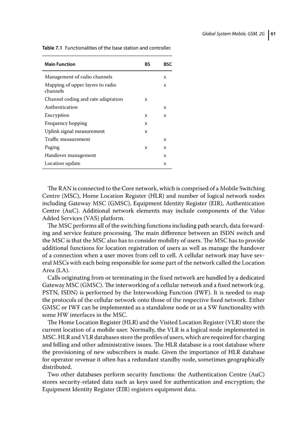


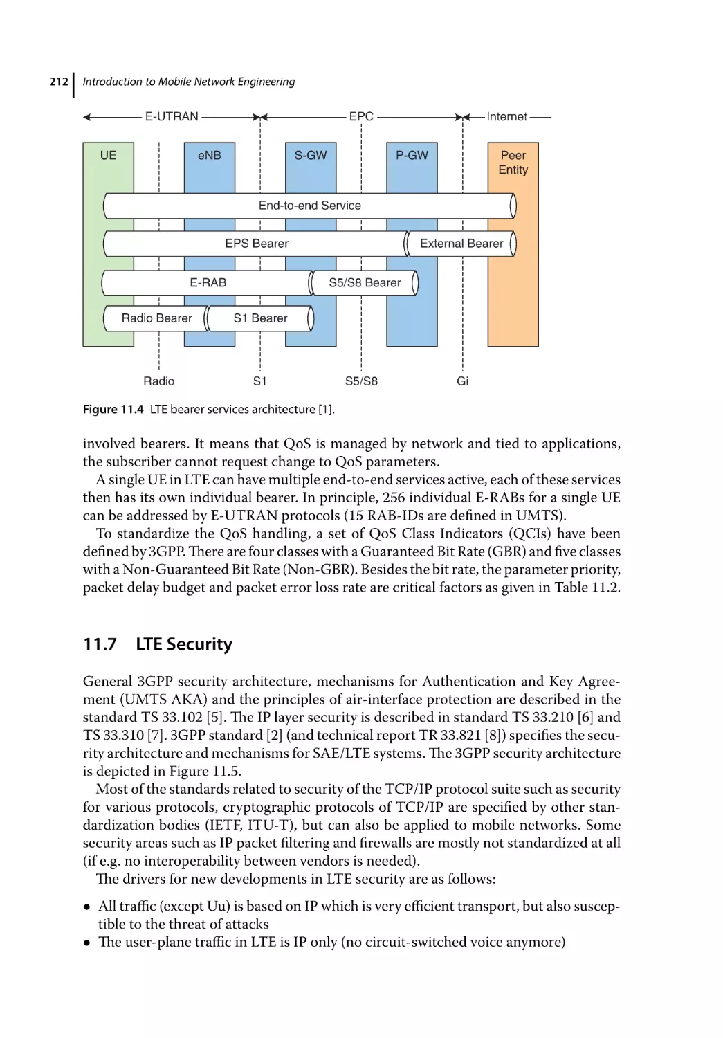


Text
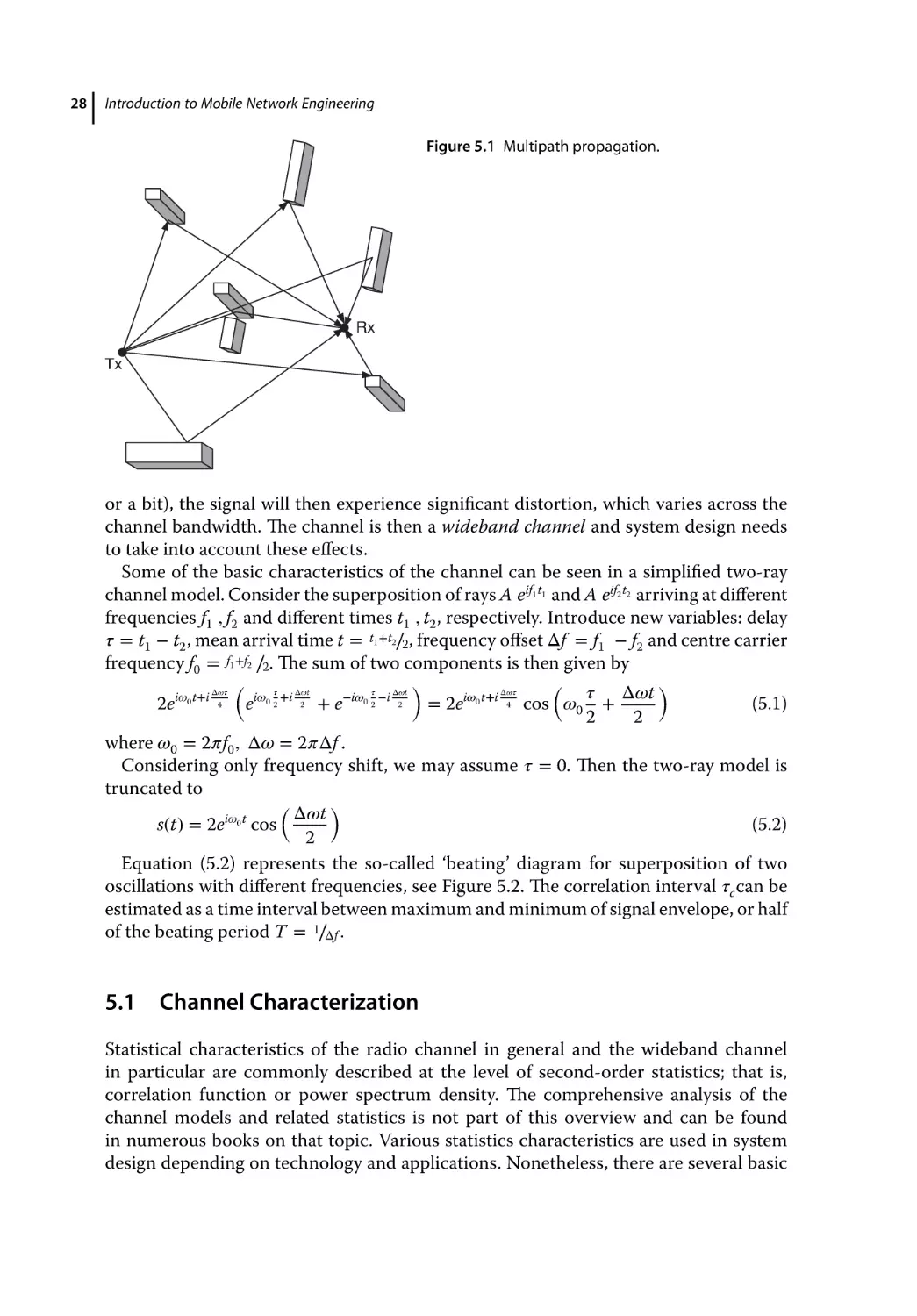
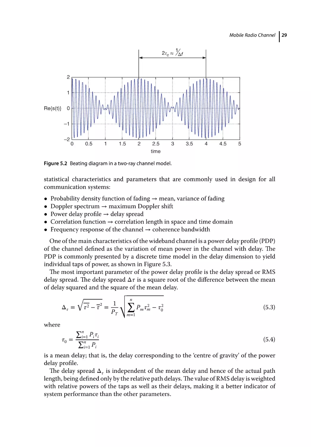
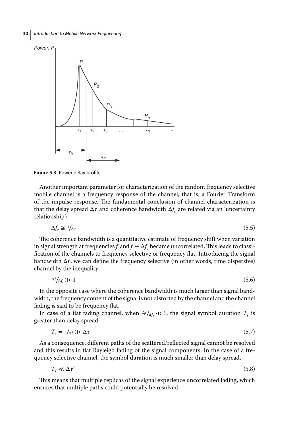
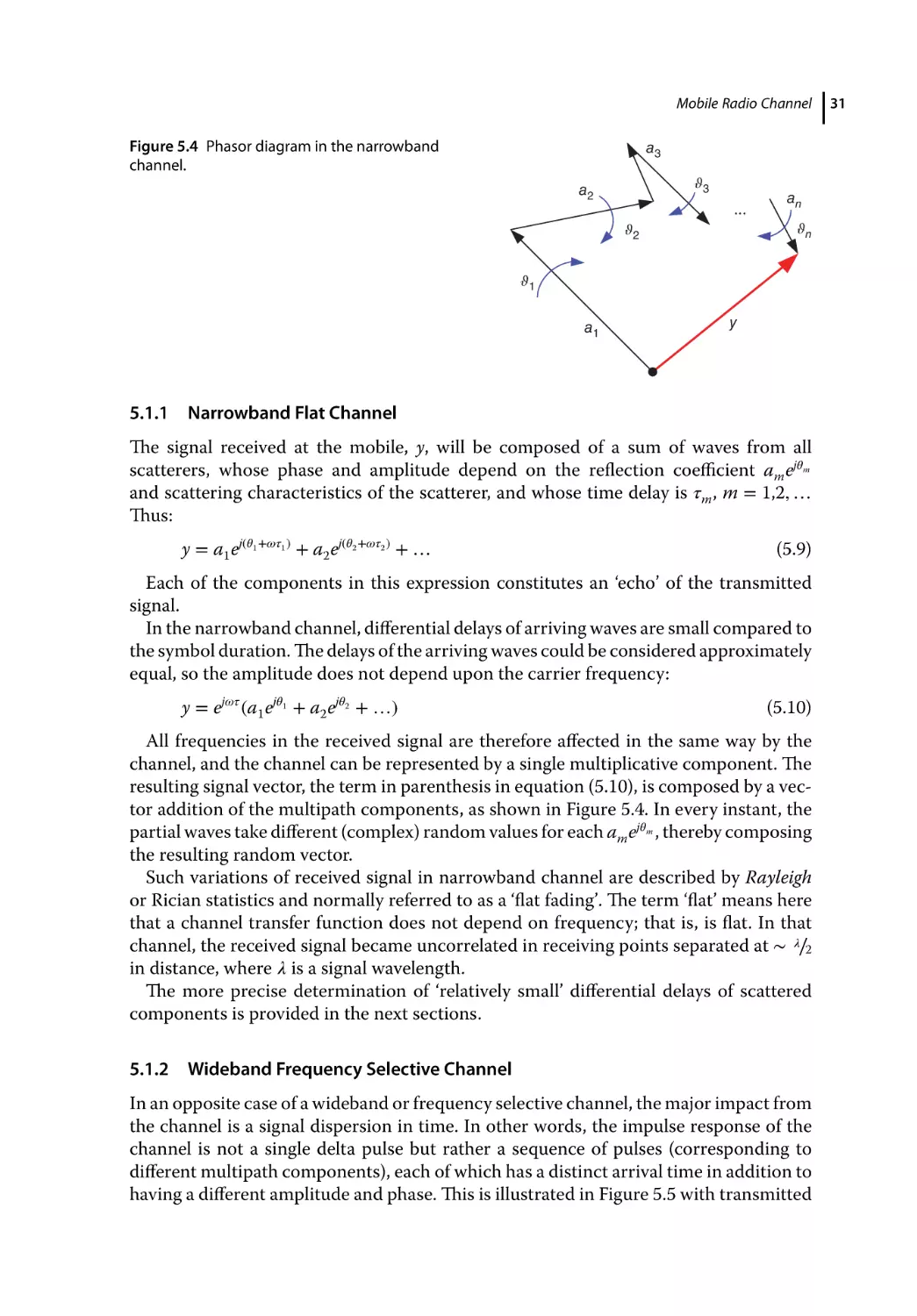
Introduction to Mobile Network Engineering
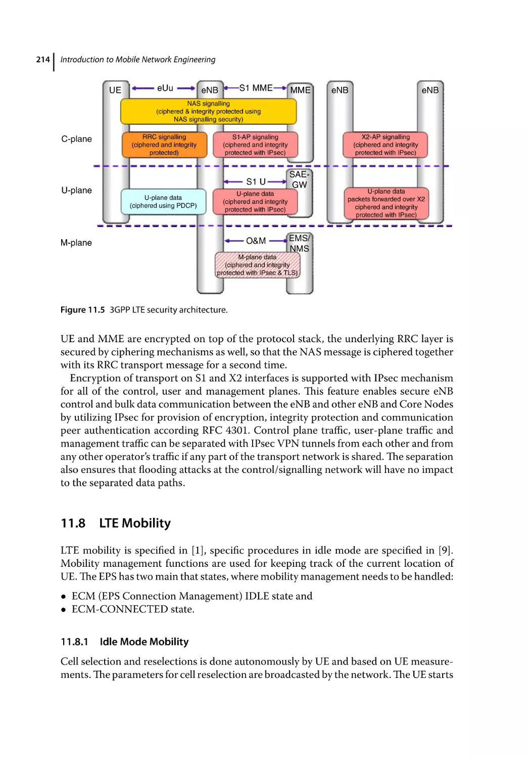
Introduction to Mobile Network Engineering
GSM, 3G-WCDMA, LTE and the Road to 5G
Alexander Kukushkin
PhD, Australia
This edition first published 2018
© 2018 John Wiley & Sons Ltd
All rights reserved. No part of this publication may be reproduced, stored in a retrieval system, or
transmitted, in any form or by any means, electronic, mechanical, photocopying, recording or otherwise,
except as permitted by law. Advice on how to obtain permission to reuse material from this title is available
at http://www.wiley.com/go/permissions.
The rights of Alexander Kukushkin to be identified as the author of this work has been asserted in
accordance with law.
Registered Offices
John Wiley & Sons, Inc., 111 River Street, Hoboken, NJ 07030, USA
John Wiley & Sons Ltd, The Atrium, Southern Gate, Chichester, West Sussex, PO19 8SQ, UK
Editorial Office
The Atrium, Southern Gate, Chichester, West Sussex, PO19 8SQ, UK
For details of our global editorial offices, customer services, and more information about Wiley products
visit us at www.wiley.com.
Wiley also publishes its books in a variety of electronic formats and by print-on-demand. Some content that
appears in standard print versions of this book may not be available in other formats.
Limit of Liability/Disclaimer of Warranty
While the publisher and authors have used their best efforts in preparing this work, they make no
representations or warranties with respect to the accuracy or completeness of the contents of this work and
specifically disclaim all warranties, including without limitation any implied warranties of merchantability or
fitness for a particular purpose. No warranty may be created or extended by sales representatives, written
sales materials or promotional statements for this work. The fact that an organization, website, or product is
referred to in this work as a citation and/or potential source of further information does not mean that the
publisher and authors endorse the information or services the organization, website, or product may provide
or recommendations it may make. This work is sold with the understanding that the publisher is not engaged
in rendering professional services. The advice and strategies contained herein may not be suitable for your
situation. You should consult with a specialist where appropriate. Further, readers should be aware that
websites listed in this work may have changed or disappeared between when this work was written and when
it is read. Neither the publisher nor authors shall be liable for any loss of profit or any other commercial
damages, including but not limited to special, incidental, consequential, or other damages.
Library of Congress Cataloging-in-Publication Data
Names: Kukushkin, Alexander, author.
Title: Introduction to mobile network engineering : GSM, 3G-WCDMA, LTE and
the road to 5G / by Alexander Kukushkin.
Description: Hoboken, NJ : John Wiley & Sons, 2018. | Includes
bibliographical references and index. |
Identifiers: LCCN 2018012499 (print) | LCCN 2018021194 (ebook) | ISBN
9781119484103 (pdf ) | ISBN 9781119484226 (epub) | ISBN 9781119484172
(cloth)
Subjects: LCSH: Mobile communication systems. | Wireless metropolitan area
networks.
Classification: LCC TK5103.2 (ebook) | LCC TK5103.2 .K85 2018 (print) | DDC
621.3845/6–dc23
LC record available at https://lccn.loc.gov/2018012499
Cover design by Wiley
Cover image: © pluie_r/Shutterstock
Set in 10/12pt WarnockPro by SPi Global, Chennai, India
10
9
8
7
6
5
4
3
2
1
To my family
vii
Contents
Foreword xvii
Acknowledgements xix
Abbreviations xxi
1
Introduction 1
2
Types of Mobile Network by Multiple-Access Scheme
3
Cellular System 5
3.1
3.2
3.3
3.4
3.5
3.6
3.7
3.8
3.9
3.10
3.10.1
3.10.2
3.10.3
Historical Background 5
Cellular Concept 5
Carrier-to-Interference Ratio 6
Formation of Clusters 8
Sectorization 9
Frequency Allocation 10
Trunking Effect 11
Erlang Formulas 13
Erlang B Formula 13
Worked Examples 14
Problem 1 14
Problem 2 16
Problem 3 16
4
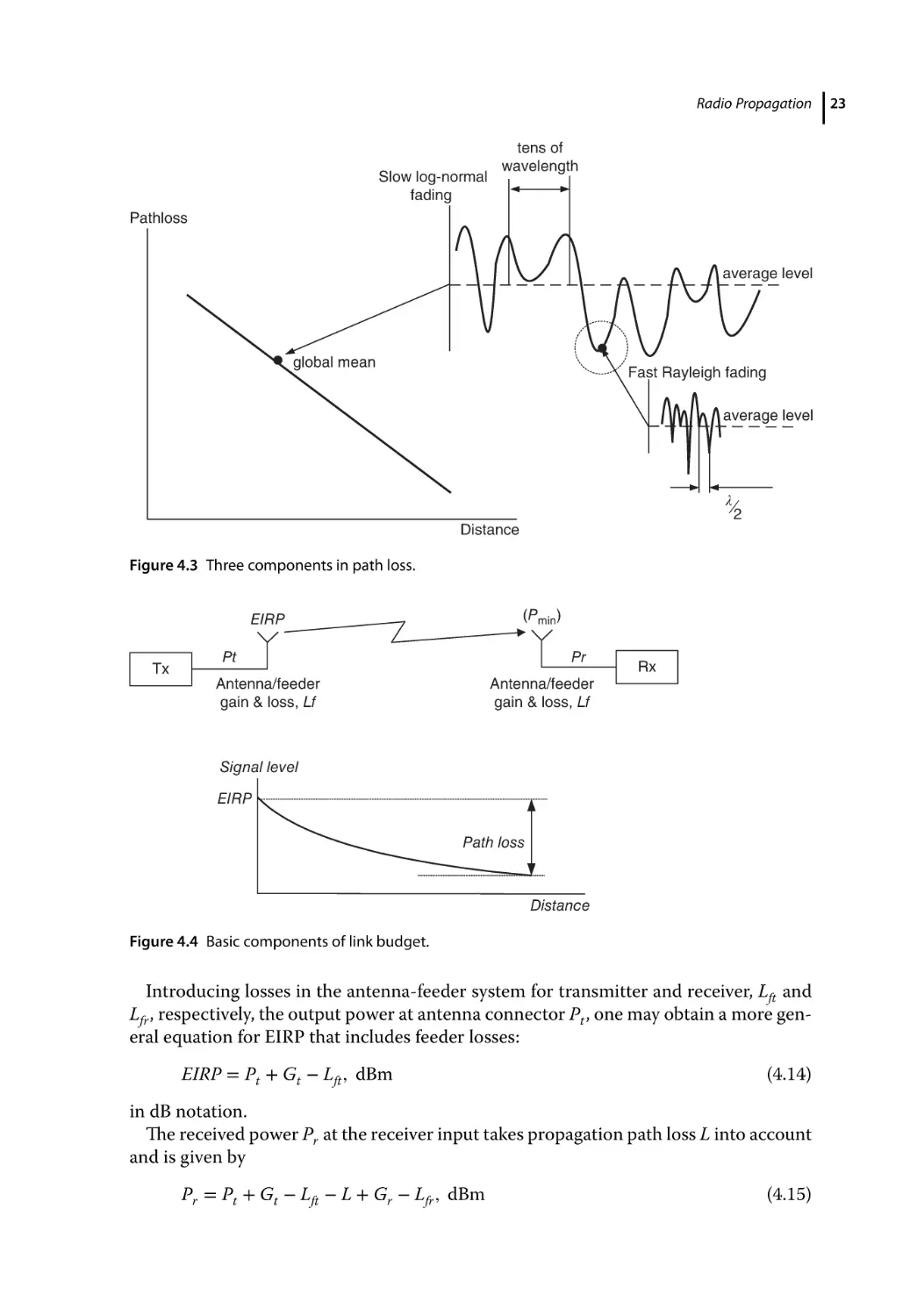
Radio Propagation
3
4.1
4.1.1
4.1.2
19
Propagation Mechanisms 19
Free-Space Propagation 19
Propagation Models for Path Loss (Global Mean) Prediction 22
5
Mobile Radio Channel 27
5.1
5.1.1
5.1.2
5.1.3
5.2
Channel Characterization 28
Narrowband Flat Channel 31
Wideband Frequency Selective Channel 31
Doppler Shift 34
Worked Examples 36
viii
Contents
5.2.1
5.2.2
5.3
5.3.1
5.3.2
5.4
5.4.1
5.5
5.5.1
5.5.2
5.5.3
5.6
Problem 1 36
Problem 2 36
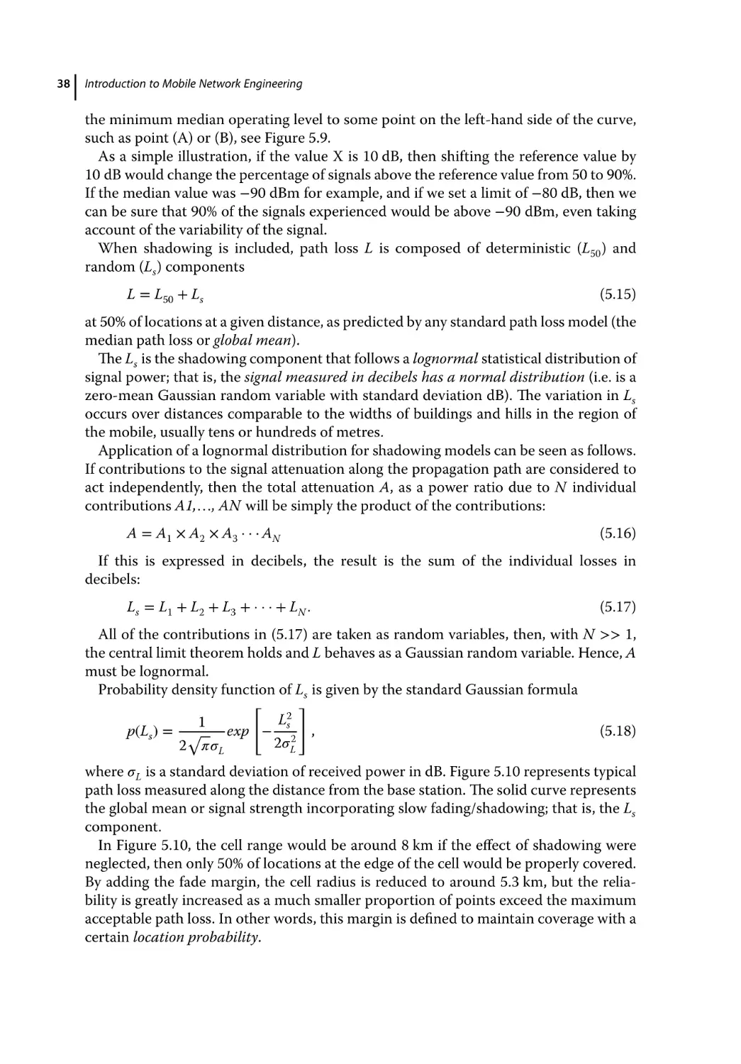
Fading 36
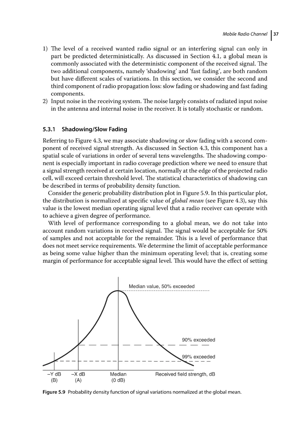
Shadowing/Slow Fading 37
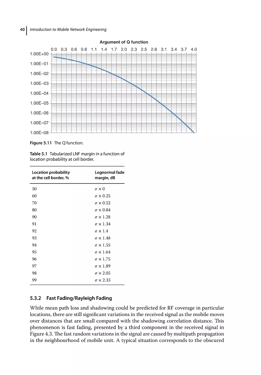
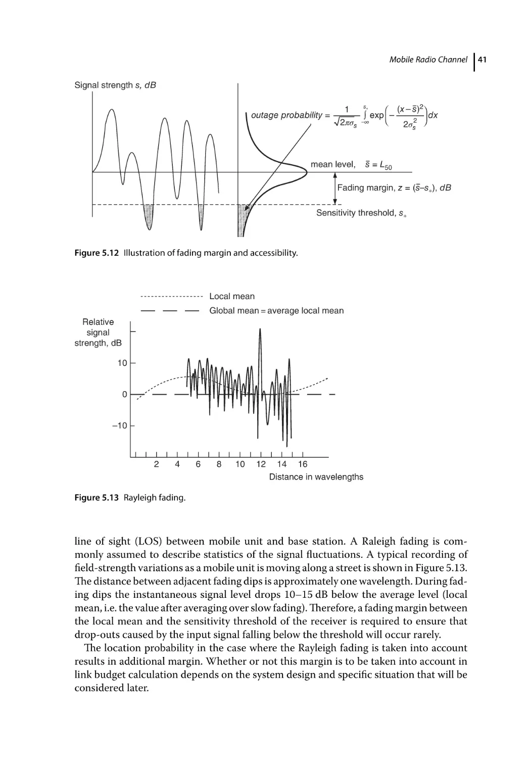
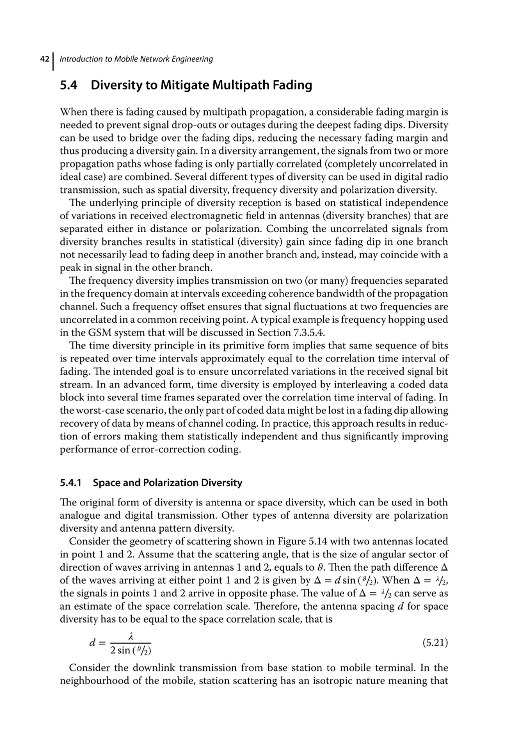
Fast Fading/Rayleigh Fading 40
Diversity to Mitigate Multipath Fading 42
Space and Polarization Diversity 42
Worked Examples 44
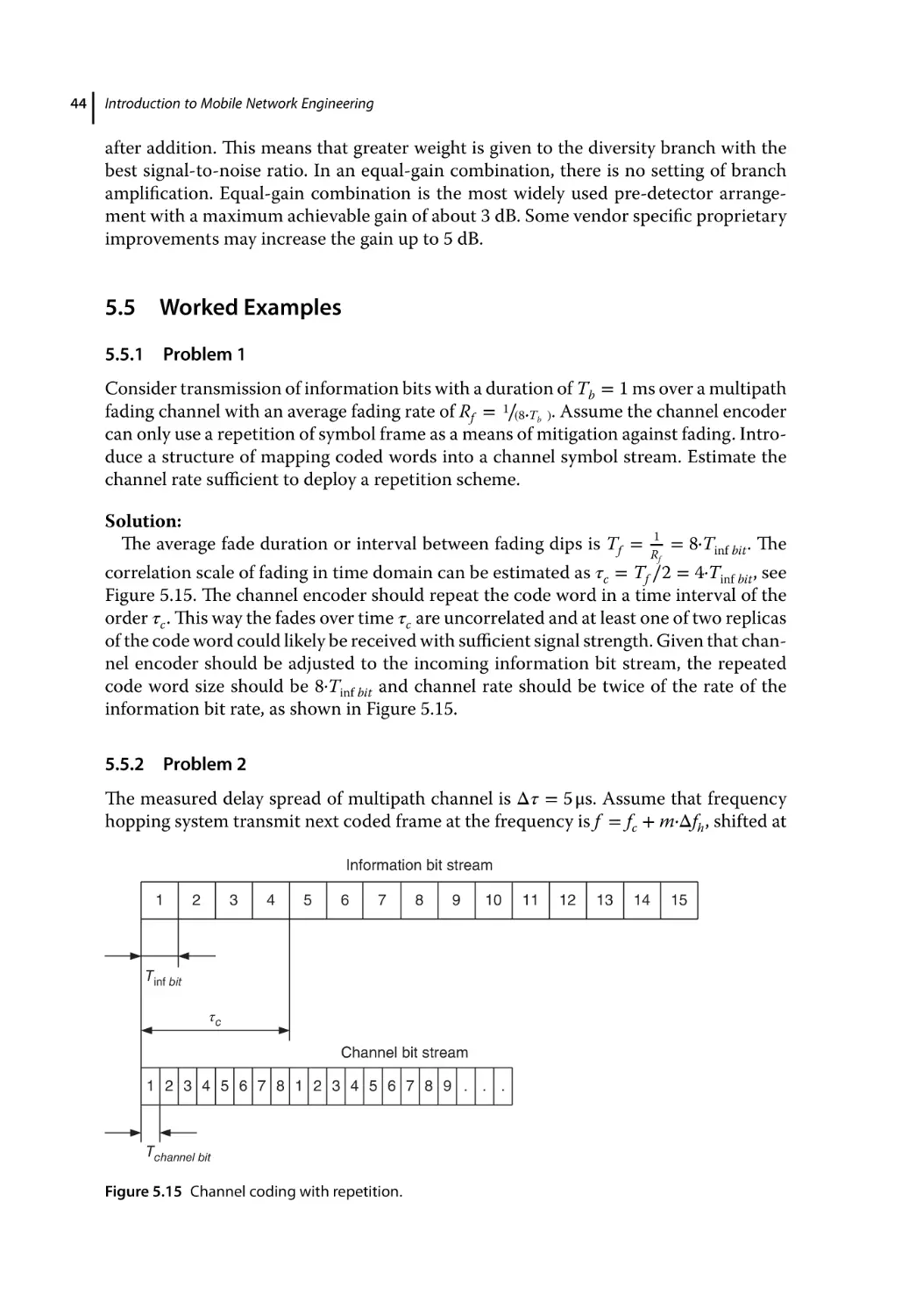
Problem 1 44
Problem 2 44
Problem 3 45
Receiver Noise Factor (Noise Figure) 45
6
Radio Network Planning 49
6.1
6.1.1
6.1.2
6.1.2.1
6.1.2.2
6.1.2.3
6.1.2.4
6.1.2.5
6.1.2.6
6.1.2.7
6.1.3
6.1.4
6.2
6.2.1
6.2.2
6.2.3
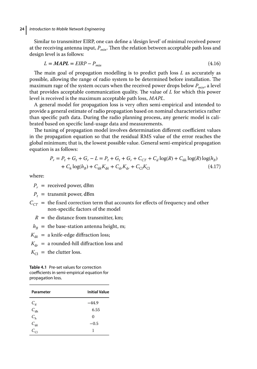
Generic Link Budget 49
Receiver Sensitivity Level 50
Design Level 50
Rayleigh Fading Margin 51
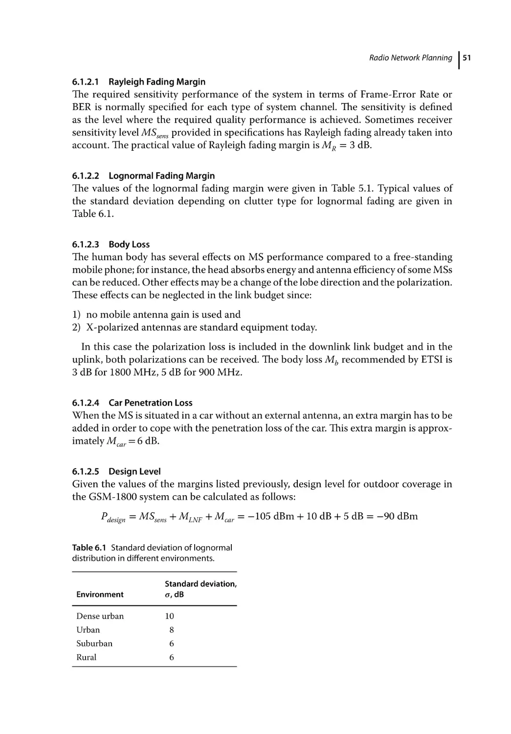
Lognormal Fading Margin 51
Body Loss 51
Car Penetration Loss 51
Design Level 51
Building Penetration Loss 52
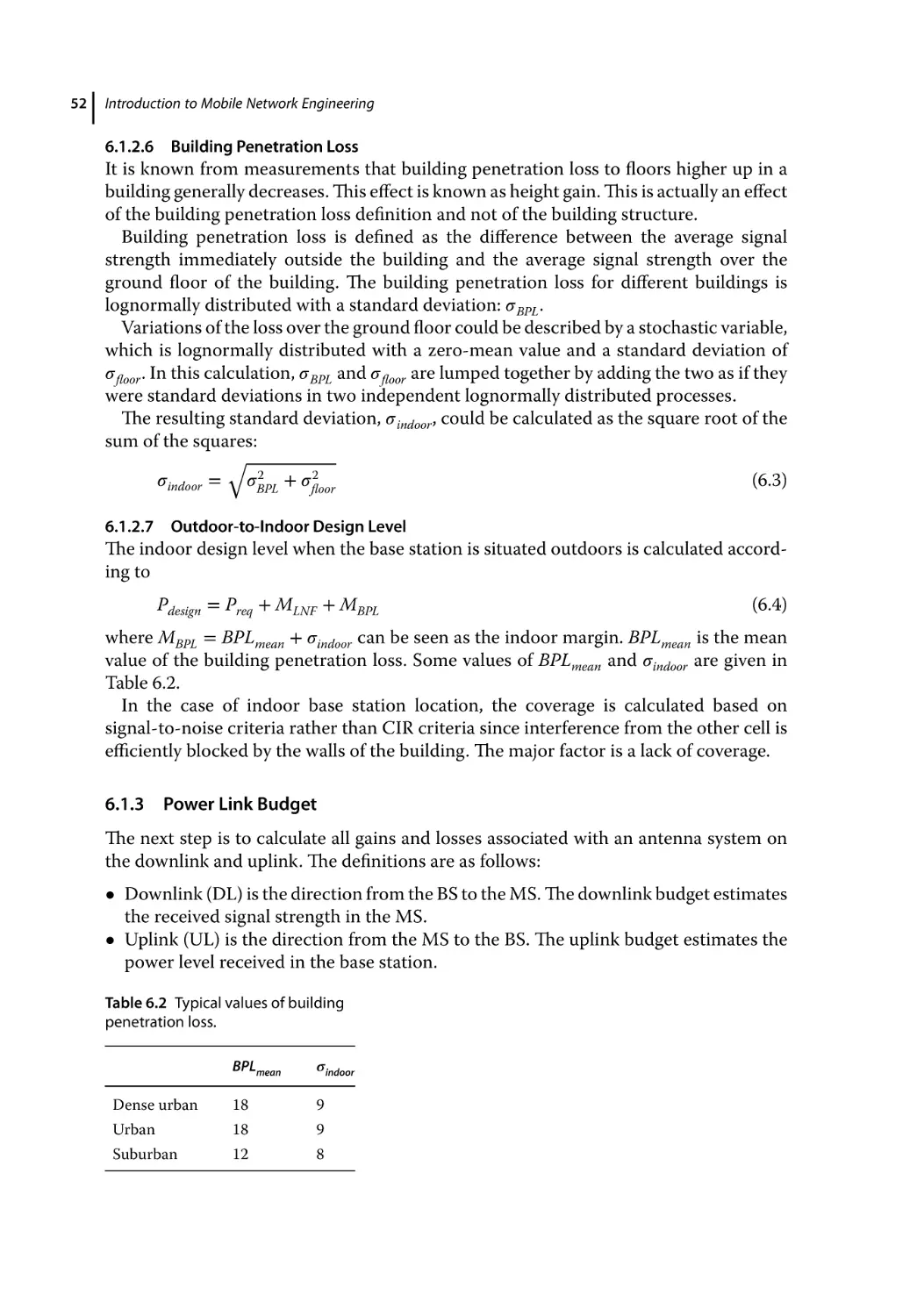
Outdoor-to-Indoor Design Level 52
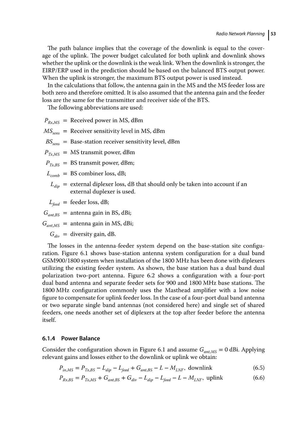
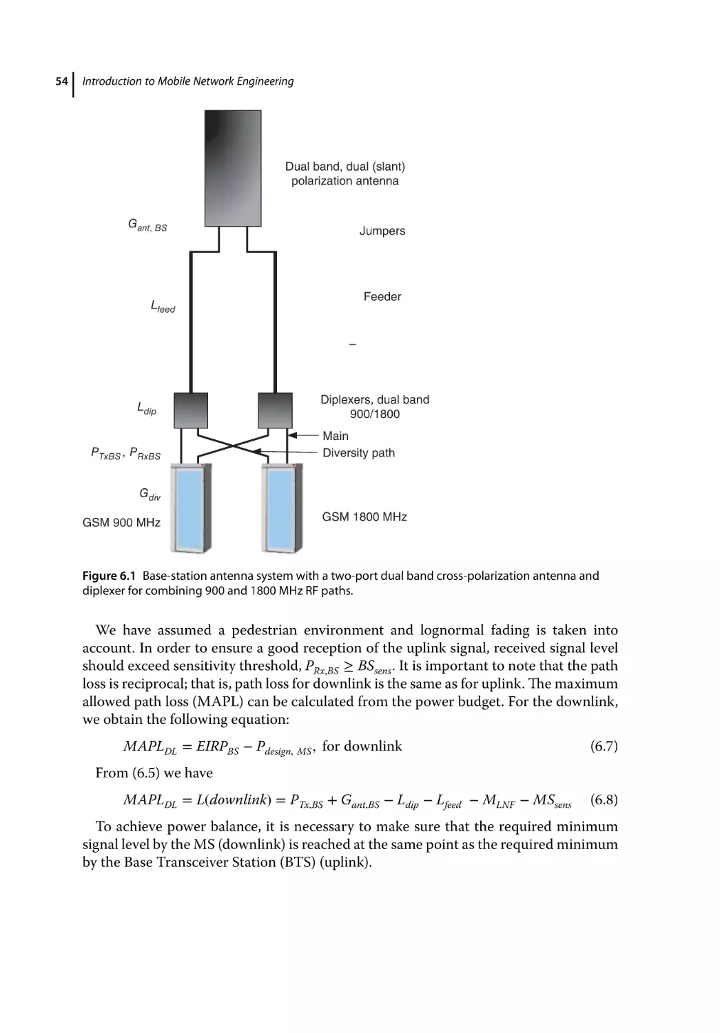
Power Link Budget 52
Power Balance 53
Worked Examples 56
Problem 1 56
Problem 2 57
Problem 3 58
7
Global System Mobile, GSM, 2G 59
7.1
7.2
7.2.1
7.2.2
7.2.3
7.2.4
7.2.5
7.2.6
7.2.7
7.2.8
7.2.9
7.2.10
7.2.11
7.2.12
7.3
General Concept for GSM System Development 59
GSM System Architecture 59
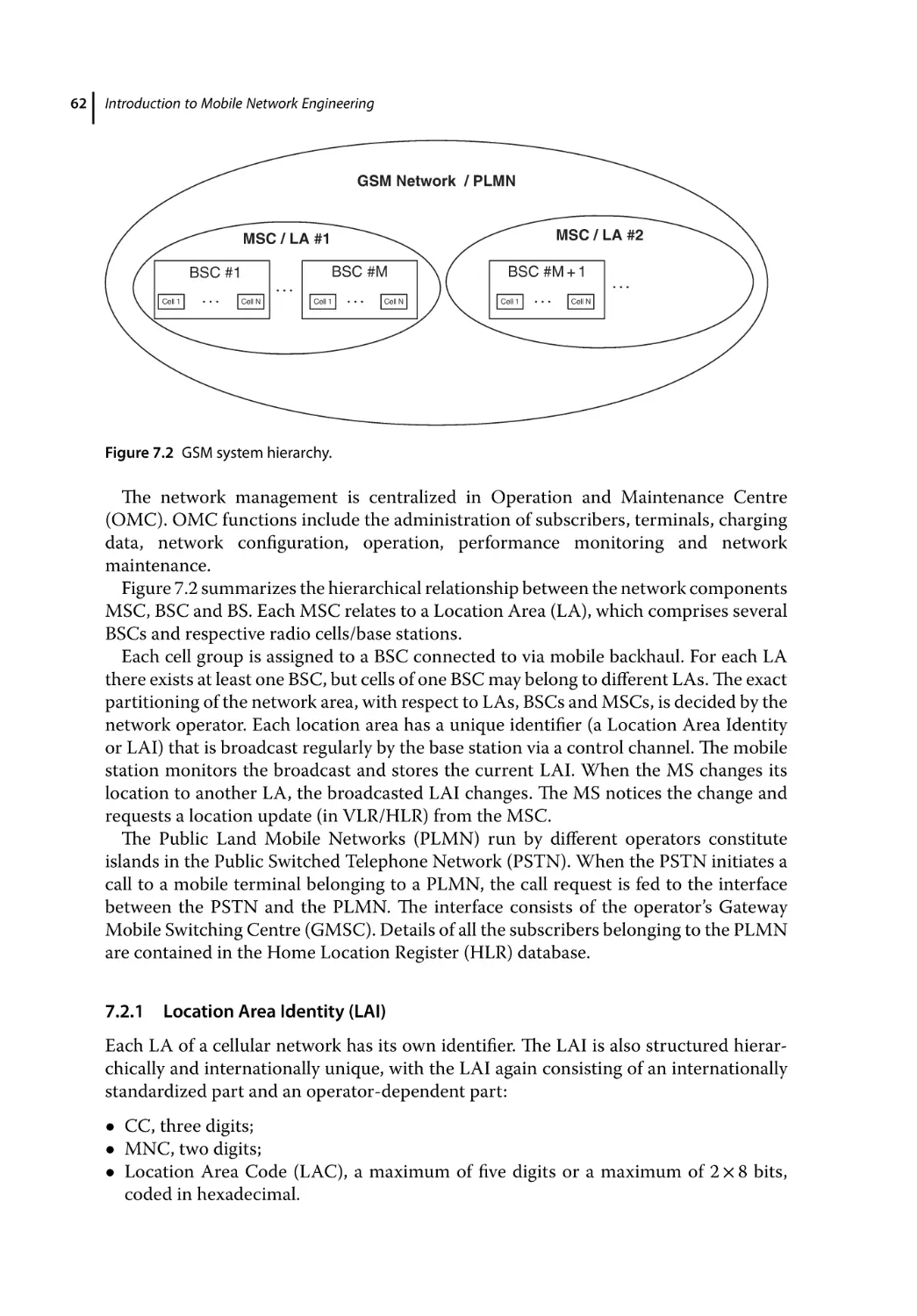
Location Area Identity (LAI) 62
The SIM Concept 63
User Addressing in the GSM Network 63
International Mobile Station Equipment Identity (IMEI) 63
International Mobile Subscriber Identity (IMSI) 64
Different Roles of MSISDN and IMSI 64
Mobile Station Routing Number 64
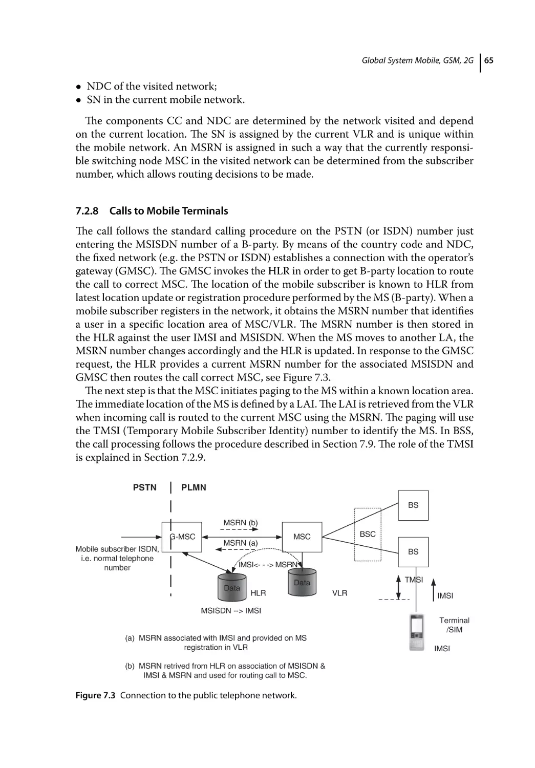
Calls to Mobile Terminals 65
Temporary Mobile Subscriber Identity (TMSI) 66
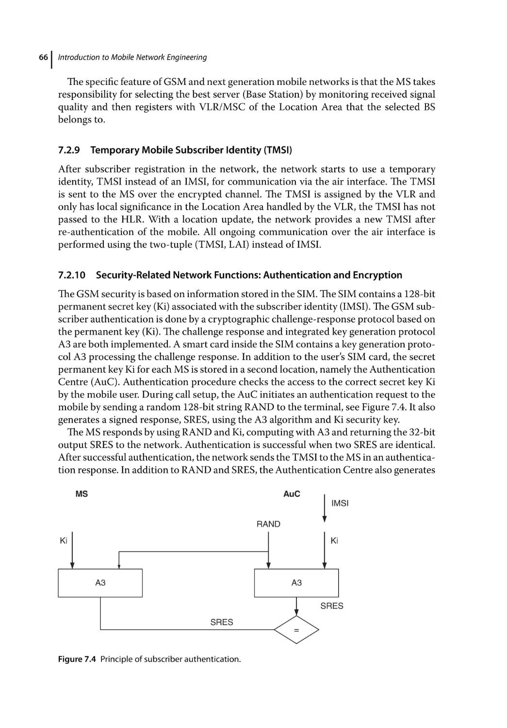
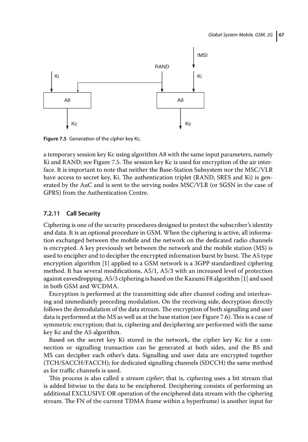
Security-Related Network Functions: Authentication and Encryption 66
Call Security 67
Operation and Maintenance Security 69
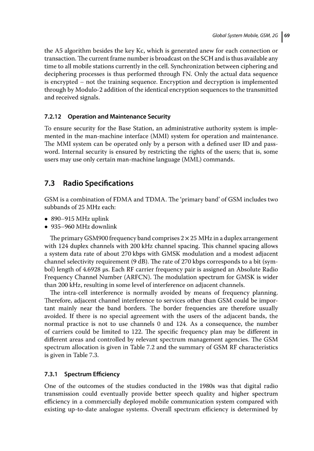
Radio Specifications 69
Contents
7.3.1
7.3.2
7.3.3
7.3.4
7.3.4.1
7.3.4.2
7.3.4.3
7.3.4.4
7.3.4.5
7.3.5
7.3.5.1
7.3.5.2
7.3.5.3
7.3.5.4
7.4
7.4.1
7.5
7.5.1
7.5.2
7.5.2.1
7.5.2.2
7.6
7.6.1
7.6.2
7.6.2.1
7.6.3
7.6.4
7.6.4.1
7.6.4.2
7.6.5
7.6.5.1
7.6.5.2
7.6.5.3
7.7
7.7.1
7.7.2
7.7.2.1
7.7.2.2
7.7.2.3
7.7.2.4
7.7.2.5
7.7.3
7.8
7.8.1
7.8.2
7.9
7.9.1
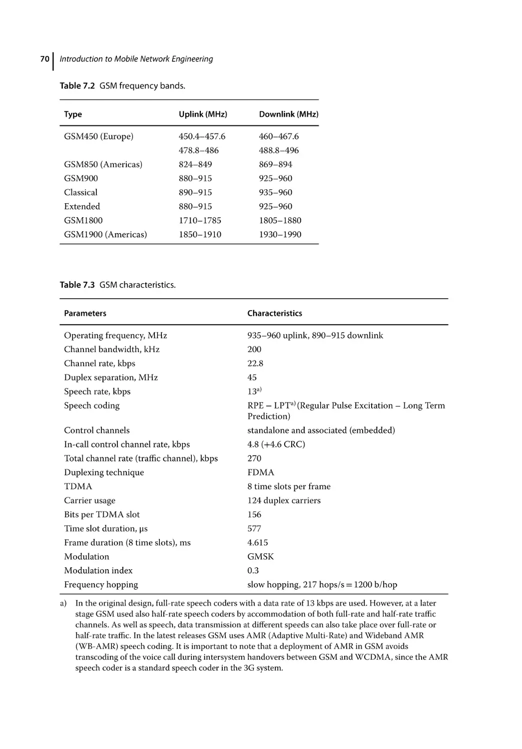
Spectrum Efficiency 69
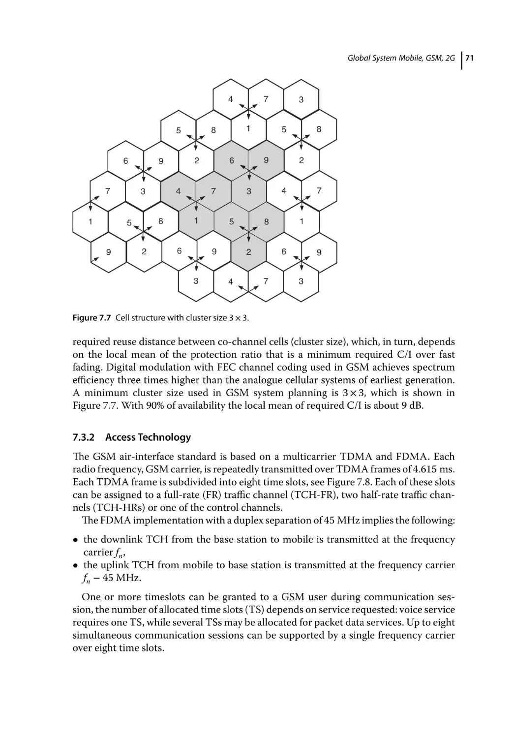
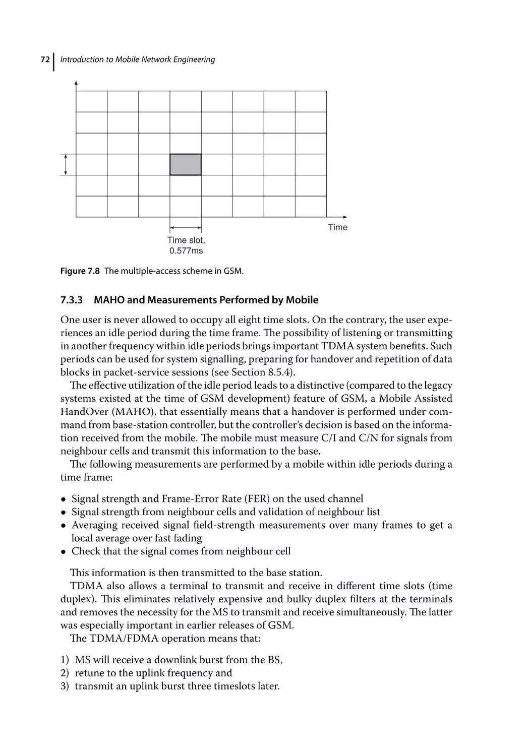
Access Technology 71
MAHO and Measurements Performed by Mobile 72
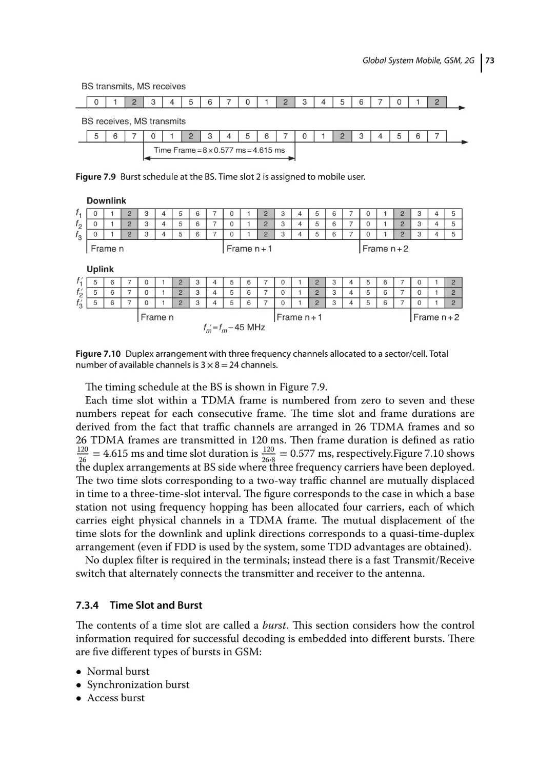
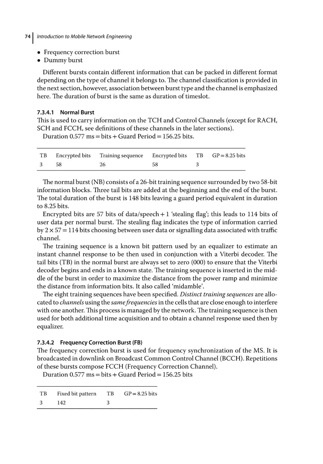
Time Slot and Burst 73
Normal Burst 74
Frequency Correction Burst (FB) 74
Synchronization Burst 75
Access Burst 75
Dummy Burst 75
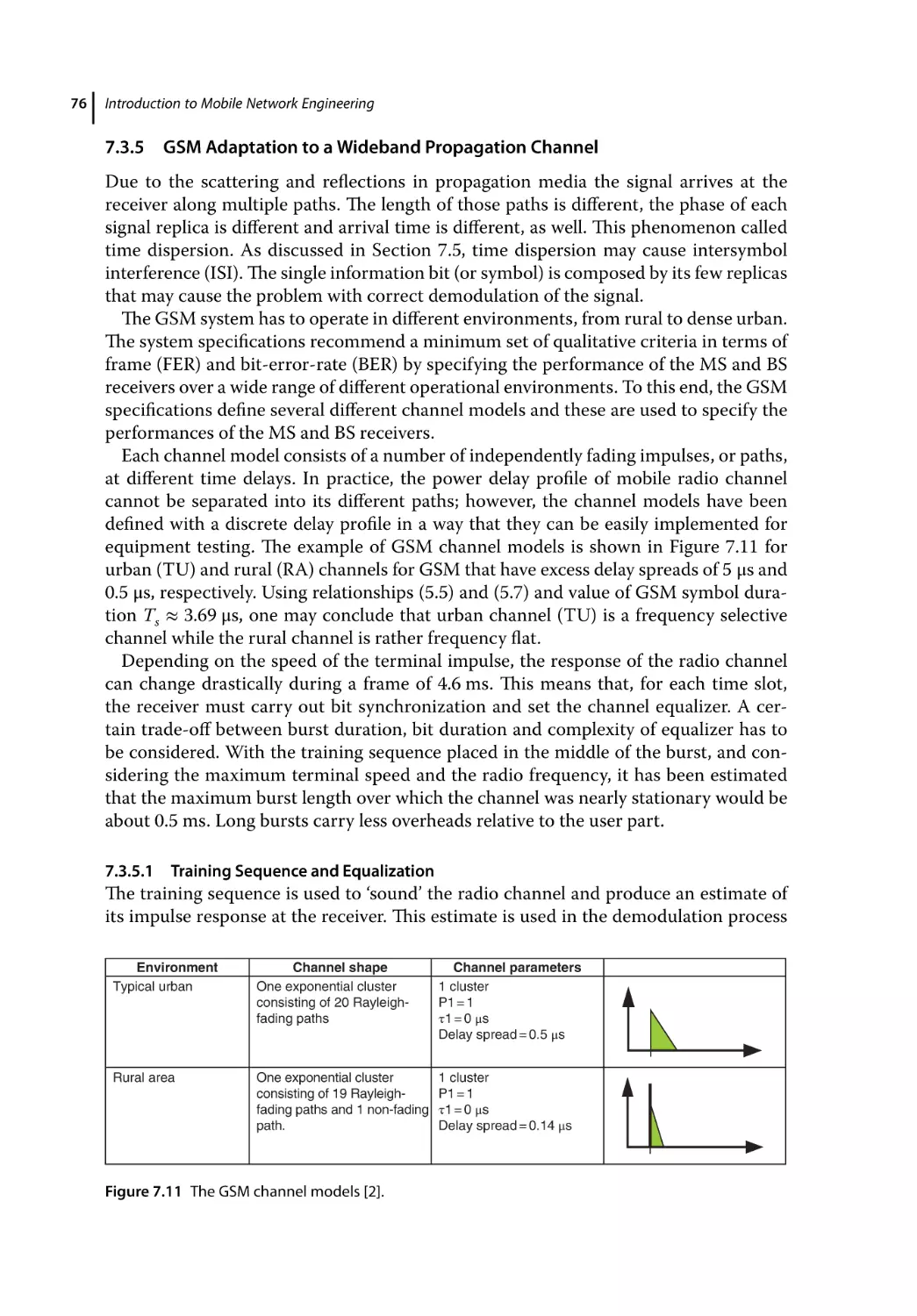
GSM Adaptation to a Wideband Propagation Channel 76
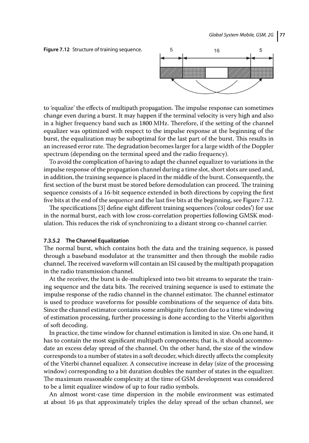
Training Sequence and Equalization 76
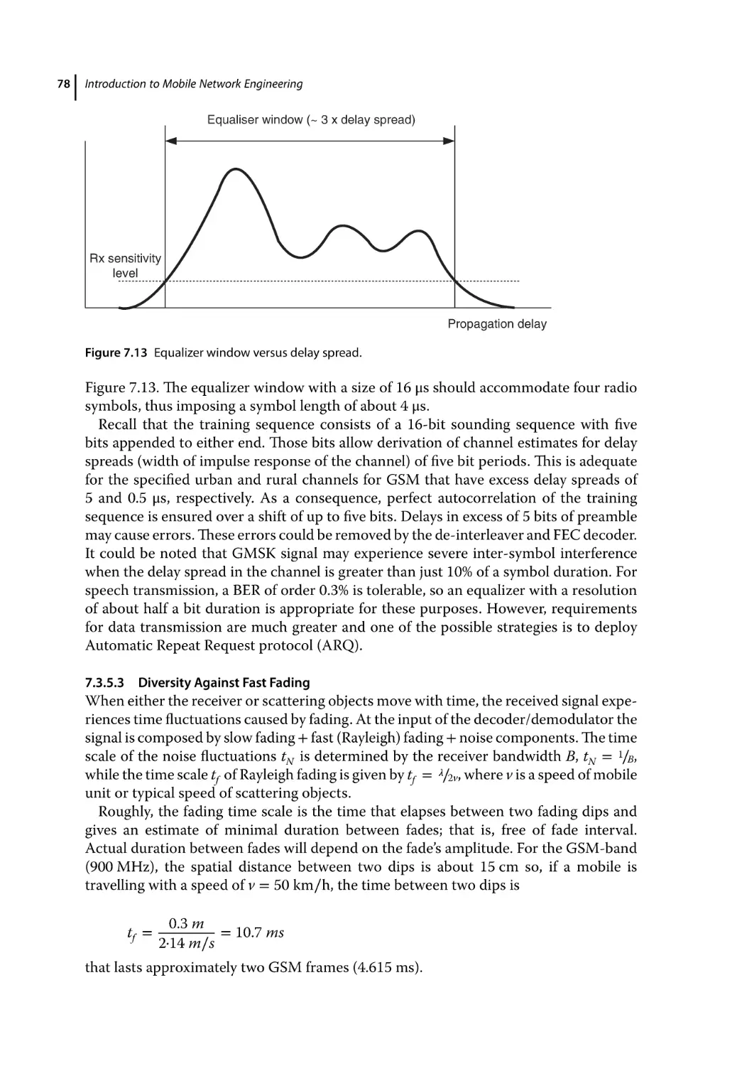
The Channel Equalization 77
Diversity Against Fast Fading 78
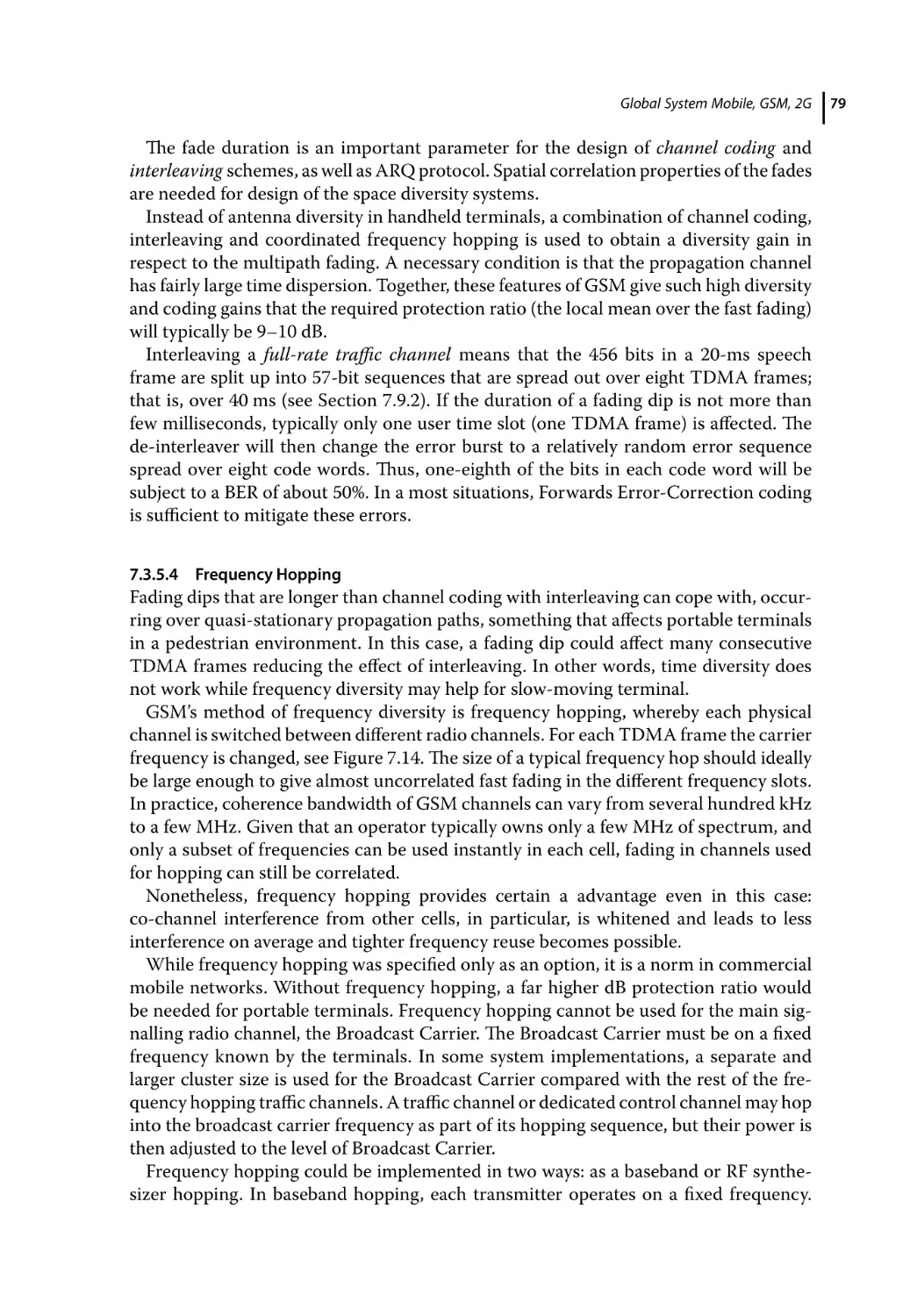
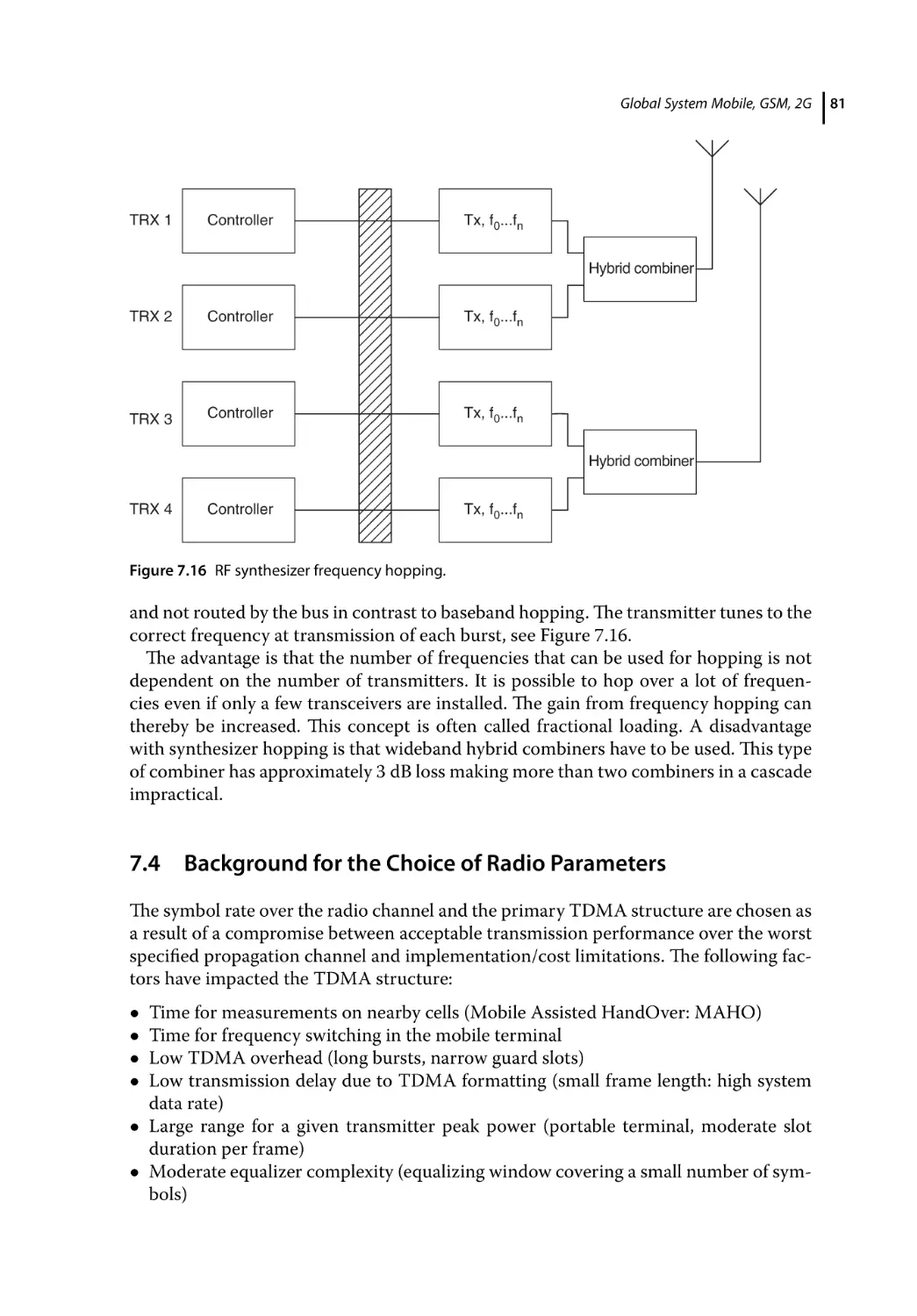
Frequency Hopping 79
Background for the Choice of Radio Parameters 81
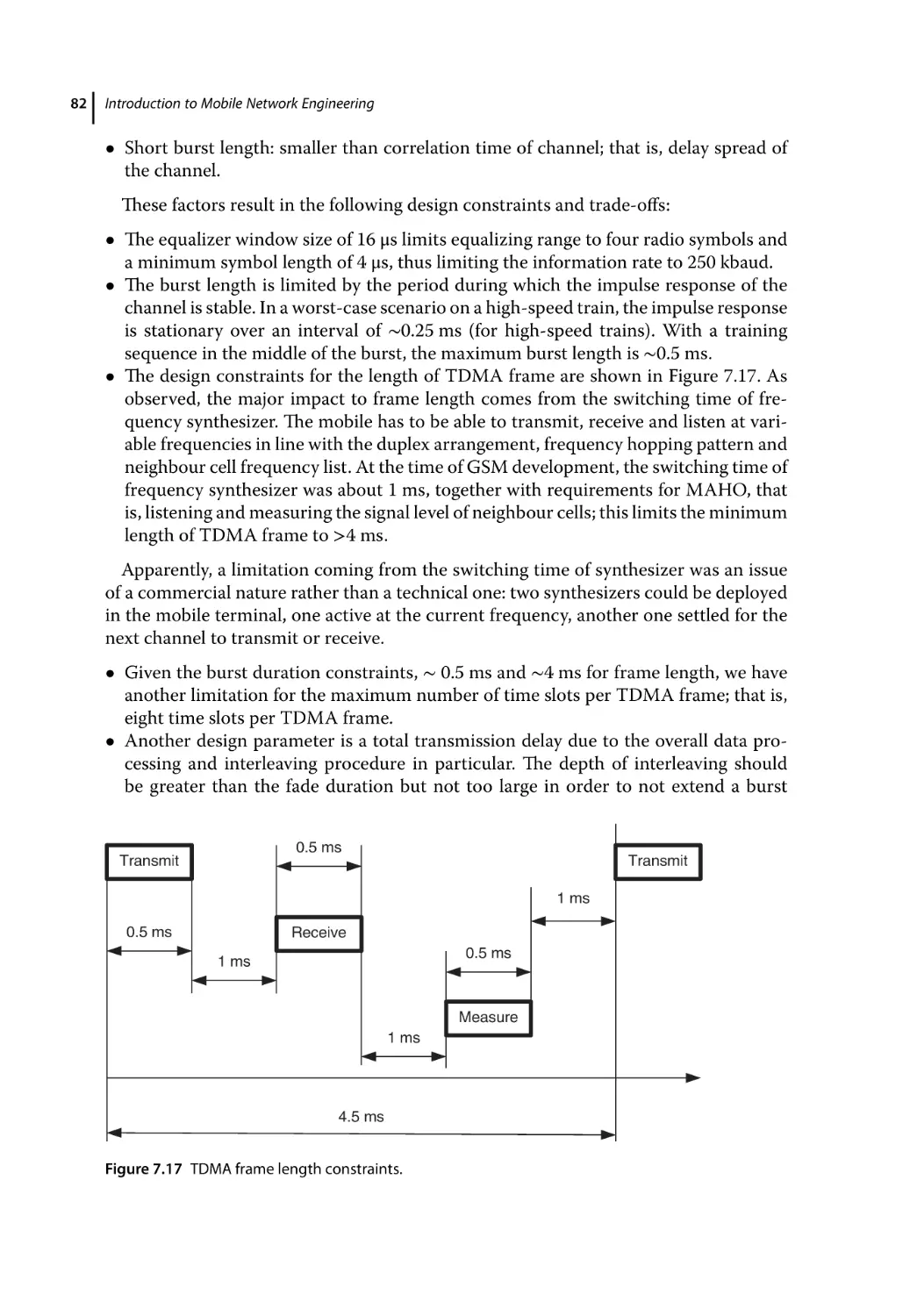
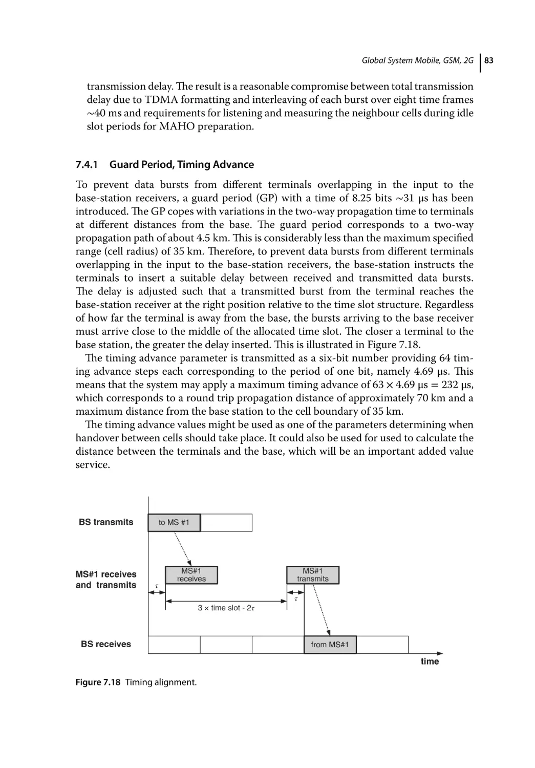
Guard Period, Timing Advance 83
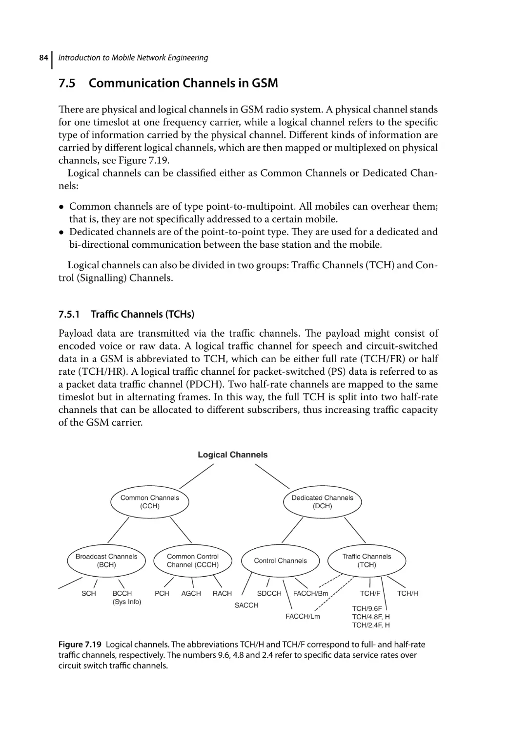
Communication Channels in GSM 84
Traffic Channels (TCHs) 84
Control Channels 85
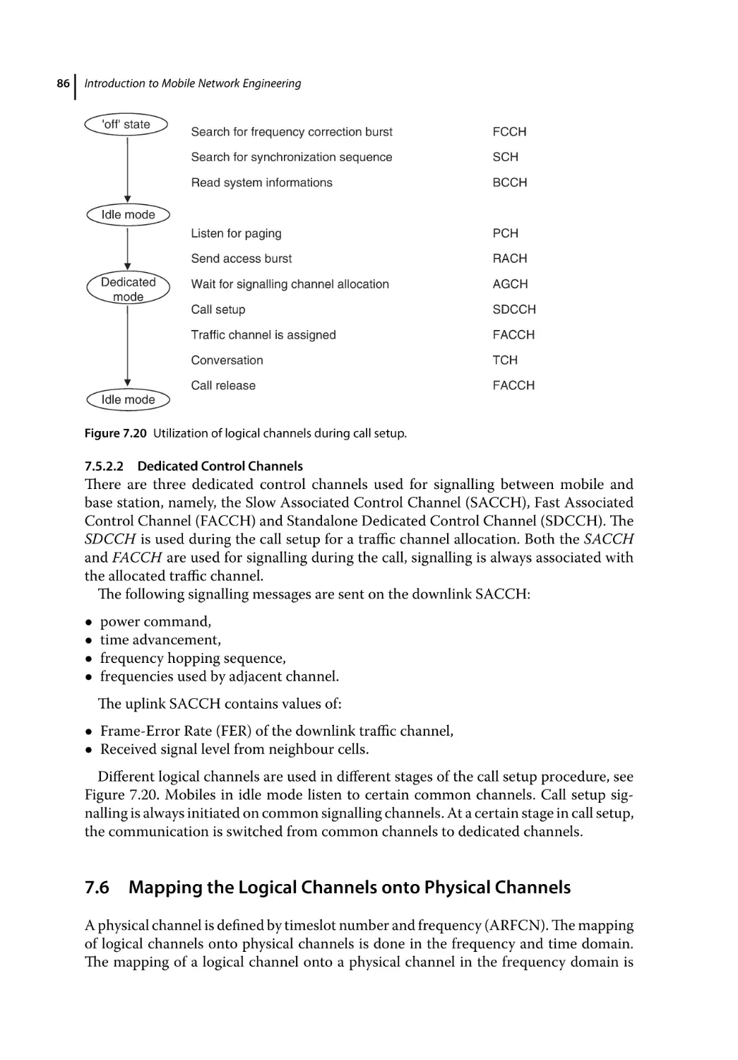
Common Control Channels 85
Dedicated Control Channels 86
Mapping the Logical Channels onto Physical Channels 86
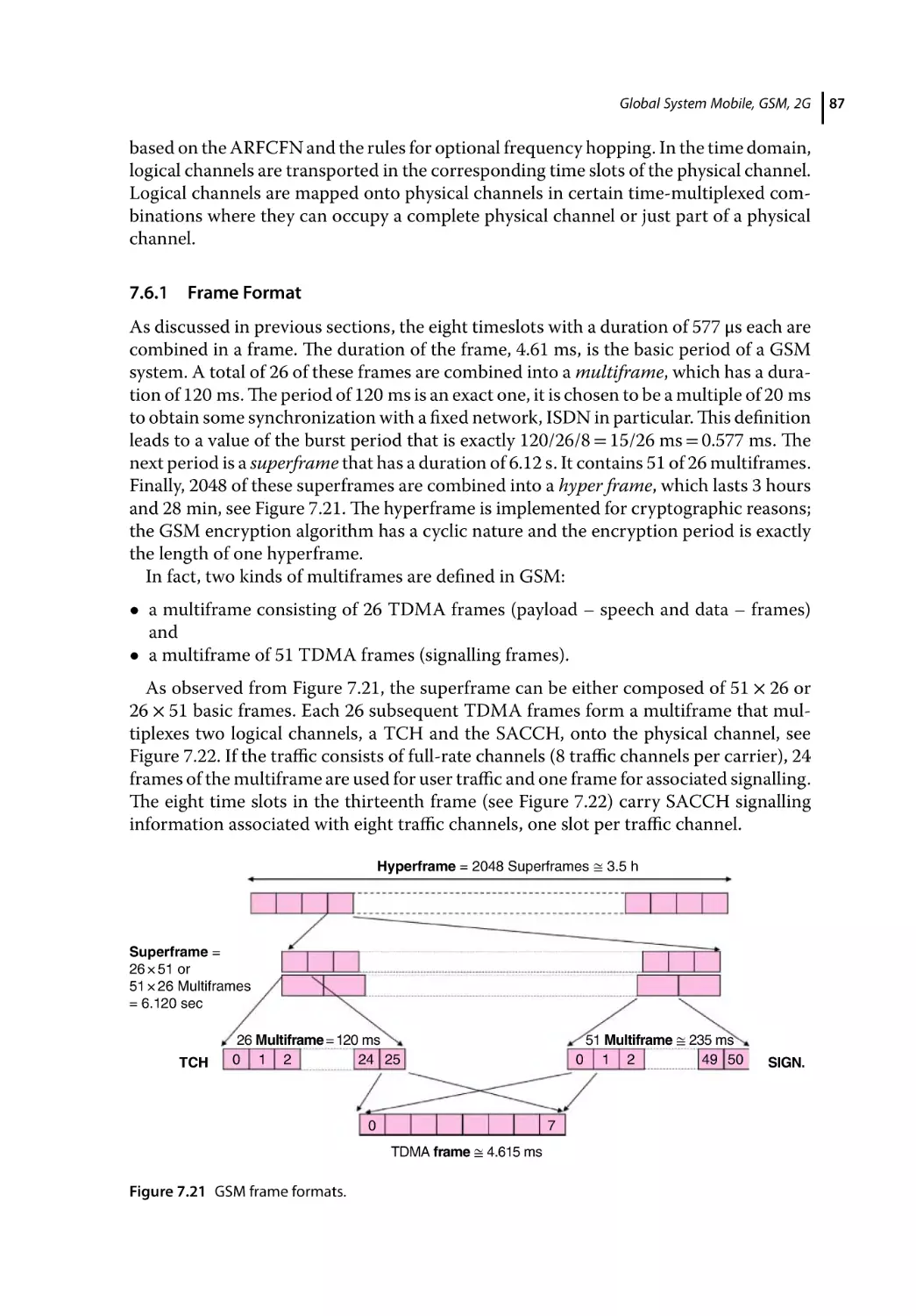
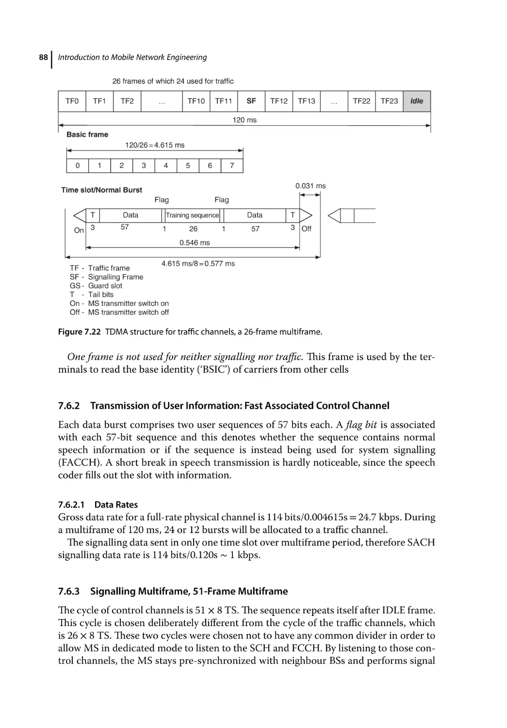
Frame Format 87
Transmission of User Information: Fast Associated Control Channel 88
Data Rates 88
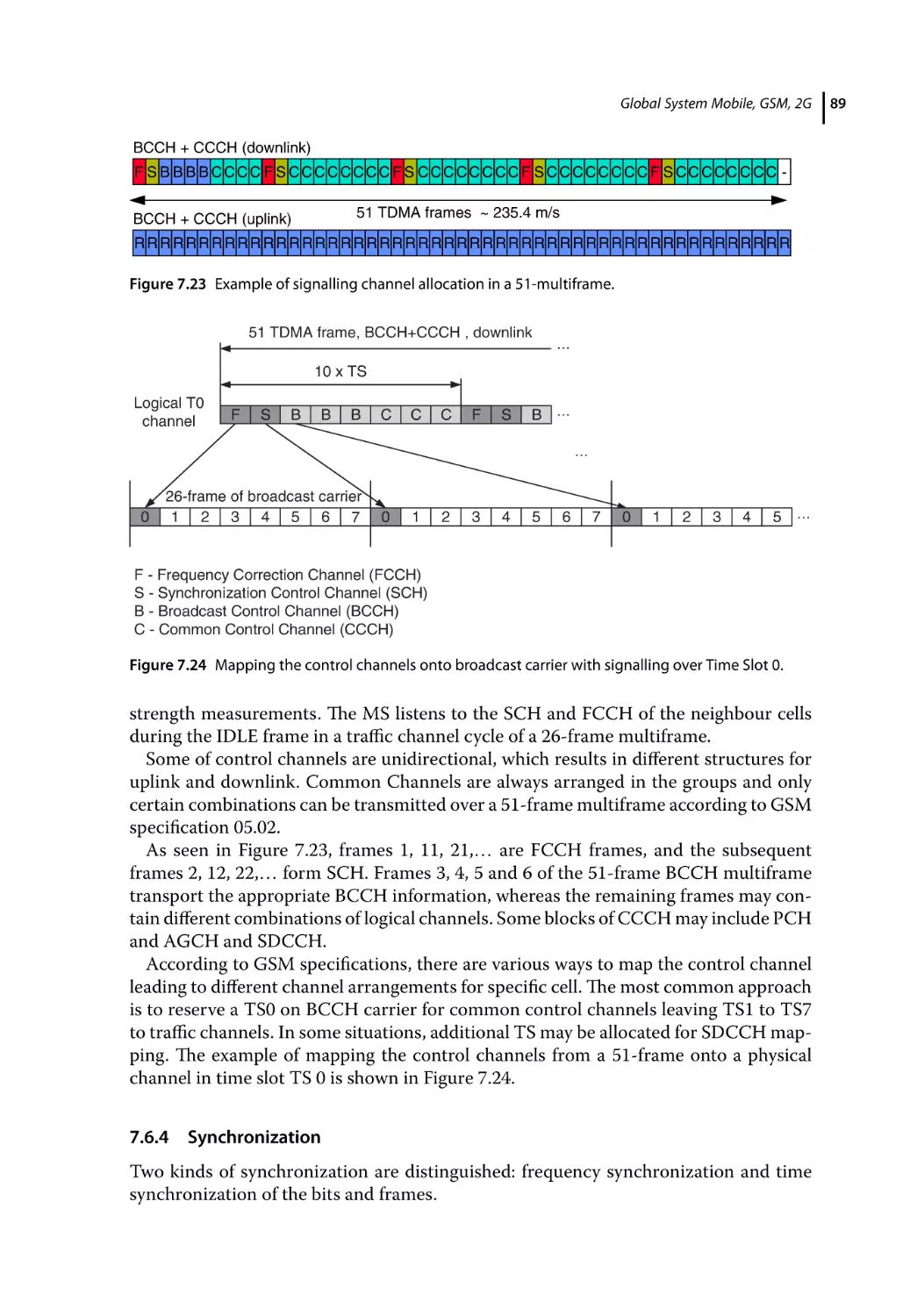
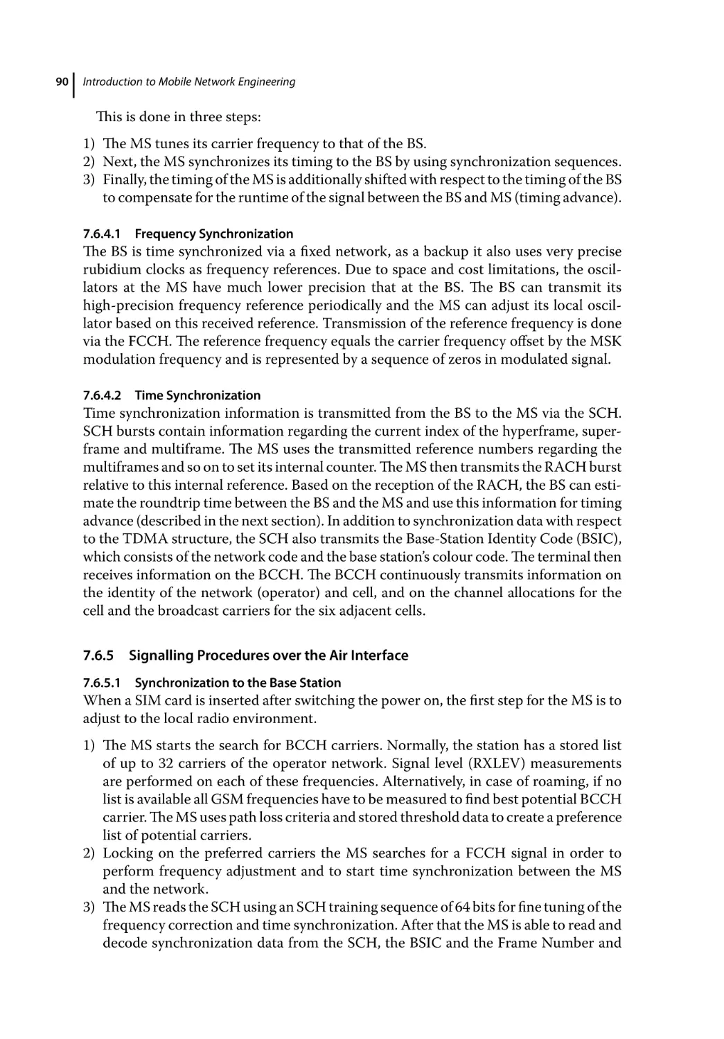
Signalling Multiframe, 51-Frame Multiframe 88
Synchronization 89
Frequency Synchronization 90
Time Synchronization 90
Signalling Procedures over the Air Interface 90
Synchronization to the Base Station 90
Registering With the Base Station 91
Call Setup 91
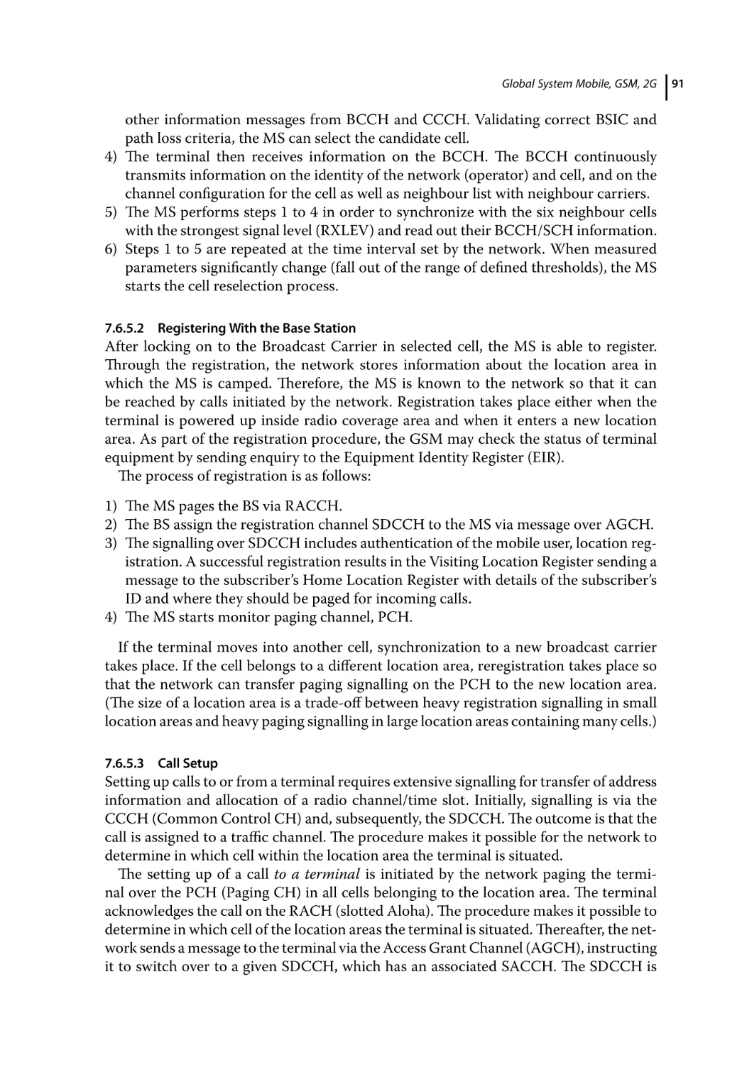
Signalling During a Call 93
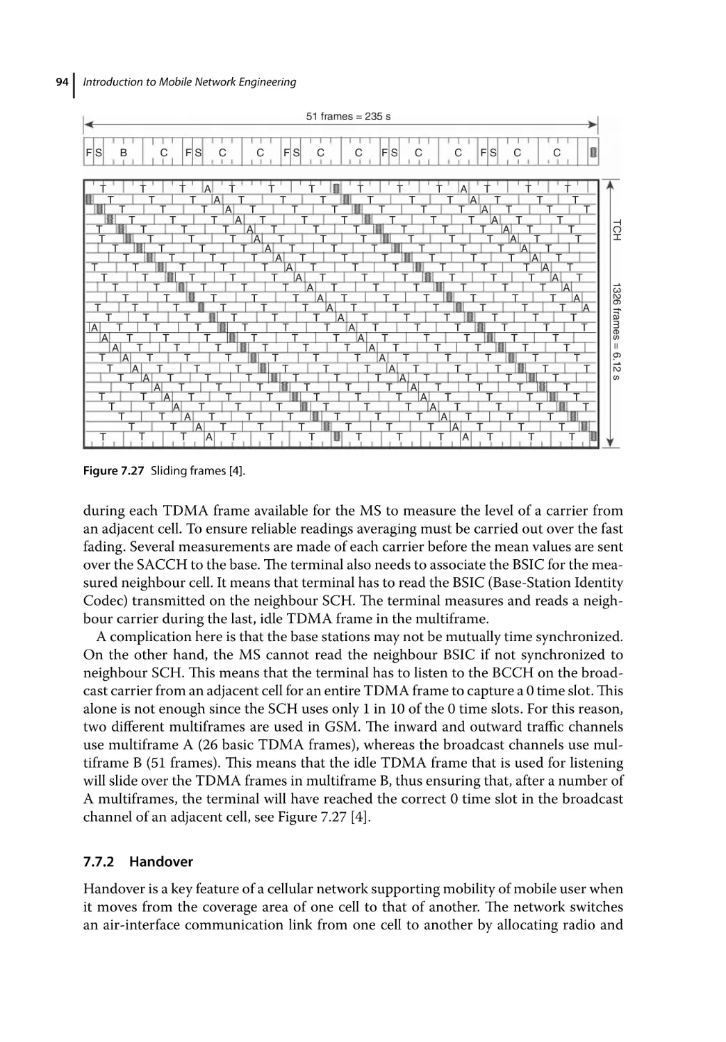
Measuring the Signal Levels from Adjacent Cells 93
Handover 94
Intra-Cell and Inter-Cell Handover 95
Intra- and Inter-BSC Handover 95
Intra- and Inter-MSC Handover 95
Intra- and Inter-PLMN Handover 95
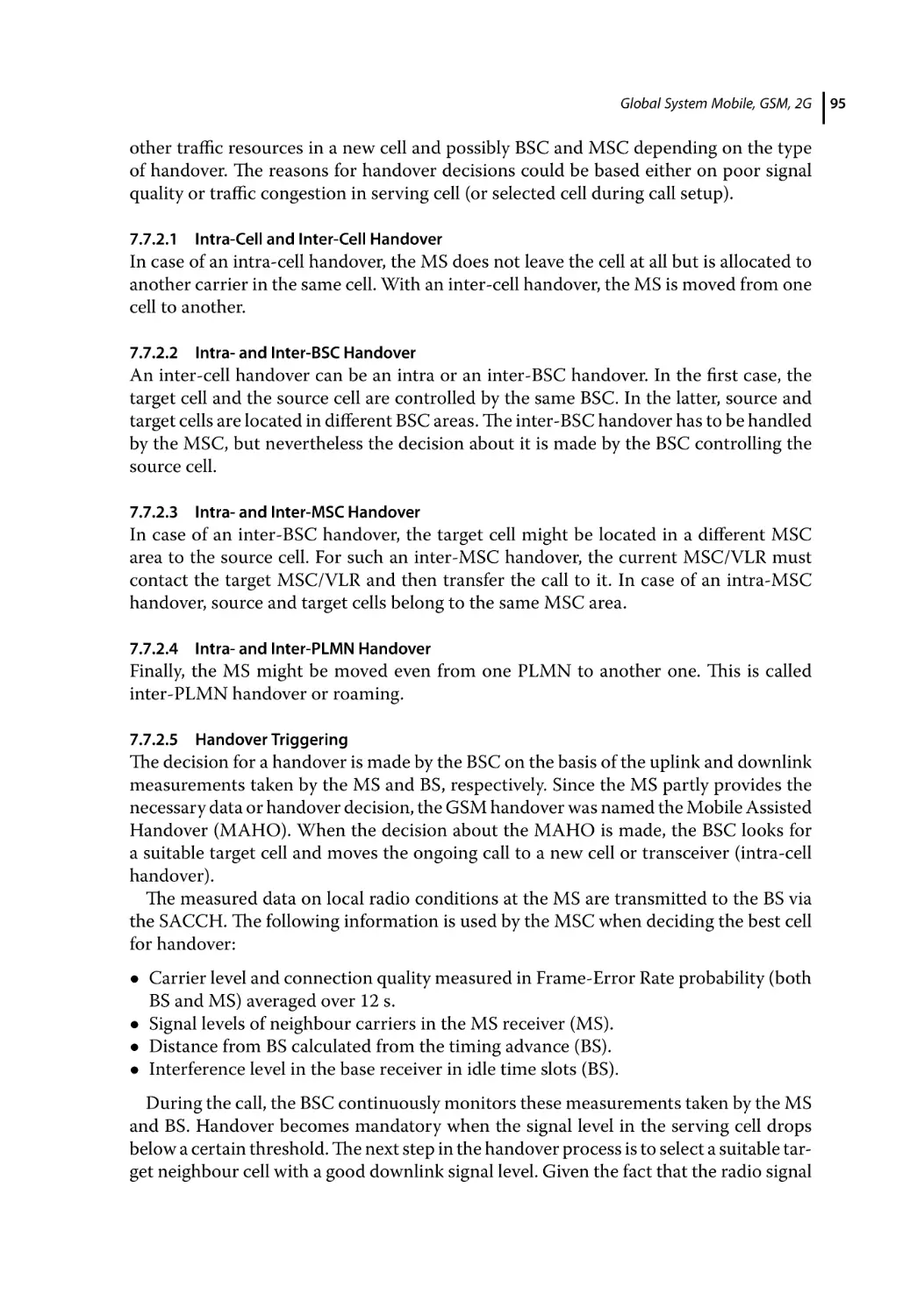
Handover Triggering 95
Power Control 96
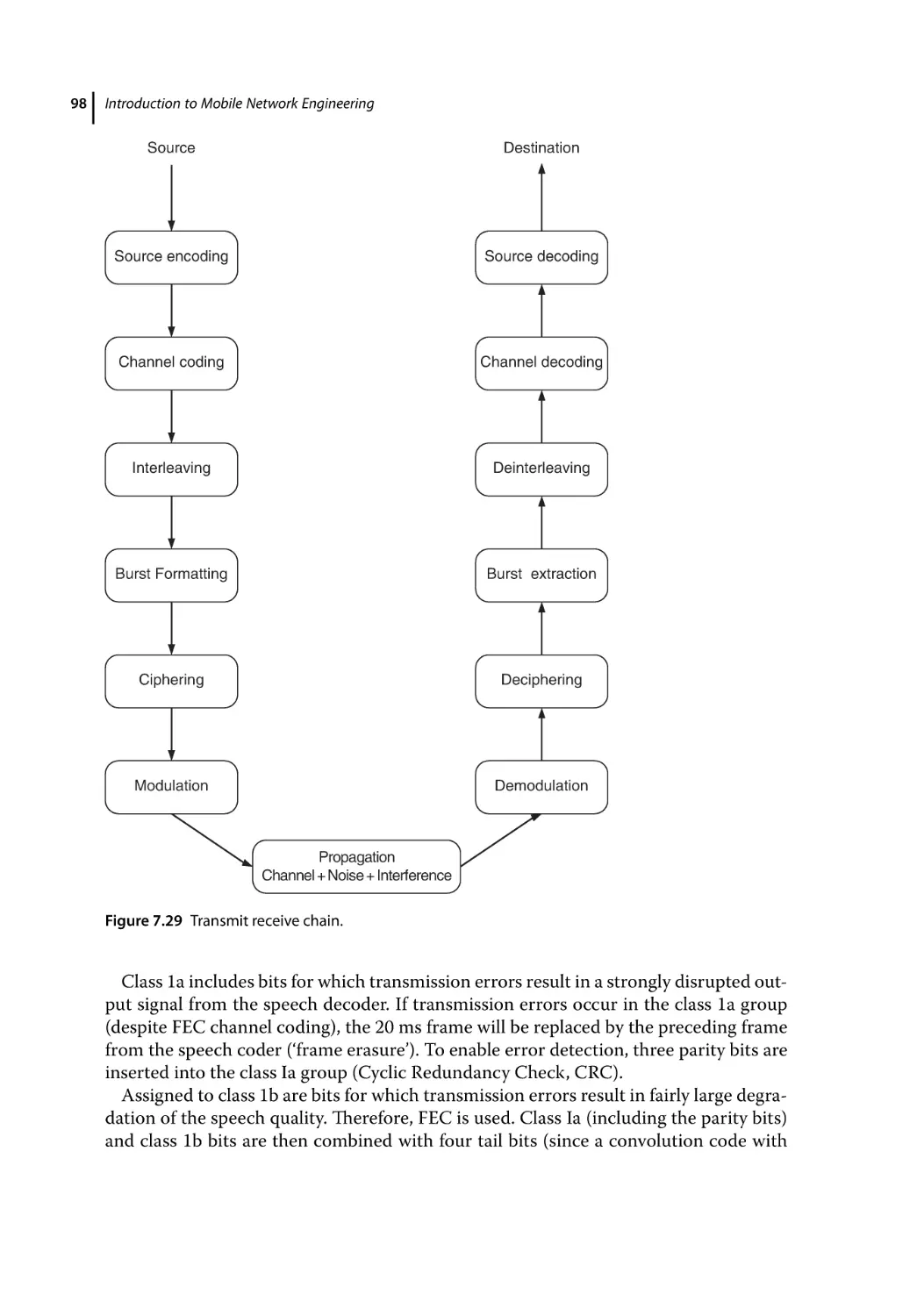
Signal Processing Chain 97
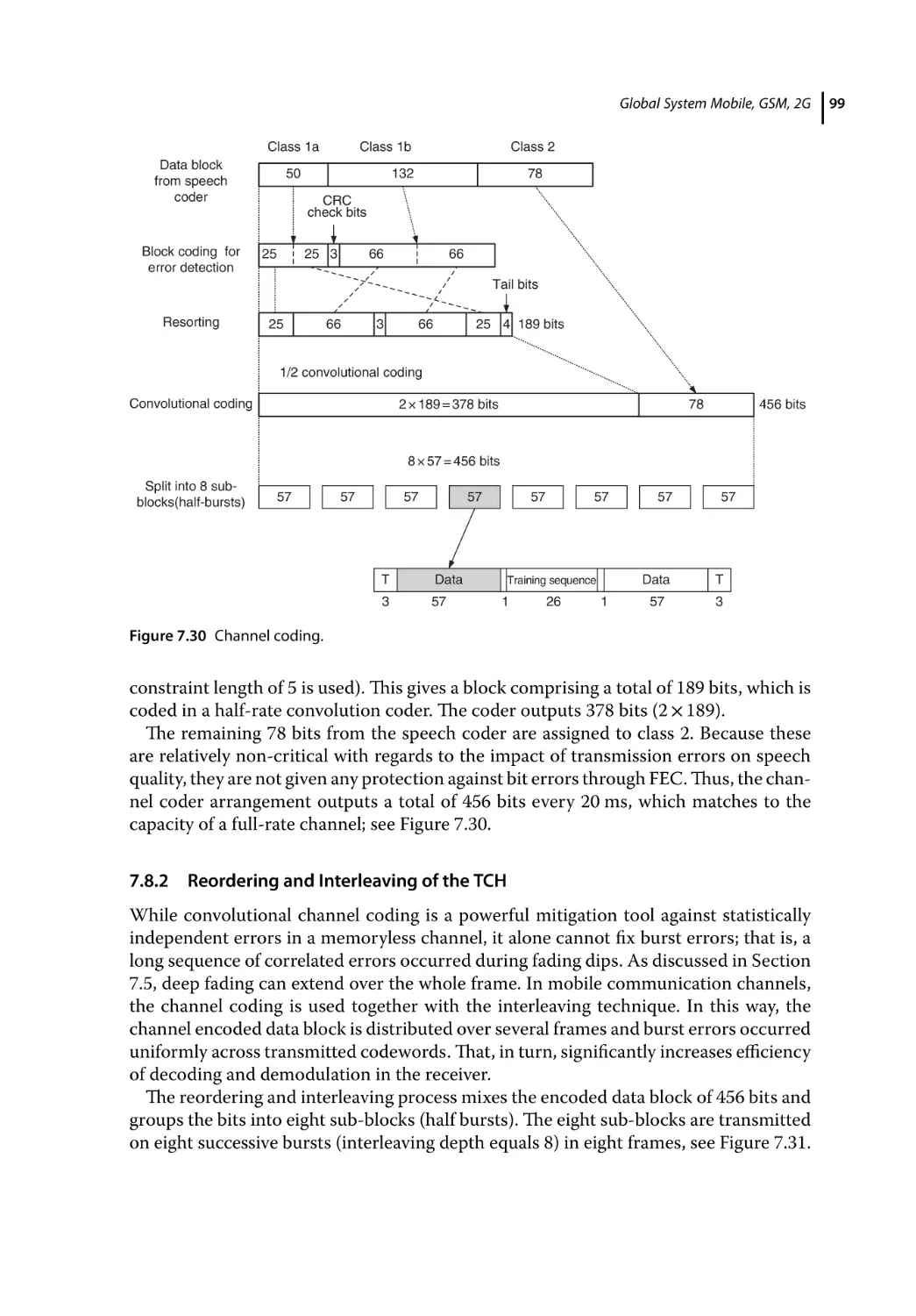
Speech and Channel Coding 97
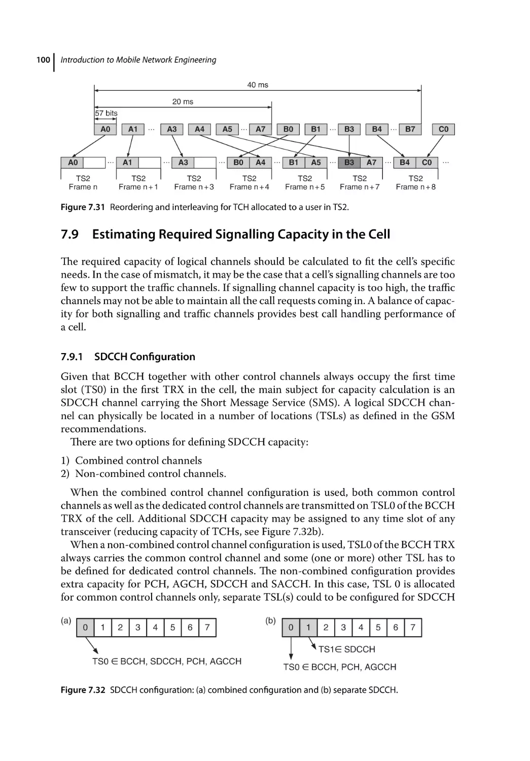
Reordering and Interleaving of the TCH 99
Estimating Required Signalling Capacity in the Cell 100
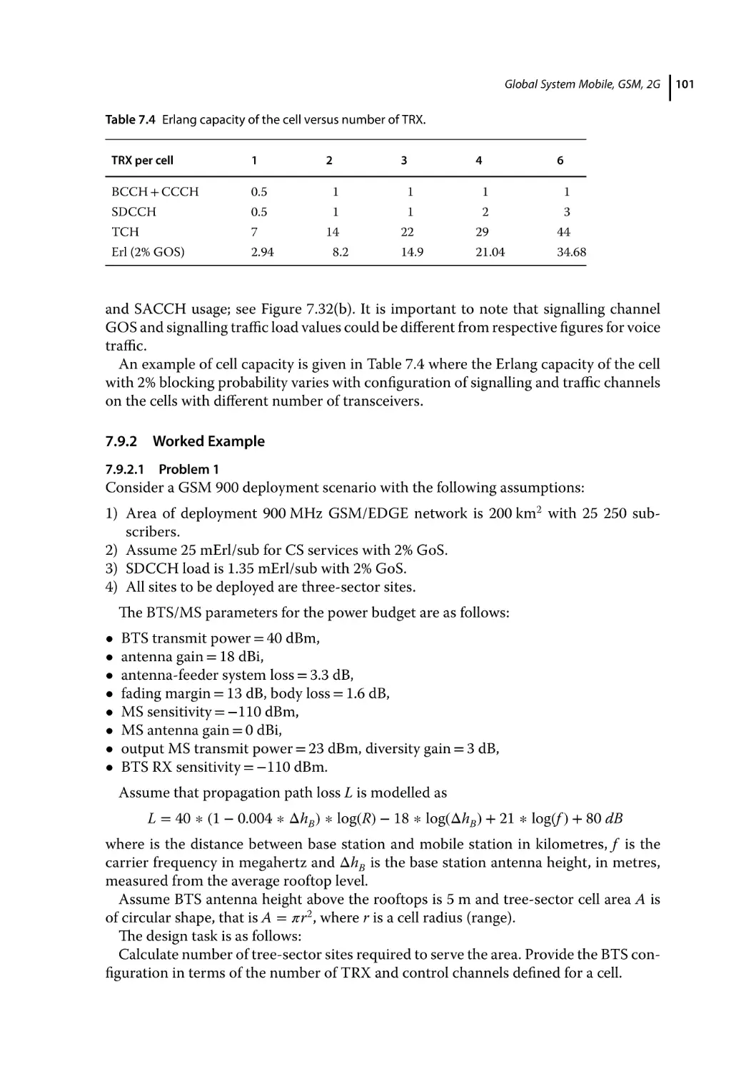
SDCCH Configuration 100
ix
x
Contents
7.9.2
7.9.2.1
Worked Example 101
Problem 1 101
References 102
8
8.1
8.2
8.3
8.4
8.4.1
8.4.1.1
8.4.1.2
8.4.1.3
8.4.2
8.4.3
8.5
8.5.1
8.5.2
8.5.3
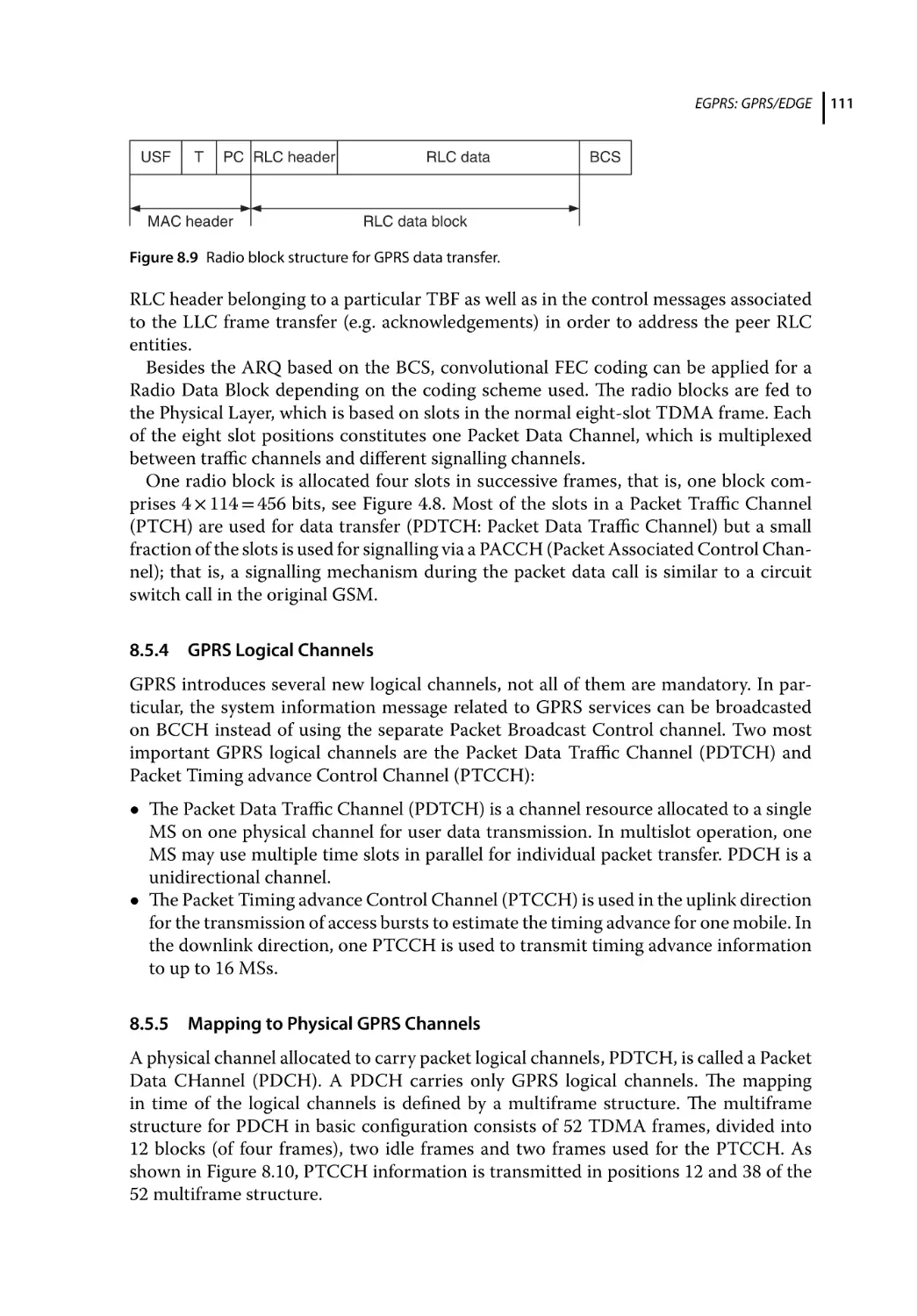
8.5.3.1
8.5.4
8.5.5
8.5.6
8.5.6.1
8.5.6.2
8.5.7
8.5.7.1
8.5.7.2
8.5.8
8.6
8.6.1
8.7
103
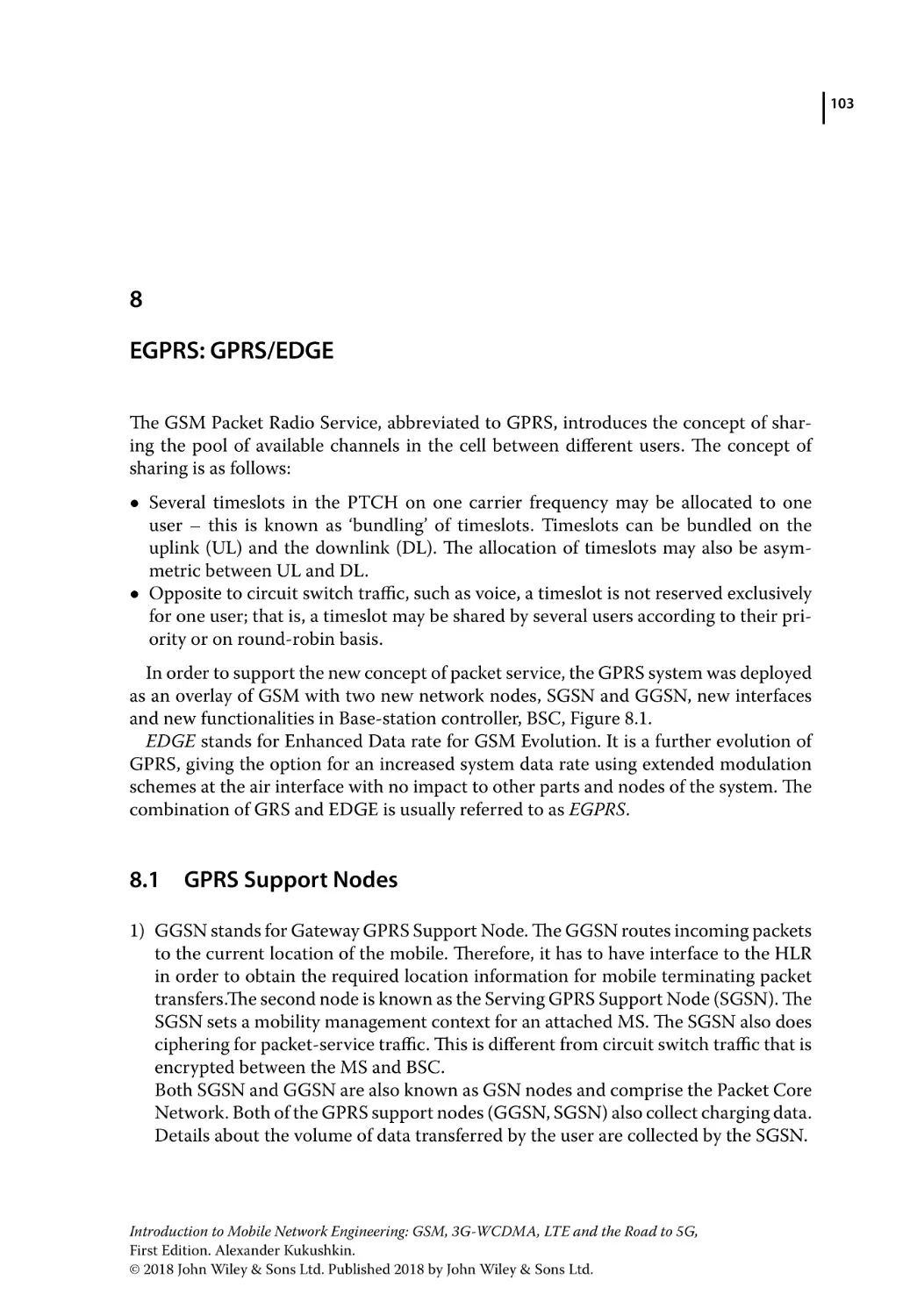
GPRS Support Nodes 103
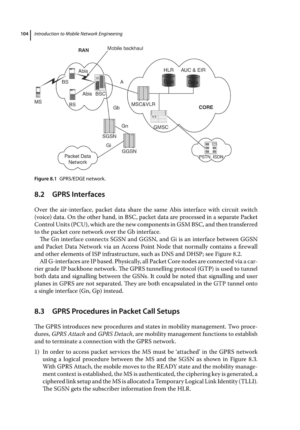
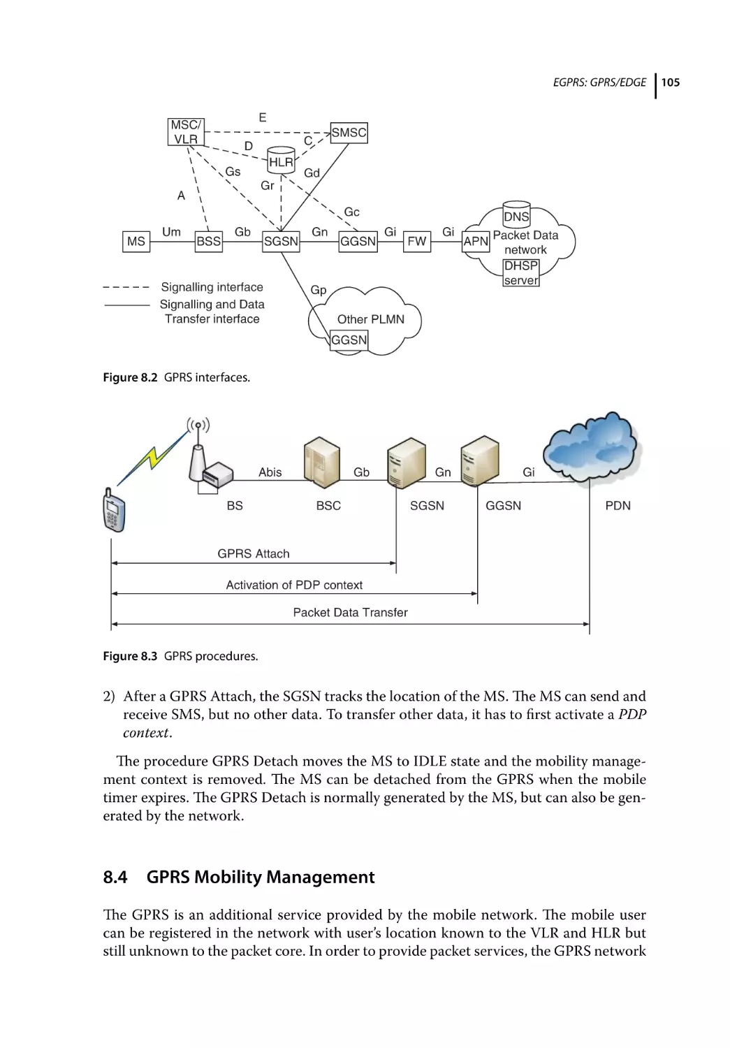
GPRS Interfaces 104
GPRS Procedures in Packet Call Setups 104
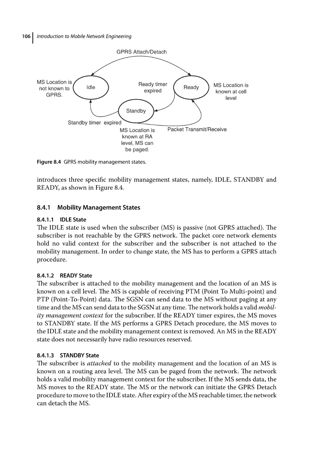
GPRS Mobility Management 105
Mobility Management States 106
IDLE State 106
READY State 106
STANDBY State 106
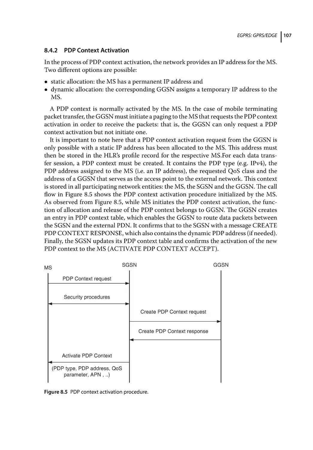
PDP Context Activation 107
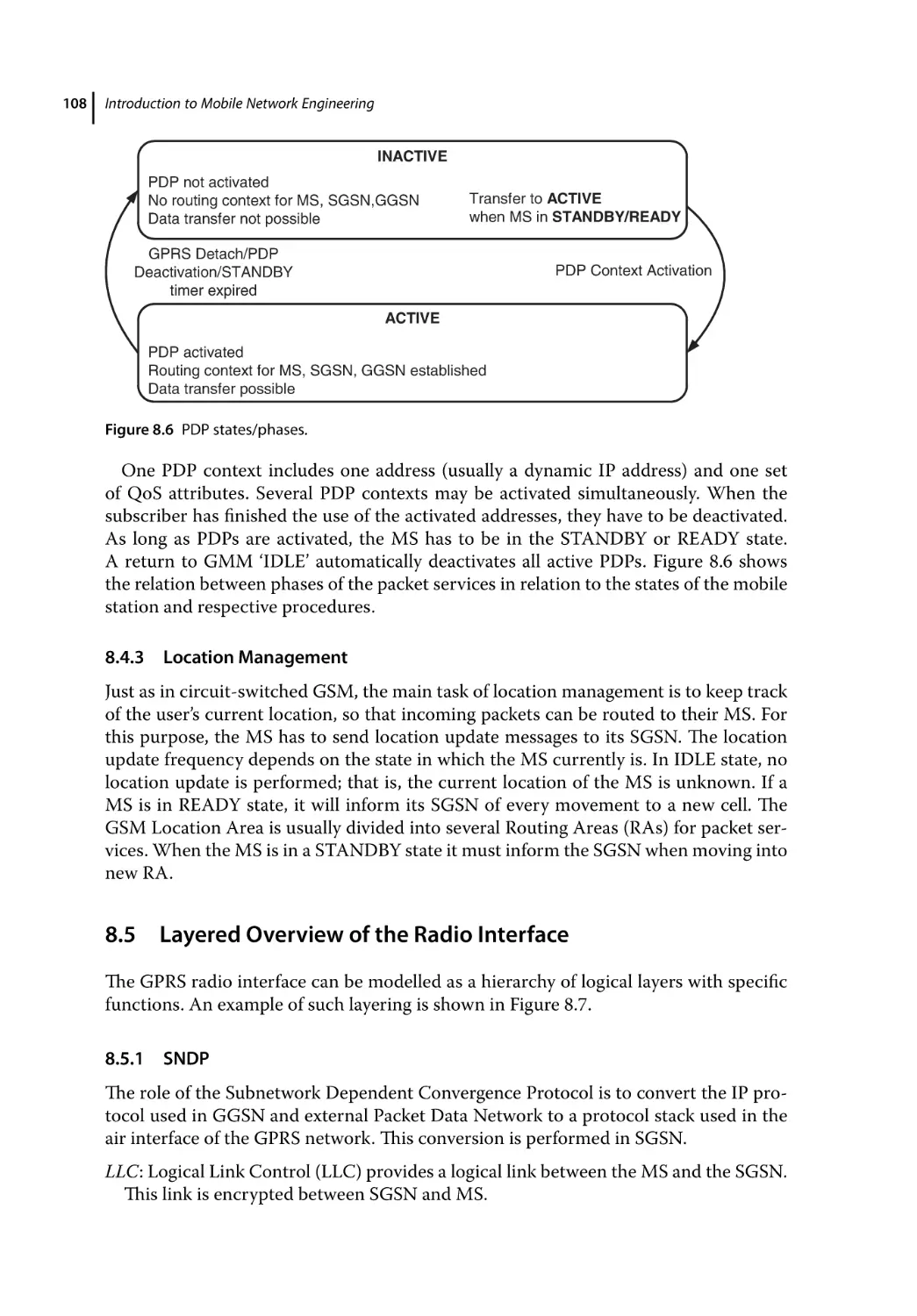
Location Management 108
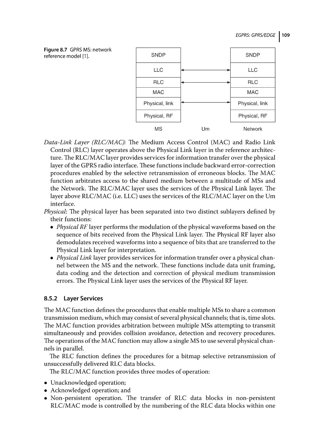
Layered Overview of the Radio Interface 108
SNDP 108
Layer Services 109
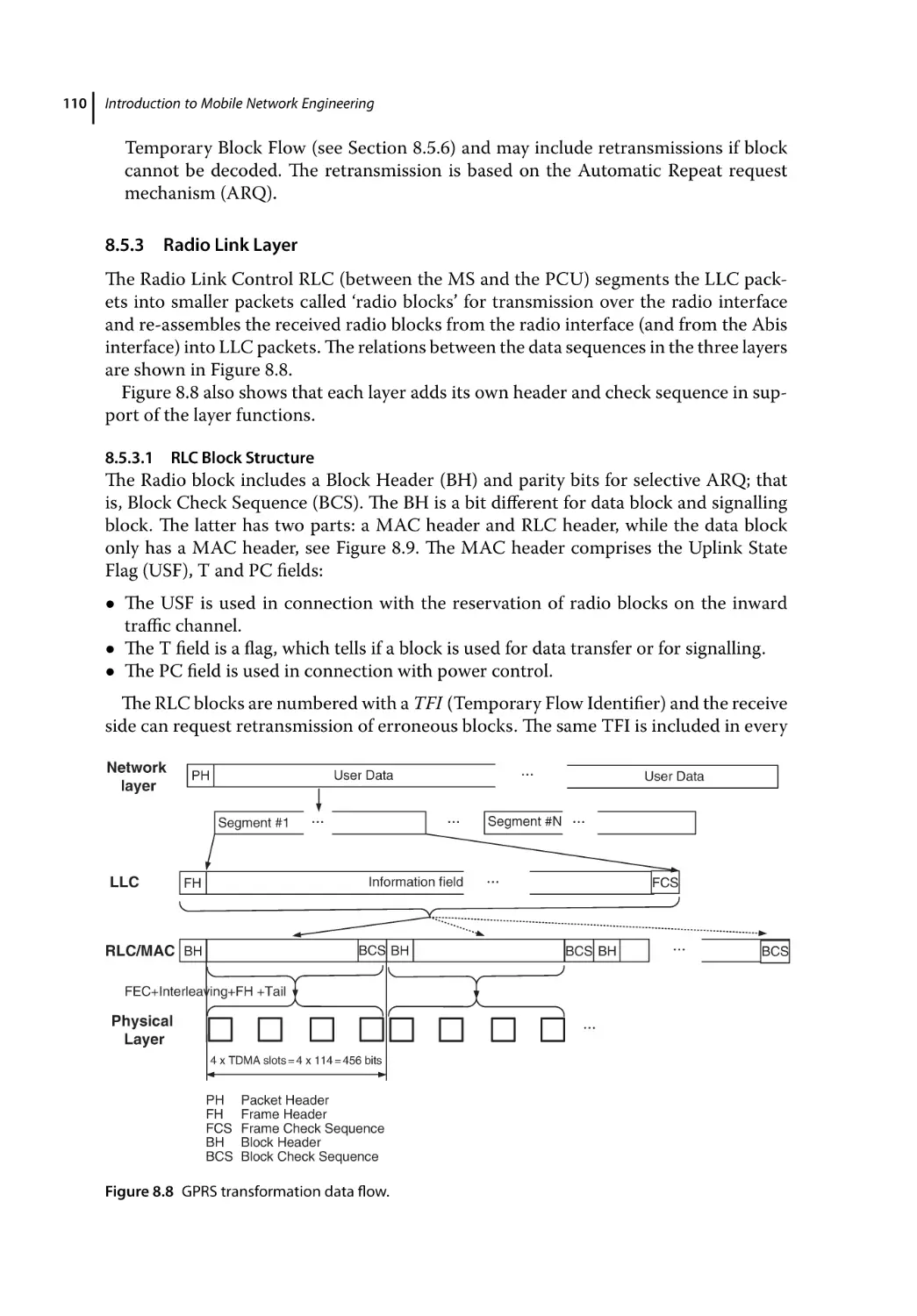
Radio Link Layer 110
RLC Block Structure 110
GPRS Logical Channels 111
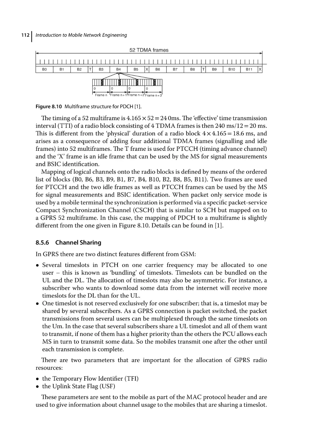
Mapping to Physical GPRS Channels 111
Channel Sharing 112
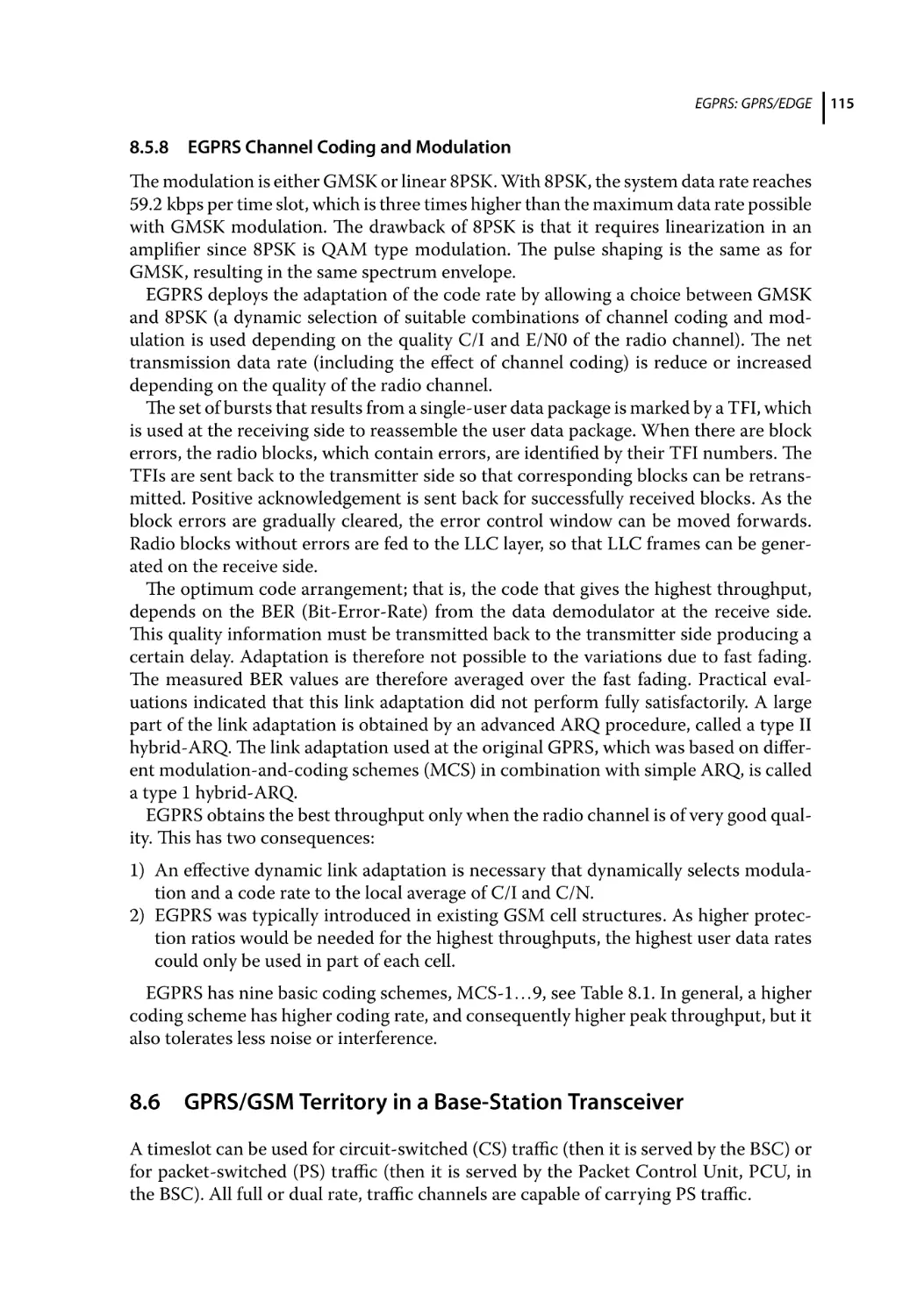
Downlink Radio Channel 113
Uplink Radio Channel 113
TBF 113
TBF Establishment 113
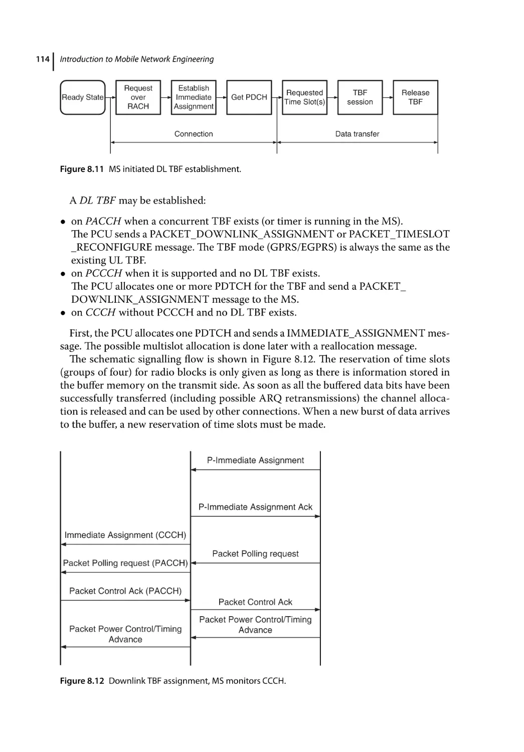
DL TBF Establishment 113
EGPRS Channel Coding and Modulation 115
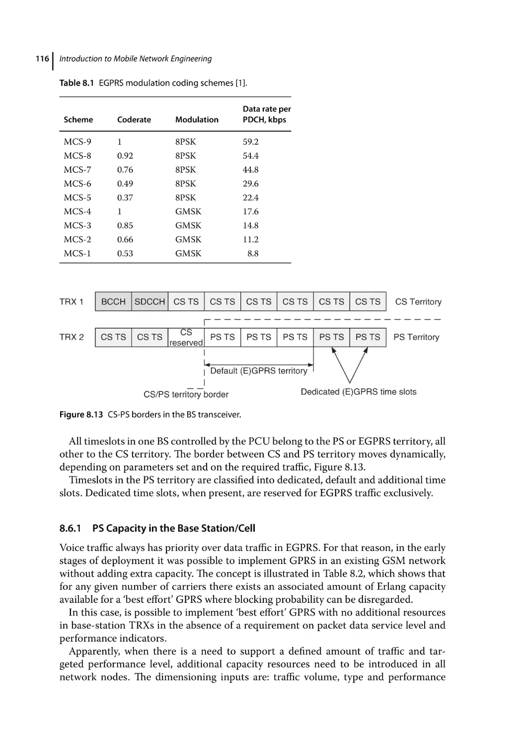
GPRS/GSM Territory in a Base-Station Transceiver 115
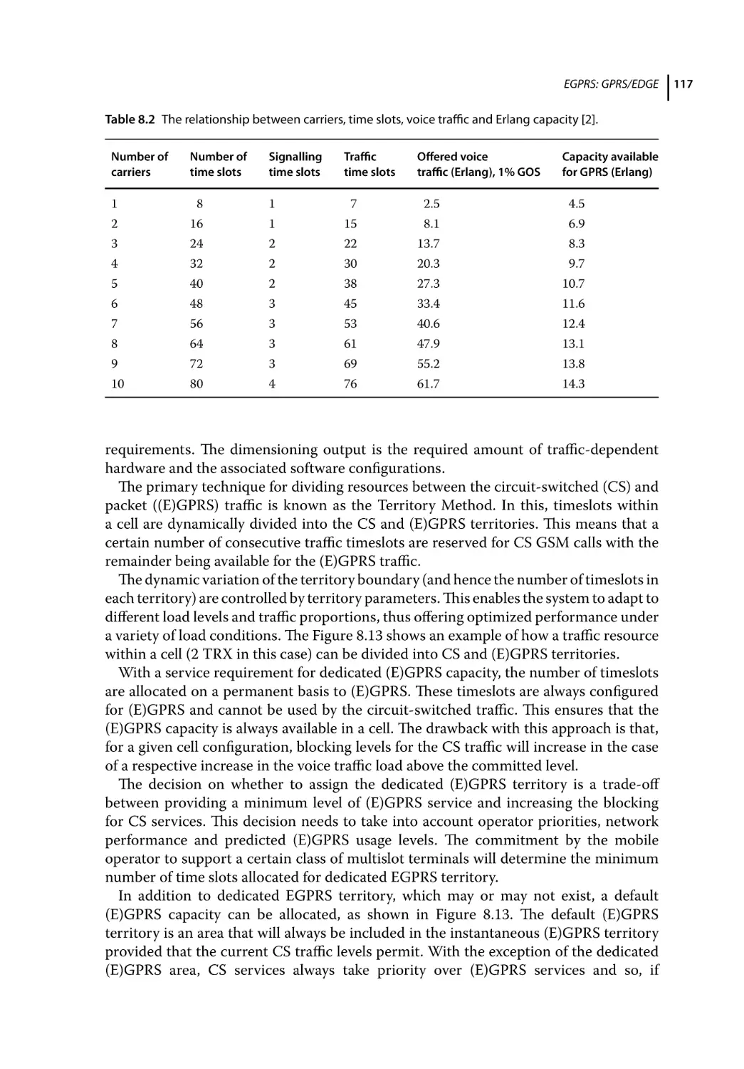
PS Capacity in the Base Station/Cell 116
Summary 118
References 119
9
Third Generation Network (3G), UMTS 121
9.1
9.1.1
9.1.2
9.1.3
9.1.4
9.1.4.1
9.1.4.2
9.1.5
9.1.5.1
9.1.5.2
9.1.5.3
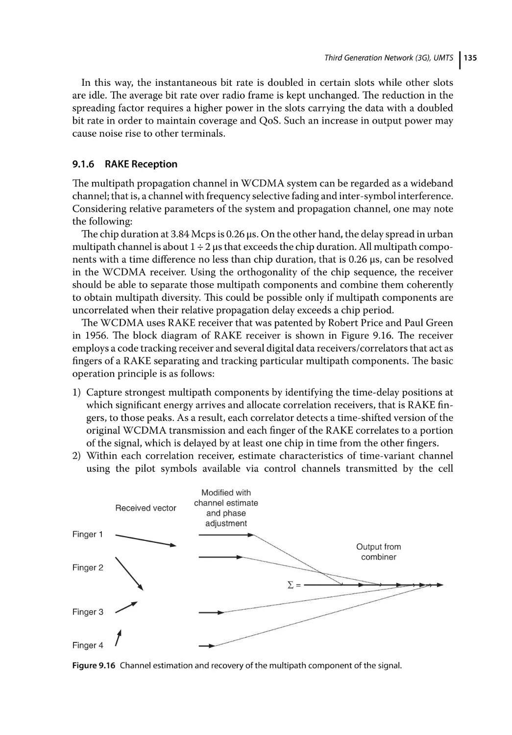
9.1.6
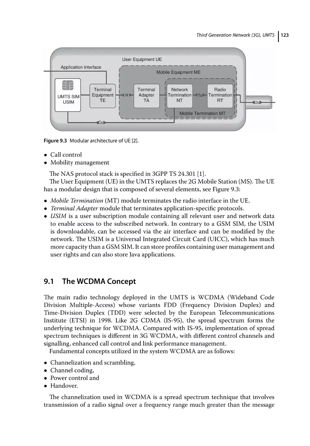
The WCDMA Concept 123
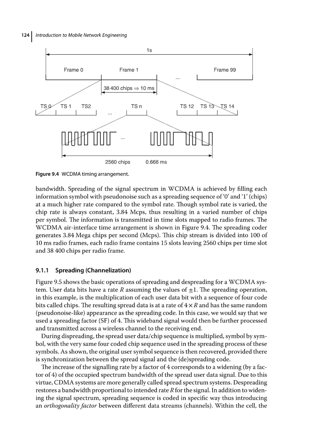
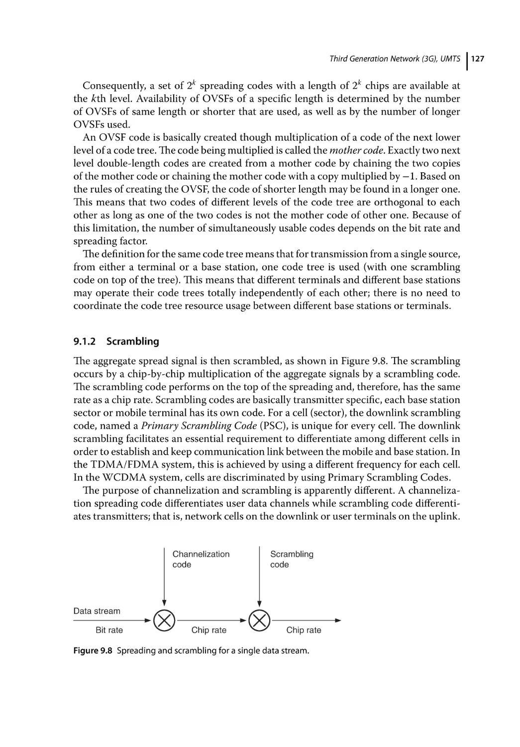
Spreading (Channelization) 124
Scrambling 127
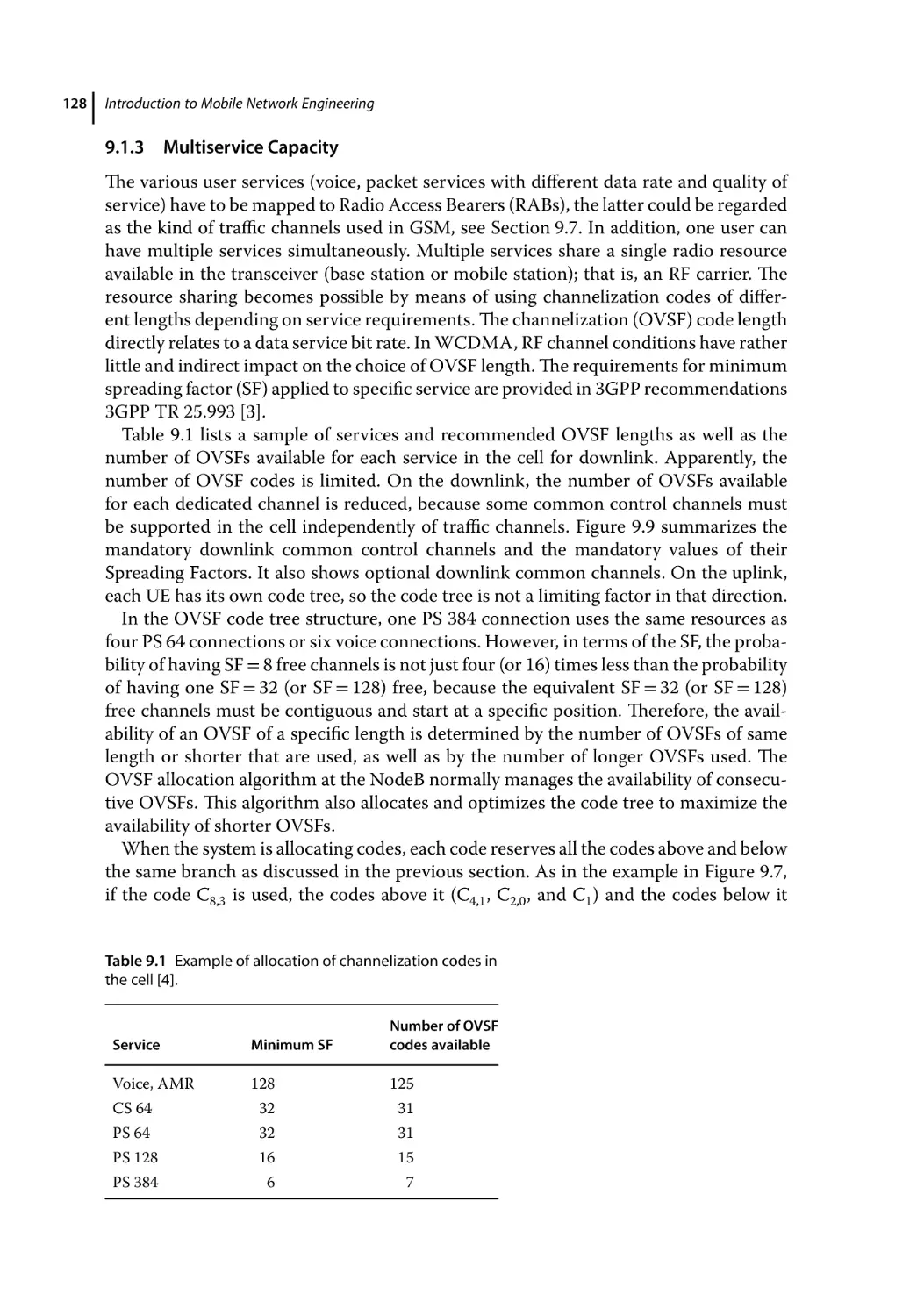
Multiservice Capacity 128
Power Control 129
Open-Loop Power Control 130
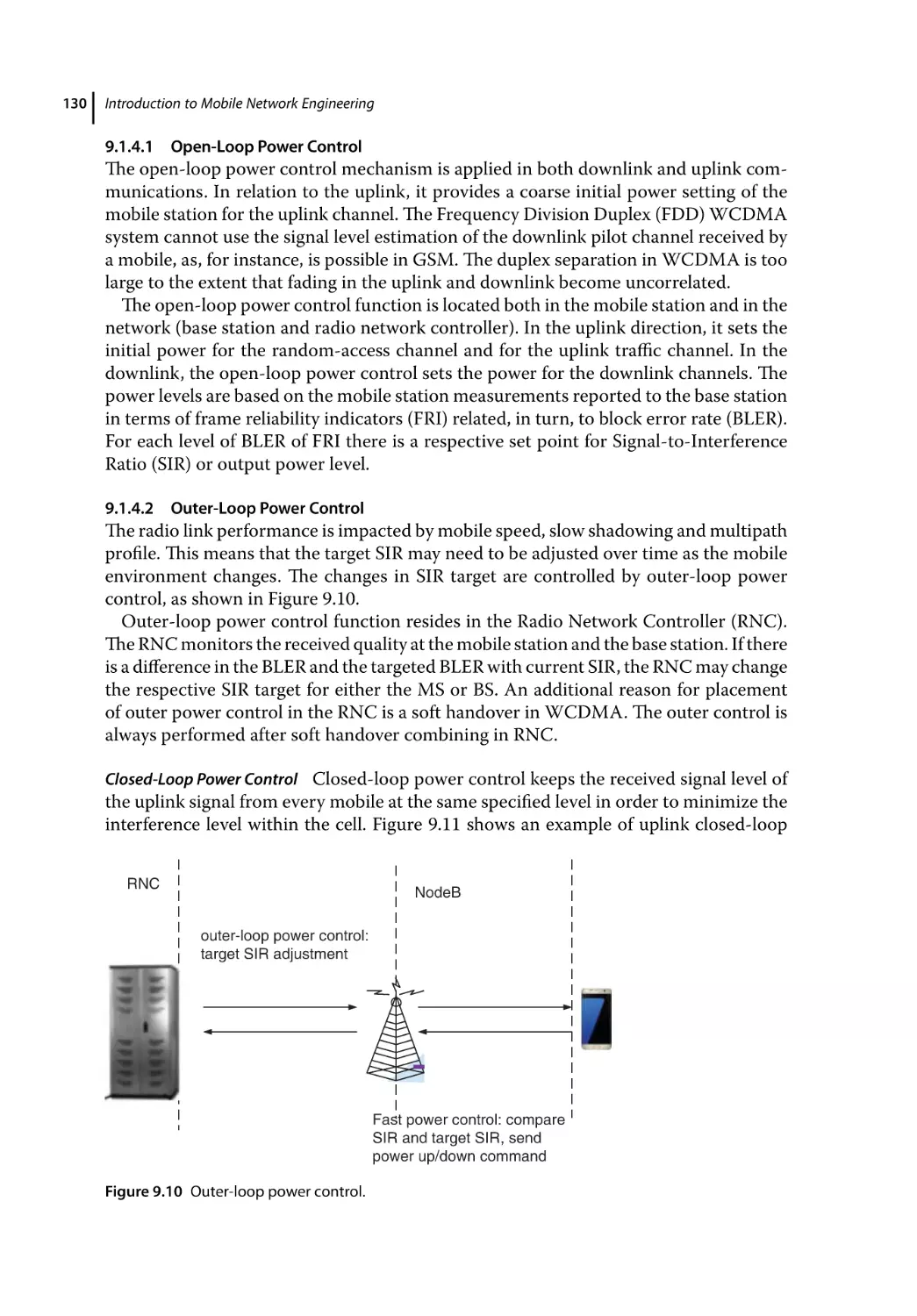
Outer-Loop Power Control 130
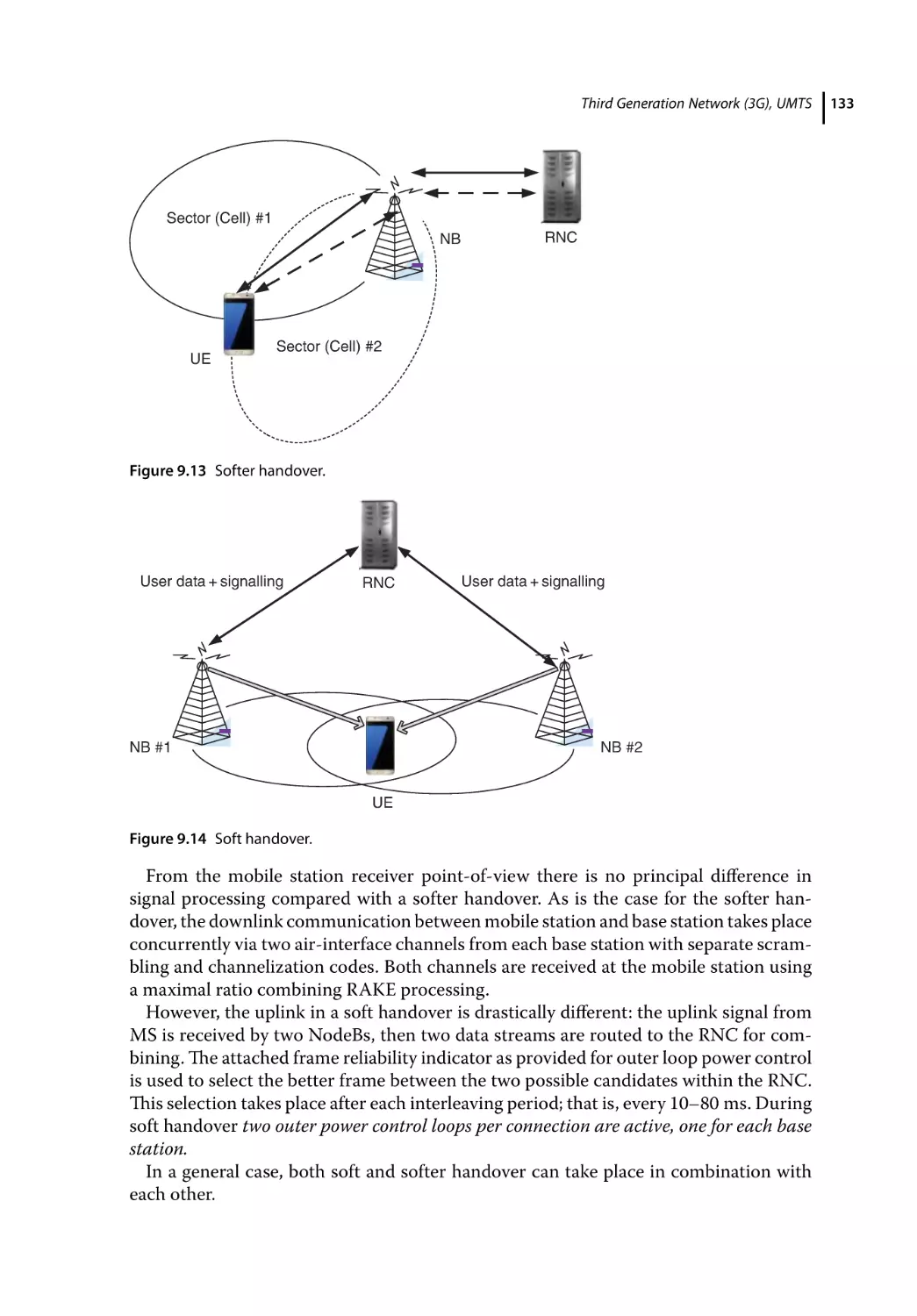
Handover 132
Softer Handover 132
Other Handovers 134
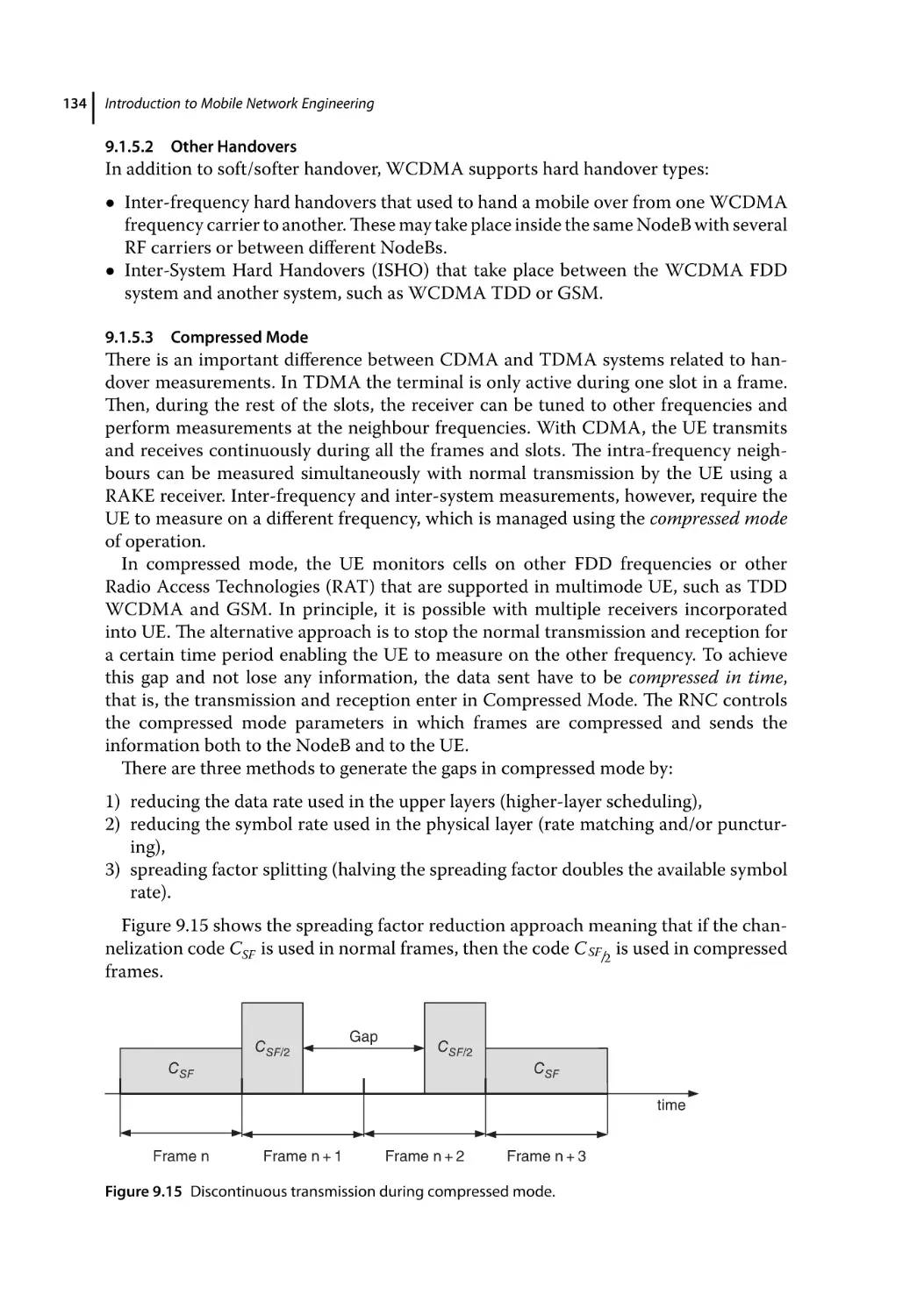
Compressed Mode 134
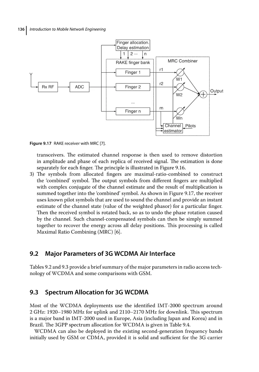
RAKE Reception 135
EGPRS: GPRS/EDGE
Contents
9.2
9.3
9.4
9.4.1
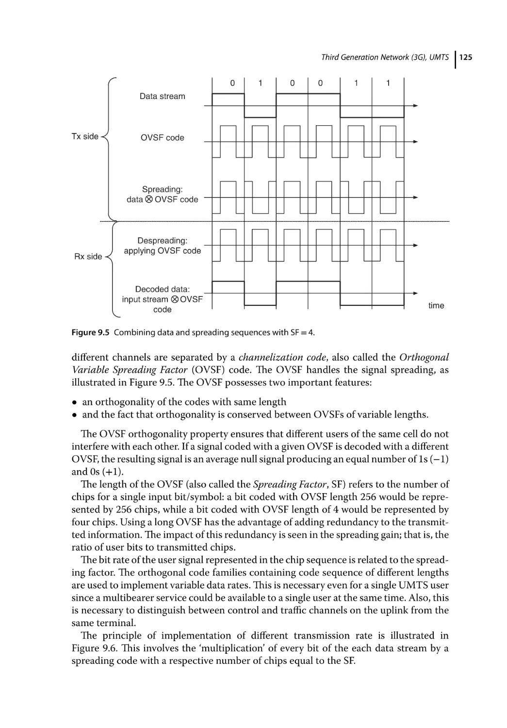
9.5
9.5.1
9.5.2
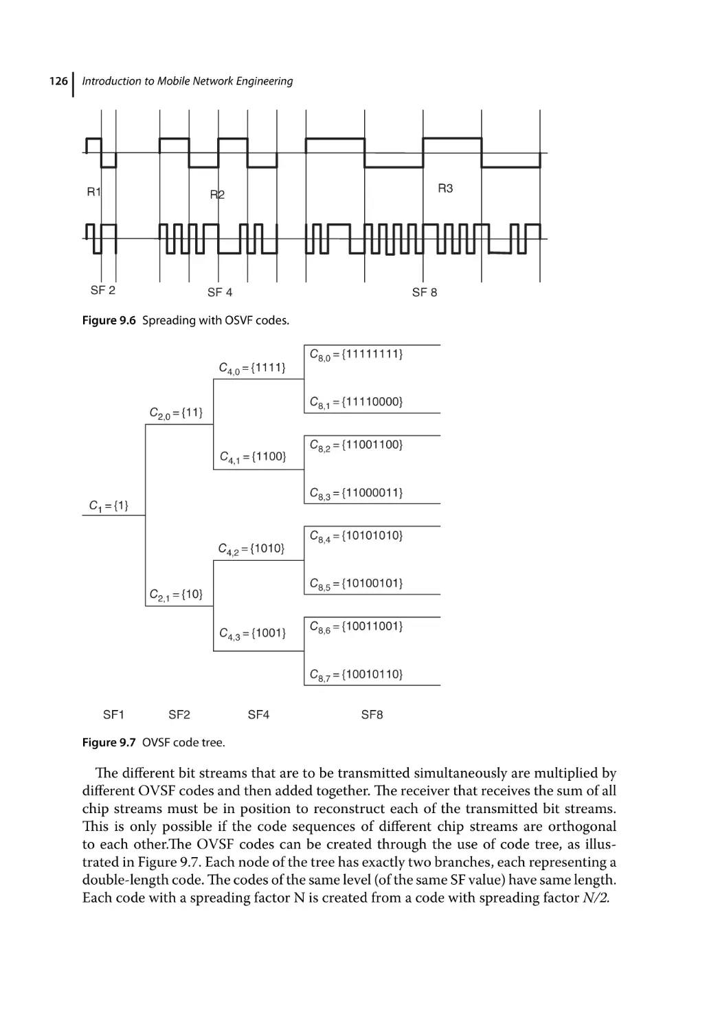
9.6
9.6.1
9.6.2
9.6.3
9.6.4
9.7
9.7.1
9.7.2
9.7.2.1
9.7.2.2
9.7.3
9.7.4
9.8
9.8.1
9.8.2
9.8.3
9.8.4
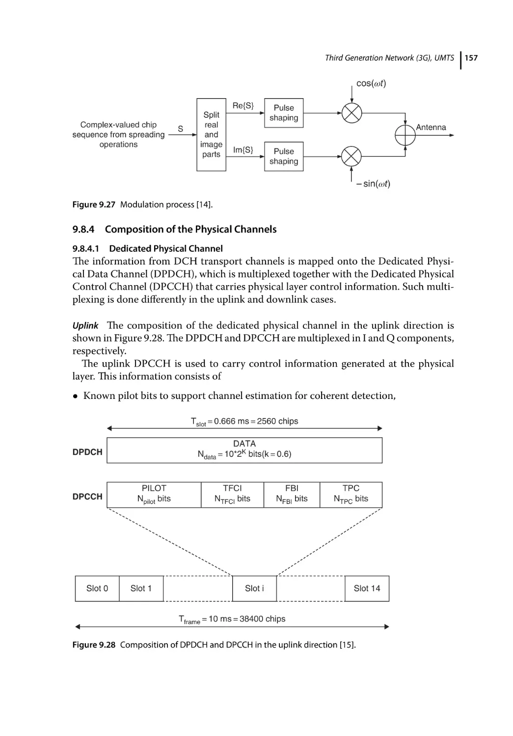
9.8.4.1
9.8.4.2
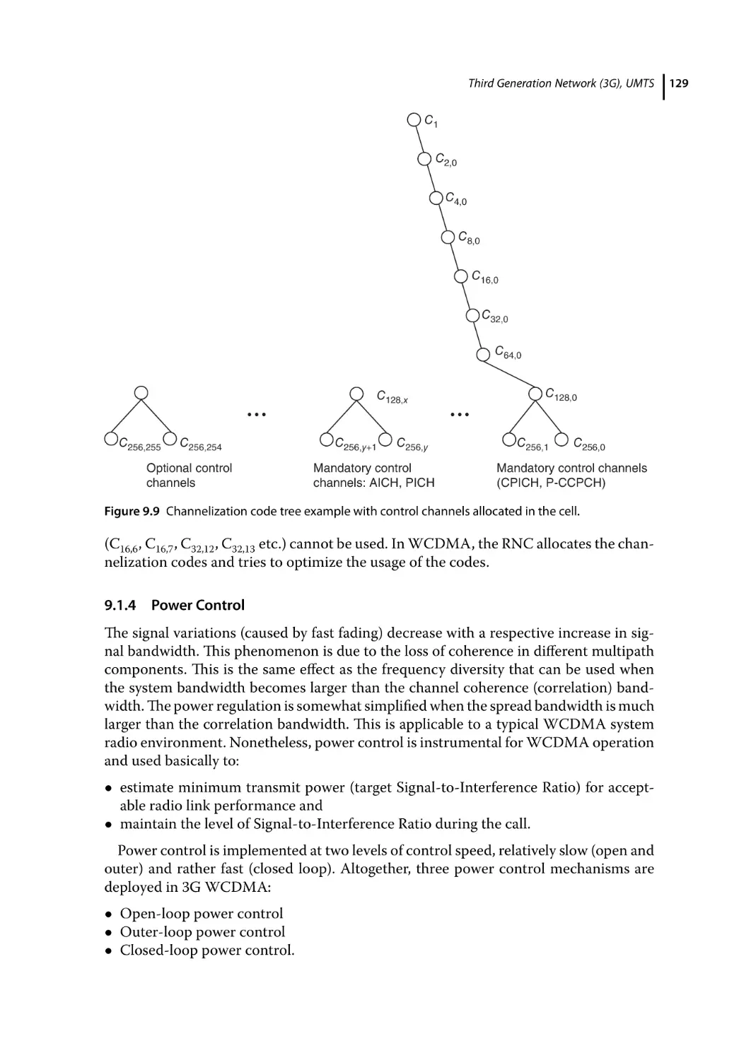
9.9
9.9.1
9.9.2
9.9.3
9.9.4
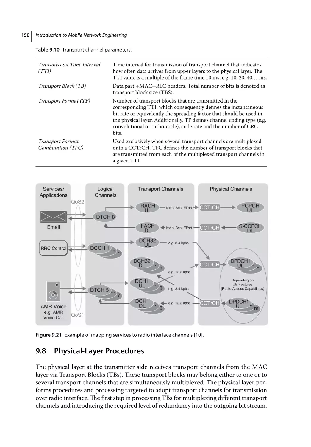
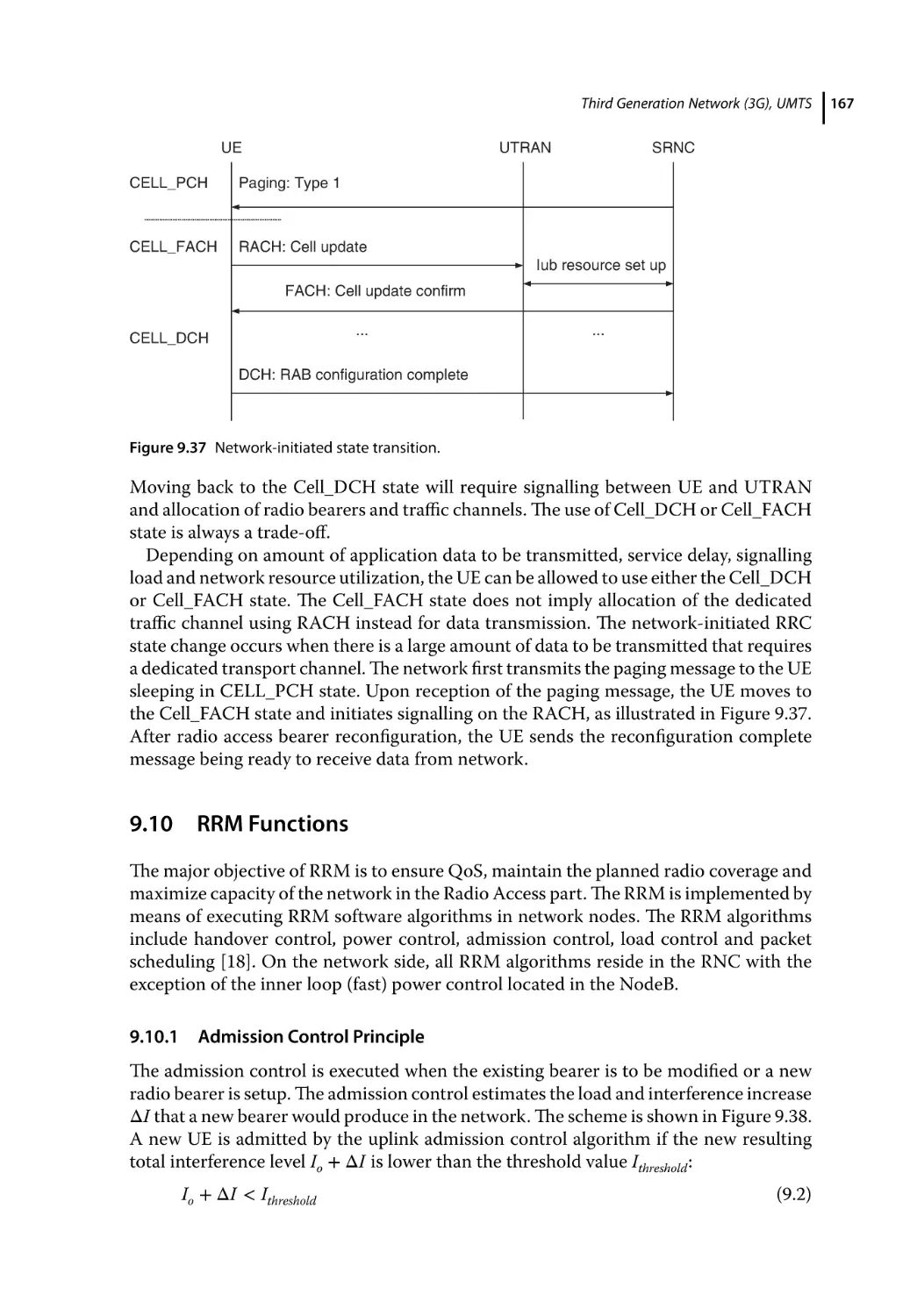
9.10
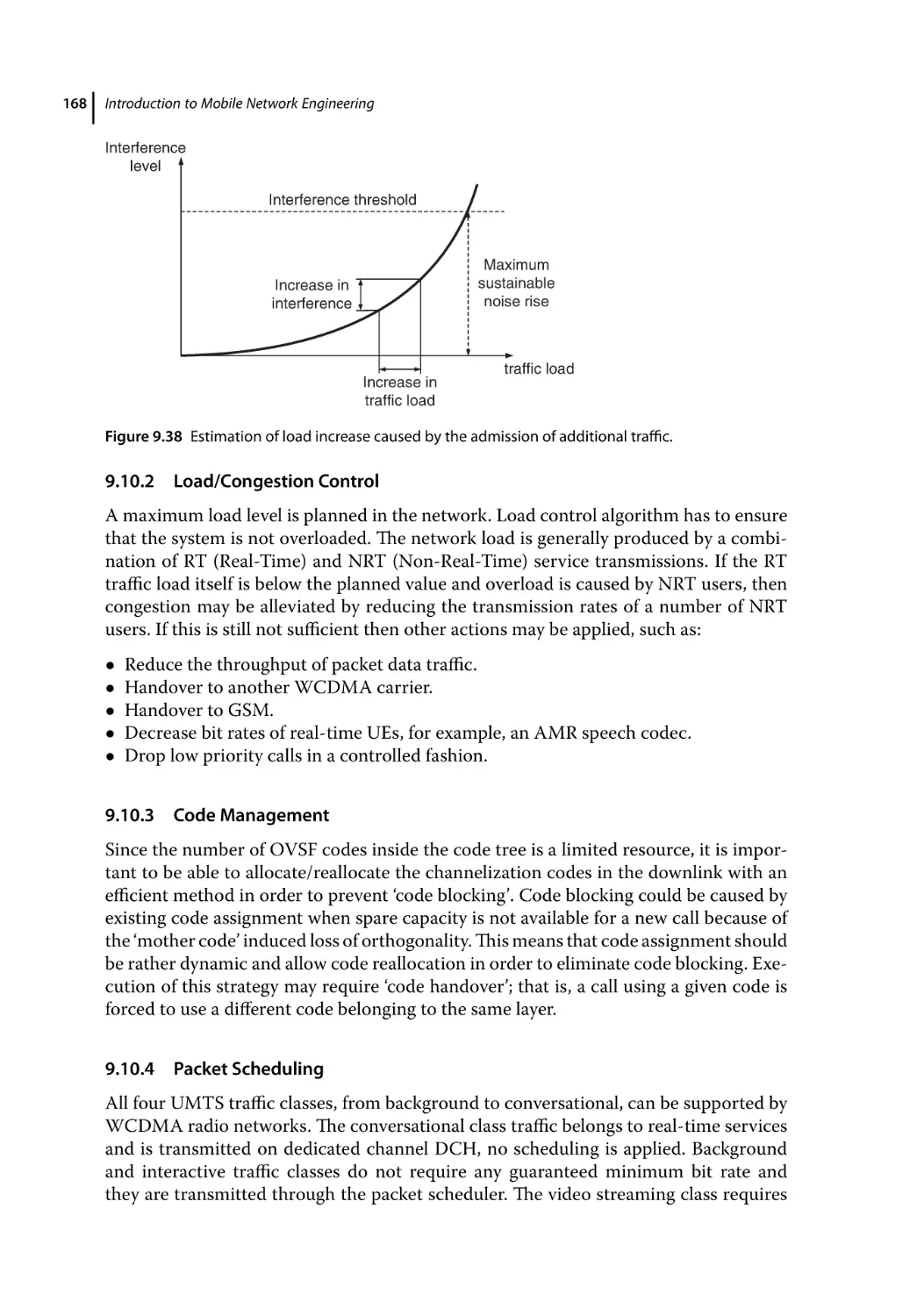
9.10.1
9.10.2
9.10.3
9.10.4
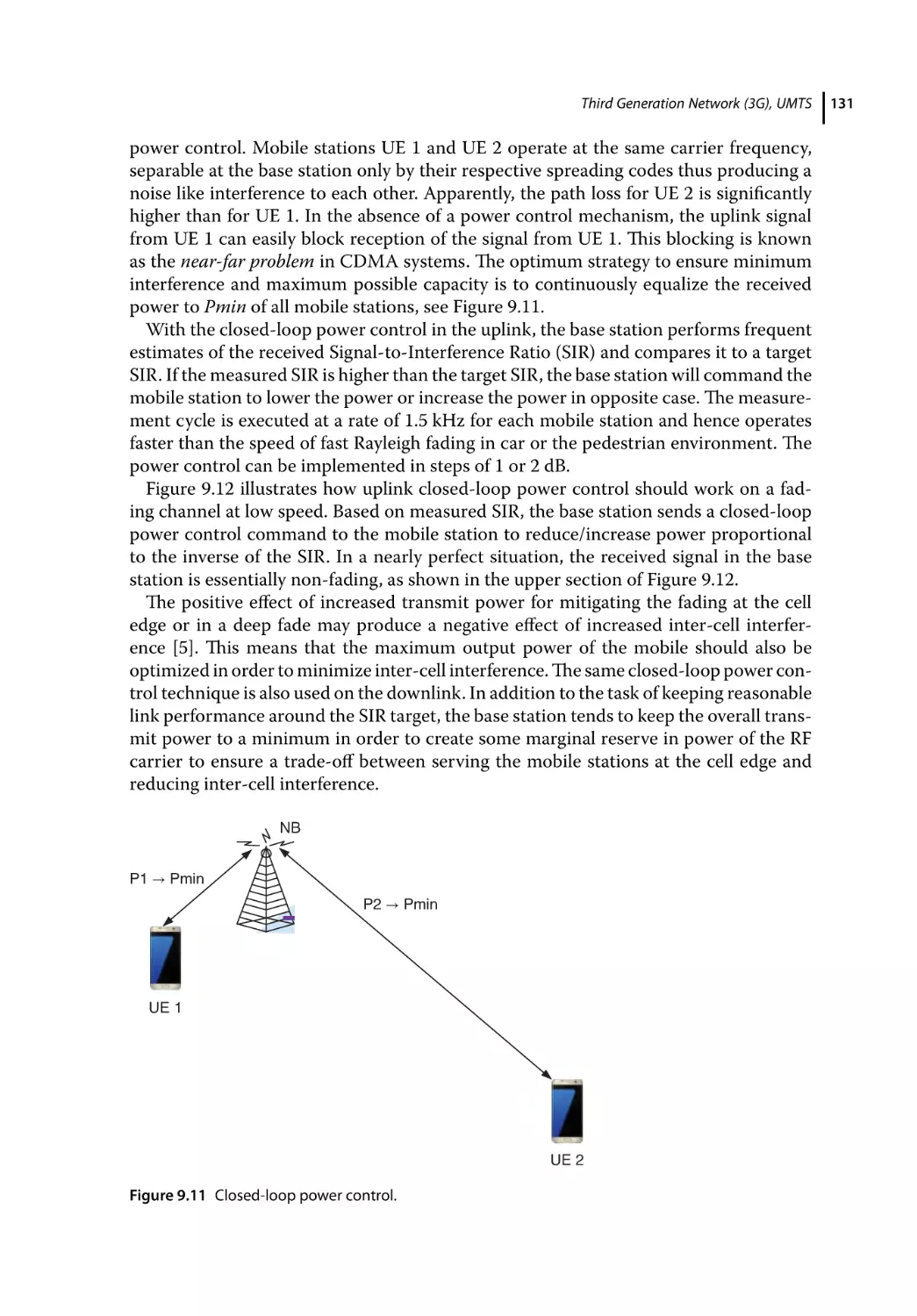
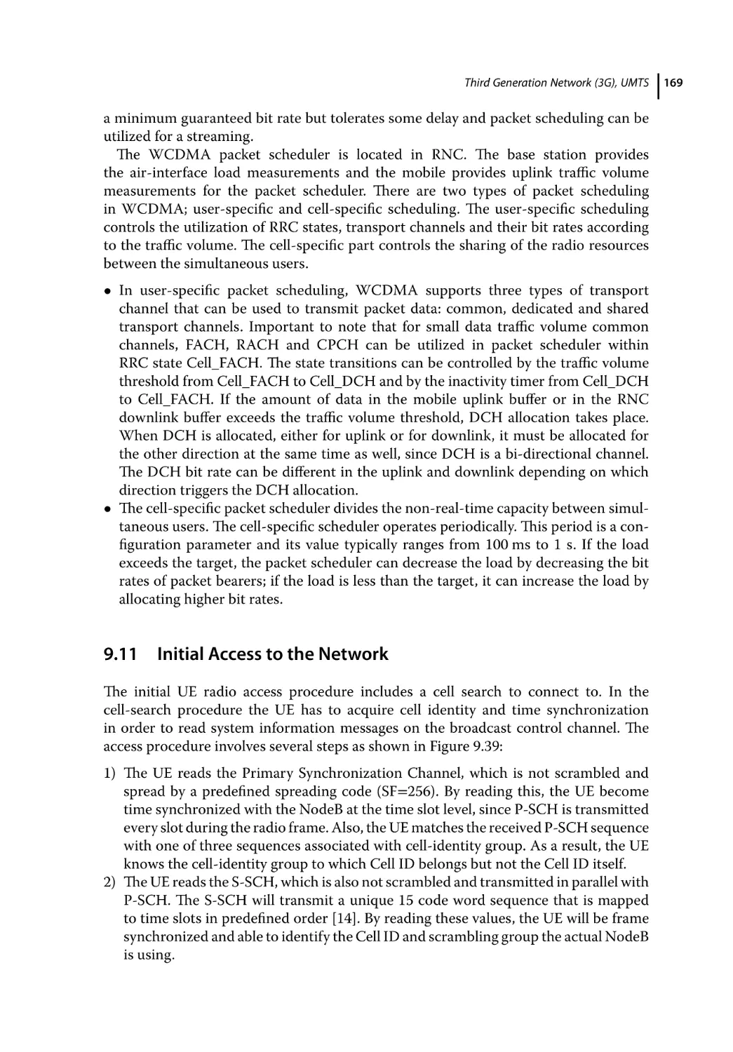
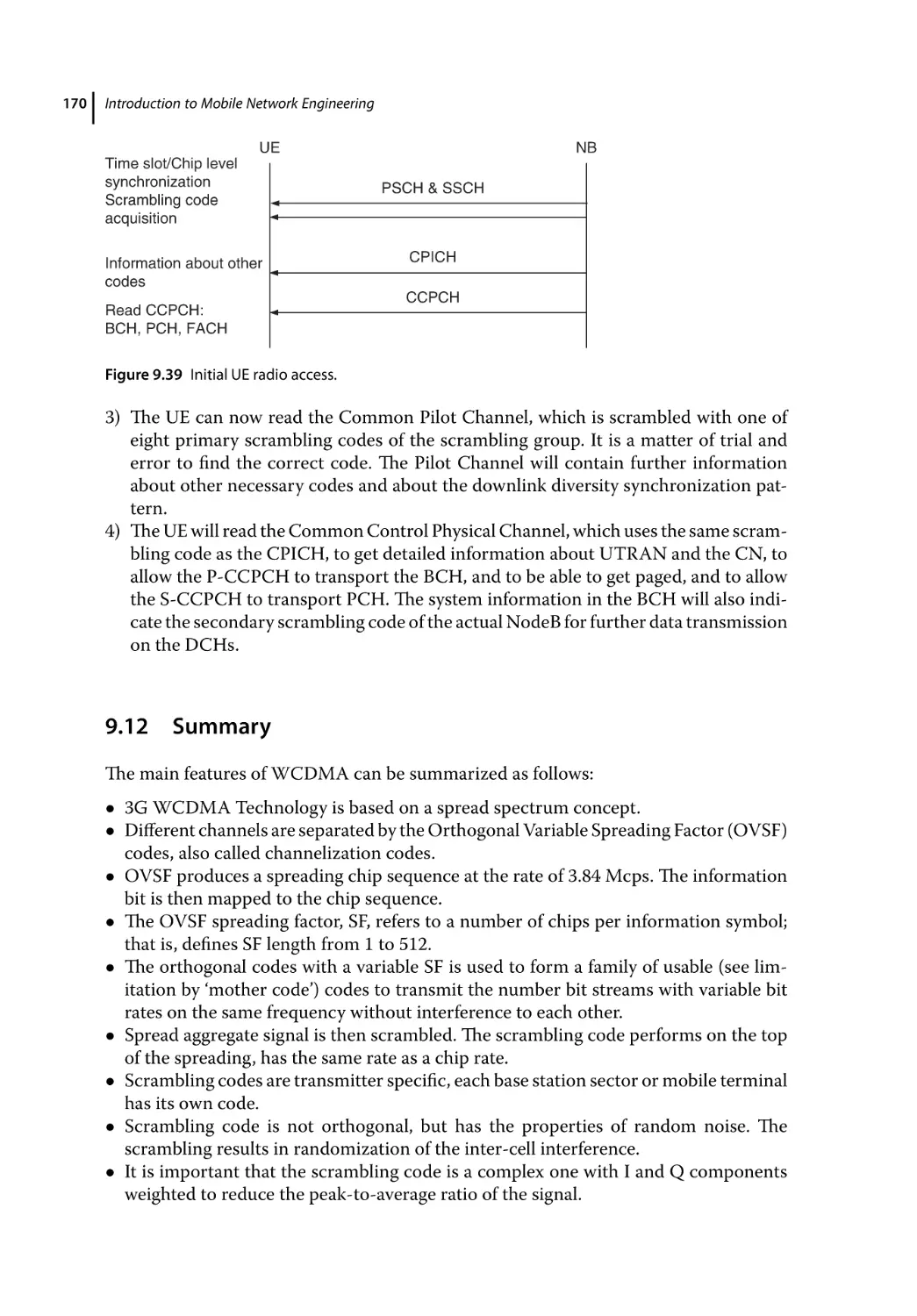
9.11
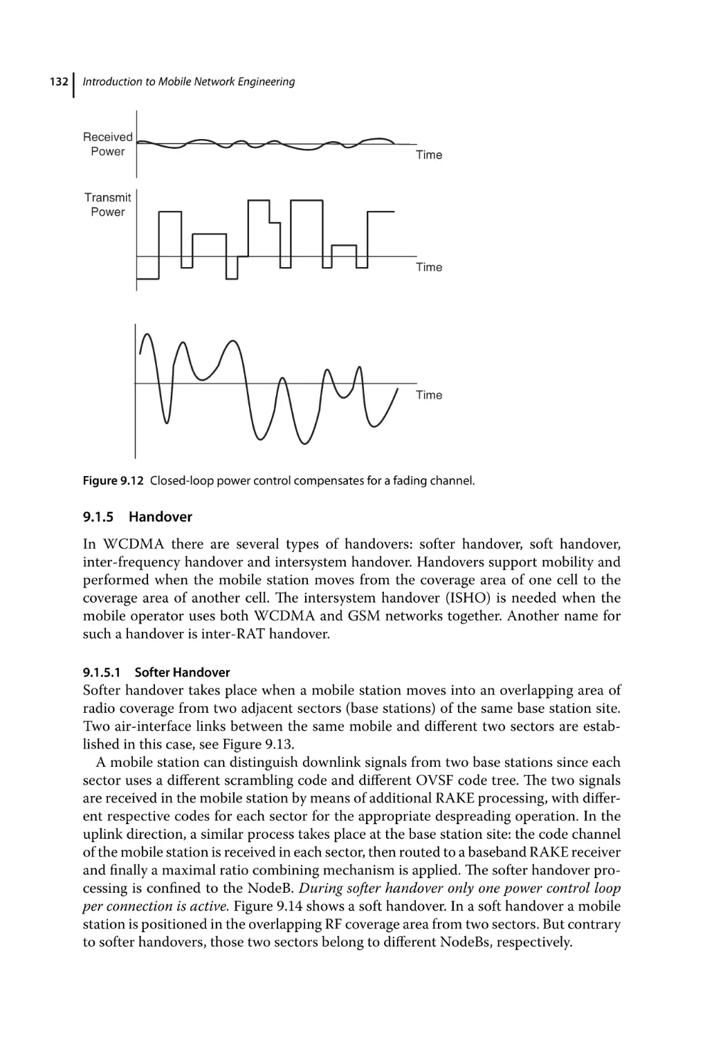
9.12
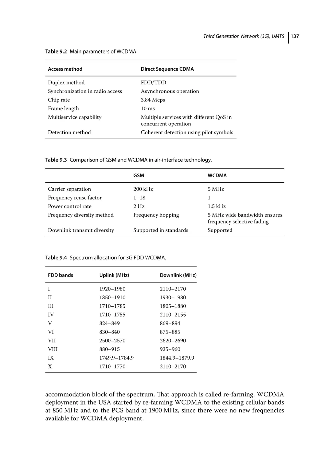
Major Parameters of 3G WCDMA Air Interface 136
Spectrum Allocation for 3G WCDMA 136
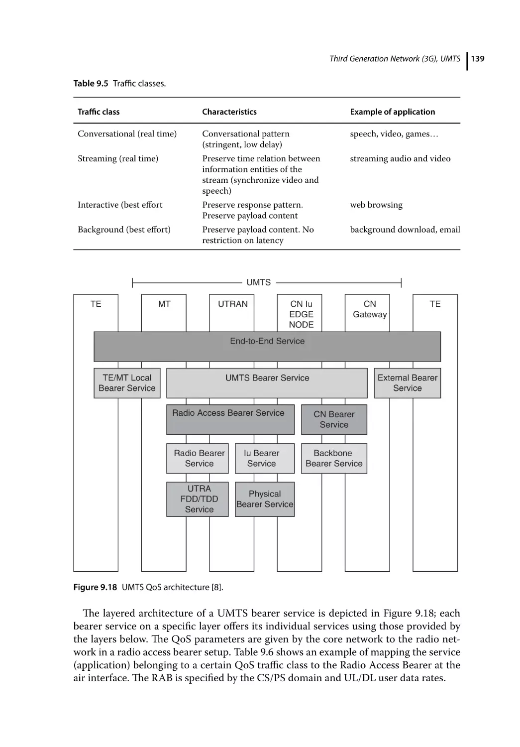
3G Services 138
Bearer Service and QoS 138
UMTS Reference Network Architecture and Interfaces 140
The NodeB (Base Station) Functions in the 3G Network 141
Role of the RNC in 3G Network 141
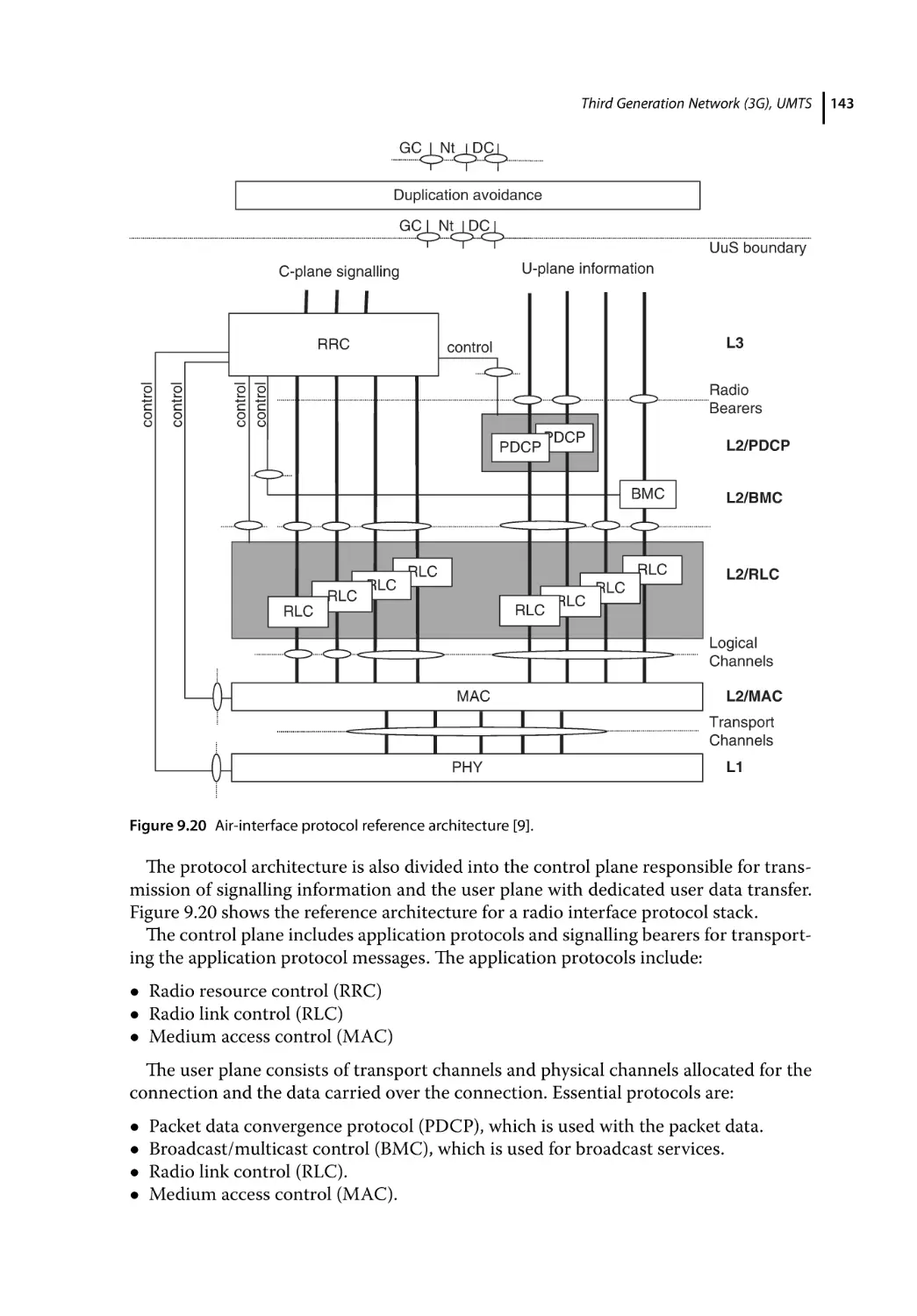
Air-Interface Architecture and Processing 142
Physical Layer (Layer 1) 144
Medium Access Control (MAC) on Layer 2 144
Radio Link Control (RLC) on Layer 2 145
RRC on Layer 3 in the Control Plane 145
Channels on the Air Interface 146
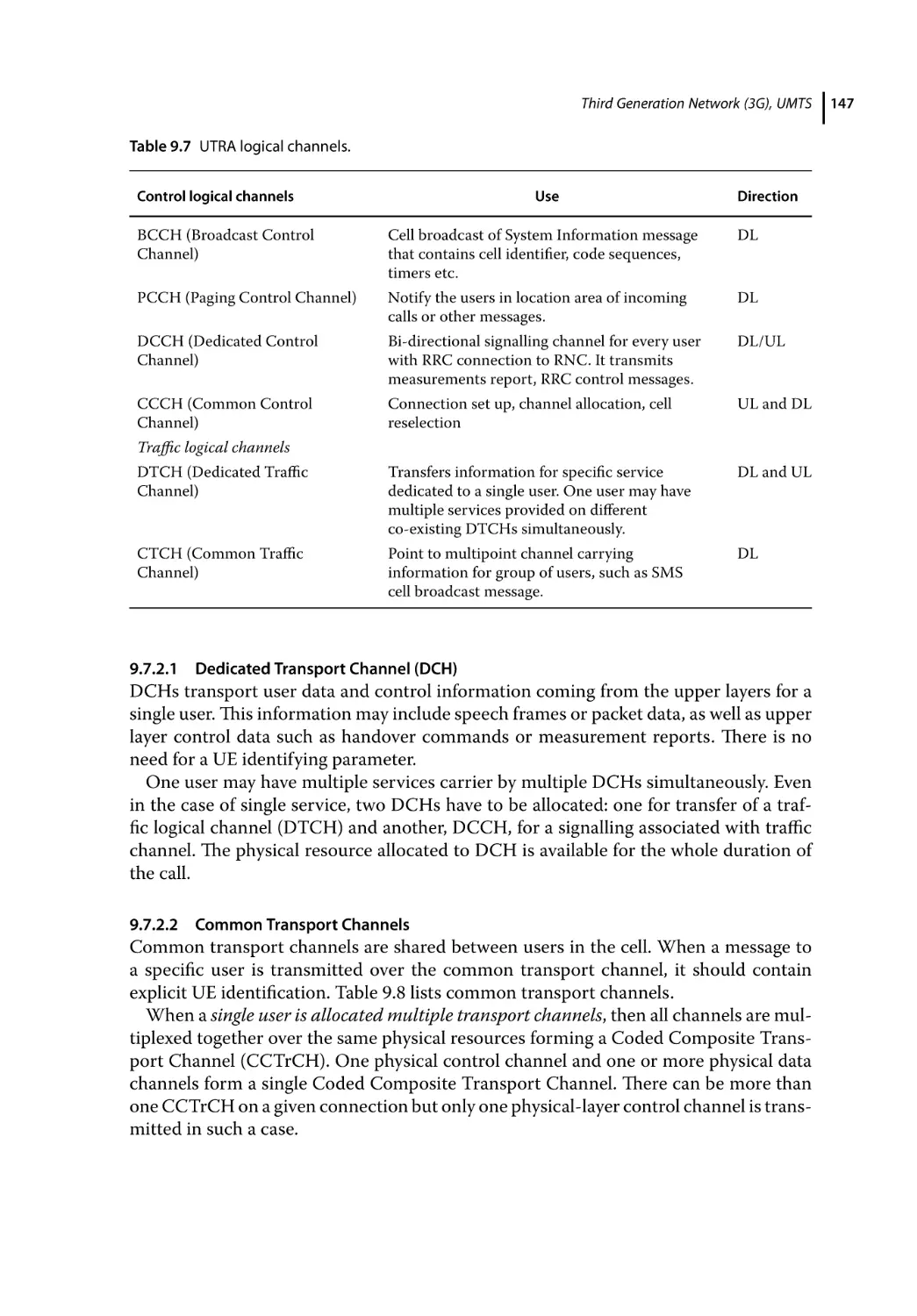
Logical Channels 146
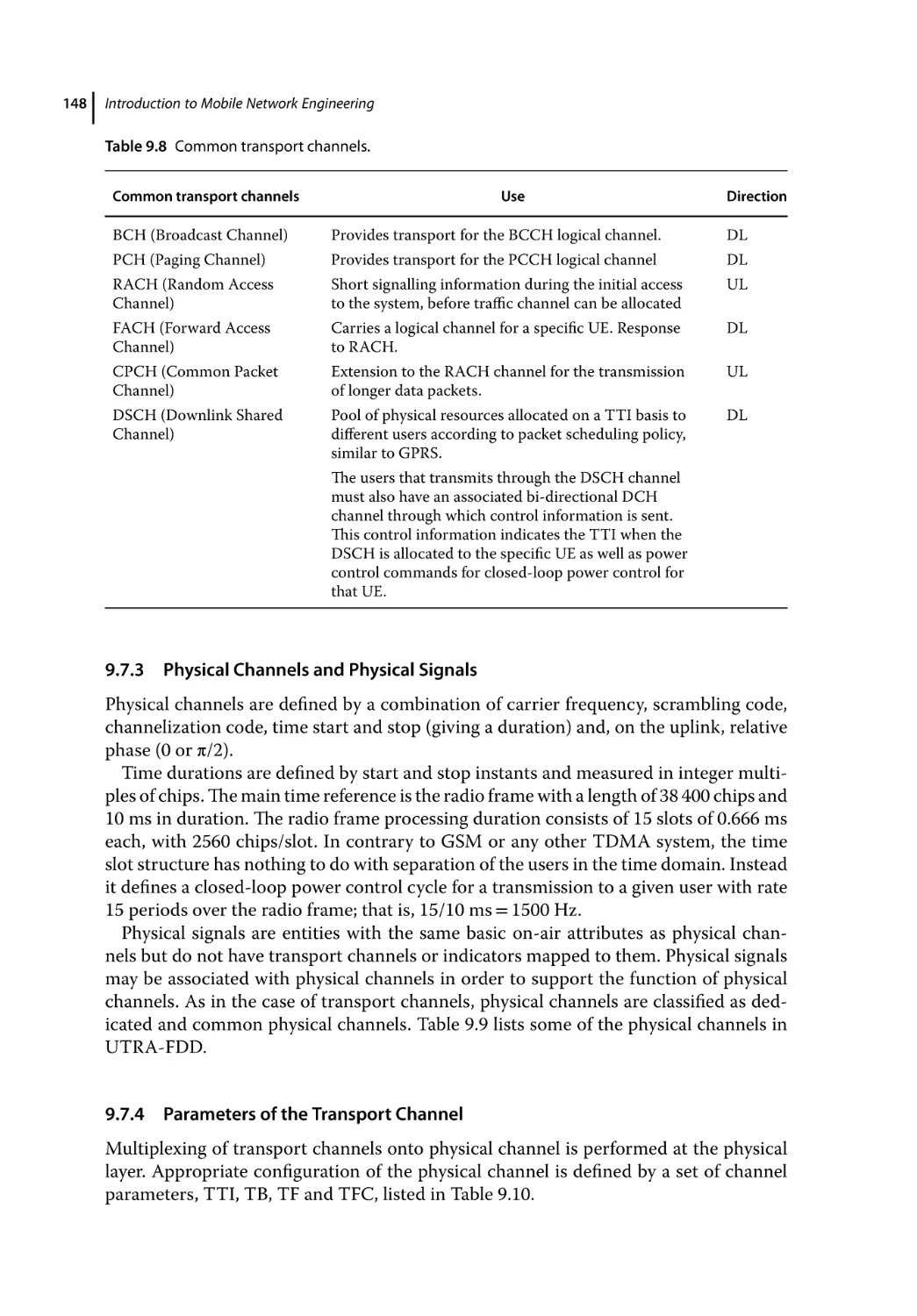
Transport Channels 146
Dedicated Transport Channel (DCH) 147
Common Transport Channels 147
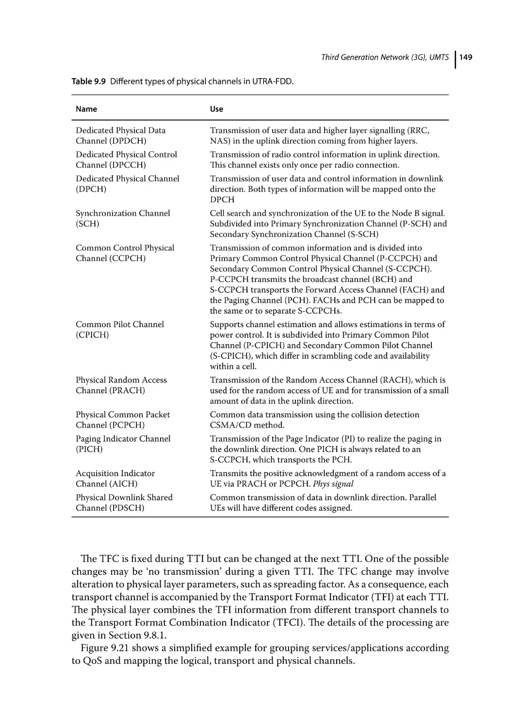
Physical Channels and Physical Signals 148
Parameters of the Transport Channel 148
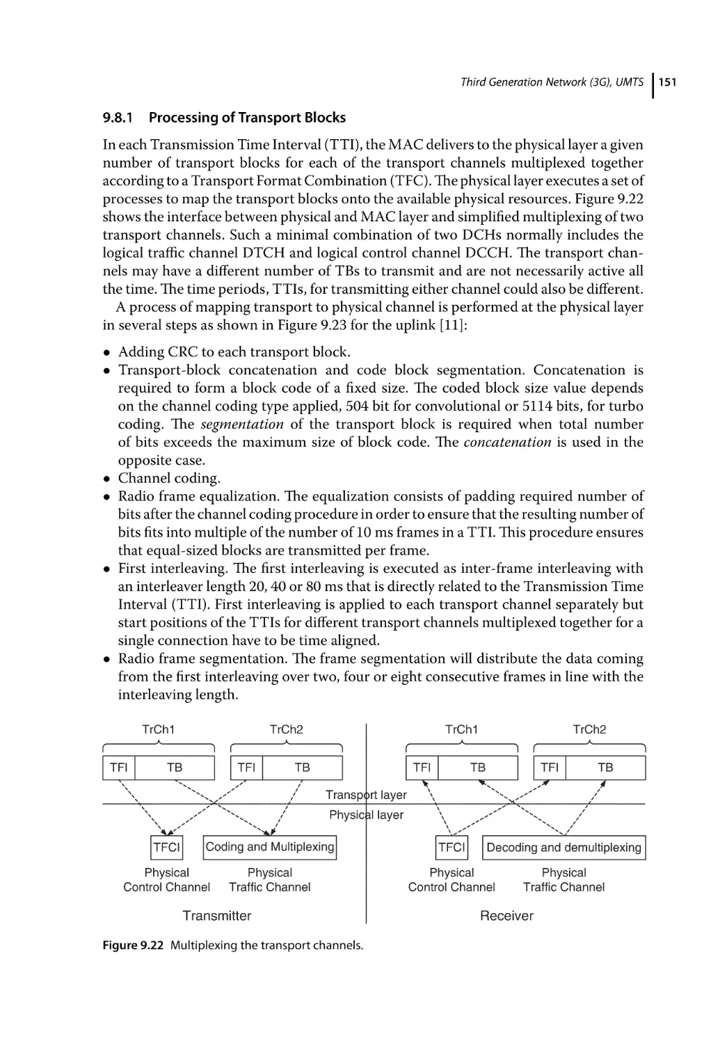
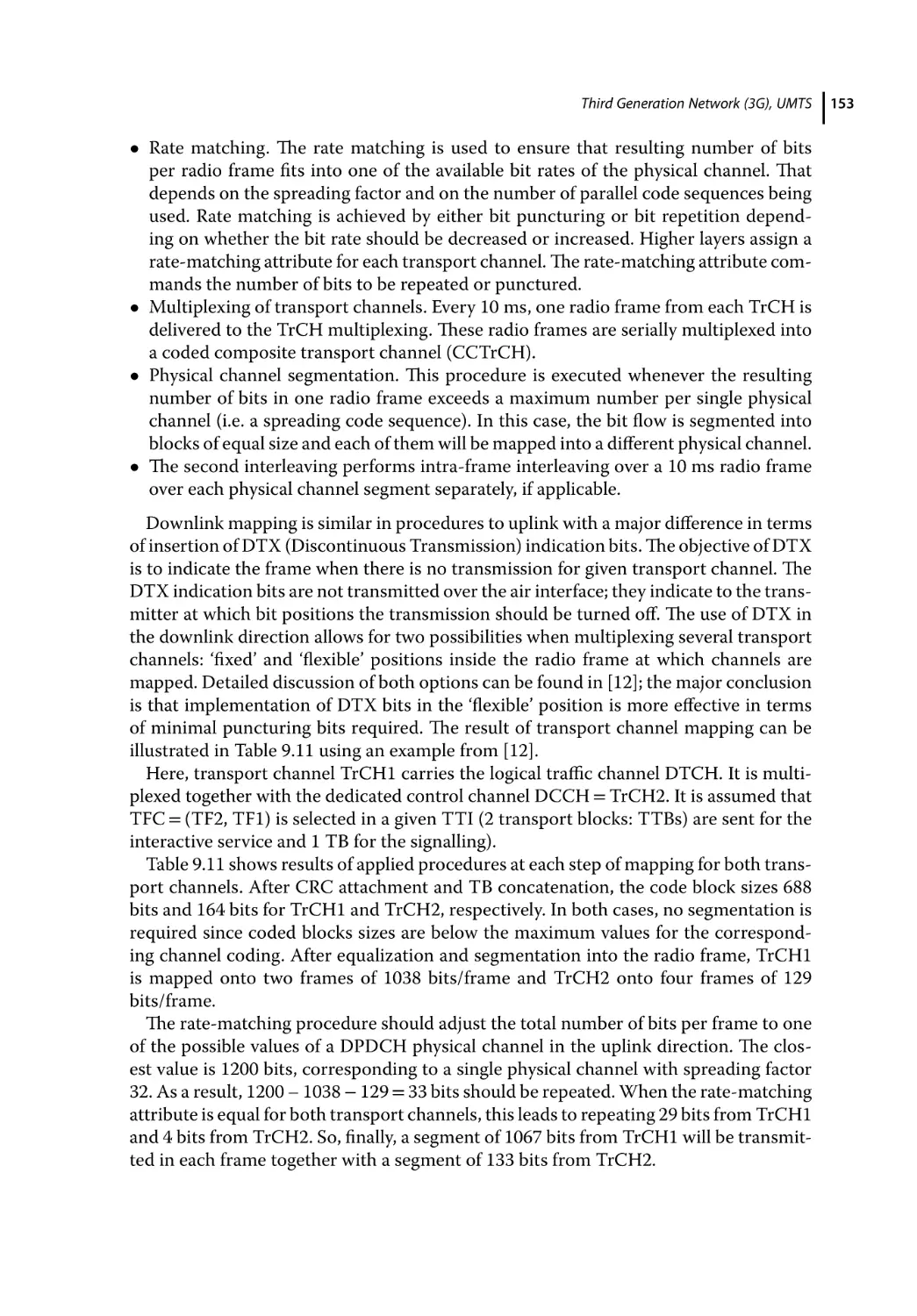
Physical-Layer Procedures 150
Processing of Transport Blocks 151
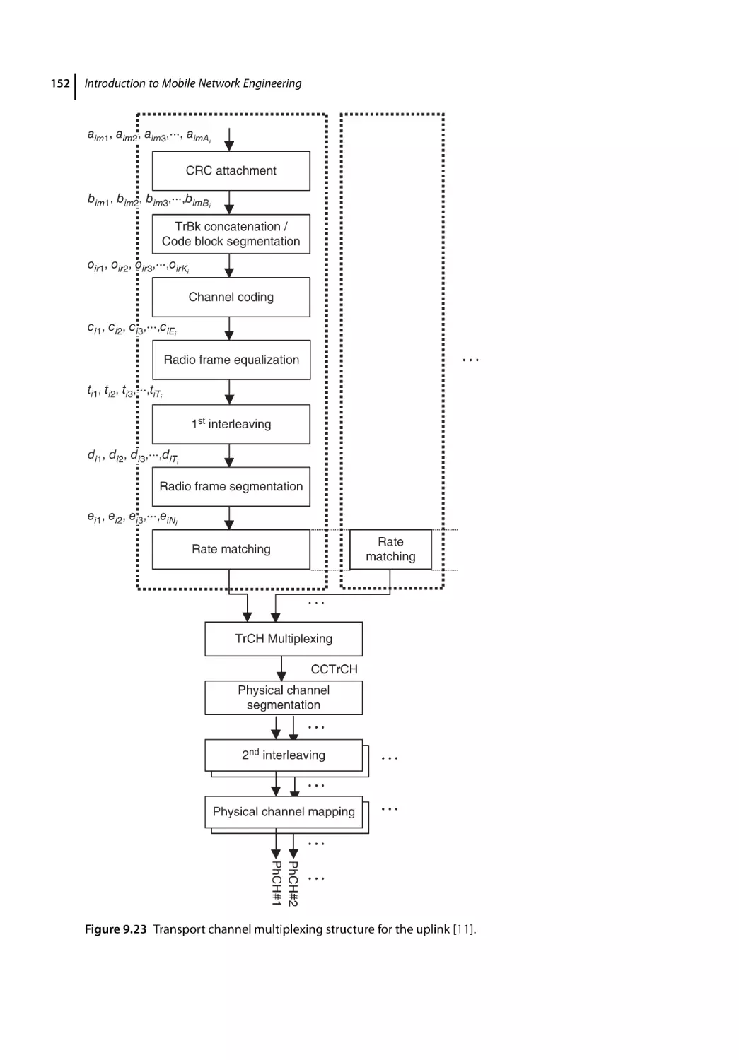
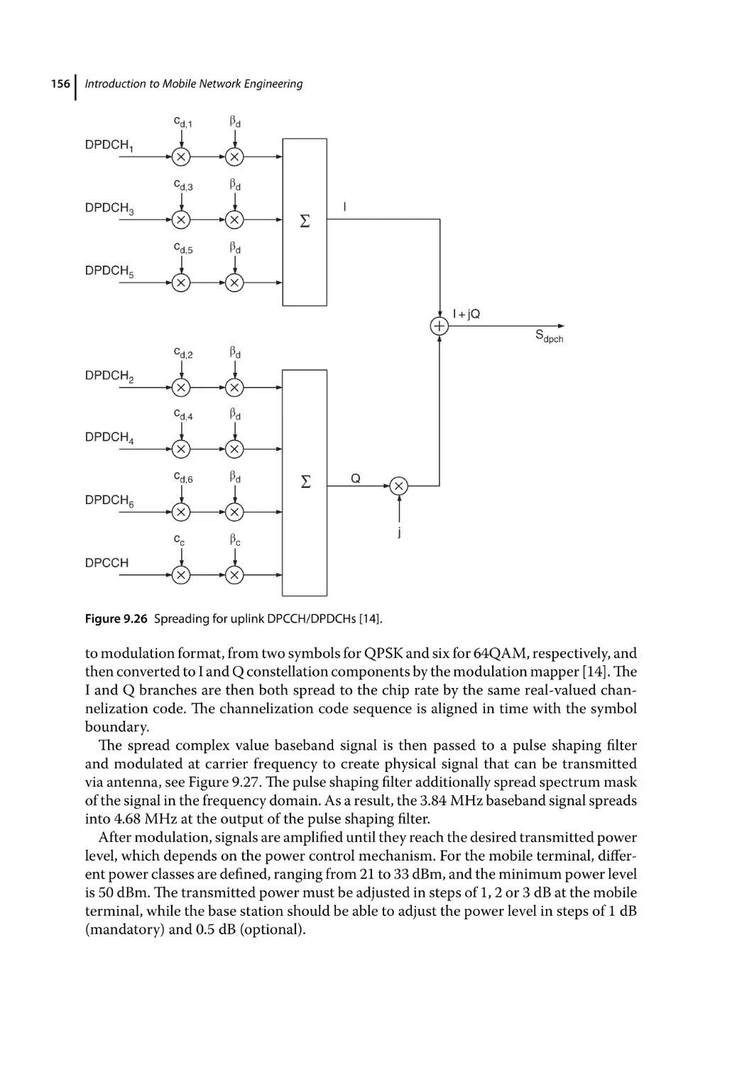
Spreading and Modulation 154
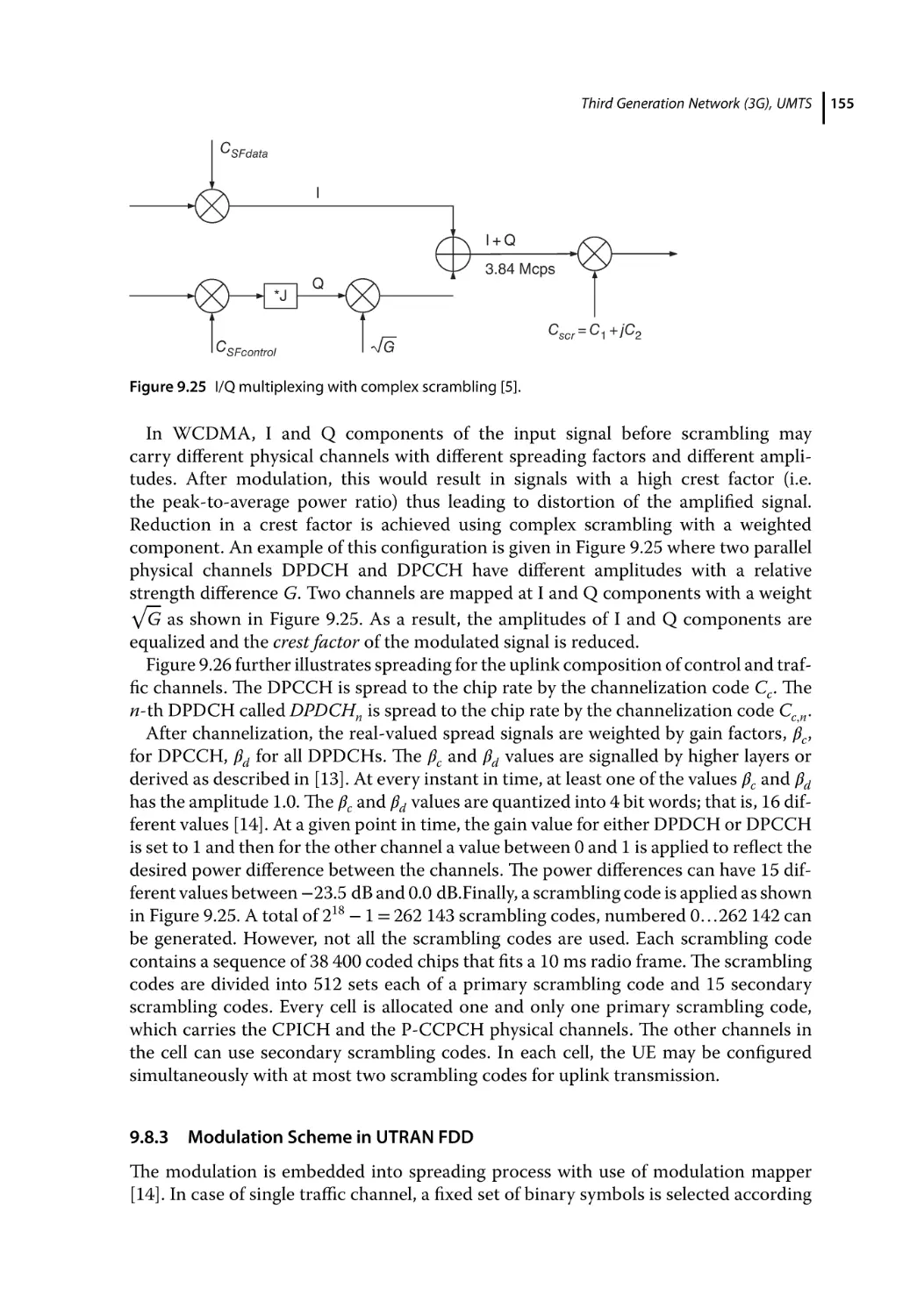
Modulation Scheme in UTRAN FDD 155
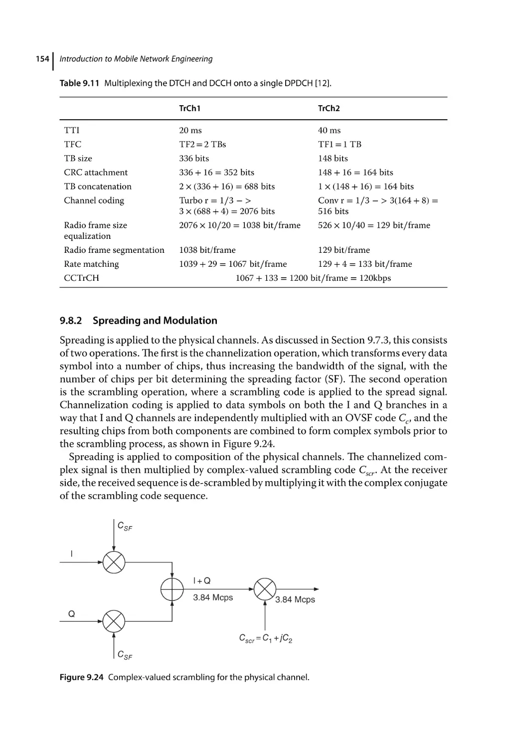
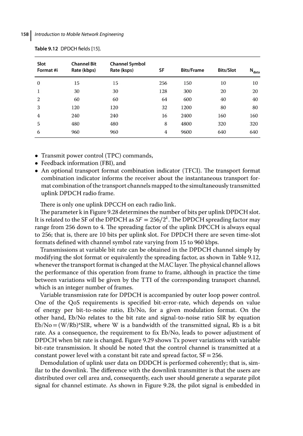
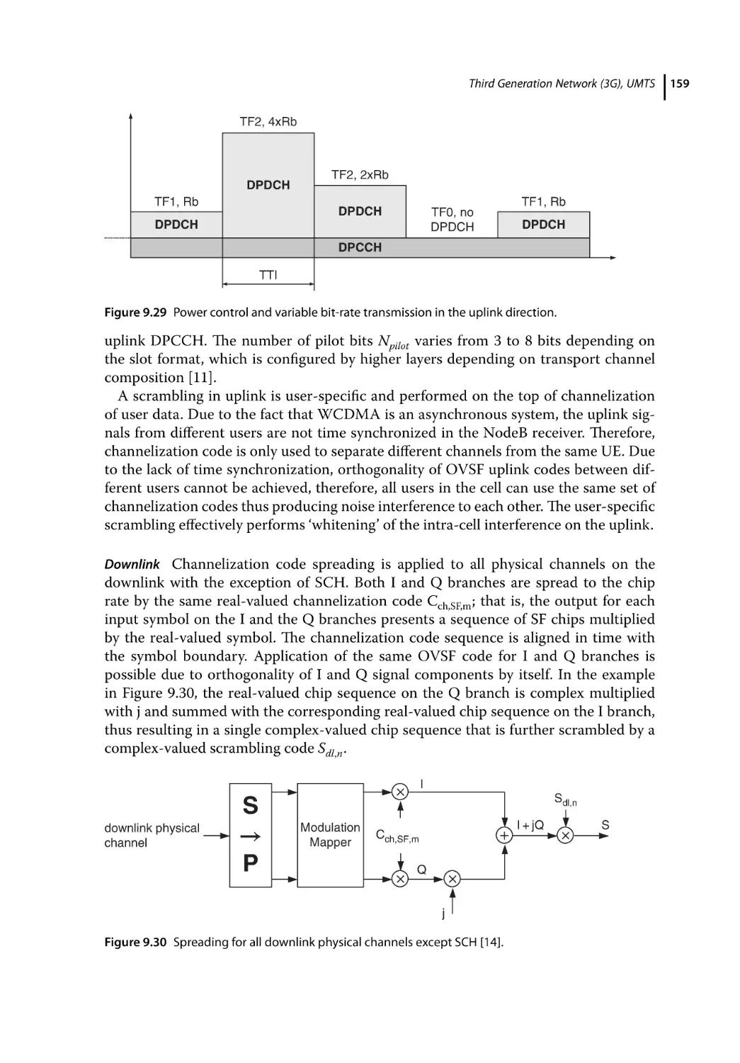
Composition of the Physical Channels 157
Dedicated Physical Channel 157
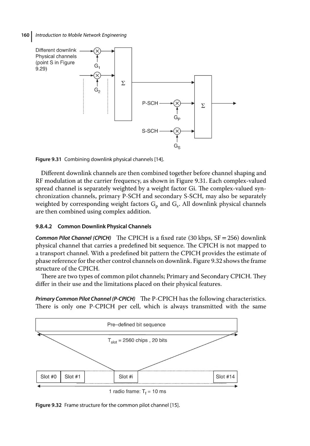
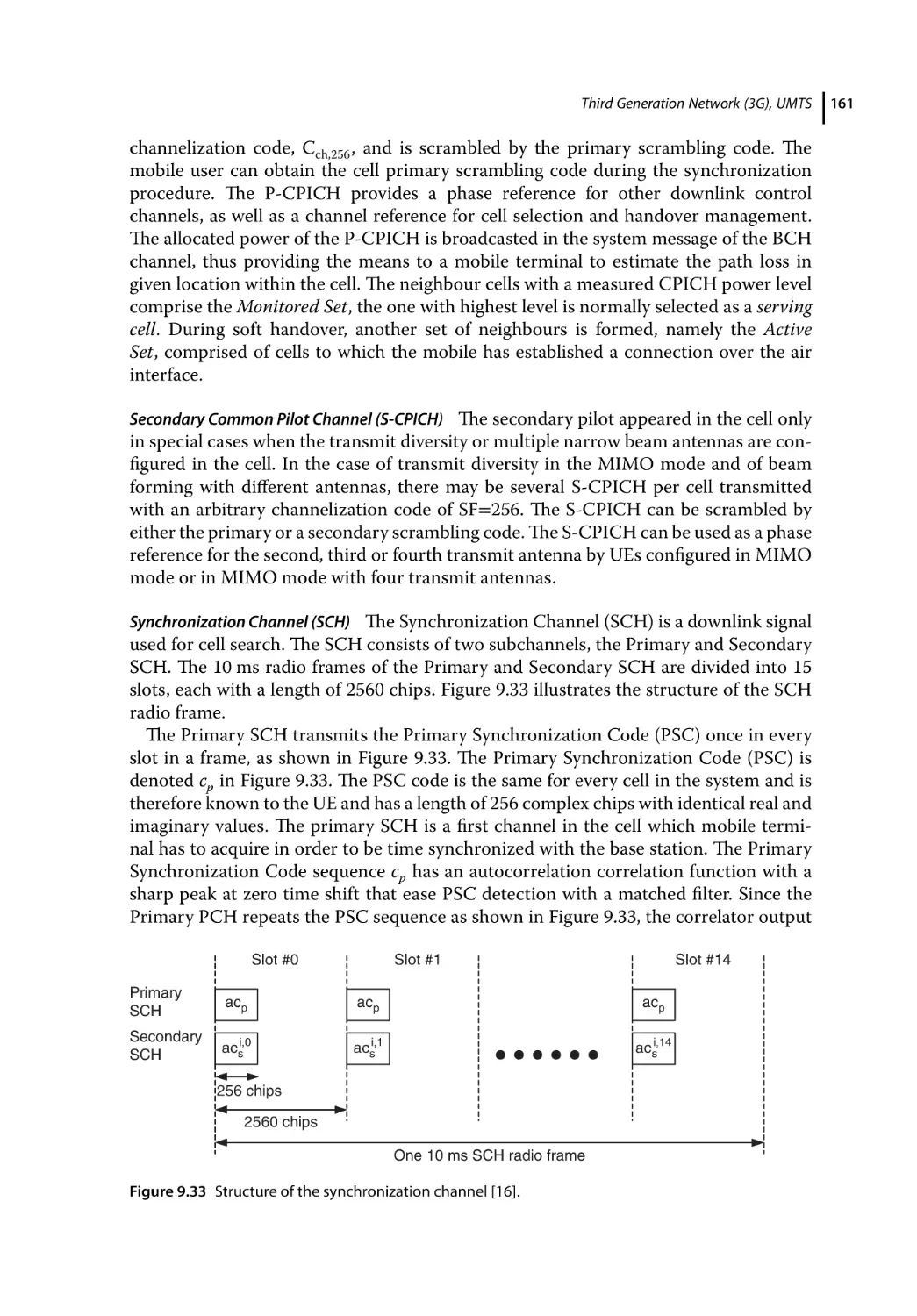
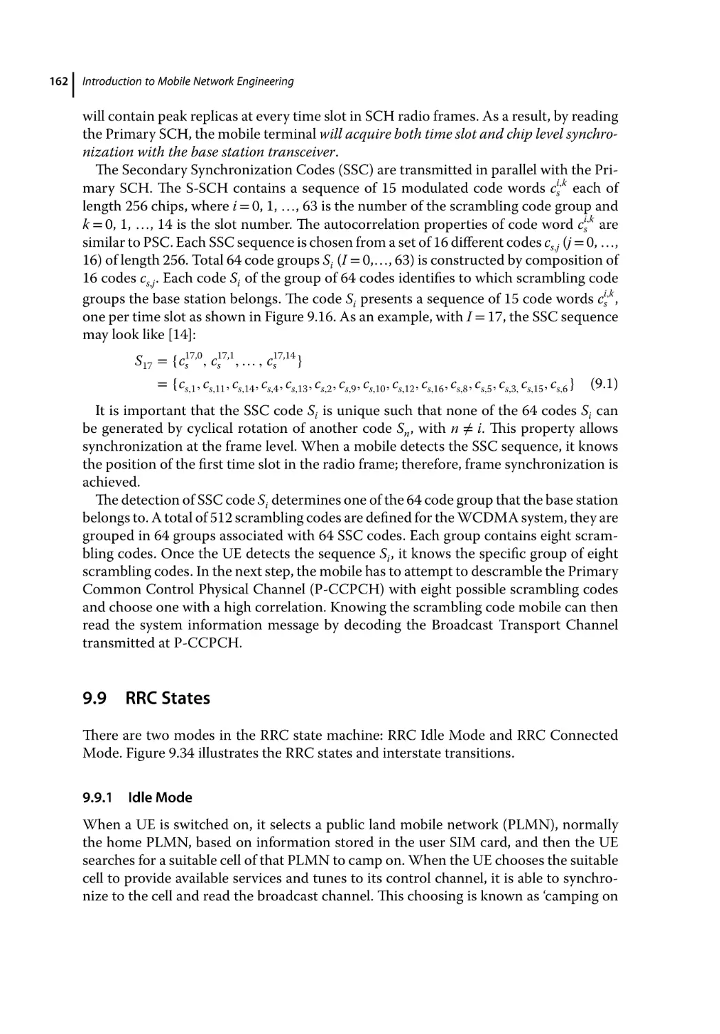
Common Downlink Physical Channels 160
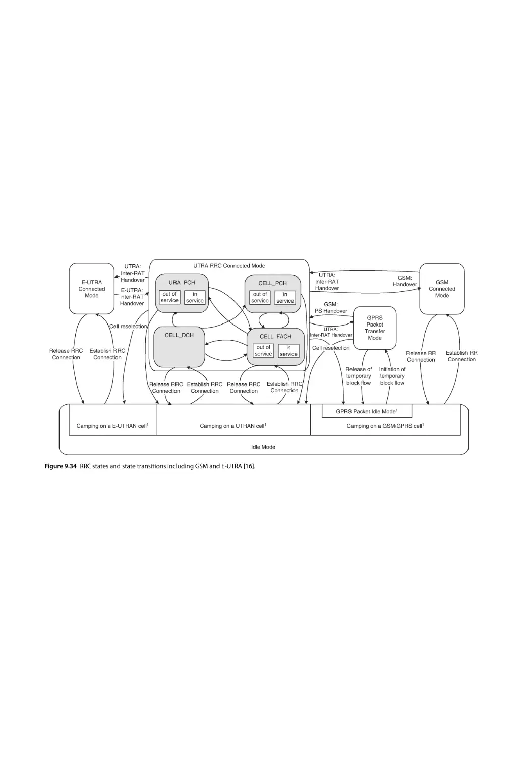
RRC States 162
Idle Mode 162
RRC Connected Mode 164
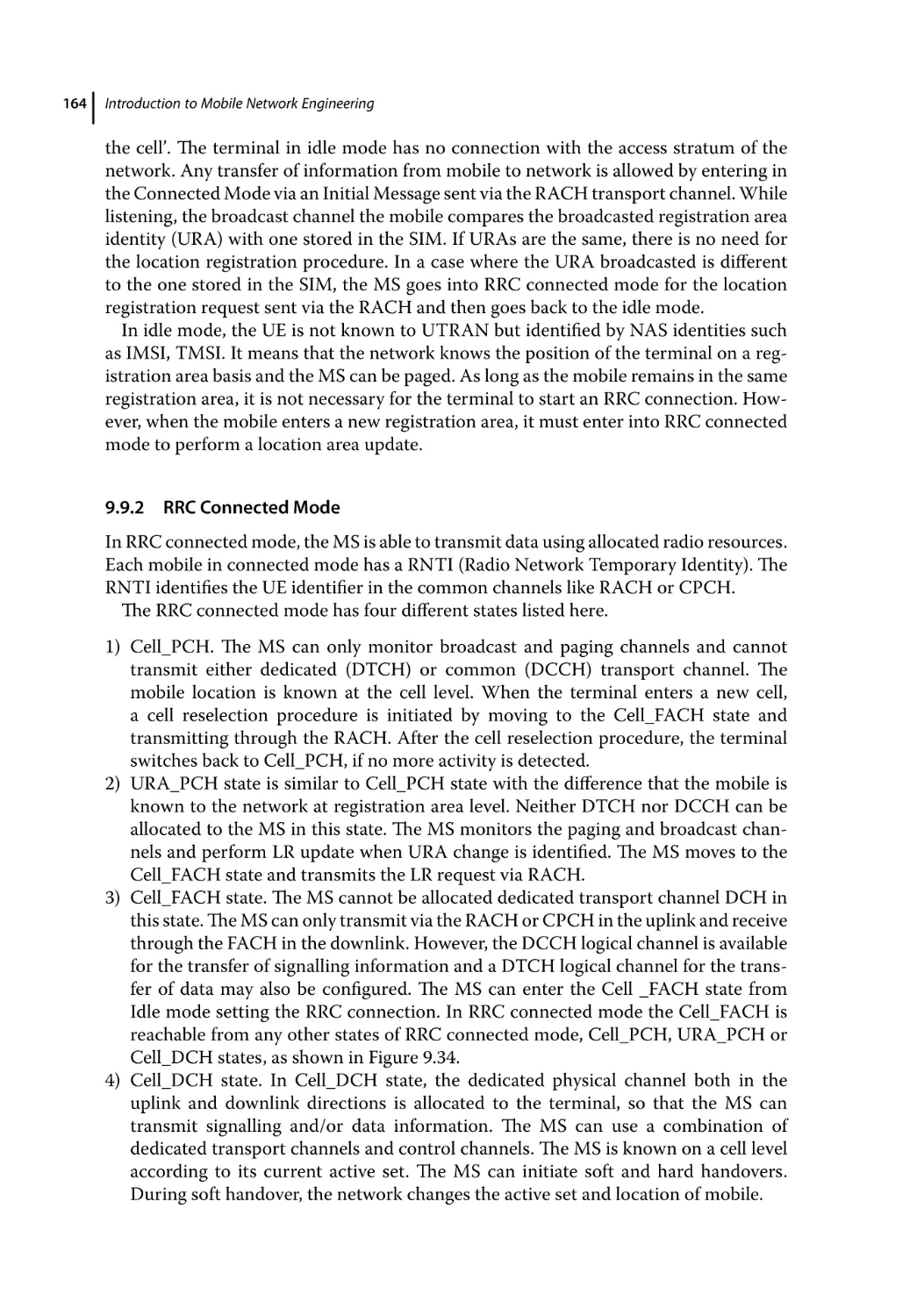
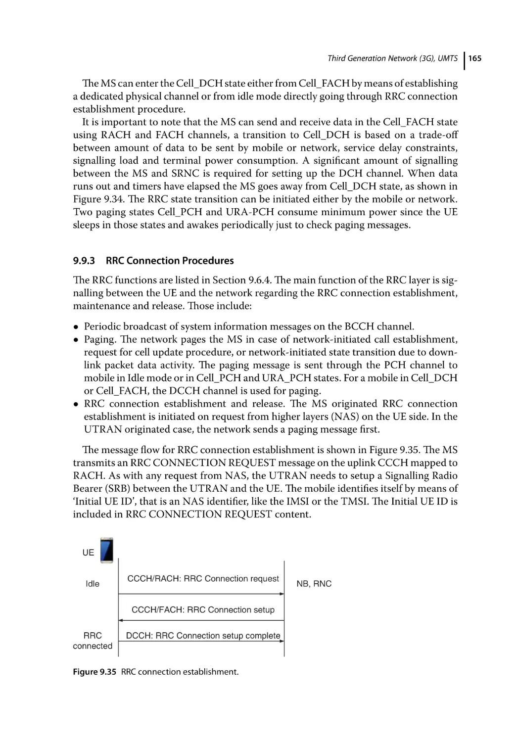
RRC Connection Procedures 165
RRC State Transition Cases 166
RRM Functions 167
Admission Control Principle 167
Load/Congestion Control 168
Code Management 168
Packet Scheduling 168
Initial Access to the Network 169
Summary 170
References 171
10
High-Speed Packet Data Access (HSPA) 173
10.1
10.2
10.2.1
10.2.2
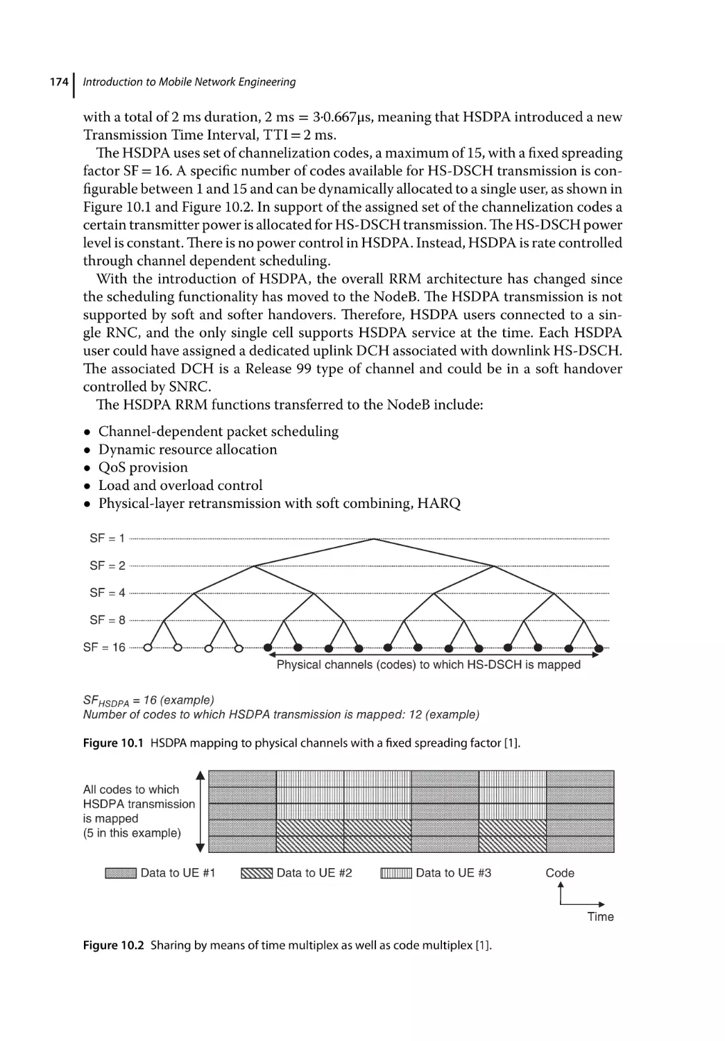
HSDPA, High-Speed Downlink Packet Data Access 173
HSPA RRM Functions 175
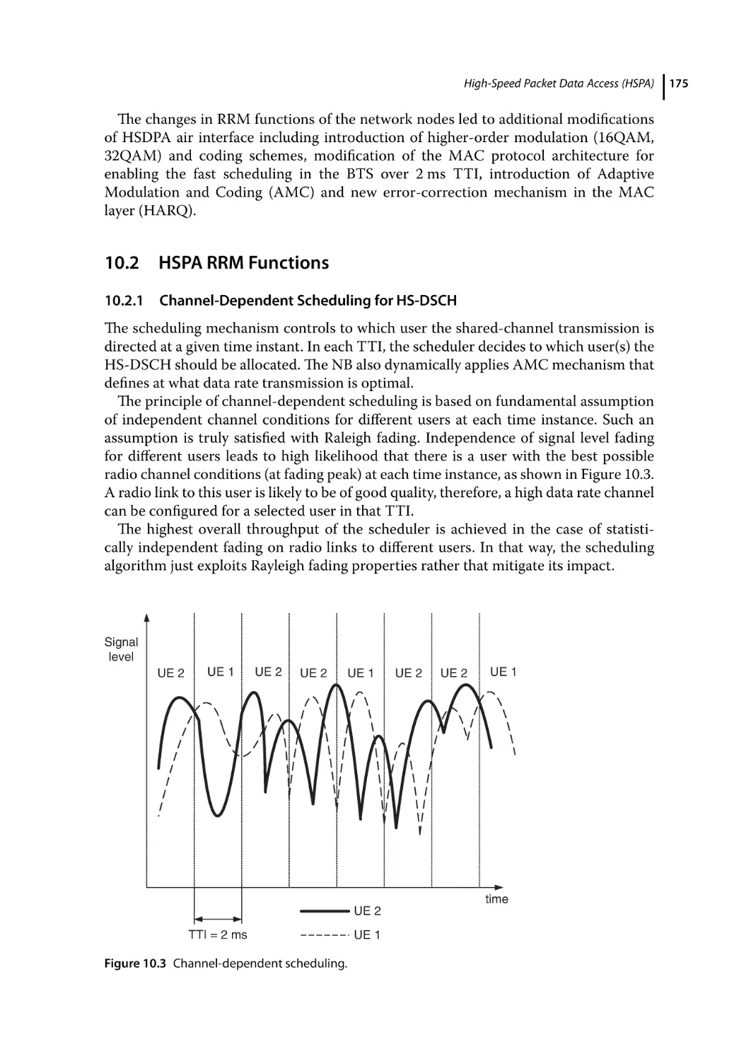
Channel-Dependent Scheduling for HS-DSCH 175
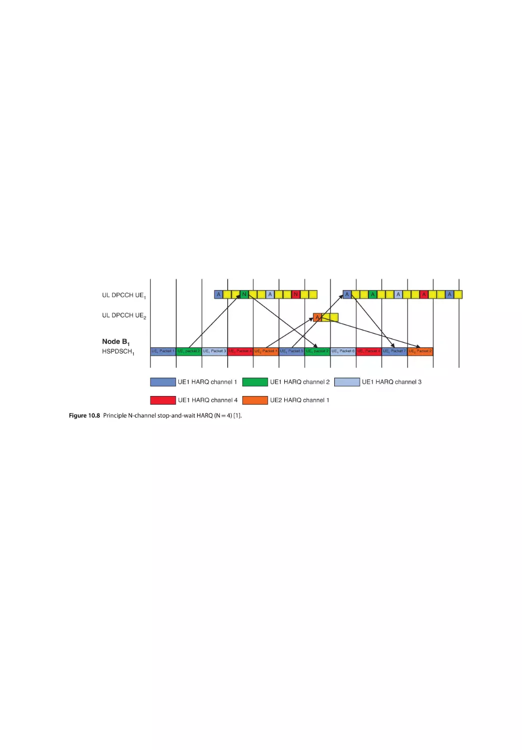
Rate Control, Dynamic Resource Allocation, Adaptive Modulation
and Coding 176
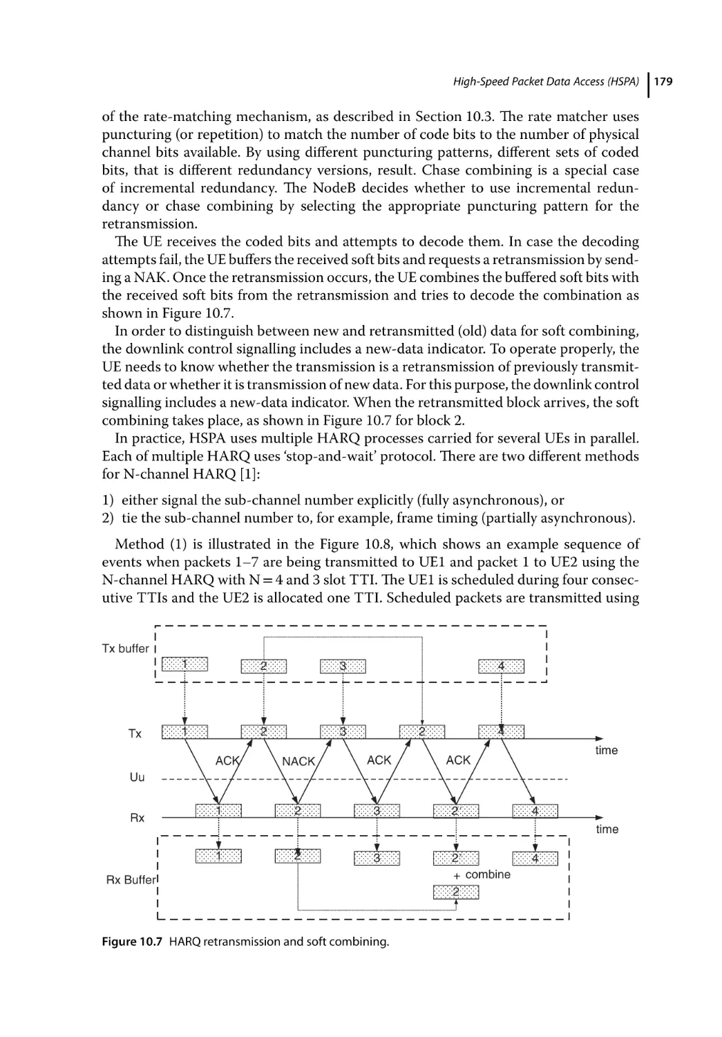
Hybrid-ARQ with Soft Combining, HARQ 176
10.2.3
xi
xii
Contents
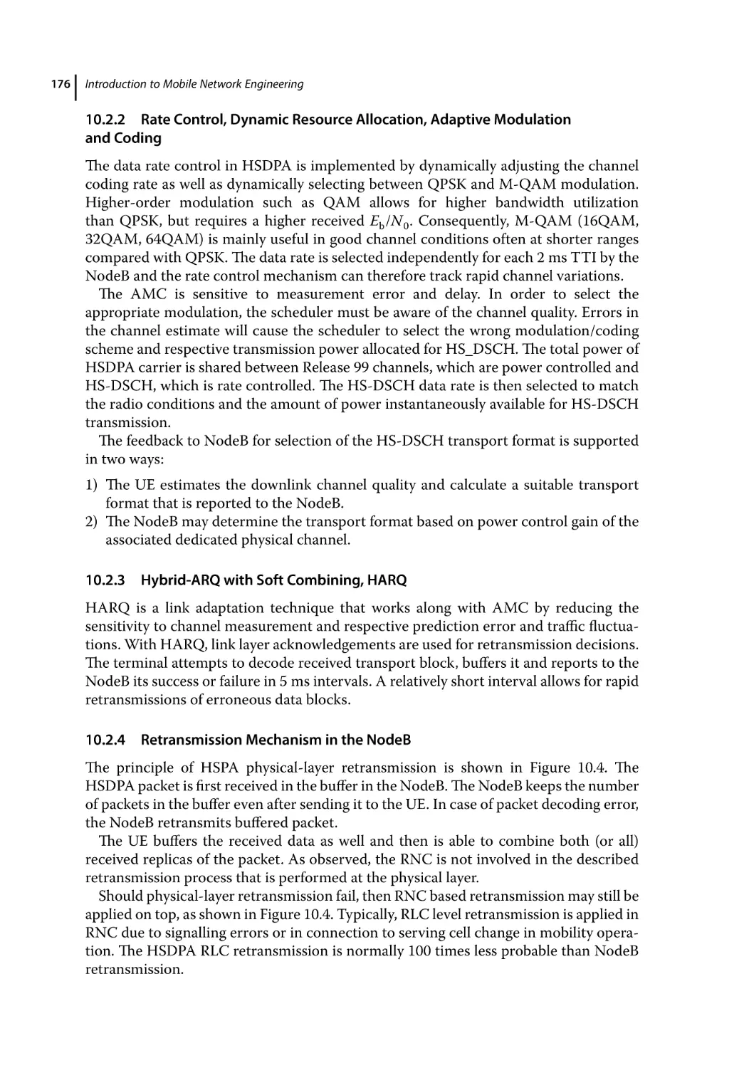
10.2.4
10.2.5
10.2.6
10.3
10.4
10.4.1
10.4.2
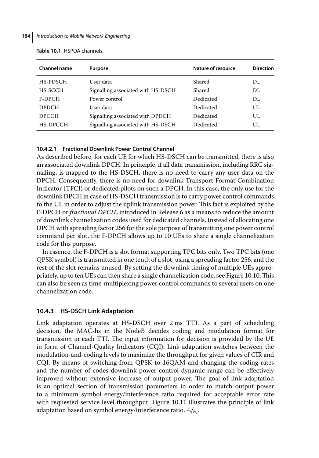
10.4.2.1
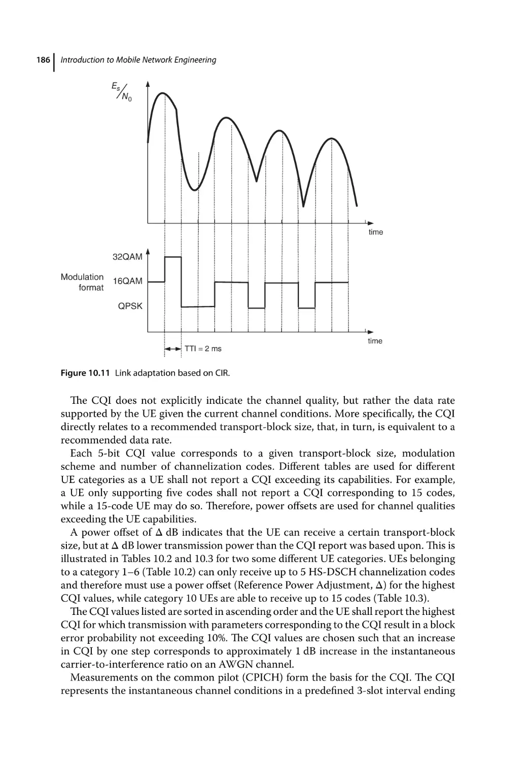
10.4.3
10.5
10.5.1
10.5.2
10.6
10.6.1
10.6.2
10.6.2.1
10.6.2.2
10.6.3
10.6.4
10.6.4.1
10.6.4.2
10.6.4.3
10.6.4.4
10.6.4.5
10.6.4.6
10.6.4.7
10.6.5
10.6.5.1
10.6.5.2
10.7
Retransmission Mechanism in the NodeB 176
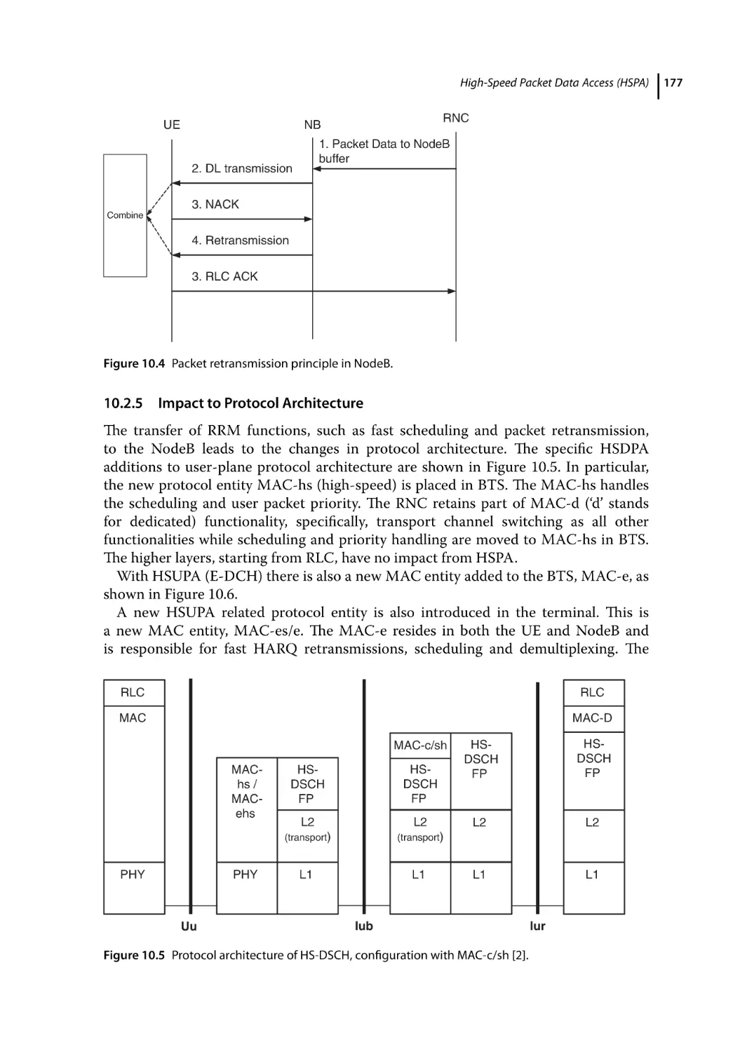
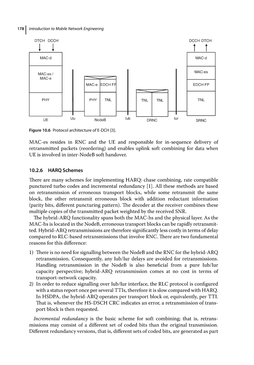
Impact to Protocol Architecture 177
HARQ Schemes 178
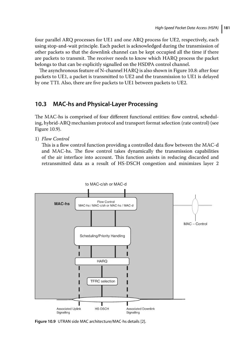
MAC-hs and Physical-Layer Processing 181
HSDPA Channels 182
High-Speed Downlink Shared Channel (HS-DSCH) 182
HSDPA Control Channels 183
Fractional Downlink Power Control Channel 184
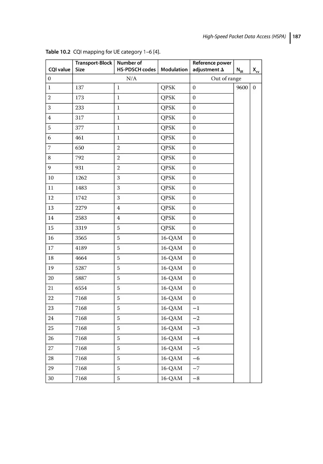
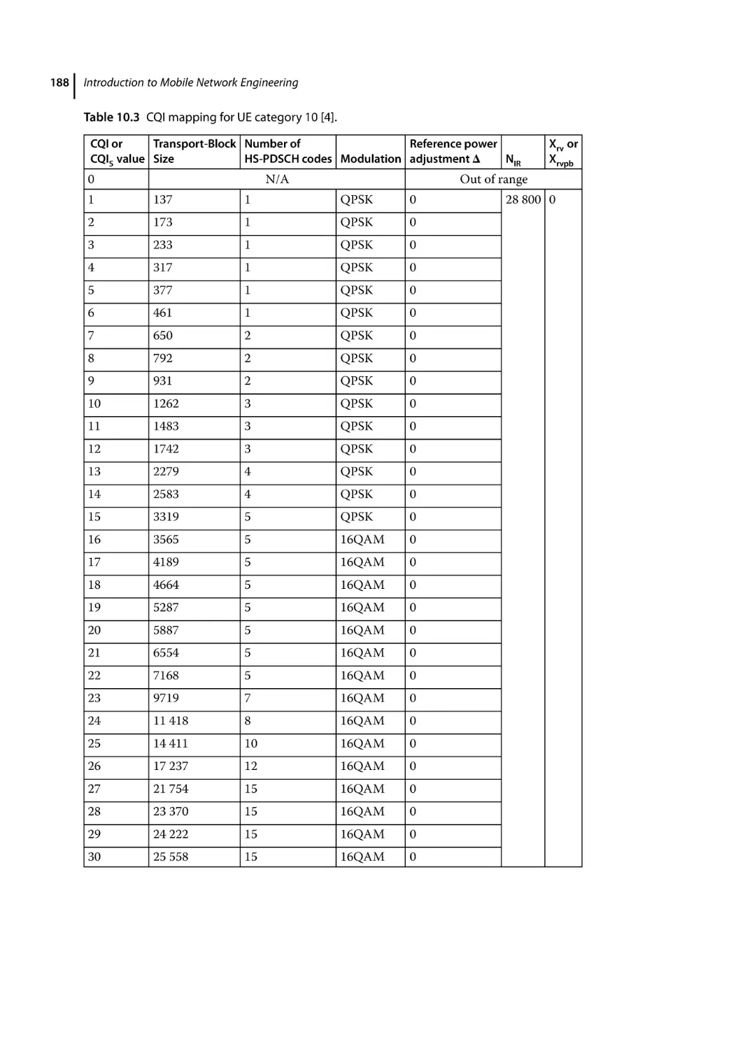
HS-DSCH Link Adaptation 184
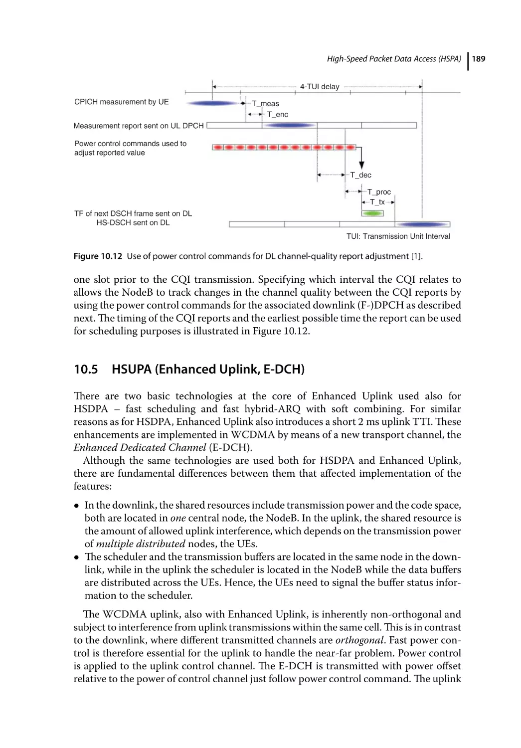
HSUPA (Enhanced Uplink, E-DCH) 189
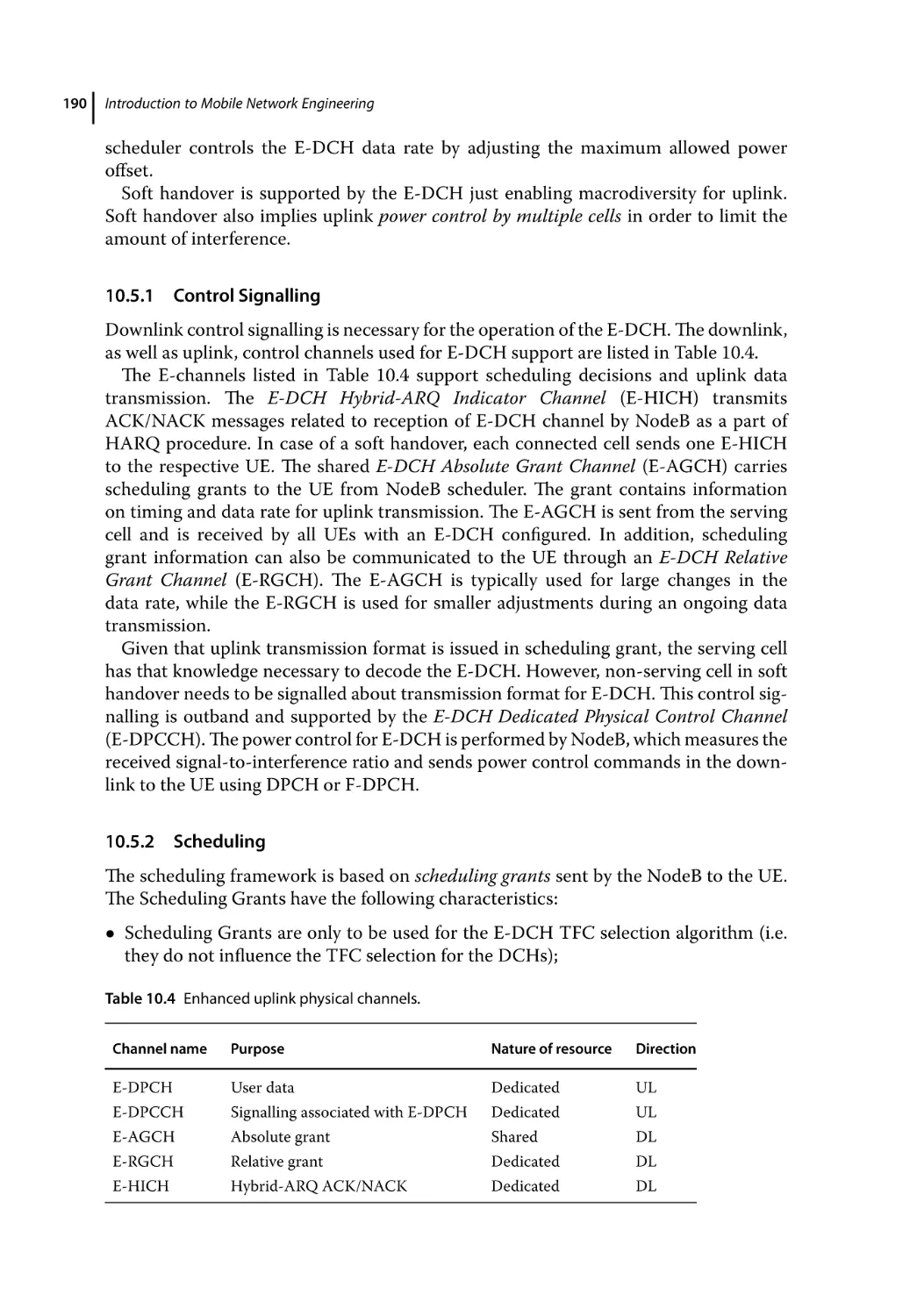
Control Signalling 190
Scheduling 190
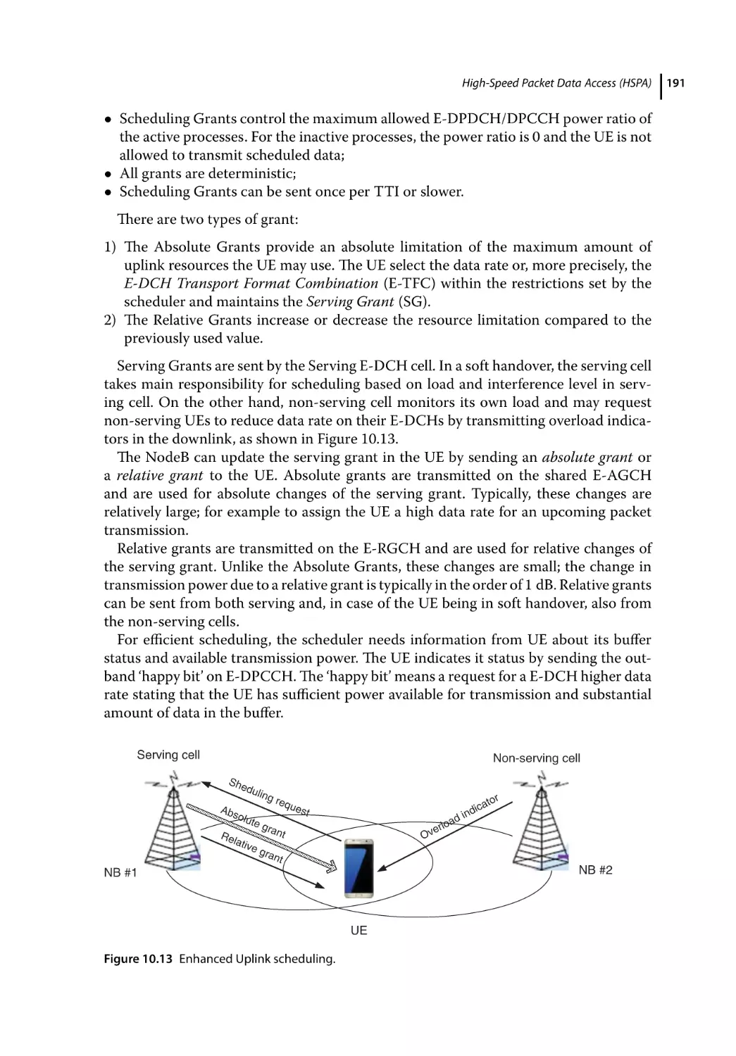
Air-Interface Dimensioning 192
Input Parameters and Requirements 192
Traffic Demand Estimation 193
PS Data Services (Release 99) 193
HSPA Data Services 193
Standard Traffic Model 194
Link Budgets 195
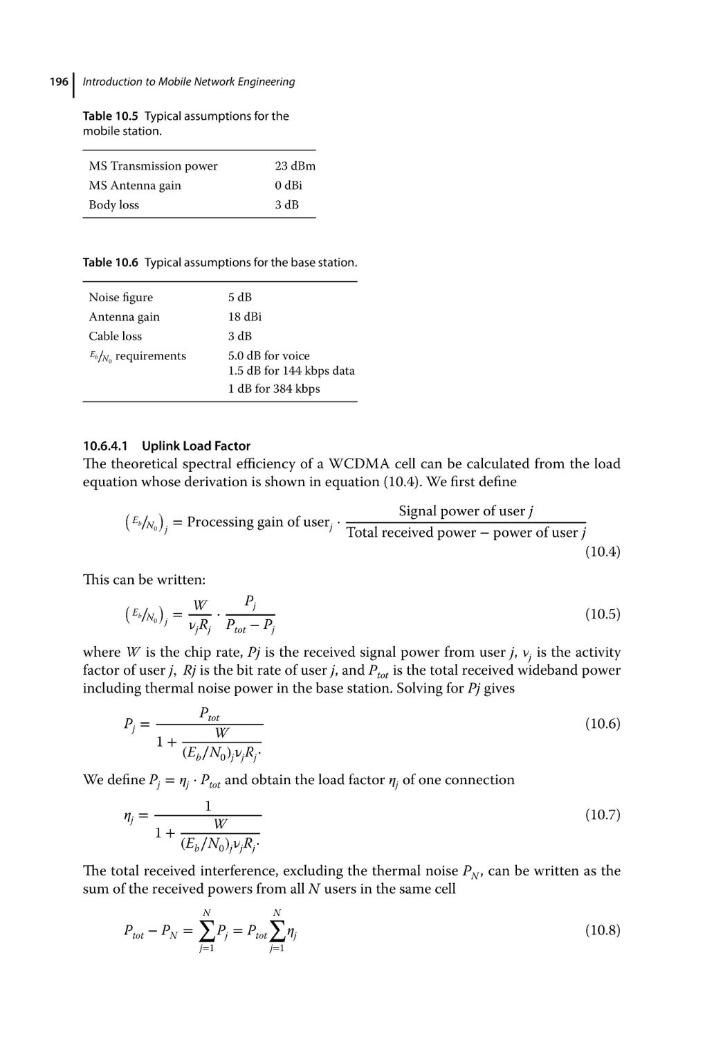
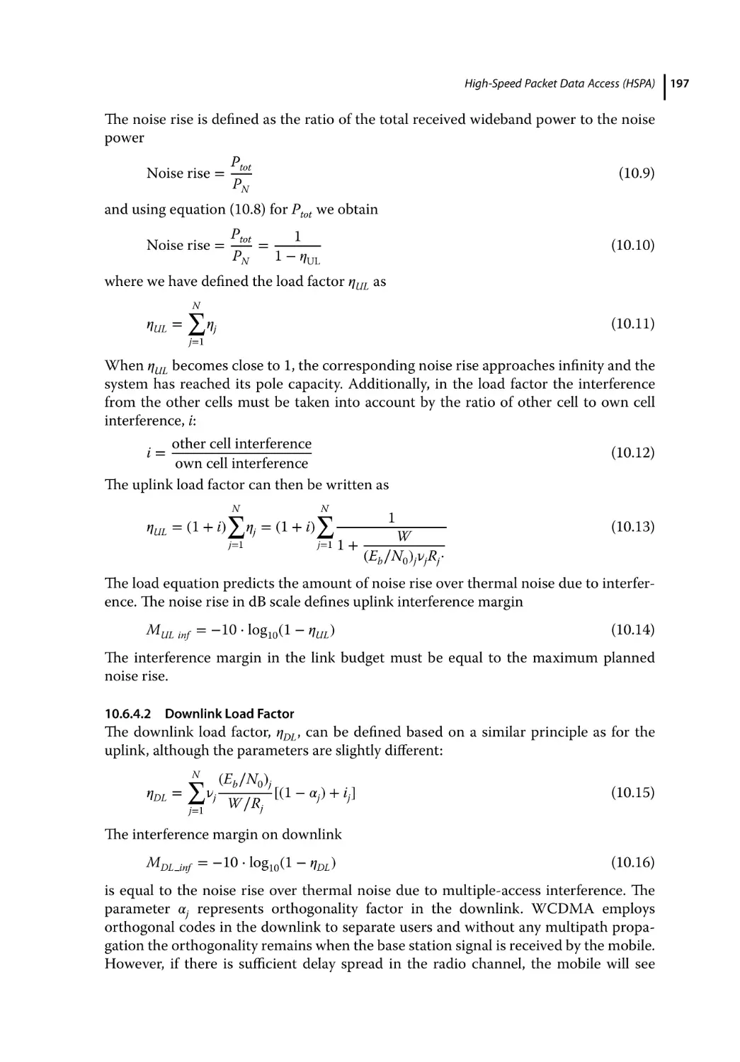
Uplink Load Factor 196
Downlink Load Factor 197
Link Budget for R99 Bearers 198
Link Budget for HSPA 199
Results of Link Budget: Cell Range Calculation, Balancing UL with DL
Link Budget for Common Pilot Channel Signal 200
Link Budget Calculation for the Shared Release 99 and HSDPA
Carriers 200
Uplink Capacity Estimation 201
Required Bandwidth and Load for Multiple Bearers with GOS
Considerations 202
Simplified Estimation of HSDPA Throughput Capacity 202
Summary 203
References 204
11
4G-Long Term Evolution (LTE) System 205
11.1
11.2
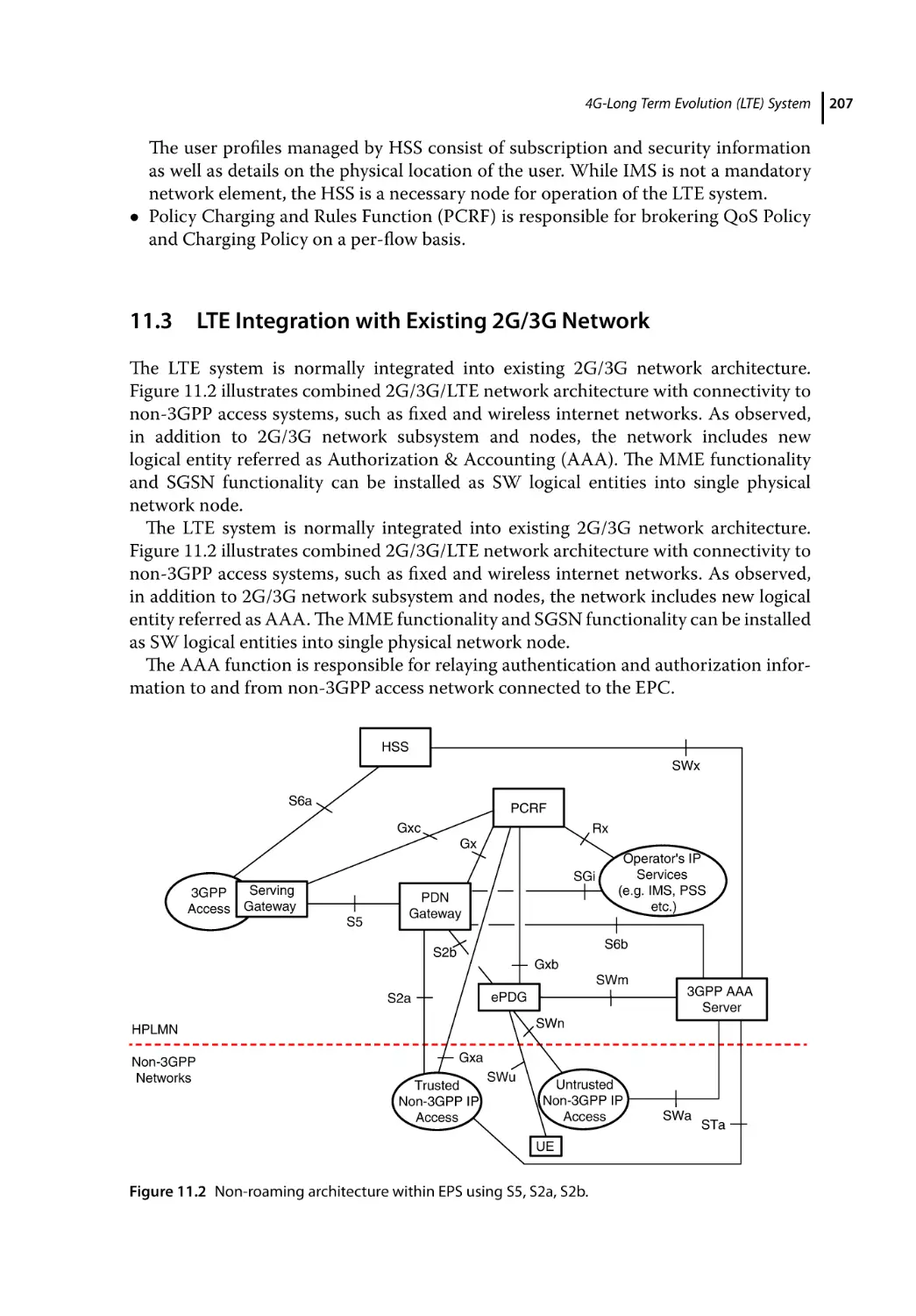
11.3
11.3.1
11.4
11.5
11.5.1
11.6
11.7
11.8
11.8.1
11.8.2
Introduction 205
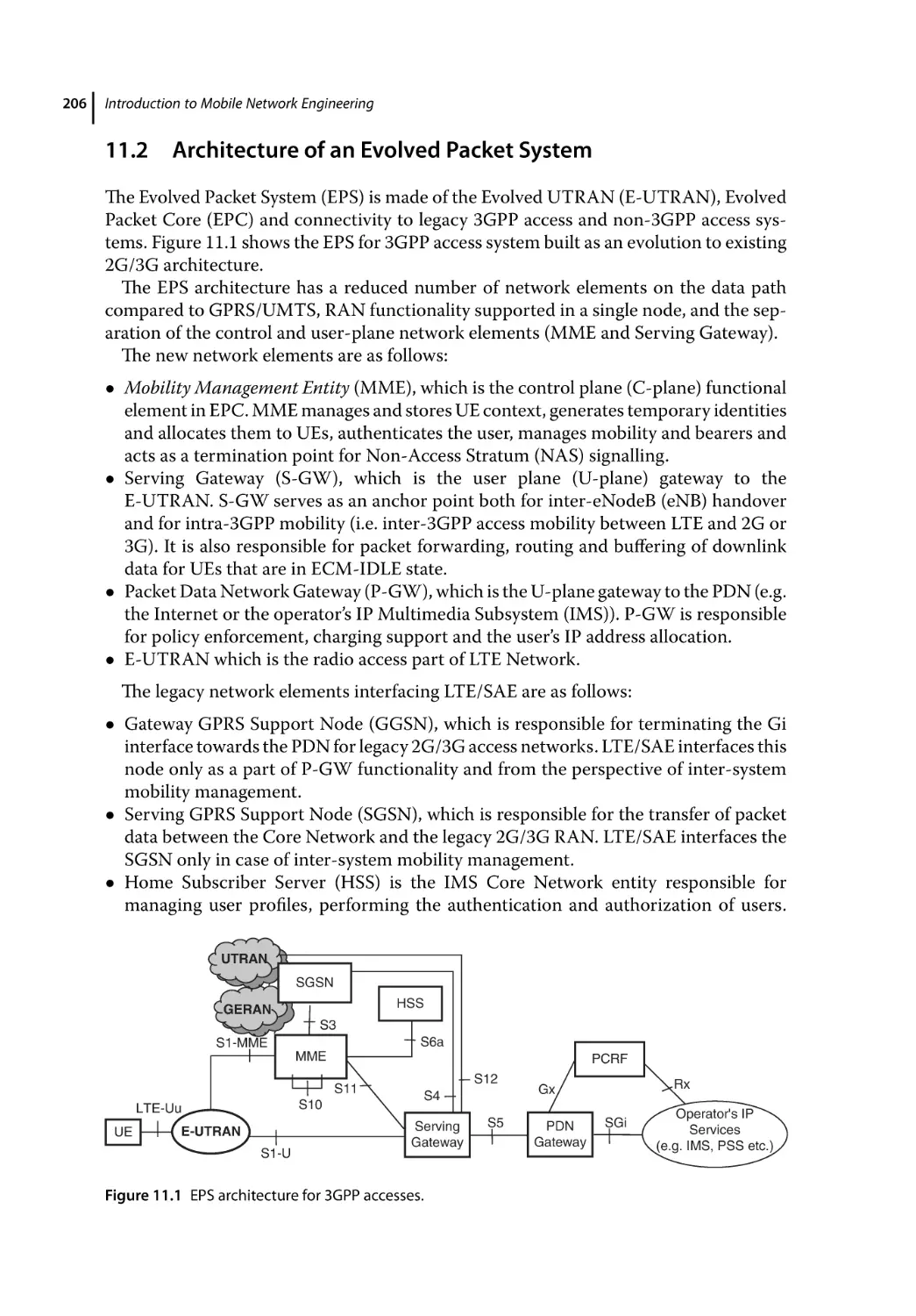
Architecture of an Evolved Packet System 206
LTE Integration with Existing 2G/3G Network 207
EPS Reference Points and Interfaces 208
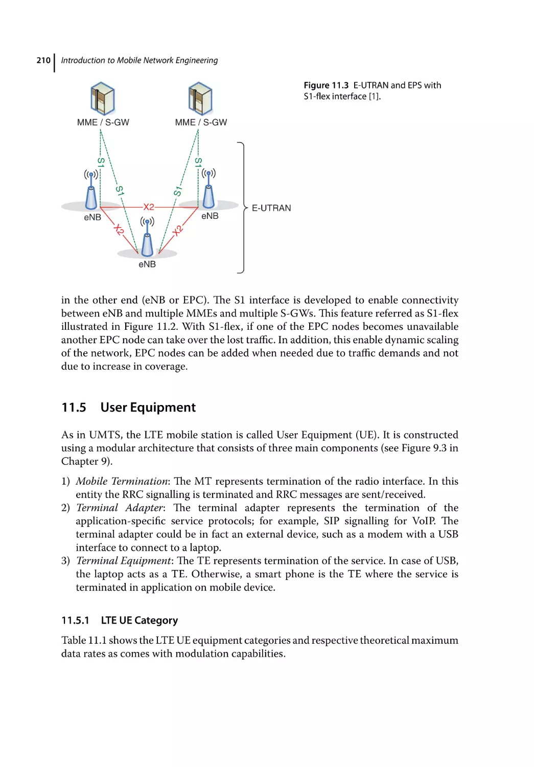
E-UTRAN Interfaces 209
User Equipment 210
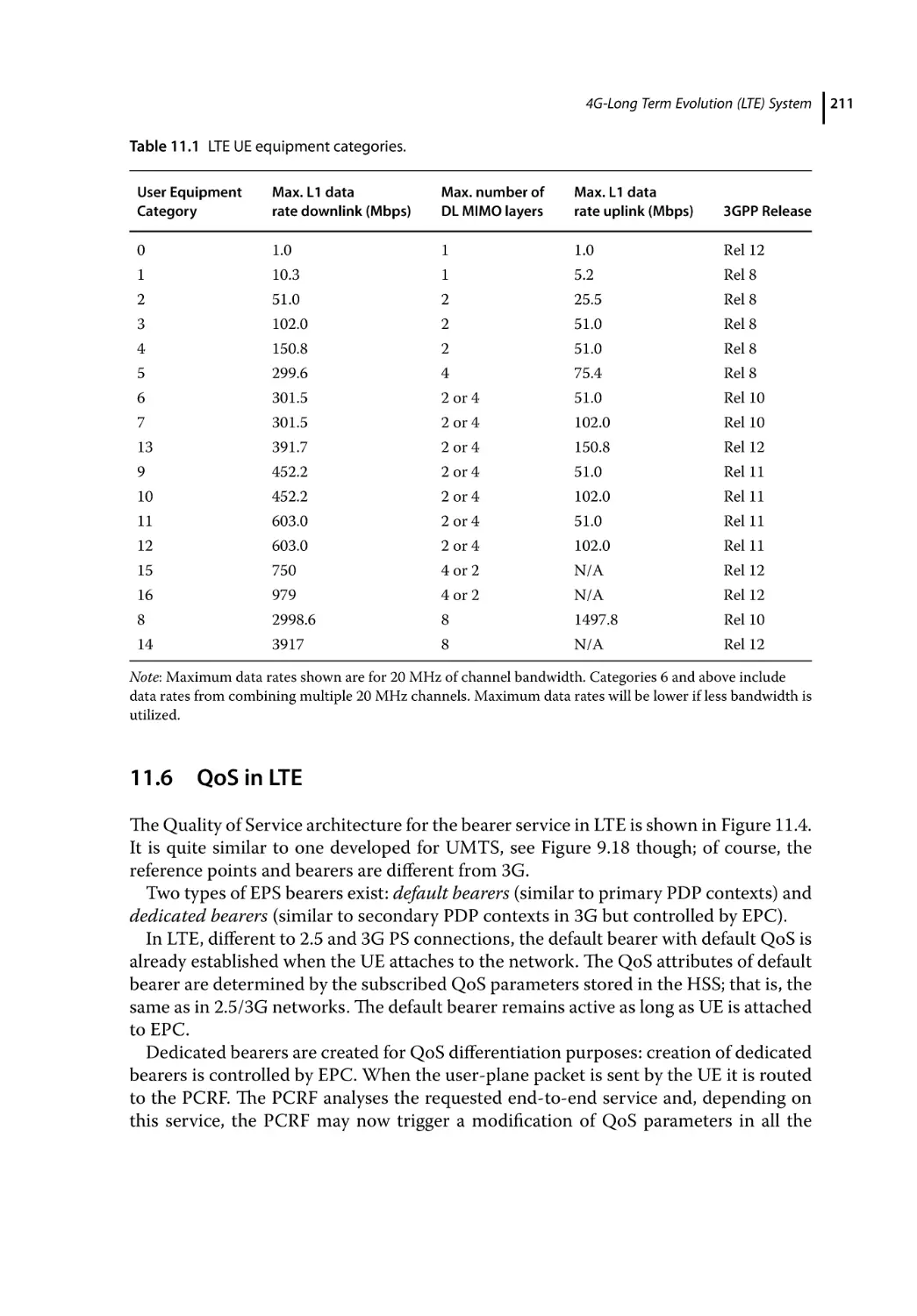
LTE UE Category 210
QoS in LTE 211
LTE Security 212
LTE Mobility 214
Idle Mode Mobility 214
ECM-CONNECTED Mode Mobility 215
199
Contents
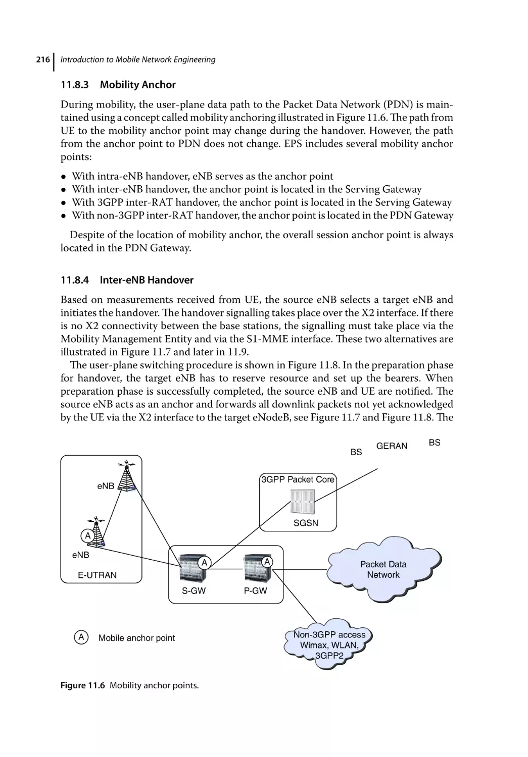
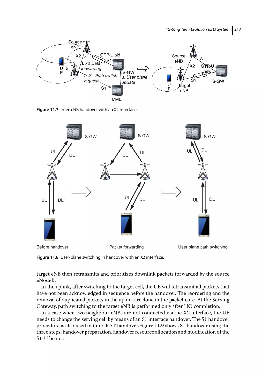
11.8.3
11.8.4
11.8.5
11.8.6
11.9
11.10
11.11
11.12
11.13
11.14
11.15
11.16
11.17
11.18
11.19
11.20
11.21
11.21.1
11.21.2
11.22
11.23
11.23.1
11.23.2
11.23.3
11.23.4
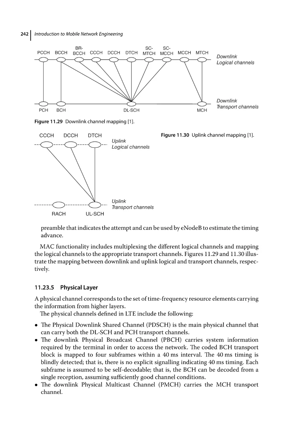
11.23.5
11.23.6
11.23.7
11.24
11.24.1
11.24.2
11.24.3
11.24.4
11.24.5
11.24.6
11.24.7
11.24.7.1
11.24.7.2
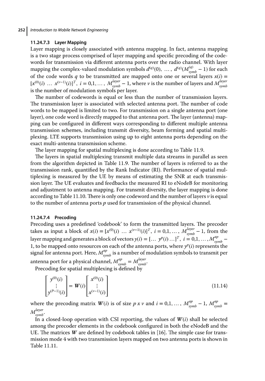
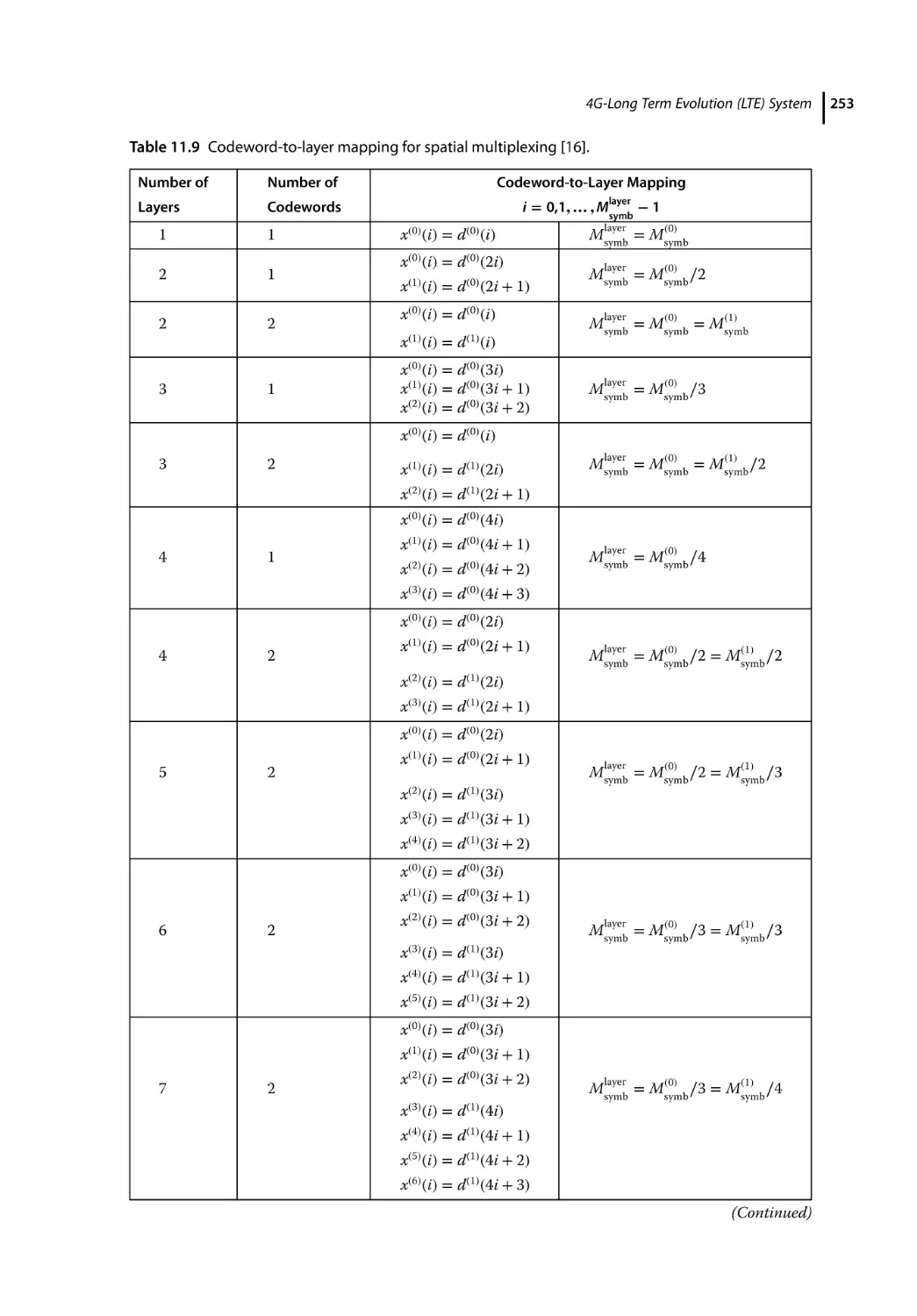
11.24.7.3
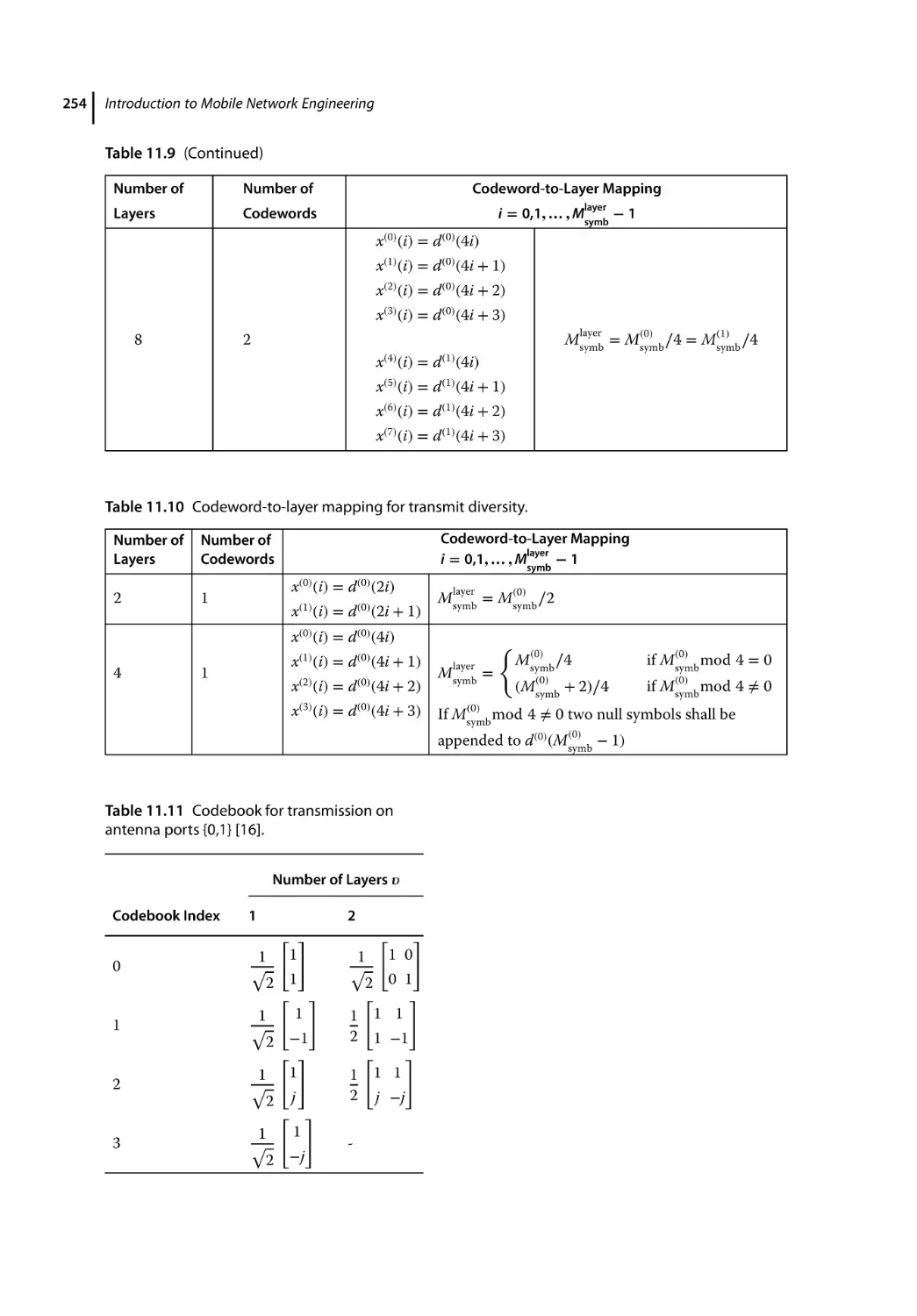
11.24.7.4
11.24.7.5
11.24.7.6
11.25
11.25.1
11.25.2
11.25.3
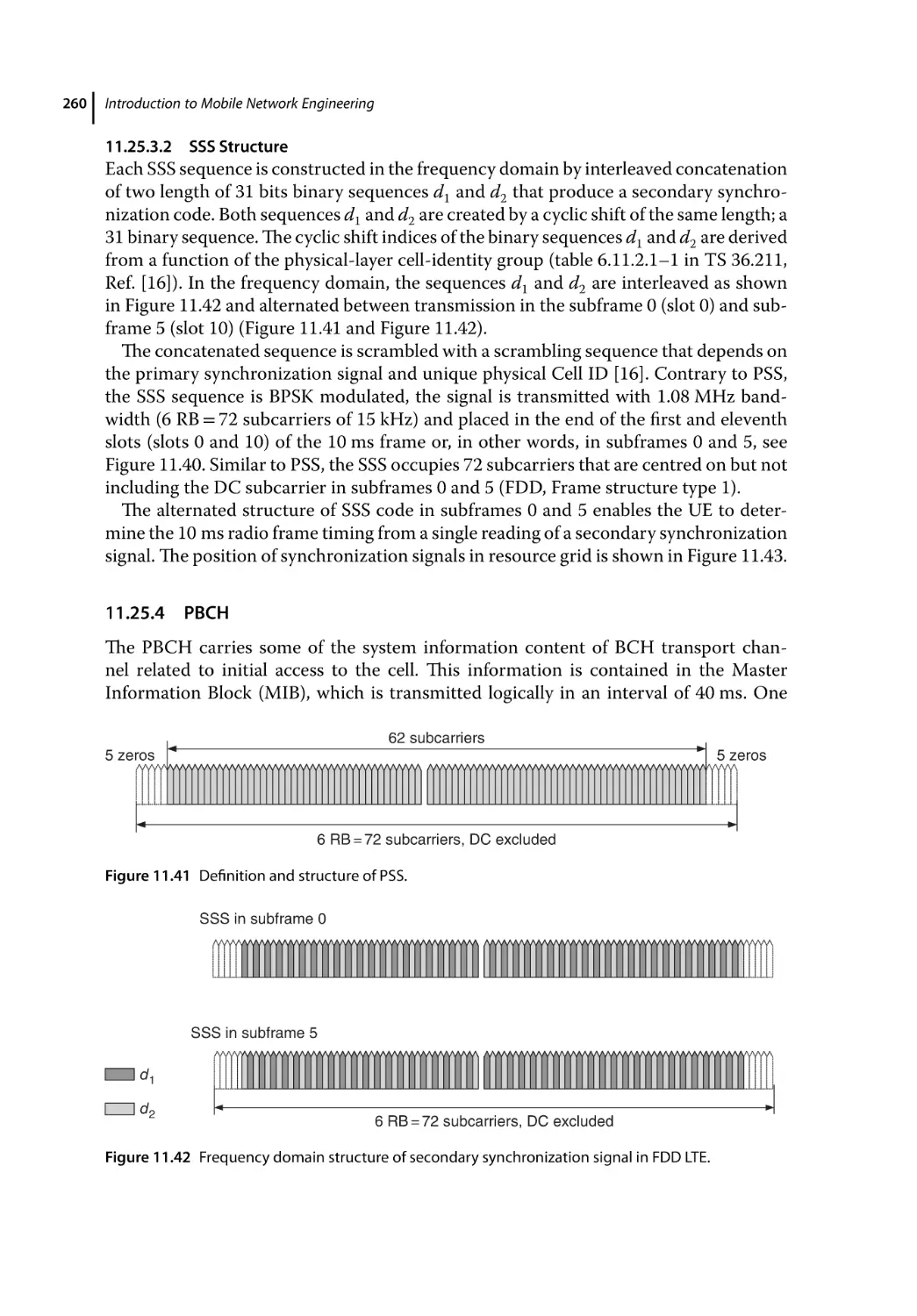
11.25.3.1
Mobility Anchor 216
Inter-eNB Handover 216
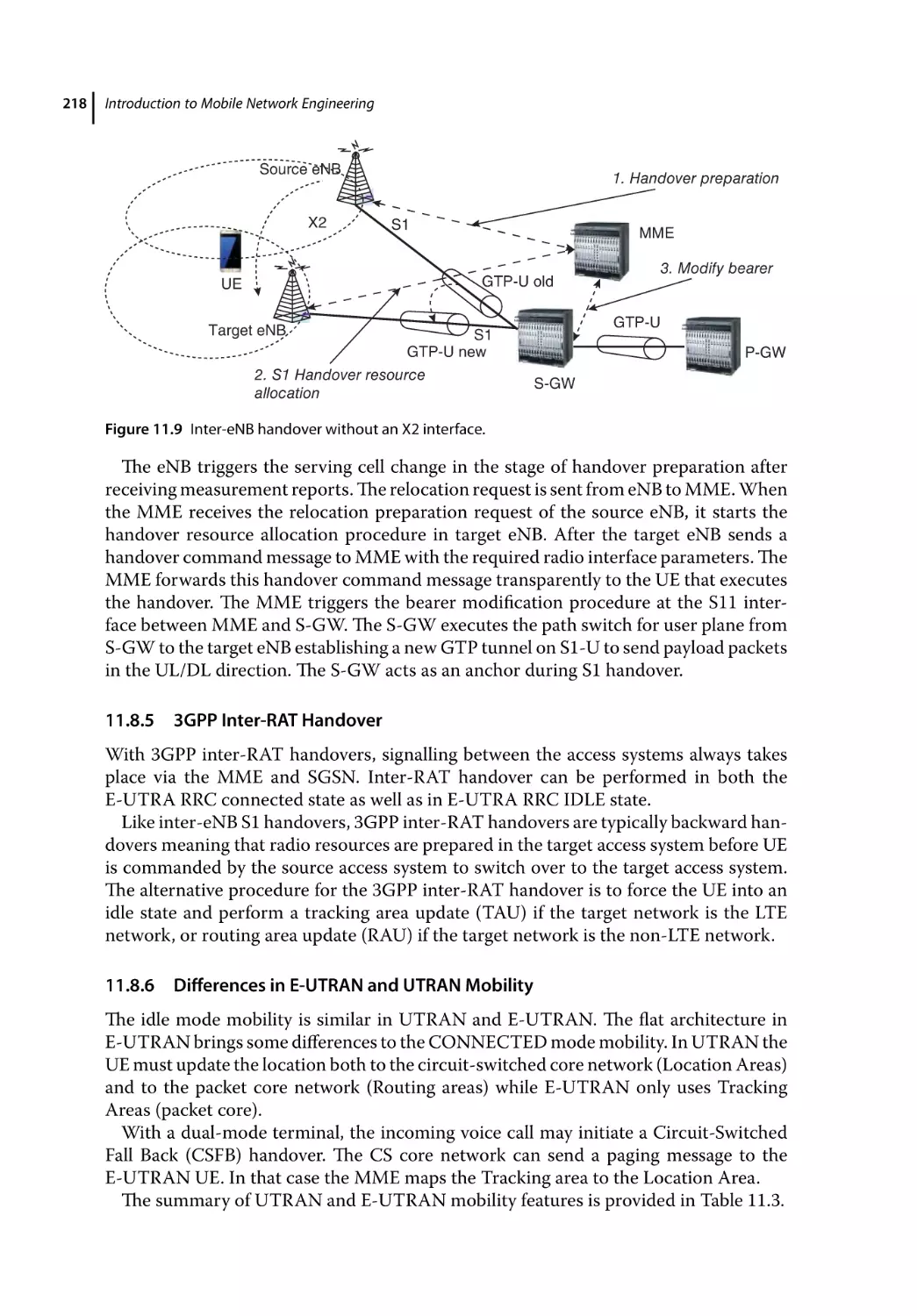
3GPP Inter-RAT Handover 218
Differences in E-UTRAN and UTRAN Mobility 218
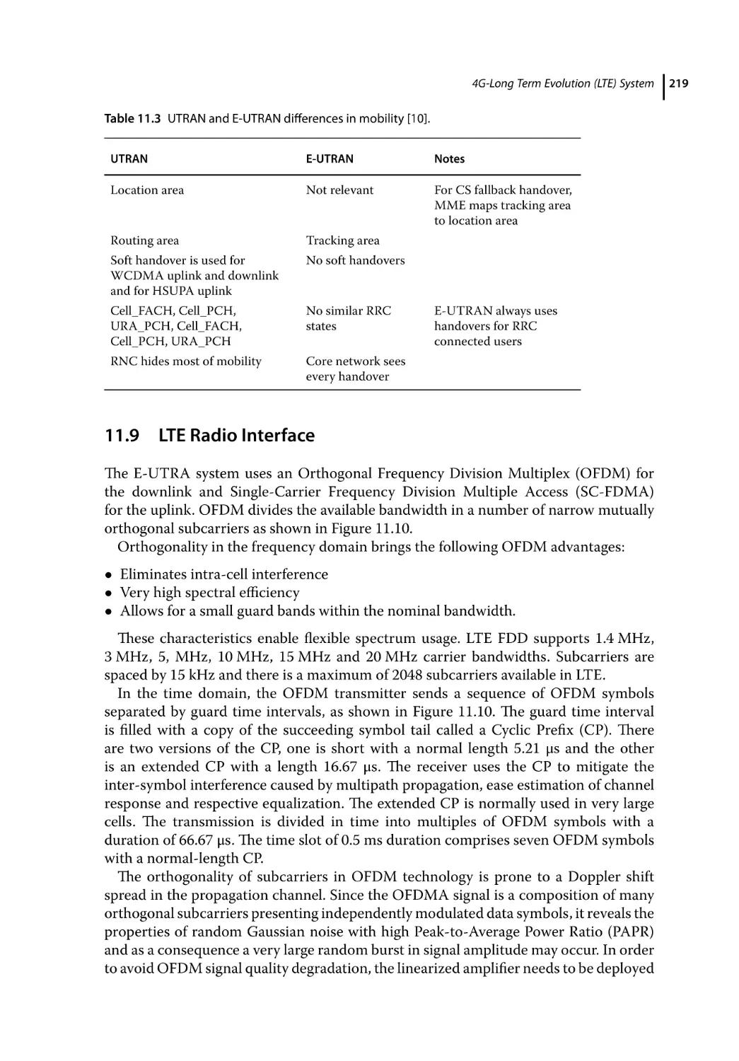
LTE Radio Interface 219
Principle of OFDM 220
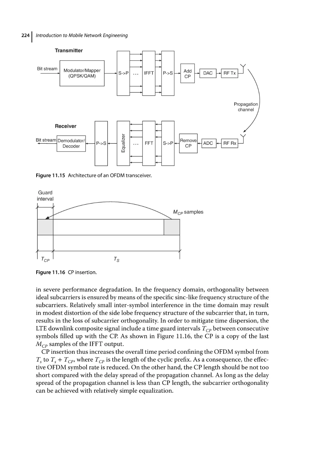
OFDM Implementation using IFFT/FFT Processing 223
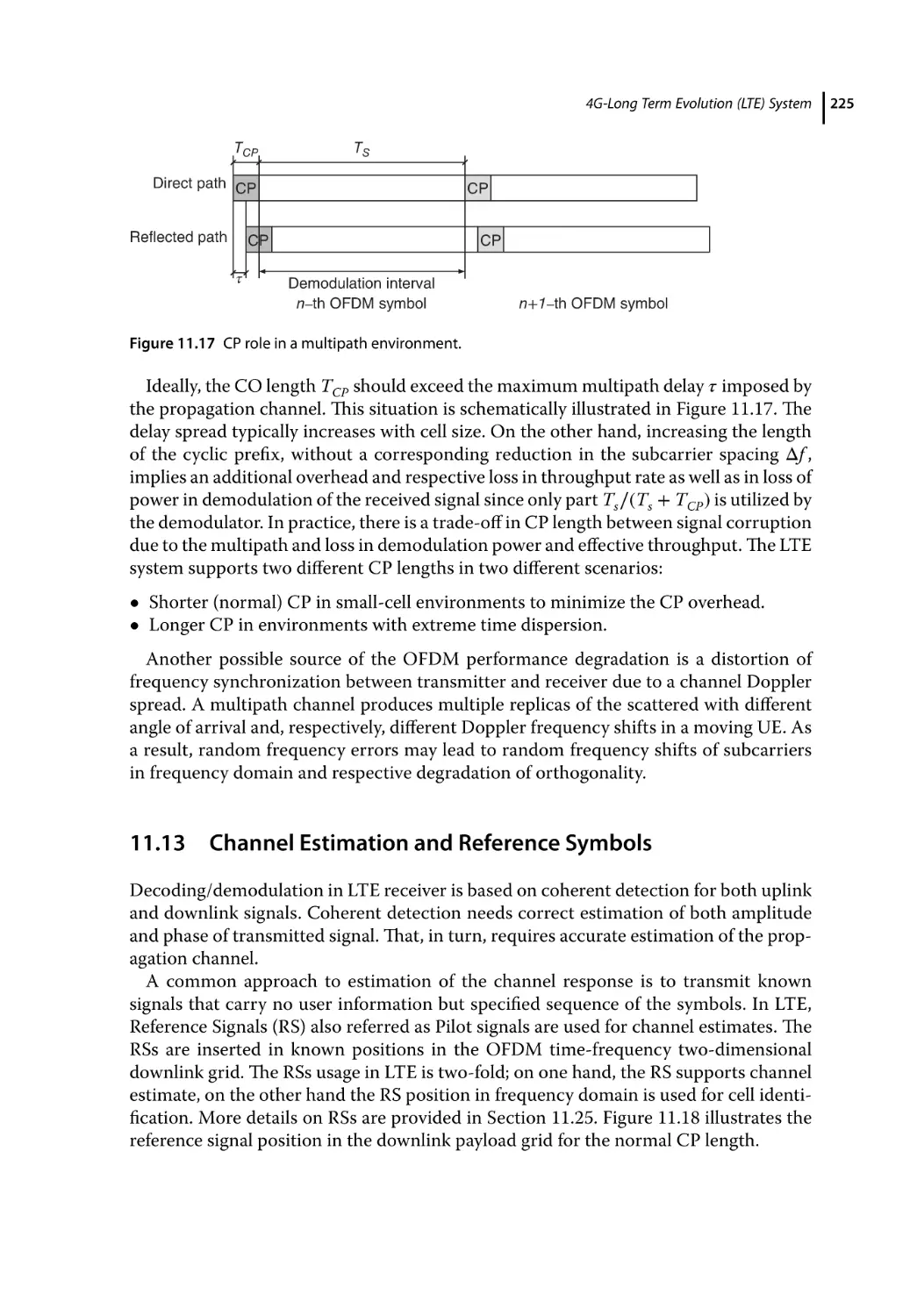
Cyclic Prefix 223
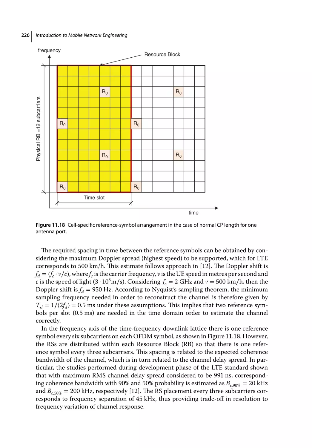
Channel Estimation and Reference Symbols 225
OFDM Subcarrier Spacing 227
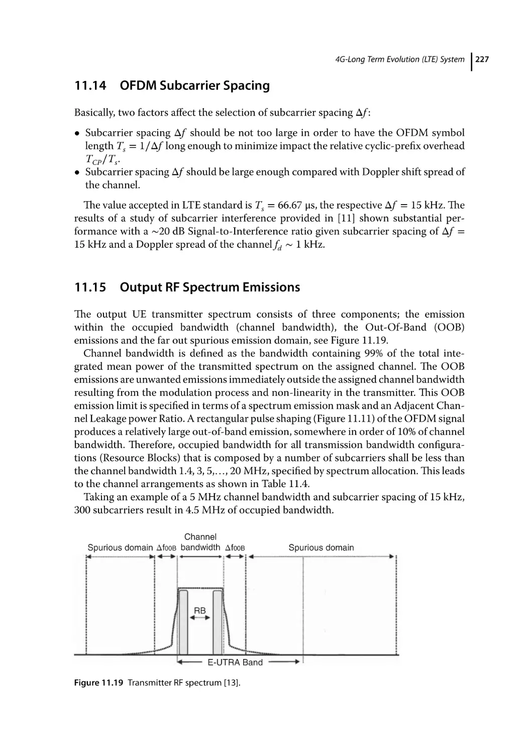
Output RF Spectrum Emissions 227
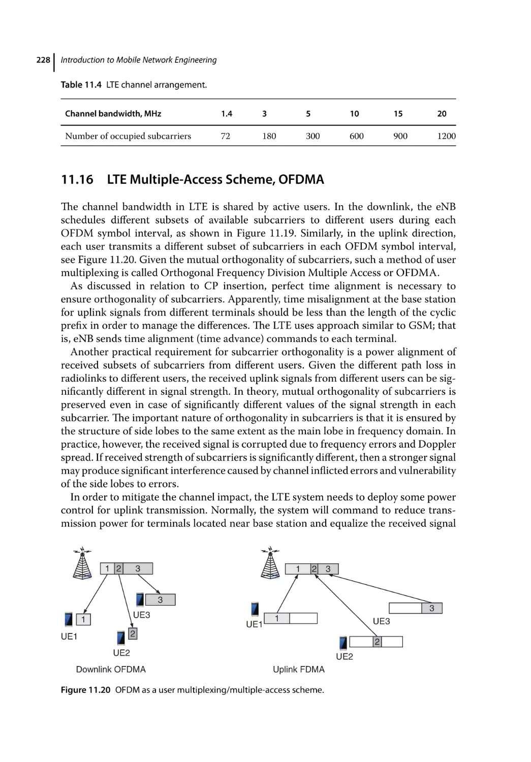
LTE Multiple-Access Scheme, OFDMA 228
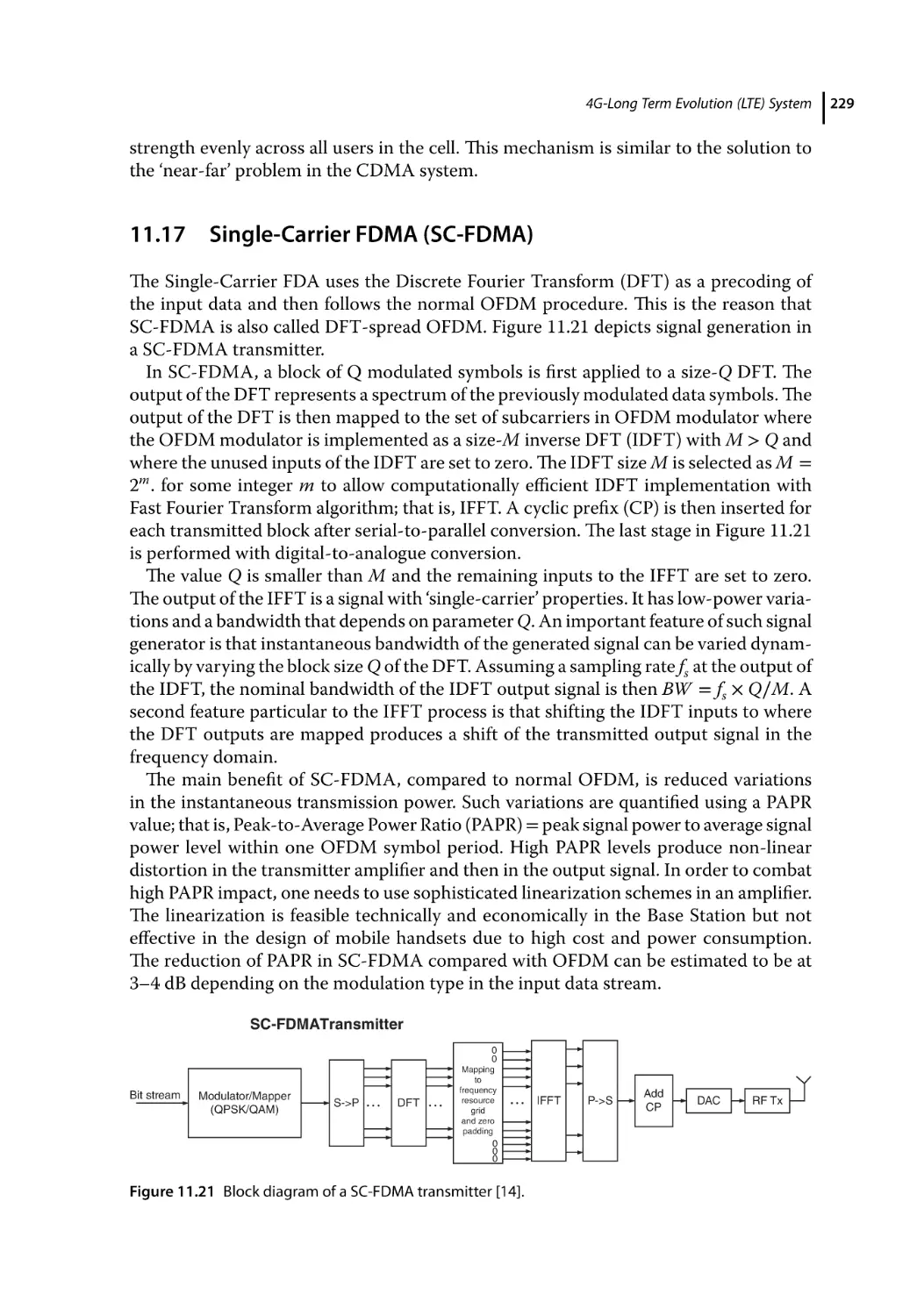
Single-Carrier FDMA (SC-FDMA) 229
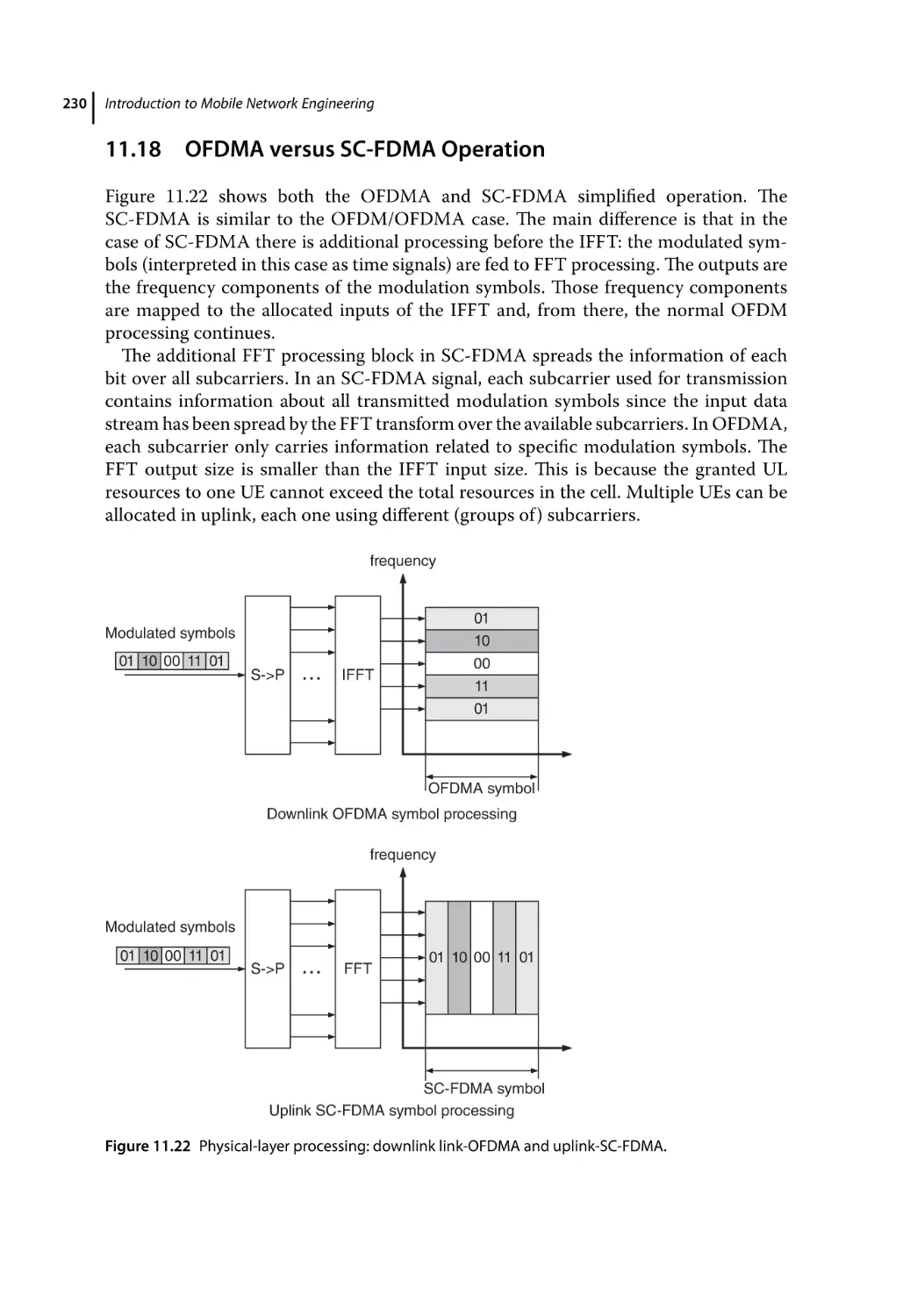
OFDMA versus SC-FDMA Operation 230
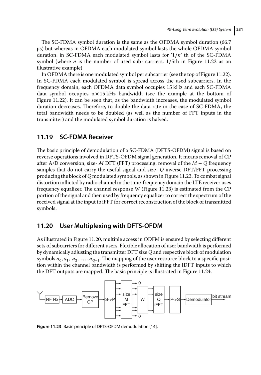
SC-FDMA Receiver 231
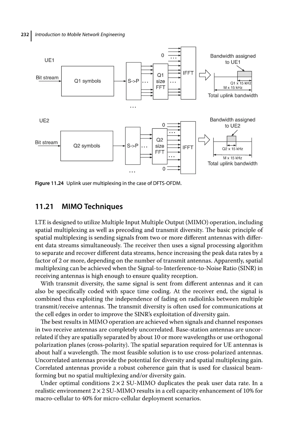
User Multiplexing with DFTS-OFDM 231
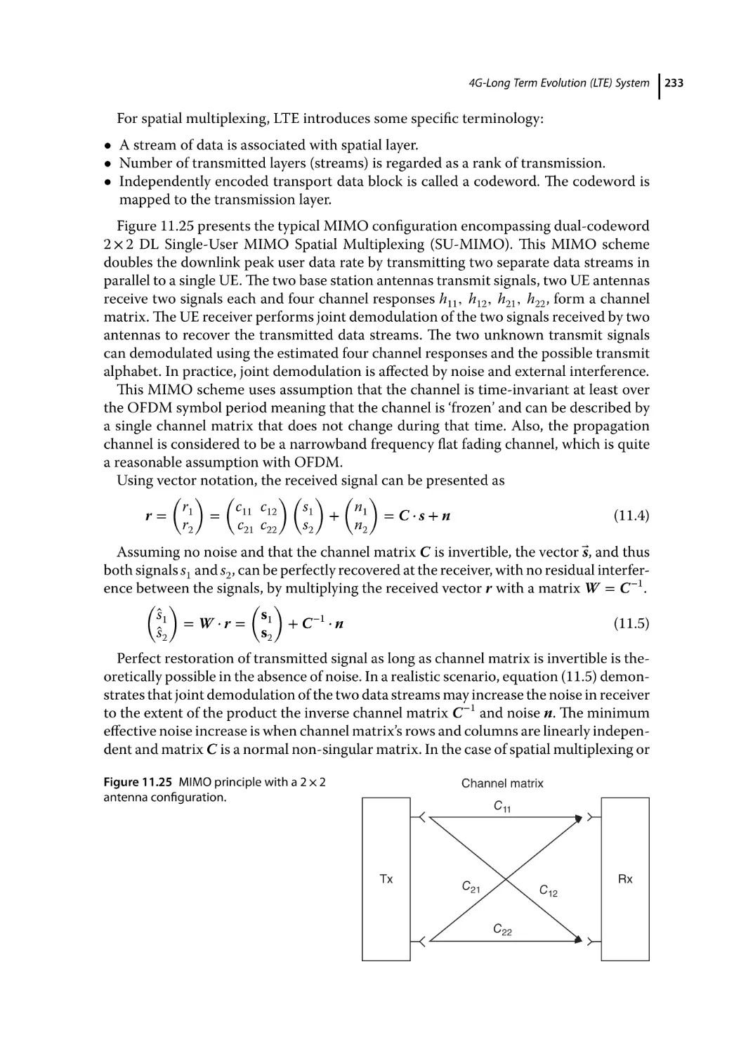
MIMO Techniques 232
Precoding 234
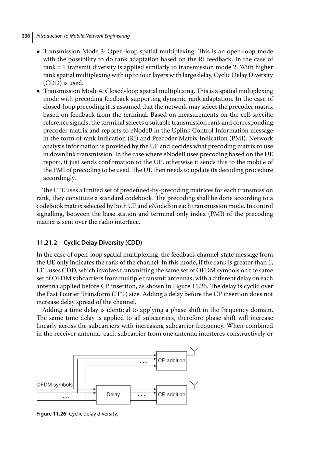
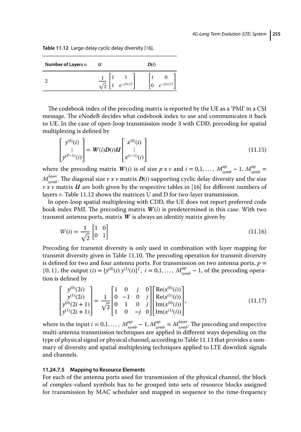
Cyclic Delay Diversity (CDD) 236
Link Adaptation and Frequency Domain Packet Scheduling 237
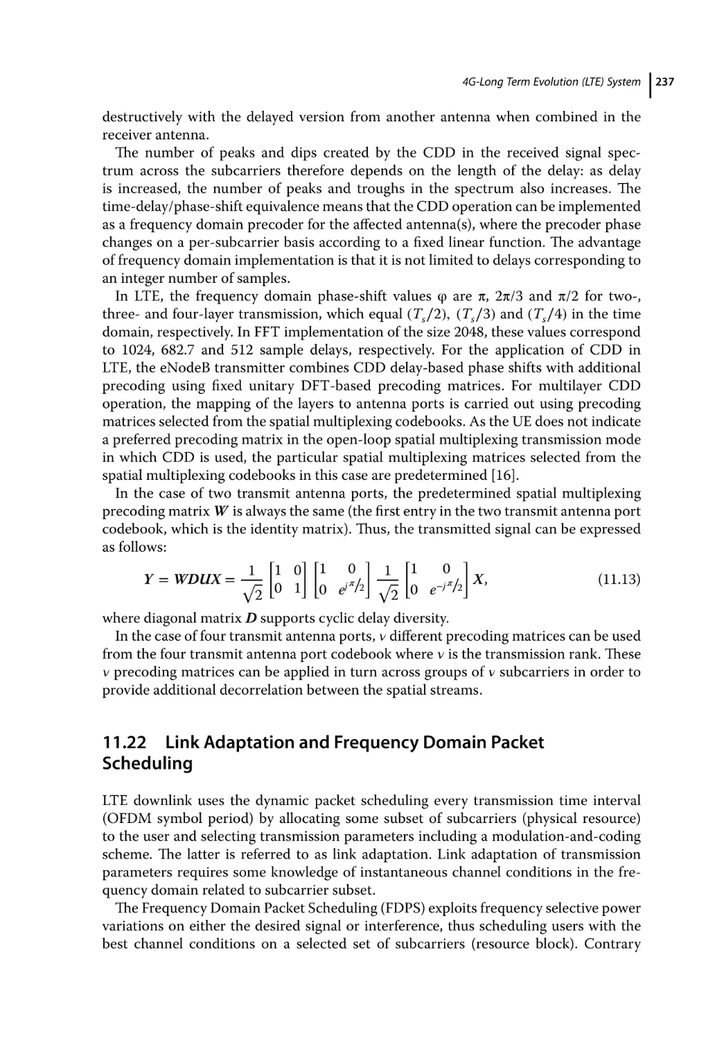
Radio Protocol Architecture 238
User Plane 239
Control Plane 239
Scheduler 240
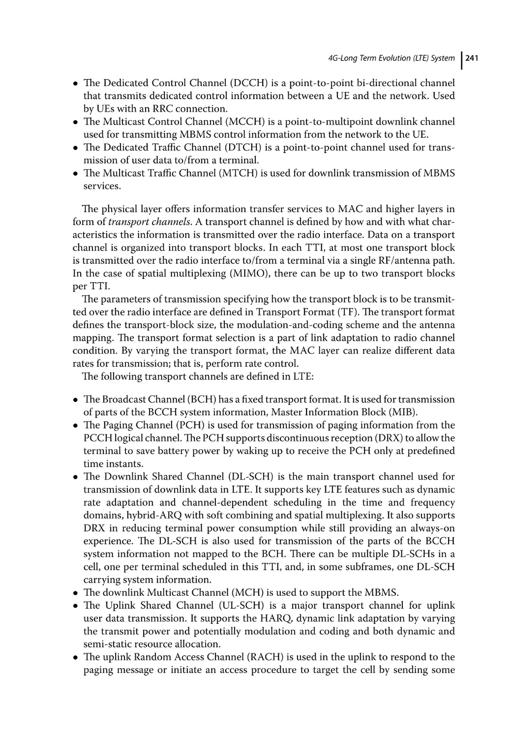
Logical and Transport Channels 240
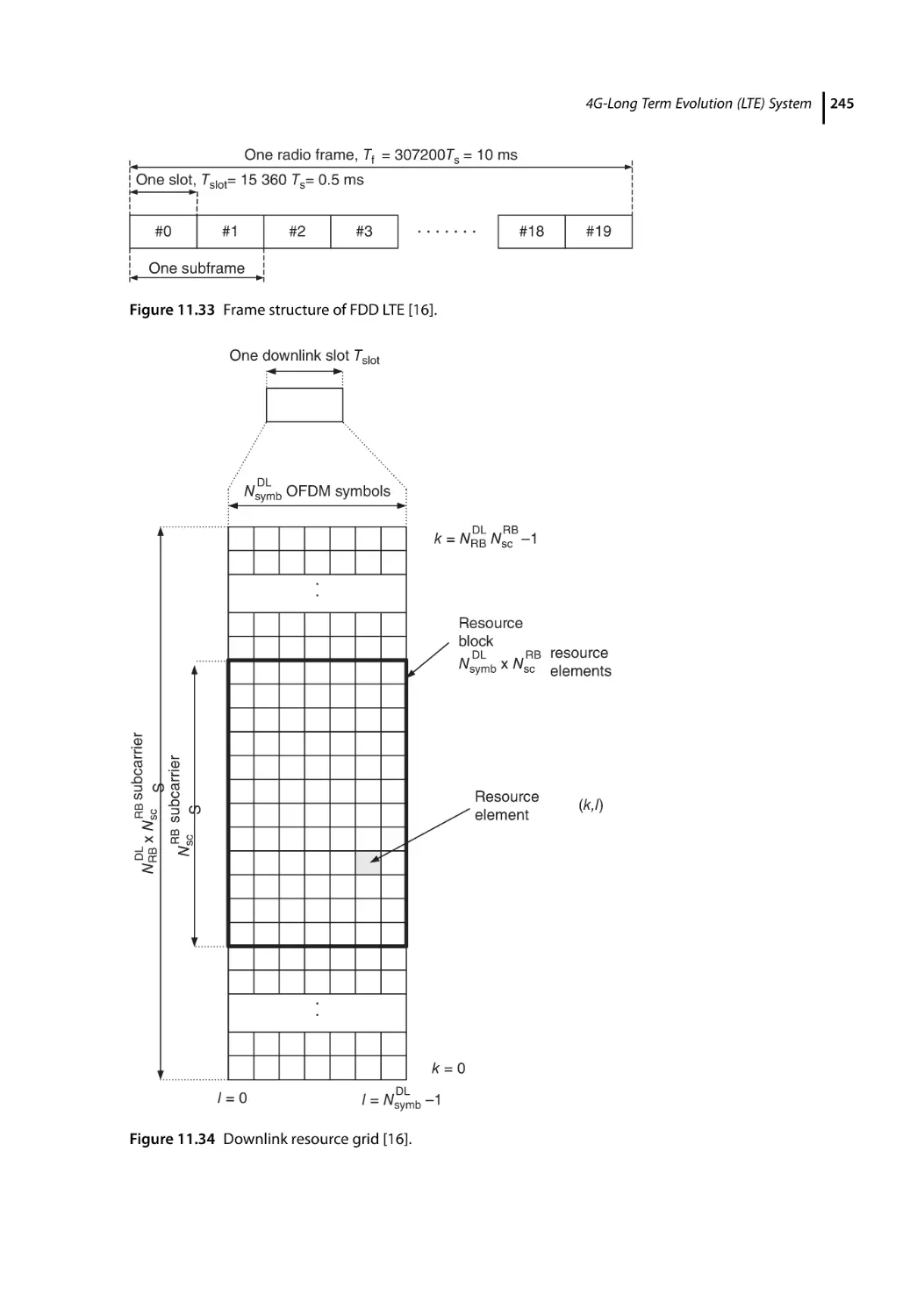
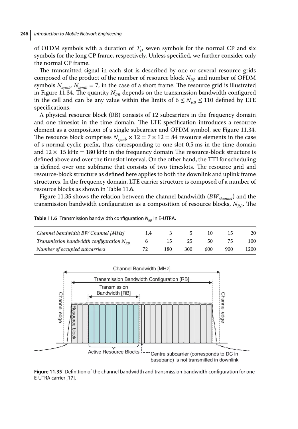
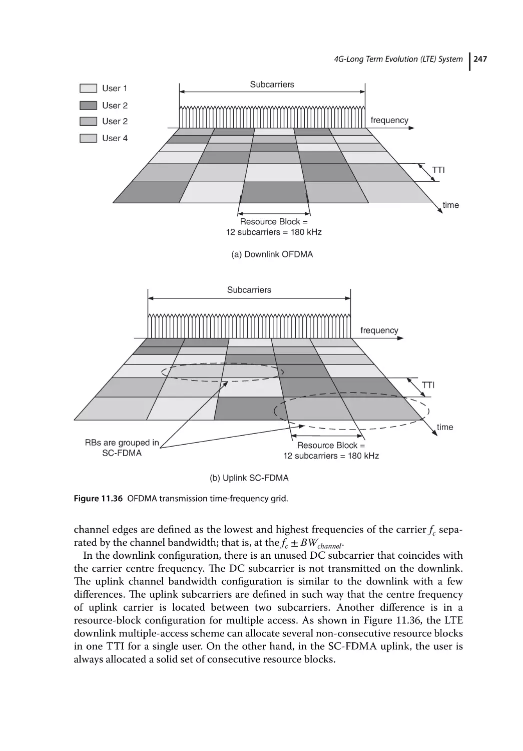
Physical Layer 242
RRC State Machine 244
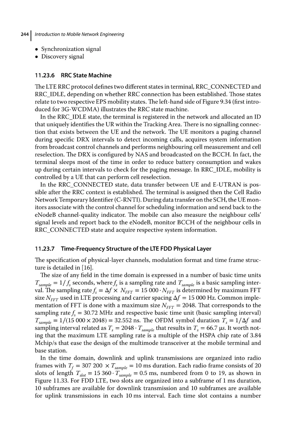
Time-Frequency Structure of the LTE FDD Physical Layer 244
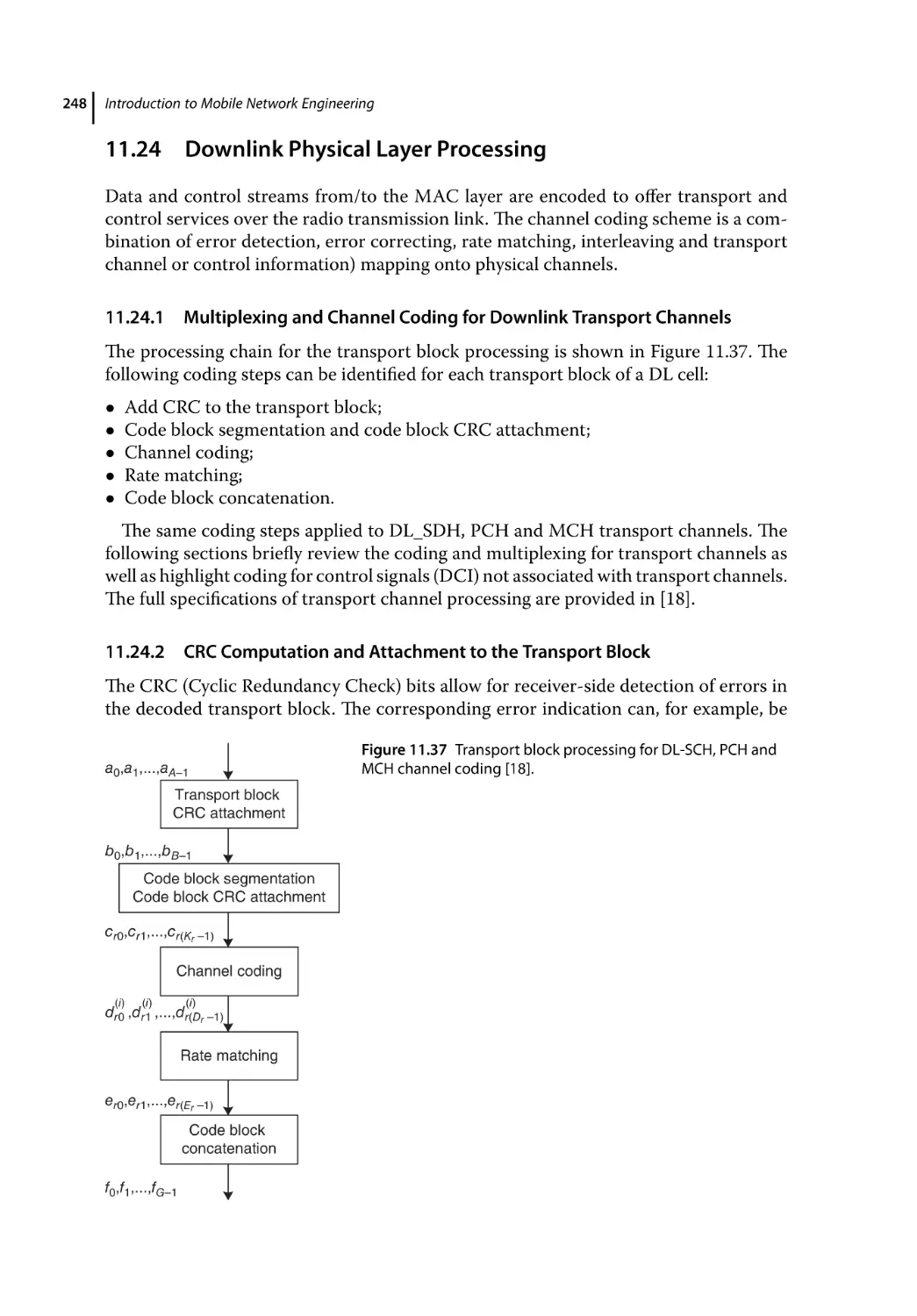
Downlink Physical Layer Processing 248
Multiplexing and Channel Coding for Downlink Transport Channels 248
CRC Computation and Attachment to the Transport Block 248
Code Block Segmentation and Code Block CRC Attachment 249
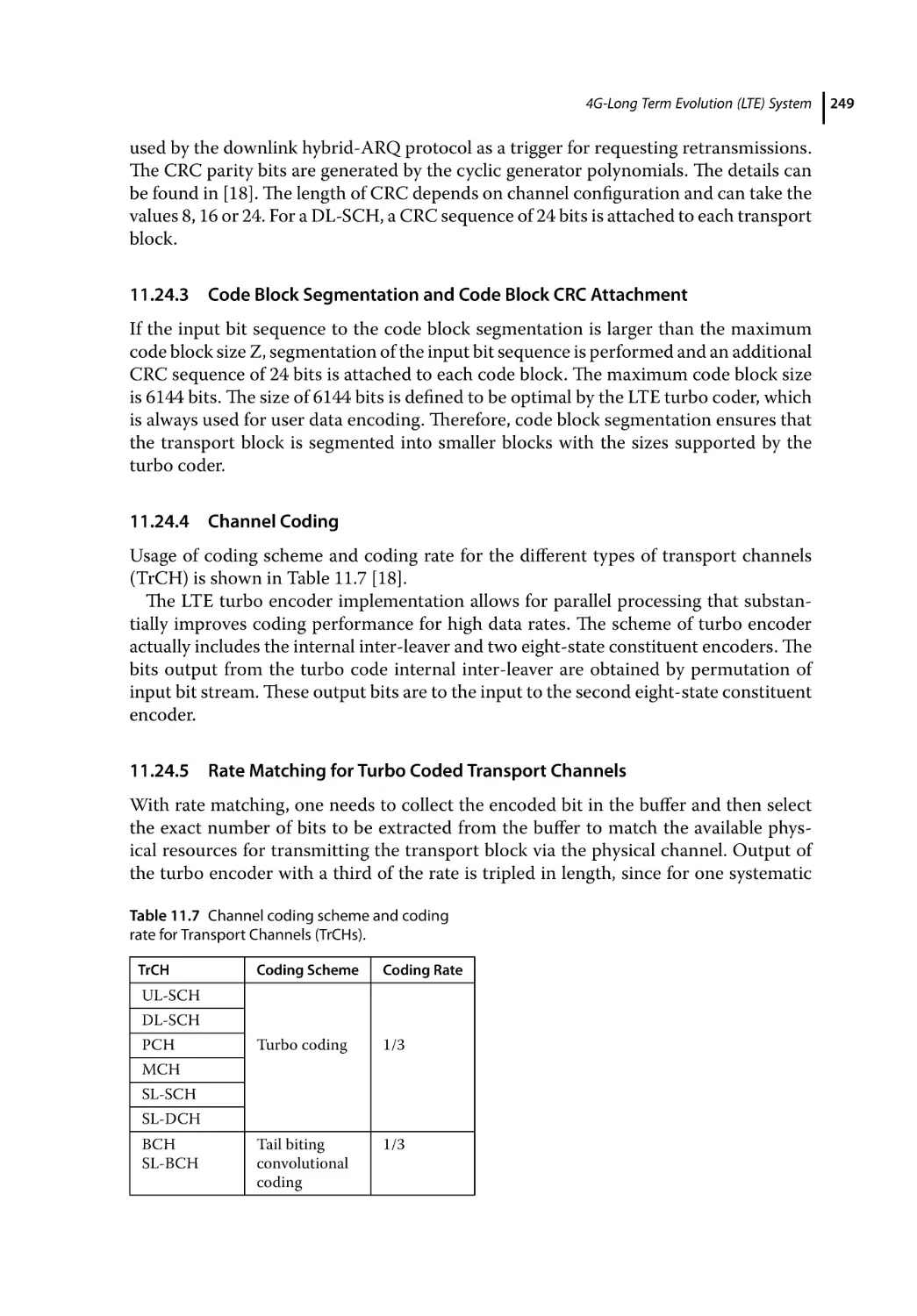
Channel Coding 249
Rate Matching for Turbo Coded Transport Channels 249
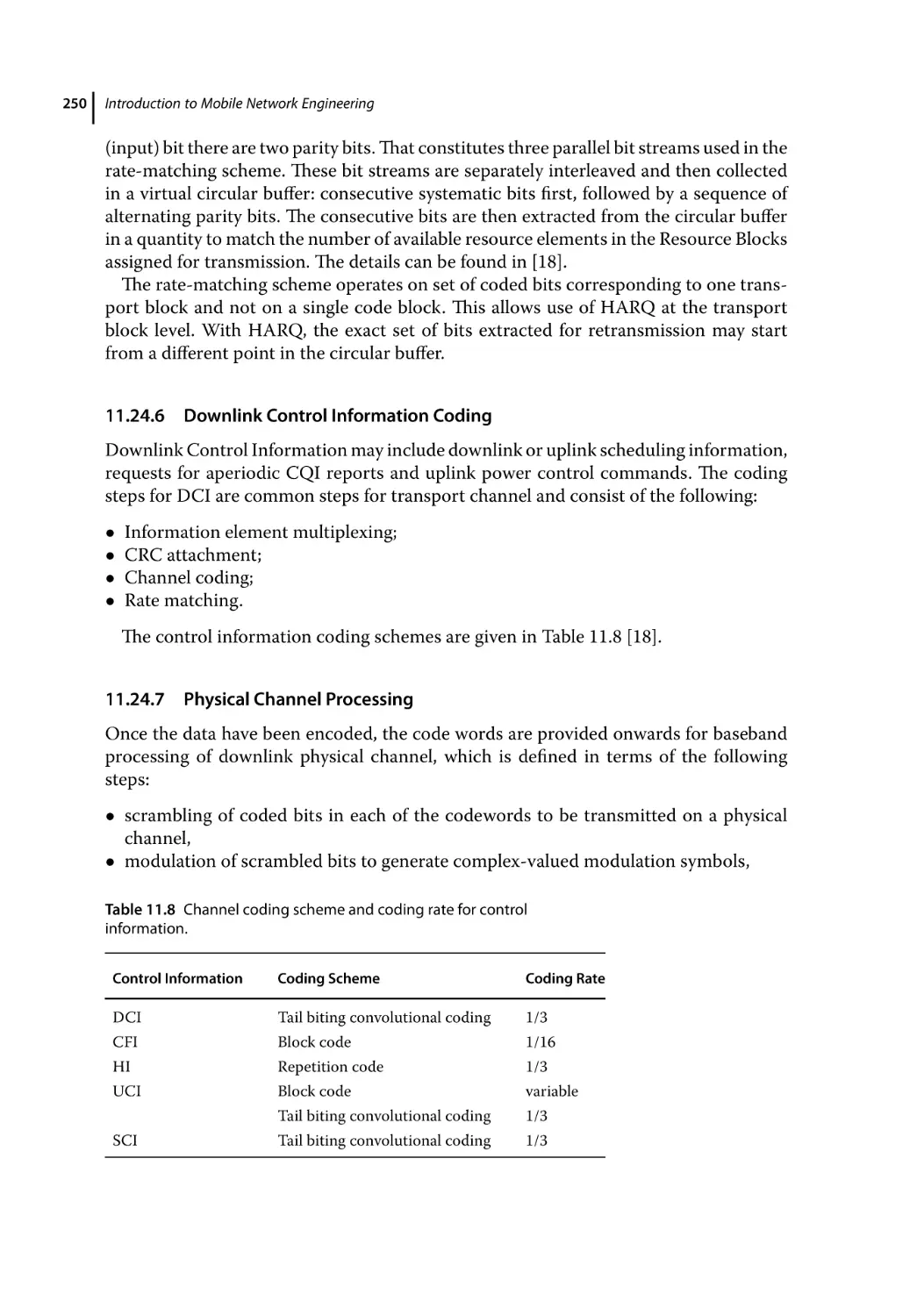
Downlink Control Information Coding 250
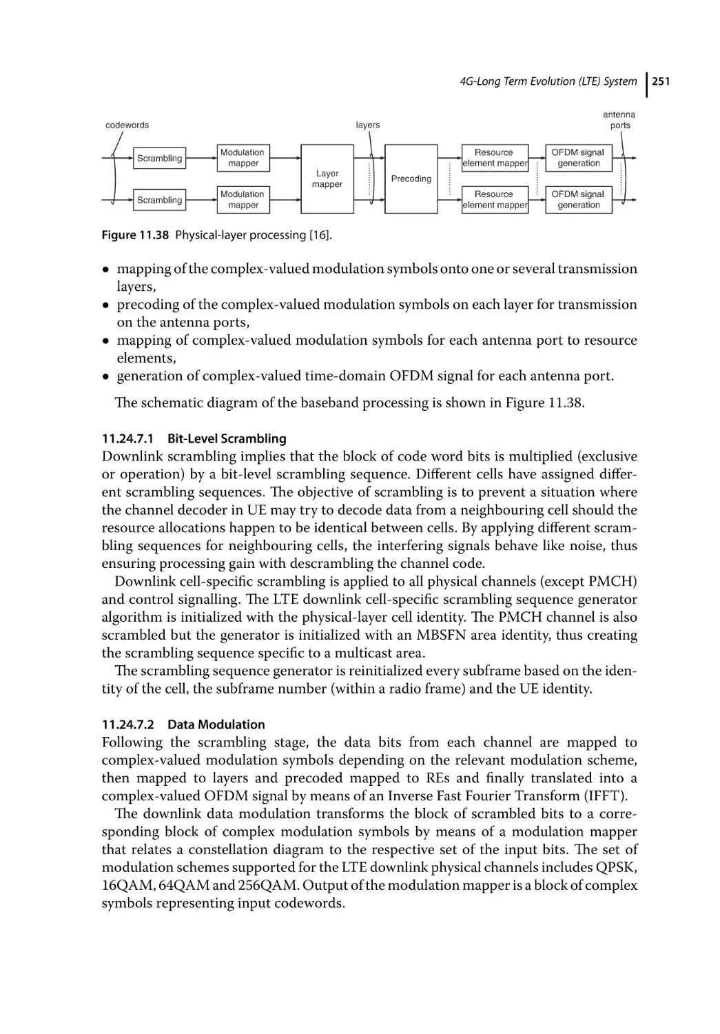
Physical Channel Processing 250
Bit-Level Scrambling 251
Data Modulation 251
Layer Mapping 252
Precoding 252
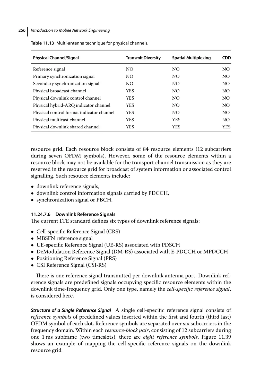
Mapping to Resource Elements 255
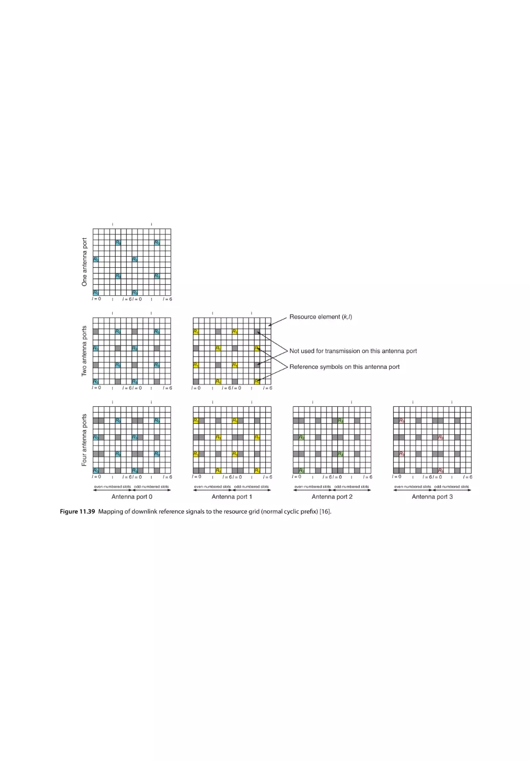
Downlink Reference Signals 256
Downlink Control Channels 258
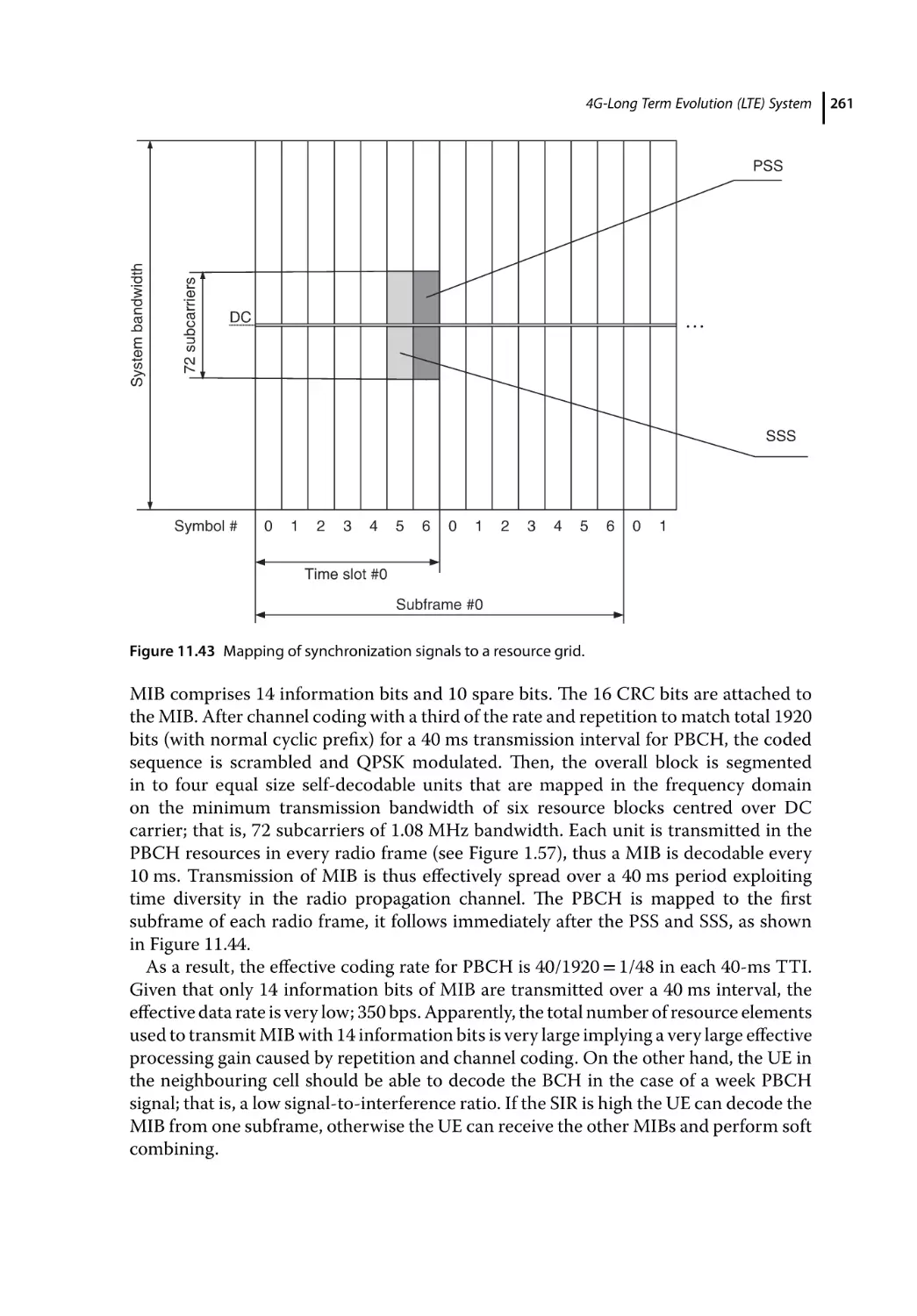
Structure of the Synchronization Channel 258
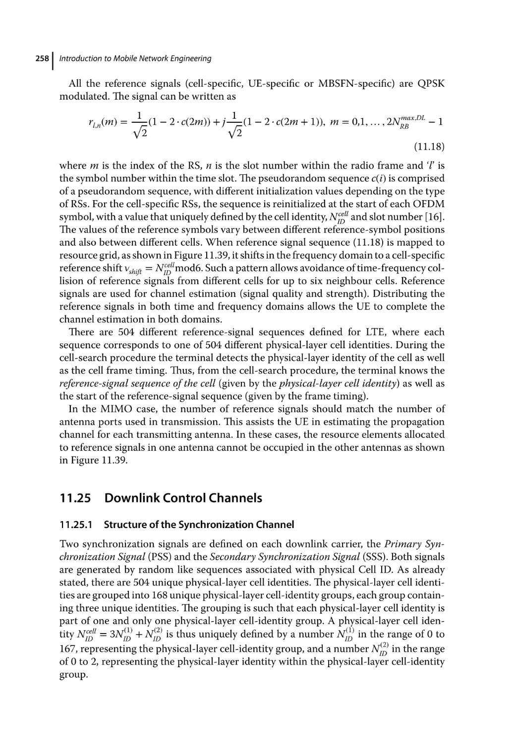
Time-Domain Position of Synchronization Signals 259
Frequency Domain Structure of Synchronization Signals 259
PSS Structure 259
xiii
xiv
Contents
11.25.3.2
11.25.4
11.25.5
11.25.6
11.25.7
11.26
11.27
11.27.1
11.27.2
11.27.3
11.27.4
11.27.5
11.27.6
11.27.7
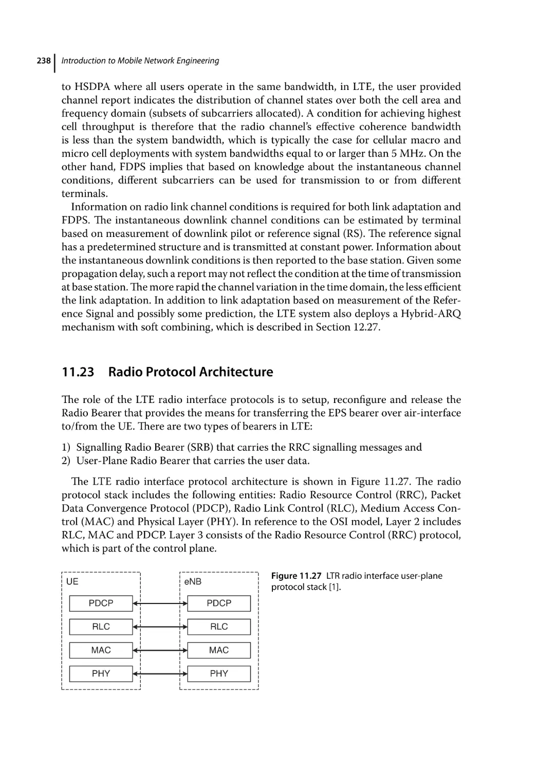
11.28
11.28.1
11.29
11.29.1
11.29.2
11.29.3
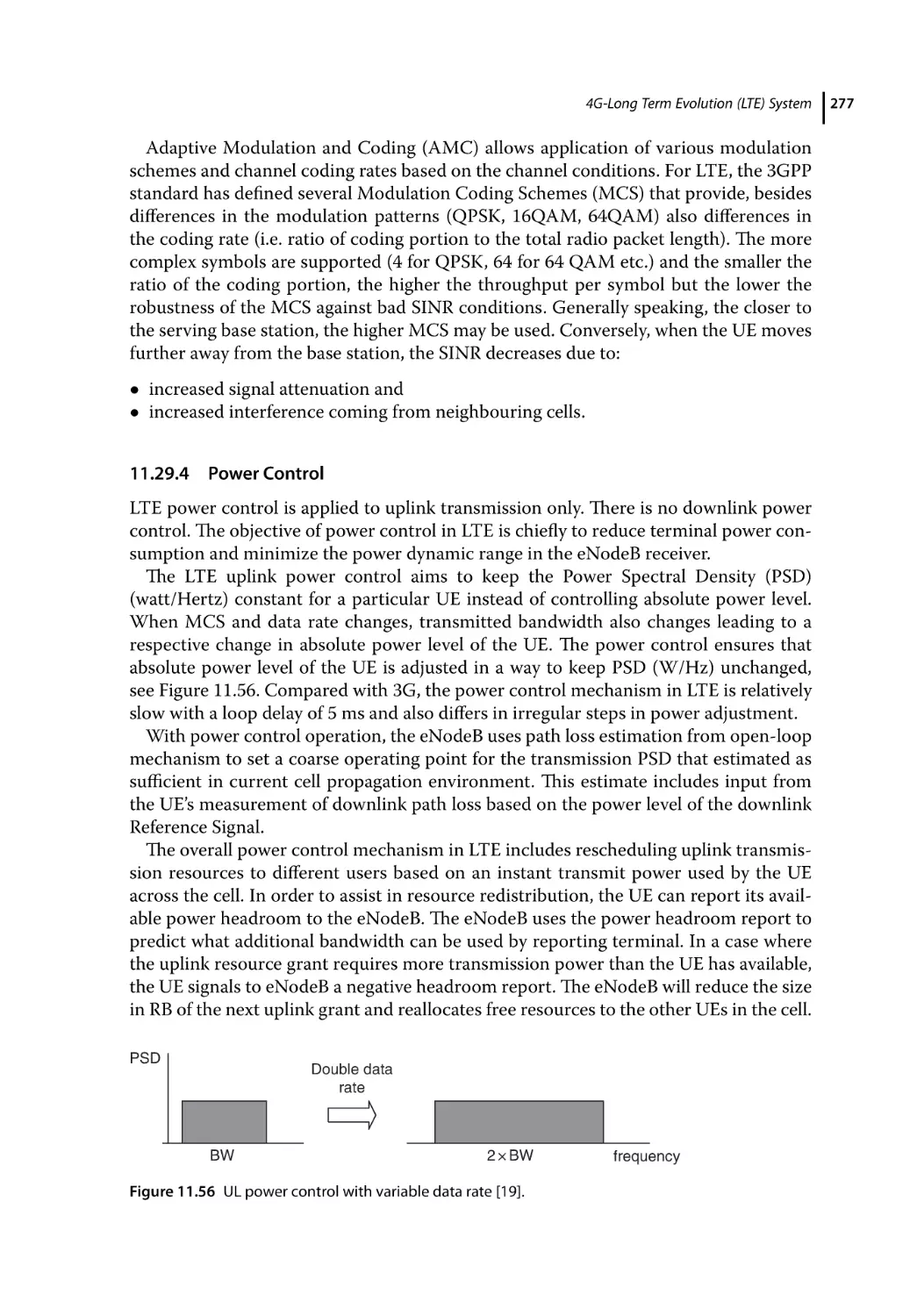
11.29.4
11.29.5
11.29.6
11.30
11.30.1
11.30.1.1
11.30.1.2
11.30.1.3
11.30.1.4
11.30.1.5
11.30.1.6
11.30.1.7
11.30.2
11.31
SSS Structure 260
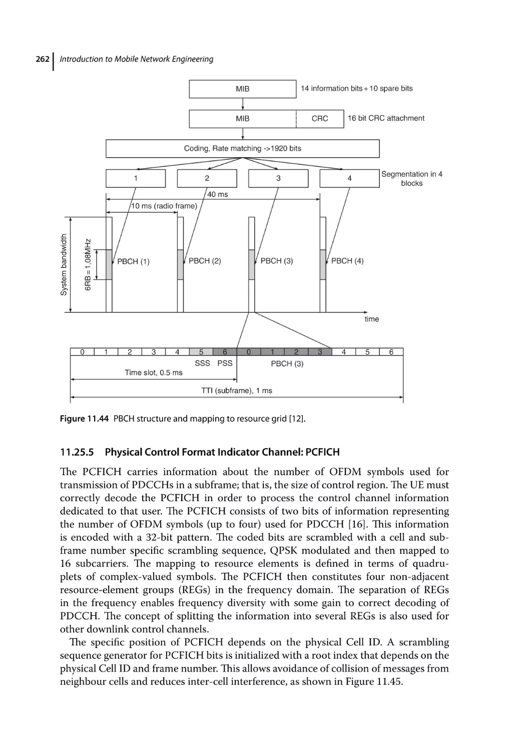
PBCH 260
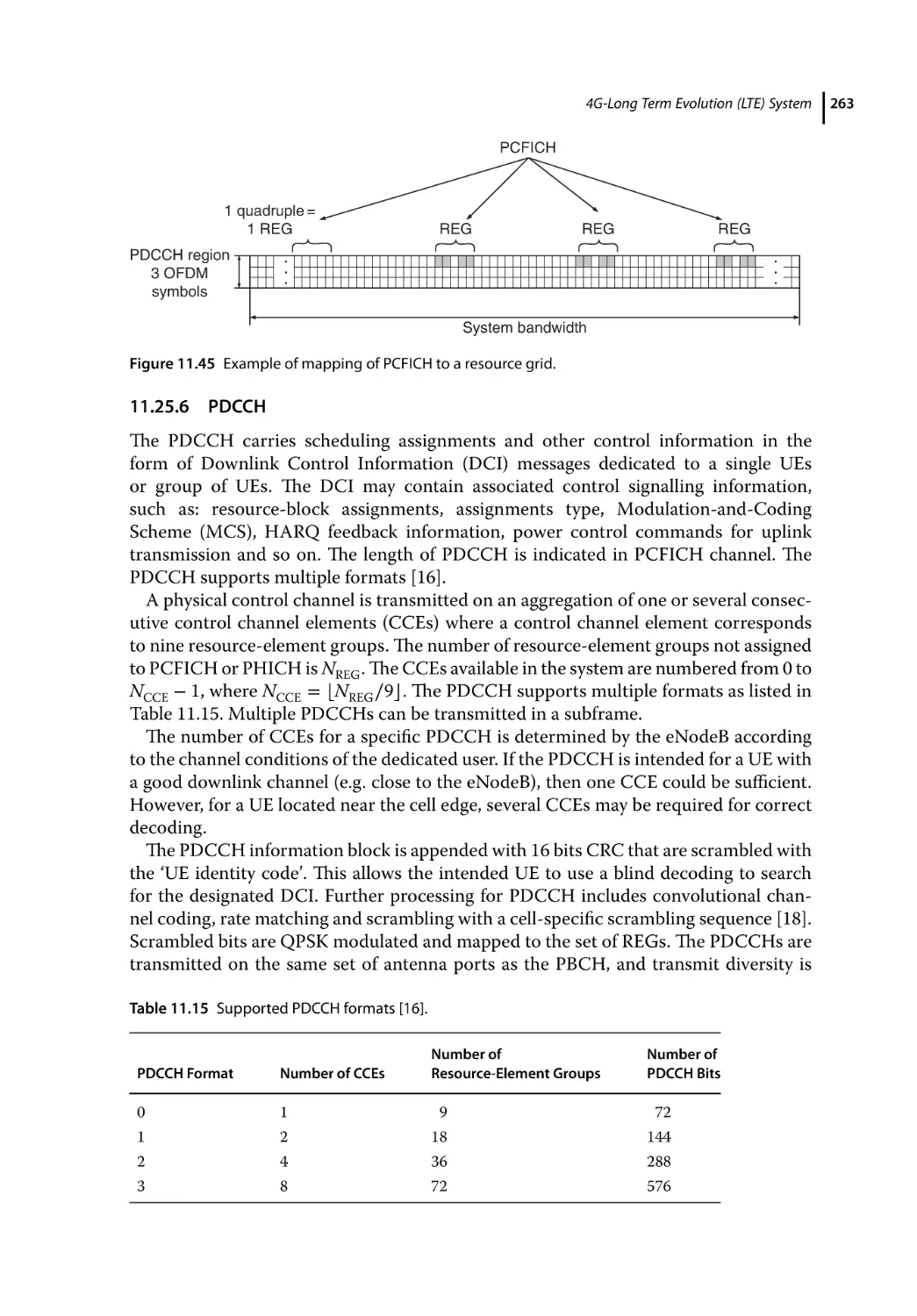
Physical Control Format Indicator Channel: PCFICH 262
PDCCH 263
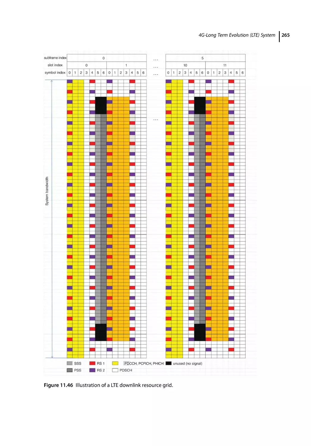
PHICH, Physical Hybrid-ARQ Indicator Channel 264
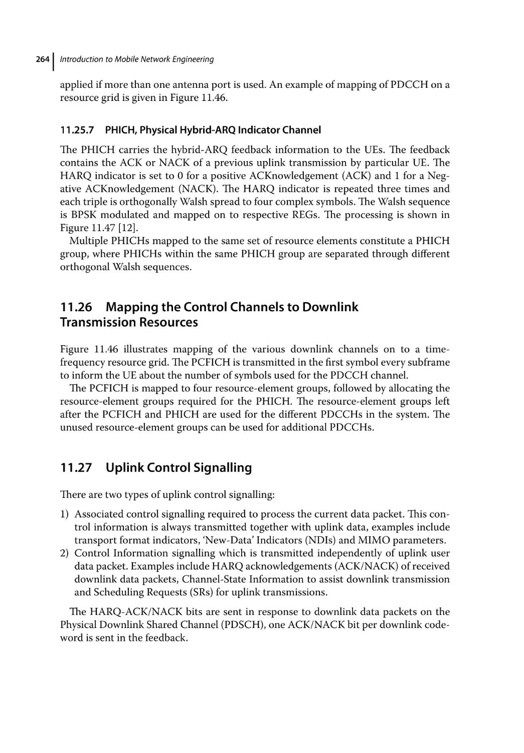
Mapping the Control Channels to Downlink Transmission Resources 264
Uplink Control Signalling 264
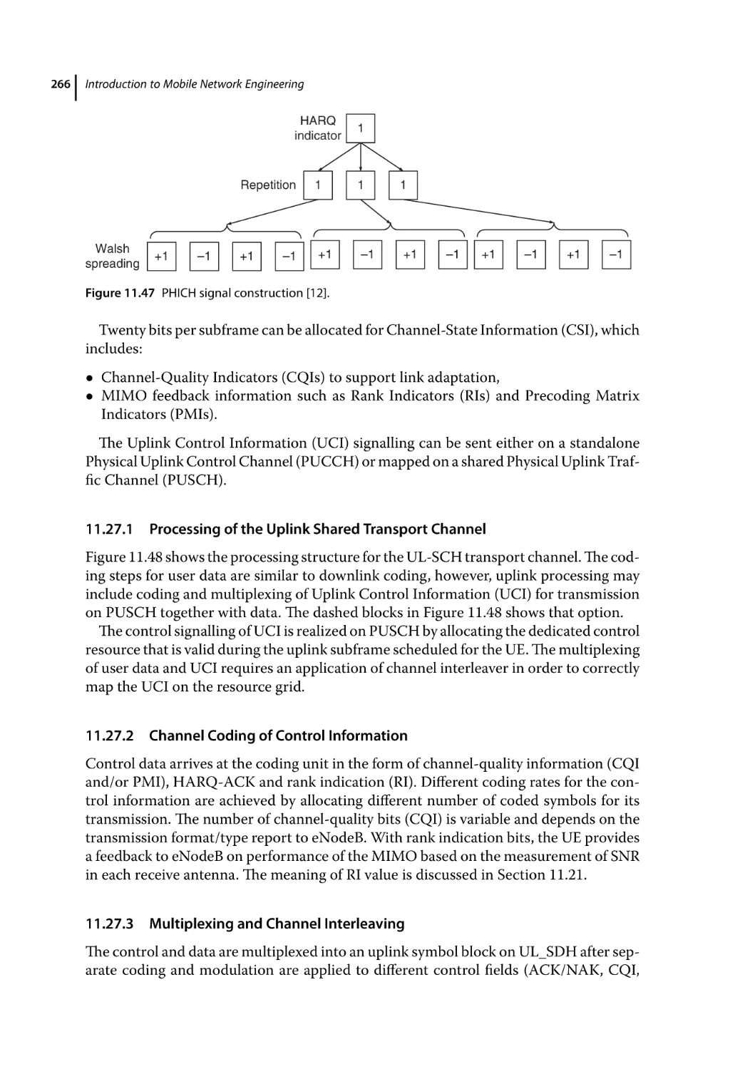
Processing of the Uplink Shared Transport Channel 266
Channel Coding of Control Information 266
Multiplexing and Channel Interleaving 266
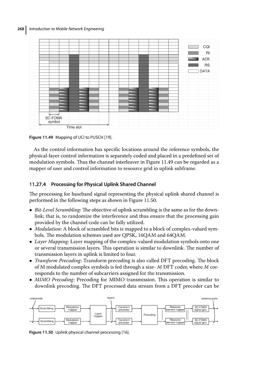
Processing for Physical Uplink Shared Channel 268
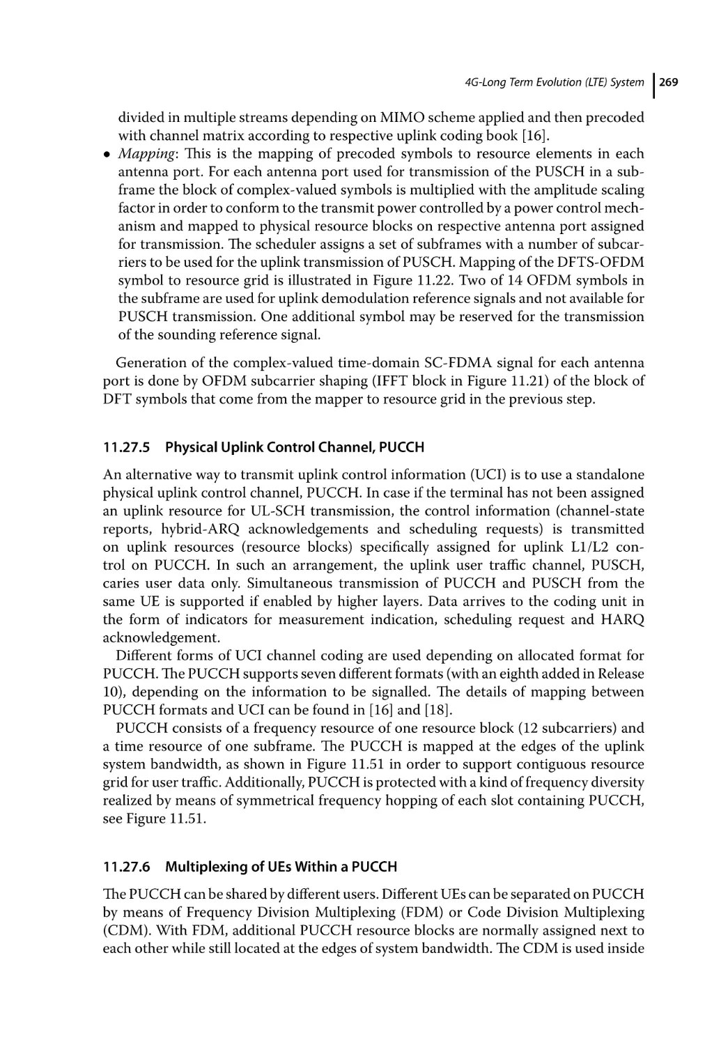
Physical Uplink Control Channel, PUCCH 269
Multiplexing of UEs Within a PUCCH 269
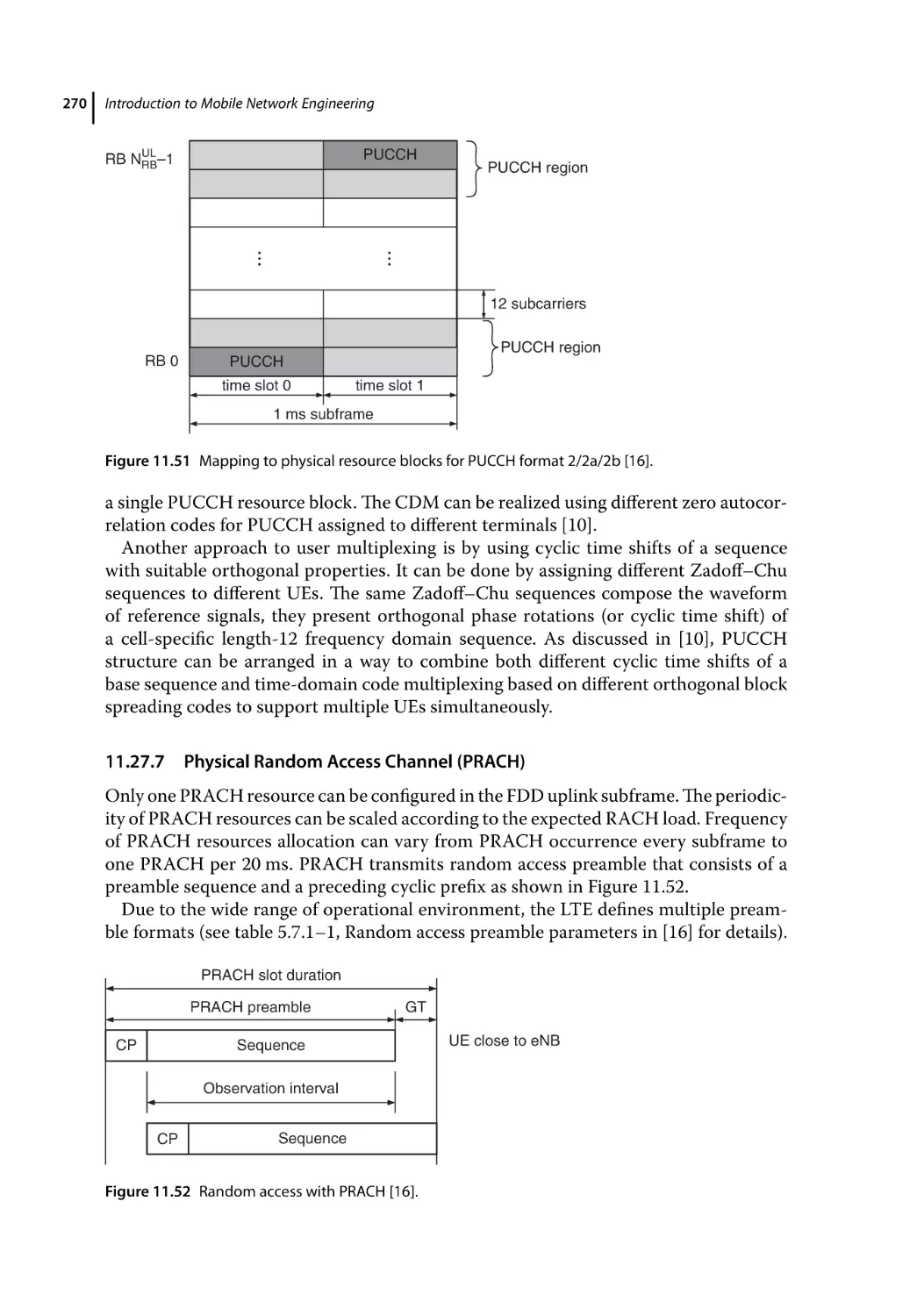
Physical Random Access Channel (PRACH) 270
Uplink Reference Signals 271
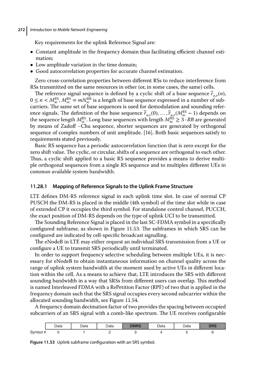
Mapping of Reference Signals to the Uplink Frame Structure 272
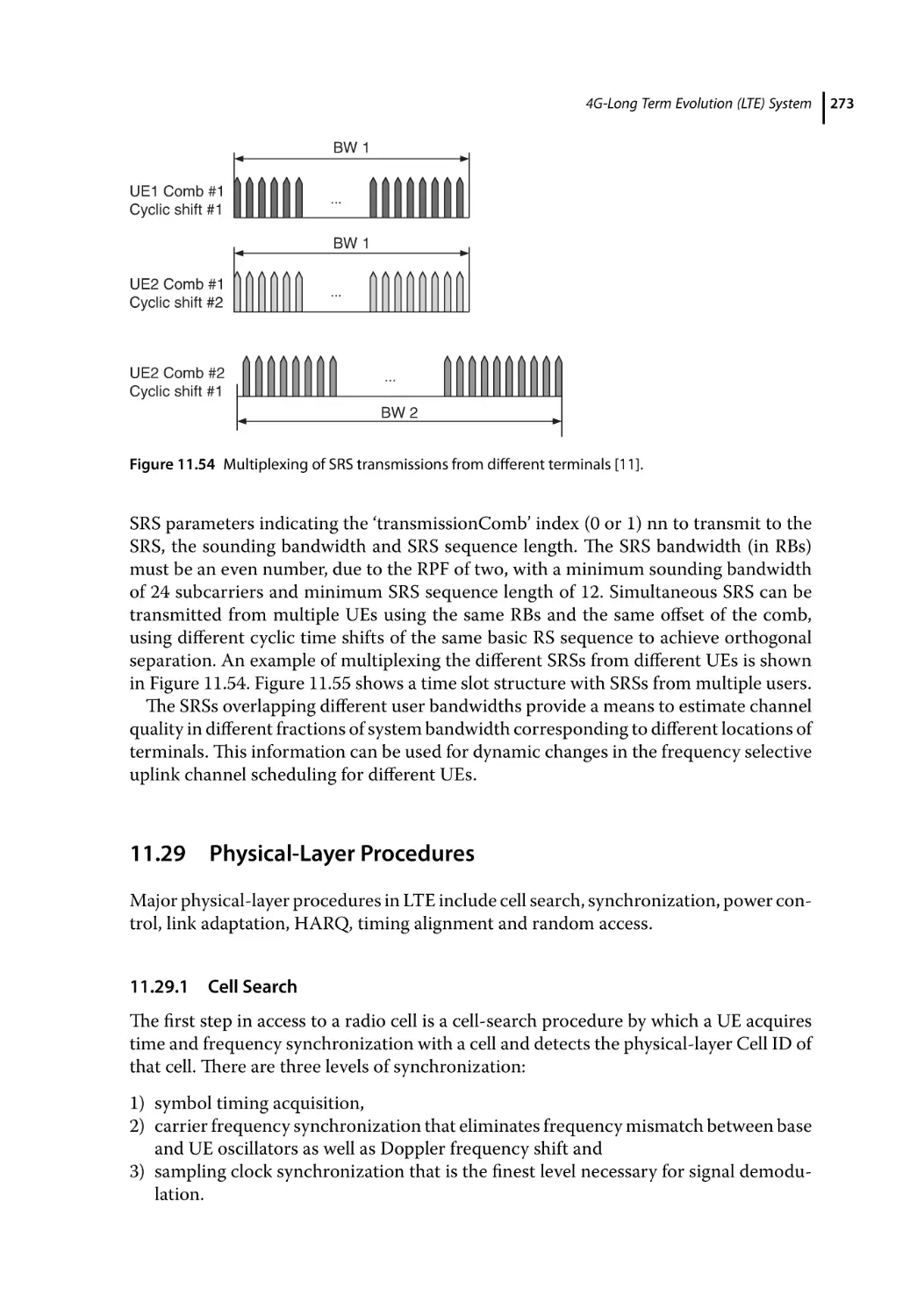
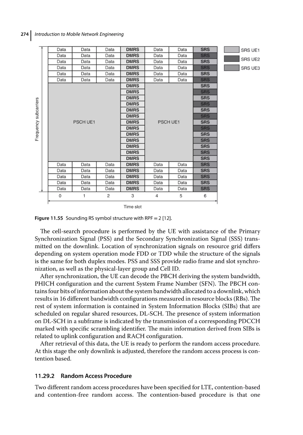
Physical-Layer Procedures 273
Cell Search 273
Random Access Procedure 274
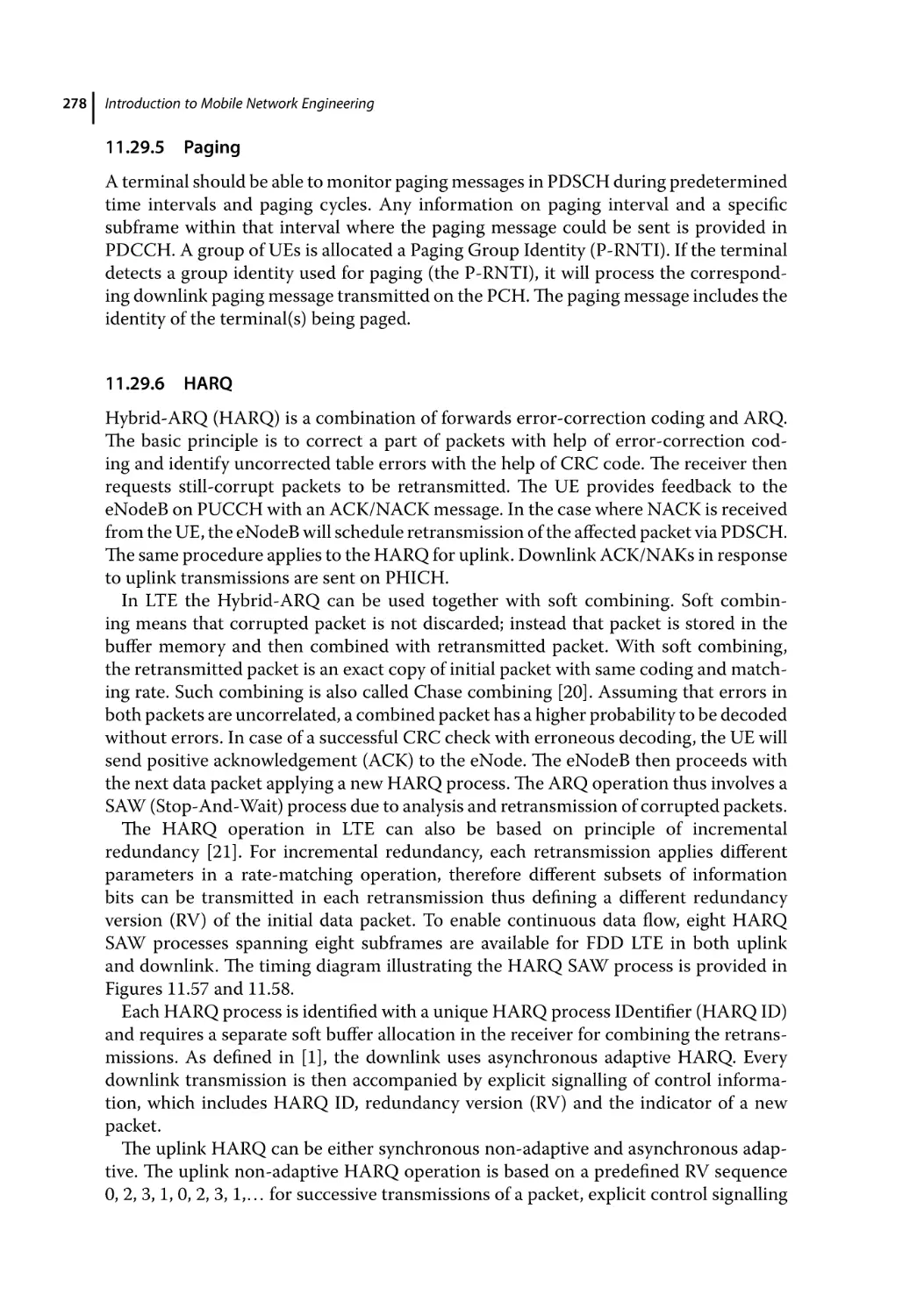
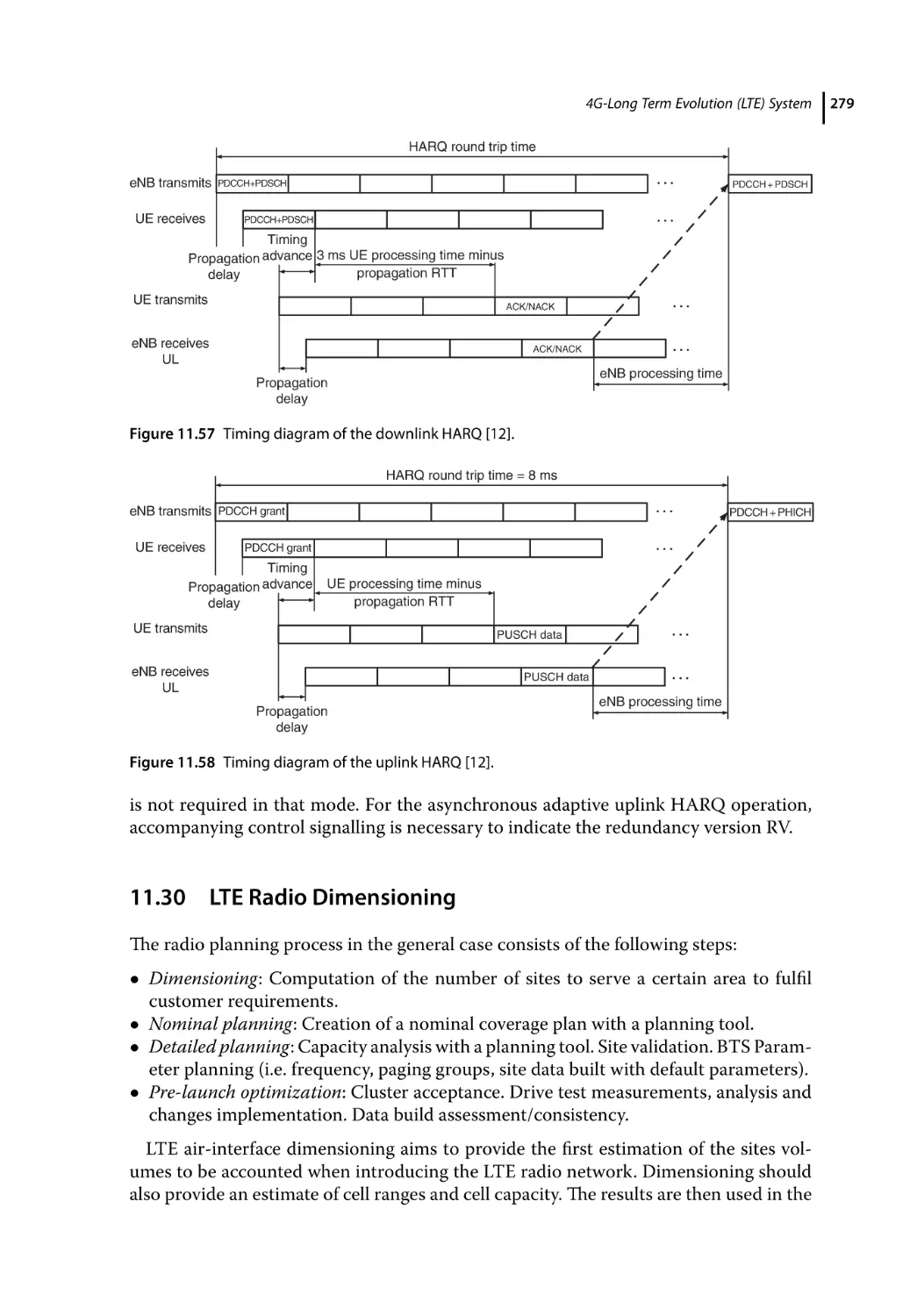
Link Adaptation 276
Power Control 277
Paging 278
HARQ 278
LTE Radio Dimensioning 279
LTE Coverage Dimensioning: Link Budget 280
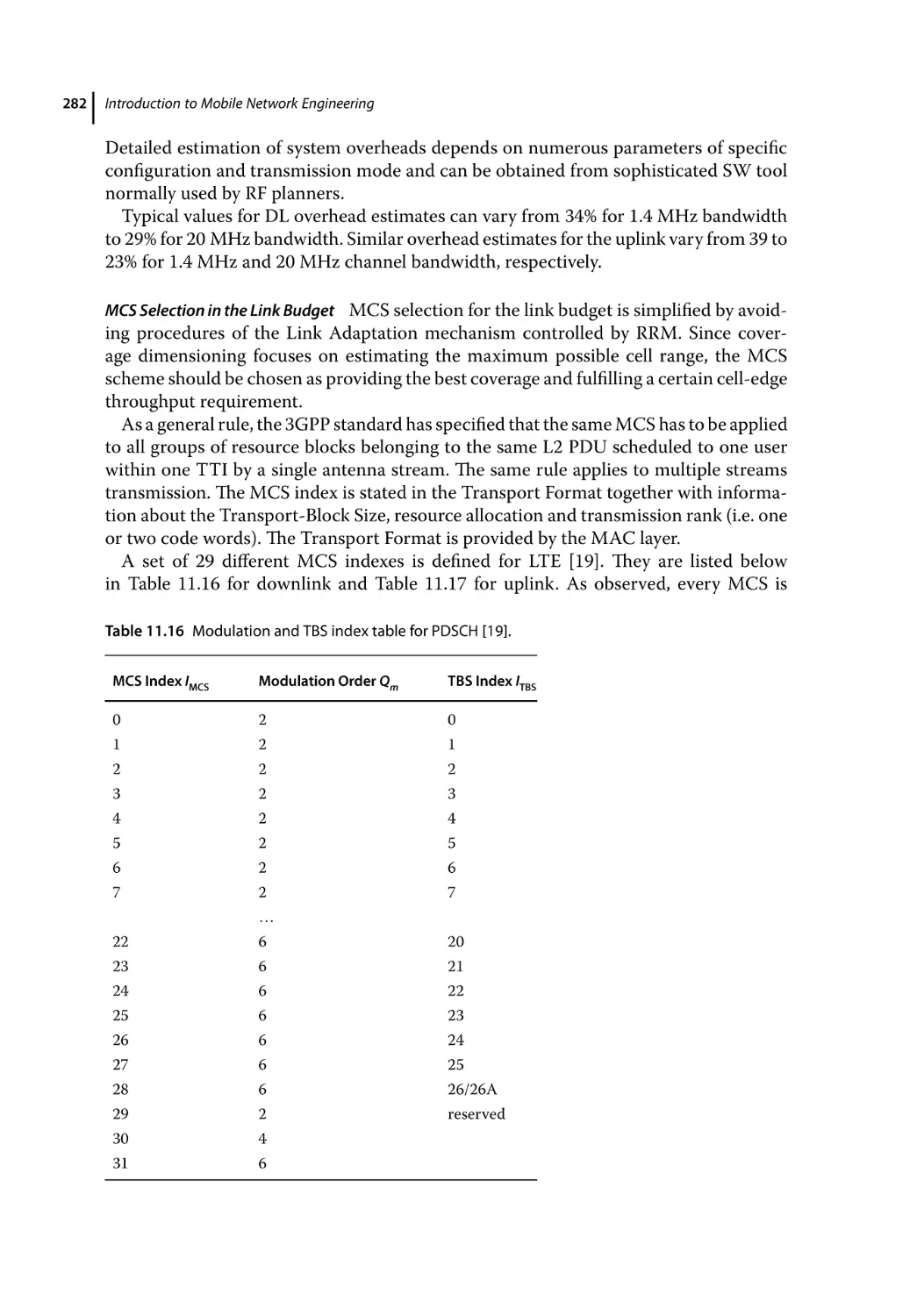
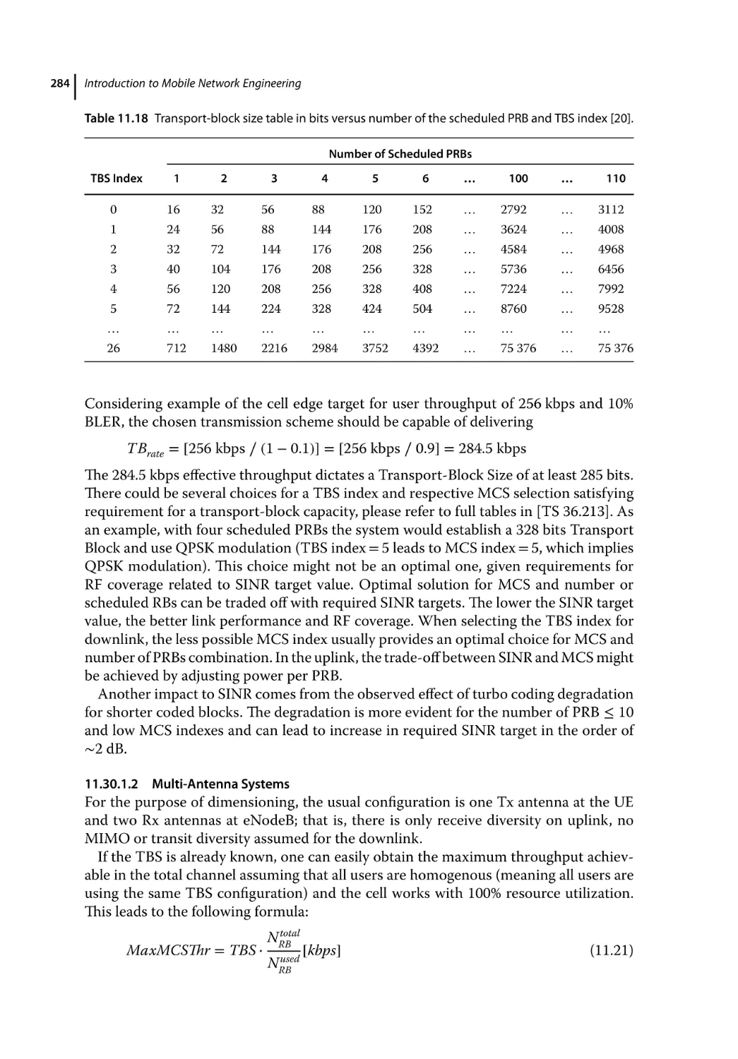
Physical-Layer Overhead Factors 281
Multi-Antenna Systems 284
Required SINR 285
Link Budget Margins 285
Interference Margin 285
Maximum Allowable Path Loss (MAPL) 287
Required SINR 288
Cell Range and Cell Capacity 288
Summary 289
References 290
12
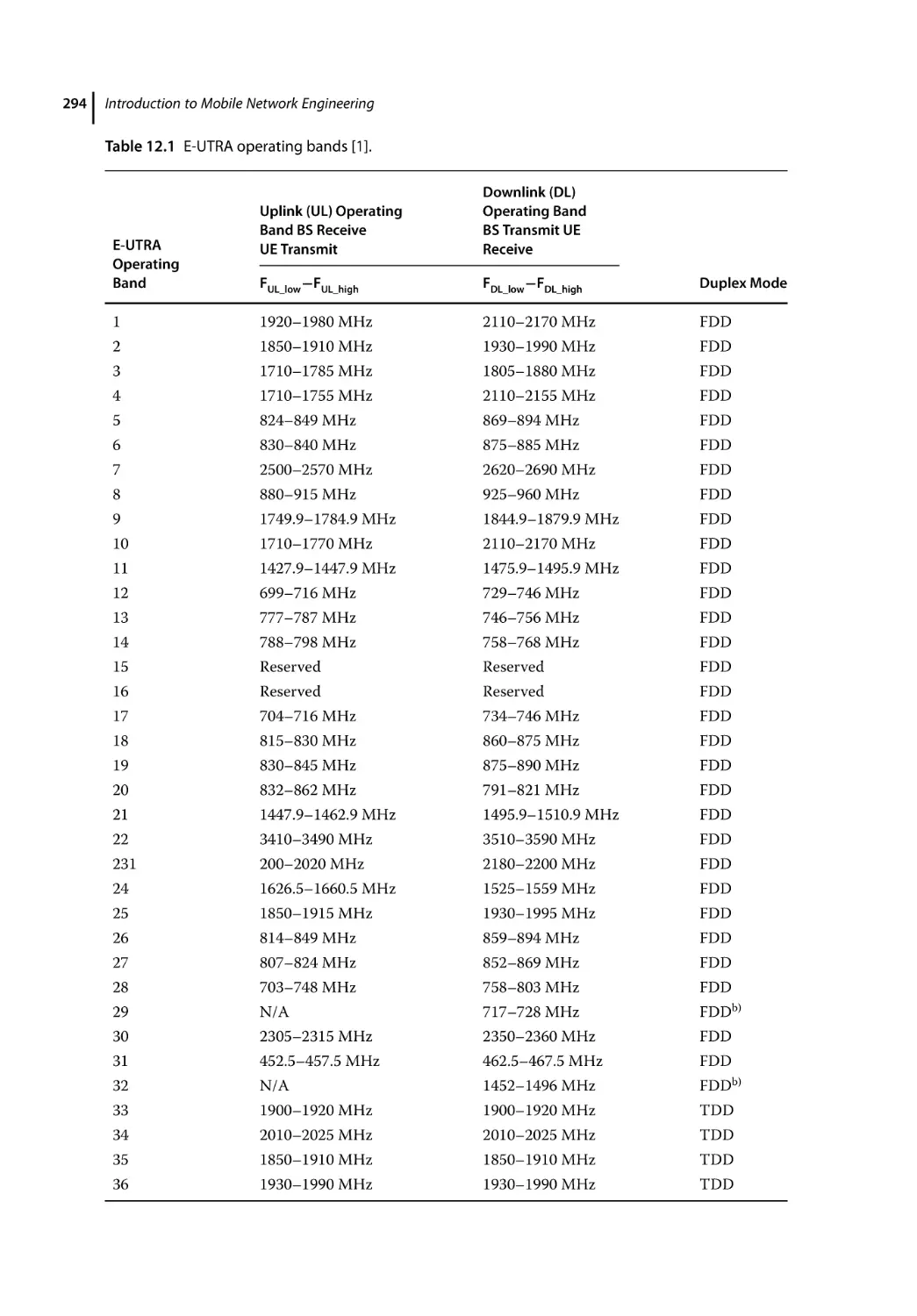
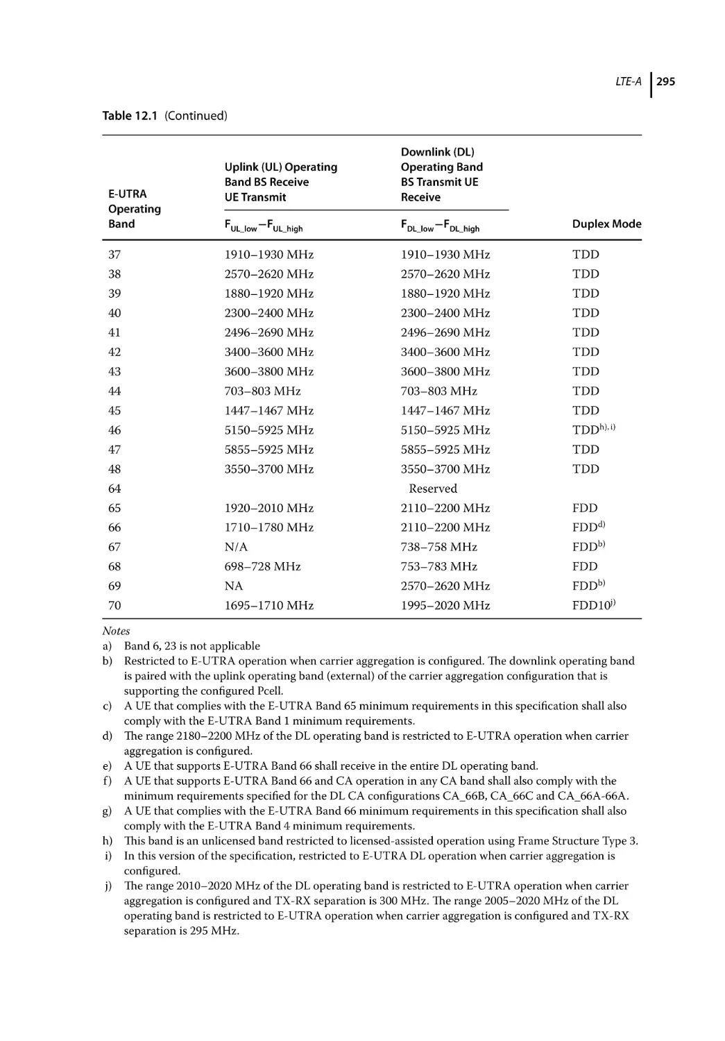
12.1
12.2
12.3
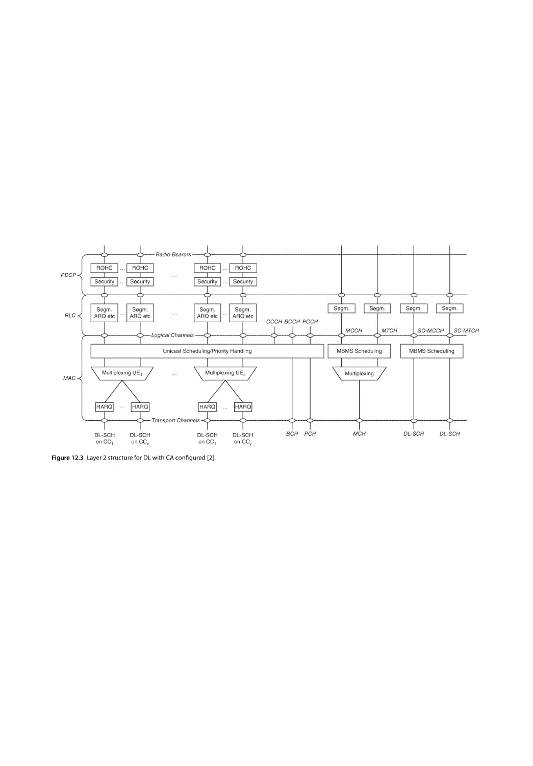
12.3.1
12.3.2
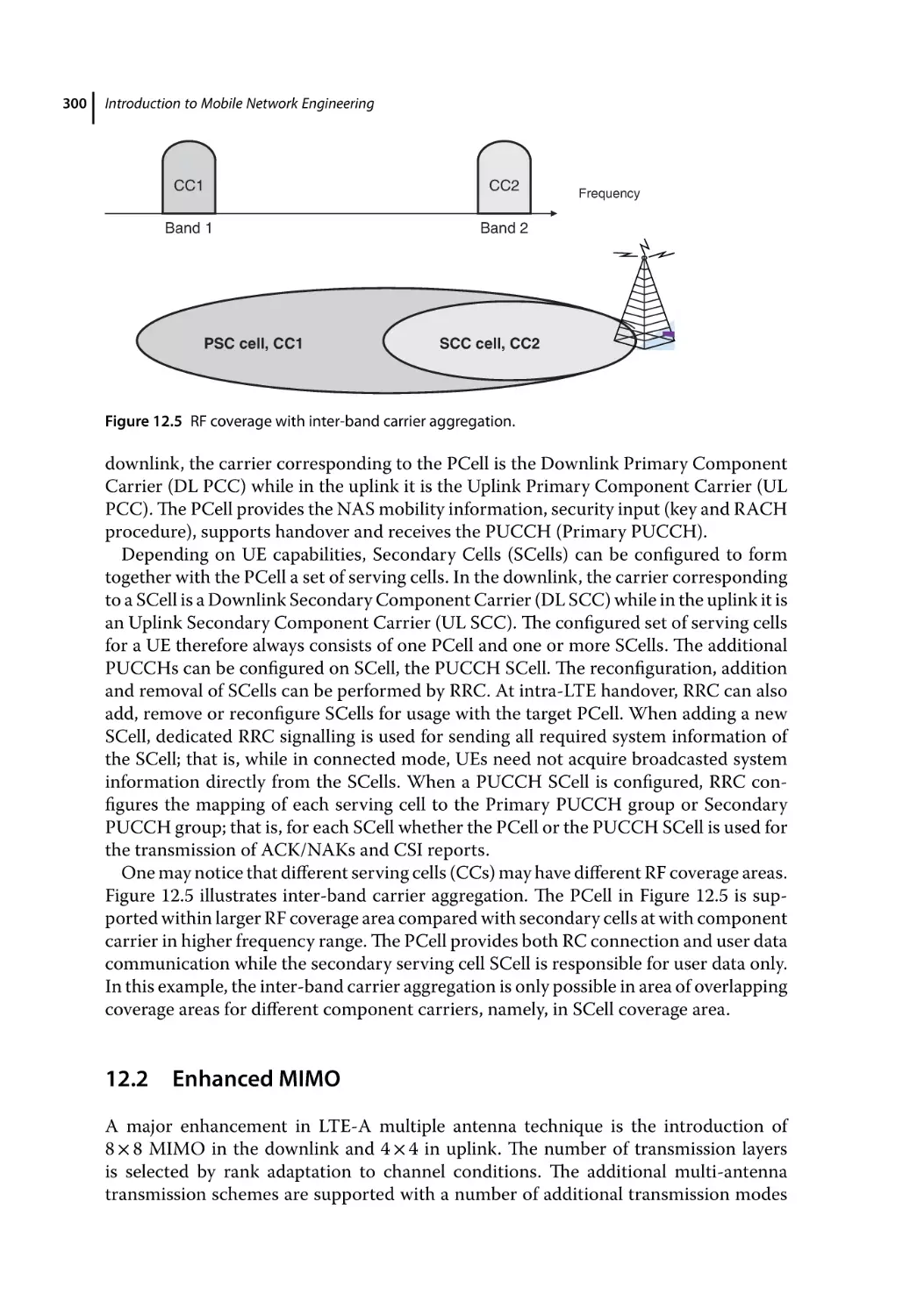
12.3.3
12.4
12.4.1
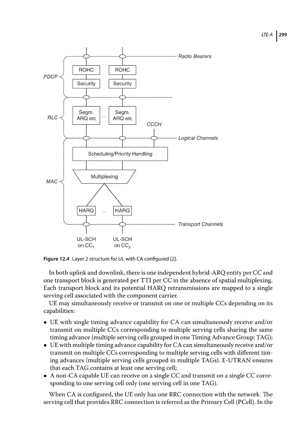
12.4.2
12.4.3
LTE-A 293
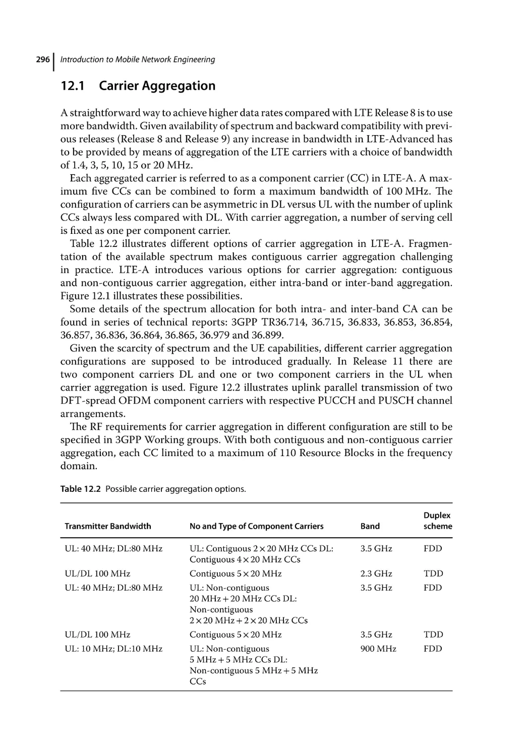
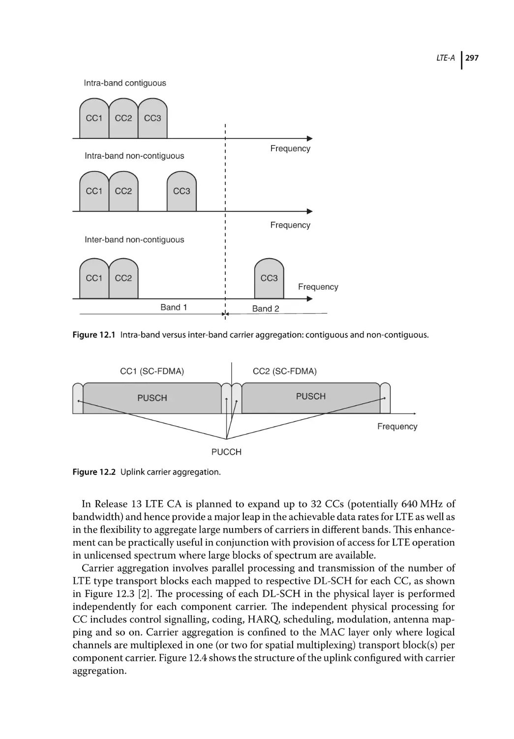
Carrier Aggregation 296
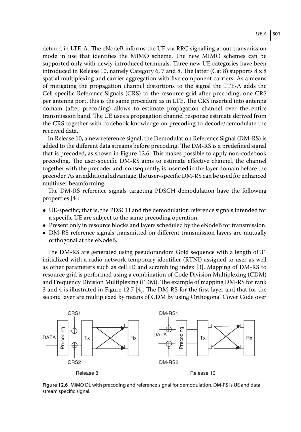
Enhanced MIMO 300
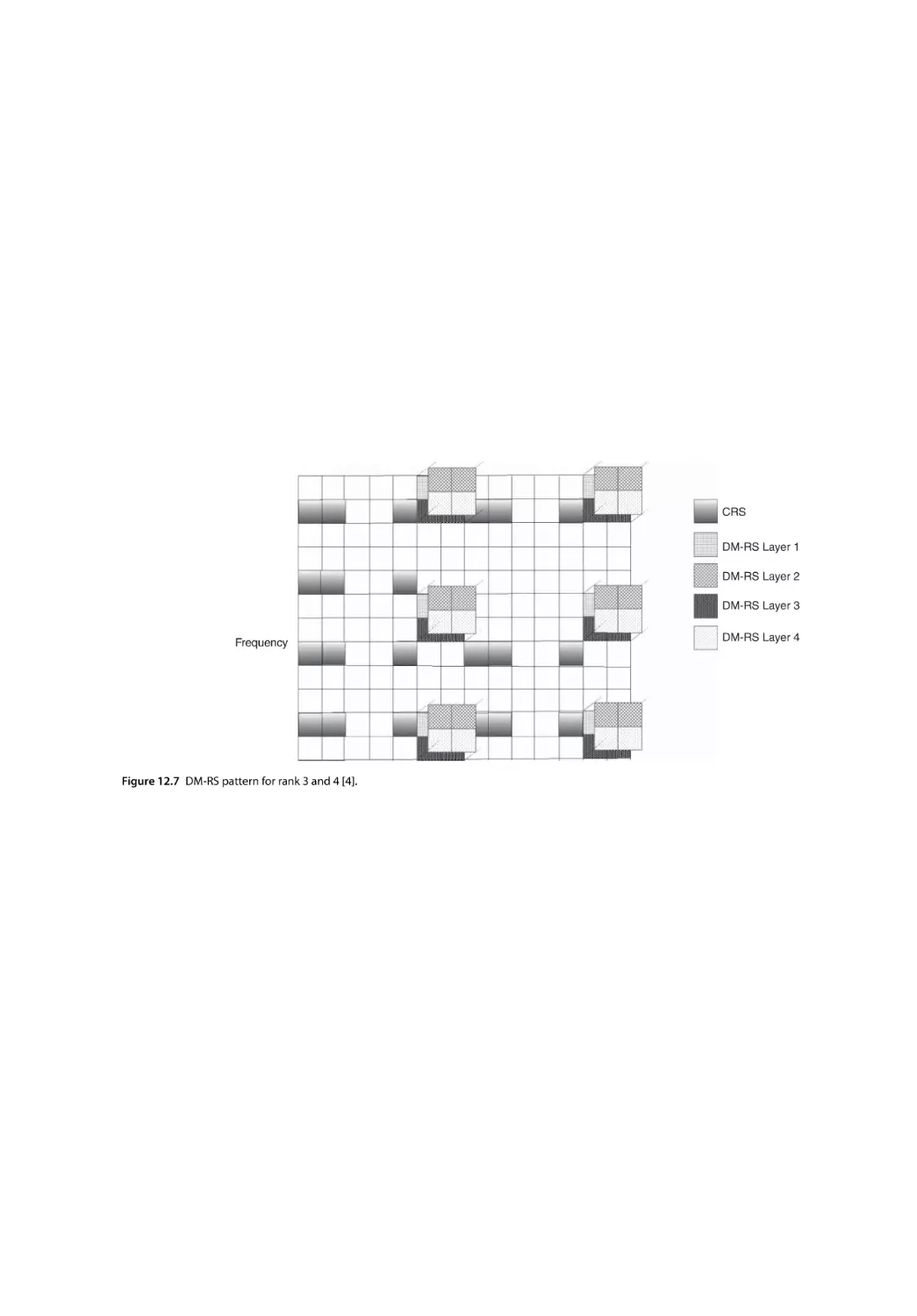
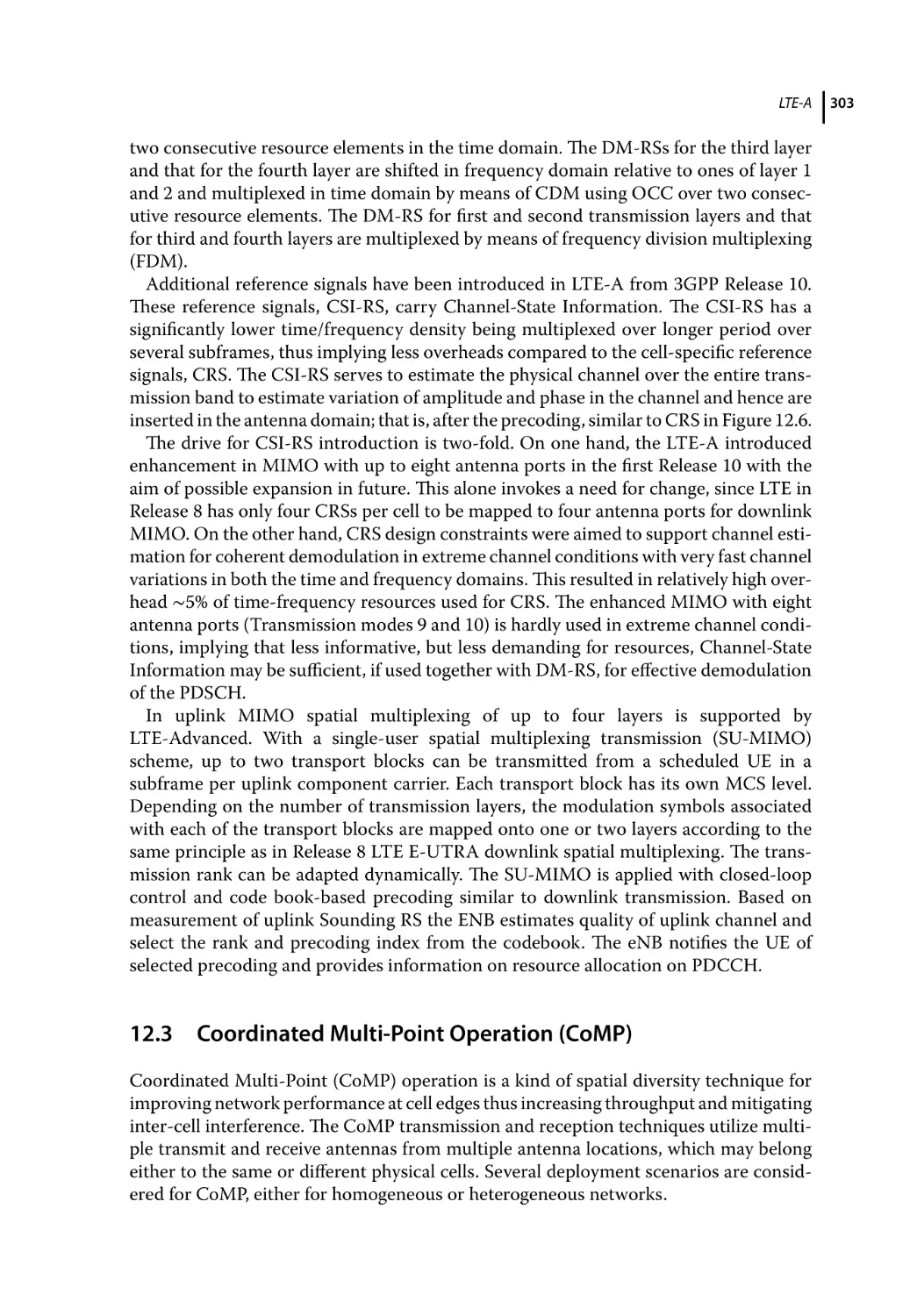
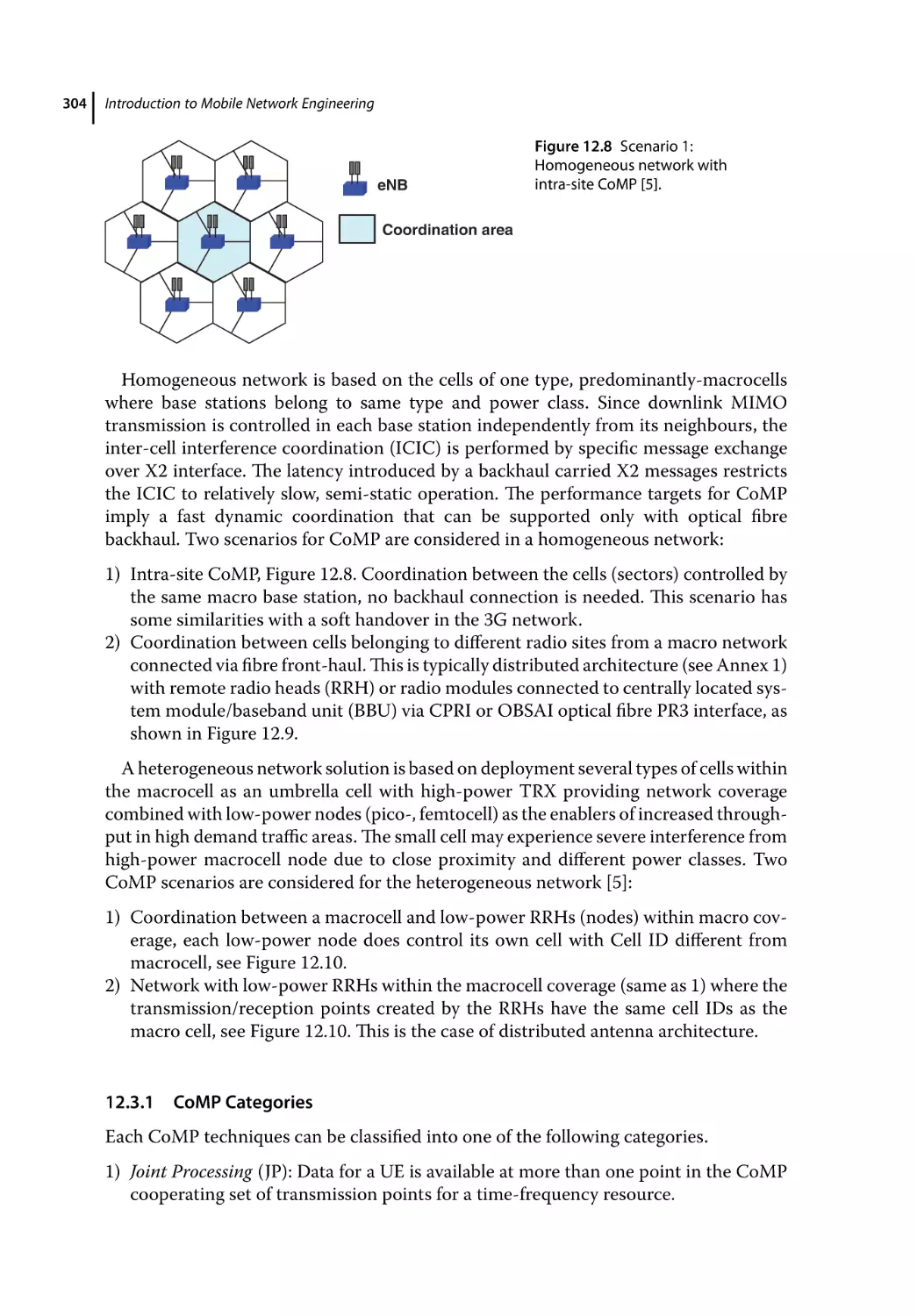
Coordinated Multi-Point Operation (CoMP) 303
CoMP Categories 304
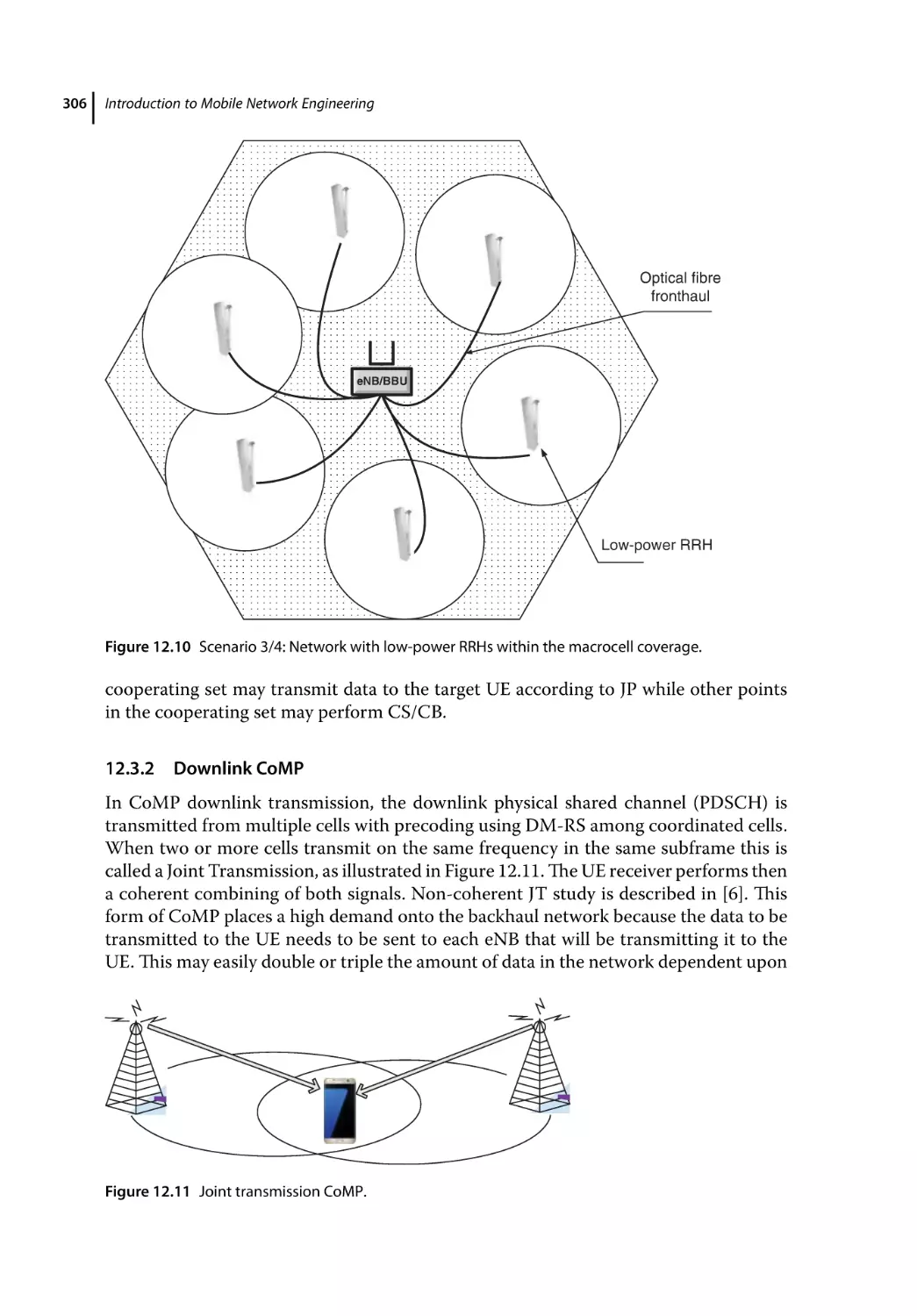
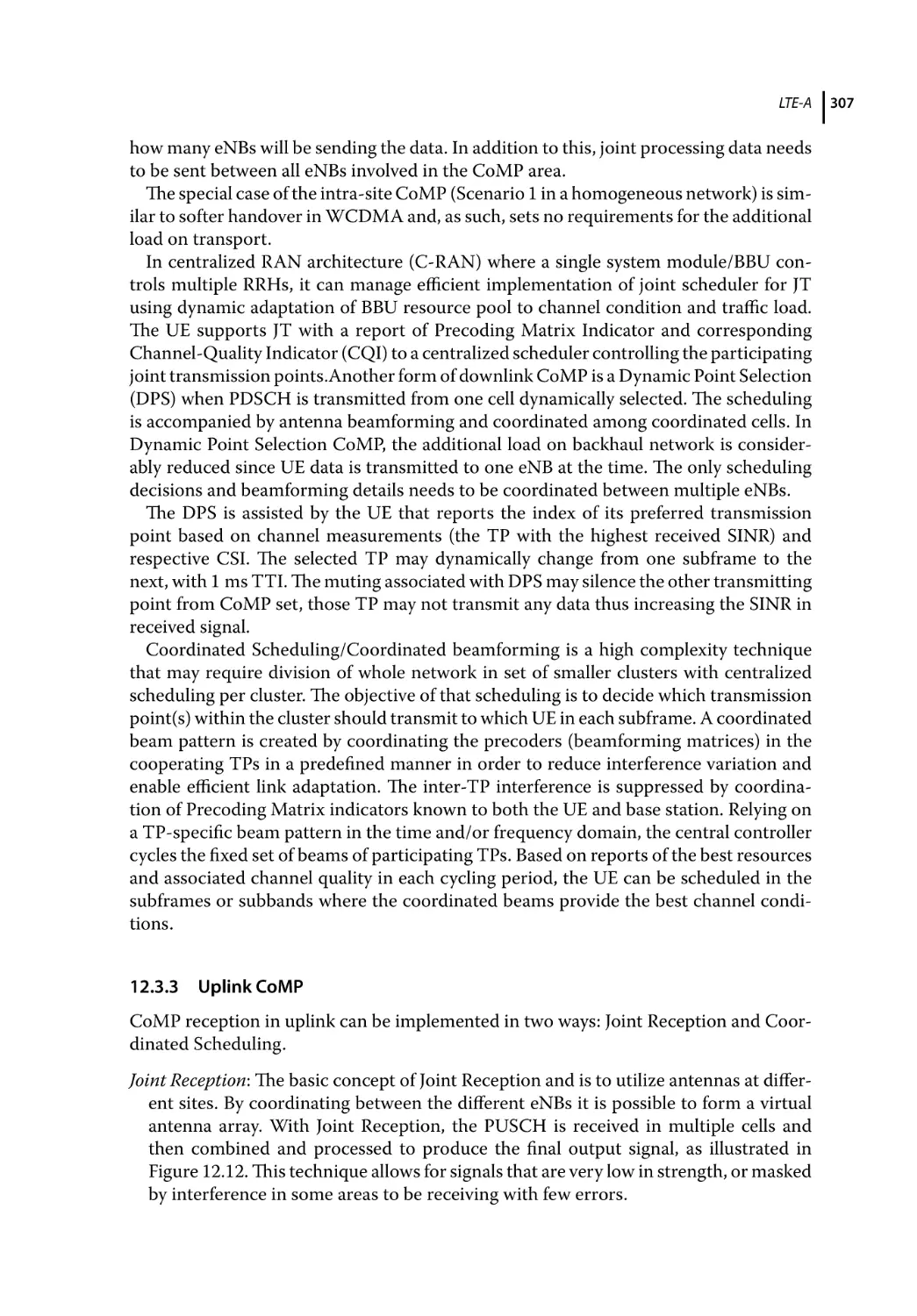
Downlink CoMP 306
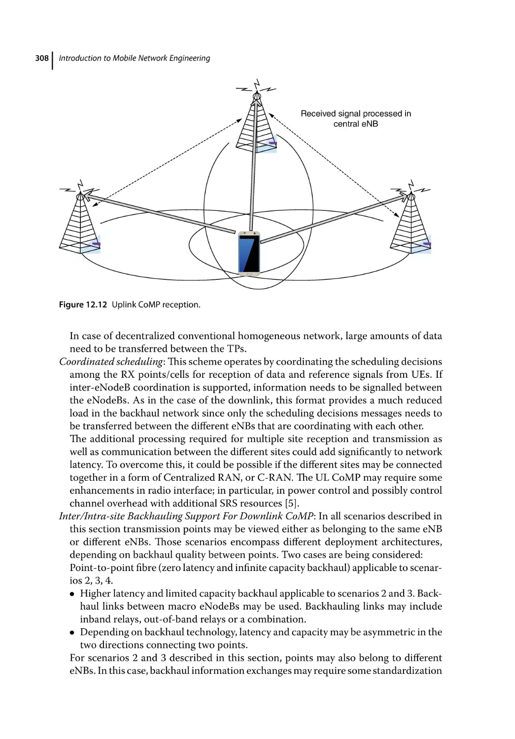
Uplink CoMP 307
Relay Nodes 309
Relay Radio Access 309
Relay Architecture 311
Resource Assignment for DeNB-RN Link in a Type 1 Relay 314
Contents
12.5
12.6
12.7
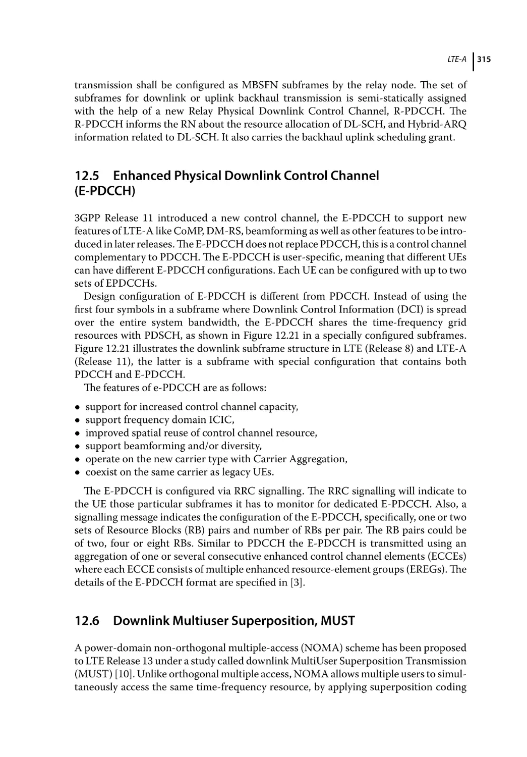
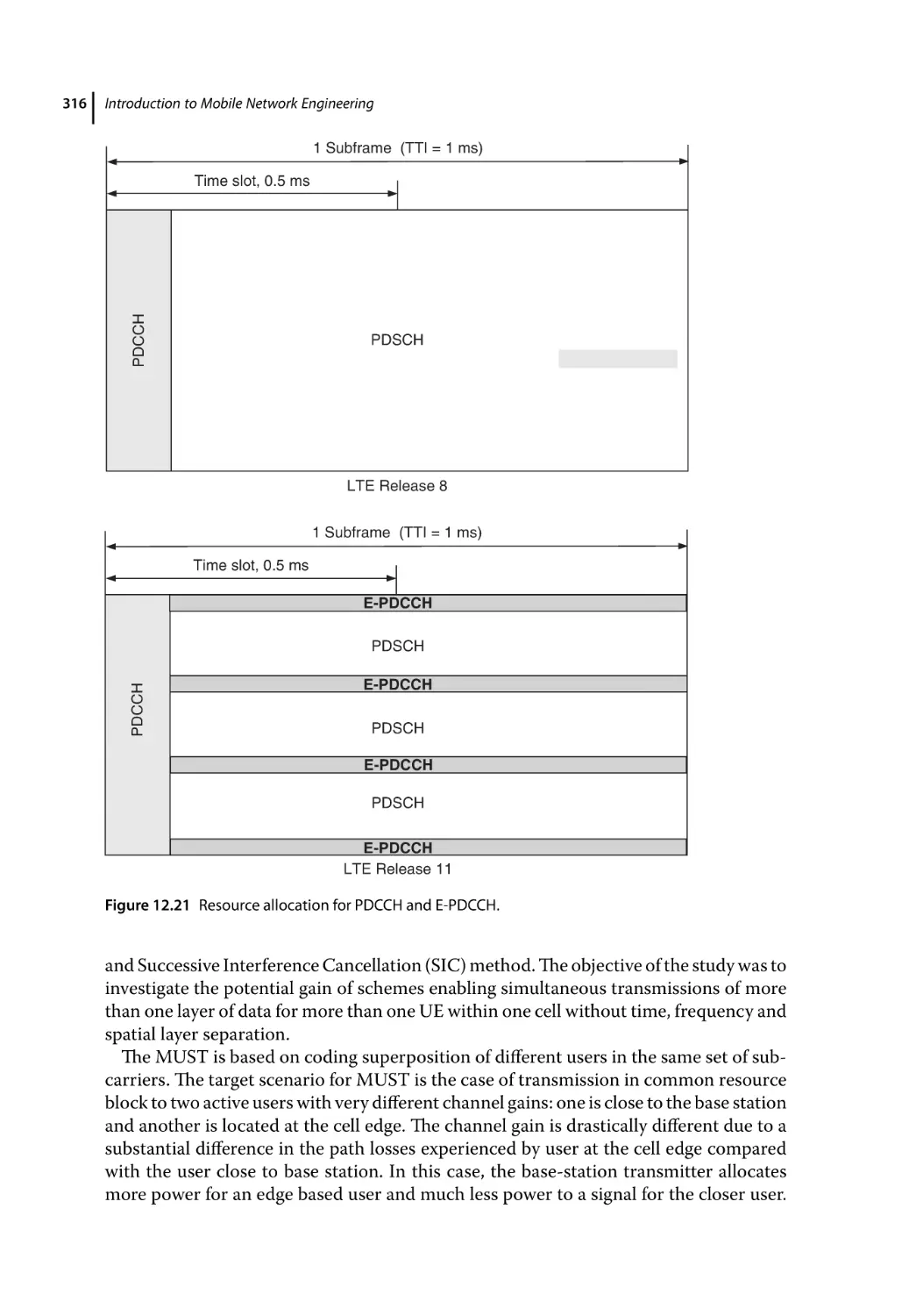
Enhanced Physical Downlink Control Channel (E-PDCCH) 315
Downlink Multiuser Superposition, MUST 315
Summary of LTE-A Features 317
References 317
13
Further Development for the Fifth Generation
13.1
13.2
13.3
13.4
13.5
13.5.1
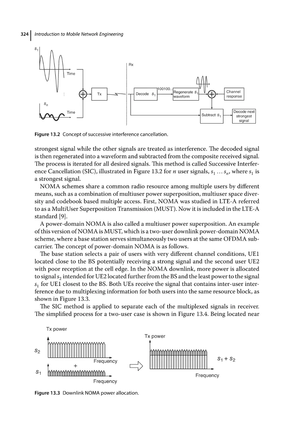
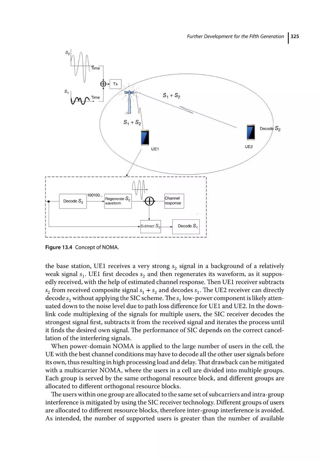
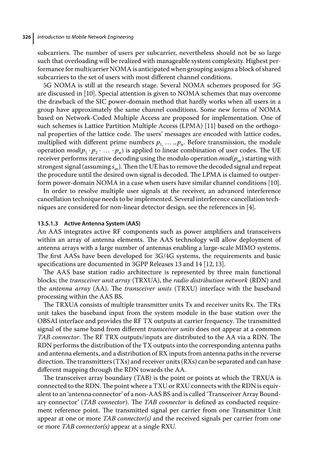
13.5.1.1
13.5.1.2
13.5.1.3
13.5.1.4
13.5.1.5
13.5.1.6
13.5.1.7
13.5.2
13.5.2.1
13.5.2.2
13.5.2.3
13.5.2.4
13.6
13.6.1
13.6.2
13.6.3
13.6.3.1
13.6.3.2
13.6.3.3
13.6.3.4
13.7
13.7.1
13.7.2
13.7.3
13.7.3.1
13.7.4
13.7.5
13.7.5.1
13.7.5.2
13.7.6
13.7.6.1
13.7.7
13.7.7.1
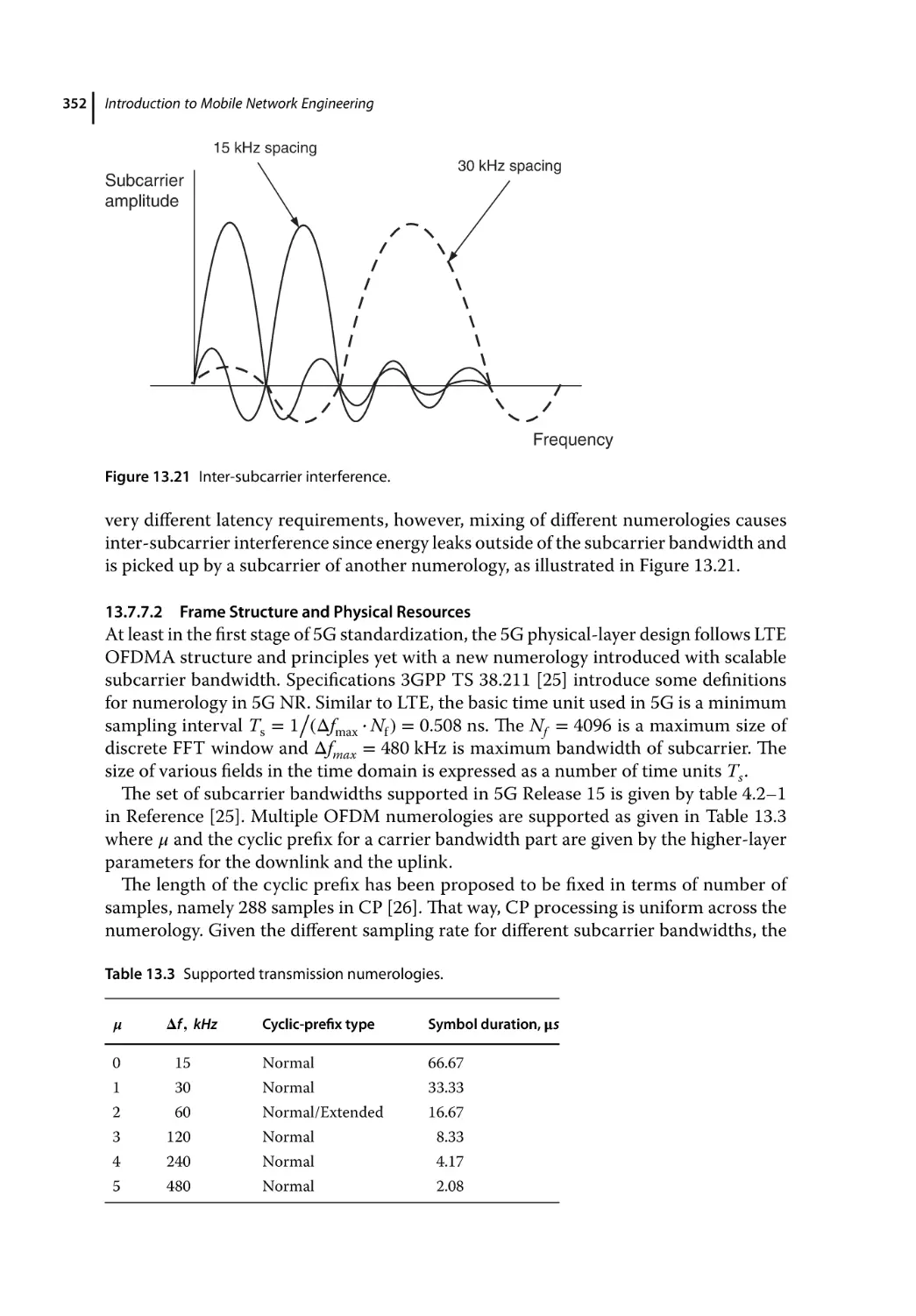
13.7.7.2
13.7.8
319
Overall Operational Requirements for a 5G Network System 320
Device Requirements 320
Capabilities of 5G 321
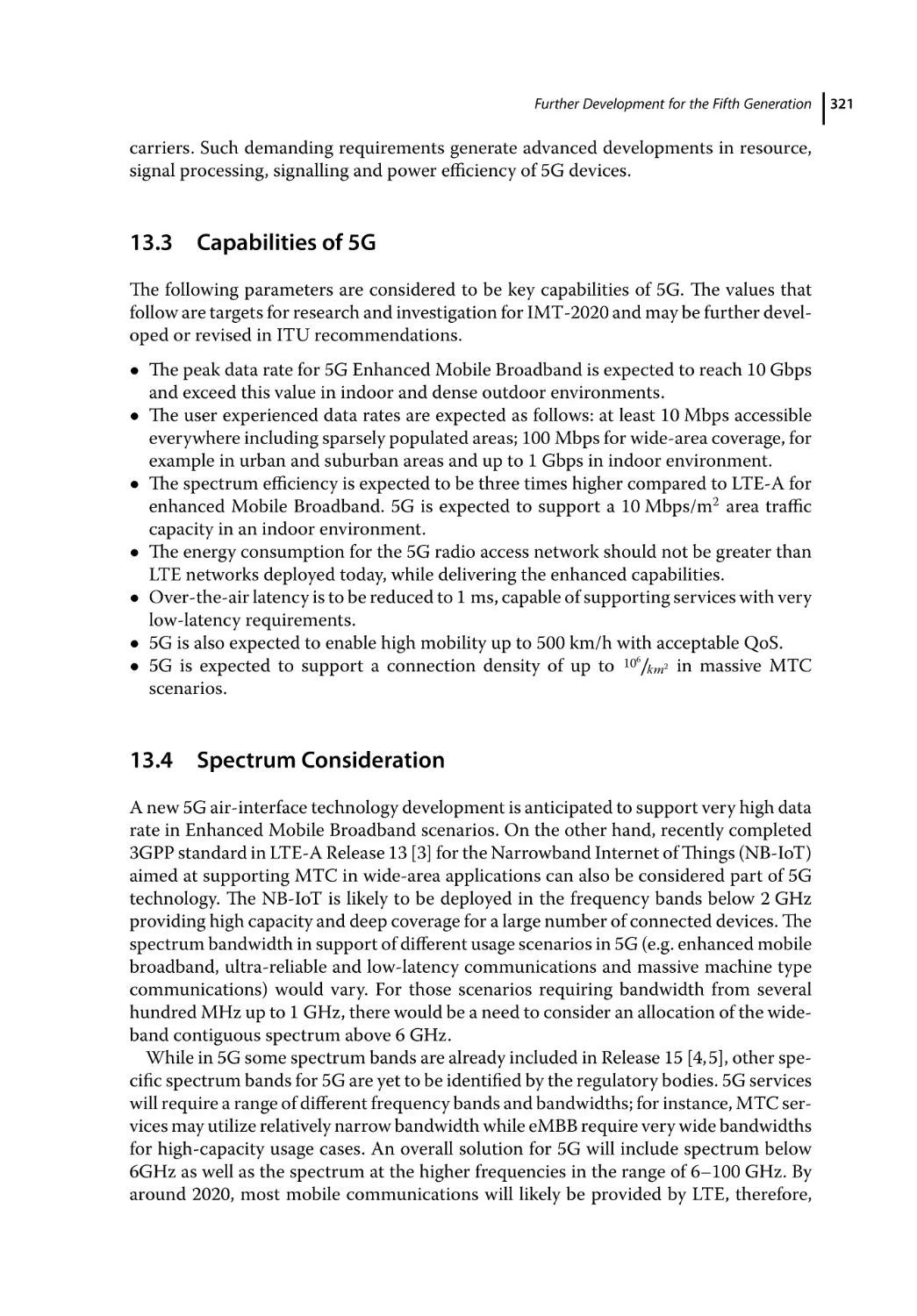
Spectrum Consideration 321
5G Technology Components 322
Technologies to Enhance the Radio Interface 322
Advanced Modulation-and-Coding Schemes 323
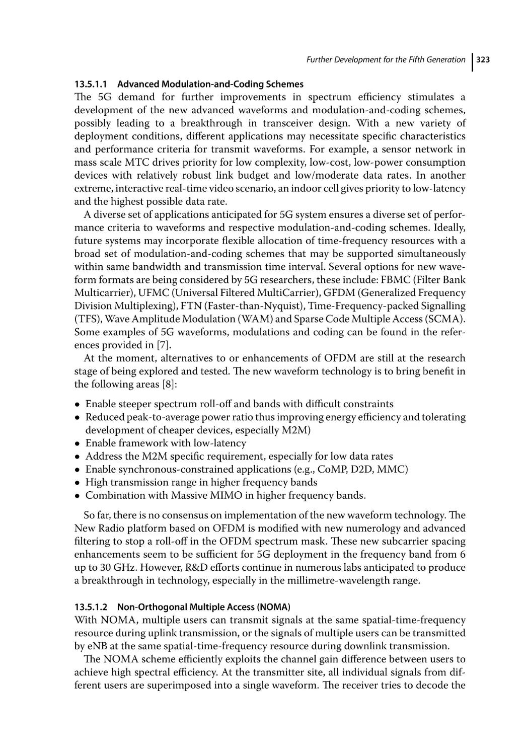
Non-Orthogonal Multiple Access (NOMA) 323
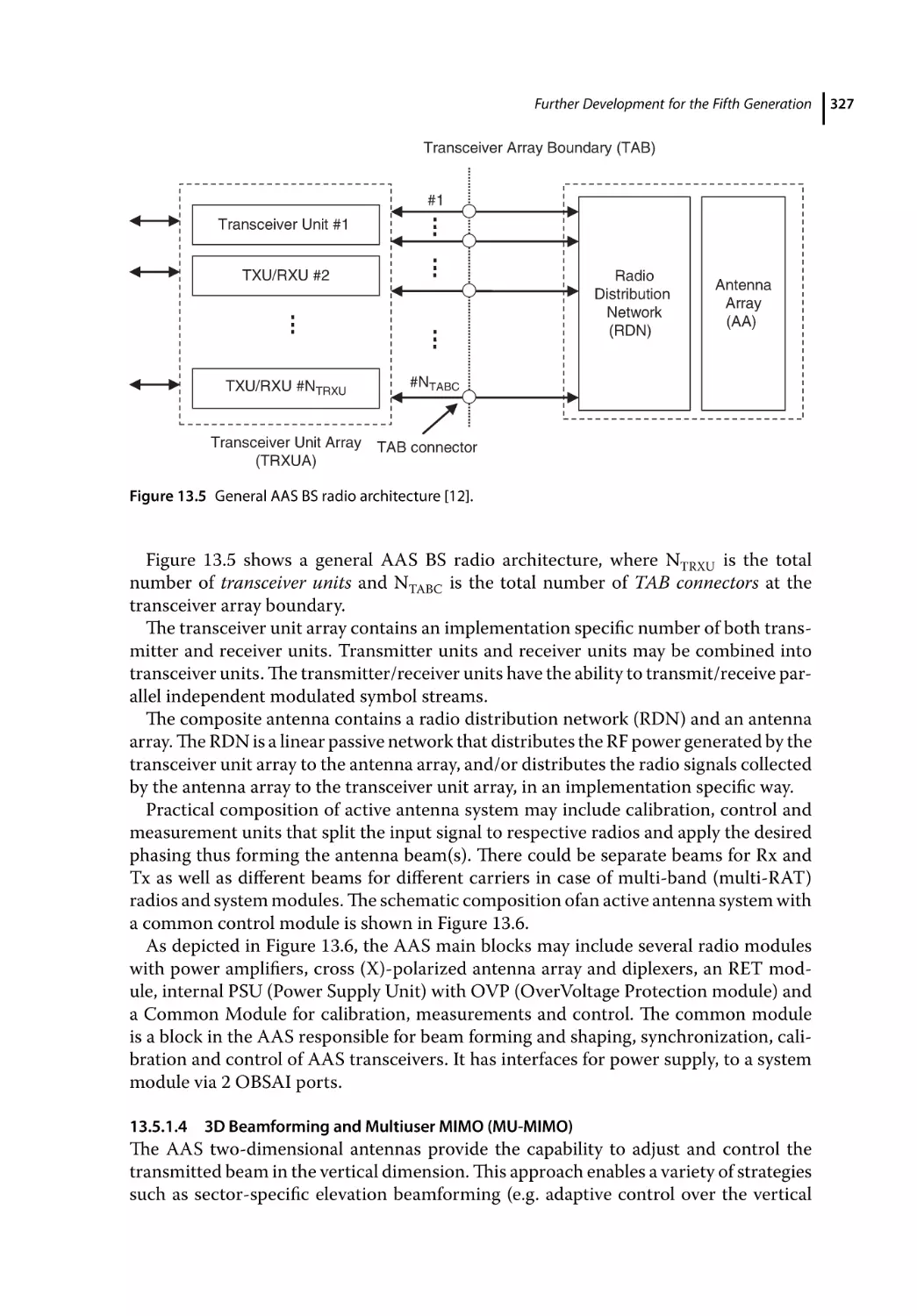
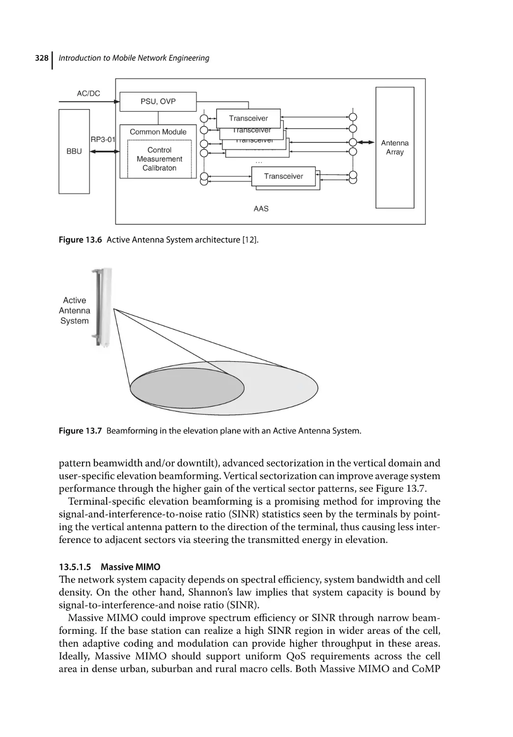
Active Antenna System (AAS) 326
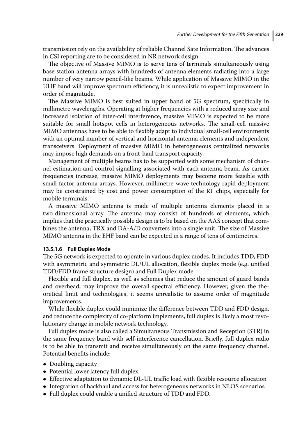
3D Beamforming and Multiuser MIMO (MU-MIMO) 327
Massive MIMO 328
Full Duplex Mode 329
Self-Backhauling 330
Technologies to Enhance Network Architectures 331
Software-Defined Network 332
Cloud RAN 332
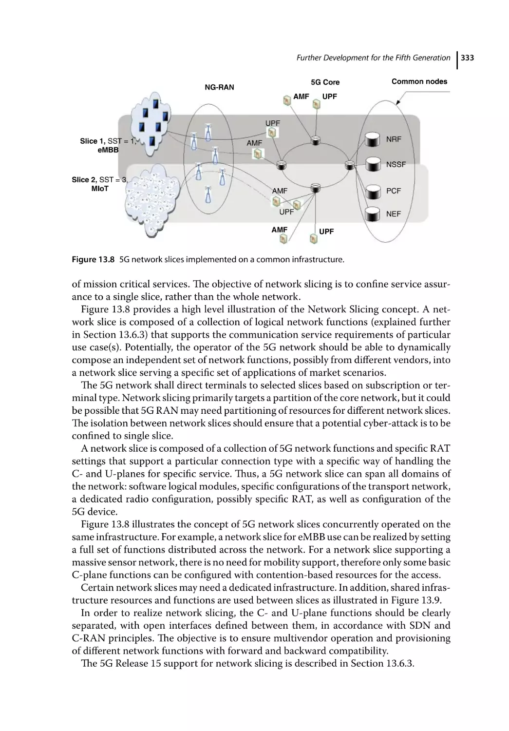
Network Slicing 332
Self-Organized Network, SON 334
5G System Architecture (Release 15) 335
General Concepts 335
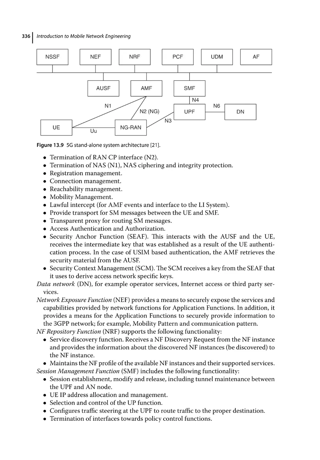
Architecture Reference Model 335
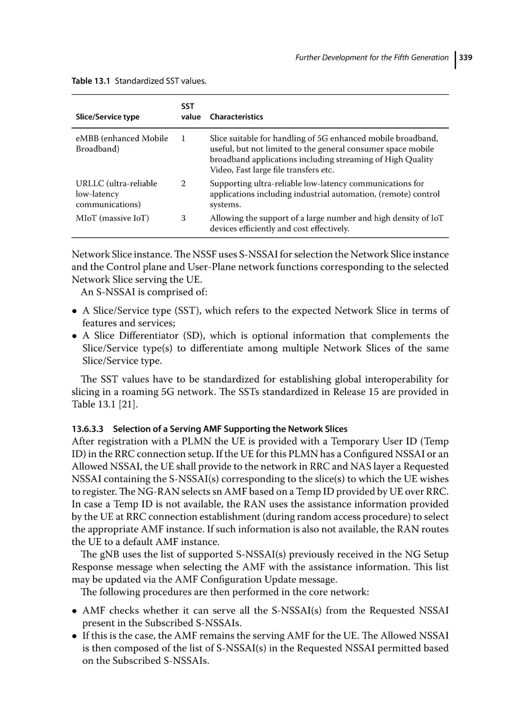
Network Slicing Support 338
General Framework 338
Network Slice Selection Assistance Information (NSSAI) 338
Selection of a Serving AMF Supporting the Network Slices 339
UE Context Handling 340
New Radio (NR) 341
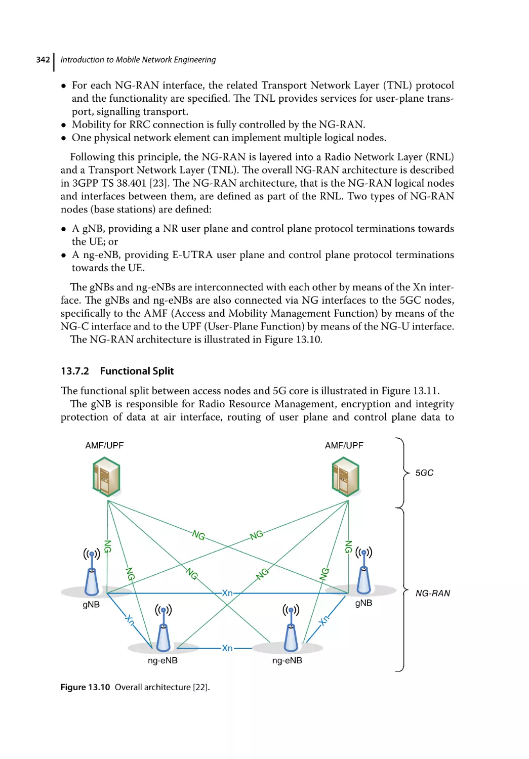
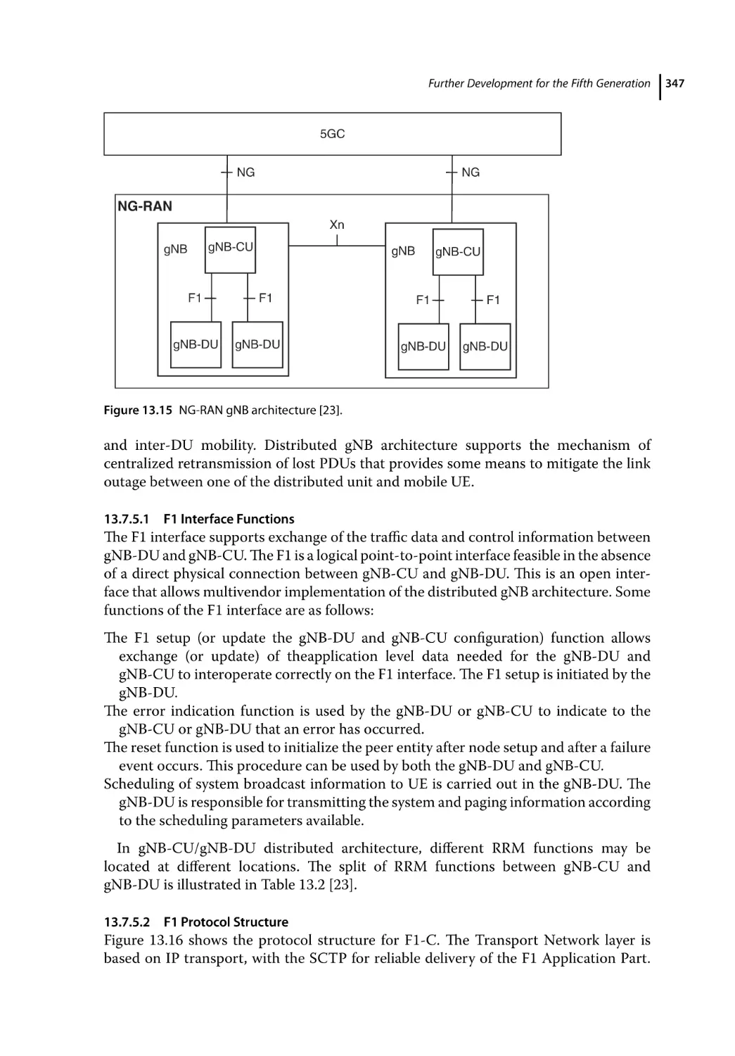
NG-RAN Architecture 341
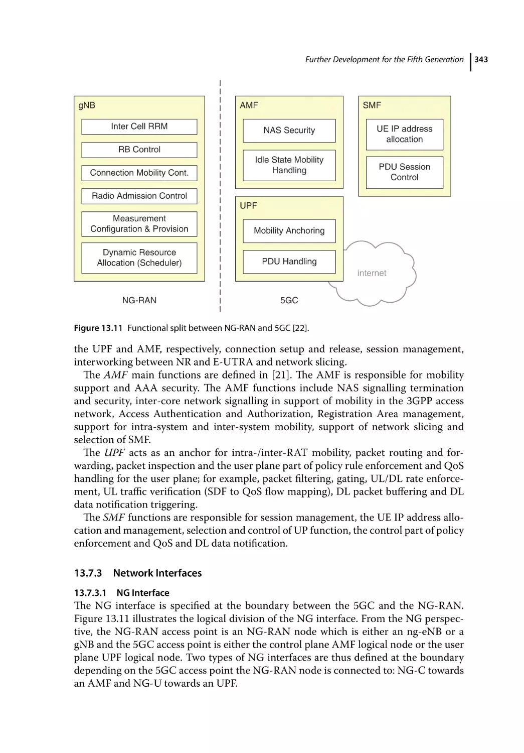
Functional Split 342
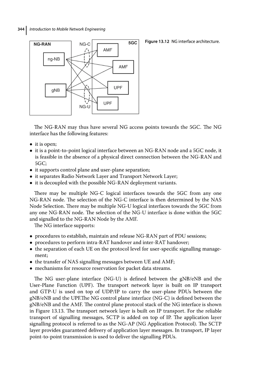
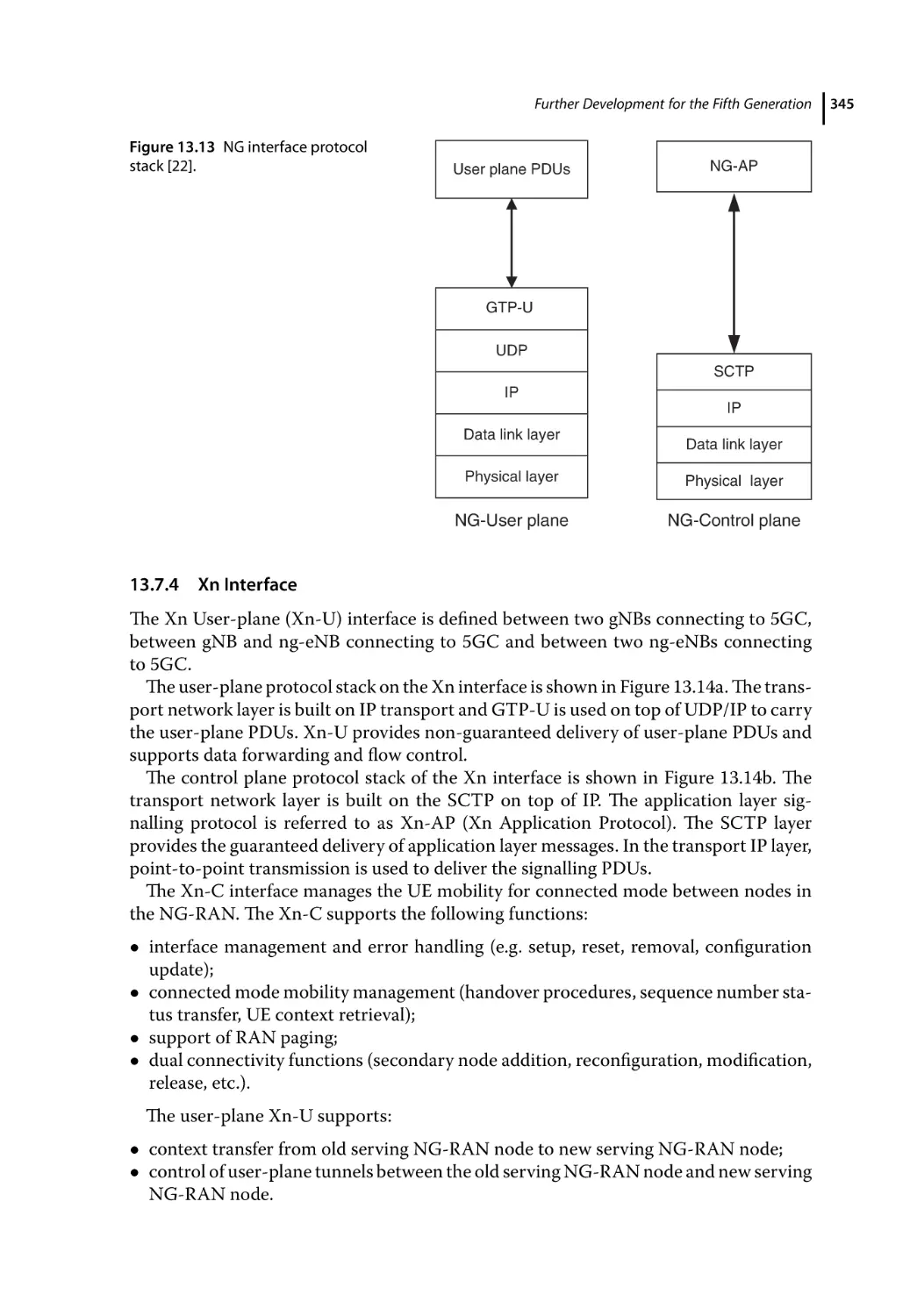
Network Interfaces 343
NG Interface 343
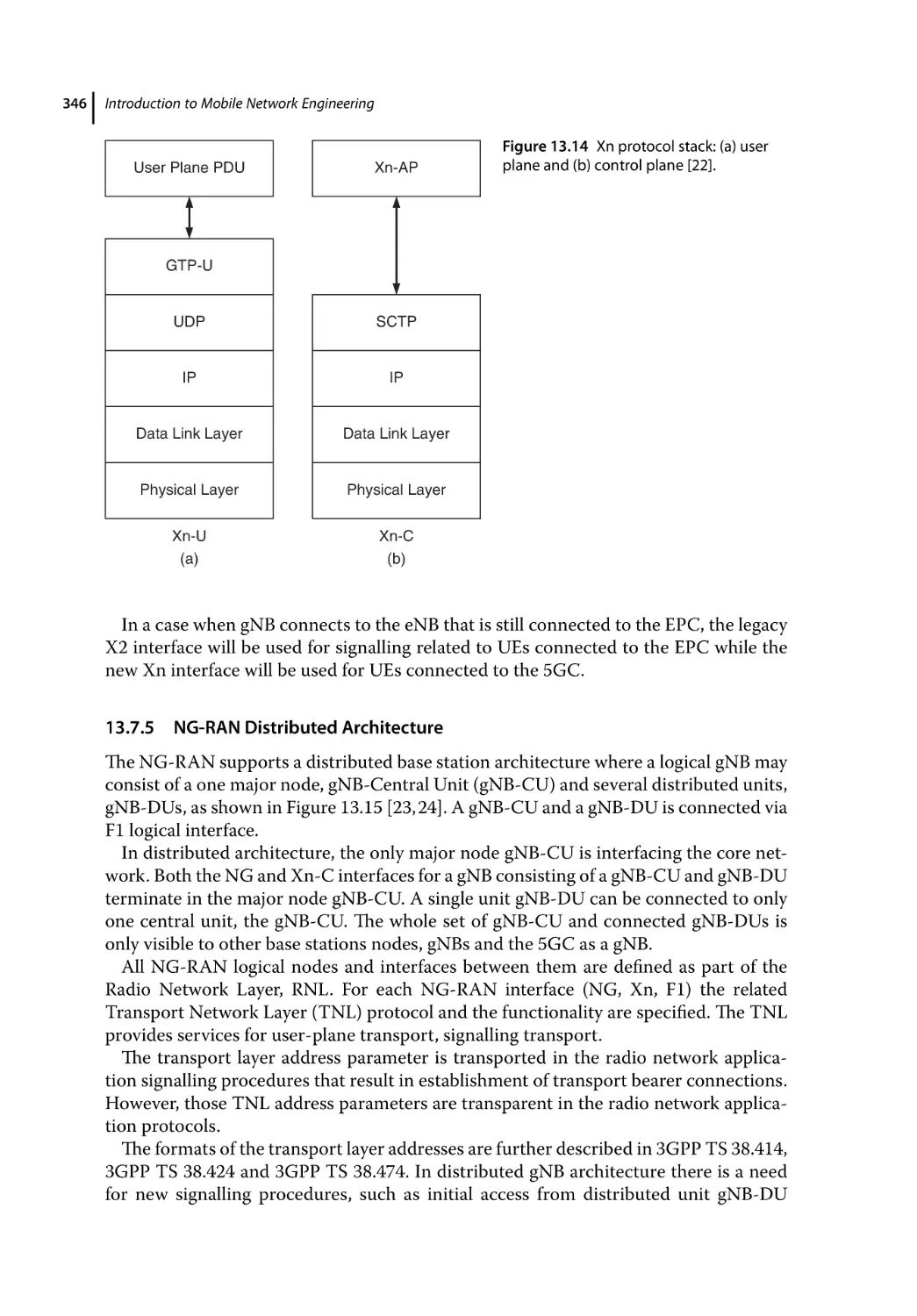
Xn Interface 345
NG-RAN Distributed Architecture 346
F1 Interface Functions 347
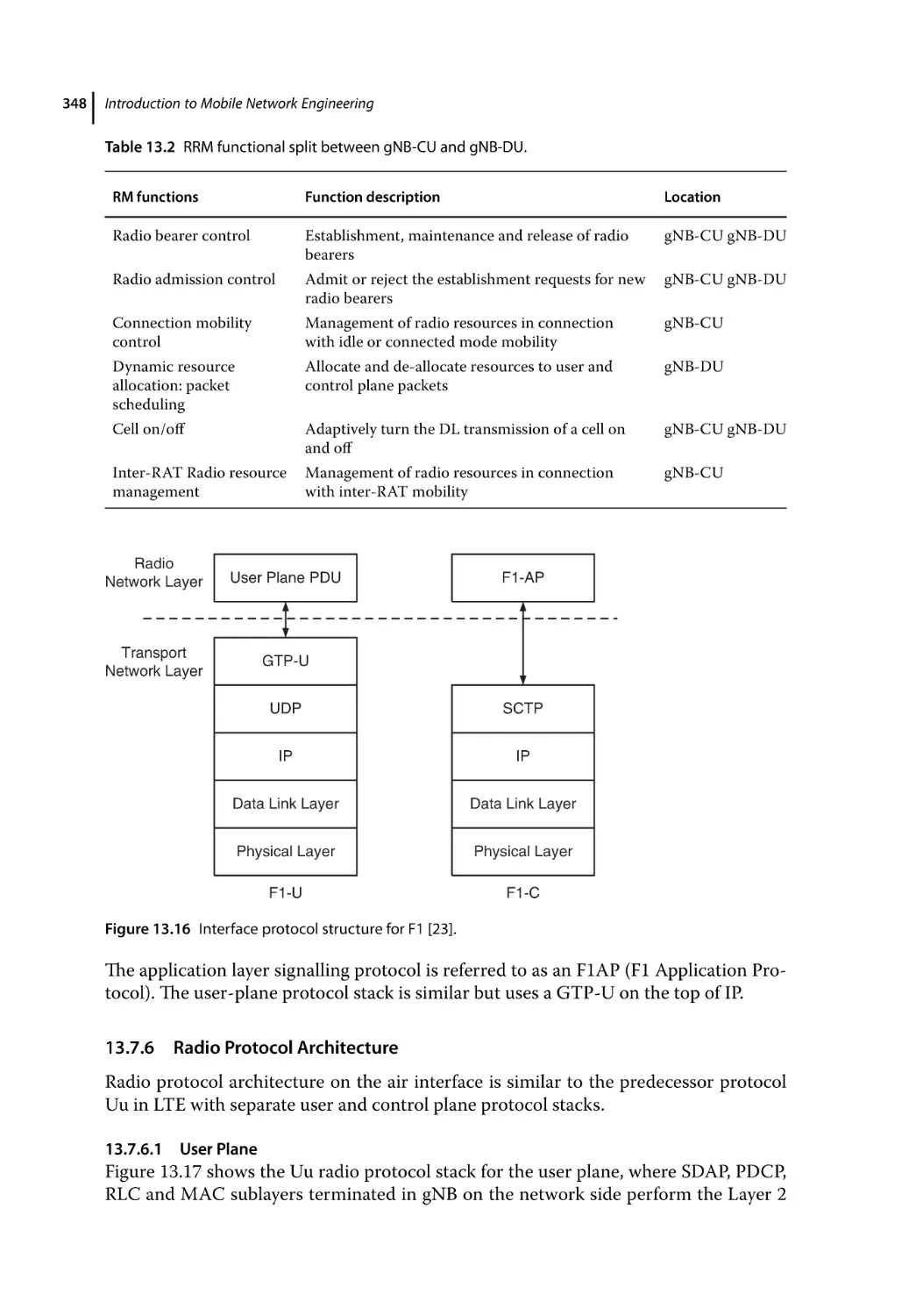
F1 Protocol Structure 347
Radio Protocol Architecture 348
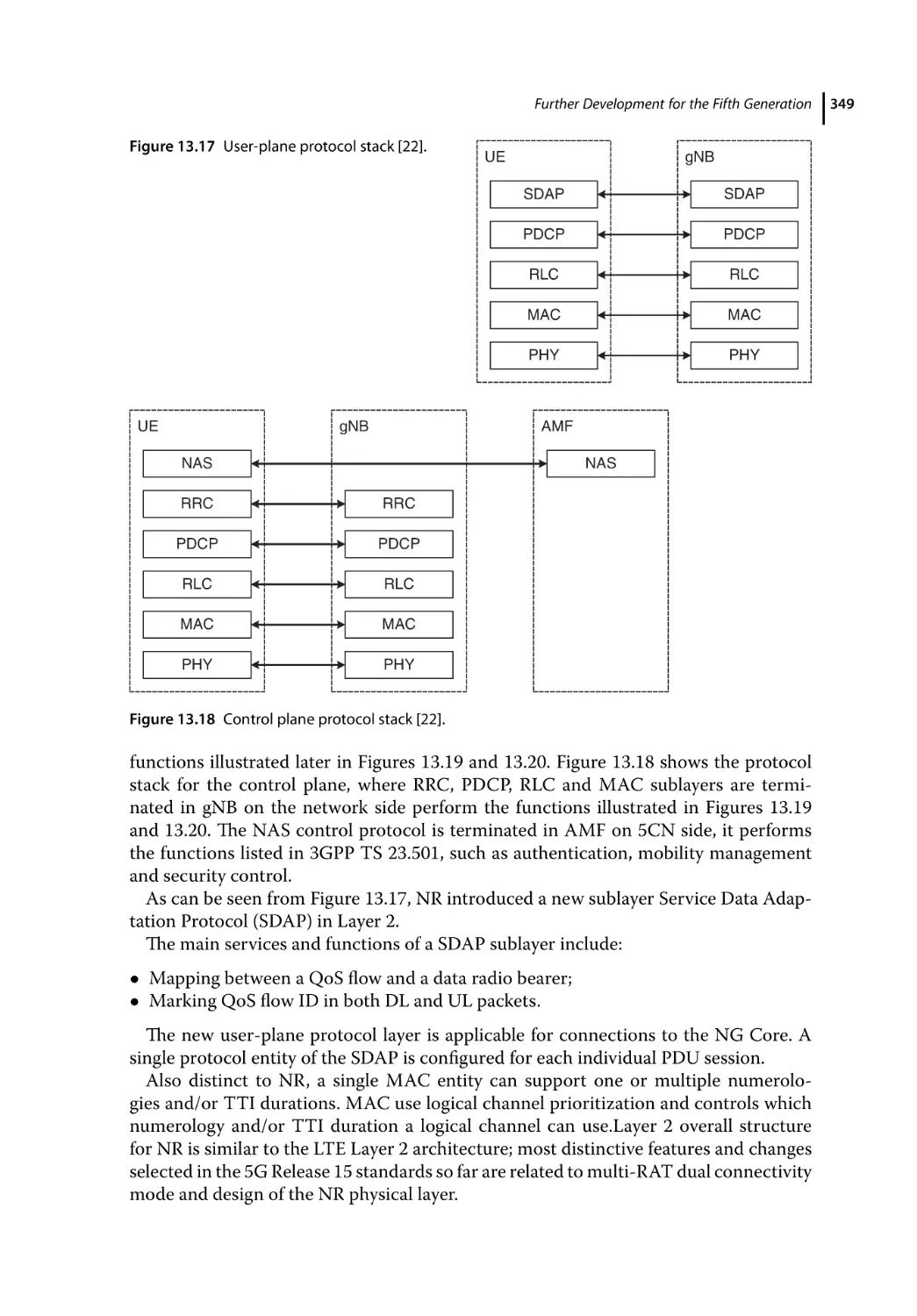
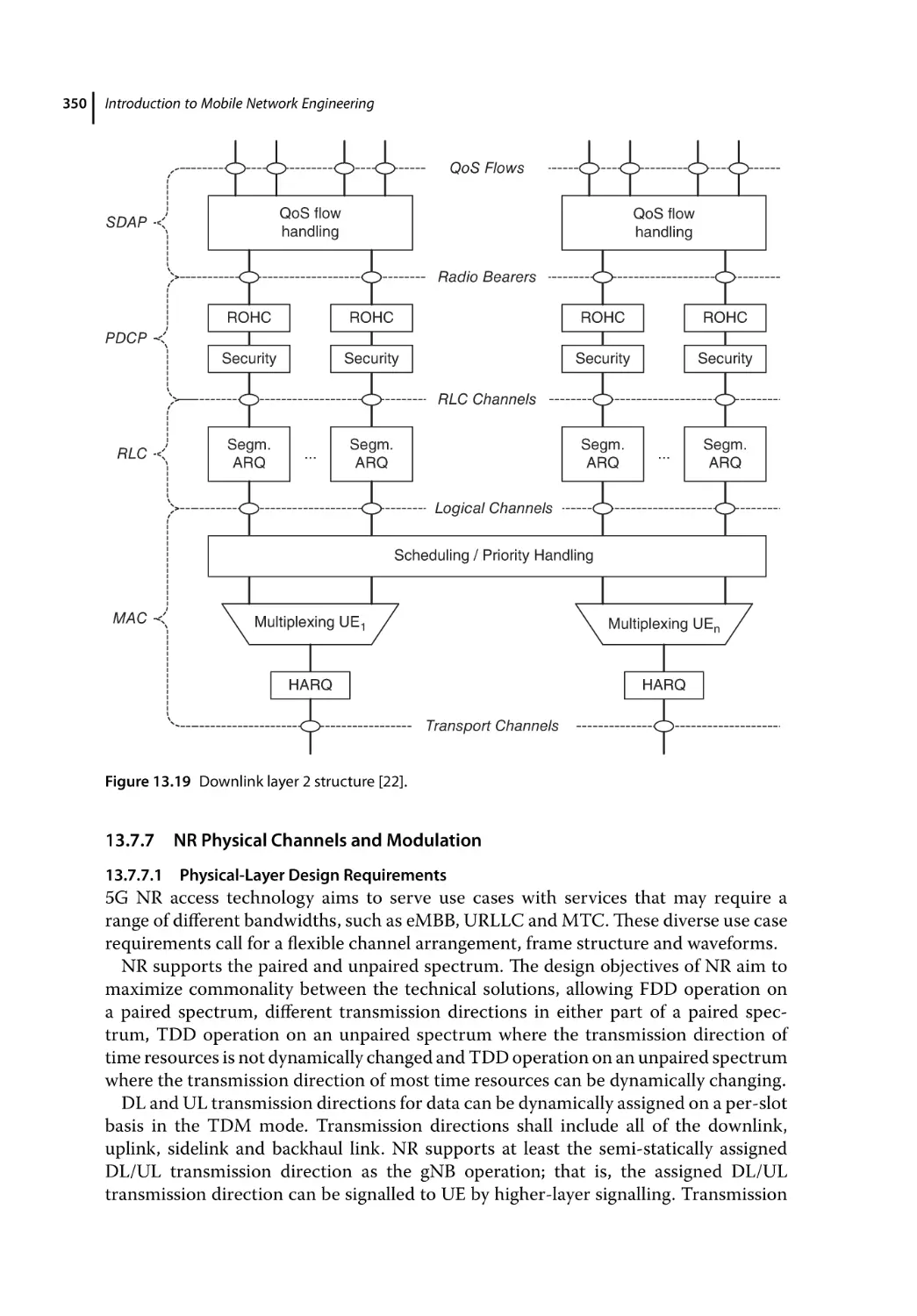
User Plane 348
NR Physical Channels and Modulation 350
Physical-Layer Design Requirements 350
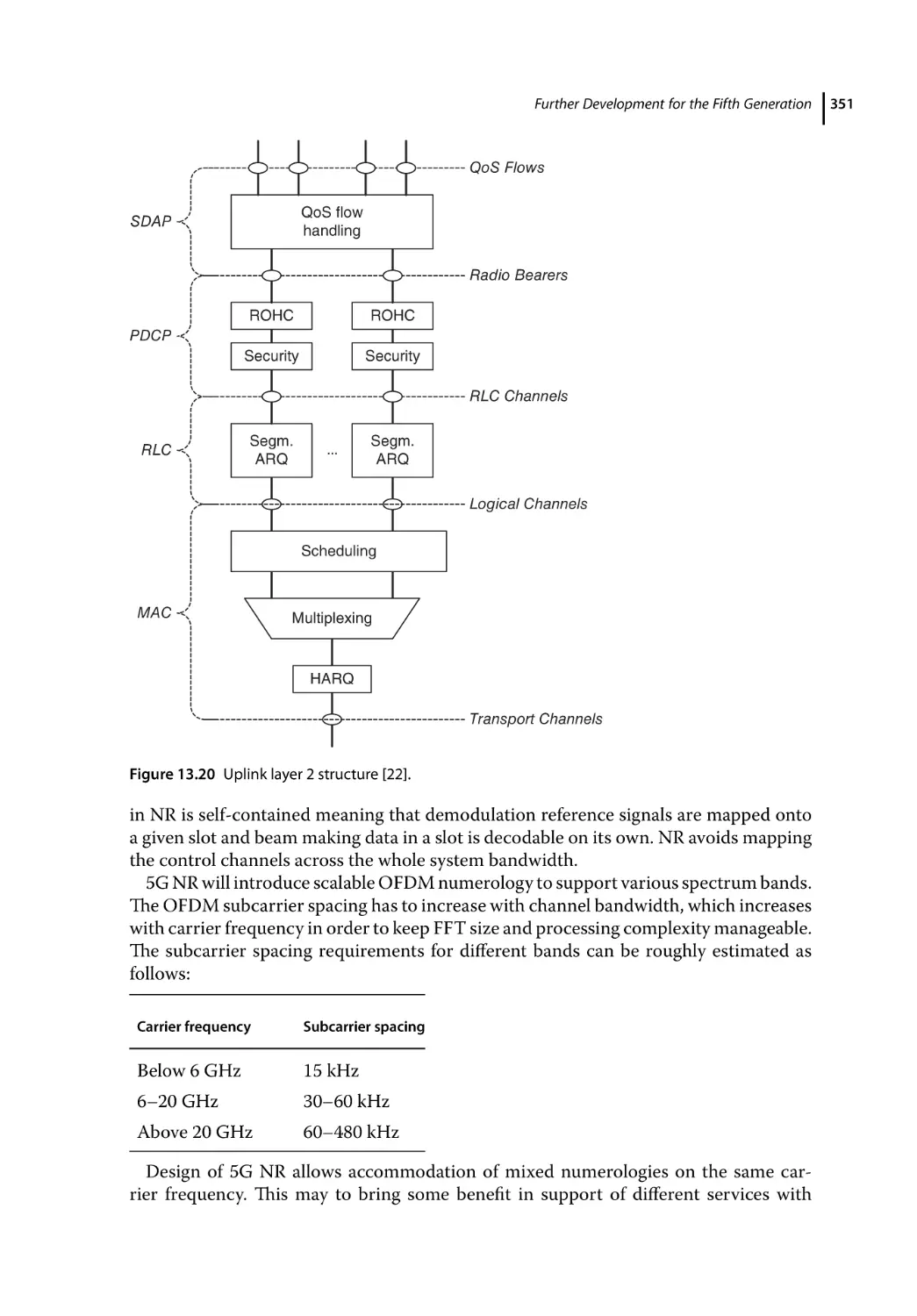
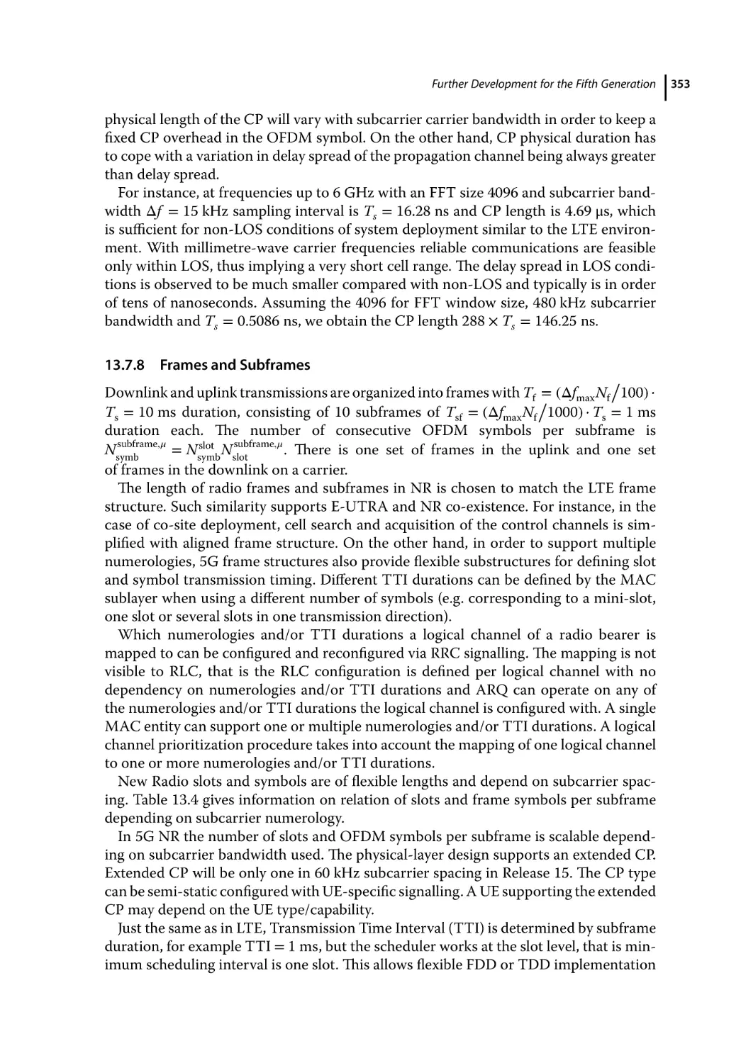
Frame Structure and Physical Resources 352
Frames and Subframes 353
xv
xvi
Contents
13.7.9
13.7.9.1
13.7.9.2
13.7.10
13.7.11
13.7.12
13.7.13
13.7.14
13.7.15
13.7.16
13.7.16.1
13.7.16.2
13.8
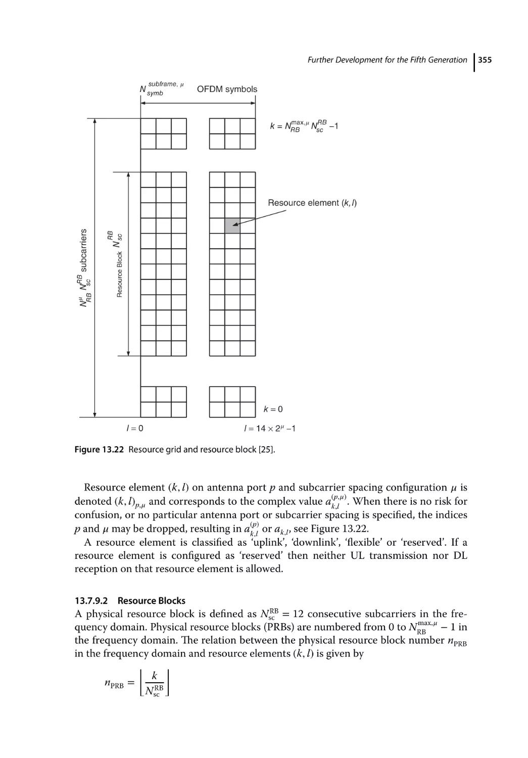
Physical Resources 354
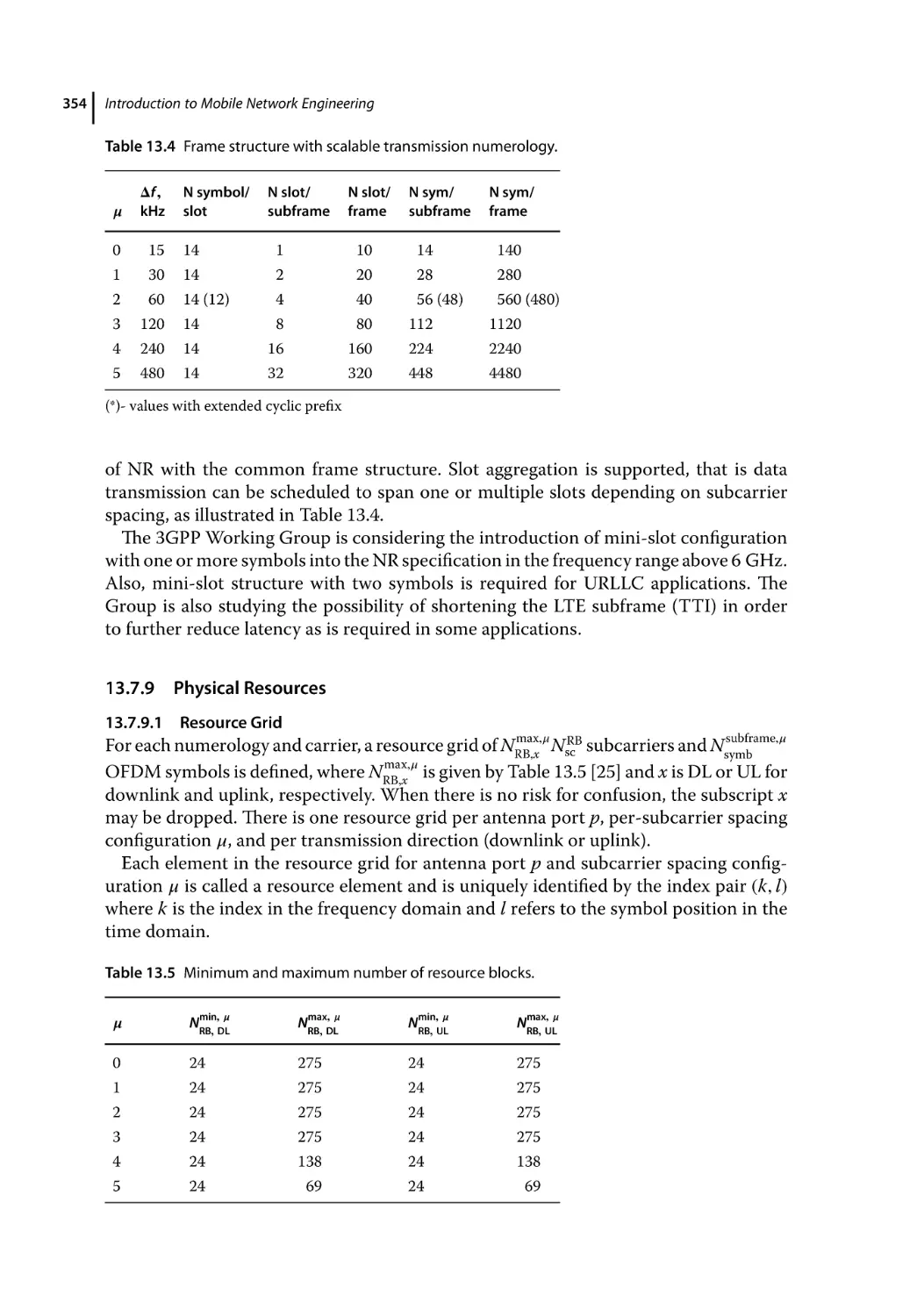
Resource Grid 354
Resource Blocks 355
Carrier Aggregation 356
Uplink Physical Channels and Signals 356
Downlink Physical Channels and Signals 357
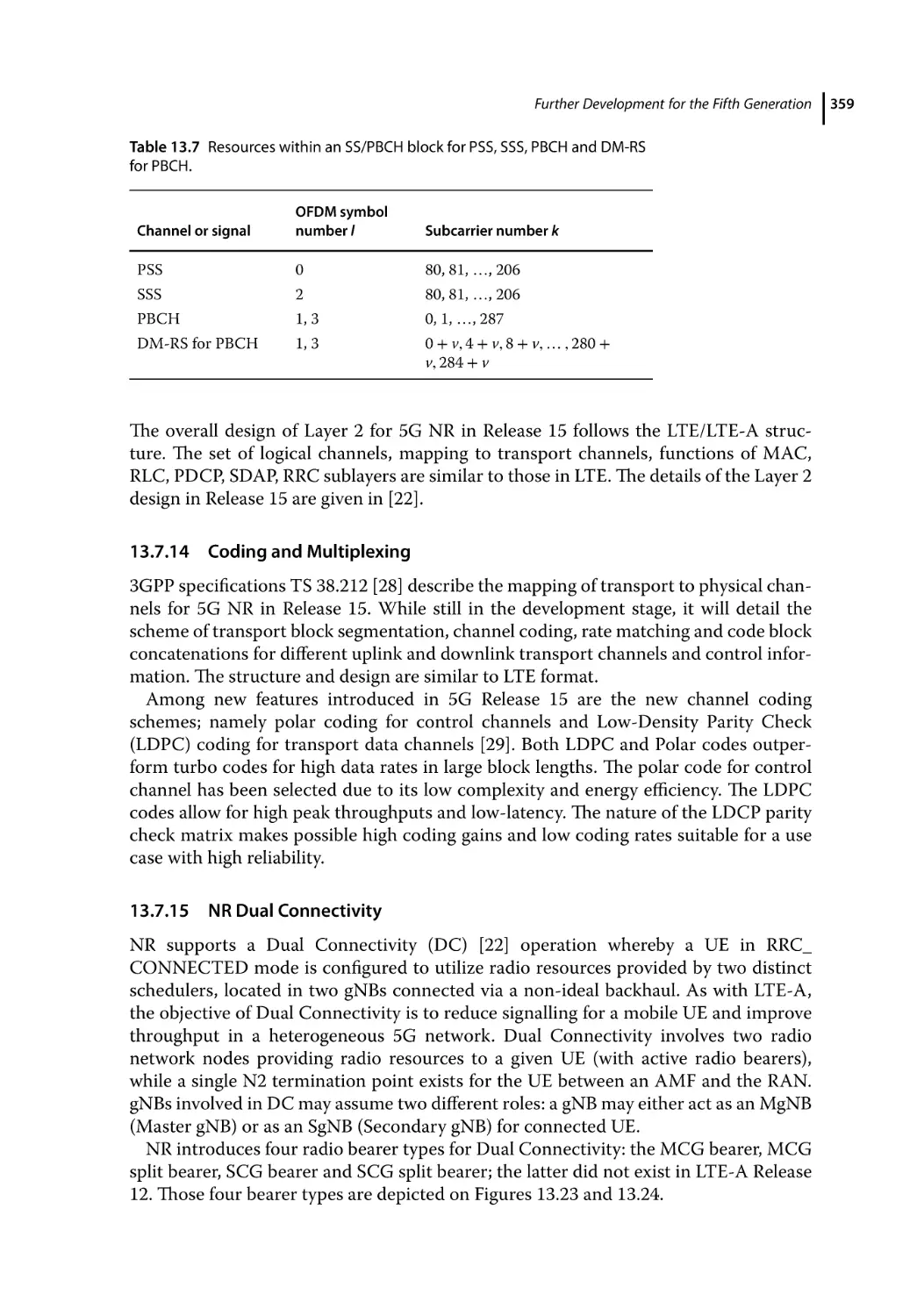
SS/PBCH Block 358
Coding and Multiplexing 359
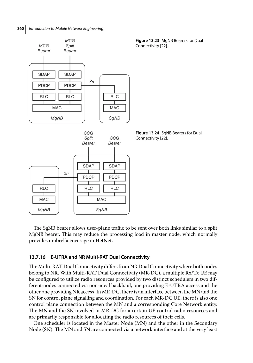
NR Dual Connectivity 359
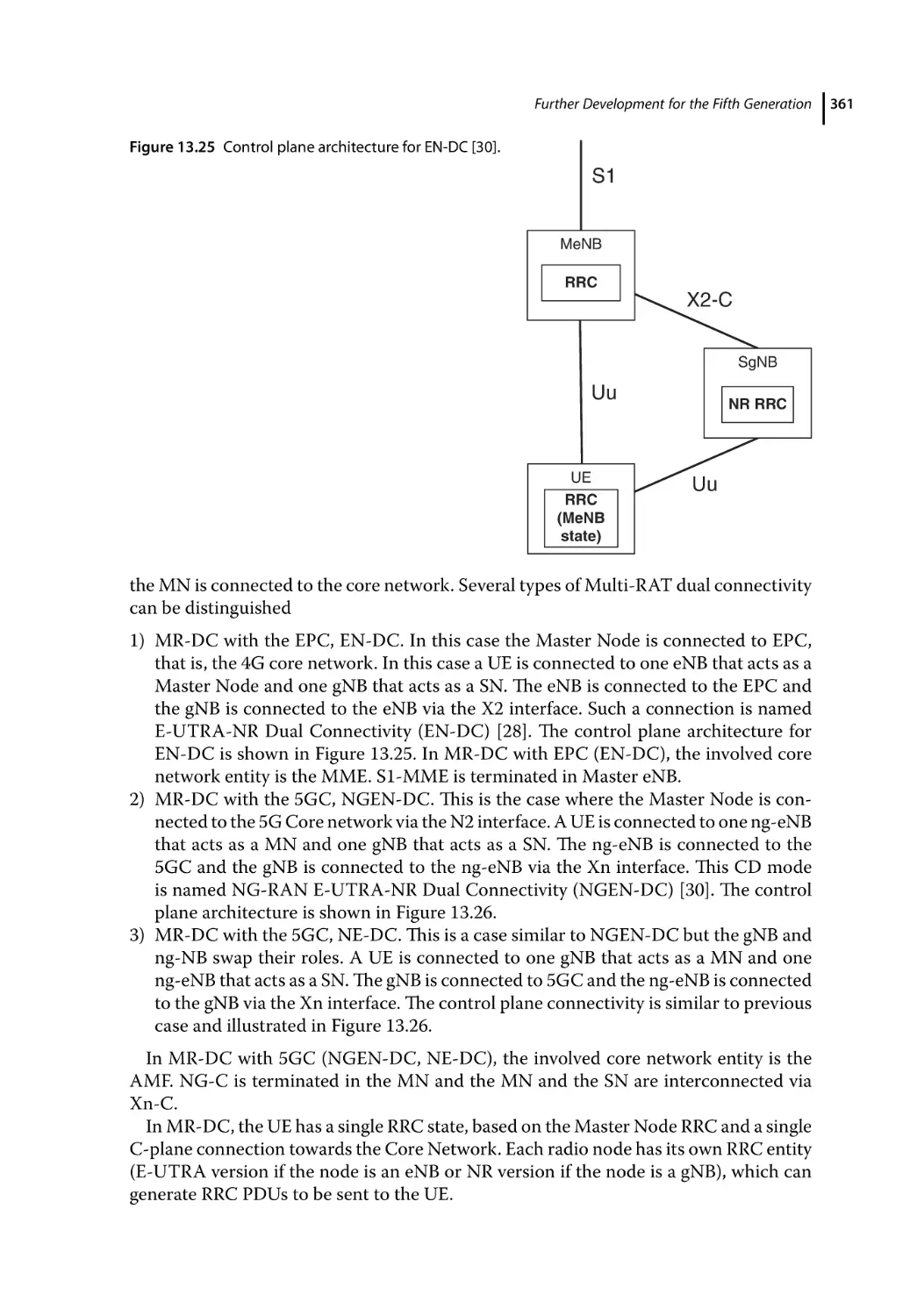
E-UTRA and NR Multi-RAT Dual Connectivity 360
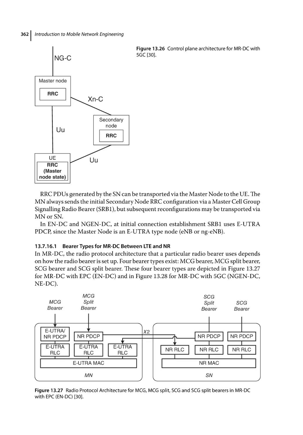
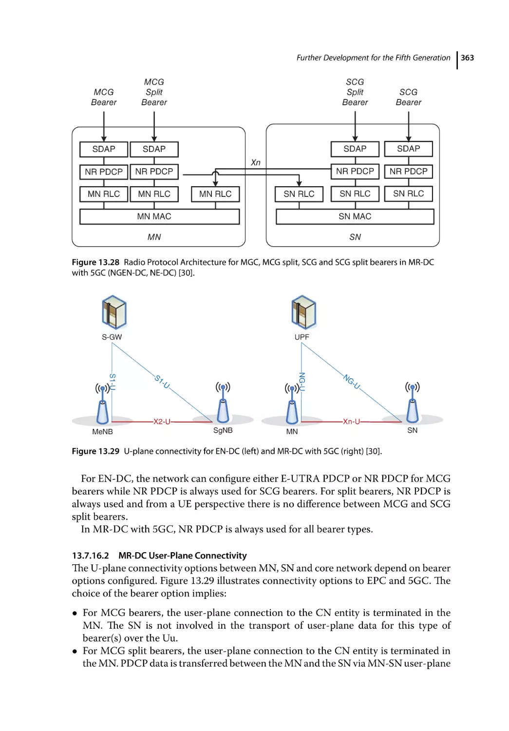
Bearer Types for MR-DC Between LTE and NR 362
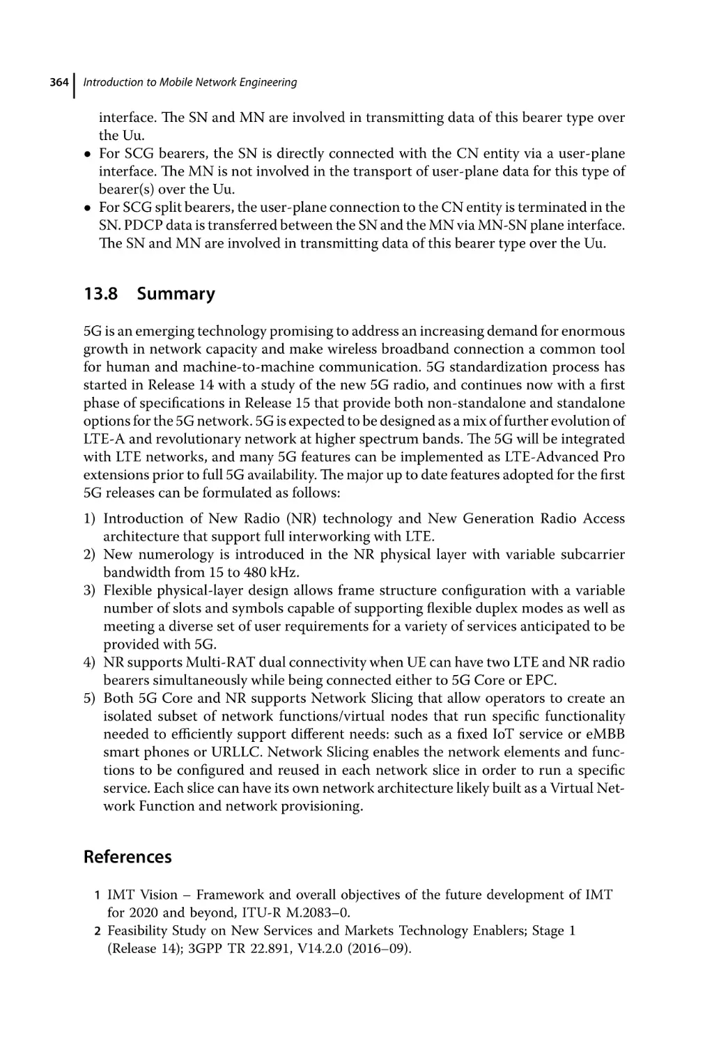
MR-DC User-Plane Connectivity 363
Summary 364
References 364
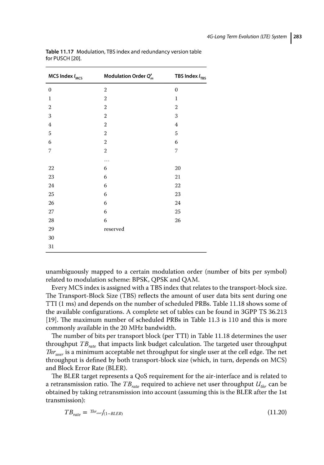
14
Annex: Base-Station Site Solutions 367
14.1
14.1.1
14.1.2
14.1.3
14.2
14.3
14.4
14.4.1
The Base-Station OBSAI Architecture 367
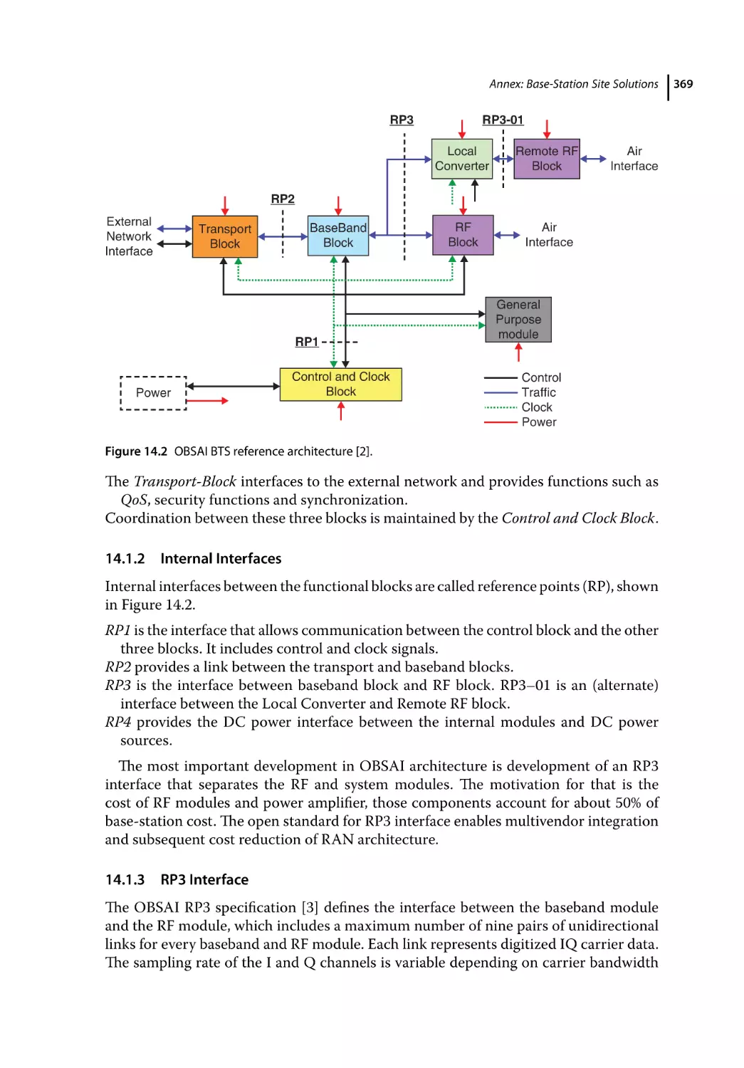
Functional Modules 367
Internal Interfaces 369
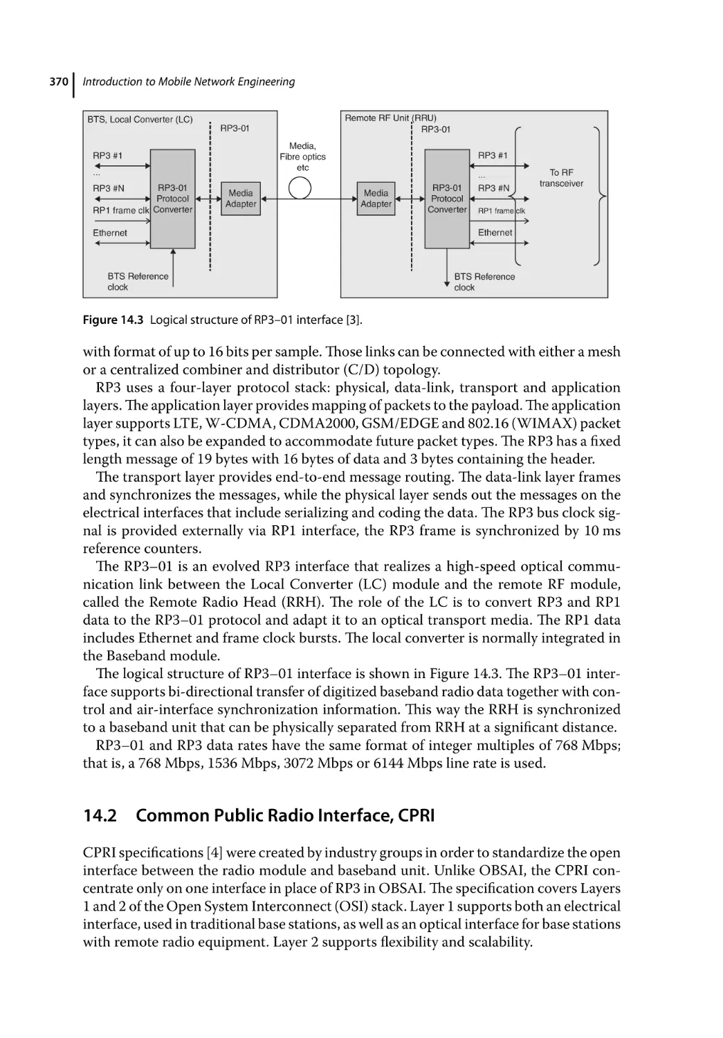
RP3 Interface 369
Common Public Radio Interface, CPRI 370
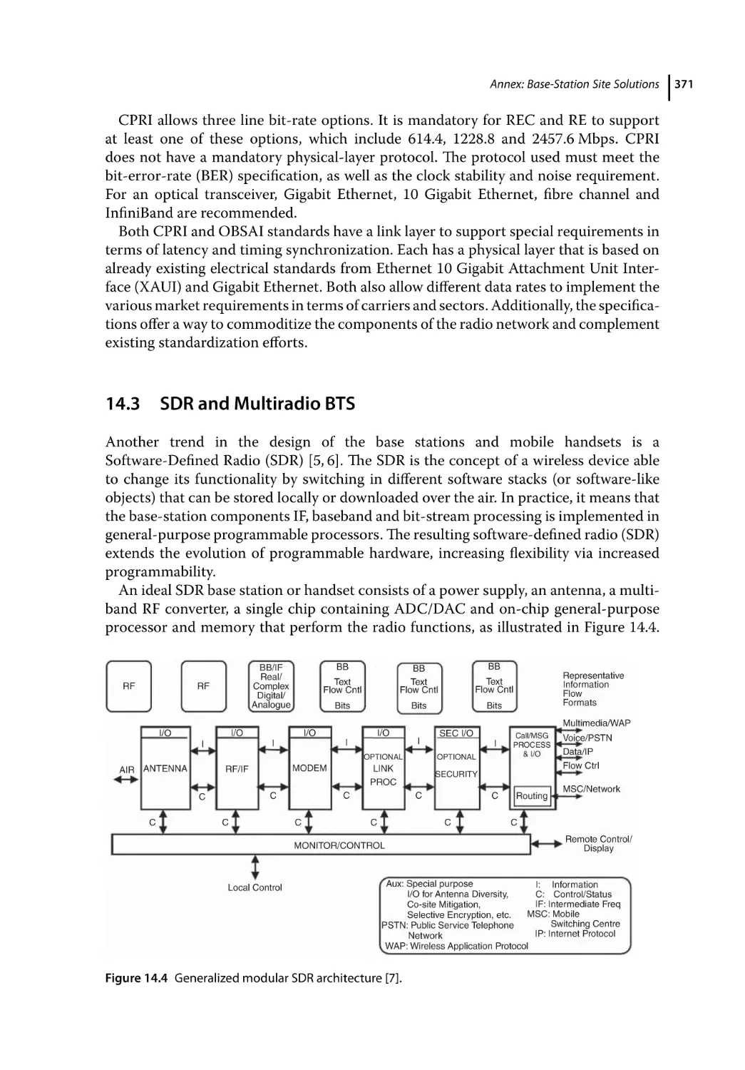
SDR and Multiradio BTS 371
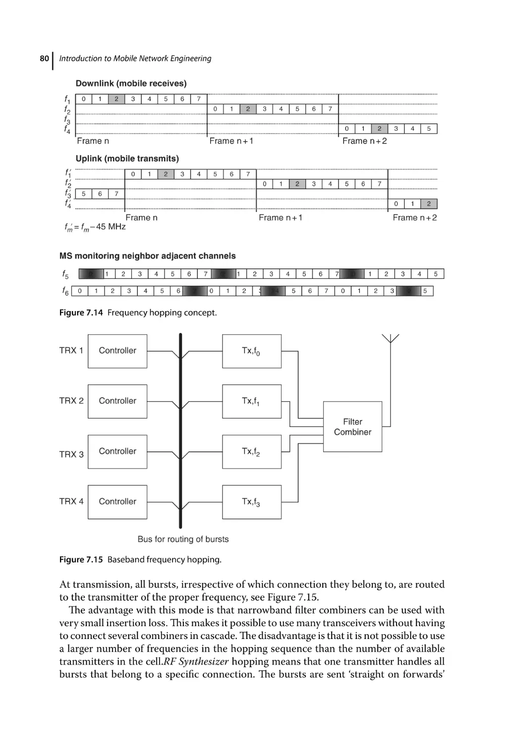
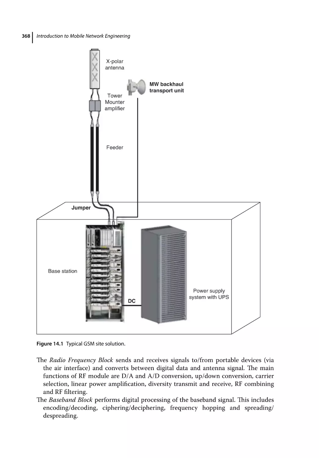
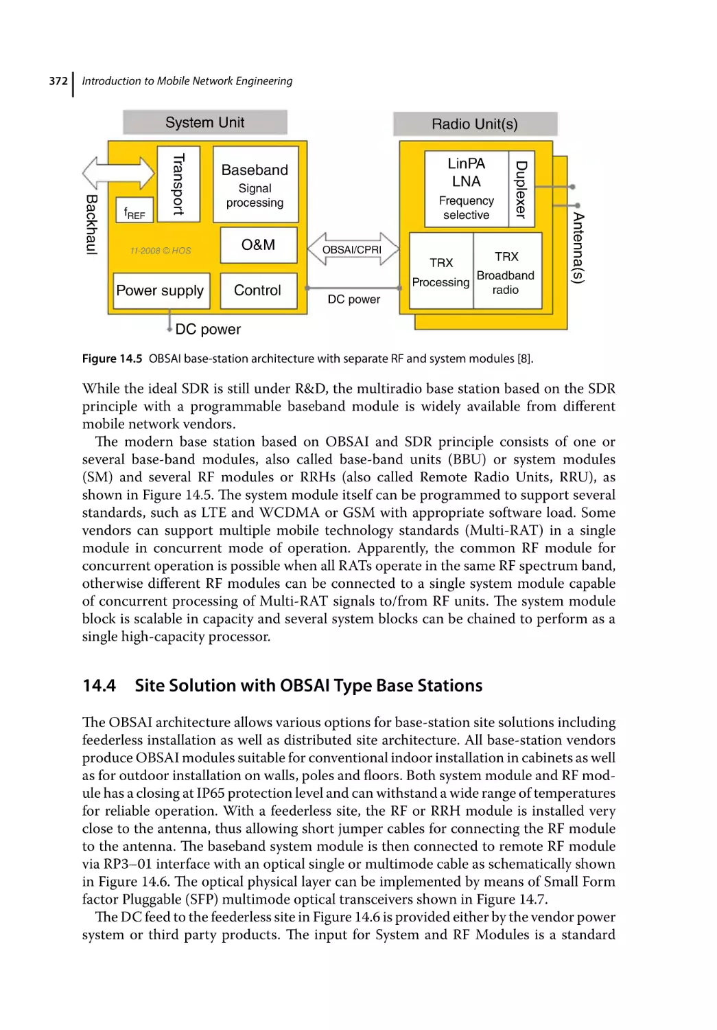
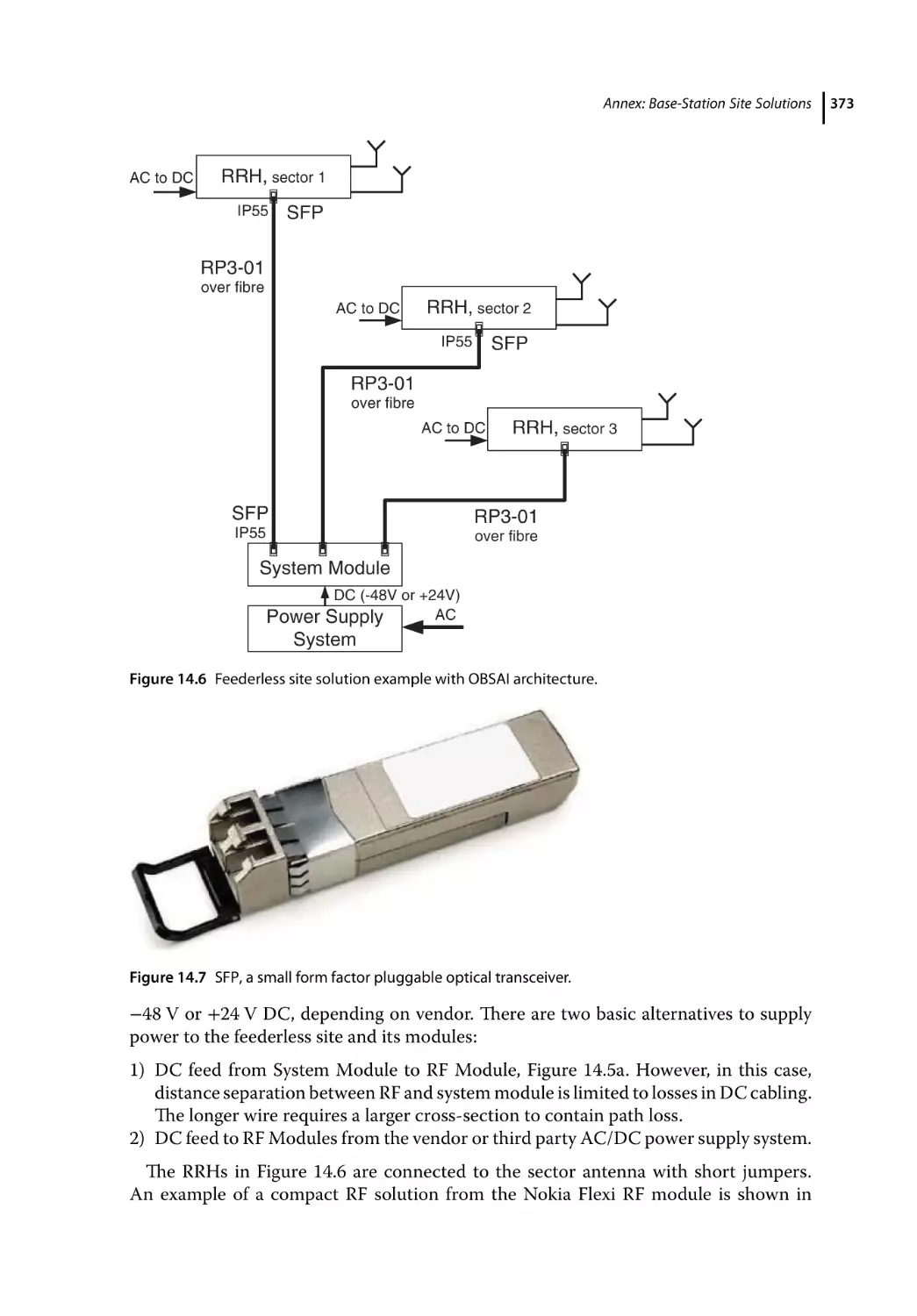
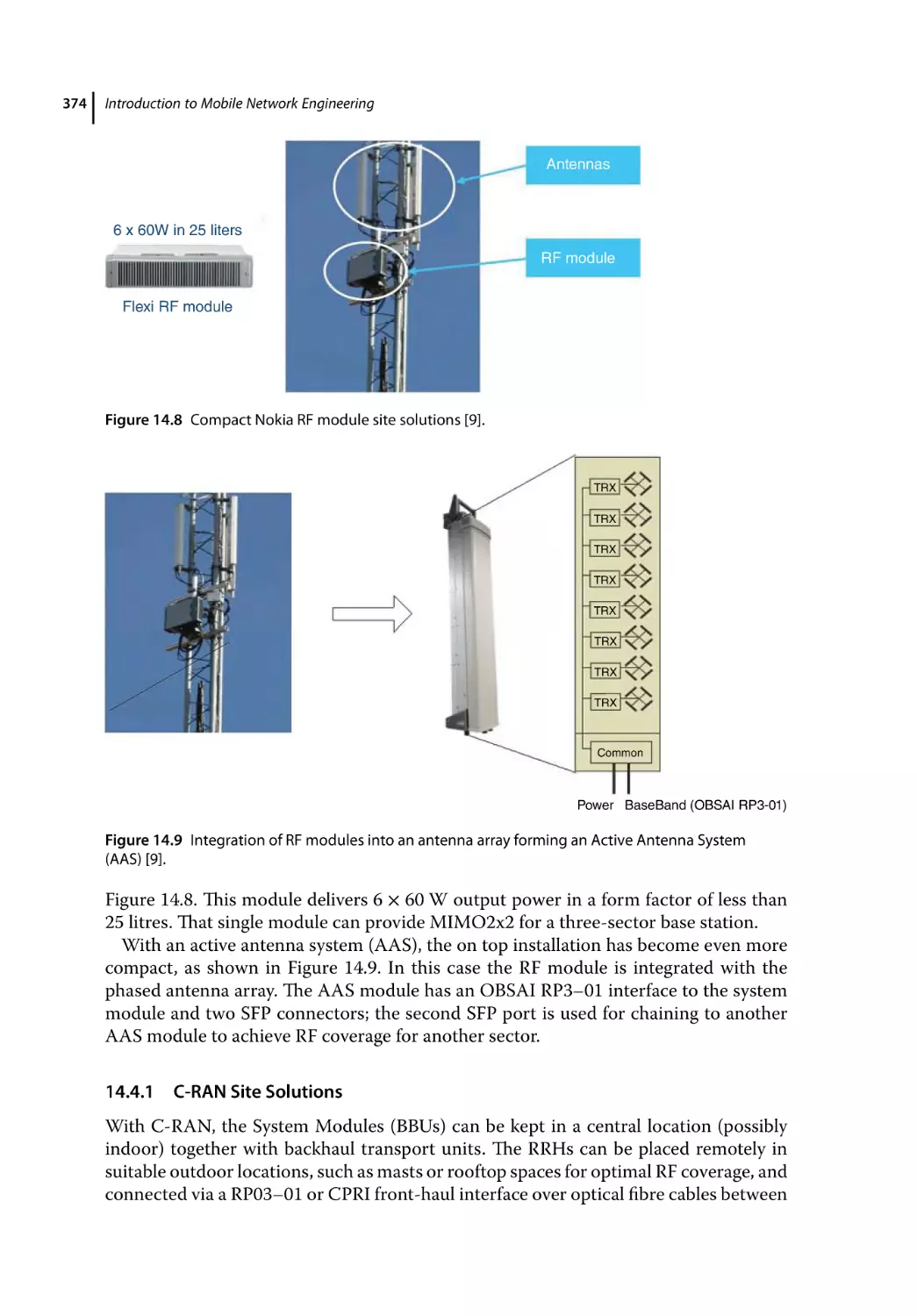
Site Solution with OBSAI Type Base Stations 372
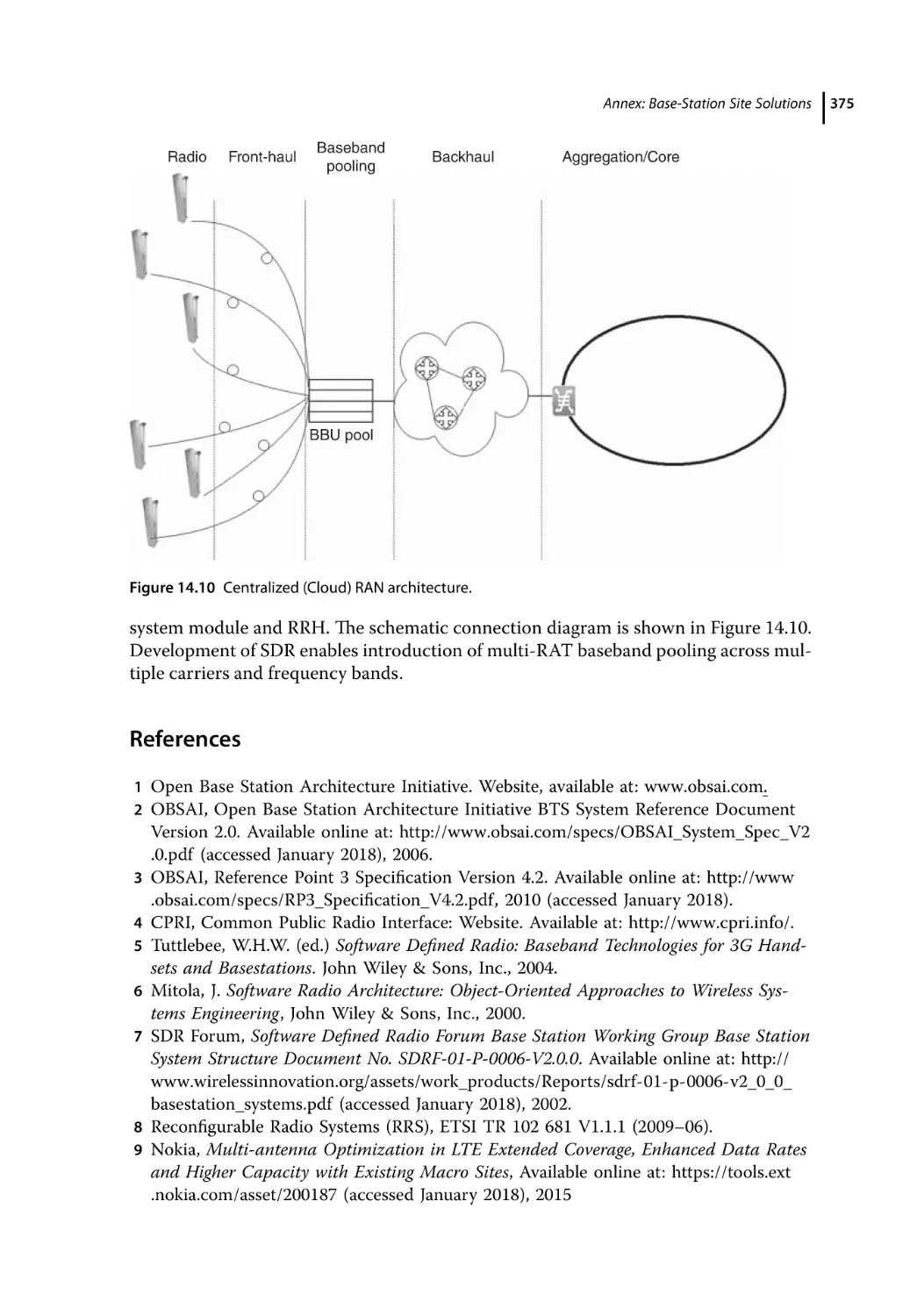
C-RAN Site Solutions 374
References 375
Index 377
xvii
Foreword
From the 1990s to the present, three generations of mobile radio networks have been
deployed in every country of the world. Those networks connect billions of customers
and provide mobile communications services. Mobile radio communications have
become ubiquitous throughout the world. People are getting used to the technology
through commercial mobile phones. The mobile network infrastructure that enables
communications has become a normal part of the urban environment in which people
live. There is also a great number of other applications for mobile radio that are essential
in the modern world and are used in navigation, transportation, machine-to-machine
communications (M2M), robotics, emergency and low enforcement services, broadcasting, space exploration, the military, and so on. The mobile radio is, in fact, a part
of a more widely defined wireless technology that, of course, includes wireless LANs
(Wi-Fi) with fixed and nomadic access.
The content of this book is limited to three major mobile communication technologies: GSM, 3G-WCDMA and LTE with the major focus on Radio Access Network (RAN)
technology. We introduce some basic concepts of mobile network engineering used in
the design and rollout of mobile networks. Then we cover principles, design constraints
and provide a more advanced insight into the radio interface protocol stack, operation and dimensioning for three major mobile network technologies; the Global System
Mobile (GSM), third (3G-WCDMA) and fourth generation (4G-LTE) mobile technologies that have been recently deployed or are shortly to be deployed. Enhancements of
fourth generation technology in LTE-Advanced (LTE-A) are described at the level of
conceptual design.
The concluding sections of the book are concerned with further development
towards the next generation of mobile networks (5G). The last section describes some
key concepts that may bring significant enhancements in network operation efficiency
and quality of services experienced by customers. A development of the fifth generation
of mobile networks can be regarded as a mix of evolutionary advances in 4G LTE
through LTE-A and new radio technology likely operating in newly allocated spectrum
bands. This development covers a broad area of applications and many different topics
that require specifically dedicated study. Therefore, many interesting and important
topics such as the Internet of Things, massive MTC, developments in new technology
for emergency services based on LTE, integration of the mobile radio access network
and Wi-Fi are out of the scope of this book.
Since the standards for 5G are still in development, most of the features of the new radio
technology are related to 3GPP Release 15. Some breakthrough technological advances
xviii
Foreword
are planned for further releases of 5G, such as a Full Duplex and self-backhauling
and are described as concepts rather than commercially available technology.
While many excellent books on mobile radio networking are available, I think many
more will be published in the near future since the subject is continuously evolving.
This book is intended to provide a generalist and compressed description of major technologies utilized in the radio access part of modern mobile networks. I envisage readers
are engineers in relatively early stages of their careers in the mobile wireless industry.
Some of them may be taking a post-graduate course to enhance their knowledge. They
may include operation support engineers, technical sale/presale engineers, technical
and account managers who may need or wish to enhance or expand their knowledge of
mobile network system engineering. Each major technology section of the book consists
of introductory material, a more advanced part and a summary.
Alexander Kukushkin
xix
Acknowledgements
I thank Professor Branka Vucetic, School of Electrical and Information Engineering,
University of Sydney, for the invitation to teach at the University that led to the writing
of this book. I wish to thank the reviewers of the book for their constructive comments
that helped to improve and extend the content, especially on the 5G related topics.
xxi
Abbreviations
3G
3GPP
5G
5GC
5G-S
TMSI
AA
AAA
AAS
ACK
ADC
AF
AGCH
AICH
AKA
AM
AMC
AMF
AMR
ARFCN
ARQ
ATCA
AUC
AUSF
BALUN
BBU
BCCH
BCH
BLER
BMC
BS
BSC
BSIC
BSS
CA
Third Generation
3rd Generation Partnership Project
Fifth Generation of mobile networks
5G Core network
5G System
Temporary Mobile Subscription Identifier
Antenna Array
Authentication, Authorization & Accounting
Active Antenna System
ACKnowledgement
Analogue to Digital Converter
Application Function
Access Grant CHannel
Acquisition Indicator CHannel
Authentication and Key Agreement
Acknowledged Mode
Adaptive Modulation and Coding
Access and Mobility Management Function
Adaptive Multi-Rate (coding)
Absolute Radio Frequency Channel Number
Automatic Repeat reQuest
Advanced Telecommunications Computing Architecture
AUthentication Centre
Authentication Server Function
BALanced to UNbalanced conversion
Base Band Unit
Broadcast Control CHannel
Broadcast CHannel
BLock Erasure Rate
Broadcast/Multicast Control
Base Station
Base Station Controller
Base Station Identity Code
Base Station Subsystem
Carrier Aggregation
xxii
Abbreviations
CAC
CC
CCCH
CCE
CCPCH
CCTrCH
CDD
CDM
CDMA
CIR
COMP
CP
CPCH
CPICH
CP-OFDM
CPRI
CQI
C-RAN
CRC
CRNC
CRNTI
CRS
CSCH
CSFB
CSI
CSI-RS
CTCH
DAC
DC
DCCH
DCH
DCI
DeNB
DFT
DFTS-OFDM
DL PCC
DL SCC
DLL
DL-SCH
DMRS
DN
DNN
DPCCH
DPCH
DPD
DPDCH
DRNC
Call Admission Control
Component Carrier
Common Control Channel
Control Channel Element
Common Control Physical Channel
Coded Composite Transport Channel
Cyclic Delay Diversity
Code Division Multiplexing
Code Division Multiple Access
Carrier to Interference Ratio
COordinated MultiPoint transmission and reception
Cyclic Prefix
Common Packet Channel
Common Pilot Channel
Cyclic Prefix-OFDM
Common Public Radio Interface
Channel Quality Indicators
Centralized Radio Access Network
Cyclic Redundancy Check
Controlling RNC
Cell Radio Network Temporary Identifier
Cell RS
Compact Synchronization Channel
Circuit Switched Fall Back
Channel State Information
Channel State Information Reference Signal
Common Traffic Channel
Digital-to-Analogue Convertor
Dual Connectivity
Dedicated Control Channel
Dedicated Transport Channel
Downlink Control Information
Donor eNB
Discrete Fourier Transform
DFT Spread-OFDM
Downlink Primary Component Carrier
Downlink Secondary Component Carrier
Data Link Layer
Downlink Shared CHannel
DeModulation Reference Signal
Data Network
Data Network Name
Dedicated Physical Control CHannel
Dedicated Physical CHannel
Digital Pre-Distortion
Dedicated Physical Data Channel
Drift RNC
Abbreviations
DRX
DSCH
DTCH
e2e
E-AGCH
ECCE
ECM
E-DCH
EDGE
E-DPCCH
E-HICH
EIR
eMBB
EN-DC
EPC
EPDCCH
EPS
EREG
E-RGCH
E-TFC
ETSI
E-UTRA
E-UTRAN
FACCH
FACH
FBI
FCCH
FDD
FDM
FDMA
F-DPCH
FDPS
FEC
FER
FFT
FN
FR
GBR
GGSN
GMSC
GMSK
GPRS
GSM
GTP
HARQ
HLR
HR
Discontinuous Transmission and Reception
Downlink Shared Channel
Dedicated Traffic Channel
End to End
E-DCH Absolute Grant CHannel
Enhanced Control Channel Element
EPS Connection Management
Enhanced Dedicated Channel
Enhanced Data rate for GSM Evolution
E-DCH Dedicated Physical Control CHannel
E-DCH Hybrid ARQ Indicator CHannel
Equipment Identity Register
Enhanced Mobile Broadband
E-UTRA-NR Dual Connectivity
Evolved Packet Core
Enhanced Physical Downlink Control CHannel
Evolved Packet System
Enhanced Resource Element Group
E-DCH Relative Grant Channel
E-DCH Transport Format Combination
European Telecommunications Standards Institute
Evolved UMTS Radio Access
Evolved UTRAN
Fast Associated Control Channel
Forward Access Channel
Feedback Information
Frequency Correction Channel
Frequency Division Duplex
Frequency Division Multiplexing
Frequency Division Multiple Access
Fractional DPCH
Frequency Domain Packet Scheduling
Forward Error Correction
Frame-Error Rate
Fast Fourier Transform
Frame Number
Full Rate
Guaranteed Bit Rate
Gateway GPRS Support Node
Gateway MSC
Gaussian Minimum Shift Keying modulation
GSM Packet Radio Service
Global System Mobile
GPRS Tunnelling Protocol
Hybrid ARQ
Home Location Register
Half Rate
xxiii
xxiv
Abbreviations
HSDPA
HS-DPCCH
HS-DSCH
HSS
HS-SCCH
HSUPA
HW
iFFT
IMEI
IMS
IMSI
IPsec
ISHO
ISI
IWF
LA
LAC
LAI
LAN
LLC
LNA
LOS
LPMA
LTE
M2M
MAC
MAHO
MAPL
MCC
MCG
MCS
MeNB
MgNB
MHA
MIB
MIMO
MME
MMI
MN
MNC
MRC
MR-DC
MS
MSC
MSISDN
MSRN
MT
High Speed Downlink Packet Access
High-Speed Dedicated Physical Control CHannel
High-Speed Downlink Shared CHannel
Home Subscriber Server
High-Speed Shared Control Channel
High Speed Uplink Packet Access
Hardware
inverse FFT
International Mobile Station Equipment Identity
IP Multimedia Subsystem
International Mobile Subscriber Identity
IP Security protocol
Inter-System Handover
Inter-Symbol Interference
Interworking Function
Location Area
Location Area Code
Location Area Identifier
Local Area Network
Logical Link Control
Low Noise Amplifier
Line Of Sight
Lattice Partition Multiple Access
Long Term Evolution
Machine to Machine communications
Medium Access Control
Mobile Assisted HandOver
Maximum Allowable Path Loss
Mobile Country Code
Master Cell Group
Modulation Coding Scheme
Master eNB
Master gNB
Mast Head Amplifier
Master Information Block
Multiple Input Multiple Output
Mobility Management Entity
Man-Machine Interface
Master Node
Mobile Network Code
Maximum Ratio Combining
Multi-RAT Dual Connectivity
Mobile Station (mobile phone)
Mobile Switching Centre
Mobile Subscriber ISDN Number
Mobile Station Routing Number
Mobile Termination
Abbreviations
MTC
MTCH
MU-MIMO
MUST
NACK
NAS
NB-IoT
NDC
NE-DC
NEF
NF
NFV
NGEN-DC
NGMN
NG-RAN
NOMA
NR
NRF
NSS
NSSAI
NSSF
OAM
OBSAI
OFDMA
OMC
OSI
OSS
OVP
OVSF
PACCH
PAPR
PCC
PCCCH
P-CCPCH
PCell
PCF
PCFICH
PCH
PCPCH
PCRF
PCU
PDCH
PDCP
PDP
PDSCH
PDTCH
PDU
Machine Type Communications
Multicast Traffic Channel
Multi-User MIMO
Multiuser Superposition Transmission
Negative ACKnowledgement
Non-Access Stratum
Narrow-Band Internet of Things
National Destination Code
MR-DC with the 5GC
Network Exposure Function
Network Functions
Network Function Virtualization
NG-RAN E-UTRA-NR Dual Connectivity
Next Generation Mobile Network Alliance
New Generation Radio Access Network
Non-Orthogonal Multiple Access
New Radio
NF Repository Function
Network Switching Subsystem
Network Slice Selection Assistance Information
Network Slice Selection Function
Operation, Administration and Maintenance
Open Base Station Architecture Initiative
Orthogonal Frequency Division Multiple Access
Operation and Maintenance Center
Open System Interconnect
Operation Support Subsystem
Over Voltage Protection
Orthogonal Variable Spreading Factor
Packet Associated Control Channel
Peak-to-Average Power Ratio
Primary Component Carrier
Packet Common Control Channel
Primary Common Control Physical Channel
Primary Cell
Policy Control Function
Physical Control Format Indicator Channel
Paging Channel
Physical Common Packet Channel
Policy Charging and Rules Function
Packet Control Units
Packet Data CHannel
Packet Data Convergence Protocol
Packet Data Protocol
Physical Downlink Shared CHannel
Packet Data Traffic CHannel
Packet Data Unit
xxv
xxvi
Abbreviations
P-GW
PHICH
PICH
PIN
PLMN
PMI
PRACH
PRB
P-RNTI
PSC
P-SCH
PSS
PSTN
PTCCH
PTCH
PT-RS
PUCCH
QCI
QoE
QoS
RAB
RACH
RAN
RAT
RAU
RB
RDN
REG
RF
RI
RLC
RN
RNC
RP
RRC
RRH
RRM
RRU
RS
SACCH
SAE
SAW
SCC
SCell
SC-FDMA
SCG
SCH
Packet Data Network Gateway
Physical Hybrid-ARQ Indicator Channel
Paging Indicator Channel
Personal Identification Number
Public Land Mobile Networks
Precoder Matrix Indication
Physical Random Access Channel
Power Resource Block
Paging Group Identity
Primary Scrambling Code
Primary Synchronization Channel
Primary Synchronization Signal
Public Switching Telephone Network
Packet Timing advance Control Channel
Packet Traffic Channel
Phase-Tracking Reference Signals
Physical Uplink Control CHannel
QoS Class Indicator
Quality Of user Experience
Quality of Service
Radio Access Bearer
Random Access CHannel
Radio Access Network
Radio Access Technology
Routing Area Update
Resource Block
Radio Distribution Network
Resource Element Group
Radio Frequency
Rank Indication
Radio Link Control
Relay Node
Radio Network Controller
Reference Point
Radio Resource Control
Remote Radio Head
Radio Resource Management
Remote Radio Unit
Reference Signals
Slow Associated Control Channel
System Architecture Evolution
Stop-And-Wait
Secondary Component Carrier
Secondary Cell
Single Carrier FDMA
Secondary Cell Group
Synchronization Channel
Abbreviations
S-CPICH
SDCCH
SDN
SDR
SDU
SF
SFN
SFP
SgNB
SGSN
S-GW
SIB
SIC
SIM
SINR
SIP
SIR
SM
SMF
SMG
SN
SecN
SNDCP
S-NSSAI
SON
SRB
SRNC
SRS
S-SCH
SSS
STR
SU-MIMO
SVD
SW
TA
TAB
TAG
TAU
TB
TBF
TCH
TCP
TDMA
TE
TF
TFC
TFCS
Secondary Common Pilot Channel
Standalone Dedicated Control Channel
Software Defined Networking
Software Designed Radio
Service Data Unit
Spreading Factor
System Frame Number
Small Form factor Pluggable
Secondary gNB
Serving GPRS Support Node
Serving Gateway
System Information Block
Successive Interference Cancellation
Subscriber Identity Module
Signal to Interference and Noise Ratio
Session Initiation Protocol
Signal to Interference Ratio
System Module
Session Management Function
Special Mobile Group
Subscriber Number
Secondary Node
Subnetwork Dependent Convergence Protocol
Single Network Slice Selection Assistance Information
Self-Organizing Network
Signalling Radio Bearer
Serving RNC
Sounding RS
Secondary Synchronization Channel
Secondary Synchronization Signal
Simultaneous Transmission and Reception
Single User-MIMO
Singular-Value Decomposition
Software
Terminal Adapter
Transceiver Array Boundary
Timing Advance Group
Tracking Area Update
Transport Block
Temporary Block Flow
Traffic Channel
Transmission Control Protocol
Time Division Multiple Access
Terminal Equipment
Transport Format
Transport Format Combination
Transport Format Combination Set
xxvii
xxviii
Abbreviations
TFI
TM
TMA
TMSI
TPC
TrCH
TRXUA
TS
TTI
UDM
UE
UL PCC
UL SCC
UL-SCH
UM
UMTS
UPF
URLLC
USB
USF
USIM
VAS
VLR
VoIP
WCDMA
Wi-Fi
Temporary Flow Identifier
Transparent Mode
Tower Mounted Amplifier
Temporary Mobile Subscriber Identity
Transmit Power Control
Transport Channel
Transceiver unit array
Time Slot
Transmission Time Interval
Unified Data Management Function
User Equipment
UpLink Primary Component Carrier
UpLink Secondary Component Carrier
UpLink Shared CHannel
Unacknowledged mode
Universal Mobile Telecommunication System
User Plane Function
Ultra-Reliable and Low Latency Critical Communications
Universal Serial Bus
Uplink State Flag
Universal Subscriber Identity Module
Value Added Services
Visited Location Centre
Voice over Internet Protocol
Wideband Code Division Multiple Access
Wireless local area networking
1
1
Introduction
Over the last few decades, mobile radio communications have become ubiquitous
throughout the world. People have become accustomed to the technology through
commercial mobile phones. The mobile network infrastructure that enables communications has become a normal part of urban environment in which people live.
There is also great number of other mobile radio applications essential in the modern
world that are used in navigation, transportation, machine-to-machine communications (M2M), robotics, emergency and low enforcement services, broadcasting, space
exploration, the military and so on. Mobile radio is, in fact, a part of more a widely
defined wireless technology that, of course, includes wireless LANs (WiFi) with fixed
and nomadic access.
Each application was developed on the basis of specific needs and, in some aspects,
the mobile radio networks for emergency services and commercial mobile services are
different. Nonetheless, the underlying principles in mobile communications, such as
radio link design given performance constraints, separation of control and traffic channels, mobility support, principles of the channel allocation in the cell, radio network
management and so on, have lots in common in many applications. Moreover, some of
the commercial technologies, such as LTE, now appeared to support land mobile radio
applications for emergency and public safety services.
This book is written as a modified and expanded set of lectures on the wireless
engineering course I had privilege to teach at the University of Sydney, Australia
for a couple of years. Most of the concepts of these lectures were adopted from
published standards and also based on personal experience in the field as well as from
some works of other authors. The course was delivered as post-graduate study. The
assumption was made that the fundamentals of digital communications were already
known to attendees and the objective was to explain the subject using mathematical
arguments as little as possible; that is, close to common practice in the commercial
communications industry. The target audience are engineers who are involved in either
network operations or technical pre-sale. The content is limited to major three mobile
communication technologies: GSM, 3G-Wideband Code Division Multiple-Access
(WCDMA) and LTE with the major focus on radio access network (RAN) technology.
The core part of the network is a complex subject on its own and is described only to
discuss its role in e2e procedures and interfaces with the radio network.
Introduction to Mobile Network Engineering: GSM, 3G-WCDMA, LTE and the Road to 5G,
First Edition. Alexander Kukushkin.
© 2018 John Wiley & Sons Ltd. Published 2018 by John Wiley & Sons Ltd.
3
2
Types of Mobile Network by Multiple-Access Scheme
Mobile radio networks can be distinguished by operation modes, services and
applications and multiple-access schemes. A major influence on the development of
commercial radio communication systems is the scarcity of radio spectrum available
for utilization. An apparent objective is to assign the maximum number of users to
an available radio frequency segment. This objective is achieved by using various
multiple-access schemes. Here, we list the four most common technologies:
1)
2)
3)
4)
frequency division multiple access (FDMA)
time-division multiple access (TDMA)
code division multiple access (CDMA)
orthogonal frequency division multiple access (OFDMA)
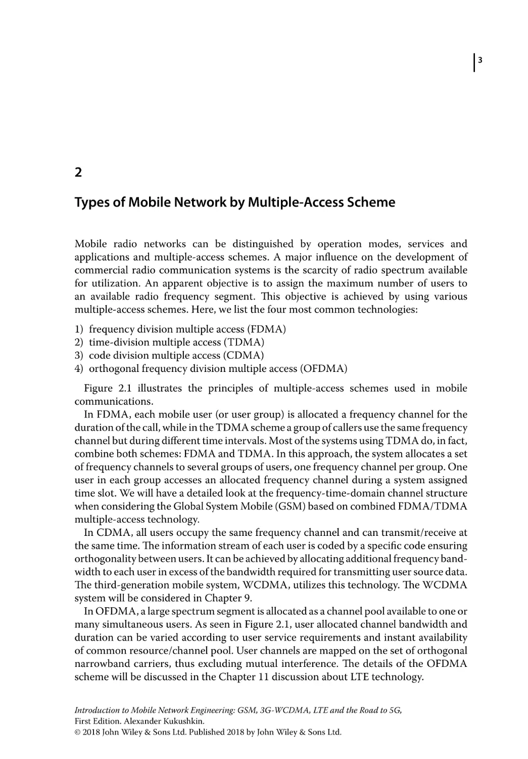
Figure 2.1 illustrates the principles of multiple-access schemes used in mobile
communications.
In FDMA, each mobile user (or user group) is allocated a frequency channel for the
duration of the call, while in the TDMA scheme a group of callers use the same frequency
channel but during different time intervals. Most of the systems using TDMA do, in fact,
combine both schemes: FDMA and TDMA. In this approach, the system allocates a set
of frequency channels to several groups of users, one frequency channel per group. One
user in each group accesses an allocated frequency channel during a system assigned
time slot. We will have a detailed look at the frequency-time-domain channel structure
when considering the Global System Mobile (GSM) based on combined FDMA/TDMA
multiple-access technology.
In CDMA, all users occupy the same frequency channel and can transmit/receive at
the same time. The information stream of each user is coded by a specific code ensuring
orthogonality between users. It can be achieved by allocating additional frequency bandwidth to each user in excess of the bandwidth required for transmitting user source data.
The third-generation mobile system, WCDMA, utilizes this technology. The WCDMA
system will be considered in Chapter 9.
In OFDMA, a large spectrum segment is allocated as a channel pool available to one or
many simultaneous users. As seen in Figure 2.1, user allocated channel bandwidth and
duration can be varied according to user service requirements and instant availability
of common resource/channel pool. User channels are mapped on the set of orthogonal
narrowband carriers, thus excluding mutual interference. The details of the OFDMA
scheme will be discussed in the Chapter 11 discussion about LTE technology.
Introduction to Mobile Network Engineering: GSM, 3G-WCDMA, LTE and the Road to 5G,
First Edition. Alexander Kukushkin.
© 2018 John Wiley & Sons Ltd. Published 2018 by John Wiley & Sons Ltd.
4
Introduction to Mobile Network Engineering
FDMA
TDMA
ChN
Ch3
Ch2
Ch1
ChN
Ch3
Ch2
Ch1
Frequency
Time
Frequency
Time
CDMA
Code
Time
0FDMA
ChN
User 2
User 1
Ch3
User 4
User 6
User 5
User 1
Ch2
User 2
User 6
Frequency
Ch1
Time
Figure 2.1 Common multiple-access schemes.
Frequency
User 3
Time
5
3
Cellular System
3.1 Historical Background
A scarcity of the available frequency spectrum is a major issue in the development of
mobile networks. We consider a well quoted and quite convincing example of a GSM
system. For example, only 25 MHz of the radio spectrum is available for the GSM system in the 900 MHz frequency range. That may allocate a maximum of 125 frequency
channels each with a carrier bandwidth of 200 kHz. Within an eightfold time multiplex for each carrier, a maximum of 1000 channels can be realized. This number is
further reduced by guard bands in the frequency spectrum and the overhead required
for signalling.
Apparently, 1000 simultaneous users cannot produce sufficient revenue to justify the
licence cost of 25 MHz of spectrum. In order to be able to serve several hundreds of
thousands or millions of subscribers in spite of this limitation, frequencies must be spatially reused; that is, deployed repeatedly in a geographic area. In this way, services can
be offered with a cost-effective subscriber density and acceptable blocking probability.
3.2 Cellular Concept
The spatial frequency reuse concept led to the development of the cellular principle,
which allowed a significant improvement in the economic use of frequencies. The essential characteristics of the cellular network principle are as follows:
• The area to be covered is subdivided into cells (radio zones). These cells are often
modelled in a simplified way as hexagons (Figure 3.1) with a base station located at
the centre of each cell. Assume that the operator has a licence on a set of channels,
called, for example, set S.
• To each cell i a subset of the frequencies Si is assigned from the total set (bundle),
which is assigned to the respective mobile radio network. In the GSM system, the
set of frequencies assigned to a cell is called the Cell Allocation (CA). Under normal circumstances the number of channels in a subset Si is driven by traffic capacity
requirements.
• Neighbouring cells do not normally use the same frequencies since this would lead to
severe co-channel interference from the adjacent cells.
Introduction to Mobile Network Engineering: GSM, 3G-WCDMA, LTE and the Road to 5G,
First Edition. Alexander Kukushkin.
© 2018 John Wiley & Sons Ltd. Published 2018 by John Wiley & Sons Ltd.
6
Introduction to Mobile Network Engineering
f3
f4
f3
f4
f2
f2
f5
f1
f5
f7
f7
f6
D, reuse distance
f1
f3
f6
f4
f3
•
f4
f2
f1
f5
f1
f5
f2
f7
f7
f6
2R
f6
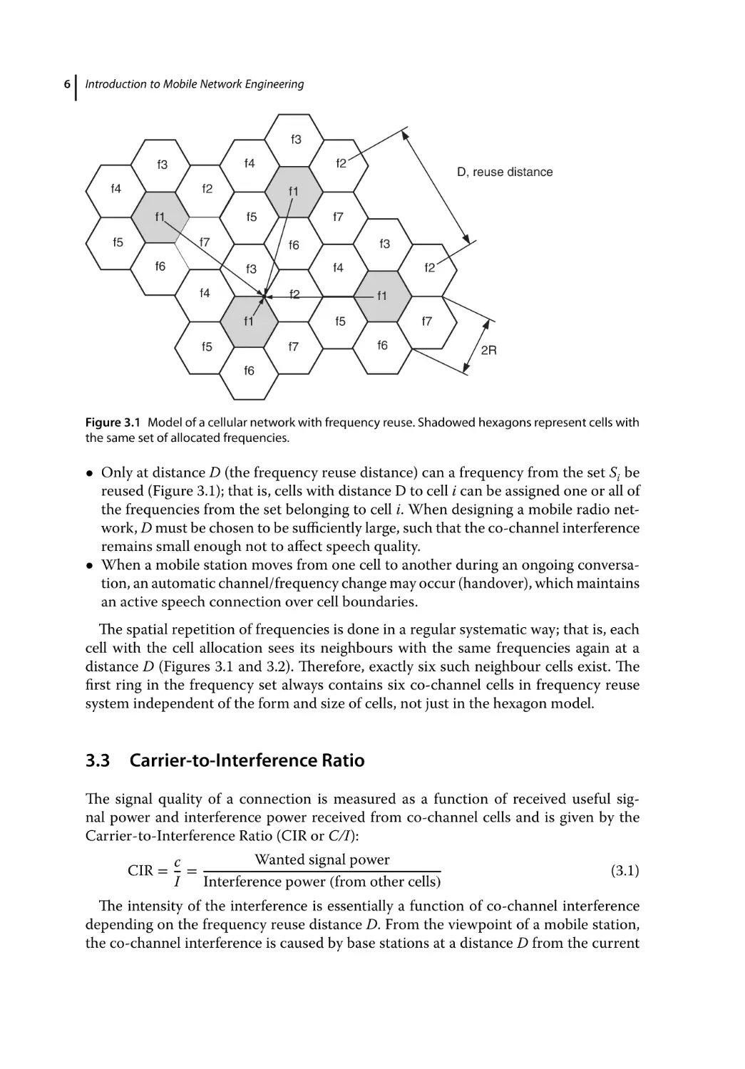
Figure 3.1 Model of a cellular network with frequency reuse. Shadowed hexagons represent cells with
the same set of allocated frequencies.
• Only at distance D (the frequency reuse distance) can a frequency from the set Si be
reused (Figure 3.1); that is, cells with distance D to cell i can be assigned one or all of
the frequencies from the set belonging to cell i. When designing a mobile radio network, D must be chosen to be sufficiently large, such that the co-channel interference
remains small enough not to affect speech quality.
• When a mobile station moves from one cell to another during an ongoing conversation, an automatic channel/frequency change may occur (handover), which maintains
an active speech connection over cell boundaries.
The spatial repetition of frequencies is done in a regular systematic way; that is, each
cell with the cell allocation sees its neighbours with the same frequencies again at a
distance D (Figures 3.1 and 3.2). Therefore, exactly six such neighbour cells exist. The
first ring in the frequency set always contains six co-channel cells in frequency reuse
system independent of the form and size of cells, not just in the hexagon model.
3.3 Carrier-to-Interference Ratio
The signal quality of a connection is measured as a function of received useful signal power and interference power received from co-channel cells and is given by the
Carrier-to-Interference Ratio (CIR or C/I):
CIR =
Wanted signal power
c
=
I
Interference power (from other cells)
(3.1)
The intensity of the interference is essentially a function of co-channel interference
depending on the frequency reuse distance D. From the viewpoint of a mobile station,
the co-channel interference is caused by base stations at a distance D from the current
Cellular System
2
1
2
1
1
3
1
2
1
3
4
2
1
3
4
2
4
4
2
3
3
2
4
3
1
3
2
4
4
1
3
4
K=4
f3
f3
f2
f1
f2
f1
f3
f3
f3
f2
f2
f1
f1
f3
f1
f3
f2
f1
f2
f2
f1
K=3
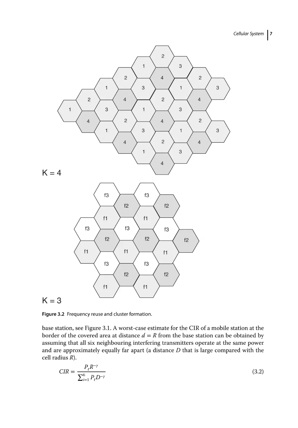
Figure 3.2 Frequency reuse and cluster formation.
base station, see Figure 3.1. A worst-case estimate for the CIR of a mobile station at the
border of the covered area at distance d = R from the base station can be obtained by
assuming that all six neighbouring interfering transmitters operate at the same power
and are approximately equally far apart (a distance D that is large compared with the
cell radius R).
P R−𝛾
CIR = ∑6 t
−𝛾
i=1 Pt D
(3.2)
7
8
Introduction to Mobile Network Engineering
Finally, we find the worst-case CIR as a function of the cell radius R, the reuse distance
D and the attenuation exponent 𝛾 as
( )
R−𝛾
1 R −𝛾
CIR =
=
(3.3)
6D−𝛾
6 D
Therefore, in a given radio environment, the CIR depends essentially on the ratio
R∕D. From these considerations, it follows that, for a desired or required CIR value at a
given cell radius, one must choose a minimum distance for frequency reuse above which
co-channel interference falls below the required threshold.
3.4 Formation of Clusters
The regular spatial repetition of frequencies results in a clustering of cells. The cells
within a cluster must each be assigned different sets of channels, while cells belonging
to neighbouring clusters can reuse the channels in the same spatial pattern. The size of
a cluster is characterized by the number of cells per cluster k, which determines the frequency reuse distance D when the cell radius R is given. Figure 3.2 shows some examples
of clusters. The numbers designate the respective frequency sets Si used within the single
cells. For each cluster, the following holds:
• A cluster can contain all of the frequencies of the mobile radio system.
• Within a cluster, no frequency can be reused. The frequencies of a setSi may be reused
at the earliest in the neighbouring cluster.
• The larger the cluster is, the larger the frequency reuse distance and the larger the
CIR. However, the larger the values of k, the smaller the number of channels and the
number of supportable active subscribers per cell.
The geometry of hexagons sets the relationship between the cluster size and the reuse
distance as:
√
D = R 3k
(3.4)
The CIR is then given by
( )
1 R −𝛾 1
CIR =
= (3k)−𝛾∕2
(3.5)
6 D
6
assuming the propagation attenuation exponent 𝛾 = 4, CIR = 3∕2k 2 . For example, if
the system can achieve acceptable quality provided the C/I is at least 18 dB, then the
required cluster size is 6.5. Hence, a cluster size of k = 7 would fit. Not all cluster sizes
are possible due to the restrictions of the hexagonal geometry. The hexagon geometry
results in following equation for cluster size
k = i2 + ij + j2 ,
(3.6)
where i, j are integers.
Possible values of k include 3, 4, 7, 12, 13, 19 and 27. The smaller the value of C/I, the
smaller the allowed cluster size. Hence the available channels can be reused on a denser
basis, serving more users and producing an increased capacity. In the example here,
had the path loss dependence on radius been slower (i.e. the propagation exponent was
less than 4), the required cluster size would have been greater than 7, so the path loss
Cellular System
characteristics have a direct impact on the system capacity. Another constraint on the
value of cluster size is that each base-station site often serves a cloverleaf of three cells.
(This can be designated, for example, by specifying 21 cells as a 3 × 7 cluster.) Commonly
used cluster sizes are multiples of three.
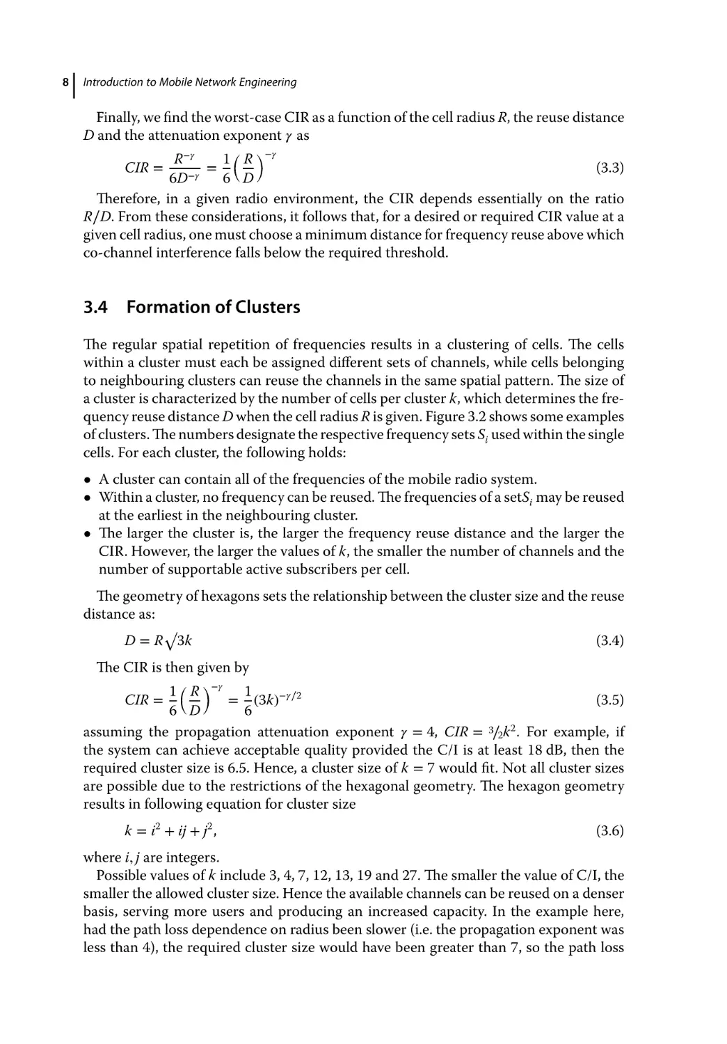
3.5 Sectorization
One way to reduce cluster size, and hence increase capacity, is to use sectorization. The
group of channels available at each cell is split into three cells (sectors), each of which is
confined in coverage to one-third of the cell area by the use of directional antennas, as
shown in Figure 3.3.
Interference now comes from just two rather than six of the first-tier interfering sites,
reducing √
interference by a factor of three and allowing cluster size to be increased by a
factor of = 1.72 in theory.
Sectorization has some disadvantages:
• Mobiles have to change channels more often, resulting in an increased signalling load
on the system.
• The available pool of channels has to be reduced by a factor of 3 (in a three-sector
site) for a mobile at any particular location; this reduces the trunking efficiency given
same cell size.
Despite these issues, sectorization is used very widely in modern cellular systems,
particularly in areas requiring high traffic density. More than three sectors can be used
to further improve the interference reduction.
The effective radiated power and, consequently, CIR can be increased with directional
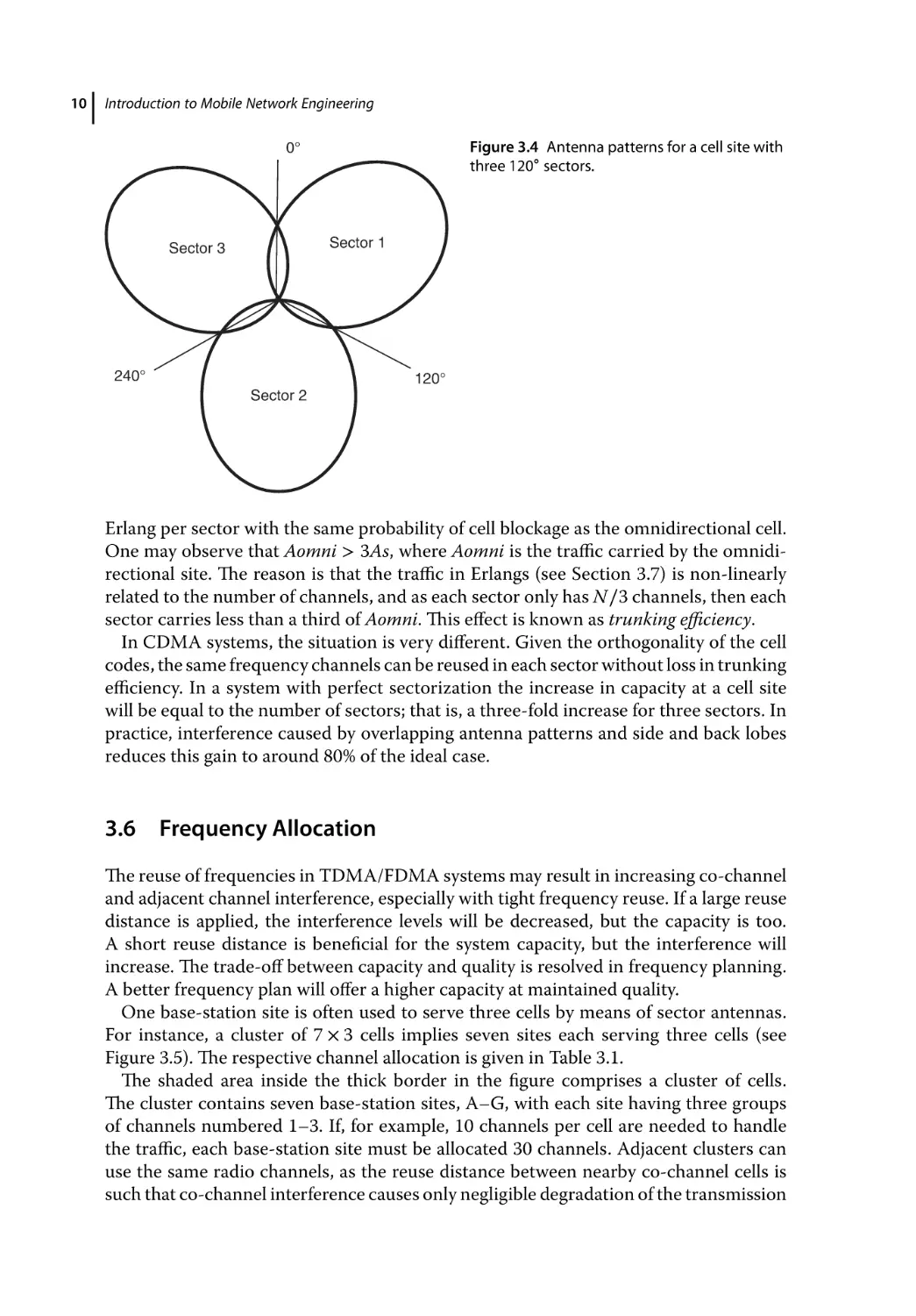
antennas. In a three-sector site the radiation pattern of sector antenna spans 120∘ in
the horizontal plane, as shown in Figure 3.4. In fact, the horizontal lobe of the sector
antenna extends over 120∘ creating overlapping regions between site sectors where a
mobile can receive a signal from both sectors. These regions facilitate an intra-sector
handover; that is, they enable an MS travelling between sectors to be switched from one
sector to another.
While sectorization does significantly increase the CIR, it often decreases the carried
traffic in time-division multiple access (TDMA) and frequency division multiple access
(FDMA) systems. For example, an omnidirectional site is allocated N frequency channels and carries a traffic Aomni Erlang with a defined probability of cell blockage. After
sectorization, each sector may be allocated N∕3 channels and may carry traffic of As
1
2
3
Omni site
Figure 3.3 Sectorization.
3 sector site
9
10
Introduction to Mobile Network Engineering
Figure 3.4 Antenna patterns for a cell site with
three 120∘ sectors.
0°
Sector 1
Sector 3
240°
120°
Sector 2
Erlang per sector with the same probability of cell blockage as the omnidirectional cell.
One may observe that Aomni > 3As, where Aomni is the traffic carried by the omnidirectional site. The reason is that the traffic in Erlangs (see Section 3.7) is non-linearly
related to the number of channels, and as each sector only has N∕3 channels, then each
sector carries less than a third of Aomni. This effect is known as trunking efficiency.
In CDMA systems, the situation is very different. Given the orthogonality of the cell
codes, the same frequency channels can be reused in each sector without loss in trunking
efficiency. In a system with perfect sectorization the increase in capacity at a cell site
will be equal to the number of sectors; that is, a three-fold increase for three sectors. In
practice, interference caused by overlapping antenna patterns and side and back lobes
reduces this gain to around 80% of the ideal case.
3.6 Frequency Allocation
The reuse of frequencies in TDMA/FDMA systems may result in increasing co-channel
and adjacent channel interference, especially with tight frequency reuse. If a large reuse
distance is applied, the interference levels will be decreased, but the capacity is too.
A short reuse distance is beneficial for the system capacity, but the interference will
increase. The trade-off between capacity and quality is resolved in frequency planning.
A better frequency plan will offer a higher capacity at maintained quality.
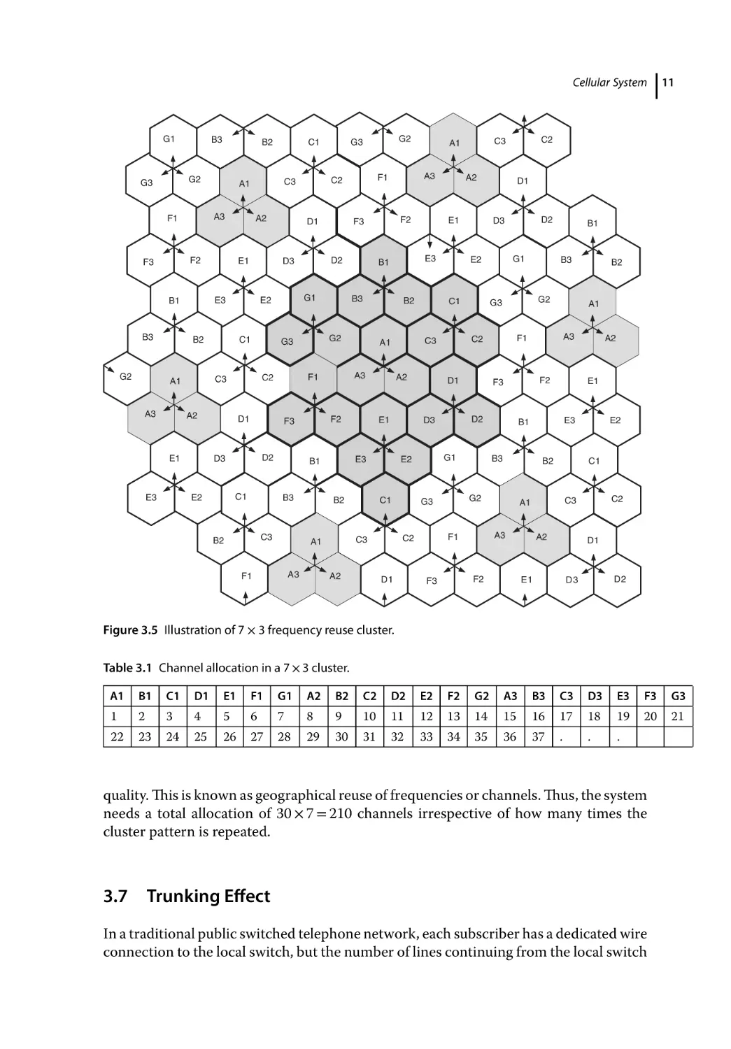
One base-station site is often used to serve three cells by means of sector antennas.
For instance, a cluster of 7 × 3 cells implies seven sites each serving three cells (see
Figure 3.5). The respective channel allocation is given in Table 3.1.
The shaded area inside the thick border in the figure comprises a cluster of cells.
The cluster contains seven base-station sites, A–G, with each site having three groups
of channels numbered 1–3. If, for example, 10 channels per cell are needed to handle
the traffic, each base-station site must be allocated 30 channels. Adjacent clusters can
use the same radio channels, as the reuse distance between nearby co-channel cells is
such that co-channel interference causes only negligible degradation of the transmission
Cellular System
G1
B3
G2
G3
A2
F2
F3
C1
B2
A3
A2
E1
G3
E3
D1
D2
C1
E2
B3
C3
B2
B2
A3
C1
A2
D1
E1
B2
E2
C1
C2
C3
A1
A3
F2
A2
G3
E3
B1
B3
F1
F3
A3
F2
G2
B2
A1
F1
D2
G3
C2
C3
G2
F3
G1
B1
B3
G3
D1
E2
G1
C2
D3
G3
E3
A1
F1
E1
D2
D3
C1
A2
D1
E2
C3
A1
A3
B1
E1
B2
F2
F3
D3
B3
F1
A2
E3
B1
G2
G3
C2
C3
A1
D2
G1
E2
F2
F3
D1
C2
C3
A1
A3
F1
C2
D3
G3
E3
B1
B3
E1
G2
G3
C1
C3
A1
A3
F1
G2
B2
11
A2
D1
E1
D2
D3
Figure 3.5 Illustration of 7 × 3 frequency reuse cluster.
Table 3.1 Channel allocation in a 7 × 3 cluster.
A1
B1
C1
D1
E1
F1
G1
A2
B2
C2
D2
E2
F2
G2
A3
B3
C3
D3
E3
F3
G3
1
2
3
4
5
6
7
8
9
10
11
12
13
14
15
16
17
18
19
20
21
22
23
24
25
26
27
28
29
30
31
32
33
34
35
36
37
.
.
.
quality. This is known as geographical reuse of frequencies or channels. Thus, the system
needs a total allocation of 30 × 7 = 210 channels irrespective of how many times the
cluster pattern is repeated.
3.7 Trunking Effect
In a traditional public switched telephone network, each subscriber has a dedicated wire
connection to the local switch, but the number of lines continuing from the local switch
12
Introduction to Mobile Network Engineering
towards the next bigger switch is typically much smaller than the sum of subscribers
served in that area.
The same applies to cellular networks as well, although the traditional subscriber line
has been replaced with wireless access to the base station. This phenomenon is known
as the trunking effect. In fact, the trunking effect reduces the number of lines at every
network element concentrating traffic (merging several lines) if the number of incoming
lines is big enough.
One can assume that calls take place during the busy hour and that the duration of
each call is constant. Subscribers initiate calls randomly during the observation time.
On one occasion, the traffic is increased by the number of one new call (top row in the
Figure 3.6). Apparently, with a sufficient number of available lines (channels) there might
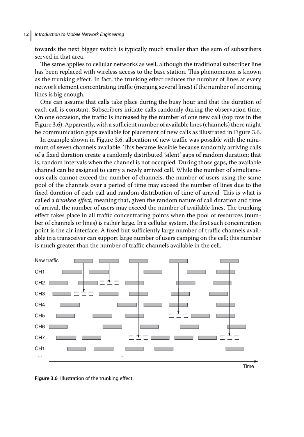
be communication gaps available for placement of new calls as illustrated in Figure 3.6.
In example shown in Figure 3.6, allocation of new traffic was possible with the minimum of seven channels available. This became feasible because randomly arriving calls
of a fixed duration create a randomly distributed ‘silent’ gaps of random duration; that
is, random intervals when the channel is not occupied. During those gaps, the available
channel can be assigned to carry a newly arrived call. While the number of simultaneous calls cannot exceed the number of channels, the number of users using the same
pool of the channels over a period of time may exceed the number of lines due to the
fixed duration of each call and random distribution of time of arrival. This is what is
called a trunked effect, meaning that, given the random nature of call duration and time
of arrival, the number of users may exceed the number of available lines. The trunking
effect takes place in all traffic concentrating points when the pool of resources (number of channels or lines) is rather large. In a cellular system, the first such concentration
point is the air interface. A fixed but sufficiently large number of traffic channels available in a transceiver can support large number of users camping on the cell; this number
is much greater than the number of traffic channels available in the cell.
New traffic
CH1
CH2
CH3
CH4
CH5
CH6
CH7
CH1
...
...
Time
Figure 3.6 Illustration of the trunking effect.
Cellular System
3.8 Erlang Formulas
The trunking effect need to be estimated quantitatively in order to calculate the number of resources (channels, lines) to meet traffic demand from users of a communications system. The estimate of channel resources depends on many statistical factors
related to traffic, such as call duration, time distributions of call arrivals and other statistical parameters. The unit of traffic is the Erlang (named after Agner Krarup Erlang
(1878–1929) who invented it).
One Erlang equals the maximum traffic available on one line. The traffic is calculated
using a simple formula:
(calls per hour) × (average conversation time)
(3.7)
3600 Seconds
It means that one call of a duration of 3600 seconds (i.e. 1 hour) produces 1 Erlang of
traffic. Erlang derived two formulas for different systems:
x Erlangs =
• If all resources are used, additional calls are lost (Erlang B case). This is the case for
voice calls in mobile cellular systems.
• If calls are put into a queue for certain time and will be served sequentially as resources
become free again, the traffic capacity is described by Erlang C formulas. This is applicable to many trunked radio systems.
3.9 Erlang B Formula
The Erlang B formula determines the probability that a call is blocked. This probability
defines a measure for the Grade of Service (GOS) for a trunked system that provides no
queuing for blocked calls (i.e. blocked calls are instantly lost). The Erlang B formula uses
the following assumptions:
• Call requests are memoryless. That is, all users, including blocked users, may request
a channel at any time all free channels are fully available for calls until all channels are
occupied.
• Probability of channel holding (i.e. usage) times is exponentially distributed. That is,
longer calls are less likely to happen than short calls.
• A finite number of channels available in the resources pool time between channel
requests follow a Poisson distribution (inter-arrival times).
• Inter-arrival times of call requests are independent of each other.
• The number of busy channels is equal to the number of busy users.
Offered traffic (in Erlangs) A is related to the call arrival rate, 𝜆, and the average
call-holding time, h, by
A = 𝜆h
(3.8)
Let us define 𝜆 as a call arrival rate, h, mean holding time (duration of the call), then
𝜆hT is a mean operating time of a single user during period T, also called the time of
13
14
Introduction to Mobile Network Engineering
blocking situation
Line 1
Line 2
Line 3
Line 4
Line 5
Line 6
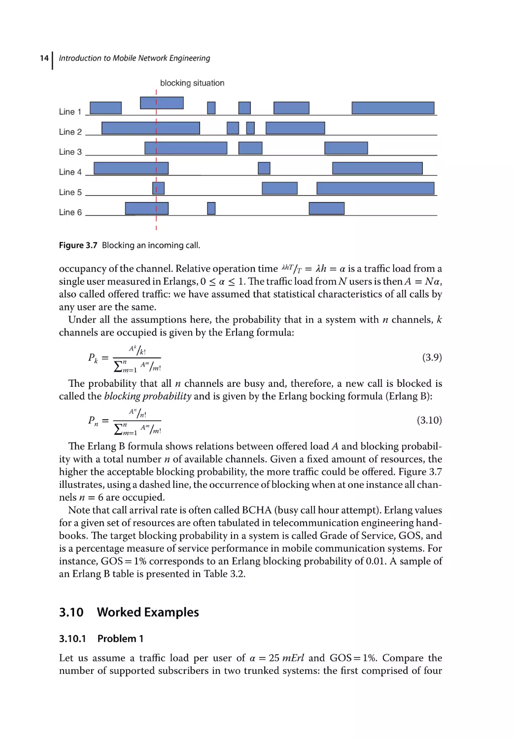
Figure 3.7 Blocking an incoming call.
occupancy of the channel. Relative operation time 𝜆hT∕T = 𝜆h = 𝛼 is a traffic load from a
single user measured in Erlangs, 0 ≤ 𝛼 ≤ 1. The traffic load from N users is then A = N𝛼,
also called offered traffic: we have assumed that statistical characteristics of all calls by
any user are the same.
Under all the assumptions here, the probability that in a system with n channels, k
channels are occupied is given by the Erlang formula:
Pk = ∑n
Ak∕k!
m=1
Am∕m!
(3.9)
The probability that all n channels are busy and, therefore, a new call is blocked is
called the blocking probability and is given by the Erlang bocking formula (Erlang B):
Pn = ∑n
An∕n!
m=1
Am∕m!
(3.10)
The Erlang B formula shows relations between offered load A and blocking probability with a total number n of available channels. Given a fixed amount of resources, the
higher the acceptable blocking probability, the more traffic could be offered. Figure 3.7
illustrates, using a dashed line, the occurrence of blocking when at one instance all channels n = 6 are occupied.
Note that call arrival rate is often called BCHA (busy call hour attempt). Erlang values
for a given set of resources are often tabulated in telecommunication engineering handbooks. The target blocking probability in a system is called Grade of Service, GOS, and
is a percentage measure of service performance in mobile communication systems. For
instance, GOS = 1% corresponds to an Erlang blocking probability of 0.01. A sample of
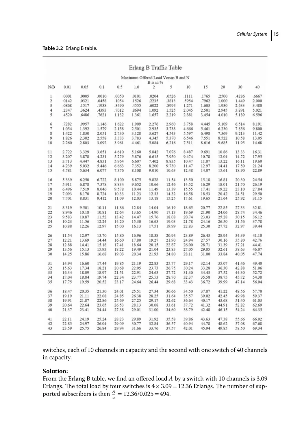
an Erlang B table is presented in Table 3.2.
3.10 Worked Examples
3.10.1
Problem 1
Let us assume a traffic load per user of 𝛼 = 25 mErl and GOS = 1%. Compare the
number of supported subscribers in two trunked systems: the first comprised of four
Cellular System
Table 3.2 Erlang B table.
switches, each of 10 channels in capacity and the second with one switch of 40 channels
in capacity.
Solution:
From the Erlang B table, we find an offered load A by a switch with 10 channels is 3.09
Erlangs. The total load by four switches is 4 × 3.09 = 12.36 Erlangs. The number of supported subscribers is then A𝛼 = 12.36/0.025 = 494.
15
16
Introduction to Mobile Network Engineering
A second system with 40 channels offers a load of 24.44 Erlangs. The number of
supported subscribers is 977. As observed, the trunking efficiency is significantly
increased with an increase in channel pool size.
3.10.2
Problem 2
Consider a cellular system with a cluster size of k = 7 with a total of 395 channels. The
call-holding time is 3 minutes, a user makes one call per hour and the blocking probability is 1%. Blocked calls are cleared, Erlang B distribution applies.
Determine:
1) The average number of calls/hour in the case of an omnidirectional site antenna.
2) The average number of calls/hour in the case of a three-sector site configuration
antenna. Calculate the decrease in trunking efficiency compared with an omni configuration.
3) The average number of calls/hour in the case of a six-sector site antenna configuration. Calculate the decrease in trunking efficiency compared with an omni configuration.
Solution:
Number of channel/cell N = total number channels/cells per cluster. For an omni site
N = 395/7 = 57
Call-holding time H = 3 min/60 min = 0.05 hour.
1) Omni configuration.
Offered traffic load for a 0.01 blocking probability (1% GOS) is A = 44.2 Erlangs for
57 channels available.
Number of calls A/H = 44.2/0.005 = 884 calls/hour
2) three-sector configuration.
Number of channels per sector N = 57/3 = 19. Offered traffic load for a 0.01 blocking
probability (1% GOS) is A = 11.2 Erlang per sector.
Number of calls A/H = 11.2/0.005 = 224 calls/hour per sector.
Number of calls per site 3 × 224 = 672 call/hour.
Decrease in trunking efficiency is (884 – 672)/884 = 24%
3) six-sector configuration.
Number of channels per sector N = 57/6 = 9.5 channel. Offered traffic load for a 0.01
blocking probability (1% GOS) is A = 4.1 Erlangs per sector.
Number of calls A/H = 4.1/0.005 = 82 calls/hour per sector.
Number of calls per site 6 × 82 = 492 call/hour.
Decrease in trunking efficiency is (884 – 492)/884 = 44%
It should be noted that there is a trade-off between reduction in co-channel interference versus loss of trunking efficiency and an increase of number of handovers
between sectors.
3.10.3
Problem 3
A cellular operator is interested in providing GSM coverage at 900 MHz in a new
entertainment centre. The marketing plan has targeted approximately 1 000 000 visitors
Cellular System
attending shows every year, of which it is believed that around 90% are typical mobile
phone users with an average traffic load 𝛼 = 25 mErl.
The following assumptions apply for the centre:
1) Busy-hour traffic takes about 30% of the total daily traffic.
2) The traffic in the entertainment centre is distributed as follows:
40% is carried in the major exhibition pavilion, 50% in the foyer and 10% in the
car park.
3) Each user makes an average of three phone calls of 2 min of duration during the busy
hour.
4) Three cells are required for this system: one in the exhibition pavilion, one in the
foyer and the other one in the car park.
5) Limit considerations to one of the mobile operators with a market penetration in the
centre of 20%.
Determine the required number of channels per cell with a GOS = 2%.
Solution:
The busy-hour number of mobile phone users needs to be calculated. If 1 000 000 passengers per year use the airport, then the average number of users per day is 1 000
000/365 = 2740.
As 90% of the passengers use a mobile phone, the cellular operator with 20% of market
penetration carries
2740 × 0.9 × 0.2 = 494 mobile phone users∕day
This number represents only the number of mobile phone users per day for this cellular operator. As capacity needs to be dimensioned on a per busy-hour basis:
Maximum number of user per hour N = 494 users∕day × 0.3 ∼ 149 users∕busy hour
Assume that the operator has installed its own infrastructure in the entertainment centre. A case where the infrastructure is shared between operators is not
considered here.
We need to distribute the estimated number of users between three cells. As the foyer
takes 50% of the traffic, the pavilion 40% and the car park 10%, we have:
In the foyer Nfoyer = 50% × N = 75 user∕hour
in the pavilion Npavilion = 40% × N = 59 user∕hour and
in the car park, Ncarpark = 10% × N = 15 user∕hour.
Given this number of users per cell, and the traffic per user, we can compute the total
traffic per cell:
Afoyer = 75 users × 30 mE∕user = 2.25 Erl
Apavilion = 59 users × 30 mE∕user = 1.77 Erl
Acar park = 15 users × 30 mE∕user = 0.45 Erl
Given a 2% blocking probability, an estimate of the required number of channels per
can be obtained from the Erlang B table.
Cfoyer = ∼ 6 channels
Cpavilion = ∼ 5 channels
Ccarpark = ∼ 3 channels
17
19
4
Radio Propagation
The electromagnetic field radiated by an antenna propagates through the radio channels
between transmitter Tx and receiver Rx. The mechanism of radio propagation can generally be described as reflection, diffraction and scattering.
Propagation models are traditionally focused on prediction of the average received
signal strength used to define the coverage area in a mobile cellular environment. The
statistics of the random component in the signal are used in RF planning and system
deployment to evaluate the uncertainties in prediction and define a necessary margin
to counteract signal fading. In addition, some statistical properties of the radio channel,
such as fading parameters, multipath and associated intersymbol interference heavily
impact the system design and various system parameters.
4.1 Propagation Mechanisms
4.1.1
Free-Space Propagation
The simplest possible scenario is that both transmit and receive antenna are placed in a
free space. Energy conservation dictates that the integral of the power density S over any
closed surface surrounding the transmit antenna must be equal to the transmitted power
Pt . If the closed surface is a sphere of radius R, centred at the transmitter (Tx) antenna
and if the Tx antenna radiates isotropically then the power density on the surface is
Pt
(4.1)
4𝜋R2
Assume that receiver (Rx) antenna has an ‘effective area’ or aperture A, then the
received power is given by
S=
Pt
(4.2)
4𝜋R2
If the transmit antenna is not isotropic, then the energy density has to be multiplied
with a transmit antenna gain Gt in the direction of the receive antenna. The relationships
between the aperture A and gain G is introduced by equation (4.3)
Pr = S • A = A •
G=
4𝜋A∕𝜆2
Introduction to Mobile Network Engineering: GSM, 3G-WCDMA, LTE and the Road to 5G,
First Edition. Alexander Kukushkin.
© 2018 John Wiley & Sons Ltd. Published 2018 by John Wiley & Sons Ltd.
(4.3)
20
Introduction to Mobile Network Engineering
and the equation for receive power Pr with a directive transmit antenna is given by
1
(4.4)
4𝜋R2
The product of transmit power and gain in the considered direction is also known as
Effective Isotropic Radiated Power (EIRP).
Pr = Ar Pt Gt •
(4.5)
EIRP = Pt Gt
The effective antenna area is proportional to the power that can be extracted from the
antenna radiators with a given energy density. For example, for a parabolic antenna, the
effective antenna area is roughly the geometrical area of the surface. However, antennas
with a very small (in terms of wavelength) geometrical area – for example dipole antennas – can also have a considerable effective area. Isotropic antenna can be represented
by a short dipole with a gain G = 1, so the effective aperture for isotropic antenna Ai is
given by
Ai = 𝜆2∕4𝜋
(4.6)
Substitution of these formulas leads to the ‘Friis law’ or equation for a relation between
received and transmitted power in a free space:
Pr = Gr Pt Gt •
𝜆2
(4𝜋)2 R2
(4.7)
The free-space equation is valid in a ‘far-field’ region, for example, at the distance R
from transmitter not less than a Fraunhofer distance (also called Rayleigh distance):
df =
2D2a∕𝜆
(4.8)
where Da is the largest dimension of the antenna. The far field requires that R ≫ Da and
R ≫ 𝜆.
It is important to note that the free-space propagation mechanism has to be independent of wavelength or frequency. This is due to the fact that the radiated energy is
not lost, but rather redistributed over a sphere surface of area 4𝜋R2 , as observed from
equations (4.1) and (4.2). On the other hand, Friis’ law seems to indicate that the ‘attenuation’ in free space increases with frequency. This seeming contradiction is caused by
the definition of antenna gain via effective aperture (4.3) and the following presumption
that antenna gain G is independent of frequency.
In the case of transmit and receive isotropic antennas, the free-space equation takes
the form
)
(
𝜆 2
(4.9)
Pr = Pt •
4𝜋R
Equation (4.9) can be re-written introducing a path loss L, which is measure of attenuation factor caused by propagation mechanism and propagation media in general case.
Pr = Pr∕L
The free-space path loss factor is
( )2
4𝜋
R2
L=
𝜆
(4.10)
(4.11)
Radio Propagation
This is a well-known free-space equation for an isotropic antenna. When written in a
logarithmic scale, it takes the form
L0 = 33.44 + 20 log f (MHz) + 20 log R(km), dB
(4.12)
As follows from (4.12), the received power in a free space falls by 6 dB when the range
is doubled; in other words, the path loss increases by 20 dB per decade. Similarly, path
loss increases by 6 dB if the frequency is doubled.
In a general case, radio propagation path loss formulas are based on the free-space
loss formula with additional empirical correction factors. The generic formula for path
loss takes the form
L = L0 (r) + 𝛼 log(R − r)
(4.13)
where L0 is a loss at reference distance (can be 1 m or 1 km) and the second term states
that the losses are exponential with distance. This is illustrated in Figure 4.1, where the
second term of equation (4.13) determines a ‘clutter loss factor’; that is, the slope of exponent in different environment related to land-usage. The slop is defined in dB/decade,
and nominal values of slop are 20–25 dB/dec for free-space–open area loss, 30 dB/dec
in a suburban area and 40 dB/dec in an urban area, respectively.
The radio signal attenuation depends on the environment the signal passes through. A
rise in signal strength can be observed despite of increasing distance, when the receiver
re-enters an open area after passing through a small urban cluster causing a higher
attenuation exponent, see Figure 4.2. Since the received signal strength depends on the
close environment of the receiver, there is no abrupt rise in signal strength but a gradual
increase as the mobile enters an open area.
The total propagation path can be divided conditionally into long-distance and local
propagation. Because the mobile terminal’s antenna is often much lower than the height
of surrounding objects, the direct line of sight to the horizon is obscured. Typically,
the received signal will comprise a number of reflected waves; that is, there is distinct
multipath propagation. The base-station antenna is often in a more open location, but
reflections or shadow effects from nearby buildings and the terrain configuration can
sometimes affect the propagation conditions.
Tube
fluid
in
Shell
fluid
out
Shell
fluid
in
Tubes
Baffle
Inlet
header
Tube
fluid
out
Tube sheet
Drain
Figure 4.1 Path loss examples with different clutter loss factors.
21
22
Introduction to Mobile Network Engineering
Open space
Signal level,
dB
Suburbian
Urban
20 dB/decade
32 dB/decade
20 dB
41 dB/decade
10 dB
20 dB
Distance, km
Figure 4.2 Path loss in a mixed environment.
Multipath propagation gives rise to a fine structure of signal fluctuations, which results
in corresponding variations (fast fading) in the input signal to the mobile unit. Averaging
with respect to the fast fading structure gives the local mean of the propagation path loss
or received signal strength.
In a typical propagation situation there are considerable shadow effects. The propagation loss with respect to the local mean is generally much greater than when there
is free-space propagation, owing to the strong influence of the terrain. This influence
manifests itself partly as an increase in the average (‘global’) propagation loss and partly
as a varying loss due to the irregularity of the terrain. The large-scale effects can be estimated from data on the terrain and built up areas. The result of the calculation is the
global mean. However, the detailed structure causes random variations in the local mean
of the signal received by the mobile unit (called shadow fading, slow fading or lognormal
fading).
Following this discussion, it is useful to divide propagation loss into three components:
the global mean of the propagation loss, that is the deterministic part, and two random
elements resulting from shadow fading (slow fading) and multipath propagation (fast
fading), see Figure 4.3. The global mean of the received signal power is typically inversely
proportional to the fourth power of the propagation distance P ∼ R−n (n = 4), where n
is the propagation exponent.
4.1.2
Propagation Models for Path Loss (Global Mean) Prediction
The ‘global mean’ component together with the ‘shadowing’ (long term fading) component of the signal are used for RF coverage prediction in mobile cellular systems.
Revising the path loss definition in the previous section, consider a general case of a
propagation mechanism with losses in an antenna system, see Figure 4.4.
Radio Propagation
Slow log-normal
fading
tens of
wavelength
Pathloss
average level
global mean
Fast Rayleigh fading
average level
λ
Distance
2
Figure 4.3 Three components in path loss.
Tx
EIRP
(Pmin)
Antenna/feeder
gain & loss, Lf
Antenna/feeder
gain & loss, Lf
Pt
Pr
Rx
Signal level
EIRP
Path loss
Distance
Figure 4.4 Basic components of link budget.
Introducing losses in the antenna-feeder system for transmitter and receiver, Lft and
Lfr , respectively, the output power at antenna connector Pt , one may obtain a more general equation for EIRP that includes feeder losses:
EIRP = Pt + Gt − Lft , dBm
(4.14)
in dB notation.
The received power Pr at the receiver input takes propagation path loss L into account
and is given by
Pr = Pt + Gt − Lft − L + Gr − Lfr , dBm
(4.15)
23
24
Introduction to Mobile Network Engineering
Similar to transmitter EIRP, one can define a ‘design level’ of minimal received power
at the receiving antenna input, Pmin . Then the relation between acceptable path loss and
design level is as follows:
L = MAPL = EIRP − Pmin
(4.16)
The main goal of propagation modelling is to predict path loss L as accurately as
possible, allowing the range of radio system to be determined before installation. The
maximum rage of the system occurs when the received power drops below Pmin , a level
that provides acceptable communication quality. The value of L for which this power
level is received is the maximum acceptable path loss, MAPL.
A general model for propagation loss is very often semi-empirical and intended to
provide a general estimate of radio propagation based on nominal characteristics rather
than specific path data. During the radio planning process, any generic model is calibrated based on specific land-usage data and measurements.
The tuning of propagation model involves determination different coefficient values
in the propagation equation so that the residual RMS value of the error reaches the
global minimum; that is, the lowest possible value. General semi-empirical propagation
equation is as follows:
Pr = Pt + Gt + Gr − L = Pt + Gt + Gr + CCT + Cd log(R) + Cdh log(R) log(hB )
+ Ch log(hB ) + Cdk Kdk + Cdr Kdr + CCl KCl
(4.17)
where:
Pr = received power, dBm
Pt = transmit power, dBm
CCT = the fixed correction term that accounts for effects of frequency and other
non-specific factors of the model
R = the distance from transmitter, km;
hB = the base-station antenna height, m;
Kdk = a knife-edge diffraction loss;
Kdr = a rounded-hill diffraction loss and
KCl = the clutter loss.
Table 4.1 Pre-set values for correction
coefficients in semi-empirical equation for
propagation loss.
Parameter
Initial Value
Cd
−44.9
C dh
6.55
Ch
0
C dk
−0.5
C Cl
1
Radio Propagation
The parameters CCT and KCl combine to give a power level at the distance of 1 m. The
initial value is normally zero and is then tuned to ensure it provides an overall RMS error
of about 6–7 dB for the entire data set for each base station and the whole clutter.
The parameters in (4.17) are defined in Table 4.1.
Apparently, the optimal set of parameters and coefficients in equation (4.17) produce
a global minimum of prediction errors only for specified clutter or land-usage type. The
method based on the tuning of the equation (4.17) model involves dividing the prediction area into a series of clutter and terrain categories; namely, open, suburban and
urban. These are summarized as follows:
• Open area: Open space, no tall trees or buildings in the path, a plot of land cleared
for 300–400 m ahead; for example, farmland, open fields.
• Suburban area: Village or highway scattered with trees and houses, some obstacles
near the mobile but not very congested.
• Urban area: Built up city or large town with large buildings and houses with two or
more storeys, or larger villages with close houses and tall, thick tree cover.
25
27
5
Mobile Radio Channel
For wireless communications, the transmission medium is the radio channel between
transmitter Tx and receiver Rx. The signal can get from the Tx to the Rx via a number
of different propagation paths. In some cases, a Line-Of-Sight (LOS) connection might
exist between Tx and Rx. In a typical mobile environment LOS is absent and the signal
can get from the Tx to the Rx by means of being reflected at or diffracted by different
objects in the environment: houses, mountains (in some hilly areas), windows, walls
and so on, as shown in Figure 5.1. The number of these possible propagation paths is
normally very large. Each of the paths has a distinct amplitude, delay (runtime of the
signal), direction of departure from the Tx and direction of arrival; most importantly,
the components have different phase shifts with respect to each other.
The envelope of the received signal is composed by many signal replicas arriving via
different paths with different amplitudes and phases, respectively. When the phase
shift between each pair of signal components is equal to 180∘ , these components tend
to cancel each other out producing a case of destructive interference, and vice versa,
when signal replicas arrive in-phase they tend to add up to each other; that is, a case
of constructive interference. Due to the random nature of amplitude and phase of the
multipath component, the subsequent composition produces random variations in a
received signal envelope. These variations are called ‘fading’.
The term mobile radio ‘channel’ refers to impact from propagation media on characteristics of the received signal; that is, it can be thought of as a filter acting on the
transmitted signal. The radio channel then can be modelled with the transfer function of
the filter that describes the channel in the time or, alternatively, in the frequency domain.
The common approach is to distinguish two types of radio channel; a narrowband
or ‘flat fading’ channel versus a wideband or frequency selective channel. In the
narrowband channel, multipath fading comes about as a result of relatively small
path differences between signals coming from scatterers in the near vicinity of the
mobile. The term ‘small’ relates to equivalent symbol length in the space domain. These
differences and individual phase shifts contributed to by the scatterers, in the order of
a few wavelengths, lead to significant phase differences in received components of the
signal arriving via a different path.
By contrast, if strong scatterers exist well off of the direct or shortest path between the
base and mobile, the time differences may be significant. If the relative delays are large
compared to the basic unit of information transmitted on the channel (usually a symbol
Introduction to Mobile Network Engineering: GSM, 3G-WCDMA, LTE and the Road to 5G,
First Edition. Alexander Kukushkin.
© 2018 John Wiley & Sons Ltd. Published 2018 by John Wiley & Sons Ltd.
28
Introduction to Mobile Network Engineering
Figure 5.1 Multipath propagation.
Rx
Tx
or a bit), the signal will then experience significant distortion, which varies across the
channel bandwidth. The channel is then a wideband channel and system design needs
to take into account these effects.
Some of the basic characteristics of the channel can be seen in a simplified two-ray
channel model. Consider the superposition of rays A eif1 t1 and A eif2 t2 arriving at different
frequencies f1 , f2 and different times t1 , t2 , respectively. Introduce new variables: delay
𝜏 = t1 − t2 , mean arrival time t = t1 +t2∕2, frequency offset Δf = f1 − f2 and centre carrier
frequency f0 = f1 +f2 ∕2. The sum of two components is then given by
)
( 𝜏 Δ𝜔t
)
(
𝜏
Δ𝜔𝜏
Δ𝜔t
Δ𝜔𝜏
𝜏 Δ𝜔t
(5.1)
2ei𝜔0 t+i 4 ei𝜔0 2 +i 2 + e−i𝜔0 2 −i 2 = 2ei𝜔0 t+i 4 cos 𝜔0 +
2
2
where 𝜔0 = 2𝜋f0 , Δ𝜔 = 2𝜋Δf .
Considering only frequency shift, we may assume 𝜏 = 0. Then the two-ray model is
truncated to
)
(
Δ𝜔t
(5.2)
s(t) = 2ei𝜔0 t cos
2
Equation (5.2) represents the so-called ‘beating’ diagram for superposition of two
oscillations with different frequencies, see Figure 5.2. The correlation interval 𝜏c can be
estimated as a time interval between maximum and minimum of signal envelope, or half
of the beating period T = 1∕Δf .
5.1 Channel Characterization
Statistical characteristics of the radio channel in general and the wideband channel
in particular are commonly described at the level of second-order statistics; that is,
correlation function or power spectrum density. The comprehensive analysis of the
channel models and related statistics is not part of this overview and can be found
in numerous books on that topic. Various statistics characteristics are used in system
design depending on technology and applications. Nonetheless, there are several basic
Mobile Radio Channel
1
2τc ≈ Δf
2
1
Re{s(t)}
0
–1
–2
0
0.5
1
1.5
2
2.5
time
3
3.5
4
4.5
5
Figure 5.2 Beating diagram in a two-ray channel model.
statistical characteristics and parameters that are commonly used in design for all
communication systems:
•
•
•
•
•
Probability density function of fading → mean, variance of fading
Doppler spectrum → maximum Doppler shift
Power delay profile → delay spread
Correlation function → correlation length in space and time domain
Frequency response of the channel → coherence bandwidth
One of the main characteristics of the wideband channel is a power delay profile (PDP)
of the channel defined as the variation of mean power in the channel with delay. The
PDP is commonly presented by a discrete time model in the delay dimension to yield
individual taps of power, as shown in Figure 5.3.
The most important parameter of the power delay profile is the delay spread or RMS
delay spread. The delay spread Δ𝜏 is a square root of the difference between the mean
of delay squared and the square of the mean delay.
√
√ n
√
1 √
2
√∑ P 𝜏 2 − 𝜏 2
2
(5.3)
Δ𝜏 = 𝜏 − 𝜏 =
0
PT m=1 m m
where
∑n
𝜏0 = ∑i=1
n
Pi 𝜏i
i=1
Pi
(5.4)
is a mean delay; that is, the delay corresponding to the ‘centre of gravity’ of the power
delay profile.
The delay spread Δ𝜏 is independent of the mean delay and hence of the actual path
length, being defined only by the relative path delays. The value of RMS delay is weighted
with relative powers of the taps as well as their delays, making it a better indicator of
system performance than the other parameters.
29
30
Introduction to Mobile Network Engineering
Power, P
P1
P2
P3
Pn
τ1
τ0
τ2
τ3
∙∙∙
τn
τ
Δτ
Figure 5.3 Power delay profile.
Another important parameter for characterization of the random frequency selective
mobile channel is a frequency response of the channel; that is, a Fourier Transform
of the impulse response. The fundamental conclusion of channel characterization is
that the delay spread Δ𝜏 and coherence bandwidth Δfc are related via an ‘uncertainty
relationship’:
Δfc ≅ 1∕Δ𝜏
(5.5)
The coherence bandwidth is a quantitative estimate of frequency shift when variation
in signal strength at frequencies f and f + Δfc became uncorrelated. This leads to classification of the channels to frequency selective or frequency flat. Introducing the signal
bandwidth Δf , we can define the frequency selective (in other words, time dispersive)
channel by the inequality:
Δf ∕Δf
c
≫1
(5.6)
In the opposite case where the coherence bandwidth is much larger than signal bandwidth, the frequency content of the signal is not distorted by the channel and the channel
fading is said to be frequency flat.
In case of a flat fading channel, when Δf∕Δfc ≪ 1, the signal symbol duration Ts is
greater than delay spread:
Ts = 1∕Δf ≫ Δ𝜏
(5.7)
As a consequence, different paths of the scattered/reflected signal cannot be resolved
and this results in flat Rayleigh fading of the signal components. In the case of a frequency selective channel, the symbol duration is much smaller than delay spread,
Ts ≪ Δ𝜏 ′
(5.8)
This means that multiple replicas of the signal experience uncorrelated fading, which
ensures that multiple paths could potentially be resolved.
Mobile Radio Channel
a3
Figure 5.4 Phasor diagram in the narrowband
channel.
ϑ3
a2
ϑ2
∙∙∙
an
ϑn
ϑ1
a1
5.1.1
y
Narrowband Flat Channel
The signal received at the mobile, y, will be composed of a sum of waves from all
scatterers, whose phase and amplitude depend on the reflection coefficient am ej𝜃m
and scattering characteristics of the scatterer, and whose time delay is 𝜏m , m = 1,2, …
Thus:
y = a1 ej(𝜃1 +𝜔𝜏1 ) + a2 ej(𝜃2 +𝜔𝜏2 ) + …
(5.9)
Each of the components in this expression constitutes an ‘echo’ of the transmitted
signal.
In the narrowband channel, differential delays of arriving waves are small compared to
the symbol duration. The delays of the arriving waves could be considered approximately
equal, so the amplitude does not depend upon the carrier frequency:
y = ej𝜔𝜏 (a1 ej𝜃1 + a2 ej𝜃2 + …)
(5.10)
All frequencies in the received signal are therefore affected in the same way by the
channel, and the channel can be represented by a single multiplicative component. The
resulting signal vector, the term in parenthesis in equation (5.10), is composed by a vector addition of the multipath components, as shown in Figure 5.4. In every instant, the
partial waves take different (complex) random values for each am ej𝜃m , thereby composing
the resulting random vector.
Such variations of received signal in narrowband channel are described by Rayleigh
or Rician statistics and normally referred to as a ‘flat fading’. The term ‘flat’ means here
that a channel transfer function does not depend on frequency; that is, is flat. In that
channel, the received signal became uncorrelated in receiving points separated at ∼ 𝜆∕2
in distance, where 𝜆 is a signal wavelength.
The more precise determination of ‘relatively small’ differential delays of scattered
components is provided in the next sections.
5.1.2
Wideband Frequency Selective Channel
In an opposite case of a wideband or frequency selective channel, the major impact from
the channel is a signal dispersion in time. In other words, the impulse response of the
channel is not a single delta pulse but rather a sequence of pulses (corresponding to
different multipath components), each of which has a distinct arrival time in addition to
having a different amplitude and phase. This is illustrated in Figure 5.5 with transmitted
31
32
Introduction to Mobile Network Engineering
Power
delay
profile
P1
P2
P3
Pn
τ1
τ2
τ3
∙∙∙
τn
τ
First path
1
1 1
0
τ1
0
0 0
τ
Second
path
τ
τ2
Third path
τ3
τ
Received signal
Figure 5.5 Inter-symbol interference in the wideband channel.
symbols presented in a simplified bipolar modulation format. As observed, the symbol
duration in much less than delay spread; that is, Ts ≪ Δ𝜏.
This signal dispersion leads to Inter-Symbol Interference (ISI) at the receiver, as
illustrated in Figure 5.5.
One may obtain a simple estimate of the reduction in energy of the received signal caused by inter-symbol interference of multipath signals with delay spread ∼ Δ𝜏.
Consider a BPSK modulated bit stream of ‘zeros’ and ‘ones’ and assume that the received
signal is composed by two rays with a relative delay 𝜏, as shown in Figure 5.6. As can be
seen from Figure 5.6, at the time intervals shown as dashed areas each of the signal components have the opposite sign being phase shifted BPSK symbols; that is, the phase of
delayed component at interval 𝜏 is opposite to a phase of signal at the consecutive interval Ts − Δ𝜏. As a result, the energy of the received symbol will be reduced at a value
of proportional to 2𝜏, see Figure 5.6. We may estimate the average value of delay in
Mobile Radio Channel
2
1.5
1
0.5
0
S(t)
–0.5
–1
–1.5
–2
0
Bit
stream
0.5
1
1.5
time
2
0
3
0
Ts
Δτ
2.5
time
1
Δτ
2
1.5
1
0.5
S(t)
0
–0.5
–1
–1.5
–2
time
0
0.5
1
1.5
2
2.5
3
Figure 5.6 Inter-symbol interference.
respective multipath components as 𝜏 ≈ Δ𝜏∕2. The energy per symbol in multipath component can then be estimated as Pm •(Ts − Δ𝜏), where Pm is a total power of multipath
component. The energy per symbol to noise density ratio is given by
(
)
Pm •Ts 1 − Δ𝜏∕Ts
)
Pm •(Ts − Δ𝜏)
E (
=
= s 1 − Δ𝜏∕Ts
(5.11)
N0
N0
N0
33
Introduction to Mobile Network Engineering
1
0.1
0.01
BER
34
0.001
0
1.10–5
0
10
20
30
40
50
SNR, dB
Figure 5.7 Average total BER versus SNR for different values of delay spread in Rayleigh channel: the
solid line corresponds to a delay spread of 0.1-bit duration, +s to 0.05 and ⋄ s to 0.01, respectively;
horizontal lines (dashes) correspond to irreducible BER values.
Therefore, the losses in Es∕N0 due to the inter-symbol interference are proportional
(
)
to a factor 1∕ 1− Δ𝜏∕Ts . When delay spread is of same order as symbol duration, correct
demodulation of the signal could be possible only with additional signal processing
allowing to mitigate the effect of ISI.
The error rate performance of a digital system in a wideband channel tends to level
off at high signal-to-noise ratios in contrast to the flat or narrowband fading case where
error rates decrease without limit (Figure 5.7). This arises because the ISI, rather than the
random AWGN noise, is the dominant source of errors. As the signal level is increased,
the ISI increases proportionately, so demodulation performance stays the same. The
final value of the error rate is known as an error floor, or sometimes the irreducible
error rate, although the ‘irreducible’ is a misnomer only meaning no dependence on
signal-to-noise ratio; in fact, the error floor can be removed using equalization and other
techniques.
5.1.3
Doppler Shift
The movement of the receiver or transmitter leads to a shift of the received frequency
called the Doppler shift, the phenomena well-known from physics. Consider a simple
case of a single sinusoidal wave reaching the receiver Rx. If Rx moves away from the
transmitter Tx with a speed v, then the distance d between Tx and Rx increases with
that speed. Thus:
]
)
(
[
v
− k0 d0 ,
(5.12)
E(t) = E0 cos(2𝜋fc t − k0 [d0 + vt]) = E0 cos 2𝜋t fc −
𝜆
where d0 is the distance at time t = 0. The frequency of the received oscillation is thus
decreased by v/𝜆; in other words, the Doppler shift is given by:
v
v
𝜈 = − = −fc ,
(5.13)
𝜆
c
where c is the speed of light.
Mobile Radio Channel
Figure 5.8 Projection of velocity vector |v| onto the
direction of propagation k.
→
v
→
k
γ
→
v cos γ
Rx
The Doppler shift is negative when Tx and Rx move away from each other. Since the
speed of the movement is always small compared with the speed of light, Doppler shifts
are relatively small. When the direction of Rx movement is not aligned with the direction
of wave propagation, the Doppler shift is determined by the cosine rule or speed of
movement in the direction of wave propagation, v cos(𝛾) (see Figure 5.8). The Doppler
shift is then
v
𝜈 = − cos 𝛾 = −𝜈max cos 𝛾
(5.14)
𝜆
In a mobile communications environment, the typical values of Doppler shift are in a
range of less than 1 KHz.
If all multipath waves were Doppler shifted by the same amount – the effect on radio
link performance would really be negligible – the local oscillator in the RX could easily
compensate for such a shift. The important point is, however, that the different multipath
components arrive with different Doppler shifts. Each pair of multipath components can
be represented by a two-ray model described by equation (5.12). The superposition of
several Doppler-shifted waves creates a sequence of fading dips. Doppler frequency is
thus an important parameter of the channel, even though it is so small. Furthermore,
the superposition of many slightly Doppler-shifted signals leads to phase shifts of the
total received signal that can impair the reception of angle-modulated signals. These
phase shifts lead to frequency dispersion, random Frequency Modulation (FM) of the
received signal, which is especially important for signals with low bit rates where the
channel delay spread is not the main source of distortion.
The sensitivity to the random frequency modulation depends on the modulation
order. The QPSK modulation can tolerate up to vmax Ts ≤ 0.05 whereas 64-QAM
requires vmax Ts ≤ 0.01, where Ts is a symbol duration and vmax is the estimate of
maximum speed of relative movement Rx, Tx and/or scatterers.
It is important to note that the main propagation characteristics that should be taken
into account when designing an OFDM system are expected delay spread, maximum
Doppler frequency and, in the case of cellular systems, the targeted cell size.
Composition of the number of multipath components with different Doppler shifts
results in a Doppler power spectrum of the received signal. The Doppler spectrum has
two important interpretations:
35
36
Introduction to Mobile Network Engineering
1) It describes frequency dispersion. For narrowband systems, as well as Orthogonal
Frequency Division Multiplexing (OFDM), such frequency dispersion can lead to
transmission errors. It has, however, no direct impact on most other wideband systems (like single-carrier Time-Division Multiple-Access (TDMA) or Code Division
Multiple-Access (CDMA) systems).
2) It is a measure for the temporal variability of the channel. As such, it is important for
all systems. Assume that Doppler power spectrum has a bandwidth of Δf ∼ 𝜈max =
fc vmax∕c and introduce a ‘stationary’ interval of the channel; that is, the time interval
when the channel can be regarded as constant. The duration of stationary interval
can be estimated as 𝜏c = 1∕2Δf . This parameter is important for designing the size of
equalizer window.
5.2 Worked Examples
5.2.1
Problem 1
Evaluate the maximum Doppler shifts in these cases:
1) a communication link with an airplane cruising at a speed of 850 km/h and carrier
frequency 900
MHz, and
2) communications at 2 GHz carrier with a user terminal in a high-speed train moving
at 250 km/h.
Solution:
The maximum Doppler shift is given by 𝜈max = fc v∕c. Substituting the input values,
we have
1. 𝜈max = 700 Hz and 2. 𝜈max = 480 Hz.
5.2.2
Problem 2
What is the minimum symbol rate to avoid mitigation of the effects of Doppler spread
in a mobile system operating at 450 MHz with a maximum speed of 100 km/h? Assume
that the ‘stationary’ interval is given by the formula 𝜏c = 1∕2𝜈max , where 𝜈max is a maximum
Doppler shift.
Solution:
The maximum Doppler shift 𝜈max = 42 Hz. The stationary time interval for the channel
is then 𝜏c ≈ 1∕2𝜈max ≈ 11 ms. This is the maximum symbol duration, so the minimum
symbol rate for undistorted symbols is the reciprocal of this, 84 symbols per second.
The symbol rate is so small that most systems will rarely encounter significant effects in
this form.
5.3 Fading
Random fluctuations in received signal can be estimated using statistical or random
distributions. There are two major contributors to randomness of the received signal:
Mobile Radio Channel
1) The level of a received wanted radio signal or an interfering signal can only in
part be predicted deterministically. As discussed in Section 4.1, a global mean is
commonly associated with the deterministic component of the received signal. The
two additional components, namely ‘shadowing’ and ‘fast fading’, are both random
but have different scales of variations. In this section, we consider the second and
third component of radio propagation loss: slow fading or shadowing and fast fading
components.
2) Input noise in the receiving system. The noise largely consists of radiated input noise
in the antenna and internal noise in the receiver. It is totally stochastic or random.
5.3.1
Shadowing/Slow Fading
Referring to Figure 4.3, we may associate shadowing or slow fading with a second component of received signal strength. As discussed in Section 4.3, this component has a
spatial scale of variations in order of several tens wavelengths. The shadowing component is especially important in radio coverage prediction where we need to ensure that
a signal strength received at certain location, normally at the edge of the projected radio
cell, will exceed certain threshold level. The statistical characteristics of shadowing can
be described in terms of probability density function.
Consider the generic probability distribution plot in Figure 5.9. In this particular plot,
the distribution is normalized at specific value of global mean (see Figure 4.3), say this
value is the lowest median operating signal level that a radio receiver can operate with
to achieve a given degree of performance.
With level of performance corresponding to a global mean, we do not take into
account random variations in received signal. The signal would be acceptable for 50%
of samples and not acceptable for the remainder. This is a level of performance that
does not meet service requirements. We determine the limit of acceptable performance
as being some value higher than the minimum operating level; that is, creating some
margin of performance for acceptable signal level. This would have the effect of setting
Median value, 50% exceeded
90% exceeded
99% exceeded
–Y dB
(B)
–X dB
(A)
Median
(0 dB)
Received field strength, dB
Figure 5.9 Probability density function of signal variations normalized at the global mean.
37
38
Introduction to Mobile Network Engineering
the minimum median operating level to some point on the left-hand side of the curve,
such as point (A) or (B), see Figure 5.9.
As a simple illustration, if the value X is 10 dB, then shifting the reference value by
10 dB would change the percentage of signals above the reference value from 50 to 90%.
If the median value was −90 dBm for example, and if we set a limit of −80 dB, then we
can be sure that 90% of the signals experienced would be above −90 dBm, even taking
account of the variability of the signal.
When shadowing is included, path loss L is composed of deterministic (L50 ) and
random (Ls ) components
L = L50 + Ls
(5.15)
at 50% of locations at a given distance, as predicted by any standard path loss model (the
median path loss or global mean).
The Ls is the shadowing component that follows a lognormal statistical distribution of
signal power; that is, the signal measured in decibels has a normal distribution (i.e. is a
zero-mean Gaussian random variable with standard deviation dB). The variation in Ls
occurs over distances comparable to the widths of buildings and hills in the region of
the mobile, usually tens or hundreds of metres.
Application of a lognormal distribution for shadowing models can be seen as follows.
If contributions to the signal attenuation along the propagation path are considered to
act independently, then the total attenuation A, as a power ratio due to N individual
contributions A1,…, AN will be simply the product of the contributions:
A = A1 × A2 × A3 · · · AN
(5.16)
If this is expressed in decibels, the result is the sum of the individual losses in
decibels:
Ls = L1 + L2 + L3 + · · · + LN .
(5.17)
All of the contributions in (5.17) are taken as random variables, then, with N >> 1,
the central limit theorem holds and L behaves as a Gaussian random variable. Hence, A
must be lognormal.
Probability density function of Ls is given by the standard Gaussian formula
]
[
L2s
1
(5.18)
exp − 2 ,
p(Ls ) = √
2𝜎L
2 𝜋𝜎L
where 𝜎L is a standard deviation of received power in dB. Figure 5.10 represents typical
path loss measured along the distance from the base station. The solid curve represents
the global mean or signal strength incorporating slow fading/shadowing; that is, the Ls
component.
In Figure 5.10, the cell range would be around 8 km if the effect of shadowing were
neglected, then only 50% of locations at the edge of the cell would be properly covered.
By adding the fade margin, the cell radius is reduced to around 5.3 km, but the reliability is greatly increased as a much smaller proportion of points exceed the maximum
acceptable path loss. In other words, this margin is defined to maintain coverage with a
certain location probability.
Mobile Radio Channel
Received power
level, dBm
–70
–80
–90
–100
–110
Fade margin
RX sensitivity
level
–120
Cell range
2
3
4
5
6
7
8
Distance, km
Figure 5.10 Effect of slow fading/shadowing on estimation of the cell range.
Another widely accepted name for location probability is accessibility. The common
definition for location probability of X% is that the path loss is less than maximum
acceptable value in X% of locations at the cell edge. Based on statistic properties of
lognormal fading the location probability Pr(Ls > z) with a given margin z can be calculated using the standard error function
( )
z
(5.19)
Pr(Ls > z) = Q
𝜎L
and
)
(
( 2)
∞
1
x
1
t
Q(t) = √
exp −
dx = erfc √
2
2
2𝜋 ∫x=t
2
(5.20)
The plot of standard error function Q(t) is provided in Figure 5.11. It can be used
to evaluate the shadowing margin z needed for any location probability with substitute
z = t •𝜎L . The lognormal (LNF) margin values versus cell edge probability are presented
in Table 5.1.
Illustration of the lognormal fading model is given in Figure 5.12. The drop-outs in
signal strength, also called outage A, are considered to occur when the local mean falls
below a critical level, see Figure 5.12. The accessibility is then defined as 1 − A = Pr(Ls >
z); that is, location probability.
39
40
Introduction to Mobile Network Engineering
Argument of Q function
0.0 0.3 0.6 0.8 1.1 1.4 1.7 2.0 2.3 2.5 2.8 3.1 3.4 3.7 4.0
1.00E+00
1.00E–01
1.00E–02
1.00E–03
1.00E–04
1.00E–05
1.00E–06
1.00E–07
1.00E–08
Figure 5.11 The Q function.
Table 5.1 Tabularized LNF margin in a function of
location probability at cell border.
Location probability
at the cell border, %
Lognormal fade
margin, dB
50
𝜎×0
60
𝜎 × 0.25
70
𝜎 × 0.52
80
𝜎 × 0.84
90
𝜎 × 1.28
91
𝜎 × 1.34
92
𝜎 × 1.4
93
𝜎 × 1.48
94
𝜎 × 1.55
95
𝜎 × 1.64
96
𝜎 × 1.75
97
𝜎 × 1.89
98
𝜎 × 2.05
99
𝜎 × 2.33
5.3.2
Fast Fading/Rayleigh Fading
While mean path loss and shadowing could be predicted for RF coverage in particular
locations, there are still significant variations in the received signal as the mobile moves
over distances that are small compared with the shadowing correlation distance. This
phenomenon is fast fading, presented by a third component in the received signal in
Figure 4.3. The fast random variations in the signal are caused by multipath propagation
in the neighbourhood of mobile unit. A typical situation corresponds to the obscured
Mobile Radio Channel
Signal strength s, dB
outage probability =
s∗
1
⎛ (x – s)2⎞
dx
∫ exp –
2
⎝
2πσs –∞
2σs ⎠
mean level,
s = L50
Fading margin, z = (s–s∗), dB
Sensitivity threshold, s∗
Figure 5.12 Illustration of fading margin and accessibility.
Local mean
Global mean = average local mean
Relative
signal
strength, dB
10
0
–10
2
4
6
8
10
12
14 16
Distance in wavelengths
Figure 5.13 Rayleigh fading.
line of sight (LOS) between mobile unit and base station. A Raleigh fading is commonly assumed to describe statistics of the signal fluctuations. A typical recording of
field-strength variations as a mobile unit is moving along a street is shown in Figure 5.13.
The distance between adjacent fading dips is approximately one wavelength. During fading dips the instantaneous signal level drops 10–15 dB below the average level (local
mean, i.e. the value after averaging over slow fading). Therefore, a fading margin between
the local mean and the sensitivity threshold of the receiver is required to ensure that
drop-outs caused by the input signal falling below the threshold will occur rarely.
The location probability in the case where the Rayleigh fading is taken into account
results in additional margin. Whether or not this margin is to be taken into account in
link budget calculation depends on the system design and specific situation that will be
considered later.
41
42
Introduction to Mobile Network Engineering
5.4 Diversity to Mitigate Multipath Fading
When there is fading caused by multipath propagation, a considerable fading margin is
needed to prevent signal drop-outs or outages during the deepest fading dips. Diversity
can be used to bridge over the fading dips, reducing the necessary fading margin and
thus producing a diversity gain. In a diversity arrangement, the signals from two or more
propagation paths whose fading is only partially correlated (completely uncorrelated in
ideal case) are combined. Several different types of diversity can be used in digital radio
transmission, such as spatial diversity, frequency diversity and polarization diversity.
The underlying principle of diversity reception is based on statistical independence
of variations in received electromagnetic field in antennas (diversity branches) that are
separated either in distance or polarization. Combing the uncorrelated signals from
diversity branches results in statistical (diversity) gain since fading dip in one branch
not necessarily lead to fading deep in another branch and, instead, may coincide with a
peak in signal in the other branch.
The frequency diversity implies transmission on two (or many) frequencies separated
in the frequency domain at intervals exceeding coherence bandwidth of the propagation
channel. Such a frequency offset ensures that signal fluctuations at two frequencies are
uncorrelated in a common receiving point. A typical example is frequency hopping used
in the GSM system that will be discussed in Section 7.3.5.4.
The time diversity principle in its primitive form implies that same sequence of bits
is repeated over time intervals approximately equal to the correlation time interval of
fading. The intended goal is to ensure uncorrelated variations in the received signal bit
stream. In an advanced form, time diversity is employed by interleaving a coded data
block into several time frames separated over the correlation time interval of fading. In
the worst-case scenario, the only part of coded data might be lost in a fading dip allowing
recovery of data by means of channel coding. In practice, this approach results in reduction of errors making them statistically independent and thus significantly improving
performance of error-correction coding.
5.4.1
Space and Polarization Diversity
The original form of diversity is antenna or space diversity, which can be used in both
analogue and digital transmission. Other types of antenna diversity are polarization
diversity and antenna pattern diversity.
Consider the geometry of scattering shown in Figure 5.14 with two antennas located
in point 1 and 2. Assume that the scattering angle, that is the size of angular sector of
direction of waves arriving in antennas 1 and 2, equals to 𝜗. Then the path difference Δ
of the waves arriving at either point 1 and 2 is given by Δ = d sin ( 𝜗∕2). When Δ = 𝜆∕2,
the signals in points 1 and 2 arrive in opposite phase. The value of Δ = 𝜆∕2 can serve as
an estimate of the space correlation scale. Therefore, the antenna spacing d for space
diversity has to be equal to the space correlation scale, that is
d=
𝜆
2 sin ( 𝜗∕2)
(5.21)
Consider the downlink transmission from base station to mobile terminal. In the
neighbourhood of the mobile, station scattering has an isotropic nature meaning that
Mobile Radio Channel
Figure 5.14 Geometry of scattering.
d sin( ϑ 2 )
2
ϑ
d
ϑ
2
1
waves arrive within an angular sector of ± 180∘ ; note that the angles from 180 to 360∘
create the same path difference with the opposite sign. Therefore, the spatial correlation
scale equals half a wavelength 𝜆∕2 that corresponds to a Rayleigh fading case.
In the opposite case of waves arriving at the base-station antenna from an individual
mobile station, arriving waves are concentrated in a narrow angular sector thus exemplifying a plane wave. The scattering volume is concentrated in the vicinity of the mobile
station. It forms a remote scattering volume of limited size that can be regarded as being
located in a far-zone relative to a base-station antenna.
This is a simplified view at the uplink wave from mobile unit reaching the base-station
antenna. The uplink scattering angle is highly dependent on the mobile environment
and is difficult to predict. From a practical point-of-view, antenna separation of several
wavelengths is needed for fairly independent fading in a base-station site.
In practice, polarization diversity is used instead. The mechanism of polarization
diversity is based on the observed fact that polarization of a radiated wave becomes
random due to multiple scattering in the multipath channel. For example, ideally
vertical polarized radiation at the source produces both vertical and horizontal components in the receiver antenna as the received electromagnetic field is formed by a
superposition of randomly polarized waves carried by multipath components. Combing
the uncorrelated signals from diversity branches results in statistical (diversity) gain
since fading dip in one branch does not necessarily lead to fading deep in another
branch and, instead, may coincide with a peak in signal in the other branch.
Diversity gain with Rayleigh fading depends on the diversity arrangement, how many
diversity branches are combined and the level of correlation between them. Most of
the potential diversity gain is achieved with two antennas. In a commercial mobile system, most common diversity implementation in a base-station antenna is based on two
cross-polar antennas. There are several types of diversity combining that could be distinguished in pre-detection and post-detection diversity. In post-detection diversity,
the signals from diversity branches are added coherently; that is, their mutual phases
must be adjusted continuously. Such a mechanism enables the signal voltages to be
added together thus producing a maximum diversity gain of 6 dB when two signals
of equal strength are combined. In pre-detector diversity, there is a choice of maximum ratio and equal-gain combination. The optimum arrangement in theory is the
maximum ratio, whereby the signal-to-noise ratio for the different diversity branches
is measured and the gain of the branches is set to maximize the signal-to-noise ratio
43
44
Introduction to Mobile Network Engineering
after addition. This means that greater weight is given to the diversity branch with the
best signal-to-noise ratio. In an equal-gain combination, there is no setting of branch
amplification. Equal-gain combination is the most widely used pre-detector arrangement with a maximum achievable gain of about 3 dB. Some vendor specific proprietary
improvements may increase the gain up to 5 dB.
5.5 Worked Examples
5.5.1
Problem 1
Consider transmission of information bits with a duration of Tb = 1 ms over a multipath
fading channel with an average fading rate of Rf = 1∕(8•Tb ). Assume the channel encoder
can only use a repetition of symbol frame as a means of mitigation against fading. Introduce a structure of mapping coded words into a channel symbol stream. Estimate the
channel rate sufficient to deploy a repetition scheme.
Solution:
The average fade duration or interval between fading dips is Tf =
1
Rf
= 8•Tinf bit . The
correlation scale of fading in time domain can be estimated as 𝜏c = Tf ∕2 = 4•Tinf bit , see
Figure 5.15. The channel encoder should repeat the code word in a time interval of the
order 𝜏c . This way the fades over time 𝜏c are uncorrelated and at least one of two replicas
of the code word could likely be received with sufficient signal strength. Given that channel encoder should be adjusted to the incoming information bit stream, the repeated
code word size should be 8•Tinf bit and channel rate should be twice of the rate of the
information bit rate, as shown in Figure 5.15.
5.5.2
Problem 2
The measured delay spread of multipath channel is Δ𝜏 = 5 μs. Assume that frequency
hopping system transmit next coded frame at the frequency is f = fc + m•Δfh , shifted at
Information bit stream
1
2
3
4
5
6
7
8
9
10
Tinf bit
τc
Channel bit stream
1 2 3 4 5 6 7 8 1 2 3 4 5 6 7 8 9 . . .
Tchannel bit
Figure 5.15 Channel coding with repetition.
11
12
13
14
15
Mobile Radio Channel
m•Δfh according to a frequency hopping pattern. What is the minimum values of Δfh
given that delay spread of the communications channel is Δ𝜏 = 5 μs?
Solution:
The objective of frequency hopping system is to deploy a frequency diversity scheme;
that is, make fading at consecutive coded frames uncorrelated. The minimum frequency
hop value should then be no less than the coherence frequency bandwidth of the channel
Δfc = 1∕Δ𝜏 . Therefore, Δfh = Δfc = 200 kHz.
5.5.3
Problem 3
Consider a mobile communication system operating at 1800 MHz in an urban environment. Consider the following:
1) assuming a vehicular speed of 60 km/h, estimate a value of time correlation of the
fades;
2) estimate value of the channel stationary interval impacted by vehicular movement.
Solution:
(
)
1) the space correlation interval is given by l = 𝜆∕2 sin 𝜗s∕2 , where 𝜗s is an angular size
of scattering sector. Assuming a typical mobile neighbourhood with absence of line
of sight, we have the case for isotropic scattering, 𝜗s = 180∘ . The space correlation
interval is l = 𝜆∕2, time correlation interval is tc = l∕v= 𝜆∕2v = 5 ms.
2) the maximum Doppler shift is Δf = v∕𝜆. The stationary interval is 𝜏c = 1∕ 2Δf = 𝜆∕2v =
5 ms, that is, equal to correlation time interval of Rayleigh fading.
5.6 Receiver Noise Factor (Noise Figure)
The impact of noise on the system needs to be calculated to determine the system performance. The major noise contributions in mobile wireless systems usually come from
the receiver itself. In any case, the total noise associated with the system can be calculated by assuming that the system consists of a two-port network, with a single input
and a single output as shown in Figure 5.16. The network is characterized by a gain G,
being the ratio of the signal power at the output to the signal power at its input, and
by a noise factor F. The noise factor is the ratio between the output noise power of the
element divided by gain G (i.e. referred to the input) and the input noise.
The noise in the input of the receiver may consist of several components, such as
man-made industrial noise, spurious emission of electrical and electronic devices and
thermal noise. Thermal noise is non-avoidable, it is always present. Thermal noise
imposes the fundamental limit on radio communications; that is, thermal noise floor.
Figure 5.16 Noisy two-port network.
Gain, G
Noise Factor, F
45
46
Introduction to Mobile Network Engineering
The power spectral density of thermal noise is given by
(5.22)
N0 = kB T
where kB is Boltzmann’s constant, kB = 1.38•10−23 J∕K = 1.38•10−23 W •Hz−1 •K −1 , T is an
environmental temperature of the noise source in Kelvin, and the noise power (noise
floor) is
(5.23)
N = N0 B
where B is a receiver bandwidth (in units of Hz). It is common to write equation (5.23)
using logarithmic units (power P expressed in units of dBm is 10 log10 (P∕1mW )).
Assuming room temperature, the noise spectral power density has the value:
N0 = −174 dBm
(5.24)
This means that the noise power contained in a 1-Hz bandwidth is −174 dBm. The
noise power contained in bandwidth B is
N = −174 + 10 log10 B , dB
(5.25)
Noise power density N0 can also be normalized to MHz bandwidth and then approximated to 114 dBm/MHz as an easier figure to work with. Any physically realizable
system introduces additional noise on the top of the thermal noise floor. That additional
noise component defines the noise figure F of network element of receiver system. The
noise figure is defined as ratio of SNR at the input to SNR at the output of the receiver
F=
Sin∕N
in
Sout∕N
out
=
Sin∕k T •B
B
G•Sin∕N
out
=
Nout∕G
kB T •B
(5.26)
We assume that the network in Figure 5.16 is impedance matched to resistance. The
noise figure is then
F=
Nout
Nout
=
Nin
kB T •B
(5.27)
where Nout is the output noise power of the network element referred to input; that
is, the actual noise output power divided by G. Noise figure F depends on the design
and physical construction of the network. Its value in decibels is the noise figure of the
network,
FdB = 10 log10 F
(5.28)
The numerical value of the noise power [dBW] can be expressed approximately as
Nout = FdB − 204 + 10 log10 B
(5.29)
and, respectively, in dBm:
Nout = FdB − 174 + 10 log10 B.
(5.30)
The value of noise power given by equations (5.29) or (5.30) is known as a receiver noise
floor, please note that it differs from thermal noise floor at noise figure FdB . For successful
recovery of the received data the signal level must exceed the noise floor with sufficient
margin, at least, for non-CDMA systems. This margin is given by the signal-to-noise
ratio required for decoding/demodulation of the received data stream with performance
Mobile Radio Channel
G1, F1
G2, F2
Gk, Fk
GN, FN
Figure 5.17 Cascade network.
levels specified in terms of Bit-Error Rate (BER) or other parameters such as SINAD,
MOS and so on.
The receiver sensitivity level is determined by addition of required SNR on the top of
receiver noise floor:
Rxsens = receiver noise floor + SNR = Nout + SNR
(5.31)
Receiver sensitivity level varies according to modulation scheme and desired level
of performance, often quoted in terms of bit-error-rate (BER). If this value is, say,
9 dB above noise (or noise and distortion), then the minimum receiver sensitivity for a
270-kHz system with a 8 dB noise figure would be:
−114 − 5.68 + 8 + 9 = −102.68 dBm
In general, a complete system can be characterized by a cascade of two-port elements,
where the ith element has gain Gk and noise factor Fk (Figure 5.17). Each element could
consist of an individual module within a receiver, such as an amplifier or filter, or one of
the elements within the channel such as the antenna, feeder or some source of external
noise.
The gain G of the complete network is then simply given by
G = G1 •G2 · · · GN ,
(5.32)
while the overall noise factor is given by the Friis formula:
F = F1 +
FN − 1
F2 − 1 F3 − 1
+
+···+
G1
G1 •G2
G 1 • G 2 · · · GN
(5.33)
where noise figures and gains in (5.33) are in absolute units, not in dB. As observed
from (5.33), the noise from the first element adds directly to the noise of the complete
network, while subsequent contributions are divided by the gains of the earlier elements.
It is therefore important that the first element in the series has a low noise factor and a
high gain, since this will dominate the noise in the whole system. As a result, receiver
systems often have a separate low noise amplifier (LNA) placed close to the antenna,
often at the top of the mast and sometimes directly attached to the feed of a dish antenna
in order to overcome the impact of feeder loss.
47
49
6
Radio Network Planning
In terms of the geographic coverage of the network, often the limit of coverage will be
determined by one of the following factors:
• Coverage or noise limited, in which the environmental noise and the minimum signal
level needed to provide the desired level of availability will be the limiting factors.
• Interference limited, in which the presence of other radio systems will increase the
level of signal that will be required to achieve the necessary level of performance.
In some cases, the network configuration can be driven by capacity limitations that
impact the cell size and cluster size in systems with frequency reuse. The example of an
interference limited system is a 3G-WCDMA system where the interference is a major
factor affecting both capacity and cell size. The GSM system exemplifies a mixed case
when both noise and co-channel interference can limit a cell range depending on service
(voice or data) and respective performance criteria.
One difference between interference and noise lies in the fact that interference suffers
from fading, while the noise power is typically constant (averaged over a short time
interval). The statistical nature of interfering signal as well as of the wanted signal is taken
into account by adding effective fade margin and, possibly, additional correction factors
into link budget. The effective fading margin can be estimated by calculating location
probability at the cell edge in the presence of multiple interfering servers. This approach
uses joint multivariate statistics of lognormal fading of the signals from multiple servers
(co-channel interferers).
When planning needs to be more detailed, a Monte-Carlo simulation of interference
in multi-server environment could be used as an advanced planning tool.
6.1 Generic Link Budget
A link budget is to be compiled before start of the dimensioning of the radio network.
In the link budget, different design criteria for coverage (e.g. outdoor, indoor, in-car) are
determined. In the link budget, factors such as receiver sensitivity and different margins
are considered. It should be noted that all the values for margins discussed are estimates only.
The specific margins and gains in link budget calculation may or may not be included
depending on system technology under consideration and details of implementation.
The goal of link budget compilation is to estimate a cell range for both uplink and
Introduction to Mobile Network Engineering: GSM, 3G-WCDMA, LTE and the Road to 5G,
First Edition. Alexander Kukushkin.
© 2018 John Wiley & Sons Ltd. Published 2018 by John Wiley & Sons Ltd.
50
Introduction to Mobile Network Engineering
downlink. As an example, we next consider the link budget for downlink in GSM
system; that is, from base station to mobile.
6.1.1
Receiver Sensitivity Level
Sensitivity level of the mobile station’s receiver MSsens varies with its class and
manufacturer and is given in specs provided by the manufacturer. The receiver sensitivity depends on the required signal carrier to noise ratio (SNR). This level is defined
for a specified BER in a Gaussian noise background, in a so-called static channel. When
frequencies are reused, the received carrier power must be large enough to combat
both noise and interference, that means C/(N+I) must exceed the receiver threshold.
Recalling that required CIR (Carrier-to-Interference Ratio) is defined at the edge in
the frequency reuse system, the additional CIR margin can just add up on the top of
the receiver noise floor plus SNR or can replace SNR in the case of CIR dominance.
To account for the dynamic propagation channel, some margins have to be added to
compensate for Rayleigh fading, interference and body loss. The obtained signal strength
Preq is a least but not last estimate for required power in the receiver to process a phone
call. Preq is rather independent of the environment since Rayleigh fading is supposed to
be present in any real mobile environment.
Preq = MSsens + MR + MI + Mb ,
(6.1)
where
MSsens = Mobile Station sensitivity level, dBm;
MR = Rayleigh fading margin, dB;
MI = Interference margin, dB;
Mb = Body loss, dB that normally taken into account RF coverage in pedestrian
environments only.
In some cases, the mobile station sensitivity level MSsens is defined in a dynamic channel taking Rayleigh fading into account, opposite to the MSsens level in a static channel.
In this case, the MR margin should be omitted in calculations of required signal level.
6.1.2
Design Level
Extra margins have to be added to Preq to handle lognormal fading as well as different types of penetration losses. These margins depend on the environment and on the
desired area of coverage. The resultant signal strength is used when planning the system
and will be referred to as the design level, Pdesign . That signal strength is the value that
should be obtained on the cell border. The design level can be calculated from
Pdesign = Preq + MLNF + MBPL + Mcar
where
MLNF – lognormal fading margin,
Mcar – car penetration loss,
MBPL – building penetration loss.
(6.2)
Radio Network Planning
6.1.2.1
Rayleigh Fading Margin
The required sensitivity performance of the system in terms of Frame-Error Rate or
BER is normally specified for each type of system channel. The sensitivity is defined
as the level where the required quality performance is achieved. Sometimes receiver
sensitivity level MSsens provided in specifications has Rayleigh fading already taken into
account. The practical value of Rayleigh fading margin is MR = 3 dB.
6.1.2.2
Lognormal Fading Margin
The values of the lognormal fading margin were given in Table 5.1. Typical values of
the standard deviation depending on clutter type for lognormal fading are given in
Table 6.1.
6.1.2.3
Body Loss
The human body has several effects on MS performance compared to a free-standing
mobile phone; for instance, the head absorbs energy and antenna efficiency of some MSs
can be reduced. Other effects may be a change of the lobe direction and the polarization.
These effects can be neglected in the link budget since:
1) no mobile antenna gain is used and
2) X-polarized antennas are standard equipment today.
In this case the polarization loss is included in the downlink link budget and in the
uplink, both polarizations can be received. The body loss Mb recommended by ETSI is
3 dB for 1800 MHz, 5 dB for 900 MHz.
6.1.2.4
Car Penetration Loss
When the MS is situated in a car without an external antenna, an extra margin has to be
added in order to cope with the penetration loss of the car. This extra margin is approximately Mcar = 6 dB.
6.1.2.5
Design Level
Given the values of the margins listed previously, design level for outdoor coverage in
the GSM-1800 system can be calculated as follows:
Pdesign = MSsens + MLNF + Mcar = −105 dBm + 10 dB + 5 dB = −90 dBm
Table 6.1 Standard deviation of lognormal
distribution in different environments.
Environment
Standard deviation,
𝝈, dB
Dense urban
10
Urban
8
Suburban
6
Rural
6
51
52
Introduction to Mobile Network Engineering
6.1.2.6
Building Penetration Loss
It is known from measurements that building penetration loss to floors higher up in a
building generally decreases. This effect is known as height gain. This is actually an effect
of the building penetration loss definition and not of the building structure.
Building penetration loss is defined as the difference between the average signal
strength immediately outside the building and the average signal strength over the
ground floor of the building. The building penetration loss for different buildings is
lognormally distributed with a standard deviation: 𝜎 BPL .
Variations of the loss over the ground floor could be described by a stochastic variable,
which is lognormally distributed with a zero-mean value and a standard deviation of
𝜎 floor . In this calculation, 𝜎 BPL and 𝜎 floor are lumped together by adding the two as if they
were standard deviations in two independent lognormally distributed processes.
The resulting standard deviation, 𝜎 indoor , could be calculated as the square root of the
sum of the squares:
√
2
2
+ 𝜎floor
(6.3)
𝜎indoor = 𝜎BPL
6.1.2.7
Outdoor-to-Indoor Design Level
The indoor design level when the base station is situated outdoors is calculated according to
Pdesign = Preq + MLNF + MBPL
(6.4)
where MBPL = BPLmean + 𝜎indoor can be seen as the indoor margin. BPLmean is the mean
value of the building penetration loss. Some values of BPLmean and 𝜎indoor are given in
Table 6.2.
In the case of indoor base station location, the coverage is calculated based on
signal-to-noise criteria rather than CIR criteria since interference from the other cell is
efficiently blocked by the walls of the building. The major factor is a lack of coverage.
6.1.3
Power Link Budget
The next step is to calculate all gains and losses associated with an antenna system on
the downlink and uplink. The definitions are as follows:
• Downlink (DL) is the direction from the BS to the MS. The downlink budget estimates
the received signal strength in the MS.
• Uplink (UL) is the direction from the MS to the BS. The uplink budget estimates the
power level received in the base station.
Table 6.2 Typical values of building
penetration loss.
BPLmean
𝝈indoor
Dense urban
18
9
Urban
18
9
Suburban
12
8
Radio Network Planning
The path balance implies that the coverage of the downlink is equal to the coverage of the uplink. The power budget calculated for both uplink and downlink shows
whether the uplink or the downlink is the weak link. When the downlink is stronger, the
EIRP/ERP used in the prediction should be based on the balanced BTS output power.
When the uplink is stronger, the maximum BTS output power is used instead.
In the calculations that follow, the antenna gain in the MS and the MS feeder loss are
both zero and therefore omitted. It is also assumed that the antenna gain and the feeder
loss are the same for the transmitter and receiver side of the BTS.
The following abbreviations are used:
PRx,MS = Received power in MS, dBm
MSsens = Receiver sensitivity level in MS, dBm
BSsens = Base-station receiver sensitivity level, dBm
PTx,MS = MS transmit power, dBm
PTx,BS = BS transmit power, dBm;
Lcomb = BS combiner loss, dB;
Ldip = external diplexer loss, dB that should only be taken into account if an
external duplexer is used.
Lfeed = feeder loss, dB;
Gant,BS = antenna gain in BS, dBi;
Gant,MS = antenna gain in MS, dBi;
Gdiv = diversity gain, dB.
The losses in the antenna-feeder system depend on the base-station site configuration. Figure 6.1 shows base-station antenna system configuration for a dual band
GSM900/1800 system when installation of the 1800 MHz has been done with diplexers
utilizing the existing feeder system. As shown, the base station has a dual band dual
polarization two-port antenna. Figure 6.2 shows a configuration with a four-port
dual band antenna and separate feeder sets for 900 and 1800 MHz base stations. The
1800 MHz configuration commonly uses the Masthead amplifier with a low noise
figure to compensate for uplink feeder loss. In the case of a four-port dual band antenna
or two separate single band antennas (not considered here) and single set of shared
feeders, one needs another set of diplexers at the top after feeder before the antenna
itself.
6.1.4
Power Balance
Consider the configuration shown in Figure 6.1 and assume Gant,MS = 0 dBi. Applying
relevant gains and losses either to the downlink or uplink we obtain:
Pin,MS = PTx,BS − Ldip − Lfeed + Gant,BS − L − MLNF , downlink
(6.5)
PRx,BS = PTx,MS + Gant,BS + Gdiv − Ldip − Lfeed − L − MLNF , uplink
(6.6)
53
54
Introduction to Mobile Network Engineering
Dual band, dual (slant)
polarization antenna
Gant, BS
Jumpers
Feeder
Lfeed
–
Ldip
PTxBS , PRxBS
Diplexers, dual band
900/1800
Main
Diversity path
Gdiv
GSM 900 MHz
GSM 1800 MHz
Figure 6.1 Base-station antenna system with a two-port dual band cross-polarization antenna and
diplexer for combining 900 and 1800 MHz RF paths.
We have assumed a pedestrian environment and lognormal fading is taken into
account. In order to ensure a good reception of the uplink signal, received signal level
should exceed sensitivity threshold, PRx,BS ≥ BSsens . It is important to note that the path
loss is reciprocal; that is, path loss for downlink is the same as for uplink. The maximum
allowed path loss (MAPL) can be calculated from the power budget. For the downlink,
we obtain the following equation:
MAPLDL = EIRPBS − Pdesign, MS , for downlink
(6.7)
From (6.5) we have
MAPLDL = L(downlink) = PTx,BS + Gant,BS − Ldip − Lfeed − MLNF − MSsens
(6.8)
To achieve power balance, it is necessary to make sure that the required minimum
signal level by the MS (downlink) is reached at the same point as the required minimum
by the Base Transceiver Station (BTS) (uplink).
Radio Network Planning
Dual band, dual (slant)
polarization antenna
Mast Head Amplifier (Tower
Mounted Amplifier)
GLNA
–
GSM 900 MHz
GSM 1800 MHz
Figure 6.2 Base-station antenna system with a four-port dual band cross-polarization antenna and
MHA for 1800 MHz.
That means that MAPLDL = MAPLUL = MAPL, where MAPLUL can be obtained from
(6.6):
MAPLUL = L(uplink) = PTx,MS + Gant,BS + Gdiv − Ldip − Lfeed − MLNF − BSsens .
(6.9)
In some configurations, the uplink becomes weaker than the downlink and power
budget is unbalanced. The unbalanced budget will lead to situation when signal at
weaker path cannot be decoded. When uplink is weaker, the mobile station can receive
base-station signal on downlink, but the base cannot ‘hear’ the mobile. A common
approach is then to use a Tower Mounted Amplifier (TMA), another term to describe
the same is MHA (Mast Head Amplifier), which is a low noise amplifier (LNA) that is
mounted close to the receiving antenna, see Figure 6.2. The TMA improves the uplink
sensitivity and extended coverage can be achieved.
In the following calculations, we consider power balance without TMA, otherwise the
TMA gain (GLNA ) should be added in the uplink power budget. The balanced budget can
be used to adjust the maximum transmit power of the base station, PTx,BS . Assuming
MAPLDL = MAPLUL , we have
PTx,BS = PTx,MS + Gdiv − BSsens + MSsens
(6.10)
55
56
Introduction to Mobile Network Engineering
Apparently, in case of a weaker uplink path we should take MAPL = MAPLUL as
allowable path loss.
Given allowable path loss we can estimate a cell range using a suitable propagation
model, as described in Section 6.4 or in the literature where numerous models have
been developed for a path loss prediction, such as Okumura–Hata, COST-231,
Ikegami–Walsh model and so on.
6.2 Worked Examples
6.2.1
Problem 1
A 900 MHz mobile system is designed with a location probability of 95% at the cell edge
with a shadowing variance of 6 dB. The propagation environment is assumed to be modelled by the Okumura–Hata propagation model for medium size cities. The mean path
losses are given by the equation
L50 = 43.6 + 33.9 • log10 f − 13.82log10 hBS − a(hMS) + (44.9 − 6.55log10 hBS )log10 d
(6.11)
where
a(hMS) = hMS (1.1 • log10 f − 0.7) − 1.56 • log10 f + 0.8
(6.12)
The units are as follows:
Frequency f in MHz, heights hMS , hBS − in m, distance d in km, hMS = 1.5 m and hBS =
30 m.
The maximum allowable path loss, MAPL, is estimated as 146 dB. Determine the
range of the cell with given accessibility. How will an increase in shadowing variance
of 2 dB affect the estimated cell range?
Solution:
The maximum allowable path loss is given by the sum of the global mean and shadowing
component; that is
L = L50 + Ls => MAPL = L50 + MLNF
(6.13)
The global mean L50 is described by the Okumura–Hata model, while the second term
in equation (6.13) is a lognormal (shadowing) margin MLNF defined by the required
level of accessibility. To find margin MLNF for Ls , we may consider error function Q(t)
or Table 5.1. With a given location probability 95% and variance 6 dB we find MLNF =
𝜎 • 1.64 = 9.84 dB from Table 5.1.
Therefore, the global mean component L50 in MAPL is
L50 = MAPL − MLNF = 146–9.84 = 136.16 dB
(6.14)
The cell range rcell can be found applying the Okumura–Hata model to the global mean
component of the MAPL:
43.6 + 33.9 • log10 f − 13.82log10 hBS − a(hMS) + (44.9 − 6.55log10 hBS )log10 rcell
= 136.16
Given the values for the heights and frequency, we obtain the cell range rcell = 2.45 km.
Radio Network Planning
With a change of fading variance to 8 dB, the fading margin required for 95% location
probability rises to 13 dB and cell range to 2 km.
6.2.2
Problem 2
Analyse hypothetical communications with an aircraft using a cellular system on the
ground. Establish a link budget assuming that the plane is flying at 10 km altitude over
an area where the mobile communication service has been provided by a cellular system
designed with a cell radius of 20 km. Assume the following:
• cell radius has been calculated for propagation exponent n = 4,
• 10 dB penetration loss through the aircraft hull and
• −10 dB antenna gain of the BS antenna in the direction of the aircraft.
Solution:
Recall the formula for the path loss L = L0 − 𝛼 log R, where 𝛼 is a propagation exponent
and L0 = 33.44 + 20 log f (MHz) + 20 log R(km). The component L0 describes the path
loss in a free space at distances R < R0 , where R0 is a break point or assured distance at
which the line of sight between the mobile and base station is observed. For simplicity,
assume R0 = 0.1 km, and fix the value of L0 at the break point R0 , that is
L0 = 33.4 + 20log10 f + 20log10 R0
From a definition of cell range, maximum allowable path loss,
MAPL = L0 + 𝛼log10 (Rcell ) = EIRP − Pdesign
The effective radiated power in direction of airplane is reduced according to antenna
pattern
EIRPair = EIRP − 10 dB
L0 has the same value, design level Pdesign should be increased to cope with penetration
loss through aircraft hull, that is
Pdesign
air
= Pdesign + 5 dB
The maximum allowable path loss in ground-to-air communication is then
MAPLair = EIRPair − Pdesign
air
= EIRP − 10 − Pdesign − 10 = MAPL − 20 dB
On the other hand, the maximum path loss in direction of aircraft in zenith is
Lair = L0 + 20log10 (Rair )
The difference between MAPLair and Lair should ensure a positive margin that determines whether the air-ground link in the zenith direction is sustainable.
ΔL = MAPLair − Lair = 40log10 (Rg
cell )
− 20log10 (Rair ) − 20
= 32.04–20 = 12 dB > 0
The horizon for the line of site to aircraft flying at the height of 10 km is approximately
41.2 km. Substituting the horizon distance into this equation we obtain
ΔL = MAPLair − Lair = 19.7–20 = 0.3 dB < 0
57
58
Introduction to Mobile Network Engineering
that is, the negative margin for a link availability towards aircraft at the horizon.
However, this estimate is rather coarse since it does not take into account variation in
antenna pattern across elevation angle and increase in path loss under sliding angles to
the surface.
6.2.3
Problem 3
Consider a trunked radio type communication system at 400 MHz. The base transmits
10 W, channel bandwidth is BW = 12.5 KHz, base-station antenna gain is 10 dBi, mobile
receiver antenna has a gain of 3 dBi and noise figure NF = 6 dB. Assume the propagation
model is given by equation (3.12) with a breaking point for L0 at 1 km and propagation
exponent 𝛼 = 3.5. Find the coverage range rc given with a required SNR = 15 dB and
95% of location probability with lognormal fading variance of 𝜎 = 10 dB.
Solution:
Find the receiver noise floor using equation (5.30)
Noise floor = −174 + 10 log10 BW + NF = −127 dBm
Adding the SNR, we obtain the receiver sensitivity level
Rxsens = Noise floor + SNR = −112 dBm
From Table 5.1, the fading margin MLNF for 95% accessibility
MLNF = 1.645 ∗ 𝜎 = 16.45 dB
The receiver design level is given by
PMS,design = Rxsens + MLNF = −95.5 dBm
Applying the propagation model, the received signal strength is calculated from
PRx,MS = PTx,BS + Gant,BS + Gant,MS − L,
where L = 33.42 + 20log10 f + 20log10 d, d ≤ d0
L = L0 + 35 • log10 (d), d > d0 ,
L0 = L(d = d0 )
Assuming that coverage range sets beyond the breakpoint distance d0 , we may consider path loss at the distances d > d0 , that is
L = L0 + 35 ∗ log10 (d) = 85.5 + 35log10 (d) dB
The received signal strength PRx,MS should be above the design level PMS,design that
defines a coverage threshold:
PMS,design = PRx,MS = PTx,BS + Gant,BS + Gant,MS − L
Then the MAPL is given by
MAPL = 85.5 + 35 • log10 (rc ) = PTx,BS + Gant,BS + Gant,MS − PMS,design
After substitution, all given system parameters into equation (6.15) we obtain
PMS,design = −95.5 dBm,
35 • log10 (rc ) = 63 dB, and coverage range rc ≈ 63 km with accessibility 95%.
(6.15)
59
7
Global System Mobile, GSM, 2G
7.1 General Concept for GSM System Development
Development of the fundamental technology for GSM started in the Nordic countries
in the 1980s, led by Ericsson and then transferred to a working group of standardization body ‘Groupe Special Mobile’ (GSM) within the Conference Europeenne des Postes
et Telecommunications (CEPT) standard committees. Since the standardization of the
basic GSM900, the GSM system has experienced extensive modifications in order to
address increasing end-user requirements presented by mobile operators participating
in standardization bodies. The main part of further standardization of the GSM system
was conducted in the European Telecommunications Standards Institute (ETSI) Special Mobile Group (SMG) until 2000 and since then by the 3rd Generation Partnership
Project (3GPP).
One of the major objectives of the GSM standard was to create a digital system suitable
for low-cost mass production. The criteria stipulated that the GSM system should provide at least the same or better speech quality and better spectrum efficiency compared
to existing (to date) analogue mobile systems.
That system, named GSM-Global System Mobile, should provide ISDN services on
the fixed side in addition to a number of specific services, named GSM specific services,
including:
•
•
•
•
Global roaming (initially Pan-European)
Authentication (fraud control)
Ciphering (speech, data, signalling)
User confidentiality (ciphered subscriber number on-air-interface).
GSM achieved global acceptance by end of the 1990s. While the share of GSM in the
modern mobile network is decreasing giving way to new generations, GSM still signifies
a considerable source of revenue for mobile operators.
7.2 GSM System Architecture
The components of the GSM network are shown in Figure 7.1. The GSM network can be
split into three subnetworks: the radio access network (RAN), the core network and the
management network. These subnetworks are called subsystems in the GSM standard.
Introduction to Mobile Network Engineering: GSM, 3G-WCDMA, LTE and the Road to 5G,
First Edition. Alexander Kukushkin.
© 2018 John Wiley & Sons Ltd. Published 2018 by John Wiley & Sons Ltd.
60
Introduction to Mobile Network Engineering
RAN
Mobile backhaul
BS
HLR
AUC & EIR
Data
Data
BSC
MS
BS
MSC&VLR
CORE
GMSC
PSTN, ISDN
Figure 7.1 GSM System architecture.
These respective three subsystems can also be called the Base-Station Subsystem (BSS),
the Network Switching Subsystem (NSS) and the Operation Support Subsystem (OSS).
The abbreviations in Figure 7.1 are as follows:
MS – Mobile Station (mobile phone)
HLR – Home Location Register
BS – Base Station (site)
VLR – Visited Location Register
BSC – Base-Station Controller
AuC – Authentication Centre
MSC – Mobile Switching Centre
EIR – Equipment Identity Register
GMSC – Gateway MSC
PSTN – Public Switching Telephone Network
User equipment (Mobile Station: MS) is normally a handheld terminal that communicates over the air with a base station, called the Base Transceiver Station (BS) in GSM.
The BS transceiver is installed on some outdoor or indoor site together with additional
site infrastructure that includes antennas, power supply and transmission equipment
for connection to a Base-Station Controller (BSC).
• The logical object related to BS is a radio cell, which is a set control and traffic channels. The cell or logical Base Station is defined by presence of Broadcast Control
Channel (BCCH). A number of BSs are controlled by one BSC.
• The BSC manages radio resources on in base stations, it is responsible for RF channel
allocation and takes part in call setup, manages handovers.
• The base stations and BSC are connected by fixed lines or point-to-point radio links,
this part of system infrastructure is named Mobile Backhaul.
• The BSs, BSCs and mobile backhaul together form the radio access network, RAN.
The BS and BSC perform different tasks in support of communications over the air
interface, the task distribution between nodes is given in Table 7.1
Global System Mobile, GSM, 2G
Table 7.1 Functionalities of the base station and controller.
Main Function
BS
BSC
Management of radio channels
x
Mapping of upper layers to radio
channels
x
Channel coding and rate adaptation
x
Authentication
x
Encryption
x
Frequency hopping
x
Uplink signal measurement
x
Traffic measurement
Paging
x
x
x
x
Handover management
x
Location update
x
The RAN is connected to the Core network, which is comprised of a Mobile Switching
Centre (MSC), Home Location Register (HLR) and number of logical network nodes
including Gateway MSC (GMSC), Equipment Identity Register (EIR), Authentication
Centre (AuC). Additional network elements may include components of the Value
Added Services (VAS) platform.
The MSC performs all of the switching functions including path search, data forwarding and service feature processing. The main difference between an ISDN switch and
the MSC is that the MSC also has to consider mobility of users. The MSC has to provide
additional functions for location registration of users as well as manage the handover
of a connection when a user moves from cell to cell. A cellular network may have several MSCs with each being responsible for some part of the network called the Location
Area (LA).
Calls originating from or terminating in the fixed network are handled by a dedicated
Gateway MSC (GMSC). The interworking of a cellular network and a fixed network (e.g.
PSTN, ISDN) is performed by the Interworking Function (IWF). It is needed to map
the protocols of the cellular network onto those of the respective fixed network. Either
GMSC or IWF can be implemented as a standalone node or as a SW functionality with
some HW interfaces in the MSC.
The Home Location Register (HLR) and the Visited Location Register (VLR) store the
current location of a mobile user. Normally, the VLR is a logical node implemented in
MSC. HLR and VLR databases store the profiles of users, which are required for charging
and billing and other administrative issues. The HLR database is a root database where
the provisioning of new subscribers is made. Given the importance of HLR database
for operator revenue it often has a redundant standby node, sometimes geographically
distributed.
Two other databases perform security functions: the Authentication Centre (AuC)
stores security-related data such as keys used for authentication and encryption; the
Equipment Identity Register (EIR) registers equipment data.
61
62
Introduction to Mobile Network Engineering
GSM Network / PLMN
MSC / LA #2
MSC / LA #1
BSC #1
Cell 1
...
Cell N
...
BSC #M
Cell 1
...
Cell N
BSC #M + 1
Cell 1
...
...
Cell N
Figure 7.2 GSM system hierarchy.
The network management is centralized in Operation and Maintenance Centre
(OMC). OMC functions include the administration of subscribers, terminals, charging
data, network configuration, operation, performance monitoring and network
maintenance.
Figure 7.2 summarizes the hierarchical relationship between the network components
MSC, BSC and BS. Each MSC relates to a Location Area (LA), which comprises several
BSCs and respective radio cells/base stations.
Each cell group is assigned to a BSC connected to via mobile backhaul. For each LA
there exists at least one BSC, but cells of one BSC may belong to different LAs. The exact
partitioning of the network area, with respect to LAs, BSCs and MSCs, is decided by the
network operator. Each location area has a unique identifier (a Location Area Identity
or LAI) that is broadcast regularly by the base station via a control channel. The mobile
station monitors the broadcast and stores the current LAI. When the MS changes its
location to another LA, the broadcasted LAI changes. The MS notices the change and
requests a location update (in VLR/HLR) from the MSC.
The Public Land Mobile Networks (PLMN) run by different operators constitute
islands in the Public Switched Telephone Network (PSTN). When the PSTN initiates a
call to a mobile terminal belonging to a PLMN, the call request is fed to the interface
between the PSTN and the PLMN. The interface consists of the operator’s Gateway
Mobile Switching Centre (GMSC). Details of all the subscribers belonging to the PLMN
are contained in the Home Location Register (HLR) database.
7.2.1
Location Area Identity (LAI)
Each LA of a cellular network has its own identifier. The LAI is also structured hierarchically and internationally unique, with the LAI again consisting of an internationally
standardized part and an operator-dependent part:
• CC, three digits;
• MNC, two digits;
• Location Area Code (LAC), a maximum of five digits or a maximum of 2 × 8 bits,
coded in hexadecimal.
Global System Mobile, GSM, 2G
This LAI is broadcast regularly by the base station on the Broadcast Control Channel
(BCCH). Thus, each cell is identified uniquely on the radio channel as belonging to an
LA, and each MS can determine its current location through the LAI.
If the LAI that is ‘heard’ by the MS changes, the MS notices this LA change and
requests an update to its location information in the VLR and HLR (location update).
The significance for GSM networks is that the MS itself rather than the network is
responsible for monitoring the local conditions of signal reception, to select the base
station that can be received best and to register with the VLR of the LA that the current base station belongs to. The LAI is requested from the VLR if the connection for
an incoming call has been routed to the current MSC using the MSRN. The LAI determines the precise location of the MS where the mobile can be subsequently paged. When
the MS answers, the exact cell and therefore also the base station become known; this
information can then be used to switch the call through.
7.2.2
The SIM Concept
GSM was the first mobile network technology that introduced a personal chip card, the
Subscriber Identity Module (SIM). The SIM card turns a handset into a mobile station
(MS) with a set of network services allowed for use by subscription. The SIM concept
allows to distinguish between equipment mobility and subscriber mobility. In general,
a subscriber can register to the locally available network with their SIM card using different handsets. This enables international roaming independent of mobile equipment
and network technology, provided that the air-interface standard in visited network is
supported by mobile terminal.
In addition to subscriber-specific data like an optional Personal Identification Number (PIN) and address book with names and telephone numbers, the SIM can also store
network-specific data; for example, lists of carrier frequencies used by the network to
broadcast system information periodically. The SIM also takes over security functions:
all of the cryptographic algorithms are realized on the SIM, which implements important functions for authentication and user data encryption based on the subscriber identity and secret keys.
7.2.3
User Addressing in the GSM Network
All mobile users in the GSM network must be assigned a certain addresses or identities
in order to identify, authenticate and localize them. The obvious address is a ‘real’
telephone number of the user provided with subscription. This number is called the
Mobile Subscriber ISDN Number (MSISDN). In addition to the telephone number,
several other identifiers have been defined; they are needed for management of user
mobility and for addressing network elements. GSM distinguishes explicitly between a
user and mobile equipment. The user identities are stored on the SIM; the equipment
identities on the mobile equipment.
7.2.4
International Mobile Station Equipment Identity (IMEI)
The International Mobile Station Equipment Identity (IMEI) is a kind of serial number
that uniquely identifies a mobile station, manufacturer and the date of manufacturing.
63
64
Introduction to Mobile Network Engineering
The IMEI is registered by the network operator, who stores it in the EIR. The IMEI can
be used to identify stolen or non-functional equipment.
7.2.5
International Mobile Subscriber Identity (IMSI)
When registering for service with a mobile network operator, each subscriber receives
a unique identifier, the International Mobile Subscriber Identity (IMSI). This IMSI is
stored in the SIM. The IMSI uses a maximum of 15 decimal digits and consists of three
parts:
1) Mobile Country Code (MCC): three digits, internationally standardized;
2) Mobile Network Code (MNC): two digits, for unique identification of mobile networks within a country;
3) Mobile Subscriber Identification Number (MSIN): a maximum of 10 digits, identification number of the subscriber in their mobile home network.
A three-digit MCC has been assigned to each of the GSM countries and two-digit
MNCs have been assigned within countries (e.g. 505 as the MCC for Australia and MNC
01, 02 and 03 for the networks of Telstra, Optus and Vodafone, respectively).
7.2.6
Different Roles of MSISDN and IMSI
The distinction between call number (MSISDN) and subscriber identity (IMSI) primarily serves to protect the confidentiality of the IMSI and subsequently the user. Opposite
to the MSISDN, the IMSI is a private identifier. The association of IMSI and MSISDN is
stored in the HLR; that is, in the internal database of the operator network.
The MSISDN composition follows the international ISDN numbering plan with the
following structure:
• Country Code (CC), up to three digits;
• National Destination Code (NDC), typically two or three digits;
• Subscriber Number (SN), a maximum of 10 digits.
The CCs are internationally standardized, complying with the ITU-T recommendation E.164.
There are country codes with one, two or three digits; for example, the country code
for the USA is 1, for the UK 44 and for Australia 61. The national operator or regulatory
administration assigns the NDC as well as the SN, which may have a variable length. The
NDCs of the mobile networks in Australia have one digit (i.e. 4), while the SN has eight
digits. The MSISDN is stored centrally in the HLR.
7.2.7
Mobile Station Routing Number
The Mobile Station Routing Number (MSRN) is a temporary location-dependent ISDN
number. It is assigned by the locally responsible VLR to each MS in its area. Calls are
routed to the MS by using the MSRN. On request, the MSRN is passed from the HLR
to the GMSC.
The MSRN has the same structure as the MSISDN:
• CC of the visited network;
Global System Mobile, GSM, 2G
• NDC of the visited network;
• SN in the current mobile network.
The components CC and NDC are determined by the network visited and depend
on the current location. The SN is assigned by the current VLR and is unique within
the mobile network. An MSRN is assigned in such a way that the currently responsible switching node MSC in the visited network can be determined from the subscriber
number, which allows routing decisions to be made.
7.2.8
Calls to Mobile Terminals
The call follows the standard calling procedure on the PSTN (or ISDN) number just
entering the MSISDN number of a B-party. By means of the country code and NDC,
the fixed network (e.g. the PSTN or ISDN) establishes a connection with the operator’s
gateway (GMSC). The GMSC invokes the HLR in order to get B-party location to route
the call to correct MSC. The location of the mobile subscriber is known to HLR from
latest location update or registration procedure performed by the MS (B-party). When a
mobile subscriber registers in the network, it obtains the MSRN number that identifies
a user in a specific location area of MSC/VLR. The MSRN number is then stored in
the HLR against the user IMSI and MSISDN. When the MS moves to another LA, the
MSRN number changes accordingly and the HLR is updated. In response to the GMSC
request, the HLR provides a current MSRN number for the associated MSISDN and
GMSC then routes the call correct MSC, see Figure 7.3.
The next step is that the MSC initiates paging to the MS within a known location area.
The immediate location of the MS is defined by a LAI. The LAI is retrieved from the VLR
when incoming call is routed to the current MSC using the MSRN. The paging will use
the TMSI (Temporary Mobile Subscriber Identity) number to identify the MS. In BSS,
the call processing follows the procedure described in Section 7.9. The role of the TMSI
is explained in Section 7.2.9.
PSTN
PLMN
BS
MSRN (b)
G-MSC
Mobile subscriber ISDN,
i.e. normal telephone
number
MSRN (a)
BSC
MSC
BS
IMSI<- - -> MSRN
Data
TMSI
Data
HLR
VLR
IMSI
MSISDN --> IMSI
Terminal
/SIM
(a) MSRN associated with IMSI and provided on MS
registration in VLR
(b) MSRN retrived from HLR on association of MSISDN &
IMSI & MSRN and used for routing call to MSC.
Figure 7.3 Connection to the public telephone network.
IMSI
65
66
Introduction to Mobile Network Engineering
The specific feature of GSM and next generation mobile networks is that the MS takes
responsibility for selecting the best server (Base Station) by monitoring received signal
quality and then registers with VLR/MSC of the Location Area that the selected BS
belongs to.
7.2.9
Temporary Mobile Subscriber Identity (TMSI)
After subscriber registration in the network, the network starts to use a temporary
identity, TMSI instead of an IMSI, for communication via the air interface. The TMSI
is sent to the MS over the encrypted channel. The TMSI is assigned by the VLR and
only has local significance in the Location Area handled by the VLR, the TMSI has not
passed to the HLR. With a location update, the network provides a new TMSI after
re-authentication of the mobile. All ongoing communication over the air interface is
performed using the two-tuple (TMSI, LAI) instead of IMSI.
7.2.10
Security-Related Network Functions: Authentication and Encryption
The GSM security is based on information stored in the SIM. The SIM contains a 128-bit
permanent secret key (Ki) associated with the subscriber identity (IMSI). The GSM subscriber authentication is done by a cryptographic challenge-response protocol based on
the permanent key (Ki). The challenge response and integrated key generation protocol
A3 are both implemented. A smart card inside the SIM contains a key generation protocol A3 processing the challenge response. In addition to the user’s SIM card, the secret
permanent key Ki for each MS is stored in a second location, namely the Authentication
Centre (AuC). Authentication procedure checks the access to the correct secret key Ki
by the mobile user. During call setup, the AuC initiates an authentication request to the
mobile by sending a random 128-bit string RAND to the terminal, see Figure 7.4. It also
generates a signed response, SRES, using the A3 algorithm and Ki security key.
The MS responds by using RAND and Ki, computing with A3 and returning the 32-bit
output SRES to the network. Authentication is successful when two SRES are identical.
After successful authentication, the network sends the TMSI to the MS in an authentication response. In addition to RAND and SRES, the Authentication Centre also generates
MS
AuC
IMSI
RAND
Ki
Ki
A3
A3
SRES
SRES
Figure 7.4 Principle of subscriber authentication.
=
Global System Mobile, GSM, 2G
IMSI
RAND
Ki
Ki
A8
A8
Kc
Kc
Figure 7.5 Generation of the cipher key Kc.
a temporary session key Kc using algorithm A8 with the same input parameters, namely
Ki and RAND; see Figure 7.5. The session key Kc is used for encryption of the air interface. It is important to note that neither the Base-Station Subsystem nor the MSC/VLR
have access to secret key, Ki. The authentication triplet (RAND, SRES and Ki) is generated by the AuC and is sent to the serving nodes MSC/VLR (or SGSN in the case of
GPRS) from the Authentication Centre.
7.2.11
Call Security
Ciphering is one of the security procedures designed to protect the subscriber’s identity
and data. It is an optional procedure in GSM. When the ciphering is active, all information exchanged between the mobile and the network on the dedicated radio channels
is encrypted. A key previously set between the network and the mobile station (MS) is
used to encipher and to decipher the encrypted information burst by burst. The A5 type
encryption algorithm [1] applied to a GSM network is a 3GPP standardized ciphering
method. It has several modifications, A5/1, A5/3 with an increased level of protection
against eavesdropping. A5/3 ciphering is based on the Kazumi F8 algorithm [1] and used
in both GSM and WCDMA.
Encryption is performed at the transmitting side after channel coding and interleaving and immediately preceding modulation. On the receiving side, decryption directly
follows the demodulation of the data stream. The encryption of both signalling and user
data is performed at the MS as well as at the base station (see Figure 7.6). This is a case of
symmetric encryption; that is, ciphering and deciphering are performed with the same
key Kc and the A5 algorithm.
Based on the secret key Ki stored in the network, the cipher key Kc for a connection or signalling transaction can be generated at both sides, and the BS and
MS can decipher each other’s data. Signalling and user data are encrypted together
(TCH/SACCH/FACCH); for dedicated signalling channels (SDCCH) the same method
as for traffic channels is used.
This process is also called a stream cipher; that is, ciphering uses a bit stream that
is added bitwise to the data to be enciphered. Deciphering consists of performing an
additional EXCLUSIVE OR operation of the enciphered data stream with the ciphering
stream. The FN of the current TDMA frame within a hyperframe) is another input for
67
Kc
FN
A5 key
stream
generator
Encrypted data (144 bits)
Pseudorandom bit stream (144 bits)
...
0
1
1
0
1
0
1
XOR
1
User data flow (144 bits)
...
0
0
1
1
1
1
...
1
0
Pseudorandom bit stream (144 bits)
...
0
1
1
0
1
0
0
XOR
0
1
Ciphering
Figure 7.6 Combining payload data stream and ciphering stream.
Deciphering
User data flow (144 bits)
...
0
0
1
1
0
A5 key
stream
generator
Kc
FN
Global System Mobile, GSM, 2G
the A5 algorithm besides the key Kc, which is generated anew for each connection or
transaction. The current frame number is broadcast on the SCH and is thus available any
time to all mobile stations currently in the cell. Synchronization between ciphering and
deciphering processes is thus performed through FN. Only the actual data sequence
is encrypted – not the training sequence. Encryption and decryption is implemented
through by Modulo-2 addition of the identical encryption sequences to the transmitted
and received signals.
7.2.12
Operation and Maintenance Security
To ensure security for the Base Station, an administrative authority system is implemented in the man-machine interface (MMI) system for operation and maintenance.
The MMI system can be operated only by a person with a defined user ID and password. Internal security is ensured by restricting the rights of the users; that is, some
users may use only certain man-machine language (MML) commands.
7.3 Radio Specifications
GSM is a combination of FDMA and TDMA. The ‘primary band’ of GSM includes two
subbands of 25 MHz each:
• 890–915 MHz uplink
• 935–960 MHz downlink
The primary GSM900 frequency band comprises 2 × 25 MHz in a duplex arrangement
with 124 duplex channels with 200 kHz channel spacing. This channel spacing allows
a system data rate of about 270 kbps with GMSK modulation and a modest adjacent
channel selectivity requirement (9 dB). The rate of 270 kbps corresponds to a bit (symbol) length of 4.6928 μs. Each RF carrier frequency pair is assigned an Absolute Radio
Frequency Channel Number (ARFCN). The modulation spectrum for GMSK is wider
than 200 kHz, resulting in some level of interference on adjacent channels.
The intra-cell interference is normally avoided by means of frequency planning.
Therefore, adjacent channel interference to services other than GSM could be important mainly near the band borders. The border frequencies are therefore usually
avoided. If there is no special agreement with the users of the adjacent bands, the
normal practice is not to use channels 0 and 124. As a consequence, the number
of carriers could be limited to 122. The specific frequency plan may be different in
different areas and controlled by relevant spectrum management agencies. The GSM
spectrum allocation is given in Table 7.2 and the summary of GSM RF characteristics
is given in Table 7.3.
7.3.1
Spectrum Efficiency
One of the outcomes of the studies conducted in the 1980s was that digital radio
transmission could eventually provide better speech quality and higher spectrum
efficiency in a commercially deployed mobile communication system compared with
existing up-to-date analogue systems. Overall spectrum efficiency is determined by
69
70
Introduction to Mobile Network Engineering
Table 7.2 GSM frequency bands.
Type
GSM450 (Europe)
Uplink (MHz)
Downlink (MHz)
450.4–457.6
460–467.6
478.8–486
488.8–496
GSM850 (Americas)
824–849
869–894
GSM900
880–915
925–960
Classical
890–915
935–960
Extended
880–915
925–960
GSM1800
1710–1785
1805–1880
GSM1900 (Americas)
1850–1910
1930–1990
Table 7.3 GSM characteristics.
Parameters
Characteristics
Operating frequency, MHz
935–960 uplink, 890–915 downlink
Channel bandwidth, kHz
200
Channel rate, kbps
22.8
Duplex separation, MHz
45
Speech rate, kbps
13a)
Speech coding
RPE − LPTa) (Regular Pulse Excitation – Long Term
Prediction)
Control channels
standalone and associated (embedded)
In-call control channel rate, kbps
4.8 (+4.6 CRC)
Total channel rate (traffic channel), kbps
270
Duplexing technique
FDMA
TDMA
8 time slots per frame
Carrier usage
124 duplex carriers
Bits per TDMA slot
156
Time slot duration, μs
577
Frame duration (8 time slots), ms
4.615
Modulation
GMSK
Modulation index
0.3
Frequency hopping
slow hopping, 217 hops/s = 1200 b/hop
a) In the original design, full-rate speech coders with a data rate of 13 kbps are used. However, at a later
stage GSM used also half-rate speech coders by accommodation of both full-rate and half-rate traffic
channels. As well as speech, data transmission at different speeds can also take place over full-rate or
half-rate traffic. In the latest releases GSM uses AMR (Adaptive Multi-Rate) and Wideband AMR
(WB-AMR) speech coding. It is important to note that a deployment of AMR in GSM avoids
transcoding of the voice call during intersystem handovers between GSM and WCDMA, since the AMR
speech coder is a standard speech coder in the 3G system.
Global System Mobile, GSM, 2G
4
6
7
1
2
7
1
8
5
9
4
3
6
5
3
2
4
7
1
8
6
2
4
8
5
3
9
3
9
6
2
9
1
8
5
7
7
9
3
Figure 7.7 Cell structure with cluster size 3 × 3.
required reuse distance between co-channel cells (cluster size), which, in turn, depends
on the local mean of the protection ratio that is a minimum required C/I over fast
fading. Digital modulation with FEC channel coding used in GSM achieves spectrum
efficiency three times higher than the analogue cellular systems of earliest generation.
A minimum cluster size used in GSM system planning is 3 × 3, which is shown in
Figure 7.7. With 90% of availability the local mean of required C/I is about 9 dB.
7.3.2
Access Technology
The GSM air-interface standard is based on a multicarrier TDMA and FDMA. Each
radio frequency, GSM carrier, is repeatedly transmitted over TDMA frames of 4.615 ms.
Each TDMA frame is subdivided into eight time slots, see Figure 7.8. Each of these slots
can be assigned to a full-rate (FR) traffic channel (TCH-FR), two half-rate traffic channels (TCH-HRs) or one of the control channels.
The FDMA implementation with a duplex separation of 45 MHz implies the following:
• the downlink TCH from the base station to mobile is transmitted at the frequency
carrier fn ,
• the uplink TCH from mobile to base station is transmitted at the frequency carrier
fn − 45 MHz.
One or more timeslots can be granted to a GSM user during communication session, the number of allocated time slots (TS) depends on service requested: voice service
requires one TS, while several TSs may be allocated for packet data services. Up to eight
simultaneous communication sessions can be supported by a single frequency carrier
over eight time slots.
71
72
Introduction to Mobile Network Engineering
Time
Time slot,
0.577ms
Figure 7.8 The multiple-access scheme in GSM.
7.3.3
MAHO and Measurements Performed by Mobile
One user is never allowed to occupy all eight time slots. On the contrary, the user experiences an idle period during the time frame. The possibility of listening or transmitting
in another frequency within idle periods brings important TDMA system benefits. Such
periods can be used for system signalling, preparing for handover and repetition of data
blocks in packet-service sessions (see Section 8.5.4).
The effective utilization of the idle period leads to a distinctive (compared to the legacy
systems existed at the time of GSM development) feature of GSM, a Mobile Assisted
HandOver (MAHO), that essentially means that a handover is performed under command from base-station controller, but the controller’s decision is based on the information received from the mobile. The mobile must measure C/I and C/N for signals from
neighbour cells and transmit this information to the base.
The following measurements are performed by a mobile within idle periods during a
time frame:
• Signal strength and Frame-Error Rate (FER) on the used channel
• Signal strength from neighbour cells and validation of neighbour list
• Averaging received signal field-strength measurements over many frames to get a
local average over fast fading
• Check that the signal comes from neighbour cell
This information is then transmitted to the base station.
TDMA also allows a terminal to transmit and receive in different time slots (time
duplex). This eliminates relatively expensive and bulky duplex filters at the terminals
and removes the necessity for the MS to transmit and receive simultaneously. The latter
was especially important in earlier releases of GSM.
The TDMA/FDMA operation means that:
1) MS will receive a downlink burst from the BS,
2) retune to the uplink frequency and
3) transmit an uplink burst three timeslots later.
Global System Mobile, GSM, 2G
BS transmits, MS receives
0
1
2
3
4
5
6
7
0
1
2
3
4
5
6
7
0
1
2
2
3
4
5
6
7
0
1
2
3
4
5
6
7
BS receives, MS transmits
5
6
7
0
1
Time Frame = 8 × 0.577 ms = 4.615 ms
Figure 7.9 Burst schedule at the BS. Time slot 2 is assigned to mobile user.
Downlink
f1
f2
f3
0
1
2
3
4
5
6
7
0
1
2
3
4
5
6
7
0
1
2
3
4
5
0
1
2
3
4
5
6
7
0
1
2
3
4
5
6
7
0
1
2
3
4
5
0
1
2
3
4
5
6
7
0
1
2
3
4
5
6
7
0
1
2
3
4
5
Frame n
f1ʹ
f2ʹ
f3ʹ
Frame n + 1
Frame n + 2
Uplink
5
6
7
0
1
2
3
4
5
6
7
0
1
2
3
4
5
6
7
0
1
2
5
6
7
0
1
2
3
4
5
6
7
0
1
2
3
4
5
6
7
0
1
2
5
6
7
0
1
2
3
4
5
6
7
0
1
2
3
4
5
6
7
0
1
2
Frame n
fmʹ = fm – 45 MHz
Frame n + 1
Frame n + 2
Figure 7.10 Duplex arrangement with three frequency channels allocated to a sector/cell. Total
number of available channels is 3 × 8 = 24 channels.
The timing schedule at the BS is shown in Figure 7.9.
Each time slot within a TDMA frame is numbered from zero to seven and these
numbers repeat for each consecutive frame. The time slot and frame durations are
derived from the fact that traffic channels are arranged in 26 TDMA frames and so
26 TDMA frames are transmitted in 120 ms. Then frame duration is defined as ratio
120
120
= 4.615 ms and time slot duration is 26
= 0.577 ms, respectively.Figure 7.10 shows
•8
26
the duplex arrangements at BS side where three frequency carriers have been deployed.
The two time slots corresponding to a two-way traffic channel are mutually displaced
in time to a three-time-slot interval. The figure corresponds to the case in which a base
station not using frequency hopping has been allocated four carriers, each of which
carries eight physical channels in a TDMA frame. The mutual displacement of the
time slots for the downlink and uplink directions corresponds to a quasi-time-duplex
arrangement (even if FDD is used by the system, some TDD advantages are obtained).
No duplex filter is required in the terminals; instead there is a fast Transmit/Receive
switch that alternately connects the transmitter and receiver to the antenna.
7.3.4
Time Slot and Burst
The contents of a time slot are called a burst. This section considers how the control
information required for successful decoding is embedded into different bursts. There
are five different types of bursts in GSM:
• Normal burst
• Synchronization burst
• Access burst
73
74
Introduction to Mobile Network Engineering
• Frequency correction burst
• Dummy burst
Different bursts contain different information that can be packed in different format
depending on the type of channel it belongs to. The channel classification is provided in
the next section, however, association between burst type and the channel is emphasized
here. The duration of burst is the same as duration of timeslot.
7.3.4.1
Normal Burst
This is used to carry information on the TCH and Control Channels (except for RACH,
SCH and FCCH, see definitions of these channels in the later sections).
Duration 0.577 ms = bits + Guard Period = 156.25 bits.
TB
Encrypted bits
Training sequence
Encrypted bits
TB
3
58
26
58
3
GP = 8.25 bits
The normal burst (NB) consists of a 26-bit training sequence surrounded by two 58-bit
information blocks. Three tail bits are added at the beginning and the end of the burst.
The total duration of the burst is 148 bits leaving a guard period equivalent in duration
to 8.25 bits.
Encrypted bits are 57 bits of data/speech + 1 ‘stealing flag’; this leads to 114 bits of
user data per normal burst. The stealing flag indicates the type of information carried
by 2 × 57 = 114 bits choosing between user data or signalling data associated with traffic
channel.
The training sequence is a known bit pattern used by an equalizer to estimate an
instant channel response to be then used in conjunction with a Viterbi decoder. The
tail bits (TB) in the normal burst are always set to zero (000) to ensure that the Viterbi
decoder begins and ends in a known state. The training sequence is inserted in the middle of the burst in order to maximize the distance from the power ramp and minimize
the distance from information bits. It also called ‘midamble’.
The eight training sequences have been specified. Distinct training sequences are allocated to channels using the same frequencies in the cells that are close enough to interfere
with one another. This process is managed by the network. The training sequence is then
used for both additional time acquisition and to obtain a channel response used then by
equalizer.
7.3.4.2
Frequency Correction Burst (FB)
The frequency correction burst is used for frequency synchronization of the MS. It is
broadcasted in downlink on Broadcast Common Control Channel (BCCH). Repetitions
of these bursts compose FCCH (Frequency Correction Channel).
Duration 0.577 ms = bits + Guard Period = 156.25 bits
TB
Fixed bit pattern
TB
3
142
3
GP = 8.25 bits
Global System Mobile, GSM, 2G
Fixed bits are all zeros. The frequency correction burst is also used by MSs as a frequency reference for their internal time bases. Every bit in the frequency correction
burst (including the tail bits) is set to zero and, after GMSK modulation, this results in a
pure sine wave at a frequency around 68 kHz (1625/24 kHz) higher than the RF carrier
centre frequency.
7.3.4.3
Synchronization Burst
The Synchronization Burst is used for time synchronization of the MS. It carries the
TDMA Frame Number and Base-Station Identity Code (BSIC). Synchronization burst
is used in the downlink direction only. This is the first burst that MS needs to demodulate.
Duration 0.577 ms = bits + Guard Period = 156.25 bits
TB
Information bits
Sync sequence
Information bits
TB
3
39
64
39
3
GP = 8.25 bits
The synchronization burst (SB) carries 78 bits of coded data formed into two blocks
of 39 bits on either side of a 64-bit training sequence. As its name suggests, this burst
carries details of the GSM frame structure and allows an MS to fully synchronize with
the BS. The synchronization burst is the first burst that the MS has to demodulate and,
for this reason, the training sequence is extended to 64 bits. This extended sequence
provides a larger autocorrelation peak than the 26-bit sequence of the normal burst. It
also allows larger multipath delay spreads to be resolved. All synchronization bursts use
the same training sequence.
7.3.4.4
Access Burst
This is used for random access on the RACH or after handover on the new TCH.
Duration 0.577 ms = bits + Guard Period = 156.25 bits
TB
Sync sequence
Encrypted bits
TB
8
41
36
3
GP = 68.25 bits
The access burst is only used in the uplink direction. The access burst is used by mobile
at the first access attempt on RACH. This is the first burst from MS that the Base Station
needs to demodulate. The access burst is much shorter than the other bursts, therefore,
a larger guard period of 68.25 bit is included. That long guard period compensates for
the propagation delay between the MS and BS. The guard period of 68.25 bit periods
extends over 252 μs, allowing the MS to be up to 38 km from the BS before its uplink
bursts will spill into the next time slot.
7.3.4.5
Dummy Burst
The dummy burst is used as a filter burst. The format is the same as a normal burst but
the dummy burst carries no information. The dummy burst contains a training sequence
and some predefined bit pattern instead of encrypted information bits on either side of
the training sequence. The dummy burst is used to fill inactive time slots, which must
be transmitted continuously and at a constant power.
75
76
Introduction to Mobile Network Engineering
7.3.5
GSM Adaptation to a Wideband Propagation Channel
Due to the scattering and reflections in propagation media the signal arrives at the
receiver along multiple paths. The length of those paths is different, the phase of each
signal replica is different and arrival time is different, as well. This phenomenon called
time dispersion. As discussed in Section 7.5, time dispersion may cause intersymbol
interference (ISI). The single information bit (or symbol) is composed by its few replicas
that may cause the problem with correct demodulation of the signal.
The GSM system has to operate in different environments, from rural to dense urban.
The system specifications recommend a minimum set of qualitative criteria in terms of
frame (FER) and bit-error-rate (BER) by specifying the performance of the MS and BS
receivers over a wide range of different operational environments. To this end, the GSM
specifications define several different channel models and these are used to specify the
performances of the MS and BS receivers.
Each channel model consists of a number of independently fading impulses, or paths,
at different time delays. In practice, the power delay profile of mobile radio channel
cannot be separated into its different paths; however, the channel models have been
defined with a discrete delay profile in a way that they can be easily implemented for
equipment testing. The example of GSM channel models is shown in Figure 7.11 for
urban (TU) and rural (RA) channels for GSM that have excess delay spreads of 5 μs and
0.5 μs, respectively. Using relationships (5.5) and (5.7) and value of GSM symbol duration Ts ≈ 3.69 μs, one may conclude that urban channel (TU) is a frequency selective
channel while the rural channel is rather frequency flat.
Depending on the speed of the terminal impulse, the response of the radio channel
can change drastically during a frame of 4.6 ms. This means that, for each time slot,
the receiver must carry out bit synchronization and set the channel equalizer. A certain trade-off between burst duration, bit duration and complexity of equalizer has to
be considered. With the training sequence placed in the middle of the burst, and considering the maximum terminal speed and the radio frequency, it has been estimated
that the maximum burst length over which the channel was nearly stationary would be
about 0.5 ms. Long bursts carry less overheads relative to the user part.
7.3.5.1
Training Sequence and Equalization
The training sequence is used to ‘sound’ the radio channel and produce an estimate of
its impulse response at the receiver. This estimate is used in the demodulation process
Environment
Typical urban
Channel shape
One exponential cluster
consisting of 20 Rayleighfading paths
Channel parameters
1 cluster
P1 = 1
τ1 = 0 μs
Delay spread = 0.5 μs
Rural area
One exponential cluster
consisting of 19 Rayleighfading paths and 1 non-fading
path.
1 cluster
P1 = 1
τ1 = 0 μs
Delay spread = 0.14 μs
Figure 7.11 The GSM channel models [2].
Global System Mobile, GSM, 2G
Figure 7.12 Structure of training sequence.
5
16
5
to ‘equalize’ the effects of multipath propagation. The impulse response can sometimes
change even during a burst. It may happen if the terminal velocity is very high and also
in a higher frequency band such as 1800 MHz. Therefore, if the setting of the channel
equalizer was optimized with respect to the impulse response at the beginning of the
burst, the equalization may be suboptimal for the last part of the burst. This results in
an increased error rate. The degradation becomes larger for a large width of the Doppler
spectrum (depending on the terminal speed and the radio frequency).
To avoid the complication of having to adapt the channel equalizer to variations in the
impulse response of the propagation channel during a time slot, short slots are used and,
in addition, the training sequence is placed in the middle of the burst. Consequently, the
first section of the burst must be stored before demodulation can proceed. The training
sequence consists of a 16-bit sequence extended in both directions by copying the first
five bits at the end of the sequence and the last five bits at the beginning, see Figure 7.12.
The specifications [3] define eight different training sequences (‘colour codes’) for use
in the normal burst, each with low cross-correlation properties following GMSK modulation. This reduces the risk of synchronizing to a distant strong co-channel carrier.
7.3.5.2
The Channel Equalization
The normal burst, which contains both the data and the training sequence, is passed
through a baseband modulator at the transmitter and then through the mobile radio
channel. The received waveform will contain an ISI caused by the multipath propagation
in the radio transmission channel.
At the receiver, the burst is de-multiplexed into two bit streams to separate the training sequence and the data bits. The received training sequence is used to estimate the
impulse response of the radio channel in the channel estimator. The channel estimator
is used to produce waveforms for possible combinations of the sequence of data bits.
Since the channel estimator contains some ambiguity function due to a time windowing
of estimation processing, further processing is done according to the Viterbi algorithm
of soft decoding.
In practice, the time window for channel estimation is limited in size. On one hand, it
has to contain the most significant multipath components; that is, it should accommodate an excess delay spread of the channel. On the other hand, the size of the window
corresponds to a number of states in a soft decoder, which directly affects the complexity
of the Viterbi channel equalizer. A consecutive increase in delay (size of the processing
window) corresponding to a bit duration doubles the number of states in the equalizer.
The maximum reasonable complexity at the time of GSM development was considered
to be a limit equalizer window of up to four radio symbols.
An almost worst-case time dispersion in the mobile environment was estimated
at about 16 μs that approximately triples the delay spread of the urban channel, see
77
78
Introduction to Mobile Network Engineering
Equaliser window (~ 3 x delay spread)
Rx sensitivity
level
Propagation delay
Figure 7.13 Equalizer window versus delay spread.
Figure 7.13. The equalizer window with a size of 16 μs should accommodate four radio
symbols, thus imposing a symbol length of about 4 μs.
Recall that the training sequence consists of a 16-bit sounding sequence with five
bits appended to either end. Those bits allow derivation of channel estimates for delay
spreads (width of impulse response of the channel) of five bit periods. This is adequate
for the specified urban and rural channels for GSM that have excess delay spreads of
5 and 0.5 μs, respectively. As a consequence, perfect autocorrelation of the training
sequence is ensured over a shift of up to five bits. Delays in excess of 5 bits of preamble
may cause errors. These errors could be removed by the de-interleaver and FEC decoder.
It could be noted that GMSK signal may experience severe inter-symbol interference
when the delay spread in the channel is greater than just 10% of a symbol duration. For
speech transmission, a BER of order 0.3% is tolerable, so an equalizer with a resolution
of about half a bit duration is appropriate for these purposes. However, requirements
for data transmission are much greater and one of the possible strategies is to deploy
Automatic Repeat Request protocol (ARQ).
7.3.5.3
Diversity Against Fast Fading
When either the receiver or scattering objects move with time, the received signal experiences time fluctuations caused by fading. At the input of the decoder/demodulator the
signal is composed by slow fading + fast (Rayleigh) fading + noise components. The time
scale of the noise fluctuations tN is determined by the receiver bandwidth B, tN = 1∕B,
while the time scale tf of Rayleigh fading is given by tf = 𝜆∕2v, where v is a speed of mobile
unit or typical speed of scattering objects.
Roughly, the fading time scale is the time that elapses between two fading dips and
gives an estimate of minimal duration between fades; that is, free of fade interval.
Actual duration between fades will depend on the fade’s amplitude. For the GSM-band
(900 MHz), the spatial distance between two dips is about 15 cm so, if a mobile is
travelling with a speed of v = 50 km∕h, the time between two dips is
tf =
0.3 m
= 10.7 ms
2•14 m∕s
that lasts approximately two GSM frames (4.615 ms).
Global System Mobile, GSM, 2G
The fade duration is an important parameter for the design of channel coding and
interleaving schemes, as well as ARQ protocol. Spatial correlation properties of the fades
are needed for design of the space diversity systems.
Instead of antenna diversity in handheld terminals, a combination of channel coding,
interleaving and coordinated frequency hopping is used to obtain a diversity gain in
respect to the multipath fading. A necessary condition is that the propagation channel
has fairly large time dispersion. Together, these features of GSM give such high diversity
and coding gains that the required protection ratio (the local mean over the fast fading)
will typically be 9–10 dB.
Interleaving a full-rate traffic channel means that the 456 bits in a 20-ms speech
frame are split up into 57-bit sequences that are spread out over eight TDMA frames;
that is, over 40 ms (see Section 7.9.2). If the duration of a fading dip is not more than
few milliseconds, typically only one user time slot (one TDMA frame) is affected. The
de-interleaver will then change the error burst to a relatively random error sequence
spread over eight code words. Thus, one-eighth of the bits in each code word will be
subject to a BER of about 50%. In a most situations, Forwards Error-Correction coding
is sufficient to mitigate these errors.
7.3.5.4
Frequency Hopping
Fading dips that are longer than channel coding with interleaving can cope with, occurring over quasi-stationary propagation paths, something that affects portable terminals
in a pedestrian environment. In this case, a fading dip could affect many consecutive
TDMA frames reducing the effect of interleaving. In other words, time diversity does
not work while frequency diversity may help for slow-moving terminal.
GSM’s method of frequency diversity is frequency hopping, whereby each physical
channel is switched between different radio channels. For each TDMA frame the carrier
frequency is changed, see Figure 7.14. The size of a typical frequency hop should ideally
be large enough to give almost uncorrelated fast fading in the different frequency slots.
In practice, coherence bandwidth of GSM channels can vary from several hundred kHz
to a few MHz. Given that an operator typically owns only a few MHz of spectrum, and
only a subset of frequencies can be used instantly in each cell, fading in channels used
for hopping can still be correlated.
Nonetheless, frequency hopping provides certain a advantage even in this case:
co-channel interference from other cells, in particular, is whitened and leads to less
interference on average and tighter frequency reuse becomes possible.
While frequency hopping was specified only as an option, it is a norm in commercial
mobile networks. Without frequency hopping, a far higher dB protection ratio would
be needed for portable terminals. Frequency hopping cannot be used for the main signalling radio channel, the Broadcast Carrier. The Broadcast Carrier must be on a fixed
frequency known by the terminals. In some system implementations, a separate and
larger cluster size is used for the Broadcast Carrier compared with the rest of the frequency hopping traffic channels. A traffic channel or dedicated control channel may hop
into the broadcast carrier frequency as part of its hopping sequence, but their power is
then adjusted to the level of Broadcast Carrier.
Frequency hopping could be implemented in two ways: as a baseband or RF synthesizer hopping. In baseband hopping, each transmitter operates on a fixed frequency.
79
80
Introduction to Mobile Network Engineering
Downlink (mobile receives)
f1
f2
f3
f4
0
1
2
3
4
5
6
7
0
1
2
3
4
5
6
7
0
Frame n
Frame n + 1
1
2
3
4
5
0
1
2
Frame n + 2
Uplink (mobile transmits)
f1ʹ
f2ʹ
f3ʹ
f4ʹ
0
1
2
3
4
5
6
7
0
5
6
1
2
3
4
5
6
7
7
Frame n
fmʹ = fm – 45 MHz
Frame n + 2
Frame n + 1
MS monitoring neighbor adjacent channels
f5
f6
02
0
1
1
2
2
3
3
4
4
5
5
6
6
02
7
2
7
0
1
1
2
2
3
3
24
4
5
5
6
6
20
7
7
0
1
1
2
2
3
3
4
42
5
5
Figure 7.14 Frequency hopping concept.
TRX 1
Controller
Tx,f0
TRX 2
Controller
Tx,f1
Filter
Combiner
TRX 3
Controller
Tx,f2
TRX 4
Controller
Tx,f3
Bus for routing of bursts
Figure 7.15 Baseband frequency hopping.
At transmission, all bursts, irrespective of which connection they belong to, are routed
to the transmitter of the proper frequency, see Figure 7.15.
The advantage with this mode is that narrowband filter combiners can be used with
very small insertion loss. This makes it possible to use many transceivers without having
to connect several combiners in cascade. The disadvantage is that it is not possible to use
a larger number of frequencies in the hopping sequence than the number of available
transmitters in the cell.RF Synthesizer hopping means that one transmitter handles all
bursts that belong to a specific connection. The bursts are sent ‘straight on forwards’
Global System Mobile, GSM, 2G
TRX 1
Controller
Tx, f0...fn
Hybrid combiner
TRX 2
Controller
Tx, f0...fn
TRX 3
Controller
Tx, f0...fn
Hybrid combiner
TRX 4
Controller
Tx, f0...fn
Figure 7.16 RF synthesizer frequency hopping.
and not routed by the bus in contrast to baseband hopping. The transmitter tunes to the
correct frequency at transmission of each burst, see Figure 7.16.
The advantage is that the number of frequencies that can be used for hopping is not
dependent on the number of transmitters. It is possible to hop over a lot of frequencies even if only a few transceivers are installed. The gain from frequency hopping can
thereby be increased. This concept is often called fractional loading. A disadvantage
with synthesizer hopping is that wideband hybrid combiners have to be used. This type
of combiner has approximately 3 dB loss making more than two combiners in a cascade
impractical.
7.4 Background for the Choice of Radio Parameters
The symbol rate over the radio channel and the primary TDMA structure are chosen as
a result of a compromise between acceptable transmission performance over the worst
specified propagation channel and implementation/cost limitations. The following factors have impacted the TDMA structure:
Time for measurements on nearby cells (Mobile Assisted HandOver: MAHO)
Time for frequency switching in the mobile terminal
Low TDMA overhead (long bursts, narrow guard slots)
Low transmission delay due to TDMA formatting (small frame length: high system
data rate)
• Large range for a given transmitter peak power (portable terminal, moderate slot
duration per frame)
• Moderate equalizer complexity (equalizing window covering a small number of symbols)
•
•
•
•
81
82
Introduction to Mobile Network Engineering
• Short burst length: smaller than correlation time of channel; that is, delay spread of
the channel.
These factors result in the following design constraints and trade-offs:
• The equalizer window size of 16 μs limits equalizing range to four radio symbols and
a minimum symbol length of 4 μs, thus limiting the information rate to 250 kbaud.
• The burst length is limited by the period during which the impulse response of the
channel is stable. In a worst-case scenario on a high-speed train, the impulse response
is stationary over an interval of ∼0.25 ms (for high-speed trains). With a training
sequence in the middle of the burst, the maximum burst length is ∼0.5 ms.
• The design constraints for the length of TDMA frame are shown in Figure 7.17. As
observed, the major impact to frame length comes from the switching time of frequency synthesizer. The mobile has to be able to transmit, receive and listen at variable frequencies in line with the duplex arrangement, frequency hopping pattern and
neighbour cell frequency list. At the time of GSM development, the switching time of
frequency synthesizer was about 1 ms, together with requirements for MAHO, that
is, listening and measuring the signal level of neighbour cells; this limits the minimum
length of TDMA frame to >4 ms.
Apparently, a limitation coming from the switching time of synthesizer was an issue
of a commercial nature rather than a technical one: two synthesizers could be deployed
in the mobile terminal, one active at the current frequency, another one settled for the
next channel to transmit or receive.
• Given the burst duration constraints, ∼ 0.5 ms and ∼4 ms for frame length, we have
another limitation for the maximum number of time slots per TDMA frame; that is,
eight time slots per TDMA frame.
• Another design parameter is a total transmission delay due to the overall data processing and interleaving procedure in particular. The depth of interleaving should
be greater than the fade duration but not too large in order to not extend a burst
0.5 ms
Transmit
Transmit
1 ms
0.5 ms
Receive
0.5 ms
1 ms
Measure
1 ms
4.5 ms
Figure 7.17 TDMA frame length constraints.
Global System Mobile, GSM, 2G
transmission delay. The result is a reasonable compromise between total transmission
delay due to TDMA formatting and interleaving of each burst over eight time frames
∼40 ms and requirements for listening and measuring the neighbour cells during idle
slot periods for MAHO preparation.
7.4.1
Guard Period, Timing Advance
To prevent data bursts from different terminals overlapping in the input to the
base-station receivers, a guard period (GP) with a time of 8.25 bits ∼31 μs has been
introduced. The GP copes with variations in the two-way propagation time to terminals
at different distances from the base. The guard period corresponds to a two-way
propagation path of about 4.5 km. This is considerably less than the maximum specified
range (cell radius) of 35 km. Therefore, to prevent data bursts from different terminals
overlapping in the input to the base-station receivers, the base-station instructs the
terminals to insert a suitable delay between received and transmitted data bursts.
The delay is adjusted such that a transmitted burst from the terminal reaches the
base-station receiver at the right position relative to the time slot structure. Regardless
of how far the terminal is away from the base, the bursts arriving to the base receiver
must arrive close to the middle of the allocated time slot. The closer a terminal to the
base station, the greater the delay inserted. This is illustrated in Figure 7.18.
The timing advance parameter is transmitted as a six-bit number providing 64 timing advance steps each corresponding to the period of one bit, namely 4.69 μs. This
means that the system may apply a maximum timing advance of 63 × 4.69 μs = 232 μs,
which corresponds to a round trip propagation distance of approximately 70 km and a
maximum distance from the base station to the cell boundary of 35 km.
The timing advance values might be used as one of the parameters determining when
handover between cells should take place. It could also be used for used to calculate the
distance between the terminals and the base, which will be an important added value
service.
BS transmits
MS#1 receives
and transmits
to MS #1
τ
MS#1
receives
MS#1
transmits
τ
3 × time slot - 2τ
BS receives
from MS#1
time
Figure 7.18 Timing alignment.
83
84
Introduction to Mobile Network Engineering
7.5 Communication Channels in GSM
There are physical and logical channels in GSM radio system. A physical channel stands
for one timeslot at one frequency carrier, while a logical channel refers to the specific
type of information carried by the physical channel. Different kinds of information are
carried by different logical channels, which are then mapped or multiplexed on physical
channels, see Figure 7.19.
Logical channels can be classified either as Common Channels or Dedicated Channels:
• Common channels are of type point-to-multipoint. All mobiles can overhear them;
that is, they are not specifically addressed to a certain mobile.
• Dedicated channels are of the point-to-point type. They are used for a dedicated and
bi-directional communication between the base station and the mobile.
Logical channels can also be divided in two groups: Traffic Channels (TCH) and Control (Signalling) Channels.
7.5.1
Traffic Channels (TCHs)
Payload data are transmitted via the traffic channels. The payload might consist of
encoded voice or raw data. A logical traffic channel for speech and circuit-switched
data in a GSM is abbreviated to TCH, which can be either full rate (TCH/FR) or half
rate (TCH/HR). A logical traffic channel for packet-switched (PS) data is referred to as
a packet data traffic channel (PDCH). Two half-rate channels are mapped to the same
timeslot but in alternating frames. In this way, the full TCH is split into two half-rate
channels that can be allocated to different subscribers, thus increasing traffic capacity
of the GSM carrier.
Logical Channels
Common Channels
(CCH)
Broadcast Channels
(BCH)
SCH
BCCH
(Sys Info)
Dedicated Channels
(DCH)
Common Control
Channel (CCCH)
PCH
AGCH
RACH
Control Channels
SDCCH
FACCH/Bm
SACCH
FACCH/Lm
Traffic Channels
(TCH)
TCH/F
TCH/H
TCH/9.6F
TCH/4.8F, H
TCH/2.4F, H
Figure 7.19 Logical channels. The abbreviations TCH/H and TCH/F correspond to full- and half-rate
traffic channels, respectively. The numbers 9.6, 4.8 and 2.4 refer to specific data service rates over
circuit switch traffic channels.
Global System Mobile, GSM, 2G
For TCH/FRs:
• Full-rate voice channels: the output data rate of the voice encoder is 13 kbps. Channel
coding increases the effective transmission rate to 22.8 kbps.
• Full-rate data channels: the payload data with data rates of 9.6, 4.8 or 2.4 kbps are
encoded with Forwards Error Correction (FEC) codes and transmitted with an effective data rate of 22.8 kbps.
• With full rate TCH, the analogue voice is digitized into a 20 ms frame that is coded
and mapped into each consecutive timeslot.
For TCH/HRs:
• Half-rate voice channels: voice encoding with a data rate as low as 6.5 kbps is feasible.
Channel coding increases the transmitted data rate to 14.4 kbps.
• A digitized analogue voice signal in every 20 ms block is coded and mapped into each
second timeslot. This effectively makes it possible to ‘fit’ two simultaneous user TCHs
into one physical channel.
It should be noted that half-rate voice coding does not deliver a good quality voice
over mobile propagation channel. It was widely used in initial deployment of the GSM
system offering price efficiency of service. At present, this service no longer exists and
modern mobile phones do not support half-rate voice coding.
7.5.2
7.5.2.1
Control Channels
Common Control Channels
Broadcast Channel (BCH). The BCH belongs to a group of Common Channels and,
transmitted at downlink, these are point-to-multipoint channels. They contain general
information about the network and the broadcasting cell. There are three types of broadcast channels:
1) Frequency Correction Channel (FCCH) contains an unmodulated sinusoidal pulse
with a frequency offset related to a nominal carrier. By acquiring the FCCH, the
mobile tunes its frequency to a BCCH carrier.
2) Synchronization Channel (SCH) contains the Base-Station Identity Code (BSIC) and
TDMA frame number.
3) Broadcast Control Channel (BCCH) transmits a system information message containing detailed network and cell-specific information such as: frequencies used in
the particular cell and neighbour cells, frequency hopping sequence, channel combination, which informs the mobile station about the mapping method used in the
particular cell, paging groups and information on neighbour cells. The BCCH should
be cleared of interference. The BCCH is always transmitted on a constant power level.
Frequency Hopping or Power Control never happen on BCCH.
Paging Channel (PCH) downlink common control channel used for paging to find a
specific MS.
Random Access Channel (RAC) is the uplink control channel accessed by the MS using
a slotted Aloha protocol in request for dedicated resources.
Access Grant Channel (AGCH) is used in the downlink to assign a dedicated signalling
channel (SDCCH) to a granted MS.
85
86
Introduction to Mobile Network Engineering
'off' state
Search for frequency correction burst
FCCH
Search for synchronization sequence
SCH
Read system informations
BCCH
Listen for paging
PCH
Send access burst
RACH
Wait for signalling channel allocation
AGCH
Call setup
SDCCH
Traffic channel is assigned
FACCH
Conversation
TCH
Call release
FACCH
Idle mode
Dedicated
mode
Idle mode
Figure 7.20 Utilization of logical channels during call setup.
7.5.2.2
Dedicated Control Channels
There are three dedicated control channels used for signalling between mobile and
base station, namely, the Slow Associated Control Channel (SACCH), Fast Associated
Control Channel (FACCH) and Standalone Dedicated Control Channel (SDCCH). The
SDCCH is used during the call setup for a traffic channel allocation. Both the SACCH
and FACCH are used for signalling during the call, signalling is always associated with
the allocated traffic channel.
The following signalling messages are sent on the downlink SACCH:
•
•
•
•
power command,
time advancement,
frequency hopping sequence,
frequencies used by adjacent channel.
The uplink SACCH contains values of:
• Frame-Error Rate (FER) of the downlink traffic channel,
• Received signal level from neighbour cells.
Different logical channels are used in different stages of the call setup procedure, see
Figure 7.20. Mobiles in idle mode listen to certain common channels. Call setup signalling is always initiated on common signalling channels. At a certain stage in call setup,
the communication is switched from common channels to dedicated channels.
7.6 Mapping the Logical Channels onto Physical Channels
A physical channel is defined by timeslot number and frequency (ARFCN). The mapping
of logical channels onto physical channels is done in the frequency and time domain.
The mapping of a logical channel onto a physical channel in the frequency domain is
Global System Mobile, GSM, 2G
based on the ARFCFN and the rules for optional frequency hopping. In the time domain,
logical channels are transported in the corresponding time slots of the physical channel.
Logical channels are mapped onto physical channels in certain time-multiplexed combinations where they can occupy a complete physical channel or just part of a physical
channel.
7.6.1
Frame Format
As discussed in previous sections, the eight timeslots with a duration of 577 μs each are
combined in a frame. The duration of the frame, 4.61 ms, is the basic period of a GSM
system. A total of 26 of these frames are combined into a multiframe, which has a duration of 120 ms. The period of 120 ms is an exact one, it is chosen to be a multiple of 20 ms
to obtain some synchronization with a fixed network, ISDN in particular. This definition
leads to a value of the burst period that is exactly 120/26/8 = 15/26 ms = 0.577 ms. The
next period is a superframe that has a duration of 6.12 s. It contains 51 of 26 multiframes.
Finally, 2048 of these superframes are combined into a hyper frame, which lasts 3 hours
and 28 min, see Figure 7.21. The hyperframe is implemented for cryptographic reasons;
the GSM encryption algorithm has a cyclic nature and the encryption period is exactly
the length of one hyperframe.
In fact, two kinds of multiframes are defined in GSM:
• a multiframe consisting of 26 TDMA frames (payload – speech and data – frames)
and
• a multiframe of 51 TDMA frames (signalling frames).
As observed from Figure 7.21, the superframe can be either composed of 51 × 26 or
26 × 51 basic frames. Each 26 subsequent TDMA frames form a multiframe that multiplexes two logical channels, a TCH and the SACCH, onto the physical channel, see
Figure 7.22. If the traffic consists of full-rate channels (8 traffic channels per carrier), 24
frames of the multiframe are used for user traffic and one frame for associated signalling.
The eight time slots in the thirteenth frame (see Figure 7.22) carry SACCH signalling
information associated with eight traffic channels, one slot per traffic channel.
Hyperframe = 2048 Superframes ≅ 3.5 h
Superframe =
26 × 51 or
51 × 26 Multiframes
= 6.120 sec
TCH
26 Multiframe = 120 ms
0 1 2
24 25
0
7
TDMA frame ≅ 4.615 ms
Figure 7.21 GSM frame formats.
0
51 Multiframe ≅ 235 ms
1 2
49 50
SIGN.
87
88
Introduction to Mobile Network Engineering
26 frames of which 24 used for traffic
TF0
TF1
...
TF2
TF10
TF11
SF
TF12
TF13
...
TF22
TF23
Idle
120 ms
Basic frame
120/26 = 4.615 ms
0
1
2
3
4
5
6
7
0.031 ms
Time slot/Normal Burst
Flag
T
On 3
Data
57
Flag
Data
Training sequence
1
26
1
57
T
3 Off
0.546 ms
TF SF GS T On Off -
4.615 ms/8 = 0.577 ms
Traffic frame
Signalling Frame
Guard slot
Tail bits
MS transmitter switch on
MS transmitter switch off
Figure 7.22 TDMA structure for traffic channels, a 26-frame multiframe.
One frame is not used for neither signalling nor traffic. This frame is used by the terminals to read the base identity (‘BSIC’) of carriers from other cells
7.6.2
Transmission of User Information: Fast Associated Control Channel
Each data burst comprises two user sequences of 57 bits each. A flag bit is associated
with each 57-bit sequence and this denotes whether the sequence contains normal
speech information or if the sequence is instead being used for system signalling
(FACCH). A short break in speech transmission is hardly noticeable, since the speech
coder fills out the slot with information.
7.6.2.1
Data Rates
Gross data rate for a full-rate physical channel is 114 bits/0.004615s = 24.7 kbps. During
a multiframe of 120 ms, 24 or 12 bursts will be allocated to a traffic channel.
The signalling data sent in only one time slot over multiframe period, therefore SACH
signalling data rate is 114 bits/0.120s ∼ 1 kbps.
7.6.3
Signalling Multiframe, 51-Frame Multiframe
The cycle of control channels is 51 × 8 TS. The sequence repeats itself after IDLE frame.
This cycle is chosen deliberately different from the cycle of the traffic channels, which
is 26 × 8 TS. These two cycles were chosen not to have any common divider in order to
allow MS in dedicated mode to listen to the SCH and FCCH. By listening to those control channels, the MS stays pre-synchronized with neighbour BSs and performs signal
Global System Mobile, GSM, 2G
BCCH + CCCH (downlink)
F S B B B B C C C C F S C C C C C C C C F S C C C C C C C C F S C C C C C C C C F S C C C CC C C C 51 TDMA frames ~ 235.4 m/s
BCCH + CCCH (uplink)
RRRRRRRRRRRRRRRRRRRRRRRRRRRRRRRRRRRRRRRRRRRRRRRRRRR
Figure 7.23 Example of signalling channel allocation in a 51-multiframe.
51 TDMA frame, BCCH+CCCH , downlink
...
10 x TS
Logical T0
channel
F
S
B
B
B
C
C
C
F
S
B ...
...
0
26-frame of broadcast carrier
1 2 3 4 5 6 7
0
1
2
3
4
5
6
7
0
1
2
3
4
5
...
F - Frequency Correction Channel (FCCH)
S - Synchronization Control Channel (SCH)
B - Broadcast Control Channel (BCCH)
C - Common Control Channel (CCCH)
Figure 7.24 Mapping the control channels onto broadcast carrier with signalling over Time Slot 0.
strength measurements. The MS listens to the SCH and FCCH of the neighbour cells
during the IDLE frame in a traffic channel cycle of a 26-frame multiframe.
Some of control channels are unidirectional, which results in different structures for
uplink and downlink. Common Channels are always arranged in the groups and only
certain combinations can be transmitted over a 51-frame multiframe according to GSM
specification 05.02.
As seen in Figure 7.23, frames 1, 11, 21,… are FCCH frames, and the subsequent
frames 2, 12, 22,… form SCH. Frames 3, 4, 5 and 6 of the 51-frame BCCH multiframe
transport the appropriate BCCH information, whereas the remaining frames may contain different combinations of logical channels. Some blocks of CCCH may include PCH
and AGCH and SDCCH.
According to GSM specifications, there are various ways to map the control channel
leading to different channel arrangements for specific cell. The most common approach
is to reserve a TS0 on BCCH carrier for common control channels leaving TS1 to TS7
to traffic channels. In some situations, additional TS may be allocated for SDCCH mapping. The example of mapping the control channels from a 51-frame onto a physical
channel in time slot TS 0 is shown in Figure 7.24.
7.6.4
Synchronization
Two kinds of synchronization are distinguished: frequency synchronization and time
synchronization of the bits and frames.
89
90
Introduction to Mobile Network Engineering
This is done in three steps:
1) The MS tunes its carrier frequency to that of the BS.
2) Next, the MS synchronizes its timing to the BS by using synchronization sequences.
3) Finally, the timing of the MS is additionally shifted with respect to the timing of the BS
to compensate for the runtime of the signal between the BS and MS (timing advance).
7.6.4.1
Frequency Synchronization
The BS is time synchronized via a fixed network, as a backup it also uses very precise
rubidium clocks as frequency references. Due to space and cost limitations, the oscillators at the MS have much lower precision that at the BS. The BS can transmit its
high-precision frequency reference periodically and the MS can adjust its local oscillator based on this received reference. Transmission of the reference frequency is done
via the FCCH. The reference frequency equals the carrier frequency offset by the MSK
modulation frequency and is represented by a sequence of zeros in modulated signal.
7.6.4.2
Time Synchronization
Time synchronization information is transmitted from the BS to the MS via the SCH.
SCH bursts contain information regarding the current index of the hyperframe, superframe and multiframe. The MS uses the transmitted reference numbers regarding the
multiframes and so on to set its internal counter. The MS then transmits the RACH burst
relative to this internal reference. Based on the reception of the RACH, the BS can estimate the roundtrip time between the BS and the MS and use this information for timing
advance (described in the next section). In addition to synchronization data with respect
to the TDMA structure, the SCH also transmits the Base-Station Identity Code (BSIC),
which consists of the network code and the base station’s colour code. The terminal then
receives information on the BCCH. The BCCH continuously transmits information on
the identity of the network (operator) and cell, and on the channel allocations for the
cell and the broadcast carriers for the six adjacent cells.
7.6.5
7.6.5.1
Signalling Procedures over the Air Interface
Synchronization to the Base Station
When a SIM card is inserted after switching the power on, the first step for the MS is to
adjust to the local radio environment.
1) The MS starts the search for BCCH carriers. Normally, the station has a stored list
of up to 32 carriers of the operator network. Signal level (RXLEV) measurements
are performed on each of these frequencies. Alternatively, in case of roaming, if no
list is available all GSM frequencies have to be measured to find best potential BCCH
carrier. The MS uses path loss criteria and stored threshold data to create a preference
list of potential carriers.
2) Locking on the preferred carriers the MS searches for a FCCH signal in order to
perform frequency adjustment and to start time synchronization between the MS
and the network.
3) The MS reads the SCH using an SCH training sequence of 64 bits for fine tuning of the
frequency correction and time synchronization. After that the MS is able to read and
decode synchronization data from the SCH, the BSIC and the Frame Number and
Global System Mobile, GSM, 2G
other information messages from BCCH and CCCH. Validating correct BSIC and
path loss criteria, the MS can select the candidate cell.
4) The terminal then receives information on the BCCH. The BCCH continuously
transmits information on the identity of the network (operator) and cell, and on the
channel configuration for the cell as well as neighbour list with neighbour carriers.
5) The MS performs steps 1 to 4 in order to synchronize with the six neighbour cells
with the strongest signal level (RXLEV) and read out their BCCH/SCH information.
6) Steps 1 to 5 are repeated at the time interval set by the network. When measured
parameters significantly change (fall out of the range of defined thresholds), the MS
starts the cell reselection process.
7.6.5.2
Registering With the Base Station
After locking on to the Broadcast Carrier in selected cell, the MS is able to register.
Through the registration, the network stores information about the location area in
which the MS is camped. Therefore, the MS is known to the network so that it can
be reached by calls initiated by the network. Registration takes place either when the
terminal is powered up inside radio coverage area and when it enters a new location
area. As part of the registration procedure, the GSM may check the status of terminal
equipment by sending enquiry to the Equipment Identity Register (EIR).
The process of registration is as follows:
1) The MS pages the BS via RACCH.
2) The BS assign the registration channel SDCCH to the MS via message over AGCH.
3) The signalling over SDCCH includes authentication of the mobile user, location registration. A successful registration results in the Visiting Location Register sending a
message to the subscriber’s Home Location Register with details of the subscriber’s
ID and where they should be paged for incoming calls.
4) The MS starts monitor paging channel, PCH.
If the terminal moves into another cell, synchronization to a new broadcast carrier
takes place. If the cell belongs to a different location area, reregistration takes place so
that the network can transfer paging signalling on the PCH to the new location area.
(The size of a location area is a trade-off between heavy registration signalling in small
location areas and heavy paging signalling in large location areas containing many cells.)
7.6.5.3
Call Setup
Setting up calls to or from a terminal requires extensive signalling for transfer of address
information and allocation of a radio channel/time slot. Initially, signalling is via the
CCCH (Common Control CH) and, subsequently, the SDCCH. The outcome is that the
call is assigned to a traffic channel. The procedure makes it possible for the network to
determine in which cell within the location area the terminal is situated.
The setting up of a call to a terminal is initiated by the network paging the terminal over the PCH (Paging CH) in all cells belonging to the location area. The terminal
acknowledges the call on the RACH (slotted Aloha). The procedure makes it possible to
determine in which cell of the location areas the terminal is situated. Thereafter, the network sends a message to the terminal via the Access Grant Channel (AGCH), instructing
it to switch over to a given SDCCH, which has an associated SACCH. The SDCCH is
91
92
Introduction to Mobile Network Engineering
MS
BSS
RACH
Immediate assignment
Channel request
AGCH
SDCCH
Authentication request
MSC
Service request
SDCCH
SDCCH Authentication response
Cypher mode commense
SDCCH
SDCCH Cypher mode complete
SDCCH
Call proceeding
SDCCH
Alert
SDCCH
Assign command
SDCCH
FACCH
Connect
Assign complete
FACCH
FACCH
Data
Setup
TCH
Figure 7.25 Mobile-initiated call setup.
Connect
acknowledgement
Data
Global System Mobile, GSM, 2G
26-frame of broadcast carrier
0
1
2
3
4
5
6
7
0
1
2
3
4
5
6
7
0
1
2
...
F
S
D
D
D
D
D
D
F
S
D
D
...
3
4
5
...
51 TDMA frame, BCCH + CCCH + SDCCH, downlink
Logical T1 channel
D - Stand-alone Dedicated Control Channel (SDCCH)
Figure 7.26 Signalling on dedicated downlink control channel during the call setup.
used for transmission of the calling and called-party numbers, for authentication, for
sending encryption keys and so on. Finally, a traffic channel is allocated to the terminal.
For setting up a call from a terminal, the terminal sends a call request via the RACH.
The network sends back details of the allocated SDCCH on the AGCH. Further signalling takes place as described previously, the procedure is shown in Figure 7.25 and
mapping of signalling frame to a broadcast carrier is shown in Figure 7.26.
7.7 Signalling During a Call
The in-call signalling performed using two control channels, SACCH and FACH. The
respective split of control commands is as follows:
• on SACCH
from base:
power command
time advancement
frequency hop structure
frequencies used by adjacent channel
from terminal
BER on traffic channel
signal levels from adjacent cells
comfort noise
• on FACCH
from base:
command to switch channel (frequency and time slot)
• on SACCH
Different training sequences (‘colour codes’)
Mobile Assisted Hand Over (MAHO)
Discontinuous transmission
7.7.1
Measuring the Signal Levels from Adjacent Cells
The terminal receives information over BCCH from the current base station about the
frequencies of the broadcast carriers from the adjacent cells. There is a time period
93
94
Introduction to Mobile Network Engineering
51 frames = 235 s
FS
T
T
T
T
C
T
T
T
T
T
T
T
T
FS
T
T
T
T
T
T
T
A
T
T
A
T
T
C
T
A
T
T
A
T
T
A
T
T
A
T
T
T
T
T
A
C
T
T
T
T
A
T
T
T
A
T
T
T
C
T
T
T
T
T
T
T
T
FS
T
T
T
C
T
T
T
T
T
T
T
T
T
C
T
T
T
T
T
T
T
T
T
T
A
T
T
FS
A
T
T
T
A
T
A
C
T
T
T
T
T
C
T
A
T
T
A
T
T
A
T
T
A
T
T
T
T
T
T
T
T
T
T
1326 frames = 6.12 s
T
T
T
T
T
A
FS
T A
T
T
A
T
T
T
T
T
T
A
T
T
T
T
T
T
A
T
T
T
T
A
T
T
T
T
T
T
A
T
T
T
T
T
T
A
T
T
T
T
T
T
A
T
T
T
T
T
T
T
A
T
T
T
T
T
T
T
T
T
T
T
A
T
T
T
T
T
T
T
A
A
T
T
T
T
T
T
A
T
T
T
T
T
A
T
T
T
T
T
T
A
T
T
T
T
T
T
A
T
T
T
T
T
T
A
T
T
T
T
T
T
A
T
T
T
T
T
T
A
T
T
T
T
T
T
A
T
T
T
T
T
T
A
T
T
T
T
T
A
T
T
T
T
T
T
A
T
T
T
T
T
T
A
T
T
T
T
T
T
A
T
T
T
T
T
T
A
T
T
T
T
A
T
T
T
T
T
T
T
T
A
T
T
T
T
T
T
A
T
T
T
T
T
A
T
T
T
T
T
T
A
T
T
T
T
T
A
T
T
A
T
T
T
T
T
T
T
T
T
T
T
C
TCH
T
T
B
Figure 7.27 Sliding frames [4].
during each TDMA frame available for the MS to measure the level of a carrier from
an adjacent cell. To ensure reliable readings averaging must be carried out over the fast
fading. Several measurements are made of each carrier before the mean values are sent
over the SACCH to the base. The terminal also needs to associate the BSIC for the measured neighbour cell. It means that terminal has to read the BSIC (Base-Station Identity
Codec) transmitted on the neighbour SCH. The terminal measures and reads a neighbour carrier during the last, idle TDMA frame in the multiframe.
A complication here is that the base stations may not be mutually time synchronized.
On the other hand, the MS cannot read the neighbour BSIC if not synchronized to
neighbour SCH. This means that the terminal has to listen to the BCCH on the broadcast carrier from an adjacent cell for an entire TDMA frame to capture a 0 time slot. This
alone is not enough since the SCH uses only 1 in 10 of the 0 time slots. For this reason,
two different multiframes are used in GSM. The inward and outward traffic channels
use multiframe A (26 basic TDMA frames), whereas the broadcast channels use multiframe B (51 frames). This means that the idle TDMA frame that is used for listening
will slide over the TDMA frames in multiframe B, thus ensuring that, after a number of
A multiframes, the terminal will have reached the correct 0 time slot in the broadcast
channel of an adjacent cell, see Figure 7.27 [4].
7.7.2
Handover
Handover is a key feature of a cellular network supporting mobility of mobile user when
it moves from the coverage area of one cell to that of another. The network switches
an air-interface communication link from one cell to another by allocating radio and
Global System Mobile, GSM, 2G
other traffic resources in a new cell and possibly BSC and MSC depending on the type
of handover. The reasons for handover decisions could be based either on poor signal
quality or traffic congestion in serving cell (or selected cell during call setup).
7.7.2.1
Intra-Cell and Inter-Cell Handover
In case of an intra-cell handover, the MS does not leave the cell at all but is allocated to
another carrier in the same cell. With an inter-cell handover, the MS is moved from one
cell to another.
7.7.2.2
Intra- and Inter-BSC Handover
An inter-cell handover can be an intra or an inter-BSC handover. In the first case, the
target cell and the source cell are controlled by the same BSC. In the latter, source and
target cells are located in different BSC areas. The inter-BSC handover has to be handled
by the MSC, but nevertheless the decision about it is made by the BSC controlling the
source cell.
7.7.2.3
Intra- and Inter-MSC Handover
In case of an inter-BSC handover, the target cell might be located in a different MSC
area to the source cell. For such an inter-MSC handover, the current MSC/VLR must
contact the target MSC/VLR and then transfer the call to it. In case of an intra-MSC
handover, source and target cells belong to the same MSC area.
7.7.2.4
Intra- and Inter-PLMN Handover
Finally, the MS might be moved even from one PLMN to another one. This is called
inter-PLMN handover or roaming.
7.7.2.5
Handover Triggering
The decision for a handover is made by the BSC on the basis of the uplink and downlink
measurements taken by the MS and BS, respectively. Since the MS partly provides the
necessary data or handover decision, the GSM handover was named the Mobile Assisted
Handover (MAHO). When the decision about the MAHO is made, the BSC looks for
a suitable target cell and moves the ongoing call to a new cell or transceiver (intra-cell
handover).
The measured data on local radio conditions at the MS are transmitted to the BS via
the SACCH. The following information is used by the MSC when deciding the best cell
for handover:
• Carrier level and connection quality measured in Frame-Error Rate probability (both
BS and MS) averaged over 12 s.
• Signal levels of neighbour carriers in the MS receiver (MS).
• Distance from BS calculated from the timing advance (BS).
• Interference level in the base receiver in idle time slots (BS).
During the call, the BSC continuously monitors these measurements taken by the MS
and BS. Handover becomes mandatory when the signal level in the serving cell drops
below a certain threshold. The next step in the handover process is to select a suitable target neighbour cell with a good downlink signal level. Given the fact that the radio signal
95
Introduction to Mobile Network Engineering
Handover (HO) margin
MS served by BS#1
Received signal strength
from neighbour BS (BS#2)
Received signal strength from
serving BS (BS #1)
96
MS served by BS#2
MS movement with time
Figure 7.28 Handover decision.
fluctuates due to shadowing that is an important factor at the borders of the cell, some
Handover Margin should be introduced in decision factors, as shown in Figure 7.28.
This is the case of power budget handover. The handover can also be triggered via timing advance data when a mobile moves too far from the base and the base is not able
further adjust timing advance.
7.7.3
Power Control
Power control in the base and terminal transmitters reduces the average interference
level to other cells and optimizes power consumption of mobile terminal. Power control
decisions to increase or reduce transmit power are based on the carrier level and transmission quality at both the terminal and base. In addition to power control, GSM uses
Discontinuous Transmission and Reception (DRX). During the natural gaps in incoming
speech there is no need to use entire signal processing chain and transmit at the same
power level as in presence of speech. The system use voice activity detector in both BS
and the MS and generate a background noise at lowest but comfortable level during the
pauses in speech. The ‘comfortable’ noise is transmitted via SACCH instead of traffic
channel.
The DRX is also used to replace speech frames with too-low transmission quality.
The process is controlled by a channel decoder. When an isolated speech frame is discarded, the previous frame is repeated. If conditions persist, several repetitions of the
speech frame will cause significant degradation of quality. In that case, after each repetition the output level is progressively reduced down to 0 and comfort noise is inserted
instead.
Global System Mobile, GSM, 2G
7.8 Signal Processing Chain
The following operations take place on the transmitting side:
• Source coding. Converts the analogue speech signal into a digital equivalent.
• Channel coding. Adds extra bits to the data flow. In this way, redundancy is introduced into the data flow increasing its rate by adding information calculated from the
source data in order to allow detection or even correction of bit errors that might be
introduced during transmission.
• Interleaving. Consists of mixing up the bits of the coded data blocks. The goal is to
have adjacent bits in the modulated signal spread out over several data blocks. The
error probability of successive bits in the modulated stream is typically highly correlated and the channel coding performance is better when errors are decorrelated.
Therefore, interleaving improves the coding performance by decorrelating errors and
their position in the coded blocks.
• Ciphering. Modifies the contents of these blocks through a secret code known only
by the mobile station and the base station.
• Burst formatting. Adds synchronization and equalization information to the ciphered
data. Part of this is the addition of a training sequence.
• Modulation. Transforms the binary signal into an analogue signal at the right frequency. Thereby the signal can be transmitted as radio waves.
The receiver side performs the reverse operations as follows:
• Demodulation. Transforms the radio signal received at the antenna into a binary signal. Today, most demodulators also deliver an estimated probability of correctness for
each bit. This extra information is referred to as soft decision or soft information.
• Deciphering. Modifies the bits by reversing the ciphering code.
• Deinterleaving. Puts the bits of the different bursts back in order to rebuild the original
code words.
• Channel decoding. Tries to reconstruct the source information from the output of the
demodulator using the added coding bits to detect or correct possible errors caused
between the coding and the decoding.
• Source decoding. Converts the digitally decoded source information into an analogue
signal to produce speech.
The processing chain is depicted in Figure 7.29.
7.8.1
Speech and Channel Coding
The speech coder in first-generation GSM outputs a binary signal in the form of
sequences of 260-bits at a rate of 50 blocks per second (20 ms per block).
From a full-rate speech encoder: 260 bits every 20 ms = 13 kbps
The channel coding introduces redundancy into the data flow by increasing the bit
rate. For the TCH/FS mode, there are three bit-coding classes. The class 1a bits have a
three-bit cyclic redundancy check (CRC) and all class 1 bits are encoded by a convolution code. The class 2 bits remain unprotected. The bits are classified according to their
sensitivity to transmission errors.
97
98
Introduction to Mobile Network Engineering
Source
Destination
Source encoding
Source decoding
Channel coding
Channel decoding
Interleaving
Deinterleaving
Burst Formatting
Burst extraction
Ciphering
Deciphering
Modulation
Demodulation
Propagation
Channel + Noise + Interference
Figure 7.29 Transmit receive chain.
Class 1a includes bits for which transmission errors result in a strongly disrupted output signal from the speech decoder. If transmission errors occur in the class 1a group
(despite FEC channel coding), the 20 ms frame will be replaced by the preceding frame
from the speech coder (‘frame erasure’). To enable error detection, three parity bits are
inserted into the class Ia group (Cyclic Redundancy Check, CRC).
Assigned to class 1b are bits for which transmission errors result in fairly large degradation of the speech quality. Therefore, FEC is used. Class Ia (including the parity bits)
and class 1b bits are then combined with four tail bits (since a convolution code with
Global System Mobile, GSM, 2G
Class 1a
Data block
from speech
coder
Block coding for
error detection
Class 1b
50
Class 2
132
78
CRC
check bits
25
25 3
66
66
Tail bits
Resorting
25
66
3
25 4 189 bits
66
1/2 convolutional coding
Convolutional coding
2 × 189 = 378 bits
78
456 bits
8 × 57 = 456 bits
Split into 8 subblocks(half-bursts)
57
57
57
57
T
Data
3
57
57
57
Training sequence
1
26
1
57
57
Data
T
57
3
Figure 7.30 Channel coding.
constraint length of 5 is used). This gives a block comprising a total of 189 bits, which is
coded in a half-rate convolution coder. The coder outputs 378 bits (2 × 189).
The remaining 78 bits from the speech coder are assigned to class 2. Because these
are relatively non-critical with regards to the impact of transmission errors on speech
quality, they are not given any protection against bit errors through FEC. Thus, the channel coder arrangement outputs a total of 456 bits every 20 ms, which matches to the
capacity of a full-rate channel; see Figure 7.30.
7.8.2
Reordering and Interleaving of the TCH
While convolutional channel coding is a powerful mitigation tool against statistically
independent errors in a memoryless channel, it alone cannot fix burst errors; that is, a
long sequence of correlated errors occurred during fading dips. As discussed in Section
7.5, deep fading can extend over the whole frame. In mobile communication channels,
the channel coding is used together with the interleaving technique. In this way, the
channel encoded data block is distributed over several frames and burst errors occurred
uniformly across transmitted codewords. That, in turn, significantly increases efficiency
of decoding and demodulation in the receiver.
The reordering and interleaving process mixes the encoded data block of 456 bits and
groups the bits into eight sub-blocks (half bursts). The eight sub-blocks are transmitted
on eight successive bursts (interleaving depth equals 8) in eight frames, see Figure 7.31.
99
100
Introduction to Mobile Network Engineering
40 ms
20 ms
57 bits
A0
...
A0
A1
...
...
A1
TS2
Frame n + 1
TS2
Frame n
A3
A4
A5
...
A3
TS2
Frame n + 3
...
B0
A7
A4
B0
...
TS2
Frame n + 4
B1
B1
...
B3
A5
...
B3
TS2
Frame n + 5
B4
A7
...
...
TS2
Frame n + 7
C0
B7
B4
C0
...
TS2
Frame n + 8
Figure 7.31 Reordering and interleaving for TCH allocated to a user in TS2.
7.9 Estimating Required Signalling Capacity in the Cell
The required capacity of logical channels should be calculated to fit the cell’s specific
needs. In the case of mismatch, it may be the case that a cell’s signalling channels are too
few to support the traffic channels. If signalling channel capacity is too high, the traffic
channels may not be able to maintain all the call requests coming in. A balance of capacity for both signalling and traffic channels provides best call handling performance of
a cell.
7.9.1
SDCCH Configuration
Given that BCCH together with other control channels always occupy the first time
slot (TS0) in the first TRX in the cell, the main subject for capacity calculation is an
SDCCH channel carrying the Short Message Service (SMS). A logical SDCCH channel can physically be located in a number of locations (TSLs) as defined in the GSM
recommendations.
There are two options for defining SDCCH capacity:
1) Combined control channels
2) Non-combined control channels.
When the combined control channel configuration is used, both common control
channels as well as the dedicated control channels are transmitted on TSL0 of the BCCH
TRX of the cell. Additional SDCCH capacity may be assigned to any time slot of any
transceiver (reducing capacity of TCHs, see Figure 7.32b).
When a non-combined control channel configuration is used, TSL0 of the BCCH TRX
always carries the common control channel and some (one or more) other TSL has to
be defined for dedicated control channels. The non-combined configuration provides
extra capacity for PCH, AGCH, SDCCH and SACCH. In this case, TSL 0 is allocated
for common control channels only, separate TSL(s) could to be configured for SDCCH
(a)
0
1
2
3
4
5
6
7
TS0 ∈BCCH, SDCCH, PCH, AGCCH
(b)
0
1
2
3
4
5
6
TS1∈SDCCH
TS0 ∈BCCH, PCH, AGCCH
Figure 7.32 SDCCH configuration: (a) combined configuration and (b) separate SDCCH.
7
Global System Mobile, GSM, 2G
Table 7.4 Erlang capacity of the cell versus number of TRX.
TRX per cell
1
2
3
4
6
BCCH + CCCH
0.5
1
1
1
1
SDCCH
0.5
1
1
2
3
22
29
44
14.9
21.04
34.68
TCH
7
Erl (2% GOS)
2.94
14
8.2
and SACCH usage; see Figure 7.32(b). It is important to note that signalling channel
GOS and signalling traffic load values could be different from respective figures for voice
traffic.
An example of cell capacity is given in Table 7.4 where the Erlang capacity of the cell
with 2% blocking probability varies with configuration of signalling and traffic channels
on the cells with different number of transceivers.
7.9.2
7.9.2.1
Worked Example
Problem 1
Consider a GSM 900 deployment scenario with the following assumptions:
1) Area of deployment 900 MHz GSM/EDGE network is 200 km2 with 25 250 subscribers.
2) Assume 25 mErl/sub for CS services with 2% GoS.
3) SDCCH load is 1.35 mErl/sub with 2% GoS.
4) All sites to be deployed are three-sector sites.
The BTS/MS parameters for the power budget are as follows:
•
•
•
•
•
•
•
•
BTS transmit power = 40 dBm,
antenna gain = 18 dBi,
antenna-feeder system loss = 3.3 dB,
fading margin = 13 dB, body loss = 1.6 dB,
MS sensitivity = −110 dBm,
MS antenna gain = 0 dBi,
output MS transmit power = 23 dBm, diversity gain = 3 dB,
BTS RX sensitivity = −110 dBm.
Assume that propagation path loss L is modelled as
L = 40 ∗ (1 − 0.004 ∗ ΔhB ) ∗ log(R) − 18 ∗ log(ΔhB ) + 21 ∗ log(f ) + 80 dB
where is the distance between base station and mobile station in kilometres, f is the
carrier frequency in megahertz and ΔhB is the base station antenna height, in metres,
measured from the average rooftop level.
Assume BTS antenna height above the rooftops is 5 m and tree-sector cell area A is
of circular shape, that is A = 𝜋r2 , where r is a cell radius (range).
The design task is as follows:
Calculate number of tree-sector sites required to serve the area. Provide the BTS configuration in terms of the number of TRX and control channels defined for a cell.
101
102
Introduction to Mobile Network Engineering
Solution:
Calculating link budget, we obtain allowable path loss on uplink and downlink estimates
140.1 dB and 154.1 dB, respectively. The MAPL is limited by the uplink and therefore
MAPL = 140.1 dB.
Using the given propagation model, we obtain the following estimates:
•
•
•
•
cell radius −1.87 km
number of three-sector sites – 19, number of cells – 57
number of subscribers/cell – 443
SDCCH Erlang/cell required – 0.6 Erl that results in three time slots required for
SDCCH per cell with 2% GoS
traffic Erlang /cell required – 25 250 sub ⋅ 0.025 Erl/57 cell = 11.075 Erl/cell
• number of TCHs with 2% blocking probability supporting 11.075 Erl – 18 TCHs
• therefore, signalling + traffic need is BCCH + SDCCH + TCH = 1 + 3 + 18 = 22 time
slots/cell, which leads to the result that three TRX/cells are to be configured.
References
Forsberg, D. Horn, G., Moeller, W.-D. and Niemi, V., LTE Security, John Wiley & Sons, Ltd,
Chichester, 2010.
Technical Specification Group Radio Access Network; Deployment aspects (Release 14),
3GPP TR 25.943 V14.0.0 (2017–03).
Technical Specification Group GSM/EDGE, Radio Access Network; Radio transmission
and reception, (Release 1999), 3GPP TS 05.05 V8.20.0 (2005–11).
Eberspächer, J., Vögel, H.-J., Bettstetter C. and Hartmann, C., GSM – Architecture,
Protocols and Services, John Wiley & Sons, Ltd, Chichester, 2009.
103
8
EGPRS: GPRS/EDGE
The GSM Packet Radio Service, abbreviated to GPRS, introduces the concept of sharing the pool of available channels in the cell between different users. The concept of
sharing is as follows:
• Several timeslots in the PTCH on one carrier frequency may be allocated to one
user – this is known as ‘bundling’ of timeslots. Timeslots can be bundled on the
uplink (UL) and the downlink (DL). The allocation of timeslots may also be asymmetric between UL and DL.
• Opposite to circuit switch traffic, such as voice, a timeslot is not reserved exclusively
for one user; that is, a timeslot may be shared by several users according to their priority or on round-robin basis.
In order to support the new concept of packet service, the GPRS system was deployed
as an overlay of GSM with two new network nodes, SGSN and GGSN, new interfaces
and new functionalities in Base-station controller, BSC, Figure 8.1.
EDGE stands for Enhanced Data rate for GSM Evolution. It is a further evolution of
GPRS, giving the option for an increased system data rate using extended modulation
schemes at the air interface with no impact to other parts and nodes of the system. The
combination of GRS and EDGE is usually referred to as EGPRS.
8.1 GPRS Support Nodes
1) GGSN stands for Gateway GPRS Support Node. The GGSN routes incoming packets
to the current location of the mobile. Therefore, it has to have interface to the HLR
in order to obtain the required location information for mobile terminating packet
transfers.The second node is known as the Serving GPRS Support Node (SGSN). The
SGSN sets a mobility management context for an attached MS. The SGSN also does
ciphering for packet-service traffic. This is different from circuit switch traffic that is
encrypted between the MS and BSC.
Both SGSN and GGSN are also known as GSN nodes and comprise the Packet Core
Network. Both of the GPRS support nodes (GGSN, SGSN) also collect charging data.
Details about the volume of data transferred by the user are collected by the SGSN.
Introduction to Mobile Network Engineering: GSM, 3G-WCDMA, LTE and the Road to 5G,
First Edition. Alexander Kukushkin.
© 2018 John Wiley & Sons Ltd. Published 2018 by John Wiley & Sons Ltd.
104
Introduction to Mobile Network Engineering
Mobile backhaul
RAN
Abis
A
BS
HLR
AUC & EIR
Data
Data
Abis BSC
MS
BS
MSC&VLR
Gb
Gn
CORE
GMSC
SGSN
Gi
Packet Data
Network
GGSN
PSTN, ISDN
Figure 8.1 GPRS/EDGE network.
8.2 GPRS Interfaces
Over the air-interface, packet data share the same Abis interface with circuit switch
(voice) data. On the other hand, in BSC, packet data are processed in a separate Packet
Control Units (PCU), which are the new components in GSM BSC, and then transferred
to the packet core network over the Gb interface.
The Gn interface connects SGSN and GGSN, and Gi is an interface between GGSN
and Packet Data Network via an Access Point Node that normally contains a firewall
and other elements of ISP infrastructure, such as DNS and DHSP; see Figure 8.2.
All G-interfaces are IP based. Physically, all Packet Core nodes are connected via a carrier grade IP backbone network. The GPRS tunnelling protocol (GTP) is used to tunnel
both data and signalling between the GSNs. It could be noted that signalling and user
planes in GPRS are not separated. They are both encapsulated in the GTP tunnel onto
a single interface (Gn, Gp) instead.
8.3 GPRS Procedures in Packet Call Setups
The GPRS introduces new procedures and states in mobility management. Two procedures, GPRS Attach and GPRS Detach, are mobility management functions to establish
and to terminate a connection with the GPRS network.
1) In order to access packet services the MS must be ‘attached’ in the GPRS network
using a logical procedure between the MS and the SGSN as shown in Figure 8.3.
With GPRS Attach, the mobile moves to the READY state and the mobility management context is established, the MS is authenticated, the ciphering key is generated, a
ciphered link setup and the MS is allocated a Temporary Logical Link Identity (TLLI).
The SGSN gets the subscriber information from the HLR.
EGPRS: GPRS/EDGE
E
MSC/
VLR
HLR
Gs
Gr
A
SMSC
C
D
Gd
Gc
MS
Um
BSS
Gb
SGSN
Signalling interface
Signalling and Data
Transfer interface
Gn
GGSN
DNS
Gi
FW
Gi
Gp
Packet Data
APN
network
DHSP
server
Other PLMN
GGSN
Figure 8.2 GPRS interfaces.
Abis
BS
Gb
BSC
Gn
SGSN
Gi
GGSN
PDN
GPRS Attach
Activation of PDP context
Packet Data Transfer
Figure 8.3 GPRS procedures.
2) After a GPRS Attach, the SGSN tracks the location of the MS. The MS can send and
receive SMS, but no other data. To transfer other data, it has to first activate a PDP
context.
The procedure GPRS Detach moves the MS to IDLE state and the mobility management context is removed. The MS can be detached from the GPRS when the mobile
timer expires. The GPRS Detach is normally generated by the MS, but can also be generated by the network.
8.4 GPRS Mobility Management
The GPRS is an additional service provided by the mobile network. The mobile user
can be registered in the network with user’s location known to the VLR and HLR but
still unknown to the packet core. In order to provide packet services, the GPRS network
105
106
Introduction to Mobile Network Engineering
GPRS Attach/Detach
MS Location is
not known to
GPRS.
Idle
Ready timer
expired
Ready
MS Location is
known at cell
level
Standby
Standby timer expired
MS Location is
known at RA
level, MS can
be paged.
Packet Transmit/Receive
Figure 8.4 GPRS mobility management states.
introduces three specific mobility management states, namely, IDLE, STANDBY and
READY, as shown in Figure 8.4.
8.4.1
8.4.1.1
Mobility Management States
IDLE State
The IDLE state is used when the subscriber (MS) is passive (not GPRS attached). The
subscriber is not reachable by the GPRS network. The packet core network elements
hold no valid context for the subscriber and the subscriber is not attached to the
mobility management. In order to change state, the MS has to perform a GPRS attach
procedure.
8.4.1.2
READY State
The subscriber is attached to the mobility management and the location of an MS is
known on a cell level. The MS is capable of receiving PTM (Point To Multi-point) and
PTP (Point-To-Point) data. The SGSN can send data to the MS without paging at any
time and the MS can send data to the SGSN at any time. The network holds a valid mobility management context for the subscriber. If the READY timer expires, the MS moves
to STANDBY state. If the MS performs a GPRS Detach procedure, the MS moves to
the IDLE state and the mobility management context is removed. An MS in the READY
state does not necessarily have radio resources reserved.
8.4.1.3
STANDBY State
The subscriber is attached to the mobility management and the location of an MS is
known on a routing area level. The MS can be paged from the network. The network
holds a valid mobility management context for the subscriber. If the MS sends data, the
MS moves to the READY state. The MS or the network can initiate the GPRS Detach
procedure to move to the IDLE state. After expiry of the MS reachable timer, the network
can detach the MS.
EGPRS: GPRS/EDGE
8.4.2
PDP Context Activation
In the process of PDP context activation, the network provides an IP address for the MS.
Two different options are possible:
• static allocation: the MS has a permanent IP address and
• dynamic allocation: the corresponding GGSN assigns a temporary IP address to the
MS.
A PDP context is normally activated by the MS. In the case of mobile terminating
packet transfer, the GGSN must initiate a paging to the MS that requests the PDP context
activation in order to receive the packets: that is, the GGSN can only request a PDP
context activation but not initiate one.
It is important to note here that a PDP context activation request from the GGSN is
only possible with a static IP address has been allocated to the MS. This address must
then be stored in the HLR’s profile record for the respective MS.For each data transfer session, a PDP context must be created. It contains the PDP type (e.g. IPv4), the
PDP address assigned to the MS (i.e. an IP address), the requested QoS class and the
address of a GGSN that serves as the access point to the external network. This context
is stored in all participating network entities: the MS, the SGSN and the GGSN. The call
flow in Figure 8.5 shows the PDP context activation procedure initialized by the MS.
As observed from Figure 8.5, while MS initiates the PDP context activation, the function of allocation and release of the PDP context belongs to GGSN. The GGSN creates
an entry in PDP context table, which enables the GGSN to route data packets between
the SGSN and the external PDN. It confirms that to the SGSN with a message CREATE
PDP CONTEXT RESPONSE, which also contains the dynamic PDP address (if needed).
Finally, the SGSN updates its PDP context table and confirms the activation of the new
PDP context to the MS (ACTIVATE PDP CONTEXT ACCEPT).
SGSN
MS
GGSN
PDP Context request
Security procedures
Create PDP Context request
Create PDP Context response
Activate PDP Context
(PDP type, PDP address, QoS
parameter, APN , ..)
Figure 8.5 PDP context activation procedure.
107
108
Introduction to Mobile Network Engineering
INACTIVE
PDP not activated
No routing context for MS, SGSN,GGSN
Data transfer not possible
Transfer to ACTIVE
when MS in STANDBY/READY
GPRS Detach/PDP
Deactivation/STANDBY
timer expired
PDP Context Activation
ACTIVE
PDP activated
Routing context for MS, SGSN, GGSN established
Data transfer possible
Figure 8.6 PDP states/phases.
One PDP context includes one address (usually a dynamic IP address) and one set
of QoS attributes. Several PDP contexts may be activated simultaneously. When the
subscriber has finished the use of the activated addresses, they have to be deactivated.
As long as PDPs are activated, the MS has to be in the STANDBY or READY state.
A return to GMM ‘IDLE’ automatically deactivates all active PDPs. Figure 8.6 shows
the relation between phases of the packet services in relation to the states of the mobile
station and respective procedures.
8.4.3
Location Management
Just as in circuit-switched GSM, the main task of location management is to keep track
of the user’s current location, so that incoming packets can be routed to their MS. For
this purpose, the MS has to send location update messages to its SGSN. The location
update frequency depends on the state in which the MS currently is. In IDLE state, no
location update is performed; that is, the current location of the MS is unknown. If a
MS is in READY state, it will inform its SGSN of every movement to a new cell. The
GSM Location Area is usually divided into several Routing Areas (RAs) for packet services. When the MS is in a STANDBY state it must inform the SGSN when moving into
new RA.
8.5 Layered Overview of the Radio Interface
The GPRS radio interface can be modelled as a hierarchy of logical layers with specific
functions. An example of such layering is shown in Figure 8.7.
8.5.1
SNDP
The role of the Subnetwork Dependent Convergence Protocol is to convert the IP protocol used in GGSN and external Packet Data Network to a protocol stack used in the
air interface of the GPRS network. This conversion is performed in SGSN.
LLC: Logical Link Control (LLC) provides a logical link between the MS and the SGSN.
This link is encrypted between SGSN and MS.
EGPRS: GPRS/EDGE
Figure 8.7 GPRS MS: network
reference model [1].
SNDP
SNDP
LLC
LLC
RLC
RLC
MAC
MAC
Physical, link
Physical, link
Physical, RF
Physical, RF
MS
Um
Network
Data-Link Layer (RLC/MAC): The Medium Access Control (MAC) and Radio Link
Control (RLC) layer operates above the Physical Link layer in the reference architecture. The RLC/MAC layer provides services for information transfer over the physical
layer of the GPRS radio interface. These functions include backward error-correction
procedures enabled by the selective retransmission of erroneous blocks. The MAC
function arbitrates access to the shared medium between a multitude of MSs and
the Network. The RLC/MAC layer uses the services of the Physical Link layer. The
layer above RLC/MAC (i.e. LLC) uses the services of the RLC/MAC layer on the Um
interface.
Physical: The physical layer has been separated into two distinct sublayers defined by
their functions:
• Physical RF layer performs the modulation of the physical waveforms based on the
sequence of bits received from the Physical Link layer. The Physical RF layer also
demodulates received waveforms into a sequence of bits that are transferred to the
Physical Link layer for interpretation.
• Physical Link layer provides services for information transfer over a physical channel between the MS and the network. These functions include data unit framing,
data coding and the detection and correction of physical medium transmission
errors. The Physical Link layer uses the services of the Physical RF layer.
8.5.2
Layer Services
The MAC function defines the procedures that enable multiple MSs to share a common
transmission medium, which may consist of several physical channels; that is, time slots.
The MAC function provides arbitration between multiple MSs attempting to transmit
simultaneously and provides collision avoidance, detection and recovery procedures.
The operations of the MAC function may allow a single MS to use several physical channels in parallel.
The RLC function defines the procedures for a bitmap selective retransmission of
unsuccessfully delivered RLC data blocks.
The RLC/MAC function provides three modes of operation:
• Unacknowledged operation;
• Acknowledged operation; and
• Non-persistent operation. The transfer of RLC data blocks in non-persistent
RLC/MAC mode is controlled by the numbering of the RLC data blocks within one
109
110
Introduction to Mobile Network Engineering
Temporary Block Flow (see Section 8.5.6) and may include retransmissions if block
cannot be decoded. The retransmission is based on the Automatic Repeat request
mechanism (ARQ).
8.5.3
Radio Link Layer
The Radio Link Control RLC (between the MS and the PCU) segments the LLC packets into smaller packets called ‘radio blocks’ for transmission over the radio interface
and re-assembles the received radio blocks from the radio interface (and from the Abis
interface) into LLC packets. The relations between the data sequences in the three layers
are shown in Figure 8.8.
Figure 8.8 also shows that each layer adds its own header and check sequence in support of the layer functions.
8.5.3.1
RLC Block Structure
The Radio block includes a Block Header (BH) and parity bits for selective ARQ; that
is, Block Check Sequence (BCS). The BH is a bit different for data block and signalling
block. The latter has two parts: a MAC header and RLC header, while the data block
only has a MAC header, see Figure 8.9. The MAC header comprises the Uplink State
Flag (USF), T and PC fields:
• The USF is used in connection with the reservation of radio blocks on the inward
traffic channel.
• The T field is a flag, which tells if a block is used for data transfer or for signalling.
• The PC field is used in connection with power control.
The RLC blocks are numbered with a TFI (Temporary Flow Identifier) and the receive
side can request retransmission of erroneous blocks. The same TFI is included in every
Network
layer
Segment #1
LLC
⋯
User Data
PH
⋯
⋯
Information field
FH
RLC/MAC BH
BCS BH
User Data
Segment #N ⋯
⋯
FCS
BCS BH
FEC+Interleaving+FH +Tail
Physical
Layer
⋯
4 x TDMA slots = 4 x 114 = 456 bits
PH
FH
FCS
BH
BCS
Packet Header
Frame Header
Frame Check Sequence
Block Header
Block Check Sequence
Figure 8.8 GPRS transformation data flow.
⋯
BCS
EGPRS: GPRS/EDGE
USF
T
PC RLC header
MAC header
RLC data
BCS
RLC data block
Figure 8.9 Radio block structure for GPRS data transfer.
RLC header belonging to a particular TBF as well as in the control messages associated
to the LLC frame transfer (e.g. acknowledgements) in order to address the peer RLC
entities.
Besides the ARQ based on the BCS, convolutional FEC coding can be applied for a
Radio Data Block depending on the coding scheme used. The radio blocks are fed to
the Physical Layer, which is based on slots in the normal eight-slot TDMA frame. Each
of the eight slot positions constitutes one Packet Data Channel, which is multiplexed
between traffic channels and different signalling channels.
One radio block is allocated four slots in successive frames, that is, one block comprises 4 × 114 = 456 bits, see Figure 4.8. Most of the slots in a Packet Traffic Channel
(PTCH) are used for data transfer (PDTCH: Packet Data Traffic Channel) but a small
fraction of the slots is used for signalling via a PACCH (Packet Associated Control Channel); that is, a signalling mechanism during the packet data call is similar to a circuit
switch call in the original GSM.
8.5.4
GPRS Logical Channels
GPRS introduces several new logical channels, not all of them are mandatory. In particular, the system information message related to GPRS services can be broadcasted
on BCCH instead of using the separate Packet Broadcast Control channel. Two most
important GPRS logical channels are the Packet Data Traffic Channel (PDTCH) and
Packet Timing advance Control Channel (PTCCH):
• The Packet Data Traffic Channel (PDTCH) is a channel resource allocated to a single
MS on one physical channel for user data transmission. In multislot operation, one
MS may use multiple time slots in parallel for individual packet transfer. PDCH is a
unidirectional channel.
• The Packet Timing advance Control Channel (PTCCH) is used in the uplink direction
for the transmission of access bursts to estimate the timing advance for one mobile. In
the downlink direction, one PTCCH is used to transmit timing advance information
to up to 16 MSs.
8.5.5
Mapping to Physical GPRS Channels
A physical channel allocated to carry packet logical channels, PDTCH, is called a Packet
Data CHannel (PDCH). A PDCH carries only GPRS logical channels. The mapping
in time of the logical channels is defined by a multiframe structure. The multiframe
structure for PDCH in basic configuration consists of 52 TDMA frames, divided into
12 blocks (of four frames), two idle frames and two frames used for the PTCCH. As
shown in Figure 8.10, PTCCH information is transmitted in positions 12 and 38 of the
52 multiframe structure.
111
112
Introduction to Mobile Network Engineering
52 TDMA frames
B0
B1
B2
T
B3
0
B4
0
B5
0
X
B6
B7
B8
T
B9
B10
B11
X
0
Frame n Frame n + 1 Frame n + 2 Frame n + 3
Figure 8.10 Multiframe structure for PDCH [1].
The timing of a 52 multiframe is 4.165 × 52 = 24 0ms. The ‘effective’ time transmission
interval (TTI) of a radio block consisting of 4 TDMA frames is then 240 ms/12 = 20 ms.
This is different from the ‘physical’ duration of a radio block 4 × 4.165 = 18.6 ms, and
arises as a consequence of adding four additional TDMA frames (signalling and idle
frames) into 52 multiframes. The T frame is used for PTCCH (timing advance channel)
and the ‘X’ frame is an idle frame that can be used by the MS for signal measurements
and BSIC identification.
Mapping of logical channels onto the radio blocks is defined by means of the ordered
list of blocks (B0, B6, B3, B9, B1, B7, B4, B10, B2, B8, B5, B11). Two frames are used
for PTCCH and the two idle frames as well as PTCCH frames can be used by the MS
for signal measurements and BSIC identification. When packet only service mode is
used by a mobile terminal the synchronization is performed via a specific packet-service
Compact Synchronization Channel (CSCH) that is similar to SCH but mapped on to
a GPRS 52 multiframe. In this case, the mapping of PDCH to a multiframe is slightly
different from the one given in Figure 8.10. Details can be found in [1].
8.5.6
Channel Sharing
In GPRS there are two distinct features different from GSM:
• Several timeslots in PTCH on one carrier frequency may be allocated to one
user – this is known as ‘bundling’ of timeslots. Timeslots can be bundled on the
UL and the DL. The allocation of timeslots may also be asymmetric. For instance, a
subscriber who wants to download some data from the internet will receive more
timeslots for the DL than for the UL.
• One timeslot is not reserved exclusively for one subscriber; that is, a timeslot may be
shared by several subscribers. As a GPRS connection is packet switched, the packet
transmissions from several users can be multiplexed through the same timeslots on
the Um. In the case that several subscribers share a UL timeslot and all of them want
to transmit, if none of them has a higher priority than the others the PCU allows each
MS in turn to transmit some data. So the mobiles transmit one after the other until
each transmission is complete.
There are two parameters that are important for the allocation of GPRS radio
resources:
• the Temporary Flow Identifier (TFI)
• the Uplink State Flag (USF)
These parameters are sent to the mobile as part of the MAC protocol header and are
used to give information about channel usage to the mobiles that are sharing a timeslot.
EGPRS: GPRS/EDGE
Any data transfer for a single user is associated with the establishment of Temporary
Block Flow (TBF), as described in the next section.
8.5.6.1
Downlink Radio Channel
Several subscribers may share a radio channel on the DL. Therefore, in each DL radio
block (see Section 8.5.7) a TFI is necessary for determining the owner of each packet.
A TFI has 5 bits, so 32 different values are possible; that is, up to 32 subscribers may theoretically share a DL radio channel. Several mobiles may also share a radio channel on
the UL. These mobiles must be informed when it is their turn to send. Therefore, an additional parameter is sent in each DL radio block: the USF. It indicates which subscriber
can send next on the relevant
8.5.6.2
Uplink Radio Channel
An USF has 3 bits, so eight different values are possible; that is, up to eight subscribers
may theoretically share a UL timeslot. If one UL timeslot has been configured (reserved)
as a PRACH (Packet Random Access Channel – used by an MS to request a connection)
then USF = 111 is reserved to identify the PRACH and the other seven values (000 to
110) remain to identify up to seven subscribers on this UL timeslot.
8.5.7
TBF
A TBF is a physical connection used by the two Radio Resource entities to support
the unidirectional transfer of LLC PDUs on packet data physical channels. The TBF is
assigned a radio resource on one or more PDCHs and comprises a number of RLC/MAC
blocks carrying one or more LLC PDUs. A TBF is a temporary resource and is maintained only for the duration of the data transfer. The major function of TBF is an orderly
transfer of a number of radio blocks (RLC/MAC) constituting a customer data packet
across the air interface.
Each TBF is assigned a Temporary Flow Identity (TFI) by the network. The TFI is
assigned in a resource assignment message and is part of the first octet of the RLC/MAC
block. The TFI allows several MSs to share one RTSL.
INACTIVE PDP phase (Packet Idle state)
In packet idle mode, no temporary block flow exists.
ACTIVE PDP Phase (Packet Transfer Mode)
In packet transfer mode, the mobile station is allocated a radio resource providing a
temporary block flow on one or more physical channels. Continuous transfer of one or
more LLC PDUs is possible. Concurrent TBFs may (but do not have to) be established
in opposite directions (as mentioned, TBFs are unidirectional and are not connected
to the TBF in the opposite direction).
8.5.7.1
TBF Establishment
The schematic procedure for the data transfer session is shown in Figure 8.11.
8.5.7.2
DL TBF Establishment
The SGSN has to know the cell of the MS. It will send the LLC PDUs to the correct PCU.
The PCU allocates one or more PDTCHs for the TBF and indicates that and the TFI to
the MS in an assignment message.
113
114
Introduction to Mobile Network Engineering
Ready State
Request
over
RACH
Establish
Immediate
Assignment
Get PDCH
Requested
Time Slot(s)
Connection
TBF
session
Release
TBF
Data transfer
Figure 8.11 MS initiated DL TBF establishment.
A DL TBF may be established:
• on PACCH when a concurrent TBF exists (or timer is running in the MS).
The PCU sends a PACKET_DOWNLINK_ASSIGNMENT or PACKET_TIMESLOT
_RECONFIGURE message. The TBF mode (GPRS/EGPRS) is always the same as the
existing UL TBF.
• on PCCCH when it is supported and no DL TBF exists.
The PCU allocates one or more PDTCH for the TBF and send a PACKET_
DOWNLINK_ASSIGNMENT message to the MS.
• on CCCH without PCCCH and no DL TBF exists.
First, the PCU allocates one PDTCH and sends a IMMEDIATE_ASSIGNMENT message. The possible multislot allocation is done later with a reallocation message.
The schematic signalling flow is shown in Figure 8.12. The reservation of time slots
(groups of four) for radio blocks is only given as long as there is information stored in
the buffer memory on the transmit side. As soon as all the buffered data bits have been
successfully transferred (including possible ARQ retransmissions) the channel allocation is released and can be used by other connections. When a new burst of data arrives
to the buffer, a new reservation of time slots must be made.
P-Immediate Assignment
P-Immediate Assignment Ack
Immediate Assignment (CCCH)
Packet Polling request
Packet Polling request (PACCH)
Packet Control Ack (PACCH)
Packet Control Ack
Packet Power Control/Timing
Advance
Packet Power Control/Timing
Advance
Figure 8.12 Downlink TBF assignment, MS monitors CCCH.
EGPRS: GPRS/EDGE
8.5.8
EGPRS Channel Coding and Modulation
The modulation is either GMSK or linear 8PSK. With 8PSK, the system data rate reaches
59.2 kbps per time slot, which is three times higher than the maximum data rate possible
with GMSK modulation. The drawback of 8PSK is that it requires linearization in an
amplifier since 8PSK is QAM type modulation. The pulse shaping is the same as for
GMSK, resulting in the same spectrum envelope.
EGPRS deploys the adaptation of the code rate by allowing a choice between GMSK
and 8PSK (a dynamic selection of suitable combinations of channel coding and modulation is used depending on the quality C/I and E/N0 of the radio channel). The net
transmission data rate (including the effect of channel coding) is reduce or increased
depending on the quality of the radio channel.
The set of bursts that results from a single-user data package is marked by a TFI, which
is used at the receiving side to reassemble the user data package. When there are block
errors, the radio blocks, which contain errors, are identified by their TFI numbers. The
TFIs are sent back to the transmitter side so that corresponding blocks can be retransmitted. Positive acknowledgement is sent back for successfully received blocks. As the
block errors are gradually cleared, the error control window can be moved forwards.
Radio blocks without errors are fed to the LLC layer, so that LLC frames can be generated on the receive side.
The optimum code arrangement; that is, the code that gives the highest throughput,
depends on the BER (Bit-Error-Rate) from the data demodulator at the receive side.
This quality information must be transmitted back to the transmitter side producing a
certain delay. Adaptation is therefore not possible to the variations due to fast fading.
The measured BER values are therefore averaged over the fast fading. Practical evaluations indicated that this link adaptation did not perform fully satisfactorily. A large
part of the link adaptation is obtained by an advanced ARQ procedure, called a type II
hybrid-ARQ. The link adaptation used at the original GPRS, which was based on different modulation-and-coding schemes (MCS) in combination with simple ARQ, is called
a type 1 hybrid-ARQ.
EGPRS obtains the best throughput only when the radio channel is of very good quality. This has two consequences:
1) An effective dynamic link adaptation is necessary that dynamically selects modulation and a code rate to the local average of C/I and C/N.
2) EGPRS was typically introduced in existing GSM cell structures. As higher protection ratios would be needed for the highest throughputs, the highest user data rates
could only be used in part of each cell.
EGPRS has nine basic coding schemes, MCS-1…9, see Table 8.1. In general, a higher
coding scheme has higher coding rate, and consequently higher peak throughput, but it
also tolerates less noise or interference.
8.6 GPRS/GSM Territory in a Base-Station Transceiver
A timeslot can be used for circuit-switched (CS) traffic (then it is served by the BSC) or
for packet-switched (PS) traffic (then it is served by the Packet Control Unit, PCU, in
the BSC). All full or dual rate, traffic channels are capable of carrying PS traffic.
115
116
Introduction to Mobile Network Engineering
Table 8.1 EGPRS modulation coding schemes [1].
Data rate per
PDCH, kbps
Scheme
Coderate
Modulation
MCS-9
1
8PSK
59.2
MCS-8
0.92
8PSK
54.4
MCS-7
0.76
8PSK
44.8
MCS-6
0.49
8PSK
29.6
MCS-5
0.37
8PSK
22.4
MCS-4
1
GMSK
17.6
MCS-3
0.85
GMSK
14.8
MCS-2
0.66
GMSK
11.2
MCS-1
0.53
GMSK
8.8
TRX 1
BCCH
SDCCH CS TS
CS TS
CS TS
CS TS
CS TS
CS TS
CS Territory
TRX 2
CS TS
CS TS
CS
PS TS
reserved
PS TS
PS TS
PS TS
PS TS
PS Territory
Default (E)GPRS territory
CS/PS territory border
Dedicated (E)GPRS time slots
Figure 8.13 CS-PS borders in the BS transceiver.
All timeslots in one BS controlled by the PCU belong to the PS or EGPRS territory, all
other to the CS territory. The border between CS and PS territory moves dynamically,
depending on parameters set and on the required traffic, Figure 8.13.
Timeslots in the PS territory are classified into dedicated, default and additional time
slots. Dedicated time slots, when present, are reserved for EGPRS traffic exclusively.
8.6.1
PS Capacity in the Base Station/Cell
Voice traffic always has priority over data traffic in EGPRS. For that reason, in the early
stages of deployment it was possible to implement GPRS in an existing GSM network
without adding extra capacity. The concept is illustrated in Table 8.2, which shows that
for any given number of carriers there exists an associated amount of Erlang capacity
available for a ‘best effort’ GPRS where blocking probability can be disregarded.
In this case, is possible to implement ‘best effort’ GPRS with no additional resources
in base-station TRXs in the absence of a requirement on packet data service level and
performance indicators.
Apparently, when there is a need to support a defined amount of traffic and targeted performance level, additional capacity resources need to be introduced in all
network nodes. The dimensioning inputs are: traffic volume, type and performance
EGPRS: GPRS/EDGE
Table 8.2 The relationship between carriers, time slots, voice traffic and Erlang capacity [2].
Number of
carriers
Number of
time slots
Signalling
time slots
Traffic
time slots
Offered voice
traffic (Erlang), 1% GOS
Capacity available
for GPRS (Erlang)
1
8
1
7
2.5
4.5
2
16
1
15
8.1
6.9
3
24
2
22
13.7
8.3
4
32
2
30
20.3
9.7
5
40
2
38
27.3
10.7
6
48
3
45
33.4
11.6
7
56
3
53
40.6
12.4
8
64
3
61
47.9
13.1
9
72
3
69
55.2
13.8
10
80
4
76
61.7
14.3
requirements. The dimensioning output is the required amount of traffic-dependent
hardware and the associated software configurations.
The primary technique for dividing resources between the circuit-switched (CS) and
packet ((E)GPRS) traffic is known as the Territory Method. In this, timeslots within
a cell are dynamically divided into the CS and (E)GPRS territories. This means that a
certain number of consecutive traffic timeslots are reserved for CS GSM calls with the
remainder being available for the (E)GPRS traffic.
The dynamic variation of the territory boundary (and hence the number of timeslots in
each territory) are controlled by territory parameters. This enables the system to adapt to
different load levels and traffic proportions, thus offering optimized performance under
a variety of load conditions. The Figure 8.13 shows an example of how a traffic resource
within a cell (2 TRX in this case) can be divided into CS and (E)GPRS territories.
With a service requirement for dedicated (E)GPRS capacity, the number of timeslots
are allocated on a permanent basis to (E)GPRS. These timeslots are always configured
for (E)GPRS and cannot be used by the circuit-switched traffic. This ensures that the
(E)GPRS capacity is always available in a cell. The drawback with this approach is that,
for a given cell configuration, blocking levels for the CS traffic will increase in the case
of a respective increase in the voice traffic load above the committed level.
The decision on whether to assign the dedicated (E)GPRS territory is a trade-off
between providing a minimum level of (E)GPRS service and increasing the blocking
for CS services. This decision needs to take into account operator priorities, network
performance and predicted (E)GPRS usage levels. The commitment by the mobile
operator to support a certain class of multislot terminals will determine the minimum
number of time slots allocated for dedicated EGPRS territory.
In addition to dedicated EGPRS territory, which may or may not exist, a default
(E)GPRS capacity can be allocated, as shown in Figure 8.13. The default (E)GPRS
territory is an area that will always be included in the instantaneous (E)GPRS territory
provided that the current CS traffic levels permit. With the exception of the dedicated
(E)GPRS area, CS services always take priority over (E)GPRS services and so, if
117
118
Introduction to Mobile Network Engineering
circuit-switched traffic levels dictate, the circuit-switched traffic will occupy as much
(E)GPRS default territory as is needed. If the CS level decreases, while previously
occupying some of the (E)GPRS default territory, these timeslots will automatically be
re-allocated back to (E)GPRS irrespective of the actual (E)GPRS load. In this approach,
allocation to (E)GPRS will only occur if the (E)GPRS load reaches a predefined (see
later).
The outcome of the EGPRS base-station dimensioning could be a supported mean
data rate per cell. Throughput performance is of the EGPRS cell is affected by many factors such as an optimization of link adaptation, application of frequency hopping, coding
schemes supported and so on. Some details can be found in [3]. The accepted measure
of cell design performance is a mean cell data rate that can be reasonably estimated to
be in the range of 30 kbps per time slot averaged over the cell area.
Once the average throughput per time slot has been defined in kbps, the corresponding EGPRS Erlang value can be obtained by dividing the total GPRS traffic load (kbps)
by the average throughput per time slot (kbps). This will give the total channel usage per
unit of time; that is, ‘carried traffic’ in Erlangs.
Dimensioning of the PS core network is far more complicated. In addition to the limitations of radio interface that acts more as a data pipe, PS core dimensioning should
take into account various overheads for various protocols associated with different traffic types, such as non-real-time versus real-time traffic and respective quality indicators.
Dimensioning is based on the internet activity model and queuing theory [2].
8.7 Summary
A summary of main features of the GSM system:
• Network architecture is built to provide Circuit Switch (CS) and Packet Switch (PS)
services.
• CS is handled by the Mobile Switch (MSC), a soft switch with a logically and physically
separate control call server and switch functionality (IP switch).
• MSC sets up and releases the CS call.
• PS is served by two nodes: SGSN and GGSN.
• SGSN handles the control plane: control signalling for PS call setup and mobility management for the attached MS.
• GGSN handles the user plane; that is, it creates PDP context, terminates mobile PS
traffic and routes to a fixed network.
• Control and user plane are not separated on interfaces. This is a clear disadvantage.
• The GSM spectrum is arranged in frequency clusters. The clusters are spatially separated and reused.
• Each cell has a partial set of frequency channels available in the frequency cluster.
• The cell is a logical object: a Base Station that must have a set of Common Control
channels mapped to available frequency and time slots.
• GSM based on the FDMA/TDMA principle. Users are separated in different time
slots or in frequency if allocated the same time slot.
• Users do not interfere with each other in same cell, neither in downlink nor in uplink,
but there is co-channel interference from cells belonging the nearest frequency
cluster.
EGPRS: GPRS/EDGE
• Normally cells are arranged in sectors (typically 120∘ ); cell, sector and base station
are the synonyms.
• The Base-Station Site/Site is a physical base station with a HW that supports several
sectors. The site must have an antenna system, transmission equipment, power supply
and a back up.
• The GSM air interface is encrypted. For a CS call, encryption/decryption takes place
in the Base station. The PS call encryption extends up to SGSN.
• GSM mitigates channel distortion with the following:
channel coding, interleaving, equalizer, frequency hopping and uplink diversity (space
or polarization).
• As an additional tool to combat channel introduced signal distortions, EDGE deploys:
1) A link adaptation mechanism that allows change to the coding scheme (related to
a gross transmission rate) depending on channel condition and
2) An ARQ protocol that indicates the TFI of erroneous radio blocks of user data to
be retransmitted over the air interface.
• GSM supports intercell mobility with Mobile Assisted Handover (MAHO). MAHO
means that a mobile station reports the downlink channel status from current and
neighbour cells as well as acquiring system information from neighbour cells. The
handover itself is commanded by the MSC via BSC and BS.
References
General Packet Radio Service (GPRS); Overall description of the GPRS radio interface;
Stage 2; 3GPP TS 43.064 version 12.2.0 Release 12.
Sanders, G., Thorens, L., Reisky, M., Rulik O. and Deylitz, S., GPRS Networks, John Wiley &
Sons, Ltd, 2003.
Halonen, T., Romero, J. and Melero, J., GSM, GPRS, and EDGE Performance: Evolution
Towards 3G/UMTS, John Wiley & Sons, Ltd, 2003.
119
121
9
Third Generation Network (3G), UMTS
After GSM/EDGE, the third generation (3G) of mobile network system first appeared
in 1999 under the name of the Universal Mobile Telecommunication System (UMTS)
according to the European approach to 3G standardization. The 3GPP specification
makes UMTS backwards compatible with GSM. In addition, GSM and UMTS networks
are able to inter-operate between them. The UMTS system has an overall network structure similar to GSM, as shown in Figure 9.1.
The 3G system mobile terminal is called the User Equipment, UE. Physically most
terminals are dual-mode multiband terminals capable of both 2G and 3G communications. The general term for the radio access part of the network is RAN (Radio Access
Network) that refers to both 2G and 3G. The radio access for WCDMA UMTS is called
Universal Terrestrial Radio Access (UTRA) or UTRAN. The base-station controller in
UMTS is called the RNC (Radio Network Controller).
The switching system can be common to both GSM and UMTS. Nonetheless, in the
lower layers within the UTRAN and the Core Network (CN), UMTS introduces a set of
new protocols that require different GSM hardware, software and interfaces.
The important difference between UMTS and GSM is that UMTS separates the user
plane from the control plane, the radio network from the transport network and the
access network from the core network. Such separation between the radio subsystem
and the network subsystem allows the network subsystem to be used with other Radio
Access Technologies (RATs). The Core Network (CN) structure is adopted from GSM
and consists of two-user traffic-dependent domains:
• circuit-switched traffic in the CS domain;
• packet-switched traffic in the PS domain.
Both traffic-dependent domains use the functions of the remaining network entities:
the Home Location Register (HLR) together with the Authentication Centre (AuC) or
the Equipment Identity Register (EIR) for subscriber management, mobile station roaming and identification and handling different services. Thus, the HLR contains GSM,
GPRS and UMTS subscriber information.
Two domains handle their respective traffic types at the same time for both the GSM
and the UMTS access networks. The CS domain handles all circuit-switched traffic for
the GSM as well as for the UMTS access network; similarly, the PS domain takes care of
all packet-switched traffic for both the access networks.
The UMTS also is composed of a modular structure separating the protocol stack
and involved network nodes in terms of support for information flow and connectivity
Introduction to Mobile Network Engineering: GSM, 3G-WCDMA, LTE and the Road to 5G,
First Edition. Alexander Kukushkin.
© 2018 John Wiley & Sons Ltd. Published 2018 by John Wiley & Sons Ltd.
122
Introduction to Mobile Network Engineering
UTRAN
MSC
NB
Iu-CS
Iub
Iub
NB
CS Core
RNC
Iub
PS Core
Iu-PS
Uu
Iub
NB
UE
SGSN
Gn
NB
Uu
GGSN
Uu
UE
UE
Figure 9.1 UMTS architecture.
Non-Access Stratum (NAS)
Access Stratum
UTRAN
Cu
Uu
USIM
Iu
CS/PS
Core
UE
Figure 9.2 Modular functionality split in the UMTS.
and mobility functions. These modules define UMTS in another domain structure that
includes Access Stratum (UE and UTRAN) and the Non-Access Stratum containing the
USIM (Universal Subscriber Identity Module), serving the Core Network and Access
Stratum, as shown in Figure 9.2.
With that definition, the Non-Access Stratum (NAS) can be described as a functional
layer in the UMTS protocol stacks between the core network and User Equipment at
application layer, while the Access Stratum is a functionality supporting the protocol
stack between the mobile and radio access network. NAS supports dialogue between the
mobile and core network Nodes (e.g. MSC, SGSN) that is passed transparently through
the radio network. Functionalities supported by NAS include the following:
• Identity management
• Communication session establishment, maintaining and terminating.
Third Generation Network (3G), UMTS
User Equipment UE
Application interface
Mobile Equipment ME
UMTS SIM
USIM
Terminal
Equipment
TE
R
Terminal
Adapter
TA
Network
Termination
NT
Tu
Radio
Termination
RT
Uu
Mobile Termination MT
Cu
Figure 9.3 Modular architecture of UE [2].
• Call control
• Mobility management
The NAS protocol stack is specified in 3GPP TS 24.301 [1].
The User Equipment (UE) in the UMTS replaces the 2G Mobile Station (MS). The UE
has a modular design that is composed of several elements, see Figure 9.3:
• Mobile Termination (MT) module terminates the radio interface in the UE.
• Terminal Adapter module that terminates application-specific protocols.
• USIM is a user subscription module containing all relevant user and network data
to enable access to the subscribed network. In contrary to a GSM SIM, the USIM
is downloadable, can be accessed via the air interface and can be modified by the
network. The USIM is a Universal Integrated Circuit Card (UICC), which has much
more capacity than a GSM SIM. It can store profiles containing user management and
user rights and can also store Java applications.
9.1 The WCDMA Concept
The main radio technology deployed in the UMTS is WCDMA (Wideband Code
Division Multiple-Access) whose variants FDD (Frequency Division Duplex) and
Time-Division Duplex (TDD) were selected by the European Telecommunications
Institute (ETSI) in 1998. Like 2G CDMA (IS-95), the spread spectrum forms the
underlying technique for WCDMA. Compared with IS-95, implementation of spread
spectrum techniques is different in 3G WCDMA, with different control channels and
signalling, enhanced call control and link performance management.
Fundamental concepts utilized in the system WCDMA are as follows:
•
•
•
•
Channelization and scrambling,
Channel coding,
Power control and
Handover.
The channelization used in WCDMA is a spread spectrum technique that involves
transmission of a radio signal over a frequency range much greater than the message
123
124
Introduction to Mobile Network Engineering
1s
Frame 0
Frame 1
Frame 99
···
38 400 chips ⇒ 10 ms
TS 0
TS 1
TS2
TS n
TS 12
TS 13
TS 14
···
···
2560 chips
0.666 ms
Figure 9.4 WCDMA timing arrangement.
bandwidth. Spreading of the signal spectrum in WCDMA is achieved by filling each
information symbol with pseudonoise such as a spreading sequence of ‘0’ and ‘1’ (chips)
at a much higher rate compared to the symbol rate. Though symbol rate is varied, the
chip rate is always constant, 3.84 Mcps, thus resulting in a varied number of chips
per symbol. The information is transmitted in time slots mapped to radio frames. The
WCDMA air-interface time arrangement is shown in Figure 9.4. The spreading coder
generates 3.84 Mega chips per second (Mcps). This chip stream is divided into 100 of
10 ms radio frames, each radio frame contains 15 slots leaving 2560 chips per time slot
and 38 400 chips per radio frame.
9.1.1
Spreading (Channelization)
Figure 9.5 shows the basic operations of spreading and despreading for a WCDMA system. User data bits have a rate R assuming the values of ±1. The spreading operation,
in this example, is the multiplication of each user data bit with a sequence of four code
bits called chips. The resulting spread data is at a rate of 4 × R and has the same random
(pseudonoise-like) appearance as the spreading code. In this case, we would say that we
used a spreading factor (SF) of 4. This wideband signal would then be further processed
and transmitted across a wireless channel to the receiving end.
During dispreading, the spread user data/chip sequence is multiplied, symbol by symbol, with the very same four coded chip sequence used in the spreading process of these
symbols. As shown, the original user symbol sequence is then recovered, provided there
is synchronization between the spread signal and the (de)spreading code.
The increase of the signalling rate by a factor of 4 corresponds to a widening (by a factor of 4) of the occupied spectrum bandwidth of the spread user data signal. Due to this
virtue, CDMA systems are more generally called spread spectrum systems. Despreading
restores a bandwidth proportional to intended rate R for the signal. In addition to widening the signal spectrum, spreading sequence is coded in specific way thus introducing
an orthogonality factor between different data streams (channels). Within the cell, the
Third Generation Network (3G), UMTS
0
1
0
0
1
1
Data stream
Tx side
OVSF code
Spreading:
data OVSF code
Rx side
Despreading:
applying OVSF code
Decoded data:
input stream OVSF
code
time
Figure 9.5 Combining data and spreading sequences with SF = 4.
different channels are separated by a channelization code, also called the Orthogonal
Variable Spreading Factor (OVSF) code. The OVSF handles the signal spreading, as
illustrated in Figure 9.5. The OVSF possesses two important features:
• an orthogonality of the codes with same length
• and the fact that orthogonality is conserved between OVSFs of variable lengths.
The OVSF orthogonality property ensures that different users of the same cell do not
interfere with each other. If a signal coded with a given OVSF is decoded with a different
OVSF, the resulting signal is an average null signal producing an equal number of 1s (−1)
and 0s (+1).
The length of the OVSF (also called the Spreading Factor, SF) refers to the number of
chips for a single input bit/symbol: a bit coded with OVSF length 256 would be represented by 256 chips, while a bit coded with OVSF length of 4 would be represented by
four chips. Using a long OVSF has the advantage of adding redundancy to the transmitted information. The impact of this redundancy is seen in the spreading gain; that is, the
ratio of user bits to transmitted chips.
The bit rate of the user signal represented in the chip sequence is related to the spreading factor. The orthogonal code families containing code sequence of different lengths
are used to implement variable data rates. This is necessary even for a single UMTS user
since a multibearer service could be available to a single user at the same time. Also, this
is necessary to distinguish between control and traffic channels on the uplink from the
same terminal.
The principle of implementation of different transmission rate is illustrated in
Figure 9.6. This involves the ‘multiplication’ of every bit of the each data stream by a
spreading code with a respective number of chips equal to the SF.
125
126
Introduction to Mobile Network Engineering
R1
R3
R2
SF 2
SF 4
SF 8
Figure 9.6 Spreading with OSVF codes.
C4,0 = {1111}
C8,0 = {11111111}
C8,1 = {11110000}
C2,0 = {11}
C4,1 = {1100}
C8,2 = {11001100}
C8,3 = {11000011}
C1 = {1}
C4,2 = {1010}
C8,4 = {10101010}
C8,5 = {10100101}
C2,1 = {10}
C4,3 = {1001}
C8,6 = {10011001}
C8,7 = {10010110}
SF1
SF2
SF4
SF8
Figure 9.7 OVSF code tree.
The different bit streams that are to be transmitted simultaneously are multiplied by
different OVSF codes and then added together. The receiver that receives the sum of all
chip streams must be in position to reconstruct each of the transmitted bit streams.
This is only possible if the code sequences of different chip streams are orthogonal
to each other.The OVSF codes can be created through the use of code tree, as illustrated in Figure 9.7. Each node of the tree has exactly two branches, each representing a
double-length code. The codes of the same level (of the same SF value) have same length.
Each code with a spreading factor N is created from a code with spreading factor N/2.
Third Generation Network (3G), UMTS
Consequently, a set of 2k spreading codes with a length of 2k chips are available at
the kth level. Availability of OVSFs of a specific length is determined by the number
of OVSFs of same length or shorter that are used, as well as by the number of longer
OVSFs used.
An OVSF code is basically created though multiplication of a code of the next lower
level of a code tree. The code being multiplied is called the mother code. Exactly two next
level double-length codes are created from a mother code by chaining the two copies
of the mother code or chaining the mother code with a copy multiplied by −1. Based on
the rules of creating the OVSF, the code of shorter length may be found in a longer one.
This means that two codes of different levels of the code tree are orthogonal to each
other as long as one of the two codes is not the mother code of other one. Because of
this limitation, the number of simultaneously usable codes depends on the bit rate and
spreading factor.
The definition for the same code tree means that for transmission from a single source,
from either a terminal or a base station, one code tree is used (with one scrambling
code on top of the tree). This means that different terminals and different base stations
may operate their code trees totally independently of each other; there is no need to
coordinate the code tree resource usage between different base stations or terminals.
9.1.2
Scrambling
The aggregate spread signal is then scrambled, as shown in Figure 9.8. The scrambling
occurs by a chip-by-chip multiplication of the aggregate signals by a scrambling code.
The scrambling code performs on the top of the spreading and, therefore, has the same
rate as a chip rate. Scrambling codes are basically transmitter specific, each base station
sector or mobile terminal has its own code. For a cell (sector), the downlink scrambling
code, named a Primary Scrambling Code (PSC), is unique for every cell. The downlink
scrambling facilitates an essential requirement to differentiate among different cells in
order to establish and keep communication link between the mobile and base station. In
the TDMA/FDMA system, this is achieved by using a different frequency for each cell.
In the WCDMA system, cells are discriminated by using Primary Scrambling Codes.
The purpose of channelization and scrambling is apparently different. A channelization spreading code differentiates user data channels while scrambling code differentiates transmitters; that is, network cells on the downlink or user terminals on the uplink.
Channelization
code
Scrambling
code
Data stream
Bit rate
Chip rate
Chip rate
Figure 9.8 Spreading and scrambling for a single data stream.
127
128
Introduction to Mobile Network Engineering
9.1.3
Multiservice Capacity
The various user services (voice, packet services with different data rate and quality of
service) have to be mapped to Radio Access Bearers (RABs), the latter could be regarded
as the kind of traffic channels used in GSM, see Section 9.7. In addition, one user can
have multiple services simultaneously. Multiple services share a single radio resource
available in the transceiver (base station or mobile station); that is, an RF carrier. The
resource sharing becomes possible by means of using channelization codes of different lengths depending on service requirements. The channelization (OVSF) code length
directly relates to a data service bit rate. In WCDMA, RF channel conditions have rather
little and indirect impact on the choice of OVSF length. The requirements for minimum
spreading factor (SF) applied to specific service are provided in 3GPP recommendations
3GPP TR 25.993 [3].
Table 9.1 lists a sample of services and recommended OVSF lengths as well as the
number of OVSFs available for each service in the cell for downlink. Apparently, the
number of OVSF codes is limited. On the downlink, the number of OVSFs available
for each dedicated channel is reduced, because some common control channels must
be supported in the cell independently of traffic channels. Figure 9.9 summarizes the
mandatory downlink common control channels and the mandatory values of their
Spreading Factors. It also shows optional downlink common channels. On the uplink,
each UE has its own code tree, so the code tree is not a limiting factor in that direction.
In the OVSF code tree structure, one PS 384 connection uses the same resources as
four PS 64 connections or six voice connections. However, in terms of the SF, the probability of having SF = 8 free channels is not just four (or 16) times less than the probability
of having one SF = 32 (or SF = 128) free, because the equivalent SF = 32 (or SF = 128)
free channels must be contiguous and start at a specific position. Therefore, the availability of an OVSF of a specific length is determined by the number of OVSFs of same
length or shorter that are used, as well as by the number of longer OVSFs used. The
OVSF allocation algorithm at the NodeB normally manages the availability of consecutive OVSFs. This algorithm also allocates and optimizes the code tree to maximize the
availability of shorter OVSFs.
When the system is allocating codes, each code reserves all the codes above and below
the same branch as discussed in the previous section. As in the example in Figure 9.7,
if the code C8,3 is used, the codes above it (C4,1 , C2,0 , and C1 ) and the codes below it
Table 9.1 Example of allocation of channelization codes in
the cell [4].
Service
Minimum SF
Number of OVSF
codes available
Voice, AMR
128
125
CS 64
32
31
PS 64
32
31
PS 128
16
15
PS 384
6
7
Third Generation Network (3G), UMTS
C1
C2,0
C4,0
C8,0
C16,0
C32,0
C64,0
C128,x
C256,255
C256,254
Optional control
channels
C256,y+1
C256,y
Mandatory control
channels: AICH, PICH
C128,0
C256,1
C256,0
Mandatory control channels
(CPICH, P-CCPCH)
Figure 9.9 Channelization code tree example with control channels allocated in the cell.
(C16,6 , C16,7 , C32,12 , C32,13 etc.) cannot be used. In WCDMA, the RNC allocates the channelization codes and tries to optimize the usage of the codes.
9.1.4
Power Control
The signal variations (caused by fast fading) decrease with a respective increase in signal bandwidth. This phenomenon is due to the loss of coherence in different multipath
components. This is the same effect as the frequency diversity that can be used when
the system bandwidth becomes larger than the channel coherence (correlation) bandwidth. The power regulation is somewhat simplified when the spread bandwidth is much
larger than the correlation bandwidth. This is applicable to a typical WCDMA system
radio environment. Nonetheless, power control is instrumental for WCDMA operation
and used basically to:
• estimate minimum transmit power (target Signal-to-Interference Ratio) for acceptable radio link performance and
• maintain the level of Signal-to-Interference Ratio during the call.
Power control is implemented at two levels of control speed, relatively slow (open and
outer) and rather fast (closed loop). Altogether, three power control mechanisms are
deployed in 3G WCDMA:
• Open-loop power control
• Outer-loop power control
• Closed-loop power control.
129
130
Introduction to Mobile Network Engineering
9.1.4.1
Open-Loop Power Control
The open-loop power control mechanism is applied in both downlink and uplink communications. In relation to the uplink, it provides a coarse initial power setting of the
mobile station for the uplink channel. The Frequency Division Duplex (FDD) WCDMA
system cannot use the signal level estimation of the downlink pilot channel received by
a mobile, as, for instance, is possible in GSM. The duplex separation in WCDMA is too
large to the extent that fading in the uplink and downlink become uncorrelated.
The open-loop power control function is located both in the mobile station and in the
network (base station and radio network controller). In the uplink direction, it sets the
initial power for the random-access channel and for the uplink traffic channel. In the
downlink, the open-loop power control sets the power for the downlink channels. The
power levels are based on the mobile station measurements reported to the base station
in terms of frame reliability indicators (FRI) related, in turn, to block error rate (BLER).
For each level of BLER of FRI there is a respective set point for Signal-to-Interference
Ratio (SIR) or output power level.
9.1.4.2
Outer-Loop Power Control
The radio link performance is impacted by mobile speed, slow shadowing and multipath
profile. This means that the target SIR may need to be adjusted over time as the mobile
environment changes. The changes in SIR target are controlled by outer-loop power
control, as shown in Figure 9.10.
Outer-loop power control function resides in the Radio Network Controller (RNC).
The RNC monitors the received quality at the mobile station and the base station. If there
is a difference in the BLER and the targeted BLER with current SIR, the RNC may change
the respective SIR target for either the MS or BS. An additional reason for placement
of outer power control in the RNC is a soft handover in WCDMA. The outer control is
always performed after soft handover combining in RNC.
Closed-Loop Power Control Closed-loop power control keeps the received signal level of
the uplink signal from every mobile at the same specified level in order to minimize the
interference level within the cell. Figure 9.11 shows an example of uplink closed-loop
RNC
NodeB
outer-loop power control:
target SIR adjustment
Fast power control: compare
SIR and target SIR, send
power up/down command
Figure 9.10 Outer-loop power control.
Third Generation Network (3G), UMTS
power control. Mobile stations UE 1 and UE 2 operate at the same carrier frequency,
separable at the base station only by their respective spreading codes thus producing a
noise like interference to each other. Apparently, the path loss for UE 2 is significantly
higher than for UE 1. In the absence of a power control mechanism, the uplink signal
from UE 1 can easily block reception of the signal from UE 1. This blocking is known
as the near-far problem in CDMA systems. The optimum strategy to ensure minimum
interference and maximum possible capacity is to continuously equalize the received
power to Pmin of all mobile stations, see Figure 9.11.
With the closed-loop power control in the uplink, the base station performs frequent
estimates of the received Signal-to-Interference Ratio (SIR) and compares it to a target
SIR. If the measured SIR is higher than the target SIR, the base station will command the
mobile station to lower the power or increase the power in opposite case. The measurement cycle is executed at a rate of 1.5 kHz for each mobile station and hence operates
faster than the speed of fast Rayleigh fading in car or the pedestrian environment. The
power control can be implemented in steps of 1 or 2 dB.
Figure 9.12 illustrates how uplink closed-loop power control should work on a fading channel at low speed. Based on measured SIR, the base station sends a closed-loop
power control command to the mobile station to reduce/increase power proportional
to the inverse of the SIR. In a nearly perfect situation, the received signal in the base
station is essentially non-fading, as shown in the upper section of Figure 9.12.
The positive effect of increased transmit power for mitigating the fading at the cell
edge or in a deep fade may produce a negative effect of increased inter-cell interference [5]. This means that the maximum output power of the mobile should also be
optimized in order to minimize inter-cell interference. The same closed-loop power control technique is also used on the downlink. In addition to the task of keeping reasonable
link performance around the SIR target, the base station tends to keep the overall transmit power to a minimum in order to create some marginal reserve in power of the RF
carrier to ensure a trade-off between serving the mobile stations at the cell edge and
reducing inter-cell interference.
NB
P1 → Pmin
P2 → Pmin
UE 1
UE 2
Figure 9.11 Closed-loop power control.
131
132
Introduction to Mobile Network Engineering
Received
Power
Time
Transmit
Power
Time
Time
Figure 9.12 Closed-loop power control compensates for a fading channel.
9.1.5
Handover
In WCDMA there are several types of handovers: softer handover, soft handover,
inter-frequency handover and intersystem handover. Handovers support mobility and
performed when the mobile station moves from the coverage area of one cell to the
coverage area of another cell. The intersystem handover (ISHO) is needed when the
mobile operator uses both WCDMA and GSM networks together. Another name for
such a handover is inter-RAT handover.
9.1.5.1
Softer Handover
Softer handover takes place when a mobile station moves into an overlapping area of
radio coverage from two adjacent sectors (base stations) of the same base station site.
Two air-interface links between the same mobile and different two sectors are established in this case, see Figure 9.13.
A mobile station can distinguish downlink signals from two base stations since each
sector uses a different scrambling code and different OVSF code tree. The two signals
are received in the mobile station by means of additional RAKE processing, with different respective codes for each sector for the appropriate despreading operation. In the
uplink direction, a similar process takes place at the base station site: the code channel
of the mobile station is received in each sector, then routed to a baseband RAKE receiver
and finally a maximal ratio combining mechanism is applied. The softer handover processing is confined to the NodeB. During softer handover only one power control loop
per connection is active. Figure 9.14 shows a soft handover. In a soft handover a mobile
station is positioned in the overlapping RF coverage area from two sectors. But contrary
to softer handovers, those two sectors belong to different NodeBs, respectively.
Third Generation Network (3G), UMTS
Sector (Cell) #1
NB
UE
RNC
Sector (Cell) #2
Figure 9.13 Softer handover.
User data + signalling
RNC
NB #1
User data + signalling
NB #2
UE
Figure 9.14 Soft handover.
From the mobile station receiver point-of-view there is no principal difference in
signal processing compared with a softer handover. As is the case for the softer handover, the downlink communication between mobile station and base station takes place
concurrently via two air-interface channels from each base station with separate scrambling and channelization codes. Both channels are received at the mobile station using
a maximal ratio combining RAKE processing.
However, the uplink in a soft handover is drastically different: the uplink signal from
MS is received by two NodeBs, then two data streams are routed to the RNC for combining. The attached frame reliability indicator as provided for outer loop power control
is used to select the better frame between the two possible candidates within the RNC.
This selection takes place after each interleaving period; that is, every 10–80 ms. During
soft handover two outer power control loops per connection are active, one for each base
station.
In a general case, both soft and softer handover can take place in combination with
each other.
133
134
Introduction to Mobile Network Engineering
9.1.5.2
Other Handovers
In addition to soft/softer handover, WCDMA supports hard handover types:
• Inter-frequency hard handovers that used to hand a mobile over from one WCDMA
frequency carrier to another. These may take place inside the same NodeB with several
RF carriers or between different NodeBs.
• Inter-System Hard Handovers (ISHO) that take place between the WCDMA FDD
system and another system, such as WCDMA TDD or GSM.
9.1.5.3
Compressed Mode
There is an important difference between CDMA and TDMA systems related to handover measurements. In TDMA the terminal is only active during one slot in a frame.
Then, during the rest of the slots, the receiver can be tuned to other frequencies and
perform measurements at the neighbour frequencies. With CDMA, the UE transmits
and receives continuously during all the frames and slots. The intra-frequency neighbours can be measured simultaneously with normal transmission by the UE using a
RAKE receiver. Inter-frequency and inter-system measurements, however, require the
UE to measure on a different frequency, which is managed using the compressed mode
of operation.
In compressed mode, the UE monitors cells on other FDD frequencies or other
Radio Access Technologies (RAT) that are supported in multimode UE, such as TDD
WCDMA and GSM. In principle, it is possible with multiple receivers incorporated
into UE. The alternative approach is to stop the normal transmission and reception for
a certain time period enabling the UE to measure on the other frequency. To achieve
this gap and not lose any information, the data sent have to be compressed in time,
that is, the transmission and reception enter in Compressed Mode. The RNC controls
the compressed mode parameters in which frames are compressed and sends the
information both to the NodeB and to the UE.
There are three methods to generate the gaps in compressed mode by:
1) reducing the data rate used in the upper layers (higher-layer scheduling),
2) reducing the symbol rate used in the physical layer (rate matching and/or puncturing),
3) spreading factor splitting (halving the spreading factor doubles the available symbol
rate).
Figure 9.15 shows the spreading factor reduction approach meaning that if the channelization code CSF is used in normal frames, then the code C SF∕2 is used in compressed
frames.
CSF
CSF/2
Gap
CSF/2
CSF
time
Frame n
Frame n + 1
Frame n + 2
Frame n + 3
Figure 9.15 Discontinuous transmission during compressed mode.
Third Generation Network (3G), UMTS
In this way, the instantaneous bit rate is doubled in certain slots while other slots
are idle. The average bit rate over radio frame is kept unchanged. The reduction in the
spreading factor requires a higher power in the slots carrying the data with a doubled
bit rate in order to maintain coverage and QoS. Such an increase in output power may
cause noise rise to other terminals.
9.1.6
RAKE Reception
The multipath propagation channel in WCDMA system can be regarded as a wideband
channel; that is, a channel with frequency selective fading and inter-symbol interference.
Considering relative parameters of the system and propagation channel, one may note
the following:
The chip duration at 3.84 Mcps is 0.26 μs. On the other hand, the delay spread in urban
multipath channel is about 1 ÷ 2 μs that exceeds the chip duration. All multipath components with a time difference no less than chip duration, that is 0.26 μs, can be resolved
in the WCDMA receiver. Using the orthogonality of the chip sequence, the receiver
should be able to separate those multipath components and combine them coherently
to obtain multipath diversity. This could be possible only if multipath components are
uncorrelated when their relative propagation delay exceeds a chip period.
The WCDMA uses RAKE receiver that was patented by Robert Price and Paul Green
in 1956. The block diagram of RAKE receiver is shown in Figure 9.16. The receiver
employs a code tracking receiver and several digital data receivers/correlators that act as
fingers of a RAKE separating and tracking particular multipath components. The basic
operation principle is as follows:
1) Capture strongest multipath components by identifying the time-delay positions at
which significant energy arrives and allocate correlation receivers, that is RAKE fingers, to those peaks. As a result, each correlator detects a time-shifted version of the
original WCDMA transmission and each finger of the RAKE correlates to a portion
of the signal, which is delayed by at least one chip in time from the other fingers.
2) Within each correlation receiver, estimate characteristics of time-variant channel
using the pilot symbols available via control channels transmitted by the cell
Received vector
Modified with
channel estimate
and phase
adjustment
Finger 1
Output from
combiner
Finger 2
∑=
Finger 3
Finger 4
Figure 9.16 Channel estimation and recovery of the multipath component of the signal.
135
136
Introduction to Mobile Network Engineering
Finger allocation.
Delay estimation
1 2 ···
n
MRC Combiner
RAKE finger bank
Finger 1
r1
W1
Rx RF
ADC
Finger 2
r2
W2
Output
···
Finger n
rn
Wn
Channel Pilots
estimator
Figure 9.17 RAKE receiver with MRC [7].
transceivers. The estimated channel response is then used to remove distortion
in amplitude and phase of each replica of received signal. The estimation is done
separately for each finger. The principle is illustrated in Figure 9.16.
3) The symbols from allocated fingers are maximal-ratio-combined to construct
the ‘combined’ symbol. The output symbols from different fingers are multiplied
with complex conjugate of the channel estimate and the result of multiplication is
summed together into the ‘combined’ symbol. As shown in Figure 9.17, the receiver
uses known pilot symbols that are used to sound the channel and provide an instant
estimate of the channel state (value of the weighted phasor) for a particular finger.
Then the received symbol is rotated back, so as to undo the phase rotation caused
by the channel. Such channel-compensated symbols can then be simply summed
together to recover the energy across all delay positions. This processing is called
Maximal Ratio Combining (MRC) [6].
9.2 Major Parameters of 3G WCDMA Air Interface
Tables 9.2 and 9.3 provide a brief summary of the major parameters in radio access technology of WCDMA and some comparisons with GSM.
9.3 Spectrum Allocation for 3G WCDMA
Most of the WCDMA deployments use the identified IMT-2000 spectrum around
2 GHz: 1920–1980 MHz for uplink and 2110–2170 MHz for downlink. This spectrum
is a major band in IMT-2000 used in Europe, Asia (including Japan and Korea) and in
Brazil. The 3GPP spectrum allocation for WCDMA is given in Table 9.4.
WCDMA can also be deployed in the existing second-generation frequency bands
initially used by GSM or CDMA, provided it is solid and sufficient for the 3G carrier
Third Generation Network (3G), UMTS
Table 9.2 Main parameters of WCDMA.
Access method
Direct Sequence CDMA
Duplex method
FDD/TDD
Synchronization in radio access
Asynchronous operation
Chip rate
3.84 Mcps
Frame length
10 ms
Multiservice capability
Multiple services with different QoS in
concurrent operation
Detection method
Coherent detection using pilot symbols
Table 9.3 Comparison of GSM and WCDMA in air-interface technology.
GSM
WCDMA
Carrier separation
200 kHz
5 MHz
Frequency reuse factor
1–18
1
Power control rate
2 Hz
1.5 kHz
Frequency diversity method
Frequency hopping
5 MHz wide bandwidth ensures
frequency selective fading
Downlink transmit diversity
Supported in standards
Supported
Table 9.4 Spectrum allocation for 3G FDD WCDMA.
FDD bands
Uplink (MHz)
Downlink (MHz)
I
1920–1980
2110–2170
II
1850–1910
1930–1980
III
1710–1785
1805–1880
IV
1710–1755
2110–2155
V
824–849
869–894
VI
830–840
875–885
VII
2500–2570
2620–2690
VIII
880–915
925–960
IX
1749.9–1784.9
1844.9–1879.9
X
1710–1770
2110–2170
accommodation block of the spectrum. That approach is called re-farming. WCDMA
deployment in the USA started by re-farming WCDMA to the existing cellular bands
at 850 MHz and to the PCS band at 1900 MHz, since there were no new frequencies
available for WCDMA deployment.
137
138
Introduction to Mobile Network Engineering
9.4 3G Services
The GSM system is efficient in delivery of voice services over a circuit switch network.
The design objective of UMTS is a delivery of any type of service with defined quality
alone or in combination to the user over all IP networks, at least starting from Release
5 of UMTS. To meet the challenge, WCDMA air-interface technology has to bring
advanced capabilities:
•
•
•
•
•
•
High bit rates, initially up to 2 Mbps, and beyond 10 Mbps later releases of the system;
Packet round trip times less than 200 ms;
Seamless mobility also for packet data applications;
QoS differentiation across the whole network;
Simultaneous voice and data capability;
Interworking with existing GSM/GPRS networks.
9.4.1
Bearer Service and QoS
There is a one-to-one relation between Bearer Services and QoS in UMTS networks.
Other than in 2G systems where a bearer was a traffic channel, in 3G the bearer represents a selected QoS for a specific service. Only from the point-of-view of the physical
layer can the bearer be regarded as a type of channel. A Bearer Service is a service that
guarantees a QoS between two endpoints of communication. Several parameters will
have to be defined from operators. A Bearer Service is classified by a set of values for
these parameters:
•
•
•
•
•
•
•
•
•
•
•
•
Traffic class.
Maximum bit-rate.
Guaranteed bit-rate.
Delivery order.
Maximum SDU (Service Data Unit) size.
SDU format information.
SDU error ratio.
Residual bit-error ratio.
Delivery of erroneous SDUs.
Transfer delay.
Traffic handling priority.
Allocation/retention priority.
From a user point-of-view, services (applications, such as speech, web browsing, video
streaming etc.) are considered end-to-end; that is, from a Terminal Equipment (TE) to
another TE. An End-to-End Service may have a certain QoS that is provided for the user
through the different networks. In UMTS, it is the UMTS Bearer Service that provides
the requested QoS through the use of different QoS classes as defined in 3GPP TS 23.107
[8]. Basic characteristics for main traffic classes are explained in Table 9.5 [3].
The UMTS Bearer Service consists of two parts; the Radio Access Bearer (RAB) Service and the Core Network Bearer Service. The Radio Access Bearer Service is realized
by a Radio Bearer (RB) Service and an Iu-Bearer Service. The relationship between the
services is illustrated in Figure 9.18.
Third Generation Network (3G), UMTS
Table 9.5 Traffic classes.
Traffic class
Characteristics
Example of application
Conversational (real time)
Conversational pattern
(stringent, low delay)
speech, video, games…
Streaming (real time)
Preserve time relation between
information entities of the
stream (synchronize video and
speech)
streaming audio and video
Interactive (best effort
Preserve response pattern.
Preserve payload content
web browsing
Background (best effort)
Preserve payload content. No
restriction on latency
background download, email
UMTS
TE
MT
UTRAN
CN Iu
EDGE
NODE
CN
Gateway
TE
End-to-End Service
TE/MT Local
Bearer Service
External Bearer
Service
UMTS Bearer Service
Radio Access Bearer Service
Radio Bearer
Service
UTRA
FDD/TDD
Service
Iu Bearer
Service
CN Bearer
Service
Backbone
Bearer Service
Physical
Bearer Service
Figure 9.18 UMTS QoS architecture [8].
The layered architecture of a UMTS bearer service is depicted in Figure 9.18; each
bearer service on a specific layer offers its individual services using those provided by
the layers below. The QoS parameters are given by the core network to the radio network in a radio access bearer setup. Table 9.6 shows an example of mapping the service
(application) belonging to a certain QoS traffic class to the Radio Access Bearer at the
air interface. The RAB is specified by the CS/PS domain and UL/DL user data rates.
139
140
Introduction to Mobile Network Engineering
Table 9.6 Mapping traffic class to RAB.
Applications
Domain
Traffic class
RAB (UL/DL) kbps
speech
CS
conversational
CS AMR 12.2/12.2 or HSPA
speech (VoIP)
PS
streaming/interactive
R99/HSDPA
video telephony
CS
conversational
CS UDI 64/64
audio streaming
PS
streaming
PS S 16/64 + PS I/B 8/8
mobile TV
PS
streaming
PS S 16/128 + PS I/B 8/8
web browsing
PS
interactive/background
PS I/B 64/384
interactive/background
PS I/B 64/384
file download
online ticketing
PS
interactive
PS I/B 64/64
Email
PS
interactive/background
PS I/B 64/384
9.5 UMTS Reference Network Architecture and Interfaces
WCDMA introduces two new nodes in Radio Access Network, namely, Radio Network Controller (RNC) and NodeB (NB), see Figure 9.1. These two nodes perform tasks
equivalent to the GSM’s BSC and BTS, respectively. Given new network protocols in 3G
WCDMA, a number of new interfaces are defined between new network nodes:
• The Iub interface is the logical interface between aNodeB (BTS) and an RNC in the
radio access network. The RNC is connected to one or many NodeBs. The NodeB is
always connected to one RNC, which is the controlling RNC. The Iub interface allows
the RNC and NodeB to negotiate about radio resources and to transport uplink and
downlink transport frames.
• The Iur interface is created to support soft handover (HO) between RNCs connecting
multiple RNCs within the same UTRAN.
The Iu interface is a logical interface connecting the radio access network to the core
network. Iu is an open interface that divides the system into the radio access network
and core network. The core network handles switching, routing and service control.
The interface is implemented in accordance with the 3GPP interface specifications. Iu
has two major different instances:
1) Iu-CS between the radio access network and the circuit-switched domain in the core
network. The interface carries the communication between an RNC, MSC Server
and an MGW. It also carries the direct communication between user equipment and
the MSC, which is transparent to the RNC.
2) Iu-PS between the radio access network and the packet-switched domain in the core
network. The interface carries the communication between an RNC and an SGSN. It
also carries the direct communication between user equipment and the SGSN, which
is transparent to the RNC.
The main functions of the Iu interface are:
• establishing, maintaining and releasing radio access bearers
Third Generation Network (3G), UMTS
• performing intra-system and inter-system handovers as well as serving RNC relocations
• general procedures, not related to specific user equipment, such as reporting general
errors
• separating each UE on the protocol level for user-specific signalling management.
In practical networks, there are other interfaces in the operator network used for value
added services and network management.
9.5.1
The NodeB (Base Station) Functions in the 3G Network
The main function of the NodeB is to perform the air-interface physical layer processing
(channel coding and interleaving, rate adaptation, spreading etc.). It also performs some
basic Radio Resource Management (RRM) operations such as the closed (inner) loop
power control. It logically corresponds to the GSM Base Station.
9.5.2
Role of the RNC in 3G Network
The RNC is responsible for the following:
1) Call admission control. The RNC must calculate the current traffic load for each
individual cell. On the basis of this information, Call Admission Control (CAC) functionality then decides whether the interference level is acceptable and, if necessary,
reject the call.
2) RRM: The RNC manages the radio resources in all attached cells. This includes calculating interference and utilization levels and priority control.
3) Radio bearer setup and release. The setup of radio bearer is about the establishment
of logical data connection and does not indicate whether PS or CS data transmitted
over the radio bearer.
4) Code allocation. The RNC allocate part of code tree to each mobile station and can
also change the allocation during the session.
5) Power control. The actual fast power control takes place in NodeB but target control
values are established in the RNC.
6) Packet scheduling. Several mobile stations share the same resource. The RNC cyclically allocates transmission capacity to the individual MS, at the same time taking
into account negotiated QoS.
7) Handover management. Based on the measurements supplied by NodeB and MS,
the RNC decides on a handover, takes responsibility of signalling with new cell and
informs the MS about the new channel.
8) Encryption of CS services. The mobile terminated call is encrypted in RNC before
transmitting over the air interface.
In order to support soft handover, three types of logical RNC are defined in the 3G
network in relation to the link between NodeB and RNC. The first is a Controlling RNC
(CRNC) that terminates the Iub interface towards NodeB. The CRNC actually performs
the load and congestion control of all connected cells, and also executes the admission control and code allocation for new radio links to be established in those cells.
Figure 9.19 illustrates the concept of Serving and Drift RNC.
141
142
Introduction to Mobile Network Engineering
SNRC
SNRC
Iub
NB
NB
Iur
Iur
DNRC
UE
DNRC
Iub
NB
UE
NB
Iub
Figure 9.19 Logical role of the RNC for one UE UTRAN connection.
In case one mobile–UTRAN connection uses resources from more than one RNS,
the RNCs involved have two separate logical roles (with respect to this mobile–UTRAN
connection):
• Serving RNC (SRNC). The SRNC for one mobile is the RNC that terminates both the
Iu link for the transport of user data and the corresponding signalling to/from the core
network. The SRNC also terminates the Radio Resource Control (RRC) Signalling;
that is, the signalling protocol between the UE and UTRAN.
• Basic RRM operations, such as the mapping of Radio Access Bearer parameters into
air-interface transport channel parameters, the handover decision and outer loop
power control, are executed in the SRNC. The SRNC may also (but not always) be
the CRNC of some NodeB used by the mobile for connection with UTRAN. One UE
connected to the UTRAN has one and only one SRNC.
• Drift RNC (DRNC). The DRNC is any RNC, other than the SRNC, that controls cells
used by the mobile. If needed, the DRNC may perform macrodiversity combining and
splitting. The DRNC routes the data transparently between the Iub and Iur interfaces.
One UE may have zero, one or more DRNCs.
The left-hand scenario in Figure 9.19 shows a case when UE is in the inter-RNC soft
handover (combining is performed in the SRNC) stage. The right-hand scenario represents one UE connected to one NodeB only, controlled by the DRNC. The solid and
dash lines correspond to user and control plane connections, respectively. Note that the
physical RNC contains all the CRNC, SRNC and DRNC functionalities.
9.6 Air-Interface Architecture and Processing
The Uu interface is the air interface between a mobile station and a radio access network.
The Uu interface consists of three layers:
• Physical layer (Layer 1)
• Data-link layer (Layer 2) contains sublayers
– Medium access control (MAC)
– Radio link control (RLC)
• Network layer (Layer 3)
Third Generation Network (3G), UMTS
GC
Nt
DC
Duplication avoidance
GC
Nt DC
UuS boundary
U-plane information
C-plane signalling
L3
control
control
control
control
control
RRC
Radio
Bearers
PDCP
RLC
RLC
PDCP
L2/PDCP
RLC
RLC
RLC
RLC
RLC
BMC
L2/BMC
RLC
L2/RLC
Logical
Channels
MAC
L2/MAC
Transport
Channels
PHY
L1
Figure 9.20 Air-interface protocol reference architecture [9].
The protocol architecture is also divided into the control plane responsible for transmission of signalling information and the user plane with dedicated user data transfer.
Figure 9.20 shows the reference architecture for a radio interface protocol stack.
The control plane includes application protocols and signalling bearers for transporting the application protocol messages. The application protocols include:
• Radio resource control (RRC)
• Radio link control (RLC)
• Medium access control (MAC)
The user plane consists of transport channels and physical channels allocated for the
connection and the data carried over the connection. Essential protocols are:
•
•
•
•
Packet data convergence protocol (PDCP), which is used with the packet data.
Broadcast/multicast control (BMC), which is used for broadcast services.
Radio link control (RLC).
Medium access control (MAC).
143
144
Introduction to Mobile Network Engineering
The layered structure of air interface implies message transfer services between layers.
Such a transfer of information requires the definition of adequate interfaces between
adjacent layers specifying the path that information follows depending on its nature.
9.6.1
Physical Layer (Layer 1)
The physical layer offers transport channels to the higher layers. The physical layer supports information transfer to the MAC and higher layers through transport channels. A
radio link is a bi-directional connection between a mobile station and a base station cell.
Each radio link is comprised of one or more traffic channels that are associated with the
same physical layer control channel (DPCCH).
The physical layer is controlled by a data-link layer that has two sublayers: MAC and
RLC. MAC realizes transport channel management and RLC realizes flow control. RRC
manages the physical layer and its activities.
The main functions of the physical layer are:
•
•
•
•
•
•
•
•
•
•
•
channel coding, interleaving and rate matching
measuring
macrodiversity splitting or combining and executing soft handovers
handling cyclic redundancy check on transport channels
multiplexing/demultiplexing of transport channels and of coded composite transport
channels
mapping of coded composite transport channels on physical channels
modulating and spreading, or demodulating and despreading of physical channels
frequency and time synchronization
closed-loop power control
power weighting and combining of physical channels
radio frequency processing
9.6.2
Medium Access Control (MAC) on Layer 2
The MAC layer maps the logical channels to the transport channels. The layer also
selects an appropriate transport format for each transport channel depending on the
instantaneous source rates of the logical channels. The transport format is selected with
respect to a transport format combination set (TFCS) that is defined by the admission
control for each connection. Some of the main functions of MAC are:
• transferring data and providing unacknowledged transfer of MAC Service Data Units
(SDU) between peer MAC entities
• reporting measurements: local measurements like traffic volume, quality indication
and so on to RRC
• selecting appropriate transport format from the TFCS for each transport channel
depending on instantaneous source rate
• priority handling, between data flows of a MS and between users, by means of
dynamic scheduling
• multiplexing or demultiplexing higher-layer protocol data units (PDU) into/from
transport blocks delivered to/from the physical layer on common transport channels
Third Generation Network (3G), UMTS
• multiplexing or demultiplexing higher-layer PDUs into/from transport-block sets
delivered to/from the physical layer on dedicated transport channels
• mapping between logical channels and transport channels, monitoring traffic volume
and dynamic transport channel type switching.
9.6.3
Radio Link Control (RLC) on Layer 2
The RLC protocol provides segmentation and retransmission services for both the user
and control data to the higher layers. In the control plane, the RLC provides a service
called the signalling radio bearer. In the user plane to circuit-switched core network,
the RLC provides a service called the radio bearer (PDCP protocol is not used by the
service). In the user plane to the packet-switched core network, PDCP above the RLC
provides the radio bearer.
Each radio link control instance is configured by the RRC to operate in one of three
modes:
1) Transparent mode (TM): no protocol overhead is added to higher-layer data and
erroneous data can be discarded or marked.
2) Unacknowledged mode (UM): no retransmission protocol is used or data delivery
guaranteed. Erroneous data is discarded or marked.
3) Acknowledged mode (AM): automatic repeat request is used for error correction,
notification is sent in case data is not delivered to the destination.
The main functions of RLC are:
•
•
•
•
•
•
establishing and releasing data-link layer connections
segmenting and reassembling packet data units, concatenation and padding
transferring user data, which is controlled by QoS setting
error correction, detecting and recovering protocol errors
sequenced delivery of higher-layer packet data units, controlling data flow
ciphering.
9.6.4
RRC on Layer 3 in the Control Plane
Control signalling consists mostly of RRC messages in the Uu interface. The control
interfaces between the RRC and all the lower layer protocols are used for:
• configuring characteristics of the lower layer protocol entities, including parameters
for the physical, transport and logical channels
• reporting measurement results and errors to the RRC.
The RRC layer handles the main part of control signalling between the Mobile Switching System and RAN. The main functions of RRC are:
• broadcasting system information
• paging
• initial cell selection and reselection in idle mode based on system information broadcasted by RNC and on measurements from mobile station (MS)
• establishing, maintaining and releasing RRC connections between mobile station and
radio access network
145
146
Introduction to Mobile Network Engineering
• controlling radio bearers, transport channels and physical channels
• controlling security functions (ciphering and integrity protection)
• RRC connection mobility functions, such as cell or UTRAN registration area (URA)
updates and handovers
• supporting SRNS relocation (information to the target SRNS)
• performing downlink outer loop power control and open-loop power control
• higher-layer signalling with core network (direct transfer).
9.7 Channels on the Air Interface
Any service provided to the MS user (e.g. a voice service, web browsing service etc.)
relates to a Radio Bearer that specifies the configuration and the parameters of RLC,
MAC and the physical layer depending on the characteristics of the service being provided. The information flow associated to a radio bearer (RAB) is mapped into different
types of channels at different protocol layers, respectively. Those types are the logical,
transport and physical channels. The respective position of different type of channels to
a layer in the air-interface protocol stack is shown later in Section 9.8.1 (and Figure 9.23
later).
9.7.1
Logical Channels
Logical channels created at the RLC layer and then mapped onto transport channels in
the MAC layer. There are two types of logical channels providing bearers for control
plane and user plane, namely:
• Control channels for signalling information and
• Traffic channels to carry user data.
Table 9.7 lists both traffic and control logical channels in UTRA-FDD.
9.7.2
Transport Channels
Compared with GSM, the UMTS transport channel is a new type of channel. This
concept is introduced to accommodate different but concurrent services (with different
transmission constraints) at the common radio interface. Transport channels are
defined between MAC and PHY layers and they specify how the information from logical channels is adapted to the radio transmission medium. Transport channels define
the transmission parameters, such as channel coding, interleaving or bit rate. Contrary
to logical channels that differentiate based on control or traffic information type, the
transport channel does not take into account the nature transmitted information. As
a consequence, the transport channel may carry information from different logical
channels if their transmission parameters are similar.
Two classes of transport channels are defined in UMTS; namely, dedicated and common transport channels.
Third Generation Network (3G), UMTS
Table 9.7 UTRA logical channels.
Control logical channels
Use
Direction
BCCH (Broadcast Control
Channel)
Cell broadcast of System Information message
that contains cell identifier, code sequences,
timers etc.
DL
PCCH (Paging Control Channel)
Notify the users in location area of incoming
calls or other messages.
DL
DCCH (Dedicated Control
Channel)
Bi-directional signalling channel for every user
with RRC connection to RNC. It transmits
measurements report, RRC control messages.
DL/UL
CCCH (Common Control
Channel)
Connection set up, channel allocation, cell
reselection
UL and DL
DTCH (Dedicated Traffic
Channel)
Transfers information for specific service
dedicated to a single user. One user may have
multiple services provided on different
co-existing DTCHs simultaneously.
DL and UL
CTCH (Common Traffic
Channel)
Point to multipoint channel carrying
information for group of users, such as SMS
cell broadcast message.
DL
Traffic logical channels
9.7.2.1
Dedicated Transport Channel (DCH)
DCHs transport user data and control information coming from the upper layers for a
single user. This information may include speech frames or packet data, as well as upper
layer control data such as handover commands or measurement reports. There is no
need for a UE identifying parameter.
One user may have multiple services carrier by multiple DCHs simultaneously. Even
in the case of single service, two DCHs have to be allocated: one for transfer of a traffic logical channel (DTCH) and another, DCCH, for a signalling associated with traffic
channel. The physical resource allocated to DCH is available for the whole duration of
the call.
9.7.2.2
Common Transport Channels
Common transport channels are shared between users in the cell. When a message to
a specific user is transmitted over the common transport channel, it should contain
explicit UE identification. Table 9.8 lists common transport channels.
When a single user is allocated multiple transport channels, then all channels are multiplexed together over the same physical resources forming a Coded Composite Transport Channel (CCTrCH). One physical control channel and one or more physical data
channels form a single Coded Composite Transport Channel. There can be more than
one CCTrCH on a given connection but only one physical-layer control channel is transmitted in such a case.
147
148
Introduction to Mobile Network Engineering
Table 9.8 Common transport channels.
Common transport channels
Use
Direction
BCH (Broadcast Channel)
Provides transport for the BCCH logical channel.
DL
PCH (Paging Channel)
Provides transport for the PCCH logical channel
DL
RACH (Random Access
Channel)
Short signalling information during the initial access
to the system, before traffic channel can be allocated
UL
FACH (Forward Access
Channel)
Carries a logical channel for a specific UE. Response
to RACH.
DL
CPCH (Common Packet
Channel)
Extension to the RACH channel for the transmission
of longer data packets.
UL
DSCH (Downlink Shared
Channel)
Pool of physical resources allocated on a TTI basis to
different users according to packet scheduling policy,
similar to GPRS.
DL
The users that transmits through the DSCH channel
must also have an associated bi-directional DCH
channel through which control information is sent.
This control information indicates the TTI when the
DSCH is allocated to the specific UE as well as power
control commands for closed-loop power control for
that UE.
9.7.3
Physical Channels and Physical Signals
Physical channels are defined by a combination of carrier frequency, scrambling code,
channelization code, time start and stop (giving a duration) and, on the uplink, relative
phase (0 or π/2).
Time durations are defined by start and stop instants and measured in integer multiples of chips. The main time reference is the radio frame with a length of 38 400 chips and
10 ms in duration. The radio frame processing duration consists of 15 slots of 0.666 ms
each, with 2560 chips/slot. In contrary to GSM or any other TDMA system, the time
slot structure has nothing to do with separation of the users in the time domain. Instead
it defines a closed-loop power control cycle for a transmission to a given user with rate
15 periods over the radio frame; that is, 15/10 ms = 1500 Hz.
Physical signals are entities with the same basic on-air attributes as physical channels but do not have transport channels or indicators mapped to them. Physical signals
may be associated with physical channels in order to support the function of physical
channels. As in the case of transport channels, physical channels are classified as dedicated and common physical channels. Table 9.9 lists some of the physical channels in
UTRA-FDD.
9.7.4
Parameters of the Transport Channel
Multiplexing of transport channels onto physical channel is performed at the physical
layer. Appropriate configuration of the physical channel is defined by a set of channel
parameters, TTI, TB, TF and TFC, listed in Table 9.10.
Third Generation Network (3G), UMTS
Table 9.9 Different types of physical channels in UTRA-FDD.
Name
Use
Dedicated Physical Data
Channel (DPDCH)
Transmission of user data and higher layer signalling (RRC,
NAS) in the uplink direction coming from higher layers.
Dedicated Physical Control
Channel (DPCCH)
Transmission of radio control information in uplink direction.
This channel exists only once per radio connection.
Dedicated Physical Channel
(DPCH)
Transmission of user data and control information in downlink
direction. Both types of information will be mapped onto the
DPCH
Synchronization Channel
(SCH)
Cell search and synchronization of the UE to the Node B signal.
Subdivided into Primary Synchronization Channel (P-SCH) and
Secondary Synchronization Channel (S-SCH)
Common Control Physical
Channel (CCPCH)
Transmission of common information and is divided into
Primary Common Control Physical Channel (P-CCPCH) and
Secondary Common Control Physical Channel (S-CCPCH).
P-CCPCH transmits the broadcast channel (BCH) and
S-CCPCH transports the Forward Access Channel (FACH) and
the Paging Channel (PCH). FACHs and PCH can be mapped to
the same or to separate S-CCPCHs.
Common Pilot Channel
(CPICH)
Supports channel estimation and allows estimations in terms of
power control. It is subdivided into Primary Common Pilot
Channel (P-CPICH) and Secondary Common Pilot Channel
(S-CPICH), which differ in scrambling code and availability
within a cell.
Physical Random Access
Channel (PRACH)
Transmission of the Random Access Channel (RACH), which is
used for the random access of UE and for transmission of a small
amount of data in the uplink direction.
Physical Common Packet
Channel (PCPCH)
Common data transmission using the collision detection
CSMA/CD method.
Paging Indicator Channel
(PICH)
Transmission of the Page Indicator (PI) to realize the paging in
the downlink direction. One PICH is always related to an
S-CCPCH, which transports the PCH.
Acquisition Indicator
Channel (AICH)
Transmits the positive acknowledgment of a random access of a
UE via PRACH or PCPCH. Phys signal
Physical Downlink Shared
Channel (PDSCH)
Common transmission of data in downlink direction. Parallel
UEs will have different codes assigned.
The TFC is fixed during TTI but can be changed at the next TTI. One of the possible
changes may be ‘no transmission’ during a given TTI. The TFC change may involve
alteration to physical layer parameters, such as spreading factor. As a consequence, each
transport channel is accompanied by the Transport Format Indicator (TFI) at each TTI.
The physical layer combines the TFI information from different transport channels to
the Transport Format Combination Indicator (TFCI). The details of the processing are
given in Section 9.8.1.
Figure 9.21 shows a simplified example for grouping services/applications according
to QoS and mapping the logical, transport and physical channels.
149
150
Introduction to Mobile Network Engineering
Table 9.10 Transport channel parameters.
Transmission Time Interval
(TTI)
Time interval for transmission of transport channel that indicates
how often data arrives from upper layers to the physical layer. The
TTI value is a multiple of the frame time 10 ms, e.g. 10, 20, 40,…ms.
Transport Block (TB)
Data part +MAC+RLC headers. Total number of bits is denoted as
transport block size (TBS).
Transport Format (TF)
Number of transport blocks that are transmitted in the
corresponding TTI, which consequently defines the instantaneous
bit rate or equivalently the spreading factor that should be used in
the physical layer. Additionally, TF defines channel coding type (e.g.
convolutional or turbo-code), code rate and the number of CRC
bits.
Transport Format
Combination (TFC)
Used exclusively when several transport channels are multiplexed
onto a CCTrCH. TFC defines the number of transport blocks that
are transmitted from each of the multiplexed transport channels in
a given TTI.
Services/
Applications
Logical
Channels
Transport Channels
QoS2
Physical Channels
RACH
UL
kpbs: Best Effort
CCTrCH
PCPCH
UL
FACH
DL
kpbs: Best Effort
CCTrCH
S-CCPCH
DL
DCH32
UL
e.g. 3.4 kpbs
DTCH 8
Email
DCCH 1 ...
RRC Control
n
DCH32
...
DL
n
CCTrCH
e.g. 12.2 kpbs
DTCH 5 ...
3
Depending on
UE Features
(Radio Access Capabilities)
e.g. 3.4 kpbs
7
DCH1
DL ... 3
AMR Voice
e.g. AMR
Voice Call
DCH1
...
UL
DPDCH1
..
UL
n
e.g. 12.2 kpbs
CCTrCH
DPDCH1 ..
UL
m
QoS1
Figure 9.21 Example of mapping services to radio interface channels [10].
9.8 Physical-Layer Procedures
The physical layer at the transmitter side receives transport channels from the MAC
layer via Transport Blocks (TBs). These transport blocks may belong either to one or to
several transport channels that are simultaneously multiplexed. The physical layer performs procedures and processing targeted to adopt transport channels for transmission
over radio interface. The first step in processing TBs for multiplexing different transport
channels and introducing the required level of redundancy into the outgoing bit stream.
Third Generation Network (3G), UMTS
9.8.1
Processing of Transport Blocks
In each Transmission Time Interval (TTI), the MAC delivers to the physical layer a given
number of transport blocks for each of the transport channels multiplexed together
according to a Transport Format Combination (TFC). The physical layer executes a set of
processes to map the transport blocks onto the available physical resources. Figure 9.22
shows the interface between physical and MAC layer and simplified multiplexing of two
transport channels. Such a minimal combination of two DCHs normally includes the
logical traffic channel DTCH and logical control channel DCCH. The transport channels may have a different number of TBs to transmit and are not necessarily active all
the time. The time periods, TTIs, for transmitting either channel could also be different.
A process of mapping transport to physical channel is performed at the physical layer
in several steps as shown in Figure 9.23 for the uplink [11]:
• Adding CRC to each transport block.
• Transport-block concatenation and code block segmentation. Concatenation is
required to form a block code of a fixed size. The coded block size value depends
on the channel coding type applied, 504 bit for convolutional or 5114 bits, for turbo
coding. The segmentation of the transport block is required when total number
of bits exceeds the maximum size of block code. The concatenation is used in the
opposite case.
• Channel coding.
• Radio frame equalization. The equalization consists of padding required number of
bits after the channel coding procedure in order to ensure that the resulting number of
bits fits into multiple of the number of 10 ms frames in a TTI. This procedure ensures
that equal-sized blocks are transmitted per frame.
• First interleaving. The first interleaving is executed as inter-frame interleaving with
an interleaver length 20, 40 or 80 ms that is directly related to the Transmission Time
Interval (TTI). First interleaving is applied to each transport channel separately but
start positions of the TTIs for different transport channels multiplexed together for a
single connection have to be time aligned.
• Radio frame segmentation. The frame segmentation will distribute the data coming
from the first interleaving over two, four or eight consecutive frames in line with the
interleaving length.
TrCh1
TFI
TrCh2
TB
TFI
TrCh1
TB
TFI
TrCh2
TB
TFI
TB
Transport layer
Physical layer
TFCI
Coding and Multiplexing
Physical
Control Channel
Physical
Traffic Channel
Transmitter
Figure 9.22 Multiplexing the transport channels.
TFCI
Decoding and demultiplexing
Physical
Control Channel
Physical
Traffic Channel
Receiver
151
152
Introduction to Mobile Network Engineering
aim1, aim2, aim3,∙∙∙,
,∙∙∙
∙∙∙, aimAi
CRC attachment
bim1, bim2, bim3,∙∙∙,b
,∙∙∙
∙∙∙,bimBi
TrBk concatenation /
Code block segmentation
oir1, oir2, oir3,∙∙∙,o
,∙∙∙
∙∙∙,oirKi
Channel coding
ci1, ci2, ci3,∙∙∙,c
,∙∙∙
∙∙∙,ciEi
Radio frame equalization
ti1, ti2, ti3,∙∙∙,t
,∙∙∙
∙∙∙,tiTi
1st interleaving
di1, di2, di3,∙∙∙,d
,∙∙∙
∙∙∙,diTi
Radio frame segmentation
ei1, ei2, ei3,∙∙∙,e
,∙∙∙
∙∙∙,eiNi
Rate
matching
Rate matching
TrCH Multiplexing
CCTrCH
Physical channel
segmentation
2nd interleaving
Physical channel mapping
PhCH#2
PhCH#1
Figure 9.23 Transport channel multiplexing structure for the uplink [11].
Third Generation Network (3G), UMTS
• Rate matching. The rate matching is used to ensure that resulting number of bits
per radio frame fits into one of the available bit rates of the physical channel. That
depends on the spreading factor and on the number of parallel code sequences being
used. Rate matching is achieved by either bit puncturing or bit repetition depending on whether the bit rate should be decreased or increased. Higher layers assign a
rate-matching attribute for each transport channel. The rate-matching attribute commands the number of bits to be repeated or punctured.
• Multiplexing of transport channels. Every 10 ms, one radio frame from each TrCH is
delivered to the TrCH multiplexing. These radio frames are serially multiplexed into
a coded composite transport channel (CCTrCH).
• Physical channel segmentation. This procedure is executed whenever the resulting
number of bits in one radio frame exceeds a maximum number per single physical
channel (i.e. a spreading code sequence). In this case, the bit flow is segmented into
blocks of equal size and each of them will be mapped into a different physical channel.
• The second interleaving performs intra-frame interleaving over a 10 ms radio frame
over each physical channel segment separately, if applicable.
Downlink mapping is similar in procedures to uplink with a major difference in terms
of insertion of DTX (Discontinuous Transmission) indication bits. The objective of DTX
is to indicate the frame when there is no transmission for given transport channel. The
DTX indication bits are not transmitted over the air interface; they indicate to the transmitter at which bit positions the transmission should be turned off. The use of DTX in
the downlink direction allows for two possibilities when multiplexing several transport
channels: ‘fixed’ and ‘flexible’ positions inside the radio frame at which channels are
mapped. Detailed discussion of both options can be found in [12]; the major conclusion
is that implementation of DTX bits in the ‘flexible’ position is more effective in terms
of minimal puncturing bits required. The result of transport channel mapping can be
illustrated in Table 9.11 using an example from [12].
Here, transport channel TrCH1 carries the logical traffic channel DTCH. It is multiplexed together with the dedicated control channel DCCH = TrCH2. It is assumed that
TFC = (TF2, TF1) is selected in a given TTI (2 transport blocks: TTBs) are sent for the
interactive service and 1 TB for the signalling).
Table 9.11 shows results of applied procedures at each step of mapping for both transport channels. After CRC attachment and TB concatenation, the code block sizes 688
bits and 164 bits for TrCH1 and TrCH2, respectively. In both cases, no segmentation is
required since coded blocks sizes are below the maximum values for the corresponding channel coding. After equalization and segmentation into the radio frame, TrCH1
is mapped onto two frames of 1038 bits/frame and TrCH2 onto four frames of 129
bits/frame.
The rate-matching procedure should adjust the total number of bits per frame to one
of the possible values of a DPDCH physical channel in the uplink direction. The closest value is 1200 bits, corresponding to a single physical channel with spreading factor
32. As a result, 1200 – 1038 − 129 = 33 bits should be repeated. When the rate-matching
attribute is equal for both transport channels, this leads to repeating 29 bits from TrCH1
and 4 bits from TrCH2. So, finally, a segment of 1067 bits from TrCH1 will be transmitted in each frame together with a segment of 133 bits from TrCH2.
153
154
Introduction to Mobile Network Engineering
Table 9.11 Multiplexing the DTCH and DCCH onto a single DPDCH [12].
TTI
TrCh1
TrCh2
20 ms
40 ms
TFC
TF2 = 2 TBs
TF1 = 1 TB
TB size
336 bits
148 bits
CRC attachment
336 + 16 = 352 bits
148 + 16 = 164 bits
TB concatenation
2 × (336 + 16) = 688 bits
1 × (148 + 16) = 164 bits
Channel coding
Turbo r = 1∕3 − >
3 × (688 + 4) = 2076 bits
Conv r = 1∕3 − > 3(164 + 8) =
516 bits
Radio frame size
equalization
2076 × 10∕20 = 1038 bit∕frame
526 × 10∕40 = 129 bit∕frame
Radio frame segmentation
1038 bit/frame
129 bit/frame
Rate matching
1039 + 29 = 1067 bit∕frame
129 + 4 = 133 bit∕frame
CCTrCH
9.8.2
1067 + 133 = 1200 bit∕frame = 120kbps
Spreading and Modulation
Spreading is applied to the physical channels. As discussed in Section 9.7.3, this consists
of two operations. The first is the channelization operation, which transforms every data
symbol into a number of chips, thus increasing the bandwidth of the signal, with the
number of chips per bit determining the spreading factor (SF). The second operation
is the scrambling operation, where a scrambling code is applied to the spread signal.
Channelization coding is applied to data symbols on both the I and Q branches in a
way that I and Q channels are independently multiplied with an OVSF code Cc , and the
resulting chips from both components are combined to form complex symbols prior to
the scrambling process, as shown in Figure 9.24.
Spreading is applied to composition of the physical channels. The channelized complex signal is then multiplied by complex-valued scrambling code Cscr . At the receiver
side, the received sequence is de-scrambled by multiplying it with the complex conjugate
of the scrambling code sequence.
CSF
I
I+Q
3.84 Mcps
3.84 Mcps
Q
Cscr = C1 + jC2
CSF
Figure 9.24 Complex-valued scrambling for the physical channel.
Third Generation Network (3G), UMTS
CSFdata
I
I+Q
3.84 Mcps
*J
CSFcontrol
Q
G
Cscr = C1 + jC2
Figure 9.25 I/Q multiplexing with complex scrambling [5].
In WCDMA, I and Q components of the input signal before scrambling may
carry different physical channels with different spreading factors and different amplitudes. After modulation, this would result in signals with a high crest factor (i.e.
the peak-to-average power ratio) thus leading to distortion of the amplified signal.
Reduction in a crest factor is achieved using complex scrambling with a weighted
component. An example of this configuration is given in Figure 9.25 where two parallel
physical channels DPDCH and DPCCH have different amplitudes with a relative
strength
difference G. Two channels are mapped at I and Q components with a weight
√
G as shown in Figure 9.25. As a result, the amplitudes of I and Q components are
equalized and the crest factor of the modulated signal is reduced.
Figure 9.26 further illustrates spreading for the uplink composition of control and traffic channels. The DPCCH is spread to the chip rate by the channelization code Cc . The
n-th DPDCH called DPDCHn is spread to the chip rate by the channelization code Cc,n .
After channelization, the real-valued spread signals are weighted by gain factors, 𝛽c ,
for DPCCH, 𝛽d for all DPDCHs. The 𝛽c and 𝛽d values are signalled by higher layers or
derived as described in [13]. At every instant in time, at least one of the values 𝛽c and 𝛽d
has the amplitude 1.0. The 𝛽c and 𝛽d values are quantized into 4 bit words; that is, 16 different values [14]. At a given point in time, the gain value for either DPDCH or DPCCH
is set to 1 and then for the other channel a value between 0 and 1 is applied to reflect the
desired power difference between the channels. The power differences can have 15 different values between −23.5 dB and 0.0 dB.Finally, a scrambling code is applied as shown
in Figure 9.25. A total of 218 − 1 = 262 143 scrambling codes, numbered 0…262 142 can
be generated. However, not all the scrambling codes are used. Each scrambling code
contains a sequence of 38 400 coded chips that fits a 10 ms radio frame. The scrambling
codes are divided into 512 sets each of a primary scrambling code and 15 secondary
scrambling codes. Every cell is allocated one and only one primary scrambling code,
which carries the CPICH and the P-CCPCH physical channels. The other channels in
the cell can use secondary scrambling codes. In each cell, the UE may be configured
simultaneously with at most two scrambling codes for uplink transmission.
9.8.3
Modulation Scheme in UTRAN FDD
The modulation is embedded into spreading process with use of modulation mapper
[14]. In case of single traffic channel, a fixed set of binary symbols is selected according
155
156
Introduction to Mobile Network Engineering
cd,1
βd
cd,3
βd
DPDCH1
DPDCH3
∑
cd,5
I
βd
DPDCH5
I + jQ
cd,2
βd
cd,4
βd
cd,6
βd
cc
βc
Sdpch
DPDCH2
DPDCH4
∑
Q
DPDCH6
j
DPCCH
Figure 9.26 Spreading for uplink DPCCH/DPDCHs [14].
to modulation format, from two symbols for QPSK and six for 64QAM, respectively, and
then converted to I and Q constellation components by the modulation mapper [14]. The
I and Q branches are then both spread to the chip rate by the same real-valued channelization code. The channelization code sequence is aligned in time with the symbol
boundary.
The spread complex value baseband signal is then passed to a pulse shaping filter
and modulated at carrier frequency to create physical signal that can be transmitted
via antenna, see Figure 9.27. The pulse shaping filter additionally spread spectrum mask
of the signal in the frequency domain. As a result, the 3.84 MHz baseband signal spreads
into 4.68 MHz at the output of the pulse shaping filter.
After modulation, signals are amplified until they reach the desired transmitted power
level, which depends on the power control mechanism. For the mobile terminal, different power classes are defined, ranging from 21 to 33 dBm, and the minimum power level
is 50 dBm. The transmitted power must be adjusted in steps of 1, 2 or 3 dB at the mobile
terminal, while the base station should be able to adjust the power level in steps of 1 dB
(mandatory) and 0.5 dB (optional).
Third Generation Network (3G), UMTS
cos(ωt)
Re{S}
Complex-valued chip
sequence from spreading
operations
S
Split
real
and
image
parts
Pulse
shaping
Antenna
Im{S}
Pulse
shaping
– sin(ωt)
Figure 9.27 Modulation process [14].
9.8.4
Composition of the Physical Channels
9.8.4.1
Dedicated Physical Channel
The information from DCH transport channels is mapped onto the Dedicated Physical Data Channel (DPDCH), which is multiplexed together with the Dedicated Physical
Control Channel (DPCCH) that carries physical layer control information. Such multiplexing is done differently in the uplink and downlink cases.
Uplink The composition of the dedicated physical channel in the uplink direction is
shown in Figure 9.28. The DPDCH and DPCCH are multiplexed in I and Q components,
respectively.
The uplink DPCCH is used to carry control information generated at the physical
layer. This information consists of
• Known pilot bits to support channel estimation for coherent detection,
Tslot = 0.666 ms = 2560 chips
DATA
Ndata = 10*2K bits(k = 0.6)
DPDCH
DPCCH
Slot 0
PILOT
Npilot bits
Slot 1
TFCI
NTFCI bits
FBI
NFBI bits
Slot i
TPC
NTPC bits
Slot 14
Tframe = 10 ms = 38400 chips
Figure 9.28 Composition of DPDCH and DPCCH in the uplink direction [15].
157
158
Introduction to Mobile Network Engineering
Table 9.12 DPDCH fields [15].
Slot
Format #i
Channel Bit
Rate (kbps)
Channel Symbol
Rate (ksps)
SF
Bits/Frame
Bits/Slot
Ndata
0
15
15
256
150
10
10
1
30
30
128
300
20
20
40
2
60
60
64
600
40
3
120
120
32
1200
80
80
4
240
240
16
2400
160
160
5
480
480
8
4800
320
320
6
960
960
4
9600
640
640
• Transmit power control (TPC) commands,
• Feedback information (FBI), and
• An optional transport format combination indicator (TFCI). The transport format
combination indicator informs the receiver about the instantaneous transport format combination of the transport channels mapped to the simultaneously transmitted
uplink DPDCH radio frame.
There is only one uplink DPCCH on each radio link.
The parameter k in Figure 9.28 determines the number of bits per uplink DPDCH slot.
It is related to the SF of the DPDCH as SF = 256∕2k . The DPDCH spreading factor may
range from 256 down to 4. The spreading factor of the uplink DPCCH is always equal
to 256; that is, there are 10 bits per uplink slot. For DPDCH there are seven time-slot
formats defined with channel symbol rate varying from 15 to 960 kbps.
Transmissions at variable bit rate can be obtained in the DPDCH channel simply by
modifying the slot format or equivalently the spreading factor, as shown in Table 9.12,
whenever the transport format is changed at the MAC layer. The physical channel allows
the performance of this operation from frame to frame, although in practice the time
between variations will be given by the TTI of the corresponding transport channel,
which is an integer number of frames.
Variable transmission rate for DPDCH is accompanied by outer loop power control.
One of the QoS requirements is specified bit-error-rate, which depends on value
of energy per bit-to-noise ratio, Eb/No, for a given modulation format. On the
other hand, Eb/No relates to the bit rate and signal-to-noise ratio SIR by equation
Eb/No = (W/Rb)*SIR, where W is a bandwidth of the transmitted signal, Rb is a bit
rate. As a consequence, the requirement to fix Eb/No, leads to power adjustment of
DPDCH when bit rate is changed. Figure 9.29 shows Tx power variations with variable
bit-rate transmission. It should be noted that the control channel is transmitted at a
constant power level with a constant bit rate and spread factor, SF = 256.
Demodulation of uplink user data on DDDCH is performed coherently; that is, similar to the downlink. The difference with the downlink transmitter is that the users are
distributed over cell area and, consequently, each user should generate a separate pilot
signal for channel estimate. As shown in Figure 9.28, the pilot signal is embedded in
Third Generation Network (3G), UMTS
TF2, 4xRb
DPDCH
TF1, Rb
TF2, 2xRb
DPDCH
DPDCH
TF0, no
DPDCH
TF1, Rb
DPDCH
DPCCH
TTI
Figure 9.29 Power control and variable bit-rate transmission in the uplink direction.
uplink DPCCH. The number of pilot bits Npilot varies from 3 to 8 bits depending on
the slot format, which is configured by higher layers depending on transport channel
composition [11].
A scrambling in uplink is user-specific and performed on the top of channelization
of user data. Due to the fact that WCDMA is an asynchronous system, the uplink signals from different users are not time synchronized in the NodeB receiver. Therefore,
channelization code is only used to separate different channels from the same UE. Due
to the lack of time synchronization, orthogonality of OVSF uplink codes between different users cannot be achieved, therefore, all users in the cell can use the same set of
channelization codes thus producing noise interference to each other. The user-specific
scrambling effectively performs ‘whitening’ of the intra-cell interference on the uplink.
Downlink Channelization code spreading is applied to all physical channels on the
downlink with the exception of SCH. Both I and Q branches are spread to the chip
rate by the same real-valued channelization code Cch,SF,m ; that is, the output for each
input symbol on the I and the Q branches presents a sequence of SF chips multiplied
by the real-valued symbol. The channelization code sequence is aligned in time with
the symbol boundary. Application of the same OVSF code for I and Q branches is
possible due to orthogonality of I and Q signal components by itself. In the example
in Figure 9.30, the real-valued chip sequence on the Q branch is complex multiplied
with j and summed with the corresponding real-valued chip sequence on the I branch,
thus resulting in a single complex-valued chip sequence that is further scrambled by a
complex-valued scrambling code Sdl,n .
downlink physical
channel
S
→
P
I
Sdl,n
Modulation
Mapper
I + jQ
Cch,SF,m
Q
j
Figure 9.30 Spreading for all downlink physical channels except SCH [14].
S
159
160
Introduction to Mobile Network Engineering
Different downlink
Physical channels
(point S in Figure
9.29)
G1
Σ
G2
P-SCH
Σ
GP
S-SCH
GS
Figure 9.31 Combining downlink physical channels [14].
Different downlink channels are then combined together before channel shaping and
RF modulation at the carrier frequency, as shown in Figure 9.31. Each complex-valued
spread channel is separately weighted by a weight factor Gi. The complex-valued synchronization channels, primary P-SCH and secondary S-SCH, may also be separately
weighted by corresponding weight factors Gp and Gs . All downlink physical channels
are then combined using complex addition.
9.8.4.2
Common Downlink Physical Channels
Common Pilot Channel (CPICH) The CPICH is a fixed rate (30 kbps, SF = 256) downlink
physical channel that carries a predefined bit sequence. The CPICH is not mapped to
a transport channel. With a predefined bit pattern the CPICH provides the estimate of
phase reference for the other control channels on downlink. Figure 9.32 shows the frame
structure of the CPICH.
There are two types of common pilot channels; Primary and Secondary CPICH. They
differ in their use and the limitations placed on their physical features.
Primary Common Pilot Channel (P-CPICH) The P-CPICH has the following characteristics.
There is only one P-CPICH per cell, which is always transmitted with the same
Pre–defined bit sequence
Tslot = 2560 chips , 20 bits
Slot #0
Slot #1
Slot #i
1 radio frame: Tf = 10 ms
Figure 9.32 Frame structure for the common pilot channel [15].
Slot #14
Third Generation Network (3G), UMTS
channelization code, Cch,256 , and is scrambled by the primary scrambling code. The
mobile user can obtain the cell primary scrambling code during the synchronization
procedure. The P-CPICH provides a phase reference for other downlink control
channels, as well as a channel reference for cell selection and handover management.
The allocated power of the P-CPICH is broadcasted in the system message of the BCH
channel, thus providing the means to a mobile terminal to estimate the path loss in
given location within the cell. The neighbour cells with a measured CPICH power level
comprise the Monitored Set, the one with highest level is normally selected as a serving
cell. During soft handover, another set of neighbours is formed, namely the Active
Set, comprised of cells to which the mobile has established a connection over the air
interface.
Secondary Common Pilot Channel (S-CPICH) The secondary pilot appeared in the cell only
in special cases when the transmit diversity or multiple narrow beam antennas are configured in the cell. In the case of transmit diversity in the MIMO mode and of beam
forming with different antennas, there may be several S-CPICH per cell transmitted
with an arbitrary channelization code of SF=256. The S-CPICH can be scrambled by
either the primary or a secondary scrambling code. The S-CPICH can be used as a phase
reference for the second, third or fourth transmit antenna by UEs configured in MIMO
mode or in MIMO mode with four transmit antennas.
Synchronization Channel (SCH) The Synchronization Channel (SCH) is a downlink signal
used for cell search. The SCH consists of two subchannels, the Primary and Secondary
SCH. The 10 ms radio frames of the Primary and Secondary SCH are divided into 15
slots, each with a length of 2560 chips. Figure 9.33 illustrates the structure of the SCH
radio frame.
The Primary SCH transmits the Primary Synchronization Code (PSC) once in every
slot in a frame, as shown in Figure 9.33. The Primary Synchronization Code (PSC) is
denoted cp in Figure 9.33. The PSC code is the same for every cell in the system and is
therefore known to the UE and has a length of 256 complex chips with identical real and
imaginary values. The primary SCH is a first channel in the cell which mobile terminal has to acquire in order to be time synchronized with the base station. The Primary
Synchronization Code sequence cp has an autocorrelation correlation function with a
sharp peak at zero time shift that ease PSC detection with a matched filter. Since the
Primary PCH repeats the PSC sequence as shown in Figure 9.33, the correlator output
Slot #0
Slot #1
Slot #14
Primary
SCH
acp
acp
acp
Secondary
SCH
acsi,0
acsi,1
acsi,14
256 chips
2560 chips
One 10 ms SCH radio frame
Figure 9.33 Structure of the synchronization channel [16].
161
162
Introduction to Mobile Network Engineering
will contain peak replicas at every time slot in SCH radio frames. As a result, by reading
the Primary SCH, the mobile terminal will acquire both time slot and chip level synchronization with the base station transceiver.
The Secondary Synchronization Codes (SSC) are transmitted in parallel with the Primary SCH. The S-SCH contains a sequence of 15 modulated code words csi,k each of
length 256 chips, where i = 0, 1, …, 63 is the number of the scrambling code group and
k = 0, 1, …, 14 is the slot number. The autocorrelation properties of code word ci,k
s are
similar to PSC. Each SSC sequence is chosen from a set of 16 different codes cs,j (j = 0, …,
16) of length 256. Total 64 code groups Si (I = 0,…, 63) is constructed by composition of
16 codes cs,j . Each code Si of the group of 64 codes identifies to which scrambling code
groups the base station belongs. The code Si presents a sequence of 15 code words ci,k
s ,
one per time slot as shown in Figure 9.16. As an example, with I = 17, the SSC sequence
may look like [14]:
17,1
17,14
S17 = {c17,0
}
s , c s , … , cs
= {cs,1 , cs,11 , cs,14 , cs,4 , cs,13 , cs,2 , cs,9 , cs,10 , cs,12 , cs,16 , cs,8 , cs,5 , cs,3, cs,15 , cs,6 } (9.1)
It is important that the SSC code Si is unique such that none of the 64 codes Si can
be generated by cyclical rotation of another code Sn , with n ≠ i. This property allows
synchronization at the frame level. When a mobile detects the SSC sequence, it knows
the position of the first time slot in the radio frame; therefore, frame synchronization is
achieved.
The detection of SSC code Si determines one of the 64 code group that the base station
belongs to. A total of 512 scrambling codes are defined for the WCDMA system, they are
grouped in 64 groups associated with 64 SSC codes. Each group contains eight scrambling codes. Once the UE detects the sequence Si , it knows the specific group of eight
scrambling codes. In the next step, the mobile has to attempt to descramble the Primary
Common Control Physical Channel (P-CCPCH) with eight possible scrambling codes
and choose one with a high correlation. Knowing the scrambling code mobile can then
read the system information message by decoding the Broadcast Transport Channel
transmitted at P-CCPCH.
9.9 RRC States
There are two modes in the RRC state machine: RRC Idle Mode and RRC Connected
Mode. Figure 9.34 illustrates the RRC states and interstate transitions.
9.9.1
Idle Mode
When a UE is switched on, it selects a public land mobile network (PLMN), normally
the home PLMN, based on information stored in the user SIM card, and then the UE
searches for a suitable cell of that PLMN to camp on. When the UE chooses the suitable
cell to provide available services and tunes to its control channel, it is able to synchronize to the cell and read the broadcast channel. This choosing is known as ‘camping on
E-UTRA
Connected
Mode
UTRA:
Inter-RAT
Handover
E-UTRA:
inter-RAT
Handover
UTRA RRC Connected Mode
URA_PCH
out of
service
CELL_PCH
in
service
out of
service
in
service
Cell reselection
CELL_DCH
Release RRC
Connection
Establish RRC
Connection
CELL_FACH
out of
service
Release RRC Establish RRC Release RRC
Connection
Connection
Connection
in
service
Establish RRC
Connection
UTRA:
Inter-RAT
Handover
GSM:
Handover
GSM:
PS Handover
UTRA:
Inter-RAT Handover
GPRS
Packet
Transfer
Mode
Cell reselection
Release RR
Connection
Release of
temporary
block flow
Initiation of
temporary
block flow
GPRS Packet Idle Mode1
Camping on a E-UTRAN cell1
Camping on a UTRAN cell1
Idle Mode
Figure 9.34 RRC states and state transitions including GSM and E-UTRA [16].
GSM
Connected
Mode
Camping on a GSM/GPRS cell1
Establish RR
Connection
164
Introduction to Mobile Network Engineering
the cell’. The terminal in idle mode has no connection with the access stratum of the
network. Any transfer of information from mobile to network is allowed by entering in
the Connected Mode via an Initial Message sent via the RACH transport channel. While
listening, the broadcast channel the mobile compares the broadcasted registration area
identity (URA) with one stored in the SIM. If URAs are the same, there is no need for
the location registration procedure. In a case where the URA broadcasted is different
to the one stored in the SIM, the MS goes into RRC connected mode for the location
registration request sent via the RACH and then goes back to the idle mode.
In idle mode, the UE is not known to UTRAN but identified by NAS identities such
as IMSI, TMSI. It means that the network knows the position of the terminal on a registration area basis and the MS can be paged. As long as the mobile remains in the same
registration area, it is not necessary for the terminal to start an RRC connection. However, when the mobile enters a new registration area, it must enter into RRC connected
mode to perform a location area update.
9.9.2
RRC Connected Mode
In RRC connected mode, the MS is able to transmit data using allocated radio resources.
Each mobile in connected mode has a RNTI (Radio Network Temporary Identity). The
RNTI identifies the UE identifier in the common channels like RACH or CPCH.
The RRC connected mode has four different states listed here.
1) Cell_PCH. The MS can only monitor broadcast and paging channels and cannot
transmit either dedicated (DTCH) or common (DCCH) transport channel. The
mobile location is known at the cell level. When the terminal enters a new cell,
a cell reselection procedure is initiated by moving to the Cell_FACH state and
transmitting through the RACH. After the cell reselection procedure, the terminal
switches back to Cell_PCH, if no more activity is detected.
2) URA_PCH state is similar to Cell_PCH state with the difference that the mobile is
known to the network at registration area level. Neither DTCH nor DCCH can be
allocated to the MS in this state. The MS monitors the paging and broadcast channels and perform LR update when URA change is identified. The MS moves to the
Cell_FACH state and transmits the LR request via RACH.
3) Cell_FACH state. The MS cannot be allocated dedicated transport channel DCH in
this state. The MS can only transmit via the RACH or CPCH in the uplink and receive
through the FACH in the downlink. However, the DCCH logical channel is available
for the transfer of signalling information and a DTCH logical channel for the transfer of data may also be configured. The MS can enter the Cell _FACH state from
Idle mode setting the RRC connection. In RRC connected mode the Cell_FACH is
reachable from any other states of RRC connected mode, Cell_PCH, URA_PCH or
Cell_DCH states, as shown in Figure 9.34.
4) Cell_DCH state. In Cell_DCH state, the dedicated physical channel both in the
uplink and downlink directions is allocated to the terminal, so that the MS can
transmit signalling and/or data information. The MS can use a combination of
dedicated transport channels and control channels. The MS is known on a cell level
according to its current active set. The MS can initiate soft and hard handovers.
During soft handover, the network changes the active set and location of mobile.
Third Generation Network (3G), UMTS
The MS can enter the Cell_DCH state either from Cell_FACH by means of establishing
a dedicated physical channel or from idle mode directly going through RRC connection
establishment procedure.
It is important to note that the MS can send and receive data in the Cell_FACH state
using RACH and FACH channels, a transition to Cell_DCH is based on a trade-off
between amount of data to be sent by mobile or network, service delay constraints,
signalling load and terminal power consumption. A significant amount of signalling
between the MS and SRNC is required for setting up the DCH channel. When data
runs out and timers have elapsed the MS goes away from Cell_DCH state, as shown in
Figure 9.34. The RRC state transition can be initiated either by the mobile or network.
Two paging states Cell_PCH and URA-PCH consume minimum power since the UE
sleeps in those states and awakes periodically just to check paging messages.
9.9.3
RRC Connection Procedures
The RRC functions are listed in Section 9.6.4. The main function of the RRC layer is signalling between the UE and the network regarding the RRC connection establishment,
maintenance and release. Those include:
• Periodic broadcast of system information messages on the BCCH channel.
• Paging. The network pages the MS in case of network-initiated call establishment,
request for cell update procedure, or network-initiated state transition due to downlink packet data activity. The paging message is sent through the PCH channel to
mobile in Idle mode or in Cell_PCH and URA_PCH states. For a mobile in Cell_DCH
or Cell_FACH, the DCCH channel is used for paging.
• RRC connection establishment and release. The MS originated RRC connection
establishment is initiated on request from higher layers (NAS) on the UE side. In the
UTRAN originated case, the network sends a paging message first.
The message flow for RRC connection establishment is shown in Figure 9.35. The MS
transmits an RRC CONNECTION REQUEST message on the uplink CCCH mapped to
RACH. As with any request from NAS, the UTRAN needs to setup a Signalling Radio
Bearer (SRB) between the UTRAN and the UE. The mobile identifies itself by means of
‘Initial UE ID’, that is an NAS identifier, like the IMSI or the TMSI. The Initial UE ID is
included in RRC CONNECTION REQUEST content.
UE
Idle
CCCH/RACH: RRC Connection request
CCCH/FACH: RRC Connection setup
RRC
connected
DCCH: RRC Connection setup complete
Figure 9.35 RRC connection establishment.
NB, RNC
165
166
Introduction to Mobile Network Engineering
UE
Idle
CN (Core Network)
UTRAN
CCCH/RACH: RRC Connection request
CCCH/FACH: RRC Connection setup
DCCH: RRC Connection setup complete
RRC
connected
DCCH: Initial direct transfer
UE request to allocate Iub resource
DCCH: Downlink direct transfer
Direct transfer
DCCH: Uplink direct transfer
Direct transfer
Figure 9.36 Service establishment process between the UE and core network.
Upon receiving an RRC CONNECTION REQUEST message, the UTRAN transmits
an RRC CONNECTION SETUP message on the downlink CCCH mapped at FACH or
transmit an RRC CONNECTION REJECT message on the downlink CCCH directing
the UE to another UTRA carrier or to another system.
The RRC Connection Setup message may include a dedicated physical channel assignment for the UE (transition to Cell_DCH state), or it can command the UE to use common channels (transition to Cell_FACH state). In the latter case, a Radio Network Temporary Identity (RNTI) to be used as UE identity on common transport channels is
allocated to the UE.
In the case of acceptance of an RRC CONNECTION REQUEST the RNC sends the
RRC Connection Setup message that includes the RNTI for the mobile and the command for state transition; that is, move to Cell_DCH or to Cell_FACH. It also includes
the characterization of the allocated dedicated radio channel in terms of code sequence
and TFCs in both the uplink and downlink direction when the user is moved to the
Cell_DCH. In any case, the mobile terminal is now in connected mode and there is a
DCCH logical channel allocated to the Signalling Radio Bearer.
The RRC connection setup procedure leads to establishment of NAS signalling
between terminal and core network. This allows the direct transfer of the upper layer
signalling messages between the UE and the core network through the RRC layer either
in the uplink or downlink direction. In UTRAN the signalling messages are mapped on
DCCH established between the UE and the RNC [17]. A simplified RRC connection
and direct transfer is illustrated in Figure 9.36.
9.9.4
RRC State Transition Cases
In RRC connected mode, the UE stays in the Cell_DCH state while transmitting and
receiving data over the dedicated traffic channel. As soon as the data runs out and timers
have elapsed, the UE will be moved away from the Cell_DCH state to other states of RRC
connected mode or to Idle mode and the respective dedicated channel will be released
together with the signalling link and all radio bearers between the UE and UTRAN.
Third Generation Network (3G), UMTS
UE
UTRAN
CELL_PCH
Paging: Type 1
CELL_FACH
RACH: Cell update
SRNC
Iub resource set up
FACH: Cell update confirm
···
CELL_DCH
···
DCH: RAB configuration complete
Figure 9.37 Network-initiated state transition.
Moving back to the Cell_DCH state will require signalling between UE and UTRAN
and allocation of radio bearers and traffic channels. The use of Cell_DCH or Cell_FACH
state is always a trade-off.
Depending on amount of application data to be transmitted, service delay, signalling
load and network resource utilization, the UE can be allowed to use either the Cell_DCH
or Cell_FACH state. The Cell_FACH state does not imply allocation of the dedicated
traffic channel using RACH instead for data transmission. The network-initiated RRC
state change occurs when there is a large amount of data to be transmitted that requires
a dedicated transport channel. The network first transmits the paging message to the UE
sleeping in CELL_PCH state. Upon reception of the paging message, the UE moves to
the Cell_FACH state and initiates signalling on the RACH, as illustrated in Figure 9.37.
After radio access bearer reconfiguration, the UE sends the reconfiguration complete
message being ready to receive data from network.
9.10 RRM Functions
The major objective of RRM is to ensure QoS, maintain the planned radio coverage and
maximize capacity of the network in the Radio Access part. The RRM is implemented by
means of executing RRM software algorithms in network nodes. The RRM algorithms
include handover control, power control, admission control, load control and packet
scheduling [18]. On the network side, all RRM algorithms reside in the RNC with the
exception of the inner loop (fast) power control located in the NodeB.
9.10.1
Admission Control Principle
The admission control is executed when the existing bearer is to be modified or a new
radio bearer is setup. The admission control estimates the load and interference increase
ΔI that a new bearer would produce in the network. The scheme is shown in Figure 9.38.
A new UE is admitted by the uplink admission control algorithm if the new resulting
total interference level Io + ΔI is lower than the threshold value Ithreshold :
Io + ΔI < Ithreshold
(9.2)
167
168
Introduction to Mobile Network Engineering
Interference
level
Interference threshold
Maximum
sustainable
noise rise
Increase in
interference
Increase in
traffic load
traffic load
Figure 9.38 Estimation of load increase caused by the admission of additional traffic.
9.10.2
Load/Congestion Control
A maximum load level is planned in the network. Load control algorithm has to ensure
that the system is not overloaded. The network load is generally produced by a combination of RT (Real-Time) and NRT (Non-Real-Time) service transmissions. If the RT
traffic load itself is below the planned value and overload is caused by NRT users, then
congestion may be alleviated by reducing the transmission rates of a number of NRT
users. If this is still not sufficient then other actions may be applied, such as:
•
•
•
•
•
Reduce the throughput of packet data traffic.
Handover to another WCDMA carrier.
Handover to GSM.
Decrease bit rates of real-time UEs, for example, an AMR speech codec.
Drop low priority calls in a controlled fashion.
9.10.3
Code Management
Since the number of OVSF codes inside the code tree is a limited resource, it is important to be able to allocate/reallocate the channelization codes in the downlink with an
efficient method in order to prevent ‘code blocking’. Code blocking could be caused by
existing code assignment when spare capacity is not available for a new call because of
the ‘mother code’ induced loss of orthogonality. This means that code assignment should
be rather dynamic and allow code reallocation in order to eliminate code blocking. Execution of this strategy may require ‘code handover’; that is, a call using a given code is
forced to use a different code belonging to the same layer.
9.10.4
Packet Scheduling
All four UMTS traffic classes, from background to conversational, can be supported by
WCDMA radio networks. The conversational class traffic belongs to real-time services
and is transmitted on dedicated channel DCH, no scheduling is applied. Background
and interactive traffic classes do not require any guaranteed minimum bit rate and
they are transmitted through the packet scheduler. The video streaming class requires
Third Generation Network (3G), UMTS
a minimum guaranteed bit rate but tolerates some delay and packet scheduling can be
utilized for a streaming.
The WCDMA packet scheduler is located in RNC. The base station provides
the air-interface load measurements and the mobile provides uplink traffic volume
measurements for the packet scheduler. There are two types of packet scheduling
in WCDMA; user-specific and cell-specific scheduling. The user-specific scheduling
controls the utilization of RRC states, transport channels and their bit rates according
to the traffic volume. The cell-specific part controls the sharing of the radio resources
between the simultaneous users.
• In user-specific packet scheduling, WCDMA supports three types of transport
channel that can be used to transmit packet data: common, dedicated and shared
transport channels. Important to note that for small data traffic volume common
channels, FACH, RACH and CPCH can be utilized in packet scheduler within
RRC state Cell_FACH. The state transitions can be controlled by the traffic volume
threshold from Cell_FACH to Cell_DCH and by the inactivity timer from Cell_DCH
to Cell_FACH. If the amount of data in the mobile uplink buffer or in the RNC
downlink buffer exceeds the traffic volume threshold, DCH allocation takes place.
When DCH is allocated, either for uplink or for downlink, it must be allocated for
the other direction at the same time as well, since DCH is a bi-directional channel.
The DCH bit rate can be different in the uplink and downlink depending on which
direction triggers the DCH allocation.
• The cell-specific packet scheduler divides the non-real-time capacity between simultaneous users. The cell-specific scheduler operates periodically. This period is a configuration parameter and its value typically ranges from 100 ms to 1 s. If the load
exceeds the target, the packet scheduler can decrease the load by decreasing the bit
rates of packet bearers; if the load is less than the target, it can increase the load by
allocating higher bit rates.
9.11 Initial Access to the Network
The initial UE radio access procedure includes a cell search to connect to. In the
cell-search procedure the UE has to acquire cell identity and time synchronization
in order to read system information messages on the broadcast control channel. The
access procedure involves several steps as shown in Figure 9.39:
1) The UE reads the Primary Synchronization Channel, which is not scrambled and
spread by a predefined spreading code (SF=256). By reading this, the UE become
time synchronized with the NodeB at the time slot level, since P-SCH is transmitted
every slot during the radio frame. Also, the UE matches the received P-SCH sequence
with one of three sequences associated with cell-identity group. As a result, the UE
knows the cell-identity group to which Cell ID belongs but not the Cell ID itself.
2) The UE reads the S-SCH, which is also not scrambled and transmitted in parallel with
P-SCH. The S-SCH will transmit a unique 15 code word sequence that is mapped
to time slots in predefined order [14]. By reading these values, the UE will be frame
synchronized and able to identify the Cell ID and scrambling group the actual NodeB
is using.
169
170
Introduction to Mobile Network Engineering
NB
UE
Time slot/Chip level
synchronization
Scrambling code
acquisition
Information about other
codes
Read CCPCH:
BCH, PCH, FACH
PSCH & SSCH
CPICH
CCPCH
Figure 9.39 Initial UE radio access.
3) The UE can now read the Common Pilot Channel, which is scrambled with one of
eight primary scrambling codes of the scrambling group. It is a matter of trial and
error to find the correct code. The Pilot Channel will contain further information
about other necessary codes and about the downlink diversity synchronization pattern.
4) The UE will read the Common Control Physical Channel, which uses the same scrambling code as the CPICH, to get detailed information about UTRAN and the CN, to
allow the P-CCPCH to transport the BCH, and to be able to get paged, and to allow
the S-CCPCH to transport PCH. The system information in the BCH will also indicate the secondary scrambling code of the actual NodeB for further data transmission
on the DCHs.
9.12 Summary
The main features of WCDMA can be summarized as follows:
• 3G WCDMA Technology is based on a spread spectrum concept.
• Different channels are separated by the Orthogonal Variable Spreading Factor (OVSF)
codes, also called channelization codes.
• OVSF produces a spreading chip sequence at the rate of 3.84 Mcps. The information
bit is then mapped to the chip sequence.
• The OVSF spreading factor, SF, refers to a number of chips per information symbol;
that is, defines SF length from 1 to 512.
• The orthogonal codes with a variable SF is used to form a family of usable (see limitation by ‘mother code’) codes to transmit the number bit streams with variable bit
rates on the same frequency without interference to each other.
• Spread aggregate signal is then scrambled. The scrambling code performs on the top
of the spreading, has the same rate as a chip rate.
• Scrambling codes are transmitter specific, each base station sector or mobile terminal
has its own code.
• Scrambling code is not orthogonal, but has the properties of random noise. The
scrambling results in randomization of the inter-cell interference.
• It is important that the scrambling code is a complex one with I and Q components
weighted to reduce the peak-to-average ratio of the signal.
Third Generation Network (3G), UMTS
• On uplink, each user runs its own OVSF code tree, as well as a scrambling code. Users
are not required to be synchronized.
• WCDMA (like CDMA) cannot work without fast power control for uplink. This is
because of all users on uplink interfere to each other and the goal of power control
is to minimize intra-cell interference by equalizing the received power per bit of all
mobile stations at all times.
• Frequency reuse is once in WCDMA: that is, all cells use the same carrier frequency
and frequency reuse principle; as such, this is not applicable in WCDMA.
• Soft/softer handover is used in WCMA in both uplink and downlink. This allows
effective space diversity mechanism to mitigate large-scale fading, it can be regarded
as effective as frequency hopping in GSM.
• During soft/softer handover, two close power control loops are active in order to handle near-far problem in both cells.
• The means for fading and multipath mitigations include channel coding, interleaving
and are specific for a CDMA-RAKE receiver that deals with the multipath at chip
level.
• Concept of WCDMA time slot is different from GSM. The 10 ms radio frame is subdivided into 15 time slots. Each time slot corresponds to a power control cycle with
a rate of 1500 Hz.
• Network architecture is similar to GSM.
• The principal difference from GSM network system architecture is a separation of
control and user planes.
References
1 Technical Specification Group Core Network and Terminals; Non-Access-Stratum
2
3
4
5
6
7
8
9
10
(NAS) protocol for Evolved Packet System (EPS); Stage 3 (Release 8); 3GPP TS
24.301 V8.1.0 (2009–03).
Kreher, R. and Gaenger, K., LTE Signalling, Troubleshooting and Optimization, John
Wiley & Sons, Ltd, 2011.
Technical Specification Group Radio Access Network; Typical examples of Radio
Access Bearers (RABs) and Radio Bearers (RBs) supported by Universal Terrestrial
Radio Access (UTRA); 3GPP TR 25.993 version 12.0.0 Release 12.
Chevallier, C., Brunner, C., Garavaglia, A., Murray, K.P. and Baker, K.R. (eds);
WCDMA (UMTS) Deployment Handbook: Planning and Optimization Aspects,
John Wiley & Sons, Ltd, 2006.
Holma, H. and Toskala, A. (eds); WCDMA for UMTS, John Wiley & Sons, Ltd, 2004.
Brennan, D.G. Linear diversity combining techniques, Proc. IRE, vol. 47, pp.
1075–1102, June 1959.
Heikkilä, T. and Järvelä, M. RAKE training slides by Nokia, 03.04.2001, Oulu.
Technical Specification Group Services and System Aspects; Quality of Service
(QoS) concept and architecture (Release 14); 3GPP TS 23.107 V14.0.0 (2017–03).
Radio Interface Protocol Architecture (Release 14); 3GPP TS 25.301 V14.0.0
(2017–03).
Kreher, R. and Rudebusch, T. UMTS Signalling, John Wiley & Sons, Ltd, 2007.
171
172
Introduction to Mobile Network Engineering
11 Multiplexing and channel coding (FDD) (Release 14); 3GPP TS 25.212 V14.0.0
(2016–12).
12 Perez-Romero, J., Sallent, O., Agustí, R. and Díaz-Guerra, M.A. Radio Resource Man-
agement Strategies in UMTS, John Wiley & Sons, Ltd, 2005.
13 Physical-layer procedures (FDD) (Release 14); 3GPP TS 25.214 V14.1.0 (2017–03).
14 Spreading and modulation (FDD) (Release 14); 3GPP TS 25.213 V14.0.0 (2017–03).
15 Physical channels and mapping of transport channels onto physical channels (FDD)
(Release 14); 3GPP TS 25.211 V14.0.0 (2017–03).
16 Radio Resource Control (RRC); Protocol specification (Release 14); 3GPP TS
25.331 V14.3.0 (2017–06).
17 Interlayer Procedures in Connected Mode (Release 1999); 3GPP TS 25.303 V3.3.0
(2000–03).
18 Technical Specification Group Radio Access Network; Radio resource management
strategies (Release 7); 3GPP TR 25.922 V7.1.0 (2007–03).
173
10
High-Speed Packet Data Access (HSPA)
Successful introduction of WCDMA UMTS in the first Release 99 assisted smooth
evolution from GSM to a third generation of mobile communications system. The
WCDMA brought tangible benefits to operators in terms of network quality, voice
capacity and new-data service capabilities considerably better that provided with
EDGE. The next step in WCDMA standards evolution was the introduction of HighSpeed Downlink Packet Access (HSDPA) and High-Speed Uplink Packet Access
(HSUPA) in Releases 5 and 6 of UMTS. The combination of HSDPA and HSUPA was
called HSPA; that is, High-Speed Packet data Access. The HSPA technology supports
much higher data rates, higher capacity in both uplink and downlink directions and
significantly reduces latency compared with the initial WCDMA system. The major
features of Release 99 that drastically changed with HSPA introduction were about
channel structure for packet services and centralized radio resource control.
Conversational, streaming or high data volume services in Release 99 are supported
with dedicated channels (DCHs) or shared (DSCHs) channels with attached priorities
identifiers. Use of DCH for packet services leads to radio resource limitations, such
resources as channel element, power and code cannot be shared with other users even
when the application is not sending or receiving data. The shared-channel DSCH was
inefficient for high throughput-low-latency services because of slow scheduling functionality in Release 99.
The packet scheduling function in WCDMA Release 99 is centralized in the RNC. The
RNC makes decisions based on the measurement reports sent by the NodeB in intervals
of order 100 ms. In practice, variation in data traffic in the cell is often much shorter than
packet scheduler’s operating period. This results in low efficiency in cell throughput and
long latency for individual application.
The HSPA addresses these issues with the introduction of new shared data channels
and transition of some RRM functions including the packet scheduler into NodeB.
10.1 HSDPA, High-Speed Downlink Packet Data Access
In the HSDPA system, downlink radio resources such as channelization codes and
transmission power belong to a common pool of resources that is dynamically shared
between users in the time domain. This constitutes a concept of shared-channel transmission that is implemented via the newly introduced High-Speed Downlink Shared
Channel (HS-DSCH). This channel operates on a three timeslot TTI frame structure
Introduction to Mobile Network Engineering: GSM, 3G-WCDMA, LTE and the Road to 5G,
First Edition. Alexander Kukushkin.
© 2018 John Wiley & Sons Ltd. Published 2018 by John Wiley & Sons Ltd.
174
Introduction to Mobile Network Engineering
with a total of 2 ms duration, 2 ms = 3•0.667μs, meaning that HSDPA introduced a new
Transmission Time Interval, TTI = 2 ms.
The HSDPA uses set of channelization codes, a maximum of 15, with a fixed spreading
factor SF = 16. A specific number of codes available for HS-DSCH transmission is configurable between 1 and 15 and can be dynamically allocated to a single user, as shown in
Figure 10.1 and Figure 10.2. In support of the assigned set of the channelization codes a
certain transmitter power is allocated for HS-DSCH transmission. The HS-DSCH power
level is constant. There is no power control in HSDPA. Instead, HSDPA is rate controlled
through channel dependent scheduling.
With the introduction of HSDPA, the overall RRM architecture has changed since
the scheduling functionality has moved to the NodeB. The HSDPA transmission is not
supported by soft and softer handovers. Therefore, HSDPA users connected to a single RNC, and the only single cell supports HSDPA service at the time. Each HSDPA
user could have assigned a dedicated uplink DCH associated with downlink HS-DSCH.
The associated DCH is a Release 99 type of channel and could be in a soft handover
controlled by SNRC.
The HSDPA RRM functions transferred to the NodeB include:
•
•
•
•
•
Channel-dependent packet scheduling
Dynamic resource allocation
QoS provision
Load and overload control
Physical-layer retransmission with soft combining, HARQ
SF = 1
SF = 2
SF = 4
SF = 8
SF = 16
Physical channels (codes) to which HS-DSCH is mapped
SFHSDPA = 16 (example)
Number of codes to which HSDPA transmission is mapped: 12 (example)
Figure 10.1 HSDPA mapping to physical channels with a fixed spreading factor [1].
All codes to which
HSDPA transmission
is mapped
(5 in this example)
Data to UE #1
Data to UE #2
Data to UE #3
Code
Time
Figure 10.2 Sharing by means of time multiplex as well as code multiplex [1].
High-Speed Packet Data Access (HSPA)
The changes in RRM functions of the network nodes led to additional modifications
of HSDPA air interface including introduction of higher-order modulation (16QAM,
32QAM) and coding schemes, modification of the MAC protocol architecture for
enabling the fast scheduling in the BTS over 2 ms TTI, introduction of Adaptive
Modulation and Coding (AMC) and new error-correction mechanism in the MAC
layer (HARQ).
10.2 HSPA RRM Functions
10.2.1
Channel-Dependent Scheduling for HS-DSCH
The scheduling mechanism controls to which user the shared-channel transmission is
directed at a given time instant. In each TTI, the scheduler decides to which user(s) the
HS-DSCH should be allocated. The NB also dynamically applies AMC mechanism that
defines at what data rate transmission is optimal.
The principle of channel-dependent scheduling is based on fundamental assumption
of independent channel conditions for different users at each time instance. Such an
assumption is truly satisfied with Raleigh fading. Independence of signal level fading
for different users leads to high likelihood that there is a user with the best possible
radio channel conditions (at fading peak) at each time instance, as shown in Figure 10.3.
A radio link to this user is likely to be of good quality, therefore, a high data rate channel
can be configured for a selected user in that TTI.
The highest overall throughput of the scheduler is achieved in the case of statistically independent fading on radio links to different users. In that way, the scheduling
algorithm just exploits Rayleigh fading properties rather that mitigate its impact.
Signal
level
UE 2
UE 1
UE 2
UE 2
UE 1
UE 2
TTI = 2 ms
Figure 10.3 Channel-dependent scheduling.
UE 1
UE 2
UE 2
UE 1
time
175
176
Introduction to Mobile Network Engineering
10.2.2 Rate Control, Dynamic Resource Allocation, Adaptive Modulation
and Coding
The data rate control in HSDPA is implemented by dynamically adjusting the channel
coding rate as well as dynamically selecting between QPSK and M-QAM modulation.
Higher-order modulation such as QAM allows for higher bandwidth utilization
than QPSK, but requires a higher received Eb /N 0 . Consequently, M-QAM (16QAM,
32QAM, 64QAM) is mainly useful in good channel conditions often at shorter ranges
compared with QPSK. The data rate is selected independently for each 2 ms TTI by the
NodeB and the rate control mechanism can therefore track rapid channel variations.
The AMC is sensitive to measurement error and delay. In order to select the
appropriate modulation, the scheduler must be aware of the channel quality. Errors in
the channel estimate will cause the scheduler to select the wrong modulation/coding
scheme and respective transmission power allocated for HS_DSCH. The total power of
HSDPA carrier is shared between Release 99 channels, which are power controlled and
HS-DSCH, which is rate controlled. The HS-DSCH data rate is then selected to match
the radio conditions and the amount of power instantaneously available for HS-DSCH
transmission.
The feedback to NodeB for selection of the HS-DSCH transport format is supported
in two ways:
1) The UE estimates the downlink channel quality and calculate a suitable transport
format that is reported to the NodeB.
2) The NodeB may determine the transport format based on power control gain of the
associated dedicated physical channel.
10.2.3
Hybrid-ARQ with Soft Combining, HARQ
HARQ is a link adaptation technique that works along with AMC by reducing the
sensitivity to channel measurement and respective prediction error and traffic fluctuations. With HARQ, link layer acknowledgements are used for retransmission decisions.
The terminal attempts to decode received transport block, buffers it and reports to the
NodeB its success or failure in 5 ms intervals. A relatively short interval allows for rapid
retransmissions of erroneous data blocks.
10.2.4
Retransmission Mechanism in the NodeB
The principle of HSPA physical-layer retransmission is shown in Figure 10.4. The
HSDPA packet is first received in the buffer in the NodeB. The NodeB keeps the number
of packets in the buffer even after sending it to the UE. In case of packet decoding error,
the NodeB retransmits buffered packet.
The UE buffers the received data as well and then is able to combine both (or all)
received replicas of the packet. As observed, the RNC is not involved in the described
retransmission process that is performed at the physical layer.
Should physical-layer retransmission fail, then RNC based retransmission may still be
applied on top, as shown in Figure 10.4. Typically, RLC level retransmission is applied in
RNC due to signalling errors or in connection to serving cell change in mobility operation. The HSDPA RLC retransmission is normally 100 times less probable than NodeB
retransmission.
High-Speed Packet Data Access (HSPA)
UE
1. Packet Data to NodeB
buffer
2. DL transmission
Combine
RNC
NB
3. NACK
4. Retransmission
3. RLC ACK
Figure 10.4 Packet retransmission principle in NodeB.
10.2.5
Impact to Protocol Architecture
The transfer of RRM functions, such as fast scheduling and packet retransmission,
to the NodeB leads to the changes in protocol architecture. The specific HSDPA
additions to user-plane protocol architecture are shown in Figure 10.5. In particular,
the new protocol entity MAC-hs (high-speed) is placed in BTS. The MAC-hs handles
the scheduling and user packet priority. The RNC retains part of MAC-d (‘d’ stands
for dedicated) functionality, specifically, transport channel switching as all other
functionalities while scheduling and priority handling are moved to MAC-hs in BTS.
The higher layers, starting from RLC, have no impact from HSPA.
With HSUPA (E-DCH) there is also a new MAC entity added to the BTS, MAC-e, as
shown in Figure 10.6.
A new HSUPA related protocol entity is also introduced in the terminal. This is
a new MAC entity, MAC-es/e. The MAC-e resides in both the UE and NodeB and
is responsible for fast HARQ retransmissions, scheduling and demultiplexing. The
RLC
RLC
MAC
MAC-D
MAC-c/sh
MAChs /
MACehs
PHY
PHY
Uu
HSDSCH
FP
HSDSCH
FP
L2
L2
(transport)
(transport)
L1
L1
HSDSCH
FP
HSDSCH
FP
L2
L2
L1
L1
Iub
Figure 10.5 Protocol architecture of HS-DSCH, configuration with MAC-c/sh [2].
lur
177
178
Introduction to Mobile Network Engineering
DTCH DCCH
DCCH DTCH
MAC-d
MAC-d
MAC-es
MAC-es /
MAC-e
MAC-e EDCH FP
PHY
UE
PHY
Uu
EDCH FP
TNL
NodeB
TNL
Iub
TNL
TNL
DRNC
Iur
SRNC
Figure 10.6 Protocol architecture of E-DCH [3].
MAC-es resides in RNC and the UE and responsible for in-sequence delivery of
retransmitted packets (reordering) and enables uplink soft combining for data when
UE is involved in inter-NodeB soft handover.
10.2.6
HARQ Schemes
There are many schemes for implementing HARQ: chase combining, rate compatible
punctured turbo codes and incremental redundancy [1]. All these methods are based
on retransmission of erroneous transport blocks, while some retransmit the same
block, the other retransmit erroneous block with addition reductant information
(parity bits, different puncturing pattern). The decoder at the receiver combines these
multiple copies of the transmitted packet weighted by the received SNR.
The hybrid-ARQ functionality spans both the MAC-hs and the physical layer. As the
MAC-hs is located in the NodeB, erroneous transport blocks can be rapidly retransmitted. Hybrid-ARQ retransmissions are therefore significantly less costly in terms of delay
compared to RLC-based retransmissions that involve RNC. There are two fundamental
reasons for this difference:
1) There is no need for signalling between the NodeB and the RNC for the hybrid-ARQ
retransmission. Consequently, any Iub/Iur delays are avoided for retransmissions.
Handling retransmission in the NodeB is also beneficial from a pure Iub/Iur
capacity perspective; hybrid-ARQ retransmission comes at no cost in terms of
transport-network capacity.
2) In order to reduce signalling over Iub/Iur interface, the RLC protocol is configured
with a status report once per several TTIs, therefore it is slow compared with HARQ.
In HSDPA, the hybrid-ARQ operates per transport block or, equivalently, per TTI.
That is, whenever the HS-DSCH CRC indicates an error, a retransmission of transport block is then requested.
Incremental redundancy is the basic scheme for soft combining; that is, retransmissions may consist of a different set of coded bits than the original transmission.
Different redundancy versions, that is, different sets of coded bits, are generated as part
High-Speed Packet Data Access (HSPA)
of the rate-matching mechanism, as described in Section 10.3. The rate matcher uses
puncturing (or repetition) to match the number of code bits to the number of physical
channel bits available. By using different puncturing patterns, different sets of coded
bits, that is different redundancy versions, result. Chase combining is a special case
of incremental redundancy. The NodeB decides whether to use incremental redundancy or chase combining by selecting the appropriate puncturing pattern for the
retransmission.
The UE receives the coded bits and attempts to decode them. In case the decoding
attempts fail, the UE buffers the received soft bits and requests a retransmission by sending a NAK. Once the retransmission occurs, the UE combines the buffered soft bits with
the received soft bits from the retransmission and tries to decode the combination as
shown in Figure 10.7.
In order to distinguish between new and retransmitted (old) data for soft combining,
the downlink control signalling includes a new-data indicator. To operate properly, the
UE needs to know whether the transmission is a retransmission of previously transmitted data or whether it is transmission of new data. For this purpose, the downlink control
signalling includes a new-data indicator. When the retransmitted block arrives, the soft
combining takes place, as shown in Figure 10.7 for block 2.
In practice, HSPA uses multiple HARQ processes carried for several UEs in parallel.
Each of multiple HARQ uses ‘stop-and-wait’ protocol. There are two different methods
for N-channel HARQ [1]:
1) either signal the sub-channel number explicitly (fully asynchronous), or
2) tie the sub-channel number to, for example, frame timing (partially asynchronous).
Method (1) is illustrated in the Figure 10.8, which shows an example sequence of
events when packets 1–7 are being transmitted to UE1 and packet 1 to UE2 using the
N-channel HARQ with N = 4 and 3 slot TTI. The UE1 is scheduled during four consecutive TTIs and the UE2 is allocated one TTI. Scheduled packets are transmitted using
Tx buffer
Tx
1
2
3
1
2
3
ACK
4
2
4
NACK
ACK
ACK
2
3
2ʹ
time
Uu
Rx
1
4
time
1
2
3
Rx Buffer
Figure 10.7 HARQ retransmission and soft combining.
2ʹ
+ combine
2
4
179
UL DPCCH UE1
A
UL DPCCH UE2
N
A
N
A
A
A
A
A
Node B1
HSPDSCH1
UE1 Packet 1 UE1 packet 2 UE1 Packet 3 UE1 Packet 4 UE2 Packet 1 UE1 Packet 5 UE1 packet 2 UE1 Packet 6 UE1 Packet 4 UE1 Packet 7 UE2 Packet 2
UE1 HARQ channel 1
UE1 HARQ channel 2
UE1 HARQ channel 4
UE2 HARQ channel 1
Figure 10.8 Principle N-channel stop-and-wait HARQ (N = 4) [1].
UE1 HARQ channel 3
A
High-Speed Packet Data Access (HSPA)
four parallel ARQ processes for UE1 and one ARQ process for UE2, respectively, each
using stop-and-wait principle. Each packet is acknowledged during the transmission of
other packets so that the downlink channel can be kept occupied all the time if there
are packets to transmit. The receiver needs to know which HARQ process the packet
belongs to that can be explicitly signalled on the HSDPA control channel.
The asynchronous feature of N-channel HARQ is also shown in Figure 10.8: after four
packets to UE1, a packet is transmitted to UE2 and the transmission to UE1 is delayed
by one TTI. Also, there are five packets to UE1 between packets to UE2.
10.3 MAC-hs and Physical-Layer Processing
The MAC-hs is comprised of four different functional entities: flow control, scheduling, hybrid-ARQ mechanism protocol and transport format selection (rate control) (see
Figure 10.9).
1) Flow Control
This is a flow control function providing a controlled data flow between the MAC-d
and MAC-hs. The flow control takes dynamically the transmission capabilities
of the air interface into account. This function assists in reducing discarded and
retransmitted data as a result of HS-DSCH congestion and minimizes layer 2
to MAC-c/sh or MAC-d
MAC-hs
Flow Control
MAC-hs / MAC-c/sh or MAC-hs / MAC-d
MAC – Control
Scheduling/Priority Handling
HARQ
TFRC selection
Associated Uplink
Signalling
HS-DSCH
Associated Downlink
Signalling
Figure 10.9 UTRAN side MAC architecture/MAC-hs details [2].
181
182
Introduction to Mobile Network Engineering
signalling. Flow control is provided independently per priority class for each
MAC-d flow.
2) Scheduling/Priority Handling
This function manages HS-DSCH resources between HARQ entities and data flows
according to their priority class. Based on status reports from associated uplink signalling either new transmission or retransmission is determined when operating in
CELL_DCH state. When operating in CELL_FACH, CELL_PCH and URA_PCH
state of the FDD system, the MAC-hs can perform retransmission without uplink
signalling. Further it sets the priority class identifier and Transmission Sequence
Number (TSN) for each new data block being serviced.
The TSN is unique to each priority class within a HS-DSCH, and is incremented for
each new data block.
3) HARQ
One HARQ entity handles the hybrid-ARQ functionality for one user. One HARQ
entity is capable of supporting multiple instances (HARQ process) of stop-and-wait
HARQ protocols.
4) TFRC selection
Selection of an appropriate transport format and resource combination (TFRC) for
the data to be transmitted on HS-DSCH.
The HS-DSCH physical-layer processing is straightforward. A 24-bit CRC is attached
to each transport block. The CRC is used by the UE to detect errors in the received
transport block. HS-DSCH supports multiple modulation schemes from QPSK to high
order QAM.
The fundamental coding scheme in HSDPA is rate-1/3 Turbo coding. The rate matching in terms of puncturing or repetition is utilized in order to match physical channel
data rate selected by MAC-hs. The rate matching mechanism is used in conjunction with
HARQ to generate different redundancy versions for soft combining with incremental
redundancy.
To obtain the code rate selected by the rate-control mechanism in the MAC-hs, rate
matching, that is, puncturing or repetition, is used to match the number of coded bits to
the number of physical-channel bits available. The rate-matching mechanism is also part
of the physical-layer hybrid-ARQ and is used to generate different redundancy versions
of retransmitted packets for incremental redundancy.
10.4 HSDPA Channels
10.4.1
High-Speed Downlink Shared Channel (HS-DSCH)
Instrumental for HSDPA is a new shared packet data channel for the downlink,
HS-DSCH. The HS-DSCH is the transport channel that carries the actual user data
with HSDPA. In the physical layer the HS-DSCH is mapped on the high-speed physical
downlink shared channel (HS-PDSCH). The key features of HS-DSCH and differences
from the Release 99 DCH-based packet data operation are as follows:
• The HS-DSCH has no power control. Instead, link adaptation selects the suitable
combination of codes, coding rates and modulation to be used.
High-Speed Packet Data Access (HSPA)
• Support of higher-order modulation than the DCH.
• Operates on short TTI = 2 ms.
• Use of physical-layer retransmissions and retransmission combining, while with DCH
if retransmissions are used they are based on RLC level retransmissions.
• There is no soft handover mechanism applied to HS-DSCH. Data are sent from one
serving HS-DSCH cell only.
• Control signalling for HS-PDSCH is carried instead on the separate control
channel, HS-SCCH for HSDPA use and on the associated DCH (uplink power
control etc.)
• The HS-DSCH corresponds to a set of channelization codes, each with a fixed spreading factor of 16. Each such channelization code is also known as an HS-PDSCH
(High-Speed Physical Downlink Shared Channel). Up to 15 channelization codes can
be configured for HS-DSCH.
• With HSDPA only turbo coding is used, while with the DCH convolutional coding
may also be used.
• There is no discontinuous transmission (DTX) on the slot level. The HS-PDSCH is
either fully transmitted or not transmitted at all during the 2-ms TTI (3 slots).
The terminal may also receive the concurrent DCH that carries services like
circuit-switched AMR speech or video.
10.4.2
HSDPA Control Channels
The HS-DSCH is accompanied by the High-Speed Shared Control Channel (HS-SCCH)
that carries downlink control signalling. The HS-SCCH uses a separate channelization
code. The HS-SCCH is a shared channel, received by all UEs scheduled at HS-DSCH.
The control information on HS-SCCH contains the identities of the UE(s) currently
being scheduled as well as the physical resource (the channelization codes) and transport format used for transmission to that UE. Several HS-SSCHs can be configured in a
single HSDPA cell depending on traffic needs and capability of scheduler.
HSDPA operation needs an uplink control channel to support channel-dependent
scheduling, rate control and HARQ. In each TTI, the UE has to confirm HS-DSCH
decoding with ACK or NAK sent on uplink. This data is carried on the uplink. The
control channel on uplink the uplink High-Speed Dedicated Physical Control Channel
(HS-DPCCH). Each HSDPA user has associated HS-DPCCH setup in the cell.
Since uplink data transfer in HSDPA is supported with the Release 99 DCH channel, the HSDPA UE need power control information from NodeB in support of the
fast closed-loop power control. The power control commands are mapped to new
downlink control channel, Fractional DPCH (F-DPCH). The F-DPCH contains power
control commands for up to 10 UEs. In that way, all users share a single downlink
channelization code.
Table 10.1 provides a summary of HSPDA channels.
None of the downlink HSDPA channels (HS-DSCH, HS-SSCH, F-DPCH) can be in
any kind of handover, since they are scheduled from a single cell. However, the uplink
channels, as well as any Rel99 dedicated downlink channels, can be in soft handover. As
these channels are not subject to channel-dependent scheduling, macrodiversity provides a direct coverage benefit.
183
184
Introduction to Mobile Network Engineering
Table 10.1 HSPDA channels.
Channel name
Purpose
Nature of resource
Direction
HS-PDSCH
User data
Shared
DL
HS-SCCH
Signalling associated with HS-DSCH
Shared
DL
F-DPCH
Power control
Dedicated
DL
DPDCH
User data
Dedicated
UL
DPCCH
Signalling associated with DPDCH
Dedicated
UL
HS-DPCCH
Signalling associated with HS-DSCH
Dedicated
UL
10.4.2.1
Fractional Downlink Power Control Channel
As described before, for each UE for which HS-DSCH can be transmitted, there is also
an associated downlink DPCH. In principle, if all data transmission, including RRC signalling, is mapped to the HS-DSCH, there is no need to carry any user data on the
DPCH. Consequently, there is no need for downlink Transport Format Combination
Indicator (TFCI) or dedicated pilots on such a DPCH. In this case, the only use for the
downlink DPCH in case of HS-DSCH transmission is to carry power control commands
to the UE in order to adjust the uplink transmission power. This fact is exploited by the
F-DPCH or fractional DPCH, introduced in Release 6 as a means to reduce the amount
of downlink channelization codes used for dedicated channels. Instead of allocating one
DPCH with spreading factor 256 for the sole purpose of transmitting one power control
command per slot, the F-DPCH allows up to 10 UEs to share a single channelization
code for this purpose.
In essence, the F-DPCH is a slot format supporting TPC bits only. Two TPC bits (one
QPSK symbol) is transmitted in one tenth of a slot, using a spreading factor 256, and the
rest of the slot remains unused. By setting the downlink timing of multiple UEs appropriately, up to ten UEs can then share a single channelization code, see Figure 10.10. This
can also be seen as time-multiplexing power control commands to several users on one
channelization code.
10.4.3
HS-DSCH Link Adaptation
Link adaptation operates at HS-DSCH over 2 ms TTI. As a part of scheduling
decision, the MAC-hs in the NodeB decides coding and modulation format for
transmission in each TTI. The input information for decision is provided by the UE
in form of Channel-Quality Indicators (CQI). Link adaptation switches between the
modulation-and-coding levels to maximize the throughput for given values of CIR and
CQI. By means of switching from QPSK to 16QAM and changing the coding rates
and the number of codes downlink power control dynamic range can be effectively
improved without extensive increase of output power. The goal of link adaptation
is an optimal section of transmission parameters in order to match output power
to a minimum symbol energy/interference ratio required for acceptable error rate
with requested service level throughput. Figure 10.11 illustrates the principle of link
adaptation based on symbol energy/interference ratio, Es∕No .
256 chips
TS = 2560 chips
DL F-DPCH at UTRAN
TPC
TPC
DTX
UE1 UE2
TPC
UEn
Propagation delay to UE2
UE2
DL F-DPCH at UE2
Propagation delay to UE1
DL F-DPCH at UE1
Figure 10.10 Fractional DPCH [4].
TPC
TPC
TPC
186
Introduction to Mobile Network Engineering
Es
N0
time
32QAM
Modulation
format
16QAM
QPSK
TTI = 2 ms
time
Figure 10.11 Link adaptation based on CIR.
The CQI does not explicitly indicate the channel quality, but rather the data rate
supported by the UE given the current channel conditions. More specifically, the CQI
directly relates to a recommended transport-block size, that, in turn, is equivalent to a
recommended data rate.
Each 5-bit CQI value corresponds to a given transport-block size, modulation
scheme and number of channelization codes. Different tables are used for different
UE categories as a UE shall not report a CQI exceeding its capabilities. For example,
a UE only supporting five codes shall not report a CQI corresponding to 15 codes,
while a 15-code UE may do so. Therefore, power offsets are used for channel qualities
exceeding the UE capabilities.
A power offset of Δ dB indicates that the UE can receive a certain transport-block
size, but at Δ dB lower transmission power than the CQI report was based upon. This is
illustrated in Tables 10.2 and 10.3 for two some different UE categories. UEs belonging
to a category 1–6 (Table 10.2) can only receive up to 5 HS-DSCH channelization codes
and therefore must use a power offset (Reference Power Adjustment, Δ) for the highest
CQI values, while category 10 UEs are able to receive up to 15 codes (Table 10.3).
The CQI values listed are sorted in ascending order and the UE shall report the highest
CQI for which transmission with parameters corresponding to the CQI result in a block
error probability not exceeding 10%. The CQI values are chosen such that an increase
in CQI by one step corresponds to approximately 1 dB increase in the instantaneous
carrier-to-interference ratio on an AWGN channel.
Measurements on the common pilot (CPICH) form the basis for the CQI. The CQI
represents the instantaneous channel conditions in a predefined 3-slot interval ending
High-Speed Packet Data Access (HSPA)
Table 10.2 CQI mapping for UE category 1–6 [4].
Transport-Block Number of
Reference power
HS-PDSCH codes Modulation adjustment 𝚫
CQI value Size
NIR
0
N/A
Xrv
Out of range
1
137
1
QPSK
0
2
173
1
QPSK
0
3
233
1
QPSK
0
4
317
1
QPSK
0
5
377
1
QPSK
0
6
461
1
QPSK
0
7
650
2
QPSK
0
8
792
2
QPSK
0
9
931
2
QPSK
0
10
1262
3
QPSK
0
11
1483
3
QPSK
0
12
1742
3
QPSK
0
13
2279
4
QPSK
0
14
2583
4
QPSK
0
15
3319
5
QPSK
0
16
3565
5
16-QAM
0
17
4189
5
16-QAM
0
18
4664
5
16-QAM
0
19
5287
5
16-QAM
0
20
5887
5
16-QAM
0
21
6554
5
16-QAM
0
22
7168
5
16-QAM
0
23
7168
5
16-QAM
−1
24
7168
5
16-QAM
−2
25
7168
5
16-QAM
−3
26
7168
5
16-QAM
−4
27
7168
5
16-QAM
−5
28
7168
5
16-QAM
−6
29
7168
5
16-QAM
−7
30
7168
5
16-QAM
−8
9600 0
187
188
Introduction to Mobile Network Engineering
Table 10.3 CQI mapping for UE category 10 [4].
CQI or
Transport-Block Number of
Reference power
CQIS value Size
HS-PDSCH codes Modulation adjustment 𝚫
NIR
0
N/A
Xrv or
Xrvpb
Out of range
1
137
1
QPSK
0
2
173
1
QPSK
0
3
233
1
QPSK
0
4
317
1
QPSK
0
5
377
1
QPSK
0
6
461
1
QPSK
0
7
650
2
QPSK
0
8
792
2
QPSK
0
9
931
2
QPSK
0
10
1262
3
QPSK
0
11
1483
3
QPSK
0
12
1742
3
QPSK
0
13
2279
4
QPSK
0
14
2583
4
QPSK
0
15
3319
5
QPSK
0
16
3565
5
16QAM
0
17
4189
5
16QAM
0
18
4664
5
16QAM
0
19
5287
5
16QAM
0
20
5887
5
16QAM
0
21
6554
5
16QAM
0
22
7168
5
16QAM
0
23
9719
7
16QAM
0
24
11 418
8
16QAM
0
25
14 411
10
16QAM
0
26
17 237
12
16QAM
0
27
21 754
15
16QAM
0
28
23 370
15
16QAM
0
29
24 222
15
16QAM
0
30
25 558
15
16QAM
0
28 800 0
High-Speed Packet Data Access (HSPA)
4-TUI delay
CPICH measurement by UE
T_meas
T_enc
Measurement report sent on UL DPCH
Power control commands used to
adjust reported value
T_dec
T_proc
T_tx
TF of next DSCH frame sent on DL
HS-DSCH sent on DL
TUI: Transmission Unit Interval
Figure 10.12 Use of power control commands for DL channel-quality report adjustment [1].
one slot prior to the CQI transmission. Specifying which interval the CQI relates to
allows the NodeB to track changes in the channel quality between the CQI reports by
using the power control commands for the associated downlink (F-)DPCH as described
next. The timing of the CQI reports and the earliest possible time the report can be used
for scheduling purposes is illustrated in Figure 10.12.
10.5 HSUPA (Enhanced Uplink, E-DCH)
There are two basic technologies at the core of Enhanced Uplink used also for
HSDPA – fast scheduling and fast hybrid-ARQ with soft combining. For similar
reasons as for HSDPA, Enhanced Uplink also introduces a short 2 ms uplink TTI. These
enhancements are implemented in WCDMA by means of a new transport channel, the
Enhanced Dedicated Channel (E-DCH).
Although the same technologies are used both for HSDPA and Enhanced Uplink,
there are fundamental differences between them that affected implementation of the
features:
• In the downlink, the shared resources include transmission power and the code space,
both are located in one central node, the NodeB. In the uplink, the shared resource is
the amount of allowed uplink interference, which depends on the transmission power
of multiple distributed nodes, the UEs.
• The scheduler and the transmission buffers are located in the same node in the downlink, while in the uplink the scheduler is located in the NodeB while the data buffers
are distributed across the UEs. Hence, the UEs need to signal the buffer status information to the scheduler.
The WCDMA uplink, also with Enhanced Uplink, is inherently non-orthogonal and
subject to interference from uplink transmissions within the same cell. This is in contrast
to the downlink, where different transmitted channels are orthogonal. Fast power control is therefore essential for the uplink to handle the near-far problem. Power control
is applied to the uplink control channel. The E-DCH is transmitted with power offset
relative to the power of control channel just follow power control command. The uplink
189
190
Introduction to Mobile Network Engineering
scheduler controls the E-DCH data rate by adjusting the maximum allowed power
offset.
Soft handover is supported by the E-DCH just enabling macrodiversity for uplink.
Soft handover also implies uplink power control by multiple cells in order to limit the
amount of interference.
10.5.1
Control Signalling
Downlink control signalling is necessary for the operation of the E-DCH. The downlink,
as well as uplink, control channels used for E-DCH support are listed in Table 10.4.
The E-channels listed in Table 10.4 support scheduling decisions and uplink data
transmission. The E-DCH Hybrid-ARQ Indicator Channel (E-HICH) transmits
ACK/NACK messages related to reception of E-DCH channel by NodeB as a part of
HARQ procedure. In case of a soft handover, each connected cell sends one E-HICH
to the respective UE. The shared E-DCH Absolute Grant Channel (E-AGCH) carries
scheduling grants to the UE from NodeB scheduler. The grant contains information
on timing and data rate for uplink transmission. The E-AGCH is sent from the serving
cell and is received by all UEs with an E-DCH configured. In addition, scheduling
grant information can also be communicated to the UE through an E-DCH Relative
Grant Channel (E-RGCH). The E-AGCH is typically used for large changes in the
data rate, while the E-RGCH is used for smaller adjustments during an ongoing data
transmission.
Given that uplink transmission format is issued in scheduling grant, the serving cell
has that knowledge necessary to decode the E-DCH. However, non-serving cell in soft
handover needs to be signalled about transmission format for E-DCH. This control signalling is outband and supported by the E-DCH Dedicated Physical Control Channel
(E-DPCCH). The power control for E-DCH is performed by NodeB, which measures the
received signal-to-interference ratio and sends power control commands in the downlink to the UE using DPCH or F-DPCH.
10.5.2
Scheduling
The scheduling framework is based on scheduling grants sent by the NodeB to the UE.
The Scheduling Grants have the following characteristics:
• Scheduling Grants are only to be used for the E-DCH TFC selection algorithm (i.e.
they do not influence the TFC selection for the DCHs);
Table 10.4 Enhanced uplink physical channels.
Channel name
Purpose
Nature of resource
Direction
E-DPCH
User data
Dedicated
UL
E-DPCCH
Signalling associated with E-DPCH
Dedicated
UL
E-AGCH
Absolute grant
Shared
DL
E-RGCH
Relative grant
Dedicated
DL
E-HICH
Hybrid-ARQ ACK/NACK
Dedicated
DL
High-Speed Packet Data Access (HSPA)
• Scheduling Grants control the maximum allowed E-DPDCH/DPCCH power ratio of
the active processes. For the inactive processes, the power ratio is 0 and the UE is not
allowed to transmit scheduled data;
• All grants are deterministic;
• Scheduling Grants can be sent once per TTI or slower.
There are two types of grant:
1) The Absolute Grants provide an absolute limitation of the maximum amount of
uplink resources the UE may use. The UE select the data rate or, more precisely, the
E-DCH Transport Format Combination (E-TFC) within the restrictions set by the
scheduler and maintains the Serving Grant (SG).
2) The Relative Grants increase or decrease the resource limitation compared to the
previously used value.
Serving Grants are sent by the Serving E-DCH cell. In a soft handover, the serving cell
takes main responsibility for scheduling based on load and interference level in serving cell. On the other hand, non-serving cell monitors its own load and may request
non-serving UEs to reduce data rate on their E-DCHs by transmitting overload indicators in the downlink, as shown in Figure 10.13.
The NodeB can update the serving grant in the UE by sending an absolute grant or
a relative grant to the UE. Absolute grants are transmitted on the shared E-AGCH
and are used for absolute changes of the serving grant. Typically, these changes are
relatively large; for example to assign the UE a high data rate for an upcoming packet
transmission.
Relative grants are transmitted on the E-RGCH and are used for relative changes of
the serving grant. Unlike the Absolute Grants, these changes are small; the change in
transmission power due to a relative grant is typically in the order of 1 dB. Relative grants
can be sent from both serving and, in case of the UE being in soft handover, also from
the non-serving cells.
For efficient scheduling, the scheduler needs information from UE about its buffer
status and available transmission power. The UE indicates it status by sending the outband ‘happy bit’ on E-DPCCH. The ‘happy bit’ means a request for a E-DCH higher data
rate stating that the UE has sufficient power available for transmission and substantial
amount of data in the buffer.
Serving cell
Non-serving cell
She
dul
Abs
ing
olu
Rel
req
te g
ues
eg
o
erl
ran
ativ
Ov
t
in
ad
r
ato
dic
t
ran
t
NB #2
NB #1
UE
Figure 10.13 Enhanced Uplink scheduling.
191
192
Introduction to Mobile Network Engineering
10.6 Air-Interface Dimensioning
The design and dimensioning of 3G networks depend significantly on the offered traffic
and its mix. Besides the voice application, the main applications of 3G networks require
high data rate bearers with symmetric and asymmetric data flow. The grade of service
(GOS) required for all these services has to be considered during the coverage and
capacity planning phase. Detailed coverage and capacity dimensioning of the WCDMA
air interface can be done with help of the SW planning and dimensioning tool. In this
section, we discuss both principles of dimensioning and approach to obtaining rough
estimates for coverage and capacity.
10.6.1
Input Parameters and Requirements
In 3G mobile networks, a mixture of different traffic types and user profiles have to be
taken into account. Because of the close relation between offered traffic and its profile and the provided coverage via the interference situation, an exact knowledge of the
expected traffic is mandatory for any accurate planning.
Evaluation of cell range is no different from other technologies, it can be obtained from
propagation loss model equation given the estimated MAPL value from link budget. The
MAPL values can be different for different bearers and depend on the cell load in own
and neighbouring cells.
The quality requirements for the network comprise firstly the coverage requirements
(already mentioned) and the quality of service aspects. There are four main QoS
classes described in the 3GPP standard – conversational, streaming, interactive and
background. Initial network design and dimensioning are mainly based on the best
effort approach for PS applications and on the commonly known blocking requirement
for CS applications.
Important QoS parameters for traffic modelling in the scope of UTRAN are:
• Radio access bearer rate (peak rate, maximum bit rate, and information rate) In
UTRAN, the radio access bearer (RAB) defines the maximum data rate (maximum
bit rate attribute allocated during RAB setup) accessible for each connection. In ideal
situations, where no transmission errors occur, this data rate can be achieved. This
rate is denoted as the information rate for CS services and as the peak rate for PS
services.
• Mean rate. This term is mainly used for PS services. It denotes the mean data rate
averaged over the session (or RAB life), taking into account possible inactive periods
where there is no data transmission.
• Traffic demand per subscriber. The traffic demand per subscriber is often given as
mean throughput per subscriber in the busy hour, typically in bps or as traffic volume
per busy hour, in bits or Bytes.
• Blocking probability. The blocking probability defines the probability of a
non-successful setup of a RAB because of non-availability of resources. It is
mainly used for CS services. It occurs because of insufficient resources on the
respective links (e.g. air interface, Iub interface) or/and in UTRAN and core network
elements (e.g. RNC, MSC). The end-to-end blocking is influenced by all the factors
introduced by certain sections of the network. PS services are assumed to be always
accepted – however, with reduced data rate in terms of lack of resources.
High-Speed Packet Data Access (HSPA)
• Delay (in terms of a time offset to the perfect transmission time). A delay requirement
is defined for PS services. This delay denotes the time offset in data transmission,
taking into account the RAB rate and the packet or file sizes to be transmitted. Overall end-to-end delay includes the propagation delay on the links, processing delay
within network elements (UTRAN and CN), and buffering delay because of insufficient resources on the respective links.
• RAB life and session. Distinction is made between RAB life and DCH session in
UTRAN (denoted by RAB session) and the session in the core network. A session in
SGSN and GGSN refers to ‘attach’ and ‘primary/secondary’ PDP context. In addition,
sessions are distinguished for each application. Note that there may be an interruption in RAB sessions because of time-outs. During the RAB Life (continuously, if
RAB is mapped on R99 RT radio bearer or discontinuously if NRT R99), the user
might have dedicated resources or share common resources (e.g. traffic inactivity of
NRT R99).
10.6.2
Traffic Demand Estimation
Speech, voice telephony and PS RT services are characterized by:
•
•
•
•
Busy-hour-call-attempts (BHCA)
Call duration (s)
Bearer rate (information rate) (kbps)
Activity (DCH activity)
The traffic demand is calculated by
Trafficvolume [kb] = Nosubscribers ⋅ BHCA ⋅ CallDuration ⋅ BearerRate ⋅ activity factor
Traffic volume[kb]
Throughput [kbps] =
(10.1)
3600 s
No subscribers ⋅ BHCA ⋅ Call Duration ⋅ 1000
Trafficdemand [mErl] =
3600
For voice services the DCH activity depends on the interface in the UTRAN to be considered. Default value of activity on-air interface is 0.5.
10.6.2.1
PS Data Services (Release 99)
The traffic demand is calculated using the same formulas (10.1) with activity factor taken
for DCH activity. Note that one DCH session per BHCA without Channel Type Switching (CTS) is assumed. In case of channel type switching, the DCH session is interrupted.
All parts of the DCH session can be added to a single DCH duration. Channel type
switching is included in the signalling traffic demand by the number of CTS events
assumed per (PS) subscriber.
10.6.2.2
HSPA Data Services
Relevant parameters for calculating the traffic demand for HSDPA services are:
•
•
•
•
Busy-hour-call-attempts (BHCA)
HS-DSCH (session) duration (s)
HS-DSCH nominal peak rate (kbps)
HS-DSCH activity
193
194
Introduction to Mobile Network Engineering
Traffic volume [kb] = Nosubscribers ⋅ BHCA ⋅ HS − SDCHduration ⋅ Nominalpeakrate
⋅ HS − SDCH activity factor
Traffic volume[kb]
Throughput[kbps] =
(10.2)
3600 s
Nosubscribers ⋅ BHCA ⋅ HS − SDCH duration ⋅ 1000
Traffic demand[mErl] =
3600
One HS-DSCH session per BHCA without channel type switching is assumed. In the
case of channel type switching, the HS-DSCH session is interrupted. All parts of the
HS-DSCH session can be added up to a single HS-DSCH duration. Channel type switching is included in the signalling traffic demand by the number of CTS events assumed
per (PS) subscriber.
Relevant parameters for calculating the HSUPA traffic demand are:
•
•
•
•
Busy-hour-call-attempts (BHCA)
E-DCH (session) duration (s)
E-DCH nominal peak rate (kbps)
E-DCH activity.
The UL traffic demand calculates as follows:
Trafficvolume [kb] = Nosubscribers ⋅ BHCA ⋅ E − DCHduration ⋅ Nominalpeakrate ⋅ E
− DCH activity factor
Trafficvolume [kb]
Throughput [kbps] =
(10.3)
3600 s
Nosubscribers ⋅ BHCA ⋅ E − DCH duration ⋅ 1000
Trafficdemand [mErl] =
3600
One E-DCH session per BHCA without channel type switching is assumed. In case
of channel type switching, the E-DCH session is interrupted. All parts of the E-DCH
session can be added to a single E-DCH duration. Channel type switching is included
in the signalling traffic demand by the number of CTS events assumed per subscriber
(PS). Note that because the HS-DSCH duration and E-DCH duration are identical, UL
E-DCH is always accompanied by DL HS-DSCH.
The R99 UL HSUPA traffic demand is calculated as described in the previous section
for R99 DCH sessions.
10.6.3
Standard Traffic Model
The purpose of a standard traffic model is to have information about the traffic demand
available if no detailed traffic model is provided for network dimensioning. Standard
traffic model is defined assuming a ‘standard’ subscriber, using all accounted services in
parallel – the service split is applied on the traffic demand basis (no split on the subscriber basis). Selected default services are:
• Speech with 0.6 BHCA and a traffic demand of 24.5 mErlang per subscriber in the
busy hour, which corresponds to a call duration of 147 s, mapped to CS Conversational AMR 12.2 and CS voice over HSPA.
High-Speed Packet Data Access (HSPA)
• Video telephony mapped to CS Conversational class, 64/64 kbps RAB, with 0.05
BHCA and a traffic demand of 3.2 mErlang per subscriber in the busy hour, which
corresponds to a call duration of 230s.
• Data services mapped to PS Interactive/Background RAB services, differentiated
between R99 and HSxPA with 0.34 BHCA and a traffic demand (in DL) of 1430 bps
per subscriber in the busy hour. This traffic demand is split into:
– R99 traffic demand per subscriber: 480 bps
– HSxPA traffic demand per subscriber: 950 bps
These are applicable assumptions:
• BHCA split between R99 – HSxPA (Release 5/6) of 60% : 40%
• BHCA split between Release 5 UE and Release 6 UE of 25% : 15%
Asymmetry:
•
•
•
•
overall (UL:DL): 1:4.54
R99 (UL:DL): 1:5.1
HSDPA Release 5 (UL R99 : DL HSDPA): 1:4.3
HSxPA Release 6 (UL HSUPA : DL HSDPA): 1:4.3
10.6.4
Link Budgets
There are some WCDMA-specific parameters in the link budget that are not used in a
TDMA-based radio access system such as GSM. The most important ones are as follows:
• Interference margin (noise rise): The interference margin is needed in the link budget
because the loading of the cell, the load factor, affects the coverage. The more loading
is allowed in the system, the larger the interference margin needed in the uplink and
the smaller the coverage area. For coverage-limited cases a smaller interference margin is suggested, while in capacity-limited cases a larger interference margin should
be used. In the coverage-limited cases, the cell size is limited by the maximum allowed
path loss in the link budget, and the maximum air-interface capacity of the base station site is not used. Typical values for the interference margin in the coverage-limited
cases are 1.0–3.0 dB, corresponding to 20–50% loading.
• Fast fading margin (power control headroom): Some allowance is needed in the mobile
station transmission power for maintaining adequate closed-loop fast power control.
This applies especially to slow-moving pedestrian mobiles where fast power control
is able to effectively compensate for the fast fading. Typical values for the fast fading
margin are 2.0–5.0 dB for slow-moving mobiles.
• Soft handover gain: Handovers – soft or hard – give a gain against slow (lognormal)
by reducing the required lognormal fading margin. This is because the slow fading is
partly uncorrelated between the base stations and by making a handover the mobile
can select a better base station. Soft handover gives an additional macrodiversity gain
against fast fading by reducing the required Eb ∕N0 relative to a single radio link, due
to the effect of macrodiversity combining. The total soft handover gain is assumed to
be between 2.0 and 3.0 dB in the examples that follow, including the gain against slow
and fast fading.
Tables 10.5 and 10.6 summarize typical assumptions for a mobile and a base station,
respectively.
195
196
Introduction to Mobile Network Engineering
Table 10.5 Typical assumptions for the
mobile station.
MS Transmission power
23 dBm
MS Antenna gain
0 dBi
Body loss
3 dB
Table 10.6 Typical assumptions for the base station.
Noise figure
5 dB
Antenna gain
18 dBi
Cable loss
3 dB
requirements
0
5.0 dB for voice
1.5 dB for 144 kbps data
1 dB for 384 kbps
Eb∕N
10.6.4.1
Uplink Load Factor
The theoretical spectral efficiency of a WCDMA cell can be calculated from the load
equation whose derivation is shown in equation (10.4). We first define
(
Eb∕N
)
0
j
= Processing gain of userj ⋅
Signal power of user j
Total received power − power of user j
(10.4)
This can be written:
Pj
(
)
W
Eb∕N
=
⋅
0 j
νj Rj Ptot − Pj
(10.5)
where W is the chip rate, Pj is the received signal power from user j, 𝜈j is the activity
factor of user j, Rj is the bit rate of user j, and Ptot is the total received wideband power
including thermal noise power in the base station. Solving for Pj gives
Pj =
Ptot
W
1+
(Eb ∕N0 )j νj Rj ⋅
(10.6)
We define Pj = 𝜂j ⋅ Ptot and obtain the load factor 𝜂j of one connection
1
𝜂j =
1+
(10.7)
W
(Eb ∕N0 )j νj Rj ⋅
The total received interference, excluding the thermal noise PN , can be written as the
sum of the received powers from all N users in the same cell
Ptot − PN =
N
N
∑
∑
Pj = Ptot 𝜂j
j=1
j=1
(10.8)
High-Speed Packet Data Access (HSPA)
The noise rise is defined as the ratio of the total received wideband power to the noise
power
Noise rise =
Ptot
PN
(10.9)
and using equation (10.8) for Ptot we obtain
Noise rise =
Ptot
1
=
PN
1 − 𝜂UL
(10.10)
where we have defined the load factor 𝜂UL as
𝜂UL =
N
∑
𝜂j
(10.11)
j=1
When 𝜂UL becomes close to 1, the corresponding noise rise approaches infinity and the
system has reached its pole capacity. Additionally, in the load factor the interference
from the other cells must be taken into account by the ratio of other cell to own cell
interference, i:
other cell interference
own cell interference
The uplink load factor can then be written as
i=
𝜂UL = (1 + i)
N
N
∑
∑
𝜂j = (1 + i)
j=1
j=1
1
1+
W
(Eb ∕N0 )j νj Rj ⋅
(10.12)
(10.13)
The load equation predicts the amount of noise rise over thermal noise due to interference. The noise rise in dB scale defines uplink interference margin
MUL inf = −10 ⋅ log10 (1 − 𝜂UL )
(10.14)
The interference margin in the link budget must be equal to the maximum planned
noise rise.
10.6.4.2
Downlink Load Factor
The downlink load factor, 𝜂DL , can be defined based on a similar principle as for the
uplink, although the parameters are slightly different:
𝜂DL =
N
∑
(Eb ∕N0 )j
νj
[(1 − 𝛼j ) + ij ]
W ∕Rj
j=1
(10.15)
The interference margin on downlink
MDL
inf
= −10 ⋅ log10 (1 − 𝜂DL )
(10.16)
is equal to the noise rise over thermal noise due to multiple-access interference. The
parameter 𝛼j represents orthogonality factor in the downlink. WCDMA employs
orthogonal codes in the downlink to separate users and without any multipath propagation the orthogonality remains when the base station signal is received by the mobile.
However, if there is sufficient delay spread in the radio channel, the mobile will see
197
198
Introduction to Mobile Network Engineering
part of the base station signal as multiple-access interference. The orthogonality of 1
corresponds to perfectly orthogonal users. Typically, the orthogonality is between 0.4
and 0.9 in multipath channels.
10.6.4.3
Link Budget for R99 Bearers
Maximum path loss for uplink and downlink are
Uplink:
Lmax
UL
= PUE + Ga,UE + Ga,NB − Lfedeer,NB − Information Rate
− Thermal noise density − NFNB − Eb∕N0 − Minf
UL
(10.16)
+ GSHO − MLNF − Mfast − Mbody
Downlink:
Lmax
DL
= PNB
per user
+ Ga,UE + Ga,NB − Lfeeder,NB − Information rate
− Thermal noise density − NFUE − Eb∕N0 − MInf
DL
(10.17)
+ GSHO − MLNF − Mfast − Mbody
Parameters in (10.16) and (10.17) are as follows:
In the uplink, the PUE [dBm] is a maximum output power of the user equipment. In the
downlink, the total power is divided between signalling and traffic channels. PNB per user
[dBm] is the power of the WCDMA BTS dedicated to one user.
In WCDMA, the base station serves all active users simultaneously. As a result, the
total power Ptot of the WCDMA BTS must be divided into the power reserved for the
signalling and the Nuser users served
(
)
(1 − sig(%))
,
(10.18)
PNB per user = 10 log Ptot
Nuser
where sig(%) is a fraction of total NodeB transmit power assigned to control channels.
The value sig∼20% can be used in rough calculation. Power assigned to a single user
(PNB per user [dBm]) cannot exceed a certain limit (Pmax) set by the RNC.
The other parameters in (10.17) and (10.18) are:
• Ga, NB [dBi] Antenna gain of the WCDMA BTS antenna.
• Ga, UE [dBi] Antenna gain of the user equipment antenna.
• LLfeeder, NB : feeder loss between the WCDMA BTS and the antenna connector. At the
site with the legacy antenna-feeder connection, a tower mounted amplifier (TMA) is
usually installed in uplink path. The TMA will compensate for the feeder loss between
the receiver antenna and the WCDMA BTS. In case of TMA the Lfeeder,NB loss could
be omitted, but additional LTMA − TMA Insertion Loss [dB] should be added to
downlink budget.
• Information_Rate = 10 log (Rb) [dB/Hz] is the channel bit rate. Rb is the bit rate in
[bps] of the considered bearer. Please note that, in the link budget formulas presented
earlier, the processing gain is taken into account by counting noise only over information rate of the channel; that is, Radio Access Bearer rate.
• Thermal_Noise_Density = –174 dBm/Hz.
• NFNB and NFUE [dB]: noise figure of the NodeB and the UE, respectively.
• Eb ∕N0 [dB], Eb ∕N0 is the minimum value of energy received per bit relative to the
noise.
High-Speed Packet Data Access (HSPA)
• MUL,DL inf [dB]: interference margins for uplink and downlink given by formulas (10.14) and (10.16). With these margins, the dependency of the cell range on the
traffic load in the cell is considered (cell breathing).
• GSHO [dB]: Soft handover gain.
• Mbody [dB]: body loss.
• MLNF [dB]: shadowing margin (Slow Fade Margin or Lognormal Fade Margin).
• Mfast [dB]: Fast fading margin (power control headroom).
10.6.4.4
Link Budget for HSPA
The link budget equation is similar to (10.16) and (10.17) with some adjustments to
inclusion of margins and losses.
Lmax
DL
= PNB−per user + Ga,NB + Ga,UE − Lfeeder,NB − Information Rate
− Thermal Noise Density − NFUE − Eb∕N0
− Minf
Lmax
UL
(10.19)
DL − MLNF − Mfast − Mbody
= PUE + Ga,UE − Lfeeder,NB − Information Rate
− Thermal Noise Density − NFNB − Eb∕N0 − Minf
UL
(10.20)
+ GSHO − MHS−DPCCH − MLNF − Mbody
The parameters in (10.19) and (10.20) are as follows:
• PNBper user −HSDPA power (per user in one TTI) [%]. The maximum amount of power
that can be dedicated to one HSDPA user is determined by setting relevant RNC
data base parameter. Default value of PNBper user is set to 6 dB over the CPICH power
level. With a CPICH power of 33 dBm (usually 10% of the total Tx power), the maximum HSDPA power per user can be estimated as a 40% of the total Tx power (∼39
dBm). Power per HSDPA user can be used by one or multiple HS-PDSCH codes
assigned to this one user. The total power per cell dedicated to HSDPA is normally
at maximum of 60% of the total Tx power. The other 40% of the power is reserved
for common control channels, HS-SCCH channels and associated DCH channels in
the cell.
• MHS−DPCCH is HS-DPCCH overhead (dB). In then UL direction, of HSDPA/Rel99 Link
Budget, additional margin for HS-DPCCH channel is considered. HS-DPCCH channel includes the ACK/NACK and CQI. HS-DPCCH Overhead is dependent upon the
selected associated DCH (16/64/128/384).
10.6.4.5
Results of Link Budget: Cell Range Calculation, Balancing UL with DL
The main result of the link budget calculation is the estimation of the cell range for
different area types and environment types. Cell range estimation is similar to any other
radio technology. Cell range is calculated from solving the propagation equation for the
maximum allowable path loss MAPL. The cell range estimate depends on the bearer
type used in calculation of link budget.
As the links are usually not balanced, the cell ranges calculated for downlink and
uplink may differ. The worst (smaller) result should always be taken. In general, changing
the load or data rate may balance the links. The process of balancing may be performed
as follows:
199
200
Introduction to Mobile Network Engineering
• Identify the limiting bearer in UL: bearer_UL;
• Identify the limiting bearer in DL: bearer_DL;
• Identify the limiting link: for example, UL.
In order to balance DL with bearer_DL one may change the load (or Data Rate at
the cell edge) in the link budget DL to match the UL cell range of the bearer_UL. The
result of the link budget calculation can be used as input for the next step of dimensioning – traffic calculation.
10.6.4.6
Link Budget for Common Pilot Channel Signal
The coverage of the pilot signal should be at least as good as the coverage of the traffic
channels. To check this, calculate a link budget for the pilot. The way the Interference
Margin is calculated in CPICH channel link budget is the same as for the HSDPA DL
channel. The pilot range calculated should be greater than or equal to the cell range.
The Tx power for the common pilot channel is given as a percentage of the total transmit
power of a WCDMA BTS. This is usually equal to around 10% (CPICH power is a part of
the overall signalling power where the other signalling channels are taken into account
with power values relative to the CPICH power).
10.6.4.7
Link Budget Calculation for the Shared Release 99 and HSDPA Carriers
In the previous sections, the link budget calculations were considered for the case when
only R99 or only HSDPA users were present in the cell. In the system, also a mix of R99
and HSDPA users in the same cell is possible. There is no difference in the UL Link Budget calculation. Therefore, the following information concentrates on DL Link Budget
calculation.
In a shared scenario, the power of the WCDMA BTS is shared among the common
control channels, shared control channels (HS-SCCH), R99 users (DCH channels) and
different simultaneously served HSDPA users (shared channels and DCCH channels).
With RF planning, several scenarios of power assignment can be considered according
to operator requirements. The example of NodeB transmit power sharing is as follows:
• CPICH,BCH,SCH,PCH/FACH− 20%
• Release 99 DCH
− 50%
• HS-SCCH
− 10%
• HS-PDSCH
− 20%
HSDPA channels can only use residual power left after the common control and R99
channels are assigned. Power assigned to HSDPA may change dynamically, depending on the demand from R99 users, specifically for voice that has priority in resource
allocation.
The reduction in power required for R99 also reduce the number of R99 users per cell.
The power demand per R99 users does not change since the user at the cell border will
always require the same power. Also, the interference experienced by the R99 user in
DL does not change as it depends on the DL Tx power and not on the type of channel
the power is used for. The lower the power available for R99, the lower the R99 load
becomes.
High-Speed Packet Data Access (HSPA)
At the same time, when HSDPA power increases, HSDPA coverage and maximum
achievable HDSPA data rate at the cell border can be higher. HSDPA power per user
cannot be increased over a certain predefined level (e.g. 20% of the total power in the
example).
10.6.5
Uplink Capacity Estimation
For the uplink, the upper boundary of the capacity (Npole) of a WCDMA carrier can be
estimated using the standard uplink capacity equation. This widely accepted formula
is derived from early Code Division Multiple-Access (CDMA) work and applies to
WCDMA if variables are set properly. Equation (10.21) estimates the capacity of a
single cell from the spreading bandwidth (W ), the
) access bearer (RAB) bit rate
( radio
(Rb), the required Energy per bit-to-Noise ratio Eb∕N0 , the activity factor (𝜈), and the
interference factor (i). To estimate the capacity of a NodeB, sectorization gain must be
included. This gain is typically estimated at 2.55 for a three-sector cell.
W ∕Rb
Npole =
(10.21)
Eb ∕N0 ⋅ ν ⋅ (1 + i)
The resultant pole capacity has no practical application; each user transmits at maximum power to overcome the noise, while the uplink coverage is reduced to nothing.
Nonetheless, the pole capacity can provide theoretical estimates of the maximum capacity of the WCDMA carrier for different types of traffic bearers, as shown in Table 10.7.
From the pole capacity, a practical capacity (Nuser ) for a system can be calculated after
the uplink loading (𝜂) operating point has been determined.
(10.22)
Nuser = Npole η
The maximum uplink loading is selected to ensure that the network remains stable
and that coverage is not adversely affected. The uplink link budget is affected by the
interference margin (noise rise), which is directly dependent on load. The traffic mix
also affects the Uplink loading, mainly when PS data is predominant, because PS data
services are asymmetric.
The capacity calculated from (10.22) represents the number of resources available on
the uplink radio link and not the capacity in Erlangs. Other resource dimensioning is
considered later in the planning process after the uplink and downlink capacity estimations are known. All calculations are based on these limiting factors.
On the downlink, in most cases the code space is a limiting factor. On the uplink, it is
assumed that code space can never be limiting factor, because users have their own code
spaces to distinguish different channels (Dedicated Physical Control Channel (DPCCH)
or Dedicated Physical Data Channel (DPDCH)). In addition, every user is differentiated
Table 10.7 Example of the maximum available channel
resources with pole capacity (100% load).
Bearer
AMR 12.2
CS 64
Pole capacity: kbps/carrier
1757
3904
Data rate
12.2
64
Number of users
144
61
201
202
Introduction to Mobile Network Engineering
by means of scrambling codes. With 224 scrambling codes available, no limitation is
expected.
10.6.5.1
Required Bandwidth and Load for Multiple Bearers with GOS Considerations
The required bandwidth is calculated individually per bearer. If GOS requirements are
given per bearer, a certain multiplexing gain can be achieved as all bearers share the
same resource: the air interface. For the circuit-switched service the Multidimensional
Erlang (MDE) formula [5] is used.
Therefore, the traffic demand per site, bearer and link must be transformed in terms of
number of basic channels. These values and the necessary number of basic channels per
bearer are the input for the MDE formula to calculate the needed number of channels
(MDE_CH) with bandwidth equal to the bandwidth of reference bearer each. In the
absence of simple analytical formulas. the input mix of RABs, CS and PS with respective
QoS requirements is handled via the SW dimensioning tool.
The HSPA capacity per cell is limited by capacity of the schedulers, number of codes
per user and modulation format.
10.6.5.2
Simplified Estimation of HSDPA Throughput Capacity
Given complex mechanism of HSPA data transfer with link adaptation and HARQ,
the theoretical analysis of HSDPA/HSUPA throughput capacity can be performed
with help of SW tool based simulations. Nonetheless, Nokia researches proposed
a simplified estimate for HDSPA throughput capacity [6]. They introduced ‘average
HSDPA Signal-to-Interference-and-Noise Ratio (SINR)’. Following that approach, the
estimate for average HSDPA is as follows:
SINR = 16
PHS−PDSCH
Ptot (1 − 𝛼 + 1∕G)
(10.23)
where PHS−PDSCH is the power of the HS-PDSCH channel; α and G are the orthogonality and the geometry factor; Ptot is the total transmit power in the downlink including
the HSDPA portion as multipath propagation influences in the same way all downlink
channels and value 16 is the fixed spreading factor for HSDPA. The geometry factor G is
defined as the ratio of the received power from the serving cell divided by the received
power from surrounding cells plus thermal noise, that is:
G=
Iown
Iother + PN
(10.24)
One can see that if the network is interference limited in the downlink, that is PN ≪ Ioth ,
then approximately G ≈ 1∕i. The geometry factor reflects the distance of the UE from the
BS antenna. A typical range is ∼3 dB for the cell edge.
Extended link-level simulations according to 3GPP specifications have produced mapping tables between the throughput and average SINR. For five parallel codes and by simple second-order curve fitting the following estimate for average HSDPA cell throughput
Thr was proposed in [6]:
Thr[Mbps] = 0.0039 ⋅ SINR2 + 0.0476 ⋅ SINR + 0.1421, −5dB ≤ SINR ≤ 20 dB
(10.25)
High-Speed Packet Data Access (HSPA)
One can notice that the equations (10.23) and (10.25) may also provide rough estimate
of NodeB transmit power to be assigned for HSDPA given projected throughput in the
planned cell.
10.7 Summary
The main features of HSPA are:
• The HSDPA use Shared-Channel transmission, that is the certain fraction of the total
downlink radio resources available within a cell, channelization codes and transmission power in case of WCDMA, is seen as a common resource that is dynamically
shared between users in the time domain.
• Spreading factor is fixed, SF = 16, code multiplexing is used to increase user data
throughput.
• There is no fast power control as in R99 WCDMA. New, and shorter, transmission
time interval is used for HSPA, TTI = 2 ms.
• In order to share downlink resources, the channel depending scheduling is deployed
in HSDPA. In each TTI, the scheduler decides to which user(s) the HS-DSCH
(downlink shared channel) should be transmitted and, in close cooperation with the
rate-control mechanism, at what data rate.
• The channel-dependent scheduling in combination with Layer 2 H-ARQ allow the
utilization of the statistical spatial property of fading in different part of the cell for
effective share of the common channel resource; that is, allocate most radio resources
to the users in the best channel conditions at the each instant TTI. Given the statistical
independence of fading in different locations within the cell, a reasonable statistical
gain in cell throughput could be achieved, as well as a ‘fair’ distribution of the channel
resources between users.
• HSDPA functions, primarily scheduling and rate control, rely on rapid adaptation of
the transmission parameters to the instantaneous channel conditions as experienced
by the UE. The NodeB estimates channel conditions using uplink control signalling
from the UEs in the form of a Channel-Quality Indicator (CQI). The CQI value corresponds to a given transport-block size, modulation scheme and number of channelization codes.
• For each UE for which HS-DSCH can be transmitted, there is also an associated
downlink control channel (DPCH). The only command transmitted on user associated downlink control channel is a power control command to the UE in order to
adjust the uplink transmission power. The fractional –DPCH (F-DPCH) is used for
this purpose, it carries two bits of TPC command (QPSK modulated) for the user
transmitted in one tenth of a slot, using a spreading factor of 256. The F-DPCH channel is a R99 channel that uses TTI = 10 ms. Up to 10 users can then share a single
channelization code being multiplexed into F-DPCH.
• The uplink HSPA (HSUPA) called also Enhanced Uplink, E-DCH, like HSDPA,
deploys fast scheduling and fast hybrid-ARQ with soft combining and short
TTI = 2 ms.
• There are fundamental differences between them, which has affected the detailed
implementation of the features:
203
204
Introduction to Mobile Network Engineering
a) In the downlink, the shared resource is transmission power and the code space,
both of which are located in one central node, the NodeB. In the uplink, the shared
resource is the amount of allowed uplink interference, which depends on the transmission power of multiple distributed nodes, the UEs.
b) The scheduler and the transmission buffers are located in the same node in the
downlink, while in the uplink the scheduler is located in the NodeB while the data
buffers are distributed in the UEs. Hence, the UEs need to signal buffer status information to the scheduler.
• The WCDMA uplink, also with Enhanced Uplink, is inherently non-orthogonal and
subject to interference between uplink transmissions within the same cell. This is in
contrast to the downlink, where different transmitted channels are orthogonal. Fast
power control is therefore essential for the uplink to handle the near-far problem. In
contrary, HSDPA transmitted power is more or less constant.
• Soft handover is supported by the E-DCH. Receiving data from a terminal in multiple
cells provides diversity. Soft handover also implies power control by multiple cells. On
the contrary, HSDPA has no soft handover.
References
1 Technical Specification Group Radio Access Network; Physical-layer aspects of
2
3
4
5
6
UTRA High-Speed Downlink Packet Access (Release 4); 3GPP TR 25.848 V4.0.0
(2001–03).
High-Speed Downlink Packet Access (HSDPA); Overall description; Stage 2 (Release
14); 3GPP TS 25.308 V14.0.0 (2016–12).
Technical Specification Group Radio Access Network; FDD Enhanced Uplink; Overall
description. Stage 2 (Release 6); 3GPP TS 25.309 V6.6.0 (2006–03).
Technical Specification Group Radio Access Network; Physical-layer procedures
(FDD) (Release 14); 3GPP TS 25.214 V14.1.0 (2017–03).
ITU-D Study Group 2, Teletraffic Engineering Handbook, Geneva, 2005. Available
online at https://www.itu.int/dms_pub/itu-d/opb/stg/D-STG-SG02.16.2.1-2002-PDFE.pdf (accessed February 2018).
Laiho, J., Wacker A. and Novosad, T. Radio Network Planning and Optimization for
UMTS, John Wiley & Sons, Ltd, 2006.
205
11
4G-Long Term Evolution (LTE) System
11.1 Introduction
Widespread acceptance of the 3G/HSPA system led to tremendous growth in usage of
mobile data. That was also stimulated by the availability of affordable mobile devices and
flat data pricing by the operators. Mobile internet access extended from laptop usage to
smart phones, thus facilitating development in mobile network performance towards
very high instant peak data rates and very low latencies. Huge growth in mobile users and
their traffic to be carried by mobile networks demands a significant increase in system
capacity that, in turn, instigates a new technological solution to network design.
When high capacity and high performance at flat pricing are offered to the end
customer, then cost per bit becomes a critical issue for the service provider. These
three key drivers, capacity, user experience and lower cost per bit, have led to the
specification of a Long Term Evolution (LTE) of UTRAN while mobile system core
specification is defined as a System Architecture Evolution (SAE), also called Enhanced
Packet Core (EPC). LTE together with EPC forms the Evolved Packet System (EPS).
In order to satisfy capacity demands, an additional portion of radio spectrum was
released for LTE in the 2.6 GHz to 700 MHz range. New radio technology deployed in
LTE delivers high spectrum efficiency and high capacity per site that reduces CAPEX
and OPEX for service providers. A major reduction in cost per bit is ensured with flat
IP-based LTE network architecture, cost efficient high bandwidth backhaul and transport network.
The 3GPP has set performance targets for an LTE of peak data rates >100 Mbps in DL
and >50 Mbps in UL with latency less than 5 ms on the air interface per link. Spectral
efficiency of LTE can exceed the one of UMTS Release 6 by a factor of 3–4 in DL and a
factor of 2–3 in UL. The access scheme in LTE is OFDMA in downlink and a SC-FDMA
in uplink.
OFDM allows for improved interference control, advanced scheduling techniques
and ease of implementation of MIMO to improve spectrum efficiency. Further, OFDM
enables scaling of user bandwidth very dynamically from very low bit rates required; for
example, for control up to very high instantaneous peak data rates above 100 Mbps in
downlink and 50 Mbps in uplink. Together with scalable RF bandwidth, OFDM allows
for scaling the operator bandwidth from 1.4 or 3 MHz in re-farming scenarios up to
20 MHz for very high capacities. OFDM technology can be used in both FDD and TDD
multiple-access schemes, so that both LTE FDD and TDD system are standardized,
thus allowing flexibility in implementation.
Introduction to Mobile Network Engineering: GSM, 3G-WCDMA, LTE and the Road to 5G,
First Edition. Alexander Kukushkin.
© 2018 John Wiley & Sons Ltd. Published 2018 by John Wiley & Sons Ltd.
206
Introduction to Mobile Network Engineering
11.2 Architecture of an Evolved Packet System
The Evolved Packet System (EPS) is made of the Evolved UTRAN (E-UTRAN), Evolved
Packet Core (EPC) and connectivity to legacy 3GPP access and non-3GPP access systems. Figure 11.1 shows the EPS for 3GPP access system built as an evolution to existing
2G/3G architecture.
The EPS architecture has a reduced number of network elements on the data path
compared to GPRS/UMTS, RAN functionality supported in a single node, and the separation of the control and user-plane network elements (MME and Serving Gateway).
The new network elements are as follows:
• Mobility Management Entity (MME), which is the control plane (C-plane) functional
element in EPC. MME manages and stores UE context, generates temporary identities
and allocates them to UEs, authenticates the user, manages mobility and bearers and
acts as a termination point for Non-Access Stratum (NAS) signalling.
• Serving Gateway (S-GW), which is the user plane (U-plane) gateway to the
E-UTRAN. S-GW serves as an anchor point both for inter-eNodeB (eNB) handover
and for intra-3GPP mobility (i.e. inter-3GPP access mobility between LTE and 2G or
3G). It is also responsible for packet forwarding, routing and buffering of downlink
data for UEs that are in ECM-IDLE state.
• Packet Data Network Gateway (P-GW), which is the U-plane gateway to the PDN (e.g.
the Internet or the operator’s IP Multimedia Subsystem (IMS)). P-GW is responsible
for policy enforcement, charging support and the user’s IP address allocation.
• E-UTRAN which is the radio access part of LTE Network.
The legacy network elements interfacing LTE/SAE are as follows:
• Gateway GPRS Support Node (GGSN), which is responsible for terminating the Gi
interface towards the PDN for legacy 2G/3G access networks. LTE/SAE interfaces this
node only as a part of P-GW functionality and from the perspective of inter-system
mobility management.
• Serving GPRS Support Node (SGSN), which is responsible for the transfer of packet
data between the Core Network and the legacy 2G/3G RAN. LTE/SAE interfaces the
SGSN only in case of inter-system mobility management.
• Home Subscriber Server (HSS) is the IMS Core Network entity responsible for
managing user profiles, performing the authentication and authorization of users.
UTRAN
SGSN
HSS
GERAN
S3
S1-MME
S6a
MME
PCRF
S11
S10
LTE-Uu
UE
E-UTRAN
S1-U
S12
S4
Serving
Gateway
Figure 11.1 EPS architecture for 3GPP accesses.
S5
Rx
Gx
PDN
Gateway
SGi
Operator's IP
Services
(e.g. IMS, PSS etc.)
4G-Long Term Evolution (LTE) System
The user profiles managed by HSS consist of subscription and security information
as well as details on the physical location of the user. While IMS is not a mandatory
network element, the HSS is a necessary node for operation of the LTE system.
• Policy Charging and Rules Function (PCRF) is responsible for brokering QoS Policy
and Charging Policy on a per-flow basis.
11.3 LTE Integration with Existing 2G/3G Network
The LTE system is normally integrated into existing 2G/3G network architecture.
Figure 11.2 illustrates combined 2G/3G/LTE network architecture with connectivity to
non-3GPP access systems, such as fixed and wireless internet networks. As observed,
in addition to 2G/3G network subsystem and nodes, the network includes new
logical entity referred as Authorization & Accounting (AAA). The MME functionality
and SGSN functionality can be installed as SW logical entities into single physical
network node.
The LTE system is normally integrated into existing 2G/3G network architecture.
Figure 11.2 illustrates combined 2G/3G/LTE network architecture with connectivity to
non-3GPP access systems, such as fixed and wireless internet networks. As observed,
in addition to 2G/3G network subsystem and nodes, the network includes new logical
entity referred as AAA. The MME functionality and SGSN functionality can be installed
as SW logical entities into single physical network node.
The AAA function is responsible for relaying authentication and authorization information to and from non-3GPP access network connected to the EPC.
HSS
SWx
S6a
PCRF
Gxc
Rx
Gx
3GPP
Access
SGi
Serving
Gateway
S5
PDN
Gateway
Operator's IP
Services
(e.g. IMS, PSS
etc.)
S6b
S2b
Gxb
SWm
ePDG
S2a
SWn
HPLMN
Non-3GPP
Networks
3GPP AAA
Server
Gxa
Trusted
Non-3GPP IP
Access
SWu
Untrusted
Non-3GPP IP
Access
UE
Figure 11.2 Non-roaming architecture within EPS using S5, S2a, S2b.
SWa
STa
207
208
Introduction to Mobile Network Engineering
11.3.1
EPS Reference Points and Interfaces
The EPS reference points as specified in [1], [2] and [3] include:
• S1-MME Control plane reference point between E-UTRAN and MME. This control
plane protocol is the S1AP, which is quite similar to UTRAN RANAP.
• S1-U is the user-plane reference point between E-UTRAN and the S GW. S1-U uses
tunnelling protocol GTP-U (GPRS Tunnelling Protocol for User plane) for bearer services.
• X2 is the control and user-plane reference point between two E-UTRAN nodes.
• S2a/S2b is PMIPv6 based reference points (S2a also supports Client Mobile IPv4 FA
mode) between P-GW and non-3GPP access network (e.g. WLAN, CDMA2000),
used for control and mobility support for non-3GPP access interworking.
• S2c is a DSMIPv6 based reference point providing user plane with related control and
mobility support between UE and P-GW.
• S3 is a reference point between MME and SGSN, used for user and bearer information
exchange for inter-3GPP access network mobility.
• Gn is the reference point between pre-release 8 SGSN and MME/P-GW.
• Gp is the reference point between pre-release 8 SGSN and P-GW in roaming scenario.
• S4 is the reference point between S GW and release 8 SGSN, used for U-plane tunnelling and related mobility support as S GW is an anchor point for 3GPP handover.
• S5 is the reference point between S GW and PGW but not crossing a PLMN boundary,
used for U-plane tunnelling and tunnel management and for S GW relocation. S5
includes both GTP and IETF variants. The protocol used at this reference point is
GTP for both the control plane and user plane.
• S6a is the reference point between MME and HSS, used for transfer of subscription
and authentication data. The S6a reference point can be regarded as the AAA interface between the MME and HSS. The functionality provided by S6a is similar to the
one on the Gr interface in 2G/3G, however, the protocol used at this reference point
is the DIAMETER protocol inherited from IP standards and modified to 3GPP specifications.
• S6b is the reference point between P-GW and 3GPP AAA Server/proxy for mobility
related authentication and retrieval of mobility/QoS related parameters.
• Gx is the reference point between P GW and the PCRF, used to transfer QoS policy and charging rules. The Packet Gateway (P-GW) enforces the rules via Policy and
Charging Enforcement Function (PCEF) that are included in the P-GW set of functionalities. The P-GW requests and applies the set of rules associated with charging
the particular service flow (user data stream) upon bearer establishment. That may
apply volume-based, time-based charging or no charging; the latter in the case of
a flat rate. Ga, Gxb are the variants of the GX reference point between PCRF and
non-3GPP network nodes.
• S10 is the reference point between MMEs, used for information transfer; for example,
during MME relocation. The signalling on this interface is triggered by UE during S1
handover.
• S11 is the reference point between MME and S GW. The S11 uses the GTP-C protocol
that is used for control information such as EPS bearer management. The respective
user plane is routed across S1-U interface.
4G-Long Term Evolution (LTE) System
• S12 is the reference point between S GW and UTRAN, used for U-plane tunnelling
when a Direct Tunnel is established. This is an optional interface that could be established by operator to route user plane from RNC to S-GW.
• SGi is the reference point between P GW and the Packet Data Network (PDN), based
on the UMTS Gi.
• STa is the reference point between trusted non-3GPP access and 3GPP AAA
Server/Proxy to carry out AAA procedures.
• SWa is the reference point between untrusted non-3GPP access and 3GPP AAA
Server/Proxy to carry out AAA procedures.
• SWd is the reference point between 3GPP AAA Server and 3GPP AAA Proxy.
• SWx is the reference point between 3GPP AAA Server and HSS for transfer of authentication data.
• Rx is the reference point between PCRF and Application Function in the PDN, based
on the Rx interface of UMTS [TS23.203]. It used for real-time applications and services different from common packet transfer.
There are multiple variants of the Gx reference point. Gx is used for transfer of policy and charging information from PCRF to P-GW. Gxa is used for transfer of policy
and charging information from PCRF to trusted non-3GPP access. The new node ePDG
(evolved Packet Data Gateway) in Figure 11.2 is a PDN Gateway to non-3GPP network.
There are 3GPP (GTP) and IETF (PMIP) variants of the S5 reference points. The protocol over the S1-U will be GTP-U. The protocols over the S3, S4, S5 reference points are
based on GTP.
11.4 E-UTRAN Interfaces
E-UTRAN contains only one type of node, eNB, which provides the air interface to UE.
eNBs can be connected to each other via the X2 interface and connected to MMEs and
S-GWs via the S1 interface. A single eNB can connect to multiple MMEs and multiple
S-GWs. This ability provides flexibility and reliability and is referred to as S1-flex. This
eNB connection options are illustrated in Figure 11.3.
The eNB is responsible for radio transmission to and reception from UE. As observed,
the RNC node is absent in the LTE network. Instead, RNC functionalities reside in the
eNB. This involves management of the radio resources (including admission control),
radio bearer control, scheduling of user data and control signalling over the air interface.
Additionally, the eNB performs ciphering and header compression over the air interface.
eNBs are interconnected via an X2 interface, which is somewhat similar to the Iur
interface between RNCs in the WCDMA network. However, the X2 interface will only
connect eNodeBs with neighbouring cells since there is no anchor point and functionality in e-UTRAN. The X2 does not have RNC drift-like functionality; instead, it supports
relocation functionality with packet forwarding.
eNB is connected to the core network using the S1 interface. The S1 interface is somewhat similar to Iu-ps interface in 3G system. Both the S1 and Iu-ps user planes are
transport tunnels based on IP, agnostic to the content of the packet sent. The IP packets of the end user are put into the S1 IP tunnel by the EPC or the eNB and retrieved
209
Introduction to Mobile Network Engineering
Figure 11.3 E-UTRAN and EPS with
S1-flex interface [1].
MME / S-GW
MME / S-GW
S1
S1
S1
S1
X2
eNB
eNB
E-UTRAN
X2
X2
210
eNB
in the other end (eNB or EPC). The S1 interface is developed to enable connectivity
between eNB and multiple MMEs and multiple S-GWs. This feature referred as S1-flex
illustrated in Figure 11.2. With S1-flex, if one of the EPC nodes becomes unavailable
another EPC node can take over the lost traffic. In addition, this enable dynamic scaling
of the network, EPC nodes can be added when needed due to traffic demands and not
due to increase in coverage.
11.5 User Equipment
As in UMTS, the LTE mobile station is called User Equipment (UE). It is constructed
using a modular architecture that consists of three main components (see Figure 9.3 in
Chapter 9).
1) Mobile Termination: The MT represents termination of the radio interface. In this
entity the RRC signalling is terminated and RRC messages are sent/received.
2) Terminal Adapter: The terminal adapter represents the termination of the
application-specific service protocols; for example, SIP signalling for VoIP. The
terminal adapter could be in fact an external device, such as a modem with a USB
interface to connect to a laptop.
3) Terminal Equipment: The TE represents termination of the service. In case of USB,
the laptop acts as a TE. Otherwise, a smart phone is the TE where the service is
terminated in application on mobile device.
11.5.1
LTE UE Category
Table 11.1 shows the LTE UE equipment categories and respective theoretical maximum
data rates as comes with modulation capabilities.
4G-Long Term Evolution (LTE) System
Table 11.1 LTE UE equipment categories.
User Equipment
Category
Max. L1 data
rate downlink (Mbps)
Max. number of
DL MIMO layers
Max. L1 data
rate uplink (Mbps)
3GPP Release
0
1.0
1
1.0
Rel 12
1
10.3
1
5.2
Rel 8
2
51.0
2
25.5
Rel 8
3
102.0
2
51.0
Rel 8
4
150.8
2
51.0
Rel 8
5
299.6
4
75.4
Rel 8
6
301.5
2 or 4
51.0
Rel 10
7
301.5
2 or 4
102.0
Rel 10
13
391.7
2 or 4
150.8
Rel 12
9
452.2
2 or 4
51.0
Rel 11
10
452.2
2 or 4
102.0
Rel 11
11
603.0
2 or 4
51.0
Rel 11
12
603.0
2 or 4
102.0
Rel 11
15
750
4 or 2
N/A
Rel 12
16
979
4 or 2
N/A
Rel 12
8
2998.6
8
1497.8
Rel 10
14
3917
8
N/A
Rel 12
Note: Maximum data rates shown are for 20 MHz of channel bandwidth. Categories 6 and above include
data rates from combining multiple 20 MHz channels. Maximum data rates will be lower if less bandwidth is
utilized.
11.6 QoS in LTE
The Quality of Service architecture for the bearer service in LTE is shown in Figure 11.4.
It is quite similar to one developed for UMTS, see Figure 9.18 though; of course, the
reference points and bearers are different from 3G.
Two types of EPS bearers exist: default bearers (similar to primary PDP contexts) and
dedicated bearers (similar to secondary PDP contexts in 3G but controlled by EPC).
In LTE, different to 2.5 and 3G PS connections, the default bearer with default QoS is
already established when the UE attaches to the network. The QoS attributes of default
bearer are determined by the subscribed QoS parameters stored in the HSS; that is, the
same as in 2.5/3G networks. The default bearer remains active as long as UE is attached
to EPC.
Dedicated bearers are created for QoS differentiation purposes: creation of dedicated
bearers is controlled by EPC. When the user-plane packet is sent by the UE it is routed
to the PCRF. The PCRF analyses the requested end-to-end service and, depending on
this service, the PCRF may now trigger a modification of QoS parameters in all the
211
212
Introduction to Mobile Network Engineering
E-UTRAN
UE
EPC
eNB
S-GW
Internet
P-GW
Peer
Entity
End-to-end Service
EPS Bearer
E-RAB
External Bearer
S5/S8 Bearer
Radio Bearer
S1 Bearer
Radio
S1
S5/S8
Gi
Figure 11.4 LTE bearer services architecture [1].
involved bearers. It means that QoS is managed by network and tied to applications,
the subscriber cannot request change to QoS parameters.
A single UE in LTE can have multiple end-to-end services active, each of these services
then has its own individual bearer. In principle, 256 individual E-RABs for a single UE
can be addressed by E-UTRAN protocols (15 RAB-IDs are defined in UMTS).
To standardize the QoS handling, a set of QoS Class Indicators (QCIs) have been
defined by 3GPP. There are four classes with a Guaranteed Bit Rate (GBR) and five classes
with a Non-Guaranteed Bit Rate (Non-GBR). Besides the bit rate, the parameter priority,
packet delay budget and packet error loss rate are critical factors as given in Table 11.2.
11.7 LTE Security
General 3GPP security architecture, mechanisms for Authentication and Key Agreement (UMTS AKA) and the principles of air-interface protection are described in the
standard TS 33.102 [5]. The IP layer security is described in standard TS 33.210 [6] and
TS 33.310 [7]. 3GPP standard [2] (and technical report TR 33.821 [8]) specifies the security architecture and mechanisms for SAE/LTE systems. The 3GPP security architecture
is depicted in Figure 11.5.
Most of the standards related to security of the TCP/IP protocol suite such as security
for various protocols, cryptographic protocols of TCP/IP are specified by other standardization bodies (IETF, ITU-T), but can also be applied to mobile networks. Some
security areas such as IP packet filtering and firewalls are mostly not standardized at all
(if e.g. no interoperability between vendors is needed).
The drivers for new developments in LTE security are as follows:
• All traffic (except Uu) is based on IP which is very efficient transport, but also susceptible to the threat of attacks
• The user-plane traffic in LTE is IP only (no circuit-switched voice anymore)
4G-Long Term Evolution (LTE) System
Table 11.2 Standardized QCI characteristics [4].
QCI
Priority
Level
Packet Delay
Budget
Packet
Error Loss
Example
Services
1
2
100 ms
1.00E-02
Conversational voice
2
4
150 ms
1.00E-03
Conversational video (live
streaming)
3
3
50 ms
1.00E-03
Real-time gaming, V2X messages
4
5
300 ms
1.00E-06
Non-conversational video
(buffered streaming)
65
0.7
75 ms
1.00E-02
Mission critical user-plane push
to talk voice (e.g. MCPTT)
66
2
100 ms
1.00E-02
Non-mission-critical user-plane
push to talk voice
75
2.5
50 ms
1.00E-02
V2X messages
5
1
100 ms
1.00E-06
IMS signalling
6
6
300 ms
1.00E-06
Video (buffered streaming)
TCP-based (e.g. www, e-mail,
chat, ftp, p2p file sharing,
progressive video, etc.)
100 ms
1.00E-03
Voice, Video (live streaming)
interactive gaming
7
8
8
300 ms
1.00E-06
Video (buffered streaming)
TCP-based (e.g. www, e-mail,
chat, ftp, p2p file sharing,
progressive video etc.)
9
9
300 ms
1.00E-06
Video (buffered streaming)
TCP-based (e.g. www, e-mail,
chat, ftp, p2p file sharing,
progressive video etc.)
69
0.5
60 ms
1.00E-06
Mission critical delay sensitive
signalling (e.g. MC-PTT
signalling)
70
5.5
200 ms
1.00E-06
Mission critical data (example
services are the same as QCI
6/8/9)
79
6.5
50 ms
1.00E-02
V2X messages
Resource
Type
GBR
Non-GBR
• Mobile backhaul on S1, X2 interfaces and also between core sites could be integrated
into external IP networks.
Compared with 2G/3G networks, two new security features have been introduced in
LTE:
• new ciphering mechanism for NAS signalling and
• encryption of transport on the S1 reference point.
As can be observed from Figure 11.5, with encryption of NAS signalling a double
ciphering is applied on the radio interface. The NAS signalling messages between the
213
214
Introduction to Mobile Network Engineering
UE
eUu
S1 MME
eNB
MME
eNB
eNB
NAS signalling
(ciphered & integrity protected using
NAS signalling security)
C-plane
U-plane
RRC signalling
(ciphered and integrity
protected)
S1 U
U-plane data
(ciphered using PDCP)
X2-AP signalling
(ciphered and integrity
protected with IPsec)
S1-AP signaling
(ciphered and integrity
protected with IPsec)
SAEGW
U-plane data
(ciphered and integrity
protected with IPsec)
O&M
M-plane
U-plane data
packets forwarded over X2
ciphered and integrity
protected with IPsec)
EMS/
NMS
M-plane data
(ciphered and integrity
protected with IPsec & TLS)
Figure 11.5 3GPP LTE security architecture.
UE and MME are encrypted on top of the protocol stack, the underlying RRC layer is
secured by ciphering mechanisms as well, so that the NAS message is ciphered together
with its RRC transport message for a second time.
Encryption of transport on S1 and X2 interfaces is supported with IPsec mechanism
for all of the control, user and management planes. This feature enables secure eNB
control and bulk data communication between the eNB and other eNB and Core Nodes
by utilizing IPsec for provision of encryption, integrity protection and communication
peer authentication according RFC 4301. Control plane traffic, user-plane traffic and
management traffic can be separated with IPsec VPN tunnels from each other and from
any other operator’s traffic if any part of the transport network is shared. The separation
also ensures that flooding attacks at the control/signalling network will have no impact
to the separated data paths.
11.8 LTE Mobility
LTE mobility is specified in [1], specific procedures in idle mode are specified in [9].
Mobility management functions are used for keeping track of the current location of
UE. The EPS has two main that states, where mobility management needs to be handled:
• ECM (EPS Connection Management) IDLE state and
• ECM-CONNECTED state.
11.8.1
Idle Mode Mobility
Cell selection and reselections is done autonomously by UE and based on UE measurements. The parameters for cell reselection are broadcasted by the network. The UE starts
4G-Long Term Evolution (LTE) System
receiving the broadcast channels of that cell and checks if the cell is suitable for camping,
which requires that the cell is not barred and that radio quality is sufficient. After cell
selection, the UE must register itself to the network. In IDLE state the location of registered is known to a Tracking Area granularity level.
Whenever UE has camped to a cell, it monitors and measures the neighbour cells
broadcast channels. The decision for cell reselection is triggered when signal of serving
cell is not high enough to satisfy default QoS criteria.
The neighbour cells are indicated in the neighbour cell list broadcasted by serving
cell. During the search for cell reselection candidate, the UE ranks the neighbour cells
in descending order according the received signal level (in dBm). The reselection occurs
when best ranked neighbour cell level exceed the signal level in serving cell to a specified
margin (in dB), called hysteresis. This criterion is similar to one used the cell reselection
in 2G/3G.
UE is known with an accuracy of Tracking Area (TA) UE is currently registered with.
The size of the Tracking Area could be in order of hundreds of eNBs and has to be optimized as a trade-off between paging signalling load and signalling related to a tracking
area update. With latter, the objective is to avoid a ping-ponging between neighbour cells
of different tracking areas. The UTRAN concept similar to Tracking Area is a Routing
Area (RA). The UE in LTE may be registered in both LTE TA and UTRAN RA.
In the ECM-IDLE state no signalling connection exists between UE and the network.
UE in ECM-IDLE state is paged in all cells of the Tracking Areas in which it is currently registered with. In IDLE state UE performs the following mobility management
functions:
•
•
•
•
Tracking area update (TAU) triggered by TA change
Periodic TAU (Tracking Area Update)
Intersystem TAU/RAU
Answer to paging from MME with Service Request.
For tracking area update in IDLE mode, UE enters to ECM-CONNECTED state in
order to establish signalling connection between UE and MME.
11.8.2
ECM-CONNECTED Mode Mobility
In the CONNECTED state, the location of UE is known with an accuracy of eNB. The
mobility in RRC connected state is entirely managed by handovers. Several mobility
scenarios are supported in CONNECTED mode:
• Intra-LTE intra-eNodeB mobility. The handover may take place between cells belonging the same eNB.
• Intra-LTE inter-eNodeB mobility. The handovers happen between adjacent base stations.
3GPP inter-radio access technology (inter-RAT) mobility involves handovers between
the Evolved UTRAN and a non-LTE 3GPP access network (UTRAN or GERAN).
In the non-3GPP inter-RAT mobility scenario, the handover takes place between the
Evolved UTRAN and a non-3GPP access network, for instance WLAN, WiMAX or
3GPP2 access network.
215
216
Introduction to Mobile Network Engineering
11.8.3
Mobility Anchor
During mobility, the user-plane data path to the Packet Data Network (PDN) is maintained using a concept called mobility anchoring illustrated in Figure 11.6. The path from
UE to the mobility anchor point may change during the handover. However, the path
from the anchor point to PDN does not change. EPS includes several mobility anchor
points:
•
•
•
•
With intra-eNB handover, eNB serves as the anchor point
With inter-eNB handover, the anchor point is located in the Serving Gateway
With 3GPP inter-RAT handover, the anchor point is located in the Serving Gateway
With non-3GPP inter-RAT handover, the anchor point is located in the PDN Gateway
Despite of the location of mobility anchor, the overall session anchor point is always
located in the PDN Gateway.
11.8.4
Inter-eNB Handover
Based on measurements received from UE, the source eNB selects a target eNB and
initiates the handover. The handover signalling takes place over the X2 interface. If there
is no X2 connectivity between the base stations, the signalling must take place via the
Mobility Management Entity and via the S1-MME interface. These two alternatives are
illustrated in Figure 11.7 and later in 11.9.
The user-plane switching procedure is shown in Figure 11.8. In the preparation phase
for handover, the target eNB has to reserve resource and set up the bearers. When
preparation phase is successfully completed, the source eNB and UE are notified. The
source eNB acts as an anchor and forwards all downlink packets not yet acknowledged
by the UE via the X2 interface to the target eNodeB, see Figure 11.7 and Figure 11.8. The
BS
GERAN
3GPP Packet Core
eNB
SGSN
A
eNB
A
A
E-UTRAN
S-GW
A
Mobile anchor point
Figure 11.6 Mobility anchor points.
Packet Data
Network
P-GW
Non-3GPP access
Wimax, WLAN,
3GPP2
BS
4G-Long Term Evolution (LTE) System
Source
eNB
X2
U
E
GTP-U old
S1
1. X2 Data
forwarding
Source
eNB
S1
X2
S-GW
2. S1 Path switch 3. User plane
request
update
S1
U
E
GTP-U
new
S1
S-GW
Target
eNB
MME
Figure 11.7 Inter-eNB handover with an X2 interface.
S-GW
S-GW
UL
UL
DL
DL
Before handover
DL
UL
UL
DL
Packet forwarding
S-GW
DL
UL
UL
DL
User plane path switching
Figure 11.8 User-plane switching in handover with an X2 interface.
target eNB then retransmits and prioritizes downlink packets forwarded by the source
eNodeB.
In the uplink, after switching to the target cell, the UE will retransmit all packets that
have not been acknowledged in sequence before the handover. The reordering and the
removal of duplicated packets in the uplink are done in the packet core. At the Serving
Gateway, path switching to the target eNB is performed only after HO completion.
In a case when two neighbour eNBs are not connected via the X2 interface, the UE
needs to change the serving cell by means of an S1 interface handover. The S1 handover
procedure is also used in inter-RAT handover.Figure 11.9 shows S1 handover using the
three steps; handover preparation, handover resource allocation and modification of the
S1-U bearer.
217
218
Introduction to Mobile Network Engineering
Source eNB
X2
1. Handover preparation
S1
MME
GTP-U old
UE
Target eNB
GTP-U
S1
GTP-U new
2. S1 Handover resource
allocation
3. Modify bearer
P-GW
S-GW
Figure 11.9 Inter-eNB handover without an X2 interface.
The eNB triggers the serving cell change in the stage of handover preparation after
receiving measurement reports. The relocation request is sent from eNB to MME. When
the MME receives the relocation preparation request of the source eNB, it starts the
handover resource allocation procedure in target eNB. After the target eNB sends a
handover command message to MME with the required radio interface parameters. The
MME forwards this handover command message transparently to the UE that executes
the handover. The MME triggers the bearer modification procedure at the S11 interface between MME and S-GW. The S-GW executes the path switch for user plane from
S-GW to the target eNB establishing a new GTP tunnel on S1-U to send payload packets
in the UL/DL direction. The S-GW acts as an anchor during S1 handover.
11.8.5
3GPP Inter-RAT Handover
With 3GPP inter-RAT handovers, signalling between the access systems always takes
place via the MME and SGSN. Inter-RAT handover can be performed in both the
E-UTRA RRC connected state as well as in E-UTRA RRC IDLE state.
Like inter-eNB S1 handovers, 3GPP inter-RAT handovers are typically backward handovers meaning that radio resources are prepared in the target access system before UE
is commanded by the source access system to switch over to the target access system.
The alternative procedure for the 3GPP inter-RAT handover is to force the UE into an
idle state and perform a tracking area update (TAU) if the target network is the LTE
network, or routing area update (RAU) if the target network is the non-LTE network.
11.8.6
Differences in E-UTRAN and UTRAN Mobility
The idle mode mobility is similar in UTRAN and E-UTRAN. The flat architecture in
E-UTRAN brings some differences to the CONNECTED mode mobility. In UTRAN the
UE must update the location both to the circuit-switched core network (Location Areas)
and to the packet core network (Routing areas) while E-UTRAN only uses Tracking
Areas (packet core).
With a dual-mode terminal, the incoming voice call may initiate a Circuit-Switched
Fall Back (CSFB) handover. The CS core network can send a paging message to the
E-UTRAN UE. In that case the MME maps the Tracking area to the Location Area.
The summary of UTRAN and E-UTRAN mobility features is provided in Table 11.3.
4G-Long Term Evolution (LTE) System
Table 11.3 UTRAN and E-UTRAN differences in mobility [10].
UTRAN
E-UTRAN
Notes
Location area
Not relevant
For CS fallback handover,
MME maps tracking area
to location area
Routing area
Tracking area
Soft handover is used for
WCDMA uplink and downlink
and for HSUPA uplink
No soft handovers
Cell_FACH, Cell_PCH,
URA_PCH, Cell_FACH,
Cell_PCH, URA_PCH
No similar RRC
states
RNC hides most of mobility
Core network sees
every handover
E-UTRAN always uses
handovers for RRC
connected users
11.9 LTE Radio Interface
The E-UTRA system uses an Orthogonal Frequency Division Multiplex (OFDM) for
the downlink and Single-Carrier Frequency Division Multiple Access (SC-FDMA)
for the uplink. OFDM divides the available bandwidth in a number of narrow mutually
orthogonal subcarriers as shown in Figure 11.10.
Orthogonality in the frequency domain brings the following OFDM advantages:
• Eliminates intra-cell interference
• Very high spectral efficiency
• Allows for a small guard bands within the nominal bandwidth.
These characteristics enable flexible spectrum usage. LTE FDD supports 1.4 MHz,
3 MHz, 5, MHz, 10 MHz, 15 MHz and 20 MHz carrier bandwidths. Subcarriers are
spaced by 15 kHz and there is a maximum of 2048 subcarriers available in LTE.
In the time domain, the OFDM transmitter sends a sequence of OFDM symbols
separated by guard time intervals, as shown in Figure 11.10. The guard time interval
is filled with a copy of the succeeding symbol tail called a Cyclic Prefix (CP). There
are two versions of the CP, one is short with a normal length 5.21 μs and the other
is an extended CP with a length 16.67 μs. The receiver uses the CP to mitigate the
inter-symbol interference caused by multipath propagation, ease estimation of channel
response and respective equalization. The extended CP is normally used in very large
cells. The transmission is divided in time into multiples of OFDM symbols with a
duration of 66.67 μs. The time slot of 0.5 ms duration comprises seven OFDM symbols
with a normal-length CP.
The orthogonality of subcarriers in OFDM technology is prone to a Doppler shift
spread in the propagation channel. Since the OFDMA signal is a composition of many
orthogonal subcarriers presenting independently modulated data symbols, it reveals the
properties of random Gaussian noise with high Peak-to-Average Power Ratio (PAPR)
and as a consequence a very large random burst in signal amplitude may occur. In order
to avoid OFDM signal quality degradation, the linearized amplifier needs to be deployed
219
220
Introduction to Mobile Network Engineering
Bandwidth
Subcarriers
Frequency
Guard interval
OFDM symbol
period
Time
Σ
Figure 11.10 Orthogonal Frequency Division Multiple Access concept.
in OFDM transceiver. Normally, an amplifier with a linearization feature is used in the
eNB for the downlink. In order to avoid complexity in the UE design, the uplink is built
using alternative technology, namely Single-Carrier FDMA, which produces a more
even signal.
11.10 Principle of OFDM
The OFDM carrier signal is composed by a very large number of relatively narrowband
subcarriers. Each subcarrier is constructed from rectangular pulse in time domain with
duration Ts that corresponds to a sinc-square shaped per-subcarrier spectrum with a
bandwidth Δf, as shown in Figure 11.11. Then Ts = 1∕Δf .
The composite OFDM carrier is packed with subcarriers separated at Δf = 1∕Ts , see
Figure 11.11. The subcarrier pulse duration Ts corresponds to the period of modulated
data symbol. The subcarrier spacing is thus equal to the per-subcarrier modulation rate
1∕Ts .
In 3GPP LTE, the basic subcarrier spacing equals 15 kHz. The number of subcarriers
depends on the transmission bandwidth. For instance, with 10 MHz spectrum allocation
about 600 subcarriers can be packed into OFDM carrier overall transmission bandwidth, as shown in Figure 11.10. In a complex baseband notation, an OFDM signal s(t)
during the time interval mTs ≤ t < (m + 1)Ts can be presented by composition of modulated subcarriers:
∑
N−1
s(t) =
n=0
∑
N−1
sn (t) =
n=0
j2𝜋nΔft
am
ne
(11.1)
4G-Long Term Evolution (LTE) System
sin
πf
πf
– 2Δf – Δf
Time
Δf
2
Δf
Δf
2Δf
f
TS = 1/Δf
Time domain
Frequency domain
Figure 11.11 Subcarrier shape in time and frequency domains.
(m)
• e2𝜋nΔft is the nth modulated subcarrier with frequency f = nΔf , a
where sn (t) = a(m)
n
n
n
is the modulation symbol (a complex one in general) applied to the nth subcarrier during
the m-th OFDM symbol interval; that is, during the time interval mTs ≤ t < (m + 1)Ts .
The subcarrier waveform is presented by the pulse function
{
e2𝜋nΔft , 0 ≤ t < Ts
𝜉n (t) =
(11.2)
0
The shape 𝜉n (t) of single subcarrier ensures mutual orthogonality between subcarriers. The fact that two modulated OFDM subcarriers sp and sq are mutually orthogonal
over the time interval Ts ≤ t < (m + 1)Ts is supported by basic equation:
(m+1)Ts
∫mTs
sp (t)s∗q (t)dt = ap a∗q
(m+1)Ts
∫mTs
ej2𝜋pΔft e−j2𝜋qΔft dt = 0, for p ≠ q
(11.3)
The orthogonal nature of subcarrier waveform given by equation (11.3) forms the basis
of the OFDM principle. OFDM transmission is performed in blocks of N symbols. During each OFDM symbol interval, N modulation symbols are transmitted in parallel. The
modulation symbols can be mapped to a modulation alphabet, such as QPSK, 16QAM
or 64QAM.
In OFDM, a block of N data symbols is first converted from serial-to-parallel for modulation onto N parallel subcarriers as shown in Figure 11.12. This effectively increases
on each subcarrier approximately by a factor N comthe OFDM symbol duration a(m)
k
pared with input symbol duration in the serial stream. The duration of OFDM symbol
sn (t) may be significantly longer than the channel delay spread as intended with the
OFDM design. Simplified structure of an OFDM modulator is provided in Figure 11.12.
It consists of a bank of N complex modulators, where each modulator corresponds to
one OFDM subcarrier.
The OFDM demodulation can be implemented using bank of correlators, one for each
subcarrier, as shown in Figure 11.13. In an ideal case, the orthogonality between subcarriers implies that the OFDM subcarriers do not cause any interference to each other
after demodulation.
221
222
Introduction to Mobile Network Engineering
e j2π·0·Δft
am
S0(t)
0
e
m
0
m
1
m
N–1
j2πΔft
am
S1(t)
1
a ,a ,..., a
S(t)
S→P
e
j2π·(N–1)Δft
S
am
N–1
N–1
(t)
Figure 11.12 OFDM modulator [11].
e
– j2π·0·Δft
(m+1)TS
m
0
a
mTS
e
– j2πΔft
(m+1)TS
m
1
a
S(t)
mTS
e
– j2π·(N–1)Δft
(m+1)TS
m
N–1
a
mTS
Figure 11.13 Basic principle of OFDM demodulation [11].
4G-Long Term Evolution (LTE) System
11.11 OFDM Implementation using IFFT/FFT Processing
A common practical approach to implementation of OFDM is based on low-cost computationally efficient Fast Fourier Transform (FFT) processing. With FFT implementation the input data stream is sampled at a sampling rate fs , which is a multiple M of
subcarrier spacing Δf ; that is, fs = M • Δf . The parameter M must exceed the number
of subcarriers N with a sufficient margin.On the other hand, the parameter M determines the size of the discrete FFT window, which should be equal to 2p for some integer
p. With 10 MHz spectrum bandwidth allocation for LTE, the number of data subcarriers N is defined as 600, also called occupied subcarriers. The nearest discrete FFT size
M > N is M = 1024. This corresponds to a sampling rate fs = M • Δf = 15.36 MHz with
Δf = 15 kHz as LTE subcarrier spacing.
Using the discrete FFT, the OFDM modulator can be implemented via Inverse Fast
Fourier Transform (IFFT), as shown in Figure 11.14. After parallel-to-serial conversion
the sampled time domain signal sn is converted to the analogue signal by means of
Digital-to-Analogue Convertor (DAC). Similar to OFDM modulation, the OFDM
demodulator can be implemented using FFT processing with same size N of FFT
window.
The high level architecture of the OFDM transceiver using FFT is depicted in
Figure 11.15.
11.12 Cyclic Prefix
Mutual orthogonality of subcarriers permits demodulation of an ideal non-distorted
OFDM signal without interference between subcarriers. In a wideband (time-dispersive)
multipath channel, an inter-symbol interference may destroy orthogonality due to
superposition of time-shifted multipath replicas of the subcarrier symbol. As a consequence, a multipath composed symbol may lose its original shape and spread outside
its borders leading to inter-symbol interference between subcarriers. While effective
symbol duration of the OFDM symbol is intended to be long enough compared with the
delay spread of the channel, a small amount of inter-symbol interference may still result
am
S0
0
am
am ,am ,..., am
0
1
1
N–1
S1
S→P
am
N–1
M-N
0
0
Size-M
IFFT
P→S
Digital to
Analogue
Conversion
S
N–1
0
Figure 11.14 OFDM modulation by means of IFFT processing [11].
S(t)
223
Introduction to Mobile Network Engineering
Transmitter
Bit stream
Modulator/Mapper
(QPSK/QAM)
S->P
IFFT
Add
CP
P->S
DAC
RF Tx
Propagation
channel
Receiver
Bit stream Demodulator/
Decoder
Equalizer
224
P->S
FFT
S->P
Remove
CP
ADC
RF Rx
Figure 11.15 Architecture of an OFDM transceiver.
Guard
interval
MCP samples
TCP
TS
Figure 11.16 CP insertion.
in severe performance degradation. In the frequency domain, orthogonality between
ideal subcarriers is ensured by means of the specific sinc-like frequency structure of the
subcarriers. Relatively small inter-symbol interference in the time domain may result
in modest distortion of the side lobe frequency structure of the subcarrier that, in turn,
results in the loss of subcarrier orthogonality. In order to mitigate time dispersion, the
LTE downlink composite signal include a time guard intervals TCP between consecutive
symbols filled up with the CP. As shown in Figure 11.16, the CP is a copy of the last
MCP samples of the IFFT output.
CP insertion thus increases the overall time period confining the OFDM symbol from
Ts to Ts + TCP , where TCP is the length of the cyclic prefix. As a consequence, the effective OFDM symbol rate is reduced. On the other hand, the CP length should be not too
short compared with the delay spread of the propagation channel. As long as the delay
spread of the propagation channel is less than CP length, the subcarrier orthogonality
can be achieved with relatively simple equalization.
4G-Long Term Evolution (LTE) System
TCP
TS
Direct path CP
Reflected path
CP
CP
τ
CP
Demodulation interval
n–th OFDM symbol
n+1–th OFDM symbol
Figure 11.17 CP role in a multipath environment.
Ideally, the CO length TCP should exceed the maximum multipath delay 𝜏 imposed by
the propagation channel. This situation is schematically illustrated in Figure 11.17. The
delay spread typically increases with cell size. On the other hand, increasing the length
of the cyclic prefix, without a corresponding reduction in the subcarrier spacing Δf ,
implies an additional overhead and respective loss in throughput rate as well as in loss of
power in demodulation of the received signal since only part Ts ∕(Ts + TCP ) is utilized by
the demodulator. In practice, there is a trade-off in CP length between signal corruption
due to the multipath and loss in demodulation power and effective throughput. The LTE
system supports two different CP lengths in two different scenarios:
• Shorter (normal) CP in small-cell environments to minimize the CP overhead.
• Longer CP in environments with extreme time dispersion.
Another possible source of the OFDM performance degradation is a distortion of
frequency synchronization between transmitter and receiver due to a channel Doppler
spread. A multipath channel produces multiple replicas of the scattered with different
angle of arrival and, respectively, different Doppler frequency shifts in a moving UE. As
a result, random frequency errors may lead to random frequency shifts of subcarriers
in frequency domain and respective degradation of orthogonality.
11.13 Channel Estimation and Reference Symbols
Decoding/demodulation in LTE receiver is based on coherent detection for both uplink
and downlink signals. Coherent detection needs correct estimation of both amplitude
and phase of transmitted signal. That, in turn, requires accurate estimation of the propagation channel.
A common approach to estimation of the channel response is to transmit known
signals that carry no user information but specified sequence of the symbols. In LTE,
Reference Signals (RS) also referred as Pilot signals are used for channel estimates. The
RSs are inserted in known positions in the OFDM time-frequency two-dimensional
downlink grid. The RSs usage in LTE is two-fold; on one hand, the RS supports channel
estimate, on the other hand the RS position in frequency domain is used for cell identification. More details on RSs are provided in Section 11.25. Figure 11.18 illustrates the
reference signal position in the downlink payload grid for the normal CP length.
225
Introduction to Mobile Network Engineering
frequency
Resource Block
R0
Physical RB =12 subcarriers
226
R0
R0
R0
R0
R0
R0
R0
Time slot
time
Figure 11.18 Cell-specific reference-symbol arrangement in the case of normal CP length for one
antenna port.
The required spacing in time between the reference symbols can be obtained by considering the maximum Doppler spread (highest speed) to be supported, which for LTE
corresponds to 500 km/h. This estimate follows approach in [12]. The Doppler shift is
fd = (fc • v∕c), where fc is the carrier frequency, v is the UE speed in metres per second and
c is the speed of light (3 • 108 m∕s). Considering fc = 2 GHz and v = 500 km∕h, then the
Doppler shift is fd = 950 Hz. According to Nyquist’s sampling theorem, the minimum
sampling frequency needed in order to reconstruct the channel is therefore given by
Tsl = 1∕(2fd ) = 0.5 ms under these assumptions. This implies that two reference symbols per slot (0.5 ms) are needed in the time domain order to estimate the channel
correctly.
In the frequency axis of the time-frequency downlink lattice there is one reference
symbol every six subcarriers on each OFDM symbol, as shown in Figure 11.18. However,
the RSs are distributed within each Resource Block (RB) so that there is one reference symbol every three subcarriers. This spacing is related to the expected coherence
bandwidth of the channel, which is in turn related to the channel delay spread. In particular, the studies performed during development phase of the LTE standard shown
that with maximum RMS channel delay spread considered to be 991 ns, corresponding coherence bandwidth with 90% and 50% probability is estimated as Bc,90% = 20 kHz
and Bc,50% = 200 kHz, respectively [12]. The RS placement every three subcarriers corresponds to frequency separation of 45 kHz, thus providing trade-off in resolution to
frequency variation of channel response.
4G-Long Term Evolution (LTE) System
11.14 OFDM Subcarrier Spacing
Basically, two factors affect the selection of subcarrier spacing Δf :
• Subcarrier spacing Δf should be not too large in order to have the OFDM symbol
length Ts = 1∕Δf long enough to minimize impact the relative cyclic-prefix overhead
TCP ∕Ts .
• Subcarrier spacing Δf should be large enough compared with Doppler shift spread of
the channel.
The value accepted in LTE standard is Ts = 66.67 μs, the respective Δf = 15 kHz. The
results of a study of subcarrier interference provided in [11] shown substantial performance with a ∼20 dB Signal-to-Interference ratio given subcarrier spacing of Δf =
15 kHz and a Doppler spread of the channel fd ∼ 1 kHz.
11.15 Output RF Spectrum Emissions
The output UE transmitter spectrum consists of three components; the emission
within the occupied bandwidth (channel bandwidth), the Out-Of-Band (OOB)
emissions and the far out spurious emission domain, see Figure 11.19.
Channel bandwidth is defined as the bandwidth containing 99% of the total integrated mean power of the transmitted spectrum on the assigned channel. The OOB
emissions are unwanted emissions immediately outside the assigned channel bandwidth
resulting from the modulation process and non-linearity in the transmitter. This OOB
emission limit is specified in terms of a spectrum emission mask and an Adjacent Channel Leakage power Ratio. A rectangular pulse shaping (Figure 11.11) of the OFDM signal
produces a relatively large out-of-band emission, somewhere in order of 10% of channel
bandwidth. Therefore, occupied bandwidth for all transmission bandwidth configurations (Resource Blocks) that is composed by a number of subcarriers shall be less than
the channel bandwidth 1.4, 3, 5,…, 20 MHz, specified by spectrum allocation. This leads
to the channel arrangements as shown in Table 11.4.
Taking an example of a 5 MHz channel bandwidth and subcarrier spacing of 15 kHz,
300 subcarriers result in 4.5 MHz of occupied bandwidth.
Channel
Spurious domain Δf00B bandwidth Δf00B
RB
E-UTRA Band
Figure 11.19 Transmitter RF spectrum [13].
Spurious domain
227
228
Introduction to Mobile Network Engineering
Table 11.4 LTE channel arrangement.
Channel bandwidth, MHz
1.4
3
5
10
15
20
Number of occupied subcarriers
72
180
300
600
900
1200
11.16 LTE Multiple-Access Scheme, OFDMA
The channel bandwidth in LTE is shared by active users. In the downlink, the eNB
schedules different subsets of available subcarriers to different users during each
OFDM symbol interval, as shown in Figure 11.19. Similarly, in the uplink direction,
each user transmits a different subset of subcarriers in each OFDM symbol interval,
see Figure 11.20. Given the mutual orthogonality of subcarriers, such a method of user
multiplexing is called Orthogonal Frequency Division Multiple Access or OFDMA.
As discussed in relation to CP insertion, perfect time alignment is necessary to
ensure orthogonality of subcarriers. Apparently, time misalignment at the base station
for uplink signals from different terminals should be less than the length of the cyclic
prefix in order to manage the differences. The LTE uses approach similar to GSM; that
is, eNB sends time alignment (time advance) commands to each terminal.
Another practical requirement for subcarrier orthogonality is a power alignment of
received subsets of subcarriers from different users. Given the different path loss in
radiolinks to different users, the received uplink signals from different users can be significantly different in signal strength. In theory, mutual orthogonality of subcarriers is
preserved even in case of significantly different values of the signal strength in each
subcarrier. The important nature of orthogonality in subcarriers is that it is ensured by
the structure of side lobes to the same extent as the main lobe in frequency domain. In
practice, however, the received signal is corrupted due to frequency errors and Doppler
spread. If received strength of subcarriers is significantly different, then a stronger signal
may produce significant interference caused by channel inflicted errors and vulnerability
of the side lobes to errors.
In order to mitigate the channel impact, the LTE system needs to deploy some power
control for uplink transmission. Normally, the system will command to reduce transmission power for terminals located near base station and equalize the received signal
1 2
3
1
2
3
3
3
UE3
1
2
UE1
UE1
1
2
UE2
Downlink OFDMA
UE3
UE2
Uplink FDMA
Figure 11.20 OFDM as a user multiplexing/multiple-access scheme.
4G-Long Term Evolution (LTE) System
strength evenly across all users in the cell. This mechanism is similar to the solution to
the ‘near-far’ problem in the CDMA system.
11.17 Single-Carrier FDMA (SC-FDMA)
The Single-Carrier FDA uses the Discrete Fourier Transform (DFT) as a precoding of
the input data and then follows the normal OFDM procedure. This is the reason that
SC-FDMA is also called DFT-spread OFDM. Figure 11.21 depicts signal generation in
a SC-FDMA transmitter.
In SC-FDMA, a block of Q modulated symbols is first applied to a size-Q DFT. The
output of the DFT represents a spectrum of the previously modulated data symbols. The
output of the DFT is then mapped to the set of subcarriers in OFDM modulator where
the OFDM modulator is implemented as a size-M inverse DFT (IDFT) with M > Q and
where the unused inputs of the IDFT are set to zero. The IDFT size M is selected as M =
2m . for some integer m to allow computationally efficient IDFT implementation with
Fast Fourier Transform algorithm; that is, IFFT. A cyclic prefix (CP) is then inserted for
each transmitted block after serial-to-parallel conversion. The last stage in Figure 11.21
is performed with digital-to-analogue conversion.
The value Q is smaller than M and the remaining inputs to the IFFT are set to zero.
The output of the IFFT is a signal with ‘single-carrier’ properties. It has low-power variations and a bandwidth that depends on parameter Q. An important feature of such signal
generator is that instantaneous bandwidth of the generated signal can be varied dynamically by varying the block size Q of the DFT. Assuming a sampling rate fs at the output of
the IDFT, the nominal bandwidth of the IDFT output signal is then BW = fs × Q∕M. A
second feature particular to the IFFT process is that shifting the IDFT inputs to where
the DFT outputs are mapped produces a shift of the transmitted output signal in the
frequency domain.
The main benefit of SC-FDMA, compared to normal OFDM, is reduced variations
in the instantaneous transmission power. Such variations are quantified using a PAPR
value; that is, Peak-to-Average Power Ratio (PAPR) = peak signal power to average signal
power level within one OFDM symbol period. High PAPR levels produce non-linear
distortion in the transmitter amplifier and then in the output signal. In order to combat
high PAPR impact, one needs to use sophisticated linearization schemes in an amplifier.
The linearization is feasible technically and economically in the Base Station but not
effective in the design of mobile handsets due to high cost and power consumption.
The reduction of PAPR in SC-FDMA compared with OFDM can be estimated to be at
3–4 dB depending on the modulation type in the input data stream.
SC-FDMATransmitter
0
0
Bit stream
Modulator/Mapper
(QPSK/QAM)
S->P
DFT
Mapping
to
frequency
resource
grid
and zero
padding
0
0
0
Figure 11.21 Block diagram of a SC-FDMA transmitter [14].
IFFT
P->S
Add
CP
DAC
RF Tx
229
230
Introduction to Mobile Network Engineering
11.18 OFDMA versus SC-FDMA Operation
Figure 11.22 shows both the OFDMA and SC-FDMA simplified operation. The
SC-FDMA is similar to the OFDM/OFDMA case. The main difference is that in the
case of SC-FDMA there is additional processing before the IFFT: the modulated symbols (interpreted in this case as time signals) are fed to FFT processing. The outputs are
the frequency components of the modulation symbols. Those frequency components
are mapped to the allocated inputs of the IFFT and, from there, the normal OFDM
processing continues.
The additional FFT processing block in SC-FDMA spreads the information of each
bit over all subcarriers. In an SC-FDMA signal, each subcarrier used for transmission
contains information about all transmitted modulation symbols since the input data
stream has been spread by the FFT transform over the available subcarriers. In OFDMA,
each subcarrier only carries information related to specific modulation symbols. The
FFT output size is smaller than the IFFT input size. This is because the granted UL
resources to one UE cannot exceed the total resources in the cell. Multiple UEs can be
allocated in uplink, each one using different (groups of ) subcarriers.
frequency
01
10
00
11
01
Modulated symbols
01 10 00 11 01
S->P
IFFT
OFDMA symbol
Downlink OFDMA symbol processing
frequency
Modulated symbols
01 10 00 11 01
S->P
FFT
01 10 00 11 01
SC-FDMA symbol
Uplink SC-FDMA symbol processing
Figure 11.22 Physical-layer processing: downlink link-OFDMA and uplink-SC-FDMA.
4G-Long Term Evolution (LTE) System
The SC-FDMA symbol duration is the same as the OFDMA symbol duration (66.7
μs) but whereas in OFDMA each modulated symbol lasts the whole OFDMA symbol
duration, in SC-FDMA each modulated symbol lasts for ‘1∕n’ th of the SC-FDMA
symbol (where n is the number of used sub- carriers, 1∕5th in Figure 11.22 as an
illustrative example)
In OFDMA there is one modulated symbol per subcarrier (see the top of Figure 11.22).
In SC-FDMA each modulated symbol is spread across the used subcarriers. In the
frequency domain, each OFDMA data symbol occupies 15 kHz and each SC-FDMA
data symbol occupies n × 15 kHz bandwidth (see the example at the bottom of
Figure 11.22). It can be seen that, as the bandwidth increases, the modulated symbol
duration decreases. Therefore, to double the data rate in the case of SC-FDMA, the
total bandwidth needs to be doubled (as well as the number of FFT inputs in the
transmitter) and the modulated symbol duration is halved.
11.19 SC-FDMA Receiver
The basic principle of demodulation of a SC-FDMA (DFTS-OFDM) signal is based on
reverse operations involved in DFTS-OFDM signal generation. It means removal of CP
after A/D conversion, size- M DFT (FFT) processing, removal of the M − Q frequency
samples that do not carry the useful signal and size- Q inverse DFT/FFT processing
producing the block of Q modulated symbols, as shown in Figure 11.23. To combat signal
distortion inflicted by radio channel in the time-frequency domain the LTE receiver uses
frequency equalizer. The channel response W (Figure 11.23) is estimated from the CP
portion of the signal and then used by frequency equalizer to correct the spectrum of the
received signal at the input to iFFT for correct reconstruction of the block of transmitted
symbols.
11.20 User Multiplexing with DFTS-OFDM
As illustrated in Figure 11.20, multiple access in ODFM is ensured by selecting different
sets of subcarriers for different users. Flexible allocation of user bandwidth is performed
by dynamically adjusting the transmitter DFT size Q and respective block of modulation
symbols a0 , a1 , a2 , … , aQ−1 . The mapping of the user resource block to a specific position within the channel bandwidth is performed by shifting the IDFT inputs to which
the DFT outputs are mapped. The basic principle is illustrated in Figure 11.24.
0
RF Rx
ADC
Remove
CP
S->P
size
M
FFT
W
size
Q
iFFT
0
Figure 11.23 Basic principle of DFTS-OFDM demodulation [14].
P->S
Demodulator
bit stream
231
232
Introduction to Mobile Network Engineering
0
UE1
Bit stream
Q1 symbols
S->P
Q1
size
FFT
Bandwidth assigned
to UE1
IFFT
Q1 x 15 kHz
M x 15 kHz
Total uplink bandwidth
UE2
Bit stream
Bandwidth assigned
to UE2
0
Q2 symbols
S->P
Q2
size
FFT
IFFT
Q2 x 15 kHz
M x 15 kHz
0
Total uplink bandwidth
Figure 11.24 Uplink user multiplexing in the case of DFTS-OFDM.
11.21 MIMO Techniques
LTE is designed to utilize Multiple Input Multiple Output (MIMO) operation, including
spatial multiplexing as well as precoding and transmit diversity. The basic principle of
spatial multiplexing is sending signals from two or more different antennas with different data streams simultaneously. The receiver then uses a signal processing algorithm
to separate and recover different data streams, hence increasing the peak data rates by a
factor of 2 or more, depending on the number of transmit antennas. Apparently, spatial
multiplexing can be achieved when the Signal-to-Interference-to-Noise Ratio (SINR) in
receiving antennas is high enough to ensure quality reception.
With transmit diversity, the same signal is sent from different antennas and it can
also be specifically coded with space time coding. At the receiver end, the signal is
combined thus exploiting the independence of fading on radiolinks between multiple
transmit/receive antennas. The transmit diversity is often used for communications at
the cell edges in order to improve the SINR’s exploitation of diversity gain.
The best results in MIMO operation are achieved when signals and channel responses
in two receive antennas are completely uncorrelated. Base-station antennas are uncorrelated if they are spatially separated by about 10 or more wavelengths or use orthogonal
polarization planes (cross-polarity). The spatial separation required for UE antennas is
about half a wavelength. The most feasible solution is to use cross-polarized antennas.
Uncorrelated antennas provide the potential for diversity and spatial multiplexing gain.
Correlated antennas provide a robust coherence gain that is used for classical beamforming but no spatial multiplexing and/or diversity gain.
Under optimal conditions 2 × 2 SU-MIMO duplicates the peak user data rate. In a
realistic environment 2 × 2 SU-MIMO results in a cell capacity enhancement of 10% for
macro-cellular to 40% for micro-cellular deployment scenarios.
4G-Long Term Evolution (LTE) System
For spatial multiplexing, LTE introduces some specific terminology:
• A stream of data is associated with spatial layer.
• Number of transmitted layers (streams) is regarded as a rank of transmission.
• Independently encoded transport data block is called a codeword. The codeword is
mapped to the transmission layer.
Figure 11.25 presents the typical MIMO configuration encompassing dual-codeword
2 × 2 DL Single-User MIMO Spatial Multiplexing (SU-MIMO). This MIMO scheme
doubles the downlink peak user data rate by transmitting two separate data streams in
parallel to a single UE. The two base station antennas transmit signals, two UE antennas
receive two signals each and four channel responses h11 , h12 , h21 , h22 , form a channel
matrix. The UE receiver performs joint demodulation of the two signals received by two
antennas to recover the transmitted data streams. The two unknown transmit signals
can demodulated using the estimated four channel responses and the possible transmit
alphabet. In practice, joint demodulation is affected by noise and external interference.
This MIMO scheme uses assumption that the channel is time-invariant at least over
the OFDM symbol period meaning that the channel is ‘frozen’ and can be described by
a single channel matrix that does not change during that time. Also, the propagation
channel is considered to be a narrowband frequency flat fading channel, which is quite
a reasonable assumption with OFDM.
Using vector notation, the received signal can be presented as
)( ) ( )
( ) (
c11 c12
s1
n1
r1
(11.4)
=
+
= C•s+n
r=
r2
c21 c22
s2
n2
Assuming no noise and that the channel matrix C is invertible, the vector ⃗s, and thus
both signals s1 and s2 , can be perfectly recovered at the receiver, with no residual interference between the signals, by multiplying the received vector r with a matrix W = C −1 .
( )
( )
s
ŝ1
•
(11.5)
= W r = 1 + C −1 • n
s2
ŝ2
Perfect restoration of transmitted signal as long as channel matrix is invertible is theoretically possible in the absence of noise. In a realistic scenario, equation (11.5) demonstrates that joint demodulation of the two data streams may increase the noise in receiver
to the extent of the product the inverse channel matrix C −1 and noise n. The minimum
effective noise increase is when channel matrix’s rows and columns are linearly independent and matrix C is a normal non-singular matrix. In the case of spatial multiplexing or
Figure 11.25 MIMO principle with a 2 × 2
antenna configuration.
Channel matrix
C11
Tx
C21
C12
C22
Rx
233
234
Introduction to Mobile Network Engineering
transmit diversity, this means that signals transmitted from different antennas (antenna
ports) experience independent fading when passed through the propagation channel.
The correlation of the fading in different antenna ports can be regarded as mutual interference in the received signal.
In the general case of NT transmit antenna ports (layers), MR receive antenna and S
symbols (subcarriers) to be transmitted, equation (11.4) can be written as
R = C • X + N,
(11.6)
where C is NT × MR channel matrix,
⎡ c11 c12 · · · c1MR
⎢ c21 c22 · · · c2MR
C=⎢
⎢ ··· ··· ··· ···
⎣cNT 1 cNT 2 · · · cNT MR
⎤
⎥
⎥
⎥
⎦
(11.7)
X is a set of T data symbols transmitted in one block via NT antennas,
⎡ x11 x12
⎢ x x
X = ⎢ 21 22
··· ···
⎢
⎣xNT 1 xNT 2
· · · x1S
· · · x2S
··· ···
· · · xNT S
⎤
⎥
⎥
⎥
⎦
(11.8)
and MR × S matrix N is additive Gaussian noise collected in MR receive antennas.
11.21.1
Precoding
Precoding is used in LTE together with spatial multiplexing to make the signals from
multiple antennas ‘quasi–orthogonal’, hence allowing for improved signal isolation at
the receiver side, reducing mutual interference and improving SINR. The purpose of
precoding is to minimize the errors in the receiver by exploiting some knowledge of
the propagation channel. An optimal transmitter over the MIMO channel is based on
a channel aware precoding that effectively includes beamforming and power allocation
across a transmitted set of symbols and antennas. Ideally, instant channel characteristics
need to be known to the transmitter side, otherwise the optimal transmitter can use
some statistical information about the channel. The channel information is reported by
the UE to the eNodeB in the uplink control information feedback messages.
Assuming that a block X of NT S data symbols is to be sent over the channel via NT
streams (or layers) of S symbols each. Stream i consists of symbols [xi,1 , xi,2 , … , xi,S ].
The precoded transmitted signal Y can now be written as
Y (X) = V PX
(11.9)
where V is an NT × NT transmit
√ beamforming matrix and P is a NT × NT diagonal
power-allocation matrix with pi as its i -th diagonal element, where pi is the power
allocated to the i -th stream. The term V P in equation (11.9) is a precoder obtained by
singular-value decomposition operation.
Using Singular-Value Decomposition (SVD), channel matrix C can be decomposed
into parallel non-interfering subchannels (also Eigen-channels) by choosing a unitary
beamforming matrix V (i.e. V H V is the identity matrix of size NT ) in such way that
∑
C=U
VH,
(11.10)
4G-Long Term Evolution (LTE) System
∑
with U as a unitary matrix and diag(𝜆i ) is an NT × NT diagonal matrix with the 𝜆i
eigenvalues of C H C as its diagonal elements. The symbol {⋅}H denotes the Hermitian
matrix operator. Thus, the i -th right singular vector of C, given by the i-th column of V ,
is used as a transmit beamforming vector for the i -th stream. The receiver combines the
signals from its MR antennas using weights W =[w1 , w2 , … , wMR ]. The received signal
is then given by
(11.11)
Z = W • R = W CX + W N
The optimal weight is a beamforming vector matched to the channel, the so-called Maximum Ratio Combining (MRC) solution = C H . This can be seen as a spatial version of the
well-known matched filter. Combining the SVD expression for channel matrix (11.10)
and equation (11.11), one may obtain that the optimal beamformer for the ith stream is
the ith left singular vector of C, obtained as the ith row of U H ; that is, uH
. The received
i
ith stream is given by
√
H
uH
(11.12)
i R = 𝜆i pi [xi,1 , xi,2 , … , xi,S ] + ui N
∑
Since is a diagonal matrix, there is no interference between the spatially multiplexed
signals at the receiver.
With a full-rank channel matrix C that equals min(NT , MR ), the multiplexed streams
are uncorrelated and can be used for parallel data transmission thus increasing throughput and the spectral efficiency. Otherwise, some streams are correlated and spatial multiplexing gain shrinks to rank(C). On the other hand, all parallel channels can be loaded
with just a single data stream, which gives us a transmit diversity gain. The relation of
rank to codeword-to-layer mapping is given in Table 11.5.
As the operation progresses, each UE is configured via RRC signalling to one of the
number of transmission modes defined in the LTE system. In the first releases of LTE, 10
transmission modes have been defined [15]. The transmission mode defines what kind of
downlink transmissions the UE should expect, such as transmit diversity or closed-loop
spatial multiplexing and also modifies the channel-state feedback according to modes
corresponding to the desired operation. We limit the current study to the four first transmission modes. The transmission modes 5–10 extend transmission up to eight antenna
ports, please refer to [15] for full details:
• Transmission Mode 1: Transmission from a single eNodeB antenna port, no precoding.
• Transmission Mode 2: Transmit diversity with two or four antenna ports using Space
Frequency Block Coding.
Table 11.5 Layer mapping.
codeword 1
codeword 2
rank 1
layer 1
rank 2
layer 1
rank 3
layer 1
layer 2 & layer 3
rank 4
layer 1 & layer 2
layer 3 & layer 4
layer 2
235
236
Introduction to Mobile Network Engineering
• Transmission Mode 3: Open-loop spatial multiplexing. This is an open-loop mode
with the possibility to do rank adaptation based on the RI feedback. In the case of
rank = 1 transmit diversity is applied similarly to transmission mode 2. With higher
rank spatial multiplexing with up to four layers with large delay, Cyclic Delay Diversity
(CDD) is used.
• Transmission Mode 4: Closed-loop spatial multiplexing. This is a spatial multiplexing
mode with precoding feedback supporting dynamic rank adaptation. In the case of
closed-loop precoding it is assumed that the network may select the precoder matrix
based on feedback from the terminal. Based on measurements on the cell-specific
reference signals, the terminal selects a suitable transmission rank and corresponding
precoder matrix and reports to eNodeB in the Uplink Control Information message
in the form of rank Indication (RI) and Precoder Matrix Indication (PMI). Network
analysis information is provided by the UE and decides what precoding matrix to use
in downlink transmission. In the case where eNodeB uses precoding based on the UE
report, it just sends confirmation to the UE, otherwise it sends this to the mobile of
the PMI of precoding to be used. The UE then needs to update its decoding procedure
accordingly.
The LTE uses a limited set of predefined-by-precoding matrices for each transmission
rank, they constitute a standard codebook. The precoding shall be done according to a
codebook matrix selected by both UE and eNodeB in each transmission mode. In control
signalling, between the base station and terminal only index (PMI) of the precoding
matrix is sent over the radio interface.
11.21.2
Cyclic Delay Diversity (CDD)
In the case of open-loop spatial multiplexing, the feedback channel-state message from
the UE only indicates the rank of the channel. In this mode, if the rank is greater than 1,
LTE uses CDD, which involves transmitting the same set of OFDM symbols on the same
set of OFDM subcarriers from multiple transmit antennas, with a different delay on each
antenna applied before CP insertion, as shown in Figure 11.26. The delay is cyclic over
the Fast Fourier Transform (FFT) size. Adding a delay before the CP insertion does not
increase delay spread of the channel.
Adding a time delay is identical to applying a phase shift in the frequency domain.
The same time delay is applied to all subcarriers, therefore phase shift will increase
linearly across the subcarriers with increasing subcarrier frequency. When combined
in the receiver antenna, each subcarrier from one antenna interferes constructively or
CP addition
OFDM symbols
Delay
Figure 11.26 Cyclic delay diversity.
CP addition
4G-Long Term Evolution (LTE) System
destructively with the delayed version from another antenna when combined in the
receiver antenna.
The number of peaks and dips created by the CDD in the received signal spectrum across the subcarriers therefore depends on the length of the delay: as delay
is increased, the number of peaks and troughs in the spectrum also increases. The
time-delay/phase-shift equivalence means that the CDD operation can be implemented
as a frequency domain precoder for the affected antenna(s), where the precoder phase
changes on a per-subcarrier basis according to a fixed linear function. The advantage
of frequency domain implementation is that it is not limited to delays corresponding to
an integer number of samples.
In LTE, the frequency domain phase-shift values φ are π, 2π/3 and π/2 for two-,
three- and four-layer transmission, which equal (Ts ∕2), (Ts ∕3) and (Ts ∕4) in the time
domain, respectively. In FFT implementation of the size 2048, these values correspond
to 1024, 682.7 and 512 sample delays, respectively. For the application of CDD in
LTE, the eNodeB transmitter combines CDD delay-based phase shifts with additional
precoding using fixed unitary DFT-based precoding matrices. For multilayer CDD
operation, the mapping of the layers to antenna ports is carried out using precoding
matrices selected from the spatial multiplexing codebooks. As the UE does not indicate
a preferred precoding matrix in the open-loop spatial multiplexing transmission mode
in which CDD is used, the particular spatial multiplexing matrices selected from the
spatial multiplexing codebooks in this case are predetermined [16].
In the case of two transmit antenna ports, the predetermined spatial multiplexing
precoding matrix W is always the same (the first entry in the two transmit antenna port
codebook, which is the identity matrix). Thus, the transmitted signal can be expressed
as follows:
]
]
[
][
[
0
1 1
1 1 0 1 0
X,
(11.13)
Y = WDUX = √
j 𝜋∕2 √
−j 𝜋∕2
2 0 1 0 e
2 0 e
where diagonal matrix D supports cyclic delay diversity.
In the case of four transmit antenna ports, 𝜈 different precoding matrices can be used
from the four transmit antenna port codebook where 𝜈 is the transmission rank. These
𝜈 precoding matrices can be applied in turn across groups of 𝜈 subcarriers in order to
provide additional decorrelation between the spatial streams.
11.22 Link Adaptation and Frequency Domain Packet
Scheduling
LTE downlink uses the dynamic packet scheduling every transmission time interval
(OFDM symbol period) by allocating some subset of subcarriers (physical resource)
to the user and selecting transmission parameters including a modulation-and-coding
scheme. The latter is referred to as link adaptation. Link adaptation of transmission
parameters requires some knowledge of instantaneous channel conditions in the frequency domain related to subcarrier subset.
The Frequency Domain Packet Scheduling (FDPS) exploits frequency selective power
variations on either the desired signal or interference, thus scheduling users with the
best channel conditions on a selected set of subcarriers (resource block). Contrary
237
238
Introduction to Mobile Network Engineering
to HSDPA where all users operate in the same bandwidth, in LTE, the user provided
channel report indicates the distribution of channel states over both the cell area and
frequency domain (subsets of subcarriers allocated). A condition for achieving highest
cell throughput is therefore that the radio channel’s effective coherence bandwidth
is less than the system bandwidth, which is typically the case for cellular macro and
micro cell deployments with system bandwidths equal to or larger than 5 MHz. On the
other hand, FDPS implies that based on knowledge about the instantaneous channel
conditions, different subcarriers can be used for transmission to or from different
terminals.
Information on radio link channel conditions is required for both link adaptation and
FDPS. The instantaneous downlink channel conditions can be estimated by terminal
based on measurement of downlink pilot or reference signal (RS). The reference signal
has a predetermined structure and is transmitted at constant power. Information about
the instantaneous downlink conditions is then reported to the base station. Given some
propagation delay, such a report may not reflect the condition at the time of transmission
at base station. The more rapid the channel variation in the time domain, the less efficient
the link adaptation. In addition to link adaptation based on measurement of the Reference Signal and possibly some prediction, the LTE system also deploys a Hybrid-ARQ
mechanism with soft combining, which is described in Section 12.27.
11.23 Radio Protocol Architecture
The role of the LTE radio interface protocols is to setup, reconfigure and release the
Radio Bearer that provides the means for transferring the EPS bearer over air-interface
to/from the UE. There are two types of bearers in LTE:
1) Signalling Radio Bearer (SRB) that carries the RRC signalling messages and
2) User-Plane Radio Bearer that carries the user data.
The LTE radio interface protocol architecture is shown in Figure 11.27. The radio
protocol stack includes the following entities: Radio Resource Control (RRC), Packet
Data Convergence Protocol (PDCP), Radio Link Control (RLC), Medium Access Control (MAC) and Physical Layer (PHY). In reference to the OSI model, Layer 2 includes
RLC, MAC and PDCP. Layer 3 consists of the Radio Resource Control (RRC) protocol,
which is part of the control plane.
UE
Figure 11.27 LTR radio interface user-plane
protocol stack [1].
eNB
PDCP
PDCP
RLC
RLC
MAC
MAC
PHY
PHY
4G-Long Term Evolution (LTE) System
On the top of radio protocol stack layers there are protocols in the core network. Those
protocols are established between the UE and the core network and generally referred
to as Non-Access Stratum (NAS) signalling, they are transparent to radio layers.
11.23.1
User Plane
Figure 11.27 shows the downlink protocol stack over the radio interface for the
user-plane, where PDCP, RLC and MAC sublayers perform respective functions for the
user plane. The uplink protocol structure is similar to downlink. The functions of radio
protocol stack for user plane are as follows:
• PDCP performs IP header compression and produces output PDCP-PDU.
• The RLC protocol is responsible for segmenting (and concatenation on uplink) of the
PDCP-PDUs for radio interface transmission. It also performs error correction with
the Automatic Repeat Request (ARQ) method.
• Medium Access Control (MAC): The MAC layer is responsible for scheduling the
data according to priorities and multiplexing data to Layer 1 transport blocks. The
MAC layer also provides error correction with Hybrid-ARQ.
• PHY performs coding, modulation, antenna and resource mapping.
11.23.2
Control Plane
The functions of radio protocol stack in control plane (Figure 11.28) are as follows:
• PDCP sublayer (terminated in eNB on the network side) performs ciphering and
integrity protection;
• RLC and MAC sublayers (terminated in eNB on the network side) perform the same
functions as for the user plane;
• RRC (terminated in eNB on the network side) performs broadcast, paging, RRC connection management, RB control, mobility functions, UE measurement reporting and
control;
eNB
UE
MME
NAS
L3
L2
L1
NAS
RRC
RRC
PDCP
PDCP
RLC
RLC
MAC
MAC
PHY
PHY
Figure 11.28 LTE radio interface control plane protocol stack [1].
239
240
Introduction to Mobile Network Engineering
• NAS control protocol (terminated in MME on the network side) performs among
other things:
– EPS bearer management;
– Authentication;
– ECM-IDLE mobility handling;
– Paging origination in ECM-IDLE;
– Security control.
11.23.3
Scheduler
The scheduler is a part of the eNodeB MAC layer, it controls the assignment of uplink
and downlink resources in terms of resource-block pairs in time and the frequency
domain. The eNodeB in each TTI = 1 ms interval takes a scheduling decision and sends
scheduling information to the selected set of terminals. The resource allocation is based
on resource blocks (RBs), each consisting of 12 subcarriers occupying 180 kHz.
Uplink and downlink scheduling are separated in LTE, and uplink and downlink
scheduling decisions can be taken independently. The downlink scheduler dynamically
controls to which UE to transmit the respective set of RBs. The uplink scheduling is
supported by a scheduling grant request sent from the mobile to eNodeB and respective
grant response to the mobile by eNodeB with transport format defined. Transport
format selection (selection of transport-block size, modulation scheme and antenna
mapping) and logical-channel multiplexing for downlink transmissions are controlled
by the eNodeB. The UE just obeys the uplink scheduling grant. The uplink scheduler
controls which terminals are to transmit on their respective uplink shared traffic
channel and on which uplink time-frequency resources.
While the uplink transport format is dictated by eNodeB, the terminal still controls
the logical channel multiplexing for uplink transmission.
11.23.4
Logical and Transport Channels
The MAC provides services to the RLC in the form of logical channels. A logical channel
is defined by the type of information it carries.
The logical channel is associated with radio bearer and can be one of two types:
• a control channel that carries control and configuration information necessary for
operating an LTE system, or
• a traffic channel carrying user data.
The set of LTE logical channels includes:
• The downlink Broadcast Control Channel (BCCH) for broadcasting the system control information.
• The downlink Paging Control Channel (PCCH) that transfers paging information and
system information change notifications. This channel is used for paging when the
network does not know the location cell of the UE.
• The downlink Common Control Channel (CCCH) transmits control information in
conjunction with random access. This channel is used for UEs with no RRC connection with the network.
4G-Long Term Evolution (LTE) System
• The Dedicated Control Channel (DCCH) is a point-to-point bi-directional channel
that transmits dedicated control information between a UE and the network. Used
by UEs with an RRC connection.
• The Multicast Control Channel (MCCH) is a point-to-multipoint downlink channel
used for transmitting MBMS control information from the network to the UE.
• The Dedicated Traffic Channel (DTCH) is a point-to-point channel used for transmission of user data to/from a terminal.
• The Multicast Traffic Channel (MTCH) is used for downlink transmission of MBMS
services.
The physical layer offers information transfer services to MAC and higher layers in
form of transport channels. A transport channel is defined by how and with what characteristics the information is transmitted over the radio interface. Data on a transport
channel is organized into transport blocks. In each TTI, at most one transport block
is transmitted over the radio interface to/from a terminal via a single RF/antenna path.
In the case of spatial multiplexing (MIMO), there can be up to two transport blocks
per TTI.
The parameters of transmission specifying how the transport block is to be transmitted over the radio interface are defined in Transport Format (TF). The transport format
defines the transport-block size, the modulation-and-coding scheme and the antenna
mapping. The transport format selection is a part of link adaptation to radio channel
condition. By varying the transport format, the MAC layer can realize different data
rates for transmission; that is, perform rate control.
The following transport channels are defined in LTE:
• The Broadcast Channel (BCH) has a fixed transport format. It is used for transmission
of parts of the BCCH system information, Master Information Block (MIB).
• The Paging Channel (PCH) is used for transmission of paging information from the
PCCH logical channel. The PCH supports discontinuous reception (DRX) to allow the
terminal to save battery power by waking up to receive the PCH only at predefined
time instants.
• The Downlink Shared Channel (DL-SCH) is the main transport channel used for
transmission of downlink data in LTE. It supports key LTE features such as dynamic
rate adaptation and channel-dependent scheduling in the time and frequency
domains, hybrid-ARQ with soft combining and spatial multiplexing. It also supports
DRX in reducing terminal power consumption while still providing an always-on
experience. The DL-SCH is also used for transmission of the parts of the BCCH
system information not mapped to the BCH. There can be multiple DL-SCHs in a
cell, one per terminal scheduled in this TTI, and, in some subframes, one DL-SCH
carrying system information.
• The downlink Multicast Channel (MCH) is used to support the MBMS.
• The Uplink Shared Channel (UL-SCH) is a major transport channel for uplink
user data transmission. It supports the HARQ, dynamic link adaptation by varying
the transmit power and potentially modulation and coding and both dynamic and
semi-static resource allocation.
• The uplink Random Access Channel (RACH) is used in the uplink to respond to the
paging message or initiate an access procedure to target the cell by sending some
241
242
Introduction to Mobile Network Engineering
PCCH
BCCH
PCH
BCH
BRBCCH
CCCH
DCCH
DTCH
SCMTCH
DL-SCH
SCMCCH
MCCH
MTCH
MCH
Downlink
Logical channels
Downlink
Transport channels
Figure 11.29 Downlink channel mapping [1].
CCCH
DCCH
DTCH
Figure 11.30 Uplink channel mapping [1].
Uplink
Logical channels
Uplink
Transport channels
RACH
UL-SCH
preamble that indicates the attempt and can be used by eNodeB to estimate the timing
advance.
MAC functionality includes multiplexing the different logical channels and mapping
the logical channels to the appropriate transport channels. Figures 11.29 and 11.30 illustrate the mapping between downlink and uplink logical and transport channels, respectively.
11.23.5
Physical Layer
A physical channel corresponds to the set of time-frequency resource elements carrying
the information from higher layers.
The physical channels defined in LTE include the following:
• The Physical Downlink Shared Channel (PDSCH) is the main physical channel that
can carry both the DL-SCH and PCH transport channels.
• The downlink Physical Broadcast Channel (PBCH) carries system information
required by the terminal in order to access the network. The coded BCH transport
block is mapped to four subframes within a 40 ms interval. The 40 ms timing is
blindly detected; that is, there is no explicit signalling indicating 40 ms timing. Each
subframe is assumed to be self-decodable; that is, the BCH can be decoded from a
single reception, assuming sufficiently good channel conditions.
• The downlink Physical Multicast Channel (PMCH) carries the MCH transport
channel.
4G-Long Term Evolution (LTE) System
BCH
PBCH
MCH
PMCH
PCH
DL-SCH
PDSCH
Downlink
Transport channels
PDCCH
Downlink
Physical channels
Figure 11.31 Mapping between downlink transport channels and downlink physical channels [1].
Figure 11.32 Mapping between
uplink transport channels and
uplink physical channels [1].
UL-SCH
PUSCH
RACH
PRACH
Uplink
Transport channels
PUCCH
Uplink
Physical channels
• The Physical Uplink Shared Channel (PUSCH) carries the UL-SCH transport channel.
This is a main user-plane channel for uplink.
Figures 11.31 and 11.32 depict the mapping between transport and physical channels:
LTE define some physical channels that have no corresponding transport channel.
These channels carry control necessary for proper reception and decoding of the downlink
and uplink data transmission. Control information channels include the following:
• The Physical Downlink Control Channel (PDCCH). The PDCCH informs the UE
and (relay node (RN) in LTE-A) about the resource allocation of PCH and DL-SCH
and Hybrid-ARQ information related to DL-SCH. The PDCCH carries the uplink
scheduling grant
• The downlink Physical Hybrid-ARQ Indicator Channel (PHICH) carries Hybrid-ARQ
ACK/NAKs in response to uplink transmissions
• The downlink Physical Control Format Indicator Channel (PCFICH). The PCFICH
informs the UE (and the Relay Node) about the number of OFDM symbols used for
the PDCCHs. This info is necessary to correctly decode PDCCH. The PCFICH transmitted in every downlink or special subframe
• The Physical Uplink Control Channel (PUCCH). The PUCCH carries:
– Hybrid-ARQ ACK/NAKs in response to downlink transmission;
– Scheduling Request (SR);
– Channel-State Information (CSI) reports.
In addition to the physical channels, some physical signals are defined in LTE radio
interface architecture. A downlink physical signal corresponds to a set of resource elements used by the physical layer but does not carry information originating from higher
layers. The following downlink physical signals are defined:
• Reference signal
243
244
Introduction to Mobile Network Engineering
• Synchronization signal
• Discovery signal
11.23.6
RRC State Machine
The LTE RRC protocol defines two different states in terminal, RRC_CONNECTED and
RRC_IDLE, depending on whether RRC connection has been established. Those states
relate to two respective EPS mobility states. The left-hand side of Figure 9.34 (first introduced for 3G-WCDMA) illustrates the RRC state machine.
In the RRC_IDLE state, the terminal is registered in the network and allocated an ID
that uniquely identifies the UR within the Tracking Area. There is no signalling connection that exists between the UE and the network. The UE monitors a paging channel
during specific DRX intervals to detect incoming calls, acquires system information
from broadcast control channels and performs neighbouring cell measurement and cell
reselection. The DRX is configured by NAS and broadcasted on the BCCH. In fact, the
terminal sleeps most of the time in order to reduce battery consumption and wakes
up during certain intervals to check for the paging message. In RRC_IDLE, mobility is
controlled by a UE that can perform cell reselection.
In the RRC_CONNECTED state, data transfer between UE and E-UTRAN is possible after the RRC context is established. The terminal is assigned then the Cell Radio
Network Temporary Identifier (C-RNTI). During data transfer on the SCH, the UE monitors associate with the control channel for scheduling information and send back to the
eNodeB channel-quality indicator. The mobile can also measure the neighbour cells’
signal levels and report back to the eNodeB, monitor BCCH of the neighbour cells in
RRC_CONNECTED state and acquire respective system information.
11.23.7
Time-Frequency Structure of the LTE FDD Physical Layer
The specification of physical-layer channels, modulation format and time frame structure is detailed in [16].
The size of any field in the time domain is expressed in a number of basic time units
Tsample = 1∕ fs seconds, where fs is a sampling rate and Tsample is a basic sampling interval. The sampling rate fs = Δf × NFFT = 15 000 • NFFT is determined by maximum FFT
size NFFT used in LTE processing and carrier spacing Δf = 15 000 Hz. Common implementation of FFT is done with a maximum size NFFT = 2048. That corresponds to the
sampling rate fs = 30.72 MHz and respective basic time unit (basic sampling interval)
Tsample = 1∕(15 000 × 2048) = 32.552 ns. The OFDM symbol duration Ts = 1∕Δf and
sampling interval related as Ts = 2048 • Tsample that results in Ts = 66.7 μs. It worth noting that the maximum LTE sampling rate is a multiple of the HSPA chip rate of 3.84
Mchip/s that ease the design of the multimode transceiver at the mobile terminal and
base station.
In the time domain, downlink and uplink transmissions are organized into radio
frames with Tf = 307 200 × Tsample = 10 ms duration. Each radio frame consists of 20
slots of length Tslot = 15 360 • Tsample = 0.5 ms, numbered from 0 to 19, as shown in
Figure 11.33. For FDD LTE, two slots are organized into a subframe of 1 ms duration,
10 subframes are available for downlink transmission and 10 subframes are available
for uplink transmissions in each 10 ms interval. Each time slot contains a number
4G-Long Term Evolution (LTE) System
One radio frame, Tf = 307200Ts = 10 ms
One slot, Tslot= 15 360 Ts= 0.5 ms
#0
#1
#2
#3
#18
#19
One subframe
Figure 11.33 Frame structure of FDD LTE [16].
One downlink slot Tslot
DL
Nsymb OFDM symbols
DL
RB
k = NRB Nsc –1
S
subcarrier
S
RB
Resource
element
Nsc
DL
NRB x Nsc
RB subcarrier
Resource
block
DL
RB resource
Nsymb x Nsc elements
k=0
l=0
l=
DL
Nsymb
Figure 11.34 Downlink resource grid [16].
–1
(k,l)
245
246
Introduction to Mobile Network Engineering
of OFDM symbols with a duration of Ts , seven symbols for the normal CP and six
symbols for the long CP frame, respectively. Unless specified, we further consider only
the normal CP frame.
The transmitted signal in each slot is described by one or several resource grids
composed of the product of the number of resource block NRB and number of OFDM
symbols Nsymb . Nsymb = 7, in the case of a short frame. The resource grid is illustrated
in Figure 11.34. The quantity NRB depends on the transmission bandwidth configured
in the cell and can be any value within the limits of 6 ≤ NRB ≤ 110 defined by LTE
specifications.
A physical resource block (RB) consists of 12 subcarriers in the frequency domain
and one timeslot in the time domain. The LTE specification introduces a resource
element as a composition of a single subcarrier and OFDM symbol, see Figure 11.34.
The resource block comprises Nsymb × 12 = 7 × 12 = 84 resource elements in the case
of s normal cyclic prefix, thus corresponding to one slot 0.5 ms in the time domain
and 12 × 15 kHz = 180 kHz in the frequency domain The resource-block structure is
defined above and over the timeslot interval. On the other hand, the TTI for scheduling
is defined over one subframe that consists of two timeslots. The resource grid and
resource-block structure as defined here applies to both the downlink and uplink frame
structures. In the frequency domain, LTE carrier structure is composed of a number of
resource blocks as shown in Table 11.6.
Figure 11.35 shows the relation between the channel bandwidth (BWchannel ) and the
transmission bandwidth configuration as a composition of resource blocks, NRB . The
Table 11.6 Transmission bandwidth configuration NRB in E-UTRA.
Channel bandwidth BW Channel [MHz]
1.4
3
5
10
15
20
Transmission bandwidth configuration NRB
6
15
25
50
75
100
72
180
300
600
900
1200
Number of occupied subcarriers
Channel Bandwidth [MHz]
Transmission Bandwidth Configuration [RB]
Active Resource Blocks
Channel edge
Resource block
Channel edge
Transmission
Bandwidth [RB]
Centre subcarrier (corresponds to DC in
baseband) is not transmitted in downlink
Figure 11.35 Definition of the channel bandwidth and transmission bandwidth configuration for one
E-UTRA carrier [17].
4G-Long Term Evolution (LTE) System
User 1
Subcarriers
User 2
frequency
User 2
User 4
TTI
time
Resource Block =
12 subcarriers = 180 kHz
(a) Downlink OFDMA
Subcarriers
frequency
TTI
time
RBs are grouped in
SC-FDMA
Resource Block =
12 subcarriers = 180 kHz
(b) Uplink SC-FDMA
Figure 11.36 OFDMA transmission time-frequency grid.
channel edges are defined as the lowest and highest frequencies of the carrier fc separated by the channel bandwidth; that is, at the fc ± BWchannel .
In the downlink configuration, there is an unused DC subcarrier that coincides with
the carrier centre frequency. The DC subcarrier is not transmitted on the downlink.
The uplink channel bandwidth configuration is similar to the downlink with a few
differences. The uplink subcarriers are defined in such way that the centre frequency
of uplink carrier is located between two subcarriers. Another difference is in a
resource-block configuration for multiple access. As shown in Figure 11.36, the LTE
downlink multiple-access scheme can allocate several non-consecutive resource blocks
in one TTI for a single user. On the other hand, in the SC-FDMA uplink, the user is
always allocated a solid set of consecutive resource blocks.
247
248
Introduction to Mobile Network Engineering
11.24 Downlink Physical Layer Processing
Data and control streams from/to the MAC layer are encoded to offer transport and
control services over the radio transmission link. The channel coding scheme is a combination of error detection, error correcting, rate matching, interleaving and transport
channel or control information) mapping onto physical channels.
11.24.1
Multiplexing and Channel Coding for Downlink Transport Channels
The processing chain for the transport block processing is shown in Figure 11.37. The
following coding steps can be identified for each transport block of a DL cell:
•
•
•
•
•
Add CRC to the transport block;
Code block segmentation and code block CRC attachment;
Channel coding;
Rate matching;
Code block concatenation.
The same coding steps applied to DL_SDH, PCH and MCH transport channels. The
following sections briefly review the coding and multiplexing for transport channels as
well as highlight coding for control signals (DCI) not associated with transport channels.
The full specifications of transport channel processing are provided in [18].
11.24.2
CRC Computation and Attachment to the Transport Block
The CRC (Cyclic Redundancy Check) bits allow for receiver-side detection of errors in
the decoded transport block. The corresponding error indication can, for example, be
a0,a1,...,aA–1
Transport block
CRC attachment
b0,b1,...,bB–1
Code block segmentation
Code block CRC attachment
cr0,cr1,...,cr(Kr –1)
Channel coding
(i)
(i)
(i)
dr0 ,dr1 ,...,dr(Dr –1)
Rate matching
er0,er1,...,er(Er –1)
Code block
concatenation
f0,f1,...,fG–1
Figure 11.37 Transport block processing for DL-SCH, PCH and
MCH channel coding [18].
4G-Long Term Evolution (LTE) System
used by the downlink hybrid-ARQ protocol as a trigger for requesting retransmissions.
The CRC parity bits are generated by the cyclic generator polynomials. The details can
be found in [18]. The length of CRC depends on channel configuration and can take the
values 8, 16 or 24. For a DL-SCH, a CRC sequence of 24 bits is attached to each transport
block.
11.24.3
Code Block Segmentation and Code Block CRC Attachment
If the input bit sequence to the code block segmentation is larger than the maximum
code block size Z, segmentation of the input bit sequence is performed and an additional
CRC sequence of 24 bits is attached to each code block. The maximum code block size
is 6144 bits. The size of 6144 bits is defined to be optimal by the LTE turbo coder, which
is always used for user data encoding. Therefore, code block segmentation ensures that
the transport block is segmented into smaller blocks with the sizes supported by the
turbo coder.
11.24.4
Channel Coding
Usage of coding scheme and coding rate for the different types of transport channels
(TrCH) is shown in Table 11.7 [18].
The LTE turbo encoder implementation allows for parallel processing that substantially improves coding performance for high data rates. The scheme of turbo encoder
actually includes the internal inter-leaver and two eight-state constituent encoders. The
bits output from the turbo code internal inter-leaver are obtained by permutation of
input bit stream. These output bits are to the input to the second eight-state constituent
encoder.
11.24.5
Rate Matching for Turbo Coded Transport Channels
With rate matching, one needs to collect the encoded bit in the buffer and then select
the exact number of bits to be extracted from the buffer to match the available physical resources for transmitting the transport block via the physical channel. Output of
the turbo encoder with a third of the rate is tripled in length, since for one systematic
Table 11.7 Channel coding scheme and coding
rate for Transport Channels (TrCHs).
TrCH
Coding Scheme
Coding Rate
Turbo coding
1/3
Tail biting
convolutional
coding
1/3
UL-SCH
DL-SCH
PCH
MCH
SL-SCH
SL-DCH
BCH
SL-BCH
249
250
Introduction to Mobile Network Engineering
(input) bit there are two parity bits. That constitutes three parallel bit streams used in the
rate-matching scheme. These bit streams are separately interleaved and then collected
in a virtual circular buffer: consecutive systematic bits first, followed by a sequence of
alternating parity bits. The consecutive bits are then extracted from the circular buffer
in a quantity to match the number of available resource elements in the Resource Blocks
assigned for transmission. The details can be found in [18].
The rate-matching scheme operates on set of coded bits corresponding to one transport block and not on a single code block. This allows use of HARQ at the transport
block level. With HARQ, the exact set of bits extracted for retransmission may start
from a different point in the circular buffer.
11.24.6
Downlink Control Information Coding
Downlink Control Information may include downlink or uplink scheduling information,
requests for aperiodic CQI reports and uplink power control commands. The coding
steps for DCI are common steps for transport channel and consist of the following:
•
•
•
•
Information element multiplexing;
CRC attachment;
Channel coding;
Rate matching.
The control information coding schemes are given in Table 11.8 [18].
11.24.7
Physical Channel Processing
Once the data have been encoded, the code words are provided onwards for baseband
processing of downlink physical channel, which is defined in terms of the following
steps:
• scrambling of coded bits in each of the codewords to be transmitted on a physical
channel,
• modulation of scrambled bits to generate complex-valued modulation symbols,
Table 11.8 Channel coding scheme and coding rate for control
information.
Control Information
Coding Scheme
Coding Rate
DCI
Tail biting convolutional coding
1/3
CFI
Block code
1/16
HI
Repetition code
1/3
UCI
SCI
Block code
variable
Tail biting convolutional coding
1/3
Tail biting convolutional coding
1/3
4G-Long Term Evolution (LTE) System
antenna
ports
layers
codewords
Scrambling
Modulation
mapper
Scrambling
Modulation
mapper
Layer
mapper
Resource
element mapper
OFDM signal
generation
Resource
element mapper
OFDM signal
generation
Precoding
Figure 11.38 Physical-layer processing [16].
• mapping of the complex-valued modulation symbols onto one or several transmission
layers,
• precoding of the complex-valued modulation symbols on each layer for transmission
on the antenna ports,
• mapping of complex-valued modulation symbols for each antenna port to resource
elements,
• generation of complex-valued time-domain OFDM signal for each antenna port.
The schematic diagram of the baseband processing is shown in Figure 11.38.
11.24.7.1
Bit-Level Scrambling
Downlink scrambling implies that the block of code word bits is multiplied (exclusive
or operation) by a bit-level scrambling sequence. Different cells have assigned different scrambling sequences. The objective of scrambling is to prevent a situation where
the channel decoder in UE may try to decode data from a neighbouring cell should the
resource allocations happen to be identical between cells. By applying different scrambling sequences for neighbouring cells, the interfering signals behave like noise, thus
ensuring processing gain with descrambling the channel code.
Downlink cell-specific scrambling is applied to all physical channels (except PMCH)
and control signalling. The LTE downlink cell-specific scrambling sequence generator
algorithm is initialized with the physical-layer cell identity. The PMCH channel is also
scrambled but the generator is initialized with an MBSFN area identity, thus creating
the scrambling sequence specific to a multicast area.
The scrambling sequence generator is reinitialized every subframe based on the identity of the cell, the subframe number (within a radio frame) and the UE identity.
11.24.7.2
Data Modulation
Following the scrambling stage, the data bits from each channel are mapped to
complex-valued modulation symbols depending on the relevant modulation scheme,
then mapped to layers and precoded mapped to REs and finally translated into a
complex-valued OFDM signal by means of an Inverse Fast Fourier Transform (IFFT).
The downlink data modulation transforms the block of scrambled bits to a corresponding block of complex modulation symbols by means of a modulation mapper
that relates a constellation diagram to the respective set of the input bits. The set of
modulation schemes supported for the LTE downlink physical channels includes QPSK,
16QAM, 64QAM and 256QAM. Output of the modulation mapper is a block of complex
symbols representing input codewords.
251
252
Introduction to Mobile Network Engineering
11.24.7.3
Layer Mapping
Layer mapping is closely associated with antenna mapping. In fact, antenna mapping
is a two stage process comprised of layer mapping and specific precoding of the codewords for transmission via different antenna ports over the radio channel. With layer
(q)
mapping the complex-valued modulation symbols d(q) (0), … , d(q) (Msymb − 1) for each
of the code words q to be transmitted are mapped onto one or several layers x(i) =
layer
layer
[x(0) (i) … x(v−1) (i)]T , i = 0,1, … , Msymb − 1, where v is the number of layers and Msymb
is the number of modulation symbols per layer.
The number of codewords is equal or less than the number of transmission layers.
The transmission layer is associated with selected antenna port. The number of code
words to be mapped is limited to two. For transmission on a single antenna port (one
layer), one code word is directly mapped to that antenna port. The layer (antenna) mapping can be configured in different ways corresponding to different multiple antenna
transmission schemes, including transmit diversity, beam forming and spatial multiplexing. LTE supports transmission using up to eight antenna ports depending on the
exact multi-antenna transmission scheme.
The layer mapping for spatial multiplexing is done according to Table 11.9.
The layers in spatial multiplexing transmit multiple data streams in parallel as seen
from the algorithm depicted in Table 11.9. The number of layers is referred to as the
transmission rank, quantified by the Rank Indicator (RI). Performance of spatial multiplexing is measured by the UE by means of estimating the SNR at each transmission layer. The UE evaluates and feedbacks the measured RI to eNodeB for monitoring
and adjustment to antenna mapping. For transmit diversity, the layer mapping is done
according to Table 11.10. There is only one codeword and the number of layers v is equal
to the number of antenna ports p used for transmission of the physical channel.
11.24.7.4
Precoding
Precoding uses a predefined ‘codebook’ to form the transmitted layers. The precoder
layer
takes as input a block of x(i) = [x(0) (i) … x(v−1) (i)]T , i = 0,1, … , Msymb − 1, from the
ap
layer mapping and generates a block of vectors y(i) = [… yp (i) …]T , i = 0,1, … , Msymb −
1, to be mapped onto resources on each of the antenna ports, where yp (i) represents the
ap
signal for antenna port. Here, Msymb is a number of modulation symbols to transmit per
ap
layer
antenna port for a physical channel, Msymb = Msymb .
Precoding for spatial multiplexing is defined by
⎡ y(0) (i) ⎤
⎡ x(0) (i) ⎤
⎢ ⋮ ⎥ = W (i) ⎢ ⋮ ⎥
⎢ (P−1) ⎥
⎢ (v−1) ⎥
(i)⎦
(i)⎦
⎣y
⎣x
(11.14)
ap
ap
where the precoding matrix W (i) is of size p x v and i = 0,1, … , Msymb − 1, Msymb =
layer
Msymb .
In a closed-loop operation with CSI reporting, the values of W (i) shall be selected
among the precoder elements in the codebook configured in both the eNodeB and the
UE. The matrices W are defined by codebook tables in [16]. The simple case for transmission mode 4 with two transmission layers mapped on two antenna ports is shown in
Table 11.11.
4G-Long Term Evolution (LTE) System
Table 11.9 Codeword-to-layer mapping for spatial multiplexing [16].
Number of
Number of
Codeword-to-Layer Mapping
Layers
Codewords
i = 0,1, … , Msymb − 1
1
1
2
1
2
2
layer
x(0) (i) = d(0) (i)
x(0) (i) = d(0) (2i)
x(1) (i) = d(0) (2i + 1)
x(0) (i) = d(0) (i)
x(1) (i) = d(1) (i)
3
1
x(0) (i) = d(0) (3i)
x(1) (i) = d(0) (3i + 1)
x(2) (i) = d(0) (3i + 2)
layer
(0)
Msymb = Msymb
layer
(0)
Msymb = Msymb
∕2
layer
(0)
(1)
Msymb = Msymb
= Msymb
layer
(0)
Msymb = Msymb
∕3
x(0) (i) = d(0) (i)
3
2
x(1) (i) = d(1) (2i)
layer
(0)
(1)
Msymb = Msymb
= Msymb
∕2
x(2) (i) = d(1) (2i + 1)
x(0) (i) = d(0) (4i)
4
1
x(1) (i) = d(0) (4i + 1)
x(2) (i) = d(0) (4i + 2)
layer
(0)
Msymb = Msymb
∕4
x(3) (i) = d(0) (4i + 3)
x(0) (i) = d(0) (2i)
4
2
x(1) (i) = d(0) (2i + 1)
layer
(0)
(1)
Msymb = Msymb
∕2 = Msymb
∕2
x(2) (i) = d(1) (2i)
x(3) (i) = d(1) (2i + 1)
x(0) (i) = d(0) (2i)
5
2
x(1) (i) = d(0) (2i + 1)
layer
(0)
(1)
Msymb = Msymb
∕2 = Msymb
∕3
x(2) (i) = d(1) (3i)
x(3) (i) = d(1) (3i + 1)
x(4) (i) = d(1) (3i + 2)
x(0) (i) = d(0) (3i)
x(1) (i) = d(0) (3i + 1)
6
2
x(2) (i) = d(0) (3i + 2)
layer
(0)
(1)
Msymb = Msymb
∕3 = Msymb
∕3
x(3) (i) = d(1) (3i)
x(4) (i) = d(1) (3i + 1)
x(5) (i) = d(1) (3i + 2)
x(0) (i) = d(0) (3i)
x(1) (i) = d(0) (3i + 1)
7
2
x(2) (i) = d(0) (3i + 2)
(3)
layer
(0)
(1)
Msymb = Msymb
∕3 = Msymb
∕4
(1)
x (i) = d (4i)
x(4) (i) = d(1) (4i + 1)
x(5) (i) = d(1) (4i + 2)
x(6) (i) = d(1) (4i + 3)
(Continued)
253
254
Introduction to Mobile Network Engineering
Table 11.9 (Continued)
Number of
Number of
Codeword-to-Layer Mapping
Layers
Codewords
i = 0,1, … , Msymb − 1
layer
x(0) (i) = d(0) (4i)
x(1) (i) = d(0) (4i + 1)
x(2) (i) = d(0) (4i + 2)
x(3) (i) = d(0) (4i + 3)
8
layer
(0)
(1)
Msymb = Msymb
∕4 = Msymb
∕4
2
(4)
(1)
x (i) = d (4i)
x(5) (i) = d(1) (4i + 1)
x(6) (i) = d(1) (4i + 2)
x(7) (i) = d(1) (4i + 3)
Table 11.10 Codeword-to-layer mapping for transmit diversity.
Number of
Layers
Number of
Codewords
2
1
Codeword-to-Layer Mapping
layer
i = 0,1, … , Msymb − 1
x(0) (i) = d(0) (2i)
x(1) (i) = d(0) (2i + 1)
layer
(0)
Msymb = Msymb
∕2
x(0) (i) = d(0) (4i)
4
x(1) (i) = d(0) (4i + 1)
1
x(2) (i) = d(0) (4i + 2)
x(3) (i) = d(0) (4i + 3)
layer
Msymb
=
{ (0)
Msymb ∕4
(0)
if Msymb
mod 4 = 0
(0)
(Msymb
(0)
mod 4 ≠ 0
if Msymb
+ 2)∕4
(0)
If Msymb
mod 4 ≠ 0 two null symbols shall be
(0)
− 1)
appended to d(0) (Msymb
Table 11.11 Codebook for transmission on
antenna ports {0,1} [16].
Number of Layers 𝝊
Codebook Index
0
1
2
3
1
2
[ ]
1 1
√
2 1
[ ]
1
1
√
2 −1
[ ]
1 1
√
2 j
[ ]
1
1
√
−j
2
]
[
1 1 0
√
2 0 1
[
]
1 1 1
2 1 −1
]
[
1 1 1
2 j −j
-
4G-Long Term Evolution (LTE) System
Table 11.12 Large-delay cyclic delay diversity [16].
Number of Layers 𝝊
U
D(i)
[
1
1 1
√
−j2𝜋∕2
1
e
2
2
]
[
1
0
]
0 e−j2𝜋i∕2
The codebook index of the precoding matrix is reported by the UE as a ‘PMI’ in a CSI
message. The eNodeB decides what codebook index to use and communicates it back
to UE. In the case of open-loop transmission mode 3 with CDD, precoding for spatial
multiplexing is defined by
⎡ y(0) (i) ⎤
⎡ x(0) (i) ⎤
⎢ ⋮ ⎥ = W (i)D(i)U ⎢ ⋮ ⎥
⎢ (P−1) ⎥
⎢ (v−1) ⎥
(i)⎦
(i)⎦
⎣y
⎣x
(11.15)
ap
ap
where the precoding matrix W (i) is of size p x v and i = 0,1, … , Msymb − 1, Msymb =
layer
Msymb . The diagonal size v x v matrix D(i) supporting cyclic delay diversity and the size
v x v matrix U are both given by the respective tables in [16] for different numbers of
layers v. Table 11.12 shows the matrices U and D for two-layer transmission.
In open-loop spatial multiplexing with CDD, the UE does not report preferred code
book index PMI. The precoding matrix W (i) is predetermined in this case. With two
transmit antenna ports, matrix W is always an identity matrix given by
[
]
1 1 0
(11.16)
W (i) = √
2 0 1
Precoding for transmit diversity is only used in combination with layer mapping for
transmit diversity given in Table 11.10. The precoding operation for transmit diversity
is defined for two and four antenna ports. For transmission on two antenna ports, p =
ap
{0, 1}, the output (i) = [y(0) (i) y(1) (i)]T , i = 0,1, … , Msymb − 1, of the precoding operation is defined by
⎡1 0 j
⎡ y(0) (2i) ⎤
⎢ y(1) (2i) ⎥
1 ⎢0 −1 0
⎢y(0) (2i + 1)⎥ = √ ⎢0 1 0
2⎢
⎢ (1)
⎥
⎣1 0 −j
⎣y (2i + 1)⎦
ap
0⎤ ⎡ Re(x(0) (i)) ⎤
j ⎥ ⎢ Re(x(1) (i)) ⎥
,
j ⎥ ⎢Im(x(0) (i))⎥
⎥
⎥⎢
(1)
0⎦ ⎣Im(x (i))⎦
ap
(11.17)
layer
where in the input i = 0,1, … , Msymb − 1, Msymb = Msymb . The precoding and respective
multi-antenna transmission techniques are applied in different ways depending on the
type of physical signal or physical channel, according to Table 11.13 that provides a summary of diversity and spatial multiplexing techniques applied to LTE downlink signals
and channels.
11.24.7.5
Mapping to Resource Elements
For each of the antenna ports used for transmission of the physical channel, the block
of complex-valued symbols has to be grouped into sets of resource blocks assigned
for transmission by MAC scheduler and mapped in sequence to the time-frequency
255
256
Introduction to Mobile Network Engineering
Table 11.13 Multi-antenna technique for physical channels.
Physical Channel/Signal
Transmit Diversity
Spatial Multiplexing
CDD
Reference signal
NO
NO
NO
Primary synchronization signal
NO
NO
NO
Secondary synchronization signal
NO
NO
NO
Physical broadcast channel
YES
NO
NO
Physical downlink control channel
YES
NO
NO
Physical hybrid-ARQ indicator channel
YES
NO
NO
Physical control format indicator channel
YES
NO
NO
Physical multicast channel
YES
YES
NO
Physical downlink shared channel
YES
YES
YES
resource grid. Each resource block consists of 84 resource elements (12 subcarriers
during seven OFDM symbols). However, some of the resource elements within a
resource block may not be available for the transport channel transmission as they are
reserved in the resource grid for broadcast of system information or associated control
signalling. Such resource elements include:
• downlink reference signals,
• downlink control information signals carried by PDCCH,
• synchronization signal or PBCH.
11.24.7.6
Downlink Reference Signals
The current LTE standard defines six types of downlink reference signals:
•
•
•
•
•
•
Cell-specific Reference Signal (CRS)
MBSFN reference signal
UE-specific Reference Signal (UE-RS) associated with PDSCH
DeModulation Reference Signal (DM-RS) associated with E-PDCCH or MPDCCH
Positioning Reference Signal (PRS)
CSI Reference Signal (CSI-RS)
There is one reference signal transmitted per downlink antenna port. Downlink reference signals are predefined signals occupying specific resource elements within the
downlink time-frequency grid. Only one type, namely the cell-specific reference signal,
is considered here.
Structure of a Single Reference Signal A single cell-specific reference signal consists of
reference symbols of predefined values inserted within the first and fourth (third last)
OFDM symbol of each slot. Reference symbols are separated over six subcarriers in the
frequency domain. Within each resource-block pair, consisting of 12 subcarriers during
one 1 ms subframe (two timeslots), there are eight reference symbols. Figure 11.39
shows an example of mapping the cell-specific reference signals on the downlink
resource grid.
One antenna port
R0
R0
R0
R0
R0
R0
l=0
R0
R0
l = 6l = 0
l=6
Two antenna ports
Resource element (k,l)
R0
R0
R0
R0
Four antenna ports
R0
l=0
R1
l=6
R0
R0
l = 6l = 0
R1
R1
l=0
l=6
R1
R1
l=6
Reference symbols on this antenna port
l = 6l = 0
R1
R0
Not used for transmission on this antenna port
R1
l=0
R0
R0
R1
R1
R0
l = 6l = 0
R0
R1
R1
R0
R0
R0
l=0
R1
R0
R1
R3
R2
R1
R1
R3
R2
R1
l = 6l = 0
R3
R2
l=6
R2
l=0
l = 6l = 0
l=6
l=0
R3
l = 6l = 0
l=6
even-numbered slots odd-numbered slots
even-numbered slots odd-numbered slots
even-numbered slots odd-numbered slots
even-numbered slots odd-numbered slots
Antenna port 0
Antenna port 1
Antenna port 2
Antenna port 3
Figure 11.39 Mapping of downlink reference signals to the resource grid (normal cyclic prefix) [16].
258
Introduction to Mobile Network Engineering
All the reference signals (cell-specific, UE-specific or MBSFN-specific) are QPSK
modulated. The signal can be written as
1
1
max,DL
−1
rl,n (m) = √ (1 − 2 • c(2m)) + j √ (1 − 2 • c(2m + 1)), m = 0,1, … , 2NRB
2
2
(11.18)
where m is the index of the RS, n is the slot number within the radio frame and ‘l’ is
the symbol number within the time slot. The pseudorandom sequence c(i) is comprised
of a pseudorandom sequence, with different initialization values depending on the type
of RSs. For the cell-specific RSs, the sequence is reinitialized at the start of each OFDM
cell
and slot number [16].
symbol, with a value that uniquely defined by the cell identity, NID
The values of the reference symbols vary between different reference-symbol positions
and also between different cells. When reference signal sequence (11.18) is mapped to
resource grid, as shown in Figure 11.39, it shifts in the frequency domain to a cell-specific
cell
mod6. Such a pattern allows avoidance of time-frequency colreference shift 𝜈shift = NID
lision of reference signals from different cells for up to six neighbour cells. Reference
signals are used for channel estimation (signal quality and strength). Distributing the
reference signals in both time and frequency domains allows the UE to complete the
channel estimation in both domains.
There are 504 different reference-signal sequences defined for LTE, where each
sequence corresponds to one of 504 different physical-layer cell identities. During the
cell-search procedure the terminal detects the physical-layer identity of the cell as well
as the cell frame timing. Thus, from the cell-search procedure, the terminal knows the
reference-signal sequence of the cell (given by the physical-layer cell identity) as well as
the start of the reference-signal sequence (given by the frame timing).
In the MIMO case, the number of reference signals should match the number of
antenna ports used in transmission. This assists the UE in estimating the propagation
channel for each transmitting antenna. In these cases, the resource elements allocated
to reference signals in one antenna cannot be occupied in the other antennas as shown
in Figure 11.39.
11.25 Downlink Control Channels
11.25.1
Structure of the Synchronization Channel
Two synchronization signals are defined on each downlink carrier, the Primary Synchronization Signal (PSS) and the Secondary Synchronization Signal (SSS). Both signals
are generated by random like sequences associated with physical Cell ID. As already
stated, there are 504 unique physical-layer cell identities. The physical-layer cell identities are grouped into 168 unique physical-layer cell-identity groups, each group containing three unique identities. The grouping is such that each physical-layer cell identity is
part of one and only one physical-layer cell-identity group. A physical-layer cell iden(1)
(2)
(1)
cell
= 3NID
+ NID
is thus uniquely defined by a number NID
in the range of 0 to
tity NID
(2)
167, representing the physical-layer cell-identity group, and a number NID
in the range
of 0 to 2, representing the physical-layer identity within the physical-layer cell-identity
group.
4G-Long Term Evolution (LTE) System
Table 11.14 Root indices for the primary
synchronization signal [16].
(2)
NID
RootIindex u
0
25
1
29
2
34
The sequence d(n) used to generate three types of the PSS from a frequency domain
Zadoff–Chu sequence according to
{ 𝜋un(n+1)
n = 0,1, … , 30
e−j 63
(11.19)
du (n) =
−j 𝜋u(n+1)(n+2)
63
e
n = 31,32, … , 61
where the Zadoff–Chu root sequence index u is given by Table 11.14.
11.25.2
Time-Domain Position of Synchronization Signals
The time-domain positions of the synchronization signals within the frame depends on
the frame type structure that, in turn, depends on operation mode FDD or TDD. In the
case of FDD (Frame structure Type 1) the PSS is transmitted within the last symbol of
the first slot of subframes 0 and 5, while the SSS is transmitted within the second last
symbol of the same slot; that is, just prior to the PSS, see Figure 11.40.
11.25.3
11.25.3.1
Frequency Domain Structure of Synchronization Signals
PSS Structure
The PSS occupies a 1.08 MHz bandwidth composed of six resource blocks; that is,
72 subcarriers centred around a DC carrier that is not transmitted, as shown in
Figure 11.41. The OFDM modulator for PSS is composed of 62 subcarriers with a
Zadoff–Chu binary sequence extended with five zeros at the edges.
The central position around the DC carrier of the PSS allows for a bandwidthindependent cell and frame synchronization as well as initial cell access.
Radio frame = 10 ms
subframes
OFDM
symbols
0
1
0
2
1
3
2
4
3
5
4
6
5
6
SSS PSS
7
8
0
9
1
Time slot, 0.5 ms
TTI (subframe), 1 ms
Figure 11.40 Time-domain position of PSS and SSS for FDD.
2
3
4
5
6
259
260
Introduction to Mobile Network Engineering
11.25.3.2
SSS Structure
Each SSS sequence is constructed in the frequency domain by interleaved concatenation
of two length of 31 bits binary sequences d1 and d2 that produce a secondary synchronization code. Both sequences d1 and d2 are created by a cyclic shift of the same length; a
31 binary sequence. The cyclic shift indices of the binary sequences d1 and d2 are derived
from a function of the physical-layer cell-identity group (table 6.11.2.1–1 in TS 36.211,
Ref. [16]). In the frequency domain, the sequences d1 and d2 are interleaved as shown
in Figure 11.42 and alternated between transmission in the subframe 0 (slot 0) and subframe 5 (slot 10) (Figure 11.41 and Figure 11.42).
The concatenated sequence is scrambled with a scrambling sequence that depends on
the primary synchronization signal and unique physical Cell ID [16]. Contrary to PSS,
the SSS sequence is BPSK modulated, the signal is transmitted with 1.08 MHz bandwidth (6 RB = 72 subcarriers of 15 kHz) and placed in the end of the first and eleventh
slots (slots 0 and 10) of the 10 ms frame or, in other words, in subframes 0 and 5, see
Figure 11.40. Similar to PSS, the SSS occupies 72 subcarriers that are centred on but not
including the DC subcarrier in subframes 0 and 5 (FDD, Frame structure type 1).
The alternated structure of SSS code in subframes 0 and 5 enables the UE to determine the 10 ms radio frame timing from a single reading of a secondary synchronization
signal. The position of synchronization signals in resource grid is shown in Figure 11.43.
11.25.4
PBCH
The PBCH carries some of the system information content of BCH transport channel related to initial access to the cell. This information is contained in the Master
Information Block (MIB), which is transmitted logically in an interval of 40 ms. One
62 subcarriers
5 zeros
5 zeros
6 RB = 72 subcarriers, DC excluded
Figure 11.41 Definition and structure of PSS.
SSS in subframe 0
SSS in subframe 5
d1
d2
6 RB = 72 subcarriers, DC excluded
Figure 11.42 Frequency domain structure of secondary synchronization signal in FDD LTE.
4G-Long Term Evolution (LTE) System
72 subcarriers
System bandwidth
PSS
...
DC
SSS
Symbol #
0
1
2
3
4
5
6
0
1
2
3
4
5
6
0
1
Time slot #0
Subframe #0
Figure 11.43 Mapping of synchronization signals to a resource grid.
MIB comprises 14 information bits and 10 spare bits. The 16 CRC bits are attached to
the MIB. After channel coding with a third of the rate and repetition to match total 1920
bits (with normal cyclic prefix) for a 40 ms transmission interval for PBCH, the coded
sequence is scrambled and QPSK modulated. Then, the overall block is segmented
in to four equal size self-decodable units that are mapped in the frequency domain
on the minimum transmission bandwidth of six resource blocks centred over DC
carrier; that is, 72 subcarriers of 1.08 MHz bandwidth. Each unit is transmitted in the
PBCH resources in every radio frame (see Figure 1.57), thus a MIB is decodable every
10 ms. Transmission of MIB is thus effectively spread over a 40 ms period exploiting
time diversity in the radio propagation channel. The PBCH is mapped to the first
subframe of each radio frame, it follows immediately after the PSS and SSS, as shown
in Figure 11.44.
As a result, the effective coding rate for PBCH is 40/1920 = 1/48 in each 40-ms TTI.
Given that only 14 information bits of MIB are transmitted over a 40 ms interval, the
effective data rate is very low; 350 bps. Apparently, the total number of resource elements
used to transmit MIB with 14 information bits is very large implying a very large effective
processing gain caused by repetition and channel coding. On the other hand, the UE in
the neighbouring cell should be able to decode the BCH in the case of a week PBCH
signal; that is, a low signal-to-interference ratio. If the SIR is high the UE can decode the
MIB from one subframe, otherwise the UE can receive the other MIBs and perform soft
combining.
261
Introduction to Mobile Network Engineering
14 information bits + 10 spare bits
MIB
MIB
16 bit CRC attachment
CRC
Coding, Rate matching ->1920 bits
1
2
3
4
PBCH (3)
PBCH (4)
Segmentation in 4
blocks
40 ms
10 ms (radio frame)
6RB = 1,08MHz
System bandwidth
262
PBCH (2)
PBCH (1)
time
0
1
2
3
4
5
6
SSS PSS
0
1
2
3
4
5
6
PBCH (3)
Time slot, 0.5 ms
TTI (subframe), 1 ms
Figure 11.44 PBCH structure and mapping to resource grid [12].
11.25.5
Physical Control Format Indicator Channel: PCFICH
The PCFICH carries information about the number of OFDM symbols used for
transmission of PDCCHs in a subframe; that is, the size of control region. The UE must
correctly decode the PCFICH in order to process the control channel information
dedicated to that user. The PCFICH consists of two bits of information representing
the number of OFDM symbols (up to four) used for PDCCH [16]. This information
is encoded with a 32-bit pattern. The coded bits are scrambled with a cell and subframe number specific scrambling sequence, QPSK modulated and then mapped to
16 subcarriers. The mapping to resource elements is defined in terms of quadruplets of complex-valued symbols. The PCFICH then constitutes four non-adjacent
resource-element groups (REGs) in the frequency domain. The separation of REGs
in the frequency enables frequency diversity with some gain to correct decoding of
PDCCH. The concept of splitting the information into several REGs is also used for
other downlink control channels.
The specific position of PCFICH depends on the physical Cell ID. A scrambling
sequence generator for PCFICH bits is initialized with a root index that depends on the
physical Cell ID and frame number. This allows avoidance of collision of messages from
neighbour cells and reduces inter-cell interference, as shown in Figure 11.45.
4G-Long Term Evolution (LTE) System
PCFICH
1 quadruple =
1 REG
REG
REG
REG
PDCCH region
3 OFDM
symbols
System bandwidth
Figure 11.45 Example of mapping of PCFICH to a resource grid.
11.25.6
PDCCH
The PDCCH carries scheduling assignments and other control information in the
form of Downlink Control Information (DCI) messages dedicated to a single UEs
or group of UEs. The DCI may contain associated control signalling information,
such as: resource-block assignments, assignments type, Modulation-and-Coding
Scheme (MCS), HARQ feedback information, power control commands for uplink
transmission and so on. The length of PDCCH is indicated in PCFICH channel. The
PDCCH supports multiple formats [16].
A physical control channel is transmitted on an aggregation of one or several consecutive control channel elements (CCEs) where a control channel element corresponds
to nine resource-element groups. The number of resource-element groups not assigned
to PCFICH or PHICH is NREG . The CCEs available in the system are numbered from 0 to
NCCE − 1, where NCCE = ⌊NREG ∕9⌋. The PDCCH supports multiple formats as listed in
Table 11.15. Multiple PDCCHs can be transmitted in a subframe.
The number of CCEs for a specific PDCCH is determined by the eNodeB according
to the channel conditions of the dedicated user. If the PDCCH is intended for a UE with
a good downlink channel (e.g. close to the eNodeB), then one CCE could be sufficient.
However, for a UE located near the cell edge, several CCEs may be required for correct
decoding.
The PDCCH information block is appended with 16 bits CRC that are scrambled with
the ‘UE identity code’. This allows the intended UE to use a blind decoding to search
for the designated DCI. Further processing for PDCCH includes convolutional channel coding, rate matching and scrambling with a cell-specific scrambling sequence [18].
Scrambled bits are QPSK modulated and mapped to the set of REGs. The PDCCHs are
transmitted on the same set of antenna ports as the PBCH, and transmit diversity is
Table 11.15 Supported PDCCH formats [16].
Number of
Resource-Element Groups
Number of
PDCCH Bits
PDCCH Format
Number of CCEs
0
1
9
72
1
2
18
144
2
4
36
288
3
8
72
576
263
264
Introduction to Mobile Network Engineering
applied if more than one antenna port is used. An example of mapping of PDCCH on a
resource grid is given in Figure 11.46.
11.25.7
PHICH, Physical Hybrid-ARQ Indicator Channel
The PHICH carries the hybrid-ARQ feedback information to the UEs. The feedback
contains the ACK or NACK of a previous uplink transmission by particular UE. The
HARQ indicator is set to 0 for a positive ACKnowledgement (ACK) and 1 for a Negative ACKnowledgement (NACK). The HARQ indicator is repeated three times and
each triple is orthogonally Walsh spread to four complex symbols. The Walsh sequence
is BPSK modulated and mapped on to respective REGs. The processing is shown in
Figure 11.47 [12].
Multiple PHICHs mapped to the same set of resource elements constitute a PHICH
group, where PHICHs within the same PHICH group are separated through different
orthogonal Walsh sequences.
11.26 Mapping the Control Channels to Downlink
Transmission Resources
Figure 11.46 illustrates mapping of the various downlink channels on to a timefrequency resource grid. The PCFICH is transmitted in the first symbol every subframe
to inform the UE about the number of symbols used for the PDCCH channel.
The PCFICH is mapped to four resource-element groups, followed by allocating the
resource-element groups required for the PHICH. The resource-element groups left
after the PCFICH and PHICH are used for the different PDCCHs in the system. The
unused resource-element groups can be used for additional PDCCHs.
11.27 Uplink Control Signalling
There are two types of uplink control signalling:
1) Associated control signalling required to process the current data packet. This control information is always transmitted together with uplink data, examples include
transport format indicators, ‘New-Data’ Indicators (NDIs) and MIMO parameters.
2) Control Information signalling which is transmitted independently of uplink user
data packet. Examples include HARQ acknowledgements (ACK/NACK) of received
downlink data packets, Channel-State Information to assist downlink transmission
and Scheduling Requests (SRs) for uplink transmissions.
The HARQ-ACK/NACK bits are sent in response to downlink data packets on the
Physical Downlink Shared Channel (PDSCH), one ACK/NACK bit per downlink codeword is sent in the feedback.
4G-Long Term Evolution (LTE) System
subframe index
0
slot index
0
symbol index 0 1
2 3
1
4
5
6
0 1
2 3
4
5
6
...
...
...
5
10
0 1
2 3
11
4
5
6
System bandwidth
...
SSS
RS 1
PSS
RS 2
PDCCH, PCFICH, PHICH
PDSCH
Figure 11.46 Illustration of a LTE downlink resource grid.
unused (no signal)
0
1
2
3
4
5
6
265
266
Introduction to Mobile Network Engineering
Walsh
spreading
+1
–1
HARQ
indicator
1
Repetition
1
1
1
+1
+1
–1
+1
–1
–1
+1
–1
+1
–1
Figure 11.47 PHICH signal construction [12].
Twenty bits per subframe can be allocated for Channel-State Information (CSI), which
includes:
• Channel-Quality Indicators (CQIs) to support link adaptation,
• MIMO feedback information such as Rank Indicators (RIs) and Precoding Matrix
Indicators (PMIs).
The Uplink Control Information (UCI) signalling can be sent either on a standalone
Physical Uplink Control Channel (PUCCH) or mapped on a shared Physical Uplink Traffic Channel (PUSCH).
11.27.1
Processing of the Uplink Shared Transport Channel
Figure 11.48 shows the processing structure for the UL-SCH transport channel. The coding steps for user data are similar to downlink coding, however, uplink processing may
include coding and multiplexing of Uplink Control Information (UCI) for transmission
on PUSCH together with data. The dashed blocks in Figure 11.48 shows that option.
The control signalling of UCI is realized on PUSCH by allocating the dedicated control
resource that is valid during the uplink subframe scheduled for the UE. The multiplexing
of user data and UCI requires an application of channel interleaver in order to correctly
map the UCI on the resource grid.
11.27.2
Channel Coding of Control Information
Control data arrives at the coding unit in the form of channel-quality information (CQI
and/or PMI), HARQ-ACK and rank indication (RI). Different coding rates for the control information are achieved by allocating different number of coded symbols for its
transmission. The number of channel-quality bits (CQI) is variable and depends on the
transmission format/type report to eNodeB. With rank indication bits, the UE provides
a feedback to eNodeB on performance of the MIMO based on the measurement of SNR
in each receive antenna. The meaning of RI value is discussed in Section 11.21.
11.27.3
Multiplexing and Channel Interleaving
The control and data are multiplexed into an uplink symbol block on UL_SDH after separate coding and modulation are applied to different control fields (ACK/NAK, CQI,
4G-Long Term Evolution (LTE) System
a0, a1,..., aA–1
Transport block
CRC attachment
b0, b1,..., bB–1
Code block segmentation
Code block CRC attachment
cr0, cr1,...,cr(K –1)
r
Channel coding
(i)
(i)
(i)
dr0 , dr1 ,...,dr (D –1)
r
RI
RI
RI
[o0 o1 ... o oRI–1 ]
Rate matching
[o0 o1 ... oo–1]
ACK
[o0
er0, er1,...,er(E –1)
ACK
o1
ACK
... o oACK–1 ]
r
Channel
coding
Code block
concatenation
f0, f1,...,fG–1
Channel
coding
q0, q1,...,qNL·QCQI –1
RI
Channel
coding
RI
RI
q0 q1 ... q Qʹ
ACK
RI –1
q0
ACK
q1
ACK
... q QʹACK –1
Data and control multiplexing
g0, g1,...,gHʹ–1
Channel Interleaver
h0, h1,...,hH+NL·QRI –1
Figure 11.48 Transport-block processing for UL-SCH [18].
PMI, RI). The control and data multiplexing is performed such that HARQ-ACK
information is present on both slots and is mapped to resources around the
demodulation reference signals. In addition, the multiplexing ensures that control and
data information are mapped to different modulation symbols.
The channel interleaver implements a mapping of modulation symbols onto the
time-frequency resource grid while ensuring that the HARQ-ACK and RI information
are present on both slots in the subframe. HARQ-ACK information is mapped to
resources around the uplink demodulation reference signals while RI information is
mapped to resources around those used by HARQ-ACK. The RI is placed on symbols
next to ACK/NACK. CQI/PMI symbols are placed at the beginning of the SC-FDMA
symbols and they are spread over all the available SC-FDMA symbols. The example of
mapping is presented in Figure 11.49.
267
268
Introduction to Mobile Network Engineering
CQI
RI
ACK
RS
DATA
SC-FDMA
symbol
Time slot
Figure 11.49 Mapping of UCI to PUSCH [19].
As the control information has specific locations around the reference symbols, the
physical-layer control information is separately coded and placed in a predefined set of
modulation symbols. Thus the channel interleaver in Figure 11.49 can be regarded as a
mapper of user and control information to resource grid in uplink subframe.
11.27.4
Processing for Physical Uplink Shared Channel
The processing for baseband signal representing the physical uplink shared channel is
performed in the following steps as shown in Figure 11.50.
• Bit-Level Scrambling: The objective of uplink scrambling is the same as for the downlink; that is, to randomize the interference and thus ensure that the processing gain
provided by the channel code can be fully utilized.
• Modulation: A block of scrambled bits is mapped to a block of complex-valued symbols. The modulation schemes used are QPSK, 16QAM and 64QAM.
• Layer Mapping: Layer mapping of the complex-valued modulation symbols onto one
or several transmission layers. This operation is similar to downlink. The number of
transmission layers in uplink is limited to four.
• Transform Precoding: Transform precoding is also called DFT precoding. The block
of M modulated complex symbols is fed through a size- M DFT coder, where M corresponds to the number of subcarriers assigned for the transmission.
• MIMO Precoding: Precoding for MIMO transmission. This operation is similar to
downlink precoding. The DFT processed data stream from a DFT precoder can be
layers
codewords
Scrambling
Modulation
mapper
antenna ports
Transform
precoder
Layer
mapper
Scrambling
Modulation
mapper
Resource
element mapper
SC-FDMA
signal gen.
Resource
element mapper
SC-FDMA
signal gen.
Precoding
Transform
precoder
Figure 11.50 Uplink physical channel processing [16].
4G-Long Term Evolution (LTE) System
divided in multiple streams depending on MIMO scheme applied and then precoded
with channel matrix according to respective uplink coding book [16].
• Mapping: This is the mapping of precoded symbols to resource elements in each
antenna port. For each antenna port used for transmission of the PUSCH in a subframe the block of complex-valued symbols is multiplied with the amplitude scaling
factor in order to conform to the transmit power controlled by a power control mechanism and mapped to physical resource blocks on respective antenna port assigned
for transmission. The scheduler assigns a set of subframes with a number of subcarriers to be used for the uplink transmission of PUSCH. Mapping of the DFTS-OFDM
symbol to resource grid is illustrated in Figure 11.22. Two of 14 OFDM symbols in
the subframe are used for uplink demodulation reference signals and not available for
PUSCH transmission. One additional symbol may be reserved for the transmission
of the sounding reference signal.
Generation of the complex-valued time-domain SC-FDMA signal for each antenna
port is done by OFDM subcarrier shaping (IFFT block in Figure 11.21) of the block of
DFT symbols that come from the mapper to resource grid in the previous step.
11.27.5
Physical Uplink Control Channel, PUCCH
An alternative way to transmit uplink control information (UCI) is to use a standalone
physical uplink control channel, PUCCH. In case if the terminal has not been assigned
an uplink resource for UL-SCH transmission, the control information (channel-state
reports, hybrid-ARQ acknowledgements and scheduling requests) is transmitted
on uplink resources (resource blocks) specifically assigned for uplink L1/L2 control on PUCCH. In such an arrangement, the uplink user traffic channel, PUSCH,
caries user data only. Simultaneous transmission of PUCCH and PUSCH from the
same UE is supported if enabled by higher layers. Data arrives to the coding unit in
the form of indicators for measurement indication, scheduling request and HARQ
acknowledgement.
Different forms of UCI channel coding are used depending on allocated format for
PUCCH. The PUCCH supports seven different formats (with an eighth added in Release
10), depending on the information to be signalled. The details of mapping between
PUCCH formats and UCI can be found in [16] and [18].
PUCCH consists of a frequency resource of one resource block (12 subcarriers) and
a time resource of one subframe. The PUCCH is mapped at the edges of the uplink
system bandwidth, as shown in Figure 11.51 in order to support contiguous resource
grid for user traffic. Additionally, PUCCH is protected with a kind of frequency diversity
realized by means of symmetrical frequency hopping of each slot containing PUCCH,
see Figure 11.51.
11.27.6
Multiplexing of UEs Within a PUCCH
The PUCCH can be shared by different users. Different UEs can be separated on PUCCH
by means of Frequency Division Multiplexing (FDM) or Code Division Multiplexing
(CDM). With FDM, additional PUCCH resource blocks are normally assigned next to
each other while still located at the edges of system bandwidth. The CDM is used inside
269
Introduction to Mobile Network Engineering
PUCCH
PUCCH region
...
UL
RB NRB
–1
...
270
12 subcarriers
RB 0
PUCCH region
PUCCH
time slot 0
time slot 1
1 ms subframe
Figure 11.51 Mapping to physical resource blocks for PUCCH format 2/2a/2b [16].
a single PUCCH resource block. The CDM can be realized using different zero autocorrelation codes for PUCCH assigned to different terminals [10].
Another approach to user multiplexing is by using cyclic time shifts of a sequence
with suitable orthogonal properties. It can be done by assigning different Zadoff–Chu
sequences to different UEs. The same Zadoff–Chu sequences compose the waveform
of reference signals, they present orthogonal phase rotations (or cyclic time shift) of
a cell-specific length-12 frequency domain sequence. As discussed in [10], PUCCH
structure can be arranged in a way to combine both different cyclic time shifts of a
base sequence and time-domain code multiplexing based on different orthogonal block
spreading codes to support multiple UEs simultaneously.
11.27.7
Physical Random Access Channel (PRACH)
Only one PRACH resource can be configured in the FDD uplink subframe. The periodicity of PRACH resources can be scaled according to the expected RACH load. Frequency
of PRACH resources allocation can vary from PRACH occurrence every subframe to
one PRACH per 20 ms. PRACH transmits random access preamble that consists of a
preamble sequence and a preceding cyclic prefix as shown in Figure 11.52.
Due to the wide range of operational environment, the LTE defines multiple preamble formats (see table 5.7.1–1, Random access preamble parameters in [16] for details).
PRACH slot duration
PRACH preamble
CP
GT
Sequence
Observation interval
CP
Sequence
Figure 11.52 Random access with PRACH [16].
UE close to eNB
4G-Long Term Evolution (LTE) System
Those formats differ in the duration of cyclic prefix and preamble sequence that can span
800 μs for small and medium cells to 1600 μs for large cells up to ∼100 km. The design
constraints for preamble parameters are discussed in detail in [12]. The length of preamble is driven by a trade-off between sequence length and requirement to fit into single
subframe and accommodate a guard period after the preamble that is necessary due to
time delay between different terminals within the cell. The length of the cyclic prefix is
also adjusted to a radio propagation environment, the longer CP assists in mitigating a
long delay spread in larger cells.
In each cell, there are 64 preamble sequences available. The set of parameters
defining the generation of specific preamble sequence from the Zadoff–Chu root
sequence are signalled as a part of system information for PRACH configuration.
When performing an unsynchronized random access attempt, the UE randomly
selects one set and respective preamble sequence. Since the preamble sequence is
constructed from the Zadoff–Chu sequence it retains its native correlation properties. The ‘quasi-orthogonality’ of Zadoff–Chu sequence minimizes interference
from overlapping PRACH attempts by different users in the cell in case of collision.
PRACH occupies six RB with 1.08 MHz bandwidth that provides an acceptable
resolution ∼±0.5 μs for the timing estimate in uplink transmission of PUCCH and
PUSCH.
11.28 Uplink Reference Signals
As in the downlink, the LTE Single-Carrier Frequency Division Multiple-Access
(SC-FDMA) uplink incorporates Reference Signals (RSs) for data demodulation and
channel sounding. The roles of the uplink RSs include enabling channel estimation to
aid coherent demodulation, channel-quality estimation for uplink scheduling, power
control, timing estimation and direction-of-arrival estimation to support downlink
beamforming. Two types of RS are supported on the uplink:
1) DeModulation RS (DM-RS), associated with transmissions of uplink data on the
Physical Uplink Shared CHannel (PUSCH) and/or control signalling on the Physical Uplink Control CHannel (PUCCH). These RSs are used for channel estimation
for coherent demodulation.
2) Sounding RS (SRS), not associated with uplink data and/or control transmissions, and
primarily used for channel-quality estimation to enable frequency selective scheduling on the uplink.
The uplink Demodulation RSs are time-multiplexed with the data symbols. The
DMRSs of a given UE (User Equipment) occupy the same bandwidth (i.e. the same
Resource Blocks, RBs) as its PUSCH/PUCCH data transmission. Thus, the allocation of orthogonal (in frequency) sets of RBs to different UEs for data transmission
automatically ensures that their DM RSs are also orthogonal to each other.
The SRSs, if configured by higher-layer signalling, are transmitted on the last
SC-FDMA symbol in a subframe; SRS can occupy a bandwidth different from that used
for data transmission. UEs transmitting SRS in the same subframe can be multiplexed
via either Frequency or Code Division Multiplexing (FDM or CDM, respectively).
271
272
Introduction to Mobile Network Engineering
Key requirements for the uplink Reference Signal are:
• Constant amplitude in the frequency domain thus facilitating efficient channel estimation;
• Low amplitude variation in the time domain;
• Good autocorrelation properties for accurate channel estimation.
Zero cross-correlation properties between different RSs to reduce interference from
RSs transmitted on the same resources in other (or, in some cases, the same) cells.
The reference signal sequence is defined by a cyclic shift of a base sequence ru,v (n),
RS
RS
, Msc
= mNscRB is a length of base sequence expressed in a number of sub0 ≤ n < Msc
carriers. The same set of base sequences is used for demodulation and sounding referRS
− 1) depends on
ence signals. The definition of the base sequence ru,v (0), … , ru,v (Msc
RS
RS
the sequence length Msc . Long base sequences with length Msc ≥ 3 • RB are generated
by means of Zadoff –Chu sequence, shorter sequences are generated by orthogonal
sequence of complex numbers of unit amplitude. [16]. Both basic sequences satisfy to
requirements stated previously.
Basic RS sequence has a periodic autocorrelation function that is zero except for the
zero shift value. The cyclic, or circular, shifts of a sequence are orthogonal to each other.
Thus, a cyclic shift applied to a basic RS sequence provides a means to derive multiple orthogonal sequences from a single RS sequence and to multiplex different UEs in
common available system bandwidth.
11.28.1
Mapping of Reference Signals to the Uplink Frame Structure
LTE defines DM-RS reference signal in each uplink time slot. In case of normal CP
PUSCH the DM-RS is placed in the middle (4th symbol) of the time slot while in case
of extended CP it occupies the third symbol. For standalone control channel, PUCCH,
the exact position of DM-RS depends on the type of uplink UCI to be transmitted.
The Sounding Reference Signal is placed in the last SC-FDMA symbol in a specifically
configured subframe, as shown in Figure 11.53. The subframes in which SRS can be
configured are indicated by cell-specific broadcast signalling.
The eNodeB in LTE may either request an individual SRS transmission from a UE or
configure a UE to transmit SRS periodically until terminated.
In order to support frequency selective scheduling between multiple UEs, it is necessary for eNodeB to obtain instantaneous information on channel quality across the
range of uplink system bandwidth at the moment used by active UEs in different location within the cell. As a means to achieve that, LTE introduces the SRS with different
sounding bandwidth in a way that SRSs from different users can overlap. This method
is named Interleaved FDMA with a RePetition Factor (RPF) of two that is applied in the
frequency domain such that the SRS signal occupies every second subcarrier within the
allocated sounding bandwidth, see Figure 11.54.
A frequency domain decimation factor of two provides the spacing between occupied
subcarriers of an SRS signal with a comb-like spectrum. The UE receives configurable
Symbol #
Data
Data
Data
DMRS
Data
Data
SRS
0
1
2
3
4
5
6
Figure 11.53 Uplink subframe configuration with an SRS symbol.
4G-Long Term Evolution (LTE) System
BW 1
UE1 Comb #1
Cyclic shift #1
...
BW 1
UE2 Comb #1
Cyclic shift #2
UE2 Comb #2
Cyclic shift #1
...
...
BW 2
Figure 11.54 Multiplexing of SRS transmissions from different terminals [11].
SRS parameters indicating the ‘transmissionComb’ index (0 or 1) nn to transmit to the
SRS, the sounding bandwidth and SRS sequence length. The SRS bandwidth (in RBs)
must be an even number, due to the RPF of two, with a minimum sounding bandwidth
of 24 subcarriers and minimum SRS sequence length of 12. Simultaneous SRS can be
transmitted from multiple UEs using the same RBs and the same offset of the comb,
using different cyclic time shifts of the same basic RS sequence to achieve orthogonal
separation. An example of multiplexing the different SRSs from different UEs is shown
in Figure 11.54. Figure 11.55 shows a time slot structure with SRSs from multiple users.
The SRSs overlapping different user bandwidths provide a means to estimate channel
quality in different fractions of system bandwidth corresponding to different locations of
terminals. This information can be used for dynamic changes in the frequency selective
uplink channel scheduling for different UEs.
11.29 Physical-Layer Procedures
Major physical-layer procedures in LTE include cell search, synchronization, power control, link adaptation, HARQ, timing alignment and random access.
11.29.1
Cell Search
The first step in access to a radio cell is a cell-search procedure by which a UE acquires
time and frequency synchronization with a cell and detects the physical-layer Cell ID of
that cell. There are three levels of synchronization:
1) symbol timing acquisition,
2) carrier frequency synchronization that eliminates frequency mismatch between base
and UE oscillators as well as Doppler frequency shift and
3) sampling clock synchronization that is the finest level necessary for signal demodulation.
273
Introduction to Mobile Network Engineering
Frequency subcarriers
274
Data
Data
Data
Data
Data
Data
DATA
DATA
DATA
DATA
DATA
DATA
DATA
DATA
DATA
DATA
DATA
DATA
DATA
Data
Data
Data
Data
Data
0
Data
Data
Data
Data
Data
Data
DATA
DATA
DATA
DATA
DATA
DATA
PSCH
UE1
DATA
DATA
DATA
DATA
DATA
DATA
DATA
Data
Data
Data
Data
Data
1
Data
Data
Data
Data
Data
Data
DATA
DATA
DATA
DATA
DATA
DATA
DATA
DATA
DATA
DATA
DATA
DATA
DATA
Data
Data
Data
Data
Data
2
DMRS
DMRS
DMRS
DMRS
DMRS
DMRS
DMRS
DMRS
DMRS
DMRS
DMRS
DMRS
DMRS
DMRS
DMRS
DMRS
DMRS
DMRS
DMRS
DMRS
DMRS
DMRS
DMRS
DMRS
3
Data
Data
Data
Data
Data
Data
Data
Data
Data
Data
Data
Data
DATA
DATA
DATA
DATA
DATA
DATA
DATA
DATA
DATA
DATA
DATA
DATA
PSCH UE1
DATA
DATA
DATA
DATA
DATA
DATA
DATA
DATA
DATA
DATA
DATA
DATA
DATA
DATA
Data
Data
Data
Data
Data
Data
Data
Data
Data
Data
4
5
SRS
SRS
SRS
SRS
SRS
SRS
SRS
SRS
SRS
SRS
SRS
SRS
SRS
SRS
SRS
SRS
SRS
SRS
SRS
SRS
SRS
SRS
SRS
SRS
SRS UE1
SRS UE2
SRS UE3
6
Time slot
Figure 11.55 Sounding RS symbol structure with RPF = 2 [12].
The cell-search procedure is performed by the UE with assistance of the Primary
Synchronization Signal (PSS) and the Secondary Synchronization Signal (SSS) transmitted on the downlink. Location of synchronization signals on resource grid differs
depending on system operation mode FDD or TDD while the structure of the signals
is the same for both duplex modes. PSS and SSS provide radio frame and slot synchronization, as well as the physical-layer group and Cell ID.
After synchronization, the UE can decode the PBCH deriving the system bandwidth,
PHICH configuration and the current System Frame Number (SFN). The PBCH contains four bits of information about the system bandwidth allocated to a downlink, which
results in 16 different bandwidth configurations measured in resource blocks (RBs). The
rest of system information is contained in System Information Blocks (SIBs) that are
scheduled on regular shared resources, DL-SCH. The presence of system information
on DL-SCH in a subframe is indicated by the transmission of a corresponding PDCCH
marked with specific scrambling identifier. The main information derived from SIBs is
related to uplink configuration and RACH configuration.
After retrieval of this data, the UE is ready to perform the random access procedure.
At this stage the only downlink is adjusted, therefore the random access process is contention based.
11.29.2
Random Access Procedure
Two different random access procedures have been specified for LTE, contention-based
and contention-free random access. The contention-based procedure is that one
4G-Long Term Evolution (LTE) System
described next, it also called a non-synchronized access procedure [20]. The
contention-based random access procedure is initiated by the mobile, when the
UEs transmit randomly selected preambles on a common resource to establish
a network connection or request resources for uplink transmission in four steps
described next.
Contention-free random access is initiated by the network. It is used for a time
alignment during handover and when RRC connected UE needs to be synchronized for
downlink data reception. The network sends and the UE receives an index of dedicated
preamble sequence to transmit then on PRACH. This message is received either in the
handover command or in PDCCH. In addition, eNodeB transmits some information on
frequency and time resources for PRACH. Since eNodeB knows the identity (C-RNTI)
of the UE since the UE is already in RRC CONNECTED state, the contention resolution
(with Steps 3 and 4) is not needed in that case.
At the physical-layer, the random access procedure involves transmission of random
access preamble and random access response. The main objective is an acquisition of
uplink timing. The procedure is performed in the following steps:
Step 1
The UE selects a random access preamble and transmits it in the time and frequency
resources of the PRACH with initial PRACH power settings derived from SIBs. The
base station may estimate time delay in transmission between eNodeB and user terminal.
Step 2
The UE monitors the PDCCH for a downlink response from base station within a time
window. The start and end of monitoring window are configured by the eNodeB and
broadcasted as part of the cell-specific system information.
On receiving the access preamble, the eNodeB estimates uplink timing and responds
with timing advance command contained in the Random Access Response (RAR)
message. The RAR is scheduled with a special identifier called a Random Access Radio
Network Temporary Identifier (RA-RNTI).
The identity RA-RNTI is constructed using with frequency and time resource of the
preamble selected in PRACH and should match those parameters on reception by the
UE. The RAR to different users are bundled together. The eNodeB response indicates
the sequence numbers of the observed preambles and, for all acknowledged PRACH,
it provides:
• A timing advance command
• An uplink grant for transmission on PUSCH including information on channel configuration, such as frequency hopping, power control command for uplink transmission and so on.
• A temporary allocation for identity called Cell Radio Network Temporary Identifier
(C-RNTI), which is used for addressing PUSCH grants and DL-SCH assignments
in further steps of the procedure. The TC-RNTI identity is can be granted permanently to the UE after contention resolution in following steps of random access
procedure.
If multiple UEs have collided by selecting the same signature sequence in the same
preamble and time-frequency resource, they each receive the same RAR. If the
UE does not receive a RAR within the configured time window, it retransmits the
275
276
Introduction to Mobile Network Engineering
preamble. The RAR responses in the contention-based and contention-free based
procedures are identical, however, the provision of C-RNTI is not mandatory in
contention-free access, since the UE already has a valid C-RNTI identity being in
RRC CONNECTED state.
Step 3
On reception of the RAR message the UE switches directly to UL-SCH and schedules
the first uplink message on PUSCH. The message includes RRC connection request,
temporary C-RNTI provided in RAR message in Step 2 and unique UE identity (48
bits). The uplink transmission in Step 3 makes use of HARQ.
If collision has happened in Step 1, collided UE would have received the same temporary C-RNTI in the RAR. The uplink messages from these terminals will also collide
occupying the same time-frequency resource. The eNodeB may not be able to decode
any colliding message from contending UEs. In that case, the UEs will restart random
access procedure. In case one UE’s message is decoded, the eNodeB selects the UE
unique identity ignoring the messages from other collided UEs with the same temporary C-RNTI. This is to be resolved in Step 4 with the help of a contention-resolution
message.
Step 4
The contention-resolution message is sent on the DL-SCH. The message is addressed
to all UE(s) with the same temporary C-RNTI. It contains the UE identity of the
decoded uplink message. This transmission is supported with the HARQ. The collided UEs attempt to decode the contention-resolution message. The outcome may
be as follows:
• The UE correctly decodes the message and detects its own unique identity. The UE
transmits to eNodeB a positive ACKnowledgement, ‘ACK’.
• The UE correctly decodes the message and discovers mismatch between its own
and received UE identity. The UE does not transmit anything in HARQ, it needs to
restart random access procedure from the Step 1.
• The UE fails to decode the message, send nothing back to eNodeB, needs to restart
random access procedure from Step 1.
11.29.3
Link Adaptation
Link adaptation operates in combination with the dynamic packet scheduler, as
discussed in Section 11.23. The link adaptation supplies information on selected
modulation-and-coding scheme (MCS) to the scheduler to be applied to the resource
blocks dedicated to a given user. The decision for MCS is based on CSI feedback
messages from participating users in the cell. Also, link adaptation decisions may be
based on HARQ acknowledgements.
Three types of link adaptation are performed according to the channel conditions, the
UE capability such as the maximum transmission power and maximum transmission
bandwidth and so on, and the required QoS such as the data rate, latency, packet error
rate and so on. Three link adaptation methods are as follows.
• Adaptive transmission bandwidth;
• Transmission power control;
• Adaptive modulation and channel coding rate.
4G-Long Term Evolution (LTE) System
Adaptive Modulation and Coding (AMC) allows application of various modulation
schemes and channel coding rates based on the channel conditions. For LTE, the 3GPP
standard has defined several Modulation Coding Schemes (MCS) that provide, besides
differences in the modulation patterns (QPSK, 16QAM, 64QAM) also differences in
the coding rate (i.e. ratio of coding portion to the total radio packet length). The more
complex symbols are supported (4 for QPSK, 64 for 64 QAM etc.) and the smaller the
ratio of the coding portion, the higher the throughput per symbol but the lower the
robustness of the MCS against bad SINR conditions. Generally speaking, the closer to
the serving base station, the higher MCS may be used. Conversely, when the UE moves
further away from the base station, the SINR decreases due to:
• increased signal attenuation and
• increased interference coming from neighbouring cells.
11.29.4
Power Control
LTE power control is applied to uplink transmission only. There is no downlink power
control. The objective of power control in LTE is chiefly to reduce terminal power consumption and minimize the power dynamic range in the eNodeB receiver.
The LTE uplink power control aims to keep the Power Spectral Density (PSD)
(watt/Hertz) constant for a particular UE instead of controlling absolute power level.
When MCS and data rate changes, transmitted bandwidth also changes leading to a
respective change in absolute power level of the UE. The power control ensures that
absolute power level of the UE is adjusted in a way to keep PSD (W/Hz) unchanged,
see Figure 11.56. Compared with 3G, the power control mechanism in LTE is relatively
slow with a loop delay of 5 ms and also differs in irregular steps in power adjustment.
With power control operation, the eNodeB uses path loss estimation from open-loop
mechanism to set a coarse operating point for the transmission PSD that estimated as
sufficient in current cell propagation environment. This estimate includes input from
the UE’s measurement of downlink path loss based on the power level of the downlink
Reference Signal.
The overall power control mechanism in LTE includes rescheduling uplink transmission resources to different users based on an instant transmit power used by the UE
across the cell. In order to assist in resource redistribution, the UE can report its available power headroom to the eNodeB. The eNodeB uses the power headroom report to
predict what additional bandwidth can be used by reporting terminal. In a case where
the uplink resource grant requires more transmission power than the UE has available,
the UE signals to eNodeB a negative headroom report. The eNodeB will reduce the size
in RB of the next uplink grant and reallocates free resources to the other UEs in the cell.
PSD
Double data
rate
BW
2 × BW
Figure 11.56 UL power control with variable data rate [19].
frequency
277
278
Introduction to Mobile Network Engineering
11.29.5
Paging
A terminal should be able to monitor paging messages in PDSCH during predetermined
time intervals and paging cycles. Any information on paging interval and a specific
subframe within that interval where the paging message could be sent is provided in
PDCCH. A group of UEs is allocated a Paging Group Identity (P-RNTI). If the terminal
detects a group identity used for paging (the P-RNTI), it will process the corresponding downlink paging message transmitted on the PCH. The paging message includes the
identity of the terminal(s) being paged.
11.29.6
HARQ
Hybrid-ARQ (HARQ) is a combination of forwards error-correction coding and ARQ.
The basic principle is to correct a part of packets with help of error-correction coding and identify uncorrected table errors with the help of CRC code. The receiver then
requests still-corrupt packets to be retransmitted. The UE provides feedback to the
eNodeB on PUCCH with an ACK/NACK message. In the case where NACK is received
from the UE, the eNodeB will schedule retransmission of the affected packet via PDSCH.
The same procedure applies to the HARQ for uplink. Downlink ACK/NAKs in response
to uplink transmissions are sent on PHICH.
In LTE the Hybrid-ARQ can be used together with soft combining. Soft combining means that corrupted packet is not discarded; instead that packet is stored in the
buffer memory and then combined with retransmitted packet. With soft combining,
the retransmitted packet is an exact copy of initial packet with same coding and matching rate. Such combining is also called Chase combining [20]. Assuming that errors in
both packets are uncorrelated, a combined packet has a higher probability to be decoded
without errors. In case of a successful CRC check with erroneous decoding, the UE will
send positive acknowledgement (ACK) to the eNode. The eNodeB then proceeds with
the next data packet applying a new HARQ process. The ARQ operation thus involves a
SAW (Stop-And-Wait) process due to analysis and retransmission of corrupted packets.
The HARQ operation in LTE can also be based on principle of incremental
redundancy [21]. For incremental redundancy, each retransmission applies different
parameters in a rate-matching operation, therefore different subsets of information
bits can be transmitted in each retransmission thus defining a different redundancy
version (RV) of the initial data packet. To enable continuous data flow, eight HARQ
SAW processes spanning eight subframes are available for FDD LTE in both uplink
and downlink. The timing diagram illustrating the HARQ SAW process is provided in
Figures 11.57 and 11.58.
Each HARQ process is identified with a unique HARQ process IDentifier (HARQ ID)
and requires a separate soft buffer allocation in the receiver for combining the retransmissions. As defined in [1], the downlink uses asynchronous adaptive HARQ. Every
downlink transmission is then accompanied by explicit signalling of control information, which includes HARQ ID, redundancy version (RV) and the indicator of a new
packet.
The uplink HARQ can be either synchronous non-adaptive and asynchronous adaptive. The uplink non-adaptive HARQ operation is based on a predefined RV sequence
0, 2, 3, 1, 0, 2, 3, 1,… for successive transmissions of a packet, explicit control signalling
4G-Long Term Evolution (LTE) System
HARQ round trip time
eNB transmits
UE receives
...
PDCCH+PDSCH
PDCCH + PDSCH
...
PDCCH+PDSCH
Timing
Propagation advance 3 ms UE processing time minus
propagation RTT
delay
UE transmits
ACK/NACK
eNB receives
UL
ACK/NACK
...
...
eNB processing time
Propagation
delay
Figure 11.57 Timing diagram of the downlink HARQ [12].
HARQ round trip time = 8 ms
...
eNB transmits PDCCH grant
UE receives
...
PDCCH grant
Timing
Propagation advance
delay
PDCCH + PHICH
UE processing time minus
propagation RTT
UE transmits
PUSCH data
eNB receives
UL
PUSCH data
Propagation
delay
...
...
eNB processing time
Figure 11.58 Timing diagram of the uplink HARQ [12].
is not required in that mode. For the asynchronous adaptive uplink HARQ operation,
accompanying control signalling is necessary to indicate the redundancy version RV.
11.30 LTE Radio Dimensioning
The radio planning process in the general case consists of the following steps:
• Dimensioning: Computation of the number of sites to serve a certain area to fulfil
customer requirements.
• Nominal planning: Creation of a nominal coverage plan with a planning tool.
• Detailed planning: Capacity analysis with a planning tool. Site validation. BTS Parameter planning (i.e. frequency, paging groups, site data built with default parameters).
• Pre-launch optimization: Cluster acceptance. Drive test measurements, analysis and
changes implementation. Data build assessment/consistency.
LTE air-interface dimensioning aims to provide the first estimation of the sites volumes to be accounted when introducing the LTE radio network. Dimensioning should
also provide an estimate of cell ranges and cell capacity. The results are then used in the
279
280
Introduction to Mobile Network Engineering
radio network planning process. Some network planning parameters have to be decided
first and then used as input parameters to dimensioning tool. The input parameters to
the air-interface dimension are as follows:
• General parameters: define possible operating bands, system (channel) bandwidth,
UE power class.
• Equipment parameters: provide equipment specifications, antenna configurations,
gains and losses, System Overhead Parameters and so on.
• Radio propagation parameters: consist of parameters which describe wave propagation in a specific radio environment; for example, channel models, mobility and so
on.
• Capacity requirement parameters: some parameters of this group are necessary in
E-UTRAN for a correct definition of power and resource sharing among users.
• Interference parameters: represents the group of parameters related to interference
calculation; for example, cell loads, G-factor and so on.
• Radio propagation prediction parameters: represents the group of parameters related
to propagation models; for example, intercept points, propagation model slopes,
eNodeB antenna and UE heights.
• Radio Network Configuration: represents the group of parameters that specify cell
layout and sectorization.
The output of the air-interface dimensioning could be the following:
• Maximum Allowable Path Loss, MAPL
• Cell ranges based on propagation models’ formulas
• Site-to-Site (ISD) distance and site areas for different site layouts, which finally yields
an estimation of the number of sites and site density required to cover the given area
• Cell and site throughputs
11.30.1
LTE Coverage Dimensioning: Link Budget
The link budget is based on a minimum throughput requirement at the cell edge. By
defining the service throughput value prior to the link budget calculation, it is possible to
roughly estimate bandwidth and power allocation per one user; this allows for an appropriate estimation of the scheduling behaviour in a real system. The general parameters
used for link budget calculation are described next.
Operating Band and Channel Bandwidth
For link budget calculation only the carrier centre frequencies are considered. The
system bandwidth configuration impacts factors such as overhead ratio and total cell
throughput. The best network performance (regarding maximum peak data rates and
cell throughputs) is achieved by the deployment of maximum 20 MHz bandwidth.
With narrow bandwidth scheduling, gain is decreased leading to relative performance
degradation.
Tx/Rx Path Parameters
The eNodeB transmission power has to be set with respect to known hardware restrictions. The typical eNodeB output power/sector can be set from 8 to 100 W depending on the vendor of eNodeB equipment. Transmission power per eNodeB antenna
should comply with the deployment specific requirements and law regulations in the
4G-Long Term Evolution (LTE) System
given country (power spectral density limitations). As a general rule, low Tx power is
to be set for small bandwidth and high Tx power for a large system bandwidth.
The UE transmit power depends on the UE power class. UE Power Class 3 with 23
dBm output power can be assumed for dimensioning. The eNodeB allocates constant
power per subcarrier in downlink transmission, which is configurable by the operator as an O&M parameter. The total eNodeB power is shared among all subcarriers,
no matter how many of them are used for data allocation. The lower the number of
subcarriers assigned to the user, the less power is received at the UE. If cell coverage
is limited by the eNodeB Tx power, the TX power should be increased or channel
bandwidth decreased.
UE output power is shared between only subcarriers assigned to transmission.
When UE operates with smaller amount of subcarriers, it may increase the Tx power
per subcarrier thus improving the uplink coverage. It should be noted that uplink
power control is not taken into account in the link budget calculation since the
focus is on estimating maximum possible coverage maximum output power for UE
at the cell edge. The improvement in uplink coverage does not necessarily lead to
better UL performance. Smaller amount of scheduled resources may require higher
modulation-and-coding scheme (MCS) with better SINR (Signal-to-Interference-and
Noise Ratio) requirements. Additionally, channel interleaving over smaller amount
of resources degrades frequency diversity that may impact UL performance.
Antenna Gain and Feeder Loss
The antenna gain value depends on the antenna type and is usually indicated in the
technical data sheets of the antenna manufacturer. Typical values for antenna gain is
18 dBi for 2 × 2 MIMO DL and 0 dBi for UL, 3 dBi gain can be accepted for PCIMCIA.
Feeder loss is normally omitted for feederless sites; only jumper connection losses of
0.4 dB can be accounted for.
Other Losses
Other losses depend on scenario specific assumptions. For indoor coverage calculation it is required to assume a certain penetration loss depending on the environment
(i.e. glass surface, concrete walls, room dividers etc.). Body loss should be considered
only when dimensioning is done for a handset (voice service at the cell-edge). On
the other hand, body losses are irrelevant when LTE deployment scenario is about
providing the broadband internet service to home CPE (Customer Premises Equipment) with the rooftop/outside-mounted antenna. Dimensioning for two-sector sites
located along highways/tracks should be done with additional in-car/in-train loss.
Default values for body loss and in-car loss are 3 dB and 6 dB, respectively.
Noise Figure
A typical noise figure for a base station receiver is 2–3 dB. The UE noise figure can be
assumed to be 7 dB.
11.30.1.1
Physical-Layer Overhead Factors
The correct amount of the resources allocated to the given user can be estimated only
if the whole amount of system overhead and BLER (Block Erasure Rate) target are
taken into account. In order to determine the amount of radio resources and power
that are available for user data transmission, it is necessary to subtract the system
overhead portion that is consumed by signalling messages and control fields from the
overall amount of physical resources provided by the channel bandwidth configuration.
281
282
Introduction to Mobile Network Engineering
Detailed estimation of system overheads depends on numerous parameters of specific
configuration and transmission mode and can be obtained from sophisticated SW tool
normally used by RF planners.
Typical values for DL overhead estimates can vary from 34% for 1.4 MHz bandwidth
to 29% for 20 MHz bandwidth. Similar overhead estimates for the uplink vary from 39 to
23% for 1.4 MHz and 20 MHz channel bandwidth, respectively.
MCS Selection in the Link Budget MCS selection for the link budget is simplified by avoid-
ing procedures of the Link Adaptation mechanism controlled by RRM. Since coverage dimensioning focuses on estimating the maximum possible cell range, the MCS
scheme should be chosen as providing the best coverage and fulfilling a certain cell-edge
throughput requirement.
As a general rule, the 3GPP standard has specified that the same MCS has to be applied
to all groups of resource blocks belonging to the same L2 PDU scheduled to one user
within one TTI by a single antenna stream. The same rule applies to multiple streams
transmission. The MCS index is stated in the Transport Format together with information about the Transport-Block Size, resource allocation and transmission rank (i.e. one
or two code words). The Transport Format is provided by the MAC layer.
A set of 29 different MCS indexes is defined for LTE [19]. They are listed below
in Table 11.16 for downlink and Table 11.17 for uplink. As observed, every MCS is
Table 11.16 Modulation and TBS index table for PDSCH [19].
MCS Index IMCS
Modulation Order Qm
TBS Index ITBS
0
2
0
1
2
1
2
2
2
3
2
3
4
2
4
5
2
5
6
2
6
7
2
7
…
22
6
20
23
6
21
24
6
22
25
6
23
26
6
24
27
6
25
28
6
26/26A
29
2
reserved
30
4
31
6
4G-Long Term Evolution (LTE) System
Table 11.17 Modulation, TBS index and redundancy version table
for PUSCH [20].
MCS Index IMCS
Modulation Order Q′m
TBS Index ITBS
0
2
0
1
2
1
2
2
2
3
2
3
4
2
4
5
2
5
6
2
6
7
2
7
…
22
6
20
23
6
21
24
6
22
25
6
23
26
6
24
27
6
25
28
6
26
29
reserved
30
31
unambiguously mapped to a certain modulation order (number of bits per symbol)
related to modulation scheme: BPSK, QPSK and QAM.
Every MCS index is assigned with a TBS index that relates to the transport-block size.
The Transport-Block Size (TBS) reflects the amount of user data bits sent during one
TTI (1 ms) and depends on the number of scheduled PRBs. Table 11.18 shows some of
the available configurations. A complete set of tables can be found in 3GPP TS 36.213
[19]. The maximum number of scheduled PRBs in Table 11.3 is 110 and this is more
commonly available in the 20 MHz bandwidth.
The number of bits per transport block (per TTI) in Table 11.18 determines the user
throughput TBrate that impacts link budget calculation. The targeted user throughput
Thruser is a minimum acceptable net throughput for single user at the cell edge. The net
throughput is defined by both transport-block size (which, in turn, depends on MCS)
and Block Error Rate (BLER).
The BLER target represents a QoS requirement for the air-interface and is related to
a retransmission ratio. The TBrate required to achieve net user throughput Uthr can be
obtained by taking retransmission into account (assuming this is the BLER after the 1st
transmission):
TBrate =
Thruser∕(1−BLER)
(11.20)
283
284
Introduction to Mobile Network Engineering
Table 11.18 Transport-block size table in bits versus number of the scheduled PRB and TBS index [20].
Number of Scheduled PRBs
TBS Index
1
2
3
4
5
6
…
100
…
110
0
16
32
56
88
120
152
…
2792
…
3112
1
24
56
88
144
176
208
…
3624
…
4008
2
32
72
144
176
208
256
…
4584
…
4968
3
40
104
176
208
256
328
…
5736
…
6456
4
56
120
208
256
328
408
…
7224
…
7992
9528
5
72
144
224
328
424
504
…
8760
…
…
…
…
…
…
…
…
…
…
…
…
26
712
1480
2216
2984
3752
4392
…
75 376
…
75 376
Considering example of the cell edge target for user throughput of 256 kbps and 10%
BLER, the chosen transmission scheme should be capable of delivering
TBrate = [256 kbps ∕ (1 − 0.1)] = [256 kbps ∕ 0.9] = 284.5 kbps
The 284.5 kbps effective throughput dictates a Transport-Block Size of at least 285 bits.
There could be several choices for a TBS index and respective MCS selection satisfying
requirement for a transport-block capacity, please refer to full tables in [TS 36.213]. As
an example, with four scheduled PRBs the system would establish a 328 bits Transport
Block and use QPSK modulation (TBS index = 5 leads to MCS index = 5, which implies
QPSK modulation). This choice might not be an optimal one, given requirements for
RF coverage related to SINR target value. Optimal solution for MCS and number or
scheduled RBs can be traded off with required SINR targets. The lower the SINR target
value, the better link performance and RF coverage. When selecting the TBS index for
downlink, the less possible MCS index usually provides an optimal choice for MCS and
number of PRBs combination. In the uplink, the trade-off between SINR and MCS might
be achieved by adjusting power per PRB.
Another impact to SINR comes from the observed effect of turbo coding degradation
for shorter coded blocks. The degradation is more evident for the number of PRB ≤ 10
and low MCS indexes and can lead to increase in required SINR target in the order of
∼2 dB.
11.30.1.2
Multi-Antenna Systems
For the purpose of dimensioning, the usual configuration is one Tx antenna at the UE
and two Rx antennas at eNodeB; that is, there is only receive diversity on uplink, no
MIMO or transit diversity assumed for the downlink.
If the TBS is already known, one can easily obtain the maximum throughput achievable in the total channel assuming that all users are homogenous (meaning all users are
using the same TBS configuration) and the cell works with 100% resource utilization.
This leads to the following formula:
MaxMCSThr = TBS •
total
NRB
used
NRB
[kbps]
(11.21)
4G-Long Term Evolution (LTE) System
MaxMCSThr – overall channel throughput that can be achieved if all resources are
used;
TBS
– Transport-Block Size;
total
NRB
used
NRB
– total number of PRBs within the available bandwidth;
– number of PRBs used by a single user.
total
used
∕NRB
indicates the percentage of
The reciprocal value of the expression NRB
resources Ru used by a single user:
Ru =
11.30.1.3
used
NRB
total
NRB
(11.22)
Required SINR
SINR is the power ratio of useful signal to total interference coming from neighbouring cells plus thermal noise. From the point of link budget evaluation, SINR values are
considered as the targets for which transmission using a certain MCS can still be accomplished with a predefined quality (BLER). This target SINR value is also called ‘required
SINR’.
11.30.1.4
Link Budget Margins
The MAPL calculation is based on a particular SINR target that defines receiver sensitivity level and linked to throughput requirements. Several additional margins also
need to be taken into account to reflect SINR degradations due to propagation impact
and interference from other cells. As with the other systems, one of the additional margins is caused by lognormal fading, the values of which can be taken from Table 5.1 in
Chapter 5, given accepted location probability.
The Rayleigh fading margin is normally omitted from calculations assuming that fast
scheduling and link adaptation with TTI = 1 ms is sufficient to mitigate the fast fading
effect.
11.30.1.5
Interference Margin
The LTE is deployed with frequency reuse 1, the same as 3G WCDMA. While the causes
are similar, the interference estimation calculus is different.
Intra-Cell Interference
Intra-cell interference refers to any interference caused by the active terminals within
the same cell. The 3G systems suffer from the cell breathing effect because of working
with one frequency (frequency reuse = 1) and multiplexing the users based on the
orthogonal codes assignment. In OFDMA there is no interference between users in
the same cell, occupied subcarriers cannot interfere with each other because they
are orthogonal. A higher number of active users causes a decrease of the available
resources but it does not influence the G-factor (wideband C/I).
Inter-Cell Interference
Downlink and uplink interference between cells is to be taken into account. Unless the
cells are synchronized in time and frequency, the orthogonality between subcarriers
in different cells does not exist.
285
286
Introduction to Mobile Network Engineering
Calculation of Downlink Interference Margin
Given constant power per subcarrier, the power received by a single mobile is given
by the following expression:
S=
used
PRB • NRB
(11.23)
L
S
– power per user/per UE;
PRB
– power per resource block;
used
NRB
– number of resource blocks assigned to user;
L
– signal attenuation factor (∼ Rn , R = range, n = propagation exponent)
In general, interference is comprised of two components intra-cell and inter-cell interference: Iown + Ioth . Since there is no need to consider intra-cell interference, Iown can
be set to 0.
Interference power coming from another cell Ioth is given as follows (the result
should be aggregated over all neighbour cells assuming corresponding L figures):
Ioth =
used
PRB • NRB
L
•
𝜂•
1
,
G
(11.24)
where
𝜂 – cell load (the average amount of occupied frequency resources during the time of
interest);
G – G-factor, corresponds to the C/I ratio (the offset between the target signal level
C and any interference affecting the transmission). In this situation, the only part
of channel bandwidth to be considered is the one on which the user receives data.
The power coming from other cells needs to be multiplied by the factor 𝜂 in order
to take into account interfering cells’ load.
The interference margin IM can be defined as a relative increase of the total noise
level in presence of interference compared to a thermal noise only:
I +N
I+N
= oth
N
N
Introducing SINR by the formula
IM =
SINR =
S
S
=
,
I+N
Ioth + N
(11.25)
(11.26)
and redefining the expression for noise level
S
− Ioth
SINR
One can obtain the following equations for downlink interference margin
N=
S
S
S
− Ioth
SINR
SINR
SINR
=
=
I
S
S
• N used
P
RB
S
1
RB
− Ioth
− Ioth
• 𝜂 •
−
SINR
SINR
SINR
L
G
Ioth +
IM =
(11.27)
4G-Long Term Evolution (LTE) System
1
SINR
,
(11.28)
1
1
−𝜂•
SINR
G
or, in logarithmic form
)
(
1
(11.29)
IM = −10 • log 1 − SINR • 𝜂 •
G
Uplink Interference Margin
There are no analytical estimates for uplink interference margin. The values obtained
from the system-level simulations are used instead in link budget calculations. The
margin depends on system bandwidth and cell load, typical values are 2 dB for 50%
load and 3 dB for 85% cell load with 10 MHz bandwidth.
M=
11.30.1.6
Maximum Allowable Path Loss (MAPL)
The MAPL formula expresses the maximum allowable attenuation of the radio wave
traversing the air interface. Together with the propagation model it is used for cell range
estimation. MAPL is usually presented in a logarithmic scale. The formula comprises all
the gains and losses that can be experienced in the system. The formula is the same for
DL and UL and is independent from the chosen operating band.
eNB
eNB
UE
DL
+ Gantenna
− LeNB
− LTMA
MAPLDL = PTx
ins − SRx − MLNF − IM
feeder
UE
+ Gantenna
− MBPL ,
UL
MAPL
=
UE
PTx
+
UE
Gantenna
−
eNB
SRx
(11.30)
− MLNF − IM
UL
+
eNB
Gantenna
−
LeNB
feeder
− MBPL ,
The parameters in (11.30) are as follows:
MAPL
– maximum allowable path loss;
SRx
– receiver sensitivity;
MLNF
– lognormal fading margin;
IM
– interference margin;
Gantenna
– antenna gain;
MBPL
– building penetration loss.
Lfeeder
– feeder loss;
PTx
– total transmission power;
LTMA
ins
– mast head amplifier insertion loss (when TMA is installed).
Receiver Sensitivity The general formula for receiver sensitivity level SRx is an applied
addition to the required SNR on top of the receiver noise floor. The noise floor is determined by power of thermal noise and receiver noise figure, as discussed in Chapter 5.
In the LTE case the SINR is used as SNR value, and formula for receiver sensitivity level
SRx takes the form:
SRx = NT + SINR + Fnoise ,
(11.31)
287
288
Introduction to Mobile Network Engineering
where
SINR – signal-to-interference-and noise ratio, dB;
– thermal noise power, dBm;
NT
Fnoise – receiver noise figure, dB.
The thermal noise power is given by the following equation:
(11.32)
NT = N0 B,
Where:
N0 is a spectral power density of the thermal noise, N0 = −174 dBm/Hz,
B is a receiver bandwidth.
There is important difference in definition of receiver bandwidth for uplink and downlink in the link budget equations (11.30) and (11.31). The UE receives the total downlink
OFDMA system bandwidth for further processing, whereas the bandwidth of the eNB
receiver selected for a given user is limited to a number of resource blocks assigned
to a given user for the uplink SC-FDMA transmission. It is convenient to define the
equation (11.31) for receiver sensitivity in terms of power resource blocks assigned for
transmission:
SRx = NTRB + SINR + Fnoise + 10 log(NRB )
(11.33)
NTRB is the noise power per resource block,
NRB
is the number of resource blocks assigned to transmission.
Given the size of the resource block in the frequency domain, 15kHz
ers = 180 kHz, the thermal noise per resource block is
•
12 subcarri-
NTRB = N0 + 30 + 10 log(180) = −121.5 dBm
11.30.1.7
Required SINR
From the point of link budget evaluation, SINR values are considered the targets for
which the transmission using a certain MCS can still be accomplished with a predefined quality (BLER). The SINR requirements can be obtained from detailed simulation
reports generated by specialized SW dimensioning tools. In a link budget estimation,
the low index MCS with QPSK modulation is used in common calculations, which lead
to SINR values in order of up to 7 dB for 1Tx–1Rx in the downlink and ∼0.6 to 6 dB for
1Tx–2Rx in the uplink, depending on number of assigned power resource blocks and
coding scheme.
11.30.2
Cell Range and Cell Capacity
The evaluation of the cell range Rcell in LTE is similar to other technology and based on
combining the MAPL values and radio propagation model for the path loss L(R), where
R is a distance between transmitter and receiver and solving equation MAPL = L(Rcell )
4G-Long Term Evolution (LTE) System
for cell range Rcell . The cell range can be used then in estimation of the cell capacity. Calculation of an average cell throughput is based on the method that utilizes the spectrum
can be obtained from the dynamic system-level simulator. The simulation commonly
takes into effect scheduling, MIMO configuration, power and admission control, link
adaptation mechanism, the UE mobility, channel fading model and so on. The other
input parameters significantly affecting results are Inter-Site Distance, defined as ISD =
2 × Rcell and cell load. The results can presented in terms of spectral efficiency bps/Hz
that can be scaled with different system bandwidth in operation.
11.31 Summary
The main features of LTE are as follows:
• LTE uses OFDM technology with up to 2048 of 15 kHz wide subcarriers with a
sinc-square shaped subcarrier spectrum. Resultant OFDM symbol duration 66.7 μs
is significantly longer than the channel delay spread. Operation of OFDM relies on
orthogonality between OFDM subcarriers that could only be achieved with perfect
time alignment of the OFDM symbols and precise synchronization of transmitter
and receiver frequencies.
• Time alignment of transmitted subcarriers in a time dispersive channel is achieved by
cyclic-prefix insertion that implies that the last part of the OFDM symbol is copied
and inserted at the beginning of the OFDM symbol.
• The frequency alignment between eNodeB transmitter and UE receiver is achieved by
means of acquiring the Reference Signal (RS) inserted in the downlink time-frequency
resource grid. The reference signal is a predefined cell-specific signal in the
cell-specific position on the resource grid that became known to UE after acquisition
of the synchronization channel. The RS is used for channel estimation and coherent
demodulation of the received signal.
• In OFDM the user data is transmitted in parallel across multiple orthogonal narrowband subcarriers. Each subcarrier only transports a part of the whole transmission.
• In the time domain, LTE transmissions are organized into (radio) frames of length
10 ms, each of which is divided into ten equally sized subframes of length 1 ms. Each
subframe consists of two equally sized slots of length Tslot = 0.5 ms, with each slot
consisting of a number of OFDM symbols including the cyclic prefix.
• A resource element, consisting of one subcarrier during one OFDM symbol,
is the smallest physical resource in LTE. Resource elements are grouped into
resource blocks, where each resource block consists of 12 consecutive subcarriers = 15 × 12 = 180 kHz in frequency domain and one 0.5 ms slot in the time domain.
Each resource block thus consists of 7 (symbols) × 12 (subcarriers) = 84 resource
elements in the case of a normal cyclic prefix and 6 × 12 = 72 resource elements in
the case of an extended cyclic prefix.
• Although resource blocks are defined over one slot, the basic time-domain unit for
dynamic scheduling in LTE is one subframe, consisting of two consecutive slots. The
reason for defining the resource blocks over one slot is that distributed downlink
transmission and uplink frequency hopping) are defined on a slot or resource-block
basis. The minimum scheduling unit consists of two time-consecutive resource blocks
within one subframe.
289
290
Introduction to Mobile Network Engineering
• The LTE uplink uses Single-Carrier FDMA, SC-FDMA. The main difference from
OFDMA is that in the case of SC-FDMA there is additional processing before the
IFFT: the modulated symbols (interpreted in this case as time signals) are fed to
the FFT processing. The outputs are the frequency components of the modulation
symbols; that is, each symbol spread over allocated bandwidth. Those frequency components are mapped to the allocated inputs of the IFFT and from there, the normal
OFDM processing continues. The SC-FDMA ensures smaller peak-to-average power
ratio (PAPR) of the signal variations compared with downlink OFDMA and lower
complexity frequency acquisition.
• As in the downlink, the LTE uplink incorporates Reference Signals (RSs) for data
demodulation and channel sounding. The roles of the uplink RSs include enabling
channel estimation to aid coherent demodulation, channel-quality estimation for
uplink scheduling, power control and timing estimation.
• The LTE incorporates frequency selective (channel-dependent) scheduling in both
downlink and uplink. The downlink channel status information provided to eNodeB
in UE periodic reports via uplink control channel (PUCCH). The uplink channel estimate made available to eNodeB from detection of uplink sounding reference signals.
• In contrary to WCDMA, the LTE deploys timing advance procedure to ensure time
alignment of the received uplink time slots. This is necessary for orthogonal multiplexing the received OFDM symbols and, consequently, to eliminate intra-cell interference between users’ signals on the uplink.
• There is no intra-cell interference in LTE, neither in downlink nor in uplink, however,
intra-cell interference is present and its impact should be taken into account in RF
planning and dimensioning.
• LTE RF planning need to consider a physical-layer cell-identity planning, CELL ID.
The isolation between cells which are assigned the same physical-layer cell identity
has to be maximized in order to ensure that UE never simultaneously receive the
same identity from more than a single cell.
• The LTE network architecture is flat including only a packet-service nodes, MME and
SGW/PGW. The distinctive feature of LTE is direct control plane interface between
eNodeBs, X2, that supports handover related signalling between participating
eNodeBs. The voice can be supported in LTE using SIP agent in UE and IP voice
server or IMS in Core network. Alternative implementation is a ‘fall back’ option to
3G/GSM, whatever NW is deployed.
References
1 Evolved Universal Terrestrial Radio Access (E-UTRA) and Evolved Universal
Terrestrial Radio Access Network (E-UTRAN); Overall description; 3GPP TS
36.300 V14.0.0 (2016–09).
2 General Packet Radio Service (GPRS) enhancements for Evolved Universal
Terrestrial Radio Access Network (E-UTRAN) access (Release 14), 3GPP TS
23.401 V14.3.0 (2017–03).
3 Architecture enhancements for non-3GPP accesses (Release 14), 3GPP TS
23.402 V14.3.0 (2017–03).
4G-Long Term Evolution (LTE) System
4 Policy and charging control architecture (Release 14), 3GPP TS 23.203 V14.3.0
(2017–03).
5 3G Security; Security architecture (Release 14), 3GPP TS 33.102 V14.1.0 (2017–03).
6 3G security; Network Domain Security (NDS); IP network layer security (Release
14), 3GPP TS 33.210 V14.0.0 (2016–12).
7 Network Domain Security (NDS); Authentication Framework (AF) (Release 14),
3GPP TS 33.310 V14.0.0 (2016–12).
8 Rationale and track of security decisions in Long Term Evolved (LTE) RAN/3GPP
System Architecture Evolution (SAE) (Release 9), 3GPP TR 33.821 V9.0.0 (2009–06).
9 Evolved Universal Terrestrial Radio Access (E-UTRA); User Equipment (UE) proce-
dures in idle mode (Release 14), 3GPP TS 36.304 V14.0.0 (2016–09).
10 Holma, H. and Toskala, A. (eds). LTE for UMTS – OFDMA and SC-FDMA Based
Radio Access, John Wiley & Sons, Ltd, 2009.
11 Dahlman, E., Parkvall, S. and Sköld, J. 4G LTE/LTE-Advanced for Mobile Broadband,
Elsevier Ltd, 2011.
12 Sesia, S., Baker M. and Toufik, I. LTE – The UMTS Long Term Evolution: From
Theory to Practice, John Wiley & Sons, Ltd, 2009.
13 Evolved Universal Terrestrial Radio Access (E-UTRA); User Equipment (UE) radio
transmission and reception (Release 14), 3GPP TS 36.101 V14.3.0 (2017–03).
14 Kreher, R. and Gaenger, K. LTE Signalling, Troubleshooting, and Optimization, John
Wiley & Sons, Ltd, 2011.
15 Evolved Universal Terrestrial Radio Access (E-UTRA); Physical layer procedures
(Release 14), 3GPP TS 36.213 V14.2.0 (2017–03).
16 Evolved Universal Terrestrial Radio Access (E-UTRA); Physical channels and modu-
lation (Release 14), 3GPP TS 36.211 V14.2.0 (2017–03).
17 Evolved Universal Terrestrial Radio Access (E-UTRA); Base Station (BS) radio trans-
mission and reception (Release 14), 3GPP TS 36.104 V14.1.0 (2016–09)].
18 Evolved Universal Terrestrial Radio Access (E-UTRA); Multiplexing and channel
coding (Release 14), 3GPP TS 36.212 V14.2.0 (2017–03).
19 Evolved Universal Terrestrial Radio Access (E-UTRA); Physical layer procedures
(Release 14), 3GPP TS 36.213 V14.2.0 (2017–03).
20 Chase, D. Code combining – a maximum-likelihood decoding approach for combin-
ing and arbitrary number of noisy packets, IEEE T. Communications, 33 (May 1985):
385–393.
21 Pursley, M.B. and Sandberg, S.D. Incremental-redundancy transmission for
meteor-burst communications, IEEE T. Communications, 39 (May 1991): 689–702.
291
293
12
LTE-A
A new concept for a mobile system with capabilities beyond LTE Release 8 has been
developed in ITU working groups. This concept, as applied to the entire network system,
is called International Mobile Telecommunications-Advanced (IMT-Advanced). 3GPP
has started to develop the standard for radio networks under the name LTE-Advanced
(LTE-A) with the first release in 3GPP Release 10.
The requirements for radio networks from IMT-Advanced include:
• peak data rates up to 1 Gbps for nomadic (low mobility case) and 100 Mbps for the
high mobility case;
• support for up to 100 MHz bandwidth;
• improved spectral efficiency in different environments.
An additional 3GPP requirement is for backward compatibility with 3GPP Release 8
LTE including support for inter-RAT mobility between LTE-A and LTE, GSM/EDGE,
HSPA and cdma2000.
The LTE-A also has to support flexibility in spectrum allocation. Given differences
in the available spectrum in different countries, LTE-A should support asymmetric
bandwidth allocation for FDD downlink/uplink as well as non-contiguous spectrum
allocation. The E-UTRA operating bands for LTE/LTE-A are listed in Table 12.1.
System performance targets for 3GPP Release 10 (LTE-A) are as follows:
•
•
•
•
cost efficient data rates 3 Gbps for downlink and 1.5 Gbps for uplink;
spectral efficiency up to 30 bps/Hz;
higher capacity with increased number of simultaneously active subscribers;
improved performance at cell edges.
Main new functionalities introduced in LTE-Advanced are:
•
•
•
•
Carrier Aggregation (CA),
enhanced MIMO,
support for Relay Nodes (RN) and
Coordinated multipoint transmission and reception (CoMP).
Introduction to Mobile Network Engineering: GSM, 3G-WCDMA, LTE and the Road to 5G,
First Edition. Alexander Kukushkin.
© 2018 John Wiley & Sons Ltd. Published 2018 by John Wiley & Sons Ltd.
294
Introduction to Mobile Network Engineering
Table 12.1 E-UTRA operating bands [1].
Uplink (UL) Operating
Band BS Receive
UE Transmit
Downlink (DL)
Operating Band
BS Transmit UE
Receive
FUL_low −FUL_high
FDL_low −FDL_high
Duplex Mode
1
1920–1980 MHz
2110–2170 MHz
FDD
2
1850–1910 MHz
1930–1990 MHz
FDD
3
1710–1785 MHz
1805–1880 MHz
FDD
4
1710–1755 MHz
2110–2155 MHz
FDD
5
824–849 MHz
869–894 MHz
FDD
6
830–840 MHz
875–885 MHz
FDD
7
2500–2570 MHz
2620–2690 MHz
FDD
8
880–915 MHz
925–960 MHz
FDD
9
1749.9–1784.9 MHz
1844.9–1879.9 MHz
FDD
10
1710–1770 MHz
2110–2170 MHz
FDD
11
1427.9–1447.9 MHz
1475.9–1495.9 MHz
FDD
12
699–716 MHz
729–746 MHz
FDD
13
777–787 MHz
746–756 MHz
FDD
E-UTRA
Operating
Band
14
788–798 MHz
758–768 MHz
FDD
15
Reserved
Reserved
FDD
16
Reserved
Reserved
FDD
17
704–716 MHz
734–746 MHz
FDD
18
815–830 MHz
860–875 MHz
FDD
19
830–845 MHz
875–890 MHz
FDD
20
832–862 MHz
791–821 MHz
FDD
21
1447.9–1462.9 MHz
1495.9–1510.9 MHz
FDD
22
3410–3490 MHz
3510–3590 MHz
FDD
231
200–2020 MHz
2180–2200 MHz
FDD
24
1626.5–1660.5 MHz
1525–1559 MHz
FDD
25
1850–1915 MHz
1930–1995 MHz
FDD
26
814–849 MHz
859–894 MHz
FDD
27
807–824 MHz
852–869 MHz
FDD
28
703–748 MHz
758–803 MHz
FDD
29
N/A
717–728 MHz
FDDb)
30
2305–2315 MHz
2350–2360 MHz
FDD
31
452.5–457.5 MHz
462.5–467.5 MHz
FDD
32
N/A
1452–1496 MHz
FDDb)
33
1900–1920 MHz
1900–1920 MHz
TDD
34
2010–2025 MHz
2010–2025 MHz
TDD
35
1850–1910 MHz
1850–1910 MHz
TDD
36
1930–1990 MHz
1930–1990 MHz
TDD
LTE-A
Table 12.1 (Continued)
Uplink (UL) Operating
Band BS Receive
UE Transmit
Downlink (DL)
Operating Band
BS Transmit UE
Receive
FUL_low −FUL_high
FDL_low −FDL_high
Duplex Mode
37
1910–1930 MHz
1910–1930 MHz
TDD
38
2570–2620 MHz
2570–2620 MHz
TDD
39
1880–1920 MHz
1880–1920 MHz
TDD
40
2300–2400 MHz
2300–2400 MHz
TDD
41
2496–2690 MHz
2496–2690 MHz
TDD
42
3400–3600 MHz
3400–3600 MHz
TDD
43
3600–3800 MHz
3600–3800 MHz
TDD
44
703–803 MHz
703–803 MHz
TDD
45
1447–1467 MHz
1447–1467 MHz
TDD
46
5150–5925 MHz
5150–5925 MHz
TDDh), i)
47
5855–5925 MHz
5855–5925 MHz
TDD
48
3550–3700 MHz
3550–3700 MHz
TDD
E-UTRA
Operating
Band
64
Reserved
65
1920–2010 MHz
2110–2200 MHz
FDD
66
1710–1780 MHz
2110–2200 MHz
FDDd)
67
N/A
738–758 MHz
FDDb)
68
698–728 MHz
753–783 MHz
FDD
69
NA
2570–2620 MHz
FDDb)
70
1695–1710 MHz
1995–2020 MHz
FDD10j)
Notes
a) Band 6, 23 is not applicable
b) Restricted to E-UTRA operation when carrier aggregation is configured. The downlink operating band
is paired with the uplink operating band (external) of the carrier aggregation configuration that is
supporting the configured Pcell.
c) A UE that complies with the E-UTRA Band 65 minimum requirements in this specification shall also
comply with the E-UTRA Band 1 minimum requirements.
d) The range 2180–2200 MHz of the DL operating band is restricted to E-UTRA operation when carrier
aggregation is configured.
e) A UE that supports E-UTRA Band 66 shall receive in the entire DL operating band.
f ) A UE that supports E-UTRA Band 66 and CA operation in any CA band shall also comply with the
minimum requirements specified for the DL CA configurations CA_66B, CA_66C and CA_66A-66A.
g) A UE that complies with the E-UTRA Band 66 minimum requirements in this specification shall also
comply with the E-UTRA Band 4 minimum requirements.
h) This band is an unlicensed band restricted to licensed-assisted operation using Frame Structure Type 3.
i) In this version of the specification, restricted to E-UTRA DL operation when carrier aggregation is
configured.
j) The range 2010–2020 MHz of the DL operating band is restricted to E-UTRA operation when carrier
aggregation is configured and TX-RX separation is 300 MHz. The range 2005–2020 MHz of the DL
operating band is restricted to E-UTRA operation when carrier aggregation is configured and TX-RX
separation is 295 MHz.
295
296
Introduction to Mobile Network Engineering
12.1 Carrier Aggregation
A straightforward way to achieve higher data rates compared with LTE Release 8 is to use
more bandwidth. Given availability of spectrum and backward compatibility with previous releases (Release 8 and Release 9) any increase in bandwidth in LTE-Advanced has
to be provided by means of aggregation of the LTE carriers with a choice of bandwidth
of 1.4, 3, 5, 10, 15 or 20 MHz.
Each aggregated carrier is referred to as a component carrier (CC) in LTE-A. A maximum five CCs can be combined to form a maximum bandwidth of 100 MHz. The
configuration of carriers can be asymmetric in DL versus UL with the number of uplink
CCs always less compared with DL. With carrier aggregation, a number of serving cell
is fixed as one per component carrier.
Table 12.2 illustrates different options of carrier aggregation in LTE-A. Fragmentation of the available spectrum makes contiguous carrier aggregation challenging
in practice. LTE-A introduces various options for carrier aggregation: contiguous
and non-contiguous carrier aggregation, either intra-band or inter-band aggregation.
Figure 12.1 illustrates these possibilities.
Some details of the spectrum allocation for both intra- and inter-band CA can be
found in series of technical reports: 3GPP TR36.714, 36.715, 36.833, 36.853, 36.854,
36.857, 36.836, 36.864, 36.865, 36.979 and 36.899.
Given the scarcity of spectrum and the UE capabilities, different carrier aggregation
configurations are supposed to be introduced gradually. In Release 11 there are
two component carriers DL and one or two component carriers in the UL when
carrier aggregation is used. Figure 12.2 illustrates uplink parallel transmission of two
DFT-spread OFDM component carriers with respective PUCCH and PUSCH channel
arrangements.
The RF requirements for carrier aggregation in different configuration are still to be
specified in 3GPP Working groups. With both contiguous and non-contiguous carrier
aggregation, each CC limited to a maximum of 110 Resource Blocks in the frequency
domain.
Table 12.2 Possible carrier aggregation options.
Transmitter Bandwidth
No and Type of Component Carriers
Band
Duplex
scheme
UL: 40 MHz; DL:80 MHz
UL: Contiguous 2 × 20 MHz CCs DL:
Contiguous 4 × 20 MHz CCs
3.5 GHz
FDD
UL/DL 100 MHz
Contiguous 5 × 20 MHz
2.3 GHz
TDD
UL: 40 MHz; DL:80 MHz
UL: Non-contiguous
20 MHz + 20 MHz CCs DL:
Non-contiguous
2 × 20 MHz + 2 × 20 MHz CCs
3.5 GHz
FDD
UL/DL 100 MHz
Contiguous 5 × 20 MHz
3.5 GHz
TDD
UL: 10 MHz; DL:10 MHz
UL: Non-contiguous
5 MHz + 5 MHz CCs DL:
Non-contiguous 5 MHz + 5 MHz
CCs
900 MHz
FDD
LTE-A
Intra-band contiguous
CC1
CC2
CC3
Frequency
Intra-band non-contiguous
CC1
CC2
CC3
Frequency
Inter-band non-contiguous
CC1
CC2
CC3
Band 1
Frequency
Band 2
Figure 12.1 Intra-band versus inter-band carrier aggregation: contiguous and non-contiguous.
CC1 (SC-FDMA)
CC2 (SC-FDMA)
PUSCH
PUSCH
Frequency
PUCCH
Figure 12.2 Uplink carrier aggregation.
In Release 13 LTE CA is planned to expand up to 32 CCs (potentially 640 MHz of
bandwidth) and hence provide a major leap in the achievable data rates for LTE as well as
in the flexibility to aggregate large numbers of carriers in different bands. This enhancement can be practically useful in conjunction with provision of access for LTE operation
in unlicensed spectrum where large blocks of spectrum are available.
Carrier aggregation involves parallel processing and transmission of the number of
LTE type transport blocks each mapped to respective DL-SCH for each CC, as shown
in Figure 12.3 [2]. The processing of each DL-SCH in the physical layer is performed
independently for each component carrier. The independent physical processing for
CC includes control signalling, coding, HARQ, scheduling, modulation, antenna mapping and so on. Carrier aggregation is confined to the MAC layer only where logical
channels are multiplexed in one (or two for spatial multiplexing) transport block(s) per
component carrier. Figure 12.4 shows the structure of the uplink configured with carrier
aggregation.
297
Radio Bearers
PDCP
RLC
ROHC
…
ROHC
Security … Security
Segm.
Segm.
…
ARQ etc
ARQ etc
…
…
ROHC
…
ROHC
Security … Security
Segm.
Segm.
…
ARQ etc
ARQ etc
Segm.
MCCH
Unicast Scheduling/Priority Handling
Multiplexing UE1
HARQ
…
HARQ
…
…
MTCH
MBMS Scheduling
Multiplexing UEn
HARQ
Segm.
Segm.
CCCH BCCH PCCH
Logical Channels
MAC
Segm.
SC-MCCH
SC-MTCH
MBMS Scheduling
Multiplexing
HARQ
Transport Channels
DL-SCH
on CC1
DL-SCH
on CCx
DL-SCH
on CC1
Figure 12.3 Layer 2 structure for DL with CA configured [2].
DL-SCH
on CCy
BCH
PCH
MCH
DL-SCH
DL-SCH
LTE-A
Radio Bearers
ROHC
ROHC
Security
Security
PDCP
RLC
Segm.
ARQ etc
…
Segm.
ARQ etc
CCCH
Logical Channels
Scheduling/Priority Handling
MAC
Multiplexing
HARQ
…
HARQ
Transport Channels
UL-SCH
on CC1
UL-SCH
on CCz
Figure 12.4 Layer 2 structure for UL with CA configured [2].
In both uplink and downlink, there is one independent hybrid-ARQ entity per CC and
one transport block is generated per TTI per CC in the absence of spatial multiplexing.
Each transport block and its potential HARQ retransmissions are mapped to a single
serving cell associated with the component carrier.
UE may simultaneously receive or transmit on one or multiple CCs depending on its
capabilities:
• UE with single timing advance capability for CA can simultaneously receive and/or
transmit on multiple CCs corresponding to multiple serving cells sharing the same
timing advance (multiple serving cells grouped in one Timing Advance Group: TAG);
• UE with multiple timing advance capability for CA can simultaneously receive and/or
transmit on multiple CCs corresponding to multiple serving cells with different timing advances (multiple serving cells grouped in multiple TAGs). E-UTRAN ensures
that each TAG contains at least one serving cell;
• A non-CA capable UE can receive on a single CC and transmit on a single CC corresponding to one serving cell only (one serving cell in one TAG).
When CA is configured, the UE only has one RRC connection with the network. The
serving cell that provides RRC connection is referred as the Primary Cell (PCell). In the
299
300
Introduction to Mobile Network Engineering
CC1
CC2
Band 1
Band 2
PSC cell, CC1
Frequency
SCC cell, CC2
Figure 12.5 RF coverage with inter-band carrier aggregation.
downlink, the carrier corresponding to the PCell is the Downlink Primary Component
Carrier (DL PCC) while in the uplink it is the Uplink Primary Component Carrier (UL
PCC). The PCell provides the NAS mobility information, security input (key and RACH
procedure), supports handover and receives the PUCCH (Primary PUCCH).
Depending on UE capabilities, Secondary Cells (SCells) can be configured to form
together with the PCell a set of serving cells. In the downlink, the carrier corresponding
to a SCell is a Downlink Secondary Component Carrier (DL SCC) while in the uplink it is
an Uplink Secondary Component Carrier (UL SCC). The configured set of serving cells
for a UE therefore always consists of one PCell and one or more SCells. The additional
PUCCHs can be configured on SCell, the PUCCH SCell. The reconfiguration, addition
and removal of SCells can be performed by RRC. At intra-LTE handover, RRC can also
add, remove or reconfigure SCells for usage with the target PCell. When adding a new
SCell, dedicated RRC signalling is used for sending all required system information of
the SCell; that is, while in connected mode, UEs need not acquire broadcasted system
information directly from the SCells. When a PUCCH SCell is configured, RRC configures the mapping of each serving cell to the Primary PUCCH group or Secondary
PUCCH group; that is, for each SCell whether the PCell or the PUCCH SCell is used for
the transmission of ACK/NAKs and CSI reports.
One may notice that different serving cells (CCs) may have different RF coverage areas.
Figure 12.5 illustrates inter-band carrier aggregation. The PCell in Figure 12.5 is supported within larger RF coverage area compared with secondary cells at with component
carrier in higher frequency range. The PCell provides both RC connection and user data
communication while the secondary serving cell SCell is responsible for user data only.
In this example, the inter-band carrier aggregation is only possible in area of overlapping
coverage areas for different component carriers, namely, in SCell coverage area.
12.2 Enhanced MIMO
A major enhancement in LTE-A multiple antenna technique is the introduction of
8 × 8 MIMO in the downlink and 4 × 4 in uplink. The number of transmission layers
is selected by rank adaptation to channel conditions. The additional multi-antenna
transmission schemes are supported with a number of additional transmission modes
LTE-A
defined in LTE-A. The eNodeB informs the UE via RRC signalling about transmission
mode in use that identifies the MIMO scheme. The new MIMO schemes can be
supported only with newly introduced terminals. Three new UE categories have been
introduced in Release 10, namely Category 6, 7 and 8. The latter (Cat 8) supports 8 × 8
spatial multiplexing and carrier aggregation with five component carriers. As a means
of mitigating the propagation channel distortions to the signal the LTE-A adds the
Cell-specific Reference Signals (CRS) to the resource grid after precoding, one CRS
per antenna port, this is the same procedure as in LTE. The CRS inserted into antenna
domain (after precoding) allows to estimate propagation channel over the entire
transmission band. The UE uses a propagation channel response estimate derived from
the CRS together with codebook knowledge on precoding to decode/demodulate the
received data.
In Release 10, a new reference signal, the Demodulation Reference Signal (DM-RS) is
added to the different data streams before precoding. The DM-RS is a predefined signal
that is precoded, as shown in Figure 12.6. This makes possible to apply non-codebook
precoding. The user-specific DM-RS aims to estimate effective channel, the channel
together with the precoder and, consequently, is inserted in the layer domain before the
precoder. As an additional advantage, the user-specific DM-RS can be used for enhanced
multiuser beamforming.
The DM-RS reference signals targeting PDSCH demodulation have the following
properties [4]:
• UE-specific; that is, the PDSCH and the demodulation reference signals intended for
a specific UE are subject to the same precoding operation.
• Present only in resource blocks and layers scheduled by the eNodeB for transmission.
• DM-RS reference signals transmitted on different transmission layers are mutually
orthogonal at the eNodeB.
The DM-RS are generated using pseudorandom Gold sequence with a length of 31
initialized with a radio network temporary identifier (RTNI) assigned to user as well
as other parameters such as cell ID and scrambling index [3]. Mapping of DM-RS to
resource grid is performed using a combination of Code Division Multiplexing (CDM)
and Frequency Division Multiplexing (FDM). The example of mapping DM-RS for rank
3 and 4 is illustrated in Figure 12.7 [4]. The DM-RS for the first layer and that for the
second layer are multiplexed by means of CDM by using Orthogonal Cover Code over
DM-RS1
Tx
CRS2
Release 8
Rx
DATA
Precoding
DATA
Precoding
CRS1
Tx
Rx
DM-RS2
Release 10
Figure 12.6 MIMO DL with precoding and reference signal for demodulation. DM-RS is UE and data
stream specific signal.
301
CRS
DM-RS Layer 1
DM-RS Layer 2
DM-RS Layer 3
Frequency
Figure 12.7 DM-RS pattern for rank 3 and 4 [4].
DM-RS Layer 4
LTE-A
two consecutive resource elements in the time domain. The DM-RSs for the third layer
and that for the fourth layer are shifted in frequency domain relative to ones of layer 1
and 2 and multiplexed in time domain by means of CDM using OCC over two consecutive resource elements. The DM-RS for first and second transmission layers and that
for third and fourth layers are multiplexed by means of frequency division multiplexing
(FDM).
Additional reference signals have been introduced in LTE-A from 3GPP Release 10.
These reference signals, CSI-RS, carry Channel-State Information. The CSI-RS has a
significantly lower time/frequency density being multiplexed over longer period over
several subframes, thus implying less overheads compared to the cell-specific reference
signals, CRS. The CSI-RS serves to estimate the physical channel over the entire transmission band to estimate variation of amplitude and phase in the channel and hence are
inserted in the antenna domain; that is, after the precoding, similar to CRS in Figure 12.6.
The drive for CSI-RS introduction is two-fold. On one hand, the LTE-A introduced
enhancement in MIMO with up to eight antenna ports in the first Release 10 with the
aim of possible expansion in future. This alone invokes a need for change, since LTE in
Release 8 has only four CRSs per cell to be mapped to four antenna ports for downlink
MIMO. On the other hand, CRS design constraints were aimed to support channel estimation for coherent demodulation in extreme channel conditions with very fast channel
variations in both the time and frequency domains. This resulted in relatively high overhead ∼5% of time-frequency resources used for CRS. The enhanced MIMO with eight
antenna ports (Transmission modes 9 and 10) is hardly used in extreme channel conditions, implying that less informative, but less demanding for resources, Channel-State
Information may be sufficient, if used together with DM-RS, for effective demodulation
of the PDSCH.
In uplink MIMO spatial multiplexing of up to four layers is supported by
LTE-Advanced. With a single-user spatial multiplexing transmission (SU-MIMO)
scheme, up to two transport blocks can be transmitted from a scheduled UE in a
subframe per uplink component carrier. Each transport block has its own MCS level.
Depending on the number of transmission layers, the modulation symbols associated
with each of the transport blocks are mapped onto one or two layers according to the
same principle as in Release 8 LTE E-UTRA downlink spatial multiplexing. The transmission rank can be adapted dynamically. The SU-MIMO is applied with closed-loop
control and code book-based precoding similar to downlink transmission. Based on
measurement of uplink Sounding RS the ENB estimates quality of uplink channel and
select the rank and precoding index from the codebook. The eNB notifies the UE of
selected precoding and provides information on resource allocation on PDCCH.
12.3 Coordinated Multi-Point Operation (CoMP)
Coordinated Multi-Point (CoMP) operation is a kind of spatial diversity technique for
improving network performance at cell edges thus increasing throughput and mitigating
inter-cell interference. The CoMP transmission and reception techniques utilize multiple transmit and receive antennas from multiple antenna locations, which may belong
either to the same or different physical cells. Several deployment scenarios are considered for CoMP, either for homogeneous or heterogeneous networks.
303
304
Introduction to Mobile Network Engineering
eNB
Figure 12.8 Scenario 1:
Homogeneous network with
intra-site CoMP [5].
Coordination area
Homogeneous network is based on the cells of one type, predominantly-macrocells
where base stations belong to same type and power class. Since downlink MIMO
transmission is controlled in each base station independently from its neighbours, the
inter-cell interference coordination (ICIC) is performed by specific message exchange
over X2 interface. The latency introduced by a backhaul carried X2 messages restricts
the ICIC to relatively slow, semi-static operation. The performance targets for CoMP
imply a fast dynamic coordination that can be supported only with optical fibre
backhaul. Two scenarios for CoMP are considered in a homogeneous network:
1) Intra-site CoMP, Figure 12.8. Coordination between the cells (sectors) controlled by
the same macro base station, no backhaul connection is needed. This scenario has
some similarities with a soft handover in the 3G network.
2) Coordination between cells belonging to different radio sites from a macro network
connected via fibre front-haul. This is typically distributed architecture (see Annex 1)
with remote radio heads (RRH) or radio modules connected to centrally located system module/baseband unit (BBU) via CPRI or OBSAI optical fibre PR3 interface, as
shown in Figure 12.9.
A heterogeneous network solution is based on deployment several types of cells within
the macrocell as an umbrella cell with high-power TRX providing network coverage
combined with low-power nodes (pico-, femtocell) as the enablers of increased throughput in high demand traffic areas. The small cell may experience severe interference from
high-power macrocell node due to close proximity and different power classes. Two
CoMP scenarios are considered for the heterogeneous network [5]:
1) Coordination between a macrocell and low-power RRHs (nodes) within macro coverage, each low-power node does control its own cell with Cell ID different from
macrocell, see Figure 12.10.
2) Network with low-power RRHs within the macrocell coverage (same as 1) where the
transmission/reception points created by the RRHs have the same cell IDs as the
macro cell, see Figure 12.10. This is the case of distributed antenna architecture.
12.3.1
CoMP Categories
Each CoMP techniques can be classified into one of the following categories.
1) Joint Processing (JP): Data for a UE is available at more than one point in the CoMP
cooperating set of transmission points for a time-frequency resource.
LTE-A
Optical fibre
eNB/BBU
High-power RRH
Figure 12.9 Scenario 2: Homogeneous network with high Tx power RRHs.
2) Joint Transmission (JT): Simultaneous data transmission from multiple geographically separated points to a single UE or multiple UEs in a time-frequency resource.
Data to the UE is simultaneously transmitted from multiple points; for example,
to (coherently or non-coherently) improve the received signal quality and/or data
throughput.
3) Dynamic Point Selection (DPS)/muting: Data transmission from one point (within
the cooperating g set of transmission points) in a time-frequency resource. The transmitting/muting point may change from one subframe to another including varying
over the RB pairs within a subframe. Data is available simultaneously at multiple
points. DPS enables UE to be dynamically scheduled by the most appropriate transmission point chosen on the basis of best propagation channel conditions. DPS may
be combined with JT in which case multiple points can be selected for data transmission in the time-frequency resource.
4) Coordinated Scheduling/Beamforming (CS/CB): Data for a UE is only available at
and transmitted from one point in the CoMP cooperating transmission point set
(DL data transmission is done from that point) for a time-frequency resource. The
user scheduling/beamforming decisions are made with coordination among points
corresponding to the CoMP cooperating set. The transmitting points are chosen
semi-statically.
A hybrid category of JP and CS/CB may be possible. Data for a UE may be available
only in a subset of points in the CoMP cooperating set for a time-frequency resources,
but user scheduling/beamforming decisions are made with coordination among
points corresponding to the CoMP cooperating set. For example, some points in the
305
306
Introduction to Mobile Network Engineering
Optical fibre
fronthaul
eNB/BBU
Low-power RRH
Figure 12.10 Scenario 3/4: Network with low-power RRHs within the macrocell coverage.
cooperating set may transmit data to the target UE according to JP while other points
in the cooperating set may perform CS/CB.
12.3.2
Downlink CoMP
In CoMP downlink transmission, the downlink physical shared channel (PDSCH) is
transmitted from multiple cells with precoding using DM-RS among coordinated cells.
When two or more cells transmit on the same frequency in the same subframe this is
called a Joint Transmission, as illustrated in Figure 12.11. The UE receiver performs then
a coherent combining of both signals. Non-coherent JT study is described in [6]. This
form of CoMP places a high demand onto the backhaul network because the data to be
transmitted to the UE needs to be sent to each eNB that will be transmitting it to the
UE. This may easily double or triple the amount of data in the network dependent upon
Figure 12.11 Joint transmission CoMP.
LTE-A
how many eNBs will be sending the data. In addition to this, joint processing data needs
to be sent between all eNBs involved in the CoMP area.
The special case of the intra-site CoMP (Scenario 1 in a homogeneous network) is similar to softer handover in WCDMA and, as such, sets no requirements for the additional
load on transport.
In centralized RAN architecture (C-RAN) where a single system module/BBU controls multiple RRHs, it can manage efficient implementation of joint scheduler for JT
using dynamic adaptation of BBU resource pool to channel condition and traffic load.
The UE supports JT with a report of Precoding Matrix Indicator and corresponding
Channel-Quality Indicator (CQI) to a centralized scheduler controlling the participating
joint transmission points.Another form of downlink CoMP is a Dynamic Point Selection
(DPS) when PDSCH is transmitted from one cell dynamically selected. The scheduling
is accompanied by antenna beamforming and coordinated among coordinated cells. In
Dynamic Point Selection CoMP, the additional load on backhaul network is considerably reduced since UE data is transmitted to one eNB at the time. The only scheduling
decisions and beamforming details needs to be coordinated between multiple eNBs.
The DPS is assisted by the UE that reports the index of its preferred transmission
point based on channel measurements (the TP with the highest received SINR) and
respective CSI. The selected TP may dynamically change from one subframe to the
next, with 1 ms TTI. The muting associated with DPS may silence the other transmitting
point from CoMP set, those TP may not transmit any data thus increasing the SINR in
received signal.
Coordinated Scheduling/Coordinated beamforming is a high complexity technique
that may require division of whole network in set of smaller clusters with centralized
scheduling per cluster. The objective of that scheduling is to decide which transmission
point(s) within the cluster should transmit to which UE in each subframe. A coordinated
beam pattern is created by coordinating the precoders (beamforming matrices) in the
cooperating TPs in a predefined manner in order to reduce interference variation and
enable efficient link adaptation. The inter-TP interference is suppressed by coordination of Precoding Matrix indicators known to both the UE and base station. Relying on
a TP-specific beam pattern in the time and/or frequency domain, the central controller
cycles the fixed set of beams of participating TPs. Based on reports of the best resources
and associated channel quality in each cycling period, the UE can be scheduled in the
subframes or subbands where the coordinated beams provide the best channel conditions.
12.3.3
Uplink CoMP
CoMP reception in uplink can be implemented in two ways: Joint Reception and Coordinated Scheduling.
Joint Reception: The basic concept of Joint Reception and is to utilize antennas at different sites. By coordinating between the different eNBs it is possible to form a virtual
antenna array. With Joint Reception, the PUSCH is received in multiple cells and
then combined and processed to produce the final output signal, as illustrated in
Figure 12.12. This technique allows for signals that are very low in strength, or masked
by interference in some areas to be receiving with few errors.
307
308
Introduction to Mobile Network Engineering
Received signal processed in
central eNB
Figure 12.12 Uplink CoMP reception.
In case of decentralized conventional homogeneous network, large amounts of data
need to be transferred between the TPs.
Coordinated scheduling: This scheme operates by coordinating the scheduling decisions
among the RX points/cells for reception of data and reference signals from UEs. If
inter-eNodeB coordination is supported, information needs to be signalled between
the eNodeBs. As in the case of the downlink, this format provides a much reduced
load in the backhaul network since only the scheduling decisions messages needs to
be transferred between the different eNBs that are coordinating with each other.
The additional processing required for multiple site reception and transmission as
well as communication between the different sites could add significantly to network
latency. To overcome this, it could be possible if the different sites may be connected
together in a form of Centralized RAN, or C-RAN. The UL CoMP may require some
enhancements in radio interface; in particular, in power control and possibly control
channel overhead with additional SRS resources [5].
Inter/Intra-site Backhauling Support For Downlink CoMP: In all scenarios described in
this section transmission points may be viewed either as belonging to the same eNB
or different eNBs. Those scenarios encompass different deployment architectures,
depending on backhaul quality between points. Two cases are being considered:
Point-to-point fibre (zero latency and infinite capacity backhaul) applicable to scenarios 2, 3, 4.
• Higher latency and limited capacity backhaul applicable to scenarios 2 and 3. Backhaul links between macro eNodeBs may be used. Backhauling links may include
inband relays, out-of-band relays or a combination.
• Depending on backhaul technology, latency and capacity may be asymmetric in the
two directions connecting two points.
For scenarios 2 and 3 described in this section, points may also belong to different
eNBs. In this case, backhaul information exchanges may require some standardization
LTE-A
support. Note that the case of a higher latency and limited capacity backhaul is most
relevant for this deployment architecture.
The backhaul capacity required by CoMP depends on the system bandwidth, the number of UEs served in a CoMP way, the size of the cluster and the network topology in a
backhaul (e.g. ring or star). The technology used in backhaul (fibre or MW) affects the
latency. In case of leased transport the additional security protocol stack adds additional delays. This means that implementation of inter-site CoMP with coordination
over the X2 interface is constrained by availability of low-latency backhaul transport.
The preferable option for CoMP deployment is a C-RAN architecture.
Another requirement for X2 based inter-site CoMP is a perfect phase synchronization, which is easily achievable with C-RAN architecture but may require additional
means, like GPS receivers deployed in TPs connected via backhaul.
12.4 Relay Nodes
Relaying in LTE is another way of enhancing system performance at the cell edge. LTE
relaying is supported with Relay Node (RN), which is usually a low-power base station
that provides enhanced coverage and capacity at cell edges. LTE relaying is different to
the use of a repeater that re-broadcasts the signal. A relay node in LTE receives, demodulates and decodes the data, applies any error correction and then retransmits a new
signal. In Relaying, the UEs communicate with the Relay Node, which in turn communicates with a Donor eNB (DeNB).
Besides edge coverage enhancement there are several scenarios where LTE relaying
brings considerable benefits.
RF Coverage Extension: LTE relays can be used instead of repeater for providing RF coverage in otherwise difficult to cover areas. With no need to install a complete base
station with respective backhaul, the RN can be quickly installed so that it fills in the
coverage blackspot.
Network Capacity Enhancement: When capacity is to be increased by deployment of
the small cells in a high density network, the LTE relay nodes can substitute the eNBs
without separate backhaul. Physically, typical Relay Node is much smaller than eNB
(due to relatively low output power and absence transport block and associated processing) and therefore can allow flexible installation. The RN is wirelessly connected
to the Donor eNB (DeNB) via a modified version of the E-UTRA radio interface-Un
interface. The DeNB is in turn connected to the core network, see Figure 12.13.
The Relay Node supports the eNB functionality meaning it terminates the radio protocols of the E-UTRA radio interface, and the S1 and X2 interfaces. In addition to
the eNB functionality, the Relay Node also supports a subset of the UE functionality,
for example physical layer, layer-2, RRC and NAS functionality, in order to wirelessly
connect to the DeNB replicating the mobile terminal.
12.4.1
Relay Radio Access
The relaying technology in LTE-A is based on the Layer 3 relay. The RF downlink signal
from DeNB is decoded and demodulated in Relay Node and then undergoes full Layer 1
309
310
Introduction to Mobile Network Engineering
Un
Uu
Uu
UE
RN
DeNB
MME/SGW
UE
Cell-ID B
Cell-ID A
Figure 12.13 Relay configuration.
to Layer 3 processing as per the Uu radio interface requirements for retransmitting the
data to the mobile station. With that processing, both the intercell interference and noise
at the backhaul link are eliminated and a clear signal is transmitted on the downlink from
RN to the UE. The UE sees the RN as a normal eNB that terminates the Uu radio interface
protocol. However, the RN has a cell ID different from DeNB, as shown in Figure 12.9.
This way the UE can distinguish the relay cell from macrocell covered by DeNB.With
respect to the relay node’s usage of spectrum, its operation can be classified into:
• Type 1. Inband relaying, in which case the DeNB-RN wireless backhaul link (Un)
shares the same carrier frequency with RN-UE radio access links (Uu). The only way
to operate access and bakhaul radio frames in a Time-Division Multiplexing scheme,
which implies that, on the downlink carrier frequency at a given time, the RN either
transmits on the access link or receives on the backhaul link. Likewise, at a given
time on the uplink carrier frequency the RN either receives on the Uu access link or
transmits on the Un backhaul link.
• Type 1a. Outband relaying, in which case the DeNB-RN link (Uu) operates on
different carrier frequency from RN-UE radio access link, Uu. This transmission
scheme does not invoke and changes to radio interface lower level protocol stack
but leads to introduction of additional carrier. If deployed, the frequency domain
isolation between backhaul and access links benefits in terms of reduced intercell
interference.
For both inband and outband relaying, it is possible to operate the eNB-to-relay link
on the same carrier frequency as eNB-to-UE links. At least ‘Type 1’ and ‘Type 1a’ RNs
are supported by LTE-Advanced at current stage of standardization.
The Relay Node of either Type 1 or 1a is characterized by the following:
• It controls cells, each of which appears to a UE as a separate cell distinct from the
donor cell.
• The cells shall have their own Physical Cell ID (as defined in LTE Release 8) and transmit their own synchronization channels, reference symbols and so on.
• In the context of single-cell operation, the UE receives scheduling information and
HARQ feedback directly from the RN and sends its control channels (SR/CQI/ACK)
to the RN.
LTE-A
12.4.2
Relay Architecture
The architecture for supporting RNs is shown in Figure 12.14 [2]. The RN terminates the
S1, X2 and Un interfaces. The DeNB provides S1 and X2 proxy functionality between
the RN and other network nodes (other eNBs, MMEs and S-GWs). The S1 and X2 proxy
functionality includes passing UE-dedicated S1 and X2 signalling messages as well as
GTP data packets between the S1 and X2 interfaces associated with the RN and the S1
and X2 interfaces associated with other network nodes. Due to the proxy functionality,
the DeNB appears as an MME (for S1-MME), an eNB (for X2) and an S-GW (for S1-U)
to the Relay Node.
Figure 12.15 details functional entities in relaying architecture. As shown, the
S1-MME interfaces terminates in DeNB due to its proxy role for UE. The Relay GW in
Figure 12.9A hosts a ‘home eNB GW’ type of functionality, which is transparent to the
relay, the core network of the UE and other eNBs. The relay node accommodates two
logical entities: eNB and UE with respective protocol states
The user-plane protocol stack and packet delivery process in relay mode are shown
in Figure 12.16 and 12.17, respectively. With proxy GW architecture packet delivery
process is performed as follows:
• The downlink UE packet is mapped to UE bearer at the PGW serving the UE and the
packet is sent in the corresponding UE bearer GTP tunnel to the donor eNB, one GTP
tunnel is created per UE bearer.
• The donor eNB classifies the incoming packets into RN radio bearers based on the
QCI of the UE bearer and switches the UE bearer GTP tunnel from the SGW/PGW
to another UE bearer GTP tunnel towards the RN (one-to-one mapping). As pointed
out in Figure 12.9C, the EPS bearers of different UEs connected to the RN with similar
QoS are mapped in one radio bearer over the Un interface.
MME/S-GW
S11
S1
1
S1
S1
S1
S1
MME/S-GW
X2
E-UTRAN
DeNB
S1
X2
Un
eNB
RN
Figure 12.14 Overall E-UTRAN architecture supporting relay node [2].
311
312
Introduction to Mobile Network Engineering
Relay Network Elements
UE Network Elements
Relay-UE's
MME
S11
(Relay)
S1-MME
(Relay)
E-UTRA
Uu
(UE)
E-UTRA
Un
(Relay)
Relay
eNB
UE
S1-U
(Relay)
Donor-eNB
function
Relay-SGW/
PGW
S1-U
(UE)
User-UE's
SGW/PGW
User-UE
S1-MME (UE)
S11
(UE)
User-UE's
MME
Figure 12.15 Functional entities in relaying architecture [7].
App.
TCP/UDP
IP
GTP-u
GTP-u
GTP-u
IP
GTP-u
UDP
UDP
UDP
UDP
IP
IP
IP
IP
L2
PDCP
RLC
MAC
PDCP
RLC
MAC
PDCP
RLC
MAC
PDCP
RLC
MAC
L2
PHY
PHY
PHY
PHY
L1
L1
Donor eNB
(+ “Home eNB GW”)
Relay
UE
S-GW/P-GW
(serving the UE)
Figure 12.16 User-plane protocol stack [7].
Alt2: Proxy S1
- RN looks like cell under DeNB -
UE
RN
UE radio bearer associated
with UE bearer tunnel
UE radio bearer
SGW/PGW
(UE)
donor eNB
+ “home eNB GW”
P-GW maps UE IP packet to UE
EPS bearer according to filters
mapping between per
UE bearer GTP tunnels
mapping UE bearer
to RN radio bearer
UE bearer GTP tunnel
RN radio bearer
Figure 12.17 Packet delivery with relay architecture [7].
UE bearer GTP tunnel
incoming packet
other UE bearer
tunnels
LTE-A
• The RN associates the received packet with the corresponding UE radio bearer based
on the per UE bearer GTP tunnel.
In the uplink, the RN performs the UE bearer to RN bearer mapping, which can be
done based on the QCIs of UE bearers.
The control plane protocol architecture and signalling connections is shown in
Figure 12.18.
During attach and bearer setup procedures the S1-AP messages are sent between the
MME and the DeNB, and between the DeNB and the RN. Upon the DeNB receiving
the S1-AP messages, it translates the UE IDs between the two interfaces by means of
modifying the S1-AP UE IDs in the message but leaving other parts of the message
unchanged. This operation corresponds to an S1-AP proxy mechanism and would be
similar to the HeNB GW function. The S1-AP proxy operation is transparent for the
MME and the RN. That is, as seen from the MME it looks like as if the UE would be
connected to the DeNB, while from the RN’s perspective it would look like as if the RN
would be talking to the MME directly. The S1-AP messages encapsulated by SCTP/IP
are transferred over an EPS data bearer of the RN where the PGW functionality for the
RN’s EPS bearers is incorporated into the DeNB.
The S1 interface relations and signalling connections are shown in Figure 12.19. One
S1 interface relation is established between the RN and the DeNB while another S1
interface is between the DeNB and the MME (serving the UE). Note that the RN has to
maintain only one S1 interface (to the DeNB), while the DeNB maintains one S1 interface to each MME in the respective MME pool (one S1 connection to each MME serving
the UE).
As shown in Figure 12.19, there is S1 interface relation and S1 signalling connection corresponding to the RN as a UE, going from the DeNB to the MME serving the
RN. A similar logical structure applies to X2 interface between DeNB and eNB, see
Figure 12.14. As can be seen from Figures 12.16 and 12.18, on the Uu interface between
UE and RN, all control plane (RRC) and user plane (PDCP, RLC and MAC) protocols
are terminated in RN. On the Un interface between RN and eNB, the user plane is based
on standardized protocols (PDCP, RLC, MAC). The control plane on Un uses RRC (for
the RN in its role as UE) protocol.
NAS
RRC
NAS
RRC
S1-AP
S1-AP
S1-AP
S1-AP
SCTP
SCTP
SCTP
SCTP
IP
IP
IP
IP
PDCP
RLC
MAC
PDCP
RLC
MAC
PDCP
RLC
MAC
PDCP
RLC
MAC
L2
L2
PHY
PHY
PHY
PHY
L1
L1
UE
Relay
Donor eNB
(+ “Home eNB GW”)
Figure 12.18 Control-plane protocol stack in relay architecture [7].
MME
(serving the UE)
313
314
Introduction to Mobile Network Engineering
MME
(UE)
donor
eNB
RN
S1 signalling
connections (per UE)
S1 interface relation
S1 interface relation
MME
(RN)
S1 signalling connection
for the RN (as a UE)
S1 interface relation
Figure 12.19 Signalling connection in relay architecture.
12.4.3
Resource Assignment for DeNB-RN Link in a Type 1 Relay
In order to allow inband relaying, some resources in the time-frequency space are set
aside for the backhaul link (Un) and cannot be used for the access link (Uu).
The Relay Node is not transmitting to terminals when it is supposed to receive data
from the donor eNodeB; that is, to create ‘gaps’ in the relay-to-UE transmission. These
‘gaps’ during which terminals (including Release 8 terminals) are not supposed to
expect any relay transmission can be created by configuring MBSFN subframes as
shown in Figure 12.20. Relay-to-DeNB transmissions can be facilitated by not allowing
any terminal-to-relay transmissions in some subframes. The RN declares an MBSFN
subframe in the DL in order to create a transmission gap. When the UE is informed of
MBSFN subframe it processes the first symbols carrying the control information, but
ignores the rest of the subframe. The RN switches the RF circuitry for receiving the Un
channel from DeNB in that sunbframe.
The set of rules for resource partitioning and multiplexing in the relay physical layer
is specified in [9]. The subframes during which DeNB-RN transmission may take place
are configured by higher layers. Downlink subframes configured for DeNB-to-RN
eNB-to-relay transmission
One subframe
Ctrl
Data
Ctrl
transmission gap
(“MBSFN subframe”)
No relay-to-UE transmission
Figure 12.20 Relay Node DL radio frame configuration: normal subframes (left) composed with
reference, control signals and user data, and gap in transmission to UE on Uu in declared MBSFN
subframes (right). This gap is used for reception of Un by RN from DeNB [8].
LTE-A
transmission shall be configured as MBSFN subframes by the relay node. The set of
subframes for downlink or uplink backhaul transmission is semi-statically assigned
with the help of a new Relay Physical Downlink Control Channel, R-PDCCH. The
R-PDCCH informs the RN about the resource allocation of DL-SCH, and Hybrid-ARQ
information related to DL-SCH. It also carries the backhaul uplink scheduling grant.
12.5 Enhanced Physical Downlink Control Channel
(E-PDCCH)
3GPP Release 11 introduced a new control channel, the E-PDCCH to support new
features of LTE-A like CoMP, DM-RS, beamforming as well as other features to be introduced in later releases. The E-PDCCH does not replace PDCCH, this is a control channel
complementary to PDCCH. The E-PDCCH is user-specific, meaning that different UEs
can have different E-PDCCH configurations. Each UE can be configured with up to two
sets of EPDCCHs.
Design configuration of E-PDCCH is different from PDCCH. Instead of using the
first four symbols in a subframe where Downlink Control Information (DCI) is spread
over the entire system bandwidth, the E-PDCCH shares the time-frequency grid
resources with PDSCH, as shown in Figure 12.21 in a specially configured subframes.
Figure 12.21 illustrates the downlink subframe structure in LTE (Release 8) and LTE-A
(Release 11), the latter is a subframe with special configuration that contains both
PDCCH and E-PDCCH.
The features of e-PDCCH are as follows:
•
•
•
•
•
•
support for increased control channel capacity,
support frequency domain ICIC,
improved spatial reuse of control channel resource,
support beamforming and/or diversity,
operate on the new carrier type with Carrier Aggregation,
coexist on the same carrier as legacy UEs.
The E-PDCCH is configured via RRC signalling. The RRC signalling will indicate to
the UE those particular subframes it has to monitor for dedicated E-PDCCH. Also, a
signalling message indicates the configuration of the E-PDCCH, specifically, one or two
sets of Resource Blocks (RB) pairs and number of RBs per pair. The RB pairs could be
of two, four or eight RBs. Similar to PDCCH the E-PDCCH is transmitted using an
aggregation of one or several consecutive enhanced control channel elements (ECCEs)
where each ECCE consists of multiple enhanced resource-element groups (EREGs). The
details of the E-PDCCH format are specified in [3].
12.6 Downlink Multiuser Superposition, MUST
A power-domain non-orthogonal multiple-access (NOMA) scheme has been proposed
to LTE Release 13 under a study called downlink MultiUser Superposition Transmission
(MUST) [10]. Unlike orthogonal multiple access, NOMA allows multiple users to simultaneously access the same time-frequency resource, by applying superposition coding
315
Introduction to Mobile Network Engineering
1 Subframe (TTI = 1 ms)
PDCCH
Time slot, 0.5 ms
PDSCH
LTE Release 8
1 Subframe (TTI = 1 ms)
Time slot, 0.5 ms
E-PDCCH
PDSCH
PDCCH
316
E-PDCCH
PDSCH
E-PDCCH
PDSCH
E-PDCCH
LTE Release 11
Figure 12.21 Resource allocation for PDCCH and E-PDCCH.
and Successive Interference Cancellation (SIC) method. The objective of the study was to
investigate the potential gain of schemes enabling simultaneous transmissions of more
than one layer of data for more than one UE within one cell without time, frequency and
spatial layer separation.
The MUST is based on coding superposition of different users in the same set of subcarriers. The target scenario for MUST is the case of transmission in common resource
block to two active users with very different channel gains: one is close to the base station
and another is located at the cell edge. The channel gain is drastically different due to a
substantial difference in the path losses experienced by user at the cell edge compared
with the user close to base station. In this case, the base-station transmitter allocates
more power for an edge based user and much less power to a signal for the closer user.
LTE-A
The SIC receiving method implies that user close to base station can detect the strongest
signal (intended to edge based user) first, then subtracts it from the composite waveform
and then decodes its own signal. The edge user may just decode his signal assuming
that weak signal transmitted to ‘near’ user is received at the noise level. More details of
NOMA are described in Section 13.5.1.2.
In a practical deployment, the distribution of the users in a given cell is rather arbitrary
where a larger difference of distances between the base station and different users can
result in different path losses, (i.e. near-far effects). In a typical mobile environment
where the path loss exponent is about four, the difference of the path losses could be
∼40 dB between a user 5 km away from the BS and another user 500 m away from the
BS. The superposition coded-multiplexing signals exploits the large path loss difference
between different users in the cell by increasing the number of subchannels or spatial
reuse. Therefore, the aggregate data rate of the downlink can be improved at the expense
of UE decoding complexity.
12.7 Summary of LTE-A Features
LTEA is deployed as an evolution of LTE Release 8. LTEA is backward compatible with
LTE. Key features of LTE-A are:
• Carrier aggregation for aggregated bandwidth up to 640 MHz;
• Relaying functionality as a substitute for a backhaul transmission;
• Advanced multiple antenna transmission technique: Up to 8 × M8 DL MIMO, 4 × 4
UL MIMO, Multiuser MIMO;
• Improved peak data rates up to 1 GHz (Release 10);
• Coordinated Multipoint Transmission supporting macro transmit/receive diversity;
• Downlink MUST improves spectrum efficiency and cell throughput.
References
1 Evolved Universal Terrestrial Radio Access (E-UTRA); User Equipment (UE) radio
transmission and reception (Release 14), 3GPP TS 36.101 V14.3.0 (2017–03).
2 Evolved Universal Terrestrial Radio Access (E-UTRA) and Evolved Universal
3
4
5
6
7
Terrestrial Radio Access Network (E-UTRAN); Overall description; 3GPP TS
36.300 V14.0.0 (2016–09).
Evolved Universal Terrestrial Radio Access (E-UTRA); Physical channels and modulation (Release 14), 3GPP TS 36.211 V14.4.0 (2017–09).
Evolved Universal Terrestrial Radio Access (E-UTRA); Further advancements for
E-UTRA physical layer aspects (Release 9), 3GPP TR 36.814 V9.2.0 (2017–03).
Coordinated multipoint operation for LTE physical layer aspects (Release 11), 3GPP
TR 36.819 V11.2.0 (2013–09).
Study on further enhancements to Coordinated Multipoint (CoMP) Operation for
LTE (Release 14), 3GPP TR 36.741 V14.0.0 (2017–03).
Evolved Universal Terrestrial Radio Access (E-UTRA); Relay architectures for
E-UTRA (LTE-Advanced) (Release 9), 3GPP TR 36.806 V9.0.0 (2010–03).
317
318
Introduction to Mobile Network Engineering
8 Feasibility study for Further Advancements for E-UTRA (LTE-Advanced) (Release
14), 3GPP TR 36.912 V14.0.0 (2017–03).
9 Physical layer for relaying operation (Release 14); 3GPP TS 36.216 V14.0.0
(2017–03).
10 Study on Downlink Multiuser Superposition Transmission (MUST) for LTE (Release
13); 3GPP TR 36.859 V13.0.0 (2015–12).
319
13
Further Development for the Fifth Generation
5G is a Fifth Generation of mobile communication technology, anticipated to come to
the market sometime after 2020. The driving force for a new generation of technologies
is generated by increasing demands from a networked human society. Those demands
include more traffic volume, more devices with diverse service requirements, better
quality of user experience (QoE) and better affordability by further reducing costs.
The 5G system is expected to be able to provide optimized support for a variety of
different services, different traffic loads and different end-user communities. The 5G
White paper by the Next Generation Mobile Network Alliance (NGMN) describes a
multi-faceted 5G system capable of simultaneously supporting multiple combinations
of reliability, latency, throughput, positioning and availability. This is achievable with
the introduction of new technologies, both in access and the core parts of the network,
which allow flexible, scalable assignment of the network resources.
According to ITU-R studies [1] major usage scenarios for the new 5G system can be
largely classified into five categories:
1) Enhanced Mobile Broadband: Mobile Broadband addresses the human-centric use
cases for access to multimedia content, services and data. This usage scenario covers a range of cases, including wide-area coverage and hotspot, which have different
requirements.
2) Ultra-reliable and low-latency critical communications: This use case has stringent
requirements for capabilities such as throughput, latency and availability. This may
cover interactive games, sports, communications to/from drones, robots and emergency communications. Some examples include wireless control of industrial manufacturing or production processes, remote medical surgery, distribution automation
in a smart grid, transportation safety and so on, and can be referred as machine types
of communications.
3) Machine Type Communications (MTC): Two types of MTC can be distinguished: either massive or critical. Massive MTC is characterized by a very large
number of connected devices typically transmitting a relatively low volume of
non-delay-sensitive data. Devices are required to be low cost and have a very long
battery life. Critical MTC refers to applications such as traffic safety/control, control
of critical infrastructure and wireless connectivity for industrial processes. Such
applications require very high reliability and availability in terms of wireless connectivity, as well as very low latency. While the average volume of data transported to
Introduction to Mobile Network Engineering: GSM, 3G-WCDMA, LTE and the Road to 5G,
First Edition. Alexander Kukushkin.
© 2018 John Wiley & Sons Ltd. Published 2018 by John Wiley & Sons Ltd.
320
Introduction to Mobile Network Engineering
and from devices may not be large, wide instantaneous bandwidths may be required
in order to meet capacity and latency requirements.
A later study by 3GPP [2] added two other 5G use cases:
4) Network Operation that is enhanced with network slicing, routing, migration and
interworking and energy saving.
5) Enhancement of Vehicle-to-Everything: for example, autonomous driving, safety and
non-safety aspects associated with vehicles.
The overall objective of 5G is to provide ubiquitous connectivity for any type of device
and any kind of application. It is expected that 5G networks will not be based on one
specific radio access technology but, instead, 5G accommodates a number of access and
connectivity solutions addressing requirements from various usage scenarios. 5G solution will incorporate existing and evolved LTE systems as well as new radio interface
technology. The integration of LTE in 5G follows a key interoperability principle of ICT
industry. It will allow legacy devices to operate in 5G network within compatible operational bands.
13.1 Overall Operational Requirements for a 5G Network
System
The 5G system will support roaming and interworking between home and visited mobile
networks by establishing either home or visited network data connectivity and providing
subscribed services.
In addition to many new services, the 5G system will support most of the existing EPS
services. The existing EPS services may be accessed using the new 5G access technologies even where the EPS specifications might indicate E-UTRA(N) only. The following
exceptions will apply:
•
•
•
•
CS voice service continuity and/or fallback to GERAN or UTRAN,
seamless handover between NG-RAN and GERAN,
seamless handover between NG-RAN and UTRAN, and
access to a 5G core network via GERAN or UTRAN.
The 5G system will support mobility procedures between a 5G core network and an
EPC with minimum impact to the user experience (e.g. QoS, QoE).
13.2 Device Requirements
5G terminals will have a high degree of programmability and over-the-air configurability by the network in terms of access technology and transport protocol. This will
enable efficient logical division for different services (slicing) while removing dependency on terminal type. 5G UE will be capable of choosing specific profiles in dynamic
way depending on QoS needs, radio node capability and/or radio conditions.
5G UE has to support multiple frequency bands as well as multiple modes
(TDD/FDD/mixed). The 5G device will have the capability of concurrent Multi-RAT
(multiband) connectivity with aggregation of data flows from different technologies and
Further Development for the Fifth Generation
carriers. Such demanding requirements generate advanced developments in resource,
signal processing, signalling and power efficiency of 5G devices.
13.3 Capabilities of 5G
The following parameters are considered to be key capabilities of 5G. The values that
follow are targets for research and investigation for IMT-2020 and may be further developed or revised in ITU recommendations.
• The peak data rate for 5G Enhanced Mobile Broadband is expected to reach 10 Gbps
and exceed this value in indoor and dense outdoor environments.
• The user experienced data rates are expected as follows: at least 10 Mbps accessible
everywhere including sparsely populated areas; 100 Mbps for wide-area coverage, for
example in urban and suburban areas and up to 1 Gbps in indoor environment.
• The spectrum efficiency is expected to be three times higher compared to LTE-A for
enhanced Mobile Broadband. 5G is expected to support a 10 Mbps/m2 area traffic
capacity in an indoor environment.
• The energy consumption for the 5G radio access network should not be greater than
LTE networks deployed today, while delivering the enhanced capabilities.
• Over-the-air latency is to be reduced to 1 ms, capable of supporting services with very
low-latency requirements.
• 5G is also expected to enable high mobility up to 500 km/h with acceptable QoS.
• 5G is expected to support a connection density of up to 106∕km2 in massive MTC
scenarios.
13.4 Spectrum Consideration
A new 5G air-interface technology development is anticipated to support very high data
rate in Enhanced Mobile Broadband scenarios. On the other hand, recently completed
3GPP standard in LTE-A Release 13 [3] for the Narrowband Internet of Things (NB-IoT)
aimed at supporting MTC in wide-area applications can also be considered part of 5G
technology. The NB-IoT is likely to be deployed in the frequency bands below 2 GHz
providing high capacity and deep coverage for a large number of connected devices. The
spectrum bandwidth in support of different usage scenarios in 5G (e.g. enhanced mobile
broadband, ultra-reliable and low-latency communications and massive machine type
communications) would vary. For those scenarios requiring bandwidth from several
hundred MHz up to 1 GHz, there would be a need to consider an allocation of the wideband contiguous spectrum above 6 GHz.
While in 5G some spectrum bands are already included in Release 15 [4,5], other specific spectrum bands for 5G are yet to be identified by the regulatory bodies. 5G services
will require a range of different frequency bands and bandwidths; for instance, MTC services may utilize relatively narrow bandwidth while eMBB require very wide bandwidths
for high-capacity usage cases. An overall solution for 5G will include spectrum below
6GHz as well as the spectrum at the higher frequencies in the range of 6–100 GHz. By
around 2020, most mobile communications will likely be provided by LTE, therefore,
321
322
Introduction to Mobile Network Engineering
5G New Radio Spectrum
LTE Evolution
1 GHz
6 GHz
100 GHz
Figure 13.1 Planned frequency spectrum allocation for 5G.
an evolution of LTE to 5G has to support dual connectivity between the LTE operating
below 6 GHz and New Radio (NR) technology operating in the range above 6 GHz. The
schematic spectrum allocation for further evolution of LTE and 5G New radio is illustrated in Figure 13.1.
The results of a study on radio propagation environment of IMT in the bands between
6 GHz and 100 GH are reported in [6]. The report includes performance simulations
results for several different deployment scenarios and describes solutions based on
MIMO and beamforming with a large number of antenna elements, which compensate
for the increasing propagation loss with frequency.
The practicality of manufacturing commercial transmitters and receivers at millimetre wavelengths is investigated and evidenced by the availability of commercial
60 GHz multi-gigabit wireless systems products and prototyping activities that are
already underway at frequencies such as 11, 15, 28, 44, 70 and 80 GHz. Also, the report
considers the potential advantage of an integrated backhaul solution using the same
spectrum for both access and front-haul/backhaul [6].
13.5 5G Technology Components
Technical and operational characteristics of the 5G system can be supported through
advances in technology and techniques. Some technical aspects of the 5G system are
discussed in [7] where technology enablers are presented in following groups:
•
•
•
•
•
•
•
Technologies to enhance the radio interface
Technologies to support wide range of emerging services
Technologies to enhance user experience
Technologies to improve network energy efficiency
Terminal technologies
Network technologies
Technologies to enhance privacy and security.
The whole spectrum of 5G technology enhancements is out of the scope of this study.
We briefly consider a few technological developments related to the radio access part
of 5G.
13.5.1
Technologies to Enhance the Radio Interface
The summary of some major developments considered for enhancement in 5G radio
interface technology is provided in the following subsections.
Further Development for the Fifth Generation
13.5.1.1
Advanced Modulation-and-Coding Schemes
The 5G demand for further improvements in spectrum efficiency stimulates a
development of the new advanced waveforms and modulation-and-coding schemes,
possibly leading to a breakthrough in transceiver design. With a new variety of
deployment conditions, different applications may necessitate specific characteristics
and performance criteria for transmit waveforms. For example, a sensor network in
mass scale MTC drives priority for low complexity, low-cost, low-power consumption
devices with relatively robust link budget and low/moderate data rates. In another
extreme, interactive real-time video scenario, an indoor cell gives priority to low-latency
and the highest possible data rate.
A diverse set of applications anticipated for 5G system ensures a diverse set of performance criteria to waveforms and respective modulation-and-coding schemes. Ideally,
future systems may incorporate flexible allocation of time-frequency resources with a
broad set of modulation-and-coding schemes that may be supported simultaneously
within same bandwidth and transmission time interval. Several options for new waveform formats are being considered by 5G researchers, these include: FBMC (Filter Bank
Multicarrier), UFMC (Universal Filtered MultiCarrier), GFDM (Generalized Frequency
Division Multiplexing), FTN (Faster-than-Nyquist), Time-Frequency-packed Signalling
(TFS), Wave Amplitude Modulation (WAM) and Sparse Code Multiple Access (SCMA).
Some examples of 5G waveforms, modulations and coding can be found in the references provided in [7].
At the moment, alternatives to or enhancements of OFDM are still at the research
stage of being explored and tested. The new waveform technology is to bring benefit in
the following areas [8]:
• Enable steeper spectrum roll-off and bands with difficult constraints
• Reduced peak-to-average power ratio thus improving energy efficiency and tolerating
development of cheaper devices, especially M2M)
• Enable framework with low-latency
• Address the M2M specific requirement, especially for low data rates
• Enable synchronous-constrained applications (e.g., CoMP, D2D, MMC)
• High transmission range in higher frequency bands
• Combination with Massive MIMO in higher frequency bands.
So far, there is no consensus on implementation of the new waveform technology. The
New Radio platform based on OFDM is modified with new numerology and advanced
filtering to stop a roll-off in the OFDM spectrum mask. These new subcarrier spacing
enhancements seem to be sufficient for 5G deployment in the frequency band from 6
up to 30 GHz. However, R&D efforts continue in numerous labs anticipated to produce
a breakthrough in technology, especially in the millimetre-wavelength range.
13.5.1.2
Non-Orthogonal Multiple Access (NOMA)
With NOMA, multiple users can transmit signals at the same spatial-time-frequency
resource during uplink transmission, or the signals of multiple users can be transmitted
by eNB at the same spatial-time-frequency resource during downlink transmission.
The NOMA scheme efficiently exploits the channel gain difference between users to
achieve high spectral efficiency. At the transmitter site, all individual signals from different users are superimposed into a single waveform. The receiver tries to decode the
323
324
Introduction to Mobile Network Engineering
s1
Rx
Time
100100...
…
Tx
Decode s1
Regenerate s1
waveform
Channel
response
sn
Time
Subtract s1
Decode next
strongest
signal
Figure 13.2 Concept of successive interference cancellation.
strongest signal while the other signals are treated as interference. The decoded signal
is then regenerated into a waveform and subtracted from the composite received signal.
The process is iterated for all desired signals. This method is called Successive Interference Cancellation (SIC), illustrated in Figure 13.2 for n user signals, s1 … sn , where s1 is
a strongest signal.
NOMA schemes share a common radio resource among multiple users by different
means, such as a combination of multiuser power superposition, multiuser space diversity and codebook based multiple access. First, NOMA was studied in LTE-A referred
to as a MultiUser Superposition Transmission (MUST). Now it is included in the LTE-A
standard [9].
A power-domain NOMA is also called a multiuser power superposition. An example
of this version of NOMA is MUST, which is a two-user downlink power-domain NOMA
scheme, where a base station serves simultaneously two users at the same OFDMA subcarrier. The concept of power-domain NOMA is as follows.
The base station selects a pair of users with very different channel conditions, UE1
located close to the BS potentially receiving a strong signal and the second user UE2
with poor reception at the cell edge. In the NOMA downlink, more power is allocated
to signal s2 intended for UE2 located further from the BS and the least power to the signal
s1 for UE1 closest to the BS. Both UEs receive the signal that contains inter-user interference due to multiplexing information for both users into the same resource block, as
shown in Figure 13.3.
The SIC method is applied to separate each of the multiplexed signals in receiver.
The simplified process for a two-user case is shown in Figure 13.4. Being located near
Tx power
Tx power
s2
s1
+
Frequency
s1 + s 2
Frequency
Frequency
Figure 13.3 Downlink NOMA power allocation.
Further Development for the Fifth Generation
S2
Time
Tx
S1
S1 + S2
Time
S1 + S2
Decode S2
UE2
UE1
100100...
Decode S2
Regenerate S2
waveform
Channel
response
Subtract
S2
Decode S1
Figure 13.4 Concept of NOMA.
the base station, UE1 receives a very strong s2 signal in a background of a relatively
weak signal s1 . UE1 first decodes s2 and then regenerates its waveform, as it supposedly received, with the help of estimated channel response. Then UE1 receiver subtracts
s2 from received composite signal s1 + s2 and decodes s1 . The UE2 receiver can directly
decode s2 without applying the SIC scheme. The s1 low-power component is likely attenuated down to the noise level due to path loss difference for UE1 and UE2. In the downlink code multiplexing of the signals for multiple users, the SIC receiver decodes the
strongest signal first, subtracts it from the received signal and iterates the process until
it finds the desired own signal. The performance of SIC depends on the correct cancellation of the interfering signals.
When power-domain NOMA is applied to the large number of users in the cell, the
UE with the best channel conditions may have to decode all the other user signals before
its own, thus resulting in high processing load and delay. That drawback can be mitigated
with a multicarrier NOMA, where the users in a cell are divided into multiple groups.
Each group is served by the same orthogonal resource block, and different groups are
allocated to different orthogonal resource blocks.
The users within one group are allocated to the same set of subcarriers and intra-group
interference is mitigated by using the SIC receiver technology. Different groups of users
are allocated to different resource blocks, therefore inter-group interference is avoided.
As intended, the number of supported users is greater than the number of available
325
326
Introduction to Mobile Network Engineering
subcarriers. The number of users per subcarrier, nevertheless should not be so large
such that overloading will be realized with manageable system complexity. Highest performance for multicarrier NOMA is anticipated when grouping assigns a block of shared
subcarriers to the set of users with most different channel conditions.
5G NOMA is still at the research stage. Several NOMA schemes proposed for 5G
are discussed in [10]. Special attention is given to NOMA schemes that may overcome
the drawback of the SIC power-domain method that hardly works when all users in a
group have approximately the same channel conditions. Some new forms of NOMA
based on Network-Coded Multiple Access are proposed for implementation. One of
such schemes is Lattice Partition Multiple Access (LPMA) [11] based on the orthogonal properties of the lattice code. The users’ messages are encoded with lattice codes,
multiplied with different prime numbers p1, … ., pn . Before transmission, the module
operation mod(p1 • p2 • … • pn ) is applied to linear combination of user codes. The UE
receiver performs iterative decoding using the modulo operation mod(pm ) starting with
strongest signal (assuming sm ). Then the UE has to remove the decoded signal and repeat
the procedure until the desired own signal is decoded. The LPMA is claimed to outperform power-domain NOMA in a case when users have similar channel conditions [10].
In order to resolve multiple user signals at the receiver, an advanced interference
cancellation technique needs to be implemented. Several interference cancellation techniques are considered for non-linear detector design, see the references in [4].
13.5.1.3
Active Antenna System (AAS)
An AAS integrates active RF components such as power amplifiers and transceivers
within an array of antenna elements. The AAS technology will allow deployment of
antenna arrays with a large number of antennas enabling a large-scale MIMO systems.
The first AASs have been developed for 3G/4G systems, the requirements and basic
specifications are documented in 3GPP Releases 13 and 14 [12, 13].
The AAS base station radio architecture is represented by three main functional
blocks; the transceiver unit array (TRXUA), the radio distribution network (RDN) and
the antenna array (AA). The transceiver units (TRXU) interface with the baseband
processing within the AAS BS.
The TRXUA consists of multiple transmitter units Tx and receiver units Rx. The TRx
unit takes the baseband input from the system module in the base station over the
OBSAI interface and provides the RF TX outputs at carrier frequency. The transmitted
signal of the same band from different transceiver units does not appear at a common
TAB connector. The RF TRX outputs/inputs are distributed to the AA via a RDN. The
RDN performs the distribution of the TX outputs into the corresponding antenna paths
and antenna elements, and a distribution of RX inputs from antenna paths in the reverse
direction. The transmitters (TXs) and receiver units (RXs) can be separated and can have
different mapping through the RDN towards the AA.
The transceiver array boundary (TAB) is the point or points at which the TRXUA is
connected to the RDN. The point where a TXU or RXU connects with the RDN is equivalent to an ‘antenna connector’ of a non-AAS BS and is called ‘Transceiver Array Boundary connector’ (TAB connector). The TAB connector is defined as conducted requirement reference point. The transmitted signal per carrier from one Transmitter Unit
appear at one or more TAB connector(s) and the received signals per carrier from one
or more TAB connector(s) appear at a single RXU.
Further Development for the Fifth Generation
Transceiver Array Boundary (TAB)
#1
Transceiver Unit #1
TXU/RXU #2
TXU/RXU #NTRXU
Transceiver Unit Array
(TRXUA)
Radio
Distribution
Network
(RDN)
Antenna
Array
(AA)
#NTABC
TAB connector
Figure 13.5 General AAS BS radio architecture [12].
Figure 13.5 shows a general AAS BS radio architecture, where NTRXU is the total
number of transceiver units and NTABC is the total number of TAB connectors at the
transceiver array boundary.
The transceiver unit array contains an implementation specific number of both transmitter and receiver units. Transmitter units and receiver units may be combined into
transceiver units. The transmitter/receiver units have the ability to transmit/receive parallel independent modulated symbol streams.
The composite antenna contains a radio distribution network (RDN) and an antenna
array. The RDN is a linear passive network that distributes the RF power generated by the
transceiver unit array to the antenna array, and/or distributes the radio signals collected
by the antenna array to the transceiver unit array, in an implementation specific way.
Practical composition of active antenna system may include calibration, control and
measurement units that split the input signal to respective radios and apply the desired
phasing thus forming the antenna beam(s). There could be separate beams for Rx and
Tx as well as different beams for different carriers in case of multi-band (multi-RAT)
radios and system modules. The schematic composition ofan active antenna system with
a common control module is shown in Figure 13.6.
As depicted in Figure 13.6, the AAS main blocks may include several radio modules
with power amplifiers, cross (X)-polarized antenna array and diplexers, an RET module, internal PSU (Power Supply Unit) with OVP (OverVoltage Protection module) and
a Common Module for calibration, measurements and control. The common module
is a block in the AAS responsible for beam forming and shaping, synchronization, calibration and control of AAS transceivers. It has interfaces for power supply, to a system
module via 2 OBSAI ports.
13.5.1.4
3D Beamforming and Multiuser MIMO (MU-MIMO)
The AAS two-dimensional antennas provide the capability to adjust and control the
transmitted beam in the vertical dimension. This approach enables a variety of strategies
such as sector-specific elevation beamforming (e.g. adaptive control over the vertical
327
328
Introduction to Mobile Network Engineering
AC/DC
PSU, OVP
Transceiver
RP3-01
BBU
Common Module
Control
Measurement
Calibraton
Transceiver
Transceiver
Transceiver
…
Antenna
Array
Transceiver
Transceiver
AAS
Figure 13.6 Active Antenna System architecture [12].
Active
Antenna
System
Figure 13.7 Beamforming in the elevation plane with an Active Antenna System.
pattern beamwidth and/or downtilt), advanced sectorization in the vertical domain and
user-specific elevation beamforming. Vertical sectorization can improve average system
performance through the higher gain of the vertical sector patterns, see Figure 13.7.
Terminal-specific elevation beamforming is a promising method for improving the
signal-and-interference-to-noise ratio (SINR) statistics seen by the terminals by pointing the vertical antenna pattern to the direction of the terminal, thus causing less interference to adjacent sectors via steering the transmitted energy in elevation.
13.5.1.5
Massive MIMO
The network system capacity depends on spectral efficiency, system bandwidth and cell
density. On the other hand, Shannon’s law implies that system capacity is bound by
signal-to-interference-and noise ratio (SINR).
Massive MIMO could improve spectrum efficiency or SINR through narrow beamforming. If the base station can realize a high SINR region in wider areas of the cell,
then adaptive coding and modulation can provide higher throughput in these areas.
Ideally, Massive MIMO should support uniform QoS requirements across the cell
area in dense urban, suburban and rural macro cells. Both Massive MIMO and CoMP
Further Development for the Fifth Generation
transmission rely on the availability of reliable Channel Sate Information. The advances
in CSI reporting are to be considered in NR network design.
The objective of Massive MIMO is to serve tens of terminals simultaneously using
base station antenna arrays with hundreds of antenna elements radiating into a large
number of very narrow pencil-like beams. While application of Massive MIMO in the
UHF band will improve spectrum efficiency, it is unrealistic to expect improvement in
order of magnitude.
The Massive MIMO is best suited in upper band of 5G spectrum, specifically in
millimetre wavelengths. Operating at higher frequencies with a reduced array size and
increased isolation of inter-cell interference, massive MIMO is expected to be more
suitable for small hotspot cells in heterogeneous networks. The small-cell massive
MIMO antennas have to be able to flexibly adapt to individual small-cell environments
with an optimal number of vertical and horizontal antenna elements and independent
transceivers. Deployment of massive MIMO in heterogeneous centralized networks
may impose high demands on a front-haul transport capacity.
Management of multiple beams has to be supported with some mechanism of channel estimation and control signalling associated with each antenna beam. As carrier
frequencies increase, massive MIMO deployments may become more feasible with
small factor antenna arrays. However, millimetre-wave technology rapid deployment
may be constrained by cost and power consumption of the RF chips, especially for
mobile terminals.
A massive MIMO antenna is made of multiple antenna elements placed in a
two-dimensional array. The antenna may consist of hundreds of elements, which
implies that the practically possible design is to be based on the AAS concept that combines the antenna, TRX and DA-A/D converters into a single unit. The size of Massive
MIMO antenna in the EHF band can be expected in a range of tens of centimetres.
13.5.1.6
Full Duplex Mode
The 5G network is expected to operate in various duplex modes. It includes TDD, FDD
with asymmetric and symmetric DL/UL allocation, flexible duplex mode (e.g. unified
TDD/FDD frame structure design) and Full Duplex mode.
Flexible and full duplex, as well as schemes that reduce the amount of guard bands
and overhead, may improve the overall spectral efficiency. However, given the theoretical limit and technologies, it seems unrealistic to assume order of magnitude
improvements.
While flexible duplex could minimize the difference between TDD and FDD design,
and reduce the complexity of co-platform implements, full duplex is likely a most revolutionary change in mobile network technology.
Full duplex mode is also called a Simultaneous Transmission and Reception (STR) in
the same frequency band with self-interference cancellation. Briefly, full duplex radio
is to be able to transmit and receive simultaneously on the same frequency channel.
Potential benefits include:
•
•
•
•
•
Doubling capacity
Potential lower latency full duplex
Effective adaptation to dynamic DL-UL traffic load with flexible resource allocation
Integration of backhaul and access for heterogeneous networks in NLOS scenarios
Full duplex could enable a unified structure of TDD and FDD.
329
330
Introduction to Mobile Network Engineering
Single channel full duplex is a technology that will bring significant advantages in
terms of operation, cost and efficiency to 5G mobile communications systems. Once
fully developed, most immediate applications of full duplex can cover backhaul solutions
with significantly reduced end-to-end transmission delay, such as:
•
•
•
•
•
self-backhauling,
millimetre wave backhauling,
small-cell backhauling,
relay operation,
low-latency C-Plane backhaul for CoMP.
The key challenge for full duplex radio is an enormous (over 100 dB) level of interference from transmitter to receiver that needs to be cancelled in order to make a single frequency full duplex radio feasible. The target for interference cancellation level is
∼120 dB for a pico cell and ∼140 dB for a macro cell [8].
Current full duplex technology is not mature enough for the extreme self-interference
cancellation required in mobile network conditions. Most developments in
self-interference cancellation area follow a mixed signal design and combine RF
analogue cancellation with digital cancellation algorithms operating on the digital
baseband IQ samples between the transceiver and the baseband modem. Some
tailored solutions relying on combinations of more antenna isolation and advanced
interference suppression may be feasible to enable the full duplex for backhauling
applications [14, 15]. Some early prototypes are implemented with balun (Balanced to
Unbalanced Conversion) techniques or an antenna cancellation technique by means of
two transmit antenna separated at half a wavelength [15]. The remaining interference
cancellation is performed in the baseband by means of digital cancellation algorithms
that are similar to digital pre-distortion (DPD) algorithms widely used in linearization
of power amplifiers and other applications.
When fully developed, full duplex will be applied where feasible to resolve issues
around FDD (e.g. guard bands) and TDD (e.g. guard time, synchronization). Recommendations from industry suggest that, even if implementation technologies limit
the achievable performance by 2020, protocols should be designed to support flexible
and full duplex from the beginning if advances in implementation technologies are
foreseen [8].
13.5.1.7
Self-Backhauling
The basic concept of self-backhauling is not to use a conventional MW link radio spectrum for the mobile backhaul but, instead, utilize the already licensed mobile radio
access spectrum for connection between base stations and core network. The 5G network shall support wireless self-backhaul using NR and E-UTRA with a flexible partitioning of radio resources between access and backhaul functions.
It is anticipated that the 5G network for Enhanced Mobile Broadband will be deployed
with a great number of small cells in order to meet demands for high density/high
throughput traffic. Deployment of small cells may not always be supported with the fibre
connection available for a mobile backhaul. In such circumstances, the reuse of the available access radio spectrum for mobile backhaul can provide a significant cost benefit
for deployment and operation. The concept of sharing access spectrum for a backhaul is
already implemented in LTE-Advanced Relay Node and will be further developed in 5G.
Further Development for the Fifth Generation
Wireless self-backhauling is expected to be an integral part of the radio access
architecture. Wireless self-backhauling in the radio access network can enable simple
deployment and incremental rollout. Network planning and installation efforts can
be reduced by leveraging plug and play type features of the Self Organized Network
(SON); that is, self-configuration and self-optimization. The requirements for wireless
backhauling [16] include the following features:
• multi-hop wireless self-backhauling;
• autonomous adaptation on wireless self-backhaul network topologies to minimize
service disruptions;
• topologically redundant connectivity on the wireless self-backhaul.
The requirement for integrated access and backhaul links is quite challenging in
the spectrum band below 6 GHz. On the other hand, the large spectrum bandwidth
available for NR in the band above 6 GHz makes integrated backhaul practically
possible. This may allow easier deployment of a dense network of self-backhauled NR
cells in a more integrated manner by building backhaul system design upon many of
the control and data channels/procedures defined for providing access to UE. To some
extent, LTE-A relay nodes enable such integrated access and backhaul links where relay
nodes RN can multiplex access and backhaul links in time, and frequency and space
(beamforming).
The operation of the access and backhaul links may be supported on the same
(inband) or different (outband) frequencies. Support for outband relays could be
important in some specific scenarios. Most of the benefit of wireless self-backhauling
is anticipated with inband operation. The cost effective and scalable solution for
wireless self-backhauling have not been standardized yet, still being at the R&D stage.
Operating NR wireless self-backhauling in a millimetre wave spectrum may present
some unique challenges due to requirements for LOS propagation. In some deployment
environments, the millimetre wave links may experience relatively long term blockage
caused by moving obstacles. Instead of using RRC-Based handover, which may involve
core networks, the NG-RAN should be capable of fast switching between and rerouting
backhaul between the access nodes, essentially creating the mesh type network.
13.5.2
Technologies to Enhance Network Architectures
Network technologies associated with 5G have to meet requirements for optimal processing of the network node functions and operational efficiency. Major developments
are expected in areas of:
• Network virtualization with Software-Defined Networking (SDN);
• Centralized and collaborative system operation based on the Cloud RAN (C-RAN)
concept;
• Network Slicing;
• Automation of Operation Support System functions based on advanced SelfOrganizing Network technology.
It should be noted, that SDN, SON and C-RAN have been under development for
many years. To some extent, these technologies already realized in SW and HW and
became operational in current 3G and 4G systems.
331
332
Introduction to Mobile Network Engineering
13.5.2.1
Software-Defined Network
One of the emerging trends in mobile network architecture is an introduction of SW
configurable network nodes that are configurable based on the Software-Defined Network (SDN) architecture and network function virtualization (NFV) for optimal processing of the node functions and improving the operational efficiency of network. The
HW for those nodes can be based on ATCA (Advanced Telecommunications Computing Architecture) blades. The ATCA blade is a generic high-speed processor unit that
can be SW configured as a switch carrier, processor and so on. Each blade has a standard
high-speed Ethernet interface to connect to backplane fabric and other boards. An SDN
with virtual functional nodes will provide a novel system with flexibility and enhancements for dynamic, scalable and self-optimization capabilities for data processing and
connection with the radio access network.
The Radio Access nodes based on SDR technology have already become reality.
Further development in 5G will provide on-demand signal processing and capacity
wherever needed. The SDR technology is seamlessly integrated in the 5G network
architecture. The 5G core network will evolve on cloud computing and network
virtualization to accommodate new applications and services and make a way for a
seamless integration with current 3G and 4G networks.
These new capabilities and technologies in the 5G network need to be enhanced to
manage the network and associated nodes with new interfaces supporting real-time
software updates.
13.5.2.2
Cloud RAN
Future networks will deploy dense networks, which will be more heterogeneous
than today. The RAN architecture needs to be very flexible in order to support fully
distributed, fully centralized implementations, as well as hybrids of centralized and
distributed implementations. A cloud RAN (C-RAN) features centralized and collaborative system operation. The C-RAN network centralizes the baseband and higher-layer
processing resources to form a pool so that the processing resources can be managed
and allocated dynamically on demand, while the radio units and antenna facilities are
deployed in a distributed manner.
The C-RAN architecture can be implemented with a centralized baseband pool
and many small cells equipped with radio modules only and are connected via a
front-haul interface (CPRI or OBSAI RP3–01). This configuration facilitates joint radio
resource management, consolidated traffic steering, effective mobility management of
mobility and call re-direction among multiple cells and multiple RATs. The C-RAN
with baseband pool enables ‘virtual transceiver’; that is, joint transmission and joint
processing at the same time to realize the suitable selection and optimal coordination
from among a large number of pooled transmitters/receivers. This concept is shown in
Figure 14.10 in Chapter 14.
13.5.2.3
Network Slicing
As described in the NGMN white paper [8], diverse new use cases come with great
variety of requirements on performance and functionality such as mobility, security,
policy control, charging, throughput, latency, reliability and so on. Simultaneous operation of a multitude of service segments and verticals in shared network infrastructure
is more effective when different segments are logically isolated from each other into
different network slices. Scenarios such as eMBB should not impact on the performance
Further Development for the Fifth Generation
5G Core
NG-RAN
AMF
Common nodes
UPF
UPF
Slice 1, SST = 1,
eMBB
NRF
AMF
NSSF
Slice 2, SST = 3,
MIoT
AMF
PCF
UPF
AMF
NEF
UPF
Figure 13.8 5G network slices implemented on a common infrastructure.
of mission critical services. The objective of network slicing is to confine service assurance to a single slice, rather than the whole network.
Figure 13.8 provides a high level illustration of the Network Slicing concept. A network slice is composed of a collection of logical network functions (explained further
in Section 13.6.3) that supports the communication service requirements of particular
use case(s). Potentially, the operator of the 5G network should be able to dynamically
compose an independent set of network functions, possibly from different vendors, into
a network slice serving a specific set of applications of market scenarios.
The 5G network shall direct terminals to selected slices based on subscription or terminal type. Network slicing primarily targets a partition of the core network, but it could
be possible that 5G RAN may need partitioning of resources for different network slices.
The isolation between network slices should ensure that a potential cyber-attack is to be
confined to single slice.
A network slice is composed of a collection of 5G network functions and specific RAT
settings that support a particular connection type with a specific way of handling the
C- and U-planes for specific service. Thus, a 5G network slice can span all domains of
the network: software logical modules, specific configurations of the transport network,
a dedicated radio configuration, possibly specific RAT, as well as configuration of the
5G device.
Figure 13.8 illustrates the concept of 5G network slices concurrently operated on the
same infrastructure. For example, a network slice for eMBB use can be realized by setting
a full set of functions distributed across the network. For a network slice supporting a
massive sensor network, there is no need for mobility support, therefore only some basic
C-plane functions can be configured with contention-based resources for the access.
Certain network slices may need a dedicated infrastructure. In addition, shared infrastructure resources and functions are used between slices as illustrated in Figure 13.9.
In order to realize network slicing, the C- and U-plane functions should be clearly
separated, with open interfaces defined between them, in accordance with SDN and
C-RAN principles. The objective is to ensure multivendor operation and provisioning
of different network functions with forward and backward compatibility.
The 5G Release 15 support for network slicing is described in Section 13.6.3.
333
334
Introduction to Mobile Network Engineering
13.5.2.4
Self-Organized Network, SON
With full scale LTE deployment and further introduction of 5G system, the number of
base stations will expand significantly together with the complexity of a heterogeneous
network incorporating several subsystems, such as LTE, 3G and GSM. The concept of
the Self-Organizing Network (SON) was introduced to reduce the operating expenditure (OPEX) associated with the management of a huge number of nodes in a multivendor network [17]. While the concept and some functionalities are accepted in 3GPP
recommendations [18–20], the SON algorithms themselves are not standardized. The
SON objective is an automation of some Operation System Support (OSS) functions
eliminating manual operation in several areas:
Self-Configuration: automated network integration of a new eNB by auto-connection
and auto-configuration, core connectivity (via S1) and automated neighbour site configuration (via X2).
Self-configuration requires an auto-configuration SW agent preloaded in the base station. The base-station agent SW establishes a connection with the SW Repository Server
in central Network Management System and downloads the required SW build files. The
plan files include the site configuration file, radio and transmission configurations. After
the commissioning data is downloaded and activated in the base station, commissioning
continues with possible base station tests (antenna line communication tests, Ethernet
tests, etc.). Next, a communication exchange involving BS SW agent and commissioner
agent in a Central management server follows a standard commissioning procedure
resulting in the BS commissioning acceptance and transfer of the control of the base
station from commissioner to administration of the operational network.
Self-Optimization: real-time optimization of network parameters based on monitoring performance measurements, fault alarms, notifications and so on.
Self-healing: automated repair that may include fault management and node restart
or, for example, power adaptation of neighbour sites to mitigate holes in RF coverage
caused by eNB outage. At the base station level, self-healing can be integrated in system
maintenance, which includes a supervision system, alarm system, recovery system and
diagnostic system.
Self-planning: dynamic re-computation of network plan parameters due to capacity
extensions, traffic monitoring or optimization results. The replanned network parameters may include a physical cell identifier, pilot specific settings, neighbour list and so on.
SON Architecture Three major architectural solutions can be proposed for a Self-
Organizing Network according to the location of optimization algorithms: Centralized
SON, Distributed SON and Hybrid SON.
• Centralized SON: In Centralized SON, optimization algorithms are executed in the
Centralized Management System. In such solutions, SON functionality resides in a
small number of locations at a high level in the architecture. In Centralized SON, all
SON functions are located in OAM systems, so it is easy to deploy them. But since
different vendors have their own OAM systems, there is low support for optimization
cases among different vendors. And it also does not support those simple and quick
optimization implement Centralized SON, the existing Itf-N interface needs to be
extended.
• Distributed SON: In Distributed SON, optimization algorithms are executed in the
eNB. In such solutions, SON functionality resides in many locations at a relatively low
Further Development for the Fifth Generation
level in the architecture. In Distributed SON, all SON functions are relocated in the
eNB, so it causes a lot of deployment work. And it is also difficult to support complex
optimization schemes, which require the coordination of lots of eNBs. But in Distributed SON, it is easy to support those cases that only concern one or two eNBs and
require quick optimization responses. For Distributed SON, the X2 interface needs
to be extended.
• Hybrid SON: In Hybrid SON, parts of the optimization algorithms are executed in
the OAM system, while others are executed in the eNB. In Hybrid SON, simple and
quick optimization schemes are implemented in the eNB and complex optimization
schemes are implemented in the OAM. So it is very flexible and supports different
kinds of optimization cases. And it also supports the optimization between different
vendors through the X2 interface. But on the other hand, it costs lots of deployment
effort and interface extension work.
SON features have been introduced gradually with the rollout of 4G systems in radio
access networks. SON functions have been adapted to the 3G system in order to manage
a heterogeneous operator network as a single entity. The introduction of the 5G network
triggers further development of the SON to incorporate new technology and features.
13.6 5G System Architecture (Release 15)
13.6.1
General Concepts
The 5G system architecture is defined to support Network Function Virtualization
(NFV) and Software-Defined Networking (SDN). The 5G system design envisages structural separation of hardware and software. Key principles of 5G system
architecture design are specified in [21]. Those include the following:
• Separate the User-Plane (UP) functions from the Control Plane (CP) function thus
ensuring independent scalability, evolution and flexible deployment.
• Modular design enabling efficient Network Slicing.
• Separation of Access Network (AN) and the Core Network (CN).
• The core network is to be designed as a converged core network with a common
AN-CN interface integrating different 3GPP and non-3GPP access types.
• The architecture should support concurrent access to local and centralized services.
• Architecture should support roaming with both home routed traffic and local traffic
breakout in the visited PLMN.
13.6.2
Architecture Reference Model
The 5G system architecture consists of the set of Network Functions (NF) as illustrated
in Figure 13.9.
Authentication Server Function (AUSF). The AUSF supports Authentication Server
Function (AUSF)
Core Access and Mobility Management Function (AMF). The Access and Mobility Management function (AMF) includes the following functionality:
335
336
Introduction to Mobile Network Engineering
NSSF
NEF
NRF
AUSF
PCF
AMF
UDM
AF
SMF
N4
N1
N6
N2 (NG)
UPF
DN
N3
UE
Uu
NG-RAN
Figure 13.9 5G stand-alone system architecture [21].
Termination of RAN CP interface (N2).
Termination of NAS (N1), NAS ciphering and integrity protection.
Registration management.
Connection management.
Reachability management.
Mobility Management.
Lawful intercept (for AMF events and interface to the LI System).
Provide transport for SM messages between the UE and SMF.
Transparent proxy for routing SM messages.
Access Authentication and Authorization.
Security Anchor Function (SEAF). This interacts with the AUSF and the UE,
receives the intermediate key that was established as a result of the UE authentication process. In the case of USIM based authentication, the AMF retrieves the
security material from the AUSF.
• Security Context Management (SCM). The SCM receives a key from the SEAF that
it uses to derive access network specific keys.
Data network (DN), for example operator services, Internet access or third party services.
Network Exposure Function (NEF) provides a means to securely expose the services and
capabilities provided by network functions for Application Functions. In addition, it
provides a means for the Application Functions to securely provide information to
the 3GPP network; for example, Mobility Pattern and communication pattern.
NF Repository Function (NRF) supports the following functionality:
• Service discovery function. Receives a NF Discovery Request from the NF instance
and provides the information about the discovered NF instances (be discovered) to
the NF instance.
• Maintains the NF profile of the available NF instances and their supported services.
Session Management Function (SMF) includes the following functionality:
• Session establishment, modify and release, including tunnel maintenance between
the UPF and AN node.
• UE IP address allocation and management.
• Selection and control of the UP function.
• Configures traffic steering at the UPF to route traffic to the proper destination.
• Termination of interfaces towards policy control functions.
•
•
•
•
•
•
•
•
•
•
•
Further Development for the Fifth Generation
• The control part of policy enforcement and QoS.
• Lawful intercept (for SM events and interface to LI System).
• Charging data collection and support of charging interfaces.
• Control and coordination of charging data collection at UPF.
• Downlink data notification.
• Roaming functionality.
User-plane function (UPF), which includes the following functionality:
• Anchor point for intra-/inter-RAT mobility.
• Packet routing and forwarding.
• Packet inspection and user-plane part of policy rule enforcement.
• Lawful intercept (UP collection).
• Traffic usage reporting.
• Uplink classifier to support routing traffic flows to a data network.
• QoS handling for the user plane; for example, packet filtering, gating, UL/DL rate
enforcement.
• Uplink traffic verification (SDF to QoS flow mapping).
• Downlink packet buffering and downlink data notification triggering.
Policy Control function (PCF) supports a unified policy framework to govern network
behaviour. The PCF provides policy rules to the Control Plane function(s) to enforce
them. It accesses subscription information relevant for policy decisions in a Unified
Data Repository (UDR).
Unified Data Management (UDM) supports for the following functionality:
• 3GPP AKA Authentication Credential Processing.
• User Identification Handling.
• Access Authorization.
• Registration/Mobility management.
• Subscription management.
• SMS management.
Application Function (AF) is specified and deployed by the operator. As a trusted function, it is allowed to interact directly with other NFs and with the 3GPP Core Network
in order to provide services. Examples of services could be application influence on
traffic routing or interaction with the policy framework for policy control [21, 22].
Network Slice Selection Function (NSSF) supports the following functionality:
• Selecting the set of network slice instances serving the UE.
• Determining the allowed Network Slice Selection Assistance Information (NSSAI).
• Determining the AMF Set to be used to serve the UE or, based on configuration, a
list of candidate AMF(s), possibly by querying the NRF.
The 5G system architecture identifies the following reference points:
N1:
Reference point between the UE and the AMF.
N2:
Reference point between the New Generation-Radio Access Network
(NG-RAN) and the AMF.
N3:
Reference point between the NG-RAN and the UPF.
N4:
Reference point between the SMF and the UPF.
N6:
Reference point between the UPF and a Data Network.
N9:
Reference point between two UPFs.
337
338
Introduction to Mobile Network Engineering
Also, each Network Function in 5G architecture contains its own service-based
interface. Since 5G system architecture allows direct interaction between NFs, two
interfaces from both ends are involved in respective dialogue using a common message
structure. For instance, an interaction between PCF and SMF enables the PCF to have
a dynamic policy and charging control at an SMF by means of:
•
•
•
•
•
Establishment of PDU session by the SMF;
Request for policy and charging control decision from the SMF to the PCF;
Provision of policy and charging control decision from the PCF to the SMF;
Delivery of network events and PDU session parameters from the SMF to the PCF;
Termination of PDU session by the SMF or the PCF.
13.6.3
13.6.3.1
Network Slicing Support
General Framework
The Network Slice is defined within a PLMN and shall include the Core Network Control Plane and User-Plane Network Functions and, in the serving PLMN, at least one of
the following: the NG Radio Access Network function or interworking function to the
non-3GPP Access Network.
Network slices may differ for supported features and network function optimizations.
The operator may deploy multiple Network Slice instances delivering exactly the same
features but for different groups of UEs because they may be dedicated to a customer.
A single UE can simultaneously be served by one or more Network Slices via a 5G
access network. A single UE may be served by at most eight Network Slices at a time. The
AMF instance serving the UE logically belongs to each of the Network Slice instances
serving the UE; that is, this AMF instance is common to the Network Slice instances
serving a UE.
The role of various common network functions depicted in Figure 13.9 in support of
network slicing is as follows: When the UE sends a Session Management message to
establish a PDU session to AMF, the AMF initiates SMF discovery and selection within
the selected Network Slice instance. The NRF is used to assist the discovery and selection
tasks of the required network functions for the selected Network Slice instance. A PDU
session belongs to one and only one specific Network Slice instance per PLMN. Different
Network Slice instances do not share a PDU session, though different slices may have
slice-specific PDU sessions using the same Data Network Name (DNN).
13.6.3.2
Network Slice Selection Assistance Information (NSSAI)
The NSSAI is a collection of Single Network Slice Selection Assistance Information
modules, S-NSSAIs. Each S-NSSAI identifies a Network Slice. The UE subscription may
contain multiple S-NSSAIs. One or at most eight of the Subscribed S-NSSAIs can be
marked as default S-NSSAI. The NSSAI the UE provides in the Registration Request is
verified against the user’s subscription data.
A UE can be configured by the Home PLMN with a Configured NSSAI per PLMN.
Upon successful completion of a UE’s Registration procedure, the UE may obtain from
the AMF an Allowed NSSAI for this PLMN, which may include one or more S-NSSAIs.
The Allowed NSSAI shall take precedence over the Configured NSSAI for this PLMN.
There can be at most eight S-NSSAIs in the NSSAI sent in signalling messages between
the UE and the Network. Each S-NSSAI assists the network in selecting a particular
Further Development for the Fifth Generation
Table 13.1 Standardized SST values.
Slice/Service type
SST
value
Characteristics
eMBB (enhanced Mobile
Broadband)
1
Slice suitable for handling of 5G enhanced mobile broadband,
useful, but not limited to the general consumer space mobile
broadband applications including streaming of High Quality
Video, Fast large file transfers etc.
URLLC (ultra-reliable
low-latency
communications)
2
Supporting ultra-reliable low-latency communications for
applications including industrial automation, (remote) control
systems.
MIoT (massive IoT)
3
Allowing the support of a large number and high density of IoT
devices efficiently and cost effectively.
Network Slice instance. The NSSF uses S-NSSAI for selection the Network Slice instance
and the Control plane and User-Plane network functions corresponding to the selected
Network Slice serving the UE.
An S-NSSAI is comprised of:
• A Slice/Service type (SST), which refers to the expected Network Slice in terms of
features and services;
• A Slice Differentiator (SD), which is optional information that complements the
Slice/Service type(s) to differentiate among multiple Network Slices of the same
Slice/Service type.
The SST values have to be standardized for establishing global interoperability for
slicing in a roaming 5G network. The SSTs standardized in Release 15 are provided in
Table 13.1 [21].
13.6.3.3
Selection of a Serving AMF Supporting the Network Slices
After registration with a PLMN the UE is provided with a Temporary User ID (Temp
ID) in the RRC connection setup. If the UE for this PLMN has a Configured NSSAI or an
Allowed NSSAI, the UE shall provide to the network in RRC and NAS layer a Requested
NSSAI containing the S-NSSAI(s) corresponding to the slice(s) to which the UE wishes
to register. The NG-RAN selects sn AMF based on a Temp ID provided by UE over RRC.
In case a Temp ID is not available, the RAN uses the assistance information provided
by the UE at RRC connection establishment (during random access procedure) to select
the appropriate AMF instance. If such information is also not available, the RAN routes
the UE to a default AMF instance.
The gNB uses the list of supported S-NSSAI(s) previously received in the NG Setup
Response message when selecting the AMF with the assistance information. This list
may be updated via the AMF Configuration Update message.
The following procedures are then performed in the core network:
• AMF checks whether it can serve all the S-NSSAI(s) from the Requested NSSAI
present in the Subscribed S-NSSAIs.
• If this is the case, the AMF remains the serving AMF for the UE. The Allowed NSSAI
is then composed of the list of S-NSSAI(s) in the Requested NSSAI permitted based
on the Subscribed S-NSSAIs.
339
340
Introduction to Mobile Network Engineering
• If this is not the case, the AMF queries the NSSF.
• The AMF queries the NSSF with Requested NSSAI, the Subscribed S-NSSAIs, PLMN
ID of the subscriber, location information and access technology being used by the
UE.
• Based on this information, local configuration and other locally available information
including RAN capabilities in the Registration Area, the NSSF does the following:
1) selects the Network Slice instance(s) to serve the UE;
2) determines the target AMF Set to be used to serve the UE;
3) determines the Allowed NSSAI;
4) based on operator configuration, the NSSF may determine the NRF(s) to be used
to select NFs/services within the selected Network Slice instance(s).
• The NSSF returns to the current AMF the Allowed NSSAI and the target AMF Set, or,
based on configuration, the list of candidate AMF(s). The NSSF may return the NRF(s)
to be used to select NFs/services within the selected Network Slice instance(s).
• Depending on the available information and based on configuration, the AMF may
query the NRF with the target AMF Set. The NRF returns a list of candidate AMFs.
The serving AMF shall return to the UE the Allowed NSSAI. It may also indicate to the
UE regarding Requested S-NSSAI(s) not included in the Allowed NSSAI, whether the
rejection is permanent (e.g. the S-NSSAI is not supported in the PLMN) or temporary
(e.g. the S-NSSAI is not currently available in the Registration Area).
Upon successful registration, the UE is provided with a 5G-S-TMSI by the serving
AMF. The UE shall include this 5G-S-TMSI in any RRC Connection Establishment during subsequent initial accesses to enable the RAN to route the NAS signalling between
the UE and the appropriate AMF.
13.6.3.4
UE Context Handling
Following the initial access, the establishment of the RRC connection and the selection
of the correct AMF, the AMF establishes the complete UE context by sending the Initial
Context Setup Request message to the NG-RAN over NG-C. The message contains the
S-NSSAI as part of the PDU session/s resource description.
The AMF queries the NRF to select an SMF in a Network Slice instance based on
S-NSSAI, DNN and other information, for example UE subscription and local operator policies, when the UE triggers the establishment of a PDU session. The selected
SMF establishes a PDU session based on S-NSSAI and DNN. Upon successful establishment of the UE context and allocation of PDU resources to the relevant NW slice/s,
the NG-RAN responds with the Initial Context Setup Response message. The establishment of a PDU session in a Network Slice to a DN allows data transmission in a Network
Slice. A Data Network is associated to an S-NSSAI and a Data Network Name (DNN).
NG-RAN confirms the establishment/modification/release of a PDU session associated to a certain NW slice by responding with the PDU Session Setup/Modify/Release
Response message over the NG-C interface.
When new PDU sessions need to be established or existing ones modified or released,
the 5GC requests the NG-RAN to allocate/release resources relative to the relevant
PDU sessions by means of the PDU Session Setup/Modify/Release procedures over
NG-C. In the case of network slicing, S-NSSAI information is added per PDU session, so an NG-RAN is enabled to apply policies at the PDU session level according
Further Development for the Fifth Generation
to the SLA represented by the network slice, while still being able to apply (for example)
differentiated QoS within the slice.
Further details of the 5G system architecture, interfaces and functionalities can be
found in [21].
13.7 New Radio (NR)
NR interface technology will be introduced in 5G in the spectrum band mainly above
6 GHz, while at lower frequencies, the LTE radio interface will be supported in the 5G
system. The following are planned capabilities and features of NR in the first Release 15:
• A network can support both LTE and 5G NR, including dual connectivity with which
devices have simultaneous connections to LTE and NR.
• Carrier aggregation for multiple NR carriers.
• 5 Gbps peak downlink throughput in initial releases, increasing to 50 Gbps in subsequent versions.
• OFDMA in downlink and uplink, with optional Single-Carrier Frequency Division
Multiple Access (SC-FDMA) for uplink.
• Massive MIMO and beamforming.
• Ability to support either FDD or TDD modes for 5G radio bands.
• Numerologies of 2N × 15 kHz for subcarrier spacing up to 120 kHz or 240 kHz.
This approach supports both narrow radio channels (e.g. 1 MHz), or wide ones (e.g.
400 MHz). Phase 1 is likely to support a maximum of 400 MHz bandwidth with
240 kHz subcarrier spacing.
• Error correction through low-density parity codes (LDPC), which are computationally more efficient than LTE turbo codes at higher data rates.
• Standards-based cloud RAN support, compared with proprietary LTE approaches,
which specifies a split between the PDCP and Radio Link Control (RLC) protocol
layers.
• Self-contained integrated subframes that combine scheduling, data and acknowledgement.
• Future-proof flexible radio framework that has forward compatibility to future developed services.
• Scalable transmission time intervals with short time intervals for low-latency and
longer time intervals for higher spectral efficiency.
• QoS support using a new model.
• Dynamic co-existence with LTE in the same radio channels.
13.7.1
NG-RAN Architecture
The New Generation Radio Access Network (NG-RAN) architecture for NR is based on
several principles:
• Logical separation of signalling and data transport interfaces and networks.
• NG-RAN and 5GC functions are fully separated from transport functions. Addressing the scheme used in NG-RAN and 5GC shall not be tied to the addressing schemes
of transport functions.
341
Introduction to Mobile Network Engineering
• For each NG-RAN interface, the related Transport Network Layer (TNL) protocol
and the functionality are specified. The TNL provides services for user-plane transport, signalling transport.
• Mobility for RRC connection is fully controlled by the NG-RAN.
• One physical network element can implement multiple logical nodes.
Following this principle, the NG-RAN is layered into a Radio Network Layer (RNL)
and a Transport Network Layer (TNL). The overall NG-RAN architecture is described
in 3GPP TS 38.401 [23]. The NG-RAN architecture, that is the NG-RAN logical nodes
and interfaces between them, are defined as part of the RNL. Two types of NG-RAN
nodes (base stations) are defined:
• A gNB, providing a NR user plane and control plane protocol terminations towards
the UE; or
• A ng-eNB, providing E-UTRA user plane and control plane protocol terminations
towards the UE.
The gNBs and ng-eNBs are interconnected with each other by means of the Xn interface. The gNBs and ng-eNBs are also connected via NG interfaces to the 5GC nodes,
specifically to the AMF (Access and Mobility Management Function) by means of the
NG-C interface and to the UPF (User-Plane Function) by means of the NG-U interface.
The NG-RAN architecture is illustrated in Figure 13.10.
13.7.2
Functional Split
The functional split between access nodes and 5G core is illustrated in Figure 13.11.
The gNB is responsible for Radio Resource Management, encryption and integrity
protection of data at air interface, routing of user plane and control plane data to
AMF/UPF
AMF/UPF
5GC
NG
NG
NG
NG
NG
NG
NG
NG
NG-RAN
Xn
gNB
gNB
Xn
Xn
342
Xn
ng-eNB
Figure 13.10 Overall architecture [22].
ng-eNB
Further Development for the Fifth Generation
gNB
AMF
Inter Cell RRM
SMF
NAS Security
UE IP address
allocation
RB Control
Connection Mobility Cont.
Idle State Mobility
Handling
PDU Session
Control
Radio Admission Control
UPF
Measurement
Configuration & Provision
Mobility Anchoring
Dynamic Resource
Allocation (Scheduler)
PDU Handling
internet
NG-RAN
5GC
Figure 13.11 Functional split between NG-RAN and 5GC [22].
the UPF and AMF, respectively, connection setup and release, session management,
interworking between NR and E-UTRA and network slicing.
The AMF main functions are defined in [21]. The AMF is responsible for mobility
support and AAA security. The AMF functions include NAS signalling termination
and security, inter-core network signalling in support of mobility in the 3GPP access
network, Access Authentication and Authorization, Registration Area management,
support for intra-system and inter-system mobility, support of network slicing and
selection of SMF.
The UPF acts as an anchor for intra-/inter-RAT mobility, packet routing and forwarding, packet inspection and the user plane part of policy rule enforcement and QoS
handling for the user plane; for example, packet filtering, gating, UL/DL rate enforcement, UL traffic verification (SDF to QoS flow mapping), DL packet buffering and DL
data notification triggering.
The SMF functions are responsible for session management, the UE IP address allocation and management, selection and control of UP function, the control part of policy
enforcement and QoS and DL data notification.
13.7.3
13.7.3.1
Network Interfaces
NG Interface
The NG interface is specified at the boundary between the 5GC and the NG-RAN.
Figure 13.11 illustrates the logical division of the NG interface. From the NG perspective, the NG-RAN access point is an NG-RAN node which is either an ng-eNB or a
gNB and the 5GC access point is either the control plane AMF logical node or the user
plane UPF logical node. Two types of NG interfaces are thus defined at the boundary
depending on the 5GC access point the NG-RAN node is connected to: NG-C towards
an AMF and NG-U towards an UPF.
343
344
Introduction to Mobile Network Engineering
NG-RAN
5GC
NG-C
Figure 13.12 NG interface architecture.
AMF
ng-NB
AMF
UPF
gNB
NG-U
UPF
The NG-RAN may thus have several NG access points towards the 5GC. The NG
interface has the following features:
• it is open;
• it is a point-to-point logical interface between an NG-RAN node and a 5GC node, it
is feasible in the absence of a physical direct connection between the NG-RAN and
5GC;
• it supports control plane and user-plane separation;
• it separates Radio Network Layer and Transport Network Layer;
• it is decoupled with the possible NG-RAN deployment variants.
There may be multiple NG-C logical interfaces towards the 5GC from any one
NG-RAN node. The selection of the NG-C interface is then determined by the NAS
Node Selection. There may be multiple NG-U logical interfaces towards the 5GC from
any one NG-RAN node. The selection of the NG-U interface is done within the 5GC
and signalled to the NG-RAN Node by the AMF.
The NG interface supports:
• procedures to establish, maintain and release NG-RAN part of PDU sessions;
• procedures to perform intra-RAT handover and inter-RAT handover;
• the separation of each UE on the protocol level for user-specific signalling management;
• the transfer of NAS signalling messages between UE and AMF;
• mechanisms for resource reservation for packet data streams.
The NG user-plane interface (NG-U) is defined between the gNB/eNB and the
User-Plane Function (UPF). The transport network layer is built on IP transport
and GTP-U is used on top of UDP/IP to carry the user-plane PDUs between the
gNB/eNB and the UPF.The NG control plane interface (NG-C) is defined between the
gNB/eNB and the AMF. The control plane protocol stack of the NG interface is shown
in Figure 13.13. The transport network layer is built on IP transport. For the reliable
transport of signalling messages, SCTP is added on top of IP. The application layer
signalling protocol is referred to as the NG-AP (NG Application Protocol). The SCTP
layer provides guaranteed delivery of application layer messages. In transport, IP layer
point-to-point transmission is used to deliver the signalling PDUs.
Further Development for the Fifth Generation
Figure 13.13 NG interface protocol
stack [22].
User plane PDUs
NG-AP
GTP-U
UDP
SCTP
IP
Data link layer
13.7.4
IP
Data link layer
Physical layer
Physical layer
NG-User plane
NG-Control plane
Xn Interface
The Xn User-plane (Xn-U) interface is defined between two gNBs connecting to 5GC,
between gNB and ng-eNB connecting to 5GC and between two ng-eNBs connecting
to 5GC.
The user-plane protocol stack on the Xn interface is shown in Figure 13.14a. The transport network layer is built on IP transport and GTP-U is used on top of UDP/IP to carry
the user-plane PDUs. Xn-U provides non-guaranteed delivery of user-plane PDUs and
supports data forwarding and flow control.
The control plane protocol stack of the Xn interface is shown in Figure 13.14b. The
transport network layer is built on the SCTP on top of IP. The application layer signalling protocol is referred to as Xn-AP (Xn Application Protocol). The SCTP layer
provides the guaranteed delivery of application layer messages. In the transport IP layer,
point-to-point transmission is used to deliver the signalling PDUs.
The Xn-C interface manages the UE mobility for connected mode between nodes in
the NG-RAN. The Xn-C supports the following functions:
• interface management and error handling (e.g. setup, reset, removal, configuration
update);
• connected mode mobility management (handover procedures, sequence number status transfer, UE context retrieval);
• support of RAN paging;
• dual connectivity functions (secondary node addition, reconfiguration, modification,
release, etc.).
The user-plane Xn-U supports:
• context transfer from old serving NG-RAN node to new serving NG-RAN node;
• control of user-plane tunnels between the old serving NG-RAN node and new serving
NG-RAN node.
345
346
Introduction to Mobile Network Engineering
User Plane PDU
Xn-AP
Figure 13.14 Xn protocol stack: (a) user
plane and (b) control plane [22].
GTP-U
UDP
SCTP
IP
IP
Data Link Layer
Data Link Layer
Physical Layer
Physical Layer
Xn-U
(a)
Xn-C
(b)
In a case when gNB connects to the eNB that is still connected to the EPC, the legacy
X2 interface will be used for signalling related to UEs connected to the EPC while the
new Xn interface will be used for UEs connected to the 5GC.
13.7.5
NG-RAN Distributed Architecture
The NG-RAN supports a distributed base station architecture where a logical gNB may
consist of a one major node, gNB-Central Unit (gNB-CU) and several distributed units,
gNB-DUs, as shown in Figure 13.15 [23,24]. A gNB-CU and a gNB-DU is connected via
F1 logical interface.
In distributed architecture, the only major node gNB-CU is interfacing the core network. Both the NG and Xn-C interfaces for a gNB consisting of a gNB-CU and gNB-DU
terminate in the major node gNB-CU. A single unit gNB-DU can be connected to only
one central unit, the gNB-CU. The whole set of gNB-CU and connected gNB-DUs is
only visible to other base stations nodes, gNBs and the 5GC as a gNB.
All NG-RAN logical nodes and interfaces between them are defined as part of the
Radio Network Layer, RNL. For each NG-RAN interface (NG, Xn, F1) the related
Transport Network Layer (TNL) protocol and the functionality are specified. The TNL
provides services for user-plane transport, signalling transport.
The transport layer address parameter is transported in the radio network application signalling procedures that result in establishment of transport bearer connections.
However, those TNL address parameters are transparent in the radio network application protocols.
The formats of the transport layer addresses are further described in 3GPP TS 38.414,
3GPP TS 38.424 and 3GPP TS 38.474. In distributed gNB architecture there is a need
for new signalling procedures, such as initial access from distributed unit gNB-DU
Further Development for the Fifth Generation
5GC
NG
NG
NG-RAN
Xn
gNB-CU
gNB
F1
gNB-DU
gNB
F1
gNB-DU
gNB-CU
F1
gNB-DU
F1
gNB-DU
Figure 13.15 NG-RAN gNB architecture [23].
and inter-DU mobility. Distributed gNB architecture supports the mechanism of
centralized retransmission of lost PDUs that provides some means to mitigate the link
outage between one of the distributed unit and mobile UE.
13.7.5.1
F1 Interface Functions
The F1 interface supports exchange of the traffic data and control information between
gNB-DU and gNB-CU. The F1 is a logical point-to-point interface feasible in the absence
of a direct physical connection between gNB-CU and gNB-DU. This is an open interface that allows multivendor implementation of the distributed gNB architecture. Some
functions of the F1 interface are as follows:
The F1 setup (or update the gNB-DU and gNB-CU configuration) function allows
exchange (or update) of theapplication level data needed for the gNB-DU and
gNB-CU to interoperate correctly on the F1 interface. The F1 setup is initiated by the
gNB-DU.
The error indication function is used by the gNB-DU or gNB-CU to indicate to the
gNB-CU or gNB-DU that an error has occurred.
The reset function is used to initialize the peer entity after node setup and after a failure
event occurs. This procedure can be used by both the gNB-DU and gNB-CU.
Scheduling of system broadcast information to UE is carried out in the gNB-DU. The
gNB-DU is responsible for transmitting the system and paging information according
to the scheduling parameters available.
In gNB-CU/gNB-DU distributed architecture, different RRM functions may be
located at different locations. The split of RRM functions between gNB-CU and
gNB-DU is illustrated in Table 13.2 [23].
13.7.5.2
F1 Protocol Structure
Figure 13.16 shows the protocol structure for F1-C. The Transport Network layer is
based on IP transport, with the SCTP for reliable delivery of the F1 Application Part.
347
348
Introduction to Mobile Network Engineering
Table 13.2 RRM functional split between gNB-CU and gNB-DU.
RM functions
Function description
Location
Radio bearer control
Establishment, maintenance and release of radio
bearers
gNB-CU gNB-DU
Radio admission control
Admit or reject the establishment requests for new
radio bearers
gNB-CU gNB-DU
Connection mobility
control
Management of radio resources in connection
with idle or connected mode mobility
gNB-CU
Dynamic resource
allocation: packet
scheduling
Allocate and de-allocate resources to user and
control plane packets
gNB-DU
Cell on/off
Adaptively turn the DL transmission of a cell on
and off
gNB-CU gNB-DU
Inter-RAT Radio resource
management
Management of radio resources in connection
with inter-RAT mobility
gNB-CU
Radio
Network Layer
User Plane PDU
Transport
Network Layer
GTP-U
F1-AP
UDP
SCTP
IP
IP
Data Link Layer
Data Link Layer
Physical Layer
Physical Layer
F1-U
F1-C
Figure 13.16 Interface protocol structure for F1 [23].
The application layer signalling protocol is referred to as an F1AP (F1 Application Protocol). The user-plane protocol stack is similar but uses a GTP-U on the top of IP.
13.7.6
Radio Protocol Architecture
Radio protocol architecture on the air interface is similar to the predecessor protocol
Uu in LTE with separate user and control plane protocol stacks.
13.7.6.1
User Plane
Figure 13.17 shows the Uu radio protocol stack for the user plane, where SDAP, PDCP,
RLC and MAC sublayers terminated in gNB on the network side perform the Layer 2
Further Development for the Fifth Generation
Figure 13.17 User-plane protocol stack [22].
UE
gNB
UE
gNB
SDAP
SDAP
PDCP
PDCP
RLC
RLC
MAC
MAC
PHY
PHY
AMF
NAS
NAS
RRC
RRC
PDCP
PDCP
RLC
RLC
MAC
MAC
PHY
PHY
Figure 13.18 Control plane protocol stack [22].
functions illustrated later in Figures 13.19 and 13.20. Figure 13.18 shows the protocol
stack for the control plane, where RRC, PDCP, RLC and MAC sublayers are terminated in gNB on the network side perform the functions illustrated in Figures 13.19
and 13.20. The NAS control protocol is terminated in AMF on 5CN side, it performs
the functions listed in 3GPP TS 23.501, such as authentication, mobility management
and security control.
As can be seen from Figure 13.17, NR introduced a new sublayer Service Data Adaptation Protocol (SDAP) in Layer 2.
The main services and functions of a SDAP sublayer include:
• Mapping between a QoS flow and a data radio bearer;
• Marking QoS flow ID in both DL and UL packets.
The new user-plane protocol layer is applicable for connections to the NG Core. A
single protocol entity of the SDAP is configured for each individual PDU session.
Also distinct to NR, a single MAC entity can support one or multiple numerologies and/or TTI durations. MAC use logical channel prioritization and controls which
numerology and/or TTI duration a logical channel can use.Layer 2 overall structure
for NR is similar to the LTE Layer 2 architecture; most distinctive features and changes
selected in the 5G Release 15 standards so far are related to multi-RAT dual connectivity
mode and design of the NR physical layer.
349
350
Introduction to Mobile Network Engineering
QoS Flows
QoS flow
handling
SDAP
QoS flow
handling
Radio Bearers
ROHC
ROHC
ROHC
ROHC
Security
Security
Security
Security
PDCP
RLC Channels
RLC
Segm.
ARQ
...
Segm.
ARQ
Segm.
ARQ
...
Segm.
ARQ
Logical Channels
Scheduling / Priority Handling
MAC
Multiplexing UE1
Multiplexing UEn
HARQ
HARQ
Transport Channels
Figure 13.19 Downlink layer 2 structure [22].
13.7.7
13.7.7.1
NR Physical Channels and Modulation
Physical-Layer Design Requirements
5G NR access technology aims to serve use cases with services that may require a
range of different bandwidths, such as eMBB, URLLC and MTC. These diverse use case
requirements call for a flexible channel arrangement, frame structure and waveforms.
NR supports the paired and unpaired spectrum. The design objectives of NR aim to
maximize commonality between the technical solutions, allowing FDD operation on
a paired spectrum, different transmission directions in either part of a paired spectrum, TDD operation on an unpaired spectrum where the transmission direction of
time resources is not dynamically changed and TDD operation on an unpaired spectrum
where the transmission direction of most time resources can be dynamically changing.
DL and UL transmission directions for data can be dynamically assigned on a per-slot
basis in the TDM mode. Transmission directions shall include all of the downlink,
uplink, sidelink and backhaul link. NR supports at least the semi-statically assigned
DL/UL transmission direction as the gNB operation; that is, the assigned DL/UL
transmission direction can be signalled to UE by higher-layer signalling. Transmission
Further Development for the Fifth Generation
QoS Flows
QoS flow
handling
SDAP
Radio Bearers
ROHC
ROHC
Security
Security
PDCP
RLC Channels
RLC
Segm.
ARQ
...
Segm.
ARQ
Logical Channels
Scheduling
MAC
Multiplexing
HARQ
Transport Channels
Figure 13.20 Uplink layer 2 structure [22].
in NR is self-contained meaning that demodulation reference signals are mapped onto
a given slot and beam making data in a slot is decodable on its own. NR avoids mapping
the control channels across the whole system bandwidth.
5G NR will introduce scalable OFDM numerology to support various spectrum bands.
The OFDM subcarrier spacing has to increase with channel bandwidth, which increases
with carrier frequency in order to keep FFT size and processing complexity manageable.
The subcarrier spacing requirements for different bands can be roughly estimated as
follows:
Carrier frequency
Subcarrier spacing
Below 6 GHz
15 kHz
6–20 GHz
30–60 kHz
Above 20 GHz
60–480 kHz
Design of 5G NR allows accommodation of mixed numerologies on the same carrier frequency. This may to bring some benefit in support of different services with
351
352
Introduction to Mobile Network Engineering
15 kHz spacing
30 kHz spacing
Subcarrier
amplitude
Frequency
Figure 13.21 Inter-subcarrier interference.
very different latency requirements, however, mixing of different numerologies causes
inter-subcarrier interference since energy leaks outside of the subcarrier bandwidth and
is picked up by a subcarrier of another numerology, as illustrated in Figure 13.21.
13.7.7.2
Frame Structure and Physical Resources
At least in the first stage of 5G standardization, the 5G physical-layer design follows LTE
OFDMA structure and principles yet with a new numerology introduced with scalable
subcarrier bandwidth. Specifications 3GPP TS 38.211 [25] introduce some definitions
for numerology in 5G NR.
/ Similar to LTE, the basic time unit used in 5G is a minimum
sampling interval Ts = 1 (Δfmax • Nf ) = 0.508 ns. The Nf = 4096 is a maximum size of
discrete FFT window and Δfmax = 480 kHz is maximum bandwidth of subcarrier. The
size of various fields in the time domain is expressed as a number of time units Ts .
The set of subcarrier bandwidths supported in 5G Release 15 is given by table 4.2–1
in Reference [25]. Multiple OFDM numerologies are supported as given in Table 13.3
where 𝜇 and the cyclic prefix for a carrier bandwidth part are given by the higher-layer
parameters for the downlink and the uplink.
The length of the cyclic prefix has been proposed to be fixed in terms of number of
samples, namely 288 samples in CP [26]. That way, CP processing is uniform across the
numerology. Given the different sampling rate for different subcarrier bandwidths, the
Table 13.3 Supported transmission numerologies.
𝝁
𝚫f , kHz
Cyclic-prefix type
Symbol duration, 𝛍s
66.67
0
15
Normal
1
30
Normal
33.33
2
60
Normal/Extended
16.67
3
120
Normal
8.33
4
240
Normal
4.17
5
480
Normal
2.08
Further Development for the Fifth Generation
physical length of the CP will vary with subcarrier carrier bandwidth in order to keep a
fixed CP overhead in the OFDM symbol. On the other hand, CP physical duration has
to cope with a variation in delay spread of the propagation channel being always greater
than delay spread.
For instance, at frequencies up to 6 GHz with an FFT size 4096 and subcarrier bandwidth Δf = 15 kHz sampling interval is Ts = 16.28 ns and CP length is 4.69 μs, which
is sufficient for non-LOS conditions of system deployment similar to the LTE environment. With millimetre-wave carrier frequencies reliable communications are feasible
only within LOS, thus implying a very short cell range. The delay spread in LOS conditions is observed to be much smaller compared with non-LOS and typically is in order
of tens of nanoseconds. Assuming the 4096 for FFT window size, 480 kHz subcarrier
bandwidth and Ts = 0.5086 ns, we obtain the CP length 288 × Ts = 146.25 ns.
13.7.8
Frames and Subframes
/
Downlink and uplink transmissions are organized into frames with Tf /= (Δfmax Nf 100) •
Ts = 10 ms duration, consisting of 10 subframes of Tsf = (Δfmax Nf 1000) • Ts = 1 ms
duration each. The number of consecutive OFDM symbols per subframe is
subframe,𝜇
subframe,𝜇
slot
= Nsymb
Nslot
. There is one set of frames in the uplink and one set
Nsymb
of frames in the downlink on a carrier.
The length of radio frames and subframes in NR is chosen to match the LTE frame
structure. Such similarity supports E-UTRA and NR co-existence. For instance, in the
case of co-site deployment, cell search and acquisition of the control channels is simplified with aligned frame structure. On the other hand, in order to support multiple
numerologies, 5G frame structures also provide flexible substructures for defining slot
and symbol transmission timing. Different TTI durations can be defined by the MAC
sublayer when using a different number of symbols (e.g. corresponding to a mini-slot,
one slot or several slots in one transmission direction).
Which numerologies and/or TTI durations a logical channel of a radio bearer is
mapped to can be configured and reconfigured via RRC signalling. The mapping is not
visible to RLC, that is the RLC configuration is defined per logical channel with no
dependency on numerologies and/or TTI durations and ARQ can operate on any of
the numerologies and/or TTI durations the logical channel is configured with. A single
MAC entity can support one or multiple numerologies and/or TTI durations. A logical
channel prioritization procedure takes into account the mapping of one logical channel
to one or more numerologies and/or TTI durations.
New Radio slots and symbols are of flexible lengths and depend on subcarrier spacing. Table 13.4 gives information on relation of slots and frame symbols per subframe
depending on subcarrier numerology.
In 5G NR the number of slots and OFDM symbols per subframe is scalable depending on subcarrier bandwidth used. The physical-layer design supports an extended CP.
Extended CP will be only one in 60 kHz subcarrier spacing in Release 15. The CP type
can be semi-static configured with UE-specific signalling. A UE supporting the extended
CP may depend on the UE type/capability.
Just the same as in LTE, Transmission Time Interval (TTI) is determined by subframe
duration, for example TTI = 1 ms, but the scheduler works at the slot level, that is minimum scheduling interval is one slot. This allows flexible FDD or TDD implementation
353
354
Introduction to Mobile Network Engineering
Table 13.4 Frame structure with scalable transmission numerology.
𝝁
𝚫f ,
kHz
0
15
14
1
10
14
140
1
30
14
2
20
28
280
2
60
14 (12)
4
40
56 (48)
560 (480)
3
120
14
8
80
112
1120
4
240
14
16
160
224
2240
5
480
14
32
320
448
4480
N symbol/
slot
N slot/
subframe
N slot/
frame
N sym/
subframe
N sym/
frame
(*)- values with extended cyclic prefix
of NR with the common frame structure. Slot aggregation is supported, that is data
transmission can be scheduled to span one or multiple slots depending on subcarrier
spacing, as illustrated in Table 13.4.
The 3GPP Working Group is considering the introduction of mini-slot configuration
with one or more symbols into the NR specification in the frequency range above 6 GHz.
Also, mini-slot structure with two symbols is required for URLLC applications. The
Group is also studying the possibility of shortening the LTE subframe (TTI) in order
to further reduce latency as is required in some applications.
13.7.9
13.7.9.1
Physical Resources
Resource Grid
max,𝜇 RB
subframe,𝜇
For each numerology and carrier, a resource grid of NRB,x
Nsc subcarriers and Nsymb
max,𝜇
OFDM symbols is defined, where NRB,x is given by Table 13.5 [25] and x is DL or UL for
downlink and uplink, respectively. When there is no risk for confusion, the subscript x
may be dropped. There is one resource grid per antenna port p, per-subcarrier spacing
configuration 𝜇, and per transmission direction (downlink or uplink).
Each element in the resource grid for antenna port p and subcarrier spacing configuration 𝜇 is called a resource element and is uniquely identified by the index pair (k, l)
where k is the index in the frequency domain and l refers to the symbol position in the
time domain.
Table 13.5 Minimum and maximum number of resource blocks.
𝝁
min, 𝝁
NRB,
DL
max, 𝝁
NRB,
DL
min, 𝝁
NRB,
UL
max, 𝝁
NRB,
UL
0
24
275
24
275
1
24
275
24
275
2
24
275
24
275
3
24
275
24
275
4
24
138
24
138
5
24
69
24
69
Further Development for the Fifth Generation
subframe, 𝜇
N symb
OFDM symbols
max,𝜇
k = NRB
RB
Nsc −1
RB
N sc
Resource Block
RB
RB
N𝜇 Nsc
subcarriers
Resource element (k,l)
k=0
l=0
l = 14 × 2𝜇 −1
Figure 13.22 Resource grid and resource block [25].
Resource element (k, l) on antenna port p and subcarrier spacing configuration 𝜇 is
(p,𝜇)
denoted (k, l)p,𝜇 and corresponds to the complex value ak,l . When there is no risk for
confusion, or no particular antenna port or subcarrier spacing is specified, the indices
(p)
p and 𝜇 may be dropped, resulting in ak,l or ak,l , see Figure 13.22.
A resource element is classified as ‘uplink’, ‘downlink’, ‘flexible’ or ‘reserved’. If a
resource element is configured as ‘reserved’ then neither UL transmission nor DL
reception on that resource element is allowed.
13.7.9.2
Resource Blocks
A physical resource block is defined as NscRB = 12 consecutive subcarriers in the fremax,𝜇
quency domain. Physical resource blocks (PRBs) are numbered from 0 to NRB
− 1 in
the frequency domain. The relation between the physical resource block number nPRB
in the frequency domain and resource elements (k, l) is given by
⌊
⌋
k
nPRB =
NscRB
355
356
Introduction to Mobile Network Engineering
A carrier bandwidth part is a contiguous subset of the physical resource blocks for a
given numerology 𝜇i on a given carrier. The resource blocks in a carrier bandwidth part
𝜇
− 1 where x is DL or UL for downlink or uplink, respecare numbered from 0 to NRB,x
min, 𝜇
tively. The number of resource blocks in a carrier bandwidth part shall fulfil NRB,
≤
x
𝜇
max, 𝜇
NRB,x ≤ NRB, x where the minimum and maximum values are given by Table 13.5.
A UE can be configured with one or more carrier bandwidth parts in the downlink
with a subset of carrier bandwidth parts being active at a given time. The UE is not
expected to receive PDSCH or PDCCH outside an active bandwidth part.
A UE can be configured with one or more carrier bandwidth parts in the uplink with a
subset of carrier bandwidth parts being active at a given time. The UE shall not transmit
PUSCH or PUCCH outside an active bandwidth part.
13.7.10
Carrier Aggregation
Transmissions in multiple cells can be aggregated where up to 15 secondary cells can be
used in addition to the primary cell. Unless otherwise noted, the description in this specification applies to each of the up to 16 serving cells. Mechanism of carrier aggregation
follows the scheme defined in LTE-A.
13.7.11
Uplink Physical Channels and Signals
On the uplink, a Cyclic-Prefix-OFDM (CP-OFDM)-based waveform is supported in
NR. Also, a SC-FDMA (DFT-OFDM) based waveform is supported, complementary
to the CP-OFDM waveform at least for an eMBB uplink for up to 40 GHz. A CP-OFDM
waveform can be used for single-stream and multi-stream MIMO transmissions, while
a DFT-S-OFDM based waveform is limited to single-stream transmissions (targeting
for link budget limited cases).
Both CP-OFDM and DFT-S-OFDM based waveforms are mandatory for UEs. The
network can decide and communicate to the UE which one of the CP-OFDM and
DFT-S-OFDM based waveforms to use. Dynamic switching between transmission
methods/schemes is supported.
An uplink physical channel corresponds to a set of resource elements carrying
information originating from higher layers. The following uplink physical channels are
defined in NR Release 15:
• Physical Uplink Shared Channel, PUSCH
• Physical Uplink Control Channel, PUCCH
• Physical Random Access Channel, PRACH
An uplink physical signal is used by the physical layer but does not carry information
originating from higher layers. The following uplink physical signals are defined:
• Demodulation reference signals, DM-RS
• Phase-tracking reference signals, PT-RS
• Sounding reference signal, SRS.
The reference signals DM-RS and SRS are used in a same way as in LTE(A). DM-RS is a
user-specific signal that used to estimate radio channel for demodulation. It is confined
Further Development for the Fifth Generation
in the scheduled resource for PUSCH and PUCCH. The SRS is used by a base station in
CSI measurements for scheduling and link adaptation.
PT-RS is a newly introduced reference signal in NR. PT-RS is used for compensation
of the phase noise in an oscillator. The phase noise impact increases with frequency
and, therefore, impact is weighty in the millimetre wave frequency range. For a given
UE, the designated PT-RS is confined in the scheduled resource as a baseline. The
presence and pattern of PT-RS is RRC configured. Multiple PT-RS densities defined in
the time/frequency domain are supported. When present, frequency domain density is
associated with dynamic configuration of the scheduled bandwidth.
The signal processing chain for physical channels and signals follows an LTE scheme.
This includes scrambling, modulation, layer mapping, precoding, amplitude scaling to
conform with the transmit power setting and mapping to the physical time-frequency
resource grid.
The NR in Release 15 supports QPSK, 16QAM to 256QAM modulation formats.
Additionally, 𝜋∕2-BPSK is included in the uplink modulation scheme set for low rate
applications that need economically efficient devices in mass deployment, such as
mMTC. The physical uplink control channel supports multiple formats with different
payloads and numbers of OFDM symbols. A single UE can transmit up to two PUCCHs
with different formats [25].
13.7.12
Downlink Physical Channels and Signals
A downlink physical channel corresponds to a set of resource elements carrying information originating from higher layers. The following downlink physical channels are
defined:
• Physical Downlink Shared Channel, PDSCH
• Physical Broadcast Channel, PBCH
• Physical Downlink Control Channel, PDCCH.
A downlink physical signal corresponds to a set of resource elements used by the physical layer but does not carry information originating from higher layers.
The following downlink physical signals are defined:
• Demodulation reference signals, DM-RS, for demodulations of PDSCH, PDCCH and
PBCCH
• Phase-tracking reference signals, PT-RS, with the same purpose as in uplink
• Channel-state information reference signal, CSI-RS
• Primary synchronization signal, PSS
• Secondary synchronization signal, SSS
In general, the signal processing chain for physical channels and signals is similar to
the one developed in LTE. This includes scrambling, modulation, layer mapping, precoding, amplitude scaling to conform with transmit power allocation and mapping to
the physical time-frequency resource grid.
To support MIMO transmission, multiple orthogonal DM-RS ports can be scheduled, one per each layer. At the least, the eight orthogonal DL DM-RS ports are supported for SU-MIMO and the maximal 12 orthogonal DL DM-RS ports are supported
357
358
Introduction to Mobile Network Engineering
Table 13.6 Supported PDCCH
aggregation levels.
Aggregation
level
Number of
CCEs
1
1
2
2
4
4
8
8
for MU-MIMO. With DL DM-RS port multiplexing orthogonality can be achieved by
FDM (comb), CDM (Code Division Multiplexing) and TDM.
The number of CSI-RS antenna ports can be independently configured for
periodic/semi-persistent CSI reporting and aperiodic CSI reporting. UE can be configured with a CSI-RS resource configuration with up to 32 ports. UE is configured by RRC
signalling with one or more CSI-RS resource sets and CSI-RS resources is dynamically
allocated from the one or more sets to one or more users. Allocation can be aperiodic
(single-shot) and can be on a semi-persistent basis. CSI-RS is mapped in one or multiple
symbols. Presence and patterns of PT-RS in a scheduled resource is UE-specific and
configured by RRC signalling. In addition to time-frequency synchronization, PSS and
SSS are used for a beam training with massive MIMO deployment.
A physical downlink control channel, PDCCH, is structured in a way similar to LTE
PDCCH and consists of one or more control-channel elements (CCEs) as indicated in
Table 13.6 [25].
CCE consists of six Resource-Element Groups (REGs) where a resource-element
group equals one resource block during one OFDM symbol. Resource-element groups
within a control-resource set are numbered in increasing order in a time-first manner,
starting with 0 for the first OFDM symbol and the lowest-numbered resource block in
the control-resource set.
A UE can be configured with multiple control-resource sets. Each control-resource
set is associated with one CCE-to-REG mapping only.
13.7.13
SS/PBCH Block
Control information needed for cell search and acquiring basic system information is
composed in a self-contained SS/PBCH block. The SS/PBCH consists of 24 contiguous PRB resource blocks with 288 subcarriers in the frequency domain. In the time
domain, the SS/PBCH block spans over four OFDM symbols thus making quick acquisition of basic control information for the cell-search and access procedure possible. The
resource allocation for the SS/PBCH block is given in Table 13.7 [25].
cell
mod4 defines position DM-RS in the frequency domain dependHere index v = NID
ing on Physical Cell ID.
A UE can be configured with a set of SS/PBCH block indexes for radio link monitoring in the time domain on a serving cell [27]. The number and OFDM symbol indexes
for candidate SS/PBCH blocks depend on carrier frequency and subcarrier bandwidth.
Further Development for the Fifth Generation
Table 13.7 Resources within an SS/PBCH block for PSS, SSS, PBCH and DM-RS
for PBCH.
Channel or signal
OFDM symbol
number l
Subcarrier number k
PSS
0
80, 81, …, 206
SSS
2
80, 81, …, 206
PBCH
1, 3
0, 1, …, 287
DM-RS for PBCH
1, 3
0 + v, 4 + v, 8 + v, … , 280 +
v, 284 + v
The overall design of Layer 2 for 5G NR in Release 15 follows the LTE/LTE-A structure. The set of logical channels, mapping to transport channels, functions of MAC,
RLC, PDCP, SDAP, RRC sublayers are similar to those in LTE. The details of the Layer 2
design in Release 15 are given in [22].
13.7.14
Coding and Multiplexing
3GPP specifications TS 38.212 [28] describe the mapping of transport to physical channels for 5G NR in Release 15. While still in the development stage, it will detail the
scheme of transport block segmentation, channel coding, rate matching and code block
concatenations for different uplink and downlink transport channels and control information. The structure and design are similar to LTE format.
Among new features introduced in 5G Release 15 are the new channel coding
schemes; namely polar coding for control channels and Low-Density Parity Check
(LDPC) coding for transport data channels [29]. Both LDPC and Polar codes outperform turbo codes for high data rates in large block lengths. The polar code for control
channel has been selected due to its low complexity and energy efficiency. The LDPC
codes allow for high peak throughputs and low-latency. The nature of the LDCP parity
check matrix makes possible high coding gains and low coding rates suitable for a use
case with high reliability.
13.7.15
NR Dual Connectivity
NR supports a Dual Connectivity (DC) [22] operation whereby a UE in RRC_
CONNECTED mode is configured to utilize radio resources provided by two distinct
schedulers, located in two gNBs connected via a non-ideal backhaul. As with LTE-A,
the objective of Dual Connectivity is to reduce signalling for a mobile UE and improve
throughput in a heterogeneous 5G network. Dual Connectivity involves two radio
network nodes providing radio resources to a given UE (with active radio bearers),
while a single N2 termination point exists for the UE between an AMF and the RAN.
gNBs involved in DC may assume two different roles: a gNB may either act as an MgNB
(Master gNB) or as an SgNB (Secondary gNB) for connected UE.
NR introduces four radio bearer types for Dual Connectivity: the MCG bearer, MCG
split bearer, SCG bearer and SCG split bearer; the latter did not exist in LTE-A Release
12. Those four bearer types are depicted on Figures 13.23 and 13.24.
359
360
Introduction to Mobile Network Engineering
MCG
Bearer
MCG
Split
Bearer
SDAP
SDAP
PDCP
PDCP
RLC
RLC
Xn
RLC
MAC
MAC
MgNB
SgNB
Xn
RLC
Figure 13.23 MgNB Bearers for Dual
Connectivity [22].
SCG
Split
Bearer
SCG
Bearer
SDAP
SDAP
PDCP
PDCP
RLC
RLC
MAC
MAC
MgNB
SgNB
Figure 13.24 SgNB Bearers for Dual
Connectivity [22].
The SgNB bearer allows user-plane traffic to be sent over both links similar to a split
MgNB bearer. This may reduce the processing load in master node, which normally
provides umbrella coverage in HetNet.
13.7.16
E-UTRA and NR Multi-RAT Dual Connectivity
The Multi-RAT Dual Connectivity differs from NR Dual Connectivity where both nodes
belong to NR. With Multi-RAT Dual Connectivity (MR-DC), a multiple Rx/Tx UE may
be configured to utilize radio resources provided by two distinct schedulers in two different nodes connected via non-ideal backhaul, one providing E-UTRA access and the
other one providing NR access. In MR-DC, there is an interface between the MN and the
SN for control plane signalling and coordination. For each MR-DC UE, there is also one
control plane connection between the MN and a corresponding Core Network entity.
The MN and the SN involved in MR-DC for a certain UE control radio resources and
are primarily responsible for allocating the radio resources of their cells.
One scheduler is located in the Master Node (MN) and the other in the Secondary
Node (SN). The MN and SN are connected via a network interface and at the very least
Further Development for the Fifth Generation
Figure 13.25 Control plane architecture for EN-DC [30].
S1
MeNB
RRC
X2-C
SgNB
Uu
UE
RRC
(MeNB
state)
NR RRC
Uu
the MN is connected to the core network. Several types of Multi-RAT dual connectivity
can be distinguished
1) MR-DC with the EPC, EN-DC. In this case the Master Node is connected to EPC,
that is, the 4G core network. In this case a UE is connected to one eNB that acts as a
Master Node and one gNB that acts as a SN. The eNB is connected to the EPC and
the gNB is connected to the eNB via the X2 interface. Such a connection is named
E-UTRA-NR Dual Connectivity (EN-DC) [28]. The control plane architecture for
EN-DC is shown in Figure 13.25. In MR-DC with EPC (EN-DC), the involved core
network entity is the MME. S1-MME is terminated in Master eNB.
2) MR-DC with the 5GC, NGEN-DC. This is the case where the Master Node is connected to the 5G Core network via the N2 interface. A UE is connected to one ng-eNB
that acts as a MN and one gNB that acts as a SN. The ng-eNB is connected to the
5GC and the gNB is connected to the ng-eNB via the Xn interface. This CD mode
is named NG-RAN E-UTRA-NR Dual Connectivity (NGEN-DC) [30]. The control
plane architecture is shown in Figure 13.26.
3) MR-DC with the 5GC, NE-DC. This is a case similar to NGEN-DC but the gNB and
ng-NB swap their roles. A UE is connected to one gNB that acts as a MN and one
ng-eNB that acts as a SN. The gNB is connected to 5GC and the ng-eNB is connected
to the gNB via the Xn interface. The control plane connectivity is similar to previous
case and illustrated in Figure 13.26.
In MR-DC with 5GC (NGEN-DC, NE-DC), the involved core network entity is the
AMF. NG-C is terminated in the MN and the MN and the SN are interconnected via
Xn-C.
In MR-DC, the UE has a single RRC state, based on the Master Node RRC and a single
C-plane connection towards the Core Network. Each radio node has its own RRC entity
(E-UTRA version if the node is an eNB or NR version if the node is a gNB), which can
generate RRC PDUs to be sent to the UE.
361
362
Introduction to Mobile Network Engineering
Figure 13.26 Control plane architecture for MR-DC with
5GC [30].
NG-C
Master node
RRC
Xn-C
Secondary
node
Uu
UE
RRC
(Master
node state)
RRC
Uu
RRC PDUs generated by the SN can be transported via the Master Node to the UE. The
MN always sends the initial Secondary Node RRC configuration via a Master Cell Group
Signalling Radio Bearer (SRB1), but subsequent reconfigurations may be transported via
MN or SN.
In EN-DC and NGEN-DC, at initial connection establishment SRB1 uses E-UTRA
PDCP, since the Master Node is an E-UTRA type node (eNB or ng-eNB).
13.7.16.1
Bearer Types for MR-DC Between LTE and NR
In MR-DC, the radio protocol architecture that a particular radio bearer uses depends
on how the radio bearer is set up. Four bearer types exist: MCG bearer, MCG split bearer,
SCG bearer and SCG split bearer. These four bearer types are depicted in Figure 13.27
for MR-DC with EPC (EN-DC) and in Figure 13.28 for MR-DC with 5GC (NGEN-DC,
NE-DC).
MCG
Bearer
MCG
Split
Bearer
E-UTRA/
NR PDCP
NR PDCP
E-UTRA
RLC
E-UTRA
RLC
X2
E-UTRA
RLC
NR RLC
SCG
Split
Bearer
SCG
Bearer
NR PDCP
NR PDCP
NR RLC
NR RLC
E-UTRA MAC
NR MAC
MN
SN
Figure 13.27 Radio Protocol Architecture for MCG, MCG split, SCG and SCG split bearers in MR-DC
with EPC (EN-DC) [30].
Further Development for the Fifth Generation
MCG
Bearer
MCG
Split
Bearer
SCG
Split
Bearer
SCG
Bearer
SDAP
SDAP
SDAP
SDAP
NR PDCP
NR PDCP
NR PDCP
NR PDCP
MN RLC
MN RLC
SN RLC
SN RLC
Xn
MN RLC
SN RLC
MN MAC
SN MAC
MN
SN
Figure 13.28 Radio Protocol Architecture for MGC, MCG split, SCG and SCG split bearers in MR-DC
with 5GC (NGEN-DC, NE-DC) [30].
UPF
S-GW
NG-U
S1-U
S1
-U
-U
Xn-U
X2-U
MeNB
NG
SgNB
MN
SN
Figure 13.29 U-plane connectivity for EN-DC (left) and MR-DC with 5GC (right) [30].
For EN-DC, the network can configure either E-UTRA PDCP or NR PDCP for MCG
bearers while NR PDCP is always used for SCG bearers. For split bearers, NR PDCP is
always used and from a UE perspective there is no difference between MCG and SCG
split bearers.
In MR-DC with 5GC, NR PDCP is always used for all bearer types.
13.7.16.2
MR-DC User-Plane Connectivity
The U-plane connectivity options between MN, SN and core network depend on bearer
options configured. Figure 13.29 illustrates connectivity options to EPC and 5GC. The
choice of the bearer option implies:
• For MCG bearers, the user-plane connection to the CN entity is terminated in the
MN. The SN is not involved in the transport of user-plane data for this type of
bearer(s) over the Uu.
• For MCG split bearers, the user-plane connection to the CN entity is terminated in
the MN. PDCP data is transferred between the MN and the SN via MN-SN user-plane
363
364
Introduction to Mobile Network Engineering
interface. The SN and MN are involved in transmitting data of this bearer type over
the Uu.
• For SCG bearers, the SN is directly connected with the CN entity via a user-plane
interface. The MN is not involved in the transport of user-plane data for this type of
bearer(s) over the Uu.
• For SCG split bearers, the user-plane connection to the CN entity is terminated in the
SN. PDCP data is transferred between the SN and the MN via MN-SN plane interface.
The SN and MN are involved in transmitting data of this bearer type over the Uu.
13.8 Summary
5G is an emerging technology promising to address an increasing demand for enormous
growth in network capacity and make wireless broadband connection a common tool
for human and machine-to-machine communication. 5G standardization process has
started in Release 14 with a study of the new 5G radio, and continues now with a first
phase of specifications in Release 15 that provide both non-standalone and standalone
options for the 5G network. 5G is expected to be designed as a mix of further evolution of
LTE-A and revolutionary network at higher spectrum bands. The 5G will be integrated
with LTE networks, and many 5G features can be implemented as LTE-Advanced Pro
extensions prior to full 5G availability. The major up to date features adopted for the first
5G releases can be formulated as follows:
1) Introduction of New Radio (NR) technology and New Generation Radio Access
architecture that support full interworking with LTE.
2) New numerology is introduced in the NR physical layer with variable subcarrier
bandwidth from 15 to 480 kHz.
3) Flexible physical-layer design allows frame structure configuration with a variable
number of slots and symbols capable of supporting flexible duplex modes as well as
meeting a diverse set of user requirements for a variety of services anticipated to be
provided with 5G.
4) NR supports Multi-RAT dual connectivity when UE can have two LTE and NR radio
bearers simultaneously while being connected either to 5G Core or EPC.
5) Both 5G Core and NR supports Network Slicing that allow operators to create an
isolated subset of network functions/virtual nodes that run specific functionality
needed to efficiently support different needs: such as a fixed IoT service or eMBB
smart phones or URLLC. Network Slicing enables the network elements and functions to be configured and reused in each network slice in order to run a specific
service. Each slice can have its own network architecture likely built as a Virtual Network Function and network provisioning.
References
1 IMT Vision – Framework and overall objectives of the future development of IMT
for 2020 and beyond, ITU-R M.2083–0.
2 Feasibility Study on New Services and Markets Technology Enablers; Stage 1
(Release 14); 3GPP TR 22.891, V14.2.0 (2016–09).
Further Development for the Fifth Generation
3 Evolved Universal Terrestrial Radio Access (E-UTRA); NB-IOT, 3GPP TS 36.802.
4 New frequency range for NR (3.3–4.2 GHz) (Release 15); 3GPP TR 38.813 V0.0.1
(2017–08).
5 New frequency range for NR (4.4–4.99 GHz) (Release 15); 3GPP TR 38.814 V0.0.1
(2017–08).
6 Technical feasibility of IMT in bands above 6 GHz, Report ITU-R M.2376–0
(07/2015).
7 Future technology trends of terrestrial IMT systems, Report ITU-R M.2320–0
(11/2014).
8 5G White Paper, By NGMN Alliance, 17-February-2015.
9 Study on Downlink Multiuser Superposition Transmission (MUST) for LTE (Release
13); 3GPP TR 36.859 V13.0.0 (2015–12).
10 Ding, Z., Lei, X., Karagiannidis, K. et al., A survey on non-orthogonal multiple
11
12
13
14
15
16
17
18
19
20
21
22
23
24
25
access for 5G Networks: Research challenges and future trends, IEEE Journal on
Selected Areas in Communications, 35(10), Oct. 2017: 2181–2195.
Fang, D., Huang, Y.-C., Ding, Z. et al., Lattice partition multiple access: a new
method of downlink non-orthogonal multiuser transmissions; Proceedings of
GLOBECOM 2016 – 2016 IEEE Global Communications Conference. Washington
DC, USA, 2016.
Radio Frequency (RF) requirement background for Active Antenna System (AAS)
Base Station (BS), 3GPP TR 37.842 V13.2.0 (2017–03).
Active Antenna System (AAS) Base Station (BS) transmission and reception,
(Release 14); 3GPP TS 37.105 V14.0.0 (2017–03).
Hong, S., Brand, J., Choi, J. et al., Applications of self-interference cancellation in 5G
and beyond, IEEE Communications Magazine, February 2014: 114–121.
Choi, J., Jain, M., Srinivasan, K. et al., Achieving single channel, full duplex wireless communication. Available online at: https://web.stanford.edu/~skatti/pubs/
mobicom10-fd.pdf (accessed January 2018). Stanford University, Stanford, CA, USA.
Service requirements for next generation new services and markets; Stage 1 (Release
15); 3GPP TS 22.261 V0.1.1 (2016–08).
Self-Organizing Networks (SON); Concepts and requirements, 3GPP TS
32.500 V10.0.0 (2010–06).
Self-configuration of network elements; Concepts and requirements, 3GPP TS
32.501 V14.0.0 (2017–04).
Automatic Neighbour Relation (ANR) management; Concepts and requirements,
3GPP TS 32.511 V14.0.0 (2017–04).
Self-Organizing Networks (SON) Policy Network Resource Model (NRM) Integration Reference Point (IRP); 3GPP TS 32.521 V11.1.0 (2012–12).
System Architecture for the 5G System; Stage 2, (Release 15); 3GPP TS
23.501 V1.3.0 (2017–09).
NR; NR and NG-RAN Overall Description; Stage 2 (Release 15); 3GPP TS
38.300 V1.0.0 (2017–09).
NG-RAN; Architecture description (Release 15); 3GPP TS 38.401 V0.2.0 (2017–07).
NG-RAN; NG general aspects and principles (Release 15); 3GPP TS 38.410 V0.4.0
(2017–09).
NR; Physical channels and modulation (Release 15); 3GPP TS 38.211 V1.0.0
(2017–09).
365
366
Introduction to Mobile Network Engineering
26 Ali A. Zaidi, A.A., Baldemair, R., Tullberg, H. et al., Waveform and numerology to
27
28
29
30
support 5G services and requirements, IEEE Communications Magazine, 54, Nov.
2016: 90–98.
NR; Physical-layer procedures for control (Release 15); 3GPP TS 38.213 V1.0.0
(2017–09).
NR; Multiplexing and channel coding (Release 15); 3GPP TS 38.212 V1.0.0
(2017–09).
Study on New Radio (NR) access technology (Release 14); 3GPP TR 38.912 V14.1.0
(2017–06).
Evolved Universal Terrestrial Radio Access (E-UTRA) and NR; Multi-connectivity;
Stage 2 (Release 15); 3GPP TS 37.340 V1.0.0 (2017–09).
367
14
Annex: Base-Station Site Solutions
In earlier days, the GSM base stations used to be housed in large racks installed indoors
in air-conditioned rooms. An example of an old site solution is shown in Figure 14.1.
Current requirements for base-station design include ensuring easy and cost-effective
deployment, scalable modular design, efficient OAM and high reliability in different
environmental conditions. All mobile network vendors offer base stations based on Software Designed Radio (SDR) with various options for installing the base-station modules
indoor and outdoors, just by using suitable module casing.
The installation requirements for the base-station site normally follow a country’s
environmental standards for operation of mobile networks. Those typically set constraints for electromagnetic emission shielding, acoustic noise, ingress protection, electrical requirements for grounding, lighting and Over Voltage Protection (OVP). From an
operational point-of-view a site has to have an AC or DC power supply and capabilities
for backhaul transport connectivity via microwave or fibre to the core network.
Major site constraints may come from power backup requirements due to battery
string size and weight. Depending on the requirement for power backup duration, one
may need additional racks to house the number of battery strings.
14.1 The Base-Station OBSAI Architecture
The modern base-station architecture is based on the OBSAI standard recently developed by Industry Working Groups. The OBSAI (Open Base-Station Architecture Initiative) [1] defines both open standardized modular base-station structure and digital
interfaces between modules. OBSAI provide a complete set of interface specifications to
cover the functions of all base-station modules: control, transport, baseband and radio.
The standardized functions of each module and defined internal digital interfaces make
possible multivendor interoperability and integration of a set of common modules into
the base-station structure. The OBSAI Reference Architecture defines functional modules, interfaces between them and requirements for external interfaces.
14.1.1
Functional Modules
There are four main blocks (modules) in defined in an OBSAI base transceiver station
(BTS): Radio Frequency (RF) block, baseband block, control and clock block and transport block, as depicted in Figure 14.2.
Introduction to Mobile Network Engineering: GSM, 3G-WCDMA, LTE and the Road to 5G,
First Edition. Alexander Kukushkin.
© 2018 John Wiley & Sons Ltd. Published 2018 by John Wiley & Sons Ltd.
368
Introduction to Mobile Network Engineering
X-polar
antenna
MW backhaul
transport unit
Tower
Mounter
amplifier
Feeder
Jumper
Base station
DC
Power supply
system with UPS
Figure 14.1 Typical GSM site solution.
The Radio Frequency Block sends and receives signals to/from portable devices (via
the air interface) and converts between digital data and antenna signal. The main
functions of RF module are D/A and A/D conversion, up/down conversion, carrier
selection, linear power amplification, diversity transmit and receive, RF combining
and RF filtering.
The Baseband Block performs digital processing of the baseband signal. This includes
encoding/decoding, ciphering/deciphering, frequency hopping and spreading/
despreading.
Annex: Base-Station Site Solutions
RP3
RP3-01
Local
Converter
Remote RF
Block
RF
Block
Air
Interface
Air
Interface
RP2
External
Network
Interface
Transport
Block
BaseBand
Block
RP1
Power
Control and Clock
Block
General
Purpose
module
Control
Traffic
Clock
Power
Figure 14.2 OBSAI BTS reference architecture [2].
The Transport-Block interfaces to the external network and provides functions such as
QoS, security functions and synchronization.
Coordination between these three blocks is maintained by the Control and Clock Block.
14.1.2
Internal Interfaces
Internal interfaces between the functional blocks are called reference points (RP), shown
in Figure 14.2.
RP1 is the interface that allows communication between the control block and the other
three blocks. It includes control and clock signals.
RP2 provides a link between the transport and baseband blocks.
RP3 is the interface between baseband block and RF block. RP3–01 is an (alternate)
interface between the Local Converter and Remote RF block.
RP4 provides the DC power interface between the internal modules and DC power
sources.
The most important development in OBSAI architecture is development of an RP3
interface that separates the RF and system modules. The motivation for that is the
cost of RF modules and power amplifier, those components account for about 50% of
base-station cost. The open standard for RP3 interface enables multivendor integration
and subsequent cost reduction of RAN architecture.
14.1.3
RP3 Interface
The OBSAI RP3 specification [3] defines the interface between the baseband module
and the RF module, which includes a maximum number of nine pairs of unidirectional
links for every baseband and RF module. Each link represents digitized IQ carrier data.
The sampling rate of the I and Q channels is variable depending on carrier bandwidth
369
370
Introduction to Mobile Network Engineering
BTS, Local Converter (LC)
Media,
Fibre optics
etc
RP3 #1
...
RP3-01
Protocol
RP1 frame clk Converter
RP3 #N
Remote RF Unit (RRU)
RP3-01
RP3-01
Media
Adapter
RP3 #1
...
Media
Adapter
RP3-01
Protocol
Converter
Ethernet
BTS Reference
clock
RP3 #N
To RF
transceiver
RP1 frame clk
Ethernet
BTS Reference
clock
Figure 14.3 Logical structure of RP3–01 interface [3].
with format of up to 16 bits per sample. Those links can be connected with either a mesh
or a centralized combiner and distributor (C/D) topology.
RP3 uses a four-layer protocol stack: physical, data-link, transport and application
layers. The application layer provides mapping of packets to the payload. The application
layer supports LTE, W-CDMA, CDMA2000, GSM/EDGE and 802.16 (WIMAX) packet
types, it can also be expanded to accommodate future packet types. The RP3 has a fixed
length message of 19 bytes with 16 bytes of data and 3 bytes containing the header.
The transport layer provides end-to-end message routing. The data-link layer frames
and synchronizes the messages, while the physical layer sends out the messages on the
electrical interfaces that include serializing and coding the data. The RP3 bus clock signal is provided externally via RP1 interface, the RP3 frame is synchronized by 10 ms
reference counters.
The RP3–01 is an evolved RP3 interface that realizes a high-speed optical communication link between the Local Converter (LC) module and the remote RF module,
called the Remote Radio Head (RRH). The role of the LC is to convert RP3 and RP1
data to the RP3–01 protocol and adapt it to an optical transport media. The RP1 data
includes Ethernet and frame clock bursts. The local converter is normally integrated in
the Baseband module.
The logical structure of RP3–01 interface is shown in Figure 14.3. The RP3–01 interface supports bi-directional transfer of digitized baseband radio data together with control and air-interface synchronization information. This way the RRH is synchronized
to a baseband unit that can be physically separated from RRH at a significant distance.
RP3–01 and RP3 data rates have the same format of integer multiples of 768 Mbps;
that is, a 768 Mbps, 1536 Mbps, 3072 Mbps or 6144 Mbps line rate is used.
14.2 Common Public Radio Interface, CPRI
CPRI specifications [4] were created by industry groups in order to standardize the open
interface between the radio module and baseband unit. Unlike OBSAI, the CPRI concentrate only on one interface in place of RP3 in OBSAI. The specification covers Layers
1 and 2 of the Open System Interconnect (OSI) stack. Layer 1 supports both an electrical
interface, used in traditional base stations, as well as an optical interface for base stations
with remote radio equipment. Layer 2 supports flexibility and scalability.
Annex: Base-Station Site Solutions
CPRI allows three line bit-rate options. It is mandatory for REC and RE to support
at least one of these options, which include 614.4, 1228.8 and 2457.6 Mbps. CPRI
does not have a mandatory physical-layer protocol. The protocol used must meet the
bit-error-rate (BER) specification, as well as the clock stability and noise requirement.
For an optical transceiver, Gigabit Ethernet, 10 Gigabit Ethernet, fibre channel and
InfiniBand are recommended.
Both CPRI and OBSAI standards have a link layer to support special requirements in
terms of latency and timing synchronization. Each has a physical layer that is based on
already existing electrical standards from Ethernet 10 Gigabit Attachment Unit Interface (XAUI) and Gigabit Ethernet. Both also allow different data rates to implement the
various market requirements in terms of carriers and sectors. Additionally, the specifications offer a way to commoditize the components of the radio network and complement
existing standardization efforts.
14.3 SDR and Multiradio BTS
Another trend in the design of the base stations and mobile handsets is a
Software-Defined Radio (SDR) [5, 6]. The SDR is the concept of a wireless device able
to change its functionality by switching in different software stacks (or software-like
objects) that can be stored locally or downloaded over the air. In practice, it means that
the base-station components IF, baseband and bit-stream processing is implemented in
general-purpose programmable processors. The resulting software-defined radio (SDR)
extends the evolution of programmable hardware, increasing flexibility via increased
programmability.
An ideal SDR base station or handset consists of a power supply, an antenna, a multiband RF converter, a single chip containing ADC/DAC and on-chip general-purpose
processor and memory that perform the radio functions, as illustrated in Figure 14.4.
RF
BB
BB/IF
Real/
Complex
Digital/
Analogue
RF
BB
Text
Flow Cntl
BB
Text
Flow Cntl
Text
Flow Cntl
Bits
Bits
Bits
Representative
Information
Flow
Formats
Multimedia/WAP
I/O
I/O
AIR ANTENNA
I
MODEM
RF/IF
C
I/O
C
SEC I/O
I
OPTIONAL
LINK
PROC
SECURITY
C
Call/MSG
PROCESS
& I/O
Voice/PSTN
Data/IP
Flow Ctrl
C
C
C
MONITOR/CONTROL
Local Control
I
OPTIONAL
C
C
C
C
I/O
I
I
Routing
MSC/Network
C
Remote Control/
Display
Aux: Special purpose
I: Information
I/O for Antenna Diversity,
C: Control/Status
IF: Intermediate Freq
Co-site Mitigation,
MSC: Mobile
Selective Encryption, etc.
Switching Centre
PSTN: Public Service Telephone
IP: Internet Protocol
Network
WAP: Wireless Application Protocol
Figure 14.4 Generalized modular SDR architecture [7].
371
372
Introduction to Mobile Network Engineering
System Unit
LinPA
LNA
Baseband
Signal
processing
OBSAI/CPRI
TRX
Power supply
Control
DC power
TRX
Broadband
Processing
radio
Antenna(s)
O&M
11-2008 © HOS
Frequency
selective
Duplexer
Transport
Backhaul
fREF
Radio Unit(s)
DC power
Figure 14.5 OBSAI base-station architecture with separate RF and system modules [8].
While the ideal SDR is still under R&D, the multiradio base station based on the SDR
principle with a programmable baseband module is widely available from different
mobile network vendors.
The modern base station based on OBSAI and SDR principle consists of one or
several base-band modules, also called base-band units (BBU) or system modules
(SM) and several RF modules or RRHs (also called Remote Radio Units, RRU), as
shown in Figure 14.5. The system module itself can be programmed to support several
standards, such as LTE and WCDMA or GSM with appropriate software load. Some
vendors can support multiple mobile technology standards (Multi-RAT) in a single
module in concurrent mode of operation. Apparently, the common RF module for
concurrent operation is possible when all RATs operate in the same RF spectrum band,
otherwise different RF modules can be connected to a single system module capable
of concurrent processing of Multi-RAT signals to/from RF units. The system module
block is scalable in capacity and several system blocks can be chained to perform as a
single high-capacity processor.
14.4 Site Solution with OBSAI Type Base Stations
The OBSAI architecture allows various options for base-station site solutions including
feederless installation as well as distributed site architecture. All base-station vendors
produce OBSAI modules suitable for conventional indoor installation in cabinets as well
as for outdoor installation on walls, poles and floors. Both system module and RF module has a closing at IP65 protection level and can withstand a wide range of temperatures
for reliable operation. With a feederless site, the RF or RRH module is installed very
close to the antenna, thus allowing short jumper cables for connecting the RF module
to the antenna. The baseband system module is then connected to remote RF module
via RP3–01 interface with an optical single or multimode cable as schematically shown
in Figure 14.6. The optical physical layer can be implemented by means of Small Form
factor Pluggable (SFP) multimode optical transceivers shown in Figure 14.7.
The DC feed to the feederless site in Figure 14.6 is provided either by the vendor power
system or third party products. The input for System and RF Modules is a standard
Annex: Base-Station Site Solutions
AC to DC
RRH, sector 1
IP55
SFP
RP3-01
over fibre
AC to DC
RRH, sector 2
IP55
SFP
RP3-01
over fibre
AC to DC
SFP
RRH, sector 3
RP3-01
IP55
over fibre
System Module
DC (-48V or +24V)
AC
Power Supply
System
Figure 14.6 Feederless site solution example with OBSAI architecture.
Figure 14.7 SFP, a small form factor pluggable optical transceiver.
−48 V or +24 V DC, depending on vendor. There are two basic alternatives to supply
power to the feederless site and its modules:
1) DC feed from System Module to RF Module, Figure 14.5a. However, in this case,
distance separation between RF and system module is limited to losses in DC cabling.
The longer wire requires a larger cross-section to contain path loss.
2) DC feed to RF Modules from the vendor or third party AC/DC power supply system.
The RRHs in Figure 14.6 are connected to the sector antenna with short jumpers.
An example of a compact RF solution from the Nokia Flexi RF module is shown in
373
374
Introduction to Mobile Network Engineering
Antennas
6 x 60W in 25 liters
RF module
Flexi RF module
Figure 14.8 Compact Nokia RF module site solutions [9].
TRX
TRX
TRX
TRX
TRX
TRX
TRX
TRX
Common
Power BaseBand (OBSAI RP3-01)
Figure 14.9 Integration of RF modules into an antenna array forming an Active Antenna System
(AAS) [9].
Figure 14.8. This module delivers 6 × 60 W output power in a form factor of less than
25 litres. That single module can provide MIMO2x2 for a three-sector base station.
With an active antenna system (AAS), the on top installation has become even more
compact, as shown in Figure 14.9. In this case the RF module is integrated with the
phased antenna array. The AAS module has an OBSAI RP3–01 interface to the system
module and two SFP connectors; the second SFP port is used for chaining to another
AAS module to achieve RF coverage for another sector.
14.4.1
C-RAN Site Solutions
With C-RAN, the System Modules (BBUs) can be kept in a central location (possibly
indoor) together with backhaul transport units. The RRHs can be placed remotely in
suitable outdoor locations, such as masts or rooftop spaces for optimal RF coverage, and
connected via a RP03–01 or CPRI front-haul interface over optical fibre cables between
Annex: Base-Station Site Solutions
Radio
Front-haul
Baseband
pooling
Backhaul
Aggregation/Core
BBU pool
Figure 14.10 Centralized (Cloud) RAN architecture.
system module and RRH. The schematic connection diagram is shown in Figure 14.10.
Development of SDR enables introduction of multi-RAT baseband pooling across multiple carriers and frequency bands.
References
1 Open Base Station Architecture Initiative. Website, available at: www.obsai.com.
2 OBSAI, Open Base Station Architecture Initiative BTS System Reference Document
3
4
5
6
7
8
9
Version 2.0. Available online at: http://www.obsai.com/specs/OBSAI_System_Spec_V2
.0.pdf (accessed January 2018), 2006.
OBSAI, Reference Point 3 Specification Version 4.2. Available online at: http://www
.obsai.com/specs/RP3_Specification_V4.2.pdf, 2010 (accessed January 2018).
CPRI, Common Public Radio Interface: Website. Available at: http://www.cpri.info/.
Tuttlebee, W.H.W. (ed.) Software Defined Radio: Baseband Technologies for 3G Handsets and Basestations. John Wiley & Sons, Inc., 2004.
Mitola, J. Software Radio Architecture: Object-Oriented Approaches to Wireless Systems Engineering, John Wiley & Sons, Inc., 2000.
SDR Forum, Software Defined Radio Forum Base Station Working Group Base Station
System Structure Document No. SDRF-01-P-0006-V2.0.0. Available online at: http://
www.wirelessinnovation.org/assets/work_products/Reports/sdrf-01-p-0006-v2_0_0_
basestation_systems.pdf (accessed January 2018), 2002.
Reconfigurable Radio Systems (RRS), ETSI TR 102 681 V1.1.1 (2009–06).
Nokia, Multi-antenna Optimization in LTE Extended Coverage, Enhanced Data Rates
and Higher Capacity with Existing Macro Sites, Available online at: https://tools.ext
.nokia.com/asset/200187 (accessed January 2018), 2015
375
377
Index
a
A5/1, A5/3 ciphering 67
Access and Mobility Management Function
(AMF) 336
access stratum 122
active antenna system (AAS) 326
Advanced Telecommunications Computing
Architecture (ATCA) 332
Air-interface protocol reference
architecture 143
allocation of channelization codes 128
antenna array (AA) 326
antenna mapping 252
Application Function (AF) 337
ARQ procedure 115
Authentication 66
Authentication Centre (AuC) 61
Authentication Server Function
(AUSF) 335
authentication triplet 67
b
baseband block 368
base-band units (BBU) 372
base-station controller (BSC) 60
Base-Station Subsystem (BSS) 60
BCCH (Broadcast Control channel)
bearer services 138
bit-level scrambling 251
Block Check Sequence (BCS) 110
bursts in GSM 73–75
c
Call Admission Control (CAC)
call setup in GSM 91, 92
141
60
carrier aggregation (CA) 293, 296, 356
Carrier-to-Interference Ratio (CIR or C/I)
6
cell-search procedure 274
cell-specific reference signal 256
centralized SON 334
channel coding 98, 99
channel composition 157
channel-dependent scheduling 175
channel equalization 77, 78
channelization 124, 159
channel mapping 242
Channel-state information reference signal
(CSI-RS) 357
ciphering 67
closed-loop power control 130, 131
cloud RAN (C-RAN) 331, 332, 374
cluster formation 7
clutter loss factor 21
coded composite transport channel
(CCTrCH) 147
code division multiple access (CDMA) 3
code management 168
coherence bandwidth 30
common control channels 85
common downlink physical channels 160
Common Public Radio Interface
(CPRI) 332, 370
common transport channels 148
component carrier (CC) 296
compressed mode 134
control-channel elements (CCE) 358
controlling RNC (CRNC) 141
coordinated multipoint transmission
(CoMP) 293, 303
Introduction to Mobile Network Engineering: GSM, 3G-WCDMA, LTE and the Road to 5G,
First Edition. Alexander Kukushkin.
© 2018 John Wiley & Sons Ltd. Published 2018 by John Wiley & Sons Ltd.
378
Index
Coordinated Scheduling/Beamforming
(CS/CB) 305
Core Network Bearer 138
correlation function 29
CQI mapping 187, 188
crest factor 155
cyclic delay diversity (CDD) 236
cyclic prefix (CP) 223
d
Data network (DN) 336
dedicated control channels 86
DeModulation RS (DM-RS) 271, 356
design Level 50
digital pre-distortion (DPD) 330
discontinuous transmission and reception
96, 134, 153
distributed architecture 346
distributed SON 334–335
Doppler shift 34
Doppler spectrum 29
downlink load factor 197
downlink Multiuser Superposition,
MUST 315, 324
downlink reference signals 256
downlink resource grid 245, 354
Drift RNC (DRNC) 142
dual connectivity (DC) 359
duplex arrangement 73
Dynamic Point Selection (DPS) 305
e
ECM-CONNECTED 215
ECM-IDLE state 215
effective antenna area 20
EGPRS modulation coding schemes 116
EIRP (Effective Isotropic Radiated
Power) 20
eNB scheduler 240
encryption 67
enhanced MIMO 300
enhanced Mobile Broadband (eMBB) 319
Enhanced Packet Core (EPC) 205
Enhanced Physical Downlink Control
Channel (E-PDCCH) 315
Enhanced Uplink 189
EPS bearers 211
EPS reference points 208
Equipment Identity Register (EIR)
Erlang formula 13
E-UTRAN Interfaces 209
61
f
F1 interface 347
F1 protocol 347
fading 22, 27, 36
fast fading margin 195
flat fading channel 27, 31
frame structure for FDD LTE 245
free-space propagation 19
frequency diversity 42
frequency division multiple access
(FDMA) 3
Frequency Domain Packet Scheduling
(FDPS) 237
frequency hopping 79, 81
frequency response of the channel 29
frequency selective channel 27, 32
frequency synchronization 90
Friis’ law 20
front-haul interface 332
full duplex 329
full-rate (FR) traffic channel 71, 85
g
gain factors 155
Gateway MSC (GMSC) 61
global mean of the propagation
loss 22, 38
gNB-Central Unit (gNB-CU) 346
gNB-Distributed Unit (gNB-DU) 346
GPRS Attach 104
GPRS Detach 104
GSM System Architecture 59
3G spectrum allocation 136, 137
5G waveforms 323
h
half-rate (HR) traffic channel 71, 85
handover 94–96
hard handover 134
HARQ Schemes 178, 278
High-Speed Downlink Shared Channel
(HS-DSCH) 182
High-Speed Shared Control Channel
(HS-SCCH) 183
Index
Home Location Register (HLR) 61
Home Subscriber Server (HSS) 206
HSDPA (High-Speed Downlink Packet Data
Access) 173
HSDPA RRM functions 173, 175
Hybrid SON 335
hyper frame 87, 88
lognormal fading 38
low-density parity check coding
(LDPC) 359
low noise amplifier (LNA) 47
LTE logical channels 240
LTE RRC state machine 244
m
i
IDLE state 106
inband relaying 310
in-call signalling 93
incremental redundancy 179
Inter-eNB handover 217, 218
Interference margin 195
interleaving 99
International Mobile Station Equipment
Identity (IMEI) 63
International Mobile Subscriber Identity
(IMSI) 64
inter-symbol interference 32
Inter-System Hard Handovers (ISHO) 134
interworking Function (IWF) 61
IPsec mechanism 214
Iub interface 140
Iu interface 140
Iur interface 140
j
joint Processing (JP) 304
Joint Reception 307
joint transmission (JT) 305, 306
k
key generation protocol A3 66
l
LAI-Location Area Identity 62
Lattice Partition Multiple Access
(LPMA) 326
link adaptation 184, 276
link budget 49, 53
LNF margin 39, 40
load control 168
Location Area (LA) 62
location probability 38
logical channels 146, 147
Logical Link Control (LLC) 108
MAC function 109
machine type communications
(MTC) 319
MAPL 24, 54, 55
mapping to resource elements 255
Massive MIMO 328
Master gNB (MgNB) 359
Master Node (MN) 360
MCG bearer 359
MCG split bearer 359
MCS Selection 282
Medium access control (MAC) 144
Mobile Assisted HandOver (MAHO) 72
Mobile Country Code (MCC) 64
Mobile Network Code (MNC) 64
Mobile Station Routing Number
(MSRN) 64
Mobile Subscriber Identification Number
(MSIN) 64
mobility anchoring 216
Mobility Management Entity (MME) 206
MSC-Mobile Switching Centre 61
MSISDN-Mobile Subscriber ISDN
Number 63
MS-mobile station 60
multiframe 87
multipath propagation 28
multiple-access schemes 3
Multiplexing of SRS 273
multi-RAT dual connectivity
(MR-DC) 360
n
narrowband channel 27
Narrowband Internet ofThings
(NB-IoT) 321
network-coded multiple access 326
Network Exposure Function (NEF) 336
network function virtualization
(NFV) 332
379
380
Index
Network Slice Selection Assistance
Information (NSSAI) 338
Network Slice Selection Function
(NSSF) 337
network slicing 331, 332, 338
Network Switching Subsystem 60
New Generation Radio Access Network
(NG-RAN) 341
New Radio (NR) 322, 341
NF Repository Function (NRF) 336
NG-AP (NG Application Protocol) 344
NG control plane interface (NG-C) 344
NG interface 343
NG user-plane interface (NG-U) 344
noise figure 45, 46
Non-Access Stratum (NAS) 122
non-orthogonal multiple-access
(NOMA) 315, 323
NR frames 353
o
OBSAI Reference Architecture 367
OFDMA symbol processing 230
OFDM carrier 220
OFDM modulation 221, 223
Open Base-Station Architecture Initiative
(OBSAI) 332, 367
open-loop power control 130
Operation and Maintenance Centre
(OMC) 62
Operation Support Subsystem (OSS) 60
Orthogonal Cover Code (OCC) 302
orthogonal frequency division multiple
access (OFDMA) 3, 228
Orthogonal Variable Spreading Factor
(OVSF) 125
Outband relaying 310
Outer-loop power control 130
Over Voltage Protection (OVP) 327, 367
OVSF code tree 126
packet retransmission 177
packet transfer mode 113
PBCH structure 262
PDCCH 263
PDP context 107, 108
Peak-to-Average Power Ratio (PAPR) 229
Phase-tracking reference signals
(PT-RS) 356
phasor diagram 31
physical channel processing 250
physical channel segmentation 153
physical channels in UTRA-FDD 149
Physical Control Format Indicator Channel
(PCFICH) 262
Physical Hybrid-ARQ Indicator Channel
(PHICH) 264
physical-layer cell-identity 258
physical layer functions 144
physical uplink control channel
(PUCCH) 269, 356
polarization diversity 43
Policy Charging and Rules Function
(PCRF) 207
policy control function (PCF) 337
power balance 53
power control 96, 277
power control mechanisms 129
power delay profile 29, 30
Power Supply Unit (PSU) 327
precoding 234, 252
Primary Cell (PCell) 299
primary scrambling code
(PSC) 127
Primary Synchronization Code (PSC) 161
primary synchronization signal (PSS) 258
probability density function 29
PSS Structure 259
PS territory 116
Public Land Mobile Networks (PLMN)
60, 62
PUCCH user multiplexing 270
p
Packet Control Unit (PCU) 115
Packet Core Network 103
Packet Data CHannel (PDCH) 111
PacketData NetworkGateway (P-GW)
Packet Idle state 113
r
206
Radio Access Bearer (RAB) 138
Radio Access Technologies (RATs) 121
radio block 110, 368
radio distribution network (RDN) 326
Index
Radio Link Control (RLC) 145
Radio Network Layer (RNL) 342
radio network temporary identifier
(RTNI) 301
radio resource control (RRC) 145
radio resource management (RRM) 141
RAKE receiver 135
random access procedure 274–276
Random access with PRACH 270
rate matching 153
Rayleigh Fading 40
READY state 106
receiver sensitivity level 47, 50
reference signals (RS) 225
reference-symbol arrangement 226
registration with base station 91
relay architecture 311
Relay Node DL radio frame
configuration 314
relay nodes (RN) 293, 309
relay signalling 314
Remote Radio Unit/Head (RRU/RRH) 372
resource block 355
resource-element group (REG) 358
RF Spectrum Emission 227
RLC function 109
RP3 Interface 369
RRC connected mode 164
RRC Connection Procedures 165, 166
RRC Idle Mode 162
s
scalable numerology 351
SC-FDMA symbol processing 230
SCG bearer 359
SCG split bearer 359
scheduling grants 190
scrambling 127, 154, 159
Secondary Cell (SCell) 300
Secondary gNB (SgNB) 359
Secondary Node (SN) 360
Secondary Synchronization Codes
(SSC) 162
secondary synchronization signal (SSS)
258
sectorization 9
Security Anchor Function (SEAF) 336
Security Context Management
(SCM) 336
self-backhauling 330
self-configuration 334
Self-healing 334
self-interference cancellation 330
self-Optimization 334
Self Organized Network (SON) 331,
334
self-planning 334
semi-empirical propagation equation 24
serving gateway (S-GW) 206
serving RNC (SRNC) 142
Session Management Function
(SMF) 336
signalling multiframe 88, 89
Signalling Radio Bearer (SRB) 238
Simultaneous Transmission and Reception
(STR) 329
Single-Carrier FDMA 229
Single-User MIMO Spatial Multiplexing
(SU-MIMO) 233
Slice Differentiator (SD) 339
Slice/Service type (SST) 339
sliding frames 94
Small Form factor Pluggable (SFP) 372
soft combining 179, 278
Softer handover 132
Soft handover 133
Soft handover gain 195
Software-Defined Networking
(SDN) 331, 332
software-defined radio (SDR) 371
Sounding RS (SRS) 271, 356
space diversity 42
spatial frequency reuse 5
speech coding 97
spreading 124, 154
spreading factor (SF) 125
SS/PBCHblock 358
SSS Structure 260
standard traffic model 194
STANDBY State 106
stream cipher 67
Subnetwork Dependent Convergence
Protocol (SNDCP) 108
Subscriber Identity Module (SIM) 63
381
382
Index
Successive Interference Cancellation
(SIC) 324
superframe 87, 88
synchronization channel 161
System Architecture Evolution (SAE)
system modules (SM) 372
205
transport format 150
transport format combination (TFC) 150
transport format combination set
(TFCS) 144
transport network layer (TNL) 342
trunking 11
two-ray channel model 28
t
TAB connector 326
TBS index 283
TDMA/FDMA operation 72
TDMA frame 71
temporary block flow (TBF) 113, 114
Temporary Flow Identity (TFI) 113
Temporary Logical Link Identity (TLLI)
104
Temporary Mobile Subscriber Identity
(TMSI) 66
territory method. 117
third generation (3G) 121
time diversity 42
time-division multiple access (TDMA) 3
time-domain positions of the
synchronization signals 259
time synchronization 90
timing advance 83
Timing Advance Group (TAG) 299
Tracking Area (TA) 215
training sequence 76
transceiver array boundary (TAB) 326
transceiver unit array (TRXUA) 326
transmission bandwidth configuration
246
transmission modes 235
transmission numerologies 352
transmission time interval 150
transport block 150, 369
transport block processing, downlink 248,
249
transport-block processing for UL-SCH
266, 267
transport-block size (TBS) 283
transport channel multiplexing 151, 152
u
Ultra-reliable and low-latency critical
communications 319
UMTS bearer service architecture 139
UMTS transport channel 146
Unified Data Repository (UDR) 337
uplink control signalling 190
uplink HARQ 279
uplink load factor 196
uplink physical channel processing 268
Uplink State Flag (USF) 110
uplink subframe configuration 272
uplink user multiplexing 232
user equipment (UE) 123, 210
User-plane function (UPF) 337
User-Plane Radio Bearer 238
USIM (user subscription module) 123
UTRAN modulation 156, 157
v
Vehicle-to-Everything 320
vertical sectorization 328
Visited Location Register (VLR) 61
w
WCDMA packet scheduler
wideband channel 27
169
x
Xn Application Protocol (Xn-AP) 345
Xn Control-plane (Xn-C) 345
Xn User-plane (Xn-U) 345
z
Zadoff–Chu sequence
259